Properties of cirrus and subvisible cirrus from nighttime Cloud-Aerosol Lidar with Orthogonal Polarization (CALIOP), related to atmospheric dynamics and water vapor

Properties of cirrus and subvisible cirrus from nighttimeCloud‐Aerosol Lidar with Orthogonal Polarization (CALIOP),related to atmospheric dynamics and water vapor

E. Martins,1 V. Noel,2 and H. Chepfer1

Received 21 May 2010; revised 4 November 2010; accepted 8 November 2010; published 25 January 2011.

[1] We map cirrus and subvisible cirrus clouds (SVC, optical depth <0.03)on a global scale, detecting optically thin clouds in 2.5 years of Cloud‐Aerosol Lidarwith Orthogonal Polarization (CALIOP) spaceborne lidar observations. Cirrus clouds aremostly concentrated around strong convection areas in the tropics (cloud fractions (CF)50%–60%, up to 90%), while SVC spread over higher latitudes (CF 30%–40%). Wedocument cloud properties (geometrical thickness, top altitude, and midlayer temperature)and ice crystal depolarization ratios. SVC are thin (<1 km), are 2°C–3°C colder than cirrusclouds, and produce depolarization ratio lower by 0.03 on average, suggesting that theshapes of their crystals deviate from other cirrus clouds. We investigate correlationsbetween retrieved properties and vertical and horizontal wind speed from European Centrefor Medium‐Range Weather Forecasts reanalyses characterizing vertical air motions in thetropics and jet streams in midlatitudes. In the tropics, cloud occurrence is correlated withvertical motions: cirrus CF goes from 5%–15% in subsidence to 30%–50% in updraftconditions, where clouds are 0.6 km thicker, ∼1 km higher, and ∼3° colder than insubsidence. In updraft conditions, cirrus CF is double the SVC CF (15%–25%). Opticalproperties of ice crystals do not change with vertical motions. In midlatitudes, horizontalwinds faster than 30 m/s lead to higher CF, clouds ∼8°C warmer (i.e., 1.8 km lower),and particulate depolarization ratio 0.1 lower. Changes in wind speeds affect SVCand cirrus clouds alike. Where CALIOP detects cirrus and SVC clouds, uppertropospheric water vapor concentrations from collocated MLS observations increaseby 15–30 ppmv (cirrus) and 5–10 ppmv (SVC).

Citation: Martins, E., V. Noel, and H. Chepfer (2011), Properties of cirrus and subvisible cirrus from nighttime Cloud‐AerosolLidar with Orthogonal Polarization (CALIOP), related to atmospheric dynamics and water vapor, J. Geophys. Res., 116, D02208,doi:10.1029/2010JD014519.

1. Introduction

[2] Cirrus clouds are found at all latitudes in the uppertroposphere, with reported minimal global cover from 40%[Liou, 1986; Wang et al., 1996] to 60% [Wylie et al., 2005].These clouds are important regulators of the planets radiativebalance, despite their optical thinness [Liou et al., 2002].Their role in the regulation of water vapor [Dessler andMinschwaner, 2007] near the upper troposphere–lowerstratosphere (UTLS), including troposphere‐to‐stratospheretransport, is not yet fully understood [Corti et al., 2008], asthey play a part in several competing mechanisms. Recentstudies suggest our current mental model of cirrus formationis lacking as their conditions of formation are still notwel understood [Peter et al., 2006], especially the levels of

supersaturation required [Krämer et al., 2009], the crystalgrowth mechanisms involved [Murray and Bertram, 2007]and to which extent these are influenced by third‐partyatmospheric components such as organic aerosols [Zobristet al., 2008] or nitric acid [Scheuer et al., 2010]. Theseunknowns limit progress in their representation in models[Gettelman and Kinnison, 2007], which is a major source ofuncertainty for the prediction of climate evolution [Dufresneand Bony, 2008; Chepfer et al., 2008]; observations so farhave not been able to provide relevant information requiredto improve this situation.[3] The launch in April 2006 of the CALIPSO (Cloud

Aerosol Lidar and Infrared Pathfinder Satellite Observation)satellite allows the accurate retrieval of optical properties ofaerosols and clouds from spaceborne lidar [Winker et al.,2007]. Analysis of CALIPSO data can provide informationabout the vertical and horizontal distribution of all clouds at aglobal scale [Chepfer et al., 2010]; in this paper, we apply tothese observations a cloud detection algorithm specificallyadapted to optically very thin clouds. Results from thisalgorithm are first used to describe macrophysical properties

1Laboratoire de Météorologie Dynamique, Institut Pierre‐SimonLaplace, Université Paris VI, Paris, France.

2Laboratoire de Météorologie Dynamique, Institut Pierre‐SimonLaplace, Ecole Polytechnique, CNRS, Palaiseau, France.

Copyright 2011 by the American Geophysical Union.0148‐0227/11/2010JD014519

JOURNAL OF GEOPHYSICAL RESEARCH, VOL. 116, D02208, doi:10.1029/2010JD014519, 2011

D02208 1 of 19

of cirrus clouds (spatiotemporal distribution, vertical exten-sion) and optical properties of ice crystals on a global scale.Those are then correlated with large‐scale dynamic indicatorsfrom reanalyses and water vapor observations to investigatelinks between the properties of a cloud and its environment.CALIPSO observations are described in section 2, where weemphasize links between optical measurements from thelidar, the cloud optical depth, and optical properties of icecrystals. Section 3 presents the selection criteria applied onobservations for cirrus cloud detection, and the resultingcloud fraction maps, macrophysical properties (cloud geo-metrical thickness, top height, temperature) and cloud depo-larization ratios. These are then correlated with vertical windspeed in the tropics (section 4) and high‐altitude horizontalwind speed in the midlatitudes (section 5) from ECMWF(European Centre for Medium‐Range Weather Forecasts)reanalyses, used as proxies for two atmospheric dynamicalsituations (deep convection versus subsidence and intensityof the jet streams, respectively). Section 6 documents the linkbetween water vapor amount in the upper troposphereobserved from the spaceborne Microwave Limb Sounder(MLS) and clouds identified in collocated CALIPSO mea-surements. Results are discussed in section 7.

2. Cloud Optical Properties Observed From theCALIOP Lidar

2.1. Lidar Observations and Retrievals

[4] CALIPSO belongs to the A‐train satellite constellation[Stephens et al., 2002], in which satellites follow Sun‐synchronous polar orbits (82°S–82°N) at an altitude of705 km, cross the equator at 1:30 local time and circleEarth 14–15 times a day. The passive and active measure-ments from instruments onboard these satellites provide aglobal coverage of the Earth’s atmosphere.[5] CALIOP (Cloud‐Aerosol Lidar with Orthogonal

Polarization) is a dual‐wavelength (532 and 1064 nm)polarization‐sensitive lidar onboard CALIPSO. The highsensitivity of lidar observations to optically thin atmosphericcomponents makes CALIOP ideally suited to the study ofcirrus clouds [McGill et al., 2007; Sassen et al., 2008] andthe optical properties of their particles [e.g., Noel andChepfer, 2010], provided the probed layers are opticallythin (optical thickness t below ∼3).[6] The present study uses CALIOP NASA level 1 (v. 2.01

and 2.02) and level 2 data products over 2.5 years from June2006 to December 2008 [Winker et al., 2009]. Followingother recent studies [e.g., Chepfer and Noel, 2009], onlynighttime observations were considered in the present study,thanks to their higher signal‐to‐noise ratio compared todaytime observations (in which solar light increases noiselevels). Observations between 60°S and 60°N were used,with tropical areas defined as the region between 30°S and30°N, and midlatitudes between 30° and 60°.[7] From the CALIOP NASA level 1 product, the present

analysis used the attenuated total backscatter coefficients(b′532 and b′1064) and the perpendicular component of thebackscatter at 532 nm (b′532?) from the ground to 40 km(deducing the complementary parallel component b′532// =b′532 − b′532?). Here b′532 contains backscattering contribu-tions from molecules (b532m) and aerosol and cloudparticles (b′532p); b532m is deduced by normalizing the

molecular density number (obtained from ancillary meteo-rological data provided by the Global Modeling andAssimilation Office in CALIOP NASA level 1 data files)averaged over 100 consecutive 333 m horizontal resolutionprofiles on clear‐sky b′532 at altitudes between 26 and28 km: high enough to ensure clear sky and low enough tohave a significant and stable signal to get a correct nor-malization of molecular signal. The particulate backscatteris obtained by b′532p = b′532 − b532m. Since aerosols aremostly nonexistent in the upper troposphere [Yu et al.,2010], in the context of this paper “particulate” describescloud particles (as in the work of Hu et al. [2009]).[8] In addition, the optical thickness t of each cloud layer

is obtained by the following equation [Platt et al., 1999],also used in CALIOP NASA product algorithms [Noel et al.,2007]:

� ¼ � 1

2�ln 1� 2S��′ð Þ ð1Þ

where g′ is the total attenuated backscatter coefficient (sr−1) at532 nm integrated over each cloud layer, S is the lidar ratioand h the multiple scattering coefficient. In order to be con-sistent with the CALIOP NASA level 2 data processing, weassumed constant values S = 25 sr and h = 0.7. While theimpact of the multiple scattering is very limited for opticallythin clouds, it should be noted that a relative change of lidarratio is directly transmitted to the optical depth (Dt/t =DS/S[Winker et al., 2009]).[9] From the CALIOP NASA level 2 product (called NL2

hereafter), the present analysis used the tropopause level (forcloud detection, section 3.1), deduced from the GEOS‐5general circulation model, and the cloud boundaries forcomparison with the present algorithm (section 3.2).

2.2. Optical Properties of Ice Crystals

2.2.1. Mean Depolarization Ratio and Color Ratioin a Cloud Layer[10] CALIOP provides two parameters sensitive to the

optical properties of ice crystals: the depolarization ratio d andthe color ratio c; d is the ratio between b′532? and b′532//[Sassen, 1977] and provides a qualitative way to discriminateparticle shapes [Noel et al., 2002]; it is often used to distin-guish between liquid (spherical droplets) and solid (non-spherical) particles [Sassen, 1991]. The color ratio c is theratio between b′1064 and b′532; it deviates from unity as the sizeof observed particles gets close to the incident wavelengths.Thus, c provides information about particle size variationinside a cloud [Tao et al., 2008]. The numerator anddenominator of each ratio are calculated by summing therelevant signals between the base and top of each detectedcloud layer (section 3.1).2.2.2. Ice Crystals Optical Properties: Correction ofMolecular Contribution[11] Since most cirrus clouds are optically thin, for the

532 nm wavelength the lidar signal associated to theseclouds can be very close to the molecular backscatter signalencountered in clear‐sky areas; this gets worse as clouds getoptically thinner. It is thus necessary to remove the molec-ular contribution of the lidar signal to access the particulatecontribution representative of the optical properties of icecrystals. To remove the molecular contribution in d and c,

MARTINS ET AL.: CIRRUS AND SVC FROM CALIOP D02208D02208

2 of 19

we calculate the particulate depolarization ratio dp andparticulate color ratio cp.[12] The calculation of dp requires the particulate (index p)

and molecular (index m) contributions of the perpendicular(b′p? and b′m?) and parallel (b′p// and b′m//) components ofthe total lidar signal at 532 nm, and an assumed constantmolecular depolarization dm = 2% [Young, 1980; Bodhaineet al., 1999]. Assuming that the transmissivities are equal inthe two polarization planes (as in work by Schotland andStone [1971]) leads to

�p ¼ �p?′�p==′

¼ �532?′ � �m?′�532==′ � �m==′

ð2Þ

where

�m?′ ¼ 0:02

1:02�m′

�m==′ ¼ �532m′ � �m?′ð3Þ

To calculate cp, in the absence of available particulatebackscatter profiles, we use the approximated particulatecolor ratio formula from Tao et al. [2008]:

�p ffi �1064′ � �1064m

�532′

T 2532m

� �532m

ð4Þ

with b′ and bm the attenuated backscatter coefficient andthe supposed molecular backscatter coefficient at 532 and1064 nm, and T532m, the molecular transmittance at 532 nm.For each detected layer, each term is integrated betweencloud base and top. Analysis of a continuous clear‐skynighttime tropical overpass showed that b1064m is muchlower than b′1064 so it can be safely neglected in equation (4)[see, e.g., Vaughan, 2004].

3. Cloud Fractions

3.1. Cirrus Cloud Detection

3.1.1. Accounting for Low Signal‐to‐Noise Ratios[13] The native horizontal resolution of CALIOP lidar

data is 333 m. In order to improve the signal‐to‐noise ratio(SNR), 15 consecutive profiles of attenuated total back-scatter at this resolution were averaged to produce a singleprofile, leading to a final horizontal resolution of 5 kmsimilar to the NL2 product.[14] Then, remaining regions of low SNR within profiles

are removed, taking into account variations in the verticalresolution of the data. SNR is deduced for each profile bycalculating the variability of the signal when normalized bythe standard deviation between 28 and 30 km (clear sky):SNR should be greater than 4 for an altitude over 8.2 km(vertical resolution 60 m) and greater than 9 below (verticalresolution 30 m). This removes cases of total extinction (likeunder thick convective towers or cumulonimbus clouds) andareas affected by high noise levels.3.1.2. Identification of Cloud Layers[15] Cloud layers are detected by considering a minimum

threshold on the attenuated particulate backscatter b′532p.An extensive sensitivity study showed a threshold of 5 ×

10−5 km−1 sr−1 is optimal to keep atmospheric features,provided it is combined with the following four criteriaof cloud spatial homogeneity which help avoid falsedetections.[16] 1. In the vertical direction, b′532p must be over the

threshold for at least 240 consecutive meters.[17] 2. In the horizontal direction, there must be a con-

tinuous vertical overlap between cloud layer boundariesover at least four consecutive profiles (20 km).[18] 3. Cloud layers less than 120 m apart are combined.[19] 4. Cloud layers whose base is higher than 1 km above

the tropopause are removed from the study. The tropopauseheight is obtained from CALIOP level 2 data. Thus purelystratospheric features are not considered in this study.[20] These four criteria remove the majority of small areas

misidentified as clouds that are due to noise, as well asclouds with horizontal extent smaller than 20 km. Note thatin the possible presence of particularly strong stratosphericaerosol layers at the calibration level (section 2.1), theunderlying particulate backscatter signal will be under-estimated [Vernier et al., 2009], and the thinnest clouds,which would have otherwise exceeded the detectionthreshold, might escape detection.[21] Furthermore, in significantly thick clouds (optical

depth greater than ∼4) the lidar signal can get totallyattenuated before reaching the base, in which case cloudboundaries cannot be accurately retrieved. Such saturatedlayers are removed from the study in order not to bias thedistributions of cloud altitude, optical and geometricalthicknesses. A layer is considered totally attenuating ifno significant ground backscatter appears in the signalbelow. According to Sassen et al. [2008] and later studies,CALIOP’s inability to penetrate clouds of higher opticaldepths should not lead to a significant undersampling ofcirrus clouds.3.1.3. Selection of Cold Cloud layers (T < −40°C)and Rejection of Aerosol Layers[22] The last step of ice cloud detection is a filtering on

physical and optical parameters of the remaining cloudlayer: (1) temperature, (2) optical thickness and (3) cp anddp. First, only cloud layers whose maximal temperature iscolder than −40°C are taken into account in order to keeponly cirrus clouds, following the criteria defined by Sassenand Campbell [2001], also used in CALIPSO cirrus cli-matologies [Sassen et al., 2008; Sassen and Zhu, 2009].Below this temperature, it is assumed that all condensedwater vapor appears as ice [Pruppacher and Klett, 1997].This temperature filtering removes liquid water and mixed‐phase clouds while avoiding the many uncertainties linkedto complex phase detection algorithms. Second, cloud layerswith optical thickness t < 10−3 are removed because theyare considered to be below the threshold confidence of lidardata and can be attributed to noise. Finally, a permissivefiltering on optical parameters is applied on detected layers,taking into account typical distributions of optical propertiesfor cirrus clouds in order to remove possible aerosols,supercooled liquid droplets and obvious misdetections: onlylayers with layer‐integrated 0.7 < cp < 1.5 and 0.1 < dp < 0.7are kept. This has the side effect of removing cloud layerscontaining horizontally oriented plate‐like crystals, whichproduced near‐zero depolarization ratio in CALIOPobservations preceding the increase of its pointing angle to

MARTINS ET AL.: CIRRUS AND SVC FROM CALIOP D02208D02208

3 of 19

3° in November 2007 [Hu et al., 2009]; such orientedcrystals are however almost nonexistent in clouds colderthan −40°C [Noel and Chepfer, 2010] and their removalshould not impact the present results. The permitted colorratio range is voluntarily large in order to account forfluctuations in the 1064 nm channel calibration [Hunt et al.,2009]. However, due to these fluctuations, the color ratiowill only be used for cloud filtering purposes.3.1.4. Application of the Cloud Layer Detectionto a Single Orbit[23] As an example, Figure 1 shows the nighttime orbit

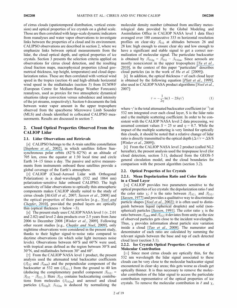
1155 UT on 1 January 2007. Figure 1 (top) shows b′532(using a logarithmic color scale) between 60°S and 60°Nfrom ground to 22 km, Figure 1 (middle) shows the result ofthe cloud detection and filtering described above. Cloudsthat completely attenuate the signal (e.g., around 5°N at15 km and 30°–45°N at 10 km) are entirely removed exceptat their edges (because of their lower geometrical thickness)while the highest and thinnest clouds, mostly found in thetropical latitudes, keep an accurate structure. Figure 1(bottom) shows b′532 inside cloud layers after applying thesame selection and filtering, but using cloud boundariesfrom the NL2 data set. There is little difference betweenFigure 1 (middle) and Figure 1 (bottom) except between15°N and 25°N where NL2 algorithms detect a smaller partof the thin high cloud at ∼18 km of altitude.

3.2. Statistical Comparison of Retrieved CloudFraction With CALIOP NASA Level 2 Products

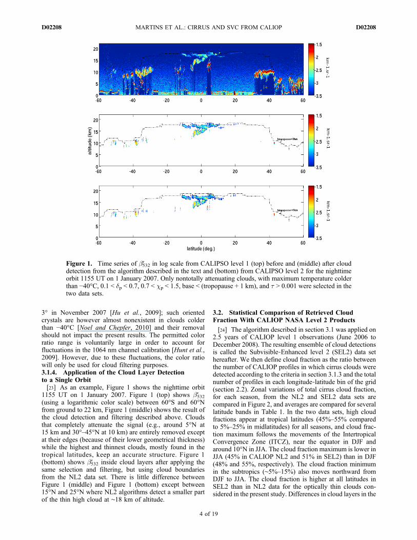
[24] The algorithm described in section 3.1 was applied on2.5 years of CALIOP level 1 observations (June 2006 toDecember 2008). The resulting ensemble of cloud detectionsis called the Subvisible‐Enhanced level 2 (SEL2) data sethereafter. We then define cloud fraction as the ratio betweenthe number of CALIOP profiles in which cirrus clouds weredetected according to the criteria in section 3.1.3 and the totalnumber of profiles in each longitude‐latitude bin of the grid(section 2.2). Zonal variations of total cirrus cloud fraction,for each season, from the NL2 and SEL2 data sets arecompared in Figure 2, and averages are compared for severallatitude bands in Table 1. In the two data sets, high cloudfractions appear at tropical latitudes (45%–55% comparedto 5%–25% in midlatitudes) for all seasons, and cloud frac-tion maximum follows the movements of the IntertropicalConvergence Zone (ITCZ), near the equator in DJF andaround 10°N in JJA. The cloud fraction maximum is lower inJJA (45% in CALIOP NL2 and 51% in SEL2) than in DJF(48% and 55%, respectively). The cloud fraction minimumin the subtropics (∼5%–15%) also moves northward fromDJF to JJA. The cloud fraction is higher at all latitudes inSEL2 than in NL2 data for the optically thin clouds con-sidered in the present study. Differences in cloud layers in the

Figure 1. Time series of b′532 in log scale from CALIPSO level 1 (top) before and (middle) after clouddetection from the algorithm described in the text and (bottom) from CALIPSO level 2 for the nighttimeorbit 1155 UT on 1 January 2007. Only nontotally attenuating clouds, with maximum temperature colderthan −40°C, 0.1 < dp < 0.7, 0.7 < cp < 1.5, base < (tropopause + 1 km), and t > 0.001 were selected in thetwo data sets.

MARTINS ET AL.: CIRRUS AND SVC FROM CALIOP D02208D02208

4 of 19

NL2 and SEL2 data sets are documented in the auxiliarymaterial, in which possible explanations are discussed.1

3.3. Cirrus and Subvisible Cirrus Cloud Properties

[25] Subvisible cirrus (SVC), identified by their very lowoptical depth t < 0.03 [Sassen and Benson, 2001] have beenshown to occur frequently in the tropics using SAGE(Stratospheric Aerosol and Gas Experiment) II [Wang et al.,1998]; lidars are well suited to their observation thanks totheir sensitivity to thin atmospheric features [Goldfarb et al.,2001], but before CALIOP no long‐term global‐scale dataset was available. For these reasons, the global‐scale coverof SVC is still poorly known, depending on it these cloudsmight have a significant greenhouse effect due to their coldtemperatures; moreover, their global role as regulators of thevertical transport of water vapor is not assessed [Froyd et al.,2010]. Since the mechanisms leading to the formation ofSVC are different from other ice clouds [Kärcher, 2002], onecan expect their characteristics to be different as well, thusthe rest of this study will consider separately SVC and cirrusclouds with optical depth above 0.03, which will be referredto simply as cirrus clouds from now on. It should be notedthat the retrieved optical depth depends on the used lidarratio S (section 2.1). Here we used S = 25, but according toSassen and Comstock [2001] cirrus lidar ratios lie in the 20–50 range, thus 0.8 < Dt/t = DS/S < 2.0. SVC optical depthscan therefore go up to 0.06.[26] Seasonal maps of cloud fraction (section 3.2) for

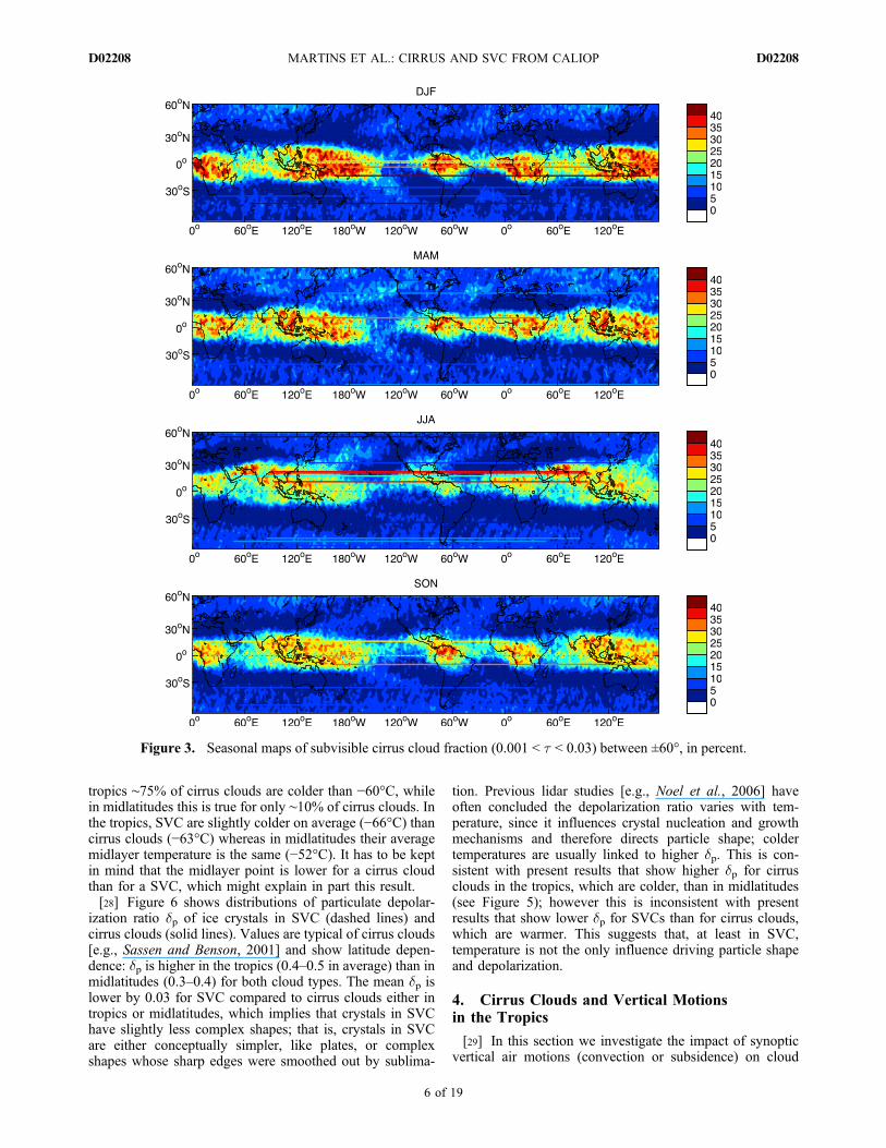
SVC (Figure 3) and cirrus clouds (Figure 4) from the SEL2data set show clouds concentrate over the three main deepconvective tropical areas (South America, Central Africaand Western Pacific), and are fewer in the subtropics, north

and south of these tropical cells. Cloud fraction maximas aresmaller for SVC (∼65%) than for cirrus clouds (∼90%), andSVC spread over larger areas. Both types of clouds movenorthward like the ITCZ during JJA, when the WesternPacific and Central Africa cells join. The locations andvalues of cirrus cloud fractions are comparable to resultsfrom Sassen et al. [2008].[27] Geometrical thickness distributions (Figure 5, left)

are considerably narrower for SVC (0.25–0.75 km) than forcirrus clouds (0.75–2 km). On average, in midlatitudes cir-rus clouds are 1.32 km thick and SVC 0.45 km thick(∼0.9 km thinner); in the tropics cirrus clouds are 1.77 kmthick and SVC 0.57 km thick (∼1.2 km thinner); that is, bothare 30% thicker than in midlatitudes. Tropical cirrus CTH(Figure 5, middle) is predominantly above 11 km with amost frequent value of 15 km; it is on average 4 km higherthan midlatitudes cirrus CTH. The shape of SVC CTHdistributions is very similar, whether in the tropics (meanCTH ∼ 14.4 km) or in the midlatitudes (mean CTH ∼10.3 km); however SVC CTH distributions appear shiftedby 200–300 m compared to cirrus CTH: upward in thetropics, downward in midlatitudes. Finally, distributions ofmidlayer temperature (Figure 5, right) show clouds are∼10°C colder in the tropics compared to midlatitudes: in the

Table 1. Cloud Fractions in Several Bands of Latitudesa

SEL2 (%) NASA L2 (%)

15°S–15°N 43.5 38.430°S–30°N 31.2 27.430°–60° 15.9 12.4

aFor nontotally attenuating clouds with maximum temperature colderthan −40°C, 0.1 < dp < 0.7, 0.7 < cp < 1.5, base < (tropopause + 1 km),and optical depth above 0.001 in the SEL2 and NASA level 2 data sets,considering the entire time period (June 2006 to December 2008).

Figure 2. Seasonal cloud fraction (%) as a function of latitude from the SEL2 data set (dashed lines) andfrom NASA level 2 data set (solid lines). Only nontotally attenuating clouds, with maximum temperaturecolder than −40°C, 0.1 < dp < 0.7, 0.7 < cp < 1.5, base < (tropopause + 1 km), and t > 0.001 wereselected in the two data sets. See also Table 1.

1Auxiliary materials are available in the HTML. doi:10.1029/2010JD014519.

MARTINS ET AL.: CIRRUS AND SVC FROM CALIOP D02208D02208

5 of 19

tropics ∼75% of cirrus clouds are colder than −60°C, whilein midlatitudes this is true for only ∼10% of cirrus clouds. Inthe tropics, SVC are slightly colder on average (−66°C) thancirrus clouds (−63°C) whereas in midlatitudes their averagemidlayer temperature is the same (−52°C). It has to be keptin mind that the midlayer point is lower for a cirrus cloudthan for a SVC, which might explain in part this result.[28] Figure 6 shows distributions of particulate depolar-

ization ratio dp of ice crystals in SVC (dashed lines) andcirrus clouds (solid lines). Values are typical of cirrus clouds[e.g., Sassen and Benson, 2001] and show latitude depen-dence: dp is higher in the tropics (0.4–0.5 in average) than inmidlatitudes (0.3–0.4) for both cloud types. The mean dp islower by 0.03 for SVC compared to cirrus clouds either intropics or midlatitudes, which implies that crystals in SVChave slightly less complex shapes; that is, crystals in SVCare either conceptually simpler, like plates, or complexshapes whose sharp edges were smoothed out by sublima-

tion. Previous lidar studies [e.g., Noel et al., 2006] haveoften concluded the depolarization ratio varies with tem-perature, since it influences crystal nucleation and growthmechanisms and therefore directs particle shape; coldertemperatures are usually linked to higher dp. This is con-sistent with present results that show higher dp for cirrusclouds in the tropics, which are colder, than in midlatitudes(see Figure 5); however this is inconsistent with presentresults that show lower dp for SVCs than for cirrus clouds,which are warmer. This suggests that, at least in SVC,temperature is not the only influence driving particle shapeand depolarization.

4. Cirrus Clouds and Vertical Motionsin the Tropics

[29] In this section we investigate the impact of synopticvertical air motions (convection or subsidence) on cloud

Figure 3. Seasonal maps of subvisible cirrus cloud fraction (0.001 < t < 0.03) between ±60°, in percent.

MARTINS ET AL.: CIRRUS AND SVC FROM CALIOP D02208D02208

6 of 19

properties. However, convective events are generally smallscale, limited in time, and may influence clouds distant intime and space from the convection event itself. Moreover,information about the convection/subsidence state of theatmosphere is not available at the fine temporal and geo-graphical scale of CALIOP cloud observations. Therefore,in this section we do not attempt to directly relate discreteconvective events or subsidence motions with cloud detec-tions. Instead, we assume the effect of these vertical motionswill be reflected by changes in distributions of cloud prop-erties in regions statistically dominated over months byspecific vertical motion regimes.

4.1. Cirrus Cloud Fraction and VerticalMotion Regimes

[30] A common indicator used to describe the intensity ofthe vertical motions in the atmosphere is the vertical pres-sure velocity at 500 hPa, hereafter called w500 (as in thework of, e.g., Bony and Dufresne [2005]). In the present

study, values of w500 come from monthly averages ofECMWF reanalyses [Uppala et al., 2005] over the sameperiod as CALIOP observations (June 2006 to December2008) on a 1.125° × 1.125° grid and 21 vertical pressurelevels (from 1000 to 1 hPa) 4 times a day at 0000, 0600,1200 and 1800 UTC. Monthly averages of w500 were usedsince dynamical processes are not represented correctly onshorter timeframes, due to the large variability between twoconsecutive reanalyses in time [Bony and Dufresne, 2005].[31] Negative w500 are linked with upward air mass mo-

tions and positive w500 with subsidence motions. Deepconvection occurs primarily along the tropical convectionbelt, and subsidence in the subtropics, around the Hadleycell (near ±30° of latitude). We posit that areas with monthlymeans w500 < −35 hPa/d are statistically dominated by deepconvection, areas with monthly means w500 > 25 hPa/d bystrong subsidence, and areas with intermediate values byweak convection (−35 to 0 hPa/d) and subsidence (0 to25 hPa/d). These boundaries were obtained by visually

Figure 4. Seasonal maps of cirrus cloud fraction (t > 0.03) between ±60°, in percent.

MARTINS ET AL.: CIRRUS AND SVC FROM CALIOP D02208D02208

7 of 19

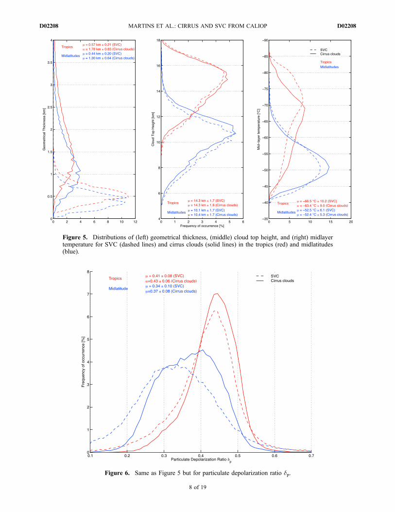
Figure 5. Distributions of (left) geometrical thickness, (middle) cloud top height, and (right) midlayertemperature for SVC (dashed lines) and cirrus clouds (solid lines) in the tropics (red) and midlatitudes(blue).

Figure 6. Same as Figure 5 but for particulate depolarization ratio dp.

MARTINS ET AL.: CIRRUS AND SVC FROM CALIOP D02208D02208

8 of 19

inspecting the monthly maps of vertical wind speed andidentifying areas typically dominated by one of the desiredsynoptic conditions, while making sure each regimecontained a significant cloud population.[32] Figure 7 shows the number of profiles where clouds

were detected in the tropics and the associated cloudfraction for SVC (Figure 7, top) and cirrus cloud (Figure 7,bottom) in DJF and JJA depending on the monthly meanw500. Weak subsidence areas dominate tropical latitudes,which explains the large number of cloudy profilesobserved there (red lines in Figure 7). This number is,

however, low compared to the total number of availableprofiles there, leading to relatively low cloud fractions(10%–15% for weak subsidence and 5%–10% for strongsubsidence areas, black lines in Figure 7). By contrast,deep convective areas (<−35 hPa/d) are concentrated in afew tropical regions (South America, Central Africa andWestern Pacific, and along the ITCZ), leading to a smallertotal number of cloudy profiles (red lines), but the relativenumber of cloudy profiles is much higher there, leading tohigh cloud fractions (20%–30% for weak convection,35%–50% for strong convection regions, black lines). The

Figure 7. Number of cloudy profiles (red) and cloud fraction (black) for (top) SVC and (bottom) cirrusclouds as a function of vertical wind speed at 500 hPa w500 (hPa/d) for DJF (solid lines) and JJA (dash‐dotted lines) periods. The vertical dashed lines at −35, 0, and 25 hPa/d limit the four defined w500 regimes.Wind speeds with less than 1000 associated CALIOP profiles are ignored.

MARTINS ET AL.: CIRRUS AND SVC FROM CALIOP D02208D02208

9 of 19

cirrus cloud fraction is lower in JJA since in that period,deep convective areas are moving northward of the equa-tor, where they are sparser and partially above land,leading to less intense convection than over the large warmpool in DJF. Cloud fraction trends are similar for SVC andcirrus clouds, except in regions dominated by strong con-vection (w500 < −35 hPa/d) where SVC cloud fractions arehalf (20%–25%) those for cirrus clouds (35%–50%).

4.2. Macrophysical Properties of Cirrus Clouds andVertical Motion Regimes

[33] Figure 8 shows distributions of monthly means ofcirrus cloud geometrical thickness, CTH and midlayertemperature in the tropics, for the 4 convective regimes(section 4.1). The distribution of geometrical thickness(Figure 8, left) changes very little with the sign of the ver-tical wind speed for tropical SVC (dashed lines), and stayscentered on the mean value (∼0.6 km). On the other hand,cirrus clouds (solid lines) become thinner with downwardair speed, and thicker with upward air speed. Cirrus cloudsare on average 2 km thick in regions affected by convectionand 1.4 km thick in regions affected by subsidence. Verticalvelocity thus seems to affect regular cirrus clouds more thanSVC, with clouds becoming thinner in the transition fromdeep convective to subsidence regions.[34] Distributions of CTH (Figure 8, middle) show a

maximum around 14–16.5 km for cirrus clouds and SVC,and appear to depend on w500: cloud top is on average0.5 km (SVC) and 0.9 km (cirrus clouds) higher in regionsdominated by upward motions compared to subsidence

regions. This result is linked with deep convection, whichincreases the probability of finding clouds higher in theatmosphere. In strong subsidence regions, SVC CTH is∼0.2 km higher than cirrus clouds CTH; other convectiveregimes do not show such a clear trend.[35] Midlayer temperatures (Figure 8, right) are colder

for pronounced upward motions (i.e., negative w500); mostfrequent values are ∼−72°C for SVC and ∼−68°C for cirrusclouds. Furthermore, midlayer temperatures of SVC arealways colder than the one for cirrus clouds, independentof w500. This is probably because SVC are thinner thancirrus clouds while sharing a similar CTH; their midlayerpoint is therefore higher in altitude, thus colder.

4.3. Optical Properties of Ice Crystals and VerticalMotion Regimes

[36] Figure 9 shows distributions of monthly means ofparticulate depolarization ratio dp for SVC (dashed lines) andcirrus clouds (solid lines) depending on w500. Mean valuesare similar for both (dp ∼ 0.45), with standard deviations∼0.1. The average and standard deviation of dp are slightlydependent on w500 for cirrus clouds, not for SVC.[37] Figure 10 shows distributions of depolarization dp

and temperature observations in SVC (Figure 10, top) andcirrus clouds (Figure 10, bottom), normalized by the totalnumber of observations in each vertical wind speed regime.A linear relationship appears between both variables in allcases, with dp increasing with colder temperatures (i.e., withaltitude) from dp ∼ 0.1–0.2 near −40°C to dp ∼ 0.4–0.5 near−55°C for both types of clouds. The relation between dp and

Figure 8. Distributions of (left) geometrical thickness, (middle) cloud top height, and (right) midlayertemperature for SVC (dashed lines) and cirrus clouds (solid lines) in the tropics for the four w500 regimes,with associated mean and standard deviation.

MARTINS ET AL.: CIRRUS AND SVC FROM CALIOP D02208D02208

10 of 19

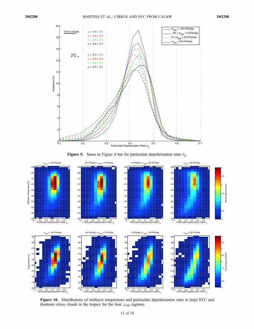
Figure 10. Distributions of midlayer temperature and particulate depolarization ratio in (top) SVC and(bottom) cirrus clouds in the tropics for the four w500 regimes.

Figure 9. Same as Figure 8 but for particulate depolarization ratio dp.

MARTINS ET AL.: CIRRUS AND SVC FROM CALIOP D02208D02208

11 of 19

the midlayer temperature seems to be linear for cirrus cloudswhatever w500, while it is sparser but with an increasinglinear‐like component for SVC in strong subsidence areas.Even if the most frequent values are the same and centeredat dp ∼ 0.45 and T ∼ −70°C for both types of clouds, theshape of distributions is different. The maximum value of

Table 2. Repartition of Horizontal Wind Speed Regimes in theTropics and Midlatitudes

Vhmax < 20 m s−1

(%)20 < Vhmax < 30 m s−1

(%)Vhmax > 30 m s−1

(%)

Tropics 47 38 15Midlatitudes 6 26 68

Figure 11. Number of cloudy profiles (red) and cloud fraction (blue) for (top) SVC and (bottom) cirrusclouds in midlatitudes as a function of the mean horizontal wind maxima near the tropopause Vhmax (m/s)in DJF (solid lines) and JJA (dash‐dotted lines). The vertical dashed lines at 20 and 30 m/s limit the threedefined Vhmax regimes. Wind speeds with fewer than 1000 associated CALIOP profiles are ignored.

MARTINS ET AL.: CIRRUS AND SVC FROM CALIOP D02208D02208

12 of 19

the histogram decreases with subsidence strength, meaningthe distributions are broader in strong subsidence.

5. Cirrus Clouds and MidlatitudesHorizontal Winds

5.1. Cirrus Cloud Fraction and Jet Stream Intensity

[38] Jet streams are narrow and discontinuous bands of airthat move rapidly around the globe near the tropopauselevel. They are located at the boundaries between polar,midlatitudes and tropical latitudes and characterized by theirmean latitude. The Tropical Easterly Jet (TEJ) is locatednear the equator at the tropopause level even if its strongestwinds appear in Southern Asia during NH summer. TheSubtropical Jet (SJ) occurs at subtropical latitudes, presentsa seasonal variation in each hemisphere, and gets stronger inwinter, when it often merges with the Polar Jet (PJ). Fol-lowing the same approach as in section 4, we used monthlymeans of horizontal wind maximum Vhmax in ECMWFreanalyses between the tropopause level from CALIOPNL2 data (section 2.1) and 50 hPa to characterize thedominant jet stream regime in a given region. Three situa-tions are defined following the same visual inspection ofmaps as in section 4.1: no jet streams (Vhmax < 20 m/s),weak jet streams (20 < Vhmax < 30 m/s) and strong jetstreams (Vhmax > 30 m/s). Tropical jets are on average muchslower than midlatitudes jets, i.e., 20–50 m/s for the TEJversus 40–80 m/s for the SJ and PJ. While 68% of midlat-itudes areas show Vhmax faster than 30 m/s, this is only thecase for 15% of tropics (Table 2). Thus, in our terminology,the fastest tropical winds are more comparable to weak

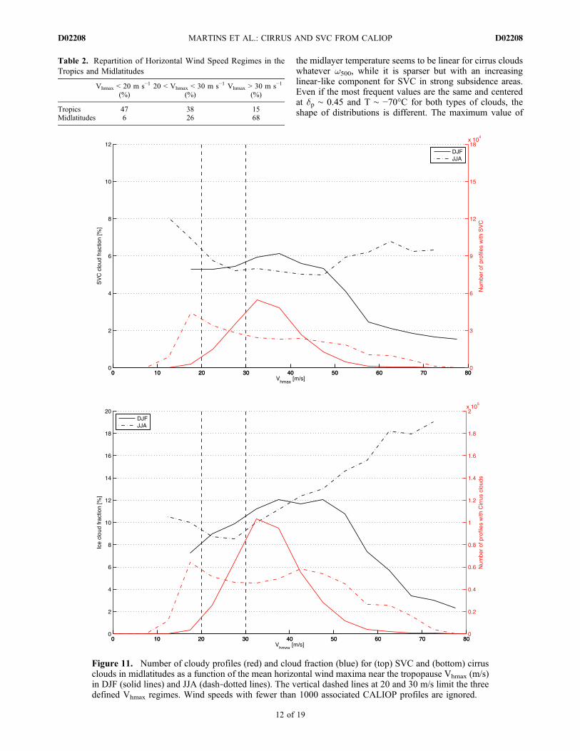
than to strong midlatitude jets. In order not to mix differentsynoptic situations, the rest of this section focuses onthe link between midlatitude cirrus clouds and jet streams(SJ/PJ), i.e., latitudes above 30°.[39] Figure 11 shows the number of cloudy profiles and

the cloud fraction (CF) in midlatitudes for SVC (top) andcirrus clouds (bottom) in DJF and JJA as a function of themonthly mean Vhmax. CF appears strongly dependent onVhmax. In DJF, CF is maximal at ∼35 m/s for both SVC andcirrus clouds; in JJA CF is maximal for Vhmax above 50 m/s.In both seasons, largest cloud fractions are found forVhmax > 30 m/s; for higher Vhmax, cloud fractions keepincreasing up to Vhmax ∼ 60 m/s in JJA, but quickly decreasein DJF. Cirrus cloud fractions (maximum 12% in DJF,∼18% in JJA) are nearly twice SVC CF (maximum 6% inDJF, ∼8% in JJA). The highest SVC CF is observed forJJA in low wind conditions (Vhmax < 20 m/s). The mostfrequent Vhmax where clouds are detected is ∼35 m/s inDJF and ∼15 m/s in JJA (red lines in Figure 11), whichshows the enhancing of wind speeds in the winter hemi-sphere (where SJ and PJ often merge and higher Vhmax

are observed).

5.2. Macrophysical Properties of Clouds and JetStream Intensity

[40] Figure 12 displays distributions for monthly meansof geometrical thickness, CTH and midlayer temperaturefor SVC and cirrus clouds in the three wind situations(section 5.1). While the geometrical thickness (Figure 12,left) of cirrus clouds does not change significantly withthe wind situation, SVC are on average ∼20% thinner

Figure 12. Distributions of (left) geometrical thickness, (middle) cloud top height, and (right) midlayertemperature of SVC (dashed lines) and cirrus clouds (solid lines) for the three Vhmax regimes, with asso-ciated mean and standard deviation.

MARTINS ET AL.: CIRRUS AND SVC FROM CALIOP D02208D02208

13 of 19

(∼0.08 km) in presence of strong compared to weak winds(SVC are 0.4 km thick on average). Such strong windsmostly appear at the boundaries between tropics and mid-latitudes (SJ) and between midlatitudes and poles (PJ),where cirrus clouds are sparse (section 3.2).[41] Cloud tops (Figure 12, middle) are lower in presence

of faster winds (∼1.8 km lower in regions where Vhmax >30 m/s compared to regions where Vhmax < 20 m/s). Tem-perature distributions echo this result (Figure 12, right):midlayer cloud temperatures are colder by ∼2° in presenceof weak winds compared to strong wind conditions. Onaverage, SVC (dashed lines) are slightly lower (by ∼300 m)and colder (by ∼1°) than cirrus clouds (solid lines). Overallshapes of CTH and temperature distributions are similar.

5.3. Optical Properties of Ice Crystals and JetStreams Intensity

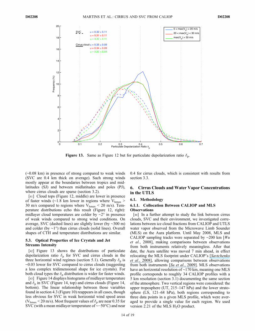
[42] Figure 13 shows the distributions of particulatedepolarization ratio dp for SVC and cirrus clouds in thethree horizontal wind regimes (section 5.1). Generally dp is∼0.03 lower for SVC compared to cirrus clouds (suggestinga less complex tridimensional shape for ice crystals). Forboth cloud types the dp distribution is wider for faster winds.[43] Figure 14 displays histograms of midlayer temperature

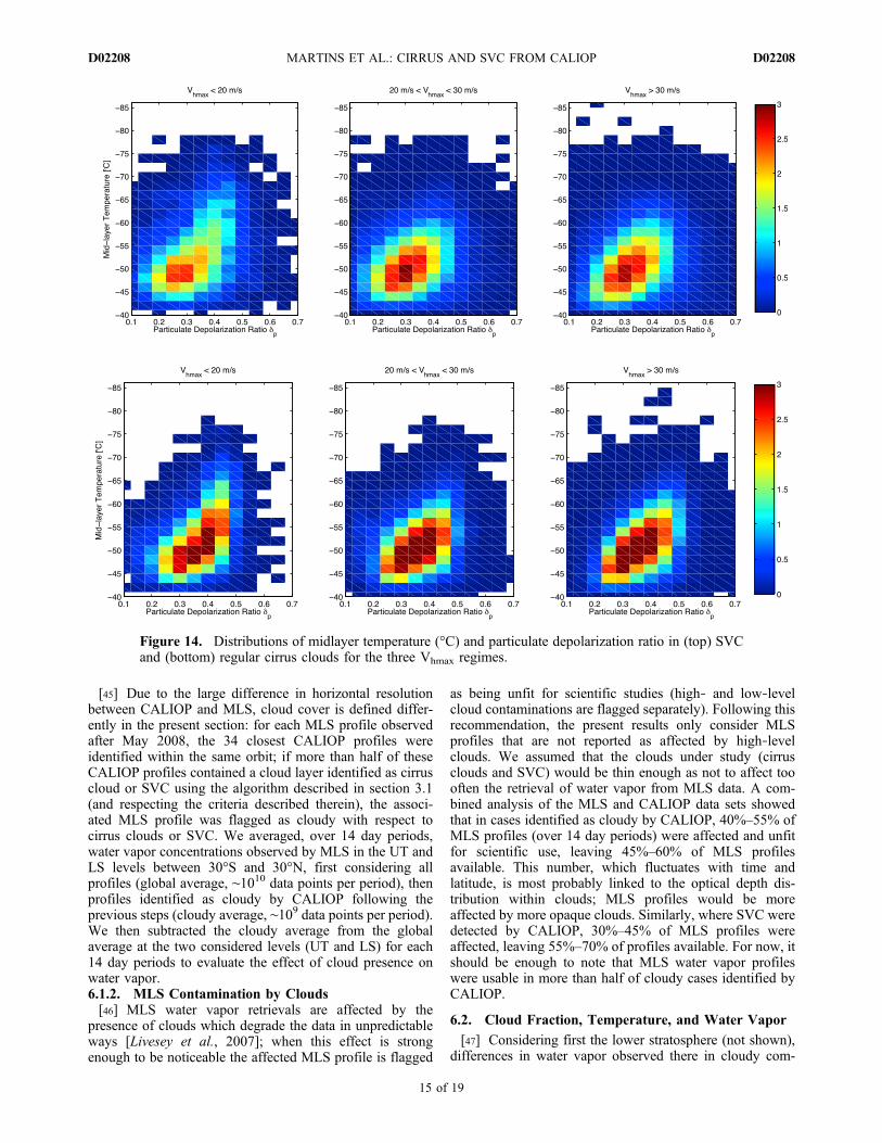
and dp in SVC (Figure 14, top) and cirrus clouds (Figure 14,bottom). The linear relationship between those variablesfound in section 4.3 (Figure 10) reappears in all cases, thoughless obvious for SVC in weak horizontal wind speed areas(Vhmax < 20 m/s). Most frequent values of dp are near 0.35 forSVC (with a mean midlayer temperature of ∼−50°C) and near

0.4 for cirrus clouds, which is consistent with results fromsection 3.3.

6. Cirrus Clouds andWater Vapor Concentrationsin the UTLS

6.1. Methodology

6.1.1. Collocation Between CALIOP and MLSObservations[44] In a further attempt to study the link between cirrus

clouds, SVC and their environment, we investigated corre-lations between ice cloud fractions from CALIOP and UTLSwater vapor observed from the Microwave Limb Sounder(MLS) on the Aura platform. Until May 2008, MLS andCALIOP sampling tracks were separated by ∼200 km [Wuet al., 2008], making comparisons between observationsfrom both instruments relatively meaningless. After thatdate, the Aura satellite was moved 7 min ahead, in effectrelocating the MLS footprint under CALIOP’s [Savtchenkoet al., 2008], allowing comparisons between observationsfrom both instruments [Su et al., 2009]. MLS observationshave an horizontal resolution of ∼170 km, meaning one MLSprofile corresponds to roughly 34 CALIOP profiles with a5 km resolution (section 3.1) documenting the same sectionof the atmosphere. Two vertical regions were considered: theupper troposphere (UT, 215–147 hPa) and the lower strato-sphere (LS, 121–68 hPa), both regions corresponding tothree data points in a given MLS profile, which were aver-aged to provide a single value for each region. We usedversion 2.21 of the MLS H2O product.

Figure 13. Same as Figure 12 but for particulate depolarization ratio dp.

MARTINS ET AL.: CIRRUS AND SVC FROM CALIOP D02208D02208

14 of 19

[45] Due to the large difference in horizontal resolutionbetween CALIOP and MLS, cloud cover is defined differ-ently in the present section: for each MLS profile observedafter May 2008, the 34 closest CALIOP profiles wereidentified within the same orbit; if more than half of theseCALIOP profiles contained a cloud layer identified as cirruscloud or SVC using the algorithm described in section 3.1(and respecting the criteria described therein), the associ-ated MLS profile was flagged as cloudy with respect tocirrus clouds or SVC. We averaged, over 14 day periods,water vapor concentrations observed by MLS in the UT andLS levels between 30°S and 30°N, first considering allprofiles (global average, ∼1010 data points per period), thenprofiles identified as cloudy by CALIOP following theprevious steps (cloudy average, ∼109 data points per period).We then subtracted the cloudy average from the globalaverage at the two considered levels (UT and LS) for each14 day periods to evaluate the effect of cloud presence onwater vapor.6.1.2. MLS Contamination by Clouds[46] MLS water vapor retrievals are affected by the

presence of clouds which degrade the data in unpredictableways [Livesey et al., 2007]; when this effect is strongenough to be noticeable the affected MLS profile is flagged

as being unfit for scientific studies (high‐ and low‐levelcloud contaminations are flagged separately). Following thisrecommendation, the present results only consider MLSprofiles that are not reported as affected by high‐levelclouds. We assumed that the clouds under study (cirrusclouds and SVC) would be thin enough as not to affect toooften the retrieval of water vapor from MLS data. A com-bined analysis of the MLS and CALIOP data sets showedthat in cases identified as cloudy by CALIOP, 40%–55% ofMLS profiles (over 14 day periods) were affected and unfitfor scientific use, leaving 45%–60% of MLS profilesavailable. This number, which fluctuates with time andlatitude, is most probably linked to the optical depth dis-tribution within clouds; MLS profiles would be moreaffected by more opaque clouds. Similarly, where SVC weredetected by CALIOP, 30%–45% of MLS profiles wereaffected, leaving 55%–70% of profiles available. For now, itshould be enough to note that MLS water vapor profileswere usable in more than half of cloudy cases identified byCALIOP.

6.2. Cloud Fraction, Temperature, and Water Vapor

[47] Considering first the lower stratosphere (not shown),differences in water vapor observed there in cloudy com-

Figure 14. Distributions of midlayer temperature (°C) and particulate depolarization ratio in (top) SVCand (bottom) regular cirrus clouds for the three Vhmax regimes.

MARTINS ET AL.: CIRRUS AND SVC FROM CALIOP D02208D02208

15 of 19

pared to noncloudy cases, averaged over 14 days, do notshow any discernable pattern and stay below 0.1 ppmv,which is the minimum concentration detectable by MLS[Livesey et al., 2007] and well below the background fluc-tuations in water vapor concentrations (∼4 ± 1ppmv). Thesefluctuations appear similar when considering SVC or cirrusclouds. Dessler [2009], applying a very similar methodol-ogy on CALIOP and MLS observations, found a significantrelative humidity enhancement in the tropical lower strato-sphere (200–100 hPa) in the presence of upper troposphericclouds; however the present study ignored clouds too highwith respect to the tropopause (section 3.1.2), while Desslerfocused specifically on clouds near and above the tropo-pause, which probably explains the discrepancy.[48] On the other hand, MLS observations in the upper

troposphere (Figure 15) show a 15–30 ppmv increase inwater vapor compared to the average where CALIOPidentified the presence of cirrus clouds, and a 5–10 ppmvincrease where SVC were identified. For reference, averageUT water vapor concentrations are in the range 25–60 ppmv;the observed increase is of the same order of magnitude.This increase appears symmetric around the equator andquite stable with time, except for a significant peak inOctober 2008 for which we have no explanation at thispoint. Moreover, temperatures observed by MLS in the UTshow a ∼1° decrease compared to the average when cloudsare observed by CALIOP. This difference is comparable tofluctuations around the average for UT background tem-peratures observed by MLS (−61.5°C ± 1°C) in the con-sidered region. This difference is also symmetric around theequator, and less pronounced in presence of SVC (−0.5°).

[49] In summary, the presence of cirrus clouds in the uppertroposphere (1) does not affect water vapor noticeably in thelower stratosphere above and (2) in the upper troposphere, iscorrelated with water vapor concentrations noticeably higherthan average and temperatures 1° colder than average. Thepresence of SVC leads to the same observations, althoughthe differences with average in UT are smaller. This maysuggest that colder temperatures trigger SVC formation inareas with ice supersaturation just above the threshold forcloud formation.[50] However, it should be kept it mind that water

vapor fluctuations happen on much smaller scales than theone permitted by MLS observations (horizontal resolution∼170 km); thus the averaging implied by the relatively lowresolution can lead to a smoothing of high supersaturationand the water vapor increase observed in cloudy cases ismost likely underestimated [Lamquin et al., 2008; Massieet al., 2010]. If this were the case, the smaller differenceobserved in presence of SVC could mean their formation isdue to local fluctuations of temperature and/or water vaporleading to regions supersaturated with respect to ice smallerthan those leading to the formation of cirrus clouds.

7. Discussion and Conclusion

[51] In this article an algorithm was presented to detectoptically thin clouds in CALIOP level 1 observations, whichhas been applied to 2.5 years of observations between 60°Sand 60°N to create a Subvisible‐Enhanced L2 data set(SEL2). We used this data set to document the cover andproperties of cirrus clouds and SVC, and investigated how

Figure 15. Difference in water vapor observed by MLS in the upper troposphere, when CALIOPobserved either regular cirrus clouds (solid lines) or SVCs (dashed lines), compared to the average over14 day periods for the Northern (blue) and Southern (red) hemispheres.

MARTINS ET AL.: CIRRUS AND SVC FROM CALIOP D02208D02208

16 of 19

their properties are affected by surrounding atmosphericproperties, most notably (1) vertical and horizontal winds,used as proxies for convection in the tropics and jet streamsin the midlatitudes, and (2) water vapor in the UTLS. Cloudproperties are summarized in Table 3 (SVC) and Table 4(cirrus clouds).[52] First, cloud fractions (CF) for all cirrus clouds colder

than −40°C in SEL2 (Table 1) are in the 30%–60% range inthe tropics (reaching 90% above South America, CentralAfrica, Western Pacific and along the ITCZ), with yearlyaverages of 31% between 30°S and 30°N and 44% between15°S and 15°N. In midlatitudes CF is in the 10%–20% range,with a yearly average of 16% between 30° and 60°. Highcirrus cloud fractions move northward in JJA and southwardin DJF, like the ITCZ. These results are consistent with recentstudies of cloud cover from CALIOP (detection based onNASA level 2 algorithm): For instance, Mace et al. [2009]found on average CF ∼ 30% in the tropics and ∼15% inmidlatitudes from the first year of CALIOP observations forclouds with tops above 6 km. For the same period, Sassenet al. [2008] found CF ∼ 35% in the tropical belt (±15°),∼15% in latitudes 15°–30° (N/S), and ∼15% in midlati-tudes; the same study found a secondary maximum at theinterface between midlatitudes and polar regions. In ourstudy, this maximum can only be observed in MAM sincethis is the only period when the maximum is below 60°.Cirrus cloud fraction maximas (70% near convection cen-ters) are consistent with results from Nazaryan et al.[2008].[53] Regarding macrophysical properties of cirrus clouds,

results in the present study are globally consistent with

Sassen et al. [2008]: CTHs in both studies are ∼14 km in thetropics and ∼10 km in midlatitudes, which illustrates thepoleward decrease of CTHs. Sassen et al. [2008] foundclouds between −72° and −55°C in the tropics and between−56°C and −45°C in midlatitudes, while in the present studyaverage midlayer temperatures are −63°C in the tropics and−52°C in midlatitudes which is consistent assuming a lineardecrease of temperature with increasing altitude in the UT.Finally, Sassen et al. found a latitude‐independent thicknessof 2.0 km globally, while in the present study cirrus cloudsare on average 1.8 km thick in the tropics and 1.3 km thickin midlatitudes (Table 4).[54] The present study presents optical properties of

crystals in cirrus clouds, but also in SVC, which up to nowwere poorly known on a global scale. Results show thataverage depolarization ratio is slightly lower in SVC (dp ∼0.35) than in cirrus clouds (dp ∼ 0.4), and higher in thetropics (∼0.43) than in midlatitudes (∼0.37), as in the workof Sassen and Zhu [2009]. SVC are on average three timesthinner (∼0.4 km) than cirrus clouds (∼1.5 km), have asimilar top height (CTH ∼ 14.4 km in the tropics, CTH ∼10.5 km in midlatitudes), which explain why their midlayertemperature is 3° colder in the tropics (∼−66°C) than cirrusclouds (∼−63°C). Distributions of properties are generallybroader for SVC, most probably due to the weaker signalthey produce.[55] The relationships between properties of clouds and

dynamic indicators (Tables 3 and 4) change with latitude. Inthe tropics, high CF (∼23% for SVC and ∼40% for cirrusclouds) are found in areas dominated on average by strongupward winds (w500 < −35 hPa/d), low CF (<10% for SVC

Table 3. Summary of Average Properties and Standard Deviation of SVCa

CF (%) Thickness (km) CTH (km) Midlayer Temperature (deg) dp

Tropics ± 30° 14.5 0.6 ± 0.2 14.3 ± 1.7 −66 ± 10 0.41 ± 0.08w500 hPa/d<−35 23.0 0.5 ± 0.2 14.6 ± 1.5 −68 ± 9 0.41 ± 0.08−35–0 17.9 0.5 ± 0.2 14.3 ± 1.6 −67 ± 10 0.40 ± 0.080–25 12.1 0.5 ± 0.2 14.2 ± 1.7 −66 ± 10 0.39 ± 0.09>25 7.8 0.5 ± 0.2 14.0 ± 1.9 −66 ± 11 0.39 ± 0.09

Midlatitudes 30°–60° 5.8 0.4 ± 0.2 10.1 ± 1.7 −53 ± 6 0.34 ± 0.10vhmax m/s<20 7.0 0.4 ± 0.2 11.6 ± 0.21 −55 ± 7 0.32 ± 0.1120–30 6.1 0.4 ± 0.2 10.5 ± 1.8 −53 ± 6 0.31 ± 0.11>30 5.6 0.4 ± 0.2 9.8 ± 1.7 −53 ± 6 0.32 ± 0.11

aFor optical depth above 0.001 and below 0.03, maximum temperature colder than −40°C, 0.1 < dp < 0.7, 0.7 < cp < 1.5, and base < (tropopause + 1 km)in the tropics and midlatitudes: cloud fraction (CF), geometrical thickness, cloud top height, midlayer temperature, and particulate depolarization ratio. Thesame properties are also documented in the four vertical motion regimes in the tropics (section 4) and the three horizontal wind speed regimes in mid-latitudes (section 5).

Table 4. Same as Table 3 but for Cirrus Clouds (Optical Depth Above 0.03)

CF (%) Thickness (km) CTH (km) Midlayer Temperature (deg) dp

Tropics ± 30° 20.6 1.8 ± 0.8 14.3 ± 1.6 −63 ± 9 0.43 ± 0.08w500 hPa/d<−35 39.7 2.0 ± 0.9 14.7 ± 1.3 −65 ± 8 0.42 ± 0.06−35–0 26.7 1.7 ± 0.8 14.3 ± 1.5 −63 ± 8 0.42 ± 0.060–25 14.5 1.5 ± 0.7 14.0 ± 1.6 −62 ± 9 0.42 ± 0.07>25 8.6 1.4 ± 0.7 13.8 ± 1.8 −62 ± 10 0.41 ± 0.08

Midlatitudes 30°–60° 11.1 1.3 ± 0.6 10.4 ± 1.7 −52 ± 5 0.37 ± 0.1vhmax m/s<20 10.1 1.2 ± 0.6 11.9 ± 1.9 −54 ± 6 0.35 ± 0.0920–30 10.4 1.2 ± 0.6 10.8 ± 1.7 −52 ± 5 0.34 ± 0.09>30 11.6 1.3 ± 0.7 10.1 ± 1.7 −52 ± 5 0.35 ± 0.08

MARTINS ET AL.: CIRRUS AND SVC FROM CALIOP D02208D02208

17 of 19

and cirrus clouds) in areas dominated by moderate down-ward winds (w500 > 25 hPa/d). The trend showing CFincreasing from subsidence to convection is consistent withresults for upper level clouds in the work of Bony andDufresne [2005] using ISCCP data over 16 years (1984–2000). Strong winds are associated to higher (+0.2 km) andcolder (−2°C) clouds, thicker cirrus clouds (+0.2 km) andthinner SVC (−0.1 km) compared to the average; it can behypothesized that these properties are due to the increasedinfluence of convective motions. By contrast, downwardwinds appear associated to lower (0.5 km), warmer (∼1°C)and thinner clouds (−0.1 km for SVC and −0.4 km for cirrusclouds). Changes in vertical winds only slightly affect thedepolarization ratio (it is slightly higher for strong upwardwinds).[56] In midlatitudes, CF do not appear affected by hori-

zontal winds (∼11% for cirrus clouds and ∼5%–7% forSVC); although for SVC stronger wind speeds (Vhmax >30 m/s) lead to lower CF. Results show that faster windsare associated with slightly thinner (by ∼0.08 km), warmer(by ∼2°C) and lower (by ∼1.8 km) clouds; it can behypothesized that these changes in properties are due to theinfluence of strong jets.[57] The relatively low cloud fraction found in subsidence

regions must be taken with caution, as subsidence affects alarger area than convection in the tropics: monthly averagesfrom 2.5° × 2.5° horizontal resolution ECMWF reanalysesshow that in the considered data set ∼62% of tropics areunder subsidence conditions, while convection dominates anarrow belt. Thus, even if the cloud fraction is lower insubsidence‐dominated areas than in ascending air regions,cirrus clouds and SVC there still represent a large cloudpopulation in absolute terms.[58] Finally, comparing CALIOP observations with col-

located MLS retrievals showed that cirrus cloud detectionsin the upper troposphere are correlated with a significantincrease (+15–30 ppmv) in observed upper troposphericwater vapor concentrations compared to the average. Asmaller increase (+5–10 ppmv) is observed in presenceof SVC. These differences are probably underestimated,as (1) the MLS resolution is poor compared to the scaleof water vapor atmospheric fluctuations and (2) cloud‐contaminated MLS profiles were not considered, and thoseprobably contain the optically thickest cirrus clouds, whichwe expect to be related to the highest water vapor con-centrations. A small decrease in temperature (∼1°) is alsoobserved. These findings are not surprising, since a higherwater vapor content linked with low temperatures isexpected for cloud formation, but the difference in theincrease between cirrus clouds and SVC might shed light onour understanding of the mechanisms leading to SVC for-mation, as these clouds most probably form at water vaporconcentration just slightly above the threshold for cloudformation (it is relevant to note that among all the variablesconsidered in the present study, water vapor shows theclearest difference between cirrus clouds and SVC).[59] Future work involves adapting the cloud detection

algorithm for daytime CALIOP level 1 observations in orderto be able to study diurnal changes in cirrus cloud properties[Sassen et al., 2003], which appear to be significant for SVC[Sassen et al., 2009]. The SEL2 data set described in the

present paper will be shortly available online, in the hope tohelp future global‐scale studies on optically thin clouds.

[60] Acknowledgments. We would like to thank NASA and CNESfor creating CALIOP and MLS observations, the CALIPSO NASA ScienceTeam for creating the scientific data sets, the ICARE center and the NASALangley ASDC for access to the data, and the ClimServ center for essentialcomputing resources. This work is supported in part by ANR grant ANR‐07‐JCJC‐0016CSD6. Finally, we would like to thank the anonymousreviewers for useful comments and suggestions.

ReferencesBodhaine, B. A., N. B. Wood, E. G. Dutton, and J. R. Slusser (1999), OnRayleigh optical depth calculations, J. Atmos. Oceanic Technol., 16,1854–1861, doi:10.1175/1520-0426(1999)016<1854:ORODC>2.0.CO;2.

Bony, S., and J.‐L. Dufresne (2005), Marine boundary layer clouds at theheart of tropical cloud feedback uncertainties in climate models, Geo-phys. Res. Lett., 32, L20806, doi:10.1029/2005GL023851.

Chepfer, H., and V. Noel (2009), A tropical “NAT‐like” belt observed fromspace, Geophys. Res. Lett., 36, L03813, doi:10.1029/2008GL036289.

Chepfer, H., S. Bony, D. Winker, M. Chiriaco, J.‐L. Dufresne, and G. Seze(2008), Use of CALIPSO lidar observations to evaluate the cloudiness sim-ulated by a climate model, Geophys. Res. Lett., 35, L15704, doi:10.1029/2008GL034207.

Chepfer, H., S. Bony, D. Winker, G. Cesana, J. L. Dufresne, P. Minnis,C. J. Stubenrauch, and S. Zeng (2010), The GCM‐Oriented CALIPSOCloud Product (CALIPSO‐GOCCP), J. Geophys. Res., 115, D00H16,doi:10.1029/2009JD012251.

Corti, T., et al. (2008), Unprecedented evidence for deep convectionhydrating the tropical stratosphere, Geophys. Res. Lett., 35, L10810,doi:10.1029/2008GL033641.

Dessler, A. E. (2009), Clouds and water vapor in the Northern Hemispheresummertime stratosphere, J. Geophys. Res., 114, D00H09, doi:10.1029/2009JD012075.

Dessler, A. E., and K. Minschwaner (2007), An analysis of the regulationof tropical tropospheric water vapor, J. Geophys. Res., 112, D10120,doi:10.1029/2006JD007683.

Dufresne, J.‐L., and S. Bony (2008), An assessment of the primary sourcesof spread of global warming estimates from coupled atmosphere‐oceanmodels, J. Clim., 21, 5135–5144, doi:10.1175/2008JCLI2239.1.

Froyd, K. D., D. M. Murphy, P. Lawson, D. Baumgardner, and R. L. Herman(2010), Aerosols that forms subvisible cirrus at the tropical tropopause,Atmos. Chem. Phys., 10, 209–218, doi:10.5194/acp-10-209-2010.

Gettelman, A., and D. E. Kinnison (2007), The global impact of supersat-uration in a coupled chemistry‐climate model, Atmos. Chem. Phys., 7,1629–1643, doi:10.5194/acp-7-1629-2007.

Goldfarb, L., P. Keckhut, M.‐L. Chanin, and A. Hauchecorne (2001), Cir-rus climatological results from lidar measurements at OHP (44°N, 6°E),Geophys. Res. Lett., 28, 1687–1690, doi:10.1029/2000GL012701.

Hu, Y. X., et al. (2009), CALIPSO/CALIOP cloud phase discriminationalgorithm, J. Atmos. Oceanic Technol., 26, 2293–2309, doi:10.1175/2009JTECHA1280.1.

Hunt, W. H., D. M. Winker, M. A. Vaughan, K. A. Powell, P. L. Lucker,and C. Weimer (2009), CALIPSO lidar description and performanceassessment, J. Atmos. Oceanic Technol., 26, 1214–1228, doi:10.1175/2009JTECHA1223.1.

Kärcher, B. (2002), Properties of subvisible cirrus clouds formed by homo-geneous freezing, Atmos. Chem. Phys., 2, 161–170, doi:10.5194/acp-2-161-2002.

Krämer, M., et al. (2009), Ice supersaturations and cirrus cloud crystalnumbers, Atmos. Chem. Phys., 9, 3505–3522, doi:10.5194/acp-9-3505-2009.

Lamquin, N., C. Stubenrauch, and J. Pelon (2008), Upper tropospherichumidity and cirrus geometrical and optical thickness: Relationshipsinferred from 1 year of collocated AIRS and CALIPSO data, J. Geophys.Res., 113, D00A08, doi:10.1029/2008JD010012.

Liou, K.‐N. (1986), Influence of cirrus clouds on weather and climate pro-cesses: A global perspective, Mon. Weather Rev., 114(6), 1167–1199,doi:10.1175/1520-0493(1986)114<1167:IOCCOW>2.0.CO;2.

Liou, K. N., Y. Takano, P. Yang, and Y. Gu (2002), Radiative transfer incirrus clouds: Light scattering and spectral information, in Cirrus, editedby D. Lynch et al., pp. 265–296, Oxford Univ. Press, New York.

Livesey, N. J., et al. (2007), EOS‐Aura MLS version 2.2 level 2 data qualityand description document, Jet Propul. Lab., Pasadena, Calif. (Available athttp://mls.jpl.nasa.gov/data/v2‐2_data_quality_document.pdf)

MARTINS ET AL.: CIRRUS AND SVC FROM CALIOP D02208D02208

18 of 19

Mace, G. G., Q. Zhang, M. A. Vaughan, R. Marchand, G. Stephens, C. R.Trepte, and D. M. Winker (2009), A description of hydrometeor layeroccurrence statistics derived from the first year of merged CloudSatand CALIPSO data, J. Geophys. Res., 114, D00A26, doi:10.1029/2007JD009755.

Massie, S. T., J. Gille, C. Craig, R. Khosravi, J. Barnett, W. Read, andD. Winker (2010), HIRDLS and CALIPSO observations of tropicalcirrus, J. Geophys. Res., 115, D00H11, doi:10.1029/2009JD012100.

McGill, M. J., M. A. Vaughan, C. R. Trepte, W. D. Hart, D. L. Hlavka,D. M. Winker, and R. Kuehn (2007), Airborne validation of spatial prop-erties measured by the CALIPSO lidar, J. Geophys. Res., 112, D20201,doi:10.1029/2007JD008768.

Murray, B. J., and A. K. Bertram (2007), Strong dependence of cubic iceformation on droplet ammonium to sulfate ratio, Geophys. Res. Lett.,34, L16810, doi:10.1029/2007GL030471

Nazaryan, H., M. P. McCormick, and W. P. Menzel (2008), Global char-acterization of cirrus clouds using CALIPSO data, J. Geophys. Res.,113, D16211, doi:10.1029/2007JD009481.

Noel, V., and H. Chepfer (2010), A global view of horizontally orientedcrystals in ice clouds from Cloud‐Aerosol Lidar and Infrared PathfinderSatellite Observation (CALIPSO), J. Geophys. Res., 115, D00H23,doi:10.1029/2009JD012365.

Noel, V., H. Chepfer, G. Ledanois, A. Delaval, and P. H. Flamant (2002),Classification of particle shape ratios in cirrus clouds based on the lidardepolarization ratio, Appl. Opt., 41, 4245–4257, doi:10.1364/AO.41.004245.

Noel, V., H. Chepfer, M. Haeffelin, and Y. Morille (2006), Classificationof ice crystal shapes in midlatitude ice clouds from three years of lidarobservations over the SIRTA observatory, J. Atmos. Sci., 63, 2978–2991,doi:10.1175/JAS3767.1.

Noel, V., D. M. Winker, T. J. Garrett, and M. McGill (2007), Extinctioncoefficients retrieved in deep tropical ice clouds from lidar observationsusing a CALIPSO‐like algorithm compared to in‐situ measurementsfrom the cloud integrating nephelometer during CRYSTAL‐FACE,Atmos. Chem. Phys., 7, 1415–1422, doi:10.5194/acp-7-1415-2007.

Peter, T., C. Marcolli, P. Spichtinger, T. Corti, M. B. Baker, and T. Koop(2006), When dry air is too humid, Science, 314, 1399–1402, doi:10.1126/science.1135199.

Platt, C., D. Winker, M. Vaughan, and S. Miller (1999), Backscatter toextinction ratios in the top layers of tropical mesoscale convective systemsand in isolated cirrus from LTE observations, J. Appl. Meteorol., 38,1330–1345, doi:10.1175/1520-0450(1999)038<1330:BTERIT>2.0.CO;2.

Pruppacher, H. R., and J. D. Klett (1997), Microphysics of Clouds and Pre-cipitation, 954 pp., Kluwer Acad., Dordrecht, Netherlands.

Sassen, K. (1977), Ice crystal habit discrimination with the optical back-scatter depolarization technique, J. Appl. Meteorol., 16, 425–431,doi:10.1175/1520-0450(1977)016<0425:ICHDWT>2.0.CO;2.

Sassen, K. (1991), The polarization lidar technique for cloud research: Areview and current assessment, Bull. Am. Meteorol. Soc., 72, 1848–1866,doi:10.1175/1520-0477(1991)072<1848:TPLTFC>2.0.CO;2.

Sassen, K., and S. Benson (2001), A midlatitude cirrus cloud climatologyfrom the Facility for Atmospheric Remote Sensing. Part II: Microphysicalproperties derived from lidar depolarization, J. Atmos. Sci., 58, 2103–2112,doi:10.1175/1520-0469(2001)058<2103:AMCCCF>2.0.CO;2.

Sassen, K., and J. Campbell (2001), A midlatitude cirrus cloud climatologyfrom the Facility for Atmospheric Remote Sensing. Part I: Macrophysicaland synoptic properties, J. Atmos. Sci., 58, 481–496, doi:10.1175/1520-0469(2001)058<0481:AMCCCF>2.0.CO;2.

Sassen, K., and J. Comstock (2001), A midlatitude cirrus cloud climatologyfrom the Facility for Atmospheric Remote Sensing, part III: Radiative prop-erties, J. Atmos. Sci., 58, 2113–2127, doi:10.1175/1520-0469(2001)058<2113:AMCCCF>2.0.CO;2.

Sassen, K., and J. Zhu (2009), A global survey of CALIPSO linear depo-larization ratios in ice clouds: Initial findings, J. Geophys. Res., 114,D00H07, doi:10.1029/2009JD012279.

Sassen, K., K.‐N. Liou, Y. Takano, and V. I. Khvorostyanov (2003), Diurnaleffects in the composition of cirrus clouds, Geophys. Res. Lett., 30(10),1539, doi:10.1029/2003GL017034.

Sassen, K., Z. Wang, and D. Liu (2008), Global distribution of cirrus cloudsfrom CloudSat/Cloud‐Aerosol Lidar and Infrared Pathfinder Satellite Obser-

vations (CALIPSO) measurements, J. Geophys. Res., 113, D00A12,doi:10.1029/2008JD009972.

Sassen, K., Z. Wang, and D. Liu (2009), Cirrus clouds and deep convectionin the tropics: Insights from CALIPSO and CloudSat, J. Geophys. Res.,114, D00H06, doi:10.1029/2009JD011916.

Savtchenko, A., R. Kummerer, P. Smith, A. Gopalan, S. Kempler, andG. Leptoukh (2008), A‐train data depot: Bringing atmospheric measure-ments together, IEEE Trans. Geosci. Remote Sens., 46(10), 2788–2795,doi:10.1109/TGRS.2008.917600.

Scheuer, E., J. E. Dibb, C. Twohy, D. C. Rogers, A. J. Heymsfield, andA. Bansemer (2010), Evidence of nitric acid uptake in warm cirrusanvil clouds during the NASA TC4 campaign, J. Geophys. Res., 115,D00J03, doi:10.1029/2009JD012716.

Schotland, R., and R. Stone (1971), Observations by lidar of linear depo-larization ratios by hydrometeors, J. Appl. Meteorol., 10, 1011–1017,doi:10.1175/1520-0450(1971)010<1011:OBLOLD>2.0.CO;2.

Stephens, G. L., et al. (2002), The CloudSat mission and the A‐train: A newdimension of space‐based observations of clouds and precipitation, Bull.Am. Meteorol. Soc., 83, 1771–1790, doi:10.1175/BAMS-83-12-1771.

Su, H., J. H. Ziang,G.L. Stephens, D.G.Vane, andN. J. Livesey (2009), Radi-ative effects of upper tropospheric clouds observed by Aura MLS andCloudSAT, Geophys. Res. Lett., 36, L09815, doi:10.1029/2009GL037173.

Tao, Z., M. P. McCormick, D. Wu, Z. Liu, and M. A. Vaughan (2008),Measurements of cirrus cloud backscatter color ratio with a two‐wave-length lidar, Appl. Opt., 47, 1478–1485, doi:10.1364/AO.47.001478.

Uppala, S. M., et al. (2005), The ERA‐40 re‐analysis, Q. J. R. Meteorol.Soc., 131, 2961–3012, doi:10.1256/qj.04.176.

Vaughan, M. A. (2004), Algorithm for retrieving lidar ratios at 1064 nmfrom space‐based lidar backscatter data, Proc. SPIE, 5240, 104–115.

Vernier, J.‐P., et al. (2009), Tropical stratospheric aerosol layer fromCALIPSO lidar observations, J. Geophys. Res., 114, D00H10, doi:10.1029/2009JD011946.

Wang, P. H., P. Minnis, M. P. McCormick, G. S. Kent, and K. M. Skeens(1996), A 6‐year climatology of cloud occurrence frequency from Strato-spheric Aerosol and Gas Experiment II observations (1985–1990), J. Geo-phys. Res., 101, 29,407–29,429, doi:10.1029/96JD01780.

Wang, P. H., P. Minnis, M. P. McCormick, G. S. Kent, G. K. Yue, D. F.Young, and K. M. Skeens (1998), A study of the vertical structure oftropical (20°S–20°N) optically thin clouds from SAGE II observations,Atmos. Res., 47–48, 599–614, doi:10.1016/S0169-8095(97)00085-9.

Winker, D. M., W. H. Hunt, and M. J. McGill (2007), Initial performanceassessment of CALIOP, Geophys. Res. Lett., 34, L19803, doi:10.1029/2007GL030135.

Winker, D. M., M. A. Vaughan, A. Omar, Y. Hu, K. A. Powell, Z. Liu,W. H. Hunt, and S. A. Young (2009), Overview of the CALIPSO mis-sion and CALIOP data processing algorithms, J. Atmos. Oceanic Tech-nol., 26, 2310–2323, doi:10.1175/2009JTECHA1281.1.

Wu, D. L., J. H. Jiang, W. G. Read, R. T. Austin, C. P. Davis, A. Lambert,G. L. Stephens, D. G. Vane, and J. W. Waters (2008), Validation of theAura MLS cloud ice water content measurements, J. Geophys. Res., 113,D15S10, doi:10.1029/2007JD008931.

Wylie, D. P., D. L. Jackson, W. P. Menzel, and J. J. Bates (2005), Trends inglobal cloud cover in two decades of HIRS observations, J. Clim., 18,3021–3031, doi:10.1175/JCLI3461.1.

Young, A. T. (1980), Revised depolarization corrections for atmosphericextinction, Appl. Opt., 19, 3427–3428, doi:10.1364/AO.19.003427.

Yu, H., M. Chin, D. M. Winker, A. H. Omar, Z. Liu, C. Kittaka, andT. Diehl (2010), Global view of aerosol vertical distributions from CALIPSOlidar measurements and GOCART simulations: Regional and seasonal varia-tions, J. Geophys. Res., 115, D00H30, doi:10.1029/2009JD013364.

Zobrist, B., C. Marcolli, D. Pedernera, and T. Koop (2008), Do atmo-spheric aerosols form glasses?, Atmos. Chem. Phys., 8, 5221–5244,doi:10.5194/acp-8-5221-2008.

H. Chepfer and E. Martins, Laboratoire de Météorologie Dynamique,Institut Pierre‐Simon Laplace, Université Paris VI, F‐91128 Paris, France.V. Noel, Laboratoire de Météorologie Dynamique, Ecole Polytechnique,

F‐91128 Palaiseau, France. ([email protected])

MARTINS ET AL.: CIRRUS AND SVC FROM CALIOP D02208D02208

19 of 19