Proper Conditioning for Coherent VaR in Portfolio Management

Proper Conditioning for Coherent VaR inPortfolio Management∗

René GarciaUniversité de Montréal, CIRANO and CIREQ

Éric RenaultUniversity of North Carolina at Chapel Hill, CIRANO and CIREQ

Georges TsafackUniversité de Montréal, CIRANO and CIREQ

First Draft: November 2003, This Version: May 2005

AbstractValue at Risk (VaR) is a central concept in risk management. As stressed by Artzner

et al. (1999), VaR may not possess the subadditivity property required to be a coherentmeasure of risk. The key idea of this paper is that, when tail thickness is responsible forviolation of subadditivity, eliciting proper conditioning information may restore VaRrationale for decentralized risk management. The argument is threefold. First, sinceindividual traders are hired because they possess a richer information on their specificmarket segment than senior management, they just have to follow consistently the pru-dential targets set by senior management to ensure that decentralized VaR control willwork in a coherent way. The intuition is that if one could build a fictitious conditioninginformation set merging all individual pieces of information, it would be rich enoughto restore VaR subadditivity. Second, in this decentralization context, we show that ifsenior management has access ex-post to the portfolio shares of the individual traders,it amounts to recovering some of their private information. These shares can be used toimprove backtesting in order to check that the prudential targets have been enforced bythe traders. Finally, we stress that tail thickness required to violate subadditivity, evenfor small probabilities, remains an extreme situation since it corresponds to such poorconditioning information that expected loss appears to be infinite. We then concludethat lack of coherency of decentralized VaR management, that is VaR non-subadditivityat the richest level of information, should be an exception rather than a rule.

Keywords: Value at risk, Decentralized risk management, Coherent measures of risk,Subadditivity of VaR, Heavy-tail distributions, Stable distributions

JEL classification: G1, C1, C4

∗The authors gratefully acknowledge financial support from the Institut de Finance Mathématique deMontréal (IFM2), the Fonds québécois de la recherche sur la société et la culture (FQRSC), the SocialSciences and Humanities Research Council of Canada (SSHRC), and the Network of Centres of ExcellenceMITACS. The first author also thanks Hydro-Québec and the Bank of Canada for financial support. Addressfor correspondence: Département de Sciences Économiques, Université de Montréal, C.P. 6128, Succ. Centre-Ville, Montréal (Québec) H3C 3J7, Canada.

1 Introduction

Value at risk (VaR) - the amount of money such that there is typically a 95% or 99%

probability of a portfolio losing less than that amount over a certain horizon, has become

a central concept in risk management. Financial institutions, regulators as well as non-

financial corporations use this method to measure financial risk. Although the VaR risk

measure seems to agree with a concept of maximum loss popular with practitioners, it is

not a coherent measure of risk, as stressed by Artzner et al.(1999), since it is not subaddi-

tive. Subadditivity appears as a natural requirement in a decentralization context within a

financial institution. Suppose the supervisory unit in charge of portfolio management, say

in a pension fund, wants to decentralize the management of certain parts of the portfolio

to specialists of market segments. If the unit wants to impose a global VaR amount on the

whole portfolio, subadditivity will allow to decentralize its VaR constraint into several VaR

constraints, one per specialist. The supervisory unit will then be assured that the VaR of

the global risk will not surpass the sum of the individual VaRs.

Artzner et al.(1999) give examples of the nonsubadditivity of VaR and conclude that

it creates severe aggregation problems since it does not behave nicely with respect to the

addition of risks, even independent ones. A notable exception is the case where all risks are

jointly normally distributed, since the quantiles satisfy subadditivity as long as probabilities

of exceedence are smaller than 0.5. In this paper, we provide an analysis of the robustness

of subadditivity for a portfolio VaR under various departures from the joint normality case.

The main idea is that, when tail thickness is responsible for violation of subadditivity,

eliciting proper conditioning information may restore VaR rationale for decentralized risk

management, in spite of spurious evidence of the contrary. This provides an argument for

the robustness of VaR coherency in practice, that is for decentralized portfolio management

often called Rent-a-Trader system. The specialists are hired because they have access to

specific information on which they condition their portfolio decisions. Therefore, the central

management unit possesses only a subset of the conditioning information which belongs to

each specialist. Naturally, in such a context, a distribution appears always more leptokurtic

to the central unit than to the specialist. Because of a lack of information, VaR may appear

non subadditive to the central management unit, but without bad consequences for the

actual risk incurred. We are then able to show that decentralized portfolio management

with a VaR allocation to each specialist will work despite evidence to the contrary. VaR

is therefore decentralizable if specialists obey their VaR requirements. Of course, central

management will still want to assess VaR exceedence. We distinguish the case where they

have access to some information from the case where they have to rely on unconditional

information only.

1

We first provide an illustration where traders have access to private information, which

is unobservable to both central management and the other traders, but where they commu-

nicate their individual portfolio shares to central management. We discuss ways for central

management to improve backtesting of VaR requirements in this context.

In the absence of conditioning information such as the make-up of portfolios, central

management can only rely on thicker tailed distributions to assess VaR exceedence. There-

fore, we analyze VaR subadditivity in the context of portfolios with heavy-tailed return

distributions. We use stable distributions to characterize the unconditional return distrib-

utions of traders’ portfolios. By appealing to a mixture representation property of stable

distributions, we link formally the Rent-a-Trader system to stable distributions. More gen-

erally, as shown in early work by Mandelbrot (1963) and Fama (1965), stable distributions

accommodate well heavy-tailed financial series, with the consequence that it produces mea-

sures of risk based on the tails of the distribution, such as value at risk, which are more

reliable (see in particular Mittnik and Rachev, 1993, and Mittnik, Paolella and Rachev,

2000). We generally investigate the robustness of VaR subadditivity in the context of port-

folios with stable distributions.

We show that for stable distributions, the subadditivity property is maintained for real-

istic levels of the probability of exceedence given that the loss has a finite expectation. The

result stands even if the segments of the portfolio exhibit skewness, as long as this skewness

is not different among the segments. We then study the robustness of VaR subadditivity

in the more general case of heavy-tailed distributions whose tails decay like power func-

tions. We show that VaR remains subadditive, at least for sufficiently small probabilities,

again when the expected loss is finite. In this respect we are inclined to conclude that

non-subadditive VaR remains an extreme situation.

The rest of the paper is organized as follows. Section 2 details the Rent-a-Trader system

whereby portfolio management is decentralized to specialists. We show that deconditioning

by central management always increase tail fatness and spuriously make VaR look non-

subadditive. We provide a simple illustration with private signals to traders and show how

the transmission of information in the form of portfolio shares helps to assess risk more

accurately. Section 3 specializes the discussion of deconditioning to stable distributions and

extends the analysis of the robustness of VaR subadditivity to heavy-tailed distributions in

general. Section 4 concludes. Proofs of the various propositions are collected in Appendices.

2 Decentralized VaR control in a Rent-a-Trader System

In many financial institutions, a central management unit delegates the investment decisions

for parts of the portfolio to specialists either inside or outside the firm. These specialists

2

know very well specific segments of the financial markets and their specific information is

perceived to add value to the general portfolio management process. The usual way to

proceed is for senior management to allocate some VaR targets to the various traders. The

main questions which arise in such a context is to determine if the VaR of the institutional

portfolio is respected as long as the specialists respect their own VaR, all these VaRs being

set at a certain level of confidence. This question translates directly into the subadditivity

property of the VaR risk measure but in a particular way. Evaluating VaR exceedence in

a context of decentralization raises an additional issue since the same information is not

shared by every segment of the portfolio. In fact, the very usefulness of decentralization is

precisely to try to exploit the informational advantage of the specialists.

In this section we set up the problem accounting for the specific information of the

individual traders and the control problem of central management. The main message is

that even though senior management might perceive violations of subadditivity given its

coarse information set, these violations do not prevent controlling an aggregate VaR through

decentralized management. The rationale for this apparent paradox is that violations of

subadditivity disappear when conditioning on the finer information set made up of all the

specific information sets of the individual traders. Of course, this finer information is not

available to central management and aggregate VaR control can only be achieved insofar as

individual traders use their private information, while consistently following the prudential

rules imposed by the senior management. When it comes to backtesting of VaR exceedences

by the individual traders, individual portfolio shares, which are usually available to senior

management, could serve as a partial substitute to traders’ private information sets.

2.1 VaR Decentralization with Differential Information

Senior management is interested in the value at risk V aRp(X) associated to the random

value X of its portfolio:

P [X ≤ −V aRp(X)] = p. (2.1)

This value X will be conformable to a VaR requirement V aR∗p if and only if: V aRp(X) ≤V aR∗p , that is if:

P [X ≤ −V aR∗p] ≤ p. (2.2)

But X is the aggregation of the net results Xj of n traders j = 1, . . . , n:

X = Σnj=1Xj (2.3)

3

Trader j has obtained result Xj by building a portfolio θj(Ij), which is a function of his

private information Ij .

Let us consider that trader j has received from senior management a target Sj in terms

of VaR, that is:

V aRp(Xj |Ij ) ≤ Sj (2.4)

where:

P [Xj ≤ −V aRp(Xj |Ij ) |Ij ] = p. (2.5)

Note that Sj is a given number chosen by senior management. Typically, the quantity

V aRp(Xj |Ij ), which depends on private information, cannot be observed at the centrallevel. Therefore, senior management cannot check directly that the requested target (2.4)

has been met or equivalently that:

P [Xj ≤ −Sj |Ij ] ≤ p. (2.6)

In this respect, the purpose of backtesting will be twofold. First, as usual, senior manage-

ment must check on a time series of portfolios returns that X = Σnj=1Xj fulfills the VaR

requirement (2.2). It is quite natural for central management to imagine that this require-

ment will be ensured by the enforcement of targets Sj if and only if these targets are chosen

ex-ante in order to fulfill:

Σnj=1Sj ≤ V aR∗p. (2.7)

Second, even though (2.6) cannot be observed, senior management should be interested to

seek valuable information about individual trader j behavior. Of course, historical obser-

vation allows him to test for a weak consequence of (2.6), that is:

P [Xj ≤ −Sj ] ≤ p. (2.8)

But, for the targets to appear credible, a tighter control should be performed. The purpose

of the next section is to show that, under a set of natural assumptions, both goals may

be met. In other words, it will be true that the enforcement of targets conformable to

(2.7) will ensure (2.2). Moreover, senior management will have at its disposal some relevant

information for a more powerful test of (2.6) than only through its weak consequence (2.8).

4

2.2 Proper Conditioning for Subadditive VaR

The first crucial assumption amounts to consider that, even though sub-additivity of VaR is

not guaranteed at the senior management level, there exists a latent information I, nesting

all individual information sets, such that the (unfeasible) conditioning by this information

would restore subadditivity of VaR:

Assumption A1: There exists I ⊃ ∪nj=1Ij such that

V aRp(Σnj=1Xj |I ) ≤ Σnj=1V aRp(Xj |I ) (2.9)

The larger is the conditioning information set, the more likely is the proximity to normal-

ity that is required for subadditivity. However, there is a bound to this data augmentation

strategy insofar as one wants to get something relevant for decentralization of risk man-

agement. This upper bound for latent information is actually produced by assumption

A2:

Assumption A2: For all j = 1, . . . , n:

V aRp(Xj |I ) ≤ V aRp(Xj |Ij ) (2.10)

It is worth noticing that assumption A2 is fulfilled in particular if for all j, the conditional

distributions of Xj given I or Ij coincide. In other words, latent information other than Ij

is irrelevant for forecasting the result Xj of trader’s j investment. This latter condition, a

kind of cross-sectional equivalent to a non-causality assumption (external information does

not cause Xj given Ij) is fairly natural if one imagines trader j as an expert of his market

segment. Trader j has at his disposal all the relevant information for his market segment.

However, assumption A2 is more general than this special case of cross-sectional non-

causality. It only means that the part of latent information that trader j does not observe

does not affect his perceived potential loss with probability p. In particular, we have:

Proposition 2.1: Assumption A2 implies that, Ij almost certainly:

Xj ≤ −V aRp(Xj |Ij )⇔ Xj ≤ −V aRp(Xj |I ) (2.11)

Under assumption A2, taking into account the larger latent information does not change,

Ij almost certainly, the occurrence of VaR exceedence for j. Note that the converse is not

true in general even though we have, by the law of iterated expectations:

Ij ⊂ I =⇒ P [Xj ≤ −V aRp(Xj |I )|Ij ] = p = P [Xj ≤ −V aRp(Xj |Ij )|Ij ] (2.12)

5

But the equality of probabilities does not imply the equality of events. The most important

result of this section is stated in the following proposition.

Proposition 2.2: Under assumptions A1 and A2, Σnj=1Sj ≤ V aR∗p and V aRp(Xj |Ij ) ≤Sj for all j implies that:

P [Σnj=1Xj ≤ −V aR∗p] ≤ p (2.13)

Proofs for these two propositions are provided in Appendix 1.

In other words, the VaR target V aRp(Xj |Ij ) ≤ Sj imposed to each specialist j =

1, . . . , n ensures that the VaR of the portfolionP

j=1Xj will not exceed

nPj=1

Sj . It is worth

reminding that this result has been obtained while VaR may not be subadditive for senior

management, that is V aRp(nP

j=1Xj) may exceed

nPj=1

V aRp(Xj). This convenient result has

basically been obtained thanks to additional conditioning which has restored sub-additivity

without introducing additional perceived risk thanks to assumptions A1 and A2.

As already mentioned, assumption A2 is also useful for the purpose of backtesting, or

more precisely for ex-post control of the risk taking behaviour of the specialists. Senior man-

agement would like to check that the announced target Sj has been respected by specialist

j, that is:

V aRp(Xj |Ij ) ≤ Sj (2.14)

While it cannot be checked directly since the specialist’s information set Ij cannot be

observed, assumption A2 is telling central management that a necessary condition for the

target to be respected is:

V aRp(Xj |I ) ≤ Sj , (2.15)

that is :

P [Xj ≤ −Sj |I ] ≤ p. (2.16)

Although senior management cannot observe the information set I, it has access to some

partial information such as the specialists’ actions. Let us assume, at it is often the case

in practice, that the portfolio composition θk(Ik) selected by each trader k = 1, . . . , n is

available to central management. Since by definition:

θk(Ik) Ik ⊂ I

6

inequality (2.13) implies, by application of the law of iterated expectations, that:

P [Xj ≤ −Sj |θk(Ik), k = 1, . . . , n ] ≤ p (2.17)

This condition can actually be tested by senior management from an econometric model of

conditional probability distributions, including for instance ARCH effects. Then, the control

over trader j behaviour appears a priori much more powerful than the solely unconditional

control P [Xj ≤ −Sj ] ≤ p that could have been performed without resorting to assumption

A2. An example is given in the next section.

2.3 A Simple Illustration of a Rent-a-Trader System

We provide an illustration of the general propositions of the previous sections in a simple

setting. We assume that there exists two traders and that each can choose a portfolio made

up of one risk-free asset and two risky funds. The returns of the two risky funds depend on

two state variables s1 and s2. State variable s1 is observable to trader 1, but unobservable

to trader 2 and to central management. Similarly, trader 2 is the only one to observe s2.

The two state variables are assumed to be i.i.d. Bernoulli (λ). This setting fulfills both

assumptions A1 and A2. Subadditivity is maintained when conditioning on both s1 and

s2, and the example is constructed to ensure cross-sectional non-causality between traders

1 and 2.

We can write the returns as eR1 = s1R11 + (1− s1)R

01, and eR2 = s2R

12 + (1− s2)R

02,

where R11, R12, R

01 and R02 are mutually independent with R11 and R12 following the same

probability distribution N¡µ1, σ

2¢and R01 and R02 following N

¡µ0, σ

2¢. Moreover, the

unconditional mean µ of the two distributions is assumed to be equal to the risk-free rate1.

These assumptions imply that, without any information on the state variables, a risk averse

agent will only invest in the risk free asset. Therefore, central management will have an

incentive to hire traders 1 and 2, who have private information on state variables s1 and s2respectively. In this context, if each trader forms his portfolio such that the VaR requirement

imposed by central management is satisfied conditionally to any possible value of his private

information, then the VaR requirement of the global portfolio will be satisfied and the

apparent violation of subadditivity will not matter.

We further assume that each trader communicates his portfolio shares to central man-

agement. We show how, based on this information, central management can recover statis-

tically the parameters of the conditional distributions of the traders’ portfolio returns and

assess whether traders have respected the VaR requirement or not.

1 It is important to realize that funds 1 and 2 have the same conditional means µ1 in state 1 and µ0 instate 0 and the same conditional variance σ2 in any state. They differ only by the realization of the states,which do not necessarily coincide. For example, fund 1 could be in state 0 when fund 2 is in state 1.

7

2.3.1 Trader behavior

We start by computing the optimal mean-variance portfolio of traders 1 and 2 given their

private information on s1 and s2 respectively. We assume for simplicity that the VaR of

their optimal portfolio is always below Sj2, the target set by central management. A first

result is that a trader will never invest in the risky fund for which he does not have any

information3. Moreover, traders will always include a non-zero share of their respective

risky fund in their optimal portfolio along with the risk-free asset. In the good state, they

will hold a long position, in the bad state they will sell the risky fund short4.

We can write the portfolio return of trader 1 as eR1 = Rf+θ11

³ eR1 −Rf

´+θ12

³ eR2 −Rf

´.

The expectation and the variance conditional on the state are:

E³ eR1 |s1 = i

´= Rf + θ11 (µi −Rf )

V ar³ eR1 |s1 = i

´= θ211σ

2 + θ212σ2

(2.18)

Normalizing initial wealth to one, and denoting the risk aversion coefficient of trader 1

by γ1, the optimal portfolio is solution of:

Maxθ1

©(Rf + θ11 (µi −Rf ))− γ1

2

¡θ211σ

2 + θ212σ2¢ª

with θ1 = (θ11, θ12). The solution bθ1 = ³bθ11,bθ12´ is given bybθ11 = (µi −Rf ) /γ1σ

2bθ12 = 0 (2.19)

The proportion invested in the risk-free asset is 1−bθ11. Trader 1 never invests in fund 2for which he has no information. Intuitively, investing in asset 2 without any information on

s2 will mean investing in an asset which has the same mean as the risk-free asset but a higher

variance. Therefore, a simple second-order stochastic dominance argument implies that any

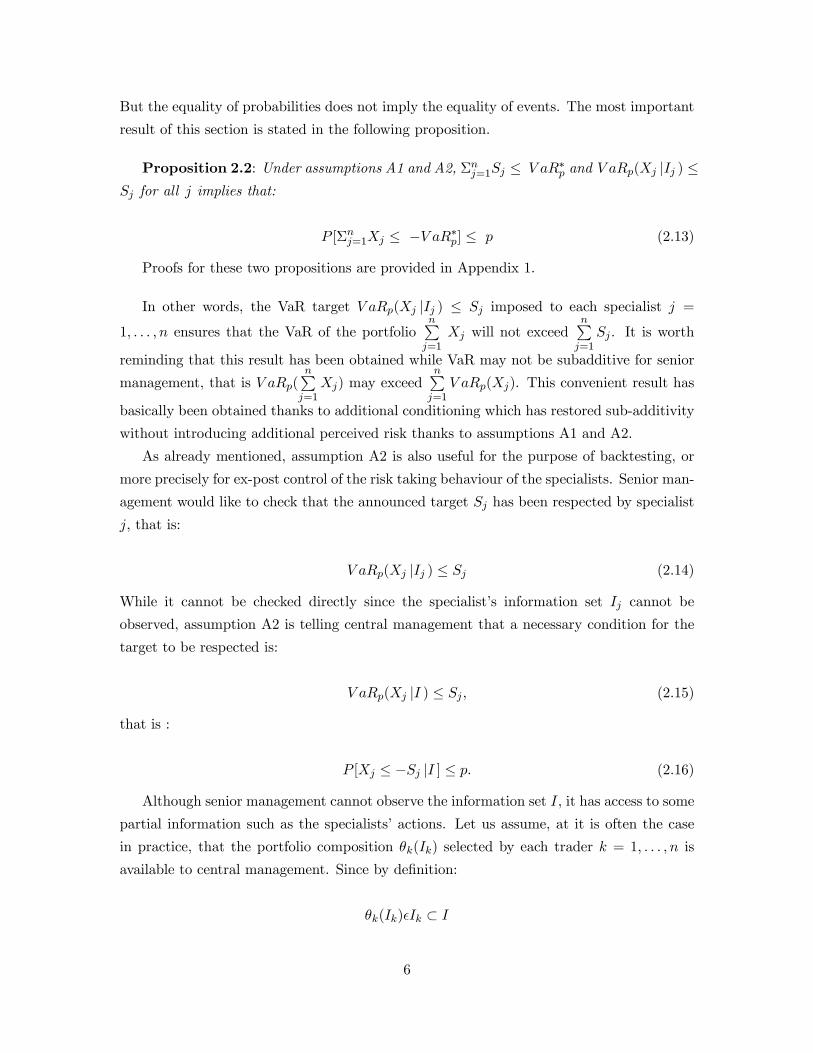
risk-averse agent will not invest in asset 2. Additionally, in the bad state (µ1 < Rf ), we havebθ11 < 0, which means that the trader is short selling fund 1, for which he has information.In the good state (µ0 > Rf ), bθ11 > 0 and trader 1 takes a long position in fund 1. Figure 1illustrates these results.

2When the VaR constraint of trader 1 (resp. 2) binds, it can be shown that he may have to invest anonzero part in asset 2 (resp. 1).

3 In a general framework, Merton (1987) assumes this result and justifies his assumption by the fact thatthe portfolios held by actual investors contain only a small fraction of the thousand of traded securitiesavailable. In our setting, the result follows directly from the private information held by the traders.

4 In a framework with only two assets (a risk-free asset and a risky asset with the same unconditionalexpected return), Sentana (1998) assumes and rationalizes the fact that the wealth invested in the riskyasset is a linear function of the information that the investor has on this asset.

8

2.3.2 Subadditivity and Coherence of VaR when properly conditioned

In this context, we show that VaRmay appear non subadditive to central management, while

in fact it remains subadditive conditionally to the private information of the traders. To

show this, we assume for simplicity that both traders have the same risk aversion γ and that

their initial wealth is normalized to one. We further assume that both information variables

s1 and s2 are in the good state (s1 = s2 = 0). Therefore, it follows that bθ11 = bθ22 = θ > 0,

traders’ portfolios are R1= (1− θ)Rf + θR1 and R

2= (1− θ)Rf + θR2 and the aggregate

portfolio at central management level is R1+R

2= 2 (1− θ)Rf + θ

¡R1 +R2

¢First, let us start by the apparent non subadditivity of VaR for central management.

Proposition 2.3 below shows that even for small probability p, the VaR subadditivity of

the central portfolio can be apparently seen as violated due to the asymmetric information

between traders and central management.

Proposition 2.3: For any mixture probability values λ < 1/2, at the level p =

Pr¡R1 +R2 ≤ µ1 + µ0

¢we have

V aRp

³R1+R

2´> V aRp

³R1´+ V aRp

³R2´

and

p = λ2Φ¡−µ/√2σ¢+ λ (1− λ) + (1− λ)2Φ

¡µ/√2σ¢

where Φ denotes the cumulative standard normal distribution.

Proof: see Appendix 1.

However, conditionally to information on both states, all returns become normal and

then it is well-known that for all p ≤ 0.5, subadditivity follows. Therefore, with λ < 1/2, at

the level p = Pr¡R1 +R2 ≤ µ1 + µ0

¢, we have shown that without conditioning on private

information, decentralization may appear as increasing the risk of the aggregate portfolio as

measured by the VaR, while in fact it does not since conditionally to the private information

of traders, returns become normal and subadditivity prevails. In the next section, we

provide central management with some information, namely the composition of the traders’

portfolios.

2.3.3 Backtesting VaR requirements

In this simple model, a central unit can test condition (2.17), which can be written P [Xj ≤−Sj |θk(Ik), k = 1, 2] ≤ p for all j, when the shares of the portfolios held by traders 1

and 2 are known. It is important to realize that in this setting, knowing the portfolio

9

composition of traders 1 and 2 is equivalent to knowing their private information s1 and

s2. Indeed, if trader 1 takes a long position in risky fund 1 it means that s1 is in the

good state and inversely if he short-sells fund 1. Similarly, the position of trader 2 will

be fully revealing. We can write sj = 1{θjj<0}. Since each private information completelydefines the return distribution of the fund in which the corresponding trader invests and

given that the two informations s1 and s2 are independent, the condition to test is exactly

P [Xj ≤ −Sj |θj(sj) ] ≤ p for j = 1, 2.

By the conditional normality of the return distributions, central management needs only

to infer the means and variances in the good and bad states for each trader in order to test

if each trader obeys his VaR limit with probability p. In section 2, we assume that central

management knows the underlying model. In practice, central management must estimate

the model based on time series of returns and compute V aR conditionally on past returns.

In this dynamic setting, assumption 2 can be rewritten as:

V aRp [Xj |It, Iτ , τ ≤ t] ≤ V aRp [Xj |Ijt, Iτ , τ ≤ t] . (2.20)

In other words, we will assume that all past information becomes common knowledge.

Propositions equivalent to Propositions 2.1 and 2.2 can be derived in a dynamic context.

We provide below an example of a filtering procedure that central management can follow

to recover the needed information about the returns distributions based on the available

information on portfolio shares.

To start, central management can assume that conditional returns of a particular trader

are normal and follow a switching-GARCH model for a given number of states:

(Rt+1 = µstt + σsttεt+1

σ2stt = ωst + αstσ2st−1t−1 + βst

³Rt − µst−1t−1

´2 (2.21)

where εt+1 ∼ N (0, 1) and st is a Markovian process taking two values 1 or 2 with transition

matrix Λ. By using the optimal portfolio share in a mean-variance context as in (2.19), cen-

tral management can use the information on the portfolio shares and the publicly available

risk-free rate to estimate the model:

Rt+1 = Rft + γσ2sttθt + σsttεt+1

σ2stt = ωst + αstσ2st−1t−1 + βst

³Rt −Rft−1 − γσ2st−1t−1θt−1

´2 (2.22)

This model can be estimated by using for example the procedure described in Gray

(1996), which applies the filtering algorithm of Hamilton (1989) in a GARCH model. In this

procedure, to avoid an infinite recursion, the state-dependent conditional variance σ2st−1t−1is replaced by the state-independent conditional variance σ2t−1 given by:

10

σ2t−1 = λt−1h¡Rft−1 + ρσ21t−1θt−1

¢2+ σ21t−1

i+(1− λt−1)

h¡Rft−1 + ρσ22t−1θt−1

¢2+ σ22t−1

i− £λt−1 ¡Rft−1 + ρσ21t−1θt−1

¢+ (1− λt−1)

¡Rft−1 + ρσ22t−1θt−1

¢¤2 (2.23)

where λt is the probability that st = 1 conditional on the information available at time t.

This probability is the by-product of the maximum likelihood estimation. The estimation

also provides the means and variances of the trader’s portfolio returns in both states. One

can therefore compute the conditional VaR with probability p and compare it to the VaR

requirement set by central management.

Our main argument until now has been to illustrate how conditioning and deconditioning

could affect the VaR subadditivity of a portfolio in the context of decentralized management.

In the example just developed, the unconditional distribution of returns was a mixture of

normals. In the absence of information on the make-up of portfolios, central management

can only rely on this thicker tailed distribution to assess VaR exceedence. In the next

section, we analyze VaR subadditivity in the context of portfolios with heavy-tailed return

distributions. This realistic setting for financial applications will provide a sense of how

robust is the subadditivity property for most practical purposes.

3 Stable distributions, Deconditioning and VaR Subadditiv-ity

In this section, we use stable distributions to characterize the unconditional return distri-

butions of traders’ portfolios. By appealing to a mixture representation property of stable

distributions, we link formally the Rent-a-Trader system of the last section to stable distri-

butions. More generally, as shown in early work by Mandelbrot (1963) and Fama (1965),

stable distributions accommodate well heavy-tailed financial series, with the consequence

that it produces measures of risk based on the tails of the distribution, such as value at risk,

which are more reliable (see in particular Mittnik and Rachev, 1993, and Mittnik, Paolella

and Rachev, 2000). The main purpose of this section is to investigate the robustness of

VaR subadditivity in the context of portfolios with stable distributions.

3.1 The Stable Distribution

A random variable X is said to have a stable distribution if for any positive numbers a and

b, there is a positive number c and a real number d such that

aX1 + bX2d= cX + d

11

whereX1 andX2 are independent copies ofX, and whered= denotes equality in distribution.

Then, it can be shown that there is a number α ∈ ]0, 2] , called the index of stability, suchthat: cα = aα + bα. For sake of expositional simplicity, we will assume in what follows

that α is different from one. From the Lévy-Khinchine representation of the characteristic

function, the characteristic function of a stable random variable can be written as:

E exp(iθX) = exp

½−σα |θ|α

∙1− iβ (sign θ) tan

Πα

2

¸+ iµθ

¾(3.1)

The parameters σ, β and µ are unique (β is irrelevant when α = 2) and it is clear that µ is

a location parameter and σ is a scale parameter.

In other words, while (3.1) defines the Sα [σ, β, µ] stable distribution:

X Ã Sα [σ, β, µ]

⇔ X − µ

σà Sα [1, β, 0] (3.2)

Since the characteristic function is real if and only if µ = β = 0, we see that β is a

skewness parameter. Sα [σ, β, µ] is symmetric around µ if and only β = 0.

X Ã Sα [σ, β, 0]⇔ (−X)Ã Sα [σ,−β, 0]

The distribution Sα (σ, β, 0) is said to be:⎧⎪⎪⎨⎪⎪⎩Skewed to the right if β > 0and totally skewed if β = 1.Skewed to the left if β < 0and totally skewed if β = −1.

For −1 < β < 1, the support of Sα(σ, β, µ) is the whole real line while the support of

the distribution Sα(σ, 1, 0) (resp. Sα(σ,−1, 0)) is the positive half line (resp. the negativehalf line).

3.2 Linking the Rent-a-Trader System to Stable Distributions

In this section, we rationalize the use of stable distributions in the context of the Rent-

a-Trader system of the last section. We argued that conditioning on the information of

specialists can reduce the thickness of the tails and therefore make the conditional VaR

subadditive whereas the unconditional VaR appeared non-subadditive. For stable distri-

butions, we recall below that a symmetric stable distribution can be seen as a mixture

of normal distributions or again as a mixture of stable distributions with less fat tails.

Therefore, we appeal to this mixture representation to make the link with the decentralized

portfolio management system setting discussed earlier.

12

Proposition 3.1.: Let X be a random variable with a symmetric α− stable distribu-tion, X Ã Sα(σ, 0, 0), 0 < α < 2, then X can be seen as a mixture of normal distributions:

X|AÃ N(0, σ2A), (3.1)

or more generally as a mixture of stable distributions:

X|AÃ Sα0 (σA1/α

0, 0, 0), 0 < α < α

0, (3.2)

and the probability distribution of the mixing variable A is defined by its Laplace transform:

E(exp(−γA)) = exp(−γα/α0) (3.3)

Proof: See Proposition 1.3.1 p. 20 in Samorodnitsky and Taqqu (1994).

The main message of this proposition is that proper conditioning of a random variable

with a symmetric stable distribution can produce either a normal random variable or a stable

distribution with less fat tails (higher α). In the first case we recover the VaR subadditivity

for a p less than 0.5, in the second we increase the range of validity of the subadditivity

property as we will see in the next subsection.

To complete the argument, we need to discuss how realistic is the symmetry assumption

for distributions produced by portfolio traders. A first observation is that the central unit

does not need to give a benchmark to the traders in the context of a decentralization

portfolio management system. Therefore, the distribution of interest is not the deviations

of the trader’s portfolio returns from the benchmark, which ought to be skewed to the right,

but simply the raw returns of the trader’s strategy. The right skewness of the latter returns

is less of a necessity. Of course the central unit may ex-post want to assess the performance

of the trader relatively by benchmarking with an index or other traders in similar markets

but ex-ante it is enough to control for the risk taken by the trader. Therefore, stable

distributions can appropriately be used to characterize the returns of the traders’ portfolios

when central management does not have any information to condition upon, such as the

portfolio shares. Then, the next question is to what extent is subadditivity lost when

portfolio returns follow stable distributions.

3.3 Very Heavy-tailed Distributions and Subadditivity

We will first treat the general case of Pareto-like distributions and show that they satisfy an

asymptotic convolution stability property. This allows us to get asymptotic assessments of

VaR subadditivity. In the second subsection, we specialize the results to the stable distrib-

ution and obtain under certain assumptions some finite assessments of VaR subadditivity.

13

3.3.1 The General Case

The probability distribution of a real random variable X is said to be “very heavy-tailed”

if, for some positive α:

Eh(Max(X, 0))δ

i= +∞ for all δ > α.

This is in particular the case of all distributions in the maximum domain of attraction

of the Frechet distribution, because they are such that:

1− F (x) = x−αL(x) (3.1)

for some function L on ]0,+∞[ slowly varying at (+∞). We focus here on the particularcase when the function L converges at infinity to a positive constant. It is convenient to

denote this positive limit as L(+∞) = σα. Then, the distribution function F has a power

right tail:

F̄ (x) = 1− F (x) ∼³σx

´α(3.2)

For expositional simplicity, we will assume in addition that F is continuous and strictly

increasing in some neighborhood of infinity. This allows us to characterize the limit σα =

L(+∞) from the tail behavior of a well-defined inverse function F̄−1 of F̄ :

σ = limq→1q

1/αF̄−1(q) (3.3)

Distributions functions conformable to (3.2) and (3.3) are often termed “Pareto-like”

and include, besides the Pareto distribution itself, the Cauchy and Burr distributions as

well as stable distributions with exponent α < 2.

As far as subadditivity of VaR is concerned, the nice feature of Pareto like distributions

is to fulfill an asymptotic convolution stability property. This property is fulfilled on the

whole support by stable distributions themselves. More precisely, the following lemma is a

straightforward application of Feller convolution theorem (Feller, 1971, p. 278):

Lemma 3.2: If X and Y are two independent Pareto-like random variables, with the same

exponent α, that is:

1− FX(x) ∼x→+∞

³σXx

´α1− FY (x) ∼

x→+∞

³σYx

´αwhere FX and FY denote respectively the distribution functions of X and Y , then X + Y

is also Pareto-like with the same exponent α and:

1− FX+Y (x) ∼x→+∞

σαX + σαYxα

14

Fron now on, the Pareto-like distribution will be applied to losses. In other words,

when X denotes the end-of-period wealth of interest, we maintain the assumption that

(−X) follows a Pareto-like distribution. Therefore, with obvious notations, formula (3.3)becomes:

limp→0V aRp(X)p

1/α = σX (3.4)

Then, the asymptotic convolution stability allows us to use the convexity/concavity

properties of the function σ → σα to get asymptotic assessments of VaR subadditivity.

This is the result of proposition 4.1 below.

Proposition 3.2

If X and Y are two independent random variables such that (−X) and (−Y ) followPareto-like distributions with the same exponent α :

(i) If α > 1:

There exists p0 ∈ ]0, 1] such that, for any p ∈ ]0, p0[:

V aRp [X + Y ] < V aRp(X) + V aRp(Y )

(ii) If α < 1 :

There exists po ∈ ]0, 1[ such that, for any p ∈ ]0, p0[

V aRp [X + Y ] > V aRp(X) + V aRp(Y )

(iii) If α = 1 :

limp→0p [V aRp (X + Y )− V aRp(X)− V aRp(Y )]= 0

Proof: See Appendix 2.

Proposition 3.2 shows that VaR is subadditive, at least for sufficiently small probabilities,

when the possible loss has finite expectation (α > 1). In this respect, non-subadditive VaR

remains quite an extreme situation5.

However, in the case of very heavy tail distributions (α close to zero), violation of

subadditivity may be arbitrarily extreme. We propose below a way to measure the degree

of violation of subadditivity. While non-subadditivity means:

V aRp (X + Y ) > V aRp(X) + V aRp(Y ), (3.5)

5Recently, Ibragimov (2004) obtained a similar result with a different approach based on the analysis ofmajorization properties of linear combinations of random variables.

15

that is the loss of the portfolio (X + Y ) can exceed V aRp(X) + V aRp(Y ) with probability

p, the question is: with what probability kp, k ≥ 1, can we loose more than V aRp(X) +

V aRp(Y ) with probability p? In other words, the question is with what probability kp, k ≥1, can we have:

V aRkp(X + Y ) > (V aRp(X) + V aRp(Y ). (3.6)

While violation (3.5) of subadditivity means that (3.6) is fulfilled with k = 1, it cannot

be fulfilled with k = 2 since, for any random variables X and Y :

V aR2p(X + Y ) ≤ V aRp(X) + V aRp(Y ) (3.7)

Indeed:

P [X + Y ≤ −V aRp(X)− V aRp(Y )] ≤ 2p

P [X + Y ≤ −V aRp(X)− V aRp(Y )]

≤ P [X ≤ −V aRp(X)] + P [Y ≤ −V aRp(Y )] .

However, we can show:

Proposition 3.3:

For any k in ]0, 2[, there exists α0 in ]0, 1[ such that for any α in ]0, α0[, there exists p0in ]0, 1[ such that for any p in ]0, p0[:

V aRkp(X + Y ) > V aRp(X) + V aRp(Y )

Proof: See Appendix 3.

In other words, when α is arbitrarily small, the possible loss of X + Y can exceed

V aRp(X) + V aRp(Y ) with a probability kp, for k arbitrarily close to 2. Therefore, by iter-

ating the argument, the loss of a portfolionPi=1

Xi can exceednPi=1

V aRpXi with a probability

arbitrarily close to (np). It is clear that such a non-subadditivity would definitely make

unreliable any decentralized risk management strategy based on VaR targets assigned to

the independent segments of the portfolio.

3.3.2 The Case of the Stable Distribution

The left tail behaviour of the stable distribution is characterized as follows.

Proposition 3.4: Let X Ã Sα [σ, β, µ] with 0 < α < 2.

Then:

limλ→+∞

λαP [X < −λ] = Cα1− β

2σα

16

where Cα =1− α

Γ(2− α) cos(Πα

2 ).

By comparison with the notations of the previous section, we see that whenX Ã Sα(σ, β, µ),

with −1 ≤ β < 1, it is heavy-tailed on the left with α as left tail power parameter and σX =hCα

(1−β)2

i1/ασ as left tail scale parameter. The following result expresses the convolution

property for stable distributions.

Proposition 3.5: If X Ã Sα [σ1, β1, µ1] and Y Ã Sα [σ2, β2, µ2] are independent stable

variables, then X + Y = Z Ã Sα[σ, β, µ] with:

¯̄̄̄¯̄̄̄ σ = [σα1 + σα2 ]

1/α

β =β1σ

α1 + β2σ

α2

σαµ = µ1 + µ2

It is then clear that:

σαX = Cα(1− β1)

2σα1

σαY = Cα(1− β2)

2σα2

σαZ = Cα(1− β)

2σα

fulfill the convolution property:

σαZ = σαX + σαY .

Therefore, all the results of the previous section can be applied to stable distributions.

Besides their stability property, stable distributions are of interest since they allow to extend

some results to the case of finite p (and not only p → 0). To see this, let us first remark

that, thanks to the location-scale property:

X Ã Sα(σ, β, µ)

⇒ −V aRp(X) = µ+ σφ−1α,β(p)

where φα,β denotes the cumulative distribution function of Sα [1, β, 0] .

A simple corollary of proposition 3.2 is then.

Corollary 3.1: For |β| < 1 and p such that φ−1α,β(p) < 0, we have:Let X,Y be two independent stable variables¯̄̄̄X Ã Sα [σ1, β, µ1]Y Ã Sα [σ2, β, µ2]

(i) If α > 1 :

17

V aRp [X + Y ] < V aRp(X) + V aRp(Y ).

(ii) If α < 1 :

V aRp [X + Y ] > V aRp(X) + V aRp(Y ).

It is worth noticing that, by contrast with proposition 3.1, corollary 3.1 can surely be

applied for values of the probability p which are not excessively small. For instance, if

β = 0, corollary 3.1 applies for p < 1/2. The price to pay to get this stronger result is

that we have assumed that X and Y have the same skewness parameter. This assumption,

which was not needed to apply the convolution property, may appear overly restrictive to

the point where only β = 0 has some practical content. Hopefully, the subbaditivity should

not be lost for not too different skewness parameters.

4 Conclusion

In this paper, we have argued that, in the context of decentralized portfolio management,

central management possesses only a fraction of information which belongs to each specialist.

In such a context, a distribution appears always thicker to the central unit than to the

specialist. Therefore, because of a lack of information, VaR may appear fallaciously non

subadditive to the central management unit. We were then able to show that decentralized

portfolio management with a VaR allocation to each specialist will work despite evidence to

the contrary. Furthermore, we have shown that value at risk remains subadditive in many

situations of practical interest. In the case of heavy-tail distributions, we have shown, at

least for sufficiently small probabilities, that VaR remains subadditive when the possible

loss has finite expectation. In this respect, non-subadditive VaR remains quite an extreme

situation.

Even though we show that for all practical purposes VaR is not as incoherent a measure

of risk as it is often argued, it remains that portfolio optimization practices using VaR

as a simple substitute to variance, i.e. maximization of expected return under a VaR

constraint) may generate perverse effects. In particular, there is a risk that a manager who

is controlled only through a maximal loss level with probability (1 − p) will be enticed to

expose himself to huge possible losses with probability p. To control for such a risk, one

can add to VaR the expected loss beyond the VaR or consider a parameterized family of

more limited possible risks. Ortobelli, Rachev and Schwartz (2000) provide a thourough

analysis of optimal portfolio allocation with stable distributed returns, including with a

safety-first optimal allocation problem, whereby investors maximize their expected wealth

while minimizing at the same time the risk of loss. Efficient frontiers in the latter case are

a function of the threshold VaR.

18

References

[1] Artzner, P., F. Delbaen, J.-M. Eber and D. Heath (1999), “Coherent Measures of Risk,”

Mathematical Finance, 9, 3, 203-228.

[2] Basak, S. and Shapiro, A. (2001) “Value-at-Risk-Based Risk Management: Optimal

Policies and Asset Prices”, Review of Financial Studies, 14, 371-405.

[3] Bollerslev, T. (1986) “Generalized Autoregressive Conditional Heteroskedasticity”,

Journal of Econometrics, 31, 307-327

[4] Duffie, D.J., Pan, J., (1997), “An Overview of Value at Risk”, Journal of Derivatives,

4, 7-49.

[5] Engle, R. (1982) “Autoregressive Conditional Heteroskedasticity Models with estima-

tion of Variance of United Kingdom Inflation”, Econometrica, 50, 987-1007.

[6] Fama, E. (1965), “Behavior of Stock Market Prices”, Journal of Business, 38, 34-105.

[7] Gray, S. F. (1996) “Modeling the conditional distribution of interest rates as a regime-

switching process”, Journal of Financial Economics, 42, 27-62

[8] Hamilton, J.D. (1989) “A New Approach to the Economic Analysis of Nonstationary

Time Series and the Business Cycle”, Econometrica, 57, 357-384.

[9] Hamilton, J.D. (1994) Time Series Analysis, Princeton University Press.

[10] Ibragimov, R. (2004), “On the Robustness of Economic Models to Heavy-Tailedness

Assumptions,” Working Paper, Yale University.

[11] Jorion, P. (2001) Value at Risk: The New Benchmark for Managing Financial Risk,

McGraw-Hill, New York.

[12] Mandelbrot, B. (1963), “The Variation of Speculative Prices”, Journal of Business, 36,

394-419.

[13] Merton, R.C., (1987), “A Simple Model of Capital Market Equilibrium with Incomplete

Information”, Journal of Finance, 42, 483-510.

[14] Mittnik, S. and S. T. Rachev (1993), “Modeling Asset Returns with Alternative Stable

Distributions”, Econometric Reviews, 12(3), 261-330.

[15] Mittnik, S., M. S. Paolella,and S. T. Rachev (2000), “Diagnosis and treating the fat

tails in financial returns data”, Journal of Empirical Finance, 7, 389-416.

19

[16] Ortobelli, S., S. T. Rachev and E. Schwartz (2000), “The Problem of Optimal As-

set Allocation with Stable Distributed Returns”, Working Paper, Anderson Graduate

School of Management.

[17] Samorodnitsky and M. S. Taqqu (1994), “Stable Non-Gaussian Random Processes -

Stochastic Models with Infinite Variance,” Chapman &Hall, New York.

[18] Sentana, Enrique (1998), “Least Squares Predictions and Mean-Variance Analysis”,

CEMFI Working Paper.

20

Appendix 1

Proof of Proposition 2.1:

For A random event, we define the random variable:

1A =

½1 if A occurs0 otherwise.

Assumption A2 implies that:

1[Xj≤−V aRp(Xj |Ij )] ≤ 1[Xj≤−V aRp(Xj |I )].

But these two random variables have the same conditional expectation given Ij since by

definition:

Eh1[Xj≤−V aRp(Xj |Ij )] |Ij

i= Pr {Xj ≤ −V aRp(Xj |Ij ) |Ij }= p

and by the law of iterated expectations:

Eh1[Xj≤−V aRp(Xj |I )] |Ij

i= E

hEh1[Xj≤−V aRp(Xj |I )] |I

i|Iji

= E [Pr {Xj ≤ −V aRp(Xj |I ) |I } |Ij ]= E [p |Ij ]= p

Therefore, these two random variables must coincide Ij almost surely. This achieves the

proof of proposition 2.1.

Proof of Proposition 2.2:

Since for all j, V aRp (Xj |Ij ) ≤ Sj and, by assumption A2:

V aRp (Xj |I ) ≤ V aRp (Xj |Ij )

we have:

p(I) = P

⎡⎣ nXj=1

Xj ≤ −nX

j=1

Sj |I⎤⎦ ≤ P

⎡⎣ nXj=1

Xj ≤ −nX

j=1

V aRp(Xj |I ) |I⎤⎦

But, by assumption A1:

V aRp

⎛⎝ nXj=1

Xj |I⎞⎠ ≤ nX

j=1

V aRp(Xj |I ).

Thus:

21

p(I) ≤ P

"nP

j=1Xj ≤ −V aRp(

nPj=1

Xj |I ) |I#= p.

Since this inequality is identically true, for all possible values of the random information

set I, we conclude by considering unconditional expectations that:

P

⎡⎣ nXj=1

Xj ≤ −nX

j=1

Sj

⎤⎦ ≤ p.

A fortiori:

P

⎡⎣ nXj=1

Xj ≤ −V aR∗p

⎤⎦ ≤ p

Proof of Proposition 2.3:

Proof of Proposition 2.3: we have

R1= (1− θ)Rf + θR1

R2= (1− θ)Rf + θR2 and

R1+R

2= 2 (1− θ)Rf + θ

¡R1 +R2

¢Since Rf is nonrandom and θ > 0, by using translation invariance and positive homo-

geneity of VaR, we have that

V aRp

³R1+R

2´> V aRp

³R1´+ V aRp

³R2´is equivalent to

V aRp

¡R1 +R2

¢> V aRp

¡R1¢+ V aRp

¡R2¢, we will then show this second formulation.

Let µ ≡ µ1 − µ0 < 0 and let us define the following variables

X1 ≡ R11 − µ0 ∼ N¡µ, σ2

¢X2 ≡ R12 − µ0 ∼ N

¡µ, σ2

¢Z1 ≡ R01 − µ0 ∼ N

¡0, σ2

¢Z2 ≡ R02 − µ0 ∼ N

¡0, σ2

¢we have

R1 = s1X1 + (1− s1)Z1 + µ0

R2 = s2X2 + (1− s2)Z2 + µ0

andp = Pr

¡R1 +R2 ≤ µ1 + µ0

¢= Pr (s1X1 + (1− s1)Z1 + s2X2 + (1− s2)Z2 ≤ µ1 − µ0)

= Pr

µs1s2 (X1 +X2) + s1 (1− s2) (X1 + Z2)++s2 (1− s1) (X2 + Z1) + (1− s1) (1− s2) (Z1 + Z2) ≤ µ

¶= λ2FX1+X2 (µ) + λ (1− λ)FX1+Z2 (µ)+

+λ (1− λ)FX2+Z1 (µ) + (1− λ)2 FZ1+Z2 (µ)

= λ2FX1+X2 (µ) + λ (1− λ) + (1− λ)2 FZ1+Z2 (µ)

22

i.e. p = λ2FX1+X2 (µ) + λ (1− λ) + (1− λ)2 FZ1+Z2 (µ)

Remark:

p = 1/2 for µ = 0,

and p→ λµ→−∞

. To see this second result we can notice that FZ1+Z2 (µ) −→ 0µ→−∞

, and

FX1+X2 (µ) = Pr (X1 +X2 ≤ µ)= Pr ((X1 − µ) + (X2 − µ) ≤ −µ)= Pr

¡N¡0, 2σ21

¢ ≤ −µ¢−→ 1µ→−∞

therefore

for λ < 1/2, p can takes any value into (λ, 1/2) as µ varies into (−∞, 0)

and for λ > 1/2, p can takes any value into (1/2, λ) as µ varies into (−∞, 0)

so while λ and µ vary p can takes any value into (0, 1)

Let us pose

U1 ≡ s1X1 + (1− s1)Z1U2 ≡ s2X2 + (1− s2)Z2

We can easily see that Uj = eRj −µ0, j = 1, 2. Therefore the proposition is equivalent to

V aRp (U1 + U2) > V aRp (U1)+ V aRp (U2). By definition of p, we have V aRp (U1 + U2) =

−µ, and since U1 d= U2 then V aRp (U1) = V aRp (U2) and the problem becomes V aRp (U1 + U2) >

2V aRp (U1) i.e. V aRp (U1) < −µ/2 or equivalently Pr (U1 ≤ µ/2) < p.

we have

Pr (U1 ≤ µ/2) = Pr (s1X1 + (1− s1)Z1 ≤ µ/2)= λFX1 (µ/2) + (1− λ)FZ1 (µ/2)

let ε be a N (0, 1) random variable and Φ its c.d.f., we have:

FX1+X2 (µ) = Pr¡2µ+

√2σε < µ

¢= Φ

¡−µ/√2σ¢ ;FX1 (µ/2) = Pr (µ+ σε < µ/2)

= Φ (−µ/2σ) ;

FZ1+Z2 (µ) = Pr¡√2σε < µ

¢= Φ

¡µ/√2σ¢;

and

23

FZ1 (µ/2) = Pr (σε < µ/2)= Φ (µ/2σ) .

so

p− Pr (U1 ≤ µ/2) = λ2Φ¡−µ/√2σ¢+ λ (1− λ) + (1− λ)2Φ

¡µ/√2σ¢

−λΦ (−µ/2σ)− (1− λ)Φ (µ/2σ)

=

⎡⎢⎣Φ³−µ/√2σ´+Φ³µ/√2σ´| {z }=1

− 1

⎤⎥⎦λ2++

⎡⎢⎣−2Φ ¡µ/√2σ¢+ 1−Φ (−µ/2σ)| {z }=Φ(µ/2σ)

+Φ (µ/2σ)

⎤⎥⎦λ+£Φ¡µ/√2σ¢−Φ (µ/2σ)¤

i.e.

p− Pr (U1 ≤ µ/2) =£Φ¡µ/√2σ¢− Φ (µ/2σ)¤ [1− 2λ]

> 0 since λ < 1/2 and Φ¡µ/√2σ¢> Φ (µ/2σ)

which means Pr (U1 ≤ µ/2) < p, and therefore the proposition follows. Q.E.D

24

Appendix 2

Proof of Proposition 3.2: Let us denote Z = X + Y.

(i) If α > 1 :

σZ = [σαX + σαY ]

1/α < σX + σY

Consider a real r such that:

σZ < r < σX + σY

Since σZ = Limp→0V aRp(Z)p

1/α,

there exists p1 such that, for any p ]0, p1[:

V aRp(Z)p1/α < r.

For similar reasons, there exists p2 such that, for any p ]0, P2[

r < V aRp(X)p1/α + V aRp(Y )p

1/α.

Therefore, with p0 =Min(p1, p2)we have for any p ]0, po[ :

V aRp(Z) < V aRp(X) + V aRp(Y )

(ii) If α < 1

σZ = [σαX + ραY ]

1/α > σX + σY .

A similar argument shows that there exists p0 such that, for any p ]0, p0[:

V aRp(Z) > V aRp(X) + V aRp(Y ).

(iii) If α = 1

σZ = σX + σY

that is:

limp→0pV aRp (Z) = lim

p→0pV aRp(X) + limp→0pV aRp (Y ) .

Proof of Proposition 3.3:

As a function of α ∈ ]0, 1[, the function [σX + σY ]α

σαX + σαYis continuous and increasing, from

the value 1/2 for α = 0 to the value 1 for α = 1. Then, for k given in ]0, 2[, there exists α0such that, for any α in ]0, α0[ :

[σX + σY ]α

σαX + σαY<1

k,

that is:

σX + σY < k−1/α [σαX + σαY ]1/α = k−1/ασZ .

25

Since σX = limp→0p

1/αV aRp(X), σY = limp→0p

1/αV aRp(Y )

and σZ = limp→0(kp)

1/αV aRkp(z), we have the existence of p0 such that for any p in ]0, p0[:

p1/αV aRp(X) + p1/αV aRp(Y ) < k−1/α(kp)1/αV aRkp(Z)

that is V aRp(X) + V aRp(Y ) < V aRkp(Z).

26

Optimal part invested in risky fund ( )

210

σγµµ −

1µ 0µ fR Risk-free return

-( )

210

σγµµ −

In good state In bad state

Part

inve

sted

in r

isky

fund

Figure 1: Optimal Share Invested in Risky Fund as Function of the Risk-free return

27