Propagation effects - University of Houston–Clear Lakesce.uhcl.edu/goodwin/ceng5332/downloads/chapter_4.pdf · Consider the obstacle shown in green to be a knife-edge of known height

Slides for “Wireless Communications” © Edfors, Molisch, Tufvesson

Chapter 4

Propagation effects

77Slides for “Wireless Communications” © Edfors, Molisch, Tufvesson

Why channel modelling?

• The performance of a radio system

is ultimately determined by the radio

channel

• The channel models basis for

– system design

– algorithm design

– antenna design etc.

• Trend towards more systeminteraction with channel- MINO- UWB- 4G

Without reliable

channel models, it

is hard to design

radio systems that

work in real environments.

78Slides for “Wireless Communications” © Edfors, Molisch, Tufvesson

THE RADIO CHANNEL

It is more than just a loss

• Some examples:

– behavior in time/place?

– behavior in frequency?

– directional properties?

– bandwidth dependency?

– behavior in delay?

80Slides for “Wireless Communications” © Edfors, Molisch, Tufvesson

Free-space loss

d

ARX

If we assume RX antenna to be isotropic:

2

4RX TXP Pd

Attenuation between two

isotropic antennas in free

space is (free-space loss):

24

ddL free

81Slides for “Wireless Communications” © Edfors, Molisch, Tufvesson

Free-space loss

Friis’ law

Received power, with antenna gains GTX and GRX:

2

4RX TX

RX TX TX RX TX

free

G GP d P P G G

L d d

| | | | |

2

| | 10 |410log

RX dB TX dB TX dB free dB RX dB

TX dB TX dB RX dB

P d P G L d G

dP G G

Valid in the far field only

this leaves the free space loss factor ( .. )2, the path loss PRX/PTX = Pout/Pin

82Slides for “Wireless Communications” © Edfors, Molisch, Tufvesson

Free-space loss

What is far field?

Rayleigh distance:

22 aR

Ld

where La is the largest dimesion of

the antenna.

-dipole2/

2/

2/aL

2/Rd

Parabolic

rLa 2

28rdR

r2

The effective area of the dish antenna is the area projected on the red lineminus the blockage caused by the feed point and its supports

83Slides for “Wireless Communications” © Edfors, Molisch, Tufvesson

Reflection and transmission (1)

ir

t

1

2

When source is "low" to the medium ( Θi > 53o

for the air/water interface) it is all reflected, no energy directed into the second medium (water). However for waves that are reflected there is a phase shift of 180o (reflection coefficient = -1) as Θi --> 90o which is important in wireless systems when ground-reflected waves are considered.

84Slides for “Wireless Communications” © Edfors, Molisch, Tufvesson

Reflection and transmission (2)

• Snell’s law

– Reflection angle

– Transmission angle

• Transmission and reflection: distinguish TE and TM waves

r e

sint

sine

1

2

85Slides for “Wireless Communications” © Edfors, Molisch, Tufvesson

Reflection and transmission (3)

TM 2 cose 1 cost

2 cose 1 costTE

1 cose 2 cost

1 cose 2 cost

Brewster

angle

Phase inverted

For grazing angle

Both waves have a magnitude of 1 anda phase shift of 1800 as the glazing incidence approaches 900 - a ground reflected wave

This doesn't apply to Millimeter waves (30 - 300 GHz) which don't penetrate much of anything since dielectrics have losses at these high frequencies

dlayer is the geometrical length of the layer

87Slides for “Wireless Communications” © Edfors, Molisch, Tufvesson

The d-4 law

PRXd PTXGTXGRXhTXhRX

d2

2.

• For the following scenario

• the power goes like

• for distances greater than

dbreak 4hTXhRX/

The d-4 law is NOT a universal description of a wireless channel just a case to show that n = -4 is mathematically possible

88Slides for “Wireless Communications” © Edfors, Molisch, Tufvesson

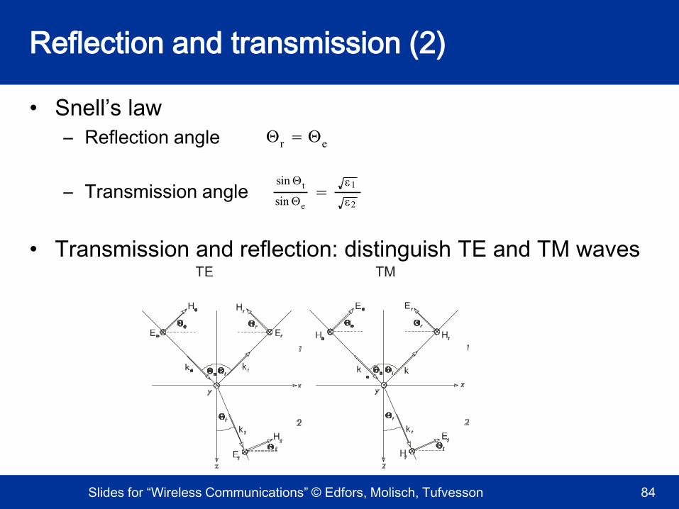
The d-4 law (continued)

Diffraction and Fresnel Zones

Material Related to Chapter 4 Textbook Pages 55 - 59

Wavefront Encountering an Obstacle

Consider the obstacle shown in green to be a knife-edge of known height (0 to 3)and infinite width - into and out of the paper (your looking at the side)

Blockage Signal Levels

Signal Levels on the Far Side of the Shadowing Object

Note leakage of signal into blocked/shadowed area (0-3) but also that the field strength above the top of the obstacle

( 0 to -2) is also disturbed.

ν is the dimensionless Fresnel-Kirchoff diffraction parameter. The graph shows the loss in dB due to knife-edge diffraction, a graphical solution for finding the Fresnel integral F(νF)

Knife-edgeDiffractionGain

dB

Huygens’ Principle

Representation of Radio Waves as Wavelets

Slides for “Wireless Communications” © Edfors, Molisch, Tufvesson

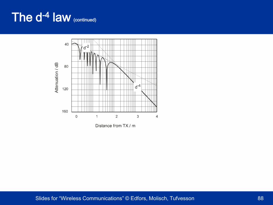
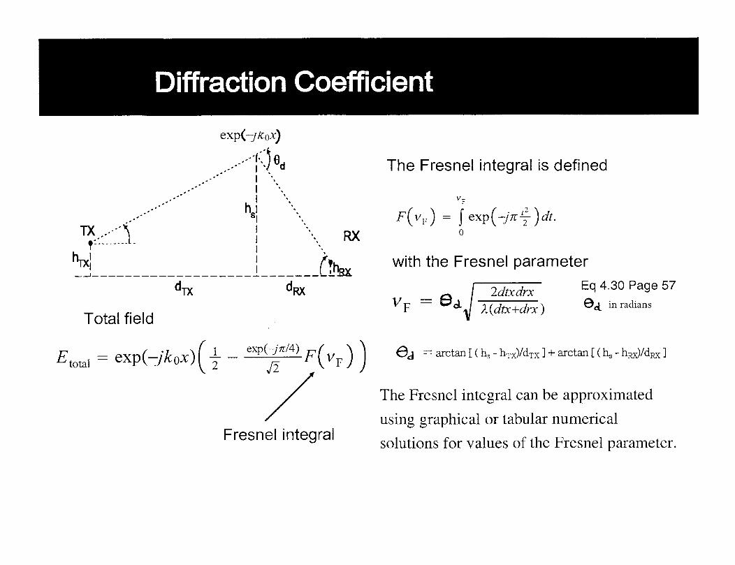
Diffraction, Huygen’s principle

Result (ETOTAL) at specific point is the superposition of the spherical waves, both constructive and desctructive interference

Page 55 in textbook - see errata regarding Eq 4.27

Fresnel Zones

To visualize what happens to radio waves when theyencounter an obstacle, we have to develop a picture of thewavefront after the obstacle as a function of the wavefrontjust before the obstacle

How much space around the direct path between thetransmitter and receiver should be clear of obstaclesincluding the ground? Objects within a series of concentric circles around the line of sight between

transceivers have constructive/destructive effects on communication

A radio path has first Fresnel zone clearance if no objectscapable of causing significant diffraction penetrate thecorresponding ellipsoid

Fresnel Zones

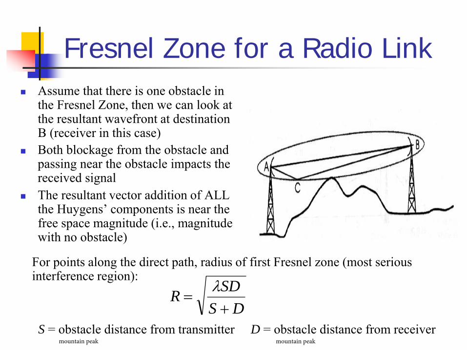
Fresnel Zone for a Radio Link

Assume that there is one obstacle inthe Fresnel Zone, then we can look atthe resultant wavefront at destinationB (receiver in this case)

Both blockage from the obstacle andpassing near the obstacle impacts thereceived signal

The resultant vector addition of ALLthe Huygens’ components is near thefree space magnitude (i.e., magnitudewith no obstacle)

For points along the direct path, radius of first Fresnel zone (most serious interference region):

S = obstacle distance from transmitter D = obstacle distance from receiver DS

SDR

mountain peak mountain peak

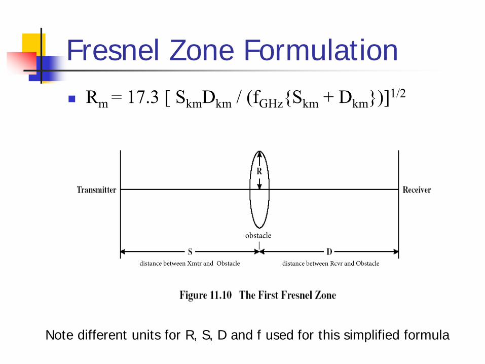
Fresnel Zone Formulation

Rm = 17.3 [ SkmDkm / (fGHz{Skm + Dkm})]1/2

Note different units for R, S, D and f used for this simplified formula

obstacle |

distance between Xmtr and Obstacle distance between Rcvr and Obstacle

Slides for “Wireless Communications” © Edfors, Molisch, Tufvesson

Diffraction

Note that the Fresnel Integral can be larger than 1 and actually be increased by the screen but later decreased (no free energy)

Slides for “Wireless Communications” © Edfors, Molisch, Tufvesson

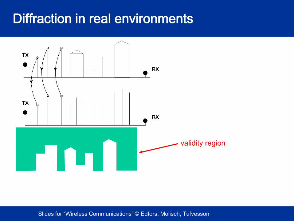
Diffraction in real environments

validity region

Eq 4.29 on page 56 for angle in radians

Slides for “Wireless Communications” © Edfors, Molisch, Tufvesson

Diffraction – Epstein-Petersen Method

Diffraction –

compute diffraction loss for each

screen separately and add the

losses

L1

L2

L3

Ltot=L1+L2+L3

Copyright: Wiley

Slides for “Wireless Communications” © Edfors, Molisch, Tufvesson

Scattering

Smooth surface

Specular

reflection

Scattering

Rough surface

Specular

reflection

Slides for “Wireless Communications” © Edfors, Molisch, Tufvesson

Kirchhoff theory – scattering by rough surfaces

rough smooth exp 2 k0h sin 2

for Gaussian surface distribution

standard deviation of height

angle of incidence

Slides for “Wireless Communications” © Edfors, Molisch, Tufvesson

Pertubation theory – scattering by rough surfaces

h2W E r h r h r

h r

More accurate than Kirchhoff theory, especially for large angles of

incidence and “rougher” surfaces

h r

Slides for “Wireless Communications” © Edfors, Molisch, Tufvesson

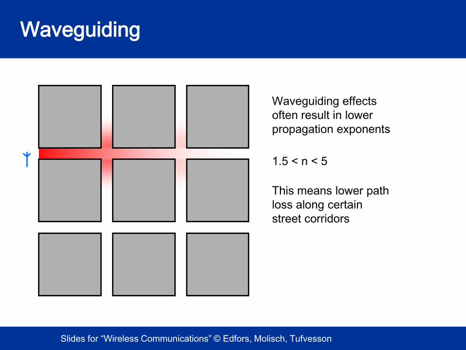
Waveguiding

Waveguiding effects

often result in lower

propagation exponents

1.5 < n < 5

This means lower path

loss along certain

street corridors

Atmospheric Absorption Radio waves at frequencies above 10 GHz are

subject to molecular absorption Peak of water vapor absorption at 22 GHz Peak of oxygen absorption near 60 GHz

Favorable windows for communication: From 28 GHz to 42 GHz From 75 GHz to 95 GHz

Millimeter waves are generally considered to be from30 to 300 GHz. These frequencies are an area of great interest for 5G wireless systems; however, the signals hardly penetrate anything which will probably lead to utilizing mesh networks for system connectivity

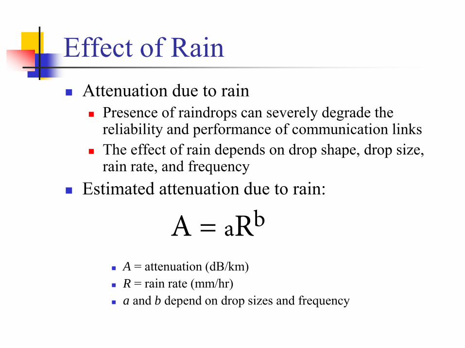
Effect of Rain Attenuation due to rain

Presence of raindrops can severely degrade thereliability and performance of communication links

The effect of rain depends on drop shape, drop size,rain rate, and frequency

Estimated attenuation due to rain:

A = attenuation (dB/km) R = rain rate (mm/hr) a and b depend on drop sizes and frequency

A = aRb

Effects of Vegetation Trees near subscriber sites can lead to multipath

fading The tree canopy multipath effects are diffraction

and scattering Measurements in orchards found considerable

attenuation values when the foliage is within 60% of the first Fresnel zone

Multipath effects highly variable due to wind since the leaves, tree limbs, …. move in the wind in addition to the time of the year (season – path loss is generally lower during the winter)