Projects and Team Dynamics

Projects and Team Dynamics

George Georgiadis ∗

April 16, 2014

Abstract

I study a dynamic problem in which a group of agents collaborate over time to

complete a project. The project progresses at a rate that depends on the agents’ efforts,

and it generates a payoff upon completion. I show that agents work harder the closer

the project is to completion, and members of a larger team work harder than members

of a smaller team - both individually and on aggregate - if and only if the project is

sufficiently far from completion. I apply these results to determine the optimal size of

a self-organized partnership, and to study the manager’s problem who recruits agents

to carry out a project, and must determine the team size and its members’ incentive

contracts. The main results are (i) that the optimal symmetric contract compensates

the agents only upon completing the project, and (ii) the optimal team size decreases in

the expected length of the project.

Keywords: Projects, moral hazard in teams, team formation, partnerships, differential games.

∗California Institute of Technology and Boston University. E-mail: [email protected]. I am grate-ful to the co-editor, Marco Ottaviani, and to three anonymous referees whose comments have immeasurablyimproved this paper. I am indebted to Simon Board and Chris Tang for their guidance, suggestions and crit-icisms. I also thank Andy Atkeson, Sushil Bikhchandani, Andrea Bertozzi, Miaomiao Dong, Florian Ederer,Hugo Hopenhayn, Johannes Horner, Moritz Meyer-Ter-Vehn, Kenny Mirkin, James Mirrlees, Salvatore Nun-nari, Ichiro Obara, Tom Palfrey, Gabriela Rubio, Tomasz Sadzik, Yuliy Sannikov, Pierre-Olivier Weill, BillZame, Joe Zipkin, as well as seminar participants at Bocconi, BU, Caltech, Northwestern University, NYU,TSE, UCLA, UCSD, the University of Chicago, the University of Michigan, USC, UT Austin, UT Dallas,the Washington University in St. Louis, the 2012 Southwest Economic Theory conference, the 2012 NorthAmerican Summer Meetings of the Econometric Society, GAMES 2012, and the SITE 2013 Summer Workshopfor many insightful comments and suggestions.

1

1 Introduction

Teamwork and projects are central in the organization of firms and partnerships. Most

large corporations engage a substantial proportion of their workforce in teamwork (Lawler,

Mohrman and Benson (2001)), and organizing workers into teams has been shown to in-

crease productivity in both manufacturing and service firms (Ichniowski and Shaw (2003)).

Moreover, the use of teams is especially common in situations in which the task at hand will

result in a defined deliverable, and it will not be ongoing, but will terminate (Harvard Busi-

ness School Press (2004)). Motivated by these observations, I analyze a dynamic problem in

which a group of agents collaborate over time to complete a project, and I address a number

of questions that naturally arise in this environment. In particular, what is the effect of the

group size to the agents’ incentives? How should a manager determine the team size and the

agents’ incentive contracts? For example, should they be rewarded for reaching intermediate

milestones, and should rewards be equal across the agents?

I propose a continuous-time model, in which at every moment, each of n agents exerts costly

effort to bring the project closer to completion. The project progresses stochastically at a

rate that is equal to the sum of the agents’ effort levels (i.e., efforts are substitutes), and it is

completed when its state hits a pre-specified threshold, at which point each agent receives a

lump sum payoff and the game ends.

This model can be applied both within firms, for instance, to research teams in new product

development or consulting projects, and across firms, for instance, to R&D joint ventures.

More broadly, the model is applicable to settings in which a group of agents collaborate

to complete a project, which progresses gradually, its expected duration is sufficiently large

such that the agents discounting time matters, and it generates a payoff upon completion.

A natural example is the Myerlin Repair Foundation (MRF): a collaborative effort among a

group of leading scientists in quest of a treatment for multiple sclerosis (Lakhani and Carlile

(2012)). This is a long-term venture, progress is gradual, each principal investigator incurs

an opportunity cost by allocating resources to MRF activities (which gives rise to incentives

to free-ride), and it will pay off predominantly when an acceptable treatment is discovered.

In Section 3, I characterize the Markov Perfect equilibrium (hereafter MPE) of this game,

wherein at every moment, each agent observes the state of the project (i.e., how close it is

to completion), and chooses his effort level to maximize his expected discounted payoff, while

anticipating the strategies of the other agents. A key result is that each agent increases his

effort as the project progresses. Intuitively, because he discounts time and is compensated

2

upon completion, his incentives are stronger the closer the project is to completion. An

implication of this result is that efforts are strategic complements across time, in that a higher

effort level by one agent at time t brings the project (on expectation) closer to completion,

which in turn incentivizes himself, as well as the other agents to raise their future efforts.

In Section 4, I examine the effect of the team size to the agents’ incentives. I show that

members of a larger team work harder than members of a smaller team - both individually

and on aggregate - if and only if the project is sufficiently far from completion.1 Intuitively, by

increasing the size of the team, two forces influence the agents’ incentives. First, they obtain

stronger incentives to free-ride. However, because the total progress that needs to be carried

out is fixed, the agents benefit from the ability to complete the project quicker, which increases

the present discounted value of their reward, and consequently strengthens their incentives.

I refer to these forces as the free-riding and the encouragement effect, respectively. Because

the marginal cost of effort is increasing and agents work harder the closer the project is to

completion, the free-riding effect becomes stronger as the project progresses. On the other

hand, the benefit of being able to complete the project faster in a bigger team is smaller the

less progress remains, and hence the encouragement effect becomes weaker with progress. As a

result, the encouragement effect dominates the free-riding effect, and consequently members of

a larger team work harder than those of a smaller team if and only if the project is sufficiently

far from completion.

I first apply this result to the problem faced by a group of agents organizing into a partnership.

If the project is a public good so that each agent’s reward is independent of the team size,

then each agent is better off expanding the partnership ad-infinitum. On the other hand, if

the project generates a fixed payoff upon completion that is shared among the team members,

then the optimal partnership size increases in the length of the project.2

Motivated by the fact that projects are often run by corporations (rather than self-organized

partnerships), in Section 5, I introduce a manager who is the residual claimant of the project,

and she recruits a group of agents to undertake it on her behalf. Her objective is to determine

the size of the team and each agent’s incentive contract to maximize her expected discounted

profit.

1This result holds both if the project is a public good so that each agent’s reward is independent of theteam size, and if the project generates a fixed payoff that is shared among the team members so that doublingthe team size halves each agent’s reward.

2The length of the project refers to the expected amount of progress necessary to complete it (given a fixedpayoff).

3

First, I show that the optimal symmetric contract compensates the agents only upon comple-

tion of the project. The intuition is that by backloading payments (compared to rewarding

the agents for reaching intermediate milestones), the manager can provide the same incentives

at the early stages of the project (via continuation utility), while providing stronger incen-

tives when the project is close to completion. This result simplifies the manager’s problem to

determining the team size and her budget for compensating the agents. Given a fixed team

size, I show that the manager’s optimal budget increases in the length of the project. This is

intuitive: to incentivize the agents, the manager should compensate them more, the longer the

project. Moreover, the optimal team size increases in the length of the project. Recall that a

larger team works harder than a smaller one if the project is sufficiently far from completion.

Therefore, the benefit from a larger team working harder while the project is far from com-

pletion outweighs the loss from working less when it is close to completion only if the project

is sufficiently long. Lastly, I show that the manager can benefit from dynamically decreasing

the size of the team as the project nears completion. The intuition is that she prefers a larger

team while the project is far from completion since it works harder than a smaller one, while

a smaller team becomes preferable near completion.

The restriction to symmetric contracts in not without loss of generality. In particular, the

scheme wherein the size of the team decreases dynamically as the project progresses can be

implemented with an asymmetric contract that rewards the agents upon reaching different

milestones. Finally, with two (identical) agents, I show that the manager is better off com-

pensating them asymmetrically if the project is sufficiently short. Intuitively, the agent who

receives the larger reward will carry out the larger share of the work in equilibrium, and hence

he cannot free-ride on the other agent as much.

First and foremost, this paper is related to the moral hazard in teams literature (Holmstrom

(1982), Ma, Moore and Turnbull (1988), Bagnoli and Lipman (1989), Legros and Matthews

(1993), Strausz (1999), and others). These papers focus on the free-rider problem that arises

when each agent must share the output of his effort with the other members of the team, and

they explore ways to restore efficiency. My paper ties in with this literature in that it analyzes

a dynamic game of moral hazard in teams with stochastic output.

Closer related to this paper is the literature on dynamic contribution games, and in particular,

the papers that study threshold or discrete public good games. Formalizing the intuition

of Schelling (1960), Admati and Perry (1991) and Marx and Matthews (2000) show that

contributing little by little over multiple periods, each conditional on the previous contributions

4

of the other agents, mitigates the free-rider problem. Lockwood and Thomas (2002) and

Compte and Jehiel (2004) show how gradualism can arise in dynamic contribution games,

while Battaglini, Nunnari and Palfrey (2013) compare the set of equilibrium outcomes when

contributions are reversible to the case in which they are not. Whereas these papers focus

on characterizing the equilibria of dynamic contribution games, my primary focus is on the

organizational questions that arise in the context of such games.

Yildirim (2006) studies a game in which the project comprises of multiple discrete stages,

and in every period, the current stage is completed if at least one agent exerts effort. Effort

is binary, and each agent’s effort cost is private information, and re-drawn from a common

distribution in each period. In contrast, in my model, following Kessing (2007), the project

progresses at a rate that depends smoothly on the team’s aggregate effort. Yildirim (2006)

and Kessing (2007) show that if the project generates a payoff only upon completion, then

contributions are strategic complements across time even if there are no complementarities

in the agents’ production function. This is in contrast to models in which the agents receive

flow payoffs while the project is in progress (Fershtman and Nitzan (1991)), and models

in which the project can be completed instantaneously (Bonatti and Horner (2011)), where

contributions are strategic substitutes. Yildirim also examines how the team size influences

the agents’ incentives in a dynamic environment, and he shows that members of a larger team

work harder than those of a smaller team at the early stages of the project, while the opposite

is true at its later stages.3 This result is similar to Theorem 2 (i) in this paper. However,

leveraging the tractability of my model, I also characterize the relationship between aggregate

effort and the team size, which is the crucial metric for determining the manager’s optimal

team size.

In summary, my contributions to this literature are two-fold. First, I propose a natural

framework to analyze the dynamic problem faced by a group of agents who collaborate over

time to complete a project. The model provides several testable implications, and it can be

useful for studying other dynamic moral hazard problems with multiple agents. For example,

in an earlier version of this paper, I also analyze the cases in which the agents are asymmetric

and the project size is endogenous (Georgiadis (2011)). Second, I derive insights for the

3It is worth pointing out however that in Yildirim’s model, this result hinges on the assumption that inevery period, each agent’s effort cost is re-drawn from a non-degenerate distribution. In contrast, if effortcosts are deterministic, then this comparative static is reversed: the game becomes a dynamic version of the“reporting a crime” game (ch. 4.8 in Osborne (2003)), and one can show that in the unique symmetric,mixed-strategy MPE, both the probability that each agent exerts effort, and the probability that at least oneagent exerts effort at any given stage of the project (which is the metric for individual and aggregate effort,respectively) decreases in the team size.

5

organization of partnerships, and for team design where a manager must determine the size of

her team and the agents’ incentive contracts. To the best of my knowledge, this is one of the

first papers to study this problem; one notable exception being Rahmani, Roels and Karmarkar

(2013), who study the contractual relationship between the members of a two-person team.

This paper is also related to the literature on free-riding in groups. To explain why teamwork

often leads to increased productivity in organizations in spite of the theoretical predictions that

effort and group size should be inversely related (Olson (1965) and Andreoni (1988)), scholars

have argued that teams benefit from mutual monitoring (Alchian and Demsetz (1972)), peer

pressure to achieve a group norm (Kandel and Lazear (1992)), complementary skills (Lazear

(1998)), warm-glow (Andreoni (1990)), and non-pecuniary benefits such as more engaging

work and social interaction. While these forces are helpful for explaining the benefits of

teamwork, this paper shows that they are actually not necessary in settings in which the

team’s efforts are geared towards completing a project.

Lastly, the existence proofs of Theorems 1 and 3 are based on Hartman (1960), while the proof

techniques for the comparative statics draw from Cao (2013), who studies a continuous-time

version of the patent race of Harris and Vickers (1985).

The remainder of this paper is organized as follows. Section 2 introduces the model. Section 3

characterizes the Markov Perfect equilibrium of the game, and establishes some basic results.

Section 4 examines how the size of the team influences the agents’ incentives, and charac-

terizes the optimal partnership size. Section 5 studies the manager’s problem, and Section 6

concludes. Appendix A contains a discussion of non-Markovian strategies and four extensions

of the base model. The major proofs are provided in Appendix B, while the omitted proofs

are available in the online Appendix.

2 The Model

A team of n agents collaborate to complete a project. Time t ∈ [0,∞) is continuous. The

project starts at some initial state q0 < 0, its state qt evolves according to a stochastic

process, and it is completed at the first time τ such that qt hits the completion state which is

normalized to 0. Agent i ∈ 1, .., n is risk neutral, discounts time at rate r > 0, and receives

a pre-specified reward Vi > 0 upon completing the project.4 An incomplete project has zero

4In the base model, the project generates a payoff only upon completion. The case in which the projectalso generates a flow payoff while it is in progress is examined in Appendix A.1, and it is shown that the mainresults continue to hold.

6

value. At every moment t, each agent observes the state of the project qt, and privately

chooses his effort level to influence the drift of the stochastic process

dqt =

(n∑i=1

ai,t

)dt+ σdWt ,

where ai,t ≥ 0 denotes the effort level of agent i at time t, σ > 0 captures the degree of

uncertainty associated with the evolution of the project, and Wt is a standard Brownian

motion.5,6 As such, |q0| can be interpreted as the expected length of the project.7 Finally,

each agent is credit constrained, his effort choices are not observable to the other agents, and

his flow cost of exerting effort a is given by c (a) = ap+1

p+1, where p ≥ 1.8

At every moment t, each agent i observes the state of the project qt, and chooses his effort level

ai,t to maximize his expected discounted payoff while taking into account the effort choices

a−i,s of the other team members. As such, for a given set of strategies, his expected discounted

payoff is given by

Ji (qt) = Eτ[e−r(τ−t)Vi −

ˆ τ

t

e−r(s−t)c (ai,s) ds

], (1)

where the expectation is taken with respect to τ : the random variable that denotes the

completion time of the project.

Assuming that Ji (·) is twice differentiable for all i, and using standard arguments (Dixit

(1999)), one can derive the Hamilton-Jacobi-Bellman (hereafter HJB) equation for the ex-

pected discounted payoff function of agent i:

rJi (q) = −c (ai,t) +

(n∑j=1

aj,t

)J ′i (q) +

σ2

2J ′′i (q) (2)

5For simplicity, I assume that the variance of the stochastic process (i.e., σ) does not depend on the agents’effort levels. While the case in which effort influences both the drift and the diffusion of the stochastic process is

intractable, numerical examples with dqt = (∑ni=1 ai,t) dt+ σ (

∑ni=1 ai,t)

1/2dWt suggest that the main results

continue to hold. See Appendix A.3 for details.6I assume that efforts are perfect substitutes. To capture the notion that when working in teams, agents

may be more (less) productive due to complementary skills (coordination costs), one can consider a super-

(sub-) additive production function such as dqt =(∑n

i=1 a1/γi,t

)γdt + σdWt, where γ > 1 (0 < γ < 1). The

main results continue to hold.7Because the project progresses stochastically, the total amount of effort to complete it may be greater or

smaller than |q0|.8The case in which c (·) is an arbitrary strictly increasing and convex function is discussed in Remark

1, while the case in which effort costs are linear is analyzed in Appendix A.5 The restriction that p ≥ 1 isnecessary only for establishing that a MPE exists. If the conditions in Remark 1 are satisfied, then all resultscontinue to hold for any p > 0.

7

defined on (−∞, 0] subject to the boundary conditions

limq→−∞

Ji (q) = 0 and Ji (0) = Vi . (3)

Equation (2) asserts that agent i’s flow payoff is equal to his flow cost of effort, plus his

marginal benefit from bringing the project closer to completion times the aggregate effort of

the team, plus a term that captures the sensitivity of his payoff to the volatility of the project.

To interpret (3), observe that as q → −∞, the expected time until the project is completed

so that agent i collects his reward diverges to ∞, and because r > 0, his expected discounted

payoff asymptotes to 0. On the other hand, because he receives his reward and exerts no

further effort after the project is completed, Ji (0) = Vi.

3 Markov Perfect Equilibrium

I assume that strategies are Markovian, so that at every moment, each agent chooses his effort

level as a function of the current state of the project.9 Therefore, given q, agent i chooses his

effort level ai (q) such that

ai (q) ∈ arg maxai≥0aiJ ′i (q)− c (ai) .

Each agent chooses his effort level by trading off marginal benefit of bringing the project closer

to completion and the marginal cost of effort. The former comprises of the direct benefit

associated with the project being completed sooner, and the indirect benefit associated with

influencing the other agents’ future effort choices.10 By noting that c′ (0) = 0 and c (·) is

strictly convex, it follows that for any given q, agent i’s optimal effort level ai (q) = f (J ′i (q)),

where f (·) = c′−1 (max 0, ·). By substituting this into (2), the expected discounted payoff

for agent i satisfies

rJi (q) = −c (f (J ′i (q))) +

[n∑j=1

f(J ′j (q)

)]J ′i (q) +

σ2

2J ′′i (q) (4)

subject to the boundary conditions (3).

A MPE is characterized by the system of ODE defined by (4) subject to the boundary con-

ditions (3) for all i ∈ 1, .., n. To establish existence of a MPE, it suffices to show that a

9The possibility that the agents play non-Markovian strategies is discussed in Remark 5, in Section 3.2.10Because each agent’s effort level is a function of q, his current effort level will impact his and the other

agents’ future effort levels.

8

solution to this system exists. I then show that this system has a unique solution if the agents

are symmetric (i.e., Vi = Vj for all i 6= j). Together with the facts that every MPE must

satisfy this system and the first-order condition is both necessary and sufficient, it follows that

the MPE is unique in this case.

Theorem 1. A Markov Perfect equilibrium (MPE) for the game defined by (1) exists. For

each agent i, the expected discounted payoff function Ji (q) satisfies:

(i) 0 < Ji (q) ≤ Vi for all q.

(ii) J ′i (q) > 0 for all q, and hence the equilibrium effort ai (q) > 0 for all q.

(iii) J ′′i (q) > 0 for all q, and hence a′i (q) > 0 for all q.

(iv) If agents are symmetric (i.e., Vi = Vj for all i 6= j), then the MPE is symmetric and

unique.11

J ′i (q) > 0 implies that each agent is strictly better off, the closer the project is to completion.

Because c′ (0) = 0 (i.e., the marginal cost of little effort is negligible), each agent exerts a

strictly positive amount of effort at every state of the project: ai (q) > 0 for all q.12

Because the agents incur the cost of effort at the time effort is exerted but are only com-

pensated upon completing the project, their incentives are stronger, the closer the project is

to completion: a′i (q) > 0 for all q. An implication of this result is that efforts are strategic

complements across time. That is because a higher effort by an agent at time t brings the

project (on expectation) closer to completion, which in turn incentivizes himself, as well as

the other agents to raise their effort at times t′ > t.

Note that Theorem 1 hinges on the assumption that r > 0. If the agents are patient (i.e.,

r = 0), then in equilibrium, each agent will always exert effort 0.13 Therefore, this model

is applicable to projects whose expected duration is sufficiently large such that the agents

discounting time matters

Remark 1. For a MPE to exist, it suffices that c (·) is strictly increasing and convex with

c (0) = 0, it satisfies the INADA condition lima→∞ c′ (a) = ∞, and σ2

4

´∞0

s dsr∑ni=1 Vi+n s f(s)

>

11To simplify notation, if the agents are symmetric, then the subscript i is interchanged with the subscriptn to denote the team size throughout the remainder of this paper.

12If c′ (0) > 0, then there exists a quitting threshold Qq, such that each agent exerts 0 effort on (−∞, Qq],while he exerts strictly positive effort on (Qq, 0], and his effort increases in q.

13If σ = 0, because effort costs are convex and the agents do not discount time, in any equilibrium in whichthe project is completed, each agent finds it optimal to exert an arbitrarily small amount of effort over anarbitrarily large time horizon, and complete the project asymptotically. (A project-completing equilibriumexists only if c′ (0) is sufficiently close to 0.)

9

∑ni=1 Vi. If c (a) = ap+1

p+1and p ≥ 1, then the LHS equals ∞, so that the inequality is always

satisfied. On the other hand, if p ∈ (0, 1), then the inequality is satisfied only if∑n

i=1 Vi, r

and n are sufficiently small, or if σ is sufficiently large. More generally, other things equal,

this inequality is satisfied if c (·) is sufficiently convex.

The existence proof requires that Ji (·) and J ′i (·) are always bounded. It is easy to show that

Ji (q) ∈ [0, Vi] and J ′i (q) ≥ 0 for all i and q. The inequality in Remark 1 ensures that the

marginal cost of effort c′ (a) is sufficiently large for large values of a that no agent ever has

an incentive to exert an arbitrarily high effort, which by the first order condition implies that

J ′i (·) is bounded from above.

Remark 2. An important assumption of the model is that the agents are compensated only

upon completion of the project. In Appendix A.1, I consider the case in which during any

interval (t, t+ dt) while the project is in progress, each agent receives a flow payoff h (qt) dt,

in addition to the lump sum reward V upon completion. Assuming that h (·) is increasing

and satisfies certain regularity conditions, there exists a threshold ω (not necessarily interior)

such that a′n (q) ≥ 0 if and only if q ≤ ω; i.e., effort is hump-shaped in progress.

The intuition why effort can decrease in q follows by noting that as the project nears comple-

tion, each agent’s flow payoff becomes larger, which in turn decreases his marginal benefit from

bringing the project closer to completion. Numerical analysis indicates that this threshold is

interior as long as the magnitude of the flow payoffs is sufficiently large relative to V .

Remark 3. The model assumes that the project is never “canceled”. If there is an exogenous

cancellation state QC < q0 < 0 such that the project is canceled (and the agents receive

payoff 0) at the first time that qt hits QC , then statements (i) and (ii) of Theorem 1 continue

to hold, but effort needs no longer be increasing in q. Instead, there exists a threshold ω

(not necessarily interior) such that a′n (q) ≤ 0 if and only if q ≤ ω; i.e., effort is U-shaped in

progress. See Appendix A.2 for details.

Intuitively, the agents have incentives to exert effort (i) to complete the project, and (ii) to

avoid hitting the cancellation state QC . Because the incentives due to the former (latter)

are stronger the closer the project is to completion (to QC), depending on the choice of QC ,

the agent’s incentives may be stronger near QC and near the completion state relative to the

midpoint. Numerical analysis indicates that ω = 0 so that effort increases monotonically in q

10

if QC is sufficiently small; it is interior if QC is in some intermediate range, and ω = −∞ so

that effort always decreases in q if QC is sufficiently close to 0.

Remark 4. Agents have been assumed to have outside option 0. In a symmetric team, if

each agent has a positive outside option u > 0, then there exists an optimal abandonment

state QA > −∞ satisfying the smooth-pasting condition ∂∂qJn (q, QA)

∣∣∣q=QA

= 0 such that the

agents find it optimal to abandon the project at the first moment q hits QA, where Jn (·, QA)

satisfies (4) subject to Jn (QA, QA) = u and Ji (0, QA) = Vi. In this case, each agent’s effort

increases monotonically with progress.

3.1 Comparative Statics

This Section establishes some comparative statics, which are helpful to understand how the

agents’ incentives depend on the parameters of the problem. To examine the effect of each

parameter to the agents’ incentives, I consider two symmetric teams that differ in exactly one

attribute: their members’ rewards V , patience levels r, or the volatility of the project σ.14

Proposition 1. Consider two teams comprising of symmetric agents.

(i) If V1 < V2, then other things equal, a1 (q) < a2 (q) for all q.

(ii) If r1 > r2, then other things equal, there exists an interior threshold Θr such that a1 (q) ≤a2 (q) if and only if q ≤ Θr.

(iii) If σ1 > σ2, then other things equal, there exist interior thresholds Θσ,1 ≤ Θσ,2 such that

a1 (q) ≥ a2 (q) if q ≤ Θσ,1 and a1 (q) ≤ a2 (q) if q ≥ Θσ,2.15

The intuition behind statement (i) is straightforward. If the agents receive a bigger reward,

then they always work harder in equilibrium.

Statement (ii) asserts that less patient agents work harder than more patient agents if and only

if the project is sufficiently close to completion. Intuitively, less patient agents have more to

gain from an earlier completion (provided that the project is sufficiently close to completion).

However, bringing the completion time forward requires that they exert more effort, the cost

of which is incurred at the time that effort is exerted, whereas the reward is only collected

upon completion of the project. Therefore, the benefit from bringing the completion time

14Since the teams are symmetric and differ in a single parameter (e.g., their reward Vi in statement (i)),abusing notation, I let ai (·) denote each agent’s effort strategy corresponding to the parameter with subscripti.

15Unable to show that J ′′′i (q) is unimodal in q, this result does not guarantee that Θσ,1 = Θσ,2, whichimplies that it does not provide any prediction about how the agents’ effort depends on σ when q ∈ [Θσ,1,Θσ,2].However, numerical analysis indicates that in fact Θσ,1 = Θσ,2.

11

forward (by exerting more effort) outweighs its cost only when the project is sufficiently close

to completion.

Finally, statement (iii) asserts that incentives become stronger in the volatility of the project σ

when it is far from completion, while the opposite is true when it gets close to completion. As

the volatility increases, it becomes more likely that the project will be completed either earlier

than expected (upside), or later than expected (downside). If the project is sufficiently far

from completion, then Ji (q) is close to 0 so that the downside is negligible, while J ′′i (q) > 0

implies that the upside is not (negligible), and consequently a1 (q) ≥ a2 (q). On the other

hand, because the completion time of the project is non-negative, the upside diminishes as

it approaches completion, which implies that the downside is bigger than the upside, and

consequently a1 (q) ≤ a2 (q).

3.2 Comparison with First-Best Outcome

To obtain a benchmark for the agents’ equilibrium effort levels, I compare them to the first-

best outcome, where at every moment, each agent chooses his effort level to maximize the

team’s, as opposed to his individual expected discounted payoff. I focus on the symmetric

case, and denote by Jn (q) and an (q) the first-best expected discounted payoff and effort level

of each member of an n-person team, respectively. The first-best effort level satisfies an (q) ∈arg maxa

anJ ′n (q)− c (a)

, and the first-order condition implies that an (q) = f

(nJ ′n (q)

).

Substituting this into (2) yields

rJn (q) = −c(f(nJ ′n (q)

))+ nf

(nJ ′n (q)

)J ′n (q) +

σ2

2J ′′n (q)

subject to the boundary conditions (3). It is straight-forward to show that the properties

established in Theorem 1 apply for Jn (q) and an (q). In particular, the first-best ODE subject

to (3) has a unique solution, and a′n (q) > 0 for all q; i.e., similar to the MPE, the first-best

effort level increases with progress.

The following Proposition compares each agent’s effort and his expected discounted payoff in

the MPE to the first best outcome.

Proposition 2. In a team of n ≥ 2 agents, an (q) < an (q) and Jn (q) < Jn (q) for all q.

This result is intuitive: because each agent’s reward is independent of his contribution to the

project, he has incentives to free-ride. As a result, in equilibrium, each agent exerts strictly

less effort and he is strictly worse off at every state of the project relative to the case in which

12

agents behave collectively by choosing their effort level at every moment to maximize the

team’s expected discounted payoff.

Remark 5. A natural question is whether the agents can increase their expected discounted

payoff by adopting non-Markovian strategies, so that their effort at t depends on the entire

evolution path of the project qss≤t. While a formal analysis is beyond the scope of this

paper, the analysis of Sannikov and Skrzypacz (2007), who study a related model, suggests

that no, there does not exist a symmetric Public Perfect equilibrium (hereafter PPE) in which

agents can achieve a higher expected discounted payoff than the MPE at any state of the

project. See Appendix A.4 for details.

It is important to emphasize however that this conjecture hinges upon the assumption that

the agents cannot observe each other’s effort choices. For example, if efforts are publicly

observable, then in addition to the MPE characterized in Theorem 1, using a similar approach

as in Georgiadis, Lippman and Tang (2014), who study a deterministic version of this model

(i.e., with σ = 0), one can show that there exists a PPE in which the agents exert the first-best

effort level along the equilibrium path. Such equilibrium is supported by trigger strategies,

wherein at every moment t, each agent exerts the first-best effort level if all agents have exerted

the first-best effort level for all s < t, while he reverts to the MPE otherwise.16

4 The Effect of Team Size

When examining the relationship between the agents’ incentives and the size of the team, it

is important to consider how each agent’s reward depends on the team size. I consider the

following (natural) cases: the public good allocation scheme, wherein each agent receives a

reward V upon completing the project irrespective of the team size, and the budget allocation

scheme, wherein each agent receives a reward Vn

upon completing the project.

With n symmetric agents, each agent’s expected discounted payoff function satisfies

rJn (q) = −c (f (J ′n (q))) + nf (J ′n (q)) J ′n (q) +σ2

2J ′′n (q)

subject to limq→−∞ Jn (q) = 0 and Jn (0) = Vn, where Vn = V or Vn = Vn

under the public

good or the budget allocation scheme, respectively.

16There is a well known difficulty associated with defining trigger strategies in continuous-time games, whichGeorgiadis, Lippman and Tang (2014) resolve using the concept of inertia strategies proposed by Bergin andMacLeod (1993).

13

The following Theorem shows that under both allocation schemes, members of a larger team

work harder than members of a smaller team - both individually and on aggregate - if and

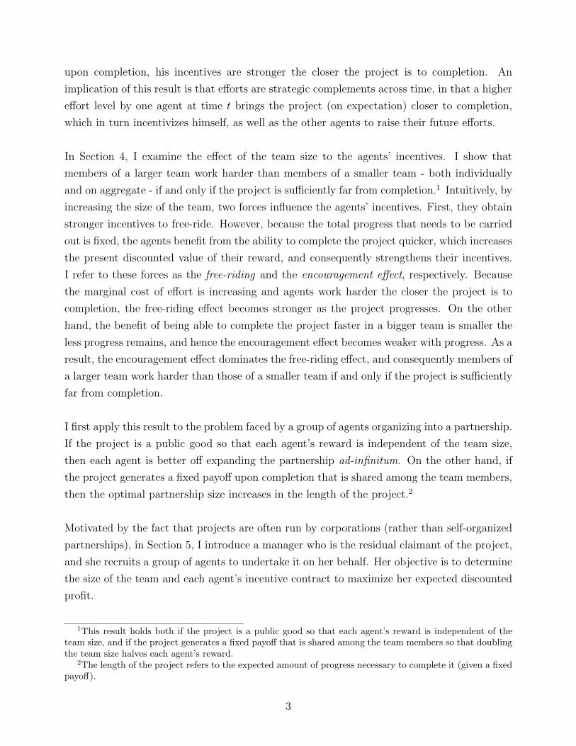
only if the project is sufficiently far from completion. Figure 1 illustrates an example.

Theorem 2. Consider two teams comprising of n and m > n identical agents. Under both

allocation schemes, other things equal, there exist thresholds Θn,m and Φn,m such that

(i) am (q) ≥ an (q) if and only if q ≤ Θn,m ; and

(ii) mam (q) ≥ nan (q) if and only if q ≤ Φn,m.

By increasing the size of the team, two opposing forces influence the agents’ incentives: First,

agents obtain stronger incentives to free-ride. To see why, consider an agent’s dilemma at

time t to (unilaterally) reduce his effort by a small amount ε for a short interval ∆. By

doing so, he saves approximately εc′ (a (qt)) ∆ in effort costs, but at t + ∆, the project is

ε∆ father from completion. In equilibrium, this agent will carry out only 1n

of that lost

progress, which implies that the benefit from shirking increases in the team size. Second,

recall that each agent’s incentives are proportional to the marginal benefit of bringing the

completion time τ forward: − ddτVnE [e−rτ ] = rVnE [e−rτ ], which implies that holding strategies

fixed, an increase in the team size decreases the completion time of the project, and hence

strengthens the agents’ incentives. Following the terminology of Bolton and Harris (1999),

who study an experimentation in teams problem, I refer to these forces as the free-riding and

the encouragement effect, respectively, and the intuition will follow from examining how the

magnitude of these effects changes as the project progresses.

It is convenient to consider the deterministic case in which σ = 0. Because c′ (0) = 0 and

effort vanishes as q → −∞, and noting that each agent’s gain from free-riding is proportional

to c′ (a (q)), it follows that the free-riding effect is negligible when the project is sufficiently far

from completion. As the project progresses, the agents raise their effort, and because effort

costs are convex, the free-riding effect becomes stronger. The magnitude of the encouragement

effect can be measured by the ratio of the marginal benefits of bringing the completion time

forward: rV2ne− rτ2

rVne−rτ= V2n

Vnerτ2 . Observe that this ratio increases in τ , which implies that the

encouragement effect becomes weaker as the project progresses (i.e., as τ becomes smaller),

and it diminishes under public good allocation (since V2n/Vn = 1) while it becomes negative

under budget allocation (since V2n/Vn < 1).

In summary, under both allocation schemes, the encouragement effect dominates the free-

riding effect if and only if the project is sufficiently far from completion. This implies that by

14

increasing the team size, the agents obtain stronger incentives when the project is far from

completion, while their incentives become weaker near completion.

Turning attention to the second statement, it follows from statement (i) that aggregate effort

in the larger team exceeds that in the smaller team if the project is far from completion.

Perhaps surprisingly however, when the project is near completion, not only the individual

effort, but also the aggregate effort in the larger team is less than that in the smaller team. The

intuition follows by noting that when the project is very close to completion (e.g., qt = −ε),this game resembles the (static) “reporting a crime” game (ch. 4.8 in Osborne (2003)), and

it is well-known that in the unique symmetric mixed-strategy Nash equilibrium of this game,

the probability that at least one agent exerts effort (which is analogous to aggregate effort)

decreases in the group size.

q

J n(q)

-80 -70 -60 -50 -40 -30 -20 -10 00

100

200

300

400

500

q

J n(q)

-60 -50 -40 -30 -20 -10 00

100

200

300

400

500

q

a n(q)

-80 -70 -60 -50 -40 -30 -20 -10 0

0

5

10

15

20

25

q

a n(q)

-60 -50 -40 -30 -20 -10 0

0

5

10

15

20

25

J3(q)

J5(q)

J3(q)

J5(q)

a3(q)

a5(q)

a3(q)

a5(q)

Θ3,5

Θ3,5Φ

3,5

Public Good Allocation Budget AllocationExpected Discounted Payoff Functions Expected Discounted Payoff Functions

Individual Effort Levels Individual Effort Levels

Φ3,5

Θ3,5

Θ3,5

Figure 1: Illustration of Theorem 2. The upper panels illustrate each agent’s expected discounted payoff

under public good (left) and budget (right) allocation for two different team sizes: n = 3 and 5. The lower

panels illustrate each agent’s equilibrium effort.

The same proof technique can be used to show that under both allocation schemes, the first-

best aggregate effort increases in the team size at every q. This difference is a consequence of

the free-riding effect being absent in this case, so that the encouragement effect alone leads a

larger team to always work on aggregate harder than a smaller team.

15

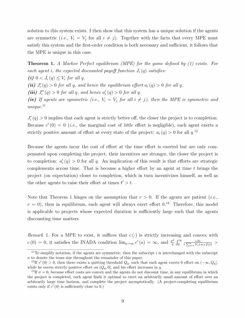
It is noteworthy that the thresholds of Theorem 2 need not always be interior. Under budget

allocation, it is possible that Θn,m = −∞, which would imply that each member of the smaller

team always works harder than each member of the larger team. However, numerical analysis

indicates that Θn,m is always interior under both allocation schemes. Turning to Φn,m, the

proof of Theorem 2 ensures that it is interior only under budget allocation if effort costs are

quadratic, while one can find examples in which Φn,m is interior as well as examples in which

Φn,m = 0 otherwise. Numerical analysis indicates that the most important parameter that

determines whether Φn,m is interior is the convexity of the effort cost function, and it is interior

as long as c (·) is not too convex (i.e., p is sufficiently small). This is intuitive, as more convex

effort costs favor the larger team more.17 In addition, under public good allocation, for Φn,m to

be interior, it is also necessary that n and m are sufficiently small. Intuitively, this is because

the size of the pie increases in the team size under this scheme, which (again) favors the larger

team. Figure 2 illustrates an example with quartic effort costs (i.e., p = 3) in which case Θn,m

is interior but Φn,m = 0 under both allocation schemes.

q

a n(q)

Individual Effort Levels

-100 -90 -80 -70 -60 -50 -40 -30 -20 -10 0

0

0.5

1

1.5

2

2.5

3

3.5

q

a n(q)

Individual Effort Levels

-100 -90 -80 -70 -60 -50 -40 -30 -20 -10 0

0

0.5

1

1.5

2

2.5

3

3.5

q

n a n(q

)

Aggregate Effort Levels

-100 -90 -80 -70 -60 -50 -40 -30 -20 -10 00

5

10

15

q

n a n(q

)

Aggregate Effort Levels

-100 -90 -80 -70 -60 -50 -40 -30 -20 -10 00

5

10

15

a3(q)

a5(q)

a3(q)

a5(q)

a3(q)

a5(q)

a3(q)

a5(q)

Θ3,5

Θ3,5

Budget AllocationPublic Good Allocation

Figure 2: An example with quartic effort costs (p = 3). The upper panels illustrate that under both

allocation schemes, Θn,m is interior, whereas the lower panels illustrate that Φn,m = 0, in which case the

aggregate effort in the larger team always exceeds that of the smaller team.

17This finding is consistent with the results of Esteban and Ray (2001), who show that in a static setting,the aggregate effort increases in the team size if effort costs are sufficiently convex. In their setting however,individual effort always decreases in the team size irrespective of the convexity of the effort costs. To furtherexamine the impact of the convexity of the agents’ effort costs, in Appendix A.5, I consider the case in whicheffort costs are linear, and I establish an analogous result to Theorem 2: members an (n+ 1)-person teamhave stronger incentives relative to those of an n-person team as long as n is sufficiently small.

16

4.1 Partnership Formation

In this Section, I examine the problem faced by a group of agents who seek to organize into

a partnership. The following Proposition characterizes the optimal partnership size.

Proposition 3. Suppose that the partnership composition is finalized before the agents begin

to work, so that the optimal partnership size satisfies arg maxn Jn (q0).(i) Under public good allocation, the optimal partnership size n = ∞ independent of the

project length |q0|.(ii) Under budget allocation, the optimal partnership size n increases in the project length

|q0|.

Increasing the size of the partnership has two effects. First, the expected completion time of

the project changes; from Theorem 2 it follows that it decreases, thus increasing each agent’s

expected discounted reward, if the project is sufficiently long. Second, in equilibrium, each

agent will exert less effort to complete the project, which implies that his total expected

discounted cost of effort decreases. This Proposition shows that if each agent’s reward does

not depend on the partnership size (i.e., under public good allocation), then the latter effect

always dominates the former, and hence agents are better off the bigger the partnership. Under

budget allocation however, these effects outweigh the decrease in each agent’s reward caused

by the increase in the partnership size only if the project is sufficiently long, and consequently,

the optimal partnership size increases in the length of the project.

An important assumption underlying Proposition 3 is that the partnership composition is

finalized before the agents begin to work. Under public good allocation, this assumption is

without loss of generality, because the optimal partnership size is equal to ∞ irrespective of

the length of the project. However, it may not be innocuous under budget allocation, where

the optimal partnership size does depend on the project length. If the partnership size is

allowed to vary with progress, an important modeling assumption is how the rewards of new

and exiting members will be determined. While a formal analysis is beyond the scope of this

paper, abstracting from the above modeling issue and based on Theorem 2, it is reasonable to

conjecture that the agents will have incentives to expand the partnership after setbacks, and

to decrease its size as the project nears completion.

5 Manager’s Problem

Most projects require substantial capital to cover infrastructure and operating costs. For

example, the design of a new pharmaceutical drug, in addition to the scientists responsible for

17

the drug design (i.e., the project team), necessitates a laboratory, expensive and maintenance-

intensive machinery, as well as support staff. Because individuals are often unable to cover

these costs, projects are often run by corporations instead of the project team, which raises

the questions of (i) how to determine the optimal team size, and (ii) how to best incentivize

the agents. These questions are addressed in this Section, wherein I consider the case in which

a third party (to be referred to as a manager) is the residual claimant of the project, and she

hires a group of agents to undertake it on her behalf. Section 5.1 describes the model, Section

5.2 establishes some of the properties of the manager’s problem, and Section 5.3 studies her

contracting problem.

5.1 The Model with a Manager

The manager is the residual claimant of the project, she is risk neutral, and she discounts time

at the same rate r > 0 as the agents. The project has (expected) length |q0|, and it generates

a payoff U > 0 upon completion. To incentivize the agents, at time 0, the manager commits

to an incentive contract that specifies the size of the team, denoted by n, a set of milestones

q0 < Q1 < .. < QK = 0 (where K ∈ N), and for every k ∈ 1, .., K, allocates non-negative

payments Vi,kni=1 that are due upon reaching milestone Qk for the first time.18

5.2 The Manager’s Profit Function

I begin by considering the case in which the manager compensates the agents only upon

completing the project, and I show in Theorem 3 that her problem is well-defined and it

satisfies some desirable properties. Then I explain how this result extends to the case in which

the manager also rewards the agents for reaching intermediate milestones.

Given the team size n and the agents’ rewards Vini=1 that are due upon completion of the

project (where I can assume without loss of generality that∑n

i=1 Vi ≤ U), the manager’s

expected discounted profit function can be written as

F (q) =

(U −

n∑i=1

Vi

)Eτ[e−rτ | q

],

18The manager’s contracting space is restricted. In principle, the optimal contract should condition eachagent’s payoff on the path of qt (and hence on the completion time of the project). Unfortunately however,this problem is not tractable; for example, the contracting approach developed in Sannikov (2008) boils downa partial differential equation with n+1 variables (i.e., the state of the project q and the continuation value ofeach agent), which is intractable even for the case with a single agent. As such, this analysis is left for futureresearch.

18

where the expectation is taken with respect to the project’s completion time τ , which depends

on the agents’ strategies and the stochastic evolution of the project.19 By using the first

order condition for each agent’s equilibrium effort as determined in Section 3, the manager’s

expected discounted profit at any given state of the project satisfies

rF (q) =

[n∑i=1

f (J ′i (q))

]F ′ (q) +

σ2

2F ′′ (q) (5)

defined on (−∞, 0] subject to the boundary conditions

limq→−∞

F (q) = 0 and F (0) = U −n∑i=1

Vi , (6)

where Ji (q) satisfies (2) subject to (3). The interpretation of these conditions is similar to

(3). As the state of the project diverges to −∞, its expected completion time diverges to ∞,

and because r > 0, the manager’s expected discounted profit diminishes to 0. On the other

hand, the manager’s profit is realized when the project is completed, and it equals her payoff

U less the payments∑n

i=1 Vi disbursed to the agents.

Theorem 3. Given (n, Vini=1), a solution to the manager’s problem defined by (5) subject

to the boundary conditions (6) and the agents’ problem as defined in Theorem 1 exists, and it

has the following properties:

(i) F (q) > 0 and F ′ (q) > 0 for all q.

(ii) F (·) is unique if the agents’ rewards are symmetric (i.e., if Vi = Vj for i 6= j).

Now let us discuss how Theorems 1 and 3 extend to the case in which the manager rewards

the agents upon reaching intermediate milestones. Recall that she can designate a set of

milestones, and attach rewards to each milestone that are due as soon as the project reaches

the respective milestone for the first time. Let Ji,k (·) denote agent i’s expected discounted

payoff given that the project has reached k − 1 milestones, which is defined on (−∞, Qk],

and note that it satisfies (4) subject to limq→−∞ Ji,k (q) = 0 and Ji,k (Qk) = Vi,k + Ji,k+1 (Qk),

where Ji,K+1 (0) = 0. The second boundary condition states that upon reaching milestone

k, agent i receives the reward attached to that milestone, plus the continuation value from

future rewards. Starting with Ji,K (·), it is straightforward that it satisfies the properties of

Theorem 1, and in particular, that Ji,K (Qk−1) is unique (as long as rewards are symmetric)

so that the boundary condition of Ji,K−1 (·) at QK−1 is well-defined. Proceeding backwards,

it follows that for every k, Ji,k (·) satisfies the properties of Theorem 1.

19The subscript k is dropped when K = 1 (in which case Q1 = 0).

19

To examine the manager’s problem, let Fk (·) denote her expected discounted profit given

that the project has reached k − 1 milestones, which is defined on (−∞, Qk], and note that

it satisfies (5) subject to limq→−∞ Fk (q) = 0 and Fk (Qk) = Fk+1 (Qk) −∑n

i=1 Vi,k, where

FK+1 (Qk) = U . The second boundary condition states that upon reaching milestone k, the

manager receives the continuation value of the project, less the payments that she disburses to

the agents for reaching this milestone. Again starting with k = K and proceeding backwards,

it is straightforward that for all k, Fk (·) satisfies the properties established in Theorem 3.

5.3 Contracting Problem

The manager’s problem entails choosing the team size and the agents’ incentive contracts to

maximize her ex-ante expected discounted profit subject to the agents’ incentive compatibility

constraints.20 I begin by analyzing symmetric contracts. Then I examine how the manager

can increase her expected discounted profit with asymmetric contracts.

Symmetric Contracts

The following Theorem shows that within the class of symmetric contracts, one can without

loss of generality restrict attention to those that compensate the agents only upon completion

of the project.

Theorem 4. The optimal symmetric contract compensates the agents only upon completion

of the project.

To prove this result, I consider an arbitrary set of milestones and arbitrary rewards attached

to each milestone, and I construct an alternative contract that rewards the agents only upon

completing the project and renders the manager better off. Intuitively, because rewards are

sunk in terms of incentivizing the agents after they are disbursed, and all parties are risk

neutral and they discount time at the same rate, by backloading payments, the manager

can provide the same incentives at the early stages of the project, while providing stronger

incentives when it is close to completion.21

The value of Theorem 4 lies in that it reduces the infinite-dimensional problem of determining

the team size, the number of milestones, the set of milestones, and the rewards attached to

20While it is possible to choose the team size directly via the incentive contract (e.g., by setting the rewardof n < n agents to 0, the manager can effectively decrease the team size to n − n), it is analytically moreconvenient to analyze the two “levers” (for controlling incentives) separately.

21As shown in part II of the proof of Theorem 4, the agents are also better off if their rewards are backloaded.In other words, each agent could strengthen his incentives and increase his expected discounted payoff bydepositing any rewards from reaching intermediate milestones in an account with interest rate r, and closingthe account upon completion of the project.

20

each milestone into a two-dimensional problem, in which the manager only needs to determine

her budget B =∑n

i=1 Vi for compensating the agents and the team size. The following

Propositions characterize the manager’s optimal budget and her optimal team size.

Proposition 4. Suppose that the manager employs n agents whom she compensates symmet-

rically. Then her optimal budget B increases in the length of the project |q0|.

Contemplating an increase in her budget, the manager trades off a decrease in her net profit

U−B and an increase in the project’s expected present discounted value Eτ [e−rτ | q0]. Because

a longer project takes (on average) a larger amount of time to be completed, a decrease in her

net profit has a smaller effect on her ex-ante expected discounted profit the longer the project.

Therefore, the benefit from raising the agents’ rewards outweighs the decrease in her net profit

if and only if the project is sufficiently long, which in turn implies that the manager’s optimal

budget increases in the length of the project.

Lemma 1. Suppose that the manager has a fixed budget B and she compensates the agents

symmetrically. For any m > n, there exists a threshold Tn,m such that she prefers employing

an m-member team instead of an n-member team if and only if |q0| ≥ Tn,m.

Given a fixed budget, the manager’s objective is to choose the team size to minimize the

expected completion time of the project. This is equivalent to maximizing the aggregate

effort of the team along the evolution path of the project. Hence, the intuition behind this

result follows from statement (B) of Theorem 2. If the project is short, then on expectation,

the aggregate effort of the smaller team will be greater than that of the larger team due to

the free-riding effect (on average) dominating the encouragement effect. The opposite is true

if the project is long. Figure 3 illustrates an example.

Applying the Monotonicity Theorem of Milgrom and Shannon (1994) leads one to the fol-

lowing Proposition.

Proposition 5. Given a fixed budget to (symmetrically) compensate a group of agents, the

manager’s optimal team size n increases in the length of the project |q0|.

Proposition 5 suggests that a larger team is more desirable while the project is far from com-

pletion, whereas a smaller team becomes preferable when the project gets close to completion.

Therefore, it seems desirable to construct a scheme that dynamically decreases the team size

as the project progresses. Suppose that the manager employs two identical agents on a fixed

budget, and she designates a retirement state R, such that one of the agents is permanently

retired (i.e., he stops exerting effort) at the first time that the state of the project hits R. From

that point onwards, the other agent continues to work alone. Both agents are compensated

21

q

Man

ager

's E

xpec

ted

Dis

coun

ted

Pro

fit

-50 -45 -40 -35 -30 -25 -20 -15 -10 -5 0

0

100

200

300

400

500

600

700

800

900

1000

F3(q)

F5(q)

T3,5

Figure 3: Illustration of Lemma 1. Given a fixed budget, the manager’s expected discounted profit is

higher if she recruits a 5-member team relative to a 3-member team if and only if the initial state of the project

q0 is to the left of the threshold −T3,5; or equivalently, if and only if |q0| ≥ T3,5.

only upon completion of the project, and the payments (say V1 and V2) are chosen such that

the agents are indifferent with respect to who will retire at R; i.e., their expected discounted

payoffs are equal at qt = R.22

Proposition 6. Suppose the manager employs two agents with quadratic effort costs. Con-

sider the retirement scheme described above, where the retirement state R > max q0,−T1,2and T1,2 is taken from Lemma 1. There exists a threshold ΘR > |R| such that the manager is

better off implementing this retirement scheme relative to allowing both agents to work together

until the project is completed if and only if its length |q0| < ΘR.

First, note that after one agent retires, the other will exert first-best effort until the project is

completed. Because the manager’s budget is fixed, this retirement scheme is preferable only

if it increases the aggregate effort of the team along the evolution path of the project. A key

part of the proof involves showing that agents have weaker incentives before one of them is

retired as compared to the case in which they always work together (i.e., when a retirement

scheme is not used). Therefore, the benefit from having one agent exert first-best effort after

one of them retires outweighs the loss from the two agents exerting less effort before one of

them retires (relative to the case in which they always work together) only if the project is

sufficiently short. Hence, this retirement scheme is preferable if and only if |q0| < ΘR.

From an applied perspective, this result should be approached with caution. In this en-

vironment, the agents are (effectively) restricted to playing the MPE, whereas in practice,

22Note that this is one of many possible retirement schemes. A complete characterization of the optimaldynamic team size management scheme is beyond the scope of this paper, and is left for future research.

22

groups are often able to coordinate to a more efficient equilibrium, for example, by monitoring

each other’s efforts, thus mitigating the free-rider problem (and hence weakening this result).

Moreover, Weber (2006) shows that while efficient coordination does not occur in groups that

start off large, it is possible to create efficiently coordinated large groups by starting with small

groups that find it easier to coordinate, and adding new members gradually who are aware

of the group’s history. Therefore, one should be aware of the tension between the free-riding

effect becoming stronger with progress, and the force identified by Weber.

Asymmetric Contracts

Insofar, I have restricted attention to contracts that compensate the agents symmetrically.

However, Proposition 6 suggests that an asymmetric contract that rewards the agents upon

reaching intermediate milestones can do better than the best symmetric one if the project is

sufficiently short. Indeed, the retirement scheme proposed above can be implemented using

the following asymmetric rewards-for-milestones contract.

Remark 6. Let Q1 = R, and suppose that agent 1 receives V as soon as the project is

completed, while he receives no intermediate rewards. On the other hand, agent 2 receives

the equilibrium present discounted value of B − V upon hitting R for the first time (i.e.,

(B − V )Eτ [e−rτ |R]), and he receives no further compensation, so that he effectively retires

at that point. From Proposition 6 we know that there exists a V ∈ (0, B) and a threshold ΘR

such that this asymmetric contract is preferable to a symmetric one if and only if |q0| < ΘR.

It is important to note that while the expected cost of compensating the agents in the above

asymmetric contract is equal to B, the actual cost is stochastic, and in fact, it can exceed the

project’s payoff U . As a result, unless the manager is sufficiently solvent, there is a positive

probability that she will not be able to honor the contract, which will negatively impact the

agents’ incentives.

The following result shows that an asymmetric contract may be preferable even if the manager

compensates the (identical) agents upon reaching the same milestone; namely, upon complet-

ing the project.

Proposition 7. Suppose that the manager has a fixed budget B > 0, and she employs two

agents with quadratic effort costs whom she compensates upon completion of the project. Then

for all ε ∈(0, B

2

], there exists a threshold Tε such that the manager is better off compensating

23

the two agents asymmetrically such that V1 = B2

+ ε and V2 = B2− ε instead of symmetrically,

if and only if the length of the project |q0| ≤ Tε.23

To see the intuition behind this result, note that ε = B2

is equivalent to the case in which the

manager employs a single agent, and from Lemma 1 we know that there exists a threshold

T1,2 such that the manager is better off employing one agent instead of two if and only if

|q0| ≤ T1,2. The intermediate cases in which ε ∈(0, B

2

)can be thought of as if the manager

employs a full-time agent and a part-time one. Part of the proof involves showing that the

aggregate effort under an asymmetric contract is larger compared to a symmetric one if and

only if the project is sufficiently close to completion. Intuitively, this is because the full-time

agent cannot free-ride on the other agent as much. By noting that the manager’s objective

is to allocate her budget so as to maximize the agents’ expected aggregate effort along the

evolution path of the project, it follows that this is best done by allocating it asymmetrically

between the agents if the project is sufficiently short.

6 Concluding Remarks

To recap, I study a dynamic problem in which a group of agents collaborate over time to

complete a project, which progresses at a rate that depends on the agents’ efforts, and it

generates a payoff upon completion. The analysis provides several testable implications. In

the context of the Myerlin Repair Foundation (MRF) for example, one should expect that

principal investigators will allocate more resources to MRF activities as the goal comes closer

into sight. Second, in a drug discovery venture for instance, the model predicts that the

amount of time and resources (both individually and on aggregate) that the scientists allocate

to the project will be positively related to the group size at the early stages of the project,

and negatively related near completion. Moreover, this prediction is consistent with empirical

studies of voluntary contributions by programmers to open-source software projects (Yildirim

(2006)). These studies report an increase in the average contributions with the number of

programmers, especially in the early stages of the projects, and a decline in the mature stages.

Third, the model prescribes that the members of a project team should be compensated

asymmetrically if the project is sufficiently short.

In a related paper, Georgiadis, Lippman and Tang (2014) consider the case in which the

project size is endogenous. Motivated by projects involving design or quality objectives that

are often difficult to define in advance, they examine how the manager’s optimal project size

23Note that the solution to the agents’ problem need not be unique if the contract is asymmetric. However,this comparative static holds for every solution to (5) subject to (6), (4), and (3) (if more than one exists).

24

depends on her ability to commit to a given project size in advance. In another related paper,

Ederer, Georgiadis and Nunnari (2014) examine how the team size affects incentives in a

discrete public good contribution game using laboratory experiments. Preliminary results

support the predictions of Theorem 2.

This paper opens several opportunities for future research. First, the optimal contracting

problem is an issue that deserves further exploration. As discussed in Section 5, I have

considered a restricted contracting space. Intuitively, the optimal contract will be asymmetric,

and it will backload payments (i.e., each agent will be compensated only at the end of his

involvement in the project). However, each agent’s reward should depend on the path of qt,

and hence on the completion time of the project. Second, the model assumes that efforts are

unobservable, and that at every moment, each agent chooses his effort level after observing

the current state of the project. An interesting extension might consider the case in which

the agents can obtain a noisy signal of each other’s effort (by incurring some cost) and the

state of the project is observed imperfectly. The former should allow the agents to coordinate

to a more efficient equilibrium, while the latter will force the agents to form beliefs about

how close the project is to completion, and to choose their strategies based on those beliefs.

Finally, from an applied perspective, it may be interesting to examine how a project can be

split into subprojects that can be undertaken by separate teams.

A Additional Results

A.1 Flow Payoffs while the Project is in Progress

An important assumption of the base model is that the agents are compensated only upon

completion of the project. In this Section, I extend the model by considering the case in

which during any small [t, t+ dt) interval while the project is in progress, each agent receives

h (qt) dt, in addition to the lump sum reward V upon completion. To make the problem

tractable, I shall make the following assumptions about h (·):

Assumption 1. h (·) is thrice continuously differentiable on (−∞, 0], it has positive first,

second and third derivatives, and it satisfies limq→−∞ h (q) = 0 and h (0) ≤ rV .

Using a similar approach as in Section 3, it follows that in a MPE, the expected discounted

payoff function of agent i satisfies

rJi (q) = maxai

h (q)− c (ai) +

(n∑j=1

aj

)J ′i (q) +

σ2

2J ′′i (q)

25

subject to (3), and his optimal effort level satisfies ai (q) = f (J ′i (q)), where f (·) = c′−1 (max 0, ·).

The following Proposition characterizes the unique MPE of this game, and it shows (i) that

each agent’s effort level is either increasing, or hump-shaped in q, and (ii) the team size

comparative static established in Theorem 2 continues to hold.

Proposition 8. Suppose that each agent receives a flow payoff h (q) while the project is in

progress, , and h (·) satisfies Assumption 1.

(i) A symmetric MPE for this game exists, it is unique, and it satisfies 0 ≤ Jn (q) ≤ V and

J ′n (q) ≥ 0 for all q.

(ii) There exists a threshold ω (not necessarily interior) such that each agent’s effort a′n (q) ≥ 0

if and only if q ≤ ω.

(iii) Under both allocation schemes and for any m > n, there exists a threshold Θn,m (Φn,m)

such that am (q) ≥ an (q) (mam (q) ≥ n an (q)) if and only if q ≤ Θn,m (q ≤ Φn,m).

The intuition why effort can be decreasing in q when the project is close to completion can

be explained as follows: Far from completion, the agents are incentivized by the future flow

payoffs and the lump sum V upon completion. As the project nears completion, the current

flow payoffs become larger, and hence the agents have less to gain by bringing the project closer

to completion, and consequently, they decrease their effort. While establishing conditions

under which ω is interior does not seem possible, numerical analysis indicates that this is the

case if h(0)r

is sufficiently close to V .

Finally, statement (iii) follows by noting that J ′n (q) being unimodal in q is sufficient for the

proof of Theorem 2. Figure 4 illustrates an example.

A.2 Cancellation States

In this Section, I consider the case in which the project is canceled at the first moment that

qt hits some (exogenous) cancellation state QC > −∞ and the game ends with the agents

receiving 0 payoff. The expected discounted payoff for each agent i satisfies (4) subject to the

boundary conditions

Ji (QC) = 0 and Ji (0) = V .

In contrast to the model analyzed in Section 3, with a finite cancellation state, it need not be

the case that J ′i (QC) = 0. It follows that all statements of Theorem 1 hold except for (iii)

(which asserts that effort increases with progresses).24 Instead, there exists some threshold ω

(not necessarily interior), such that a′n (q) ≥ 0 if and only if q ≥ ω.

24This result requires that limq→−∞ J ′i (q) = 0.

26

q

a n(q)

Public Good Allocation

-16 -14 -12 -10 -8 -6 -4 -2 0

0

0.5

1

1.5

2

2.5

q

a n(q)

Budget Allocation

-16 -14 -12 -10 -8 -6 -4 -2 0

0

0.5

1

1.5

2

2.5

a3(q)

a4(q)

a3(q)

a4(q)

Φ

ΘΦ

Θ

Figure 4: An example in which agents receive flow payoffs while the project is in progress

with h (q) = 10eq/2. Observe that effort strategies are hump-shaped in q, and the predictions of

Theorem 2 continue to hold under both allocation schemes.

Similarly, by noting that J ′n (q) being unimodal in q is sufficient for the proof of Theorem

2, it follows that even with cancellation states, members of a larger team work harder than

members of a smaller team, both individually and on aggregate, if and only if the project is

sufficiently far from completion. These results are summarized in the following Proposition.

Proposition 9. Suppose that the project is canceled at the first moment such that qt hits a

given cancellation state QC > −∞ and the game ends with the agents receiving 0 payoff.

(i) A symmetric MPE for this game exists, it is unique, and it satisfies 0 ≤ Jn (q) ≤ V and

J ′n (q) ≥ 0 for all q.

(ii) There exists a threshold ω (not necessarily interior) such that each agent’s effort a′n (q) ≥ 0

if and only if q ≥ ω.

(iii) Under both allocation schemes and for any m > n, there exists a threshold Θn,m (Φn,m)

such that am (q) ≥ an (q) (mam (q) ≥ n an (q)) if and only if q ≤ Θn,m (q ≤ Φn,m).

While a sharper characterization of the MPE is not possible, numerical analysis indicates that

effort increases in q if QC is sufficiently small (i.e., ω = −∞), it is U-shaped in q if QC is in

some intermediate range (i.e., ω is interior), while it decreases in q (i.e., ω = 0) if QC is close

to 0. An example is illustrated in Figure 5.

Intuitively, the agents have incentives to exert effort in order to (i) complete the project, and

(ii) avoid hitting the cancellation state QC . Moreover, observe that the incentives due to the

former (latter) are stronger the closer the project is to completion (to QC). Therefore, if QC

is small, then the latter incentive is weak, so that the agents’ incentives are driven primarily

by (i), and effort increases with progress. As QC increases, (ii) becomes stronger, so that

27

effort becomes U-shaped in q, and if QC is sufficiently close to 0, then the incentives from (ii)

dominate those from (i), and consequently, effort decreases in q.

q

Effo

rt L

evel

a(q

)

-25 -20 -15 -10 -5 00

0.5

1

1.5

2

2.5

3

3.5

4

4.5

QC= -30

QC= -10

QC= -4.5

Figure 5: Illustration of the agents’ effort functions given three different cancellation

states. Observe that when QC is small (e.g., QC = −30), effort increases in q. When QC is in an

intermediate range (e.g., QC = −10), then effort is U-shaped in q, while it decreases in q if QC is

sufficiently large (e.g., QC = −4.5).

A.3 Effort Affects Drift and Variance of Stochastic Process

A simplifying assumption in the base model is that the variance of the process that governs

the evolution of the project (i.e., σ) does not depend on the agents’ effort levels. As a result,

even if no agent ever exerts any effort, the project is completed in finite time with probability

1. To understand the impact of this assumption, in this Section, I consider the case in which

the project progresses according to

dqt =n∑i=1

ai,tdt+

√√√√ n∑i=1

ai,t σdWt .

25 The expected discounted payoff function of agent i satisfies the HJB equation

rJi (q) = −c (ai,t) +

(n∑j=1

aj,t

)(J ′i (q) +

σ2

2J ′′i (q)

)25Note that the total effort of the team is instantly observable here. Therefore, there typically exist non-

Markovian equilibria that are sustained via trigger strategies that revert to the MPE after observing a devia-tion. Moreover, provided that the state qt is verifiable, the team’s total effort becomes contractible.

28

subject to (3). Restricting attention to symmetric MPE and guessing that each agent’s first or-

der condition always binds, it follows that his effort level satisfies a (q) = f(J ′ (q) + σ2

2J ′′ (q)

).

Using a similar approach to that used to prove Theorem 1, one can show that a non-trivial

solution to this ODE exists. However, the MPE need not be unique in this case: unless a single

agent is willing to undertake the project single-handedly, then there exists another equilibrium

in which no agent ever exerts any effort, and the project is never completed.

Unfortunately, analyzing how the agents’ effort levels change with progress and how individ-

ual and aggregate effort depends on the team size is analytically intractable. However, as

illustrated in Figure 6, numerical examples indicate that the main results of the base model

continue to hold: effort increases with progress (i.e., a′ (q) ≥ 0 for all q) and the predictions

of Theorem 2 continues to hold: under both allocation schemes and for any m > n, there

exists a threshold Θn,m (Φn,m) such that am (q) ≥ an (q) (mam (q) ≥ n an (q)) if and only if

q ≤ Θn,m (q ≤ Φn,m).

q

J n(q)

-160 -140 -120 -100 -80 -60 -40 -20 00

50

100

150

200

250

300

q

a n(q)

-180 -160 -140 -120 -100 -80 -60 -40 -20 0

0

1

2

3

4

5

6

7

q

J n(q)

-120 -100 -80 -60 -40 -20 00

50

100

150

200

250

300

q

a n(q)

-120 -100 -80 -60 -40 -20 0

0

1

2

3

4

5

6

7

J3(q)

J5(q)

J3(q)

J5(q)

a3(q)

a5(q)

a3(q)

a5(q)

Individual Effort LevelsIndividual Effort Levels

Expected Discounted Payoff FunctionsExpected Discounted Payoff Functions

Public Good Allocation Budget Allocation

ΘΦ

Θ

Φ

Figure 6: An example in which the agents’ effort influences both the drift and the

variance of the stochastic process. Observe that effort increases in q, and that the predictions

of Theorem 2 continue to hold under both allocation schemes.

A.4 Equilibria with Non-Markovian Strategies

Insofar, I have restricted attention to Markovian strategies, so that at every moment, each

agent’s effort is a function of only the current state of the project qt. This raises the question

whether agents can increase their expected discounted payoff by adopting non-Markovian

strategies that at time t depend on the entire evolution path of the project qss≤t. Sannikov

29

and Skrzypacz (2007) study a related model in which the agents can change their actions only

at times t = 0,∆, 2∆, .., where ∆ > 0 (but small), and the information structure is similar;

i.e., the state variable evolves according to a diffusion process whose drift is influenced by

the agents’ actions. They show that the payoffs from the best symmetric Public Perfect

equilibrium (hereafter PPE) converge to the payoffs corresponding to the MPE as ∆→ 0 (see

their Proposition 5).

A natural, discrete-time analog of the model considered in this paper is one in which at

t ∈ 0,∆, 2∆, .. each agent chooses his effort level ai,t at cost c (ai,t) ∆, and at t+∆ the state

of the project is equal to qt+∆ = qt + (∑n

i=1 ai,t) ∆ + εt+∆, where εt+∆ ∼ N (0, σ2∆). In light

of the similarities between this model and the model in Section VI of Sannikov and Skrzypacz

(2007), it is reasonable to conjecture that in the continuous-time limit (i.e., as ∆→ 0), there

does not exist a PPE in which agents can achieve a higher expected discounted payoff than

the MPE at any state of the project. However, because a rigorous proof is difficult for the

continuous-time game and the focus of this paper is on team formation and contracting, a

formal analysis of non-Markovian PPE of this game is left for future work.

Nevertheless, it is useful to present some intuition. Following Abreu, Pearce and Stacchetti

(1986), an optimal PPE involves a collusive regime and a punishment regime, and in every

period, the decision whether to remain in the collusive regime or to switch is guided by the

outcome in that period alone. In the context of this model, at t + ∆, each agent will base

his decision on qt+∆−qt∆

. As ∆ decreases, two forces influence the scope of cooperation. First,

the gain from a deviation in a single period decreases, which helps cooperation. On the other

hand, because V( qt+∆−qt

∆

)= σ2

∆, the agents must decide whether to switch to the punishment

regime by observing noisier information, which increases the probability of type I errors (i.e.,

triggering a punishment when no deviation has occurred), thus hurting cooperation. As San-

nikov and Skrzypacz (2007) show, the latter force becomes overwhelmingly stronger than the

former as ∆→ 0, thus eradicating any gains from cooperation.

A.5 Linear Effort costs

The assumption that effort costs are convex affords tractability as it allows for comparative

statics despite the fact that the underlying system of HJB equations does not admit a closed-

form solution. However, convex effort costs also favor larger teams. Therefore, it is useful

to examine how the comparative statics with respect to the team size extend to the case

in which effort costs are linear; i.e., c (a) = a. In this case, the marginal value of effort

is equal to J ′i (q) − 1, so agent i finds it optimal to exert the largest possible effort level if

30

J ′i (q) > 1, he is indifferent across any effort level if J ′i (q) = 1, and he exerts no effort if

J ′i (q) < 1. As a result, I shall impose a bound on the maximum effort that each agent can

exert: a ∈ [0, u]. Moreover, suppose that agents are symmetric, and σ = 0 so that the project

evolves deterministically.26 This game has multiple MPE: (i) a symmetric MPE with bang-

bang strategies, (ii) a symmetric MPE with interior strategies, and (iii) asymmetric MPE.

The reader is referred to Section 5.2 of Georgiadis, Lippman and Tang (2014) for details.

Because (ii) is sensitive to the assumption that σ = 0, I shall focus on the symmetric MPE

with bang-bang strategies.27

By using (2) subject to (3) and the corresponding first order condition, it follows that there

exists a symmetric MPE in which each agent’s discounted payoff and effort strategy satisfies

Jn (q) =[−ur

+(Vn +

u

r

)erqnu

]1q≥ψn and an (q) = u1q≥ψn ,

where ψn = nur

ln(

nurVn+u

). In this equilibrium, the project is completed only if q0 ≥ ψn.28 Ob-

serve that agents have stronger incentives the closer the project is to completion, as evidenced

by the facts that J ′′n (q) ≥ 0 for all q, and an (q) = 1 if and only if q ≥ ψn. To investigate

how the agents’ incentives depend on the team size, one needs to examine how ψn depends

on n. This threshold decreases in the team size n under both allocation schemes (i.e., both

if Vn = V and Vn = Vn

for some V > 0) if and only if n is sufficiently small. This implies

that members of an (n+ 1) − member team have stronger incentives relative to those of an

n−member team as long as n is sufficiently small.

If agents maximize the team’s rather than their individual discounted payoff, then the first-

best threshold ψn = nur

ln(

urVn+u

), and it is straightforward to show that it decreases in n

under both allocation schemes. Therefore, similar to the case in which effort costs are convex,

members of a larger team always have stronger incentives than those of a smaller one.

B Proofs

26While the corresponding HJB equation can be solved analytically if effort costs are linear, the solution istoo complex to obtain the desired comparative statics if σ > 0.

27In the MPE with interior strategies, J ′n (q) = 1 for all q, and the equilibrium effort is chosen so as to satisfythis indifference condition. Together with the boundary condition Jn (0) = Vn, this implies that Jn (q) = 0and an (q) = 0 for all q ≤ −Vn. However, such an equilibrium cannot exist if σ > 0, because in this case,Jn (q) > 0 for all q even if an (q) = 0.

28If q0 ∈ [ψn, ψ1) so that each agent is not willing to undertake the project single-handedly, then thereexists another equilibrium in which no agent exerts any effort and the project is never completed.

31

Proof of Theorem 1. This proof is organized in 7 parts. I first show that a MPE for the

game defined by (1) exists. Next I show that properties (i) thru (iii) hold, and that the

value functions are infinitely differentiable. Finally, I show that with symmetric agents, the

equilibrium is symmetric and unique.

Part I: Existence of a MPE.

To show that a MPE exists, it suffices to show that a solution satisfying the system of ordinary

nonlinear differential equations defined by (4) subject to the boundary conditions (3) for all

i = 1, .., n exists.

To begin, fix some arbitrary N ∈ N and rewrite (4) and (3) as

J ′′i,N (q) =2

σ2

[rJi,N (q) + c

(f(J ′i,N (q)

))−

(n∑j=1

f(J ′j,N (q)

))J ′i,N (q)

](7)

subject to Ji,N (−N) = 0 and Ji,N (0) = Vi

for all i. Let gi (JN , J′N) denote the the RHS of (7), where JN and J ′N are vectors whose

ith row corresponds to Ji,N (q) and J ′i,N (q), respectively , and note that gi (·, ·) is continuous.

Now fix some arbitrary K > 0, and define a new function

gi,K (JN , J′N) = max min gi (JN , J ′N) , K , −K .

Note that gi,K (·, ·) is continuous and bounded. Therefore, by Lemma 4 in Hartman (1960),

there exists a solution to J ′′i,N,K = gi,K(JN,K , J

′N,K

)on [−N, 0] subject to Ji,N,K (−N) = 0 and

Ji,N,K (0) = Vi for all i. This Lemma, which is due to Scorza-Dragoni (1935), states:

Let g (q, J, J ′) be a continuous and bounded (vector-valued) function for α ≤ q ≤ β and

arbitrary (J, J ′). Then, for arbitrary qα and qβ, the system of differential equations J ′′ =

g (q, J, J ′) has at least one solution J = J (q) satisfying J (α) = qα and J (β) = qβ.

The next part of the proof involves showing that there exists a K such that gi,K(Ji,N,K (q) , J ′i,N,K (q)

)∈(

−K, K)

for all i, K and q, which will imply that the solution Ji,N,K (·) satisfies (7) for all i.

The final step involves showing that a solution exists when N →∞, so that the first boundary

condition in (7) is replaced by limq→−∞ Ji (q) = 0.

First, I show that 0 ≤ Ji,N,K (q) ≤ Vi and J ′i,N,K (q) ≥ 0 for all i and q. Because Ji,N,K (0) >

Ji,N,K (−N) = 0, either Ji,N,K (q) ∈ [0, Vi] for all q, or it has an interior extreme point z∗ such

that Ji,N,K (z∗) /∈ [0, Vi]. If the former is true, then the desired inequality holds. Suppose

32

the latter is true. By noting that Ji,N,K (·) is at least twice differentiable, J ′i,N,K (z∗) = 0, and

hence J ′′i,N,K (z∗) = max

min

2rσ2Ji,N,K (z∗) , K

, −K

. Suppose z∗ is a global maximum.

Then J ′′i,N,K (z∗) ≤ 0 =⇒ Ji,N,K (z∗) ≤ 0, which contradicts the fact that Ji,N,K (0) > 0. Now

suppose that z∗ is a global minimum. Then J ′′i,N,K (z∗) ≥ 0 =⇒ Ji,N,K (z∗) ≥ 0. Therefore,

0 ≤ Ji,N,K (q) ≤ Vi for all i and q.

Next, let us focus on J ′i,N,K (·). Suppose that there exists a z∗∗ such that J ′i,N,K (z∗∗) < 0.

Because Ji,N,K (−N) = 0, either Ji,N,K (·) is decreasing on [−N, z∗∗], or it has a local maximum

z ∈ (−N, z∗∗). If the former is true, then J ′i,N,K (z∗∗) < 0 implies that Ji,N,K (q) < 0 for some

q ∈ (−N, z∗∗], which is a contradiction because Ji,N,K (q) ≥ 0 for all q. So the latter must

be true. Then J ′i,N,K (z) = 0 implies that J ′′i,N,K (z) = max

min

2rσ2Ji,N,K (z) , K

, −K

.

However, because z is a maximum, J ′′i,N,K (z) ≤ 0, and together with the fact that Ji,N,K (q) ≥ 0

for all q, this implies that Ji,N,K (q) = 0 for all q ∈ [−N, z∗∗). But since J ′i,N,K (z∗∗) < 0, it

follows that Ji,N,K (q) < 0 for some q in the neighborhood of z∗∗, which is a contradiction.

Therefore, it must be the case that J ′i,N,K (q) ≥ 0 for all i and q.

The next step involves establishing that there exists an A, independent of N and K, such that

J ′i,N,K (q) < A for all i and q. First, let SN,K (q) =∑n

i=1 |Ji,N,K (q)|. By summing J ′′i,N,K =

gi,K(Ji,N,K , J

′i,N,K

)over i, using that (i) 0 ≤ Ji,N,K (q) ≤ Vi and 0 ≤ J ′i,N,K (q) ≤ S ′N,K (q) for

all i and q, (ii) f (x) = x1/p, and (iii) c (x) ≤ x c′ (x) for all x ≥ 0, and letting Γ = r∑n

i=1 Vi,

we have that for all q

∣∣S ′′N,K (q)∣∣ ≤ 2

σ2

n∑i=1

[rJi,N,K (q) + c

(f(J ′i,N,K (q)

))+

[n∑j=1

f(J ′j,N,K (q)

)]J ′i,N,K (q)

]

≤ 2

σ2

[Γ +

n∑i=1

c′(c′−1

(J ′i,N,K (q)

))c′−1

(J ′i,N,K (q)

)+ S ′N,K (q)

n∑j=1

f(J ′j,N,K (q)

)]

≤ 4

σ2

[Γ + nS ′N,K (q) f

(S ′N,K (q)

)]=

4

σ2

[Γ + n

(S ′N,K (q)

) p+1p

].

By noting that SN,K (0) =∑n

i=1 Vi, SN,K (−N) = 0, and applying the mean value theorem, it

follows that there exists a z∗ ∈ [−N, 0] such that S ′N,K (z∗) =∑ni=1 ViN

. It follows that for all

z ∈ [−N, 0]

n∑i=1

Vi >

ˆ z

z∗S ′N,K (q) dq ≥ σ2

4

ˆ z

z∗S ′N,K (q)

S ′′N,K (q)

Γ + n(S ′N,K (q)

) p+1p

dq ≥ σ2

4

ˆ S′N (z)

0

s

Γ + nsp+1p

ds ,

where I let s = S ′N,K (q) and used that S ′N,K (q)S ′′N,K (q) dq = S ′N,K (q) dS ′N,K (q). It suffices

33

to show that there exists a A < ∞ such that σ2

4

´ A0

s

Γ+nsp+1pds =

∑ni=1 Vi. This will imply

that S ′N,K (q) < A, and consequently J ′i,N,K (q) ≤ A for all q ∈ [−N, 0]. To show that such

A exists, it suffices to show that´∞

0s

Γ+nsp+1pds = ∞. First, observe that if p = 1, then´∞

0s

Γ+ns2ds = 1

2nln (Γ + ns2) |∞0 = ∞. By noting that s

Γ+ns2is bounded for all s ∈ [0, 1],

s

Γ+nsp+1p

> sΓ+ns2

for all s > 1 and p > 1, and´∞

0s

Γ+ns2ds = ∞, integrating both sides over

[0,∞] yields the desired inequality.

Because A is independent of both N and K, this implies that J ′i,N,K (q) ∈[0, A

]for all

q ∈ [−N, 0], N ∈ N and K > 0. In addition, we know that Ji,N,K (q) ∈ [0, Vi] for all

q ∈ [−N, 0], N ∈ N and K > 0. Now let K = maxi

2σ2

[rVi + c

(f(A))]

, and observe that

a solution to J ′′i,N,K

= gi,K

(JN,K , J

′N,K

)subject to Ji,N,K (−N) = 0 and Ji,N,K (0) = Vi for

all i exists, and gi,K

(JN,K (q) , J ′

N,K(q))

= gi

(JN,K (q) , J ′

N,K(q))

for all i and q ∈ [−N, 0].

Therefore, Ji,N,K (·) solves (7) for all i.

To show that a solution for (7) exists at the limit as N →∞, I use the Arzela-Ascoli theorem,

which states that:

Consider a sequence of real-valued continuous functions (fn)n∈N defined on a closed and

bounded interval [a, b] of the real line. If this sequence is uniformly bounded and equicontin-

uous, then there exists a subsequence (fnk) that converges uniformly.

Recall that 0 ≤ Ji,N (q) ≤ Vi and that there exists a constant A such that 0 ≤ J ′i,N (q) ≤ A

on [−N, 0] for all i and N > 0. Hence the sequences Ji,N (·) andJ ′i,N (·)

are uniformly

bounded and equicontinuous on [−N, 0]. By applying the Arzela-Ascoli theorem to a sequence

of intervals [−N, 0] and letting N →∞, it follows that the system of ODE defined by (4) has

at least one solution satisfying the boundary conditions (3) for all i.

Finally, note that (i) the RHS of (2) is strictly concave in ai so that the first-order condition

is necessary and sufficient for a maximum and (ii) Ji (q) ∈ [0, Vi] for all q and i so that

the transversality condition limt→∞ E [e−rtJi (qt)] = 0 is satisfied. Therefore, the verification

theorem is satisfied (p. 123 in Chang (2004)), thus ensuring that a solution to the system

given by (4) subject to (3) is indeed optimal for (1).

Part II: Ji (q) > 0 for all q and i.

By the boundary conditions we have that limq→−∞ Ji (q) = 0 and Ji (0) = Vi > 0. Suppose

that there exists an interior z∗ that minimizes Ji (·) on (−∞, 0]. Clearly z∗ < 0. Then

34

J ′i (z∗) = 0 and J ′′i (z∗) ≥ 0, which by applying (4) imply that

rJi (z∗) =

σ2

2J ′′i (z∗) ≥ 0 .

Because limq→−∞ Ji (q) = 0, it follows that Ji (z∗) = 0. Next, let z∗∗ = arg maxq≤z∗ Ji (q). If

z∗∗ is on the boundary of the desired domain, then Ji (q) = 0 for all q ≤ z∗. Suppose that z∗∗ is

interior. Then J ′i (z∗∗) = 0 and J ′′i (z∗∗) ≤ 0 imply that Ji (z∗∗) ≤ 0, so that Ji (q) = J ′i (q) = 0

for all q < z∗. Using (4) we have that

|J ′′i (q)| ≤ 2r

σ2|Ji (q)|+

2

σ2(n+ 1) f

(A)|J ′i (q)| ,

where this bound follows from part I of the proof. Now let hi (q) = |Ji (q)| + |J ′i (q)|, and

observe that hi (q) = 0 for all q < z∗, hi (q) ≥ 0 for all q, and

h′i (q) ≤ |J ′i (q)|+ |J ′′i (q)| ≤ 2r

σ2|Ji (q)|+

2

σ2

[(n+ 1) f

(A)

+σ2

2

]|J ′i (q)| ≤ C hi (q) ,

where C = 2σ2 max

r, (n+ 1) f

(A)

+ σ2

2

. Fix some z < z∗, and applying the differential

form of Gronwall’s inequality yields hi (q) ≤ hi (z) exp(´ q

zCdx

)for all q. Because (i) hi (z) =

0, (ii) exp(´ q

z∗Cdx

)< ∞ for all q, and (iii) hi (q) ≥ 0 for all q, this inequality implies that

Ji (q) = 0 for all q. However this contradicts the fact that Ji (0) = Vi > 0. As a result, Ji (·)cannot have an interior minimum, and there cannot exist a z∗ > −∞ such that Ji (q) = 0 for

all q ≤ z∗. Hence Ji (q) > 0 for all q.

Part III: J ′i (q) > 0 for all q and i.

Pick a K such that Ji (0) < Ji (K) < Vi. Such K is guaranteed to exist, because Ji (·) is

continuous and Ji (0) > 0 = limq→−∞ Ji (q). Then by the mean-value theorem there exists a

z∗ ∈ (K, 0) such that J ′i (z∗) = Ji(0)−Ji(K)−K = Vi−Ji(K)

−K > 0. Suppose that there exists a z∗∗ ≤ 0

such that J ′i (z∗∗) ≤ 0. Then by the intermediate value theorem, there exists a z between z∗

and z∗∗ such that J ′i (z) = 0, which using (4) and part II implies that rJi (z) = σ2

2J ′′i (z) > 0

(i.e., z is a local minimum). Consider the interval (−∞, z]. Because limq→−∞ Ji (q) = 0,

Ji (z) > 0 and J ′′i (z) > 0, there exists an interior local maximum z < z. Since z is interior,

it must be the case that J ′i (z) = 0 and J ′′i (z) ≤ 0, which using (4) implies that Ji (z) ≤ 0.

However this contradicts the fact that Ji (q) > 0 for all q. As a result there there cannot exist

a z ≤ 0 such that J ′i (z) ≤ 0. Together with part II, this proves properties (i) and (ii).

Part IV: Ji (q) is infinitely differentiable on (−∞, 0] for all i.

35

By noting that limq→−∞ Ji (q) = limq→−∞ J′i (q) = 0 for all i, and by twice integrating both

sides of (7) over the interval (−∞, q], we have that

Ji (q) =

ˆ q

−∞

ˆ y

−∞

2r

σ2Ji (z) +

2

σ2

[c (f (J ′i (z)))−

(n∑j=1

f(J ′j (z)

))J ′i (z)

]dz dy .

Recall that c (a) = ap+1

p+1, f (x) = x1/p, and J ′i (q) > 0 for all q. Since Ji (q) and J ′i (q) satisfy

(4) subject to the boundary conditions (3) for all i, Ji (q) and J ′i (q) are continuous for all i.

As a result, the function under the integral is continuous and infinitely differentiable in Ji (z)

and J ′i (z) for all i. Because Ji (q) is differentiable twice more than the function under the

integral, the desired result follows by induction.

Part V: J ′′i (q) > 0 and a′i (q) > 0 for all q and i.

I have thus far established that for all q, Ji (q) > 0 and J ′i (q) > 0. By applying the envelope

theorem to (4) we have that

rJ ′i (q) = [f (J ′i (q)) + A−i (q)] J′′i (q) +

σ2

2J ′′′i (q) , (8)

whereA−i (q) =∑n

j 6=i f(J ′j (q)

). Choose some finite z ≤ 0, and let z∗∗ = arg max J ′i (q) : q ≤ z.

By part III, J ′i (z∗∗) > 0 and because limq→−∞ J′i (q) = 0, either z∗∗ = z, or z∗∗ is interior.

Suppose z∗∗ is interior. Then J ′′i (z∗∗) = 0 and J ′′′i (z∗∗) ≤ 0, which using (8) implies that

J ′i (z∗∗) ≤ 0. However this contradicts the fact that J ′i (z∗∗) > 0, and therefore J ′i (·) does not

have an interior maximum on (−∞, z] for any z ≤ 0. Therefore z∗∗ = z, and since z was

chosen arbitrarily, J ′i (·) is strictly increasing; i.e., J ′′i (q) > 0 for all q. By differentiating ai (q)

and using that J ′i (q) > 0 for all q, we have that

d

dqai (q) =

d

dqc′−1 (J ′i (q)) =

J ′′i (q)

c′′ (c′−1 (J ′i (q)))> 0 .

Part VI: When the agents are symmetric, the MPE is also symmetric.

Suppose agents are symmetric; i.e., Vi = Vj for all i 6= j. In any MPE, Ji (·)ni=1 must satisfy

(4) subject to (3). Pick two arbitrary agents i and j, and let ∆ (q) = Ji (q)− Jj (q). Observe

that ∆ (·) is smooth, and limq→−∞∆ (q) = ∆ (0) = 0. Therefore either ∆ (·) ≡ 0 on (−∞, 0],

which implies that Ji (·) ≡ Jj (·) on (−∞, 0] and hence the equilibrium is symmetric, or ∆ (·)has at least one interior global extreme point. Suppose the latter is true, and denote this

extreme point by z∗. By using (4) and the fact that ∆′ (z∗) = 0, we have r∆ (z∗) = σ2

2∆′′ (z∗).

Suppose that z∗ is a global maximum. Then ∆′′ (z∗) ≤ 0, which implies that ∆ (z∗) ≤ 0.

However, because ∆ (0) = 0 and z∗ is assumed to be a maximum, ∆ (z∗) = 0. Next, suppose

36

that z∗ is a global minimum. Then ∆′′ (z∗) ≥ 0, which implies that ∆ (z∗) ≥ 0. However,

because ∆ (0) = 0 and z∗ is assumed to be a minimum, ∆ (z∗) = 0. Therefore it must be

the case that ∆ (·) ≡ 0 on (−∞, 0]. Since i and j were chosen arbitrarily, Ji (·) ≡ Jj (·) on

(−∞, 0] for all i 6= j, which implies that the equilibrium is symmetric.

Part VII: Suppose that Vi = Vj for all i 6= j. Then the system of ordinary nonlinear

differential equations defined by (4) subject to (3) has at most one solution.

From Part VI of the proof, we know that if agents are symmetric, then the MPE is symmetric.

Therefore to facilitate exposition, I drop the notation for the ith agent. Any solution J (·) must

satisfy

rJ (q) = −c (f (J ′ (q)))+nf (J ′ (q)) J ′ (q)+σ2

2J ′′ (q) subject to lim

q→−∞J (q) = 0 and J (0) = V .

Suppose that there exist 2 functions JA (q) , JB (q) that satisfy the above boundary value prob-

lem. Then define D (q) = JA (q)− JB (q), and note that D (·) is smooth and limq→−∞D (q) =

D (0) = 0. Hence either D (·) ≡ 0 in which case the proof is complete, or D (·) has an interior

global extreme point z∗. Suppose the latter is true. Then D′(z∗) = 0, which implies that

rD (z∗) = σ2

2D′′ (z∗). Suppose that z∗ is a global maximum. Then D′′ (z∗) ≤ 0⇒ D (z∗) ≤ 0,

and D (0) = 0 implies that D (z∗) = 0. Next, suppose that z∗ is a global minimum. Then

D′′ (z∗) ≥ 0 ⇒ D (z∗) ≥ 0, and D (0) = 0 implies that D (z∗) = 0 . Therefore it must be the

case that D (·) ≡ 0 and the proof is complete.

In light of the fact that J ′i (q) > 0 for all q, it follows that the first-order condition for each

agent’s best response always binds. As a result, any MPE must satisfy the system of ODE

defined by (4) subject to (3). Since this system of ODE has a unique solution with n symmetric,

it follows that in this case, the dynamic game defined by (1) has a unique MPE.

Proof of Proposition 1. See online Appendix.

Proof of Proposition 2. See online Appendix.

Proof of Theorem 2. This proof is organized in 4 parts.

Proof for (i) under Public Good Allocation:

37

To begin, let us define Dn,m (q) = Jm (q) − Jn (q), and note that Dn,m (q) is smooth, and

Dn,m (0) = limq→−∞Dn,m (q) = 0. Therefore, either Dn,m (·) ≡ 0, or it has an interior extreme

point. Suppose the former is true. Then Dn,m (·) ≡ D′n,m (·) ≡ D′′n,m (·) ≡ 0 together with (4)

implies that f (J ′n (q)) J ′n (q) = 0 for all q. However, this contradicts Theorem 1 (ii), so that

Dn,m (·) must have an interior extreme point, which I denote by z∗. Then D′n,m (z∗) = 0 ⇒J ′m (z∗) = J ′n (z∗), and using (4) yields

rDn,m (z∗) =σ2

2D′′n,m (z∗) + (m− n) f (J ′n (z∗)) J ′n (z∗) .

By noting that any local interior minimum must satisfy D′′n,m (z∗) ≥ 0 and hence Dn,m (z∗) > 0,

it follows that z∗ must satisfy Dn,m (z∗) ≥ 0. Therefore, Jm (q) ≥ Jn (q) (i.e., Dn,m (q) ≥ 0)

for all q.

I now show that Dn,m (q) is single-peaked. Suppose it is not. Then there must exist a

local maximum z∗ followed by a local minimum z > z∗. Clearly, Dn,m (z) < Dn,m (z∗),

D′n,m (z) = D′n,m (z∗) = 0, D′′n,m (z) ≥ 0 ≥ D′′n,m (z∗), and by Theorem 1 (iii), J ′n (z) > J ′n (z∗).

By using (4), at z we have

rDn,m (z) =σ2

2D′′n,m (z) + (m− n) f (J ′m (z)) J ′m (z)

>σ2

2D′′n,m (z∗) + (m− n) f (J ′m (z∗)) J ′m (z∗) = rDn,m (z∗) ,

which contradicts the assumption that z∗ is a local maximum and z is a local minimum.

Therefore, there exists a Θn,m ≤ 0 such that J ′m (q) ≥ J ′n (q) (because D′n,m (q) ≥ 0), and

consequently am (q) > an (q), if and only if q ≤ Θn,m.

Proof for (i) under Budget Allocation

Recall that under the public good allocation scheme, we had the boundary conditionDn,m (0) =

0. This condition is now replaced by Dn,m (0) = Vm− V

n< 0. Therefore, Dn,m (·) is either

decreasing, or it has at least one extreme point. Using similar arguments as above, it follows

that any extreme point z∗ is a global maximum and Dn,m (·) may be at most single-peaked.

Hence either Dn,m (·) is decreasing in which case Θn,m = −∞, or there exists an interior Θn,m

such that am (q) ≥ an (q) if and only if q ≤ Θn,m. The details are omitted.

Proof for (ii) under Public Good Allocation:

Note that c (a) = ap+1

p+1implies that f (x) = x1/p and c (f (x)) = x

p+1p

p+1. As a result, (4) can be

38

written for an n−member team as

rJn (q) =

(n− 1

p+ 1

)(J ′n (q))

p+1p +

σ2

2J ′′n (q) . (9)

To compare the total effort of the teams at every state of the project, we need to compare

mf (J ′m (q)) = (mpJ ′m (q))1/p and nf (J ′n (q)) = (npJ ′n (q))1/p. Define Dn,m (q) = mpJm (q) −npJn (q), and observe that D′n,m (q) ≥ 0 ⇐⇒ mam (q) ≥ nan (q). Note that Dn,m (0) =

(mp − np)V > 0 and limq→−∞ Dn,m (q) = 0. As a result, either Dn,m (q) is increasing for

all q, which implies that mam (q) ≥ nan (q) for all q and hence Φn,m = 0, or Dn,m (q) has

an interior extreme point z∗. Suppose the latter is true. Then D′n,m (z∗) = 0 implies that

J ′m (z∗) =(nm

)pJ ′n (z∗). Multiplying both sides of (9) by mp and np for Jm (·) and Jn (·),

respectively, and subtracting the two quantities yields

rDn,m (z∗) =np

p+ 1

(m− nm

)(J ′n (z∗))

p+1p +

σ2

2D′′n,m (z∗) ,

and observe that the first term in the RHS is strictly positive. Now suppose z∗ is a global

minimum. Then D′′n,m (z∗) ≥ 0, which implies that Dn,m (z∗) > 0, but this contradicts the

facts that limq→−∞ Dn,m (q) = 0 and z∗ is interior. Hence z∗ must be a global maximum or a

local extreme point satisfying Dn,m (z∗) ≥ 0.

To complete the proof for this case, I now show that Dn,m (·) can be at most single-peaked.

Suppose that the contrary is true. Then there exists a local maximum z∗ followed by a

local minimum z > z∗. Because D′n,m (z∗) = D′n,m (z) = 0, D′′n,m (z) ≥ 0 ≥ D′′n,m (z∗), and

by Theorem 1 (iii) J ′n (z∗) < J ′n (z), it follows that Dn,m (z∗) < Dn,m (z). However, this

contradicts the facts that z∗ is a local maximum and z is a local minimum, which implies

that Dn,m (·) is either strictly increasing in which case Φn,m = 0, or it has a global interior

maximum and no other local extreme points, in which case there exists an interior Φn,m such

that mam (q) ≥ n an (q) if and only if q ≤ Φn,m.

Proof for (ii) under Budget Allocation

The only difference compared to the proof under public good allocation is the boundary

condition at 0; i.e., Dn,m (0) = mpJm (0) − npJn (0) = (mp−1 − np−1)V > 0 (recall p ≥ 1).

As a result, the same proof applies. Note that if p = 1 (i.e., effort costs are quadratic), then

Dn,m (0) = 0 and hence Φn,m must be interior (whereas otherwise Dn,m (0) > 0 and hence

Φn,m ≤ 0).

39

Proof of Proposition 3. Let us first consider the statement under public good allocation. In

the proof of Theorem 2 (i), I showed that Dn,n+1 (q) = Jn+1 (q) − Jn (q) ≥ 0 for all q. This

implies that Jn+1 (q0) ≥ Jn (q0) for all n and q0, and hence the optimal partnership size n =∞for any project length |q0|.

Now consider the statement under budget allocation. In the proof of Theorem 2 (i), I showed

that Dn,m (·) = Jm (·)− Jn (·) is either decreasing, or it has exactly one extreme point which

must be a maximum. Because limq→−∞Dn,n+1 (q) = 0 and Dn,m (0) < 0, there exists a

threshold Tn,m (may be −∞) such that Jm (q0) ≥ Jn (q0) if and only if q0 ≤ −Tn,m, or

equivalently if and only if |q0| ≥ Tn,m. By noting that the necessary conditions for the

Monotonicity Theorem (i.e., Theorem 4) of Milgrom and Shannon (1994) to hold are satisfied,

it follows that the optimal partnership size increases in the length of the project |q0|.

Proof of Theorem 3. See online Appendix.

Proof of Theorem 4. To prove this result, first fix a set of arbitrary milestones Q1 < .. < QK =

0 where K is arbitrary but finite, and assume that the manager allocates budget wk > 0 for

compensating the agents upon reaching milestone k for the first time. Now consider the

following two compensation schemes. Let B =∑K

k=1 wk. Under scheme (a), each agent is

paid Bn

upon completion of the project and receives no intermediate compensation while the

project is in progress. Under scheme (b), each agent is paid wknEτk [erτk |Qk]

when qt hits Qk for

the first time, where τk denotes the random time to completion given that the current state of

the project is Qk. I shall show that the manager is always better off using scheme (a) relative

to scheme (b). Note that scheme (b) ensures that the expected total cost for compensating

each agent equals Bn

to facilitate comparison between the two schemes.

This proof is organized in 3 parts. In part I, I introduce the necessary functions (i.e., ODEs)

that will be necessary for the proof. In part II, I show that each agent exerts higher effort

under scheme (a) relative to scheme (b). Finally, in part III, I show that the manager’s

expected discounted profit is higher under scheme (a) relative to scheme (b) for any choice of

Qk’s and wk’s.

Part I: To begin, I introduce the expected discounted payoff and discount rate functions that

will be necessary for the proof. Under scheme (a), given the current state q, each agent’s

40

expected discounted payoff satisfies

rJ (q) = −c (f (J ′ (q)))+nf (J ′ (q)) J ′ (q)+σ2

2J ′′ (q) subject to lim

q→−∞J (q) = 0 and J (0) =

B

n.

On the other hand, under scheme (b), given the current state q and that k−1 milestones have

been reached, each agent’s expected discounted payoff, which is denoted by Jk (q), satisfies

rJk (q) = −c (f (J ′k (q))) + nf (J ′k (q)) J ′k (q) +σ2

2J ′′k (q) on (−∞, Qk]

subject to

limq→−∞

Jk (q) = 0 and Jk (Qk) =wk

nEτk [erτk |Qk]+ Jk+1 (Qk) ,

where JK+1 (QK) = 0.29 The second boundary condition states that upon reaching milestone

Qk for the first time, each agent is paid wknEτk [erτk |Qk]

, and he receives the continuation value

Jk+1 (Qk) from future progress. Eventually upon reaching the Kth milestone, the project is

completed so that each agent is paid wKn

, and receives no continuation value. Note that due to

the stochastic evolution of the project, even after the kth milestone has been reached for the

fist time, the state of the project may drift below Qk. Therefore, the first boundary condition

ensures that as q → −∞, the expected time until the project is completed so that each agent

collects his reward diverges to ∞, which together with the fact that r > 0, implies that his

expected discounted payoff asymptotes to 0. It follows from Theorem 1 that for each k, Jk (·)exists, it is unique, smooth, strictly positive, strictly increasing and strictly convex on its

domain.

Next, let us denote the expected present discounted value function under scheme (a), given

the current state q, by T (q) = Eτ [e−rτ | q]. Using the same approach as used to derive the

manager’s HJB equation, it follows that

rT (q) = nf (J ′ (q))T ′ (q) +σ2

2T ′′ (q) subject to lim

q→−∞T (q) = 0 and T (0) = 1 .

The first boundary condition states that as q → −∞, the expected time until the project is

completed diverges to ∞, so that limq→−∞ T (q) = 0. On the other hand, when the project is

completed so that q = 0, then τ = 0 with probability 1, which implies that T (0) = 1.

Next, let us consider scheme (b). Similarly, we denote the expected present discounted value

29Since this proof considers a fixed team size n, we use to subscript k to denote that k − 1 milestones havebeen reached.

41

function, given the current state q and that k − 1 milestones have been reached, by Tk (q) =

Eτk [e−rτk | q]. Then, it follows that

rTk (q) = nf (J ′k (q))T ′k (q) +σ2

2T ′′k (q) on (−∞, Qk]

subject to

limq→−∞

Tk (q) = 0 , Tk (Qk) = Tk+1 (Qk) for all k ≤ n ,

where TK+1 (QK) = 1. The first boundary condition has the same interpretation as above.

The second boundary condition ensures value matching; i.e., that upon reaching milestone k

for the first time, Tk (Qk) = Tk+1 (Qk). Using the same approach as used in Theorem 3, it is

straightforward to show that T (·) and for each k, Tk (·) exists, it is unique, smooth, strictly

positive, and strictly increasing on its domain.

Note that by Jensen’s inequality, 1Eτk [erτk ]

≤ Eτk [e−rτk ]. Therefore, using this inequality, and

the second boundary condition for Jk (·), it follows that Jk (Qk) ≤ wknTk (Qk) + Jk+1 (Qk).

Part II: The next step of the proof is to show that for any k, J (Qk) ≥ Jk (Qk), and as

a consequence of Proposition 1 (i), J ′ (q) ≥ J ′k (q) for all q ≤ Qk. This will imply that

agents exert higher effort under scheme (a) at every state of the project. To proceed, let

us define ∆k (q) = J (q) − Jk (q) − 1n

(∑k−1i=1 wi

)Tk (q) on (−∞, Qk] for all k, and note that

limq→−∞∆k (q) = 0 and ∆k (·) is smooth.

First, I consider the case in which k = K, and then I proceed by backward induction. Noting

that ∆K (QK) = 0 (where QK = 0), either ∆K (·) ≡ 0 on (−∞, QK ], or ∆K (·) has some

interior global extreme point z. If the former is true, then ∆K (q) = 0 for all q ≤ QK , so that

J (QK) ≥ JK (QK). Now suppose that the latter is true. Then ∆′K (z) = 0 so that

r∆K (z) = −c (f (J ′ (z))) + nf (J ′ (z)) J ′ (z) + c (f (J ′K (z)))− nf (J ′K (z)) J ′K (z)

−

(m−1∑i=1

wi

)f (J ′K (z))T ′K (z) +

σ2

2∆′′K (z) .

Because ∆′K (z) = 0 implies that(∑k−1

i=1 wi

)T ′K (z) = n [J ′ (z)− J ′K (z)], the above equation

42

can be re-written as

r∆K (z) = c (f (J ′K (z)))− c (f (J ′ (z))) + nf (J ′ (z)) J ′ (z)− nf (J ′K (z)) J ′ (z) +σ2

2∆′′K (z)

=

[J ′K (z)]

p+1p − [J ′ (z)]

p+1p

p+ 1+ n [J ′ (z)]

p+1p − n [J ′K (z)]

1p J ′ (z)

+σ2

2∆′′K (z) .

To show that the term in brackets is strictly positive, note that J (QK) > JK (QK) so that

J ′ (z) > J ′K (z) by Proposition 1 (i), and J ′K (z) > 0. Therefore, let x =J ′K(z)

J ′(z), where x < 1,

and observe that the term in brackets is non-negative if and only if

n (p+ 1) [J ′ (z)]p+1p − [J ′ (z)]

p+1p ≥ n (p+ 1) [J ′K (z)]

1p J ′ (z)− [J ′K (z)]

p+1p

=⇒ n (p+ 1)− 1 ≥ n (p+ 1)x1p − x

p+1p .

Because the RHS is strictly increasing in x, and it converges to the LHS as x→ 1, it follows

that the above inequality holds.

Suppose that z is a global minimum. Then ∆′′K (z) ≥ 0 together with the fact that the

term in brackets is strictly positive implies that ∆K (z) > 0. Therefore, any interior global

minimum must satisfy ∆K (z) ≥ 0, which in turn implies that ∆K (q) ≥ 0 for all q. As a

result, ∆K (QK−1) ≥ 0 or equivalently J (QK−1) ≥ JK (QK−1) + 1n

(∑K−1i=1 wi

)TK (QK−1).

Now consider ∆K−1 (·), and note that limq→−∞∆K−1 (q) = 0. By using the last inequality,

that JK−1 (QK−1) ≤ wK−1

nTK−1 (QK−1)+JK (QK−1), and TK−1 (QK−1) = TK (QK−1), it follows

that

∆K−1 (QK−1) = J (QK−1)− JK−1 (QK−1)− 1

n

(K−2∑i=1

wi

)TK−1 (QK−1) ≥ 0 .

Therefore, either ∆K−1 (·) is increasing on (−∞, QK−1], or it has some interior global extreme

point z < QK−1 such that ∆′K−1 (z) = 0. If the former is true, then ∆K−1 (QK−2) ≥ 0. If

the latter is true, then by applying the same technique as above we can again conclude that

∆K−1 (QK−2) ≥ 0.

Proceeding inductively, it follows that for all k ∈ 2, .., K, ∆k (Qk−1) ≥ 0 or equivalently

J (Qk−1) ≥ Jk (Qk−1) + 1n

(∑k−1i=1 wi

)Tk (Qk−1) and using that Jk−1 (Qk−1) ≤ wk−1

nTk (Qk−1) +

Jk (Qk−1), it follows that J (Qk−1) ≥ Jk−1 (Qk−1). Finally, by using Proposition 1 (i), it follows

that for all k, J ′ (q) ≥ J ′k (q) for all q ≤ Qk. In addition, it follows that for all k, J (q) ≥ Jk (q)

for all q ≤ Qk, which implies that given a fixed expected budget, the agents are better off if

their rewards are backloaded.

43

Part III: Given a fixed expected budgetB, the manager’s objective is to maximize Eτ [e−rτ | q0]

or equivalently T (q0), where τ denotes the completion time of the project, and it depends on

the agents’ strategies, which themselves depend on the set of milestones QkKk=1 and pay-

ments wkKk=1. Since q0 < Q1 < .. < QK , it suffices to show that T (q0) ≥ T1 (q0) in order to

conclude that given any arbitrary choice of Qk, wkKk=1, the manager is better off compensat-

ing the agents only upon completing the project relative to also rewarding them for reaching

intermediate milestones.

Define Dk (q) = T (q)−Tk (q) on (−∞, Qk] for all k ∈ 1, .., K, and note that Dk (·) is smooth

and limq→−∞Dk (q) = 0. Let us begin with the case in which k = K. Note that DK (QK) = 0

(where QK = 0). So either DK (·) ≡ 0 on (−∞, QK ], or DK (·) has an interior global extreme

point z < QK . Suppose that z is a global minimum. Then D′K (z) = 0 so that

rDK (z) = n [J ′ (z)− J ′K (z)]T ′ (z) +σ2

2D′′K (z) .

Recall that J ′ (q) ≥ J ′k (q) for all q ≤ Qk from part II. Since z is assumed to be a minimum,

it must be true that D′′K (z) ≥ 0, which implies that that DK (z) ≥ 0. Therefore, any interior

global minimum must satisfy DK (z) ≥ 0, which implies that DK (q) ≥ 0 for all q ≤ QK . As

a result, T (QK−1) ≥ TK (QK−1) = TK−1 (QK−1).

Next, consider DK−1 (·), recall that limq→−∞DK−1 (q) = 0, and note that the above in-

equality implies that DK−1 (QK−1) ≥ 0. By using the same technique as above, it follows

that T (QK−2) ≥ TK−1 (QK−2) = TK−2 (QK−2), and proceeding inductively we obtain that

D1 (q) ≥ 0 for all q ≤ Q1 so that T (q0) ≥ T1 (q0).

Proof of Proposition 4. See online Appendix.

Proof of Lemma 1. Let us denote the manager’s expected discounted profit when she employs

n (symmetric) agents by Fn (·), and note that limq→−∞ Fn (q) = 0 and Fn (0) = U − V > 0

for all n. Now let us define ∆n,m (·) = Fm (·) − Fn (·) and note that ∆n,m (·) is smooth and

limq→−∞∆n,m (q) = ∆n,m (0) = 0. Note that either ∆n,m (·) ≡ 0, or ∆n,m (·) has at least one

global extreme point. Suppose that the former is true. Then ∆n,m (q) = ∆′n,m (q) = ∆′′n,m (q) =

0 for all q, which together with (5) implies that [Am (q)− An (q)]F ′n (q) = 0 for all q, where

An (·) ≡ nan (·). However, this is a contradiction, because Am (q) > An (q) for at least some q

44

by Theorem 2 (ii), and F ′n (q) > 0 for all q by Theorem 3 (i). Therefore, ∆n,m (·) has at least

one global extreme point, which I denote by z. By using that ∆′n,m (z) = 0 and (5), we have

that

r∆n,m (z) = [Am (z)− An (z)]F ′n (z) +σ2

2∆′′n,m (z) .

Recall that F ′n (z) > 0, and from Theorem 2 (ii) that for each n and m there exists an (interior)

threshold Φn,m such that Am (q) ≥ An (q) if and only if q ≤ Φn,m. It follows that z is a global

maximum if z ≤ Φn,m, while it is a global minimum if z ≥ Φn,m. Next observe that if z ≤ Φn,m

then any local minimum must satisfy ∆n,m (z) ≥ 0, while if z ≥ Φn,m then any local maximum

must satisfy ∆n,m (z) ≤ 0. Therefore either one of the following three cases must be true: (i)

∆n,m (·) ≥ 0 on (−∞, 0], or (ii) ∆n,m (·) ≤ 0 on (−∞, 0], or (iii) ∆n,m (·) crosses 0 exactly once

from above. Therefore there exists a Tn,m such that ∆n,m (q0) ≥ 0 if and only if q0 ≤ −Tn,m,

or equivalently the manager is better off employing m > n rather than n agents if and only if

|q0| ≥ Tn,m. By noting that Tn,m = 0 under case (i), and Tn,m =∞ under case (ii), the proof

is complete.

Proof of Proposition 5. Other things equal, the manager chooses the team size n ∈ N to

maximize her expected discounted profit at q0; i.e., she chooses n (|q0|) = arg maxn∈N Fn (q0).By noting that the necessary conditions for the Monotonicity Theorem (i.e., Theorem 4) of

Milgrom and Shannon (1994) to hold are satisfied, it follows that the optimal team size n (|q0|)is (weakly) increasing in the project length |q0|.

Proof of Propositions 6-9. See online Appendix.

45

C Online Appendix (Not for Publication)

Proof of Proposition 1. This proof is organized in 4 parts. To begin, let Ji (·) denote the

expected discounted payoff of each member of an n-person team with parameters ri, Vi who

undertakes a project with volatility σi.

Proof for property (i): First, pick α < 1 and V such that V1 = αV2 < V2 = V , and let

r = r1 = r2 and σ = σ1 = σ2. Let DV (q) = J1 (q) − J2 (q), and note that it is smooth,

and DV (0) = (α− 1)V < 0 = limq→−∞DV (q) = 0. Suppose that DV (·) has some interior

extreme point, which I denote by z∗. Then D′V (z∗) = 0, and by using (4) we have

rDV (z∗) =σ2

2D′′V (z∗) .

Suppose that z∗ is a global minimum. Then D′′V (z∗) ≥ 0 =⇒ DV (z∗) ≥ 0, which contradicts

the fact that DV (0) < 0. So z∗ must be a global maximum. Then D′′V (z∗) ≤ 0 =⇒ DV (z∗) ≤0, which contradicts the fact that z∗ is interior. Hence DV (·) cannot have any interior extreme

points, and thus it must be decreasing for all q; i.e., D′V (q) ≤ 0 for all q and D′V (q) < 0 for

at least some q.

The next step involves showing that in fact, D′V (q) < 0 for all q. Suppose that there exists

a z such that D′V (z) = 0. Then either DV (z) = 0 or DV (z) < 0. First, suppose that

DV (z) = 0. Because limq→−∞DV (q) = 0, any interior maximum on (−∞, z] must satisfy

DV (z) = σ2

2rD′′V (z) ≤ 0, and any interior minimum must satisfy DV (z) = σ2

2rD′′V (z) ≥ 0.

Therefore, DV (q) = D′V (q) = 0 for all q < z. Next, suppose that DV (z) < 0, and let

z = arg minq≤z DV (q). Clearly, z > −∞. To show that z < z, suppose that the contrary

is true; i.e., z = z. Then D′V (z) = 0, DV (z) < 0, and (4) imply that D′′V (z) < 0, which

contradicts the assumption that z is a minimum. Hence z is interior, so that D′V (z) = 0 and

D′′V (z) ≥ 0, which together with (4) imply that DV (z) ≥ 0. However, this contradicts the

assumption that DV (z) < 0. Therefore, DV (z) = 0, and it follows that DV (q) = D′V (q) = 0

for all q < z. Next, let M (q) = [J1 (q)− J2 (q)]+ [J ′1 (q)− J ′2 (q)], and note that M (q) ≤ 0 for

all q, M (0) < 0, and M (q) = 0 for all q < z. By applying the differential form of Gronwall’s

inequality, it follows that M (q) = 0 for all q, which contradicts the fact that M (0) < 0.

Hence, I conclude that there does not exist a z such that D′V (z) = 0. Therefore, D′V (q) < 0

for all q, which implies that a1 (q) < a2 (q) for all q.

Proof for property (ii): First pick δ > 1 and r such that r1 = δr > r = r2. Next,

define Dr (q) = J1 (q) − J2 (q). By noting that limq→−∞Dr (q) = Dr (0) = 0, observe that

46

either Dr (·) ≡ 0, or Dr (·) has at least one interior extreme point. Suppose Dr (·) ≡ 0.

Then D′r (·) ≡ D′′r (·) ≡ 0, and using (4) we have that δJ1 (·) ≡ J2 (·). However this is a

contradiction, because J1 (·) ≡ J2 (·), ,Ji (·) > 0 and δ > 1. Therefore Dr (·) must have at

least one interior extreme point, which I denote by z∗. By noting that D′r (z∗) = 0 and using

(4), we have that

r [δJ1 (z∗)− J2 (z∗)] =σ2

2D′′r (z∗) .

Suppose that z∗ is a global maximum. Then D′′r (z∗) ≤ 0, and hence δJ1 (z∗) − J2 (z∗) ≤ 0.

However because Ji (·) > 0 and δ > 1, this implies thatDr (z∗) < 0 = Dr (0), which contradicts

the assumption that z∗ is a global maximum. Therefore, z∗ must be a global minimum, and

Dr (q) ≤ 0 for all q.

I next show that Dr (·) is single-troughed. Suppose it is not. Then I can find an interior local

minimum z∗ followed by an interior a local maximum z > z∗. Since z is an interior maximum,

D′r (z) = 0 and D′′r (z) ≤ 0, and from (4) it follows that δJ1 (z) ≤ J2 (z). Because z∗ is

an interior minimum, D′′r (z∗) ≥ 0 implies that δJ1 (z∗) ≥ J2 (z∗) ⇒ −δJ1 (z∗) ≤ −J2 (z∗),

and by using δJ1 (z) ≤ J2 (z), we have that 0 < δ [J1 (z)− J1 (z∗)] ≤ J2 (z) − J2 (z∗), where

the first inequality follows from Theorem 1 (iii) and the fact that z > z∗. By assumption

Dr (z) > Dr (z∗), which implies that J2 (z)− J2 (z∗) < J1 (z)− J1 (z∗), so that

δ [J1 (z)− J1 (z∗)] ≤ J2 (z)− J2 (z∗) < J1 (z)− J1 (z∗) ,

which contradicts the facts that δ > 1 and J1 (z)− J1 (z∗) > 0. Hence Dr (·) must be single-

troughed. Because limq→−∞Dr (q) = Dr (0) = 0, there exists a Θr < 0 such that D′r (q) ≤ 0,

and hence a1 (q) ≤ a2 (q), if and only if q ≤ Θr.

Proof for property (iii): First pick α > 1 and σ such that σ21 = ασ2

2 > σ22 = σ2. Let

J1 (·) and J2 (·) denote each agent’s expected discounted payoff associated with σ1 and σ2,

respectively. Moreover let Dσ (q) = J1 (q)−J2 (q) and observe that limq→−∞Dσ (q) = Dσ (0) =

0. So either Dσ (·) ≡ 0 on (−∞, 0], or Dσ (·) has some interior global extreme point. Suppose

that Dσ (·) ≡ 0 on (−∞, 0]. This implies that Dσ (q) = D′σ (q) = D′′σ (q) = 0 for all q, and

using (4) it follows that for all q

rDσ (q) =σ2

2[αD′′σ (q) + (α− 1) J ′′2 (q)] =⇒ J ′′2 (q) = 0 .

However this contradicts Theorem 1 (iii), which implies that Dσ (·) has at least one interior

global extreme point, denoted by z∗. Then D′σ (z∗) = 0, and using (4) yields rDσ (z∗) =

47

σ2

2[αD′′σ (z∗) + (α− 1) J ′′2 (z∗)]. Suppose that z∗ is a global minimum. Then D′′σ (z∗) ≥ 0,

α > 1, and J ′′2 (z∗) > 0 imply that Dσ (z∗) > 0. However, this contradicts the fact that

Dσ (0) = 0. Therefore z∗ must be a maximum. This implies that there exist interior thresholds

Θσ,1 ≤ Θσ,2 such that Dσ (·) is increasing on (−∞,Θσ,1] and decreasing on [Θσ,2, 0].30 Finally,

because a1 (q) ≥ a2 (q) if and only if D′σ (q) ≥ 0, the desired result follows.

Proof of Proposition 2. This proof is organized in 3 parts. I first show that the desired rela-

tionships hold with weak inequality. Then I show that they in fact hold with strict inequality.

Part I: a (q) ≥ a (q) for all q.

Note that c (a) = ap+1

p+1implies that f (x) = x1/p and c (f (x)) = x

p+1p

p+1. As a result (4) and the

first-best HJB equation can be written as

rJ (q) =

(n− 1

p+ 1

)[J ′ (q)]

p+1p +

σ2

2J ′′ (q) and

rJ (q) =p

p+ 1

[nJ ′ (q)

] p+1p

+σ2

2J ′′ (q) ,

respectively, where the subscript for the ith agent has been suppressed since the equilibria

are symmetric. Note that the equilibrium effort level of each agent is given by f (J ′ (q)),

while the first-best effort level of each agent is given by f(nJ ′ (q)

). Because f (·) is strictly

increasing, it suffices to show that nJ ′ (q) ≥ J ′ (q) for all q. Let α =[

npnp+(n−1)

]pn, and note

that α|n=1 = 1, α ≤ n and α is strictly increasing in n for all p > 0 and n ≥ 2, which implies

that 1 < α ≤ n for all p > 0 and n ≥ 2. Because J ′ (q) > 0 and J ′ (q) > 0 for all q, it suffices

to show that αJ ′ (q) ≥ J ′ (q) for all q. Now define ∆α (q) = αJ (q)−J (q) and note that ∆α (·)is smooth, limq→−∞∆α (q) = 0, and ∆α (0) = (α− 1)V > 0. So either ∆α (·) is increasing

on (−∞, 0] or it has at least one interior global extreme point. If the former is true, then the

desired inequality holds. Now suppose the latter is true and let us denote this extreme point

by z∗. Using that αJ ′ (z∗) = J ′ (z∗), (4) and the first-best HJB equation, we have that

r∆α (z∗) =

[αp

p+ 1

(nα

) p+1p − n+

1

p+ 1

][J ′ (q)]

p+1p +

σ2

2∆′′α (z∗)

=⇒ r∆α (z∗) =σ2

2∆′′α (z∗) .

Suppose that z∗ is a global maximum. Then ∆′′α (z∗) ≤ 0 implies that ∆α (z∗) ≤ 0, contra-

30Unfortunately, it is not possible to prove that J ′′′i (q) is unimodal (or monotone) in q, and consequentlythat Dσ (·) does not have any local extrema so that Θσ,1 = Θσ,2, which would in turn imply that a1 (q) ≥ a2 (q)if and only if q ≤ Θσ,i.

48

dicting the fact that ∆α (0) > 0. Therefore, z∗ must be a global minimum. Then ∆′′α (z∗) ≥ 0

implies that ∆α (z∗) ≥ 0, contradicting the facts that limq→−∞∆α (q) = 0 and that z∗ is

interior. Therefore ∆α (·) cannot have any interior extreme points, which implies that ∆α (·)is increasing on (−∞, 0].

Part II: J (q) ≥ J (q) for all q.

Let us define ∆1 (q) = J (q) − J (q) and note that ∆1 (·) is smooth, and limq→−∞∆1 (q) =

∆1 (0) = 0. Therefore either ∆1 (·) ≡ 0, or ∆1 (·) has at least one local interior extreme point.

If the former is true, then ∆′1 (q) = ∆′′1 (q) = 0 for all q. Then using (4) and the first-best

HJB equation, it follows that 1p+1

[pn

p+1p − n (p+ 1) + 1

][J ′ (q)]

p+1p = 0, which contradicts

the facts that J ′ (z∗) > 0 and[pn

p+1p − n (p+ 1) + 1

]> 0 for all n ≥ 2 and p > 0. Therefore

it must be the case that ∆1 (·) has an interior extreme point, which we denote by z∗. Using

that J ′ (z∗) = J ′ (z∗), (4) and the first-best HJB equation, we have that

r∆1 (z∗) =pn

p+1p − n (p+ 1) + 1

p+ 1[J ′ (z∗)]

p+1p +

σ2

2∆′′1 (z∗) .

By noting that pnp+1p −n (p+ 1) + 1 > 0, and any interior minimum must satisfy ∆′′1 (z∗) ≥ 0,

it follows that ∆1 (z∗) > 0, and hence ∆1 (q) ≥ 0, or equivalently J (q) ≥ J (q) for all q.

Part III: a (q) > a (q) and J (q) > J (q) for all q.

Recall that in proving existence of a MPE in Theorem 1 (Part I), I obtained a bound |J ′′ (q)| ≤C [|J (q)|+ |J ′ (q)|] for all q, where C > 0 is a constants. Using an analogous approach, one

can obtain a similar bound for∣∣∣J ′′ (q)∣∣∣; i.e.,

∣∣∣J ′′ (q)∣∣∣ ≤ C[∣∣∣J (q)

∣∣∣+∣∣∣J ′ (q)∣∣∣]for all q.

Suppose that there exists a z ≤ 0 such that ∆′α (z) = 0. Because r∆α (z) = σ2

2∆′′α (z),

using the same argument used to establish Proposition 1 (ii), it follows that z must be a

minimum such that ∆α (z) = 0, and ∆α (q) = 0 for all q ≤ z. The last equality implies that

∆′α (q) = 0 for all q < z. Now define Mα (q) = α[J (q) + J ′ (q)

]− [J (q) + J ′ (q)], and note

by parts I and II that Mα (q) ≥ 0 for all q. Also Mα (q) = 0 for all q < z, and there exists a

constant Cα > 0 such that M ′α (q) ≤ Cα ·Mα (q) for all q. By applying the differential form of

Gronwall’s inequality, it follows that Mα (q) = 0 for all q. However this contradicts the facts

that αJ (0) − J (0) > 0 and αJ ′ (0) ≥ J ′ (0). Therefore there does not exist a z such that

∆′α (z) = 0, so that αJ ′ (q) > J ′ (q) for all q, which implies that a (q) > a (q) for all q.

To show that J (q) > J (q) for all q, I use the same approach as above. First note that if

there exists a z < 0 such that ∆1 (z) = 0, then ∆1 (q) = 0 for all q ≤ z. Then by defining

49

M (q) =[J (q) + J ′ (q)

]− [J (q) + J ′ (q)], and by using the fact that M (q) > 0 for at least

some q, and the differential form of Gronwall’s inequality, the desired result follows. The

details are omitted.

Proof of Theorem 3. This proof is organized in 5 parts. I first show that a solution to (5)

subject to the boundary conditions (6) exists. Then I show that property (i) holds. Finally, I

show that the solution to the above boundary value problem is unique. The proofs resemble

those in Theorem 1 closely.

Part I: Existence of a solution.

First note that Ji (·) depends only on Vi for all i and not on F (·), so for given Vi I can solve

F (·) by taking Ji (·) as given for all i. I shall use a similar approach as that used to prove

existence for Ji (·). Let us re-write(5) and (6) as

F ′′N (q) =2r

σ2FN (q) +

2

σ2

[n∑i=1

f (J ′i (q))

]F ′N (q) (10)

subject to FN (−N) = 0 and FN (0) = F0 ,

where F0 = U −∑n

i=1 Vi > 0. Let h (FN , F′N) denote the RHS of (10), and observe that h (·, ·)

is continuous. Now fix some arbitrary K > 0 and define a new function

hK (FN , F′N) = max min h (FN , F

′N) , K , −K .

Note that hK (·, ·) is continuous and bounded, so that by the Scorza-Dragoni Lemma (see

Lemma 4 in Hartman (1960)), there exists a solution to F ′′N,K = hK(FN,K , F

′N,K

)[−N, 0]

subject to FN,K (−N) = 0 and FN,K (0) = F0. The next part of the proof involves showing

that there exists some K such that hK(FN,K , F

′N,K

)∈[−K, K

]for all K on [−N, 0], which

will imply that the solution F ′′N,K

(·) satisfies (10). The final step involves showing that a

solution exists when N →∞, so that a solution to (5) subject to (6) exists.

By part I of Theorem 1, there exists an A such that |J ′i (q)| ≤ A for all q, and it is straightfor-

ward to show that FN,K (q) ∈ [0 , F0] and F ′N,K (q) ≥ 0 for all q. Letting Ω = nf(A), a bound

for∣∣F ′′N,K (q)

∣∣ can be obtained by

∣∣F ′′N,K (q)∣∣ ≤ 2r

σ2F0 +

2

σ2ΩF ′N,K (q) .

50

By noting that FN (0) > 0 and using the mean-value theorem, it follows that there exists a

z∗ ∈ [−N, 0] such that F ′N (z∗) = F0

N. Hence, for all z ∈ [−N, 0]

F0 >

∣∣∣∣ˆ z

z∗F ′N (q) dq

∣∣∣∣ ≥ σ2

2

∣∣∣∣ˆ z

z∗F ′N (q)

F ′′N (q)

rF0 + ΩF ′N (q)dq

∣∣∣∣ ≥ σ2

2

∣∣∣∣∣ˆ F ′N (z)

0

s

rF0 + Ωsds

∣∣∣∣∣ ,where I let s = F ′N (q) and used that F ′N (q)F ′′N (q) = F ′N (q) dF ′N (q). The fact that

´∞0

srF0+Ωs

ds =

∞ implies that there exists a B < ∞ such that σ2

2

∣∣∣´ B0 srF0+Ωs

ds∣∣∣ = F0. This implies that

F ′N (q) ≤ B for all q ∈ [−N, 0].

Because B is independent of both N and K, F ′N,K (q) ∈[0, B

]for all q ∈ [−N, 0], N ∈ N, and

K > 0. In addition, we know that FN,K (q) ∈ [0 , F0] for all q ∈ [−N, 0], N ∈ N, and K > 0.

Now let K = 2rσ2F0 + 2

σ2 ΩB, and observe that a solution to F ′′N,K

= hK

(FN,K , F

′N,K

)subject to

FN,K (−N) = 0 and FN,K (0) = F0 exists, and hK

(FN,K (q) , F ′

N,K(q))

= h(FN,K (q) , F ′

N,K(q))

for all q ∈ [−N, 0]. Therefore, FN,K (·) solves (10).

To show that a solution for (10) as N →∞ exists, recall that there exists a constant B such

that |F ′N (q)| ≤ B on [−N, 0] for all N ∈ N. Hence the sequences FN (·) and F ′N (·) are

uniformly bounded and equicontinuous on [−N, 0]. By applying the Arzela-Ascoli theorem to

a sequence of intervals [−N, 0] and letting N →∞, it follows that the system of ODE defined

by (5) subject to (6) has at least one solution.

Part II: F (q) > 0 for all q.

First note that limq→−∞ F (q) = 0 and F (0) > 0. Suppose that F (q) < 0 for some q. Then

F (·) has an interior minimum z such that F (z) < 0. Then F ′ (z) = 0 together with (5)

implies that rF (z) = σ2

2F ′′ (z) ≥ 0, which is a contradiction. Therefore, F (q) ≥ 0 for all q.

Next, suppose that there exists some z∗ such that F (z∗) = 0. Either F (q) = 0 for all q < z∗

or F (q) 6= 0 for at least some q < z∗. Suppose that the latter is true. Then there exists some

interior extreme point z < z∗, which using F ′ (z) = 0 and (5) implies that rF (z) = σ2

2F ′′ (z).

By noting that any maximum must satisfy F ′′ (z) ≤ 0 =⇒ F (z) ≤ 0, while any minimum

must satisfy F ′′ (z) ≥ 0 =⇒ F (z) ≥ 0, it follows that F (q) = 0 and F ′ (q) = 0 for all

q < z∗. By applying the differential form of Gronwall’s inequality to |F (q)| + |F ′ (q)| and

using that |F ′′ (q)| ≤ 2rσ2 |F (q)| + 2nf(A)

σ2 |F ′ (q)|, it follows that F (q) = 0 for all q. However

this contradicts the fact that F (0) > 0. Hence F (·) cannot have an interior minimum, and

there cannot exist an interior z∗ such that F (z∗) = 0. Hence F (q) > 0 for all q.

51

Part III: F ′ (q) > 0 for all q.

Because F (·) is continuous and limq→−∞ F (q) = 0 < F (0), there exists an interior Λ such

that F (Λ) < F (0), and by the mean-value theorem, there exists a z∗ ∈ (Λ, 0) such that

F ′ (z∗) = F (0)−F (Λ)−Λ

> 0. Suppose that there exists a z∗∗ such that F ′ (z∗∗) ≤ 0. Then by the

intermediate value theorem, there exists a z between z∗ and z∗∗ such that F ′ (z) = 0. Using

(5) and the fact that F (q) > 0 for all q, it follows that rF (z) = σ2

2F ′′ (z) > 0; i.e., z is a

minimum. Because z is interior, limq→−∞ F (q) = 0, and F (z) > 0, there exists an interior

local maximum z < z, so that F ′ (z) = 0 and F ′′ (z) ≤ 0. Using (5), it follows that F (z) ≤ 0,

which contradicts the fact that F (q) > 0 for all q. Therefore, F ′ (q) > 0 for all q.

Part IV: Uniqueness of a solution.

Because F (·) is a function of J ′i (·) for all i, and Theorem 1 established that the equilibrium

is symmetric and unique if the contract is symmetric (i.e., Vi = Vj for all i 6= j), I focus only

on this case only. Suppose that there exist two solutions that solve (5) subject to the initial

conditions (6), denoted by F1 (·) and F2 (·), respectively. Let ∆F (q) = F1 (q) − F2 (q), and

note that ∆F (0) = limq→−∞∆F (q) = 0, and ∆F (·) is smooth. Also observe that either

∆F (·) ≡ 0, or ∆F (·) has a global extreme point. Suppose the latter is true and letting z∗ be

such extreme point, we have that ∆F ′ (z∗) = 0. Using (5) and the facts that ∆F ′′ (z∗) ≥ 0 if

z∗ is a minimum and ∆F ′′ (z∗) ≤ 0 if z∗ is a maximum, it follows that ∆F (q) = 0 for all q.

Hence F1 (·) ≡ F2 (·) and the proof is complete.

Proof of Proposition 4. In preparation, I establish a Lemma that ensures that the single-

crossing property of Milgrom and Shannon (1994) is satisfied.

Lemma 2. Suppose the manager employs n identical agents, each of whom receives Bn

upon

completion. Then for all δ ∈ (0, U −B), there exists a threshold Tδ such that she is better off

increasing each agent’s reward by δn

so that each agent receives B+δn

if and only if the length

of the project |q0| ≥ Tδ.

Proof of Lemma 2. Consider two teams each comprising of n symmetric agents. Upon com-

pletion of the project, each member of the first team receives a reward Bn

, while each member

of the second team receives a reward B+δn

, where δ > 0. Let us denote each agent’s expected

discounted payoff and equilibrium effort level of the two teams given q by J0 (q) , a0 (q)and Jδ (q) , aδ (q), respectively. From Proposition 1 (i) we know that aδ (q) > a0 (q) for

all q; i.e., each agent’s effort level is strictly increasing in his compensation. Abusing nota-

tion, let us denote the manager’s expected discounted profit given q for the two cases by

52

FB (q) and FB+δ (q), respectively. Now let ∆V (·) = FB (·) − FB+δ (·), and observe that

limq→−∞∆V (q) = 0 < δ = ∆V (0). Because ∆V (·) is smooth, it is either increasing on

(−∞, 0], or it has an interior global extreme point. Suppose the latter is true and denote that

extreme point by z. By using (5), it follows that

r∆V (z) = n [aB (z)− aB+δ (z)]F ′B (z) +σ2

2∆′′V (z) .

Because F ′B (z) > 0, aB (z) < aB+δ (z), ∆V (0) > 0, and z is interior, it follows that z must be

a global minimum. By noting that any local maximum z must satisfy ∆V (z) ≤ 0, it follows

that ∆V (·) is either increasing on (−∞, 0], or it crosses 0 exactly once from below. Therefore

there exists a Tδ such that ∆V (q0) ≤ 0 if and only if q0 ≤ −Tδ, or equivalently, the manager

is better off increasing each agent’s reward by δn

if and only if |q0| ≥ Tδ. By noting that

Tδ = −∞ if ∆V (·) is increasing on (−∞, 0], the proof is complete.

Other things equal, the manager chooses her budget B ∈ [0, U ] to maximize her expected

discounted profit at q0; i.e., she chooses B (|q0|) = arg maxB∈[0,U ] Fn (q0;B). By noting that

the necessary conditions for the Monotonicity Theorem (i.e., Theorem 4) of Milgrom and

Shannon (1994) to hold are satisfied, it follows that the manager’s optimal budget B (|q0|) is

(weakly) increasing in the project length |q0|.

Proof of Proposition 6. This proof is organized in 2 parts.

Part I: Agents’ Problem

(a) Formulation of the Agents’ Problem

To begin, fix the manager’s budget B < U and the retirement state R. Then denote by J (·)each agent’s expected discounted payoff when both agents carry out the project to completion

together. Let us assume by convention that as soon as the project hits R for the first time,

agent 2 will retire, and agent 1 will carry out the remainder of the project on his own. Upon

completion of the project, each agent i receives Vi, where V1 +V2 = B. The Vi’s will be chosen

such that J1 (R) = J2 (R); i.e., the agents have the same expected discounted payoff when

the project hits R for the first time. This will ensure that strategies are symmetric before

agent 2 retires (which makes the analysis tractable). Therefore, denote by JR (·) the expected

discounted payoff of each agent before agent 2 retires. Note that J (·) and Ji (·) are defined

on (−∞, 0], while JR (·) is defined on (−∞, R]. Using (4), J (·) satisfies

rJ (q) = −c(f(J ′ (q)

))+ 2f

(J ′ (q)

)J ′ (q) +

σ2

2J ′′ (q) s.t. lim

q→−∞J (q) = 0 and J (0) =

B

2.

53

Because the state of the project q can drift back below R after agent 2 has retired, J1 (·) and

J2 (·) satisfy

rJ1 (q) = −c (f (J ′1 (q))) + f (J ′1 (q)) J ′1 (q) +σ2

2J ′′1 (q) s.t. lim

q→−∞J1 (q) = 0 and J1 (0) = V1 , and

rJ2 (q) = f (J ′1 (q)) J ′2 (q) +σ2

2J ′′2 (q) s.t. lim

q→−∞J2 (q) = 0 and J2 (0) = B − V1

on (−∞, 0], respectively. Observe that after agent 2 retires, his expected discounted payoff

depends on the effort of agent 1 and on his net payoff V2 upon completion of the project. By

using the same approach as used to prove Proposition 1 (i), it follows that J1 (·) J2 (·)increases decreases in V1, and J1 (·) and J2 (·) depend continuously on V1. Moreover,

J1 (R) > J2 (R) = 0 if V1 = B, and it is straightforward to show that J1 (R) < J2 (R) if

V1 = B2

. Therefore, by the intermediate value theorem, there exists a V1 > B2

such that

J1 (R) = J2 (R); i.e., when qt hits R for the first time, the agents are indifferent with respect

to which one will retire.

Next, using (4), JR (·) satisfies

rJR (q) = −c (f (J ′R (q)))+2f (J ′R (q)) J ′R (q)+σ2

2J ′′R (q) s.t. lim

q→−∞JR (q) = 0 and JR (R) = J1 (R) ,

where the second condition ensures value matching at q = R. Because J1 (·) and J2 (·) are

pinned down independently of JR (·), the above boundary conditions completely characterize

JR (·).

(b) Show that JR (R) ≤ J (R) and J ′R (q) ≤ J ′ (q) for all q ≤ R.

Let D (q) = J1 (q)+J2 (q)−2J (q), note that limq→−∞D (q) = D (0) = 0, and D (·) is smooth.

Therefore either D (·) ≡ 0 on (−∞, 0], or D (·) has at least one interior extreme point. Suppose

the latter is true, and let us denote this extreme point by z. Then D′ (z) = 0 so that

rD (z) = −c (f (J ′1 (z))) + 2c(f(J ′ (z)

))+ 2

[f (J ′1 (z))− 2f

(J ′ (z)

)]J ′ (z) +

σ2

2D′′ (z)

= −1

2

2[J ′ (z)

]2+[J ′1 (z)− 2J ′ (z)

]2+σ2

2D′′ (z) .

Suppose that z is a maximum. Then D′′ (z) ≤ 0, and because the first term in the RHS is

strictly negative, it follows that D (z) < 0. This implies that any local maximum z must

satisfy D (z) ≤ 0, and hence D (q) ≤ 0 for all q. Moreover, because the inequality is strict,

note that it cannot be case that D (·) ≡ 0 on (−∞, 0]. Because JR (R) = J1 (R) = J2 (R),

54

the result implies that JR (R) ≤ J (R). Finally, by applying Proposition 1 (i), it follows that

J ′R (q) ≤ J ′ (q) for all q ≤ R.

Part II: Manager’s Problem

(a) Formulation of the Manager’s Problem

To begin, denote by F (·) the manager’s expected discounted profit when both agents carry

out the project to completion together. Denote by F1 (·) the manager’s expected discounted

profit when one agent carries out the project alone (i.e., after agent 2 has retired). Denote by

FR (·) the manager’s expected discounted profit taking into account that agent 2 will retire at

the first time that the state of the project hits R. Note that F (·) and F1 (·) are defined on

(−∞, 0], while FR (·) is defined on (−∞, R]. Using (5), F (·) and F1 (·) satisfy

rF (q) = 2f(J ′ (q)

)F ′ (q) +

σ2

2F ′′ (q) s.t. lim

q→−∞F (q) = 0 and F (0) = U −B , and

rF1 (q) = f (J ′1 (q))F ′1 (q) +σ2

2F ′′1 (q) s.t. lim

q→−∞F1 (q) = 0 and F1 (0) = U −B ,

respectively. Finally, the manager’s expected discounted profit before one agent is retired

satisfies

rFR (q) = 2f (J ′R (q))F ′R (q) +σ2

2F ′′R (q) s.t. lim

q→−∞FR (q) = 0 and FR (R) = F1 (R) ,

where the second condition ensures value matching at q = R. Because F1 (·) is determined

independently of FR (·), these boundary conditions completely characterize FR (·).

(b) Show that there exists a ΘR > |R| such that FR (q0) ≥ F (q0) if and only if |q0| < ΘR.

First, let ∆1 (q) = F1 (q)− F (q), and note that limq→−∞∆1 (q) = ∆1 (0) = 0, and that ∆1 (·)is smooth. As a result, either ∆1 (·) ≡ 0 on (−∞, 0], or it has at least one interior extreme

point. Suppose that the latter is true, and let us denote such extreme point by z∗. Then

∆′1 (z∗) = 0, which implies that

r∆1 (z∗) =[f (J ′1 (z∗))− 2f

(J ′ (z∗)

)]F ′ (z∗) +

σ2

2∆′′1 (z∗) .

It is straightforward to prove a result analogous to Theorem 2 (ii): that there exists a threshold

Φ such that f (J ′1 (z∗)) ≤ 2f(J ′ (z∗)

)if and only if z∗ ≤ Φ. As a result ∆1 (z∗) ≤ 0 if z∗ ≤ Φ,

while ∆1 (z∗) ≥ 0 if z∗ ≥ Φ. It follows that ∆1 (·) crosses 0 at most once from below.

Next, define ∆R (q) = FR (q) − F (q) on (−∞, R]. Note that limq→−∞∆R (q) = 0, ∆R (R) =

55

∆1 (R), and ∆R (·) is smooth, where the second equality follows from the value matching

condition FR (R) = F1 (R). Because ∆1 (·) crosses 0 at most once from below, depending on

the choice of the retirement point R, it may be the case that ∆1 (R) S 0.

Suppose ∆1 (R) ≥ 0. Then either ∆R (·) increases in (−∞, R], or it has at least one interior

extreme point. Suppose the latter is true, and let us denote such extreme point by z. Then

∆′R (z) = 0 implies that

r∆R (z) = 2[f (J ′R (z))− f

(J ′ (z)

)]F ′ (z) +

σ2

2∆′′R (z) .

Recall from part I (c) of this proof that J ′R (q) ≤ J ′ (q) for all q ≤ R , which implies that

f (J ′R (z)) ≤ f(J ′ (z)

). It follows that z must satisfy ∆R (z) ≤ 0. Because ∆1 (R) ≥ 0, it

follows that there exists a threshold ΘR > |R| such that ∆1 (q0) ≥ 0 if and only if |q0| < ΘR. If

∆1 (R) < 0, the same analysis yields that ∆R (·) decreases in (−∞, R], and hence ∆1 (q0) ≤ 0

for all q0 ≤ R.

(c) Conclusion of the Proof

I have shown that as long as R is chosen such that F1 (R) ≥ F (R) (so that ∆1 (R) ≥ 0),

there exists a threshold ΘR > |R| such that FR (q0) ≥ F (q0) for all |q0| < ΘR. The last

relationship implies that as long as the the length of the project |q0| < ΘR, the manager is

better off implementing the proposed retirement scheme relative to allowing both agents to

carry out the project to completion together. Finally, the requirement that R is chosen such

that F1 (R) ≥ F (R) is equivalent to the requirement that if the project length were |q0| = |R|and the manager did not use a dynamic team size management scheme, then she would be

better off employing one instead of two agents.

Proof of Proposition 7. In preparation, I first establish two Lemmas.

Lemma 3. Consider a project undertaken by two identical agents who differ only in their final

rewards such that V1 > V2. Also, suppose that effort costs are quadratic. Then ddq

[a1 (q)− a2 (q)] ≥0 for all q.

Proof of Lemma 3. Observe that when effort costs are quadratic, then ai (q) = J ′i (q), so it

suffices to show that D′J (·) = J ′1 (·)− J ′2 (·) is (weakly) increasing on (−∞, 0]. First note that

limq→−∞D′J (q) = 0, and from Proposition 1 (i), it follows that D′J (q) > 0 for all q. Fix

z ≤ 0, and let z = arg max D′J (q) : q ≤ z. Clearly, z > −∞. Suppose that z is interior.

56

Then D′′J (z) = 0 and D′′′J (z) ≤ 0, and by using (8) we have that rD′J (z) = σ2

2D′′′J (z) ≤ 0.

However, this contradicts the fact that D′J (z) > 0, which implies that z = z. Since z was

chosen arbitrarily, this implies that D′J (·) is (weakly) increasing on (−∞, 0].

Lemma 4. Consider a project undertaken by two identical agents, and suppose that effort

costs are quadratic. Consider the following two scenarios for the agents’ compensation: (i)

V1 = V2 = B2

, and (ii) V1 = B2

+ ε > B2− ε = V2. Then for all ε ∈

(0, B

2

]there exists a

Θε < 0 such that the aggregate effort of the team is larger under asymmetric rewards ( i.e.,

under scenario (ii)) if and only if q ≥ Θε.

Proof of Lemma 4. First let us denote the expected discounted payoff function of the agents

under asymmetric compensation by J1 (q) and J2 (q), respectively, and let us denote the ex-

pected discounted payoff function of the agents under symmetric compensation by JS (q).

Because effort costs are quadratic, ai (q) = J ′i (q). Observe that we are interested in compar-

ing 2aS (q) and a1 (q) + a2 (q), or equivalently 2J ′S (q) and J ′1 (q) + J ′2 (q) on (−∞, 0]. Let us

define M (q) = 2JS (q)−J1 (q)−J2 (q). By noting that limq→−∞M (q) = M (0) = 0 and M (·)is smooth on (−∞, 0], it follows that either M (·) ≡ 0, or it has at least one interior global

extreme point. Suppose the latter is true and let us denote that extreme point by z∗. By

using (4), and the facts that f (x) = x and c (f (x)) = x2

2, it follows that

rM (z∗) =1

2

[6 (J ′S (z∗))

2 − 2 (J ′1 (z∗) + J ′2 (z∗))2

+ (J ′1 (z∗))2 − (J ′2 (z∗))

2]

+σ2

2M ′′ (z∗) .

Because z∗ is an extreme point, M ′ (z∗) = 0 implies that J ′S (z∗) = J1(z∗)+J2(z∗)2

. By substituting

into the above equality and simplifying the terms, we have

rM (z∗) =1

4[J ′1 (z∗)− J ′2 (z∗)]

2+σ2

2M ′′ (z∗) .

Suppose that z∗ is a global interior minimum. Then the facts that M ′′ (z∗) ≥ 0 and J ′1 (z∗) >

J ′2 (z∗) (which follows from Proposition 1 (i)), imply that M (z∗) > 0. However, this contra-

dicts the fact that M (0) = 0, which implies that z∗ must be a maximum and M (q) ≥ 0 for

all q. Moreover, because J1 (z∗) > J2 (z∗), note that it cannot be the case that M (·) ≡ 0.

Now suppose that M (·) has more than one extreme points. Then there must exist a local

maximum z∗ followed by a local minimum z > z∗. This implies that M ′′ (z∗) ≤ 0 ≤ M ′′ (z),

and by Lemma 3, 0 ≤ J ′1 (z∗)−J ′2 (z∗) ≤ J ′1 (z)−J ′2 (z). These equalities imply that M (z∗) ≤M (z), which contradicts the assumption that z∗ is a maximum and z is a minimum. Hence

57

M (·) has a global maximum on (−∞, 0] and no other local extreme points. Therefore there

exists a Θε < 0 such that M ′ (q) ≥ 0 if and only if q ≤ Θε.

To begin, let us denote the manager’s expected discounted profit by F0 (q) and Fε (q) under

the symmetric (i.e.,(B2, B

2

)) and the asymmetric (i.e.,

(B2

+ ε, B2− ε)) compensation scheme,

respectively. Moreover, let us denote the expected discounted payoff of each agent by JS (·),J1 (·), and J2 (·), where the subscripts follow the convention from Lemma 4. Next, let ∆ε (q) =

F0 (q) − Fε (q), and observe that limq→−∞∆ε (q) = ∆ε (0) = 0. Therefore, either ∆ε (·) ≡ 0,

or ∆ε (·) has at least one interior global extreme point. Suppose the latter is true, and let us

denote that extreme point by z. By using (5) and the fact that ∆′ε (z) = 0, it follows that

r∆ε (z) = [2J ′S (z)− J ′1 (z)− J ′2 (z)]F ′0 (z) +σ2

2∆′′ε (z) .

From Lemma 3, we know that there exists a threshold Θε such that 2J ′S (q) ≥ J ′1 (q) + J ′2 (q)

if and only if q ≤ Θε, and from Theorem 3 (ii) that F ′0 (q) > 0 for all q. It follows that

z is a global maximum if z ≤ Θε, while it is a global minimum if z ≥ Θε. Moreover, any

local extreme point z ≤ Θε must satisfy ∆ε (z) ≥ 0, while any local extreme point z ≥ Θε

must satisfy ∆ε (z) ≤ 0. Moreover, because 2J ′S (q) > J ′1 (q) + J ′2 (q) for at least some q, and

F ′0 (q) > 0 for all q, it cannot be the case that ∆ε (·) ≡ 0. Therefore, either one of the following

three cases must be true: (i) ∆ε (·) ≥ 0 on (−∞, 0], (ii) ∆ε (·) ≤ 0 on (−∞, 0], or (iii) ∆ε (·)crosses 0 exactly once from above. Hence, there exists a Tε such that F0 (q0) ≥ Fε (q0) if and

only if q0 ≤ −Tε, or equivalently if and only if |q0| ≥ Tε.

Proof of Proposition 8.

Proof for Statement (i): I shall use a similar approach to that used to prove Theorem

1. By substituting agent i’s first order condition into his HJB equation, it follows that his

expected discounted payoff satisfies

rJi (q) = h (q)− c (f (J ′i (q))) +

[n∑j=1

f(J ′j (q)

)]J ′i (q) +

σ2

2J ′′i (q)

subject to the boundary conditions (3). By part VI of the proof of Theorem 1, it follows that

any solution to the above ODE must be symmetric, so that the above ODE can be re-written

as

rJn (q) = h (q)− c (f (J ′n (q))) + nf (J ′n (q)) J ′n (q) +σ2

2J ′′n (q) . (11)

58

By part VII of the proof of Theorem 1, it follows that there may exist at most one solution

to (11). Next, I show that any solution to the above ODE must satisfy 0 ≤ Jn (q) ≤ V and

J ′n (q) ≥ 0 for all i and q.

To begin, let D (q) = Jn (q)− h(q)r

, and observe that D (·) is smooth and limq→−∞D (q) = 0 ≤D (0). To obtain a contradiction, suppose that D (q) < 0 for some q. Then D (·) must have

an interior local minimum z such that D (z) < 0, D′ (z) = 0, and D′′ (z) ≥ 0. By substituting

this into (11) one obtains

rD (z) = −c(f

(h′ (z)

r

))+ nf

(h′ (z)

r

)(h′ (z)

r

)︸ ︷︷ ︸

(n− 1p+1)

(h′(z)r

) p+1p ≥0

+σ2

2

(D′′ (z) +

h′′ (z)

r

)︸ ︷︷ ︸

≥0

≥ 0 ,

which is a contradiction. Therefore, D (q) ≥ 0 and hence Jn (q) ≥ 0 for all q.

Because limq→−∞ Jn (q) = 0 ≤ Jn (0) and Jn (q) ≥ 0 for all q, observe that either Jn (·) is

non-decreasing, or it has an interior strict maximum y (in addition to possibly more extreme

points). Suppose that the latter is true. Then J ′n (y) = 0 and J ′′n (y) < 0, and by substituting

these into (11) one obtains rD (y) = σ2

2J ′′n (y) < 0, which is a contradiction because D (y) ≥ 0.

Therefore, it must be the case that J ′n (q) ≥ 0 for all q. This result also implies that the

first order condition indeed always binds, and 0 ≤ Jn (q) ≤ V for all q. Insofar, I have

established that if a solution to (11) subject to (3) exists, then it satisfies statement (i). It

is now straightforward to apply the approach used in part I of the proof of Theorem 1 to

establish that a MPE exists, and to verify that the verification theorem (p. 123 in Chang

(2004)) is satisfied, thus ensuring that the solution to (11) subject to (3) is optimal for the

original problem.

Proof for Statement (ii): Because limq→−∞D (q) = 0 ≤ D (0) and D (q) ≥ 0 for all q,

D (·) either has at most one interior extreme point that is a maximum, or it has an interior

local maximum y followed by a local minimum z > y satisfying D (y) > D (z) (in addition to

possibly other interior extreme points). Aiming for a contradiction, suppose that the latter

is true. By noting that D′ (y) = D′ (z) = 0, D′′ (y) ≤ 0 ≤ D′′ (z), h′ (y) ≤ h′ (z), and

59

h′′ (y) ≤ h′′ (z), it follows that

rD (y) =

(n− 1

p+ 1

)(h′ (y)

r

) p+1p

+σ2

2

(D′′ (y) +

h′′ (y)

r

)≤

(n− 1

p+ 1

)(h′ (z)

r

) p+1p

+σ2

2

(D′′ (z) +

h′′ (z)

r

)= rD (z) ,

which is a contradiction. Therefore, there exists some threshold θ (not necessarily interior)

such that D′ (q) ≥ 0 if and only if q ≤ θ. By applying the envelope theorem to (11) we have

that

rJ ′n (q) = h′ (q) + nf (J ′n (q)) J ′′n (q) +σ2

2J ′′′n (q) .

Suppose that J ′n (·) has an interior extreme point, denoted by z. Then J ′′n (z) = 0, so that

rD′ (z) = σ2

2J ′′′n (z), and recall that D′ (q) ≥ 0 if and only if q ≤ θ. Therefore, J ′′′n (z) ≥ 0 and

hence z is a minimum if and only if z ≤ θ. Because limq→−∞ J′n (q) = 0 and Jn (q) ≥ 0 for

all q, if J ′n (·) has an interior strict minimum (say z), then it must also have an interior strict

maximum y < z. However, this is a contradiction, because z ≤ θ and J ′n (·) cannot have an

interior strict maximum y < θ. Therefore, z ≥ θ and z must be a maximum. Using a similar

argument, it follows that J ′n (·) cannot have any other interior extreme points, which implies

that there exists some threshold ω (not necessarily interior) such that J ′′n (q) ≥ 0, and hence

a′n (q) ≥ 0, if and only if q ≤ ω.

Proof for Statement (iii): By noting that J ′n (q) being unimodal in q is sufficient for the

proof of Theorem 2, it follows that the comparative statics of Theorem 2 continue to hold,

which proves statement (iii).

Proof of Proposition 9.

Statement (i) follows by noting that the only difference compared to the model analyzed in

Section 3, (i.e., without cancellation states) is that it need not be the case that J ′i (QC) = 0,

and that the condition limq→−∞ Ji (q) = 0 is only used in the proof of Theorem 1 (iii).

To prove statement (ii), suppose that J ′n (·) has an interior strict maximum y. Then J ′′n (y) = 0

and J ′′′n (y) < 0, and by substituting these into (8), it follows that rJ ′n (y) = σ2

2J ′′′n (y) < 0,

which is a contradiction, because J ′n (q) ≥ 0 for all q. Therefore, J ′n (·) cannot have any

interior maxima, and hence it can have at most one interior minimum. Therefore, there exists

a threshold ω (not necessarily interior) such that J ′′n (q) ≥ 0 and hence a′n (q) ≥ 0 if and only

if q ≥ ω.

60

Finally, statement (iii) follows by noting that J ′n (q) being unimodal in q is sufficient for the

proof of Theorem 2.

References

Abreu D., Pearce D. and Stacchetti E., (1986), ”Optimal Cartel Equilibria with Imperfect

Monitoring”, Journal of Economic Theory, 39 (1), 251-269.

Admati A.R. and Perry M., (1991), “Joint Projects without Commitment”, Review of Eco-

nomic Studies, 58 (2), 259-276.

Alchian A.A. and Demsetz H., (1972), “Production, Information Costs, and Economic Orga-

nization”, American Economic Review, 62 (5), 777-795.

Andreoni J., (1988), “Privately Provided Public Goods in a Large Economy: The Limits of

Altruism”, Journal of Public Economics, 35 (1), 57-73.

Andreoni J., (1990), “Impure Altruism and Donations to Public Goods: A Theory of Warm-

Glow Giving”, Economic Journal, 100 (401), 464–477.

Bagnoli M. and Lipman B.L., (1989), “Provision of Public Goods: Fully Implementing the

Core through Private Contributions”, Review of Economic Studies, 56 (4), 583-601.

Baron J. and Kreps D., (1999), “Strategic Human Resources: Frameworks for General Man-

agers”, John Wiley, New York.

Battaglini M., Nunnari S., and Palfrey T., (2013), “Dynamic Free Riding with Irreversible

Investments”, American Economic Review, Forthcoming.

Bergin J. and MacLeod W.B., (1993), “Continuous Time Repeated Games”, International

Economic Review, 43 (1), 21-37.

Bolton P. and Harris C., (1999), “Strategic Experimentation”, Econometrica, 67 (2), 349–374.

Bonatti A. and Horner J., (2011), “Collaborating”, American Economic Review, 101 (2),

632-663.

Campbell A., Ederer F.P. and Spinnewijn J., (2013), “Delay and Deadlines: Freeriding and

Information Revelation in Partnerships”, American Economic Journal: Microeconomics,

Forthcoming.

61

Cao D., (2013), “Racing Under Uncertainty: Boundary Value Problem Approach”, Journal of

Economic Theory, Forthcoming.

Chang F.R., (2004), “Stochastic Optimization in Continuous Time”, Cambridge University

Press.

Compte O. and Jehiel P., (2004),“Gradualism in Bargaining and Contribution Games”, Review

of Economic Studies, 71 (4), 975–1000.

Dixit A., (1999), “The Art of Smooth Pasting”, Taylor & Francis.

Ederer F.P., Georgiadis G. and Nunnari S., (2014), “Team Size Effects in Dynamic Contribu-

tion Games: Experimental Evidence”, Work in Progress.

Esteban J. and Ray D., (2001), “Collective Action and the Group Size Paradox”, American

Political Science Review, 95 (3), 663-972.

Fershtman C. and Nitzan S., (1991), “Dynamic Voluntary Provision of Public Goods”, Euro-

pean Economic Review, 35 (5), 1057-1067.

Georgiadis G., (2011), “Projects and Team Dynamics”, Unpublished Manuscript.

Georgiadis G., Lippman S.A. and Tang C.S., (2014), “Project Design with Limited Commit-

ment and Teams”, RAND Journal of Economics, Forthcoming.

Gradstein M., (1992), “Time Dynamics and Incomplete Information in the Private Provision

of Public Goods”, Journal of Political Economy, 100 (3), 581-597.

Hartman P., (1960), “On Boundary Value Problems for Systems of Ordinary, Nonlinear, Sec-

ond Order Differential Equations”, Transactions of the American Mathematical Society, 96

(3), 493-509.

Hamilton B.H., Nickerson J.A. and Owan H., (2003), “Team Incentives and Worker Hetero-

geneity: An Empirical Analysis of the Impact of Teams on Productivity and Participation”,

Journal of Political Economy, 111 (3), 465–497.

Harris C. and Vickers J., (1985), “Perfect Equilibrium in a Model of a Race”, Review of

Economic Studies, 52, 193-209.

Harvard Business School Press, (2004), “Managing Teams: Forming a Team that Makes a

Difference”, Harvard Business School Press.

Holmstrom B., (1982), “Moral Hazard in Teams”, Bell Journal of Economics, 13 (2), 324-340.

62

Ichniowski C. and Shaw K., (2003), “Beyond Incentive Pay: Insiders’ Estimates of the Value

of Complementary Human Resource Management Practices”, Journal of Economic Perspec-

tives, 17 (1), 155-180.

Kandel E. and Lazear E.P., (1992), “Peer Pressure and Partnerships”, Journal of Political

Economy, 100, 801-817.

Kessing S.G., (2007), “Strategic Complementarity in the Dynamic Private Provision of a

Discrete Public Good”, Journal of Public Economic Theory, 9 (4), 699-710.

Lakhani K.R. and Carlile P.R., (2012), “Myelin Repair Foundation: Accelerating Drug Dis-

covery Through Collaboration”, HBS Case No. 9-610-074, Harvard Business School, Boston.

Lawler E.E., Mohrman S.A. and Benson G., (2001), “Organizing for High Performance: Em-

ployee Involvement, TQM, Reengineering, and Knowledge Management in the Fortune

1000”, Jossey-Bass, San Fransisco.

Lazear E.P., (1989), “Pay Equality and Industrial Politics”, Journal of Political Economy, 97

(3), 561-580.

Lazear E.P., (1998), “Personnel Economics for Managers”, Wiley, New York.

Lazear E.P. and Shaw K.L., (2007), “Personnel Economics: The Economist’s View of Human

Resources”, Journal of Economic Perspectives, 21 (4): 91–114.

Legros P. and Matthews S., (1993), “Efficient and Nearly-Efficient Partnerships”, Review of

Economic Studies, 60 (3), 599–611.

Lockwood B. and Thomas J.P., (2002), “Gradualism and Irreversibility”, Review of Economic

Studies, 69 (2), 339–356.

Ma C., Moore J. and Turnbull S., (1988), “Stopping agents from Cheating”, Journal of Eco-

nomic Theory, 46 (2), 355–372.

Marx L. M. and Matthews S. A., (2000), “Dynamic Voluntary Contribution to a Public

Project”, Review of Economic Studies, 67 (2), 327-358.

Matthews S. A., (2013), “Achievable Outcomes of Dynamic Contribution Games”, Theoretical

Economics, 8 (2), 365-403.

Milgrom P. and Shannon C., (1994), “Monotone Comparative Statics”, Econometrica, 62 (1),

157-180.

63

Olson M., (1965), “The Logic of Collective Action: Public Goods and the Theory of Groups”,

Harvard University Press.

Osborne M. J., (2003), “An Introduction to Game Theory”, New York: Oxford University

Press.

Rahmani M., Roels G., and Karmarkar U., (2013), “Contracting and Work Dynamics in

Collaborative Projects”, Working Paper.

Sannikov Y. and Skrzypacz A., (2007), “Impossibility of Collusion under Imperfect Monitoring

with Flexible Production”, American Economic Review, 97 (5), 1794-1823.

Sannikov Y., (2008), “A Continuous-Time Version of the Principal-Agent Problem”, Review

of Economic Studies, 75 (3), 957–984.

Schelling T.C., (1960), “The Strategy of Conflict”, Harvard University Press.

Strausz R., (1999), “Efficiency in Sequential Partnerships”, Journal of Economic Theory, 85,

140-156.

Weber R., (2006), “Managing Growth to Achieve Efficient Coordination in Large Groups”,

American Economic Review, 96 (1), 114-126.

Yildirim H., (2006), “Getting the Ball Rolling: Voluntary Contributions to a Large-Scale

Public Project”, Journal of Public Economic Theory, 8 (4), 503-528.

64