Projected sea level rise and changes in extreme storm ... · wave events during the 21st century in the region of Singapore Heather Cannaby1, Matthew D. Palmer2, Tom Howard2, Lucy

Ocean Sci., 12, 613–632, 2016

www.ocean-sci.net/12/613/2016/

doi:10.5194/os-12-613-2016

© Author(s) 2016. CC Attribution 3.0 License.

Projected sea level rise and changes in extreme storm surge and

wave events during the 21st century in the region of Singapore

Heather Cannaby1, Matthew D. Palmer2, Tom Howard2, Lucy Bricheno1, Daley Calvert2, Justin Krijnen2,

Richard Wood2, Jonathan Tinker2, Chris Bunney2, James Harle1, Andrew Saulter2, Clare O’Neill2,

Clare Bellingham1, and Jason Lowe2

1National Oceanography Centre, 6 Brownlow Street, Liverpool, L3 5DA, UK2Met Office, Fitz Roy Road, Exeter, Devon, EX1 3PB, UK

Correspondence to: Heather Cannaby ([email protected])

Received: 5 November 2015 – Published in Ocean Sci. Discuss.: 4 December 2015

Revised: 26 February 2016 – Accepted: 16 March 2016 – Published: 2 May 2016

Abstract. Singapore is an island state with considerable pop-

ulation, industries, commerce and transport located in coastal

areas at elevations less than 2 m making it vulnerable to sea

level rise. Mitigation against future inundation events re-

quires a quantitative assessment of risk. To address this need,

regional projections of changes in (i) long-term mean sea

level and (ii) the frequency of extreme storm surge and wave

events have been combined to explore potential changes to

coastal flood risk over the 21st century. Local changes in

time-mean sea level were evaluated using the process-based

climate model data and methods presented in the United Na-

tions Intergovernmental Panel on Climate Change Fifth As-

sessment Report (IPCC AR5). Regional surge and wave so-

lutions extending from 1980 to 2100 were generated using

∼ 12 km resolution surge (Nucleus for European Modelling

of the Ocean – NEMO) and wave (WaveWatchIII) models.

Ocean simulations were forced by output from a selection of

four downscaled (∼ 12 km resolution) atmospheric models,

forced at the lateral boundaries by global climate model sim-

ulations generated for the IPCC AR5. Long-term trends in

skew surge and significant wave height were then assessed

using a generalised extreme value model, fit to the largest

modelled events each year. An additional atmospheric so-

lution downscaled from the ERA-Interim global reanalysis

was used to force historical ocean model simulations extend-

ing from 1980 to 2010, enabling a quantitative assessment of

model skill. Simulated historical sea-surface height and sig-

nificant wave height time series were compared to tide gauge

data and satellite altimetry data, respectively. Central esti-

mates of the long-term mean sea level rise at Singapore by

2100 were projected to be 0.52 m (0.74 m) under the Rep-

resentative Concentration Pathway (RCP)4.5 (8.5) scenarios.

Trends in surge and significant wave height 2-year return lev-

els were found to be statistically insignificant and/or physi-

cally very small under the more severe RCP8.5 scenario. We

conclude that changes to long-term mean sea level consti-

tute the dominant signal of change to the projected inunda-

tion risk for Singapore during the 21st century. We note that

the largest recorded surge residual in the Singapore Strait of

∼ 84 cm lies between the central and upper estimates of sea

level rise by 2100, highlighting the vulnerability of the re-

gion.

1 Introduction

Singapore is an island state with considerable population, in-

dustries, commerce and transport located in coastal areas at

elevations less than 2 m (Wong, 1992). Singapore is thus po-

tentially exposed to the effects of sea level rise and climate

induced changes in extreme events. Mitigation against fu-

ture inundation events requires a quantitative assessment of

risk. Global-scale climate projections generated for the In-

tergovernmental Panel on Climate Change Assessment Re-

ports (Meehl et al., 2007; Church et al., 2013) are generally

on too coarse a grid scale to provide relevant information

at the regional scale (e.g. Allen et al., 2010; Penduff et al.,

2010). Hence, the assessment of climate change impacts on

regional coastlines requires a focused regional study. To ad-

dress this need, regional projections of changes in (i) long-

Published by Copernicus Publications on behalf of the European Geosciences Union.

614 H. Cannaby et al.: Projected sea level rise and changes

Figure 1. (a) Bathymetric map showing the location of Singa-

pore (black circle) in relation to the climate model domain (out-

ermost square), the surge model domain (shaded depth contours),

and the wave model domain (innermost square). (b) Map of Singa-

pore showing the location of tide gauge metres utilised for model

validation, and showing the location of grid point “a” as referred to

in the results section (black rectangle).

term mean sea level and (ii) the frequency of extreme storm

surge and wave events have been combined to explore poten-

tial changes to coastal flood risk in Singapore over the 21st

century. The following paragraphs briefly summarise the pro-

cesses that influence temporal variability in sea level in the

Singapore Strait.

Located in the middle of the Sunda shelf, the Singapore

Strait (Fig. 1a) is connected via the South China Sea to the

Pacific Ocean in the northeast, to the Java Sea in the south-

east, and via the Malacca Strait to the Indian Ocean in the

west. Regional tides are complex with several amphidromic

points located in the South China Sea. Tides propagate into

the Singapore Strait via the Malacca Strait and from the open

seas to the east, resulting in a complex mix of diurnal and

semi-diurnal tides observed around the coastline of Singa-

pore (Maren and Gerritsen, 2012). The mean tidal range at

Singapore is ∼ 2 m and the spring maximum range is ∼ 3 m.

The weather in Singapore is influenced by the Northern

Hemisphere and Southern Hemisphere monsoon systems.

Winds are from the north and northeast during the north-

east monsoon season, which extends from December to early

March and from the south or southeast during the southwest

monsoon season, which extends from June to September. In

response to the monsoon winds, the sea level in the Singapore

Strait exhibits seasonal variability of the order of ±20 cm,

being the highest during the northeast monsoon when the

fetch is greatest. Extreme sea level anomaly events in Singa-

pore tend to coincide with prolonged (lasting for several days

in duration) northeast winds over the South China Sea during

this season (e.g. Tkalich et al., 2009). Interannual variability

in sea level is dominated by El Niño and La Niña events,

which cause the sea-surface height (SSH) to vary by ±5 cm,

with lower SSH observed during El Niño events (Tkalich et

al., 2013).

The sheltered location of Singapore results in significant

wave heights that are typically less than 1 m. Waves of close

to 1 m in height occur along the southwest coast during squall

events associated with the southwest monsoon. However, ex-

treme wave events occurring during the northwest monsoon

have the potential to be more damaging due to the higher sea

level during this season.

Tkalich et al. (2013) reported that sea level in the Sin-

gapore strait has been rising at an average rate of 1.2–

1.7 mm yr−1 between 1975 and 2009, 1.8–2.3 mm yr−1 be-

tween 1984 and 2009 and 1.9–4.5 mm yr−1 between 1996

and 2009. The trend is larger than the global mean during

the earlier period and smaller during the latter period. Over

multi-decadal timescales, accounting for glacial isostatic ad-

justment, sea level in the Singapore Strait has been rising

at approximately the same rate as the global mean. Bird et

al. (2010) considered the impact of pre-observational (early

Holocene) sea level change on human dispersal in coastal re-

gions of Singapore, and provide evidence of the rapid rate

at which regional sea levels changed during this period. The

authors suggest sea levels rose at a rate of 1.8 m 100 yr−1

between 8900 and 8100 cal BP, exhibited little change in be-

tween 7800 and 7400 cal BP and then a rose by 4–5 m by

6500 cal BP.

2 Methods

Change in the long-term climate of extreme sea level can

arise due to (i) change in regional time-mean relative sea

level and (ii) change in the frequency/intensity of extreme

events. There is evidence from dynamical modelling studies

based in the North Sea (e.g. Howard et al., 2010; Sterl et al.,

2009) and the Gulf of Mexico (e.g. Smith et al., 2010) that

these two components of change can be modelled separately

and then combined linearly to give a total projected extreme

sea level change. This is the approach taken in this study, al-

though we note that this finding is not necessarily applicable

to all locations (e.g. Mousavi et al., 2011; Smith et al., 2010).

In this study climate projections are generated for

two Representative Concentration Pathways (RCPs; Mein-

shausen et al., 2011), these being RCP4.5 and RCP8.5. The

United Nations Intergovernmental Panel on Climate Change

(IPCC) describe RCP4.5 as an intermediate emissions sce-

nario and it was chosen to provide a moderate mitigation pol-

icy scenario. RCP4.5 is comparable to the Special Report on

Emissions Scenarios (SRES) scenario B1, used in the United

Nations Intergovernmental Panel on Climate Change Fourth

Assessment Report (IPCC AR4) and is consistent with a fu-

ture with relatively ambitious emissions reductions. RCP8.5

is described as a high emissions scenario and is consistent

with a future with no policy changes to reduce emissions.

RCP8.5 was chosen to provide an upper estimate of expected

change (Meinshausen et al., 2011).

Ocean Sci., 12, 613–632, 2016 www.ocean-sci.net/12/613/2016/

H. Cannaby et al.: Projected sea level rise and changes 615

2.1 Calculation of local changes in time-mean sea level

Projections of global mean sea level (GMSL) rise have been

presented by the IPCC AR5 (Church et al., 2013) for a

range of climate change scenarios. These projections in-

clude estimates of (1) global thermal expansion, (2) ice

sheet mass changes from surface mass balance, (3) ice sheet

mass changes from ice dynamics, (4) glacier mass changes

and (5) changes in land water (from ground water extrac-

tion and reservoir impoundment). Time series for each com-

ponent (1)–(5), under different RCPs, over the 21st cen-

tury are available from the IPCC AR5 Chapter 13 sup-

plementary data files (http://www.climatechange2013.org/

report/full-report/). These time series are derived from the di-

rect output of climate models (1), combining climate model

projections with empirical relationships and/or glacier mod-

els (2 and 4) and bounding scenarios based on the scientific

literature (3 and 5). The upper and lower limits of each time

series represent the “likely range” of GMSL change, taking

the IPCC AR5 assessment that there is a >= 66 % chance

that the observed sea level rise would fall within these bounds

for a given RCP. The additional uncertainty implied by this

arises from the authors’ expert judgement of methodological

or structural uncertainty that is not captured by the CMIP5

ensemble.

Local changes in time-mean sea level associated with

ocean mass changes (2–5 above) over the 21st century

are evaluated using the fingerprint patterns of Slangen et

al. (2014), which represent the ratio of a local sea level

change to a unit rise in GMSL for each contributing term.

Time series of each term obtained from the AR5 supplemen-

tary data files (available at: http://www.climatechange2013.

org/report/full-report/) were converted into local values for

Singapore by multiplying by a local scaling factor (Table 1)

derived from the Slangen et al. (2014) fingerprints, using

the closest 1× 1◦ grid box. Maps showing the ratio of lo-

cal relative sea level change per unit of GMSL rise due to

Greenland and Antarctica surface mass balance terms and

changes in glacial ice content and land water use are shown in

Fig. 2. Rates of glacial isostatic adjustment (GIA) for Singa-

pore were determined using the combined ice and rheological

models ICE-5G(VM2) (Peltier, 2004; http://www.atmosp.

physics.utoronto.ca/~peltier/data.php), provided by Slangen

et al. (2014), again taking data from the closest 1× 1◦ grid

box (Fig. 2f). Given the long timescales associated with GIA,

the rates of change are assumed to be constant and indepen-

dent of climate change scenario.

Local changes in ocean density (steric change) and circu-

lation are also important for projections of regional sea level

(e.g. Pardaens et al., 2011). We follow the approach taken

in IPCC AR5 (Church et al., 2013; Slangen et al., 2014)

and combine changes in local dynamic sea level (which rep-

resents local departures from global mean sea level) with

changes in global thermal expansion to estimate the com-

bined effects of local density and ocean circulation (the

Figure 2. Spatial fingerprints for changes in (a) Greenland surface

mass balance, (b) Greenland dynamical change, (c) Antarctica sur-

face mass balance, (d) Antarctica dynamical change, (e) glaciers,

(f) glacial isostatic adjustment and (g) changes in land water use.

Panels (a)–(e) represent the ratio of local relative sea level change

per unit of GMSL rise associated with mass input to the oceans. The

location of Singapore is shown by the black circle. Source: Slangen

et al. (2014).

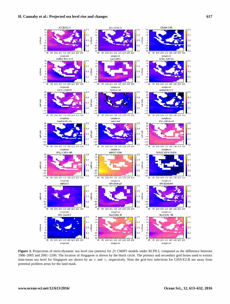
“oceanographic” term). As has been shown by previous stud-

ies (Pardaens et al., 2011; Slangen et al., 2014), we find a

large model spread in projections of regional oceanographic

sea level rise (Fig. 3). However, all models show relatively

weak gradients in the pattern of change in the vicinity of Sin-

gapore. This result appears to be largely independent of the

underlying ocean model resolution, which varies across the

CMIP5 models from about 2 to 0.3◦.

The sensitivity of results to the choice of grid box was

tested by selecting a primary and secondary grid box to rep-

resent Singapore. The difference in multi-model median es-

timates between boxes is about ±1 and ±2 mm for RCP4.5

and RCP8.5, respectively. This represents less than 1 % of

the change signal and therefore is considered a negligible

uncertainty. In order to provide an estimate of the projected

oceanographic sea level rise that is continuous with time,

it was assumed that the change signal (and model spread)

emerges proportionally to the global thermal expansion time

www.ocean-sci.net/12/613/2016/ Ocean Sci., 12, 613–632, 2016

http://www.climatechange2013.org/report/full-report/




http://www.atmosp.physics.utoronto.ca/~peltier/data.php

http://www.atmosp.physics.utoronto.ca/~peltier/data.php


Table 1. Summary table of methodologies employed to estimate the different components of sea level rise at Singapore, including scaling

factors used to convert global mean trends into local trends.

Component Methodology

1. Oceanographic sea level CMIP5 climate model estimates of global thermal expansion and dynamic sea level

are combined for each model. Differences between the two periods 1986–2005 and

2081–2100 are computed for each climate change scenario. A multi-model mean

and spread in this component is extracted for Singapore using a nearest-neighbour

approach. Time series are constructed based on the assumption that the change sig-

nal emerges proportionally to AR5 estimates of global thermal expansion.

2. Glaciers Time series of global sea level rise from AR5 data files are scaled by a factor of 1.11,

according to the spatial fingerprint information provided by Slangen et al. (2014).

3. Greenland surface mass

balance

Time series of global sea level rise from AR5 data files are scaled by a factor of 1.14,


4. Antarctica surface mass

balance

Time series of global sea level rise from AR5 data files are scaled by a factor of 1.13,


5. Greenland dynamics Time series of global sea level rise from AR5 data files are scaled by a factor of 1.16,


6. Antarctica dynamics Time series of global sea level rise from AR5 data files are scaled by a factor of 1.19,


7. Land water storage Time series of global sea level rise from AR5 data files are scaled by a factor of 0.81,


8. Glacial isostatic adjust-

ment (GIA)

Estimate based on ICE5G (Peltier, 2004) model as provided by Slangen et al. (2014).

9. Inverse barometer Assessed from AR5 supplementary data files. Not included in projections, given the

negligible contribution.

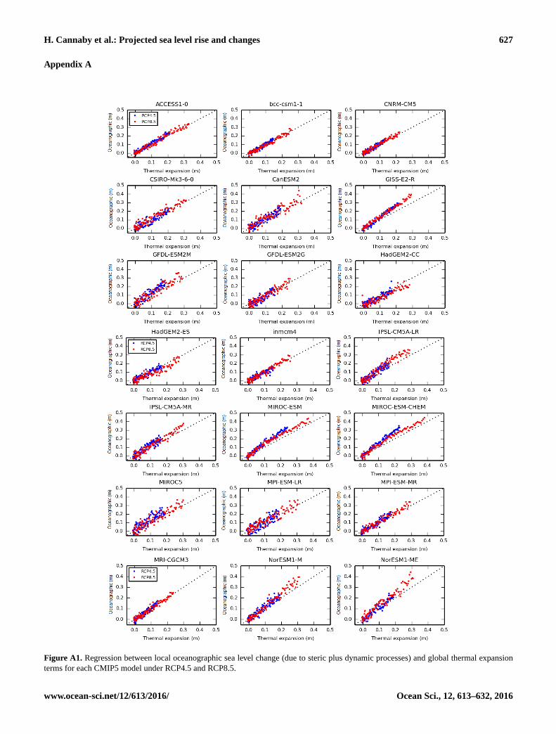
series of the IPCC AR5. This approach is justified since, to

a good approximation, all models show a linear relationship

between the local oceanographic sea level change near Sin-

gapore, and global thermal expansion (this relationship in

demonstrated in Fig. A1 for all CMIP5 models for RCP4.5

and RCP8.5). This permits us to estimate the sea level change

for the Singapore region throughout the 21st century for each

scenario.

IPCC AR5 estimates of the effect of changes in atmo-

spheric loading for the RCP4.5 and RCP8.5 scenarios are

available as part of the Chapter 13 supplementary data files

(Church et al., 2013). However, the projections for the Sin-

gapore region are very small compared to the other terms –

representing only about 1 % of the total estimated sea level

change, with relatively little spread among different model

projections. Given the substantial combined uncertainties of

the leading terms in total sea level change, we do not in-

clude the inverse barometer effect in our final projections as

we consider this term constitutes a negligible contribution to

projected sea level change.

The sea level change for Singapore was computed as the

difference between the 1986–2005 and 2081–2100 periods.

The median of the model ensemble change was taken as the

central estimate and the 5th and 95th percentiles were calcu-

lated based on the multi-model standard deviation, assuming

a normal distribution. Time series of each of the terms listed

in Table 1 have a central estimate (based on the median for

all terms except the oceanographic term, for which the mean

is used) and both an upper and lower bound, which are in-

dicative of the 5th and 95th percentiles of the distribution

and/or the likely range assessed in the IPCC AR5. The cen-

tral estimates of the different components are simply added

together to arrive at values for total sea level change at Singa-

pore. To combine the associated uncertainties we follow the

approach outlined by Church et al. (2013), in which total un-

certainty (σtot) expressed as a variance is estimated according

to Eq. (1),

σ 2tot = (σocean+ σsmb_a+ σsmb_g)

2+ σ 2

glac+ σ2LW

+ σ 2dyn_ a+ σ

2dyn_g, (1)

where σocean, σsmb_a, σsmb_gσglac, σLW, σdyn_a and σdyn_g

represent uncertainties in sea level rise projections due to

changes in oceanographic processes, Antarctic surface mass

balance, Greenland surface mass balance, glaciers, land wa-

ter, Antarctic dynamics and Greenland dynamics, respec-

tively. It is assumed that the first three terms, which have

a strong correlation with global air temperature, have corre-



Figure 3. Projections of steric/dynamic sea level rise (metres) for 21 CMIP5 models under RCP8.5, computed as the difference between

1986–2005 and 2081–2100. The location of Singapore is shown by the black circle. The primary and secondary grid boxes used to extract

time-mean sea level for Singapore are shown by an × and +, respectively. Note the grid box selections for GISS-E2-R are away from

potential problem areas for the land mask.



lated uncertainties and can therefore be added linearly. This

combined uncertainty is then added to the other components’

uncertainties in quadrature. The uncertainties in the projected

ice sheet surface mass balance changes are reported to be

dominated by the magnitude of climate change, rather than

their methodological uncertainty (see AR5 Chapter 13 sup-

plementary materials for details), while the uncertainty in

the projected glacier change was assumed to be dominated

by methodological uncertainty. We do not include an uncer-

tainty contribution for GIA or the inverse barometer effect

(which as noted above has a negligible contribution to sea

level projections at Singapore) in our method.

2.2 Design of model study

The surge and wave projections described in this work were

conducted utilising high-resolution (12 km) regional atmo-

spheric simulations, forced at the open boundaries by a se-

lection of nine Global Climate Model (GCM) solutions gen-

erated for the IPCC AR5 (IPCC AR4, 2007; see McSweeny

et al., 2015 for further details on downscaled atmospheric

simulations). Figure 1a shows the downscaled atmospheric

model domain. Computational expense dictated the need to

select only the most suitable GCMs from which to generate

downscaled atmospheric solutions. Approaches for selecting

climate models for downscaling are discussed in various pa-

pers (e.g. Wilby et al., 2009; Whetton et al., 2012). Criteria

of particular importance in selecting climate models for im-

pact studies include (a) that the climate models under his-

torical conditions accurately represent the processes or fea-

tures that are of particular relevance to the impact study and

(b) that the climate models sample the range of projected

change in the features of interest (Whetton et al., 2012).

Both these criteria were considered when selecting mod-

els for downscaling. In particular, it was essential that the

GCMs used should appropriately represent wind speed dur-

ing both the Northern Hemisphere and Southern Hemisphere

monsoon systems. Selection was further constrained by the

availability of suitable data on the CMIP5 archive. Of nine

downscaled atmospheric simulations conducted, four were

selected to force the high-resolution surge and wave models:

HadGEM2-ES, CNRM-CM5, IPSL-CM5A-MR and GFDL-

CM3. These four models sample a range of projected change

in wind speed and include the model GFDL-CM3, which

out of the nine downscaled atmospheric simulations exhib-

ited the largest area-averaged change in 850 hPa wind speeds

during both the SW and NE monsoon seasons. Computa-

tional expense also dictated that downscaled ocean simula-

tions could only be conducted for a single RCP. We therefore

chose RCP8.5, which is expected to give the largest climate

change signal.

Surge and wave climate projections were generated ex-

tending from 1970 to 2100. An additional atmospheric so-

lution downscaled from the ERA-Interim (Dee et al., 2011)

global atmospheric reanalysis was used to force historical

surge and wave simulations extending from 1980 to 2010.

These historical simulations were used to compare model re-

sults with contemporary observations.

2.3 Description of surge model

The model used to generate surge projections was the Nu-

cleus for European Modelling of the Ocean (NEMO) ver-

sion 3.4 ocean model (www.nemo-ocean.eu, Madec, 2008).

NEMO was run with a horizontal resolution of 1/12◦ and

nine sigma levels in the vertical. The domain extended from

95 to 117◦ east and from 10◦ south to 17◦ north as indicated

in Fig. 1a. Initial conditions specified a constant uniform den-

sity and this was maintained throughout the simulations by

setting surface heat and salt fluxes to zero. Hence, NEMO

was effectively run as a barotropic model. Tidal forcing was

applied at the open boundary as a time series of sea-surface

elevation representing 15 harmonic tidal constituents: Q1,

O1, P1, S1, K1, 2N2, MU2, N2, NU2, M2, L2, T2, S2, K2

and M4. In order to allow tides to propagate through the nar-

row and very shallow (< 12 m in places) Strait of Malacca,

it was necessary to modify the z envelope (which allows

sigma levels to intercept land in regions of steep topogra-

phy, thus preventing steep gradients in the vertical levels that

may introduce pressure gradient errors) such that the min-

imum number of vertical levels at any location was 7. The

model was run with logarithmic bottom friction and a 4 s

barotropic time step. Atmospheric forcing was prescribed as

hourly mean sea level pressure and 10 m wind fields. For the

case of the 4 GCM-forced simulations, atmospheric forcing

was prescribed at the same horizontal resolution as the ocean

model. ERA-Interim (Dee et al, 2011) atmospheric forcing

was prescribed at∼ 80 km resolution. Sea-surface height was

recorded at hourly intervals.

The climate models used to generate the atmospheric forc-

ing use different calendar years (only CNRM-CM5 uses a

Gregorian calendar, GFDL-CM3 and IPSL-CM5A-MR use

a 365-day calendar, and HadGEM2-ES uses a 360-day cal-

endar. This introduced difficulties in maintaining consistency

between tidal and atmospheric forcing. Consequently the

surge model was not run as a transient simulation, rather each

year was run independently, following a 5-day spin-up. To

avoid splitting model simulations during the winter monsoon

period when extreme events are most common, the model

was run 360 days forward in time from 1st July. Atmospheric

forcing for the 5-day spin-up was taken from the last 5 days

of June during the start year of the simulation.

The surge metric with which we are concerned in this

study is skew surge. Skew surge is the difference between

the elevation of the predicted astronomical high tide and the

maximum high water observed during the same tidal cycle

(e.g. de Vries et al., 1995). Skew surge is considered a more

significant and practical measure than surge residual (the dif-

ference between the predicted astronomical tide and the ob-

served water level at any time during a tidal cycle). This is


www.nemo-ocean.eu


because winds are most effective at generating surge in shal-

low water, meaning peaks in surge residual are typically ob-

tained prior to the predicted high water (Horsburgh and Wil-

son, 2007). In order to allow for calculation of skew surge, an

additional NEMO simulation was conducted extending from

1970 to 2100 with tidal forcing only (i.e. without any meteo-

rological forcing).

2.4 Description of wave model

Wave simulations were performed using WAVEWATCHIII

(WW3) (Tolman, 1997, 1999, 2009), a third generation wave

model developed by National Oceanographic and Atmo-

spheric Administration/National Centers for Environmental

Prediction (NOAA/NCEP). We used version 3.14 with Tol-

man and Chalikov (1996) physics. In a spectral wave model,

the choice of source terms dictates how the model represents

energy input through winds, and dissipation through wave

breaking and white capping. Regional validation runs were

initially performed using two sets of source terms for com-

parison: WAM cycle 4 (Monbaliu et al., 2000) and Tolman

and Chalikov (1996). The latter has problems with shorter

fetch, as wind waves grow slowly and dissipate slowly caus-

ing a model bias. WAM cycle 4 has a reduced bias over-

all but also reduced performance in the tropics. Very little

difference was found between these two source terms for

the domain of interest and consequently Tolman and Cha-

likov (1996) source terms were chosen due to the quicker in-

tegration time. The regional model was run at 1/12◦ resolu-

tion on a grid extending from 95 to 117◦ E and 9◦ S to 14◦ N

as indicated in Fig. 1a. The model was run with a global time

step of 900 s, a spectral resolution of 30 frequency bins, and

24 directional bins. The model was forced at the surface by

hourly mean 10 m wind speed at 1/12◦ resolution. Signif-

icant wave height, mean wave energy period, mean wave

direction, mean directional spread and mean wave period

were recorded at hourly intervals. We focus here on projected

changes in significant wave height.

In order to capture swell incoming at the open bound-

aries of the regional domain, a 50 km resolution global wave

model was also run, forced with 3 hourly wind and daily sea

ice values taken from the CMIP5 models. The global WW3

domain consisted of a spherical multiple cell grid with a res-

olution of 0.7031250◦× 0.4687500◦, which extended from

∼ 80◦ N to 80◦ S. Three-hourly wind data were not available

for the entire future period for IPSL-CM5A-MR, and so daily

data were used between 2046 and 2065. The model produced

nest files, which were used to force the regional domain at 3 h

intervals.

2.5 Model validation

To assess model performance in simulating local tides,

harmonic analyses of modelled and observed sea-surface

heights were performed using T_TIDE (Pawlowicz et al.,

2002). Comparisons were made at four tide gauge stations

situated close to Singapore: Raffles Light House, Keling,

Tanah Merah and Kukup (see Fig. 1b for locations). Simu-

lated SSH time series were extracted from the closest model

grid points to the tide gauge locations. Amplitudes and

phases of each tidal constituent were then compared using

scatter diagrams. During initial test runs the model was tuned

by adjusting the bottom friction parameterisation in order to

best represent tidal range, and in particular maximum spring

high-water events in the immediate vicinity of Singapore.

To assess model performance in representing surge events,

simulated annual maximum extreme water levels at grid

point “a” (Fig. 1b) were compared to an 18-year (1996–

2013) tide-gauge record from Raffles Light House. Six non-

overlapping samples of 18 consecutive years were extracted

from each of the model simulations. Return levels were

compared to average recurrence interval (ARI) measured in

years. For large return periods ARI is very similar to re-

turn period (RP; defined as the reciprocal of the annual ex-

ceedance probability). ARI and RP are related by Eq. (2).

ARI=1

log RPRP−1

(2)

The advantage of using ARI is that a Gumbel distribution fit-

ted to the tide gauge observations appears as a straight line on

a plot of return level versus ARI, even for small ARI. A Gum-

bel distribution was fitted to the tide gauge observations and

to each of the samples of model data, to give a distribution

of model-scale parameters. This distribution, along with the

scale parameter of the observations, is used to assess whether

the observations lie comfortably within the distribution of the

model samples.

Modelled significant wave heights were compared to those

derived from EnviSat satellite observations (Atlas et al.,

2011), utilising the along-track level-2 data collected be-

tween 2003 and 2005. Data were obtained via the Glob-

wave data portal (http://globwave.ifremer.fr/). All satellite

data falling within the model domain during this period were

directly compared to the closest model data point in both

space and time. A suite of metrics was then generated from

the model–data comparisons: mean errors (ME), root mean

square errors (RMSE), correlation coefficients (PC) and stan-

dard deviations (SD).

2.6 Analysis of extreme events

Analysis of extreme skew surge and significant wave height

return levels was limited by the length of the model simula-

tion. Furthermore, there was considerable interannual vari-

ability in both modelled and observed extreme water lev-

els, making long-term trends difficult to identify against the

background natural variability. To address these limitations a

statistical model was used, firstly to derive return levels for

periods longer than the period of the simulation, secondly to

better model the behaviour of the system at any given return


http://globwave.ifremer.fr/


period and thirdly to make a more informed assessment of

the century-scale trends. The model used was the generalised

extreme value (GEV) distribution (e.g. Coles, 2001; Hosking

et al., 1985; Huerta and Bruno, 2007; Kotz and Nadarajah,

2000; Méndez et al., 2007, 2008) applied to annual maximum

skew surge and significant wave height values. We tested the

impact of using the R largest events (R ranging from 1 to 5)

each year, subject to a separation of at least 120 h in an effort

to ensure independence. Results were not strongly sensitive

to the value of R, and furthermore for the GFDL and IPSL

simulations the parameter estimates did not remain stable as

R increased, which is a requirement for making meaning-

ful use of R > 1 (Coles, 2001). Thus, for consistency R = 1

(annual maxima only) was selected for all simulations. In-

voking the external types theorem (ETT) we assume that the

data are well approximated by a GEV distribution since each

data point is representative of the extreme of a large data

block. On fitting a generalised extreme value distribution to

the data, the three parameters of the GEV distribution (loca-

tion, scale and shape) can be used to make statements about

the probability of the annual maximum exceeding a particu-

lar level. The location parameter of the GEV is analogous to

the mean of the normal distribution meaning that a change

slides the whole distribution up or down. The scale param-

eter of the GEV is analogous to the standard deviation of

the normal distribution, meaning that an increase widens the

spread of the distribution, in the case of the GEV moving

the long-period return levels further from the short-period

return levels. Thus, a change in either parameter can affect

the long-period return levels. In this work we considered the

century-scale change in location and scale. It is assumed that

the shape parameter remains constant for a given simulation.

The GEV distribution was fitted to modelled extreme skew

surge and wave heights time series over the 1970–2099 pe-

riod. Allowing the location parameter to change accommo-

dates potential change in all extreme events (e.g. at both long

and short return periods). Allowing the scale parameter to

change accommodates the potential for an increase (or de-

crease) in the spread of extreme events (e.g. an increase in

intensity of the most extreme surges accompanied by a de-

crease in intensity of the more frequent surges). A compar-

ison of the quality of the stationary and non-stationary fits

gives an indication of the significance of any trend. Linear

century-scale trends in return level associated with any given

return period were diagnosed from the non-stationary GEV

fit to the data. In order to produce a four-model mean (µ)

trend estimate, the mean of the ensemble central estimates

of trend was taken. The (Bessel-corrected) standard devia-

tion of these four (σ) then represents the uncertainty in the

projection. We then identify (µ− 1.64σ ) as the lower bound

and (µ+ 1.64σ ) as the upper bound. Note that the implied

symmetry is in the distribution of trends, not the distribution

of the extremes themselves, which will in general be asym-

metrical. We note that a limitation of the statistical modelling

is an implicit assumption that the behaviour of the extremes

Figure 4. Projections of sea level rise relative to 1986–2005 and

its contributions as a function of time for (a) global mean sea level

(RCP4.5), (b) Singapore region (RCP4.5), (c) global mean sea level

(RCP8.5) and (d) Singapore region (RCP8.5). Lines show the me-

dian projections. The likely ranges for the total and thermal expan-

sion or steric/dynamic sea level changes are shown by the shaded

regions. The contributions from ice sheets include the contributions

from ice sheet rapid dynamical change. The dotted line shows an

extrapolation of the observed 1984–2011 rate of sea level change

for the Singapore Strait reported by Tkalich et al. (2013).

in 1 year is independent of the behaviour of the extremes in

neighbouring years. In fact we expect some autocorrelation

due to multi-annual cycles in the climate system. This can

reduce the effective number of degrees of freedom compared

to the number implied by the assumption of independence.

In this circumstance there is a risk of diagnosing a trend as

statistically significant simply because the assumed number

of degrees of freedom is too large. However, we find a pos-

teriori that this is not a big issue in this work since we do not

diagnose large significant positive trends.



3 Model validation

3.1 Surge model

Comparisons of modelled and observed tidal amplitudes and

phases at four tide gauge stations (Raffles Light House,

Kukup, Tanah Merah and Keling, located as indicated in

Fig. 1b) are presented in Fig. 4a for the seven largest tidal

constituents (M2, N2, K2, K1, O1, M4 and P1). Modelled

tidal amplitudes compare well to those observed, particularly

for the dominant semi-diurnal constituents (M2, N2 and K2)

for which differences between observed and modelled am-

plitudes averaged 1.1 cm. The smaller diurnal components

(K1, O1, M4, P1) are less well captured by the model with

a mean difference between observed and modelled ampli-

tudes of 3 cm. Tidal phase is also well captured by the model

(Fig. 5b). Modelled and observed tidal phases differed by less

than 50◦, with the exception at two stations of the smallest

amplitude (M4) constituent.

Model skill in simulating extreme events is demonstrated

by comparing simulated annual maximum extreme water lev-

els at grid point “a” with annual maximum events extracted

from an 18-year (1996–2013) tide-gauge record at Raffles

Light House. In order to make a like-for-like comparison, six

non-overlapping samples of 18 consecutive years were ex-

tracted from each of the model simulations. This treatment of

the 130-year-long simulations as essentially stationary is jus-

tifiable in view of the very small trends described in Sect. 4.2.

Extreme still-water return levels from each time series are

plotted as a function of return period in Fig. 5a. Simulated

return levels are approximately 20 cm larger than those de-

rived from observations for all return periods. Importantly,

it is also evident that the scale parameter (the gradient in

Fig. 5a) of the model data is comparable to that of the ob-

servations. This reveals that the model is doing a good job

of simulating the interannual variability (or “spread”) in ex-

treme water levels. The Gumbel distribution, fitted to the ob-

servations, is shown by the straight line in Fig. 6a. The distri-

bution of model-scale parameters derived from the Gumbel

distribution fitted to each of the samples of model data and

the observations, is shown in Fig. 5b. (NB detrending ob-

served and model data had little effect on the results shown

in this plot.) It can be seen that the scale parameter of the

observations lies comfortably within the distribution of the

model samples, indicating that the observed-scale parameter

is well modelled and that interannual variability in extreme

water levels changes little over the course of the simulations.

Aside from the mean sea level uncertainty, it is the uncer-

tainty in the scale parameter that primarily determines the un-

certainty in long-period return levels (i.e. the uncertainty in

the most extreme events) under the Gumbel distribution. The

good agreement between the modelled and observed-scale

parameter increases our confidence in applying the model to

project century-scale changes in extreme water levels.

Figure 5. Comparison of modelled and observed (a) tidal ampli-

tude and (b) tidal phase at four tide gauge stations close to Singa-

pore (Keling, Tanah Merah, Raffles lighthouse and Kukup) station

locations are marked in Fig. 1.

3.2 Wave model

The relationship between simulated significant wave heights

and those observed by satellite altimetry across the model

domain between 2003 and 2005 is summarised by a corre-

lation coefficient of 0.85, a standard deviation of 0.52 m and

a mean bias of −0.11 m. These statistics demonstrate good

model performance, comparable to the UK Met Office’s op-

erational wave model performance in tropical regions (Bidlot

and Holt, 2006; Bidlot et al., 2000, 2007). Qualitative com-

parison of modelled and observed seasonal mean cycles in

significant wave height at Singapore (not shown), demon-

strates that the model is able to represent seasonality in sig-

nificant wave heights at Singapore. A seasonal climatology

generated from the ERA-Interim-forced simulation exhibits

maximum significant wave heights of ∼ 0.3 m during the

southwest monsoon season and maximum significant wave

heights of ∼ 0.35 m during the northeast monsoon season.

Significant wave heights decrease to ∼ 0.1 m outside of the

monsoon seasons.



Table 2. Median values and likely (in IPCC calibrated language – see Sect. 2.1) ranges (square brackets) for projections of time-mean sea

level rise and its contribution in metres for 2081–2100 relative to 1986–2005 for Singapore and the global average (as reported in Table 13.5

of AR5, Church et al., 2013).

Sea level RCP4.5 change (m) RCP8.5 change (m)

component Singapore Global Singapore Global

Expansion/ 0.20 0.19 0.27 0.27

Oceanographic [0.12,0.27] [0.14,0.23] [0.18,0.36] [0.21,0.33]

Glaciers 0.14 0.12 0.18 0.16

[0.07,0.22] [0.06,0.19] [0.10,0.26] [0.09,0.23]

Greenland Surface 0.05 0.04 0.08 0.07

Mass Balance [0.01,0.18] [0.01,0.09] [0.03,0.18] [0.03,0.16]

Antarctica Surface −0.02 −0.02 −0.05 −0.04

Mass Balance [−0.06,−0.01] [−0.05,−0.01] [−0.08,−0.01] [−0.07,−0.01]

Greenland 0.05 0.04 0.06 0.05

Dynamics [0.01,0.07] [0.01,0.06] [0.02,0.08] [0.02,0.07]

Antarctica 0.08 0.07 0.08 0.07

Dynamics [−0.01,0.19] [−0.01,0.16] [−0.01,0.19] [−0.01,0.16]

Land Water 0.03 0.04 0.03 0.04

[−0.01,0.07] [−0.01,0.09] [−0.01,0.07] [−0.01,0.09]

GIA −0.03 N/A −0.03 N/A

Table 3. Estimates of global sea level rise from the IPCC AR5 (Church et al., 2013) alongside our regional estimates for Singapore. Following

the definitions in AR5, there is a 66–100 % chance that future sea level rise will fall within the ranges quoted. Based on current understanding,

only the collapse of marine-based sectors of the Antarctic ice sheet, if initiated, could cause global mean sea level to rise substantially above

the likely range during the 21st century. This potential additional contribution cannot be precisely quantified but there is medium confidence

that it would not exceed several tenths of a metre of sea level rise during the 21st century (Church et al, 2013).

2050 2100

Scenario Central Lower Upper Central Lower Upper

RCP4.5 Global 0.23 0.17 0.29 0.53 0.36 0.71

Singapore 0.22 0.14 0.29 0.52 0.29 0.73

RCP8.5 Global 0.25 0.19 0.32 0.74 0.52 0.98

Singapore 0.25 0.17 0.32 0.74 0.45 1.02

4 Projections of regional sea level change

4.1 Time-mean sea level

Time series of projected total sea level rise at Singapore

and its components for RCP4.5 and RCP8.5 are presented in

Fig. 6. The changes between 1986–2005 and 2081–2100 for

each contributing component are presented in Table 2. Cen-

tral, lower and upper ranges of total sea level rise at Singa-

pore out to 2050 and 2100 are presented in Table 3, alongside

global mean values for comparison. The central estimates of

total sea level rise at Singapore are similar to the global mean

projections reported in the IPCC AR5. Glacier and ice sheet

surface mass balance terms result in a larger increase in sea

level at Singapore compared to the global mean. This is be-

cause there is a far-field rise in sea level as a result of the

associated change in Earth’s gravity field as the mass is re-

distributed away from high latitudes (Tamisiea and Mitro-

vica, 2011). The larger ice mass balance term is, however,

offset by a negative contribution to sea level rise at Singa-

pore from glacial isostatic adjustment. This is the result of

additional ocean mass from the last deglaciation depressing

the sea floor and causing mantle material to flow underneath

the continents causing uplift (Tamisiea et al., 2014).

The uncertainty in projections of sea level rise at Singa-

pore is substantially larger than for global mean projections,

mainly due to the additional uncertainty associated with rep-

resentation of regional oceanographic processes (the oceano-



Figure 6. (a) Empirical return level data of extreme water level

based on 18 years of tide gauge data from Raffles Light House

(1996–2013), and 18-year long samples from the model simulations

at grid point “a”. The fitted Gumbel distribution of the observations

is shown by the straight line. (b) Empirical cumulative density func-

tion of the scale parameters of the model samples, showing that the

scale parameter of the tide gauge data sits well within the model

distribution.

Table 4. Projected century-scale trends in skew surge for five re-

turn periods (excluding mean sea level change). Units are mm per

century.

Period/years 2 20 100 1000 10 000

Lower −20 −40 −63 −90 −120

Central 0 −10 −20 −20 −30

Upper 20 20 30 50 60

graphic contribution to sea level change) by the coarse-

resolution CMIP5 models. Scaling up of the ice sheet and

glacier terms using the Slangen et al. (2014) fingerprints also

contributed to the increased uncertainty of the regional pro-

jections. This increased uncertainty is larger for RCP8.5 than

for RCP4.5. Over the first half of the 21st century the pro-

jected rate of sea level rise is similar for both RCP4.5 and

RCP8.5. Hence, on this timescale, sea level rise projections

are largely independent of emissions pathway, meaning the

uncertainty range is dominated by methodological and model

uncertainty. In both RCP4.5 and RCP8.5 there is a substan-

tial acceleration in the rate of sea level rise over the 21st cen-

tury, particularly during the early and mid-periods of the 21st

century. A simple linear extrapolation of observed long-term

regional trends (as reported for Singapore by Tkalich et al.,

2013) is therefore likely to grossly underestimate future sea

level rise.

4.2 Surge changes

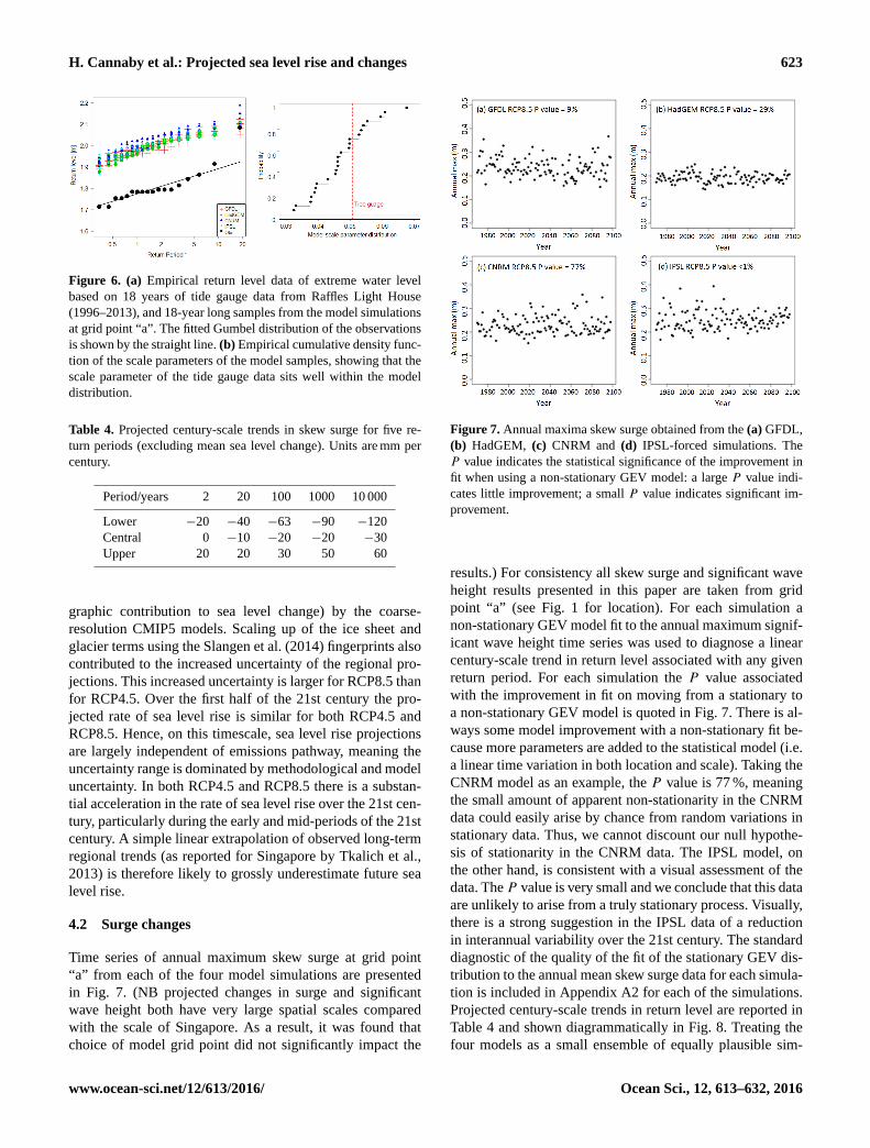
Time series of annual maximum skew surge at grid point

“a” from each of the four model simulations are presented

in Fig. 7. (NB projected changes in surge and significant

wave height both have very large spatial scales compared

with the scale of Singapore. As a result, it was found that

choice of model grid point did not significantly impact the

Figure 7. Annual maxima skew surge obtained from the (a) GFDL,

(b) HadGEM, (c) CNRM and (d) IPSL-forced simulations. The

P value indicates the statistical significance of the improvement in

fit when using a non-stationary GEV model: a large P value indi-

cates little improvement; a small P value indicates significant im-

provement.

results.) For consistency all skew surge and significant wave

height results presented in this paper are taken from grid

point “a” (see Fig. 1 for location). For each simulation a

non-stationary GEV model fit to the annual maximum signif-

icant wave height time series was used to diagnose a linear

century-scale trend in return level associated with any given

return period. For each simulation the P value associated

with the improvement in fit on moving from a stationary to

a non-stationary GEV model is quoted in Fig. 7. There is al-

ways some model improvement with a non-stationary fit be-

cause more parameters are added to the statistical model (i.e.

a linear time variation in both location and scale). Taking the

CNRM model as an example, the P value is 77 %, meaning

the small amount of apparent non-stationarity in the CNRM

data could easily arise by chance from random variations in

stationary data. Thus, we cannot discount our null hypothe-

sis of stationarity in the CNRM data. The IPSL model, on

the other hand, is consistent with a visual assessment of the

data. The P value is very small and we conclude that this data

are unlikely to arise from a truly stationary process. Visually,

there is a strong suggestion in the IPSL data of a reduction

in interannual variability over the 21st century. The standard

diagnostic of the quality of the fit of the stationary GEV dis-

tribution to the annual mean skew surge data for each simula-

tion is included in Appendix A2 for each of the simulations.

Projected century-scale trends in return level are reported in

Table 4 and shown diagrammatically in Fig. 8. Treating the

four models as a small ensemble of equally plausible sim-



Table 5. Projected century-scale trends in significant wave height

for five return periods due to storminess changes (mm per century,

to two decimal places).

Period/years 2 20 100 1000 10 000

Lower −15 −460 −730 −1260 −2030

Central −30 −140 −220 −390 −620

Upper 80 190 290 490 780

●

●●

●●

5 10 50 500 5000

−10

0−

500

5010

0

Century−scale trend vs return period. [lower,central,upper]

Return period (years)

Tre

nd m

m/c

entu

ry

●

●

●

●

●

●

●

●

●

●

Figure 8. Projected century-scale trends in skew surge for five re-

turn periods due to storminess changes only (i.e. excluding mean

sea level change; millimetres per century). Central, lower and upper

estimates are shown.

ulations, we obtain an ensemble [5, 95 ‰] of the diagnosed

trend in the 100-year return level of [−63, 30] mm century−1.

We do not find a statistically significant trend in skew surge

for any of the return levels tested. Uncertainties in skew surge

trends are small compared to the uncertainties in projected

mean sea level change of, e.g., [450, 1020] mm (see Table 3)

over the 21st century under RCP8.5. As no statistically sig-

nificant trends in skew surge return levels are projected for

RCP8.5, we would not expect to find tends for the less severe

RCP4.5 scenario.

4.3 Wave changes

Time series of annual maximum significant wave height at

grid point “a” from each of the four simulations are pre-

sented in Fig. 9. The standard diagnostic of the quality of

the fit of the stationary GEV distribution to the significant

wave height and annual maxima for each simulation is shown

in Appendix A3. All of the resulting projections of century-

scale trends were small and negative, with the exception of

the IPSL-forced simulation for which a 35 mm century−1 in-

crease in the 2-year return level was obtained. The model en-

semble of the diagnosed trend in 100-year significant wave

height return level is [−0.73, 0.29] mm century−1. Diag-

Figure 9. Simulated annual maxima of significant wave height (me-

tres) obtained from the (a) GFDL, (b) HadGEM, (c) CNRM and

(d) IPSL-forced simulations. The P value indicates the statistical

significance of the improvement in fit when using a non-stationary

GEV model: a large P value indicates little improvement; a small

P value indicates significant improvement.

nosed trends in 2, 20, 100, 1000 and 10000-year return lev-

els are given in Table 5 and presented diagrammatically in

Fig. 10. The small sample size of four climate models and the

large spread in projections of century-scale change in signifi-

cant wave height at long return periods means that we cannot

rule out positive trends, even though the central estimates of

the trends are small and negative in each of the four models.

5 Discussion

The overriding conclusion from this study is that change in

time-mean sea level will be the dominant process influencing

the changing vulnerability of Singapore to coastal inundation

over the 21st century. Several studies have drawn similar con-

clusions for other parts of the world, e.g., in the North Sea

(Sterl et al., 2009), around the UK (Lowe et al., 2009) and

globally (Bindoff et al., 2007). It is notable that the central

estimates of sea level rise by 2100 (of 0.52 and 0.74 m under

the RCP4.5 and RCP8.5 scenarios, respectively) are of simi-

lar magnitude to the most damaging surge events recorded at

Singapore over recent decades (in describing extreme events

occurring since the 1970s, Tkalich et al. (2009) reported sea

level anomalies ranging from 43 to ∼ 60 cm). Hence, Sin-

gapore is a country particularly vulnerable to sea level rise.

Wong (1992) previously highlighted this vulnerability, not-

ing that by adding 1 m to current chart datum levels at Singa-

pore (comparable to our upper estimate of a 1.02 m sea level



●●

●

●

●

5 10 50 500 5000

−20

00−

1000

010

0020

00

Century−scale trend vs return period. [lower,central,upper]

Return period (years)

Tre

nd m

m/c

entu

ry

●

●

●

●

●

●●

●

●

●

Figure 10. Projected century-scale trends in significant wave height

for five return periods due to storminess changes only (i.e. excluding

mean sea level change; mm per century). Central, lower and upper

estimates are shown.

rise by 2100), the mean spring high water level of 3.8 m will

be close to the highest recorded water level to date, of 3.9 m.

The climate simulations presented in this work suggest

there will be no significant change in the frequency of ex-

treme storm surge or wave events during the 21st century

over and above that due to mean sea level rise. Extreme

events of the magnitude seen over recent decades will, how-

ever, have a much greater impact when superimposed on ris-

ing sea levels. Those involved in mitigating the potential im-

pacts of future climate change on Singapore’s coastline there-

fore need to combine projections of sea level rise with skew

surge return level data. Site-specific projections of future ex-

treme still-water level can be obtained by linearly combin-

ing return levels derived from tide gauge data with the sea

level change projections presented in Table 3. (Tide-gauge

data represent the best information available about present-

day location-specific return levels; however, it is worth not-

ing that uncertainties in the present-day return levels derived

from relatively short tide-gauge records are likely to be a

large component of the combined uncertainty in projected

future return-level curves.) In the longer term there is poten-

tial to develop better estimates of current risk by combining

model-derived information with observed time series. The

skew surge joint probability method (Batstone et al., 2013)

provides an approach to addressing this problem.

There are several caveats to the sea level, surge and wave

projections presented in this study and we consider each in

turn in the following paragraphs. Mean sea level projections

are presented as likely (66–100 % probability) ranges for the

RCP4.5 and RCP8.5 climate change scenarios, taking into

account a number of uncertainties that cannot be robustly

quantified with the present state of scientific knowledge. We

note that recent studies have attempted to provide informa-

tion outside of the IPCC likely range (Kopp et al., 2014;

Jevrejeva et al., 2014) and this is an important topic of on-

going discussion by the research community (Hinkel et al.,

2015). As noted previously, our sea level projections do not

account for the unlikely event of a collapse of the marine-

based sectors of the Antarctic ice sheet. Based on current

understanding, AR5 assessed that such a collapse, if initi-

ated, could cause global mean sea level to rise substantially

above the given likely range during the 21st century. This

potential additional contribution cannot be precisely quanti-

fied, but the AR5 report assessed with medium confidence

that it would not exceed several tenths of a metre of sea level

rise during the 21st century (Church et al., 2013). This re-

mains one of the most important structural uncertainties in

projecting sea level extremes. An additional source of uncer-

tainty arises from taking patterns of change associated with

land ice, land water and GIA from a single source (i.e. the

maps generated by Slangen et al., 2014). While Slangen’s

data are considered very credible estimates based on current

understanding, we do not include here any estimate of un-

certainties in sea level change that could arise from using

alternative estimates of these patterns. The CMIP5 models,

due to their low resolution, have limited ability to represent

meso-scale hydrographic processes important to regional dy-

namics. Previous studies (e.g. Lowe et al., 2009; Perrette et

al., 2013) suggest, however, that large-scale oceanic signals

propagate freely into the coastal region, and are not overtly

affected by the coarse resolution of the models. In common

with previous studies (e.g. Lowe et al., 2009; Perrette et al.,

2013), we assume that large-scale oceanic signals propagate

freely into the coastal region. The effects of anthropogenic

disturbance such as resource extraction and land reclamation

on sea level projections are also not considered in this work.

Finally, it is important to note that the probability attributed

to the sea level projections is calculated without accounting

for the potential effects of future seismic activity; the only

vertical land movement process considered in this study be-

ing glacial-isostatic adjustment. It is possible that vertical

land movement associated with seismic activity may dom-

inate changes in relative sea level over decadal timescales.

The Earth Observatory of Singapore state that

“Sea level could rise faster than the IPCC predicted af-

ter a big earthquake on the Sunda Megathrust. This is

due to the overall tectonics of the region. After a big

earthquake on the megathrust, the whole Sunda shelf will

experience a subsidence.” (http://www.earthobservatory.sg/

faq-on-earth-sciences/singapore-threatened-earthquakes-0)

There are a number of further caveats associated with

the modelling of extreme events. Waves and surge have

been modelled separately, meaning wave–surge interactions

are not accounted for. Surge propagation from outside the

boundaries of the surge model domain is also not consid-

ered (except by application of a static inverse barometer ef-

fect at the boundaries). Over shallow seas, however, wind

is the dominant factor in surge generation, suggesting that


http://www.earthobservatory.sg/faq-on-earth-sciences/singapore-threatened-earthquakes-0

http://www.earthobservatory.sg/faq-on-earth-sciences/singapore-threatened-earthquakes-0


surge propagation from outside the boundaries will not be a

dominant factor in driving extreme water levels on the Sunda

shelf (Horsburgh and Wilson, 2007). The impacts of changes

in mean water depth on tidal resonance and on surge propa-

gation are also not considered in this work. Pickering (2014)

investigated the impact on tidal dynamics of raising GMSL

by 2 m and found a change in mean high water level of the

order of 10 cm around Singapore. Howard et al. (2010), Sterl

et al. (2009) and Lowe et al. (2001) found in studies of the

northwest European shelf that changing the water depth af-

fects the time of arrival of a storm surge, but not the surge

height. Hence, we suggest that any impact of rising sea lev-

els on tidal dynamics will be small compared to sea level

rise. Finally, our simulations assume a fixed coastline with

no inundation. Further work with a high-resolution inunda-

tion model is required to understand the land area at risk

from inundation due to sea level rise, and to design appro-

priate coastal defences to best mitigate this risk.

6 Conclusions

Regional projections of changes in long-term mean sea level

and in the frequency of extreme storm surge and wave events

over the 21st century have been generated for Singapore. Lo-

cal changes in time-mean sea level were evaluated using the

process-based climate model data and methods presented in

the IPCC AR5. Regional surge and wave forecast simulations

extending from 1970 to 2100 were generated using high-

resolution (∼ 12 km) regional surge (Nucleus for European

Modelling of the Ocean – NEMO) and wave (WaveWatchIII)

models. Ocean simulations were forced by four regional at-

mospheric model solutions, which were in turn nested within

global atmospheric simulations generated for the IPCC AR4.

The four climate models were chosen to best represent his-

torical conditions and included the GFDL-CM3 model which

exhibited the largest area-averaged changes in 850 hPa wind

speeds during both the southwest and northeast monsoon sea-

sons. An additional atmospheric regional model simulation

driven by a global atmospheric reanalysis was used to force

historical regional ocean model simulations extending from

1980 to 2010. The hindcast simulation was used to demon-

strate the skill of the models in simulating regional tides and

surge events (through comparison to tide gauge data) and sig-

nificant wave heights (through comparison to satellite altime-

try data).

Central estimates of long-term mean sea level rise at Sin-

gapore by 2100 are projected to be 0.52 m (0.74 m) under the

RCP 4.5(8.5) scenarios, respectively. These values are very

close to the global mean estimates presented in the IPCC

AR5. Sea level rise at Singapore resulting from mass loss

from ice sheets and glaciers is projected to be 10–15 % larger

than the global mean. This will, however, be offset by ele-

vation of the land mass due to glacial isostatic adjustment.

The likely ranges of projected sea level rise at Singapore

are substantially larger than the global mean projections,

mainly due to the uncertainty associated with representation

of regional oceanographic processes by the coarse-resolution

CMIP5 models. Due to an acceleration in the rate of sea level

rise throughout the early and mid-21st century, extrapolation

of long-term tide-gauge records does not provide reliable es-

timates of future sea level change and systematically under-

estimates the magnitude of future sea level rise for both sce-

narios.

The [5, 95 ‰] of diagnosed trend in 100-year skew surge

return level, obtained by treating the four models as a

small ensemble of equally plausible simulations is [−63,

30] mm century−1. The corresponding [5, 95 ‰] of the diag-

nosed trend in 100-year significant wave height return level is

[−0.73, 0.29] mm century−1. The uncertainties in projected

century-scale trend in skew surge and significant wave height

are small compared to the uncertainties in projected mean sea

level change of, e.g., [450, 1020] mm over the 21st century

under RCP8.5. We find no statistically significant changes

in extreme skew surge events and no statistically signifi-

cant changes in extreme significant wave height under the

RCP8.5 scenario over and above that due to mean sea level

change using the four model ensembles. Our primary finding

is then that change in time-mean sea level will be the domi-

nant process influencing the changing vulnerability of Singa-

pore to coastal inundation over the 21st century. We note that

the largest recorded surge residual in the Singapore Strait of

∼ 84 cm (Tkalich et al., 2009) lies between the central and

upper estimates of sea level rise by 2100.

Data availability

This study was conducted as part of Singapore’s Sec-

ond National Climate Change Study – Phase 1 (see

http://ccrs.weather.gov.sg/publications-second-national-

climate, McSweeney et al., 2015). Data are available

through application to CCRS.


http://ccrs.weather.gov.sg/publications-second-national-climate-change-study-science-reports

http://ccrs.weather.gov.sg/publications-second-national-climate-change-study-science-reports


Appendix A

Figure A1. Regression between local oceanographic sea level change (due to steric plus dynamic processes) and global thermal expansion

terms for each CMIP5 model under RCP4.5 and RCP8.5.



Figure A2. Standard diagnostic plots for stationary fit to skew surge annual maxima from (a) HadGEM2-ES, (b) IPSL, (c) CNRM, and

(d) GFDL simulations. The quantile and probability plots compare the theoretical distribution fitted to the data with the actual data and give

an indication of confidence in the fit of the return period.



Figure A3. Standard diagnostic plots for stationary fit to significant wave height annual maxima from (a) HadGEM2-ES, (b) IPSL, (c) CNRM

and (d) GFDL simulations. The quantile and probability plots compare the theoretical distribution fitted to the data with the actual data and

give an indication of confidence in the fit of the return period.



Acknowledgements. This study was carried out as part of Singa-

pore’s Second National Climate Change Study and was funded by

the government of Singapore. Full reports of the study can be found

of the Centre for Climate Research Singapore (CCRS) website at

http://ccrs.weather.gov.sg/publications-second-National-Climate.

Jamie Kettleborough and Ian Edmond provided scripts for

downloading and archiving the CMIP5 data used in this study. We

thank Aimée Slangen for providing spatial fingerprint data used

in the projections of regional sea level change and Mark Carson

for assistance with carrying out the comparison with the Slangen

et al. (2014) oceanographic sea level changes. We acknowledge

use of the MONSooN system, a collaborative facility supplied

under the Joint Weather and Climate Research Programme, which

is a strategic partnership between the Met Office and the Natural

Environment Research Council. This work also used the ARCHER

UK National Supercomputing Service (http://www.archer.ac.uk).

Edited by: M. Hecht

References

Allen, J. I., Aiken, J., Anderson, T. R., Buitenhuis, E., Cornell,

S., Geider, R., Haines, K., Hirata, T., Holt, J., Le Quéré, C.,

Hardman-Mountford, N., Ross, O. N., Sinha, B., and While,

J.: Marine ecosystem models for earth systems applications: the

MarQUEST experience, J. Marine Syst., 81, 19–33, 2010.

Atlas, R., Hoffman, R. N., Ardizzone, J., Leidner, S. M., Jusem,

J. C., Smith, D. K., and Gombos, D.: A cross-calibrated, multi-

platform ocean surface wind velocity product for meteorological

and oceanographic applications, B. Am. Meteorol. Soc., 92, 157–

174, doi:10.1175/2010BAMS2946.1, 2011.

Batstone, C., Lawless, M., Tawn, J., Horsburgh, K., Black-

man, D., McMillan, A., Worth, D., Laeger, S., and Hunt, T.:

A UK best-practice approach for extreme sea-level analysis

along complex topographic coastlines, Ocean Eng., 71, 28–39,

10.1016/j.oceaneng.2013.02.003, 2013.

Bidlot, J. R. and Holt, M. W.: Verification of operational global and

regional wave forecasting systems against measurements from

moored buoys, JCOMM Technical Report, 30, WMO/TD no.

1333, 2006.

Bidlot, J. R., Holmes-Bell, D. J., Wittmann, P. A., Lalbeharry, R.,

and Chen, H. S.: Intercomparison of the performance of opera-

tional ocean wave forecasting systems with buoy data, European

Centre for Medium-Range Weather Forecasts (ECMWF) Tech-

nical Memorandum Number 315 also 2002, Weather Forecast.,

17, 287–310, 2000.

Bidlot, J. R., Li, L. G., Wittmann, P., Fauchon, M., Chen, H.,

Lefevre, J. M., Bruns, T., Greenslade, D., Ardhuin, F., Kohno, N.,

Park, S., and Gomez, M.: Inter-comparison of operational wave

forecasting systems, 10th International Workshop on Wave Hind-

casting and Forecasting and Coastal Hazard Symposium, North

Shore, Oahu, Hawaii, 11–16 November 2007.

Bindoff, N. L., Willebrand, J., Artale, V., Cazenave, A., Gregory,

J., Gulev, S., Hanawa, K., Le Quéré, C., Levitus, S., Nojiri, Y.,

Shum, C. K., Talley, L. D., and Unnikrishnan, A.: Observations:

Oceanic Climate Change and Sea Level, in: Climate Change

2007: The Physical Science Basis, Contribution of Working

Group I to the Fourth Assessment Report of the Intergovern-

mental Panel on Climate Change, edited by: Solomon, S., Qin,

D., Manning, M., Chen, Z., Marquis, M., Averyt, K. B., Tignor,

M., and Miller, H. L., Cambridge University Press, Cambridge,

United Kingdom and New York, NY, USA, 2007.

Bird, M. I., Austin, W. E. N., Wurster, C. M., Fifield, L.

K., Mojtahis, M., and Sargeant, C.: Punctuated eustatic sea-

level rise in the early mid-Holocene, Geology, 38, 803–806,

doi:10.1130/G31066.1, 2010.

Church, J. A., Clark, P. U., Cazenave, A., Gregory, J. M., Jevrejeva,

S., Levermann, A., Merrifield, M. A., Milne, G. A., Nerem, R. S.,

Nunn, P. D., Payne, A. J., Pfeffer, W. T., Stammer, D., and Un-

nikrishnan, A. S.: Sea Level Change, in: Climate Change 2013:

The Physical Science Basis, Contribution of Working Group I to

the Fifth Assessment Report of the Intergovernmental Panel on

Climate Change, edited by: Stocker, T. F., Qin, D., Plattner, G.

K., Tignor, M., Allen, S. K., Boschung, J., Nauels, A., Xia, Y.,

Bex, V., and Midgley, P. M., Cambridge University Press, Cam-

bridge, United Kingdom and New York, NY, USA, 2013.

Coles, S.: An introduction to statistical modeling of extreme values,

208 pp., London, Springer, 2001.

Dee, D. P., Uppala, S. M., Simmons, A. J., Berrisford, P., Poli,

P., Kobayashi, S., Andrae, U., Balmaseda, M. A., Balsamo, G.,

Bauer, P., Bechtold, P., Beljaars, A. C. M., van de Berg, L., Bid-

lot, J., Bormann, N., Delsol, C, Dragani, R., Fuentes, M., Geer,

A. J., Haimberger, L., Healy, S. B., Hersbach, H., Hólm, E. V.,

Isaksen, L., Kållberg, P., Köhler, M., Matricardi, M., McNally,

A. P., Monge-Sanz, B. M., Morcrette, J. J., Park, B. K., Peubey,

C., de Rosnay, P., Tavolato, C., Thépaut, J. N., and Vitart, F.: The

ERA-Interim reanalysis: configuration and performance of the

data assimilation system, Q. J. Roy. Meteor. Soc., 137, 553–597,

doi:10.1002/qj.828, 2011.

de Vries, H., Breton, M., de Mulder, T., Krestenitis, Y., Ozer, J.,

Proctor, R., Ruddick, K., Saloman, J. C., and Voorrips, A.: A

comparison of 2-D storm-surge models applied to three shallow

European seas, Environ. Softw., 10, 23–42, 1995.

Hinkel, J., Jaeger, C., Nicholls, R. J., Lowe, J., Renn, O., and Peijun,

S.: Sea-level rise scenarios and coastal risk management, Nature

Climate Change, 5, 188–190, doi:10.1038/nclimate2505, 2015.

Horsburgh, K. J. and Wilson, C.: Tide-surge interaction and its role

in the distribution of surge residuals in the North Sea, J. Geophys.

Res., 112, C08003, doi:10.1029/2006JC004033, 2007.

Hosking, J. R. M., Wallis, J. R., and Wood, E. F.: Estimation

of the generalized extreme-value distribution by the method

of probability-weighted moments, Technometrics, 27, 251–261,

1985.

Howard, T., Lowe, J., and Horsburgh, K.: Interpreting century-scale

changes in southern North Sea storm surge climate derived from

coupled model simulations, J. Climate, 23, 6234–6247, 2010.

Howard, T., Pardaens, A. K., Bamber, J. L., Ridley, J., Spada, G.,

Hurkmans, R. T. W. L., Lowe, J. A., and Vaughan, D.: Sources of

21st century regional sea-level rise along the coast of northwest

Europe, Ocean Sci., 10, 473–483, doi:10.5194/os-10-473-2014,

2014.

Huerta, G. and Bruno, S.: Time-varying models for extreme values,

Environ. Ecol. Stat., 14, 285–299, 2007.

IPCC: AR4 Climate change 2007, The physical science basis, Sum-

mary for policymakers, in: Contribution of Working Group I to

the Fourth Assessment Report of the Intergovernmental Panel on

Climate Change, edited by: Solomon, S., Qin, D., Manning, M.,


http://ccrs.weather.gov.sg/publications-second-National-Climate-Change-Study-Science-Reports

http://www.archer.ac.uk

http://dx.doi.org/10.1175/2010BAMS2946.1

http://dx.doi.org/10.1130/G31066.1

http://dx.doi.org/10.1002/qj.828

http://dx.doi.org/10.1038/nclimate2505

http://dx.doi.org/10.1029/2006JC004033

http://dx.doi.org/10.5194/os-10-473-2014


Chen, Z., Marquis, M., Averyt, K. B., Tignor, M., and Miller, H.

L., 2007.

Jevrejeva, S., Grinsted, A., and Moore, C. J.: Upper limit for sea

level projections by 2100, Environ. Res. Lett., 9, 1–9, 2014.

Kotz, S. and Nadarajah, S.: Extreme Value Distributions: Theory

and Applications, London, Imperial College Press, 2000.

Kopp, R. E., Horton, R. M., Little, C. M., Mitrovica, J. X., Op-

penheimer, M., Rasmussen, D. J., Strauss, B. H., and Tebaldi,

C.: Probabilistic 21st and 22nd century sea-level projections at

a global network of tide-gauge sites, Earth’s future, 2, 383–406,

2014.

Lowe, J. A., Gregory, J., and Flather, R.: Changes in the occur-

rence of storm surges around the United Kingdom under a future

climate scenario using a dynamic storm surge model driven by

the Hadley Centre climate models, Clim. Dynam., 18, 179–188,

2001.

Lowe, J. A., Howard, T. P., Pardaens, A., Tinker, J., Holt, J., Wake-

lin, S., Milne, G., Leake, J., Wolf, J., Horsburgh, K., Reeder, T.,

Jenkins, G., Ridley, J., Dye, S., and Bradley, S.: UK Climate Pro-

jections science report: Marine and coastal projections, Met Of-

fice Hadley Centre, Exeter, UK, 2009.

Madec, G.: NEMO reference manual 3/4 Stable: NEMO ocean

engine, Note du Pôle de modélisation, Institut Pierre-Simon

Laplace (IPSL), France, 27, 1288–1619, 2008.

Maren, D. V. and Gerritsen, H.: Residual flow and tidal asymmetry

in the Singapore Strait, with implications for resuspension and

residual transport of sediment, J. Geophys. Res., 117, C04021,

doi:10.1029/2011JC007615, 2012.

McSweeney, C., Rahmat, R., Redmond, G., Marzin, C., Murphy,

J., Jones, R., Cheong, W. K., Lim, S. Y., and Sun, X.: Sin-

gapore’s Second National Climate Change Study – Phase 1,

Chapter 3, Sub-selection of CMIP5 GCMs for downscaling over

Singapore, available at: http://ccrs.weather.gov.sg/publications-

second-National, last access: 28 Oktober 2015.

McSweeney, C. F., Jones, R. G., Lee, R. W., and Rowell, D. P.:

Selecting CMIP5 GCMs for downscaling over multiple regions,

Clim. Dynam., 44, 3237–3260, 2015.

Méndez, F. J., Menéndez, M., Luceño, A., and ILosada, I.

J.: Analyzing Monthly Extreme Sea Levels with a Time-

Dependent GEV Model, J. Atmos. Ocean. Technol., 24, 894–

911, doi:10.1175/JTECH2009.1, 2007.

Mendez, F. J., Menendez, M., Luceo, A., and Losada, I.

J.: Estimation of the long-term variability of extreme sig-

nificant wave height using a time-dependent Peak Over

Threshold (POT) model, J. Geophys. Res., 111, C07024,

doi:10.1029/2005JC003344, 2008.

Meinshausen, M., Smith, S. J., Calvin, K. V., Daniel, J. S., Kainuma,

M. L. T., Lamarque, J. F., Matsumoto, K, Montzka, S. A., Raper,

S. C. B., Riahi, K., Thomson, A. M., Velders, G. J. M., and van

Vuuren, D.: The RCP Greenhouse Gas Concentrations and their

Extension from 1765 to 2300, Climatic Change, 109, 213–241,

doi:10.1007/s10584-011-0156-z, 2011.

Monbaliu, J., Padilla-Hernandez, R., Hargreaves, J. C., Albiach, J.

C. C., Luo, W., Sclavo, M., and Gunther, H: The spectral wave

model, WAM, adapted for applications with high spatial resolu-

tion, Coast. Eng., 41, 41–62, 2000

Mousavi, M., Irish, J., Frey, A., Olivera, F., and Edge., B: Global

warming and hurricanes: The potential impact of hurricane inten-

sification and sea level rise on coastal flooding, Climatic Change,

104, 575–597, 2011.

Pardaens, A., Gregory, J. M., and Lowe, J.: A model study of fac-

tors influencing projected changes in regional sea level over the

twenty-first century, Clim. Dynam., 36, 2015–2033, 2011.

Pawlowicz, R., Beardsley, B., and Lentz, S.: Classical Tidal Har-

monic Analysis Including Error Estimates in MATLAB using

TTIDE, Comput. Geosci., 28, 929–937, 2002.

Peltier, W. R.: Global Glacial Isostasy and the Surface of the Ice-

Age Earth: The ICE-5G (VM2) Model and GRACE, Annu. Rev.

Earth Planet. Sci., 32, 111–149, 2004.

Penduff, T., Juza, M., Brodeau, L., Smith, G. C., Barnier, B., Mo-

lines, J.-M., Treguier, A.-M., and Madec, G.: Impact of global

ocean model resolution on sea-level variability with emphasis on

interannual time scales, Ocean Sci., 6, 269–284, doi:10.5194/os-

6-269-2010, 2010.

Perrette, M., Landerer, F., Riva, R., Frieler, K., and Meinshausen,

M.: A scaling approach to project regional sea level rise and its

uncertainties, Earth Syst. Dynam., 4, 11–29, doi:10.5194/esd-4-

11-2013, 2013.

Pickering, M.: The impact of future sea-level rise on the tides, Uni-

versity of Southampton, Ocean and Earth Science, Doctoral The-

sis, 347 pp., 2014.

Slangen, A. B. A., Carson, M., Katsman, C. A., van de Wal, R. S.

W., Koehl, A., Vermeersen, L. L. A., and Stammer, D.: Projecting

twenty-first century regional sea-level changes, Climatic Change,

124, 317–332, doi:10.1007/s10584-014-1080-9, 2014.

Smith, J. M., Cialone, M. A., Wamsley, T. V., and McAlpin, T. O.:

Potential impact of sea level rise on coastal surges in southeast

Louisiana, Ocean Eng., 37, 37–47, 2010.

Sterl, A., van den Brink, H., de Vries, H., Haarsma, R., and van

Meijgaard, E.: An ensemble study of extreme storm surge related

water levels in the North Sea in a changing climate, Ocean Sci.,

5, 369–378, doi:10.5194/os-5-369-2009, 2009.

Tamisiea, M. E. and Mitrovica, J. X.: The moving boundaries of

sea level change: Understanding the origins of geographic vari-

ability, Oceanography, 24, 24–39, doi:10.5670/oceanog.2011.25,

2011.

Tamisiea, M. E., Hughes, C. W., Williams, S. D. P., and Bingley, R.

M.: Sea level: measuring the bounding surfaces of the ocean, Phi-

los. T. R. Soc. A, 372, 1–26, doi:10.1098/rsta.2013.0336, 2014.

Tkalich, P., Vethamony, P., Babu, M. T., and Pokratath, R.: Seasonal

sea level variability and anomalies in the Singapore Strait, Pro-

ceedings of International Conference in Ocean Eng., ICOE 2009

IIT Madras, Chennai, India, 10–5 February 2009.

Tkalich, P., Vethamony, P., Luu, Q.-H., and Babu, M. T.: Sea level

trend and variability in the Singapore Strait, Ocean Sci., 9, 293–

300, doi:10.5194/os-9-293-2013, 2013.

Tolman, H. L.: User manual and system documentation of

WAVEWATCH-III version 1.15, NOAA/NWS/NCEP/OMB

Technical Note 151, 97 pp., 1997.

Tolman, H. L.: User manual and system documentation of

WAVEWATCH-III version 1.18, NOAA/NWS/NCEP/OMB

Technical Note 166, 110 pp., 1999.

Tolman, H. L.: User manual and system documentation of WAVE-

WATCH III version 3.14, NOAA/NWS/NCEP/MMAB Techni-

cal Note 276, 194 pp., 2009.

Tolman, H. L. and Chalikov, D. V.: Source terms in a 3rd generation

wind-wave model, J. Phys. Oceaonogr., 26, 2497–2518, 1996.


http://dx.doi.org/10.1029/2011JC007615



http://dx.doi.org/10.1175/JTECH2009.1

http://dx.doi.org/10.1029/2005JC003344

http://dx.doi.org/10.1007/s10584-011-0156-z

http://dx.doi.org/10.5194/os-6-269-2010

http://dx.doi.org/10.5194/os-6-269-2010

http://dx.doi.org/10.5194/esd-4-11-2013

http://dx.doi.org/10.5194/esd-4-11-2013

http://dx.doi.org/10.1007/s10584-014-1080-9

http://dx.doi.org/10.5194/os-5-369-2009

http://dx.doi.org/10.5670/oceanog.2011.25

http://dx.doi.org/10.1098/rsta.2013.0336

http://dx.doi.org/10.5194/os-9-293-2013


Wilby, R. L., Troni, J., Biot, Y., Tedd, L., Hewitson, B. C., Smith,

D. M., and Sutton, R. T.: A review of climate risk information

for adaptation and development planning, Int. J. Climatol., 29,

1193–1215, 2009.

Whetton, P., Hennessy, K., Clarke, J., McInnes, K., and Kent, K.:

Use of Representative Climate Futures in impact and adaptation

assessment, Climatic Change, 115, 433–442, 2012.

Wong, P. P.: Impact of a sea level rise on the coasts of Singapore:

preliminary observations, J. Southe. Asian Earth, 7, 65–70, 1992.


Projected sea level rise and changes in extreme storm ... · wave events during the 21st century in the region of Singapore Heather Cannaby1, Matthew D. Palmer2, Tom Howard2, Lucy

Documents