Project AC460 Image Processing and Pattern Recognition with Java Jon Campbell and Fionn Murtagh IVS, School of Computer Science The Queen’s University of Belfast December 1998

Welcome message from author
This document is posted to help you gain knowledge. Please leave a comment to let me know what you think about it! Share it to your friends and learn new things together.
Transcript

Project AC460
Image Processingand
Pattern RecognitionwithJava
Jon Campbell and Fionn Murtagh
IVS, School of Computer ScienceThe Queen’s University of Belfast
December 1998

2
Contents
1 Introduction 31.1 Motivation and Rationale . . . . . . . . . . . . . . . . . . . . . . 31.2 Applications . . . . . . . . . . . . . . . . . . . . . . . . . . . . . 41.3 What is a Digital Image? . . . . . . . . . . . . . . . . . . . . . . 6
1.3.1 Other Examples of Digital Quantities . . . . . . . . . . . 81.3.2 Raster Sampling or Scanning . . . . . . . . . . . . . . . . 81.3.3 Pixel . . . . . . . . . . . . . . . . . . . . . . . . . . . . 81.3.4 Spatial Resolution . . . . . . . . . . . . . . . . . . . . . 81.3.5 Graylevel Resolution . . . . . . . . . . . . . . . . . . . . 8
1.4 Signal Processing . . . . . . . . . . . . . . . . . . . . . . . . . . 101.4.1 Colour and Spectral Bands . . . . . . . . . . . . . . . . . 101.4.2 Sensing . . . . . . . . . . . . . . . . . . . . . . . . . . . 10
1.5 General Concepts of Image Processing . . . . . . . . . . . . . . . 101.6 Further Examples of Images . . . . . . . . . . . . . . . . . . . . 141.7 Exercises for Chapter 1 . . . . . . . . . . . . . . . . . . . . . . . 14
2 Digital Image Fundamentals 232.1 Visual Perception . . . . . . . . . . . . . . . . . . . . . . . . . . 232.2 An Image Model: a General Imaging System . . . . . . . . . . . 24
2.2.1 Radiometric Measurement and Calibration . . . . . . . . 252.2.2 Motivation . . . . . . . . . . . . . . . . . . . . . . . . . 252.2.3 Uneven Illumination . . . . . . . . . . . . . . . . . . . . 262.2.4 Uneven Sensor Response . . . . . . . . . . . . . . . . . . 26
2.3 Imaging Geometry . . . . . . . . . . . . . . . . . . . . . . . . . 272.3.1 General . . . . . . . . . . . . . . . . . . . . . . . . . . . 272.3.2 Geometric Distortion . . . . . . . . . . . . . . . . . . . . 272.3.3 Geometric Calibration . . . . . . . . . . . . . . . . . . . 282.3.4 Object Frame versus Camera Frame . . . . . . . . . . . . 282.3.5 Lighting Angles . . . . . . . . . . . . . . . . . . . . . . 28
2.4 Sampling and Quantization . . . . . . . . . . . . . . . . . . . . . 292.5 Colour . . . . . . . . . . . . . . . . . . . . . . . . . . . . . . . . 29
2.5.1 Electromagnetic Waves and the Electromagnetic Spectrum 292.5.2 The Visible Spectrum . . . . . . . . . . . . . . . . . . . . 29
3
4 CONTENTS
2.5.3 Sensors . . . . . . . . . . . . . . . . . . . . . . . . . . . 302.5.4 Spectral Selectivity and Colour . . . . . . . . . . . . . . 332.5.5 Spectral Responsivity . . . . . . . . . . . . . . . . . . . . 342.5.6 Colour Display . . . . . . . . . . . . . . . . . . . . . . . 342.5.7 Additive Colour . . . . . . . . . . . . . . . . . . . . . . . 352.5.8 Colour Reflectance . . . . . . . . . . . . . . . . . . . . . 352.5.9 Exercises . . . . . . . . . . . . . . . . . . . . . . . . . . 35
2.6 Photographic Film . . . . . . . . . . . . . . . . . . . . . . . . . 362.7 General Characteristics of Sensing Methods . . . . . . . . . . . . 36
2.7.1 Active versus Passive . . . . . . . . . . . . . . . . . . . . 362.7.2 Methods of Interaction . . . . . . . . . . . . . . . . . . . 372.7.3 Contrast . . . . . . . . . . . . . . . . . . . . . . . . . . . 372.7.4 Exercises . . . . . . . . . . . . . . . . . . . . . . . . . . 38
2.8 Worked Example on Calibration . . . . . . . . . . . . . . . . . . 392.9 CCD Calibration in Astronomy . . . . . . . . . . . . . . . . . . . 43
2.9.1 CCD Detectors versus Photographs . . . . . . . . . . . . 432.9.2 CCD Detectors and Their Calibration . . . . . . . . . . . 44
2.10 Questions on Chapters 1 and 2 – Fundamentals, Sensors, and Cal-ibration . . . . . . . . . . . . . . . . . . . . . . . . . . . . . . . 46
3 The Fourier Transform in Image and Signal Processing 493.1 Introduction . . . . . . . . . . . . . . . . . . . . . . . . . . . . . 493.2 Digital Signal Processing . . . . . . . . . . . . . . . . . . . . . . 49
3.2.1 Introduction . . . . . . . . . . . . . . . . . . . . . . . . . 493.2.2 Finite Sampled Signals. . . . . . . . . . . . . . . . . . . 503.2.3 Sampling Frequency . . . . . . . . . . . . . . . . . . . . 533.2.4 Amplitude Resolution . . . . . . . . . . . . . . . . . . . 533.2.5 Frequencies . . . . . . . . . . . . . . . . . . . . . . . . . 543.2.6 Phase . . . . . . . . . . . . . . . . . . . . . . . . . . . . 553.2.7 Periodic Signals . . . . . . . . . . . . . . . . . . . . . . 56
3.3 Fourier Series . . . . . . . . . . . . . . . . . . . . . . . . . . . . 563.3.1 General . . . . . . . . . . . . . . . . . . . . . . . . . . . 563.3.2 Orthogonal Functions . . . . . . . . . . . . . . . . . . . 583.3.3 Finite Fourier Series . . . . . . . . . . . . . . . . . . . . 593.3.4 Complex Fourier Series . . . . . . . . . . . . . . . . . . 59
3.4 The Fourier Transform . . . . . . . . . . . . . . . . . . . . . . . 603.5 Discrete Fourier Transform . . . . . . . . . . . . . . . . . . . . . 62
3.5.1 Definition . . . . . . . . . . . . . . . . . . . . . . . . . . 623.5.2 Discrete Fourier Spectrum . . . . . . . . . . . . . . . . . 623.5.3 Interpretation . . . . . . . . . . . . . . . . . . . . . . . . 633.5.4 Frequency Discrimination by the DFT . . . . . . . . . . . 633.5.5 Implementation of the DFT . . . . . . . . . . . . . . . . 71
3.6 Fast Fourier Transform . . . . . . . . . . . . . . . . . . . . . . . 733.6.1 General . . . . . . . . . . . . . . . . . . . . . . . . . . . 73
CONTENTS 5
3.6.2 Software Implementation . . . . . . . . . . . . . . . . . . 743.7 Convolution . . . . . . . . . . . . . . . . . . . . . . . . . . . . . 77
3.7.1 General . . . . . . . . . . . . . . . . . . . . . . . . . . . 773.7.2 Impulse Response . . . . . . . . . . . . . . . . . . . . . 813.7.3 Linear Systems . . . . . . . . . . . . . . . . . . . . . . . 813.7.4 Some Interpretations of Convolution . . . . . . . . . . . . 823.7.5 Convolution of Continuous Signals . . . . . . . . . . . . 823.7.6 Two-Dimensional Convolution . . . . . . . . . . . . . . . 823.7.7 Digital Filters . . . . . . . . . . . . . . . . . . . . . . . . 83
3.8 Fourier Transforms and Convolution . . . . . . . . . . . . . . . . 853.9 The Discrete Fourier Transform as a Matrix Transformation . . . . 883.10 Cross-Correlation . . . . . . . . . . . . . . . . . . . . . . . . . . 893.11 The Two-Dimensional Discrete Fourier Transform . . . . . . . . . 903.12 The Two-Dimensional DFT as a Separable Transformation . . . . 913.13 Other Transforms . . . . . . . . . . . . . . . . . . . . . . . . . . 92
3.13.1 General . . . . . . . . . . . . . . . . . . . . . . . . . . . 923.13.2 Discrete Cosine Transform . . . . . . . . . . . . . . . . . 923.13.3 Walsh-Hadamard Transform . . . . . . . . . . . . . . . . 93
3.14 Applications of the Discrete Fourier Transform . . . . . . . . . . 943.14.1 Introduction . . . . . . . . . . . . . . . . . . . . . . . . . 943.14.2 Frequency Analysis . . . . . . . . . . . . . . . . . . . . . 953.14.3 Filtering . . . . . . . . . . . . . . . . . . . . . . . . . . . 953.14.4 Fast Convolution . . . . . . . . . . . . . . . . . . . . . . 963.14.5 Fast Correlation . . . . . . . . . . . . . . . . . . . . . . . 963.14.6 Data Compression . . . . . . . . . . . . . . . . . . . . . 973.14.7 Deconvolution . . . . . . . . . . . . . . . . . . . . . . . 97
3.15 Questions on Chapter 3 – the Fourier Transform . . . . . . . . . . 99
4 Image Enhancement 1014.1 Introduction . . . . . . . . . . . . . . . . . . . . . . . . . . . . . 1014.2 Noise and Degradation . . . . . . . . . . . . . . . . . . . . . . . 1024.3 Point Operations . . . . . . . . . . . . . . . . . . . . . . . . . . 104
4.3.1 Grey Level Mapping by Lookup Table . . . . . . . . . . . 1044.3.2 Colour Lookup Tables . . . . . . . . . . . . . . . . . . . 1054.3.3 Greyscale Transformation . . . . . . . . . . . . . . . . . 1074.3.4 Thresholding and Slicing . . . . . . . . . . . . . . . . . . 1084.3.5 Contrast Enhancement Based on Statistics . . . . . . . . . 1094.3.6 Histogram Modification . . . . . . . . . . . . . . . . . . 1104.3.7 Local Enhancement . . . . . . . . . . . . . . . . . . . . . 116
4.4 Noise Reduction by Averaging of Multiple Images . . . . . . . . 1174.5 Spatial Operations . . . . . . . . . . . . . . . . . . . . . . . . . . 118
4.5.1 Neighbourhood Averaging . . . . . . . . . . . . . . . . . 1184.5.2 Lowpass Filtering . . . . . . . . . . . . . . . . . . . . . . 1194.5.3 Median Filtering . . . . . . . . . . . . . . . . . . . . . . 122

6 CONTENTS
4.5.4 Other Non-linear Smoothing . . . . . . . . . . . . . . . . 1294.6 Image Sharpening – General . . . . . . . . . . . . . . . . . . . . 1304.7 Gradient Based Edge Enhancement . . . . . . . . . . . . . . . . . 130
4.7.1 Introduction . . . . . . . . . . . . . . . . . . . . . . . . . 1304.7.2 Gradient, Slope and Differentiation . . . . . . . . . . . . 1304.7.3 Discrete Differentiation – Differences . . . . . . . . . . . 1314.7.4 Differentiation in 2-D – Partial Differentials . . . . . . . . 1334.7.5 Windows for Differentiation . . . . . . . . . . . . . . . . 1334.7.6 Other Gradient Windows . . . . . . . . . . . . . . . . . . 1344.7.7 Gradient Magnitude and Direction . . . . . . . . . . . . . 134
4.8 Laplacian . . . . . . . . . . . . . . . . . . . . . . . . . . . . . . 1414.9 Edge Detection by Template Matching . . . . . . . . . . . . . . . 1424.10 Highpass Filtering . . . . . . . . . . . . . . . . . . . . . . . . . . 142
4.10.1 Marr-Hildreth Operators . . . . . . . . . . . . . . . . . . 1424.11 Additional Exercises . . . . . . . . . . . . . . . . . . . . . . . . 1434.12 Answers to Selected Questions . . . . . . . . . . . . . . . . . . . 1444.13 Examples of Image Enhancement Operations . . . . . . . . . . . 1504.14 Questions on Chapter 4 – Image Enhancement . . . . . . . . . . . 158
5 Data and Image Compression 1635.1 Introduction and Summary . . . . . . . . . . . . . . . . . . . . . 1635.2 Compression – Motivation . . . . . . . . . . . . . . . . . . . . . 1645.3 Context of Data Compression . . . . . . . . . . . . . . . . . . . . 1665.4 Information Theory . . . . . . . . . . . . . . . . . . . . . . . . . 167
5.4.1 Introduction to Information Theory . . . . . . . . . . . . 1675.4.2 Entropy or Average Information per Symbol . . . . . . . 1685.4.3 Redundancy . . . . . . . . . . . . . . . . . . . . . . . . . 1705.4.4 Redundancy is Sometimes Useful! . . . . . . . . . . . . . 170
5.5 Introduction to Image Compression . . . . . . . . . . . . . . . . 1715.6 Run-Length Encoding . . . . . . . . . . . . . . . . . . . . . . . . 1725.7 Quantization Coding . . . . . . . . . . . . . . . . . . . . . . . . 1735.8 Source Coding . . . . . . . . . . . . . . . . . . . . . . . . . . . 174
5.8.1 Variable Length Coding . . . . . . . . . . . . . . . . . . 1745.8.2 Unique Decoding . . . . . . . . . . . . . . . . . . . . . . 1755.8.3 Huffman Coding . . . . . . . . . . . . . . . . . . . . . . 1765.8.4 Some Problems with Single Symbol Source Coding . . . . 1805.8.5 Alternatives/Solutions . . . . . . . . . . . . . . . . . . . 181
5.9 Transform Coding . . . . . . . . . . . . . . . . . . . . . . . . . . 1835.9.1 General . . . . . . . . . . . . . . . . . . . . . . . . . . . 1835.9.2 Subimage Coding . . . . . . . . . . . . . . . . . . . . . . 1855.9.3 Colour Image Coding . . . . . . . . . . . . . . . . . . . . 185
5.10 Image Model Coding . . . . . . . . . . . . . . . . . . . . . . . . 1855.11 Differential and Predictive Coding . . . . . . . . . . . . . . . . . 1865.12 Dimensionality and Compression . . . . . . . . . . . . . . . . . . 186
CONTENTS 7
5.13 Vector Quantization . . . . . . . . . . . . . . . . . . . . . . . . . 1875.14 The JPEG Still Picture Compression Standard . . . . . . . . . . . 1885.15 Error Criteria for Lossy Compression . . . . . . . . . . . . . . . 1895.16 Additional References on Image and Data Compression . . . . . . 1895.17 Additional Exercises . . . . . . . . . . . . . . . . . . . . . . . . 1905.18 Questions . . . . . . . . . . . . . . . . . . . . . . . . . . . . . . 191
6 From Images to Objects 1976.1 Introduction . . . . . . . . . . . . . . . . . . . . . . . . . . . . . 1976.2 Introduction to Segmentation . . . . . . . . . . . . . . . . . . . . 197
6.2.1 Single Pixel Classification . . . . . . . . . . . . . . . . . 1996.2.2 Boundary-Based Methods . . . . . . . . . . . . . . . . . 2076.2.3 To Read Further on Image Segmentation . . . . . . . . . 2096.2.4 Exercises on Image Segmentation . . . . . . . . . . . . . 209
6.3 Mathematical Morphology . . . . . . . . . . . . . . . . . . . . . 2106.3.1 Introduction to Mathematical Morphology . . . . . . . . . 2106.3.2 Scanned Operators . . . . . . . . . . . . . . . . . . . . . 2166.3.3 Grey-level Morphology . . . . . . . . . . . . . . . . . . . 2176.3.4 Composite Operations – Open and Close . . . . . . . . . 2186.3.5 Program Implementation . . . . . . . . . . . . . . . . . . 2186.3.6 Examples of Morphological Operations . . . . . . . . . . 2196.3.7 To Read Further on Mathematical Morphology . . . . . . 2226.3.8 DataLab-J Demonstrations on Mathematical Morphology . 2236.3.9 Exercises on Mathematical Morphology . . . . . . . . . . 226
6.4 The Wavelet Transform . . . . . . . . . . . . . . . . . . . . . . . 2276.4.1 Introduction . . . . . . . . . . . . . . . . . . . . . . . . . 2276.4.2 The a trous Wavelet Transform . . . . . . . . . . . . . . . 2286.4.3 Examples of the A Trous Wavelet Transform . . . . . . . 2306.4.4 The Haar Wavelet Transform . . . . . . . . . . . . . . . . 2356.4.5 Examples of the Haar Wavelet Transform . . . . . . . . . 2376.4.6 To Read Further on the Wavelet Transform . . . . . . . . 2406.4.7 DataLab-J Demonstrations of the Wavelet Transform . . . 2406.4.8 Exercises on the Wavelet Transform . . . . . . . . . . . . 242
7 Pattern Recognition 2457.1 Introduction . . . . . . . . . . . . . . . . . . . . . . . . . . . . . 2457.2 Features and Classifiers . . . . . . . . . . . . . . . . . . . . . . . 246
7.2.1 Features and Feature Extraction . . . . . . . . . . . . . . 2467.2.2 Classifier . . . . . . . . . . . . . . . . . . . . . . . . . . 2477.2.3 Training and Supervised Classification . . . . . . . . . . . 2497.2.4 Statistical Classification . . . . . . . . . . . . . . . . . . 2497.2.5 Feature Vector – Update . . . . . . . . . . . . . . . . . . 2507.2.6 Distance . . . . . . . . . . . . . . . . . . . . . . . . . . . 2517.2.7 Other Classification Paradigms . . . . . . . . . . . . . . . 251

8 CONTENTS
7.2.8 Neural Networks . . . . . . . . . . . . . . . . . . . . . . 2537.2.9 Summary on Features and Classifiers . . . . . . . . . . . 253
7.3 A Simple but Practical Problem . . . . . . . . . . . . . . . . . . 2547.3.1 Introduction . . . . . . . . . . . . . . . . . . . . . . . . . 2547.3.2 Naive Character Recognition . . . . . . . . . . . . . . . . 2547.3.3 Invariance for Two-Dimensional Patterns . . . . . . . . . 2587.3.4 Feature Extraction – Another Update . . . . . . . . . . . 258
7.4 Classification Rules . . . . . . . . . . . . . . . . . . . . . . . . . 2597.4.1 Similarity Measures Between Vectors . . . . . . . . . . . 2617.4.2 Nearest Mean Classifier . . . . . . . . . . . . . . . . . . 2637.4.3 Nearest Neighbour Classifier . . . . . . . . . . . . . . . . 2657.4.4 Condensed Nearest Neighbour Algorithm . . . . . . . . . 2657.4.5 k-Nearest Neighbour Classifier . . . . . . . . . . . . . . . 2667.4.6 Box Classifier . . . . . . . . . . . . . . . . . . . . . . . . 2667.4.7 Hypersphere Classifier . . . . . . . . . . . . . . . . . . . 2677.4.8 Statistical Classifier . . . . . . . . . . . . . . . . . . . . . 2677.4.9 Bayes Classifier . . . . . . . . . . . . . . . . . . . . . . . 270
7.5 Linear Transformations in Pattern Recognition and Estimation . . 2707.5.1 Linear Partitions of Feature Space . . . . . . . . . . . . . 2717.5.2 Discriminants . . . . . . . . . . . . . . . . . . . . . . . . 2737.5.3 Linear Discriminant as Projection . . . . . . . . . . . . . 2747.5.4 The Connection with Neural Networks . . . . . . . . . . 2757.5.5 Fisher Linear Discriminant . . . . . . . . . . . . . . . . . 2767.5.6 Karhunen-Loeve Transform . . . . . . . . . . . . . . . . 2777.5.7 Least-Square Error Linear Discriminant . . . . . . . . . . 2797.5.8 Computational Considerations . . . . . . . . . . . . . . . 2807.5.9 Eigenimages . . . . . . . . . . . . . . . . . . . . . . . . 2817.5.10 Other Connections and Discussion . . . . . . . . . . . . . 283
7.6 Shape and Other Features . . . . . . . . . . . . . . . . . . . . . . 2837.6.1 Two-dimensional Shape Recognition . . . . . . . . . . . 2837.6.2 Two-dimensional Invariant Moments for Planar Shape Recog-
nition . . . . . . . . . . . . . . . . . . . . . . . . . . . . 2847.6.3 Classification Based on Spectral Features . . . . . . . . . 2867.6.4 Some Common Problems in Pattern Recognition . . . . . 2877.6.5 Problems Solvable by Pattern Recognition Techniques . . 2877.6.6 For Further Reading . . . . . . . . . . . . . . . . . . . . 288
7.7 Exercises . . . . . . . . . . . . . . . . . . . . . . . . . . . . . . 289
8 Neural Networks 2978.1 Introduction . . . . . . . . . . . . . . . . . . . . . . . . . . . . . 2978.2 Historical Background . . . . . . . . . . . . . . . . . . . . . . . 2988.3 Neural Networks Basics . . . . . . . . . . . . . . . . . . . . . . 300
8.3.1 Introduction . . . . . . . . . . . . . . . . . . . . . . . . . 3008.3.2 Brain Cells . . . . . . . . . . . . . . . . . . . . . . . . . 300

CONTENTS 9
8.3.3 Artificial Neurons . . . . . . . . . . . . . . . . . . . . . . 3018.3.4 Neural Networks and Knowledge Based Systems . . . . . 3048.3.5 Neurons for Recognising Patterns . . . . . . . . . . . . . 3068.3.6 Perceptrons . . . . . . . . . . . . . . . . . . . . . . . . . 3088.3.7 Neural Network Training . . . . . . . . . . . . . . . . . . 3098.3.8 Limitations of Perceptrons . . . . . . . . . . . . . . . . . 3098.3.9 Neurons for Computing Functions . . . . . . . . . . . . . 3108.3.10 Complex Boundaries via Multiple Layer Nets . . . . . . . 3128.3.11 ‘Soft’ Threshold Functions . . . . . . . . . . . . . . . . . 3138.3.12 Multilayer Feedforward Neural Network . . . . . . . . . 3138.3.13 Exercises . . . . . . . . . . . . . . . . . . . . . . . . . . 314
8.4 Implementation . . . . . . . . . . . . . . . . . . . . . . . . . . . 3218.4.1 Software . . . . . . . . . . . . . . . . . . . . . . . . . . 3218.4.2 Hardware . . . . . . . . . . . . . . . . . . . . . . . . . . 3218.4.3 Optical Implementations . . . . . . . . . . . . . . . . . . 322
8.5 Training Neural Networks . . . . . . . . . . . . . . . . . . . . . 3228.5.1 Introduction . . . . . . . . . . . . . . . . . . . . . . . . . 3228.5.2 Hebbian Learning Algorithm . . . . . . . . . . . . . . . . 3228.5.3 The Perceptron Training Rule . . . . . . . . . . . . . . . 3238.5.4 Widrow-Hoff Rule . . . . . . . . . . . . . . . . . . . . . 3238.5.5 Statistical Training . . . . . . . . . . . . . . . . . . . . . 3248.5.6 Backpropogation . . . . . . . . . . . . . . . . . . . . . . 3248.5.7 Simulated Annealing . . . . . . . . . . . . . . . . . . . . 3258.5.8 Genetic Algorithms . . . . . . . . . . . . . . . . . . . . . 325
8.6 Other Neural Networks . . . . . . . . . . . . . . . . . . . . . . . 3258.7 Conclusion . . . . . . . . . . . . . . . . . . . . . . . . . . . . . 325
8.7.1 Exercises . . . . . . . . . . . . . . . . . . . . . . . . . . 3268.8 Recommended Reading . . . . . . . . . . . . . . . . . . . . . . . 3298.9 References and Bibliography . . . . . . . . . . . . . . . . . . . . 3308.10 Questions on Chapters 7, 8 and 9 – Segmentation, Pattern Recog-
nition and Neural Networks . . . . . . . . . . . . . . . . . . . . . 3358.11 Recommended Texts and Indicative Reading . . . . . . . . . . . . 343
A Appendix: Essential Mathematics 347A.1 Introduction . . . . . . . . . . . . . . . . . . . . . . . . . . . . . 347A.2 Random Variables, Random Signals and Random Fields . . . . . 347
A.2.1 Basic Probability and Random Variables . . . . . . . . . . 347A.2.2 Random Processes . . . . . . . . . . . . . . . . . . . . . 351A.2.3 Further Background Reading . . . . . . . . . . . . . . . . 356
A.3 Linear Algebra . . . . . . . . . . . . . . . . . . . . . . . . . . . 357A.3.1 Basic Definitions . . . . . . . . . . . . . . . . . . . . . . 357A.3.2 Linear Simultaneous Equations . . . . . . . . . . . . . . 359A.3.3 Basic Matrix Operations . . . . . . . . . . . . . . . . . . 362A.3.4 Particular Matrices . . . . . . . . . . . . . . . . . . . . . 366

CONTENTS 1
A.3.5 Complex Numbers . . . . . . . . . . . . . . . . . . . . . 367A.3.6 Further Matrix and Vector Operations . . . . . . . . . . . 369A.3.7 Vector Spaces . . . . . . . . . . . . . . . . . . . . . . . . 372
B Appendix: Image Analysis and Pattern Recognition in Java 377

2 CONTENTS

Chapter 1
Introduction
1.1 Motivation and Rationale
Digital image processing and digital signal processing – this book covers both – areamongst the fastest growing computer technologies of the 1990s. With increasingcomputing power, it is increasingly possible to do numerically many tasks that werepreviously done using analogue techniques. More importantly, it is now feasible toperform processing on signals and images that were previously unthinkable. Thereare related advances in performance and cost of sensors. A room-full of computingequipment of yesteryear now fits in the palm of your hand. Likewise the capacityof communications channels and storage devices have grow dramatically. Digitaltelevision has arrived. We routinely transfer images over World-Wide Web.
It is now as valid to think of an image as data for processing just as a column ofnumbers in a bank balance, or strings of text in a database. Digital image process-ing is now state-of-the-art in many areas of high-technology: industrial inspection,monitoring of the earth and weather forecasting, document handling; and in areasof low(ish)-technology: personal computers and multimedia, digital cameras andelectronic darkrooms.
Although some image processing requires special architectures (e.g. the real-time processing of video images – 25–30 per second), much practical work can bedone on a general purpose computer, and even a modest PC. Thus, it is as valid tothink of a picture as data for processing as a column of numbers in a bank balance,or strings of text in a database.
The principal objective of this unit is to lay a foundation for further study andresearch in this field.
On completion of this first chapter, you should be able to:
• understand the fundamentals of digital image representation and the ele-ments of a digital image processing system.
• be familiar with a simple model of visual perception.
• describe and apply image enhancement techniques.
3
4 CHAPTER 1. INTRODUCTION
• understand the fundamental concepts of one-dimensional signal processing,and its link with image processing.
• understand the concepts and applications of image transforms.
• describe and apply image data compression techniques.
• appreciate the concept of data compression applied to text, signals, and im-ages.
• describe and apply image segmentation techniques.
• understand the fundamentals of pattern recognition.
• be aware of current advances in, and applications of, image processing.
1.2 Applications
Throughout this book we will continuously refer to the applications of image pro-cessing technology. Some of the areas we shall touch are:
Machine Vision: How to get a machine to sense a scene and perform the percep-tion, recognition, and knowledge acquisition tasks that are routine for humanobservers. Broadly speaking there are two important sub-areas of machinevision:
• 3-dimensional scene analysis, e.g. for automatic vehicle navigation.Difficult, except in very limited domains. Still a research area.
• automatic/automated inspection, e.g. quality control of computer printedcircuit boards, or of pastry cases, metal parts, etc... The Signal and Im-age Processing Group at Magee is doing research into flaw detection intextiles. Here the world is essentially two dimensional. Now state ofthe art technology.
Character recognition: The grand-daddy of all image processing / pattern recog-nition tasks. How to convert ink marks on a page into text characters. Similartechnology can be used for recognising any planar shape, e.g. for a robot topick from a selection of parts on a conveyer belt. Printed (block) characterrecognition is more or less state-of-the-art; cursive, and handwritten scriptmuch more difficult - still a research area.
Medical: A small set of applications include:
• blood cell analysis; looking for abnormal shapes, or abnormal propor-tions of shapes.

1.2. APPLICATIONS 5
• computer-aided tomography. Construction of 3D ‘image’ from a set of2-d X-ray images of cross-sections.
• automatic screening of chest X-ray images.
• teleradiology and telemedecine, i.e. enabling a specialist to medicalimages and other measurements of a patient while they (doctor andpatient) are separated by large distances.
Remote Sensing: Images of the earth, sensed from satellites and aircraft, can beprocessed to:
• assist in weather forecasting. Of course, fairly ‘raw’ unprocessed im-ages are routinely used in weather processing, as can be noted in anyTV weather forecast.
• automatically produce land-use maps,
• mineral exploration,
• evaluate the extent of global warming, – earth’s radiation budget stud-ies.
• pollution monitoring.
• some of the earliest digital image processing work was done at the JetPropulsion Laboratory, California, to ‘clean-up’ images sent from deepspace probes (e.g. Venus).
Military: Some applications include:
• automatic guidance of heat seeking missiles; images are infrared,
• interpreting remotely sensed images from spy satellites and aircraft,
• determination if ‘friend’ aircraft, from ‘foe’ using, e.g., silhouette im-ages,
Previously military applications were the primary instigators of most elec-tronics related research and development, and this was especially so in imagescience. Not so important now that the cold-war is over.
Document Image Processing: Increasingly, business records (letters, balance sheets,etc...) are prepared on computer, and stored on them, i.e. as strings of digits,alphabetic characters, even computer-aided-design drawing codes. But, cer-tain types of document originate outside the computer, e.g. cheques, deliverydocuments with receipt signatures, or are difficult to convert into symbols,so that the best that can be done is to make a digital picture record of them,and store that on a computer.
Entertainment and Consumer Items: We can mention:
• digital video,
6 CHAPTER 1. INTRODUCTION
• still images on computers,
• digital cameras.
Geographical Information Systems: The combination of many different sorts ofspatial information in one data-base, e.g. Ordnance Survey map, satelliteimage (see above), census data, gas and electricity mains, geology mapsetc...
As in general artificial intelligence, we shall find the irony that many of theimage processing tasks that humans regard as routine (‘childs-play’) are difficultfor machines. Fortunately, the reverse is true: some processing tasks that appearimpossible to human eyes and brains, that require enormous attention to detail,that are boring and repetitive, or have to be done in hostile environments, can beautomated quite simply.
1.3 What is a Digital Image?
Image: As used in most of these lectures, the term image or, strictly, monochromeimage, refers to a two-dimensional brightness function f (x,y), where x and y de-note spatial coordinates, and the value of f at any point (x,y) gives the brightness(or, graylevel) at that point.
Monochrome versus colour: Mostly we shall deal with monochrome (‘black-and-white’) images – i.e. f (,) is a graylevel. In a colour image f (,) gives a colour.A colour image can be represented by three mono. images, each representing theintensity of a primary colour (eg. red, green, blue). Thus,
fr(x,y), fg(x,y), fb(x,y).
More usefully, a colour image is represented by f (b,x,y), where b denotes colour(b = band), where band = 0, 1, or 2, for red, green blue.
Digital?The monochrome image, f (x,y), mentioned above is continuous (or analogue insome parlance), in two senses:
• f (., .) is a real number, and,
• x and y are real numbers.
Thus, you can achieve infinitessimally fine resolution in f (., .), x, and y.As always in computers we must use ’digital’ or ’discrete’ approximations. We
approximate f (., .) by restricting it to a discrete set of graylevels (often, in imageprocessing systems, an 8-bit integer 0..255, and we sample f (., .) at discrete pointsxi, i = 0 . . .n−1, and y j, j = 0 . . .m−1. See Figure 1.1.
1.3. WHAT IS A DIGITAL IMAGE? 7
-
?
-
?
0 ymax 0 m−10
xmax
0
n−1
xi,y j fd(n−1,m−1)
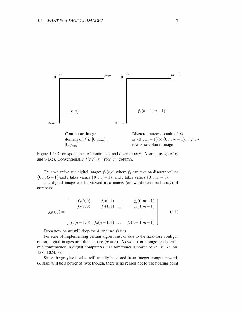
Continuous image:domain of f is [0,xmax]×[0,ymax]
Discrete image: domain of fdis 0 . . .n− 1 × 0 . . .m− 1, i.e. n-row × m-column image
Figure 1.1: Correspondence of continuous and discrete axes. Normal usage of x-and y-axes. Conventionally f (r,c), r = row, c = column.
Thus we arrive at a digital image: fd(r,c) where fd can take on discrete values0 . . .G−1 and r takes values 0 . . .n−1, and c takes values 0 . . .m−1.
The digital image can be viewed as a matrix (or two-dimensional array) ofnumbers:
fd(i, j) =
fd(0,0) fd(0,1) . . . fd(0,m−1)fd(1,0) fd(1,1) . . . fd(1,m−1)
fd(n−1,0) fd(n−1,1) . . . fd(n−1,m−1)
(1.1)
From now on we will drop the d, and use f (r,c).For ease of implementing certain algorithms, or due to the hardware configu-
ration, digital images are often square (m = n). As well, (for storage or algorith-mic convenience in digital computers) n is sometimes a power of 2: 16, 32, 64,128...1024, etc.
Since the graylevel value will usually be stored in an integer computer word,G, also, will be a power of two; though, there is no reason not to use floating point
8 CHAPTER 1. INTRODUCTION
or some other numerical representation.
1.3.1 Other Examples of Digital Quantities
Music on tape, or vinyl LP is continuous. Music on CD is digital. CD samplingrate is 44,100 samples per second, 12-bits per sample, 2 channels (stereo).
In modern telephone systems, speech is transferred digitally between majorexchanges – here you can get away with 8,000 samples per second, and 8-bits persample.
1.3.2 Raster Sampling or Scanning
The image model given above corresponds to the image model used in raster graph-ics, i.e. the image is formed by regular sampling of the x-, and y-axes.
1.3.3 Pixel
Each f (r,c) in eqn. 1.1 is a picture element or pixel (the equivalent term ‘pel’ isused in some texts).
1.3.4 Spatial Resolution
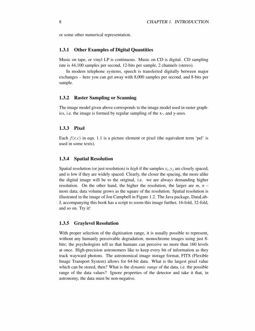
Spatial resolution (or just resolution) is high if the samples xi,y j are closely spaced,and is low if they are widely spaced. Clearly, the closer the spacing, the more alikethe digital image will be to the original, i.e. we are always demanding higherresolution. On the other hand, the higher the resolution, the larger are m, n –more data; data volume grows as the square of the resolution. Spatial resolution isillustrated in the image of Jon Campbell in Figure 1.2. The Java package, DataLab-J, accompanying this book has a script to zoom this image further, 16-fold, 32-fold,and so on. Try it!
1.3.5 Graylevel Resolution
With proper selection of the digitisation range, it is usually possible to represent,without any humanly perceivable degradation, monochrome images using just 8-bits; the psychologists tell us that humans can perceive no more than 160 levelsat once. High-precision astronomers like to keep every bit of information as theytrack wayward photons. The astronomical image storage format, FITS (FlexibleImage Transport System) allows for 64-bit data. What is the largest pixel valuewhich can be stored, then? What is the dynamic range of the data, i.e. the possiblerange of the data values? Ignore properties of the detector and take it that, inastronomy, the data must be non-negative.

1.3. WHAT IS A DIGITAL IMAGE? 9
Figure 1.2: Upper left: original image. Upper right: zoomed by a factor 2. Lowerleft and right: zoomed by 4 and by 8.
10 CHAPTER 1. INTRODUCTION
1.4 Signal Processing
Signal processing – and digital signal processing - are closely related to imageprocessing; whereas images are two-dimensional, signals are one-dimensional.
A music signal coming from a microphone, or going to a loudspeaker, is acontinuous voltage signal – a continuous function of time: f (t).
A digital signal is a sequence of numbers:
f0, f1, ... fn−1
where f0 may represent the (digitised) voltage at t = t0, f1 at t1, . . . . i.e. the functionis sampled (and digitised) at t0, t1, t2, . . .
We shall cover some aspects of signal processing because some processingtechniques are more easily understood in one-dimension; and they are easily trans-ferred to 2D.
1.4.1 Colour and Spectral Bands
As mentioned earlier, a colour image can be represented by three monochromeimages or bands. But, image sensors are not just limited to visible light; someremotely sensed images are made up of 10 or more spectral bands.
1.4.2 Sensing
To produce f (x,y) (forget about digitisation for a moment) from a scene, sensingmust take place. That is, the brightness of each point (x,y), in the field-of-view(FOV) of the observer, must be measured.
In a practical system this can be considered to be accomplished by passing asmall aperture (opening) over the field of view, stopping when the aperture centreis over the discrete sample point (xi,y j) and taking the average brightness withinthe aperture. Usually, the width and height of the aperture are about the same asthe horizontal and vertical sampling periods, respectively.
1.5 General Concepts of Image Processing
The general concept of a process involving image processing may be seen in Fig.1.3. The flow of information is from right (the original scene) which reflects lightinto the the sensor; the sensor converts light into a voltage; the voltage (a continu-ous quantity) is sampled and digitised to yield a number; some (numerical/digital)image processing is done; the numbers must be converted back into a voltage andtransferred to a display which produces patters of light that the user can see.
Typical image processing operations are:
• smooth out the graininess, speckle or noise in an image,

1.5. GENERAL CONCEPTS OF IMAGE PROCESSING 11
Quantities usedScene
LightSensor
VoltageDigitize
NumbersImage processing
Numbers/voltsDisplay (*)
LightUser’s eyes
* Alternatives: printer, file store, transmission.
Figure 1.3: Overview of imaging and image processing.
• remove the blur from an image,
• improve the contrast,
• segment the image into regions, e.g. on a printed circuit board, plastic region,copper region.
• remove warps or distortions,
• code the image in some efficient way for storage or transmission.
In later Chapters, we will look fairly often at actual pixel values. High valuesmay appear as white, and very low values as black. A lookup table establishes thiscorrespondence. We may similarly color grayscale images which is often a usefulthing to do, in order to show up faint parts of the image.
Our images may well be noisy, reminiscent of a poor television or audio signal.One way to handle such noisy images is to smooth them. This we do by ‘passing awindow’ over the image, changing the value of the pixel covered by this window.Each pixel in the output image, for example, becomes the average of the originalpixel together with its eight neighbours. The smoothing may well be somewhatsuccessful, but significant blurring of some edges and corners can also happen.
Contrast is very considerably enhanced by defining edges, or regions of sharpcontrast in the image. Notionally we can turn an image into a line drawing versionin this way. In practice, this is not so easy!
Appendix 1 describes the overall structure of DataLab-J which accompaniesthis book. Here we provide an example.

12 CHAPTER 1. INTRODUCTION
A short example of Java code for image negation follows. The program scriptsneg1.dlj and neg2.dlj provide examples of such image negating, which is turn-ing an image into its negative, or vice versa.
/****<p>*This method negates an image**@param x input Im**/
public static Im negate(Im x)int nr= x.nrows();int nc= x.ncols();float mm = x.max()+ x.min();Im z= new Im(nr,nc);for(int r= 0;r< nr;r++)
for(int c= 0;c< nc;c++)z.put(mm - x.get(r,c),r,c);
return z;
An input image, rct1010.pgm in the image collection supplied on disk, is asfollows.
P210 103
0 0 0 0 0 0 0 0 0 00 0 1 1 0 1 0 0 0 00 0 0 0 0 0 0 0 0 00 0 3 3 3 3 3 0 0 00 0 3 3 3 3 3 0 0 00 0 3 3 3 3 3 0 0 00 0 3 3 3 3 3 1 0 0

1.5. GENERAL CONCEPTS OF IMAGE PROCESSING 13
0 0 3 3 3 3 3 0 0 00 0 0 1 0 0 1 0 0 00 0 0 0 0 0 0 0 0 0
This is in ASCII PGM (portable gray map) format. The output image producedis r2neg.pgm:
P210 103
3 3 3 3 3 3 3 3 3 33 3 2 2 3 2 3 3 3 33 3 3 3 3 3 3 3 3 33 3 0 0 0 0 0 3 3 33 3 0 0 0 0 0 3 3 33 3 0 0 0 0 0 3 3 33 3 0 0 0 0 0 2 3 33 3 0 0 0 0 0 3 3 33 3 3 2 3 3 2 3 3 33 3 3 3 3 3 3 3 3 3
The following list gives an indication of the range of functions available inDataLab-J.
• Arithmetic: typically, add two images to produce a third.
• Display: all graphic and text displays, including to printer and file.
• Miscellaneous Data Handling: includes creation and deletion of images,copying.
• Data Generation: generation of test data and patterns, random and determin-istic.
• File Handling: file input-output, both formatted (ASCII) and unformatted.
• One-dimensional Digital Filters: simple recursive digital filters.
• Correlation and Convolution: 1- and 2-dimensional correlation using ‘fast’FFT methods.
• Image Enhancement: smoothing, edge detection, median filtering etc.
14 CHAPTER 1. INTRODUCTION
• Fourier and other Transforms: one-dimensional DFT operations (using FFT),two-dimensional DFT, Wavelet transform, Walsh transform, Hough trans-form.
• Pattern Classification: numeric pattern classification, especially statisticalpattern recognition; includes multilayer perceptron (backpropogation trained)neural network, and fuzzy rule-based classier.
• Estimation: estimation, eg. multivariate linear regression; includes multi-layer perceptron (backpropogation trained) neural network estimation, andfuzzy rule- based estimation.
• Feature Extraction and Discriminant Analysis: linear transformations forfeature extraction and discrimination.
• Two-dimensional Texture Analysis: e.g. various measures obtained from co-occurrence matrix.
• Two-dimensional Shape Recognition: two-dimensional moments.
• Image Morphology: both binary and graylevel.
• Matrix and Vector Arithmetic: provides a basic calculator for matrix andvector arithmetic.
1.6 Further Examples of Images
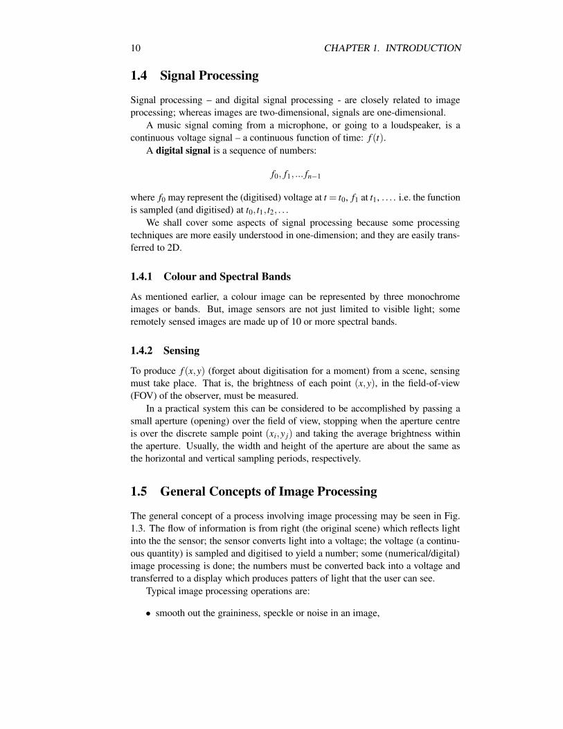
Here are just a few interesting images, the analysis of which could require manydozen pages, and maybe even a book-length text.
1.7 Exercises for Chapter 1
1. For a monochrome image, G = 255, n = 1024, and m = 1024, how manybytes will the image occupy?
2. Repeat Exercise 1 for a color image.
3. If you had to digitize a TV image, suggest suitable values of m, n.
4. Using the results of Exercise 3, and assuming 25 frames (images) per second,how much data for a one-hour film?
5. Laser printers commonly work at 600 dots per inch (dpi). How many pixelsare there in an A4 page (assuming that an individual dot can be representedin a single pixel)? How many bits per pixel for a laser printer image? Suggestsome more appropriate conversion factor between a laser printer and a raster-scanned image.
1.7. EXERCISES FOR CHAPTER 1 15
Figure 1.4: An image of a galaxy (NGC 5128, Cen A, from ESO Southern SkySurvey) following compression and uncompression.

16 CHAPTER 1. INTRODUCTION
Figure 1.5: An image of a piece of textile – jeans – showing a production fault.

1.7. EXERCISES FOR CHAPTER 1 17
5 516
551
6
Figure 1.6: A comet nucleus.

18 CHAPTER 1. INTRODUCTION
5 516
551
6
Figure 1.7: A plane from a wavelet transform of the previous image. Note the faintstructures (outgassing) emanating from the nucleus.

1.7. EXERCISES FOR CHAPTER 1 19
Figure 1.8: A reconstructed MRI (magnetic resonance) image of the brain.
20 CHAPTER 1. INTRODUCTION
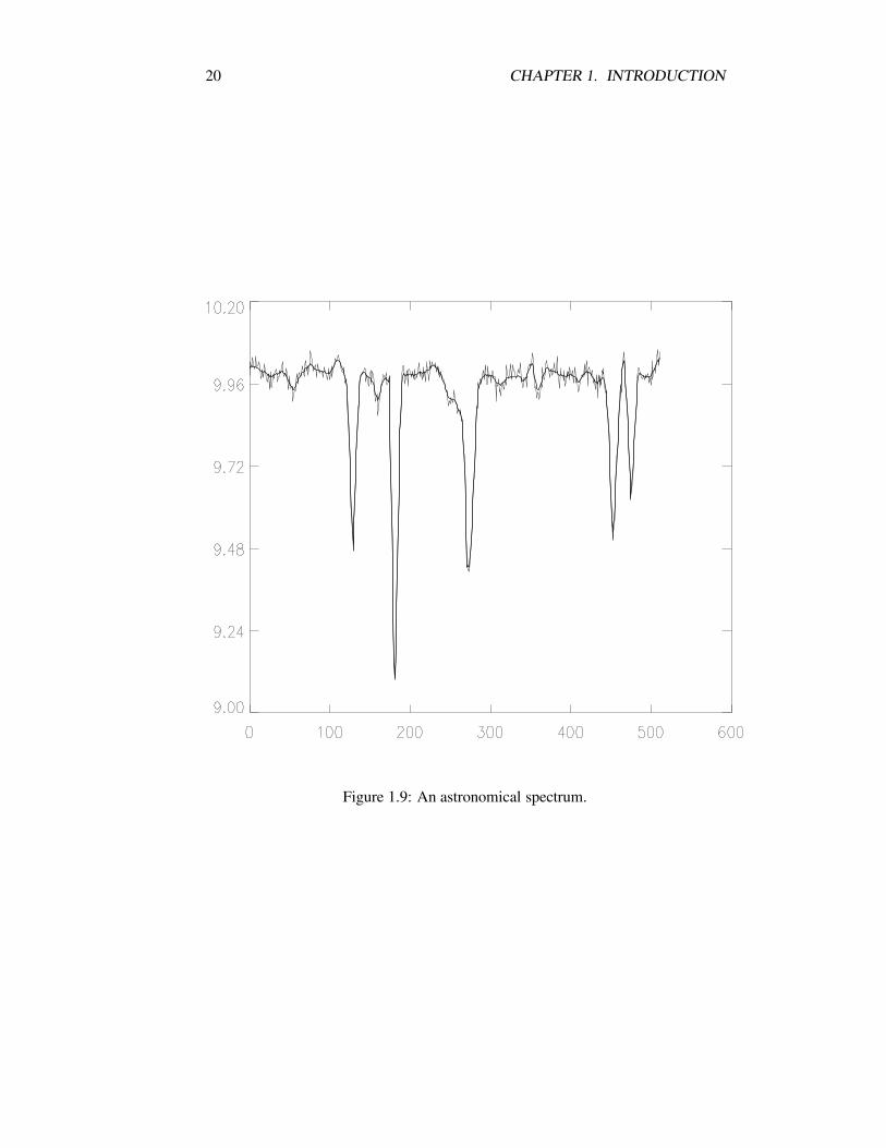
Figure 1.9: An astronomical spectrum.

1.7. EXERCISES FOR CHAPTER 1 21
6. (a) From your conclusions from the previous question, how much data isthere in a laser printer image of an A4 page?
(b) Compare with the data volume in an A4 page stored as ASCII text.
7. The ground resolution of weather satellites is about 1 to 5 kilometers. Theground resolution for some spy satellites is reported to be 15 centimeters.
(a) A satellite image has a ground resolution of 15 cm. What does a groundresolution of 15 cm mean?
(b) Using such an image, could a skilled interpreter
(i) read the number plate of a car?
(ii) determine the type of a car?
(iii) count the number of cars in a car park?
(iv) evaluate how many people at a football match?
(v) tell where the football was at the time the image was taken?
8. Assuming monochrome, ground resolution of 15 km and 8 bits per pixel,how much data in an image of your city or region? (You will have to estimatethe dimenensions you choose for your region.)
9. You are designing an image processing system to do quality control of lacefabric. The structure of the lace is such that thread separation is 0.5 mm.Suggest a suitable sampling resolution (in millimeters). The fabric is pro-duced in 1.8 metres wide rolls, and it passes the inspection point at 1 metreper second). How many pixels per second? What does this suggest about thetype of processor required?
10. Take some measurements and suggest a resolution for flaw detection in denim(jean) fabric.
11. Assuming 12-bits per sample, 44.1K samples per second (44.1 kiloHertz,KHz), 2 channels, how much data on a 1 hour CD? Compare this to theresult obtained in Exercise 4 (one hour of video).
12. What are typical local area network speeds in the networked work-place?Would it be possible to send or receive digitised speech or CD music oversuch links?
13. What are typical modem speeds for dial-up access to your work-place, or toyour local Internet provider, or to a local access point of an online system?Would it be possible to send speech or CD music over it? If you cannot senddigital speech over that line, can you see any paradox?
14. If you had an image of a photographic negative, suggest a digital method ofproducing a ‘positive’ of this.

22 CHAPTER 1. INTRODUCTION
15. If you had an image of a face – in colour, i.e. three monochrome imagesfr, fg, fb for red green and blue. You find that the flesh tones correspond to:
fr = 100±10, fg = 70±6, fb = 50±10
Sketch an algorithm that will convert the flesh colour to pure bright white(255,255,255), while leaving other tones untouched.
16. You have a satellite image in blue, green, red, and infrared (4 mono. imagesthis time, fr, fg, fb, and fir). Let m12 be the mean colour for class 1 in band1, etc. Let s14 be the standard deviation of the colours for class 1 in band 4,etc. You find that water (landuse type 1) is usually
(m11± s11,m12± s12,m13± s13,m14± s14)
and farmland (type 2)
(m21± s11,m22± s12,m23± s13,m24± s14)
Sketch an algorithm that will produce a label image (i.e. landuse map), f l ,containing 1 where there is water, 2 where there is farmland, and 0 otherwise.
17. Suggest a window (or algorithm) for detecting bright spots one pixel wide.
18. Take the example DataLab-J code used in this Chapter for image negationand do the following.
(a) Add 2 to each pixel of image.
(a) Add two images f1 and f2 to produce a third f3. What precautionsshould you take?
(c) Apply a 3×3 smoothing window.
(d) Implement the algorithm that is the answer to the previous questions,assuming three input images fr1, fg1, fb1 and three output images fr2,fg2, fb2.
(e) Re-implement your algorithm assuming your parameters, w and s, arestored in two-dimensional arrays, and similarly your multispectral image, f,is stored in a three-dimenional array.
Samples of most of this question are available in the script directory (dljbook)on the disk.
Chapter 2
Digital Image Fundamentals
2.1 Visual Perception
Here, briefly, are some points about human visual perception:
• the perceived image may differ from the actual light image (i.e. the perceivedbrightness image is a considerably modified ‘copy’ of the physical light in-tensity emanating from the scene),
• there are two types of light sensors on the retina – rods and cones,
• rods are more sensitive than cones; rods are used for night (scotopic) vision;rods are largely colour insensitive (e.g. no colour evident in moonlight),
• cones are used for brighter light, cones can sense colour,
• perceived (subjective) brightness (Bs) is roughly a logarithmic function oflight intensity (L): thus, if you increase L by 10, Bs increases by only 1 unit,increase L by 100 Bs increases by 2 units, 1000 increases by 3 etc.
• the visual system can handle a range of about 1010 (10 thousand million)in light intensity (from the threshold of scotopic vision to the glare limit).(Question: how many bits is that?)
• to handle this range, the pupil must adapt by opening and closing the pupil;opening the pupil – in darkness – lets more light in; closing it – in brightlight – lets less light in,
• the eye can handle only a range of about 160 at any one instant, i.e. wherethere is no opening and closing of the pupil; of course, this explains why8-bits (256 levels) usually suffice in a display memory,
23
24 CHAPTER 2. DIGITAL IMAGE FUNDAMENTALS
2.2 An Image Model: a General Imaging System
Note: in this chapter we treat physical units somewhat informally – we do not dealrigorously with the physics of light radiation.
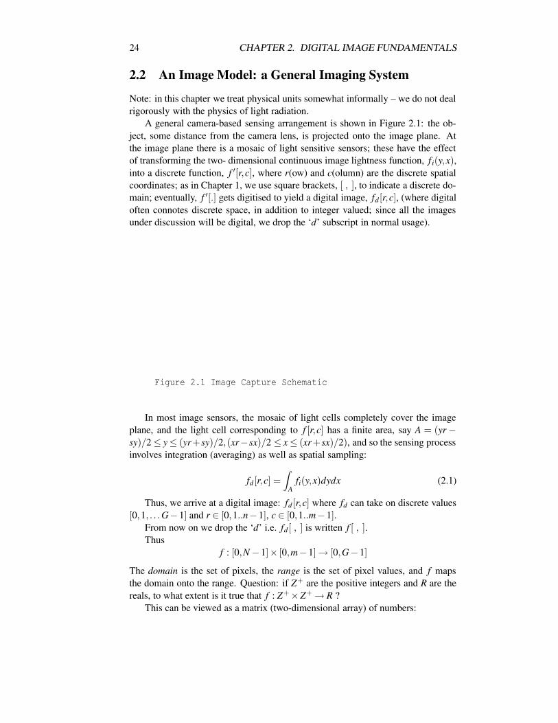
A general camera-based sensing arrangement is shown in Figure 2.1: the ob-ject, some distance from the camera lens, is projected onto the image plane. Atthe image plane there is a mosaic of light sensitive sensors; these have the effectof transforming the two- dimensional continuous image lightness function, f i(y,x),into a discrete function, f ′[r,c], where r(ow) and c(olumn) are the discrete spatialcoordinates; as in Chapter 1, we use square brackets, [ , ], to indicate a discrete do-main; eventually, f ′[.] gets digitised to yield a digital image, fd [r,c], (where digitaloften connotes discrete space, in addition to integer valued; since all the imagesunder discussion will be digital, we drop the ‘d’ subscript in normal usage).
Figure 2.1 Image Capture Schematic
In most image sensors, the mosaic of light cells completely cover the imageplane, and the light cell corresponding to f [r,c] has a finite area, say A = (yr−sy)/2≤ y≤ (yr+sy)/2,(xr−sx)/2 ≤ x≤ (xr+sx)/2), and so the sensing processinvolves integration (averaging) as well as spatial sampling:
fd [r,c] =
Z
Afi(y,x)dydx (2.1)
Thus, we arrive at a digital image: fd [r,c] where fd can take on discrete values[0,1, . . .G−1] and r ∈ [0,1..n−1], c ∈ [0,1..m−1].
From now on we drop the ‘d’ i.e. fd [ , ] is written f [ , ].Thus
f : [0,N−1]× [0,m−1]→ [0,G−1]
The domain is the set of pixels, the range is the set of pixel values, and f mapsthe domain onto the range. Question: if Z+ are the positive integers and R are thereals, to what extent is it true that f : Z+×Z+→ R ?
This can be viewed as a matrix (two-dimensional array) of numbers:
2.2. AN IMAGE MODEL: A GENERAL IMAGING SYSTEM 25
f [r,c] =
f [0,0] f [0,1] ... f [0,m−1]f [1,0] f [1,1] ... f [1,m−1]
f [n−1,0] f [n−1,1] ... f [n−1,m−1]
(2.2)
In many image processing applications, f (., .) is represented by an 8-bit byte( f → [0 . . .255]); the range [0 . . .255] derives not only from storage convenience,but from the facts that:
• human eyes can, simultaneously, perceive only about 160 light levels (seesection 2.1), and,
• most optical sensors are troubled to exceed a signal-to-noise ratio of 48 deci-bels [48 dB = 20log(1/256)].
Mostly we will be dealing with monochrome images – i.e. f [r,c] represents agrey level. In a colour image f (,) must give a colour. From the point of view ofimage processing, a colour image can be represented by three monochrome images,each representing the intensity of a primary colour (eg. red, green, blue). Thus,fr[r,c], fg[r,c], and fb[r,c], for red, green and blue. Of course, we can generaliseto any number of ‘wavebands’/ ‘colours’, in or out of the visible spectrum. Ageneralised ‘colour’ image is represented by f [b,x,y], where b denotes colour (b =band), where, normally, band = 0, 1, and 2, for red, green, and blue.
2.2.1 Radiometric Measurement and Calibration
2.2.2 Motivation
In Chapter 1 we defined an image thus: “ ... monochrome image, refers to a two-dimensional brightness function f (x,y), where x and y denote spatial coordinates,and the value of f at any point (x,y) gives the brightness (or, grey level) at thatpoint”.
For this section it would be better to talk of light intensity or lightness (insteadof brightness). Correct terms: lightness describes the real physical light intensity,brightness is only in the mind.
Think now of the scene as a flat two-dimensional plane – a sheet of colouredpaper. Its lightness, f (x,y), is the product of two factors:
• i(x,y) – the illumination of the scene, i.e. the amount of light falling on thescene, at (x,y),
• r(x,y) – the reflectance of the scene, i.e. the ratio of reflected light intensityto incident light.
26 CHAPTER 2. DIGITAL IMAGE FUNDAMENTALS
f (x,y) = i(x,y)r(x,y) (2.3)
Naturally occurring ranges of values of i and r:
Illumination (i) unitsSunny day at surface of earth 9000Cloudy day 1000Full Moon 0.01Office lighting 100
Reflectance (r) unitsSnow 0.93White paint 0.80Stainless steel 0.65Black velvet 0.01
Note: pure white (r=1) and pure black (r=0.0) are hard to achieve.
2.2.3 Uneven Illumination
More often than not, when we sense a scene, we want to measure r(x,y), so weassume that i(x,y) is constant I0, so that f (x,y) = r(x,y)I0 . Thus except for themultiplicative constant, we have r(x,y).
If illumination is not constant across the scene, then we have problems disen-tangling what variations are due to r, and what are due to i.
2.2.4 Uneven Sensor Response
Most modern electronic cameras are charge-coupled device (CCD) based. In aCCD you have a rectangular array of light sensitive devices i = 0,1, ...n− 1, j =0,1, ...m− 1 at the image plane. The voltage given out by these is proportional tothe amount of light falling on it.
Often it is assumed that an image f (x,y) arriving at the cameras image plane,is converted into values (analogue or digital), fc(x,y), which are proportional tof (x,y), i.e.
fc(x,y) = K f (x,y) (2.4)
If K = K(x,y), i.e. it varies across the image plane, then we have non-evenillumination. However, in this case, if K(x,y) can be relied on to stay constantwith time, we can estimate it, e.g. by imaging a sheet of constant reflectance, andconstant illumination. This is radiometric calibration. An example is given at theend of the chapter.
2.3. IMAGING GEOMETRY 27
2.3 Imaging Geometry
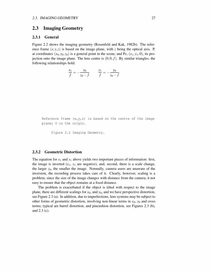
2.3.1 General
Figure 2.2 shows the imaging geometry (Rosenfeld and Kak, 1982b). The refer-ence frame (x,y,z) is based on the image plane, with z being the optical axis. P,at coordinates (x0,y0,z0) is a general point in the scene, and Pc, (x1,y1,0), its pro-jection onto the image plane. The lens centre is (0,0, f ). By similar triangles, thefollowing relationships hold:
x1
f=− x0
z0− fy1
f=− y0
z0− f
Reference frame (x,y,z) is based on the centre of the imageplane; O is the origin.
Figure 2.2 Imaging Geometry.
2.3.2 Geometric Distortion
The equation for x1 and y1 above yields two important pieces of information: first,the image is inverted (x1, y1 are negative), and, second, there is a scale change,the larger z0, the smaller the image. Normally, camera users are unaware of theinversion, the recording process takes care of it. Clearly, however, scaling is aproblem, since the size of the image changes with distance from the camera; it noteasy to ensure that the object remains at a fixed distance.
The problem is exacerbated if the object is tilted with respect to the imageplane, there are different scalings for x0, and y0, and we have perspective distortion,see Figure 2.3 (a). In addition, due to imperfections, lens systems may be subject toother forms of geometric distortion, involving non-linear terms in x0, y0 and crossterms; typical are barrel distortion, and pincushion distortion, see Figures 2.3 (b),and 2.3 (c).

28 CHAPTER 2. DIGITAL IMAGE FUNDAMENTALS
These show the distorted images of an object consisting oforthogonal, parallel, and equally spaced lines ruled on aplane.
(a) Perspective (b) Barrel (c) Pin-cushiondistortion distortion distortion
Figure 2.3 Geometric Distortion
The existence of a range of distortion types, as well as parameters has seriousimplications for machine vision and pattern recognition: essentially they increasethe ‘search-space’ for any matching procedure; an alternative, but equivalent, in-terpretation is that they introduce extra ‘invariance’ requirements on a recognitionalgorithm (see Chapter 8).
2.3.3 Geometric Calibration
In cases where we must make accurate spatial measurements from an image, itmay be necessary to geometrically calibrate it. Essentially, this entails performing,numerically, the inverse of the image creation distortion.
2.3.4 Object Frame versus Camera Frame
Figure 2.2 shows two reference frames, (x,y,z) based on the camera, and (x ′,y′,z′)based on the object. The position of the origin of the object frame (its range) withrespect to the camera frame and the relative orientation of the object frame is calledits pose; in the aerospace industry this is called attitude).
Thus, pose = range vector (r = (rx,ry,rz)) and attitude which consists of: pitch= rotation about the x-axis, yaw = rotation about the y-axis, and roll = rotationabout the z-axis.
2.3.5 Lighting Angles
As mentioned in section 2.2, the spatial and colour distribution of the light sourceare important factors. In addition directionality may be important: e.g. (a) direc-tional light from a single oblique source causes shadows; (b) a light source closeto the camera axis may cause specular reflection from shiny surfaces.
2.4. SAMPLING AND QUANTIZATION 29
2.4 Sampling and Quantization
See Chapter 1. Be aware of:
• the squared increase in data volume with increase in spatial resolution; i.e.go from 2 mm × 2 mm pixels to 1mm × 1mm and the number of pixelsincreases by four (not two),
• ditto as the image size increases.
Look at pages Gonzalez and Woods, pp. 35–37 to see the effects of reducingresolution (sampling grid), and of reducing grey levels; notice how contouringbecomes evident in Figure 2.10 (e) (16 levels, 4 bits), and (f) (8 levels, 4 bits).
2.5 Colour
2.5.1 Electromagnetic Waves and the Electromagnetic Spectrum
Light is a form of energy conveyed by waves of electromagnetic radiation. Theradiation is characterised by the length of its wavelength; the range of wavelengthsis called the electromagnetic (EM) spectrum. Visible light occupies a very smallpart of the spectrum.
Table 2.1 shows the EM spectrum: the left hand column gives the wavelengthin meters, the middle gives the name of the band, and the right gives the frequencyof the radiation in Hertz (cycles per second).
Thus, crudely, if you were to ‘speed-up’ the frequency of vibration of a TVsignal, you would get microwaves, speed-up microwaves→ heat radiation,→ light→ UV → X-rays, etc. (Incidentally, microwave cookers work at approximately900 MHz, which happens to be the frequency at which the water molecule, H2O,resonates).
It is possible to use various parts of the EM spectrum for imaging: e.g. X-rays,microwaves, infrared (near), and thermal infrared. Our major interest will be invisible light.
2.5.2 The Visible Spectrum
The visible spectrum streches from about 400 nm to 700 nm. The reason why thispart of the spectrum is visible is that the rods and cones in our retinas are sensitiveto these wavelengths, and insensitive to the remainder; e.g. if you look at a clothesiron in the dark, you may ‘feel’ the heat radiated from it, but your eyes will notconvert that energy into a light sensation; similarly, microwaves and X-rays, theymay cause damage, but you will not ‘see’ them.
The relative spectral sensitivity of human eyes within the visible spectrum isshown in Figure 2.4, with approximate indication of corresponding colours. Figure

30 CHAPTER 2. DIGITAL IMAGE FUNDAMENTALS
Wavelength (m) Name Freqency (Hz)10−15 1 femtometer (fm) gamma rays 3×10²³ Hz10−12 1 picameter X-rays 3×10²⁰ Hz10−9 1 nanometer X-rays 3×10¹⁷ Hz10−8 10 nm Ultraviolet 3×10¹⁶ Hz10−7 100 nm U-V4×10−7 400 nm Visible light (violet)7×10⁻⁷ 700 nm Visible (red)10−6 1 micrometer Infrared (near) 3×10¹⁴ Hz10−5 10 micrometers Infrared 3×10¹³ Hz
Infrared (heat)10−3 1 millimeter Infrared (heat) + 3×10¹¹ Hz
microwaves (300 GigaHz)10−1 0.1 meters microwaves 3×10⁹ (3 GigaHz)1 meter TV etc. (UHF) 3×10⁸ (300 MegaHz)
FM radio is ∼ 100 Mhz (VHF)10 meters radio (shortwave) 30 Mhz100 meters radio (shortwave) 3 MHz200−600 m radio (medium wave) 1.5 MHz to 500 KHz1500 m (1 Km) radio (long wave) 200 KHz
Table 2.1: The electromagnetic spectrum.
2.5 shows the sensitivity on the earth of light from space, resulting from the block-ing effects of the earth’s atmosphere. This explains why X-ray and radio astronomywere fairly late developments, compared to optical (i.e., visual light) astronomy.
The term ‘spectral’ is often used – it refers to the electromagnetic radiationfrequency spectrum – the range of frequencies which make up the light; we willhave cause to cover other forms of spectra (see Chapter 3).
From Figure 2.4 we can see that the eye is very sensitive to radiation in thegreen-yellow range (peak at 550 nm), and relatively insensitive to blue, violet, anddeep red; a blue light around 475 nm (relative sensitivity approx. 10%) would haveto put out 10 times more power than the equivalent green-yellow light. Why didthe human evolve this way? Well, the energy emitted by the sun (at least that partthat reaches the earth) has an energy spectrum graph similar to Figure 2.4.
2.5.3 Sensors
A light sensor is likely to have a similar spectral response curve to Figure 2.4,though usually flatter and wider – i.e. more equally sensitive to wavelengths, andsensitive to UV and to near infrared.
If Figure 2.4 was the spectral response of a sensor, then a blue light (see above),compared to a green-yellow light of the same power, would produce a sensor outputof 10% of the voltage of the green-yellow.

2.5. COLOUR 31
Violet Blue Green Yellow Orange Red100% + *
| * *|
80% + * *| * *|
60% + * *| * *|
40% + * *|| * *
20% + * *| * *|* *+------+------+------+------+------+------+400 450 500 550 600 650 700
Figure 2.4 Relative spectral sensitivity of the eye.

32 CHAPTER 2. DIGITAL IMAGE FUNDAMENTALS
Figure 2.5 The earth’s atmosphere blocks out different parts of the EMspectrum -- fortunately for humankind.

2.5. COLOUR 33
2.5.4 Spectral Selectivity and Colour
We have already mentioned that a colour sensor (e.g. in a colour TV camera) ismerely three monochrome sensors: one which senses blue, one green, and one red.
What is meant by sensing blue, green, or red? What we do is arrange forthe sensor to have an effective response curve that is high in green (for example)and low elsewhere. But, we have already said that sensors have a fairly flat curve(maybe 200–1000 nm), so we must arrange somehow to block out the non-greenlight.
Wavelength sensitive blocking is done by a colour filter. A green filter allowsthrough green light but absorbs the other; similarly blue and red.
Violet Blue Green Yellow Orange Red100% + *
| * *|
80% + * *| * *|
60% + * *| * *|
40% + * *|| * *
20% + * *| * *| * *+------+------+------+------+------+------+400 450 500 550 600 650 700
Figure 2.6 Relative sensitivity of a green filter.
So, we use three separate sensors, each with its own filter (blue, green, and red)located somewhere between the lens and the sensor. I.e. we have f [d,r,c], d = 0(blue), 1 (green), and 2 (red).

34 CHAPTER 2. DIGITAL IMAGE FUNDAMENTALS
2.5.5 Spectral Responsivity
The relative response of a sensor can be described as a function of wavelength(forget about (x,y) or (r,c) for the present): d(λ), where λ denotes wavelength.The light arriving through the lens can also be described as a function of λ: g(λ),and the overall output is found by integration:
voltage =
Z ∞
0d(λ)g(λ)dλ (2.5)
Obviously, the integral can be limited to (say) 100 nm to 1000 nm.If we have a filter in front of the sensor, relative transmittance (the amount
of energy it lets through), t(λ), then the light arriving at the sensor, g ′(λ), is theproduct of g() and t():
g′(λ) = g(λ)t(λ) (2.6)
and equation 2.5 changes to:
voltage =Z ∞
0d(λ)g(λ)t(λ)dλ (2.7)
or,
voltage =
Z ∞
0d(λ)g′(λ)dλ (2.8)
2.5.6 Colour Display
So now we have three images stored in memory; how to display them to produce aproper sensation of colour?
Similarly to our model of a colour camera as three monochrome cameras, acolour monitor can be thought of as three monochrome monitors: one which givesout blue light, one green and one red.
A monochrome cathode ray tube display works by using an electron gun tosquirt electrons at a fluorescent screen; the more electrons the brighter the image;what controls the amount of electrons is a voltage that represents brightness, sayfv(r,c).
A monochrome screen is coated uniformly with phosphor that gives out whitelight – i.e. its energy spectrum is similar to Figure 2.4.
A colour screen is coated with minute spots of colour phosphor: a blue phos-phor spot, a green, a red, a blue, a green, ... following the raster pattern mentionedin Chapter 1. The green phosphor has a relative energy output like the curve inFigure 2.6; the blue has a curve that peaks in the blue, etc. There are three electronguns – one controlled by the blue image voltage (say, f (0,r,c)), one by the green( fg(r,c)) and one by the red ( fr(r,c)). Between the guns and the screen, there is anintricate arrangement called a ‘shadow-mask’ that ensures that electrons from theblue gun reach only the blue phosphor spots, green→ green spots, etc.
2.5. COLOUR 35
2.5.7 Additive Colour
If you add approximately equal measures (we are being very casual here, and notmentioning units of measure) of blue light, green light and red light, you get whitelight. That’s what happens on a colour screen when you see bright white: each ofthe blue, green, and red spots are being excited a lot, and equally. Bring down thelevel of excitation, but keep them equal, and you get varying shades of grey.
Your intuition may lead you to think of subtractive colour; filters are subtrac-tive: the more filters, the darker; combine blue, green and red filters and you getblack. However, with additive colour, the more light added in, the brighter; themore mixture, the closer to grey – and eventually white.
2.5.8 Colour Reflectance
This subsection may be skimmed at the first reading.All this brings a new dimension to the discussion of illumination and reflectance
in section 2.2. Now we can think of illumination (i) and reflectance(r) as functionsof λ as well as (x,y).
Thus, the lightness function is now spectral (and therefore a function of λ), i.e.
f (λ,x,y) is the product of two factors:
• i(λ,x,y) – the spectral illumination of the scene, i.e. the amount of lightfalling on the scene, at (x,y), at wavelength λ,
• r(λ,x,y) – the reflectance of the scene, i.e. the ratio of reflected light intensityto incident light
f (λ,x,y) = i(λ,x,y)r(λ,x,y) (2.9)
Why does an object look green (assuming it is being illuminated with whitelight)? Simply because its r(λ, ..) function is high for λ in the green region (500-550 nm), and low elsewhere (again, see Figure 2.6). Of course, illumination comesinto the equation: a white card illuminated with green light (in this case i(λ, ..)looks like Figure 2.4) will look green, etc.
2.5.9 Exercises
Ex. 2.5-1 Write down cases where you might want to use very narrow band filters,i.e. you want to be very selective about the colour of light you let into thesensor.
Ex. 2.5-2 A coloured card whose reflectivity is r(λ,x,y) is illuminated with colouredlight with a spectrum i(λ) (constant over spatial coordinates (x,y); this issensed with a camera whose CCD sensor has a responsivity d(λ) (again con-stant over x,y); a filter with transmittance t(λ) is used. Show that the overallvoltage output is

36 CHAPTER 2. DIGITAL IMAGE FUNDAMENTALS
v(x,y) =Z
r(λ,x,y)i(λ)t(λ)d(λ)dλ
Ex. 2.5-3 A blue card is illuminated with white light; explain the relative levels ofoutput from a colour camera for blue, green, red.
Ex. 2.5-4 A blue card is illuminated with red light; explain the relative levels ofoutput from a colour camera for blue, green, red.
Ex. 2.5-5 A blue card is illuminated with blue light; explain the relative levels ofoutput from a colour camera for blue, green, red. What, if any, will be thechange from Ex. 2.5-4 ?
Ex. 2.5-6 A white card is illuminated with yellow light; explain the relative levelsof output from a colour camera for blue, green, red.
Ex. 2.5-7 A white card is illuminated with both blue and red lights; explain therelative levels of output from a colour camera for blue, green, red.
Ex. 2.5-8 A blue card is illuminated with both blue and red lights; explain therelative levels of output from a colour camera for blue, green, red; what, ifany, will be the change from Ex. 2.5-6.
2.6 Photographic Film
Many images start off as photographs, so film cannot be ignored. Realise that:
• just like the eye, film is limited in the range of illumination that it can handle,
• a camera adapts by opening / closing the lens diaphragm, – or, by increasingdecreasing exposure time.
2.7 General Characteristics of Sensing Methods
2.7.1 Active versus Passive
Active methods require, in addition to a sensor, a source of energy which illumi-nates or otherwise probes or excites the object. See Figures 2.7 (a), (b), and (c).
Passive methods operate by sensing some emission that emanates naturally(e.g. reflected sunlight) from the object, see Figure 2.8.

2.7. GENERAL CHARACTERISTICS OF SENSING METHODS 37
Figure 2.8 Active sensing configurations.
2.7.2 Methods of Interaction
1. Absorption.
Here we assume that the object is relatively transparent, see Figure 2.7 (c).This is how X-rays work.
2. Reflection.
See section 2.5.8, and Figures 2.7 (a), (b) and Figure 2.8 (a).
3. Emission.
See Figure 2.8 (b); here the sensed object creates the sensed energy (e.g. apiece of hot metal, the sun).
2.7.3 Contrast
For sensing to be effective the sensed signal must change for different parts of theobject (otherwise we have the equivalent of a blank screen); contrast defines themagnitude of sensed signal change that differentiates (generally speaking) betweenobject present and not present. E.g. X-rays, let G0 be the image grey level corre-sponding to just soft tissue, let Gb be the grey level for bone, then the contrast forbone, Cb, is
Cb = (Gb−G0)/G0 (2.10)
38 CHAPTER 2. DIGITAL IMAGE FUNDAMENTALS
Figure 2.9 Passive sensing configurations.
2.7.4 Exercises
Ex. 2.7-1 (a) What is meant by active sensing.
(b) Explain how, and why, active infra red sensing cameras could be used bywildlife film-makers.
Ex. 2.7-2 (a) What is meant by passive sensing.
(b) Explain how, and why, passive infrared sensing cameras could be usedby wildlife film-makers.
(c) In a military application, why would passive sensing be preferred to ac-tive.
Ex. 2.7-3 Identify and explain one application of aerial thermal infrared sensing.
Ex. 2.7-4 (a) Explain how a medical X-ray system works.
(b) Identify and explain uses of X-ray images, other than medical.
Ex. 2.7-5 Referring to Figures 2.7 and 2.8 identify a suitable sensing arrangementfor detecting flaws (small holes) in paper manufacture.
Ex. 2.7-6 In problem 2.7-5, assume that you have a single line of sensors (512 ofthem across the moving roll of paper). The sensor is sampled rapidly, givingout 512 samples for every millimetre of paper longitudinal movement; thesensor width also corresponds to a transverse extent of 1 mm.
(a) Assuming that you have a function, say sread(f), that reads the samplesinto an array f (unsigned char f[512]), and that your computer can keep

2.8. WORKED EXAMPLE ON CALIBRATION 39
up with the processing, suggest processing to detect small holes. [Assumebackground readout (normal) of 10, and much higher when there is a hole].
Hint:
#define NPIXELS 512unsigned char f[NPIXELS];
while(1) /*do forever*/
waitForSignal(); /*waits for sampling signal*/sread(f);
for(i=0;i<NPIXELS;i++)a = s[i];b = s[i+1];if( a ???? b ???) flaw[i]=TRUE;else flaw[i]=FALSE;
(b) Revise your program to distinguish between holes that are (i) about 1 to2 mm wide, and (ii) more than 3 mm wide.
Ex. 2.7-7 Repeat 2.7-6 (b) now bringing the longitudinal dimension into consid-eration, i.e. we want to distinguish holes whose area is 4 sq mm (4 pixels) orless and those above that.
Ex. 2.7-8 How would you make your answer to Ex. 2.7-6 generalise to the caseof holes and flaws caused by dark marks in the paper.
2.8 Worked Example on Calibration
A monochrome CCD camera (followed by a digitiser etc.) is monitoring partspassing along a conveyer belt; the scene is illuminated from above. There are fourmajor difficulties:
1. uneven illumination,
2. bias (an uneven bias) in the CCD cells,
3. uneven gain in the CCDs,
4. in addition, there is noise (assume Gaussian and zero mean – like the noisegenerated by DataLab function ‘ggn’).

40 CHAPTER 2. DIGITAL IMAGE FUNDAMENTALS
Develop a technique (a program of measurements, followed by calibrationcomputation) by which the effects of the uneven illumination and the bias maybe removed (calibrated). This calibration may take place, for example, once a day,or however often the effects change.
There are two equations (or models) that are applicable:
• Equation (i): g(x,y) = r(x,y).i(x,y) , [g()=light entering camera].
i.e. light entering camera is a product of r(), reflectance of the scene, and i()illumination.
• Equation (ii): f (x,y, t) = b(x,y)+h(x,y).g(x,y)+n(x,y, t)
This says that the output from the cell corresponding to position (x,y) is afunction of:
– the bias of the cell (x,y), b(x,y), i.e. b is called bias, because it is addedto all output; you have b even for zero bias,
– the gain of the system, h(x,y), for cell (x,y); one cell may be more re-sponsive than another, i.e. more output for the same input – its amplifieris turned up more!
– the noise.
I expect that your answer will contain correction tables for each (x,y).Assume that you have constant reflectance white and grey cards (where r(x,y)
= constant, for all (x,y) ). Assume also that you can shut out all light from thecamera (e.g. using a lens cap).
Describe how you would compensate for:
1. Uneven illumination on its own; i.e. assume that b(x,y) = 0.0, h(x,y) = 1.0for all cells, and that n(x,y, t) = 0.0 for all (x,y, t).
2. Variable bias on its own; i.e. all the other effects are missing.
3. Variable gain on its own.
4. Noise on its own. Hint: the conveyer belt is moving very slowly, and youhave enough time to capture a large number of images of the object.
5. The whole lot, together.
6. How should the calibration results be used (in operational mode)?
Answer:
Extract from chapter 4.

2.8. WORKED EXAMPLE ON CALIBRATION 41
Assume you have the possibility of obtaining many still, ‘identical’, images ofa scene; but, the images are picking up noise in transmission, or from the sensorsystem. Then averaging together these images pixel by pixel:
fa(r,c) = (1/Na) ∑i=1..Na
fi(r,c)
for r = rl ..rh,c = cl ..ch, where Na = number of images averaged, and fi(., .) is theith image. Note: this is done for each pixel independently; we are not smoothingacross pixels. Thus, we can talk about the mean, m(r,c), and variance v(r,c) ofeach pixel.
If our model is that the only distortion is noise, then f i(r,c) can be written:
fi(r,c) = f (r,c)+ni(r,c)
i.e. the ith image is the true, noiseless image, plus the ith noise image. Most natu-rally occurring noise has the characteristic (or is assumed to have) that it is ran-dom and uncorrelated. Often too, it is zero mean.
Roughly speaking, these last two statements indicate that for every positivenoise value, you will eventually get a negative one, and if you take enough valuesin the average you end up with zero.
It can be shown that if the noise level (e.g., as indicated by the standard devia-tion of the pixel values (at (r,c) ) is s1 for 1 image (no averaging), then it is
sn = s1/√
Na
for Na images averaged.You can easily experience two examples of this:
1. On a noisy stereo radio reception, switch the tuner to mono; this causesthe system to add the left and right signals to produce one signal; the noisestandard deviation reduces by 1/
√2 = 1/1.414, i.e. reduces to 0.707 of what
it was,
2. freeze frame on a videoplayer, see how noisy the image is compared to mov-ing: the eye tends to average over a number of the 25 images painted on thescreen per second.
The process involved here is calibration, in particular photometric or radiomet-ric calibration (to do with grey level values). The other sort is geometric calibration,i.e. correcting the geometric shape of the image.
It would be relatively safe to assume that, except for the noise, all the otherfactors are invariant with time (at least, after the system has warmed up). If this isnot the case, at least the factors will vary slowly, so that you can stop and recalibrateoften enough to catch the changes.
Even though the question mentions only bias (b()), we will also consider gain(h()) in this answer. We have:
42 CHAPTER 2. DIGITAL IMAGE FUNDAMENTALS
f (x,y, t) = b(x,y)+h(x,y).g(x,y)+n(x,y, t),
Using eqn. 2.9:
f (x,y, t) = b(x,y)+h(x,y).r(x,y).i(x,y)+n(x,y, t),
Now, h() and i() can be combined
d(x,y) = h(x,y).i(x,y)
so we only need determine d(x,y) for all cells.Noise: we must assume that the noise is random and uncorrelated (from t = t1,
to another t = t2), and zero mean. I.e. if we start off with, on one image, with fluctu-ations of standard deviation s1, if we average over P images the standard deviationreduces to sP = s1/
√P. We will always have some fluctuation; this corresponds to
an error. The average size of the error can be reduced from (say) 10 units to 1 unitif (say) we average over P=100 images (see notes in section 4.10).
You would probably assume that the noise was the same level for all cells.How to find out s1, the standard deviation for 1 image?Collect many images of (say) a white card. Calculate the average pixel value
for each (x,y). Calculate the variance v(x,y) for each (x,y), then SD s1(x,y) =√
v(x,y). Let this be s1.Then if you want your error level to be s′, calculate P froms′ = s1/
√P, i.e.
(c) P = s21/s′2
so if s1 is 10, and you want to get to s′ = 2, P must be 25.
Calibration steps
1. Measure noise SD s1.2. Decide on acceptable error for calibration data: s′.3. Estimate P from s1,s′ (foregoing equation above).4. Calibrate bias:4.1. Put the lens cap on the camera. Measure P images.4.2. Estimate b(x,y)± error by averaging pixel at (x,y) over all P images.Result: be(x,y), for all cells x,y5. Calibrate gain and illumination:5.1. Put a white card in the scene (r(x,y) = constant, for all x,y))5.2. Estimate d(x,y) by averaging pixel at (x,y) over P images, and subtracting
be(x,y). (if r() does not equal 1, but some other constant, K, then this will beincluded in our estimate – but no matter – the image is not absolute units anyway.
Result: de(x,y), for all cells x,y.
Use of calibration in operation
2.9. CCD CALIBRATION IN ASTRONOMY 43
Note: if the noise level is unacceptable, then you will have to average multipleimages in the manner described for ‘calibration mode’.
1. Measure f a1(x,y) = average of P f (x,y, t) images.2. Remove bias: f a2(x,y) = f a1(x,y)−be(x,y)3. Remove (‘cancel-out’) effects of uneven gain and illumination:
f a3(x,y) = f a2(x,y)/de(x,y)
f a3() is the calibrated image (noise reduced as well)
There will be errors/fluctuations, but the level of these can be controlled by theappropriate choice of Ps.
2.9 CCD Calibration in Astronomy
2.9.1 CCD Detectors versus Photographs
In astronomy, CCDs (charge-coupled device detectors) are widely-used. Photo-graphic plates are also used for particular purposes and we will say a few wordsabout images which are produced from photographs.
Photographic plates are subsequently digitized, using microdensitometers – thename is indicative of how the relative density of the photographic emulsion, fol-lowing chemical perturbation effects caused by the detected light, is sampled atregular, very fine intervals at the micrometer level. These microdensitometer ma-chines are only available in certain institutes world-wide. One such machine (atSpace Telescope Science Institute, Baltimore), it was once pointed out to me, waspositioned on huge concrete blocks in the bottom floor of the building, to avoideven the most minute vibration from the ambient environment. Needless to say,Baltimore does not suffer from any earthquakes. The level of precision obtainablewith such machines is far beyond that offered by regular scanners.
The photographic plates themselves are of very high quality. A chemical emul-sion known as IIIa-J is often used. This has very high-quality behaviour. About 3years, the one company in the world which supplies such photographic plates, Ko-dak, was going to cease to do so, and this caused a lot of worry among professionalastronomers. Photographic plates are used for wide fields of view, – hence surveywork (i.e. surveys of lots of astronomical objects – stars, galaxies, etc.). CCDs,especially big ones (lots of pixels) are costly.
The dynamic range of photographs is very good. However, they suffer fromnonlinear response effects, e.g. as one looks towards the central area of a star ona photographic, there is a levelling off of the responsiveness of the photographicplate. For so-called wide-field (large field of view) survey work, this is not toomuch of a problem. CCDs have the property of being much more linear in theirresponse, i.e. output respresentation proportional to input.
44 CHAPTER 2. DIGITAL IMAGE FUNDAMENTALS
Digitized photographic images may have to be corrected for geometric distor-tion. In addition there may be impurities detected on the photograph (e.g. dust),unevenness in the chemical constituents of the photographic plate, etc.
2.9.2 CCD Detectors and Their Calibration
Arriving photons of light dislodge electrons, which are read off a regular samplinggrid. The electrons are converted to so-called data numbers, and these give us pixelvalues.
In the course notes, we have mentioned two equations of relevance:
g(x,y) = r(x,y)i(x,y)
where g is the light entering the camera; r is the reflectance; and i is the illumina-tion.
f (x,y, t) = b(x,y)+h(x,y)g(x,y)+n(x,y, t)
where b is the bias, a constant added to the output even for zero input light; h isthe gain of the system, the responsiveness of an individual pixel; and n is the noise.Note the time-dependence of some of these terms which we will ignore. It is alsopossible that there would be dependence on the wavelength of the incoming light.
We can merge these equations, getting
f (x,y) = b(x,y)+h(x,y)r(x,y)i(x,y)+n(x,y)
or simplifying by representing hi by d, the product of detector gain and illumina-tion:
f (x,y) = b(x,y)+d(x,y)r(x,y)+n(x,y)
There may be added complications but we ignore them. These include thetime dependence mentioned above; additional small non-linear terms; and chargetransfer inefficiencies. So we have the nominal output of the detector, f . We wantto correct this, to get estimates of bias, b, and of the gain as expressed in the term,d.
Now, we use three different items of information:
1. We use a so-called dark frame, an image with output current measured in theabsence of any input. E.g. we put a lens cap on the detector.
2. We also use a so-called flat-field, an image (or a set of images) with the de-tector turned towards a uniformly-emitting source. This could be the insideof the observatory dome, for a ground-based observatory, or images of theocean for Hubble Space Telescope. For a digital camera, we could use awhite card. The flat-field describes the sensitivity over the CCD which is notuniform.
2.9. CCD CALIBRATION IN ASTRONOMY 45
3. We take many images of the same scene, for the same duration, and aver-age them. We do likewise for the darks and flat-fields. Why? Because inaveraging them, we dramatically decrease the noise. The relationship is asfollows. Let n1, n2, . . . be the noise associated with images 1, 2 , etc. Eachof these will be a standard deviation (which can be understood as the spreadof possible values) for each pixel. For pixels i and j we are just representingthe noise images n1(x,y) for convenience by n1. Over a given image, thesimplest case to consider is when the noise is constant over all pixels.
Let the average of these noise values be n = 1/N ∑Ni=1 ni. This is the usual
definition of the (statistical) mean.
Now consider averaging N noisy images f1 +n1, f2 +n2, . . . , fN +nN . We getthe following interesting and not immediately intuitive result: f + n/
√N. We
have considerably decreased the noise, all the more so if N is large. What isthe reason for this? To fully explain this we would have to step back, and startby clearly stating that the noise is Gaussian (normally-distributed). Considerthe following: a noisy image means an uncertainty in measurement. Havinglots of images provides us with a good deal of information, and hence helpsto reduce the uncertainty. That is what the above expression for the averagednoisy image tells us.
Let us now approximate getting rid of the noise by taking N large enough,i.e. by having many identical images (note: the images will never be indentically-valued in regard to noise! This is axiomatic.)
We now tackle the problem in the following stages: (i) use the darks to estimatethe bias; (ii) use the flats to estimate the gain-times-illumination detector response;and (iii) use these in practice subsequently on ’real’ images.
• Consider a stack (or set of N) dark images. Since there is no incoming light,we have f1 = b+n1. Averaging N such images, with N large enough so thatthe noise gets quite small, yeilds the average dark frame: f = b. This is away to estimate the bias, in practice. In this paragraph, each f was a dark.In the next paragraph, each f will be different, – a flat-field.
• Consider now a stack (or set) of N flat-fields. By definition, the reflectivity, r,is constant, say r0. The first such flat-field is f1 = b+d1r0 +n1. Averaging Nsuch flat-fields, and again ignoring noise which is very much lessened by theaveraging, gives f = b+ r0d. This gives enough information to estimate d =( f −b)/r0. If we don’t have a value for r0, this gives us relative calibration.If we have some absolute reference values for the pixels in our image, thenwe can estimate the constant reflectance r0 and have an absolute calibration.
• Finally, having estimates of bias b, and of uneven detector response (gaintimes illumination) d, we put these results to use in the original imagingequation, f = b + dr + n, to determine r in practice. Needless to say, weagain average frames to reduce the noise term.

46 CHAPTER 2. DIGITAL IMAGE FUNDAMENTALS
Final remarks on this analysis: CCD detectors produce images with accom-panying noise which to a good approximation is Gaussian. CCD detectors sufferfrom defective columns or rows (remember, the ejected electrons are made to runout along these), and these need to be allowed for, in the darks and flats as well asthe ‘substantive’ images
2.10 Questions on Chapters 1 and 2 – Fundamentals, Sen-sors, and Calibration
1. (a) Explain in detail the steps (and data flow) in the progression from a3-dimensional scene to a two-dimensional digital image.
(b) Explain, using appropriate examples, the neccessity to carefully trade-off spatial resolution versus data volume.
(c) An industrial inspection system is monitoring lace manufacture; thefabric is lace, and you want to detect very small stich flaws in it. Thestructure of the lace is such that thread separation is 0.5 mm.
i. Supporting your work with appropriate illustrations, derive a suit-able sampling resolution (in millimeters).
ii. Discuss data-rates and data volumes for this problem.
2. (a) Explain in detail the steps (and data flow) in the progression from a3-dimensional scene to a two-dimensional digital image.
(b) Explain, using appropriate examples, the neccessity to carefully trade-off spatial resolution versus data volume.
(c) A satellite earth observation system is required to be able to monitorlanduse in fields of two hectares and above.
i. Supporting your work with appropriate illustrations, derive a suit-able spatial ground sampling resolution (in meters). [1 Hectare =100m × 100m].
ii. Discuss data-rates and data volumes for this problem.
3. (a) Explain the components of the (monochrome) image sensing modelgiven in the figure below. [8 marks]
(b) Essentially, a CCD camera is comprised of many such sensors. Explainhow the problem of ’calibration’ arises. [4 marks]
(c) Distinguish between photometric (or radiometrical) calibration, andgeometric rectification. [3 marks]
(d) Briefly, explain how you would calibrate / measure detector ‘bias’ [Hint:d0], and how you would use this result in practice to compensate foruneven bias. [5 marks]
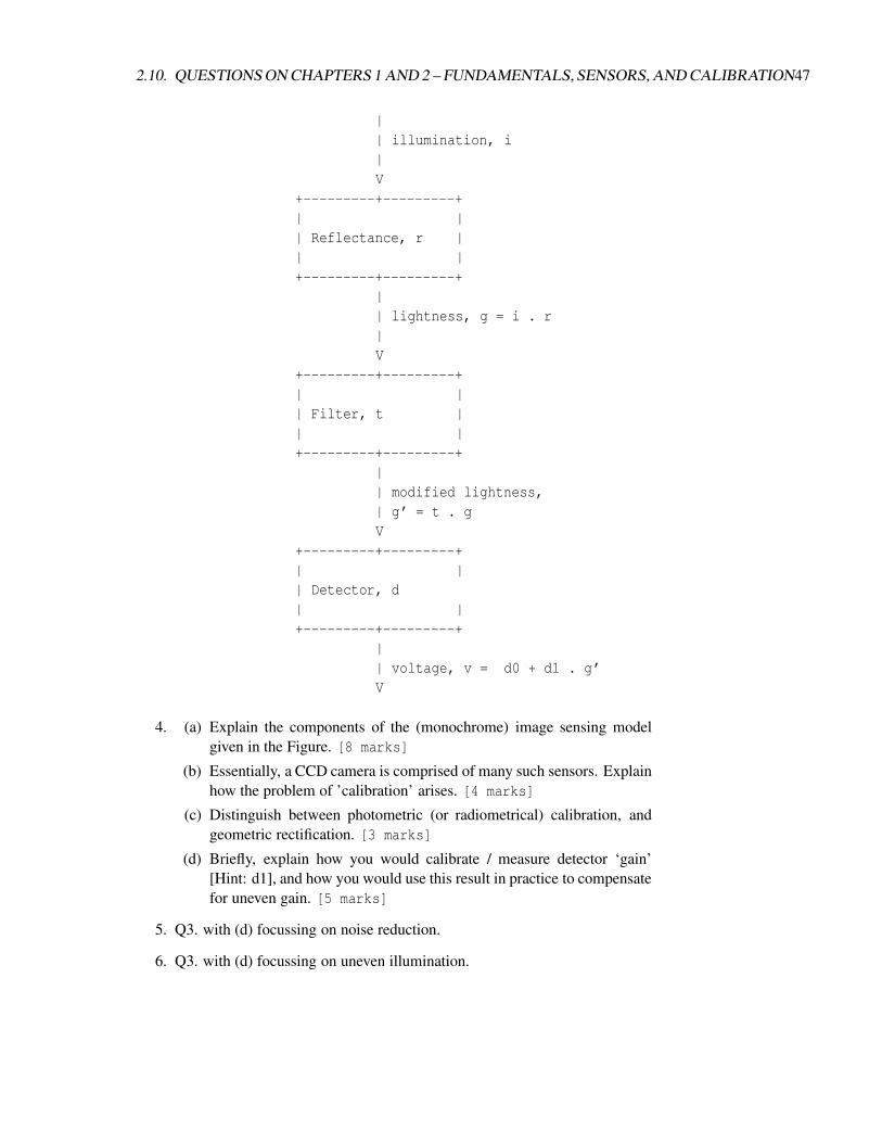
2.10. QUESTIONS ON CHAPTERS 1 AND 2 – FUNDAMENTALS, SENSORS, AND CALIBRATION47
|| illumination, i|V
+---------+---------+| || Reflectance, r || |+---------+---------+
|| lightness, g = i . r|V
+---------+---------+| || Filter, t || |+---------+---------+
|| modified lightness,| g’ = t . gV
+---------+---------+| || Detector, d| |+---------+---------+
|| voltage, v = d0 + d1 . g’V
4. (a) Explain the components of the (monochrome) image sensing modelgiven in the Figure. [8 marks]
(b) Essentially, a CCD camera is comprised of many such sensors. Explainhow the problem of ’calibration’ arises. [4 marks]
(c) Distinguish between photometric (or radiometrical) calibration, andgeometric rectification. [3 marks]
(d) Briefly, explain how you would calibrate / measure detector ‘gain’[Hint: d1], and how you would use this result in practice to compensatefor uneven gain. [5 marks]
5. Q3. with (d) focussing on noise reduction.
6. Q3. with (d) focussing on uneven illumination.

48 CHAPTER 2. DIGITAL IMAGE FUNDAMENTALS
7. (a) Explain the components of the (monochrome) image sensing modelgiven in the Figure. [8 marks]
(b) Extend the equations to include wavelength sensitivity. [NB. the detec-tor will now have an integration]. [6 marks]
(c) Hence, use appropriate diagrams and/or equations to explain the op-eration of a ’colour’ sensing (ie. one which senses ’red’, ’green’ and’blue’.). [6 marks]
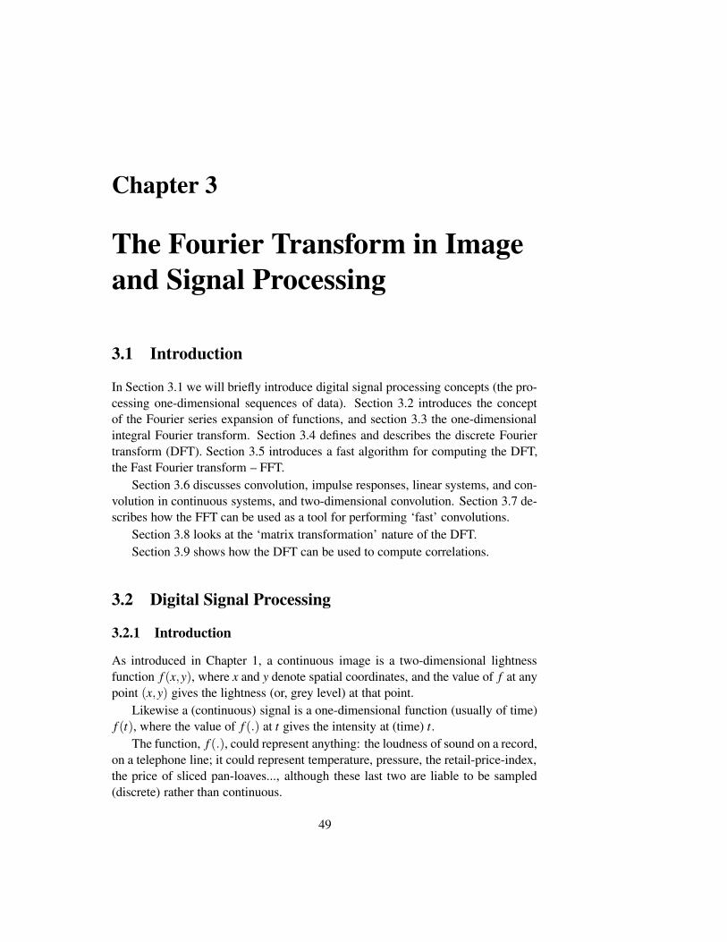
Chapter 3
The Fourier Transform in Imageand Signal Processing
3.1 Introduction
In Section 3.1 we will briefly introduce digital signal processing concepts (the pro-cessing one-dimensional sequences of data). Section 3.2 introduces the conceptof the Fourier series expansion of functions, and section 3.3 the one-dimensionalintegral Fourier transform. Section 3.4 defines and describes the discrete Fouriertransform (DFT). Section 3.5 introduces a fast algorithm for computing the DFT,the Fast Fourier transform – FFT.
Section 3.6 discusses convolution, impulse responses, linear systems, and con-volution in continuous systems, and two-dimensional convolution. Section 3.7 de-scribes how the FFT can be used as a tool for performing ‘fast’ convolutions.
Section 3.8 looks at the ‘matrix transformation’ nature of the DFT.Section 3.9 shows how the DFT can be used to compute correlations.
3.2 Digital Signal Processing
3.2.1 Introduction
As introduced in Chapter 1, a continuous image is a two-dimensional lightnessfunction f (x,y), where x and y denote spatial coordinates, and the value of f at anypoint (x,y) gives the lightness (or, grey level) at that point.
Likewise a (continuous) signal is a one-dimensional function (usually of time)f (t), where the value of f (.) at t gives the intensity at (time) t.
The function, f (.), could represent anything: the loudness of sound on a record,on a telephone line; it could represent temperature, pressure, the retail-price-index,the price of sliced pan-loaves..., although these last two are liable to be sampled(discrete) rather than continuous.
49

50CHAPTER 3. THE FOURIER TRANSFORM IN IMAGE AND SIGNAL PROCESSING
The sorts of objectives we have in signal processing match those of imageprocessing:
• clean up signals so that humans find them more useful, e.g. remove noisefrom a telephone signal, to make it more audible.
• automate human tasks, e.g. recognition of spoken words.
Whilst the main impetus for digital image processing came from the need forcleaning up pictures from space probes, and tasks like optical character recogni-tion, much of early digital signal processing research was based on seismic dataprocessing for oil prospecting; such was the complexity of the required processing,that available analogue (continuous) methods were inadequate and the processinghad to be done (digitally) on computers.
We have already indicated the forces that have driven systems from analogue/continuousto discrete/digital; signal processing has also been subject to these forces and moreand more signal processing is becoming digital.
3.2.2 Finite Sampled Signals.
The domain of the function f (.) is, strictly, −∞ to +∞, but, for practical purposes,attention is often limited to some piece of the infinite domain:
t0 ≤ t ≤ t1, where t0, t1 are finite.
This is the same as in imaging, where we limit our attention to some finiterectangular part of an infinite image.
Notation: the literature on signal processing commonly uses x(t) as the ‘gen-eral’ signal. We use xc(t) to explicitly state that xc() is continuous.
If xc(t) is sampled (cf. discussion of images in Chapter 1) we obtain an arrayof numbers (a discrete or digital data sequence),
x[n], n = 0,1,2 . . . ,N−1
where N is the number of samples.Normally we use the notation [ . ] to denote a discrete function.Typically, x[n] is obtained by sampling x(t) periodically at intervals T , i.e.
x[n] = xc(nT ), n = 0,1,2, . . . ,N−1
Of course, x[n] is some digital representation of a real number, i.e. in additionto time sampling it is digitized.
The following figures show examples of some sampled signals. If these werecontinuous, we would have two changes:
1. instead of existing just at discrete sample points, n = 0,1,2 etc. they wouldexist continuously – there would be a continuous line joining the points, and
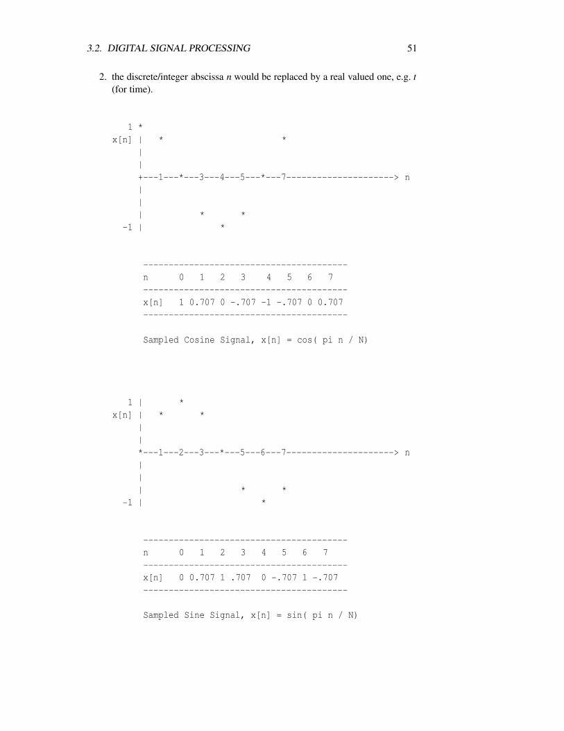
3.2. DIGITAL SIGNAL PROCESSING 51
2. the discrete/integer abscissa n would be replaced by a real valued one, e.g. t(for time).
1 *x[n] | * *
||+---1---*---3---4---5---*---7---------------------> n||| * *
-1 | *
----------------------------------------n 0 1 2 3 4 5 6 7----------------------------------------x[n] 1 0.707 0 -.707 -1 -.707 0 0.707----------------------------------------
Sampled Cosine Signal, x[n] = cos( pi n / N)
1 | *x[n] | * *
||*---1---2---3---*---5---6---7---------------------> n||| * *
-1 | *
----------------------------------------n 0 1 2 3 4 5 6 7----------------------------------------x[n] 0 0.707 1 .707 0 -.707 1 -.707----------------------------------------
Sampled Sine Signal, x[n] = sin( pi n / N)

52CHAPTER 3. THE FOURIER TRANSFORM IN IMAGE AND SIGNAL PROCESSING
Ex. 3.3.2-1 (a) Use a calculator to verify the values in the figures showing thesampled sine and cosine signals.
(b) Verify that 0.707 =√
2/2.
(c) Verify that both cosine and sine are periodic, i.e. the repeat themselvesfor n = 8,9, . . .
1 *x[n] |
||+---*---*---*---*---*---*---*----> n0 1 2 3 4 5 6 7
--------------------------------------n 0 1 2 3 4 5 6 7--------------------------------------x[n] 1 0 0 0 0 0 0 0--------------------------------------
Impulse Signal
1 * * * * * * * *x[n] |
||+-------------------------------> n0 1 2 3 4 5 6 7
--------------------------------------n 0 1 2 3 4 5 6 7--------------------------------------x[n] 1 1 1 1 1 1 1 1--------------------------------------
DC (Direct Current), i.e. constant value, Signal

3.2. DIGITAL SIGNAL PROCESSING 53
3.2.3 Sampling Frequency
The symbol T in the sampling equation, x[n] = xc(nT ), is the sampling period. Thesampling frequency ( fs) is
fs = 1/T
Nyquist Sampling Theorem: If a continuous signal contains only frequencies inthe range 0 to fmax (the bandwidth), then by sampling it at twice fmax we obtaina discrete sequence from which it is possible to exactly reconstruct the originalcontinuous signal; that is, there is no loss of information.
Therefore
fs = 2 fmax
for no loss of information.
Ex. 3.3.2-2 For most voice recognition tasks, the effective bandwidth is 5 kHz(5,000 cycles per second). Thus, fs = 10 kHz. Sampling period, T :
T = 1/ fs= 1/10,000 seconds = 100 microseconds
Ex. 3.3.2-2 If hi-fi music has a bandwidth of 15 kHz, calculate the minimum al-lowable sampling frequency fs; what is the corresponding sampling periodT?
Ex. 3.3.2-3 Compact discs (CDs) actually use fs=44.1 kHz.
(a) What is sampling period, T?
(b) For one second of music, what is N in the sampling equation, x[n] =xc(nT ), n = 0,1, . . .N−1?
Answer: 44,100. But note – this requires two channels – 88,200 – for stereo.
(c) one minute?
(d) one hour?
(e) Assuming 16 bits per sample, how many Megabytes are there on a one-hour CD.
Answer: 635 Megabytes.
3.2.4 Amplitude Resolution
If the dynamic range is properly chosen, 12-bits ([0 . . .4095]), is adequate for hi-fireproduction of audible signals; CDs use 16-bits.
54CHAPTER 3. THE FOURIER TRANSFORM IN IMAGE AND SIGNAL PROCESSING
3.2.5 Frequencies
When we say fmax is 15 kHz, we mean that the most rapidly varying component(xm(t)) of the signal corresponds to a ‘pure’ tone, or sinusoid (sine function), whosefrequency is 15 kHz. I.e.
xm(t) = amsin(2π fmaxt)
where π = 3.1415926... and am is the ‘amount’ of that frequency present.
Ex. 3.3.4-1 If fmax is 1 Hz, work out the values of xm(t) for time samples
t = 0,0.125,0.25,0.375,0.5,0.625,0.75,0.875,1.0
Assume am = 1.
t 2πt xm(t) = sin()
0.0 0.0 0.00.125 0.785 0.7070.25 1.57 1.0
0.375 2.36 0.7070.5 3.14 0.0
0.625 3.93 –0.7070.75 4.71 –1.0
0.875 5.50 –0.7071.0 6.28 0.0
Ex. 3.3.4-2 Plot xm(t) from the foregoing Ex.
Answer:
1 | *x[n] | * *
||*---1---2---3---*---5---6---7---------------------> n||| * *
-1 | *
----------------------------------------n 0 1 2 3 4 5 6 7----------------------------------------
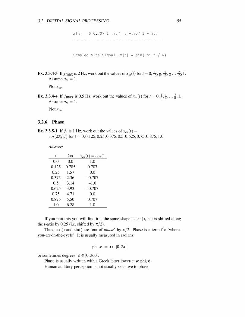
3.2. DIGITAL SIGNAL PROCESSING 55
x[n] 0 0.707 1 .707 0 -.707 1 -.707----------------------------------------
Sampled Sine Signal, x[n] = sin( pi n / N)
Ex. 3.3.4-3 If fmax is 2 Hz, work out the values of xm(t) for t = 0, 116 , 1
8 , 316 , 1
4 . . . 1516 ,1.
Assume am = 1.
Plot xm.
Ex. 3.3.4-4 If fmax is 0.5 Hz, work out the values of xm(t) for t = 0, 18 , 1
4 , . . . 78 ,1.
Assume am = 1.
Plot xm.
3.2.6 Phase
Ex. 3.3.5-1 If fn is 1 Hz, work out the values of xcn(t) =cos(2π fnt) for t = 0,0.125,0.25,0.375,0.5,0.625,0.75,0.875,1.0.
Answer:
t 2πt xcn(t) = cos()0.0 0.0 1.0
0.125 0.785 0.7070.25 1.57 0.00.375 2.36 –0.7070.5 3.14 –1.0
0.625 3.93 –0.7070.75 4.71 0.00.875 5.50 0.7071.0 6.28 1.0
If you plot this you will find it is the same shape as sin(), but is shifted alongthe t-axis by 0.25 (i.e. shifted by π/2).
Thus, cos() and sin() are ‘out of phase’ by π/2. Phase is a term for ‘where-you-are-in-the-cycle’. It is usually measured in radians:
phase = φ ∈ [0,2π]
or sometimes degrees: φ ∈ [0,360].Phase is usually written with a Greek letter lower-case phi, φ.Human auditory perception is not usually sensitive to phase.

56CHAPTER 3. THE FOURIER TRANSFORM IN IMAGE AND SIGNAL PROCESSING
3.2.7 Periodic Signals
A signal x(t) is periodic with period Td if:
x(t) = x(t +Td)
Thus, the 1 Hz sines and cosines, above, are periodic with period 1 sec. The 2Hz signals have a period 0.5 seconds. A 4 Hz signal would have a period 0.25 sec.,etc.
In analysis of signals it is often convenient to assume that signals are periodic.This can be done by taking a sufficiently large chunk of signal and assuming thatit is repeated.
3.3 Fourier Series
3.3.1 General
Roughly speaking, any signal can be represented as a weighted sum of pure sinu-soids:
xn(t) = sin(2π fnt), t = t0 . . . t1
x(t) =nmax∑n=0
anxn(t)
where an is the ‘weight’ of the contribution from frequency fn.
Ex. 3.4-1 What does component 0 (n = 0) look like?
Thus if the signal is sin(2π1 f t), i.e. a pure 1 Hz sinusoid, we have:nmax = 1,a0 = 0,a1 = 1.0,fnmax = 1.0Notation: it is useful to introduce a symbol for 2π f (the radian frequency).
Greek lower-case ‘omega’, ω, is normally used. Thus
sin(ωt) = sin(2π f t)
Ex. 3.4-2 Add the following components:
1sin(ωt)+(1/3)sin(3ωt)+(1/5)sin(5ωt) . . .
where ω = 2π1.
What does the result look like?
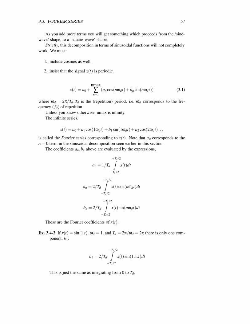
3.3. FOURIER SERIES 57
As you add more terms you will get something which proceeds from the ‘sine-wave’ shape, to a ‘square-wave’ shape.
Strictly, this decomposition in terms of sinusoidal functions will not completelywork. We must:
1. include cosines as well,
2. insist that the signal x(t) is periodic.
x(t) = a0 +nmax∑n=1
(an cos(nωdt)+bn sin(nωdt)) (3.1)
where ωd = 2π/Td ,Td is the (repetition) period, i.e. ωd corresponds to the fre-quency ( fd) of repetition.
Unless you know otherwise, nmax is infinity.The infinite series,
x(t) = a0 +a1 cos(1ωdt)+b1 sin(1ωdt)+a2 cos(2ωdt) . . .
is called the Fourier series corresponding to x(t). Note that a0 corresponds to then = 0 term in the sinusoidal decomposition seen earlier in this section.
The coefficients an,bn above are evaluated by the expressions,
a0 = 1/Td
+Td/2Z
−Td/2
x(t)dt
an = 2/Td
+Td/2Z
−Td/2
x(t)cos(nωdt)dt
bn = 2/Td
+Td/2Z
−Td/2
x(t)sin(nωdt)dt
These are the Fourier coefficients of x(t).
Ex. 3.4-2 If x(t) = sin(1.t), ωd = 1, and Td = 2π/ωd = 2π there is only one com-ponent, b1:
b1 = 2/Td
+Td/2Z
−Td/2
x(t)sin(1.1.t)dt
This is just the same as integrating from 0 to Td ,
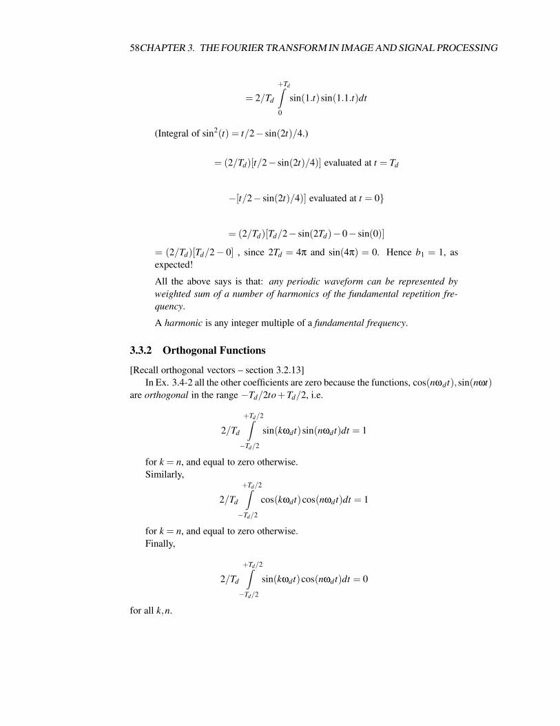
58CHAPTER 3. THE FOURIER TRANSFORM IN IMAGE AND SIGNAL PROCESSING
= 2/Td
+TdZ
0
sin(1.t)sin(1.1.t)dt
(Integral of sin2(t) = t/2− sin(2t)/4.)
= (2/Td)[t/2− sin(2t)/4)] evaluated at t = Td
−[t/2− sin(2t)/4)] evaluated at t = 0
= (2/Td)[Td/2− sin(2Td)−0− sin(0)]
= (2/Td)[Td/2− 0] , since 2Td = 4π and sin(4π) = 0. Hence b1 = 1, asexpected!
All the above says is that: any periodic waveform can be represented byweighted sum of a number of harmonics of the fundamental repetition fre-quency.
A harmonic is any integer multiple of a fundamental frequency.
3.3.2 Orthogonal Functions
[Recall orthogonal vectors – section 3.2.13]In Ex. 3.4-2 all the other coefficients are zero because the functions, cos(nωdt),sin(nωt)
are orthogonal in the range −Td/2to+Td/2, i.e.
2/Td
+Td/2Z
−Td/2
sin(kωdt)sin(nωdt)dt = 1
for k = n, and equal to zero otherwise.Similarly,
2/Td
+Td/2Z
−Td/2
cos(kωdt)cos(nωdt)dt = 1
for k = n, and equal to zero otherwise.Finally,
2/Td
+Td/2Z
−Td/2
sin(kωdt)cos(nωdt)dt = 0
for all k,n.

3.3. FOURIER SERIES 59
3.3.3 Finite Fourier Series
The Fourier series is given by eqn. 3.1,
x(t) = a0 +nmax∑n=1
[an cos(nωdt)+bn sin(nωdt)]
where ωd = 2π/Td , Td is the (repetition) period, i.e. ωd corresponds to the fre-quency ( fd) of repetition.
If the largest frequency present is just less than Nωd , i.e. N times the repetitionfrequency, then we can set nmax = N − 1 and we can represent x(t) with: a0,(N−1) a-coefficients and (N−1) b-coefficients.
This gives a total of 2N−1 coefficients.
3.3.4 Complex Fourier Series
x(t) = a0 +nmax∑n=1
[an cos(nωdt)+bn sin(nωdt)]
can be written even more compactly as:
x(t) =+nmax
∑−nmax
[cn exp( jnωdt)]
Now the coefficients are complex numbers cn = an + jbn, ( j =√−1)
Note that:
exp( jB) = cos(B)+ j sin(B)
cos(B) = (exp( jB)+ exp(− jB))/2
sin(B) = (exp( jB)− exp(− jB)/2 j
Now the coefficients are given by:
cn = (1/Td)
−Td/2Z
+Td/2
x(t)exp(− jnωdt)dt
These equations introduce nothing new - they are just shorthand for the earlierdefinition of the Fourier series.
Ex. 3.4-3 Verify the last statement by substituting the equation for exp( jB) abovein
cn = (an− jbn)/2
c−n = (an+ jbn)/2

60CHAPTER 3. THE FOURIER TRANSFORM IN IMAGE AND SIGNAL PROCESSING
andc0 = a0
3.4 The Fourier Transform
If we now relax the ‘periodic’ restriction, i.e. let Td −→ ∞, we have
x(t) =−∞
∑+∞
cn exp( jnωdt)
and
cn = (1/Td)
−Td/2Z
+Td/2
x(t)exp(− jnωdt)dt
Td −→ ∞ =⇒ ωd = 2π/Td −→ dw
(i.e. very small),
nωd −→ n dω
(call this ω).The above equation for cn now becomes:
cn = (dω/2π)
−∞Z
+∞
x(t)exp(− jωt)dt
and the equation for x(t) is now a sum of infinitely many terms, i.e. an integral:
x(t) =
−∞Z
+∞
cn exp( jωt)
Substituting for cn gives:
x(t) =
+∞Z
−∞
dω [
+∞Z
−∞+
x(t)exp(− jωt)dt]exp( jωt)/(2π)
The expression in the square brackets [.] is a function of angular frequency (ω)and is called the Fourier transform of x(t).
Fourier transform:
X(w) = (1/2π)
+∞Z
−∞
x(t)exp(− jωt)dω
If we substitute X(ω) = . . . in the equation for x(t) above, we get:
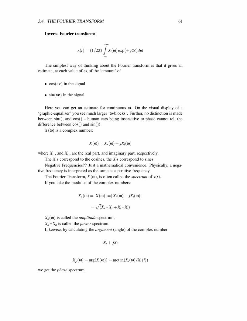
3.4. THE FOURIER TRANSFORM 61
Inverse Fourier transform:
x(t) = (1/2π)
+∞Z
−∞
X(ω)exp(+ jωt)dω
The simplest way of thinking about the Fourier transform is that it gives anestimate, at each value of ω, of the ‘amount’ of
• cos(ωt) in the signal
• sin(ωt) in the signal
Here you can get an estimate for continuous ω. On the visual display of a‘graphic-equaliser’ you see much larger ‘ω-blocks’. Further, no distinction is madebetween sin(), and cos() – human ears being insensitive to phase cannot tell thedifference between cos() and sin()!
X(ω) is a complex number:
X(ω) = Xr(ω)+ jXi(ω)
where Xr , and Xi , are the real part, and imaginary part, respectively.The Xrs correspond to the cosines, the Xis correspond to sines.Negative Frequencies?? Just a mathematical convenience. Physically, a nega-
tive frequency is interpreted as the same as a positive frequency.The Fourier Transform, X(ω), is often called the spectrum of x(t).If you take the modulus of the complex numbers:
Xa(ω) =| X(ω) |=| Xr(ω)+ jXi(ω) |
=√
(Xr ∗Xr +Xi ∗Xi)
Xa(ω) is called the amplitude spectrum;Xa ∗Xa is called the power spectrum.Likewise, by calculating the argument (angle) of the complex number
Xr + jXi
Xp(ω) = arg(X(ω)) = arctan(Xi(ω)/Xr(i))
we get the phase spectrum.
62CHAPTER 3. THE FOURIER TRANSFORM IN IMAGE AND SIGNAL PROCESSING
3.5 Discrete Fourier Transform
3.5.1 Definition
The Discrete Fourier Transform (DFT) of the digital signal/sequence x[n], i = 0,1 . . . N−1, is
X [u] = (1/N)N−1
∑n=0
x[n]exp(− j π u n/N)
for u = 0,1 . . .N−1.The Inverse DFT (IDFT) is
x[n] =N−1
∑n=0
X [u]exp(+ j π u n/N)
Interpretation of DFT:If x[n] has been produced by sampling at fs = 1/T , the largest frequency
present in x[n] is fs/2 (section 3.3.3).Examine the DFT equation, and look at just the cosine part,
X [u] = (1/N)N−1
∑n=0
x[n]exp(− j π u n/N)
Cosine part:
Xc[u] = (1/N)N−1
∑n=0
x[n]cos(π u n/N)
At u = 0 : cos() = cos(π (0) n/N) = cos(0) = 1i.e. we are matching x[n] with a constant (sometimes called the DC component
– DC = direct current) signal.At u = 1 : cos() = cos(π 1 n/N).This term varies slowly from cos(0) at n = 0 to cos(π (N− 1)/N)) = cos(π)
i.e. just one cycle in the sequence.At u = 2: we get 2 cycles in the sequence.At N/2: we get N/2 cycles in the sequence, i.e. 2 samples per cycle, i.e. very
rapidly varying, this corresponds to fs/2.
3.5.2 Discrete Fourier Spectrum
As with the continuous Fourier Transform, X(ω),X [u] is often also called the spec-trum of x[n] – or the discrete spectrum.
If you take the modulus of the complex numbers, X [u] = Xc[u]+ jXs[u]:
Xa(w) =| X [u] | = | Xc[u]+ jXs[u] |=√(Xc ∗Xc +Xs ∗Xs)
3.5. DISCRETE FOURIER TRANSFORM 63
Xa[u] is called the amplitude spectrum;Xa ∗Xa is called the power spectrum.Likewise, by calculating the argument (angle) of the complex number
Xp[u] = arg(X [u]) = arctan(Xs[u]/Xc(i))
we get the phase spectrum.
3.5.3 Interpretation
The components near the beginning of the DFT correspond to the ‘slowly varying’parts of the signal; the components near the middle, the ‘fast moving’ parts.
Domains: Often when working with sequences x[n], or signals x(t) we say weare in the time domain; in image processing, this becomes the spatial domain. Ifwe are working with X [u], or X(ω), then we are in the frequency domain.
3.5.4 Frequency Discrimination by the DFT
In general, if we have N samples, the spacing of each frequency sample is fs/N.
d f = fs/N
The larger the N, the finer is our discrimination of frequency. If N −→ ∞, thenwe have a continuous spectrum, i.e. the continuous Fourier transform.
Above N/2 we have no additional information; these terms correspond to the‘negative’ frequencies of the continuous transform.
Ex. 3.6-1 Consider a CD signal sequence; it (one channel) is sampled at fs = 44.1KHz. Take a one second sequence, i.e. 44,100 samples.
Take a DFT of x[n],n = 0,1, ...,44099.
We have d f = 44100/44100 = 1 Hz, i.e. a sampling of 1 Hz of the spectrum.
The highest frequency is N/2; this is
fmax = 44100/2 = 22050
i.e. the highest frequency represented ( fs/2).
Ex. 3.6-2 Show how the DFT obtained in Ex. 3.6-1 could be used to create‘graphic-spectrum-analyser’ output in 10 ‘bands’ representing the frequencyrange 0 to 15 KHz?
0 to 15 KHz, so we are interested in the first 15000 frequency samples. Thereare 10 bands so each band will have 1500 Hz.
First band: 0 – 1500 Hz
2nd band: 1501 – 3000 Hz etc.
Therefore, for band 1, sum the amplitude spectrum from ω = 0 to ω = 1500.
Band 2: sum for ω = 1501 to 3000 etc.

64CHAPTER 3. THE FOURIER TRANSFORM IN IMAGE AND SIGNAL PROCESSING
Ex. 3.6-3 (a) What is the DFT of a sequence containing the following single cycleof a cosine wave. Think, before you calculate.
1 *x[n] | * *
||+---1---*---3---4---5---*---7---------------------> n||| * *
-1 | *
----------------------------------------n 0 1 2 3 4 5 6 7----------------------------------------x[n] 1 0.707 0 -.707 -1 -.707 0 0.707----------------------------------------
Answer: Note all real, imaginary parts = 0, for all u.
----------------------------------------u 0 1 2 3 4 5 6 7----------------------------------------Xr [u] 0 1/2 0 0 0 0 0 1/2Xi [u] 0 0 0 0 0 0 0 0----------------------------------------
(b) What is the amplitude spectrum?
Answer:
----------------------------------------u 0 1 2 3 4 5 6 7----------------------------------------Xa [u] 0 1/2 0 0 0 0 0 1/2----------------------------------------

3.5. DISCRETE FOURIER TRANSFORM 65
(c) Phase spectrum?
Ex. 3.6-4 (a) What is the DFT of a sequence containing the following single cycleof a sine wave. Again, think, before you calculate.
1 | *x[n] | * *
||*---1---2---3---*---5---6---7---------------------> n||| * *
-1 | *
----------------------------------------n 0 1 2 3 4 5 6 7----------------------------------------x[n] 0 0.707 1 .707 0 -.707 1 -.707----------------------------------------
Answer: Note all imaginary, real parts = 0, for all u, i.e. just the opposite ofthe cosine.
----------------------------------------u 0 1 2 3 4 5 6 7----------------------------------------Xr [u] 0 0 0 0 0 0 0 0Xi [u] 0 1/2 0 0 0 0 0 1/2----------------------------------------
(b) What is the amplitude spectrum?
Answer:
----------------------------------------
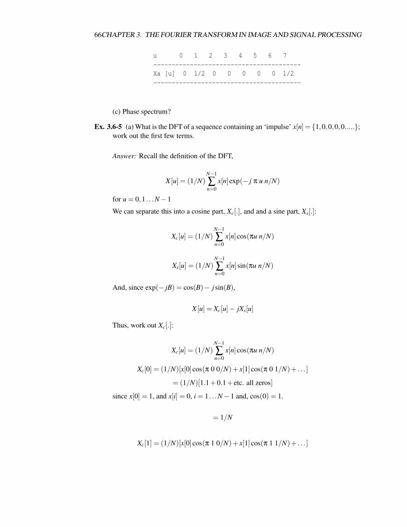
66CHAPTER 3. THE FOURIER TRANSFORM IN IMAGE AND SIGNAL PROCESSING
u 0 1 2 3 4 5 6 7----------------------------------------Xa [u] 0 1/2 0 0 0 0 0 1/2----------------------------------------
(c) Phase spectrum?
Ex. 3.6-5 (a) What is the DFT of a sequence containing an ‘impulse’ x[n] = 1,0,0,0,0.....;work out the first few terms.
Answer: Recall the definition of the DFT,
X [u] = (1/N)N−1
∑n=0
x[n]exp(− j π u n/N)
for u = 0,1 . . .N−1
We can separate this into a cosine part, Xc[.], and and a sine part, Xs[.]:
Xc[u] = (1/N)N−1
∑n=0
x[n]cos(πu n/N)
Xs[u] = (1/N)N−1
∑n=0
x[n]sin(πu n/N)
And, since exp(− jB) = cos(B)− j sin(B),
X [u] = Xc[u]− jXs[u]
Thus, work out Xc[.]:
Xc[u] = (1/N)N−1
∑n=0
x[n]cos(πu n/N)
Xc[0] = (1/N)[x[0]cos(π 0 0/N)+ x[1]cos(π 0 1/N)+ . . . ]
= (1/N)[1.1+0.1+ etc. all zeros]
since x[0] = 1, and x[i] = 0, i = 1 . . .N−1 and, cos(0) = 1.
= 1/N
Xc[1] = (1/N)[x[0]cos(π 1 0/N)+ x[1]cos(π 1 1/N)+ . . . ]
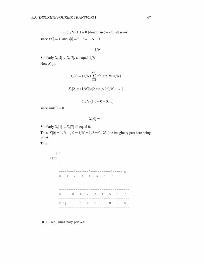
3.5. DISCRETE FOURIER TRANSFORM 67
= (1/N)[1 1+0.(don’t care)+ etc. all zeros]
since x[0] = 1, and x[i] = 0, i = 1..N−1
= 1/N
Similarly Xc[2] . . .Xc[7], all equal 1/N.
Now Xs[.]:
Xs[u] = (1/N)N−1
∑n=0
x[n]sin(πu n/N)
Xs[0] = (1/N)[x[0]sin(π.0.0/N + . . . ]
= (1/N)[1.0+0+0 . . . ]
since sin(0) = 0
Xs[0] = 0
Similarly Xs[1] . . .Xs[7] all equal 0.
Thus, X [0] = 1/N + j.0 = 1/N = 1/8 = 0.125 (the imaginary part here beingzero).
Thus:
1 *x[n] |
||+---*---*---*---*---*---*---*----> n0 1 2 3 4 5 6 7
--------------------------------------n 0 1 2 3 4 5 6 7--------------------------------------x[n] 1 0 0 0 0 0 0 0--------------------------------------
DFT – real, imaginary part = 0.

68CHAPTER 3. THE FOURIER TRANSFORM IN IMAGE AND SIGNAL PROCESSING
----------------------------------------------u 0 1 2 3 4 5 6 7---------------------------------------------X[u] 1/8 1/8 1/8 1/8 1/8 1/8 1/8 1/8----------------------------------------------
(b) What is the amplitude spectrum? Work out the first few terms, you willbe able to guess the remainder.
Recall the definition of the discrete amplitude spectrum:
Xa[u] =| X [u] |=| Xc[u]+ jXs[u] |=√
(Xc ∗Xc +Xs ∗Xs)
Thus, the amplitude spectrum of the impulse is simply:
----------------------------------------------u 0 1 2 3 4 5 6 7
---------------------------------------------X[u] 1/8 1/8 1/8 1/8 1/8 1/8 1/8 1/8----------------------------------------------
I.e. an ‘impulse’ has equal amounts of all frequencies. So, if you fed im-pulses into your amplifier, the ‘graphic-spectrum-analyser’ would show anequal reading on all bands.
Ex. 3.6-6 Work out the DFT, amplitude spectrum of a DC signal, i.e. 1,1,1,1, . . . .A pattern should emerge for u = 1,2,3 . . . .
1 * * * * * * * *x[n] |
||+-------------------------------> n0 1 2 3 4 5 6 7
--------------------------------------n 0 1 2 3 4 5 6 7--------------------------------------
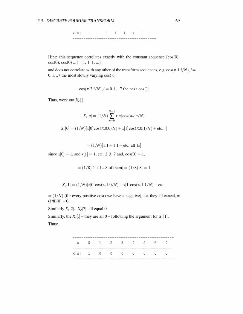
3.5. DISCRETE FOURIER TRANSFORM 69
x[n] 1 1 1 1 1 1 1 1--------------------------------------
Hint: this sequence correlates exactly with the constant sequence [cos(0),cos(0), cos(0) ...] =[1, 1, 1, ...]
and does not correlate with any other of the transform sequences, e.g. cos(π.1.i/N), i =0,1, ..7 the most slowly varying cos():
cos(π.2.i/N), i = 0,1, ..7 the next cos()]
Thus, work out Xc[.]:
Xc[u] = (1/N)N−1
∑n=0
x[n]cos(πu n/N)
Xc[0] = (1/N)[x[0]cos(π.0.0/N)+ x[1]cos(π.0.1/N)+ etc...]
= (1/N)[1.1+1.1+ etc. all 1s]
since x[0] = 1, and x[1] = 1, etc. 2,3..7 and, cos(0) = 1.
= (1/8)[1+1...8 of them] = (1/8)[8] = 1
Xc[1] = (1/N)[x[0]cos(π.1.0/N)+ x[1]cos(π.1.1/N)+ etc.]
= (1/N) (for every positive cos() we have a negative), i.e. they all cancel, =(1/8)[0] = 0.
Similarly Xc[2]...Xc[7], all equal 0.
Similarly, the Xs[.] – they are all 0 – following the argument for Xc[1].
Thus:
----------------------------------------------u 0 1 2 3 4 5 6 7
---------------------------------------------X[u] 1 0 0 0 0 0 0 0----------------------------------------------
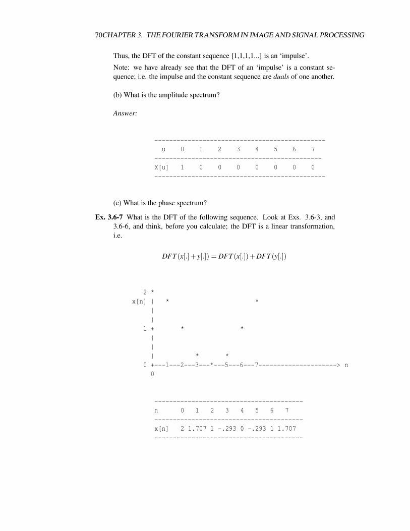
70CHAPTER 3. THE FOURIER TRANSFORM IN IMAGE AND SIGNAL PROCESSING
Thus, the DFT of the constant sequence [1,1,1,1...] is an ‘impulse’.
Note: we have already see that the DFT of an ‘impulse’ is a constant se-quence; i.e. the impulse and the constant sequence are duals of one another.
(b) What is the amplitude spectrum?
Answer:
----------------------------------------------u 0 1 2 3 4 5 6 7
---------------------------------------------X[u] 1 0 0 0 0 0 0 0----------------------------------------------
(c) What is the phase spectrum?
Ex. 3.6-7 What is the DFT of the following sequence. Look at Exs. 3.6-3, and3.6-6, and think, before you calculate; the DFT is a linear transformation,i.e.
DFT (x[.]+ y[.]) = DFT (x[.])+DFT (y[.])
2 *x[n] | * *
||
1 + * *||| * *
0 +---1---2---3---*---5---6---7---------------------> n0
----------------------------------------n 0 1 2 3 4 5 6 7----------------------------------------x[n] 2 1.707 1 -.293 0 -.293 1 1.707----------------------------------------
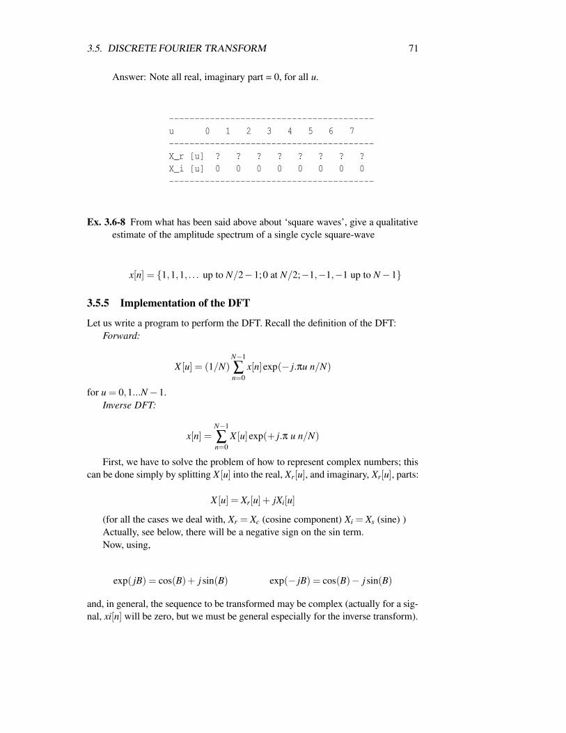
3.5. DISCRETE FOURIER TRANSFORM 71
Answer: Note all real, imaginary part = 0, for all u.
----------------------------------------u 0 1 2 3 4 5 6 7----------------------------------------X_r [u] ? ? ? ? ? ? ? ?X_i [u] 0 0 0 0 0 0 0 0----------------------------------------
Ex. 3.6-8 From what has been said above about ‘square waves’, give a qualitativeestimate of the amplitude spectrum of a single cycle square-wave
x[n] = 1,1,1, . . . up to N/2−1;0 at N/2;−1,−1,−1 up to N−1
3.5.5 Implementation of the DFT
Let us write a program to perform the DFT. Recall the definition of the DFT:Forward:
X [u] = (1/N)N−1
∑n=0
x[n]exp(− j.πu n/N)
for u = 0,1...N−1.Inverse DFT:
x[n] =N−1
∑n=0
X [u]exp(+ j.π u n/N)
First, we have to solve the problem of how to represent complex numbers; thiscan be done simply by splitting X [u] into the real, Xr[u], and imaginary, Xr[u], parts:
X [u] = Xr[u]+ jXi[u]
(for all the cases we deal with, Xr = Xc (cosine component) Xi = Xs (sine) )Actually, see below, there will be a negative sign on the sin term.Now, using,
exp( jB) = cos(B)+ j sin(B) exp(− jB) = cos(B)− j sin(B)
and, in general, the sequence to be transformed may be complex (actually for a sig-nal, xi[n] will be zero, but we must be general especially for the inverse transform).
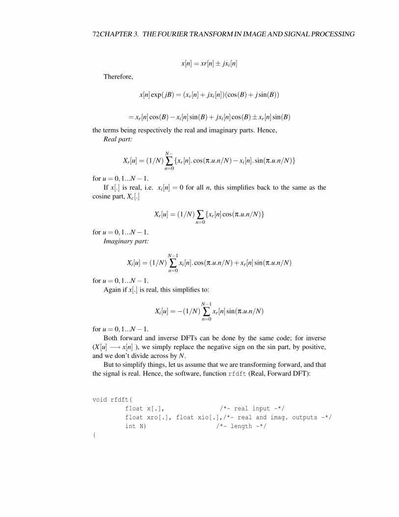
72CHAPTER 3. THE FOURIER TRANSFORM IN IMAGE AND SIGNAL PROCESSING
x[n] = xr[n]± jxi[n]
Therefore,
x[n]exp( jB) = (xr[n]+ jxi[n])(cos(B)+ j sin(B))
= xr[n]cos(B)− xi[n]sin(B)+ jxi[n]cos(B)± xr[n]sin(B)
the terms being respectively the real and imaginary parts. Hence,Real part:
Xr[u] = (1/N)N−∑n=0xr[n].cos(π.u.n/N)− xi[n].sin(π.u.n/N)
for u = 0,1...N−1.If x[.] is real, i.e. xi[n] = 0 for all n, this simplifies back to the same as the
cosine part, Xc[.]
Xr[u] = (1/N) ∑n=0xr[n]cos(π.u.n/N)
for u = 0,1...N−1.Imaginary part:
Xi[u] = (1/N)N−1
∑n=0
xi[n].cos(π.u.n/N)+ xr[n]sin(π.u.n/N)
for u = 0,1...N−1.Again if x[.] is real, this simplifies to:
Xi[u] =−(1/N)N−1
∑n=0
xr[n]sin(π.u.n/N)
for u = 0,1...N−1.Both forward and inverse DFTs can be done by the same code; for inverse
(X [u] −→ x[n] ), we simply replace the negative sign on the sin part, by positive,and we don’t divide across by N.
But to simplify things, let us assume that we are transforming forward, and thatthe signal is real. Hence, the software, function rfdft (Real, Forward DFT):
void rfdft(float x[.], /*- real input -*/float xro[.], float xio[.],/*- real and imag. outputs -*/int N) /*- length -*/
3.6. FAST FOURIER TRANSFORM 73
float pi = 3.1415926,tpi;int n, u;
tpi=2.0*pi;
for(u=0;u<N;u++)xro[u]=0.0;xio[u]=0.0;for(n=0;n<N;n++)
/*-- X_r [u] = (1/N) # xr[n].cos( PI .u.n/N) --*/xro[u] = xro[u] + x[n]*cos(tpi*u*n/N);
/*-- X_i [u] = - (1/N) # xr[n].sin( PI .u.n/N) --*/xio[u] = xio[u] - x[n]*sin(tpi*u*n/N);
xro[u]=xro[u]/N;xio[u]=xio[u]/N;
Ex. 3.6-8 Implement rfdft, and compare its results with the DFT in DataLab.
Ex. 3.6-9 Compare the running time for rdftr with its FFT counterpart in Data-Lab, for N = 512, 1024, 2048, 4096, 8192. (See section 3.7).
3.6 Fast Fourier Transform
3.6.1 General
For N point sequences the DFT,
X [u] = (1/N)N−1
∑n=0
x[n]exp(− j.π.u.n/N)
will require
N x (multiply + add)
for each u, see section 3.6.5. That is, for u = 1,2..N−1, a total of N*N operations.A very clever algorithm called the Fast Fourier transform (FFT) allows X(u),u =
0,1...N−1 to be computed in N log2(N) operations, but only for N = powers of 2,i.e. N = 2,4,8,16 . . . 1024,2048 . . . .
74CHAPTER 3. THE FOURIER TRANSFORM IN IMAGE AND SIGNAL PROCESSING
Note: Otherwise the FFT is identical to the DFT.
Ex. 3.7-1 Consider the number of operations for an N = 1024 DFT.
N*N = 1024*1024 = 1 Million,
Say a (complex add + multiply) takes 100 microsecs on a PC, then to a firstapproximation, the DFT will take 1 M x 100 microsec = 100 seconds.
If we use the FFT, the number of operations is N log2(N) = 1024.10 = 10,000approx.
So, to a first approximation, the FFT will take
10,000 × 100 microsec = 1 sec.
If N= 16384 the saving is 15,000× 100 microsec (1.5 secs) versus 270,000,000× 100 microsec (27,000 secs), i.e. 1.5 secs versus 7.5 hours.
Before the FFT computation of the DFT was practically impossible. The FFTwas one of the inventions that really opened up the territory of digital signal pro-cessing.
3.6.2 Software Implementation
[This may be skipped by those who have no need to apply an FFT; the reason thissection is included is that, in the past, some students have undertaken final yearprojects that needed the FFT.]
The following is the ‘prototype’ of a C function that computes the DFT – usingthe FFT algorithm; if you are interested, see Press et al (1992; Numerical Recipes inC), or any book on image processing or signal processing giving some descriptionof FFT algorithms.
void four1(float data[.],int N,int isign)
The arguments are:
data[.]: is an array containing the input data; because we mustaccomodate complex data, the FFT expects both real andimaginary parts; these are interleaved (and, in addition,the arrays are ’1’ offset, i.e. start at index 1):
xre0 -> data[1], xim0 -> data[2], ... i.e.
3.6. FAST FOURIER TRANSFORM 75
xre0, xim0, xre1, xim1, ..., xreN-1, ximN-1;
Likewise, the output (transformed) data are interleaved:
Xre0, Xim0, Xre1, Xim1, ..., XreN-1, XimN-1; or using ourearlier notation:
Xc0, Xs0, Xc1, Xs1, ..., XcN-1, XsN-1;
N: is the length of the array - which must be a power of 2(2, 4, 8, 16, 32, 1024, ... etc.)
isign: defines whether the transform is Inverse (+1) or Forward(-1); all this does is set the sign in the exp( ) toselect the appropriate equation:
X [u] = (1/N)N−1
∑n=0
x[n]exp(− j.π.u.n/N)
x[n] =N−1
∑n=0
X [u]exp(+ j.π.u.n/N)
A typical calling program:
/* get data from image store */d=0; /*dimension 0 - assume there is only one */r=0; /*row 0 - assume there is only one row */
for(j=1,c=cl;c<=ch;c++,j+=2)IMget(&val,d,r,c,ims);data[j]=val;data[j+1]=0.0; /*zero complex part*/
/* now do fft */
four1(data,len,-1);/* we use -1 for forward*/
/*Now extract the DFT re. and imag. parts. and, ifrequired, compute the amplitude and phase spectrum

76CHAPTER 3. THE FOURIER TRANSFORM IN IMAGE AND SIGNAL PROCESSING
- recall these equations:
Xa(w) =| X [u] |=| Xc[u]+ jXs[u] |=√
(Xc ∗Xc +Xs ∗Xs)
Xa[u] is called the amplitude spectrum;Xa ∗Xa is called the power spectrum.Xp[u] = arg(X [u]) = arctan(Xs[u]/Xc(i)) = phase spectrum.
*//* now extract re and cmplx parts*/
for(j=1,c=cl;c<=ch;c++,j+=2)re=data[j]; /* Real and Imaginary are interleaved*/im=data[j+1];if(ftrri)
IMput(&re,d,r,c,imd0);IMput(&im,d,r,c,imd1);
else if(ftrap) /*amplitude and phase reqd. */
amp=sqrt(re*re+im*im);pha=0.0;if(fabs(re)>100.0*FLT_EPSILON)pha=atan2(im,re);IMput(&,d,r,c,imd0);IMput(&pha,d,r,c,imd1);
else if(ftra) /*amplitude only reqd.*/
amp=sqrt(re*re+im*im);IMput(&,d,r,c,imd0);
Frequencies associated with output data.
Positive frequencies:
data[1] = Xc [0], cosine(0) - DC termdata[2] = Xs[0], sine(1) term; always 0 for real input.data[3] = Xc [1], cosine(1) term; freq 1 => 1. dfdata[4] = Xs[1], sine(1) termdata[5] = Xc [2], cosine(2) term freq 2 => 2. dfdata[6] = Xs[2], sine(2) term
3.7. CONVOLUTION 77
...data[N+1] = Xc [N/2], cos(N/2) term => (N/2). dfdata[N+2] = Xs[N/2], sin(N/2) term
Negative Frequencies.
data[N+3] = Xc [N/2 +1], cos(-[N/2+1]) termdata[N+4] = Xs[N/2 +1], sin(-[N/2+1]) term
...data[2N] = Xc [N-1] cos(-1) termdata[2N+1]= Xs[N-1] sin(-1) term.
If you look at any amplitude or power spectrum, you will see that the negativefrequencies contain exactly the same information as the positive, i.e. the spectrumis symmetrical about (N/2).d f term.
Recall section 3.6.4, where we defined d f = fs/N thus, the highest frequencyin the DFT/FFT:
(N/2). fs/N = fs/2
which is reassuring, since the whole of sampled data theory is based on the as-sumption that we cannot represent frequencies higher than sampling frequency/2.
The larger the N, the finer is our discrimination of frequency. If N −→ ∞, thenwe have a continuous spectrum, i.e. the continuous Fourier transform.
Above N/2 we have no additional information; these terms correspond to the‘negative’ frequencies of the continuous transform.
Ex. 3.7-1 If, in the program above, the sampling frequency is 10,000 Hz, work outd f and, hence, write the few lines of program that compute the amplitude offrequencies (get as close as possible): 0 Hz, 50 Hz, 100 Hz, 3000 Hz, 5000Hz, 6000 Hz (be careful!).
Ex. 3.7-2 If we have data from a CD, and an FFT of length 32768, write the fewlines of program that compute the average amplitude in five bands of fre-quencies between 0 and 15000 Hz. What is the highest frequency available?
3.7 Convolution
3.7.1 General
A great many signal processing operations can be defined in terms of convolution.Here we will deal with discrete convolution, using sums. There is an equivalentcontinuous convolution which is defined in section 3.8.5 below.
The discrete convolution of x[.], and h[.] is given by,
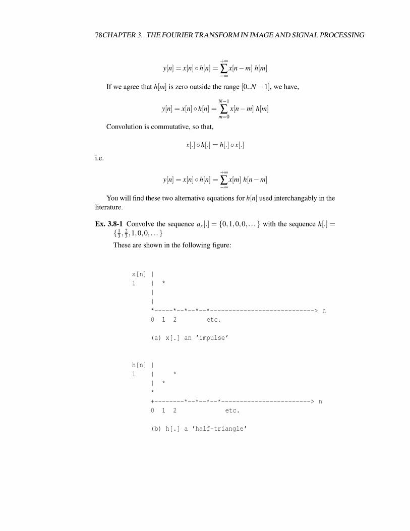
78CHAPTER 3. THE FOURIER TRANSFORM IN IMAGE AND SIGNAL PROCESSING
y[n] = x[n]h[n] =+∞
∑−∞
x[n−m] h[m]
If we agree that h[m] is zero outside the range [0..N−1], we have,
y[n] = x[n]h[n] =N−1
∑m=0
x[n−m] h[m]
Convolution is commutative, so that,
x[.]h[.] = h[.] x[.]
i.e.
y[n] = x[n]h[n] =+∞
∑−∞
x[m] h[n−m]
You will find these two alternative equations for h[n] used interchangably in theliterature.
Ex. 3.8-1 Convolve the sequence ax[.] = 0,1,0,0, . . . with the sequence h[.] = 1
3 , 23 ,1,0,0, . . .
These are shown in the following figure:
x[n] |1 | *
||*-----*--*--*--*----------------------------> n0 1 2 etc.
(a) x[.] an ’impulse’
h[n] |1 | *
| **+--------*--*--*--*------------------------> n0 1 2 etc.
(b) h[.] a ’half-triangle’

3.7. CONVOLUTION 79
hr[n] |1 * |
* |*
----------+--*--*--*--*--*--*---------------------> n-2 -1 0 1 2 etc.
(c) h[.] reversed - flipped about the n = 0 axis
Sequences for convolution – apply the following equation:
y[n] = x[n]h[n] =N−1
∑m=0
x[n−m].h[m]
y[n=0]: m=0 x[n-m].h[m] = x[0-0].h[0] = 0.1/3 =0m=1 x[0-1].h[1] = 0.2/3 =0m=2 x[0-2].h[2] = 0.1 =0
y[0] = 0========
y[n=1]: m=0 x[n-m].h[m] = x[1-0].h[0] = 1.1/3 =1/3m=1 x[1-1].h[1] = 0.2/3 =0m=2 x[1-2].h[2] = 0.1 =0
y[1] = 1/3==========
y[n=2]: m=0 x[n-m].h[m] = x[2-0].h[0] = 0.1/3 =0m=1 x[2-1].h[1] = 1.2/3 =2/3m=2 x[2-2].h[2] = 0.1 =0
y[2] = 2/3==========
y[n=3]: m=0 x[n-m].h[m] = x[3-0].h[0] = 0.1/3 =0m=1 x[3-1].h[1] = 0.2/3 =0m=2 x[3-2].h[2] = 1.1 =1

80CHAPTER 3. THE FOURIER TRANSFORM IN IMAGE AND SIGNAL PROCESSING
y[2] = 1==========
If you continue, you will find that the remainder of ys are zero.
Thus convolution can be done mechanically as follows:
– reverse (‘flip’) the convolution sequence h[n] about n = 0, i.e.
13 , 2
3 ,1 becomes 1, 23 , 1
3, call this hr[.], see above figure (c).
– For each point, n, in the input sequence (x[n]):
– – overlay hr[.] on x[.], with hr[.]’s rightmost point at n (i.e. hr[.] slides alongby one for each iteration),
– – multiply the corresponding values, hr[.]x[.],
– – sum the products
– – the sum is the convolved result at [n]
Summary: ‘flip’,
sum of products, slide right,
sum of products, slide right,
....
Ex. 3.8-2 Show that is the convolution of the ‘rectangular’ sequence 1,1,1,0,0,0,0,. . . with itself is a ‘triangular’ sequence; here we do it out mechanically:
1,1,1,0,0,0,0...1,1,1,0,0,0,0... (flip)
1
1,1,1,0,0,0,0...1,1,1,0,0,0,0... (slide, multiply, add)
2
1,1,1,0,0,0,0...1,1,1,0,0,0,0... (slide, multiply, add)
3
1,1,1,0,0,0,0...1,1,1,0,0,0,0... (slide, multiply, add)
2

3.7. CONVOLUTION 81
1,1,1,0,0,0,0...1,1,1,0,0,0,0...
1
1,1,1,0,0,0,0...1,1,1,0,0,0,0...
0
Thus, output is y[.] = 1,2,3,2,1,0,0,0...
y[n] |3 | *2 | * *1 * *
+-------------*--*------------------------> n0 1 2 etc.
3.7.2 Impulse Response
In digital signal processing, a sequence consisting of a single ‘1’ is called an ‘im-pulse’ sequence, see Ex. 3.8-1.
In the convolution operation, h[.] is called the impulse response. That is, if weconvolve an impulse sequence with h[.] we get an output identical to h[.].
Likewise, see Ex. 3.9-3, if we convolve any sequence, x[.], with an h[.] that isan impulse, we get an output identical to x[.]. This is easy to verify – replace h[.]in Ex. 3.8-2 with [1,0,0, . . . ] and work it out.
3.7.3 Linear Systems
Let y1[n] be the result of passing x1[n] through a ‘system’, and y2[.] the result ofx2[.] passing through the same system. Then if the system is linear, the result ofpassing
x[.] = x1[.]+ x2[.]
through the system isy[.] = y1[.]+ y2[.]
That is, we can add before or after the system.The term system is very general. We mean anything which applies processing
to a sequence.
82CHAPTER 3. THE FOURIER TRANSFORM IN IMAGE AND SIGNAL PROCESSING
In this chapter we deal almost exclusively with linear systems (system = filteror other similar processing); in Chapter 4 we will deal with some operations thatare not linear (e.g. median filtering).
Any filter or operation that can be applied by a straight convolution (one-dimensional, or two-dimensional) is sure to be linear; but if you do anything likesquaring, or taking absolute values, it becomes non-linear.
3.7.4 Some Interpretations of Convolution
1. Weighted sum: the output is a weighted sum of past inputs; i.e. weightedaccording to the impulse response.
2. Delayed impulses: any sequence is just a sum of delayed and weighted (i.e.have values other than 1) impulse sequences. Thus the convolution is just aweighted sum of delayed impulse responses. This is a consequence of thelinearity of convolution. Linear systems can always be completely definedby their impulse response.
3. Tapped Delay Line: a method of applying a weighted sum; of interest onlyto engineers.
Ex. 3.8-3 What is the result of convolving any sequence, x[.], with h[n] = 1,0,0,0, . . . ,i.e. h[.] is an impulse.
It may help to recall that: x[.]h[.] = h[.] x[.].
3.7.5 Convolution of Continuous Signals
For continuous signals convolution is given by:
y(t) = x(t)h(t) =
+∞Z
−∞
x(t1)h(t− t1)dt1
3.7.6 Two-Dimensional Convolution
Convolution can be extended to two-dimensions in a straightforward manner, iff [r,c] is the input image, h[r,c] the convolution kernel (or convolution mask), andg[r,c] the output image,
Recall that:
y[n] = x[n]h[n] =N−1
∑m=0
x[n−m]h[m]
g[.] = f [.]h[.]
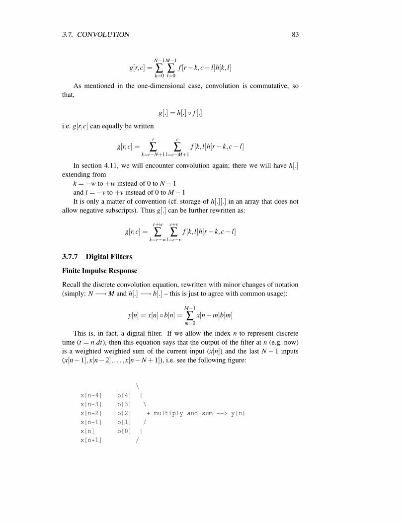
3.7. CONVOLUTION 83
g[r,c] =N−1
∑k=0
M−1
∑l=0
f [r− k,c− l]h[k, l]
As mentioned in the one-dimensional case, convolution is commutative, sothat,
g[.] = h[.] f [.]
i.e. g[r,c] can equally be written
g[r,c] =r
∑k=r−N+1
c
∑l=c−M+1
f [k, l]h[r− k,c− l]
In section 4.11, we will encounter convolution again; there we will have h[.]extending from
k =−w to +w instead of 0 to N−1and l =−v to +v instead of 0 to M−1It is only a matter of convention (cf. storage of h[.][.] in an array that does not
allow negative subscripts). Thus g[.] can be further rewritten as:
g[r,c] =r+w
∑k=r−w
c+v
∑l=c−v
f [k, l]h[r− k,c− l]
3.7.7 Digital Filters
Finite Impulse Response
Recall the discrete convolution equation, rewritten with minor changes of notation(simply: N −→M and h[.]−→ b[.] – this is just to agree with common usage):
y[n] = x[n]b[n] =M−1
∑m=0
x[n−m]b[m]
This is, in fact, a digital filter. If we allow the index n to represent discretetime (t = n.dt), then this equation says that the output of the filter at n (e.g. now)is a weighted weighted sum of the current input (x[n]) and the last N− 1 inputs(x[n−1],x[n−2], . . . ,x[n−N +1]), i.e. see the following figure:
\x[n-4] b[4] |x[n-3] b[3] \x[n-2] b[2] + multiply and sum --> y[n]x[n-1] b[1] /x[n] b[0] |x[n+1] /

84CHAPTER 3. THE FOURIER TRANSFORM IN IMAGE AND SIGNAL PROCESSING
x[n+2]
Another Way of Looking at Convolution
The above digital filter is called a finite impulse response (FIR) filter, becausethe impulse response is b[0] . . .b[M−1], which is clearly finite in duration; or non-recursive – for reasons which will become evident soon. If we were doing runningaverages over the last five samples, this would be
y[n] =15(x[n]+ x[n−1]+ x[n−2]+ x[n−3]+ x[n−4])
i.e. b[i] = 15 , i = 0, . . .4, and 0 otherwise.
Recursive or Infinite Impulse Response (IIR)
The general form for a recursive filter is:
y[n] =M−1
∑m=0
x[n−m]b[m]−K
∑k=1
y[n− k]a[k]
That is, to get the current output, we do a weighted sum of the last M inputs(as before), plus, we also use the last K outputs. Thus, the filter is called recursive;also infinite impulse response – because of the recursion, the impulse response is,theoretically, infinite in duration.
For M = 5 and K = 3, we have the situation depicted in the following figure:
\ y[n-5]x[n-4] b[4] | y[n-4]x[n-3] b[3] \ |a[3] y[n-3]x[n-2] b[2] + mult & sum + <---|a[2] y[n-2]x[n-1] b[1] / | |a[1] y[n-1]x[n] b[0] | +-------> y[n]x[n+1] /x[n+2]
Recursive Filter
Ex. 3.8-4 Express the moving average
y[n] =15(x[n]+ x[n−1]+ x[n−2]+ x[n−3]+ x[n−4])
as a recursive filter.
3.8. FOURIER TRANSFORMS AND CONVOLUTION 85
This can be reworked recursively as:
y[n] =15(5y[n−1]− x[n−5]+ x[n])
= y[n−1]− 15
x[n−5]+15
x[n]
i.e. K = 1,a[1] = 1
N = 5, b[0] = 15 , b[1] = 0, b[2] = 0, b[3] = 0, b[4] = 0, b[5] = 1
5 .
3.8 Fourier Transforms and Convolution
Although the DFT is useful in its own right, one of its greatest uses is as a tool forefficient computation of convolutions.
Let
y[n] = x[n]h[n] =N−1
∑m=0
x[n−m]h[m]
Then,
Y [u] = NX [u]H[u]
where:X [.] is the DFT of x[.]H[.] is the DFT of h[.]Y [.] is the DFT of y[.]N is the length of the DFT.
That is, convolution in the time or spatial domain is replaced by multiplicationin the frequency domain (except for the multiplicative factor 1/N).
Thus, we can do convolution as follows:
1. Take DFT of x[.]: X [u] = DFT(x[.])
2. Take DFT of h[.]: H[u] = DFT(h[.])
3. Multiply DFTs : Y [u] = X [u].H[u],u = 1, . . .N−1
4. Take InverseDFT of Y, multiplied by N : y[n] = IDFT(NY [.])
Why go to all this bother, when we have an easily applied formula for theconvolution? Unless we implement the DFT using the FFT there is no reason. Butwith the FFT there is great saving to be made.
Consider N = 1024, log2(1024) = 10(210 = 1024). Let us convolve h[.] andx[.], each 1024-long sequences.

86CHAPTER 3. THE FOURIER TRANSFORM IN IMAGE AND SIGNAL PROCESSING
(a) Calculations for straight convolution: N ∗N (multiplies + add) = 1 Million(b) Using FFT:
Step 1. FFT of x : N log2(N) complex operationsStep 2. FFT of h : dittoStep 3. Multiply X .H: N complex multiplies.Step 4. IFFT of Y : N log2(N) complex ops.
Thus, a total of (3N log2(N)+N) complex operations, assuming multiply takesnearly the same time as mult. + add., yielding = 3000.10 + 1000 complex ops. =31000.
Now if complex operations take about twice the time of ordinary, we have:62000 time units for the FFT method, compared to 1000000 for straight convolu-tion.
Thus, the FFT is 16 times faster.With larger signals, and with images (as we shall see), the savings are even
greater.
Ex. 3.9-1 The convolution of a rectangular sequence (see Ex. 3.8-2) 1,1,1,1,0,0,0,0....with itself is a triangular sequence (i.e. shaped like a triangle).
If the DFT of the rectangular sequence is a sin(x)/x function – see Gonzalez& Woods p.83, what is the DFT of a ‘triangle’.
Ex. 3.9-2 Verify that for h[.] = [1,0,0, ...] (an impulse), and for x[.] = anything, thefollowing equation makes good sense:
Y [u] = NX [u]H[u]
We will work with a sequence of length 8.
Recall Ex. 3.6-3, where we worked out the DFT of an impulse h[.] = [1,0,0,0 . . . ]:
----------------------------------------------u 0 1 2 3 4 5 6 7
---------------------------------------------H[u] 1/8 1/8 1/8 1/8 1/8 1/8 1/8 1/8----------------------------------------------
Therefore the right-hand side of the foregoing equation becomes:
= 8.X [u]. 18 = X [u]
Therefore Y [u] = X [u] u = 0,1 . . .7 and if we take the Inverse DFT (IDFT):
IDFT(Y [.]) = IDFT(X [.]) = x[.]

3.8. FOURIER TRANSFORMS AND CONVOLUTION 87
i.e. we have shown, via this exercise that the convolution of x[.] with animpulse is itself (unchanged). And, see section 3.8.2, we know this to betrue. So the equation to be demonstrated has been shown to be valid in thiscase.
Here is an example, from DataLab, of convolution via DFT, see section 3.7.2for a better description of the FFT function, ‘four1’.
for(i=1,c=cl;c<=ch;c++,i+=2)IMget(&val,d,r,c,ims1);data1[i]=val;data1[i+1]=0.0; /*zero complex part*/IMget(&val,d,r,c,ims2);data2[i]=val;data2[i+1]=0.0; /*zero complex part*/
/* now do fft */
four1(data1,len,-1);/* see Num. Rec. p 411NB. use of -1 for forward*/
four1(data2,len,-1);
/* now extract re and cmplx parts and multiply*/
for(i=1,c=cl;c<=ch;c++,i+=2)re1=data1[i];im1=data1[i+1];re2=data2[i];im2=data2[i+1];/* --- multiply DFTs --- */re=re1*re2-im1*im2;im=im1*re2+im2*re1;
four1(dt1,len,1); /* -- inverse DFT --- */
for(i=1,c=cl;c<=ch;c++,i+=2)re=dt1[i];IMput(&re,d,r,c,imd);

88CHAPTER 3. THE FOURIER TRANSFORM IN IMAGE AND SIGNAL PROCESSING
3.9 The Discrete Fourier Transform as a Matrix Trans-formation
Why is the DFT called a ‘transformation’?In section 3.2.1 we said that multiplying a vector by a matrix is a transforma-
tion, i.e.
y = Ax
with respective dimensions of these terms being (m×1),(m×n), and (n×1).If y is (N×1) and x is (N×1), A must be (N×N),
y = Ax
with respective dimensions of these terms being (N×1),(N×N), and (N×1).This can be expressed using summation as,
y[u] =N−1
∑n=0
aunx[n]
u = 0,1, . . .N−1 where aun is the element of A in row u, column ny[u] is the uth element of vector y, andx[n] is the nth element of vector x.
This equation is precisely the same form as one met earlier:
X [u] =1N
N−1
∑n=0
x[n]exp(− jπun/N)
u = 0,1 . . .N−1 where aun is now complex,
aun =1N
exp(− jπun/N)
But, as pointed out in sections 3.2.8 and 3.2.9, this makes no difference to thegeneral principle.
We repeat an earlier interpretation of the DFT, as follows: row u of the trans-formation matrix is made up of
cos(πun/N)− j sin(πun/N), n = 0,1 . . .N−1
i.e. the cos() part is the cosine-wave with frequency u, and ditto the sine part, againwith the same frequency. The values y[u] depend on how well x[.], the input signal,matches the sine and cosine waves.
Of course y[.] is now complex, with,
– the ‘real’ part corresponding to cos(u...)
– the imaginary part corresponding to sin(u..).

3.10. CROSS-CORRELATION 89
If you prefer, you can think of the transformation as being non-complex andhaving 2N rows, N rows corresponding to cosine terms, and N corresponding tosine terms. However, you can lose a lot of mathematical flexibility in this move.
As can be imagined, the Inverse DFT just applies the inverse matrix, B = At ,
bnu = exp( j.πnu/N)
Ex. 3.10-1 Check that the DFT and IDFT are indeed inverses of each other, i.e.find a few elements of
C = AB where A and B are as defined earlier in this section.
Check that C is, indeed, the identity matrix (see section 3.2.6), i.e. it has 1salong the diagonal, zero elsewhere.
Ex. 3.10-2 Verify that the DFT matrix is orthogonal, i.e. its transpose is its inverse(see section 3.2.7).
3.10 Cross-Correlation
The cross-correlation of two sequences is given defined as:
c[k] = x[n](c)y[n] =+∞
∑−∞
x[m]y[m+ k]
What we obtain from the cross-correlation is how well y[.], shifted right by kpoints, matches x[.].
For example, if x[.] is exactly the same shape as y[.], only delayed by 10 points,then c[.] above will exhibit a strong peak at c[k = 10].
Cross-correlation is the same as convolution only we do not ‘flip’ the correla-tion signal, y[.], prior to application; see section 3.8.1 for a discussion of convolu-tion, (and the ‘flip’).
Thus cross-correlation can be done efficiently using the FFT – see section 3.9;we just reverse one of the signals, before applying the DFT.
As we shall see later, there are a great many applications of cross-correlationin image processing:
1. Template matching.
We want to find if (or where) an object of a certain shape is in an image. First,we create an image containing the object – a ‘template’ (w[.], say). Thenwe cross-correlate the template with the image ( f [.]), to produce the cross-correlation image c[.]. Those pixels in c[.] that are greater than a threshold,correspond to centres of ‘matching’ objects in the image, i.e. objects thatmatch the template.
Obviously, ‘template-matching’ has many applications in 1-dimensional sig-nal processing, e.g. radar signal analysis, electrocardiogram analysis.
90CHAPTER 3. THE FOURIER TRANSFORM IN IMAGE AND SIGNAL PROCESSING
2. Image registration.
Two images, f1[.], and f2[.], represent the same scene, perhaps satellite im-ages taken at different dates. But, they are not registered, i.e. pixel [r,c]of f1[.] does not correspond to pixel [r,c] of f2[.]. Assume thay are shiftedin rows and columns, with respect to one another. Solution: cross-correlatethe two images, find the point of maximum correlation, the indices of thatpoint give the shifts. Clearly, also, there are many similar applications in 1-dsignals.
Ex. 3.11-1 The autocorrelation is the cross-correlation of a signal with itself,
axx[k] = x[n](c)x[n] =+∞
∑−∞
x[m]x[m+ k]
Explain how the DFT can be used to compute this.
3.11 The Two-Dimensional Discrete Fourier Transform
The two-dimensional DFT can be written down simply by extending the one-dimensional equation.
However, if we left it at that, we would miss a lot, in fact the two-dimensionalDFT can be applied by successive applications of the one-dimensional DFT – thisis why we spent so much time on the one-dimensional version.
For an N row ×M column input image f [r,c],c = 0 . . .M−1,r = 0 . . .N−1.
Two-Dimensional DFT:
F[u,v] = (1/MN)N−1
∑r=0
M−1
∑c=0
f [r,c]exp[− jπ(ur/(N + v)c/M)]
for u = 0,1 . . .N−1, and v = 0,1 . . .M−1.
Two-Dimensional Inverse DFT:
f [r,c] =N−1
∑u=0
M−1
∑v=0
F [u,v]exp[ jπ(ur/(N + v)c/M)]
for r = 0,1 . . .N−1, and c = 0,1 . . .M−1.
Interpretation of Two-dimensional DFT:
Remember that the uth component of the 1-dimensional version corresponds tohow well the input sequence matches the sine-wave, sin(πun/N) – imaginary part,and cos(πun/N) – real part.
The u,vth component of the 2-dimensional DFT corresonds to how well theinput image (2-dimensions) matches an image made up by multiplying a sine-wave,

3.12. THE TWO-DIMENSIONAL DFT AS A SEPARABLE TRANSFORMATION91
sin(πur/N), along the columns, by a sine-wave, sin(πvc/M) along the columns;ditto the cosine part. Thus, recalling our interpretation of the one-dimensionalDFT in section 3.6:
“The components near the beginning of the DFT correspond to the ‘slowlyvarying’ parts of the signal; the components near the middle, the ‘fast moving’parts”.
The same is true for the two-dimensional, only now we have to think of relative‘speed of variation’ in two-dimensions.
3.12 The Two-Dimensional DFT as a Separable Transfor-mation
In section 3.10 we saw that the one-dimensional DFT could be written as a matrixtransformation,
y = Ax
of respective dimensions (N×1),(N×N),(N×1).Things are more complicated for the two-dimensional version, but only just.
To write the two-dimensional DFT
F [u,v] = (1/MN)N−1
∑r=0
M−1
∑c=0
f [r,c]exp[− jπ(ur/(N + v)c/M)]
in matrix form, we have to observe that the transformation kernel,
exp[− jπ(ur/(N + v)c/M)]
can be separated into a ‘row part’, exp[− jπ(ur/N)], and a ‘column part’, exp[− jπ(vc/M)],by noting that,
exp[− jπ(ur/(N + v)c/M)] = exp[− jπur/N]exp[− jπvc/M]
The consequence is that F[u,v] can be written in matrix form as
F[u,v] = P f Q
of respective dimensions (N×M),(N×N),(N×M),and(M×M).Matrix Q is just the (M×M) one-dimensional DFT matrix (kernel) that corre-
sponds to DFTing each row. Matrix P is the (N×N) one-dimensional DFT matrixthat corresponds to DFTing each column. For this reason the two-dimensional DFTcan be said to be separable.
We will encounter other separable operators, i.e. those that can be separatedinto two sets of one-dimensional operations (one for rows, one for columns). Sep-arable operators are particularly important because they generally require O(N 3)operations, while non-separable operations require O(N 4).
92CHAPTER 3. THE FOURIER TRANSFORM IN IMAGE AND SIGNAL PROCESSING
Note that, if N = 1024,N3 = 1000 million, N4 = 1,000,000 million (i.e. 1000times more). If an O(N3) operation takes one minute, an O(N4) operation takesnearly 17 hours.
Of course, for the DFT, we can use the FFT and achieve even greater savings,i.e. O(N3)−→ O(N2 logN). If N = 1024,N2 log N = 10,000,000 = 10 million.
Thus, 1 million million, reduces to 10 million!The matrix form of the DFT looks a bit horrendous, but becomes more placid
if we approach it one step at a time:
(a) DFT each column, individually, forgetting that it is part of an image; i.e.apply Q to f .
Result: (N×M) image f ′ with the columns now DFTs.(b) Now DFT each row of image f ′, again individually.Result: Image F[u,v] that is the two-dimensional DFT of f [r,c].
The same considerations apply to the Inverse transform.
3.13 Other Transforms
3.13.1 General
A good many other transforms are used in image and signal processing. They allobey the same principles seen for the DFT in the one-dimensional case or in thetwo dimensional case; only the matrix kernels, A, in one-dimensional, or P and Qin 2-dimensional, change.
y = Ax
of respective dimensions (N×1),(N×N)and(N×1).
F[u,v] = P f Q
of respective dimensions (N×M),(N×M),(N×M)and(M×M).As mentioned above, only transformations that are separable are of much in-
terest; indeed, again for performance reasons, we are often interested only in trans-forms that have ‘fast’ implementations, like the FFT; i.e. O(N log N) operationsinstead of O(N2).
3.13.2 Discrete Cosine Transform
The one dimensional Discrete Cosine transform (DCT) is given by,
Xc(u) = (2au/N)N−1
∑n=0
x[n]cos πu(2n+1)/(2N)]
where au = 1/√
(2), for u = 0; = 1 , for u = 1,2 . . .N−1.That is we are using cosine functions, only, as a basis for the transform.

3.13. OTHER TRANSFORMS 93
The Inverse DCT is given by
x[n] =N−1
∑n=0
auXc[u]cos πu(2n+1)/(2N)]
The major interest in the DCT is for image compression, where, for a largeclass of images, it can be shown to offer better compression than the DFT.
The DCT forms the basis of a major image compression standard being pro-moted by a world authority, the Joint Photographic Experts Group (JPEG).
The DCT can be implemented using a double sized FFT, see Rosenfeld andKak Vol 1. p. 155; the only significance of this statement is that we have a ‘fast’algorithm for the DCT.
3.13.3 Walsh-Hadamard Transform
We return to the matrix version of transforms, as given by
y = Ax
of respective dimensions (N×1),(N×N)and(N×1).We can write the matrix for the Walsh-Hadamard transform entirely in terms
of +1s and −1s, e.g.
2x2 Hadamard:
A(2x2) = 1 11 -1
(8×8) Walsh-Hadamard transform: aun is given by the following table:
--------------------------------------------n 0 1 2 3 4 5 6 7
u--------------------------------------------0 + + + + + + + +1 + - + - + - + -2 + + - - + + - -3 + - - + + - - +4 + + + + - - - -5 + - + - - + - +6 + + - - - - + +7 + - - + - + + ---------------------------------------------
Walsh-Hadamard Transform Kernel for N=8
94CHAPTER 3. THE FOURIER TRANSFORM IN IMAGE AND SIGNAL PROCESSING
Examination of this table indicates the nature of the Walsh-Hadamard trans-form – the basis waveforms are ‘square-wave’ in form, compared to the sine/cosinewaves of the DFT. In Walsh-Hadamard transforms we speak of sequency, as a gen-eralised frequency.
The Walsh-Hadamard transform has a ‘fast’ implementation; in addition, sincethe elements of the matrices are either +1, or −1, no multiplication is required.
As with the DCT, the major interest in the Walsh-Hadamard transform is imagecompression.
3.14 Applications of the Discrete Fourier Transform
3.14.1 Introduction
This section discusses the applications of the DFT. Since we have shown the strongrelationship between he one-dimensional DFT and the two-dimensional version,and, having noted their analogous properties, we will sometimes discuss just theDFT and make no distinction between one-, and two-dimensions. Often we work inone-dimension for simplicity of notation; extention to two-dimensions is generallystraightforward.
The major applications are:
1. Analysis of images and signals. That is analyse the frequency content, forexample, compute the amplitude spectrum, or power spectrum.
2. Filtering.
3. As a tool for ‘fast’ computation of convolutions, and correlations.
4. In data compression.
5. In template matching and image registration (i.e. using correlation).
6. Various applications related to description of one-, and two-dimensionalshapes; of particular importance, here, is the shift invariant property of theDFT power-spectrum.
7. Image restoration and deblurring.
Since Chapter 3 is already very long, we will try to be brief! You are stronglyencouraged to glance at the recommended texts – these give many good examples,especially pictures, which we cannot reproduce here.
In what follows,
F[u] is the DFT of sequence f [n],F[u,v] is the 2-dimensional DFT of image f [u,v],Fc[u] refers to cosine ‘parts’,Fs[u] refers to sine.
3.14. APPLICATIONS OF THE DISCRETE FOURIER TRANSFORM 95
3.14.2 Frequency Analysis
The power spectrum given by
P[u] = Fc[u]2 +Fs[u]2
This gives an estimate of the relative ‘strength’, in the sequence, of frequencyu.
In two-dimensions, P[u,v] gives the relative strength of cross terms, e.g. alow (slowly varying) frequency along the rows, a high (rapidly varying) frequencyalong the columns.
3.14.3 Filtering
Filtering refers to frequency filtering. A low-pass filter is an operation which,when applied to a sequence, rejects all high-frequencies, and ‘passes’ all low, i.e.it ‘smoothes’ the input. A low-pass filter is defined by two parameters:
• the cut-off frequency,
• the rate of cutoff.
A high-pass filter does the opposite, it rejects low-frequencies, and passes high,i.e. ‘sharpens’ the input.
A band-pass filter passes intermediate frequencies, e.g. in a telephone systemvery low frequencies, below about 300 Hz, and high frequencies, above about 3000Hz, are attenuated. That is, a band-pass filter with cut-off frequencies at 300 Hzand 3000 Hz is used.
Filters can be applied in the spatial domain (or time domain) or in the frequencydomain.
Spatial domain filters are applied using convolution, see Chapter 4.Frequency domain filters are applied by:
1. taking the DFT, x[n] −→ X [u],
2. multiplying the DFT array by an array of weights,
X ′[u] = F[u]X [u],u = 0,1, . . .N−1
3. applying the IDFT, X ′[u]−→ y[n], the filtered output sequence.
For a low-pass filter: F [u] = 1.0 , for u < cutoff, and F[u] = 0.0, above cutoff.For a high-pass filter: F[u] = 0.0 , for u < cutoff, and F[u] = 1.0, above.In practical cases more tapered weighting may be applied.In the two-dimensional case, similarly, we define pass and reject regions in the
(u,v) plane.
96CHAPTER 3. THE FOURIER TRANSFORM IN IMAGE AND SIGNAL PROCESSING
3.14.4 Fast Convolution
We have already indicated in section 3.9 that the FFT can be used to perform fastconvolutions:
If
y[n] = x[n]h[n] =+∞
∑−∞
x[n−m]h[m]
then,Y [u] = X [u]H[u]
That is, convolution in the time or spatial domain is replaced by multiplicationin the frequency domain.
Thus, we can do convolution as follows:
1. Take DFT of x[.]: X [u] = DFT(x[.])
2. Take DFT of h[.]: H[u] = DFT(h[.])
3. Multiply DFTs : Y [u] = X [u]H[u] , u = 1, . . .N−1
4. Take InverseDFT of Y : y[n] = IDFT(Y [.])
For N×M images, each of the arrays above, X [.],H[.],Y [.] are two-dimensional.The multiplication in step (3) becomes:
Y [u,v] = X [u,v]H[u,v]
for u = 0,1,2 . . .N−1, v = 0,1,2 . . .M−1.
3.14.5 Fast Correlation
If we observe that cross-correlation (sometimes called just correlation), defined as,
c[k] = x[n](c)y[n] =+∞
∑−∞
x[m]y[m+ k]
is ‘convolution’ with one of the sequences reversed, then the method given in sec-tion 3.15.4 can be used to provide ‘fast’ correlation, i.e. we only require the pre-liminary reversal,
x[i] = x[N−1− i], i = 0,1 . . .N−1
Again, the extension to two-dimensions is straightforward.Note: the reversal is not really neccessary. Examine the DFT as given by
X [u] = (1/N)N−1
∑n=0
x[n]exp(− jπun/N)
3.14. APPLICATIONS OF THE DISCRETE FOURIER TRANSFORM 97
Arguing qualitatively, reversing x[n] is equivalent to setting n =−n , in exp().Now,
exp( jB) = cos B+ j sinB
exp(− jB) = cosB− j sinB
i.e. exp( jB) is the complex conjugate of exp(− jB),so that the DFT of the reversed sequence is the complex conjugate of X [u], writtenX∗[u].
Thus, for correlation, we replace,
3. Multiply DFTs : Y [u] = X [u]H[u] , u = 1, . . .N−1
with,
3. Multiply complex conjugate of DFT of x[.], with DFT of H[.] : Y [u] =X [u]H[u] , u = 1, . . .N−1
3.14.6 Data Compression
Generally speaking, observe that the ‘large’ components of an image are moreimportant to human viewers, in the majority of cases, for the majority of uses.Observe, also, the ready acceptance of fairly blurred pictures in newspapers, or asfamily snaps – the usefullness of the picture is only slightly degraded by lack ofsharpness.
The essence of data compression (image data compression, signal compres-sion, or any other) is to reduce the amount of data to be transmitted, stored, etc.
Now recall that the DFT of an N×N image has, itself, N×N data elements, andthat the original image can be reconstructed from the DFT by applying the IDFT.Consider, then, dispensing with some of the higher frequencies, say K of them.Now we have only N−K DFT data elements to transmit. We can reconstruct usingthe IDFT, the only loss will be in a slight smoothing of the image (equivalent tolow-pass filtering).
This is a very qualitative argument – but you can see what is happening. If weremoved K rows, or K columns, or K arbitrary pixels from an image, the efffectwould be enormous, by removing K elements from the DFT, the effect is muchless, or, at least, much more subtle.
The Discrete Cosine and Walsh-Hadamard transforms can be used in an anal-ogous manner.
3.14.7 Deconvolution
Deconvolution is the process of restoring an image (or signal) that has been sub-jected to (unwanted) degradation by convolution. Usually this takes the form ofblurring.
The convolution,
98CHAPTER 3. THE FOURIER TRANSFORM IN IMAGE AND SIGNAL PROCESSING
y[n] = x[n]h[n] =+∞
∑−∞
x[n−m]h[m]
is not, in general, reversible.If we have y[n], the result of convolving a wanted signal x[n] with some ‘un-
wanted’ operator (e.g. blurring), and we don’t know the operator’s impulse re-sponse, h[.], we have very little chance – but see below. It is as if we have the sumof ten numbers, and are asked to estimate what are the individuals that were usedto make up the sum – impossible!
If, however, we know h[.], or can estimate it, we can use the DFT to deconvolveh[.] (invert the convolution) as follows:
1. If the observe that Y [u] = X [u].H[u] (convolution −→ multiplication in fre-quency domain),
2. therefore, using h[n], or an estimate of it, compute using the DFT, H[u].
3. Compute X ′[u] = Y [u]/H[u] , u = 0,1...N− 1 (i.e. you can ‘cancel-out’ theeffects of the convolution, in the frequency domain),
4. obtain the ‘restored’ x[n], using the IDFT.
The extension to two-dimensions is again straightforward.
Ex. 3.15-1 An amateur photographer chances upon a bank robbery. As the rob-bers’ van speeds past him he takes a photograph of the side of the van. Whenprinted the photograph turns out to be blurred – the photographer forgot to‘pan’ with the moving van; thus the photograph has been ‘convolved’ with asmoothing function. The sign on the van cannot be read.
Assuming the the smoothing was along the horizontal (i.e. along the rows)suggest a digital image processing method for restoring the image. (Theimage is scanned at 100 pixels per inch, the smoothing appears to be about1/10 inch wide, i.e. 10 pixels).
Suggest a restoration technique.
Ex. 3.15-2 If, in the previous question, the smoothing was not along the horizon-tal, how could we remedy the situation. (The processing is simpler if thesmoothing is along one dimension, only).
Ex. 3.15-3 Suggest a way in which we might estimate the blurring function. Hint:if the van was black, and there was a shiny bright spot somewhere in the fieldof view of the photograph,...?
The Hubble Space Telescope was launched by the shuttle in 1989. Unfor-tunately, the optics had not been tested properly, and the resulting imageswere blurred. From a knowledge of the source defect, and, by examining

3.15. QUESTIONS ON CHAPTER 3 – THE FOURIER TRANSFORM 99
actual blurred results, it was possible to estimate the blurring function, and,by deconvolution, to partially restore the images.
Deconvolution (1-D sound signals) is also very important in oil prospecting.
3.15 Questions on Chapter 3 – the Fourier Transform
TBD

100CHAPTER 3. THE FOURIER TRANSFORM IN IMAGE AND SIGNAL PROCESSING
Chapter 4
Image Enhancement
4.1 Introduction
Whenever an image passes through a ‘system’, i.e. gets sensed, and/or digitised,and/or compressed and decompressed, and/or transmitted, and/or displayed, the‘quality’ of the image may be degraded in some way – for example, the addition ofnoise. Image enhancement is about the improvement of the ‘quality’ of the image– usually an attempt at returning it to some ‘original’ state.
Of course, quality is subjective – it depends on what the (human or machine)user/observer intends to use the image for. Indeed, the original image may be oflow quality from a few points of view, but we are content with this, and all we wantto do is highlight (enhance) some features of the image – i.e. improve the qualitywith respect to one particular criterion.
In general, the improvement of quality – no matter what the criterion for im-provement – will usually be called image enhancement; and so to some extent thischapter contains a fairly mixed bag of techniques and processes.
In this chapter we will cover two broad categories of image enhancement: point(or pixel, or grey level) operations, and spatial operations (or neighbourhood oper-ations).
1. Point operations
We apply some function to each pixel value, individually, to yield a newvalue; there is a net enhancement effect on the image viewed as a whole,even though the global relationship between pixel values is ignored. In thiscategory, the enhancement is usually for the benefit of a human observer, andthe enhancement is often connected with contrast enhancement (e.g. turningup the contrast on a TV monitor – see section 2.7 for a definition of contrast).
We differ from Gonzalez and Woods in calling these point operations – they(incorrectly, and in disagreement with most authors) call them spatial opera-tions.
2. Spatial operations
101
102 CHAPTER 4. IMAGE ENHANCEMENT
Here we apply a function to a pixel and its neighbours, to yield a new valuefor the pixel; the function takes into account the relationship between thevalue of the pixel and the values of its neighbours – thus spatial or neigh-bourhood operations. Broadly speaking, spatial operations come in two cat-egories: smoothing, and sharpening.
Sections 4.3–4.10 will cover point operations, and from section 4.11 onwardswe will be dealing with spatial operations.
In general this chapter will concentrate on the ‘enhancement’ operations, e.g.smoothing out noise, enhancement of edges. We will leave it to later chapters andlectures to apply further processing to the enhanced images, e.g. application ofa threshold to an edge-enhanced image, to produce edge points, tracing a path ofedge points, segmentation etc.
But first we must look a little more closely at noise.
4.2 Noise and Degradation
Figure 4.1 shows an image passing through a system. At any stage in the system‘noise’ may be added. Here we are using ‘noise’ in a very general sense – i.e. anydegradation. It could be the type of noise mentioned in Chapter 1 – i.e. randomnumbers added to the actual image numbers; it could be thumbprint on a photo-graph, or grain, or streaks on a negative, or any form of sensor noise, or as on aTV electrical noise, caused by, e.g., electromagnetic noise from a starter motor thatgets onto the TV transmission signal.
In general, noise is data that we don’t want!
Additive noise: More often than not, noise is additive, i.e. the ‘noisy’ image is thetrue, noiseless, image with noise added; thus
f (r,c) = ftrue(r,c)+n(r,c) (4.1)
where ftrue(., .) is the true, noiseless image n(., .) is a noise image, e.g. as gener-ated by DataLab ‘ggn’.
Incidentally, not only is additive noise very common, but it is also the mosteasy analyzed and dealt with.
Reduction of additive noise is covered in Section 4.10.
Non-additive noise: Some of image restoration deals with removal of non-additivenoise; examples are: noise ‘convolved’ into an image – blur is a good example; gaincalibration errors on a CCD camera is an example of multiplicative noise. (Note –bias is additive).
If you think of an audio channel as conveying a sequence of data (albeit ana-logue), then hiss, crackle, or clicks are all undesirable data added to the ‘wanted’data – the voice or music – i.e. noise. The noise obscures the wanted data. The

4.2. NOISE AND DEGRADATION 103
Scene|
Light |∨
Sensor ←− Noise|
Voltage |∨
Digitize ←− Noise|
Numbers |∨
Code ←− Noise||∨
Transmit ←− Noise||∨
Decode ←− Noise||∨
Display ←− Noise
Figure 4.1: From top to bottom: image passing through a system.
104 CHAPTER 4. IMAGE ENHANCEMENT
noise that causes hiss on an audio channel shares many characteristics with thenoise that causes ‘snow’ on a TV screen; and both are very similar to the imagenoise shown in Chapter 1.
It is not surprising, therefore, that many noise reduction processes in imageprocessing have been borrowed from analogue (and, more recently, digital) signalprocessing.
4.3 Point Operations
4.3.1 Grey Level Mapping by Lookup Table
The simplest form of point operation. Suppose you have an image whose data is allsquashed in the range 0 to 10; it won’t look like much when displayed on a 0–255display; it will have low contrast and look grey and muddy.
A simple solution is to form and apply a lookup table as follows:
#define MAX 11int lut[MAX]=0,25,50,...250;
#define NROW 64#define NCOL 64unsigned char f1[NROW][NCOL],f2[NROW][NCOL];int rl,rh,cl,ch,r,l;float val;int ival,ival2;
/* read in image...*/.....
rl=0;rh=NROW-1;cl=0;ch=NCOL-1;for(r=rl;r<=rh;r++)
for(c=cl;c<=ch;c++)ival=f1[r][c];if(ival<=0)ival2=lut[0];else if(ival>MAX)ival2=lut[MAX];else ival2=lut[ival];f2[r][c]=ival2;
The example above is rather trivial, since multiplying by 25 would do the same.But, lookup tables are useful in many circumstances:
1. it may be desirable to leave the original image unaffected and send the datato display via a LUT,
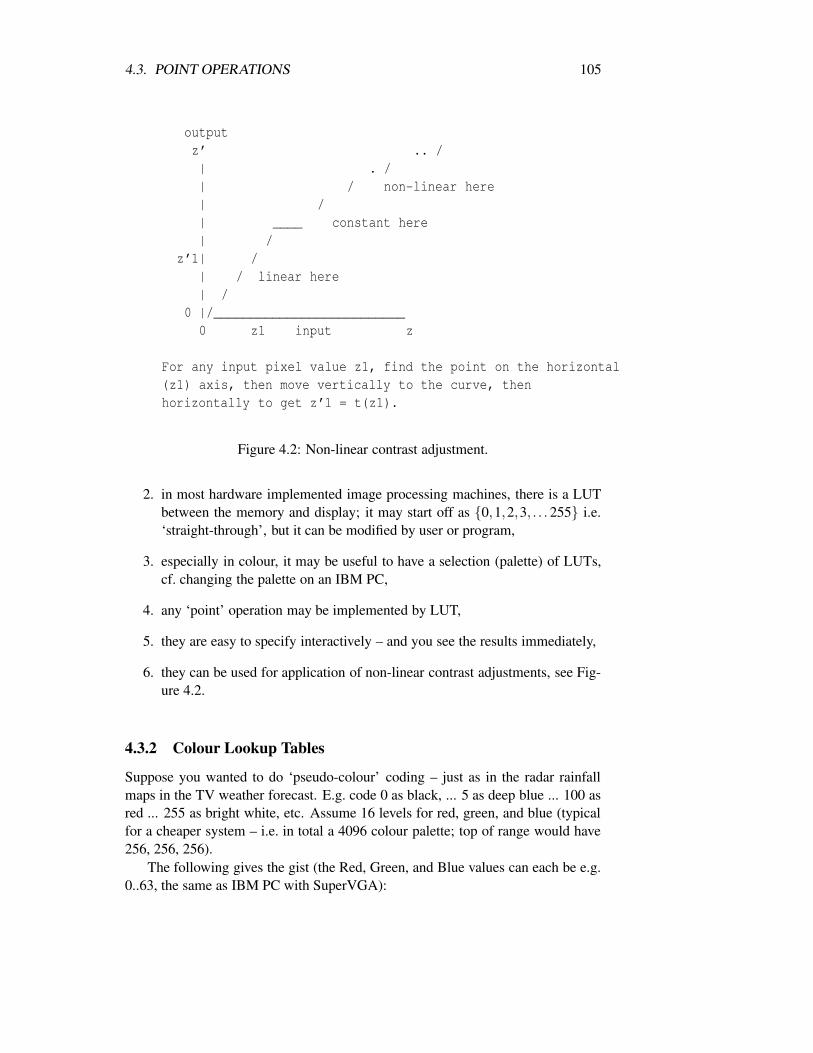
4.3. POINT OPERATIONS 105
outputz’ .. /| . /| / non-linear here| /| ____ constant here| /
z’1| /| / linear here| /
0 |/__________________________0 z1 input z
For any input pixel value z1, find the point on the horizontal(z1) axis, then move vertically to the curve, thenhorizontally to get z’1 = t(z1).
Figure 4.2: Non-linear contrast adjustment.
2. in most hardware implemented image processing machines, there is a LUTbetween the memory and display; it may start off as 0,1,2,3, . . . 255 i.e.‘straight-through’, but it can be modified by user or program,
3. especially in colour, it may be useful to have a selection (palette) of LUTs,cf. changing the palette on an IBM PC,
4. any ‘point’ operation may be implemented by LUT,
5. they are easy to specify interactively – and you see the results immediately,
6. they can be used for application of non-linear contrast adjustments, see Fig-ure 4.2.
4.3.2 Colour Lookup Tables
Suppose you wanted to do ‘pseudo-colour’ coding – just as in the radar rainfallmaps in the TV weather forecast. E.g. code 0 as black, ... 5 as deep blue ... 100 asred ... 255 as bright white, etc. Assume 16 levels for red, green, and blue (typicalfor a cheaper system – i.e. in total a 4096 colour palette; top of range would have256, 256, 256).
The following gives the gist (the Red, Green, and Blue values can each be e.g.0..63, the same as IBM PC with SuperVGA):

106 CHAPTER 4. IMAGE ENHANCEMENT
Red Green Blueint lut[3][256]= 0, 0, 0, /*0,0,0 = black*/
0, 0, 10, /*add some blue*/0, 0, 20, /*and some more*/
...0, 10, 0, /*now green*/0, 20, 0, /*and some more*/
...0, 63, 0, /*very bright green*/
15, 0, 0, /* red*/...
63, 0, 0, /*bright red */
10, 10, 10, /*dark grey*/
30, 30, 30, /*lighter grey*/
63, 63, 63 /* bright white*/
Now, apply LUT:
for(r=rl;r<=rh;r++)for(c=cl;c<=ch;c++)
ival=f1[r][c];forb=0;b<=2;b++
f2[b][r][c]=lut[b][ival]; /*f2 is the outputcolour image*/
Again, as noted in section 4.3, LUTs are:(1) easy to do in hardware,(2) easy to specify interactively.
Exercises: [see Chapters 1 and (especially) 2 for some discussion of colour].
Ex. 4.4-1 Describe, in English, what colour would appear for:
(a) red=63, green=63, blue=0.
(b) red=5, green=5, blue=5.
(c) red=63, green=63, blue=63.

4.3. POINT OPERATIONS 107
(d) if red=30, green=30, blue=50 is light blue, what is red=50, green=30,blue=30 Hint: think additive (see Chapter 2).
Ex. 4.4-2 Suggest, in English, a colour coding scheme for coding magnitude (ex-amples: temperature on a map, altitude on a map, rainfall, etc.).
4.3.3 Greyscale Transformation
This section is a slight generalization of section 4.3.A lookup table is nothing more than a discrete function; again, the terms func-
tion and transformation are used interchangeably. Expressed as a function, thetransformation from input image to output image is z′ = t(z) where z′ is outputpixel value, z the input value, i.e. z = 0 . . . zG,z′ = 0 . . . zG, replacing G ofChapter 1 with zG, and t(.) is the transformation function.
Suppose, as in section 4.3, the input image does not occupy the full dynamicrange, e.g., an “underexposed” photograph.
Suppose, a≤ f1(x,y)≤ b, i.e. the range of f1() is [a,b], and you want the rangestretched to z0 ≤ z′ ≤ G, then the transformation is
z′ = (zG− z0).(z−a)/(b−a)+ z0 = (zG− z0).z/(b−a)+(z0.b− zG.a)/(b−a)(4.2)
The right hand side terms are respectively scale and shift terms.Equation 4.2 is a simple linear transformation which stretches and shifts the
original greyscale [a,b] to [z0,zG]. If you are familiar with graphics transformationsyou will recognise a one-dimensional shift and scale.
Now suppose that most of the input pixels are in the range [a,b], and thoseoutside are only due to noise, or some uninteresting artifact. Then we can usez′ = (zG− z0).(z− a)/(b− a) + z0 , for a ≤ z ≤ b, z′ = z0 for z < a, and finallyz′ = zG for z > b.
This stretches [a,b] as before, but compresses intervals [z0,a] and [b,zG] intosingle points, z0, and zG, respectively.
In addition, there is nothing to stop you applying different linear transforma-tions to many regions of the greyscale: see exercises.
Ex. 4.5-1 Let a = 0, b = 10, z0 = 0, and zG = 255 – we want to stretch the inputrange [0,10] to an output range of [0,255]. Thus equation 4.2 becomes:
z′ = (255−0).(z−0)/(10−0)+0 = 25.5∗ z (4.3)
I.e. we need no shift, and a scaling by a factor of 25.5.
Ex. 4.5-2 Let a = 15, b = 35, z0 = 0, and zG = 255 – we want to stretch the inputrange [15,35] to an output range of [0,255].
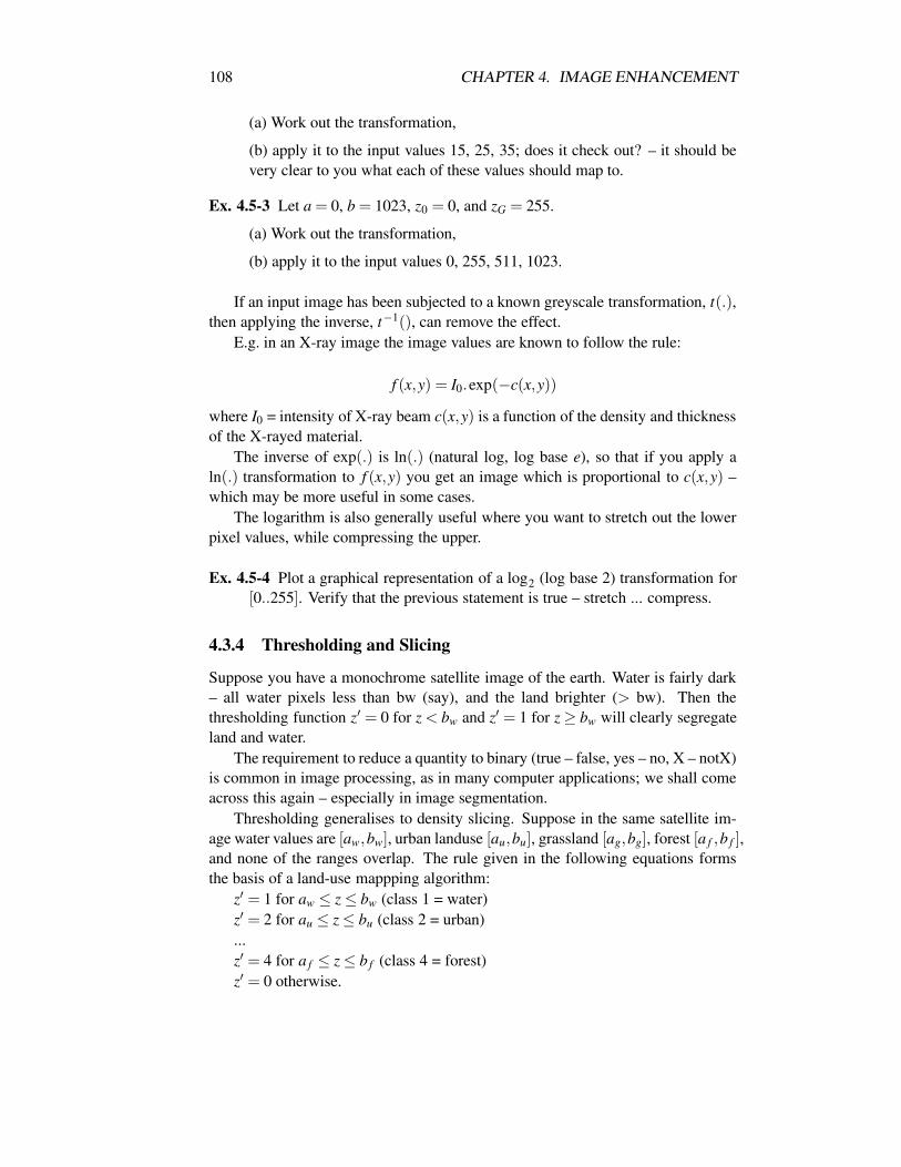
108 CHAPTER 4. IMAGE ENHANCEMENT
(a) Work out the transformation,
(b) apply it to the input values 15, 25, 35; does it check out? – it should bevery clear to you what each of these values should map to.
Ex. 4.5-3 Let a = 0, b = 1023, z0 = 0, and zG = 255.
(a) Work out the transformation,
(b) apply it to the input values 0, 255, 511, 1023.
If an input image has been subjected to a known greyscale transformation, t(.),then applying the inverse, t−1(), can remove the effect.
E.g. in an X-ray image the image values are known to follow the rule:
f (x,y) = I0.exp(−c(x,y))
where I0 = intensity of X-ray beam c(x,y) is a function of the density and thicknessof the X-rayed material.
The inverse of exp(.) is ln(.) (natural log, log base e), so that if you apply aln(.) transformation to f (x,y) you get an image which is proportional to c(x,y) –which may be more useful in some cases.
The logarithm is also generally useful where you want to stretch out the lowerpixel values, while compressing the upper.
Ex. 4.5-4 Plot a graphical representation of a log2 (log base 2) transformation for[0..255]. Verify that the previous statement is true – stretch ... compress.
4.3.4 Thresholding and Slicing
Suppose you have a monochrome satellite image of the earth. Water is fairly dark– all water pixels less than bw (say), and the land brighter (> bw). Then thethresholding function z′ = 0 for z < bw and z′ = 1 for z≥ bw will clearly segregateland and water.
The requirement to reduce a quantity to binary (true – false, yes – no, X – notX)is common in image processing, as in many computer applications; we shall comeacross this again – especially in image segmentation.
Thresholding generalises to density slicing. Suppose in the same satellite im-age water values are [aw,bw], urban landuse [au,bu], grassland [ag,bg], forest [a f ,b f ],and none of the ranges overlap. The rule given in the following equations formsthe basis of a land-use mappping algorithm:
z′ = 1 for aw ≤ z≤ bw (class 1 = water)z′ = 2 for au ≤ z≤ bu (class 2 = urban)...z′ = 4 for a f ≤ z≤ b f (class 4 = forest)z′ = 0 otherwise.
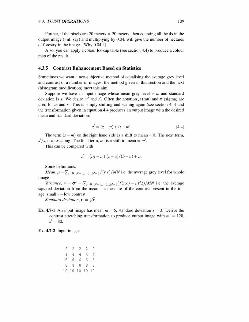
4.3. POINT OPERATIONS 109
Further, if the pixels are 20 meters × 20 meters, then counting all the 4s in theoutput image (=nf, say) and multiplying by 0.04, will give the number of hectaresof forestry in the image. [Why 0.04 ?]
Also, you can apply a colour lookup table (see section 4.4) to produce a colourmap of the result.
4.3.5 Contrast Enhancement Based on Statistics
Sometimes we want a non-subjective method of equalising the average grey leveland contrast of a number of images; the method given in this section and the next(histogram modification) meet this aim.
Suppose we have an input image whose mean grey level is m and standarddeviation is s. We desire m′ and s′. Often the notation µ (mu) and σ (sigma) areused for m and s. This is simply shifting and scaling again (see section 4.5) andthe transformation given in equation 4.4 produces an output image with the desiredmean and standard deviation:
z′ = (z−m).s′/s+m′ (4.4)
The term (z−m) on the right hand side is a shift to mean = 0. The next term,s′/s, is a rescaling. The final term, m′ is a shift to mean = m′.
This can be compared with
z′ = (zG− z0).(z−a)/(b−a)+ z0
Some definitions:Mean, µ = ∑r=0...N−1,c=0...M−1 f (r,c)/MN i.e. the average grey level for whole
imageVariance, v = σ2 = ∑r=0...N−1,c=0...M−1( f (r,c)− µ)22)/MN i.e. the average
squared deviation from the mean – a measure of the contrast present in the im-age; small v – low contrast.
Standard deviation, σ =√
v
Ex. 4.7-1 An input image has mean m = 5, standard deviation s = 3. Derive thecontrast stretching transformation to produce output image with m′ = 128,s′ = 80.
Ex. 4.7-2 Input image:
2 2 2 2 24 4 4 4 46 6 6 6 68 8 8 8 810 10 10 10 10

110 CHAPTER 4. IMAGE ENHANCEMENT
(a) What is mean, m? (b) What is standard deviation, s? (c) Derive thetransformation to yield mean, m′= 128, standard deviation s′ = 80. (d) Thencompute the output image. (e) Will it fit into [0,255]? If not, ‘clip’ values< 0 to 0, and values > 255 to 255.
4.3.6 Histogram Modification
First some definitions.A histogram is a table, with an entry for each possible pixel value, giving the
number of pixels which have that value; usual notation:
h(z),z = [z0 . . . zG]
∑z=z0..zG
h(z) = M.N
for an M×N image.
Ex. 4.8-1 Input image
2 2 2 2 24 4 4 4 46 6 6 6 68 8 8 8 810 10 10 10 10
Thus: h(0) = 0, h(1) = 0, h(2) = 5, h(4) = 5,... h(10) = 5, all others = 0.
A histogram is usually shown as a graph as follows (graph on its side):
0 5-----------------------> p
0|1|2|*****||*****||*****||*****|
10|*****
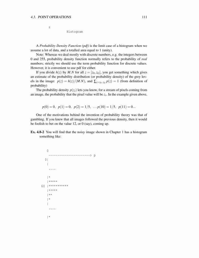
4.3. POINT OPERATIONS 111
zHistogram
A Probability Density Function (pdf) is the limit case of a histogram when weassume a lot of data, and a totalled area equal to 1 (unity).
Note: Whereas we deal mostly with discrete numbers, e.g. the integers between0 and 255, probability density function normally refers to the probability of realnumbers; strictly we should use the term probability function for discrete values.However, it is convenient to use pdf for either.
If you divide h(z) by M.N for all z = [z0,zG], you get something which givesan estimate of the probability distribution (or probability density) of the grey lev-els in the image: p(z) = h(z)/(M.N), and ∑z=z0..zG p(z) = 1 (from definition ofprobability)
The probability density p(zi) lets you know, for a stream of pixels coming froman image, the probability that the pixel value will be zi. In the example given above,
p(0) = 0, p(1) = 0, p(2) = 1/5, . . . p(10) = 1/5, p(11) = 0...
One of the motivations behind the invention of probability theory was that ofgambling. If you knew that all images followed the previous density, then it wouldbe foolish to bet on the value 12, or 0 (say), coming up.
Ex. 4.8-2 You will find that the noisy image shown in Chapter 1 has a histogramsomething like:
0-----------------------> p
0||....
|*|*****
60 |***********|*****|**|*|....
|*
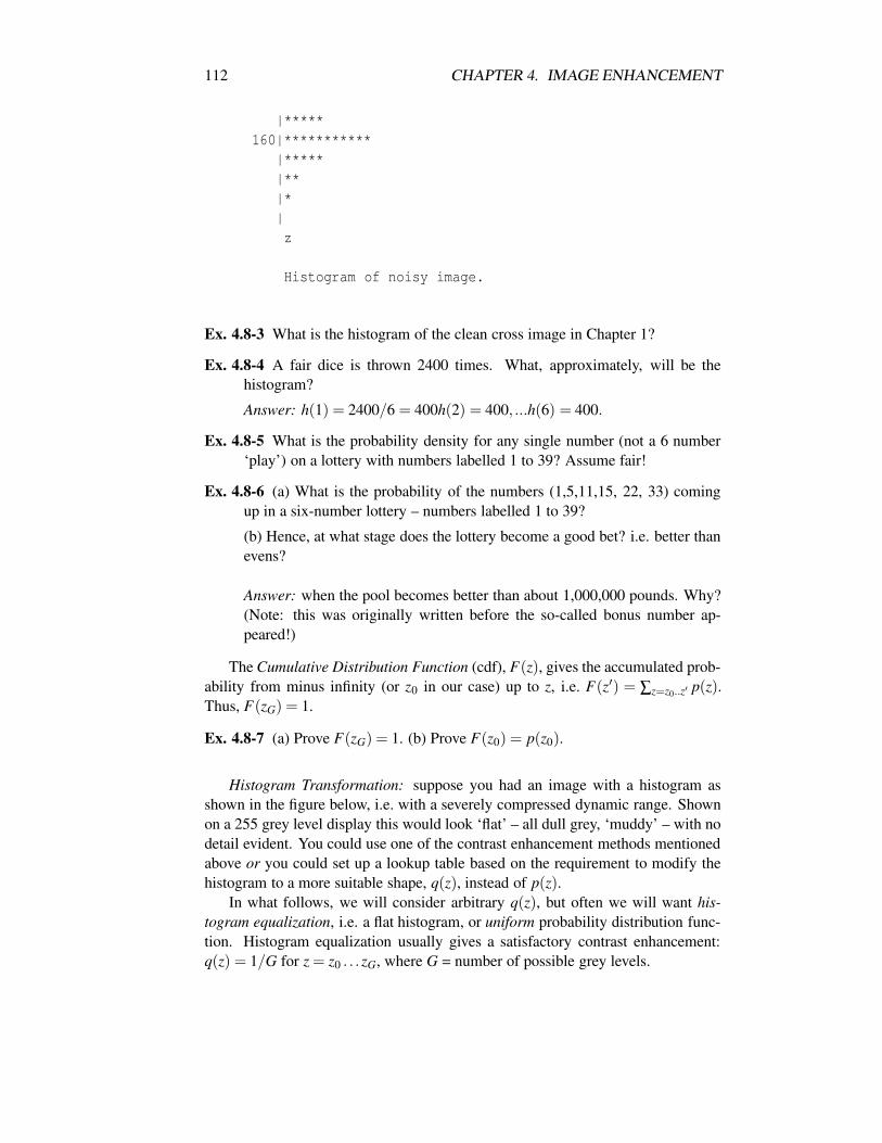
112 CHAPTER 4. IMAGE ENHANCEMENT
|*****160|***********
|*****|**|*|z
Histogram of noisy image.
Ex. 4.8-3 What is the histogram of the clean cross image in Chapter 1?
Ex. 4.8-4 A fair dice is thrown 2400 times. What, approximately, will be thehistogram?
Answer: h(1) = 2400/6 = 400h(2) = 400, ...h(6) = 400.
Ex. 4.8-5 What is the probability density for any single number (not a 6 number‘play’) on a lottery with numbers labelled 1 to 39? Assume fair!
Ex. 4.8-6 (a) What is the probability of the numbers (1,5,11,15, 22, 33) comingup in a six-number lottery – numbers labelled 1 to 39?
(b) Hence, at what stage does the lottery become a good bet? i.e. better thanevens?
Answer: when the pool becomes better than about 1,000,000 pounds. Why?(Note: this was originally written before the so-called bonus number ap-peared!)
The Cumulative Distribution Function (cdf), F(z), gives the accumulated prob-ability from minus infinity (or z0 in our case) up to z, i.e. F(z′) = ∑z=z0..z′ p(z).Thus, F(zG) = 1.
Ex. 4.8-7 (a) Prove F(zG) = 1. (b) Prove F(z0) = p(z0).
Histogram Transformation: suppose you had an image with a histogram asshown in the figure below, i.e. with a severely compressed dynamic range. Shownon a 255 grey level display this would look ‘flat’ – all dull grey, ‘muddy’ – with nodetail evident. You could use one of the contrast enhancement methods mentionedabove or you could set up a lookup table based on the requirement to modify thehistogram to a more suitable shape, q(z), instead of p(z).
In what follows, we will consider arbitrary q(z), but often we will want his-togram equalization, i.e. a flat histogram, or uniform probability distribution func-tion. Histogram equalization usually gives a satisfactory contrast enhancement:q(z) = 1/G for z = z0 . . . zG, where G = number of possible grey levels.
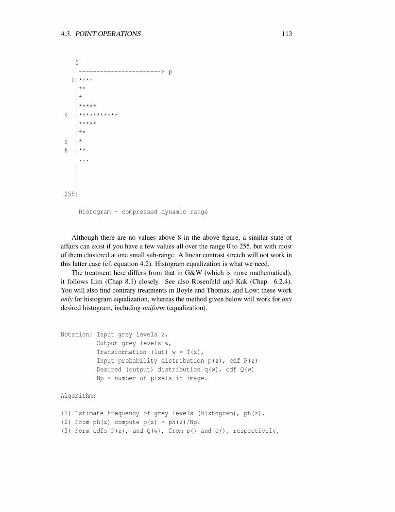
4.3. POINT OPERATIONS 113
0-----------------------> p
0|****|**|*|*****
4 |***********|*****|**
z |*8 |**
...|||
255|
Histogram - compressed dynamic range
Although there are no values above 8 in the above figure, a similar state ofaffairs can exist if you have a few values all over the range 0 to 255, but with mostof them clustered at one small sub-range. A linear contrast stretch will not work inthis latter case (cf. equation 4.2). Histogram equalization is what we need.
The treatment here differs from that in G&W (which is more mathematical);it follows Lim (Chap 8.1) closely. See also Rosenfeld and Kak (Chap. 6.2.4).You will also find contrary treatments in Boyle and Thomas, and Low; these workonly for histogram equalization, whereas the method given below will work for anydesired histogram, including uniform (equalization).
Notation: Input grey levels z,Output grey levels w,Transformation (lut) w = T(z),Input probability distribution p(z), cdf P(z)Desired (output) distribution q(w), cdf Q(w)Np = number of pixels in image.
Algorithm:
(1) Estimate frequency of grey levels (histogram), ph(z).(2) From ph(z) compute p(z) = ph(z)/Np.(3) Form cdfs P(z), and Q(w), from p() and q(), respectively,

114 CHAPTER 4. IMAGE ENHANCEMENT
i.e. P(z′) =z′
∑z=z0
p(z)
(4) for each z in the input do:choose w such that Q(w) is closest to P(z),set T(z) = w;
(5) Apply T(z) to input image f1[r,c]: f2[r,c] = T(f1[r,c])
Exercise 4.8-8 Suppose an 8-level image, (G = 8); M = 8, N = 16 (M.N = no. ofpixels = 128). Input histogram ph(), output q() – see table:
Input and Output Histograms:
z 0 1 2 3 4 5 6 7-----------------------------------------ph(z) 1 7 21 35 35 21 7 1q(w) 16 16 16 16 16 16 16 16
(1) Form P(z), and Q(w), from p() and q():
Input and Output cdfs:
z 0 1 2 3 4 5 6 7-----------------------------------------P(z) 1 8 29 64 99 120 127 128Q(w) 16 32 48 64 80 96 112 128
(2) for each z in the input do:
(2.1) choose w such that Q(w) is closest to P(z), T (z) = w; (i.e. set up lookuptable/function)
z=0 : must choose T(0) = 0 (closest)z=1 : T(1) = 0z=2 : T(2) = 1z=3 : T(3) = 3z=4 : T(4) = 5z=5 : T(5) = 6z=6 : T(6) = 7z=7 : T(7) = 7
Thus, resulting histogram:

4.3. POINT OPERATIONS 115
Input and Output Histograms:
z 0 1 2 3 4 5 6 7-----------------------------------------p(z ) 1 7 21 35 35 21 7 1q’(w) 8 21 0 35 0 35 21 8
Notice that q′(w) is only an approximation to q(w). In general, for discretelevels, this will be the case.
Remark: We could make the equalization exact by modifying the algorithmto allocate the pixels at input grey level zi, not just to one output level w j, butput some in w j−1, and some in w j+1 – to produce an exact q(w) histogram.Rosenfeld and Kak, Chap 6.2, do this. To me it doesn’t make much senseto map one pixel value 3 (say) to 1, another to 2, and maybe another to 4.Furthermore, the lookup table algorithm would have to be made considerablymore complex – for very little gain.
Ex. 4.8-9 Suppose that a 64×64, 8-level image has the greylevel distribution val-ues of p(z), the density calculated from the histogram, shown below. Cal-culate the transformation function, T (z), to give histogram equalization, us-ing the algorithm given above. Then calculate q′(w), the actual output his-togram, and plot it.
Recommendation: Proceed as follows. Work out q(w). The work out thecumulatives P(), and Q(); then apply the algorithm. Note: this example istaken from G&W 2nd ed., Don’t copy their answer, it’s wrong!
Histogram for Ex. 4.8-9:
------------------------------------------------------------z ph(z) p(z)= q(w) P(z) Q(z) T(z)
ph(z)/M.N-----------------------------------------------------------
0 790 0.191 1023 0.252 850 0.213 656 0.164 329 0.085 245 0.066 122 0.037 81 0.02
-----------------------------------------------------------

116 CHAPTER 4. IMAGE ENHANCEMENT
Ex. 4.8-10 Using the same input histogram as in Ex. 4.8-9, produce a transforma-tion to yield the density shown, q(w) in the following table. Again, be waryof the G&W answer for this.
Densities for ex. 4.8-10:
------------------------------------------------------------z ph(z) p(z)= q(w) P(z) Q(z) T(z)
ph(z)/M.N-----------------------------------------------------------
0 790 0.19 0.001 1023 0.25 0.002 850 0.21 0.003 656 0.16 0.154 329 0.08 0.205 245 0.06 0.306 122 0.03 0.207 81 0.02 0.15
-----------------------------------------------------------
Low (Chap. 5), G&W (Chap. 4.2) give good examples of effectiveness ofhistogram modification.
Ex. 4.8-11 Someone has asserted: “histogram modification (or any form of con-trast stretching) is unlikely to be of assistance in a purely automatic machinevision application (i.e. one in which there is no human intervention), sincethese techniques introduce no new information – in fact, they often destroyinformation”.
On the basis of sections 4.4 to 4.8, comment on this assertion. Hint: Lookcarefully at the histogram equalization transformation function in Ex. 4.8-8.
Compare the input and output histograms. How many grey levels in theinput? How many in the output?
4.3.7 Local Enhancement
The point (grey level) methods in sections 4.5 to 4.8 are applied globally, i.e. tothe whole image. But suppose that the contrast differs across the image, e.g. dueto shadow, or parts of a TV camera sensing surface having lost sensitivity. Or, asin the example in G&W (p. 159), you have a global dynamic range that is greaterthan the display can handle, i.e. you would like to, adaptively, focus on a diiferentpart of the greyscale, at different parts of the image.
Thus, you need to allow the transformation to vary across the image.This can be done by defining an m× n neighbourhood. The neighbourhood
is ‘scanned’ across the image pixel by pixel. It stops at each pixel, computes the
4.4. NOISE REDUCTION BY AVERAGING OF MULTIPLE IMAGES 117
transformation for the current m× n pixels, and applies that transformation to thecentre pixel (only).
Obviously, this is a lot of computing, which can be reduced by not overlappingthe neighbourhoods; however, a checkerboard effect may result.
See G&W for some results of local enhancement.
4.4 Noise Reduction by Averaging of Multiple Images
Assume you have the possibility of obtaining many still, ‘identical’, images of ascene; but, the images are picking up noise in transmission, or from the sensorsystem. Then averaging together these images pixel by pixel:
fa(r,c) = (1/Na) ∑i=1..Na
fi(r,c)
for r = rl ..rh,c = cl ..ch, where Na = number of images averaged, and fi(., .) is theith image.
Note: this is done for each pixel independently; we are not smoothing acrosspixels. Thus, we can talk about the mean, m(r,c), and variance v(r,c) of each pixel.
If our model is that the only distortion is noise, then f i(r,c) can be written:
fi(r,c) = f (r,c)+ni(r,c)
i.e. the ith image is the true, noiseless image, plus the ith noise image. Most natu-rally occurring noise has the characteristic (or is assumed to have) that it is randomand uncorrelated. Often too, it is zero mean.
Roughly speaking, these last two statements indicate that for every positivenoise value, you will eventually get a negative one, and if you take enough valuesin the average you end up with zero.
Ex. 4.10-1 Throw a dice many times; for each throw you get one of 1,2,..6; fromeach throw subtract 3.5 and add the number to a running sum (which was ini-tialised with zero); as the number of throws gets larger, the sum approaches0.0 more closely.
It can be shown that if the noise level (e.g., as indicated by the standarddeviation of the pixel values (at (r,c) ) is s1 for 1 image (no averaging), thenit is
sn = s1/√
Na
for Na images averaged.
You can easily experience two examples of this:
1. On a noisy stereo radio reception, switch the tuner to mono; this causesthe system to add the left and right signals to produce one signal; thenoise standard deviation reduces by 1/
√2 = 1/1.414, i.e. reduces to
0.707 of what it was,

118 CHAPTER 4. IMAGE ENHANCEMENT
2. freeze frame on a videoplayer, see how noisy the image is comparedto moving: the eye tends to average over a number of the 25 imagespainted on the screen per second.
Ex. 4.10-2 In DataLab, generate a rectangle, (grect) add Gaussian noise to it (ggna)– observe the noiselike mottled effect; now add more noise (ggna) say 10times; notice how the mottled effect decreases; the noise is cancelling itselfout.
Ex. 4.10-3 You are working with a noisy TV camera and a digitiser. You observethat the noise standard deviation, after the digitiser, is about 16 grey levels.You have detail in the image that requires better than 5 grey levels precision,to be sure of resolving it; thus, in single images, the detail is ‘buried’ in thenoise. If possible, how many images should you average?
Incidentally, image averaging does not directly smooth the image, nor sharpen,or otherwise spatially affect it.
4.5 Spatial Operations
4.5.1 Neighbourhood Averaging
Suppose that small neighbourhoods (e.g. 3× 3) of an image are known to exhibitvery smooth variations in pixel values; so that any abrupt variations have to bedue to noise; of course, this is not always true. For this sort of image, if youaverage over the neighbourhood (window), you will average the noise, which (inthe average) tends to zero.
The window (or mask) can be any shape, but is usually square, and often 3×3.The following formally describes the process.
g(r,c) = (1/Nw) ∑window (r,c)
f (i, j)
where the window is centred on (r,c) ), g is the output image, and f is the inputimage.
For a window which stretches −w to +w on either side of the central pixel,in the vertical dimension (rows) and −v to +v in the horizontal (columns) thisbecomes:
g(r,c) =r+w
∑k=r−w
c+v
∑l=c−v
f (k, l).(1/Nw)
where Nw = (2.w+1).(2.v+1)
Window (w=1, v=1, 3x3) centred on pixel (r,c):

4.5. SPATIAL OPERATIONS 119
-v 0 +v-w +-----------------------------+
| 1/9 | 1/9 | 1/9 ||f(r-1,c-1|f(r-1,c) |f(r-1,c+1|| | | |+-----------------------------+| 1/9 | 1/9 | 1/9 |
0 |f(r,c-1) |f(r,c) |f(r,c+1) || | | |+-----------------------------+| 1/9 | 1/9 | 1/9 ||f(r+1,c-1|f(r+1,c) |f(r+1,c+1|| | | |
+w +-----------------------------+
The above equation for g(r,c) allows for any window whose dimensions areodd numbers (2.w + 1,2.v + 1) – so that the window extends symmetrically oneach side of the central pixel. The factor 1/Nw(= 1/9 for 3× 3), is the so-calledweight of the window or mask. For averaging, all weights are equal.
The formal style of the equation for g(r,c) will allow us extend the notion ofwindows to perform any function, (smooth, sharpen, filter); generally this is calledconvolution. Equivalent terms are: window, mask, template, convolution kernel,kernel, weighting function; also, see later, impulse response.
The major problem with averaging is that real spikes and discontinuities aresmoothed as well, not just the noise induced ones. Thus edges and points areblurred. If you start off with a resolution of 10m × 10m (say), and use a 3× 3window, you effectively reduce the resolution to 30m × 30m.
4.5.2 Lowpass Filtering
If you use a window like the one seen in the previous section the process is giventhe general term lowpass filtering; it is called this because you are filtering out highfrequency components from the image (for more about frequency, filtering etc. seeChapter 3).
Sometimes these windows produce better results than straight averaging.
1/10 1/10 1/10 1/16 2/16 1/16 1/9 1/9 1/91/10 2/10 1/10 2/16 4/16 2/16 1/9 1/9 1/91/10 1/10 1/10 1/16 2/16 1/16 1/9 1/9 1/9
(a) (b) (c)
1/5 1/6
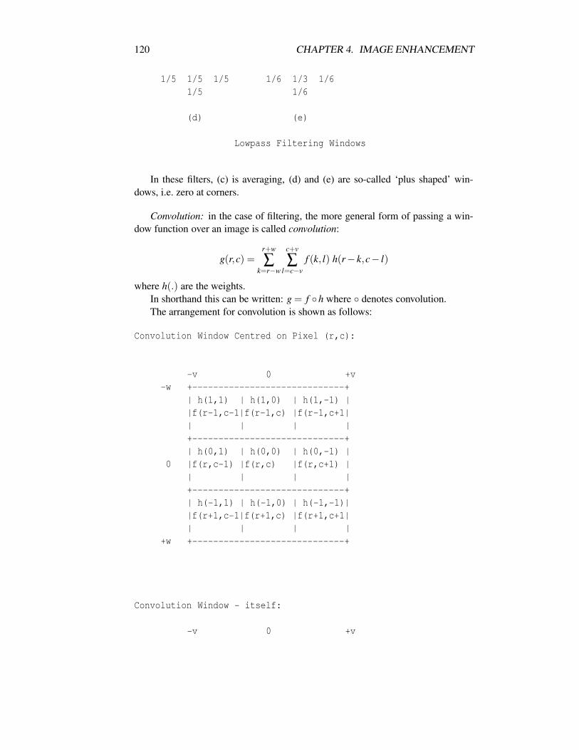
120 CHAPTER 4. IMAGE ENHANCEMENT
1/5 1/5 1/5 1/6 1/3 1/61/5 1/6
(d) (e)
Lowpass Filtering Windows
In these filters, (c) is averaging, (d) and (e) are so-called ‘plus shaped’ win-dows, i.e. zero at corners.
Convolution: in the case of filtering, the more general form of passing a win-dow function over an image is called convolution:
g(r,c) =r+w
∑k=r−w
c+v
∑l=c−v
f (k, l) h(r− k,c− l)
where h(.) are the weights.In shorthand this can be written: g = f h where denotes convolution.The arrangement for convolution is shown as follows:
Convolution Window Centred on Pixel (r,c):
-v 0 +v-w +-----------------------------+
| h(1,1) | h(1,0) | h(1,-1) ||f(r-1,c-1|f(r-1,c) |f(r-1,c+1|| | | |+-----------------------------+| h(0,1) | h(0,0) | h(0,-1) |
0 |f(r,c-1) |f(r,c) |f(r,c+1) || | | |+-----------------------------+| h(-1,1) | h(-1,0) | h(-1,-1)||f(r+1,c-1|f(r+1,c) |f(r+1,c+1|| | | |
+w +-----------------------------+
Convolution Window - itself:
-v 0 +v
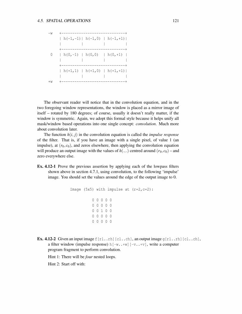
4.5. SPATIAL OPERATIONS 121
-w +-----------------------------+| h(-1,-1)| h(-1,0) | h(-1,+1)|| | | |+-----------------------------+
0 | h(0,-1) | h(0,0) | h(0,+1) || | | |+-----------------------------+| h(+1,1) | h(+1,0) | h(+1,+1)|| | | |
+w +-----------------------------+
The observant reader will notice that in the convolution equation, and in thetwo foregoing window representations, the window is placed as a mirror image ofitself – rotated by 180 degrees; of course, usually it doesn’t really matter, if thewindow is symmetric. Again, we adopt this formal style because it helps unify allmask/window based operations into one single concept: convolution. Much moreabout convolution later.
The function h(i, j) in the convolution equation is called the impulse responseof the filter. That is, if you have an image with a single pixel, of value 1 (animpulse), at (r0,c0), and zeros elsewhere, then applying the convolution equationwill produce an output image with the values of h(., .) centred around (r0,c0) – andzero everywhere else.
Ex. 4.12-1 Prove the previous assertion by applying each of the lowpass filtersshown above in section 4.7.1, using convolution, to the following ‘impulse’image. You should set the values around the edge of the output image to 0.
Image (5x5) with impulse at (r=2,c=2):
0 0 0 0 00 0 0 0 00 0 1 0 00 0 0 0 00 0 0 0 0
Ex. 4.12-2 Given an input image f[rl..rh][cl..ch], an output image g[rl..rh][cl..ch],a filter window (impulse response) h[-w..+w][-v..+v], write a computerprogram fragment to perform convolution.
Hint 1: There will be four nested loops.
Hint 2: Start off with:

122 CHAPTER 4. IMAGE ENHANCEMENT
for r:= rl+w to rh-w dofor c:=...sum:=0.0
Test the fragment by dry running it to do Ex. 4.12-1.
Ex. 4.12-3 You want to save memory. You decide to use only one image, f (), andstore the results of filtering back in f (), i.e. f () is input (source) and output(destination).
(a) Explain why this will not work.
(b) For what sort of operations will this work okay?
(c) try out on DataLab (e.g. functions esobx, esm).
Ex. 4.12-4 Adapt the algorithm of Ex. 4.12-2 to work in a programming languagethat insists that all array indices start at 0 (or 1).
4.5.3 Median Filtering
As mentioned in section 4.11, a problem with averaging is its tendency to bluredges. Median filtering is a method which largely avoids this problem. In additionmedian filtering is better suited to removing ‘impulse’ noise, i.e. noise charac-terised by large irregular spikes, or so-called ‘salt-and-pepper’ noise. In an audiosignal this is the type of noise that comes from a scratch on a record, rather thanthe more normal ‘hiss’.
Median filtering works by taking all the values in a neighbourhood, sortingthem according to magnitude, and taking the middle ranked value (median) as theoutput value.
Consider this one-dimensional example which will use a 3 wide kernel or win-dow. Input values:
0 0 6 0 0 0 12 0 0 0 15 15 15 15 33 15 15 15 0 0 0 0 0
If we apply a 3 wide averaging window to this we get
0 2 2 2 0 4 4 4 0 5 10 15 15 21 21 21 15 10 5 0 0 0 0
(1) The noise ‘spikes’ (6,12,33) are smoothed – rather smeared – but not re-moved.
(2) Step edges (0 0 0 15 15 15 ) are blurred (to 0 5 10 15 15).Application of a 3 sample wide median filter produces:
(original first)0 0 6 0 0 0 12 0 0 0 15 15 15 15 33 15 15 15 0 0 0 0 0
(median filtered)0 0 0 0 0 0 0 0 0 0 15 15 15 15 15 15 15 15 0 0 0 0 0
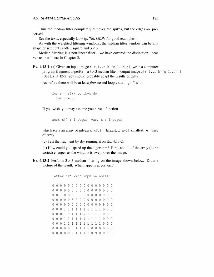
4.5. SPATIAL OPERATIONS 123
Thus the median filter completely removes the spikes, but the edges are pre-served.
See the texts, especially Low (p. 76), G&W for good examples.As with the weighted filtering windows, the median filter window can be any
shape or size; but is often square and 3×3.Median filtering is a non-linear filter – we have covered the distinction linear
versus non-linear in Chapter 3.
Ex. 4.13-1 (a) Given an input image f[r_l..r_h][c_l..c_h], write a computerprogram fragment to perform a 3×3 median filter – output image g[r_l..r_h][c_l..c_h].(See Ex. 4.12-2: you should probably adapt the results of that).
As before there will be at least four nested loops, starting off with:
for r:= rl+w to rh-w dofor c:=...
If you wish, you may assume you have a function
sort(x[] : integer, var, n : integer)
which sorts an array of integers: x[0] = largest, x[n-1] smallest. n = sizeof array.
(c) Test the fragment by dry running it on Ex. 4.13-2.
(d) How could you speed up the algorithm? Hint: not all of the array (to besorted) changes as the window is swept over the image.
Ex. 4.13-2 Perform 3× 3 median filtering on the image shown below. Draw apicture of the result. What happens at corners?
Letter ’T’ with impulse noise:
0 0 0 0 0 0 0 0 0 0 0 0 0 0 0 00 0 0 0 0 0 0 0 0 0 0 0 0 0 0 00 0 1 0 0 9 0 0 6 0 0 0 0 9 0 00 0 0 0 0 3 0 0 0 0 0 0 0 0 0 00 0 0 0 0 0 0 0 0 0 0 0 0 9 0 00 0 0 1 1 1 1 1 1 1 1 1 1 0 0 00 0 0 1 9 1 1 1 9 1 1 1 1 0 0 00 0 0 1 1 1 1 1 9 1 1 1 1 0 0 00 0 0 1 1 1 1 1 1 1 1 1 1 0 0 00 0 0 0 0 0 1 1 1 1 0 0 0 0 0 00 0 0 0 0 0 1 1 1 1 0 9 0 0 0 0

124 CHAPTER 4. IMAGE ENHANCEMENT
0 0 0 0 0 0 1 1 1 1 0 0 0 0 0 00 0 0 9 9 0 1 1 1 1 0 0 0 9 0 00 0 0 0 0 0 1 1 9 1 0 0 0 0 0 00 0 0 9 0 0 1 1 1 1 0 0 0 0 0 00 0 0 0 0 0 0 0 0 0 0 0 0 0 0 0
Ex. 4.13-3 Perform 3× 3 averaging on the above image of the letter ’T’ withimpulse noise. Compare the result with that obtained by median filtering.Which would be best if you wanted to recognise the character?
Ex. 4.13-4 A so-called ‘separable median filter’ is performed by sweeping a 1×3median filter along each of the rows, followed by a 3x1 median filter downeach of the columns.
(a) Apply this to the noisy letter ‘T’.
(b) Compare the result with that for Ex. 4.13-2.
Ex. 4.13-5 The separable median filter should be much faster; make a brief com-parison of the likely speed performance of separable, and square medianfilters.
Another example: the following figures show the following sequence of im-ages:
(a) 16×16 image with rectangle(b) Rectangle with random spots added.(c) Result of 3×3 smoothing(d) Result of 3×3 median filter.In each case the corresponding data are printed.

4.5. SPATIAL OPERATIONS 125
16 x 16 image with rectangle:
0123456789012345----------------
0| |1| |2| |3| |4| MMMMMMMMM |5| MMMMMMMMM |6| MMMMMMMMM |7| MMMMMMMMM |8| MMMMMMMMM |9| MMMMMMMMM |0| MMMMMMMMM |1| MMMMMMMMM |2| MMMMMMMMM |3| |4| |5| |+----------------+
Data for previous figure:
0 0 0 0 0 0 0 0 0 0 0 0 0 0 0 00 0 0 0 0 0 0 0 0 0 0 0 0 0 0 00 0 0 0 0 0 0 0 0 0 0 0 0 0 0 00 0 0 0 0 0 0 0 0 0 0 0 0 0 0 00 0 0 0 99 99 99 99 99 99 99 99 99 0 0 00 0 0 0 99 99 99 99 99 99 99 99 99 0 0 00 0 0 0 99 99 99 99 99 99 99 99 99 0 0 00 0 0 0 99 99 99 99 99 99 99 99 99 0 0 00 0 0 0 99 99 99 99 99 99 99 99 99 0 0 00 0 0 0 99 99 99 99 99 99 99 99 99 0 0 00 0 0 0 99 99 99 99 99 99 99 99 99 0 0 00 0 0 0 99 99 99 99 99 99 99 99 99 0 0 00 0 0 0 99 99 99 99 99 99 99 99 99 0 0 00 0 0 0 0 0 0 0 0 0 0 0 0 0 0 00 0 0 0 0 0 0 0 0 0 0 0 0 0 0 00 0 0 0 0 0 0 0 0 0 0 0 0 0 0 0

126 CHAPTER 4. IMAGE ENHANCEMENT
Rectangle image with random spots added:
0123456789012345----------------
0| / |1| / |2| / / |3| / / / / |4| ////////// |5| //M////// |6| ///////// |7| /////M/// |8| ///////// |9| ///////// / |0| ///////// |1| ///M///// / |2|/ ///////// |3| |4| / |5| |+----------------++0123456789012345
Data for previous figure:
0 0 0 0 0 0 0 0 0 0 0 0 99 0 0 00 99 0 0 0 0 0 0 0 0 0 0 0 0 0 00 0 0 0 0 0 0 0 0 99 0 99 0 0 0 00 0 99 0 0 99 0 99 0 0 0 99 0 0 0 00 0 0 0 99 99 99 99 99 99 99 99 99 99 0 00 0 0 0 99 99 198 99 99 99 99 99 99 0 0 00 0 0 0 99 99 99 99 99 99 99 99 99 0 0 00 0 0 0 99 99 99 99 99 198 99 99 99 0 0 00 0 0 0 99 99 99 99 99 99 99 99 99 0 0 00 0 0 0 99 99 99 99 99 99 99 99 99 0 99 00 0 0 0 99 99 99 99 99 99 99 99 99 0 0 00 0 0 0 99 99 99 198 99 99 99 99 99 0 99 099 0 0 0 99 99 99 99 99 99 99 99 99 0 0 00 0 0 0 0 0 0 0 0 0 0 0 0 0 0 00 0 0 0 99 0 0 0 0 0 0 0 0 0 0 00 0 0 0 0 0 0 0 0 0 0 0 0 0 0 0

4.5. SPATIAL OPERATIONS 127
Previous image moothed with 3x3 window:
0123456789012345----------------
0| ... |1| ... |2|... . . ,.. |3| .,-/-/-=//. |4| ,/XBX+=++=, |5| ,=MMMBBBB+- |6| ,=MMMMMMB=, |7| ,=BBBMMMB=, |8| ,=BBBMMMB=- |9| ,=BBBBBBB=- |0| ,=BMMMBBB=/..|1| ,=BMMMBBB=- |2| .-=+++===-, |3| .,-,,,,,,. |4| |5| |+----------------++0123456789012345
Data for previous image:
10 10 10 0 0 0 0 0 10 10 21 21 21 10 0 010 10 10 0 0 0 0 0 10 10 21 21 21 10 0 021 21 21 10 10 10 21 10 21 10 32 21 21 0 0 010 10 10 21 32 43 54 43 54 43 65 54 54 21 10 1010 10 10 32 54 87 98 87 76 65 76 76 65 32 10 100 0 0 32 65 109 109 109 98 98 98 98 76 43 10 100 0 0 32 65 109 109 109 109 109 109 98 65 32 0 00 0 0 32 65 98 98 98 109 109 109 98 65 32 0 00 0 0 32 65 98 98 98 109 109 109 98 65 43 10 100 0 0 32 65 98 98 98 98 98 98 98 65 43 10 100 0 0 32 65 98 109 109 109 98 98 98 65 54 21 2110 10 0 32 65 98 109 109 109 98 98 98 65 43 10 1010 10 0 21 43 65 76 76 76 65 65 65 43 32 10 1010 10 0 21 32 43 32 32 32 32 32 32 21 10 0 00 0 0 10 10 10 0 0 0 0 0 0 0 0 0 00 0 0 10 10 10 0 0 0 0 0 0 0 0 0 0
Note smudging of edges.

128 CHAPTER 4. IMAGE ENHANCEMENT
Noisy rectangle median filtered:
0123456789012345----------------
0| |1| |2| |3| M M MMM |4| MMMMMMMMM |5| MMMMMMMMM |6| MMMMMMMMM |7| MMMMMMMMM |8| MMMMMMMMM |9| MMMMMMMMM |0| MMMMMMMMMM |1| MMMMMMMMM |2| MMMMMMM |3| |4| |5| |+----------------++0123456789012345
Data for previous image:
0 0 0 0 0 0 0 0 0 0 0 0 0 0 0 00 0 0 0 0 0 0 0 0 0 0 0 0 0 0 00 0 0 0 0 0 0 0 0 0 0 0 0 0 0 00 0 0 0 0 0 99 0 99 0 99 99 99 0 0 00 0 0 0 99 99 99 99 99 99 99 99 99 0 0 00 0 0 0 99 99 99 99 99 99 99 99 99 0 0 00 0 0 0 99 99 99 99 99 99 99 99 99 0 0 00 0 0 0 99 99 99 99 99 99 99 99 99 0 0 00 0 0 0 99 99 99 99 99 99 99 99 99 0 0 00 0 0 0 99 99 99 99 99 99 99 99 99 0 0 00 0 0 0 99 99 99 99 99 99 99 99 99 99 0 00 0 0 0 99 99 99 99 99 99 99 99 99 0 0 00 0 0 0 0 99 99 99 99 99 99 99 0 0 0 00 0 0 0 0 0 0 0 0 0 0 0 0 0 0 00 0 0 0 0 0 0 0 0 0 0 0 0 0 0 00 0 0 0 0 0 0 0 0 0 0 0 0 0 0 0

4.5. SPATIAL OPERATIONS 129
4.5.4 Other Non-linear Smoothing
Mode
The output value is the most common in the neighbourhood. Gives similar resultsto median in many cases. Very useful if the image is made up of labels (e.g. oflanduse), i.e. after classification or segmentation. In that case you are taking a voteas to the most common label in the neighbourhood; certainly in that case averagingor median would make no sense. Why?
k-Nearest Neighbour (kNN)
Set g(r,c) to the average of the k pixels, in n(r,c) (the neighbourhood, centred on(r,c)) whose values are closest to f (r,c). Typically use k = 6 for a 3× 3 neigh-bourhood. Preserves edges.
Sigma Filter
Set g(r,c) to the average of all input pixels, in n(r,c), whose values are within Tof f (r,c). T is a parameter. Called sigma (greek letter, the symbol for standarddeviation) because T may be based on the standard deviation. Similar performanceto kNN.
Out-of-range filtering
Compute average in the neighbourhood (n(r,c)) of (r,c); average = fa(r,c). If thedifference between f (r,c) and fa(r,c) is greater than some threshold, set the outputg(r,c) to the average, otherwise set it to f (r,c) (i.e. leave it the same). I.e.
If |f(r,c) - fa(r,c)| > Threshthen g(r,c) = fa(r,c)else g(r,c) = f(r,c)
Ex. 4.14.1 Repeat Ex. 4.13-1 for the out-of-range filter.
Ex. 4.14.2 Repeat Ex. 4.13-2 for the out-of-range filter.
Closest-of-minimum-and-maximum
Compute the min and max values in n(r,c). Set g(r,c) to the one that is closestto f (r,c). Useful for sharpening boundaries. Usually iterated. Will leave isolatedspikes – these can be removed by median filter.
Min-Max
Compute minimum (or maximum) value in n(r,c) and set g(r,c) to that. Useful forshrinking or expanding 1s in a binary picture. More on this when we talk aboutsegmentation.

130 CHAPTER 4. IMAGE ENHANCEMENT
4.6 Image Sharpening – General
Often called ‘edge detection’ – but, strictly, we need thresholding to follow thesharpening to qualify for this name. The following shows a full edge detectionsystem, based on gradient.
f (x,y) −→ Gradient −→| . |−→ Threshold −→ Edge thinning −→ Edge
Here | . | denotes absolute value.Most edge sharpening processes will also sharpen spikes.In contrast with smoothing operations, which are usually lowpass filters, sharp-
ening operations are associated with highpass filtering.Noise is usually high frequency, so sharpening will often increase noise effects.The generalized windowing / masking introduced in section 4.12 is easily ap-
plied to sharpening – you just change the weights.
4.7 Gradient Based Edge Enhancement
4.7.1 Introduction
The first part of this section introduces differentiation (of continuous functions),indicates how gradient and ‘edginess’ are related, then shows how to constructwindows that do the discrete (digital) version of differentiation.
The use of gradient is based on the reasoning that edges are characterised bylarge slopes in the image function f (x,y) (view f (x,y) as forming the height coor-dinate on the x− y plane).
4.7.2 Gradient, Slope and Differentiation
The following figure illustrates gradient of a one-dimensional function f (.) of vari-able x, f (x).
f(x)
| /| / (3)| /| ____ (2)
f(x2)12| /| /|
f(x1) 6| /__| Df (1)| / Dx
0 |/__________________________ x
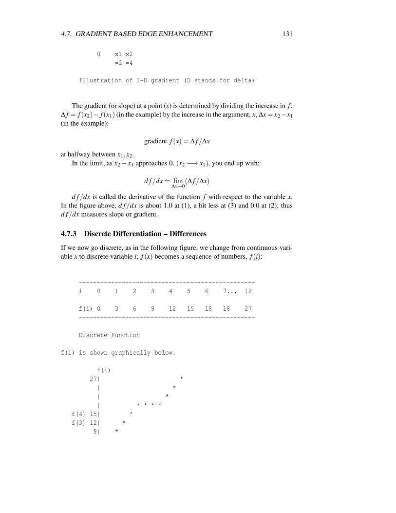
4.7. GRADIENT BASED EDGE ENHANCEMENT 131
0 x1 x2=2 =4
Illustration of 1-D gradient (D stands for delta)
The gradient (or slope) at a point (x) is determined by dividing the increase in f ,∆ f = f (x2)− f (x1) (in the example) by the increase in the argument, x, ∆x = x2−x1(in the example):
gradient f (x) = ∆ f/∆x
at halfway between x1,x2.In the limit, as x2− x1 approaches 0, (x2 −→ x1), you end up with:
d f/dx = lim∆x→0
(∆ f/∆x)
d f/dx is called the derivative of the function f with respect to the variable x.In the figure above, d f/dx is about 1.0 at (1), a bit less at (3) and 0.0 at (2); thusd f/dx measures slope or gradient.
4.7.3 Discrete Differentiation – Differences
If we now go discrete, as in the following figure, we change from continuous vari-able x to discrete variable i; f (x) becomes a sequence of numbers, f (i):
-------------------------------------------------i 0 1 2 3 4 5 6 7... 12
f(i) 0 3 6 9 12 15 18 18 27-------------------------------------------------
Discrete Function
f(i) is shown graphically below.
f(i)27| *| *| *| * * * *
f(4) 15| *f(3) 12| *
9| *

132 CHAPTER 4. IMAGE ENHANCEMENT
3| *0|*__________________________ i
0 1 2 3 4 5 6 7 8 9 ...12
Graph of Discrete Function
The discrete version of differentiation is differencing. If we have a sampledversion of an analogue function, then the difference gives the best available ap-proximation of differential. At any point i, the difference of f (i) is ∆ f (i) =f (i)− f (i−1).
If the sampling period (∆x) is 1 then this gives a direct replacement for thedifferential. ∆ f (i) gives an output value centred on (i+1/2); to make it symmetricwe can use: ∆ f (i) = f (i+1)− f (i−1).
Ex. 4.16-1 In the figure illustrating the 1-D gradient above, assume that, in region(1), f (x) = 3x.
(a) What is d f/dx in this region?
In the figure showing a sampled (discrete) version of f (x), the samplingperiod is ∆x = 1.
(b) What is ∆ f (i) at i = 3?
(c) Compare the results of (a), and (b).
(d) What are two circumstances in which the results will differ?
Second Differences
If you differentiate d f/dx, you get d2 f/dx2. In terms of differences, assume youhave the difference sequence:
∆ f (0),∆ f (1), . . . ,∆ f (i−1),D f (i), . . . ,∆ f (n−1)
Taking differences on this (equivalent to d2 f/dx2 in continuous functions)yields (just apply the definition of ∆ again): ∆2 f (i) = ∆ f (i)−∆ f (i−1).
But we have seen that ∆ f (i) = f (i)− f (i−1), and similarly, ∆ f (i−1) = f (i−1)− f (i−2).
Substituting gives:
∆2 f (i) = f (i−2)−2 f (i−1)+ f (i)
This is offset by 1 sample, so a better (symmetric) approximation of d 2 f/dx2
is:
∆2 f (i) = f (i−1)−2. f (i)+ f (i+1)
.Usually, the signs are negated.
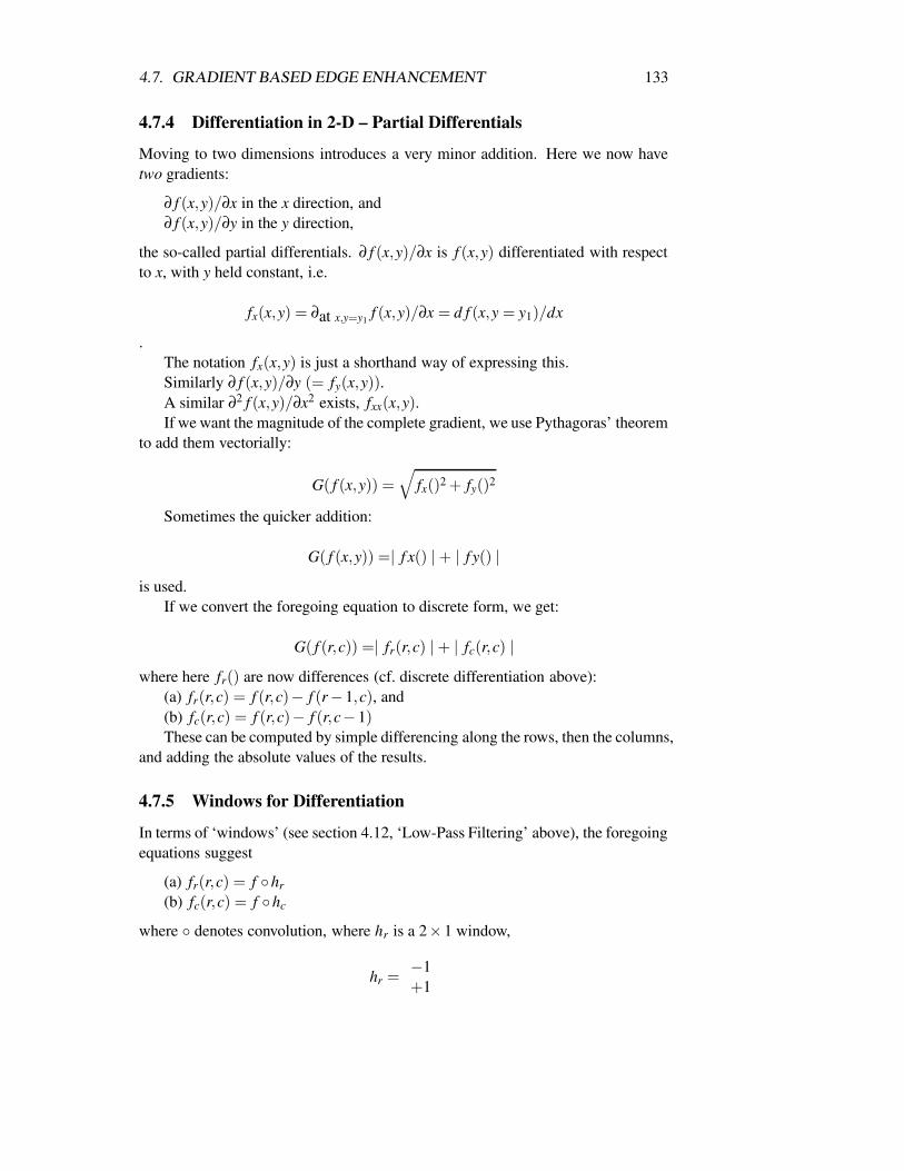
4.7. GRADIENT BASED EDGE ENHANCEMENT 133
4.7.4 Differentiation in 2-D – Partial Differentials
Moving to two dimensions introduces a very minor addition. Here we now havetwo gradients:
∂ f (x,y)/∂x in the x direction, and∂ f (x,y)/∂y in the y direction,
the so-called partial differentials. ∂ f (x,y)/∂x is f (x,y) differentiated with respectto x, with y held constant, i.e.
fx(x,y) = ∂at x,y=y1f (x,y)/∂x = d f (x,y = y1)/dx
.The notation fx(x,y) is just a shorthand way of expressing this.Similarly ∂ f (x,y)/∂y (= fy(x,y)).A similar ∂2 f (x,y)/∂x2 exists, fxx(x,y).If we want the magnitude of the complete gradient, we use Pythagoras’ theorem
to add them vectorially:
G( f (x,y)) =√
fx()2 + fy()2
Sometimes the quicker addition:
G( f (x,y)) =| f x() |+ | f y() |is used.
If we convert the foregoing equation to discrete form, we get:
G( f (r,c)) =| fr(r,c) |+ | fc(r,c) |where here fr() are now differences (cf. discrete differentiation above):
(a) fr(r,c) = f (r,c)− f (r−1,c), and(b) fc(r,c) = f (r,c)− f (r,c−1)These can be computed by simple differencing along the rows, then the columns,
and adding the absolute values of the results.
4.7.5 Windows for Differentiation
In terms of ‘windows’ (see section 4.12, ‘Low-Pass Filtering’ above), the foregoingequations suggest
(a) fr(r,c) = f hr(b) fc(r,c) = f hc
where denotes convolution, where hr is a 2×1 window,
hr =−1+1
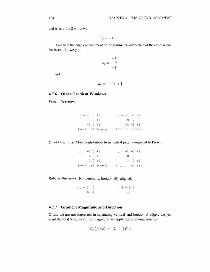
134 CHAPTER 4. IMAGE ENHANCEMENT
and hc is a 1×2 window:
hc =−1 +1
If we base the edge enhancement of the symmetric difference of the expressionsfor hr and hc, we get
hr =−1
0+1
and
hc =−1 0 +1
4.7.6 Other Gradient Windows
Prewitt Operators:
hr = -1 0 +1 hc = -1 -1 -1-1 0 +1 0 0 0-1 0 +1 +1 +1 +1
(vertical edges) (horiz. edges)
Sobel Operators: More contribution from central pixel, compared to Prewitt.
hr = -1 0 +1 hc = -1 -2 -1-2 0 +2 0 0 0-1 0 +1 +1 +2 +1
(vertical edges) (horiz. edges)
Roberts Operators: Not vertically, horizontally aligned.
h1 = 1 0 h2 = 0 10 -1 -1 0
4.7.7 Gradient Magnitude and Direction
Often, we are not interested in separating vertical and horizontal edges, we justwant the total ‘edginess’. For magnitude we apply the following equation:
Gm( f (r,c)) =| Gx |+ | Gy |

4.7. GRADIENT BASED EDGE ENHANCEMENT 135
= | f (r,c)hr |+ | f (r,c) | hc |
or,
Gm( f (r,c)) =√
G2r +G2
c
Likewise, you can add the Roberts gradients.If we want direction: Ga( f (r,c)) = arctan(Gr/Gc). (As usual, r corresponds to
y, c corresponds to x, in the notation of some texts.)Direction is sometimes useful, if you are trying to trace the path of a continuous
edge, based on an edge enhanced image.
Ex. 4.16.8-1 Apply a Sobel vertical gradient operator to the letter ‘T’ image givenbelow. Draw a picture of the result. What happens at corners?
0 0 0 0 0 0 0 0 0 0 0 0 0 0 0 00 0 0 0 0 0 0 0 0 0 0 0 0 0 0 00 0 0 0 0 0 0 0 0 0 0 0 0 0 0 00 0 0 0 0 0 0 0 0 0 0 0 0 0 0 00 0 0 0 0 0 0 0 0 0 0 0 0 0 0 00 0 0 1 1 1 1 1 1 1 1 1 1 0 0 00 0 0 1 1 1 1 1 1 1 1 1 1 0 0 00 0 0 1 1 1 1 1 1 1 1 1 1 0 0 00 0 0 1 1 1 1 1 1 1 1 1 1 0 0 00 0 0 0 0 0 1 1 1 1 0 0 0 0 0 00 0 0 0 0 0 1 1 1 1 0 0 0 0 0 00 0 0 0 0 0 1 1 1 1 0 0 0 0 0 00 0 0 0 0 0 1 1 1 1 0 0 0 0 0 00 0 0 0 0 0 1 1 1 1 0 0 0 0 0 00 0 0 0 0 0 1 1 1 1 0 0 0 0 0 00 0 0 0 0 0 0 0 0 0 0 0 0 0 0 0
Letter ‘T’ image.
Ex. 4.16.8-2 Apply a Sobel horizontal gradient operator to the letter ‘T’ image.Draw a picture of the result.
Ex. 4.16.8-3 Add the results (absolute values) of Ex. 4.16.8-1, and −2. Draw apicture of the result.
Ex. 4.16.8-4 Given an input image f[r_l..r_h][c_l..c_h], an output imageg[r_l..r_h][c_l..c_h], write a computer program fragment to apply theSobel vertical operator.
Hint: Look at your answer for Ex. 4.12-2.

136 CHAPTER 4. IMAGE ENHANCEMENT
Another example:The following Figures show the following sequence of images:(a) 16×16 image with rectangle,(b) Sobel vertical gradient of (a),(c) Sobel horizontal gradient of (a),(d) Overall gradient (b) + (c).In each case the corresponding data are printed.

4.7. GRADIENT BASED EDGE ENHANCEMENT 137
0123456789012345----------------
0| |1| |2| |3| |4| MMMMMMMMM |5| MMMMMMMMM |6| MMMMMMMMM |7| MMMMMMMMM |8| MMMMMMMMM |9| MMMMMMMMM |0| MMMMMMMMM |1| MMMMMMMMM |2| MMMMMMMMM |3| |4| |5| |+----------------++0123456789012345
(a) 16 x 16 image with rectangle
0123456789012345----------------
0| |1| |2| |3| +,MMMMMMM,+ |4| +,MMMMMMM,+ |5| |6| |7| |8| |9| |0| |1| |2| +,MMMMMMM,+ |3| +,MMMMMMM,+ |4| |5| |+----------------++0123456789012345

138 CHAPTER 4. IMAGE ENHANCEMENT
(b) Sobel vertical gradient

4.7. GRADIENT BASED EDGE ENHANCEMENT 139
0 0 0 0 0 0 0 0 0 0 0 0 0 0 0 00 0 0 0 0 0 0 0 0 0 0 0 0 0 0 00 0 0 0 0 0 0 0 0 0 0 0 0 0 0 00 0 0 99 297 396 396 396 396 396 396 396 297 99 0 00 0 0 99 297 396 396 396 396 396 396 396 297 99 0 00 0 0 0 0 0 0 0 0 0 0 0 0 0 0 00 0 0 0 0 0 0 0 0 0 0 0 0 0 0 00 0 0 0 0 0 0 0 0 0 0 0 0 0 0 00 0 0 0 0 0 0 0 0 0 0 0 0 0 0 00 0 0 0 0 0 0 0 0 0 0 0 0 0 0 00 0 0 0 0 0 0 0 0 0 0 0 0 0 0 00 0 0 0 0 0 0 0 0 0 0 0 0 0 0 00 0 0 99 297 396 396 396 396 396 396 396 297 99 0 00 0 0 99 297 396 396 396 396 396 396 396 297 99 0 00 0 0 0 0 0 0 0 0 0 0 0 0 0 0 00 0 0 0 0 0 0 0 0 0 0 0 0 0 0 0
(b.2) Data for (b)
0123456789012345----------------
0| |1| |2| |3| ++ ++ |4| ,, ,, |5| MM MM |6| MM MM |7| MM MM |8| MM MM |9| MM MM |0| MM MM |1| MM MM |2| ,, ,, |3| ++ ++ |4| |5| |+----------------++0123456789012345
(c) Sobel horizontal gradient

140 CHAPTER 4. IMAGE ENHANCEMENT
0123456789012345----------------
0| |1| |2| |3| M+++++++++M |4| +-+++++++-+ |5| ++ ++ |6| ++ ++ |7| ++ ++ |8| ++ ++ |9| ++ ++ |0| ++ ++ |1| ++ ++ |2| +-+++++++-+ |3| M+++++++++M |4| |5| |+----------------++0123456789012345
(d) Sobel gradient - overall
0 0 0 0 0 0 0 0 0 0 0 0 0 0 0 00 0 0 0 0 0 0 0 0 0 0 0 0 0 0 00 0 0 0 0 0 0 0 0 0 0 0 0 0 0 00 0 0 198 396 396 396 396 396 396 396 396 396 198 0 00 0 0 396 594 396 396 396 396 396 396 396 594 396 0 00 0 0 396 396 0 0 0 0 0 0 0 396 396 0 00 0 0 396 396 0 0 0 0 0 0 0 396 396 0 00 0 0 396 396 0 0 0 0 0 0 0 396 396 0 00 0 0 396 396 0 0 0 0 0 0 0 396 396 0 00 0 0 396 396 0 0 0 0 0 0 0 396 396 0 00 0 0 396 396 0 0 0 0 0 0 0 396 396 0 00 0 0 396 396 0 0 0 0 0 0 0 396 396 0 00 0 0 396 594 396 396 396 396 396 396 396 594 396 0 00 0 0 198 396 396 396 396 396 396 396 396 396 198 0 00 0 0 0 0 0 0 0 0 0 0 0 0 0 0 00 0 0 0 0 0 0 0 0 0 0 0 0 0 0 0
(d.2) Data for (d)

4.8. LAPLACIAN 141
4.8 Laplacian
As mentioned above, edge enhancement is based on the highlighting of regionswhere the values are changing rapidly. Usually, we say we have an edge whenthe gradient is greater than a threshold. An alternative is to look for points wherethe gradient reaches a local extremum, i.e. where the second differential has a zerocrossing. That is, compute the second differential and mark as edge those pointswhere it changes sign.
The Laplacian gives a method of computing the discrete equivalent of the sec-ond differential. Recall that in section 4.16.4, we found the approximation to this,d2 f/dx2, to be ∆2 f = f (i−1)−2 f (i)+ f (i+1). If we extend second differencesto two dimensions we get the following plus-shaped window:
hlap4 =−1
−1 4 −1−1
This is called the Laplacian operator, after Laplace’s differential equation:
∂2 f/∂x2 +∂2 f/∂y2 = 0
even though it is really the negative of the Laplacian.The following square windows also approximate the Laplacian:
hlap8 =−1 −1 −1−1 8 −1−1 −1 −1
hlap8 =1 −2 1−2 4 −2
1 −2 1
If you need direction (or separate x-, and y-components), you can use:
hlapr =−1
2−1
hlapc =−1 2 −1
The Laplacian is sometimes called ∇2, grad squared.The Laplacian tends to go a bit crazy on noisy images (i.e. noise is high fre-
quency – the Laplacian enhances high frequencies), so some sort of noise reduction– prior to applying the Laplacian – is advisable.
Lim (p. 488) gives a method of eliminating some of the noise susceptabilityfrom the edge detection process:
1. Compute the Laplacian,
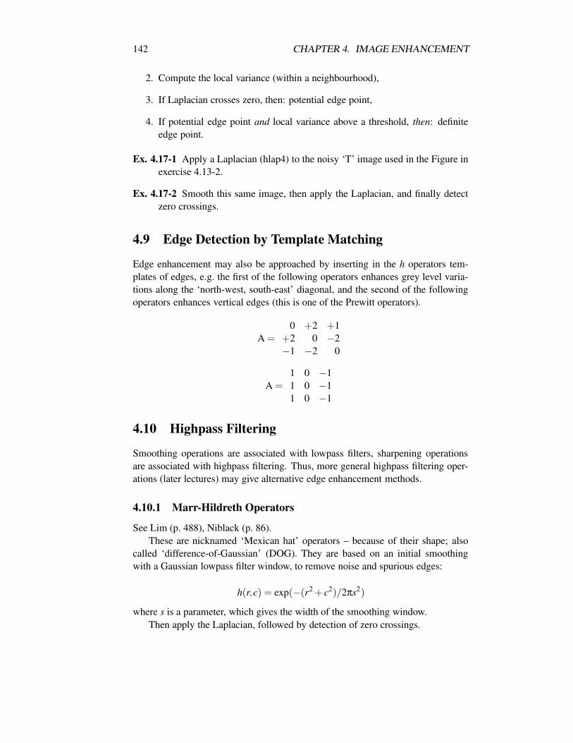
142 CHAPTER 4. IMAGE ENHANCEMENT
2. Compute the local variance (within a neighbourhood),
3. If Laplacian crosses zero, then: potential edge point,
4. If potential edge point and local variance above a threshold, then: definiteedge point.
Ex. 4.17-1 Apply a Laplacian (hlap4) to the noisy ‘T’ image used in the Figure inexercise 4.13-2.
Ex. 4.17-2 Smooth this same image, then apply the Laplacian, and finally detectzero crossings.
4.9 Edge Detection by Template Matching
Edge enhancement may also be approached by inserting in the h operators tem-plates of edges, e.g. the first of the following operators enhances grey level varia-tions along the ‘north-west, south-east’ diagonal, and the second of the followingoperators enhances vertical edges (this is one of the Prewitt operators).
A =0 +2 +1
+2 0 −2−1 −2 0
A =1 0 −11 0 −11 0 −1
4.10 Highpass Filtering
Smoothing operations are associated with lowpass filters, sharpening operationsare associated with highpass filtering. Thus, more general highpass filtering oper-ations (later lectures) may give alternative edge enhancement methods.
4.10.1 Marr-Hildreth Operators
See Lim (p. 488), Niblack (p. 86).These are nicknamed ‘Mexican hat’ operators – because of their shape; also
called ‘difference-of-Gaussian’ (DOG). They are based on an initial smoothingwith a Gaussian lowpass filter window, to remove noise and spurious edges:
h(r,c) = exp(−(r2 + c2)/2πs2)
where s is a parameter, which gives the width of the smoothing window.Then apply the Laplacian, followed by detection of zero crossings.
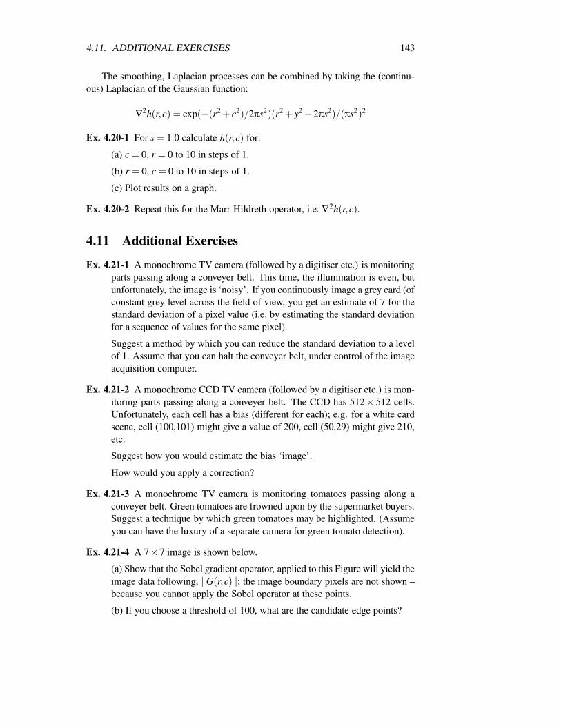
4.11. ADDITIONAL EXERCISES 143
The smoothing, Laplacian processes can be combined by taking the (continu-ous) Laplacian of the Gaussian function:
∇2h(r,c) = exp(−(r2 + c2)/2πs2)(r2 + y2−2πs2)/(πs2)2
Ex. 4.20-1 For s = 1.0 calculate h(r,c) for:
(a) c = 0, r = 0 to 10 in steps of 1.
(b) r = 0, c = 0 to 10 in steps of 1.
(c) Plot results on a graph.
Ex. 4.20-2 Repeat this for the Marr-Hildreth operator, i.e. ∇2h(r,c).
4.11 Additional Exercises
Ex. 4.21-1 A monochrome TV camera (followed by a digitiser etc.) is monitoringparts passing along a conveyer belt. This time, the illumination is even, butunfortunately, the image is ‘noisy’. If you continuously image a grey card (ofconstant grey level across the field of view, you get an estimate of 7 for thestandard deviation of a pixel value (i.e. by estimating the standard deviationfor a sequence of values for the same pixel).
Suggest a method by which you can reduce the standard deviation to a levelof 1. Assume that you can halt the conveyer belt, under control of the imageacquisition computer.
Ex. 4.21-2 A monochrome CCD TV camera (followed by a digitiser etc.) is mon-itoring parts passing along a conveyer belt. The CCD has 512× 512 cells.Unfortunately, each cell has a bias (different for each); e.g. for a white cardscene, cell (100,101) might give a value of 200, cell (50,29) might give 210,etc.
Suggest how you would estimate the bias ‘image’.
How would you apply a correction?
Ex. 4.21-3 A monochrome TV camera is monitoring tomatoes passing along aconveyer belt. Green tomatoes are frowned upon by the supermarket buyers.Suggest a technique by which green tomatoes may be highlighted. (Assumeyou can have the luxury of a separate camera for green tomato detection).
Ex. 4.21-4 A 7×7 image is shown below.
(a) Show that the Sobel gradient operator, applied to this Figure will yield theimage data following, | G(r,c) |; the image boundary pixels are not shown –because you cannot apply the Sobel operator at these points.
(b) If you choose a threshold of 100, what are the candidate edge points?
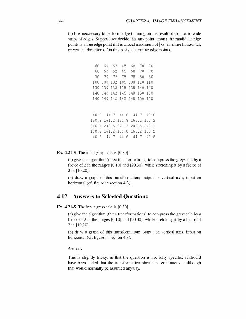
144 CHAPTER 4. IMAGE ENHANCEMENT
(c) It is neccessary to perform edge thinning on the result of (b), i.e. to widestrips of edges. Suppose we decide that any point among the candidate edgepoints is a true edge point if it is a local maximum of |G | in either horizontal,or vertical directions. On this basis, determine edge points.
60 60 62 65 68 70 7060 60 62 65 68 70 7070 70 72 75 78 80 80
100 100 102 105 108 110 110130 130 132 135 138 140 140140 140 142 145 148 150 150140 140 142 145 148 150 150
40.8 44.7 46.6 44 7 40.8160.2 161.2 161.8 161.2 160.2240.1 240.8 241.2 240.8 240.1160.2 161.2 161.8 161.2 160.240.8 44.7 46.6 44 7 40.8
Ex. 4.21-5 The input greyscale is [0,30];
(a) give the algorithm (three transformations) to compress the greyscale by afactor of 2 in the ranges [0,10] and [20,30], while stretching it by a factor of2 in [10,20],
(b) draw a graph of this transformation; output on vertical axis, input onhorizontal (cf. figure in section 4.3).
4.12 Answers to Selected Questions
Ex. 4.21-5 The input greyscale is [0,30];
(a) give the algorithm (three transformations) to compress the greyscale by afactor of 2 in the ranges [0,10] and [20,30], while stretching it by a factor of2 in [10,20],
(b) draw a graph of this transformation; output on vertical axis, input onhorizontal (cf. figure in section 4.3).
Answer:
This is slightly tricky, in that the question is not fully specific; it shouldhave been added that the transformation should be continuous – althoughthat would normally be assumed anyway.

4.12. ANSWERS TO SELECTED QUESTIONS 145
Continuous answer:
(i) [0..10] -> [0..5](ii) [10..20] -> [5..25](iii) [20..30] -> [25..30]
if(betw(z,0,10))z’:=(z-0)/2 + 0if(betw(z,10,20))z’:=(z-10)*2 + 5if(betw(z,20,30))z’:=(z-20)/2 + 25
where betw(z,z0,z1) = if(z>=z1 and z<=z2)
Here I have made explicit the shift to zero before the scale, followed bya shift back (to the appropriate start point – the end point of the previoustransformation).
A non-continuous answer would be:
(i) [0..10] -> [0..5](ii) [10..20] -> [20..40](iii) [20..30] -> [10..20]
though this does not make too much sense.
Ex. 4.7-2 Input image:
2 2 2 2 24 4 4 4 46 6 6 6 68 8 8 8 810 10 10 10 10
(a) What is the mean, m? What is the standard deviation, s?
(b) Transform to mean, m′ = 128, standard deviation s′ = 80.
(c) Will it fit into [0,255]?
(d) If not, ‘clip’ to 0 below 0 and to 255 above 255.
Answer:

146 CHAPTER 4. IMAGE ENHANCEMENT
m = (1/25)(sum) = (1/25)(2+2+2...+10+10)
= (1/25)(10+20+30+40+50) = 6
v = (1/25)((2−6)2....) = (1/25)(5.16+5.4+5.4+5.16) = 200/25 = 8
s =√
v = 2.8
Formula: z′ = (z−m)× s′/s+m′ = (z−6)×80/2.8+128
at 2 z′ =−4×80/2.8...+128 = 13.7 etc.
...
at 10 z′ = 4×80/2.8+128 = 242.
i.e. the range is reasonably filled.
You can see that the purpose of such a transformation is to shift the data intothe middle of the range, and expand the range.
Ex. 4.8-9 Suppose that a 64× 64, 8-level image has the grey level distributionshown below. We have also included in the table p(z), the density calculatedfrom the histogram. Calculate the transformation function, T (z), to givehistogram equalization, using the algorithm given above. Then calculateq′(w), the actual output histogram, and plot it.
Recommendation: Proceed as follows. Work out q(w). Then work out thecumulatives P(), and Q(); then apply the algorithm.
------------------------------------------------------------z ph(z) p(z)= q(w) P(z) Q(z) T(z)
ph(z)/M.N-----------------------------------------------------------
0 790 0.19 .125 .19 .125 11 1023 0.25 .125 .44 .25 32 850 0.21 .125 .65 .375 43 656 0.16 .125 .81 .5 54 329 0.08 .125 .89 .625 65 245 0.06 .125 .95 .75 76 122 0.03 .125 .98 .875 77 81 0.02 .125 1.0 1.0 7
-----------------------------------------------------------
Histogram for exercise 4.8-9
Answer:
4.12. ANSWERS TO SELECTED QUESTIONS 147
See above. Note, you can work with histograms or with ‘probabilities’, solong as p() and q() are both histograms or probabilities.
q() = .125 is merely dividing the total probability (1.0) into 8 for 8 slots.
Ex. 4.8-10 Someone has asserted: “histogram modification (or any form of con-trast stretching) is unlikely to be of assistance in a purely automatic machinevision application (i.e. one in which there is no human intervention), sincethese techniques introduce no new information – in fact, they often destroyinformation”
On the basis of sections 4.4 to 4.8, comment on this assertion.
Hint: Look carefully at the histogram equalization transformation functionin Exercise 4.8-8. Compare the input and output histograms. How manygrey levels in the input? How many in the output?
Answer:
(i) If you look at the transformation for Exercise 4.8-9 above you will seethat there are eight grey levels in the input image, and only six in the output(0, 2 are missing). Thus information was destroyed in the transformation.Thus features that were previously evident, may now be obscured.
(ii) The purpose of histogram modification is to better match the picture tothe human visual system – i.e. stretch the contrast. In a machine the mostcommon activity will be comparing the values of two pixels; transformingthe input (in the manner described above) cannot improve the outcome – butit can disimprove the outcome – i.e. by making pixels equal that were notequal in the input.
There may be some cases where the reason for the transformation has to dowith the physics of the problem.
Ex. 4.12-2 Given an input image f[rl..rh][cl..ch], an output image g[rl..rh][cl..ch],a filter mask (impulse response): h[-w..+w][-v..+v], write a computerprogram fragment to perform convolution (section 4.12).
Hint 1: there will be four nested loops.
Answer:
Start off with:
g(r,c) =r+w
∑k=r−w
c+v
∑l=c−v
f (k, l) h(r− k,c− l)
where h() are the weights.
Note: this assumes that h[] is stored in an a rectangular array, h[-w..+w][-v..+v].In most computer languages an array must start at 0 or 1; in C this is 0. Thus,in C the formula would have to read

148 CHAPTER 4. IMAGE ENHANCEMENT
...f[k][l]*h[r-k+w][c-l+v]
so that the indices go from 0..w*2 + 1, 0..v*2 + 1
Code: (in C)
for(r= rl+w;r<= rh-w; r++)for(c=cl+v;c<=ch-v;c++)
sum=0.0;for(k=r-w;k<=r+w;k++)for(l=c-v;l<=c+w;l++)
sum+=f[k][l]*h[r-k+w][c-l+v];g[r][c] = sum;
Test the fragment by dry running on an ‘impulse’ image.
If you operate on an impulse with h[] you will get a copy of h[] where theimpulse was. I.e. h[] is the impulse response of the operator.
Ex. 4.13-2 Perform 3×3 median filtering on the image given in Ex. 4.13-2 (letter‘T’ with impulse noise). Draw a picture of the result. What happens atcorners?
Answer:
Median filtering removes all the ‘spikes’, and leaves the ‘T’ intact, except itremoves the corners.
An averaging filter is not well suited to this sort of noise, or this sort of image– where there are sharp edges, which presumably should be preserved. Thenoise is just smeared, not removed; the edges are blurred.
Ex. 4.16.8-1 Apply a Sobel vertical gradient operator to the image of the letter ‘T’in Exercise 4.13-2. Draw a picture of the result. What happens at corners?
Ex. 4.16.8-2 Apply a Sobel horizontal gradient operator to the ‘T’ image given inExercise 4.13-2. Draw a picture of the result.
Answer:
The Sobel operator gives 1,3, or 4 for positive edges, and −1,−3,−4 fornegative edges; the magnitude depends on whether we are at the end or mid-dle of an edge line.
Usually sign does not matter; although, if you were following edges, using asimilarity criterion, it might.
Whan adding vertical and horizontal edges, the signs must be removed –otherwise you may lose edge points at corners etc.

4.12. ANSWERS TO SELECTED QUESTIONS 149
Ex. 4.16.8-4 Given an input image f[r_l..r_h][c_l..c_h], an output imageg[r_l..r_h][c_l..c_h], write a computer program fragment to apply theSobel vertical operator.
Hint: Look at your answer for Ex. 4.12-2.
Answer:
h =1 0 −12 0 −21 0 −1
Declare h[] as follows:
int h[3][3] =1,0,-1,2,0,-2,1,0,-1;
and use answer to Ex. 4.12-2.
Note the way C stores such arrays.
Of course, you can save time by avoiding multiplying by 1, and avoidingthe 0s altogether – but that is a minor implementation concern, secondary togetting the program to work, and to making it readable.
Given that C stores the array like it does, why is it better to have ‘c’, thesecond index, in the inner loop?
Answer:
If you are in a virtual memory system (e.g. paged), such an arrangement willgenerate far less vitual memory handling. Consider NR = NC = 512 = pagesize. Done the right way you may get away with 1 page fault. Done thewrong way, you may get 512 page faults.
But, PCs don’t have paging, I hear you say. Maybe, but, increasingly, theyhave caches – which operate in the same way to paging – only the pages aresmaller.

150 CHAPTER 4. IMAGE ENHANCEMENT
4.13 Examples of Image Enhancement Operations
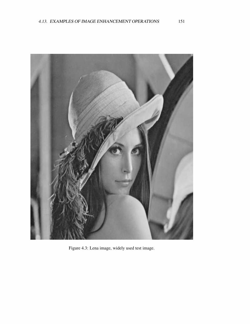
4.13. EXAMPLES OF IMAGE ENHANCEMENT OPERATIONS 151
Figure 4.3: Lena image, widely used test image.
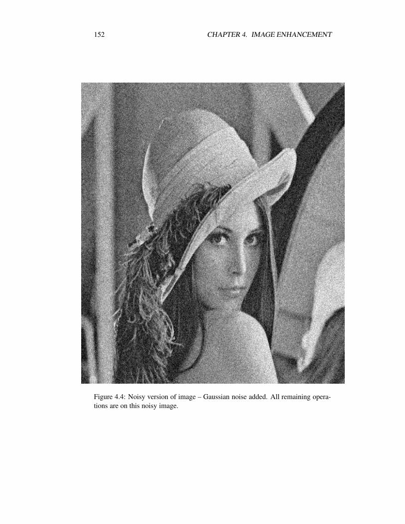
152 CHAPTER 4. IMAGE ENHANCEMENT
Figure 4.4: Noisy version of image – Gaussian noise added. All remaining opera-tions are on this noisy image.
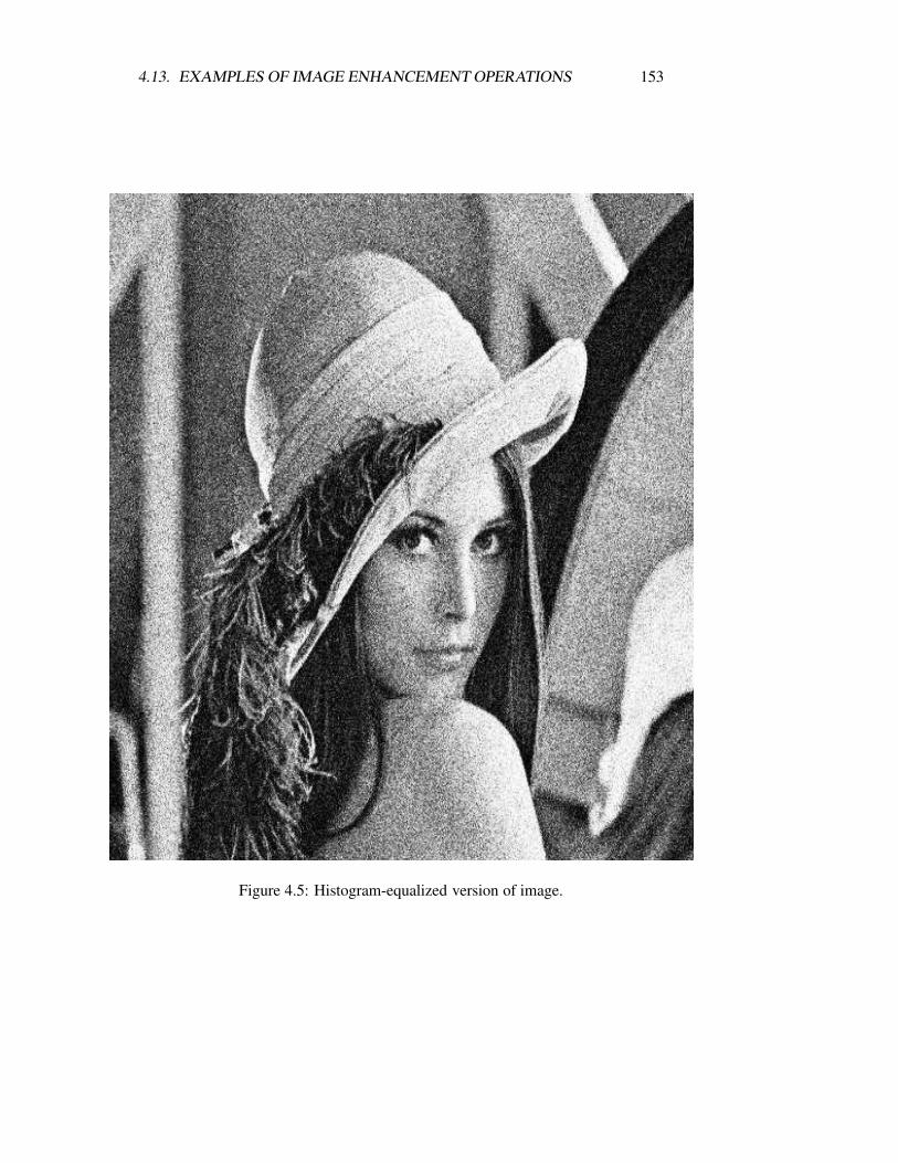
4.13. EXAMPLES OF IMAGE ENHANCEMENT OPERATIONS 153
Figure 4.5: Histogram-equalized version of image.
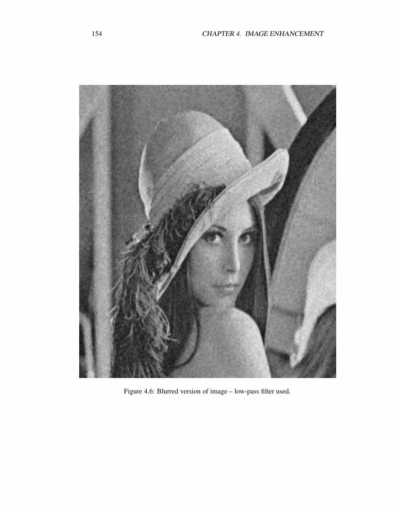
154 CHAPTER 4. IMAGE ENHANCEMENT
Figure 4.6: Blurred version of image – low-pass filter used.
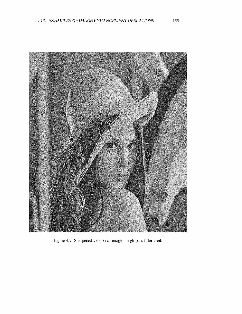
4.13. EXAMPLES OF IMAGE ENHANCEMENT OPERATIONS 155
Figure 4.7: Sharpened version of image – high-pass filter used.

156 CHAPTER 4. IMAGE ENHANCEMENT
Figure 4.8: Edge detector used on image.

4.13. EXAMPLES OF IMAGE ENHANCEMENT OPERATIONS 157
Figure 4.9: Edge detector used on image, followed by histogram equalization.
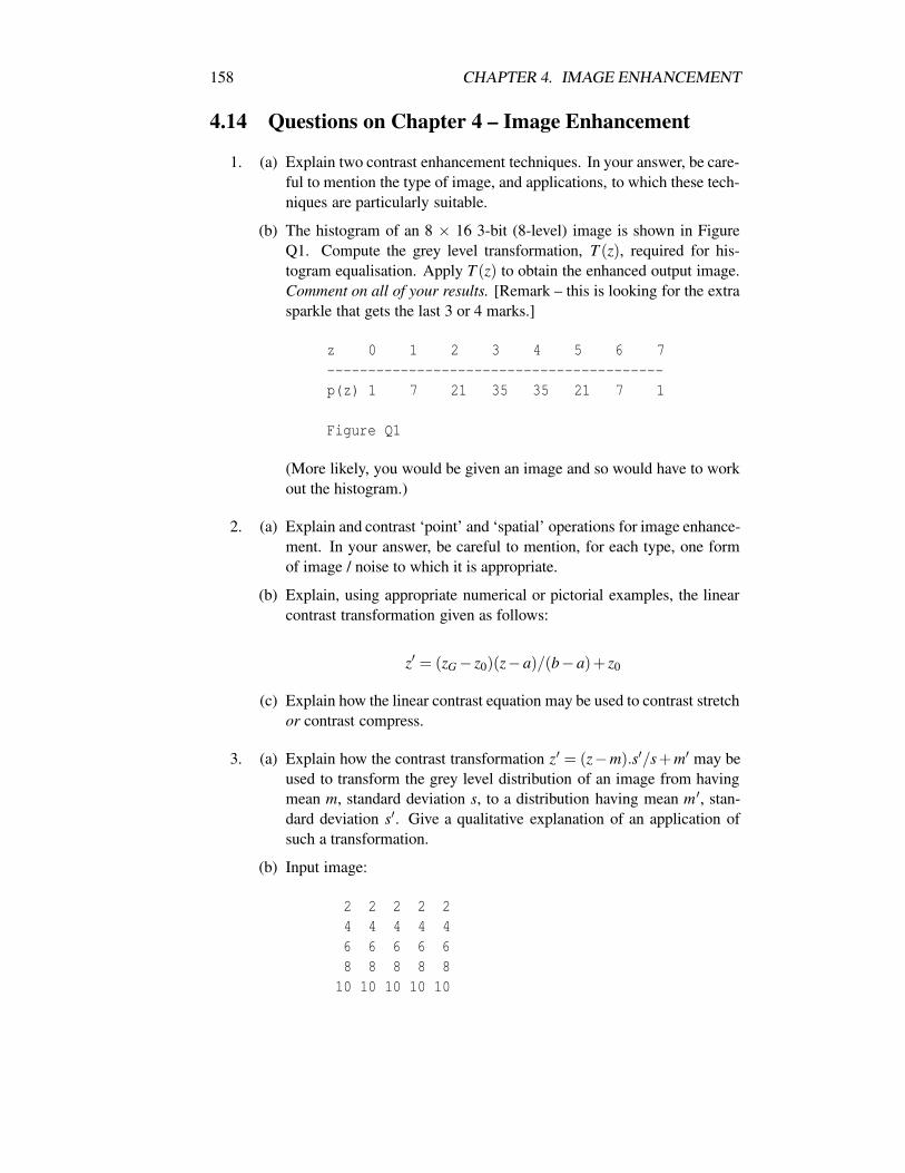
158 CHAPTER 4. IMAGE ENHANCEMENT
4.14 Questions on Chapter 4 – Image Enhancement
1. (a) Explain two contrast enhancement techniques. In your answer, be care-ful to mention the type of image, and applications, to which these tech-niques are particularly suitable.
(b) The histogram of an 8 × 16 3-bit (8-level) image is shown in FigureQ1. Compute the grey level transformation, T (z), required for his-togram equalisation. Apply T (z) to obtain the enhanced output image.Comment on all of your results. [Remark – this is looking for the extrasparkle that gets the last 3 or 4 marks.]
z 0 1 2 3 4 5 6 7-----------------------------------------p(z) 1 7 21 35 35 21 7 1
Figure Q1
(More likely, you would be given an image and so would have to workout the histogram.)
2. (a) Explain and contrast ‘point’ and ‘spatial’ operations for image enhance-ment. In your answer, be careful to mention, for each type, one formof image / noise to which it is appropriate.
(b) Explain, using appropriate numerical or pictorial examples, the linearcontrast transformation given as follows:
z′ = (zG− z0)(z−a)/(b−a)+ z0
(c) Explain how the linear contrast equation may be used to contrast stretchor contrast compress.
3. (a) Explain how the contrast transformation z′ = (z−m).s′/s+m′ may beused to transform the grey level distribution of an image from havingmean m, standard deviation s, to a distribution having mean m′, stan-dard deviation s′. Give a qualitative explanation of an application ofsuch a transformation.
(b) Input image:
2 2 2 2 24 4 4 4 46 6 6 6 68 8 8 8 810 10 10 10 10

4.14. QUESTIONS ON CHAPTER 4 – IMAGE ENHANCEMENT 159
What is mean, m? What is standard deviation, s? Transform to mean,m′ = 128, std. dev s′ = 80. Will it fit into [0,255]? If not, ‘clip’ to 0below 0 and to 255 above 255.
4. (a) Explain how certain types of noise may be reduced by averaging mul-tiple images.
(b) Local or ‘point’ enhancement operations have the disadvantage thatthey operate uniformly over an image, however, the image may not beuniform. Discuss, and explain methods of overcoming this problem.
5. (a) Using appropriate numerical and/or pictorial illustrations, compare andcontrast the algorithms for spatial smoothing and edge enhancement.(You should employ appropriate equations and masks provided in theappendix to the exam paper.)
(b) Explain applications of each.
6. (a) Using appropriate numerical and/or pictorial illustrations, compare andcontrast the algorithms for spatial smoothing and median filter. (Youshould employ appropriate equations and masks given in the appendixto the exam paper.)
(b) Explain applications of each.
7. (a) Using appropriate numerical and/or pictorial illustrations, compare andcontrast the algorithms for spatial smoothing and median filter. (Youshould employ appropriate equations and masks given in the appendixto the exam paper.)
(b) Explain why any convolution operation is called linear, yet medianfiltering is called non-linear.
(c) Explain any other non-linear filter (other than median).
8. (a) Explain Sobel edge enhancement.
(b) Explain how the results of edge enhancement may be used to completeedge detection.
9. (a) Explain the roles of ‘gradient’ and ‘differentiation’ in edge enhance-ment. (Use one- or two-dimensional examples to illustrate your an-swer.)
(b) Apply Sobel edge enhancement to the image given in Figure Q2. Drawa picture of the result.
0 0 0 0 0 0 0 0 0 0 0 0 0 0 0 00 0 0 0 0 0 0 0 0 0 0 0 0 0 0 00 0 0 0 0 0 0 0 0 0 0 0 0 0 0 00 0 0 0 0 0 0 0 0 0 0 0 0 0 0 0

160 CHAPTER 4. IMAGE ENHANCEMENT
0 0 0 0 0 0 0 0 0 0 0 0 0 0 0 00 0 0 1 1 1 1 1 1 1 1 1 1 0 0 00 0 0 1 1 1 1 1 1 1 1 1 1 0 0 00 0 0 1 1 1 1 1 1 1 1 1 1 0 0 00 0 0 1 1 1 1 1 1 1 1 1 1 0 0 00 0 0 0 0 0 1 1 1 1 0 0 0 0 0 00 0 0 0 0 0 0 0 0 0 0 0 0 0 0 0
Figure Q2
10. (a) Explain the connection between the Prewitt operators and differentia-tion.
(b) Given an input image f[rl..rh][cl..ch], an output image g[rl..rh][cl..ch],write a computer program fragment to apply the Prewitt vertical oper-ator.
11. (a) Explain the connection between the Sobel operators and differentia-tion.
(b) Given an input image f[rl..rh][cl..ch], an output image g[rl..rh][cl..ch],write a computer program fragment to apply the Sobel vertical opera-tor.
12. (a) Explain the connection between cross-correlation and convolution.
(b) Given an input image f[rl..rh][cl..ch], a convolution mask h[0..w-1][0..v-1]and an output image g[rl..rh][cl..ch], write a computer programfragment to apply two dimensional convolution.
(c) (Assignment question only: give at least two sets of sample inputs andoutputs).
13. A 7 × 7 image is shown in Figure Q3.
(a) Show that the Sobel gradient operator, applied to Figure Q3 will yieldFigure Q4, | G(r,c) |; the image boundary pixels are not shown in Fig-ure Q4 - because you cannot apply the Sobel operator at these points.
(b) If you choose a threshold of 100, what are the candidate edge points?
(c) It is neccessary to perform edge thinning on the result of (b), i.e. to widestrips of edges. Suppose we decide that any point among the candidateedge points is a true edge point if it is a local maximum of |G | in eitherhorizontal, or vertical directions. On this basis, determine edge points.
60 60 62 65 68 70 7060 60 62 65 68 70 7070 70 72 75 78 80 80100 100 102 105 108 110 110

4.14. QUESTIONS ON CHAPTER 4 – IMAGE ENHANCEMENT 161
130 130 132 135 138 140 140140 140 142 145 148 150 150140 140 142 145 148 150 150
Figure Q3
40.8 44.7 46.6 44 7 40.8160.2 161.2 161.8 161.2 160.2240.1 240.8 241.2 240.8 240.1160.2 161.2 161.8 161.2 160.240.8 44.7 46.6 44 7 40.8
Figure Q4

162 CHAPTER 4. IMAGE ENHANCEMENT
Chapter 5
Data and Image Compression
5.1 Introduction and Summary
The following are the important concepts introduced in this chapter:
• Data compression should be considered whenever large amounts of data arestored on a limited storage resource (e.g. a magnetic disk), or transmittedover a communications channel that has limited capacity (e.g. a communica-tions line with restricted data rate).
• Data compression exploits the fact that you need only store or transmit ‘realinformation’.
• ‘(Real) information’ is strongly related to uncertainty; if no uncertainty ex-ists, there cannot be any flow of ’real’ information; you give no ‘information’if you tell someone something that he/she knows already.
• Entropy is a suitable mathemetical measure of uncertainty.
• Formally, the ‘size’ of a piece of ‘information’ (its entropy) can be mea-sured in terms of the number of binary-digits (bits) required to represent itunambiguously.
• The number of bits is exactly the number of ‘twenty-questions’ type ques-tions that need to be asked to unambiguously determine the information.
• The measure is zero if there is no uncertainty, and there is no point is sendingor storing anything.
• The measure is small if there is small uncertainty (small variation), e.g. ahexadecimal digit can be expressed in 4 bits.
• The measure is large if there is big uncertainty, a big number requires a largenumber of bits, e.g. a list of the populations of Irish towns and cities would
163

164 CHAPTER 5. DATA AND IMAGE COMPRESSION
range (say) 100 to 1,000,000 (a large variation) and would require about 20bits for each number.
• In sequences of pieces of information, sometimes one piece of information‘gives the game away’ as to another piece of information; e.g. given theoccurrence of the letter ‘q’, surely ‘u’ follows; this is variously called ‘re-dundancy’ (the ‘u’ is redundant), ‘correlation’, and ‘dependence’.
• Simple entropy-based compression schemes look at the probability (and hencethe uncertainty/entropy) of single symbols (a symbol can be e.g. a pixelvalue, or a text character).
• However, the true entropy of the source must be measured using all possi-ble strings of symbols; hence, single symbol entropy-based methods (e.g.Huffman coding) do not achieve optimum efficiency.
• In signals and images, there usually is dependence (correlation) betweenneighboring points.
• The bigger the dimensionality (signals: dimensionality = 1, images = 2, mov-ing sequences of images = 3) the more neighbors, so the more correlation,and so the greater the scope for correlation.
• Various compression methods exploit correlation in markedly different ways:
– run-length encoding,
– differential (predictive) encoding,
– transform coding.
5.2 Compression – Motivation
We mentioned in the introductory chapter that technological advances (sensors,display devices, speed of processors, size of memories) are allowing image pro-cessing into the arena of data processing (i.e. processing of text, numbers).
Nevertheless, the vast amount of data required to represent a digital image isstill a major obstacle:
• Storage: disk and tape devices are getting large and fast (and smaller in size),but not infinitely so. The amount of data produced is increasing ever morerapidly.
• Communications channel capacity: the capacity of a communication channelis finite; fiber optics with their vastly increased capacity are on the way, butcopper lines will prevail for most of the next 10 years.
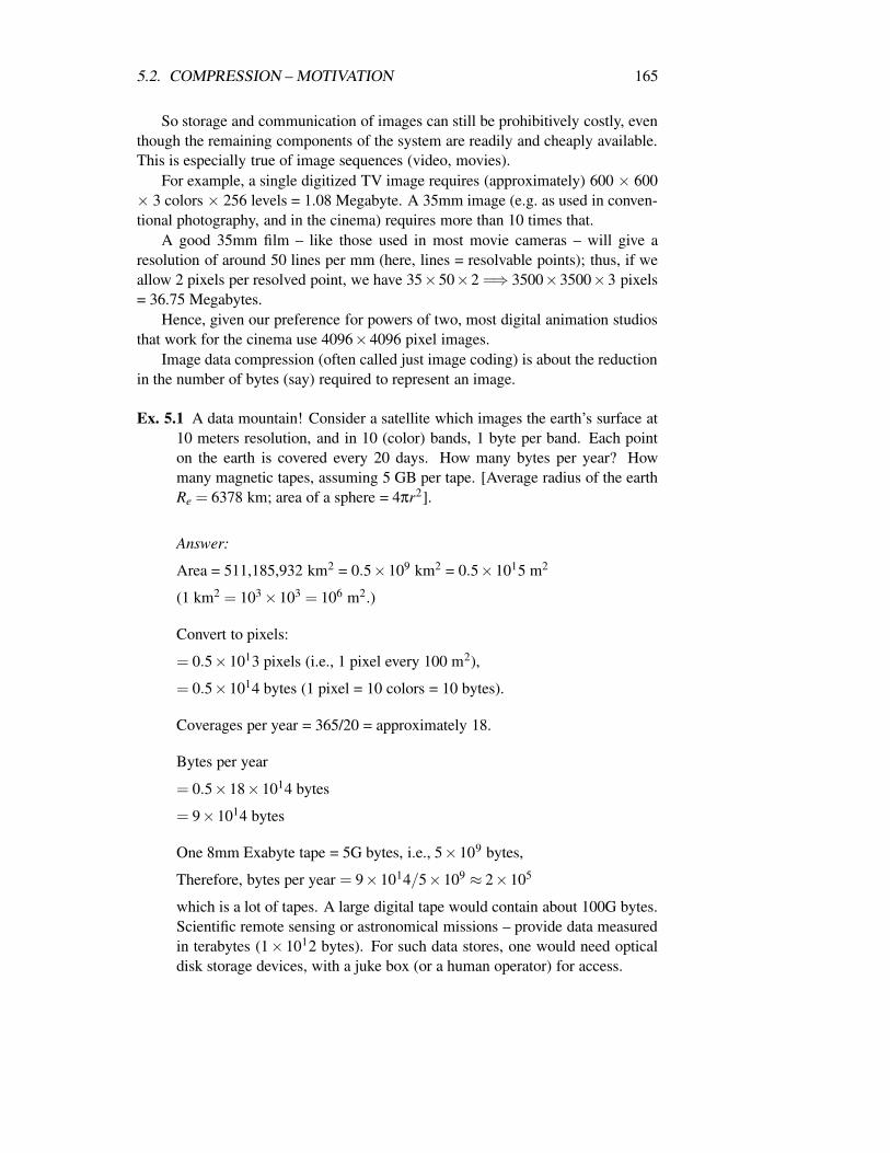
5.2. COMPRESSION – MOTIVATION 165
So storage and communication of images can still be prohibitively costly, eventhough the remaining components of the system are readily and cheaply available.This is especially true of image sequences (video, movies).
For example, a single digitized TV image requires (approximately) 600 × 600× 3 colors × 256 levels = 1.08 Megabyte. A 35mm image (e.g. as used in conven-tional photography, and in the cinema) requires more than 10 times that.
A good 35mm film – like those used in most movie cameras – will give aresolution of around 50 lines per mm (here, lines = resolvable points); thus, if weallow 2 pixels per resolved point, we have 35×50×2 =⇒ 3500×3500×3 pixels= 36.75 Megabytes.
Hence, given our preference for powers of two, most digital animation studiosthat work for the cinema use 4096×4096 pixel images.
Image data compression (often called just image coding) is about the reductionin the number of bytes (say) required to represent an image.
Ex. 5.1 A data mountain! Consider a satellite which images the earth’s surface at10 meters resolution, and in 10 (color) bands, 1 byte per band. Each pointon the earth is covered every 20 days. How many bytes per year? Howmany magnetic tapes, assuming 5 GB per tape. [Average radius of the earthRe = 6378 km; area of a sphere = 4πr2].
Answer:
Area = 511,185,932 km2 = 0.5×10⁹ km2 = 0.5×10¹⁵ m2
(1 km2 = 103×103 = 106 m2.)
Convert to pixels:
= 0.5×1013 pixels (i.e., 1 pixel every 100 m2),
= 0.5×1014 bytes (1 pixel = 10 colors = 10 bytes).
Coverages per year = 365/20 = approximately 18.
Bytes per year
= 0.5×18×1014 bytes
= 9×1014 bytes
One 8mm Exabyte tape = 5G bytes, i.e., 5×109 bytes,
Therefore, bytes per year = 9×10¹⁴/5×109 ≈ 2×10⁵
which is a lot of tapes. A large digital tape would contain about 100G bytes.Scientific remote sensing or astronomical missions – provide data measuredin terabytes (1× 1012 bytes). For such data stores, one would need opticaldisk storage devices, with a juke box (or a human operator) for access.
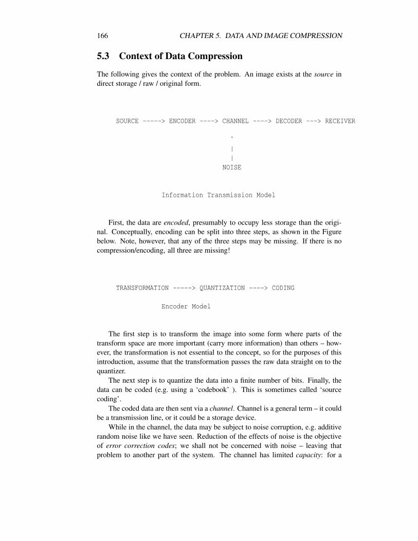
166 CHAPTER 5. DATA AND IMAGE COMPRESSION
5.3 Context of Data Compression
The following gives the context of the problem. An image exists at the source indirect storage / raw / original form.
SOURCE -----> ENCODER ----> CHANNEL ----> DECODER ---> RECEIVER
ˆ||
NOISE
Information Transmission Model
First, the data are encoded, presumably to occupy less storage than the origi-nal. Conceptually, encoding can be split into three steps, as shown in the Figurebelow. Note, however, that any of the three steps may be missing. If there is nocompression/encoding, all three are missing!
TRANSFORMATION -----> QUANTIZATION ----> CODING
Encoder Model
The first step is to transform the image into some form where parts of thetransform space are more important (carry more information) than others – how-ever, the transformation is not essential to the concept, so for the purposes of thisintroduction, assume that the transformation passes the raw data straight on to thequantizer.
The next step is to quantize the data into a finite number of bits. Finally, thedata can be coded (e.g. using a ‘codebook’ ). This is sometimes called ‘sourcecoding’.
The coded data are then sent via a channel. Channel is a general term – it couldbe a transmission line, or it could be a storage device.
While in the channel, the data may be subject to noise corruption, e.g. additiverandom noise like we have seen. Reduction of the effects of noise is the objectiveof error correction codes; we shall not be concerned with noise – leaving thatproblem to another part of the system. The channel has limited capacity: for a

5.4. INFORMATION THEORY 167
transmission line – bits per second, for a data file – perhaps some agreed limitationin size.
Channel bandwidth: The bandwidth of a channel is measured in Hertz, Hz.The capacity of the channel – its ability to pass information – is proportional tobandwidth. Hertz is measured in cycles/second.
The capacity of a channel depends on (a) its bandwidth, and (b) its signal-to-noise ratio. Noise reduces capacity.
On leaving the channel, the data is not in a directly usable form: it must bedecoded. Obviously the decoding process is strongly dependent on the encodingprocess – clearly, there must be cooperation between sender and receiver.
Finally, the image arrives at the receiver. Ideally, the receiver should receivethe data as they left the source, or as close as possible.
Source Coding versus Channel CodingMost books introduce two extra stages: channel encoding and channel decod-
ing – just before, and just after, the channel. These are the equivalent of modulationand demodulation; they are associated with getting the signal into a form in whichit can be carried by the so-called ‘physical-layer’. For the sort of approach usedhere, it is much better to include these in the channel – and to associate any noisedue to them with the channel. If neccessary we will make the distinction by explic-itly naming the encoder and decoder as source encoder, and source decoder.
Next, we introduce the theoretical notion of information.
5.4 Information Theory
5.4.1 Introduction to Information Theory
We need a precise definition of information, particularly a quantitative unit and amethod for measuring it.
Information theory defines information as the reduction of uncertainty.Thus, the sentence “IBM make computers” conveys little or no information –
because there is no uncertainty in your minds about the matter.
Informal discussion of Information:
Roughly speaking, the more variance, the more information. More precisely,the information (in bits) in a message is the number of ‘twenty questions’ typequestions you would have to use to get the information.
Thus, if I tell you I have written down a number between 0 and 15 (say 5),you can ask me: is it less-than-or-equal-to 7? (yes), is it less-than-or-equal-to 3?(no), less-than-or-equal-to 5? (yes), therefore it is 5 or 4, and the next questionclinches it; thus, 4 questions or 4 bits; i.e. a hexadecimal digit contains 4 bits ofinformation.
In this last example, each value was equally likely, and the information for avalue can be calculated as:
168 CHAPTER 5. DATA AND IMAGE COMPRESSION
I =− log2(p) = log2(1/p)
where p = probability of the value = 1/16. log2(1/16) =−4.Information and entropy (to follow) is associated with the pioneering work of
Shannon in the late 40s.Review of logarithms: log2 x = y implies that 2y = x. Note that y = 0⇐= x = 1.
Prove that log2 x = k1 log1 0x = k2 loge x for constants k1 and k2.What is the difference between information and data? This is a bit subtle,
and can lead to problems and apparent paradoxes. For example, if you wanted totransmit Hamlet’s ‘To be or not to be’ speech to a friend and you knew they had acollected works on their bookshelf, all you need to transmit is ‘Hamlet Act 3 Scene2, speech 4’ i.e. about 30 alphabetic characters, or 240 bits – instead of the 2000or so characters in the speech.
Magic? paradox? No. The friend had received the major part of the informa-tion previously – the book.
Most of data compression depends on this principle: don’t waste resources onsending ‘information’ that is already known.
Ex. Fair coin: I =−log2(0.5) = 1 bit.
Ex. Dice: I = log2(6), approx = 2.5 bits. NB log2(1/6) =−log2(6)
Ex. Hexadecimal digit, see section above,
I =− log2(1/16) =− log2(1/24) =− log2(2−4) = 4.
Ex. One letter from an equally probable 26-letter alphabet:
I =− log2(1/26) = 4.7 bits i.e. 5 bits would do.
Ex. ASCII code (128 allowable symbols) – information of specified symbol:
I =− log2(1/128) = 7 bits
which is precisely the number of bits used.
5.4.2 Entropy or Average Information per Symbol
Information theory uses a measure of information called entropy; entropy is asso-ciated with ‘mixed-up-ness’ – uncertainty.
Entropy (H) is measured in units of bits – BInary digiTs. A bit is the funda-mental quantum of information required to distinguish between two equally likelyalternatives, e.g. the result of the toss of a fair coin.
Mathematically, for N equally probable outcomes,
H =− log2(1/N) (= log2N)
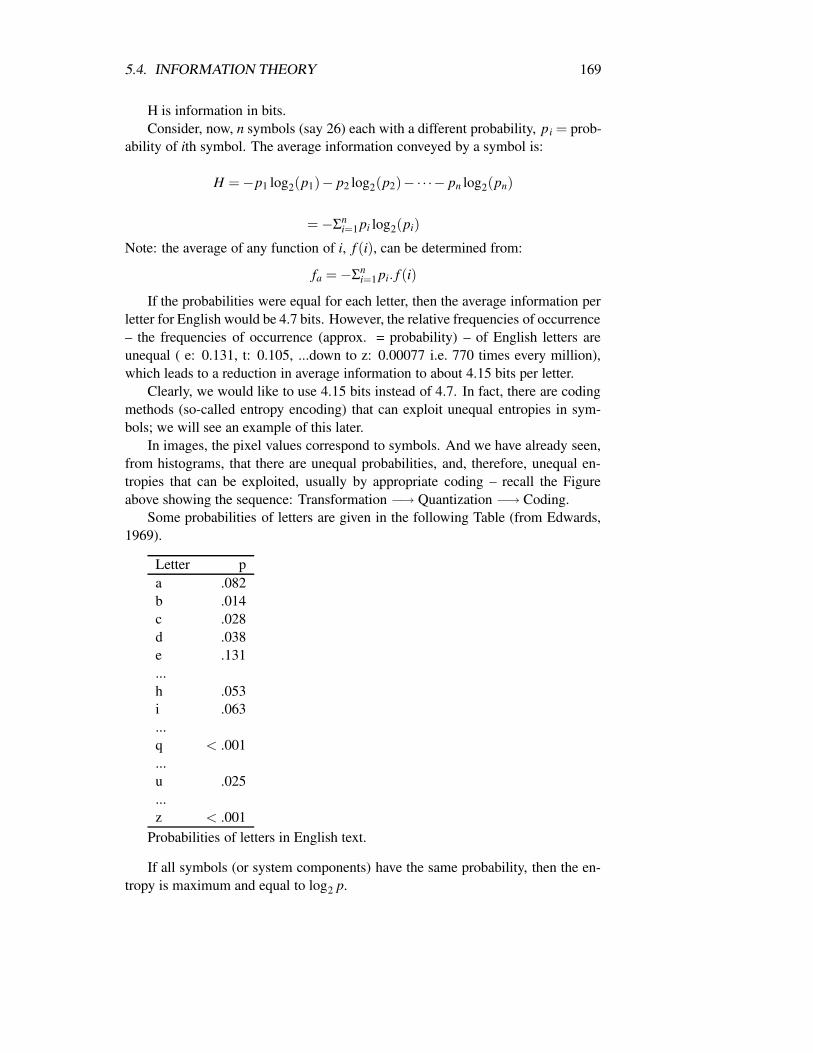
5.4. INFORMATION THEORY 169
H is information in bits.Consider, now, n symbols (say 26) each with a different probability, pi = prob-
ability of ith symbol. The average information conveyed by a symbol is:
H =−p1 log2(p1)− p2 log2(p2)−·· ·− pn log2(pn)
=−Σni=1 pi log2(pi)
Note: the average of any function of i, f (i), can be determined from:
fa =−Σni=1 pi. f (i)
If the probabilities were equal for each letter, then the average information perletter for English would be 4.7 bits. However, the relative frequencies of occurrence– the frequencies of occurrence (approx. = probability) – of English letters areunequal ( e: 0.131, t: 0.105, ...down to z: 0.00077 i.e. 770 times every million),which leads to a reduction in average information to about 4.15 bits per letter.
Clearly, we would like to use 4.15 bits instead of 4.7. In fact, there are codingmethods (so-called entropy encoding) that can exploit unequal entropies in sym-bols; we will see an example of this later.
In images, the pixel values correspond to symbols. And we have already seen,from histograms, that there are unequal probabilities, and, therefore, unequal en-tropies that can be exploited, usually by appropriate coding – recall the Figureabove showing the sequence: Transformation −→ Quantization −→ Coding.
Some probabilities of letters are given in the following Table (from Edwards,1969).
Letter pa .082b .014c .028d .038e .131...h .053i .063...q < .001...u .025...z < .001
Probabilities of letters in English text.
If all symbols (or system components) have the same probability, then the en-tropy is maximum and equal to log2 p.
170 CHAPTER 5. DATA AND IMAGE COMPRESSION
5.4.3 Redundancy
We mentioned “independent” symbols above. In a message composed of Englishtext, the symbols are not independent: there are varying degrees of dependencebetween successive symbols (and indeed between groups of them). If the letter“q” has just been transmitted, then the probability of “u” surely increases and theinformation contained in the next letter decreases accordingly; therefore, very littleinformation is contained in the “u” because the receiver had a fair idea what it wasbefore it arrived.
Redundancy is the information theory term for ‘dependence’ (or ‘lack of inde-pendence’) between symbols; literally, redundancy means ‘not needed’. Of course,redundancy is not always as clear-cut as in the case of the ‘q’ and ‘u’ mentionedabove – given ‘q’, the probability of ‘u’ might jump from 0.025 to 0.95 (95%) (not100%), and given ‘t’ the probability of ‘h’ jumps from 0.053 to maybe 0.2. A mea-sure of redundancy can be defined, in terms of the ratio of ‘lost’ entropy to entropywith no redundancy, as follows:
redundancy = (Hind−Hred)/Hind = (1−Hred/Hind)
where Hred = average entropy for dependent symbols, taking into account redun-dancy, Hind = average entropy for independent symbols.
Overall, English is more than 50 percent redundant.Here, we have just been discussing dependency/correlation between pairs of
symbols (so called ‘digrams’); there is additional redundancy if we look at triplets(so called ‘trigrams’); e.g. given ‘in’, ‘g’ becomes much more likely.
In images redundancy crops up as correlation between neighboring pixels.Deep down, most data compression algorithms are based on removal of redun-
dancy – don’t send parts of the message that are already known – or on non-uniformentropy (and these are related). Transformation coding and predictive coding areexamples of redundancy removal – but the redundancy removal is implicit and nottoo obvious.
5.4.4 Redundancy is Sometimes Useful!
In most forms of communication redundancy can sometimes be useful; humansuse it all the time; e.g. you can often reply before the previous speaker has finished,misspellings in text are an irritation, but the message still gets across.
Of course, parity and checksums are classical forms of redundancy – used forerror checking and correction.
Note: You will find that some authors, e.g. Edwards (1969), include, in thedefinition of redundancy, the loss of entropy due to unequal probabilities; we willreserve redundancy for loss of entropy due to dependence – as above in the equationdefining redundancy.
Ex. 5.4-1 Derive an estimate of the redundancy contained in the original of thefollowing sentence (from Cover and Thomas, 1991, p. 136).

5.5. INTRODUCTION TO IMAGE COMPRESSION 171
TH_R_ _S _NLY _N_ W_Y T_ F_LL _N TH_ V_W_LS _N TH_S S_NT_NC_.
5.5 Introduction to Image Compression
Image data compression techniques are very much problem-oriented. Neverthe-less, there are general methods, and general categorizations that can be made.
In some cases there will be a difference (error) between what leaves the source,and what arrives at the receiver. If perfect reconstruction (after the decoder) isdemanded, i.e. zero error, the encoder-decoder (compression) system is calledinformation preserving, or lossless; typically, for text communication, we requirelossless compression; often, for image communication, we may tolerate some loss,after all, we are used to fuzzy pictures in newspapers, badly set-up video recorders,etc.
Therefore, if the nature of the application allows some error, we can use a com-pression technique that merely maximises some fidelity criterion; these techniquesare called lossy.
Note: Chapter 8 (Pattern Recognition) mentions feature extraction. Featureextraction is strongly related to compression, because:
• we want to minimize the number of features,
• we want them to ‘classify’ as well as possible (the fidelity criterion).
It is important to realise that, for error-free compression, there is ‘no freelunch’. As mentioned in the previous section, there are two major sources of sav-ings: non-uniform entropy, and redundancy. If each pixel truly contains 8-bits ofinformation and is truly independent, no compression is possible. But, if the greylevels are not equally likely (say, the average entropy is 6 bits) then compressionis possible; however, it will not be possible to reduce below the theoretical limit of6-bits. In this case the savings can be achieved through proper coding.
If there is correlation, it will be possible to transform the data such that there isless correlation (or none) – recall the Figure showing the encoder model: transfor-mation−→ quantization −→ coding. E.g. transformation to the frequency domain,via the Fourier transform.
Summary:
There are two major categories of data compression:
• Lossless; the data are reconstructed as if no compression had taken place.
• Lossy; here distortion/errors are tolerated to a limited extent; minimize theerrors by maximising some fidelity criterion.
Major compression principles:
• transform compression,
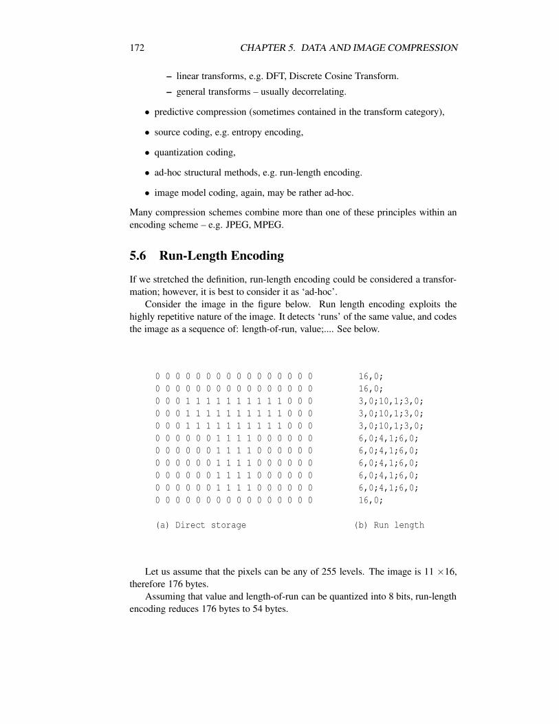
172 CHAPTER 5. DATA AND IMAGE COMPRESSION
– linear transforms, e.g. DFT, Discrete Cosine Transform.
– general transforms – usually decorrelating.
• predictive compression (sometimes contained in the transform category),
• source coding, e.g. entropy encoding,
• quantization coding,
• ad-hoc structural methods, e.g. run-length encoding.
• image model coding, again, may be rather ad-hoc.
Many compression schemes combine more than one of these principles within anencoding scheme – e.g. JPEG, MPEG.
5.6 Run-Length Encoding
If we stretched the definition, run-length encoding could be considered a transfor-mation; however, it is best to consider it as ‘ad-hoc’.
Consider the image in the figure below. Run length encoding exploits thehighly repetitive nature of the image. It detects ‘runs’ of the same value, and codesthe image as a sequence of: length-of-run, value;.... See below.
0 0 0 0 0 0 0 0 0 0 0 0 0 0 0 0 16,0;0 0 0 0 0 0 0 0 0 0 0 0 0 0 0 0 16,0;0 0 0 1 1 1 1 1 1 1 1 1 1 0 0 0 3,0;10,1;3,0;0 0 0 1 1 1 1 1 1 1 1 1 1 0 0 0 3,0;10,1;3,0;0 0 0 1 1 1 1 1 1 1 1 1 1 0 0 0 3,0;10,1;3,0;0 0 0 0 0 0 1 1 1 1 0 0 0 0 0 0 6,0;4,1;6,0;0 0 0 0 0 0 1 1 1 1 0 0 0 0 0 0 6,0;4,1;6,0;0 0 0 0 0 0 1 1 1 1 0 0 0 0 0 0 6,0;4,1;6,0;0 0 0 0 0 0 1 1 1 1 0 0 0 0 0 0 6,0;4,1;6,0;0 0 0 0 0 0 1 1 1 1 0 0 0 0 0 0 6,0;4,1;6,0;0 0 0 0 0 0 0 0 0 0 0 0 0 0 0 0 16,0;
(a) Direct storage (b) Run length
Let us assume that the pixels can be any of 255 levels. The image is 11 ×16,therefore 176 bytes.
Assuming that value and length-of-run can be quantized into 8 bits, run-lengthencoding reduces 176 bytes to 54 bytes.

5.7. QUANTIZATION CODING 173
A form of run-length encoding is used in fax machines. First, the image isquantized to 1 bit (black-white), and then runs of black (or white) are determined.
If we recognise the two-dimensionality of the image, we can run-length encodeboth horizontally and vertically.
In its plain form, run-length encoding is error free – lossless.
Ex. 5.6-1 Obviously, run length encoding will not provide any compresssion for‘busy’ images (i.e. where the pixel values are rapidly varying, and there isvery little correlation between adjacent pixels). Considering the model of achecker-board (alternate black (0), white (1), squares, and a 16 x 16 image,and starting with (1) a pure white image, next, (2) an image with 4 squares
white, blackblack, white
and so on, at what stage does run-length encoding start to increase the data(i.e. more than 256 bytes)?
Ex. 5.6-2 Assume images are first quantized to 1 bit, and that maximum run lengthis 128; this allows the length-of-run and value to be both coded in one byte.Calculate the number of bytes for the ‘T’ Figure above.
Ex. 5.6-3 Using the scheme of Ex. 5.6-2, recalculate the cut-off point for Ex.5.6-1 (checker-board).
5.7 Quantization Coding
For example, in the case of faxed documents, we agree that there are only two greylevels in the image (black=0, white=1). Thus we can quantize the source image to1 bit. Thus, a saving of 8 times (over 256 levels).
If we have a pictorial image with 255 levels, but know that it will only ever beused to print on a newspaper with 16 grey levels (say), then we can quantize it to 4bits.
Choice of quantization should depend on knowledge of the source, and of thereceiver – the expected use of the image. E.g. if the image is known to be from(source) a black/white page, then one bit is enough; likewise, if (any) image is onlyever going to be printed on such a page, again one bit will suffice.
From our knowledge of vision, we know that humans can, simultaneously, onlycope with 160 levels at once; therefore we can restrict most images to 256 levels,or 8 bits. Nevertheless, in an X-ray image, a clinician may view parts of the imagenon-simultaneously; X-ray images tend to be stored using 12 bits.
In general, quantization coding is lossy.
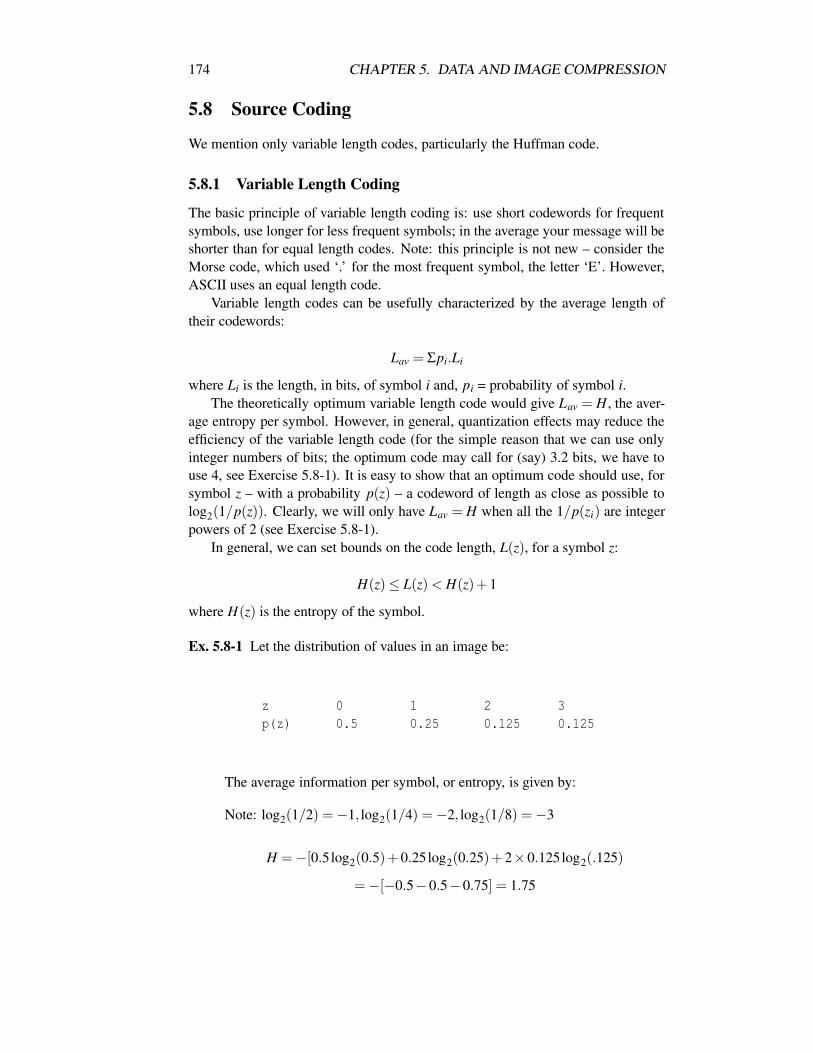
174 CHAPTER 5. DATA AND IMAGE COMPRESSION
5.8 Source Coding
We mention only variable length codes, particularly the Huffman code.
5.8.1 Variable Length Coding
The basic principle of variable length coding is: use short codewords for frequentsymbols, use longer for less frequent symbols; in the average your message will beshorter than for equal length codes. Note: this principle is not new – consider theMorse code, which used ‘.’ for the most frequent symbol, the letter ‘E’. However,ASCII uses an equal length code.
Variable length codes can be usefully characterized by the average length oftheir codewords:
Lav = Σpi.Li
where Li is the length, in bits, of symbol i and, pi = probability of symbol i.The theoretically optimum variable length code would give Lav = H , the aver-
age entropy per symbol. However, in general, quantization effects may reduce theefficiency of the variable length code (for the simple reason that we can use onlyinteger numbers of bits; the optimum code may call for (say) 3.2 bits, we have touse 4, see Exercise 5.8-1). It is easy to show that an optimum code should use, forsymbol z – with a probability p(z) – a codeword of length as close as possible tolog2(1/p(z)). Clearly, we will only have Lav = H when all the 1/p(zi) are integerpowers of 2 (see Exercise 5.8-1).
In general, we can set bounds on the code length, L(z), for a symbol z:
H(z)≤ L(z) < H(z)+1
where H(z) is the entropy of the symbol.
Ex. 5.8-1 Let the distribution of values in an image be:
z 0 1 2 3p(z) 0.5 0.25 0.125 0.125
The average information per symbol, or entropy, is given by:
Note: log2(1/2) =−1, log2(1/4) =−2, log2(1/8) =−3
H =−[0.5log2(0.5)+0.25log2(0.25)+2×0.125log2(.125)
=−[−0.5−0.5−0.75] = 1.75

5.8. SOURCE CODING 175
This compares with the 2 bits per pixel that would be required without sourcecoding.
If we allocate codewords as follows:
z 0 1 2 3p(z) 0.5 0.25 0.125 0.125code 0 10 110 111Length 1 2 3 3
we get an average codeword length of:
Lav = 0.5×1+0.25×2+0.125×3+0.125×3 = 1.75
i.e. the code is optimal.
Note: it is just by chance that 0 is mapped onto 0.
5.8.2 Unique Decoding
Obviously, we need codes to be uniquely decodable; and, we don’t want the enor-mous overhead of ‘start’ and ‘stop’ codes !
At a first glance, the codes in the previous example, Example 5.8-1, might lookas if a sequence of them would be difficult to disentangle. Consider
1101110101110
well, in fact, this uniquely separates into
110 111 0 10 111 0
and, hence, can be uniquely decoded as: 2 3 0 1 3 0
Ex. 5.8-2 Using the results of Ex. 5.8-1, derive a variable length code for the fol-lowing symbols – given their probabilities; hence compute the compressionachieved.
z 1 2 3 4p(z) 0.5 0.25 0.125 0.125

176 CHAPTER 5. DATA AND IMAGE COMPRESSION
Ex. 5.8-3 Using the results of Example 5.8-1, derive a variable length code for thefollowing symbols – given their probabilities; hence compute the compres-sion achieved.
z 1 120 122 250p(z) 0.5 0.25 0.125 0.125
Ex. 5.8-4 Using the results of Example 5.8-1, derive a variable length code for thefollowing symbols – given their probabilities; hence compute the compres-sion achieved.
z 122 120 250 1p(z) 0.5 0.25 0.125 0.125
5.8.3 Huffman Coding
The Huffman coding algorithm is an efficient algorithm for optimal source encod-ing.
The Huffman procedure is given as follows:
1. List the symbols, along with their probability. Elements of the list are nodes– we are building a binary tree.
2. Pick the two least probable nodes.
3. Make a new node out of these two – adding the probabilities.
4. Repeat steps 2, 3, until only one node remains – the root (effectively, we arebuilding a binary rooted tree).
5. Bit allocation. Starting at the root, allocate 1 to one branch (left, say), and 0to the other; until all branches have been allocated.
6. Read out the codes. Starting at the root, travel to the leaf that represents eachlevel, reading off the bits that make up the code for that level.
Ex. 5.8-4 In an image, the 8 symbols z0,z1, . . . z7 occur with respective probabili-ties: 0.4, 0.08, 0.08, 0.2, 0.12, 0.08, 0.03, 0.01;
1. derive the Huffman code,
2. derive the average entropy per symbol,

5.8. SOURCE CODING 177
3. using the results of (a) derive the average length of the Huffman gener-ated code symbols,
4. hence, compare the efficiency of the Huffman code with the optimum.
Solution:
Figure 5.1 shows steps (1) to (4), and Figure 5.2 step (5).
Level z0 z1 z2 z3 z4 z5 z6 z7
StartingProbs. 0.4 0.08 0.08 0.2 0.12 0.08 0.03 0.01
------|
1st Iter 0.4 0.08 0.08 0.2 0.12 0.08 0.04----------
|2nd Iter 0.4 0.08 0.08 0.2 0.12 0.12
---------|
3rd Iter 0.4 0.16 0.2 0.12 0.12-----------
|4th Iter 0.4 0.16 0.2 0.24
---------|
5th Iter 0.4 0.36 0.24----------------
|6th Iter 0.4 0.6
--------------------|
7th Iter 1.0
Figure 5.1 Steps (1) to (4) of Huffman Procedure.
Level z0 z1 z2 z3 z4 z5 z6 z7
Code 1 0111 0110 010 001 0001 00001 00000
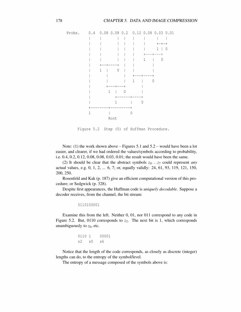
178 CHAPTER 5. DATA AND IMAGE COMPRESSION
Probs. 0.4 0.08 0.08 0.2 0.12 0.08 0.03 0.01| | | | | | | || | | | | | +-+-+| | | | | | 1 | 0| | | | | +---+---+| | | | | 1 | 0| +--+----+ | | || 1 | 0 | | || | | +---+----+| | | 1 | 0| +---+---+ || 1 | 0 || +------+----+| 1 | 0+--------+---------+1 | 0
Root
Figure 5.2 Step (5) of Huffman Procedure.
Note: (1) the work shown above – Figures 5.1 and 5.2 – would have been a loteasier, and clearer, if we had ordered the values/symbols according to probability,i.e. 0.4, 0.2, 0.12, 0.08, 0.08, 0.03, 0.01; the result would have been the same.
(2) It should be clear that the abstract symbols z0 . . . z7 could represent anyactual values, e.g. 0, 1, 2, ... 6, 7; or, equally validly: 24, 61, 93, 119, 121, 150,200, 250.
Rosenfeld and Kak (p. 187) give an efficient computational version of this pro-cedure; or Sedgwick (p. 328).
Despite first appearances, the Huffman code is uniquely decodable. Suppose adecoder receives, from the channel, the bit stream:
0110100001
Examine this from the left. Neither 0, 01, nor 011 correspond to any code inFigure 5.2. But, 0110 corresponds to z2. The next bit is 1, which correspondsunambiguously to z0, etc.
0110 1 00001z2 z0 z6
Notice that the length of the code corresponds, as closely as discrete (integer)lengths can do, to the entropy of the symbol/level.
The entropy of a message composed of the symbols above is:
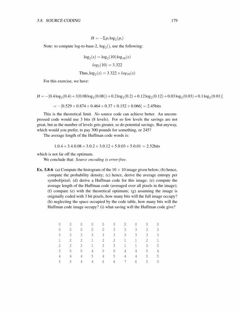
5.8. SOURCE CODING 179
H =−Σpi log2(pi)
Note: to compute log-to-base-2, log2(), use the following:
log2(x) = log2(10) log10(x)
log2(10) = 3.322
Thus, log2(x) = 3.322× log10(x)
For this exercise, we have:
H =−[0.4log2(0.4)+3(0.08log2(0.08))+0.2log2(0.2)+0.12log2(0.12)+0.03log2(0.03)+0.1log2(0.01)]
=−[0.529+0.874+0.464+0.37+0.152+0.066] = 2.45bits
This is the theoretical limit. No source code can achieve better. An uncom-pressed code would use 3 bits (8 levels). For so few levels the savings are notgreat, but as the number of levels gets greater, so do potential savings. But anyway,which would you prefer, to pay 300 pounds for something, or 245?
The average length of the Huffman code words is:
1.0.4+3.4.0.08+3.0.2+3.0.12+5.0.03+5.0.01 = 2.52bits
which is not far off the optimum.We conclude that: Source encoding is error-free.
Ex. 5.8-6 (a) Compute the histogram of the 10× 10 image given below; (b) hence,compute the probability density; (c) hence, derive the average entropy persymbol/pixel; (d) derive a Huffman code for this image; (e) compute theaverage length of the Huffman code (averaged over all pixels in the image);(f) compare (e) with the theoretical optimum; (g) assuming the image isoriginally coded with 3 bit pixels, how many bits will the full image occupy?(h) neglecting the space occupied by the code table, how many bits will theHuffman code image occupy? (i) what saving will the Huffman code give?
0 0 0 0 0 0 0 0 0 00 0 0 0 0 3 3 3 3 33 3 3 3 3 3 3 3 3 31 2 2 1 2 2 1 1 2 12 2 2 1 3 3 1 1 3 33 0 0 4 0 0 4 4 0 44 4 4 5 4 5 4 4 5 55 5 4 4 6 6 7 6 5 5
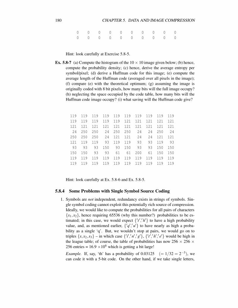
180 CHAPTER 5. DATA AND IMAGE COMPRESSION
0 0 0 0 0 0 0 0 0 00 0 0 0 0 0 0 0 0 0
Hint: look carefully at Exercise 5.8-5.
Ex. 5.8-7 (a) Compute the histogram of the 10× 10 image given below; (b) hence,compute the probability density; (c) hence, derive the average entropy persymbol/pixel; (d) derive a Huffman code for this image; (e) compute theaverage length of the Huffman code (averaged over all pixels in the image);(f) compare (e) with the theoretical optimum; (g) assuming the image isoriginally coded with 8 bit pixels, how many bits will the full image occupy?(h) neglecting the space occupied by the code table, how many bits will theHuffman code image occupy? (i) what saving will the Huffman code give?
119 119 119 119 119 119 119 119 119 119119 119 119 119 119 121 121 121 121 121121 121 121 121 121 121 121 121 121 12124 250 250 24 250 250 24 24 250 24
250 250 250 24 121 121 24 24 121 121121 119 119 93 119 119 93 93 119 9393 93 93 150 93 150 93 93 150 150
150 150 93 93 61 61 200 61 150 150119 119 119 119 119 119 119 119 119 119119 119 119 119 119 119 119 119 119 119
Hint: look carefully at Ex. 5.8-6 and Ex. 5.8-5.
5.8.4 Some Problems with Single Symbol Source Coding
1. Symbols are not independent, redundancy exists in strings of symbols. Sin-gle symbol coding cannot exploit this potentially rich source of compression.Ideally, we would like to compute the probabilities for all pairs of charactersx1,x2, hence requiring 65536 (why this number?) probabilities to be es-timated; in this case, we would expect ′t ′,′ h′ to have a high probabilityvalue, and, as mentioned earlier, ′q′,′ u′ to have nearly as high a proba-bility as a single ‘q’. But, we wouldn’t stop at pairs, we would go on totriples x,x2,x3 – in which case ′i′,′ n′,′ g′, ′t ′,′ h′,′ e′ would be high inthe league table; of course, the table of probabilities has now 256 × 256 ×256 entries = 16.9 ×10⁶ which is getting a bit large!
Example. If, say, ‘th’ has a probability of 0.03125 (= 1/32 = 2−5), wecan code it with a 5-bit code. On the other hand, if we take single letters,
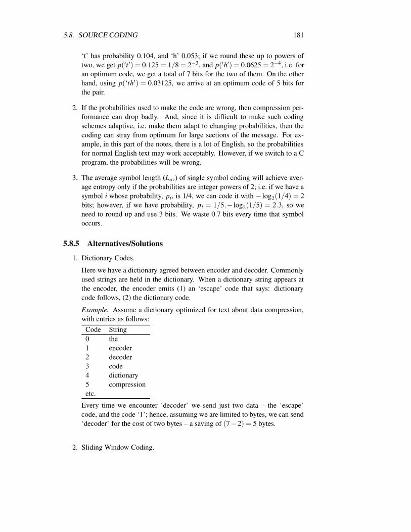
5.8. SOURCE CODING 181
‘t’ has probability 0.104, and ‘h’ 0.053; if we round these up to powers oftwo, we get p(′t ′) = 0.125 = 1/8 = 2−3, and p(′h′) = 0.0625 = 2−4, i.e. foran optimum code, we get a total of 7 bits for the two of them. On the otherhand, using p(‘th′) = 0.03125, we arrive at an optimum code of 5 bits forthe pair.
2. If the probabilities used to make the code are wrong, then compression per-formance can drop badly. And, since it is difficult to make such codingschemes adaptive, i.e. make them adapt to changing probabilities, then thecoding can stray from optimum for large sections of the message. For ex-ample, in this part of the notes, there is a lot of English, so the probabilitiesfor normal English text may work acceptably. However, if we switch to a Cprogram, the probabilities will be wrong.
3. The average symbol length (Lav) of single symbol coding will achieve aver-age entropy only if the probabilities are integer powers of 2; i.e. if we have asymbol i whose probability, pi, is 1/4, we can code it with − log2(1/4) = 2bits; however, if we have probability, pi = 1/5,− log2(1/5) = 2.3, so weneed to round up and use 3 bits. We waste 0.7 bits every time that symboloccurs.
5.8.5 Alternatives/Solutions
1. Dictionary Codes.
Here we have a dictionary agreed between encoder and decoder. Commonlyused strings are held in the dictionary. When a dictionary string appears atthe encoder, the encoder emits (1) an ‘escape’ code that says: dictionarycode follows, (2) the dictionary code.
Example. Assume a dictionary optimized for text about data compression,with entries as follows:
Code String0 the1 encoder2 decoder3 code4 dictionary5 compressionetc.
Every time we encounter ‘decoder’ we send just two data – the ‘escape’code, and the code ‘1’; hence, assuming we are limited to bytes, we can send‘decoder’ for the cost of two bytes – a saving of (7−2) = 5 bytes.
2. Sliding Window Coding.
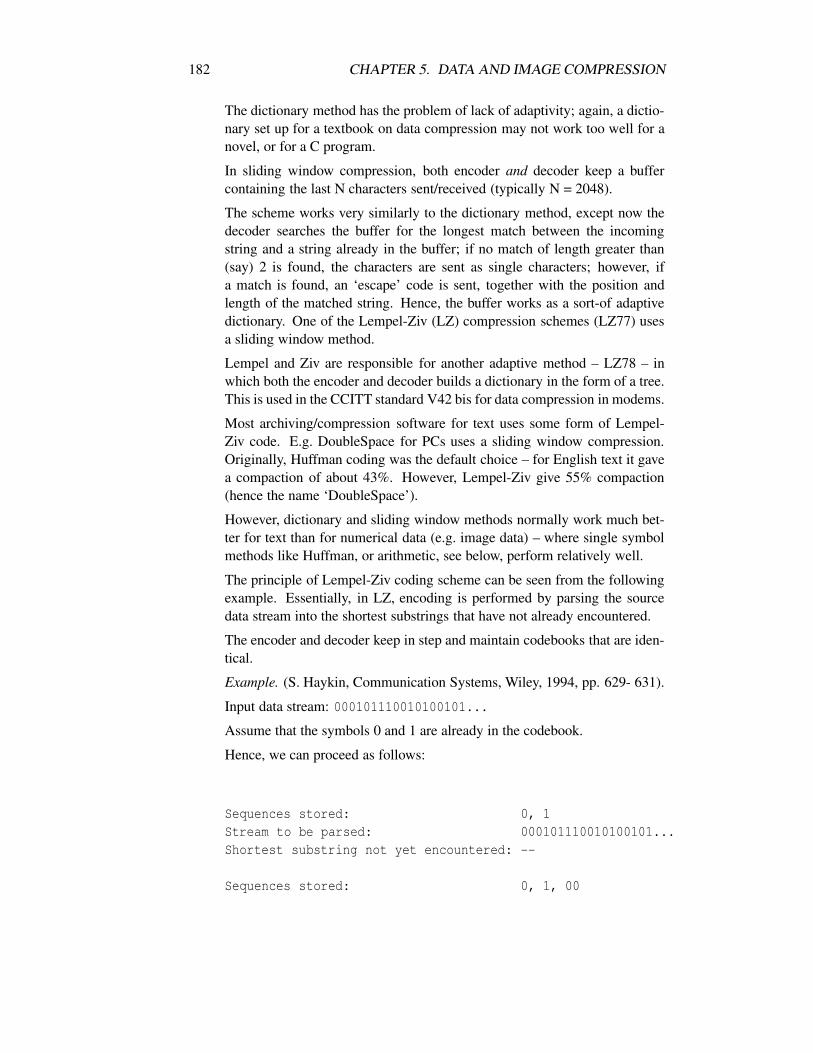
182 CHAPTER 5. DATA AND IMAGE COMPRESSION
The dictionary method has the problem of lack of adaptivity; again, a dictio-nary set up for a textbook on data compression may not work too well for anovel, or for a C program.
In sliding window compression, both encoder and decoder keep a buffercontaining the last N characters sent/received (typically N = 2048).
The scheme works very similarly to the dictionary method, except now thedecoder searches the buffer for the longest match between the incomingstring and a string already in the buffer; if no match of length greater than(say) 2 is found, the characters are sent as single characters; however, ifa match is found, an ‘escape’ code is sent, together with the position andlength of the matched string. Hence, the buffer works as a sort-of adaptivedictionary. One of the Lempel-Ziv (LZ) compression schemes (LZ77) usesa sliding window method.
Lempel and Ziv are responsible for another adaptive method – LZ78 – inwhich both the encoder and decoder builds a dictionary in the form of a tree.This is used in the CCITT standard V42 bis for data compression in modems.
Most archiving/compression software for text uses some form of Lempel-Ziv code. E.g. DoubleSpace for PCs uses a sliding window compression.Originally, Huffman coding was the default choice – for English text it gavea compaction of about 43%. However, Lempel-Ziv give 55% compaction(hence the name ‘DoubleSpace’).
However, dictionary and sliding window methods normally work much bet-ter for text than for numerical data (e.g. image data) – where single symbolmethods like Huffman, or arithmetic, see below, perform relatively well.
The principle of Lempel-Ziv coding scheme can be seen from the followingexample. Essentially, in LZ, encoding is performed by parsing the sourcedata stream into the shortest substrings that have not already encountered.
The encoder and decoder keep in step and maintain codebooks that are iden-tical.
Example. (S. Haykin, Communication Systems, Wiley, 1994, pp. 629- 631).
Input data stream: 000101110010100101...
Assume that the symbols 0 and 1 are already in the codebook.
Hence, we can proceed as follows:
Sequences stored: 0, 1Stream to be parsed: 000101110010100101...Shortest substring not yet encountered: --
Sequences stored: 0, 1, 00
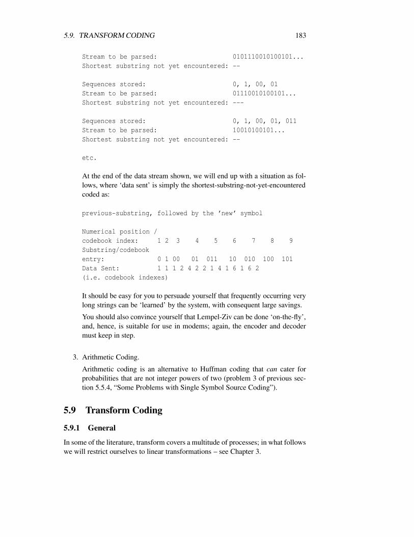
5.9. TRANSFORM CODING 183
Stream to be parsed: 0101110010100101...Shortest substring not yet encountered: --
Sequences stored: 0, 1, 00, 01Stream to be parsed: 01110010100101...Shortest substring not yet encountered: ---
Sequences stored: 0, 1, 00, 01, 011Stream to be parsed: 10010100101...Shortest substring not yet encountered: --
etc.
At the end of the data stream shown, we will end up with a situation as fol-lows, where ‘data sent’ is simply the shortest-substring-not-yet-encounteredcoded as:
previous-substring, followed by the ’new’ symbol
Numerical position /codebook index: 1 2 3 4 5 6 7 8 9Substring/codebookentry: 0 1 00 01 011 10 010 100 101Data Sent: 1 1 1 2 4 2 2 1 4 1 6 1 6 2(i.e. codebook indexes)
It should be easy for you to persuade yourself that frequently occurring verylong strings can be ‘learned’ by the system, with consequent large savings.
You should also convince yourself that Lempel-Ziv can be done ‘on-the-fly’,and, hence, is suitable for use in modems; again, the encoder and decodermust keep in step.
3. Arithmetic Coding.
Arithmetic coding is an alternative to Huffman coding that can cater forprobabilities that are not integer powers of two (problem 3 of previous sec-tion 5.5.4, “Some Problems with Single Symbol Source Coding”).
5.9 Transform Coding
5.9.1 General
In some of the literature, transform covers a multitude of processes; in what followswe will restrict ourselves to linear transformations – see Chapter 3.
184 CHAPTER 5. DATA AND IMAGE COMPRESSION
Generally speaking, linear transforms exploit the correlations between pixels;they remove the redundancy, by transforming into a domain where the values arenot correlated.
There is a statistical procedure called Karhunen-Loeve Transform (also calledHotelling Transform, Principal Components Analysis, Eigenvector Analysis, orFactor Analysis) which is optimal in producing decorrelated values. However, wehave not the prerequisite statistics and mathematical background required to coverit. Also, no fast algorithms (O(n log n)) exist for K-L.
Currently (see the section below on “The JPEG Still Picture Compression Stan-dard”), the Discrete Cosine transform (DCT) is the most commonly used for com-pression; the DCT is a very close relative of the DFT (see Chapter 3). It can beshown that the DCT closely approaches the K-L. In the past the Hadamard trans-form has been used.
It is possible to justify transform compression mathematically, but we willavoid that. There are three intuitive ways of explaining transform compression.
1. Frequency selection. If the adjacent pixels of an image are correlated, thismeans that the pixel values change by only a small amount between neigh-boring pixels; which, in turn, means that the lower frequencies in the imagefrequency spectrum are dominant. Therefore, we code the data in terms offrequencies, and we can throw away some of the high frequency elements;or, you can code the higher frequencies using less bits.
Thus, the encoder takes the DFT of the input image, picks the dominant(say) 10% of frequencies and sends these. The decoder reconstructs theDFT ‘image’ (setting the missing 90% to zero), and takes the Inverse DFT.(There will be some overhead, since the encoder must tell the decoder whichfrequencies were left out).
2. Mathematical transformation – simply by saying that we are transformingto a domain in which the values are less correlated. Since the informationcontent must remain the same, we can represent the image, in the decorre-lated domain, using fewer values; for more details, see any description of theKarhunen-Loeve transform.
3. Description in terms of basis images. The image is expressed in terms of itscorrelation with (similarity to) basis images; e.g. the image can be describedas 0.5 parts of basis-image 1, 0.2 of basis-image 2, etc. You send the 0.5, 0.2,... ; the receiver knows the basis-images and can reconstruct. If the transformused is Fourier or Cosine, these basis-images correspond to sine and cosinefunctions at different frequencies – see Chapter 3 (DFT).
Generally, transform image compression is lossy.Although we will not mention them further here, wavelet transforms are now
attracting great interest for image compression. Chapter 13 of Numerical Recipes

5.10. IMAGE MODEL CODING 185
by Press et al. have a readable introduction using Daubechies wavelets, and alsoprovide accompanying code.
5.9.2 Subimage Coding
Usually transform coding is applied, not to the full image, but to subimages, e.g.8 × 8, 16 ×16. See section below on “The JPEG Still Picture Compression Stan-dard”.
5.9.3 Colour Image Coding
For naturally occurring scenes, there is usually very strong correlation betweencolors; do a scatter plot (function d2s of DataLab) of the green and red bands(bands 1 and 2 – band 0 is infrared) of the SPOT image in DataLab – you will seethat the data lie very close to a straight line along the diagonal, thereby indicatingvery high correlation. Decorrelating transforms can help here, too. But, note thatwe are decorrelating the vector formed by the bands, not the vector/image formedby the spatial array of pixels.
5.10 Image Model Coding
Again, image model coding covers a multitude of techniques. We shall only give aflavor.
A trivial example: consider the 11 × 16 ‘T’ image in the Figure below. Thisstarted off as 176 bytes.
0 0 0 0 0 0 0 0 0 0 0 0 0 0 0 00 0 0 0 0 0 0 0 0 0 0 0 0 0 0 00 0 0 1 1 1 1 1 1 1 1 1 1 0 0 00 0 0 1 1 1 1 1 1 1 1 1 1 0 0 00 0 0 1 1 1 1 1 1 1 1 1 1 0 0 00 0 0 0 0 0 1 1 1 1 0 0 0 0 0 00 0 0 0 0 0 1 1 1 1 0 0 0 0 0 00 0 0 0 0 0 1 1 1 1 0 0 0 0 0 00 0 0 0 0 0 1 1 1 1 0 0 0 0 0 00 0 0 0 0 0 1 1 1 1 0 0 0 0 0 00 0 0 0 0 0 0 0 0 0 0 0 0 0 0 0
‘T’ image

186 CHAPTER 5. DATA AND IMAGE COMPRESSION
1. Run-length encoding reduces to 54 bytes.
2. Simply quantizing to 1 bit reduces to 176/8 = 22 bytes.
3. My guess is that the first 4 Fourier frequency components (out of 256) wouldproduce an intelligible version of the ‘T’.
But, if we know we have a page of text, it can be reduced to 1 byte – thecode for ‘T’ !
Or, if we know it is a graphics image with only rectangles, we can get awaywith 4 bytes per rectangle.
5.11 Differential and Predictive Coding
Consider the following sequence of data representing (say) 12-bit speech data:
s1 s2 s3 s4 s11300, 305, 312, 320, 324, 326, 327, 327, 323, 319, 310, ...
This sequence is smoothly varying; compare with the rapidly varying:
300, 1092, 2935, 123, 4000, ....
If we take differences di = si+1− si, we have
d1 d2 d3 d45 7 8 4
Assume that the maximum difference is 15, and that we can arrange to wecan transmit the starting value (300). We can then transmit the signal as the d iquantized to 4 bits, thus saving 8 bits per sample.
(In practice differential coding works slightly differently – it needs to guardagainst one error destroying all the signal, as the above simple method is prone to).
5.12 Dimensionality and Compression
Because of the importance of correlation in image and signal data compression(roughly, correlation means that a pixel is strongly related to – correlated with– some of its neighbors, there is redundancy) multiple dimensions in data offer
5.13. VECTOR QUANTIZATION 187
greater opportunities for data compression. The greater the dimensionality thegreater the number of neighbours and therefore potential for correlation, and therbyredundancy, along each dimension.
Thus, familiar examples are:
• Audio signal – one dimension,
f0, f1, . . . , fi−1, fi, fi+1, . . .
fi has 2 neighbors.
• Monochrome image – two dimensions,
f(0,0) f(0,1) .....
.... f(r-1,c-1) f(r-1,c) f(r-1,c+1)
.... f(r,c-1) f(r,c) f(r,c+1)
.... f(r+1,c-1) f(r+1,c) f(r+1,c+1)
f (r,c) has 8 neighbors.
• Sequence of mono images (e.g. a movie) – three dimensions.
each point has 26 neighbors.
The sequence is: 2, 8, 26, i.e. (3n−1), where n is the dimensionality.
It is well known that the compression factor increases quite non-linearly asyou go down the above list; the more neighbors, the more correlation that can beexploited by the compression algorithm.
Colour is a fourth dimension present in most image sequences – and this di-mension offers its own correlation, and additional scope for compression.
Incidentally, I would consider a single datum to be zero-dimensional, and, con-sequently, a collection of data whose only relationship is that they are members ofa set would be zero-dimensional.
5.13 Vector Quantization
The section above entitled “Quantization Coding” discussed quantization for singlegrey levels, i.e. assuming a monochrome image. What if we have a color image?In general a multispectral image where each pixel is represented by a vector of nbands.
We could quantize each band separately. However, it would make sense totake account of the bands together, i.e. divide the ‘space’ formed by the n bands
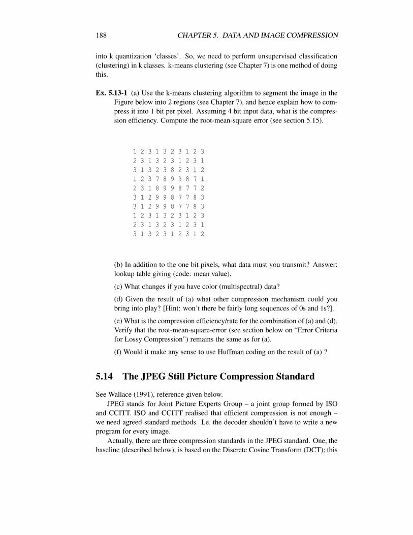
188 CHAPTER 5. DATA AND IMAGE COMPRESSION
into k quantization ‘classes’. So, we need to perform unsupervised classification(clustering) in k classes. k-means clustering (see Chapter 7) is one method of doingthis.
Ex. 5.13-1 (a) Use the k-means clustering algorithm to segment the image in theFigure below into 2 regions (see Chapter 7), and hence explain how to com-press it into 1 bit per pixel. Assuming 4 bit input data, what is the compres-sion efficiency. Compute the root-mean-square error (see section 5.15).
1 2 3 1 3 2 3 1 2 32 3 1 3 2 3 1 2 3 13 1 3 2 3 8 2 3 1 21 2 3 7 8 9 9 8 7 12 3 1 8 9 9 8 7 7 23 1 2 9 9 8 7 7 8 33 1 2 9 9 8 7 7 8 31 2 3 1 3 2 3 1 2 32 3 1 3 2 3 1 2 3 13 1 3 2 3 1 2 3 1 2
(b) In addition to the one bit pixels, what data must you transmit? Answer:lookup table giving (code: mean value).
(c) What changes if you have color (multispectral) data?
(d) Given the result of (a) what other compression mechanism could youbring into play? [Hint: won’t there be fairly long sequences of 0s and 1s?].
(e) What is the compression efficiency/rate for the combination of (a) and (d).Verify that the root-mean-square-error (see section below on “Error Criteriafor Lossy Compression”) remains the same as for (a).
(f) Would it make any sense to use Huffman coding on the result of (a) ?
5.14 The JPEG Still Picture Compression Standard
See Wallace (1991), reference given below.JPEG stands for Joint Picture Experts Group – a joint group formed by ISO
and CCITT. ISO and CCITT realised that efficient compression is not enough –we need agreed standard methods. I.e. the decoder shouldn’t have to write a newprogram for every image.
Actually, there are three compression standards in the JPEG standard. One, thebaseline (described below), is based on the Discrete Cosine Transform (DCT); this

5.15. ERROR CRITERIA FOR LOSSY COMPRESSION 189
one is lossy. Another is also lossy but allows the user to specify the compressionratio required. The third is lossless.
We will just give a flavor of the principles behind the JPEG baseline standard;it uses a concatenation of some of the methods mentioned in the previous subsec-tions:
1. the image is split into 8 × 8 subimages and these 8 ×8 subimages are trans-formed using the DCT,
2. The DCT coefficients are quantized: e.g. starting with 8 bits for the DCcoefficient, down to 7 for the verly low frequency components, down to 0(i.e. the data are ignored) for the very high frequency terms,
3. The DCT components obtained from (2) are ‘differenced’ (see section aboveentitled “Differential and Predictive Coding”) with respect to the correspond-ing component of the previous subimage,
4. The difference values obtained from (3) are Huffman encoded (using a fixedpreset Huffman code).
Hard on the heels of JPEG, comes MPEG standard – Moving Picture Ex-perts Group; MPEG standard would be used for such applications as our video-conferencing link. High Definition TV (HDTV) also requires some form of movingpicture compression.
5.15 Error Criteria for Lossy Compression
For lossy compression schemes it is neccessary to specify how the loss/error is tobe computed. Root-mean-square-error (RMSE) is a natural choice:
RMSE =√
[Σ(z− zc)2]
where zc is the value after compression,z is the (true) value before,and the summation is over all pixels.
5.16 Additional References on Image and Data Compres-sion
1. G.V. Wallace, “The JPEG Still Picture Compression Standard”, Comm. ACM,Vol. 34, No. 4 April 1991.
Gives a good introduction to the current state of play in image compression.JPEG is Joint Picture Experts Group – a joint group formed by ISO andCCITT.

190 CHAPTER 5. DATA AND IMAGE COMPRESSION
2. E. Edwards, Information Transmission, Chapman and Hall, 1969.
Very easy, readable introduction to information theory.
3. Gonzalez and Woods, Chap. 6.
4. M. Purser, Data Communications for Programmers, Addison-Wesley, 1986.
5.17 Additional Exercises
Ex. 5.17-1 Explain the use of the following methods by which the 16 × 16 im-age in the following figure may be compressed; give the compression factor(compressed bits / direct bits). Assume the source is 16 × 16 ×8 levels (3bits) = 768 bits.
1. Run-length encoding
2. Image model coding
3. Quantization.
4. Hadamard transform [Hint: see Gonzalez and Woods, Figure 3.26, p.143, and shift and scale the pixel values so that the pixels are −1,+1instead of 0,1].
1 1 1 1 1 1 1 1 0 0 0 0 0 0 0 01 1 1 1 1 1 1 1 0 0 0 0 0 0 0 01 1 1 1 1 1 1 1 0 0 0 0 0 0 0 01 1 1 1 1 1 1 1 0 0 0 0 0 0 0 01 1 1 1 1 1 1 1 0 0 0 0 0 0 0 01 1 1 1 1 1 1 1 0 0 0 0 0 0 0 01 1 1 1 1 1 1 1 0 0 0 0 0 0 0 01 1 1 1 1 1 1 1 0 0 0 0 0 0 0 00 0 0 0 0 0 0 0 1 1 1 1 1 1 1 10 0 0 0 0 0 0 0 1 1 1 1 1 1 1 10 0 0 0 0 0 0 0 1 1 1 1 1 1 1 10 0 0 0 0 0 0 0 1 1 1 1 1 1 1 10 0 0 0 0 0 0 0 1 1 1 1 1 1 1 10 0 0 0 0 0 0 0 1 1 1 1 1 1 1 10 0 0 0 0 0 0 0 1 1 1 1 1 1 1 10 0 0 0 0 0 0 0 1 1 1 1 1 1 1 1
Ex. 5.17-2 (a) Explain how the image in the figure below may be compressedusing a Huffman code.

5.18. QUESTIONS 191
1 1 1 1 1 1 1 1 0 0 0 0 0 0 0 01 1 1 1 1 1 1 1 0 0 0 0 0 0 0 01 1 1 1 1 1 1 1 0 0 0 0 0 0 0 01 1 1 1 1 1 1 1 0 0 0 0 0 0 0 01 1 1 1 1 1 1 1 0 0 0 0 0 0 0 01 1 1 1 1 1 1 1 0 0 0 0 0 0 0 01 1 1 1 1 1 1 1 0 0 0 0 0 0 0 01 1 1 1 1 1 1 1 0 0 0 0 0 0 0 02 2 2 2 2 2 2 2 3 3 3 3 3 3 3 32 2 2 2 2 2 2 2 3 3 3 3 3 3 3 32 2 2 2 2 2 2 2 3 3 3 3 3 3 3 32 2 2 2 2 2 2 2 3 3 3 3 3 3 3 34 4 4 4 4 4 4 4 5 5 5 5 5 5 5 54 4 4 4 4 4 4 4 5 5 5 5 5 5 5 54 4 4 4 4 4 4 4 6 6 6 6 6 6 6 67 7 7 7 7 7 7 7 6 6 6 6 6 6 6 6
(b) Assuming that the symbol probabilities are the same for all such images,show that the average entropy per symbol is 2.73.
(c) Calculate the average entropy per symbol for your Huffman code.
(d) Compare the compression achieved with the results obtained in Ex. 5.17-1.
Ex. 5.17-3 Identify, with explanations, applications that
(a) can tolerate lossy compression,
(b) cannot tolerate lossy compression.
5.18 Questions
1. (a) Define a quantitative measure of information; make sure to give intu-itive explanations.
(b) Explain, using appropriate numerical examples, why data compressionis needed.
2. (a) Explain the role of entropy in data compression.
(b) Explain the role of redundancy in data compression.
(c) “A sequence is one-dimensional, an image two-dimensional, a ’movie’three-dimensional; as the dimensionality increases, so does the scopefor exploiting redundancy for data compression”. Discuss.

192 CHAPTER 5. DATA AND IMAGE COMPRESSION
3. (a) In the context of data compression, explain the components of the fig-ure:
SOURCE----->ENCODER---->CHANNEL---->DECODER--->RECEIVERˆ||
NOISE
Information Transmission Model
(b) Explain how channel capacity is limited.
4. (a) Explain, giving examples of each, lossless and lossy data compression.
(b) Explain applications for which each is (i) definitely appropriate, (ii)definitely inappropriate.
(c) Explain a ‘fidelity criterion’ for lossy data compression.
5. (a) Explain the terms entropy, redundancy in the context of image datacompression [Remark: “in the context of...” – examples needed!].
(b) Compute the probability density function of the 10× 16 image givenin the figure below. Hence, derive the average entropy per the averagelength of the Huffman codewords (averaged over the image). Assum-ing that the image is originally coded with 2 bit pixels, and, neglectingthe space occupied by the code table, derive the compression perfor-mance of the Huffman code. Hence compare this compression perfor-mance with that of the theoretically optimum source code.
0 0 0 0 0 2 0 0 2 0 0 0 0 0 0 00 0 0 0 0 0 0 0 0 0 0 0 0 0 0 00 0 0 1 1 1 1 1 1 1 1 1 1 0 0 00 0 0 1 1 1 1 3 3 1 1 1 1 0 0 00 0 0 1 1 1 1 3 3 1 1 1 1 0 0 00 0 0 0 0 0 1 1 1 1 0 0 0 0 0 00 0 0 0 0 0 1 1 1 1 0 0 0 0 0 00 0 0 0 0 0 1 1 1 1 0 0 0 0 0 00 0 0 0 0 0 1 1 1 1 0 0 0 0 0 00 0 2 0 0 0 1 1 1 1 0 0 0 2 0 0
(c) Hence, derive a compression code for the image in the following figure.
9 9 9 9 9 0 9 9 0 9 9 9 9 9 9 99 9 9 9 9 9 9 9 9 9 9 9 9 9 9 99 9 9 1 1 1 1 1 1 1 1 1 1 9 9 99 9 9 1 1 1 1 5 5 1 1 1 1 9 9 9

5.18. QUESTIONS 193
9 9 9 1 1 1 1 5 5 1 1 1 1 9 9 99 9 9 9 9 9 1 1 1 1 9 9 9 9 9 99 9 9 9 9 9 1 1 1 1 9 9 9 9 9 99 9 9 9 9 9 1 1 1 1 9 9 9 9 9 99 9 9 9 9 9 1 1 1 1 9 9 9 9 9 99 9 0 9 9 9 1 1 1 1 9 9 9 0 9 9
6. (a) Explain run-length encoding.
(b) Apply run-length encoding to the figure below. Assuming ‘runs’ can beencoded as 4 bits [1..16], and grey level as two bits compute the codingefficiency (see Appendix provided in examinations for formulas).
0 0 0 0 0 2 0 0 2 0 0 0 0 0 0 00 0 0 0 0 0 0 0 0 0 0 0 0 0 0 00 0 0 1 1 1 1 1 1 1 1 1 1 0 0 00 0 0 1 1 1 1 3 3 1 1 1 1 0 0 00 0 0 1 1 1 1 3 3 1 1 1 1 0 0 00 0 0 0 0 0 1 1 1 1 0 0 0 0 0 00 0 0 0 0 0 1 1 1 1 0 0 0 0 0 00 0 0 0 0 0 1 1 1 1 0 0 0 0 0 00 0 0 0 0 0 1 1 1 1 0 0 0 0 0 00 0 2 0 0 0 1 1 1 1 0 0 0 2 0 0
(c) Obviously, run length encoding will not provide any compresssion for‘busy’ images (i.e., where the pixel values are rapidly varying, andthere is very little correlation between adjacent pixels). Consideringthe model of a checker-board (alternate black (0), white (1), squares,and a 16×16 image, and starting with (1) a pure white image, next, (2)an image with 4 squares
(white,blackblack, white)
and so on, at what stage does run-length encoding start to increaserather than compress the data?
7. (a) Explain the principle undelying variable length source coding; give anappropriate example.
(b) Explain how variable length codes need to be uniquely decodable; givean appropriate example.
8. (a) Compute the histogram of the 10× 10 image given below; (b) hence,compute the probability density; (c) hence, derive the average entropyper symbol / pixel; (d) derive a Huffman code for this image; (e) com-pute the average length of the Huffman code (averaged over all pixels

194 CHAPTER 5. DATA AND IMAGE COMPRESSION
in the image); (f) compare (e) with the theoretical optimum; (g) assum-ing the image is originally coded with 3 bit pixels, how many bits willthe full image occupy? (h) neglecting the space occupied by the codetable, how many bits will the Huffman code image occupy? (i) whatsaving will the Huffman code give?
0 0 0 0 0 0 0 0 0 00 0 0 0 0 3 3 3 3 33 3 3 3 3 3 3 3 3 31 2 2 1 2 2 1 1 2 12 2 2 1 3 3 1 1 3 33 0 0 4 0 0 4 4 0 44 4 4 5 4 5 4 4 5 55 5 4 4 6 6 7 6 5 50 0 0 0 0 0 0 0 0 00 0 0 0 0 0 0 0 0 0
(b) Use the the previous results to derive a Huffman code for the imagebelow.
119 119 119 119 119 119 119 119 119 119119 119 119 119 119 121 121 121 121 121121 121 121 121 121 121 121 121 121 12124 250 250 24 250 250 24 24 250 24
250 250 250 24 121 121 24 24 121 121121 119 119 93 119 119 93 93 119 9393 93 93 150 93 150 93 93 150 150
150 150 93 93 61 61 200 61 150 150119 119 119 119 119 119 119 119 119 119119 119 119 119 119 119 119 119 119 119
(c) Compare the coding efficiencies of the original image (assume 8 bits)and coded image.
(d) Apply quantization coding to the image above; compare the codingefficiency of the quantization coding with that of (1) the raw image,and (2) the Huffman code found in sub-question (k).
9. (a) The distribution of values in an image are:
z 0 1 2 3p(z) 0.5 0.25 0.125 0.125
(i) Compute average entropy per symbol.(ii) Derive a Huffman variable length code for this set of values.(iii) Compare the average length of the Huffman code with that of (1)the average entropy per symbol, and (2) the average codeword lengthin the raw image. Comment.
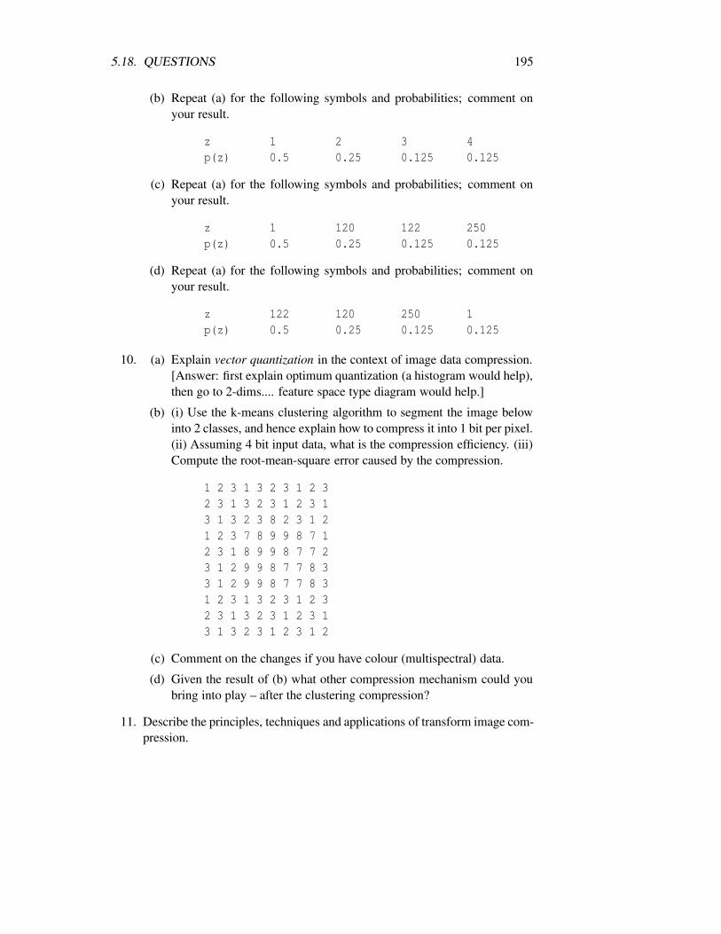
5.18. QUESTIONS 195
(b) Repeat (a) for the following symbols and probabilities; comment onyour result.
z 1 2 3 4p(z) 0.5 0.25 0.125 0.125
(c) Repeat (a) for the following symbols and probabilities; comment onyour result.
z 1 120 122 250p(z) 0.5 0.25 0.125 0.125
(d) Repeat (a) for the following symbols and probabilities; comment onyour result.
z 122 120 250 1p(z) 0.5 0.25 0.125 0.125
10. (a) Explain vector quantization in the context of image data compression.[Answer: first explain optimum quantization (a histogram would help),then go to 2-dims.... feature space type diagram would help.]
(b) (i) Use the k-means clustering algorithm to segment the image belowinto 2 classes, and hence explain how to compress it into 1 bit per pixel.(ii) Assuming 4 bit input data, what is the compression efficiency. (iii)Compute the root-mean-square error caused by the compression.
1 2 3 1 3 2 3 1 2 32 3 1 3 2 3 1 2 3 13 1 3 2 3 8 2 3 1 21 2 3 7 8 9 9 8 7 12 3 1 8 9 9 8 7 7 23 1 2 9 9 8 7 7 8 33 1 2 9 9 8 7 7 8 31 2 3 1 3 2 3 1 2 32 3 1 3 2 3 1 2 3 13 1 3 2 3 1 2 3 1 2
(c) Comment on the changes if you have colour (multispectral) data.
(d) Given the result of (b) what other compression mechanism could youbring into play – after the clustering compression?
11. Describe the principles, techniques and applications of transform image com-pression.

196 CHAPTER 5. DATA AND IMAGE COMPRESSION

Chapter 6
From Images to Objects
6.1 Introduction
This chapter presents methods for segmentation; mathematical morphology opera-tions; and multiresolution transforms, focusing on two wavelet transforms. Thereis a common theme in these different processing methods: open up an image, toreveal the objects represented within it. The objects of interest may well be closelyassociated with “segments” derived from the image. The objects of interest mayexist on a number of resolution scales, – in the foreground or background, embed-ded, and so on. Mathematical morphology provides us with highly-effective toolsfor improving, often dramatically, the objects derived from our images.
6.2 Introduction to Segmentation
Image segmentation is a process which partitions an image into regions (or seg-ments) based upon similarities within regions – and differences between regions.
Commonly, an image represents a scene in which there are different objectsor, more generally, regions; it is a widely held view that the first stage, in humaninterpretation of a scene, is its division into regions; hence, there is great interset inimage segmentation. However, although humans have little difficulty in separatingthe scene into regions, this process can be difficult to automate.
The following depiction of operations performed on an image shows a pos-sible context for segmentation – this might represent the information flow in anautomated inspection system that monitors that manufactured parts are the correctshape, or a character recognition system, etc. The following can be characterizedas our image analysis model, or even vision model.
RAW IMAGE (pixel values are intensities, noise-corrupted)
−→ preprocessing −→PREPROCESSED IMAGE (pixels represent physical attribute, e.g. thickness ofabsorber, greyness of scene)
197

198 CHAPTER 6. FROM IMAGES TO OBJECTS
−→ segmentation −→
SEGMENTED or SYMBOLIC IMAGE (each pixel labelled, e.g. into object andbackground)
−→ feature extraction (e.g. line detection, moments) −→
EXTRACTED FEATURES or RELATIONAL STRUCTURE
−→ shape detection and matching (pattern recognition) −→
OBJECT ANALYSIS
The major point to note in this depiction is that we start off with raw data(an array of grey levels) and we end up with information – the identification andposition of an object. As we progress, the data and processing move from low-levelto high-level.
But here we are mainly concerned with the process of labelling each pixel aseither object or background, one major task of segmentation.
Examples of practical segmentation tasks are:
• segment an image of metal parts on a conveyer belt into metal (object), back-ground non-metal, i.e. conveyer belt.
• segment a scanned image of a printed page into ink, white page (back-ground). The result could be used for fax transmittal, or for further pro-cessing to recognise characters.
• segment an X-ray image of a printed circuit board into metal (object), orplastic (background). Again, further processing may be desired to identifyindividual tracks and other features.
• the same could apply to a medical X-ray: soft-tissue, bone.
• segment a multispectral satellite image of the earth into regions of differentlanduse. Although, in this case the pixels are vector valued (each pixel hasmany attributes – not just one grey level), the underlying principles are thesame.
• segmentation for data compression: if we have an image with (say) only two‘colours’ of interest in it; let us say metal, non-metal; assume the image is256 grey-levels × 3 colours, i.e. 24 bits per pixel. Now if we can segmentinto metal, non-metal, we can get away with 1 bit! – provided we transmit,before the 1 bit label data, what is called a code-book; the code-book givesthe mean colour of the two regions or objects, from which the picture can bereconstructed.
6.2. INTRODUCTION TO SEGMENTATION 199
Haralick and Shapiro (1985) give the following wish-list for segmentation:“What should a good image segmentation be? Regions of an image segmentationshould be uniform and homogeneous with respect to some charactersitic (property)such as grey tone or texture. Region interiors should be simple and without manysmall holes. Adjacent regions of a segmentation should have significantly differentvalues with respect to the characteristic on which they (the regions themselves) areuniform. Boundaries of each segment should be simple, not ragged, and must bespatially accurate”.
In this chapter we will cover the three general approaches to image segmen-tation, namely, single pixel classification, boundary-based methods, and regiongrowing methods. There are other methods – many of them. Segmentation isone of the areas of image processing where there is certainly no agreed theory, noragreed set of methods.
Broadly speaking, single pixel classification methods label pixels on the basisof the pixel value alone, i.e. the process is concerned only with the position ofthe pixel in grey-level space, or colour space in the case of multivalued images.The term classification is used beacuse the different regions are considered to bepopulated by pixels of different classes.
Boundary-based methods detect boundaries of regions; subsequently pixels en-closed by a boundary can be labelled accordingly.
Finally, region growing methods are based on the identification of spatiallyconnected groups of similarly valued pixels; often the grouping procedure is ap-plied iteratively – in which case the term relaxation is used.
6.2.1 Single Pixel Classification
Introduction
Single pixel classification is reminiscent of the point enhancement methods cov-ered in Chapter 4; each pixel is labelled according to its own value, and for thatlabelling, the values of its neighbours are irrelevant.
We start off with simple thresholding, where choice of label depends on whichside of a threshold the pixel value lies; this is applied globally. Next, as in Chap-ter 4, we discuss how we can make the threshold adaptive to local variations inthe image. Then we explain how thresholding can be used to determine bound-aries, and hence regions. Then we generalize thresholding to “level-banding” formultilevel/multiclass problems. Next we generalize monochrome thresholding tomultispectral classification, and finish off with unsupervised classification, whichis also termed clustering.
Threshold Selection
Let the input image have a histogram p(z). Let there be two peaks in p(), at z i,z j ,i.e. p(zi) is a local maximum (local = the maximum of p() within zl grey levels,e.g. zl = 10), and similarly p(z j) is a local peak.

200 CHAPTER 6. FROM IMAGES TO OBJECTS
Let zk be the mid-point between zi and z j , ( zk = (zi + z j)/2 ). Then if p(zk) ismuch smaller than either p(zi) or p(z j) (i.e. zk is in a significant valley), zk shouldbe a useful threshold for segmenting the picture. The segmentation rule is:
label background if z < T1label object otherwise
or in pseudo-code:
if z < T1 label = backgroundelse label = object.
The following figure gives an example (it is reminiscent of the histogram of anobject superimposed on a background, with noise added).
0
5
10
15
20
25
30
0 5 10 15
Pe
rce
nt
of
To
tal
The values used in this histogram were 0, 1, 2, 2, 2, 2, 2, 2, 2, 3, 3, 4, 5, 6, 7,9, 11, 12, 14, 14, 14, 14, 14, 14, 14, 14, 15, 16, 16, 16, 18. The mean of the lower“chunk” of data is zi = 3.25. The mean of the larger “chunk” is z j = 14.4. Themid-point between these two means is pk = 8.825 (or nearly 9). Thus thresholdingat 9 would do a reasonable job of separating the object from the background.
This method is highly intuitive. Often ad hoc changes have to be made tocope with particular distributions of grey levels. The clustering methods mentionedbelow are more general.
Visually, 10 would be even easier in our example, and would be a solution alsoin this case. Therefore we have proposed two solutions: (i) find the clusters, andtheir means, and use the mid-point of means as a threshold; and (ii) find the deepestvalley(s) in the histogram of the data.
6.2. INTRODUCTION TO SEGMENTATION 201
Local versus Global
If there is unevenness of illumination the histogram approach may run into difficul-ties – the histogram may tell more about the illumination distribution, than aboutthe colours of the object(s) and background. In such cases it may be beneficial toperform segmentation first on small local areas, followed by some rationalisationof the different segmentation results.
Segmentation Based on Boundary Pixels
In some cases there may be two or more background levels (the same may be truefor illumination effects – see (b) above), which may confuse the segmentation, e.g.there will be significant peaks in the histogram corresponding to each level. Insuch cases it may be better to work on a histogram of only those points on or nearboundaries. This implies working on points with a large gradient value (cf. Chapter4 on edge detection).
Multilevel Thresholding
We use here the same principle as was used for simple single level thresholding.For an image with three peaks, the lowest peak is noise on the dark background,the next corresponds to a grey object, and the third to a white object. Again, welook for local peaks in the histogram. We choose (multiple) thresholds in between.We then apply the rule:
label background if z < T1label object1 if T1≤ z < T2label object2 if T 2 < z
or in pseudo-code:
if z < T1 then label = backgroundelse if z < T2 then label = object1else label = object2.
Multilevel Thresholding for Edge Detection
Consider an image that has two main regions (say grey level 3± 2 for region A,and grey level 10±2 for region B). It is likely that at the boundary between A andB the grey level will gradually increase between (say) 3 and 10, i.e. the sequenceof pixels along a row might be 3, 5, 6, 7, 9, 10. If we segment the image into 5..7(edge) and others, we will get a contour showing the edge between the two regions.
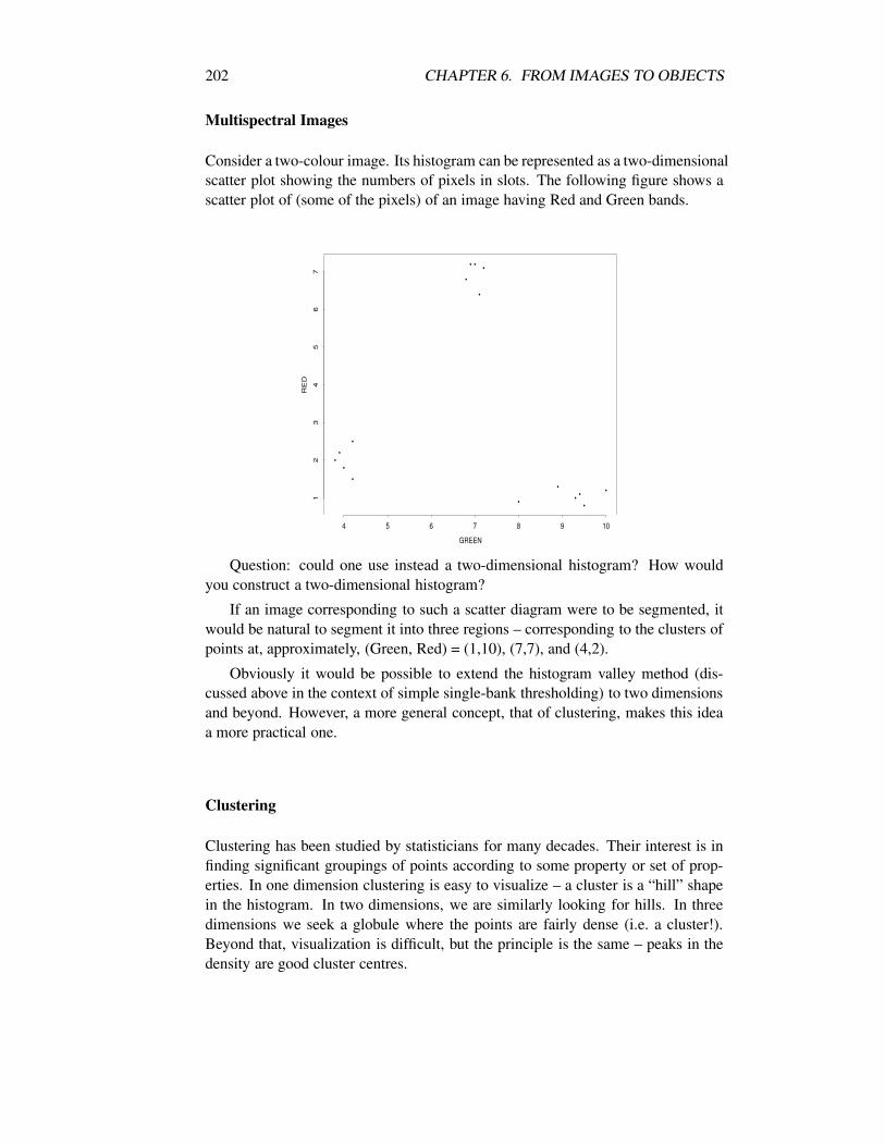
202 CHAPTER 6. FROM IMAGES TO OBJECTS
Multispectral Images
Consider a two-colour image. Its histogram can be represented as a two-dimensionalscatter plot showing the numbers of pixels in slots. The following figure shows ascatter plot of (some of the pixels) of an image having Red and Green bands.
•••••
••
••
•
•
•
••
•
•
GREEN
RE
D
4 5 6 7 8 9 10
12
34
56
7
Question: could one use instead a two-dimensional histogram? How wouldyou construct a two-dimensional histogram?
If an image corresponding to such a scatter diagram were to be segmented, itwould be natural to segment it into three regions – corresponding to the clusters ofpoints at, approximately, (Green, Red) = (1,10), (7,7), and (4,2).
Obviously it would be possible to extend the histogram valley method (dis-cussed above in the context of simple single-bank thresholding) to two dimensionsand beyond. However, a more general concept, that of clustering, makes this ideaa more practical one.
Clustering
Clustering has been studied by statisticians for many decades. Their interest is infinding significant groupings of points according to some property or set of prop-erties. In one dimension clustering is easy to visualize – a cluster is a “hill” shapein the histogram. In two dimensions, we are similarly looking for hills. In threedimensions we seek a globule where the points are fairly dense (i.e. a cluster!).Beyond that, visualization is difficult, but the principle is the same – peaks in thedensity are good cluster centres.
6.2. INTRODUCTION TO SEGMENTATION 203
k-Means Clustering
There is a vast array of clustering methods – see any book on image processingor pattern recognition. A very simple, but powerful method is k-means clustering(sometimes called ISODATA – though ISODATA is really a special algorithm fordoing k-means clustering):
Procedure k-Means Clustering:
Inputs: nc = number of classes,xij data to be clustered; i=1..d; j=1..Nd = dimensionality of data vectors (d colours)N = total number of pixels.
Outputs: labj, j=1..N, labels of pixels xjlabj = 1..nc
For the purposes of this procedure we are totally unconcerned with the spatialposition of pixels – just their position in data space or parameter space or featurespace – cf. the two-dimensional scatter plot above.
1. Partition the pixels arbitrarily into nc classes (labels), e.g. divide the imageinto nc regions, label all the pixels in the first region 1, second region, label2, etc.
2. Compute the mean vectors of each class: mic[i][c], i=1..d, c=1..nc
3. Procedure: k-Means Classifier:
3.0 Change = False3.1 for j = 1..N do
3.2 reset Distmin = Bignumber, class = 03.3 Find nearest mean:
3.3.1 for c = 1..nc do3.3.2 Compute Dist = Distance(xj to mean mc)3.3.3 if Dist < Distmin then Distmin = Dist
class = c3.3.4 end
3.4 labj = class; if ‘changed’ set Change = True3.5 end
4. if Change = True goto 2 (loop again)
5. end (we are finished)
204 CHAPTER 6. FROM IMAGES TO OBJECTS
Function Distance(x,m)
(*this calculates squared Euclidean distance - because thereis no need to take square root, since we are not interested inactual values, just in finding the minimum*)
Dist = 0for i = 1 .. d do
Dist = Dist + (xi -mi)**2 (*Euclidean distance*)return Dist
end
The above algorithm terminates when there are no class changes. It will gen-erally iterate to the same result if the classes are well separated, but not necessarilyso when the classes are confused and overlapping. In fact, this algorithm is rep-resentative of suboptimal algorithms – a good but not best result is produced. Itis fast, – as an indication, it terminates in about nc2 iterations, i.e. if there are 4classes, about 15 to 20 iterations. Note in particular that this method works equallywell for 1-dimensional data as for 50-dimensional.
The following distance may be quicker to calculate:
Dist = Dist + abs(xi-mi)
This is called the city-block distance due to the fact that it is reminiscent ofa regularly planned city, where travel means going down some blocks in a givendirection, then some blocks in another direction, and so on. On the other hand, theEuclidean distance is the distance “as the crow flies”.
We note in passing that the neural network method known as the Kohonenneural network, or self-organizing feature map, effectively implements a k-meansclustering.
Example 1
The following 10× 10 image is a small part of a satellite image of the RiverFoyle and its east bank at St. Columb’s Park. We can consider segmenting theimage using
(a) k-means clustering, with k = 2,(b) thresholding based on histogram; we can use broad grey level slots for your
histogram, e.g. 20 levels: 0-19, 20-39, ...
0 2 7 7 7 10 10 10 13 15

6.2. INTRODUCTION TO SEGMENTATION 205
5 7 10 10 10 10 10 10 15 317 10 10 10 10 13 15 23 71 92
10 10 10 13 15 23 63 106 132 11610 10 18 45 47 79 124 135 124 12213 45 87 79 79 119 138 116 116 12750 114 87 77 106 132 140 124 132 122106 103 90 119 132 146 146 135 138 135108 85 108 132 146 148 143 132 124 12792 100 127 140 151 148 148 135 98 92
From the k-means clustering, we find class means of 15.79 and 118.07.The segmented image can be represented as follows.
1 1 1 1 1 1 1 1 1 11 1 1 1 1 1 1 1 1 11 1 1 1 1 1 1 1 1 21 1 1 1 1 1 1 2 2 21 1 1 1 1 1 2 2 2 21 2 2 1 2 2 2 2 2 21 2 2 2 2 2 2 2 2 22 2 2 2 2 2 2 2 2 22 2 2 2 2 2 2 2 2 22 2 2 2 2 2 2 2 2 2
Example 2
Verify that the 3-colour image below gives the same labelling as the one-colourimage used in the previous example.
Dim: 0 (infrared)
0 2 7 7 7 10 10 10 13 155 7 10 10 10 10 10 10 15 317 10 10 10 10 13 15 23 71 92
10 10 10 13 15 23 63 106 132 11610 10 18 45 47 79 124 135 124 12213 45 87 79 79 119 138 116 116 12750 114 87 77 106 132 140 124 132 122106 103 90 119 132 146 146 135 138 135108 85 108 132 146 148 143 132 124 12792 100 127 140 151 148 148 135 98 92
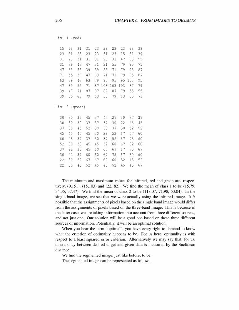
206 CHAPTER 6. FROM IMAGES TO OBJECTS
Dim: 1 (red)
15 23 31 31 23 23 23 23 23 3923 31 23 23 23 31 23 15 31 3931 23 31 31 31 23 31 47 63 5531 39 47 47 31 31 55 79 95 7147 63 55 39 39 55 71 79 95 8771 55 39 47 63 71 71 79 95 8763 39 47 63 79 95 95 95 103 9547 39 55 71 87 103 103 103 87 7939 47 71 87 87 87 87 79 55 5539 55 63 79 63 55 79 63 55 71
Dim: 2 (green)
30 30 37 45 37 45 37 30 37 3730 30 30 37 37 37 30 22 45 4537 30 45 52 30 30 37 30 52 5245 45 45 45 30 22 52 67 67 6060 45 37 37 30 37 52 67 75 6052 30 30 45 45 52 60 67 82 6037 22 30 45 60 67 67 67 75 6730 22 37 60 60 67 75 67 60 6022 30 52 67 67 60 60 52 45 5222 30 45 52 45 45 52 45 45 67
The minimum and maximum values for infrared, red and green are, respec-tively, (0,151), (15,103) and (22, 82). We find the mean of class 1 to be (15.79,34.35, 37.47). We find the mean of class 2 to be (118.07, 71.98, 53.04). In thesingle-band image, we see that we were actually using the infrared image. It ispossible that the assignments of pixels based on the single band image would differfrom the assignments of pixels based on the three-band image. This is because inthe latter case, we are taking information into account from three different sources,and not just one. Our solution will be a good one based on these three differentsources of information. Potentially, it will be an optimal solution.
When you hear the term “optimal”, you have every right to demand to knowwhat the criterion of optimality happens to be. For us here, optimality is withrespect to a least squared error criterion. Alternatively we may say that, for us,discrepancy between desired target and given data is measured by the Euclideandistance.
We find the segmented image, just like before, to be:The segmented image can be represented as follows.

6.2. INTRODUCTION TO SEGMENTATION 207
1 1 1 1 1 1 1 1 1 11 1 1 1 1 1 1 1 1 11 1 1 1 1 1 1 1 1 21 1 1 1 1 1 1 2 2 21 1 1 1 1 1 2 2 2 21 2 2 1 2 2 2 2 2 21 2 2 2 2 2 2 2 2 22 2 2 2 2 2 2 2 2 22 2 2 2 2 2 2 2 2 22 2 2 2 2 2 2 2 2 2
Discussion
With respect to the Haralick and Shapiro desiderata quoted in the introduction, thesingle pixel methods which we have described clearly perform well on the homo-geneity criteria. But, since they are concerned only with single pixels, they maynot perform well on the spatial criteria. We may well want to ignore small holes inthe interiors of regions. We may also want to ignore very ragged boundaries.
It is possible to smooth the results of single pixel segmentations using “shrink-expand” or “expand-shrink” smooothing (see Niblack, 1986, p. 117). An approachfor doing this will be looked at later in this chapter, using mathematical morphol-ogy.
A general remark is that one should be wary of ad hoc methods that work onone type of image. They may not transfer well to another type, nor (maybe) berobust to changes in (say) noise level.
6.2.2 Boundary-Based Methods
Boundary-based methods involving finding boundaries (which are connected andclosed) between regions; pixels enclosed by the boundary are then taken as be-longing to the region. (See Niblack, 1986, Chapter 5.2; Rosenfeld and Kak, 1982,Chapter 10.)
Chapter 4 has described methods of enhancing edge points, i.e. gradients.However, these merely produce a measure of edginess for each pixel and thereare a few extra steps before we get a set of linked boundary points:
1. Compute the gradient, e.g. using the combination of Sobel horizontal andvertical operators (see Chapter 4).
2. Thin the edges. There are many methods; two examples:
(i) retain only points whose gradient is a local maximum in its gradient di-rection,

208 CHAPTER 6. FROM IMAGES TO OBJECTS
(ii) (simpler). Work on horizontal and vertical edges (e.g. Sobel, before theyare added). For vertical edges, choose a threshold (T); eliminate all pixelswith values less than T. Then scan the image vertically eliminating all butthe maximum of groups (connected runs) of edge points. Ditto horizontal.Then add vertical and horizontal thinned edge points.
3. Determine possible edge neighbours. If edge points are to be linked, theymust (a) be neighbours, (b) have edge values in the same direction (see gra-dient angle in Chapter 4)
4. Link edge points, thereby yielding edge chains.
5. Link edge chains.
6. Extend edge chains, e.g. to jump across a discontinuity in an otherwise con-tinuous chain.
7. Eliminate edge chains:
i.e. those that are
– too short,
– too curvy,
– or other such elimination criteria.
8. Eliminate non-closed chains.
9. The closed chains now form the boundaries of regions.
Region Growing Methods
A simple intuitive region growing method works as follows; note the similaritywith clustering – but with a spatial criterion added.
1. Choose a seed point (perhaps a pixel having a value at the peak of the his-togram).
2. Grow the region using the two criteria:
(a) the difference in grey level (or colour distance if multicolour – see k-means clustering algorithm above) between the seed and the candidate isless than D; typically, D would be chosen as some percentage of the imagegrey level range (maximum grey level – minimum grey level).
(b) the candidate must be connected to another pixel which has already beenincluded. Connected can be defined as touching, i.e. one of the eight pixelswhich border a central pixel.
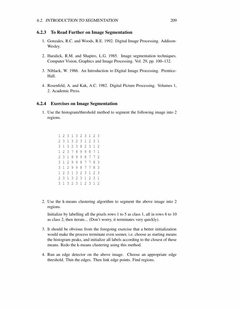
6.2. INTRODUCTION TO SEGMENTATION 209
6.2.3 To Read Further on Image Segmentation
1. Gonzales, R.C. and Woods, R.E. 1992. Digital Image Processing. Addison-Wesley.
2. Haralick, R.M. and Shapiro, L.G. 1985. Image segmentation techniques.Computer Vision, Graphics and Image Processing. Vol. 29, pp. 100–132.
3. Niblack, W. 1986. An Introduction to Digital Image Processing. Prentice-Hall.
4. Rosenfeld, A. and Kak, A.C. 1982. Digital Picture Processing. Volumes 1,2. Academic Press.
6.2.4 Exercises on Image Segmentation
1. Use the histogram/threshold method to segment the following image into 2regions.
1 2 3 1 3 2 3 1 2 32 3 1 3 2 3 1 2 3 13 1 3 2 3 8 2 3 1 21 2 3 7 8 9 9 8 7 12 3 1 8 9 9 8 7 7 23 1 2 9 9 8 7 7 8 33 1 2 9 9 8 7 7 8 31 2 3 1 3 2 3 1 2 32 3 1 3 2 3 1 2 3 13 1 3 2 3 1 2 3 1 2
2. Use the k-means clustering algorithm to segment the above image into 2regions.
Initialize by labelling all the pixels rows 1 to 5 as class 1, all in rows 6 to 10as class 2, then iterate... (Don’t worry, it terminates very quickly).
3. It should be obvious from the foregoing exercise that a better initializationwould make the process terminate even sooner, i.e. choose as starting meansthe histogram peaks, and initialize all labels according to the closest of thesemeans. Redo the k-means clustering using this method.
4. Run an edge detector on the above image. Choose an appropriate edgethreshold. Thin the edges. Then link edge points. Find regions.

210 CHAPTER 6. FROM IMAGES TO OBJECTS
5. Analyze the problem of segmenting an image of a human face. Ideally youwant to be able to extract the face from its background.
(a) Identify the major problems with respect to the simple models mentionedabove.
(b) Will we need to segment into multiple classes? – As well as separating“face” from background we may need to segment within the face. Mentionproblems.
(c) Would colour help?
(d) How will lighting affect the problem?
(e) Suggest a layout for the subject (face), camera, and background.
6. Segmentation for data compression. Take the image given in the first exerciseabove. Assume the grey levels are coded in four bits [0..15].
(a) Now as in the first exercise, segment it into two regions – call them re-gions 0, 1;
(b) Calculate the means for each region, m0,m1.
(c) code region 0 pixels as 0 and region 1 pixels as 1;
(d) Assuming 8 bits for the means (the code-book), how many bits are therein the coded image?
(e) reconstruct the image, using the code-book and coded 1-bit image.
(f) How would you estimate the loss or distortion caused by the compres-sion?
7. Repeat this compression experiment for the 10×10 three-colour image usedat the end of section 6.2.1.
6.3 Mathematical Morphology
6.3.1 Introduction to Mathematical Morphology
This section begins with some basic definitions, symbols and terminology to domorphological image processing. First binary morphological operations are treated.These are then extended to their corresponding grey-level operations. The discus-sion focusses on the application of these operations to detection of high intensitypeaks, low intensity valleys, and edges in grey-level images; the application is fea-ture extraction in images of human faces.
We first present relevant definitions in terms of – the original basis of mathe-matical morphology – spatial set theory, and then look at the same topic using ahit-or-miss operator definition and scanned operator approach. Following this, wecover the extension of this approach to grey-level images, and finally composite

6.3. MATHEMATICAL MORPHOLOGY 211
operations (i.e. those that can be defined in terms of the basic operations of dila-tion and erosion). Examples are then used to illustrate the powerfulness of theseoperations.
Basic Morphological Operations
Morphological image processing operations take account of the spatial structure orcorrespondence between groups of neighbouring pixels. To some extent, therefore,there are similarities with convolution based spatial enhancement operations, e.g.smoothing and edge detection; these are essentially linear operations. On the otherhand, morphological operations are based on set theory operations, i.e. union, in-tersection, or in terms of Boolean algebra: AND, OR; hence they are definitelynon-linear.
Both convolution and morphological operations can be considered “geomet-ric”, but, while many morphological operations are implemented by scanning “op-erator” masks across the image – in the same way as convolution the theory andbackground of the two are very different.
In the literature there are two distinct methods of introducing morphologicaloperations: (i) using the original spatial set theory – traced back to Matheron(1975) and Minkowski (1903), and used as the basis of Serra’s work (Serra, 1982,1988), (ii) a practical approach, by describing the common operations via their im-plementation as scanned operators and by discussing their effects and applications.In deference to history, we will mention (i) but quickly move onto (ii) since thatinterpretation is easier to understand.
Set Theoretic Basis
Consider the binary images shown in the following. The first is called a structuringelement for reasons soon to become clear. For pixels numbered 0, 1 and 2, it is a3×3 image. The second is a 16×16 image.
0 1 20 1 1 11 1 1 12 1 1 1
0 0 0 0 0 0 0 0 0 0 0 0 0 0 0 00 0 0 0 0 0 0 0 0 0 0 0 0 0 0 00 0 0 0 0 0 0 0 0 0 0 0 0 0 0 00 0 0 1 1 1 1 1 0 0 0 1 1 0 0 00 0 0 0 1 1 1 1 0 0 0 1 1 0 0 00 0 0 1 1 1 1 1 0 0 0 1 1 0 0 00 0 0 1 1 1 1 1 1 1 1 1 1 0 0 00 0 0 1 0 0 1 1 1 1 1 1 1 0 0 00 0 0 1 1 0 0 1 1 1 1 1 1 0 0 0
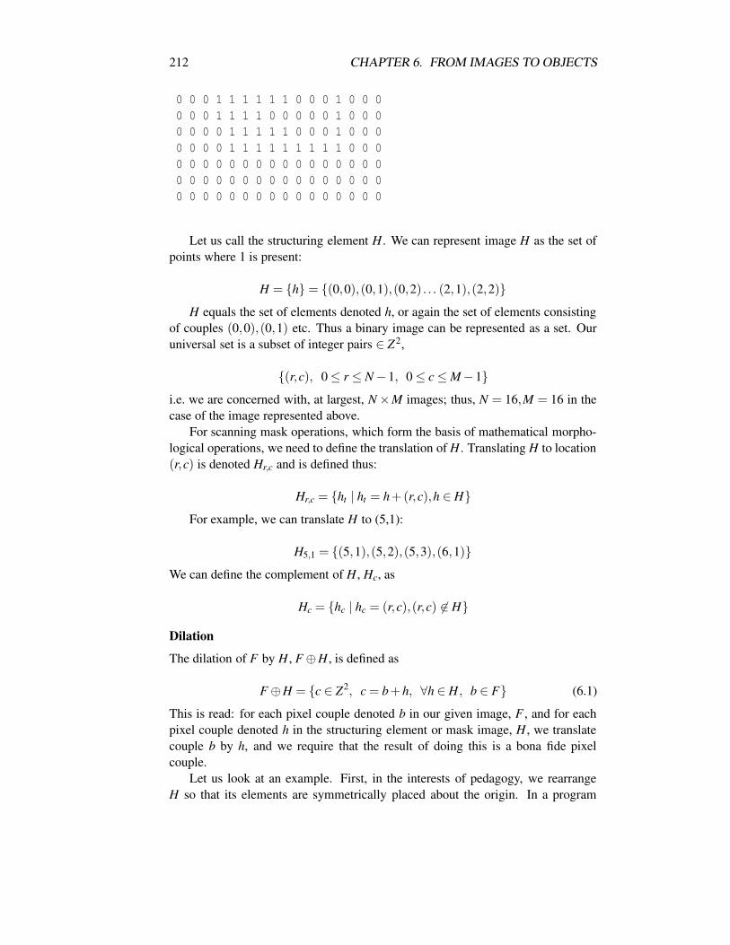
212 CHAPTER 6. FROM IMAGES TO OBJECTS
0 0 0 1 1 1 1 1 1 0 0 0 1 0 0 00 0 0 1 1 1 1 0 0 0 0 0 1 0 0 00 0 0 0 1 1 1 1 1 0 0 0 1 0 0 00 0 0 0 1 1 1 1 1 1 1 1 1 0 0 00 0 0 0 0 0 0 0 0 0 0 0 0 0 0 00 0 0 0 0 0 0 0 0 0 0 0 0 0 0 00 0 0 0 0 0 0 0 0 0 0 0 0 0 0 0
Let us call the structuring element H . We can represent image H as the set ofpoints where 1 is present:
H = h = (0,0),(0,1),(0,2) . . . (2,1),(2,2)H equals the set of elements denoted h, or again the set of elements consisting
of couples (0,0),(0,1) etc. Thus a binary image can be represented as a set. Ouruniversal set is a subset of integer pairs ∈ Z2,
(r,c), 0≤ r ≤ N−1, 0≤ c≤M−1i.e. we are concerned with, at largest, N×M images; thus, N = 16,M = 16 in thecase of the image represented above.
For scanning mask operations, which form the basis of mathematical morpho-logical operations, we need to define the translation of H . Translating H to location(r,c) is denoted Hr,c and is defined thus:
Hr,c = ht | ht = h+(r,c),h ∈HFor example, we can translate H to (5,1):
H5,1 = (5,1),(5,2),(5,3),(6,1)We can define the complement of H , Hc, as
Hc = hc | hc = (r,c),(r,c) 6∈ H
Dilation
The dilation of F by H , F⊕H , is defined as
F⊕H = c ∈ Z2, c = b+h, ∀h ∈ H, b ∈ F (6.1)
This is read: for each pixel couple denoted b in our given image, F , and for eachpixel couple denoted h in the structuring element or mask image, H , we translatecouple b by h, and we require that the result of doing this is a bona fide pixelcouple.
Let us look at an example. First, in the interests of pedagogy, we rearrangeH so that its elements are symmetrically placed about the origin. In a program

6.3. MATHEMATICAL MORPHOLOGY 213
implementation, we can use the same convention: the origin of the structuringelement is its centre. We consider only odd-sized structuring elements. Hence,
H = (−1,−1),(−1,0), ...(1,1)
The dilation of F by H can be expressed in English as: for all 1 pixels f = (r,c)in image (set) F , the output set C is extended by adding elements f +h, for all theelements h ∈ H . The first 1 in F is at location (4,3). Shown below is the extensionor expansion at this point: the additional locations are (2,2), (2,3), (2,4) etc.
Structuring element, 3×3, for pixels numbered −1, 0 and 1:
−1 0 1−1 1 1 10 1 1 11 1 1 1
First five rows of input image, F:
0 0 0 0 0 0 0 0 0 0 0 0 0 0 0 00 0 0 0 0 0 0 0 0 0 0 0 0 0 0 00 0 0 0 0 0 0 0 0 0 0 0 0 0 0 00 0 0 1 1 1 1 1 0 0 0 1 1 0 0 00 0 0 0 1 1 1 1 0 0 0 1 1 0 0 0
Dilation, with b = (3,3):
0 0 0 0 0 0 0 0 0 0 0 0 0 0 0 00 0 0 0 0 0 0 0 0 0 0 0 0 0 0 00 0 0(1) 0(1) 0(1) 0 0 0 0 0 0 0 0 0 0 00 0 0(1) 1(1) 1(1) 1 1 1 0 0 0 1 1 0 0 00 0 0(1) 0(1) 1(1) 1 1 1 0 0 0 1 1 0 0 0
The overall result of this dilation by a 3×3 structuring element is shown next.We can see that dilation swells the shape in F , and fills in small “lakes” and “bays”– using a geographical metaphor, 1 = land, 0 = water.
0 0 0 0 0 0 0 0 0 0 0 0 0 0 0 00 0 0 0 0 0 0 0 0 0 0 0 0 0 0 00 0 1 1 1 1 1 1 1 0 1 1 1 1 0 00 0 1 1 1 1 1 1 1 0 1 1 1 1 0 0
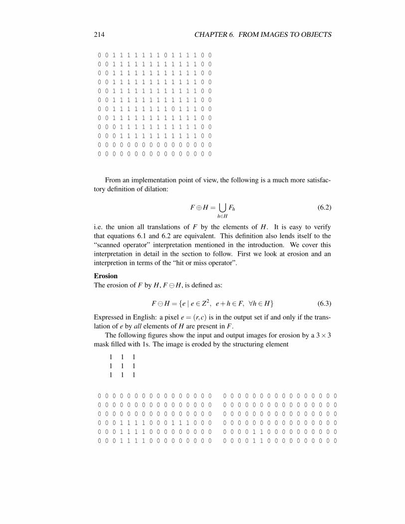
214 CHAPTER 6. FROM IMAGES TO OBJECTS
0 0 1 1 1 1 1 1 1 0 1 1 1 1 0 00 0 1 1 1 1 1 1 1 1 1 1 1 1 0 00 0 1 1 1 1 1 1 1 1 1 1 1 1 0 00 0 1 1 1 1 1 1 1 1 1 1 1 1 0 00 0 1 1 1 1 1 1 1 1 1 1 1 1 0 00 0 1 1 1 1 1 1 1 1 1 1 1 1 0 00 0 1 1 1 1 1 1 1 1 0 1 1 1 0 00 0 1 1 1 1 1 1 1 1 1 1 1 1 0 00 0 0 1 1 1 1 1 1 1 1 1 1 1 0 00 0 0 1 1 1 1 1 1 1 1 1 1 1 0 00 0 0 0 0 0 0 0 0 0 0 0 0 0 0 00 0 0 0 0 0 0 0 0 0 0 0 0 0 0 0
From an implementation point of view, the following is a much more satisfac-tory definition of dilation:
F⊕H =[
h∈H
Fh (6.2)
i.e. the union all translations of F by the elements of H . It is easy to verifythat equations 6.1 and 6.2 are equivalent. This definition also lends itself to the“scanned operator” interpretation mentioned in the introduction. We cover thisinterpretation in detail in the section to follow. First we look at erosion and aninterpretion in terms of the “hit or miss operator”.
ErosionThe erosion of F by H , FH , is defined as:
FH = e | e ∈ Z2, e+h ∈ F, ∀h ∈H (6.3)
Expressed in English: a pixel e = (r,c) is in the output set if and only if the trans-lation of e by all elements of H are present in F .
The following figures show the input and output images for erosion by a 3×3mask filled with 1s. The image is eroded by the structuring element
1 1 11 1 11 1 1
0 0 0 0 0 0 0 0 0 0 0 0 0 0 0 0 0 0 0 0 0 0 0 0 0 0 0 0 0 0 0 00 0 0 0 0 0 0 0 0 0 0 0 0 0 0 0 0 0 0 0 0 0 0 0 0 0 0 0 0 0 0 00 0 0 0 0 0 0 0 0 0 0 0 0 0 0 0 0 0 0 0 0 0 0 0 0 0 0 0 0 0 0 00 0 0 1 1 1 1 0 0 0 1 1 1 0 0 0 0 0 0 0 0 0 0 0 0 0 0 0 0 0 0 00 0 0 1 1 1 1 0 0 0 0 0 0 0 0 0 0 0 0 0 1 1 0 0 0 0 0 0 0 0 0 00 0 0 1 1 1 1 0 0 0 0 0 0 0 0 0 0 0 0 0 1 1 0 0 0 0 0 0 0 0 0 0

6.3. MATHEMATICAL MORPHOLOGY 215
0 0 0 1 1 1 1 1 1 0 0 1 1 0 0 0 0 0 0 0 1 1 0 0 0 0 0 0 0 0 0 00 0 0 1 1 1 1 1 1 0 0 0 0 0 0 0 0 0 0 0 1 1 0 0 0 0 0 0 0 0 0 00 0 0 1 1 1 1 0 0 0 0 0 0 0 0 0 0 0 0 0 1 1 0 0 0 0 0 0 0 0 0 00 0 0 1 1 1 1 0 0 0 0 1 0 0 0 0 0 0 0 0 1 1 0 0 0 0 0 0 0 0 0 00 0 0 1 1 1 1 1 1 1 1 1 1 0 0 0 0 0 0 0 1 1 0 0 0 0 0 0 0 0 0 00 0 0 1 1 1 1 1 1 1 1 1 1 0 0 0 0 0 0 0 1 1 1 1 1 1 1 1 0 0 0 00 0 0 1 1 1 1 1 1 1 1 1 1 0 0 0 0 0 0 0 0 0 0 0 0 0 0 0 0 0 0 00 0 0 0 0 0 0 0 0 0 0 0 0 0 0 0 0 0 0 0 0 0 0 0 0 0 0 0 0 0 0 00 0 0 0 0 0 0 0 0 0 0 0 0 0 0 0 0 0 0 0 0 0 0 0 0 0 0 0 0 0 0 00 0 0 0 0 0 0 0 0 0 0 0 0 0 0 0 0 0 0 0 0 0 0 0 0 0 0 0 0 0 0 0
Thus, we can see the erosion of the boundaries of the shape in F , and deletionof small “islands” and “headlands” – using the geographical metaphor, 1 = land, 0= water, mentioned before.
Recalling equation 6.2, there is a corresponding definition of erosion,
FH =\
h∈H
F−h (6.4)
where F−h is the translation of F by the reflection of H =−h = (−r,−c) i.e. theintersection of all translations of F by the elements of the reflection of H; actually,in the case of square structuring elements the reflection of H is identical to H . It iseasy to verify that equations 6.3 and 6.4 are equivalent.
Hit or Miss Operations
In hit or miss operations, a mask is scanned over the input image. At each pointin the scanning – each pixel – a check is made, whether the pattern in the maskmatches the pattern in the image, and the output pixel is set to some appropriatestate. Trivially, single pixel “spot-noise” can be removed by scanning with
0 0 00 1 00 0 0
When this pattern is encountered, the output is set to 0, otherwise 1.An eight-neighbour dilate in terms of hit or miss can be defined as follows (see
Pratt, 1991).
d[r,c] = 1 iff at least it or one of its eight-neighbours is 1
If we regard 1-valued pixels an Boolean true, and 0 as false, we can defineeight-neighbour dilate as:
d[r,c] = f [r,c] OR neighbour1 . . . OR neighbour8We can define a cumulative OR operator, COR, to represent this:
d[r,c] = COR j,k∈8−n f [ j,k]

216 CHAPTER 6. FROM IMAGES TO OBJECTS
where j,k ∈ 8−n means that ( j,k) is in the neighbourhood.Similarly, Pratt (1991) defines eight-neighbour erosion,
e[r,c] = 0 iff it or any of its neighbours is 0.We can define a cumulative AND operator, CAND:
e[r,c] = CAND j,k∈8−n f [ j,k]
6.3.2 Scanned Operators
We now describe the implementation of erosion and dilation in terms of equations6.2 and 6.4. This is based on the treatment of Pratt (1991, chapter 15.4) whointroduced the conceptually tidier generalized dilation and erosion operations.
Generalized Dilation
Recall equation 6.2:
F⊕H =[
h∈H
Fh
This can be expanded to make the scanning explicit
F⊕H = d[r,c] =[
r′∈H
[
c′∈H
f [r,c]r′,c′ (6.5)
The set operations defined here are not easy to visualize; also we need a defi-nition whose program implementation is easy and direct. The following Booleanalgebra representation, and based on hit or miss operations, satisfies both require-ments.
Regard 1-valued pixels an Boolean true and 0 as false; then the above equationcan be expressed as
d[r,c] = CORr+qrr′=r−qrCORc+qc
c′=c−qc( f [r′,c′] AND h[r′− r,c′− c]) (6.6)
This is depicted graphically below, which shows a mask containing H , placedon the image F , and centred at (r,c). H extends vertically −qr to +qr on eitherside of its center, and horizontally, −qc to +qc. Thus, the mask is a matrix of size(2qr +1)× (2qc+1); in the example shown, qc = qr = 1.
The corresponding elements f (., .) and h(., .) are ANDed, and the results thenORed, to produce the output at (r,c),d[r,c]. This is done for every (r,c) – hencethe scanned operator view of the operation.
Here is the dilation mask centred on pixel (r,c):

6.3. MATHEMATICAL MORPHOLOGY 217
h(1,1) h(1,0) h(1,–1)f(r–1,c–1) f(r–1,c) f(r–1,c+1
h(0,1) h(0,0) h(0,–1)f(r,c–1) f(r,c) f(r,c+1)
h(–1,1) h(–1,0) h(–1,–1)f(r+1,c–1 f(r+1,c) f(r+1,c+1
Analogy with Convolution
The analogy with two-dimensional discrete convolution should be obvious, – seeequation 6.6. With convolution we have multiplication (instead of ANDing) ofthe corresponding elements under the convolution mask, followed by summation(instead of cumulative ORing):
d[r,c] =r+qr
∑r′=r−qr
c+qc
∑c′=c−qc
( f [r′,c′] h[r′− r,c′− c])
Generalized Erosion
By analogy, generalized erosion can be defined as,
e[r,c] = CANDr+qrr′=r−qrCANDc+qc
c′=c−qc( f [r′,c′] OR h[r′− r,c′− c])
6.3.3 Grey-level Morphology
The operations described above work only on binary valued images and structuringelements. They can be extended (Pratt, 1991, chapter 15.6) to grey-level imagesby generalizing the Boolean operations to extremum operations:
OR(a,b) −→MAX(a,b)
AND(a,b) −→MIN(a,b)
Generalized Grey-level Dilation
Hence, extending equation 6.5, (generalized) grey-level dilation can be definedas:
d[r,c] = MAXr+qrr′=r−qrMAXc+qc
c′=c−qcMIN(f[r′,c′],h[r′− r,c′− c])
We constrain H to contain only binary values.The formulation above allows for arbitrarily-shaped structuring elements, i.e.
the shape is “drawn” within the rectangularly shaped mask: h(., .) = 1 or 0.
218 CHAPTER 6. FROM IMAGES TO OBJECTS
Often, we deal only with rectangular structuring elements, so that generalizedgrey-level dilation can be defined as:
d[r,c] = MAXr+qrr′=r−qrMAXc+qc
c′=c−qcf[r′,c′]
Generalized Grey-level Erosion
Likewise, we can define grey-level erosion as,
e[r,c] = MINr+qrr′=r−qrMINc+qc
c′=c−qcMAX(f[r′,c′],h[r′− r,c′− c])
and, for the special case of rectangular structuring elements:
e[r,c] = MINr+qrr′=r−qrMINc+qc
c′=c−qcf[r′,c′]
Completeness of Extension
By substituting 1 for true and 0 for false, it is easy to verify that the extension iscomplete: i.e. grey-level operations applied to binary images give the same resultas the equivalent binary operation.
6.3.4 Composite Operations – Open and Close
Morphological open is defined as erosion followed by dilation.Likewise, close is dilation followed by erosion.
6.3.5 Program Implementation
In the following C code, both dilation and erosion are carried out, depending onthe Boolean dilate (== FALSE for erosion). Moreover, it does open and close byusing two passes.
As it is, the routine uses rectangular structuring elements. We have left evi-dence (commented-out) of the general shaped element.
for(r=rl;r<=rh;r++)for(c=cl;c<=ch;c++)if(r<sr||r>rh1||c<sc||c>ch1) /*boundaries */
rv=0.0;IMDput(&rv,d,r,c,pd); continue;if(binary)val=dilate?0:1;else rv=dilate?min:max;
rrl=MAX(rl,r-qr);rrh=MIN(rh,r+qr);ccl=MAX(cl,c-qc);cch=MIN(ch,c+qc);for(rr=rrl,hp=0;rr<=rrh;rr++)
6.3. MATHEMATICAL MORPHOLOGY 219
for(cc=ccl;cc<=cch;cc++,hp++)/*hh=h[hp];*//*rectangular structuring element*/IMDget(&rv1,d,rr,cc,ps);if(binary)
val1=rv1<1.0?0:1;if(dilate)val=val||(val1);/*prev. (val1&&hh)*/else val=val&&(val1);/*prev. (val1||!hh)*/
else /*grey-level*/
if(dilate)rv=MAX(rv,rv1); /*prev. dilate&&hh)*/else rv=MIN(rv,rv1);
if(binary)rv=val;IMDput(&rv,d,r,c,pd);
6.3.6 Examples of Morphological Operations
In the following figures, we give examples of practical applications of morpholog-ical operations. In all cases, a 3×3 structuring element is used.
We use an image consisting of some touching blocks and some straight lines.Next we see erosion. Erosions of edges and of protrusions takes place. The
effect of this can be clearly seen when we subtract the eroded image from theoriginal image.
Next we see dilation, where the swelling effect is clearly evident.Finally we show (Figures 6.2, 6.3) the opening (dilate followed by erode), and
closing (erode followed by dilate).We can go further if we wish. Morphological edge highlighting, using the
difference (dilate – erode), uses the fact that dilate swells the edge regions outwardsand inwards, while erosion is the opposite, hence, the difference highlights regionsthat are subject to erosion and swelling – especially both, i.e. edges.
Peak (peak = localised high intensity) highlighting can be performed by sub-tracting, from the original, the open using a structuring element that is large com-pared to the peak’s spatial size; this can be explained by the tendancy of openingto erase peaks.
Valleys (valley = thin channel of low intensity) can be highlighted by subtract-ing, from the original, the close using a structuring element that is large comparedto the valley’s spatial size; this can be explained by the tendancy of close to blockup valley regions.
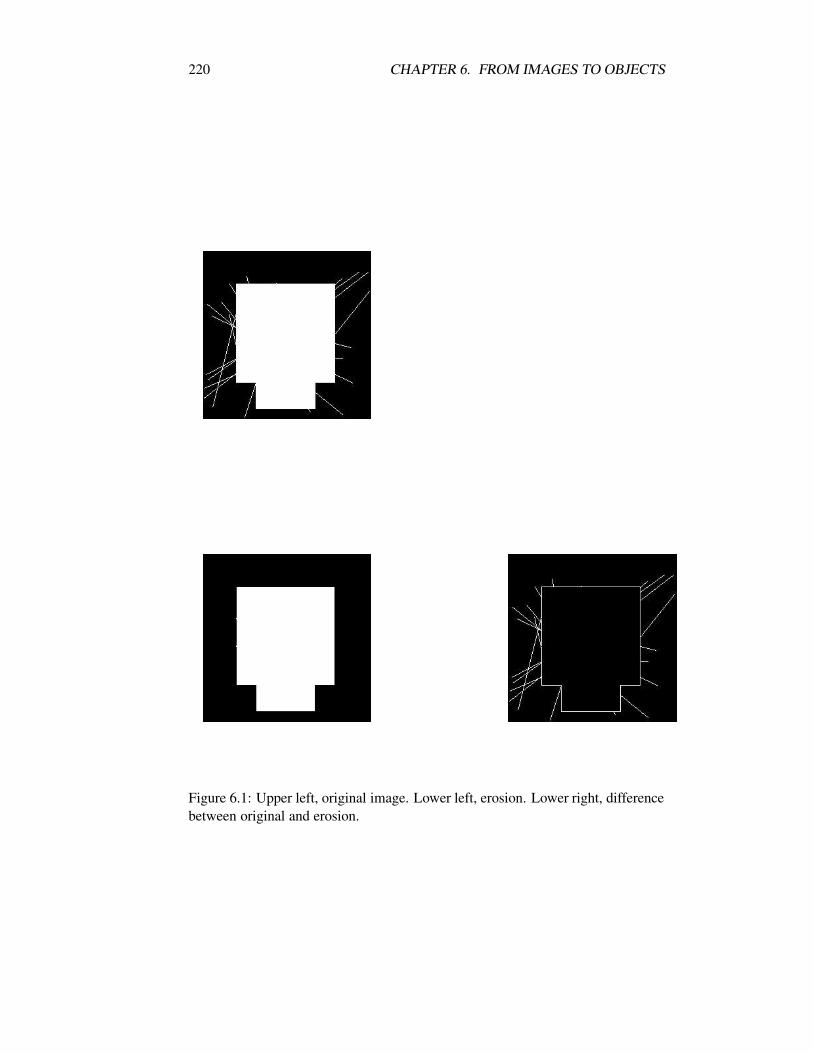
220 CHAPTER 6. FROM IMAGES TO OBJECTS
Figure 6.1: Upper left, original image. Lower left, erosion. Lower right, differencebetween original and erosion.
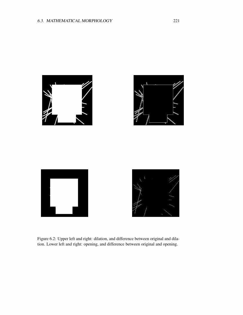
6.3. MATHEMATICAL MORPHOLOGY 221
Figure 6.2: Upper left and right: dilation, and difference between original and dila-tion. Lower left and right: opening, and difference between original and opening.
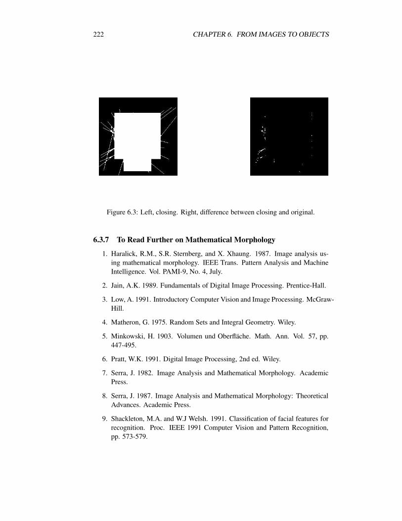
222 CHAPTER 6. FROM IMAGES TO OBJECTS
Figure 6.3: Left, closing. Right, difference between closing and original.
6.3.7 To Read Further on Mathematical Morphology
1. Haralick, R.M., S.R. Sternberg, and X. Xhaung. 1987. Image analysis us-ing mathematical morphology. IEEE Trans. Pattern Analysis and MachineIntelligence. Vol. PAMI-9, No. 4, July.
2. Jain, A.K. 1989. Fundamentals of Digital Image Processing. Prentice-Hall.
3. Low, A. 1991. Introductory Computer Vision and Image Processing. McGraw-Hill.
4. Matheron, G. 1975. Random Sets and Integral Geometry. Wiley.
5. Minkowski, H. 1903. Volumen und Oberflache. Math. Ann. Vol. 57, pp.447-495.
6. Pratt, W.K. 1991. Digital Image Processing, 2nd ed. Wiley.
7. Serra, J. 1982. Image Analysis and Mathematical Morphology. AcademicPress.
8. Serra, J. 1987. Image Analysis and Mathematical Morphology: TheoreticalAdvances. Academic Press.
9. Shackleton, M.A. and W.J Welsh. 1991. Classification of facial features forrecognition. Proc. IEEE 1991 Computer Vision and Pattern Recognition,pp. 573-579.

6.3. MATHEMATICAL MORPHOLOGY 223
6.3.8 DataLab-J Demonstrations on Mathematical Morphology
Call the following script mob.dlj and run is with the command java Dlj mob.jlj.It constructs the various images shown as examples of application of morphologi-cal operations.

224 CHAPTER 6. FROM IMAGES TO OBJECTS
//----- mob.dlj ----------------------------------//j.g.c. 18/6/98//simple tests on binary morphological operators//------------------------------------------------//generate rectangle, top left (50,50), bottom right (200,200)//put in image 0grect0256,256, 50,50,200,200//another rect, (180,80) (240,170)grect1256,256, 180,80,240,170//generate 20 random linesgrlines2256,256, 20//now we add (actually binary OR) the two rects and the random//lines an put the result in image 3mobor1,23mobor3,03//save the combined imagesavei3moborig,0,0,0//erode original with a 3x3 structuring elementmobe343//and save in file "moberod.pgm"savei4moberod,0,0,0//dilate original with a 3x3 structuring elementmobd353

6.3. MATHEMATICAL MORPHOLOGY 225
savei5mobdil,0,0,0
//open original with a 3x3 structuring elementmobo363savei6mobopen,0,0,0//closemobc373savei7mobclos,0,0,0//XOR original, eroded to show differencemobxor3,48savei8mobderod,0,0,0//original, dilatedmobxor3,59savei9mobddil,0,0,0//original, openedmobxor3,610savei10mobdopen,0,0,0//original, closedmobxor3,7

226 CHAPTER 6. FROM IMAGES TO OBJECTS
11savei11mobdclos,0,0,0end
6.3.9 Exercises on Mathematical Morphology
1. Using the 3×3 structuring element
1 1 11 1 11 1 1
show (i) dilation and (ii) erosion on the following image:
0 0 0 0 0 0 0 0 0 0 0 00 0 0 0 0 0 0 0 0 0 0 00 1 1 1 1 0 0 0 0 0 0 00 1 1 1 1 0 0 0 0 1 1 00 1 1 1 1 0 0 0 0 0 0 00 0 0 0 0 0 0 0 0 0 0 00 0 0 0 0 0 0 0 0 0 0 0
2. Morphological opening is an erosion followed by a dilation. Find the open-ing of the image given above.
3. Morphological closure is a dilation followed by an erosion. Find the closureof the image given above.
4. Find (i) the original image minus the erosion, and (ii) the original imageminus the dilation. Comment on what you find in the case of both results.
5. Using the results found for erosion, dilation, open, and close, comment onthe use of mathematical morphological operations for the purposes of (i)noise removal, and (ii) edge detection.
6. Indicate how and where morphological operators could be usefully employedin the application area of face recognition.

6.4. THE WAVELET TRANSFORM 227
6.4 The Wavelet Transform
6.4.1 Introduction
We have looked at the Fourier transform in Chapter 3. We saw that it allows afrequency-based decomposition of our image or signal data. The data can be ex-actly reconstituted from the transform. As with any transform, we can carry outcertain surgical interventions before reconstituting the data. We can, for instance,remove high frequencies, which amounts to saying that noisy and edgy parts of thedata will be smoothed.
The wavelet transform shares some of the same objectives. Both transformslead to a new representation of the data, which can serve a useful purpose such asallowing us to remove components (strata, if you like) which are a nuisance to ourunderstanding of the data. Both transforms also allow us to exactly reconstitute ourdata if this is required. Different perspectives are provided by these two transformson the high and low frequencies in our data, i.e. the relative local “activity” orvariation.
High frequency data means rapidly changing data, which could be, but doesnot have to be, related to noise. Low frequency means slowly varying. Band-passfiltering our data means that we kill, say, high frequencies in our data, leavingbehind a band of low pass frequencies and then reconstitute an approximation toour input data from this. If we do remove high frequencies, then this is the sameas running a low-pass filter which is tantamount to smoothing or blurring our data.We can achieve such objectives with either the wavelet or Fourier transform.
Interfering in this way in transform space leads to denoising, or “data clean-ing”, or generally data filtering.
The wavelet transform has become popular in recent years even though its rootsgo back many decades. The Haar wavelet transform goes back to the early 20thcentury.
Although lots of justifications for the wavelet transform could be given, we willjust mention two major justifications. Firstly, it is a useful tool for finding faintfeatures in an image – it is a mathematical and algorithmic “microscope”. Thisobjective is favoured by the wavelet transform which we will look at in the nextsection. Secondly, the wavelet transform is found in practice to provide a sparse setof values (many zeros or many very small values) representing the original data. Asa direct byproduct it is a useful preprocessing step towards the goal of compression.We will discuss this objective when we describe the Haar wavelet transform.
We will describe two wavelet transform methods. The first, the a trous method,is representative of so-called redundant methods. The second method, the Haartransform, is representative of a large family of orthornormal methods. We mentionthese facts in passing, to note that there are many wavelet transforms available, butthat the ones we will deal with are useful entry points into this rapidly growing andvery popular field.

228 CHAPTER 6. FROM IMAGES TO OBJECTS
6.4.2 The a trous Wavelet Transform
We will perform a sequence of operations on our image which appears at firstsight to be a strange thing to do. We smooth the image, f0, to form f1 = s( f0).Smoothing uses convolution (Chapter 3). We smooth the image we thereby get toform f2 = s( f1). We continue doing this for a user-specified number of times, oftenabout p = 4 or 5.
That looks like a counterproductive thing to do. Now, we take the successionof coarser images, f0, f1, ..., fp, and form a set of detail signal images as follows:f0− f1, f1− f2, . . . , fp−1− fp. We have trivially
f0 = ( f0− f1)+( f1− f2)+ · · ·+( fp−1− fp)+ fp
orf0 = d1 +d2 + · · ·+dp + fp (6.7)
where the last image here is the coarsest image which we are considering.These detail images contain structure which was present at one scale, and
which did not survive the blurring in going to the next scale.Equation 6.7 is an image expansion in the form of a sum of component images.
These component images, d1 = ( f0− f1) etc., do not form an independent (i.e.orthogonal) system, whereas in the case of other wavelet transform approaches, in-cluding the Haar wavelet transform explored below, orthogonality of an analogousdecomposition is considered a desirable property.
The above decomposition of f0 gives us a fine-to-coarse transition of informa-tion. To understand what the detail images convey, take d1. This detail imagesprovide information on features which “died” in the blurring at stage f1. Such faintaspects of the image f0 did not survive the blurring, since they were too small andfaint. We talk about the scale of such features. The succession of detail images,d1,d2, . . . , yields information which is scale-related.
The algorithm used can be stated as follows. Index k ranges over all pixels.
1. We initialize i to 0 and we start with an image f i(k).
2. We increment i, and we carry out a discrete convolution of the data f i−1(k)using the filter h. The distance between a central pixel and adjacent ones is2i−1.
3. From this smoothing we obtain the discrete wavelet transform, di(k)= fi−1(k)−fi(k).
4. If i is less than the number p of resolutions we want to compute, then go tostep 2.
5. The set W = d0,d1, ...,dp, fp represents the wavelet transform of the data.
6.4. THE WAVELET TRANSFORM 229
In one dimension, we take h = ( 116 , 1
4 , 38 , 1
4 , 116). In two dimensions, we can
use this same kernel sweeping out the horizontal (column) direction, followed bya sweep over the vertical direction (rows). The explanation for this choice is that itis associated with a B3 spline, a function which is known for its good interpolationproperties. The only messy aspect is handling the extremities of the signal. Afew choices are open to us. We recommend reflection in the extremity, giving a“mirror” effect.
That is the general idea. Various other issues are also of importance. The imagef1 is most usually a half-resolution version of input image f0, and f2 is a half-resolution version of f1, and so on. This is almost always the case, even if there isno necessity for doing things this way. To justify this dyadic decomposition, we canpoint to certain aspects of human perception being logarithmic in receptiveness,and to the computational advantages of doing things in this way.
In the case of the Haar or Daubechies methods (see Press et al., 1992, for anoverview), such diminishing of resolution is made use of to halve the dimensional-ity of the image which is output. I.e. if f2 is reduced in resolution by 2, then we canbenefit by reducing its dimensionality (along each dimension) by 2 also. This is re-ferred to as decimation or down-sampling and means that from a two-dimensionalinput image, we arrive at a transform which can be represented as a pyramid. Or,in the case of a one-dimensional transform consisting of d1,d2, ...,dp, fp, the trans-form result can all be fit into an n-length vector of values, where n is the length ofthe f0 signal.
The a trous method tackles the issue of halving resolution at each stage some-what differently. Decimation is not used with this method, which means thatd1,d2, . . . continue to have exactly the same dimensionality as the input data, f0.Therefore the a trous transform is a redundant one. This redundancy may be ofgreat help to us in exactly demarcating features thrown up by the various detailimages. We relate the features to what we can see, or not see, in the original image,and there is no aliasing introduced by the decimation.
In the a trous method the succession of smoothings or blurrings is carriedout using a scaling function. Say that the smoothing is achieved by a length5 scaling function, implying that at each image pixel value (we’ll take a one-dimensional view for simplicity) the surrounding pixel values (−2,−1,0,+1,+2)enter into the calculation. Then at the following smoothing, we will use pixel val-ues (−4,−2,0,+2,+4). At the following one again, we use (−8,−4,0,+4,+8).This is a versatile way to enforce two-fold diminishing of resolution. It also givesrise to the name a trous, “with holes”.
The images f1, f2, . . . are formed by repeatedly smoothing. Consider these asbeing created instead directly from the original image, f0. The smoothing meansthat we convolve, which involves translating a function – the scaling function. Ateach successive scale, we dilate this function. One possible form for the scalingfunction which is a very practical one and also one that we have used very exten-sively is shown in Figure 6.4. We see that it is like a Gaussian, but of compactsupport (i.e. the wings are clipped).

230 CHAPTER 6. FROM IMAGES TO OBJECTS
Figure 6.4: A trous wavelet transform. The scaling function here is defined by theB3-spline function, which is a function with good interpolation properties.
We can consider similarly the direct determining of d1,d2, . . . from f0. Thefunction needed to do this is a translated and dilated version of a mother waveletfunction. The one which of necessity goes hand in hand with the scaling functiondescribed above is also shown in Figure 6.4. These dilated versions of the waveletfunction constitute a new basis for the original data signal. We have already notedthat in the case of the a trous method, they are not mutually orthogonal. We canalso note a parallel with the Fourier transform: the latter defines a new basis interms of sine and cosine functions.
The original data, f0, can be recreated exactly from the wavelet transform ordecomposition. A property which follows from this is that the wavelet coefficientvalues in d1 or d2 etc. are of zero mean.
We have discussed the wavelet transform in terms of a discrete transform, andalso in terms of a dyadic scale. A more general, continuous wavelet transform canalso be considered. Mathematically, this is given by
W (a,b) =1√a
Z ∞
∞f (x)ψ∗(
x−ba
)dx
where W is the set of wavelet coefficients of the function f (x); ψ is the motherwavelet (and we take its complex conjugate above in the convolution); and a and bare, respectively, the scale and the position parameters. An admissability conditiondefines the circumstances under which exact recreation of f from the transformvalues, W , is possible.
6.4.3 Examples of the A Trous Wavelet Transform
Figure 6.5 shows one important application, denoising. The denoising here is adata-driven, based on Gaussian noise at each wavelet transform scale (see Starcket al., 1998, for more background on filtering).

6.4. THE WAVELET TRANSFORM 231
Figure 6.6 shows a succession of scales resulting from the a trous wavelet trans-form of the (noisy) image shown in Figure 6.5. By adding these images, we canreconstitute exactly the input image.
Figure 6.7 shows a different view of this, using a perspective plot. The plateauson the peaks are for display purposes only, and show 3σ values (σ is the standarddeviation of the given resolution level or scale). Again exact reconstitution of theinput data can be carried out.
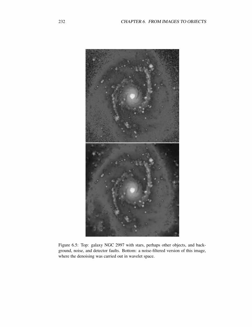
232 CHAPTER 6. FROM IMAGES TO OBJECTS
Figure 6.5: Top: galaxy NGC 2997 with stars, perhaps other objects, and back-ground, noise, and detector faults. Bottom: a noise-filtered version of this image,where the denoising was carried out in wavelet space.

6.4. THE WAVELET TRANSFORM 233
Figure 6.6: The a trous transform (3 resolution levels, together with the finalsmoothed version of the image) produces these images for the NGC 2997 image.Read in this order: lower left, upper left, lower right, upper right. The “shadow”effect (especially in the upper right) is due to the colour lookup data used in thedisplay.

234 CHAPTER 6. FROM IMAGES TO OBJECTS
Figure 6.7: A perspective plot of the a trous transform of NGC 2997. Read frombottom to top.
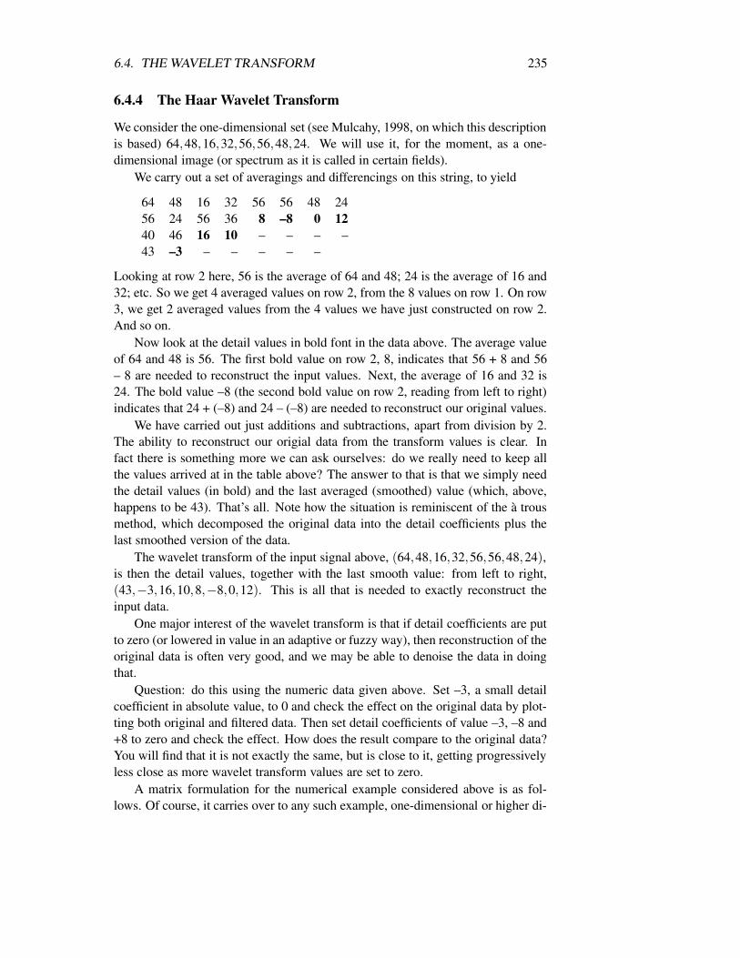
6.4. THE WAVELET TRANSFORM 235
6.4.4 The Haar Wavelet Transform
We consider the one-dimensional set (see Mulcahy, 1998, on which this descriptionis based) 64,48,16,32,56,56,48,24. We will use it, for the moment, as a one-dimensional image (or spectrum as it is called in certain fields).
We carry out a set of averagings and differencings on this string, to yield
64 48 16 32 56 56 48 2456 24 56 36 8 –8 0 1240 46 16 10 – – – –43 –3 – – – – –
Looking at row 2 here, 56 is the average of 64 and 48; 24 is the average of 16 and32; etc. So we get 4 averaged values on row 2, from the 8 values on row 1. On row3, we get 2 averaged values from the 4 values we have just constructed on row 2.And so on.
Now look at the detail values in bold font in the data above. The average valueof 64 and 48 is 56. The first bold value on row 2, 8, indicates that 56 + 8 and 56– 8 are needed to reconstruct the input values. Next, the average of 16 and 32 is24. The bold value –8 (the second bold value on row 2, reading from left to right)indicates that 24 + (–8) and 24 – (–8) are needed to reconstruct our original values.
We have carried out just additions and subtractions, apart from division by 2.The ability to reconstruct our origial data from the transform values is clear. Infact there is something more we can ask ourselves: do we really need to keep allthe values arrived at in the table above? The answer to that is that we simply needthe detail values (in bold) and the last averaged (smoothed) value (which, above,happens to be 43). That’s all. Note how the situation is reminiscent of the a trousmethod, which decomposed the original data into the detail coefficients plus thelast smoothed version of the data.
The wavelet transform of the input signal above, (64,48,16,32,56,56,48,24),is then the detail values, together with the last smooth value: from left to right,(43,−3,16,10,8,−8,0,12). This is all that is needed to exactly reconstruct theinput data.
One major interest of the wavelet transform is that if detail coefficients are putto zero (or lowered in value in an adaptive or fuzzy way), then reconstruction of theoriginal data is often very good, and we may be able to denoise the data in doingthat.
Question: do this using the numeric data given above. Set –3, a small detailcoefficient in absolute value, to 0 and check the effect on the original data by plot-ting both original and filtered data. Then set detail coefficients of value –3, –8 and+8 to zero and check the effect. How does the result compare to the original data?You will find that it is not exactly the same, but is close to it, getting progressivelyless close as more wavelet transform values are set to zero.
A matrix formulation for the numerical example considered above is as fol-lows. Of course, it carries over to any such example, one-dimensional or higher di-

236 CHAPTER 6. FROM IMAGES TO OBJECTS
mensional. We form the first row of the transform by premultiplying our 8-valuedvector by the following 8 × 8 matrix:
12 0 0 0 1
2 0 0 00 1
2 0 0 0 12 0 0
0 12 0 0 0 − 1
2 0 00 0 1
2 0 0 0 12 0
0 0 12 0 0 0 − 1
2 00 0 0 1
2 0 0 0 12
0 0 0 12 0 0 0 − 1
2
For the next row, we premultiply our 4-valued vector by the following 4×4 matrix:
12 0 1
2 012 0 − 1
2 00 1
2 0 12
0 12 0 − 1
2
Finally, the last row is formed by premultiplying the 2-valued vector by the 2× 2 matrix:
( 12
12
12 − 1
2
)
We can easily verify orthonormality properties for these matrices. Reconstructingthe input data at each stage is easy, using matrix inversion. Furthermore, if wewish, we can use redundant rows and columns with 1-values on the diagonal whichcarries over input values into the outputs produced at each stage. This has theadvantage that we can keep 8-valued vectors at each stage – we will use 8 × 8transform matrices at each stage. Then the entire transform can be made morecompact, by just taking the product of the three 8 × 8 matrices, to produce – ofcourse – an overall 8 × 8 matrix. In other words, the entire wavelet transform canbe neatly expressed by a product with a particular orthonormal matrix.
We can do the same thing for the a trous method, but the result will be muchmore messy (due to handling of data extremities). The transform matrix will not beorthonormal. This is a big difference between the two wavelet transform methodswe are dealing with in this chapter. Another difference is that the Haar transforminvolves half the amount of data at each resolution level.
The wavelet function, the mother wavelet, in the case of the Haar transform isdefined by
1 when 0≤ x <12
−1 when12≤ x < 1
0 otherwise
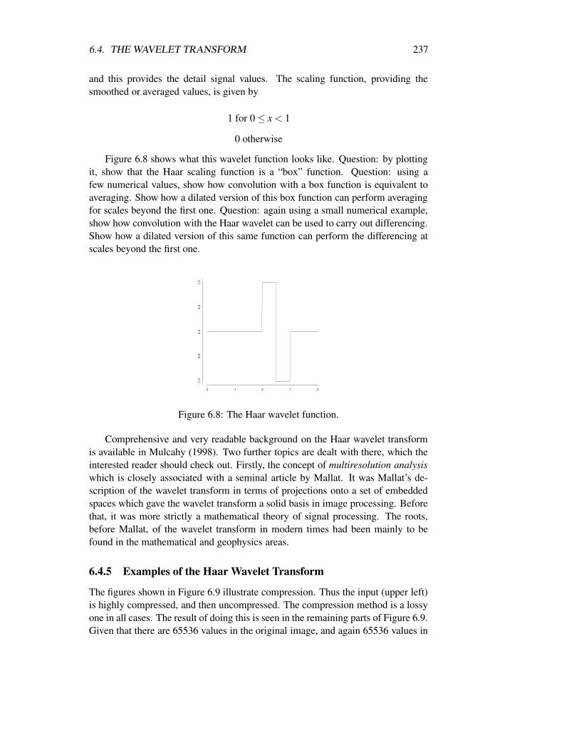
6.4. THE WAVELET TRANSFORM 237
and this provides the detail signal values. The scaling function, providing thesmoothed or averaged values, is given by
1 for 0≤ x < 1
0 otherwise
Figure 6.8 shows what this wavelet function looks like. Question: by plottingit, show that the Haar scaling function is a “box” function. Question: using afew numerical values, show how convolution with a box function is equivalent toaveraging. Show how a dilated version of this box function can perform averagingfor scales beyond the first one. Question: again using a small numerical example,show how convolution with the Haar wavelet can be used to carry out differencing.Show how a dilated version of this same function can perform the differencing atscales beyond the first one.
-2 -1 0 1 2
-1.0
-0.5
0.0
0.5
1.0
Figure 6.8: The Haar wavelet function.
Comprehensive and very readable background on the Haar wavelet transformis available in Mulcahy (1998). Two further topics are dealt with there, which theinterested reader should check out. Firstly, the concept of multiresolution analysiswhich is closely associated with a seminal article by Mallat. It was Mallat’s de-scription of the wavelet transform in terms of projections onto a set of embeddedspaces which gave the wavelet transform a solid basis in image processing. Beforethat, it was more strictly a mathematical theory of signal processing. The roots,before Mallat, of the wavelet transform in modern times had been mainly to befound in the mathematical and geophysics areas.
6.4.5 Examples of the Haar Wavelet Transform
The figures shown in Figure 6.9 illustrate compression. Thus the input (upper left)is highly compressed, and then uncompressed. The compression method is a lossyone in all cases. The result of doing this is seen in the remaining parts of Figure 6.9.Given that there are 65536 values in the original image, and again 65536 values in

238 CHAPTER 6. FROM IMAGES TO OBJECTS
the Haar wavelet transform (question: why is this?), we find in these cases just1310 non-zero values retained for a fairly acceptable rebuilding of the data (upperright).
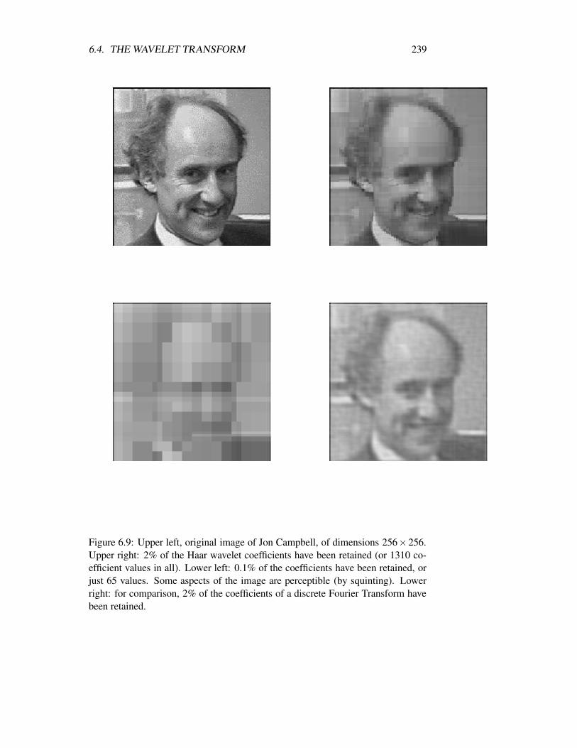
6.4. THE WAVELET TRANSFORM 239
Figure 6.9: Upper left, original image of Jon Campbell, of dimensions 256×256.Upper right: 2% of the Haar wavelet coefficients have been retained (or 1310 co-efficient values in all). Lower left: 0.1% of the coefficients have been retained, orjust 65 values. Some aspects of the image are perceptible (by squinting). Lowerright: for comparison, 2% of the coefficients of a discrete Fourier Transform havebeen retained.

240 CHAPTER 6. FROM IMAGES TO OBJECTS
6.4.6 To Read Further on the Wavelet Transform
1. Mulcahy, C. 1998. Workshop on wavelets. Course notes 40 pp.
(This covers the Haar wavelet transform from the point of view of appli-cations relating to compression. It goes on to look at the “lifting scheme”which allows a large family of wavelet transforms to be defined.)
2. Press, W.H., Teukolsky, S.A., Vetterling, W.T., and Flannery, B.P. 1992. Nu-merical Recipes. 2nd edition. Cambridge University Press.
(C and Fortran code. The emphasis in Chapter 13 is on the Daubechiestransform, and on the compression application.)
3. Starck, J.-L., Murtagh, F., and Bijaoui, A. 1998. Image and Data Analysis:The Multiscale Approach. Cambridge University Press.
(This covers the a trous wavelet transform with many applications. Details ofan associated software package can be found at Web address http://visitweb.com/multiresFurther examples from application domains such as astronomy, medicine, in-formation science, cluster and pattern detection, financial engineering, telecom-munications traffic modelling, geographic information systems, and other ar-eas, can be found at Web addresshttp://hawk.infm.ulst.ac.uk:1998/multires)
4. Wavelet Digest, http://www.wavelet.org/wavelet
(An important source of information on the latest developments in this field.)
6.4.7 DataLab-J Demonstrations of the Wavelet Transform
The following script, haar.dlj, carries out the examples shown above using theHaar wavelet transform. It uses image jon.pgm as input. To run it, do java Dljhaar.dlj.
//haar24.dlj j.g.c. 3/9/98//tests on 2-d Haar transform//data compression clipping smaller componentsread0jon.pgmhaar2f01//coefficients, 2 pcent -- 1310 coeffs. retainedtftrunc1

6.4. THE WAVELET TRANSFORM 241
20, 2.haar2i23savei3haar22pc,0,0,0//components, 0.1 pcent -- 65 coeffs. retainedtftrunc140, 0.1haar2i45savei5haar201pc,0,0,0//DFT for comparison2ftrri06//components, 2 pcenttftrunc670, 2.2ift78savei8dft22pc,0,0,0end
The following script carries out an a trous wavelet transform decomposition. Ituses image jon.pgm and to run it, do java Dlj atrous.dlj.
//atrous21.dlj j.g.c. 3/9/98//tests on 2-d a-trous wavelet transformread

242 CHAPTER 6. FROM IMAGES TO OBJECTS
0jon.pgmatrous2014savei1at20,0,0,0savei1at21,1,0,0savei1at22,2,0,0savei1at23,3,0,0savei1at24,4,0,0end
6.4.8 Exercises on the Wavelet Transform
1. Take the one-dimensional signal (25,33,33,17,28,14,12,6) and determinethe Haar wavelet transform.
Proceed as follows. Take the first pair of values, and form their average. Takethe next pair of values and form their average. Continue until all data valueshave been processed. Next write down the succession of difference termswhich are needed by the average values to give back the values on which theaverage was calculated. (I.e., if a and b are values in the original data, thenthe average is (a+b)/2 and the difference term is a− (a+b)/2.) Continuefor successive levels.
Answer: the Haar wavelet transform of this set of values is (21,6,2,6,−4,8,7,3),where we have written the final average term, followed by detail coefficients.
The implementation of the above algorithm gives:
25 33 33 17 28 14 12 629 25 21 9 –4 8 7 327 15 2 6 – – – –21 6 – – – – –

6.4. THE WAVELET TRANSFORM 243
2. What are the requirements for the Haar wavelet transform algorithm, as de-scribed here? Comment on (i) length of the input signal, and (ii) integerversus real data types.
3. Given the input data signal (25,33,33,17,28,14,12,6), the a trous wavelettransform with 2 scales, plus the final smooth of the data, is given by
scale 1: (−5,3,4.8125,−7.5625,6.9375,−2.6875,0,−4)
scale 2: (2.02344,2.53125,2.33984,1.17969,0.492188,−1.12891,−3.84375,−5.16406)
scale 3: (27.9766,27.4688,25.8477,23.3828,20.5703,17.8164,15.8438,15.1641)
Graph these scales. Comment on why the values are so small in the case ofscales 1 and 2, and much larger for scale 3.
4. The a trous wavelet transform, 3 levels, of the one-dimensional dataset
(0,0,4,4,4,8,4,4,0,0,8,0,0,4,4,0)
produces the following result:
scale 1: (−0.5,−1.25,1.25,0.0,−1.0,2.5,−0.75,1.0,
−1.75,−2.25,5.0,−2.25,−1.75,1.5,1.25,−2.5)
scale 2: (−1.6875,−1.125,−0.125,0.546875,1.10938,1.46875,0.921875,−0.453125,
−1.26563,−0.40625,0.53125,−0.125,−0.625,0.078125,0.296875,0.03125)
scale 3: (2.1875,2.375,2.875,3.45313,3.89063,4.03125,3.82813,3.45313,
3.01563,2.65625,2.46875,2.375,2.375,2.42188,2.45313,2.46875)
Plot these. Verify that scale 1 pinpoints the large isolated spike. Verify thatscale 2 favours more the left block and spike. Finally, verify that the finalsmoothed version of the data again favours the stronger signal to the left ofthe data.
Comment on the objectives of an a trous wavelet transform, in regard tosuperimposed resolution scales in a dataset.

244 CHAPTER 6. FROM IMAGES TO OBJECTS
Chapter 7
Pattern Recognition
7.1 Introduction
Much of our interaction with our environment requires recognition of ‘things’:shapes in a scene (text characters, faces, animals, plants, etc.), sounds, smells,etc. Ifwe are to automate certain tasks, clearly we must give machines some ca-pability to recognise. And, obviously, from the point of view of this module wemust pay attention to automatic recognition of patterns in images. Indeed, the term‘pattern-recognition’ is strongly linked to image processing, particularly for histor-ical reasons: the first studies in so-called pattern recognition were aimed at opticalcharacter recognition.
However, the allusion to human recognition of ‘things’, in the initial paragraph,is merely by way of motivation; usually, it will not be helpful to try to imitate thehuman recognition process – even if we claim to know how it is done! and nomatter how much we would like to emulate its marvellous abilities.
On the other hand, pattern recognition encompasses a very broad area of studyto do with automatic decision making. Typically, we have a collection of dataabout a situation; completely generally, we can assume that these data come as aset of p numbers, x1,x2, . . .xp; usually, they will be arranged as a tuple or vector,x = (x1,x2, . . .xp)
T . Extreme examples are: the decision whether a burgular alarmstate is (intruder, no intruder) – based on a set of radar, acoustic, and electricalmeasurements, whether the state of a share is (sell, no sell, buy) – based on currentmarket state, or, the decision by a bank on whether to loan money to an individual –based on certain data gathered in an interview. Hence pattern recognition principlesare applicable to a wide range of problems, from electronic detection to decisionsupport.
From the point of view of this chapter, and that of most pattern recognitiontheory, we define/summarize a pattern recognition system using the block diagramin the following figure.
+-------------------+
245
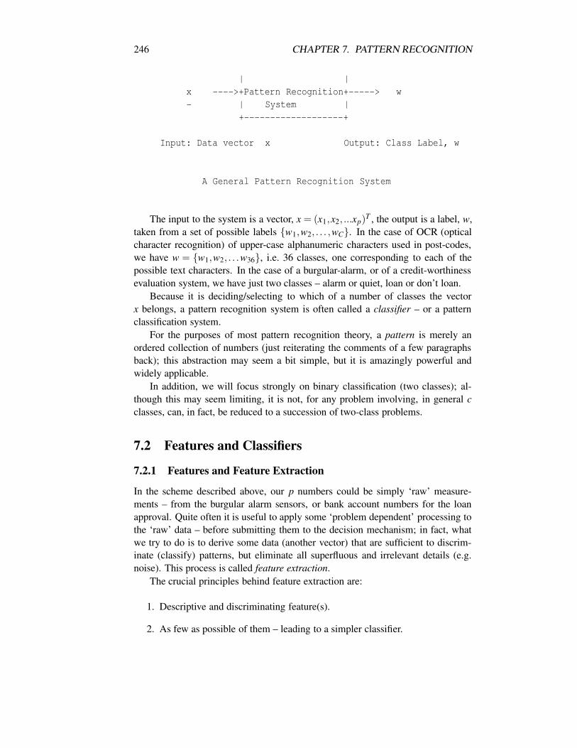
246 CHAPTER 7. PATTERN RECOGNITION
| |x ---->+Pattern Recognition+-----> w- | System |
+-------------------+
Input: Data vector x Output: Class Label, w
A General Pattern Recognition System
The input to the system is a vector, x = (x1,x2, ...xp)T , the output is a label, w,
taken from a set of possible labels w1,w2, . . . ,wC. In the case of OCR (opticalcharacter recognition) of upper-case alphanumeric characters used in post-codes,we have w = w1,w2, . . .w36, i.e. 36 classes, one corresponding to each of thepossible text characters. In the case of a burgular-alarm, or of a credit-worthinessevaluation system, we have just two classes – alarm or quiet, loan or don’t loan.
Because it is deciding/selecting to which of a number of classes the vectorx belongs, a pattern recognition system is often called a classifier – or a patternclassification system.
For the purposes of most pattern recognition theory, a pattern is merely anordered collection of numbers (just reiterating the comments of a few paragraphsback); this abstraction may seem a bit simple, but it is amazingly powerful andwidely applicable.
In addition, we will focus strongly on binary classification (two classes); al-though this may seem limiting, it is not, for any problem involving, in general cclasses, can, in fact, be reduced to a succession of two-class problems.
7.2 Features and Classifiers
7.2.1 Features and Feature Extraction
In the scheme described above, our p numbers could be simply ‘raw’ measure-ments – from the burgular alarm sensors, or bank account numbers for the loanapproval. Quite often it is useful to apply some ‘problem dependent’ processing tothe ‘raw’ data – before submitting them to the decision mechanism; in fact, whatwe try to do is to derive some data (another vector) that are sufficient to discrim-inate (classify) patterns, but eliminate all superfluous and irrelevant details (e.g.noise). This process is called feature extraction.
The crucial principles behind feature extraction are:
1. Descriptive and discriminating feature(s).
2. As few as possible of them – leading to a simpler classifier.
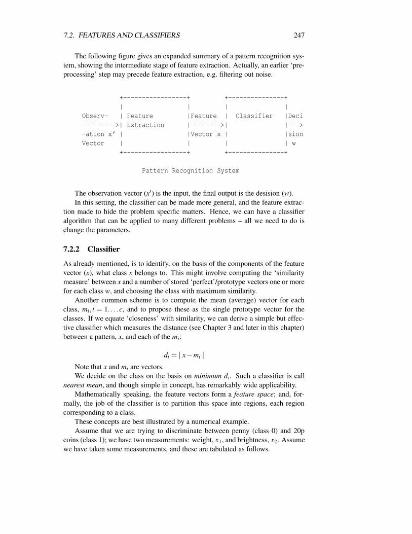
7.2. FEATURES AND CLASSIFIERS 247
The following figure gives an expanded summary of a pattern recognition sys-tem, showing the intermediate stage of feature extraction. Actually, an earlier ‘pre-processing’ step may precede feature extraction, e.g. filtering out noise.
+-----------------+ +---------------+| | | |
Observ- | Feature |Feature | Classifier |Deci--------->| Extraction |-------->| |--->-ation x’ | |Vector x | |sionVector | | | | w
+-----------------+ +---------------+
Pattern Recognition System
The observation vector (x′) is the input, the final output is the desision (w).In this setting, the classifier can be made more general, and the feature extrac-
tion made to hide the problem specific matters. Hence, we can have a classifieralgorithm that can be applied to many different problems – all we need to do ischange the parameters.
7.2.2 Classifier
As already mentioned, is to identify, on the basis of the components of the featurevector (x), what class x belongs to. This might involve computing the ‘similaritymeasure’ between x and a number of stored ‘perfect’/prototype vectors one or morefor each class w, and choosing the class with maximum similarity.
Another common scheme is to compute the mean (average) vector for eachclass, mi, i = 1. . . . c, and to propose these as the single prototype vector for theclasses. If we equate ‘closeness’ with similarity, we can derive a simple but effec-tive classifier which measures the distance (see Chapter 3 and later in this chapter)between a pattern, x, and each of the mi:
di = | x−mi |Note that x and mi are vectors.We decide on the class on the basis on minimum di. Such a classifier is call
nearest mean, and though simple in concept, has remarkably wide applicability.Mathematically speaking, the feature vectors form a feature space; and, for-
mally, the job of the classifier is to partition this space into regions, each regioncorresponding to a class.
These concepts are best illustrated by a numerical example.Assume that we are trying to discriminate between penny (class 0) and 20p
coins (class 1); we have two measurements: weight, x1, and brightness, x2. Assumewe have taken some measurements, and these are tabulated as follows.
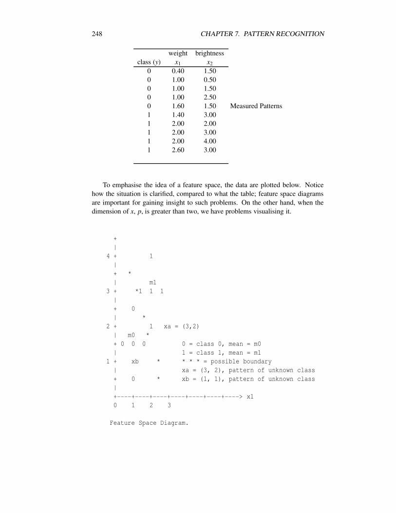
248 CHAPTER 7. PATTERN RECOGNITION
weight brightnessclass (y) x1 x2
0 0.40 1.500 1.00 0.500 1.00 1.500 1.00 2.500 1.60 1.501 1.40 3.001 2.00 2.001 2.00 3.001 2.00 4.001 2.60 3.00
Measured Patterns
To emphasise the idea of a feature space, the data are plotted below. Noticehow the situation is clarified, compared to what the table; feature space diagramsare important for gaining insight to such problems. On the other hand, when thedimension of x, p, is greater than two, we have problems visualising it.
+|
4 + 1|+ *| m1
3 + *1 1 1|+ 0| *
2 + 1 xa = (3,2)| m0 *+ 0 0 0 0 = class 0, mean = m0| 1 = class 1, mean = m1
1 + xb * * * * = possible boundary| xa = (3, 2), pattern of unknown class+ 0 * xb = (1, 1), pattern of unknown class|+----+----+----+----+----+----+----> x10 1 2 3
Feature Space Diagram.
7.2. FEATURES AND CLASSIFIERS 249
The 20ps are heavier than the 1ps, but errors (noise) in the weighing machinemake this unreliable on its own, i.e. you cannot just apply a threshold:
x1 > 1.5 =⇒ class = 1 (20p)
≤ 1.5 =⇒ class = 0 (1p)
There would be an overlap, and some errors. Likewise brightness, on its own,is not a reliable discriminator.
Now, we can test a number of classification rules, on two patterns whose classesare unknown, xa = (x1 = 3,x2 = 2), and xb = (1,1).
(a) Nearest neighbour. Find the ‘training’/prototype pattern in the table whichis closest to the pattern, and take its class; thus xb −→ class 1, and xa −→ class 0.
(b) Nearest mean. The class means are m0 = (1.0,1.5), m1 = (2.0,3.0). Findthe class mean closest to the pattern, and take its class; thus xb −→ class 1, andxa −→ class 0.
(c) Linear Partition. Draw a straight line between the classes (in three dimen-sions it is a plane, in general p-dimensions it is a hyperplane); one side class 0, theother class 1. We will find that such a rule can be expressed as:
a0 +a1x1 +a2x2 > 0 class 1
a0 +a1x1 +a2x2 <= 0 class 0
a0 +a1x1 +a2x2 = 0, on the boundary
7.2.3 Training and Supervised Classification
The classifier rules we have described above, are all supervised classifiers, and thedata in the table correspond to training data.
Hence, we can have a subdivision of classifiers between supervised and un-supervised, i.e. whether or not the classifier rule is based on training data. Theclustering/segmentation covered in Chapter 6 is unsupervised – the algorithm seg-ments the image with no prior knowledge of the problem; i.e. in the example wedid, the algorithm has not been ‘trained’ to recognise water pixels, and land pix-els. On the other hand, if the algorithm is supervised, like all those covered in thischapter, it will have already been given example of water, and land, or 1ps and20ps, i.e. trained. In this chapter, we will say no more about unsupervised – seeChapter 6.
7.2.4 Statistical Classification
In the example of the 1ps and 20ps, we have made the pattern vectors lie in a nicesymmetric distribution centred on the means. Usually, in a practical situation, the
250 CHAPTER 7. PATTERN RECOGNITION
training data will form a cloud of points. And, maybe, there will be an overlap, i.e.we have to decide a ‘best’ boundary, whose errors are a minimum, yet not zero.Here, we can usually develop a decision rules based on statistical/probabilistic cri-teria. Classification is based on some decision theoretic criterion such as maximumlikelihood.
Note: statistical decision theory has a long history – from before that of com-puters, starting around the early 1900’s.
In statistical pattern recognition, we usually adopt the model: pattern vector =perfect-pattern + noise; thus, for each class we have a cloud of points centred onthe ‘perfect-pattern’ vector. The class means are often good estimates of the classperfect-vectors.
The spread of each class ‘cloud’/cluster will depend on the noise amplitude.Obviously, the degree to which the classes are separable depends on two factors:(a) the distance between the ‘perfect-patterns’, and the cluster spread.
The major characteristic of the statistical pattern recognition approach is that itis ‘low-level’. The image (pattern) is merely an array of numbers; the only modelapplied is that of the random process, there would be no difference in the process,whether the data represented scanned text characters, or parts on a conveyer belt,or faces, or, indeed, if all three were mixed together. Only the data, and estimatedparameters would change.
7.2.5 Feature Vector – Update
The components of a pattern vector are commonly called features, thus the termfeature vector introduced above. Other terms are attribute, characteristic.
Often all patterns are called feature vectors, despite the literal unsuitability ofthe term if it is composed of raw data.
It can be useful to classify feature extractors according to whether they arehigh- or low-level.
A typical low-level feature extractor is a transformation IRp′ −→ IRp which,presumably, either enhances the separability of the classes, or, at least, reduces thedimensionality of the data (p < p′) to the extent that the recognition task morecomputationally tractable, or simply to compress the data (see Chapter 5 – manydata compression schemes are used as feature extractors, and vice- versa.
Examples of low-level feature extractors are:
• Fourier power spectrum of a signal – appropriate if frequency content is agood discriminator; additionally, it has the property of shift invariance – itdoesn’t matter what co-ordinates the objects appears at in the image,
• Karhunen-Loeve transform – transforms the data to a space in which the fea-tures are ordered according to their variance/information content, see Chap-ter 5.

7.2. FEATURES AND CLASSIFIERS 251
At a higher-level, for example in image shape recognition, we could have a vec-tor composed of: length, width, circumference. Such features are more in keepingwith the everyday usage of the term feature.
A recent paper on face recognition has classified recognition techniques into:(a) geometric feature based, i.e. using high-level features such as distance be-
tween eyes, width of head at ears, length of feace, etc.(b) template based, where we use the whole of the face image, possibly Fourier
transformed, or such-like.
7.2.6 Distance
Statistical classifiers may use maximum likelihood (probability) as a criterion. In awide range of cases, likelihood corresponds to ‘closeness’ to the class cluster, i.e.closeness to the center/mean, or closeness to individual points. Hence, distance isan important criterion/metric.
7.2.7 Other Classification Paradigms
Just to ensure that you are aware of the meanings of some terms that you may comeacross in textbooks, we will try to introduce some other paradigms – though, forthe most part, you can ignore them.
Structural Pattern Recognition
Because in statistical pattern recognition, patterns are viewed as vectors, theinformation carried by the pattern is no more than its position in pattern space;nevertheless, there may exist structural relationships between pattern componentsarising from shape, for example. Thus, structural pattern recognition has the richermodel of a pattern as a structured collection of symbols. Here the distance metricis no longer the sole basis for recognition (nor is it really suitable); simple methodssuch as string matching may be applied, or syntactic/linguistic methods which arebased on the model of pattern generation by one of a family of grammars (classes);the recognition task usually involves parsing to find which grammar generated theunidentified pattern. In relational pattern matching, the symbols are stored in arelational graph structure and the recognition process involves graph matching.
Usually, there exists ‘structure’ in the pattern (e.g. in an image shapes formedby conjunctions of specific grey level values in adjacent regions, or, in a signal,peaks, troughs, valleys, etc.) which is not extracted when the pattern is treated as amere p -dimensional vector; obviously, if the structure is the major discriminatorycharacteristic, and the position in p-space is relatively insignificant, this form ofrecognition will not work well.
As an example, the letter ‘A’ might be described, not as a vector containinginvariant moments – or grey levels, but as as sentence:
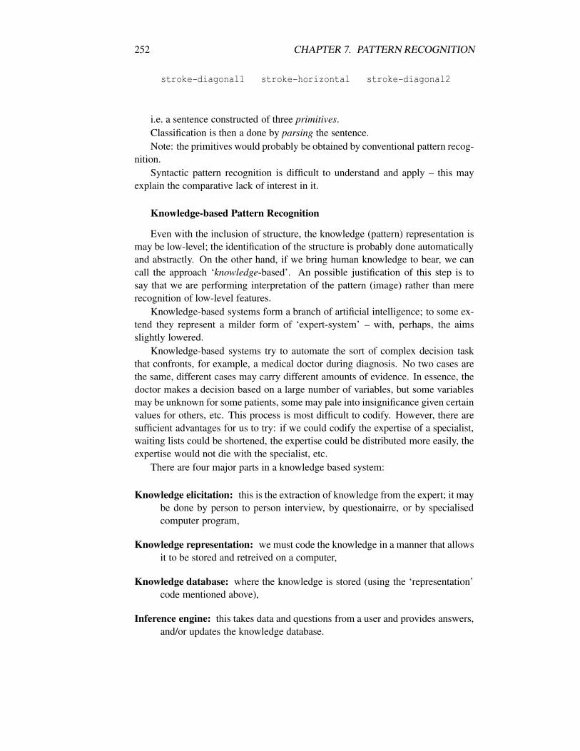
252 CHAPTER 7. PATTERN RECOGNITION
stroke-diagonal1 stroke-horizontal stroke-diagonal2
i.e. a sentence constructed of three primitives.Classification is then a done by parsing the sentence.Note: the primitives would probably be obtained by conventional pattern recog-
nition.Syntactic pattern recognition is difficult to understand and apply – this may
explain the comparative lack of interest in it.
Knowledge-based Pattern Recognition
Even with the inclusion of structure, the knowledge (pattern) representation ismay be low-level; the identification of the structure is probably done automaticallyand abstractly. On the other hand, if we bring human knowledge to bear, we cancall the approach ‘knowledge-based’. An possible justification of this step is tosay that we are performing interpretation of the pattern (image) rather than mererecognition of low-level features.
Knowledge-based systems form a branch of artificial intelligence; to some ex-tend they represent a milder form of ‘expert-system’ – with, perhaps, the aimsslightly lowered.
Knowledge-based systems try to automate the sort of complex decision taskthat confronts, for example, a medical doctor during diagnosis. No two cases arethe same, different cases may carry different amounts of evidence. In essence, thedoctor makes a decision based on a large number of variables, but some variablesmay be unknown for some patients, some may pale into insignificance given certainvalues for others, etc. This process is most difficult to codify. However, there aresufficient advantages for us to try: if we could codify the expertise of a specialist,waiting lists could be shortened, the expertise could be distributed more easily, theexpertise would not die with the specialist, etc.
There are four major parts in a knowledge based system:
Knowledge elicitation: this is the extraction of knowledge from the expert; it maybe done by person to person interview, by questionairre, or by specialisedcomputer program,
Knowledge representation: we must code the knowledge in a manner that allowsit to be stored and retreived on a computer,
Knowledge database: where the knowledge is stored (using the ‘representation’code mentioned above),
Inference engine: this takes data and questions from a user and provides answers,and/or updates the knowledge database.
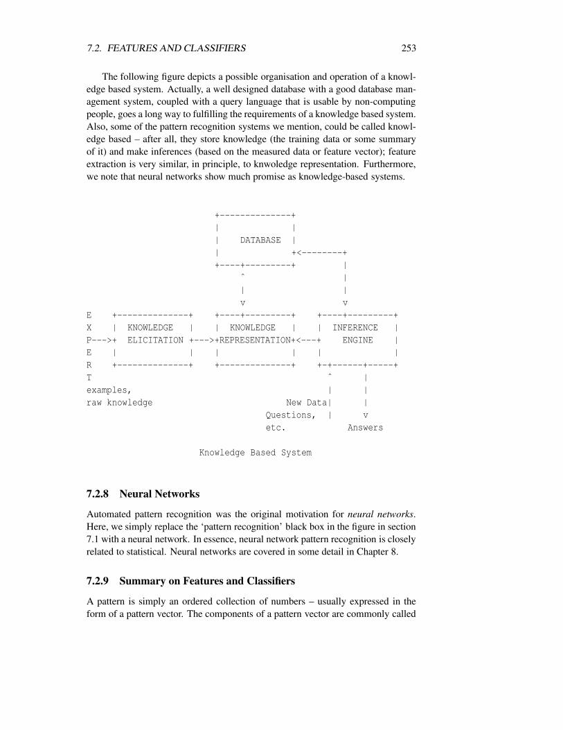
7.2. FEATURES AND CLASSIFIERS 253
The following figure depicts a possible organisation and operation of a knowl-edge based system. Actually, a well designed database with a good database man-agement system, coupled with a query language that is usable by non-computingpeople, goes a long way to fulfilling the requirements of a knowledge based system.Also, some of the pattern recognition systems we mention, could be called knowl-edge based – after all, they store knowledge (the training data or some summaryof it) and make inferences (based on the measured data or feature vector); featureextraction is very similar, in principle, to knwoledge representation. Furthermore,we note that neural networks show much promise as knowledge-based systems.
+--------------+| || DATABASE || +<--------++----+---------+ |
ˆ || |v v
E +--------------+ +----+---------+ +----+---------+X | KNOWLEDGE | | KNOWLEDGE | | INFERENCE |P--->+ ELICITATION +--->+REPRESENTATION+<---+ ENGINE |E | | | | | |R +--------------+ +--------------+ +-+------+-----+T ˆ |examples, | |raw knowledge New Data| |
Questions, | vetc. Answers
Knowledge Based System
7.2.8 Neural Networks
Automated pattern recognition was the original motivation for neural networks.Here, we simply replace the ‘pattern recognition’ black box in the figure in section7.1 with a neural network. In essence, neural network pattern recognition is closelyrelated to statistical. Neural networks are covered in some detail in Chapter 8.
7.2.9 Summary on Features and Classifiers
A pattern is simply an ordered collection of numbers – usually expressed in theform of a pattern vector. The components of a pattern vector are commonly called
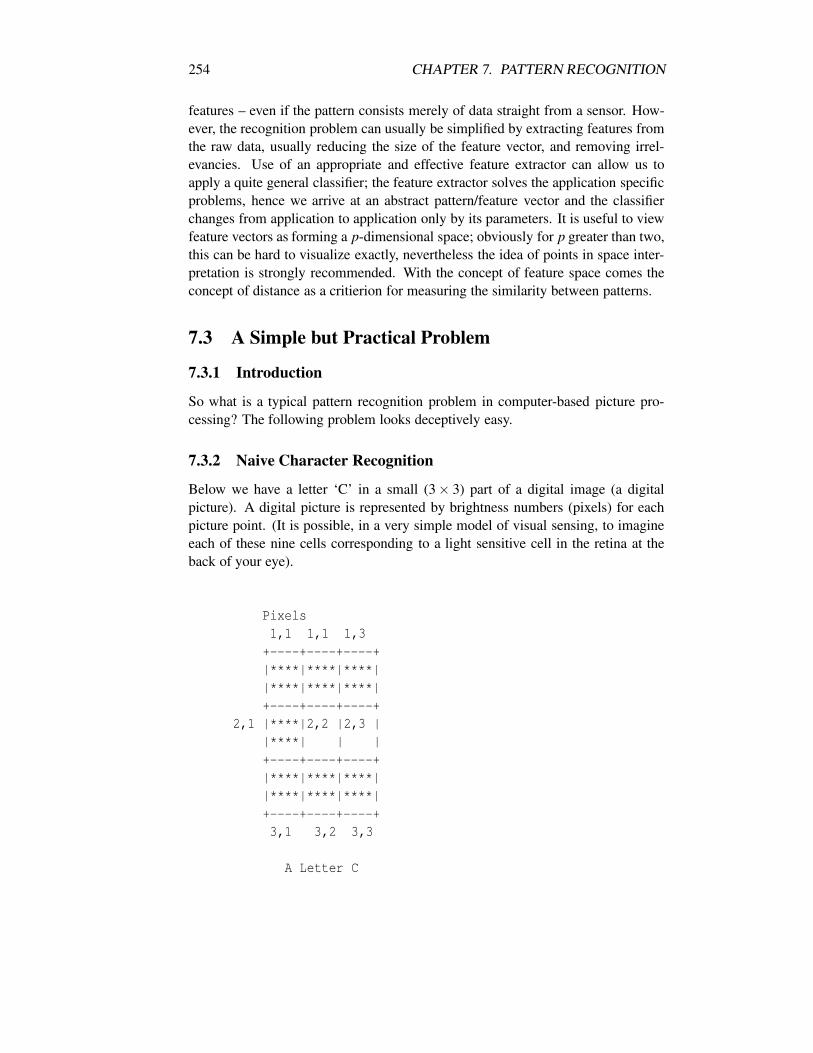
254 CHAPTER 7. PATTERN RECOGNITION
features – even if the pattern consists merely of data straight from a sensor. How-ever, the recognition problem can usually be simplified by extracting features fromthe raw data, usually reducing the size of the feature vector, and removing irrel-evancies. Use of an appropriate and effective feature extractor can allow us toapply a quite general classifier; the feature extractor solves the application specificproblems, hence we arrive at an abstract pattern/feature vector and the classifierchanges from application to application only by its parameters. It is useful to viewfeature vectors as forming a p-dimensional space; obviously for p greater than two,this can be hard to visualize exactly, nevertheless the idea of points in space inter-pretation is strongly recommended. With the concept of feature space comes theconcept of distance as a critierion for measuring the similarity between patterns.
7.3 A Simple but Practical Problem
7.3.1 Introduction
So what is a typical pattern recognition problem in computer-based picture pro-cessing? The following problem looks deceptively easy.
7.3.2 Naive Character Recognition
Below we have a letter ‘C’ in a small (3× 3) part of a digital image (a digitalpicture). A digital picture is represented by brightness numbers (pixels) for eachpicture point. (It is possible, in a very simple model of visual sensing, to imagineeach of these nine cells corresponding to a light sensitive cell in the retina at theback of your eye).
Pixels1,1 1,1 1,3+----+----+----+|****|****|****||****|****|****|+----+----+----+
2,1 |****|2,2 |2,3 ||****| | |+----+----+----+|****|****|****||****|****|****|+----+----+----+3,1 3,2 3,3
A Letter C

7.3. A SIMPLE BUT PRACTICAL PROBLEM 255
Assume that the picture has been quantized – into ink (1) and background (0).How can we mechanise the process of recognition of the ‘C’? Certainly if we
can do it for one letter, we can do it for all the others – by looping over all thecharacters. The naive approach tackles the problem almost like that of a lookuptable:
1. Pixel by pixel comparison: Compare the input (candidate) image pixel forpixel, with each perfect letter, and select the character that fits exactly:
for j = 1..nlettersmatch = truefor r= 0..NR-1 dofor c= 0..NC-1 doif(f[r,c] != X[j][r,c]) /*r,cth pixel of jth letter
match = falseexit for r /*i.e. just ONE mismatch causes complete FAIL
endifendfor cendfor rif(match==true) return j /* j is label
endfor jreturn NULL
As we will see later, this naive approach has many shortcomings – especially,in general, pairwise comparisons of collections of numbers is usually fraughtwith difficulty: what if just one is wrong – by just a small amount? what iftwo dissimilar, by an even smaller amount? is one pixel more important thanthe others?
So, we’re uncomfortable with comparison of individual elements of the pat-tern. Can we compare the full vectors. Yes, in fact much of classical patternrecognition is about the comparison of vectors, finding distances betweenthem, etc.
Hence, to make this into a general pattern recognition problem, we representthe nine pixel values as elements of a vector (array), i.e. we collect themtogether in an array; assuming the character is white-on-black and that bright(filled in with ‘*’) corresponds to ‘1’, and dark to ‘0’, the array correspondingto the ‘C’ is
x[0]=1, x[1]=1, x[2]=1, x[3]=1, x[4]=0, x[5]=0, x[6]=1, x[7]=1,x[8]=1.

256 CHAPTER 7. PATTERN RECOGNITION
Note: from now on, in the usual fashion, we will index vector elements from0 to p-1.
’Feature’ number:
0 1 2+----+----+----+|****|****|****||****|****|****|+----+----+----+
3 |****|4 |5 ||****| | |+----+----+----+|****|****|****||****|****|****|+----+----+----+6 7 8
A Letter C
The letter ‘T’ would give a different observation vector:
’T’: 1,1,1, 0,1,0, 0,1,0
’O’: 1,1,1, 1,0,1, 1,1,1
’C’: 1,1,1, 1,0,0, 1,1,1 etc...
So how is the recognition done? We could base decision-making on a set ofvectors (X[j]) corresponding to ‘perfect’ characters (‘T’, ‘C’ etc.); let thesebe denoted by X[1] - C , X[2] - T, etc.
Let the input (unknown) be x, a 9-dimensional vector; and let us assumethat the components can be real, i.e. no longer binary; let them be any realnumber between 0 and 1, and subject to noise. The recognition system needsto be invariant (tolerant) to noise.
What if there is a minor change in grey level? Grey Cs are the same aswhite Cs: the system needs to be amplitude invariant – tolerant to changesin amplitude.
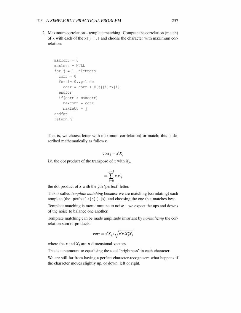
7.3. A SIMPLE BUT PRACTICAL PROBLEM 257
2. Maximum correlation – template matching: Compute the correlation (match)of x with each of the X[j][.] and choose the character with maximum cor-relation:
maxcorr = 0maxlett = NULLfor j = 1..nletters
corr = 0for i= 0..p-1 docorr = corr + X[j][i]*x[i]
endforif(corr > maxcorr)maxcorr = corrmaxlett = j
endforreturn j
That is, we choose letter with maximum corr(elation) or match; this is de-scribed mathematically as follows:
corr j = x′X j
i.e. the dot product of the transpose of x with X j,
=p−1
∑i=0
xixpi j
the dot product of x with the jth ‘perfect’ letter.
This is called template matching because we are matching (correlating) eachtemplate (the ‘perfect’ X[j][.]s), and choosing the one that matches best.
Template matching is more immune to noise – we expect the ups and downsof the noise to balance one another.
Template matching can be made amplitude invariant by normalizing the cor-relation sum of products:
corr = x′X j/√
x′x.X ′jX j
where the x and X j are p-dimensional vectors.
This is tantamount to equalising the total ‘brightness’ in each character.
We are still far from having a perfect character-recogniser: what happens ifthe character moves slightly up, or down, left or right.
258 CHAPTER 7. PATTERN RECOGNITION
3. Shifting Correlation: Use two-dimensional correlation, as described in Chap-ter 4, i.e., move the character successively across and down, find the positionof maximum correlation (match), then compare that maximum with the max-ima for the other characters.
But now, what about rotation?
4. We could put a loop around the shifting correlation, each time rotating thecharacter a little.
What happens if the size of the character changes – it’s still the same char-acter – the observation vector will change radically. We require scale invari-ance.
5. Now, we could loop over scale factor.
By now, I hope you have realised that things have fairly well got out of hand;and we haven’t mentioned small variations in character shape.
The main point is: this sort of ad hoc adding to, and changing of algorithmsrarely ever works. We need to build a general theory which is applicable to a widevariety of problems.
7.3.3 Invariance for Two-Dimensional Patterns
From the forgoing discussion, we can summarise some of the requirements of sys-tems system for recognizing two-dimensional shapes in images:
• noise tolerance
• amplitude invariance
• shift invariance
• rotation invariance
• scale invariance
Note that, in the examples given above, ‘C’ differs from ‘O’ by only one ele-ment – so, naturally, ‘C’ is likely to be confused with ‘O’ and vice versa. There isvery little we can do about that – except to change the character shapes! – this iswhy they use funny shaped characters on cheques.
7.3.4 Feature Extraction – Another Update
Let us say we have a simple two-class subset of the previous character recognitionproblem: ‘C’ versus ‘O’. Clearly, the only attribute of discriminating value is theone in which they differ – number 5. Hence, a sensible feature extractor extracts

7.4. CLASSIFICATION RULES 259
this, call it y; we end up with a scalar (one-dimensional) pattern, and the classifierbecomes a simple thresholding:
y > 0.5 =⇒ class O
y≤ 0.5 =⇒ class C
7.4 Classification Rules
In this section we discuss the common classification rules used with feature-basedclassifiers.
In summary, roughly speaking, a supervised classifier involves:
Training: gathering and storing example feature vectors – or some summary ofthem,
Operation: extracting features, and classifying, i.e. by computing similarity mea-sures, and either finding the maximum, or applying some sort of threshold-ing.
When developing a classifier, we distinguish between training data, and testdata:
• training data are used to ‘train’ the classifier – i.e. set its parameters,
• test data are used to check if the trained classifier works, especially if it cangeneralise to new/unseen data.
Although it is normal enough to do an initial test of a classifier using the sametraining data, in general it is a dangerous practice – we must check if the classifiercan generalise to data it has not seen before.
Example Data
The following ‘toy’ data will be used to exemplify some of the algorithms. It istwo-dimensional, two-class. If you run DataLab batch file ‘ip2dcl’, that will set upthe configuration and input the data for you, and show some histograms and scatterplots. The data are in file dl\dat\toy4.asc.
Here it is – DataLab output:
Type = REALBounds = Rows: 0 - 0, Cols: 0 - 9, Dims: 0 - 1.Number of classes: 2
The 2 labels are: 1 2
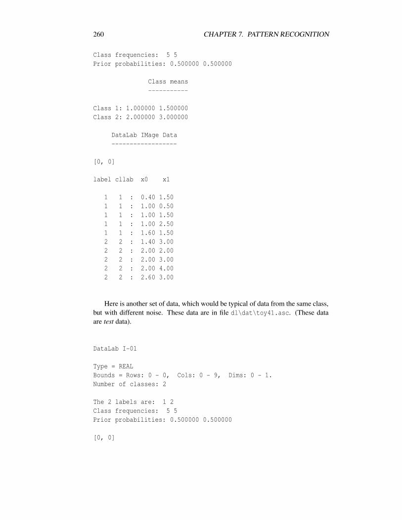
260 CHAPTER 7. PATTERN RECOGNITION
Class frequencies: 5 5Prior probabilities: 0.500000 0.500000
Class means-----------
Class 1: 1.000000 1.500000Class 2: 2.000000 3.000000
DataLab IMage Data------------------
[0, 0]
label cllab x0 x1
1 1 : 0.40 1.501 1 : 1.00 0.501 1 : 1.00 1.501 1 : 1.00 2.501 1 : 1.60 1.502 2 : 1.40 3.002 2 : 2.00 2.002 2 : 2.00 3.002 2 : 2.00 4.002 2 : 2.60 3.00
Here is another set of data, which would be typical of data from the same class,but with different noise. These data are in file dl\dat\toy41.asc. (These dataare test data).
DataLab I-01
Type = REALBounds = Rows: 0 - 0, Cols: 0 - 9, Dims: 0 - 1.Number of classes: 2
The 2 labels are: 1 2Class frequencies: 5 5Prior probabilities: 0.500000 0.500000
[0, 0]
7.4. CLASSIFICATION RULES 261
1 1 : 0.80 2.001 1 : 1.20 1.801 1 : 1.40 2.201 2 : 1.60 2.401 2 : 1.80 2.602 2 : 1.60 2.602 2 : 2.20 3.202 2 : 2.40 3.402 2 : 2.60 3.602 2 : 2.80 3.80
7.4.1 Similarity Measures Between Vectors
Two possibilities are correlation, and distance; these are closely related, and inmost cases give identical results. See Chapter 3 for the mathematical foundation.
1. Correlation. Correlation is a very natural and obvious form of similaritymeasure. It is sometimes called ‘template matching’ because of the similar-ity with comparing a two-dimensional shape with a template.
The correlation between two vectors is given by the dot product of them. Itis usually neccessary to normalize the vectors, which is the purpose of thedenominator in the following equation:
c j = x′X j/√
x′x.X ′jX j
Here c j gives the correlation (or match) between our unknown x and X j,the jth ‘perfect’ vector. The transpose operations (denoted by prime) arenecessary for the sole reason of making the vectors conformable for multi-plication.
The dot product can be written as a summation:
x′X j =p−1
∑i=0
xiX ji
where xi is the ith component of vector x and X ji is the ith component of‘perfect’ vector X j (class j) for p-dimensional vectors.
Usually, classification would involve finding the X j that has the maximumcorrelation value – the output from the classifier (the class) is then j.
Later, we shall see that correlation rules are at the basis of most neural net-works.
262 CHAPTER 7. PATTERN RECOGNITION
2. Distance. Distance is another natural similarity measure. Points (featurevectors) that are close in feature space are similar, those far apart are dissim-ilar. The distance between two vectors is given by the following equations.
d(x,X j) = | x−X j |
de(x,X j) =
√
√
√
√
p−1
∑i=0
(xi−X ji)2
The latter gives the ‘true’ Euclidean distance, i.e. that would be obtainedusing a piece of string! Quite often when implementing the Euclidean dis-tance in a program, we will be content with the squared Euclidean distance.This provides enough information e.g. to find the ‘nearest neighbour’ dis-tance. There are other distances, the most notable being the Hamming (orManhattan, or city-block) distance:
dm(x,X j) =p−1
∑i=0
(xi−X ji)
Why is it called Manhattan/city-block? Answer: Think of getting from pointa to point b in New York – you have to go up, then across, etc.
The Hamming distance requires no multiplication, and this explains its pop-ularity in the days before hardware multipliers and arithmetic co-processors.
To impress friends at parties, you can use the following. The Hamming andEuclidean distances are referred to in mathematics as the L1 and L2 distances.The term ‘metric’ is often used as a synonym for distance. A metric space isa space with some definition of distance. In fact, scalar product is enough forus, since the scalar product of a vector with itself gives the norm, and withboth of these we can define a metric. The L1 and L2 distances are just twofrom a class of distances called the Minkowski metrics.
Using distance for classification involves finding the minimum distance.
Actually, maximum normalised correlation can be shown to be exactly equiv-alent to minimum Euclidean distance.
Distance is perhaps used more often than correlation. However, even whenminimum distance is used, most writers call it template matching; for thoseunfamiliar with the similarity mentioned in the previous paragraph, this useof terminology can cause confusion.
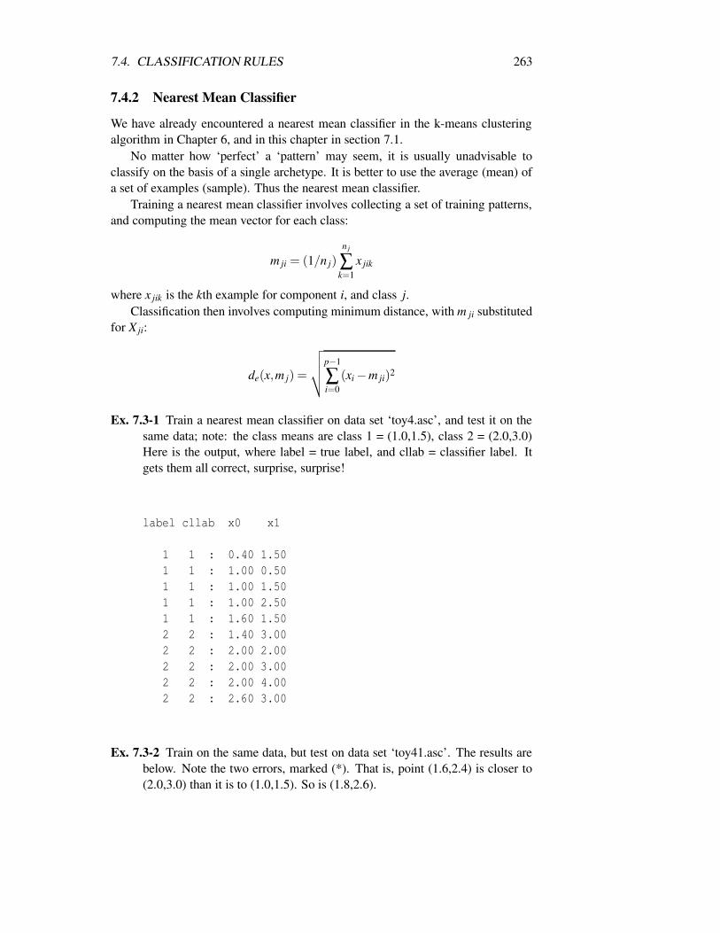
7.4. CLASSIFICATION RULES 263
7.4.2 Nearest Mean Classifier
We have already encountered a nearest mean classifier in the k-means clusteringalgorithm in Chapter 6, and in this chapter in section 7.1.
No matter how ‘perfect’ a ‘pattern’ may seem, it is usually unadvisable toclassify on the basis of a single archetype. It is better to use the average (mean) ofa set of examples (sample). Thus the nearest mean classifier.
Training a nearest mean classifier involves collecting a set of training patterns,and computing the mean vector for each class:
m ji = (1/n j)n j
∑k=1
x jik
where x jik is the kth example for component i, and class j.Classification then involves computing minimum distance, with m ji substituted
for X ji:
de(x,m j) =
√
√
√
√
p−1
∑i=0
(xi−m ji)2
Ex. 7.3-1 Train a nearest mean classifier on data set ‘toy4.asc’, and test it on thesame data; note: the class means are class 1 = (1.0,1.5), class 2 = (2.0,3.0)Here is the output, where label = true label, and cllab = classifier label. Itgets them all correct, surprise, surprise!
label cllab x0 x1
1 1 : 0.40 1.501 1 : 1.00 0.501 1 : 1.00 1.501 1 : 1.00 2.501 1 : 1.60 1.502 2 : 1.40 3.002 2 : 2.00 2.002 2 : 2.00 3.002 2 : 2.00 4.002 2 : 2.60 3.00
Ex. 7.3-2 Train on the same data, but test on data set ‘toy41.asc’. The results arebelow. Note the two errors, marked (*). That is, point (1.6,2.4) is closer to(2.0,3.0) than it is to (1.0,1.5). So is (1.8,2.6).
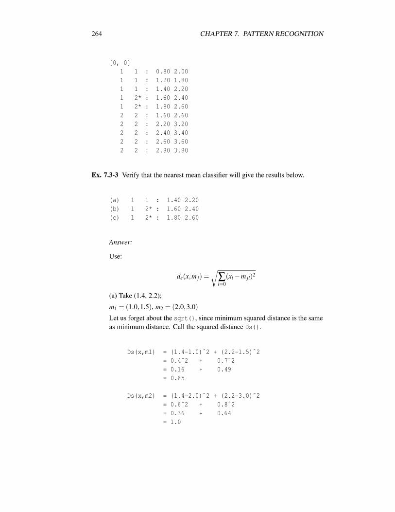
264 CHAPTER 7. PATTERN RECOGNITION
[0, 0]1 1 : 0.80 2.001 1 : 1.20 1.801 1 : 1.40 2.201 2* : 1.60 2.401 2* : 1.80 2.602 2 : 1.60 2.602 2 : 2.20 3.202 2 : 2.40 3.402 2 : 2.60 3.602 2 : 2.80 3.80
Ex. 7.3-3 Verify that the nearest mean classifier will give the results below.
(a) 1 1 : 1.40 2.20(b) 1 2* : 1.60 2.40(c) 1 2* : 1.80 2.60
Answer:
Use:
de(x,m j) =√
∑i=0
(xi−m ji)2
(a) Take (1.4, 2.2);
m1 = (1.0,1.5), m2 = (2.0,3.0)
Let us forget about the sqrt(), since minimum squared distance is the sameas minimum distance. Call the squared distance Ds().
Ds(x,m1) = (1.4-1.0)ˆ2 + (2.2-1.5)ˆ2= 0.4ˆ2 + 0.7ˆ2= 0.16 + 0.49= 0.65
Ds(x,m2) = (1.4-2.0)ˆ2 + (2.2-3.0)ˆ2= 0.6ˆ2 + 0.8ˆ2= 0.36 + 0.64= 1.0
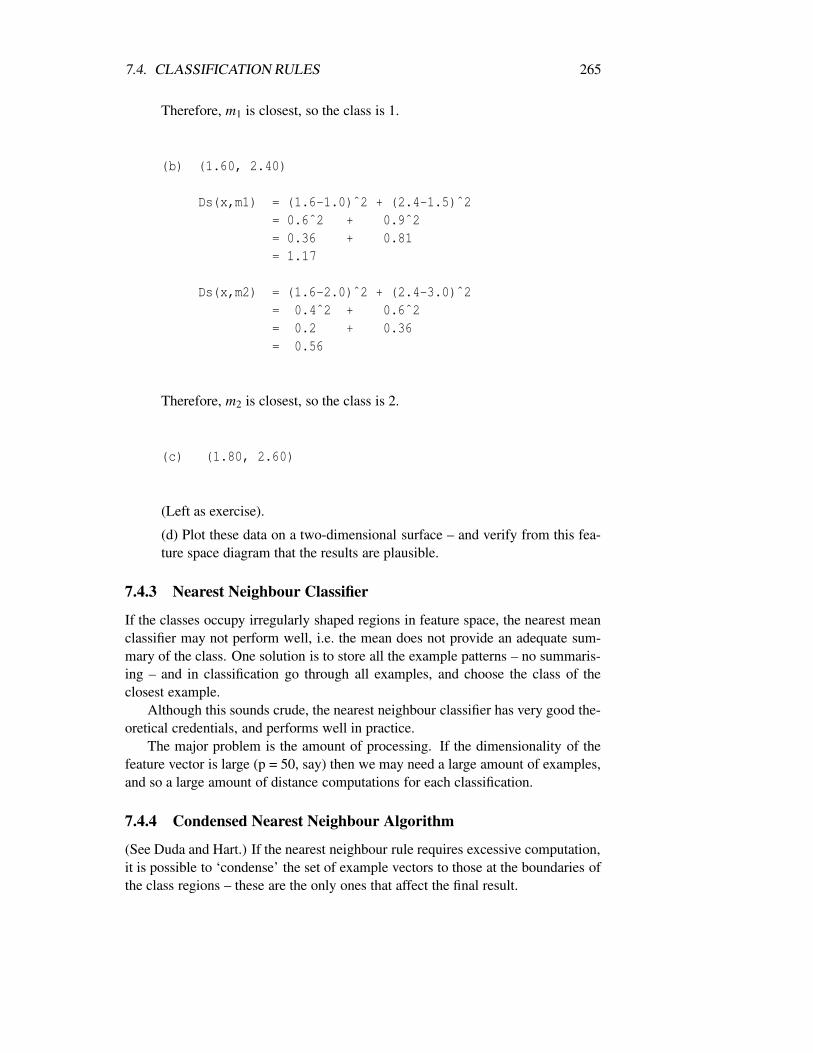
7.4. CLASSIFICATION RULES 265
Therefore, m1 is closest, so the class is 1.
(b) (1.60, 2.40)
Ds(x,m1) = (1.6-1.0)ˆ2 + (2.4-1.5)ˆ2= 0.6ˆ2 + 0.9ˆ2= 0.36 + 0.81= 1.17
Ds(x,m2) = (1.6-2.0)ˆ2 + (2.4-3.0)ˆ2= 0.4ˆ2 + 0.6ˆ2= 0.2 + 0.36= 0.56
Therefore, m2 is closest, so the class is 2.
(c) (1.80, 2.60)
(Left as exercise).
(d) Plot these data on a two-dimensional surface – and verify from this fea-ture space diagram that the results are plausible.
7.4.3 Nearest Neighbour Classifier
If the classes occupy irregularly shaped regions in feature space, the nearest meanclassifier may not perform well, i.e. the mean does not provide an adequate sum-mary of the class. One solution is to store all the example patterns – no summaris-ing – and in classification go through all examples, and choose the class of theclosest example.
Although this sounds crude, the nearest neighbour classifier has very good the-oretical credentials, and performs well in practice.
The major problem is the amount of processing. If the dimensionality of thefeature vector is large (p = 50, say) then we may need a large amount of examples,and so a large amount of distance computations for each classification.
7.4.4 Condensed Nearest Neighbour Algorithm
(See Duda and Hart.) If the nearest neighbour rule requires excessive computation,it is possible to ‘condense’ the set of example vectors to those at the boundaries ofthe class regions – these are the only ones that affect the final result.
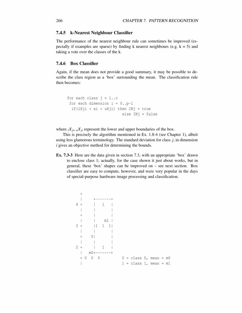
266 CHAPTER 7. PATTERN RECOGNITION
7.4.5 k-Nearest Neighbour Classifier
The performance of the nearest neighbour rule can sometimes be improved (es-pecially if examples are sparse) by finding k nearest neighbours (e.g. k = 5) andtaking a vote over the classes of the k.
7.4.6 Box Classifier
Again, if the mean does not provide a good summary, it may be possible to de-scribe the class region as a ‘box’ surrounding the mean. The classification rulethen becomes:
for each class j = 1..cfor each dimension i = 0..p-1if(lXji < xi < uXji) then INj = true
else INj = false
where lX ji, uX ji represent the lower and upper boundaries of the box.This is precisely the algorithm mentioned in Ex. 1.8-4 (see Chapter 1), albeit
using less glamorous terminology. The standard deviation for class j, in dimensioni gives an objective method for determining the bounds.
Ex. 7.3-3 Here are the data given in section 7.3, with an appropriate ‘box’ drawnto enclose class 1; actually, for the case shown it just about works, but ingeneral, these ‘box’ shapes can be improved on – see next section. Boxclassifier are easy to compute, however, and were very popular in the daysof special-purpose hardware image processing and classification.
+| +-------+
4 + | 1 || | |+ | || | m1 |
3 + |1 1 1|| | |+ 0| || | |
2 + | 1 || m0+-------++ 0 0 0 0 = class 0, mean = m0| 1 = class 1, mean = m1

7.4. CLASSIFICATION RULES 267
1 +|+ 0|+----+----+----+----+----+----+----> x10 1 2 3
Feature Space Diagram.
7.4.7 Hypersphere Classifier
Instead of a ‘box’ – a hyperrectangle – we define a hypersphere, of radius r j, sur-rounding the mean m j. The classification rule then becomes: “if the distance be-tween vector x and m j is less than r j, then the class is j”.
7.4.8 Statistical Classifier
Consider the noisy image of (say) a mark on a page shown in the following figure.And assume that all we want to do is classify each pixel according to ink/no-ink(two classes).
0123456789012345678901234567890123456789012345678901----------------------------------------------------
0|-/,/.--. -,,,-.-.-,-,,-/-,,,---,-,./.,,----,--/-,,,,|1|-,/--,,//-,/,--.,-//,--,/-/,,-,,,--.-,,.--,---/,./.,|2|,-,./,/..---/.--..-.-,,,.-=--,,,,,--,-,,---.,,--,-. |3|//./,,,-. .-,,,,,-.,,,,,--,,--,,,,-,,---,./,.-,,.,,,|4|,,-,--,,,-,.,,,, ,,,-,-X=+X=X+---,,,,,-,./-,,-,,,---|5|---,.-,,,./,-,,,--,.,-,+=X=BX+-,--,,,-,,-=--/-,.,--.|6|--/,./,/.=,/-.,-.,---,-+++=X=+,,-,-,,--.-,,-,/,,-/,.|7|,..--..---,-,,,-,.-,,-,B=/+XXX,,.,-/-/,/-,-,,,/-/,,-|8|-,-,.,/-.,-..,--,,,,-,./++==XX.-,/-/--,/-,-.,,,--/,-|9|-..//-,,/,-....-,,,,,,.=+X=BXX--,-,/.,/--,--.-.-.-,-|0|,-.-=XXX++=+BXBX+X+BX++=+X+X=X+++X=XX++=++X+X++X,,--|1|.-.-++X+X+X+XXBBB+X+X+BX+=+=XXXX+X+XXXXX+++BXX++,-,,|2|----+X+X=+X+XX=+X/XX+XX=+BXX+XBX+X+=++++++X+X++X,,-,|3|,,-,+++B=X=+X+X+X+XXB+XXX=XXB+=+X+=MX++B==X+M+XX,/,,|4|-,/-+X++X=+B=XX+XX+XB+BB+BX++BB==B++X=++XXB=XXB+.,.-|5|--,,+XXX+XXX==X++++++++XXXX+=++=X+B=X=++XXX++=XX,,,,|6|,,,-+XBXXX++++++B+=+BX+XXXXXB=+=X+=+X+++++++M++=.---|7|-,-.,--,.-/-,-/,.-,,,,,X+X+XBX,--,,,--,,,-,--.-.--..|8|-,.--/,,,-/,,.,.,-.,---+=+XBXX-,/--.-,--,-.,.-,,,.--|

268 CHAPTER 7. PATTERN RECOGNITION
9|-,-,,-,/,,,/--./,.-,/,,XX+XX++--,,.--,-,--,,--.,/,,-|0|.. ,,-.--,/,/.---.--/.,++X+X+X,,--,,-- ,..--,,-,/-.,|1|,/--,-.--,---,-..,,...,XBX+++=--,,.,-,---,,,,-.,--.-|2|,-,,.,...,,-/--,,--. -,--,,.,/---.,,-,,,--=,,.,-.,./|3|,,--,.,--,-.,,--.,--,.--/-,-.-.-.--,,.-,-,.,,-/,,,--|4|,.,-,.,,,-,,.---,---,,/,.-.,-/--.-./-/--.,--,,-,-,--|5|.,,/,,,/,-,-,-.-,-,---.,,/,-,,.,-.,,,,-,--,,.-,.--,,|+----------------------------------------------------++0123456789012345678901234567890123456789012345678901
LISSP I-03:0008/01/92 18:07
[11,0]76 106 76 116 179 189 203 189 217 195217 191 199 201 231 231 223 195 203 195205 193 225 219 185 159 195 173 207 201205 201 189 221 185 201 219 209 203 199197 181 187 239 203 201 191 179 82 11886 84
[12,0]118 108 124 116 181 205 177 211 163 175217 189 205 207 173 195 211 147 199 213197 205 213 167 183 233 217 201 197 201223 221 185 207 197 157 195 187 195 193189 181 201 195 221 195 183 205 82 84116 94
[13,0]98 88 104 84 197 177 197 225 169 203155 195 203 187 201 187 201 193 199 209225 177 199 199 199 173 221 203 225 193171 187 211 191 169 247 209 195 195 229165 161 209 189 247 197 209 203 80 12696 90
Noisy Image of Mark on a Page
A histogram/probability distribution of the image would look something like:
z p(z)0 +----------------------------------->
|...

7.4. CLASSIFICATION RULES 269
60|*70 |***80 |*****90 |******100|*****110|**120|*...
160|@170|@@@180|@@@@@190|@@@@@@200|@@@@@210|@@220|@...
* represent non-ink, pn(z)@ represents ink, pi(z)
Histogram of Grey Levels
In this figure the pi(z), and pn(z) can be taken to represent the probability,at z, of ink, and non-ink, respectively. This suggests a classifier rule (z is the inputpattern, i.e. one-dimensional feature):
if (pi(z) > pn(z)) then inkelse non-ink
I.e. maximum probability, or maximum likelihood.This is the basis of all statistical pattern recognition. In the case under discus-
sion, training the classifier simply involves histogram estimation.Unfortunately, except for very small dimensionalities, histograms are hard to
measure. Usually we must use parametric representations of probability density.Quite often, a maximum likelihood classifier turns out to be remarkably similar
in practice to a minimum distance (nearest mean) classifier; the reason for this isthat likelihood/probability is maximum at the mean, and tapers off as we moveaway from the mean.
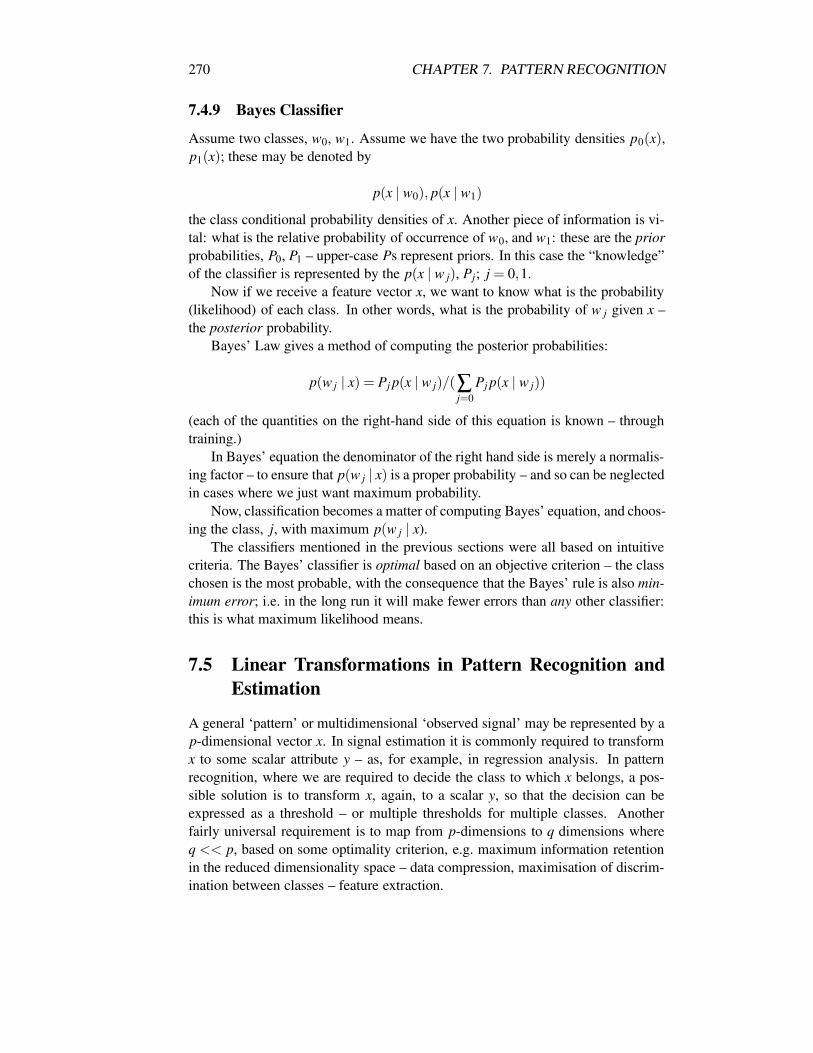
270 CHAPTER 7. PATTERN RECOGNITION
7.4.9 Bayes Classifier
Assume two classes, w0, w1. Assume we have the two probability densities p0(x),p1(x); these may be denoted by
p(x | w0), p(x | w1)
the class conditional probability densities of x. Another piece of information is vi-tal: what is the relative probability of occurrence of w0, and w1: these are the priorprobabilities, P0, P1 – upper-case Ps represent priors. In this case the “knowledge”of the classifier is represented by the p(x | w j), Pj; j = 0,1.
Now if we receive a feature vector x, we want to know what is the probability(likelihood) of each class. In other words, what is the probability of w j given x –the posterior probability.
Bayes’ Law gives a method of computing the posterior probabilities:
p(w j | x) = Pj p(x | w j)/(∑j=0
Pj p(x | w j))
(each of the quantities on the right-hand side of this equation is known – throughtraining.)
In Bayes’ equation the denominator of the right hand side is merely a normalis-ing factor – to ensure that p(w j | x) is a proper probability – and so can be neglectedin cases where we just want maximum probability.
Now, classification becomes a matter of computing Bayes’ equation, and choos-ing the class, j, with maximum p(w j | x).
The classifiers mentioned in the previous sections were all based on intuitivecriteria. The Bayes’ classifier is optimal based on an objective criterion – the classchosen is the most probable, with the consequence that the Bayes’ rule is also min-imum error; i.e. in the long run it will make fewer errors than any other classifier:this is what maximum likelihood means.
7.5 Linear Transformations in Pattern Recognition andEstimation
A general ‘pattern’ or multidimensional ‘observed signal’ may be represented by ap-dimensional vector x. In signal estimation it is commonly required to transformx to some scalar attribute y – as, for example, in regression analysis. In patternrecognition, where we are required to decide the class to which x belongs, a pos-sible solution is to transform x, again, to a scalar y, so that the decision can beexpressed as a threshold – or multiple thresholds for multiple classes. Anotherfairly universal requirement is to map from p-dimensions to q dimensions whereq << p, based on some optimality criterion, e.g. maximum information retentionin the reduced dimensionality space – data compression, maximisation of discrim-ination between classes – feature extraction.

7.5. LINEAR TRANSFORMATIONS IN PATTERN RECOGNITION AND ESTIMATION271
For each of the above problems, it is possible (at least theoretically) to obtainsolutions based on linear transformations of the form y = Ax, where x is a p× 1vector, y a q×1 vector, and A, a q× p matrix. Most of the transformations are basedon statistical criteria, in particular least-square-error or maximum likelihood.
If the data are in image format, i.e. in the form of a N row ×M column image,the above form is not directly applicable. However such an image easily can berearranged as a single NM×1 vector, so the transformations are still valid – thoughthe size of NM may make the matrix A difficult to handle, and worse still, estimate.
The section identifies some special solutions for image data and concludeswith a focus on the application to human face recognition. Each principal trans-formation is summarized according to its criterion/premise (e.g. maximises sepa-ration of classes), enough theory to enable understanding of the mechanism, for-mula/algorithm or reference to existing software, and some evaluative commentary.
7.5.1 Linear Partitions of Feature Space
This section forms the basis of linking of classifiers with neural networks.Consider template matching in the case of two classes:Actually, to be perfectly correct, we must subtract the mean of the data, call
it m, and mi = ith component of mean. Note – this is the overall mean, not classmeans.
x′X j =p−1
∑i=0
(xi−mi)′(X ji−mi)
where xi is the ith component of vector x and X ji the ith component of X j for p-dimensional vectors. Prime denotes transpose.
Therefore finding maximum correlation reduces to:
p−1
∑i=0
(xi−mi)(X0i−mi) >p−1
∑i=0
(xi−mi)(X1i−mi) =⇒ class = 0
and otherwise =⇒ class = 1Or:
p−1
∑i=0
(xi−mi)(X0i−mi)−p−1
∑i=0
(xi−mi)(X1i−mi) > 0 =⇒ class = 0
and otherwise =⇒ class = 1.The left hand side is:
∑(xiX0i +mimi−miX0i−mixi− (xiX1i +mimi−miX1i−mixi))
= ∑(xiX0i +mimi−miX0i−mixi− xiX1i−mimi +miX1i +mixi)

272 CHAPTER 7. PATTERN RECOGNITION
= ∑(xiX0i−miX0i− xiX1i +miX1i)
= ∑(xi(X0i−X1i)−miX0i +miX1i)
=p−1
∑i=0
(xiai)+a0 > 0 =⇒ class = 0
else =⇒ class = 1
where
a0 =p−1
∑i=0
(−miX0i +miX1i) = constant
and ai = (X0i−X1i).Geometrically, the decision is defined by the line
p−1
∑i=0
(xiai)+a0 = 0
which is an equation of a straight line through the origin; points above the line arejudged class 0, those below are class 1.
Usually X0, X1 would be m0, m1 the mean vectors of the classes; in this case theline given by ∑aixi bisects and is perpendicular to the line joining the two means.
Example. Look again at the data from section 7.3. The * * * shows a linearpartition for the two classes.
+|
4 + 1|+ *|
3 + *1 1 1|+ 0| *
2 + 1| *+ 0 0 0 0 = class 0, mean = m0| 1 = class 1, mean = m1
1 + * * * * = boundary|
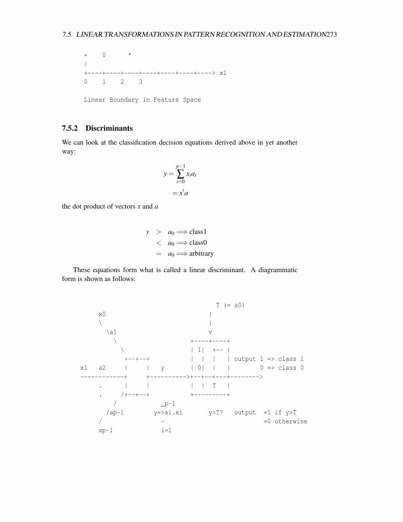
7.5. LINEAR TRANSFORMATIONS IN PATTERN RECOGNITION AND ESTIMATION273
+ 0 *|+----+----+----+----+----+----+----> x10 1 2 3
Linear Boundary in Feature Space
7.5.2 Discriminants
We can look at the classification decision equations derived above in yet anotherway:
y =p−1
∑i=0
xiai
= x′a
the dot product of vectors x and a
y > a0 =⇒ class1
< a0 =⇒ class0
= a0 =⇒ arbitrary
These equations form what is called a linear discriminant. A diagrammaticform is shown as follows:
T (= a0)x0 |\ |
\a1 v\ +----+----+\ | 1| +-- |+--+--+ | | | | output 1 => class 1
x1 a2 | | y | 0| | | 0 => class 0------------+ +---------->+--+--+---+-------->
. | | | | T |
. /+--+--+ +---------+/ _p-1
/ap-1 y=>ai.xi y>T? output =1 if y>T/ - =0 otherwisexp-1 i=1
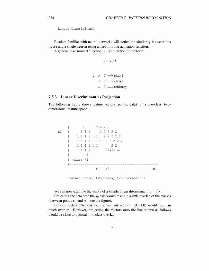
274 CHAPTER 7. PATTERN RECOGNITION
Linear Discriminant
Readers familiar with neural networks will notice the similarity between thisfigure and a single neuron using a hard-limiting activation function.
A general discriminant function, g, is a function of the form:
y = g(x)
y > T =⇒ class1
< T =⇒ class2
= T =⇒ arbitrary
7.5.3 Linear Discriminant as Projection
The following figure shows feature vectors (points, data) for a two-class, two-dimensional feature space.
| 1 2 2 2 2x2 | 1 1 1 2 2 2 2 2
| 1 1 1 1 1 1 2 2 2 2 2| 1 1 1 1 1 1 1 2 2 2 2 2| 1 1 1 1 1 1 2 2| 1 1 1 1 class w2| 1| class w1+--------------+---+--------------------------->
t1 t2 x1
Feature space, two-class, two-dimensional.
We can now examine the utility of a simple linear discriminant, y = a′x.Projecting the data onto the x0 axis would result in a little overlap of the classes
(between points t1, and t2 – see the figure).Projecting data onto axis x2, discriminant vector = (0.0,1.0) would result in
much overlap. However, projecting the vectors onto the line shown as followswould be close to optimal – no class overlap.
*

7.5. LINEAR TRANSFORMATIONS IN PATTERN RECOGNITION AND ESTIMATION275
| 1 2 2 2 *x1 | 1 1 1 2 * 2 2 2
| 1 1 1 1 1 1* 2 2 2 2 2| 1 1 1 1 1* 1 1 2 2 2 2 2| 1 1 1 * 1 1 2 2| 1*1 1 1 class w2| * 1| *+----------------------------------------------->
x0
* * * projection line - y0
Linear Discriminant as Projection.
Projecting the data onto different axes is equivalent to rotating the axes – i.e.in the case above, we would rotate to a new set of axes y0, y1, where y0 is the axisshown as * * * ; obviously, in the case above, we would ignore the second, y1dimension, since it would contribute nothing to the discrimination of the classes.
7.5.4 The Connection with Neural Networks
Recall the following equation – we will call the expression s – which interprets cor-relation as a linear partitioning (assume we are using means as ‘perfect’ vectors).Note: many treatments of pattern recognition deal with only with two-class cases– the math is usually easier, and it is usually easy to extend to the multiclass casewithout any loss of generality.
s =p−1
∑i=0
xiai +a0 = 0
As noted above, this is a straight line. It bisects the line joining the two means,and is perpindicular to them.
In neural networks, a0 is called the bias term. Alternatively, for mathematicaltidyness, we can include a0 in the summation, and insist that the zeroth element ofeach feature is always 1 – the so-called bias input in neural networks.
We then subject s to a threshold function,
s > 0 =⇒ class 1
≤ 0 =⇒ class 0
as seen before.In neural networks nowadays, this thresholding is usually done with the so-
called sigmoid function, see Chapter 8.
276 CHAPTER 7. PATTERN RECOGNITION
7.5.5 Fisher Linear Discriminant
See Fisher (1936), Duda and Hart (1973), Fukunaga (1990).Linear Discriminant Analysis, first proposed in Fisher’s 1936 article, relates
only to the two-class case. The Fisher discriminant is one of the best known of allpattern recognition algorithms. It projects the data onto a single axis, see section3.3, defined by the Fisher discriminant vector a:
y = aT x
The Fisher discriminant simultaneously optimises two measures/criteria:(a) maximum between-class separation, expressed as separation of the class
means m1,m2,(b) minimum within-class scatter, expressed as the within class variances, v1,v2.The Fisher criterion combines (a), and (b) as:
J = (m1−m2)/(v1 + v2)
where the transformed means and variances are:
m j = aT m j
v j = aS jaT
where S j = covariance for class j, and m j = mean vector for class j.The discriminant is computed using:
a = W−1(m1−m2)
where W is the pooled (overall, class independent) covariance matrix, W = p1S1 +p2S2, p1, p2 are the prior probabilities. – see Appendix.
Procedure:
1. Estimate class means m j and covariance matrices S j , and prior probabilities,p j .
2. Compute pooled covariance matrix, W (see definition above).
3. Invert matrix W (using some standard matrix inversion subprogram).
4. Compute the discriminant vector, a (see above).
5. Apply the discriminant using eqn. 3.4-1.
See DataLab function ’da’ (Campbell, 1993).

7.5. LINEAR TRANSFORMATIONS IN PATTERN RECOGNITION AND ESTIMATION277
7.5.6 Karhunen-Loeve Transform
See Fukunaga (1990). Also called Principal Components Analysis, Factor Analy-sis, Hotelling Transform.
The Karhunen-Loeve (KL) transform rotates the axes such that the covariancematrix is diagonalised:
y = Ux
where (see Appendix) U is the eigenvector matrix of S the covariance matrix (overall classes), i.e.
UT SU = L
where
L = | l1 0 0 ... 0 || 0 l2 0 0 |
...| lp |
L is a diagonal matrix containing the variances in the transformed space, and,
U = | u1 || u2 || u2 || ..|| ui || ..|| up |
is the matrix formed by the eigenvectors, ui, of S.There is an eigenvector, ui, corresponding to each eigenvalue λi; If we order the
eigenvectors, ui, according to decreasing size of the corresponding eigenvalue, wearrive at a transform (eqn. 3.5-1) in which the variance in dimension y0 is largest,y1, the next largest, etc.
If we equate variance and information, then the KL transform gives a method ofmapping to a lower dimensionality space, m, say, m < p, with maximum retentionof information; thus its theoretical appeal for data compression. Let U ′ be them× p matrix containing the first m rows of U , i.e. the m eigenvectors/projectionscorresponding to the m largest eigenvalues. We can rewrite eqn. (3.5-1) as
y′ = U ′x
This corresponds to the coding part of the compression; we have reduced the datafrom p to m numbers. We can decode using,
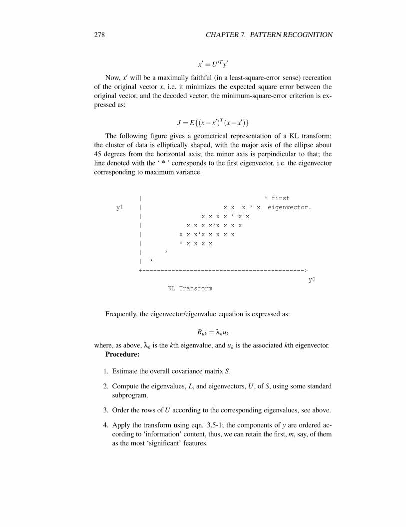
278 CHAPTER 7. PATTERN RECOGNITION
x′ = U ′T y′
Now, x′ will be a maximally faithful (in a least-square-error sense) recreationof the original vector x, i.e. it minimizes the expected square error between theoriginal vector, and the decoded vector; the minimum-square-error criterion is ex-pressed as:
J = E(x− x′)T (x− x′)The following figure gives a geometrical representation of a KL transform;
the cluster of data is elliptically shaped, with the major axis of the ellipse about45 degrees from the horizontal axis; the minor axis is perpindicular to that; theline denoted with the ‘ * ’ corresponds to the first eigenvector, i.e. the eigenvectorcorresponding to maximum variance.
| * firsty1 | x x x * x eigenvector.
| x x x x * x x| x x x x*x x x x| x x x*x x x x x| * x x x x| *| *+-------------------------------------------->
y0KL Transform
Frequently, the eigenvector/eigenvalue equation is expressed as:
Ruk = λkuk
where, as above, λk is the kth eigenvalue, and uk is the associated kth eigenvector.Procedure:
1. Estimate the overall covariance matrix S.
2. Compute the eigenvalues, L, and eigenvectors, U , of S, using some standardsubprogram.
3. Order the rows of U according to the corresponding eigenvalues, see above.
4. Apply the transform using eqn. 3.5-1; the components of y are ordered ac-cording to ‘information’ content, thus, we can retain the first, m, say, of themas the most ‘significant’ features.
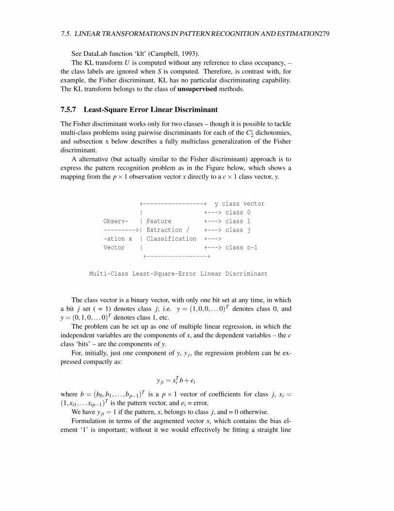
7.5. LINEAR TRANSFORMATIONS IN PATTERN RECOGNITION AND ESTIMATION279
See DataLab function ‘klt’ (Campbell, 1993).The KL transform U is computed without any reference to class occupancy, –
the class labels are ignored when S is computed. Therefore, is contrast with, forexample, the Fisher discriminant, KL has no particular discriminating capability.The KL transform belongs to the class of unsupervised methods.
7.5.7 Least-Square Error Linear Discriminant
The Fisher discriminant works only for two classes – though it is possible to tacklemulti-class problems using pairwise discriminants for each of the Cc
2 dichotomies,and subsection x below describes a fully multiclass generalization of the Fisherdiscriminant.
A alternative (but actually similar to the Fisher discriminant) approach is toexpress the pattern recognition problem as in the Figure below, which shows amapping from the p×1 observation vector x directly to a c×1 class vector, y.
+-----------------+ y class vector| +---> class 0
Observ- | Feature +---> class 1--------->| Extraction / +---> class j-ation x | Classification +--->Vector | +---> class c-1
+-----------------+
Multi-Class Least-Square-Error Linear Discriminant
The class vector is a binary vector, with only one bit set at any time, in whicha bit j set ( = 1) denotes class j; i.e. y = (1,0,0, . . . 0)T denotes class 0, andy = (0,1,0, . . .0)T denotes class 1, etc.
The problem can be set up as one of multiple linear regression, in which theindependent variables are the components of x, and the dependent variables – the cclass ‘bits’ – are the components of y.
For, initially, just one component of y, y j , the regression problem can be ex-pressed compactly as:
y ji = xTi b+ ei
where b = (b0,b1, . . . ,bp−1)T is a p× 1 vector of coefficients for class j, xi =
(1,xi1, . . .xip−1)T is the pattern vector, and ei = error,
We have y ji = 1 if the pattern, x, belongs to class j, and = 0 otherwise.Formulation in terms of the augmented vector x, which contains the bias el-
ement ‘1’ is important; without it we would effectively be fitting a straight line
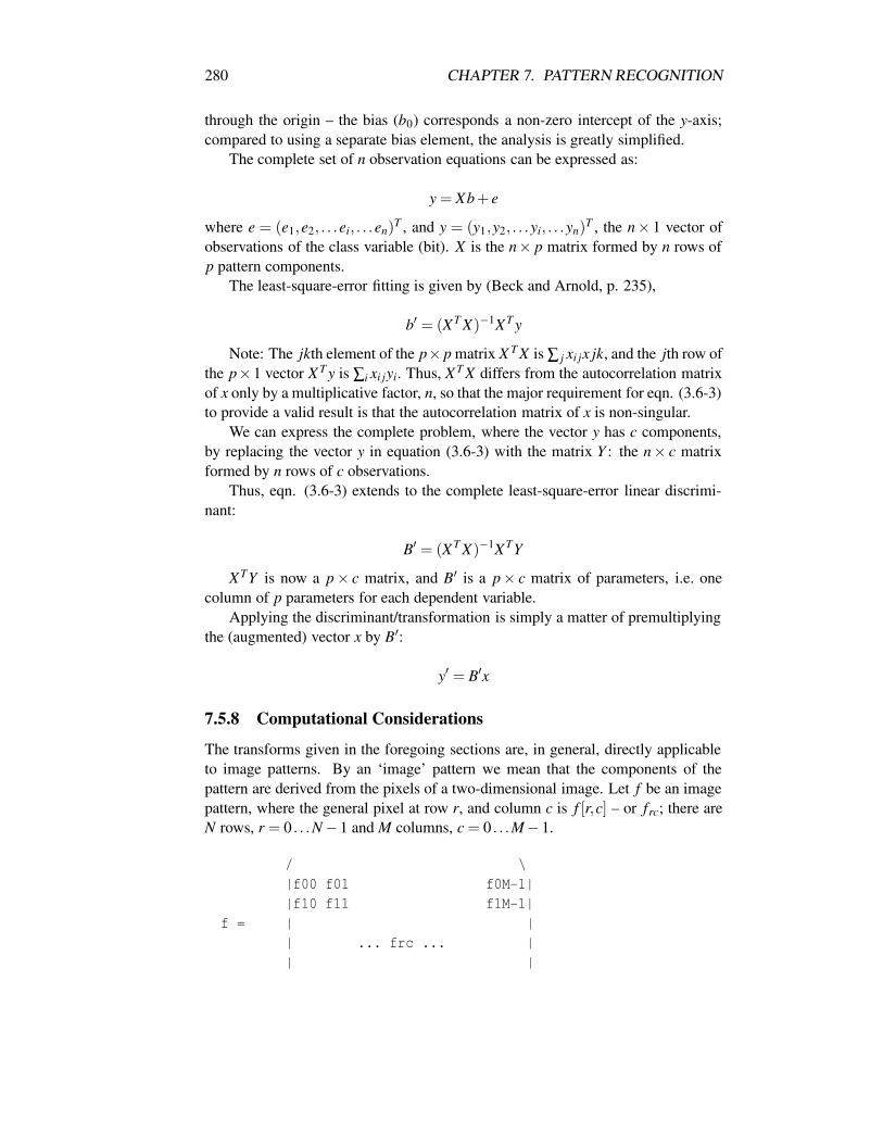
280 CHAPTER 7. PATTERN RECOGNITION
through the origin – the bias (b0) corresponds a non-zero intercept of the y-axis;compared to using a separate bias element, the analysis is greatly simplified.
The complete set of n observation equations can be expressed as:
y = Xb+ e
where e = (e1,e2, . . .ei, . . .en)T , and y = (y1,y2, . . .yi, . . .yn)
T , the n× 1 vector ofobservations of the class variable (bit). X is the n× p matrix formed by n rows ofp pattern components.
The least-square-error fitting is given by (Beck and Arnold, p. 235),
b′ = (XT X)−1XT y
Note: The jkth element of the p× p matrix X T X is ∑ j xi jx jk, and the jth row ofthe p×1 vector X T y is ∑i xi jyi. Thus, XT X differs from the autocorrelation matrixof x only by a multiplicative factor, n, so that the major requirement for eqn. (3.6-3)to provide a valid result is that the autocorrelation matrix of x is non-singular.
We can express the complete problem, where the vector y has c components,by replacing the vector y in equation (3.6-3) with the matrix Y : the n× c matrixformed by n rows of c observations.
Thus, eqn. (3.6-3) extends to the complete least-square-error linear discrimi-nant:
B′ = (XT X)−1XTY
XTY is now a p× c matrix, and B′ is a p× c matrix of parameters, i.e. onecolumn of p parameters for each dependent variable.
Applying the discriminant/transformation is simply a matter of premultiplyingthe (augmented) vector x by B′:
y′ = B′x
7.5.8 Computational Considerations
The transforms given in the foregoing sections are, in general, directly applicableto image patterns. By an ‘image’ pattern we mean that the components of thepattern are derived from the pixels of a two-dimensional image. Let f be an imagepattern, where the general pixel at row r, and column c is f [r,c] – or frc; there areN rows, r = 0 . . .N−1 and M columns, c = 0 . . .M−1.
/ \|f00 f01 f0M-1||f10 f11 f1M-1|
f = | || ... frc ... || |

7.5. LINEAR TRANSFORMATIONS IN PATTERN RECOGNITION AND ESTIMATION281
|fN-10 fN-11 fN-1M-1 |\ /
Trivially, f can be represented as an NM×1 vector as follows:
x = ( f00, f01, . . . f0M−1, f10 . . . frc . . . fN−10 . . . fN−1M−1)
Pratt (1991), p. 130 gives an analytic form of this expression for x, which issometimes useful in formal mathematical treatment of image patterns as vectors.
Usually, the major problem with extending the results of the foregoing sectionsto images is in the difficulty of estimating statistics. For example, if the images fare N×M, the vectors x are NM×1; therefore the autocorrelation and covariancematrices for x (and f ) are NM×NM. If the images are modestly sized at 128×128 (N = 128,M = 128) we have an autocorrelation matrix of 16,384× 16,384which means that there are 269× 106 components. Such a matrix is simply notestimatible, nor handleable.
7.5.9 Eigenimages
(See Turk and Pentland, 1991) Note: the treatment of the Karhunen-Loeve trans-form (eigenvector expansion) in section 3.5 uses the autocorrelation matrix R asthe basis of the eigenvectors. Frequently, the covariance matrix S is used; this isthe case in the Turk and Pentland (1991) work on ‘eigenfaces’; in this section, wewill use the covariance matrix.
Naively, the Karhunen-Loeve transform given by eqn. (3.5-1) (y = Ux) can beeasily extended to apply to image patterns, using eqn. 4.1-2 to express the sampleimages as vectors. However, the problem mentioned in the previous section, of ahuge dimensionality covariance matrix, is immediately obvious; the dimensionalityof x is p = NM; assume for the remainder that N = M, i.e. we have a square image.
If the express the image patterns fi as vectors xi using eqn. 4.1-2; let there be nof them in the sample, xi, i = 1 . . .n.
If, see section 2.2, eqn. 2.2-11, x′ = (x−m), i.e. the pattern vector reduced tozero mean, and
X ′ = [x′1x′2 . . .x′i . . .x′n]
which is of dimensions p× n, p = N2, the sample covariance matrix can be ex-pressed as can be rewritten as
S =1n
X ′X ′T
which is N2×N2. However, see Appendix A.12, the rank of S is only n, andtherefore there are only n non-zero eigenvalues when S is diagonalized. Basedon this, Turk and Pentland (1991) give a method of finding these n eigenval-ues/eigenvectors based on a reduced dimensionality n× n matrix – in their papern = 16.
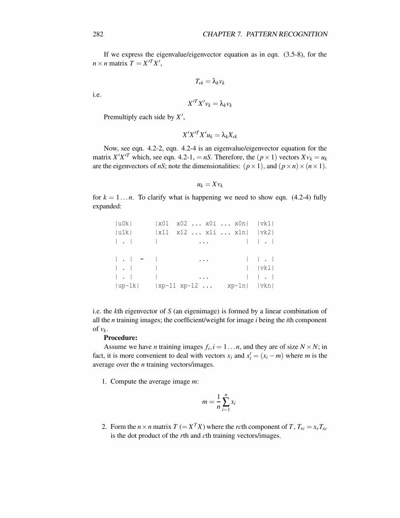
282 CHAPTER 7. PATTERN RECOGNITION
If we express the eigenvalue/eigenvector equation as in eqn. (3.5-8), for then×n matrix T = X ′T X ′,
Tvk = λkvk
i.e.X ′T X ′vk = λkvk
Premultiply each side by X ′,
X ′X ′T X ′uk = λkXvk
Now, see eqn. 4.2-2, eqn. 4.2-4 is an eigenvalue/eigenvector equation for thematrix X ′X ′T which, see eqn. 4.2-1, = nS. Therefore, the (p×1) vectors Xvk = ukare the eigenvectors of nS; note the dimensionalities: (p×1), and (p×n)×(n×1).
uk = Xvk
for k = 1 . . .n. To clarify what is happening we need to show eqn. (4.2-4) fullyexpanded:
|u0k| |x01 x02 ... x0i ... x0n| |vk1||u1k| |x11 x12 ... x1i ... x1n| |vk2|| . | | ... | | . |
| . | = | ... | | . || . | | | |vki|| . | | ... | | . ||up-1k| |xp-11 xp-12 ... xp-1n| |vkn|
i.e. the kth eigenvector of S (an eigenimage) is formed by a linear combination ofall the n training images; the coefficient/weight for image i being the ith componentof vk.
Procedure:Assume we have n training images fi, i = 1 . . .n, and they are of size N×N; in
fact, it is more convenient to deal with vectors xi and x′i = (xi−m) where m is theaverage over the n training vectors/images.
1. Compute the average image m:
m =1n
n
∑i=1
xi
2. Form the n×n matrix T (= X T X ) where the rcth component of T , Trc = xrTxcis the dot product of the rth and cth training vectors/images.

7.6. SHAPE AND OTHER FEATURES 283
3. Find the n eigenvectors of T , vk.
4. Order the vk according to decreasing eigenvalue (see section 3.5).
5. Use eqn. 4.2-4 to compute the n′(< n) most significant eigenimages, uk,k =1 . . .n′.
7.5.10 Other Connections and Discussion
In the early days of pattern recognition (late 1950s, early 60s) there were two majorinfluences:
1. communication and radar engineering, for which the decision expression, sabove, is a matched filter, i.e. maximum correlation device,
2. those who wished to model human pattern recognition. To these, s above isa single neuron. See chapter 8.
In all the pattern recognition approaches discussed in this section, the classi-fication rules end up as minimum distance, or very similar. It is comforting toknow that correlation and minimum distance boil down to the same thing, and thatthese are related to maximum likelihood, and, very closely, to neural networks.Furthermore, it can be shown that the nearest neighbour classifier – which is basedon intuitition – is very closely related to the Bayes’ classifier. Also, many practi-cal implementations of the Bayes’ classifier end up using minimum distance (e.g.nearest mean).
Usually, it is the choice of features that governs the effectiveness of the system,not the classifier rule.
We now consider two practical pattern recognition problems related to imageprocessing.
7.6 Shape and Other Features
7.6.1 Two-dimensional Shape Recognition
We now return to the character recognition problem. Of course, this is represen-tative of many two-dimensional shape recognition problems, e.g. text-characterrecognition. The major problem is locating the character/shape, and extractinginvariant features.
A possible solution is given by the following steps:
1. Segmentation: label ink/object pixels, versus background/non-ink pixels.See Chapter 6. This removes the effects of amplitude/brightness; also makesstep (2) easier.
284 CHAPTER 7. PATTERN RECOGNITION
2. Isolate the object: e.g. starting off at the top-left corner of the object, moveright and down, simultaneously scanning each column and each row; whenthere is a break – no ink – this marks the bottom-right corner of the object.
3. Feature Extraction: we need invariant features, e.g. 2-d. central moments,see G&W section 8.3.4 (p. 514) and the next section of these notes.
4. Gather Training Data: obtain a representative set of feature vectors for eachclass of object,
5. Test data: same requirement as training.
6. Train the classifier: train on the training set for each class, e.g. learn statistics(mean, standard deviation), or somehow find out the occupancy of the classesin measurement/feature space.
7. Classifier: see section 7.3:
• Statistical: Bayes’ Rule.
• Geometric: simple nearest mean classifier, or ‘box’ classifier
• nearest neighbor, or k-nn.
7.6.2 Two-dimensional Invariant Moments for Planar Shape Recog-nition
Assume we have isolated the object in the image (see chapter 7.4): its bounds arexl..xh, yl..yh. Two-dimensional moments are given by:
mpq = ∑x
∑y
xpyq f (x,y)
for p,q = 0,1,2, . . . .These are not invariant to anything, yet.
x = m10/m00
gives the x-centre of gravity of the object,and
y = m01/m00
gives the y-centre of gravity.Now we can obtain shift invariant features by referring all coordinates to the
centre of gravity (x, y). These are the so-called central moments:
m′pq = ∑x
∑y
(x− x)p(y− y)q f (x,y)
7.6. SHAPE AND OTHER FEATURES 285
The first few m′ can be interpreted as follows:m′00 = m00 = sum of the grey levels in the object,m′10 = m′01 = 0, always, i.e. center of gravity is (0,0) with respect to itself.m′20 = measure of width along x-axism′02 = measure of width along y-axis.From the m′pq can be derived a set of normalized moments:
µpq = m′pq/((m′00)
g)
where g = (p+q)/2+1Finally, a set of seven fully shift, rotation, and scale invariant moments can be
defined:
p1 = n20 +n02
p2 = (n20−n02)2 +4n2
11
Etc.
See G&W for further details.
Ex. 7.5-1 An apple pie manufacturer is setting up an automatic conveyer belt in-spection system for the pastry tops for his pies. He requires:
1. the tops must be circular (to within some defined tolarance),
2. there must be no holes in the top.
The inspection can be carried out using the model given in section 7.4 andChapter 2. Assuming the background grey level sufficiently contrasts withthat of the pastry, location and segmentation should be simple.
After segmentation, inspection (2) can be carried out by searching for anybackground pixels in the interior of the pastry.
Inspection (1) can be done using invariant moments; we demand featurevectors within a certain small distance (the tolerance) of the perfect shape.
Note: if the input camera is always the same distance from the conveyer belt,we don’t need scale invariance. And, because the pie tops are circular, wedon’t need rotation invariance. Thus, simple features might be (say) four, oreight diameters sampled at equally spaced angles around the pie; of course,x and y give the center of the pie top, through which the diameters must pass.
An alternative would be to detect the edges of the pie top, and therby com-pute the circumference, c. Compute the diameter as above, d. Then, c/dmust be close to π, otherwise it’s a bad pi(e)!
Ex. 7.5-2 At Easter the pie manufacturer branches into hot-cross buns. In thiscase, he is interested, not only in the roundness, but in the perfection of thecross on top of the bun. Suggest possible features, and classifier techniques.
286 CHAPTER 7. PATTERN RECOGNITION
7.6.3 Classification Based on Spectral Features
For example, we require a system to automate the process of land-use mappingusing multispectral (i.e. multicolour) satellite images. Or, maybe, to discriminaterain clouds from non-rain; or, to detect pollution in water.
Feature Extraction:
In this case the features are easier to obtain; in fact, the pixel values (in eachcolour) will do; i.e. the feature vector is the same as the observation vector – theplain radiance value in the spectral band. It might be neccessary to do some pre-processing, e.g. correction for atmospheric effects.
Training data:
Obtain representative (note: representative) samples of each land-use class(this is called ground data, or ground-truth). This requires field work, or use exist-ing maps.
Test data:
Same requirement as training; again – note – we need fully representative data.
Train classifier:
Train on samples for each class, learn statistics (mean, standard deviation), orsomehow find out the occupancy of the classes in measurement/feature space.
Classifier:
See above. The output is an image containing class labels, these can be appro-priately colour coded for map production.
Test/Evaluation:
Run the classifier on the test data. Compare ‘true’ classes, and ‘classifier’classes. Produce error matrix, or simply percentage of pixels incorrectly classified.
NB We must use different data for testing – not training data.
Geometric Correction:
Scale, shift, rotate the image to correspond to map coordinates. Sometimescalled geometric calibration.
Pitfalls and difficulties:
Poor features. The features just do not discriminate the classes. If the rawspectral bands do not discriminate, we may need to take the ratio of colors/bands.Or, we may need to use texture. Or, we may need to combine images from different
7.6. SHAPE AND OTHER FEATURES 287
parts of season – this will require image registration (see Chapter 3 for rotation andscaling, etc.).
Poor training data. Not representative – maybe contains only one sub-set of thereal class – and so is not representative of the true class variability. Or, we havepixels of another class mixed in.
Mixed pixels. I.e. pixels that ‘straddle’ boundaries between class regions; badfor training data. Also difficult to classify correctly.
Overlapping classes. Some of our classes actually may have same ‘colour’; tosolve this problem we need additional ‘features’ e.g. texture. Or use context, or trymultiseason data – see above.
Testing on training data. This is a common error, somewhat akin to the sameperson specifying, writing, and testing a piece of software: the results of the testsusually give good news – whatever the reality!
7.6.4 Some Common Problems in Pattern Recognition
• Bad features. No amount of ‘clever’ classification can remedy the situationif the features are not properly desciptive.
• Large dimensionality. The larger the dimensionality of the feature vectors,the more training data required. Typically four or more samples per class,per dimension. E.g. dimensionality, d, = 50, no. of samples = 250 per class.
• Mismatch in range of features. E.g. feature 1 ranges 0 to 1, feature 2 ranges0 to 100: variations in feature 2 will swamp variations in feature 1, in forexample, distance or correlation measures. We need to normalise the com-ponents of the feature vector, to equal ranges of (say) 0 to 1.
• Testing using training data.
• Multimodal distributions, i.e. really two classes combined. May fool statis-tical algorithms.
7.6.5 Problems Solvable by Pattern Recognition Techniques
Engine Monitoring
Observation vector: sound signal.Feature vector: Fourier Spectrum of sound signal.Classes: Healthy, not healthy – needs maintenance.
Medical Diagnosis
Observation vector: Binary – list of symtoms, e.g.x1 = pain in hamstring,x2 = history of back trouble,

288 CHAPTER 7. PATTERN RECOGNITION
x3 = pain intermittentx4 = pain constantx5 = recent athletic activity
Feature vector: = observation vectorClasses:w1 = Sciatica,w2 = pulled muscle,w3 = stiffness,w4 = don’t know – refer to specialist.
Information Retrieval
Features: presence of keywords.Classes: subject areas.
Burgular Alarm
Features: sound level in microphone, current level in loop sensors, readingsfrom infrared temperature sensors.
Classes: Intruder – ring bell, no intruder.
7.6.6 For Further Reading
1. S. Aeberhard, D. Coomans, and O. de Vel. 1994. Comparative Analysisof Statistical Pattern Recognition Methods in High Dimensional Settings.Pattern Recognition, Vol. 27, No. 8.
2. A.K. Agrawala (ed.). 1976. Machine Recognition of Patterns. IEEE Press.[Collection of Key Papers + tutorial].
3. J.V. Beck, and K.J. Arnold. 1977. Parameter Estimation in Engineering andScience. John Wiley and Sons.
4. R.O. Duda, and P.E. Hart. 1973. Pattern Classification and Scene Analysis.Wiley-Interscience.
5. R.A. Fisher. 1936. The Use of Multiple Measurements in Taxonomic Prob-lems. Annals of Eugenics. [contained in (Agrawala, 1976)]
6. D.H. Foley, and J.W. Sammon. 1975. An Optimal Set of Discriminant Vec-tors. IEEE Trans. Comp. March.
7. K. Fukunaga. 1990. Introduction to Statistical Pattern Recognition. 2nd. ed.Academic Press.
8. K. Fukunaga, and W. Koontz. 1970. A Criterion and an Algorithm forGrouping Data. IEEE. Trans. Comp. October.
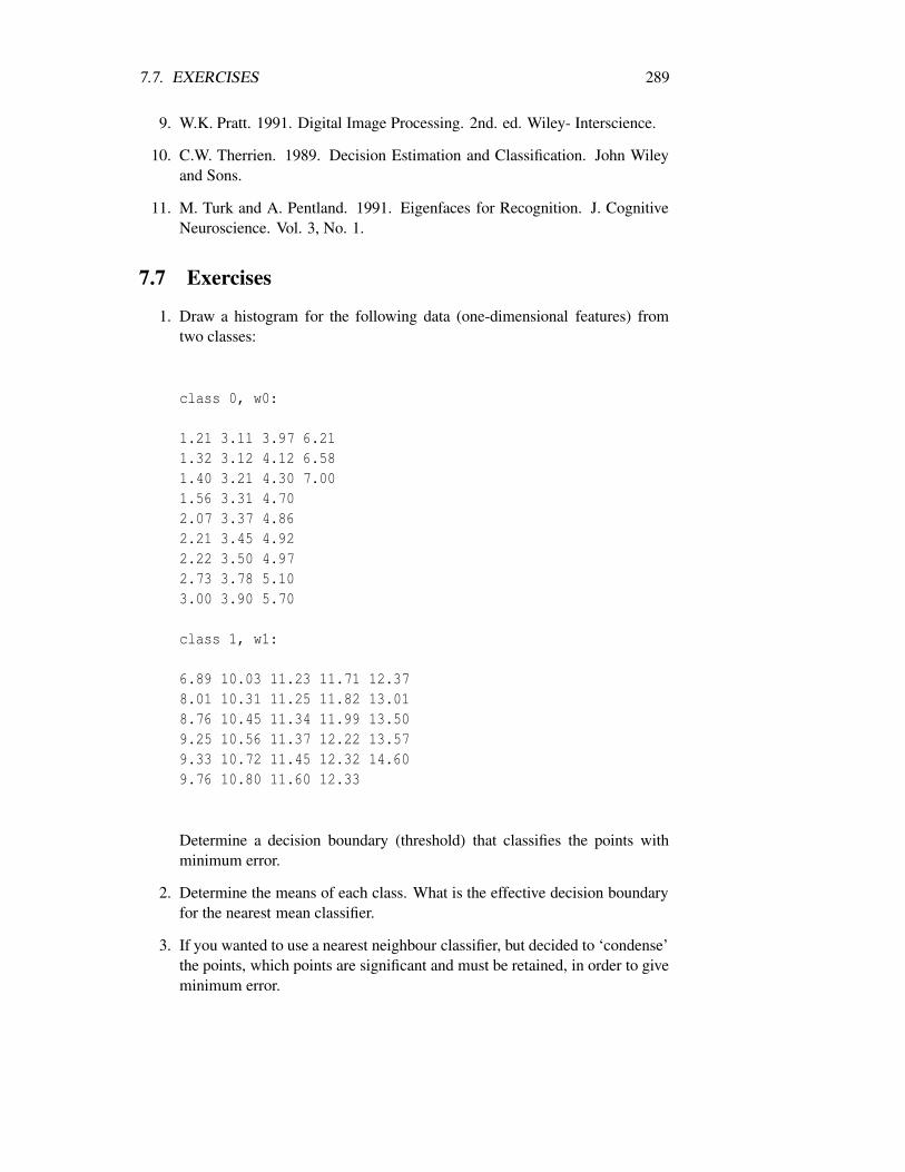
7.7. EXERCISES 289
9. W.K. Pratt. 1991. Digital Image Processing. 2nd. ed. Wiley- Interscience.
10. C.W. Therrien. 1989. Decision Estimation and Classification. John Wileyand Sons.
11. M. Turk and A. Pentland. 1991. Eigenfaces for Recognition. J. CognitiveNeuroscience. Vol. 3, No. 1.
7.7 Exercises
1. Draw a histogram for the following data (one-dimensional features) fromtwo classes:
class 0, w0:
1.21 3.11 3.97 6.211.32 3.12 4.12 6.581.40 3.21 4.30 7.001.56 3.31 4.702.07 3.37 4.862.21 3.45 4.922.22 3.50 4.972.73 3.78 5.103.00 3.90 5.70
class 1, w1:
6.89 10.03 11.23 11.71 12.378.01 10.31 11.25 11.82 13.018.76 10.45 11.34 11.99 13.509.25 10.56 11.37 12.22 13.579.33 10.72 11.45 12.32 14.609.76 10.80 11.60 12.33
Determine a decision boundary (threshold) that classifies the points withminimum error.
2. Determine the means of each class. What is the effective decision boundaryfor the nearest mean classifier.
3. If you wanted to use a nearest neighbour classifier, but decided to ‘condense’the points, which points are significant and must be retained, in order to giveminimum error.

290 CHAPTER 7. PATTERN RECOGNITION
4. Pick 10 men and 10 women, at random (more if you have time). Find theirheight – inches. Plot a histogram. Design a histogram based (statistical)classifier that distinguishes men from women.
5. Design a nearest mean classifier using the data from 4. Compare the result.
6. Add an additional, second, feature to Ex. 4, i.e. shoe size. Plot a two dimen-sional scatter plot (or histogram, if you wish). Plot the optimum boundarybetween the classes – based on the scatter plot.
7. Using the data from 6 work out the means vectors of the classes. Plot thelinear boundary that would be formed by a nearest mean classifier.
8. Design a pattern recognition system for coins (money). What are the:
• observations,
• features.
Suggest simple classifier rules.
9. In the character recognition example given in section 7.1 the feature space isnine dimensional. Thus, visualisation of the data in feature space is difficult.The following example is easier to visualise.
Consider an imaging system which has just two pixels – or, an animal whichhas just two light sensitive cells in its retina, see following figure. Call theoutputs of these x1, and x2, therefore they form a two-dimensional vectorx = (x1,x2).
x1 x2+-----+-----+| | || | |+-----+-----+
Two-Pixel Image
(a) If the components are binary (0 or 1) we can consider a problem whichwishes to distinguish ‘bright’ objects – class 1, from dark – class 0. For nowwe will define class 1 as ‘both pixels light’. I.e. we have (where ‘*’ denoteslight, or class 1):
x1 x2

7.7. EXERCISES 291
+-----+-----+|*****|*****| class 1|*****|*****|+-----+-----+
x1 x2+-----+-----+|*****| | class 0|*****| |+-----+-----+
x1 x2+-----+-----+| |*****| class 0| |*****|+-----+-----+
x1 x2+-----+-----+| | | class 0| | |+-----+-----+
Note the similarity with the Boolean and function.
The feature space representation of these classes are shown in the next fig-ure; ‘@’ represents class 0, ‘*’ represents class 1. We have shown a linearboundary which segregates the classes.
ˆ \1 @ \ *
| \| \
x2 | class 0 \ class 1| \| \| \| \
0 @-----------------------------@> \0 x1 1

292 CHAPTER 7. PATTERN RECOGNITION
Two-Dimensional Scatter Diagram - Feature Space
(b) Let us change to a problem which wishes to distinguish striped objects(class 0, say) from plain (class 1). I.e. we have (‘*’ denotes light, class 1):
x1 x2+-----+-----+|*****|*****| class 1|*****|*****|+-----+-----+
x1 x2+-----+-----+|*****| | class 0|*****| |+-----+-----+
x1 x2+-----+-----+| |*****| class 0| |*****|+-----+-----+
x1 x2+-----+-----+| | | class 1| | |+-----+-----+
Draw the feature space diagram. Draw appropriate decision boundary line(s)– note the difficulty compared to (a).
Note the similarity with the Boolean XOR function.
(c) Let us change to a problem which wishes to distinguish left-handed ob-jects (class 1, say) from right-handed (class 2), with neither left- or right-handed as reject, class 0. I.e. we have (here ‘*’ denotes light, class 1):
x1 x2+-----+-----+|*****|*****| class 0

7.7. EXERCISES 293
|*****|*****|+-----+-----+x1 x2
+-----+-----+|*****| | class 1|*****| |+-----+-----+x1 x2
+-----+-----+| |*****| class 2| |*****|+-----+-----+x1 x2
+-----+-----+| | | class 0| | |+-----+-----+
Draw the feature space diagram. Show the linear boundaries.
(d) (See (a)) Describe a state of affairs that corresponds to Boolean or; drawthe diagrams. Will a single linear boundary do? [Yes].
10. Change the system in Ex. 9 to allow non-binary data. Allow the data toextend from 0 to +1 and assume Real values (e.g. 0.995, 0.0256). Nowextend 9(a) to (d) assuming that there are small amounts of noise on thepixels, e.g. we have values spread over the range 0.9 to 1.0 for light, and 0.0to 0.1 for dark.
Draw the feature space diagrams for each case (a) to (d).
Draw suggested linear boundaries.
11. Now let the noise in Ex. 10 increase. Now, we have values spread over therange 0.55 to 1.0 for light, and 0.0 to 0.45 for dark.
(i) Draw the feature space diagrams for each case (a) to (d).
(ii) Draw suggested linear boundaries.
12. Now let the noise in Ex. 11 increase further. Now, we have values spreadover the range 0.4 to 1.0 for light, and 0.0 to 0.6 for dark.
(i) Draw the feature space diagrams for each case (a) to (d).
(ii) Draw suggested linear boundaries.
(iii) Suggest alternatives to the ‘linear’ classifiers.

294 CHAPTER 7. PATTERN RECOGNITION
13. In section 7.31 we mentioned the problem of mixed pixels. Research ‘fuzzysets’ and suggest how they could be applied to this problem.
[Note: a class can be considered to be defined as a binary membership func-tion in feature space; i.e. it is a set – a feature value is either a member (1)or not (0). A fuzzy set is one which can take on continuous membershipvalues in the range 0 to 1, e.g. 0.0, 0.1, low membership; 0.9,0.95, 1.0 highmembership].
How would fuzzy classes change our ability to define decision boundaries?
14. Iris data. [R.A. Fisher. 1936. Use of Multiple Measurements in TaxonomicProblems. Annals of Eugenics, Vol. 7, pp. 179-188.]
The following data (in files ’ih1.asc’) contain a subset of the famous iris(flowers) data. The data are four-dimensional: x0 = sepal length, x1 = sepalwidth, x2 = petal length, x3 = petal width. There are two classes – corre-sponding to two families of iris.
/*dh rh ch3, 0, 49cl x0 x1 x2 x31 5.1,3.5,1.4,0.21 4.9,3.0,1.4,0.21 4.7,3.2,1.3,0.21 4.6,3.1,1.5,0.21 5.0,3.6,1.4,0.21 5.4,3.9,1.7,0.41 4.6,3.4,1.4,0.31 5.0,3.4,1.5,0.21 4.4,2.9,1.4,0.21 4.9,3.1,1.5,0.11 5.4,3.7,1.5,0.21 4.8,3.4,1.6,0.21 4.8,3.0,1.4,0.11 4.3,3.0,1.1,0.11 5.8,4.0,1.2,0.21 5.7,4.4,1.5,0.41 5.4,3.9,1.3,0.41 5.1,3.5,1.4,0.31 5.7,3.8,1.7,0.31 5.1,3.8,1.5,0.31 5.4,3.4,1.7,0.21 5.1,3.7,1.5,0.41 4.6,3.6,1.0,0.2

7.7. EXERCISES 295
1 5.1,3.3,1.7,0.51 4.8,3.4,1.9,0.22 7.0,3.2,4.7,1.42 6.4,3.2,4.5,1.52 6.9,3.1,4.9,1.52 5.5,2.3,4.0,1.32 6.5,2.8,4.6,1.52 5.7,2.8,4.5,1.32 6.3,3.3,4.7,1.62 4.9,2.4,3.3,1.02 6.6,2.9,4.6,1.32 5.2,2.7,3.9,1.42 5.0,2.0,3.5,1.02 5.9,3.0,4.2,1.52 6.0,2.2,4.0,1.02 6.1,2.9,4.7,1.42 5.6,2.9,3.6,1.32 6.7,3.1,4.4,1.42 5.6,3.0,4.5,1.52 5.8,2.7,4.1,1.02 6.2,2.2,4.5,1.52 5.6,2.5,3.9,1.12 5.9,3.2,4.8,1.82 6.1,2.8,4.0,1.32 6.3,2.5,4.9,1.52 6.1,2.8,4.7,1.22 6.4,2.9,4.3,1.3
I have split the original data into two halves; the other half is in ‘ih2.asc’.
(a) Run DataLab batch file ‘ipiris’, which will configure and read in ih1.asc– to image 0, and ih2.asc – to image 1. It will also show some scatter plotsand histograms.
(b) (b-1) run clnm (nearest mean classifier) on image 0 (source – trainingdata) and image 1 (destination – test data).
(b-2) Run ‘clcfus’ on 1 to see the result.
(b-3) Check by examining image 1 using ‘tpsv’.
(c) (c-1) run clnn (nearest neighbour classifier) on image 0 (source – trainingdata) and image 1 (destination – test data).
(c-2) Run ‘clcfus’ on 1 to see the result.
(c-3) Check by examining image 1 using ‘tpsv’.
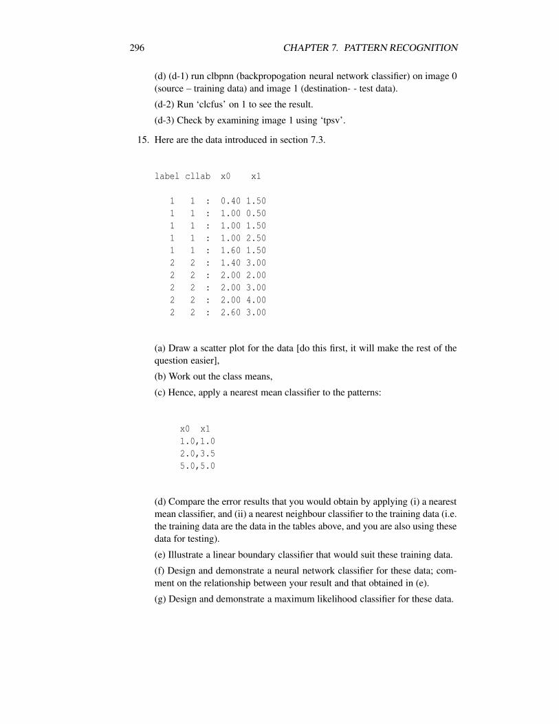
296 CHAPTER 7. PATTERN RECOGNITION
(d) (d-1) run clbpnn (backpropogation neural network classifier) on image 0(source – training data) and image 1 (destination- - test data).
(d-2) Run ‘clcfus’ on 1 to see the result.
(d-3) Check by examining image 1 using ‘tpsv’.
15. Here are the data introduced in section 7.3.
label cllab x0 x1
1 1 : 0.40 1.501 1 : 1.00 0.501 1 : 1.00 1.501 1 : 1.00 2.501 1 : 1.60 1.502 2 : 1.40 3.002 2 : 2.00 2.002 2 : 2.00 3.002 2 : 2.00 4.002 2 : 2.60 3.00
(a) Draw a scatter plot for the data [do this first, it will make the rest of thequestion easier],
(b) Work out the class means,
(c) Hence, apply a nearest mean classifier to the patterns:
x0 x11.0,1.02.0,3.55.0,5.0
(d) Compare the error results that you would obtain by applying (i) a nearestmean classifier, and (ii) a nearest neighbour classifier to the training data (i.e.the training data are the data in the tables above, and you are also using thesedata for testing).
(e) Illustrate a linear boundary classifier that would suit these training data.
(f) Design and demonstrate a neural network classifier for these data; com-ment on the relationship between your result and that obtained in (e).
(g) Design and demonstrate a maximum likelihood classifier for these data.
Chapter 8
Neural Networks
8.1 Introduction
In the search for efficient computing structures for artificial intelligence and knowledge-based systems, one natural and reasonable approach is to attempt to model theworkings of mammalian brains.
The term ‘artificial neural network’ or simply ‘neural network’ refers to com-puting architectures which are supposedly based on the networks present in brains.
There are two common motivations for the study of neural networks:
• to research computational models of human/mammalian mental activity.
• as novel computational structures and algorithms.
We will focus on the latter (algorithmic), and show that neural networks per-form well at a range of computational tasks, and, moreover, that they are stronglyrelated to many well known traditional algorithms.
In addition, our view is that, while human cognitive and computational pro-cesses are surely of interest, so little that is known seems to be practically imple-mentable that psychology seems mostly irrelevant to those who are attempting todevelop artificially intelligent systems. Indeed, there is good reason to questionthe validity of the term ‘artificial intelligence’, per se; it is significant that researchin this area is often now called ‘knowledge engineering’. Futhermore, perhaps thehistory of mechanical intelligence may parallel that of mechanical flight: the realprogress was made when the obsession with feathers and flapping was removed!
However, we will initially accept the claim that, at a mechanical level, much ofwhat goes on in human brains can expressed in terms of (1) pattern recognition, and(2) computation of functions – either logical functions or numerical functions. Wewill show that artificial neural networks are capable of performing simple versionsof these tasks.
As discussed in the previous chapter, pattern recognition is concerned with‘making sense’ of what we see, hear, smell, touch. When you see a face that you
297

298 CHAPTER 8. NEURAL NETWORKS
have seen before, you recognise it: learning, perception, recognition. In the exam-ple developed below, we show a very simple model of text character recognition.
Very roughly, in the context of artificial intelligence and knowledge-based sys-tems, ‘computation of functions’ is to do with creating some new information outof information you already have, e.g. you recognise the character ‘2’ followed by‘+’ followed by ‘5’ and you can infer ‘7’, i.e. arithmetic.
For engineers and computer scientists (forgetting now psychologists and neu-robiologists), interest in neural networks is twofold:
• the fact that the algorithms associated with them seem to be efficient at cer-tain tasks, e.g. pattern recognition; they can ‘learn’ from examples, and are‘model-free’, unlike some competing statistical algorithms (e.g. multiple lin-ear regression).
• they are implementable in parallel and special purpose hardware, i.e. theycan be made to work fast.
Additional impetus arises from the possiblility of implementing neural net-works using optical components – fast, and use little power.
In this lecture we will explain some of the applications of neural networks toimage processing – specifically pattern recognition.
First, in section 9.2, we give a historical background, and discuss the early mo-tivation for neural network research. Then, in section 9.3, we describe the basicsof artificial neurons, their relationship with ‘real’ neurons, and go on to describeperceptrons and multilayer networks. Next, section 9.4, gives a very brief introduc-tion to the implementation of neural networks in software and hardware. Section9.5 introduces training. Since most of the chapter is on backpropogation trainedmultilayer feedforward networks, section 9.6 mentions some other architectures.Section 9.7 is conclusions and summary. Finally, Section 9.8 gives a bibliographyand references.
8.2 Historical Background
See Nagy (1991), Widrow and Lehr (1990), Hecht-Nielsen (1991). The initialstudies of neural networks started in the 1940s by psychologists trying to come upwith a mechanical/mathematical model of human thought (MacCarthy 1955). Itwas then taken up in the 1950s by the AI (artificial-intelligence) community, es-pecially those interested in pattern recognition, – who, not unreasonably, reckonedthat the best way to produce artificial intelligence was to produce artificial brains.And, since brains were believed to be made of networks of ‘processing units’ thatwe call neurons, how better to produce artificial brains than use artificial neuralnetworks.
Significant work on neurophysiology started about 1850, however, the earli-est notable paper is McCullough and Pitts (1943), which started by identifing the

8.2. HISTORICAL BACKGROUND 299
equivalence of the ON/OFF response of a neuron with a (logical) proposition, i.e.has value true or false.
They then went on to show how simple one- and two-input neurons could im-plement the NOT, AND, and OR Boolean functions. Consequently, of course, morecomplex Boolean functions are only a matter of connecting up a network.
Some early work in machine pattern recognition focussed on human patternrecognition from a psychological perspective (e.g. Deutsch 1955), and other con-tributions in the collection Uhr (1966). Others focussed on the physiological struc-ture of mammalian brains and vision and auditory systems, e.g. (Hubel and Wiesel1962). Work on the brains of frogs, culminating in Barlow (1953), identified evi-dence for a ‘matched detector’ for small dark objects (e.g. a fly) – a ‘fly detector’neuron that ‘fires’ when a fly-like object enters the frogs visual field; this was aninspiration for the ‘perceptron’.
Starting around 1956, Frank Rosenblatt, at Cornell University, invented andbuilt the ‘Perceptron’, which, amongst other things, was used to model the pro-cessing that happens in the visual cortex – the part of the brain that does initialprocessing on signals sent from the retina (sensitive part of the eye). It was shownthat a perceptron could recognise (differentiate between) different patterns (seenext section for definition of a pattern). More importantly, it was proved mathe-matically, and demonstrated that a perceptron could ‘learn’; by giving it examplepatterns along with what each pattern ‘represents’ you can get it to self-organise(learn) such that if a pattern similar to one of the learned patterns is encountered,the machine can recognise what it represents. See, for example, Duda and Hart(1973), Block (1962), Rosenblatt (1960), Hecht-Nielsen (1991).
There was also an active group at Stanford led by Bernard Widrow, (Widrowand Lehr, 1990), which developed perceptron-like structures: Adaline, and Mada-line. They developed the Widrow-Hoff or ‘delta-rule’ training algorithm for Ada-line (effectively a perceptron).
However, at the same time, another school of artificial intelligence was beingset up – mostly based on ‘symbolic processing’; this is what you will read in mostcurrent books on AI (see Minsky, 1960). The language LISP was developed forthis sort of AI. PROLOG (PROgramming LOGic) (Bratko, 1991) is another (moreadvanced) example of a symbolic processing approach to AI and knowledge-basedsystems.
Also, much of the pattern recognition work going on was based on statisticaltheory – statistical decision theory; statistical pattern recognition was probablyborn in Chow (1957), but statistical decision theory has been around since theearly 1900s.
Actually, statistics and statistical decision theory are remarkably good exam-ples of knowledge-based systems: knowledge capture may be easy (estimate thestatistical parameters), representation is easy (the parameters), and statistcal infer-ence and decision theory are well understood.
Much work was done on perceptron-like structures until 1969, when MarvinMinsky and Seymour Papert (Massachussetts Institute of Technology) published a

300 CHAPTER 8. NEURAL NETWORKS
book called ‘Perceptrons’, Minsky and Papert (1969), which showed that a sim-ple, single layer perceptron could not differentiate between certain quite dissimilarpatterns (see next section); in addition, they showed that a perceptron could notcompute a very simple function – the XOR function. (Minsky had studied compu-tational aspects of neural networks in his PhD. thesis, 1953 – but I don’t know ofany publications arising from that time). This Minsky-Papert attack proved a greatsetback to neural network research; it caused what neural net researchers call the‘Dark Ages’ – government funding almost completely dried up.
Hecht-Nielsen (1991) attributes a conspiratorial motive to Minsky and Papert,namely, that the MIT AI Laboratory had just been set up and was focussing on LISPbased AI, and needed to spike other consumers of grants. A good story, whateverthe truth, and given extra spice by the coincidence that Minsky and Rosenblattattended the same high-school, and the same class. Moreover, any bitterness isprobably justified because neural network researchers spent the best part of 20years in the wilderness.
Work did not stop however, and the current upsurge of interest began in 1986with the famous PDP books which announced the invention of a viable trainingalgorithm (backpropogation) for multilayer networks (Rumelhart and McClelland,1986).
8.3 Neural Networks Basics
8.3.1 Introduction
This section motivates the study of neural networks by demonstrating how neuralnets do pattern recognition and compute functions. First we give a simplified ac-count of ‘real’ neurons. Then we show how a very simple neuron can perform alimited pattern recognition task. We introduce the ‘perceptron’, and its limitations.Then we show how these limitations can be mitigated by combining neurons in‘layers’.
8.3.2 Brain Cells
Here is a very brief mention of how mammalian brains are thought to be con-structed; and, at a small scale, one theory of how they ‘work’. These brains arecomposed from networks of interconnected neurons.
The following figure shows a neuron and its surroundings. A neuron has acell body with one axon stretching out from the cell body, which also has manydendrites protruding from it.

8.3. NEURAL NETWORKS BASICS 301
A ‘Real’ Neuron.
The axon is the channel by which the neuron sends signals to other neurons.These signals are in the form of a series of electrical pulses – the more frequent thepulses, the stronger the effect of the signal. Axons only transmit – away from theirneuron.
Dendrites receive signals from the axons of other neurons. Between the ax-ons of the transmitter neuron and the dendrites of receiver neurons are synapses.Synapses are narrow regions of conductive material; the strength of the excitationsignal received by the receiver neuron is depends on how well the pulses are con-ducted from the axon (sender) to dentrite (receiver).
Neurons operate by sending signals between one another, and each neuron fires(sends pulses) only if it receives a minimum number of excitory pulses via itsdendrites. The number of excitory pulses received obviously depends on (a) theamount of pulses injected by the connected axons (from other neurons), and (b)the amount of those pulses that are conducted by the synapses.
There are a great many neurons in a typical human brain, perhaps 1011. Thereare even more synapses – perhaps 1016. There is good reason to believe thatsynapses form what we understand as memory.
Artificial neural networks were initially studied in an attempt to model thebrain. In fact, the similarity – actual to artificial – may be relatively slight; however,artificial neural networks are now used as computing structures in their own right.
In the retina of an eye there are light sensitive cells – like neurons; when a cellis illuminated it will transmit pulses via its axon to one (or more than one) otherneuron(s).
8.3.3 Artificial Neurons
The feedforward neural network shown in the following igure is a parallel networkof neurons (processing units, sometimes called nodes).
Each circle in the ANN figure represents a neuron of the form shown; eachperforms the weighted-sum given by the first of the two following equations, fol-lowed by application of the threshold given by the second equation and shown inthe figure.
sum = ∑i=1,n
wixi
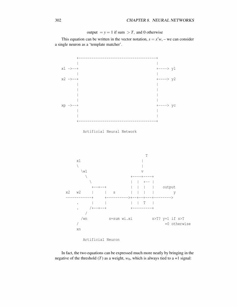
302 CHAPTER 8. NEURAL NETWORKS
output = y = 1 if sum > T, and 0 otherwise
This equation can be written in the vector notation, s = x′w, – we can considera single neuron as a ‘template matcher’.
+------------------------------------+| |
x1 ->--+ +----> y1| |
x2 ->--+ +----> y2| || || || |
xp ->--+ +----> yc| || |+------------------------------------+
Artificial Neural Network
Tx1 |\ |
\w1 v\ +----+----+
\ | | +-- |+--+--+ | | | | output
x2 w2 | | s | | | | y------------+ +---------->+--+--+---+-------->
. | | | | T |
. /+--+--+ +---------+/
/wn s=sum wi.xi s>T? y=1 if s>T/ =0 otherwisexn
Artificial Neuron
In fact, the two equations can be expressed much more neatly by bringing in thenegative of the threshold (T ) as a weight, w0, which is always tied to a +1 signal:
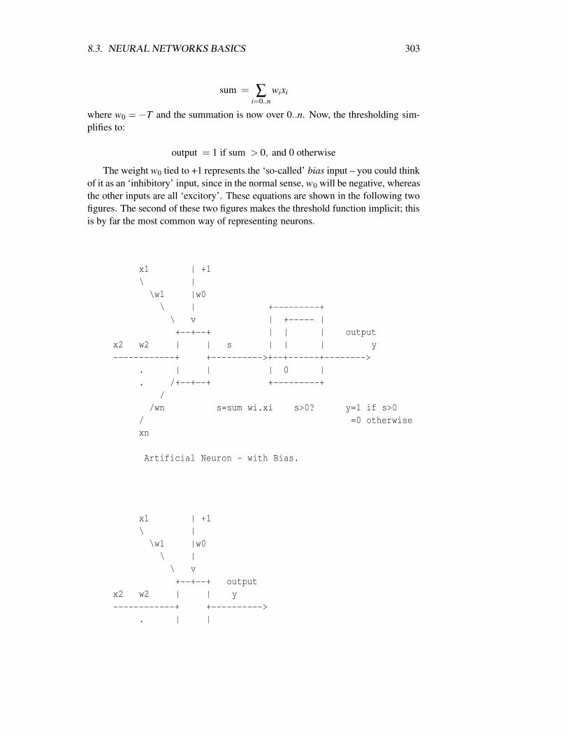
8.3. NEURAL NETWORKS BASICS 303
sum = ∑i=0..n
wixi
where w0 = −T and the summation is now over 0..n. Now, the thresholding sim-plifies to:
output = 1 if sum > 0, and 0 otherwise
The weight w0 tied to +1 represents the ‘so-called’ bias input – you could thinkof it as an ‘inhibitory’ input, since in the normal sense, w0 will be negative, whereasthe other inputs are all ‘excitory’. These equations are shown in the following twofigures. The second of these two figures makes the threshold function implicit; thisis by far the most common way of representing neurons.
x1 | +1\ |
\w1 |w0\ | +---------+\ v | +----- |+--+--+ | | | output
x2 w2 | | s | | | y------------+ +---------->+--+------+-------->
. | | | 0 |
. /+--+--+ +---------+/
/wn s=sum wi.xi s>0? y=1 if s>0/ =0 otherwisexn
Artificial Neuron - with Bias.
x1 | +1\ |
\w1 |w0\ |\ v+--+--+ output
x2 w2 | | y------------+ +---------->
. | |
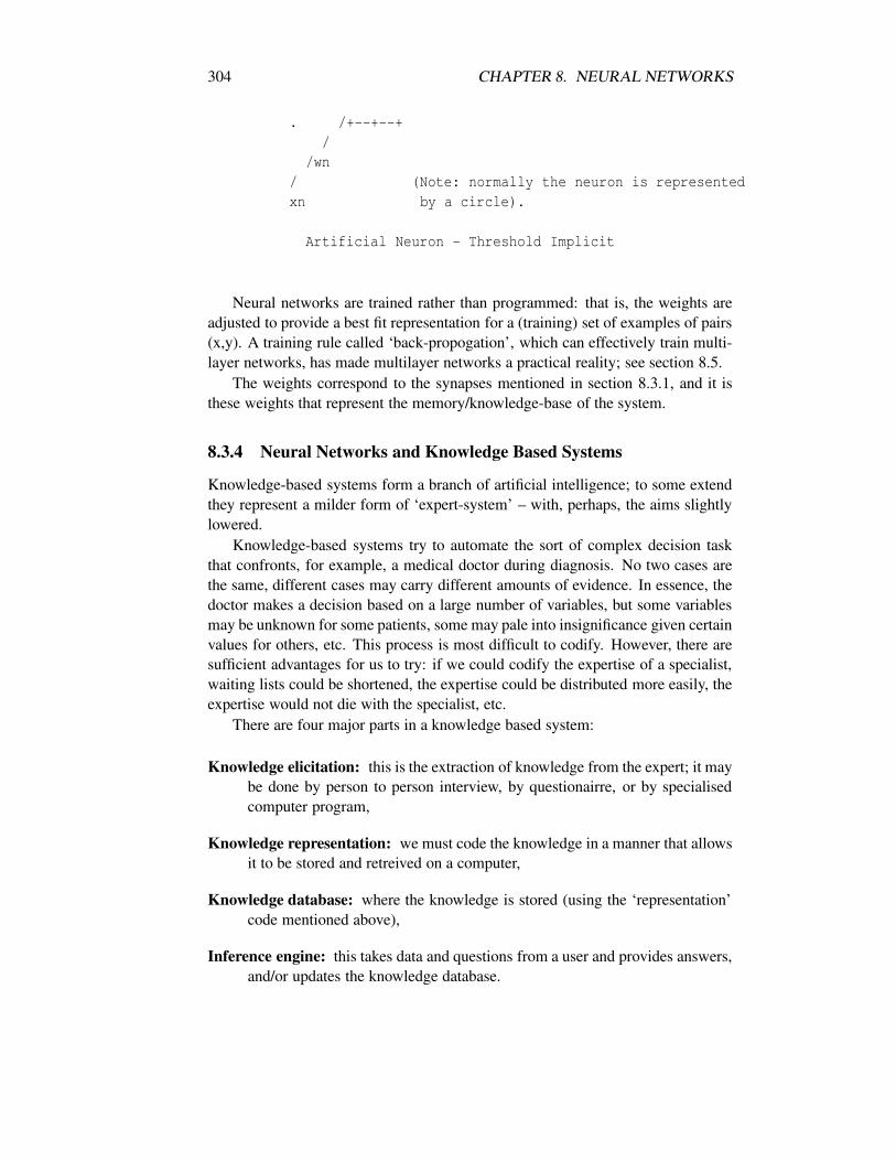
304 CHAPTER 8. NEURAL NETWORKS
. /+--+--+/
/wn/ (Note: normally the neuron is representedxn by a circle).
Artificial Neuron - Threshold Implicit
Neural networks are trained rather than programmed: that is, the weights areadjusted to provide a best fit representation for a (training) set of examples of pairs(x,y). A training rule called ‘back-propogation’, which can effectively train multi-layer networks, has made multilayer networks a practical reality; see section 8.5.
The weights correspond to the synapses mentioned in section 8.3.1, and it isthese weights that represent the memory/knowledge-base of the system.
8.3.4 Neural Networks and Knowledge Based Systems
Knowledge-based systems form a branch of artificial intelligence; to some extendthey represent a milder form of ‘expert-system’ – with, perhaps, the aims slightlylowered.
Knowledge-based systems try to automate the sort of complex decision taskthat confronts, for example, a medical doctor during diagnosis. No two cases arethe same, different cases may carry different amounts of evidence. In essence, thedoctor makes a decision based on a large number of variables, but some variablesmay be unknown for some patients, some may pale into insignificance given certainvalues for others, etc. This process is most difficult to codify. However, there aresufficient advantages for us to try: if we could codify the expertise of a specialist,waiting lists could be shortened, the expertise could be distributed more easily, theexpertise would not die with the specialist, etc.
There are four major parts in a knowledge based system:
Knowledge elicitation: this is the extraction of knowledge from the expert; it maybe done by person to person interview, by questionairre, or by specialisedcomputer program,
Knowledge representation: we must code the knowledge in a manner that allowsit to be stored and retreived on a computer,
Knowledge database: where the knowledge is stored (using the ‘representation’code mentioned above),
Inference engine: this takes data and questions from a user and provides answers,and/or updates the knowledge database.
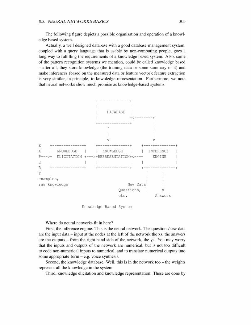
8.3. NEURAL NETWORKS BASICS 305
The following figure depicts a possible organisation and operation of a knowl-edge based system.
Actually, a well designed database with a good database management system,coupled with a query language that is usable by non-computing people, goes along way to fulfilling the requirements of a knowledge based system. Also, someof the pattern recognition systems we mention, could be called knowledge based– after all, they store knowledge (the training data or some summary of it) andmake inferences (based on the measured data or feature vector); feature extractionis very similar, in principle, to knwoledge representation. Furthermore, we notethat neural networks show much promise as knowledge-based systems.
+--------------+| || DATABASE || +<--------++----+---------+ |
ˆ || |v v
E +--------------+ +----+---------+ +----+---------+X | KNOWLEDGE | | KNOWLEDGE | | INFERENCE |P--->+ ELICITATION +--->+REPRESENTATION+<---+ ENGINE |E | | | | | |R +--------------+ +--------------+ +-+------+-----+T ˆ |examples, | |raw knowledge New Data| |
Questions, | vetc. Answers
Knowledge Based System
Where do neural networks fit in here?First, the inference engine. This is the neural network. The questions/new data
are the input data – input at the nodes at the left of the network the xs, the answersare the outputs – from the right hand side of the network, the ys. You may worrythat the inputs and outputs of the network are numerical, but is not too difficultto code non-numerical inputs to numerical, and to translate numerical outputs intosome appropriate form – e.g. voice synthesis.
Second, the knowledge database. Well, this is in the network too – the weightsrepresent all the knowledge in the system.
Third, knowledge elicitation and knowledge representation. These are done by
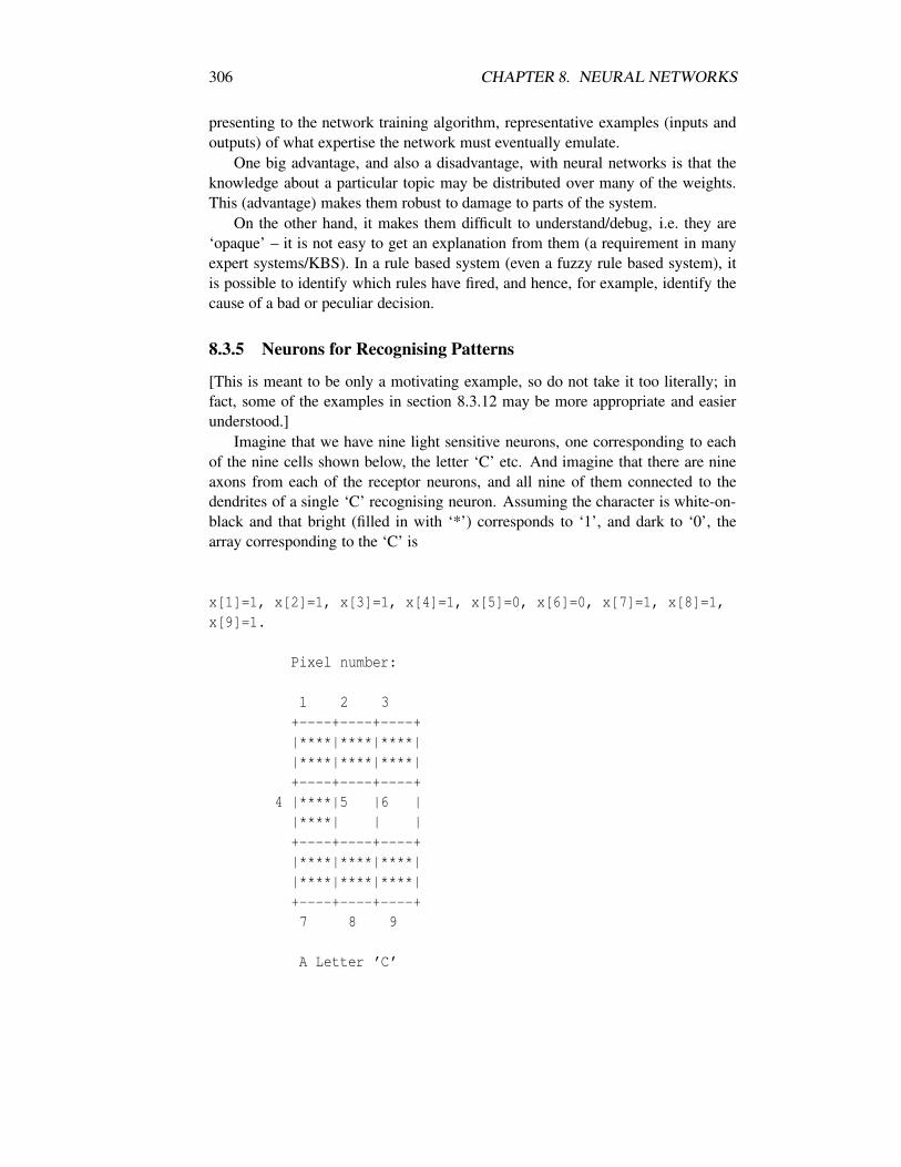
306 CHAPTER 8. NEURAL NETWORKS
presenting to the network training algorithm, representative examples (inputs andoutputs) of what expertise the network must eventually emulate.
One big advantage, and also a disadvantage, with neural networks is that theknowledge about a particular topic may be distributed over many of the weights.This (advantage) makes them robust to damage to parts of the system.
On the other hand, it makes them difficult to understand/debug, i.e. they are‘opaque’ – it is not easy to get an explanation from them (a requirement in manyexpert systems/KBS). In a rule based system (even a fuzzy rule based system), itis possible to identify which rules have fired, and hence, for example, identify thecause of a bad or peculiar decision.
8.3.5 Neurons for Recognising Patterns
[This is meant to be only a motivating example, so do not take it too literally; infact, some of the examples in section 8.3.12 may be more appropriate and easierunderstood.]
Imagine that we have nine light sensitive neurons, one corresponding to eachof the nine cells shown below, the letter ‘C’ etc. And imagine that there are nineaxons from each of the receptor neurons, and all nine of them connected to thedendrites of a single ‘C’ recognising neuron. Assuming the character is white-on-black and that bright (filled in with ‘*’) corresponds to ‘1’, and dark to ‘0’, thearray corresponding to the ‘C’ is
x[1]=1, x[2]=1, x[3]=1, x[4]=1, x[5]=0, x[6]=0, x[7]=1, x[8]=1,x[9]=1.
Pixel number:
1 2 3+----+----+----+|****|****|****||****|****|****|+----+----+----+
4 |****|5 |6 ||****| | |+----+----+----+|****|****|****||****|****|****|+----+----+----+7 8 9
A Letter ’C’

8.3. NEURAL NETWORKS BASICS 307
The letter ‘T’ would give a different observation vector:
’T’: 1,1,1, 0,1,0, 0,1,0
’O’: 1,1,1, 1,0,1, 1,1,1
’C’: 1,1,1, 1,0,0, 1,1,1
etc.So how is the recognition done?
(1) Pixel-by-pixel comparison: Compare the input (candidate) image pixel forpixel; we could code this up in a rule-based system:
if (x[1] == 1) and (x[2] == 1) and (x[3] == 1) and(x[4] == 1) and (x[5] == 0) and (x[6] == 0) and(x[7] == 1) and (x[8] == 1) and (x[9] == 1)
then letter is ’C’.
But we haven’t really solved anything: any minor difference in any pixel wouldfool the system, e.g. addition of a small amount of noise.
(a) The recognition system needs to be invariant (tolerant) to noise.(b) What if there is a minor change in grey level? grey Cs are the same as white
Cs: the system needs to be amplitude invariant – tolerant to changes in amplitude.(2) Maximum Correlation or Template Matching: Compute the correlation
(match) of x with each of the templates for each of the potential letters, and choosethe character with maximum correlation. That is, we choose letter with maximumcorr(elation); this is described mathematically as follows:
x′X j =p−1
∑i=0
xiXi j
i.e. the dot product of x and X j where the latter is the jth template letter.This is called template matching because we are matching (correlating) each
template (the X js), and choosing the one that matches best.Template matching is more immune to noise – we expect the ups and downs of
the noise to balance one another.Returning to artificial neurons, we want to make the ‘C’ neuron emit a ‘1’ when
a ‘C’ appears, and ‘0’ otherwise.If we set up the following vector of weights, wC, for the ‘C’ recognising neuron:
308 CHAPTER 8. NEURAL NETWORKS
set the threshold = w0 = - 6.5
vector element 0 1 2 3 4 5 6 7 8 9
wC = [-6.5, 1,1,1, 1,-1,-1, 1,1,1]
then for a ’C’ input we get:
sumC = -6.5+ 1+1+1+ +1-0-0, +1+1+1= 0.5
which is > 0, so the neuron will fire for a ‘C’.For a ‘T’ input we get:
sumT = -6.5+ 1+1+1 +0-1-0 +0+1+0= -3.5
which is < 0 and so the neuron does not fire.The foregoing discussion is grossly simplified; for example, we have not men-
tioned ‘shift-invariance’: a ‘C’ is a ‘C’ no matter where it appears in the visualfield.
[Actually, we would get better discrimination if we substituted for 0, −1 in theabove, but that is fine detail which will not concern us for now]
8.3.6 Perceptrons
The neuron presented in section 8.3.3 is a single perceptron; actually, it is a ‘straight-through’ perceptron. The distinction is neccessary because Rosenblatt’s perceptronhad an additional layer of so-called ‘associator’ units between the retina and the in-puts to the variable weights, see the following figure.
8.3. NEURAL NETWORKS BASICS 309
Each input of an associator unit is connected via a weight tosome, relatively randomly positioned, cell in the retina; aswell as random positioning, the weights are randomlydistributed in -1, 0, +1.
Perceptron with Associator Units.
8.3.7 Neural Network Training
As stated earlier, neural networks are trained – not programmed. Therefore, thesimple ’C’ neuron would be trained presenting it with a number of examples of’Cs’ and of the other letters, and by adjusting the nine weights until it reliably gave’1’ for ’Cs’ and ’0’ for the others.
8.3.8 Limitations of Perceptrons
For ease of explanation we reduce now the input vector to two dimensions.Recall the following equations:
sum = ∑i=0..n
wixi
where w0 =−T and the summation is now over 0,1,2(n = 2);and the neuron fires if sum > 0 implying, when writing out the equation in full:
sum = w0.(+1)+w1.x1 +w2.x2 (= f (x,w))
> 0 for fire i.e. 1 output≤ 0 for 0 output.
Thus, the (sharp) boundary between the ft(x,w) = 1, and ft(x,w) = 0 ( ft isthresholded function) is given by:
f (x,w) = 0
i.e.w0 +w1x1 +w2x2 = 0
i.e.w1x1 +w2x2 =−w0
This is a straight line which cuts the x1 axis at −(w0/w1) and cuts the x2 axisat −(w0/w2). See the following figure.

310 CHAPTER 8. NEURAL NETWORKS
\ |+ -w0/w2| \| \| \| \
x2 |class 0 \ class 1| \| \| \| \ -w0/w1
0 +-------------------+-------->0 x1 \
Perceptron Linear Decision Boundary
Thus, the perceptron can only discriminate between patterns which can be sep-arated by a (single) straight line. Likewise functions, see section 8.3.8: OR andAND can be computed, BUT XOR cannot; see exercises in section 8.3.12. Thiswas one of the achilles heels that Minsky and Papert successfully attacked.
8.3.9 Neurons for Computing Functions
The neuron in the figure to follow can compute the AND function. The ANDfunction is:
x1 x2 AND(x1,x2) Neuron summation Hard-limit (>0?)----------------- ------------------------------ --------------0 0 0 sum= -1x0.5 + 0.35x0 + 0.35x2 = -0.5 => output=01 0 0 sum= -1x0.5 + 0.35x0 + 0.35x2 = -0.15 => output=00 1 0 sum= -1x0.5 + 0.35x0 + 0.35x2 = -0.15 => output=01 1 1 sum= -1x0.5 + 0.35x0 + 0.35x2 = +0.2 => output= 1------------------ ------------------------------- -------------
x1 +1\ |
\0.35 |\ |-0.5
\ |+--+--+
x2 0.35 | |
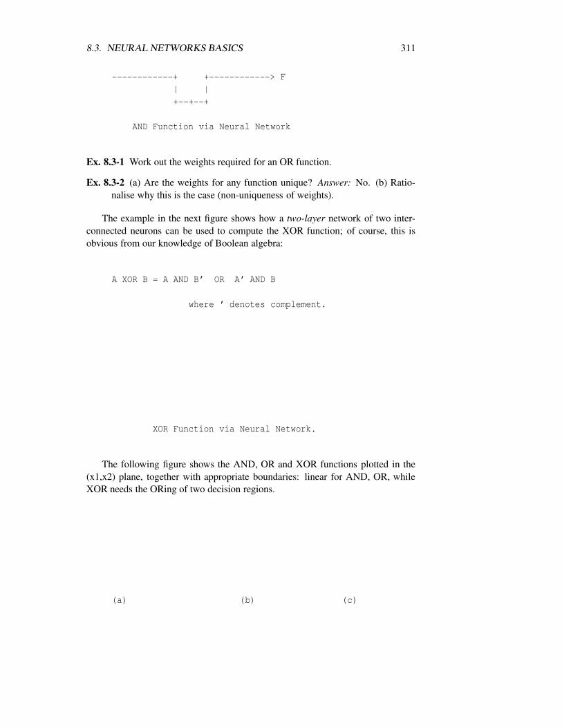
8.3. NEURAL NETWORKS BASICS 311
------------+ +------------> F| |+--+--+
AND Function via Neural Network
Ex. 8.3-1 Work out the weights required for an OR function.
Ex. 8.3-2 (a) Are the weights for any function unique? Answer: No. (b) Ratio-nalise why this is the case (non-uniqueness of weights).
The example in the next figure shows how a two-layer network of two inter-connected neurons can be used to compute the XOR function; of course, this isobvious from our knowledge of Boolean algebra:
A XOR B = A AND B’ OR A’ AND B
where ’ denotes complement.
XOR Function via Neural Network.
The following figure shows the AND, OR and XOR functions plotted in the(x1,x2) plane, together with appropriate boundaries: linear for AND, OR, whileXOR needs the ORing of two decision regions.
(a) (b) (c)

312 CHAPTER 8. NEURAL NETWORKS
Decision Boundaries for (a) AND, (b) OR, (c) XOR
Even though we have analyses only these simple functions, it should be obviousthat combinations of neurons – in a network – can implement arbitrarily complexfunctions, with many inputs.
8.3.10 Complex Boundaries via Multiple Layer Nets
We have shown in the previous section how how two-layers can implement a non-linear decision boundary, now we give qualitative arguments to show that two- andthree-layer networks can implement more complex boundaries/decision regions;actually, three-layers can implement arbitrarily complex boundaries.
The following figures show two input neurons fed into a second-layer neuronthat implements the AND function as given in the previous section. Each of theinput neurons implements a linear boundary, and ANDing the boundaries producesthe decision region shown. Now, it is easy to argue that N input neurons, ANDedtogether, can yield any arbitrary open or closed convex decision region as shown.
Finally, if we add another, third, layer that effectively ORs the convex regionsproduced by the second layer, we can obtain completely arbitrary decision regions.
Feeding perceptron output to another perceptron

8.3. NEURAL NETWORKS BASICS 313
(a) ANDing two (b) (c) ANDing many (d) Thirdlinear boundaries linear boundaries. layer
Complex Decision Regions via Multiple Layers.
8.3.11 ‘Soft’ Threshold Functions
Up to now we have used the hard-limit (McCullough-Pitts ‘all-or-nothing’) neuronactivation function:
output = 1 if sum > 0
= 0 otherwise
For reasons mostly to do with training, most neural networks now use a ‘softer’activation function, namely the sigmoid function (also called the logistic function):
output = 1/(1+ exp(−a sum ))
represented in the following figure. Usually, the ‘gain’ factor is set to 1.0 (obvi-ously, setting a to a very high value yields the simple threshold function ( > 0)).
Sigmoid Function
8.3.12 Multilayer Feedforward Neural Network
The generalised feedforward neural network is a parallel network of neurons. Al-though there is no intrisnic reason against a general topology, so long as the dataflow forward, the layered structure, in which outputs from layer n flow only toinputs in layer n + 1, is preferred in most practical hardware and software imple-mentations.
Early neural network designs, e.g. Nilsson (1965), used so-called threshold(hard-limit) activation functions mentioned earlier; however, the sigmoid is pre-ferred where the network is required to provide other than ‘hard’ decision outputs,and, particularly, for ease of training – see below.
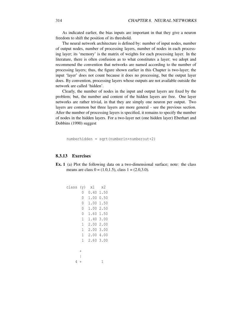
314 CHAPTER 8. NEURAL NETWORKS
As indicated earlier, the bias inputs are important in that they give a neuronfreedom to shift the position of its threshold.
The neural network architecture is defined by: number of input nodes, numberof output nodes, number of processing layers, number of nodes in each process-ing layer; its ‘memory’ is the matrix of weights for each processing layer. In theliterature, there is often confusion as to what constitutes a layer; we adopt andrecommend the convention that networks are named according to the number ofprocessing layers; thus, the figure shown earlier in this Chapter is two-layer; theinput ‘layer’ does not count because it does no processing, but the output layerdoes. By convention, processing layers whose outputs are not available outside thenetwork are called ‘hidden’.
Clearly, the number of nodes in the input and output layers are fixed by theproblem; but, the number and content of the hidden layers are free. One layernetworks are rather trivial, in that they are simply one neuron per output. Twolayers are common but three layers are more general - see the previous section.After the number of processing layers is specified, it remains to specify the numberof nodes in the hidden layers. For a two-layer net (one hidden layer) Eberhart andDobbins (1990) suggest
numberhidden = sqrt(numberin+numberout+2)
8.3.13 Exercises
Ex. 1 (a) Plot the following data on a two-dimensional surface; note: the classmeans are class 0 = (1.0,1.5), class 1 = (2.0,3.0).
class (y) x1 x20 0.40 1.500 1.00 0.500 1.00 1.500 1.00 2.500 1.60 1.501 1.40 3.001 2.00 2.001 2.00 3.001 2.00 4.001 2.60 3.00
+|
4 + 1

8.3. NEURAL NETWORKS BASICS 315
|+|
3 + 1 1 1|+ 0|
2 + 1|+ 0 0 0|
1 +|+ 0|+----+----+----+----+----+----+----> x10 1 2 3
Feature Space Diagram
(b) Verify that a single neuron neural network with the following weights:
w0 = 38.0 (bias)w1 = -13.6 weight on x1w2 = - 8.0 weight on x2
will discriminate between the two classes.
(c) Recall the two-class scatter plot figure earlier in the chapter, and draw theclass boundary. Hint:
intercepts y-axis at -w0/w2 = 4.5x-axis at -w0/w1 = 2.8
(d) Verify that this boundary line approximately bisects the line joining thetwo means.
Ex. 2 In the character recognition example given in section 8.3.4 the feature spaceis nine dimensional. Thus, visualization of the data in feature space is diffi-cult. The following example is easier to visualize.

316 CHAPTER 8. NEURAL NETWORKS
Consider an imaging system which has just two pixels – or, a simple organ-ism which has just two light sensitive cells in its retina, see following figure.Call the outputs of these x1, and x2, therefore they form a two-dimensionalvector x = (x1,x2).
x1 x2+-----+-----+| | || | |+-----+-----+
Two Pixel Image
(a) If the components are binary (0 or 1) we can consider a problem whichwishes to distinguish ‘bright’ objects – class 1, from dark – class 0. For nowwe will define class 1 as ‘both pixels light’. I.e. ’*’ denotes light and class 1:
x1 x2+-----+-----+|*****|*****| class 1|*****|*****|+-----+-----+
x1 x2+-----+-----+|*****| | class 0|*****| |+-----+-----+
x1 x2+-----+-----+| |*****| class 0| |*****|+-----+-----+
x1 x2+-----+-----+| | | class 0| | |+-----+-----+

8.3. NEURAL NETWORKS BASICS 317
Note the similarity with the Boolean AND function.
The feature space representation of these classes are shown in the figurebelow; ‘@’ represents class 0, ‘*’ represents class 1. We have shown a linearboundary which segregates the classes.
ˆ \1 @ \ *
| \| \
x2 | class 0 \ class 1| \| \| \| \
0 @-----------------------------@> \0 x1 1
Two-dimensional Scatter Diagram - Feature Space
(b) Let us change to a problem which wishes to distinguish striped objects(class 0, say) from plain (class 1). I.e. we have (where ’*’ denotes light, class1):
x1 x2+-----+-----+|*****|*****| class 1|*****|*****|+-----+-----+x1 x2
+-----+-----+|*****| | class 0|*****| |+-----+-----+x1 x2
+-----+-----+| |*****| class 0

318 CHAPTER 8. NEURAL NETWORKS
| |*****|+-----+-----+
x1 x2+-----+-----+| | | class 1| | |+-----+-----+
Draw the feature space diagram. Draw appropriate decision boundary line(s)- note the difficulty compared to (a).
Note the similarity with the Boolean XOR function.
(c) Let us change to a problem which wishes to distinguish left-handed ob-jects (class 1, say) from right-handed (class 2), with neither left- or right-handed as reject, class 0. I.e. we have (where ’*’ denotes light, class 1):
x1 x2+-----+-----+|*****|*****| class 0|*****|*****|+-----+-----+
x1 x2+-----+-----+|*****| | class 1|*****| |+-----+-----+
x1 x2+-----+-----+| |*****| class 2| |*****|+-----+-----+
x1 x2+-----+-----+| | | class 0| | |+-----+-----+
Draw the feature space diagram. Show the linear boundaries.
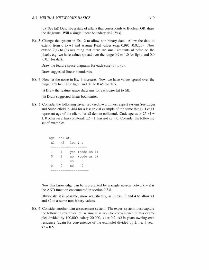
8.3. NEURAL NETWORKS BASICS 319
(d) (See (a)) Describe a state of affairs that corresponds to Boolean OR; drawthe diagrams. Will a single linear boundary do? [Yes].
Ex. 3 Change the system in Ex. 2 to allow non-binary data. Allow the data toextend from 0 to +1 and assume Real values (e.g. 0.995, 0.0256). Nowextend 2(a) to (d) assuming that there are small amounts of noise on thepixels, e.g. we have values spread over the range 0.9 to 1.0 for light, and 0.0to 0.1 for dark.
Draw the feature space diagrams for each case (a) to (d).
Draw suggested linear boundaries.
Ex. 4 Now let the noise in Ex. 3 increase. Now, we have values spread over therange 0.55 to 1.0 for light, and 0.0 to 0.45 for dark.
(i) Draw the feature space diagrams for each case (a) to (d).
(ii) Draw suggested linear boundaries.
Ex. 5 Consider the following trivialised credit-worthiness expert system (see Lugerand Stubblefield, p. 484 for a less trivial example of the same thing). Let x1represent age of the client, let x2 denote collateral. Code age as > 25 x1 =1, 0 otherwise; has collateral: x2 = 1, has not x2 = 0. Consider the followingset of examples:
age collat.x1 x2 loan? y-------------------1 1 yes (code as 1)0 1 no (code as 0)1 0 no 00 0 no 0--------------------
Now this knowledge can be represented by a single neuron network – it isthe AND function encountered in section 9.3.8.
Obviously, it is possible, more realistically, as in exs. 3 and 4 to allow x1and x2 to assume non-binary values.
Ex. 6 Consider another loan-assessement system. The expert system must capturethe following examples. x1 is annual salary (for convenience of this exam-ple) divided by 100,000, salary 20,000, x1 = 0.2. x2 is years owning ownresidence (again for convenience of the example) divided by 2, i.e. 1 year,x2 = 0.5.
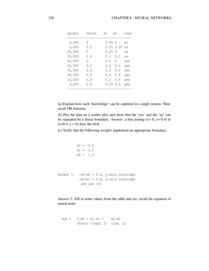
320 CHAPTER 8. NEURAL NETWORKS
salary resid. x1 x2 loan----------------------------------5,000 0 0.05 0 no5,000 0.5 0.05 0.25 no
25,000 0 0.25 0 no10,000 0.2 0.1 0.1 no50,000 0 0.5 0 yes40,000 0.2 0.4 0.1 yes30,000 0.4 0.3 0.2 yes20,000 0.6 0.2 0.3 yes10,000 0.8 0.1 0.4 yes5,000 1.0 0.05 0.5 yes
----------------------------------
(a) Explain how such ‘knowledge’ can be captured in a single neuron. Hint:recall OR function.
(b) Plot the data on a scatter plot, and show that the ‘yes’ and the ‘no’ canbe separated by a linear boundary. Answer: a line joining (x= 0, y= 0.4) to(x=0.4, y = 0) does the trick.
(c) Verify that the following weights implement an appropriate boundary:
w0 = -0.4w1 = 1.0w2 = 1.0
Answer 1. -w0/w2 = 0.4, y-axis intercept-w0/w1 = 0.4, x-axis interceptand see (c)
Answer 2. Fill in some values from the table and see, recall the equation ofneural node:
sum = 1.w0 + x1.w1 + x2.w2(bias) (input 1) (inp. 2)

8.4. IMPLEMENTATION 321
if sum > 0, then output = 1else output = 0
(d) How could this arrangement be extended to include more input variables?
(e) How could this arrangement be extended to include more output vari-ables?
8.4 Implementation
8.4.1 Software
Currently, most neural networks are implemented in software, for example, theneuron in eqns. 9.3-3 and 9.3-4 could be implemented as:
sum: FLOAT;w : ARRAY [0..9] of FLOAT;x : ARRAY [0..9] of FLOAT;
(*NB element 0 = bias*)output,i : INTEGER;
...initialise x
...initialise w
sum:=0;FOR i=0 TO 9 DO
sum:=sum+w[i]*x[i];END;
IF (sum > 0) output =1;ELSE output =0;
8.4.2 Hardware
If we are to operate neural networks in real-time, we must implement them in par-allel or some sort of special purpose fast hardware, so, there are plenty of hardwareimplemented (digital) neural network boards as add-ons for PCs; usually these arebased on DSP chips such as the Texas Instruments TMS32040, or the Intel i860.
Also, there are a number of analogue integrated circuit neural network chips,see e.g. Brauch et al (1992), and IEEE (1992), IEEE (1993) for special issues onneural network hardware.
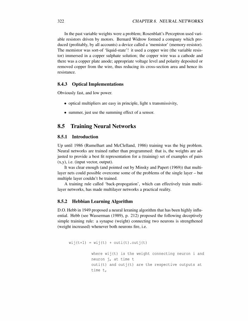
322 CHAPTER 8. NEURAL NETWORKS
In the past variable weights were a problem; Rosenblatt’s Perceptron used vari-able resistors driven by motors. Bernard Widrow formed a company which pro-duced (profitably, by all accounts) a device called a ‘memistor’ (memory-resistor).The memistor was sort-of ‘liquid-state’! it used a copper wire (the variable resis-tor) immersed in a copper sulphate solution; the copper wire was a cathode andthere was a copper plate anode; appropriate voltage level and polarity deposited orremoved copper from the wire, thus reducing its cross-section area and hence itsresistance.
8.4.3 Optical Implementations
Obviously fast, and low power.
• optical multipliers are easy in principle, light x transmissivity,
• summer, just use the summing effect of a sensor.
8.5 Training Neural Networks
8.5.1 Introduction
Up until 1986 (Rumelhart and McClelland, 1986) training was the big problem.Neural networks are trained rather than programmed: that is, the weights are ad-justed to provide a best fit representation for a (training) set of examples of pairs(x,y), i.e. (input vector, output).
It was clear enough (and pointed out by Minsky and Papert (1969)) that multi-layer nets could possible overcome some of the problems of the single layer – butmultiple layer couldn’t be trained.
A training rule called ‘back-propogation’, which can effectively train multi-layer networks, has made multilayer networks a practical reality.
8.5.2 Hebbian Learning Algorithm
D.O. Hebb in 1949 proposed a neural leraning algorithm that has been highly influ-ential. Hebb (see Wasserman (1989), p. 212) proposed the following deceptivelysimple training rule: a synapse (weight) connecting two neurons is strengthened(weight increased) whenever both neurons fire, i.e.
wij(t+1) = wij(t) + outi(t).outj(t)
where wij(t) is the weight connecting neuron i andneuron j, at time touti(t) and outj(t) are the respective outputs attime t,

8.5. TRAINING NEURAL NETWORKS 323
wij(t+1) is the (updated) weight at time t+1.
8.5.3 The Perceptron Training Rule
This is a supervised training rule: the weights are adjusted to provide a best fit rep-resentation for a (training) set of examples of pairs (x,y), i.e. (input vector, output).
Algorithm:---------
Initialise: Set all weights to small random numbers.Loop:
1. Apply an input pattern to the net;compute the output y’
2. Compare y’ with y, the target output3.1 If y’ = y (correct) goto 1.3.2 If incorrect and y’ = 0; add each input xi to its
corresponding weight wi;3.3 If incorrect and y’ = 1; subtract each input xi
from its corresponding weight wi;
Until overall result satisfactory.
Rosenblatt proved that if there was a solution (complete separation) the per-ceptron would find it. However, suboptimal solutions? when to stop? etc.
8.5.4 Widrow-Hoff Rule
Widrow’s Adaline (Widrow and Lehr, 1990) was just a continuous valued versionof the perceptron (as well as binary output, the perceptron has binary inputs). TheWidrow-Hoff training rule is a steepest descent algorithm – it adjusts the weights(and biases) to minimise the sum-of-squares-error (sum of (target − output)2).
Actually, it is only a little different from the perceptron rule: step 3 needsmodification to cope with continuous values:
Algorithm:---------Initialise: Set all weights to small random numbers.Loop:
1. Apply an input pattern to the net;compute the output y’
2. Compare y’ with y, the target output

324 CHAPTER 8. NEURAL NETWORKS
3.1 errorj = yj - y’j ; i.e. target - output, for neuron j3.2 modify weight ij according to:
wij(n+1) = wij(n) + a.xi.errorj
Until overall result satisfactory.
8.5.5 Statistical Training
Actually, the Adaline (continuous valued perceptron) training problem is identicalto linear regression, and so, where the data are suitable, the Moore-Penrose pseudo-inverse yields an appropriate solution. See Duda and Hart (1973).
8.5.6 Backpropogation
Backpropogation is another iterative descent rule. Back-propogation training pro-ceeds in stages:
Initialise:
The weights are initialized to small random values in the range [–.3, .3]
Train:
Repeat until total error small enough:
Repeat for all training data:
(1) a training input vector is applied to the input layer ofthe network and the outputs of the hidden layers, and finally,the output layer are computed,
(2) then the weights of the output neurons (layer n) areadjusted according to gradient descent on the error betweenthe target outputs and the actual outputs;
(3) the weights of the previous layer are adjusted accordingto the same criterion (NB. the adjustments at layer n-1 arestill optimising the overall output -- layer n);
The theory is remarkably concise and simple, depending only on chain rulederivatives; however, the continuity of the sigmoid function, and the simplicity

8.6. OTHER NEURAL NETWORKS 325
of its derivative are crucial. Training continues iteratively: at each iteration allthe example inputs and outputs are presented and they all contribute towards theestimation of the error gradient. Lippmann (1987) gives a concise (half-page) andcomplete specification of the algorithm; van Camp (1993), and Winston (1992)also give good explanations.
There are two big problems with backpropogation:
• long training time (usually), and this is not easy to parallelise,
• the algorithm may get stuck in local minima; the only thing to do (providedyou can determine when it has go stuck, is to reinitialise with fresh randomweights and start again). It is said that XOR will only train correctly 90%of the time; I’ve had no problems with XOR (two-bit input, one bit out), butI’ve had problems with the equivalent four-bit problem. Simulated annealingprovides a possible solution to this problem.
• it is not easy to interpret the weights.
8.5.7 Simulated Annealing
– see Boltzmann training (Wasserman, 1989), p. 81...
8.5.8 Genetic Algorithms
- see Luger and Stubblefield.
8.6 Other Neural Networks
[This is very short, so see any of the textbooks, but especially Wasserman (1989).]– Hopfield: acts as content-addressable memory that can tolerate imperfect inputs,– Kohonen: self-organising (i.e. unsupervised training); for the most part, acts as ak-means clustering algorithm,– Neocognitron: (Fukushima, 1983) shift- and scale-invariant neural network thatis supposed to more closely model the human visual system, than any other net-work,– WISARD (see Boyle and Thomas (1988) ); remarkably simple in concept – basedon RAM memory; a cross between straight look-up table and a perceptron; trainingsimply consists of writing to the RAM, application, readout.– recurrent: layer n+1 outputs fed back to layer n; some promise for prediction.
8.7 Conclusion
The objective of this chapter has been just to give you a flavour of the sorts ofprocessing tasks that neural networks can do. We have made some simplifications,however, the major principles of neural networks are present.
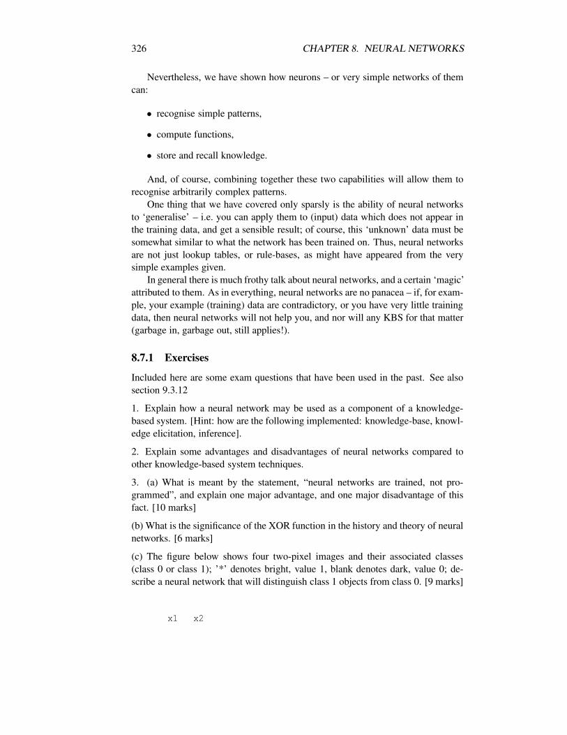
326 CHAPTER 8. NEURAL NETWORKS
Nevertheless, we have shown how neurons – or very simple networks of themcan:
• recognise simple patterns,
• compute functions,
• store and recall knowledge.
And, of course, combining together these two capabilities will allow them torecognise arbitrarily complex patterns.
One thing that we have covered only sparsly is the ability of neural networksto ‘generalise’ – i.e. you can apply them to (input) data which does not appear inthe training data, and get a sensible result; of course, this ‘unknown’ data must besomewhat similar to what the network has been trained on. Thus, neural networksare not just lookup tables, or rule-bases, as might have appeared from the verysimple examples given.
In general there is much frothy talk about neural networks, and a certain ‘magic’attributed to them. As in everything, neural networks are no panacea – if, for exam-ple, your example (training) data are contradictory, or you have very little trainingdata, then neural networks will not help you, and nor will any KBS for that matter(garbage in, garbage out, still applies!).
8.7.1 Exercises
Included here are some exam questions that have been used in the past. See alsosection 9.3.12
1. Explain how a neural network may be used as a component of a knowledge-based system. [Hint: how are the following implemented: knowledge-base, knowl-edge elicitation, inference].
2. Explain some advantages and disadvantages of neural networks compared toother knowledge-based system techniques.
3. (a) What is meant by the statement, “neural networks are trained, not pro-grammed”, and explain one major advantage, and one major disadvantage of thisfact. [10 marks]
(b) What is the significance of the XOR function in the history and theory of neuralnetworks. [6 marks]
(c) The figure below shows four two-pixel images and their associated classes(class 0 or class 1); ’*’ denotes bright, value 1, blank denotes dark, value 0; de-scribe a neural network that will distinguish class 1 objects from class 0. [9 marks]
x1 x2

8.7. CONCLUSION 327
+-----+-----+|*****|*****| class 1|*****|*****|+-----+-----+
x1 x2+-----+-----+|*****| | class 0|*****| |+-----+-----+
x1 x2+-----+-----+| |*****| class 0| |*****|+-----+-----+
x1 x2+-----+-----+| | | class 0| | |+-----+-----+
4. (a) Describe the operation of a two-input, single layer neural network, anddiscuss the difficulty of implementing an XOR function using such a network. [10marks]
(b) The figure below shows four two-pixel images and their associated classes(class 0 or class 1); ’*’ denotes bright, value 1, blank denotes dark, value 0; de-scribe a neural network that will distinguish class 1 objects from class 0. [10 marks]
x1 x2+-----+-----+|*****|*****| class 1|*****|*****|+-----+-----+
x1 x2+-----+-----+|*****| | class 0|*****| |+-----+-----+
x1 x2+-----+-----+| |*****| class 0
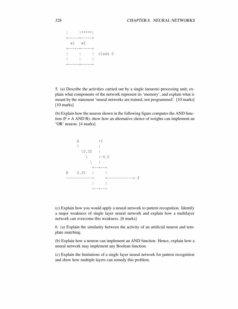
328 CHAPTER 8. NEURAL NETWORKS
| |*****|+-----+-----+
x1 x2+-----+-----+| | | class 0| | |+-----+-----+
5. (a) Describe the activities carried out by a single (neuron) processing unit; ex-plain what components of the network represent its ‘memory’, and explain what ismeant by the statement ‘neural networks are trained, not programmed’. [10 marks][10 marks]
(b) Explain how the neuron shown in the following figure computes the AND func-tion (F = A AND B); show how an alternative choice of weights can implement an’OR’ neuron. [4 marks]
A +1\ |
\0.35 |\ |-0.5
\ |+--+--+
B 0.35 | |------------+ +------------> F
| |+--+--+
(c) Explain how you would apply a neural network to pattern recognition. Identifya major weakness of single layer neural network and explain how a multilayernetwork can overcome this weakness. [6 marks]
6. (a) Explain the similarity between the activity of an artificial neuron and tem-plate matching.
(b) Explain how a neuron can implement an AND function. Hence, explain how aneural network may implement any Boolean function.
(c) Explain the limitations of a single layer neural network for pattern recognitionand show how multiple layers can remedy this problem.

8.8. RECOMMENDED READING 329
7. (a) Explain what components of a neural network represent its ‘memory’, andexplain what is meant by the statement ‘neural networks are trained, not pro-grammed’.
(b) Explain how the neuron shown in the following figure computes the AND func-tion (F = A AND B); show how an alternative choice of weights can implement an’OR’ neuron.
A +1\ |
\0.35 |\ |-0.5\ |+--+--+
B 0.35 | |------------+ +------------> F
| |+--+--+
(c) Explain how you would apply a single neuron to pattern recognition.
(d) Sketch the software implementation of a single neuron.
(e) Explain a weakness of a single neuron (or single layer of neurons) and showhow multiple layers can remedy this problem.
8. (a) Give an intuitive explanation of neural network training.
(b) Explain ‘sigmoid activation function’.
(c) Explain how to use a multiple layer neural network for pattern recognition.What problem does the ‘soft’ sigmoid activation cause, and how is it solved?
(d) what is meant by the statement: “neural networks are model free”.
9. (a) Give feature space explanation of the similarity of pattern recognition andBoolean function computation.
(b) Discuss the difficulty of implementing XOR using a single layer of neurons.
(c) Relate the XOR problem to pattern recognition. [Answer: linear boundaries].
(d) Discuss two weakness of neural netorks.
8.8 Recommended Reading
[This is included mainly for someone who would like to pursue the topic further,e.g. as part of a project/dissertation].
330 CHAPTER 8. NEURAL NETWORKS
The current best book on neural networks is Haykin (1994).Wasserman (1989) is particularly easy and complete for teach-yourself; it cov-
ers all the major architectures, and training algorithms; gets to the essence of thematter often much better than most of the original papers.
From an Artificial Intelligence / Expert Systems point of view, Luger and Stub-blefield (1993), and the other popular AI textbook, Winston (1992), both give goodintroductions to neural networks.
Lippmann (1987) has been the traditional teach-yourself guide – but, in myopinion, is not easy going. Rumelhart and McClelland (1986) was obviously influ-ential but, being an edited collection, seems uneven and not easy to read. There isa companion volume (Vol. 3) that contains software.
Nagy (1991) gives a good brief account of the history; Hecht-Nielsen (1991)gives his own colourful version of the story – but is not a good teach-yourselfbook; ditto Kosko (Fuzzy Sets and Neural Networks): very clever, crusading andinspiring – but the book would have benefited from better editing.
Duda and Hart (1973) is still the classic on pattern recognition; Agrawala(1976) gives many classic pattern recgnition papers. Schalkoff (1990) is a mod-ern pretender – and gives a modern coverage of neural nets (but only feedforwardbackprop.) Uhr (1966) is a collection that includes much of the influential earlywork on human perception and pattern recognition.
IEEE publish a bi-monthly Transactions on Neural Networks. IEEE Trans.on Systems Man and Cybernetics often contains NN applications. Other journalsinclude: Neurocomputing, Neural Computation, Connection Science, Neural Net-works, Neural Network World, and many others.
Applications are covered well in Gonzalez and Woods (1992), Winston (1992),Luger and Stubblefiled (1993); the Rosenfeld Image Processing survey papers(Rosenfeld, 1993, 1992, 1991, etc.) have sections on neural network applicationsto image processing.
Mathematics packages like MATLAB now have promising neural net addi-tions. There are dedicated NN software packages: most of them seem expensivefor what they offer – don’t buy one without a good recommendation, trial, and/orreview. A considerable amount of public domain code is available – do a Websearch. The expected take-off of neural network hardware does not appear to havebeen significant. Neural network chips were available from HNC (Hecht-NielsenCorp.), Siemens, and others, but are do not have any significant market share.
8.9 References and Bibliography
1. Agrawala, A.K. 1976. Machine Recognition of Patterns. IEEE Press.
2. Aleksander, I. and H. Morton. 1990. An Introduction to Neural Computing.London: Chapman and Hall.
8.9. REFERENCES AND BIBLIOGRAPHY 331
3. Arbib, M.A., and J. Buhmann. 1990. Neural Networks Encyclopedia of AI.In Shapiro, 1990.
4. Barlow, H.B. 1953. Summation and Inhibition in the Frog’s Retina. J. Phys-iology, Vol. 119, pp. 69-88.
5. Beck, J.V., and Arnold, K.J., 1977, Parameter Estimation in Engineering andScience, John Wiley.
6. Block, H.D. 1962. The Perceptron: A Model for Brain Functioning. Re-views of Modern Physics, Vol. 34, No. 1, January.
7. Bratko, I. 1991. PROLOG: Programming for Artificial Intelligence. Addison-Wesley.
8. Boyle, R.D. and R.C. Thomas. 1988. Computer Vision: A First Course.Blackwell Scientific.
Includes simple easy to grasp description of WISARD (more than its inven-tors ever managed!).
9. Brauch, J., Tam, S.M., Holler, M.A., and Shmurun, A.L., 1992, AnalogVLSI Neural Networks for Impact Signal Processing, IEEE Micro, Vol. 12,No. 6, December.
10. Brookshear, J.G. 1991. Computer Science: An Overview. Benjamin/Cummings.
See section 10.2, p. 366, for a very accessible and simple introduction toNNs.
11. Campbell, J.G. and A.A. Hashim. 1992. Fuzzy Sets, Pattern Recognition,Linear Estimation, and Neural Networks – a Unification of the Theory withRelevance to Remote Sensing. in Cracknell, A.P. and R.A. Vaughan, eds.Proc. 18th Annual Conf. of the Remote Sensing Society. University ofDundee, September, pp. 508-517.
12. Chow, C.K. 1957. An Optimum Character Recognition System Using Deci-sion Functions. IRE Trans. Electron. Comput., Vol. EC-6, Dec. 1957.
13. Davalo, E. and P. Naim. 1991. Neural Networks, Macmillan Press.
14. Deutsch, J.A. 1955. A Theory of Shape Recognition. British Journal ofPsychology, Vol. 46, pp. 30-37. Reprinted in (Uhr 1966).
15. Devijver, P.A., and J. Kittler. 1982. Pattern Recognition: A Statistical Ap-proach. Englewood Cliffs, NJ: Prentice-Hall.
16. Duda, R.O. and Hart, P.E., 1973, Pattern Classification and Scene Analysis,Wiley-Interscience.
332 CHAPTER 8. NEURAL NETWORKS
17. Eberhart, R.C. and Dobbins, R.W., eds., 1990, Neural Network PC Tools,Academic Press.
18. Feller, W., 1966, An Introduction to Probability Theory and its Applications,Volume II, John Wiley and Sons.
19. Fisher, R.A. 1936. The Use of Multiple Measurements in Taxonomic Prob-lems. Annals of Eugneics. Vol. 7. pp. 179-188. (in Agrawala, 1976).
20. Fix, E. and J.L. Hodges. 1951. Discriminatory Analysis, NonparametricDiscrimination: Consistency Properties. USAF School of Aviation Medicine,Randolph AFB, TX. Project 21-49- 004, Report No. 4, February.
21. Fix, E. and J.L. Hodges. 1952. Discriminatory Analysis, Nonparamet-ric Discrimination: Small Sample Performance. USAF School of AviationMedicine, Randolph AFB, TX. Project 21-49- 004, Report No. 11, August.
22. Funahashi, K-I. 1989. On the Approximate Realisation of Continuous Map-pings by Neural Networks Neural Networks, Vol. 2, pp. 183-192, 1989.
23. Fukushima, K., S. Miyake, and T. Ito. 1983. Neocognitron: A Neural Net-work Model for a Mechanism of Visual Pattern Recognition. IEEE Trans.Systems, Man, and Cybernetics. Vol. SMC-13, No. 5.
24. Fukunaga, K. 1992. Introduction to Statistical Pattern Recognition 2nd ed.Academic Press 1992.
25. Gonzalez, R.C. and R.E. Woods. 1992. Digital Image Processing 3rd ed.Addison-Wesley 1992.
26. Hammerstrom, D. 1993a. Neural Networks at Work IEEE Spectrum June1993, pp. 26-32
27. Hammerstrom, D. 1993b. Working with Neural Networks. IEEE SpectrumJuly 1993, pp. 46-53
28. Haykin, S. 1994. Neural Networks. Macmillan.
29. Hecht-Nielsen, R. 1987. Kolmogorov’s Mapping Neural Network existenceTheorem Proc IEEE 1st International Conference on Neural Network, Vol.III pp. 11-14
30. Hecht-Nielsen, R., 1990, Neurocomputing, Addison-Wesley.
31. Hinton, G.E. 1992. How Neural Networks Learn from Experience ScientificAmerican Sept. 1992.
32. Hopfield, J.J. 1982. Neural Networks and Physical Systems with emergentcollective computational abilities Proc. Natl. Acad. Sci. USA Vol. 79. pp.2554-2558 April 1982
8.9. REFERENCES AND BIBLIOGRAPHY 333
33. Hubel, D.H. and T.N. Weisel. 1962. Receptive Fields, Binocular Interaction,and Functional Architecture in the Cat’s Visual Cortex. Journal of Physiol-ogy. Vol. 160, pp. 106-123. Reprinted in (Uhr 1966).
34. IEEE. 1993. Special Issue on Neural Network Hardware. IEEE Trans. Neu-ral Networks. Vol. 4 No. 3. May.
35. IEEE. 1992. Special Issue on Neural Network Hardware. IEEE Trans. Neu-ral Networks. Vol. 3 No. 3. May.
36. IEEE. 1990a. Special Issue on Neural Networks I: Theory and Modelling.Proceedings of the IEEE, 78, No. 9, Sept. 1990.
37. IEEE. 1990b. Special Issue on Neural Networks I: Analysis, Techniques,and Applications. Proceedings of the IEEE, 78, No. 10, Oct. 1990.
38. IEEE. 1983. Special Issue on Neural and Sensory Information Processing.IEEE Trans. Systems, Man, and Cybernetics. Vol. SMC-13, No. 5.
39. Karnofsky, K. 1993. Neural Networks and Character Recognition Dr. Dobb’sJournal, June 1993.
40. Kosko, B. 1992. Neural Networks and Fuzzy Systems, Prentice-Hall Int.
41. Kosko, B. 1991. Neural Networks for Signal Processing Prentice-Hall 1991
42. Lippmann, R.P., 1987, An Introduction to Computing with Neural Nets,IEEE ASSP Magazine, April.
43. Luger, G.F. and W.A. Stubblefield. 1993. Artificial Intelligence 2nd ed.Benjamin/Cummings.
44. MacCarthy, R.A. 1955. Electronic Principles in Brain Design J. Irish Medi-cal Association. Vol. 37, No. 221. November.
45. McCulloch, W.S., and W. Pitts. 1943. A Logical Calculus of the IdeasImmanent in Nervous Activity. Bulletin of Mathematical Biophysics, Vol.5, 1943.
46. Mehra, P. and B.W. Wah (eds). 1992. Artificial Neural Networks: Conceptsand Theory IEEE Press 1992. (ordered for library 10/8/93).
47. Minsky, M. 1961. Steps Towards Artificial Intelligence. Proc. IRE, Vol. 49,No.1 Jan. 1961.
48. Minsky, M.L., and Papert, S.A., 1969, Perceptrons, MIT Press. Expanded/Reprintededition, 1988, MIT Press.
49. Nagy, G. 1991. Neural Networks – Then and Now. IEEE Trans. NeuralNetworks. Vol. 2 No. 2.
334 CHAPTER 8. NEURAL NETWORKS
50. Nilsson, N.J. 1965. Learning Machines: Foundations of Trainable Pattern-Classifying Systems. New York: McGraw-Hill.
51. Rao Vemuri, V. (ed.). 1992. Artificial Neural Networks: Concepts and Con-trol Applications IEEE Press 1992. (Ordered for library 10/8/93)
52. Rosenblatt, F. 1961. Principles of Neurodynamics: Perceptrons and the The-ory of Brain Mechanisms. Washington D.C.: Spartan Books.
53. Rosenblatt, F. 1960. Perceptron Simulation Experiments. Proc. IRE. Vol.48, pp. 301-309. March.
54. Rosenfeld, A. and A.C. Kak. 1982a. Digital Picture Processing. Vol. 1Academic Press.
55. Rosenfeld, A. and A.C. Kak. 1982b. Digital Picture Processing. Vol. 2Academic Press.
56. Rosenfeld, A. 1992. Survey, Image Analysis and Computer Vision: 1991CVGIP:Image Understanding, Vol. 55, No. 3, May pp. 349-380.
57. Rosenfeld, A. 1993. Survey, Image Analysis and Computer Vision: 1992CVGIP:Image Understanding, Vol. 58, No. 1, July pp. 85-135.
58. Rosenfeld, A. 1990. Survey, Image Analysis and Computer Vision: 1989Computer Vision, Graphics, and Image Processing, Vol. 50, pp. 188-240,1990.
59. Rosenfeld, A. 1989. Survey, Image Analysis and Computer Vision: 1988Computer Vision, Graphics, and Image Processing, Vol. 46, pp. 196-264,1989.
60. Rosenfeld, A. 1988. Survey, Image Analysis and Computer Vision: 1987Computer Vision, Graphics, and Image Processing, Vol. 42, pp. 234-293,1988.
61. Schalkoff, R. 1992. Pattern Recognition: Statistical, Structural and NeuralApproaches Wiley 1992
62. Shapiro, S. (ed.) 1990 Encyclopedia of Artificial Intelligence. ?? (in refer-ence section of Magee library).
63. Therrien, C.W. 1989. Decision Estimation and Classification. New York:JohnWiley.
64. Uhr, L. 1966. Pattern Recognition: Theory, Experiment, Computer Simula-tions, and Dynamic Models of Form Perception and Discovery. New York:John Wiley.
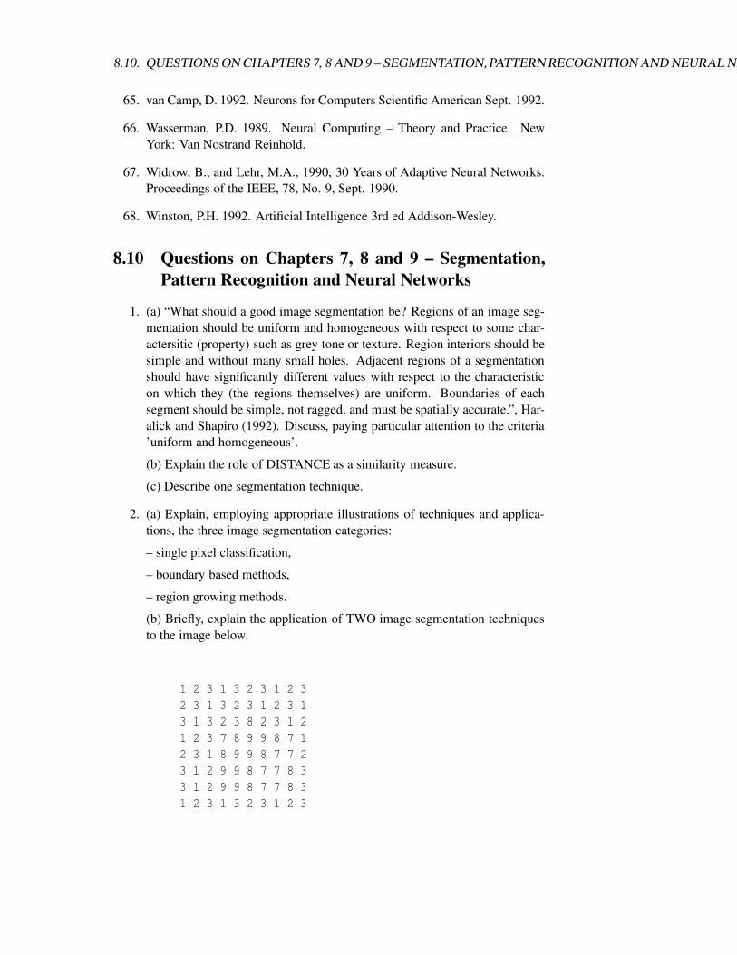
8.10. QUESTIONS ON CHAPTERS 7, 8 AND 9 – SEGMENTATION, PATTERN RECOGNITION AND NEURAL NETWORKS335
65. van Camp, D. 1992. Neurons for Computers Scientific American Sept. 1992.
66. Wasserman, P.D. 1989. Neural Computing – Theory and Practice. NewYork: Van Nostrand Reinhold.
67. Widrow, B., and Lehr, M.A., 1990, 30 Years of Adaptive Neural Networks.Proceedings of the IEEE, 78, No. 9, Sept. 1990.
68. Winston, P.H. 1992. Artificial Intelligence 3rd ed Addison-Wesley.
8.10 Questions on Chapters 7, 8 and 9 – Segmentation,Pattern Recognition and Neural Networks
1. (a) “What should a good image segmentation be? Regions of an image seg-mentation should be uniform and homogeneous with respect to some char-actersitic (property) such as grey tone or texture. Region interiors should besimple and without many small holes. Adjacent regions of a segmentationshould have significantly different values with respect to the characteristicon which they (the regions themselves) are uniform. Boundaries of eachsegment should be simple, not ragged, and must be spatially accurate.”, Har-alick and Shapiro (1992). Discuss, paying particular attention to the criteria’uniform and homogeneous’.
(b) Explain the role of DISTANCE as a similarity measure.
(c) Describe one segmentation technique.
2. (a) Explain, employing appropriate illustrations of techniques and applica-tions, the three image segmentation categories:
– single pixel classification,
– boundary based methods,
– region growing methods.
(b) Briefly, explain the application of TWO image segmentation techniquesto the image below.
1 2 3 1 3 2 3 1 2 32 3 1 3 2 3 1 2 3 13 1 3 2 3 8 2 3 1 21 2 3 7 8 9 9 8 7 12 3 1 8 9 9 8 7 7 23 1 2 9 9 8 7 7 8 33 1 2 9 9 8 7 7 8 31 2 3 1 3 2 3 1 2 3
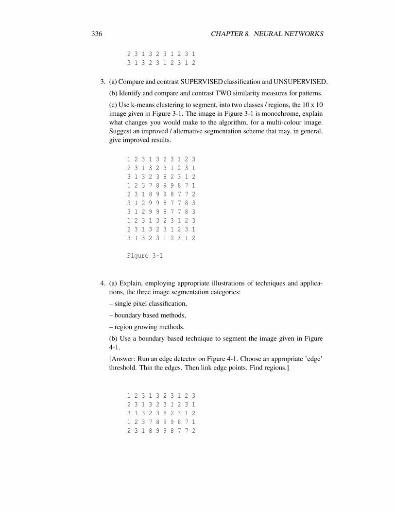
336 CHAPTER 8. NEURAL NETWORKS
2 3 1 3 2 3 1 2 3 13 1 3 2 3 1 2 3 1 2
3. (a) Compare and contrast SUPERVISED classification and UNSUPERVISED.
(b) Identify and compare and contrast TWO similarity measures for patterns.
(c) Use k-means clustering to segment, into two classes / regions, the 10 x 10image given in Figure 3-1. The image in Figure 3-1 is monochrome, explainwhat changes you would make to the algorithm, for a multi-colour image.Suggest an improved / alternative segmentation scheme that may, in general,give improved results.
1 2 3 1 3 2 3 1 2 32 3 1 3 2 3 1 2 3 13 1 3 2 3 8 2 3 1 21 2 3 7 8 9 9 8 7 12 3 1 8 9 9 8 7 7 23 1 2 9 9 8 7 7 8 33 1 2 9 9 8 7 7 8 31 2 3 1 3 2 3 1 2 32 3 1 3 2 3 1 2 3 13 1 3 2 3 1 2 3 1 2
Figure 3-1
4. (a) Explain, employing appropriate illustrations of techniques and applica-tions, the three image segmentation categories:
– single pixel classification,
– boundary based methods,
– region growing methods.
(b) Use a boundary based technique to segment the image given in Figure4-1.
[Answer: Run an edge detector on Figure 4-1. Choose an appropriate ’edge’threshold. Thin the edges. Then link edge points. Find regions.]
1 2 3 1 3 2 3 1 2 32 3 1 3 2 3 1 2 3 13 1 3 2 3 8 2 3 1 21 2 3 7 8 9 9 8 7 12 3 1 8 9 9 8 7 7 2

8.10. QUESTIONS ON CHAPTERS 7, 8 AND 9 – SEGMENTATION, PATTERN RECOGNITION AND NEURAL NETWORKS337
3 1 2 9 9 8 7 7 8 33 1 2 9 9 8 7 7 8 31 2 3 1 3 2 3 1 2 32 3 1 3 2 3 1 2 3 13 1 3 2 3 1 2 3 1 2
Figure 4-1
5. Analyse the problem of segmenting an image of a human face. (Ideally youwant to be able to extract the face from its background.)
(a) Identify the major problems with respect to the simple models of seg-mentation.
(b) Will you need to segment into multiple classes? - As well as separating’face’ from background we may need to segment within the face? Mentionproblems.
(c) Would colour help? How will it affect algorithms?
(d) How will lighting affect the problem?
(e) Suggest a layout for the subject (face), camera, and background.
6. (a) Use a simple example to describe pattern recognition.
(b) In two dimensional shape recognition explain the requirements for:
– shift invariance,
– amplitude invariance,
– scale invariance,
– rotation invariance,
– noise invariance.
(c) Define features / classification techniques that are invariant to any THREE.
7. (a) Using appropriate pictorial or numerical illustrations, explain the roles ofFEATURE VECTOR and FEATURE EXTRACTION in pattern recognition.
[Answer: raw obs -¿ feat extract -¿ feat vect -¿ class; diagram of feat. spacehelpful, .....]
(b) Define two features (ie. use a two-dimensional feature vector) that willdistinguish the shapes given below; plot each shape on a feature space dia-gram.
(c) Illustrate an appropriate classification technique.
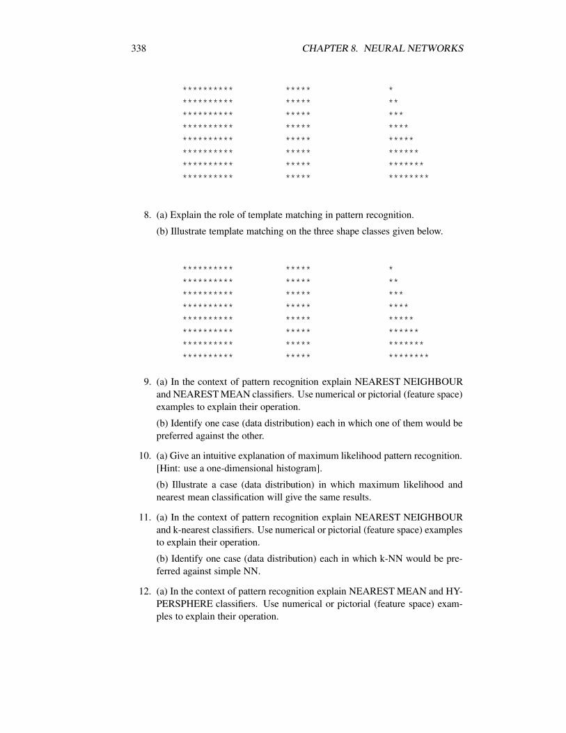
338 CHAPTER 8. NEURAL NETWORKS
********** ***** *********** ***** ************ ***** ************* ***** ************** ***** *************** ***** **************** ***** ***************** ***** ********
8. (a) Explain the role of template matching in pattern recognition.
(b) Illustrate template matching on the three shape classes given below.
********** ***** *********** ***** ************ ***** ************* ***** ************** ***** *************** ***** **************** ***** ***************** ***** ********
9. (a) In the context of pattern recognition explain NEAREST NEIGHBOURand NEAREST MEAN classifiers. Use numerical or pictorial (feature space)examples to explain their operation.
(b) Identify one case (data distribution) each in which one of them would bepreferred against the other.
10. (a) Give an intuitive explanation of maximum likelihood pattern recognition.[Hint: use a one-dimensional histogram].
(b) Illustrate a case (data distribution) in which maximum likelihood andnearest mean classification will give the same results.
11. (a) In the context of pattern recognition explain NEAREST NEIGHBOURand k-nearest classifiers. Use numerical or pictorial (feature space) examplesto explain their operation.
(b) Identify one case (data distribution) each in which k-NN would be pre-ferred against simple NN.
12. (a) In the context of pattern recognition explain NEAREST MEAN and HY-PERSPHERE classifiers. Use numerical or pictorial (feature space) exam-ples to explain their operation.

8.10. QUESTIONS ON CHAPTERS 7, 8 AND 9 – SEGMENTATION, PATTERN RECOGNITION AND NEURAL NETWORKS339
(b) Identify one case (data distribution) each in which one of them would bepreferred against the other.
13. Describe a possible set of steps to be carried out to perform planar shaperecognition in digital images. Illustrate your answer with appropriate pic-tures and numbers. Explain two pitfalls.
14. (a) Draw a histogram for the following data (one-dimensional features) fromtwo classes:
class 0, w0:1.21 3.11 3.97 6.211.32 3.12 4.12 6.581.40 3.21 4.30 7.001.56 3.31 4.702.07 3.37 4.862.21 3.45 4.922.22 3.50 4.972.73 3.78 5.103.00 3.90 5.70
class 1, w1:
6.89 10.03 11.23 11.71 12.378.01 10.31 11.25 11.82 13.018.76 10.45 11.34 11.99 13.509.25 10.56 11.37 12.22 13.579.33 10.72 11.45 12.32 14.609.76 10.80 11.60 12.33
(b) Hence, determine a decision boundary (threshold) that classifies the pointswith minimum error.
(c) Determine the means of each class. What is the effective decision bound-ary for the nearest mean classifier.
(d) If you wanted to use a nearest neighbour classifier, but decided to ’con-dense’ the points, which points are significant and must be retained, in orderto give minimum error.
15. Draw a two-dimensional scatter plot showing the following data:
Class 0:

340 CHAPTER 8. NEURAL NETWORKS
1,11,21,32,12,22,33,13,23,33.5,3.5
class 1:3,33,43,54,34,44,55,35,45,52.5,2.5
(b) Work out the mean vectors of each class.
(c) Hence, apply a nearest mean classifier to the patterns:
2,3.52,5
(d) Compare the error results that you would obtain by applying (i) a nearestmean classifier, and (ii) a nearest neighbour classifier to the training data (ie.the training data are the data in the tables above, and you are also using thesedata for testing).
(e) Illustrate a linear boundary classifier that would suit these training data.
16. Look at Section 8.10, problems 9, 10, 11, 12.
17. (a) Explain the similarity between the activity of an artificial neuron andtemplate matching.
(b) Explain how a neuron can implement an AND function. Hence, explainhow a neural network may implement any Boolean function.

8.10. QUESTIONS ON CHAPTERS 7, 8 AND 9 – SEGMENTATION, PATTERN RECOGNITION AND NEURAL NETWORKS341
(c) Explain the limitations of a single layer neural network for pattern recog-nition and show how multiple layers can remedy this problem.
18. (a) Explain what components of a neural network represent its ’memory’,and explain what is meant by the statement ’neural networks are trained, notprogrammed’.
(b) Explain how the neuron shown in Figure 18-1 computes the AND func-tion (F = A AND B); show how an alternative choice of weights can imple-ment an ’OR’ neuron.
A +1\ |\0.35 |
\ |-0.5\ |+--+--+
B 0.35 | |------------+ +------------> F
| |+--+--+
(c) Explain how you would apply a single neuron to pattern recognition.
(d) Sketch the software implementation of a single neuron.
(e) Explain a weakness of a single neuron (or single layer of neurons) andshow how multiple layers can remedy this problem.
19. (a) Give an intuitive explanation of neural network training.
(b) Explain ’sigmoid activation function’.
(c) Explain how to use a multiple layer neural network for pattern recogni-tion. What problem does the ’soft’ sigmoid activation cause, and how is itsolved?
(d) what is meant by the statement: ”neural networks are model free”.
20. (a) Give feature space explanation of the similarity of pattern recognitionand Boolean function computation.
(b) Discuss the difficulty of implementing XOR using a single layer of neu-rons.
(c) Relate the XOR problem to pattern recognition. [Ans: linear boundaries].
(d) Discuss two weakness of neural netorks.

342 CHAPTER 8. NEURAL NETWORKS
21. (a) In pattern recognition, what is meant by a discriminant. Explain twocommon forms of discriminant.

8.11. RECOMMENDED TEXTS AND INDICATIVE READING 343
8.11 Recommended Texts and Indicative Reading
1. D.H. Ballard and C.M. Brown, Computer Vision, Prentice-Hall 1982
2. H. Bassmann and P.W. Besslich, Ad Oculos – Digital Image Processing,International Thompson 1995. Bassman and Besslich is down to earth andpractical. It has plenty of software examples and comes with a disk.
3. B. Batchelor and P. Whelan, Intelligent Vision Systems for Industry, Springer,1997
4. T.C. Bell, J.G. Cleary, I.H. Witten, Text Compression, Prentice-Hall, 1989
5. C.M. Bishop,
Neural Networks for Pattern Recognition, Oxford University Press, 1995
6. R.D. Boyle and R.C. Thomas, Computer Vision: A First Course, BlackwellScientific 1988
7. S.M. Bozic, Digital and Kalman Filtering, 2nd ed., Edward Arnold, 1994
8. R.N. Bracewell, Two-Dimensional Imaging, Prentice Hall 1995
9. K.R. Castleman, Digital Image Processing, Prentice Hall, 1996
10. S. Chang, Principles of Pictorial Information Systems, Prentice-Hall 1989
11. R. Chellappa, Digital Image Processing, 2nd ed. IEEE Press 1991
12. E.O. Doebelin, Measurement Systems, 4th ed., McGraw-Hill
13. R.O. Duda and P.E. Hart, Pattern Classification and Scene Analysis, Wiley1973. A classic and still very relevant in spite of its age.
14. K.S. Fu, R.C. Gonzalez, and C.S.G. Lee, Robotics – Control, Sensing, Vi-sion, and Intelligence, McGraw-Hill 1987
15. K. Fukunaga, Introduction to Statistical Pattern Recognition, 2nd ed., Aca-demic Press 1992
16. R.C. Gonzalez and P. Wintz, Digital Image Processing, 2nd Ed., Addison-Wesley 1987
17. R.C. Gonzalez and R.E. Woods, Digital Image Processing, Addison-Wesley1992 (effectively 3rd ed. of Gonzalez and Wintz). Gonzalez and Woods isprobably the closest treatment to these notes.
18. U. Grenander, Elements of Pattern Theory, The Johns Hopkins UniversityPress, 1996
344 CHAPTER 8. NEURAL NETWORKS
19. R.W. Hamming, Digital Filters, 3rd ed., Prentice-Hall 1989
20. R.M. Haralick and L.G. Shapiro, Computer and Robot Vision, Volume 1,Addison-Wesley 1992
21. R.M. Haralick and L.G. Shapiro, Computer and Robot Vision, Volume 2,Addison-Wesley 1993
22. D. Harel, Algorithmics – the Spirit of Computing, 2nd ed., Addison-Wesley1992
23. R. Hecht-Nielsen, Neurocomputing, Addison-Wesley 1992
24. C.W. Helstrom, Elements of Signal Detection and Estimation, Prentice Hall1995
25. J. Hertz, A. Krogh and R.G. Palmer, Introduction to the Theory of NeuralComputation, Addison-Wesley, 1991
26. A.K. Jain, Fundamentals of Digital Image Processing, Prentice-Hall 1989
27. R. Jain, R. Kasturi and B. Schunck, Machine Vision, McGraw-Hill, 1995
28. R. Kasturi and R. Jain, Computer Vision: Principles, IEEE 1991. A collec-tion of some key papers.
29. R. Kasturi and R. Jain, Computer Vision: Advances and Applications, IEEE1991. Another collection of pepers.
30. A.D. Kulkarni, Artificial Neural Networks for Image Understanding, VanNostrand Reinhold, 1994
31. J. Lesurf, “Inside Science – Information”, New Scientist, 7 November 1992.A simple introduction to information theory – important for data compres-sion.
32. T.M. Lillesand and R.W. Kiefer, Remote Sensing and Image Interpretation,2nd. ed., John Wiley 1987
33. J.S. Lim, Two-Dimensional Signal and Image Processing, Prentice-Hall 1990
34. A. Low, Introductory Computer Vision and Image Processing McGraw-Hill1991
35. G.F. Luger and W.A. Stubblefield, Artificial Intelligence, 2nd ed., Benjamin/Cummings1993
36. P.A. Lynn and W. Fuerst, Introductory Digital Signal Processing with Com-puter Applications, John Wiley and Sons 1989
8.11. RECOMMENDED TEXTS AND INDICATIVE READING 345
37. David J. Maguire et al. (eds.), Geographical Information Systems, Vol. 1:Principles, Longman 1991
38. David J. Maguire et al. (eds.), Geographical Information Systems, Vol. 2:Applications, Longman 1991
39. T. Masters, Practical Neural Network Recipes in C++, London: AcademicPress, 1993
40. T. Masters, Signal and Image Processing with Neural Networks: A C++Sourcebook, John Wiley, 1994
41. T. Masters, Advanced Algorithms for Neural Networks: a C++ sourcebook,John Wiley 1995
42. T. Masters, Neural, Novel and Hybrid Algorithms for Time Series Prediction,John Wiley 1995
43. J.M. Mendel, Lessons in estimation Theory for Signal Processing Commu-nications and Control, Prentice-Hall 1995
44. M. Nelson, The Data Compression Book, MIS Press, 2nd edn., 1996
45. W. Niblack, An Introduction to Digital Image Processing, 2nd Ed. Prentice-Hall 1986. This is by far the easiest introduction to the material which wecover.
46. A.V. Oppenheim and R.W. Schafer, Digital Signal Processing, Prentice-Hall1975
47. A.V. Oppenheim and R.W. Schafer, Discrete Time Signal Processing, Prentice-Hall 1989
48. J.R. Parker, Practical Computer Vision Using C, Wiley 1994. May be con-sulted for software.
49. J.R. Parker, Algorithms for Image Processing and Computer Vision, JohnWiley, 1997
50. I. Pitas, Digital Image Processing Algorithms, Prentice Hall 1993 This isvery complete but difficult (mathematical) in places.
51. W.K. Pratt, Digital Image Processing, 2nd ed., Wiley 1991
52. W.K. Pratt, PIKS Foundation – C Programmer’s Guide, Prentice-Hall 1995
53. B.D. Ripley, Pattern Recognition and Neural Networks, Cambridge Univer-sity Press, 1996

346 CHAPTER 8. NEURAL NETWORKS
54. A. Rosenfeld and A.C. Kak, Digital Picture Processing – Vol. 1, AcademicPress 1982.
55. A. Rosenfeld and A.C. Kak, Digital Picture Processing – Vol. 2, AcademicPress 1982. Rosenfeld and Kak, in two volumes, is still the best overalltreatment of image processing – the most complete and correct.
56. R.J. Schalkoff, Digital Image Processing and Computer Vision, Wiley 1989
57. R. Schalkoff, Pattern Recognition: Statistical, Structural and Neural Ap-proaches, Wiley 1992
58. M. Sonka, V. Hlavac, and R. Boyle, Image Processing, Analysis and Ma-chine Vision, Chapman and Hall, 1993
59. J.L. Starck, F. Murtagh, and A. Bijaoui, Image and Data Analysis: the Mul-tiscale Approach, Cambridge University Press, 1998
60. J.E. Szymanski, Basic Mathematics for Electronic Engineers, Van NostrandReinhold 1989
61. J. Teuber, Digital Image Processing, Prentice-Hall 1993
62. C.W. Therrien, Decision Estimation and Classification, John Wiley 1989
63. F. van der Heijden, Image Based Measurement Systems, Wiley 1994. Con-tains some good practical material.
64. D. Vernon, Machine Vision, Prentice-Hall 1991
65. P.D. Wasserman, Neural Computing: Theory and Practice, Van Nostrand1989
66. P.D. Wasserman, Advanced Methods in Neural Computing, Van Nostrand1993
67. B. Widrow and S Stearns, Adaptive Signal Processing, Prentice-Hall 1985
68. P.H. Winston, Artificial Intelligence, 3rd ed., Addison-Wesley 1992
Appendix A
Appendix: Essential Mathematics
A.1 Introduction
This Appendix firstly gathers together some basic definitions, symbols and termi-nology to do with random variables, random processes, and random fields; thetopics are chosen according to their applicability to pattern recognition, signal pro-cessing, image processing and data compression. We resent some fundamentaltheorems and definitions related to estimation, prediction, and general analysis ofdata that are generated by random processes.
Secondly, basic definitions of linear algebra are covered. This mathematicallanguage, and tool-set, is invaluable for topics such as pattern recognition and neu-ral networks, image segmentation, and many other areas besides.
A.2 Random Variables, Random Signals and Random Fields
We start by presenting relevant definitions and theorems, and progress to identify-ing the types of (theoretical) processes that will be appropriate models for our data.We identify properties of these processes that are relevant to pattern recognition,signal processing, image processing and data compression.
A.2.1 Basic Probability and Random Variables
Events and Probability
See Rosenfeld and Kak (1982), Mortensen (1987).Let there be a set of outcomes to an experiment:
ω1,ω2,ω3, . . .= Ω
For each wi there is a probability pi:
pi ≥ 0 (A.1)
347

348 APPENDIX A. APPENDIX: ESSENTIAL MATHEMATICS
∑ pi = 1
The simple definition of probability over outcomes is satisfactory for simpleapplications, but for many applications we need to extend it to apply to subsets ofΩ, called events.
Let there be subsets of Ω called events: a general event is a, the set of all a isA. We define a probability measure P on A; P is a number. P satisfies the followingaxioms:
P(a)≥ 0 (A.2)
P(Ω) = 1 (certain event)
ai∩a j = /0∀i, j
a1,a2, . . .are disjoint members ofAand /0is the empty set
P(∪∞k=1 =
∞
∑k=1
P(ak)
Put simply, if ai and a j are disjoint,
P(ai∪ak) = P(ai)+P(ak)
A fourth axiom, which is really a corollary of these is sometimes included:
P(0) = 0 the impossible event
Some Comments on Events and the Probability Measure
This subsection discusses some limitations on events and probabilities which aretheoretical and, in practice of little restriction. This subsection primarily introducessome further terminology related to the previous subsection, and may be skippedby the reader who prefers to continue with more central themes.
Some papers and texts, though of an applied nature, feel obliged to use theterminology of rigorous probability theory; the purpose of this note is to dispelsome of the mystique of that terminology.
As in earlier and subsequent sections, Ω is the set of (elementary) outcomes;and A is the set of subsets of Ω to which probabilities can be allocated.
Theoretically, it is not possible to assign probabilities to all subsets of Ω, butonly to a class of these subsets that form a type of field called a Borel field. This isof no practical consequence, but is an analytical neccessity arising (inter alia) fromthe impossibility of assigning probabilities in the case where there are infinitelymany subsets of Ω, and still have these probabilities satisfy the axioms of proba-bility (eqns. 2.1-2a, b and c). In general, the powerset of Ω is infinite, and the Borel
A.2. RANDOM VARIABLES, RANDOM SIGNALS AND RANDOM FIELDS349
field A which defines the restricted collection of subsets which can be allocated aprobability is not.
The term ‘probability measure was used deliberately; roughly speaking, mea-sure is a method of associating a number with a subset. Measure is a general formof integration: for example, in many practical applications, the definition of prob-ability involves integration over a domain, e.g. integral between x1 and x2 on thereal line. The measurability of a function depends on its values, and its domain.
Example: A simple function, f (x) that is 1 between 0 and 1, and 0 elsewhere:f (x) = 1 : 0≤ x≤ 1, f (x) = 0 : otherwise. Obviously,
Z 1
0f (x)dx = 1
i.e. the area is 1.What then if the function drops to 0 at 0.5, but only at 0.5? Clearly the inte-
gral (area) is still 1, and so on for many such zero values; i.e. the integral is stilldefined, even though the function is not ‘well behaved’ according to our ordinaryunderstanding. However, at some stage, when the number of zeros become infinite,the area must decrease: at this stage (still roughly speaking) the function becomesunmeasurable.
Incidentally, Borel measurability is a general criterion applied to functions; itis claimed that the class of multilayer neural networks with three layers, feedfor-ward, and using a sigmoid activation function can be trained to represent any Borelmeasurable function (see Hecht-Nielsen 1990, p. 122 for a discussion).
Random Variable
If, to every outcome, ω, of an experiment, we assign a number, X(ω), X is called arandom variable (r.v.). X is a function over the set Ω = ω1,ω2, . . . of outcomes;if the range of X is the real numbers or some subset of them, X is a continuousr.v.; if the range of X is some integer set, then X is a discrete r.v.
Distribution Function
Also called cumulative discribution function.
1. Of a continuous r.v.FX(x) = P−∞ < X ≤ x
Note: .. is an event, so that, although X is a function over outcomes (Ω),FX is a function over events.
2. Of a discrete r.v.
If X can assume only a finite number of possible values x1,x2, . . . ,xn, theprobability of the matter can be adequately described by defining a corre-sponding list of probabilities, p1, p2, . . . , pn. In this case FX is shaped like a
350 APPENDIX A. APPENDIX: ESSENTIAL MATHEMATICS
staircase. And, there is little need for the probability density function (of adiscrete r.v.) described below.
Probability Density Function
If FX (continuous) is differentiable,
f X(x) = d/dxFX(x)
is called the probability density function of the r.v. X . Note that the values off X are not probabilities; the values of FX are. f X must be integrated to get usefulprobabilitiy values, e.g.
Px1 ≤ X ≤ x2=
Z x2
x1
f X(x)dx
Expected Value of a Random Variable
1. Continuous.
mX = EX=Z +∞
−∞x f X(x)dx
2. Discrete.
mX = EX = ∑i
xi pi
General interpretation of expected value: average over range of x, weighted byprobability of invividual values.
In practice, it is usual that neither f X(x) nor p are known, and estimates mustbe used: e.g. for the mean of a discrete random variable:
mX =N
∑j=1
x j/N
where the x j are representative examples of the r.v., and where N is large enoughthat the sample, x1, . . . ,xN is large enough that the frequency of occurrence of xvalues properly represents the probabilities.
Random Vector
If the value assigned to an outcome, ω, is vector valued,
X = [X1, . . . ,Xn]
then X is called a random vectors, i.e. X ∈ Rn, rather than X ∈ R, as in subsection2 above.

A.2. RANDOM VARIABLES, RANDOM SIGNALS AND RANDOM FIELDS351
Note: there is temptation to think of x as a sequence of random variables,i.e. each xi generated by a separate outcome, ω. Strictly, this is incorrect: in arandom vector each xi, i = 1 . . .n, is generated by the same outcome. However, Iam unaware of the consequences of making such a mistake. And, on reflection, Isuppose it is possible to ‘manufacture’ a composite experiment whose outcome isa set containing a number of ωs.
A.2.2 Random Processes
Definition
A remark first: the adjective ‘stochastic’ is entirely equivalent to ‘random’; thus thefrquently encountered term ‘stochastic process’ is equivalent to ‘random process’.
Recalling subsection 2.2, a r.v. is a rule for assigning a number, X , to eachoutcome, ω. Correspondingly, a random process is a rule for assigning, to eachoutcome, a function, X(s,ω). s is called the parameter, or the index, of the randomprocess. Sometimes X(s,ω) is written Xs(ω).
S is the set of admissable parameter values, s. In general, S is a subset of thereal line, R, or of Rn. Commonly, S is the time axis, and X is a function of time:X(t,ω), or Xt(ω); this is why t replaces s in most of the literature.
If S is one-dimensional, and discrete (i.e. the parameters can take only a finiteset of values), X is just a random vector, which is equivalent to a discrete parameterrandom process. Note: a discrete state random process refers to one in which thevalues of X are discrete.
Interpretations of a random process (one-dimensional) (see Papoulis, 1991, p.285):
1. A family (an ensemble in the literature) of functions, X(s,ω).
2. A single function, X(s), i.e. ω is fixed.
3. If s is fixed and ω is variable, then X(s) is a random variable equal to thestate of the process at ‘time’ s.
4. If s and ω are fixed, X(s) is a (plain) number.
Although we have used s in this section, we will bow to the preponderanceof usage, and use t (for time) in later sections.
Random Fields
If S is two-dimensional or of greater dimensionality then X is called a randomfield. Thus, if S = x,y : x0 ≤ x ≤ x1,y0 ≤ y ≤ y1, i.e. the domain commonlyassociated with a (continuous) image function, we have a random field (as in e.g.,Rosenfeld and Kak, p.38). Likewise for a discrete image, S = (x1,y1), . . . ,(xn,yn).
352 APPENDIX A. APPENDIX: ESSENTIAL MATHEMATICS
First Order Statistics of Random Processes
Since x(t) is a random variable for a given t, we can extend the definitions ofsection 2.3, 2.4 and 2.5 by including an extra parameter, s (or t).
1. Distribution function.
For a given t,
FX(x, t) = P−∞ < X(t)≤ x
2. Expected Value (Mean).
Continuous case.
mX(t) = EX(t)=
Z +∞
∞x(t) f X(x, t)dx
Likewise, discrete, see eqn 2.5-2.
3. Probability density function, pdf,
f X(x, t) =∂∂x
FX(x, t)
(This is the partial derivative of FX(x, t) with respect to x.)
Second Order Statistics of Random Processes
1. Distribution function.
The second order distribution of the random process x(t) is the joint distri-bution
FXX(x1,x2; t1, t2) = Px(t1)≤ x1,x(t2)≤ x2
2. Probability density function, pdf,
f XX(x, t) =∂2
∂x1∂x2FXX(x1,x2; t1, t2)
And, of course, to fully describe the probability distribution of a random pro-cess it is neccessary to extend to nth-order:
FXt1, . . . ,Xtn(x1, . . . ,xn; t1, . . . , tn) = Px(t1)≤ x1, . . . ,x(tn)≤ xn
FXt1, . . .Xtn in the foregoing equation completely determines the statisticalproperties of x(t). The joint density function f Xt1, . . .Xtn is defined by analogywith the above definition of pdf.

A.2. RANDOM VARIABLES, RANDOM SIGNALS AND RANDOM FIELDS353
Autocorrelation
The autocorrelation of a random process x(t) is the expected value of the productof the two random variables x(t1), x(t2):
Continuous.
RXX(t1, t2) = Ex(t1)x(t2)
=
Z +∞
∞
Z +∞
∞x1x2 f XX(x1,x2; t1, t2)dx1dx2
Discrete.
RXX(ti, t j) =n
∑j=1
n
∑j=1
xix j pi j
From its definition,
RXX(t1, t2) = RXX(t2, t1)
i.e. RXX is symmetric.Autocovariance.
CXX(t1, t2) = E(x(t1)−mX(t1)).(x(t2)−mX(t2))
= RXX(t1, t2)−mX(t1).mX(t2)
Stationary Process
1. Strict-sense stationary (see Papoulis, 1991, p. 297).
Let t1, . . . tn be a set of points in T , likewise t1 + t0, . . . tn + t0; the correspond-ing r.v.s are characterised by nth-order joint pdfs:
f Xt1, . . .Xtn(x(t1), . . . ,x(tn); t1, t2, . . . tn)
, and
f Xt1 + t0, . . . ,Xtn + t0(x(t1 + t0), . . . ,x(tn + t0; t1 + t0, t2 + t0, . . . tn + t0)
When these two functions are equal ∀t0, then the process is strict-sense sta-tionary, i.e. all statistical properties are invariant to shifts in the origin; thereis an analogous definition for random fields (e.g. images).
354 APPENDIX A. APPENDIX: ESSENTIAL MATHEMATICS
2. Wide-sense stationary.
Also called ‘second-order stationary’.
If the following two conditions are met, the process is called wide-sensestationary:
mX(t) = mX
i.e. m is constant for all t, and,
RXX(t1, t2) = RXX(t1− t2)
i.e. the autocorrelation depends only on (t1− t2) (the displacement).
In the discrete case, wide-sense stationarity has the following important con-sequence, when RXX is expressed as a matrix:
RXX = r00 r01 r02 ... r0 n-1r10 r11 r1 n-1
rn-1 0 rn-1 1 ... rn-1 n-1
Applying eqn. 3.6-2
RXX = r0 r1 r2 ... rn-1r1 r0 r1 rn-2
rn-1 rn-2 r1 r0
i.e. RXX is a circulant matrix – each row is merely the previous row rotatedby one position. Sets of linear simultaneous equations that are characterisedby a circulant matrix (or more generally a Toeplitz matrix) can be solvedusing ‘fast’ and recursive algorithms – such solution is required in prediction.
Another property of Toeplitz matrices is that they are diagonalised by theDiscrete Fourier Transform – an important consequence of this fact is thatthe DFT is equivalent to the Karhunen-Loeve Transform for such data (theKL transform is an important transform in lossy data compression).
Incidentally, discrete convolution can be expressed as multiplication by a cir-culant matrix – the delayed impulse response weights form the rows; there-fore the matrix may be disgonalised by the DFT, and this is why convolutiondecomposes into multiplication in the Discrete Fourier domain.
To read further, see Jain (1989), Pratt (1991), and Press et al. (1992).

A.2. RANDOM VARIABLES, RANDOM SIGNALS AND RANDOM FIELDS355
Ergodic Processes
The statistics defined in the previous sections on random processes are defined bytaking the expectation, E., over the ensemble of xs; now, as hinted in eqn. 2.5-3,we rarely have access to a sufficiently large ensemble of xs that we can estimatepdfs; indeed, practically, we rarely have more than one sample, x. If the process isergodic, i.e. roughly speaking, we can replace expectations over the ensemble withtime averages over one sample, we have a practical method by which to estimatestatistics.
Of course, a process first has to be stationary, so that these time averages donot vary with time.
Thus, the mean of a (discrete) ergodic process:
mXi = Exican be estimated
mX = 1/NN
∑i=1
xi
Another example is the estimate of autocorrelation:
R ˆXX(k) = 1/NN
∑i=1
x(i+ k)x(i)
Both eqns. 3.7-1 and 3.7-2 are normally used without qualification.As with stationarity (section 3.6), ergodicity can be wide-sense (e.g. ergodic
in the mean (first-order), ergodic in autocorrelation (second-order) etc., or strict-sense, in which the ergodicity is defined in terms of the probability functions.
Markov Process
A Markov process is a random process in which the probability of achieving anyfuture state depends only on the present, and not on the past. As with stationarityand ergodicity (see section 3.7), Markov processes can be defined as strict sense orwide sense.
The definition of a strict-sense Markov process can be given more formally, interms of conditional pdfs as follows:
f Xtm+1,Xtm+2 . . . ,Xtn | Xt1, . . .Xtm(xm+1,xtm+2 . . . ,xn | x1, . . . ,xm)
= f Xtm, . . .Xtn | Xtm(xm+1, . . . ,xn | xm)
where tm = present time, and | denotes ‘conditional’ (probability).In a strict-sense Markov process, the probabilities of states at tm+1 . . . depend
only on the state at tm (present) and not on tm−1, tm−2, . . . and backwards.

356 APPENDIX A. APPENDIX: ESSENTIAL MATHEMATICS
Clearly this has strong implications for the usage of ‘past’ states in predictingthe future.
In an image context (see Rosenfeld and Kak p. 312), we have Markov randomfields; in that context Markov means that the probability of the state (greylevel) ofa pixel depends only on the states of its eight neighbours.
Gaussian Process
The random process, Xt , is called a Gaussian process, provided that for any finitecollection of ‘times’ (t1, t2, . . . , tn) the vector of states x = (xt1,xt2, . . . ,xtn) has thejoint pdf:
f x(x) = (12
πn/2)(|Cxx | 12)exp−1
2(x−m)TCxx−1(x−m)
where Cxx is the autocovariance (see eqn 3.5-4), m = Ext and | . | denotes deter-minant.
Gaussian processes are good models for many natural random processes. Inaddition, they are analytically convenient, And, see eqn. 3.9-1, their pdf is totallydetermined by first and second order statistics (mean and autocovariance, respec-tively).
A.2.3 Further Background Reading
1. Chung, K.L. 1968. A Course in Probability Theory. New York: Harcourt,Brace and World.
2. Feller, W. 1966. An Introduction to Probability Theory and its Applications.Vol II. New York: John Wiley and Sons.
3. Hecht-Nielsen R. 1990. Neurocomputing. Reading, Mass: Addison- Wes-ley.
4. A.K. Jain. 1989. Fundamentals of Digital Image Processing. EnglewoodCliffs, NJ: Prentice-Hall Int.
5. Kosko, B. 1992. Neural Networks and Fuzzy Systems. Englewood Cliffs,NJ: Prentice-Hall Int., 1992
6. Mortensen R.E. 1987. Random Signals and Systems. New York: John Wileyand Sons.
7. Papoulis A. 1991. Probability, Random Variables and Stochastic Processes.3rd ed. New York: McGraw-Hill.
8. W.K. Pratt. 1991. Digital Image Processing. New York: Wiley- Interscience.
9. W.H. Press, S.A. Teukolsky, W.T. Vetterling,and B.P. Flannery. 1992. Nu-merical Recipes in C. Cambridge, U.K. : Cambridge University Press.

A.3. LINEAR ALGEBRA 357
10. Proakis J.G. 1989. Digital Communications. 2nd ed. New York: McGraw-Hill.
11. Rosenfeld A. and A.C. Kak. 1982. Digital Picture Processing. 2nd ed.London: Academic Press. (2 Volumes).
12. Thomasian, A.J. 1969. The Structure of Probability Theory with Applica-tions. New York: McGraw-Hill.
13. Widrow, B., and Lehr, M.A. 1990. 30 Years of Adaptive Neural Networks.Proceedings of the IEEE. 78, No. 9.
A.3 Linear Algebra
A.3.1 Basic Definitions
Vectors and Matrices
Pattern or measurement vector before any processing:
x = (x0,x1, . . .xi, . . .xp−1)T
a p×1 column vector.After transformation:
y = (y0,y1, . . .yi, . . .yp−1)T
a q×1 column vector.A matrix transformation is defined by an equation of the form:
y = Ax
wit respective dimensionalities: q×1,q× p, and p×1.
Multivariate Statistics
x = (x0,x1, . . .xi, . . .xp−1)T
a p×1 feature vector.Mean vector:
m = (m0,m1, . . .mi, . . .mp−1)T
= Ex
where E. denotes expectation.
358 APPENDIX A. APPENDIX: ESSENTIAL MATHEMATICS
Normally we estimate expected values using the sample average, e.g. mean mis estimated using the average of x computed over a sample of n values, genericallycalled xi:
m =1n
n
∑i=1
xi
Autocorrelation matrix:
R = ExxT= [ri j]
whereri j = Exix j
the expected value of the product of the ith and jth components of x.Normally we will use the sample autocorrelation matrix, i.e. R estimated from
a sample of n vectors, xi, i = 1 . . .n,
R =1n
n
∑i=1
xixi
It is sometimes convenient to write (2.2-5) completely in matrix notation; let Xbe the p×n matrix formed by arranging the n xi values as columns
X = [x1x2 . . .xi . . .xn]
a p×n matrix, now eqn. 2.2-5 can be rewritten as
R =1n
XXT
Covariance matrix:
S = E(x−m)(x−m)T
= [si j]
where
si j = E(xi−mi)(x j−m j)the expected value of the product of the ith and jth components of the deviation ofx from its mean.
The diagonal elements sii of S are the variances of the element xi.It is easy to verify that:
S = R−mmT
A.3. LINEAR ALGEBRA 359
Also, there is a matrix representation, analogous to eqn. (2.2-7), see the dis-cussion of autocorrelation above.
If x′ = (x−m), i.e. the pattern vector reduced to zero mean, and
X ′= [x′1x′2 . . .x′i . . .x′n]
of dimensions p×n, then the sample covariance can be rewritten as
S =1n
X ′X ′T
Multivariate Gaussian Random Vectors:Multivariate vectors generated by a multivariate random process follow the
probability density function (pdf):
fx(x) = (12
πn2)(| S | 1
2)exp−1
2(x−m)T S−1(x−m)
where S is the covariance matrix (see (2.2-8), m = Ex (see eqn. 2.2-1), and | . |denotes determinant.
Gaussian processes are good models for many natural random processes. Inaddition, they are analytically convenient, since their pdf is totally determined byfirst and second order statistics (mean and covariance, respectively).
Statistics after Transformation:If we transform into a feature space using eqn. (2.1-1), y = Ax, the mean,
autocorrelation, and covariance statistics are transformed as follows:Mean: m′ = AmAutocorrelation: R′= ARAT
Covariance: S′ = ASAT
Prior Probabilities:Many pattern recognition algorithms use (estimates of) the relative frequency
of occurrence of the various classes in the population; these are called prior, ora priori, probabilities, because these probabilities are known before any measure-ment is made.
Prior probabilities are denoted P1,P2 etc. for P(class 1) etc.Contrast posterior, or a posteriori probabilities, which are the probabilities of
the classes after the measurements have been taken into account.
A.3.2 Linear Simultaneous Equations
Eqn. 3.1 is a system of linear (simultaneous) equations.
y1 = 3x1 +1x2 (A.3)
y2 = 2x1 +4x2
360 APPENDIX A. APPENDIX: ESSENTIAL MATHEMATICS
Ex. 3.2.1-1 Practically, Eqn. 3.1 could express the following:
Price of an apple = x1, price of an orange = x2 (both unknown). Person Abuys 3 oranges, and 1 apple and the total bill is 5p (y1). Person B buys 2oranges, 4 apples and the total bill is 10p (y2).
Question: What is x1, the price of apples, and x2, the price of oranges?
(1) 5 = 1x1 +3x2
(2) 10 = 4x1 +2x2
(1) =⇒ x2 =−5+3x1
Substitute into (2):
10 = 4x1 +2(−5+3x1)
10 = 10x1−10
20 = 10x1
2 = x1
Now, substitute x1 = 2 into (1):
5 = 2+3x2
3 = 3x2
x2 = 1
The simultaneous equations 3.1 can be written in matrix form as follows:
y = Ax
where y is a two-dimensional vector, y =
(
y1y2
)
x is a two-dimensional vector,
x =
(
x1x2
)
and A is a 2 row × 2 column matrix, A =
(
1 34 2
)
Note: a vector is simply an array of numbers. A vector with n numbers is calledan n-dimensional vector; such a vector represents a point in n-dimensional space.Don’t try to visualise n > 3! Just think of the n numbers grouped together.
In two- or three-dimensions it is possible to visualise a vector as a line with anarrow-head – the arrow indicates the path between the origin (0,0) and the point(x,y) that the vector represents; again, for our purposes this view has limited use.
Generally, a system of m equations, in n variables,
y1 = a11x1 +a12x2 · · ·+a1nxn
A.3. LINEAR ALGEBRA 361
y2 = a21x1 +a22x2 · · ·+a2nxn
. . .
yr = ar1x1 +ar2x2 · · ·+arcxc · · ·+arnxn
. . .
ym = am1x1 +am2x2 · · ·+amnxn
can be written in matrix form as,
y = Ax (A.4)
where y is an m-dimensional vector
y =
y1y2..ym
x is an n-dimensional vector,
x =
x1x2..xm
and A is an m-row × n-column matrix
A =
a11 a12 a1na21 a22 a2n.. .. .. .... arc .. .... .. .. ..am1 am2 .. amn
That is, the matrix A is a rectangular array of numbers whose element in row r,column c is arc. The matrix A is said to be m×n, i.e. m rows, n columns.
Vectors can be considered as specialisations of matrices, i.e. matrices with onlyone column. Thus x is m×1, and y is n×1.
Eqns. 3.1 or 3.2 can be interpreted as the definition of a function which takesn arguments (x1,x2..xn) and returns m variables (y1,y2 . . .ym). Such a function isalso called a transformation: it transforms n-tuples of real numbers to m-tuples ofreal numbers.
Eqn. 3.2 is a linear transformation because there are no terms in x2r or higher,
only in xr.

362 APPENDIX A. APPENDIX: ESSENTIAL MATHEMATICS
A.3.3 Basic Matrix Operations
Matrix Multiplication
We may multiply two matrices A,m× n, and B,q× p, as long as n = q. Such amultiplication produces an m× p result. Thus,
C = A Bm× p m×n n× p
(A.5)
Method: The element at the rth row and cth column of C is the product (dot orinner or scalar product) of the rth row vector of A with the cth column vector of B.
Pictorially:
n p p---------------- ---------- -----------|----> | | | | | || A | | B | | = | C || | | | | | |
m | | | | | n | | m---------------- | V | -----------
| || |----------
Thus,C = AB
A =
(
a11 a12a21 a22
)
B =
(
b11 b12b21 b22
)
C =
(
a11b11 +a12b21 a11b12 +a12b22a21b11 +a22b21 a21b12 +a22b22
)
Ex. 3.2.2-1 Consider Eqn. 3.2, y = Ax. Thus the product of A(m×n) and x(n×1)
y1 = a11x1 +a12x2 · · ·+a1nxn
(row1 col1 = product of 1st row of A with 1st column of x) etc.
The product is (m×n)× (n×1) so the result is (m×1), i.e. y.

A.3. LINEAR ALGEBRA 363
Ex. 3.2.2-2 Apply the transformation given by(
3 12 4
)
to
x =
(
12
)
Scaling and Rotation
Consider scaling and rotation in computer graphics. Here the vectors are:(
xy
)
and the output, transformed, vector is:(
x′
y′
)
The scaling transformation takes the form:
x′ = xSx
y′ = ySy
That is, x is expanded (Sx > 1) or contracted (Sx < 1) to give x′; ditto y-axis. Sx andSy are called scaling factors. The matrix is
(
Sx 00 Sy
)
The following transformation rotates (x,y) a clockwise angle B about the origin(0,0):
x′ = xcos B+ ysinB
y′ =−xsinB+ ycosB
The matrix is
R(B) =
(
cos B sinB−sinB cosB
)
(A.6)
Ex. 3.2.3-1 (a) Rotate the point
(
0.7070.707
)

364 APPENDIX A. APPENDIX: ESSENTIAL MATHEMATICS
clockwise by 45 degrees.
(Note: sin45 = 0.707 = 1/√
2 = cos45;0.707×0.707 = 0.5 .)
(b) Rotate the point
(
01
)
clockwise by 90 degrees.
Ex. 3.2.3-2 What is the effect of applying the rotation matrix twice? That is,
what is
R(B)R(B)
(
xy
)
The following formulae may be useful:
sin(a+b) = sin(a)cos(b)+ cos(a)sin(b)
cos(a+b) = cos(a)cos(b)− sin(a)sin(b)
Ex. 3.2.3-3 What is the effect of applying the negative rotation, −B, to a point thathas already been rotated by +B. That is, what is
R(−B)R(B)
(
xy
)
Multiplication by a Scalar
c(
a11 a12a21 a22
)
=
(
ca11 ca12ca21 ca22
)
Addition of Matrices(
a11 a12a21 a22
)
+
(
b11 b12b21 b22
)
=
(
a11 +b11 a12 +b12a21 +b21 a22 +b22
)
The matrices must be the same size (dimensions).
A.3. LINEAR ALGEBRA 365
Inverses of Matrices
Only for square matrices (m = n).Consider Eqn. 3.1:
y1 = 3x1 +1x2
y2 = 2x1 +4x2
i.e. y = Ax where
y =
(
y1y2
)
x =
(
x1x2
)
A =
(
3 12 4
)
Apply this to
x =
(
12
)
Get:
y1 = 3.1+1.2 = 5
y2 = 2.1+4.2 = 10
What if you know y = (5,10) and want to retrieve x = (x1,x2)?Answer: Apply the inverse transformation to y. That is, multiply y by the
inverse of the matrix.
x = A−1y
In the case of a 2 × 2 matrix
A =
(
a11 a12a21 a22
)
A−1 =1| A |
(
a22 −a12−a21 a11
)
(A.7)
where the determinant of the array, A, is | A |= a11a22−a12a21If | A | is zero, then A is not invertible, it is singular.Thus for
A =
(
3 12 4
)
366 APPENDIX A. APPENDIX: ESSENTIAL MATHEMATICS
we have | A |= 3×4−2×1 = 10 so
A−1 = (1/10)
(
4 −1−2 3
)
=
(
0.4 −0.1−0.2 0.3
)
Therefore, apply A−1 to(
510
)
We find: A−1y =
(
0.4 −0.1−0.2 0.3
)
.
(
510
)
=
(
5×0.4+10×−0.15×−0.2+10×0.3
)
=
(
12
)
which is what we started off with, i.e.
x =
(
12
)
Note: in Ex. 3.2.1-1 (this was solving the linear equation system for the priceof apples and oranges), we were actually doing something that is very similar toinverting the matrix
A =
(
3 12 4
)
A.3.4 Particular Matrices
Diagonal Matrices
The scaling matrix mentioned in section 3.2.3
A =
(
Sx 00 Sy
)
is diagonal, i.e. the only non-zero elements are on the diagonal.The inverse of a diagonal matrix
(
a11 00 a22
)
is(
1/a11 00 1/a22
)

A.3. LINEAR ALGEBRA 367
Transpose of a Matrix (At )
Only for square matrices. If(
A =a11 a12a21 a22
)
then(
At =a11 a21a12 a22
)
i.e. replace column 1 with row 1 etc.The transpose is often written as At or AT or A′. It is pronounced ‘A-transpose’.
The Identity Matrix
I =
(
1 00 1
)
i.e. produces no transformation effect. Thus, IA = ANote: If AB = I then B = A−1.
Orthogonal Matrix
A matrix which satisfies the property:
AAt = I
i.e. the transpose of the matrix is its inverse.Another way of viewing this is:For each row of the matrix (ar1ar2....arn), the dot product with itself is 1, and
with all other rows 0 (see section 3.2.13). I.e.
∑nc=1 arcapc = 1 for r = p
= 0 otherwise
A.3.5 Complex Numbers
A complex number is simply a convenient way of representing the pair of numbersthat represent the coordinates (x,y) of points in a plane,
z = x+ jy
where j =√−1.
In many ways, a complex number is like a two-dimensional vector.The modulus of the complex number (which may be interpreted as the distance
between the origin and (x,y) ) is given by:
| z | = | x+ jy | =√
(x× x+ y× y)
368 APPENDIX A. APPENDIX: ESSENTIAL MATHEMATICS
i.e. using Pythagoras’ TheoremThe angle, or argument, which may be interpreted as the angle between the line
(0,0) to (x,y) and the x-axis, is given by:
arg z = arctan y/x
i.e. the angle whose tangent (opposite/adjacent) is y/x.Addition of complex numbers is as follows: If
z = x+ jy, w = u+ jv
thenz+w = x+u+ j(y+ v)
A graphical interpretation of addition of complex numbers is,– draw a line from (0,0) to (x,y),– using (x,y) as the origin, draw a line to (u,v),– the point reached is (x+u,y+ v).I.e. vector addition.Multiplication of complex numbers is as follows:
Ifz = x+ jy, w = u+ jv
thenz.w = (x+ jy).(u+ jv) = x.u+ j. j.y.v+ j.(y.u+ x.v)
We use j. j =−1 (i.e.√−1√−1 =−1) This gives:
z.w = (x.u− y.v)+ j.(y.u+ x.v)
Note: if complex numbers have zero imaginary parts, the rules given here col-lapse to the rules of normal arithmetic for real numbers.
Ex. 3.2.11-1 Verify the last statement, i.e. set y,v = 0 in addition and multiplica-tion of complex numbers.
The complex conjugate of a complex number, c = a+ jb is
c∗ = a− jb
Complex Numbers and Matrices
Matrices and vectors can contain complex numbers. The rules for matrix addition,multiplication, given above, all apply; we just replace the normal addition, mul-tiplication with the complex versions given in the previous section dealing with“Complex Numbers”.
A.3. LINEAR ALGEBRA 369
A.3.6 Further Matrix and Vector Operations
Vector Inner (Dot) Product
Let vector
x =
x1x2..xn
i.e. x = (x1,x2, . . .xn)t (t denotes transpose), and vector y = (y1,y2, . . .yn)
t
The inner product (dot product, scalar product) of x and y is the matrix product(see section 3.2.2)
xt y
Dimensions: 1×1, 1×n, n×1This is the same as:
xyt =n
∑i=1
xiyi
If the dot product of two vectors is 0, they are said to be orthogonal, see section3.2.10 above, and 3.2.16, 17 and 18 below.
Vector Addition
Three n×1 vectors x,y,z:
z = x+ y
with
z1z2..zn
=
x1 + y1x2 + y2..xn + yn
Distance between Vectors
Considering n-dimensional vectors as points in n-dimensional space, we can talkabout the distance, d, between vectors x and y. The following is the squared dis-tance:
d2(x,y) = (x1− y1)2 +(x2− y2)
2 + · · ·+(xn− yn)2
or
d2(x,y) =n
∑i=1
(xi− yi)2 (A.8)

370 APPENDIX A. APPENDIX: ESSENTIAL MATHEMATICS
Ex. 3.2.15-1 Determine the Euclidean distance between the points (1,1), (1,3).
|3 + * (1,3)
|2 +
|dim 2 1 + * (1,1)
|+---+---+---+---+---+---
1 2 3 4 dim 1
d =√
(1−1)2 +(1−3)2 =√
0+4 = 2
Length or Magnitude of a Vector
Considering now an n-dimensional vector as the line joining the origin to its ‘point’in n-dimensional space, we can talk about the length – or, more usually, the mag-nitude – of a vector as the distance between the vectors x and the origin (0,0,0...):
| x |=√
(n
∑i=1
(xi)2)
Ex. 3.2.16-1 Verify that the magnitude of the vector (1,0) is 1.
Ex. 3.2.16-2 Verify that the magnitude of the vector (0,2) is 2.
Ex. 3.2.16-3 Verify that the magnitude of the vector (1,1) is 1.414; i.e.√
2. Notethat it is not 1, as you can easily verify by sketching.
Normalized or Unit Length Vectors
Quite often we are just interested in the relative directions of vectors (see Chapters8 and 9) and, for easier comparison, we would like to reduce all vectors to unitymagnitude – this is called normalization.
Normalization is performed by the following (scaling – see section 3.2.3) trans-formation:
xi′ = xi/ | x |where xi′ is the ith component of the normalised vector, xi is the ith component ofthe original vector, and | x | is the magnitude of the original vector.
Ex. 3.2.17-1 Normalize the vector (0,1); Answer: (0,1).

A.3. LINEAR ALGEBRA 371
Ex. 3.2.17-2 (a) Normalize the vector (0,2); Answer: (0,1) (b) Verify, with a dia-gram, that normalization has retained the ‘direction’ of the original vector.
Ex. 3.2.17-3 (a) Normalize the vector (1,1); Answer: (0.707,0.707).
(b) Verify.
Answer:
0.707 = 1/√
2
magnitude =√
x21 + x2
2 =
√
1/√
22+1/√
22=
√
1/2+1/2 = 1
Ex. 3.2.17-4 Verify that, in two dimensions, all unit vectors lie on the unit circle(a circle with centre at the origin (0,0) and with radius 1).
Template Matching of Unit Vectors
Quite often we wish to compare two vectors, x and y (assume they have alreadybeen normalized).
One way is to compute the distance between them (see section 3.2.15).
d =√
(n
∑i=1
(xi− yi)2)
Then we can use the common sense rule:
Small distance =⇒ similarBig distance =⇒ different
Alternatively, we can compute how well the corresponding components corre-late, i.e. perform a ‘template’ matching by multiplying corresponding componentsand summing (i.e. a dot product – see section 3.2.13):
c =n
∑i=1
xiyi
Then we can use the rule:
Big correlation value (c) =⇒ similarSmall =⇒ different(See section 3.2.13: if c = 0 the two vectors are orthogonal.)Maximizing correlation is equivalent to minimizing distance.
Intuitive proof (two-dimensions):Expand Eqn. 3.6 for the case of 2-dimensions:
d = ((x1− y1)2 +(x2− y2)
2) = (x21 + y2
1−2x1y1 + x22 + y2
2−2x2y2)

372 APPENDIX A. APPENDIX: ESSENTIAL MATHEMATICS
= (x21 + x2
2 + y21 + y2
2−2x1y1−2x2y2)
d =2
∑i=1
x2i +
2
∑i=1
y2i −2
2
∑i=1
xiyi
Since x and y are normalized to unit magnitude:
2
∑i=1
x2i =
2
∑i=1
y2i = 1
Thus,
d =−2(c−1)
When the vectors are the same, x = y, so that
c = ∑xiyi = ∑xixi = 1
since x is unit magnitude. This is the highest possible value that c can attain (i.e.when the vectors are the same, the components are completely matched/correlated).
A.3.7 Vector Spaces
Vectors in Neural Networks and Pattern Recognition
Many approaches to automatic ‘pattern recognition’ (especially neural networks)use representations of patterns as arrays of numbers (vectors).
The recognition process often involves finding the ‘most similar’, of a set ofstored patterns, to an unknown pattern.
Obviously, the distance is clearly a good measure of similarity: small distancelarge similarity; clearly also, ‘template-matching’ or correlation is intuitively ap-pealing. We have shown that they both give the same result.
Neural Networks:
The computation performed by a single neuron, as used in artificial neural net-works, is simply the dot product between the input excitations xi and the weights,wi,
sum =n
∑i=1
xiwi
followed by passing ‘sum’ through some threshold function, such as:
output = 1 if sum > T
= 0 otherwise
Note the similarity with ‘template-matching’.
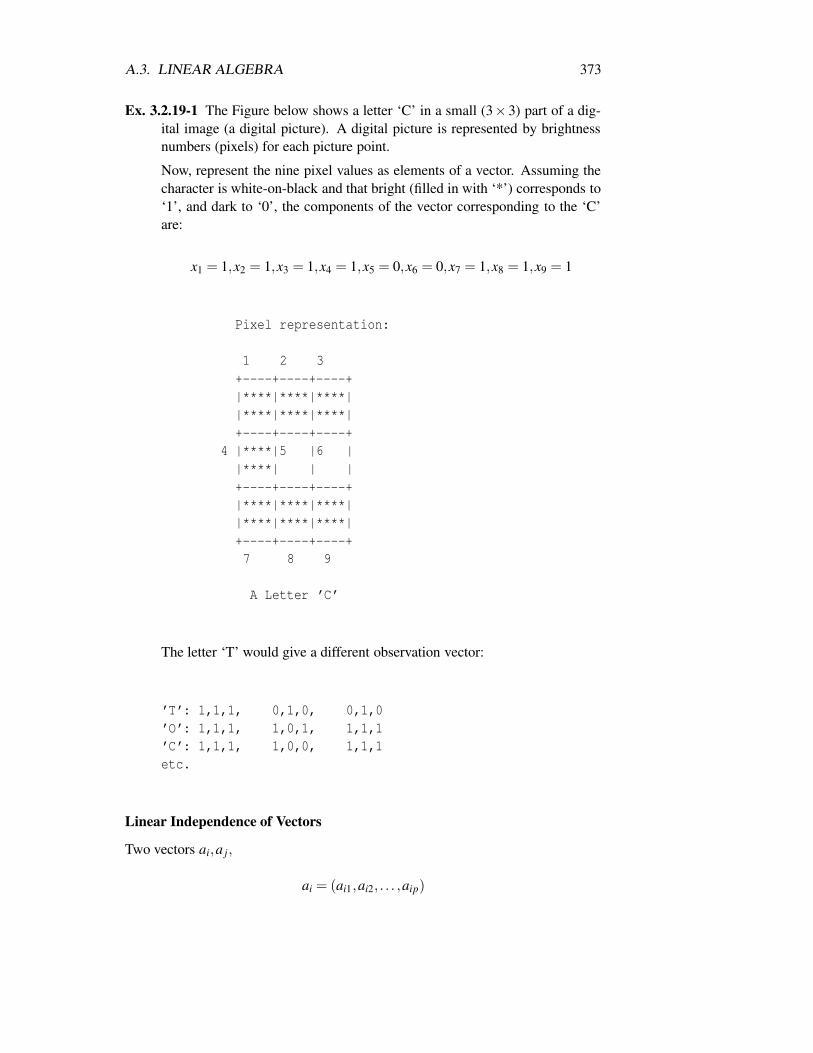
A.3. LINEAR ALGEBRA 373
Ex. 3.2.19-1 The Figure below shows a letter ‘C’ in a small (3×3) part of a dig-ital image (a digital picture). A digital picture is represented by brightnessnumbers (pixels) for each picture point.
Now, represent the nine pixel values as elements of a vector. Assuming thecharacter is white-on-black and that bright (filled in with ‘*’) corresponds to‘1’, and dark to ‘0’, the components of the vector corresponding to the ‘C’are:
x1 = 1,x2 = 1,x3 = 1,x4 = 1,x5 = 0,x6 = 0,x7 = 1,x8 = 1,x9 = 1
Pixel representation:
1 2 3+----+----+----+|****|****|****||****|****|****|+----+----+----+
4 |****|5 |6 ||****| | |+----+----+----+|****|****|****||****|****|****|+----+----+----+7 8 9
A Letter ’C’
The letter ‘T’ would give a different observation vector:
’T’: 1,1,1, 0,1,0, 0,1,0’O’: 1,1,1, 1,0,1, 1,1,1’C’: 1,1,1, 1,0,0, 1,1,1etc.
Linear Independence of Vectors
Two vectors ai,a j,
ai = (ai1,ai2, . . . ,aip)

374 APPENDIX A. APPENDIX: ESSENTIAL MATHEMATICS
a j = (a j1,a j2, . . . ,a jp)
are linearly dependent if one can be written as a scalar product of the other,
ai = ca j = (ca j1,ca j2, . . . ,ca jp)
i.e. the vectors differ only by a scale factor, c, that is applied to all elements.In such a case, the directions (see A10. above) of the vectors are the same; only
their length differs by the scaing factor c.If we have
b =n
∑j=1
c ja j
then b is a linear combination of the a js and is linearly dependent on them.Normally, as in the next section (rank) we are interested in the linear indepen-
dence of vectors formed by rows of a matrix. If we have one row of a matrix that islinearly dependent on (some – or all) the others, this means that the simultaneousequation associated with that row contributes no new information.
Rank of a Matrix
Given a q-row × p-column matrix, A
/ \|a11 a12 a1p||a21 a22 a2p|| |
A = | ... arc ... || ||aq1 aq2 aqp|\ /
the rank of A is the number of linearly independent rows in it (see A.11).If p = q the matrix is square, and we may need to invert it, it will only in-
vert if all the rows are linearly independent; otherwise, the matrix is singular –non-invertable. One simple way of viewing this problem is that, for a system ofsimultaneous equations to be solvable, we need p equations in p unknowns; if one,or more, of the equations is linearly dependent on the others, this equation con-tributes no new information, i.e. we effectively have only p−1 ‘useful’ equations,and the system is unsolvable – its rank is p−1.
In pattern recognition and estimation, the incidence of singular or nearly sin-gular matrices is insidious and common, e.g. a common source is taking reading

A.3. LINEAR ALGEBRA 375
for a dependent variable, y, say, for the same, or nearly the same values of the in-dependent variable, x. It can lead to nonsense results – analogous to what happensclose to divide by 0 in floating point arithmetic.
Eigenvalues and Eigenvectors
For any positive-definite matrix R, there exists a unitary matrix U that satisfies thefollowing equation:
UT RU = L
where
L = | l1 0 0 ... 0 || 0 l2 0 0 |
...| lp |
L is a diagonal matrix containing the eigenvalues of R, and
U = | u1 |
| u2 || ..|| ui || ..|| up |
is the matrix formed by the eigenvectors, ui, of R.Another equation governing eigenvalues and eigenvectors is
Rui = λiui
or, in matrix form, showing all the eigenvectors and eigenvalues:
RU = UL
The equivalence of (A.13-4) and (A.13-1) is easily verified by pre-multiplyingeach side of (A.13.4) by U T .

376 APPENDIX A. APPENDIX: ESSENTIAL MATHEMATICS

Appendix B
Appendix: Image Analysis andPattern Recognition in Java
377
Related Documents