Progressive graph matching: Making a move of graphs via probabilistic voting

Progressive Graph Matching:Making a Move of Graphs via Probabilistic Voting

Minsu Cho and Kyoung Mu LeeDept. of EECS, ASRI, Seoul National University, Korea

[email protected] [email protected]

Abstract

Graph matching is widely used in a variety of scientificfields, including computer vision, due to its powerful perfor-mance, robustness, and generality. Its computational com-plexity, however, limits the permissible size of input graphsin practice. Therefore, in real-world applications, the initialconstruction of graphs to match becomes a critical factorfor the matching performance, and often leads to unsatis-factory results. In this paper, to resolve the issue, we pro-pose a novel progressive framework which combines proba-bilistic progression of graphs with matching of graphs. Thealgorithm efficiently re-estimates in a Bayesian manner themost plausible target graphs based on the current match-ing result, and guarantees to boost the matching objectiveat the subsequent graph matching. Experimental evaluationdemonstrates that our approach effectively handles the lim-its of conventional graph matching and achieves significantimprovement in challenging image matching problems.

1. Introduction

Graph matching is a powerful and robust technique in avariety of scientific fields, and is widely used in computervision problems, such as feature correspondence, shapematching, object recognition, and video analysis [4, 18, 23,24, 10, 7, 2, 11]. In shape matching and object recogni-tion, both a model object and a test scene are representedas graphs using salient visual features, and graph match-ing finds the object and its corresponding features by min-imizing the distortions of the two matching graphs. Unlikepopular geometric constraints in vision (e.g. planar or rigidbody assumptions), graph matching provides greater flexi-bility to the object model and promises robust matching andrecognition [4, 18, 11]. The drawback of graph matchinglies in its NP-hard nature. Although recent research has pro-posed various approximations [17, 9, 24, 10, 7], the compu-tational costs in time and memory still limit the permissiblesizes of input graphs to match. For instance, the full compu-

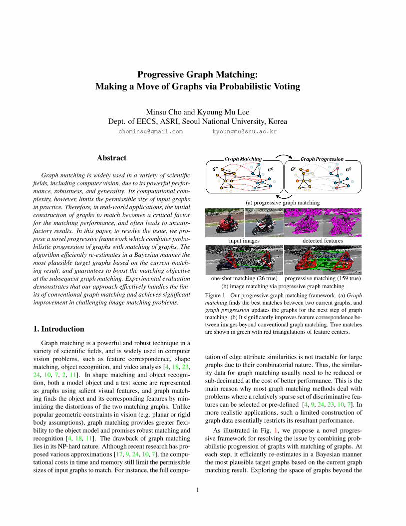
(a) progressive graph matching

input images detected features

one-shot matching (26 true) progressive matching (159 true)(b) image matching via progressive graph matching

Figure 1. Our progressive graph matching framework. (a) Graphmatching finds the best matches between two current graphs, andgraph progression updates the graphs for the next step of graphmatching. (b) It significantly improves feature correspondence be-tween images beyond conventional graph matching. True matchesare shown in green with red triangulations of feature centers.

tation of edge attribute similarities is not tractable for largegraphs due to their combinatorial nature. Thus, the similar-ity data for graph matching usually need to be reduced orsub-decimated at the cost of better performance. This is themain reason why most graph matching methods deal withproblems where a relatively sparse set of discriminative fea-tures can be selected or pre-defined [4, 9, 24, 23, 10, 7]. Inmore realistic applications, such a limited construction ofgraph data essentially restricts its resultant performance.

As illustrated in Fig. 1, we propose a novel progres-sive framework for resolving the issue by combining prob-abilistic progression of graphs with matching of graphs. Ateach step, it efficiently re-estimates in a Bayesian mannerthe most plausible target graphs based on the current graphmatching result. Exploring the space of graphs beyond the

1

current graphs, this graph progression guarantees to boostthe matching objective at the next step of graph matching.This framework can be viewed as a move-making algorithmfor graph matching. In a move-making algorithm, the so-lution is updated within a certain move space for each it-eration; for instance, move-making algorithms of graph-cuts [5, 16] generate a binary label space on MRFs to updatethe solution for multi-label problems. In the similar way,progressive graph matching creates adaptive move spacesof graphs to obtain better graph matching.

Although our approach provides a general framework forgraph matching, the current work focuses on image match-ing applications. In this regard, it is worth noting that ourprogressive graph matching essentially differs from recentpatch-based match-growing methods [14, 12, 8]. The meth-ods are commonly driven by gradually duplicating the in-dividual matches into their neighboring regions based onlocal appearances; thus, they are largely dependent on theinitial matching and restricted to the case of identical ob-jects with almost the same appearance. In contrast, our pro-gressive matching optimizes geometric distortions of fea-ture matches in a global sense, not by duplicating individ-ual matches but by considering other potential matches ina Bayesian manner. Hence, our method becomes robust toappearance variation as well as outliers, and generally ap-plicable to generic objects with intra-class variation. Exper-imental evaluation attests to this claim and shows that ourapproach effectively handles the limits of conventional one-shot graph matching and achieves significant improvementin challenging image matching problems.

2. Graph Matching RevisitedThe objective of graph matching is to find correspon-

dences between two attributed graphs GP = (VP , EP ,AP )andGQ =(VQ, EQ,AQ), where V represents a set of nodes,E , edges, and A, attributes. A solution of graph match-ing X is defined as a subset of possible correspondencesX ⊂ VP × VQ, and represented by a binary assignmentmatrix X ∈ 0, 1n

P×nQ

, where nP and nQ denote thenumbers of nodes in GP and GQ, respectively. If vPi ∈VP

matches vQa ∈ VQ, then Xi,a = 1, or Xi,a = 0. In thispaper, we denote by x∈0, 1nPnQ

a column-wise vector-ized replica of X. Then, graph matching problems can begenerally expressed as finding the indicator vector x∗ thatmaximizes a score function S(x) as follows:

x∗ = arg maxx

S(x)

s.t.

x ∈ 0, 1nPnQ

X1nQ×1 1nP×1, XT1nP×1 1nQ×1,(1)

where the two-way constraints of Eq. (1) represent the one-to-one matching from GP to GQ, thus making X an as-signment matrix. 1n×1 denotes an all-ones vector with size

n and the less-than-or-equal-to holds for every element.The graph matching objective of Eq. (1) is directly related toprogressive graph matching, as will be explained in Sec. 3.

For the score function S(x), we adopt a quadratic assign-ment formulation [4, 18, 17, 9, 19, 7]. It assumes similarityfunctions that measure the mutual similarity of the graph at-tributes; the first-order similarity function Ω1(aPi ,a

Qa ) for a

node pair of vPi ∈ VP and vQa ∈ VQ, and the second-order similarity function Ω2(aPij ,a

Qab) for an edge pair of

ePij ∈ EP and eQab ∈ EQ. The similarity functions can be en-coded in a symmetric similarity matrix W. A non-diagonalelement Wia;jb = Ω2(aPij ,a

Qab) contains a pairwise simi-

larity of two correspondences (vPi , vQa ) and (vPj , v

Qb ), and

a diagonal term Wia;ia = Ω1(aPi ,aQa ) represents a unary

similarity of a correspondence (vPi , vQa ). Using the assign-

ment vector x introduced earlier, a score function of the ac-cumulation of all the relevant similarities is defined as

S(x) = xTWx. (2)

The formulation of Eq. (2) under Eq. (1) is called the integerquadratic programming (IQP), which is proven to be NP-complete. Recently, IQP has been favored in graph match-ing research due to its generality and strong robustness,and several efficient approximate algorithms have been pro-posed [7, 19, 9, 23]. Notably, our progressive graph match-ing framework is orthogonal to specific graph matching for-mulations and algorithms; thus, any of them or any high-order algorithm [24, 10, 15] can be adopted as the graphmatching module in the framework.

2.1. Graph Construction for Real Applications

The issues of graph construction need to be discussedhere in advance before we proceed to progressive graphmatching. In the application of graph matching to real-world problems, the first step is to construct graphs basedon given observations. As graphs are usually not given asraw data, nodes and edges should be defined based on aspecific type of the given observations. For instance, salientfeatures and their proper relations from an image consti-tute a scene graph used for image matching [4, 18]. Inmost real applications, however, graphs made of all pos-sible features and their relations are not only intractable but

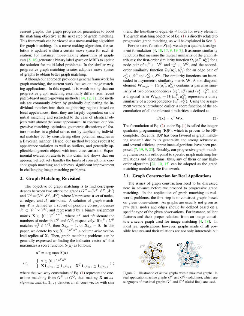
Figure 2. Illustration of active graphs within maximal graphs. Inreal applications, active graphs GP and GQ (solid line), which aresubgraphs of maximal graphs GP and GQ (faded line), are used.

also inappropriate because such graphs are usually highlycomplex and contain too much clutter information, whichdistracts graph matching. Therefore, as depicted in Fig. 2,a reduced set of features and their relations is selectivelyused to construct a graph. We term such a graph used forpractical graph matching an “active graph”, whereas wecall the largest complete graph covering all the given fea-tures a “maximal graph”. Given two active graphs, simi-larity values of edge (and node) attributes between the twographs should be computed. As repeatedly used in the graphmatching process, the similarity values are commonly pre-computed and stored in the form of a similarity matrix (ortensor) [13, 17, 9, 23, 24, 10, 7, 15], which corresponds toW of Eq. (2) in our case. The size of non-zero elements inthe similarity matrix is another critical factor to determinethe complexity of the graph matching process.

Therefore, if a graph matching method is given, the waysof reducing complexity in practice are (1) to reduce the sizesof active graphs and (2) to sparsify the similarity matrix (re-duce the number of similarity values to be considered ingraph matching). An effective way to achieve both (1) and(2) is to establish a set of candidate matches. Once the can-didate matches C are selected from the given possible fea-tures, the active graphs are determined by the nodes andedges involved in C, and their similarity matrix is sparsifiedby restricting the edge similarity comparison to the pairsfrom C. In many applications, the candidate matches can bereadily established using unary descriptors of the featuresat a relatively low cost. Such methods are widely adoptedin the practical problems of feature matching and objectrecognition in the literature [4, 18, 7, 10]. In many cases,however, all these methods for graph construction lead tounsatisfactory matching results due to the loss of useful in-formation hidden in the maximal graphs.

3. Our Progressive FrameworkWe propose a progressive framework for graph match-

ing to explore the space of maximal graphs beyond the ac-tive graphs in an efficient way. As sketched in Fig. 1, ourframework basically consists of two alternating processes:graph matching and graph progression. Graph match-ing finds the best matches between current active graphs,whereas graph progression updates the active graphs andtheir similarity matrix to boost the score in the next graphmatching. The objective of progressive graph matching isto further maximize the graph matching score in Eq. (1)by adaptively re-organizing graphs GP and GQ. To for-malize this approach at time step t, we assume two ac-tive graphs GP

t = (VPt , EPt ,AP

t ) and GQt = (VQ

t , EQt ,A

Qt ),

and candidate matches Ct ⊂ VPt ×V

Qt . The matching so-

lution between GPt and GQ

t is denoted by Mt(⊂ Ct) un-der the constraints of Eq. (1), and its score is denoted bysGMt . On the other hand, maximal graphs are represented

by GP = (VP , EP , AP ) and GQ = (VQ, EQ, AQ), whereGP ⊃GP

t and GQ⊃GQt for any t.

For graph progression, we consider a conditional jointprobability distribution p(V P, V Q|Mt) of V P ∈ VP andV Q ∈ VQ, the domain of which represents possible nodematches of two maximal graphs; p(vPj , v

Qb |Mt) denotes the

conditional probability of a match (vPj , vQb ) between the two

maximal graphs. In graph progression, given the currentgraph matching Mt, the distribution of p(V P, V Q|Mt) isestimated, and then the new set of candidate matches Ct+1

is selected based on the distribution to construct the new ac-tive graphs GP

t+1 and GQt+1 and their similarity matrix. The

new active graphs consist of the nodes and edges involved inCt+1 and their similarity matrix considers only the similar-ity values within Ct+1. Under a managable size of Ct+1, thisgraph progression effectively explores the space of maximalgraphs beyond the current active graphs and thus enablesbetter graph matching. In the progressive graph matching,the use of the inclusion constraint Ct+1⊃Mt guarantees thenon-decreasing score sGM

t+1 ≥ sGMt by the optimal graph

matching of each step. The iterations continue until thescore no longer increases.

3.1. Bayesian Formulation for Graph Progression

In a Bayesian framework, the conditional joint distri-bution p(V P, V Q|M) for graph progression can be ana-lyzed as follows. Suppose a current graph matching solu-tionMt = m1, · · · ,m|Mt| where mi = (vPpi

, vQqi). Tofacilitate a generative model of p(V P, V Q|M), we intro-duce an auxiliary variable of an anchor match M ∈ Mt

so that p(V P, V Q|Mt) can be obtained by marginalizingp(V P, V Q,M |Mt) over M . Then, by the chain rule, it canbe further decomposed as

p(V P, V Q|Mt) =∑

mi∈Mt

p(V P, V Q,M=mi|Mt)

=∑

mi∈Mt

p(V Q|V P,M=mi,Mt)

p(V P|M=mi,Mt) p(M=mi|Mt),

(3)

where p(M = mi|Mt) expresses a conditional prior forchoosing mi as an anchor amongMt. p(V P|M=mi,Mt)describes the probability of V P relating to the anchor mi

amongMt. p(V Q|V P,M = mi,Mt) expresses the prob-ability of V Q relating to the node V P and the anchor mi

amongMt. Interestingly, the marginalizing formulation ofEq. (3) can be interpreted as probabilistic voting, where thevoting elements are individual anchor matches mi ∈Mt.Unlike the pseudo-probabilistic formulation of the Houghtransform1, our formulation is naturally fitted to probabilis-

1 For the analysis on the Hough transform, refer to [3].

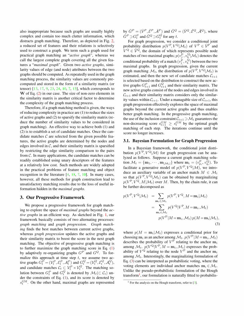
Algorithm 1: Progressive Graph Matching

Input: maximal graphs GP, GQ, # of candidates Nc

Output: graph matchingM∗ with the highest score( Initial Active Graphs )C0 ← FindInitialCandidates(VP, VQ, Nc);( Progressive Loop )t← 0, sGM

0 ← 0;while score sGM increases do

( Graph Matching )(Mt, s

GMt )← GraphMatching(Ct);

( Graph Progression )p(vPp , v

Qq |Mt)← 0 ∀vPp ∈ VP, vQq ∈ VQ;

foreach mi = (vPp , vQq ) ∈Mt do

NA ← vP ∈ VP|p(vP|mi,Mt) > ε;foreach vPj ∈ NA doNB←vQ ∈ VQ|p(vQ|vPj ,mi,Mt)>ε;foreach vQb ∈ NB do

p(vPj , vQb |Mt)← p(vPj , v

Qb |Mt) +

p(vQb |vPj ,mi,Mt)p(vPj |mi,Mt)p(mi|Mt);

endend

end( Updated Active Graphs )Ct+1 ← Nc best matches based on p(V P,V Q|Mt),which containsMt;t← t+ 1;

end

tic interpretation in the Bayesian manner. After the distri-bution of p(V P, V Q|Mt) is obtained via the probabilisticvoting, the most frequently voted pairs in the joint spaceare selected as potential candidates for the next stage ofgraph matching. Non-maximal suppression is not neces-sary to this step because the purpose here is to collect theplausible candidates. The set of candidate matches Ct+1 isassigned as Nc matches consisting of the matches in Mt

and Nc−|Mt| best matches based on p(V P, V Q|Mt). Theprogressive framework is summarized in Algorithm 1. Thedetailed design of three terms in Eq. (3) depends on specificapplication domains.

3.2. Application to Image Matching

In this section, we deal with feature correspondence be-tween two images, which is one of the most common andfundamental problems in computer vision. To constructscene graphs, the popular features of local (affine- or scale-) invariant regions such as SIFT [20], MSER [21], Harris-Affine [22] is adopted. We focus on the case of complexreal-world images with more than hundreds or thousands of

detected features. The graphs are constructed with the fea-tures as nodes and their geometric relations as edges. Inthis case, graph matching on maximal graphs is virtuallyintractable or impractical due to time and memory.

Graph Matching Given two images IP and IQ, nodesVP and VQ represent features detected in IP and IQ, re-spectively. Each feature usually has a unary appearanceinformation of its local patch, and thus the initial candi-date matches in Algorithm 1 can be collected by comparingtheir descriptors. This approach to active graphs is widelyadopted in conventional graph matching [17, 4, 23, 7]. Fora pairwise edge similarity Wia;jb =Ω2(aPij ,a

Qab) of Eq. (2)

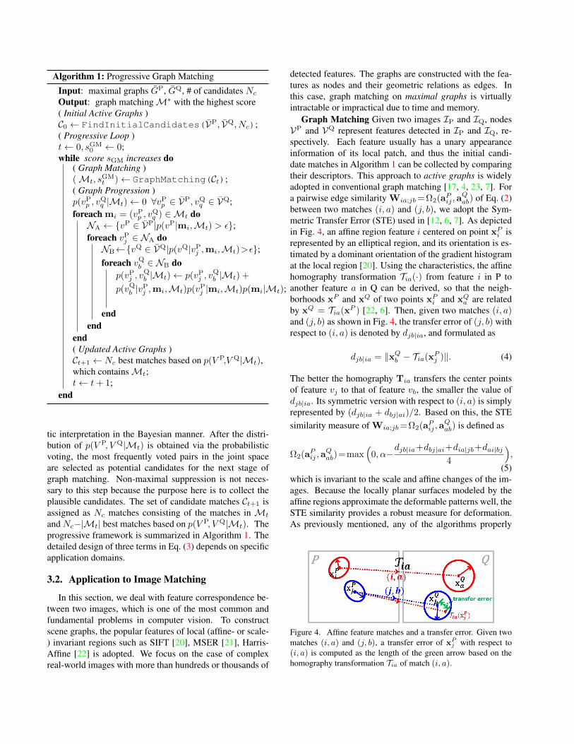
between two matches (i, a) and (j, b), we adopt the Sym-metric Transfer Error (STE) used in [12, 6, 7]. As depictedin Fig. 4, an affine region feature i centered on point xP

i isrepresented by an elliptical region, and its orientation is es-timated by a dominant orientation of the gradient histogramat the local region [20]. Using the characteristics, the affinehomography transformation Tia(·) from feature i in P toanother feature a in Q can be derived, so that the neigh-borhoods xP and xQ of two points xP

i and xQa are related

by xQ = Tia(xP ) [22, 6]. Then, given two matches (i, a)and (j, b) as shown in Fig. 4, the transfer error of (j, b) withrespect to (i, a) is denoted by djb|ia, and formulated as

djb|ia = ‖xQb − Tia(xP

j )‖. (4)

The better the homography Tia transfers the center pointsof feature vj to that of feature vb, the smaller the value ofdjb|ia. Its symmetric version with respect to (i, a) is simplyrepresented by (djb|ia + dbj|ai)/2. Based on this, the STEsimilarity measure of Wia;jb =Ω2(aPij ,a

Qab) is defined as

Ω2(aPij ,aQab)=max

(0, α−

djb|ia+dbj|ai+dia|jb+dai|bj

4

),

(5)which is invariant to the scale and affine changes of the im-ages. Because the locally planar surfaces modeled by theaffine regions approximate the deformable patterns well, theSTE similarity provides a robust measure for deformation.As previously mentioned, any of the algorithms properly

Figure 4. Affine feature matches and a transfer error. Given twomatches (i, a) and (j, b), a transfer error of xP

j with respect to(i, a) is computed as the length of the green arrow based on thehomography transformation Tia of match (i, a).

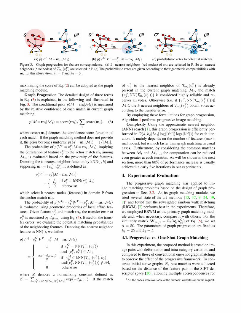
(a) p(V P|M =mi,Mt) (b) p(V Q|V P =vPj ,M =mi,Mt) (c) probabilistic votes to potential matches

Figure 3. Graph progression for feature correspondence. (a) k1 nearest neighbors (red nodes) of mi are selected in P. (b) k2 nearestneighbors (blue nodes) of Tmi(v

Pj ) are selected in P. (c) The probabilistic votes are given according to their geometric compatabilities with

mi. In this illustration, k1 = 7 and k2 = 3.

maximizing the score of Eq. (2) can be adopted as the graphmatching module.

Graph Progression The detailed design of three termsin Eq. (3) is explained in the following and illustrated inFig. 3. The conditional prior p(M = mi|Mt) is measuredby the relative confidence of each match in current graphmatching:

p(M=mi|Mt) = score(mi)/∑i

score(mi). (6)

where score(mi) denotes the confidence score function ofeach match. If the graph matching method does not provideit, the prior becomes uniform: p(M=mi|Mt) = 1/|Mt|.

The probability of p(V P = vPj |M =mi,Mt), implyingthe correlation of feature vPj to the achor match mi amongMt, is evaluated based on the proximity of the features.Denoting the k-nearest neighbor function by kNN(·, k) andsupposing mi = (vPpi

, vQqi), it is defined as

p(V P =vPj |M=mi,Mt)

=

1k1

if vPj ∈ kNN(vPpi, k1)

0 otherwise

which select k nearest nodes (features) in domain P fromthe anchor match mi.

The probability of p(V Q = vQb |V P = vPj ,M =mi,Mt)is evaluated using geometric properties of local affine fea-tures. Given feature vPj and match mi, the transfer error tovQb is measured by djb|mi

using Eq. (4). Based on the trans-fer errors, we evaluate the potential matching probabilitiesof the neighboring features. Denoting the nearest neighborfeature as NN(·), we define

p(V Q =vQb |VP =vPj ,M=mi,Mt)

=

1 if vQb = NN(Tmi(vPj ))

and (vPj , vQb ) ∈Mt

exp(−djb|mi)

Z if vQb ∈ kNN(Tmi(vPj ), k2)

and(vPj ,NN(Tmi

(vPj )))/∈Mt

0 otherwise

where Z denotes a normalizing constant defined asZ =

∑vQb ∈kNN(Tmi

(vPj ),k2)

exp(−djb|mi). If the match

of vPj to the nearest neighbor of Tmi(vPj ) is already

present in the current graph matching Mt, the match(vPj ,NN(Tmi

(vPj )))

is considered highly reliable and re-ceives all votes. Otherwise (i.e. if

(vP,NN(Tmi(v

Pj )))/∈

Mt), the k nearest neighbors of Tmi(vPj ) obtain votes ac-

cording to the transfer error.By employing these formulations for graph progression,

Algorithm 1 performs progressive image matching.Complexity Using the approximate nearest neighbor

(ANN) search [1], this graph progression is efficiently per-formed in O(k1k2|Mt| log(|VP |) log(|VQ|)) for each iter-ation. It mainly depends on the number of features (maxi-mal nodes), but is much faster than graph matching in usualcases. Furthermore, by considering the common matchesbetween Mt and Mt−1, the computation can be reducedeven greater at each iteration. As will be shown in the nextsection, more than 80% of performance increase is usuallyachieved in early five iterations in our experiments.

4. Experimental EvaluationThe progressive graph matching was applied to im-

age matching problems based on the design of graph pro-gression in Sec. 3.2. As its graph matching module, wetried several state-of-the-art methods [13, 17, 9, 24, 19,7]2 and found that the reweighted random walk matching(RRWM) [7] performs best in the experiments. Therefore,we employed RRWM as the primary graph matching mod-ule and, when necessary, compare it with others. For thesimilarity matrix Wia;jb = Ω2(aPija

Qab) of Eq. (5), we set

α = 50. The parameters of graph progression are fixed ask1 = 25 and k2 = 5.

4.1. Progressive vs. One-Shot Graph Matching

In this experiment, the proposed method is tested on im-age pairs with deformation and intra-category variation, andcompared to those of conventional one-shot graph matchingto observe the effect of the progressive framework. To con-struct initial active graphs, Nc best matches were collectedbased on the distance of the feature pair in the SIFT de-scriptor space [20], allowing multiple correspondences for

2All the codes were available at the authors’ websites or on the request.

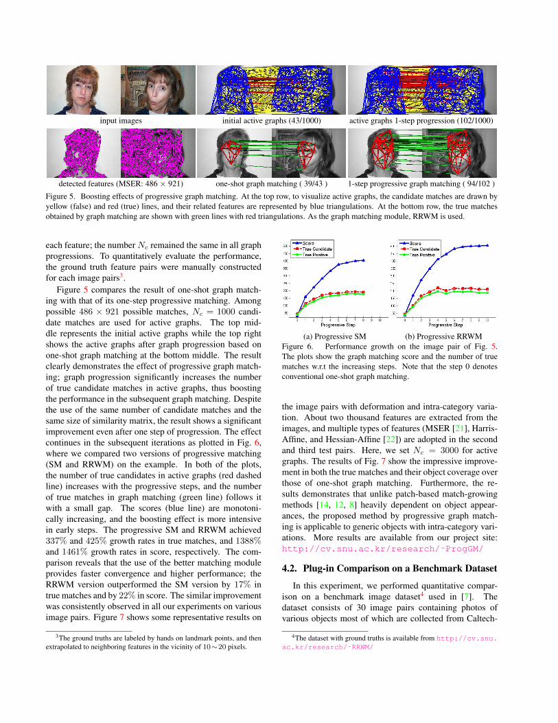
input images initial active graphs (43/1000) active graphs 1-step progression (102/1000)

detected features (MSER: 486 × 921) one-shot graph matching ( 39/43 ) 1-step progressive graph matching ( 94/102 )

Figure 5. Boosting effects of progressive graph matching. At the top row, to visualize active graphs, the candidate matches are drawn byyellow (false) and red (true) lines, and their related features are represented by blue triangulations. At the bottom row, the true matchesobtained by graph matching are shown with green lines with red triangulations. As the graph matching module, RRWM is used.

each feature; the number Nc remained the same in all graphprogressions. To quantitatively evaluate the performance,the ground truth feature pairs were manually constructedfor each image pairs3.

Figure 5 compares the result of one-shot graph match-ing with that of its one-step progressive matching. Amongpossible 486 × 921 possible matches, Nc = 1000 candi-date matches are used for active graphs. The top mid-dle represents the initial active graphs while the top rightshows the active graphs after graph progression based onone-shot graph matching at the bottom middle. The resultclearly demonstrates the effect of progressive graph match-ing; graph progression significantly increases the numberof true candidate matches in active graphs, thus boostingthe performance in the subsequent graph matching. Despitethe use of the same number of candidate matches and thesame size of similarity matrix, the result shows a significantimprovement even after one step of progression. The effectcontinues in the subsequent iterations as plotted in Fig. 6,where we compared two versions of progressive matching(SM and RRWM) on the example. In both of the plots,the number of true candidates in active graphs (red dashedline) increases with the progressive steps, and the numberof true matches in graph matching (green line) follows itwith a small gap. The scores (blue line) are monotoni-cally increasing, and the boosting effect is more intensivein early steps. The progressive SM and RRWM achieved337% and 425% growth rates in true matches, and 1388%and 1461% growth rates in score, respectively. The com-parison reveals that the use of the better matching moduleprovides faster convergence and higher performance; theRRWM version outperformed the SM version by 17% intrue matches and by 22% in score. The similar improvementwas consistently observed in all our experiments on variousimage pairs. Figure 7 shows some representative results on

3The ground truths are labeled by hands on landmark points, and thenextrapolated to neighboring features in the vicinity of 10∼20 pixels.

(a) Progressive SM (b) Progressive RRWMFigure 6. Performance growth on the image pair of Fig. 5.The plots show the graph matching score and the number of truematches w.r.t the increasing steps. Note that the step 0 denotesconventional one-shot graph matching.

the image pairs with deformation and intra-category varia-tion. About two thousand features are extracted from theimages, and multiple types of features (MSER [21], Harris-Affine, and Hessian-Affine [22]) are adopted in the secondand third test pairs. Here, we set Nc = 3000 for activegraphs. The results of Fig. 7 show the impressive improve-ment in both the true matches and their object coverage overthose of one-shot graph matching. Furthermore, the re-sults demonstrates that unlike patch-based match-growingmethods [14, 12, 8] heavily dependent on object appear-ances, the proposed method by progressive graph match-ing is applicable to generic objects with intra-category vari-ations. More results are available from our project site:http://cv.snu.ac.kr/research/˜ProgGM/

4.2. Plug-in Comparison on a Benchmark Dataset

In this experiment, we performed quantitative compar-ison on a benchmark image dataset4 used in [7]. Thedataset consists of 30 image pairs containing photos ofvarious objects most of which are collected from Caltech-

4The dataset with ground truths is available from http://cv.snu.ac.kr/research/˜RRWM/

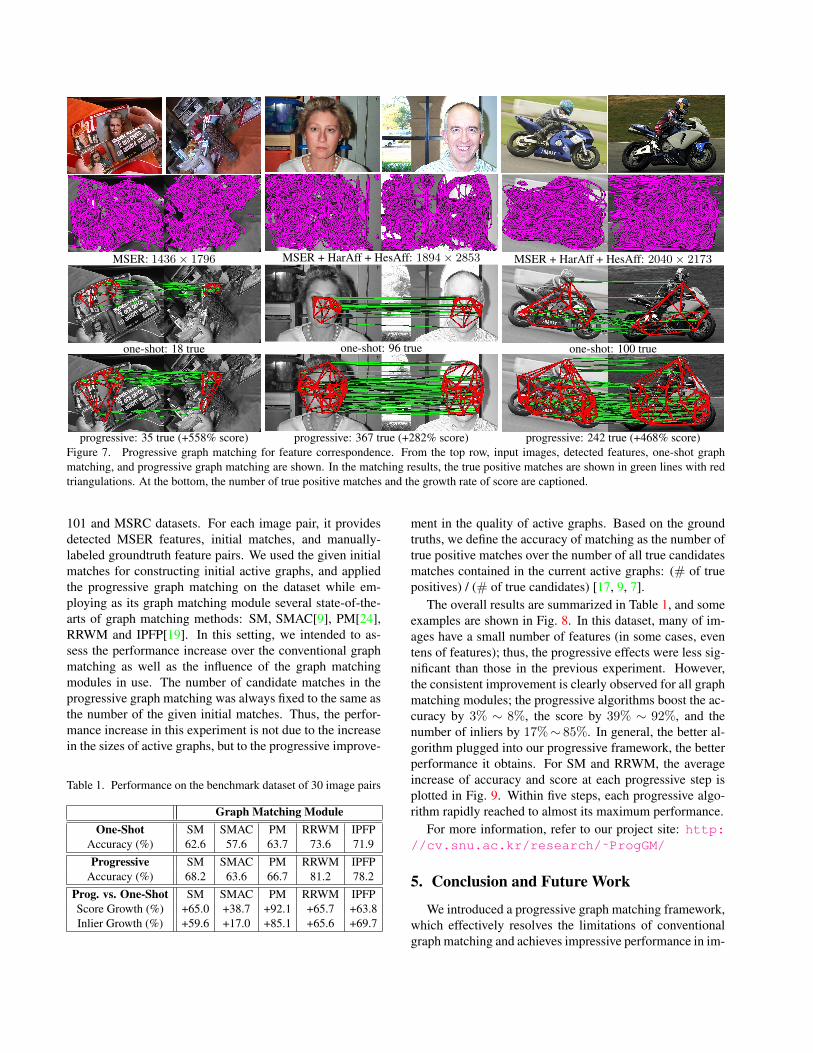
MSER: 1436× 1796

one-shot: 18 true

progressive: 35 true (+558% score)

MSER + HarAff + HesAff: 1894× 2853

one-shot: 96 true

progressive: 367 true (+282% score)

MSER + HarAff + HesAff: 2040× 2173

one-shot: 100 true

progressive: 242 true (+468% score)Figure 7. Progressive graph matching for feature correspondence. From the top row, input images, detected features, one-shot graphmatching, and progressive graph matching are shown. In the matching results, the true positive matches are shown in green lines with redtriangulations. At the bottom, the number of true positive matches and the growth rate of score are captioned.

101 and MSRC datasets. For each image pair, it providesdetected MSER features, initial matches, and manually-labeled groundtruth feature pairs. We used the given initialmatches for constructing initial active graphs, and appliedthe progressive graph matching on the dataset while em-ploying as its graph matching module several state-of-the-arts of graph matching methods: SM, SMAC[9], PM[24],RRWM and IPFP[19]. In this setting, we intended to as-sess the performance increase over the conventional graphmatching as well as the influence of the graph matchingmodules in use. The number of candidate matches in theprogressive graph matching was always fixed to the same asthe number of the given initial matches. Thus, the perfor-mance increase in this experiment is not due to the increasein the sizes of active graphs, but to the progressive improve-

Table 1. Performance on the benchmark dataset of 30 image pairs

Graph Matching ModuleOne-Shot SM SMAC PM RRWM IPFP

Accuracy (%) 62.6 57.6 63.7 73.6 71.9Progressive SM SMAC PM RRWM IPFP

Accuracy (%) 68.2 63.6 66.7 81.2 78.2Prog. vs. One-Shot SM SMAC PM RRWM IPFPScore Growth (%) +65.0 +38.7 +92.1 +65.7 +63.8Inlier Growth (%) +59.6 +17.0 +85.1 +65.6 +69.7

ment in the quality of active graphs. Based on the groundtruths, we define the accuracy of matching as the number oftrue positive matches over the number of all true candidatesmatches contained in the current active graphs: (# of truepositives) / (# of true candidates) [17, 9, 7].

The overall results are summarized in Table 1, and someexamples are shown in Fig. 8. In this dataset, many of im-ages have a small number of features (in some cases, eventens of features); thus, the progressive effects were less sig-nificant than those in the previous experiment. However,the consistent improvement is clearly observed for all graphmatching modules; the progressive algorithms boost the ac-curacy by 3% ∼ 8%, the score by 39% ∼ 92%, and thenumber of inliers by 17%∼ 85%. In general, the better al-gorithm plugged into our progressive framework, the betterperformance it obtains. For SM and RRWM, the averageincrease of accuracy and score at each progressive step isplotted in Fig. 9. Within five steps, each progressive algo-rithm rapidly reached to almost its maximum performance.

For more information, refer to our project site: http://cv.snu.ac.kr/research/˜ProgGM/

5. Conclusion and Future Work

We introduced a progressive graph matching framework,which effectively resolves the limitations of conventionalgraph matching and achieves impressive performance in im-

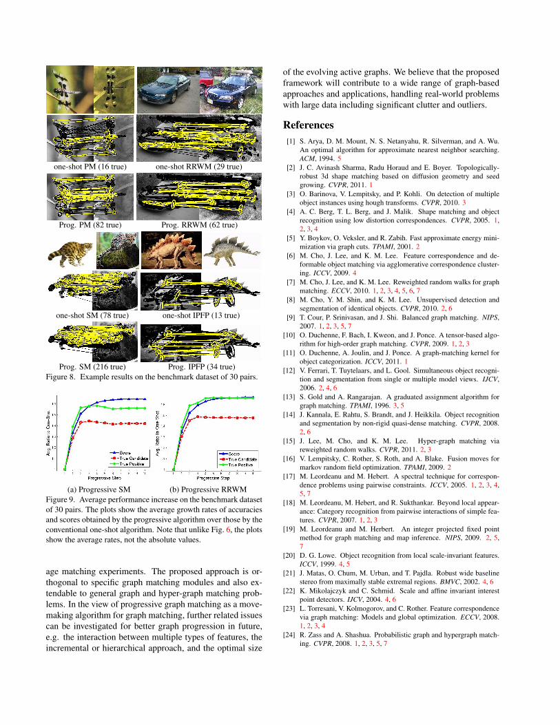
one-shot PM (16 true) one-shot RRWM (29 true)

Prog. PM (82 true) Prog. RRWM (62 true)

one-shot SM (78 true) one-shot IPFP (13 true)

Prog. SM (216 true) Prog. IPFP (34 true)Figure 8. Example results on the benchmark dataset of 30 pairs.

(a) Progressive SM (b) Progressive RRWMFigure 9. Average performance increase on the benchmark datasetof 30 pairs. The plots show the average growth rates of accuraciesand scores obtained by the progressive algorithm over those by theconventional one-shot algorithm. Note that unlike Fig. 6, the plotsshow the average rates, not the absolute values.

age matching experiments. The proposed approach is or-thogonal to specific graph matching modules and also ex-tendable to general graph and hyper-graph matching prob-lems. In the view of progressive graph matching as a move-making algorithm for graph matching, further related issuescan be investigated for better graph progression in future,e.g. the interaction between multiple types of features, theincremental or hierarchical approach, and the optimal size

of the evolving active graphs. We believe that the proposedframework will contribute to a wide range of graph-basedapproaches and applications, handling real-world problemswith large data including significant clutter and outliers.

References[1] S. Arya, D. M. Mount, N. S. Netanyahu, R. Silverman, and A. Wu.

An optimal algorithm for approximate nearest neighbor searching.ACM, 1994. 5

[2] J. C. Avinash Sharma, Radu Horaud and E. Boyer. Topologically-robust 3d shape matching based on diffusion geometry and seedgrowing. CVPR, 2011. 1

[3] O. Barinova, V. Lempitsky, and P. Kohli. On detection of multipleobject instances using hough transforms. CVPR, 2010. 3

[4] A. C. Berg, T. L. Berg, and J. Malik. Shape matching and objectrecognition using low distortion correspondences. CVPR, 2005. 1,2, 3, 4

[5] Y. Boykov, O. Veksler, and R. Zabih. Fast approximate energy mini-mization via graph cuts. TPAMI, 2001. 2

[6] M. Cho, J. Lee, and K. M. Lee. Feature correspondence and de-formable object matching via agglomerative correspondence cluster-ing. ICCV, 2009. 4

[7] M. Cho, J. Lee, and K. M. Lee. Reweighted random walks for graphmatching. ECCV, 2010. 1, 2, 3, 4, 5, 6, 7

[8] M. Cho, Y. M. Shin, and K. M. Lee. Unsupervised detection andsegmentation of identical objects. CVPR, 2010. 2, 6

[9] T. Cour, P. Srinivasan, and J. Shi. Balanced graph matching. NIPS,2007. 1, 2, 3, 5, 7

[10] O. Duchenne, F. Bach, I. Kweon, and J. Ponce. A tensor-based algo-rithm for high-order graph matching. CVPR, 2009. 1, 2, 3

[11] O. Duchenne, A. Joulin, and J. Ponce. A graph-matching kernel forobject categorization. ICCV, 2011. 1

[12] V. Ferrari, T. Tuytelaars, and L. Gool. Simultaneous object recogni-tion and segmentation from single or multiple model views. IJCV,2006. 2, 4, 6

[13] S. Gold and A. Rangarajan. A graduated assignment algorithm forgraph matching. TPAMI, 1996. 3, 5

[14] J. Kannala, E. Rahtu, S. Brandt, and J. Heikkila. Object recognitionand segmentation by non-rigid quasi-dense matching. CVPR, 2008.2, 6

[15] J. Lee, M. Cho, and K. M. Lee. Hyper-graph matching viareweighted random walks. CVPR, 2011. 2, 3

[16] V. Lempitsky, C. Rother, S. Roth, and A. Blake. Fusion moves formarkov random field optimization. TPAMI, 2009. 2

[17] M. Leordeanu and M. Hebert. A spectral technique for correspon-dence problems using pairwise constraints. ICCV, 2005. 1, 2, 3, 4,5, 7

[18] M. Leordeanu, M. Hebert, and R. Sukthankar. Beyond local appear-ance: Category recognition from pairwise interactions of simple fea-tures. CVPR, 2007. 1, 2, 3

[19] M. Leordeanu and M. Herbert. An integer projected fixed pointmethod for graph matching and map inference. NIPS, 2009. 2, 5,7

[20] D. G. Lowe. Object recognition from local scale-invariant features.ICCV, 1999. 4, 5

[21] J. Matas, O. Chum, M. Urban, and T. Pajdla. Robust wide baselinestereo from maximally stable extremal regions. BMVC, 2002. 4, 6

[22] K. Mikolajczyk and C. Schmid. Scale and affine invariant interestpoint detectors. IJCV, 2004. 4, 6

[23] L. Torresani, V. Kolmogorov, and C. Rother. Feature correspondencevia graph matching: Models and global optimization. ECCV, 2008.1, 2, 3, 4

[24] R. Zass and A. Shashua. Probabilistic graph and hypergraph match-ing. CVPR, 2008. 1, 2, 3, 5, 7