Technical Report Number 843 Computer Laboratory UCAM-CL-TR-843 ISSN 1476-2986 Programming for humans: a new paradigm for domain-specific languages Robin Message November 2013 15 JJ Thomson Avenue Cambridge CB3 0FD United Kingdom phone +44 1223 763500 http://www.cl.cam.ac.uk/

Welcome message from author
This document is posted to help you gain knowledge. Please leave a comment to let me know what you think about it! Share it to your friends and learn new things together.
Transcript

Technical ReportNumber 843
Computer Laboratory
UCAM-CL-TR-843ISSN 1476-2986
Programming for humans:a new paradigm for
domain-specific languages
Robin Message
November 2013
15 JJ Thomson AvenueCambridge CB3 0FDUnited Kingdomphone +44 1223 763500
http://www.cl.cam.ac.uk/

c© 2013 Robin Message
This technical report is based on a dissertation submittedMarch 2013 by the author for the degree of Doctor ofPhilosophy to the University of Cambridge, RobinsonCollege.
Technical reports published by the University of CambridgeComputer Laboratory are freely available via the Internet:
http://www.cl.cam.ac.uk/techreports/
ISSN 1476-2986

Programming for humans – a new paradigm for domain-specific
languages
Robin Message
Summary
Programming is a difficult, specialist skill. Despite much research in software engineer-
ing, programmers still work like craftsmen or artists, not engineers. As a result, programs
cannot easily be modified, joined together or customised. However, unlike a craft product,
once a programmer has created their program, it can replicated infinitely and perfectly.
This means that programs are often not a good fit for their end-users because this infinite
duplication gives their creators an incentive to create very general programs.
My thesis is that we can create better paradigms, languages and data structuring
techniques to enable end-users to create their own programs.
The first contribution is a new paradigm for programming languages which explicitly
separates control and data flow. For example, in a web application, the control level would
handle user clicks and database writes, while the data level would handle form inputs and
database reads. The language is strongly typed, with type reconstruction. We believe
this paradigm is particularly suited to end-user programming of interactive applications.
The second contribution is an implementation of this paradigm in a specialised visual
programming language for novice programmers to develop web applications. We describe
our programming environment, which has a novel layout algorithm that maps control and
data flow onto separate dimensions. We show that experienced programmers are more
productive in this system than the alternatives.
The third contribution is a novel data structuring technique which infers fuzzy types
from example data. This inference is theoretically founded on Bayesian statistics. Our
inference aids programmers in moving from semi-structured data to typed programs. We
discuss how this data structuring technique could be visualised and integrated with our
visual programming environment.

Acknowledgments
I would like to thank my wife Naomi, my supervisors Alan Mycroft and Alastair Beresford,
and my family, without whose help and support you would not be reading this.

Contents
Contents 5
1 Introduction 7
2 Technical Background and Literature Review 11
2.1 What is end-user programming? . . . . . . . . . . . . . . . . . . . . . . . . 13
2.2 Programming languages and environments . . . . . . . . . . . . . . . . . . 13
2.3 Designing environments for end-user programmers . . . . . . . . . . . . . . 15
2.4 Prior end-user programming languages . . . . . . . . . . . . . . . . . . . . 17
2.5 Web execution model . . . . . . . . . . . . . . . . . . . . . . . . . . . . . . 19
2.6 Web programming languages . . . . . . . . . . . . . . . . . . . . . . . . . . 22
2.7 End-user web programming languages . . . . . . . . . . . . . . . . . . . . . 23
2.8 Programming language execution models . . . . . . . . . . . . . . . . . . . 27
2.9 Data structures and storage . . . . . . . . . . . . . . . . . . . . . . . . . . 30
2.10 Data type inference . . . . . . . . . . . . . . . . . . . . . . . . . . . . . . . 33
2.11 Summary . . . . . . . . . . . . . . . . . . . . . . . . . . . . . . . . . . . . 36
3 A new paradigm for programming languages: separating control and
data flow 39
3.1 Execution model . . . . . . . . . . . . . . . . . . . . . . . . . . . . . . . . 43
3.2 Theoretical basis . . . . . . . . . . . . . . . . . . . . . . . . . . . . . . . . 45
3.3 Concurrency . . . . . . . . . . . . . . . . . . . . . . . . . . . . . . . . . . . 53
3.4 Comparison to other paradigms . . . . . . . . . . . . . . . . . . . . . . . . 54
3.5 cd-sep: A new paradigm for end-user programming languages . . . . . . . 59
4 Visual web programming 61
4.1 Description . . . . . . . . . . . . . . . . . . . . . . . . . . . . . . . . . . . 62
4.2 Example application . . . . . . . . . . . . . . . . . . . . . . . . . . . . . . 69
4.3 User study . . . . . . . . . . . . . . . . . . . . . . . . . . . . . . . . . . . . 72
4.4 Cognitive Dimensions of Notations Analysis . . . . . . . . . . . . . . . . . 76
4.5 VisualWebFlows: A new platform for end-user web programming . . . . . 81
5

5 Inferring types from data 83
5.1 Overview of algorithm principles . . . . . . . . . . . . . . . . . . . . . . . . 85
5.2 Statistical model evaluation . . . . . . . . . . . . . . . . . . . . . . . . . . 88
5.3 Model generation and selection . . . . . . . . . . . . . . . . . . . . . . . . 94
5.4 Comparison to existing techniques . . . . . . . . . . . . . . . . . . . . . . . 101
5.5 Results . . . . . . . . . . . . . . . . . . . . . . . . . . . . . . . . . . . . . . 102
5.6 Integrating with VisualWebFlows . . . . . . . . . . . . . . . . . . . . . . . 103
5.7 Conclusion . . . . . . . . . . . . . . . . . . . . . . . . . . . . . . . . . . . . 105
6 Conclusions 107
6.1 Contributions . . . . . . . . . . . . . . . . . . . . . . . . . . . . . . . . . . 108
6.2 Further Work . . . . . . . . . . . . . . . . . . . . . . . . . . . . . . . . . . 108
Appendices 111
A User study instructions . . . . . . . . . . . . . . . . . . . . . . . . . . . . . 111
B User study survey results . . . . . . . . . . . . . . . . . . . . . . . . . . . . 115
Bibliography 119
6

Chapter 1
Introduction
Seeing this old advert for “The Last One” several years into my PhD inspired both
fear and relief. Fear, because the idea of end-user programming has had a long pedigree
but few results. But relief, because the problems that led to the creation of “The Last
One” still exist and a solution would be even more valuable now than it was in 1983.
The problem is this: allowing end-users rather than programmers to develop their own
7

applications, based on their data and their processes. End-users have varied and exacting
needs for an enormous variety of small-scale automation and data processing tasks. For
example, users might want to track inventory in a small company, keep a personal gift
registry, or create an online tournament scoreboard. These kinds of problems can be
solved with a small database and some simple forms, reports, calculations and processes,
but are too small-scale to warrant getting a professional programmer to build them. Thus,
there should be a way for end users to create such programs themselves.
Many different systems have attempted this, from COBOL’s use of psuedo-natural
language in order to make it usable by non-programmers to the somewhat empty promises
of fourth generation languages. No general system for end-user programming has yet
succeeded, and it seems unlikely one ever will.
Having said that, many end-user data systems have been extremely successful in par-
ticular niches. Hypercard was a genuinely innovative system and widely used for the
creation of databases and simple end-user programs (Apple, 1998). Visicalc and its main
descendant Excel continue to be used for financial and other mathematical record-keeping
and modelling (Bricklin and Frankston, 1979; Microsoft, 2010b). Wikipedia demonstrates
how many collaborators can work together to create a linked semi-structured database.
Each of these systems has been successful in a limited domain. However, there are no
general end-user programming tools for the kind of processes we described above.
The thrust of this thesis is therefore to investigate failures in creating end-user pro-
gramming tools and find new ways to overcome the problems identified by these failures.
Attempts to create end-user programming environments have fallen into three different
sorts of failure: excessive power, excessive specialisation, and excessive weakness.
Power It is very straightforward for computer scientists and commercial program-
mers to add to end-user programming languages until they reach what we might call
“computational takeoff” – generally in the form of Turing-completeness. Whilst Turing-
completeness is a useful metric for general purpose programming languages, as a proxy
for “being able to write the sort of programs the user wants” it is overkill by several orders
of magnitude.
Specialisation Where languages are entirely specialised within specific domains, they
tend not to be useful for end-user programming. End-user programs may not fit inside a
pre-defined domain, and where they do they will often cross into others. A useful end-user
programming language must be able to work with a variety of domains simultaneously
and must have ways to allow the user to express their own data and algorithms.
Weakness Environments like Excel, whilst offering a variety of abilities in visual for-
matting, structuring data and deriving facts from data, do not have the ability to build
user interfaces or interact with external data sources or sinks. The user is locked into the
interactive data system, which while useful, is not a programming environment. A useful
8

language must be expressive enough to automate the repetitive tasks a user has to do in
this kind of system.
All of these problems coalesce into one: an end-user programming language (EUPL)
must have capabilties that accurately match the needs and abilities of its users. Finding
a solution to the problem of matching EUPLs to users depends on understanding the
requirements and skills of users. In general, naıve users do not understand recursion,
abstraction, particularly in the form of user-defined functions, locking, or the relational
model. That is not to say that recursion is not an elegant mathematical construct for
certain types of expert program; only that it is unsuitable for end users. Abstraction is
not a problem per se, but the cognitive dimensions of notations and attention investment
models show that the costs usually outweigh the benefits for end-users (Green, 1989;
Blackwell, 2002). Even professionals disagree about how much abstraction is necessary –
for example, Pierce argues for no duplication whatsoever (Pierce, 2002, p. 339), while
Fowler suggests that the third copy should be the sign abstraction is needed (Fowler
et al., 1999, p. 58). One particular area of abstraction – user-defined functions – has been
extensively studied, for example in adding functions to Excel (Peyton Jones et al., 2003).
By and large these studies have shown the perceived costs outweigh the benefits for most
users. Even in professional programs, some level of code cloning has been considered
beneficial to maintainability (Kapser and Godfrey, 2006). Novice programmers have been
shown to make far fewer errors using transactions rather than explicit locking in concurrent
programs, despite a slightly harder-looking learning curve (Rossbach et al., 2010). Excel
shows that users are capable of using understandable references and mathematics. They
also understand multi-parameter functions, although less readily than single-parameter
mathematical ones. Users understand operations on collections more readily than manual
iteration, and they understand and explain the operation of systems in terms of responding
to events.
In order to be successful, programming languages for end-users need to take this
understanding of users’ capabilities into account. In particular, they should have tools
and structures for data modelling that end-users can understand, semantics for side effects
that prevent common errors but are still easy to comprehend, and integrate these features
within a useful domain.
The ultimate goal of this thesis is to suggest better ways to create end-user pro-
gramming environments. It does this by suggesting better paradigms and interfaces for
end-user programming, and new techniques for type inference that are useful for end-user
programming.
The rest of this dissertation proceeds as follows. Chapter 2 reviews the relevant
literature on end-user programming. We discuss state of the art techniques for end-user
programming, both in terms of techniques for end-users and evaluation techniques for
researchers. We explain how the web acts as an unusual platform, but a potentially
useful one for end-user programming. We classify the execution models of a variety of
programming languages and identify an area of interest where there are currently few
9

good languages. We describe how data structuring and modelling has been done by end-
users, and review techniques for aiding users in this. Finally we investigate the current
state of the art in end-user web-based database programming.
Chapter 3 describes a new programming paradigm and compares it extensively to
existing ones. The execution model that it provides is particularly suited to end-user
programming and fits within the niche identified in Section 2.8. The types and semantics
of our paradigm are explained in detail and we provide proof sketches of important prop-
erties. We show how concurrency can also be naturally supported by this paradigm and
how it compares with other language paradigms.
Chapter 4 details and evaluates our web-based end-user programming environment.
We evaluate it using example applications, a small-scale user study, and a comparison to
existing tools within the cognitive dimensions of notations framework.
Chapter 5 discusses a novel algorithm for type and model inference for end-user data.
We explain the algorithm in terms of the principles it uses before describing optimisa-
tions needed to acheive reasonable performance. We use a Bayesian technique to evaluate
models which we show is both more principled and more configurable than existing ap-
proaches. Generated data is used to show the effectiveness of the algorithm. We conclude
by describing how this algorithm could be integrated with our programming environment
to give users a more natural view of their data.
Chapter 6 concludes this dissertation, and describes some avenues of further work.
The key contributions of this thesis are as follows:
• A new programming paradigm that is particularly suited to end-user programming.
This paradigm is rooted in research into end-user and novice programmers. It
also provides a straightforward approach to concurrency, particularly in web-based
systems.
• A programming environment designed for end-user web database programming.
Whilst the environment is not complete, early indications suggest it is a good basis
for end-user programming and improves on the state of the art.
• A new algorithm for inferring types in semi-structured data. This algorithm is
particularly suited to the kinds of data produced by end-users. We also discuss how
this algorithm could be integrated with an end-user programming environment to
make the learning curve significantly more shallow.
10

Chapter 2
Technical Background and
Literature Review
“Those who cannot remember
the past are condemned to
repeat it.”
The Life of Reason, Volume I
George Santayana (1905)
End-user programming allows non-specialist users to create programs that can auto-
matically process and act on their data. A system for end-user programmers must be
useful, so it can be used to solve problems the user has, and usable, so it can be used by
the user to solve those problems. Arguably the most successful end-user programming
system has been Excel, which has demonstrated that non-specialists can do complex data
processing.
In order to evaluate end-user programming tools, we need to consider more than just
the programming language syntax and semantics. Research has shown that the environ-
ment in which programs are read, written, tested and debugged is just as important (Green
and Petre, 1996). Many alternatives to the pure text of standard programming languages
and environments have been evaluated for use by end-user programmers. One important
area of success has been in reducing the burden of syntax on end users through visual
environments, and in helping them create programs they and others can comprehend
more easily. We discuss some of the key features of useful end-user programming environ-
ments and look at the cognitive dimensions of notations framework which gives a basis for
comparing notations within these environments. Overall, useful and usable end-user pro-
gramming languages are rare, but possible. Successful ones have typically been focused
around environments with live data and a strong, concrete explanatory metaphor. As we
identify in Section 2.3, users think in terms of events (if this happens then this should
follow) and collections (the total is the sum of product prices times order quantities), and
this is reflected in these successful languages.
11

The web provides a powerful platform for end-user programmers to share their pro-
grams with others. As a platform for client-server applications, it has a number of unusual
properties: heterogeneous client capabilities, a continuation-based evaluation strategy,
distributed concurrency and the need to scale to millions of clients. Libraries and pro-
gramming languages have been developed to handle the complexities of the web execution
model and have co-evolved with the web. In particular, there have been repeating phases
of simple scripting-based approaches and more complex, statically-typed systems. Re-
search and practice has often focused on integrating or eliminating databases and hiding
the complexity of the web platform in order to reduce the problem of impedance mis-
match. Several attempts have been made at creating an end-user language for the web,
but none of these have proven to be sufficiently useful and usable. These have fallen into
four main categories: customisable tools for data collection and processing, which are gen-
erally useful but can never scale down to a particular user’s precise needs; mashup and
automation tools, which can improve other programs but do not allow users to store or
process their own data; web databases, which provide useful ways to store and report on
data, but are not programmable enough to flexibly automate users’ processes; and finally
end-user programming tools that combine data storage and reporting with processing,
which are useful. However, many of these end-user tools fall down by making their pro-
cessing functionality too complex and their data structuring too weak. We address these
problems in this dissertation.
Excel has proven to be the most popular end-user programming language, but its
paradigm is too weak for general programming. Paradigms for programming languages
can be categorised according to the three dimensions of concurrency, interactivity and
Turing-completeness. Few languages have focused on the area of concurrent interactivity.
This work suggests a paradigm for languages in this area which is better for end-user web
programming.
End-user programming environments have also often overlooked the area of data stor-
age and persistence. End users need guiding in creating suitable data abstractions but few
programming environments aid this. Relational and other approaches are too complex and
counter-intuitive for end users. Users often generate data that is called semi-structured
since it has some structure, but is not necessarily uniformly or well typed. A system that
could adapt to such data would be more suitable for end users. However, it is difficult to
design languages to handle this data because there are no general and well-founded tech-
niques for data type inference on semi-structured data. We discuss various approaches
that have been taken to this area in Section 2.10, and show how a combination of statis-
tical techniques for automated schema matching and ad-hoc methods for type inference
could be combined in Chapter 5.
12

2.1 What is end-user programming?
End-user programming allows non-specialist computer users to create automatic processes
for their data without necessarily using or understanding general purpose programming
languages. They may write computer programs occasionally or often, but are not pri-
marily engaged in programming. End-user programmers are typically solving complex
problems in a domain where they have specialised knowledge. Some examples of end-
user programmers are financial analysts using Excel, administrators creating databases
to manage organisation information, and graphic designers using macro tools for repet-
itive image processing and effects. Many other examples of end-user programmers are
given by Ko et al. (Ko et al., 2011).
End-user programming also includes cases where a user has less specialised domain
knowledge. For example, consider the owner of a restaurant who wants to create an online
booking system for their regular customers. They have no particular domain knowledge
about booking systems, only the requirements of their restaurant and some ideas about
the requirements of their customers. As in this case, often end-user programmers will have
other users utilise their software, so they will need to use software engineering techniques
for ensuring accuracy and reliability. We discuss some of these techniques further below.
End-user programming is an important area of computer science since there are many
more end-user programmers than professional programmers (Myers et al., 2006). End-
user programming is necessary where experts have domain knowledge but need to do
more computation or organisation of data than can be done manually. Thus, end-user
programmers need to use computers to achieve their main goals. However, current tools
for end-user programming are lacking. For example, about 95% of real-world Excel spread-
sheets have been found to contain errors (Powell et al., 2009). This clearly highlights the
need for better tools for creating end-user programs.
In addition to areas where computers are necessary, there are also many data collec-
tion and processing tasks that are done manually because they are too small to merit a
programmer and the end user does not have suitable tools to automate them. Excel is
very good for off-line financial calculations; however, there is a need for more end-user
programming tools that suit other problem domains. This dissertation aims to explore
ways of filling part of that gap.
2.2 Programming languages and environments
When considering how software is written, it is important to give as much consideration
to the environment the user works within as the language in which their programs are
written. This distinction between notation (the language) and environment (the tools
used to manipulate the language) was first made by Green (Green, 1989). As a well-
known example, the experience of writing Java in a modern IDE with auto-completion
13

and refactoring tools is quite different to writing Java on a line-editor. An environment
gives the user additional powers to discover information. For example, an environment
can aid navigation by showing a list of subclasses. An environment can also allow the
user to make conceptual changes that cannot be done in a single step at the source-code
level, such as automatically updating all the callers of a function after the user reorders
the definition of its arguments.
In order to consider environments and their properties, it is necessary to make a
distinction between what is part of the language and what belongs to the environment.
Obviously the syntax of the language is part of the language, although environments
may also provide views of programs in other languages, e.g. an automatically-generated
UML class diagram. The syntax can be further divided into the primary notation, which
affects the semantics of the program; and the secondary notation, which does not affect the
semantics. Secondary notation encompasses things like whitespace, comments, and the
exact choice of variable and function names (since anything beyond enumeration conveys
information to the programmer but does not change the semantics).
The semantics are generally part of the language, although the environment may
have an effect on them. For example, setting a breakpoint in a debugger can affect the
semantics of the program if execution is then terminated or values in the running program
are changed.
The libraries of a language can be considered as part of the notation where they are
built-in or where the programmer is expected to be familiar with them, otherwise they
fall outside this classification and become part of the program itself. Similarly, features
external to the notation, for example, data storage, I/O or GUI toolkits, can be considered
as libraries. Accessing these features may also require the programmer to understand an
additional notation and environment accessed through an interface or via a library. This
is most clearly illustrated by the use of SQL to communicate with a database within a
program – a separate notation and environment with a simple library in-between.
The environment is what the programmer uses to interact with the notation. Statically,
this includes any editing and browsing functionality. When a program is run, this can also
occur in the environment, for example using a debugger. Additionally, some programming
languages do not distinguish edit-time and run-time, meaning the program is always live
inside the environment, for example in Excel. Tanimoto describes four levels of liveness in
an environment (Tanimoto, 1990): 1. informative, 2. runnable, 3. edit-triggered updating
and 4. stream-driven updating. In Tanimoto’s classification, only level 4 environments,
which respond to external changes, are considered live. In our example, Excel does not
generally allow access to external changes, so it is a level 3 language by Tanimoto’s
classification. However, since Tanimoto made his classification, environments at level 3
have also begun to be considered as live, especially compared to the level 2 code/execute
cycle of standard programming languages.
Programming environments vary widely in their complexity and abilities. A pro-
gramming environment may vary from a command-editor coupled with a compiler to an
14

advanced IDE with many refactoring and navigation tools like Eclipse (Eclipse, 2004). We
also consider tools like read-eval-print-loops (REPLs) and Excel to be programming envi-
ronments. Finally, the user interface of many advanced programs may be an environment
for the configuration or use of that program, e.g. Wordpress or Photoshop.
2.3 Designing environments for end-user
programmers
End-user programming environments often use notation that is very dissimilar to the
standard textual notations used in professional programming languages. Many of these
notations are visual in nature, typically consisting of diagrams and often using shape,
colour, position and style to represent meaning. These notations also often support more
intricate secondary notation. One of the problems with this more varied notation is that,
while diagrams drawn by experts may appear more understandable, novices’ diagrams are
often confusing and lack consistency (Petre, 1995). This consistency can also be a problem
in textual programming languages: correctly formatting programs is frustrating for novice
programmers. However, good formatting, particularly correct indentation, increases the
comprehension of novices and experts alike (Pane and Myers, 1996, Section 6-3). This
justifies Python’s use of significant whitespace, since it forces novices to indent code
correctly by giving semantic meaning to the layout (Python, 2012, Section 2.1.8).
These alternative notations and environments are popular for end-user programming
for several reasons. Firstly, they help avoid the problem of syntax. A visit to an introduc-
tory programming class will demonstrate that writing even syntactically correct programs
in a professional programming language is difficult and frustrating for novices who wish to
become computer scientists. Various environments have been proposed that make textual
syntax less challenging, for example, structured editors (Ko and Myers, 2006). Diagrams
are inherently structured, and so gain some of the advantages of structured editors in by-
passing syntax. Additionally, because diagrams are designed to be edited visually, some
of the problems of structured text editing (e.g. inability to perform large-scale edits or to
represent partial changes) are avoided.
A larger problem solved by visual environments is helping users to understand their
code better. Ko et al. identify six barriers to end-user programming, including prob-
lems with choosing and using primitives and with understanding the operation of their
program (Ko et al., 2004). Visual environments present possibilities for suggesting and
demonstrating primitives to users, which helps with several of the barriers mentioned.
Additionally, as debuggers help professional programmers to understand bugs in their
programs, environments where a user can observe and understand the operation of their
program are also useful for end-user programmers.
Finally, recognising that programs do not need to be written in code opens the door
to possibilities such as programming-by-demonstration (Cypher, 1993) and programming-
15

by-example (Halbert, 1984). Edwards suggests a technique for professional programmers
to convert examples into permanent unit tests (Edwards, 2004) – there is no reason similar
techniques could not be used to aid end-user programmers in testing their programs.
For these reasons, visual languages and environments are still the primary technique for
end-user programming: they balance the ability to express complexity with concreteness
and direct manipulation. However, there are several problems with visual environments.
The most obvious problem with visual languages is scaling , that is, representing and
editing large programs. Burnett et al. identify several problems in scaling visual lan-
guages (Burnett et al., 1995): 1. using screen real estate efficiently; 2. navigating within
programs; 3. providing a static representation of programs; 4. inserting documentation;
5. making procedural abstraction comprehensible; 6. event handling; 7. type checking;
8. persistence; and 9. efficiency. Good solutions have been found to some of these prob-
lems. In particular, efficient screen updating and execution are no longer a problem; type
checking using unification and inference with symbolic representations of different types
is well understood and accepted; cognitive dimensions of notations and the attention
investment model have provided tools for designing and evaluating abstractions; inline
documentation is now simple and common; and visual languages using flow-chart-like
syntaxes to represent programs have solved the problem of static representation since
pure programming-by-demonstration systems have largely been abandoned.
The problems of making effective use of screen real estate and allowing the user to
navigate effectively cannot be solved generally, but a variety of techniques have been
developed to mitigate them. Visual languages targeted at end-users tend to suffer less from
real estate problems since the programs written in them tend to be simple and therefore
short. Visual languages also tend to group parts of programs together, for example,
showing all of the events associated with a particular entity, providing a mechanism for
showing related parts of the program at the same time without having to show the entirety.
We discuss the remaining issues of event handling and persistence below and further
in Chapters 3 and 5 respectively.
Pane makes several suggestions for better programming languages for children (Myers
et al., 2004). These suggestions are based on studies of children and adults and therefore
apply generally to end-user programming. The studies asked participants to carefully de-
scribe the solution to programming tasks on paper in whatever way they wanted. These
tasks were focused around the game of PacMan. The following observations seem es-
pecially relevant to end-user programming languages: operations were often described as
happening in response to events (as in, “When PacMan loses all his lives, it’s game over”);
and operations were aggregated over sets of items without explicitly describing iterating
over the items (for example, “Move everyone below the 5th place down by one.”)
Petre et al. identify a small but significant problem: it can be impossible to take a
version to bed, both figuratively and literally. Often programmers prefer to move away
from the computer and into an environment where more ponderous, abstract thought
is encouraged (Petre et al., 1996). This links to the need for a static representation of
16

programs that could, for example, be printed out for this purpose.
Green and Petre use analysis based on the cognitive dimensions of notations to evaluate
the usability of visual programming environments (Green and Petre, 1996). Cognitive
dimensions of notations (CDNs) are a set of somewhat orthogonal measures of properties
of programming languages, for example, the abstraction gradient (ability and extent to
which program can be encapsulated) or the viscosity (amount of effort needed to make
a change to a program). Because the dimensions are not fully orthogonal, a change to
improve an environment in one dimension may impair usability in other dimensions. For
example, adding the ability to make functional abstractions might lead to an improvement
in usability from the point of view of the abstraction gradient, but increases the number
of hidden dependencies . It is obvious that every notation inevitably has trade-offs. CDNs
can be used to map the design of a programming language or to evaluate an existing
design in order to understand these trade-offs.
McIver and Conway identify several problems in the design of introductory program-
ming languages (McIver and Conway, 1996). Since end-user programmers are often using
languages designed for introductory programmers, and have a similar novice skill level,
much of the same analysis applies. In particular, the principles of differentiating semantics
with syntax; providing a small set of orthogonal features; meeting the expectations of the
user; and providing good error diagnosis also apply to end-user programming languages.
2.4 Prior end-user programming languages
Few end-user programming languages have been successful, either by being widely-used,
sold commercially, or found to be effective in extensive user testing. Languages that
have been successful have had several features in common. All successful languages have
combined some symbolic code with a visual or graphical interface. Most of them have
had a live environment where changes take immediate effect. Each of the languages is
specialised to a concrete domain with a strong metaphorical or actual link to the real
world, or an application the user is already familiar with.
Basic was for a while perhaps the mostly widely known programming language. How-
ever, as an end-user programming language it was weakened by a lack of libraries and
interfaces that would provide the user with an framework for creating useful applications.
Logo was widely used to teach programming in the ’90s. It had a strong metaphor
and a simple progression of abilities, but lacked the ability to do useful tasks. This lack
of useful abilities meant it did not drive users towards learning more about how to use it.
Excel is the most popular end-user programming language (Scaffidi et al., 2005). Excel
provides a concrete view of tabular data and makes it easy to incrementally improve and
augment a program in a live environment. Excel has a variety of built-in types and
functions that are particularly focused on financial modelling, and so it is not surprising
that this is the primary use of Excel. However, Excel is general enough to be used as a
17

database for a wide variety of problem domains.
Hypercard, whilst now defunct, was extremely popular during the early ’90s (Apple,
1998). Its card metaphor for record keeping was instantly understandable and it allowed
the user to progressively learn the associated HyperTalk programming language.
Microsoft’s integration of Basic with its office productivity applications to create Visual
Basic for Applications (VBA) was quite successful and as well as enabling professional
programmers to integrate with Office, it also enabled end-user programmers to create
programs that worked with their data. VBA also had a programming-by-demonstration
facility which enabled programmers to record actions carried out in the normal way and
then repeat them. This was very powerful because recorded macros were converted into
VBA code which could then be further viewed and edited by the programmer. This
teaching tool narrowed the gap between demonstrating actions and writing code, and
made VBA’s programming-by-demonstration facility more interesting and useful than
many others.
There are several languages for scientists and engineers who are not primarily program-
mers. Prograph and Labview use a circuit diagram metaphor which is familiar to electrical
engineers and they are primarily aimed at building simulations of physical circuits and
hardware (Matwin and Pietrzykowski, 1985; National Instruments, 2012). Labview can
also integrate with physical hardware interfaces, further cementing the metaphor.
In contrast, Matlab is more like a traditional programming language, but is specialised
towards mathematicians and scientists with features like matrices, advanced mathematical
functions and graphing libraries built-in (MathWorks, 2012). Matlab is typically used in
a REPL, and used in this fashion it is familiar to mathematicians, who are used to writing
out sequences of equations and then solving them and potentially plotting the results.
Programming environments for novice programmers are extensively surveyed by Kelle-
her and Pausch (Kelleher and Pausch, 2005). Given the cross-over between end-user and
novice programming, we review the most relevant environments here.
The Fabrik environment (Ingalls et al., 1988) allowed end users to create user interfaces
and wire up components of those interfaces with dataflow connections. Primitives were
provided for ordinary graphical user interfaces such as buttons and text boxes as well as
for drawing graphics. No symbolic code was used; instead users join together blocks that
produce and consume data.
Forms/3 (Burnett et al., 2001a) is a spreadsheet-based system that adds functional
abstraction and concept of time to create a full programming language. Functional ab-
straction allows regions of spreadsheets to share a single formula which can include terms
dependent on the location of each cell. This is equivalent to structured-grid computation.
Forms/3 uses a discrete global time to turn each value in the program into a stream of
values, as is done in Lucid (Wadge and Ashcroft, 1985). This use of time makes Forms/3
Turing-complete.
Scratch (Maloney et al., 2010) is an end-user programming environment designed for
children to create animated stories and interactive games. Scratch uses a visual program-
18

ming environment made up of different types of jigsaw-like blocks which fit together in
specific ways which correspond to correctly-typed programs. Execution is event-driven,
enabling complex behaviours to be sequenced.
We discuss end-user programming environments for web applications later in Sec-
tion 2.7 after we have described the web platform and the challenges it presents.
2.5 Web execution model
The web was originally conceived by Berners-Lee as a platform for scientists to share
and discuss data and results (Berners-Lee, 1989). From this simple beginning the web
has become the dominant platform for distributed programs. The web is made up of
two components: the hypertext transfer protocol (HTTP) and the hypertext markup
language (HTML). We describe the current usage and extensions to these technologies,
before discussing some of the challenges and benefits of using the web as a platform for
distributed programs.
The web is built on a fairly simple, stateless client-server protocol, HTTP (Berners-
Lee et al., 1996; Fielding et al., 1999). Servers respond to requests made up of four parts:
a method , a URL, zero or more headers and an optional payload . The method is the
type of request being made of the server. Typical methods are GET, which retrieves data
from the server, and POST, which sends data to the server. Various other methods exist,
such as PUT, DELETE and HEAD, but these are rarely used and are unnecessary for web
applications, although the REpresentational State Transfer (REST) technique of Fielding
makes use of them (Fielding, 2000). The URL (Uniform Resource Locator) names the
particular document or piece of information to be retrieved or sent to the server (Berners-
Lee et al., 1994). The headers may be used for things like negotiating the form of response,
informing the server about the client’s capabilities and to affect caching behaviours. The
payload may be used to send data from the client to the server in conjunction with the
POST method.
The server responds with a status , similar optional headers and a payload. The status
indicates the result of the client operation on the server. Various status codes are defined
by the HTTP standard, for example, 200 for success, 404 for “resource not found” and
500 for internal error. HTTP also defines a range of status codes (such as 303 for “See
other”) which can direct the client to make another request suggested by the server. This
process is called redirection. The payload from the server is typically an HTML document
or a resource such as an image that was included in such a document.
Originally, HTML was a simple document formatting language, with the added ability
to create hyperlinks – pieces of text that, when selected by the user, caused the client to
request and display a new document from a server. A browser is an HTTP client that
can render HTML for the user.
In practice, and as a standard, HTML has evolved extensively over time. For our
19

purposes, the most significant addition to HTML was the ability to create forms, which
allowed users of a web site to submit information to the server using the POST method
described above. Web application user interfaces are built from these form controls. Two
other additions to HTTP and HTML make it more amenable to creating fully-featured
applications: cookies and AJAX.
Since HTTP is stateless, headers are used to communicate client identity and state
between the client and server in the Cookie and Set-Cookie headers (Kristol and Mon-
tulli, 1997). Cookies are short pieces of data and are typically used as a nonce to identify
the client to the server. The server is responsible for storing any state information about
the client between requests if that information needs to be kept secret or not editable
by the client. For example, rather than storing the currently logged-in user’s credentials
in a cookie, which could be subverted by the client, credentials are stored on the server,
and the cookie merely stores a handle to them. On the other hand, preference informa-
tion, for example user interface settings, need not be secured and can be kept in a cookie
and stored directly on the client. Cookies can be temporary or have a lifespan, allowing
credentials and preferences to be preserved on the user’s machine.
For some time, HTML has embedded the programming language Javascript, which
could initially be used for simple tasks such as form validation. More recently, scripts can
be embedded into HTML which can manipulate what is displayed to the user (dynamic
HTML) and scripts have been given the ability to communicate with servers through
asynchronous XML messages (asynchronous Javascript and XML (AJAX)). These tech-
niques make much more dynamic web applications possible, e.g. updating a report based
on data entered by the users without a round-trip to the server or adding rows to a table
dynamically using new data received from the server.
HTML5 is a new version of HTML which incorporates many new powerful features
such as client-to-client communication, client databases and location-awareness. How-
ever, no browsers yet support all of these. Browser vendors have continually competed
over features and frequently introduced new ones without standardisation. This, coupled
with the fact that users may be running any version of any browser, means that web
applications need to be written to support heterogeneous clients with potentially wildly
varying capabilities.
The combination of URLs and stateless clients, combined with client features such as
bookmarking (storing a URL for future retrieval), has created an overall system where
the server does not and cannot know the exact state of the client. This situation was first
described by Queinnec, who identified browsers as consumers of continuations (Queinnec,
2000) and characterised by Graunke and Krishnamurthi, who identified three properties of
the web that differed from traditional user interfaces: back and forward buttons, cloning
windows, and bookmarking (Graunke and Krishnamurthi, 2002). Both of these papers
suggest continuation-based solutions, but they do not address the problem of actually
implementing a continuation-based approach in a programming language without native
continuations, and they do not handle global session state effectively. For example, if
20

a user opens multiple windows on a shopping site, these windows should share a single
shopping basket.
With my supervisor, I showed how HTTP and HTML could be improved to support
web applications with these properties more naturally, and how these properties could be
handled at the server level without needing continuations, in an earlier paper (Message
and Mycroft, 2008). Overall, whatever technique is used, any language or environment for
creating web applications needs to provide support for handling the unusual UI capabilities
of browsers, in particular unexpected navigation and window duplication.
Because of the possibility of window duplication, coupled with the multi-user nature
of the web, and the possibility of a session being abandoned without the user logging out,
concurrency is also a tricky problem for web applications. In order to support concurrency,
it should be safe for multiple users to use the same part of an application at the same
time. However, actions taken by the users may conflict, and the users cannot be aware of
the conflict. For example, suppose two users, Alice and Bob, load the editing screen of the
same Wikipedia article. What should be done if Alice adds a sentence at the beginning
of the article and clicks save, but before her save is processed Bob has also edited the
article? We could have locked the article when Bob first requested it for editing. This
would have prevented Alice attempting to make a concurrent modification. However,
this is not practical on the web since Bob may abandon a web application at any point,
without the server being notified. One solution is to add a time-limit to Bob’s lock on
the document. This style is used in web applications with hard reservation requirements,
for example, a flight reservation which is held until Bob has paid, or a time limit expires.
This reservation mechanism is too heavy-handed for typical web application, especially
if edits often do not overlap, or if it is difficult or impossible to measure the scope of an
edit before it has been made. In most cases, an optimistic form of concurrency control
(OCC), as suggested by Kung and Robinson, is preferable (Kung and Robinson, 1981).
In OCC, instead of holding locks on data items that have been viewed in a transaction,
a transaction instead simply records when the transaction began and which data items
are retrieved. Writes to the database are stored in a per-transaction shadow copy so
that they do not interfere with other transactions until they are committed. When a
transaction comes to commit, it is checked against all the transactions that committed
after it began. If a committed transaction has interfered with state that the current
transaction depends upon, or their writes overlap, the current transaction is aborted and
retried. In this way, long-running transactions can be supported with low overheads by
deferring checking isolation until commit time. This is also useful if many transactions
are abandoned, since the overhead of checking isolation is completely avoided in that case.
In any case, whatever concurrency technique is used, it is necessary for web applications
to support concurrent, long-running transactions.
Web applications also need to scale to a large number of clients. In general, it is
impossible to guarantee being able to handle all clients on one machine, and the demands
of high uptime and low latency generally require that multiple, distributed servers are
21

available. This makes handling state shared between processes difficult. In general, web
applications are split into three tiers to help mitigate this: a fast, stateless front-end which
handles requests for static resources and load-balances other requests; a layer of stateless
application servers that do the processing required by the application; and a distributed
database where all state is stored. This strategy and variations of it are used for most
web applications. Because of this, any web programming language needs to support a
distributed database and generally stateless operation in order to be scalable.
Overall, the web is a useful platform for client-server applications, but has some
awkward properties which web programming must address: heterogeneous clients, a
continuation-based evaluation, distributed concurrency and high scalability.
2.6 Web programming languages
Programming languages and libraries have evolved over time to handle the complexities
of the web execution model. Early web applications were written in general purpose
languages, such as C, and used the simple CGI protocol to accept HTTP requests and
return HTTP responses (Robinson and Coar, 2004).
Since C and other systems languages are not ideal for the kind of string handling
needed for web applications, scripting languages such as Perl quickly became popular
for creating web applications. Most famously, the PHP and Coldfusion languages were
created specifically for web applications and had syntaxes that combined HTML and
code. The overheads of the CGI protocol (particularly for interpreted languages with a
large startup time) meant that various other methods to connect programs to HTTP were
devised, primarily integrating scripting language run-times with web servers.
The Java Enterprise Edition (JEE) was released at this point in history in 1999 and
integrated a Java run-time with a web server, as well as a variety of mechanisms for
state management. JEE was one of the first realistic attempts at creating a system that
would make it possible to write web applications that were inherently scalable. However,
this meant that JEE was excessively complex for small and medium sized applications,
and this led to a commercial backlash against it, although it is still used by some large
systems.
None of these systems attacked the problem of unexpected navigation in browsers, and
this is where some early research already mentioned on web applications as continuation-
based systems took place (Queinnec, 2000; Graunke and Krishnamurthi, 2002). However,
these new continuation-based systems were unsuitable for use with existing programming
languages.
At this point, powerful and flexible frameworks for web applications began appearing.
Frameworks are libraries that also control how the program interacts with external sys-
tems. Most web frameworks were based on the Model-View-Controller design (Reenskaug,
1979). These frameworks mostly addressed the problems of handling heterogeneous clients
22

and allowed programs to be written with more structure than previously. Perhaps the
most famous of these are Struts (Apache, 2007) and Ruby on Rails (Hansson et al., 2004),
both of which focused on convenience and convention over the perceived complexity of
solutions like JEE.
Academic research then focused on producing languages which combined web pro-
gramming into one consistent language. The Links (Cooper et al., 2006) system inte-
grated client-side code running in the browser, server-side HTTP handling code and code
that compiled into SQL for communicating with databases into one language. Links also
supported concurrent message passing and stored state on the client, which helps with
both the problem of unusual browser navigation as well as handling concurrent clients.
JWIG (Christensen et al., 2003) and its predecessor <bigwig> (Møller, 2001) focused
on ensuring the HTML output was free of errors and that form elements in HTML matched
up with data reads in the server on the data POSTed back to it.
The Hop (Serrano et al., 2006) system provided a dialect of Lisp that separates the
user interface and the application logic of the program so that each can be run on the
client and server respectively.
These special languages provided a variety of interesting analyses, static checks and
features for custom web programming. However, they were often tied to relatively weak
research run-times or clunky source translation systems. Further research into program-
ming languages for web applications has tended to focus on doing similar things to these
special languages but using the type systems of advanced research programming lan-
guages, such as Haskell (Thiemann, 2005), Curry (Hanus, 2006) and Ur (Chlipala, 2010).
These systems have focused on using advanced type system features to ensure the safe
construction of HTML and to checking the connection between forms and programs. None
of these efforts have been helpful for improving end-user programming.
2.7 End-user web programming languages
Several attempts have been made at creating an end-user language for the web. These
fall into various categories which we enumerate below. We only consider languages in the
final category as useful end-user programming languages for web applications. Systems
in the other categories lack the ability either to create customised user interfaces, to store
data, or to carry out side effects in response to input.
Customisable applications Programs like Automattic’s WordPress and Microsoft’s
Frontpage enable end-users to create static sites or sites with predefined functionality.
Although these systems provide a great number and variety of features, as well as allow-
ing users to connect together various plug-in modules offering a variety of functionality,
ultimately they do not enable users to structure data or do customised processing, i.e.
23

programming. We also include form creation tools such as Google Docs and formsite (a
web app for creating surveys and reporting on the results) in this category.
Mash-ups and automation tools Other research and commercial tools have been
developed to allow end-users to create so called “mash-ups”, combinations of the data or
functionality of existing web applications.
Mash-up creation tools include Yahoo Pipes, Intel Mash Maker, JDA, WIPER, Needle-
base and Marmite (Yahoo!, 2007; Ennals et al., 2007; Lim and Lucas, 2006; Lim et al.,
2007; Wong and Hong, 2007).
Yahoo Pipes provides a data flow programming language for combining web data
sources, but has no functionality to allow the end-user to receive and store input (Yahoo!,
2007). There is also no way to build a user interface.
Intel Mash Maker provides a toolbar for automatically integrating data sources, for
example allowing leg room information to be displayed on a flight booking web site (Ennals
et al., 2007). It has no way of storing or processing data that belongs to the user.
The JDA system allows end-users to reuse parts of Javascript from around the web to
build applications (Lim and Lucas, 2006). However, large questions of usability remain
and it is not clear how much users will actually be able to build mash-ups using JDA.
WIPER allows users to combine existing data sources and Javascript components
within a visual programming environment (Lim et al., 2007). As with other mash-up
tools, the inability to store data or co-ordinate side effects makes it unsuitable for creating
web applications.
Needlebase is similar to Intel Mash Maker in that it can be used to scrape and extract
data from web sites (ITA, 2010). It can also merge data from multiple sources and enables
users to create customised reports.
Marmite is an end-user programming environment that enables users to combine ex-
isting web applications using a simple data flow language (Wong and Hong, 2007). It does
not store data but enables the combination of data sources and the display of information
in different formats.
Various tools exist for allowing end users to automate web applications and services.
The Koala/coScripter and Chickenfoot systems allow users to script interactions within
web applications. IfThisThenThat and TarPipe allow users to script interactions between
web applications, generally through services those applications provide.
Koala (later coScripter) uses pseudo-natural-language programming to allow the user
to specify actions to occur within applications (Little et al., 2007; Leshed et al., 2008).
The Chickenfoot environment contains a simple programming language with heuristics
for extracting the names of form fields and other elements of web applications in order to
aid the user in scripting them (Bolin et al., 2005).
A system called, aptly enough, IfThisThenThat allows end-users to trigger side ef-
fects on web applications based on actions from other applications (Tibbets and Tane,
24

2011). IfThisThenThat is not a full programming language, but suggestive of the sort of
combination of triggers and actions this thesis discusses later.
TarPipe is a system that functions similarly to IfThisThenThat but casts actions as
data flow between components rather than control flow (Pedro and Rodrigues, 2008). It
is primarily aimed at publishing workflows, for example so that a twitter feed announces
new blog entries.
We do not consider these mash-up and automation tools further as they either do
not provide mechanisms for creating data or do not allow the user to specify actions to
carry out in response to data being entered, and thus do not fit our definition of a web
programming language.
Web databases Various research and commercial projects have put database systems
similar to Microsoft Access onto the web. These tools are characterised by their ability
to capture, store and report on data, but they lack the ability to do complex processing
or carry out side effects based on the data.
The FAR project by Burnett et al. was a WYSIWYG database reporting tool designed
for creating e-commerce websites (Burnett et al., 2001b). FAR made advanced reporting
possible, but did not have a way to capture input or process it.
iFreeTools and appnowgo allow users to create database tables, forms and reports (Sa-
hasvat, 2009; appnowgo, 2010).
Ragic builder is a tool for building database applications (Ragic, 2008). The user in-
terface of reports and forms can be customised extensively, although the actual behaviour
of the application is limited to standard create, update and delete actions (CRUD). Ragic
allows editing of data through a spreadsheet-like interface, including drill-down into linked
data.
AppRabbit has similar abilities to these tools. Additionally, it can automatically turn
spreadsheets into databases with relationships (AppRabbit, 2010).
DabbleDB provided a powerful interface for managing the relationships between tables
within a database and enabled the user to semi-automatically normalise their data (Small-
thought Systems, 2007). Since its development was discontinued, it is difficult to say
whether useful applications could be developed with it, but the data management tools
alone were powerful. We discuss automatic structuring of data further in Section 2.10
and Chapter 5.
End-user programming environments Having discussed these other types of tool,
we now consider the main existing tools for end-user programming in detail. The tools
we discuss below, and the system we describe in Chapter 4, combine aspects of the
categories above: allowing both data storage and customisable manipulation. There are
two academic research projects that have produced usable web application environments,
app2you and WebRB. We will consider these before reviewing the commercial systems in
this area.
25

app2you Provides a very straightforward interface for creating certain types of ap-
plications (Kowalczykowski et al., 2009). In particular, app2you provides constructs for
simple form creation and storing the corresponding forms in tables. It also provides very
strong constructs for workflow management, but no general ability to run arbitrary pro-
cessing on data or to affect multiple tables with a single operation. Additionally, app2you
does not provide fully-featured data processing tools like sorting and filtering. Because
of these limitations, although app2you is very slick for certain applications, it is not ap-
plicable to a wide variety of programs. For example, it would not be possible to build
something like an invoicing system with calculated discounts.
WebRB Leff and Rayfield describe a system which enables users to create web
applications based on a relational database (Leff and Rayfield, 2007). Their visual pro-
gramming system overlays programs on top of a WYSIWYG interface builder. This does
not help the user to lay code out well and causes figurative spaghetti code. The relational
model is not generally a good fit for end-users’ mental models. The language supports
side effects based on user actions, but there is no strong type system to ensure side effects
occur safely. WebRB uses run-time restrictions on redirections and only permits a form
to edit one table, which seems unnecessarily restrictive but stems from the weak compu-
tational model. The system lacks features for formatting or layout, which is important to
users in creating useful applications, e.g. creating attractive reports.
Commercial tools Agility is a relational-database-based programming tool with
support for customising workflows and a visual programming language for more complex
applications (outsystems, 2008).
Longjump is an online relational database with support for workflows and actions (Re-
lational Networks, 2007). More advanced applications require programming in Java to be
supported.
openjacob is a database application builder with a dataflow slant, some visual program-
ming tools for creating custom workflows and a relational database model (FreeGroup,
2006).
Tersus is a commercial visual environment for creating database-driven web applica-
tions (Brandes et al., 2007). It uses the visual paradigm for editing code and also uses
representative UI components for layout. The environment requires installation which
would discourage usage by the ordinary end-user and may not be possible in commercial
contexts. The programming language, while graphical, is not designed for non-specialist
programmers. For example, there are no restrictions on programs to ensure termination.
Zoho Creator is a full-featured web database application builder including supporting
business processes, reporting and email (Zoho, 2006)
Each of these tools has a variety of similar features and some unique ones. They all
have in common a relational database model and relatively complex visual programming
languages. We discuss these areas further below and suggest new approaches to struc-
26

turing user data in Chapter 5 and to designing programming languages for end-users in
Chapter 3. This thesis also contributes a new web programming language for end users
that improves in these areas, which we detail in Chapter 4.
2.8 Programming language execution models
Excel is the most successful programming language for end-user programmers. According
to Myers et al. (2006) there are many times as many end-user programmers as profes-
sionals, and according to Abraham and Erwig (2006) Excel is the most popular tool for
end-user programming. The popularity of Excel can also be seen in its long pedigree,
reaching back to VisiCalc in the ’80s; the number of derivative tools, for example Open
Office Calc, Gnumeric and Google Docs; and the lack of successful alternatives with dif-
ferent semantics or data models, despite over twenty years of investment and innovation
in products like Access, Hypercard and DabbleDB. A conservative estimate would be that
there are ten times as many end-user programmers using Excel on a day-to-day basis as
there are professional programmers in all languages combined.
Computation in Excel is equivalent to computation in a pure data flow graph with no
cycles. As such, Excel is quite limited in the programming tasks it can complete. Because
of Excel’s success with end users, and the wide variety of problems that can be modelled
in Excel, visual data flow languages are the right starting point for any paradigm aimed
at end-user programming.
There are three main areas where the semantics of the Excel programming paradigm
can be extended: (1) the ability to handle control flow as well as data flow, in particular
in creating a user interface to a program; (2) concurrent access to programs by more
than one user; and (3) the language could be expanded to be Turing-complete. We refer
to these directions as interactivity , concurrency and Turing-completeness respectively.
These are not the only plausible set of dimensions but they are useful because they
classify the majority of current programming paradigms and suggest an under-explored
area for programming paradigms. We should note that since we started from a data flow
language, not all programming languages fit well into this classification. In particular,
most mainstream imperative languages contain mutable state which is not well-modelled
by data flow.
These directions are orthogonal in that they can each be added separately or together
to an Excel-like programming language. These dimensions are shown in Figure 2.1a.
Using these dimensions, we can construct the diagram shown in Figure 2.1b which gives
a representative language for each of the eight possible vertices. This diagram is similar
to Barendregt’s lambda cube (Barendregt, 1991). We believe that the interactivity and
concurrency vertex would be the current sweet spot for an end-user programming language
but there are no representative languages in this area, which we have therefore marked
with ‘?’. We have already discussed Excel, so we will now look at the three primary
27

InteractivityOO
Turing-completeness
∅
??
Concurrency//
(a) Dimensions
Haskell FRP
Fabrik ?
Lucid Erlang
Excel Access
(b) Representative languages
Figure 2.1: Cube of extensions to the data flow paradigm
vertices (with one dimension added), two of the secondaries (with two dimensions) and
the single tertiary vertex (with all three extra dimensions.)
Lucid: Turing-completeness There are several approaches for making a data flow
language Turing-complete. The most popular is to add history to each variable so data
flow can depend on the current or past values of variables. Languages that implement this
paradigm include Lucid and Forms/3 (Wadge and Ashcroft, 1985; Burnett et al., 2001a).
Access: Concurrency Adding concurrency to Excel leads to a system like Access,
which also structures the data somewhat differently but is still essentially a data flow
language (Microsoft, 2010a). With the same data model as Excel, Google Docs is also
within the Excel+concurrency vertex. The other web-based database systems described
in Section 2.7 also fit into this category.
Fabrik: Interactivity We give a firmer definition of interactivity, especially with re-
spect to the distinction between data and control flow in Chapter 3. For now, interactivity
refers to the ability to create a user interface that is separate from the program itself.
A few projects have added just interactivity to a simple data flow language but Fabrik
is representative of this category of languages1 (Ingalls et al., 1988). The Scratch pro-
gramming system also provides an interactive data flow-based programming language,
although again full Scratch is Turing-complete (Maloney et al., 2010).
Haskell: Turing-completeness + Interactivity Adding programmable interactivity
to a Turing-complete data flow language like Lucid gives us a language like Haskell,
where pure functions are equivalent to Lucid-like data flow, and computation with the IO
monad enables interactivity (Peyton Jones and Wadler, 1993). Most other programming
languages are in this area, although, as already mentioned, the data flow element is not
really present in imperative languages that are mutable-by-default, so they do not exactly
fit into the categorisation anywhere.
1Fabrik provides interactivity based on a bidirectional data flow model that cannot do arbitrary com-putation. However, Fabrik provides constructs like looping that can be used to do arbitrary computation;we are ignoring those constructs here, since Fabrik is still interesting without them.
28
Erlang: Concurrency + Turing-completeness Moving a concurrent system to be
Turing-complete without explicitly addressing interactivity gives us a system like Er-
lang (Armstrong, 2003). In Erlang, each process can be seen as a Turing-complete data
flow program, and additionally the processes can communicate. Allowing Erlang processes
to communicate with non-Erlang processes or networks or peripherals moves Erlang into
the tertiary vertex which we address next.
FRP: Concurrency + Interactivity + Turing-completeness The tertiary vertex
in the cube adds concurrency, interactivity and Turing-completeness to a data flow lan-
guage. We believe the best characterisation of this vertex is functional reactive program-
ming (FRP), first introduced by Elliott and Hudak (Elliott and Hudak, 1997). Cooper
and Krishnamurthi give an account of how FRP can be seen as an extension of data
flow (Cooper and Krishnamurthi, 2006). Functional reactive programming is based on
data flow, but with the addition of time, which easily models interactivity and concur-
rency, and adds Turing-completeness through feedback and recursion2.
?: Concurrency + Interactivity There are a few languages that could fit into the
Excel+interactivity+concurrency vertex such as WebRB and app2you, as well as some of
the commercial systems discussed at the end of Section 2.7. However, we do not believe
any of these languages represents a general paradigm in the same way the other languages
already discussed do. As there are no established paradigms in the interactive, concurrent,
but not Turing-complete space, one of the contributions of this thesis is to create one.
This new paradigm could describe these languages better. We could characterise this
paradigm three different ways: FRP without completeness, Access with interactivity, or
Fabrik with concurrency.
To expand on each of these, firstly we consider FRP. FRP is too powerful and complex
for end-user programming. Turing-completeness is not necessary for the vast majority of
programs. A useful paradigm for end-user programming should retain the power of FRP
in the cases where it is needed to support concurrency and interactivity without the overall
complexity.
Access lacks the ability to build interactive user interfaces because it is impossible
to initiate or coordinate side effects since it is not a programming language on its own.
Typically Visual Basic for Applications (VBA) is added to Access, but this suffers from
an impedance mismatch between the imperative, single-threaded VBA program and the
concurrent database. VBA is not a clean or sensible solution to making Access more
powerful and is not suitable for non-technical end users. Instead, interactivity should be
integrated within the environment of a system like Access and the notation for controlling
interactivity should be part of the overall notation rather than a bolted-on extra.
2It is interesting to note how merely adding time and all that entails moves us to the opposite vertexof our cube.
29

Fabrik achieves the aims of simplicity and interactivity, but is unsuitable for end-user
developers in the current era since it is not web-based and it is not clear how it could
be expanded to support multiple simultaneous users. Fabrik is also incompatible with
current desktop systems and tied to primitives which, while powerful, now appear far too
simplistic and require excessive work in combining them. With a suitable concurrency
model, a Fabrik-like language could easily be connected to a modern web interface.
We take up this thread again in Chapter 3 where we detail such a paradigm and show
how it relates to those already discussed and how it is superior for end-user programming.
We now move to the area of improving tools for structuring user data.
2.9 Data structures and storage
An end-user programming environment for managing and processing data must make
persistent data part of the notation and the environment, and must help the user to
structure their data. Persistent data must be part of the notation in order to avoid the
impedance mismatch of having a separate notation for the persistent parts of the system
from the non-persistent parts. The well-understood impedance-mismatch between SQL
and ordinary programming languages is a typical manifestation of this (Ireland et al.,
2009). Attempts to automatically map between programming languages and databases
(Object-Relational Mapping) have been considered so incorrect as to be called “The
Vietnam of Computer Science” (Neward, 2007) – a quagmire from which none can escape.
A language designed for processing persistent data must contain that data within the
notation. A good example of this is the Links project for web application development
which includes data persistence within the language (Cooper et al., 2006).
As well as being part of the notation, persistent data also needs to be integrated into
the programming environment. By putting persistent data in environments, users avoid
the problem of versioning and maintaining separate data repositories from program repos-
itories. If some of the data in a program is persisted automatically, it becomes necessary
for the environment to manage that persistence. However, this automatic persistence
also creates some problems, particularly in managing side effects. Environments that mix
persistent data with purely declarative programs like Excel cannot represent programs
with side effects. Adding history like Lucid makes modelling side effects possible but
not convenient. The most natural approach to handling side effects with persistent data
is probably the one taken by Scratch, where persistent data objects can be modified by
operations with side effects. This then means we need to account for sequencing and
serialisation of side effects, which we discuss further in Chapter 3.
Additionally, by integrating persistent data into environments, the environment can
be made live as discussed above in Section 2.2. This requires significantly less effort
for end-users to manage data, at the expense of making it harder to make explicit dis-
tinctions about data sources – for example, connecting to a development or production
30
database. We expect environments to have such advanced distinctions built in where they
are necessary.
Finally, enabling users to manage and process their data requires that the user can
specify the structure of their data. By this, we mean that if the user has a collection of
facts, they must produce some kind of description of the type of facts they are collecting
in order to enter them into a computer. Obviously, a user could just enter the facts
as plain text (in fact, they could write them on paper) but unless they are structured
in a way that makes sense to the machine, they cannot do any useful processing on the
data. This then gives our definition of structured data: data that can be processed by
the machine. Of course, we now need to define processed . By process we mean run
computations, do calculations, summarize, classify, mail-merge, reformat or any other
syntactic or semantic transform that is applicable to the domain of the data. Note that
this definition of structuring is useful because it tells us how much structure needs to be
applied to the data – enough to process it in the ways that the user might want to process
it.
Most database systems require users to define the structure of the data before the data
itself can be entered. This presents an additional problem for end-user programmers, who
may not be equipped for this kind of abstract, computational thinking (Blackwell et al.,
2008). It also causes a problem which we look at briefly later – what if the data is already
structured in a way that is unsuitable for the process the user wishes to perform?
Most end-user data systems that have been successful have enabled users to enter data
without first giving it a structure. For example, Excel does not require the creation of
tables in order to input data in the way a database system does3. Wikis and PIMs with
wiki-like semantics such as Popcorn (Davies et al., 2006) allow users to enter textual data
without any specific structure. Wiki-like tools also enable users to connect data items
together using hyperlinks, which we discuss further below. The Hypercard system allowed
users to collect structured data without necessarily having a global design. Each of these
tools allows users to evolve the structure of their data as more data is collected.
One final problem with this kind of unstructured data is that it does not tell the
environment how to store additional data. For example, inserting a new row in a table in
Excel may break formulas that are visually associated with that table but will now have
the wrong bounds; or creating a number of different cards in Hypercard does not help the
user to create a new card which is similar to one or more of the existing ones.
As an aside, there are also various database systems termed NoSQL which have re-
duced the amount of structure that needs to be entered up-front, but have not changed
the overall table structure of the database. Since NoSQL systems are aimed more at
scalability and the needs of developers rather than at reducing complexity for end-users,
3Whilst Excel does provide tools for formatting tables, these have no semantic meaning and representthe worst possible sort of secondary notation – namely where the secondary notation is the only part ofthe notation that is visible and the primary notation of the semantics is not actually visible at all. Thisis like using a block structured language where indentation is not significant but the tokens that defineblocks are invisible unless the mouse is pointing at them.
31

they do not solve the problems users have with structuring data. Thus, despite the sur-
face similarity in simplifying database schemas and allowing schemas to evolve, NoSQL
systems are not a solution to the problems we are discussing.
Some user data systems give the user predefined or narrowly customisable data struc-
tures to put their data into. Address books, mail-merge tools and customisable forms are
examples of this kind of data system. Unfortunately, such systems often cannot model the
data the user actually has. Additionally, they are generally not designed for processing
or combining data and so are not suitable for the purposes we are talking about. We will
not discuss such specific solutions further.
Traditional relational databases have been available to end users for a long time, for
example in the form of Microsoft Access (Microsoft, 2010a). These have not caught on for
end users for three reasons. Firstly, as already noted, having to define the structure ahead
of time can be a problem for users. Secondly, although tools like Access provide a view
of relationships between tables, they do not actually aid users in creating and specifying
those relationships, for example by allowing users to directly draw lines between tables
or draw boxes of inclusion between entities to indicate their relationships. Tools like
DabbleDB could be better in helping end-users to use the relational model but no such
tool has yet made the mainstream or been tested scientifically with end users. This brings
us to the final point: the relational model is hard. It pays off for users who understand
it and can normalise their data, but otherwise there is no benefit to the relational model,
and the downside is that it appears to naıve users to have the same functionality as Excel
but with much less flexibility. As an informal example, end users are not likely to ever
think of introducing an intermediate table to represent many-to-many relationships. A
better data model is one priority for helping end users to structure their data, and one
thing it should support is scaling relationships within the same framework – so one-to-one,
one-to-many and many-to-many relationships can be created, accessed and refined in the
same way.
The relational model is also a bad fit for some of the data users wish to store, in par-
ticular hierarchical data. A tree-structured model like XML provides a better structuring
for hierarchical data at the expense of making it harder to normalise correctly. Because
XML is tightly tree-structured, its expressiveness is limited for many-to-many relation-
ships, which then require messy indirections and thus still require the user to understand
the relational model.
Other models, such as those suggested by the semantic web movement aim to do
processing on relationships between data. There are several data models such as RDF
which emphasise the relationships between entities in the data system. However, none of
these models is a particularly good fit for end-users either. RDF is more expressive than
is necessary for the sort of data users create and is more focused on providing mechanisms
to integrate many disparate but structured data sources.
As we noted above, often users have data before they have devised the structure of
the data. As each piece of data is collected, it and the rest of the data must be made
32

to agree in format. Aiding this refactoring of existing data could be a profitable avenue
for research. Sometimes this refactoring does not happen immediately, so there is a lot
of data collected in arbitrary formats that do not match. For example, Wikipedia adds
infoboxes (which contain tagged, machine readable information) to articles that already
contain the same data in order to get that data into a consistent format. More directly,
database-like wikis are being developed which may enable users to merge and combine
data types as they go (Buneman et al., 2011). Again, automatic tools for aiding these
kinds of refactorings would be a fruitful line of research, but is not something we consider
further.
The sort of user data we are talking about is often referred to as semi-structured . Semi-
structured data are like values in dynamically typed programming languages: each data
item can be examined and given a type, but the type of data items cannot be determined
statically. These types can also evolve, similarly to prototype-based or dynamic-record
based object-orientated programming languages like Javascript or Ruby. We think it
would be useful to provide approximate typings to this kind of semi-structured data, to
aid the user in collecting, categorising and ultimately processing their data.
Unfortunately, there are no general and well-founded techniques for type inference in
semi-structured data. Existing approaches for type inference are unsuitable for the kinds
of structure end-users create. However, some of these approaches could be combined to
inform a useful technique. We examine these approaches in the next section.
2.10 Data type inference
There are several existing approaches to inferring the types of data. Obviously, if the
data is statically typed, inference like Hindley-Milner (Hindley, 1969; Milner, 1978) will
give exact types. However, in the absence of static types this technique cannot work, so
we need more flexible techniques for user data.
Ad-hoc techniques for type inference on semi-structured data have been suggested. For
example, ad-hoc inference on spreadsheets (Cunha et al., 2010) has given useful results for
the problem of inferring entity-relationship models from spreadsheets. Markov clustering
on spreadsheet formulas can be used to group similar cells automatically (Kankuzi and
Ayalew, 2008). Work has also been done on inferring the units used in spreadsheets (Abra-
ham and Erwig, 2006) in order to reduce the errors resulting from incorrect combinations
of units, but this work could also be used to help categorise data.
There has been a lot of work in converting between structured data representations.
This work is not directly relevant to the inference we suggest in Chapter 5, but provides
a background to some of the other work we use, so we will examine it in the following two
sections.
33

View updating The obvious starting point is the extensively studied area of SQL view
updating. In an SQL view update the type of the view is well defined and the data in a
view is derived from other well-typed tables. The problem is then to translate updates
in the view into the correct set of updates in the source tables. This problem has been
solved for SQL, although it cannot work in all cases since there is often more than one
possible update or insufficient information to do the update. The Lens work begun by
Pierce gives a better way to express views that makes it possible to handle these cases
of excessive or insufficient information systematically. Lenses are also more general than
the SQL view update problem, and have been applied to text files (Foster et al., 2008),
databases (Bohannon et al., 2006) and tree-structures (Foster et al., 2007).
Lenses and views use programmer-defined mappings to match data from one source
to another. Systems have also been developed to generate mappings between schemas
automatically.
Schema Matching Berlin and Motro suggest a technique for using machine learning
to match schemas based on probabilistic models about the source data (Berlin and Motro,
2002).
Doan et al. use multiple learning techniques which are then combined to give a meta-
learner for matching entities between schemas (Doan et al., 2003). They also used integrity
constraints, feedback from users and the structures within the data to improve matching
and demonstrate these techniques work on matching real-world data from databases.
A matching technique for diagrams based on Bayesian reasoning (Mandelin et al.,
2006) could also be applied to the schema matching problem, since a schema can generally
be drawn as a diagram and the same matching techniques based on relationships, name
matching, and connectivity would apply.
As we are more interested in structuring a single database of user data, we do not
look at schema matching further, except where it presents techniques that are relevant to
our work. We do however note that schema matching would be useful for further work in
matching user data with external data source (and external data sources with each other)
in order to enable users’ applications to import and export data.
Having explored the matching of disparate schemas for databases holding similar data,
we now return to the original problem of discovering a schema for an existing database
without one.
The TREC series focused on directly mining structured data from semi-structured and
unstructured sources. Modern web search engines like Google extract structured data from
unstructured or natural language sources. Kosala and Blockeel made a wide survey of
web mining techniques (Kosala and Blockeel, 2000). These techniques are useful as a last
resort for extracting data, but it should be possible to make use of the local structures
within data to create a better overall structuring.
34

Ad-hoc techniques Wikipedia has been used as a source of semi-structured data. A
variety of different projects have combined it with structured data to create a larger
database of structured data (Suchanek et al., 2007; Wu and Weld, 2008; Wu et al., 2008).
Most of these systems rely on ad-hoc heuristics and are specialised to the particular
domain of extraction.
Other work has extracted schemas from semi-structured data, typically using matching
heuristics and exhaustive search of the schema space based on the source data. Lots
has been done in rediscovering schemas, for example in generating a schema for HTML
documents that are generated from databases with nullable fields (Yang et al., 2003), or in
recovering XML schemas for documents that are well-typed but not well-documented (Bex
et al., 2007).
Various techniques have been suggested for converting formatted HTML documents
into valid XML data (Chung et al., 2002; Mukherjee et al., 2003; Fu, 2004). All of the
techniques rely on heuristics for extracting data labels from HTML and do not provide
general technique for typing semi-structured data.
Papakonstantinou and Vianu suggest how DTDs can be inferred for views of XML
data (Papakonstantinou and Vianu, 2000). They show that the DTDs are not a particu-
larly strong mechnism for creating schemas. Their method focuses on recovering typings
from well-typed XML documents; they do not address the issue of variation so this is not
a useful technique for end-user programming.
Bex et al. suggest a technique for recovering certain types of XML Schemas from
sets of XML documents (Bex et al., 2007). They also present an algorithm which can
handle incomplete data sets; again however this technique is ad-hoc in basis and could be
improved upon by a more principled technique.
Nestorov et al. produced the first major work on creating schemas for truly semi-
structured data (Nestorov et al., 1998). They represent schemas as monadic datalog
programs on data that is represented as labelled, directed graphs. They use a heuristic
method to group together similar types and a k-means style clustering to choose a set of
types. By using k-means clustering they avoid the difficult problem of selecting model
size. A statistical technique gives more straightforward ways to select appropriate models.
The above approaches tackle the problem of type inference for semi-structured data.
However, the main problem with these approaches is that they rely on ad-hoc heuristics
to choose the best types and to unify the types of values that are not exactly equal. A
smaller, secondary problem is that despite being ad-hoc, these approaches attempt to be
complete, trying a large number of model combinations. Several of the approaches are
NP-complete or worse in terms of complexity, and one of the approaches even notes that it
is impossible to infer the type in the type system they initially suggest with only positive
examples of values. Because these techniques define their search space based on the input
data, outliers may be responsible for a disproportionate blowup in the amount of extra
computation because their complexities are exponential in the number of variations in
the input data.
35

All of these techniques are intended to find structures in data that is already well-
structured, whereas a system for end-users would also have to work with badly structured
data. Three other techniques have been suggested which are closer to the inference we
are suggesting.
Statistical techniques Garofalakis et al. suggest a way to infer document type defi-
nitions (DTDs) for XML documents using the minimum description length (MDL) prin-
ciple (Garofalakis et al., 2003). They target XML DTDs which gives them a relatively
powerful data model. They principally use MDL in order to detect repetition within XML
documents but the approach is also able to deal with added and removed attributes. The
MDL technique is based on using compression to give an upper bound on the amount of
information contained in a description. The schema with the smallest compressed size is
considered the best fit.
Abiteboul et al. suggest a technique for creating sets of XML documents that con-
form to a schema with the same statistical properties as a collection of sample docu-
ments (Abiteboul et al., 2012). They suggest this technique could also be used to evalu-
ate schemas by testing how well the generative model suggested by a generated schema
matches a collection of documents.
Cozzie et al. suggest a technique using unsupervised learning to find data structures in
memory for virus detection (Cozzie et al., 2008). Their technique is useful in identifying
structures within noise which suggests a statistical approach could also work for user data.
They use Occam’s razor to penalise additional model elements.
Our approach Based on a combination of these approaches, a contribution of this
thesis is a technique for inferring data types that is useful for end-user programmers.
Our approach uses a well-founded statistical technique to evaluate the quality of types.
Because of the enormous state space of possible types already identified, we use a heuristic
search technique to generate the types that can then be evaluated on a systematic basis.
Our technique could be applied to a wide variety of structuring methods, including typed
records, tree structures and relational data. We define our approach in detail in Chapter 5.
2.11 Summary
This dissertation investigates creating a web-based end-user programming language for
handling data. We draw three themes from the literature cited above which we tackle
in the following chapters: using web as a platform for end-user programming, creating
usable end-user programming environments, and aiding users in structuring data within
programs.
The web provides a platform for client-server applications with several unusual prop-
erties: heterogeneous client capabilities, a continuation-based evaluation strategy, dis-
tributed concurrency and high scalability. Programming languages have evolved to handle
36

the complexities of the web execution model. However, there are no general paradigms
that support end-user programming languages within concurrent platforms like the web.
Chapter 3 introduces a programming language execution model that is suitable for end-
user web applications.
Programming languages are more than just the syntax and semantics, and there are
alternatives to text. Several attempts have been made at creating an end-user language for
the web. We detail the general approach and unique features of our system in Chapter 4.
End-user programming languages are rare, but possible. They are focused around strong,
concrete environments with live data. We evaluated our system in relation to these other
systems in Section 4.4.
Data storage and persistence is an overlooked area of programming environments,
especially for end-user programming languages. It would be useful to help users add
structure to their data, and to enable machines to comprehend data that lacks explicit
structure. In order to do this, a general and well-founded techniques for data type in-
ference in semi-structured data would be helpful. We therefore suggest such an inference
technique in Chapter 5, and show how this technique could be used to improve end-user
programming environments.
37


Chapter 3
A new paradigm for programming
languages: separating control and
data flow
“It is tempting, if the only tool
you have is a hammer, to treat
everything as if it were a nail.”
The Psychology of Science
Abraham H. Maslow (1966)
Programming languages often concentrate on uniformity at the expense of clarity.
This uniformity needs to be tempered so that different concepts in users’ programs have
different representations in the programming language in order to avoid Maslow’s above
“hammer problem.”
Current programming languages tend to have multiple overlapping sequencing mech-
anisms, for example line-by-line execution, threads, processes, events and timers, but
they do not clearly identify dependencies between operations sequenced in different ways.
We wish to distinguish between causally independent operations, data-dependencies and
control-dependencies.
We consider programs as blocks of sequential instructions. These blocks are inde-
pendent from each other and may be executed concurrently except in case of a data
dependency or a control dependency between them.
If a block requires some results from another block in order to execute, we say the
first block has a data dependency on the second. We define data dependency as using
the results of another computation. A data dependency occurs when one computation
is dependent on (can only be calculated using) the values created by another computa-
tion. The minimum, canonical example of data dependency is functional composition,
e.g. g(f(x)). It is straightforward to distinguish data dependencies from independent
operations in a pure functional language. For example, the tuple (g(f(x)), h(y)) contains
39

two independent computations (f(x) and h(y)) and one data-dependent computation (g
applied to f(x)). Some programming languages only have data dependencies, for ex-
ample, the data flow language Lucid, pipeline-based processing tools such as Toolbox,
and graph-based computations like Excel. However, as already discussed in Section 2.8,
these languages tend to be limited or unwieldy. The issue is therefore how to add control
dependencies in a modular way.
If a block only executes when some condition is met by another block, then there is
a control dependency from the second block to the first. A control dependency occurs
when a program takes a different execution path depending on the status of processing
some input or data. By status, we mean a boolean value, flag, type or other value
drawn from a predefined, finite set and which relates to the outcome of an operation or
some predicates about the state of the world. The best canonical example of a control
dependency is waiting to receive a message in the communicating sequential processes
model of computation1. Another good example of control dependency is the use of the IO
monad in Haskell programs to order side effects (Peyton Jones and Wadler, 1993). The IO
monad models sequential composition, which is not normally a control dependency unless
it is composition of externally visible operations, which is exactly what the IO monad
sequences. Note that although there is only one possible status (that the operation is
now finished), there is an implicit waiting status in the case where the operation has not
yet completed. Many parts of ordinary sequential programs without external visibility do
not have control dependencies, since they are parallelisable.
In many languages there is an overlap between data and control dependencies. It
is often clear where there is a dependency between computations, but not whether the
dependency is a control or data dependency.
One problem is what appears to be a control dependency inside a block of code may not
be observable from outside that block, and so becomes a data dependency. For example,
code to filter a list will probably have a statement to remove an item or add it to a new
list based on a predicate on each value in the list. There is therefore control dependency
between the predicate on each item and the removal/addition of that item. However,
viewed as a whole, filtering the list with a predicate has no control dependencies, only a
data dependency between the input and output lists, because the control dependencies
are no longer observable. This is why we consider Lucid not to contain control flow:
although it has expressions with data dependencies, it has no concept of explicit, global
control flow, so there is no way for part of a Lucid program to unilaterally affect the rest
of a program in the way an imperative language can (for example, by jumping to the
entry point for a different program entirely).
On the other hand, sometimes the flow of control may depend on some properties of
the input data. For example, showing an error message if an input list is empty, but
1Note the message could contain data, which then leads to an additional data dependency, but here weintend some kind of flag in the message that the computation needs in order to select the next instructionto execute.
40

displaying a report otherwise. In this case we are lifting a value (length of the input list)
into a status (empty/not) and the computation executed depends on that status, thus
this is a control dependency. Without this lifting of a value to a status, it is reasonable
to assume variables are not responsible for control flow. For example, Sajaniemi identifies
nine different roles of variables in novice imperative programs (Sajaniemi, 2002). Only
1% of the variables were of the type one-way flag which was the only type of variable
which had a direct effect on control flow in their classification.
As a final example, throwing exceptions from a function that normally returns a value
gives us a way to express a computation that has both a data and control dependency in
a succinct way. Obviously, exceptions can be modelled by returning a sum type from the
function. However, the semantics of exceptions in programming languages are generally
sufficiently different from the semantics of a sum type to make the distinction worthwhile.
This distinction fits nicely into our separation of dependencies since an exception is a
computation status and thus obviously causes a control dependency. While an exception
can contain data in the same way a return value is data, and there is a data dependency
between the exception and the receiver (and between the return statement and the caller),
there is an additional control dependency from block that can throw the exception since
it can lead to an entirely different piece of code executing.
Two computations can be said to be independent if there is no control or data de-
pendency between them. Two sequential statements in a typical imperative language are
independent if the first does not change the flow of control and the second does not rely
on any values produced or state changed by the first. For example, the statements a =
x + 1 and b = y + 2 are independent, i.e. they can be reordered without affecting the
output of the program.
Now we have defined data and control dependencies, we return to considering whether
typical programming languages represent them clearly. A sequential language cannot
easily express independence, and conflates data and control dependencies. The most
extreme example is a language with higher-order functions and if statements. A language
with a variety of constructs for looping is more distinguishable, but most languages allow
an uneasy mixture of data and control flow.
For example, take the admittedly obfuscated but classic C string copy loop:
while(∗d++ = ∗s++);
This loop has an independent component (the order of individual character copies is
irrelevant), a data dependency (write to d after reading from s) and a control dependency
(do this to each character, then do something else), yet only the data dependency is
clearly captured with the equals sign. Independence is missing from the code and the
control dependency is hidden in various syntactic tokens throughout the program. This
program is also subtly buggy: if d points to a character in s, then the copy will become
an infinite loop, trashing the whole of memory with a repeated substring until stopped
by some memory protection or overwriting its own code (which, if the substring copied
can be controlled, is then a remote code execution vulnerability as well). A similar but
41

clearer program might state ∀i . 0 ≤ i < length(s), set di = si but this precision often
scales badly in real programs that have side conditions and other awkwardnesses. It does
however capture the intention of the programmer, whilst avoiding the kind of subtle error
that is in the C program.
Functional languages augment recursion with operations on data structures like map,
filter and fold. These operations help separate the flow of the program from data pro-
cessing, but they are generally insufficient. For example, writing a complex fold is often
harder than writing the equivalent recursive functions. However, the fold is more likely
to be correct, so it would be helpful if we refactor the recursive function into the fold, or
make it easier to write the fold in the first place. Other syntactic structures like list com-
prehensions and for comprehensions provide aspects of restricted control flow, but these
are insufficient to completely separate control and data flow because they are merely op-
tional extra constructs, not a mandated part of the core language. These more advanced
techniques are helpful for expert programmers, but they are not widely used by average
programmers and as add-ons are certainly insufficient to tame programming languages
for novices.
We propose a new paradigm for programming languages called cd-sep2. We are
particularly focusing on end-user programming languages. As a consequence, we wish to
emphasise clarity over expressibility. There are programs that cannot be expressed in our
paradigm, for example, Ackerman’s function3. We argue that this lack of expressibility is
an advantage – if all the programs a user might wish to write can be expressed, any extra
expressibility is a waste and since increased expressibility typically leads to less clarity, it
is of negative worth.
cd-sep separates control flow and data flow. Languages in cd-sep have two levels – a
pure level which functions as a terminating data flow language, with all of the attendant
benefits of reasoning ability via referential transparency and explicit dependencies, and
a control level where side effectful actions happen. Our language can be visualised as
a graph of control flow nodes, which may have input which are fed by graphs of data
flow nodes. Flow in both levels is restricted to be acyclic, except through special top-
level trigger control nodes. The acyclic restriction prevents recursion, which means data
processing must be done using library functions which operate on collections such as
lists, sets, maps and tables in order to process variable amounts of data. Our execution
model is outlined in Section 3.1. We define a simple language that implements our cd-
sep in theoretical terms and explain its semantics in Section 3.2. We then discuss how
concurrency is handled automatically and optimistically in cd-sep in Section 3.3.
2Pronounced seed-sep.3There are probably simpler functions that are not expressible. Since we do not have recursion, even
factorial would not be natively supported. Instead of looping, it would be necessary to generate a list ofnumbers from 1 to n, and then multiply that list together. Fibonacci would be harder but possible, sinceyou can easily create an input list of size proportional to the number of steps required to calculate theanswer. However, for a function that explodes like Ackerman it is definitely not going to be possible tocreate an input list proportional in size to the number of computations, and thus it is inexpressible.
42

The semantics of cd-sep are similar to but not the same as Haskell with control depen-
dencies represented by binds on the IO monad, Erlang, functional reactive programming,
and some other existing paradigms. Others have also proposed restricting programming
languages to be non-Turing complete, in particular, Turner suggested total functional
programming which can only express primitive recursive functions (Turner, 2004). The
exact restrictions and differences between cd-sep and other modern programming lan-
guages and paradigms are discussed in Section 3.4. We then conclude and discuss how
this paradigm would be useful for end-user programming in Section 3.5.
3.1 Execution model
Figure 3.1 shows a simple cd-sep program. Programs in a cd-sep language consist of a
graph of nodes, which are divided into data nodes and control nodes. In the figure, the
rounded nodes in boxes 2 and 4 are data nodes; rectangular nodes in boxes 3 and 5 are
control nodes; and the triangle in box 1 is a trigger node, as shown by the key. Data
dependencies are shown as thin solid lines and control dependencies as bold dashed lines.
A data node can participate in data dependencies, but cannot participate in control
dependencies. A control node can participate in control dependencies, and additionally
can act as a sink to data dependencies. We use data flow to refer to edges carrying data
from data nodes to other data or control nodes. A control flow is an edge between one
control node and another. There can be no edges from control nodes to data nodes.
Execution occurs by a node pointer (analagous to an instruction pointer in a processor)
starting at a trigger node and then moving along control flows. As the pointer arrives at
a node, its data dependencies are evaluated, using a lazy, pull data flow semantics. Once
its dependencies have been resolved, any side effects are executed based on the calculated
data and then, based on the result of those side effects, a descendent control node is
selected to be executed.
For example, in Figure 3.1, execution begins at the trigger node, Click . Click is a
control node, and can activate zero or one of the control nodes it is connected to: in this
case AddPost . AddPost needs to fulfil its data dependencies before it can execute, so
MakeRow is activated next. MakeRow in turn activates GetForm, which has no depen-
dencies so it can return a value. MakeRow then processes this value from GetForm and
returns it to AddPost . Now all the dependencies of AddPost have been fulfilled it can
be executed. In this case, AddPost is presumed to have some side effect like adding a
row to a certain database table. AddPost can now activate a control node it is attached
to. ShowList then executes its dependencies in box 4 in a similar way before executing
its action (showing the list of posts from the database). Highlight can access the value
of MakeRow previously calculated since the pure data flow language can be memoised.
ShowList has no successors, so execution terminates here.
As already mentioned, when the node pointer reaches a node, before any side effects
43

1
2
3
4
5
Key
click
add_post
show_list
get_form
make_row
highlight
get_post
data
control
data
trigger
control
Figure 3.1: A simple program in cd-sep
occur, all of the data that flows into that node is requested. This request propagates up
the data flows until it can be fulfilled; data then flows down, into the node that initiated
the request. This means that data flow cannot be cyclic (so the data flow graph must be
a DAG), and that each data node must produce output (so it must terminate).
Therefore, each control node is guaranteed to terminate, and since the control nodes
cannnot form a cycle either, this guarantees termination of each execution. A control
node may have a side effect which creates new trigger nodes. In this way, a program
can show user interface elements and have them trigger new executions. This means that
something like a read-eval-print loop could be built in our language, since a trigger can be
fired each time the user enters a line of code to run, even though an infinite loop without
user interaction cannot be expressed.
In order to create a useful language in cd-sep, it is necessary to augment the simple
language with constructs for processing data and performing actions in a domain, in order
to create a domain-specific language (DSL) that is an instance of cd-sep. For example,
in web application programming, there will be specialist elements for HTML pages, form
elements, databases, data processing like sorting and filtering, e-mailing and URL routing.
Special elements can be divided into four types:
• Sources, which store persistent data or provide inputs to programs. They are data
nodes with no predecessors, like GetForm above. As data nodes, these nodes are
idempotent.
• Processors, which are all other data nodes that take some data input and provide
some data outputs, e.g. MakeRow above.
44

• Triggers, which start programs based on external events or inputs. They are control
nodes with no predecessors, such as Click above.
• Actions, which are control nodes which can perform side effectful actions. They
have predecessors and can have successors, for example AddPost above.
An action that displays some user interface or carries out some irreversible external
action (for example, launching the missiles) may optionally not have any successors, since
the rest of the program is irrelevant at that point. Otherwise, each type of control node
has an associated set of statuses that may result from executing that node. These statuses
are used to control which sucessor node to activate. Opportunities for concurrency and
handling of external side effects are discussed further in Section 3.3.
We design and build an instance of cd-sep which is a DSL for web applications in
Chapter 4, where we also discuss issues relating to the usability of cd-sep for program-
mers, particularly novices.
3.2 Theoretical basis
In order to discuss the exact semantics of cd-sep, we now describe a symbolic form for
cd-sep programs. We then give the typing rules and reduction rules of the symbolic
version in order to explain the semantics.
3.2.1 Syntax
Converting a visual cd-sep program into symbolic form requires two steps: naming each
node and then writing out an expression for each node. Since cd-sep programs form a
forest of directed acyclic graphs (DAGs), we write out expressions by making a depth-first
traversal from each of the trigger nodes. We now investigate each part of the grammar
in turn and show how it relates to the visual example. Grammar rules are written as
〈rule〉 and rules are defined using standard BNF syntax with the extension that 〈rule-list〉is parsed as a comma-separated list of zero or more 〈rule〉 elements. Concrete syntax
elements are written in a fixed-width font like token.
A program is defined with the following grammar rule:
〈program〉 ::= (〈data-node〉 | 〈control-node〉 | 〈trigger-node〉)∗
This means a program is made up of a list of data (including source and processor
nodes), control (action) and trigger nodes, each listed after their predecessors. These can
occur in any order, but forward references are prohibited. This will occur automatically
if a program is written out by a depth-first traversal as described above.
Data nodes are defined by the 〈data-node〉 rule and associated rules:
〈data-node〉 ::= data 〈ident〉 = 〈expr〉〈expr〉 ::= 〈value〉 | 〈ident〉 | 〈built-in〉
45

〈built-in〉 ::= 〈ident〉(〈expr-list〉)
Data nodes are syntactically simple; they define a named node to be equal to an
expression. Expressions can be either values or the results of evaluating other data nodes
or of calling built-in functions from the domain. The following statements correspond to
the data nodes in Figure 3.1:
data form = get form()
data row = make row(form)
data posts = get post()
data highlighted posts = highlight(posts, row)
Control nodes are defined by the 〈control-node〉 rule as follows:
〈control-node〉 ::= control 〈ident〉 = 〈action〉〈map〉〈action〉 ::= 〈ident〉(〈ident-list〉)〈map〉 ::= {〈mapping-list〉}〈mapping〉 ::= 〈status〉->〈ident〉〈status〉 ::= 〈ident〉
When a control node is activated, it completes some kind of built-in action identified
using the 〈action〉 rule. It is a requirement that any arguments to the action are identifiers
that reference data nodes. A control node contains a map, which decides which control
node to activate next based on the status of the built-in action. Each built-in action will
define an associated set of possible statuses which may be the result of activating that
action as part of its type. The following pair of statements correspond with the control
nodes in Figure 3.1:
control add = add post(row){ok -> show}control show = show list(highlighted posts){}
Trigger nodes are defined similarly to control nodes, except they are not named and
can only take constant parameters:
〈trigger〉 ::= trigger 〈ident〉(〈value-list〉)〈map〉
The identifier in a trigger node names a trigger function. The constant parameters
of a trigger node are used to configure the exact conditions under which a trigger node
activates. When those conditions are met, the trigger function activates one of the control
nodes in its map in exactly the same way as a control node, except the status comes from
the trigger rather than the status of some operation. Only concrete values can be passed
in the 〈trigger-node〉 rule. Since trigger nodes are constantly waiting for some trigger
condition to be met, it does not make sense to allow a calculation to affect the trigger
conditions, since this would then necessitate constantly re-evaluating that expression in
order to know when the trigger should fire. This does not mean triggers cannot activate in
46

response to changes in external data; the data source to watch is specified as a constant
and the implementation of the trigger node is responsible for getting notifications or
polling. Since triggers have a map in the same way as control nodes, it is possible for a
trigger to start different executions depending on some status generated by the trigger.
For example, a trigger node representing a switch could generate two different statuses
“on” and “off” depending on whether the switch had been turned on or off. This is no
more powerful than simply having multiple triggers, but can be more convenient and
allows a single trigger node to correspond directly with a user interface element even if
the user can interact with it in multiple ways. The following statement corresponds with
the trigger in Figure 3.1:
trigger button("Add"){click -> add}
We give the full grammar for reference in Figure 3.2 and show the complete example
corresponding to Figure 3.1 in Figure 3.3.
〈program〉 ::= (〈data-node〉 | 〈control-node〉 | 〈trigger-node〉)∗
〈data-node〉 ::= data 〈ident〉 = 〈expr〉〈expr〉 ::= 〈value〉 | 〈ident〉 | 〈built-in〉〈built-in〉 ::= 〈ident〉(〈expr-list〉)
〈control-node〉 ::= control 〈ident〉 = 〈action〉〈map〉〈action〉 ::= 〈ident〉(〈ident-list〉)〈map〉 ::= {〈mapping-list〉}〈mapping〉 ::= 〈status〉->〈ident〉〈status〉 ::= 〈ident〉
〈trigger〉 ::= trigger 〈ident〉(〈value-list〉)〈map〉
Figure 3.2: The grammar of cd-sep
data form = get form()
data row = make row(form)
data posts = get post()
data highlighted posts = highlight(posts, row)
control show = show list(highlighted posts){}control add = add post(row){ok -> show}trigger button("Add"){click -> add}
Figure 3.3: A simple program in cd-sep as text
47

3.2.2 Type checking
Given this syntax, we then check the types of the program. While doing this, we also
check that the graph formed is acyclic.
Typing judgements are given in the usual syntax of Γ ` e : τ , which means that an
expression e has type τ in environment Γ. Γ is the environment of identifier-type pairs
in the program. Data node identifiers in the program are mapped to their type by Γ.
Control node identifiers are mapped to the special type κ (for control) by Γ.
Firstly, we consider the types of data nodes and expressions. Figure 3.4 gives the
rules for this. The types are part of the domain that cd-sep is specialised in. We
do not support passing functions as parameters, so all expressions are of a basic type.
Expressions may refer to other expressions by name, as long as that does not form a cycle.
All invocations of built-in functions require checking the correct number of arguments of
the correct types.
Lit The rule Lit states that values have the type of the constant, in any environment.
Var References to other data nodes are checked that the named node existed in Γ by
rule Var . This rule assigns the type of the other data node to this expression.
App Built-in functions are checked to ensure they exist and that they are passed the
correct number of arguments of the correct types by rule App. The expression is
given the type of the return value of the built-in function.
Data Data node definitions do not have a type but instead update the type environment
for all subsequent definitions using rule Data. In this way, cycles can be prevented
by simply disallowing forward references, since a DAG is always linearisable.
Litv is a constant of type τ
Γ ` v : τ
Varx : τ ∈ ΓΓ ` x : τ
App
builtin is a function of type (τ1, . . . , τn)→ τΓ ` e1 : τ1, . . . ,Γ ` en : τnΓ ` builtin(e1, . . . , en) : τ
DataΓ ` e : τ
Γ ` data x = e adds (x : τ) to Γ
Figure 3.4: Data flow typechecking
To check the control level, we need to check three things: nodes do not form cycles,
action functions are called with values of the correct types, and that for each action the
map from statuses to nodes only mention statuses defined for that action function. The
rules for checking the control level are given in Figure 3.5.
48

Action Action functions are checked to ensure the correct number and types of arguments
are passed in by rule Action. The rule Action also checks that the status to node
map only contains statuses that are in the set of possible statuses for that action
function and that each status is either unmapped or mapped to a single other control
node. The action definition does not have a type of its own, but instead updates
the type environment for subsequent declarations, again to avoid cycles.
Trigger Trigger functions are checked similarly to action functions by rule Trigger . Since
triggers are anonymous nothing is added to the environment by rule Trigger .
Action
action is an action function of type (τ1, . . . , τn)→ ΣΓ ` x1 : τ1, . . . ,Γ ` xn : τn{s1, . . . , sm} ⊇ Σ
Γ ` c1 : κ, . . . ,Γ ` cm : κ∀j, k . j 6= k ⇒ sj 6= sk
Γ ` control c = action(x1, . . . , xn){s1 → c1, . . . , sm → cm}adds (c : κ) to Γ
Trigger
trigger is a trigger function of type (τ1, . . . , τn)→ ΣΓ ` v1 : τ1, . . . ,Γ ` vn : τn{s1, . . . , sm} ⊇ Σ
Γ ` c1 : κ, . . . ,Γ ` cm : κ∀j, k . j 6= k ⇒ sj 6= sk
Γ ` trigger trigger(v1, . . . , vn){s1 → c1, . . . , sm → cm}Figure 3.5: Control flow typechecking
3.2.3 Semantics
Our semantics are defined as reductions on a configuration. Configurations are made up
of a state and an expression to be reduced. Each execution (which corresponds to a node
pointer and is started by a trigger node) has a separate state ∆, which is distinct from
the type environment Γ. The state acts as a cache of evaluations of data flow nodes, in
order that each data flow node is evaluated at most once per execution. The state starts
out as an empty map over the domain of data flow node names and range over values
of the type of the data flow node in Γ, augmented with a π value to record in-progress
evaluations.
We describe a small step operational semantics showing how expressions can be re-
duced with the relation:
〈∆, e〉 → 〈∆′, e′〉As well as yielding a new expression to be reduced, a reduction may also update the
state to give a new state, which we have typically named ∆′. We define each reduction
49

rule in the usual way, with the reduction consequent occurring when the assumptions are
satisfied, as long as any side conditions are met:
NameAssumptions
InitialState→ ReducedStateSide conditions
We take all the declarations in the program as assumptions which may appear as
antecedents of reduction rules. The semantics of our data flow language defined in Fig-
ure 3.6 are slightly interesting in order to fit with our concurrency model and memoisation
scheme. In this part of the semantics, declarations of data nodes appear in the assump-
tions of the rule Var2 . We now describe the semantics of the data flow part of the
language. It should be noted that the semantics of this language are non-deterministic
but confluent.
Var1 Any evaluation of a named expression first checks the state to see if this expression
has already been fully evaluated. If it has, the previous value from the state is reused
by rule Var1 . If evaluation has begun but is not yet finished (that is, ∆(x) = π),
no reduction of x is yet possible.
Var2 Otherwise, we use the assumption of the declaration of that data node in the
program to get the expression that is bound to that named expression in rule Var2 .
Once we have reduced this expression, we will want to store it into the state for
future use. We therefore tag the expression with its name so that the memoise rule
can add it to the state later. We also make an initial entry into the state to show
that evaluation has begun for this data node.
EvalI We can reduce inside parameterised brackets using rule EvalI .
Var1v = ∆(x)
〈∆, x〉 → 〈∆, v〉if x ∈ dom(∆) ∧∆(x) 6= π
Var2data x = e
〈∆, x〉 → 〈∆ + {x = π}, [e]x〉if x /∈ dom(∆)
EvalI〈∆, e〉 → 〈∆′, e′〉〈∆, [e]x〉 → 〈∆′, [e′]x〉
Memoise〈∆, [v]x〉 → 〈∆ + {x = v}, v〉
EvalE〈∆, ei〉 → 〈∆′, e′i〉
〈∆, builtin(e1, . . . , ei, . . . , en)〉 → 〈∆′, builtin(e1, . . . , e′i, . . . , en)〉
Applyv = [[builtin]](v1, . . . , vn)
〈∆, builtin(v1, . . . , vn)〉 → 〈∆, v〉Figure 3.6: Data flow semantics
50

Memoise Once we have reduced a tagged expression to a value, we store the value in
the state for later use and reduce the expression to that value with rule Memoise.
This binding is assumed to replace the temporary binding of the data-node name to
π by rule Var2 . Together these rules ensure that each data node is only evaluated
once per execution.
EvalE We represent expressions which are calls to built-in functions as builtin(. . . ) in
the semantic rules. We reduce functions in the normal way, first reducing their
arguments using rule EvalE . Note our evaluation rule does not provide an ordering
on evaluation of arguments, so any order is permissible, including parallelisation of
independent reductions. We later show that this leads to the same results, even in
the presence of memoisation, as long as all built-in functions are idempotent.
Apply We refer to calling a built-in function from the domain as [[builtin]](v1, . . . , vn)
and call it with the reduced arguments in order to yield a value with rule Apply .
Since this rule does not affect the state, it can always be parallelised.
We now look at the semantics of the control flow part of the language in detail, which
are defined in Figure 3.7. Expressions in the program are evaluated with the data flow
semantics we described above. A cd-sep program begins executing when a trigger node
is activated. When a trigger node activates, it spawns a new thread of execution with
a new, empty state. This explains the slightly odd form of the rule Trig which has an
empty initial state. The rule Term is also odd in having an empty reduced state. This
is because execution terminates after the rule Term is applied so there is no subsequent
state. Each execution runs in a separate thread and is isolated from other executions
until it terminates, as described further in Section 3.3 below.
Lookup The rule Lookup describes how a status and a map from statuses to identifiers
can be reduced to a new control node, using the definitions of the control nodes in
the program as assumptions. This rule only fires when the status is mapped to a
control node, as checked by the status ∈ dom(M) side condition.
Term The rule Term shows how execution terminates when no successor control node
is linked to the resulting status of a control node. The environment is destroyed
at this point, and any concurrency commitment occurs as described in Section 3.3
below.
Trig The node pointer is started with a new, empty state with rule Trig . This rule
evaluates the status returned by the trigger function and then reduces to the con-
trol node in the trigger’s node map for that status via rule Lookup. We use
[[trigger]](v1, . . . , vn) to mean the execution of the trigger function in the domain
with the values given as arguments. The trigger definition in the program is taken as
an assumption. For example, the earlier definition trigger button("Add"){click
51
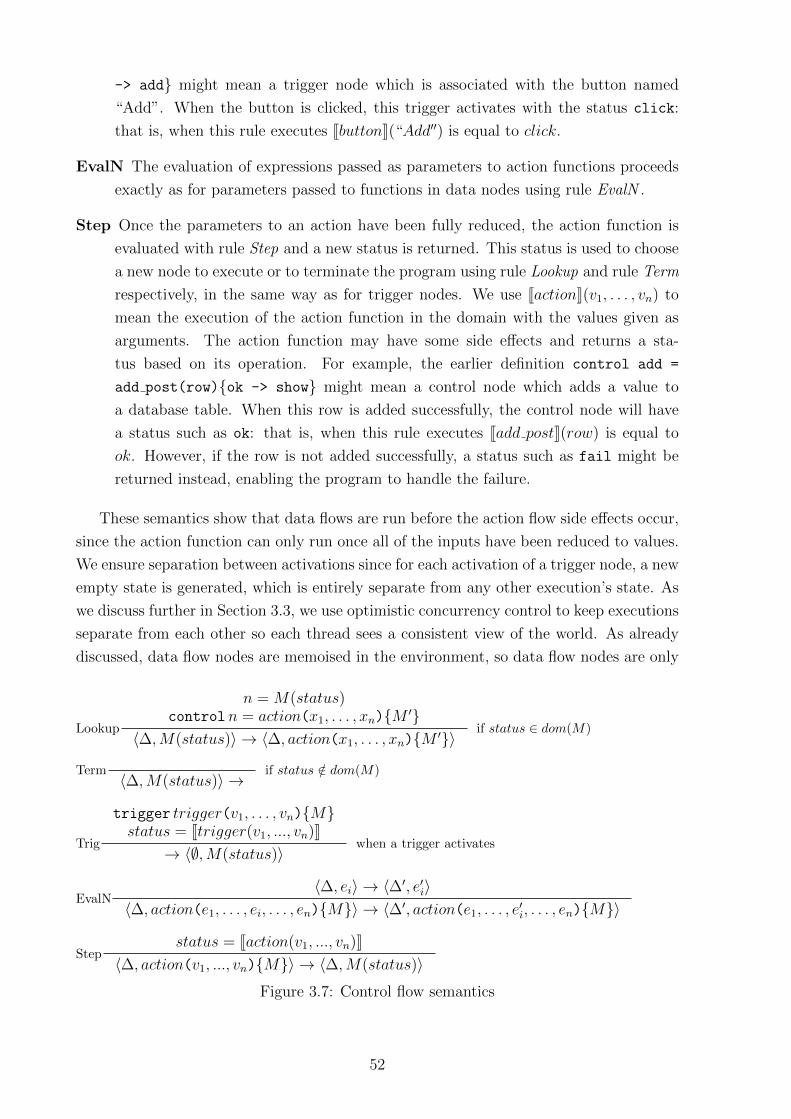
-> add} might mean a trigger node which is associated with the button named
“Add”. When the button is clicked, this trigger activates with the status click:
that is, when this rule executes [[button]](“Add′′) is equal to click.
EvalN The evaluation of expressions passed as parameters to action functions proceeds
exactly as for parameters passed to functions in data nodes using rule EvalN .
Step Once the parameters to an action have been fully reduced, the action function is
evaluated with rule Step and a new status is returned. This status is used to choose
a new node to execute or to terminate the program using rule Lookup and rule Term
respectively, in the same way as for trigger nodes. We use [[action]](v1, . . . , vn) to
mean the execution of the action function in the domain with the values given as
arguments. The action function may have some side effects and returns a sta-
tus based on its operation. For example, the earlier definition control add =
add post(row){ok -> show} might mean a control node which adds a value to
a database table. When this row is added successfully, the control node will have
a status such as ok: that is, when this rule executes [[add post]](row) is equal to
ok. However, if the row is not added successfully, a status such as fail might be
returned instead, enabling the program to handle the failure.
These semantics show that data flows are run before the action flow side effects occur,
since the action function can only run once all of the inputs have been reduced to values.
We ensure separation between activations since for each activation of a trigger node, a new
empty state is generated, which is entirely separate from any other execution’s state. As
we discuss further in Section 3.3, we use optimistic concurrency control to keep executions
separate from each other so each thread sees a consistent view of the world. As already
discussed, data flow nodes are memoised in the environment, so data flow nodes are only
Lookup
n = M(status)controln = action(x1, . . . , xn){M ′}
〈∆,M(status)〉 → 〈∆, action(x1, . . . , xn){M ′}〉if status ∈ dom(M)
Term〈∆,M(status)〉 →
if status /∈ dom(M)
Trig
trigger trigger(v1, . . . , vn){M}status = [[trigger(v1, ..., vn)]]
→ 〈∅,M(status)〉when a trigger activates
EvalN〈∆, ei〉 → 〈∆′, e′i〉
〈∆, action(e1, . . . , ei, . . . , en){M}〉 → 〈∆′, action(e1, . . . , e′i, . . . , en){M}〉
Stepstatus = [[action(v1, ..., vn)]]
〈∆, action(v1, ..., vn){M}〉 → 〈∆,M(status)〉Figure 3.7: Control flow semantics
52

evaluated once. However, if the program needs to evaluate the same expression again
after some control node has executed, it can do so by defining a freshly named date node
that evaluates the same expression.
Since control nodes form an acyclic graph, data nodes are similarly acyclic, and re-
duction of expressions usually leads to a smaller expression, it is fairly obvious that the
execution resulting from a trigger node activating is guaranteed to terminate. We could
prove this more systematically by induction on each rule, showing it either makes the
expression smaller, or accesses or activates another node (data or control respectively),
which reduces the scope for expressions to expand further in the future. Specifically,
once each node has been visited, expressions cannot grow any larger since the only rules
that expand expressions have an unvisited node in their assumptions. Therefore, in the
worst case we visit every node once and then reduce the resulting expression with strictly
shrinking rules.
3.3 Concurrency
No explicit concurrency within a program is possible – node pointers (which correspond
roughly to threads of execution) cannot be manually spawned or forked. This simplifies
the execution model and the programmer’s understanding. Instead, node pointers are
spawned in special trigger nodes, which are control flow nodes that interact with the
user or the environment. Trigger nodes spawn a node pointer whenever the event they
are watching for occurs. This means that having multiple simultaneous node pointers,
corresponding to overlapping triggerings of the program, is possible. There is no special
handling in the case of having multiple trigger nodes connected into the same control
node – each trigger node activation creates a new independent thread of execution which is
isolated from all others. To give a concrete example, each time a user of a web application
requests a new page a new node pointer is spawned. Node pointers do not interact, except
through an external data source or other external state. This is similar to the idea of a
continuation-passing web server, first introduced by Queinnec (Queinnec, 2000), but is
simpler than continuations, since no state can be carried between one node pointer and
another.
One big advantage of cd-sep is that this implicit concurrency lends itself to easily and
automatically implementing optimistic concurrency control (OCC) (Kung and Robinson,
1981). For example, in the web application case, after a user has made a change to some
data and pressed save, we can first check which version of the data they received and
ensure no intervening modifications have occurred. This can be done easily by the system
since the data flows can be statically analysed, so data which needs to be unchanged can be
automatically identified. In the case that the data has changed, two solutions are possible.
If the data changed in the course of this flow execution, then we rollback any side effects
that have happened during this execution and then restart the execution with access
53

to the updated data. This approach corresponds to running concurrent programs with
software transactional memory (STM) (Knight, 1986). Primitives that access external
resources mean we either need external transactions to rollback external side effects after
failures, or we need external side effects that can provide a compensation, which reverses
their effect, as described by Hoare (Hoare, 2010). This compensation or rollback is used
if the flow has to be restarted. If neither of these ways of reversing external side effects
is available, then any internal primitives which access the side effects must themselves
provide a way to reverse this side effect. If we cannot reverse the side effect internally
or externally, then we have an irreversible side effect. If we have at most one irreversible
side effect, and this side effect is not observed during the execution (that is, nothing that
depends on it happens, or we have a way to pretend it happened internally), we can work
around the irreversible side effect by deferring it to the end of the execution, and rolling
back all other side effects if it fails. With multiple irreversible side effects, we have to
accept a loss of some of our concurrency control on external services, which may not be
rolled back when they should be. Note we cannot delay all side effects because the flow
of execution may depend on the statuses resulting from those effects.
If the input to the flow execution depends on data which has changed since it was
retrieved, then we can cause the part of the flow execution with the dependency to fail.
This can then be transparently treated as an error in that part of the execution (and can
additionally be reported to the end-user as having failed due to stale data). The normal
error handling in the program can then be used to present the end-user with the ability
to reattempt the action based on updated data.
The separation of control and data flow will enable this kind of analysis far more easily
than current systems. It will also aid partitioning, for example, pushing filters and sorts
up to a database server, since the data flow part of the program has no side effects it can
have more aggressive optimisations applied to it than otherwise might be possible.
3.4 Comparison to other paradigms
These semantics can be neatly compared to the semantics of a pure call-by-need language
with limited side effects, for example, Haskell. The evaluation strategy of our data flow
language is exactly the evaluation strategy of Haskell. However, Haskell without side
effects can still recurse, which we explicitly disallow.
Haskell uses the IO monad to thread side effects through the program, as proposed
by Peyton-Jones and Wadler (Peyton Jones and Wadler, 1993). The programmer cannot
create an instance of the IO monad, and so is required to pass an instance created at
the outermost-level throught the whole program, thus threading control flow through the
program and making any dependencies explicit. In the same way, in our system, only
our action level has primitives for accessing external state, and it is impossible to get
to the action level from the data level (the proof of this is obvious by case analysis on
54

the data-level constructors.) There is therefore a correspondence between our data and
control flow separation and pure Haskell functions and Haskell functions that are tainted
with the IO monad in the type signature.
However, the semantics of a program in our system as a whole are slightly different
from Haskell. In our system, the firing of multiple triggers causes multiple threads of
execution to run with separate local state. These threads are independent except for any
shared access to global state which we discussed in Section 3.3. In contrast, the IO monad
in Haskell generally forces the whole program into sequential order, which does not mesh
well with interaction with other systems. Alternatives such as the STM monad give other
concurrency choices but do not allow Haskell to integrate with external systems.
In addition, Haskell requires that even idempotent reads from external state are
threaded through the IO monad. This forces lots of what would otherwise be pure com-
putations into the sequential IO path and confuses side effects with state. In contrast,
programs in our language can be viewed as “striped” – each side effectful action forces a
break in pure functions, but between side effects access to state is unrestricted. Colouring
each data node with a colour based on the first control node that is connected to it would
result in the program having “stripes” corresponding to these unrestricted read zones.
This makes programs more easily parallelisable than Haskell.
Haskell also permits side effects to occur at the data level (using a primitive called
performUnsafeIO). In contrast, we prevent all unsafe actions by having no similar escape
hatches. These are necessary in Haskell in order to make it a useful general purpose
language; our system can enforce more safety in exchange for being less useful for more
advanced programs.
Restricting programming languages to be non-Turing-complete is a common technique
in end-user programming. Most of these attempts are either data flow languages, which
we consider below, or languages with ad-hoc restrictions that excessively limit their ex-
pressibility, for example macro languages with no branching or recursion. These languages
are typical domain-specific configuration languages or macro recordings. We will not dis-
cuss these restricted languages further, since a language without conditionals is simply a
list of instructions which cannot be considered as programs, since programming is usually
about details and edge cases. The ability to create a process that is just a simple list of
instructions should be part of any end-user programming language, but a programming
language is too restricted if it does not have the ability to do anything more complex.
One interesting area of restricted programming languages is total functional programming,
suggested by Turner (Turner, 2004). Total functional programming (TFP) restricts func-
tions in a functional language to be total by removing the possibility of exceptional errors
or unrestricted recursion. Instead, recursion can only be done on syntactically identified
sub-components of parameters. Turner also suggests the use of corecursion4 on codata
4This is just recursion on codata, but with the added restriction for TFP that the right-hand sidemention of the codata is larger than the left-hand side, i.e. that the output grows. This is the dualrestriction to total recursion, which requires the right-hand side to be smaller than the left, i.e. the
55

to represent infinite computations, for example, receiving and responding to events in
an event-driven system. This separation is similar to our data/control separation: total
functions on data corresponds to data dependencies between data nodes; and corecursion
on a stream, with a terminating process occurring for each stream element, corresponds to
our system of triggers causing executions which are guaranteed to terminate. In this way,
both systems are unable to generate non-termination, but are able to compute indefinitely
on infinite input.
Our restrictions on recursion are even more restrictive than the restrictions of TFP to
primitive recursion on data. Our lack of recursion is made up for by libraries which support
powerful operations, e.g. filter and fold, on data structures. Note a DSL containing fold
and map is already quite powerful and capable of implementing something like a fuel-
limited interpreter. Programs in cd-sep are automatically embedded in a corecursive
environment, which has the same properties as the corecursion on codata possible in
TFP.
The use of controlled mutable state also increases the power and expressiveness of our
language. Persistent mutable state makes it simple to handle long-running computations
and user interaction without having to resort to codata. Persistent mutable state also
permits greater parallelism than storing state as part of the codata input, which by its
nature requires the program to be sequential. We believe that cd-sep is closer to user
mental models than a total functional language. In particular, the stylistic restrictions
imposed on the language by the need to be able to prove syntactically that computations
terminate can make programs unwieldy. Coupled with the purely functional nature of the
language, we argue this means TFP is unsuitable for end-user programming.
The data flow level of our language can be compared to several other data flow-based
paradigms. Many pure data flow languages are stateless. For example, Excel can be seen
as a data flow language. In the same way as us, pure data flow does not allow circular
dependencies, since there is no clear way for a such a program to be evaluated. Interaction
in such a pure data flow language is generally limited to either batch-processing, for
example in an image processing pipeline (Strandgaard and Hansen, 2008) which uses
a graph of modifications to an input image to create an output image, or to provide
an interactive environment, again, like Excel. Interactive environments are good for
exploring solutions and simple data processing, but tend to be unwieldy for larger scale
data processing. Many interactive environments also layer a scripting language on top
of the environment, e.g. VBA within Excel. This is awkward, and typically loses the
advantages of the data flow language such as user friendliness. In contrast, cd-sep adds
principled control flow on top of the data flow language itself.
Batch data flow is more scalable to processing a variable collection of data, providing
the program can be written at the granularity of processing a single element of input.
Batch data flow can also be extended to infinite streams of input and output, for example,
argument shrinks.
56

Unix line-ordered utilities. cd-sep distinguishes between long lists of data, which can be
processed in one go, and the creation or arrival of new data, which can be recognised with
a trigger and processed individually.
The Lucid language adds a concept of discrete time to the data flow paradigm. In
Lucid, each update to the world is discrete, so there is no requirement for programs to
be acyclic. Instead of cycles causing non-termination of the data flow computation, each
element is updated based on the current values of its dependencies. This can lead to
inconsistencies and does not guarantee that an element converges to particular value, or
even stabilises at all. This makes more advanced computation possible at the expense
of making it harder to reason about programs. Interaction in Lucid can be handled by
making a stream dependent on some external data (e.g. keyboard input), and by making
some external data dependent on a stream (e.g. printable output.) Our approach is
stronger than Lucid’s since Lucid still has the classic programming language problem –
forcing too many types of dependency into one construct. Lucid is the opposite of most
programming languages, forcing the user to do control flow with data flow.
Functional reactive programming (FRP) (Elliott and Hudak, 1997) typically adds
infinite streams to a functional language (Cooper and Krishnamurthi, 2006). Most FRP
languages also add events. Events happen at a discrete time, triggered by some update
to a stream. Because FRP events can trigger arbitrary other FRP events, FRP is Turing-
complete even without being embedded in a Turing-complete language. In contrast,
we place a strict restriction on cycles which prevents our programs from being Turing-
complete.
Some interactive data flow languages permit cycles, as long as the graph is made lin-
earisable by fixing the value of an input node. For example, the Fabrik language (Ingalls
et al., 1988) provides a UI toolkit with data flow constructs. It is possible to make two
sliders that are both set in relation to each other (for example, Celsius to Fahrenheit
temperature conversion and vice versa.) Normally this cycle is not evaluated, but if one
slider is moved manually, the cycle is broken and the other slider can move automati-
cally. In general, while bidirectionality often appears neat for small examples and limited
domains (for example Lenses (Bohannon et al., 2006; Foster et al., 2007) make good use
of restricted bidirectional programming in a narrow domain), in general it requires pro-
grams to be isomorphisms which is very difficult to ensure in large-scale programs. Thus,
although neat, we do not support any bidirectional dependencies, instead preferring to
have two separate control flows which handle changes in either slider by updating the
value of the other.
Many other programming languages use a flow-like analogy, especially coupled with a
visual environment as we describe in Chapter 4, for example, LabView. However, existing
flow languages do not make a distinction between control flow and data flow. At the most
extreme, some languages use “enable signals”, which are data flow, to simulate control
flow (Leff and Rayfield, 2007). These languages are very similar to hardware, where a
57

control line is just another type of data line5.
The Erlang language is an implementation of the Actor model, where independent
actors have their own thread of execution and communicate by sending message asyn-
chronously (Hewitt et al., 1973). Erlang has complex, structured signals between indepen-
dent nodes. Within each node, Erlang is purely functional, which is similar to our data
flow language. Between nodes Erlang allows unrestricted, asynchronous message-passing.
This gives a good separation between data and control flow, but makes the control flow
layer overly powerful. Erlang places no restrictions on how messages propagate, allowing
non-determinism and branching, whereas we demand a predictable and linear ordering of
program operations. This makes Erlang powerful and expressive at the expense of ease
of use for smaller programs.
The Scratch end-user programming environment described earlier (Maloney et al.,
2010) has similar semantics to our system. Scratch has control nodes and triggers that
function in the same way as cd-sep. Scratch has a data model based on simple variables
and animation sprites with stored properties; this data model could be fitted within cd-
sep. However, Scratch has several control blocks which surround other control blocks
and can cause them to run repeatedly, including an explicit infinite loop and conditional
loops which could be infinite through user error. Scratch also allows the programmer to
broadcast messages that can trigger one or more other executions. These features mean
that programmer error can easily cause Scratch programs to not terminate. Because
Scratch programs can intentionally run in infinite loops (for example, using a loop with a
delay in it to animate an object) there is no way to isolate different parts of the program
from each other with automatic transactions as we describe in Section 3.3. This forces
users to consider concurrency explicitly, and this is generally a repudiated technique even
for professional programmers. In contrast, by having isolated, terminating subprograms,
cd-sep makes reasoning about concurrency purely local.
The WebRB system for end-user web programming (Leff and Rayfield, 2007) has
somewhat simpler and more restrictive semantics than cd-sep. WebRB uses a similar
automatically transactional concurrency system. WebRB makes no distinction between
control and data dependencies, which significantly weakens the operations a WebRB can
carry out. Because of the pure data flow semantics of WebRB, which uses flags to select
side effectful actions to perform, only one or zero side effects are permitted in each execu-
tion, which are carried out after the execution is complete. This causes a second problem:
there can be no control dependencies on the status of a side effect. In contrast, cd-sep
gives a well-defined way to manage multiple side effects and to act based on the status of
side effects.
5On the subject of hardware comparisons, clocked registers in hardware description languages likeVerilog behave very similarly to Lucid, although access to history must have special hardware synthesisedand typically other types of control can be layered on top, e.g. reset signals. Asynchronous circuitry hasno direct software parallel, since the handshaking mechanisms necessary to connect separate asynchronouscircuits make even less sense in software.
58

3.5 cd-sep: A new paradigm for end-user
programming languages
We have described a non-recursive, two-level language paradigm that is a novel way of
structuring programming languages. We argue that the philosophy of restricting the
language to a level of expressiveness and abstraction which is appropriate to the users
of the language represents an effective approach in programming language design. cd-
sep is related to monadic IO; data flow programming; functional reactive programming;
and the actor model, but hits a sweet spot of expressiveness and simplicity. cd-sep
explicitly separates and handles control flow, making it particularly suitable for event-
driven systems that may have multiple concurrent operations occurring. Because of these
features, cd-sep is especially suited to end-user programming in event-driven systems.
However, cd-sep is only a paradigm and it is hard to demonstrate or evaluate its
effectiveness without a more concrete implementation of the paradigm. Chapter 4 now
shows how this paradigm could be implemented in the area of programming web appli-
cations. As we discussed in the introduction and Chapter 2, the web is an ideal platform
for end-user programmers but there are few appropriate tools. A tool based on cd-sep
would have all of the benefits of termination, parallelism and simple reasoning for end
users that we have discussed. We additionally consider how these concepts fit in with a
visual environment that improves on the state of the art described in Chapter 2.
As a programming paradigm cd-sep does not particularly constrain the data model,
apart from requiring support for parallelism and transactions. We combine cd-sep with
the relational data model in Chapter 4. While powerful and straightforward to implement,
this is probably too complex for end-users. We therefore suggest a more suitable data
model for end users and discuss how it fits with cd-sep and our visual programming
environment in Chapter 5.
59


Chapter 4
Visual web programming
“A favorite subject for Ph.D.
dissertations in software
engineering is graphical, or
visual, programming – the
application of computer
graphics to software design.
Nothing even convincing, much
less exciting, has yet emerged
from such efforts. I am
persuaded that nothing will.”
No silver bullet
Frederick P. Brooks (1987)
Syntax is a large barrier to end-user programmers. For programmers learning their
second, or tenth, or hundredth language, a new syntax is at worst an irritation, especially
as languages almost all follow similar conventions of structure and reading order. However,
for a novice learning their first language, syntax is a big barrier. Freeform text input is
good for experts, like using a cello bow, but for novices something like a piano keyboard,
with only two variations of input (which key and how hard) is preferable. In fact, I would
argue for something even simpler. To extend the piano analogy further, since most pieces
are written for a key signature1, the piano should disable the notes which fall outside the
key signature2.
By restricting the programmer to direct manipulation of program elements, syntac-
tically incorrect programs can be avoided, making a visual language better for novices.
One of the problems with visual programming languages has been it is hard to scale up
1For non-musicians, a key signature is which of the notes in a scale need sharps or flats. An octaveusually contains 12 equally spaced semitones, but a particular piece of music usually uses just 7 unequallyspaced notes from each octave.
2Actually, this is done for beginners since many easy pieces are written in C major, whose 7 notesare just all the easily accessible white keys.
61

as programs get bigger. I address this by restricting the visual layout severely (allowing
only for horizontal rearrangement of unrelated nodes.) This, coupled with the splitting
of programs into control and data flow makes even large programs manageable. Control
flow is mapped onto the horizontal dimension, and data flow onto the vertical dimension.
This means data always flows downwards and control to the right, so it is easy to see how
execution might proceed. This is in contrast to current visual languages where layout
is completely freeform. Petre’s review of visual programming (Petre, 1995) showed that
experts stick to conventions without help, but novices appeared ignorant of convention.
By enforcing convention, we hope to make beginners function as well as experts, at least
in this area.
Despite much research and many commercial systems such as Microsoft Access and
Hypercard, most users keep data in spreadsheet applications like Excel or Google Docs.
This data is often structured or semi-structured, but users lack suitably powerful tools
for sharing and processing it. Many systems have been proposed to mix or “mash-up”
existing data, or to help skilled programmers access databases more easily, but no new
paradigms for end-user database programming have emerged. We believe there is a need
for a data management and programming system that can be used by all computer users.
In this chapter, we make the following contributions:
• We describe how the novel separation of control and data flow described in the
previous chapter can be used in a visual programming language. This separation
can be shown by layout, colouring and other visual effects. We believe this sep-
aration makes it easy to follow and reason about programs. This separation also
facilitates the separation of reading and writing from persistent databases, again
making reasoning easier.
• Useful visual tools for building functional programs over collections. We believe
Turing-completeness is a bug, not a feature, in end-user programming languages
because complex loops are hard to reason about.
• A live, web-based, WYSIWYG environment for web development. We believe in-
stallation is a significant barrier to entry. By running on Google App Engine, our
application provides a scalable cloud-based service.
• A user study demonstrating that such a system is usable. Although we used com-
puter scientists as our study participants, we were impressed with their success with
the system.
4.1 Description
The Flows language is an implementation of the cd-sep paradigm described in Chapter 3.
We refer to the restricted control flow in the Flows language as action flow because, from
62
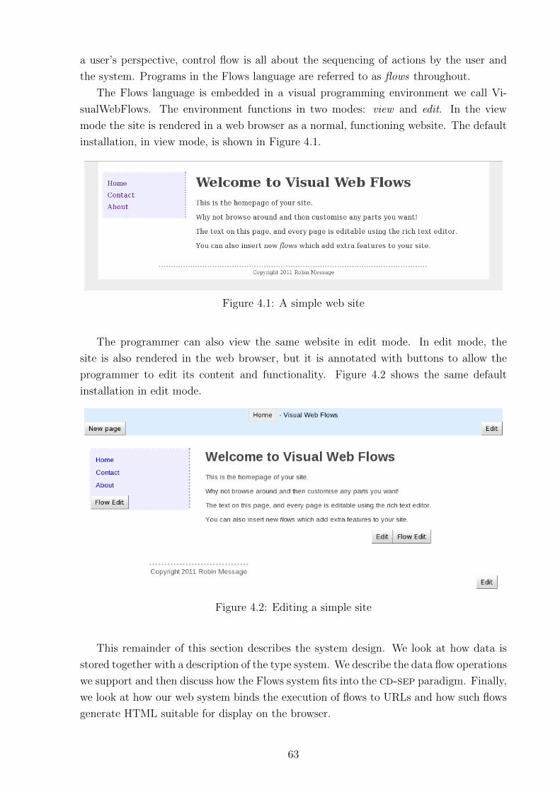
a user’s perspective, control flow is all about the sequencing of actions by the user and
the system. Programs in the Flows language are referred to as flows throughout.
The Flows language is embedded in a visual programming environment we call Vi-
sualWebFlows. The environment functions in two modes: view and edit. In the view
mode the site is rendered in a web browser as a normal, functioning website. The default
installation, in view mode, is shown in Figure 4.1.
Figure 4.1: A simple web site
The programmer can also view the same website in edit mode. In edit mode, the
site is also rendered in the web browser, but it is annotated with buttons to allow the
programmer to edit its content and functionality. Figure 4.2 shows the same default
installation in edit mode.
Figure 4.2: Editing a simple site
This remainder of this section describes the system design. We look at how data is
stored together with a description of the type system. We describe the data flow operations
we support and then discuss how the Flows system fits into the cd-sep paradigm. Finally,
we look at how our web system binds the execution of flows to URLs and how such flows
generate HTML suitable for display on the browser.
63

4.1.1 Data types
Our type system is built at two levels: primitives and tables. Primitive types are used
to describe simple datatypes such as integers, strings, HTML text and dates. Whilst
our implementation does not currently support many datatypes, it could be extended to
support a richer set of primitives, including such things as e-mail address and location.
New primitive types could be added using a system like Topes (Scaffidi et al., 2008).
User-defined types are called tables, which are similar to named records and aim to
build on user experience with spreadsheets or SQL. A table has one or more columns, and
each column has a name and a type; the name of a column is unique within the table.
All tables have a column called id of primitive type ID, whose values are required to be
unique (if not provided by the programmer, numeric IDs are generated.) Each table also
has an ordered list of tuples called rows whose contents match the types specified by the
columns. Below is a simple example table type with three columns:
id:ID full name:Text age:Integer
rhm31 Robin Message 25
arb33 Alastair Beresford 32
The system has a persistence mechanism which associates a system-wide unique table
name with the contents of the table. These persistent tables are backed by Google App
Engine, giving end-users scalability. New rows can be added to persistent tables, and
existing rows can be retrieved, updated and removed by referencing their ID value.
4.1.2 Data Flows
We first consider flows that only contain data flow; we refer to these as data flows. The
user creates a flow visually in the web browser by placing the nodes of the graph, called
blocks, and joining the nodes with edges, called connections.
All blocks output a new table except for a special output block: instead of outputting
a new table, it displays its input rendered as HTML which will be displayed to the user
on the website. The output of each block is rendered as part of the block in the visual
environment, in order to aid programmer understanding of the result of the current flow.
In the case of ordinary blocks, this means a scrollable table, and for the output block, the
actual HTML rendering of the output as it would be seen on the website.
Blocks may have zero or more inputs and an output from one block can be wired to
any number of inputs, but each input can only accept a single output.
The output block can be configured to display output in one of four different ways: (i)
plain, this output style renders its input without any formatting; (ii) list, this configuration
renders the value of each row in the input as an HTML list; (iii) table, this output style
displays the input table as an HTML table, with the column names as a header row; and
(iv) report, this configuration displays each row of the table input according to an HTML
template. The HTML template can be edited using a WYSIWYG interface. Values from
64

cells in the current row can be displayed using mail-merge style grey boxes in the HTML
template. A detailed example using this feature is presented in Figure 4.6 of Section 4.2.
The output block could easily be extended to support other output types, such as
graphs or maps. This is not something the end-user could be expected to define, but it
should be possible to add mappings to existing libraries to a VisualWebFlows system for
these types of output.
We considered making it possible to nest other flows inside a report. Whilst potentially
useful, this feature seemed excessively powerful. Instead we would like to provide a
mechanism for adding buttons to reports that support contextualised triggering. The
action flow for these buttons would be editable from the report editor and would have
a special data flow input which would contain the row that the button that was pressed
was on. Such buttons would be useful for, for example, deleting a row from a table, or
switching to a more detailed view of that item of a report.
Blocks other than the output block can be divided into two categories: producer blocks
which have no input and therefore merely provide data; and stateless processor blocks
whose output is a strict function of inputs.
Producer blocks
There are four types of producer blocks that take no input: (i) form, a row of the values
containing all the HTML form elements on a page; (ii) page, a row of values representing
the arguments found in the URL. Further information on this input block is described in
Section 4.1.4 as part of our URL processing scheme; (iii) text, produces a piece of static
text. This text can be edited from within the flow editor; and (iv) table, loads a named
persistent table from the system.
We would add a block that can import data from other web applications dynamically.
One problem with such a block is converting the input into our data types. Converting a
particular, identified table on a web page would be fairly easy to do, and we could provide
a WYSIWYG GUI for the user to select which table to import from a page. Access to
structured or semi-structured data sources would depend on our ability to convert that
data into our table format, which we do not in general have a good way to do. For things
like RSS feeds and simple query methods from web services that return two dimensional
data it would be fairly easy to import these as tables.
Processor blocks
All processor blocks have one or more inputs and a single output. These blocks offer
simple processing steps which are similar to SQL and spreadsheet functions, such as
where (select only those rows in a table which have a specific set of values), order by
(re-order the rows in a table) and limit (only output the first n rows). These blocks are
similar to the features provided by the Yahoo Pipes system (Yahoo!, 2007). Our system
also supports an equi-join block which implements the SQL equi-join feature for tables,
65

and an aggregate block which supports operators including sum, count, minimum and
maximum on a particular column.
Finally, we have a link block which accepts a table as input and combines this with
the special controller table (described later). The block then outputs a column of URLs
suitable for generating clickable web links in the rendered HTML output of the output
block. The full operation of the link block is described in Section 4.1.4 after we have
described URL handling and the “system” tables.
As an example data flow, consider the flow that puts the name of the current page in
the web browser title bar. Pages within VisualWebFlows are also stored in a persistent
table, and flows are used to display them similarly to any other part of the program. The
program which generated the name of the current page in the title is shown in Figure 4.3.
Figure 4.3: Page title in flow editor
The program written in Figure 4.3 is installed in the default installation and represents
a simple data flow. On the left-hand side is a selection palette from which the user can
select data sources and processing blocks. In the centre of the screen at the top are two
blocks, one representing a portion of the page URL labelled “Page arguments” (in this
case with the value “home”), and the other representing a persistent table stored in the
66

system (in this case the table containing all the pages of the website). These two blocks
are wired into a processing where block, which selects a single row from the pages table.
Finally, the choose block selects the title column from the output of the where block; this
is connected to the output block at the bottom of the screen and is then displayed in the
browser title bar.
4.1.3 Action flows
We now consider flows that contain control flow in addition to data flow. These flows are
called action flows but may also contain data flow blocks. An action flow is only created
when the state of the server needs to be modified, for example by the submission of data
contained in a web form; the action flow then allows the programmer to modify the state
of persistent tables and cause other side effects to occur. Action flows are represented by
a DAG of action blocks rooted at a single special start block, like data flows are rooted in
an output block, but with the arrows in the opposite direction, so action flows out of the
start block into only one subsequent block, and action may flow into a block from multiple
other blocks. The use of DAGs prevents loops of control being formed, which prevents a
variety of programming errors. A block can be triggered by multiple other blocks to allow
sharing of code between operations, e.g. redirecting to a certain page whether or not an
action succeeds. Data flows can also be rooted in an action block. The precise semantics
are based on those described in Chapter 3 and summarized below.
Every normal action block has exactly one trigger input, and at least one trigger
output; in addition, zero or more data flows can be connected to an action block. No
action block has a data flow output.
An individual action block starts processing when it receives a trigger event on its
trigger input and fires exactly one trigger output when processing is complete. In this
way, processing of an action flow begins at the root of the action tree, represented by the
start block, and follows a single path through to a leaf node (i.e. an action block with
nothing connected to its output trigger).
Currently, the only start block we support in an action flow is the clicking of a submit
button on a web form. Other start blocks could be triggered by, for example, timed
events, updates to external data sources or e-mail messages received. These start blocks
would be managed through a separate trigger administration area, since they are not part
of the user interface of the site in view mode. Where external data sources do not have
a notification mechanism, the VisualWebFlows could be configured to poll data sources
like RSS feeds and trigger a flow when new items are added. Asynchronous messaging
systems like e-mail, twitter or XMPP would be easy to add to the system. However,
these triggers would need a special mechanism to get the content of the new message.
Web applications that can call callbacks could also be supported through auto-generating
callback URLs for callback triggers.
67

In the context of a web application, a web form submission carries out two tasks: (1)
it (possibly) modifies the state of the server, and (2) displays a new page to the user. By
default, the VisualWebFlows system re-displays the same page the user came from (i.e.
the one containing the form submitted) after executing the action flow. This is useful for
a variety of applications, such as writing a search page, or providing simple data entry. It
also enables the programmer to return a user to a form if there is an error acting on it, so
that the user may adjust their submission and try again. In more complex applications,
the programmer can attach a redirect action block at the end of an action flow to control
the page the VisualWebFlows system will return to after the action has been processed.
If the programmer wants to display the same page but with any form controls having
their default values, they can just redirect to that same page.
By convention, action blocks are arranged from left to right across the bottom of page,
while ordinary blocks, describing a data flow, are arranged from top to bottom of the page.
In this way an action flow resembles a timeline of events which begins at the start block
and proceeds along a single path through a set of action blocks. Also, as mentioned earlier,
data flows can be connected to action blocks. Since action blocks may modify the state
of persistent tables, it is important to define when any data flows are evaluated as their
contents may be updated as the action flow is processed. In the VisualWebFlows system,
any data flow connected to an action block is evaluated immediately before the action
block is executed. In particular, connected data flows are evaluated after the execution
of the preceding action block that triggered the current action block.
Our current implementation supports three action blocks in addition to the start and
redirect blocks already mentioned. The insert action block adds one or more new rows
to a persistent table. It has two output triggers, labelled “success” and “failure”, which
fire under the obvious circumstances. In addition, the insert action block accepts a single
data flow input which provides the values for the new row or rows to be added to the
persistent table. The update action block is similar to the insert action block but has a
second data flow input to provide the id values of the rows to update. A delete action
block removes one or more rows from a table. It takes the id values of the rows to remove
from the table.
We could also have action blocks that are the opposites to the trigger blocks discussed
above for messaging services. An e-mail block would be similar to an output block in
report mode, but would have an additional input to select which column contains the
destination e-mail addresses.
We need an if-block, which enables a user to choose between alternatives, for example
for data validation. Such a block would have a similar interface to the where block, but
would activate a true or false trigger based on the condition on the input data. A block
more like a switch statement might be useful but would require us to have types that are
drawn from sets in order to give a usable semantics.
Action flows are designed to hide the fact that web applications are made up of separate
pages and instead give a more direct representation of data processing. In particular, the
68

user does not have to worry about form submission URLs, since all forms submit to the
page they are from and are then processed by the system. These properties have been
chosen deliberately to provide a simple interface for programmers. This is an improvement
on the HTTP programming model of having forms and the code which handles those forms
separated, which is something that even experienced programmers can find complicated.
This mechanism will also support AJAX-based forms, which could execute asynchronously
without making any changes to the flow language itself.
4.1.4 System tables and URL handling
Every installation of VisualWebFlows contains system tables to control URL handling,
rendering of HTML, and to provide storage for static content. URLs are handled in the
following way: The domain name is removed and the path is split on slashes into a list
of strings. For example, http://www.example.com/pages/home becomes [pages,home].
The first element of the URL is used to look up the controller to use from a special system
table. A controller provides a layout for the page (so pages can have consistent formatting
and menus) and a block of HTML that is used as the main body of the page. This HTML
may contain flows. For example, the built-in pages controller just returns the body of
the row specified by the second URL argument in the pages table. The current URL,
represented as a row, is made available as a producer block in every flow the programmer
writes, and can therefore be used by the programmer to control the execution of flows on
any page.
The combination of controller, layout and pages system tables allows users to quickly
create static web pages, and also provides a place to attach the output of flows which
utilize new, user-defined tables, into the URL address space of the site. When a new
table is created, controllers to add and edit rows from that table are autogenerated as
an aid to users. These generated controllers can be edited in exactly the same way as
built-in and user-created controllers.
Now that we have described the controller table we can provide a better description of
the flow language link block mentioned earlier. The link block expects its input to have a
single id field, which came from a table. If there is more than one id field, the user must
select which one they want to link to. If the id field did not come from a table, no link
to it can be made, so the link block fails. The link block then examines the controller
table to find which controllers can render the table the id came from. The first of these
is selected by default and the user is offered a choice of controllers if there is more than
one for that table.
4.2 Example application
In this example application, we show how a blogging system could be added to a Visu-
alWebFlows site. We demonstrate the utility of the system, and how it is used to build
69

applications.
Firstly the user creates a new page that will contain the blog, or chooses an existing
page to incorporate the blog into. New pages can be created by clicking the “New Page”
button, which is always available within edit mode. The user is asked to give a title for
this page, which is then displayed in edit mode.
The programmer can use the HTML editor to add any titles or other information to
the new page. The next step is to insert a new flow which will show the latest posts of the
blog. Newly inserted flows just display the text “Default” and can be edited by clicking
on them. The outputs of flows are displayed with a grey background in the HTML editor,
as shown in Figure 4.4, to distinguish them from editable text. These features mean that
flows can be combined with HTML code and formatted as the user desires.
Figure 4.4: HTML editor on the home page
The user edits the new flow to create a view of the latest posts. Three flow elements are
needed: a table to store the posts, a sort block to arrange the posts in reverse chronological
order, and an output block to display the posts.
From the palette on the left (Figure 4.5), the user clicks the “New table” button
(marked 1). The user is then taken to the table editor where they specify the columns
needed. In this example, we want a title, some body text, and a date “posted at” column
for each post. The user can also add any rows to the table; in this example the user has
added a couple of posts.
The new table then appears in the palette of the flow editor. The user can add the
new table to the flow and see its contents (marked 2 in Figure 4.5.)
The user adds a sort block to the output of the posts table (marked 3) and sets it to
sort its input by the “posted at” column, in descending order3. Next, the user connects
the output of the sort block to the output block.
3We do not yet have a primitive date type, so we have cheated and used ISO formatted dates wherelexicographic sorting is also temporal sorting.
70

Figure 4.5: Latest posts flow
Since we want to format each element of an entry differently, the user switches the
output block to report mode and clicks “Edit report”. In report mode, each row of the
input is displayed according to a template, which the user can now create. Figure 4.6
shows the report format editor for this report. The report editor enables the user to insert
output fields into a rich text editor, using the drop-down menu and insert button on the
top right. The editor also enables the user to manipulate and format any static text and
output cells. The user inserts three fields, “title”, “body” and “posted at”, and formats
them so that the title is be displayed centered, followed by the body of the post and the
right-aligned date. The user also adds the text “Posted at ” before the date field.
Figure 4.6: Report editor for the blog flow
71

We will now look at an example of an action flow in the context of editing a blog post.
Creating a new table usually implies the need for a method to add and edit entries in
the table on the site. As explained in Section 4.1.4, the system auto-generates two new
controllers for this purpose. The view of the edit controller generated for the posts table
is shown in Figure 4.7.
Figure 4.7: Editing a post
Automatically generated controllers and flows can be edited in exactly the same way as
user created ones. For example, the default behaviour after the “Save” button is pressed
is to return to the same page. Figure 4.8 shows how the action flow for the “Save” button
in Figure 4.7 could be modified to redirect the user back to a list of all posts after a
modification is saved successfully.
The action flow editor has two additional sections in its palette compared to the
normal flow editor – form elements and actions. Form elements enable the user to get
the values of any controls on the page when the button was clicked. In this example, the
automatically generated code pulls in each of the form elements on the page and merges
them to give a row suitable for adding to the “posts” table.
We can see how data flows downwards and action flows left-to-right. The “Save” node
on the bottom left runs when the save button is clicked. It causes the row specified by
the page arguments in the “posts” table to be updated with the values taken from the
form elements.
Figure 4.8 shows a modification to the generated action flow. The generated flow stops
after the update table block, so the user remains on the edit posts page after an update.
The user adds a redirect action to the update success trigger, which means the user is
taken to a list of posts after a successful save. If the update fails, the user stays on the same
page so they can try submitting their changes again. A more advanced implementation
might display an error message to the user explaining the reason for failure.
4.3 User study
In order to assess the suitability of the Flows system for end user programmers, we decided
to do a preliminary user study to see if people could use the system to create simple web
applications. We recruited computer science students to participate in the study. Whilst
72

Fig
ure
4.8:
Sav
eac
tion
flow
–pro
gram
mer
modifi
cati
ons
onth
eri
ght
hig
hligh
ted
by
the
gree
nbac
kgr
ound
73

our system is aimed at end-user programmers, we felt computer science students would
be a good baseline – if they could not understand the system, there is little hope for
end-users. We set study participants the task of building a simple web application in 30
minutes, and measured whether they were able to complete this task successfully in the
time allotted. We also used a follow-up interview to gather qualitative feedback, and assess
their understanding of the Flows system. We found that 7 out of the 8 students completed
the task in the time allowed and all of the students showed a good understanding of the
Flows system. Many of them agreed the system was quicker than using a conventional
programming language for the kinds of tasks assigned. The next step for this research
would be to repeat the same study with non-computer scientist participants in order to
ensure beginners can also understand and use the Flows system. We now examine the
participants, goals, results and evaluation of the study in more detail.
4.3.1 Participants
For ease of recruitment we found 8 computer science students to participate in the study,
all male and between 18 and 25 years old. They had a variable amount of experience,
averaging about 3 years of programming knowledge. Their exact experience can be seen
in the answers to question 1 of the interview.
4.3.2 Goals
Participants were shown a ten minute training video which demonstrated the Visual-
WebFlows system. They were then asked to solve the following problem: Starting with
a new, blank application, please create a new page for people to sign up to an impromptu
five-a-side football match. The page should show a list of who is signed up for the match.
People should be able to add their names to the list. People should also be able to remove
their names from the list. The full instructions given to participants are reproduced in
Appendix A.
We assessed the outcome of the study in multiple ways. We had a simple pass/fail
cut-off after thirty minutes to see if they could complete the assigned task in that time.
We observed the participants working to try and identify any problems with the system
that could be fixed. We interviewed participants after they had attempted the task to
get qualitative feedback on what was good and bad about the Flows system, and to ask
them some questions to test their understanding of the Flows paradigm.
This assessment was designed to test the usability and understandability of the Flows
system, and to gather feedback that could improve the system and the study. We also
set an extension problem for the students if they finished the main task in less than 30
minutes: 1. So as to be fair, ensure players show up in the order they add themselves. 2.
Show the first five players as Team 1, the next five as Team 2 and the rest as Substitutes.
This extension problem was designed to test the data handling capabilities of the system.
74

4.3.3 Results
The full results of the study, including details on the participants and notes on their
answers to the interview questions, are given in Appendix B. Here we discuss the results in
relation to the goals of the study. Most importantly, although some students were delayed
by bugs in the prototype implementation, seven out of eight participants completed the
task in 30 minutes, and most participants attempted some of the extension tasks.
All of the participants showed a good understanding of the nature of flows in their
answers to the interview questions. Additionally, four of the eight answered the more
tricky question “Is a form control a flow?” correctly.
The qualitative feedback was good, with many positive comments and suggestions for
how the tool could be improved. The overall idea was considered good by several partic-
ipants, one of whom explicitly commented that it was quicker than using a programming
language. The flows concept was commented on by several participants who thought it
was “expressive”, “quite good” and “intuitive”.
Negative comments fell into three main categories. The rename, merge, and delete
blocks were commented on as being hard to understand; the pages table and mechanisms
associated with it were “confusing”, “[too] magical”, and fragile (one participant broke
their instance of VisualWebFlows completely); and the environment lacked supportive
features, such as copy-paste and undo, and was inconsistent in places, for example, in the
naming of blocks.
Feature requests were mostly obvious things, such as extra form controls like check-
boxes and select boxes; the ability to add controls to reports to do things like deleting a
certain row; and being able to have multiple output blocks in a single flow.
As we observed participants, it became obvious that their computer science training
actually hindered them in certain cases, for example, as they searched for a way to add
abstraction to their programs, and looking for ways to do more advanced things with the
output of flows like adding buttons to rows and splitting the output into multiple parts.
Most participants attempted the extension tasks, but they struggled to structure their
data in a way that would allow them to complete the tasks within the constraints of the
VisualWebFlows system.
4.3.4 Evaluation
The system was useful and usable for students with varied amounts of programming
knowledge and experience. Whilst many students had issues with bugs and inconsistencies
in the prototype implementation, the idea of a flow-based programming language appeared
to be appealing to the study participants, and was well-understood by them.
The biggest problem participants had with the system, particularly in the extensions
tasks, was with structuring and managing data. We consider how this could be improved
in Chapter 5.
75

Because we used computer scientists as study participants, this unfortunately weakens
the claims we can make about the suitability of our system for end-users. However, these
students, some with limited expertise and experience, were able to quickly understand and
effectively use the system, which are least eliminates the possibility that it is completely
incomprehensible and gives us some confidence that end-users will be able to pick the
system up. Additionally, even computer scientists might be quicker using the Flows system
than a conventional programming language for some tasks; although not the original
goal, this would still mean the Flows system is useful for some users. Due to a lack of
time and resources we were not able to carry out a further study with non-computer
scientists. Because of this, in the next section we carry out a systematic assessment of
our environment in order to answer the question of whether it is a suitable system for
end-user programmers.
4.4 Cognitive Dimensions of Notations Analysis
In this section we use the Cognitive Dimensions of Notations framework (Green, 1989)
to analyse the usability of the system we have designed. We make comparisons to Excel,
as our standard of end-user programmability, and a standard web programming language
like PHP that might be used instead of our system. We first compare these three systems
on each dimension separately. Figure 4.9 gives an overview of where each system falls on
each dimension4. We then discuss where we have improved end-user usability compared
to existing systems, and identify areas for future work that would improve a system like
ours further.
Abstraction gradient Our notation requires the user to work at a fairly low level of
abstraction. Crucially, there is no procedure for packaging up a collection of nodes in
a graph as a reusable node, unlike how a function can be created in most programming
languages. This abstraction-hating is close to the level of abstraction possible in Excel,
where formulas must be copied if they are to be used repeatedly. We do support structured
data types as tables which, when compared to Excel, are an abstraction over multiple cells.
The amount of abstraction required by the user seems acceptable compared to Excel, and
less than the programming language.
Closeness of mapping The notation maps quite well to the problem domain. In
particular, our WYSIWYG editor enables the user to put programs directly into web
pages. The use of tables as the pervasive data structure forces a tight mapping between
the notation and the possible problems that can be expressed. This could make it much
4Note that these dimensions are not orthogonal, so a change in one dimension will affect otherdimensions. Additionally, whilst the dimensions are not intrinsically good or bad, we organise themaccording to the preferred direction of each dimension for end-users, for example, low abstraction andhigh visibility are considered good.
76

Figure 4.9: Overview of where each system falls on each dimension
harder to work on other data structures. For example, handling tree structured data
would be better done by adding new primitives to the language than by attempting to
force trees into tables, but for an end user having to handle tree structured data is likely
to be awkward.
Consistency There is a high degree of consistency between the flow operations. The
user would need to learn about the distinction between data and control flow. This is
the biggest inconsistency in the system (although deliberately so). In our user study
(admittedly of computer scientists), users had generated excellent hypotheses about the
workings of flows, suggesting a good degree of consistency. One problem area is that
the operation of each flow node is unique and specific, requiring the user to consult the
manual to be sure of the exact operation of each type of node. This requirement to search
for and understand operations is worse in Excel and PHP which both have many more
operations and many operations that are only provided for legacy reasons, but are not
hidden from new users.
Diffuseness / terseness The use of simple flow building blocks makes the language
quite verbose. This is a common problem in visual languages compared to textual ones
like PHP. However, an improvement we have made is to use a WYSIWYG environment to
link the various parts of the program to their related user interface so that any particular
part of the program can easily be found and displayed. This modularity enables users
77

to build large programs, as long as the parts of those programs are still small enough,
avoiding some aspects of the scaling problem (Burnett et al., 1995). We also improve on
Excel by having structured data, so that the display size of a collection is not proportional
to the number of elements as it is in Excel.
Error-proneness The lack of static type checking makes it more likely a mistake by the
user will not be picked up by the environment. The previews of the output of each flow
element are designed to mitigate this, enabling the user to try test values and observe
the effect on the program, helping avoid mistakes. We currently do not provide good
feedback to users on what the table operation control blocks will do with the inputs they
are given. Excel has live feedback which avoids this problem, but despite this, errors in
Excel spreadsheets are pervasive (Powell et al., 2009) due to the hidden nature of formulas
and reliance on copy and paste.
Hard mental operations The user has fewer hard mental operations in understanding
a particular flow than Excel5 or PHP. However, understanding how side effects occur and
how one part of the program may affect another is hard, as it is in full programming
languages. Our use of optimistic concurrency control and automatic retrying means that
users do not have to think in order to handle concurrency correctly. In contrast, a language
like PHP requires many hard mental operations to reason about multiple simultaneous
users.
Hidden dependencies Within a single flow, most dependencies are very visible, more
so than Excel or PHP. The dependencies between database operations are hidden both
within a flow and between flows. This kind of dependency is also hidden in PHP and
Excel; it is hard to see how it could be shown in any environment.
Juxtaposability Similarly to Excel, it is not possible to view multiple parts of the
notation at once. This is mostly a restriction to simplify the interface, but is weaker than
most programming environments.
Premature commitment The system requires the user to design data tables before
they can be used. If a user structures data in the wrong way, they might have to rewrite
the whole application to recover. This is a common problem in all programming languages
and so is usually overcome by methodology – primarily systems analysis and reducing cou-
pling. VisualWebFlows is weaker than Excel and PHP in requiring too much premature
commitment due to weaknesses in the environment.
5Because of the environment of Excel, it is time consuming and error prone to manually trace causeand effect. Excel comes with special tools for highlighting dependencies but they are insufficiently pow-erful and not well-known. In contrast, our graph based approach makes tracing cause and effect trivial.
78

Progressive evaluation Within a flow it is very easy to get feedback because of the
preview feature. It is also possible to build and use parts of a program separately. Overall,
similar to Excel and better than PHP.
Role-expressiveness It is easy to see the role of components within our flow system,
since they show previews of what they do. However, choosing which component to use
to achieve a particular goal is more difficult for users. This is a common problem in
programming languages, so we are no worse than PHP, but Excel is better in providing
searchable help and advice about the role of functions within the environment.
Secondary notation We provide the opportunity to use layout as a secondary notation
in our visual editor. We do not provide any comment ability which is weaker than both
Excel and PHP.
Viscosity The lack of functional abstraction means some changes to the structure of
data may require multiple repetitive changes. This is compounded by our relatively weak
environment – we do not have features like copy/paste or autofill that make this less of
a problem in Excel. Overall, localised changes are very easy but more dramatic changes
have noticeable viscosity.
Visibility When not in the flow editor, although it is possible to identify which parts
of the page are flows, it is not possible to see how those flows function. This is no worse
than Excel, where cells display their output instead of the formula used to generate that
output, or PHP, where a function call tells you the name of the function but not how it
actually functions.
We will now elaborate on what we believe are the important differences between our
system and Excel and PHP, before considering areas where our environment could be
improved according to our analysis.
According to our analysis, we believe we have managed to remain fairly similar to
Excel on most cognitive dimensions.
In the area of secondary notation, we are weaker than Excel. Excel is what you
might call a “notational playground”, allowing arbitrary mixing of primary and secondary
notation within a sheet. This makes Excel very powerful for exploration as a task, and
enables it to be used in ways that were almost certainly not intended6. In contrast, our
tool is more structured and lacks this ability to use secondary notation so powerfully.
We particularly improve on Excel in the area of hard mental operations and hidden
dependencies. One of the main hard mental operations in Excel is tracing the dependen-
6The author’s father designed a garden in Excel, including a hedge maze, by resizing the columns sothe cells were square and then colouring the cells to represent the plant in that area. The only missingfeature was the ability to count how many cells were of a certain colour, which would have helped himbuy the correct amount of gravel for paths.
79

cies, which are hidden. By making dependencies visible, we aid the user in doing this.
The same argument applies to comparisons with other non-graph-based languages.
We think we have improved on PHP (which we use as representative of a simple pro-
gramming language for web applications) in two key areas for end-user programming. By
providing the ability to see the results of programs as they are written (progressive eval-
uation) we make it easier for users to develop programs and self-correct as they proceed.
Our modelling of web applications in our new paradigm enables more consistency in how
operations occur and makes the mapping between the domain and the language closer.
However, there are a number of areas where our system would hold back more ex-
perienced programmers. The lack of tools for abstraction would lead to the attendant
problems of copy-paste coding and is likely to be irritating to more advanced users. We
considered adding the ability to define new blocks based on other blocks but felt it did not
fit well with our aim at end-user programming7. This lack of abstraction ability is also
the cause of some of the viscosity in our system, since without abstraction, common parts
of programs are repeated, necessitating multiple, spread-out edits. Our environment is
more diffuse than a typical programming environment, showing about equivalent to one
method in the space of several methods.
This analysis has caused us to identify several areas where our environment could be
enhanced to support users better without changing the notation. The lack of juxtapos-
ability in our environment is unrelated to the notation. A windowed system for opening
more than one flow at a time would be easy to implement and would solve this problem.
However, the diffuseness of our representation means that it will never be possible
to show as much at once as with a more compact representation. A more compact
representation (perhaps based on the syntax in Chapter 3) would be useful for power
users as an alternative and completely compatible representation.
Some action blocks do not demonstrate their operation to the user in an intuitive way,
and so use of these blocks can be error-prone. A better display on these blocks would
help users avoid errors.
Our environment forces some viscosity due to a lack of features. Copy/paste could be
added easily, as well as multiple selection. The use of basic block coalescing and automatic
layout would make it much easier to rearrange flows and add new flow elements, which
reduces viscosity at the expense of slightly weakening secondary notation. Because the
flows language has various constraints on the types of connections between nodes, it would
be possible to automatically lay flows out in a systematic and helpful way. In particular,
data flows could always go downwards and action flows could always be to the right. These
constraints would ensure that the layout follows the semantics of the flows language and
would work well with an online layout system like that described by He and Marriott (He
and Marriott, 1998). Given that secondary notation such as laying out graphs is often
7Note that Excel still does not have user-defined functions, despite research into how this could beimplemented (Peyton Jones et al., 2003).
80

done badly by novices (Petre, 1995), we think this reduced expressibility could be a good
trade-off.
A simple idea to improve secondary notation would be to add free text blocks that
could be placed anywhere and contain uninterpreted comments. However, as with com-
ments in programs, it would be easy for these to get out of date and to get left in
inappropriate places. Therefore, comments should be attached to specific nodes, edges or
groups of nodes, in order to force them to be connected to the program. This is another
case where weakening the secondary notation to be less expressive makes it more useful
in practice.
Overall, the Flows language improves the notation for beginners from an existing pro-
gramming language like PHP on almost every dimension. Additionally, it is as good or
better than Excel on most axes, which suggests it would be well suited to end users. Fur-
ther work to improve the environment would remove most of the remaining disadvantages.
4.5 VisualWebFlows: A new platform for end-user
web programming
We created the VisualWebFlows system to showcase the semantics described in Chapter 3.
This chapter has explained the workings of this system and demonstrated how visual
languages can be used for data processing tasks. We have shown how the novel separation
of control and data flow in cd-sep can be translated into a real programming language,
and how the visual environment can support this separation through syntactic features
such as layout and colour changes. We have also demonstrated a technique which allows
users to observe the dynamic operation of programs statically through the preview tables
we show next to each block in the environment. Flows is a scalable, web-based system
which allows end-users to create distributed programs in a familiar online environment
without software installation. We have also addressed aspects of the scaling problem for
visual languages by separating out parts of the user’s program and linking each part to
the interface they are creating.
We evaluated the system through a user study and using the cognitive dimensions of
notations framework. Our user study was small-scale and relied on computer scientists
as study participants. Although the participants were not the target users of our sys-
tem there are still some useful conclusions that can be drawn from the study. Firstly,
study participants with a variety of experience and exposure to different systems found
VisualWebFlows to be usable, and most of them successfully completed the study task.
Secondly, many participants commented on the usefulness and effectiveness of the system,
which suggested that even for computer scientists it might still fill a gap in the available
programming languages for simple data gathering and processing tasks. A further user
study with non-computer scientists would be necessary to validate these conclusions and
ensure the system is usable for end-users. A more polished system, which could take into
81
account some of the feedback from study participants and conclusions drawn from the
cognitive dimensions analysis, would be needed to make a full evaluation.
We used a cognitive dimensions of notations analysis to make up for some of the weak-
nesses of the user study. In most areas our system improved on programming languages
for beginners and was closer to Excel, which is considered a successful end-user program-
ming language. We also identified areas where we significantly improved on Excel, such
as minimising hard mental operations and having fewer hidden dependencies. In several
areas our prototype environment is understandably weaker than a commercial product,
such as in secondary notation, juxtaposability and viscosity.
The main area that did not work well was the relational data model. Even technically
savvy users struggled with how to structure their data, and the cognitive dimensions
analysis revealed this to be primarily a problem of premature commitment. In the next
chapter we consider how users could be aided in structuring their data by allowing them
to restructure data after they have gathered it, and suggest how this data structuring
technique could be integrated with the VisualWebFlows environment.
82

Chapter 5
Inferring types from data
“All problems in computer
science can be solved by
another level of indirection.”
David Wheeler
“...except for the problem of
too many layers of indirection.”
Unknown
This chapter describes an inference technique which helps users to structure and re-
structure their data. Users need help structuring data because, while humans are good at
identifying patterns, they are relatively poor at doing so over large data sets and at unify-
ing related patterns. It is also helpful to aid users in restructuring data because end-users
are relatively poor at abstract planning, so early choices may need to be changed in order
to avoid premature commitment problems like those identified in the VisualWebFlows
system in Chapter 4.
We expect users to be able to work with elements of data that have some structure,
and to use our technique to create a unified structure over these elements. Many existing
information systems contain data that is neither fully structured nor entirely unstructured,
so called semi-structured data. The study of semi-structured data has mainly focused on
structured records that contain unstructured fields. However, our inference must focus
on the opposite problem – organising untyped records of typed data.
Some examples of data organised like this are:
• Key-value databases
• Badly normalised databases with many NULL values and multi-purpose fields
• Objects within dynamically-typed programs
83

In each of these cases, any particular value plucked from the data is structured, but there
is no overall, predictable structuring on the data, making type checking, error detection
or optimisation difficult or impossible. This may happen because the structuring has been
lost, in which case we are reconstructing it, or that no overall structure ever existed, so
we are constructing one. A further example is e-mail, which (from a semantic point of
view) is an unstructured list of semi-structured records.
We use records (a record being a map from textual keys to primitive values) as the
basic element within a database system for end-users because they fit well with user’s
understanding of paper filing systems, where each record is a self-contained unit of data,
and computer filing systems, where again each file is a self-contained document. Records
were used very successfully as the basis of Hypercard (Apple, 1998), one of the most
popular and successful end-user database systems. We want to enable users to store data
in records without thinking too much about how those records are structured, but to then
be able to have programs act on sets of related records.
To give a concrete example, consider a key-value database. This database contains
records and each record is made up of key-value pairs. For example, we might have three
records {Processor:“3GHz”, Memory:“4GB”}, {Processor:“2GHz”, RAM:“1GB”}, and
{Benchmark:“Memory copy”}. The ideal structuring would be into two sets of records,
one of type {Processor, Memory/RAM} and another of type {Benchmark}. This structur-
ing reveals the two types of data within the database and identifies the variation within
one of those types (although this relies on an ontology to equate Memory and RAM).
An acceptable and more feasible structuring would be {Processor, Memory, RAM} and
{Benchmark}, which identifies the two datatypes, but does not fully categorise the for-
mer. A poor structuring would be {Processor, Benchmark}, which does not separate the
two datatypes. An absurd structuring would be {Clowns}, {Chickens} and {Cowboys},which bears no relation to the input data.
We infer a good structuring of the user’s data by using a statistical clustering tech-
nique. We discover the types within the set of records created by the user in a principled
and robust way. We do this by building a simple trained simulation of the user’s prefer-
ences about matching of records and by then combining these matching judgements into
an evaluation function for a set of types using standard Bayesian techniques. We then use
a search technique with this evaluation function to find the best set of types for the user’s
data. The technique attempts to match records that the user would consider related and
tries to also minimise the number of different types generated. Because of the statistical
approach, it is robust to minor variations between records. As well as finding records that
are related to each other, this technique also generates types that could be used by the
user as templates for creating new records.
Section 5.1 begins by giving an overview of the statistical principles used. We describe
how we formalise our intuitions about user preferences and how we can combine judge-
ments about individual types to give an overall structure. In Section 5.2 we describe how
we calculate similarity between records and types; and how we build this into a statistical
84

evaluation of a set of types for a set of records. Section 5.3 shows how we use this statis-
tical evaluation measure to generate and select the best set of types for a particular data
set. We compare different search techniques for checking a manageable number of models
before settling on simulated annealing as most suitable. In Section 5.4 we then compare
the techniques described to existing techniques such as K-clustering, minimum descriptor
length, ad-hoc analyses and others. Section 5.5 discusses some possible applications for
our technique and looks at whether it is suitable for those applications. In Section 5.6 we
show how these data structuring techniques could be integrated with the VisualWebFlows
system described in Chapter 4 in order to reduce the premature commitment problem it
has. Section 5.7 concludes and discusses how this work fits into other areas of computer
science.
5.1 Overview of algorithm principles
In this section we consider how we can formalise our intuitions about how users consider
types (and whether there is a match between a record and a type) into a statistically-
sound evaluation. We then show how these statistical evaluations can be combined to give
a measure of the match between a set of records (evidence) and a set of types (a model).
We then define some notation and terminology which is used throughout this chapter.
5.1.1 Statistical typing of records
Since we are making a system for end-users, we want the structuring that our system
imposes to resemble the intuitions of users about the similarity and differences between
types. We treat the eventual user as an oracle that may or may not agree that a record
has a certain type. We therefore create an algorithm that simulates that oracle in order
to estimate the likelihood of a type being acceptable to the user.
What does it mean for a type to be acceptable to the oracle? And what does it mean
for our algorithm to provide the type of a set of records? To answer the second question,
the mapping from each record to a type is similar to a classical type environment, but
it maps values instead of variables. A classical typing would provide a type for a set
of records by providing a set of types (a model) and a mapping from each record to a
type in the model. Such a classical environment can be written as a mapping Γ of type
v → τ . We can rewrite such an environment as v → P(τ) which removes the restriction
that each variable is of exactly one type. This could be written as v → τ → {false,true}. We can then lift the restriction that a value either has a type or not by defining
an environment ∆ of type v → τ → [0, 1], which maps a value onto a function from types
to probabilities. This shows how each value may be considered to have multiple types,
each with a specified probability of being accepted. Note we can create a classical-style
value environment Γ(v) = arg max τ ∆(v)(τ) which chooses the most probable type for
each value. However, what we are most interested in is the range of Γ: that is, the set
85

of preferred types is what we will call the model, and the mapping ∆ is implicit1. We
first consider the mapping of individual values to types, and then show below and in
Section 5.2 how these individual mappings can be combined to give an overall evaluation
of how well a particular model fits the evidence.
To return to our earlier question, “what does it mean for a type to be acceptable to
the oracle?”, we measure our estimate of whether the oracle accepts a type as a proba-
bility, which encompasses both the uncertainty of the oracle accepting a type2 and our
algorithm’s uncertainty about what the oracle will accept. Obviously, for any particular
record, there may be multiple types that are acceptable to the oracle with equal prob-
ability. Equally there may be an infinite number of types that are at least somewhat
acceptable.
An exact match between the record and its type would obviously be accepted by the
oracle with a very high probability and an arbitrary but unrelated type would be accepted
with a very low probability. We can therefore use these probabilities comparatively to
choose the type most likely to be accepted by the oracle; and we can also combine them
to find the probability that the oracle accepts a set of types.
Because our typing judgement ascribes a probability instead of a boolean, a value may
be considered to have a type that is not an exact match classically. For example, a value
that does not contain an entry for a label in its type could just be considered to have a
null value for that field (database-like semantics). On the other hand, a value containing
an entry not found in its type can just be considered as a subclass of the type given
(object-orientated semantics).
These different semantics may also be applied differently depending on the number of
values of a certain type, because, like many statistical calculations, these preferences are
not linear. A small number of values that are variations of one type implies the object-
orientated semantics, where those values are subclasses of the type, because the variations
are rare in the evidence so do not support the same variations in the model. Whereas, a
large number of values that are variations of one type implies the database-like semantics,
where those values merely have fields missing, because a large number of examples in the
evidence supports a variation in the model. As an analogy, getting 3 out of 4 heads after
flipping a coin you believe to be fair does not suggest the coin is biased, but 750 out of
1000 heads certainly would. The exact workings of our oracle estimator are described
further in Subsection 5.2.1.
1∆ is fully determined given the set of types and the evaluation function that takes a type and valueand returns a probability, so there is no need to specify it as part of the model.
2This is the Bayesian view that a probability is a single measure of uncertainty of any and all kinds.From a frequentist perspective, the uncertainty of the oracle can be interpreted as asking the oraclerepeatedly and measuring how many times it accepts the type.
86

5.1.2 Combining typing judgements with Bayes’ theorem
We need a way to combine the above idea of statistical typing judgements about individual
types in order to create an evaluation function of the whole model. However, for our
generated models to be useful, we need to balance match quality with model complexity.
On the one hand, we can create a perfectly matching (but useless) model that has one
type per value. On the other hand, a model consisting only of the empty type is simple,
but does not explain the evidence well and is equally useless. We can see there are
two opposing forces on the model, one trying to add elements and the other trying to
remove them, and our evaluation function should reflect that. Trying to calculate model
complexity and match quality and then combine these on an ad-hoc basis is unprincipled
and difficult. We use Bayes’ theorem to evaluate the model in a way that enables us to
consider model complexity as well as closeness of match. In particular, we wish to find the
probability that a particular model M is acceptable given the evidence E. This is denoted
by P (M |E), but unfortunately we cannot calculate it directly from our typing judgements
since they are based around the acceptability of evidence given a certain model. Instead,
we need to turn our estimates of the likelihood of the oracle accepting that a certain value
has a certain type into a conditional model probability.
Bayes’ theorem shows P (M |E) = P (E|M)P (M)P (E)
. We have already discussed how we will
calculate P (E|M) by combining probability estimates of the acceptability of types from
the model for each value in the evidence. We show how P (M) can be calculated on a
similar basis in Subsection 5.2.3. From the formula above, P (E|M)P (M) is proportional
to P (M |E) if P (E) is constant, which it is for fixed evidence, so our evaluation function for
assessing models simplifies to P (E|M)P (M). Note that these two terms are affected by
the size of the model in opposite directions and therefore correspond to the two opposing
forces on the model that we anticipated our evaluation function would contain.
We calculate the closeness of the match P (E|M) by looking at the match between
each element of the evidence and each element of the model. We describe this further
in Subsection 5.2.2. A good model will have few self-matches as these represent overlaps
between types. Therefore we evaluate the complexity of the model P (M) similarly by
looking at the match between each element of the model and every other model element.
This will be explained in Subsection 5.2.3.
5.1.3 Terminology and typing model
We create the candidate types (types that could explain some of the evidence and denoted
t) by examining the values (v) in the evidence multiset (E). A candidate model (denoted
M) is a set of candidate types that together might explain the evidence.
As a simple initial way of describing and comparing types, we consider evidence which
consists of a collection of values that are records with fields of type unit3, e.g. {A:unit,3We use unit since our algorithm does not examine the type or value of record fields. We consider
how to handle more advanced data types in Subsection 5.3.3.
87

B:unit}, {C:unit}. Records could have fields of other types, e.g. strings or integers, but
our inference does not look at these types so we treat them as unit. A type can therefore
be unambiguously represented as a set of record labels. We write types in our text as {A,B,C} and we express values in the evidence in the same way, since with unit values the
only distinguishing features of records are the labels. The evidence may contain multiple
values of the same classical type. In that case, we represent that multiple evidence using a
multiplication sign. For example, evidence containing 5 records of type {A,B,C} is written
as 5 × {A,B,C}. The empty type {} is written as ⊥. The set union of the classical types
of each of the records in the evidence (that is, the type with all of the labels that appear
anywhere in the evidence) is called >.
5.2 Statistical model evaluation
Evaluating a model requires two steps – assessing the closeness of match between the
model and the evidence P (E|M), and assessing the complexity of the model P (M).
As discussed above, our final evaluation score for a model is P (E|M)P (M) which, by
Bayes’ theorem, is proportional to the probability a particular model could have been the
source of some evidence P (M |E). This gives us a way to rank models and compare them
quantitatively.
We show how to estimate the probability a user accepts that a record has a particular
type in Subsection 5.2.1. We then consider how we can combine these probability measures
to calculate P (E|M) and P (M) in Subsections 5.2.2 and 5.2.3 respectively.
5.2.1 Lifting similarities to probabilities
As discussed in Subsection 5.1.1, because we want to create typing judgements that a
user would agree with, we need to simulate the user. We denote the probability that
a user accepts a type for a particular value as P (v|t). Since all the user has available
to consider are the labels in the value and in the type, we presume that any similarity
function on these labels would give a good estimate of the likelihood of a user accepting a
typing judgement. We could just use a similarity function that varied between 0 and 1 as
a probability, despite this being unprincipled and technically incorrect. However, in order
to create a more principled approach, we use a conditioning function on the similarity
measure to convert it into a probability. This approach has the added advantage that
it gives us a straightforward way to combine different similarity measures and also to
incorporate measures that do not vary between 0 and 1. The function we use to lift
similarity measures to probabilities will be based on a set of training data from users on
whether they accept typings with different similarities. We do not anticipate doing any
kind of curve fitting or non-parametric modeling; instead we propose choosing a simple
probability distribution that fits with the similarity measure being considered, and then
using linear regression to fit the parameters of that distribution to the training data.
88

Whether we use a conditioning function or not, we first need to identify some possible
measures of similarity. We have investigated several different similarity measures. We
need similarity measures that are fast to calculate and not overly dependent on the types
of things we are comparing since we are trying to develop a general technique. The
two most promising ones are total overlap and the Jaccard similarity coefficient. Total
overlap between labels O(v, t) = |v ∩ t| gives us a measure of similarity that weights a
larger amount of evidence of overlap more highly. Total overlap is useful since a large
number of overlapping labels is suggestive of similarity, even if there are also many labels
that do not overlap. However, overlap is not constrained to the [0, 1] range, so it cannot
approximate a probability directly. The Jaccard similarity coefficient J(v, t) = |v∩t||v∪t| is
symmetric in addition or removal of labels, which gives no bias to the OO-like or database-
like semantics for outliers and variations (Jaccard, 1901). An interesting extension might
be to use either string similarity measures or an ontology such as WordNet (WordNet,
2010) to match together non-equal record labels, but we do not pursue that any further
here.
As we mentioned, a simple, unprincipled approach would be to use the Jaccard simi-
larity coefficient directly as an estimate of the match probability since it ranges between
0 and 1. As a slight enhancement, we could clip it to between some ε1 and 1 − ε2, to
include the intuition that even a very poor match is not impossible and a perfect match
might not always be considered acceptable by a user4.
Instead of (mis)using a similarity coefficient in this way, we will estimate a probability
of an acceptable match based on some distribution function on the similarity coefficient.
The distribution function will return an estimate of the probability that a particular
value came from a particular type in the model, based on the output of some similarity
function. We define a function Ψ on each similarity coefficient which converts the result
of that similarity measurement to a probability estimate. This is the probability that
a user accepts that type for that value, according to that similarity measure. Since we
need a different Ψ function for each similarity measure, we refer to the similarity measure
with a subscript on the Ψ, i.e. for the Jaccard similarity measure, we refer to ΨJ and for
total overlap we use ΨO. We can then combine similarity measures, for example using
both total overlap and the Jaccard similarity coefficient, by combining these probability
estimates using the naıve Bayesian assumption5. Each similarity probability is treated
independently and the outputs of the different Ψ functions are simply multiplied to give
the overall probability estimate.
4As an example of a perfect match not being acceptable, consider the record of type {length,height,wadth [sic]} – most users would consider the typing {length,height,width} more acceptable.
5The author has been unable to find who first coined this term. Lewis’ survey paper on the as-sumption, Naive (Bayes) at forty: The independence assumption in information retrieval , identifies twopapers by Maron and Kuhns that make the assumption from 1960 and 1961 but they do not name it.Russell and Norvig suggest in Artificial Intelligence: A Modern Approach that either Duda and Hart,or Robertson and Sparck-Jones coined the term in 1973 or 1976 respectively. In any case, it refers tothe treatment of all variables, even obviously dependent ones, as independent in order to simplify theanalysis.
89

We expect each Ψ function to have a range of [0, 1], and to be monotonically related
to the similarity measure, so that more similarity leads to higher probability. We do not
expect the exact values of a Ψ function to make a big difference in most cases; it only
affects the results of the algorithm in borderline cases. We now discuss some examples of
the effect of different Ψ functions.
Effect of different Ψ functions We wish to choose Ψ functions which give us an
appropriate estimate of the actual probability based on each similarity measure. We
consider some possibilities for different Ψ functions below.
If we directly use J as a probability, that is the same as making our ΨJ function the
identity:
0
0.2
0.4
0.6
0.8
1
0 0.2 0.4 0.6 0.8 1
Iden
tity
estim
ate
of p
(v|t)
Jaccard similarity of v and t
We might expect a sharper cut-off, and would like a way to vary the Ψ functions
parametrically. We choose a probability distribution to generate the functions that have
properties appropriate to the similarity function we are using. For example, the normal
distribution is a straightforward parametric distribution that is probably suitable for ΨJ .
Taking arbitrary values for mean and variance of 0.5 and 0.1 respectively, we get the
following function:
90

0
0.2
0.4
0.6
0.8
1
0 0.2 0.4 0.6 0.8 1
Nor
mal
ly d
istr
ibut
ed e
stim
ate
of p
(v|t)
with
mea
n of
0.5
and
var
ianc
e of
0.1
Jaccard similarity of v and t
In order to choose suitable parameters for each distribution, we use a set of training
data. Note this training is not complex or non-parameterised fitting, but instead selecting
a small number of parameters to affect the match probability distribution. We give more
details on the training process below. In this case, we might expect training to lead to a
ΨJ function like the one below:
0
0.2
0.4
0.6
0.8
1
0 0.2 0.4 0.6 0.8 1
Nor
mal
ly d
istr
ibut
ed e
stim
ate
of p
(v|t)
with
mea
n of
0.7
and
var
ianc
e of
0.2
2
Jaccard similarity of v and t
Turning now to the total overlap similarity function, we might expect a distribution
which starts low when there is no overlap and then tends to 1 as the number of overlapping
labels increases. The Gamma distribution is probably a suitable parametric distribution
for the ΨO function like so:
91

0.00
0.10
0.20
0.30
0.40
0.50
0.60
0.70
0.80
0.90
1.00
0 2 4 6 8 10 12 14
Gam
ma-
dist
ribut
ed e
stim
ate
of p
(v|t)
with
shap
e of
3.2
and
rat
e of
0.6
Total overlap of v and t
These mapping functions will not affect type mapping in the obvious cases, when
there is no overlap between types, but in the case of some overlap, the functions serve
two purposes. They provide a real probability estimate of the likelihood that a particular
value came from a particular type. They can have the properties we expect, in particular,
never reaching 1, which makes sense since even if the types match exactly, the value could
be a variation of some other, similar type. They also allow us to condition the response
to a low degree of matching, so that (as shown in the latter two example functions) poor
matching leads to almost no probability that the type is the source of the value, which
again makes sense. Since the output of the trained functions is still somewhat similar to
the identity function, we would expect them to only make a difference in borderline cases.
Using training to set Ψ parameters In order to create a Ψ function for each simi-
larity measure, we need some kind of labelled training set of examples for that similarity
measure. We want to create our function Ψ such that it closely matches the points in the
training set, which includes both values for the similarity measure and for the probability
of a match. We choose a probability distribution such as a normal distribution that has a
small number of parameters and draw a random variable from that distribution for each Ψ
function, e.g. XJ ∼ N(µJ , σ2J). We define our probability function (Ψs) as the probability
that a number from that distribution is less than the similarity value: P (v|t) = Ψs(v,
t) = P (Xs < s(v, t)). Note that Ψ gives us a cumulative probability estimate, not an
estimate of the probability density for that similarity.
Finally, we use linear regression to choose the parameters of the probability distribu-
tion (e.g. µ and σ) that give the best match between the training probabilities and the
output of the probability function. Note we are not using a large training set to create the
Ψ function as a point-wise curve-fitting; instead we are using a small number of examples
92

to train the small number of parameters used to control the distribution behind the Ψ
function.
5.2.2 Bayesian evaluation of evidence given a model
Now we have an estimator for P (v|t) we need to construct an estimate for P (E|M). We
do this in two steps. Firstly, we again use the standard naıve Bayesian assumption and
treat each value in the evidence independently, so P (E|M) is∏v∈E
p(v|M). If the same
value occurs multiple times in the evidence, e.g. 10 × {A,B,C}, we include the probability
that many times in the product, so in this case we include a p({A,B,C}|M)10 term in the
probability.
Secondly, since we do not know which type a value has come from (and finding out is
part of the process), we must calculate the probability a value has come from each of the
types in the model and then combine these. We can only reject the notion that a model
gives an acceptable typing for a value if none of the types in the model are acceptable
typings for that value. For a model consisting of a single element t, the probability p(v|M)
equals 1 − (1 − p(v|t)) which is obviously just p(v|t) as you might expect. In the case
of a model of two elements, t, u ∈ M , the value could have come from either t or u.
Therefore, the probability p(v|M) must be the probability that either t and/or u explains
the evidence. This is just the negation of the probability that neither t nor u explains the
evidence, giving us 1− ((1− p(v|t))× (1− p(v|u))). This formula generalises with p(v|M)
given by 1−∏t∈M
(1− p(v|t)). Our overall estimate of P (E|M) is therefore:
∏v∈E
(1−
∏t∈M
(1− p(v|t)
))
5.2.3 Bayesian evaluation of models
We evaluate the complexity of the model by looking at the match between each element
of the model and all its other elements. The justification for this is as follows. Supposing
a model contains types t1 and t2, and that a value of classical type t1 could be generated
by a variation of t2, then it is likely that the model could do without t1, since if t2
can generate values of type t1 then it is likely that any values generated by t1 could be
generated by t2 instead. It is also possible that we could do without t2 instead and so the
exact decision will depend on the evidence through the P (E|M) term. For example, if
the evidence contains values that are very unlikely to have been generated by t2 but could
be generated by t1, this is good evidence for including t1 and will outweigh the model
evaluation’s preference for t2 over t1. We therefore calculate P (M) similarly to P (E|M),
which also allows us to leverage the same similarity measures.
In the model, we are concerned with penalising self-similarity. A good model will have
few self-matches, so we compare the model against itself, in a similar way to how we
93

compared the evidence against the model, but with the scoring inverted, so a good match
makes the model improbable and a bad match makes the model likely. For a two element
model, t and u, the probability P (M) is (1 − p(t|u)) × (1 − p(u|t)). This generalises so
P (t|M) is equal to∏
u∈M,u6=t(1− p(t|u)), which is essentially the negation of P (v|M), just
taking both elements to be compared for similarity from the model, instead of one from
the model and one from the evidence, and excluding the case of comparing a type against
itself. P (M) is calculated in exactly the same way as P (E|M), that is,∏t∈M
P (t|M).
Instead of using 1 − P (t|u) as the probability of a model containing both t and u
as types, we could create an estimator specifically for models. This would improve our
model evaluation by creating a separate set of Ψ functions for evaluating whether a user
would expect two types to appear in the same model. These could be trained in exactly
the same way as the ones described in Subsection 5.2.1, but on pairs of types instead of
types and values.
However, we would again expect a specially trained estimator for models to only have
an effect in marginal cases, so we keep the original 1− P (t|u) formulation. Our estimate
of P (M) is then: ∏t∈M
∏u∈M,u6=t
(1− p(t|u)
)which gives an overall evaluation function of:[∏
v∈E
(1−
∏t∈M
(1− p(v|t)
))][∏t∈M
∏u∈M,u6=t
(1− p(t|u)
)]
5.3 Model generation and selection
Now we have a way of evaluating models we need a way of generating candidate models
in order to find the one with the highest score. A simple way to do this would be to
generate a list containing all possible models and then select the highest scoring one. In
order to generate all possible models we must first generate a list of all possible types
(which we can create by taking the powerset of >) and then take all subsets of that list to
get the set of all possible models (the powerset of the powerset of >). We might compare
this algorithm to the permutation sort algorithm: generate all permutations of the input
list, then return the one that scores highest with an evaluation function that rewards
ordering6. This is clearly an inefficient way to sort. Listing all of the possible models
made up of all of the possible types and then selecting the best one is similarly inefficient.
Since this method generates a powerset of a powerset, the set of candidate models is
intractably large for even small collections of evidence. Therefore, in the same way better
sorting algorithms try to generate only more-sorted lists as they proceed, we wish to make
our algorithm more tractable by generating only high-scoring models.
6That is, return the permutation that is sorted.
94

We improve the two subset-generating steps differently. Firstly, we reduce the number
of candidate types by applying heuristics to generate them instead of forming the powerset.
Secondly, we search the space of candidate models more intelligently instead of brute force.
Note this still does not change which model is selected by the algorithm overall, so long as
the algorithm encounters the model that the evaluation function considers best at some
point. We designed our heuristics to generate all of the types that are even slightly likely
to appear in the best model and therefore our search will be able to find the best model.
5.3.1 Fast heuristic type generation
We first describe in detail the powerset method of candidate type generation as a basis
for two improvements: forming a lattice only of types that combine whole other types,
and only forming the parts of that lattice that have similar members in the evidence.
Some types in the evidence may not appear in the model. This would typically happen
when those types are rare variations of more common types. As we discussed in Subsec-
tion 5.1.1, this breaks down into two cases. Where there are rare values with overlapping
types, for example, 1 × {A,B,C}, 1 × {A,B,D}, 1 × {A,B,E}, these might be best mod-
elled by a type that covers their common elements, in this case {A,B}. Where there are
many values with many fields in common, we might generate a type that incorporates all
of the fields, including those that appear optional. For example, 100 × {A,B,C}, 100 ×{A,B,D} might be best modelled as {A,B,C,D}7.
In order to generate these types that do not appear in the evidence, we take the union
of the types in the evidence (considering them as sets), to create the type >, here {A,B,C,D,E} (i.e. > is the set of all record labels used in the evidence). > can represent any
value in the evidence, albeit with some fields missing or considered to have default values.
Similarly, the type called ⊥ (always {}) corresponding to the empty set can represent any
value if we consider that value to be of the empty type with some extra fields.
It never makes sense for the model to contain a type with a record label that never
appears in the evidence. Because of this, any useful type must be a subset of > in the set
representation. Therefore the collection of candidate types is the set of all subsets, the
powerset, of >, written as P(>).
We can eliminate many of the types in P(>) since they do not correspond to any
sensible type in the evidence. For example, if the evidence is 100 × {A,B} and 100 ×{C,D}, then the types {A,C} and {B,D} are unlikely to be useful. We create only useful
types by forming a lattice of the types that exist in the evidence. Our lattice operations
are set union and set intersection over the set representations of the types8. This already
improves our runtime since the lattice is formed by union and intersection on existing
types, which will mean it potentially has far fewer elements than P(>). Specifically, if
7We later consider variant types that take into account exclusion between properties, i.e. forming{A,B,C+D} (where + is a sum type) in this example.
8This explains the origin of naming of the > and ⊥ types.
95

the types in the evidence do not overlap, then the lattice will only consist of combinations
of entire types, whereas P(>) will contain partial combinations of types. For example,
if the evidence contains 100 × {A,B} and 100 × {C,D}, the powerset of > will contain
24 = 16 elements9, but the lattice only has four members – the original types {A,B} and
{C,D}, and additionally {A,B,C,D} and {}.
We can improve on the lattice method further by building a sparse lattice of the types
found from the values in the evidence, and only adding types to the lattice that are
suggested by a heuristic. To do this, we first define a type as being supported if it is in the
evidence or suggested by it. The union of two very common types with a large overlap
is obviously supported by the evidence, whereas a variation of a common type in the
evidence that has nothing in common with anything else in the evidence is unsupported.
We then assign weights to the lattice and retain only the non-zero elements. Initially,
we assign a weight to each element in the type lattice according to the number of occur-
rences of that type in the evidence and zero weight to types not occurring in the evidence.
We then apply a blurring kernel to the lattice repeatedly until it stops changing. This
takes each pair of elements in the lattice and checks if they have more than one label in
common. If they do, we add weight to the lattice at their union and intersection equal to
the weight of the heaviest of them divided by two, as long as that weight is at least 1. To
prevent an endless increase in weight, once a type has been compared against all other
types, it is not used as a source again. Types with non-zero weight after this process are
considered as candidates.
To give an example, consider the evidence: 4 × {A,B,C}, 2 × {A,B,D}, 2 × {D,E},and 1 × {E,F}. Our first stage of blurring would generate the following additional types
(we write the weight of these types as if extra values existed): 2 × {A,B} and 2 × {A,B,C,D} from combining the first two values; 1 × {D} and 1 × {A,B,C,D,E} from the second
and third values; and 1 × {E} and 1 × {D,E,F} from the third and fourth values. Next
we would run the blurring again on these values, discarding any types already discovered:
1 × {A,B,C,D,E} from the second and fourth new values; and 1 × {A,B,C,D,E,F} from
the second and sixth new values. Because all the new values have a weight of 1, no more
blurring is possible, so we stop there, having generated 12 of the possible 64 types in the
powerset.
The idea of this algorithm is to spread the weight of support from defined elements in
the evidence, which are obviously supported since they are in the evidence, to types which
are not in the evidence but are similar to those types. This heuristic is designed to create
the types that we need to form the best model with high probability whilst creating a set
of candidate types that is more tractable than >.
9 The powerset of a finite set of n elements contains 2n members.
96

5.3.2 Model generation and search
We then create combinations of these candidate types to make candidate models. A model
M is a set of types (and an implicit mapping of each element of the evidence onto one
of those types10). As discussed, the simplest way to generate candidate models is to take
the powerset of all candidate types.
Although our set of candidate types is smaller than a powerset, evaluating every model
from the powerset of these types is still impractical since there are still 2|T | candidate
models, where T is the set of candidate types. Given that we expect a model to contain
relatively few types, a simple way to make this more tractable is to restrict the number
of types to some k and consider all models containing k or fewer types, which gives us
O(|T |k) to consider.
However, this is still intractable for non-small integer k, and requires us to select
an appropriate value for k. Instead of attempting to generate all possible models and
evaluating them, we can achieve greater efficiency by lazily searching through the space of
possible models using the evaluation function to guide our search. A simple greedy search
would work well in some cases by adding the type that gives the biggest improvement to
the model until no improvements can be found. This algorithm has an attractive O(|T |2)run time, but in some cases it would precommit to types that are too broad and then be
unable to discard them. For example, given values 100 × {A,B,C} and 100 × {A,B,D,E}, the first type selected is likely to be {A,B}, which will then inhibit having {A,B,C}or {A,B,D,E} in the model, preventing us from reaching the model containing only those
two elements ({A,B,C} and {A,B,D,E}), which seems like the best model in this case.
Most improvements on best-first search, for example A* search, require some kind of
distance metric and/or some kind of estimator of how close we are to ‘success’. Unfortu-
nately, our model evaluation function is not a distance metric and we have not found a
way to create a useful distance metric from it. Additionally, metrics are less suitable for
use on high-dimensional spaces. We also lack a good way to estimate how close we are to
‘success’ in the search.
Therefore, an optimisation method is more suitable for this task than search algo-
rithms. Gradient-based methods are of no use since our model evaluation has no usable
gradient because our models are defined in a discrete space of {0, 1} × |T | – that is, once
a type has been added to the model, finding that it has improved the evaluation does not
help improve the model further, since it cannot be added again.
One way to look at our evaluation function is to consider it as a measure of the energy of
the model, where similarity between model elements and evidence has an attractive force;
and similar model elements feel a repulsive force. Because of this, simulated annealing
makes sense as an algorithmic technique for minimising the energy stored by these forces.
10The mapping tends to be implicit as we map each value onto the type that is the best match for thatvalue, but it is important formally. If there are equally good matches, we arbitrarily select a mappingfor all values of that type.
97

We simulate annealing by making random adjustments of adding or removing a type
from the model. When these changes improve the score, we accept them unconditionally.
Otherwise, we accept them with a probability that decreases as the algorithm proceeds.
As the algorithm proceeds we keep track of the best model found so far. Once we have
finished the predefined annealing schedule (the schedule of how the acceptance probability
decreases), we return the best model found. This method is robust against local maxima
and effective for quickly finding good models whilst the unconditional acceptance of model
improvements encourages the best model to appear.
5.3.3 Handling more data types
We now show how the same approach could support more advanced data structures. In
particular, these techniques could be expanded to handle distinct primitive types, sum
types, recursive types (tree structures and DAGs), and mutually recursive records (cyclic
graph structures). With these four features it would be possible to handle all of the
current popular formats of semi-structured data. Calculating match probabilities would
not be any more difficult with these data types, but further work would be needed to
efficiently generate models with these characteristics. We now briefly explain how each of
these features could be implemented.
Simply typed values Up to now, we have considered record types simply as a set of
labels. However, classically, a record type is a mapping from a set of labels to a set of
other types. We could extend our model to cover records of this kind. As well as covering
primitive types like strings, integers and unit, we could also support richer types such as
postal codes or email addresses using Scaffidi et al.’s Topes system (Scaffidi et al., 2008).
In order to infer a model for these records it would be necessary to handle the
case where the values of matching record labels have different primitive types. We
would use training data to create a matrix of similarity probabilities between each prim-
itive type. This would be combined with the existing probabalistic similarity measures
by multiplying the label match probability for a value and a type with the similarity
probabilities between the primitive types of each matched label. For example, match-
ing {A:"foo",B:2,C:true} with {A:string,B:integer,C:integer,D:boolean} would
mean multiplying p({A,B,C}|{A,B,C,D}) with p(“foo” is a string), p(2 is a integer) and
p(true is a integer).
We also envisage a synthetic type that represents the union of all primitive types. It
would be included in the matrix of similarity probabilities and generated in candidate
models where the same label is used for a variety of different primitive types in the
evidence.
Disjoint typed records These allow us to express choice inside records, for example,
showing that a record representing a person could contain either a date of birth or an
98

age. A record type would no longer be a simple map, but instead a structure of sums
(disjunctions) and products (conjunctions) on label to type mappings. We write the
conjunctions with commas as before; the disjunctions as pluses; and use parentheses for
grouping, giving types like {A,B,(C+D,(E+F))}, which means the type with labels {A,B,C}, {A,B,D,E} or {A,B,D,F}. We find the similarity of these records by walking down
the record structure, trying each branch crosswise in the case of disjunctions, and taking
the best match probability. For example, matching {A+B} with {B+C} requires matching
A with B, A with C, B with B, and B with C.
Creating models containing these new types is straightforward – in addition to the
union and intersection operations we used before to form a lattice we also consider a
disjoint union operation (]) which forms a sum of the dissimilar labels between the two
types. For example, {A,B,C} ] {A,B,D} = {A,B,C+D}.
Recursive types We can handle recursively typed records relatively easily by first
identifying leaf records which do not have any record children, typing them, and then
working up the structure. Starting from level zero, we assign types using the above
algorithm to all records at that level. Since level zero contains no child records, the above
algorithm works without modification. However, we need to refine the algorithm to handle
higher levels. In order to handle level n + 1, given level n has been typed, we have two
choices. Firstly, we could simply run the inference on records at level n + 1. We would
calculate the similarity between two records containing lower level records by considering
the record types already discovered as possible types in addition to the primitive types.
The similarity between record types could be calculated recursively and memoised, so this
would not require much additional work.
The second option is to assign types according to the types already discovered for all
records at level n and below, but to rerun the inference on all of the records from level 0
to n + 1. This would enable us to recognise structures like organisational charts, where
records at different levels are actually of the same type (although there will be an obvious
difference between employees, who would be leaf nodes with no children, and managers,
who would have descendants), at the expense of running the inference on more records
repeatedly. However, this overhead would be minimal for graphs with a branching factor
above 1, which would generally be the case.
Mutually recursive records The above technique for structures that are directed
acyclic graphs cannot handle mutually recursive records and may require many repetitions
to terminate. A better technique that can handle mutually recursive records neatly is to
use the second technique for recursive records, but to apply it to all of the records at
every step, and then to repeat the analysis, using the types from the previous run to
match child records. The first run would give an arbitrary marker type to child records,
which would mean all child records have a fixed similarity probability. After the first run,
actual types would be used, with the child record types gradually being refined with more
99

specific types: if all the records referred to by a field are of the same type, then that field
can take on the type of the record instead of the generic record type. We expect this
technique would give useful results with only a few repetitions and would quickly reach
a fixed point. To give an example of how it would proceed, consider the data structures
shown in Figure 5.1.
We have four classical types: {name:string,teaches:record list}, {name:string,dob: date,classes: record list}, {name: string,lecturer: record,attendees:
record, assistant: record}, and { name: string, professor: record, attendees:
record list}. At the first stage of the algorithm, none of the types would be joined
together but the annotations on types would become more precise as follows: C has type
{name:string,teaches:record list}1, B and E have type {name:string,dob:date,classes: record list}2, A has type {name: string,lecturer: record1,attendees:record2,assistant: record2}3, and D has type {name: string,professor: record1,attendees: record2}4.
We are using subscripts on the record types to indicate specific other record types
in the model. The second stage of the algorithm might now tip over into unifying types
record3 and record4 now that the lecturer and professor labels are more clearly the same
type: C has type {name:string,teaches:record3 list}1, B and E have type {name:string,dob: date,classes: record3 list}2, and A and D have type {name: string,lecturer/professor: record1,attendees: record2,assistant: record2}3.
The third iteration would probably result in the same types, showing a fixed point
has been reached. We would not expect more iterations to be required than the length of
the longest chain through distinct types in the final structuring. In this case, the longest
chain is three records (trivially since we only found three types, but a disconnected set
of other records would not have increased the chain length even though there might have
Figure 5.1: A recursive data structure of faculty, courses and students
100

been many more types) and as expected three iterations were required.
5.4 Comparison to existing techniques
As discussed in Section 2.10, various techniques have already been applied to similar sorts
of semi-structured data. These include ad-hoc approaches to extract structured data from
certain data sets or kinds of document; clustering techniques such as k-means built on
top of similarity functions; using Occam’s razor as a straightforward way to penalise
overfitting in clustering; fitting generative probabilistic models to document sets; and
the Minimum Descriptor Length (MDL) approach which uses an information-theoretic
approach to decide between structurings.
Ad-hoc techniques for finding data structures can be very successful and achieve a
great deal of accuracy. However, they are obviously not suited to discovering structures
in new sets of data because the new data may have different properties from the data the
technique was designed to work on. They are also weak because they cannot continue to
work consistently and accurately as the structure of the data evolves over time.
Clustering techniques such as k-means can be used to find the kinds of structurings our
technique can be used for. The biggest problem with the k-means algorithm is selecting
the correct value for k, something the algorithm merely takes as an input. A low k value
gives a very simple model that may have an unacceptably high variance. On the other
hand, we can create as many clusters as there are types in the evidence, which gives a
total variance of zero, but a very complex model with no predictive power. Our evaluation
function acts like a repulsive force between the k centres, so if the centres are too close
together the model is given a less favourable evaluation. This enables us to choose the
optimal number of data types at the same time as choosing what those types are. Occam’s
razor (the principle of minimising the number of additional entities in an explanation) is
a reasonable principle, but, similarly to k-means, does not give a way of deciding between
a better fit and a smaller model.
The generative probabilistic approach suggested by Abiteboul and colleagues fits a
generative model to a set of documents (Abiteboul et al., 2012). The main aim of that
work is to create a generator of sample documents with similar properties for testing
purposes. However, they comment that the fit between their generative model and the
set of documents can be used as a quality measure of the model, and thus they can generate
good schemas by extracting the schema from the best generative model (a simple process
since the generative model is just an annotated schema.) This process focuses on the
proportions of different types of node (since they are generating tree structures, this is
more interested than for our flat set of records), and so is quite different from our approach
which focuses on the probability of a user accepting a schema.
The MDL approach measures the total length of both the structuring and the infor-
mation needed to reconstruct the input from the structuring (Garofalakis et al., 2003).
101

This means that, like our approach, it has the two opposing forces on the size of the
model. This information-theoretic approach is mathematically equivalent to a statistical
approach. However, because the evaluation criterion is the length of the structuring plus
the length of the modification needed, a better structuring that fits less well with the
input data is penalised. One example of this is a misspelt record label, where the struc-
turing is the same size but the modification needed is longer for the correct structuring. In
these kinds of marginal cases, our technique is stronger because the evaluation function is
influenced by a simulation of the user’s preferences about structure rather than a strictly
information-theoretic evaluation.
Overall, the use of a statistical model of the user to infer types provides a simpler and
more principled way to balance model size and match quality than existing techniques.
Additionally, it allows us to take user preferences into account in marginal cases. It is
also robust to changes in the source data and indifferent to the size of the best model.
5.5 Results
This inference technique was originally designed for use within the end-user programming
environment described in Chapter 4. The VisualWebFlows environment is designed to
allow users to write programs on data stored in an Excel-like system. The focus of this
technique is to allow users to write programs that work correctly on data that is not
explicitly structured.
We assume that users produce data that is internally consistent (so each record makes
sense on its own) but records do not necessarily fit into a predesigned structure. Karger
et al.’s Haystack project suggest that users are capable of creating semistructured data by
adding arbitrary properties and relationships to records (Karger et al., 2005). Users often
use copy/paste/modify to create new records from existing records, often adding relevant
fields and removing unused fields in the process. As an example, consider Wikipedia
infoboxes (records of structured information about particular entities): a user adding a
new artist, for example, is likely to take another artist, filling in new field values, removing
any that are not relevant, and adding new fields for information that does not fit the
existing fields. When users have novel data to record (i.e. creating new records that are
not similar to existing types) then they will typically start from a blank record and add
the fields that make sense for that data. For example, the first article about a planet to
get an infobox probably had the infobox generated from scratch since planets are not very
similar to anything else. A further way of creating records is to draw on multiple existing
infoboxes, copying many of the fields from each of them and then making modifications.
Leonardo da Vinci is a good example: as an artist and an inventor, it might have made
sense to pull up infoboxes on both Botticelli and Edison and combine them.
It was our intention to run the inference algorithm on these infoboxes to discover the
underlying structure. Unfortunately, our predictions about how infoboxes are generated
102

were wrong for three reasons. Firstly, infoboxes are not free-form records but each infobox
is an instance of a particular infobox template. These templates mean that the data is
already structured and this structure is readily available. Secondly, because Wikipedia is
intensively curated, incorrect or misidentified data is rare – we postulate much rarer than
in private data kept by an individual or organisation. Thirdly, many similar-looking in-
foboxes share no record labels because, rather than the evolutionary process we described,
there was a parallel design process where each template developed field names which were
entirely different from those of similar templates.
For these reasons, our inference technique does not work well on infoboxes and we
have struggled to find data sets that meet these assumptions about how users create
data. Published data sets tend to be curated, so they do not exhibit the properties we
would expect of data created by users. Because there are no tools that can act on the
sort of semi-structured data users could collect, we postulate that users do not collect this
data as much as they would if they could use it.
Therefore, we have been unable to find a data set that lets us make a convincing
argument about the suitability of this technique for end-users. Instead, in the next section
we show how this technique could be integrated with the VisualWebFlows system of
Chapter 4 and thus how it could be used by end-users to structure, refine and process
their data.
5.6 Integrating with VisualWebFlows
We created this data structuring algorithm to help end-users structure their data without
having to plan types in advance; and to aid them in evolving their types and programs
simultaneously. By avoiding having to name and define types, users can instead gather
semi-structured data and act on it without explicitly categorising everything. Variations
in types can be dealt with by the system and similar structures from different sources
can be processed similarly. This technique could also be used in order to join types from
different sources that have overlapping but not identical schemas.
In this section we show how the structuring algorithm could be combined with the
VisualWebFlows system described in Chapter 4 to create an environment with less pre-
mature commitment. We first describe the user interface for viewing and creating data.
Users can create and modify records, and see the structuring that has been inferred. Next,
we specify operations for creating, fetching, updating and manipulating data; and show
how we generate previews of these operations to aid user understanding. We conclude by
discussing how types can evolve over time and how manual changes to the inferred types
could be made.
The simplest part of the integrated system is a visual record viewer which allows the
user to see all of the records in the system and the type that has been assigned to them.
The user can filter and group records by type, and edit them in place with feedback on
103

how any of the edits they are making will affect the type of that record or any other
inferred type. In the UI, the inferred types are referred to as archetypes to distinguish
them from the types of the records themselves. The record viewer would allow the user
to create new records, optionally using an archetype as a template. As an additional
benefit for end-user database creation, rather than the user having to clone and modify
an existing record to create one of a similar type (a prototype-based approach), the
archetypes provided by the inference are automatically representative of their class as a
whole, and are more convenient to use as a basis for a new record rather than manually
searching for an appropriate prototype to clone and modify.
As well as the user being able to view and edit their data statically, the user can write
programs that create, modify and delete data. The control nodes within VisualWebFlows
would be modified to handle these new operations in the following ways. Firstly, instead
of a node to insert a row into a specified table, there would be a node to create a new
record and store it in the database. The type of the record would not need to be specified
and instead would be inferred from the properties assigned to the record. Next, rather
than having table nodes to fetch persistent data, there would be a fetch node which
would take a record or an archetype and output all of the records of that archetype or
which shared an archetype with the record provided. Because we no longer have unique
IDs to identify rows in a table, deletion would be trickier to handle. In order to delete
a record, it would be necessary to first retrieve it, and then pass it to a deletion node
that would be responsible for removing it from the persistent database. The environment
would be responsible for tracking the flow of records through the program in order to know
which record to delete; handling this is already well understood as the SQL view-updating
problem. Changes to records would be handled similarly, by having an update node which
could take a set of records and a set of new field values that would be changed for those
records – note this might also change the type of those records. The general filtering,
sorting and mapping operations described in Subsection 4.1.2 could operate similarly on
lists of records, so no modifications would be needed there.
One important part of VisualWebFlows is the way it gives users previews of operations
by showing changes to sample records visually inside control nodes in the environment.
We would like this new system to have similar useful previews. For some situations, like
retrieving all the records of a certain archetype and then filtering that list, the approach
we have currently taken of showing the results with real records would continue to apply.
However, for modifications and creating new records, it might be more helpful to show
the results in terms of archetypes, particularly if a modification is likely to result in a
record changing type. When a user is creating a new record, the system could use the
inferred archetype to suggest fields that are in the archetype but missing from the record;
and to highlight fields that are in the record but not part of the archetype. Both of these
operations are valid, but highlighting and suggesting would warn the user if they had, for
example, incorrectly labelled a piece of data (something real users struggled with in the
user study of VisualWebFlows).
104

Because records are not of a fixed type, it is important that programs continue to
work even if the types change. Operations that act on a type (e.g. a node that fetches all
records of that type) store a copy of that type. When that operation is run, the stored
type is classified into an archetype by the system in the usual way. The operation then
acts on all of the records with that archetype. In this way, programs are robust to later
changes in the types stored. As their data evolves, users may discover that records that
should be of the same type are having different types inferred. This may be because the
older records are too dissimilar to newer ones. In this case, the user can write a special
flow that takes the records of the old type and turns them into records of the new type.
The main problem with such an automated framework is that the inferred types may
not accurately match the intentions of the user. Therefore we need a way for the user to
manually indicate records that are misclassified or types that are unacceptable. Because
this is not a fully implemented aspect of the VisualWebFlows system we have not been
able to evaluate the various ways of handling this. The main aim is to allow the user
to indicate errors in the inferred types with the minimum of operations, and to do so
using concrete examples. For example, a set of records of a certain type could be selected
and forced to join another type. Alternatively, a type could be split using examples, by
iteratively annotating some records that should stay in the type and some that should
be in another type, until the user is happy with the overall separation. Ideally, rather
than just overriding the statistical model in these cases, user preferences that certain
records belong in the same type or in different types could be added to the statistical
model, giving extra weight to models that satisfied user preferences. This would provide
a natural and scalable way of influencing the result of the inference.
We have shown how this inference technique could be used by end-users to structure
their data. We argue this technique would be a more natural fit for users than existing
systems. By not having to make upfront declarations of types, we avoid the premature
commitment problems of VisualWebFlows. Our semantics for operations are relatively
simple and allow us to handle records in a scalable way, and for programs to evolve over
time to suit the data the user is storing. The proposed user interface makes working with
records straightforward and helps to guide users into creating consistent types without
requiring up-front design. The biggest risk with such a system is it appearing to be too
magical and therefore hard to predict, reason about and ultimately understand. This risk
would be mitigated by a clear visual presentation of records and archetypes, combined
with manual controls for overriding incorrect inferences.
5.7 Conclusion
This chapter has described a novel type inference algorithm for end-users which uses
statistical techniques to make typing judgements. We created this algorithm to help
end-users to structure and restructure their data. We enable users to avoid premature
105

commitment problems by not requiring up-front commitment or design of data structures.
This algorithm is general purpose but focused on recovering the overall structure of
a set of untyped but structured records. We have taken elements of other algorithms,
including standard results in probability and search, clustering techniques, the Minimum
Descriptor Length approach, and probabilistic generative models. By using statistical
techniques, we have created a generally applicable technique with few special cases or
prerequisites. By considering user preferences in calibrating the algorithms, we hope to
fit user preferences more precisely than models that use a straightforward mathematical
view of similarity.
We have extensively described the statistical evaluation function, and shown how it
can be built up from an understanding of how users compare individual types into a fully-
fledged evaluation of structurings. We have also shown how this evaluation function can
be used to find acceptable structurings tractably. Our informal testing of this technique
suggested good results with the sorts of data users might generate; however more work is
needed to find or create suitable data sets to test this technique further. We described how
this work could be extended to handle more complex data types, up to and including fully
recursive records with typed fields. Finally, we showed how this data structuring could
be integrated with our visual programming environment in order to make it significantly
simpler for users.
Further work would be needed to build the full integration with the VisualWebFlows
system. It would also be interesting to locate some data sets that meet the criteria of the
technique and demonstrating the applicability of the technique upon them.
106

Chapter 6
Conclusions
My thesis is that it is possible to create better programming tools for end-users to process
their data. To that end, this dissertation has described and evaluated novel techniques for
end-user programming and type reconstruction to enable end-users to store, manipulate
and process their data.
Our tool for web-based end-user programming demonstrates several novel features.
Firstly, the integrated WYSIWYG editing and programming environment aids end-users
in creating and styling applications. In particular, the use of preview tables within the
VisualWebFlows environment enables the user to understand and reason about the effect
of operations on data. Secondly, the cd-sep paradigm separates data and control flow
in a novel way which is useful for end-user programming and makes it easier to reason
about concurrent programs. We highlight that Turing-completeness is unnecessary for a
wide variety of useful applications, and that without it we avoid a variety of bugs such
as infinite loops and off-by-one errors. Thirdly, we conducted various evaluations which
demonstrated that, while not perfect, the tool was understandable and filled a niche not
covered by existing research.
Through the user study and cognitive dimensions analysis we identified that users need
better tools for structuring their data. To aid users in this and in avoiding premature
commitment problems, we also proposed a novel technique for type reconstruction which
would be useful for end-users with semi-structured data sets. This technique recovers
structures from users’ data using statistical techniques and enables them to write programs
that operate on their data using the inferred structuring. We developed this technique
using synthetic data that simulated the data we envisage end-users would create with
the tool; however we were unsuccessful in our attempts to find real data sets suitable for
testing the technique. We also showed how this technique would fit with the programming
environment described earlier.
107

6.1 Contributions
This thesis makes the following contributions to the state-of-the-art in end-user program-
ming:
• In Section 2.8 we made an analysis of existing programming paradigms with respect
to their suitability for end-user web programming and showed that there are no
current paradigms with the most desirable set of properties.
• In Chapter 3 we proposed a novel programming paradigm that separates control
and data flow within programs in order to make them easier to understand by
end-users. This paradigm improves on many existing paradigms including those of
Haskell, Turner, batch-processing systems, Lucid, FRP, Fabrik, Erlang, Scratch and
WebRB.
• In Chapter 4 we detailed a programming environment for end-users to create web ap-
plications that has several novel features, including WYSIWYG integration of code
and automatic previewing of the operation of code; a visual language based on our
new paradigm; and a sensible solution to concurrency using optimistic concurrency
control and the automatic scoping our programming paradigm provides.
• Chapter 4 also includes an evaluation of our end-user programming environment
from a variety of perspectives, including a pilot user study which suggested the en-
vironment was usable and useful for skilled users; an analysis based on the cognitive
dimensions of notations framework which identified some problems with premature
commitment but broadly validated our approach and suggested we had achieved our
goal of comparable usability to Excel; and comparisons to existing research which
showed our environment to be more powerful and usable than other approaches.
• In Chapter 5 we explained a technique for statistical type inference in semi-structured
data which is particularly suited to programming environments for end users. We
showed that this technique is straightforward to implement and principled. We also
showed how it could take user preferences about structuring into account, and how
it could be integrated with the visual programming environment of Chapter 4.
6.2 Further Work
This thesis aimed to create an end-user programming environment for web-based database
applications. Whilst many aspects of this have been been successful, there are several
areas open to further work.
With more resources, a more extensive user study could be designed to test and
develop the usability of the system for end-users. In particular, the visual programming
environment, while functional, is very much a prototype implementation. A test with
108

less-technical users would require significant engineering effort to make it more sufficiently
solid. It would also be helpful to include some of the improvements discussed from the
user study and CDN analysis.
It would also be interesting to integrate our programming environment with a semi-
structured data environment that uses the novel type inference technique to make it
possible to run programs on user data. Such a system would have a data model similar
to Hypercard but would require less data design up front by end users. It would also
provide a more suitable basis for integrating with existing web services, for example, by
automatically discovering types for JSON feeds from existing APIs.
109


Appendices
Appendix A: User study instructions
Included below are the information sheets, which was given to participants to describe the
study being performed, and includes the post-study interview questions used; the consent
form used; and the exact instructions given to users in the study.
111

Information Sheet
Purpose of the study
To measure the effectiveness of a new software tool for end-user programming. Participants will use the tool to complete simple tasks and their performance and feedback will be measured by the researchers.
Participant requirements
After giving their consent and beginning the study, participants will be shown a ten minute demonstration video of the tool being used. They will then be shown the instructions (attached) and asked to spend 30 minutes completing the task. After that, they will either be interviewed individually or in a group, or asked to fill in a short questionnaire. No personally identifiable information will be collected.
Consent form
See attached.
Study instructions
See attached.
Survey questions
1. Please describe any previous programming experience, in terms of languages known and amount of experience with each language.
2. What didn't make sense about the system?
3. What did you like about the system?
4. How could the demonstration video be improved?
5. What is a flow?
6. What is an action flow?
7. Are form controls flows?
8. Any other comments?

Welcome to the Visual Web Flows User Study
This study is being run by Robin Message and Alastair Beresford of the University of Cambridge. If you are not here to participate in
that study, please leave this page.
This study is designed so we can observe how effective our system is for technical computer users. You will watch a demonstration
video for 10 minutes, then attempt a task on your own.
The video will demonstrate some features of the system. You'll be free to watch any of it again if you need to during the task.
We'll then give you a task to attempt on the system. Please don't spend more than 30 minutes on the tasks. As part of the testing
there will be a window for you to type any ideas, comments, questions that arise as you complete the task.
Browser
Please use an up-to-date web browser. Visual Web Flows is tested with Mozilla Firefox and Google Chrome. Please use one of
these browsers or inform an experimenter if you cannot.
It looks like you're using: Mozilla/5.0 (X11; U; Linux x86_64; en-GB; rv:1.9.1.9) Gecko/20100330 Fedora/3.5.9-1.fc11
Firefox/3.5.9,gzip(gfe)
Consent
The purpose of this user study is to evaluate the design of a web application we?ve developed. As a volunteer in this study, your
participation will be anonymous. We may contact you with follow-up questions, but any feedback you give will not be attributed. As
you work, you will be observed by an experimenter who may take notes on your activities. You will also be asked to write down any
reflections you have on the system as you work on it. The screen you are working on will be recorded. The entire study should take
no more than an hour. If for any reason you are uncomfortable with the study, you may end it at any time.
Please check this to indicate you have read and fully understood the extent of the study and anyrisks involved.
Continue with the study
© 2010 Computer Laboratory, University of Cambridge
Visual Web Flows User Study
Visual Web Flows User Study http://visualwebflows.appspot.com/testing/ut-26ac...
1 of 1 12/11/10 11:06

The Task
Starting with a new, blank application, please create a new page for people to sign up to an impromptu five-a-side football match.
Please create a new page on the site for people to sign up to an impromptu five-a-side football match. The page should show a list
of who is signed up for the match. People should be able to add their names to the list. People should also be able to remove their
names from the list.
Open your site in a new windowNotes
Please put any notes, observations, or questions in this area so we can review it alongside your results later.
Extra tasks
If you complete the task in the time allowed, feel free to attempt any of the following tasks, or terminate the experiment.
So as to be fair, ensure players show up in the order they add themselves.
Show the first five players as Team 1, the next five as Team 2 and the rest as Substitutes.
Finished?
Remember we suggest you only spend 30 minutes on the task. If you finish before then, feel free to attempt any of the extra tasks,
or just stop.
Suggested time remaining: 30:00
I'm finished
Demonstration Video
© 2010 Computer Laboratory, University of Cambridge
Visual Web Flows User Study
Visual Web Flows User Study http://visualwebflows.appspot.com/testing/ut-26ac...
1 of 1 12/11/10 11:06

Appendix B: User study survey results
Question 1. Please describe any previous programming
experience, in terms of languages known and amount of
experience with each language.
3 years PHP, 4 years variety, 1 year PHP, 1 year .net, 3 years variety, 5 years variety, 6
years variety, 5 years variety
Question 2. What didn’t make sense about the system?
Cannot edit tables manually, where column selection not a dropdown.
Not clear how to use merge block, cannot work on data except in flows, layouts could be
messy.
Renaming block confusing, not sure what is editable.
Cannot undo mistakes, join block unclear even after reading help, unclear which edit/flow
edit button corresponds with which part of the page, flows could get crowded.
Heuristic for field matching would be better than rename blocks, edit screen unattractive.
Changing the id in the pages table breaks things, some visual inconsistencies.
Not clear to what extent pages are magic.
Self-hosting of pages cool but confusing, delete block unclear, too much renaming.
Question 3. What did you like about the system?
Interface bugs are annoying but tool could definitely be useful.
N/A
Storing/retrieving data comes naturally, idea has potential.
Flow concept quite good.
Good idea in large niche, flow model is intuitive.
Fairly expressive, good use of drag and drop.
Intuitive for certain tasks.
Quite cool. Nesting is powerful.
115

Question 4. How could the demonstration video be improved?
Good, made sense.
N/A
N/A
Pace too fast, hard to remember sequence of actions, worked tutorial would be better.
Video differed slightly from application.
Fairly instructive.
Very good but didn’t cover every feature.
Mentions some unnecessary aspects.
Question 5. What is a flow?
A data flow graph.
A collection of blocks that handle data.
A set of linked flow elements, which can produce, process or display data.
Elements of a page that can dynamically fill in data from tables etc.
Provides, consumes, acts or modifies data in some way.
Two kinds: data and control. A flow is a thing that displays data.
SQL in graph form.
Data flow doing computation for display, embedded in a page.
Question 6. What is an action flow?
A flow graph that handles user control.
Blocks that handle user input and actions – side effects.
A flow in response to a user action.
One that does something such as post when the user clicks on it. More active; doesn’t
just display the data; user can interact with it, so buttons and textboxes.
Invokes a flow when something happens.
Action flow is control of the program – handling events.
Similar, but with form inputs and database actions instead of output blocks.
A control flow something like a petri-net.
116

Question 7. Are form controls flows?
Not sure.
Yes, to set default values.
Not really; can be access from flows, but not flows in themselves.
Placed inside a flow. Places where you can e.g. Add a button.
No, would have thought not.
No. Well, actually, come to think, yes they are.
Yes.
No, they are inputs and outputs to flows.
Question 8. Any other comments?
Parameterised links in reports.
Want to add a button to the report to delete a row.
Checkboxes, more control over styling.
Highlight connections when flow node selected, mini-map.
N/A
Ability to create multiple reports from one flow, ability to concatenate lists of rows to-
gether.
Conditional report formatting - e.g. ”Nobody has signed up yet”, checkboxes, heirarchical
pages.
Buttons inside reports, select boxes.
117


Bibliography
Serge Abiteboul, Yael Amsterdamer, Daniel Deutch, Tova Milo and Pierre Senel-
lart (2012)
Finding Optimal Probabilistic Generators for XML Collections
In Proceedings of the 15th International Conference on Database Theory (ICDT’12),
March 2012
DOI http://www.edbt.org/Proceedings/2012-Berlin/papers/icdt/
a17-Abiteboul.pdf
URL http://pierre.senellart.com/publications/abiteboul2012finding.pdf
(accessed on 20th January, 2013)
Robin Abraham and Martin Erwig (2006)
Type inference for spreadsheets
In Proceedings of the 8th ACM SIGPLAN international conference on Principles and
practice of declarative programming, PPDP ’06, pages 73–84. ACM
ISBN 1-59593-388-3
DOI http://dx.doi.org/10.1145/1140335.1140346
URL http://web.engr.oregonstate.edu/~erwig/papers/TypeInf_PPDP06.pdf
(accessed on 20th January, 2013)
The Apache Software Foundation (2007)
Struts
Free and open source framework
URL http://struts.apache.org/ (accessed on 28th June, 2012)
Apple Computer Inc. (1998)
Hypercard
Commercial software application
appnowgo (2010)
Commercial software application
URL http://www.appnowgo.com/index.php (accessed on 30th March, 2012)
AppRabbit (2010)
Commercial software application
URL https://www.apprabbit.com/ (accessed on 2nd April, 2012)
119

Joe Armstrong (2003)
Making reliable distributed systems in the presence of software errors
Ph.D. thesis, The Royal Institute of Technology, Stockholm, Sweden, November 2003
URL http://www.sics.se/~joe/thesis/armstrong_thesis_2003.pdf (accessed on
20th January, 2013)
Henk Barendregt (1991)
An Introduction to Generalized Type Systems
Journal of Functional Programming, 1(2):125–154, April 1991
ISSN 0956-7968
Jacob Berlin and Amihai Motro (2002)
Database Schema Matching Using Machine Learning with Feature Selection
In Proceedings of the Conference on Advanced Information Systems Engineering
(CAiSE), volume 2348, pages 452–466. Springer-Verlag
ISBN 3-540-43738-X
DOI http://dl.acm.org/citation.cfm?id=646090.680403
URL http://helios.mm.di.uoa.gr/~rouvas/ssi/caise2002/23480452.pdf (ac-
cessed on 20th January, 2013)
Tim Berners-Lee (1989)
Information Management: A Proposal
Technical Report, CERN, March 1989
DOI http://www.w3.org/History/1989/proposal.html
Tim Berners-Lee, Roy T. Fielding and Henrik Frystyk Nielsen (1996)
Hypertext Transfer Protocol – HTTP/1.0
The Internet Society RFC 1945, May 1996
DOI http://tools.ietf.org/html/rfc1945
Tim Berners-Lee, Larry Masinter and Mark P. McCahill (1994)
Uniform Resource Locators (URL)
The Internet Society RFC 1738, December 1994
DOI http://tools.ietf.org/html/rfc1738
Geert Jan Bex, Frank Neven and Stijn Vansummeren (2007)
Inferring XML schema definitions from XML data
In Proceedings of the 33rd international conference on Very large data bases, VLDB
’07, pages 998–1009. VLDB Endowment
ISBN 978-1-59593-649-3
DOI http://dl.acm.org/citation.cfm?id=1325851.1325964
URL https://doclib.uhasselt.be/dspace/bitstream/1942/7741/1/schemax.pdf
(accessed on 20th January, 2013)
120

Alan F. Blackwell (2002)
First Steps in Programming: A Rationale for Attention Investment Models
In Proceedings of the IEEE 2002 Symposia on Human Centric Computing Languages
and Environments (HCC’02), HCC ’02, pages 2–10. IEEE Computer Society
ISBN 0-7695-1644-0
DOI http://dx.doi.org/10.1109/HCC.2002.1046334
Alan F. Blackwell, Luke Church and Thomas R. G. Green (2008)
The Abstract is ‘an Enemy’: Alternative Perspectives to Computational Thinking
In Proceedings of the 20th Annual Workshop, Psychology of Programming Interest
Group
DOI http://www.ppig.org/papers/20th-blackwell.pdf
URL http://www.lukechurch.net/Professional/Publications/
PPIG-2008-09-TheAbstractisanEnemy.pdf (accessed on 20th January, 2013)
Aaron Bohannon, Jeffrey A. Vaughan and Benjamin C. Pierce (2006)
Relational Lenses: A Language for Updateable Views
In Principles of Database Systems (PODS), pages 338–347. ACM
ISBN 1-59593-318-2
Extended version available as University of Pennsylvania technical report MS-CIS-05-
27
DOI http://dx.doi.org/10.1145/1142351.1142399
URL http://www.cis.upenn.edu/~bcpierce/papers/dblenses-pods.pdf (accessed
on 20th January, 2013)
Michael Bolin, Matthew Webber, Philip Rha, Tom Wilson and Robert C. Miller (2005)
Automation and customization of rendered web pages
In UIST ’05: Proceedings of the 18th annual ACM symposium on User interface soft-
ware and technology, pages 163–172. ACM
ISBN 1-59593-271-2
DOI http://dx.doi.org/10.1145/1095034.1095062
URL http://groups.csail.mit.edu/uid/projects/chickenfoot/uist05.pdf (ac-
cessed on 20th January, 2013)
Ofer Brandes, Youval Bronicki, Joel Barel and David Davidson (2007)
Tersus
Commercial software application
URL http://www.tersus.com/ (accessed on 3rd April, 2012)
Dan Bricklin and Bob Frankston (1979)
Visicalc
Commercial software application
URL http://www.bricklin.com/visicalc.htm (accessed on 5th July, 2012)
121

Peter Buneman, James Cheney, Sam Lindley and Heiko Mueller (2011)
The database Wiki project: a general-purpose platform for data curation and collabo-
ration
SIGMOD Record, 40:15–20, November 2011
ISSN 0163-5808
DOI http://dx.doi.org/10.1145/2070736.2070740
URL http://www.sigmod.org/publications/sigmod-record/1109/pdfs/04.
prototypes.buneman.pdf (accessed on 20th January, 2013)
Margaret Burnett, John Atwood, Rebecca Walpole Djang, James Reichwein, Herkimer
Gottfried and Sherry Yang (2001a)
Forms/3: A first-order visual language to explore the boundaries of the spreadsheet
paradigm
J. Funct. Program., 11:155–206, March 2001
ISSN 0956-7968
DOI http://dl.acm.org/citation.cfm?id=968486.968487
URL ftp://ftp.engr.orst.edu/pub/burnett/Forms3.JFP.pdf (accessed on
20th January, 2013)
Margaret Burnett, Marla Baker, Carisa Bohus, Paul Carlson, Sherry Yang and Pieter
van Zee (1995)
Scaling Up Visual Programming Languages
Computer, 28(3):45–54
ISSN 0018-9162
DOI http://dx.doi.org/10.1109/2.366157
URL http://web.engr.oregonstate.edu/~burnett/Scaling/ScalingUp.html (ac-
cessed on 20th January, 2013)
Margaret Burnett, Sudheer Chekka and Rajeev Pandey (2001b)
FAR: an end-user language to support cottage e-services
In Human-Centric Computing Languages and Environments, 2001. Proceedings IEEE
Symposia on, pages 195–202
DOI http://dx.doi.org/10.1109/HCC.2001.995259
URL ftp://ftp.cs.orst.edu/pub/burnett/hcc01.FAR.pdf (accessed on 20th Jan-
uary, 2013)
Adam Chlipala (2010)
Ur: Statically-Typed Metaprogramming with Type-Level Record Computation
In Proceedings of the 2010 ACM SIGPLAN conference on Programming language de-
sign and implementation, PLDI ’10. ACM, June 2010
DOI http://dx.doi.org/10.1145/1806596.1806612
URL http://adam.chlipala.net/papers/UrPLDI10/ (accessed on 20th January,
2013)
122

Aske Simon Christensen, Anders Møller and Michael I. Schwartzbach (2003)
Extending Java for High-Level Web Service Construction
ACM Transactions on Programming Languages and Systems, 25(6):814–875, November
2003
DOI http://dx.doi.org/10.1145/945885.945890
URL http://cs.au.dk/~amoeller/papers/jwig/ (accessed on 20th January, 2013)
Christina Y. Chung, Michael Gertz and Neel Sundaresan (2002)
Reverse Engineering for Web Data: From Visual to Semantic Structures
In Proceedings of the 18th International Conference on Data Engineering, ICDE ’02,
pages 53–63. IEEE Computer Society
DOI http://dx.doi.org/10.1109/ICDE.2002.994697
URL http://dbs.ifi.uni-heidelberg.de/fileadmin/publications/2002/
reverse_engineering.pdf (accessed on 20th January, 2013)
Ezra Cooper, Sam Lindley, Philip Wadler and Jeremy Yallop (2006)
Links: Web Programming Without Tiers
In Proceedings of the 5th International Symposium on Formal Methods for Components
and Objects, pages 266–296. Springer, November 2006
DOI http://dx.doi.org/10.1007/978-3-540-74792-5_12
URL http://groups.inf.ed.ac.uk/links/papers/links-fmco06.pdf (accessed on
20th January, 2013)
Gregory H. Cooper and Shriram Krishnamurthi (2006)
Embedding Dynamic Dataflow in a Call-by-Value Language
In Proceedings of the European Symposium on Programming, volume 3924 of Lecture
Notes in Computer Science, pages 294–308. Springer
DOI http://dx.doi.org/10.1007/11693024_20
URL http://cs.brown.edu/~sk/Publications/Papers/Published/ck-frtime/
(accessed on 20th January, 2013)
Anthony Cozzie, Frank Stratton, Hui Xue and Samuel T. King (2008)
Digging for data structures
In Proceedings of the 8th USENIX conference on Operating systems design and imple-
mentation, OSDI’08, pages 255–266. USENIX Association
URL http://www.usenix.org/event/osdi08/tech/full_papers/cozzie/cozzie.
pdf (accessed on 28th June, 2012)
123

Jacome Cunha, Martin Erwig and Joao Saraiva (2010)
Automatically Inferring ClassSheet Models from Spreadsheets
In Visual Languages and Human-Centric Computing (VL/HCC), 2010 IEEE Sympo-
sium on, pages 93–100. September 2010
ISSN 1943-6092
DOI http://dx.doi.org/10.1109/VLHCC.2010.22
URL http://web.engr.oregonstate.edu/~erwig/papers/InferCS_VLHCC10.pdf
(accessed on 20th January, 2013)
Allen Cypher (1993)
Watch What I Do: Programming by Demonstration
The MIT Press
ISBN 0262032139
URL http://acypher.com/wwid/ (accessed on 3rd April, 2012)
Stephen Davies, Scotty Allen, Jon Raphaelson, Emil Meng, Jake Engleman, Roger King
and Clayton Lewis (2006)
Popcorn: the personal knowledge base
In DIS ’06: Proceedings of the 6th conference on Designing Interactive systems, pages
150–159. ACM
ISBN 1-59593-367-0
DOI http://dx.doi.org/10.1145/1142405.1142431
URL http://rosemary.umw.edu/~stephen/writings/Popcorn_the_personal_
knowledge_base.pdf (accessed on 20th January, 2013)
Anhai Doan, Pedro Domingos and Alon Halevy (2003)
Learning to Match the Schemas of Data Sources: A Multistrategy Approach
Machine Learning, 50:279–301, March 2003
ISSN 0885-6125
DOI http://dx.doi.org/10.1023/A:1021765902788
URL http://homes.cs.washington.edu/~pedrod/papers/mlj03b.pdf (accessed on
20th January, 2013)
The Eclipse Foundation (2004)
Eclipse
Free and open source software application
URL http://www.eclipse.org/ (accessed on 5th July 2012)
Jonathan Edwards (2004)
Example centric programming
SIGPLAN Notices, 39(12):84–91
ISSN 0362-1340
124

DOI http://dx.doi.org/10.1145/1052883.1052894
URL http://subtextual.org/OOPSLA04.pdf (accessed on 20th January, 2013)
Conal Elliott and Paul Hudak (1997)
Functional reactive animation
In Proceedings of the second ACM SIGPLAN international conference on Functional
programming, ICFP ’97, pages 263–273. ACM
ISBN 0-89791-918-1
DOI http://dx.doi.org/10.1145/258948.258973
URL http://conal.net/papers/icfp97/ (accessed on 20th January, 2013)
Rob Ennals, Eric Brewer, Minos Garofalakis, Michael Shadle and Prashant
Gandhi (2007)
Intel Mash Maker: join the web
SIGMOD Record, 36:27–33, December 2007
ISSN 0163-5808
DOI http://dx.doi.org/10.1145/1361348.1361355
URL http://www.sigmod.org/publications/sigmod-record/0712/p27.
balazisnka-ennals.pdf (accessed on 20th January, 2013)
Roy Thomas Fielding (2000)
Architectural Styles and the Design of Network-based Software Architectures
Ph.D. thesis, University of California, Irvine
URL http://www.ics.uci.edu/~fielding/pubs/dissertation/top.htm (accessed
on 28th June, 2012)
Roy Thomas Fielding et al. (1999)
Hypertext Transfer Protocol – HTTP/1.1
The Internet Society RFC 2616, June 1999
DOI http://tools.ietf.org/html/rfc2616
J. Nathan Foster, Michael B. Greenwald, Jonathan T. Moore, Benjamin C. Pierce and
Alan Schmitt (2007)
Combinators for bidirectional tree transformations: A linguistic approach to the view-
update problem
ACM Trans. Program. Lang. Syst., 29(3):17
ISSN 0164-0925
DOI http://dx.doi.org/10.1145/1232420.1232424
URL http://www.cis.upenn.edu/~bcpierce/papers/newlenses-full-toplas.pdf
(accessed on 20th January, 2013)
125

J. Nathan Foster, Alexandre Pilkiewicz and Benjamin C. Pierce (2008)
Quotient lenses
In Proceeding of the 13th ACM SIGPLAN international conference on Functional pro-
gramming, ICFP ’08, pages 383–396. ACM
ISBN 978-1-59593-919-7
DOI http://dx.doi.org/10.1145/1411204.1411257
URL http://repository.upenn.edu/cis_papers/390/ (accessed on 20th January,
2013)
Martin Fowler, Kent Beck, John Brant, William Opdyke and Don Roberts (1999)
Refactoring: Improving the Design of Existing Code
Addison-Wesley, first edition
ISBN 0-201-48567-2
FreeGroup (2006)
openjacob
Commercial software application
URL http://www.openjacob.org/ (accessed on 26th October, 2011)
Tao Fu (2004)
Wrapping Web Pages into XML Documents
In Qing Li, Guoren Wang and Ling Feng, editors, Advances in Web-Age Informa-
tion Management, volume 3129 of Lecture Notes in Computer Science, pages 419–428.
Springer
ISBN 978-3-540-22418-1
DOI http://dx.doi.org/10.1007/978-3-540-27772-9_42
Minos N. Garofalakis, Aristides Gionis, Rajeev Rastogi, S. Seshadri and Kyuseok
Shim (2003)
DTD Inference from XML Documents: The XTRACT Approach
IEEE Data Eng. Bull., 26(3):19–25
URL http://sites.computer.org/debull/A03sept/bell-labs.ps (accessed on
28th June, 2012)
Paul T. Graunke and Shriram Krishnamurthi (2002)
Advanced control flows for flexible graphical user interfaces: or, growing GUIs on trees
or, bookmarking GUIs
In ICSE ’02: Proceedings of the 24th International Conference on Software Engineer-
ing, pages 277–287. ACM
ISBN 1-58113-472-X
DOI http://dx.doi.org/10.1145/581339.581375
URL http://cs.brown.edu/~sk/Publications/Papers/Published/
gk-gui-cont-flow/paper.pdf (accessed on 20th January, 2013)
126

Thomas R. G. Green (1989)
Cognitive Dimensions of Notations
In People and Computers V: Proceedings of the Fifth Conference of the British Com-
puter Society Human-Computer Interaction Specialist Group, pages 443–460. Cam-
bridge University Press, September 1989
ISBN 0-521-38430-3
Thomas R. G. Green and Marian Petre (1996)
Usability Analysis of Visual Programming Environments: A ‘Cognitive Dimensions’
Framework
Journal of Visual Languages & Computing, 7(2):131–174
ISSN 1045-926X
URL http://homepage.ntlworld.com/greenery/workStuff/Papers/
UsabilityVPs.PDF (accessed on 28th June, 2012)
Dan Halbert (1984)
Programming by Example
Ph.D. thesis, University of California, Berkeley
URL http://www.halwitz.org/halbert/pbe.pdf (accessed on 28th June, 2012)
David Heinemeier Hansson, Jeremy Kemper, Michael Koziarski, Rick Olson and Pratik
Naik (2004)
Ruby on Rails
Free and open source framework
URL http://www.rubyonrails.org/ (accessed on 28th June, 2012)
Michael Hanus (2006)
Type-oriented construction of web user interfaces
In PPDP ’06: Proceedings of the 8th ACM SIGPLAN international conference on Prin-
ciples and practice of declarative programming, pages 27–38. ACM
ISBN 1-59593-388-3
DOI http://dx.doi.org/10.1145/1140335.1140341
URL http://www.informatik.uni-kiel.de/~mh/papers/PPDP06.pdf (accessed on
20th January, 2013)
Weiqing He and Kim Marriott (1998)
Constrained Graph Layout
Constraints, 3(4), October 1998
DOI http://dx.doi.org/10.1023/A:1009771921595
URL http://www.csse.monash.edu.au/~marriott/HeMar98.pdf (accessed on
20th January, 2013)
127

Carl Hewitt, Peter Bishop and Richard Steiger (1973)
A universal modular ACTOR formalism for artificial intelligence
In Proceedings of the 3rd international joint conference on Artificial intelligence, pages
235–245. Morgan Kaufmann Publishers Inc.
DOI http://dl.acm.org/citation.cfm?id=1624775.1624804
URL http://ijcai.org/Past%20Proceedings/IJCAI-73/PDF/027B.pdf (accessed
on 20th January, 2013)
J. Roger Hindley (1969)
The Principal Type-Scheme of an Object in Combinatory Logic
Transactions of the American Mathematical Society, 146:29–60
DOI http://www.jstor.org/stable/1995158
Tony Hoare (2010)
Compensable Transactions
In Peter Muller, editor, Advanced Lectures on Software Engineering, volume 6029 of
Lecture Notes in Computer Science, pages 21–40. Springer
ISBN 978-3-642-13009-0
DOI http://dx.doi.org/10.1007/978-3-642-13010-6_2
URL http://laser.inf.ethz.ch/2007/slides/Compensable%20transactions.pdf
(accessed on 20th January, 2013)
Dan Ingalls, Scott Wallace, Yu-Ying Chow, Frank Ludolph and Ken Doyle (1988)
Fabrik: a visual programming environment
SIGPLAN Notices, 23(11):176–190
ISSN 0362-1340
DOI http://dx.doi.org/10.1145/62084.62100
Christopher Ireland, David Bowers, Mike Newton and Kevin Waugh (2009)
A Classification of Object-Relational Impedance Mismatch
In First International Conference on Advances in Databases, Knowledge, and Data
Applications (DBKDA), pages 36–43. March 2009
DOI http://dx.doi.org/10.1109/DBKDA.2009.11
ITA Software (2010)
Needlebase
Commercial software application
URL http://needlebase.com/ (accessed on 26th October, 2011)
Paul Jaccard (1901)
Etude comparative de la distribution florale dans une portion des Alpes et des Jura
Bulletin de la Societe Vaudoise des Sciences Naturelles, 37:547–579
128

Bennett Kankuzi and Yirsaw Ayalew (2008)
An MCL algorithm based technique for comprehending spreadsheets
In Proceedings of the 20th Annual Workshop, Psychology of Programming Interest
Group, September 2008
URL http://www.ppig.org/papers/20th-kankuzi.pdf (accessed on 28th June,
2012)
Cory Kapser and Michael W. Godfrey (2006)
“Cloning Considered Harmful” Considered Harmful
In 13th Working Conference on Reverse Engineering (WCRE ’06), pages 19–28. Octo-
ber 2006
ISSN 1095-1350
DOI http://dx.doi.org/10.1109/WCRE.2006.1
URL http://plg.uwaterloo.ca/~migod/papers/2008/emse08-ClonePatterns.pdf
(accessed on 20th January, 2013)
David R. Karger, Karun Bakshi, David Huynh, Dennis Quan and Vineet Sinha (2005)
Haystack: A Customizable General-Purpose Information Management Tool for End
Users of Semistructured Data
In Conference on Innovative Database Research (CIDR), pages 13–26
DOI http://www.cidrdb.org/cidr2005/papers/P02.pdf
URL http://www-db.cs.wisc.edu/cidr/cidr2005/papers/P02.pdf (accessed on
20th January, 2013)
Caitlin Kelleher and Randy Pausch (2005)
Lowering the barriers to programming: A taxonomy of programming environments and
languages for novice programmers
ACM Computing Surveys, 37(2):83–137
ISSN 0360-0300
DOI http://dx.doi.org/10.1145/1089733.1089734
URL http://www.cs.cmu.edu/~caitlin/papers/NoviceProgSurvey.pdf (accessed
on 20th January, 2013)
Tom Knight (1986)
An architecture for mostly functional languages
In Proceedings of the 1986 ACM conference on LISP and functional programming, LFP
’86, pages 105–112. ACM
ISBN 0-89791-200-4
DOI http://dx.doi.org/10.1145/319838.319854
URL http://web.mit.edu/mmt/Public/Knight86.pdf (accessed on 20th January,
2013)
129

Andrew J. Ko, Robin Abraham, Laura Beckwith, Alan Blackwell, Margaret Bur-
nett, Martin Erwig, Chris Scaffidi, Joseph Lawrance, Henry Lieberman, Brad Myers,
Mary Beth Rosson, Gregg Rothermel, Mary Shaw and Susan Wiedenbeck (2011)
The state of the art in end-user software engineering
ACM Comput. Surv., 43(21):1–44, April 2011
ISSN 0360-0300
DOI http://dx.doi.org/10.1145/1922649.1922658
URL http://www.cs.cmu.edu/~Compose/Ko2009EndUserSoftwareEngineering.pdf
(accessed on 20th January, 2013)
Andrew J. Ko and Brad A. Myers (2006)
Barista: An implementation framework for enabling new tools, interaction techniques
and views in code editors
In CHI ’06: Proceedings of the SIGCHI conference on Human Factors in computing
systems, pages 387–396. ACM
ISBN 1-59593-372-7
DOI http://dx.doi.org/10.1145/1124772.1124831
URL http://www.cs.cmu.edu/~NatProg/papers/Ko2006Barista.pdf (accessed on
20th January, 2013)
Andrew J. Ko, Brad A. Myers and Htet Htet Aung (2004)
Six Learning Barriers in End-User Programming Systems
In VLHCC ’04: Proceedings of the 2004 IEEE Symposium on Visual Languages -
Human Centric Computing, pages 199–206. IEEE Computer Society
ISBN 0-7803-8696-5
DOI http://dx.doi.org/10.1109/VLHCC.2004.47
URL http://faculty.washington.edu/ajko/papers/Ko2004LearningBarriers.
pdf (accessed on 20th January, 2013)
Raymond Kosala and Hendrik Blockeel (2000)
Web mining research: a survey
SIGKDD Explor. Newsl., 2:1–15, June 2000
ISSN 1931-0145
DOI http://dx.doi.org/10.1145/360402.360406
URL http://www.cs.kuleuven.ac.be/cgi-bin-dtai/publ_info.pl?id=33042 (ac-
cessed on 20th January, 2013)
Keith Kowalczykowski, Kian Win Ong, Kevin Keliang Zhao, Alin Deutsch, Yannis
Papakonstantinou and Michalis Petropoulos (2009)
Do-It-Yourself custom forms-driven workflow applications
In Conference on Innovative Data Systems Research (CIDR),
URL http://www-db.cs.wisc.edu/cidr/cidr2009/Paper_108.pdf (accessed on
28th June, 2012)
130

David M. Kristol and Lou Montulli (1997)
HTTP State Management Mechanism
The Internet Society RFC 2109, February 1997
DOI http://tools.ietf.org/html/rfc2109
H.T. Kung and John T. Robinson (1981)
On optimistic methods for concurrency control
ACM Trans. Database Syst., 6:213–226, June 1981
ISSN 0362-5915
DOI http://dx.doi.org/10.1145/319566.319567
Avraham Leff and James T. Rayfield (2007)
Webrb: evaluating a visual domain-specific language for building relational web-
applications
In OOPSLA ’07: Proceedings of the 22nd annual ACM SIGPLAN conference on Object
oriented programming systems and applications, pages 281–300. ACM
ISBN 978-1-59593-786-5
DOI http://dx.doi.org/10.1145/1297027.1297048
Gilly Leshed, Eben M. Haber, Tara Matthews and Tessa A. Lau (2008)
CoScripter: Automating & Sharing How-To Knowledge in the Enterprise
In CHI ’08: Proceeding of the twenty-sixth annual SIGCHI conference on Human
factors in computing systems, pages 617–626. ACM
ISBN 978-1-60558-011-1
DOI http://dx.doi.org/10.1145/1357054.1357323
URL http://tlau.org/research/papers/chi08-coscripter.pdf (accessed on
20th January, 2013)
Seung Chan Lim, Sandi Lowe and Jeremy Koempel (2007)
Application of Visual Programming to Web Mash Up Development
In Human-Computer Interaction. Interaction Design and Usability, pages 1139–1148.
Springer, August 2007
DOI http://dx.doi.org/10.1007/978-3-540-73105-4_124
Seung Chan Lim and Peter Lucas (2006)
JDA: a step towards large-scale reuse on the web
In Companion to the 21st ACM SIGPLAN symposium on Object-oriented programming
systems, languages, and applications, OOPSLA ’06, pages 586–601. ACM
ISBN 1-59593-491-X
DOI http://dx.doi.org/10.1145/1176617.1176631
URL http://www.maya.com/file_download/17/maya_jda.pdf (accessed on
20th January, 2013)
131

Greg Little, Tessa A. Lau, Allen Cypher, James Lin, Eben M. Haber and Eser Kando-
gan (2007)
Koala: capture, share, automate, personalize business processes on the web
In CHI ’07: Proceedings of the SIGCHI conference on Human factors in computing
systems, pages 943–946. ACM
ISBN 978-1-59593-593-9
DOI http://dx.doi.org/10.1145/1240624.1240767
URL http://tlau.org/research/papers/koala-chi07.pdf (accessed on 20th Jan-
uary, 2013)
John Maloney, Mitchel Resnick, Natalie Rusk, Brian Silverman and Evelyn East-
mond (2010)
The Scratch Programming Language and Environment
Trans. Comput. Educ., 10:16:1–16:15, November 2010
ISSN 1946-6226
DOI http://dx.doi.org/10.1145/1868358.1868363
URL http://web.media.mit.edu/~jmaloney/papers/
ScratchLangAndEnvironment.pdf (accessed on 20th January, 2013)
David Mandelin, Doug Kimelman and Daniel Yellin (2006)
A Bayesian approach to diagram matching with application to architectural models
In Proceedings of the 28th international conference on Software engineering, ICSE ’06,
pages 222–231. ACM
ISBN 1-59593-375-1
DOI http://dx.doi.org/10.1145/1134285.1134317
URL http://www.irisa.fr/lande/lande/icse-proceedings/icse/p222.pdf (ac-
cessed on 20th January, 2013)
The MathWorks Inc. (2012)
Matlab
Commercial software application
URL http://www.mathworks.co.uk/products/matlab/ (accessed on 26th July, 2012)
Stan Matwin and Tomasz Pietrzykowski (1985)
PROGRAPH: A preliminary report
Computer Languages, 10(2):91 – 126
ISSN 0096-0551
DOI http://dx.doi.org/10.1016/0096-0551(85)90002-5
Linda McIver and Damian Conway (1996)
Seven Deadly Sins of Introductory Programming Language Design
In Proceedings of the 1996 International Conference on Software Engineering: Educa-
tion and Practice (SE:EP ’96), pages 309–316. IEEE Computer Society
132

ISBN 0-8186-7379-6
DOI http://dx.doi.org/10.1109/SEEP.1996.534015
URL http://www.csse.monash.edu.au/~damian/papers/PDF/SevenDeadlySins.
pdf (accessed on 20th January, 2013)
Robin Message and Alan Mycroft (2008)
Controlling control flow in web applications
In Proceedings of the Third International Workshop on Automated Specification and
Verification of Web Systems (WWV 2007), volume 200 of Electronic Notes in Theoret-
ical Computer Science. December 2008
DOI http://dx.doi.org/10.1016/j.entcs.2008.04.096
URL http://robinmessage.com/wwv07.pdf (accessed on 20th January, 2013)
Microsoft Corporation (2010a)
Access
Commercial software application
URL http://office.microsoft.com/en-gb/access/ (accessed on 5th July, 2012)
Microsoft Corporation (2010b)
Excel
Commercial software application
URL http://office.microsoft.com/en-gb/excel/ (accessed on 5th July, 2012)
Robin Milner (1978)
A theory of type polymorphism in programming
Journal of Computer and System Sciences, 17:348–375
ISSN 0022-0000
DOI http://dx.doi.org/10.1016/0022-0000(78)90014-4
URL http://citeseerx.ist.psu.edu/viewdoc/summary?doi=10.1.1.67.5276 (ac-
cessed on 20th January, 2013)
Anders Møller (2001)
The <bigwig> runtime system
Research project
URL http://www.brics.dk/bigwig/ (accessed on 28th June, 2012)
Saikat Mukherjee, Guizhen Yang and I. V. Ramakrishnan (2003)
Automatic Annotation of Content-Rich HTML Documents: Structural and Semantic
Analysis
In International Semantic Web Conference, volume 2870 of Lecture Notes in Computer
Science, pages 533–549. Springer
DOI http://dx.doi.org/10.1007/b14287
URL http://www.cs.sunysb.edu/~hearsay/publications/automatic_
annotation.pdf (accessed on 20th January, 2013)
133

Brad A. Myers, Andrew J. Ko and Margaret Burnett (2006)
Invited research overview: end-user programming
In CHI ’06: CHI ’06 extended abstracts on Human factors in computing systems, pages
75–80. ACM
ISBN 1-59593-298-4
DOI http://dx.doi.org/10.1145/1125451.1125472
Brad A. Myers, John F. Pane and Andrew J. Ko (2004)
Natural programming languages and environments
Communications of the ACM, 47(9):47–52
ISSN 0001-0782
DOI http://dx.doi.org/10.1145/1015864.1015888
URL http://www.cs.cmu.edu/~NatProg/papers/Myers2004NaturalProgramming.
pdf (accessed on 20th January, 2013)
National Instruments Corporation (2012)
Labview
Commercial software application
URL http://www.ni.com/labview/ (accessed on 26th July, 2012)
Svetlozar Nestorov, Serge Abiteboul and Rajeev Motwani (1998)
Extracting schema from semistructured data
In Proceedings of the 1998 ACM SIGMOD international conference on Management
of data, SIGMOD ’98, pages 295–306. ACM
ISBN 0-89791-995-5
DOI http://dx.doi.org/10.1145/276304.276331
URL http://ilpubs.stanford.edu:8090/328/1/1998-34.pdf (accessed on
20th January, 2013)
Ted Neward (2007)
The Vietnam of Computer Science
Technical Report 20070212, Object Database Management Systems
URL http://www.odbms.org/About/News/20070212.aspx (accessed on 28th June,
2012)
outsystems (2008)
Agility
Commercial software application
URL http://www.outsystems.com/agile-platform/ (accessed on 28th June, 2012)
134

John F. Pane and Brad A. Myers (1996)
Usability Issues in the Design of Novice Programming Systems
Technical Report CMU-CS-96-132, Carnegie Mellon University, School of Computer
Science, August 1996
URL http://www.cs.cmu.edu/~pane/cmu-cs-96-132.html (accessed on 28th June,
2012)
Yannis Papakonstantinou and Victor Vianu (2000)
DTD inference for views of XML data
In Proceedings of the nineteenth ACM SIGMOD-SIGACT-SIGART symposium on
Principles of database systems, PODS ’00, pages 35–46. ACM, New York, NY, USA
ISBN 1-58113-214-X
DOI http://dx.doi.org/10.1145/335168.335173
URL http://db.ucsd.edu/pubsFileFolder/144.pdf (accessed on 20th January,
2013)
Bruno Pedro and Vitor Rodrigues (2008)
tarpipe
Commercial software application
URL http://tarpipe.com/ (accessed on 28th June, 2012)
Marian Petre (1995)
Why looking isn’t always seeing: readership skills and graphical programming
Communications of the ACM, 38(6):33–44
ISSN 0001-0782
DOI http://dx.doi.org/10.1145/203241.203251
Marian Petre, Alan F. Blackwell and Thomas R. G. Green (1996)
Cognitive Questions in Software Visualisation
In J. Stasko, J. Domingue, B. Price and M. Brown, editors, Software Visualization:
Programming as a Multi-Media Experience, chapter 30, pages 453–480. MIT Press
ISBN 0-262-19395-7
DOI http://mitpress.mit.edu/books/software-visualization
URL http://homepage.ntlworld.com/greenery/workStuff/Papers/index.html
(accessed on 20th January, 2013)
135

Simon Peyton Jones, Alan F. Blackwell and Margaret Burnett (2003)
A user-centred approach to functions in Excel
In ICFP ’03: Proceedings of the eighth ACM SIGPLAN international conference on
Functional programming, pages 165–176. ACM
ISBN 1-58113-756-7
DOI http://dx.doi.org/10.1145/944705.944721
URL http://research.microsoft.com/en-us/um/people/simonpj/papers/excel/
excel.pdf (accessed on 20th January, 2013)
Simon Peyton Jones and Philip Wadler (1993)
Imperative functional programming
In Proceedings of the 20th ACM SIGPLAN-SIGACT symposium on Principles of
programming languages, POPL ’93, pages 71–84. ACM
ISBN 0-89791-560-7
DOI http://dx.doi.org/10.1145/158511.158524
URL http://research.microsoft.com/en-us/um/people/simonpj/papers/
imperative.ps.Z (accessed on 20th January, 2013)
Benjamin Pierce (2002)
Types and Programming Languages
MIT Press
ISBN 0-262-16209-1
Stephen G. Powell, Kenneth R. Baker and Barry Lawson (2009)
Errors in Operational Spreadsheets
Journal of Organizational and End User Computing, 21(3):24–36
DOI http://dx.doi.org/10.4018/joeuc.2009070102
URL http://mba.tuck.dartmouth.edu/spreadsheet/product_pubs_files/
Errors.pdf (accessed on 20th January, 2013)
The Python Software Foundation (2012)
The Python Language Reference
Free and open source programming language
URL http://docs.python.org/reference/lexical_analysis.html#indentation
(accessed on 5th July, 2012)
Christian Queinnec (2000)
The influence of browsers on evaluators or, continuations to program web servers
In ICFP ’00: Proceedings of the fifth ACM SIGPLAN international conference on
Functional programming, pages 23–33. ACM
ISBN 1-58113-202-6
DOI http://dx.doi.org/10.1145/351240.351243
136

URL http://pagesperso-systeme.lip6.fr/Christian.Queinnec/Papers/
webcont.ps.gz (accessed on 20th January, 2013)
Ragic (2008)
Ragic Builder
Commercial software application
URL http://www.ragic.com/ (accessed on 28th June, 2012)
Trygve Reenskaug (1979)
THING-MODEL-VIEW-EDITOR
Technical Report 5, Xerox PARC, May 1979
URL http://heim.ifi.uio.no/~trygver/themes/mvc/mvc-index.html (accessed
on 28th June, 2012)
Relational Networks (2007)
Longjump
Commercial software application
URL http://longjump.com/ (accessed on 28th June, 2012)
David Robinson and Ken Coar (2004)
The Common Gateway Interface (CGI) Version 1.1
The Internet Society RFC 3875, October 2004
DOI http://tools.ietf.org/html/rfc3875
Christopher J. Rossbach, Owen S. Hofmann and Emmett Witchel (2010)
Is transactional programming actually easier?
In Proceedings of the 15th ACM SIGPLAN Symposium on Principles and Practice of
Parallel Programming, pages 47–56. ACM
ISBN 978-1-60558-877-3
DOI http://dx.doi.org/10.1145/1693453.1693462
URL http://www.cs.utexas.edu/users/rossbach/pubs/ppopp012-rossbach.pdf
(accessed on 20th January, 2013)
Sahasvat (2009)
iFreeTools
Commercial software application
URL http://creator.ifreetools.com/ (accessed on 28th June, 2012)
Jorma Sajaniemi (2002)
An Empirical Analysis of Roles of Variables in Novice-Level Procedural Programs
In Proceedings of the IEEE 2002 Symposia on Human Centric Computing Languages
and Environments (HCC’02), pages 37–39. IEEE Computer Society
ISBN 0-7695-1644-0
DOI http://dx.doi.org/10.1109/HCC.2002.1046340
137

Christopher Scaffidi, Brad Myers and Mary Shaw (2008)
Topes: reusable abstractions for validating data
In ICSE ’08: Proceedings of the 30th international conference on Software engineering,
pages 1–10. ACM
ISBN 978-1-60558-079-1
DOI http://dx.doi.org/10.1145/1368088.1368090
URL http://web.engr.oregonstate.edu/~cscaffid/papers/eu_20080514_
topemod.pdf (accessed on 20th January, 2013)
Christopher Scaffidi, Mary Shaw and Brad Myers (2005)
Estimating the Numbers of End Users and End User Programmers
In Proceedings of the 2005 IEEE Symposium on Visual Languages and Human-Centric
Computing, VLHCC ’05, pages 207–214. IEEE Computer Society
ISBN 0-7695-2443-5
DOI http://dx.doi.org/10.1109/VLHCC.2005.34
Manuel Serrano, Erick Gallesio and Florian Loitsch (2006)
Hop: a language for programming the web 2.0
In OOPSLA ’06: Companion to the 21st ACM SIGPLAN conference on Object-oriented
programming systems, languages, and applications, pages 975–985. ACM
ISBN 1-59593-491-X
DOI http://dx.doi.org/10.1145/1176617.1176756
URL http://hop.inria.fr/usr/local/lib/hop/2.3.2/weblets/home/articles/
hop-lang/article.html (accessed on 20th January, 2013)
Smallthought Systems Inc. (2007)
Dabble DB
Commercial software application, discontinued 2010
Simon Strandgaard and Dennis Hansen (2008)
Toolbox - Graphics program for Mac
Commercial software application
URL http://graphicdesignertoolbox.com/ (accessed on 28th June, 2012)
Fabian M. Suchanek, Gjergji Kasneci and Gerhard Weikum (2007)
Yago: A Core of Semantic Knowledge
In Proceedings of the 16th international conference on World Wide Web, WWW ’07,
pages 697–706. ACM
ISBN 978-1-59593-654-7
DOI http://dx.doi.org/10.1145/1242572.1242667
URL http://www2007.org/papers/paper391.pdf (accessed on 20th January, 2013)
138

Steven L. Tanimoto (1990)
VIVA: A visual language for image processing
Journal of Visual Languages & Computing, 1(2):127 – 139
ISSN 1045-926X
DOI http://10.1016/S1045-926X(05)80012-6
Peter Thiemann (2005)
An embedded domain-specific language for type-safe server-side web scripting
ACM Trans. Inter. Tech., 5(1):1–46
ISSN 1533-5399
DOI http://dx.doi.org/10.1145/1052934.1052935
URL http://www.informatik.uni-freiburg.de/~thiemann/papers/wash-cgi.ps.
gz (accessed on 20th January, 2013)
Linden Tibbets and Jesse Tane (2011)
ifthisthenthat
Commercial software application
URL http://ifttt.com/ (accessed on 28th June, 2012)
David A. Turner (2004)
Total Functional Programming
Journal of Universal Computer Science, 10(7):751–768
ISSN 0948-695X
DOI http://dx.doi.org/10.3217/jucs-010-07-0751
URL http://www.jucs.org/jucs_10_7/total_functional_programming/jucs_10_
07_0751_0768_turner.pdf (accessed on 20th January, 2013)
William W. Wadge and Edward A. Ashcroft (1985)
LUCID, the dataflow programming language
Academic Press Professional, Inc.
ISBN 0-12-729650-6
Jeffrey Wong and Jason I. Hong (2007)
Making mashups with marmite: towards end-user programming for the web
In CHI ’07: Proceedings of the SIGCHI conference on Human factors in computing
systems, pages 1435–1444. ACM
ISBN 978-1-59593-593-9
DOI http://dx.doi.org/10.1145/1240624.1240842
URL http://www.cs.cmu.edu/~jasonh/publications/chi2007-marmite-final.
pdf (accessed on 20th January, 2013)
WordNet (2010)
Research Project, Princeton University
URL http://wordnet.princeton.edu (accessed on 28th June, 2012)
139

Fei Wu, Raphael Hoffmann and Daniel S. Weld (2008)
Information extraction from Wikipedia: moving down the long tail
In Proceeding of the 14th ACM SIGKDD international conference on Knowledge dis-
covery and data mining, KDD ’08, pages 731–739. ACM
ISBN 978-1-60558-193-4
DOI http://dx.doi.org/10.1145/1401890.1401978
URL http://turing.cs.washington.edu/papers/kdd08.pdf (accessed on 20th Jan-
uary, 2013)
Fei Wu and Daniel S. Weld (2008)
Automatically refining the wikipedia infobox ontology
In Proceeding of the 17th international conference on World Wide Web, WWW ’08,
pages 635–644. ACM
ISBN 978-1-60558-085-2
DOI http://dx.doi.org/10.1145/1367497.1367583
URL http://www2008.org/papers/pdf/p635-wu.pdf (accessed on 20th January,
2013)
Yahoo! Inc. (2007)
Pipes
Commercial software application
URL http://pipes.yahoo.com/pipes/ (accessed on 28th June, 2012)
Guizhen Yang, I. V. Ramakrishnan and Michael Kifer (2003)
On the complexity of schema inference from web pages in the presence of nullable data
attributes
In CIKM ’03: Proceedings of the twelfth international conference on Information and
knowledge management, pages 224–231. ACM
ISBN 1-58113-723-0
DOI http://dx.doi.org/10.1145/956863.956907
URL http://www.ai.sri.com/~yang/papers/cikm2003.pdf (accessed on 20th Jan-
uary, 2013)
Zoho (2006)
Zoho Creator
Commercial software application
URL http://www.zoho.com/creator/ (accessed on 28th June, 2012)
140
Related Documents