Program verification using templates over predicate abstraction

Program Verification using Templates over Predicate Abstraction

Saurabh Srivastava ∗

University of Maryland, College [email protected]

Sumit GulwaniMicrosoft Research, Redmond

[email protected]

AbstractWe address the problem of automatically generating invariantswith quantified and boolean structure for proving the validity ofgiven assertions or generating pre-conditions under which the as-sertions are valid. We present three novel algorithms, having dif-ferent strengths, that combine template and predicate abstractionbased formalisms to discover required sophisticated program in-variants using SMT solvers.

Two of these algorithms use an iterative approach to computefixed-points (one computes a least fixed-point and the other com-putes a greatest fixed-point), while the third algorithm uses a con-straint based approach to encode the fixed-point. The key idea in allthese algorithms is to reduce the problem of invariant discovery tothat of finding optimal solutions for unknowns (over conjunctionsof some predicates from a given set) in a template formula such thatthe formula is valid.

Preliminary experiments using our implementation of these al-gorithms show encouraging results over a benchmark of small butcomplicated programs. Our algorithms can verify program proper-ties that, to our knowledge, have not been automatically verifiedbefore. In particular, our algorithms can generate full correctnessproofs for sorting algorithms (which requires nested universally-existentially quantified invariants) and can also generate precondi-tions required to establish worst-case upper bounds of sorting algo-rithms. Furthermore, for the case of previously considered proper-ties, in particular sortedness in sorting algorithms, our algorithmstake less time than reported by previous techniques.

Categories and Subject Descriptors F.3.1 [Logics and Mean-ings of Programs]: Specifying and Verifying and Reasoning aboutPrograms—Invariants, Logics of Programs, Mechanical Verifica-tion, Pre- and Post-conditions; F.3.2 [Logics and Meanings of Pro-grams]: Semantics of Programming Languages—Program Analy-sis; D.2.4 [Software Engineering]: Software/Program Verification—Correctness Proofs, Formal Methods

General Terms Languages, Verification, Theory, Algorithms

Keywords Predicate abstraction, Quantified Invariants, TemplateInvariants, Iterative Fixed-point, Constraint-based Fixed-point,Weakest Preconditions, SMT Solvers.

∗ The work was supported in part by CCF-0430118 and in part done duringan internship at Microsoft Research.

Permission to make digital or hard copies of all or part of this work for personal orclassroom use is granted without fee provided that copies are not made or distributedfor profit or commercial advantage and that copies bear this notice and the full citationon the first page. To copy otherwise, to republish, to post on servers or to redistributeto lists, requires prior specific permission and/or a fee.PLDI’09, June 15–20, 2009, Dublin, Ireland.Copyright c© 2009 ACM 978-1-60558-392-1/09/06. . . $5.00.

1. IntroductionThere has been a traditional trade-off between automation and pre-cision for the task of program verification. At one end of the spec-trum, we have fully automated techniques like data-flow analy-sis [19], abstract interpretation [5] and model checking [8] that canperform iterative fixed-point computation over loops, but are lim-ited in the kind of invariants that they can discover. At the other end,we have approaches based on verification condition generation thatcan be used to establish sophisticated properties of a program us-ing SMT solvers [25, 32], but require the programmer to provideall the sophisticated properties along with loop invariants, whichare usually even more sophisticated. The former approach enjoysthe benefit of complete automation, while the latter approach en-joys the benefit of leveraging the engineering and state-of-the-artadvances that are continually being made in SMT solvers. In thispaper, we explore the middle ground, wherein we show how touse SMT solvers as black-boxes to discover sophisticated induc-tive loop invariants, using only a little help from the programmer inthe form of templates and predicates.

We take inspiration from recent work on template-based pro-gram analysis [26, 27, 4, 18, 1, 13, 12, 14] that has shownpromise in discovering invariants that are beyond the reach of fully-automated techniques. The programmer provides hints in the formof a set of invariant templates with holes/unknowns that are thenautomatically filled in by the analysis. However, most of existingwork in this area has focused on quantifier-free numerical invari-ants and depends on specialized non-linear solvers to find solutionsto the unknowns. In contrast, we focus on invariants that are usefulfor a more general class of programs. In particular, we consider in-variants with arbitrary but pre-specified logical structure (involvingdisjunctions and universal and existential quantifiers) over a givenset of predicates. One of the key features of our template-basedapproach is that it uses the standard interface to an SMT solver, al-lowing it to go beyond numerical properties and leverage ongoingadvances in SMT solving.

Our templates consist of formulas with arbitrary logical struc-ture (quantifiers, boolean connectives) and unknowns that take val-ues over some conjunction of a given set of predicates (Section 2).Such a choice of templates puts our work in an unexplored spacein the area of predicate abstraction, which has been highly success-ful in expressing useful non-numerical and disjunctive propertiesof programs. The area was pioneered by Graf and Seıdi [10], whoshowed how to compute quantifier-free invariants (over a given setof predicates). Later, strategies were proposed to discover univer-sally quantified invariants [9, 21, 17] and disjunctions of univer-sally quantified invariants in the context of shape analysis [22]. Ourwork extends the field by discovering invariants that involve an ar-bitrary (but pre-specified) quantified structure over a given set ofpredicates. Since the domain is finite, one can potentially searchover all possible solutions, but this naive approach would be infea-sible.

(a) InsertionSort(Array A, int n)1 i := 1;2 while (i < n)3 j := i− 1; val := A[i];4 while (j ≥ 0 ∧A[j] > val)5 A[j + 1] := A[j];6 j := j − 1;7 A[j + 1] := val;8 i := i + 1;9 Assert(∀y∃x : (0 ≤ y < n)

10 ⇒ (A[y] = A[x] ∧ 0 ≤ x < n))

User Input:Invariant Template: v1 ∧ (∀y : v2 ⇒ v3) ∧ (∀y∃x : v4 ⇒ v5)Predicate Set: AllPreds({x, y, i, j, n}, {0,±1}, {≤,≥, 6=}) ∪

AllPreds({val, A[t], A[t] | t ∈ {i, j, x, y, n}}, {0}, {=})

Tool Output: Proof of validity of assertion:Outer Loop Invariant:∀y : (i ≤ y < n) ⇒ (A[y] = A[y]) ∧∀y∃x : (0 ≤ y < i) ⇒ (A[y] = A[x] ∧ 0 ≤ x < i)

Inner Loop Invariant:val = A[i] ∧ −1 ≤ j < i ∧∀y : (i < y < n) ⇒ A[y] = A[y] ∧∀y∃x : (0 ≤ y < i) ⇒ (A[y] = A[x] ∧ 0 ≤ x ≤ i ∧ x 6= j + 1)

(b) SelectionSort(Array A, int n)1 i := 0;2 while (i < n− 1)3 min := i; j := i + 1;4 while (j < n)5 if (A[j] < A[min]) min := j;6 j := j + 1;7 Assert(i 6= min);8 if (i 6= min) swap A[i] and A[min];9 i := i + 1;

User Input:Invariant Template: v0 ∧ (∀k : v1 ⇒ v2)∧ (∀k : v3 ⇒ v4)∧ (∀k1, k2 : v5 ⇒ v6)Predicate Set: AllPreds({k, k1, k2, i, j, min, n}, {0, 1}, {≤,≥, >}) ∪

AllPreds({A[t] | t ∈ {k, k1, k2, i, j, min, n}}, {0, 1}, {≤,≥})

Tool Output: Assertion valid under following precondition.Precondition Required:∀k : (0 ≤ k < n− 1) ⇒ A[n− 1] < A[k]∀k1, k2 : (0 ≤ k1 < k2 < n− 1) ⇒ A[k1] < A[k2]

Outer Loop Invariant:∀k1, k2 : (i ≤ k1 < k2 < n− 1) ⇒ A[k1] < A[k2]∀k : i ≤ k < n− 1 ⇒ A[n− 1] < A[k]

Inner Loop Invariant:∀k1, k2 : (i ≤ k1 < k2 < n− 1) ⇒ A[k1] < A[k2]∀k : (i ≤ k < n− 1) ⇒ A[n− 1] < A[k]j > i ∧ i < n− 1 ∧ ∀k : (i ≤ k < j) ⇒ A[min] ≤ A[k]

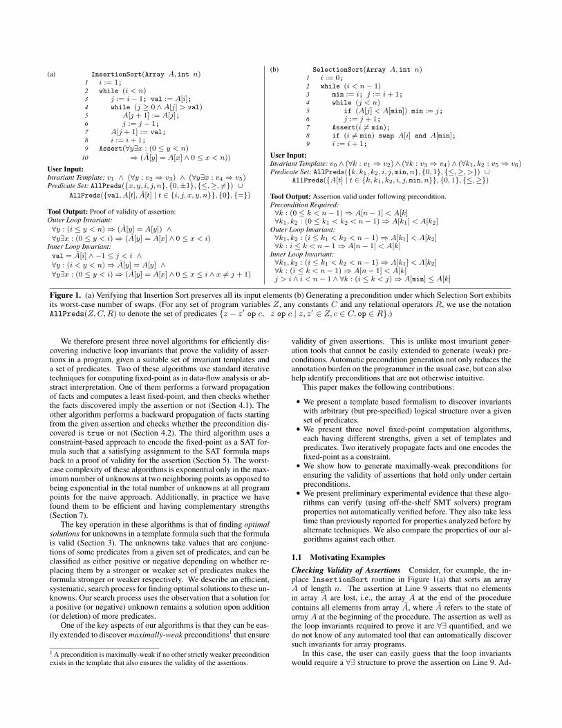
Figure 1. (a) Verifying that Insertion Sort preserves all its input elements (b) Generating a precondition under which Selection Sort exhibitsits worst-case number of swaps. (For any set of program variables Z, any constants C and any relational operators R, we use the notationAllPreds(Z,C,R) to denote the set of predicates {z − z′ op c, z op c | z, z′ ∈ Z, c ∈ C, op ∈ R}.)

We therefore present three novel algorithms for efficiently dis-covering inductive loop invariants that prove the validity of asser-tions in a program, given a suitable set of invariant templates anda set of predicates. Two of these algorithms use standard iterativetechniques for computing fixed-point as in data-flow analysis or ab-stract interpretation. One of them performs a forward propagationof facts and computes a least fixed-point, and then checks whetherthe facts discovered imply the assertion or not (Section 4.1). Theother algorithm performs a backward propagation of facts startingfrom the given assertion and checks whether the precondition dis-covered is true or not (Section 4.2). The third algorithm uses aconstraint-based approach to encode the fixed-point as a SAT for-mula such that a satisfying assignment to the SAT formula mapsback to a proof of validity for the assertion (Section 5). The worst-case complexity of these algorithms is exponential only in the max-imum number of unknowns at two neighboring points as opposed tobeing exponential in the total number of unknowns at all programpoints for the naive approach. Additionally, in practice we havefound them to be efficient and having complementary strengths(Section 7).

The key operation in these algorithms is that of finding optimalsolutions for unknowns in a template formula such that the formulais valid (Section 3). The unknowns take values that are conjunc-tions of some predicates from a given set of predicates, and can beclassified as either positive or negative depending on whether re-placing them by a stronger or weaker set of predicates makes theformula stronger or weaker respectively. We describe an efficient,systematic, search process for finding optimal solutions to these un-knowns. Our search process uses the observation that a solution fora positive (or negative) unknown remains a solution upon addition(or deletion) of more predicates.

One of the key aspects of our algorithms is that they can be eas-ily extended to discover maximally-weak preconditions1 that ensure

1 A precondition is maximally-weak if no other strictly weaker preconditionexists in the template that also ensures the validity of the assertions.

validity of given assertions. This is unlike most invariant gener-ation tools that cannot be easily extended to generate (weak) pre-conditions. Automatic precondition generation not only reduces theannotation burden on the programmer in the usual case, but can alsohelp identify preconditions that are not otherwise intuitive.

This paper makes the following contributions:

• We present a template based formalism to discover invariantswith arbitrary (but pre-specified) logical structure over a givenset of predicates.

• We present three novel fixed-point computation algorithms,each having different strengths, given a set of templates andpredicates. Two iteratively propagate facts and one encodes thefixed-point as a constraint.

• We show how to generate maximally-weak preconditions forensuring the validity of assertions that hold only under certainpreconditions.

• We present preliminary experimental evidence that these algo-rithms can verify (using off-the-shelf SMT solvers) programproperties not automatically verified before. They also take lesstime than previously reported for properties analyzed before byalternate techniques. We also compare the properties of our al-gorithms against each other.

1.1 Motivating ExamplesChecking Validity of Assertions Consider, for example, the in-place InsertionSort routine in Figure 1(a) that sorts an arrayA of length n. The assertion at Line 9 asserts that no elementsin array A are lost, i.e., the array A at the end of the procedurecontains all elements from array A, where A refers to the state ofarray A at the beginning of the procedure. The assertion as well asthe loop invariants required to prove it are ∀∃ quantified, and wedo not know of any automated tool that can automatically discoversuch invariants for array programs.

In this case, the user can easily guess that the loop invariantswould require a ∀∃ structure to prove the assertion on Line 9. Ad-

ditionally, the user needs to guess that an inductive loop invariantmay require a ∀ fact (to capture some fact about array elements) anda quantified-free fact relating non-array variables. The quantifiedfacts contain an implication as is there in the final assertion. Theuser also needs to provide the set of predicates. In this case, the setconsisting of inequality and disequality comparisons between terms(variables and array elements that are indexed by some variable) ofappropriate types suffices. This choice of predicates is quite naturaland has been used in several works based on predicate abstraction.Given these user inputs, our tool then automatically discovers thenon-trivial loop invariants mentioned in the figure.

Our tool eases the task of validating the assertion by requiringthe user to only provide a template in which the logical structurehas been made explicit, and provide some over-approximation ofthe set of predicates. Guessing the template is a much easier taskthan providing the precise loop invariants, primarily because thesetemplates are usually uniform across the program and depend onthe kind of properties to be proved.

Precondition Generation Consider, for example, the in-placeSelectionSort routine in Figure 1(b) that sorts an array A oflength n. Using bound analysis [11], it is possible to prove that theworst-case number of array swaps for this example is n−1. On theother hand, suppose we want to verify that the worst-case numberof swaps, n − 1, can indeed be achieved by some input instance.This problem can be reduced to the problem of validating the as-sertion at Line 7. If the assertion holds then the swap on Line 8 isalways executed, which is n − 1 times. However, this assertionis not valid without an appropriate precondition (e.g., consider afully sorted array when the swap happens in no iteration). We wantto generate a precondition that does not impose any constraints onn while allowing the assertion to be valid—this would provide aproof that SelectionSort indeed admits a worst-case of n − 1array swaps.

In this case, the user can easily guess that a quantified fact(∀k1, k2 that compares the elements at locations k1 and k2) cap-turing some sortedness property will be required. However, thisalone is not sufficient. The user can then iteratively guess and addtemplates until a precondition is found. (The process can probablybe automated.) Two additional quantified facts and an unquantifiedfact suffice in this case. The user also supplies a predicate set con-sisting of inequality and disequality comparisons between terms ofappropriate type. The non-trivial output of our tool is shown in thefigure.

Our tool automatically infers the maximally-weak preconditionthat the input array should be sorted from A[0] to A[n − 2],while the last entry A[n − 1] contains the smallest element. Othersorting programs exhibit their worst-case behaviors usually whenthe array is reverse-sorted (For selection sort, a reverse sorted arrayis not the worst case; it incurs only n

2swaps!). By automatically

generating this non-intuitive maximally-weak precondition our toolprovides a significant insight about the algorithm and reduces theprogrammer’s burden.

2. NotationWe often use a set of predicates in place of a formula to meanthe conjunction of the predicates in the set. In our examples, weoften use predicates that are inequalities between a given set ofvariables or constants. For some subset V of the variables, we usethe notationQV to denote the set of predicates {v1 ≤ v2 | v1, v2 ∈V }. Also, for any subset V of variables, and any variable j, weuse the notation Qj,V to denote the set of predicates {j < v, j ≤v, j > v, j ≥ v | v ∈ V }.

2.1 TemplatesA template τ is a formula over unknown variables vi that takevalues over (conjunctions of predicates in) some subset of a givenset of predicates. We consider the following language of templates:

τ ::= v | ¬τ | τ1 ∨ τ2 | τ1 ∧ τ2 | ∃x : τ | ∀x : τ

We denote the set of unknown variables in a template τ by U(τ).We say that an unknown v ∈ U(τ) in template τ is a positive(or negative) unknown if τ is monotonically stronger (or weakerrespectively) in v. More formally, let v be some unknown variablein U(τ). Let σv be any substitution that maps all unknown variablesv′ in U(τ) that are different from v to some set of predicates. LetQ1, Q2 ⊆ Q(v). Then, v is a positive unknown if

∀σv, Q1, Q2 : (Q1 ⇒ Q2) ⇒ (τσv[v 7→ Q2] ⇒ τσv[v 7→ Q1])

Similarly, v is a negative unknown if

∀σv, Q1, Q2 : (Q1 ⇒ Q2) ⇒ (τσv[v 7→ Q1] ⇒ τσv[v 7→ Q2])

We use the notation U+(τ) and U−(τ) to denote the set of allpositive unknowns and negative unknowns respectively in τ .

If each unknown variable in a template/formula occurs onlyonce, then it can be shown that each unknown is either positive ornegative. In that case, the sets U+(τ) and U−(τ) can be computedusing structural decomposition of τ as follows:

U+

(v) = {v}

U+

(¬τ) = U−

(τ)

U+

(τ1 ∧ τ2) = U+

(τ1) ∪ U+

(τ2)

U+

(τ1 ∨ τ2) = U+

(τ1) ∪ U+

(τ2)

U+

(∀X : τ) = U+

(τ)

U+

(∃X : τ) = U+

(τ)

U−

(v) = ∅

U−

(¬τ) = U+

(τ)

U−

(τ1 ∧ τ2) = U−

(τ1) ∪ U−

(τ2)

U−

(τ1 ∨ τ2) = U−

(τ1) ∪ U−

(τ2)

U−

(∀X : τ) = U−

(τ)

U−

(∃X : τ) = U−

(τ)

EXAMPLE 1. Consider the following template τ with unknownvariables v1, . . , v5.

(v1 ∧ (∀j : v2 ⇒ sel(A, j) ≤ sel(B, j)) ∧(∀j : v3 ⇒ sel(B, j) ≤ sel(C, j))) ⇒

(v4 ∧ (∀j : v5 ⇒ sel(A, j) ≤ sel(C, j)))

Then, U+(τ) = {v2, v3, v4} and U−(τ) = {v1, v5}.

2.2 Program ModelWe assume that a program Prog consists of the following kind ofstatements s (besides the control-flow).

s ::= x := e | assert(φ) | assume(φ)

In the above, x denotes a variable and e denotes some expres-sion. Memory reads and writes can be modeled using memory vari-ables and select/update expressions. Since we allow assume state-ments, without loss of any generality, we can treat all conditionalsin the program as non-deterministic.

We now set up a formalism in which different templates can beassociated with different program points, and different unknownsin templates can take values from different sets of predicates. LetC be some cut-set of the program Prog. (A cut-set of a programis a set of program points, called cut-points, such that any cyclicpath in Prog passes through some cut-point.) Every cut-point in Cis labeled with an invariant template. For simplicity, we assumethat C also consists of program entry and exit locations, whichare labeled with an invariant template that is simply true. LetPaths(Prog) denote the set of all tuples (δ, τ1, τ2, σt), where δis some straight-line path between two cut-points from C that arelabeled with invariant templates τ1 and τ2 respectively. Withoutloss of any generality, we assume that each program path δ is instatic single assignment (SSA) form, and the variables that are live

at start of path δ are the original program variables, and the SSAversions of the variables that are live at the end of δ are given bythe mapping σt, while σ−1

t denotes the reverse mapping.We use the notation U(Prog) to denote the set of unknown

variables in the invariant templates at all cut-points of Prog.

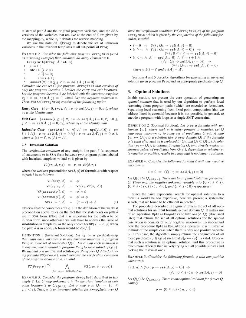
EXAMPLE 2. Consider the following program ArrayInit (usedas a running example) that initializes all array elements to 0.

ArrayInit(Array A, int n)1 i := 0;2 while (i < n)3 A[i] := 0;4 i := i+ 1;5 Assert(∀j : 0 ≤ j < n⇒ sel(A, j) = 0);

Consider the cut-set C for program ArrayInit that consists ofonly the program location 2 besides the entry and exit locations.Let the program location 2 be labeled with the invariant template∀j : v ⇒ sel(A, j) = 0, which has one negative unknown v.Then, Paths(ArrayInit) consists of the following tuples.

Entry Case (i := 0, true, ∀j : v ⇒ sel(A, j) = 0, σt), whereσt is the identity map.

Exit Case (assume(i ≥ n), ∀j : v ⇒ sel(A, j) = 0, ∀j : 0 ≤j < n⇒ sel(A, j) = 0, σt), where σt is the identity map.

Inductive Case (assume(i < n);A′ := upd(A, i, 0); i′ :=i + 1, ∀j : v ⇒ sel(A, j) = 0, ∀j : v ⇒ sel(A′, j) = 0, σt),where σt(i) = i′, σt(A) = A′.

2.3 Invariant SolutionThe verification condition of any straight-line path δ (a sequenceof statements s) in SSA form between two program points labeledwith invariant templates τ1 and τ2 is given by

VC(〈τ1, δ, τ2〉) = τ1 ⇒ WP(δ, τ2)

where the weakest precondition WP(δ, φ) of formula φ with respectto path δ is as follows:

WP(skip, φ) = φ

WP(s1; s2, φ) = WP(s1, WP(s2, φ))

WP(assert(φ′), φ) = φ′ ∧ φWP(assume(φ′), φ) = φ′ ⇒ φ

WP(x := e, φ) = (x = e) ⇒ φ (1)

Observe that the correctness of Eq. 1 in the definition of the weakestprecondition above relies on the fact that the statements on path δare in SSA form. (Note that it is important for the path δ to bein SSA form since otherwise we will have to address the issue ofsubstitution in templates, as the only choice for WP(x := e, φ) whenthe path δ is in non-SSA form would be φ[e/x].

DEFINITION 1 (Invariant Solution). Let Q be a predicate-mapthat maps each unknown v in any template invariant in programProg to some set of predicates Q(v). Let σ map each unknown vin any template invariant in program Prog to some subset of Q(v).We say that σ is an invariant solution for Prog overQ if the follow-ing formula VC(Prog, σ), which denotes the verification conditionof the program Prog w.r.t. σ, is valid.

VC(Prog, σ)def=

∧(δ,τ1,τ2,σt)∈Paths(Prog)

VC(〈τ1σ, δ, τ2σσt〉)

EXAMPLE 3. Consider the program ArrayInit described in Ex-ample 2. Let Q map unknown v in the invariant template at cut-point location 2 to Qj,{0,i,j}. Let σ map v to Q0 = {0 ≤j, j < i}. Then, σ is an invariant solution for ArrayInit over Q

since the verification condition VC(ArrayInit, σ) of the programArrayInit, which is given by the conjunction of the following for-mulas, is valid.

• i = 0 ⇒ (∀j : Q0 ⇒ sel(A, j) = 0)• (i ≥ n ∧ (∀j : Q0 ⇒ sel(A, j) = 0)) ⇒

(∀j : 0 ≤ j ≤ n⇒ sel(A, j) = 0)• (i < n ∧ A′ = upd(A, i, 0) ∧ i′ = i+ 1 ∧

(∀j : Q0 ⇒ sel(A, j) = 0)) ⇒(∀j : Q0σt ⇒ sel(A′, j) = 0)

where σt(i) = i′ and σt(A) = A′.

Sections 4 and 5 describe algorithms for generating an invariantsolution given program Prog and an appropriate predicate-map Q.

3. Optimal SolutionsIn this section, we present the core operation of generating anoptimal solution that is used by our algorithm to perform localreasoning about program paths (which are encoded as formulae).Separating local reasoning from fixed-point computation (that weaddress later) is essential because it is not possible, in general, toencode a program with loops as a single SMT constraint.

DEFINITION 2 (Optimal Solution). Let φ be a formula with un-knowns {vi}i where each vi is either positive or negative. Let Qmap each unknown vi to some set of predicates Q(vi). A map{vi 7→ Qi}i is a solution (for φ over domain Q) if the formulaφ is valid after each vi is replaced byQi, andQi ⊆ Q(vi). A solu-tion {vi 7→ Qi}i is optimal if replacing Qi by a strictly weaker orstronger subset of predicates from Q(vi), depending on whether vi

is negative or positive, results in a map that is no longer a solution.

EXAMPLE 4. Consider the following formula φ with one negativeunknown η.

i = 0 ⇒ (∀j : η ⇒ sel(A, j) = 0)

LetQ(η) beQj,{0,i,n}. There are four optimal solutions for φ overQ. These map the negative unknown variable η to {0 < j ≤ i},{0 ≤ j < i}, {i < j ≤ 0}, and {i ≤ j < 0} respectively.

Since the naive exponential search for optimal solutions to aformula would be too expensive, here we present a systematicsearch, that we found to be efficient in practice.

The procedure described in Figure 2 returns the set of all opti-mal solutions for an input formula φ over domain Q. It makes useof an operation OptimalNegativeSolutions(φ,Q) (discussedlater) that returns the set of all optimal solutions for the specialcase when φ consists of only negative unknowns. To understandhow the procedure OptimalSolutions operates, it is illustrativeto think of the simple case when there is only one positive variableρ. In this case, the algorithm simply returns the conjunction of allthose predicates q ∈ Q(ρ) such that φ[ρ 7→ {q}] is valid. Observethat such a solution is an optimal solution, and this procedure ismuch more efficient than naively trying out all possible subsets andpicking the maximal ones.

EXAMPLE 5. Consider the following formula φ with one positiveunknown ρ.

(i ≥ n) ∧ (∀j : ρ⇒ sel(A, j) = 0)) ⇒(∀j : 0 ≤ j < n⇒ sel(A, j) = 0)

LetQ(ρ) beQj,{0,i,n}. There is one optimal solution for φ overQ,namely

ρ 7→ {0 ≤ j, j < n, j < i}

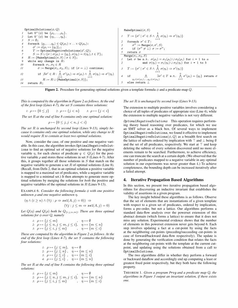
OptimalSolutions(φ, Q)1 Let U+(φ) be {ρ1, . . , ρa}.2 Let U−(φ) be {η1, . . , ηb}.3 S := ∅;4 foreach 〈q1, . . , qa〉 ∈ Q(ρ1)× . .×Q(ρa):5 φ′ := φ[ρi 7→ {qi}]i;6 T := OptimalNegativeSolutions(φ′, Q);7 S := S ∪ {σ | σ(ρi) = {qi}, σ(ηi) = t(ηi), t ∈ T};8 R := {MakeOptimal(σ, S) | σ ∈ S};9 while any change in R:

10 foreach σ1, σ2 ∈ R11 σ := Merge(σ1, σ2, S); if (σ = ⊥) continue;

12 if 6 ∃σ′ ∈ R :a∧

i=1σ′(ρi) ⇒ σ(ρi) ∧

b∧i=1

σ(ηi) ⇒ σ′(ηi)

13 R := R ∪ {MakeOptimal(σ, S)};14 return R;

MakeOptimal(σ, S)

1 T := {σ′ | σ′ ∈ S ∧b∧

i=1σ(ηi) ⇒ σ′(ηi)}

2 foreach σ′ ∈ T:3 σ′′ := Merge(σ, σ′, S)4 if (σ′′ 6= ⊥) σ := σ′′;5 return σMerge(σ1, σ2, S)

1 Let σ be s.t. σ(ρi) = σ1(ρi) ∪ σ2(ρi) for i = 1 to a2 and σ(ηi) = σ1(ηi) ∪ σ2(ηi) for i = 1 to b

3 T := {σ′ | σ′ ∈ S ∧b∧

i=1σ(ηi) ⇒ σ′(ηi)}

4 if∧

q1∈σ(ρ1),..,qa∈σ(ρa)

∃σ′ ∈ T s.t.a∧

i=1σ′(ρi) = {qi} return σ

5 else return ⊥

Figure 2. Procedure for generating optimal solutions given a template formula φ and a predicate-map Q.

This is computed by the algorithm in Figure 2 as follows. At the endof the first loop (Lines 4-7), the set S contains three solutions:

1: ρ 7→ {0 ≤ j} 2: ρ 7→ {j < n} 3: ρ 7→ {j < i}The set R at the end of line 8 contains only one optimal solution:

ρ 7→ {0 ≤ j, j < n, j < i}The set R is unchanged by second loop (Lines 9-13), simply be-cause it contains only one optimal solution, while any change to Rwould require R to contain at least two optimal solutions.

Now, consider the case, of one positive and one negative vari-able. In this case, the algorithm invokes OptimalNegativeSolut-ions to find an optimal set of negative solutions for the negativevariable η, for each choice of predicate q ∈ Q(ρ) for the posi-tive variable ρ and stores these solutions in set S (Lines 4-7). Afterthis, it groups together all those solutions in S that match on thenegative variable to generate a set R of optimal solutions (Line 8).(Recall, from Defn 2, that in an optimal solution a positive variableis mapped to a maximal set of predicates, while a negative variableis mapped to a minimal set.) It then attempts to generate more op-timal solutions by merging the solutions for both the positive andnegative variables of the optimal solutions in R (Lines 9-13).

EXAMPLE 6. Consider the following formula φ with one positiveunknown ρ and one negative unknown η.

(η ∧ (i ≥ n) ∧ (∀j : ρ⇒ sel(A, j) = 0)) ⇒(∀j : j ≤ m⇒ sel(A, j) = 0)

Let Q(η) and Q(ρ) both be Q{i,j,n,m}. There are three optimalsolutions for φ over Q, namely

1: ρ 7→ {j ≤ m} , η 7→ ∅2: ρ 7→ {j ≤ n, j ≤ m, j ≤ i}, η 7→ {m ≤ n}3: ρ 7→ {j ≤ i, j ≤ m} , η 7→ {m ≤ i}

These are computed by the algorithm in Figure 2 as follows. At theend of the first loop (Lines 4-7), the set S contains the followingfour solutions:

1: ρ 7→ {j ≤ m}, η 7→ ∅2: ρ 7→ {j ≤ n} , η 7→ {m ≤ n}3: ρ 7→ {j ≤ i} , η 7→ {m ≤ i}4: ρ 7→ {j ≤ i} , η 7→ {m ≤ n}

The set R at the end of line 8 contains the following three optimalsolutions:

1: ρ 7→ {j ≤ m} , η 7→ ∅2: ρ 7→ {j ≤ n, j ≤ m, j ≤ i}, η 7→ {m ≤ n}3: ρ 7→ {j ≤ i, j ≤ m} , η 7→ {m ≤ i}

The set R is unchanged by second loop (Lines 9-13).

The extension to multiple positive variables involves considering achoice of all tuples of predicates of appropriate size (Line 4), whilethe extension to multiple negative variables is not very different.

OptimalNegativeSolutions This operation requires perform-ing theory based reasoning over predicates, for which we usean SMT solver as a black box. Of several ways to implementOptimalNegativeSolutions, we found it effective to implementOptimalNegativeSolutions(φ,Q) as a breadth first search onthe lattice of subsets ordered by implication with > and ⊥ being ∅and the set of all predicates, respectively. We start at > and keepdeleting the subtree of every solution discovered until no more el-ements remain to be searched. Furthermore, to achieve efficiency,one can truncate the search at a certain depth. (We observed that thenumber of predicates mapped to a negative variable in any optimalsolution in our experiments was never greater than 4.) To achievecompleteness, the bounding depth can be increased iteratively aftera failed attempt.

4. Iterative Propagation Based AlgorithmsIn this section, we present two iterative propagation based algo-rithms for discovering an inductive invariant that establishes thevalidity of assertions in a given program.

The key insight behind these algorithms is as follows. Observethat the set of elements that are instantiations of a given templatewith respect to a given set of predicates, ordered by implication,forms a pre-order, but not a lattice. Our algorithms performs astandard data-flow analysis over the powerset extension of thisabstract domain (which forms a lattice) to ensure that it does notmiss any solution. Experimental evidence shows that the numberof elements in this powerset extension never gets beyond 6. Eachstep involves updating a fact at a cut-point by using the factsat the neighboring cut-points (preceding/succeeding cut-points incase of forward/backward data-flow respectively). The update isdone by generating the verification condition that relates the factsat the neighboring cut-points with the template at the current cut-point, and updating using the solutions obtained from a call toOptimalSolutions.

The two algorithms differ in whether they perform a forwardor backward dataflow and accordingly end up computing a least orgreatest fixed point respectively, but they both have the followingproperty.

THEOREM 1. Given a program Prog and a predicate map Q, thealgorithms in Figure 3 output an invariant solution, if there existsone.

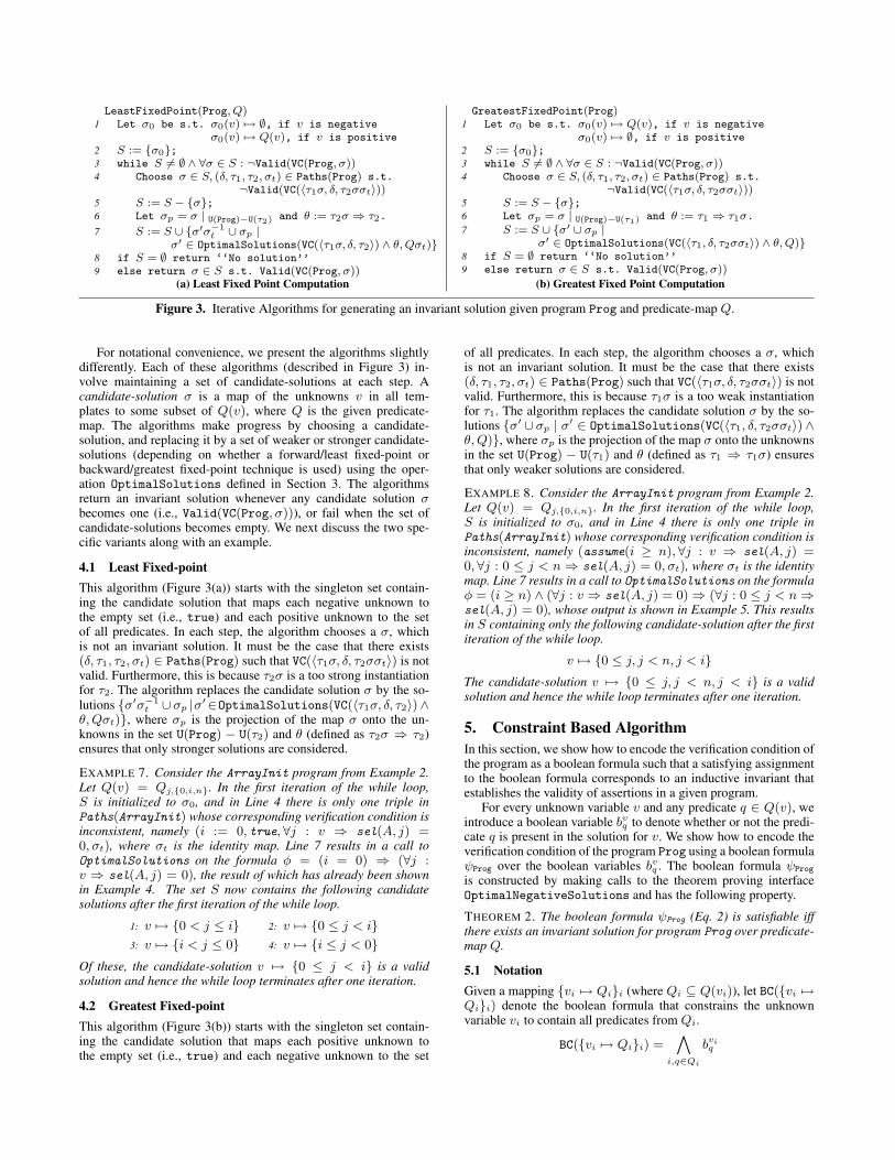
LeastFixedPoint(Prog, Q)1 Let σ0 be s.t. σ0(v) 7→ ∅, if v is negative

σ0(v) 7→ Q(v), if v is positive2 S := {σ0};3 while S 6= ∅ ∧ ∀σ ∈ S : ¬Valid(VC(Prog, σ))4 Choose σ ∈ S, (δ, τ1, τ2, σt) ∈ Paths(Prog) s.t.

¬Valid(VC(〈τ1σ, δ, τ2σσt〉))5 S := S − {σ};6 Let σp = σ | U(Prog)−U(τ2) and θ := τ2σ ⇒ τ2.

7 S := S ∪ {σ′σ−1t ∪ σp |

σ′ ∈ OptimalSolutions(VC(〈τ1σ, δ, τ2〉) ∧ θ, Qσt)}8 if S = ∅ return ‘‘No solution’’9 else return σ ∈ S s.t. Valid(VC(Prog, σ))

GreatestFixedPoint(Prog)1 Let σ0 be s.t. σ0(v) 7→ Q(v), if v is negative

σ0(v) 7→ ∅, if v is positive2 S := {σ0};3 while S 6= ∅ ∧ ∀σ ∈ S : ¬Valid(VC(Prog, σ))4 Choose σ ∈ S, (δ, τ1, τ2, σt) ∈ Paths(Prog) s.t.

¬Valid(VC(〈τ1σ, δ, τ2σσt〉))5 S := S − {σ};6 Let σp = σ | U(Prog)−U(τ1) and θ := τ1 ⇒ τ1σ.7 S := S ∪ {σ′ ∪ σp |

σ′ ∈ OptimalSolutions(VC(〈τ1, δ, τ2σσt〉) ∧ θ, Q)}8 if S = ∅ return ‘‘No solution’’9 else return σ ∈ S s.t. Valid(VC(Prog, σ))

(a) Least Fixed Point Computation (b) Greatest Fixed Point Computation

Figure 3. Iterative Algorithms for generating an invariant solution given program Prog and predicate-map Q.

For notational convenience, we present the algorithms slightlydifferently. Each of these algorithms (described in Figure 3) in-volve maintaining a set of candidate-solutions at each step. Acandidate-solution σ is a map of the unknowns v in all tem-plates to some subset of Q(v), where Q is the given predicate-map. The algorithms make progress by choosing a candidate-solution, and replacing it by a set of weaker or stronger candidate-solutions (depending on whether a forward/least fixed-point orbackward/greatest fixed-point technique is used) using the oper-ation OptimalSolutions defined in Section 3. The algorithmsreturn an invariant solution whenever any candidate solution σbecomes one (i.e., Valid(VC(Prog, σ))), or fail when the set ofcandidate-solutions becomes empty. We next discuss the two spe-cific variants along with an example.

4.1 Least Fixed-pointThis algorithm (Figure 3(a)) starts with the singleton set contain-ing the candidate solution that maps each negative unknown tothe empty set (i.e., true) and each positive unknown to the setof all predicates. In each step, the algorithm chooses a σ, whichis not an invariant solution. It must be the case that there exists(δ, τ1, τ2, σt) ∈ Paths(Prog) such that VC(〈τ1σ, δ, τ2σσt〉) is notvalid. Furthermore, this is because τ2σ is a too strong instantiationfor τ2. The algorithm replaces the candidate solution σ by the so-lutions {σ′σ−1

t ∪ σp |σ′∈OptimalSolutions(VC(〈τ1σ, δ, τ2〉)∧θ,Qσt)}, where σp is the projection of the map σ onto the un-knowns in the set U(Prog) − U(τ2) and θ (defined as τ2σ ⇒ τ2)ensures that only stronger solutions are considered.

EXAMPLE 7. Consider the ArrayInit program from Example 2.Let Q(v) = Qj,{0,i,n}. In the first iteration of the while loop,S is initialized to σ0, and in Line 4 there is only one triple inPaths(ArrayInit) whose corresponding verification condition isinconsistent, namely (i := 0, true, ∀j : v ⇒ sel(A, j) =0, σt), where σt is the identity map. Line 7 results in a call toOptimalSolutions on the formula φ = (i = 0) ⇒ (∀j :v ⇒ sel(A, j) = 0), the result of which has already been shownin Example 4. The set S now contains the following candidatesolutions after the first iteration of the while loop.

1: v 7→ {0 < j ≤ i} 2: v 7→ {0 ≤ j < i}3: v 7→ {i < j ≤ 0} 4: v 7→ {i ≤ j < 0}

Of these, the candidate-solution v 7→ {0 ≤ j < i} is a validsolution and hence the while loop terminates after one iteration.

4.2 Greatest Fixed-pointThis algorithm (Figure 3(b)) starts with the singleton set contain-ing the candidate solution that maps each positive unknown tothe empty set (i.e., true) and each negative unknown to the set

of all predicates. In each step, the algorithm chooses a σ, whichis not an invariant solution. It must be the case that there exists(δ, τ1, τ2, σt) ∈ Paths(Prog) such that VC(〈τ1σ, δ, τ2σσt〉) is notvalid. Furthermore, this is because τ1σ is a too weak instantiationfor τ1. The algorithm replaces the candidate solution σ by the so-lutions {σ′ ∪ σp | σ′ ∈ OptimalSolutions(VC(〈τ1, δ, τ2σσt〉)∧θ,Q)}, where σp is the projection of the map σ onto the unknownsin the set U(Prog) − U(τ1) and θ (defined as τ1 ⇒ τ1σ) ensuresthat only weaker solutions are considered.

EXAMPLE 8. Consider the ArrayInit program from Example 2.Let Q(v) = Qj,{0,i,n}. In the first iteration of the while loop,S is initialized to σ0, and in Line 4 there is only one triple inPaths(ArrayInit) whose corresponding verification condition isinconsistent, namely (assume(i ≥ n), ∀j : v ⇒ sel(A, j) =0, ∀j : 0 ≤ j < n ⇒ sel(A, j) = 0, σt), where σt is the identitymap. Line 7 results in a call to OptimalSolutions on the formulaφ = (i ≥ n) ∧ (∀j : v ⇒ sel(A, j) = 0) ⇒ (∀j : 0 ≤ j < n⇒sel(A, j) = 0), whose output is shown in Example 5. This resultsin S containing only the following candidate-solution after the firstiteration of the while loop.

v 7→ {0 ≤ j, j < n, j < i}The candidate-solution v 7→ {0 ≤ j, j < n, j < i} is a validsolution and hence the while loop terminates after one iteration.

5. Constraint Based AlgorithmIn this section, we show how to encode the verification condition ofthe program as a boolean formula such that a satisfying assignmentto the boolean formula corresponds to an inductive invariant thatestablishes the validity of assertions in a given program.

For every unknown variable v and any predicate q ∈ Q(v), weintroduce a boolean variable bvq to denote whether or not the predi-cate q is present in the solution for v. We show how to encode theverification condition of the program Prog using a boolean formulaψProg over the boolean variables bvq . The boolean formula ψProg

is constructed by making calls to the theorem proving interfaceOptimalNegativeSolutions and has the following property.

THEOREM 2. The boolean formula ψProg (Eq. 2) is satisfiable iffthere exists an invariant solution for program Prog over predicate-map Q.

5.1 NotationGiven a mapping {vi 7→ Qi}i (where Qi ⊆ Q(vi)), let BC({vi 7→Qi}i) denote the boolean formula that constrains the unknownvariable vi to contain all predicates from Qi.

BC({vi 7→ Qi}i) =∧

i,q∈Qi

bviq

5.2 Boolean Constraint Encoding for Verification ConditionWe first show how to generate the boolean constraint ψδ,τ1,τ2

that encodes the verification condition corresponding to any tuple(δ, τ1, τ2, σt) ∈ Paths(Prog). Let τ ′2 be the template that is ob-tained from τ2 as follows. If τ2 is different from τ1, then τ ′2 is sameas τ2, otherwise τ ′2 is obtained from τ2 by renaming all the un-known variables to fresh unknown variables with orig denoting thereverse mapping that maps the fresh unknown variables back to theoriginal. (We rename to ensure that each occurrence of an unknownvariable in the formula VC(〈τ1, δ, τ ′2〉) is unique. Note that each oc-currence of an unknown variable in the formula VC(〈τ1, δ, τ2〉) isnot unique when τ1 and τ2 refer to the same template, which is thecase when the path δ goes around a loop).

A simple approach would be to use OptimalSolutions tocompute all valid solutions for VC(〈τ1, δ, τ ′2〉) and encode their dis-junction. But because both τ1, τ ′2 are uninstantiated unknowns, thenumber of optimal solutions explodes. We describe below an effi-cient construction that involves only invoking OptimalNegative-Solutions over formulae with a smaller number of unknowns (thenegative) for a small choice of predicates for the positive variables.

Let ρ1, . . , ρa be the set of positive variables and let η1, . . , ηb

be the set of negative variables in VC(〈τ1, δ, τ ′2〉). Consider anypositive variable ρi and any qj ∈ Q′(ρi), where Q′ is the mapthat maps an unknown v that occurs in τ1 to Q(v) and an un-known v that occurs in τ2 to Q(v)σt. Consider the partial mapσρi,qj that maps ρi to {qj} and ρk to ∅ for any k 6= i. LetS

ρi,qj

δ,τ1,τ2be the set of optimal solutions returned after invok-

ing the procedure OptimalNegativeSolutions on the formulaVC(〈τ1, δ, τ ′2〉)σρi,qj as below:

Sρi,qj

δ,τ1,τ2= OptimalNegativeSolutions(VC(〈τ1, δ, τ ′2〉)σρi,qj , Q

′)

Similarly, let Sδ,τ1,τ2 denote the set of optimal solutions returnedafter invoking the procedure OptimalNegativeSolutions on theformula VC(〈τ1, δ, τ ′2〉)σ, where σ is the partial map that maps ρk

to ∅ for all 1 ≤ k ≤ a.

Sδ,τ1,τ2 = OptimalNegativeSolutions(VC(〈τ1, δ, τ ′2〉)σ,Q′)The following Boolean formula ψδ,τ1,τ2,σt encodes the verifi-

cation condition corresponding to (δ, τ1, τ2, σt).

ψδ,τ1,τ2,σt =

∨{ηk 7→Qk}k∈Sδ,τ1,τ2

BC({orig(ηk) 7→ Qkσ−1t }k)

∧

∧ρi,qj∈Q′(ρi)

borig(ρi)

qjσ−1t

⇒∨

{ηk 7→Qk}k∈Sρi,qjδ,τ1,τ2

BC({orig(ηk) 7→ Qkσ−1t }k)

The verification condition of the entire program is now given by

the following boolean formula ψProg that is the conjunction of theverification condition of all tuples (δ, τ1, τ2, σt) ∈ Paths(Prog).

ψProg =∧

(δ,τ1,τ2,σt)∈Paths(Prog)

ψδ,τ1,τ2,σt (2)

EXAMPLE 9. Consider the ArrayInit program from Example 2.Let Q(v) = Qj,{0,i,n}. The above procedure leads to generationof the following constraints.

Entry Case The verification condition corresponding to this casecontains one negative variable v and no positive variable. The setSδ,τ1,τ2 is same as the set S in Example 7, which contains 4 optimalsolutions. The following boolean formula encodes this verificationcondition.

(bv0≤j ∧ bvj<i) ∨ (bv0<j ∧ bvj≤i) ∨ (bvi≤j ∧ bvj<0) ∨ (bvi<j ∧ bvj≤0) (3)

Exit Case The verification condition corresponding to this casecontains one positive variable v and no negative variable. We nowconsider the set Sv,q

δ,τ1,τ2for each q ∈ Q(v). Let P = {0 ≤ j, j <

i, j ≤ i, j < n, j ≤ n}. If v ∈ P , the set Sv,qδ,τ1,τ2

contains theempty mapping (i.e., the resultant formula when v is replaced by qis valid). If v ∈ Q(v) − P , the set Sv,q

δ,τ1,τ2is the empty-set (i.e.,

the resultant formula when v is replaced by q is not valid). Thefollowing boolean formula encodes this verification condition.∧

q∈P

(bvq ⇒ true) ∧∧

q∈Q(v)−P

(bvq ⇒ false)

which is equivalent to the following formula

¬bv0<j ∧ ¬bvi<j ∧ ¬bvi≤j ∧ ¬bvn<j ∧ ¬bvn≤j ∧ ¬bvj<0 ∧ ¬bvj≤0 (4)

Inductive Case The verification condition corresponding to thiscase contains one positive variable v and one negative variablev′ obtained by renaming one of the occurrences of v. Note thatSδ,τ1,τ2 contains a singleton mapping that maps v′ to the empty-set. Also, note that Sv,j≤i

δ,τ1,τ2is the empty-set, and for any q ∈

Q(v′)−{j ≤ i}, Sv,qδ,τ1,τ2

contains at least one mapping that mapsv′ to the singleton {qσt}. Hence, the following boolean formulaencodes this verification condition.

(bvj≤i ⇒ false) ∧∧

q∈Q(v′)−{j≤i}

(bvq ⇒ (bvq ∨ . . .)

)which is equivalent to the formula

¬bvj≤i (5)

The boolean assignment where bv0≤j and bvj<i are set to true,and all other boolean variables are set to false satisfies theconjunction of the boolean constraints in Eq. 3,4, and 5. Thisimplies the solution {0 ≤ j, j < i} for the unknown v in theinvariant template.

6. Maximally-Weak Precondition InferenceIn this section, we address the problem of discovering maximally-weak preconditions that fit a given template and ensure that allassertions in a program are valid.

DEFINITION 3. (Maximally-Weak Precondition) Given a programProg with assertions, invariant templates at each cutpoint, and atemplate τe at the program entry, a solution σ for the unknowns inthe templates assigns a maximally-weak precondition to τe if

• σ is a valid solution, i.e. Valid(VC(Prog, σ)).• For any solution σ′, it is not the case that τeσ′ is strictly weaker

than τeσ, i.e., ∀σ′ : (τeσ ⇒ τeσ′ ∧ τeσ′ 6⇒ τeσ) ⇒

¬Valid(VC(Prog, σ′)).

The greatest fixed-point algorithm described in Section 4.2already computes one such maximally-weak precondition. If wechange the condition of the while loop in line 3 in Figure 3(b) toS 6= ∅ ∧ ∃σ ∈ S : ¬Valid(VC(Prog, σ′)), then S at the end ofthe loop contains all maximally-weak preconditions.

The constraint based algorithm described in Section 5 is ex-tended to generate maximally-weak preconditions using an itera-tive process by first generating any precondition, and then encod-ing an additional constraint that the precondition should be strictlyweaker than the precondition that was last generated, until anysuch precondition can be found. The process is repeated to gener-ate other maximally-weak preconditions by encoding an additionalconstraint that the precondition should not be stronger than any pre-viously found maximally-weak precondition. See [30] for details.

A dual notion can be defined for maximally-strong postcondi-tions, which is motivated by the need to discover invariants as op-

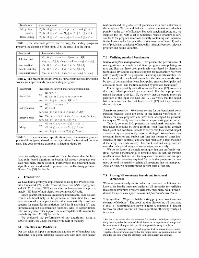
Benchmark Assertion proved

Merge Sort(inner)

∀y∃x : 0 ≤ y < m ⇒ A[y] = C[x] ∧ 0 ≤ x < t

∀y∃x : 0 ≤ y < n ⇒ B[y] = C[x] ∧ 0 ≤ x < t

Other Sorting ∀y∃x : 0 ≤ y < n ⇒ A[y] = A[x] ∧ 0 ≤ x < n

Table 1. The assertions proved for verifying that sorting programspreserve the elements of the input. A is the array A at the input.

Benchmark Precondition inferred

Selection Sort∀k : 0 ≤ k < n−1 ⇒ A[n−1] < A[k]

∀k1, k2 : 0≤k1 <k2 <n−1 ⇒ A[k1] < A[k2]

Insertion Sort ∀k : 0 ≤ k < n−1 ⇒ A[k] > A[k+1]

Bubble Sort (flag) ∀k : 0 ≤ k < n−1 ⇒ A[k] > A[k+1]

Quick Sort (inner) ∀k1, k2 : 0 ≤ k1 < k2 ≤ n ⇒ A[k1] ≤ A[k2]

Table 2. The preconditions inferred by our algorithms resulting in theworst case upper bounds runs for sorting programs.

Benchmark Preconditions inferred under given postcondition

Partial Initpre:

(a) m ≤ n

(b) ∀k : n ≤ k < m ⇒ A[k] = 0

post: ∀k : 0 ≤ k < m ⇒ A[k] = 0

Init Synthesispre:

(a) i = 1 ∧max = 0

(b) i = 0

post: ∀k : 0 ≤ k < n ⇒ A[max] ≥ A[k]

Binary Searchpre: ∀k1, k2 : 0 ≤ k1 < k2 < n ⇒ A[k1] ≤ A[k2]

post: ∀k : 0 ≤ k < n ⇒ A[k] 6= e

Mergepre:

∀k : 0 ≤ k < n ⇒ A[k] ≤ A[k+1]

∀k : 0 ≤ k < m ⇒ B[k] ≤ B[k+1]

post: ∀k : 0 ≤ k < t ⇒ C[k] ≤ C[k+1]

Table 3. Given a functional specification (post), the maximally-weakpreconditions (pre) inferred by our algorithms for functional correct-ness. The code for these examples is listed in Figure 10.

posed to verifying given assertions. It can be shown that the leastfixed-point based algorithm in Section 4.1 already computes onesuch maximally-strong solution. Furthermore, the constraint basedalgorithm can be extended to generate maximally-strong postcon-ditions. See [30] for details.

7. EvaluationWe have built a prototype implementation using the Phoenix com-piler framework [24] as the frontend parser for ANSI-C programsand Z3 [25, 7] as our SMT solver. Our implementation is approxi-mately 15K lines of non-blank, non-comment, C# code.

Since quantification makes reasoning undecidable, SMT solversrequire additional help in the presence of quantified facts. Wehave developed a wrapper interface that automatically constructspatterns for quantifier instantiation (used for E-matching [6]) andintroduces explicit skolemization functions. Also, to support linkedlists, we augment Z3’s support for select/update with axioms forreachability. See [31, 30] for details.

We evaluated the performance of our algorithms, using a2.5GHz Intel Core 2 Duo machine with 4GB of memory.

7.1 Templates and PredicatesOur tool takes as input a program and a global set of templates andpredicates. The global template is associated with each loop header

(cut-point) and the global set of predicates with each unknown inthe templates. We use a global set to reduce annotation burden butpossibly at the cost of efficiency. For each benchmark program, wesupplied the tool with a set of templates, whose structure is verysimilar to the program assertions (usually containing one unquanti-fied unknown and a few quantified unknowns, as in Figure 1) and aset of predicates consisting of inequality relations between relevantprogram and bound variables.

7.2 Verifying standard benchmarksSimple array/list manipulation: We present the performance ofour algorithms on simple but difficult programs manipulating ar-rays and lists that have been previously considered by alternativetechniques. By adding axiomatic support for reachability, we wereable to verify simple list programs illustrating our extensibility. Ta-ble 4 presents the benchmark examples, the time in seconds takenby each of our algorithm (least fixed-point, greatest fixed-point andconstraint-based) and the time reported by previous techniques2.

For the appropriately named Consumer Producer [17], we verifythat only values produced are consumed. For the appropriatelynamed Partition Array [2, 17], we verify that the output arrays arepartitions of the input. For List Init [12], we verify that the outputlist is initialized and for List Insert/Delete [12] that they maintainthe initialization.

Sortedness property: We choose sorting for our benchmark com-parisons because these are some of the hardest verification in-stances for array programs and have been attempted by previoustechniques. We verify sortedness for all major sorting procedures.

Table 6, columns 1–5, presents the benchmark examples, thetime taken in seconds by our algorithms (least fixed-point, greatestfixed-point and constraint-based) to verify that they indeed outputa sorted array and previously reported timings2. We evaluate overselection, insertion and bubble sort (one that iterates n2 times irre-spective of array contents, and one that maintains a flag checkingif the array is already sorted). For quick sort and merge sort weconsider their partitioning and merge steps, respectively.

We do not know of a single technique that can uniformly ver-ify all sorting benchmarks as is possible here. In fact, the missingresults indicate that previous techniques are not robust and are spe-cialized to the reasoning required for particular programs. In con-trast, our tool successfully verified all programs that we attempted.Also, on time, we outperform the current state-of-the-art.

7.3 Proving ∀∃, worst-case bounds and functionalcorrectness

We now present analyses for which no previous techniques areknown. We handle three new analyses: ∀∃ properties for verifyingthat sorting programs preserve elements, maximally-weak precon-ditions for worst case upper bounds and functional correctness.

∀∃ properties: We prove that the sorting programs do not lose anyelements of the input3. The proof requires discovering ∀∃ invariants(Table 1). The runtimes are shown in Table 6, columns 6–8. Exceptfor two runs that timeout, all three algorithms efficiently verify allinstances.

2 We warn the reader that the numbers for previous techniques are poten-tially incomparable because of the differences in experimental setups andbecause some techniques infer predicates, possibly using templates.3 Similar ∀∃ invariants can be used to prove that no elements are gained.Together, these invariants prove that the output array is a permutation of theinput for the case when the elements in the input array are distinct.

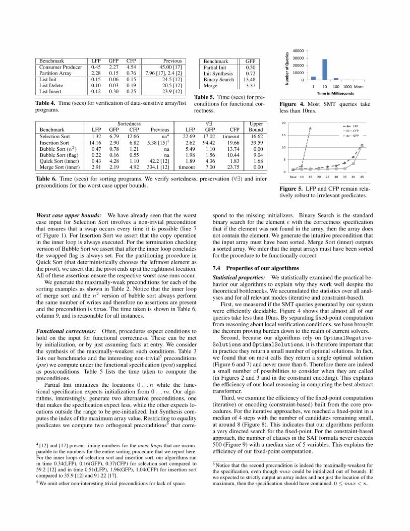
Benchmark LFP GFP CFP PreviousConsumer Producer 0.45 2.27 4.54 45.00 [17]Partition Array 2.28 0.15 0.76 7.96 [17], 2.4 [2]List Init 0.15 0.06 0.15 24.5 [12]List Delete 0.10 0.03 0.19 20.5 [12]List Insert 0.12 0.30 0.25 23.9 [12]

Table 4. Time (secs) for verification of data-sensitive array/listprograms.

Benchmark GFPPartial Init 0.50Init Synthesis 0.72Binary Search 13.48Merge 3.37

Table 5. Time (secs) for pre-conditions for functional cor-rectness.

Sortedness ∀∃ UpperBenchmark LFP GFP CFP Previous LFP GFP CFP BoundSelection Sort 1.32 6.79 12.66 na4 22.69 17.02 timeout 16.62Insertion Sort 14.16 2.90 6.82 5.38 [15]4 2.62 94.42 19.66 39.59Bubble Sort (n2) 0.47 0.78 1.21 na 5.49 1.10 13.74 0.00Bubble Sort (flag) 0.22 0.16 0.55 na 1.98 1.56 10.44 9.04Quick Sort (inner) 0.43 4.28 1.10 42.2 [12] 1.89 4.36 1.83 1.68Merge Sort (inner) 2.91 2.19 4.92 334.1 [12] timeout 7.00 23.75 0.00

Table 6. Time (secs) for sorting programs. We verify sortedness, preservation (∀∃) and inferpreconditions for the worst case upper bounds.

!

"!!!!

#!!!!

$!!!!

%!!!!

" "! "!! "!!! &'()

!"#$%&'()'*"%&+%,

-+#%'+.'/+00+,%1(.2,'

30(4',150%6

Figure 4. Most SMT queries takeless than 10ms.

0

5

10

15

20

Base 10 15 20 25 30 35 40 45

LFP

CFP

GFP

Figure 5. LFP and CFP remain rela-tively robust to irrelevant predicates.

Worst case upper bounds: We have already seen that the worstcase input for Selection Sort involves a non-trivial preconditionthat ensures that a swap occurs every time it is possible (line 7of Figure 1). For Insertion Sort we assert that the copy operationin the inner loop is always executed. For the termination checkingversion of Bubble Sort we assert that after the inner loop concludesthe swapped flag is always set. For the partitioning procedure inQuick Sort (that deterministically chooses the leftmost element asthe pivot), we assert that the pivot ends up at the rightmost location.All of these assertions ensure the respective worst case runs occur.

We generate the maximally-weak preconditions for each of thesorting examples as shown in Table 2. Notice that the inner loopof merge sort and the n2 version of bubble sort always performthe same number of writes and therefore no assertions are presentand the precondition is true. The time taken is shown in Table 6,column 9, and is reasonable for all instances.

Functional correctness: Often, procedures expect conditions tohold on the input for functional correctness. These can be metby initialization, or by just assuming facts at entry. We considerthe synthesis of the maximally-weakest such conditions. Table 3lists our benchmarks and the interesting non-trivial5 preconditions(pre) we compute under the functional specification (post) suppliedas postconditions. Table 5 lists the time taken to compute thepreconditions.

Partial Init initializes the locations 0 . . . n while the func-tional specification expects initialization from 0 . . .m. Our algo-rithms, interestingly, generate two alternative preconditions, onethat makes the specification expect less, while the other expects lo-cations outside the range to be pre-initialized. Init Synthesis com-putes the index of the maximum array value. Restricting to equalitypredicates we compute two orthogonal preconditions6 that corre-

4 [12] and [17] present timing numbers for the inner loops that are incom-parable to the numbers for the entire sorting procedure that we report here.For the inner loops of selection sort and insertion sort, our algorithms runin time 0.34(LFP), 0.16(GFP), 0.37(CFP) for selection sort compared to59.2 [12] and in time 0.51(LFP), 1.96(GFP), 1.04(CFP) for insertion sortcompared to 35.9 [12] and 91.22 [17].5 We omit other non-interesting trivial preconditions for lack of space.

spond to the missing initializers. Binary Search is the standardbinary search for the element e with the correctness specificationthat if the element was not found in the array, then the array doesnot contain the element. We generate the intuitive precondition thatthe input array must have been sorted. Merge Sort (inner) outputsa sorted array. We infer that the input arrays must have been sortedfor the procedure to be functionally correct.

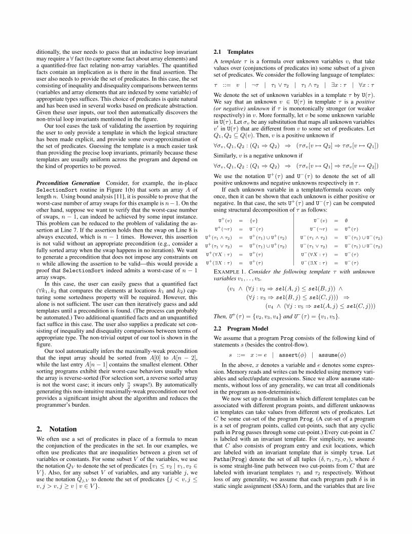
7.4 Properties of our algorithmsStatistical properties: We statistically examined the practical be-havior our algorithms to explain why they work well despite thetheoretical bottlenecks. We accumulated the statistics over all anal-yses and for all relevant modes (iterative and constraint-based).

First, we measured if the SMT queries generated by our systemwere efficiently decidable. Figure 4 shows that almost all of ourqueries take less than 10ms. By separating fixed-point computationfrom reasoning about local verification conditions, we have broughtthe theorem proving burden down to the realm of current solvers.

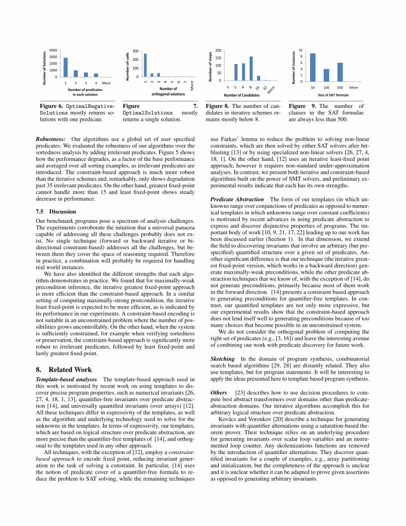
Second, because our algorithms rely on OptimalNegative-Solutions and OptimalSolutions, it is therefore important thatin practice they return a small number of optimal solutions. In fact,we found that on most calls they return a single optimal solution(Figure 6 and 7) and never more than 6. Therefore there are indeeda small number of possibilities to consider when they are called(in Figures 2 and 3 and in the constraint encoding). This explainsthe efficiency of our local reasoning in computing the best abstracttransformer.

Third, we examine the efficiency of the fixed-point computation(iterative) or encoding (constraint-based) built from the core pro-cedures. For the iterative approaches, we reached a fixed-point in amedian of 4 steps with the number of candidates remaining small,at around 8 (Figure 8). This indicates that our algorithms performa very directed search for the fixed-point. For the constraint-basedapproach, the number of clauses in the SAT formula never exceeds500 (Figure 9) with a median size of 5 variables. This explains theefficiency of our fixed-point computation.

6 Notice that the second precondition is indeed the maximally-weakest forthe specification, even though max could be initialized out of bounds. Ifwe expected to strictly output an array index and not just the location of themaximum, then the specification should have contained, 0 ≤ max < n.

!

"!!!

#!!!

$!!!

%!!!

" # $ % &'()!"#$%&'()'*(+",-(./

!"#$%&'()'0&%1-23,%/'

-.'%324'/(+",-(.

Figure 6. OptimalNegative-Solutions mostly returns so-lutions with one predicate.

!

"!!

#!!

$!!

" # $ % & ' (

)*+,

!"#$%&'()'*+,,-

!"#$%&'()'

(&./(0(1+,'-(,".2(1-

Figure 7.OptimalSolutions mostlyreturns a single solution.

0

50

100

150

200

Number of steps

Number of Candidates

Figure 8. The number of can-didates in iterative schemes re-mains mostly below 8.

!

"

#

$

%

&!

'! &!! '!! ()*+

!"#$%&'()'*+,-.+/%,

0*1%'()'023')(&#"4.

Figure 9. The number ofclauses in the SAT formulaeare always less than 500.

Robustness: Our algorithms use a global set of user specifiedpredicates. We evaluated the robustness of our algorithms over thesortedness analysis by adding irrelevant predicates. Figure 5 showshow the performance degrades, as a factor of the base performanceand averaged over all sorting examples, as irrelevant predicates areintroduced. The constraint-based approach is much more robustthan the iterative schemes and, remarkably, only shows degradationpast 35 irrelevant predicates. On the other hand, greatest fixed-pointcannot handle more than 15 and least fixed-point shows steadydecrease in performance.

7.5 DiscussionOur benchmark programs pose a spectrum of analysis challenges.The experiments corroborate the intuition that a universal panaceacapable of addressing all these challenges probably does not ex-ist. No single technique (forward or backward iterative or bi-directional constraint-based) addresses all the challenges, but be-tween them they cover the space of reasoning required. Thereforein practice, a combination will probably be required for handlingreal world instances.

We have also identified the different strengths that each algo-rithm demonstrates in practice. We found that for maximally-weakprecondition inference, the iterative greatest fixed-point approachis more efficient than the constraint-based approach. In a similarsetting of computing maximally-strong postcondition, the iterativeleast fixed-point is expected to be more efficient, as is indicated byits performance in our experiments. A constraint-based encoding isnot suitable in an unconstrained problem where the number of pos-sibilities grows uncontrollably. On the other hand, when the systemis sufficiently constrained, for example when verifying sortednessor preservation, the constraint-based approach is significantly morerobust to irrelevant predicates, followed by least fixed-point andlastly greatest fixed-point.

8. Related WorkTemplate-based analyses The template-based approach used inthis work is motivated by recent work on using templates to dis-cover precise program properties, such as numerical invariants [26,27, 4, 18, 1, 13], quantifier-free invariants over predicate abstrac-tion [14], and universally quantified invariants (over arrays) [12].All these techniques differ in expressivity of the templates, as wellas the algorithm and underlying technology used to solve for theunknowns in the templates. In terms of expressivity, our templates,which are based on logical structure over predicate abstraction, aremore precise than the quantifier-free templates of [14], and orthog-onal to the templates used in any other approach.

All techniques, with the exception of [12], employ a constraint-based approach to encode fixed point, reducing invariant gener-ation to the task of solving a constraint. In particular, [14] usesthe notion of predicate cover of a quantifier-free formula to re-duce the problem to SAT solving, while the remaining techniques

use Farkas’ lemma to reduce the problem to solving non-linearconstraints, which are then solved by either SAT solvers after bit-blasting [13] or by using specialized non-linear solvers [26, 27, 4,18, 1]. On the other hand, [12] uses an iterative least-fixed pointapproach; however it requires non-standard under-approximationanalyses. In contrast, we present both iterative and constraint-basedalgorithms built on the power of SMT solvers, and preliminary ex-perimental results indicate that each has its own strengths.

Predicate Abstraction The form of our templates (in which un-knowns range over conjunctions of predicates as opposed to numer-ical templates in which unknowns range over constant coefficients)is motivated by recent advances in using predicate abstraction toexpress and discover disjunctive properties of programs. The im-portant body of work [10, 9, 21, 17, 22] leading up to our work hasbeen discussed earlier (Section 1). In that dimension, we extendthe field to discovering invariants that involve an arbitrary (but pre-specified) quantified structure over a given set of predicates. An-other significant difference is that our technique (the iterative great-est fixed-point version, which works in a backward direction) gen-erate maximally-weak preconditions, while the other predicate ab-straction techniques that we know of, with the exception of [14], donot generate preconditions, primarily because most of them workin the forward direction. [14] presents a constraint based approachto generating preconditions for quantifier-free templates. In con-trast, our quantified templates are not only more expressive, butour experimental results show that the constraint-based approachdoes not lend itself well to generating preconditions because of toomany choices that become possible in an unconstrained system.

We do not consider the orthogonal problem of computing theright set of predicates (e.g., [3, 16]) and leave the interesting avenueof combining our work with predicate discovery for future work.

Sketching In the domain of program synthesis, combinatorialsearch based algorithms [29, 28] are distantly related. They alsouse templates, but for program statements. It will be interesting toapply the ideas presented here to template based program synthesis.

Others [23] describes how to use decision procedures to com-pute best abstract transformers over domains other than predicate-abstraction domains. Our iterative algorithms accomplish this forarbitrary logical structure over predicate abstraction.

Kovacs and Voronkov [20] describe a technique for generatinginvariants with quantifier alternations using a saturation-based the-orem prover. Their technique relies on an underlying procedurefor generating invariants over scalar loop variables and an instru-mented loop counter. Any skolemizations functions are removedby the introduction of quantifier alternations. They discover quan-tified invariants for a couple of examples, e.g., array partitioningand initialization, but the completeness of the approach is unclearand it is unclear whether it can be adapted to prove given assertionsas opposed to generating arbitrary invariants.

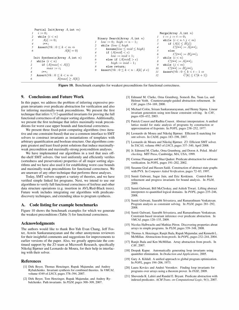
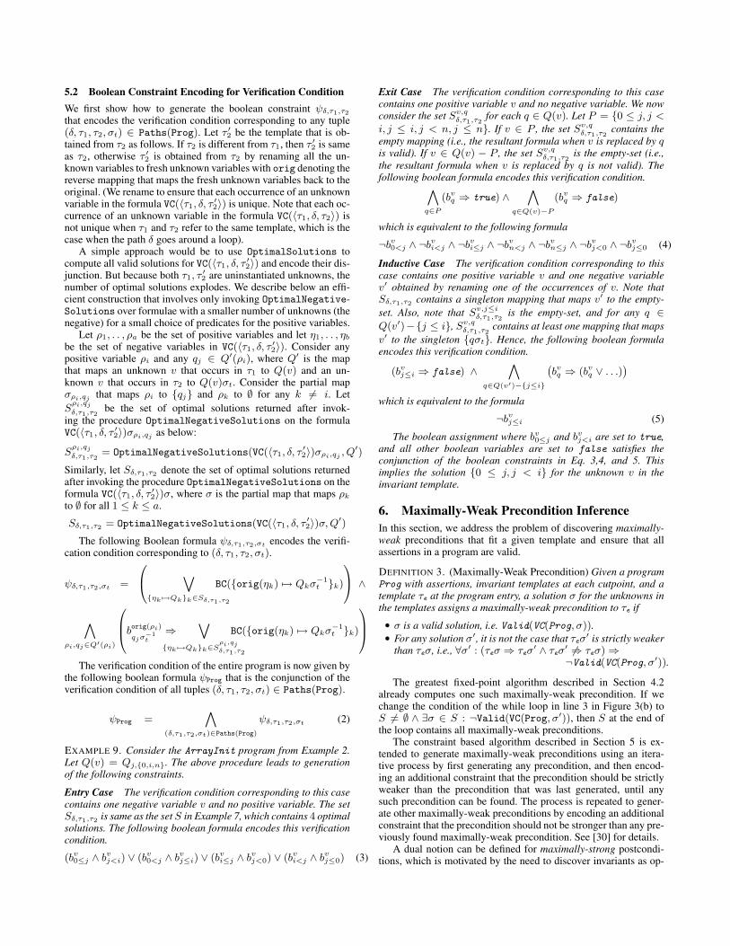
Partial Init(Array A, int m)1 i := 0;2 while (i < n)3 A[i] := 0;4 i++;5 Assert(∀k : 0 ≤ k < m ⇒6 A[k] = 0)

Init Synthesis(Array A, int n)1 while (i < n)2 if (A[max] < A[i])3 max := i;4 i++;5 Assert(∀k : 0 ≤ k < n ⇒6 A[max] ≥ A[k])

Binary Search(Array A, int n)1 low := 0; high := n− 1;2 while (low ≤ high3 Assume(low ≤ mid ≤ high)4 if (A[mid] < e)5 low := mid + 1;6 else if (A[mid] > e)7 high := mid− 1;8 else return;9 Assert(∀k : 0 ≤ k < n : A[k] 6= e)

Merge(Array A, int n)1 i := j := t := 0;2 while (i < n ∧ j < m)3 if (A[i] ≤ B[j])4 C[t++] := A[i++];5 else6 C[t++] := B[j++];7 while (i < n)8 C[t++] := A[i++];9 while (j < m)

10 C[t++] := B[j++];11 Assert(∀k : 0 ≤ k < t− 1 ⇒12 C[k] ≤ C[k + 1])

Figure 10. Benchmark examples for weakest preconditions for functional correctness.

9. Conclusions and Future WorkIn this paper, we address the problem of inferring expressive pro-gram invariants over predicate abstraction for verification and alsofor inferring maximally-weak preconditions. We present the firsttechnique that infers ∀/∀∃-quantified invariants for proving the fullfunctional correctness of all major sorting algorithms. Additionally,we present the first technique that infers maximally-weak precon-ditions for worst case upper bounds and functional correctness.

We present three fixed-point computing algorithms (two itera-tive and one constraint-based) that use a common interface to SMTsolvers to construct invariants as instantiations of templates witharbitrary quantification and boolean structure. Our algorithms com-pute greatest and least fixed-point solutions that induce maximally-weak precondition and maximally-strong postcondition analyses.

We have implemented our algorithms in a tool that uses off-the-shelf SMT solvers. Our tool uniformly and efficiently verifies(sortedness and preservation) properties of all major sorting algo-rithms and we have also used it for establishing worst case boundsand maximally-weak preconditions for functional correctness. Weare unaware of any other technique that performs these analyses.

Today, SMT solvers support a variety of theories, and we haveverified simple linked list programs. Next, we intend to use ouralgorithms to verify full functional correctness of list/tree and otherdata structure operations (e.g. insertion in AVL/Red-Black trees).Future work includes integrating our algorithms with predicate-discovery techniques, and extending ideas to program synthesis.

A. Code listing for example benchmarksFigure 10 shows the benchmark examples for which we generatethe weakest preconditions (Table 3) for functional correctness.

AcknowledgmentsThe authors would like to thank Bor-Yuh Evan Chang, Jeff Fos-ter, Aswin Sankaranarayanan and the other anonymous reviewersfor their insightful comments and suggestions for improvements toearlier versions of the paper. Also, we greatly appreciate the con-tinued support by the Z3 team at Microsoft Research, specificallyNikolaj Bjørner and Leonardo de Moura, for their help in interfac-ing with their solver.

References[1] Dirk Beyer, Thomas Henzinger, Rupak Majumdar, and Andrey

Rybalchenko. Invariant synthesis for combined theories. In VMCAI,volume 4349 of LNCS, pages 378–394, 2007.

[2] Dirk Beyer, Tom Henzinger, Rupak Majumdar, and Andrey Ry-balchenko. Path invariants. In PLDI, pages 300–309, 2007.

[3] Edmund M. Clarke, Orna Grumberg, Somesh Jha, Yuan Lu, andHelmut Veith. Counterexample-guided abstraction refinement. InCAV, pages 154–169, 2000.

[4] Michael Colon, Sriram Sankaranarayanan, and Henny Sipma. Linearinvariant generation using non-linear constraint solving. In CAV,pages 420–432, 2003.

[5] Patrick Cousot and Radhia Cousot. Abstract interpretation: A unifiedlattice model for static analysis of programs by construction orapproximation of fixpoints. In POPL, pages 238–252, 1977.

[6] Leonardo de Moura and Nikolaj Bjørner. Efficient E-matching forsmt solvers. In CADE, pages 183–198, 2007.

[7] Leonardo de Moura and Nikolaj Bjørner. Z3: Efficient SMT solver.In TACAS, volume 4963 of LNCS, pages 337–340, April 2008.

[8] Jr. Edmund M. Clarke, Orna Grumberg, and Doron A. Peled. Modelchecking. MIT Press, Cambridge, MA, USA, 1999.

[9] Cormac Flanagan and Shaz Qadeer. Predicate abstraction for softwareverification. In POPL, pages 191–202, 2002.

[10] Susanne Graf and Hassen Saıdi. Construction of abstract state graphswith PVS. In Computer Aided Verification, pages 72–83, 1997.

[11] Sumit Gulwani, Sagar Jain, and Eric Koskinen. Control-flowrefinement and progress invariants for bound analysis. In PLDI,2009.

[12] Sumit Gulwani, Bill McCloskey, and Ashish Tiwari. Lifting abstractinterpreters to quantified logical domains. In POPL, pages 235–246,2008.

[13] Sumit Gulwani, Saurabh Srivastava, and Ramarathnam Venkatesan.Program analysis as constraint solving. In PLDI, pages 281–292,2008.

[14] Sumit Gulwani, Saurabh Srivastava, and Ramarathnam Venkatesan.Constraint-based invariant inference over predicate abstraction. InVMCAI, pages 120–135, 2009.

[15] Nicolas Halbwachs and Mathias Peron. Discovering properties aboutarrays in simple programs. In PLDI, pages 339–348, 2008.

[16] Thomas A. Henzinger, Ranjit Jhala, Rupak Majumdar, and Kenneth L.McMillan. Abstractions from proofs. In POPL, pages 232–244, 2004.

[17] Ranjit Jhala and Ken McMillan. Array abstraction from proofs. InCAV, 2007.

[18] Deepak Kapur. Automatically generating loop invariants usingquantifier elimination. In Deduction and Applications, 2005.

[19] Gary A. Kildall. A unified approach to global program optimization.In POPL, pages 194–206, 1973.

[20] Laura Kovacs and Andrei Voronkov. Finding loop invariants forprograms over arrays using a theorem prover. In FASE, 2009.

[21] Shuvendu K. Lahiri and Randal E. Bryant. Predicate abstraction withindexed predicates. ACM Trans. on Computational Logic, 9(1), 2007.

[22] Andreas Podelski and Thomas Wies. Boolean heaps. In SAS, 2005.

[23] Thomas W. Reps, Shmuel Sagiv, and Greta Yorsh. Symbolic impl. ofthe best transformer. In VMCAI, pages 252–266, 2004.

[24] Microsoft Research. Phoenix. http://research.microsoft.com/Phoenix/.

[25] Microsoft Research. Z3. http://research.microsoft.com/projects/Z3/.

[26] Sriram Sankaranarayanan, Henny Sipma, and Zohar Manna. Non-linear loop invariant generation using grobner bases. In POPL, pages318–329, 2004.

[27] Sriram Sankaranarayanan, Henny B. Sipma, and Zohar Manna.Constraint-based linear-relations analysis. In SAS, pages 53–68,2004.

[28] Armando Solar-Lezama, Gilad Arnold, Liviu Tancau, RastislavBodik, Vijay Saraswat, and Sanjit A. Seshia. Sketching stencils.In PLDI, pages 167–178, June 2007.

[29] Armando Solar-Lezama, Liviu Tancau, Rastislav Bodik, VijaySaraswat, and Sanjit A. Seshia. Combinatorial sketching for finiteprograms. In ASPLOS, pages 404–415, Oct 2006.

[30] Saurabh Srivastava and Sumit Gulwani. Program verification usingtemplates over predicate abstraction. Technical Report MSR-TR-2008-173, Nov 2008.

[31] Saurabh Srivastava, Sumit Gulwani, and Jeffrey Foster. VS3: SMT-solvers for program verification. In CAV, 2009.

[32] Karen Zee, Viktor Kuncak, and Martin C. Rinard. Full functionalverification of linked data structures. In PLDI, pages 349–361, 2008.