« Program termination proofs by convex optimization » Patrick Cousot École normale supérieure 45 rue d’Ulm, 75230 Paris cedex 05, France [email protected] www.di.ens.fr/ ~ cousot IBM Research Seminar — Thomas J. Watson Research Center, Hawthorne, NY — 5 January 2006 IBM Research Seminar, Jan. 5th, 2007 — 1 — ľ P. Cousot Abstract Program termination is based on reasonings by induction (e.g. on program steps, program data) which involves the discovery of unknown inductive arguments (e.g. rank functions, in- variants) satisfying universally quantified termination conditions. For static program analysis, the discovery of the inductive arguments must be automated, which consists in solving the constraints provided by the termination conditions. Several methods have been considered: recurrence/difference equation resolution; iteration, possibly with convergence acceleration through widening/narrowing; or direct methods (such as elimination). All these methods involve some form of simplification of the constraints formalized by abstract interpretation. In this talk, we explore parametric abstraction of rank function and invariants and direct resolution of Floyd/Naur/Hoare termination constraints by Lagrangian relaxation (to handle implication) and semidefinite programming relaxation (to handle universal implication). Fi- nally the parameters are computed using numerical semidefinite programming solvers. This new approach exploits the recent progress in the numerical resolution of linear or bilinear ma- trix inequalities by semidefinite programming using efficient polynomial primal/dual interior point methods generalizing those well-known in linear programming to convex optimization. The framework is applied to invariance and termination proof of sequential, nondeterministic, concurrent, and fair parallel imperative polynomial programs and can easily be extended to other safety and liveness properties. IBM Research Seminar, Jan. 5th, 2007 — 2 — ľ P. Cousot Reference [1] P. Cousot. – Proving Program Invariance and Termination by Parametric Abstraction, Lagrangian Relaxation and Semidefinite Programming. In : Proc. Sixth Int. Conf. on Verification, Model Check- ing and Abstract Interpretation (VMCAI 2005), R. Cousot (Ed.), Paris, France, 17–19 Jan. 2005. pp. 1–24. – Lecture Notes In Computer Science 3385, Springer. IBM Research Seminar, Jan. 5th, 2007 — 3 — ľ P. Cousot Static analysis x § x x x x § x x § x x x x § x x IBM Research Seminar, Jan. 5th, 2007 — 4 — ľ P. Cousot

Welcome message from author
This document is posted to help you gain knowledge. Please leave a comment to let me know what you think about it! Share it to your friends and learn new things together.
Transcript
« Program termination proofs byconvex optimization »
Patrick CousotÉcole normale supérieure
45 rue d’Ulm, 75230 Paris cedex 05, France
[email protected]/~cousot
IBM Research Seminar — Thomas J. Watson ResearchCenter, Hawthorne, NY — 5 January 2006
IBM Research Seminar, Jan. 5th, 2007 — 1 — ľ P. Cousot
AbstractProgram termination is based on reasonings by induction (e.g. on program steps, programdata) which involves the discovery of unknown inductive arguments (e.g. rank functions, in-variants) satisfying universally quantified termination conditions. For static program analysis,the discovery of the inductive arguments must be automated, which consists in solving theconstraints provided by the termination conditions. Several methods have been considered:recurrence/difference equation resolution; iteration, possibly with convergence accelerationthrough widening/narrowing; or direct methods (such as elimination). All these methodsinvolve some form of simplification of the constraints formalized by abstract interpretation.In this talk, we explore parametric abstraction of rank function and invariants and directresolution of Floyd/Naur/Hoare termination constraints by Lagrangian relaxation (to handleimplication) and semidefinite programming relaxation (to handle universal implication). Fi-nally the parameters are computed using numerical semidefinite programming solvers. Thisnew approach exploits the recent progress in the numerical resolution of linear or bilinear ma-trix inequalities by semidefinite programming using efficient polynomial primal/dual interiorpoint methods generalizing those well-known in linear programming to convex optimization.The framework is applied to invariance and termination proof of sequential, nondeterministic,concurrent, and fair parallel imperative polynomial programs and can easily be extended toother safety and liveness properties.
IBM Research Seminar, Jan. 5th, 2007 — 2 — ľ P. Cousot
Reference
[1] P. Cousot. – Proving Program Invariance and Terminationby Parametric Abstraction, Lagrangian Relaxation andSemidefinite Programming.
In : Proc. Sixth Int. Conf. on Verification, Model Check-ing and Abstract Interpretation (VMCAI 2005), R. Cousot(Ed.), Paris, France, 17–19 Jan. 2005. pp. 1–24. – LectureNotes In Computer Science 3385, Springer.
IBM Research Seminar, Jan. 5th, 2007 — 3 — ľ P. Cousot
Static analysis
x§xxxxx§xx§xxxxx§xx
IBM Research Seminar, Jan. 5th, 2007 — 4 — ľ P. Cousot

Principle of static analysis
– Define the most precise program property as a fixpointlfpF
– Effectively compute a fixpoint approximation:- iteration-based fixpoint approximation- constraint-based fixpoint approximation
IBM Research Seminar, Jan. 5th, 2007 — 5 — ľ P. Cousot
Iteration-based static analysis
– Effectively overapproximate the iterative fixpointdefinition 1:
lfpF =G
–2O
X–
X0 = ?
X– =G
”<–
F (X”)
1 under Tarski’s fixpoint theorem hypotheses
IBM Research Seminar, Jan. 5th, 2007 — 6 — ľ P. Cousot
Constraint-based static analysis
– Effectively solve a postfixpoint constraint:
lfpF =lfX j F (X) v Xg
since F (X) v X implies lfpF v X
– Sometimes, the constraint resolution algorithm is noth-ing but the iterative computation of lfpF 2
– Constraint-based static analysis is the main subject ofthis talk.
2 An example is set-based analysis as shown in Patrick Cousot & Radhia Cousot. Formal Language, Grammarand Set-Constraint-Based Program Analysis by Abstract Interpretation. In Conference Record of FPCA’95 ACM Conference on Functional Programming and Computer Architecture, pages 170–181, La Jolla,California, U.S.A., 25-28 June 1995.
IBM Research Seminar, Jan. 5th, 2007 — 7 — ľ P. Cousot
Parametric abstraction
– Parametric abstract domain: X 2 ff(a) j a 2 ´g, a isan unknown parameter
– Verification condition: X satisfies F (X) v X if [andonly if] 9a 2 ´ : F (f(a)) v f(a) that is 9a : CF (a)where CF 2 ´ 7! B are constraints over the unknownparameter a
IBM Research Seminar, Jan. 5th, 2007 — 8 — ľ P. Cousot

Fixpoint versus Constraint-based Approachfor Termination Analysis
1. Termination can be expressed in fixpoint form 3
2. However we know no effective fixpoint underapproximationmethod needed to overestimation the termination rank
3. So we consider a constraint-based approach abstracting Floyd’sranking function method
3 See Sect. 11.2 of Patrick Cousot. Constructive Design of a hierarchy of Semantics of a Transition Systemby Abstract Interpretation. Theoret. Comput. Sci. 277(1—2):47—103, 2002. ľ Elsevier Science.
IBM Research Seminar, Jan. 5th, 2007 — 9 — ľ P. Cousot
Overview of theTermination Analysis Method
IBM Research Seminar, Jan. 5th, 2007 — 10 — ľ P. Cousot
Proving Termination of a Loop
� ������������� �����
� �����������
� ������������������ �
� ����������� ��
�����������
�
The main point in this talk is (4).IBM Research Seminar, Jan. 5th, 2007 — 11 — ľ P. Cousot
Proving Termination of a Loop
1. Perform an iterated forward/backward relational static anal-ysis of the loop with termination hypothesis to determinea necessary proper termination precondition
2. Assuming the termination precondition, perform an forwardrelational static analysis of the loop to determine the loopinvariant
3. Assuming the loop invariant, perform an forward relationalstatic analysis of the loop body to determine the loop ab-stract operational semantics
4. Assuming the loop semantics, use an abstraction of Floyd’sranking function method to prove termination of the loop
IBM Research Seminar, Jan. 5th, 2007 — 12 — ľ P. Cousot

Arithmetic Mean Example
while (x <> y) do
x := x - 1;
y := y + 1
od
The polyhedral abstraction used for the static analysis of the examples is
implemented using Bertrand Jeannet’s NewPolka library.
IBM Research Seminar, Jan. 5th, 2007 — 13 — ľ P. Cousot
Arithmetic Mean Example
1. Perform an iterated forward/backward relational static anal-ysis of the loop with termination hypothesis to determinea necessary proper termination precondition
2. Assuming the termination precondition, perform an forwardrelational static analysis of the loop to determine the loopinvariant
3. Assuming the loop invariant, perform an forward relationalstatic analysis of the loop body to determine the loop ab-stract operational semantics
4. Assuming the loop semantics, use an abstraction of Floyd’sranking function method to prove termination of the loop
IBM Research Seminar, Jan. 5th, 2007 — 14 — ľ P. Cousot
Forward/reachability properties
II
Example: partial correctness (must stay into safe states)IBM Research Seminar, Jan. 5th, 2007 — 15 — ľ P. Cousot
Backward/ancestry properties
II
F
Example: termination (must reach final states)IBM Research Seminar, Jan. 5th, 2007 — 16 — ľ P. Cousot
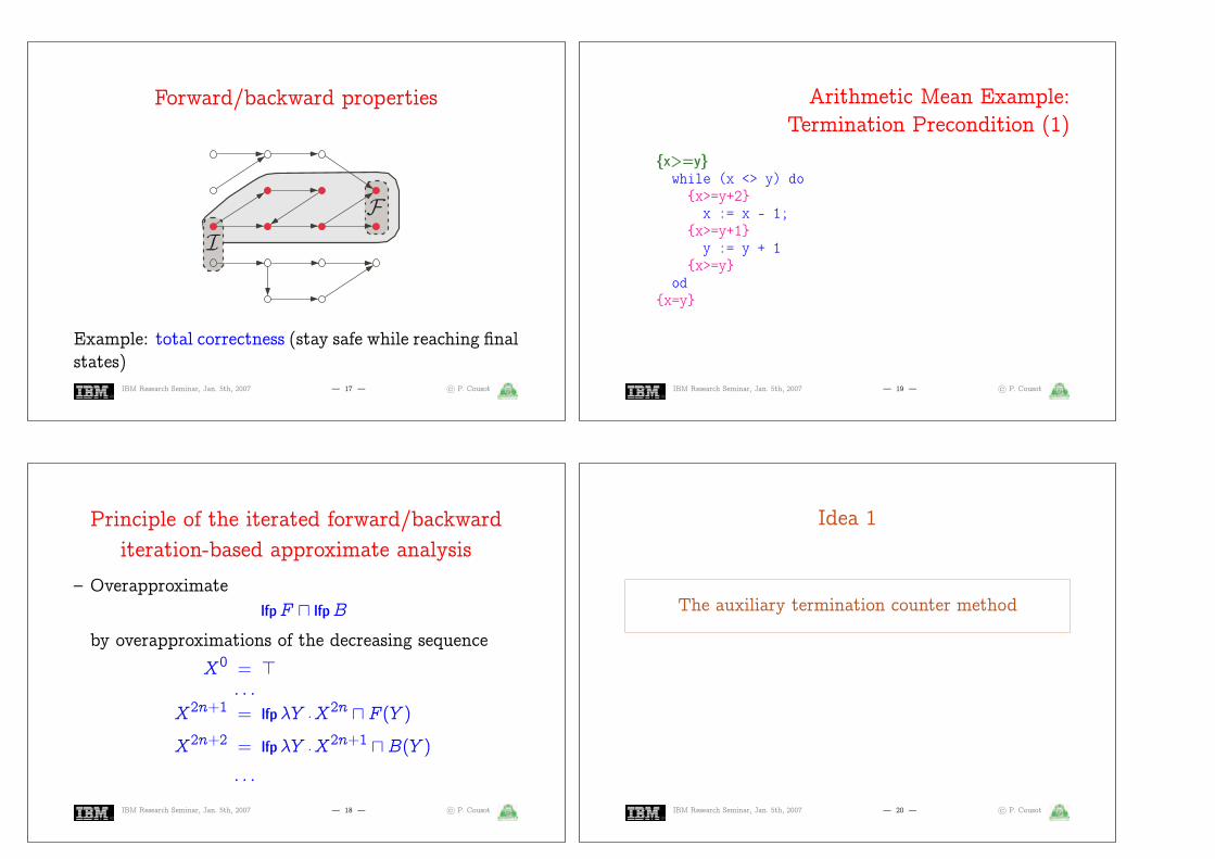
Forward/backward properties
I
F
I
Example: total correctness (stay safe while reaching finalstates)
IBM Research Seminar, Jan. 5th, 2007 — 17 — ľ P. Cousot
Principle of the iterated forward/backwarditeration-based approximate analysis
– OverapproximatelfpF u lfpB
by overapproximations of the decreasing sequence
X0 = >: : :
X2n+1 = lfp–Y .X2n u F (Y )
X2n+2 = lfp–Y .X2n+1 uB(Y )
: : :
IBM Research Seminar, Jan. 5th, 2007 — 18 — ľ P. Cousot
Arithmetic Mean Example:Termination Precondition (1)
{x>=y}while (x <> y) do
{x>=y+2}x := x - 1;
{x>=y+1}y := y + 1
{x>=y}od
{x=y}
IBM Research Seminar, Jan. 5th, 2007 — 19 — ľ P. Cousot
Idea 1
The auxiliary termination counter method
IBM Research Seminar, Jan. 5th, 2007 — 20 — ľ P. Cousot

Arithmetic Mean Example:Termination Precondition (2)
{x=y+2k,x>=y}while (x <> y) do
{x=y+2k,x>=y+2}k := k - 1;
{x=y+2k+2,x>=y+2}x := x - 1;
{x=y+2k+1,x>=y+1}y := y + 1
{x=y+2k,x>=y}od
{x=y,k=0}assume (k = 0)
{x=y,k=0}
Add an auxiliary termi-nation counter to enforce(bounded) termination inthe backward analysis!
IBM Research Seminar, Jan. 5th, 2007 — 21 — ľ P. Cousot
Arithmetic Mean Example
1. Perform an iterated forward/backward relational static anal-ysis of the loop with termination hypothesis to determinea necessary proper termination precondition
2. Assuming the termination precondition, perform an forwardrelational static analysis of the loop to determine the loopinvariant
3. Assuming the loop invariant, perform an forward relationalstatic analysis of the loop body to determine the loop ab-stract operational semantics
4. Assuming the loop semantics, use an abstraction of Floyd’sranking function method to prove termination of the loop
IBM Research Seminar, Jan. 5th, 2007 — 22 — ľ P. Cousot
Arithmetic Mean Example:Loop Invariant
assume ((x=y+2*k) & (x>=y));{x=y+2k,x>=y}
while (x <> y) do{x=y+2k,x>=y+2}
k := k - 1;{x=y+2k+2,x>=y+2}
x := x - 1;{x=y+2k+1,x>=y+1}
y := y + 1{x=y+2k,x>=y}
od{k=0,x=y}
IBM Research Seminar, Jan. 5th, 2007 — 23 — ľ P. Cousot
Arithmetic Mean Example
1. Perform an iterated forward/backward relational static anal-ysis of the loop with termination hypothesis to determinea necessary proper termination precondition
2. Assuming the termination precondition, perform an forwardrelational static analysis of the loop to determine the loopinvariant
3. Assuming the loop invariant, perform an forward relationalstatic analysis of the loop body to determine the loop ab-stract operational semantics
4. Assuming the loop semantics, use an abstraction of Floyd’sranking function method to prove termination of the loop
IBM Research Seminar, Jan. 5th, 2007 — 24 — ľ P. Cousot

Arithmetic Mean Example:Body Relational Semantics
Case x < y:assume (x=y+2*k)&(x>=y+2);{x=y+2k,x>=y+2}assume (x < y);empty(6)assume (x0=x)&(y0=y)&(k0=k);empty(6)k := k - 1;x := x - 1;y := y + 1empty(6)
Case x > y:assume (x=y+2*k)&(x>=y+2);{x=y+2k,x>=y+2}assume (x > y);{x=y+2k,x>=y+2}assume (x0=x)&(y0=y)&(k0=k);{x=y+2k0,y=y0,x=x0,x=y+2k,
x>=y+2}k := k - 1;x := x - 1;y := y + 1{x+2=y+2k0,y=y0+1,x+1=x0,
x=y+2k,x>=y}
IBM Research Seminar, Jan. 5th, 2007 — 25 — ľ P. Cousot
Arithmetic Mean Example
1. Perform an iterated forward/backward relational static anal-ysis of the loop with termination hypothesis to determinea necessary proper termination precondition
2. Assuming the termination precondition, perform an forwardrelational static analysis of the loop to determine the loopinvariant
3. Assuming the loop invariant, perform an forward relationalstatic analysis of the loop body to determine the loop ab-stract operational semantics
4. Assuming the loop semantics, use an abstraction of Floyd’sranking function method to prove termination of the loop
IBM Research Seminar, Jan. 5th, 2007 — 26 — ľ P. Cousot
Floyd’s method for termination of while B do C
Given a loop invariant I, find an R=Q=Z-valued unkownrank function r such that:
– The rank is nonnegative:
8 x0; x : I(x0) ^ JB; CK(x0; x) ) r(x0) – 0
– The rank is strictly decreasing :
8 x0; x : I(x0) ^ JB; CK(x0; x) ) r(x) » r(x0)` ”
” – 1 for Z, ” > 0 for R=Q to avoid Zeno 12,14,18. . .
IBM Research Seminar, Jan. 5th, 2007 — 27 — ľ P. Cousot
Problems
– How to get rid of the implication ) ?
! Lagrangian relaxation
– How to get rid of the universal quantification 8 ?
! Quantifier elimination/mathematical program-ming & relaxation
IBM Research Seminar, Jan. 5th, 2007 — 28 — ľ P. Cousot

Algorithmically interesting cases
– linear inequalities
! linear programming
– linear matrix inequalities (LMI)/quadratic forms
! semidefinite programming
– semialgebraic sets
! polynomial quantifier elimination, or
! relaxation with semidefinite programming
IBM Research Seminar, Jan. 5th, 2007 — 29 — ľ P. Cousot
Arithmetic Mean Example:Ranking Function with Semi-
definite ProgrammingRelaxation
» clear all;
[v0,v] = variables(’x’,’y’,’k’)
% linear inequalities
% x0 y0 k0
Ai = [ 0 0 0];
% x y k
Ai_ = [ 1 -1 0]; % x0 - y0 >= 0
bi = [0];
[N Mk(:,:,:)]=linToMk(Ai,Ai_,bi);
% linear equalities
% x0 y0 k0
Ae = [ 0 0 -2;
0 -1 0;
-1 0 0;
0 0 0];
% x y k
Ae_ = [ 1 -1 0; % x - y - 2*k0 - 2 = 0
0 1 0; % y - y0 - 1 = 0
1 0 0; % x - x0 + 1 = 0
1 -1 -2]; % x - y - 2*k = 0
be = [2; -1; 1; 0];
[M Mk(:,:,N+1:N+M)]=linToMk(Ae,Ae_,be);
Input the loop abstractsemantics
IBM Research Seminar, Jan. 5th, 2007 — 30 — ľ P. Cousot
» display_Mk(Mk, N, v0, v);
...
+1.x -1.y >= 0
-2.k0 +1.x -1.y +2 = 0
-1.y0 +1.y -1 = 0
-1.x0 +1.x +1 = 0
+1.x -1.y -2.k = 0
...
» [diagnostic,R] = termination(v0, v, Mk, N, ’integer’, ’linear’);
» disp(diagnostic)
feasible (bnb)
» intrank(R, v)
r(x,y,k) = +4.k -2
– Display the abstract se-mantics of the loop while
B do C
– compute ranking func-tion, if any
IBM Research Seminar, Jan. 5th, 2007 — 31 — ľ P. Cousot
Quantifier Elimination
IBM Research Seminar, Jan. 5th, 2007 — 32 — ľ P. Cousot

Quantifier elimination (Tarski-Seidenberg)
– quantifier elimination for the first-order theory of realclosed fields:- F is a logical combination of polynomial equationsand inequalities in the variables x1, . . . , xn- Tarski-Seidenberg decision procedure
transforms a formula
8=9x1 : : : : 8=9xn : F (x1; : : : ; xn)
into an equivalent quantifier free formula
– cannot be bound by any tower of exponentials [Heintz,Roy, Solerno 89]
IBM Research Seminar, Jan. 5th, 2007 — 33 — ľ P. Cousot
Quantifier elimination (Collins)
– cylindrical algebraic decomposition method by Collins
– implemented in Mathematicaő
– worst-case time-complexity for real quantifier elimi-nation is “only” doubly exponential in the number ofquantifier blocks
– Various optimisations and heuristics can be used 4
4 See e.g. Redlog http://www.fmi.uni-passau.de/~redlog/
IBM Research Seminar, Jan. 5th, 2007 — 34 — ľ P. Cousot
Scaling up
However
– does not scale up beyond a few variables!
– too bad!
IBM Research Seminar, Jan. 5th, 2007 — 35 — ľ P. Cousot
Proving Termination byParametric Abstraction,Lagrangian Relaxation andSemidefinite Programming
IBM Research Seminar, Jan. 5th, 2007 — 36 — ľ P. Cousot

Idea 2
Express the loop invariant and relational semanticsas numerical positivity constraints
IBM Research Seminar, Jan. 5th, 2007 — 37 — ľ P. Cousot
Relational semantics of while B do C od loops
– x0 2 R=Q=Z: values of the loop variables before a loopiteration
– x 2 R=Q=Z: values of the loop variables after a loopiteration
– I(x0): loop invariant, JB; CK(x0; x): relational seman-tics of one iteration of the loop body
– I(x0) ^ JB; CK(x0; x) =N̂
i=1
ffi(x0; x) >i 0 (>i 2 f>;–;=g)
– not a restriction for numerical programs
IBM Research Seminar, Jan. 5th, 2007 — 38 — ľ P. Cousot
Example of linear program (Arithmetic mean)[A A0][x0 x]
> > b
{x=y+2k,x>=y}
while (x <> y) do
k := k - 1;
x := x - 1;
y := y + 1
od
+1.x -1.y >= 0
-2.k0 +1.x -1.y +2 = 0
-1.y0 +1.y -1 = 0
-1.x0 +1.x +1 = 0
+1.x -1.y -2.k = 0
2
6
6
6
6
4
0 0 0 1 `1 00 0 `2 1 `1 00 `1 0 0 1 0`1 0 0 1 0 00 0 0 1 `1 `2
3
7
7
7
7
5
2
6
6
6
6
6
6
4
x0y0k0xyk
3
7
7
7
7
7
7
5
–====
2
6
6
6
6
4
0`21`10
3
7
7
7
7
5
IBM Research Seminar, Jan. 5th, 2007 — 39 — ľ P. Cousot
Example of quadratic form program (factorial)[x x0]A[x x0]> + 2[x x0] q + r > 0
n := 0;
f := 1;
while (f <= N) do
n := n + 1;
f := n * f
od
-1.f0 +1.N0 >= 0
+1.n0 >= 0
+1.f0 -1 >= 0
-1.n0 +1.n -1 = 0
+1.N0 -1.N = 0
-1.f0.n +1.f = 0
[n0f0N0nfN ]
2
6
6
6
6
6
6
6
4
0 0 0 0 0 0
0 0 0 `12 0 00 0 0 0 0 0
0 `12 0 0 0 00 0 0 0 0 00 0 0 0 0 0
3
7
7
7
7
7
7
7
5
2
6
6
6
6
6
6
4
n0f0N0nfN
3
7
7
7
7
7
7
5
+ 2[n0f0N0nfN ]
2
6
6
6
6
6
6
4
0000120
3
7
7
7
7
7
7
5
+ 0 = 0
IBM Research Seminar, Jan. 5th, 2007 — 40 — ľ P. Cousot

Example of semialgebraic program(logistic map)
eps = 1.0e-9;
while (0 <= a) & (a <= 1 - eps)
& (eps <= x) & (x <= 1) do
x := a*x*(1-x)
od
a.x.(1-x)
0.4
x a
IBM Research Seminar, Jan. 5th, 2007 — 41 — ľ P. Cousot
Floyd’s method for termination of while B do C
Find an R=Q=Z-valued unkown rank function r and ” >0 such that:
– The rank is nonnegative:
8 x0; x :N̂
i=1
ffi(x0; x) >i 0 ) r(x0) – 0
– The rank is strictly decreasing :
8 x0; x :N̂
i=1
ffi(x0; x) >i 0 ) r(x0)` r(x)` ” – 0
IBM Research Seminar, Jan. 5th, 2007 — 42 — ľ P. Cousot
Idea 3
Eliminate the conjunctionV
and implication ) byLagrangian relaxation
IBM Research Seminar, Jan. 5th, 2007 — 43 — ľ P. Cousot
Implication (general case)
BA
A) B,8x 2 A : x 2 B
IBM Research Seminar, Jan. 5th, 2007 — 44 — ľ P. Cousot
Implication (linear case)
BA
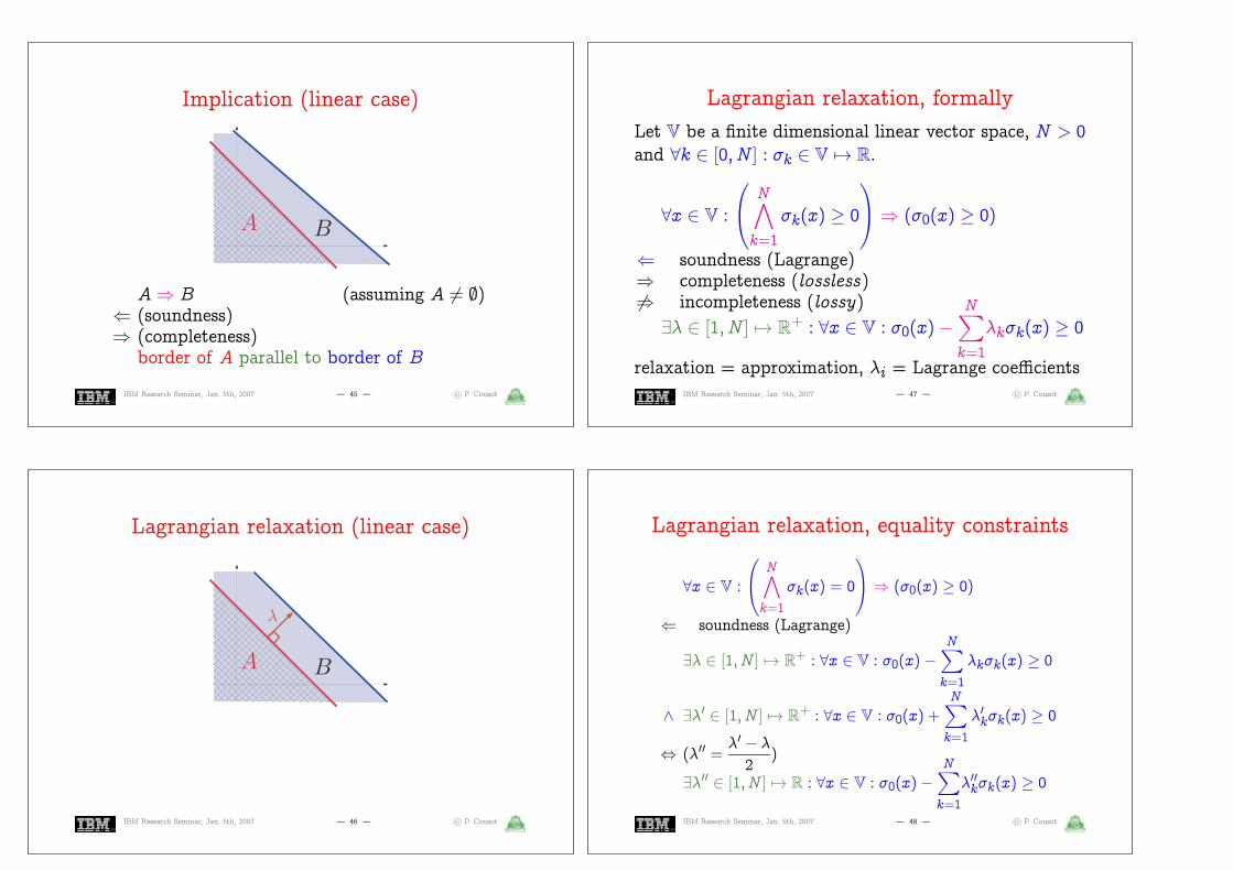
A) B (assuming A 6= ;)( (soundness)) (completeness)border of A parallel to border of B
IBM Research Seminar, Jan. 5th, 2007 — 45 — ľ P. Cousot
Lagrangian relaxation (linear case)
BA
IBM Research Seminar, Jan. 5th, 2007 — 46 — ľ P. Cousot
Lagrangian relaxation, formally
Let V be a finite dimensional linear vector space, N > 0and 8k 2 [0; N ] : ffk 2 V 7! R.
8x 2 V :
0
@
N̂
k=1
ffk(x) – 0
1
A) (ff0(x) – 0)
( soundness (Lagrange)) completeness (lossless)6) incompleteness (lossy)
9– 2 [1; N ] 7! R+ : 8x 2 V : ff0(x)`NX
k=1
–kffk(x) – 0
relaxation = approximation, –i = Lagrange coefficientsIBM Research Seminar, Jan. 5th, 2007 — 47 — ľ P. Cousot
Lagrangian relaxation, equality constraints
8x 2 V :
0
@
N̂
k=1
ffk(x) = 0
1
A) (ff0(x) – 0)
( soundness (Lagrange)
9– 2 [1; N ] 7! R+ : 8x 2 V : ff0(x)`NX
k=1
–kffk(x) – 0
^ 9–0 2 [1; N ] 7! R+ : 8x 2 V : ff0(x) +NX
k=1
–0kffk(x) – 0
, (–00 =–0 ` –
2)
9–00 2 [1; N ] 7! R : 8x 2 V : ff0(x)`NX
k=1
–00kffk(x) – 0
IBM Research Seminar, Jan. 5th, 2007 — 48 — ľ P. Cousot
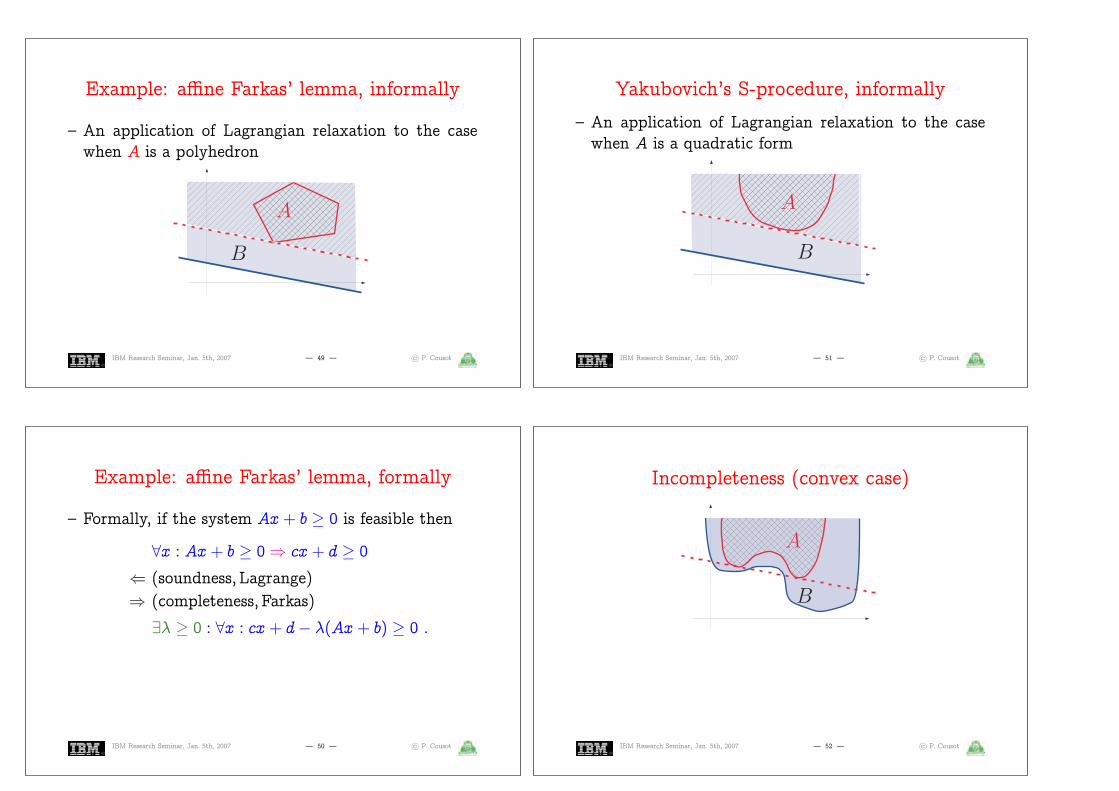
Example: affine Farkas’ lemma, informally
– An application of Lagrangian relaxation to the casewhen A is a polyhedron
B
A
IBM Research Seminar, Jan. 5th, 2007 — 49 — ľ P. Cousot
Example: affine Farkas’ lemma, formally
– Formally, if the system Ax+ b – 0 is feasible then
8x : Ax+ b – 0) cx+ d – 0
( (soundness;Lagrange)
) (completeness;Farkas)
9– – 0 : 8x : cx+ d` –(Ax+ b) – 0 :
IBM Research Seminar, Jan. 5th, 2007 — 50 — ľ P. Cousot
Yakubovich’s S-procedure, informally
– An application of Lagrangian relaxation to the casewhen A is a quadratic form
B
A
IBM Research Seminar, Jan. 5th, 2007 — 51 — ľ P. Cousot
Incompleteness (convex case)
B
A
IBM Research Seminar, Jan. 5th, 2007 — 52 — ľ P. Cousot
Yakubovich’s S-procedure, completeness cases
– The constraint ff(x) – 0 is regular if and only if 9‰ 2V : ff(‰) > 0.
– The S-procedure is lossless in the case of one regularquadratic constraint:8x 2 Rn : x>P1x+ 2q
>1 x+ r1 – 0)
x>P0x+ 2q>0 x+ r0 – 0
( (Lagrange)) (Yakubovich)
9– – 0 : 8x 2 Rn : x>
"
P0 q0q>0 r0
#
` –
"
P1 q1q>1 r1
#!
x – 0:
IBM Research Seminar, Jan. 5th, 2007 — 53 — ľ P. Cousot
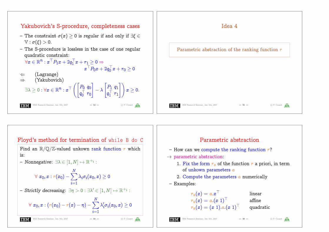
Floyd’s method for termination of while B do C
Find an R=Q=Z-valued unkown rank function r whichis:
– Nonnegative: 9– 2 [1; N ] 7! R+i :
8 x0; x : r(x0)`NX
i=1
–iffi(x0; x) – 0
– Strictly decreasing : 9” > 0 : 9–0 2 [1; N ] 7! R+i :
8 x0; x : (r(x0)` r(x)` ”)`NX
i=1
–0iffi(x0; x) – 0
IBM Research Seminar, Jan. 5th, 2007 — 54 — ľ P. Cousot
Idea 4
Parametric abstraction of the ranking function r
IBM Research Seminar, Jan. 5th, 2007 — 55 — ľ P. Cousot
Parametric abstraction
– How can we compute the ranking function r?
! parametric abstraction:
1. Fix the form ra of the function r a priori, in termof unkown parameters a
2. Compute the parameters a numerically
– Examples:
ra(x) = a:x> linear
ra(x) = a:(x 1)> affine
ra(x) = (x 1):a:(x 1)> quadratic
IBM Research Seminar, Jan. 5th, 2007 — 56 — ľ P. Cousot

Floyd’s method for termination of while B do C
Find R=Q=Z-valued unkown parameters a, such that:
– Nonnegative: 9– 2 [1; N ] 7! R+i :
8 x0; x : ra(x0)`NX
i=1
–iffi(x0; x) – 0
– Strictly decreasing : 9” > 0 : 9–0 2 [1; N ] 7! R+i :
8 x0; x : (ra(x0)` ra(x)` ”)`NX
i=1
–0iffi(x0; x) – 0
IBM Research Seminar, Jan. 5th, 2007 — 57 — ľ P. Cousot
Idea 5
Eliminate the universal quantification 8 usinglinear matrix inequalities (LMIs)
IBM Research Seminar, Jan. 5th, 2007 — 58 — ľ P. Cousot
Mathematical programming
9x 2 Rn:N̂
i=1
gi(x) > 0
[Minimizing f(x)]
feasibility problem : find a solution to the constraints
optimization problem : find a solution, minimizing f(x)
Example: Linear programming9x 2 Rn: Ax > b
[Minimizing cx]
IBM Research Seminar, Jan. 5th, 2007 — 59 — ľ P. Cousot
Feasibility
– feasibility problem: find a solution s 2 Rn to the op-
timization program, such thatN̂
i=1
gi(s) – 0, or to de-
termine that the problem is infeasible– feasible set: fx j
VNi=1 gi(x) – 0g
– a feasibility problem can be converted into the opti-mization program
minf`y 2 R jN̂
i=1
gi(x)` y – 0g
IBM Research Seminar, Jan. 5th, 2007 — 60 — ľ P. Cousot
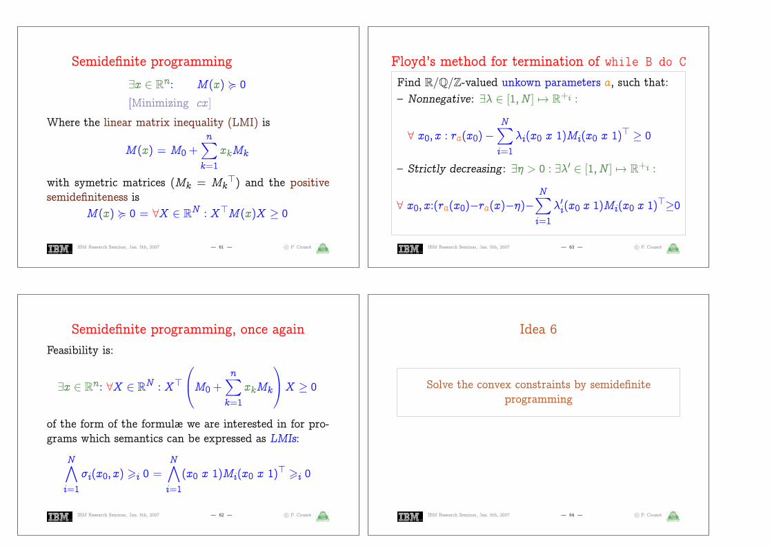
Semidefinite programming, once again
9x 2 Rn: M(x) < 0
[Minimizing cx]
Where the linear matrix inequality (LMI) is
M(x) = M0 +nX
k=1
xkMk
with symetric matrices (Mk = Mk>) and the positive
semidefiniteness is
M(x) < 0 = 8X 2 RN : X>M(x)X – 0
IBM Research Seminar, Jan. 5th, 2007 — 61 — ľ P. Cousot
Semidefinite programming, once again
Feasibility is:
9x 2 Rn: 8X 2 RN : X>
0
@M0 +nX
k=1
xkMk
1
AX – 0
of the form of the formulæ we are interested in for pro-grams which semantics can be expressed as LMIs:
N̂
i=1
ffi(x0; x) >i 0 =N̂
i=1
(x0 x 1)Mi(x0 x 1)> >i 0
IBM Research Seminar, Jan. 5th, 2007 — 62 — ľ P. Cousot
Floyd’s method for termination of while B do C
Find R=Q=Z-valued unkown parameters a, such that:
– Nonnegative: 9– 2 [1; N ] 7! R+i :
8 x0; x : ra(x0)`NX
i=1
–i(x0 x 1)Mi(x0 x 1)> – 0
– Strictly decreasing : 9” > 0 : 9–0 2 [1; N ] 7! R+i :
8 x0; x:(ra(x0)`ra(x)`”)`NX
i=1
–0i(x0 x 1)Mi(x0 x 1)>–0
IBM Research Seminar, Jan. 5th, 2007 — 63 — ľ P. Cousot
Idea 6
Solve the convex constraints by semidefiniteprogramming
IBM Research Seminar, Jan. 5th, 2007 — 64 — ľ P. Cousot
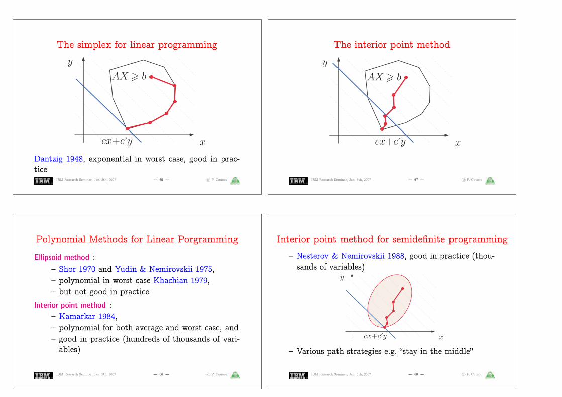
The simplex for linear programming
x
y
AX � b
cx�c y
Dantzig 1948, exponential in worst case, good in prac-tice
IBM Research Seminar, Jan. 5th, 2007 — 65 — ľ P. Cousot
Polynomial Methods for Linear Porgramming
Ellipsoid method :– Shor 1970 and Yudin & Nemirovskii 1975,– polynomial in worst case Khachian 1979,– but not good in practice
Interior point method :– Kamarkar 1984,– polynomial for both average and worst case, and– good in practice (hundreds of thousands of vari-ables)
IBM Research Seminar, Jan. 5th, 2007 — 66 — ľ P. Cousot
The interior point method
cx�c y x
y
AX � b
IBM Research Seminar, Jan. 5th, 2007 — 67 — ľ P. Cousot
Interior point method for semidefinite programming
– Nesterov & Nemirovskii 1988, good in practice (thou-sands of variables)
x
y
cx�c y
– Various path strategies e.g. “stay in the middle”
IBM Research Seminar, Jan. 5th, 2007 — 68 — ľ P. Cousot

Semidefinite programming solvers
Numerous solvers available under Mathlabő, a.o.:
– lmilab: P. Gahinet, A. Nemirovskii, A.J. Laub, M. Chilali
– Sdplr: S. Burer, R. Monteiro, C. Choi
– Sdpt3: R. Tütüncü, K. Toh, M. Todd
– SeDuMi: J. Sturm
– bnb: J. Löfberg (integer semidefinite programming)
Common interfaces to these solvers, a.o.:
– Yalmip: J. Löfberg
Sometime need some help (feasibility radius, shift,. . . )IBM Research Seminar, Jan. 5th, 2007 — 69 — ľ P. Cousot
Linear program: termination of Euclidean division» clear all
% linear inequalities
% y0 q0 r0
Ai = [ 0 0 0; 0 0 0;
0 0 0];
% y q r
Ai_ = [ 1 0 0; % y - 1 >= 0
0 1 0; % q - 1 >= 0
0 0 1]; % r >= 0
bi = [-1; -1; 0];
% linear equalities
% y0 q0 r0
Ae = [ 0 -1 0; % -q0 + q -1 = 0
-1 0 0; % -y0 + y = 0
0 0 -1]; % -r0 + y + r = 0
% y q r
Ae_ = [ 0 1 0; 1 0 0;
1 0 1];
be = [-1; 0; 0];
Iterated forward/back-ward polyhedral analysis:{y>=1}q := 0;{q=0,y>=1}r := x;{x=r,q=0,y>=1}while (y <= r) do{y<=r,q>=0}r := r - y;{r>=0,q>=0}q := q + 1{r>=0,q>=1}
od{q>=0,y>=r+1}
IBM Research Seminar, Jan. 5th, 2007 — 70 — ľ P. Cousot
» [N Mk(:,:,:)]=linToMk(Ai, Ai_, bi);
» [M Mk(:,:,N+1:N+M)]=linToMk(Ae, Ae_, be);
» [v0,v]=variables(’y’,’q’,’r’);
» display_Mk(Mk, N, v0, v);
+1.y -1 >= 0
+1.q -1 >= 0
+1.r >= 0
-1.q0 +1.q -1 = 0
-1.y0 +1.y = 0
-1.r0 +1.y +1.r = 0
» [diagnostic,R] = termination(v0, v, Mk, N, ’integer’, ’quadratic’);
» disp(diagnostic)
termination (bnb)
» intrank(R, v)
r(y,q,r) = -2.y +2.q +6.r
Floyd’s proposal r(x; y; q; r) = x` q is more intuitive but requires to discover
the nonlinear loop invariant x = r + qy.
IBM Research Seminar, Jan. 5th, 2007 — 71 — ľ P. Cousot
Imposing a feasibility radius
x
y
cx�c y
IBM Research Seminar, Jan. 5th, 2007 — 72 — ľ P. Cousot
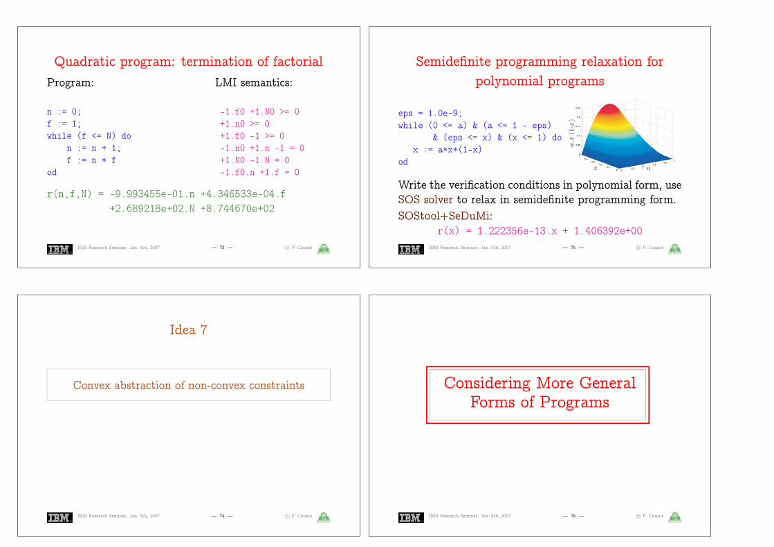
Quadratic program: termination of factorial
Program:
n := 0;
f := 1;
while (f <= N) do
n := n + 1;
f := n * f
od
LMI semantics:
-1.f0 +1.N0 >= 0
+1.n0 >= 0
+1.f0 -1 >= 0
-1.n0 +1.n -1 = 0
+1.N0 -1.N = 0
-1.f0.n +1.f = 0
r(n,f,N) = -9.993455e-01.n +4.346533e-04.f
+2.689218e+02.N +8.744670e+02
IBM Research Seminar, Jan. 5th, 2007 — 73 — ľ P. Cousot
Idea 7
Convex abstraction of non-convex constraints
IBM Research Seminar, Jan. 5th, 2007 — 74 — ľ P. Cousot
Semidefinite programming relaxation forpolynomial programs
eps = 1.0e-9;
while (0 <= a) & (a <= 1 - eps)
& (eps <= x) & (x <= 1) do
x := a*x*(1-x)
od
a.x.(1-x)
0.4
x a
Write the verification conditions in polynomial form, useSOS solver to relax in semidefinite programming form.
SOStool+SeDuMi:r(x) = 1.222356e-13.x + 1.406392e+00
IBM Research Seminar, Jan. 5th, 2007 — 75 — ľ P. Cousot
Considering More GeneralForms of Programs
IBM Research Seminar, Jan. 5th, 2007 — 76 — ľ P. Cousot

Handling disjunctive loop tests and tests inloop body
– By case analysis
– and “conditional Lagrangian relaxation” (Lagrangianrelaxation in each of the cases)
IBM Research Seminar, Jan. 5th, 2007 — 77 — ľ P. Cousot
Loop body with tests
!̀ case analysis:
i – 0i < 0
while (x < y) do
if (i >= 0) then
x := x+i+1
else
y := y+i
fi
od
lmilab:r(i,x,y) = -2.252791e-09.i -4.355697e+07.x +4.355697e+07.y
+5.502903e+08
IBM Research Seminar, Jan. 5th, 2007 — 78 — ľ P. Cousot
Quadratic termination of linear loop{n>=0} ̀ termination precondition
determined by iterated for-ward/backward polyhedralanalysis
i := n; j := n;
while (i <> 0) do
if (j > 0) then
j := j - 1
else
j := n; i := i - 1
fi
od
IBM Research Seminar, Jan. 5th, 2007 — 79 — ľ P. Cousot
sdplr (with feasibility radius of 1.0e+3):
r(n,i,j) = +7.024176e-04.n^2 +4.394909e-05.n.i ...
-2.809222e-03.n.j +1.533829e-02.n ...
+1.569773e-03.i^2 +7.077127e-05.i.j ...
+3.093629e+01.i -7.021870e-04.j^2 ...
+9.940151e-01.j +4.237694e+00
Successive values ofr(n; i; j) for n = 10 onloop entry
0
5
10
02
46
810
0
50
100
150
200
250
300
350
j
Ranking function
i
r(10
,i,j)
IBM Research Seminar, Jan. 5th, 2007 — 80 — ľ P. Cousot

Handling nested loops
– by induction on the loop depth
– use an iterated forward/backward symbolic analysis toget a necessary termination precondition
– use a forward symbolic symbolic analysis to get thesemantics of a loop body
– use Lagrangian relaxation and semidefinite program-ming to get the ranking function
IBM Research Seminar, Jan. 5th, 2007 — 81 — ľ P. Cousot
Example of termination of nested loops:Bubblesort inner loop
...
+1.i’ -1 >= 0
+1.j’ -1 >= 0
+1.n0’ -1.i’ >= 0
-1.j +1.j’ -1 = 0
-1.i +1.i’ = 0
-1.n +1.n0’ = 0
+1.n0 -1.n0’ = 0
+1.n0’ -1.n’ = 0
...
Iterated forward/backward polyhedral analysisfollowed by forward analysis of the body:
assume (n0 = n & j >= 0 & i >= 1 & n0 >= i & j <> i);
{n0=n,i>=1,j>=0,n0>=i}
assume (n01 = n0 & n1 = n & i1 = i & j1 = j);
{j=j1,i=i1,n0=n1,n0=n01,n0=n,i>=1,j>=0,n0>=i}
j := j + 1
{j=j1+1,i=i1,n0=n1,n0=n01,n0=n,i>=1,j>=1,n0>=i}
termination (lmilab)
r(n0,n,i,j) = +434297566.n0 +226687644.n -72551842.i
-2.j +2147483647
IBM Research Seminar, Jan. 5th, 2007 — 82 — ľ P. Cousot
Example of termination of nested loops:Bubblesort outer loop
...
+1.i’ +1 >= 0
+1.n0’ -1.i’ -1 >= 0
+1.i’ -1.j’ +1 = 0
-1.i +1.i’ +1 = 0
-1.n +1.n0’ = 0
+1.n0 -1.n0’ = 0
+1.n0’ -1.n’ = 0
...
Iterated forward/backward polyhedral analysisfollowed by forward analysis of the body:
assume (n0=n & i>=0 & n>=i & i <> 0);
{n0=n,i>=0,n0>=i}
assume (n01=n0 & n1=n & i1=i & j1=j);
{j1=j,i=i1,n0=n1,n0=n01,n0=n,i>=0,n0>=i}
j := 0;
while (j <> i) do
j := j + 1
od;
i := i - 1
{i+1=j,i+1=i1,n0=n1,n0=n01,n0=n,i+1>=0,n0>=i+1}
termination (lmilab)
r(n0,n,i,j) = +24348786.n0 +16834142.n +100314562.i +65646865
IBM Research Seminar, Jan. 5th, 2007 — 83 — ľ P. Cousot
Handling nondeterminacy
– By case analysis
– Same for concurrency by interleaving
– Same with fairness by nondeterministic interleavingwith encoding of an explicit bounded round-robin sched-uler (with unknown bound)
IBM Research Seminar, Jan. 5th, 2007 — 84 — ľ P. Cousot

Termination of a concurrent program[| 1: while [x+2 < y] do
2: [x := x + 1]
od
3:
||
1: while [x+2 < y] do
2: [y := y - 1]
od
3:
|]
interleaving
!̀
while (x+2 < y) do
if ?=0 then
x := x + 1
else if ?=0 then
y := y - 1
else
x := x + 1;
y := y - 1
fi fi
od
penbmi: r(x,y) = 2.537395e+00.x+-2.537395e+00.y+
-2.046610e-01
IBM Research Seminar, Jan. 5th, 2007 — 85 — ľ P. Cousot
Termination of a fair parallel program[[ while [(x>0)|(y>0) do x := x - 1] od ||
while [(x>0)|(y>0) do y := y - 1] od ]]
interleaving+ scheduler!̀
{m>=1} termination precondition determined by iteratedforward/backward polyhedral analysist := ?;
assume (0 <= t & t <= 1);
s := ?;
assume ((1 <= s) & (s <= m));
while ((x > 0) | (y > 0)) do
if (t = 1) then
x := x - 1
else
y := y - 1
fi;
s := s - 1;
if (s = 0) then
if (t = 1) then
t := 0
else
t := 1
fi;
s := ?;
assume ((1 <= s) & (s <= m))
else
skip
fi
od;;
penbmi: r(x,y,m,s,t) = +1.000468e+00.x +1.000611e+00.y
+2.855769e-02.m -3.929197e-07.s +6.588027e-06.t +9.998392e+03
IBM Research Seminar, Jan. 5th, 2007 — 86 — ľ P. Cousot
Relaxed ParametricInvariance Proof Method
IBM Research Seminar, Jan. 5th, 2007 — 87 — ľ P. Cousot
Floyd’s method for invariance
Given a loop precondition P , find an unkown loop in-variant I such that:
– The invariant is initial:
8 x : P (x) ) I"(x)
– The invariant is inductive:
8 x; x0 : I"???
(x) ^ JB; CK(x; x0) ) I
"(x0)
IBM Research Seminar, Jan. 5th, 2007 — 88 — ľ P. Cousot

Abstraction
– Express loop semantics as a conjunction of LMI con-straints (by relaxation for polynomial semantics)
– Eliminate the conjunction and implication by Lagrangianrelaxation
– Fix the form of the unkown invariant by parametricabstraction
. . . we get . . .
IBM Research Seminar, Jan. 5th, 2007 — 89 — ľ P. Cousot
Floyd’s method for numerical programs
Find R=Q=Z-valued unkown parameters a, such that:
– The invariant is initial: 9— 2 R+ :
8 x : Ia(x)` —:P (x) – 0
– The invariant is inductive: 9– 2 [0; N ] !̀ R+ :
8 x; x0 : Ia(x0)` –0:Ia(x)
" "bilinear in –0 and a
`NX
k=1
–k:ffk(x; x0) – 0
IBM Research Seminar, Jan. 5th, 2007 — 90 — ľ P. Cousot
Idea 8
Solve the bilinear matrix inequality (BMI) bysemidefinite programming
IBM Research Seminar, Jan. 5th, 2007 — 91 — ľ P. Cousot
Bilinear matrix inequality (BMI) solvers
9x 2 Rn :m̂
i=1
0
@M i0 +nX
k=1
xkMik +
nX
k=1
nX
‘=1
xkx‘Nik‘ < 0
1
A
[Minimizing x>Qx+ cx]
Two solvers available under Mathlabő:
– PenBMI: M. Kočvara, M. Stingl
– bmibnb: J. Löfberg
Common interfaces to these solvers:
– Yalmip: J. Löfberg
IBM Research Seminar, Jan. 5th, 2007 — 92 — ľ P. Cousot

Example: linear invariantProgram:i := 2; j := 0;
while (??) do
if (??) then
i := i + 4
else
i := i + 2;
j := j + 1
fi
od;
– Invariant:
+2.14678e-12*i -3.12793e-10*j +0.486712 >= 0
– Less natural than i` 2j ` 2 – 0
– Alternative:
- Determine parameters (a) by othermethods (e.g. random interpreta-tion)
- Use BMI solvers to check for invari-ance
IBM Research Seminar, Jan. 5th, 2007 — 93 — ľ P. Cousot
Conclusion
IBM Research Seminar, Jan. 5th, 2007 — 94 — ľ P. Cousot
Constraint resolution failure
– infeasibility of the constraints does not mean “non ter-mination” or “non invariance” but simply failure
– inherent to abstraction!
IBM Research Seminar, Jan. 5th, 2007 — 95 — ľ P. Cousot
Numerical errors
– LMI/BMI solvers do numerical computations with round-ing errors, shifts, etc
– ranking function is subject to numerical errors
– the hard point is to discover a candidate for the rank-ing function
– much less difficult, when the ranking function is known,to re-check for satisfaction (e.g. by static analysis)
– not very satisfactory for invariance (checking only ???)
IBM Research Seminar, Jan. 5th, 2007 — 96 — ľ P. Cousot

Related anterior work
– Linear case (Farkas lemma):- Invariants: Sankaranarayanan, Spima, Manna (CAV’03,SAS’04, heuristic solver)- Termination: Podelski & Rybalchenko (VMCAI’03,Lagrange coefficients eliminated by hand to reduceto linear programming so no disjunctions, no tests,etc)- Parallelization & scheduling: Feautrier, easily gener-alizable to nonlinear case
IBM Research Seminar, Jan. 5th, 2007 — 97 — ľ P. Cousot
Related posterior work
– Termination using Lyapunov functions: Roozbehani,Feron & Megrestki (HSCC 2005)
IBM Research Seminar, Jan. 5th, 2007 — 98 — ľ P. Cousot
Seminal work
– LMI case, Lyapunov 1890,“an invariant set of a dif-ferential equation is sta-ble in the sense that it at-tracts all solutions if onecan find a function that isbounded from below anddecreases along all solu-tions outside the invariantset”.
IBM Research Seminar, Jan. 5th, 2007 — 99 — ľ P. Cousot
THE END, THANK YOU
More details and references in the VMCAI’05 paper.
IBM Research Seminar, Jan. 5th, 2007 — 100 — ľ P. Cousot
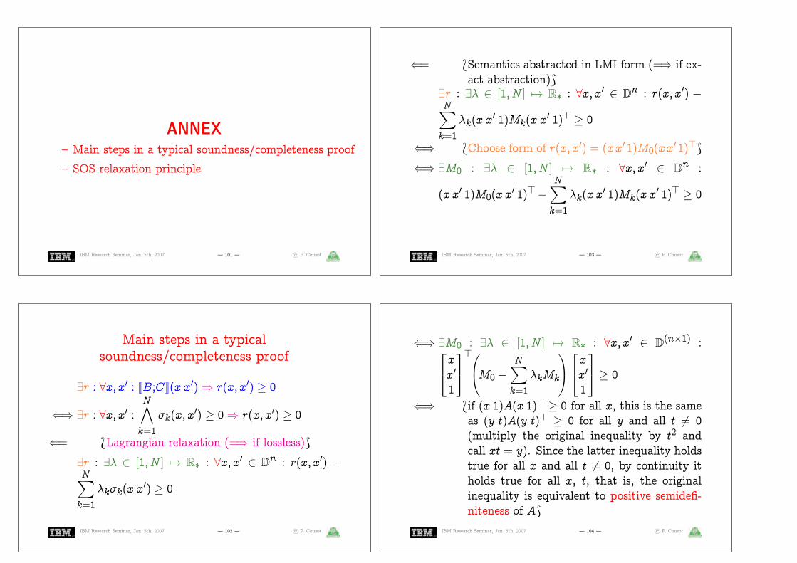
ANNEX– Main steps in a typical soundness/completeness proof
– SOS relaxation principle
IBM Research Seminar, Jan. 5th, 2007 — 101 — ľ P. Cousot
Main steps in a typicalsoundness/completeness proof
9r : 8x; x0 : JB;CK(x x0)) r(x; x0) – 0
() 9r : 8x; x0 :N̂
k=1
ffk(x; x0) – 0) r(x; x0) – 0
(= HLagrangian relaxation (=) if lossless)I9r : 9– 2 [1; N ] 7! R˜ : 8x; x
0 2 Dn : r(x; x0) `NX
k=1
–kffk(x x0) – 0
IBM Research Seminar, Jan. 5th, 2007 — 102 — ľ P. Cousot
(= HSemantics abstracted in LMI form (=) if ex-act abstraction)I
9r : 9– 2 [1; N ] 7! R˜ : 8x; x0 2 Dn : r(x; x0) `
NX
k=1
–k(x x0 1)Mk(x x
0 1)> – 0
() HChoose form of r(x; x0) = (xx01)M0(xx01)>I() 9M0 : 9– 2 [1; N ] 7! R˜ : 8x; x
0 2 Dn :
(x x0 1)M0(x x0 1)>`
NX
k=1
–k(x x0 1)Mk(x x
0 1)> – 0
IBM Research Seminar, Jan. 5th, 2007 — 103 — ľ P. Cousot
() 9M0 : 9– 2 [1; N ] 7! R˜ : 8x; x0 2 D(nˆ1) :
2
4
x
x0
1
3
5
>0
@M0 `NX
k=1
–kMk
1
A
2
4
x
x0
1
3
5 – 0
() Hif (x 1)A(x 1)> – 0 for all x, this is the sameas (y t)A(y t)> – 0 for all y and all t 6= 0(multiply the original inequality by t2 andcall xt = y). Since the latter inequality holdstrue for all x and all t 6= 0, by continuity itholds true for all x, t, that is, the originalinequality is equivalent to positive semidefi-niteness of AI
IBM Research Seminar, Jan. 5th, 2007 — 104 — ľ P. Cousot

9M0 : 9– 2 [1; N ] 7! R˜ :
0
@M0 `NX
k=1
–kMk
1
A < 0
HLMI solver provides M0 (and –)I
IBM Research Seminar, Jan. 5th, 2007 — 105 — ľ P. Cousot
SOS Relaxation Principle
– Show 8x : p(x) – 0 by 8x : p(x) =Pki=1 qi(x)
2
– Hibert’s 17th problem (sum of squares)
– Undecidable (but for monovariable or low degrees)
– Look for an approximation (relaxation) by semidefi-nite programming
IBM Research Seminar, Jan. 5th, 2007 — 106 — ľ P. Cousot
General relaxation/approximation idea
– Write the polynomials in quadratic form with mono-mials as variables: p(x; y; : : :) = z>Qz where Q < 0is a semidefinite positive matrix of unknowns and z =[: : : x2; xy; y2; : : : x; y; : : : 1] is a monomial basis
– If such a Q does exist then p(x; y; : : :) is a sum ofsquares 5
– The equality p(x; y; : : :) = z>Qz yields LMI contrainson the unkown Q: z>M(Q)z < 0
5 Since Q < 0, Q has a Cholesky decomposition L which is an upper triangular matrix L such that Q=L>L.It follows that p(x) = z>Qz = z>L>Lz = (Lz)>Lz = [Li;: ´ z]>[Li;: ´ z] =
P
i(Li;: ´ z)2 (where ´ is the vector
dot product x ´ y =P
i xiyi), proving that p(x) is a sum of squares whence 8x : p(x) – 0, which eliminatesthe universal quantification on x.
IBM Research Seminar, Jan. 5th, 2007 — 107 — ľ P. Cousot
– Instead of quantifying over monomials values x, y, re-place the monomial basis z by auxiliary variables X(loosing relationships between values of monomials)
– To find such a Q < 0, check for semidefinite positive-ness 9Q : 8X : X>M(Q)X – 0 i.e. 9Q : M(Q) < 0with LMI solver
– Implement with SOStools underMathlabő of Prajna,Papachristodoulou, Seiler and Parrilo
– Nonlinear cost since the monomial basis has size
„
n+mm
«
for multivariate polynomials of degree n with m vari-ables
IBM Research Seminar, Jan. 5th, 2007 — 108 — ľ P. Cousot
Related Documents