PROFIT-DRIVEN SERVICE REQUEST SCHEDULING IN CLOUDS TECHNICAL REPORT 646

School of ITTechnical Report

PROFIT-DRIVEN SERVICE REQUEST SCHEDULING IN CLOUDS

TECHNICAL REPORT 646

YOUNG CHOON LEE1, CHEN WANG2, ALBERT Y. ZOMAYA1 AND BING BING ZHOU1

1 SCHOOL OF INFORMATION TECHNOLOGIESTHE UNIVERSITY OF SYDNEY

2 CSIRO ICT CENTRE

NOVEMBER 2009

Profit-driven Service Request Scheduling in Clouds

Young Choon Lee1, Chen Wang

2, Albert Y. Zomaya

1, Bing Bing Zhou

1

1Centre for Distributed and High Performance Computing, School of Information Technologies

The University of Sydney

NSW 2006, Australia

{yclee,zomaya,bbz}@it.usyd.edu.au

2CSIRO ICT Center, PO Box 76,

Epping, NSW 1710, Australia

{chen.wang}@csiro.au

Abstract

A primary driving force of the recent cloud

computing paradigm is its inherent cost effectiveness.

As in many basic utilities, such as electricity and

water, consumers/clients in cloud computing

environments are charged based on their service

usage; hence the term ‘pay-per-use’. While this pricing

model is very appealing for both service providers and

consumers, fluctuating service request volume and

conflicting objectives (e.g., profit vs. response time)

between providers and consumers hinder its effective

application to cloud computing environments. In this

paper, we address the problem of service request

scheduling in cloud computing systems. We consider a

three-tier cloud structure, which consists of

infrastructure vendors, service providers and

consumers, the latter two parties are particular

interest to us. Clearly, scheduling strategies in this

scenario should satisfy the objectives of both parties.

Our contributions include the development of a pricing

model—using processor-sharing—for clouds, the

application of this pricing model to composite services

with dependency consideration (to the best of our

knowledge, the work in this study is the first attempt),

and the development of two sets of profit-driven

scheduling algorithms.

1. Introduction

In the past few years, cloud computing has emerged

as an enabling technology and it has been increasingly

adopted in many areas including science and

engineering not to mention business due to its inherent

flexibility, scalability and cost-effectiveness [1], [17].

A cloud is an aggregation of resources/services—

possibly distributed and heterogeneous—provided and

operated by an autonomous administrative body (e.g.,

Amazon, Google or Microsoft). Resources in a cloud

are not restricted to hardware, such as processors and

storage devices, but can also be software stacks and

Web service instances. Although the notion of a cloud

has existed in one form or another for some time now

(its roots can be traced back to the mainframe era [12]),

recent advances in virtualization technologies and the

business trend of reducing the total cost of ownership

(TCO) in particular have made it much more appealing

compared to when it was first introduced.

Clouds are primarily driven by economics—the

pay-per-use pricing model like similar to that for basic

utilities, such as electricity, water and gas. While the

pay-per-use pricing model is very appealing for both

service providers and consumers, fluctuation in service

request volume and conflicting objectives between the

two parties hinder its effective application. In other

words, the service provider aims to

accommodate/process as many requests as possible

with its main objective maximizing profit; and this

may conflict with consumer’s performance

requirements (e.g., response time).

There have been a number of studies exploiting

market-based resource allocation to tackle this problem.

Noticeable scheduling mechanisms include

FirstPrice[3], FirstProfit[13], and proportional-share

[4], [11], [15]. Most of them are limited to job

scheduling in conventional supercomputing settings.

Specifically, they are only applicable to scheduling

batch jobs in systems with a fixed number of resources.

User applications that require the processing of

mashup services, which is common in the cloud are not

considered by these mechanisms. The scenario

addressed in this study is different in terms of

application type and the organization of the cloud.

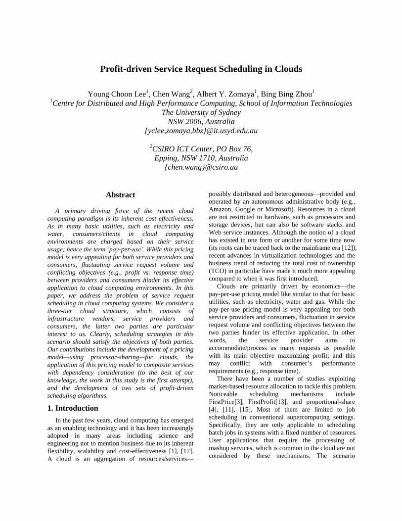
We consider a three-tier cloud structure (Figure 1),

which consists of infrastructure vendors, service

providers and consumers, even though the distinctions

between them can be blurred; the latter two parties are

of particular interest in this study.

A service provider rents resources from cloud

infrastructure vendors and prepares a set of services in

the form of virtual machine (VM) images; the provider

is then able to dynamically create instances from these

VM images. The underlying cloud computing

infrastructure service is responsible for dispatching

these instances to run on physical resources. A running

instance is charged by the time it runs at a flat rate per

time unit. It is in the service provider's interests to

minimize the cost of using the resources offered by the

cloud infrastructure vendor (i.e., resource rental costs)

and maximize the revenue (specifically, net profit)

generated through serving consumers’ applications.

From the service consumer’s viewpoint, a service

request for an application consisting of one or more

services is sent to a provider specifying two main

constraints, time and cost. Although the processing

(response) time of a service request can be assumed to

be accurately estimated, it is most likely that its actual

processing time is longer than its original estimate due

primarily to delays (e.g., queuing and/or processing)

occurring on the provider’s side. This time discrepancy

issue is typically dealt with using service level

agreements (SLAs). Hereafter, the terms application

and service request are used interchangeably.

Scheduling strategies in this cloud computing

scenario should satisfy the objectives of both parties.

The specific problem addressed in this paper is the

scheduling of consumers’ service requests (or

applications) on service instances made available by

providers taking into account costs—incurred by both

consumers and providers—as the most important

factor. Our contributions include the development of a

pricing model using processor-sharing (PS) for clouds,

the application of this pricing model to composite

services (to the best of our knowledge, the work in this

study is the first attempt), and the development of two

sets of profit-driven scheduling algorithms explicitly

exploiting key characteristics of (composite) service

requests including precedence constraints. The first set

of algorithms explicitly takes into account not only the

profit achievable from the current service, but also the

profit from other services being processed on the same

service instance. The second set of algorithms attempts

to maximize service-instance utilization without

incurring loss/deficit; this implies the minimization of

costs to rent resources from infrastructure vendors.

The rest of the paper is organized as follows.

Section 2 describes the cloud, application, pricing and

scheduling models used in this paper. Our pricing

model with the incorporation of PS is discussed in

Section 3 leading to the formulation of our objective

function. We present our profit-driven service request

scheduling algorithms in Section 4 followed by their

performance evaluation results in Section 5. Related

work is discussed in Section 6. We then summarize our

work and draw a conclusion in Section 7.

Figure 1. A three-tier cloud structure.

2. Models

2.1. Cloud system model A cloud computing system in this study consists of

a set of physical resources (server computers) in each

of which there are one or more processing

elements/cores; these resources are fully

interconnected in the sense that a route exists between

any two individual resources. We assume resources are

homogeneous in terms of their computing capability

and capacity; this can be justified using virtualization

technologies. Nowadays, as many-core processors and

virtualization tools (e.g., Linux KVM, VMware

Workstation, Xen, Parallels Desktop, VirtualBox) are

commonplace, the number of concurrent tasks on a

single physical resource is loosely bounded. Although

a cloud can span across multiple geographical

locations (i.e., distributed), the cloud model in our

study is assumed to be confined to a particular physical

location.

2.2. Application model Services offered in the cloud system can be

classified into software as a service (SaaS), platform as

a service (PaaS) and infrastructure as a service (IaaS).

Since this study’s main interest is in the economic

relationship between service providers and consumers,

services in this work can be understood as either of the

first two types.

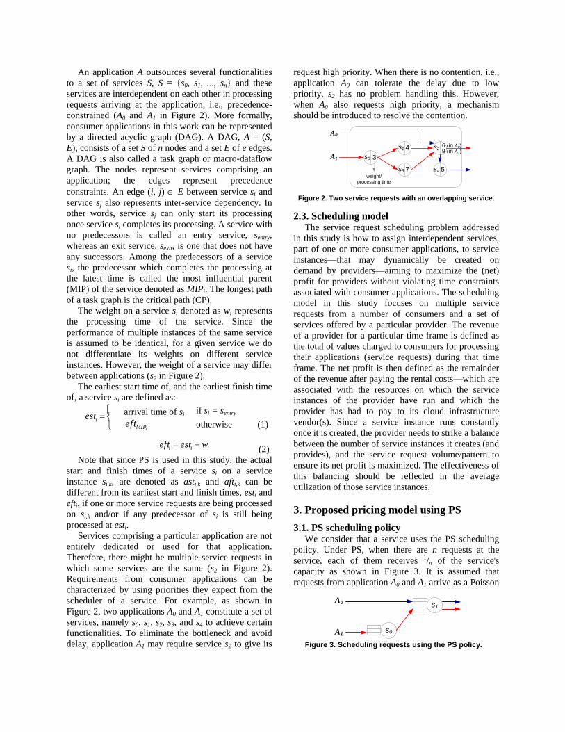
A0

s0

s1

A1

Figure 3. Scheduling requests using the PS policy.

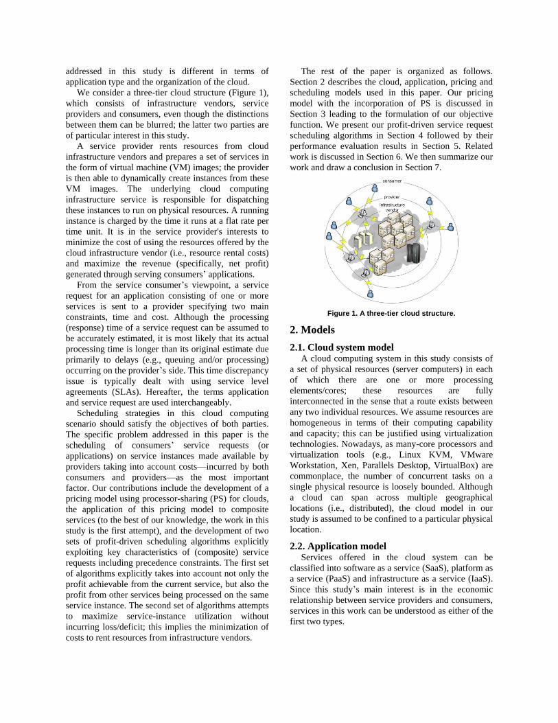
An application A outsources several functionalities

to a set of services S, S = {s0, s1, …, sn} and these

services are interdependent on each other in processing

requests arriving at the application, i.e., precedence-

constrained (A0 and A1 in Figure 2). More formally,

consumer applications in this work can be represented

by a directed acyclic graph (DAG). A DAG, A = (S,

E), consists of a set S of n nodes and a set E of e edges.

A DAG is also called a task graph or macro-dataflow

graph. The nodes represent services comprising an

application; the edges represent precedence

constraints. An edge (i, j) E between service si and

service sj also represents inter-service dependency. In

other words, service sj can only start its processing

once service si completes its processing. A service with

no predecessors is called an entry service, sentry,

whereas an exit service, sexit, is one that does not have

any successors. Among the predecessors of a service

si, the predecessor which completes the processing at

the latest time is called the most influential parent

(MIP) of the service denoted as MIPi. The longest path

of a task graph is the critical path (CP).

The weight on a service si denoted as wi represents

the processing time of the service. Since the

performance of multiple instances of the same service

is assumed to be identical, for a given service we do

not differentiate its weights on different service

instances. However, the weight of a service may differ

between applications (s2 in Figure 2).

The earliest start time of, and the earliest finish time

of, a service si are defined as:

iest

arrival time of si

iMIPeft

if si = sentry

otherwise

(1)

iii westeft (2)

Note that since PS is used in this study, the actual

start and finish times of a service si on a service

instance si,k, are denoted as asti,k and afti,k can be

different from its earliest start and finish times, esti and

efti, if one or more service requests are being processed

on si,k and/or if any predecessor of si is still being

processed at esti.

Services comprising a particular application are not

entirely dedicated or used for that application.

Therefore, there might be multiple service requests in

which some services are the same (s2 in Figure 2).

Requirements from consumer applications can be

characterized by using priorities they expect from the

scheduler of a service. For example, as shown in

Figure 2, two applications A0 and A1 constitute a set of

services, namely s0, s1, s2, s3, and s4 to achieve certain

functionalities. To eliminate the bottleneck and avoid

delay, application A1 may require service s2 to give its

request high priority. When there is no contention, i.e.,

application A0 can tolerate the delay due to low

priority, s2 has no problem handling this. However,

when A0 also requests high priority, a mechanism

should be introduced to resolve the contention.

A0

3

4

7

5

A1 s0

s1

s3

s2

s4

weight/

processing time

6 (in A0)9 (in A1)

Figure 2. Two service requests with an overlapping service.

2.3. Scheduling model The service request scheduling problem addressed

in this study is how to assign interdependent services,

part of one or more consumer applications, to service

instances—that may dynamically be created on

demand by providers—aiming to maximize the (net)

profit for providers without violating time constraints

associated with consumer applications. The scheduling

model in this study focuses on multiple service

requests from a number of consumers and a set of

services offered by a particular provider. The revenue

of a provider for a particular time frame is defined as

the total of values charged to consumers for processing

their applications (service requests) during that time

frame. The net profit is then defined as the remainder

of the revenue after paying the rental costs—which are

associated with the resources on which the service

instances of the provider have run and which the

provider has had to pay to its cloud infrastructure

vendor(s). Since a service instance runs constantly

once it is created, the provider needs to strike a balance

between the number of service instances it creates (and

provides), and the service request volume/pattern to

ensure its net profit is maximized. The effectiveness of

this balancing should be reflected in the average

utilization of those service instances.

3. Proposed pricing model using PS

3.1. PS scheduling policy We consider that a service uses the PS scheduling

policy. Under PS, when there are n requests at the

service, each of them receives 1/n of the service's

capacity as shown in Figure 3. It is assumed that

requests from application A0 and A1 arrive as a Poisson

process with rate λ0 and λ1, respectively. For simplicity,

these requests come from distribution D and have

mean µ0 if processed by service s0, and have mean µ1 if

processed by service s1.

The mean response time for requests served by s0 is

therefore defined as:

00

0

1

t (3)

Similarly, the mean response time for requests

served by s1 is defined as:

011

1

1

t (4)

Note that an M/M/1/PS server has the same service

rate as its corresponding M/M/1/FCFS server.

According to Burke's Theorem, the departure of an

M/M/1 server is a Poisson process with a rate equal to

its arrival rate. As a result, we have an arrival rate λ0 to

service s1 from service s0 in Equation 4. The result also

applies to an M/G/1/PS server.

The mean response time is determined by the

request arrival rate and the service rate in a particular

service. Assuming that in the above example, s0 and s1

have the same mean service rate, i.e., µ0 = µ1 = µ, the

mean response time for s0 and s1 is determined by λ0

and λ1. The additional times that A0 and A1 have to

wait for getting their requests processed in s1 are

defined as:

010

0

11

t (5)

110

1

11

t (6)

In order to maintain a satisfactory response time, a

consumer (for his/her service requests) may pay the

service provider to reduce the rate of incoming

requests. However, the service provider needs to

maintain a certain level of system load to cover the

cost of renting resources and gain sufficient profit. We

assume that a service provider is charged a flat rate at c

per time unit for each instance it runs on the cloud

infrastructure. If a request is charged at a rate m, the

total revenue during a time unit, denoted by r should

be greater than the cost when λ < µ, i.e.,

cmr (7)

There are incentives for a service provider to add

running instances when λ ≥ µ and Equation 7 holds for

a new instance.

Furthermore, we assume that each consumer

application has an expectation of service response time,

i.e., application A expects t < TMAX, in which TMAX

represents the maximum acceptable mean response

time of application A. We denote the average value of

finishing processing a request from application A in

time t as v(t); obviously, this average value should be

greater than the (minimum) price the consumer has to

pay. v is negatively related to t. We define a time-

varying utility function as below:

TMAXt

TMAXtTMINtV

TMINtV

tv

,0

,

,

)( (8)

where V is the maximum value obtainable from

serving a request of consumer application A, TMIN is

the minimal time required for serving a request of A,

and α is the value decay rate for the mean response

time. The V value of a request processing shall be

proportional to the service time of that application. The

function has similarity to that in [3], however, the way

we treat TMIN is different. TMIN is not the mean

service time of a request as used in [3], instead it is a

dynamic value that takes into account of the

dependency of processing the request. For example, as

shown in Figure 2, when a request of A1 is processed

by two services (s1 and s3) in parallel before

converging to another service (s2), the TMIN values

requested by A1 in s1 and s3 are interdependent. The

one with shorter service time, say TMINs1 can be

overridden by the one with longer service time, i.e.,

TMINs1 = TMINs2 without losing any value as s2 cannot

start processing a request of A1 before s1 and s3 finish

processing it.

Considering λTMAX is the request arrival rate at the

maximal acceptable mean response time, application A

requires the following upper bound for λ in order to

obtain positive value from serving a request

VTMAX

TMAX

1 (9)

Combining Equations 3, 7 and 8, and assuming

TMIN ≤ t ≤ TMAX, we further have the following:

cmV

(10)

which gives another constraint of λ as below:

V

cVVccV

V

cVVccV

2

4)(

2

4)( 22

(11)

under the condition:

cVVc 4)( 2 (12)

As V and α are different for each consumer

application, different λ values may bring different

values to consumer applications requesting the same

service (or the same set of services). As shown in

Figure 4, when V = 20 and α = 35, no arrival rate can

simultaneously satisfy both the mean response time

requirement of the consumer application and the profit

needs of the service provider. In this case, the service

provider may negotiate with the infrastructure vendor

Figure 4. The upper and lower bounds of arrival rate vs.

value decay rate with µ = 5, c = 20. The dashed lines

represent the profitable λ ranges of applications (each

color represents a different consumer application).

A0

s0

s1,1prob0

A1

1 - p

rob1

s1,2

1 - prob0

prob1

A0

s0

s1,1

A1s1,2

A0

s0

s1,1

A1s1,2

s1,3

(a) (b) (c)

Figure 5. Scheduling examples based on different criteria.

(a) probabilities. (b) utilization and/or profit. (c) net profit.

to lower c, or raise the cost for request processing.

Specifically, in the latter case, V and α associated with

the consumer application may be increased and/or

reduced, respectively.

3.2. Incorporation of PS into the pricing model In our approach, we consider that a consumer

reaches an SLA with a service provider for each of the

applications the consumer outsources. In the SLA for a

given application, the consumer specifies V, α and its

estimation of λ. The service provider makes a schedule

plan according to these pieces of information. Under

the PS scheduling scheme, the scheduler mainly plays

the role of admission controller, which controls the

request incoming rate of a particular instance. As

shown in Figure 5, the scheduler determines best

possible request-instance matches on the basis of

performance criteria, such as profit and response time.

This match-making process can be programmed with a

probability for a given service (Figure 5a) to statically

select an appropriate service instance for each request;

the probability is determined based on application

characteristics (information on composition and

service time) and consumer supplied application-

specific parameters (α and λ). However, this ―static‖

service-dispatch scheme is not suitable for our

dynamic cloud scenario in which new consumers may

randomly join and place requests, and some existing

consumers may suspend or stop their requests. Thus,

scheduling decisions in our algorithms are made

dynamically, focusing primarily on the maximization

of (net) profit (Figures 5b and 5c).

Under the above mentioned constraints, the

optimization goal of the scheduler for a particular time

frame is to dispatch requests to a set of service

instances in order for the service provider to maximize

its profit. More formally, the net profit of a service

provider for a given time frame τ is defined as:

N

i

L

j

ji

net cvp1 1

(13)

where N is the total number of requests served, vi is the

value obtained through serving request i, L is the

number of service instances run, and τi is the actual

amount of time sj has run, if sj started later than the

beginning of time frame τ.

4. Profit-driven service request scheduling

In this section, we begin by characterizing

allowable delay for composite service requests and

present two profit-driven service request scheduling

algorithms with a variant for each of these algorithms.

4.1. Characterization of allowable delay A consumer application in this study is associated

with two types of allowable delay in its processing,

i.e., application-wise allowable delay and service-wise

allowable delay. For a given consumer application Ai,

there is a certain additional amount of time that the

service provider can afford when processing the

application; this application-wise allowable delay is

possible due to the fact that the provider will gain

some profit as long as Ai is processed within the

maximum acceptable mean response time TMAXi. Note

that response time and processing time in our work are

interchangeable since the PS scheduling policy

adopted in our pricing model does not incur any

queuing delay. The minimum/base processing time

TMINi of application Ai is the summation of processing

times of services along the CP of that application. The

application-wise allowable delay aadi of application Ai

is therefore:

iii TMINTMAXaad (14)

We denote the actual processing time of Ai as ti. For

a given service sj, a service-wise allowable delay for sj

may occur when the processing of its earliest start

successor service element is bounded by another

service; that is, this service-wise delay occurs (see s1 in

Figure 2) since a service request in this study consists

of one or more precedence-constrained services and

these services may differ in their processing time. For

each service in an application, its service-wise

allowable delay time is calculated based on its actual

1. Let max_pi = Ø

2. Let *,j

s = Ø

3. Let *

js = the first service to be scheduled

4. for ∀sj,k∈Ij do

5. Letkpi = Ø

6. Let *

kpi = Ø

7. for ∀slj,k running on sj,k do

8. Let l

kjaft ,= aft of sl

j,k without considering *

js

9. Let *

,

l

kjaft = aft of slj,k with considering *

js

10. Let l

kjclft ,= l

kjaft ,+ l

kjasad ,

11. if *

,

l

kjaft > l

kjclft ,then // possible loss

12. Go to Step 4

13. end if

14. Letkpi =

kpi + l

kjclft ,– l

kjaft ,

15. Let *

kpi = *

kpi + l

kjclft ,– *

,

l

kjaft

16. end for

17. Let *

kpi = *

kpi + *

,kjclft – *

,kjaft // include *

js

18. if *

kpi > kpi then

19. Let kpi = *

kpi –kpi

20. if kpi > max_pi then

21. Let max_pi = kpi

22. Let *,j

s = sj,k

23. end if

24. end if

25. end for

26. if *,j

s = Ø then

27. Create a new service instance sj,new

28. Let *,j

s = sj,new

29. end if

30. Assign *

js to *,j

s

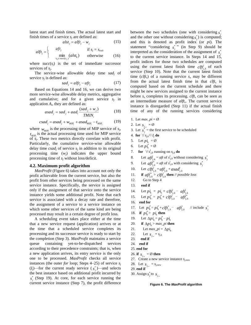
Figure 6. The MaxProfit algorithm

latest start and finish times. The actual latest start and

finish times of a service sj are defined as:

jjj walftalst (15)

jalft jaft

)(min)(

kssuccs

alstjk

if sj = sexit

otherwise

(16)

where succ(sj) is the set of immediate successor

services of sj.

The service-wise allowable delay time sadj of

service sj is defined as:

jjj aftalftsad (17)

Based on Equations 14 and 16, we can derive two

more service-wise allowable delay metrics, aggregative

and cumulative; and for a given service sj in

application Ai, they are defined as:

i

jj

ijjTMIN

wsadaadsadasad

)( (18)

jjj MIPMIPMIPjj tasadwasadcsad (19)

where jMIPw is the processing time of MIP service of sj,

jMIPt is the actual processing time used for MIP service

of sj. These two metrics directly correlate with profit.

Particularly, the cumulative service-wise allowable

delay time csadj of service sj in addition to its original

processing time (wj) indicates the upper bound

processing time of sj without loss/deficit.

4.2. Maximum profit algorithm MaxProfit (Figure 6) takes into account not only the

profit achievable from the current service, but also the

profit from other services being processed on the same

service instance. Specifically, the service is assigned

only if the assignment of that service onto the service

instance yields some additional profit. Note that each

service is associated with a decay rate and therefore,

the assignment of a service to a service instance on

which some other services of the same kind are being

processed may result in a certain degree of profit loss.

A scheduling event takes place either at the time

that a new service request (application) arrives or at

the time that a scheduled service completes its

processing and its successor service is ready to start by

the completion (Step 3). MaxProfit maintains a service

queue containing yet-to-be-dispatched services

according to their precedence constraints; that is, when

a new application arrives, its entry service is the only

one to be processed. MaxProfit checks all service

instances (the outer for loop; Steps 4–25) of service sj

(Ij)—for the current ready service ( *

js )—and selects

the best instance based on additional profit incurred by *

js (Step 19). At core, for each service running the

current service instance (Step 7), the profit difference

between the two schedules (one with considering *

js

and the other one without considering *

js ) is computed;

and this is denoted as profit index (or pi). The

statement ―considering *

js ‖ (in Step 9) should be

interpreted as the consideration of the assignment of *

js

to the current service instance. In Steps 14 and 15,

profit indices for those two schedules are computed

using the current latest finish time l

kjclft ,of each

service (Step 10). Note that the current latest finish

time (clftx) of a running service sx may be different

from the actual latest finish time in that clftx is

computed based on the current schedule and there

might be new services assigned to the current instance

before sx completes its processing. clftx can be seen as

an intermediate measure of alftx. The current service

instance is disregarded (Step 11) if the actual finish

time of any of the running services considering

1. Let min_util = 1.0

2. Let *,j

s = Ø

3. Let *

js = the first service to be scheduled

4. for ∀sj,k∈Ij do

5. for ∀slj,k running on sj,k do

6. Let l

kjaft ,= aft of sl

j,k without considering *

js

7. Let *

,

l

kjaft = aft of slj,k with considering *

js

8. Let l

kjclft ,= l

kjaft ,+ l

kjasad ,

9. if *

,

l

kjaft > l

kjclft ,then // possible loss

10. Go to Step 4

11. end if

12. end for

13. Let utilj,k = utilization of sj,k

14. if utilj,k < min_util then

15. Let min_util = utilj,k

16. Let *,j

s = sj,k

17. end if

18. end for

19. if *,j

s = Ø then

20. Create a new service instance sj,new

21. Let *,j

s = sj,new

22. end if

23. Assign *

js to *,j

s

Figure 7. The MaxUtil algorithm

*

js ( *

,

l

kjaft ) is greater than its current latest finish time

( l

kjclft ,), since this implies a possible loss in profit. The

profit index with considering *

js should include the

profit index value of *

js (Step 17). After each iteration

of the inner for loop (from Step 7 to Step 16),

MaxProfit checks if the current instance delivers the

largest profit increase (Step 20) and keeps track of the

best instance (Steps 21 and 22). If none of the current

instances is selected (i.e., no profit gain is possible

with *

js ), a new instance is created (Step 27). The final

assignment of *

js is then carried out in Step 30 onto the

best instance*,j

s .

While the ―asad metric‖ attempts to ensure

maximum profit gain by focusing more on each

individual service in an application, the ―csad metric‖

tries to maximize the net profit by balancing revenue

and utilization. In other words, ensuring high service-

instance utilization tends to avoid the creation of new

instances resulting in minimizing resource rental costs.

Based on this balancing fact, we have devised a variant

of MaxProfit using the csad metric (i.e., MaxProfitcsad)

instead of the asad metric used in Step 10.

4.3. Maximum utilization algorithm The main focus of MaxUtil is on the maximization

of service-instance utilization. This approach is an

indirect way of reducing costs to rent resources—or to

increase net profit—and it also implies a decrease in

the number of instances the service provider

creates/prepares. For a given service, MaxUtil selects

the instance with the lowest utilization. Although

scheduling decisions are made based primarily on

utilization, MaxUtil also explicitly takes into account

profit incorporating alft into its scheduling.

Specifically, alft compliance would ensure the

avoidance of deficit.

As in MaxProfit, the service with the earliest start

time, in the service queue maintained by MaxUtil, is

selected for scheduling (Step 3). A similar scheduling

routine to that of MaxProfit can also be identified—

from Step 4 to Step 11 where each instance for the

selected service *

js is checked if it can accommodate *

js

without incurring loss; hence, that instance is a

candidate. For each candidate instance, its utilization is

calculated and the instance with the minimum

utilization is identified (Steps 13–17). The utilization

utilj,k of a service instance sj,k is defined as:

)(

, startcur

used

kjutil

(20)

where τused , τcur and τstart are the amount of time used

for processing services, the current time, and the

start/creation time of sj,k, respectively. The if statement

(Steps 19–22) ensures the processing of *

js creating a

new instance in the case of absence of profitable

service-instance assignment.

A variant of MaxUtil (i.e., MaxUtilcsad) is also

devised incorporating the csad metric.

5. Performance evaluation

In this section, we present and discuss performance

evaluation results obtained from an extensive set of

simulations. Our evaluation study is conducted on the

basis of comparisons between two sets of our

algorithms (MaxProfit and MaxProfitcsad, and MaxUtil

and MaxUtilcsad) and a non PS-based algorithm (called

earliest finish time with profit taken into account or

EFTprofit).

We have implemented and used EFTprofit as a

reference algorithm for our evaluation study, since

none of the existing algorithms can be directly

comparable to our algorithms. As the name (EFTprofit)

implies, for a given service, the algorithm selects the

service instance that can finish the processing of that

service the earliest with a certain amount of profit. If

none of the current service instances is able to process

(a) (b) (c)

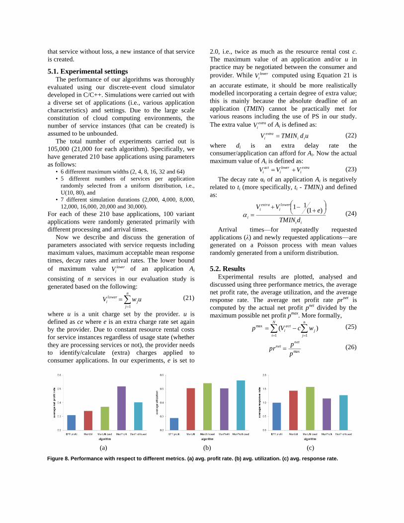
Figure 8. Performance with respect to different metrics. (a) avg. profit rate. (b) avg. utilization. (c) avg. response rate.

that service without loss, a new instance of that service

is created.

5.1. Experimental settings The performance of our algorithms was thoroughly

evaluated using our discrete-event cloud simulator

developed in C/C++. Simulations were carried out with

a diverse set of applications (i.e., various application

characteristics) and settings. Due to the large scale

constitution of cloud computing environments, the

number of service instances (that can be created) is

assumed to be unbounded.

The total number of experiments carried out is

105,000 (21,000 for each algorithm). Specifically, we

have generated 210 base applications using parameters

as follows: • 6 different maximum widths (2, 4, 8, 16, 32 and 64)

• 5 different numbers of services per application

randomly selected from a uniform distribution, i.e.,

U(10, 80), and

• 7 different simulation durations (2,000, 4,000, 8,000,

12,000, 16,000, 20,000 and 30,000).

For each of these 210 base applications, 100 variant

applications were randomly generated primarily with

different processing and arrival times.

Now we describe and discuss the generation of

parameters associated with service requests including

maximum values, maximum acceptable mean response

times, decay rates and arrival rates. The lower bound

of maximum value lower

iV of an application Ai

consisting of n services in our evaluation study is

generated based on the following:

n

j

j

lower

i uwV1

(21)

where u is a unit charge set by the provider. u is

defined as ce where e is an extra charge rate set again

by the provider. Due to constant resource rental costs

for service instances regardless of usage state (whether

they are processing services or not), the provider needs

to identify/calculate (extra) charges applied to

consumer applications. In our experiments, e is set to

2.0, i.e., twice as much as the resource rental cost c.

The maximum value of an application and/or u in

practice may be negotiated between the consumer and

provider. While lower

iV computed using Equation 21 is

an accurate estimate, it should be more realistically

modelled incorporating a certain degree of extra value;

this is mainly because the absolute deadline of an

application (TMIN) cannot be practically met for

various reasons including the use of PS in our study.

The extra value extra

iV of Ai is defined as:

udTMINV ii

extra

i (22)

where di is an extra delay rate the

consumer/application can afford for Ai. Now the actual

maximum value of Ai is defined as:

extra

i

lower

i

act

i VVV (23)

The decay rate αi of an application Ai is negatively

related to ti (more specifically, ti - TMINi) and defined

as:

it

lower

i

extra

i

idTMIN

eVV

)1(

11

(24)

Arrival times—for repeatedly requested

applications (λ) and newly requested applications—are

generated on a Poisson process with mean values

randomly generated from a uniform distribution.

5.2. Results Experimental results are plotted, analysed and

discussed using three performance metrics, the average

net profit rate, the average utilization, and the average

response rate. The average net profit rate prnet is

computed by the actual net profit pnet divided by the

maximum possible net profit pmax. More formally,

N

i

n

j

j

act

i wcVp1 1

max )( (25)

maxp

ppr

netnet (26)

The average utilization is defined as:

L

util

util

L

j

j

1 (27)

The response rate rri of an application Ai is defined

as:

i

ii

TMIN

trr (28)

Then the average response rate for all applications

serviced by the provider is defined as:

N

rr

rr

N

i

i 1 (29)

The entire results obtained from our simulations are

summarized in Table 1, followed by results (Figure 8)

based on each of those three performance metrics.

Clearly, the significance of our explicit and intuitive

incorporation of profit into scheduling decisions is

verified in these results. That is, all our algorithms

achieved utilization above 50 percent with compelling

average net profit rates reaching up to 52 percent.

Although the incorporation of the csad metric

improves utilization by 5 percent on average, the

profit—that those variants with the csad metric

gained—is not very appealing, 8 percent lower on

average compared with the profit gained by MaxProfit

and MaxUtil. This lower profit gain can be explained

by the fact that increases in utilization are enabled by

the allowance of additional delay times (i.e., csad

times) accommodating more services.

Table 1. Overall comparative results

algorithm avg. net profit avg. utilization avg response rate

EFTprofit 31% 29% 100%

MaxUtil 34% 51% 143%

MaxUtilcsad 37% 54% 157%

MaxProfit 52% 50% 115%

MaxProfitcsad 40% 56% 127%

On average, the MaxProfit suite and the MaxUtil

suite outperformed EFTprofit by 48 percent and 15

percent in terms of net profit rate, respectively, and 85

percent and 81 percent in terms of utilization. Since

EFTprofit does not adopt PS and it tends to create a

larger number of instances (compared with those

created by our algorithms) to avoid deficit, the average

response rate is constant (i.e., 1.0). This creation of

(often) an excessive number of instances results in low

utilization and in turn low net profit rate.

It is identified that our utilization-centric algorithms

(MaxUtil and MaxUtilcsad) tend not to deliver better

performance compared with those of our profit-centric

algorithms (MaxProfit and MaxProfitcsad), because the

former set focuses particularly on the utilization up to

the time of each scheduling event, but also on the

avoidance of loss.

6. Related work

Research on market-based resource allocation

started from 1981 [19]. The tools offered by

microeconomics for addressing decentralization,

competition and pricing are thought useful in handling

computing resource allocation problem [6]. Even

though some market-based resource allocation

methods are non-pricing-based [7], [19], [9], pricing-

based methods can reveal the true needs of users who

compete for shared resources and allocate resources

more efficiently [10]. The application of market-based

resource allocation ranges from computer networking

[19], distributed file systems [9], distributed database

[16] to computational job scheduling problems [4], [2],

[18]. Our work is related to pricing-based

computational job scheduling, or utility computing

[14].

B.N. Chun et al. [4] build a prototype cluster that

provides a market for time-shared CPU usage for

various jobs. K. Coleman et al. [2] use the market-

based method to address flash crowds and traffic

spikes for clusters hosting Internet applications. Libra

[13] is a scheduler built on proportional resource share

clusters. One thing in common for [4], [2], [15] is that

the value of a job does not change with the processing

time. In [3], B. N. Chun et al. introduced time-varying

resource valuation for jobs submitted to a cluster. The

changing values were used for prioritizing and

scheduling batch sequential and parallel jobs. The job

with the highest value per CPU time unit is put ahead

of the queue to run. D. E. Irwin et al. [8] extended the

time-varying resource valuation function to take

account of penalty when the value was not realized.

The optimization therefore also minimizes the loss due

to penalty. In our model, the penalty is not directly

reflected in our time-varying valuation function, but it

is implicitly reflected in the cost of physical resource

usage in the cloud. The cost incurs even when no

revenue is generated.

F. I. Popovici and J. Wilkes [13] consider a service

provider rents resources at a price, which is similar to

the scenario we deal with in cloud computing. The

difference is that resource availability is uncertain in

[13] while resource availability is often guaranteed by

the infrastructure provider in the cloud. The scheduling

algorithm (FirstProfit) proposed in [13] uses a priority

queue to maximize the per-profit for each job

independently. Our work differs from [13] in the

queuing model. As a consequence, profit maximization

is not based on a single job, but on all the concurrent

jobs in the same PS queue of a service instance.

The proportional-share allocation is commonly used

in market-based resource allocation [11], [5], in which

a user submits bids for different resources and receives

a fraction of each resource equal to his bid divided by

the sum of all the bids submitted for that resource. It is

different to our processor-sharing (PS) allocator, which

allows each admitted request to have an equal share of

the service capacity. Proportional-share requires all

jobs to have pre-defined weights in order to calculate

the fraction of resource to allocate. This works well for

batch jobs in a small cluster, but has limitations for a

service running in the cloud. The elastic resource pool

and requests from dynamic client applications make

weight-assignment a non-trivial task. Our processor-

sharing admission control is capable of

accommodating dynamic applications and ensures that

random requests do not interfere with the processing of

requests that carry certain values for an application and

a service provider.

Our method is unique in the following aspects:

1. The utility function is time-varying and

dependency aware. The latter is important for the

cloud where mashup services are common.

2. Our model allows new service instances to be

added dynamically and consistently evaluates the

profit of adding a new instance, while most previous

work deal with resource pools of fixed size.

7. Conclusion

As cloud computing is primarily driven by its cost

effectiveness and as the scheduling of composite-

service applications, particularly in cloud systems, has

not been intensively studied, we have addressed this

scheduling problem with the explicit consideration of

profit, and presented two sets of profit-driven service

request scheduling algorithms. These algorithms are

devised incorporating a pricing model using PS and

two allowable delay metrics (asad and csad). We have

demonstrated the efficacy of such an incorporation for

consumer applications with interdependent services. It

is identified that those two allowable delay metrics

enable effective exploitation of characteristics of

precedence-constrained applications. Our evaluation

results confidently confirm these claims together with

the promising performance of our algorithms.

References

[1] M. Armbrust, A. Fox, R. Griffith, A. D. Joseph, R. H.

Katz, A. Konwinski, G. Lee, D. A. Patterson, A. Rabkin, I.

Stoica, and M. Zahariam, ―Above the clouds: A Berkeley

view of Cloud computing,‖ Technical report UCB/EECS-

2009-28, Electrical Engineering and Computer Sciences,

University of California at Berkeley, USA, February 2009.

[2] K. Coleman, J. Norris, G. Candea and A. Fox, ―OnCall:

defeating spikes with a free-market application cluster‖, Proc.

the IEEE Conf. Autonomic Computing, 2004.

[3] B. N. Chun, D. E. Culler, ―User-centric performance

analysis of market-based cluster batch schedulers‖, Proc.

IEEE/ACM Int’l Symp. Cluster Computing and the Grid, pp.

30-38, May 2002.

[4] B. N. Chun and D.E. Culler, ―Market-based proportional

resource sharing for clusters‖, Technical Report CSD-1092,

University of California at Berkeley, January 2000.

[5] M. Feldman, K. Lai, and L. Zhang, ―The proportional-

share allocation market for computational resources‖, IEEE

Trans. Parallel and Distributed Systems, 20(8), 2009.

[6] D. F. Ferguson, ―The application of microeconomics to

the design of resource allocation and control algorithms‖,

PhD thesis, Columbia University, 1989.

[7] D. F. Ferguson, C. Nikolaou, J. Sairamesh, and Y.

Yemini, ―Economic models for allocating resources in

computer systems‖, In Market-Based Control: A Paradigm

for Distributed Resource Allocation (S. H. Clearwater eds.),

World Scientific, 1996.

[8] D. E. Irwin, L. E. Grit, J. S. Chase, ―Balancing risk and

reward in a market-based task service‖, Proc. IEEE Symp.

High Performance Distributed Computing, 160-169, 2004.

[9] J. F. Kurose and R. Simha, ―A microeconomic approach

to optimal resource allocation in distributed computer

systems‖, IEEE Trans. on Computers, 38(5), 1989.

[10] K. Lai, ―Markets are dead, long live markets‖, Sigecom

Exchanges, 5(4):1-10, July 2005.

[11] K. Lai, L. Rasmusson, E. Adar, S. Sorkin, L. Zhang,

B.A. Huberman, ―Tycoon: an Implementation of a

Distributed, Market-based Resource Allocation System‖,

Multiagent and Grid Systems, 1(3):169-182, 2005.

[12] D. Parkhill, The challenge of the computer utility,

Addison-Wesley Educational Publishers Inc., US, 1966.

[13] F. I. Popovici and J. Wilkes, ―Profitable services in an

uncertain world‖, Proc. the ACM/IEEE SC2005 Conf. High

Performance Networking and Computing (SC 2005), 2005.

[14] M. A. Rappa, ―The utility business model and the future

of computing services‖, IBM Syst. J., 43(1):32-42, 2004.

[15] J. Sherwani1, N. Ali, N. Lotia1, Z. Hayat and R. Buyya,

―Libra: a computational economy-based job scheduling

system for clusters‖, Softw. Pract. Exper. 34: 573–590, 2004.

[16] M. Stonebraker, P. M. Aoki, W. Litwin, A. Pfeffer, A.

Sah, J. Sidell, C. Staelin, A. Yu, ―Mariposa: a wide-area

distributed database system‖, The VLDB Journal, 5: 48–63,

1996.

[17] L. M. Vaquero, L. Rodero-Merino, J. Caceres, M.

Lindner, ―A break in the clouds: towards a cloud definition,‖

ACM SIGCOMM Computer Communication Review, 39(1):.

50–55, 2009.

[18] C. A. Waldspurger, T. Hogg, B.A. Huberman, J. O.

Kephart, and W.S. Stornetta, ―Spawn: a distributed

computational economy,‖ Software Engineering, 18(2): 103-

117, 1992.

[19] Y. Yemini, ―Selfish optimization in computer

networks,‖ Proc. the 20th IEEE Conf. Decision and Control,

281-285, 1981.

School of Information Technologies, J12The University of Sydney NSW 2006 AUSTRALIA

T +61 2 9351 3423 F +61 2 9351 3838

www.it.usyd.edu.au

ISBN 978-1-74210-175-0