Profilometry by fringe projection

Profilometry by fringe projection

Luis SalasEsteban LunaJavier SalinasVıctor Garcı´aUniversidad Nacional Autonoma de MexicoInstituto de AstronomıaObservatorio Astronomico NacionalApostado Postal 877Ensenada 22830, MexicoE-mail: [email protected]

Manuel Servı´nCentro de Investigaciones en OpticaLoma del Bosque 115Lomas del CampestreLeon 37150, Mexico

Abstract. We present a method to obtain profilometry of a suitable ob-ject by fringe projection. The method is appropriate to the case of largeobjects as compared to the distance from the illuminating source, that is,a nonconstant equivalent wavelength. We develop an experiment to lat-erally displace a set of fringes on a sphere and obtain quantitative re-sults. There are several orientation parameters involved in the method,and a minimization algorithm is developed to adjust the values of someof them. A series of numerical experiments are performed on this methodto test its accuracy under various circumstances. We show that themethod can currently attain precisions of 'leq/80 (leq stands for equiva-lent wavelength) and identify possible sources of error. © 2003 Society ofPhoto-Optical Instrumentation Engineers. [DOI: 10.1117/1.1607968]

Subject terms: profilometry; mirror blank testing; mirror blank fabrication; fringeprojection.

Paper 030026 received Jan. 14, 2003; revised manuscript received Mar. 24,2003; accepted for publication Mar. 24, 2003.

tryrioru-ch

ed.ereanhe

tesectob-

o. A

ob-blee isve-e o10t

hasrom

redentnsasat

her--yThnceencma

o-l ofppa-g aseea-d we

onateate

y ad inesovede

-ofa

g

. Angt,

1 Introduction

Fringe projection is a technique that allows the profilomeof surfaces by optical means and triangulation. It is supeto point-to-point profilometers, because it offers a continous covering of the surface, it can be carried out mufaster, and also because no mechanical contact is needcomplements normal interferometric tests in cases whsurfaces under measurement are rough or opaque,when deviations from some standard form are large. Ttechnique employs a white light source that illuminadark strips on a substrate to project them onto an objThe dark shadows deform following the shape of theject, and the equations that define the intensity patternthese fringes resemble those of a normal interferogramsimilar case to phase shifting interferometry can betained by displacing the fringes laterally, and it is possito solve for the phase of the object. When the light sourcfar from the illuminated object, a constant equivalent walength can be identified in the equations and the shapthe object can be solved. In this way precisions of up tomm ~Refs. 1 and 2! have been obtained. Many differenconfigurations have been proposed to manage the pdisplacement and to obtain the profile measurements fthe phase.3–10

However, when the object to measure is large compato the distance from the illuminating source, the equivalwavelength is no longer constant and the full equatiodescribing the phase have to be employed. This is our cin the problem of measuring the profile of 1.8-m blanks thwill be generated to off-axis parabolas and will conform tsegments of the primary mirror for the Telescopio Infrarojo Mexicano~TIM !.11 We thus describe a fringe projection method for an arbitrarily close illuminating source, bmeans of a coordinate system adapted to the object.unwrapping of the phase is avoided by finding a referenear the object to measure. The parameters of this refersurface, as well as those involved in coordinate transfor

Opt. Eng. 42(11) 3307–3314 (November 2003) 0091-3286/2003/$15.00

It

d

.

f

f

e

e

e

e-

tions, are solved by a multidimensional minimization prcedure. Numerical tests are used to show the potentiathis approach. We have constructed an experimental aratus that performs the lateral phase displacement usinslide projector, a Ronchi grid, and a pico-positioner. We uthis apparatus to carry out a series of experiments to msure a sphere that has been generated on the blanks, anshow the current limitations of the method.

2 Fringe Projection

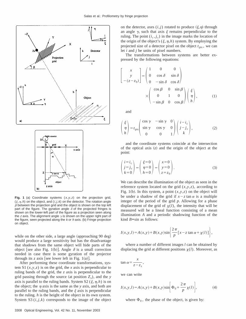
We have written the equations describing the illumination the object, paying special attention to the coordinsystems involved. For this purpose, consider the coordinsystems shown in Fig. 1~a!. S1 (x,y,z) on the projectedgrid, S2 (j,h,h) on the object, and S3 (i , j ,k) on the de-tector imaging the object. These systems are related bseries of three translations and three rotations describedetail in the following way. We begin with the detector ax( i , j ) that correspond to the imaging detector located abthe object, where axisk is the height of the object measurefrom the detector, with its origin chosen arbitrarily on thobject. We then project the plane (i , j ) on the object. It maybe necessary to rotate through a small angleg aroundk, sothat thej axis becomes theh axis well aligned parallel tothe projected fringes, while simultaneouslyi gives rise tothej axis that will be perpendicular to the fringes@see inseton the top right of Fig. 1~a!#. We then rotate axisk aroundaxis h through an angleb and around axisj through anangled, giving rise to thez axis, which is oriented perpendicular to the projection grid, located on the top-left partFig. 1~a!. The origin of this system is translated in suchway that a newz axis passes through the illuminatinsource. The illumination source is at a distance2Zs fromthe origin and the object is at a distanceZ0 . The angleb sodefined is the inclination angle of the projected fringessmall angle would project the fringes from above, resultiin a very low sensitivity to the topography of the objec

3307© 2003 Society of Photo-Optical Instrumentation Engineers

agethe

cto

ys-

.ct

ef

ex-

tione

the

ane

Salas et al.: Profilometry by fringe projection

while on the other side, a large angle~approaching 90 deg!would produce a large sensitivity but has the disadvantthat shadows from the same object will hide parts ofobject @see also Fig. 1~b!#. Angle d is a small correctionneeded in case there is some gyration of the projethrough itsz axis @see lower left in Fig. 1~a!#.

After performing these coordinate transformations, stem S1 (x,y,z) is on the grid, thex axis is perpendicular toruling bands of the grid, thez axis is perpendicular to thegrid passing through the source~at positionZs), and theyaxis is parallel to the ruling bands. System S2 (j,h,h) is onthe object; theh axis is the same as they axis, and both areparallel to the ruling bands, and thej axis is perpendicularto the ruling.h is the height of the object in its own systemSystem S3 (i , j ,k) corresponds to the image of the obje

Fig. 1 (a) Coordinate systems (x,y,z) on the projection grid,(j,h,h) on the object, and (i, j,k) on the detector. The rotation angleb between the projection grid and the object is shown on the top leftpart of the figure. The gyration angle d of the projected fringes isshown on the lower-left part of the figure as a projection seen alongthe z axis. The alignment angle g is shown on the upper right part ofthe figure, seen projected along the k or h axis. (b) Fringe projectionon object.

3308 Optical Engineering, Vol. 42 No. 11, November 2003

r

on the detector, axes (i , j ) rotated to produce~j,h! throughan angleg, such that axisj remains perpendicular to thruling. The point (i c , j c) in the image marks the location othe origin of the object’s (j,h,h) system. By employing theprojected size of a detector pixel on the objecttpix , we canlet i and j be units of pixel numbers.

The transformations between systems are betterpressed by the following equations:

F xy

2~z2z0!G5S 1 0 0

0 cosd sind

0 2sind cosdD

3S cosb 0 sinb

0 1 0

2sinb 0 cosbD S j

hhD , ~1!

and

S jhhD 5tpixS cosg 2sing 0

sing cosg 0

0 0 1D S i 2 i c

j 2 j c

kD , ~2!

and the coordinate systems coincide at the intersecof the optical axis~z! and the origin of the object at thpoint:

S i 5 i c

j 5 j c

k50D 5S j50

h50h50

D 5S x50y50z5z0

D . ~3!

We can describe the illumination of the object as seen inreference system located on the grid (x,y,z), according toFig. 1~b!. In this system, a point (x,y,z) on the object willbe under a shadow of the grid ifx2z tana is a multipleinteger of the period of the gridp. Allowing for a phasedisplacement of the grid ofx( l ), the intensity that will bemeasured will be a lineal function consisting of a meillumination A and a periodic shadowing function of thkind B* sin as follows:

I ~x,y,l !5A~x,y!1B~x,y!sinH 2p

p@x2z tana1x~ l !#J ,

where a number of different imagesl can be obtained bydisplacing the grid at different positionsx( l ). Moreover, as

tana5x

z2zs,

we can write

I ~x,y,l !5A~x,y!1B~x,y!sinFF012p

px~ l !G , ~4!

whereF0 , the phase of the object, is given by:

of

cal

d

ve-tha

-ct,i-

ralthepo

t of

is-of

ter-to

,In

toctralrthehe

ionnal

ee

ualer-

-

on

thes. Itdis--rcei-

puri-re-

s incennghenthat

fi-his

o-the

iesli-

us,-g

thefe

Salas et al.: Profilometry by fringe projection

F052p

p S 2xzs

z2zsD . ~5!

We now look at this equation in the coordinate systemthe object~S2!. By using Eqs.~1! to ~3!, the phase of theobject can be expressed as:

F052p

p F 2zs~j cosb1h sinb!

z02zs1j cosd sinb1h sind2h cosd cosb G .~6!

In particular, the phase of reference objects can beculated for simple cases similar to a flat surface (h50) orthat of a sphere@(h2R)25R22j22h2#.

Finally, the profile of the object~h! can be reconstructefrom its phase by solving Eq.~6! for h:

h5

pF0

2p~z02zs1j cosd sinb1h sind!1zsj cosb

pF0

2pcosd cosb2zs sinb

. ~7!

It is interesting to calculate the equivalent and lateral walengths. The equivalent wavelength can be obtained soDh results from a change of phase of the object of 2p, thatis, leq52pdh/df0 . This will, in general, give an equivalent wavelength that is a function of position on the objethat is, a function of~j,h!. However, to have an approxmate idea of its value, for positionsj,h,h near the origin~'0!, we can find the simple solution:

leq'p~zs2z0!

zs sinb. ~8!

In a similar way the lateral wavelength, which is the latespacing between two fringes projected on a plane atposition of the object, can be defined as the change insition j that results from a change of phase of the objec2p, or leq52pdj/df0 , leading to:

l lat'p~zs2z0!

zs cosb. ~9!

Also of practical interest is the relation between the dtance from the illuminating source to the grid in termsthe magnification of the projectorm:

zs5z0

12m.

3 Phase Determination

The intensity described by Eq.~4! is very similar to what isobtained in the case of interferometry$I 5A@11B cos(f2f0)#%. In fact, the reader could simply add a constantp/2to the phase of the object and redefineB5B/A, whichleads with no loss of generality to the exact case of inferometry. In this case there are a variety of algorithmsfind the phase of the object~e.g., the five point algorithmthe 211 algorithm, etc! that can equally be used here.

-

t

-

particular there is a fast method developed by Morimoand Fujisawa12 to directly determine the phase of the objewhen a maximum in intensity is detected, as the latedisplacementx( l ) is varied with great precision. In oucase, however, a large error would be introduced byrelatively large uncertainties of the actuator controlling tphasex( l ).

We thus consider a robust method for the determinatof the phase of the object. We start with a conventiominimum square method. Considering Eq.~4!, the

sinFF012p

px~ l !G

function can be decomposed in the equivalent

sin~F0!cosF2p

px~ l !G1cos~F0!sinF2p

px~ l !G .

In every pixel of the image, this problem is solved for thrvaluesA, B, andf0 as a linear system.

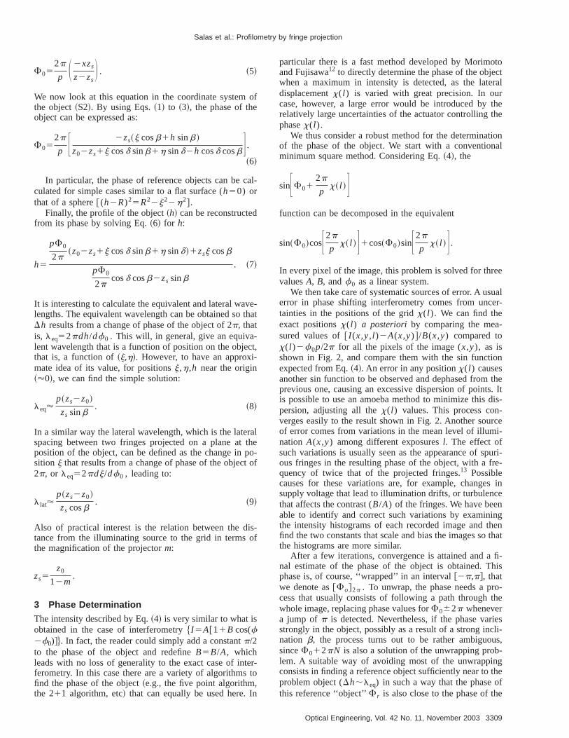
We then take care of systematic sources of error. A userror in phase shifting interferometry comes from unctainties in the positions of the gridx( l ). We can find theexact positionsx( l ) a posteriori by comparing the measured values of@ I (x,y,l )2A(x,y)#/B(x,y) compared tox( l )2f0p/2p for all the pixels of the image (x,y), as isshown in Fig. 2, and compare them with the sin functiexpected from Eq.~4!. An error in any positionx( l ) causesanother sin function to be observed and dephased fromprevious one, causing an excessive dispersion of pointis possible to use an amoeba method to minimize thispersion, adjusting all thex( l ) values. This process converges easily to the result shown in Fig. 2. Another souof error comes from variations in the mean level of illumnation A(x,y) among different exposuresl. The effect ofsuch variations is usually seen as the appearance of sous fringes in the resulting phase of the object, with a fquency of twice that of the projected fringes.13 Possiblecauses for these variations are, for example, changesupply voltage that lead to illumination drifts, or turbulenthat affects the contrast (B/A) of the fringes. We have beeable to identify and correct such variations by examinithe intensity histograms of each recorded image and tfind the two constants that scale and bias the images sothe histograms are more similar.

After a few iterations, convergence is attained and anal estimate of the phase of the object is obtained. Tphase is, of course, ‘‘wrapped’’ in an interval@2p,p#, thatwe denote as@Fo#2p . To unwrap, the phase needs a prcess that usually consists of following a path throughwhole image, replacing phase values forF062p whenevera jump of p is detected. Nevertheless, if the phase varstrongly in the object, possibly as a result of a strong incnation b, the process turns out to be rather ambiguosinceF012pN is also a solution of the unwrapping problem. A suitable way of avoiding most of the unwrappinconsists in finding a reference object sufficiently near toproblem object (Dh;leq) in such a way that the phase othis reference ‘‘object’’F r is also close to the phase of th

3309Optical Engineering, Vol. 42 No. 11, November 2003

.d

mi-ththeth-is

t of-

on-

mn,

n,the

canon.os-es

s a

s isalm-heo-

bil-of

of

ef

tied

her

d

omce-. 3,

rect

Salas et al.: Profilometry by fringe projection

object, i.e.,uF02F r u,p ~for other possibilities see Refs8, 9, and 10!. If this is the case, then it is possible to finthe unwrapped phase of the object by means of:

F05@@F0#2p2@F r #2p#2p1F r , ~10!

that is, subtracting the wrapped phases of the objectnus reference, rewrapping the result, and adding backunwrapped phase of the reference. Most interesting isfact thatF r need not be a real object, but can be a maematical description of, for example, the object that onetrying to generate. If such is the case, there will be a separameters involved inF r . However, at this stage an erro

Fig. 2 Top: Phase errors introduced by indeterminations in the po-sition of the grid x(l). Bottom: Corrected phase x(l).

3310 Optical Engineering, Vol. 42 No. 11, November 2003

e

neous estimation of the model’s parameters is of no ccern, since these are canceled out as soon as the sameF r isadded back in Eq.~10!.

The profileh of the object can then be recovered froEq. ~7!, provided that the involved parameters are knowi.e.,

h5h~F0 ;b,g,d,i c , j c ,z0 ,zs!.

The unwrapped phase of the object is already knowbut the values of the rest of the parameters that relate totransformations between different coordinate systemsturn out to be complicated to measure with great precisiHowever, if the desired surface shape is known, it is psible to raise the problem of minimization to find the valuof the parameters.

For example, in the case that the wished surface isphere,

hes f5hes f~r e ,je ,he ,he!,

with radius r e and the center in (je ,he ,he), we wouldhave to minimize:

f 5 (region

@h~F0 ;b,g,d,i c , j c ,z0 ,zs!2hes f~r e ,je ,he ,he!#2

with respect to the 11 involved parameters. This procescomplicated in general by the susceptibility of finding locminima. The accuracy of this numerical process is exained with computer simulations in the next section. Tperformance of the technique will be further tested in labratory tests in Sec. 5.

4 Numerical Experiments

We performed 100 numerical experiments to show the aity of the minimization algorithms to recover the valuesthe parameters. We chose a series of parametersb, g, d, i c ,j c , z0 , andzs that describe the orientation and alignmentthe system, and we simulated a spherehes f

5hes f(r e ,je ,he ,he). We then obtained the phase of thobject@Eq. ~6!#. From this, we simulated the acquisition oseveral intensity images@according to Eq.~4!# for x( l )50, 5, 10..., 60mm, with a grating periodp550mm andwith A51 andB50.15 constant in the image. At this poinwe intentionally lost the values of the parameters and trto determine them by minimizing functionf. We used theconjugate gradient method according to the FletcReeves Polak Riviere algorithm~Ref. 14!. In our imple-mentation, we first minimize functionf for each one of thefollowing individual parameters~in this order!: g, b, d, z0 ,zs , i c , and j c , and finally all parameters are minimizesimultaneously.

We performed 100 such experiments, providing randinitial guesses for the parameters. The minimization produre eventually converges to the values shown in Figwhere they can be compared to the original values.

As can be seen, the parametersb and zs recover wellenough in all cases. The anglesg andd recover in 40 ac-ceptable dispersions. The value ofi c is also acceptable. Theother parameters do not seem to converge to the cor

Salas et al.: Profilometry by fringe projection

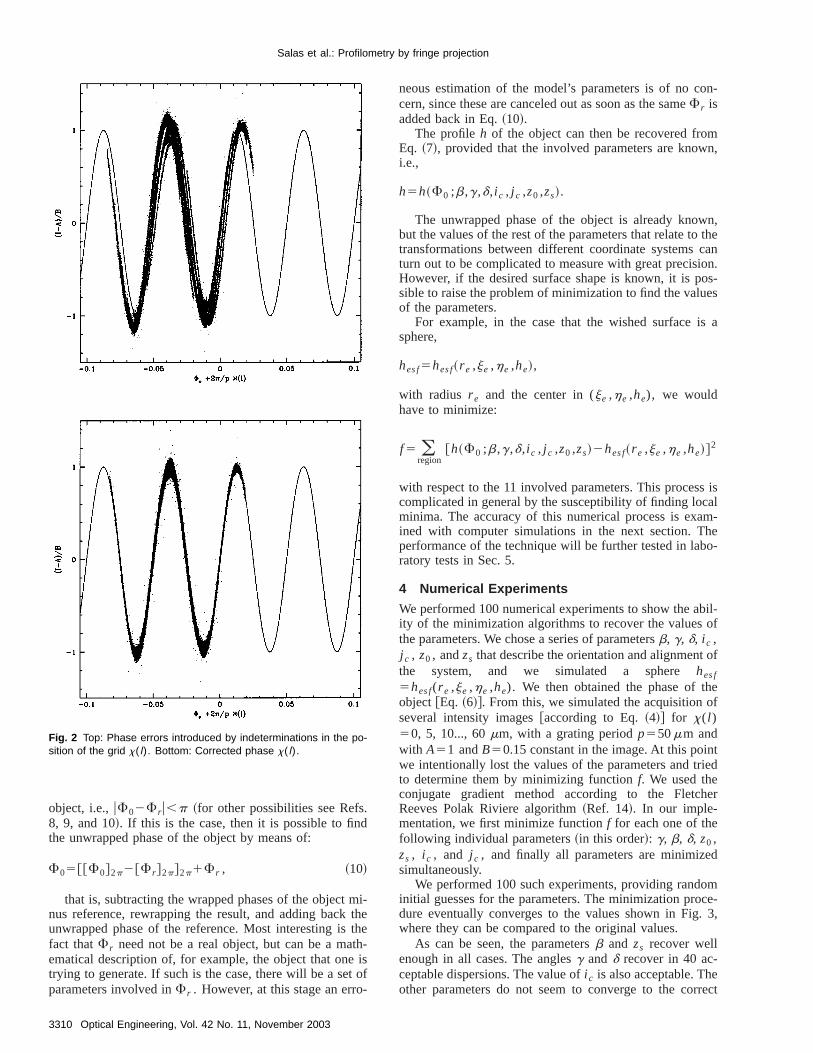
Fig. 3 Recovery of parameters by minimization algorithm. The thickline shows the histograms of initial parameters. The shaded histo-grams are the recovered parameters. The vertical line shows thecorrect value of each parameter. The top right panel shows peak-to-peak error in microns, with a median of 23 mm.

Fig. 5 Projected fringes on a mirror segment blank.

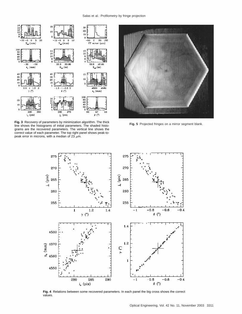
Fig. 4 Relations between some recovered parameters. In each panel the big cross shows the correctvalues.

3311Optical Engineering, Vol. 42 No. 11, November 2003

Salas et al.: Profilometry by fringe projection

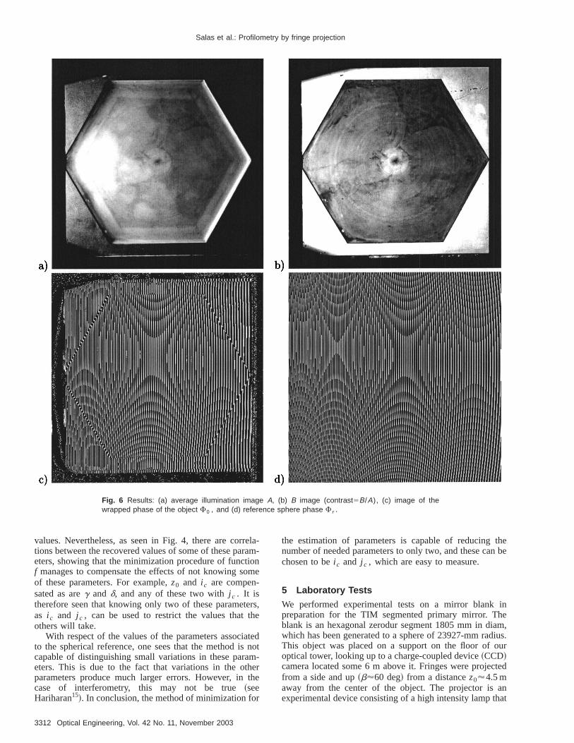
Fig. 6 Results: (a) average illumination image A, (b) B image (contrast5B/A), (c) image of thewrapped phase of the object F0 , and (d) reference sphere phase F r .

relaramionom

ershe

ateno

m-herthe

r

then be

ine

am,ius.ur

d

anhat

values. Nevertheless, as seen in Fig. 4, there are cortions between the recovered values of some of these paeters, showing that the minimization procedure of functf manages to compensate the effects of not knowing sof these parameters. For example,z0 and i c are compen-sated as areg and d, and any of these two withj c . It istherefore seen that knowing only two of these parametas i c and j c , can be used to restrict the values that tothers will take.

With respect of the values of the parameters associto the spherical reference, one sees that the method iscapable of distinguishing small variations in these paraeters. This is due to the fact that variations in the otparameters produce much larger errors. However, incase of interferometry, this may not be true~seeHariharan15!. In conclusion, the method of minimization fo

3312 Optical Engineering, Vol. 42 No. 11, November 2003

--

e

,

dt

the estimation of parameters is capable of reducingnumber of needed parameters to only two, and these cachosen to bei c and j c , which are easy to measure.

5 Laboratory Tests

We performed experimental tests on a mirror blankpreparation for the TIM segmented primary mirror. Thblank is an hexagonal zerodur segment 1805 mm in diwhich has been generated to a sphere of 23927-mm radThis object was placed on a support on the floor of ooptical tower, looking up to a charge-coupled device~CCD!camera located some 6 m above it. Fringes were projectefrom a side and up~b'60 deg! from a distancez0'4.5 maway from the center of the object. The projector isexperimental device consisting of a high intensity lamp t

Salas et al.: Profilometry by fringe projection

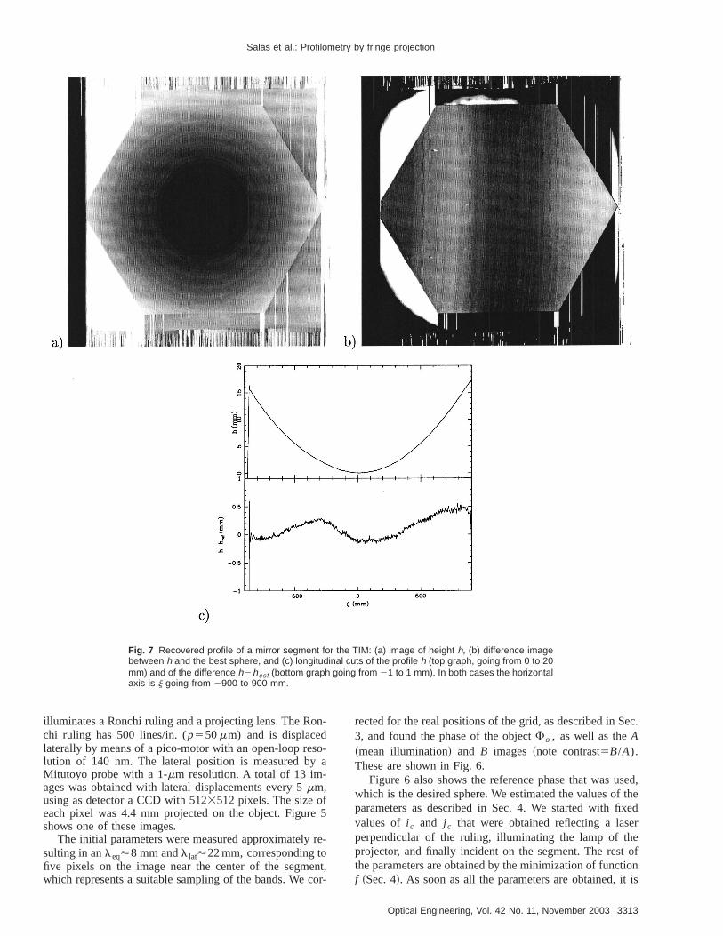
Fig. 7 Recovered profile of a mirror segment for the TIM: (a) image of height h, (b) difference imagebetween h and the best sphere, and (c) longitudinal cuts of the profile h (top graph, going from 0 to 20mm) and of the difference h2hesf (bottom graph going from 21 to 1 mm). In both cases the horizontalaxis is j going from 2900 to 900 mm.

n-

so-a

e 5

re-

entcor

ec.

sed,the

xedereof

iont is

illuminates a Ronchi ruling and a projecting lens. The Rochi ruling has 500 lines/in. (p550mm) and is displacedlaterally by means of a pico-motor with an open-loop relution of 140 nm. The lateral position is measured byMitutoyo probe with a 1-mm resolution. A total of 13 im-ages was obtained with lateral displacements every 5mm,using as detector a CCD with 5123512 pixels. The size ofeach pixel was 4.4 mm projected on the object. Figurshows one of these images.

The initial parameters were measured approximatelysulting in anleq'8 mm andl lat'22 mm, corresponding tofive pixels on the image near the center of the segmwhich represents a suitable sampling of the bands. We

,-

rected for the real positions of the grid, as described in S3, and found the phase of the objectFo , as well as theA~mean illumination! and B images~note contrast5B/A).These are shown in Fig. 6.

Figure 6 also shows the reference phase that was uwhich is the desired sphere. We estimated the values ofparameters as described in Sec. 4. We started with fivalues of i c and j c that were obtained reflecting a lasperpendicular of the ruling, illuminating the lamp of thprojector, and finally incident on the segment. The restthe parameters are obtained by the minimization of functf ~Sec. 4!. As soon as all the parameters are obtained, i

3313Optical Engineering, Vol. 42 No. 11, November 2003

aowfer-

een orstheTh

hatrider-er

byin

gemsla-

d oofrge

rrorhere3.

actsobterthetersatetoimi. 5

nt tin

e toma

re-

the

’’s,

al

semic

ns,’’

cte,’’

d

iquelo-

ea-

Pe-

e-

g

ry,e

m-

Salas et al.: Profilometry by fringe projection

possible to calculate the profileh of the object, and this ispresented in Fig. 7~a!. The characteristic concavity ofsphere is clearly visible. In the same figure, we also shthe difference between the obtained profile and the reence sphere, along with longitudinal cuts of both.

As can be seen, there are low frequency errors betwthe reference and generated sphere, seen mainly as acillation in the direction of the illumination. These erroare still errors of the method, as is demonstrated bypersistence of the structures as the blank is rotated.error reaches 0.1 mm rms (leq/80), which still limits theapplicability of the method. Nevertheless, it is feasible tthe reason for this error is due to imperfections in the gor in the projection system, and we are continuing to pfect the system. On the other hand, the high frequencyrors ~noise of the measurements! are quite small~of theorder of 20mm rms'leq/400), which is very encouragingfor the possibilities of this method.

6 Conclusion

We have presented a method to obtain profilometryfringe projection. Several new developments have beencorporated 1. A full mathematical treatment of the frinprojection geometry described in three coordinate systeprojector, object, and detector, allows us to derive a retionship between profile and phase that does not depena constant equivalent wavelength approximation. In viewthis, the method can be applied to objects that are lawhen compared to the projecting distance. 2. Phase eintroduced by indeterminations in the lateral position of tgrid, as well as those due to variations in illumination, aidentified by a minimization procedure and corrected.Phase unwrapping is aided by an algorithm that subtrand adds back a close mathematical description of theject. This procedure is insensible to errors in the parameof the model. 4. Once the phase is obtained, to obtainprofile, one needs to know the values of the paramedescribing the orientation and positions of the coordinsystems involved. We propose a minimization algorithmaccurately determine these parameters. We test this minzation procedure with a series of numerical experimentsWe present a laboratory setup and an actual experimedetermine the profile of hexagonal mirror blanks, 1.8 mdiam, with a pregenerated sphere. The method is ablrecover the profile of the object with an accuracy of 0.1 mrms (leq/80). The remaining errors, however, still showlarge scale structure with an unknown origin. The high fquency random errors~20 mm rms orleq/400) should ulti-mately limit the scope of this method once the source oflow frequency errors is identified.

References1. K. Creath and J. C. Wyant, ‘‘Moire´ and fringe projection techniques,

in Optical Shop Testing, D. Malacara, Ed., p. 653, Wiley and SonNew York ~1992!.

2. F. Chen, G. M. Brown, and M. Song, ‘‘Overview of three-dimensionshape measurement using optical methods,’’Opt. Eng.39~1!, 10–22~2000!.

3. H. Zhang, M. J. Lalor, and D. R. Burton, ‘‘Spatiotemporal phaunwrapping for the measurement of discontinuous objects in dynafringe-projection phase-shifting profilometry,’’Appl. Opt. 38~16!,3534–3541~1999!.

4. J. J. Esteves-Taboada, D. Mas, and J. Garcı´a, ‘‘Three-dimensionalobject recognition by Fourier transform profilometry,’’Appl. Opt.38~22!, 4760–4765~1999!.

3314 Optical Engineering, Vol. 42 No. 11, November 2003

ns-

e

-

-

,

n

s

-s

-.o

5. J. H. Massig, ‘‘Measurement of phase objects by simple meaAppl. Opt.38~19!, 4103–4105~1999!.

6. C. Lu and S. Inokuchi, ‘‘Intensity-modulated moire´ topography,’’Appl. Opt.38~19!, 4019–4029~1999!.

7. J. A. Munoz-Rodriguez, R. Rodriguez-Vera, and M. Servin, ‘‘Direobject shape detection based on skeleton extraction of a light linOpt. Eng.39~9!, 2463–2471~2000!.

8. G. Schirripa and D. Ambrosini, ‘‘Diffractive optical element-baseprofilometer for surface inspection,’’Opt. Eng.40~1!, 44–52~2001!.

9. J. Zhong and Y. Zhang, ‘‘Absolute phase-measurement technbased on number theory in multifrequency grating projection profimetry,’’ Appl. Opt.40~4!, 492–500~2001!.

10. P. S. Huang, C. Zhang, and F. Chiang, ‘‘High-speed 3-D shape msurement based on digital fringe projection,’’Opt. Eng.42~1!, 163–168 ~2003!.

11. L. Salas, E. Ruiz, I. Cruz-Gonzalez, E. Luna, S. Cuevas, M. H.drayes, G. Sierra, E. Sohn, G. Koenigsberger, J. Valde´z, O. Harris, F.Cobos, C. Tejada, L. Gutie´rrez, and A. Iriarte, ‘‘Mexican infrared-optical new technology telescope~TIM ! project,’’ Proc. SPIE3352,44–51~1998!.

12. Y. Morimoto and M. Fujisawa, ‘‘Fringe pattern analysis by phasshifting method using extraction of characteristic,’’Exp. Tech.40,25–29~1996!.

13. W. S. Li and X. Y. Su, ‘‘Application of improved phase-measurinprofilometry in non-constant environmental light,’’Opt. Eng.40~3!,478–485~2001!.

14. W. H. Press, S. A. Teukolsky, W. T. Vetterling, and B. P. FlanneNumerical Recipes in FORTRAN, 2nd ed., pp. 1–963, CambridgUniversity Press~1992!.

15. P. Hariharan, ‘‘Phase-shifting interferometry: minimization of systeatic errors,’’Opt. Eng.39~4!, 967–969~2000!.

Luis Salas obtained his BS degree inphysics (1982) at the National University ofMexico (UNAM). He was a member of theinstrumentation department of the Instituteof Astronomy (UNAM), from 1980 to 1986,where he developed electronic and opto-electronic instrumentation. In 1986 hejoined the Graduate School of Physics andAstronomy at the University of Massachu-setts, where he earned his PhD in as-tronomy in 1990. He has been a re-

searcher at the National Observatory of Mexico and the Institute ofAstronomy (UNAM) since then. He was head of the instrumentationdepartment from 1991 to 1994 and head of the Observatory from1994 to 1997. He has written more than 30 research papers in theareas of star formation, radiation mechanisms, active optics, andinfrared instrumentation.

Esteban Luna received his engineeringdegree from the Universidad AutonomaMetropolitana, Mexico, in 1988 and his MSand PhD in optics from Instituto Nacionalde Astrofisica, Optica y Electronica in 1991and 1996, respectively. A staff optician inthe Observatorio Astronomico Nacionalsince 1990, he is involved in the study ofactive optics and design of astronomical in-struments and hydrodynamic polishingtechniques.

Manuel Servin is a researcher at the Centro de Investigaciones enOptica, Leon, Guanajuato, Mexico. His research interests are indigital image processing, interferometry, and robotic vision. In inter-ferometry, he has contributed to the study of phase tracking systemsapplied to the demodulation of interferograms and unwrapping ofphase maps. Dr. Servin received the PhD degree (1994) in science(optics) from the Centro de Investigaciones en Optica, Leon, Gua-najuato, Mexico

Javier Salinas received his MS degree in optics in 1998 in pointingangle for segments of the Large Milimiter Telescope (LMT), and hisPhD in cophasing of segmented surfaces (2002), in the InstitutoNacional de Astrofisica, Optica y Electronica, Mexico. He holds apostdoctoral position at IAUNAM-OAN, Ensenada B.C., Mexico. Hisresearch interest is the alignment of segmented surfaces.