PROFILE-KERNEL LIKELIHOOD INFERENCE WITH DIVERGING NUMBER OF PARAMETERS1

arX

iv:m

ath/

0701

004v

2 [

mat

h.ST

] 2

1 Se

p 20

07

Profile-Kernel Likelihood Inference With

Diverging Number of Parameters ∗

By Clifford Lam and Jianqing Fan

Department of Operations Research and Financial Engineering

Princeton University, Princeton, NJ, 08544

The generalized varying coefficient partially linear model with growingnumber of predictors arises in many contemporary scientific endeavor. Inthis paper we set foot on both theoretical and practical sides of profile likeli-hood estimation and inference. When the number of parameters grows withsample size, the existence and asymptotic normality of the profile likelihoodestimator are established under some regularity conditions. Profile likelihoodratio inference for the growing number of parameters is proposed and Wilk’sphenomenon is demonstrated. A new algorithm, called the accelerated profile-kernel algorithm, for computing profile-kernel estimator is proposed and inves-tigated. Simulation studies show that the resulting estimates are as efficientas the fully iterative profile-kernel estimates. For moderate sample sizes, ourproposed procedure saves much computational time over the fully iterativeprofile-kernel one and gives stabler estimates. A set of real data is analyzedusing our proposed algorithm.

Short Title: High-dimensional profile likelihood.

AMS 2000 subject classifications. Primary 62G08; secondary 62J12, 62F12.

Key words and phrases. Generalized linear models, varying coefficients, high dimen-

sionality, asymptotic normality, profile likelihood, generalized likelihood ratio tests.

∗Clifford Lam is PhD student, Department of Operation Research and Financial Engineering, Prince-

ton University, Princeton, NJ 08544 (email: [email protected]); Jianqing Fan is Professor, Depart-

ment of Operation Research and Financial Engineering, Princeton University, Princeton, NJ 08544

(email: [email protected]). Financial support from the NSF grant DMS-0354223, DMS-0704337

and NIH grant R01-GM072611 is gratefully acknowledged.

1

1 Introduction

Semiparametric models with large number of predictors arise frequently in many con-

temporary statistical studies. Large data set and high-dimensionality characterize many

contemporary scientific endeavors ([6]; [8]). Statistical models with many predictors are

frequently employed to enhance the explanatory and predictive powers. At the same

time, semiparametric modeling is frequently incorporated to balance between modeling

biases and “curse of dimensionality”. Profile likelihood techniques ([23]) are frequently

applied to this kind of semiparametric models. When the number of predictors is large,

it is more realistic to regard it growing with the sample size. Yet, few results are avail-

able for semiparametric profile inferences when the number of parameters diverges with

sample size. This paper focuses on profile likelihood inferences with diverging number

of parameters in the context of the generalized varying coefficient partially linear model

(GVCPLM).

GVCPLM is an extension the generalized linear model ([20]) and the generalized

varying-coefficient model ([12]; [4]). It allows some coefficient functions to vary with cer-

tain covariates U such as age ([9]), toxic exposure level or time variable in a longitudinal

data or survival analysis ([22]). Therefore, general interactions, not just the linear inter-

action as in parametric models, between the variable U and these covariates are explored

nonparametrically.

If Y is a response variable and (U,X,Z) is the associated covariates, then by letting

µ(u,x, z) = EY |(U,X,Z) = (u,x, z), the GVCPLM takes the form

gµ(u,x, z) = xT α(u) + zT β, (1.1)

where g(·) is a known link function, β a vector of unknown regression coefficients and

α(·) a vector of unknown regression functions. One of the advantages over the varying

coefficient model is that GVCPLM allows more efficient estimation when some coefficient

functions are not really varying with U , after adjustment of other genuine varying ef-

fects. It also allows more interpretable model, where primary interest is focused on the

parametric component.

1.1 A motivating example

We use a real data example to demonstrate the need for GVCPLM. The Fifth National

Bank of Springfield faced a gender discrimination suit in which female received substan-

2

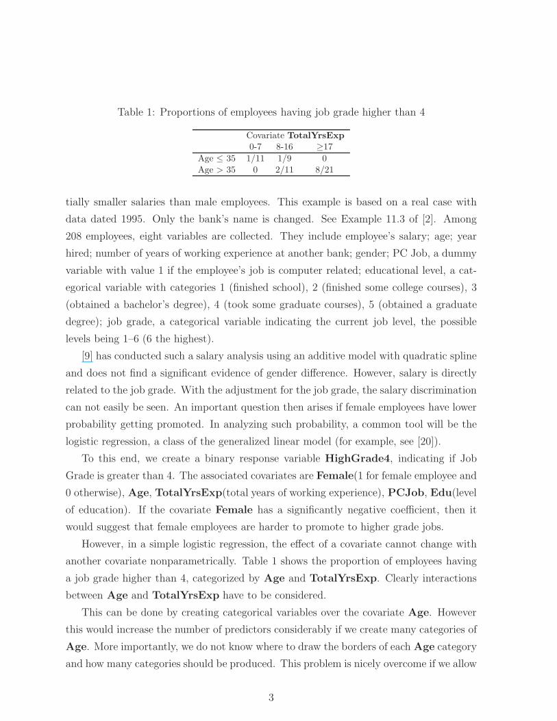
Table 1: Proportions of employees having job grade higher than 4

Covariate TotalYrsExp

0-7 8-16 ≥17

Age ≤ 35 1/11 1/9 0

Age > 35 0 2/11 8/21

tially smaller salaries than male employees. This example is based on a real case with

data dated 1995. Only the bank’s name is changed. See Example 11.3 of [2]. Among

208 employees, eight variables are collected. They include employee’s salary; age; year

hired; number of years of working experience at another bank; gender; PC Job, a dummy

variable with value 1 if the employee’s job is computer related; educational level, a cat-

egorical variable with categories 1 (finished school), 2 (finished some college courses), 3

(obtained a bachelor’s degree), 4 (took some graduate courses), 5 (obtained a graduate

degree); job grade, a categorical variable indicating the current job level, the possible

levels being 1–6 (6 the highest).

[9] has conducted such a salary analysis using an additive model with quadratic spline

and does not find a significant evidence of gender difference. However, salary is directly

related to the job grade. With the adjustment for the job grade, the salary discrimination

can not easily be seen. An important question then arises if female employees have lower

probability getting promoted. In analyzing such probability, a common tool will be the

logistic regression, a class of the generalized linear model (for example, see [20]).

To this end, we create a binary response variable HighGrade4, indicating if Job

Grade is greater than 4. The associated covariates are Female(1 for female employee and

0 otherwise), Age, TotalYrsExp(total years of working experience), PCJob, Edu(level

of education). If the covariate Female has a significantly negative coefficient, then it

would suggest that female employees are harder to promote to higher grade jobs.

However, in a simple logistic regression, the effect of a covariate cannot change with

another covariate nonparametrically. Table 1 shows the proportion of employees having

a job grade higher than 4, categorized by Age and TotalYrsExp. Clearly interactions

between Age and TotalYrsExp have to be considered.

This can be done by creating categorical variables over the covariate Age. However

this would increase the number of predictors considerably if we create many categories of

Age. More importantly, we do not know where to draw the borders of each Age category

and how many categories should be produced. This problem is nicely overcome if we allow

3

the coefficient of TotalYrsExp to vary with Age, so that we obtain a coefficient function

of Age for TotalYrsExp. See section 4.3 for a detail analysis of the data.

If interactions between different variables are considered, then the number of predic-

tors will be large compare with the sample size n = 208. This motivates us to consider

the setting pn → ∞ as n → ∞ and present general theories in section 2, where such a

setting will be faced by many modern statistical applications.

1.2 Goals of the paper

When the number of parameters β is fixed and the link g is identity, the model (1.1) has

been considered by [33], [17] and [31], and [1]. [7] propose a profile-kernel inference for

such a varying coefficient partial linear model (VCPLM) and [18] considered a backfitting-

based procedure for model selection in VCPLM. All of these papers rely critically on the

explicit form of the estimation procedures and the techniques can not easily be applied

to the GVCPLM.

Modern statistical applications often involve estimation of large number of parame-

ters. It is of interest to derive asymptotic properties for the profile likelihood estimators

under model (1.1) when number of parameters diverges. The fundamental questions arise

naturally whether the profile likelihood estimator ([23]) still possesses efficient sampling

properties, whether the profile likelihood ratio test for the parametric component pos-

sesses Wilks type of phenomenon, namely whether the asymptotic null distributions are

independent of nuisance functions and parameters, and whether the usual sandwich for-

mula provides a consistent estimator of the covariance matrix of the profile likelihood

estimator. These questions are poorly understood and will be thoroughly investigated in

Section 2. Pioneering work on statistical inference with diverging number of parameters

include [14] which gave related results on M-estimators, and [25] which analyzed a regular

exponential family under the same setting. [9] studied the penalized likelihood approach

under such setting, whereas [10] investigated a semiparametric model with growing num-

ber of nuisance parameters.

Another goal of this paper is to provide an efficient algorithm for computing profile

likelihood estimates under the model (1.1). To this end, we propose a new algorithm,

called the accelerated profile-kernel algorithm, based on an important modification of

the Newton-Raphson iterations. Computational difficulties ([19]) of the profile-kernel

approach is significantly reduced, while nice sampling properties of such approach over

4

the backfitting algorithm (e.g. [13]) are retained. This will be convincingly demonstrated

in Section 4, where the Poisson and Logistic specifications are considered for simulations.

A new difference-based estimate for the parametric component is proposed as an initial

estimate of our proposed profile-kernel procedure. Our method expands significantly the

idea used in [32] and [7] for the partial linear model.

The outline of the paper is as follows. In Section 2 we briefly introduce the profile

likelihood estimation with local polynomial modeling and present our main asymptotic

results. Section 3 turns to the computational aspect, discussing the elements of computing

in the accelerated profile-kernel algorithm. Simulation studies and an analysis of real data

set are given Section 4. The proofs of our results are given in Section 5, and technical

details in the appendix.

2 Properties of profile likelihood inference

Let (Yni;Xi,Zni, Ui), where 1 ≤ i ≤ n be a random sample where Yni is a scalar response

variable, Ui, Xi ∈ Rq and Zni ∈ R

pn are vectors of explanatory variables. We consider

model (1.1) with βn and Zn having dimensions pn → ∞ as n → ∞. Like the distri-

butions in the exponential family, we assume that the conditional variance depends on

the conditional mean so that Var(Y |U,X,Zn) = V (µ(u,X,Zn)) for a given function V

(Our result is applicable even when V is multiplied by an unknown scale). Then, the

conditional quasi-likelihood function is given by

Q(µ, y) =

∫ y

µ

s− y

V (s)ds.

As in [28], we denote by αβn(u) the ‘least favorable curve’ of the nonparametric function

α(u), which is defined as the one that maximizes

E0Q(g−1(ηTX + βnTZn), Yn)|U = u (2.1)

with respect to η, where E0 is the expectation taken under the true parameters α0(u)

and βn0. As will be discussed in section 2.1, through the use of least favorable curve,

no undersmoothing of the nonparametric component is required to achieve asymptotic

normality when pn is diverging with n. Note that αβn0(u) = α0(u). Under some mild

conditions, it satisfies

∂

∂ηE0Q(g−1(ηTX + βn

TZn), Yn)|U = u|η=αβn(u) = 0. (2.2)

5

The profile-likelihood function for βn is then

Qn(βn) =n∑

i=1

Qg−1(αβn(Ui)

TXi + βTnZni), Yni, (2.3)

if the least-favorable curve αβn(·) is known.

The least-favorable curve defined by (2.1) can be estimated by its sample version

through a local polynomial regression approximation. For U in a neighborhood of u,

approximate the jth component of αβn(·) as

αj(U) ≈ αj(u) +∂αj(u)

∂u(U − u) + · · ·+ ∂pαj(u)

∂up(U − u)p/p!

≡ a0j + a1j(U − u) + · · ·+ apj(U − u)p/p!.

Denoting ar = (ar1, · · · , arq)T for r = 0, . . . , p, for each given βn, we then maximize the

local likelihood

n∑

i=1

Qg−1(

p∑

r=0

arTXi(Ui − u)r/r! + βT

nZni), YniKh(Ui − u) (2.4)

with respect to a0, · · · , ap, where K(·) is a kernel function and Kh(t) = K(t/h)/h is a

re-scaling of K with bandwidth h. Thus, we get estimate αβn(u) = a0(u).

Plugging our estimates into the profile-kernel likelihood function (2.3), we have

Qn(βn) =

n∑

i=1

Qg−1(αβn(Ui)

TXi + βTnZni), Yni. (2.5)

Maximizing Qn(βn) with respect to βn to get βn. With βn, the varying coefficient

functions are estimated as αβn(u).

One property of the profile quasi-likelihood is that the first and second order Bartlett’s

identities continue to hold. In particular, with the definition given by (2.3), then for any

βn, we have

Eβn

(∂Qn

∂βn

)= 0, Eβn

(∂Qn

∂βn

∂Qn

∂βTn

)= −Eβn

(∂2Qn

∂βn∂βTn

). (2.6)

See [28] for more details. These properties give rise to the asymptotic efficiency of the

profile likelihood estimator.

6

2.1 Consistency and asymptotic normality of βn

We need Regularity Conditions (A) - (G) in Section 5 for the following results.

Theorem 1 (Existence of profile likelihood estimator). Assume that Conditions (A)-

(G) are satisfied. If p4n/n→ 0 as n →∞ and h = O(n−a) with (4(p + 1))−1 < a < 1/2,

then there is a local maximizer βn ∈ Ωn of Qn(βn) such that ‖βn−βn0‖ = OP (√

pn/n).

The above rate is the same as the one established by [14] for the M-estimator.

Note that the optimal bandwidth h = O(n−1/(2p+3)) is included in Theorem 1. Hence√n/pn-consistency is achieved without the need of undersmoothing of the nonparametric

component. In particular, when pn is fixed, the result is in line with those, for instance,

by [27] in a different context.

Define In(βn) = n−1Eβn(∂Qn

∂βn

∂Qn

∂βTn

), which is an extension of the Fisher matrix. Since

the dimensionality grows with sample size, we need to consider the arbitrary linear com-

bination of the profile kernel estimator βn as stated in the following theorem.

Theorem 2 (Asymptotic normality). Under Conditions (A) - (G), if p5n/n = o(1) and

h = O(n−a) for 3/(10(p + 1)) < a < 2/5, then the consistent estimator βn in Theorem 1

satisfies√

nAnI1/2n (βn0)(βn − βn0)

D−→ N(0, G),

where An is an l × pn matrix such that AnATn → G, and G is an l × l nonnegative

symmetric matrix.

A remarkable technical achievement of our result is that it does not require under-

smoothing of the nonparametric component, as in Theorem 1, thanks to the profile like-

lihood approach. The key lies in a special orthogonality property of the least favorable

curve (see equation (2.2) and Lemma 2). Asymptotic normality without undersmoothing

is also proved in [30] for both backfitting and profiling methods.

Theorem 2 shows that profile likelihood produces a semi-parametric efficient estimate

even when the number of parameters diverges. To see this more explicitly, let pn = r be

a constant. Then, by taking An = Ir, we obtain

√n(βn − βn0)

D−→ N(0, I−1(βn0)).

The asymptotic variance of βn achieves the efficient lower bound given, for example, in

[28].

7

2.2 Profile likelihood ratio test

After estimation of parameters, it is of interest to test the statistical significance of certain

variables in the parametric component. Consider the problem of testing linear hypotheses:

H0 : Anβn0 = 0←→ H1 : Anβn0 6= 0,

where An is an l × pn matrix and AnATn = Il for a fixed l. Note that both the null

and the alternative hypotheses are semi-parametric, with nuisance functions α(·). The

generalized likelihood ratio test (GLRT) is defined by

Tn = 2supΩn

Qn(βn)− supΩn;Anβn=0

Qn(βn).

Note that the testing procedure does not depend explicitly on the estimated asymptotic

covariance matrix. The following theorem shows that, even when the number of param-

eters diverges with sample size, Tn still follows a chi-square distribution asymptotically,

without reference to any nuisance parameters and functions. This reveals the Wilk’s

phenomenon, as termed in [11].

Theorem 3 Assuming Conditions (A) - (G), under H0, we have

TnD−→ χ2

l ,

provided that p5n/n = o(1) and h = O(n−a) for 3/(10(p + 1)) < a < 2/5.

2.3 Consistency of the sandwich covariance formula

The estimated covariance matrix for βn can be obtained by the sandwich formula

Σn = n2∇2Qn(βn)−1cov∇Qn(βn)∇2Qn(βn)−1,

where the middle matrix has (j, k) entry given by

(cov∇Qn(βn))jk =

1

n

n∑

i=1

∂Qni(βn)

∂βnj

∂Qni(βn)

∂βnk

−

1

n

n∑

i=1

∂Qni(βn)

∂βnj

1

n

n∑

i=1

∂Qni(βn)

∂βnk

.

With the notation Σn = I−1n (βn0), we have the following consistency result for the sand-

wich formula.

8

Theorem 4 Assuming Conditions (A) - (G). If p4n/n = o(1) and h = O(n−a) with

(4(p + 1))−1 < a < 1/2, we have

AnΣnATn − AnΣnA

Tn

P−→ 0 as n→∞

for any l × pn matrix An such that AnATn = G.

This result provides a simple way to construct confidence intervals for βn. Simulation

results show that this formula indeed provides a good estimate of the covariance of βn

for a variety of practical sample sizes.

3 Computation of the estimates

Finding βn to maximize the profile likelihood (2.5) poses some interesting challenges, as

the function αβn(u) in (2.5) depends on βn implicitly (except the least-square case). The

full profile-kernel estimate is to directly employ the Newton-Raphson iterations:

β(k+1)n = β(k)

n − ∇2Qn(β(k)n )−1∇Qn(β(k)

n ), (3.1)

starting from the initial estimate β(0). We will call the estimate β(k)n and α

β(k)n

(u) the

k-step estimate ([3]; [26]). The initial estimate for βn is critically important for the

computational speed. We will propose a new and fast initial estimate in Section 3.1.

The first two derivatives of ∇Qn(βn) is given by

∇Qn(βn) =

n∑

i=1

q1i(βn)(Zni + α′βn

(Ui)Xi),

∇2Qn(βn) =n∑

i=1

q2i(βn)(Zni + α′βn

(Ui)Xi)(Zni + α′βn

(Ui)Xi)T

+n∑

i=1

q1i(βn)

q∑

r=1

∂2α(r)βn

(Ui)

∂βn∂βTn

Xir

,

(3.2)

where ql(x, y) = ∂l

∂xl Q(g−1(x), y), qki(βn) = qk(mni(βn), Yni) (k = 1, 2) with mni(βn) =

αβn(Ui)

TXi + ZTniβn. In the above formulae, α′

βn(u) =

∂αβn(u)

∂βnis a pn by q matrix and

α(r)βn

(u) is the rth component of αβn(u).

As the first two derivatives of αβn(u) are hard to compute in (3.2), one can employ

the backfitting algorithm, which iterates between (2.4) and (2.3). This is really the same

as the fully iterated algorithm (3.1) but ignores the functional dependence of αβn(u)

9

in (2.5) on βn; it uses the value of βn in the previous step of the iteration as a proxy.

More precisely, the backfitting algorithm treats the terms α′βn

(u) and α′′βn

(u) in (3.2)

as zero and computes mni(βn) using the value of βn from the previous iteration. The

maximization is thus much easier to carry out, but the convergence speed can be reduced.

See [13] and [19] for more descriptions of the two methods and some closed-form solutions

proposed for the partially linear models.

Between these two extreme choices is our modified algorithm, which ignores the com-

putation of the second derivative of αβn(u) in (3.1), but keeps its first derivative in the

iteration. Namely, the second term in (3.2) is treated as zero. Details will be given

in Section 3.2. It turns out that this algorithm improves significantly the computation

with achieved accuracy. At the same time, it enhances dramatically the stability of the

algorithm. We will term the algorithm as the accelerated profile-kernel algorithm.

When the quasi-likelihood becomes a square loss, the accelerated profile-kernel algo-

rithm is exactly the same as that used to compute the full profile likelihood estimate,

since αβn(·) is linear in βn.

3.1 Difference-based estimation

We generalize the difference-based idea to obtain an initial estimate β(0)n . The idea has

been used in [32] and [7] to remove the nonparametric component in the partially linear

model.

We first consider the specific case of the GVCPLM:

Y = α(U)T X + βnT Zn + ε. (3.3)

This is the varying-coefficient partially linear model studied by [33] and [31]. Let the

random sample (Ui,XTi ,ZT

ni, Yi)ni=1 be from the model (3.3), with the data ordered

according to the Ui’s. Under mild conditions, the spacing Ui+j − Ui is OP (1/n), so that

α(Ui+j)−α(Ui) ≈ γ0 + γ1(Ui+j − Ui), j = 1, · · · , q. (3.4)

Indeed, it can be approximately zero; the linear term is used to reduce the approximation

errors.

For given weights wj (its dependence on i is suppressed for simplicity), define

Y ∗i =

q+1∑

j=1

wjYi+j−1, Z∗ni =

q+1∑

j=1

wjZn(i+j−1), ε∗i =

q+1∑

j=1

wjεi+j−1.

10

If we choose the weights to satisfy∑q+1

j=1 wjXi+j−1 = 0, then using (3.3) and (3.4), we

have

Y ∗i ≈ γ0

TXiw1 + γ1T

q+1∑

j=1

wjUi+j−1Xi+j−1 + βTnZ∗

ni + ε∗i ,

Ignoring the approximation, which is of order OP (n−1), the above is a multiple regression

model with parameters (γ0, γ1, βn). The parameters can be found by a weighted least

square fit to the (n− q) starred data. This yields a root-n consistent estimate of βn, as

the above approximation for the finite q is of order OP (n−1).

To solve∑q+1

j=1 wjXi+j−1 = 0, we need to find the rank of the matrix (Xi, · · · ,Xi+q),

denoted it by r. Fix q + 1 − r of the wj ’s and the rest can be determined uniquely by

solving the system of linear equations for wj, j = 1, · · · , q + 1. For random designs,

with probability 1, r = q. Hence, the direction of the weights wj, j = 1, · · · , q + 1 is

uniquely determined. For example, in the partial linear model, q = 1 and Xi = 1. Hence,

(w1, w2) = c(1,−1) and the constant c can be taken to have a norm one. This results in

the difference based estimator in [32] and [7].

To use the differencing idea to obtain an initial estimate of βn for the GVCPLM,

we apply the transformation of the data. If g is the link function, we use g(Yi) as the

transformed data and proceed with the difference-based method as for the VCPLM. Note

that for some models like the logistic regression with logit link and Poisson log-linear

model, we need to make adjustments in transforming the data. We use g(y) = log( y+δ1−y+δ

)

for the logistic regression and g(y) = log(y + δ) for the Poisson regression. Here, the

parameter δ is treated as a smoothing parameter like h, and its choice will be discussed

in Section 3.4.

3.2 Accelerated profile-kernel algorithm

As mentioned before, the accelerated profile-kernel algorithm needs to compute α′βn

(u),

which will be replaced by its consistent estimate given in the following theorem. The

proof is in section 5.

Theorem 5 Under Regularity Conditions (A)-(G), provided√

pn(h + cn log1/2(1/h)) =

o(1) where cn = (nh)−1/2, we have for each βn ∈ Ωn,

α′βn

(u) = − n∑

i=1

q2i(βn)ZniXTi Kh(Ui − u)

· n∑

i=1

q2i(βn)XiXTi Kh(Ui − u)

−1

being a consistent estimator of α′βn

(u) which holds uniformly in u ∈ Ω.

11

Since the function q2(·, ·) < 0 by Regularity Condition (D), by ignoring the second

term in (3.2), the modified ∇2Qn(βn) in equation (3.2) is still negative-definite. This

ensures the Newton-Raphson update of the profile-kernel procedure can be carried out

smoothly. The intuition behind the modification is that, for a neighborhood around the

true parameter βn0, the least favorable curve αβn(u) should be approximately linear in

βn.

3.3 One-step estimation for the nonparametric component

Given βn = β(k)n , we need to compute αβn

(u) in order to compute mni(βn) and hence the

modified gradient vector and Hessian matrix in (3.1). This is the same as estimating the

varying coefficient functions under model (1.1) with known βn. [4] propose a one-step

local MLE, which is shown to be as efficient as the fully iterated one. They also propose

an efficient algorithm to compute these varying coefficient functions. Their algorithm can

be directly adapted here. Details can be found in [4].

3.4 Choice of bandwidth

As mentioned at the end of Section 3.1, in addition to choosing the bandwidth h, we

have an extra smoothing parameter δ to be determined due to the adjustments to the

transformation of the response Yni. This two dimensional smoothing parameters (δ, h) can

be selected by a K-fold cross-validation, using the quasi-likelihood as a criterion function.

As demonstrated in Section 4, the practical accuracy can be achieved in several iterations

using the accelerated profile-kernel algorithm. Hence, the profile-kernel estimate can be

computed rapidly. As a result, the K-fold cross-validation is not too computationally

intensive, as long as K is not too large (e.g. K=5 or 10).

4 Numerical properties

To evaluate the performance of estimator α(·), we use the square-root of average errors

(RASE)

RASE =

n−1

grid

ngrid∑

k=1

‖α(uk)−α(uk)‖21/2

,

12

over ngrid = 200 grid points uk. The performance of the estimator βn is assessed by

the generalized mean square error (GMSE)

GMSE = (βn − βn0)TB(βn − βn0),

where B = EZnZTn .

Throughout our simulation studies, the dimensionality of parametric component is

taken as pn = ⌊1.8n1/3⌋ and the nonparametric component as q = 2 in which X1 = 1 and

X2 ∼ N(0, 1). The rate pn = OP (n1/3) is not the same as presented in the theorems in

section 2, but we use this to show the capability of handling a higher rate of parameters

growth for the accelerated profile-kernel method. In addition, the covariates (ZTn , X2)

T is

a (pn+1)−dimensional normal random vector with mean zero and covariance matrix (σij),

where σij = 0.5|i−j|. Furthermore, we always take U ∼ U(0, 1) independent of the other

covariates. Finally, we use SDmad to denote the robust estimate of standard deviation,

which is defined as interquartile range divided by 1.349. The number of simulations is

400 except that in Table 1 (which is 50) due to the intensive computation of the fully

iterated profile-kernel estimate.

Poisson model. The response Y , given (U,X,Zn), has a Poisson distribution with the

mean function µ(U,X,Zn) where

log(µ(U,X,Zn)) = XT α(U) + ZTnβn.

We have βn0 = (0.5, 0.3,−0.5, 1, 0.1,−0.25, 0, · · · , 0)T , the pn-dimensional parameters.

The coefficient functions are given by

α1(u) = 4 + sin(2πu), and α2(u) = 2u(1− u).

Bernoulli model. The response Y , given (U,X,Zn), has a Bernoulli distribution with

the success probability given by

p(U,X,Zn)) = expXT α(U) + ZTnβn/[1 + expXT α(U) + ZT

nβn].

The pn−dimensional parameters are βn0 = (3, 1,−2, 0.5, 2,−2, 0, · · · , 0)T and the varying

coefficient functions is given by

α1(u) = 2(u3 + 2u2 − 2u), and α2(u) = 2 cos(2πu).

Throughout our numerical studies, we use the Epanechnikov kernel K(u) = 0.75(1−u2)+ and the 5-fold cross-validation to choose a bandwidth h and δ. With the assistance of

13

the 5-fold cross-validation, we chose δ = 0.1 and h = 0.1, 0.08, 0.075 and 0.06 respectively

for n = 200, 400, 800 and 1500 for the Poisson model. For the Bernoulli model, δ = 0.005

and h = 0.45, 0.4, 0.25 and 0.18 were chosen respectively for n = 200, 400, 800 and 1500.

Note that X2 and the Zni’s are not bounded r.v.s as needed in condition (A) in section

5. However, these still satisfy the moment conditions needed in the proofs, and condition

(A) is imposed to merely simplify these proofs. Condition (B) is satisfied mainly because

the correlations between further Zni’s are weak, and condition (C) is satisfied because it

involves products of standard normal r.v.s which are bounded in the first two moments.

4.1 Comparisons of algorithms

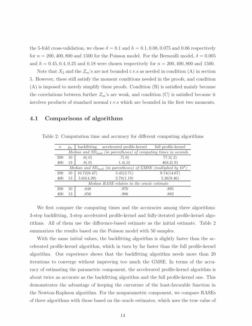
Table 2: Computation time and accuracy for different computing algorithms

n pn backfitting accelerated profile-kernel full profile-kernel

Median and SDmad (in parentheses) of computing times in seconds

200 10 .6(.0) .7(.0) 77.2(.2)

400 13 .8(.0) 1.4(.0) 463.2(.9)

Median and SDmad (in parentheses) of GMSE (multiplied by 104)

200 10 10.72(6.47) 5.45(2.71) 9.74(14.67)

400 13 5.63(4.39) 2.78(1.19) 5.26(9.46)

Median RASE relative to the oracle estimate

200 10 .848 .970 .895

400 13 .856 .986 .882

We first compare the computing times and the accuracies among three algorithms:

3-step backfitting, 3-step accelerated profile-kernel and fully-iterated profile-kernel algo-

rithms. All of them use the difference-based estimate as the initial estimate. Table 2

summarizes the results based on the Poisson model with 50 samples.

With the same initial values, the backfitting algorithm is slightly faster than the ac-

celerated profile-kernel algorithm, which in turn by far faster than the full profile-kernel

algorithm. Our experience shows that the backfitting algorithm needs more than 20

iterations to converge without improving too much the GMSE. In terms of the accu-

racy of estimating the parametric component, the accelerated profile-kernel algorithm is

about twice as accurate as the backfitting algorithm and the full profile-kernel one. This

demonstrates the advantage of keeping the curvature of the least-favorable function in

the Newton-Raphson algorithm. For the nonparametric component, we compare RASEs

of three algorithms with those based on the oracle estimator, which uses the true value of

14

βn. The ratios of the RASEs based on the oracle estimator and those based on the three

algorithms are reported in Table 1. It is clear that the accelerated profile-kernel estimate

performs very well in estimating the nonparametric components, mimicking very well the

oracle estimator. The second best is the backfitting algorithm.

We have also compared the three algorithms using the Bernoulli model. Our proposed

accelerated profile-kernel estimate still performs the best in terms of accuracy, though the

improvement is not as dramatic as those for the Poisson model. We speculate that the

poor performance of the full profile-kernel estimate is due to its unstable implementation

that is related to computing the second derivatives of the least-favorable curve.

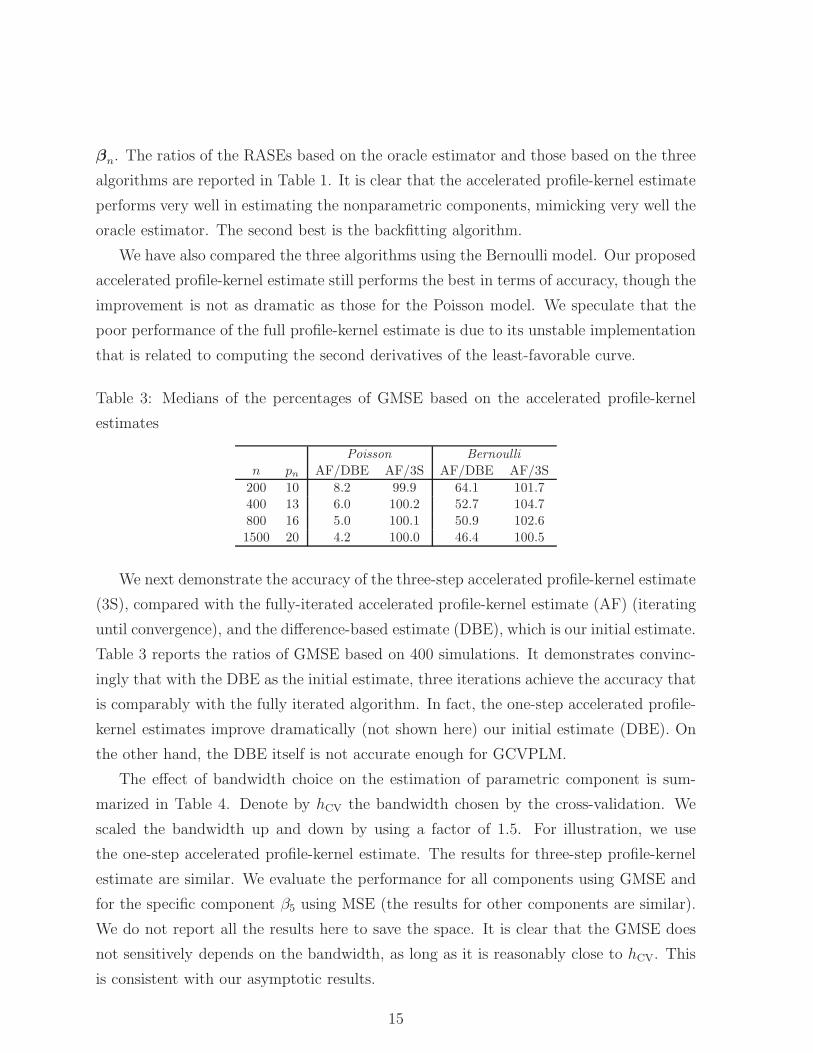
Table 3: Medians of the percentages of GMSE based on the accelerated profile-kernel

estimates

Poisson Bernoulli

n pn AF/DBE AF/3S AF/DBE AF/3S

200 10 8.2 99.9 64.1 101.7400 13 6.0 100.2 52.7 104.7

800 16 5.0 100.1 50.9 102.6

1500 20 4.2 100.0 46.4 100.5

We next demonstrate the accuracy of the three-step accelerated profile-kernel estimate

(3S), compared with the fully-iterated accelerated profile-kernel estimate (AF) (iterating

until convergence), and the difference-based estimate (DBE), which is our initial estimate.

Table 3 reports the ratios of GMSE based on 400 simulations. It demonstrates convinc-

ingly that with the DBE as the initial estimate, three iterations achieve the accuracy that

is comparably with the fully iterated algorithm. In fact, the one-step accelerated profile-

kernel estimates improve dramatically (not shown here) our initial estimate (DBE). On

the other hand, the DBE itself is not accurate enough for GCVPLM.

The effect of bandwidth choice on the estimation of parametric component is sum-

marized in Table 4. Denote by hCV the bandwidth chosen by the cross-validation. We

scaled the bandwidth up and down by using a factor of 1.5. For illustration, we use

the one-step accelerated profile-kernel estimate. The results for three-step profile-kernel

estimate are similar. We evaluate the performance for all components using GMSE and

for the specific component β5 using MSE (the results for other components are similar).

We do not report all the results here to save the space. It is clear that the GMSE does

not sensitively depends on the bandwidth, as long as it is reasonably close to hCV. This

is consistent with our asymptotic results.

15

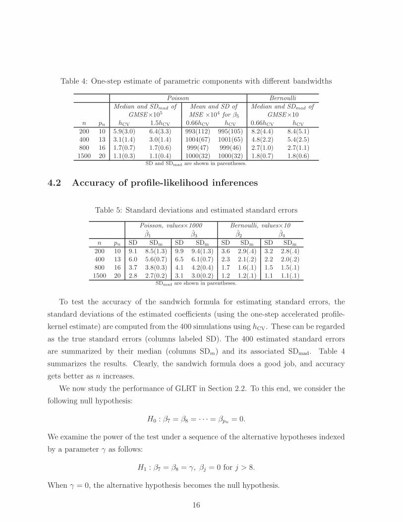
Table 4: One-step estimate of parametric components with different bandwidths

Poisson Bernoulli

Median and SDmad of Mean and SD of Median and SDmad of

GMSE×105 MSE ×104 for β5 GMSE×10

n pn hCV 1.5hCV 0.66hCV hCV 0.66hCV hCV

200 10 5.9(3.0) 6.4(3.3) 993(112) 995(105) 8.2(4.4) 8.4(5.1)400 13 3.1(1.4) 3.0(1.4) 1004(67) 1001(65) 4.8(2.2) 5.4(2.5)

800 16 1.7(0.7) 1.7(0.6) 999(47) 999(46) 2.7(1.0) 2.7(1.1)1500 20 1.1(0.3) 1.1(0.4) 1000(32) 1000(32) 1.8(0.7) 1.8(0.6)

SD and SDmad are shown in parentheses.

4.2 Accuracy of profile-likelihood inferences

Table 5: Standard deviations and estimated standard errors

Poisson, values×1000 Bernoulli, values×10

β1 β3 β2 β4

n pn SD SDm SD SDm SD SDm SD SDm

200 10 9.1 8.5(1.3) 9.9 9.4(1.3) 3.6 2.9(.4) 3.2 2.8(.4)400 13 6.0 5.6(0.7) 6.5 6.1(0.7) 2.3 2.1(.2) 2.2 2.0(.2)

800 16 3.7 3.8(0.3) 4.1 4.2(0.4) 1.7 1.6(.1) 1.5 1.5(.1)1500 20 2.8 2.7(0.2) 3.1 3.0(0.2) 1.2 1.2(.1) 1.1 1.1(.1)

SDmad are shown in parentheses.

To test the accuracy of the sandwich formula for estimating standard errors, the

standard deviations of the estimated coefficients (using the one-step accelerated profile-

kernel estimate) are computed from the 400 simulations using hCV. These can be regarded

as the true standard errors (columns labeled SD). The 400 estimated standard errors

are summarized by their median (columns SDm) and its associated SDmad. Table 4

summarizes the results. Clearly, the sandwich formula does a good job, and accuracy

gets better as n increases.

We now study the performance of GLRT in Section 2.2. To this end, we consider the

following null hypothesis:

H0 : β7 = β8 = · · · = βpn= 0.

We examine the power of the test under a sequence of the alternative hypotheses indexed

by a parameter γ as follows:

H1 : β7 = β8 = γ, βj = 0 for j > 8.

When γ = 0, the alternative hypothesis becomes the null hypothesis.

16

0 2 4 6 8 10 12 14 16 18 20 220

0.02

0.04

0.06

0.08

0.1

0.12

0.14(a) Null density estimation (n=400,h=hcv)

0 0.015 0.03 0.045 0.060

0.1

0.2

0.3

0.4

0.5

0.6

0.7

0.8

0.9

1

γ

(b) Power function (n=400,h=hcv)

0 4 8 12 16 20 24 280

0.01

0.02

0.03

0.04

0.05

0.06

0.07

0.08

0.09

0.1(c) Null density estimation (n=800,h=0.66hcv)

0 0.25 0.5 0.75 10

0.1

0.2

0.3

0.4

0.5

0.6

0.7

0.8

0.9

1

γ

(d) Power function (n=200,h=hcv)

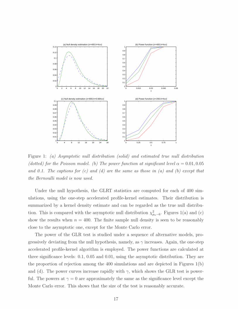
Figure 1: (a) Asymptotic null distribution (solid) and estimated true null distribution

(dotted) for the Poisson model. (b) The power function at significant level α = 0.01, 0.05

and 0.1. The captions for (c) and (d) are the same as those in (a) and (b) except that

the Bernoulli model is now used.

Under the null hypothesis, the GLRT statistics are computed for each of 400 sim-

ulations, using the one-step accelerated profile-kernel estimates. Their distribution is

summarized by a kernel density estimate and can be regarded as the true null distribu-

tion. This is compared with the asymptotic null distribution χ2pn−6. Figures 1(a) and (c)

show the results when n = 400. The finite sample null density is seen to be reasonably

close to the asymptotic one, except for the Monte Carlo error.

The power of the GLR test is studied under a sequence of alternative models, pro-

gressively deviating from the null hypothesis, namely, as γ increases. Again, the one-step

accelerated profile-kernel algorithm is employed. The power functions are calculated at

three significance levels: 0.1, 0.05 and 0.01, using the asymptotic distribution. They are

the proportion of rejection among the 400 simulations and are depicted in Figures 1(b)

and (d). The power curves increase rapidly with γ, which shows the GLR test is power-

ful. The powers at γ = 0 are approximately the same as the significance level except the

Monte Carlo error. This shows that the size of the test is reasonably accurate.

17

4.3 A real data example.

This is the analysis of the data in section 1.1 in where details of data and variables are

given.

To examine the nonlinear effect of age and its nonlinear interaction with the expe-

rience, we appeal to the following GVCPLM (interactions between age and covariates

other than TotalYrsExp are considered but found to be insignificant):

log

(pH

1− pH

)= α1(Age) + α2(Age)TotalYrsExp

+ β1Female + β2PCJob +

4∑

i=1

β2+iEdui

(4.1)

where pH is the probability of having a high grade job. Formally, we are testing

H0 : β1 = 0←→ H1 : β1 < 0. (4.2)

Table 6: Fitted coefficients (sandwich SD) for model (4.1)

Response Female PCJob Edu1 Edu2 Edu3 Edu4

HighGrade4 -1.96(.57) -0.02(.76) -5.14(.85) -4.77(.98) -2.72(.52) -2.85(.96)

HighGrade5 -2.22(.59) -1.96(.61) -5.69(.67) -5.95(.97) -3.09(.72) -1.26(1.10)

A 20-fold CV is employed to select the bandwidth h and the parameter δ in the

transformation of the data. This yields hCV = 24.2, δCV = 0.1. Table 6 shows the

results of the fit using the three-step accelerated profile-kernel estimate. The coefficient

for Female is significantly negative. The education plays also an important role in

getting high grade job. All coefficients are negative, as they are contrasted with the

highest education level. The PCJob does not seem to play any significant role in getting

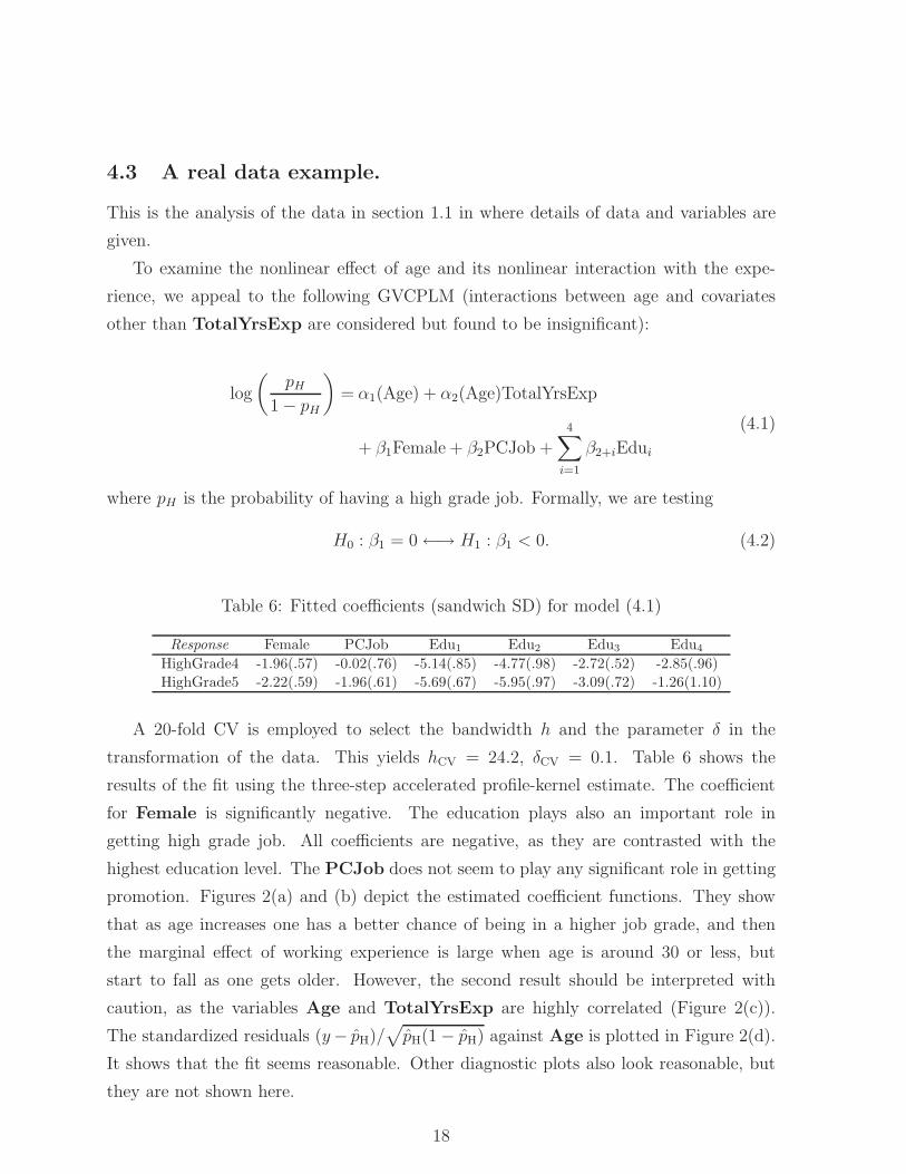
promotion. Figures 2(a) and (b) depict the estimated coefficient functions. They show

that as age increases one has a better chance of being in a higher job grade, and then

the marginal effect of working experience is large when age is around 30 or less, but

start to fall as one gets older. However, the second result should be interpreted with

caution, as the variables Age and TotalYrsExp are highly correlated (Figure 2(c)).

The standardized residuals (y− pH)/√

pH(1− pH) against Age is plotted in Figure 2(d).

It shows that the fit seems reasonable. Other diagnostic plots also look reasonable, but

they are not shown here.

18

20 25 30 35 40 45 50 55 60 65 70−4

−3

−2

−1

0

1

2

3

Age

α 1(Age

)

(a) Fitted coefficient function α1(⋅)

20 25 30 35 40 45 50 55 60 65 700

0.05

0.1

0.15

0.2

0.25

0.3

0.35

0.4

0.45

0.5

0.55

Age

α 2(Age

)

(b) Fitted coefficient function α2(⋅)

20 30 40 50 60 700

5

10

15

20

25

30

35

40

Age

Tot

alY

rsE

xp

(c) TotalYrsExp against Age

20 30 40 50 60 70

−3

−2

−1

0

1

2

3

4

Age

Sta

ndar

dize

d re

sidu

als

(d) Standardsized Residuals against Age

Figure 2: (a) Fitted coefficient function α1(·) (b) Fitted coefficient function α2(·). (c) The

scatter plot ‘TotalYrsExp’ Against ‘Age’. (d) Standardized residuals against the variable

‘Age’.

We have conducted another fit using a binary variable HighGrade5, which is 0 only

when job grade is less than 5. The coefficients are shown in Table 6 and the Female

coefficient is close to the first fit.

We now employ the generalized likelihood ratio test to the problem (4.2). The GLR

test statistic is 14.47 with one degree of freedom, resulting in a P-value of 0.0001. We have

also conduct the same analysis using HighGrade5 as the binary response. The GLR

test statistic is now 13.76 and the associated P-value is 0.0002. The fitted coefficients are

summarized in Table 5. The result provides stark evidence that even after adjusting for

other confounding factors and variables, female employees of the Fifth National Bank is

harder to get promoted to a high grade job.

Not shown in this paper, we have conducted the analysis again after deleting 6 data

points corresponding to 5 male executives and 1 female employee having many years of

working experience and high salaries. The test results are still similar.

19

5 Technical proofs

In this section the proofs of Theorems 1-4 will be given. We introduce some notations

and regularity conditions for our results. In the following and thereafter, the symbol ⊗represents the Kronecker product between matrices, and λmin(A) and λmax(A) denotes

respectively the minimum and maximum eigenvalues of a symmetric matrix A. We let

Qni(βn) be the i-th summand of (2.3).

Denote the true linear parameter by βn0, with parameter space Ωn ⊂ Rpn. Let

µk =∫ ∞

−∞ukK(u)du and Ap(X) = (µi+j)0≤i,j≤p ⊗XXT . Set

ρl(t) = (dg−1(t)/dt)l/V (g−1(t)), mni(βn) = αβn(Ui)

TXi + βTnZni,

α′βn

(u) =∂αβn

(u)

∂βn, α

(r)′′βn

(u) =∂2α

(r)βn

(u)

∂βn∂βTn

.

Regularity Conditions:

(A) The covariates Zn and X are bounded random variables.

(B) The smallest and the largest eigenvalues of the matrix In(βn0) is bounded away

from zero and infinity for all n. In addition, E0[∇T Qn1(βn0)∇Qn1(βn0)]4 = O(p4

n).

(C) Eβn| ∂l+jQn1(βn)∂jα∂βnk1

···∂βnkl

| and Eβn| ∂l+jQn1(βn)∂jα∂βnk1

···∂βnkl

|2 are bounded for all n, with l = 1, · · · , 4and j = 0, 1.

(D) The function q2(x, y) < 0 for x ∈ R and y in the range of the response variable,

and E0q2(mn1(βn), Yn1)Ap(X1)|U = u is invertible.

(E) The functions V ′′(·) and g′′′(·) are continuous. The least-favorable curve αβn(u) is

three times continuously differentiable in βn and u.

(F) The random variable U has a compact support Ω. The density function fU(u) of U

has a continuous second derivative and is uniformly bounded away from zero.

(G) The kernel K is a bounded symmetric density function with bounded support.

Note the above conditions are assumed to hold uniformly in u ∈ Ω. Condition (A)

is imposed just for the simplicity of proofs. The boundedness of covariates is imposed

to ensure various products involving ql(·, ·),X and Zn have bounded first and second

moments. Conditions (B) and (C) are uniformity conditions on higher-order moments of

20

the likelihood functions. They are stronger than those of the usual asymptotic likelihood

theory, but they facilitate technical proofs. Condition (G) is also imposed for simplicity

of technical arguments. All of these conditions can be relaxed at the expense of longer

proofs.

Before proving Theorem 1, we need two important lemmas. Lemma 1 concerns the

order approximations to the least-favorable curve αβn(·), while Lemma 2 holds the key

to showing why undersmoothing is not needed in Theorems 1 and 2. Let cn = (nh)−1/2,

a0βn, · · · , and apβn

maximize (2.4), and α(p)uβn

(u) =∂pαβn

(u)

∂up . Set

αni(u) = XTi

( p∑

k=0

(Ui − u)k

k!α

(k)uβn

(u)

)+ βT

nZni,

β∗

= c−1n

((a0βn

−αβn(u))T , · · · , hp

p!(apβn

−α(p)uβn

(u))T

)T

,

X∗i =

(1,

Ui − u

h, · · · ,

(Ui − u

h

)p)T

⊗Xi.

Lemma 1 Under Regularity Conditions (A) - (G), for each βn ∈ Ωn, the following holds

uniformly in u ∈ Ω:

‖a0βn(u)−αβn

(u)‖ = OP (hp+1 + cn log1/2(1/h)).

Likewise, the norm of the kth derivative of the above with respect to any βnj’s, for k =

1, · · · , 4, all have the same order uniformly in u ∈ Ω.

Proof of Lemma 1. Our first step is to show that, uniform in u ∈ Ω,

β∗

= A−1n Wn + OP (hp+1 + cn log1/2(1/h)),

where

An = fU(u)E0ρ2(αβn(U)T X + ZT

nβn)Ap(X)|U = u,

Wn = hcn

n∑

i=1

q1(αni, Yni)X∗i Kh(Ui − u),

An = hc2n

n∑

i=1

q2(αni, Yni)X∗i X

∗Ti Kh(Ui − u).

21

Since expression (2.4) is maximized at (a0βn, · · · , apβn

)T , β∗

maximizes

ln(β∗) = hn∑

i=1

Q(g−1(cnX∗Ti β∗ + αni), Yni)−Q(g−1(αni), Yni)

= WTnβ∗ +

1

2β∗TAnβ

∗ +hc3

n

6

n∑

i=1

q3(ηi, yni)(X∗Ti β∗)3Kh(Ui − u),

where ηi lies between αni and αni + cnX∗Ti β∗. The concavity of ln(β∗) is ensured by

Condition (D). Note that K(·) is bounded, we have under Conditions (A) and (C), the

third term on the right hand side is bounded by

OP (nhc3nE|q3(η1, Yn1)‖X1‖3Kh(U1 − u)|) = OP (cn) = oP (1).

Direct calculation yields E0An = −An + O(hp+1) and Var0((An)ij) = O((nh)−1) so that

mean-variance decomposition yields

An = −An + OP (hp+1).

Hence we have

ln(β∗) = WTnβ∗ − 1

2β∗T Anβ

∗ + oP (1). (5.1)

Note that An is a sum of i.i.d. random variables of kernel form, by a result of [21],

An = −An + OPhp+1 + cn log1/2(1/h) (5.2)

uniformly in u ∈ Ω. Hence by the Convexity Lemma ([24]), equation (5.1) also holds

uniformly in β∗ ∈ C for any compact set C. Using Lemma A.1 of [5], it yields that

supu∈Ω|β∗ − A−1

n Wn| P−→ 0. (5.3)

Furthermore, by its definition, β∗

solves the local likelihood equation:

n∑

i=1

q1(αni + cnX∗Ti β

∗, Yni)X

∗i Kh(Ui − u) = 0. (5.4)

Expanding q1(αni + cnX∗Ti β

∗, ·) at αni yields

Wn + Anβ∗+

hc3n

2

n∑

i=1

q3(αni + ζi, Yni)X∗i (X

∗Ti β

∗)2Kh(Ui − u) = 0 (5.5)

22

where ζi lies between 0 and cnX∗Ti β

∗. Using Conditions (A) and (C), the last term has

order OP (c3nhn‖β∗‖2) = OP (cn‖β

∗‖2). With this, combining (5.2) and (5.5), we obtain

β∗

= A−1n Wn + OP (hp+1 + cn log1/2(1/h)) (5.6)

holds uniformly in u ∈ Ω by (5.3). Using the result of [21] on Wn, we obtain

‖a0βn(u)−αβn

(u)‖ = OP (hp+1 + cn log1/2(1/h)) (5.7)

which holds uniformly in u ∈ Ω.

Differentiate both sides of (5.4) w.r.t. βnj ,

n∑

i=1

q2(αni + cnX∗Ti β

∗, Yni)

∂αni

∂βnj+ cn

(∂β

∗

∂βnj

)T

X∗i

X∗

i Kh(Ui − u) = 0, (5.8)

which holds for all u ∈ Ω. By Taylor’s expansion and similar treatments to (5.5),

W1n + W2

n + (An + B1n + B2

n)∂β

∗

∂βnj+ OP (cn‖β

∗‖2) = 0,

where

W1n = hcn

n∑

i=1

q2(αni, Yni)∂αni

∂βnj

X∗i Kh(Ui − u),

W2n = hcn

n∑

i=1

q3(αni, Yni)cnX∗Ti β

∗∂αni

∂βnjX∗

i Kh(Ui − u),

B1n = hc2

n

n∑

i=1

q3(αni, Yni)cnX∗Ti β

∗X∗

i X∗Ti Kh(Ui − u),

B2n =

hc2n

2

n∑

i=1

q4(αni + ζi, Yni)(c2nX

∗Ti β

∗)2X∗

i X∗Ti Kh(Ui − u),

with ζi lies between 0 and cnX∗Ti β

∗. The above equations hold for all u ∈ Ω. The order

of W2n is smaller than that of W1

n, and the orders of B1n and B2

n are smaller than that of

An. Hence∂β

∗

∂βnj

= A−1n W1

n + oP (log1/2(1/h) + c−1n hp+1)

uniformly in u ∈ Ω. From this, for j = 1, · · · , pn, we have∥∥∥∥∂a0βn

(u)

∂βnj

− ∂αβn(u)

∂βnj

∥∥∥∥ = OP (hp+1 + cn log1/2(1/h)) (5.9)

uniformly in u ∈ Ω. Differentiating (5.4) again w.r.t. βnk and repeating as needed, we get

the desired results for higher order derivatives by following similar arguments as above.

23

Lemma 2 Under Regularity Conditions (A) - (G), if psn/n→ 0 for s > 5/4, h = O(n−a)

with (2s(p + 1))−1 < a < 1− s−1, then for each βn ∈ Ωn,

n−1/2‖∇Qn(βn)−∇Qn(βn)‖ = oP (1).

Proof of Lemma 2. Define

K1 = n−1/2n∑

i=1

q2(mni(βn), Yni)(Zni + α′βn

(Ui)Xi)(αβn(Ui)−αβn

(Ui))TXi,

K2 = n−1/2

n∑

i=1

q1(mni(βn), Yni)(α′βn

(Ui)−α′βn

(Ui))TXi.

Then by Taylor’s expansion, Lemma 1 and Condition (C),

n−1/2(∇Qn(βn)−∇Qn(βn)) = K1 + K2 + smaller order terms.

Define, for Ω as in Condition (F),

S = f ∈ C2(Ω) : ‖f‖∞ ≤ 1,

equipped with a metric ρ(f1, f2) = ‖f1− f2‖∞, where ‖f‖∞ = supu∈Ω |f(u)|. We also let,

for r = 1, · · · , q and l = 1, · · · , pn,

Arl(y, u,X,Zn) = q2(XTαβn

(u) + ZTnβn, y)Xr

(Znl + XT ∂αβn

(u)

∂βnl

),

Br(y, u,X,Zn) = q1(XTαβn

(u) + ZTnβn, y)Xr.

By Lemma 1, for any positive sequences (δn) with δn → 0 as n → ∞, we have

P0(λr ∈ S)→ 1 and P0(γrl ∈ S)→ 1, where

λr = δn(hp+1 + cn log1/2(1/h))−1(α(r)βn− α

(r)βn

),

γrl = δn(hp+1 + cn log1/2(1/h))−1

(∂α

(r)βn

∂βnl−

∂α(r)βn

∂βnl

),

r = 1, · · · , q and l = 1, · · · , pn. Hence for sufficiently large n, we have λr, γrl ∈ S. The

following three points allow us to utilize [15] to prove our lemma.

I. For any v ∈ S, we will view the map v 7→ Arl(y, u,X,Zn)v(u) as an element of

C(S), the space of continuous functions on S equipped with the sup norm. For

v1, v2 ∈ S, we have

|Arl(y, u,X,Zn)v1(u)−Arl(y, u,X,Zn)v2(u)|= |Arl(y, u,X,Zn)(v1 − v2)(u)| ≤ |Arl(y, u,X,Zn)|‖v1 − v2‖.

Similar result holds for Br(y, u,X,Zn).

24

II. Note that equation (2.2) is true for all βn, and by differentiating w.r.t. βn we get

the following formulas:

E0(q1(mn(βn), Yn)X|U = u) = 0,

E0(q2(mn(βn), Yn)X(Zn + α′βn

(U)X)T |U = u) = 0.

Thus, we can easily see that

E0(Arl(Y, U,X,Zn)) = 0

for each r = 1, · · · , q and l = 1, · · · , pn. Also we have

E0(Arl(Y, U,X,Zn)2) <∞,

by Regularity Conditions (A) and (C). For Br(Y, U,X,Zn), results hold similarly.

III. Let H(·, S) denote the metric entropy of the set S w.r.t. the metric ρ. Then

H(ǫ, S) ≤ C0ǫ−1

for some constant C0. Hence∫ 1

0H1/2(ǫ, S)dǫ <∞.

Conditions of Theorem 1 in [15] can be derived from the three notes above, so that

we have

n−1/2n∑

i=1

Arl(Yi, Ui,Xi,Zni)(·),

where Arl(Yi, Ui,Xi,Zni)(·), i = 1, · · · , n being i.i.d. replicates of Arl(Y, U,X,Zn)(·) in

C(S), converges weakly to a Gaussian measure on C(S). Hence, since λr, γrl ∈ S,

n−1/2n∑

i=1

Arl(Yi, Ui,Xi,Zni)(λr) = OP (1),

which implies that

n−1/2n∑

i=1

Arl(Yi, Ui,Xi,Zni)(α(r)βn− α

(r)βn

) = OP (δ−1n (hp+1 + cn log1/2(1/h))).

Similarly, apply Theorem 1 of [15] again, we have

n−1/2n∑

i=1

Br(Yi, Ui,Xi,Zni)

(∂α

(r)βn

∂βnl

−∂α

(r)βn

∂βnl

)= OP (δ−1

n (hp+1 + cn log1/2(1/h))).

25

Then the column vector K1 which is pn−dimensional, has the lth component equals

q∑

r=1

n−1/2

n∑

i=1

Arl(Yi, Ui,Xi,Zni)(α(r)βn− α

(r)βn

)

= OP (δ−1

n (hp+1 + cn log1/2(1/h)),

using the result just proved. Hence we have shown

‖K1‖ = OP (√

pnδ−1n (hp+1 + cn log1/2(1/h))) = oP (1),

since δn can be made arbitrarily slow in converging to 0. Similarly, we have ‖K2‖ = oP (1)

as well. The conclusion of the lemma follows.

Proof of Theorem 1.

Let γn =√

pn/n. Our aim is to show that, for a given ǫ > 0,

P

sup

‖v‖=C

Qn(βn0 + γnv) < Qn(βn0)

≥ 1− ǫ, (5.10)

so that this implies with probability tending to 1 there is a local maximum βn in the ball

βn0 + γnv : ‖v‖ ≤ C such that ‖βn − βn0‖ = OP (γn).

Define the terms I1 = γn∇T Qn(βn0)v, I2 = γ2n

2vT∇2Qn(βn0)v and

I3 = γ3n

6∇T (vT∇2Qn(β∗

n)v)v. By Taylor’s expansion,

Qn(βn0 + γnv)− Qn(βn0) = I1 + I2 + I3,

where β∗n lies between βn0 and βn0 + γnv.

We further split I1 = D1 + D2, where

D1 =

n∑

i=1

q1(mni(βn0), Yni)(Zni + α′βn0

(Ui)Xi)Tvγn,

D2 =

n∑

i=1

q1(mni(βn0), Yni)XTi (α′

βn0(Ui)−α′

βn0(Ui))

Tvγn,

with mni(βn) = αβn(Ui)

TXi + βTnZni. By Condition (A) and Lemma 1, D2 has order

smaller than D1. Using Taylor’s expansion, we have

D1 = γnvT

( n∑

i=1

∂Qni(βn0)

∂βn

+√

nK1

)+ smaller order terms,

where K1 is as defined in Lemma 2 so that within the lemma’s proof we have ‖K1‖ =

oP (1). Using equation (2.6), we have by the mean-variance decomposition∥∥∥∥vT

n∑

i=1

∂Qni(βn0)

∂βn

∥∥∥∥ = OP (√

nvT In(βn0)v) = OP (√

n)‖v‖,

26

where last inequality follows from Condition (B). Hence

|I1| = OP (√

nγn)‖v‖.

Next, consider I2 = I2 + (I2 − I2), where

I2 =1

2vT∇2Qn(βn0)vγ2

n

= −n

2vT In(βn0)vγ2

n +n

2vTn−1∇2Qn(βn0) + In(βn0)vγ2

n

= −n

2vT In(βn0)vγ2

n + oP (nγ2n)‖v‖2

with the last line follows from Lemma 5 in the Appendix. Using Lemma 4,

‖I2 − I2‖ = oP (nγ2n‖v‖2).

On the other hand, by Condition (B), we have

|nγ2nv

T In(βn0)v| ≥ O(nγ2nλmin(In(βn0))‖v‖2) = O(nγ2

n‖v‖2).

Hence, I2 − I2 has a smaller order than I2.

Finally consider I3. We suppress the dependence of αβn(Ui) and its derivatives on

Ui, and denote q1i = q1(mni(βn0), Yni). Using Taylor’s expansions, expanding Qn(β∗n) at

βn0 and then Qn(βn0) at αβn0, we can arrive at

Qn(β∗n) = Qn(βn0) +

n∑

i=1

q1iXTi (αβn0

−αβn0)

+ q1i(Zni + α′βn0

Xi)T (β∗

n − βn0)(1 + oP (1)).

Substituting Qn(β∗n) into I3 with the right hand side above, by Condition (C) and Lemma

1, we have

I3 =1

6

pn∑

i,j,k=1

∂3Qn(βn0)

∂βni∂βnj∂βnk

vivjvkγ3n + smaller order terms.

Hence,

|I3| = OP (np3/2n γ3

n‖v‖3) = OP (√

p4n/n‖v‖)nγ2

n‖v‖2 = oP (1)nγ2n‖v‖2.

Comparing, we find the order of −nγ2nv

T In(βn0)v dominates all other terms by allowing

‖v‖ = C to be large enough. This proves (5.10).

27

Proof of Theorem 2.

Note that by Theorem 1, ‖βn−βn0‖ = OP (√

pn/n). Since ∇Qn(βn) = 0, by Taylor’s

expansion,

∇Qn(βn0) +∇2Qn(βn0)(βn − βn0) + C = 0, (5.11)

where β∗n lies between βn0 βn and C = 1

2(βn − βn0)

T∇2(∇Qn(β∗n))(βn − βn0)) which is

understood as a vector of quadratic components.

Using similar argument to approximating I3 in Theorem 1, by Lemma 1 and noting

‖β∗n − βn0‖ = oP (1), we have ‖∇2 ∂Qn(β∗

n)∂βnj

‖2 = OP (n2p2n). Hence

‖n−1C‖2 ≤ n−2‖βn − βn0‖4pn∑

j=1

∥∥∥∥∇2∂Qn(β∗

n)

∂βnj

∥∥∥∥2

= OP (p5n/n

2) = oP (n−1). (5.12)

At the same time, by Lemma 5 and the Cauchy-Schwarz inequality,

‖n−1∇2Qn(βn0)(βn − βn0) + In(βn0)(βn − βn0)‖= oP ((npn)−1/2) + OP (

√p3

n/n(hp+1 + cn log1/2(1/h))) = oP (n−1/2).(5.13)

Combining (5.11),(5.12) and (5.13), we have

In(βn0)(βn − βn0) = n−1∇Qn(βn0) + oP (n−1/2)

= n−1∇Qn(βn0) + oP (n−1/2),(5.14)

where the last line follows from Lemma 2. Consequently, using equation (5.14), we get

√nAnI

1/2n (βn0)(βn − βn0) = n−1/2AnI−1/2

n (βn0)∇Qn(βn0)

+ oP (AnI−1/2n (βn0))

= n−1/2AnI−1/2n (βn0)∇Qn(βn0) + oP (1),

(5.15)

since ‖AnI−1/2n (βn0)‖ = O(1) by conditions of Theorem 2.

We now check the Lindeberg-Feller Central Limit Theorem (see for example, [29]) for

the last term in (5.15). Let Bni = n−1/2AnI−1/2n (βn0)∇Qni(βn0), i = 1, · · · , n. Given

ǫ > 0,n∑

i=1

E0‖Bni‖21‖Bni‖ > ǫ ≤ n√

E0‖Bn1‖4 · P(‖Bn1‖ > ǫ).

Using Chebyshev’s inequality,

P(‖Bn1‖ > ǫ) ≤ n−1ǫ−2E‖AnI−1/2n (βn0)∇Qn1(βn0)‖2

= n−1ǫ−2tr(G) = O(n−1),(5.16)

28

where tr(A) is the trace of square matrix A. Similarly, we can show that, using Condi-

tion (B),

E0‖Bn1‖4 ≤√

ln−2λ2min(AnA

Tn )λ2

max(In(βn0))√

E0(∇Qn1(βn0)T∇Qn1(βn0))

4

= O(p2n/n

2).(5.17)

Therefore (5.16) and (5.17) together imply

n∑

i=1

E0‖Bni‖21‖Bni‖ > ǫ = O(√

p2n/n) = o(1).

Also,

n∑

i=1

Var0(Bni) = Var0(AnI−1/2n (βn0)∇Qn1(βn0))

= AnATn → G.

Therefore Bni satisfies the conditions of the Lindeberg-Feller Central Limit Theorem.

Consequently, using (5.15), it follows that

√nAnI

1/2n (βn0)(βn − βn0)

D−→ N(0, G),

and this completes the proof.

Referring back to Section 2.2, let Bn be a (pn− l)×pn matrix satisfying BnBTn = Ipn−l

and AnBTn = 0. Since Anβn = 0 under H0, rows of An are perpendicular to βn and the

orthogonal complement of rows of An is spanned by rows of Bn since AnBTn = 0. Hence

βn = BTn γ

under H0, where γ is a (pn− l)×1 vector. Then under H0 the profile likelihood estimator

is also the local maximizer γn of the problem

Qn(BTn γn) = max

γn

Qn(BTn γn).

Proof of Theorem 3.

By Taylor’s expansion, expanding Qn(BTn γn) at βn and noting that ∇T Qn(βn) = 0,

then Qn(βn)− Qn(BTn γn) = T1 + T2, where

T1 = −1

2(βn − BT

n γn)T∇2Qn(βn)(βn −BTn γn),

T2 =1

6∇T(βn − BT

n γn)T∇2Qn(β∗n)(βn − BT

n γn)(βn −BTn γn).

29

Denote by Θn = In(βn0) and Φn = 1n∇Qn(βn0). Using equation (5.14) and noting that

Θn has eigenvalues uniformly bounded away from 0 and infinity by Condition (B), we

have

βn − βn0 = Θ−1n Φn + oP (n−1/2).

Combining this with Lemma 6 in the Appendix, under the null hypothesis H0,

βn − BTn γn =Θ−1/2

n Ipn−Θ1/2

n BTn (BnΘnBT

n )−1BnΘ1/2n Θ−1/2

n Φn

+ oP (n−1/2).(5.18)

Since Sn = Ipn−Θ

1/2n BT

n (BnΘnBTn )−1BnΘ

1/2n is a pn×pn idempotent matrix with rank

l, it follows by mean-variance decomposition of the term ‖βn − BTn γn‖2 and Condition

(B) that

‖βn − BTn γn‖ = OP (n−1/2).

Hence, using similar argument as in the approximation of order for |I3| in Theorem 1, we

have

|T2| = OP (np3/2n ) · ‖βn − BT

n γn‖3 = oP (1).

Hence Qn(βn)− Q(BTn γn) = T2 + oP (1).

By Lemma 5 and an approximation to n−1‖∇2Qn(βn) − ∇2Qn(βn0)‖ = oP (p−1/2n )

(the proof is similar to that for Lemma 3 with the proof of order for |I3| in Theorem 1,

and is omitted), we have∥∥∥∥

1

2(βn −BT

n γn)T∇2Qn(βn) + nIn(βn0)(βn −BTn γn)

∥∥∥∥

= OP (l/n) · noP (p−1/2n ) + OP (pn(hp+1 + cn log1/2(1/h))) = op(1).

Therefore,

Qn(βn)− Qn(BTn γn) =

n

2(βn − BT

n γn)T In(βn0)(βn −BTn γn) + oP (1).

By (5.18), we have

Qn(βn)− Qn(BTn γn) =

n

2ΦT

nΘ−1/2n SnΘ−1/2

n Φn + oP (1).

Since Sn is idempotent, it can be written as Sn = DTn Dn where Dn is an l×pn matrix

satisfying DnDTn = Il. By Theorem 2, we have already shown that

√nDnΘ

−1/2n Φn

D−→N(0, Il). Hence

2Qn(βn)− Qn(BTn γn) = n(DnΘ−1/2

n Φn)T (DnΘ−1/2n Φn)

D−→ χ2l .

30

Proof of Theorem 4.

Let An = −n−1∇2Qn(βn), Bn = cov∇Qn(βn) and C = In(βn0). Write

I1 = A−1n (Bn − C)A−1

n , I2 = A−1n (C − An)A−1

n , I3 = A−1n (C − An)C−1.

Then, Σn − Σn = I1 + I2 + I3. Our aim is to show that, for all i = 1, · · · , pn,

λi(Σn − Σn) = oP (1),

so that An(Σn − Σn)ATn

P−→ 0, where λi(A) is the ith eigenvalue of a symmetric matrix

A. Using the inequalities

λmin(I1) + λmin(I2) + λmin(I3) ≤ λmin(I1 + I2 + I3)

λmax(I1 + I2 + I3) ≤ λmax(I1) + λmax(I2) + λmax(I3),

it suffices to show that λi(Ij) = oP (1) for j = 1, 2, 3. From the definition of I1, I2 and

I3, it is clear that we only need to show λi(C − An) = oP (1) and λi(Bn − C) = oP (1).

Let K1 = In(βn0) + n−1∇2Qn(βn0), K2 = n−1(∇2Qn(βn) − ∇2Qn(βn0)), and K3 =

n−1(∇2Qn(βn)−∇2Qn(βn)). Then,

C − An = K1 + K2 + K3.

Applying Lemma 5 to K1, Lemma 3 to K2, and Lemma 4 to K3, we have ‖C−A‖ = oP (1).

Thus, λi(C − A) = oP (1). Hence the only thing left to show is λi(Bn − C) = oP (1).

To this end, consider the decomposition

Bn − C = K4 + K5

where

K4 =

1

n

n∑

i=1

∂Qni(βn)

∂βnj

∂Qni(βn)

∂βnk

− In(βn0),

K5 = −

1

n

n∑

i=1

∂Qni(βn)

∂βnj

1

n

n∑

i=1

∂Qni(βn)

∂βnk

.

Our goal is to show that K4 and K5 are oP (1), which then implies λi(Bn − C) = oP (1).

We consider K4 first, which can be further decomposed into K4 = K6 + K7, where

K6 =

1

n

n∑

i=1

∂Qni(βn)

∂βnj

∂Qni(βn)

∂βnk− 1

n

n∑

i=1

∂Qni(βn0)

∂βnj

∂Qni(βn0)

∂βnk

,

K7 =

1

n

n∑

i=1

∂Qni(βn0)

∂βnj

∂Qni(βn0)

∂βnk

− In(βn0).

31

Observe that

K6 =

1

n

n∑

i=1

∂Qni(βn0)

∂βnj

∂Qni(βn)

∂βnk− ∂Qni(βn0)

∂βnk

+1

n

n∑

i=1

∂Qni(βn0)

∂βnk

∂Qni(βn)

∂βnj

− ∂Qni(βn0)

∂βnj

+1

n

n∑

i=1

∂Qni(βn)

∂βnk− ∂Qni(βn0)

∂βnk

∂Qni(βn)

∂βnj− ∂Qni(βn0)

∂βnj

,

and this suggests that an approximation of the order of ∂∂βnk

(Qni(βn) − Qni(βn0)) for

each k = 1, · · · , pn and i = 1, · · · , n is rewarding. Define

aik =∂

∂βnk(Qni(βn)−Qni(βn)), and bik =

∂

∂βnk(Qni(βn)−Qni(βn0)),

then ∂∂βnk

(Qni(βn)−Qni(βn0)) = aik+bik. By Taylor’s expansion, suppressing dependence

of αβn(Ui) and its derivatives on Ui,

aik =

∂2Qni(βn)

∂βnk∂αTβn

(αβn−αβn

) +∂Qni(βn)

∂αTβn

(∂αβn

∂βnk−

∂αβn

∂βnk

)(1 + oP (1)).

Using Lemma 1, Condition (C), with argument similar to the proof of Lemma 4, we then

have

aik = OP (hp+1 + cn log1/2(1/h)).

Similarly, Taylor’s expansion gives

bik =∂2Qni(βn0)

∂βnk∂βnT (βn − βn0)(1 + oP (1)),

which implies that, by Theorem 1 and Regularity Condition (C),

|bik| = OP (√

p2n/n).

Using the approximations of aik and bik above, by Condition (C),

∣∣∣∣1

n

n∑

i=1

∂Qni(βn0)

∂βnj

∂Qni(βn)

∂βnk− ∂Qni(βn0)

∂βnk

∣∣∣∣

≤ 1

n

n∑

i=1

∣∣∣∣∂Qni(βn0)

∂βnj

∣∣∣∣ · |aik + bik|

= OP (hp+1 + cn log1/2(1/h) + n−1/2pn).

32

This shows that

‖K6‖ = OP (pn(hp+1 + cn log1/2(1/h)) + p2nn−1/2) = oP (1)

by the conditions of the theorem.

For K7, note that

E0K7 = n−2(np2n)E0

∂Qni(βn0)

∂βnj

∂Qni(βn0)

∂βnk− E0

(∂Qni(βn0)

∂βnj

∂Qni(βn0)

∂βnk

)2

= O(p2n/n)

which implies that ‖(K7)‖ = OP (p2n/n) = o(1). Hence using K4 = K6 + K7,

‖K4‖ = oP (1) + OP (pn(hp+1 + cn log1/2(1/h)) +√

p4n/n) = oP (1).

Finally consider K5. Define Aj = n−1∑n

i=1(aij + bij) + n−1∑n

i=1∂Qni(βn0)

∂βnj, where aij

and bij are defined as before, we can then rewrite K5 = AjAk. Now

|Aj| ≤ supi,j|aij + bij |+

∣∣∣∣1

n

n∑

i=1

∂Qni(βn0)

∂βnj

∣∣∣∣

= OP (hp+1 + cn log1/2(1/h) + n−1/2pn) + OP (n−1/2),

where the last line follows from the approximations for aij and bij , and mean-variance

decomposition of the term n−1∑n

i=1∂Qni(βn0)

∂βnj. Hence

‖K5‖ = OP (pn(hp+1 + cn log1/2(1/h) + n−1/2pn)2) = oP (1),

and this completes the proof.

Proof of Theorem 5.

In expression (2.4), we set p = 0, which effectively assumes αβn(Ui) ≈ αβn

(u) for Ui

in a neighborhood of u. Using the same notation as in the proof of Lemma 1, we have

αni(u) = αβn(u)TXi + ZT

niβn, β∗

= c−1n (a0βn

(u)−αβn(u)) and X∗

i = Xi. Following the

proof of Lemma 1, we arrive at equation (5.8), which in this case is reduced to

n∑

i=1

q2(XTi a0βn

(u) + ZTniβn, Yni)

(Znij +

(∂a0βn

(u)

∂βnj

)T

Xi

)XiKh(Ui − u) = 0.

Solving for∂a0βn

(u)

∂βnfrom the above equation, which is true for j = 1, · · · , pn, we get the

same expression as given in the lemma.

33

Hence it remains to show that∂a0βn

(u)

∂βnis a consistent estimator of α′

βn(u). However

this is done by the proof of Lemma 1 already, where equation (5.9) becomes∥∥∥∥∂a0βn

(u)

∂βn

− α′βn

(u)

∥∥∥∥ = OP (√

pn(h + cn log1/2(1/h))) = oP (1)

and the proof completes.

APPENDIX: PROOFS OF LEMMAS 3 - 6

Lemma 3 Assuming Conditions (A) - (G) and p4n/n = o(1), we have

n−1‖∇2Qn(βn)−∇2Qn(βn0)‖ = oP (1).

Proof of Lemma 3. Consider

n−1‖∇2Qn(βn)−∇2Qn(βn0)‖2 =1

n2

pn∑

i,j=1

(∂2Qn(βn)

∂βni∂βnj− ∂2Qn(βn0)

∂βni∂βnj

)2

=1

n2

pn∑

i,j=1

( pn∑

k=1

∂3Qn(β∗)

∂βni∂βnj∂βnk(βnk − β0k)

)2

≤ 1

n2

pn∑

i,j=1

pn∑

k=1

(∂3Qn(β∗)

∂βni∂βnj∂βnk

)2

‖βnk − β0k‖2,

where β∗ lies between βn and βn0. Similar to approximating the order of I3 in the proof

of Theorem 1, the last line of the above equation is less than or equal to

n−2Op(n2p3

n)‖βn − βn0‖2 = n−2OP (n2p3n)OP (pn/n) = oP (1)

by the conclusion of Theorem 1.

Lemma 4 Assuming Regularity Conditions (A) - (G), we have for each βn ∈ Ωn,

n−1‖∇2Qn(βn)−∇2Qn(βn)‖ = OP (pn(hp+1 + cn log1/2(1/h))).

Proof of Lemma 4. By Taylor’s expansion and Lemma 1,

n−1 ∂

∂βnk

(∇Qn(βn)−∇Qn(βn))

= n−1

∂3Qn(βn)

∂βnk∂βn∂αTβn

(αβn−αβn

) +∂2Qn(βn)

∂βn∂αTβn

(∂αβn

∂βnk− ∂αβn

∂βnk

)

+

(∂α′

βn

∂βnk−

∂α′βn

∂βnk

)∂Qn(βn)

∂αβn

+ (α′βn−α′

βn)∂2Qn(βn)

∂αβn∂βnk

(1 + oP (1))

34

Hence, using Regularity Condition (C),

∥∥∥∥n−1 ∂

∂βnk(∇Qn(βn)−∇Qn(βn))

∥∥∥∥

= O(1) ·(

supi‖αβn

(Ui)−αβn(Ui)‖+ sup

i

∥∥∥∥∂αβn

(Ui)

∂βnk− ∂αβn

(Ui)

∂βnk

∥∥∥∥

+ supi‖α′

βn(Ui)− α′

βn(Ui)‖+ sup

i

∥∥∥∥∂α′

βn(Ui)

∂βnk−

α′βn

(Ui)

∂βnk

∥∥∥∥)

= OP (√

pn(hp+1 + cn log1/2(1/h))),

where the last line follows from Lemma 1. Hence

n−1‖∇2Qn(βn)−∇2Qn(βn)‖ = OP (pn(hp+1 + cn log1/2(1/h))).

Lemma 5 Under Regularity Conditions (A) - (G) and p4n/n = o(1),

‖n−1∇2Qn(βn0) + In(βn0)‖ = oP (p−1n ),

‖n−1∇2Qn(βn0) + In(βn0)‖ = oP (p−1n ) + OP (pn(hp+1 + cn log1/2(1/h))).

Proof of Lemma 5. The first conclusion follows from

E0p2n‖n−1∇2Qn(βn0) + In(βn0)‖2

= p2nn−2E0

pn∑

i,j=1

∂2Qn(βn0)

∂βni∂βnj

−E0∂2Qn(βn0)

∂βni∂βnj

2

= O(p4n/n) = o(1).

From this, triangle inequality immediately gives

‖n−1∇2Qn(βn0) + In(βn0)‖ = oP (p−1n ) + ‖n−1∇2(Qn(βn0)−Qn(βn0))‖.

The second equation then follows from Lemma 4.

Lemma 6 Assuming the conditions in Theorem 3 and under the null hypothesis H0 as

in the theorem,

BTn (γn − γn0) =

1

nBT

n BnIn(βn0)BTn −1BT

n∇Qn(βn0) + oP (n−1/2).

Proof of Lemma 6. Since BnBTn = Ipn−l, for each v ∈ R

pn−l, we have

‖BTn v‖ ≤ ‖v‖. (5.19)

35

Following the proof of Theorem 1, we have ‖BTn (γn− γn)‖ = OP (

√pn/n). Following

the proof of Theorem 2 and by Lemma 2,

In(βn0)BTn (γn − γn0) = n−1∇Qn(βn0) + oP (n−1/2).

Left-multiplying with Bn and using equation (5.19), the right hand side of the above

equation becomes n−1Bn∇Qn(βn0) + oP (n−1/2). Hence,

BTn (γn − γn0) = n−1BT

n (BnIn(βn0)BTn )−1Bn∇Qn(βn0) + oP (n−1/2),

since BnIn(βn0)BTn has eigenvalues uniformly bounded away from 0 and infinity, like

In(βn0) does.

References

[1] Ahmad, I., Leelahanon, S. and Li, Q. (2005), Efficient Estimation of a Semiparametric

Partially Linear Varying Coefficient Model, Ann. Statist., 33, 258–283.

[2] Albright, S.C., Winston, W.L. and Zappe, C.J. (1999), Data Analysis and Decision

Making with Microsoft Excel, Pacific Grove, CA: Duxbury.

[3] Bickel, P.J. (1975), One-step Huber estimates in linear models, J. Amer. Statist.

Assoc., 70, 428-433.

[4] Cai, Z., Fan, J. and Li, R. (2000), Efficient Estimation and Inferences for Varying-

Coefficient Models, J. Amer. Statist. Assoc., 95, 888–902.

[5] Carroll, R.J., Fan, J., Gijbels, I. and Wand, M.P. (1997), Generalized Partially Linear

Single-Index Models, J. Amer. Statist. Assoc., 92, 477–489.

[6] Donoho, D.L. (2000), High-Dimensional Data Analysis: The Curses and Blessings of

Dimensionality, Lecture on August 8, 2000, to the American Mathematical Society

on “Math Challenges of the 21st Century”.

[7] Fan, J. and Huang, T. (2005), Profile Likelihood Inferences on Semiparametric

Varying-Coefficient Partially Linear Models, Bernoulli., 11, 1031–1057.

[8] Fan, J. and Li, R. (2006), Statistical challenges with high-dimensionality: feature

selection in knowledge discovery, Proceedings of International Congress of Mathe-

maticians (M. Sanz-Sole, J. Soria, J.L. Varona, J. Verdera, eds.), Vol. III, 595-622.

36

[9] Fan, J. and Peng, H. (2004), Nonconcave penalized likelihood with a diverging number

of parameters, Ann. Statist., 32, 928–961.

[10] Fan, J., Peng, H. and Huang, T. (2005), Semilinear high-dimensional model for

normalization of microarray data: a theoretical analysis and partial consistency, Jour.

Ameri. Statist., (with discussion), 100, 781 – 813.

[11] Fan, J., Zhang, C. and Zhang, J. (2001), Generalized Likelihood Ratio Statistics and

Wilks Phenomenon, Ann. Statist., 29, 153–193.

[12] Hastie, T.J. and Tibshirani, R. (1993), Varying-coefficient models, J. R. Statist. Soc.

B, 55, 757–796.

[13] Hu, Z., Wang, N. and Carroll, R.J. (2004), Profile-kernel versus backfitting in the

partially linear models for longitudinal/clustered data, Biometrika, 91, 251–262.

[14] Huber, P.J. (1973), Robust Regression: Asymptotics, Conjectures and Monte Carlo,

Ann. Statist., 1, 799–821.

[15] Jain, N. and Marcus, M. (1975), Central Limit Theorems for C(S)-valued Random

Variables, J. Funct. Anal., 19, 216–231.

[16] Kauermann, G. and Carroll, R.J. (2001), A note on the efficiency of sandwich co-

variance matrix estimation, J. Amer. Statist. Assoc., 96, 1387–1396.

[17] Li, Q., Huang, C.J., Li., D. and Fu, T.T. (2002), Semiparametric smooth coefficient

models, J. Bus. Econom. Statist., 20, 412–422.

[18] Li, R. and Liang, H. (2005), Variable Selection in Semiparametric Regression Mod-

eling, Manuscript.

[19] Lin, X. and Carroll, R.J. (2006), Semiparametric estimation in general repeated

measures problems, J. R. Statist. Soc. B, 68, Part 1, 69–88.

[20] McCullagh, P. and Nelder, J.A. (1989), Generalized Linear Models (2nd ed.), London:

Chapman and Hall.

[21] Mack, Y. P., Silverman, B. W. (1982), Weak and strong uniform consistency of kernel

regression estimates, Z. Wahrscheinlichkeitstheorie verw. Gebiete, 61, 405–415.

37

[22] Murphy, S.A. (1993), Testing for a time dependent coefficient in Cox’s regression

model, Scand. J. Statist., 20, 35–50.

[23] Murphy, S.A. and van der Vaart, A.W. (2000), On Profile likelihood (with discus-

sion), Journal of American Statistical Association, 95, 449–485.

[24] Pollard, D. (1991), Asymptotics for least absolute deviation regression estimators,

Econ. Theory, 7, 186–199.

[25] Portnoy, S. (1988), Asymptotic Behavior of Likelihood Methods for Exponential

Families When the Number of Parameters Tends to Infinity, Ann. Statist., 16, 356–

366.

[26] Robinson, P.M. (1988), The stochastic difference between econometric and statistics,

Econometrica, 56, 531-547.

[27] Severini, T.A. and Staniswalis, J.G. (1994), Quasi-likelihood Estimation in Semi-

parametric Models, J. Amer. Statist. Assoc., 89, 501–511.

[28] Severini, T.A. and Wong, W.H. (1992), Profile Likelihood and Conditionally Para-

metric Models, Ann. Statist., 20, 1768–1802.

[29] Van der Vaart, A.W. (1998), Asymptotic Statistics, Cambridge Univ. Press.

[30] Van Keilegom, I. and Carroll, R.J. (2007), Backfitting versus profiling in general

criterion functions, Statist. Sinica, 17, 797–816.

[31] Xia, Y., Zhang, W. and Tong, H. (2004), Efficient estimation for semivarying-

coefficient models, Biometrika, 91, 661–681.

[32] Yatchew, A. (1997), An elementary estimator for the partially linear model, Eco-

nomics Letters, 57, 135–143.

[33] Zhang, W., Lee, S.Y., and Song, X.Y. (2002), Local Polynomial fitting in

semivarying coefficient model, J. Mult. Anal., 82, 166–188.

38