PRODUCTIVITY, DEMAND AND GROWTH

PRODUCTIVITY, DEMAND AND

GROWTH*

Marek Ignaszak

Goethe University Frankfurt

Petr Sedlacek

University of New South Wales & University of Oxford

September 9, 2021

Abstract

Modern theories of endogenous growth posit a tight link between firm-

level productivity, creative destruction (business survival and expansion)

and aggregate economic growth. However, recent empirical evidence sug-

gests that firm-level survival and growth are largely demand-driven. We

integrate these empirical patterns into a new endogenous growth model

in which heterogeneous firms survive and innovate based on not only pro-

ductivity, but also demand. We show analytically that firm-level demand

variation impacts aggregate growth by changing firms’ incentives to inno-

vate. In addition, firms with higher expected demand growth respond more

strongly to R&D subsidies. Taking our model to U.S. Census firm data, we

estimate that 20% of aggregate growth is demand-driven. Moreover, allow-

ing for demand-driven creative destruction has strong policy implications

as it substantially alters the economy’s responses to pro-growth interven-

tions. Finally, we find direct empirical support for our model mechanism in

firm-level data.

Keywords : Demand, Firm Heterogeneity, Growth, Innovation, R&D

*First version January 2021. Earlier versions were circulated under the title “Demand-DrivenGrowth”. We thank Steve Bond, Vasco Carvalho, Sergio de Ferra, Hugo Hopenhayn, MaartenDe Ridder, Georg Duernecker, Giammario Impullitti, Leo Kaas, Benjamin Moll, Lukasz Rachel,Federica Romei, Benjamin Schoefer, Moritz Schularick, Emily Swift, Francesco Zanetti and semi-nar participants at Cambridge University, European Commission and ECFIN, Goethe UniversityFrankfurt, London Business School, University of Copenhagen and the University of Oxford foruseful comments. Ignaszak gratefully acknowledges research support by Deutsche Forschungs-gemeinschaft under Germany’s Excellence Strategy –EXC 2126/1– 390838866 and the ResearchTraining Group 2281. Sedlacek gratefully acknowledges the financial support of the EuropeanCommission: this project has received funding from the European Research Council [grant num-ber 802145]. Ignaszak: [email protected]; Sedlacek: [email protected].

1

1 Introduction

On average, more than half of U.S. business startups shut down within the first

5 years of existence, while those that survive almost double in size.1 These “up-

or-out” dynamics, and associated job turnover, have been linked to productivity-

enhancing reallocation of resources (see e.g. Haltiwanger, 2012). Modern growth

theory embraces such patterns and explicitly models the entry, growth and exit of

individual firms which endogenously innovate on their heterogeneous productivity

levels (see e.g. Acemoglu et al., 2018). The resulting productivity-driven process

of firm survival and growth, so called “creative destruction,” is the key factor

behind advances in aggregate productivity.

However, an increasing body of empirical evidence suggests that firms’ sur-

vival and growth is predominantly driven by demand-side factors, rather than

productivity alone (see e.g. Foster et al., 2008; Hottman et al., 2016; Kehrig and

Vincent, 2021). These findings, therefore, challenge the current understanding of

aggregate growth as a purely productivity-driven phenomenon. In this paper, we

show – theoretically and quantitatively – that aggregate economic growth is in

fact partly demand-driven and that accounting for firm-level demand variation

fundamentally changes the impact of pro-growth policies.

Towards this end, we develop a novel model of endogenous growth by hetero-

geneous firms which builds on existing theory (see e.g. Klette and Kortum, 2004;

Acemoglu et al., 2018), but extends it by allowing firm-level outcomes to be af-

fected by variation in demand (see e.g. Arkolakis, 2016; Sterk rO al., 2021). Our

framework accommodates a broad interpretation of demand as any force which

increases firms’ market shares, but which is unrelated to firms’ production effi-

ciency. As we explain below, the interplay between demand and productivity at

the firm level is critical for understanding the sources of aggregate growth and its

sensitivity to policy interventions.

In our model, businesses produce differentiated consumption goods and invest

into research and development (R&D). Successful innovations lead to improve-

ments in firm-level productivity, allowing businesses to produce at lower prices

and, in turn, to attract more demand for their goods. At the same time, firms also

face stochastic idiosyncratic changes in demand (firm-level market size) which are

unrelated to production efficiency.2 We begin our analysis by analytically showing

1These values are based on Business Dynamic Statistics of the U.S. Census Bureau. Halti-wanger et al. (2016) document that in fact only a small share of high-growth firms, “gazelles”,is responsible for the observed average growth of young firms.

2The Appendix extends the baseline model to allow for endogenous demand accumulationand shows that our baseline results become slightly stronger.

2

three key properties of our baseline economy.

First, demand growth at the firm-level increases incentives to conduct R&D.

This is because firms are able to reap larger benefits from successful innovations

if the demand for their product expands, akin to the “aggregate market size ef-

fect” identified in earlier growth models (see e.g. Jones, 1995). However, in our

framework this effect occurs at the firm-level, consistent with a range of empirical

studies (see e.g. Acemoglu and Linn, 2004; Jaravel, 2019; Aghion et al., 2020).

Second, higher demand growth at the firm level raises aggregate economic

growth. Recall that our economy does not feature aggregate market size effects

and, therefore, changes in firm-level demand impact aggregate growth only indi-

rectly through their effect on firms’ innovation incentives.

Third, businesses with faster expected demand growth respond more strongly

to R&D subsidies. This is because higher expected demand growth, which allows

firms to reap greater benefits from successful innovation, tilts firms’ discounting to-

wards future periods. Therefore, businesses with higher expected demand growth

respond relatively more strongly to a reduction in R&D costs through subsidies.

Next, we take our model to the data. Towards this end, we first extend our

framework to include endogenous firm entry and exit, allowing for rich up-or-out

business dynamics. We then discipline our model by making it match a range of

empirical moments based on aggregate information and firm data from the U.S.

Census Bureau.

A key ingredient in our parametrization strategy is the autocovariance struc-

ture of firm-level log-employment.3 In particular, we show analytically that a large

class of endogenous growth models is inconsistent with the observed autocovari-

ance structure.4 In contrast, our model – in which both productivity and demand

are allowed to vary at the firm-level – can match the autocovariance structure of

log-employment well.5 Given that firm dynamics lie at the heart of modern mod-

els of endogenous growth, this is key for the quantitative analysis of aggregate

growth. Importantly, we show that our model-implied productivity and demand

dynamics are very close to those estimated in the data (Foster et al., 2008, see).

We use our parametrized model for two purposes. First, we quantify the three

analytical properties described above. Second, we use our model to shed light on

how demand-driven creative destruction impacts our understanding of the sources

3Sterk rO al. (2021) argue that the autocovariance structure of firm-level employment iscrucial for disciplining firm-level heterogeneity.

4Specifically, models implying firm-level employment growth to follow a random walk withdrift feature zero covariances between the level and the growth rate of employment which iscounterfactual to the data.

5Other extensions, discussed in Section 4.2, may also reconcile the model with the data.

3

of aggregate growth and it’s sensitivity to policies.6 Towards this end, we consider

a counterfactual economy which is identical to our baseline model, but in which

firms assume their idiosyncratic demand is fixed. Comparing the outcomes in our

baseline model to those of the counterfactual allows us to isolate the impact of

idiosyncratic demand variation on firms’ choices.

We find that firm-level demand variation plays a dominant role in determining

business survival and up-or-out dynamics. In addition, expected growth in firm-

level demand (market size) is also crucial for R&D decisions, confirming our the-

oretical results and consistent with a range of empirical studies discussed above.

Focusing on aggregate outcomes, we estimate that firm-level demand variation

alone accounts for about 20 percent of aggregate economic growth. These results

therefore suggest that – contrary to the dominant view – aggregate growth is not

a purely demand-driven phenomenon.

Next, we show that ignoring firm-level demand growth can fundamentally

change the aggregate impact of pro-growth policies. To do so, we compare re-

sults from our baseline economy to a restricted version of our model which ignores

firm-level demand variation altogether, as is common in existing models of endoge-

nous growth.7 We consider two examples of growth policies: subsidies to R&D

and to the costs of operation.

As in our theoretical analysis, also in the quantitative model, an R&D subsidy

is relatively more beneficial to businesses which expect high demand growth in

the future. Quantitatively, aggregate growth rises more than twice as much in the

baseline, compared to the restricted model in which firms face fixed demand.

In contrast, a subsidy to firms’ operations has a more muted impact in the

baseline, compared to the restricted model. The reason lies in the nature of the

firm selection process. In the restricted model – by assumption – firm selection

occurs only on productivity. In contrast, demand factors play the dominant role for

firms’ survival in the baseline mode, consistent with empirical evidence. Therefore,

policies which affect the process of firm selection imply larger productivity changes

when firm-level demand variation is ignored.

As the last step in our analysis, we use firm-level data from Compustat to

provide direct empirical evidence for our key channel – a link between expected

demand expansions and productivity growth at the firm-level. Specifically, we

follow the procedure in Foster et al. (2008) and methodology of Levinsohn and

Petrin (2003) to estimate firm-level TFP and (expected) demand shocks. Our

6Our framework opens the door to a systematic study of the impact of demand-side policiesfor long-run growth. We leave this, as well as the question of optimal policies for future research.

7We parametrize the restricted model to match the same targets as the baseline economy,with the exception of the autocovariance structure which we show that it cannot match.

4

estimates show that the key model mechanism is not only present in the data,

but also quantitatively very similar to that predicted by the model. These results,

therefore, further validate our model and the associated quantitative analysis.

Finally, let us note that we believe our framework opens the door to several

other intriguing policy questions. For instance, to what extent can established

demand-oriented tools, such as monetary policy or fiscal transfers, be used to

impact aggregate growth? How effective are pro-growth policies in developing

economies, in which firms’ growth profiles are much flatter compared to developed

countries? Or can aggregate growth be affected by increasing income inequality

and the associated changes in firm-level consumption expenditure allocations? We

leave these questions for future research.

Literature overview. Our paper is related to a number of different strands

of research. First, we build on the literature of firm dynamics, which highlights

the importance of firm-level heterogeneity for understanding aggregate patterns

(see e.g. Jovanovic, 1982; Hopenhayn and Rogerson, 1993; Lee and Mukoyama,

2015) and in particular to those papers which focus on demand-side factors at

the firm-level (see e.g. Gourio and Rudanko, 2014; Arkolakis, 2016; Sedlacek and

Sterk, 2017; Perla, 2019; Sterk rO al., 2021). We add to these papers the context

of aggregate growth.

In doing so, we bridge the literature on firm dynamics with models of endoge-

nous innovation by heterogeneous firms which, however, ignore demand side factors

at the firm level (see e.g. Klette and Kortum, 2004; Lentz and Mortensen, 2008;

Acemoglu et al., 2018). Exceptions include Cavenaile and Roldan-Blanco (2021)

and Rachel (2021).8 The former extends the model of Akcigit and Kerr (2018)

by assuming that firms can raise (perceived) product quality either through inno-

vation or by static advertising decisions.9 Rachel (2021) studies how firms build

brand equity by providing free leisure-enhancing technologies and how this inter-

acts with innovation and productivity growth. In contrast, we focus on a broader

definition of demand – encompassing any force that impacts sales but is unrelated

to productivity – and stress the role of heterogeneous demand growth profiles for

innovation decisions.

Finally, our paper also relates to research studying the link between growth

expectations and aggregate demand (see e.g. Benigno and Fornaro, 2018). How-

ever, our framework focuses on firm-level, as opposed to aggregate, demand as a

8Comin et al. (2021) consider non-homothetic preferences in a multi-sector growth model andstudy the role of demand and supply in driving structural change in developing economies.

9Cavenaile et al. (2021) consider the link between intrinsic (affected by innovation) andextrinsic quality (affected by advertising) and its impact on market concentration and welfare.

5

driver of economic growth and it refrains from relying on wage rigidities, the zero

lower bound or multiple equilibria as forces connecting the two.

Paper outline. The next Section describes our theoretical framework. Section

3 provides our key analytical results. In Section 4, we extend and parametrizes

our model and Section 5 describes the quantitative results. Section 6 provides

empirical support for our key channel using firm-level data and the final section

concludes.

2 Theoretical framework

This section builds a novel general equilibrium model of endogenous growth with

heterogeneous firms. The key distinction from existing models is that we allow

firms’ profits, and therefore decisions, to depend not only on their firm-specific

productivity levels but also on other – “demand-side” – factors.

While our terminology and modelling choices are firmly grounded in exist-

ing empirical and theoretical studies (see e.g. Foster et al., 2016), demand in our

framework should be interpreted broadly. In particular, any forces which affect

firms’ market shares, but are unrelated to their production efficiency, fall under our

umbrella of “demand-side” factors.10 This paper highlights that such factors drive

a wedge between the tight link connecting firm-specific productivity, R&D deci-

sions and aggregate economic growth assumed in existing models of endogenous

growth.

2.1 The model

We now introduce our new structural model and define its balanced growth equi-

librium.

Consumers. We assume a representative household which consists of workers

who supply labor, consume a final goods and invest into assets (firms). The utility

function of the representative household has the following form:

U = E0

∞∑t=0

βt [lnCt − υNt] , (1)

10Examples may include entrepreneurial learning, expansions of production or customer net-works or the development of long-term business relationships (see e.g. Stein, 1997; Foster et al.,2016; Bernard et al., forthcoming).

6

where β ∈ (0, 1) is the discount factor, Ct is consumption and Nt is aggregate

labor supply in period t.11 As in Hansen (1985) and Rogerson (1988), we adopt

the indivisible-labor formulation in which Nt represents the fraction of workers

who are employed.

Aggregate consumption, Ct, is the numeraire in our economy and consists of

a combination of individual goods varieties, cj,t. For direct comparability with

existing models of endogenous growth (see e.g. Acemoglu et al., 2018), we assume

that preferences over these goods varieties are described by the following CES

structure:12

Ct =

[∫j∈Ωt

(bj,t)1η c

η−1η

j,t dj

] ηη−1

, (2)

where Ωt is the mass of producers, η > 1 is the elasticity of substitution be-

tween goods varieties and bj,t > 0 is a potentially time-varying utility (demand)

weight of good j.13 While time-varying demand weights can be micro-founded

through a process of customer acquisition or product awareness (see e.g. Gourio

and Rudanko, 2014; Sedlacek and Sterk, 2017; Perla, 2019), here we model them

as exogenous for the sake of simplicity. In particular, we assume

bj,t+1 = θj,tbj,t, (3)

where θj,t > 0 is goods-specific and potentially time-varying and stochastic de-

mand growth and where initial values of demand bj,0 are given. Note that this

specification allows for both increases and decreases in the level of demand for

good j, and it naturally nests existing endogenous growth models which assume

fixed firm-level demand, i.e. θj,t = 1 for all j and t. Let us also define “aggregate

demand” as

Bt =

∫j∈Ωt

bj,tdj.

The representative household maximizes (1) subject to the following budget

constraint:

At+1 +

∫j∈Ωt

pj,tcj,t = WtNt + (1 + rt)At, (4)

where At are total assets, pj,t are variety-specific prices relative to the aggregate

price index Pt which we normalize to 1, Wt is the wage and rt is the interest

rate. Given that the representative household owns all the firms, the asset market

11For tractability, we abstract from workers skills. For an analysis of how labor heterogeneityimpacts growth, see e.g. Acemoglu et al. (2018).

12See e.g. Mrazova and Neary (2017) for a general analysis of demand structures and firmbehavior, but without endogenous growth.

13In what follows, we will use the terms utility weight and demand interchangeably.

7

clearing condition implies

At =

∫j∈Ωt

Vj,tdj, (5)

where Vj,t is the value of a firm producing goods variety j in period t. The

optimality conditions of the household can be written as:

1 =βEtCtCt+1

(1 + rt+1), (6)

Wt =υCt, (7)

cj,t =bj,tp−ηj,t Ct. (8)

The conditions above constitute, respectively, the Euler equation (6), optimal

labor supply (7) and the demand for individual goods varieties (8).

Incumbent firms. Goods varieties are produced by heterogeneous firms using

labor supplied by the household. In addition to using labor in production, busi-

nesses can also hire workers to conduct research and development (R&D) allowing

them to increase their production efficiency, qj,t.

We assume that consumption varieties are produced using the following linear

technology:

cj,t = qj,tncj,t, (9)

where ncj,t is labor used in production at firm j in period t. In order to improve

their production efficiency, firms can hire nrj,t workers to conduct R&D, yielding

an innovation probability of xj,t. If successful, innovations lead to an increase in

production efficiency by a factor of (1 + λ), where λ > 0. We assume that R&D

costs are given by:

nrj,t = ν(bj,t, qj,t)xψj,tγ, (10)

where ψ > 1 and γ > 0 and constants and where ν(b, q) > 0 is a scaling factor,

potentially depending on both firm-level productivity and demand levels.

Before describing the firm’s optimization problem, let us note that a firm’s

idiosyncratic state is given by its production efficiency, qj,t, its demand level, bj,t

and the growth of idiosyncratic demand, θj,t. To lighten the exposition, we group

these into a vector of firm-specific state variables sj,t = (qj,t, bj,t, θj,t). In addition,

let us define next period’s state – depending on the outcome of the innovation

process – as s+j,t = (qj,t(1 + λ), θj,tbj,t, θj,t+1) and s−j,t = (qj,t, θj,tbj,t, θj,t+1).

8

We are now ready to describe the value of a firm producing good j as

V (sj,t) = maxpj,t,ncj,t,n

rj,t

pj,tcj,t −Wt(n

cj,t + nrj,t)+

Eβt(1− δ)[xj,tV (s+

j,t+1) + (1− xj,t)V (s−j,t+1)] , (11)

s.t. cj,t = bj,tp−ηj,t Ct, cj,t = qj,tn

cj,t, nrj,t = ν(bj,t, qj,t)

xψj,tγ, xj,t ∈ [0, 1],

where δ is an exogenous firm exit rate and where βt = βECt/Ct+1 = 1/(1 + rt+1)

is the household’s stochastic discount factor. The optimality conditions of an

incumbent firm can then be written as:

pj,t =η

η − 1

Wt

qj,t, (12)

ψWtν(bj,t, qj,t)xψ−1j,t

γ=Eβt(1− δ)

[V (s+

j,t+1)− V (s−j,t+1)]. (13)

The conditions above describe optimal pricing as a constant markup over

marginal costs (12) and the optimal innovation investment as a balance between

marginal costs and benefits (13). As is common in models of endogenous growth,

the latter depends on the change in firm value brought about by a successful

innovation.

Finally, notice that our setting incorporates two sources of firm-level growth.

First, a higher production efficiency enables firms to produce their goods at a

lower price. This, in turn, attracts higher demand from the side of the household

(8) enabling the firm to expand. Second, the demand for a firm’s good j is

also governed by the household’s demand weight, bj,t, which evolves over time

independently of a firm’s production efficiency.

Therefore, firm-level market shares can be written as pjcj/(PC) = bjp1−ηj =

(Wη/(η − 1))1−ηbjqη−1j . Notice that in our model market shares depend not only

on productivity – as in existing growth models – but also on demand. In what

follows, we show that the presence of firm-level demand variation fundamentally

alters firms’ incentives to conduct R&D.

Entrants. Every period, a mass of potential startups has the option to enter

the economy. In order to do so, they must first pay a fixed entry cost κ (denoted

in labor units). It is assumed that, upon paying the entry cost, startups obtain

a random draw of the idiosyncratic state, se = qe, be, θe which is identically

and independently distributed across firms and time according to a cumulative

9

distribution function H(se).14 After the realization of the initial draws, entrants

decide on investment into R&D, xe.

The free entry condition is given by

κWt =

∫se

−Wtν(be,t, qe,t)

xψe,tγ

+

Eβt(1− δ)[xe,tV (s+

e,t+1) + (1− xe,t)V (s−e,t+1)] dH(se). (14)

The associated optimal entrant innovation probability, xe, is then defined by

the following condition which mirrors that of incumbent businesses:

Wtψν(be,t, qe,t)xψ−1e

γ= Eβt(1− δ)

[V (s+

e,t+1)− V (s−e,t+1)]. (15)

Balanced growth equilibrium. To close the model, we define labor market

clearing, the law of motion for the mass of firms and aggregate economic growth.

Labor market clearing requires that all labor demanded by firms (for produc-

tion, R&D and entry costs) is supplied by the household

Nt =

∫j∈Ωt

(ncj,t + nrj,t)dj + κMt. (16)

where M is the mass of entrants determined by free entry (14). The mass of firms

evolves according to the following law of motion

Ωt = (1− δ)Ωt−1︸ ︷︷ ︸surviving incumbents

+ Mt︸︷︷︸entrants

. (17)

Finally, we turn to defining aggregate economic growth. We focus on the

balanced growth path (BGP) of the economy, along which all growing variables

grow at the same rate 1 + g given by:

1 + g =Qt+1

Qt

, (18)

where Qt is an aggregate productivity index, defined as

Qt ≡(∫

j∈Ωt

bj,tqη−1j,t dj

) 1η−1

. (19)

14Initial production efficiency, qe,t, is assumed to be proportional to last period’s aggregateproductivity index (Qt−1) defined below. This setup is characterized by entrants “standing onthe shoulders of giants” since aggregate production efficiency determines their initial productivitydraws as is common in the literature (see e.g. Akcigit and Kerr, 2018).

10

Intuitively, our economy grows at the pace of (demand) weighted average firm-

level productivity growth, adjusted for the elasticity of substitution in consump-

tion.15

Therefore, along the BGP we can stationarize our economy by dividing all

growing variables by Q. In what follows, we denote stationarized variables with

“hats”, e.g. C = C/Q.

Definition 1 (Balanced Growth Path Equilibrium). A balanced growth

path equilibrium of our model consists of the following tuple in every period t with

j ∈ Ω: bj, cj, pj, xj, xe, ncj, n

rj , V (sj), r, W , C, A, M , Ω, Q, g, such that (i)

demand, output and prices, bj, cj and pj, satisfy (3), (8) and (12), (ii) optimal

innovation probabilities of incumbents and entrants, xj and xe, satisfy (13) and

(15), (iii) labor demand, ncj and nrj , satisfy (9) and (10), (iv) firm values, V (sj),

satisfy (11), (v) the interest and wage rates, r and W , satisfy (6) and (16), (vi)

aggregate consumption and assets, C and A, are defined by (2) and (5), (vii) the

mass of entrants and firms, M and Ω, satisfy (14) and (17), (viii) the aggregate

productivity index and its growth, Q and g, are defined by (19) and (18).

2.2 Possible extensions and discussion

Before describing our theoretical results, we briefly discuss possible extensions to

our model framework.

Endogenous exit and firm selection. A crucial aspect of firm-level growth

is the process of creative destruction, or so called up-or-out dynamics (see e.g.

Haltiwanger et al., 2013). As e.g. Foster et al. (2008) have documented, demand-

side factors play a dominant role in determining firm selection and growth.

For tractability, our theoretical model features only exogenous business exit.

However, given the importance of creative destruction for growth, our quantitative

analysis extends the theoretical model to incorporate endogenous entry and exit

and, in turn, to allow for rich up-or-out dynamics.

Heterogeneity in R&D ability and innovation speed. At least since Lentz

and Mortensen (2008), researchers have emphasized the importance of accounting

for heterogeneity in the ability to conduct R&D, γ. Similarly, several models

assume that certain types of firms differ in the “step size” of innovations, λ (see

e.g. Mukoyama and Osotimehin, 2019, for a recent analysis).

15Note that firm-level productivity, qj , grows at the rate of average productivity, q =1/Ω

∫jqjdj. However, since firm-level productivity is always paired with a demand weight,

this simple productivity average is inconsequential for the model.

11

While our framework does not feature heterogeneity in R&D ability or innova-

tion step size, the qualitative conclusions from our framework remain unchanged in

their presence. As will become clear below, our theoretical results are qualitatively

unaffected in the presence of an R&D “firm fixed effect” (γj or λj). Moreover, as

shown in Section 4.4, our quantitative model leads to empirically realistic produc-

tivity and demand shocks, as estimated by Foster et al. (2008).16

Imperfect information and endogenous demand accumulation. Informa-

tion frictions play a key role in firm dynamics models (see Jovanovic, 1982, for

a seminal contribution). Similarly, endogenous accumulation of demand has fea-

tured in several recent theoretical and empirical studies of firm growth (see e.g.

Arkolakis, 2016; Foster et al., 2016).

For tractability, our theoretical framework features individual firms with per-

fect information facing exogenous demand variation. However, in our quantitative

analysis we extend the baseline model to include uncertainty about idiosyncratic

demand variation. In addition, the Appendix shows that the role of firm-level

demand variation for aggregate growth increases somewhat when demand accu-

mulation is endogenous.

3 Analytical results

This section presents three key analytical results stemming from our model. Specif-

ically, we show that firm-level demand variation affects (i) firm-level innovation,

(ii) aggregate economic growth and (iii) the responsiveness of firm-level innovation

to R&D subsidies. We defer all proofs to the Appendix.

3.1 Parametric and function form assumptions

Before presenting the results, we lay out assumptions allowing us to derive closed

form solutions in our model. We relax these assumptions and extend our model

along several dimensions in the next section where we take our framework to the

data.

16That said, Acemoglu et al. (2018) highlight that policy evaluation may crucially depend onthe interaction between firm selection and ex-ante heterogeneity in R&D ability. As will becomeclear, one of the key conclusions from our model is that the nature of firm selection – whether itoccurs on productivity or demand – is key for understanding the impact of pro-growth policies.Therefore, incorporating ex-ante heterogeneity in R&D ability into our framework may be apromising avenue for future research.

12

Assumption 1. Assume (i) constant and common demand growth across firms

and time, θj,t = θ ∈(0, 1

1−δ

)and bj,0 = b0 ∈ R+ for all j and t, (ii) R&D costs

proportional to market shares ν(bj,t, qj,t) = bqη−1j,t and (iii) η = ψ = 2.

Note that Assumption 1 is not particularly restrictive. First, a common and

constant demand growth across firms and time, θj,t = θ and bj,0 = b0, naturally

nests fixed demand levels (i.e. θ = 1) assumed in existing endogenous growth

models. The restriction θ ∈(0, 1

1−δ

)ensures that aggregate demand is positive

and constant.17 To understand the latter, let us use µa to denote the mass of firms

of particular age a. In addition, note that because of exogenous exit, the mass of

entrants along the balanced growth path is given by δΩ. Furthermore, because

of common demand growth, θ, and initial demand levels, b0, all businesses of the

same age face the same level of demand, ba. Therefore, when θ ∈ (0, 11−δ ), we can

write aggregate demand as

B =

∫j∈Ω

bjdj =∞∑a=0

baµa =∞∑a=0

θab0(1− δ)aµ0 =b0δΩ

1− (1− δ)θ.

Second, assuming that R&D costs are proportional to firms’ market shares

implies that a relatively more sought after product is more expensive to innovate

on further.18 Similar specifications, albeit in purely productivity-driven models,

are common in the literature (see e.g. Acemoglu et al., 2018).

Finally, empirical evidence on the curvature of the R&D cost function typically

points to a value of ψ = 2 (see e.g. Hall et al., 2001; Bloom et al., 2002). Similarly,

while at the lower end of estimates, an elasticity of substitution of η = 2 falls

within the range documented in Broda and Weinstein (2006).

3.2 Firm-level demand variation, R&D and growth

Under Assumption 1, we are now able to present three key analytical results related

to innovation and growth. The Appendix presents several of other analytical

results, such as the model’s predictions about firm size growth and its distribution.

Innovation increases with firm-level demand growth. The following propo-

sition shows how firm-level demand growth affects R&D decisions.

17Note that our results would remain qualitatively unchanged if we explicitly considered ag-gregate demand growth, Bt+1/Bt = 1 + gb > 1.

18The Appendix provides quantitative results for a more general scaling of R&D costs.

13

Proposition 1 (Firm-level innovation). The firm-specific innovation rate

x ∈ [0, 1] is given by

x = γβ(1− δ)(1 + g)

θλA,

where A is implicitly defined as the positive real solution to

A =

14υ− x2

2γ

1− β(1−δ)(1+g)

(1 + λx) θ> 0.

Firm-level innovation increases with firm-level demand growth

∂x

∂θ> 0.

Proposition 1 shows that the optimal innovation rate is constant and indepen-

dent of production efficiency q and demand b. Therefore, it is common across all

businesses and thus independent of firm size. However, optimal innovation rates

do depend on demand growth, θ. Therefore, changes in market shares unrelated

to productivity directly impacts incentives to conduct R&D.

To understand this further, recall that firms’ R&D decisions are driven by

expected future profits (13). Therefore, firm-level demand growth provides an

extra boost as businesses expect to reap greater benefits from innovation. This is

akin to the “market size effect” identified at the aggregate level in earlier vintages

of endogenous growth models (see e.g. Jones, 1995). Note, however, that our

framework does not feature aggregate market size effects.19

We dub this effect the profitability distortion because it emerges only when

firm-level profitability is not driven by productivity alone. In the Appendix, we

derive the planner’s allocation and show that the profitability distortion can in

principle lead to over-investment in R&D. Therefore, accounting for firm-level de-

mand variation has implications for the design and efficacy of pro-growth policies,

a topic we address both theoretically and quantitatively below.

Aggregate economic growth increases with firm-level demand growth.

Next, we focus on the aggregate implications of demand variation at the firm level.

19Intuitively, our model lacks aggregate market size effects because R&D costs are proportionalto market shares and firm mass is a function of labor supply. An increase in the scale of theeconomy due to, say, an increase in labor supply N , would translate into a proportional rise inthe mass of firms, and hence, offered varieties, Ω. As in e.g. Young (1998), this means thatconsumption is spread more thinly over a larger number of products nullifying the impact ofincreased scale on aggregate growth.

14

Proposition 2 (Aggregate growth). Aggregate growth is given by

Qt+1

Qt

= 1 + g = 1 + λx(A).

Aggregate growth increases with firm-level demand growth

∂g

∂θ= λ

∂x

∂θ> 0.

Proposition 2 first makes clear that aggregate economic growth reflects firms’

endogenous R&D choices. Notice that aggregate growth does not directly depend

on demand growth, reflecting our model’s lack of aggregate market size effects

discussed above.

To understand this further, note that Proposition 2 focuses on comparing long-

run effects, ignoring transitional dynamics. Consider an increase in firm-level

demand growth from θ to θ′, where θ′ > θ. This change spurs a transition during

which aggregate demand grows. Eventually, however, aggregate demand settles

at a new, constant, level B′ = b0δΩ1−(1−δ)θ′ > B. It is this new long-run equilibrium

– in which aggregate demand is constant and, therefore, does not affect economic

growth – which we compare to the initial equilibrium.

That said, firm-level demand variation does impact aggregate economic growth

indirectly. This is because firm-level innovation decisions depend on idiosyncratic

demand growth (see Proposition 1). Our model, therefore, provides a new view

on the driving forces of long-run economic growth. In Section 5 we take our

model to the data and quantify the extent to which growth in the U.S. economy

is demand-driven.

Efficacy of R&D subsidies increases with firm-level demand growth. As

is well understood, endogenous growth models – including our framework – feature

various distortions and externalities resulting in sub-optimal R&D investment and,

therefore, growth.20 Therefore, as a final step in our theoretical analysis, we

present results on how the presence of demand-side variation impacts the efficacy

of R&D subsidies – a popular pro-growth tool.

Towards this end, consider that a fraction τ of R&D expenditures is per-

manently paid by the government which, in turn, finances these subsidies using

lump-sum taxes on the household. Firm-level R&D expenditures are, therefore,

equal to W (1 − τ)bq x2

γ. Notice that this is isomorphic to assuming an increase

20See e.g. Aghion and Howitt (1994) for a seminal contribution. In addition, see the Appendixfor a discussion of how various distortions, including our new profitability distortion, impactinnovation decisions in our model.

15

in R&D efficiency, γ, by the factor of 1/(1 − τ). Therefore, in what follows we

focus on the (partial equilibrium) impact of changes in R&D efficiency, keeping

in mind that the results are qualitatively identical to those of an introduction of

R&D subsidies.

Proposition 3 (R&D subsidies and innovation). All else equal, R&D sub-

sidies raise the innovation rate

εx,γ =∂x

∂γ

γ

x> 0.

All else equal, the efficacy of R&D subsidies increases with expected demand growth

∂εx,γ∂θ

> 0.

The first part of Proposition 3 states that, all else equal, R&D subsidies lead

to an increase in innovation rates. This is intuitive as R&D investment becomes

cheaper, raising the incentives to innovate.

The second part of Proposition 3 shows that the sensitivity of innovation to

R&D subsidies increases with firm-level expected demand growth. The intuition

for this result hinges once again on the profitability distortion discussed above. In

particular, while discounting all future profits, individual firms take into account

their expected demand growth θ. With higher expected demand growth, firms

place more weight on the future benefits of conducting R&D, making them more

sensitive to R&D subsidies. Therefore, taking firm-level demand variation into

account is important for the efficacy of pro-growth policies. We return to this

question quantitatively below.

4 Estimation and Quantitative Analysis

In this section, we relax Assumption 1 and extend our model to allow for endoge-

nous firm entry and exit and for heterogeneity and time-variation in firm-level

demand growth.

As such, our quantitative model features two important advantages over our

theoretical framework. First, we are able to estimate a realistic combination of

demand and productivity dynamics at the firm level and, in turn, to quantitatively

evaluate our structural model. Second, we can analyze the role played by firm

selection – along both productivity and demand – in driving aggregate growth.

16

4.1 Endogenous firm exit

In order to introduce endogenous firm exit, we assume that at the beginning of

each period (i.e. before demand shocks realize) firms must pay a per-period fixed

cost φ (denoted in units of labor) in order to stay in operation. If businesses choose

not to pay the cost, they shut down and obtain a return of zero. Specifically, the

beginning-of-period firm value can be written as21

V c(sj,t) = max[0,Et−1V (sj,t)−Wtφ],

where V (sj,t) now represents beginning-of-period firm value, conditional on re-

maining in operation, defined as

V (sj,t) = maxpj,t,ncj,t,n

rj,t

pj,tcj,t −Wt(n

cj,t + nrj,t)+

Eβt(1− δ)[xj,tV

c(s+j,t+1) + (1− xj,t)V c(s−j,t+1)

] , (20)

All optimality conditions remain the same as before with future firm values

redefined accordingly. The above setting results in a cutoff rule for firm exit. In

particular, there exists a threshold sj,t (a combination of idiosyncratic productivity

and demand) at which businesses are exactly indifferent between shutting down

and remaining in operation, s.t. Et−1V (sj,t) = Wtφ. Finally, labor market clearing

now also takes into account the labor used in firm operation:

Nt =

∫j∈Ωt

(ncj,t + nrj,t + φ)dj + κMt. (21)

4.2 Model parametrization

We now match our model to firm data and a set of aggregate moments. The quan-

titative results crucially depend on realistic productivity and demand dynamics

and this section shows that our parametrized model delivers such patterns.

The majority of our model is disciplined by aggregated firm-level information

taken from the Business Dynamics Statistics (BDS) of the U.S. Census Bureau.

The moments that we will utilize are the firm size and exit life-cycle profiles and

the autocovariance structure of log-employment at the firm-level.22 Sterk rO al.

(2021) highlight the importance of the latter for correctly pinning down the nature

of driving forces at the firm level and we discuss in detail how we use these moments

21Note that innovations realize at the end of a given period and, therefore, productivity isgiven at the beginning of the period.

22While the BDS does not offer these moments, they form the central focus in Sterk rO al.(2021) who also provide them on their websites.

17

to discipline our framework. Finally, aggregate economic growth is measured by

average real GDP growth in the U.S. National Accounts. The sample period is

1979− 2012, dictated by the available BDS data.

Productivity, profitability and the autocovariance of employment. Be-

fore describing our parametrization choices, let us begin by showing why the auto-

covariance structure of firm-level employment is crucial in disciplining endogenous

growth models.

Specifically, the empirical autocovariance structure of firm-level log-employment

(see Panel (c) in Figure 1) features strongly decreasing autocovariances in hori-

zon, i.e. cov(lnna, lnna+h1) > cov(lnna, lnna+h2) with h1 < h2. In contrast, the

following proposition shows that a large class of endogenous growth models is at

odds with these empirical patterns.

Proposition 4 (Autocovariance of log-employment). Let j indicate in-

dividual firms and a indicate their age. Consider a class of endogenous growth

models in which

(i) firm-level employment is proportional to productivity, nj,a = χqj,a with χ > 0,

(ii) realized firm-level productivity growth is independent of past productivity levels

cov(ln qj,a − ln qj,a−h, ln qj,a−h) = 0, for h = 1, ..., a and a > 0,

(iii) demand is fixed at the firm-level, bj,a = bj for all ages a.

In this class of models, the firm-level autocovariance of log-employment is con-

stant with horizon h > 0

cov(lnnj,a, lnnj,a+h) = var(lnnj,a).

The Appendix provides a proof of the proposition and a discussion of model

features which deliver such autocovariance patterns. Examples include models

in which firm-level innovation rates are constant, though possibly heterogeneous

across firms (see e.g. Klette and Kortum, 2004; Lentz and Mortensen, 2008), but

also features such as idiosyncratic and transitory exogenous variation in innovation

step size, λ (see e.g. Sedlacek, 2019). Our current structural framework falls under

the conditions in Proposition 4 when η = ψ = 2 and θj,a = 1 for all firms j.

Therefore, Proposition 4 shows that a large class of endogenous growth mod-

els is inconsistent with the data. Extensions that have the potential to reconcile

such models with the data include those adopted in Akcigit and Kerr (2018) or

Mukoyama and Osotimehin (2019). The latter consider labor adjustment frictions

(firing costs) and, in addition to endogenous innovation, also exogenous, station-

18

ary and persistent shocks affecting sales. Akcigit and Kerr (2018), instead, allow

for heterogeneous innovation types which do not perfectly scale with firm size,

resulting in innovation rates that vary over the firm size distribution. These ex-

tensions lead to departures from Gibrat’s law and, therefore, are better placed to

match the autocovariance structure of log-employment.

Our framework features similar mechanisms. In particular, as in Akcigit and

Kerr (2018), our model predicts innovation rates that differ across the firm size

distribution even if firm-level demand is fixed.23 As in Mukoyama and Osotimehin

(2019), sales in our model are also affected by persistent stochastic shocks. The

key difference is that our framework allows for rich firm-level demand variation –

unrelated to productivity – which is quantitatively disciplined by the autocovari-

ance structure of log-employment.

In addition, we believe that our approach has at least four advantages. First,

as we show in the next subsection, the productivity and demand shocks resulting

from our parametrization are very close to those estimated in the data. Second, our

approach is firmly grounded in existing research as it combines standard features

of endogenous growth models with those found in demand-driven models of firm

dynamics (see e.g. Klette and Kortum, 2004; Sterk rO al., 2021). Third, our

framework conforms with existing research into the determinants of firm-level

R&D, which suggest an important role for market power and frictions in expanding

market size (see e.g. Acemoglu and Linn, 2004). Fourth, our model is consistent

with existing empirical evidence on the importance of demand-side factors for firm

selection and growth (see e.g. Foster et al., 2008).

Demand and productivity processes. Let us now provide details of how we

incorporate firm-level demand variation into our framework. Towards this end, we

follow Sterk rO al. (2021) and specify the following process for firm-level demand:

ln bj,a = lnuj,a + ln vj,a + ln zj,a

lnuj,a = uj + ρu lnuj,a−1, lnuj,−1 ∼ N(0, σ2u), uj ∼ N(µu, σ

2u), |ρu| ≤ 1

ln vj,a = ρvvj,a−1 + εj,a, ln vj,−1 ∼ N(0, σ2v), εj,a ∼ N(0, σ2

ε ) |ρv| ≤ 1,

ln zj,a ∼ N(0, σ2z)

where lnu represents a demand profile (with a stochastic initial value, uj,−1) which

gradually evolves, eventually settling at lnuj,∞ = uj/(1 − ρu).24 The term ln v

23Because R&D costs scale with firms’ market shares in our model, more productive (and thuslarger) businesses face higher innovation costs. Nevertheless, the Appendix shows that our keyresults are robust to different R&D scaling.

24This specification of the demand process ensures zero expected firm-level demand growthin the long-run. Therefore, our quantitative framework implies that aggregate demand, B, isconstant, as was assumed in the analytical model.

19

Table 1: Parameter values

parameter value parameter value

β discount factor 0.970 σu u, standard deviation 1.216η elasticity of substitution 6.000 µu u, mean −1.733υ disutility of labor 1.000 σu lnu, standard deviation 1.256κ entry cost 0.242 ρu lnu, persistence 0.397φ fixed cost of operation 0.388 σv ln v, standard deviation 0.594δ exogenous exit rate 0.021 ρv ln v, persistence 0.984γ R&D efficiency 0.158 σε ε, standard deviation 0.285λ innovation step size 0.137 σz ln z, standard deviation 0.285

σq qe, standard deviation 0.090

Note: β, η, υ and κ are calibrated as discussed in the main text. The remaining parameters areset such that the model matches the empirical age profiles of average size, exit rates, and theautocovariance of log-employment from startup (age 0) to age 19 in the BDS.

represents demand shocks (with a stochastic initial value, vj,−1) and ln z represents

transitory demand disturbances. Therefore, expected demand growth is given by

Ea[∆ ln bj,a+1] = uj + (ρu − 1) lnuj,a + (ρv − 1) ln vj,a − ln zj,a. (22)

In addition to the initial values of demand specified above, entrants also draw

stochastic productivity levels. In particular, we assume that

qj,0,t = Qt−1qj,e, qj,e ∼ N(0, σ2q ),

where entrants obtain a productivity draw proportional to last period’s aggregate

productivity index.

Parameters set a priori, normalizations and functional forms. We retain

the functional form ν(bj,t, qj,t) = bj,tqη−1j,t from our theoretical analysis. The Ap-

pendix shows that our results are robust to a more general scaling or R&D costs.

In addition, we set three parameters a priori and make two normalizations.

First, we assume the model period to be one year and therefore we set the

discount factor to β = 0.97. Second, we set the elasticity of substitution between

goods to η = 6, within the range of values reported in Broda and Weinstein (2006)

and implying a markup of 20%. Third, following the microeconometric evidence

on innovation, we set the elasticity of the R&D cost with respect to the success

probability of innovation to ψ = 2 (see e.g. Hall et al., 2001; Bloom et al., 2002).

Next, we set the fixed cost of entry, κ, which controls the mass of firms in the

economy such that aggregate consumption is normalized to C = 1. Finally, we set

the disutility of labor, υ, such that the aggregate wage is normalized to W = 1.

20

Remaining parameters. The remaining 13 parameters – those of the demand

and productivity processes, the exogenous exit rate and the operational cost – are

set by matching our model to key moments in the data.

In particular, we target 250 moments which can be grouped into four sets:

(i) average growth of real GDP (1 moment), (ii) the firm size life-cycle profile

(20 moments), (iii) the firm exit life-cycle profile (19 moments) and (iv) the upper

triangle of the autocovariance matrix of log-employment, by age and for a balanced

panel of firms surviving up to at least the age of 19 years (210 moments). All

model parameters are shown in Table 1 and we defer the details of the solution

and simulation procedures to the Appendix.

4.3 Model-implied productivity and demand dynamics

The dynamics of firm-level productivity and demand are crucial for our quantita-

tive analysis. Therefore, the following paragraphs document that our parametriza-

tion strategy delivers realistic firm-level driving forces which closely match existing

empirical evidence.

Estimating productivity and demand shocks. To gauge the realism of the

driving forces of our model, we draw upon the methodology and empirical evidence

presented in Foster et al. (2008). We begin by replicating their estimation pro-

cedure in order to obtain physical total factor productivity (TFPQ) and demand

shocks. Specifically, TFPQ is estimated as the residual from

ln cj,t = α0 + α1 lnnj,t + χj,t,

where cj,t and nj,t are physical output and employment in firm j.25 Finally, demand

shocks, ζj,t, are estimated from

ln cj,t = β0 + β1 ln pj,t + ζj,t,

where prices are instrumented using the TFPQ estimates, χj,t.26

Comparison to the data. Panel A of Table 2 shows the estimated persistence

and standard deviations of TFPQ and demand shocks estimated on simulated data

from our model. The model-implied dynamics of both productivity and demand

25In addition to employment, Foster et al. (2008) also consider capital, material and energyinputs, none of which, however, are present in our model. They use the respective cost sharesat the 7-digit industry level to measure input elasticities. We, instead, estimate α1 directly inour model. Imposing it to be equal to 1, the true elasticity in production, changes little.

26Using prices directly, which are known in the model, changes little of our results.

21

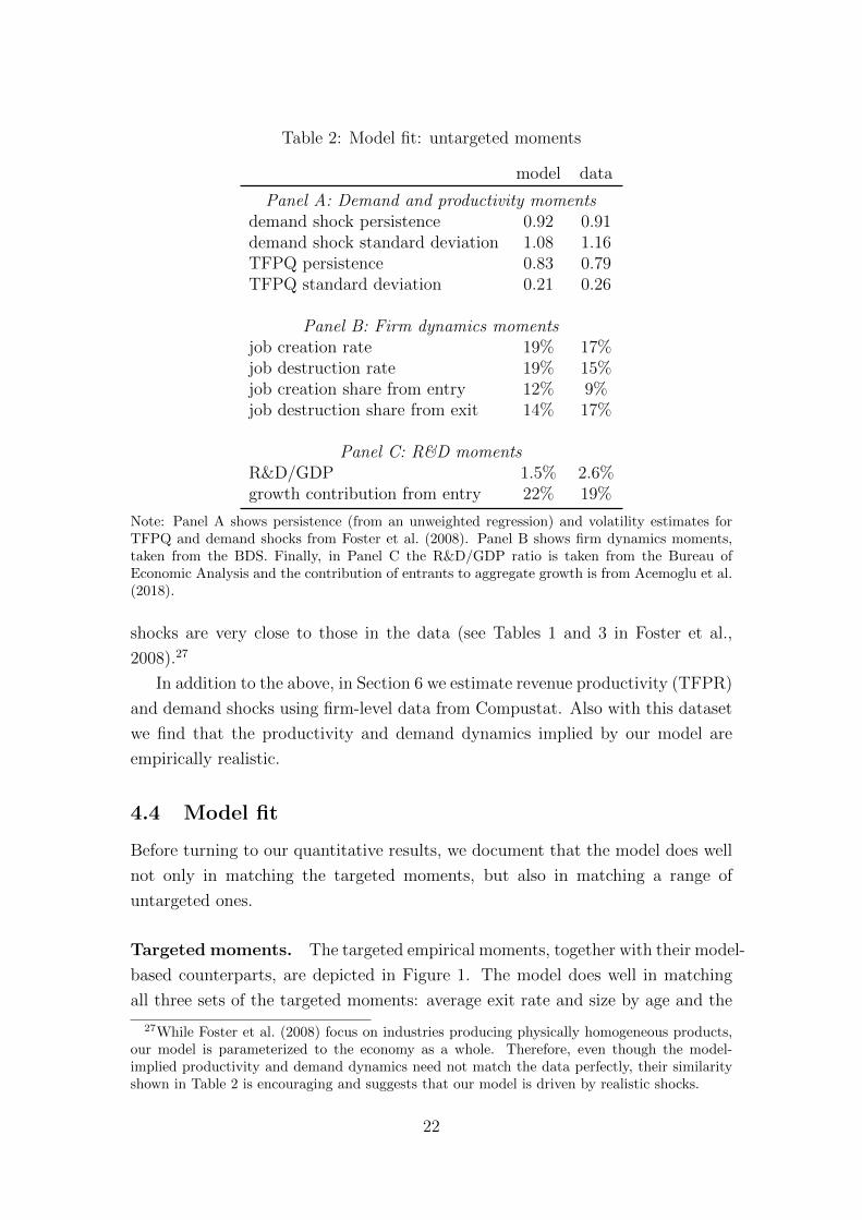
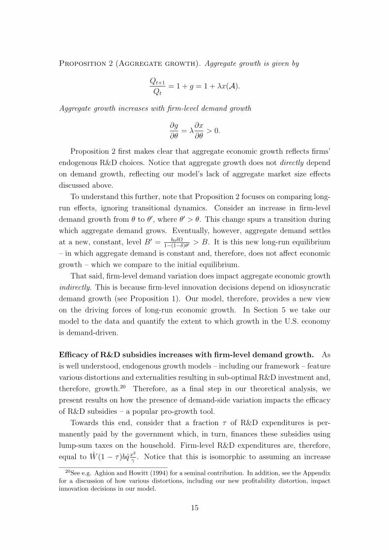
Table 2: Model fit: untargeted moments

model data

Panel A: Demand and productivity momentsdemand shock persistence 0.92 0.91demand shock standard deviation 1.08 1.16TFPQ persistence 0.83 0.79TFPQ standard deviation 0.21 0.26

Panel B: Firm dynamics momentsjob creation rate 19% 17%job destruction rate 19% 15%job creation share from entry 12% 9%job destruction share from exit 14% 17%

Panel C: R&D momentsR&D/GDP 1.5% 2.6%growth contribution from entry 22% 19%

Note: Panel A shows persistence (from an unweighted regression) and volatility estimates forTFPQ and demand shocks from Foster et al. (2008). Panel B shows firm dynamics moments,taken from the BDS. Finally, in Panel C the R&D/GDP ratio is taken from the Bureau ofEconomic Analysis and the contribution of entrants to aggregate growth is from Acemoglu et al.(2018).

shocks are very close to those in the data (see Tables 1 and 3 in Foster et al.,

2008).27

In addition to the above, in Section 6 we estimate revenue productivity (TFPR)

and demand shocks using firm-level data from Compustat. Also with this dataset

we find that the productivity and demand dynamics implied by our model are

empirically realistic.

4.4 Model fit

Before turning to our quantitative results, we document that the model does well

not only in matching the targeted moments, but also in matching a range of

untargeted ones.

Targeted moments. The targeted empirical moments, together with their model-

based counterparts, are depicted in Figure 1. The model does well in matching

all three sets of the targeted moments: average exit rate and size by age and the

27While Foster et al. (2008) focus on industries producing physically homogeneous products,our model is parameterized to the economy as a whole. Therefore, even though the model-implied productivity and demand dynamics need not match the data perfectly, their similarityshown in Table 2 is encouraging and suggests that our model is driven by realistic shocks.

22

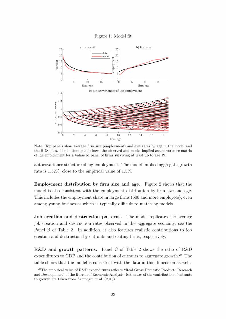
Figure 1: Model fit

Note: Top panels show average firm size (employment) and exit rates by age in the model andthe BDS data. The bottom panel shows the observed and model-implied autocovariance matrixof log employment for a balanced panel of firms surviving at least up to age 19.

autocovariance structure of log-employment. The model-implied aggregate growth

rate is 1.52%, close to the empirical value of 1.5%.

Employment distribution by firm size and age. Figure 2 shows that the

model is also consistent with the employment distribution by firm size and age.

This includes the employment share in large firms (500 and more employees), even

among young businesses which is typically difficult to match by models.

Job creation and destruction patterns. The model replicates the average

job creation and destruction rates observed in the aggregate economy, see the

Panel B of Table 2. In addition, it also features realistic contributions to job

creation and destruction by entrants and exiting firms, respectively.

R&D and growth patterns. Panel C of Table 2 shows the ratio of R&D

expenditures to GDP and the contribution of entrants to aggregate growth.28 The

table shows that the model is consistent with the data in this dimension as well.

28The empirical value of R&D expenditures reflects “Real Gross Domestic Product: Researchand Development” of the Bureau of Economic Analysis. Estimates of the contribution of entrantsto growth are taken from Acemoglu et al. (2018).

23

Figure 2: Firm size-age distribution: data and model

Note: Size-age distribution in the BDS data and in the model. Both distributions are expressedas shares of employment in a given age category (young: < 6 years, middle-aged: 6 − 10 yearsand older: 11− 19 years).

Up-or-out dynamics. Our model is parameterized to match average life-cycle

profiles of firm size and exit. However, the Appendix shows that our model also

predicts realistic dynamics for high-growth firms, so called “gazelles”, and that

it is consistent with the empirical finding that demand is a primary driver of the

observed up-or-out dynamics (see e.g. Foster et al., 2016).

5 Quantitative results

Our analytical results highlight that models which ignore firm-level demand varia-

tion may provide very different predictions regarding (i) firm-level innovation, (ii)

aggregate economic growth and (iii) the sensitivity of the economy to pro-growth

policies.

In this section, we revisit the above conclusions quantitatively and extend our

analysis along several dimensions. As will become clear, endogenous firm selection

– which was absent in our theoretical analysis – plays a key role in this regard.

24

5.1 Two alternative economies

Before presenting our results, we first describe the procedure used to quantify

the key mechanisms in our model. In particular, we make use of two alternative

economies.

The first alternative, referred to as the “counterfactual”, retains all features

of our baseline model, including its parametrization and equilibrium outcomes,

but assumes that firms ignore future expected demand growth. This is, therefore,

conceptually similar to our analytical results in Section 3. This counterfactual

allows us to isolate (in partial equilibrium) the role of expected demand growth

on firm-level innovation and aggregate economic growth.

The second alternative, which we refer to as the “restricted model”, assumes

instead – as in existing endogenous growth models – that firm-level demand is fixed

and common across firms. Importantly, however, we recalibrate the restricted

model to (partially) match the moments targeted by our baseline. Therefore,

the restricted model allows us to pinpoint what is lost in our understanding of

economic growth if we ignore firm-level demand variation.

The counterfactual economy: A decomposition of the baseline. To iso-

late the impact of expected firm-level demand growth on outcomes in the baseline

model, we consider the following counter-factual economy. We retain the entire

model structure and parametrization of the baseline model, but we assume that

firms ignore expected demand growth in their decisions. Instead, we assume that,

in each period, firms do not expect any change in their future idiosyncratic de-

mand levels.29 Therefore, our counterfactual economy is identical to the baseline

model, except for the specification of firm values which are given by

V (qj,t, bj,t) = maxpj,t,ncj,t,n

rj,t

pj,tcj,t −Wt(n

cj,t + nrj,t)+

Etβ(1− δ)

[xj,tV

c(qj,t(1 + λ), bj,t)+

(1− xj,t)V c(qj,t, bj,t)

] , (23)

where “underbars” indicate firm-level variables in the counterfactual economy and

where we’ve made the firm’s state variables explicit. Notice that the only difference

between (23) and firm values in the baseline (20) is in expected future demand.30

29Alternatively, we could assume that firms recognize the stochastic nature of the demandprocess, but expect Et[∆bj,t+1] = 0. We do not prefer this counterfactual, because it effectivelyrestricts demand shocks εj,t+1 to follow a particular life-cycle pattern. The latter is then furtheraway from existing endogenous growth models which ignore demand variation altogether.

30The Appendix provides further details by separately considering “extensive” and “intensive”margin effects. The former relate to changes in the composition of firms, while the latter relateto choices of individual firms.

25

The restricted economy: A comparison to existing growth models. A

natural question to consider is: how much do we miss in understanding aggre-

gate economic growth, when using models which ignore firm-level demand vari-

ation altogether? In order to answer this questions, we consider a “restricted”

(productivity-only) economy which abstracts from firm-level demand variation al-

together – as in existing models of endogenous growth.

In particular, the restricted economy is assumed to be exactly the same as

our baseline except that firm-level demand is fixed and common to all firms, i.e.

σz = σε = σu = σu = σv = 0. In order to achieve a meaningful comparison between

our baseline model and the productivity-only restricted model, we recalibrate the

latter to match the same targets as discussed in Section 4.2, with the exception of

the autocovariance structure of firm-level employment.31 As we discuss in Section

4.2, a model without firm-level demand variation is not able to match the auto-

covariance structure well. Instead, we target the baseline R&D/output ratio, a

common empirical target (see e.g. Akcigit and Kerr, 2018).32

5.2 Selection on productivity or demand?

The decision to remain in operation depends on firms’ expected discounted profits.

Unlike in existing endogenous growth models – in which firm-level productivity is

the sole source of variation in profits – our framework allows also for changes in

firm-level demand to impact firms’ profits and, in turn, their survival.

Given the prominence of creative destruction in modern growth models, the

firm selection process plays a crucial role in understanding the determinants of

aggregate growth. Therefore, we begin our analysis by quantifying the extent to

which firm selection is driven by productivity or demand in our model.

Productivity and demand of entering and exiting firms. The left panel

of Figure 3 shows the distribution of demand, bj, and (relative) productivity, qj,

from the simulated model. Darker shades indicate more densely populated parts

of the state-space.

Since firms select on firm values and firm values are a combination of demand

and productivity, there is a clear negative relationship between the two among

surviving incumbents. Intuitively, if firms enjoy high demand for their product,

they manage to survive despite having lower relative productivity and vice versa.

31Assuming fixed firm-level demand without recalibrating dramatically changes firms’ life-cycle profiles and, in turn, aggregate outcomes. Therefore, such an exercise does not offer ameaningful comparison to our baseline economy.

32The Appendix provides details on the productivity-only model and its fit to the data.

26

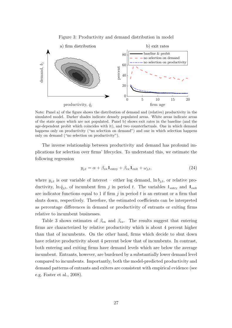
Figure 3: Productivity and demand distribution in model

Note: Panel a) of the figure shows the distribution of demand and (relative) productivity in thesimulated model. Darker shades indicate densely populated areas. White areas indicate areasof the state space which are not populated. Panel b) shows exit rates in the baseline (and theage-dependent probit which coincides with it), and two counterfactuals. One in which demandhappens only on productivity (“no selection on demand”) and one in which selection happensonly on demand (“no selection on productivity”).

The inverse relationship between productivity and demand has profound im-

plications for selection over firms’ lifecycles. To understand this, we estimate the

following regression

yj,t = α + βen1entry + βex1exit + ωj,t, (24)

where yj,t is our variable of interest – either log demand, ln bj,t, or relative pro-

ductivity, ln qj,t, of incumbent firm j in period t. The variables 1entry and 1exit

are indicator functions equal to 1 if firm j in period t is an entrant or a firm that

shuts down, respectively. Therefore, the estimated coefficients can be interpreted

as percentage differences in demand or productivity of entrants or exiting firms

relative to incumbent businesses.

Table 3 shows estimates of βen and βex. The results suggest that entering

firms are characterized by relative productivity which is about 4 percent higher

than that of incumbents. On the other hand, firms which decide to shut down

have relative productivity about 4 percent below that of incumbents. In contrast,

both entering and exiting firms have demand levels which are below the average

incumbent. Entrants, however, are burdened by a substantially lower demand level

compared to incumbents. Importantly, both the model-predicted productivity and

demand patterns of entrants and exiters are consistent with empirical evidence (see

e.g. Foster et al., 2008).

27

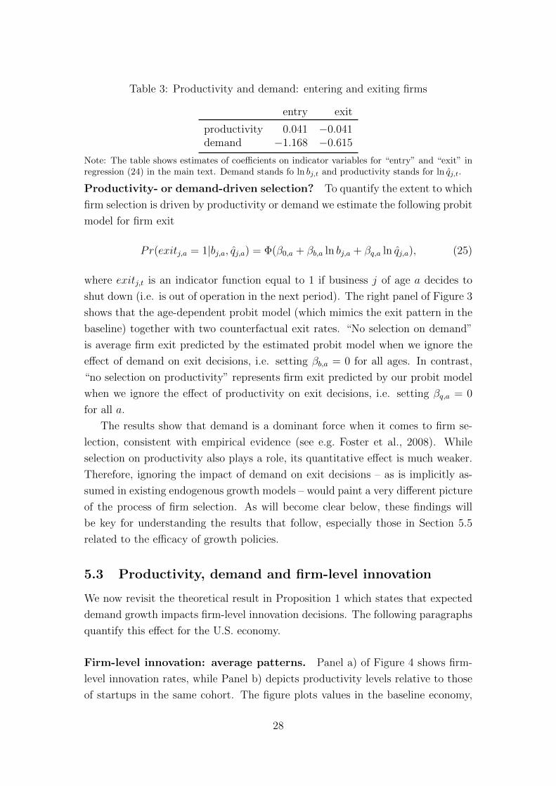
Table 3: Productivity and demand: entering and exiting firms

entry exit

productivity 0.041 −0.041demand −1.168 −0.615

Note: The table shows estimates of coefficients on indicator variables for “entry” and “exit” inregression (24) in the main text. Demand stands fo ln bj,t and productivity stands for ln qj,t.

Productivity- or demand-driven selection? To quantify the extent to which

firm selection is driven by productivity or demand we estimate the following probit

model for firm exit

Pr(exitj,a = 1|bj,a, qj,a) = Φ(β0,a + βb,a ln bj,a + βq,a ln qj,a), (25)

where exitj,t is an indicator function equal to 1 if business j of age a decides to

shut down (i.e. is out of operation in the next period). The right panel of Figure 3

shows that the age-dependent probit model (which mimics the exit pattern in the

baseline) together with two counterfactual exit rates. “No selection on demand”

is average firm exit predicted by the estimated probit model when we ignore the

effect of demand on exit decisions, i.e. setting βb,a = 0 for all ages. In contrast,

“no selection on productivity” represents firm exit predicted by our probit model

when we ignore the effect of productivity on exit decisions, i.e. setting βq,a = 0

for all a.

The results show that demand is a dominant force when it comes to firm se-

lection, consistent with empirical evidence (see e.g. Foster et al., 2008). While

selection on productivity also plays a role, its quantitative effect is much weaker.

Therefore, ignoring the impact of demand on exit decisions – as is implicitly as-

sumed in existing endogenous growth models – would paint a very different picture

of the process of firm selection. As will become clear below, these findings will

be key for understanding the results that follow, especially those in Section 5.5

related to the efficacy of growth policies.

5.3 Productivity, demand and firm-level innovation

We now revisit the theoretical result in Proposition 1 which states that expected

demand growth impacts firm-level innovation decisions. The following paragraphs

quantify this effect for the U.S. economy.

Firm-level innovation: average patterns. Panel a) of Figure 4 shows firm-

level innovation rates, while Panel b) depicts productivity levels relative to those

of startups in the same cohort. The figure plots values in the baseline economy,

28

Figure 4: Profitability vs productivity and innovation

Note: The figure shows average innovation rates (panel a) and productivity relative to that ofstartups (panel b) by age in the baseline and in the counterfactual economy in which firms ignoreexpected demand growth. The figures shows results from the “baseline” and a counterfactualeconomy in which firms expect future demand to be fixed at their, respective, current level.

together with those from our counterfactual in which firms ignore expected demand

growth.

Three points stand out when it comes to the innovation rate. First, in the

baseline economy, the innovation rate declines strongly with firm age. Since young

firms are also on average smaller than incumbents (see Panel b in Figure 1), the

model also predicts that smaller businesses innovate more, consistent with the

empirical evidence (see e.g. Akcigit and Kerr, 2018).33

Second, turning to the impact of demand variation on innovation choices, we

find that firm-level demand variation is quantitatively important for R&D in-

centives. In particular, innovation rates decline by about one half (3 percentage

points) in the counterfactual. This effect is particularly strong for young businesses

which are characterized by the strongest expected demand growth.

Third, the negative relationship of the innovation rate with age in the base-

line is absent in the counterfactual model. These results, therefore, highlight that

expected demand growth is not only quantitatively important for firm-level in-

novation decisions, but that it is also the source of the negative innovation-age

relationship.34

33Akcigit and Kerr (2018) find a negative relationship between patents per worker and logemployment. A similar relationship holds in our model. Specifically, estimating xj,t/cj,t =α+ β ln cj,t + εj,t yields β = −0.02. Similar results hold when replacing sales with employment.

34Note that the impact of firm-level demand on innovation operates predominantly throughexpected benefits from R&D, rather than the assumed scaling of R&D costs, ν(b, q). In par-ticular, expected demand growth is highest for young businesses (about 20% on average), butquickly drops to just below zero from businesses older than five years. Moreover, the Appendixshows that our main results are robust to alternative scaling of R&D costs.

29

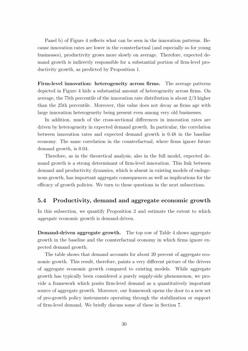
Panel b) of Figure 4 reflects what can be seen in the innovation patterns. Be-

cause innovation rates are lower in the counterfactual (and especially so for young

businesses), productivity grows more slowly on average. Therefore, expected de-

mand growth is indirectly responsible for a substantial portion of firm-level pro-

ductivity growth, as predicted by Proposition 1.

Firm-level innovation: heterogeneity across firms. The average patterns

depicted in Figure 4 hide a substantial amount of heterogeneity across firms. On

average, the 75th percentile of the innovation rate distribution is about 2/3 higher

than the 25th percentile. Moreover, this value does not decay as firms age with

large innovation heterogeneity being present even among very old businesses.

In addition, much of the cross-sectional differences in innovation rates are

driven by heterogeneity in expected demand growth. In particular, the correlation

between innovation rates and expected demand growth is 0.48 in the baseline

economy. The same correlation in the counterfactual, where firms ignore future

demand growth, is 0.04.

Therefore, as in the theoretical analysis, also in the full model, expected de-

mand growth is a strong determinant of firm-level innovation. This link between

demand and productivity dynamics, which is absent in existing models of endoge-

nous growth, has important aggregate consequences as well as implications for the

efficacy of growth policies. We turn to these questions in the next subsections.

5.4 Productivity, demand and aggregate economic growth

In this subsection, we quantify Proposition 2 and estimate the extent to which

aggregate economic growth is demand-driven.

Demand-driven aggregate growth. The top row of Table 4 shows aggregate

growth in the baseline and the counterfactual economy in which firms ignore ex-

pected demand growth.

The table shows that demand accounts for about 20 percent of aggregate eco-

nomic growth. This result, therefore, paints a very different picture of the drivers

of aggregate economic growth compared to existing models. While aggregate

growth has typically been considered a purely supply-side phenomenon, we pro-

vide a framework which posits firm-level demand as a quantitatively important

source of aggregate growth. Moreover, our framework opens the door to a new set

of pro-growth policy instruments operating through the stabilization or support

of firm-level demand. We briefly discuss some of these in Section 7.

30

Table 4: Aggregate economic growth: baseline and counterfactual

Baseline Counterfactual

Aggregate growth 0.0153 0.0126Entrant contribution 22% 32%

Note: The table shows results from the “baseline” and the “counterfactual” in which firmsassume future demand to be fixed at their current, respective, levels.

Creative destruction and aggregate growth. Section 4.2 already discussed

the fact that in the baseline economy startups account for about 22% of aggregate

growth, consistent with empirical estimates (see the second row, first column, of

Table 4).

However, the contribution of entrants to growth is considerably larger (by

almost a half) in the counterfactual economy. This is intuitive since expected

demand growth helps incumbents survive and incentivizes them to conduct R&D,

see Figure 4.

Therefore, models which ignore firm-level demand variation may – at least

partly – overstate the contribution of entrants to pushing aggregate economic

growth. Such conclusions may have important policy implications which often

stress the role of entrants (see e.g. Acemoglu et al., 2018).

5.5 Implications for Growth Policies

As a final step in our quantitative analysis, we explore the extent to which fail-

ing to account for firm-level demand variation changes our understanding of the

macroeconomic impact of growth policies. In doing so, we consider the restricted

(“productivity-only”) economy described in Section 5.1. Recall that this restricted

economy completely abstracts from firm-level demand variation – as is common

in existing growth models – but it is recalibrated to (partially) match the same

targets as our baseline.

Using our baseline and the restricted economy, we analyze two distinct pro-

growth policies studied extensively in existing models and used in practice: subsi-

dies to the costs of R&D and to firms’ operation. As will become clear, our results

suggest that ignoring firm-level demand variation paints a very different picture

of the efficacy of pro-growth policies.

Introducing subsidies to R&D and operational costs. We assume that

– both in the baseline and the restricted model – subsidies to R&D, τr, and to

the costs of operation, τφ, are financed by lump-sum taxes on households, and

31

Table 5: Impact of growth policies

n δ(1− F ) x N W g

Panel A: R&D subsidiesrestricted model +3.7 +3.3 +3.3 −14.6 −0.5 +5.6baseline model +3.4 +5.2 +11.4 −29.4 −1.3 +12.6

Panel B: Operational cost subsidiesrestricted model −9.6 −17.9 +9.5 +15.7 +2.1 −7.3baseline model −24.1 +1.6 −1.2 +39.0 +0.0 −0.8

Note: The table shows long-run effects of subsidies to R&D costs (Panel A) and to the operationof firms (Panel B). The table shows results for the baseline model and a restricted, productivity-only, economy in which firms face constant and common levels of demand. The table depictseffects on average firm size (n), average exit rates (δ(1 − F )), average innovation rates (x),aggregate employment (N), aggregate wage (W ) and aggregate growth (g). Values are reportedin percent deviations from the respective economies without policies.

provided to each business at a common rate. Firm values, therefore, become

V (sj,t) = maxpj,t,ncj,t,n

rj,t

pj,tcj,t −Wt(n

cj,t + (1− τr)nrj,t)+

Eβt(1− δ)[xj,tV

c(s+j,t+1) + (1− xj,t)V c(s−j,t+1)

] , (26)

where V c(sj,t) = max[0,Et−1V (sj,t)−Wtφ(1−τφ)]. In what follows, we will consider

two cases in each economy, one with positive R&D subsidies (but zero subsidies

to operation costs) and one with positive subsidies to costs of operation (but zero

R&D subsidies). In doing so, we ensure comparability by calibrating the subsidies

such that they account for the same share of output in both economies. Finally,

we restrict ourselves to analyzing long-run effects (abstracting from transitional

dynamics) in general equilibrium. We therefore resolve for the models’ equilibria

after the introduction of the policies.

Impact of R&D subsidies. Panel A of Table 5 shows the long-run impact of

R&D subsidies in the baseline and the restricted economies. The implications are

qualitatively similar in both models. R&D subsidies increases innovation rates

and, in turn, raise aggregate growth. Faster economic growth, however, comes

with higher exit rates as firms which are unsuccessful in their innovation attempts

become unprofitable relatively faster. Higher firm exit (especially among younger

businesses) tilts the distribution of firms towards older businesses, raising average

firm size. Despite this, aggregate employment falls as the economy is inhabited

by fewer businesses.35

35We acknowledge that, due to free entry and linear disutility of labor, our framework isparticularly flexible. Note, however, that these two margins are modelled in the same way bothin the baseline and the restricted model.

32

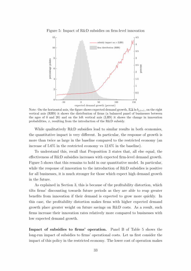
Figure 5: Impact of R&D subsidies on firm-level innovation

-50 0 50 100 150

expected demand growth (percent)

0

2

4

6

8

10

12

percentage

points

0

0.5

1

1.5

2

2.5

3

3.5

4

4.5

percent

subsidy impact on x (LHS)

-rm distribution (RHS)

Note: On the horizontal axis, the figure shows expected demand growth, E∆ ln bj,t+1, on the rightvertical axis (RHS) it shows the distribution of firms (a balanced panel of businesses betweenthe ages of 0 and 20) and on the left vertical axis (LHS) it shows the change in innovationprobabilities, x, resulting from the introduction of the R&D subsidy.

While qualitatively R&D subsidies lead to similar results in both economies,

the quantitative impact is very different. In particular, the response of growth is

more than twice as large in the baseline compared to the restricted economy (an

increase of 5.6% in the restricted economy vs 12.6% in the baseline).

To understand this, recall that Proposition 3 states that, all else equal, the

effectiveness of R&D subsidies increases with expected firm-level demand growth.

Figure 5 shows that this remains to hold in our quantitative model. In particular,

while the response of innovation to the introduction of R&D subsidies is positive

for all businesses, it is much stronger for those which expect high demand growth

in the future.

As explained in Section 3, this is because of the profitability distortion, which

tilts firms’ discounting towards future periods as they are able to reap greater

benefits from innovation if their demand is expected to grow more quickly. In

this case, the profitability distortion makes firms with higher expected demand

growth place greater weight on future savings on R&D costs. As a result, such

firms increase their innovation rates relatively more compared to businesses with

low expected demand growth.

Impact of subsidies to firms’ operation. Panel B of Table 5 shows the

long-run impact of subsidies to firms’ operational costs. Let us first consider the

impact of this policy in the restricted economy. The lower cost of operation makes

33

Figure 6: Demand and productivity distribution in baseline model

Note: The figure shows the distribution of demand and (relative) productivity in the simulatedmodel. Darker shades indicate more densely populated areas. White areas indicate areas of thestate space which are not populated. Panel a) depicts the baseline model without any subsidies.Panel b) depicts the baseline model with a subsidy to operation costs equal to τφ = 0.25. Thevalues q, q, b and b in both the left and right panels indicate the respective lower and upperbounds in the baseline with τφ = 0.

it easier for businesses to survive, resulting in lower exit rates. The decreased

risk of firm exit raises the returns from innovation and therefore firms invest more

into R&D, raising the average probability of innovating. Lower exit rates also

increase the number of businesses in the economy, raising labor demand and thus

wages (consumption) and equilibrium employment. Finally, despite the higher

probability of innovation, aggregate growth slows. This is because the distribution

of firms shifts towards less productive firms which can afford to survive under the

new policy.

While qualitatively the results are similar in the baseline, accounting for firm-

level demand variation renders the model largely insensitive to the subsidy on

operational costs. The reason for this stark quantitative contrast between the

two models lies in the firm selection process, as discussed in Section 5.2. While

in the restricted model – by assumption – firms select purely on productivity,

the baseline model features selection on demand. The latter turns out to be the

dominant driver of business exit, as discussed in Section 5.2.

To understand the impact of the selection process in the baseline model, Figure

6 depicts the joint distribution of productivity and demand before (Panel a) and

after the policy change (Panel b). In addition, both panels of Figure 6 also plot

34

the respective lower (b and q) and upper (b and q) bounds of the distribution prior

to the policy change.

Consistent with our conclusions in Section 5.2, Figure 6 visualizes that the

distribution of firms shifts mainly towards businesses with lower demand levels.

In contrast, the distribution along the productivity dimension changes very little.

Therefore, considering firm-level demand variation fundamentally changes the firm

selection process, affecting the economy’s sensitivity to policies which impact firms’

survival chances.

Taking stock. The results of our two policy experiments show that ignoring

firm-level demand variation – as in existing endogenous growth models – funda-

mentally changes the effects of pro-growth policies. This happens for two reasons.

First, the baseline economy features a novel channel influencing firm-level in-

novation decisions and, in turn, aggregate growth – the profitability distortion.

Businesses with higher expected demand growth are more responsive to R&D in-

centives, because expansions in their market shares help them reap greater benefits

from innovation. Such a mechanism is consistent with existing empirical evidence

(see e.g. Acemoglu and Linn, 2004; Jaravel, 2019).

Second, accounting for firm-level demand variation alters the nature of firm

selection. Consistent with empirical evidence (see e.g. Foster et al., 2008), id-

iosyncratic demand variation is crucial for firm survival in the baseline model.

Therefore, ignoring demand variation leads to a skewed perspective on how pro-

growth policies can affect the process of creative destruction and, in turn, aggre-

gate growth.

6 Empirical support for model mechanism

This subsection provides empirical support for our key channel linking firms’ ex-

pected demand expansions to their innovation decisions and productivity growth.

We first briefly review existing studies which empirically document this relation-

ship in various settings. Next, we draw on firm-level data from Compustat to

estimate this key relationship directly to show that our model is both qualita-

tively and quantitatively consistent with the data.

Brief review of existing evidence on firm-level market size effects. While

the aggregate market size effect has been questioned (see e.g. Jones, 1995), a

number of existing empirical studies find support of such effects at the firm-level.

35

For instance, there is a range of papers focusing on the pharmaceutical indus-

try which identify significant effects between market size expansions (proxied by

demographic changes, introduction of health policies or variation in patent laws)

and firms’ innovation (see e.g Acemoglu and Linn, 2004; Finkelstein, 2004; Kyle

and McGahan, 2012). In addition, using scanner data from the U.S. retail sector,

Jaravel (2019) finds that increasing relative demand leads to increasing product

variety. Finally, Lileeva and Trefler (2010) and Aghion et al. (2020) focus on ex-

ogenous expansions of firms’ export markets and show that they lead to increases

in firm-level innovation and productivity.

Estimating the demand-productivity link using firm-level data. We now

draw on Compustat data between 1962 and 2019, to directly estimate the key

channel predicted by our model. The Appendix provides a description of the data

cleaning process, variable definitions as well as further details of the estimation

procedure and robustness checks.

Our goal is to estimate the extent to which idiosyncratic expected demand

changes affect firms’ decisions to innovate and, in turn, their productivity growth.

In order to estimate expected firm-level demand growth, we proceed in two steps.

First, we follow the procedure in Foster et al. (2008) and estimate idiosyncratic

demand levels, ln bj,t, as the residual from the following regression

ln(salesj,t) = αsq ln(tfpj,t) + αsxXj,t + ln(bj,t), (27)

where Xj,t collects a range of control variables and where tfpj,t is estimated as in

Foster et al. (2016), using the methodology of Levinsohn and Petrin (2003).36

Second, using estimated firm-level demand from (27), we proxy firm-level ex-

pected demand growth, Et−1∆ ln(bj,t), using the predicted values from the following

regression37

∆ ln(bj,t) = αbb∆ ln(bj,t−1) + αbxXj,t−1 + εbj,t. (28)

Having estimated firm-level expected demand growth in (28), we can directly

estimate its effect on idiosyncratic productivity growth, ∆ ln(tfpj,t) from

∆ ln(tfpj,t) = αbj + βbEt−1∆ ln(bj,t) + αqxXj,t + εqj,t, (29)

where αj are firm fixed effects and where the key coefficient of interest is βb.

36Xj,t includes 3-digit-industry-year fixed effects, dividend value, total assets and liquidityratio. Note further that we do not include firm fixed effects, our model features firm fixed effectsin demand which we want to capture in our estimation.

37This effectively assumes firms use mean squared error linear forecasts to form expectations.

36

Table 6: Estimated impact of expected demand growth on productivity growth

(I) (II)

Compustat data 0.060∗∗ 0.057∗∗

(2.48) (2.19)

Baseline model 0.041 0.041

Industry & year fixed effects X XAdditional controls, Xj,t X

Number of observations 93876 93876

Note: Table shows estimates of βb, the relationship between expected demand growth andproductivity growth at the firm level, from (29). The first column does not include additionalcontrols (dividend value, total assets, and liquidity ratio), while the second does. None of theseare included in the model regressions. Brackets indicate bootstrapped z-statistics and ∗∗ indicatesstatistical significance at the 5 percent level. Standard errors are calculated by bootstrap, seethe Appendix for details.

Results from firm-level estimation. Table 6 shows that the link between

expected demand growth and productivity growth, βb, is positive and statistically

significant. Moreover, conducting the same estimation procedure in the baseline

model shows a very similar coefficient.38 While TFP and demand estimates should

always be taken with care, especially when lacking firm-level price data, our results

are encouraging. In particular, they suggest that our key model mechanism – a

link between expected demand growth and productivity changes at the firm level

– is not only present in the data, but also quantitatively reasonable.

7 Concluding remarks

In this paper, we build on the recent and expanding evidence that demand-side

factors are crucial for driving firm-level outcomes. Incorporating this feature into

a new model of endogenous growth in which heterogeneous firms innovate and

operate based on not only productivity, but also demand, we show that firm-level

demand variation partly drives aggregate growth. Estimating our model using

firm data suggests that this link is quantitatively important and that ignoring

demand-side factors can fundamentally alter model predictions about the impact

of growth policies.

We believe that our framework opens the door to several intriguing questions

which we have left for future research. For instance, what new tools could policy-

38While in the data we proxy physical TFP with revenue-based TFP, we do not need to do soin the model. Foster et al. (2008) document that the two are highly correlated. In addition, themodel does not allow for industry fixed effects or additional controls.

37

makers use to spur aggregate growth? While demand-side growth policies have

been debated in policy circles (see e.g. European Commission, 2003), they have

been largely missing from systematic academic analysis within state-of-the-art

models of endogenous growth.39 Our framework suggests that recognized demand-

oriented tools, such as monetary policy, could be used to impact long-run growth.

However, more unconventional and understudied growth policies, such as public

procurement or fiscal transfers, may also be effective in promoting growth.

Finally, our results suggest that economies with different firm life-cycle growth

profiles may have very different aggregate dynamics. What does this imply for

the efficacy of pro-growth policies in developing economies, in which firms’ growth

profiles are much flatter compared to developed countries? And can income in-

equality dynamics affect long-run growth because of associated changes in the

consumption expenditure allocations and, in turn, firm-level growth?

References

Acemoglu, Daron, Ufuk Akcigit, Nicholas Bloom, and William Kerr (2018) “In-

novation, Reallocation and Growth,” American Economic Review, 108 (11),

3450–3491.

Acemoglu, Daron and Joshua Linn (2004) “Market Size in Innovation: Theory And

Evidence from the Pharmaceutical Industry,” Quarterly Journal of Economics,

119 (3), 1049–1090.

Aghion, Philipe, Antonin Bergeaud, Matthieu Lequien, and Marc Melitz (2020)

“The Heterogenous Impact of Market Size on Innovation: Evidence from French

Firm-Level Exports,” mimeo.

Aghion, Philippe and Peter Howitt (1994) “Growth and Unemployment,” Review

of Economic Studies, 61, 477–494.

Akcigit, Ufuk and William Kerr (2018) “Growth through Heterogeneous Innova-

tions,” Journal of Political Economy, 126 (4), 1374–1443.

Arkolakis, Costas (2016) “A Unified Theory of Firm Selection and Growth,” Quar-

terly Journal of Economics, 131 (1), 89–155.

39A notable exception is Slavtchev and Wiederhold (2016) who study the impact of publicprocurement within a multi-sector endogenous growth model with heterogeneous innovationstep sizes.

38

Benigno, Gianluca and Luca Fornaro (2018) “Stagnation Traps,” Review of Eco-

nomic Studies, 85 (3), 1425–1470.

Bernard, Andrew, Emmanuel Dhyne, Glenn Magerman, Kalina Manova, and An-

dreas Moxnes (forthcoming) “The Origins of Firm Heterogeneity: A Production

Network Approach,” Journal of Political Economy.

Bloom, Nicholas, Rachel Griffith, and John Van Reenen (2002) “Do R&D Tax

Credits Work?” Journal of Public Economics, 85 (1), 1–31.

Broda, Christian and David Weinstein (2006) “Globalization and the Gains form

Variety,” Quarterly Journal of Economics, 121 (2), 541–585.

Cavenaile, Laurent, Murat Alp Celik, Pau Roldan-Blanco, and Xu Tian (2021)

“Style over Substance? Advertising, Innovation, and Endogenous Market Struc-

ture,” mimeo.

Cavenaile, Laurent and Pau Roldan-Blanco (2021) “Advertising, Innovation and

Economic Growth,” American Economic Journal: Macroeconomics, 13 (3).

Comin, Diego, Danial Lashkari, and Marti Mestieri (2021) “Structural Change

with Long-Run Income and Price Effects,” Econometrica, 89 (1), 311–374.

European Commission (2003) “Raising EU R&D intensity Improving the effec-

tiveness of the mix of public support mechanisms for private sector research

and development.,”Technical Report EUR 20713, Luxembourg.

Finkelstein, Amy (2004) “Static and Dynamic Effects of Health Policy: Evidence

from the Vaccine Industry,” Quarterly Journal of Economics, 119 (2), 527–564.

Foster, Lucia, John Haltiwanger, and Chad Syverson (2008) “Reallocation, Firm

Turnover, and Efficiency: Selection on Productivity or Profitability?” American

Economic Review, 98 (1), 394–425.

(2016) “The Slow Growth of New Plants: Learning about Demand?”

Economica, 83 (329), 91–129.

Gourio, Francois and Leena Rudanko (2014) “Customer Capital,” The Review of

Economic Studies, 81 (3), 1102–1136.

Hall, Bronwyn, Adam Jaffe, and Manuel Trajtenberg (2001) “The NBER Patent

Citation Data File: Lessons, Insights and Methodological Tools,” NBER Work-

ing Paper 8498.

39

Haltiwanger, John (2012) “Job Creation and Firm Dynamics in the U.S.,” Inno-

vation Policy and the Economy, 17–38.

Haltiwanger, John, Ron Jarmin, Robert Kulick, and Javier Miranda (2016) “High

Growth Young Firms: Contribution to Job, Output and Productivity Growth,”

mimeo.

Haltiwanger, John, Ron Jarmin, and Javier Miranda (2013) “Who Creates Jobs?

Small Versus Large Versus Young,” Review of Economics and Statistics, 95 (2),

347–361.

Hansen, Gary (1985) “Indivisible Labor and the Business Cycle,” Journal of Mon-

etary Economics, 16 (3), 309–327.

Hopenhayn, Hugo A. and Richard Rogerson (1993) “Job Turnover and Policy

Evaluation: A General Equilibrium Analysis,” Journal of Political Economy,

101 (5), 915–938, 10.1086/261909.

Hottman, Collin, Stephen Redding, and David Weinstein (2016) “Quantifying the

Sources of Establishment Heterogeneity,” Quarterly Journal of Economics, 131

(3), 1291–1364.

Jaravel, Xavier (2019) “The Unequal Gains from Product Innovations: Evidence

from the U.S. Retail Sector,” Quarterly Journal of Economics, 134 (2), 715–783.

Jones, Charles (1995) “R&D-Based Models of Economic Growth,” Journal of Po-

litical Economy, 103 (4), 759–784.

Jovanovic, Boyan (1982) “Selection and the Evolution of Industry,” Econometrica,

50 (3), 649–670.

Kehrig, Matthias and Nicolas Vincent (2021) “The Micro-Level Anatomy of the

Labor Share Decline,” Quarterly Journal of Economics, 136 (2), 1031–1087.

Klette, Tor Jakob and Samuel Kortum (2004) “Innovating Firms and Aggregate

Innovation,” Journal of Political Economy, 112 (5), 986–1018.

Kyle, Margaret and Anita McGahan (2012) “Investments in Pharmaceuticals Be-

fore and After TRIPS,” The Review of Economics and Statistics, 94 (4), 1157–

1172.

Lee, Yoonsoo and Toshihiko Mukoyama (2015) “Productivity and employment

dynamics of US manufacturing plants,” Economics Letters, 136, 190–193.

40

Lentz, Rasmus and Dale T Mortensen (2008) “An empirical model of growth

through product innovation,” Econometrica, 76 (6), 1317–1373, Publisher: Wi-

ley Online Library.

Levinsohn, James and Amil Petrin (2003) “Estimating Production Functions Us-

ing Inputs to Control for Unobservables,” The Review of Economic Studies, 70

(2), 317–341.

Lileeva, Alla and Daniel Trefler (2010) “Improved Access to Foreign Markets

Raises Plant-Level Productivity... For Some Plants,” The Quarterly Journal

of Economics, 125 (3), 1051–1099.

Mrazova, Monika and Peter Neary (2017) “Not So Demanding: Demand Structure

and Firm Behavior,” American Economic Review, 107 (12), 3835–3874.

Mukoyama, Toshihiko and Sophie Osotimehin (2019) “Barriers to Reallocation

and Economic Growth: The Effects of Firing Costs,” American Economic Jour-

nal: Macroeconomics, 11 (4), 235–270.

Perla, Jesse (2019) “A Model of Product Awareness and Industry Life Cycles,”

mimeo.

Rachel, Lukasz (2021) “Leisure-Enhancing Technological Change,” mimeo.

Rogerson, Richard (1988) “Indivisible Labor, Lotteries, and Equilibrium,” Journal

of Monetary Economics, 21 (1), 3–16.

Sedlacek, Petr (2019) “Creative Destruction and Uncertainty,” Journal of the Eu-

ropean Economic Association, 18 (4), 1814–1843.

Sedlacek, Petr and Vincent Sterk (2017) “The Growth Potential of Startups over

the Business Cycle,” American Economic Review, 107 (10), 3182–3210.

Slavtchev, Viktor and Simon Wiederhold (2016) “Does the Technological Content

of Government Demand Matter for Private R&D? Evidence from US States,”

American Economic Journal: Macroeconomics, 8 (2), 45–84, https://pubs.

aeaweb.org/doi/10.1257/mac.20130069.

Stein, Jeremy (1997) “Waves of Creative Destruction: Firm-Specific Learning-by-

Doing and the Dynamics of Innovation,” Review of Economic Studies, 64 (2),

265–288.

Sterk, Vincent rO Petr Sedlacek rO Benjamin Pugsley (2021) “The Nature of Firm

Growth,” American Economic Review, 111 (2).

41

Young, Alwyn (1998) “Growth without Scale Effects,” Journal of Political Econ-

omy, 106 (1), 41–63.

Appendix

Proof of Proposition 1. Substituting the demand constraint (8) and optimal

pricing (12) into the consumption aggregator (2), we can write W = Q(η − 1)/η.

Using this expression, together with optimal labor supply (7) and pricing condi-

tions (12), stationarized per-period profits are given by π = bq[

14υ− x2

2γ

]. Firm

value can, therefore, be written as

V (s) = π + β(1− δ)[xV (s+) + (1− x)V (s−)

], (30)

where s = (bq, b, θ), where q = q/Q, s+ = (bqθ(1 + λ)/(1 + g), bθ, θ) and s− =

(bqθ/(1 + g), bθ, θ), implying x = γbqβ(1 − δ)

(V (s+)− V (s−)

). Using our guess

for the value function, V = Abq, yields

x = γβ(1− δ)(1 + g)

θλA. (31)

Using (31) in (30), equating it with our guess that V = Abq and solving for A as

the positive real solution to the resulting quadratic equation implies

A(θ) =

[(1

4υ− x2

2γ

)][1− β(1− δ)

(1 + g)(1 + λx (A)) θ

]−1

> 0. (32)

Finally, letting β = β 1−δ1+g

and β(x, θ) = 1

1−β(1+λx)θ, taking g as given in partial

equilibrium (PE), using (32), totally differentiating (31) and collecting terms we

get

εx,θ|PE =dx

dθ

θ

x|PE = 1 + ββ(1 + λx)θ > 0.

Doing the same, but accounting for the fact that g = λx in general equilibrium

(GE), we get

εx,θ|GE =dx

dθ

θ

x|GE =

1 + g

(1 + g)(1− β(1− δ)θ) + g> 0.

42

Proof of Proposition 2. Under Assumption 1 we can write

Q′ =∑a=0

∫j∈µa

baq′jdj =

∑a=0

∫q

baθqQ(1 + λx)(1− δ)µa(q) +

∫qeb0q

eQ(1 + λx)µ0(qe)

=Q(1 + λx)

[∑a=1

∫q

baqµa(q) +

∫qeb0q

eµ0(qe)

]= Q(1 + λx),

where primes indicate next period’s values. Therefore, 1 + g = Q′/Q = 1 + λx.

Finally, using Proposition 1, we have ∂g/∂θ = λ∂x/∂θ > 0.

Proof of Proposition 3. Taking g as given and differentiating (31) with respect

to γ gives dx = ββ(x, θ)λθ 14υdγ and hence

εx,γ =dx

dγ

γ

x=ββ(x, θ)λθγ 1

4υ

x=x+ ββ(x, θ)λθ x

2

2

x= 1 + ββ(x, θ)λθ

x

2> 1. (33)

Finally, given εxθ > 0 and ∂β(x,θ)∂θ

+ ∂β(x,θ)∂x

∂x∂θ

= β(x, θ)2β(1+λ(x+θ)) > 0, we have

∂εxγ∂θ

=ββ(x, θ)λx

2+ ββ(x, θ)λ

θ

2

∂x

∂θ+ βλθ

x

2

(∂β(x, θ)

∂θ+∂β(x, θ)

∂x

∂x

∂θ

)=1 + εxθ +

θ

β(x, θ)

(∂β(x, θ)

∂θ+∂β(x, θ)

∂x

∂x

∂θ

)> 0

Proof of Proposition 4. By premise i) of the Proposition, we can write lnnj,a =

lnχ+ ln qj,a and hence

cov(lnnj,a, lnnj,a−h) = cov(ln qj,a, ln qj,a−h). (34)

By premise ii) of the Proposition, we know that cov(ln qj,a − ln qj,a−h, ln qj,a−h) =

cov(ln qj,a, ln qj,a−h)− var (ln qj,a−h) = 0, implying

cov(ln qj,a, ln qj,a−h) = var (ln qj,a−h) . (35)

Using (35) in (34) implies cov(lnnj,a, lnnj,a−h) = var (ln qj,a−h) = var(lnnj,a−h).

43