Productivity and the Natural Rate of Unemployment€¦ · · 2006-02-08Productivity and the Natural Rate of Unemployment* Jiri Slacalek Department of Macro Analysis and Forecasting,

Productivity and the Natural Rate of Unemployment*

Jiri Slacalek

Department of Macro Analysis and Forecasting, DIW Berlin

March 2005

E-mail: [email protected]

I propose an econometric model that improves upon existing meth-

ods of estimating the natural rate of unemployment (NAIRU) by us-

ing information contained in the trend of productivity growth. My

approach enhances the recently proposed model of Staiger, Stock and

Watson (1997) in several respects. Statistically speaking, the method

substantially shrinks the width of the 95% confidence interval, performs

better in an out-of-sample inflation forecasting exercise, and is more

robust to alternative statistical assumptions. In economic terms, the

productivity-augmented model generates a more realistic time profile of

the NAIRU, and implies estimates of the Phillips curve slope and the

sacrifice ratio that are more in line with conventional wisdom. I also

test whether the natural rate is correlated with the level or with the

change of the productivity growth trend. I find support for the “level”

hypothesis in both the US and international data.

Keywords: natural rate of unemployment, productivity, Phillips curve, time-

varying parameters, Kalman filter

JEL Classification: C22, E31, E50

* This research is a part of my dissertation in the Department of Economics, Johns

Hopkins University. I am grateful to Laurence Ball, Christopher Carroll, Louis Maccini,

Athanasios Orphanides and Jonathan Wright for many helpful discussions. I would like to

thank to Elif Arbatli, Danny Gubits, Daniel Leigh and participants of the Johns Hopkins

Macro Lunch for comments. Replication files are available at http://www.econ.jhu.edu/

people/slacalek/.

1. INTRODUCTION

Two central features of the natural rate of unemployment (NAIRU, nonac-

celerating inflation rate of unemployment) are its substantial time variation

and the considerable uncertainty that surrounds it. Furthermore, recent em-

pirical work (Staiger, Stock and Watson, 2001) has found a strong negative

correlation between the natural rate and the trend of productivity growth

in the United States. This paper proposes an econometric model that im-

proves upon existing method for estimating the NAIRU of Staiger, Stock

and Watson (1997) by using information contained in the trend of produc-

tivity growth. My method makes it possible to estimate the natural rate

more precisely and outperforms current approaches in several other respects.

Many authors (Gordon, 1997, Gordon, 1998, Katz and Krueger, 1998,

Staiger et al., 2001, and others) document that the time profile of the natural

rate varies substantially over time. For example, Gordon’s (1997) preferred

estimate of the NAIRU declines from a peak of about 6.5% in 1980 to a low

of 5.6% by mid-1996. Besides being of interest for the monetary authority,

the estimate of the natural rate is crucial for producing accurate inflation

forecasts. The failure to account for the time variation in the natural rate

caused the forecasting performance of the standard Phillips curves to break

down in the late 1990s (Ball and Moffitt, 2001). Consequently, it is not

acceptable to model the natural rate as a constant.

Staiger et al. (2001) report that the trends of unemployment and produc-

tivity growth co-move strongly. I reproduce their finding in Figure 1. The

correlation between the trends in unemployment and productivity growth

(as measured by Staiger et al., 2001) over the 1960–2001 period is −0.8.

2

PRODUCTIVITY AND THE NATURAL RATE 3

FIG. 1. Productivity and the Natural Rate of Unemployment (NAIRU) Bandpass

1960 1965 1970 1975 1980 1985 1990 1995 2000

0

2

4

6

8

10

Productivity and the NAIRU

NAIRUProductivityUnemployment

Notes: The trends are estimated using the Baxter and King (1999) bandpass filter

with upper cutoff frequency of 60 quarters.

TABLE 1.

Averages for Productivity, Unemployment and Inflation

1960–1973 1974–1995 1995–2002

Productivity Nonfarm Business 2.759 2.009 2.286

Unemployment 4.953 5.925 4.869

Inflation 2.818 4.234 2.378

Diff Productivity Nonfarm Business −0.016 −0.001 0.026

Notes: Quarterly Data. The productivity means are calculated from the productivity

trend generated by the Baxter and King (1999) bandpass filter with upper cutoff

frequency of 60 quarters.

The descriptive statistics for productivity and unemployment displayed in

Table 1 also illustrate this inverse relationship. Productivity growth was

rapid before 1973, slowed down after 1973 for more than twenty years and

then resumed vigorously after 1995. The average unemployment rate, on the

other hand, was more than 1 percentage point higher between 1973 and 1995

4 JIRI SLACALEK

than before and after that period. The co-movement of unemployment and

productivity growth trends is an impressive result since no unemployment

data are used to construct productivity data (and vice versa).

This paper extends the random walk framework (Staiger et al., 1997)

by using information contained in the trend of productivity growth. The

original formulation assumes that the natural rate is completely driven by

an unobserved white noise variable. The productivity growth trend explains

a large fraction of the variation in the NAIRU and including it significantly

shrinks the unexplained part. This finding is intuitive since including a

relevant variable in the regression usually improves its explanatory power.

My approach improves upon the random walk method in several respects.

Statistically speaking, the method substantially shrinks the width of the

95% confidence interval, performs better in an out-of-sample inflation fore-

casting exercise, and is more robust to alternative statistical assumptions.

In economic terms, the productivity-augmented model generates a more re-

alistic time profile of the NAIRU, and implies estimates of the Phillips curve

slope and the sacrifice ratio that are in line with conventional wisdom.

I also test whether the natural rate is correlated with the level or with

the change of the productivity growth trend. I find support for the “level”

hypothesis in both the US and international data. This is surprising because

many models proposed recently to explain the relationship between the nat-

ural rate and productivity growth (Meyer, 2001, Ball and Moffitt, 2001,

Mankiw and Reis, 2003) are consistent with the “change” hypothesis. A

crucial assumption of this recent research is that workers’ estimates of pro-

ductivity growth adjust slowly to true productivity growth. As a result,


these models explain the negative correlation between the natural rate and

the change in productivity growth, rather than between the natural rate and

the level of productivity growth. However, there is some theoretical work

in the job search and matching literature that might be able to explain a

negative correlation of the NAIRU and the level of productivity growth.

The paper is organized as follows. Section 2 reviews the theoretical litera-

ture on the relationship between the natural rate and productivity. Section 3

proposes the econometric model and discusses econometric issues. Section 4

reports the empirical findings of the baseline model for the US. Section 5

summarizes the robustness of the results and tests the “level vs. change” hy-

pothesis. Section 6 focuses on the international evidence on the relationship

between productivity growth and the natural rate. Section 7 concludes.

2. PRODUCTIVITY AND THE NAIRU: THEORY REVIEW

There are two lines of research that attempt to explain the inverse relation-

ship between productivity growth and the natural rate. Some economists

argue that the link is caused by a mismatch between the perceptions of

productivity growth by workers and firms. Other explanations, based on

search and matching models, propose that productivity growth translates

into structural change that also raises unemployment.

In the first line of research, firms are typically assumed to observe the

productivity growth trend. Workers, in contrast, have to infer the pro-

ductivity trend based on limited information. For instance, Braun (1984)

and Meyer (2001) assume that workers base their wage claims on a real-

time estimate of the productivity trend. Ball and Moffitt (2001) suggest

6 JIRI SLACALEK

that workers’ real wage targets depend on aspirations, a weighted average

of past real wages. Mankiw and Reis (2003) propose a sticky-information

model in which a randomly chosen fraction of workers updates informa-

tion on productivity each period. While these models start from different

premises, they have similar implications. They all predict that an increase

in productivity growth temporarily lowers inflation and the natural rate.

Strictly speaking, these models do not explain the correlation between the

levels of the NAIRU and of productivity growth. However, if the workers’

estimates of the productivity growth trend adjusts slowly to the true value,

the implications of these models will be hard to distinguish from the level

hypothesis.

There is a modest amount of work on the effect of productivity growth on

unemployment in the theoretical job search literature (Aghion and Howitt,

1994, Mortensen and Pissarides, 1998). Productivity growth has two com-

peting effects. First, higher labor productivity growth increases the value

of a worker to the firm, and stimulates the creation of job vacancies. This,

in turn, causes unemployment to decline (the capitalization effect). Second,

higher productivity growth is often accompanied by structural change. Old

jobs are destroyed and replaced by new ones (the creative destruction ef-

fect). As a result, productivity acceleration shortens employment duration

and raises the natural rate. Consequently, the correlation between produc-

tivity growth and the natural rate depends on the relative size of these two

effects.


Empirically, the negative correlation between the productivity growth

trend and the natural rate in Figure 1 along with the results below sug-

gest that the capitalization effect is stronger.

3. ECONOMETRIC MODEL

In the empirical literature, the NAIRU is typically estimated in the Phillips

curve framework as the rate of unemployment that is consistent with stable

inflation expectations. This section first reviews existing methods of mod-

elling the natural rate both as a constant and in the time-varying parameter

framework. I then propose the productivity-augmented model and discuss

some econometric issues.

Assume for the moment that the natural rate u is constant. To estimate

the NAIRU, start with the expectations-augmented Phillips curve,

∆πt = γ(L)(ut−1 − u) + δ(L)∆πt−1 + α(L)Xt + εt, (1)

where γ(L), δ(L) and α(L) are lag polynomials and Xt includes supply

shocks. The Phillips curve (1) follows much of the empirical literature in

assuming that inflation expectations follow a random walk, πet = πt−1. The

natural rate can be estimated by ordinary least squares (OLS) as the hori-

zontal intercept. Specifically, after running the regression

∆πt = γ0 + γ(L)ut−1 + δ(L)∆πt−1 + α(L)Xt + εt

the estimate of the NAIRU is u = −γ0/γ(1), where γ(1) is the sum of

unemployment coefficients.

The constancy of the natural rate is a very restrictive assumption. As

Gordon (1997, p. 12) puts it, “the NAIRU is not carved in stone.” Fried-

8 JIRI SLACALEK

man (1968) defines the natural rate as the “level which would be ground out

by the Walrasian system of general equilibrium equations, provided there is

imbedded in them the actual structural characteristics of the labor and com-

modity markets.” To capture the effects of changes in these characteristics

on the NAIRU, Staiger, Stock and Watson (1997) propose the time-varying

parameter model (Kalman filter),

∆πt = γ(L)(ut−1 − ut−1) + δ(L)∆πt−1 + α(L)Xt + εt,

ut = ut−1 + ηt, var(ηt) = λvar(εt).(2)

The natural rate ut is now assumed to follow a random walk. The variation

in ut is governed by the signal-to-noise parameter λ ≡ var(ηt)/var(εt). If

λ = 0, the NAIRU is constant and (2) reduces to (1).

The random walk model is a flexible device that captures the unobserved

time-variation in the natural rate. However, when there are variables that

are informative about the NAIRU, it is more efficient to include them in the

model. This decreases the unexplained variation, var(ηt) and increases .

The Kalman filter framework can be generalized by including exogenous

variables Zt in the second equation of (2),

∆πt = γ(L)(ut−1 − ut−1) + δ(L)∆πt−1 + α(L)Xt + εt,

ut = ut−1 + β>∆Zt + ηt, var(ηt) = λvar(εt).(3)

In model (3) a fraction of the variation in the state variable ut is explained

by exogenous variables in Zt. Consequently, the variance of the error term

ηt in the random walk model (2) is greater than the variance of the error in

(3) and as a result model (3) explains ut better.

The natural rate in (3) is modelled as a random walk driven by the ex-

ogenous variables Zt and the error term ηt. This specification is chosen, as


is usual in the literature to allow for persistent deviations of ut from βZt.

It is important to note that the specification (3) implies that differences in

Zt affect differences in the natural rate ut or, equivalently, that levels of Zt

affect levels of ut.

In the baseline specification the exogenous variables Zt consist of the pro-

ductivity trend θ∗t , obtained by the Kalman filter as explained below. Spec-

ification (3) assumes that Zt only influences ut. Therefore, there is no direct

effect of Zt on ∆πt. Supply shocks Xt are, in contrast, very volatile and I

therefore follow the existing literature in assuming that they do not affect

the natural rate ut.

Econometric Issues

The productivity trend θ∗t is estimated by the random walk plus noise (or

local level) model,

θt = θ∗t + zTt, θ∗t = θ∗t−1 + zPt, var(zTt) = λθvar(zPt) (4)

where θt is the observed, measured productivity growth rate, θ∗t is the un-

observed trend to be estimated and zTt and zPt are the temporary and

permanent shocks to productivity, respectively. This specification is a flexi-

ble device that makes it possible to extract the long-run trend from the time

series using the Kalman filter algorithm. The Kalman filter is an alterna-

tive to the more common filters, such as the Hodrick–Prescott filter. The

advantage of the Kalman filter model (4) is that the algorithm produces

10 JIRI SLACALEK

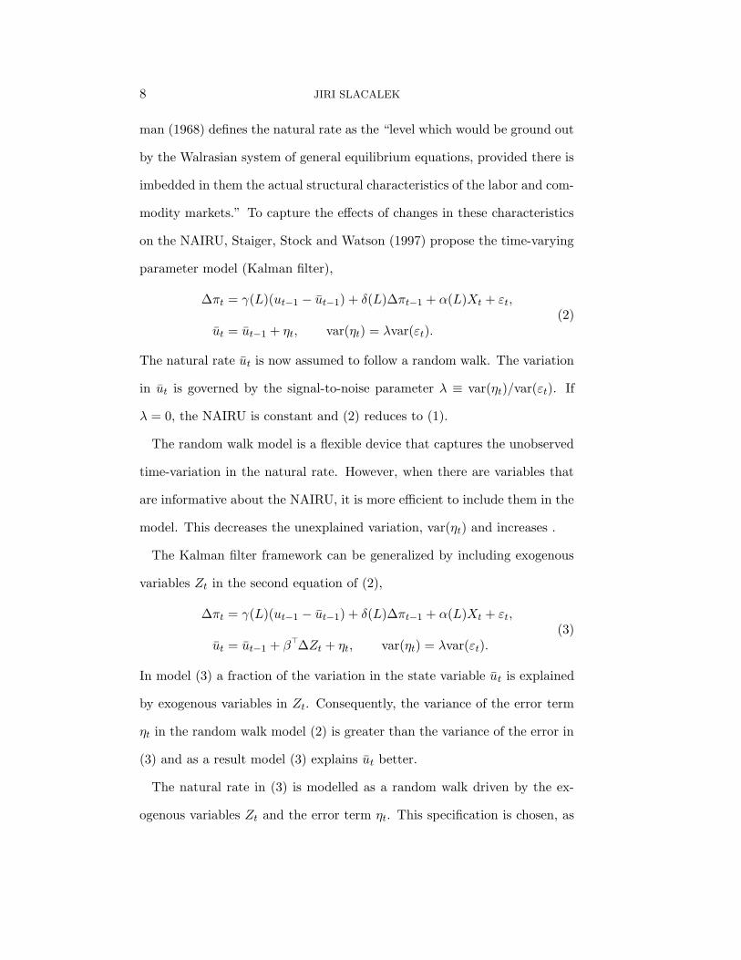
FIG. 2. Productivity Growth and Trend

1960 1965 1970 1975 1980 1985 1990 1995 2000−4

−3

−2

−1

0

1

2

3

4

5

6US Productivity Growth

Kalman SmootherBandpassActual


with upper cutoff frequency of 60 quarters and Kalman smoother with the signal-to-noise

ratio λθ = 0.005. The actual productivity growth is year-on-year quarterly growth.

an optimal estimator of the trend (the minimum mean squared error linear

estimator), see for example Harvey (1989).1

I assume that the disturbances εt and ηt in (2) and (3) are i.i.d. normal

N(0, var(εt)) and N(0, var(ηt)), respectively. Furthermore, the disturbances

εt and ηt are also assumed to be uncorrelated. I estimate the parameters

{γ(L), δ(L), α(L), β, var(εt)} by maximum likelihood (ML), as described in

Harvey (1989).

The amount of time variation in ut is governed by the signal-to-noise pa-

rameter λ. Since the NAIRU varies slowly over time, the variance of ηt is

usually very small. Consequently, the estimate of var(ηt) has bad small-

1I consider the productivity trend θ∗t obtained by the bandpass filter in section 5 below.

Figure 2 compares the productivity trends measured by the Kalman and bandpass filters.


sample properties—it is estimated very imprecisely, with a downward bias.

Besides, in small samples the distribution of the signal-to-noise ratio λ has a

non-zero probability mass at zero, a so-called pile-up problem. This results

in the implied natural rate of unemployment being too smooth, often almost

constant. Consequently, I follow existing literature (Staiger et al., 2001,

King, Stock and Watson, 1995, and others) in imposing a reasonable value

for λ instead and estimating the remaining parameters by ML. Interestingly,

the estimate of the natural rate in the productivity model (3) is consider-

ably more robust to the choice of λ than in the random walk model, as

documented in section 5.

Stock and Watson (1998) propose an alternative to imposing λ. The

method consists of conducting the sup-Wald structural break test for a break

in the constant in the Phillips curve. One then compares the test statistic

to the table of Stock and Watson (1998) critical values and retrieves the

implied median-unbiased estimate of λ together with its confidence inter-

vals. I estimate the signal-to-noise ratios λ using this method and report

the median-unbiased estimates of var(ηt) in the last line of Table 2 below.

However, I do not use the method in the calculations because the confidence

intervals for λ tend to be very wide and the estimated signal-to-noise ratios

are less satisfactory in some cases than the imposed ones.

4. EMPIRICAL RESULTS

In this section I compare three benchmark models estimating the natural

rate: the constant NAIRU model (1), the random walk model (2) of Staiger

et al. (1997), and the productivity-augmented model (3). The major flaw

12 JIRI SLACALEK

TABLE 2.

Estimation Results, Baseline Models

OLS Random Walk Productivity

Sum of Coeffs on Unemployment −0.199 −0.147 −0.224

Std Error on Sum of Unemployment 0.076 0.111 0.121

P value on Lags of Unemployment 0.009 0.000 0.000

P value on Lags of Inflation 0.000 0.000 0.000

P value on Supply Shocks 0.004 0.285 0.024

P value on Productivity – – 0.062

Coefficient on Productivity – – −2.251

Mean Width of Confidence Intervals 3.078 4.114 2.985

Sacrifice Ratio 2.297 2.979 2.101

Estimate of the Signal-to-Noise Ratio – 0.011 0.022

Log-likelihood – −127.880 −129.380

Notes: The confidence intervals for the OLS model are calculated following Staiger et

al. (1997)using the Anderson–Rubin exact method based on inverting the F statistic of

H0: u = u0 for various values of u0. All p values are based on the White heteroscedasticity-

robust standard errors. P value of 0 means less than 5× 10−4.

of the first model is the assumption of the constant NAIRU. The random

walk model performs poorly in several respects. It produces wide confidence

intervals and an unrealistic time profile of the natural rate. Moreover, the

slope of the Phillips curve and the implied sacrifice ratio are not in line with

the conventional wisdom. The productivity model alleviates these short-

comings.

Table 2 reports the findings. Column one summarizes the traditional

backward-looking Phillips curve with the constant NAIRU. Its principal

strength is that the statistics are in line with conventional wisdom. The lags

of inflation, unemployment, and supply shocks are significant. The value of

the slope, γ(1), is comparable to the findings of other authors. Finally, the

implied sacrifice ratio, the unemployment cost of reducing inflation, is in

the upper range of estimates obtained by Ball (1994) and others. In light


of the recent decline of the natural rate, its assumed constancy is a crucial

shortcoming. The reported estimate of the natural rate of about 6% can

be in principle interpreted as the average value of the true time-varying

NAIRU (TV-NAIRU). However, it is questionable how useful it is for the

monetary authority to know the average natural rate when the NAIRU varies

substantially.

4.1. Confidence Intervals

The random walk model (2) was proposed to account for the time-variation

in the natural rate. However, it is problematic in other respects. First, the

slope of the random walk Phillips curve in column 2 of Table 2 is consid-

erably smaller in magnitude than the slope of the OLS Phillips curve and

statistically insignificant.2 This has a crucial implication for the estimate of

the natural rate. The slope γ(1) enters the denominator of the estimate of

the NAIRU, which causes the natural rate to be unidentified when the slope

is zero. Similarly, when γ(1) is small the confidence intervals for the natural

rate tend to be extremely wide (see Staiger et al., 2001). The productivity

model, in contrast, implies a greater Phillips curve slope, which narrows

the NAIRU confidence intervals. This subsection compares the confidence

intervals implied by the various models.

Figure 3 depicts the NAIRU confidence intervals implied by the random

walk and the productivity models. The confidence intervals are calculated

from the variance of the Kalman smoother estimate of ut with a delta method

2The estimates of slopes of the OLS and random walk Phillips curves are consistent with

other specifications in the literature, e.g. Staiger et al. (1997) and Staiger et al. (2001),

respectively.

14 JIRI SLACALEK

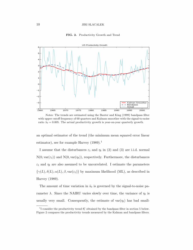
FIG. 3. Comparison of Productivity-driven and Random Walk Confidence Intervals

for the NAIRU

σ2η/σ2

ε=λ=0.01, λ imposed

The NAIRU as an Unobserved Random Walk (Kalman Filter) Driven By Productivity II.

1960 1965 1970 1975 1980 1985 1990 1995 20000

1

2

3

4

5

6

7

8

9

10

11Kalman SmootherUnemployment95% RW CI95% Prod CI

Notes: The natural rate of unemployment is estimated by the Kalman filter model

(3) with the signal-to-noise ratio λ = 0.01. The confidence intervals have 95% size and

are obtained from the estimate of the variance of the Kalman smoother and corrected

for parameter uncertainty following Ansley and Kohn (1986).

correction for parameter uncertainty due to Ansley and Kohn (1986). The

method is consistent with Staiger et al. (1997).

The average width of confidence intervals shrinks from 4.1 percentage

points for the random walk model to 3.1 percentage points with the pro-

ductivity model. The black solid line in Figure 3 depicts the replication

with quarterly data, 1960–2002 of the 95% confidence intervals of Staiger et

al. (1997). In fact, even though the point estimates of the natural rates in

Figure 4 differ by up to 1%, the shaded confidence band for the productivity

model is for most periods within the confidence band of the random walk

model.


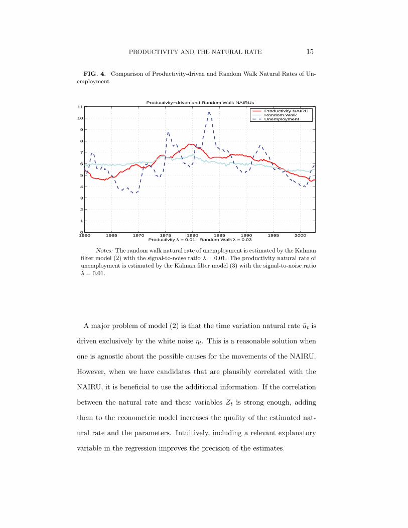
FIG. 4. Comparison of Productivity-driven and Random Walk Natural Rates of Un-

employment

1960 1965 1970 1975 1980 1985 1990 1995 20000

1

2

3

4

5

6

7

8

9

10

11

Productivity λ = 0.01, Random Walk λ = 0.03

Productivity−driven and Random Walk NAIRUs

Productivity NAIRU Random WalkUnemployment

Notes: The random walk natural rate of unemployment is estimated by the Kalman

filter model (2) with the signal-to-noise ratio λ = 0.01. The productivity natural rate of

unemployment is estimated by the Kalman filter model (3) with the signal-to-noise ratio

λ = 0.01.

A major problem of model (2) is that the time variation natural rate ut is

driven exclusively by the white noise ηt. This is a reasonable solution when

one is agnostic about the possible causes for the movements of the NAIRU.

However, when we have candidates that are plausibly correlated with the

NAIRU, it is beneficial to use the additional information. If the correlation

between the natural rate and these variables Zt is strong enough, adding

them to the econometric model increases the quality of the estimated nat-

ural rate and the parameters. Intuitively, including a relevant explanatory

variable in the regression improves the precision of the estimates.

16 JIRI SLACALEK

FIG. 5. Random Walk Natural Rate of Unemployment

σ2η/σ2

ε=λ=0.03

The NAIRU as an Unobserved Random Walk (Kalman Filter)

1960 1965 1970 1975 1980 1985 1990 1995 20000

1

2

3

4

5

6

7

8

9

10

11Kalman SmootherUnemployment95% CI

Notes: The natural rate of unemployment is estimated by the Kalman filter model

(2) and assumed to follow unobserved random walk model with the signal-to-noise ratio

λ = 0.03. The parameter λ is chosen to mimic the estimates of Staiger et al. (1997). The

confidence intervals have 95% size and are obtained from the estimate of the variance

of the Kalman smoother and corrected for parameter uncertainty following Ansley and

Kohn (1986).

4.2. Time Profile of the Estimates of the Natural Rate

One important shortcoming of the random walk model is that it implies

an unrealistic estimate of the time profile of the natural rate. There is not

only evidence that the NAIRU is not constant, we actually have a prior on

how it varies. We typically think of it as a slowly varying, smooth function

of time. Large abrupt changes in the natural rate are very unlikely.

The NAIRU time profile of the random walk model is displayed in Fig-

ure 5, a replication of Staiger’s et al. (1997) Figure 6. There are at least

two problems with the NAIRU profile: it is both excessively sensitive and

excessively smooth. More precisely, there is too much high-frequency varia-


tion and not enough low-frequency variation in the estimate of the natural

rate. The natural rate of Figure 5 is not very smooth, at the same time

its constancy cannot be rejected. Unfortunately, increasing the λ param-

eter affects the high-frequency variation in the natural rate and does not

improve the results much.3 The random walk model substitutes the lack of

low-frequency variation in the natural rate with the high-frequency varia-

tion. Figure 4 documents that this does not work satisfactorily. Both the

rise in the NAIRU in the late 1970s and its fall in the late 1990s are much

less pronounced for the random walk model than for the productivity model.

Interestingly, the shape of the time-varying NAIRU implied by the pro-

ductivity model is much closer to the conventional wisdom. This is because

the productivity growth adds more low-frequency variation and at the same

time decreasing λ makes it possible to lower the high-frequency variation in

the NAIRU. The productivity growth is borderline significant with a p value

of 0.048. The sensitivity of the natural rate with respect to the productiv-

ity growth, β, is about −2, which means that if the level of productivity

growth increases by 1%, the natural rate declines by 2 percentage points.

Assuming productivity growth went up by 0.6 percentage points in the late

1990s, this translates into a 1.2 percentage points fall in the NAIRU, as is

also documented in Figure 4.

4.3. Slope of the Phillips Curve and the Sacrifice Ratio

I note above that using the information from the productivity growth

trend increases the magnitude of the Phillips curve coefficient and its signif-

3I explore the effects on the estimates of the natural rate of imposing other values of λ

in subsection 5.2 below.

18 JIRI SLACALEK

icance. The first row of Table 2 documents this finding. The slope implied

by the random walk model is substantially smaller and considerably less

significant than the slopes of the OLS and productivity models.

The magnitude of the slope of the Phillips curve determines the sacri-

fice ratio, the unemployment cost of decreasing inflation by one percentage

point. The sacrifice ratio is estimated from the Phillips curve as the long-run

response of inflation πt to a one percentage point increase in the unemploy-

ment rate over one year. To get the intuition, suppose one has the Phillips

curve with no inflation lags on the right-hand side. The long-run response

of inflation to a one percentage point increase in unemployment over a one

year period is the sum of the unemployment coefficients γ(1). Equivalently,

an increase in unemployment by |1/γ(1)| percentage points results in a 1

percentage point decline in inflation rate.

Figure 6 compares the long-run inflation responses to a 1% unemployment

shock for the productivity and random walk models. As already suggested by

the slopes of the Phillips curves, the long-run response of the productivity

model is about 30% bigger than that of the random walk model, −0.11

vs. −0.08. This translates to different sacrifice ratios, as documented by

second last line of Table 2. The estimate of the sacrifice ratio implied by the

random walk model is substantially higher than the estimates from the OLS

and productivity models. Assuming a coefficient of 2 in Okun’s law, the

output cost of disinflation is about 6 for the random walk model and about

4.5 for the productivity model. Ball’s (1994) estimates of sacrifice ratios for

the disinflation episodes in the OECD countries generally range between 0

and 4. Consequently, the sacrifice ratio implied by the random walk model


FIG. 6. Comparison of the Implied Inflation Responses to a 1% Shock to Unemploy-

ment

−5 0 1 2 5 10 15 20 25 30 35 40 45−0.4

−0.3

−0.2

−0.1

0

0.1

0.2

0.3

Quarters

%

Impulse Response of a 1% Shock to Unemployment,1960−2002,Quarterly Data

−0.084−0.112

ProductivityRandom WalkImpulse

seems too high. In contrast, the sacrifice ratio implied by the productivity

model is more in line with the conventional wisdom.

4.4. Forecasting

It is standard to use the Phillips curve as an inflation forecasting tool. To

produce h-period ahead inflation forecasts the following modification of the

Phillips curve (1) is often used,

∆hπt = γ(L)(ut−1 − ut−1) + δ(L)∆πt−1 + εt, (5)

where ∆hπt = πt+h − πt is the h-period change in inflation. Stock and

Watson (1999) argue that the Phillips curve (5) generates more accurate

one-year-ahead inflation forecasts than the majority of other relationships.

20 JIRI SLACALEK

TABLE 3.

Out-of-Sample and In-Sam-le Forecasts, MSEs Relative to the Constant NAIRU MSE

Out-of-Sample In Sample

Horizon h (quarters) Prod RW Prod RW

1 0.991 1.101 0.975 0.926

2 0.915 0.928 1.043 1.098

3 0.918 0.948 0.978 0.994

4 0.876 0.921 0.958 0.996

8 0.857 0.942 0.894 0.951

12 0.876 0.934 0.924 0.955

Mean 0.906 0.962 0.962 0.986

Notes: The out-of-sample results are based on the rolling regressions with in-

creasing window and fixed initial date, 1960–2002.

To evaluate the quality of the two alternative estimates of the natural rate,

ut,1 and ut,2, I employ the following procedure. Given ut,i and inflation and

unemployment data I estimate the regression (5) and produce both out-

of-sample and in-sample inflation forecasts. The out-of-sample forecasts are

generated by rolling regressions that are recursively estimated based on vari-

ables dated time 1, . . . , t. Because it is first necessary to use the information

in the whole sample 1, . . . , T to estimate the NAIRU, ut, these regressions

should not be interpreted as a real-time procedure. However, the method is

still valid for evaluation of the quality of alternative NAIRU estimates.4 As

an alternative to the out-of-sample procedure one can produce the forecasts

in an in-sample framework as fitted values from regression (5) based on the

information 1, . . . , T .

4One can in principle imagine implementing this procedure in a real-time-like framework

and estimating the models (2) or (3) at each time period t. However, because there is

much of uncertainty about the natural rate at the end of the sample, this would probably

produce extremely noisy inflation forecasts and is not pursued here.


Table 3 displays the mean squared errors (MSE) of the forecasts of the

productivity and random walk models relative to the MSE of the constant

NAIRU for various forecasting horizons h. The out-of-sample forecasts of

the productivity model are on average 9% better than the constant NAIRU

forecasts and 5% more precise than the random walk forecasts. The differ-

ences are more pronounced at longer forecasting horizons. This is because

the slopes of the Phillips curve are greater for longer horizons. This makes

sense since when unemployment is above the NAIRU one would expect in-

flation to steadily increase. As a result, ∆hπt ≈ h×∆1πt. The right panel

of Table 3 displays the in-sample results. The differences in quality of the

various models are not as significant as in the out-of-sample case. However,

the productivity model still performs best and the constant model does rel-

atively poorly.

Overall, accounting for the time-variation in the natural rate results in

more precise inflation forecasts. These forecasts are further improved by

using the information about productivity growth.

5. SPECIFICATION TESTING AND ROBUSTNESS

This section considers various issues in specification testing. I first test

whether the natural rate is correlated with the level or with the change in

productivity growth. I then focus on the choice of the signal-to-noise ratio λ.

Finally, I investigate whether my findings from the previous sections hold

for alternative productivity, unemployment, inflation, inflation expectations

series.

22 JIRI SLACALEK

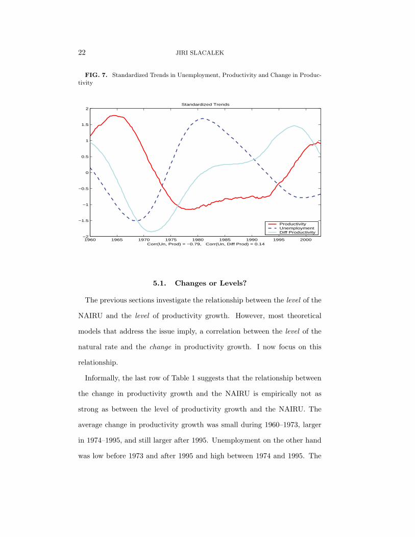
FIG. 7. Standardized Trends in Unemployment, Productivity and Change in Produc-

tivity

1960 1965 1970 1975 1980 1985 1990 1995 2000−2

−1.5

−1

−0.5

0

0.5

1

1.5

2

Corr(Un, Prod) = −0.79, Corr(Un, Diff Prod) = 0.14

Standardized Trends

ProductivityUnemploymentDiff Productivity

5.1. Changes or Levels?

The previous sections investigate the relationship between the level of the

NAIRU and the level of productivity growth. However, most theoretical

models that address the issue imply, a correlation between the level of the

natural rate and the change in productivity growth. I now focus on this

relationship.

Informally, the last row of Table 1 suggests that the relationship between

the change in productivity growth and the NAIRU is empirically not as

strong as between the level of productivity growth and the NAIRU. The

average change in productivity growth was small during 1960–1973, larger

in 1974–1995, and still larger after 1995. Unemployment on the other hand

was low before 1973 and after 1995 and high between 1974 and 1995. The


TABLE 4.

Estimation Results, Difference vs. Level of Productivity

Diff Model Level and Diff Model

Sum of Coeffs on Unemployment −0.169 −0.202

Std Error on Sum of Unemployment 0.101 0.115

P value on Lags of Unemployment 0.000 0.000

P value on Lags of Inflation 0.000 0.000

P value on Supply Shocks 0.021 0.030

Coefficients Level Diff

P value on Productivity 0.441 0.064 0.6075

Coefficient on Productivity −31.529 −1.876 −18.754

Mean Width of Confidence Intervals 3.866 –

Sacrifice Ratio 2.686 2.349

Estimate of the Signal-to-Noise Ratio 0.030 0.000

Notes: All p values are based on the White heteroscedasticity-robust standard errors. P value of 0

means less than 5× 10−4.

first column in Table 6 below displays the correlations between productivity

and unemployment trends in the US. The correlations between the changes

in productivity growth θ∗t+h − θ∗t and unemployment trend are often posi-

tive and tend to be negative only for very long horizons (h = 7 years and

longer). The correlation between the levels of productivity trend and the

NAIRU, in contrast, is high and negative, −0.81. Finally, Figure 7 displays

the trends in unemployment, productivity, and productivity growth stan-

dardized to have a zero mean and unit variance. The figure confirms that

the correlation between the change in productivity growth and the natu-

ral rate has the wrong sign. In particular, in the 1970s unemployment was

rising, productivity growth was falling and yet the change in productivity

growth was increasing.

To obtain more rigorous evidence I estimate model (3) with the change

in the productivity trend as an exogenous variable, Zt = ∆θ∗t . The first

24 JIRI SLACALEK

column of Table 4 summarizes this case. This model does not improve on

the random walk model. While the coefficient on the productivity variable

∆θ∗t is quite high (because the difference varies less than the level), it is

insignificant. The confidence intervals for the natural rate are almost as

wide as with the random walk model and the sacrifice ratio is very high.

The second column of Table 4 shows the findings for the model with the

exogenous variable consisting of both the productivity level and change,

Zt = (θ∗t ,∆θ∗t )

> . The change in productivity growth is again insignificant.

Other than that the implications of this model are similar to those of the

baseline productivity model in Table 2. The value of the coefficient on the

productivity level, θ∗t , is −1.9, the slope of the Phillips curve is greater than

in the first column, and the sacrifice ratio smaller.5

On the whole, both simple correlations and the more rigorous Kalman

filter model (3) support the “level” rather than “change” hypothesis. One

interpretation is that this finding contradicts the implications of recent mod-

els proposed to explain the relationship between productivity and the nat-

ural rate (Ball and Moffitt, 2001, Mankiw and Reis, 2003). However, the

evidence for the “level” hypothesis may instead suggest that workers update

their estimate of the productivity trend very slowly.

5.2. Signal-to-Noise Ratios

In the previous computations I follow much of the literature in impos-

ing the signal-to-noise ratio λ, as opposed to estimating it. The size of

λ determines the high-frequency variation in the natural rate. The ideal

5One reason why the change in productivity growth ∆θ∗t does not perform well is that

it is relatively volatile. However, the results still hold even after filtering ∆θ∗t .


FIG. 8a. Comparison of Various Signal-to-Noise Ratios, Random Walk Model

1960 1965 1970 1975 1980 1985 1990 1995 20000

1

2

3

4

5

6

7

8

9

10

11Unemployment and the NAIRU

Prod NAIRURandom Walk, λ = 0.01Random Walk, λ = 0.03Random Walk, λ = 0.2Unemployment

signal-to-noise ratio is big enough for the implied natural rate to capture

the time variation and at the same time small enough for the NAIRU to be

smooth. I now investigate the sensitivity of the NAIRU time profiles to the

choice of the signal-to-noise ratio.

Figure 8a compares the estimates of the natural rates for various λs in

the random walk model. This model is sensitive to the choice of λ. Unfor-

tunately, none of the λs delivers the shape generated by the productivity

model. The problem is that the choice of λ affects the high-frequency vari-

ation rather than the low-frequency variation in ut. Consequently, small

values of the signal-to-noise ratio imply a smooth but almost constant esti-

mate of the NAIRU. In contrast, a large λ generates a volatile natural rate

which fails to capture the smoothness.

26 JIRI SLACALEK

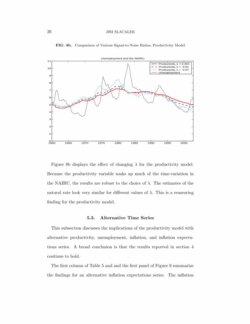
FIG. 8b. Comparison of Various Signal-to-Noise Ratios, Productivity Model

1960 1965 1970 1975 1980 1985 1990 1995 20000

1

2

3

4

5

6

7

8

9

10

11Unemployment and the NAIRU

Productivity, λ = 0.001Productivity, λ = 0.01Productivity, λ = 0.07Unemployment

Figure 8b displays the effect of changing λ for the productivity model.

Because the productivity variable soaks up much of the time-variation in

the NAIRU, the results are robust to the choice of λ. The estimates of the

natural rate look very similar for different values of λ. This is a reassuring

finding for the productivity model.

5.3. Alternative Time Series

This subsection discusses the implications of the productivity model with

alternative productivity, unemployment, inflation, and inflation expecta-

tions series. A broad conclusion is that the results reported in section 4

continue to hold.

The first column of Table 5 and and the first panel of Figure 9 summarize

the findings for an alternative inflation expectations series. The inflation


FIG. 9. Alternative Time Series

AR Expectations

1960 1965 1970 1975 1980 1985 1990 1995 20000

2

4

6

8

10

Bandpass

1960 1965 1970 1975 1980 1985 1990 1995 20000

2

4

6

8

10

Manufacturing

1960 1965 1970 1975 1980 1985 1990 1995 20000

2

4

6

8

10

GDP Deflator

1960 1965 1970 1975 1980 1985 1990 1995 20000

2

4

6

8

10

CPI X

1960 1965 1970 1975 1980 1985 1990 1995 20000

2

4

6

8

10

Demographically Adjusted Unemployment

1960 1965 1970 1975 1980 1985 1990 1995 20000

2

4

6

8

10

28 JIRI SLACALEK

TABLE 5.

MLE Estimation Results, Alternative Time Series

Base ARExp Bpass Mnfctrg GDPD CPI X DemAdjUn

Sum of Coeffs on Unemployment -0.213 -0.277 -0.250 -0.212 -0.201 -0.227 -0.218

Std Error on Sum of Unemployment 0.116 0.118 0.131 0.097 0.087 0.133 0.116

P value on Lags of Unemployment 0.000 0.000 0.000 0.000 0.000 0.000 0.000

P value on Lags of Inflation 0.000 0.000 0.000 0.000 0.000 0.000 0.000

P value on Supply Shocks 0.026 0.018 0.027 0.021 0.017 0.230 0.031

P value on Productivity 0.049 0.033 0.133 0.114 0.039 0.074 0.056

Coefficient on Productivity -1.944 -1.821 -1.159 -2.384 -1.582 -1.688 -1.944

Mean Width of Confidence Intervals 3.083 2.699 2.808 3.155 2.423 2.846 3.012

Sacrifice Ratio 2.224 1.325 1.882 2.341 2.437 2.007 2.206

Estimate of the Signal-to-Noise Ratio 0.006 0.000 0.004 0.004 0.000 0.004 0.004

Log-likelihood -128.900 -138.330 -130.170 -129.280 -78.157 -121.820 -123.230

Notes: All p values are based on the White heteroscedasticity-robust standard errors. P value of 0 means less than 5× 10−4.

expectations were generated as inflation forecasts from an AR(4) process in

∆πt. Interestingly, this model performs even better than the baseline model.

Both the Phillips curve slope and the productivity variable are significant.

The mean width of confidence intervals for the natural rate shrinks to 2.7%,

and the implied sacrifice ratio in terms of GDP is 2× 1.3 = 2.6.

The second column reports the results for an alternative measure of pro-

ductivity trend, the bandpass filter (see also Figure 2). The confidence

intervals shrink considerably again, to 2.8% on average. The sacrifice ratio,

2× 1.9 = 3.8, is in the reasonable range.

The third column describes the implications of model (3) with produc-

tivity measured as productivity in manufacturing sector, instead of in the

non-farm business sector. The model reduces the sacrifice ratio and increases

the magnitude of the Phillips curve slope. Productivity in manufacturing

is not a preferred measure of productivity because manufacturing is a rela-


tively small fraction of the economy. Not surprisingly, it turns out that the

correlation between this productivity measure and the NAIRU is not as high

as in the case of non-farm business sector productivity. Consequently, the

productivity variable is not significant. However, the model does a good job

at reducing the confidence intervals and obtaining the intuitive time profile

of the NAIRU.

The fourth column collects the findings for the GDP deflator as a measure

of inflation. These results mimic the implications of the baseline model. The

slope of the Phillips curve is significant and the NAIRU confidence intervals

are narrow. The sacrifice ratio of 2× 2.5 = 5 is still considerably lower than

the random walk sacrifice ratio.

Inflation in the next column is measured by the CPI excluding food and

energy. The findings are again similar to the baseline model. The natural

rate confidence intervals are narrow, 2.8%. The sacrifice ratio of 2×2 = 4 is

consistent with Ball (1994). The coefficient on productivity is about −1.7.

The supply shocks are not significant as one would expect with the CPI-X

price index.

The last column shows the findings for the case when an alternative mea-

sure of unemployment, demographically adjusted unemployment series, is

used. The series is calculated as the weighted average of unemployment

weights of various age groups. As opposed to the usual unemployment rate,

the weights are constant and are calculated as fractions of various age groups

in the labor force in 1985. It is interesting to consider this series because

some authors (Shimer, 1998) have suggested that demographic factors may

be able to account for a substantial portion of the variation in the natural

30 JIRI SLACALEK

rate. I find that the results with this specification are very similar to the

baseline in terms of the width of the NAIRU confidence intervals, signifi-

cance of the Phillips curve slope and the magnitude of the sacrifice ratio.

The robustness checks in this section confirm that the productivity model

improves upon the random walk model.

6. INTERNATIONAL EVIDENCE

Existing empirical work investigating the relationship between productiv-

ity growth and the natural rate focuses almost exclusively on the US data.

One reason for this is the lack of comparable international productivity data.

Fortunately, the shortage of higher frequency data is not such a serious prob-

lem with respect to the relationship between the long-run trends. In this

case, the range of the data matters more than frequency and consequently

40 years of annual data are almost as valuable as 40 years of quarterly data.

Laubach (2001) illustrates other difficulties of estimating the Phillips curves

with TV-NAIRUs for various countries. Laubach argues that the Phillips

curves (2) produce NAIRU estimates that mimic the low frequency move-

ments in unemployment rates only after a somewhat ad hoc adjustment.

An alternative feasible approach with annual data, is to evaluate the rela-

tionship between unemployment and productivity trends. It is reassuring

that the unemployment trends depicted in Figure 10 are broadly similar

to Laubach’s (2001) preferred estimates of the natural rates based on the

Phillips curves.

Figure 10 shows the trends in unemployment and in the level of pro-

ductivity growth and correlations between the two variables for eight non-


FIG. 10. International Trends in Productivity and Unemployment

1960 1965 1970 1975 1980 1985 1990 1995 20000

5

10

15Japan correlation: −0.7

ProductivityUnemployment

1960 1965 1970 1975 1980 1985 1990 1995 20000

5

10

15Germany correlation: −0.79

1960 1965 1970 1975 1980 1985 1990 1995 20000

5

10

15France correlation: −0.88

1960 1965 1970 1975 1980 1985 1990 1995 20000

5

10

15Great Britain correlation: 0.09

1960 1965 1970 1975 1980 1985 1990 1995 20000

5

10

15Canada correlation: −0.89

1960 1965 1970 1975 1980 1985 1990 1995 20000

5

10

15Italy correlation: −0.94

1960 1965 1970 1975 1980 1985 1990 1995 20000

5

10

15Netherlands correlation: −0.4

1960 1965 1970 1975 1980 1985 1990 1995 20000

5

10

15Sweden correlation: 0.42


with upper cutoff frequencies of 15 years.

32 JIRI SLACALEK

TABLE 6.

Correlations Between Productivity and the NAIRU in International Data

h USA Japan Germany France Britain Canada Italy Neth Sweden

1 0.04 0.52 0.70 0.38 0.13 0.35 0.06 -0.29 0.72

2 0.12 0.45 0.64 0.33 0.17 0.45 -0.01 -0.15 0.76

3 0.06 0.39 0.70 0.38 0.19 0.49 0.05 -0.70 0.79

4 0.07 0.28 0.59 0.34 0.21 0.64 -0.20 -0.66 0.82

5 -0.06 0.38 0.65 0.39 0.32 0.54 -0.30 -0.79 0.84

6 0.01 0.46 0.60 0.43 0.34 0.64 0.02 -0.88 0.87

7 -0.12 0.31 0.52 0.51 0.39 0.64 0.12 -0.96 0.87

8 -0.23 0.36 0.52 0.52 0.39 0.44 -0.03 -0.89 0.89

9 -0.32 0.37 0.59 0.64 0.52 0.39 -0.03 -0.87 0.90

10 -0.49 0.45 0.64 0.70 0.54 0.50 -0.42 -0.86 0.90

Mean Diff -0.09 0.40 0.61 0.46 0.32 0.51 -0.07 -0.70 0.84

Level -0.81 -0.70 -0.79 -0.88 0.09 -0.89 -0.94 -0.40 0.42

Notes: The correlations are calculated from annual data, 1960–2002.

US countries: Japan, Germany, France, Great Britain, Canada, Italy, the

Netherlands and Sweden. In most cases there are sizeable negative corre-

lations between the level of productivity growth and the natural rate of

unemployment estimated by the long-run trend. The average correlation

between the level of productivity growth and the NAIRU is −0.54. Two

countries that do not exhibit large negative correlations are Great Britain

and Sweden.

Table 6 displays the correlations between the unemployment trends and

changes in productivity growths θ∗t+h − θ∗t for various horizons h. There is

more evidence for a negative relationship between the level of productivity

growth and the natural rate than between the change in productivity growth

and the natural rate. This finding is robust across most countries and hori-

zons h. In all countries except for the Netherlands the correlations between


the NAIRU and the change in productivity growth are either ambiguous or,

more often, positive and large. The last line of Table 6 shows the correla-

tions between the levels of productivity growth and the natural rate. These

correlations mimic the findings for the US in that they are negative in most

cases and often large, Great Britain and Sweden are the two exceptions.

Overall, the international data support the evidence from the US on the

relationship between the productivity and the natural rates. For most coun-

tries there is a strong negative correlation between the level of productivity

growth and the natural rate. In contrast, the data speak less clearly about

the sign of the correlation between the change in productivity growth and

the NAIRU.

7. CONCLUSION

This paper shows that the estimate of the natural rate can be improved

considerably by using information contained in the trend of productivity

growth. The proposed econometric model provides a more precise estimate

and a more realistic time profile of the NAIRU. Both these results are

prerequisites for superior estimates of the unemployment gap. Policy makers

often consider this gap when making interest rate decisions.

I also find support for a negative correlation between the natural rate and

the level of productivity growth both in the US and international data. This

seems to contradict many theoretical models proposed to explain the recent

decline in the natural rate. However, the theory and the empirics are recon-

ciled if workers update their estimates of the trend in productivity growth

very slowly. Nevertheless, explaining the negative correlation between the

34 JIRI SLACALEK

natural rate and the level of productivity growth is an important area of

future research.

APPENDIX: DATA DESCRIPTION

This appendix describes the data used in the paper. The US data are

quarterly, 1960:1–2002:1. They are obtained from the DRI database. In the

baseline model, inflation is constructed from the CPI for all urban consumers

(PUNEW in the DRI mnemonics). Unemployment is the unemployment rate

for all workers of 16 years and over (LHUR). Productivity is the output per

hour in non-farm business sector for all persons (LBOUTU). Supply shocks

are calculated following Staiger et al. (1997). Define the price index for food

and energy as pfe = 0.66 ·pf +0.34 ·pe, where pf is the “producer price index

of foodstuffs and feedstuffs” (PW1100) and pe is the “producer price index

of crude fuel” (PW1300). Supply shocks are constructed as the demeaned

difference between the inflation of pfe and CPI inflation.

Alternative series in the Robustness section 5 are measured as follows.

Productivity in manufacturing is the LOUTM series. GDP implicit deflator

inflation is measured by GDPD96. CPI-X inflation is measured by the CPI

U index less food and energy, PUXX. Finally, unemployment for men of

25–54 years is LHMU25.

International data are annual, 1960–2001. They are downloaded from

the Bureau of Labor Statistics web site. The productivity data are output

per hour in manufacturing data from http://www.bls.gov/news.release/

prod4.t01.htm. The unemployment data are the civilian unemployment

rates approximating US concepts from Table 2 of Comparative Civilian La-

bor Force Statistics available at ftp://ftp.bls.gov/pub/special.requests/

ForeignLabor/flslforc.txt.

REFERENCES

1. Aghion, Phillipe, and Peter Howitt (1994), “Growth and Unemployment,” Review of

Economic Studies 61 477–494.

2. Ansley, Craig F., and Robert Kohn (1986), “Prediction Mean Squared Error for State

Space Models with Estimated Parameters,” Biometrika, 73, 467–73.

3. Ball, Laurence (1994), “What Determines the Sacrifice Ratio?,” in N. Gregory Mankiw

eds., Monetary Policy, NBER, The University of Chicago Press.

4. Ball, Laurence, and Robert Moffitt (2001), “Productivity Growth and the Phillips

Curve,” in Alan B. Krueger and Robert M. Solow, eds., The Roaring Nineties: Can

Full Employment Be Sustained?, Russell Sage Foundation.

5. Baxter, Mariane and Robert G. King (1999), “Measuring Business Cycles: Approxi-

mate Bandpass Filters for Economic Time Series,” Review of Economics and Statistics,


81(4), 575–593.

6. Braun, Steven (1984), “Productivity and the NIIRU (and Other Phillips Curve Is-

sues),” National Income Section Working Paper 34, Board of Governors of the Federal

Reserve System.

7. Friedman, Milton (1968), “The Role of Monetary Policy,” American Economic Review,

58(1), 1–17.

8. Gordon, Robert J. (1997), “The Time-Varying NAIRU and its Implications for Eco-

nomic Policy,” Journal of Economic Perspectives 11(1), 11–32.

9. Gordon, Robert J. (1998), “Foundations of the Goldilocks Economy: Supply Shocks

and the Time-Varying NAIRU,” Brookings Papers on Economic Activity, 2, 297–333.

Productivity, Investment, and Innovation,” working paper, Northwestern University.

10. Harvey, Andrew C. (1989), Forecasting, Structural Time Series Models and the Kalman

Filter, Cambridge University Press.

11. Katz, Lawrence F., and Allan B.Krueger (1998), “The High-pressure U. S. Labor Mar-

ket of the 1990s,” Brookings Papers on Economic Activity, 1, 1–87.

12. King, Robert G., James H. Stock, and Mark W.Watson (1995), “Temporal Instability

of the Unemployment–Inflation Relationship,” Economic Perspectives of the Federal

Reserve Bank of Chicago, May–June, 2–12.

13. Laubach (2001), Thomas, “Measuring the NAIRU: Evidence from Seven Economies,”

The Review of Economics and Statistics, 83(2), 218-231, May.

14. Mankiw, N. Gregory, and Ricardo Reis (2003), “Sticky Information: A Model of Mone-

tary Non-neutrality and Structural Slumps” in P. Aghion, R. Frydman, J. Stiglitz and

M. Woodford, eds., Knowledge, Information, and Expectations in Modern Macroeco-

nomics: In Honor of Edmund S. Phelps, Princeton University Press.

15. Meyer, Laurence H. (2000), “Remarks,” Century Club Breakfast Series, Washing-

ton University, St. Louis, October 19, available at http://www.federalreserve.gov/

boarddocs/speeches/2000/

16. Mortensen, Dale T., and Christopher A. Pissarides (1998), “Technological Progress,

Job Creation, and Job Destruction,” Review of Economic Dynamics 1, 733–753.

17. Shimer (1998), Robert, “Why is the U.S. Unemployment Rate So Much Lower?,” in

NBER Macroeconomics Annual 1998, edited by Ben Bernanke and Julio Rotemberg,

MIT Press.

18. Staiger, Douglas, James H. Stock, and MarkW.Watson (1997a), “How Precise are Esti-

mates of the Natural Rate of Unemployment?,” in Romer, Christina, and David Romer,

eds., Reducing Inflation: Motivation and Strategy. Chicago: University of Chicago

Press.

19. Staiger, Douglas, James H. Stock, and Mark W.Watson (2001), “Prices, Wages and

the U. S. NAIRU in the 1990s,” in Alan B. Krueger and Robert M. Solow, eds., The

Roaring Nineties: Can Full Employment Be Sustained?, Russell Sage Foundation.

20. Stock, James H., and Mark W.Watson (1998), “Median Unbiased Estimation of Co-

efficient Variance in a Time Varying Parameter Model,” Journal of the American

Statistical Association, 93, 349–358.

21. Stock, James H., and Mark W.Watson (1999), “Forecasting Inflation,” Journal of

Monetary Economics, 44, 293–335.

Productivity and the Natural Rate of Unemployment€¦ · · 2006-02-08Productivity and the Natural Rate of Unemployment* Jiri Slacalek Department of Macro Analysis and Forecasting,

Documents