Productivity and Efficiency of Small Scale Agriculture in Ethiopia Dawit Kelemework Mekonnen Graduate Student Department of Agricultural & Applied Economics University of Georgia, 305 Conner Hall Athens, Georgia, 30602 USA Email: [email protected] Jeffrey H. Dorfman Professor Department of Agricultural & Applied Economics University of Georgia 312 Conner Hall Athens, Georgia, 30602 USA Email: [email protected] Esendugue Greg Fonsah Associate Professor Department of Agricultural & Applied Economics University of Georgia 15 RDC Rd, Room 118 P.O. Box 1209 Tifton, Georgia, 31793 USA Email: [email protected] ✩ Selected paper prepared for presentation at the Southern Agricultural Economics Association (SAEA) Annual Meeting, Orlando, Florida, 3-5 February 2013. ✩✩ Copyright 2012 by Dawit K. Mekonnen, Jeffrey H. Dorfman, and Esendugue Greg Fonsah. All rights reserved. Readers may make verbatim copies of this document for non-commercial purposes by any means, provided that this copyright notice appears on all such copies.

Welcome message from author
This document is posted to help you gain knowledge. Please leave a comment to let me know what you think about it! Share it to your friends and learn new things together.
Transcript

Productivity and Efficiency of Small Scale Agriculture
in Ethiopia
Dawit Kelemework Mekonnen
Graduate StudentDepartment of Agricultural & Applied Economics
University of Georgia,305 Conner Hall
Athens, Georgia, 30602USA
Email: [email protected]
Jeffrey H. Dorfman
ProfessorDepartment of Agricultural & Applied Economics
University of Georgia312 Conner Hall
Athens, Georgia, 30602USA
Email: [email protected]
Esendugue Greg Fonsah
Associate ProfessorDepartment of Agricultural & Applied Economics
University of Georgia15 RDC Rd, Room 118
P.O. Box 1209Tifton, Georgia, 31793
USAEmail: [email protected]
ISelected paper prepared for presentation at the Southern Agricultural Economics Association (SAEA)Annual Meeting, Orlando, Florida, 3-5 February 2013.
IICopyright 2012 by Dawit K. Mekonnen, Jeffrey H. Dorfman, and Esendugue Greg Fonsah. All rightsreserved. Readers may make verbatim copies of this document for non-commercial purposes by any means,provided that this copyright notice appears on all such copies.

Abstract
We estimate a distance function of grains production using generalized method of mo-
ments that enables us to accommodate multiple outputs of farmers as well as address the
endogeneity issues that are related with the use of distance functions for multi-output pro-
duction. Using a panel data set of Ethiopian subsistence farmers, we find that the most
important factors determining farmers’ efficiency in Ethiopia are having access to the public
extension system, participation in off-farm activities, participation in labor sharing arrange-
ments, gender of the household head, and the extent to which farmers are forced to produce
on marginal and steeply sloped plots. Average farmers in Ethiopia are producing less than
60% of the most efficient farmers. Annual technical change between 1999 and 2004 is about
one percent while annual efficiency change during the same period is insignificant.
Keywords: Distance Function, Productivity, Efficiency, GMM, Ethiopia
1. Introduction
It stands to reason that agricultural productivity gains can help reduce rural poverty by
raising real income from farming and keeping food prices from increasing excessively by
improving the availability of food. The economic importance of improving agricultural
productivity is even more evident in a country like Ethiopia where agriculture accounts for
47% of its GDP 85% of its employment. Although Ethiopia successfully increased its crop
production in the first decade of the 2000s, increasingly binding land and water constraints
will make it increasingly difficult to achieve production gains of both crops and livestock in
the highlands without major investments in productivity-increasing technologies (Dorosh,
2012). Taffesse, Dorosh, and Gemessa (2012) also argued that with little suitable land
available for the expansion of crop cultivation, especially in the highlands, future cereal
production growth will need to come increasingly from yield improvements.
1
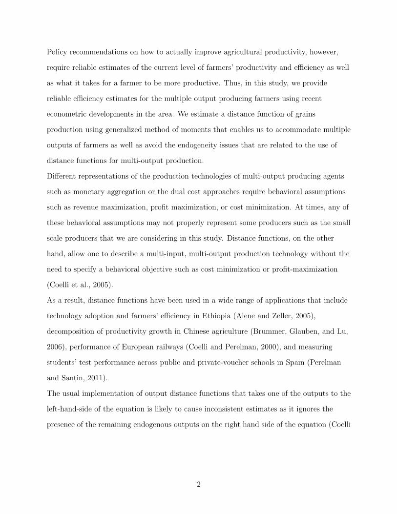
Policy recommendations on how to actually improve agricultural productivity, however,
require reliable estimates of the current level of farmers’ productivity and efficiency as well
as what it takes for a farmer to be more productive. Thus, in this study, we provide
reliable efficiency estimates for the multiple output producing farmers using recent
econometric developments in the area. We estimate a distance function of grains
production using generalized method of moments that enables us to accommodate multiple
outputs of farmers as well as avoid the endogeneity issues that are related to the use of
distance functions for multi-output production.
Different representations of the production technologies of multi-output producing agents
such as monetary aggregation or the dual cost approaches require behavioral assumptions
such as revenue maximization, profit maximization, or cost minimization. At times, any of
these behavioral assumptions may not properly represent some producers such as the small
scale producers that we are considering in this study. Distance functions, on the other
hand, allow one to describe a multi-input, multi-output production technology without the
need to specify a behavioral objective such as cost minimization or profit-maximization
(Coelli et al., 2005).
As a result, distance functions have been used in a wide range of applications that include
technology adoption and farmers’ efficiency in Ethiopia (Alene and Zeller, 2005),
decomposition of productivity growth in Chinese agriculture (Brummer, Glauben, and Lu,
2006), performance of European railways (Coelli and Perelman, 2000), and measuring
students’ test performance across public and private-voucher schools in Spain (Perelman
and Santin, 2011).
The usual implementation of output distance functions that takes one of the outputs to the
left-hand-side of the equation is likely to cause inconsistent estimates as it ignores the
presence of the remaining endogenous outputs on the right hand side of the equation (Coelli
2

et al., 2005).1 Atkinson, Cornwell, and Honerkamp (2003) have shown that Generalized
Method of Moments (GMM) can be used to address the possibility of endogeneity of either
outputs or inputs with the composite error term inherent in distance functions. The GMM
approach has an additional advantage that it doesn’t require distributional assumption on
the error term. Thus we follow the GMM approach of Atkinson, Cornwell, and Honerkamp
(2003) aiming to accommodate the multiple output nature of production in the farming
system under study through distance functions as well as address the endogeneity inherent
in distance function estimation by instrumenting the endogenous right-hand-side outputs.
2. Empirical Model
Let X be a vector of inputs X = (x1, ..., xL) ∈ RL+ and let Y be a vector of outputs denoted
by Y = (y1, ..., yM) ∈ RM+ . The output distance function is defined as
(1) Do(X, Y, t) = infθ{θ > 0 : (X,Y
θ) ∈ S(X, Y, t)}
where S(X,Y,t) is the technology set such that X can produce Y at time t. Do(X, Y, t) is
the inverse of the factor by which the production of all output quantities could be
increased while still remaining within the feasible production set for the given input level
(O’Donnell and Coelli, 2005). θ, and hence, the distance function, Do(X, Y, t), takes a
value less than or equal to 1, where a value of 1 means that the farmer is operating at the
frontier of the technology set. The output distance function is non-decreasing, linearly
homogeneous and convex in output, and non-increasing and quasi-convex in inputs
(O’Donnell and Coelli, 2005).
Given M outputs and L inputs, we have chosen a generalized quadratic Box-Cox model to
represent the distance function, Do(.), as
1The same can be said with input distance functions.
3
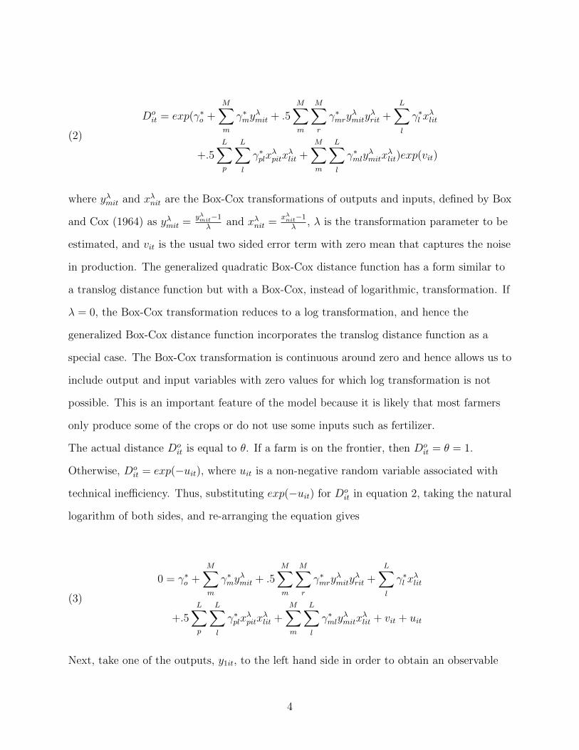
Doit = exp(γ∗o +
M∑m
γ∗myλmit + .5
M∑m
M∑r
γ∗mryλmity
λrit +
L∑l
γ∗l xλlit
+.5L∑p
L∑l
γ∗plxλpitx
λlit +
M∑m
L∑l
γ∗mlyλmitx
λlit)exp(vit)
(2)
where yλmit and xλnit are the Box-Cox transformations of outputs and inputs, defined by Box
and Cox (1964) as yλmit =yλmit−1
λand xλnit =
xλnit−1
λ, λ is the transformation parameter to be
estimated, and vit is the usual two sided error term with zero mean that captures the noise
in production. The generalized quadratic Box-Cox distance function has a form similar to
a translog distance function but with a Box-Cox, instead of logarithmic, transformation. If
λ = 0, the Box-Cox transformation reduces to a log transformation, and hence the
generalized Box-Cox distance function incorporates the translog distance function as a
special case. The Box-Cox transformation is continuous around zero and hence allows us to
include output and input variables with zero values for which log transformation is not
possible. This is an important feature of the model because it is likely that most farmers
only produce some of the crops or do not use some inputs such as fertilizer.
The actual distance Doit is equal to θ. If a farm is on the frontier, then Do
it = θ = 1.
Otherwise, Doit = exp(−uit), where uit is a non-negative random variable associated with
technical inefficiency. Thus, substituting exp(−uit) for Doit in equation 2, taking the natural
logarithm of both sides, and re-arranging the equation gives
0 = γ∗o +M∑m
γ∗myλmit + .5
M∑m
M∑r
γ∗mryλmity
λrit +
L∑l
γ∗l xλlit
+.5L∑p
L∑l
γ∗plxλpitx
λlit +
M∑m
L∑l
γ∗mlyλmitx
λlit + vit + uit
(3)
Next, take one of the outputs, y1it, to the left hand side in order to obtain an observable
4
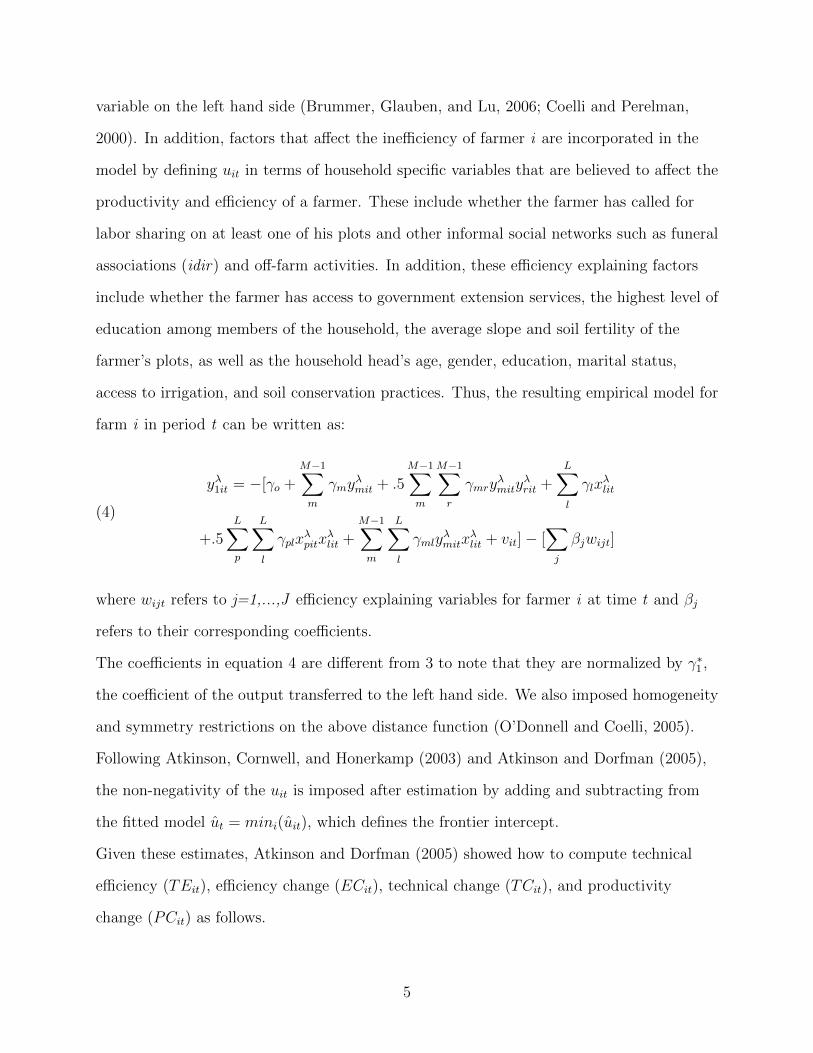
variable on the left hand side (Brummer, Glauben, and Lu, 2006; Coelli and Perelman,
2000). In addition, factors that affect the inefficiency of farmer i are incorporated in the
model by defining uit in terms of household specific variables that are believed to affect the
productivity and efficiency of a farmer. These include whether the farmer has called for
labor sharing on at least one of his plots and other informal social networks such as funeral
associations (idir) and off-farm activities. In addition, these efficiency explaining factors
include whether the farmer has access to government extension services, the highest level of
education among members of the household, the average slope and soil fertility of the
farmer’s plots, as well as the household head’s age, gender, education, marital status,
access to irrigation, and soil conservation practices. Thus, the resulting empirical model for
farm i in period t can be written as:
yλ1it = −[γo +M−1∑m
γmyλmit + .5
M−1∑m
M−1∑r
γmryλmity
λrit +
L∑l
γlxλlit
+.5L∑p
L∑l
γplxλpitx
λlit +
M−1∑m
L∑l
γmlyλmitx
λlit + vit]− [
∑j
βjwijt]
(4)
where wijt refers to j=1,...,J efficiency explaining variables for farmer i at time t and βj
refers to their corresponding coefficients.
The coefficients in equation 4 are different from 3 to note that they are normalized by γ∗1 ,
the coefficient of the output transferred to the left hand side. We also imposed homogeneity
and symmetry restrictions on the above distance function (O’Donnell and Coelli, 2005).
Following Atkinson, Cornwell, and Honerkamp (2003) and Atkinson and Dorfman (2005),
the non-negativity of the uit is imposed after estimation by adding and subtracting from
the fitted model ut = mini(uit), which defines the frontier intercept.
Given these estimates, Atkinson and Dorfman (2005) showed how to compute technical
efficiency (TEit), efficiency change (ECit), technical change (TCit), and productivity
change (PCit) as follows.
5

Farmer i’s level of technical efficiency in period t is TEit:
(5) TEit = exp(−u∗it)
where the normalization of u∗it guarantees that 0 < TEit ≤ 1.
Productivity can increase by farmers getting more efficient or by moving the the
production frontier outward. Thus, productivity change is defined as the sum of technical
change and efficiency change:
(6) PC = TC + EC.
Efficiency change is the change in the technical efficiency over time, so
(7) ECit = 4TEit = TEit − TEi,t−1.
Technical change is measured as the difference between the estimated frontier distance
function in periods t and t - 1 holding output and input quantities constant:
(8) TCit = D∗i (Y,X, t)− D∗
i (Y,X, t− 1).
3. Data
For this study, we have used the 1999 and 2004 rounds of the Ethiopian Rural Household
Survey (ERHS) data, which is a longitudinal household data set covering households in 15
peasant associations in rural Ethiopia. We focus on the five major cereals - teff, wheat,
maize, sorghum, and barley - that according to Taffesse, Dorosh, and Gemessa (2012)
occupy almost three-fourths of the total area cultivated and represent almost 70% of the
total value-added in recent years.
6
The study focuses on the main (Meher) rainy season that runs between June and
September. This helps to reduce the noise in the data as the agricultural production
system in terms of crops in the field, intensity of the rain, and utilization of inputs are
markedly different from the second small showers (Belg rains) season between February
and May (Admassu, 2004). In addition, the five cereals that are the focus of this study are
mainly produced during the main rainy season. According to data from the Central
Statistical Agency of Ethiopia, between 1995 and 2008, close to 99% of teff production,
98% of wheat production, 90% of barley production, and 89% of maize production was
done during the main rainy season (CSA, 2009). These qualifications in the data in terms
of crops produced and seasons resulted in a sample size of 815 farmers in each of the 1999
and 2004 survey rounds.
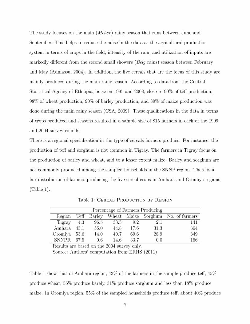
There is a regional specialization in the type of cereals farmers produce. For instance, the
production of teff and sorghum is not common in Tigray. The farmers in Tigray focus on
the production of barley and wheat, and to a lesser extent maize. Barley and sorghum are
not commonly produced among the sampled households in the SNNP region. There is a
fair distribution of farmers producing the five cereal crops in Amhara and Oromiya regions
(Table 1).
Table 1: Cereal Production by Region
Percentage of Farmers ProducingRegion Teff Barley Wheat Maize Sorghum No. of farmersTigray 4.3 96.5 33.3 9.2 2.1 141
Amhara 43.1 56.0 44.8 17.6 31.3 364Oromiya 53.6 14.0 40.7 69.6 28.9 349SNNPR 67.5 0.6 14.6 33.7 0.0 166
Results are based on the 2004 survey only.Source: Authors’ computation from ERHS (2011)
Table 1 show that in Amhara region, 43% of the farmers in the sample produce teff, 45%
produce wheat, 56% produce barely, 31% produce sorghum and less than 18% produce
maize. In Oromiya region, 55% of the sampled households produce teff, about 40% produce
7

wheat, 70% produce maize, 29% produce sorghum but only about 14% produce barley.
Among farmers in SNNP region, 68% of them produce teff, 34% of them produce maize,
less than 15% produce wheat and less than 1% produce either barley or sorghum.
Access to irrigation among the sampled farmers increased from about 6 percent in 1999 to
about 29 percent in 2004. The share of farmers with access to the public extension system
has almost doubled in the five years between 1999 and 2004. More than three quarters of
the household heads are male and less than 10 percent completed primary school. More
than three quarters of the households heads are members of idir (funeral associations), and
23 to 37 % of the farmers are engaged in off-farm activities in 1999 and 2004. About three
quarters of the household heads are married.
The ERHS data show significant variation in labor sharing participation among the four
regions covered by the study. Labor sharing is not common in the Tigray region where only
13% of the households participate in such type of arrangements. Labor sharing is common
in the other three regions with participation rates ranging from 40% to 61% .
All the output variables (Teff, Wheat, Barley, Maize, and Sorghum) as well as the two most
used chemical fertilizers (Urea and DAP) are measured in Kilograms. Average production
is the highest for teff and the lowest for Sorghum but the averages would obviously be
higher if we consider only the farmers that produce the specific crop. Average DAP use is
approximately three times more than that of Urea. The highest level of education in the
household is around 4 years on average and it is expected to capture intra-household
schooling externality. The average age of a household head is about 50 years. Soil fertility
is measured in a 1 to 3 scale where 1 refers to fertile, 2 medium fertile, and 3 infertile soil,
and it is averaged among the different plots of the farmer. Labor is measured in labor days
and it includes family, hired, and shared labor. While computing labor days, we follow
Arega (2009) to account for the physical hardship in crop production by giving adult men a
weight of 1, adult women a weight of 0.8, and child labor a weight of 0.35.
Oromiya has the highest average land holding size under the five crops which was about
8
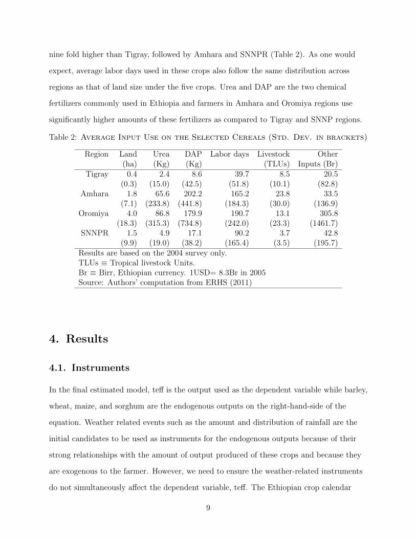
nine fold higher than Tigray, followed by Amhara and SNNPR (Table 2). As one would
expect, average labor days used in these crops also follow the same distribution across
regions as that of land size under the five crops. Urea and DAP are the two chemical
fertilizers commonly used in Ethiopia and farmers in Amhara and Oromiya regions use
significantly higher amounts of these fertilizers as compared to Tigray and SNNP regions.
Table 2: Average Input Use on the Selected Cereals (Std. Dev. in brackets)
Region Land Urea DAP Labor days Livestock Other(ha) (Kg) (Kg) (TLUs) Inputs (Br)
Tigray 0.4 2.4 8.6 39.7 8.5 20.5(0.3) (15.0) (42.5) (51.8) (10.1) (82.8)
Amhara 1.8 65.6 202.2 165.2 23.8 33.5(7.1) (233.8) (441.8) (184.3) (30.0) (136.9)
Oromiya 4.0 86.8 179.9 190.7 13.1 305.8(18.3) (315.3) (734.8) (242.0) (23.3) (1461.7)
SNNPR 1.5 4.9 17.1 90.2 3.7 42.8(9.9) (19.0) (38.2) (165.4) (3.5) (195.7)
Results are based on the 2004 survey only.TLUs ≡ Tropical livestock Units.Br ≡ Birr, Ethiopian currency. 1USD= 8.3Br in 2005Source: Authors’ computation from ERHS (2011)
4. Results
4.1. Instruments
In the final estimated model, teff is the output used as the dependent variable while barley,
wheat, maize, and sorghum are the endogenous outputs on the right-hand-side of the
equation. Weather related events such as the amount and distribution of rainfall are the
initial candidates to be used as instruments for the endogenous outputs because of their
strong relationships with the amount of output produced of these crops and because they
are exogenous to the farmer. However, we need to ensure the weather-related instruments
do not simultaneously affect the dependent variable, teff. The Ethiopian crop calendar
9
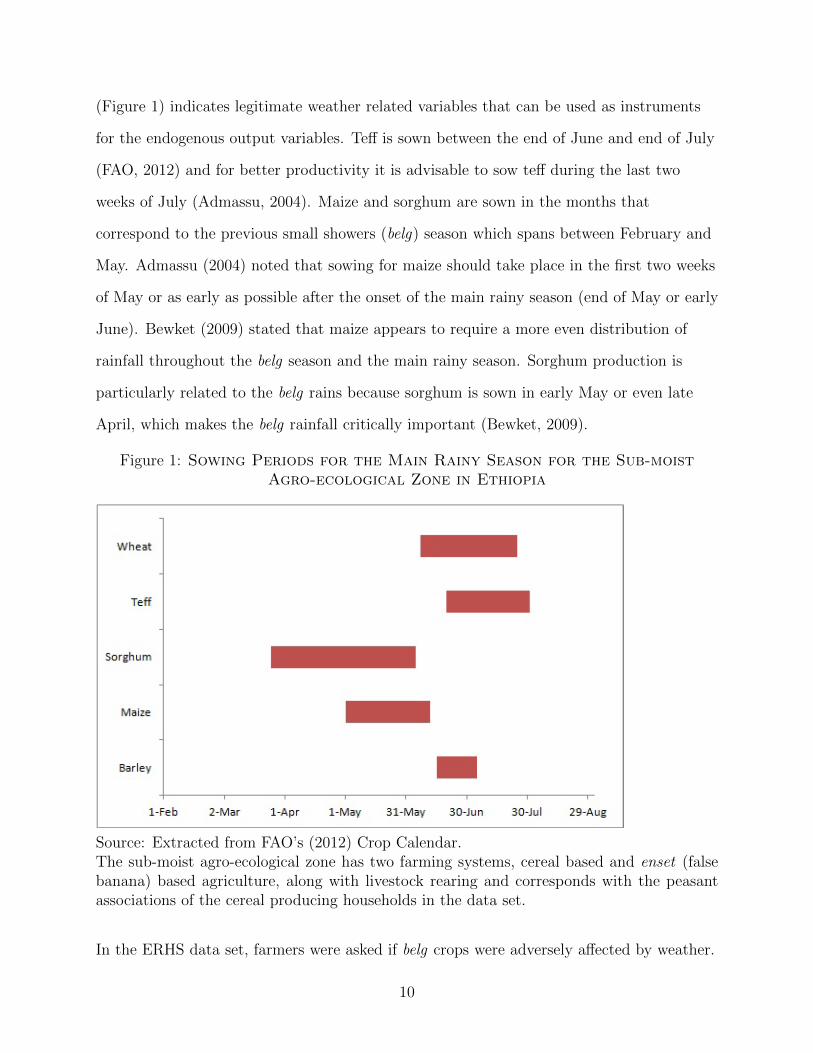
(Figure 1) indicates legitimate weather related variables that can be used as instruments
for the endogenous output variables. Teff is sown between the end of June and end of July
(FAO, 2012) and for better productivity it is advisable to sow teff during the last two
weeks of July (Admassu, 2004). Maize and sorghum are sown in the months that
correspond to the previous small showers (belg) season which spans between February and
May. Admassu (2004) noted that sowing for maize should take place in the first two weeks
of May or as early as possible after the onset of the main rainy season (end of May or early
June). Bewket (2009) stated that maize appears to require a more even distribution of
rainfall throughout the belg season and the main rainy season. Sorghum production is
particularly related to the belg rains because sorghum is sown in early May or even late
April, which makes the belg rainfall critically important (Bewket, 2009).
Figure 1: Sowing Periods for the Main Rainy Season for the Sub-moistAgro-ecological Zone in Ethiopia
Source: Extracted from FAO’s (2012) Crop Calendar.The sub-moist agro-ecological zone has two farming systems, cereal based and enset (falsebanana) based agriculture, along with livestock rearing and corresponds with the peasantassociations of the cereal producing households in the data set.
In the ERHS data set, farmers were asked if belg crops were adversely affected by weather.
10
We used this variable and its interactions with other exogenous variables as instruments for
maize and sorghum production. That is, belg rains affect maize and sorghum production
because the sowing of these two crops and part of their growing season correspond with the
belg season but belg rains don’t simultaneously affect teff production because sowing for
teff begins at the end of July, making the instrument relevant as well as legitimate.
The sowing time for wheat is the end of June and the early days of July while sowing for
barley should take place soon after the main rainy season begins in June (Admassu, 2004;
FAO, 2012). Thus, the performance of the rain at the beginning of the main rainy season
(late May and early June) is important both for wheat and barley (as well as sorghum and
maize which are in their growing stage at this time) but is not directly related with teff,
which is sown after two weeks into July (i.e, the middle of the main rainy season). The
ERHS data set is helpful in this regard because farmers were asked if the first rains of the
main rainy season came on time and if there was enough rain on the farmer’s plot at the
beginning of the rainy season. These two variables, along with their interactions with other
exogenous variables, are used to instrument for wheat and barley because they are related
to the endogenous variables but not directly related to the left-hand-side variable, making
them pass the legitimacy and relevance criteria for good instruments.
4.2. Model Estimates
The model is estimated using heteroscedasticity and autocorrelation consistent iterated
GMM with the instruments mentioned above and it fits the data well with an overall R2 of
0.598. Using the Sargen-Hansen or J test of overidentification (Baum, Schaffer, and
Stillman, 2003; Wooldridge, 2002), we fail to reject the validity of the over-identifying
restrictions. The J-test resulted in a GMM criterion function value of 41.74 which has a χ2
distribution of 40 degrees of freedom, which gives a p-value of 0.395. A rejection of this
test would have cast a doubt on the validity of our instruments.
Other than the validity of instruments, the other condition needed in GMM estimation is
11
that the instruments be sufficiently related to the endogenous variables. When instruments
are weak, the orthogonality conditions hold even at non-optimal values of the estimated
parameters when in fact they should hold or get close to zero only at the optimal values.
Our instruments do not exhibit the pathologies that GMM estimators demonstrate in the
presence of weak identification as suggested by Stock, Wright, and Yogo (2002). For
instance, two-step GMM estimators and iterated GMM point estimators can vary
significantly and produce very different confidence sets in the presence of weak
identification. As shown in Table Appendix A.1 and Table Appendix A.2 in the appendix,
the two step GMM and the iterated GMM estimators are almost identical in our case,
which differ only after two digits for almost all of the coefficients. Thus, we believe the
estimates are based on a suitable set of instruments and are credible.
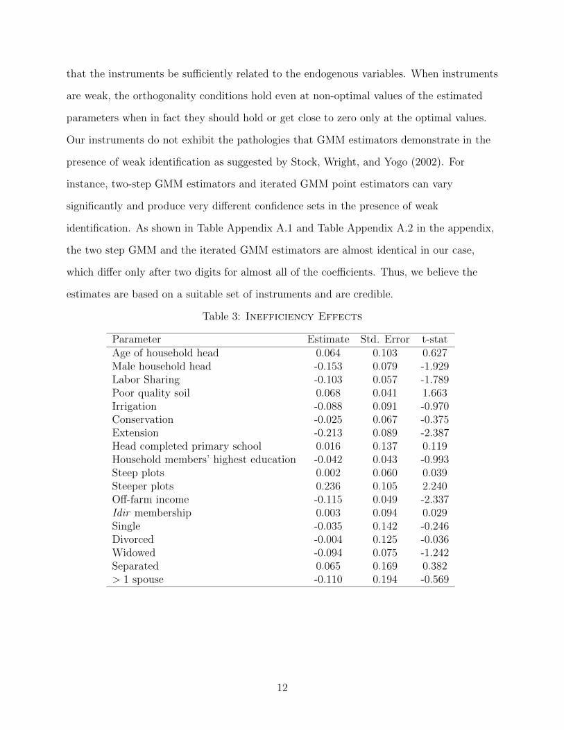
Table 3: Inefficiency Effects
Parameter Estimate Std. Error t-statAge of household head 0.064 0.103 0.627Male household head -0.153 0.079 -1.929Labor Sharing -0.103 0.057 -1.789Poor quality soil 0.068 0.041 1.663Irrigation -0.088 0.091 -0.970Conservation -0.025 0.067 -0.375Extension -0.213 0.089 -2.387Head completed primary school 0.016 0.137 0.119Household members’ highest education -0.042 0.043 -0.993Steep plots 0.002 0.060 0.039Steeper plots 0.236 0.105 2.240Off-farm income -0.115 0.049 -2.337Idir membership 0.003 0.094 0.029Single -0.035 0.142 -0.246Divorced -0.004 0.125 -0.036Widowed -0.094 0.075 -1.242Separated 0.065 0.169 0.382> 1 spouse -0.110 0.194 -0.569
12
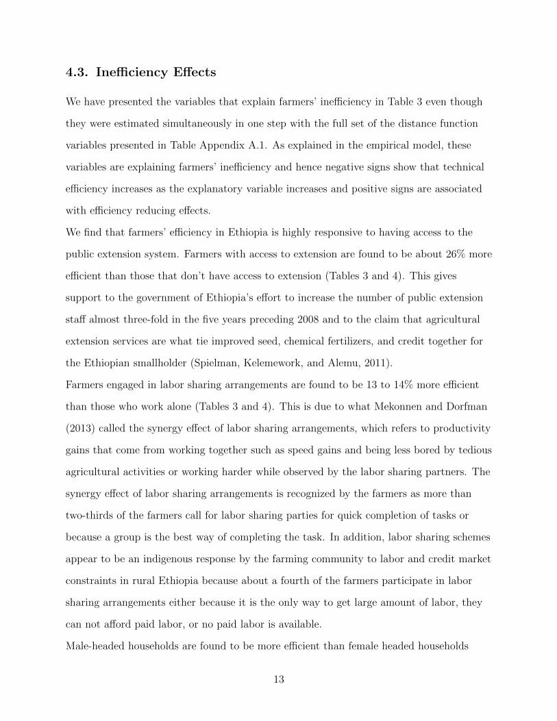
4.3. Inefficiency Effects
We have presented the variables that explain farmers’ inefficiency in Table 3 even though
they were estimated simultaneously in one step with the full set of the distance function
variables presented in Table Appendix A.1. As explained in the empirical model, these
variables are explaining farmers’ inefficiency and hence negative signs show that technical
efficiency increases as the explanatory variable increases and positive signs are associated
with efficiency reducing effects.
We find that farmers’ efficiency in Ethiopia is highly responsive to having access to the
public extension system. Farmers with access to extension are found to be about 26% more
efficient than those that don’t have access to extension (Tables 3 and 4). This gives
support to the government of Ethiopia’s effort to increase the number of public extension
staff almost three-fold in the five years preceding 2008 and to the claim that agricultural
extension services are what tie improved seed, chemical fertilizers, and credit together for
the Ethiopian smallholder (Spielman, Kelemework, and Alemu, 2011).
Farmers engaged in labor sharing arrangements are found to be 13 to 14% more efficient
than those who work alone (Tables 3 and 4). This is due to what Mekonnen and Dorfman
(2013) called the synergy effect of labor sharing arrangements, which refers to productivity
gains that come from working together such as speed gains and being less bored by tedious
agricultural activities or working harder while observed by the labor sharing partners. The
synergy effect of labor sharing arrangements is recognized by the farmers as more than
two-thirds of the farmers call for labor sharing parties for quick completion of tasks or
because a group is the best way of completing the task. In addition, labor sharing schemes
appear to be an indigenous response by the farming community to labor and credit market
constraints in rural Ethiopia because about a fourth of the farmers participate in labor
sharing arrangements either because it is the only way to get large amount of labor, they
can not afford paid labor, or no paid labor is available.
Male-headed households are found to be more efficient than female headed households
13
which implies that the design of extension systems in Ethiopia should have a gender
component that addresses efficiency-reducing challenges that women household heads in
particular face. As shown in Table 4, male headed households are on average about 15%
and 14% more efficient than female headed households in 1999 and 2004.
We also find that farmers exposed to external information through off-farm activities are 7
to 13% more efficient than those that don’t have such exposures (Tables 3 and 4). The
most important kind of off-farm activities among the sampled households is food-for-work,
which accounts for 39% and 54.4% of all off-farm activities in 1999 and 2004. The
food-for-work program in Ethiopia is a welfare safety net for food insecure areas and
instead of distributing food aid to those in need, the program involves able-bodied people
performing public work in exchange for a food wage. The food-for-work program focuses on
rehabilitation of forest, grazing, and agricultural lands as well as construction of wells,
ponds, dams, terraces, and roads. The efficiency-enhancing effects of off-farm activities
suggests that farmers involved in the food-for-work program have taken home
productivity-improving methods from the public works to their individual plots.
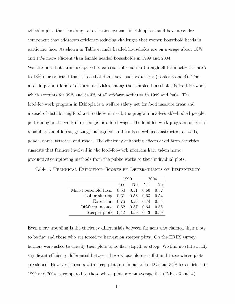
Table 4: Technical Efficiency Scores by Determinants of Inefficiency
1999 2004Yes No Yes No
Male household head 0.60 0.51 0.60 0.52Labor sharing 0.61 0.53 0.63 0.54
Extension 0.76 0.56 0.74 0.55Off-farm income 0.62 0.57 0.64 0.55
Steeper plots 0.42 0.59 0.43 0.59
Even more troubling is the efficiency differentials between farmers who claimed their plots
to be flat and those who are forced to harvest on steeper plots. On the ERHS survey,
farmers were asked to classify their plots to be flat, sloped, or steep. We find no statistically
significant efficiency differential between those whose plots are flat and those whose plots
are sloped. However, farmers with steep plots are found to be 42% and 36% less efficient in
1999 and 2004 as compared to those whose plots are on average flat (Tables 3 and 4).
14

In addition, the average fertility of the farmers’ plot plays a role in determining the
technical efficiency of farmers. The soil fertility variable was measured in such a way that
higher values refer to less fertility and hence the positive coefficient in Table 3 shows that
farmers with plots of inferior quality are less efficient than farmers whose plots are more
fertile.
Table 5: Partial Effects and Elasticities Evaluated at 2004 Values
MarginalProductivity Std. Error Elasticity
Land 0.844 0.493 1.033Oxen 0.115 0.305 0.139Urea -0.014 0.214 -0.016DAP 0.037 0.294 0.049
Other Purchased Inputs 0.008 0.201 0.064Labor 0.133 0.384 0.191
Wheat -0.548 0.266 -0.649Barley -0.231 0.202 -0.414Maize -0.295 0.232 -0.340
Sorghum 0.073 0.249 0.080
Among the sampled households in 2004, the average land size used for teff, wheat, barley,
sorghum, and maize was 0.4 hectares in Tigray region, 1.5 hectares in the SNNPR region,
1.8 hectares in Amhara region, and 4 hectares in Oromiya region. Given the small
landholding of small scale farmers in Ethiopia, agricultural output is expected to be
responsive to acreage expansion. The result from this study also confirms that a percentage
increase in land size increases teff production by a little more than one percent, implying
slightly increasing returns to scale.
Land is owned by the government and farmers can’t sell or mortgage agricultural farm
lands. Although renting agricultural land is allowed, all regions except Amhara, where land
can be rented for up to 25 years, have legal provisions limiting the amount of land to be
rented out to 50% of holding size with a maximum duration for rental contracts of 3 years
(Deininger et al., 2008). Population pressure and lack of alternative non-agricultural jobs
in villages have forced household heads to further redistribute part of their farming land to
15

their adult kids when the kids form their own family. The (near) absence of land markets
and land fragmentation have forced farmers to harvest on small plots of lands, making land
the most valuable input of all and production to be highly constrained by small land size.
The trade-off between teff production versus wheat production is also presented in Table 5.
The relationships with the other crops are statistically insignificant.
4.4. Farmer Technical Efficiency Scores
The average technical efficiency of the 815 farmers included in the final estimation was
found to be about 58.4% both in 1999 and 2004. These figures imply that at the current
level of inputs use, farmers are producing, on average, less than 60% of the output of the
most efficient farmer in the sample. Thus, there is room to increase farmers’ production by
over two thirds through better management of the existing resources. The evidence in
Table 3 suggests the government needs to intensify efficiency-enhancing investments such
as extension, irrigation, and off-farm activities, as well as facilitating venues for farmers to
work together.
For the years between 1999 and 2004, the annual efficiency change is close to zero while the
average technical change is close to one percent per year. As a result, the productivity
change, which is the sum of efficiency change and technical change, is also about one
percent per year.
As shown in Figure 2, there is significant variation in the efficiency scores of farmers in
different peasant associations (PAs) in 2004, from 46.4% in Geblen PA of Tigray Regional
State to about 69.2% in Doma PA of the Southern Nations, Nationalities, and Peoples
Regional (SNNPR) State. In terms of average efficiency scores, the two lowest performing
PAs (Geblen and Haresaw) are found in Tigray, whereas Korodegaga PA of Oromiya
Regional State closely follows the best performing Doma PA with 69.1% efficiency score.
However, such direct comparisons of the efficiency scores of peasant associations can’t be
conclusive because it doesn’t take into account the variance of efficiency scores within the
16

0.0000 0.1000 0.2000 0.3000 0.4000 0.5000 0.6000 0.7000 0.8000
Geblen
Haresaw
Debre Berhan Kormargefia
Debre Berhan Bokafia
Yetmen
Debre Berhan Karafino
Debre Berhan Milki
Sirbana Godeti
Gara Godo
Trirufe Ketchema
Full sample
Dinki
Shumsha
Adele Keke
Aze Deboa
Korodegaga
Doma
TE
Figure 2: Mean Technical Efficiency in 2004 by Peasant Association
PA. From the econometric results, the three PAs whose efficiency scores are statistically
significantly different from our base PA of Debre-Berhan Bokafia are Yetmen, Sirbana
Godeti, and Trirufe Ketchema. These three PAs are known in the country for their high
quality teff production and have long experience with improved teff production
technologies. Yetmen is located about 248 kms north west of Addis Ababa between the
towns of Dejen and Bichena. An improved variety of teff was introduced in Yetmen three
decades ago by development agents and was tried first by the producers’ cooperatives, and
soon adopted by all the peasants following its success (ERHS, 2011). Sirba na Godeti PA,
located about halfway between Debre Zeit and Mojo towns and with generally fertile soil
17
(ERHS, 2011), is known for its teff production and supply to the capital Addis Ababa.
Turufe Kecheme is a PA located about 12.5 km north east of the town of Shashemene in
the area of the Great Lakes of Zwai, Langano, Abiyata and Shalla, a plain area with fertile
soil suitable for agriculture (ERHS, 2011).
-0.0500 0.0000 0.0500 0.1000 0.1500 0.2000
Geblen
Haresaw
Debre Berhan Kormargefia
Debre Berhan Bokafia
Yetmen
Debre Berhan Karafino
Debre Berhan Milki
Sirbana Godeti
Gara Godo
Trirufe Ketchema
Full sample
Dinki
Shumsha
Adele Keke
Aze Deboa
Korodegaga
Doma
PC
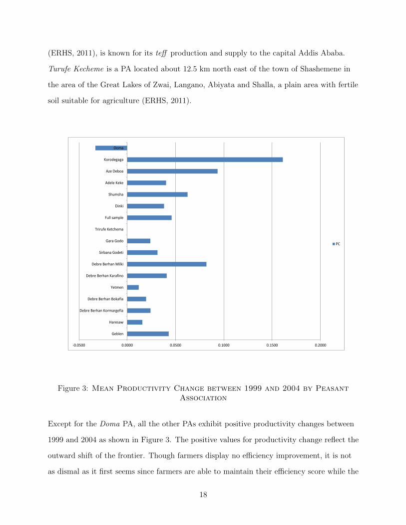
Figure 3: Mean Productivity Change between 1999 and 2004 by PeasantAssociation
Except for the Doma PA, all the other PAs exhibit positive productivity changes between
1999 and 2004 as shown in Figure 3. The positive values for productivity change reflect the
outward shift of the frontier. Though farmers display no efficiency improvement, it is not
as dismal as it first seems since farmers are able to maintain their efficiency score while the
18
production frontier is being pushed outward at one percent per year by the best performing
farmers.
5. Conclusion
We have estimated a distance function of grains production that explicitly takes into
account the interdependence among the different crops farmers produce. We have used
Box-Cox transformations, instead of logarithmic transformations, of variables to be able to
include variables with zero values in the distance function. The generalized method of
moments estimation that we follow allows us to control for the endogeneity among the
different outputs in the distance function.
The average technical efficiency of the sampled farmers is about 58.4%, implying the
potential of increasing agricultural production by over two thirds by investing the
government’s focus on efficiency-enhancing factors. The results indicate that the most
important factors determining farmers’ efficiency in Ethiopia are having access to the
public extension system, participation in off-farm activities, participation in labor sharing
parties, gender of the household head, and the extent to which farmers are forced to
produce on marginal and steeply sloped plots.
Technical change in Ethiopia’s agriculture is found to be less than one percent per year
between 1999 and 2004, while efficiency change is insignificant between the two periods.
This calls for a double sword agricultural development policy: measures that can bring
about an outward shift of the production technology such as intensification of input use
and measures that improve farmers’ efficiency given their current level of input use.
Efficiency enhancing policies in Ethiopia should emphasize an even greater expansion of
the public extension system, an extension system that has a gender component that
addresses efficiency-reducing challenges that women household heads in particular face,
that understands the traditional wisdom of farmers to work together in the face of labor
19

and credit market constraints, as well as one that gives due consideration to the availability
and generation of off-farm opportunities in rural Ethiopia.
Appendix A. Appendix
20
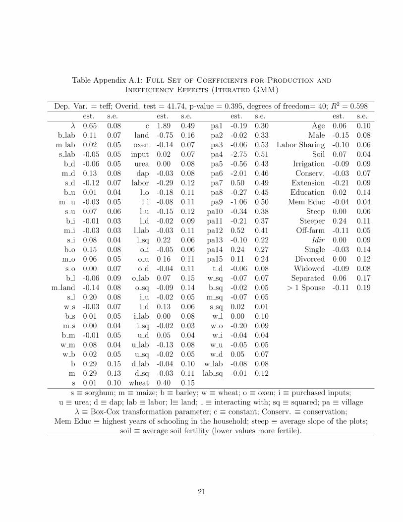
Table Appendix A.1: Full Set of Coefficients for Production andInefficiency Effects (Iterated GMM)
Dep. Var. = teff; Overid. test = 41.74, p-value = 0.395, degrees of freedom= 40; R2 = 0.598est. s.e. est. s.e. est. s.e. est. s.e.
λ 0.65 0.08 c 1.89 0.49 pa1 -0.19 0.30 Age 0.06 0.10b lab 0.11 0.07 land -0.75 0.16 pa2 -0.02 0.33 Male -0.15 0.08
m lab 0.02 0.05 oxen -0.14 0.07 pa3 -0.06 0.53 Labor Sharing -0.10 0.06s lab -0.05 0.05 input 0.02 0.07 pa4 -2.75 0.51 Soil 0.07 0.04
b d -0.06 0.05 urea 0.00 0.08 pa5 -0.56 0.43 Irrigation -0.09 0.09m d 0.13 0.08 dap -0.03 0.08 pa6 -2.01 0.46 Conserv. -0.03 0.07s d -0.12 0.07 labor -0.29 0.12 pa7 0.50 0.49 Extension -0.21 0.09b u 0.01 0.04 l o -0.18 0.11 pa8 -0.27 0.45 Education 0.02 0.14
m u -0.03 0.05 l i -0.08 0.11 pa9 -1.06 0.50 Mem Educ -0.04 0.04s u 0.07 0.06 l u -0.15 0.12 pa10 -0.34 0.38 Steep 0.00 0.06b i -0.01 0.03 l d -0.02 0.09 pa11 -0.21 0.37 Steeper 0.24 0.11
m i -0.03 0.03 l lab -0.03 0.11 pa12 0.52 0.41 Off-farm -0.11 0.05s i 0.08 0.04 l sq 0.22 0.06 pa13 -0.10 0.22 Idir 0.00 0.09
b o 0.15 0.08 o i -0.05 0.06 pa14 0.24 0.27 Single -0.03 0.14m o 0.06 0.05 o u 0.16 0.11 pa15 0.11 0.24 Divorced 0.00 0.12s o 0.00 0.07 o d -0.04 0.11 t d -0.06 0.08 Widowed -0.09 0.08b l -0.06 0.09 o lab 0.07 0.15 w sq -0.07 0.07 Separated 0.06 0.17
m land -0.14 0.08 o sq -0.09 0.14 b sq -0.02 0.05 > 1 Spouse -0.11 0.19s l 0.20 0.08 i u -0.02 0.05 m sq -0.07 0.05
w s -0.03 0.07 i d 0.13 0.06 s sq 0.02 0.01b s 0.01 0.05 i lab 0.00 0.08 w l 0.00 0.10m s 0.00 0.04 i sq -0.02 0.03 w o -0.20 0.09b m -0.01 0.05 u d 0.05 0.04 w i -0.04 0.04w m 0.08 0.04 u lab -0.13 0.08 w u -0.05 0.05w b 0.02 0.05 u sq -0.02 0.05 w d 0.05 0.07
b 0.29 0.15 d lab -0.04 0.10 w lab -0.08 0.08m 0.29 0.13 d sq -0.03 0.11 lab sq -0.01 0.12s 0.01 0.10 wheat 0.40 0.15s ≡ sorghum; m ≡ maize; b ≡ barley; w ≡ wheat; o ≡ oxen; i ≡ purchased inputs;
u ≡ urea; d ≡ dap; lab ≡ labor; l≡ land; ≡ interacting with; sq ≡ squared; pa ≡ villageλ ≡ Box-Cox transformation parameter; c ≡ constant; Conserv. ≡ conservation;
Mem Educ ≡ highest years of schooling in the household; steep ≡ average slope of the plots;soil ≡ average soil fertility (lower values more fertile).
21

Table Appendix A.2: Full Set of Coefficients for Production andInefficiency Effects (Two-step GMM)
Dep. Var. = teff; Overid. test = 47.87, p-value = 0.184, degrees of freedom= 40; R2 = 0.637est. s.e. est. s.e. est. s.e. est. s.e.
λ 0.66 0.08 c 1.74 0.51 pa1 -0.14 0.31 Age 0.04 0.11b lab 0.15 0.08 land -0.69 0.17 pa2 0.06 0.33 Male -0.18 0.08
m lab 0.03 0.05 oxen -0.14 0.08 pa3 0.00 0.56 Labor Sharing -0.11 0.06s lab -0.07 0.05 input -0.02 0.07 pa4 -2.49 0.54 Soil 0.07 0.04
b d -0.07 0.05 urea 0.01 0.08 pa5 -0.42 0.44 Irrigation -0.13 0.09m d 0.11 0.08 dap -0.08 0.08 pa6 -1.61 0.47 Conserv. -0.05 0.07s d -0.12 0.07 labor -0.31 0.13 pa7 0.53 0.50 Extension -0.21 0.09b u 0.01 0.04 l o -0.11 0.11 pa8 -0.17 0.46 Education -0.02 0.14
m u -0.01 0.05 l i -0.14 0.11 pa9 -0.88 0.51 Mem Educ -0.04 0.04s u 0.06 0.06 l u -0.10 0.12 pa10 -0.23 0.39 Steep 0.01 0.06b i -0.01 0.03 l d 0.04 0.08 pa11 -0.08 0.38 Steeper 0.24 0.11
m i -0.03 0.03 l lab 0.04 0.11 pa12 0.76 0.41 Off-farm -0.10 0.05s i 0.05 0.04 l sq 0.14 0.04 pa13 0.00 0.24 Idir -0.02 0.10
b o 0.14 0.08 o i 0.00 0.06 pa14 0.41 0.28 Single -0.08 0.14m o 0.05 0.05 o u 0.16 0.11 pa15 0.28 0.26 Divorced -0.07 0.12s o -0.01 0.07 o d -0.06 0.12 t d -0.11 0.08 Widowed -0.11 0.08b l -0.07 0.09 o lab 0.00 0.15 w sq -0.10 0.08 Separated -0.04 0.16
m land -0.03 0.08 o sq -0.12 0.15 b sq -0.03 0.05 > 1 Spouse -0.10 0.20s l 0.16 0.08 i u -0.01 0.05 m sq -0.09 0.05
w s -0.06 0.07 i d 0.11 0.06 s sq 0.01 0.01b s 0.02 0.06 i lab 0.01 0.09 w l -0.05 0.09m s 0.03 0.04 i sq -0.02 0.03 w o -0.18 0.09b m -0.05 0.05 u d 0.02 0.04 w i -0.02 0.04w m 0.11 0.04 u lab -0.14 0.09 w u -0.06 0.05w b 0.05 0.05 u sq -0.01 0.05 w d 0.08 0.08
b 0.29 0.16 d lab -0.05 0.11 w lab -0.11 0.09m 0.35 0.13 d sq -0.02 0.12 lab sq 0.02 0.13s -0.02 0.10 wheat 0.39 0.15s ≡ sorghum; m ≡ maize; b ≡ barley; w ≡ wheat; o ≡ oxen; i ≡ purchased inputs;
u ≡ urea; d ≡ dap; lab ≡ labor; l≡ land; ≡ interacting with; sq ≡ squared; pa ≡ villageλ ≡ Box-Cox transformation parameter; c ≡ constant; Conserv. ≡ conservation;
Mem Educ ≡ highest years of schooling in the household; steep ≡ average slope of the plots;soil ≡ average soil fertility (lower values more fertile).
22
Admassu, S. 2004. “Rainfall Variation and its Effect on Crop Production in Ethiopia.” MS
thesis, Addis Ababa University, School of Graduate Studies.
Alene, A.D., and M. Zeller. 2005. “Technology Adoption and Farmer Efficiency in Multiple
Crops Production in Eastern Ethiopia: A Comparison of Parametric and Non-parametric
Distance Functions.” Agricultural Economics Review 6:5 – 17.
Arega, M. 2009. “Determinants of Intensity of Adoption of Old Coffee Stumping
Technology in Dale Woreda, SNNPR, Ethiopia.” MS thesis, Haramaya University.
Atkinson, S.E., C. Cornwell, and O. Honerkamp. 2003. “Measuring and Decomposing
Productivity Change: Stochastic Distance Function Estimation versus Data
Envelopment Analysis.” Journal of Business and Economic Statistics 21:284 – 294.
Atkinson, S.E., and J.H. Dorfman. 2005. “Bayesian measurement of productivity and
efficiency in the presence of undesirable outputs: crediting electric utilities for reducing
air pollution.” Journal of Econometrics 126:445 – 468, Current developments in
productivity and efficiency measurement.
Baum, C.F., M.E. Schaffer, and S. Stillman. 2003. “Instrumental Variables and GMM:
Estimation and Testing.” The Stata Journal 3:1 – 31.
Bewket, W. 2009. “Rainfall variability and crop production in Ethiopia: Case study in the
Amhara region.” In Proceedings of the 16th International Conference of Ethiopian
Studies, ed. by S. Ege, H. Aspen, B. Teferra, and S. Bekele.
Brummer, B., T. Glauben, and W. Lu. 2006. “Policy Reform and Productivity Change in
Chinese Agriculture: A Distance Function Approach.” Journal of Development
Economics 81:61 – 79.
Coelli, T., and S. Perelman. 2000. “Technical Efficiency of European Railways: A Distance
Function Approach.” Applied Economics 32:1967 – 1976.
23

Coelli, T.J., D.P. Rao, C.J. O’Donnell, and G.E. Battese. 2005. An Introduction to
Efficiency and Productivity Analysis , 2nd ed. Springer.
CSA. 2009. “Statistical Abstracts and Statistical Bulletins.Various years.” Working paper,
Central Statistics Agency: Federal Democratic Republic of Ethiopia., Addis Ababa:
CSA.
Deininger, K., D.A. Ali, S. Holden, and J. Zevenbergen. 2008. “Rural Land Certification in
Ethiopia: Process, Initial Impact, and Implications for Other African Countries.” World
Development 36:1786 – 1812.
Dorosh, P. 2012. Food and Agriculture in Ethiopia: Progress and Policy Challenges ,
University of Pennsylvania Press: Philadelphia, chap. The Evolving Role of Agriculture
in Ethiopia’s Economic Development. pp. 318 – 326.
ERHS. 2011. “Ethiopia Rural Household Survey: 1989 - 2009. International Food Policy
Research Institute.”
FAO. 2012. “Crop Calendar - An Information Tool for Food Security.”
Mekonnen, D., and J.H. Dorfman. 2013. “Learning and Synergy in Social Networks:
Productivity Impacts of Informal Labor Sharing Arrangements.” Unpublished.
O’Donnell, C.J., and T.J. Coelli. 2005. “A Bayesian Approach to Imposing Curvature on
Distance Functions.” Journal of Econometrics 126:493 – 523.
Perelman, S., and D. Santin. 2011. “Measuring Educational Efficiency at Student Level
with Parametric Stochastic Distance Functions: An Application to Spanish PISA
Results.” Education Economics 19:29 – 49.
Spielman, D.J., D. Kelemework, and D. Alemu. 2011. “Seed, Fertilizer, and Agricultural
Extension in Ethiopia.” Unpublished, ESSP II Working Paper 020, International Food
Policy Research Institute.
24
Stock, J.H., J. Wright, and M. Yogo. 2002. “GMM, Weak Instruments, and Weak
Identification.” Unpublished, Journal of Business and Economic Statistics symposium on
GMM.
Taffesse, A.S., P. Dorosh, and S.A. Gemessa. 2012. Food and Agriculture in Ethiopia:
Progress and Policy Challenges , University of Pennsylvania Press: Philadelphia, chap.
Crop Production in Ethiopia: Regional Patterns and Trends. pp. 53 – 83.
Wooldridge, J.M. 2002. Econometric Analysis of Cross Section and Panel Data. The MIT
Press.
25
Related Documents


