FA M ag sti pr pe FACTOR M Tel: +32 (0)2 Firm ABSTR Drawing matchin allocatio find tha variable €1,000 total fa improve farms. T labour, credit co No. 3, Pavel d’Art ACTOR MAR ARKETS rese griculture in t imulating reac roject. Unless ersonal capacit Availa © Co MARKETS Coo 2 229 3911 • Fax Prod m-Leve RACT g on a uniq ng estimato on and farm at farms ar e inputs an of addition actor produ ement in ac This findin suggesting onstrained Septem l Ciaian tis Kanc RKETS Worki earch project, the member s ctions from ot otherwise ind ty and not to a able for free do opyright 2011, ordination: Ce x: +32 (0)2 229 ductiv el Evide que, farm-l or, this pa m efficiency re asymmet nd capital i nal credit. O uctivity up ccess to cre ng is furthe g that these with respec mber 201 n, Jan F cs & Ja ing Papers p which analys states, candid ther experts in dicated, the v any institution ownloading fro and CEPS ISBN-1 , Pavel Ciaian, entre for Euro 4151 • E-mail: i vity an ence fro level panel aper analys y in the Cen trically cred investment Our estimat to 1.9% pe edit results i r supported e two are su ct to land. 11 Fałkow an Pokr presents work ses and comp date countries n the field. See iews expresse n with which t om the Factor (www.ceps.eu 3: 978-94-613 , Jan Fałkowsk opean Policy nfo@factormar nd Cre om Pro dataset wit ses how far ntral and Ea dit constrai increases tes also sug er €1,000 in an adjus d by a neg ubstitutes. wski, rivcak k being cond pares the func s and the EU e the back cove ed are attribut hey are associ r Markets (ww u ) websites 38-127-9 ki, d’Artis Kan Studies (CEPrkets.eu • web: w edit Co opensit th 37,409 o rm access astern Euro ned with re up to 2.3% ggest that fa of addition stment in th ative effect Interesting ducted within ctioning of fac U as a whole, er for more inf table only to iated. ww.factormark ncs & Jan Pokr S), 1 Place du C www.factormark onstr ty Score observation to credit opean trans espect to in % and 29% arm access nal credit, he relative i t of better a ly, farms a n the FACTO ctor markets with a view formation on t the authors in kets.eu ) rivcak Congrès, 1000 B kets.eu aints e Match ns and emp affects farm sition count nputs. Farm %, respectiv to credit in indicating input intens access to c are found n OR for to the n a Brussels, Belgiuhing ploying a m input tries. We m use of vely, per ncreases that an sities on credit on not to be m

Welcome message from author
This document is posted to help you gain knowledge. Please leave a comment to let me know what you think about it! Share it to your friends and learn new things together.
Transcript
FAMAagstiprpe
FACTOR MTel: +32 (0)2
Firm
ABSTR
Drawingmatchinallocatiofind thavariable€1,000 total faimprovefarms. Tlabour, credit co
No. 3,
Paveld’Art
ACTOR MARARKETS rese
griculture in timulating reacroject. Unless ersonal capacit
Availa
© Co
MARKETS Coo2 229 3911 • Fax
Prodm-Leve
RACT
g on a uniqng estimatoon and farmat farms are inputs an of addition
actor produement in acThis findin suggestingonstrained
Septem
l Ciaiantis Kanc
RKETS Workiearch project, the member sctions from ot otherwise indty and not to a
able for free do
opyright 2011,
ordination: Cex: +32 (0)2 229
ductivel Evide
que, farm-lor, this pam efficiencyre asymmetnd capital inal credit. Ouctivity up ccess to cre
ng is furtheg that these with respec
mber 201
n, Jan Fcs & Ja
ing Papers p which analysstates, candid
ther experts indicated, the vany institution
ownloading froand CEPS
ISBN-1
, Pavel Ciaian,
entre for Euro 4151 • E-mail: i
vity anence fro
level panel aper analysy in the Centrically credinvestment Our estimatto 1.9% pe
edit results ir supported
e two are suct to land.
11
Fałkowan Pokr
presents workses and compdate countriesn the field. Seeviews expressen with which t
om the Factor (www.ceps.eu
3: 978-94-613
, Jan Fałkowsk
opean Policy Snfo@factormar
nd Creom Pro
dataset witses how farntral and Eadit constrai increases tes also suger €1,000 in an adjusd by a negubstitutes.
wski, rivcak
k being condpares the funcs and the EUe the back coveed are attributhey are associ
r Markets (wwu) websites
38-127-9
ki, d’Artis Kan
Studies (CEPSrkets.eu • web: w
edit Coopensit
th 37,409 orm access astern Euroned with reup to 2.3%
ggest that faof addition
stment in thative effectInteresting
ducted withinctioning of fac
U as a whole,er for more inftable only to iated.
ww.factormark
ncs & Jan Pokr
S), 1 Place du Cwww.factormark
onstrty Score
observationto credit
opean transespect to in% and 29%farm access nal credit, he relative it of better aly, farms a
n the FACTOctor markets with a viewformation on tthe authors in
kets.eu)
rivcak
Congrès, 1000 Bkets.eu
aints e Match
ns and empaffects farm
sition countnputs. Farm
%, respectiv to credit inindicating
input intensaccess to c
are found n
OR for
w to the n a
Brussels, Belgium
hing
ploying a m input tries. We m use of vely, per ncreases that an
sities on credit on not to be
m
Contents
Introduction .................................................................................................................................. 1
1. Farm sector and farm credit in Central and Eastern Europe: Descriptive statistics ........... 3
2. Theoretical framework ........................................................................................................... 5
2.1 Related literature ......................................................................................................... 5
2.2 The model ..................................................................................................................... 6
2.3 The impact of credit constraints on production .......................................................... 7
3. Econometric specification ................................................................................................... 10
4. Data and variable construction ........................................................................................... 12
5. Estimation results ................................................................................................................ 14
5.1 Matching ..................................................................................................................... 14
5.2 Pooled sample ............................................................................................................ 15
5.3 Country-level analysis ................................................................................................ 17
5.4 Limitations ................................................................................................................. 21
6. Conclusions .......................................................................................................................... 22
References ................................................................................................................................... 23
Appendix: Data............................................................................................................................ 26
List of Tables
Table 1. Farm sector and credit in CEE and (selected) developed EU countries in 2005 ....... 4
Table 2. Definition and summary of credit groups ................................................................. 13
Table 3. Credit and farm behaviour: Matching estimates of the effect of accessing credit on farm output and inputs – Pooled sample ............................................................. 16
Table 4. Percentage change of productivity and use of inputs per €1,000 of additional credit – Pooled sample (%/€ credit) ......................................................................... 16
Table 5. Credit and farm behaviour: Czech Republic ............................................................. 18
Table 6. Credit and farm behaviour: Estonia .......................................................................... 19
Table 7. Credit and farm behaviour: Hungary ........................................................................ 19
Table 8. Credit and farm behaviour: Lithuania ...................................................................... 20
Table 9. Credit and farm behaviour: Latvia ........................................................................... 20
Table 10. Credit and farm behaviour: Poland ........................................................................... 21
| 1
Productivity and Credit Constraints Firm-Level Evidence from Propensity Score Matching
Pavel Ciaian, Jan Fałkowski, d’Artis Kancs and Jan Pokrivcak*
Factor Markets Working Paper No. 3/September 2011
Introduction
The shortage of credit has been identified as a crucial element determining farm performance and development. Budget constraints have been found to be a decisive factor limiting farms’ use of inputs not only in developing countries but also in developed economies (Bhattacharyya and Kumbhakar, 1997; Heltberg, 1998; Lee and Chambers, 1986; Färe et al., 1990; Blancard et al., 2006). Owing to a series of transition-related issues, this problem has been especially acute in the agricultural sector of Central and Eastern Europe (CEE) (Swinnen and Gow, 1999; OECD, 1999; OECD, 2001; Dries and Swinnen, 2004).
The main focus of the emerging literature on agricultural credit in transition countries is the determinants of farm access to credit (Bezemer, 2002; Davidova and Thomson, 2003; Latruffe et al., 2010). Considerably less attention has been paid to the relationship between credit constraints and farm behaviour, such as farm input choices and productivity. Notable exceptions include Dries and Swinnen (2004) and Latruffe (2005). That there are only a few studies looking at the relationship between credit constraints and farm behaviour can be explained by a lack of the necessary micro data for addressing the identification and endogeneity issues. The complexity of the imperfections in rural credit markets makes it extremely difficult to test which farms are credit constrained, by how much and what impact this may have on farm behaviour. This is especially difficult in cross-section regressions, since the estimated correlations may reflect an omitted variable or reverse causation problems.
The objective of this paper is to analyse how farm production and input use (land, variable inputs, labour and capital) is related to farm access to credit in the CEE transition countries. The main contribution of the paper to the literature is the application of a unique cross-country sample of harmonised firm-level panel data (from the Farm Accountancy Data Network (FADN)), and the empirical methodology, which is based on matching estimators. To our knowledge, the present paper is the first to investigate the importance of access to credit for farm performance in the CEE region as a whole.1 In contrast to existing studies, which are usually for single countries, we use a harmonised farm-level panel dataset for eight CEE transition countries. This allows us to investigate the effect of access to credit not only in each particular country, but also in the whole region. This is important because notwithstanding the country-specific issues, all transition countries faced a number of * Pavel Ciaian is a researcher at the Joint Researcher Center at the European Commission, and an associated researcher at the Catholic University of Leuven (LICOS), and Slovak Agricultural University. Jan Fałkowski is a researcher at the Faculty of Economic Sciences (Chair of Political Economy), University of Warsaw and Centre for Economic Analyses of Public Sector (CEAPS). D’Artis Kancs is a researcher at the Joint Researcher Center at the European Commission and an associated researcher at the Catholic University of Leuven (LICOS), and Economics and Econometrics Research Institute (EERI). Jan Pokrivcak is a professor at the Slovak Agricultural University. The authors are grateful to the Microeconomic Analysis Unit L.3 of the European Commission for granting access to the firm-level FADN data. The views expressed are purely those of the authors and may not under any circumstances be regarded as stating an official position of the European Commission. 1 For cross-country studies of other regions, see for example Benjamin and Phimister (2002).
2 | CIAIAN, FAŁKOWSKI, KANCS & POKRIVCAK
common problems related to local credit markets, ranging from a lack of skilled and experienced banking staff, a lack of accountancy and bookkeeping systems at the farm level, and the politically rather than economically motivated asset (re)distribution at the beginning of the 1990s, to farms’ accumulated debts and incomplete property rights to land that reduced the suitability of land as collateral (Swinnen and Gow, 1999; OECD, 1999; OECD, 2001).
The large size of the FADN dataset has an additional advantage. It allows us to employ a semi-parametric estimator based on propensity score matching (Rosenbaum and Rubin, 1983). The use of more than 37,409 observations ensures that the loss in efficiency of semi-parametric estimates compared with parametric ones is not a problem. This is critical for at least two reasons. First, applying a semi-parametric, propensity score-matching estimator allows us to control for any heterogeneity in the relationship between farm performance and observable characteristics (particularly access to credit). Second, matching estimators are robust in situations in which farms that have access to credit differ systematically from those that do not.
The conceptual framework of our study is based on Blancard et al. (2006). In our model the availability of credit is determined by several factors, as farms have various options for accessing financial resources.2 The theoretical model offers two testable hypotheses for farm adjustments in input use and output supply. The first hypothesis says that with perfect credit markets the source of financing is irrelevant; hence a farm’s access to credit will affect neither farm input choices nor the level of farm output. Thus, we implicitly assume that farm input and the productivity response to credit access reflect a farm’s credit constraint. The second hypothesis says that a symmetric credit constraint affects the scale of input use, but not the relative input intensities, whereas an asymmetric credit constraint affects both the level of input use and the relative factor intensities. A symmetric credit constraint does not affect the relative (shadow) prices of inputs. In effect, if farms face symmetric credit constraints on all inputs, improved access to credit increases the use of all inputs (Blancard et al., 2006). On the other hand, an asymmetric credit constraint affects the relative, marginal value product of inputs as well as the scale of input use (Lee and Chambers, 1986; Färe et al., 1990). As a result, it will affect both the level of input use and the relative factor intensities. More credit-constrained inputs will be substituted for less credit-constrained inputs.
Our results have important policy implications, because in the CEE transition countries farms receive a substantial amount of support from the EU’s common agricultural policy (CAP). Farms are granted direct payments either per hectare or coupled to production.
2 First, financial resources are channelled to the agricultural sector through vertical integration (Dries and Swinnen, 2004; Gorton and White, 2007; Swinnen, 2007). Second, governments in many countries intervene in agricultural markets with agricultural support policies. Even though agricultural support measures may not be intended to directly improve farm access to credit, they may alleviate farms’ budget constraints by increasing farms’ cash flow and thus increasing their credit-worthiness (Ciaian and Swinnen, 2009). Moreover, the interaction of rural financial structures and government intervention may lead to input-specific adjustments. For example, agricultural subsidies may increase short-term credit, which is needed to finance variable inputs, rather than long-term credit, which is needed for fixed inputs (Ciaian and Swinnen, 2009). Third, in the presence of costly contract enforcement and asymmetric information, the collateral may represent an important instrument in securing farms’ access to credit (Bester, 1985; Ghosh et al., 2000). The use of collateral for securing credit is in turn conditional on the functioning of rural land markets (Ciaian and Swinnen, 2009). Finally, factors such as rural insurance markets and informal rural institutions may have a direct or indirect impact on farm credit, for example by affecting, among others, the risk level of agricultural production, loan guarantee options and income volatility.
IMPACT OF CAPITAL USE | 3
In addition, farms receive investment support from the EU’s rural development policies. Our study examines which farm inputs are particularly credit constrained, and consequently indicates what kinds of support measures might be especially efficient for policy interventions to alleviate farm credit problems in the transition economies in Central and Eastern Europe. The fact that all transition countries under study benefit from a number of common policy instruments additionally supports our approach to working with both pooled and country-specific data.
1. Farm sector and farm credit in Central and Eastern Europe: Descriptive statistics
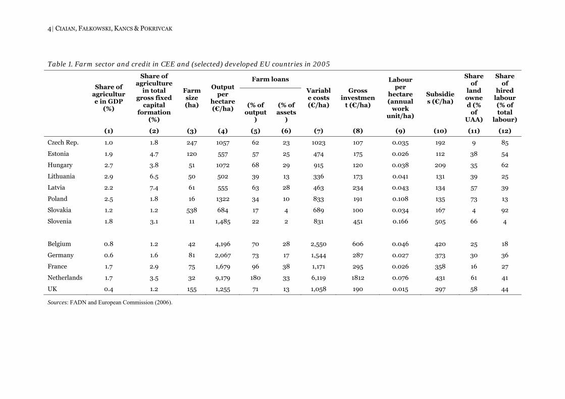
In Table 1 we provide descriptive statistics on agriculture and credit in CEE and selected, developed EU member states. In developed and developing countries the agricultural sector represents a small proportion of total economic production. The share of the agricultural sector in GDP is less than 3% in CEE countries but higher than in developed EU member states (column 1 in Table 1). Although the contribution of agriculture to overall production is low, in terms of fixed capital formation its share is disproportionally higher – in several countries it is twice the share of agriculture in GDP (column 2). This indicates higher capital intensity and potentially higher credit requirements by agricultural production than the average for the overall economy (Barry and Robinson, 2001). This holds for both developed EU member states and less developed CEE countries.
There are several structural differences between the agricultural sector in CEE countries and that in developed EU member states. First, consistent with overall economic development, agriculture in CEE countries is less productive than the agriculture in developed EU member states if measured by output per hectare (column 4). Lower productivity is also reflected in less use of variable inputs (column 7), lower gross investment (column 8) and smaller subsidies (column 10), because the payment system of the CAP is linked to past productivity levels.
Second, corporate farming is more widespread in CEE countries because of its heritage from the former communist system. There is a particularly high share of corporate farms in the Czech Republic and Slovakia. Alongside corporate farms, small (often subsistence) individual farms coexist, which tend to be smaller than their counterparts in more developed EU member states. Poland and Slovenia are prominent examples of countries with a farm sector dominated by individual farms. The farm structure in Estonia and Lithuania is also mainly composed of individual farms. Other CEE countries have a mixed farm structure (Ciaian and Swinnen, 2006). Farm corporatisation is reflected in higher average farm size (column 3), a lower level of land ownership by farms (column 11), less labour use (column 9) and greater use of hired labour (column 12).
Third, credit use in CEE countries tends to be smaller than in developed EU member states (columns 5 and 6). Yet within Central and Eastern Europe, those countries where a mixed farm structure and corporate farming dominate the agricultural sector (with the exception of Slovakia) tend to rely more on financing through credit compared with countries where individual farms are more prominent. Empirical evidence tends to support the view that farm size may be an important determinant of access to credit. Bezemer (2003) finds in the case of the Czech Republic that long-established and larger corporate farms have better access to credit than small individual farms.
4 | CIAIAN, FAŁKOWSKI, KANCS & POKRIVCAK
Table 1. Farm sector and credit in CEE and (selected) developed EU countries in 2005
Share of agriculture in GDP
(%)
Share of agriculture
in total gross fixed
capital formation
(%)
Farm size (ha)
Output per
hectare (€/ha)
Farm loans
Variable costs (€/ha)
Gross investmen
t (€/ha)
Labour per
hectare (annual
work unit/ha)
Subsidies (€/ha)
Share of
land owned (%
of UAA)
Share of
hired labour (% of total
labour)
(% of output
)
(% of assets
)
(1) (2) (3) (4) (5) (6) (7) (8) (9) (10) (11) (12)
Czech Rep. 1.0 1.8 247 1057 62 23 1023 107 0.035 192 9 85
Estonia 1.9 4.7 120 557 57 25 474 175 0.026 112 38 54
Hungary 2.7 3.8 51 1072 68 29 915 120 0.038 209 35 62
Lithuania 2.9 6.5 50 502 39 13 336 173 0.041 131 39 25
Latvia 2.2 7.4 61 555 63 28 463 234 0.043 134 57 39
Poland 2.5 1.8 16 1322 34 10 833 191 0.108 135 73 13
Slovakia 1.2 1.2 538 684 17 4 689 100 0.034 167 4 92
Slovenia 1.8 3.1 11 1,485 22 2 831 451 0.166 505 66 4
Belgium 0.8 1.2 42 4,196 70 28 2,550 606 0.046 420 25 18
Germany 0.6 1.6 81 2,067 73 17 1,544 287 0.027 373 30 36
France 1.7 2.9 75 1,679 96 38 1,171 295 0.026 358 16 27
Netherlands 1.7 3.5 32 9,179 180 33 6,119 1812 0.076 431 61 41
UK 0.4 1.2 155 1,255 71 13 1,058 190 0.015 297 58 44
Sources: FADN and European Commission (2006).
IMPACT OF CAPITAL USE | 5
2. Theoretical framework
2.1 Related literature
Approaches on credit constraint can be grouped into at least three groups.3 First, static farm/household, profit/utility maximisation models are extensively used to explain the observed patterns of farm/household behaviour in the presence of credit constraints (e.g. Lee and Chambers, 1986; Färe et al., 1990; Blancard et al., 2006; Feder, 1985; Carter and Wiebe, 1990). The second strand of literature entails dynamic investment models, such as intertemporal investment maximisation models and accelerator models (e.g. Konings et al., 2003; Agbola, 2005; Bakucs et al., 2009; Latruffe et al., 2010). The third approach includes asymmetric information models. The risk and asymmetrical information may lead to adverse selection and moral hazard, and may induce lenders to ration the amount of credit supplied to the farm sector, giving rise to liquidity or credit constraints and impacting on farm behaviour (e.g. Carter, 1988).
In the present study we develop a farm profit-maximisation model along the first approach. We start with a brief review of the previous literature upon which we draw in our theoretical framework. A notable early paper on the farm-level effects of credit constraint is that by Lee and Chambers (1986), who develop a theoretical farm profit-maximisation model with farms facing constraints on funding short-term farm operating expenses. They consider a situation whereby a farm’s total expenditures on variable inputs are constrained by a predetermined level of expenditure. Testing the model on US data, Lee and Chambers reject unconstrained farm profit-maximisation behaviour, while expenditure-constrained profit maximisation could not be rejected.
Färe et al. (1990) adopt a nonparametric alternative to the Lee and Chambers (1986) model. Similar to Lee and Chambers, they compare the behaviour of farms with constrained expenditure on variable inputs with that of farms not being credit constrained. Specifically, Färe et al. construct a deterministic frontier profit function with and without expenditure constraints using a linear programming approach. They apply the model to a sample of Californian rice farms. Their results indicate that 21% of farms face a binding credit constraint. The average profit loss of the expenditure-constrained farms was found to be around 8% of their unconstrained profit.
Blancard et al. (2006) extend the models of Lee and Chambers (1986) and Färe et al. (1990) to differentiate credit constraints between the short and long run. They assume that in the short run only the expenditures on variable inputs are constrained, while in the long run the expenditures on all (variable and fixed) inputs are constrained. They test the model predictions using a panel of French farmers in the Nord-Pas-de-Calais region. Blancard et al. find that in the short run 67% of farms are credit constrained, while in the long run almost all farms are credit constrained. The losses in profits owing to credit constraint amount on average to 8% and 49% of profits in the short and long run, respectively.
The farm model has also been employed to investigate, among others, the productivity effect of farm credit constraint (Bhattacharyya and Kumbhakar, 1997; Briggeman et al., 2009), productivity and farm size in developing countries (Feder, 1985; Carter and Wiebe, 1990), the allocation of farm inputs (Bhattacharyya et al., 1996) and the distributional effects of agricultural support policies in the presence of credit constraint (Ciaian et al., 2008; Ciaian and Swinnen, 2009). Except for the latter two studies, however, the existing literature does not deal with the transition countries.
3 For more details on credit rationing in agriculture, see the summary outlined by Barry and Robinson (2001).
6 | CIAIAN, FAŁKOWSKI, KANCS & POKRIVCAK
2.2 The model
We build the theoretical framework of the present study on the model of Blancard et al. (2006). Accordingly, we consider the case of a representative profit-maximising farm with the possibility of input credit constraints. The constant returns to scale production technology (f(X,Y)) of the representative farm is assumed to be a function of two inputs, X and Y. The representative farm’s profits are given by YwXwYXpf YX −−=Π ),( , where p is
the output price and iw are the input prices for i = X, Y.
Following Blancard et al. (2006), we model an imperfect credit market by assuming that the credit-constrained farm has C amount of credit available for financing input purchases.4 The value of credit C is a predetermined level of expenditure, which cannot be exceeded when purchasing inputs:5
CYwXw YX ≤+δα (1)
where α and δ are dummy variables that distinguish farm credit constraint between inputs. If 1=α and 1=δ , this suggests a symmetric farm credit constraint for both inputs. A farm may be more credit constrained with respect to some inputs than others, implying an asymmetry in the credit constraint. For simplicity, we assume that the farm is credit constrained with respect to either input X ( 1=α and 0=δ ) or input Y ( 0=α and 1=δ ).
The farm maximises profits subject to credit constraint (1) according to Lagrangean:
( )CYwXwYwXwYXpf YXYX −+−−−=Ψ δαλ),( (2)
where λ is the shadow price of the credit constraint. The optimal conditions for a credit-constrained farm are as follows:
( ) XX wpf λα+= 1 (3)
( ) YY wpf λδ+= 1 (4)
From equations (3) and (4) it follows that the marginal value product of both inputs is higher than the price of inputs in equilibrium if a farm is symmetrically credit constrained (i.e. if
1=α , 1=δ and 0>λ ): XX wpf > and YY wpf > , respectively. A farm could potentially increase its profits by increasing input use but it cannot do so because of a binding credit constraint. If a farm is asymmetrically credit constrained for the input X (i.e. if 1=α , 0=δ and 0>λ ), then only the marginal value product of input X exceeds its price, while the
4 An important source of credit constraint can arise from a time lag between agricultural production and payment for variable inputs throughout the season. For example, variable inputs are paid at the beginning of the season, whereas the revenue from the sale of production is collected after the harvest at the end of the season (Feder, 1985; Carter and Wiebe, 1990; Ciaian and Swinnen, 2009). These characteristics of agricultural production require the pre-financing of inputs. 5 The evidence from the literature shows that farm characteristics (e.g. reputation, owned assets and profitability) are important determinants of farm credit (e.g. Benjamin and Phimister, 2002; Latruffe, 2005; Briggeman et al., 2009). For example, using micro data from Poland, Latruffe (2005) finds that farmers with more tangible assets and with more owned land were less credit constrained than others. Briggeman et al. (2009) find that for farm and non-farm sole proprietorships in the US the probability of being denied credit is reduced, among other factors, by net worth, income, price of assets and subsidies.
IMPACT OF CAPITAL USE | 7
marginal value product of input Y is equal to the own price: XX wpf > and YY wpf = ,
respectively. Conversely, if a farm is asymmetrically constrained for input Y (i.e. if 0=α ,
1=δ and 0>λ ), then it holds that XX wpf = and YY wpf > . Finally, if the farm’s credit
constraint (1) is non-binding (i.e. if 0=λ ), then in equilibrium the marginal value product of
both inputs is equalised with their respective prices: XX wpf = and YY wpf = .
2.3 The impact of credit constraints on production
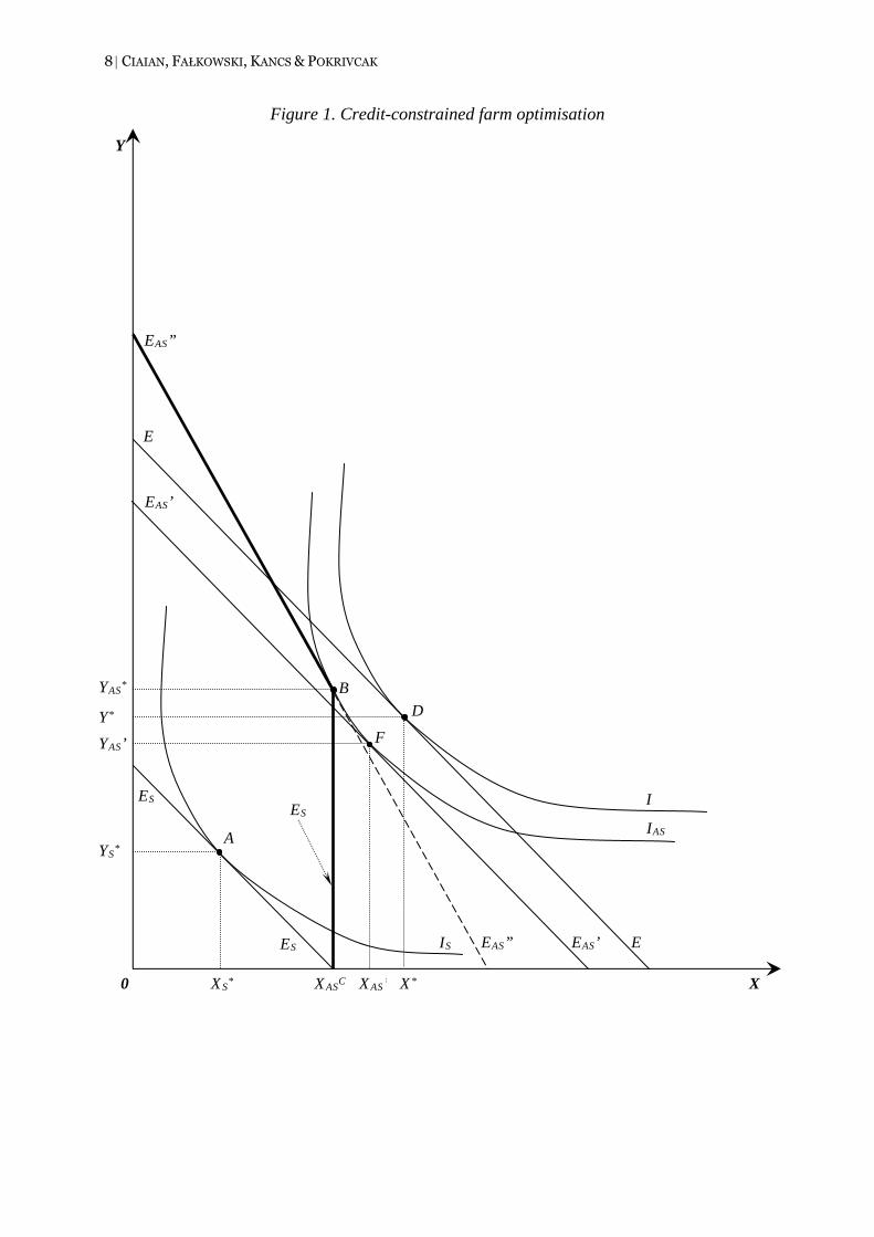
To establish a reference for comparative statics, we first identify the equilibrium without credit constraint ( 0=λ ). This is illustrated in Figure 1. The vertical axis shows the quantity of input Y, whereas the horizontal axis shows the quantity of input X. The equilibrium farm use of inputs with non-binding credit C is determined at point D, i.e. where the relative marginal value product of inputs is equal to their relative market prices,
** YXYX wwpfpf = .6 The equilibrium D is determined by the tangency between the
isoquant I and the isocost EE. We assume that the output level given by the isoquant I represents the optimal farm output for the given input and output prices and with non-binding credit constraints. The amount of credit is irrelevant in this case; the credit does not affect the output level and farm input choices.
Asymmetric credit constraint
An asymmetric credit constraint binds one input: a farm is credit constrained with respect to
either input X ( 1=α , 0=δ ) or input Y ( 0=α , 1=δ ). Consider a reduction of available farm credit from C to C1 (C1 < C). We assume that C1 makes the credit constraint (1) binding
( 01 >λ ). The binding credit C1 affects one of the farm’s equilibrium conditions (3) and (4), depending on which input is credit constrained. The asymmetric credit constraint increases the marginal value product of the constrained input above its market price, whereas for the
unconstrained input the equality is not affected: 0)()( 1 =−>−
ASjjASii wCpfwCpf, for i, j
= X, Y (this follows from equations (3) and (4)), where input i is assumed to be credit constrained.
The impact of an asymmetric credit constraint can be decomposed into two effects: a scale effect and an input substitution effect. For example, consider a case in which the input X is
constrained ( 1=α , 0=δ ). Relative to a situation with a non-binding credit constraint, less credit reduces production scale. In Figure 1 it leads to a parallel shift of the isocost from EE to EAS‘EAS’. This scale effect of an asymmetric credit constraint shifts the equilibrium from D to F, which is the tangent point between the isocost EAS‘EAS’ and the isoquant IAS. The isoquant IAS is below the no-credit constraint isoquant I, implying a lower output with than without the binding (asymmetric) credit constraint. Note that the lower output scale reduces the use
of both inputs (*' XX AS < and
*' YYAS < ).
6 We define the notations
*x ,
Sx and
ASx for equilibriums with non-binding, symmetric and asymmetric
credit constraints, respectively.
8 | CIAIAN, FAŁKOWSKI, KANCS & POKRIVCAK
Figure 1. Credit-constrained farm optimisation
A
B
X
Y
0
D
E
E
ES ES
XS* X* XAS
C
YS*
YAS*
Y*
I
IS
IAS
EAS’’
F
XAS’
YAS’
EAS’’ EAS’ ES
EAS’
9 | CIAIAN, FAŁKOWSKI, KANCS & POKRIVCAK
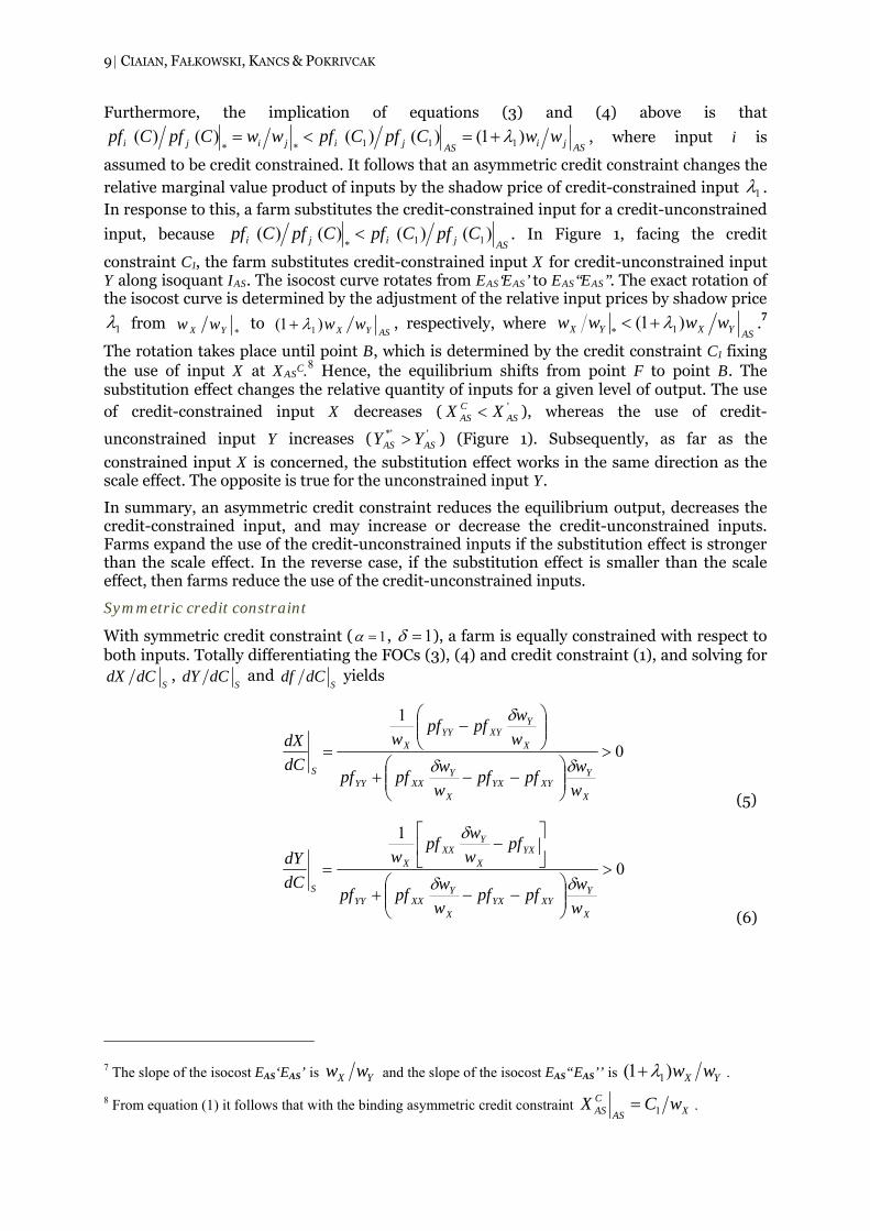
Furthermore, the implication of equations (3) and (4) above is that
ASjiASjijiji wwCpfCpfwwCpfCpf )1()()()()( 111**λ+=<= , where input i is
assumed to be credit constrained. It follows that an asymmetric credit constraint changes the relative marginal value product of inputs by the shadow price of credit-constrained input 1λ . In response to this, a farm substitutes the credit-constrained input for a credit-unconstrained
input, because ASjiji CpfCpfCpfCpf )()()()( 11*
< . In Figure 1, facing the credit
constraint C1, the farm substitutes credit-constrained input X for credit-unconstrained input Y along isoquant IAS. The isocost curve rotates from EAS‘EAS’ to EAS“EAS’’. The exact rotation of the isocost curve is determined by the adjustment of the relative input prices by shadow price
1λ from *YX ww to
ASYX ww)1( 1λ+ , respectively, where ASYXYX wwww )1( 1*
λ+< .7
The rotation takes place until point B, which is determined by the credit constraint C1 fixing the use of input X at XAS
C.8 Hence, the equilibrium shifts from point F to point B. The substitution effect changes the relative quantity of inputs for a given level of output. The use of credit-constrained input X decreases ( '
ASCAS XX < ), whereas the use of credit-
unconstrained input Y increases ( '*'ASAS YY > ) (Figure 1). Subsequently, as far as the
constrained input X is concerned, the substitution effect works in the same direction as the scale effect. The opposite is true for the unconstrained input Y.
In summary, an asymmetric credit constraint reduces the equilibrium output, decreases the credit-constrained input, and may increase or decrease the credit-unconstrained inputs. Farms expand the use of the credit-unconstrained inputs if the substitution effect is stronger than the scale effect. In the reverse case, if the substitution effect is smaller than the scale effect, then farms reduce the use of the credit-unconstrained inputs.
Symmetric credit constraint
With symmetric credit constraint ( 1=α , 1=δ ), a farm is equally constrained with respect to both inputs. Totally differentiating the FOCs (3), (4) and credit constraint (1), and solving for
SdCdX ,
SdCdY and
SdCdf yields
0
1
>
⎟⎟⎠
⎞⎜⎜⎝
⎛−−+
⎟⎟⎠
⎞⎜⎜⎝
⎛−
=
X
YXYYX
X
YXXYY
X
YXYYY
X
S
wwpfpf
wwpfpf
wwpfpf
wdCdX
δδ
δ
(5)
0
1
>
⎟⎟⎠
⎞⎜⎜⎝
⎛−−+
⎥⎦
⎤⎢⎣
⎡−
=
X
YXYYX
X
YXXYY
YXX
YXX
X
S
wwpfpf
wwpfpf
pfwwpf
wdCdY
δδ
δ
(6)
7 The slope of the isocost EAS‘EAS’ is YX ww and the slope of the isocost EAS“EAS’’ is YX ww)1( 1λ+ .
8 From equation (1) it follows that with the binding asymmetric credit constraint XAS
CAS wCX 1= .
10 | CIAIAN, FAŁKOWSKI, KANCS & POKRIVCAK
10
0>
⎥⎦
⎤⎢⎣
⎡⎟⎟⎠
⎞⎜⎜⎝
⎛−−+
⎥⎦
⎤⎢⎣
⎡−+⎥
⎦
⎤⎢⎣
⎡−
=
X
YXYYX
X
YXXYYX
X
YXYYYXYX
X
YXXY
S
wwpfpf
wwpfpfw
wwpfpffpf
wwpff
dCdf
δδ
δδ
(7)
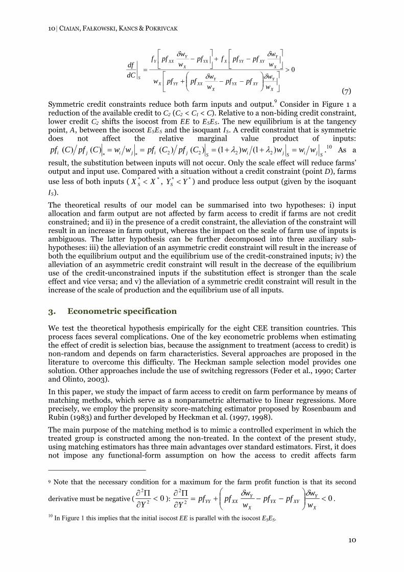
Symmetric credit constraints reduce both farm inputs and output.9 Consider in Figure 1 a reduction of the available credit to C2 (C2 < C1 < C). Relative to a non-biding credit constraint, lower credit C2 shifts the isocost from EE to ESES. The new equilibrium is at the tangency point, A, between the isocost ESES and the isoquant IS. A credit constraint that is symmetric does not affect the relative marginal value product of inputs:
SjiSjiSjijiji wwwwCpfCpfwwCpfCpf =++=== )1()1()()()()( 2222**λλ .10 As a
result, the substitution between inputs will not occur. Only the scale effect will reduce farms’ output and input use. Compared with a situation without a credit constraint (point D), farms use less of both inputs ( ** XX S < , ** YYS < ) and produce less output (given by the isoquant
IS).
The theoretical results of our model can be summarised into two hypotheses: i) input allocation and farm output are not affected by farm access to credit if farms are not credit constrained; and ii) in the presence of a credit constraint, the alleviation of the constraint will result in an increase in farm output, whereas the impact on the scale of farm use of inputs is ambiguous. The latter hypothesis can be further decomposed into three auxiliary sub-hypotheses: iii) the alleviation of an asymmetric credit constraint will result in the increase of both the equilibrium output and the equilibrium use of the credit-constrained inputs; iv) the alleviation of an asymmetric credit constraint will result in the decrease of the equilibrium use of the credit-unconstrained inputs if the substitution effect is stronger than the scale effect and vice versa; and v) the alleviation of a symmetric credit constraint will result in the increase of the scale of production and the equilibrium use of all inputs.
3. Econometric specification
We test the theoretical hypothesis empirically for the eight CEE transition countries. This process faces several complications. One of the key econometric problems when estimating the effect of credit is selection bias, because the assignment to treatment (access to credit) is non-random and depends on farm characteristics. Several approaches are proposed in the literature to overcome this difficulty. The Heckman sample selection model provides one solution. Other approaches include the use of switching regressors (Feder et al., 1990; Carter and Olinto, 2003).
In this paper, we study the impact of farm access to credit on farm performance by means of matching methods, which serve as a nonparametric alternative to linear regressions. More precisely, we employ the propensity score-matching estimator proposed by Rosenbaum and Rubin (1983) and further developed by Heckman et al. (1997, 1998).
The main purpose of the matching method is to mimic a controlled experiment in which the treated group is constructed among the non-treated. In the context of the present study, using matching estimators has three main advantages over standard estimators. First, it does not impose any functional-form assumption on how the access to credit affects farm
9 Note that the necessary condition for a maximum for the farm profit function is that its second
derivative must be negative ( 02
2
<∂Π∂
Y): 02
2
<⎟⎟⎠
⎞⎜⎜⎝
⎛−−+=
∂Π∂
X
YXYYX
X
YXXYY w
wpfpf
ww
pfpfY
δδ.
10 In Figure 1 this implies that the initial isocost EE is parallel with the isocost ESES.
IMPACT OF CAPITAL USE | 11
11
behaviour. Accordingly, we can allow for all types of heterogeneities and non-linearities in the effects of credit as long as they relate to observable characteristics. Second, it allows us to address the unobservable heterogeneity, as we base our analysis only on comparisons among farms that are similar in terms of observable characteristics. By doing so we avoid the potential problem of drawing inferences from comparing very different farms, which are likely to bias linear regression results (see for instance, Blundell and Costa Dias, 2009). Third, propensity score matching addresses the issue of self-selection bias owing to observed characteristics. The propensity score reduces selection bias by equating groups based on many known characteristics (covariates) and provides an appropriate method for estimating the treatment effect when treatment assignment is not random.11
Despite these advantages, because of the high demand for data, matching methods have scarcely been used in agricultural economics (a few examples include Dabalen et al., 2004; Bento et al., 2007; Key and Roberts, 2008; Pufahl and Weiss, 2009). The popularity of matching methods for studying the impact of farm access to credit on farm performance is even lower (to our knowledge the only exception is Briggeman et al., 2009). An important advantage of the present study is the large size of the FADN farm-level panel data, which allows us to employ the matching approach to study the determinants and implications of rural credit constraints in the transition context.
Using the same notation as in the theoretical model, C denotes an indicator for a farm having access to credit (C=1) or no (limited) access to credit (C=0). Let Q1i be the potential performance of farm i with access to credit (i.e. exposed to the treatment) and Q0i the potential performance of farm i with no (limited) access to credit (i.e. not exposed to the treatment, control). Finally, denote a vector of observable covariates by Z. Then the expected casual effect of the treatment on the performance of farm i and the parameter of our interest would be E(Q1i – Q0i|Zi,Ci = 1). This is the ‘average treatment on the treated’ (ATT), which measures the effect of access to credit on the outcome variable for those farms that actually used credit (e.g. to pre-finance the purchase of inputs) compared with what would have happened if they had not relied on credit (or they had relied on other sources of finance).
Given that we do not observe what would have happened if farms with credit had been denied access to external funding (or vice versa), we construct an estimate of the counterfactual: E(Q0i|Zi, Ci=1). As shown by Rosenbaum and Rubin (1983), comparing farms with a similar probability of obtaining credit given the observables in Z is equivalent to comparing farms with similar values of Z. Accordingly, using a probit model the probability of each farm obtaining credit (propensity score) is computed. Next, based on this propensity score, for each treated observation a counterfactual is estimated using the kernel matching procedure.12 This allows us to compare each treated observation solely with controls having similar values of the observables in Z. To ensure that the compared farms are not too different in terms of the propensity score, we employ matching with calliper 0.01.
Note that the adopted matching procedure relies on two critical assumptions: first, the so-called ‘selection on observables’ assumption and second, the common support assumption. The former assumes that the propensity score is a balancing function, i.e. conditional on Z, without access to credit the treated farms would behave in the same way as the control
11 The FADN is an unbalanced panel, where every year 5 to 20% of farms is dropped from the sample. Farms are excluded either because of the FADN sampling strategy of the regular annual replacement of observations or other reasons (voluntary drop-out, exit from farming). Nevertheless, farms that drop out from the sample are replaced by farms having similar characteristics in order to keep the sample representative. This sampling strategy further reduced the selection bias problem. 12 A 1-to-1 matching estimator was also used. Yet while the matching performed somewhat worse in terms of reducing the differences in the distribution of observable covariates among treated and non-treated farms, the main results remained unaffected, and therefore they are not reported here but may be obtained by request.
12 | CIAIAN, FAŁKOWSKI, KANCS & POKRIVCAK
12
farms.13 The latter assumes that the propensity score is bounded between 0 and 1. Thanks to this, each treated observation has its counterpart among the controls. We discuss how these assumptions hold in our case below, where we motivate our choice of covariates to be included in Z.
4. Data and variable construction
The econometric model outlined in the previous section requires data on farm credit, variables determining farm access to credit and outcome variables capturing farm behaviour. The main data source we use in the present study is the FADN. It covers 37,409 farms in 8 transition countries.14 The appendix presents more details about the FADN data, including the sources for each variable.
To gain a detailed and robust view about the potential impact of access to credit on farm performance, we use six outcome variables for which we identify ATT. All of them are measured in euros. Farm output is directly available in the FADN data (SE131). The same applies to the investment variable, which captures gross investment in fixed assets (SE516). Variable costs are calculated by summing up the total specific costs (SE281), total farming overheads (SE336) and wages paid (SE370). Labour and land use are directly available in the FADN data (SE010 and SE025, respectively). We normalise all cost variables – the gross investment, variable costs, land and labour – by output. Finally, based on the FADN data, we use the total factor productivity (TFP) estimates based on the Olley and Pakes (1996) estimator as the sixth outcome variable.
The dependent variable in the probit model – farm credit – is constructed from the FADN variable, total farm loans (liabilities) (SE485), which we normalise by farm output (SE131). We use a dummy variable to determine whether the farm has normalised liabilities greater than zero.15 Note that we observe solely the farm usage of credit, but not the (potential) availability of credit (i.e. whether a farm is credit constrained), as information about the latter is not available in our dataset. Nevertheless, testing the theoretical hypotheses derived above also allows us to indirectly investigate the impact of credit constraints. This is possible because of the ability to exploit the relationship between farm access to credit and the use of different inputs as well as to investigate the relationship between farm access to credit and farm output.
As noted by Briggeman et al. (2009), the impact of a credit constraint may be non-linear. To estimate the impact of different levels of credit constraints, in addition to identifying the treatment effect of using credit, we also estimate the treatment effect of heterogeneous intensities of credit reliance. For this purpose, we split the whole sample into eight credit groups.16 Group 1 contains farms with zero credit.17 Group 2 contains farms with a small 13 As noted by Heckman et al. (1997), treated and controls may still differ even after conditioning on observables. This may be because of unobservable characteristics. One possible solution to mitigate this problem is to combine the matching procedure with the difference-in-differences method (see for instance, Pufahl and Weiss, 2009). Yet given that our data only spans two years and does not include information on the time credit is granted, this method cannot be applied in our study. 14 At the end, after cleaning the data from outliers, our analysis is based on 34,169 observations. 15 We also investigate other specifications where the treatment is defined over the relative amount of credit. In that case a dummy dependent variable equals to one if the normalised liabilities are greater than a given threshold (see the further discussion). 16 The division of farms into these eight groups was done to satisfy the condition that the number of treated observations should be smaller than the number of controls. We have also tested the model for more than eight farm groups. The results are consistent with those reported in the paper. The statistical power decreases, however, because the number of observations per group is lower, thus reducing the model’s predictability. The matching estimator requires a relatively large number of observations, as each treated observation needs to have its counterfactual among the non-treated ones. Moreover, it should be noted that imposing the common support assumption is likely to result in dropping some observations for which the treatment status is predicted too well
IMPACT OF CAPITAL USE | 13
13
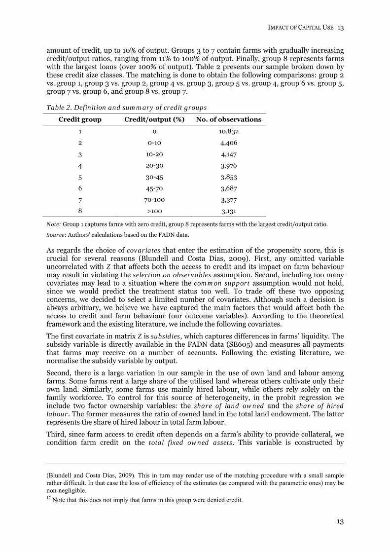
amount of credit, up to 10% of output. Groups 3 to 7 contain farms with gradually increasing credit/output ratios, ranging from 11% to 100% of output. Finally, group 8 represents farms with the largest loans (over 100% of output). Table 2 presents our sample broken down by these credit size classes. The matching is done to obtain the following comparisons: group 2 vs. group 1, group 3 vs. group 2, group 4 vs. group 3, group 5 vs. group 4, group 6 vs. group 5, group 7 vs. group 6, and group 8 vs. group 7.
Table 2. Definition and summary of credit groups
Credit group Credit/output (%) No. of observations
1 0 10,832
2 0-10 4,406
3 10-20 4,147
4 20-30 3,976
5 30-45 3,853
6 45-70 3,687
7 70-100 3,377
8 >100 3,131
Note: Group 1 captures farms with zero credit, group 8 represents farms with the largest credit/output ratio.
Source: Authors’ calculations based on the FADN data.
As regards the choice of covariates that enter the estimation of the propensity score, this is crucial for several reasons (Blundell and Costa Dias, 2009). First, any omitted variable uncorrelated with Z that affects both the access to credit and its impact on farm behaviour may result in violating the selection on observables assumption. Second, including too many covariates may lead to a situation where the common support assumption would not hold, since we would predict the treatment status too well. To trade off these two opposing concerns, we decided to select a limited number of covariates. Although such a decision is always arbitrary, we believe we have captured the main factors that would affect both the access to credit and farm behaviour (our outcome variables). According to the theoretical framework and the existing literature, we include the following covariates.
The first covariate in matrix Z is subsidies, which captures differences in farms’ liquidity. The subsidy variable is directly available in the FADN data (SE605) and measures all payments that farms may receive on a number of accounts. Following the existing literature, we normalise the subsidy variable by output.
Second, there is a large variation in our sample in the use of own land and labour among farms. Some farms rent a large share of the utilised land whereas others cultivate only their own land. Similarly, some farms use mainly hired labour, while others rely solely on the family workforce. To control for this source of heterogeneity, in the probit regression we include two factor ownership variables: the share of land owned and the share of hired labour. The former measures the ratio of owned land in the total land endowment. The latter represents the share of hired labour in total farm labour.
Third, since farm access to credit often depends on a farm’s ability to provide collateral, we condition farm credit on the total fixed owned assets. This variable is constructed by
(Blundell and Costa Dias, 2009). This in turn may render use of the matching procedure with a small sample rather difficult. In that case the loss of efficiency of the estimates (as compared with the parametric ones) may be non-negligible. 17 Note that this does not imply that farms in this group were denied credit.
14 | CIAIAN, FAŁKOWSKI, KANCS & POKRIVCAK
14
subtracting long- and medium-term loans (SE490) from the total fixed assets (SE441). As above, we normalise the total own fixed assets by farm output.
Moreover, according to Briggeman et al. (2009), it is reasonable to assume that farm access to credit and a farm’s investment decisions (input use) may be determined by its size and general economic performance. To control for this source of heterogeneity, we also include a covariate economic size, which represents the economic size of farms measured in European size units (SE005).
In addition to the described explanatory variables, in the first stage regressions we also include dummy variables to control for the time aspect, the sector and geographical location. All dummy variables are directly available from the FADN data: time dummy (year), sector (A8) and region dummy (A2).18
Finally, the findings of Bezemer (2002) and Davidova and Thomson (2003) suggest that the effects of credit are heterogeneous across countries. For example, countries with higher land fragmentation are particularly prone to suffer from the credit-constraint problem. Therefore, in addition to pooled estimations (eight countries), we also examine each country separately (the Czech Republic, Estonia, Hungary, Lithuania, Latvia and Poland).19
5. Estimation results
5.1 Matching
The quality of the matching depends on the extent to which the propensity score is a truly balancing function. Table A1 in the appendix provides an overview of the distribution of the selected covariates across the treated and control farms for the pooled sample.20 Three key points are worth noting. First, before imposing the common support assumption (columns (1) and (2)), the treated and control farms differ significantly for most variables used to calculate the propensity score (irrespective of which credit size classes we compare). These differences are removed with matching (columns (3) and (4)), which should be recognised as a second important observation. Only in the comparison between credit size 2 and credit size 1 do the variables fixed owned assets, economic size and a time dummy retain a different distribution in the treated and control farms. This suggests that these covariates should be included among the explanatory variables that we use for the propensity score estimation. With this caveat in mind, we conclude that the matching of treated and non-treated farms performed well and is valid for meaningful comparisons.
Third, for the vast majority of probit regressions (not shown) the pseudo R2 is relatively low (ranging from 0.08 to 0.15),21 suggesting that the covariates used leave a lot of residual variation unexplained. One may argue, therefore, that the covariates included do not
18 In addition, we also experiment with the lagged debt/asset ratio as an explanatory variable. Although it improved the prediction power of our first-stage probit models, it did not affect the results of our second stage, treatment effect estimations. Furthermore, it limited our sample to only farms with observations for two points in time, which had a detrimental effect on the balancing properties of our matching procedure. Therefore, for reasons of brevity we do not report these results here. 19 Slovenia and Slovakia were dropped because of an insufficient number of observations for the given size classes. 20 Owing to the large number of comparisons made, the results of tests showing how well the propensity score did as a balancing function for the country sub-samples are not reported here (although these may be obtained from authors upon request). The balancing properties were fulfilled in three out of seven cases for Latvia, five out of seven cases for the Czech Republic, Estonia and Lithuania, and six out of seven cases for Poland. 21 This especially concerned regressions predicting transitions between groups of farms with a credit/output ratio larger than zero. Somewhat better predictions were obtained for transitions between credit groups 2 and 1, i.e. between farms having no credit at all and farms having credit not exceeding 10% of the production value (pseudo R2 ranging from 0.1 to 0.3 depending on the (sub-)sample used).
IMPACT OF CAPITAL USE | 15
15
accurately predict the state of being granted (higher) credit. This presumably stems from the fact that our dataset does not contain any information about the individual characteristics of farmers (e.g. age, education and having a successor), informal institutions or social norms (e.g. relatives or friends among lenders and credit recipients), which are nonetheless important for making decisions about (not) granting credit to a farm. The objective of this study, however, is not to specify a statistical model explaining farm access to credit in the best possible way. Having probit regressions with large prediction power would lead to a much smaller number of treated farms meeting the common support assumption. This is especially important for country sub-samples, where the number of observations per credit size group is relatively small (sometimes around 200). Moreover, other empirical studies employing matching estimators for studying farm access to credit also report low pseudo R2 (e.g. Briggeman et al. (2009) report pseudo R2 equal to 0.31).
Bearing these limitations in mind, we conclude that the balancing property of our matching is both statistically and economically satisfactory and it is justifiable to estimate the treatment effect of farm access to credit according to the econometric strategy outlined above.
5.2 Pooled sample
Tables 3 and 4 report the results for the pooled sample in absolute values and in percentages, respectively. Each column refers to a different output variable. All estimators are based on kernel matching and the reported numbers should read as follows: positive (negative) numbers refer to an increase (decrease) in the output variable for farms in the treated group compared with farms in the control group.22 For example, the results for investment shown in column 3 of Table 4 (Table 3) indicate that farms in credit class 2 have 29.04% more investment per €1,000 of additional credit (higher normalised investment by 0.086) than farms in credit class 1.
Several conclusions can be drawn based on these results. First, no statistically significant impact of credit on the value of production was found (column 1). Although the results suggest that farm access to (higher) credit positively affects the value of production in all except the two highest credit-per-output groups, the precision of the estimates obtained is too low to render them significantly different from zero.23 Second, the results obtained suggest that farm access to (higher) credit has a positive impact on the TFP. The increase in the TFP between credit classes ranges between 0.07% and 1.87% per €1,000 of additional credit with the largest gain in productivity being for low levels of credit (Table 4). This indicates a decrease in the marginal productivity per additional credit. This result is consistent with the estimates reported in column 3, suggesting that access to credit increases the level of relative investment, which should be recognised as a third important observation. The increase in investment is significant for most of the credit group comparisons ranging between 0.14% and 29.04% per €1,000 of additional credit (Table 4). Interestingly, no impact on the relative land endowments was found (column 4). Furthermore, our results suggest that credit has a positive effect on the use of variable inputs (between 0.01%, and 2.34% per €1,000 of additional credit, Table 4). Finally, a negative impact of access to credit was found on the use of labour (between -0.14%, and -1.64% per €1,000 of additional credit, Table 4). This can be explained by the fact that through credit farms mainly finance capital equipment, which is usually labour saving. The negative relationship between farm access to credit and labour use is reversed for the two highest credit/output ratio groups (by 0.02% per €1,000 of additional credit, Table 4). This indicates that labour is being substituted by capital up to a point, where more investment ultimately reduces such a possibility.
22 To facilitate the reading of Tables 3-10, the treated group is indicated in bold. 23 Yet given that semi-parametric methods trade off reduced bias due to specification error against less efficiency, this result is not that surprising.

16 | CIAIAN, FAŁKOWSKI, KANCS & POKRIVCAK
16
Table 3. Credit and farm behaviour: Matching estimates of the effect of accessing credit on farm output and inputs – Pooled sample
Credit classes:
Treated vs. control
Output
(€)
(1)
TFP
(index)
(2)
Investment
(€ per output)
(3)
Land
(Ha per output)
(4)
Variable inputs
(€ per output)
(5)
Labour
(persons per output)
(6)
2 vs. 1 5,186 0.057 *** 0.086 *** 0.005 0.116 *** -0.031 ***
t-stat 1.18 9.30 26.97 0.59 24.36 -5.97
3 vs. 2 5,613 0.027 *** 0.006 -0.006 0.011 ** -0.006 *
t-stat 1.06 5.41 1.40 -0.76 2.48 -1.82
4 vs. 3 7,131 0.035 *** 0.024 *** -0.004 0.0005 -0.016 ***
t-stat 1.15 6.55 4.98 -0.61 0.13 -4.91
5 vs. 4 8,586 0.031 *** 0.028 *** -0.005 0.003 -0.010 ***
t-stat 1.12 5.23 4.91 -0.72 0.68 -3.31
6 vs. 5 3,746 0.022 *** 0.059 *** -0.007 0.005 -0.002
t-stat 0.40 3.44 8.70 -0.87 1.13 -0.80
7 vs. 6 -2,864 0.009 0.059 *** -0.002 0.010 * 0.001
t-stat -0.29 1.31 6.75 -0.27 1.84 0.37
8 vs. 7 -7,179 -0.014 0.128 *** 0.0009 0.016 ** 0.009 **
t-stat -0.73 -1.53 9.56 0.09 2.53 2.30
***, ** and * denote 1%, 5% and 10% significance levels, respectively
Source: Authors’ estimations.
Table 4. Percentage change of productivity and use of inputs per €1,000 of additional credit – Pooled sample (%/€ credit)
Output TFP Investment Land Variable
inputs Labour
(1) (2) (3) (4) (5) (6)
2 vs. 1 1.87 1.87*** 29.04*** 0.12 2.34*** -1.64***
3 vs. 2 0.36 0.31*** 0.56 -0.05 0.05** -0.20*
4 vs. 3 0.03 0.25*** 0.62*** 0.00 0.00 -0.31***
5 vs. 4 0.00 0.14*** 0.41*** 0.00 0.00 -0.14***
6 vs. 5 0.0 0.07*** 0.44*** -0.01 0.00 -0.01
7 vs. 6 -0.03 0.02 0.21*** 0.00 0.01* 0.02
8 vs. 7 -0.03 0.00 0.14*** 0.00 0.01** 0.02**
***, ** and * denote 1%, 5% and 10% significance levels, respectively
Source: Authors’ estimations.
IMPACT OF CAPITAL USE | 17
17
It is important now to compare these findings with the theoretical hypotheses mentioned above. Recall that the model developed in section 2 predicts that in the presence of a credit constraint, access to external funding should result in a positive impact on farm output and an indeterminable ad hoc effect on the scale of use of inputs. The exact adjustment pattern depends on whether the constraint is symmetric. Overall, the results obtained suggest that farms are asymmetrically credit constrained. Farms tend to be credit constrained with respect to investment and variable inputs, but credit unconstrained with respect to land and labour. For labour the results indicate that the substitution effect tends to be stronger than the scale effect (particularly for low credit classes) leading to a substitution of labour for credit-constrained investment and variable inputs. For land the substitution effect tends to offset the scale effect, resulting in no impact of credit on land use. The change in the relative input intensities is further highlighted by the positive impact of improved access to credit on farm productivity.
Our results indicate that the credit behaviour of farms is an important determinant of performance and the modernisation of the farming sector in Central and Eastern Europe. This is in particular related to the high, fixed capital intensity of agricultural production, indirectly reflected by a disproportional contribution of the agricultural sector to overall gross fixed capital formation (Table 1). Indeed our results indicate that investment performance is one the factors that is most strongly affected by access to credit. Sustained credit problems in CEE countries may significantly hold back adjustments in agricultural technology, potentially keeping agricultural productivity in CEE countries behind the developed EU member states.
5.3 Countrylevel analysis
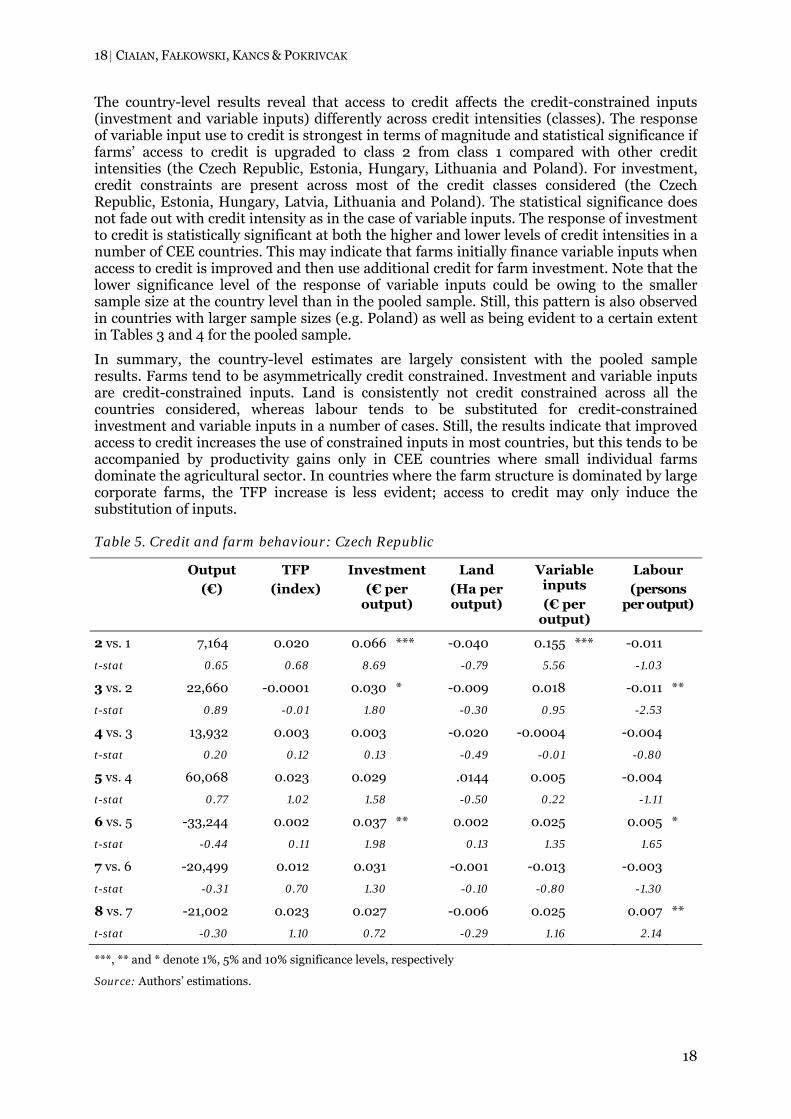
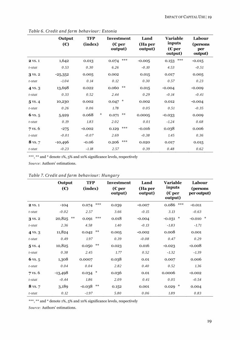
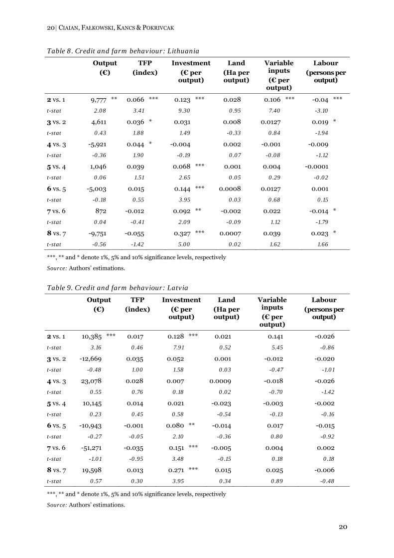
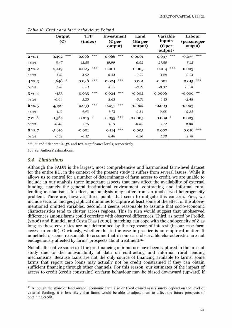
To gather more country-specific insights, we examine how these patterns differ across the CEE transition countries. The estimates obtained of treatment effects based on country sub-samples are presented in Tables 5-10. Generally, the country-specific results complement our findings based on a pooled sample. First, we observe robust evidence on the positive and significant impact of access to credit on investment. The effect, however, appears to be statistically stronger in countries where small individual farms are important, such as in Lithuania and Poland. Second, no evidence was found that the credit constraint would influence farms’ land use. This result again suggests that farms in Central and Eastern Europe are not credit constrained with respect to land. Third, except for the two groups with the highest credit/output ratio, farm access to credit has a negative impact on labour use. As noted above, this can be explained by the fact that through credit farms mainly finance capital equipment, which is usually labour saving. Fourth, an interesting pattern emerges concerning farm productivity. The estimates obtained suggest a statistically significant increase in TFP in Estonia, Lithuania and Poland. These results are intriguing, because Estonia, Lithuania and Poland are those countries with the highest shares of small individual farms. Among the countries where corporate farms are more widespread or dominant, the credit effect on TFP is significant only in Hungary, and not in the Czech Republic or Latvia. This in turn indicates that credit constraints might be more problematic for small individual farms compared with large corporate farms. Moreover, in these three countries a significantly positive impact of farm access to credit on output could be observed. Fifth, at the country level the pattern of the impact of credit on variable inputs is much less clear than in the pooled sample, which may stem from the sizeable cross-country differences in farm structure. On the one hand, for all countries where the amount of credit tends to be small, the use of variable inputs increases significantly. On the other hand, for other credit size groups the estimates are much less stable and statistically insignificant from zero.
18 | CIAIAN, FAŁKOWSKI, KANCS & POKRIVCAK
18
The country-level results reveal that access to credit affects the credit-constrained inputs (investment and variable inputs) differently across credit intensities (classes). The response of variable input use to credit is strongest in terms of magnitude and statistical significance if farms’ access to credit is upgraded to class 2 from class 1 compared with other credit intensities (the Czech Republic, Estonia, Hungary, Lithuania and Poland). For investment, credit constraints are present across most of the credit classes considered (the Czech Republic, Estonia, Hungary, Latvia, Lithuania and Poland). The statistical significance does not fade out with credit intensity as in the case of variable inputs. The response of investment to credit is statistically significant at both the higher and lower levels of credit intensities in a number of CEE countries. This may indicate that farms initially finance variable inputs when access to credit is improved and then use additional credit for farm investment. Note that the lower significance level of the response of variable inputs could be owing to the smaller sample size at the country level than in the pooled sample. Still, this pattern is also observed in countries with larger sample sizes (e.g. Poland) as well as being evident to a certain extent in Tables 3 and 4 for the pooled sample.
In summary, the country-level estimates are largely consistent with the pooled sample results. Farms tend to be asymmetrically credit constrained. Investment and variable inputs are credit-constrained inputs. Land is consistently not credit constrained across all the countries considered, whereas labour tends to be substituted for credit-constrained investment and variable inputs in a number of cases. Still, the results indicate that improved access to credit increases the use of constrained inputs in most countries, but this tends to be accompanied by productivity gains only in CEE countries where small individual farms dominate the agricultural sector. In countries where the farm structure is dominated by large corporate farms, the TFP increase is less evident; access to credit may only induce the substitution of inputs.
Table 5. Credit and farm behaviour: Czech Republic
Output
(€)
TFP
(index)
Investment
(€ per output)
Land
(Ha per output)
Variable inputs
(€ per output)
Labour
(persons per output)
2 vs. 1 7,164 0.020 0.066 *** -0.040 0.155 *** -0.011
t-stat 0.65 0.68 8.69 -0.79 5.56 -1.03
3 vs. 2 22,660 -0.0001 0.030 * -0.009 0.018 -0.011 **
t-stat 0.89 -0.01 1.80 -0.30 0.95 -2.53
4 vs. 3 13,932 0.003 0.003 -0.020 -0.0004 -0.004
t-stat 0.20 0.12 0.13 -0.49 -0.01 -0.80
5 vs. 4 60,068 0.023 0.029 .0144 0.005 -0.004
t-stat 0.77 1.02 1.58 -0.50 0.22 -1.11
6 vs. 5 -33,244 0.002 0.037 ** 0.002 0.025 0.005 *
t-stat -0.44 0.11 1.98 0.13 1.35 1.65
7 vs. 6 -20,499 0.012 0.031 -0.001 -0.013 -0.003
t-stat -0.31 0.70 1.30 -0.10 -0.80 -1.30
8 vs. 7 -21,002 0.023 0.027 -0.006 0.025 0.007 **
t-stat -0.30 1.10 0.72 -0.29 1.16 2.14
***, ** and * denote 1%, 5% and 10% significance levels, respectively
Source: Authors’ estimations.
IMPACT OF CAPITAL USE | 19
19
Table 6. Credit and farm behaviour: Estonia
Output
(€)
TFP
(index)
Investment
(€ per output)
Land
(Ha per output)
Variable inputs
(€ per output)
Labour
(persons per
output)
2 vs. 1 1,642 0.013 0.074 *** -0.005 0.153 *** -0.015
t-stat 0.53 0.30 6.26 -0.10 4.53 -0.51
3 vs. 2 -25,352 0.005 0.002 0.015 0.017 0.005
t-stat -1.04 0.14 0.12 0.30 0.57 0.23
4 vs. 3 13,698 0.022 0.060 ** 0.015 -0.004 -0.009
t-stat 0.33 0.52 2.44 0.29 -0.14 -0.41
5 vs. 4 10,230 0.002 0.047 * 0.002 0.012 -0.004
t-stat 0.26 0.06 1.78 0.05 0.51 -0.35
6 vs. 5 5,929 0.068 * 0.071 ** 0.0005 -0.033 0.009
t-stat 0.19 1.83 2.02 0.01 -1.24 0.68
7 vs. 6 -275 -0.002 0.129 *** -0.016 0.038 0.006
t-stat -0.01 -0.07 2.69 -0.38 1.45 0.36
8 vs. 7 -10,496 -0.06 0.206 *** 0.020 0.017 0.015
t-stat -0.23 -1.18 2.57 0.39 0.48 0.62
***, ** and * denote 1%, 5% and 10% significance levels, respectively
Source: Authors’ estimations.
Table 7. Credit and farm behaviour: Hungary
Output
(€)
TFP
(index)
Investment
(€ per output)
Land
(Ha per output)
Variable inputs
(€ per output)
Labour
(persons per output)
2 vs. 1 -104 0.074 *** 0.039 -0.007 0.086 *** -0.011
t-stat -0.02 2.57 3.66 -0.15 3.13 -0.63
3 vs. 2 20,825 ** 0.091 *** 0.018 -0.004 -0.031 * -0.010 *
t-stat 2.36 4.58 1.40 -0.13 -1.83 -1.71
4 vs. 3 11,824 0.042 ** 0.005 -0.002 0.008 0.001
t-stat 0.49 1.97 0.39 -0.08 0.47 0.29
5 vs. 4 10,825 0.050 ** 0.023 0.016 -0.023 -0.008
t-stat 0.38 2.45 1.77 0.52 -1.32 -1.39
6 vs. 5 1,308 0.0007 0.038 0.01 0.007 0.006
t-stat 0.04 0.04 2.82 0.40 0.52 1.36
7 vs. 6 -13,498 0.034 * 0.036 0.01 0.0006 -0.002
t-stat -0.44 1.86 2.09 0.41 0.05 -0.54
8 vs. 7 3,189 -0.038 ** 0.152 0.001 0.029 * 0.004
t-stat 0.12 -1.97 5.80 0.06 1.89 0.83
***, ** and * denote 1%, 5% and 10% significance levels, respectively
Source: Authors’ estimations.
20 | CIAIAN, FAŁKOWSKI, KANCS & POKRIVCAK
20
Table 8. Credit and farm behaviour: Lithuania
Output
(€)
TFP
(index)
Investment
(€ per output)
Land
(Ha per output)
Variable inputs
(€ per output)
Labour
(persons per output)
2 vs. 1 9,777 ** 0.066 *** 0.123 *** 0.028 0.106 *** -0.04 ***
t-stat 2.08 3.41 9.30 0.95 7.40 -3.10
3 vs. 2 4,611 0.036 * 0.031 0.008 0.0127 0.019 *
t-stat 0.43 1.88 1.49 -0.33 0.84 -1.94
4 vs. 3 -5,921 0.044 * -0.004 0.002 -0.001 -0.009
t-stat -0.36 1.90 -0.19 0.07 -0.08 -1.12
5 vs. 4 1,046 0.039 0.068 *** 0.001 0.004 -0.0001
t-stat 0.06 1.51 2.65 0.05 0.29 -0.02
6 vs. 5 -5,003 0.015 0.144 *** 0.0008 0.0127 0.001
t-stat -0.18 0.55 3.95 0.03 0.68 0.15
7 vs. 6 872 -0.012 0.092 ** -0.002 0.022 -0.014 *
t-stat 0.04 -0.41 2.09 -0.09 1.12 -1.79
8 vs. 7 -9,751 -0.055 0.327 *** 0.0007 0.039 0.023 *
t-stat -0.56 -1.42 5.00 0.02 1.62 1.66
***, ** and * denote 1%, 5% and 10% significance levels, respectively
Source: Authors’ estimations.
Table 9. Credit and farm behaviour: Latvia
Output
(€)
TFP
(index)
Investment
(€ per output)
Land
(Ha per output)
Variable inputs
(€ per output)
Labour
(persons per output)
2 vs. 1 10,385 *** 0.017 0.128 *** 0.021 0.141 -0.026
t-stat 3.16 0.46 7.91 0.52 5.45 -0.86
3 vs. 2 -12,669 0.035 0.052 0.001 -0.012 -0.020
t-stat -0.48 1.00 1.58 0.03 -0.47 -1.01
4 vs. 3 23,078 0.028 0.007 0.0009 -0.018 -0.026
t-stat 0.55 0.76 0.18 0.02 -0.70 -1.42
5 vs. 4 10,145 0.014 0.021 -0.023 -0.003 -0.002
t-stat 0.23 0.45 0.58 -0.54 -0.13 -0.16
6 vs. 5 -10,943 -0.001 0.080 ** -0.014 0.017 -0.015
t-stat -0.27 -0.05 2.10 -0.36 0.80 -0.92
7 vs. 6 -51,271 -0.035 0.151 *** -0.005 0.004 0.002
t-stat -1.01 -0.95 3.48 -0.15 0.18 0.18
8 vs. 7 19,598 0.013 0.271 *** 0.015 0.025 -0.006
t-stat 0.57 0.30 3.95 0.34 0.89 -0.48
***, ** and * denote 1%, 5% and 10% significance levels, respectively
Source: Authors’ estimations.
IMPACT OF CAPITAL USE | 21
21
Table 10. Credit and farm behaviour: Poland
Output (€)
TFP (index)
Investment (€ per
output)
Land (Ha per output)
Variable inputs (€ per
output)
Labour (persons per
output)
2 vs. 1 9,492 *** 0.066 *** 0.066 *** 0.0001 0.097 *** -0.035 ***
t-stat 5.47 13.55 19.90 0.02 27.56 -8.12
3 vs. 2 2,419 0.025 *** -0.001 -0.005 0.014 *** -0.003
t-stat 1.10 4.52 -0.34 -0.79 3.48 -0.74
4 vs. 3 4,648 * 0.038 *** 0.024 *** 0.001 -0.001 0.015 ***
t-stat 1.70 6.61 4.35 -0.21 -0.32 -3.70
5 vs. 4 -133 0.035 *** 0.024 *** -0.002 0.0006 -0.009 **
t-stat -0.04 5.25 3.63 -0.31 0.15 -2.48
6 vs. 5 4,190 0.033 *** 0.057 *** -0.002 -0.003 -0.003
t-stat 1.12 4.43 6.73 -0.34 -0.68 -0.85
7 vs. 6 -1,565 0.015 * 0.055 *** -0.0005 0.009 * 0.003
t-stat -0.40 1.75 4.91 -0.06 1.72 0.80
8 vs. 7 -5,619 -0.001 0.114 *** 0.005 0.007 0.016 ***
t-stat -1.62 -0.12 6.46 0.50 1.08 2.78
***, ** and * denote 1%, 5% and 10% significance levels, respectively
Source: Authors’ estimations.
5.4 Limitations
Although the FADN is the largest, most comprehensive and harmonised farm-level dataset for the entire EU, in the context of the present study it suffers from several issues. While it allows us to control for a number of determinants of farm access to credit, we are unable to include in our analysis three important aspects that may affect the availability of external funding, namely the general institutional environment, contracting and informal rural lending mechanisms. In effect, our analysis may suffer from an unobserved heterogeneity problem. There are, however, three points that seem to mitigate this concern. First, we include sectoral and geographical dummies to capture at least some of the effect of the above-mentioned omitted variables. Second, it seems reasonable to assume that socio-economic characteristics tend to cluster across regions. This in turn would suggest that unobserved differences among farms could correlate with observed differences. Third, as noted by Frölich (2006) and Blundell and Costa Dias (2009), matching can cope with the endogeneity of Z as long as these covariates are not determined by the regressor of interest (in our case farm access to credit). Obviously, whether this is the case in practice is an empirical matter. It nonetheless seems reasonable to assume that in our case observable characteristics are not endogenously affected by farms’ prospects about treatment.24
Not all alternative sources of the pre-financing of input use have been captured in the present study due to the unavailability of data on contracting and informal rural lending mechanisms. Because loans are not the only source of financing available to farms, some farms that report zero loans may actually not be credit constrained if they can obtain sufficient financing through other channels. For this reason, our estimates of the impact of access to credit (credit constraint) on farm behaviour may be biased downward (upward) if
24 Although the share of land owned, economic farm size or fixed owned assets surely depend on the level of external funding, it is less likely that farms would be able to adjust them to affect the future prospects of obtaining credit.
22 | CIAIAN, FAŁKOWSKI, KANCS & POKRIVCAK
22
farm access to loans is negatively (positively) correlated with farm access to other sources of finance. Our estimates are accurate if loans and other sources of finance are uncorrelated with one another. The above-mentioned caveats should be kept in mind while interpreting the results presented.
6. Conclusions
This paper has studied the impact of credit constraints on farm behaviour in the CEE transition countries. The theoretical model suggests that in the presence of a binding credit constraint, improved access to credit may lead to a productivity increase in farm output and the use of inputs. In the case of a symmetric credit constraint, the alleviation of a farm credit constraint increases the use of all inputs. Yet if a farm is asymmetrically credit constrained, then the improved access to credit may lead to a substitution of credit-constrained inputs with credit-unconstrained inputs.
The empirical testing of the hypotheses through the theoretical framework suggests that farms in Central and Eastern Europe are credit constrained. Access to credit increases TFP up to 1.9% per €1,000 of additional credit. At the same time, our estimates indicate that farms are asymmetrically credit constrained. Farms in CEE countries are particularly credit constrained with respect to variable inputs and capital investment, as variable inputs and capital investment increase up to 2.3% and 29% respectively, per €1,000 of additional credit. On the other hand, land and labour are not credit constrained. This could stem from the relatively high degree of land abundance and high level of agricultural labour employment in the CEE transition countries, particularly in Poland, Slovenia and the Baltic states. An alternative explanation could be that farms are better able to cope with the financing issues associated with land and labour compared with variable inputs and investment. Individual farms mainly use their own labour in production, which reduces the need for pre-financing. Family labour can address credit problems by postponing household consumption to a later period, when the revenue from production sales is collected (after the harvest at the end of the season). The same holds for land. Farms can increase land use through rental markets. Rental markets are relatively important in transition countries, with more than 50% of land being rented (Ciaian and Kancs, 2009). Additionally, in most cases rents are paid at the end of the season, which further reduces the pre-financing needs for land (Ciaian and Kancs, 2009). Furthermore, (own) land serves as good collateral and therefore represents an added factor that may reduce farm credit constraints on land.
From a policy perspective, our results indicate that the targeting of coupled subsidies might be directed towards credit-constrained inputs, such as variable inputs and capital investment. Indeed, farms in Central and Eastern Europe receive investment subsidies under the EU’s rural development policy, which, according to our findings, is an appropriate policy for addressing access to credit in CEE countries. Yet direct payments are an important part of CAP subsidies. These payments may reduce farm capital constraints for all farm inputs as they may represent an alternative source for financing farm activities. The actual impact of direct payments on farm credit constraints depends on the extent of the leakage of subsidies outside the farming sector. For example, direct payments may be benefiting other agents instead of farms if they are capitalised in input prices. In this case, farm credit constraints may not be alleviated by direct payments. A policy seeking to boost the productivity of the farming sector may partially avoid this problem by supporting credit-constrained inputs. Our results indicate that improved access to credit in the farming sector may also be accompanied by a productivity increase if targeted at individual farms. An additional and important factor that may reduce farm capital constraints for variable inputs and investment is vertical contracting with processors or traders (or both). Even though CAP subsidies and contracting have increased in recent years, our results suggest that they have been unable to fully eliminate farm credit problems in the CEE transition economies. Investigating these two issues in more detail may provide a potentially fruitful line of research and an important extension of the present work.

IMPACT OF CAPITAL USE | 23
23
References
Agbola, F.W. (2005), “Optimization intertemporal investments in Australian agriculture: An empirical investigation”, Agricultural Economics Review, 6: 5–15.
Bakucs, L.Z., I. Ferto and J. Fogarasi (2009), “Investment, financial constraints and soft budget constraint in Hungarian agriculture”, Economics Letters, 104(3): 122–124.
Barry, P.J. and L.J. Robinson (2001), “Agricultural Finance: Credit, Credit Constraints and Consequences”, in B. Gardner and G. Rausser (eds), Handbook of Agricultural Economics, Vol. 1A, Amsterdam: Elsevier, pp. 513–571.
Bento, A., C. Towe and J. Geoghegan (2007), “The Effects of Moratoria on Residential Development: Evidence from a Matching Approach”, American Journal of Agricultural Economics, 89(5): 1211–1218.
Bester, H. (1985), “Screening vs. Rationing in Credit Markets with Imperfect Information”, American Economic Review, 75: 850–855.
Benjamin, C. and E. Phimister (2002), “Does Capital Market Structure Affect Farm Investment? A Comparison Using French and British Farm-Level Panel Data”, American Journal of Agricultural Economics, 84: 1115–29.
Bezemer, D.J. (2002), “Credit markets for agriculture in the Czech Republic”, Europe-Asia Studies, 54(8): 1301–1317.
––––––––– (2003), “Credit Allocation and Farm Structures in the Czech Republic, 1993–1997”, Comparative Economic Studies, 45:25–43.
Bhattacharyya, A., A. Bhattacharyya and S. Kumbhakar (1996), “Governmental Interventions, Market Imperfections, and Technical Inefficiency in a Mixed Economy: A Case Study of Indian Agriculture”, Journal of Comparative Economics, 79: 219–41.
––––––––– (1997), “Market Imperfections and Output Loss in the Presence of Expenditure Constraint: A Generalised Shadow Prise Approach”, American Journal of Agricultural Economics, 22: 860–871.
Blancard, S., J.P. Boussemart, W. Briec and K. Kerstens (2006), “Short- and Long-Run Credit Constraints in French Agriculture: A Directional Distance Function Framework Using Expenditure-Constrained Profit Functions”, American Journal of Agricultural Economics, 88(2): 351–364.
Blundell, R. and M. Costa Dias (2009), “Alternative Approaches to Evaluation in Empirical Microeconomics”, Journal of Human Resources, 44(3): 565–640.
Briggeman, B.C., C. Towe and M.J. Morehart (2009), “Credit Constraints: Their Existence, Determinants, and Implications for U.S. Farm and Nonfarm Sole Proprietorships”, American Journal of Agricultural Economics, 91(1): 275–289.
Carter, M.R. (1988), “Equilibrium Credit Rationing of Small Farm Agriculture”, Journal of Development Economics, 28: 83–103.
Carter, M.R. and K.D. Wiebe (1990), “Access to Capital and its Impact on Agrarian Structure and Productivity in Kenya”, American Journal of Agricultural Economics, 72: 1146–1150.
Carter, M.R. and P. Olinto (2003), “Getting Institutions ‘Right’ for Whom? Credit Constraints and the Impact of Property Rights on the Quantity and Composition of Investment”, American Journal of Agricultural Economics, 85: 173–86.
Ciaian, P. and J.F.M. Swinnen (2006), “Land Market Imperfections and Agricultural Policy Impacts in the New EU Member States: A Partial Equilibrium Analysis”, American Journal of Agricultural Economics, 88(4): 799–815.
24 | CIAIAN, FAŁKOWSKI, KANCS & POKRIVCAK
24
––––––––– (2009), “Credit Market Imperfections and the Distribution of Policy Rents”, American Journal of Agricultural Economics, 91(4): 1124–1139.
Ciaian, P., and D. Kancs (2009), The Capitalisation of Area Payments into Farmland Rents: Theory and Evidence from the New EU Member State, EERI Research Paper Series 4/2009, Economics and Econometrics Research Institute, Brussels.
Ciaian, P., D. Kancs and J.F.M. Swinnen (2008), Static and Dynamic Distributional Effects of Decoupled Payments: Single Farm Payments in the European Union, LICOS Discussion Paper 207/2008, LICOS, Leuven.
Dabalen, A., S. Paternostro and G. Pierre (2004), The Returns to Participation in the Non-farm Sector in Rural Rwanda, World Bank Policy Research Paper No. 3462, World Bank, Washington, D.C.
Davidova, S. and K. Thomson (2003), Romanian Agriculture and Transition toward the EU, Lanham, MD, Boulder, CO, New York, NY and Oxford: Lexington Books.
Dries, L. and J.F.M. Swinnen (2004), “Foreign Direct Investment, Vertical Integration and Local Suppliers: Evidence from the Polish Dairy Sector”, World Development, 32: 1525–1544.
European Commission (2006), Agriculture in the European Union – Statistical and economic information 2006, DG Agriculture and Rural Development, European Commission, Brussels.
Färe, R., S. Grosskopf and H. Lee (1990), “A Nonparametric Approach to Expenditure-Constrained Profit Maximisation”, American Journal of Agricultural Economics, 72: 574–581.
Feder, G. (1985), “The Relation between Farm Size and Farm Productivity – The Role of Family Labour, Supervision and Credit Constraints”, Journal of Development Economics, 18: 297–313.
Feder, G., L. Lau, J. Lin and X. Luo (1990), “The Relationship between Credit and Productivity in Chinese Agriculture: A Microeconomic Model of Disequilibrium”, American Journal of Agricultural Economics, 72: 1151–57.
Frölich, M. (2006), A Note on Parametric and Nonparametric Regression in the Presence of Endogenous Control Variables, IZA Discussion Paper 2126, Institute for the Study of Labour, Bonn.
Ghosh, P., D. Mookherjee and D. Ray (2000), “Credit Rationing in Developing Countries: An Overview of the Theory”, in D. Mookherjee and D. Ray (eds), A Reader in Development Economics, London: Blackwell, pp. 283–301.
Gorton, M. and J. White (2007), “Transformation and Contracting in the Supply Chains of the Former Soviet Union: Evidence from Armenia, Georgia, Moldova, Ukraine and Russia”, in J.F.M. Swinnen (ed.), Global Supply Chains, Standards and the Poor, Oxford: CABI Publishing, pp. 175–187.
Heckman, J., H. Ichimura and P. Todd (1997), “Matching as an Econometric Evaluation Estimator: Evidence from Evaluating a Job Training Program”, Review of Economic Studies, 64(4): 605–654.
––––––––– (1998), “Matching as an Econometric Evaluation Estimator”, Review of Economic Studies, 65(2): 261–294.
Heltberg, R. (1998), “Rural Market Imperfections and the Farm Size-Productivity Relationship: Evidence from Pakistan”, World Development, 26(10): 1807–1826.
Key, N. and M.J. Roberts (2008), Do Decoupled Payments Stimulate Production? Estimating the Effect on Program Crop Acreage Using Matching, Selected Paper presented at the Annual Meeting of the AAEA, Orlando, Florida, 27-29 July.
IMPACT OF CAPITAL USE | 25
25
Konings, J., M. Rizov and H. Vandenbussche (2003), “Investment and Credit Constraints in Transition Economies: Micro Evidence from Poland, the Czech Republic, Bulgaria and Romania”, Economic Letters, 78: 253–258.
Latruffe, L. (2005), “The Impact of Credit Market Imperfections on Farm Investment in Poland”, Post-Communist Economies, 17(3): 349–362.
Latruffe, L., S. Davidova, E. Douarin and M. Gorton (2010), “Farm expansion in Lithuania after accession to the EU: The role of CAP payments in alleviating potential credit constraints”, Europe-Asia Studies, 62(2): 351–365.
Lee, H. and R.G. Chambers (1986), “Expenditure Constraints and Profit Maximisation in US Agriculture”, American Journal of Agricultural Economics, 68(4): 857–865.
OECD (1999), Agricultural Finance and Credit Infrastructure in Transition Economies, Proceedings of OECD Expert Meeting, OECD Center for Co-operation with Non-Members, Moscow, February.
OECD (2001), Agricultural Finance and Credit Infrastructure in Transition Economies: Focus on South Eastern Europe, Proceedings of OECD Expert Meeting, OECD Center for Co-operation with Non-Members, Portoroz, Slovenia, May.
Olley, S.G. and A. Pakes (1996), “The dynamics of productivity in the telecommunications equipment industry”, Econometrica, 64: 1263–1297.
Pufahl, A. and C.R. Weiss (2009), “Evaluating the Effects of Farm Programs: Results from Propensity Score Matching”, European Review of Agricultural Economics, 36(1): 79–101.
Rosenbaum, P.R. and D.B. Rubin (1983), “The Central Role of the Propensity Score in Observational Studies for Casual Effects”, Biometrika, 71(1): 41–55.
Swinnen, J.F.M. (2007), “The Dynamics of Vertical Coordination in Agri-food Supply Chains in Transition Countries”, in J.F.M. Swinnen (ed.), Global Supply Chains, Standards and the Poor, Oxford: CABI Publishing, pp. 42–58.
Swinnen, J.F.M. and H. Gow (1999), “Agricultural credit problems and policies during the transition to a market economy in Central and Eastern Europe”, Food Policy, 24(1): 21–47.
26 | CIAIAN, FAŁKOWSKI, KANCS & POKRIVCAK
Appendix: Data
The main source of data we use in the empirical analysis comes from the Farm Accountancy Data Network (FADN), compiled and maintained by the European Commission. The FADN is a European system of sample surveys that take place each year and which collect structural and accountancy data on the farms. In total there is information on about 150 variables on farm structure and yield, output, costs, subsidies and taxes, income, balance sheet and financial indicators. The yearly FADN sample covers approximately 18,700 agricultural farms in eight new member states. In 2004 it represented a population of almost 1,000,000 farms in seven new member states, covering approximately 90% of the total utilised agricultural area and accounting for more than 90% of total agricultural production. The aggregate FADN data are publicly available. At the same time, farm-level data are confidential and for the purposes of this study they are accessed under a special agreement.
To our knowledge, the FADN is the only source of micro-economic data that is harmonised (the bookkeeping principles are the same across all EU member states) and is representative of the commercial agricultural holdings in the EU. Holdings are selected to take part in the survey on the basis of sampling plans established at the level of each region in the EU. The survey does not, however, cover all the agricultural holdings in the Union (the universe defined by Community surveys on the structure of agricultural holdings), but only those of a size allowing them to rank as commercial holdings.
In the present study we use a sub-sample, which covers the eight new member states from Central and Eastern Europe. From the FADN data for two years (2004 and 2005) we create a panel of farming operations. For each year the FADN contains information about approximately 18,700 farms. Although the total number of farms is roughly equal over the two years, this masks a great deal of turnover. The unbalanced panel contains 37,409 observations.
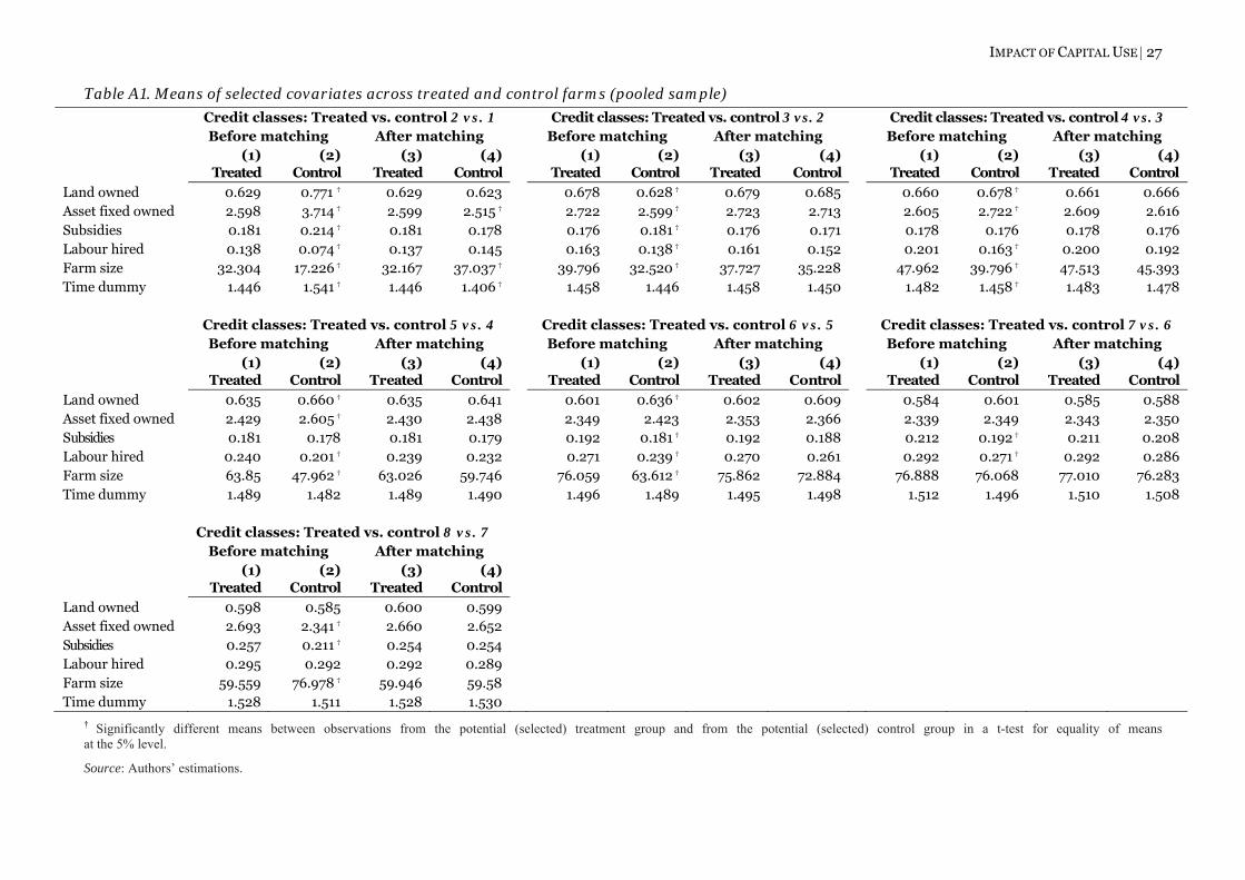
IMPACT OF CAPITAL USE | 27
Table A1. Means of selected covariates across treated and control farms (pooled sample)
Credit classes: Treated vs. control 2 vs. 1 Credit classes: Treated vs. control 3 vs. 2 Credit classes: Treated vs. control 4 vs. 3 Before matching After matching Before matching After matching Before matching After matching (1)
Treated (2)
Control (3)
Treated (4)
Control (1)
Treated (2)
Control (3)
Treated (4)
Control (1)
Treated (2)
Control (3)
Treated (4)
Control Land owned 0.629 0.771 † 0.629 0.623 0.678 0.628 † 0.679 0.685 0.660 0.678 † 0.661 0.666 Asset fixed owned 2.598 3.714 † 2.599 2.515 † 2.722 2.599 † 2.723 2.713 2.605 2.722 † 2.609 2.616 Subsidies 0.181 0.214 † 0.181 0.178 0.176 0.181 † 0.176 0.171 0.178 0.176 0.178 0.176 Labour hired 0.138 0.074 † 0.137 0.145 0.163 0.138 † 0.161 0.152 0.201 0.163 † 0.200 0.192 Farm size 32.304 17.226 † 32.167 37.037 † 39.796 32.520 † 37.727 35.228 47.962 39.796 † 47.513 45.393 Time dummy 1.446 1.541 † 1.446 1.406 † 1.458 1.446 1.458 1.450 1.482 1.458 † 1.483 1.478 Credit classes: Treated vs. control 5 vs. 4 Credit classes: Treated vs. control 6 vs. 5 Credit classes: Treated vs. control 7 vs. 6 Before matching After matching Before matching After matching Before matching After matching (1)
Treated (2)
Control (3)
Treated (4)
Control (1)
Treated (2)
Control (3)
Treated (4)
Control (1)
Treated (2)
Control (3)
Treated (4)
Control Land owned 0.635 0.660 † 0.635 0.641 0.601 0.636 † 0.602 0.609 0.584 0.601 0.585 0.588 Asset fixed owned 2.429 2.605 † 2.430 2.438 2.349 2.423 2.353 2.366 2.339 2.349 2.343 2.350 Subsidies 0.181 0.178 0.181 0.179 0.192 0.181 † 0.192 0.188 0.212 0.192 † 0.211 0.208 Labour hired 0.240 0.201 † 0.239 0.232 0.271 0.239 † 0.270 0.261 0.292 0.271 † 0.292 0.286 Farm size 63.85 47.962 † 63.026 59.746 76.059 63.612 † 75.862 72.884 76.888 76.068 77.010 76.283 Time dummy 1.489 1.482 1.489 1.490 1.496 1.489 1.495 1.498 1.512 1.496 1.510 1.508 Credit classes: Treated vs. control 8 vs. 7 Before matching After matching (1)
Treated (2)
Control (3)
Treated (4)
Control
Land owned 0.598 0.585 0.600 0.599 Asset fixed owned 2.693 2.341 † 2.660 2.652 Subsidies 0.257 0.211 † 0.254 0.254 Labour hired 0.295 0.292 0.292 0.289 Farm size 59.559 76.978 † 59.946 59.58 Time dummy 1.528 1.511 1.528 1.530
† Significantly different means between observations from the potential (selected) treatment group and from the potential (selected) control group in a t-test for equality of means at the 5% level.
Source: Authors’ estimations.
Related Documents