Production Scheduling Approaches for Operations Management

Production Scheduling Approaches for 1

Operations Management 2

Marcello Fera1, Fabio Fruggiero2, Alfredo Lambiase1, Giada Martino1, Maria 3 Elena Nenni3 4

5 1University of Salerno – Dpt. of Industrial Engineering- Via Ponte don Melillo 1, 84084 6

Fisciano (Salerno) – Italy 7 2 University of Basilicata – School of Engineering – Via Ateneo Lucano 10, 8

85100 Potenza – Italy 9 3 University of Naples Federico II – Dpt. of Economic Management – P.le Tecchio 80, 10

80125 Napoli - Italy 11

12

1. Introduction 13

Scheduling is essentially the short-term execution plan of a production planning model. 14 Production scheduling consists of the activities performed in a manufacturing company in 15 order to manage and control the execution of a production process. A schedule is an 16 assignment problem that describes into details (in terms of minutes or seconds) which 17 activities must be performed and how the factory’s resources should be utilized to satisfy 18 the plan. Detailed scheduling is essentially the problem of allocating machines to competing 19 jobs over time, subject to the constraints. Each work center can process one job at a time and 20 each machine can handle at most one task at a time. A scheduling problem, typically, 21 assumes a fixed number of jobs and each one has its own parameters (i.e., tasks, the 22 necessary sequential constraints, the time estimates for each operation and the required 23 resources, no cancellations). All scheduling approaches require some estimate of how long it 24 takes to perform the work. Scheduling affects, and is affected by, the shop floor 25 organization. All scheduling changes can be projected over time enabling the identification 26 and analysis of starting time, completion times, idle time of resources, lateness, etc… . 27

A right scheduling plan can drive the forecast to anticipate completion date for each 28 released part and to provide data for deciding what to work on next. Questions about “Can 29 we do it?” and/or “How are we doing?” presume the existence of approaches for 30 optimisation. The aim of a scheduling study is, in general, to perform the tasks in order to 31 comply with priority rules and to respond to strategy. An optimal short-term production 32 planning model aims at gaining time and saving opportunities. It starts from the execution 33 orders and it tries to allocate, in the best possible way, the production of the different items 34 to the facilities. A good schedule starts from planning and springs from respecting resource 35 conflicts, managing the release of jobs to a shop and optimizing completion time of all jobs. 36 It defines the starting time of each task and determines whatever and how delivery 37 promises can be met. The minimization of one or more objectives has to be accomplished 38 (e.g., the number of jobs that are shipped late, the minimization set up costs, the maximum 39 completion time of jobs, maximization of throughput, etc.). Criteria could be ranked from 40 applying simple rules to determine which job has to be processed next at which work-centre 41

Operations Management

2

(i.e., dispatching) or to the use of advanced optimizing methods that try to maximize the 1 performance of the given environment. Fortunately many of these objectives are mutually 2 supportive (e.g., reducing manufacturing lead time reduces work in process and increases 3 probability to meeting due dates). To identify the exact sequence among a plethora of 4 possible combinations, the final schedule needs to apply rules in order to quantify urgency 5 of each order (e.g., assigned order’s due date - defined as global exploited strategy; amount 6 of processing that each order requires - generally the basis of a local visibility strategy). It’s 7 up to operations management to optimize the use of limited resources. Rules combined into 8 heuristic* approaches and, more in general, in upper level multi-objective methodologies 9 (i.e., meta-heuristics†), become the only methods for scheduling when dimension and/or 10 complexity of the problem is outstanding [1]. In the past few years, metaheuristics have 11 received much attention from the hard optimization community as a powerful tool, since 12 they have been demonstrating very promising results from experimentation and practices in 13 many engineering areas. Therefore, many recent researches on scheduling problems focused 14 on these techniques. Mathematical analyses of metaheuristics have been presented in 15 literature [2, 3]. 16

This research examines the main characteristics of the most promising meta-heuristic 17 approaches for the general process of a Job Shop Scheduling Problems (i.e., JSSP). Being a 18 NP complete and highly constrained problem, the resolution of the JSSP is recognized as a 19 key point for the factory optimization process [4]. The chapter examines the soundness and 20 key contributions of the 7 meta-heuristics (i.e., Genetics Approaches, Ants Colony 21 Optimization, Bees Algorithm, Electromagnetic Like Algorithm, Simulating Annealing, 22 Tabu Search and Neural Networks), those that improved the production scheduling vision. 23 It reviews their accomplishments and it discusses the perspectives of each meta approach. 24 The work represents a practitioner guide to the implementation of these meta-heuristics in 25 scheduling job shop processes. It focuses on the logic, the parameters, representation 26 schemata and operators they need. 27

2. The Job Shop Scheduling Problem 28

The two key problems in production scheduling are „priorities“ and „capacity“. Wight 29 (1974) described scheduling as „establishing the timing for performing a task“ and observes 30 that, in manufacturing firms, there are multiple types of scheduling, including the detailed 31 scheduling of a shop order that shows when each operation must start and be completed [5]. 32 Baker (1974) defined scheduling as „a plan than usually tells us when things are supposed 33 to happen“ [6]. Cox et al. (1992) defined detailed scheduling as „the actual assignment of 34 starting and/or completion dates to operations or groups of operations to show when these 35

* The etymology of the word heuristic derives from a Greek word heurìsco (�������) - it means „to find“- and is considered the art of discovering new strategy rules to solve problems. Heuristics aims at a solution that is „good enough“ in a computing time that is „small enough“. † The term metaheuristc originates from union of prefix meta (����) - it means „behind, in the sense upper level methodology“ – and word heuristic - it means „to find“. Metaheuristcs’ search methods can be defined as upper level general methodologies guiding strategies in designing heuristics to obtain optimisation in problems.

Production Scheduling Approaches for Operations Management

3

must be done if the manufacturing order is to be completed on time“[7]. Pinedo (1995) listed 1 a number of important surveys on production scheduling [8]. For Hopp and Spearman 2 (1996) „scheduling is the allocation of shared resources over time to competing activities“ 3 [9]. Makowitz and Wein (2001) classified production scheduling problems based on 4 attributes: the presence of setups, the presence of due dates, the type of products. 5

Practical scheduling problems, although more highly constrained, are high difficult to solve 6 due to the number and variety of jobs, tasks and potentially conflicting goals. Recently, a lot 7 of Advanced Production Scheduling tools arose into the market (e.g., Aspen PlantTM 8 Scheduler family, Asprova, R2T – Resourse To Time, DS APS – DemandSolutions APS, DMS 9 – Dynafact Manufacturing System, i68Group, ICRON-APS, JobPack, iFRP, Infor SCM, 10 SchedulePro, ., Optiflow-Le, Production One APS, MQM – Machine Queue Management, 11 MOM4, JDA software, Rob-ex, Schedlyzer, , OMP Plus, MLS and MLP, Oracle Advanced 12 Scheduling, Ortec Schedule, ORTEMS Productionscheduler, Outperform, AIMMS, Planet 13 Together, Preactor, Quintiq, FactoryTalk Scheduler, SAP APO-PP/DS, and others). Each of 14 these automatically reports graphs. Their goal is to drive the scheduling for assigned 15 manufacturing processes. They implement rules and optimise an isolated sub-problem but 16 none of the them will optimise a multi stage resource assignment and sequencing problem. 17

In a Job Shop (i.e., JS) problem a classic and most general factory environment, different 18 tasks or operations must be performed to complete a job [10]; moreover, priorities and 19 capacity problems are faced for different jobs, multiple tasks and different routes. In this 20 contest, each job has its own individual flow pattern through assigned machines, each 21 machine can process only one operation at a time and each operation can be processed by 22 only one machine at a time. The purpose of the procedure is to obtain a schedule which aims 23 to complete all jobs and, at the same time, to minimize (or maximize) the objective function. 24 Mathematically, the JS Scheduling Problem (i.e., JSSP) can be characterized as a 25 combinatorial optimization problem. It has been generally shown to be NP-hard‡ belonging 26 to the most intractable problems considered [4, 11, 12]. This means that the computation 27 effort may grow too fast and there are not universal methods making it possible to solve all 28 the cases effectively. Just to understand what the technical term means, consider the single-29 machine sequencing problem with three jobs. How many ways of sequencing three jobs do 30 exist? Only one of the three jobs could be in the first position, which leaves two candidates 31 for the second position and only one for the last position. Therefore the no. of permutations 32 is 3!. Thus, if we want to optimize, we need to consider six alternatives. This means that as 33 the no. of jobs to be sequenced becomes larger (i.e., n>80), the no. of possible sequences 34 become quite ominous and an exponential function dominates the amount of time required 35 to find the optimal solution [13]. Scheduling, however, performs the definition of the 36 optimal sequence of n jobs in m machines. If a set of n jobs is to be scheduled on m machines, 37 there are (n!)m possible ways to schedule the job. 38

It has to undergo a discrete number of operations (i.e., tasks) on different resources (i.e., 39 machines). Each product has a fixed route defined in the planning phase and following 40 ‡ A problem is NP-complete if exists no algorithm that solves the problem in a polynomial time. A problem is NP-hard if it is possible to show that it can solve a NP-complete problem.

Operations Management

4

processing requirements (i.e., precedence constraints). Other constraints, e.g. zoning which 1 binds the assignment of task to fixed resource, are also taken into consideration. Each 2 machine can process only one operation at a time with no interruptions. The schedule we 3 must derive aims to complete all jobs with minimization (maximization) of an objective 4 function on the given production plant. 5

Let: 6 •

1 2{ , ,......., }nJ J J J= the set of the job order existing inside the system; 7

• 1 2{ , ,......., }mM M M M= the set of machines that make up the system. 8

JSSP, marked as jΠ , consists in a finite set J of n jobs

1{ }ni iJ =. Each Ji is characterized by a 9

manufacturing cycle iCL regarded as a finite set M of m machines 1{ }mk kM =

with an 10

uninterrupted processing time ikτ . iJ , ∀ 𝑖 = 1,… ,𝑛 , is processed on a fixed machine im 11

and requires a chain of tasks 1 2, , ......., ,ii i imO O O scheduled under precedence constraints. 12

ikO is the task of job iJ which has to be processed on machine kM for an uninterrupted 13

processing time period ikτ and no operations may pre-empted. 14

To accommodate extreme variability in different parts of a job shop, schedulers separate 15 workloads in each work-centres rather than aggregating them [14]. Of more than 100 16 different rules proposed by researchers and applied by practitioners, some have become 17 common in Operations Management systems: First come- First served, Shortest Processing 18 Time, Earliest Due Date, Slack Time Remaining, Slack Time Remaining For each Operation, 19 Critical Ratio, Operation Due Date, etc. [15]. Besides these, Makespan is often the 20 performance feature in the study of resource allocation [16]. Makespan represents the time 21 elapsed from the start of the first task to the end of the last task in schedule. The 22 minimisation of makespan arranges tasks in order to level the differences between the 23 completion time of each work phase. It tries to smooth picks in work centre occupancysuch 24 to obtain batching in load assignment per time. Although direct time constraints, such as 25 minimization of processing time or earliest due date, are sufficient to optimize industrial 26 scheduling problems, for the reasons as above the minimization of the makespan is 27 preferable for general/global optimization performances because it enhances the overall 28 efficiency in shop floor and reduces manufacturing lead time variability [17]. 29

Thus, in JSSP optimization variant of j

Π , the objective of a scheduling problem is typically 30

to assign the tasks to time intervals in order to minimise the makespan and referred to as: 31 *

max1 1( ) ( , , ), ... ; ...

ik iki sC t f CL i n k mτ= ∀ = ∀ = (1)

32

where t represent time (i.e. iteration steps) 33

max

*

maxmin( min max) { [ ] : , }( ) ( )

iik ik i kiCC s J J M Mt t τ= = + ∀ ∈ ∀ ∈

(2)

34

Production Scheduling Approaches for Operations Management

5

and 0iks ≥ represents the starting time of k-th operation of i-th job. 𝑠!" is the time value that 1

we would like to determinate in order to establish the suited schedule activities order. 2

3. Representation of scheduling instances 3

The possible representation of a JS problem could be done through a Gantt chart or through 4 a Network representation. 5

Gantt (1916) created innovative charts for visualizing planned and actual production [18]. 6 According to Cox et al. (1992), a Gantt chart is “the earliest and best known type of control 7 chart especially designed to show graphically the relationship between planned 8 performance and actual performance” [19]. Gantt designed his charts so that foremen or 9 other supervisors could quickly know whether production was on schedule, ahead of 10 schedule or behind schedule. A Gantt chart, or bar chart as it is usually named, measures 11 activities by the amount of time needed to complete them and use the space on the chart to 12 represent the amount of the activity that should have been done in that time [7]. 13

A Network representation was first introduced by Roy and Sussman [20]. The 14 representation is based on “disjunctive graph model” [21]. This representation starts from the 15 concept that a feasible and optimal solution of JSP can originate from a permutation of 16 task’s order. Tasks are defined in a network representation through a probabilistic model, 17 observing the precedence constraints, characterized in a machine occupation matrix M and 18 considering the processing time of each tasks, defined in a time occupation matrix T. 19

11 1 11 1

1 1

( ) ( )

( ) ( ) ;

n n

n nn n nn

M M M M

M M M MM T

τ τ

τ τ

= =

K KM O M M O M

L L

20

JS processes are mathematically described as disjunctive graph G = (V, C, E). The 21 descriptions and notations as follow are due to Adams et. al. [22], where: 22

• V is a set of nodes representing tasks of jobs. Two additional dummy tasks are to 23 be considered: a source(0) node and a sink(*) node which stand respectively for the 24 Source (S) task τ0= 0, necessary to specify which job will be scheduled first, and an 25 end fixed sink where schedule ends (T) τ*= 0; 26

• C is the set of conjunctive arcs or direct arcs that connect two consecutive tasks 27 belonging to the same job chain. These represent technological sequences of 28 machines for each job; 29

• E= 𝐷!!!!! , where Dr is a set of disjunctive arcs or not-direct arcs representing pair 30

of operations that must be performed on the same machine Mr. 31

Each job-tasks pair (i,j) is to be processed on a specified machine M(i,j) for T(i,j) time units, 32 so each node of graph is weighted with j operation’s processing time. In this representation 33 all nodes are weighted with exception of source and sink node. This procedure makes 34

Operations Management

6

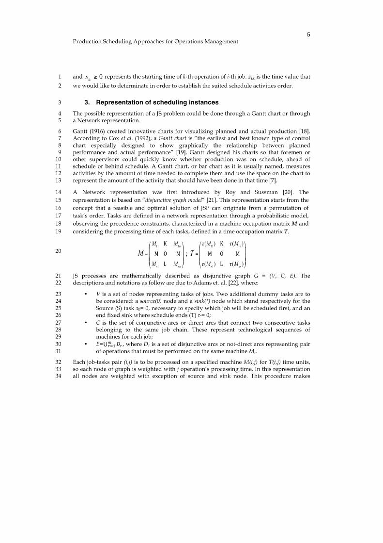
always available feasible schedules which don’t violate hard constraints§. A graph 1 representation of a simple instance of JSP, consisting of 9 operations partitioned into 3 jobs 2 and 3 machines, is presented in fig. 1. Here the nodes correspond to operations numbered 3 with consecutive ordinal values adding two fictitious additional ones: S = “source node” 4 and T = “sink node”. The processing time for each operation is the weighted value τij 5 attached to the corresponding node, 𝑣 ∈ 𝑉, and for the special nodes, τ0 = τ*= 0. 6

Let sv be the starting time of an operation to a node v. By using the disjunctive graph 7 notation, the JSPP can be formulated as a mathematical programming model as follows: 8 9 Minimize s* subject to: 10

s! − 𝑠!  ≥   𝜏! (v,w) ∈ C (3) 11 𝑠!  ≥  0 v ∈ V (4) 12 s! − 𝑠!  ≥   𝜏!     s! − 𝑠!  ≥   𝜏!  (v, w) ∈  𝐷!,! ≤ 𝑟 ≤ 𝑚, (5) 13

14

15 Figure 1: Disjunctive graph representation. There are disjunctive arcs between every pair of tasks that 16 has to be processed on the same machine (dashed lines) and conjunctive arcs between every pair of 17 tasks that are in the same job (dotted lines). Omitting processing time, the problem specification is18

2{ , ) {1, 2, 3}, ( }ij i jO o ∈= , ), 1, 2, 3}{ , ({ }iji i jJ J o == = , , ( , ) 1, 2, 3}{ }{ ijj i jM M o= == . Job notation 19

is used. 20

s* is equal to the completion time of the last operation of the schedule, which is therefore 21 equal to Cmax. The first inequality ensures that when there is a conjunctive arc from a node v 22 to a node w, w must wait of least τv time after v is started, so that the predefined 23 technological constraints about sequence of machines for each job is not violated. The 24 second condition ensures time to start continuities. The third condition affirms that, when 25 there is a disjunctive arc between a node v and a node w, one has to select either v to be 26 processed prior to w (and w waits for at least τv time period) or the other way around, this 27 avoids overlap in time due to contemporaneous operations on the same machine. 28

§ Hard constraints are physical ones, while soft constraints are those related to human factor e.g., relaxation, fatigue etc… .

O11

O21

O32

O31

O13

O22

O12

O23

O33

S

Sink

Conjunctive arc (technological sequences).

Source

T

Production Scheduling Approaches for Operations Management

7

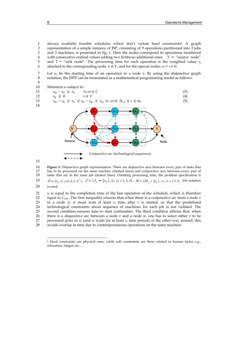
In order to obtain a scheduling solution and to evaluate makespan, we have to collect all 1 feasible permutations of tasks to transform the undirected arcs in directed ones in such a 2 way that there are no cycles. 3

The total number of nodes, 𝑛 = 𝑂 + 2 −  fixed by taking into account the total number of 4 tasks |O|, is properly the total number of operations with more two fictitious ones. While 5 the total number of arcs, in job notation, is fixed considering the number of tasks and jobs of 6 instance: 7

2n (| |) {(| |) 1}

arcs= | | +2 | |2 2

O OJ J

× −+ × = ×

(6) 8

The number of arcs defines the possible combination paths. Each path from source to sink is 9 a candidate solution for JSSP. The routing graph is reported in figure 2: 10

11 Figure 2: Problem routing representation. 12

4. Meta-heuristics for solving the JSSP 13

A logic has to be implemented in order to translate the scheduling problem into an 14 algorithm structure. Academic researches on scheduling problems have produced countless 15 papers [23]. Scheduling has been faced from many perspectives, using formulations and 16 tools of various disciplines such as control theory, physical science and artificial intelligence 17 systems [24]. Criteria for optimization could be ranked from applying simple priority rules 18 to determine which job has to be processed next at the work-centres (i.e., dispatching) to the 19 use of advanced optimizing methods that try to maximize the performance of the given 20 environment [25]. Their way to solution is generally approximate – heuristics – but it 21 constitutes promising alternatives to the exact methods and becomes the only one possible 22 when dimension and/or complexity of the problem is outstanding [26]. 23

Guidelines in using heuristics in combinatorial optimization can be found in Hertz (2003) 24 [27]. A classification of heuristic methods was proposed by Zanakis et al. (1989) [28]. 25 Heuristics are generally classified into constructive heuristics and improvement heuristics. The 26 first ones are focused on producing a solution based on an initial proposal, the goal is to 27 decrease the solution until all the jobs are assigned to a machine, not considering the size of 28

S

O11

O21

O32O31

O22

O12

O13

O23

O33

T

Operations Management

8

the problem [29]. The second ones are iterative algorithms which explore solutions by 1 moving step by step form one solution to another. The method starts with an arbitrary 2 solution and transits from one solution to another according to a series of basic 3 modifications defined on case by case basis [30]. 4

Relatively simple rules in guiding heuristic, with exploitation and exploration, are capable 5 to produce better quality solutions than other algorithms from the literature for some classes 6 of instances. These variants originate the class of meta-heuristic approaches [31]. The meta-7 heuristics**, and in general the heuristics, do not ensure optimal results but they usually tend 8 to work well [32]. The purpose of the paper is to illustrate the most promising optimization 9 methods for the JSSP. 10

As optimization techniques, metaheuristics are stochastic algorithms aiming to solve a 11 broad range of hard optimization problems, for which one does not know more effective 12 traditional methods. Often inspired by analogies with reality, such as physics science, 13 Simulated Annealing [33] and Electromagnetic like Methods [34], biology (Genetic 14 Algorithms [35], Tabu Search [36]) and ethnology (Ant Colony [37,], Bees Algorithm [38]), 15 human science (Neural Networks [39]), they are generally of discrete origin but can be 16 adapted to the other types of problems. 17

4.1. Genetic Algorithms (GAs) 18

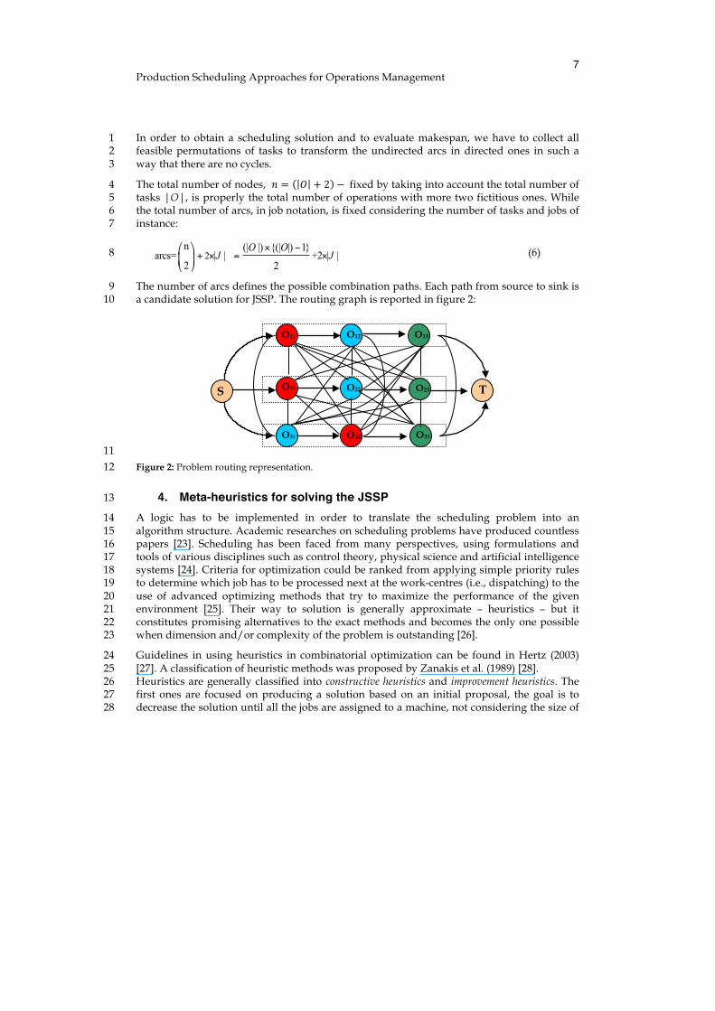
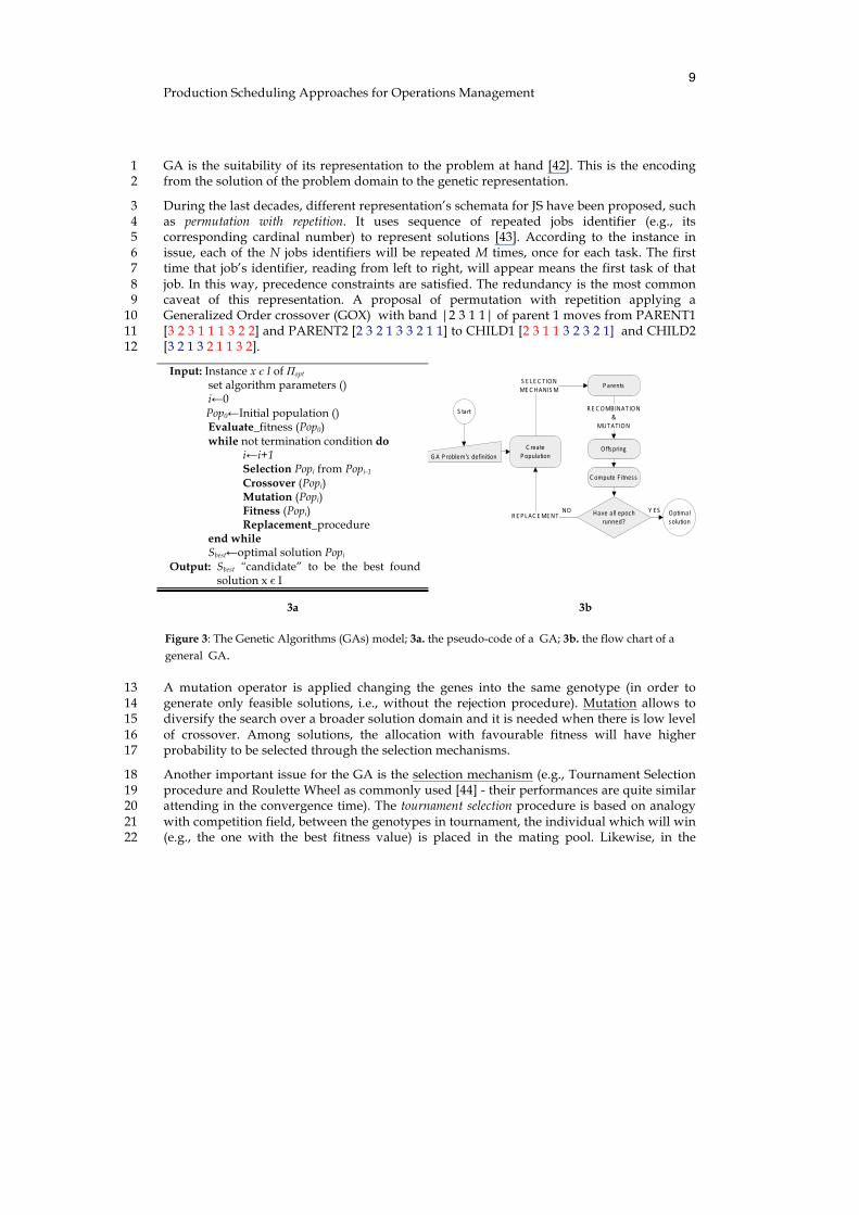
The methodology of a Gas - based on the evolutionary strategy- trasforms a population (set) 19 of individual objects, each with an associated fitness value, into a new generation of the 20 population occurring genetic operations such as crossover (sexual recombination) and mutation 21 (figg. 3). 22

The theory of evolutionary computing was formalized by Holland in 1975 [40]. GAs are 23 stochastic search procedures for combinatorial optimization problems based on Darwinian 24 principle of natural reproduction, survival and environment’s adaptability [41]. The theory 25 of evolution is biologically explained, the individuals with a stronger fitness are considered 26 better able to survive. . Cells, with one or more strings of DNA (i.e., a chromosome), make 27 up an individual. The gene (i.e., a bit of chromosome located into its particular locus) is, 28 responsible for encoding traits (i.e., alleles). Physical manifestations are raised into genotype 29 (i.e., disposition of genes). Each genotype has is physical manifestation into phenotype. 30 According to these parameters is possible to define a fitness value. Combining individuals 31 through a crossover (i.e., recombination of genetic characteristics of parents) across the 32 sexual reproduction, the chromosomal inheritance process performs to offspring. In each 33 epoch a stochastic mutation procedure occurs. The implemented algorithm is able to 34 simulate the natural process of evolution, coupling solution of scheduling route in order to 35 determinate an optimal tasks assignment. Generally, GA has different basic component: 36 representation, initial population, evaluation function, the reproduction selection scheme, 37 genetic operators (mutation and crossover) and stopping criteria. Central to success of any 38

** The term metaheuristics was introduced by F. Glover in the paper about Tabu search.

Production Scheduling Approaches for Operations Management

9

GA is the suitability of its representation to the problem at hand [42]. This is the encoding 1 from the solution of the problem domain to the genetic representation. 2

During the last decades, different representation’s schemata for JS have been proposed, such 3 as permutation with repetition. It uses sequence of repeated jobs identifier (e.g., its 4 corresponding cardinal number) to represent solutions [43]. According to the instance in 5 issue, each of the N jobs identifiers will be repeated M times, once for each task. The first 6 time that job’s identifier, reading from left to right, will appear means the first task of that 7 job. In this way, precedence constraints are satisfied. The redundancy is the most common 8 caveat of this representation. A proposal of permutation with repetition applying a 9 Generalized Order crossover (GOX) with band |2 3 1 1| of parent 1 moves from PARENT1 10 [3 2 3 1 1 1 3 2 2] and PARENT2 [2 3 2 1 3 3 2 1 1] to CHILD1 [2 3 1 1 3 2 3 2 1] and CHILD2 11 [3 2 1 3 2 1 1 3 2]. 12

Input: Instance x є I of Пopt set algorithm parameters () i←0 Pop0←Initial population () Evaluate_fitness (Pop0) while not termination condition do

i←i+1 Selection Popi from Popi-1

Crossover (Popi) Mutation (Popi) Fitness (Popi) Replacement_procedure

end while Sbest←optimal solution Popi

Output: Sbest “candidate” to be the best found solution x є I

S tart

C reateP opulationGAP roblem's definition

P arents

Offspring

S E LE C T IONME C HANIS M

R E C OMBINAT ION&

MUTAT ION

R E P LAC EMENT

C omputeF itness

Haveallepochrunned?

Optimalsolution

NO Y ES

3a 3b

Figure 3: The Genetic Algorithms (GAs) model; 3a. the pseudo-code of a GA; 3b. the flow chart of a general GA.

A mutation operator is applied changing the genes into the same genotype (in order to 13 generate only feasible solutions, i.e., without the rejection procedure). Mutation allows to 14 diversify the search over a broader solution domain and it is needed when there is low level 15 of crossover. Among solutions, the allocation with favourable fitness will have higher 16 probability to be selected through the selection mechanisms. 17

Another important issue for the GA is the selection mechanism (e.g., Tournament Selection 18 procedure and Roulette Wheel as commonly used [44] - their performances are quite similar 19 attending in the convergence time). The tournament selection procedure is based on analogy 20 with competition field, between the genotypes in tournament, the individual which will win 21 (e.g., the one with the best fitness value) is placed in the mating pool. Likewise, in the 22

Operations Management

10

roulette wheel selection mechanism each individual of population has a selection’s likelihood 1 proportional to its objective score (in analogy with the real roulette item) and with a 2 probability equal to one of a ball in a roulette, one of the solutions is chosen. 3

It is very important, for the Gas success, to select the correct ratio between crossover and 4 mutation, because the first one allows to allows to diversify a search field, while a mutation 5 to modify a solution. 6

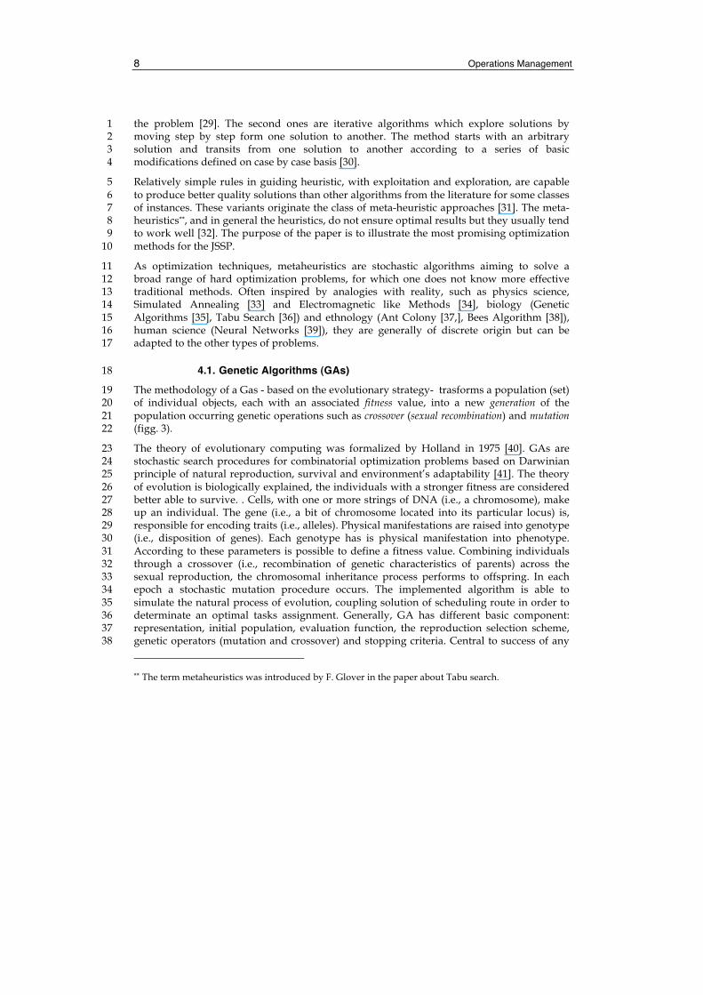
4.2. Ant Colony Optimization (ACO) algorithms 7

If we are on a pic-nic and peer into our cake bitten by a colony of ants, moving in a tidy way 8 and caring on a lay-out that is the optimal one in view of stumbling-blocks and length, we 9 discover how remarkable is nature and we find its evolution as the inspiring source for 10 investigations on intelligence operation scheduling techniques [45]. Natural ants are capable 11 to establish the shortest route path from their colony to feeding sources, relying on the 12 phenomena of swarm intelligence for survival. They make decisions that seemingly require an 13 high degree of co-operation, smelling and following a chemical substance (i.e. pheromone††) 14 laid on the ground and proportional to goodness load that they carry on (i.e. in a scheduling 15 approach, the goodness of the objective function, reported to makespan in this applicative 16 case). 17

The same behaviour of natural ants can be overcome in an artificial system with an artificial 18 communication strategy regard as a direct metaphoric representation of natural evolution. 19 The essential idea of an ACO model is that “good solutions are not the result of a sporadic 20 good approach to the problem but the incremental output of good partial solutions item. 21 Artificial ants are quite different by their natural progenitors, maintaining a memory of the 22 step before the last one [37]. Computationally, ACO [46] are population based approach 23 built on stochastic solution construction procedures with a retroactive control improvement, 24 that build solution route with a probabilistic approach and through a suitable selection 25 procedure by taking into account: (a) heuristic information on the problem instance being 26 solved; (b) (mat-made) pheromone amount, different from ant to ant, which stores up and 27 evaporates dynamically at run-time to reflect the agents’ acquired search training and 28 elapsed time factor. 29

The initial schedule is constructed by taking into account heuristic information, initial 30 pheromone setting and, if several routes are applicable, a self-created selection procedure 31 chooses the task to process. The same process is followed during the whole run time. The 32 probabilistic approach focused on pheromone. Path’s attractive raises with path choice and 33 probability increases with the number of times that the same path was chosen before [47]. At 34 the same time, the employment of heuristic information can guide the ants towards the most 35 promising solutions and additionally, the use of an agent’s colony can give the algorithm: (i) 36 Robustness on a fixed solution; (ii) Flexibility between different paths. 37

The approach focuses on co-operative ant colony food retrieval applied to scheduling 38 routing problems. Colorni et al, basing on studies of Dorigo et al [48], were the first to apply 39

†† It is an organic compound highly volatile that shares on central neural system as an actions’ releaser.

Production Scheduling Approaches for Operations Management

11

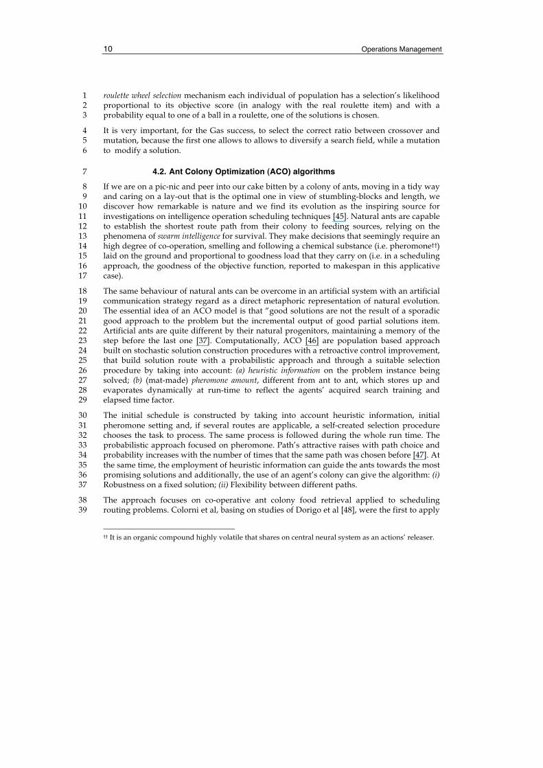
Ant System (AS) to job scheduling problem [49] and dubbed this approach as Ant Colony 1 Optimization (ACO). They iteratively create route, adding components to partial solution, 2 by taking into account heuristic information on the problem instance being solved (i.e. 3 visibility) and “artificial” pheromone trials (with its storing and evaporation criteria). Across 4 the representation of scheduling problem like acyclic graph, see fig. 2, the ant’s rooting from 5 source to food is assimilated to the scheduling sequence.Think at ants as agents, nodes like 6 tasks and arcs as the release of production order. According to constraints, the ants perform 7 a path from the row material warehouse to the final products one. 8

Constraints are introduced hanging from jobs and resources. Fitness is introduced to 9 translate how good the explored route was. Artificial ants live in a computer realized world. 10 They have an overview of the problem instance they are going to solve across a visibility 11 factor. In the Job Shop side of ACO implementation the visibility has chosen tied with the 12 run time of the task (Eq. 7). The information was about the inquired task’s (i.e., j) completion 13 time Ctimej and idle time Itimej from the previous position (i.e., i): 14

1 1( )

( )ij

j j j

tCtime Itime Rtime

η = =−

(7) 15

Input: Instance x є I of Пopt Set algorithm parameters () i, j ← 0 for j= 1 to colonies do

Ant s0 ← Create sub-colony and release agent while not-termination conditions

on sub-colony do i=i+1 Manage_ants activity () Manage_Pheromone () Manage_Demon Action () Selection Procedure () Compute solution Quality ()

end while j=j+1 Sbest←candidate to be optimal solution Update pheromone on arc ()

end for Output: Sbest“candidate” to be the best found

solution x є I

S tart

C reatenewsub‐colonyandreleaseagent

AS P roblem's definition

P robabilityandS electionprocedure

Y ES

ManageAntActivity

ManagePheromone

ManageDemonActioon

AddandUpdatepheromoneonpaths

Haveallantsbuilta

solution?

Haveallcolonies beencreated?

NO

R eleasepheromone

Optimalsolution

Y ES

NO

C omputeS olutionquality

4a 4b

Figure 4: The Ant Colony Optimization (ACO) model; 4a. the pseudo-code of an ACO algorithm; 4b. the flow chart of a general ACO procedure.

Operations Management

12

The colony is composed of a fixed number of agents ant=1,…, n. A probability is associated 1 to each feasible movement (Sant(t)) and a selection procedure (generally based on RWS or 2 Tournament procedure) is applied. 3

0 ( ) 1ant

ijP t≤ ≤ is the probability that at time t the generic agent ant chooses edge i j→ as 4

next routing path; at time t each ant chooses the next operation where it will be at time t+1. 5 This value is valuated through visibility (η) and pheromone (τ) information. The probability 6 value (Eq. 8) is associated to a fitness into selection step. 7

( )

otherwise

[ ( )] [ ( )]if j ( )

[ ( )] [ ( )]

( )

0 ant

ij ij

ant

ih ih i

h S t

ant

ij

t tS t

t tP t

α β

α β

τ η

τ η∈

∈

=

∑ (8) 8

Where: ( )ijtτ represents the intensity of trail on connection ( , )i j at time t . Set the 9

intensity of pheromone at iteration t=0: �ij(o) to a general small positive constant in order to 10 ensure the avoiding of local optimal solution; � and � are user’s defined values tuning the 11 relative importance of the pheromone vs. the heuristic time-distance coefficient. They have 12 to be chosen 0 , 10α β< ≤ (in order to assure a right selection pressure). 13

For each cycle the agents of the colony are going out of source in search of food. When all 14 colony agents have constructed a complete path, i.e. the sequence of feasible order of visited 15 nodes, a pheromone update rule is applied (Eq. 9): 16

( 1) (1 ) ( 1) ( )ij ij ijt t tλτ τ τ+ = − + + Δ (9) 17

Besides ants’ activity, pheromone trail evaporation has been included trough a coefficient 18 representing pheromone vanishing during elapsing time. These parameters imitate the 19 natural world decreasing of pheromone trail intensity over time. It implements a useful 20 form of forgetting. It has been considered a simple decay coefficient (i.e., 0 1λ< < ) that 21 works on total laid pheromone level between time t and t+1. 22

The laid pheromone on the inquired path is evaluated taking into consideration how many 23 agents chose that path and how was the objective value of that path (Eq. 10). The weight of 24 the solution goodness is the makespan (i.e., Lant). A constant of pheromone updating (i.e., Q), 25 equal for all ants and user, defined according to the tuning of the algorithm, is introduced as 26 quantity of pheromone per unit of time (Eq. 11). The algorithm works as follow. It is 27 computed the makespan value for each agent of the colony (Lant(0)), following visibility and 28 pheromone defined initially by the user (τij(0)) equal for all connections. It is evaluated and 29 laid, according to the disjunctive graph representation of the instance in issue, the amount of 30 pheromone on each arc (evaporation coefficient is applied to design the environment at the 31 next step). 32

Production Scheduling Approaches for Operations Management

13

1

( )( )ij

antsant

ij

ant

ttτ τ=

=Δ Δ∑ (10) ant-th followed edge (i,j)

otherwise

if( )

0

antantij

QLtτΔ =

(11) 1

Visibility and updated pheromone trail fixes the probability (i.e., the fitness values) of each 2 node (i.e., task) at each iteration; for each cycle, it is evaluated the output of the objective 3 function (Lant(t)). An objective function value is optimised accordingly to partial good 4 solution. In this improvement, relative importance is given to the parameters α and β. Good 5 elements for choosing these two parameters are: / 0α β ≅ (which means low level of α) and 6 little value of α ( 0 2α< ≤ ) while ranging β in a larger range ( 0 6β< ≤ ). 7

4.3. Bees Algorithm (BA) approach 8

A colony of bees exploits, in multiple directions simultaneously, food sources in the form of 9 antera with plentiful amounts of nectar or pollen. They are able to cover kilometric distances 10 for good foraging fields [50]. Flower paths are covered based on a stigmergic approach – 11 more nectar places should be visited by more bees [51]. 12

The foraging strategies in colonies of bees starts by scout bees – a percentage of beehive 13 population. They wave randomly from one patch to another. Returning at the hive, those 14 scout bees deposit their nectar or polled and start a recruiting mechanism rated above a 15 certain quality threshold on nectar stored [52]. The recruiting mechanism is properly a 16 launching into a wild dance over the honeycomb. This natural process is known as “waggle 17 dance” [53]. Bees, stirring up for discovery, flutter in a number from one to one hundred 18 circuits with a waving and returning phase. The waving phase contains information about 19 direction and distance of flower patches. Waving phases in ascending order on vertical 20 honeycomb suggest flower patches on straightforward line with sunbeams. This 21 information is passed using a kind of dance, that is possible to be developed on right or on 22 left. So through this dance, it is possible to understand the distance from the flower, the 23 presence of nectar and the sunbeam side to choose [54]. 24

The waggle dance is used as a guide or a map to evaluate merits of explored different 25 patches and to exploit better solutions. After waggle dancing on the dance floor, the dancer 26 (i.e. the scout bee) goes back to the flower patch with follower bees that were waiting inside 27 the hive. A squadron moves forward into the patches. More follower bees are sent to more 28 promising patches, while harvest paths are explored but they are not carried out in the long 29 term. A swarm intelligent approach is constituted [55]. This allows the colony to gather food 30 quickly and efficiently with a recursive recruiting mechanism [56]. 31

The Bees Algorithm (i.e., BA) is a population-based search; it is inspired to this natural 32 process [38]. In its basic version, the algorithm performs a kind of neighbourhood search 33 combined with random search. Advanced mechanisms could be guided by genetics [57] or 34 taboo operators [58]. The standard Bees Algorithm first developed in Pham and Karaboga in 35 2006 [59, 60] requires a set of parameters: no. of scout bees (n), no. of sites selected out of n 36

Operations Management

14

visited sites (m), no. of best sites out of m selected sites (e), no. of bees recruited for the best e 1 sites (nep), no. of bees recruited for the other m-e selected sites (nsp), initial size of patches 2 (ngh). The standard BA starts with random search. 3

The honey bees‘ effective foraging strategy can be applied in operation management 4 problems such as JSSP. For each solution, a complete schedule of operations in JSP is 5 produced. The makespan of the solution is analogous to the profitability of the food source 6 in terms of distance and sweetness of the nectar. Bees, n scouts, explore patches, m sites - 7 initially a scout bee for each path could be set, over total ways, ngh, accordingly to the 8 disjunctive graph of fig. 2, randomly at the first stage, choosing the shorter makespan and 9 the higher profitability of the solution path after the first iteration. 10

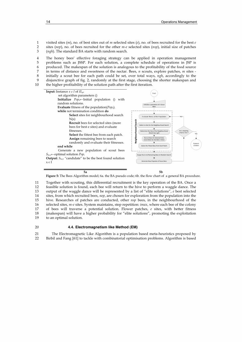
Input: Instance x є I of Пopt set algorithm parameters () Initialize Pop0←Initial population () with random solutions. Evaluate fitness of the population(Pop0). while not termination condition do

Select sites for neighbourhood search N(s) Recruit bees for selected sites (more bees for best e sites) and evaluate fitnesses. Select the fittest bee from each patch. Assign remaining bees to search randomly and evaluate their fitnesses.

end while Generate a new population of scout bees

Sbest←optimal solution Popi

Output: Sbest “candidate” to be the best found solution x є I

S tart

E valuatefitness oftheP opulation

Ares toppingcriteriamet?

Optimalsolution

InitializeapolulationofnScoutBees

SelectmsitesfortheNeighbourhoodSearch

DeterminetheSizeoftheNeighbourhood(PatchSizengh)

RecruitBeesforSelectedSites(moreBeesfortheBest eSites)

SelecttheFittestBeesfromEachPatch

Assignthe(n‐m)RemainingBeestoRandomSearch

GenerateNewPopulateofScoutBees

Neighbo

urho

ood Search

NO

YES

5a 5b

Figure 5: The Bees Algorithm model; 6a. the BA pseudo code; 6b. the flow chart of a general BA procedure.

Together with scouting, this differential recruitment is the key operation of the BA. Once a 11 feasible solution is found, each bee will return to the hive to perform a waggle dance. The 12 output of the waggle dance will be represented by a list of “elite solutions”, e best selected 13 sites, from which recruited bees, nep, are chosen for exploration from the population into the 14 hive. Researches of patches are conducted, other nsp bees, in the neighbourhood of the 15 selected sites, m-e sites. System maintains, step repetition: imax, where each bee of the colony 16 of bees will traverse a potential solution. Flower patches, e sites, with better fitness 17 (makespan) will have a higher probability for “elite solutions”, promoting the exploitation 18 to an optimal solution. 19

4.4. Electromagnetism like Method (EM) 20

The Electromagnetic Like Algorithm is a population based meta-heuristics proposed by 21 Birbil and Fang [61] to tackle with combinatorial optimisation problems. Algorithm is based 22

Production Scheduling Approaches for Operations Management

15

on the natural law of attraction and repulsion between charges (Coulomb’s law) [62]. EM 1 simulates electromagnetic interaction [63]. The algorithm evaluates fitness of solutions 2 considering charge of particles. Each particle represents a solution. Two points into the 3 space had different charges in relation to what electromagnetic field acts on them [64]. An 4 electrostatic force, in repulsion or attraction, manifests between two points charges. The 5 electrostatic force is directly proportional to the magnitudes of each charge and inversely 6 proportional to the square of the distance between the charges. The fixed charge at time 7 iteration (t) of particle i is shown as follows: 8

( ) ( ) ( ) ( )( ) mitxftxftxftxfntqm

ibestibestii ,..,1,,/,,*exp)(

1=∀

−−−= ∑

=

(12) 9

Where t represents the iteration step, qi (t) is the charge of particle i at iteration t, f(xi,,t), 10 f(xbest,t), and f(xk,t) denote the objective value of particle i, the best solution, and particle k 11 from m particles at time t; finally, n is the dimension of search space.The charge of each 12 point i, qi(t), determines point’s power of attraction or repulsion. Points (xi) could be 13 evaluated as a task into the graph representation (fig. 2). 14

The particles move along with total force and so diversified solutions are generated. The 15 following formulation is the resultant force of particle i: 16

( ) ( ) ( ) ( )

( ) ( ) ( ) ( )mi

txftxftxtx

tqtqtxtx

txftxftxtx

tqtqtxtx

tF

ij

ij

jiji

ij

ij

jiij

i ,...,1,,,:

)()(

)(*)(*)()(

,,:)()(

)(*)(*)()(

)(

2

2

=∀

≥−

−

<−

−

=∑ (13) 17

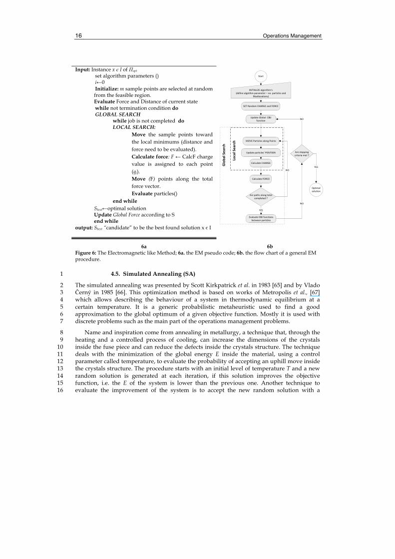
The following notes described an adapted version of EM for JSSP. According to this 18 application, the initial population is obtained by choosing randomly from the list or pending 19 tasks, as for the feasibility of solution, particles’ path. The generic pseudo-code for the EM is 20 reported in figure 6. Each particle is initially located into a source node (see disjunctive 21 graph of figure 2). Particle is uniquely defined by a charge and a location into the node’s 22 space. Particle’s position in each node is defined in a multigrid discrete set. While moving, 23 particle jumps in a node based on its attraction force, defined in module and direction and 24 way. If the force from starting line to arrival is in relation of positive inequality, the particles 25 will be located in a plane position in linear dependence with force intensity. A selection 26 mechanism could be set in order to decide where particle is directed, based on node force 27 intensity. Force is therefore the resultant of particles acting in node. A solution for the JS is 28 obtained only after a complete path from the source to the sink and the resulting force is 29 updated according to the normalized makespan of different solutions. 30

Operations Management

16

Input: Instance x є I of Пopt

set algorithm parameters () i←0 Initialize: m sample points are selected at random from the feasible region. Evaluate Force and Distance of current state while not termination condition do GLOBAL SEARCH

while job is not completed do LOCAL SEARCH:

Move the sample points toward the local minimums (distance and force need to be evaluated). Calculate force: F ← CalcF charge value is assigned to each point (qi). Move (F) points along the total force vector. Evaluate particles()

end while Sbest←optimal solution Update Global Force according to S end while

output: Sbest “candidate” to be the best found solution x є I

Start

SETRandomCHARGEandFORCE

Arestoppingcriteriamet?

Optimalsolution

INITIALIZEalgorithm’s(definealgotihmparameter–no.particlesand

MaxIterations)

UpdateGlobalOBJfunction

MOVEParticlesalongPoints

Updateparticles’POSITION

CalculateCHARGE

EvaluateOBJfunctionsbetweenparticles

Local Search

NO

YES

Arepathsalongtotalcompleted?

NO

YES

Glob

al Search

CalculateFORCE

NO

6a 6b Figure 6: The Electromagnetic like Method; 6a. the EM pseudo code; 6b. the flow chart of a general EM procedure.

4.5. Simulated Annealing (SA) 1

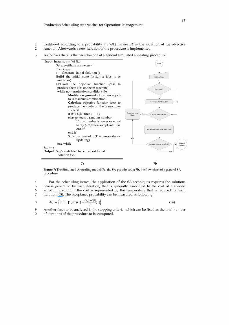
The simulated annealing was presented by Scott Kirkpatrick et al. in 1983 [65] and by Vlado 2 Černý in 1985 [66]. This optimization method is based on works of Metropolis et al., [67] 3 which allows describing the behaviour of a system in thermodynamic equilibrium at a 4 certain temperature. It is a generic probabilistic metaheuristic used to find a good 5 approximation to the global optimum of a given objective function. Mostly it is used with 6 discrete problems such as the main part of the operations management problems. 7

Name and inspiration come from annealing in metallurgy, a technique that, through the 8 heating and a controlled process of cooling, can increase the dimensions of the crystals 9 inside the fuse piece and can reduce the defects inside the crystals structure. The technique 10 deals with the minimization of the global energy E inside the material, using a control 11 parameter called temperature, to evaluate the probability of accepting an uphill move inside 12 the crystals structure. The procedure starts with an initial level of temperature T and a new 13 random solution is generated at each iteration, if this solution improves the objective 14 function, i.e. the E of the system is lower than the previous one. Another technique to 15 evaluate the improvement of the system is to accept the new random solution with a 16

Production Scheduling Approaches for Operations Management

17

likelihood according to a probability exp(-ΔE), where ΔE is the variation of the objective 1 function. Afterwards a new iteration of the procedure is implemented. 2

As follows there is the pseudo-code of a general simulated annealing procedure: 3

Input: Instance x є I of Пopt Set algorithm parameters () T ← Tiniziale s ← Generate_Initial_Solution () Build the initial state (assign n jobs to m machines)

Evaluate the objective function (cost to produce the n jobs on the m machine). while not-termination conditions do

Modify assignment of certain n jobs to m machines combination Calculate objective function (cost to produce the n jobs on the m machine) s’ є N(s) if f(s’) ≤ f(s) then s ← s’; else generate a random number

If this number is lower or equal to exp (-ΔE) then accept solution end if

end if Slow decrease of c. (The temperature c

updating) end while

Sbest ← s Output : Sbest“candidate” to be the best found

solution x є I

S tart

Updatecurrentsolution

Initialsolution

Decreasetemperature(choosec)

Gnerateanewsolution

S toppingcriteriasatis fied?

NO

NO

Optimalsolution

Y E S

Accepted?

C hangetemperature?

Y E S

NO

7a 7b

Figure 7: The Simulated Annealing model; 7a. the SA pseudo code; 7b. the flow chart of a general SA procedure

For the scheduling issues, the application of the SA techniques requires the solutions 4 fitness generated by each iteration, that is generally associated to the cost of a specific 5 scheduling solution; the cost is represented by the temperature that is reduced for each 6 iteration [68]. The acceptance probability can be measured as following: 7

𝐴𝑖𝑗 = 𝑚𝑖𝑛   [1, 𝑒𝑥𝑝 [(− ! ! !! !!

)]] (14) 8

Another facet to be analysed is the stopping criteria, which can be fixed as the total number 9 of iterations of the procedure to be computed. 10

Operations Management

18

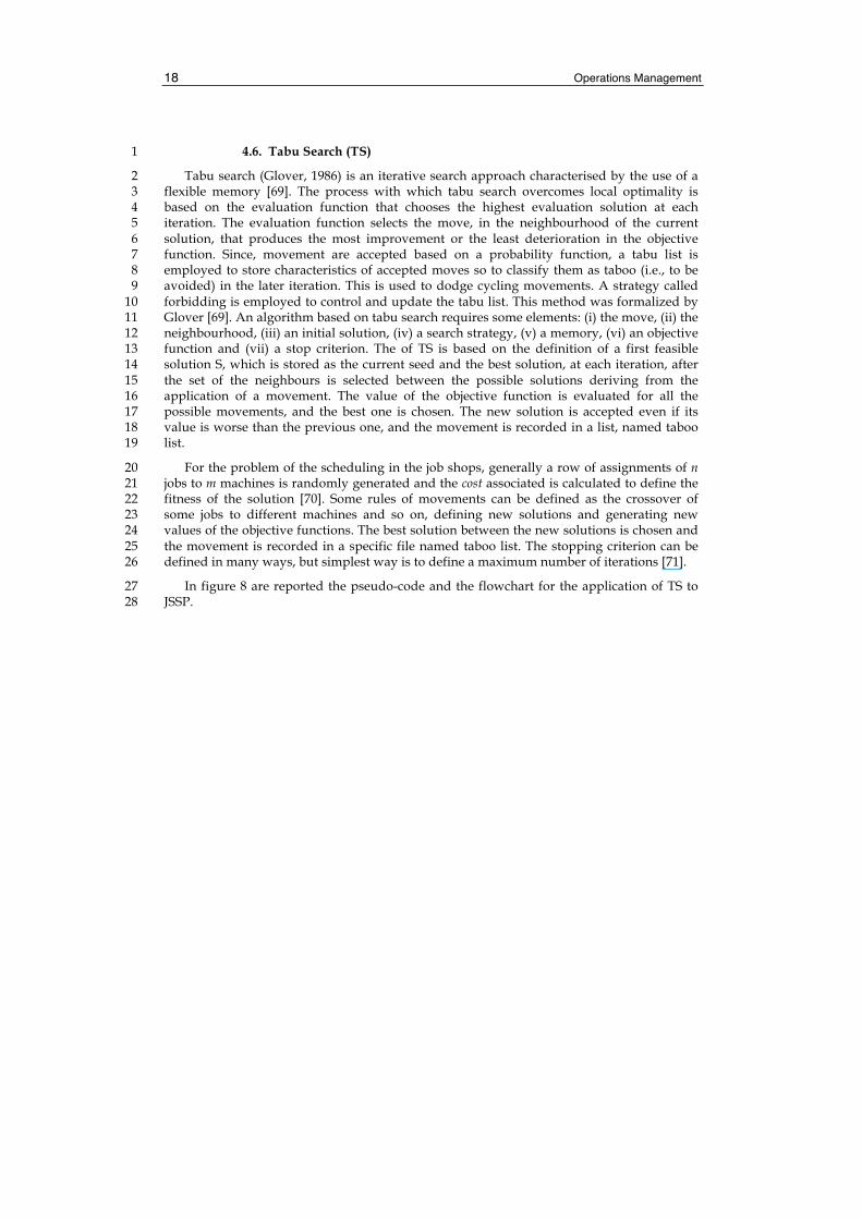
4.6. Tabu Search (TS) 1

Tabu search (Glover, 1986) is an iterative search approach characterised by the use of a 2 flexible memory [69]. The process with which tabu search overcomes local optimality is 3 based on the evaluation function that chooses the highest evaluation solution at each 4 iteration. The evaluation function selects the move, in the neighbourhood of the current 5 solution, that produces the most improvement or the least deterioration in the objective 6 function. Since, movement are accepted based on a probability function, a tabu list is 7 employed to store characteristics of accepted moves so to classify them as taboo (i.e., to be 8 avoided) in the later iteration. This is used to dodge cycling movements. A strategy called 9 forbidding is employed to control and update the tabu list. This method was formalized by 10 Glover [69]. An algorithm based on tabu search requires some elements: (i) the move, (ii) the 11 neighbourhood, (iii) an initial solution, (iv) a search strategy, (v) a memory, (vi) an objective 12 function and (vii) a stop criterion. The of TS is based on the definition of a first feasible 13 solution S, which is stored as the current seed and the best solution, at each iteration, after 14 the set of the neighbours is selected between the possible solutions deriving from the 15 application of a movement. The value of the objective function is evaluated for all the 16 possible movements, and the best one is chosen. The new solution is accepted even if its 17 value is worse than the previous one, and the movement is recorded in a list, named taboo 18 list. 19

For the problem of the scheduling in the job shops, generally a row of assignments of n 20 jobs to m machines is randomly generated and the cost associated is calculated to define the 21 fitness of the solution [70]. Some rules of movements can be defined as the crossover of 22 some jobs to different machines and so on, defining new solutions and generating new 23 values of the objective functions. The best solution between the new solutions is chosen and 24 the movement is recorded in a specific file named taboo list. The stopping criterion can be 25 defined in many ways, but simplest way is to define a maximum number of iterations [71]. 26

In figure 8 are reported the pseudo-code and the flowchart for the application of TS to 27 JSSP. 28

Production Scheduling Approaches for Operations Management

19

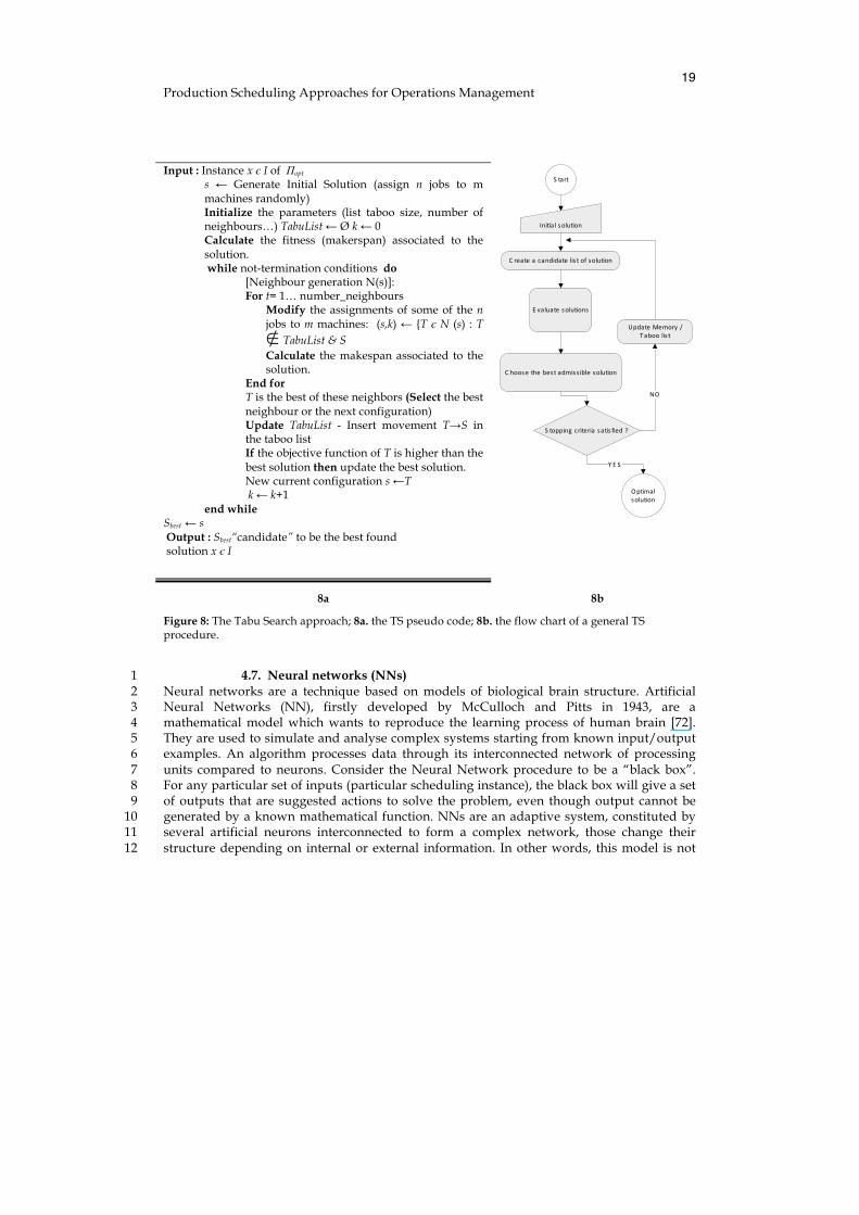
4.7. Neural networks (NNs) 1 Neural networks are a technique based on models of biological brain structure. Artificial 2 Neural Networks (NN), firstly developed by McCulloch and Pitts in 1943, are a 3 mathematical model which wants to reproduce the learning process of human brain [72]. 4 They are used to simulate and analyse complex systems starting from known input/output 5 examples. An algorithm processes data through its interconnected network of processing 6 units compared to neurons. Consider the Neural Network procedure to be a “black box”. 7 For any particular set of inputs (particular scheduling instance), the black box will give a set 8 of outputs that are suggested actions to solve the problem, even though output cannot be 9 generated by a known mathematical function. NNs are an adaptive system, constituted by 10 several artificial neurons interconnected to form a complex network, those change their 11 structure depending on internal or external information. In other words, this model is not 12

Input : Instance x є I of Пopt s ← Generate Initial Solution (assign n jobs to m machines randomly) Initialize the parameters (list taboo size, number of neighbours…) TabuList ← Ø k ← 0 Calculate the fitness (makerspan) associated to the solution. while not-termination conditions do

[Neighbour generation N(s)]: For t= 1… number_neighbours

Modify the assignments of some of the n jobs to m machines: (s,k) ← {T є N (s) : T ∉ TabuList & S Calculate the makespan associated to the solution.

End for T is the best of these neighbors (Select the best neighbour or the next configuration) Update TabuList - Insert movement T→S in the taboo list If the objective function of T is higher than the best solution then update the best solution. New current configuration s ←T k ← k+1

end while Sbest ← s

Output : Sbest“candidate” to be the best found solution x є I

S tart

C reateacandidatelis tofsolution

Initialsolution

C hoosethebestadmiss iblesolution

E valuatesolutions

UpdateMemory/Taboolis t

S toppingcriteriasatis fied?

NO

Y E S

Optimalsolution

8a 8b

Figure 8: The Tabu Search approach; 8a. the TS pseudo code; 8b. the flow chart of a general TS procedure.

Operations Management

20

programmed to solve a problem but it learns how to do that, by performing a training (or 1 learning) process which uses a record of examples. This data record, called training set, is 2 constituted by inputs with their corresponding outputs. This process reproduces almost 3 exactly the behaviour of human brain that learns from previous experience. 4

The basic architecture of a neural network, starting from the taxonomy of the problems 5 faceable with NNs, consists of three layers of neurons: the input layer, which receives the 6 signal from the external environment and is constituted by a number of neurons equal to the 7 number of input variables of the problem; the hidden layer (one or more depending on the 8 complexity of the problem), which processes data coming from the input layer; and the 9 output layer, which gives the results of the system and is constituted by as many neurons as 10 the output variables of the system. 11

The error of NNs is set according to a testing phase (to confirm the actual predictive power 12 of the network while adjusting the weights of links). After having built a training set of 13 examples coming from historical data and having chosen the kind of architecture to use 14 (among feed-forward networks, recurrent networks), the most important step of the 15 implementation of NNs is the learning process. Through the training, the network can infer 16 the relation between input and output defining the “strength” (weight) of connections 17 between single neurons. This means that, from a very large number of extremely simple 18 processing units (neurons), each of them performing a weighted sum of its inputs and then 19 firing a binary signal if the total input exceeds a certain level (activation threshold), the 20 network manages to perform extremely complex tasks. It is important to note that different 21 categories of learning algorithms exists: (i) supervised learning, with which the network 22 learns the connection between input and output thank to known examples coming from 23 historical data; (ii) unsupervised learning, in which only input values are known and similar 24 stimulations activate close neurons otherwise different stimulations activate distant 25 neurons; and (iii) reinforcement learning, which is a retro-activated algorithm capable to 26 define new values of the connection weights starting from the observation of the changes in 27 the environment. Supervised learning by back error propagation (BEP) algorithm has 28 become the most popular method of training NNs. Application of BEP in Neural Network 29 for production scheduling is in: Dagli et al. (1991) [73], Cedimoglu (1993) [74], Sim et al. 30 (1994) [75], Kim et al. (1995) [76]. 31

The mostly NNs architectures used for JSSP are: searching network (Hopfield net) and error 32 correction network (Multi Layer Perceptron). The Hopfield Network (a content addressable 33 memory systems with weighted threshold nodes) dominates, however, neural network 34 based scheduling systems [77]. They are the only structure that reaches any adequate result 35 with benchmark problems [78]. It is also the best NN method for other machine scheduling 36 problems [79]. In Storer et al. (1995) [80] this technique was combined with several iterated 37 local search algorithms among which space genetic algorithms clearly outperform other 38 implementations [81]. The technique’s objective is to minimize the energy function E that 39 corresponds to the makespan of the schedule. The values of the function are determined by 40 the precedence and resource constraints which violation increases a penalty value. The 41 Multi Layer Perceptron (i.e., MLP) consists in a black box of several layers allowing inputs 42 to be added together, strengthened, stopped, non-linearized [82], and so on [83]. The black 43 box has a great no. of knobs on the outside which can be filled with to adjust the output. For 44

Production Scheduling Approaches for Operations Management

21

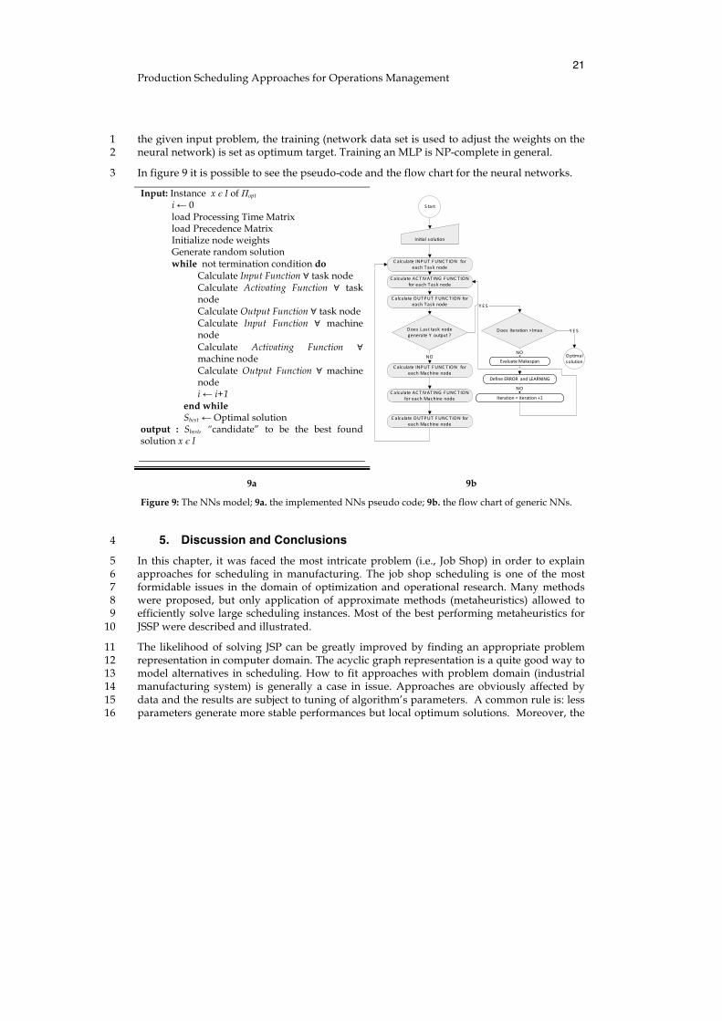
the given input problem, the training (network data set is used to adjust the weights on the 1 neural network) is set as optimum target. Training an MLP is NP-complete in general. 2

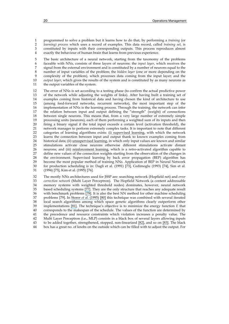
In figure 9 it is possible to see the pseudo-code and the flow chart for the neural networks. 3

Input: Instance x є I of Пopt i ← 0 load Processing Time Matrix load Precedence Matrix Initialize node weights Generate random solution while not termination condition do

Calculate Input Function ∀ task node Calculate Activating Function ∀ task node Calculate Output Function ∀ task node Calculate Input Function ∀ machine node Calculate Activating Function ∀ machine node Calculate Output Function ∀ machine node i ← i+1

end while Sbest ← Optimal solution

output : Sbest, “candidate” to be the best found solution x є I

S tart

C alculateINPUT FUNC T IONforeachTasknode

Initialsolution

Does L asttasknodegenerateY output?

Optimalsolution

C alculateAC T IVAT ING FUNC T IONforeachTasknode

C alculateOUTPUT FUNC T IONforeachTasknode

C alculateINPUT FUNC T IONforeachMachinenode

C alculateAC T IVAT ING FUNC T IONforeachMachinenode

C alculateOUTPUT FUNC T IONforeachMachinenode

Iteration=iteration+1

NOEvaluateMakespan

DefineERRORandLEARNING

Does Iteration>Imax

Y E S

Y E S

NO

NO

9a 9b

Figure 9: The NNs model; 9a. the implemented NNs pseudo code; 9b. the flow chart of generic NNs.

5. Discussion and Conclusions 4

In this chapter, it was faced the most intricate problem (i.e., Job Shop) in order to explain 5 approaches for scheduling in manufacturing. The job shop scheduling is one of the most 6 formidable issues in the domain of optimization and operational research. Many methods 7 were proposed, but only application of approximate methods (metaheuristics) allowed to 8 efficiently solve large scheduling instances. Most of the best performing metaheuristics for 9 JSSP were described and illustrated. 10

The likelihood of solving JSP can be greatly improved by finding an appropriate problem 11 representation in computer domain. The acyclic graph representation is a quite good way to 12 model alternatives in scheduling. How to fit approaches with problem domain (industrial 13 manufacturing system) is generally a case in issue. Approaches are obviously affected by 14 data and the results are subject to tuning of algorithm’s parameters. A common rule is: less 15 parameters generate more stable performances but local optimum solutions. Moreover, the 16

Operations Management

22

problem has to be concisely encoded such that the job sequence will respect zoning and 1 sequence constraints. All the proposed approaches use probabilistic transition rules and 2 fitness information function of payoff (i.e., the objective function). 3

ACO and BE manifest common performances in JSSP. They do not need a coding system. 4 This factor makes the approaches more reactive to the particular problem instance in issue. 5 Notwithstanding, too many parameters have to be controlled in order to assure 6 diversification of search. GAs surpasses their cousins in the request for robustness. The 7 matching between genotype and phenotype across the schemata must be investigated in 8 GAs in order to obtain promising results. The difficult of GA is to translate a correct 9 phenotype from a starting genotype. A right balancing between crossover and mutation 10 effect can control the performance of this algorithm. The EM approach is generally affected 11 by local stability that avoid global exploration and global performance. It is, moreover, 12 subject to infeasibility in solutions because of its way to approach at the problem. SA and 13 TS, as quite simpler approaches, dominate the panorama of metaheuristic proposal for JS 14 scheduling. They manifest simplicity in implementation and reduction in computation effort 15 but suffer in local optimum falls. These approaches are generally used to improve 16 performances of previous methodologies and they enhance their initial score. The influence 17 of initial solutions on the results, for overall approaches, is marked. Performances of NNs 18 are generally affected by the learning process, over fitting. Too much data slow down the 19 learning process without improving in optimal solution. Neural Network is, moreover, 20 affected by difficulties in including job constraints with network representation. The 21 activating signal needs to be subordinated to the constraints analysis. 22

Based on authors experience and reported paragraphs, it is difficult to definitively choose 23 any of those techniques as outstanding in comparison with the others. Measurement of 24 output and cost-justification (computational time and complexity) are vital to making good 25 decision about which approach has to be implemented. They are vital for a good scheduling 26 in operations management. In many cases there are not enough data to compare – 27 benchmark instances, as from literature for scheduling could be useful - those methods 28 thoroughly. In most cases it is evident that the efficiency of a given technique is problem 29 dependent. It is possible that the parameters may be set in such way that the results of the 30 algorithms are excellent for those benchmark problems but would be inferior for others. 31 Thus, comparison of methods creates many problems and usually leads to the conclusion 32 that there is no the only best technique. There is, however, a group of several methods that 33 dominates, both in terms of quality of solutions and computational time. But this definition 34 is case dependent. 35

What is important to notice here is: performance is usually not improved by algorithms for 36 scheduling; it is improved by supporting the human scheduler and creating a direct (visual) 37 link between scheduling actions and performances. It is reasonable to expect that humans 38 will intervene in any schedule. Humans are smarter and more adaptable than computers. 39 Even if users don’t intervene, other external changes will happen that impact the schedule. 40 Contingent maintenance plan and product quality may affect performance of scheduling. 41 An algorithmic approach could be obviously helpful but it has to be used as a computerised 42 support to the scheduling decision - evaluation of large amount of paths - where 43

Production Scheduling Approaches for Operations Management

23

computational tractability is high. So it makes sense to see what optimal configuration is 1 before committing to the final answer. 2

6. References 3

[1] Stǜtzle T. G. Local Search Algorithms for Combinatorial Problems – Analysis, Algorithms and New Applications; 1998.

[2] Reeves C.R. Heuristic search methods: A review. In D. Johnson and F.O’Brien Operational Research: Keynote Papers, pp. 122–149. Operational Research Society, Birmingham, UK,1996.

[3] Trelea, I.C.. The Particle Swarm Optimization Algorithm: convergence analysis and parameter selection. Information Processing Letters 2003; 85(6): 317–325;

[4] Garey M.R. and Johnson D.S., Computers and intractability: a guide to the theory of NP-completeness, Freeman, 1979.

[5] Wight Oliver W. Production Inventory Management in the computer Age. Boston, Van Nostrand Reinhold Company, Inc., New York, 1974.

[6] Baker K.R., Introduction to sequencing and scheduling, John Wiley, New York,1974. [7] Cox, James F., John H. Blackstone, Jr., Michael S. Spencer, editors, APICS Dictionary,

American Production &Inventory Control Society, Falls Church, Virginia, 1992. [8] Pinedo, Michael, Scheduling: Theory, Algorithms, and Systems, Prentice Hall,

Englewood Cliffs, New Jersey, 1995. [9] Hopp W., Spearman M.L. Factory Physics. Foundations of manufacturing

Management. Irwin/McGraw-Hill, Boston; 1996. [10] Muth J.F.,Thompson G.L. Industrial Scheduling. Prentice-Hall, Englewood Cliffs, N.J.,

1963. [11] Garey M. R., Johnson D. S. and Sethi R, The Complexity of Flow Shop and Job Shop

Scheduling. Math. of Operation Research, 1976; 2(2): 117-129. [12] Blazewicz J., Domschke W. and Pesch E., The job shop scheduling problem:

conventional and new solution techniques, EJOR, 1996; 93: 1-33. [13] Aarts E.H.L., Van Laarhoven P.J.M., Lenstra J.K., and Ulder N.L.J.. A computational

study of local search algorithms for job shop scheduling. ORSA Journal on Computing, 1994; 6 (2): 118–125.

[14] Brucker. P. Scheduling Algorithms. Springer-Verlag, Berlin, 1995. [15] Panwalkar S. S. and Iskander Wafix. A survey of scheduling rules. Operations

Research, 1977; 25 (1): 45–61. [16] Carlier J. and Pinson E. An algorithm for solving the job-shop problem. Management

Science, 1989; 35(2): 164–176.

Operations Management

24

[17] Bertrand, J.W.M, The use of workload information to control job lateness in controlled and uncontrolled release production systems, J. of Oper. Manag., 1983; 3(2):79 – 92.

[18] Gantt, Henry L. . Work, Wages, and Profits, second edition, Engineering Magazine Co., NewYork, 1916. Reprinted by Hive Publishing Company, Easton, Maryland, 1973.

[19] Cox, James F., John H. Blackstone, Jr., and Michael S. Spencer, edt., APICS Dictionary, American Production &Inventory Control Society, Falls Church, Virginia, 1992.

[20] Roy B., Sussman B. Les problèmes d’ordonnancement avec contraintes disjunctive, 1964.

[21] Fruggiero F., Lovaglio C., Miranda S. and Riemma S., From Ants Colony to Artificial Ants: A Nature Inspired Algorithm to Solve Job Shop Scheduling Problems. In Proc. ICRP-18; 2005

[22] Adams J., Balas E., and Zawack D.. The shifting bottleneck procedure for job shop scheduling. Management Science, 1988; Vol. 34(3): 391–401,

[23] Reeves, C.R. Modern Heuristic Techniques for Combinatorial Problems. John Wiley & Sons, Inc; 1993.

[24] Giffler B. and Thompson G.L.. Algorithms for solving production scheduling problems. Operations Research, , 1960;Vol. 8: 487–503

[25] Gere, W. S., Jr., Heuristics in Jobshop Scheduling, Manag. Science, 1966; 13(1): 167-175. [26] Rajendran, C. Holthaus, O. A comparative Study of Dispatching rules in dynamics

flowshops and job shops, European J. Of Operational Research. 1991; 116(1): 156-170. [27] Hertz A. and Widmer M., Guidelines for the use of meta-heuristics incombinatorial

optimization, European Journal of Operational Research, 2003; vol. 151: 247-252, [28] Zanakis H.S., Evans J.R. and Vazacopoulos A.A., Heuristic methods and applications: a

categorized survey, European Journal of Operational Research, 1989; vol. 43: -110. [29] Gondran M. and Minoux M., Graphes et algorithmes, Eyrolles Publishers, Paris, 1985. [30] Hubscher R. and Glover F., Applying tabu search with influential diversification to

multiprocessor scheduling, Computers Ops. Res. 1994; 21(8): 877-884, [31] Blum, C. and Roli, A., Metaheuristics in combinatorial optimization: Overview and

conceptual comparison, ACM Comput. Surv., 2003; 35: 268-308 [32] Glover F. and Kochenberger G. A., Handbook of Metaheuristics, Springer, 2003. [33] Kirkpatrick S, Gelatt C. D, Vecchi M. P. (1983) Optimization by Simulated Annealing.

Science 2000; 220(4598): 671-680. [34] Birbil S.I, Fang S An Electromagnetism-like Mechanism for Global Optimization.

Journal of Global Optimization. 2003; 25(3):263-282. [35] Mitchell M., An Introduction to Genetic Algorithms. MIT Press, 1999. [36] Glover, F. and Laguna, M. 1997. Tabu Search. Norwell, MA: Kluwer Academic Publ. . [37] Dorigo M. and G. Di Caro and L. M. Gambardella . Ant algorithm for discrete

optimization. Artificial Life, 1999; 5(2): 137-172,

Production Scheduling Approaches for Operations Management

25

[38] Pham DT, Ghanbarzadeh A, Koc E, Otri S, Rahim S and Zaidi M. The Bees Algorithm. Technical Note, Manufacturing Engineering Centre, CardiffUniversity, UK, 2005

[39] Zhou, D. N., Cherkassky, V., Baldwin, T. R., and Olson D. E., A neural network approach to job-shop scheduling. IEEE Trans. on Neural Network, 1991; 2(1), 175-179.

[40] Holland John H., Adaptation in Natural and Artificial Systems, University of Michigan,1975.

[41] Darwin Charles “Origin of the species”, 1859. [42] Beck, J.C., Prosser, P., & Selensky, E. Vehicle Routing and Job Shop Scheduling: What’s

the difference?, Proc. of 13th Int. Conf. on Autom. Plan. and Sched. (ICAPS03); 2003. [43] Bierwirth C., Mattfeld C., Kopfer H., On Permutation Representations for Scheduling

Problems PPSN, pp. 310-318; 1996. [44] Moon I., Lee J., Genetic Algorithm Application to the Job Shop Scheduling Problem

with alternative Routing, Industrial Engineering Pusan National Universit; 2000. [45] Goss S., S. Aron, J. L. Deneubourg, and J. M. Pasteels. Self-organized shortcuts in the

Argentine ant. Naturwissenschaften. 1989; 76: 579–581, [46] Van der Zwaan S. and C. Marques: Ant colony optimization for job shop scheduling. In

Proc. of the 3rd Workshop on genetic algorithms and Artificial Life (GAAL’99), 1999. [47] Dorigo M., Maniezzo V. and Colorni A. The Ant System: Optimization by a colony of

cooperating agents. IEEE Transactions on Systems, 1996; 26: 1-13. [48] Cornea D., M. Dorigo, and F. Glover, editors. New ideas in Optimization. McGraw-Hill

International, Published in 1999. [49] Colorni A., M. Dorigo, V. Maniezzo and M. Trubian. “Ant system for Job-shop

Scheduling”. JORBEL–Belgian Journal of Operations Research, Statistics and Computer Science, 1994, 34(1):39-53,

[50] Gould JL. Honey bee recruitment: the dance-language controversy. Science .1975; 189:685�693

[51] Grosan C.; Ajith A., Ramos V., Stigmergic Optimization: Inspiration, Technologies and Perspectives. Studies in Computational Intelligence.2006; Vol. 31: 1-24. Springer Berlin/Heidelberg.

[52] Camazine S, Deneubourg J, Franks NR, Sneyd J, Theraula G and Bonabeau E. Self-Organization in Biological Systems. Princeton: Princeton University Press, 2003.

[53] Von Frisch K. Bees: Their Vision, Chemical Senses and Language. (Revised edn) Cornell University Press, N.Y., Ithaca, 1976.

[54] Riley JR, Greggers U, Smith AD, Reynolds DR, Menzel R). "The flight paths of honeybees recruited by the waggle dance". Nature 2005; 435:205-207.

[55] Eberhart, R., Shi Y., and Kennedy J., Swarm Intelligence. Morgan Kaufmann, San Francisco, 2001.

Operations Management

26

[56] Seeley, T.D.. The wisdom of the Hive: The Socal Physiology of Honey Bee Colonies. Massachusetts: Harward University Press, Cambridge, 1996.

[57] Tuba, M., Artificial BeeColony(ABC) with crossover and mutation. Advances in computer Science, pp. 157-163, 2012

[58] Chong, CS Low, MYH Sivakumar AI, Gay KL. Using a Bee Colony Algorithm for Neighborhood Search in Job Shop Scheduling Problems, In 21st European Conference On Modelling and Simulation ECMS 2007

[59] Karaboga D. and B. Basturk. On The performance of Artificial Bee Colony (ABC) algorithm. Applied Soft Computing , 2008.; 8(1), : 687-697,

[60] Pham D.T., Ghanbarzadeh A., Koc E., Otri S., Rahim S., and M. Zaidi. The Bees Algorithm - A Novel Tool for Complex Optimisation Problems, Proceedings of IPROMS 2006 Conference, pp.454-461; 2006.

[61] Birbil S.I, Fang S An Electromagnetism-like Mechanism for Global Optimization. Journal of Global Optimization. 2003; 25(3): 263-282.

[62] Coulomb Premier mémoire sur l’électricité et le magnétisme, Histoire de l’Académie Royale des Sciences, pages 569-577; 1785 .

[63] Durney, Carl H. and Johnson, Curtis C. Introduction to modern electromagnetics. McGraw-Hill. 1969.

[64] Griffiths, David J. Introduction to Electrodynamics (3rd ed.). Prentice Hall; 1998. [65] Kirkpatrick, S.; Gelatt, C. D.; Vecchi, M. P.). Optimization by Simulated Annealing.

Science. 1983; 220(4598): 671–680. [66] �erný, V. Thermodynamical approach to the traveling salesman problem: An efficient

simulation algorithm. J. of Optimization Theory and Applications. 1985; 45: 41–51. [67] Metropolis, Nicholas; Rosenbluth, Arianna W.; Rosenbluth, Marshall N.; Teller,

Augusta H.; Teller, Edward. Equation of State Calculations by Fast Computing Machines. The Journal of Chemical Physics. 1953; 21(6): 1087.

[68] Van Laarhoven P.J.M., Aarts E.H.L., and J.K. Lenstra. Job shop scheduling by simulated annealing. Operations Research, Vol. 40, No. 1, pp. 113–125, 1992.

[69] Glover F. Future paths for Integer Programming and Links to Artificial Intelligence. Computers and Operations Research 1986; 5(5): 533-549.

[70] Dell’Amico M. and Trubian M. Applying tabu search to the job-shop scheduling problem. Annals of Operations Research, 1993; 41: 231–252.

[71] Taillard E.D.. Parallel taboo search techniques for the job-shop scheduling problem. ORSA Journal on Computing, 1994; 6(2): 108–117.

[72] Marquez, L., Hill, T., O’Connor, M., Remus, W., Neural network models for forecast a review. In: IEEE Proc of 25th Hawaii International Conference on System Sciences. 1992; 4: 494–498.

Production Scheduling Approaches for Operations Management

27

[73] Dagli C. H, Lammers S, Vellanki M. Intelligent scheduling in manufacturing using neural networks, Journal of Neural Network Computing Technology Design and Applications, 1991; 2(4): 4-10.

[74] Cedimoglu I. H. Neural networks in shop floor scheduling, Ph.D. Thesis, School of Industrial and Manufacturing Science, Cranfield University, UK. 1993.

[75] Sim S. K, Yeo K. T, Lee W. H. An expert neural network system for dynamic job-shop scheduling, International Journal of Production Research, 1994; 32(8): 1759 - 1773.

[76] Kim S. Y, Lee Y. H, Agnihotri D. A hybrid approach for sequencing jobs using heuristic rules and neural networks, Prod. Planning and Control, 1995; 6(5):445-454.

[77] Hopfield, J. J., and TANK, D. W., Neural computational of decisions in optimization problems. Biological Cybernetics, 1985; 52: 141-52.

[78] Foo S. Y, Takefuji Y. Stochastic neural networks for solving job-shop scheduling: Part 1. Problem representation, in: Kosko B, IEEE International Conference on Neural Networks, San Diego, CA, USA, 1988: 275 - 282.

[79] Haykin S Neural networks: a comprehensive foundation, 2nd edn. Prentice Hall, New Jersey; 2001.

[80] Storer R. H, Wu S. D, Vaccari R. Problem and heuristic space search strategies for job shop scheduling, ORSA Journal on Computing, 1995; 7(4): 453 – 467.

[81] Van Hulle M. M. A goal programming network for mixed integer linear programming: A case study for the jobshop scheduling problem, International Journal of Neural Systems, 1991, 2(3): 201 - 209.

[82] Leshno M, Lin VY, Pinkus A, Schocken S. Multilayer feedforward networks with a non-polynomial activation function can approximate any function. Neural Net. 1993; 6(6): 861–867

[83] Karlik B, Olgac AV. Performance analysis of various activation functions in generalized MLP architectures of neural networks. Int J. Artif. Int. Expert Syst. 2011; 1(4): 111–122.