Production Lot Sizing and Scheduling with Non-Triangular Sequence-Dependent Setup Times

Production Lot Sizing and Scheduling withNon-Triangular Sequence-Dependent Setup Times

Alistair R. [email protected]

Masoumeh [email protected]

Department of Engineering Design and MathematicsUniversity of the West of England, Bristol, BS16 1QY, Reino Unido.

Abstract

This paper considers a production lot sizing and scheduling problem with sequence-dependentsetup times that are not triangular. Consider, for example, a product p that contaminates someother product r unless either a decontamination occurs as part of a substantial setup time stpr orthere is a third product q that can absorb p’s contamination. When setup times are triangular thenstpr ≤ stpq + stqr and there is always an optimal lot sequence with at most one lot per productper period (AM1L). However, product q’s ability to absorb p’s contamination presents a shortcutopportunity and could result in shorter non-triangular setup times such that stpr > stpq + stqr .This implies that it can sometimes be optimal for a shortcut product such as q to be produced inmore than one lot within the same period, breaking the AM1L assumption in much research. Thispaper formulates and explains a new optimal model that not only permits multiple setups andlots per product in a period (ML), but also prohibits subtours using a polynomial number of con-straints rather than an exponential number. Computational tests demonstrate the effectivenessof the ML model, even in the presence of just one decontaminating shortcut product, and its fastspeed of solution compared to the equivalent AM1L model.

Key Words: Lot sizing and scheduling, Sequence-dependent setup times, Non-triangular setuptimes.

PRÉ-ANAIS XLIIISBPO

1 Introduction

Some manufacturing systems have to meet a regular but varying demand for products. Whenmanufacturing capacity is limited, such demand cannot be met instantaneously from production,but from inventory accumulated previously. Lot-sizing decisions then need to be made about howmuch of each product to produce in each demand period and how much inventory to accumulatein order to meet demand while keeping within production capacity.

If a setup cost or time is charged to change from one product to another, then a sequence orschedule of lots also needs to be decided. If such setups are sequence-dependent (i.e., the size of thesetup charge depends on the product processed immediately beforehand), as illustrated in Figure1, then the decisions become more complex.

Period t-1 Period t+1Period t

Lot ofProduct p

Setup State for p carries over from period t-1 to t

Setupp to q

Lot ofProduct q

Setupq to r

Lot ofProduct r

Start of period t

Setup State for r carries over from period t to t+1

Start of period t+1

p q r

Figure 1: Production and inventory to meet demand

Many manufacturers separate lot sizing decisions from lot sequencing in order to simplify thecomplexity of the decision-making. However, this can result in production being less effective andmore costly than it needs to be. To competitively satisfy the demand for products within availableproduction capacity, the lot sizing and sequencing decisions should be handled simultaneously.

2 Lot Sizing and Sequencing

Research into production lot sizing and scheduling has progressed substantially over the last decades,as shown in the reviews by Drexl and Kimms (1997) and Karimi et al. (2003), recent research (Kovacset al.; 2009), and a forthcoming special issue (Clark et al.; 2011). In July 2010 at the 24th EuropeanConference on Operational Research (EURO10) in Lisbon, a stream on lot sizing and scheduling wasorganized for the first time in the history of this conference, containing seven sessions with morethan 25 presentations.

In particular, much progress has been made in the area of lot sequencing when setup timesare sequence -dependent (Meyr; 2000; Clark and Clark; 2000; Araujo et al.; 2007). The General Lot-sizing and Scheduling Problem (GLSP), developed by Fleischmann and Meyr (1997), minimisesinventory and sequence-dependent setup costs on a single machine with finite capacity, allowingmultiple setups in each single ’large-bucket’ time period. The GLSP was extended by Meyr (2000) toconsider sequence-dependent setup times (GLSP-ST). Toso, Morabito & Clark (2007) reformulatedthe GLSP-ST model to permit backlogging and non-triangular setup times, but still assumed at mostone lot per product in each period.

Clark, Morabito & Toso (2006) pursued an alternative approach via the Asymmetric Travel-ling Salesman Problem (ATSP), which has been very extensively researched (Lawler et al 1985;Carpaneto et al 1995). The adaptation of the ATSP to modelling lot-sizing and scheduling withsequence-dependent setups is not direct, since the production system is often already setup for a


q

p r qp r

Figure 2: Triangular and Non-Triangular Setups

particular product (i.e. starting at a given city) and some products might not be produced in a givenperiod if the demand is sufficiently small or the capacity tight (Clark et al 2006).

Clark et al. (2010) extended a method that has been found to be successful in practice for op-timally solving the ATSP, namely, to quickly solve the corresponding Assignment Problem (AP)as a linear programme, identify the resulting subtours, and then resolve the AP, explicitly pro-hibiting these subtours using a potentially exponential number of Dantzig-Fulkerson-Johnson-typeconstraints adapted from Dantzig et al. (1954). The method carries on iteratively in this manner un-til no subtours result. It can be used heuristically (and its convergence rate sometimes accelerated)by patching the subtours into a single tour at each iteration (Karp 1979), thus providing a feasiblesolution (and an upper bound). Clark et al (2006) adapted the subtour elimination method to lot se-quencing over multiple periods with setup carryover between periods. An extension of the methodthen used the patching heuristic to accelerate the time to converge to a provably optimal solution.

3 Non-triangular setup times

In some industries, e.g., animal feed supplements, some products can contaminate other products,e.g., copper is essential for pigs but kills sheep even in tiny doses. Contamination is a particularconcern for the feed industry, although the problem is general and similar concerns also exist in adiverse range of other industries, such as food & beverages, and the oil industry. In the feed indus-try, blending equipment must be cleaned in order to avoid contamination, resulting in substantialsetups that consume scarce production time. Fortunately, the amount of cleaning can be minimisedby the effective sequencing of production lots.

Certain intermediate “cleansing” or shortcut products can cause non-triangular setup times.These products clean the machines whilst being processed (e.g., certain wheat mixtures) and hencereduce overall setup times. In other words, contamination cleaning can occur during value-addingproduction time as well as during non-productive setup time.

More precisely, “triangular” setup times occur when it is never worse to setup from productp to r directly than to setup via a third product q, so that triangular inequality s(p,r) ≤ s(p,q) +s(q,r) always holds (as shown on the left side of Figure 2). However, in the animal feed and otherindustries, the contamination of a product r by a previous product p just beforehand can be oftenavoided by producing enough of an intermediate product q so that it absorbs p’s contamination.For this to save time, the triangular inequality must not hold in this case, ie, the sum of the setuptimes s(p,q) from p and s(q,r) to r must be short enough so that s(p,q) + s(q,r) < s(p,r) (as shown onthe right side of Figure 2).

Existing mathematical models can be used when setup times are triangular, e.g., Meyr (2000)and Clark et al. (2010) where minimum lot-sizes are imposed to allow proper cleaning of p’s con-taminants, i.e., to avoid a setup from p to r via zero production of q rather than directly. However,the disobeying of the triangular inequality means that it could be optimal in certain circumstancesfor an intermediate shortcut product q to be produced in more than one lot within the same time-period, as shown in Figure 3. Thus the assumption of existing models (Meyr; 2000; Clark et al.;2010) of at most one lot per product per period would not hold in such a situation. The breaking ofthis assumption is the key feature of the model developed below in section 4.

The GLSP models of Fleischmann and Meyr (1997) and Meyr (2000) allow non-triangular se-tups, as in Toso et al. (2009), but the ATSP-based model of Clark et al. (2010) assumes one lot perproduct per periods and so cannot allow multiple lots of shortcut products per period, as requiredto take advantage of non-triangular setup times. A sequence with multiple lots per period for some


q q q

Figure 3: A Sequence of Non-Triangular Setups via a Shortcut Product q

CA

B C

D

D

S

Figure 4: A main sequence and different types of subtour

products could look like that illustrated in Figure 4. Subtours connected to the main sequence S byshortcut products are possible (e.g., subtours B and C in Fig. 4).

Thus an exact formulation must allow connected subtours but exclude disconnected subtours(e.g., subtours A and D in Fig. 4). Menezes et al. (2010) developed such a formulation using aniterative model and method based on a potentially exponential number of Miller-Tucker-Zemlinsubtour elimination constraints (Miller et al.; 1960).

This paper formulates and tests a new exact model for lot sizing and sequencing with non-triangular setups. The model is developed in section 4 using a polynomial number of multi-commodity-flow-type constraints adapted from Claus (1984), and then computationally tested insection 5. The model is generalised in section 6 to include period-overlapping setup operations andagain tested computationally. The paper concludes in section 7 with a discussion of the model’svalue and flags remaining challenges and opportunities for future research.

4 Modelling multiple lots per product per period

The following indices are used:

p, q, r Product families, from {1,...,P} where P = the number of families.

t Time period, from {1,...,T} where T = the number of periods (e.g., days or weeks) in thescheduling horizon.

The input data required by the model are:

Capt Available capacity time in each period t.

up Time needed to produce one batch of each product p.

mlp Minimum lot size of product p.

hp Inventory holding cost per period for product p.

gp Backlog cost per period for product p.

cot Unit cost of machine time in period t.


stpq Setup time needed to changeover from product p to product q.

dpt Forecast of demand for product p at the end of period t.

Ip0 Inventory of product p at the start of the scheduling horizon.

p* The product already setup when period 1 starts (the initial setup state).

The decisions output by the model are:

I+pt Inventory of product p at the end of period t, non-negative.

I−pt Backlogs of product p at the end of period t, non-negative.

xpt Total size of all lots of product product p in period t (an integer number of batches).

ypqt Number of times that production is to be changed over from product p to product q in periodt.

zpt Number of times that product p is in a setup state in period t.

αpt = 1 if p is the product already setup when period t starts (the setup state), = 0 otherwise.Thus the model allows the setup state at the start of a period to be carried over from theprevious period. Note that t ∈ {1, ..., T + 1} and that αp∗,1 = 1.

slackt Number of hours of slack capacity in period t.

The objective function (1) minimizes primarily backlogs via heavy penalties, then the costs of in-ventory, while maximizing slack capacity (if backlogs and inventory are readily zeroed by an excessof capacity):

Minimise∑p,t

(hp I+pt + gp I−pt

)−∑t

cot slackt + 0.01∑p,t

zpt (1)

Unnecessary capacity-eating setups are prevented by maximizing slack capacity in (1). The lastterm [0.01

∑p,t zpt] is simply a mathematical device to eliminate any excessive zero-time setups.

The value of the coefficient 0.01 may need adjusting depending on the values of the other terms in(1).

Constraints (2) balance inventory, backlogs, production and demand over consecutive weeks,as previously shown in Figure ??:

I+p,t−1 − I−p,t−1 + xpt − dpt = I+pt − I−pt ∀ p, t (2)

The capacity constraints (3) take into account setup and production times, and calculate any capac-ity slack:∑

p

up xpt +∑p,q

stpq ypqt + slackt = Capt ∀ t (3)

Constraints (4) ensure that a product can be produced in a period only if the machine is setup for itat some time in period t:

xpt ≤

(min

{Captup

,

T∑τ=1

dpτ − I+p0 + I−p0

})zpt ∀ p, t (4)

The coefficient of zpt in (4) is an upper bound on the value of xpt, calculated as the minimum of (a)the amount of product p that can be produced if period t were entirely dedicated to its production,and (b) the effective demand for product p over all periods t = 1, ..., T (given that backlogs ofdemand may have to be produced as well as current and future demand).

Note that constraint (4) is valid, but loose as zpt need only be 1, not ≥ 2. Constraint (19) willtighten and replace (4) when extra binary variables for subtour-elimination are introduced below.


p

Figure 5: Node flow modelled by constraints (8) and (9)

.... q rp ....

Figure 6: A path from carryover product p0t = p|(αpt = 1) to product r

Constraints (5) impose a minimum lot size of mlq on each of product q’s zqt lots in order toforce proper cleaning of a previous product p’s contaminants:

xqt ≥ mlqzqt ∀ t, q (5)

Without constraints (5), a model solution could incorrectly schedule a setup from p to a third prod-uct r via zero production of q rather than directly. Note that the total lot size xqt can be split intoseparate zqt lots, each of which is at least mlq units in size.

Constraints (6) prohibit setups between the same product:

yppt = 0 ∀ p, t (6)

Constraints (7) ensure that there is exactly one product in a setup state between each period:∑p

αpt = 1 for t = 2, ..., T + 1 (7)

We have left until last the consideration of the ATSP-related constraints for sequencing products.Constraints (8) and (9) relate the αpt and zpt setup state variables to the ypqt changeover variables,to and from a product respectively (Figure 5).

αpt +∑q

yqpt = zpt ∀ p, t (8)

∑q

ypqt + αp,t+1 = zpt ∀ p, t (9)

The initial optimal solution to the model specified by expressions (1) to (9) will consist of a singlesequence starting with product p|{αpt = 1} and ending with p|{αp,t+1 = 1} (possibly with embed-ded connected subtours), and maybe one or more disconnected subtours, as previously illustratedin Figure 4. Recall that subtours connected to the main sequence S are permitted (e.g., subtours Band C in Fig. 4), but disconnected subtours must be prohibited (e.g., subtours A and D in Fig. 4).

The paper by Oncan et al. (2009) reviews and analytically compares of many ATSP formu-lations, highlighting the tightness of the multi-commodity-flow (MCF) formulation by Claus (1984)which is the inspiration for the formulation that prohibits diconnnected subtours a priori.

First define additional binary decision variables arpqt as follows. Let arpqt = 1 if the arc p → q ison a path from carryover product p0t = p|(αpt = 1) to product r within period t’s sequence of lots,otherwise = 0, as shown in Figure 6.

The arc p → q must be part of a solution, so that value of arpqt is constrained as follows:

arpqt ≤ ypqt ∀ p, q, r, t (10)


p

Figure 7: The path from p0t to r traverses only those products p for which z01pt = 1

r

Figure 8: The path from p0t must reach product r

To use arpqt to prohibit subtours, a further binary decision variables z01pt are needed. Let z01pt =1 ifproduct p is ever in a setup state in period t, otherwise 0. Note that z01pt = 1 ⇔ zpt ≥ 1 and thatz01pt = 0 ⇔ zpt = 0. This is enforced by the following constraints:

zpt ≥ z01pt ∀ p, t (11)

zpt ≤ ZUBpz01pt ∀ p, t (12)

where ZUBp is a prespecified upper bound (UB) on the value of zpt, calculated in the computationaltests below as the size of the ordered set {(i, j)|stij ≥ stip + stpj}, which will often be 1 for knownnon-shortcut products.

The three sets of constraints (14, 16 and 18) below will then allow connected subtours, butprohibit disconnected ones a priori.

Constraint (13) requires that the period t path specified by the variables {arpqt | ∀ p, q} startsat carryover product p0t = p|(αpt = 1) and then traverses further products in the sequence, asillustrated in Figure 7.

αpt +∑q

arqpt =∑q

arpqt ∀ r, p = r, t (13)

However, constraint (13) should be enforced only when z01pt = z01rt = 1, but not when either is zero,i.e., only when the setup states for p and r both occur during period t. Thus constraint (14) replaces(13):

αpt +∑q

arqpt + 2− z01pt − z01rt ≥∑q

arpqt ∀ r, p = r, t (14)

Constraint (15) ensures that the period t path specified by the variables {arqrt | ∀ p, q} reachesproduct r (Figure 8):

αrt +∑q

arqrt = 1 ∀ r, t (15)

But constraint (15) should be imposed only when the setup state is configured for r at least onceduring period t (i.e., only when z01rt = 1), but not when the setup state is never configured for rduring period t, (i.e., when z01rt = 0). Thus constraint (16) replaces (15):

αrt +∑q

arqrt = z01rt ∀ r, t (16)


r

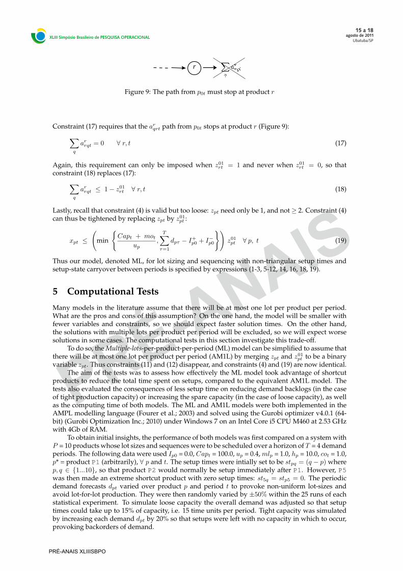
Figure 9: The path from p0t must stop at product r

Constraint (17) requires that the arqrt path from p0t stops at product r (Figure 9):∑q

arrqt = 0 ∀ r, t (17)

Again, this requirement can only be imposed when z01rt = 1 and never when z01rt = 0, so thatconstraint (18) replaces (17):∑

q

arrqt ≤ 1− z01rt ∀ r, t (18)

Lastly, recall that constraint (4) is valid but too loose: zpt need only be 1, and not ≥ 2. Constraint (4)can thus be tightened by replacing zpt by z01pt :

xpt ≤

(min

{Capt + mot

up,

T∑τ=1

dpτ − I+p0 + I−p0

})z01pt ∀ p, t (19)

Thus our model, denoted ML, for lot sizing and sequencing with non-triangular setup times andsetup-state carryover between periods is specified by expressions (1-3, 5-12, 14, 16, 18, 19).

5 Computational Tests

Many models in the literature assume that there will be at most one lot per product per period.What are the pros and cons of this assumption? On the one hand, the model will be smaller withfewer variables and constraints, so we should expect faster solution times. On the other hand,the solutions with multiple lots per product per period will be excluded, so we will expect worsesolutions in some cases. The computational tests in this section investigate this trade-off.

To do so, the Multiple-lots-per-product-per-period (ML) model can be simplified to assume thatthere will be at most one lot per product per period (AM1L) by merging zpt and z01pt to be a binaryvariable zpt. Thus constraints (11) and (12) disappear, and constraints (4) and (19) are now identical.

The aim of the tests was to assess how effectively the ML model took advantage of shortcutproducts to reduce the total time spent on setups, compared to the equivalent AM1L model. Thetests also evaluated the consequences of less setup time on reducing demand backlogs (in the caseof tight production capacity) or increasing the spare capacity (in the case of loose capacity), as wellas the computing time of both models. The ML and AM1L models were both implemented in theAMPL modelling language (Fourer et al.; 2003) and solved using the Gurobi optimizer v4.0.1 (64-bit) (Gurobi Optimization Inc.; 2010) under Windows 7 on an Intel Core i5 CPU M460 at 2.53 GHzwith 4Gb of RAM.

To obtain initial insights, the performance of both models was first compared on a system withP = 10 products whose lot sizes and sequences were to be scheduled over a horizon of T = 4 demandperiods. The following data were used Ip0 = 0.0, Capt = 100.0, up = 0.4, mlp = 1.0, hp = 10.0, cot = 1.0,p* = product P1 (arbitrarily), ∀ p and t. The setup times were intially set to be stpq = (q − p) wherep, q ∈ {1...10}, so that product P2 would normally be setup immediately after P1. However, P5was then made an extreme shortcut product with zero setup times: st5q = stp5 = 0. The periodicdemand forecasts dpt varied over product p and period t to provoke non-uniform lot-sizes andavoid lot-for-lot production. They were then randomly varied by ±50% within the 25 runs of eachstatistical experiment. To simulate loose capacity the overall demand was adjusted so that setuptimes could take up to 15% of capacity, i.e. 15 time units per period. Tight capacity was simulatedby increasing each demand dpt by 20% so that setups were left with no capacity in which to occur,provoking backorders of demand.


Mean MedianP Capacity Meas. of Perf. AM1L ML p AM1L ML p

10 Loose

No. of Setups 33.0 43.12 0.000 33.0 44.0 0.000Setup Time 22.4 11.7 0.000 23.0 12.0 0.000

Slack Capacity 49.2 60.0 0.000 49.8 60.8 0.000Inventory 131.1 118.1 0.000 121.5 109.0 0.000Backlogs 0.00 0.00 na 0.00 0.00 na

CPU time 5.96 4.34 0.201 5.50 3.50 0.028P Capacity Meas. of Perf. AM1L ML p AM1L ML p

10 Tight


Slack Capacity 2.94 7.96 0.000 0.00 2.80 0.002Inventory 268.5 302.3 0.001 264.2 307.2 0.162Backlogs 36.8 15.8 0.000 25.0 0.0 0.000

CPU time 6.72 8.06 0.551 7.0 5.0 0.317P Capacity Meas. of Perf. AM1L ML p AM1L ML p

20 Loose


Slack Capacity 123.0 139.0 0.000 121.9 137.9 0.000Inventory 240. 225.2 0.000 233.5 218.5 0.000Backlogs 0.00 0.00 na 0.00 0.00 na

CPU time 3,292 623 0.000 3,268 431 0.000P Capacity Meas. of Perf. AM1L ML p AM1L ML p

20 Tight

No. of Setups 51.5 64.9 0.000 50.5 64.5 0.000Setup Time 10.4 0 0.000 10.00 0 0.000

Slack Capacity 9.1 14.34 0.000 0 4.00 0.005Inventory 631.3 655.0 0.008 672.5 702.0 0.317Backlogs 33.7 20.6 0.000 15.0 0 0.000

CPU time 1.942 51 0.000 1,325 39 0.000

Table 1: Comparison of models AM1L and ML

Table 1 compares the performance of both models on 6 criteria, using a balanced analysis ofvariance test, and also the non-parametric Friedman test (Corder and Foreman; 2009) which is lesslikely to mistakenly indicate significance caused by outliers. Both tests used the data instance (i.e.the run) as a random blocking factor. Note the highly significant increase in numbers of setupsspare and capacity, and decrease in total setup time and backlogs in the ML results compared tothose for AM1L, particularly when capacity is tight.

For P = 10 products, model ML uses the shortcut product P5 to economise on setups times,albeit with a larger number of actual setups, most or all of which take zero time making gooduse of P5. Table 1 shows that this is particulary pronounced under tight capacity where modelML reduces the total setup time by 85%, thus keeping backlogs to a minimum. This reduction inbacklogs illustrates well the economic added value of mode ML over model AM1L. Note the fastsolution times for P = 10 products using the default settings of the Gurobi 4.0.1 solver.

Table 1 also shows the results with twice as many products (P = 20), two extreme shortcutproducts (P5 and P15), double the capacity per period, but T=4 still. The demand and setup timesfor products P11 to P20 simply replicate those for P1 to P10. The models were allowed to run fora maximum of one hour. Note the predictably longer solution times and that under tight capacitymodel M1 solves much faster than AM1L. This is an counter-intuitive result given that model M1has more binary and integer variables than AM1L and so might be assumed to be more combinato-rial complex.


6 Modelling period-overlapping setup operations

The model can be generalized to allow setup operations to overlap periods, i.e., to permit a setupto begin in a period and end in the next period. Intuition suggests a priori that it is unlikely to alterlot sequences, but may be advantageous when capacity is tight and lot sizing decisions need moreflexibility to reduce backlogs.

Consider the following additional decision variables:

OLSpqt = 1 if an overlapping last setup at the end of period t is from product p to product q, but= 0 otherwise.

St is the amount of setup time that overlaps into period t + 1, having begun at the end ofperiod t. S0 is known and fixed, being the amount of setup time still required in period1 of any setup operation that started at the end of the previous period 0 but has not yetfinished.

The value of St must be zero if there is no overlapping last setup at the end of period t:

St ≤∑pq

stpq OLSpqt ∀ t (20)

At most one setup p → q can overlap from period t to t+ 1:∑pq

OLSpqt ≤ 1 ∀ t (21)

The value of OLSpqt must be zero if p → q is not a setup initiated in period t:

OLSpqt ≤ ypqt ∀ p, q, t (22)

The capacity constraints (3) now become:

∑p

up xpt +∑p,q

stpq ypqt + St−1 − St + slackt = Capt ∀ t (23)

If OLSqpt = 1, then product p cannot be produced as the last lot in period t and the value of zpt mustbe reduced by 1 to reflect this. Thus constraints (9) now become:∑

q

ypqt + αp,t+1 = zpt +∑q

OLSqpt ∀ p, t (24)

Thus the model for lot sizing and sequencing with non-triangular setup times, setup-state carryoverbetween periods, and period-overlapping setup operations, is specified by expressions (1-2, 5-12,14, 16, 18-24).

The model was applied to the 25 instances of data set with 10 products and tight capacity. Theresults did not show any significant benefit. The 25 AM1L solutions did not change at all and thesupposedly longer solution time is due to sampling variability (p-value = 0.90). Only 2 of the 25 MLsolution instances decreased the number of setups (by about 5%), but the solutions did not changeat all on the other 5 criteria and the seemingly10% faster solution time can be ascribed to samplingvariability (p-value = 0.26).

7 Conclusions and Future Research

This paper has developed a new model for lot sizing and sequencing with a polynomial numberof constraints that can handle the multiple lot per product per period that arise in the presence ofnon-triangular sequence-dependent setup times. The computational tests validated and confirmedthat the multiple-lots feature of the model enables more efficient production than when the formu-lation is restricted to single lots per product per period. The model can also be faster to solve thanin the latter case, despite being more complex computationally, maybe because for some problem


instances (such as our tests above) there is an outstanding optimal ML solution that is quickly iden-tified whereas an optimal AM1L solution may not be so clearly superior and hence more difficultto find.

The computational tests also show that future research must also include the developmentof faster solution methods for large instances, possibly via exact methods such as (1) LagrangianRelaxation coupled with decomposition into single periods where the submodels can be solvedvery rapidly, or via heuristic methods such as (2) Relax-&-Fix methods of various types (Ferreiraet al.; 2009), (3) depth-first heuristics (Zhang; 2000), or (4) local branching (Fischetti and Lodi; 2003).Future work will also computationally compare the model against a functionally-equivalent GLSPmodel and Menezes et al. (2010)’s iterative method with Miller-Tucker-Zemlin subtour eliminationconstraints.

Given that the demand forecasts usually change as time advances from one period to the next,the question arises as to whether it is worthwhile to schedule over even a medium term horizon, letalone a long-term one. Frequent rescheduling (Haase and Kimms; 1999) implies that firm schedulesshould really only be specified for the immediate to short term over which demand forecasts willnot change (much), while approximate or aggregate planning (rather than scheduling should becarried out for medium to long term. This poses interesting (and not trivial) research challengesabout how to perform planning that result in effective and efficient short term schedules (Clark;2003).

Acknowledgements: Our thanks go to Socorro Rangel of UNESP for a critical reading of an earlierversion of this paper, and to the anonymous referees who also made valuable suggestions for im-proving it. This research was partly supported by a Global Research Award from the Royal Academyof Engineering, London, and an FP7 Marie Curie International Research Staff Exchange Scheme (IRSES)grant from the European Commission.

References

Araujo, S. A., Arenales, M. N. and Clark, A. R. (2007). Joint rolling-horizon scheduling of materialsprocessing and lot-sizing with sequence-dependent setups, Journal of Heuristics 13(4): 337–358.

Clark, A. R. (2003). Optimization approximations for capacity constrained material requirementsplanning, International Journal of Production Economics 84(2): 115–131.

Clark, A. R., Almada-Lobo, B. and Almeder, C. (2011). Editorial: Lot sizing and scheduling - in-dustrial extensions and research opportunities, special issue on lot sizing and scheduling, Inter-national Journal of Production Research 49(9): 2457–2461.

Clark, A. R. and Clark, S. J. (2000). Rolling-horizon lot-sizing when setup times are sequence-dependent, International Journal of Production Research 38(10): 2287–2308.

Clark, A. R., Morabito, R. and Toso, E. A. V. (2010). Production setup-sequencing and lot-sizing atan animal nutrition plant through ATSP subtour elimination and patching, Journal of Scheduling13(2): 111–121.

Claus, A. (1984). A new formulation for the travelling salesman problem, SIAM Journal on Algebraicand Discrete Methods 5: 21–5.

Corder, G. W. and Foreman, D. I. (2009). Nonparametric Statistics for Non-Statisticians: A Step-by-StepApproach, Wiley-Blackwell.

Dantzig, G., Fulkerson, R. and Johnson, S. (1954). Solution of a large-scale traveling-salesman prob-lem, Operations Research 2: 393–410.

Drexl, A. and Kimms, A. (1997). Lot sizing and scheduling - survey and extensions, European Journalof Operational Research 99: 221–235.

Ferreira, D., Morabito, R. and Rangel, S. (2009). Solution approaches for the soft drink integratedproduction lot sizing and scheduling problem, European Journal of Operational Research 196: 697–706.


Fischetti, M. and Lodi, A. (2003). Local branching, Mathematical Programming, Series B 98: 23–47.

Fleischmann, B. and Meyr, H. (1997). The general lotsizing and scheduling problem, OR Spektrum19(1): 11–21.

Fourer, R., Gay, D. M. and Kernighan, B. W. (2003). AMPL - A Modeling Language for Math-ematical Programming, second edn, Duxbury Press / Brooks-Cole Publishing Company, USA.http://www.ampl.com/.

Gurobi Optimization Inc. (2010). Gurobi optimizer version 3.0.0. http://www.gurobi.com.

Haase, K. and Kimms, A. (1999). Lot sizing and scheduling with sequence dependent setup costsand times and efficient rescheduling opportunities, International Journal of Production Economics66: 159–169.

Karimi, B., Fatemi Ghomia, S. M. T. and Wilson, J. M. (2003). The capacitated lot sizing problem: areview of models and algorithms, Omega 31: 365–378.

Kovacs, A., Brown, K. N. and Tarim, S. A. (2009). An efficient MIP model for the capacitatedlot-sizing and scheduling problem with sequence-dependent setups, International Journal ofProduction Economics 118(1): 282 – 291.URL: http://www.sciencedirect.com/science/article/B6VF8-4T9CCSG-3/2/8ec751c0f847ed8624677b88cf991987

Menezes, A., Clark, A. and Almada-Lobo, B. (2010). Capacitated lot-sizing and scheduling withsequence-dependent, period-overlapping and non-triangular setups, Journal of Scheduling . inpress.

Meyr, H. (2000). Simultaneous lot-sizing and scheduling by combining local search with dual opti-mization, European Journal of Operational Research 120: 311–326.

Miller, C. E., Tucker, A. W. and Zemlin, R. A. (1960). Integer programming formulations and trav-eling salesman problems, Journal of ACM 7: 326–329.

Oncan, T., Altinel, K. and Laporte, G. (2009). A comparative analysis of several asymmetric travel-ing salesman problem formulations, Computers and Operations Research 36(3): 637–654.

Toso, E. A. V., Morabito, R. and Clark, A. R. (2009). Lot-sizing and sequencing optimisation at ananimal-feed plant, Computers and Industrial Engineering 57: 813–821.

Zhang, W. (2000). Depth-first branch-and-bound versus local search: A case study, AAAI/IAAI Proc.17th National Conf. on Artificial Intelligence (AAAI-2000), Austin, Texas, pp. 930–935. Webpage:citeseer.ist.psu.edu/470650.html.


Production Lot Sizing and Scheduling with Non-Triangular Sequence-Dependent Setup Times

Documents