UNIVERSITY OF CALIFORNIA DIVISION OF AGRICULTURAL SCIENCES GIANNINI FOUNDATION OF AGRICULTURAL ECONOMICS Production Functions and Supply Applications for California Dairy Farms Irving Hoch Giannini Foundation Monograph Number 36 • July, 1976 CALIFORNIA AGRICULTURAL EXPERIMENT STATION

Welcome message from author
This document is posted to help you gain knowledge. Please leave a comment to let me know what you think about it! Share it to your friends and learn new things together.
Transcript
UNIVERSITY OF CALIFORNIA DIVISION OF AGRICULTURAL SCIENCES GIANNINI FOUNDATION OF AGRICULTURAL ECONOMICS
Production Functions and Supply Applications for California Dairy Farms
Irving Hoch
Giannini Foundation Monograph Number 36 • July, 1976
CALIFORNIA AGRICULTURAL EXPERIMENT STATION
Combined time series and cross-section data are employed in estimating production functions for California dairy farms, with application of results to analysis of supply.
The availability of approximately I0,000 observations permits a number of investigations, including development of estimates for l 2 basic samples of farms classified by region and production type, covering all state milk production. The Cobb-Douglas function is employed in most of the investigations, with maximum number of variables approaching 100, although most are dummy variables accounting for firm, year, month, cow breed, and DHIA membership. In the primary investigation, the introduction of firm effects causes estimated returns to scale to diverge from constant returns, with decreasing returns for market milk and increasing returns for manufacturing milk production. There is evidence that the firm effects are normally distributed, positively related to output, and well correlated with independent measures of farmer efficiency. Returns to scale and associated firm effects have important implications for the distribution of farm size, competitive industry structure, and supply elasticity. The year effects show upward movement over time, probably indicative of increasing productivity.
During the period covered, considerable variation in technical efficiency occurs between regions, with a 40 percent difference in productivity between most and least efficient region. Technical efficiency tends to increase in a southward direction, perhaps reflecting both size of firm and market. Allocation for feed is usually close to optimal, while levels of nonfeed input appear somewhat above optimal levels. Supply elasticities differ between major producing regions, implying that a movement toward price equalization would yield the same quantity of milk at lower prices.
Experimentation with alternative equation forms, including a quadratic function and a variable elasticity function, yields results paralleling those obtained in the primary investigation.
' THE AUTHOR:
Irving Hoch is a Fellow on the staff of Resources for the Future, Washington, D. C. This study was carried out while he was an Associate Professor of Agricultural Economics and Associate Agricultural Economist in the Experiment Station and on the Giannini Foundation, University of California, Berkeley.
Giannini Foundation Monograph • Number 36 • July, 1976
CONTENTS
INTRODUCTION
Study Overview · • • • · • The Setting and the Samples
2. VARIABLES AND ALTERNATIVE EQUATIONS
Listing of Variables and Description of Equations
Definition of Variables • • • • • · · • • ·" •
3. STATISTICAL PROCEDURE: THEORETICAL UNDERPINNING
AND REVIEW OF THE LITERATURE • · • • • • • • • • •
4. EQUATION 1 RESULTS ••••
Elasticity Estimates and Inferences
on Returns to Scale Year Effects • • • • • • • . • Month Effects . • • • • • • •
Membership in Dairy Herd Improvement
Association (DHIA) Breed Effects • • . • • • . •
Firm Effects Testing Statistical Significance of
Sets of Dummy Variables
5. EQUATION 2 RESULTS •
6. TECHNICAL EFFICIENCY, BY REGION
7. PROFITS AND ALLOCATIVE EFFICIENCY
Profits, Factor Shares, and Marginal Returns Equation 3 Results • • • • • • •
8. SOME SIDE INVESTIGATIONS Equation 4 Results • '. Equation 5 Results •
Equation 6 Results Equation 7 Results • ."
3
7 7
11
. . . ,,, 15
26
26 31
36
38
42 42
46
49
55
67
69 73
75 75 77 82 87

Hoch: California Dairy Farms
9. SUPPLY RELATIONSHIPS
Cost Functions and Supply Functions
Supply Elasticities • • . . . . . .
Some Implications on Price Equalization
Between Regions . . • . . • . •
An Evaluation of Supply Function Estimation
10. SUMMARY OF RESULTS . . . . . . . . . . .
APPENDIX A .....•......
Detail on the Definition and Measurement of Variables
Capital
Cow Service Flow
Labor
Operating Costs
Feed ..
Dummy Variable for Dairy Herd Improvement
Association (DHIA) Status
Breed Dummy Variables
Transformation of Dummy Variable Results
Tests of Significance of Sets of Dummy Variables J
APPENDIX B
Equation 5
Equation 6
Equation 7
96
96
98
98
101
• . . . . • . . 104
112
112
112
116
119
119
121
130
130
134
135
138
138
144
144
ACKNOWLEDGMENTS . . . . . . . . . . . . • · · · · · • . · . . 149
LITERATURE CITED . . . . . . . . • . . . . . . • • . . . . . . 150

Irving Hoch
PRODUCTION FUNCTIONS AND SUPPLY APPLICATIONS
FOR CALIFORNIA DAIRY FARMS
1. INTRODUCTION
Study Overview
The work of this study can be viewed both in terms of method and of con tent. In terms of method, it involves applying regression analyses using dummy variables, primarily for the Cobb-Douglas production function, with some experimental extension of the technique including slope shifters as well as intercept shifters. In terms of content, the work consists of a case study of California dairy production over a considerable time span.
In the regression analyses, combined time series and cross-section data were employed, observations having been secured on a set of firms over a period of years; thus, there was further application of an approach that has been developed over the last two decades. This use of dummy variables in regression analysis is formally equivalent to the analysis of covariance but is more flexible since each firm need not appear in every time period. Though specific to time and place, many of the case· study results should have more general applicability. Technical relationships and estimates could be useful in farm management and in marketing; estimated firm distributions and changes over time may provide clues to such basic problems as the distribution of entrepreneurial capacity and the rate of technological advance. Further, because dairy production was subject to institutional constraints in the form of specific regulation during the period under study, some hypotheses were developed relating results obtained to the regulations in effect, primarily in terms of the impact of milk price determination. A major area of application was the use of production function estimates in supply analysis, with some focus on alternative pricing policies for San Joaquin Valley and Southern California producers who accounted for three-fourths of state milk production.
The availability of a great deal of data (close to 10,000 observations) permitted relatively broad-gauge investigations, with 12 basic samples for groups of producers classified by region and milk type--which covered all state production--and a number of special-purpose samples developed for specific questions. Seven equation forms were employed (though most involved variations on the Cobb-Douglas theme), and the maximum number of variables per equation approached I00 (though most of these were dummy variables).
One of the reasons for presenting the results for all seven equation forms, though several were in effect preliminary investigations with disappointing or suspect results, is that in the age of the computer there is bound to be concern about results that were not presented. The reader wonders (more and more) about the selectivity imposed by the writer on the array of his results. To avoid that, unhappy as well as pleasant experiences in inference are presented here. Aside from documenting the interpretations on their usability, there are other reasons for presentation of primarily negative results: (I) Some positive information can often be extracted with judicious interpretation; (2) there is some educational value in seeing where and why things appear to go wrong, The final pattern of results that emerged here, given the learning process involved, seems reasonable, consistent, and useful.

2 Hoch. California Dairy Farms
Some of the major results can be sketched out as a prologue to their full statement in the body of the report. There was evidence of "excessive" expansion by farms producing for the fluid milk market in terms of production beyond then-current optimal levels, while producers of milk for manufacturing purposes tended to have inputs below optimal levels by virtue of operation in a region of increasing returns to scale. Both forms of malallocation could be explained as effects of regulation. The contrasting results for the two types of producers fit within a more general pattern conforming to the classical S-shaped production function, with returns to scale exhibiting a general tendency to decline with increasing average size of firm. This pattern was maniffst after introduction of dummy variables to account for firm effects, which caused substantial changes in returns to scale, as estimated by the sum of production elasticities, relative to the elasticity sum obtained without the firm effects. In the 10 samples of fluid milk producers, the elasticity sum fell; but in the two cases of small-scale, manufacturing milk producers, an increase occurred. This seems a significant finding for, in previous studies employing firm effects, returns to scale always fell with the introduction of those effects, leading to some speculation that a downward bias was involved. A lower value for the elasticity sum generally increases the plausibility of a supply function derived from the production function. (An elasticity sum of one corresponds to an infinitely elastic supply.) In the present study, supply estimates based on production elasticities were used to construct a scenario estimating the consequences of a policy equalizing prices between the then higher priced Southern California and the lower priced San Joaquin Valley milk supply. It was estimated that in the long run, assuming total production constant, the weighted average price for the two regions would drop by about 6 percent, with a shift of about IO percent of state production from Southern California to the San Joaquin Valley. The former region's share of state production would fall from an initial 43 percent to an ultimate 32 percent, while the latter region's share would rise from 35 to 46 percent.
The remainder of this introductory section presents some background material describing the milk production setting and the samples employed. Section 2 defines variables in brief fashion and lists the equations employed. Section 3 develops the rationale for the single-;equation regression procedure employed to estimate the parameters of those equations and briefly reviews the literature on some previous empirical studies using combined time series and cross-section data in production function estimation. Section 4 presents the main body of results obtained from the estimation procedure, relying on an equation of primary interest to yield measures of firm, year, month, and Dairy Herd Improvement Association (DHIA) effects. Sections 5, 6, and 7 primarily focus on efficiency questions. Section 5 discusses one of the preliminary equation forms used and exhibits correlations of firm effects with measures of scale and efficiency. Section 6 develops interregional comparisons of technical efficiency (essentially, measures of the level i:Jf the constant term, or scaling factor, in the production function). Section 7 considers profits and allocative efficiency for the average farm in terms of how close value of marginal product is to input price. Section 8 describes some side investigations covering preliminary, experimental, or special situations and includes the results found to be suspect or disappointing as well as cases which appear to be useful vehicles for future investigations. Section 9 involves the major application of the work in terms of the use of production function estimates for supply analysis. Finally, Section 10 reviews the major results obtained, followed by two appendices: Appendix A, giving a detailed description of the definition and measurement of variables, augmenting Section 2; and Appendix B, listing additional detail on the side investigations of Section 8.1
---··~---
1in addition, a Statistical Supplement to this report is available to interested readers on request to the Giannini Foundation of Agricultural Economics, University of California, Berkeley. For economy of presentation, the report presents only limited information on standard errors and t ratios for estimated parameters. The Supplement presents those statistics as well as information on sample size and number of independent variables appearing in each equation. Finally, the Supplement presents more detail on several sels of coefficient estimates.

3 Giannini Foundation Monograph • Number 36 • July, 1976
The Setting and the Samples
On the basis of classifications defined by California milk legislation, California dairy farms are classified as market milk or manufacturing milk producers. Market milk may be sold as fluid milk, while manufacturing milk may be used only for evaporated milk, butter, cheese, and milk powder.
Six dairy regions have been defined for the state and are exhibited in Figure I, which also shows the distribution of milk production by region as of 1960, a useful benchmark date for the period covered in the present study which spans the years 1955 through 1965. The 1960 distribution of milk production by region, as a fraction of total state production, is shown in Table 1. It can be seen that Southern California and the San Joaquin Valley produced roughly 75 percent of the total. Almost all of the Southern California production was market milk, while 30 percent of the San Joaquin Valley production was used for manufacturing milk.
There were marked price differences between market and manufacturing milk. In the period 1962-1964 (a basic period for the present study), the average statewide price for milk with 3.8 percent butterfat content was $3.30 per hundredweight for manufacturing milk and $4.86 for market milk. The average price received by individual market milk producers could differ s11bstantially from the state average; the market milk producer was paid a "blend price," obtained because the milk purchaser in effect treated part of the producer's milk as fluid milk and part as manufacturing milk. The more favorable the contractual arrangement in terms of mix between fluid and manufacturing uses, the higher the price. The average mix varied between regions of the state so that, for 1962-1964, the Southern California average price was around $5.50 per hundredweight, while the San Joaquin Valley average price was around $4.20.
Some observers saw this as posing problems in terms of both equity and efficiency; it was suggested that equal prices between the two major areas would lead to major expansion in San Joaquin Valley production. 1
The California Bureau of Milk Stabilization (BMS), as part of its regulatory function, collects data on individual dairy farm input and output, with each farm visited every other month. Records from this survey were obtained for each of the six dairy regions of the state.
For four of the regions, more than 1 sample was defined so that a total of 12 samples were obtained. More than one sample was obtained when subregions were defined or when market milk and manufacturing group producers were grouped into separate categories, or when a special group of producers was identified. The latter case occurred for the Sacramento Valley in the formation of a sample consisting of producers who had left the survey at the time of the study, often because they had sold their dairy farm or left the dairy business.
Table 2 shows the names applied to the samples and the number of producers in each, with a breakdown of the latter into market milk and manufacttlring milk producers. Table 2 also lists the counties included in each sample so that regional coverage is made explicit.
1For example. see L. B. Fletcher and C. 0. McCorkle, Jr., Growth and Adjustment of the Los Angeles Milkshed, California Agricultural Experiment Station Bulletin 787 (Davis, 1962); especially pp. 68, 69, 79, and 80 for summary evaluatfons.

Hoch: California Dairy Farms
,
production in California's
six dairy regions for 1960
Million pounds of milk fat in market milk ~ Million pounds of milk fat in. manufactured milk ~
FIGURE 1. California Dairy Regions and Milk Production, 1960
Source: Arthur Shultis, Olan D. Forker, and Robert 6. Appleman, California Dairy Farm Managemenl, California Agricultural Experiment Station Circular 417 (rev.; Berkeley, 1963), p. 7. '

5 Giannini Foundation Monograph • Number 36 • July, 19'76
TABLE 1
Distribution of California Milk Production by Region, 1960
R~_iona
Fraction of state _p_roduction Market Manufactur
milk i~ milk Total
Sacramento Valley .031 .034 .065
Northern and bSierra Mountains • 009 .003 .012
San Joaquin Valley .281 .121 .402
North Coast .010 .020 .030
Bay Areac .125 .021 .146
Southern California . 340 .005 .345
Total as fraction of state production • 796 .204 1.000
i
aFor geographic coverage, see Table 2, infra, p. 6.
bSame as Mountain Region (Figure 1), supra, p. 4.
cSame as Central Coast (Figure 1), supra, p. 4.
Source: Based on data in Arthur Shultis, Olan D. Forker, and Robert D. Appleman, California Dairy Farm Management, California Agricultural Experiment Station Circular 417 (rev.; Berkeley, 1963), p. 8.
In some applications the samples are classified into market milk or manufacturing milk groupings; the market milk group includes several samples containing a preponderance of market milk producers--Sacramento Valley (Left survey), North Coast, ·and Bay Area samples--rather than market milk producers, exclusively.
There were a total of 8,045 dairy farms in California in 1960, 1 so the sample total of 474 amounts to about 6 percent of all dairy farms in the state.
Observations available per farm varied considerably, ranging from a low of 3 to a high of 4 7, but with the bulk of the cases on the order of 20 observations per farm. With a total of 9,599 observations, the average per farm was approximately 21. There
!Arthur Shultis, Olan D. Forker, and Robert D. Appleman, California Dairy Farm Management, California Agricultural Experiment" Station Circular 417 (rev.; Berkeley, 1963), p. 8.

6 Hoch: California Dairy Farms
TABLE 2
Number of Producers by Region. Sample, and Type of Milk
Producers Market Manufactur- Total
Regiona and samp_le milk in_&. milk ...E_roducers
Sacramento Valley
Market 64 0 64 Manufacturing 0 20 20 Left survey 17 4 21
Northern and Sierra Mountains 29 0 29
San Joaquin Valley
Northern Market 46 0 46 Southern Market 51 0 51 Manufacturing 0 20 20
North Coast 23 6 29
Bay Area
Northern 57 10 67 Southern 37 4 41
Southern California ' Central 63 0 63 Peripheral 23 0 23
Total 410 64 474
aCounties covered by specific samples were:
Sacramento Valley: Market, Manufacturing, and Left survey--Butte, Coj lusa, Glenn, Placer, Sacramento, Shasta, Solano, Sutter. Tehama, Yolo,
and Yuba.
Northern and Sierra Mountains: Lassen, Nevada, Plumas. and Siskiyou.
San Joaquin Valley: Northern Market--Madera, Merced, San Joaquin. and Stanislaus. Southern Market--Fresno, Kern, Kings, and Tulare. Manufacturing--entire region.
North Coast: Del Norte, Humboldt, and Mendocino.
Bay Area: Northern--Marin, Napa, and Sonoma. Southern--Alameda, Contra Costa, Monterey, Santa Clara, and Santa Cruz.
Southern California: Central--Los Angeles, Orange, Riverside, San Bernardino, and San Diego. Peripheral--Imperial, San Luis Obispo, Santa Barbara, and Ventura.
7 Giannini Foundation Monograph • Number 36 • July, 1976
were 5 farms with fewer than 5 observations; 107 farms with 5 to 14 observations; 308 farms with 15 to 29 observations; and 54 farms with 30 or more observation.s.
Table 3 exhibits the number of observations by year and sample. Most of the observations fell in the period 1960-1964, though there were relatively small numbers of observations for earlier years and for 1965. In the statistical analysis, early years with only a few observations W\'!re generally combined into a single "initial period."
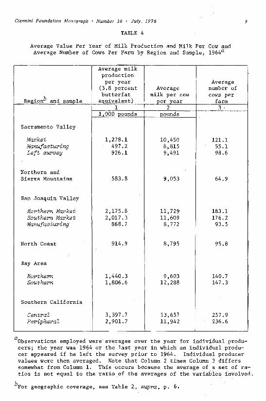
Some descriptive statistics, which give some notion of the production characteristics of the average farm by sample, appear in Table 4. The table contains data on milk production per year in terms of 3.8 percent butterfat equivalent, average milk per cow, and number of cows for the average farm. The observations employed were those for 1964 or for the last year in which an individual producer appeared if he left the survey prior to 1964. (Restricting the observations to 1964 values only does not appreciably affect results.)
There are pronounced differences in average scale of production between regions, with Southern California output about 50 percent above that of the San Joaquin Valley and Bay Area (Southern) market milk samples; twice the Bay Area (Northern); and three to six times the levels of the remaining samples.
There are marked differences as well in average milk per cow; values here tend to be correlated with level of output.
2. VARIABLES AND ALTERNATIVE EQUATIONS
The analysis portion of ari empirical study can be viewed as the tip of an iceberg, with the underwater--and much larger--portion corresponding to the operations that precede and lie behind the analysis: the organization of the data, its coding and keypunching, the organization and application of computer programs, and the checks and double checks necessary at every stage of the process. To illustrate, a 70-page manual was developed to organize and code the data for the present study. Upon completion of the preliminary operations, a number of variables were defined and a number of equation variants were investigated, _using single-equation regression analysis. The rationale for the single-equation approach is developed in Section 3.
Listing of Variables and Description of Equations
The most satisfactory equation form consisted of a Cobb-Douglas function in which milk was regressed on two factors of production and several sets of dummy variables. The factors of production were (1) feed and (2) the aggregate of all other costs. The sets of dummy variables included years, months, breeds, membership status in DHIA, and firms. In some investigations, region was also included as a dummy variable.
In formal terms, the Cobb-Douglas function can be written:
qy K TI Z. (2.1) i 1

TABLE 3
Number of Observations by Region and Sample, 1955-1965a
R~ionb and sample 1955 1956 1957 1958 1959 1960 1961 number of observations
1962 1963 1964 1965 Total
Sacramento Valley
Ma:roketc Manuf ac tu:1' i')ff
c
Le ft suroey
lJ 2 5
9 J 9
6 6
13
11 9
23
10 4
40
16 7
48
242 69 68
278 69 74
322 103
38
350 108
0
73 24
0
1,330 404 318
Northern and Sierra Mountainsc
8 8 5 16 21 11 76 99 140 112 33 529
San Joaquin Valley
Northern Markete Southern Marketf l.fcmufac turingf
0 0 0
0 0 0
0 11
3
18 45 10
140 57 23
206 55 39
265 280 94
272 259 102
274 275 112
271 250 113
0 0 0
1,446 1,232
49'6
North Coast 0 0 0 0 0 0 0 129 143 109 ' 0 381
Bay Area
Northerng Southerng
0 0
0 0
0 0
0 0
9 22
284 157
312 181
301 193
282 162
200 121
0 0
1,388 836
Southern California
Central h Peripheral
0 0
0 b
0 0
0 0
0 0
0 9
50 27
231 99
295 105
307 91
15 10
898 341
Total observations 28 29 44 132 326
l 832 1,664
I
2,106 2,251 2,032 155 9,599
aFor purposes of statistical analysis, early years with small el958 combined with 1959. numbers of observation were combined.
bFor geographic coverage, see Table 2, supra, p. 6. f1957 and 1958 combined with 1959.
cl955 through 1960 combined into one group. gl959 combined with 1960.
dl955 through 1958 combined into one group. hl960 combined with 1961.
9 Giannini Foundation Monograph • Number 36 • July, 1976
TABLE 4
Average Value Per Year of Milk Production and Milk Per Cow and Average Number of Cows Per Farm by Region and Sample, 1964a
Average milk production per year Average
(3.8 percent Average number of butterfat milk per cow cows per
iRe_g_ionb and sam~le e_CJ..uivalent) _I:>_er _y_ear farm
1 3 ; l,OOO_Eounds
2 ~ounds
Sacramento Valley
1,278.1Mar'ket 10,450 121.1 497.2 8,815Manufaaturing 55.1 926.1Left survey 9,491 98.6
Northern and Sierra Mountains 583.8 9,053 64.9
San Joaquin Valley
2,175.8NoT'theT'n Mar'ket 11, 729 183.1 2,017.3SouthePn Mar'ket 11,609 176.2
868.7 8, 772 93.5Manuf aatu!'ing
914.9North Coast 8,795 95.8
Bay Area
1,440.3Northe:r>n 9,603 140.7 1,806.6 12,288 147.3SoutheT'n
Southern California
3,397.7 13,657Central 257.9 Peripheral 2,901. 7 11,942 236.6
·_l aObservations employed were averages over the year for individual produ
cers; the year was 1964 or the last year in which an individual producer appeared if he left the survey prior to 1964. Individual producer values were then averaged. Note that Column 2 times Column 3 differs somewhat from Column 1. This occurs because the average of a set of ratios is not equal to the ratio of the averages of the variables involved.
bFor geographic coverage, see Table 2, supra, p. 6.

10 Hoch: California Dairy Farms
where
Y output
K constant
Zi amount of input
and
CTi = elasticity of output with respect to input i.
In logs, the equation is linear and, in the log form, dummy variables take on values of 0 or 1.
In the work of the present study, the two-input case had two variants. Principal reliance was placed on one of these, labeled Equation l, in which feed was measured in deflated dollars. [n earlier work, chronologically, feed was measured in terms of total digestive nutrients (TDN), and this equation has been labeled Equation 2. Equation 1 was preferred because it made some applications easier and because it appeared to avoid some measurement difficulties.
Work was also carried out using other equation variants, and brief discussions of those cases will be presented, viewing them as side investigations covering preliminary, experimental, or special situations. In Equation 3, the production factors of Equation 1 were aggregated into total dollar input so that the production function essentially becomes a total cost equation. Equation 4 modified Equation 1 by disaggregating feed into concentrates versus roughage and pasture. In Equation 5 the inputs are feed in TDN and the four components of all other costs, treated as individual variables: capital service flow, cow service flow, wages, and operating costs. Equation 5 was the initial equation form employed chronologically. Results here were often peculiar, and this was interpreted as indicating (I) the effect of high multicollinearity among independent variables, particularly between cow service flow and feed, or (2) the existence of a technical linearity between output and cow service flow (in the sense that there is often a tendency to fixed proportions between outputs and some raw materials), or (3) both of these explanations. The employment of Equation 2 and, subsequently, of Equation l seemed a way out of the
j difficulty; results for those cases appear to justify the decision. Admittedly, aggregation of inputs reduced the number of economic questions that could be posed, but the quality of results seemed greatly improved, lending credence to the answers given to those questions.
Equations l through 5 consist of variations on a theme in that (I) all are Cobb-Douglas equations and (2) the coefficients of dummy variables represent shifts in the constant term or intercept. Two experimental cases depart from these conditions. Equation 6 consists of the variables of Equation 2 in a quadratic expression. Equation 7 is a Cobb-Douglas function with the production factors of Equation I but including dummy variables whose coefficients represent shifts in input coefficients or slopes.
Results for Equation 1 comprise the bulk of the empirical material presented and make up Section 4. Equation 2 results are summarized in Section 5. Then selected results for the two equations are used to compare interregional efficiency in Section 6. Section 7 includes an application of Equation 3, while Section 8 summarizes the side investigations

11 Giannini Foundation Monograph • Number 36 • July, 1976
represented by Equations 4, 5, 6, and 7. Finally, Section 9 applies the results of Equation 1 to the question of supply estimation.
Definition of Variables
The definition of variables employed is given in brief fashion at this point, while additional detail is presented as Appendix A.
The dependent variable, milk produced per month, was measured on a 3.8 percent butterfat basis so that all milk quantities would be in comparable units. This measurement was based on a BMS formula converting milk of any butterfat content to its 3.8 percent equivalent. The formula employed is
y 30.4H [.4 + 15 (BF) M] d
where
y adjusted milk in pounds
BF butterfat fraction
H 1.0309288 (a scalar)
M unadjusted milk production in a given month
and
d actual number of days in the month.
The scalar, 30.4/d, adjusts a month's production to an "average month" basis, accounting for differences in actual number of days per month. (In practice, Y was scaled by .0000 I for data handling purposes.)
As noted above, nonfeed cost was composed of cow service flow, labor, operating costs, and capital, with each variable measured in deflated dollars on a service flow basis. Thus, capital items were measured in terms of the equivalent rental value for the services they produced on a monthly basis. Capital items included machinery and equipment, buildings and fences (including major building repairs), and land employed for barns and corrals. Cow service flow was the rental value per month of the dairy herd. The present value of capital cost per cow was obtained as a function of cow purchase price, sales price (salvage value), value of calf sales, cow productive life, and death rates. Multiplication by number of cows and conversion to a monthly service flow was then carried out. Labor was measured in terms of deflated total wages. BMS data were available on wages paid hired labor and the imputed value of family labor. The latter was based on the going rate for labor of comparable quality in the given region. The total wage bill was deflated using farm wage indexes.
Operating costs included utilities, veterinary and medicine costs, association fees, repair costs, supply costs, and tractor and truck expenses. The last item was available in deflated terms; all other items were deflated using corresponding price indexes. Repair costs were placed on a service Oow basis, assuming the typical life of repairs was three years. Costs

12 Hoch: California Dairy Farms
depending on actual days in a mont_h were multiplied by 30.4/d, where d is actual days, to put all items on a "standard" month basis.
Feed data were available in terms of pounds of TON fed per day for concentrates, roughage, and pasture.
An important difficulty arose because in some months, compnsmg perhaps 30 to 40 percent of the overall sample, the BMS estimated total TDN on the basis of milk produced. This occurred when pasture was fed or when it was hard to estimate the quantity of a specific roughage. Clearly, this procedure was not acceptable for the purpose of regression analysis. In formal terms the independent variable, feed, would be correlated with the disturbance term in the dependent variable, contradicting a fundamental assumption of regression analysis. The problem was solved by using a two-stage process. For the months at issue, total feed in TON was estimated independently. This was done by regressing TON for the other months on a large number of exogenous explanatory variables. Values taken on by the explanatory variables were inserted in the equations obtained for each month at issue, yielding the independent estimate ofTDN. When pasture was listed as having been fed, subtraction of concentrates and roughage from the TDN total gave a residual which was identified as pasture TDN when the residual was positive. In the few cases where the residual was negative, pasture was set at zero and the roughage total was reduced. Where pasture was not listed as fed, the adjustment process was carried out for roughage by subtracting the concentrates TDN from the total. An example of the kind of results obtained is exhibited in Table 5, which is for all samples combined, so that regional effects appear corresponding to coefficients for dummy variables representing regions. (In practice, a somewhat extended version of this equation was estimated for each region, but Table 5 contains essential results in a form easy to work with and to interpret.) Feed for cows not being milked (dry cows) can be interpreted as the daily maintenance allowance, with perhaps 20 percent more feed needed for cows being milked. Feed input increases with body weight and cow value. Other things equal, Holsteins consume more feed than do other breeds. There appears to be a declining trend in feed requirements over time, possibly indicating increases in efficiency. Under this kind of interpretation, the San Joaquin Valley is more efficient than the otherregions in feeding. However, some uncertainty is attached to this inference; thus, Southern California results may reflect greater intensity of feeding (as part of a generally more intensive operation) rather than lower efficiency.
J Equation 2 used feed measured in terms of total TDN, while Equation I used feed measured in dollar terms. Conversio·n of feed to a dollar measure was carried out by multiplying estimates of average price of major feed categories by the corresponding quantities, with average prices established for each sample. The conversion to dollars simplified later calculation of value of marginal product. In addition, there was concern that the TDN measure might introduce a bias because a pound of concentrate TDN cost more than did a pound of roughage and pasture TDN. 1 Differences in proportions for these feed types occurred between farms so that some differences in results between the
1In C. R. Hoglund, et al. (eds.), Nutritional and Economic Aspects of Feed Utilization by Dairy Cows (Ames: Iowa State College Press, 1959), p. IOI. "The TDN in concentrates is more productive than an equal amount in roughage. The reason for this difference is not known. . . Several systems of feed evaluation for ruminants are used for input-output studies in milk production. These systems are not in agreement." These considerations gave additional impetus for conversion of feed to a dollar measure.

13 Giannini Foundation Monograph '• Number 36 • July, 1976
TABLE 5
Results for Feed (Total Digestive Nutrients Per Day) Regressed on Selected Variables All Samples Combined, 1959-1965
Variable
Constant term Cows milking Cows dry Body weight (hundred po~nds) Value of cow per head
Coefficient
-1,476.86 26.38 22.37 94.21 2.52
t ratio
a 221.82* 48.33* 10.02*
8.37*
Dummy Variables
Breed
Guernsey Jersey Mixed
Year
1965 1964 1963 1962 1961 1960 1959
Region
Sacramento Valley
Northern and Sierra Mountains
San Joaquin Valley
Northern Market Southern Market
Bay Area
Northern Southern
Southern California
- 197.31 - 135.93 - 136.71
7.15 - 247.91 - 151. 71 - 104.53 - 107. 71 - 100.18
42.41
- 284.05
- 274.09
465.89 - 532.35
- 435.05 - 426.74
- 115.21
"
- 5.58* - 3.75* - 7.47*
0.10 - 5.10* - 3.16* - 2.17* - 2.20* - 1.90
0.68
- 4.71*
- 4.28*
- 7.49* - 8.73*
- 7.23* - 6.84*
- 1. 74
Omitted Dwrrny Variables
Breed: Holstein Year: 1958 and earlier Region: North Coast
R2: Coefficient of multiple determination
Number of observations
0 0 0
0.982
4,854.0
aBlanks indicate not applicable.
*Statistically significant at the 5 percent level.
14 Hoch: California Dairy Farms
TDN and the dollar measure could be expected. Ex post, there were differences, but they did not seem profound.
Sets of dummy variables employed included years, months, firms, membership status in DHIA, and breeds. For a given set, if a member of that set occurs, the corresponding value of its variable (in the logs) is one; if it does not occur, the variable takes on a value of zero. The coefficient of the dummy variable will generally be referred to as its "effect," e.g., the year effect for 1964, or the month effect for July. The month, year, and firm dummy variables are defined in obvious fashion, with a dummy variable assigned to each month, year, and firm, respectively. (Tables 2 and 3 above contain information on the distribution of firms and years by sample.)
Membership status in DHIA consisted of a single variable, with zero assigned for nonmembership and one for membership. In a number ~f cases, a particular producer would be a member for only some of the observations on his dairy enterprise. For all of the samples combined, there were 221 farmers who were always DHIA members (i.e., over all their observations), 112 who were never members, and 141 who were members part of the time.
The breed variables consisted of Guernsey, Holstein, Jersey, and Mixed; the few cases (statewide) of Ayrshire and Brown Swiss were included in the Mixed category. (If this were not done, the breed variable in those cases would have been exactly the same as the corresponding firm dummy variable.) In some cases a farmer changed breeds, though often this involved a change to a Mixed breed status from one of the specific breeds (or the reverse). Counting all of the breed-firm combinations--where a farm with a change in breed is counted twice--yields 585 cases, with a preponderance of Holsteins. For all samples combined, there were 322 cases of Holstein, 35 Guernsey, 63 Jersey, and 165 Mixed.
In working with dummy variables, a linear constraint must be imposed to avoid multicollinearity. In practice here, the coefficient was set equal to zero for one variable in each set (generally, the first variable appearing). After the regression estimates were obtained, results for all cases except one were adjusted so that individual effects would be deviations from the average effect set at zero in the logs or one in antilogs. This was done in the logs"'by subtracting the average from each member of the set and adding that average to the constant so that the equation was unaffected. The procedure for year
' effects was special in that the 1963 effect was set at one in the antilogs for ease of comparison across samples.
In retrospect, the breed variables were a source of difficulty in terms of exact or approximate multicollinearity with firm dummies. For example, say three firms employed a given breed and a firm dummy appeared for each firm; then the vectors of observations on the firm dummies sum to the vector of observations on the breed dummy, causing exact multicollinearity, i.e., an exact linear relation among a set of independent variables. In practice, the exact multicollinearity problem was often avoided because one of the producers changed breeds over the span of his observations. However, there were a few cases where multicollinearity did in fact occur; the computer program employed then eliminated either a firm or a breed so that matrix inversion would be possible.
Regression Equation 1 can be represented in simplified form as
(2.2)

15 Giannini Foundation Monograph • Number 36 •July, 1976
where
y log of quantity of milk
z1 log of feed in dollars
and
z2 = log of all other input in dollars.
The remaining symbols refer to coefficients (or effects) of corresponding dummy variables, with T, M, F, D, and B referring to effects for years, months, firms, DHIA status, and breeds, respectively. The explicit presentation of dummy variables and subscripts was omitted for ease of exposition. They can be introduced using this extended form:
(2 .3)
The subscripts t, m, and f refer to year, month, and firm number, respectively, with 1, ... , nT; m = 1, ... , 12; and f = 1, ... , nF.
The reference number of an observation is completely determined by specific values of these indexes. z3 through z7b are dummy variables; b is an index covering breeds. The dummy variables appearing are the nonzero members of each set that occur for given values of t, m, and f except for D6 which may take on a value of zero or one. More generally, the explicit presentation of all dummy variables (including those taking on zero values for a particular observation) is best handled using the log form of (2.1).
In practice, for some samples the number of independent variables employed approached JOO, the upper bound for computer programs available when the work was carried out.
Results for regression Equation I appear in Section 4 after a brief review in Sectiori 3 of the theoretical underpinning and related empirical work which serves as justification for the basic statistical approach employed in this study.
3. STATISTICAL PROCEDURE: TIIEORETICAL UNDERPINNING AND REVIEW OF THE LITERATURE
This section develops the rationale for the employment of firm and year dummies and, by extension, of the other sets of dummies exhibited in equation (2.3). The employment of firm and year dummies can be viewed as a generalization of the analysis of covariance with the added flexibility of not requiring an observation on every firm in every time period. The estimation of firm effects that becomes possible, given combined time series and cross-section data, can help avoid three highly interrelated. forms of error in estimation: ( l) simultaneous equation bias which involves focusing on the production function to the neglect of profit-maximizing equations, (2) omission-of-variable bias through the omission of measures of management (or entrepreneurial capacity), and

16 Hoch: California Dairy Farms
(3) treating an estimated interfarm production function as a valid measure of the intrafarm function when, in fact, efficiency increases with scale so that the interfarm relation is overstated. All three forms of error can be avoided through use of a generalized analysis of covariance approach.
A detailed consideration of simultaneous equation bias will also illuminate the other forms of bias.
In their classic article, 1 Marschak and Andrews established the occurrence of simultaneous equation bias in Cobb-Douglas estimation and the absence of identifiability for the parameters of the production function. But the Marschak and Andrews diagnosis, although correct, given their assumptions, was too harsh because some plausible alternative assumptions could be entertained. Their general case included monopoly; but if the analysis is limited to perfect competition (a plausible case in agriculture), one difficulty is removed, for the elasticity of demand for product no longer affects the production function estimates.
Given perfect competition, two extreme cases can be specified, each of which implies that the parameters of the Cobb-Douglas function can be estimated. In the first case~
input is fixed or · it can be assumed that the firm maximizes profit with respect to "anticipated" output, defined as product exclusive of the disturbance term in output. In this situation the author has shown2 that the disturbance term in output is not "transmitted" to input so that simultaneous equation bias does not occur.
In the second case the firm maximizes with respect to current output, including the disturbance term in output, so that the disturbance term is transmitted to inputs, i.e., affects their observed. values, generating simultaneous equation bias. Because the production disturbance term affects inputs, a fundamental assumption of single-equation regression is contradicted--that is, "independent variables" are statistically independent of the disturbance term in .the dependent variable. Although ordinary least squares yields biased estimates in this case, the author developed a consistent estimator3 under the assumption that disturbances in production functions and profit-maximizing equations are uncorrelated. Mundlak4 developed the point that the estimator can be interpreted as an instrumental variable estimator.
The two extreme cases can be subsumed under a third, more general case in which the. disturbance term in output is decomposed into two parts--one of which is not
j transmitted to inputs, while the other is transmitted. Setting one of the disturbance components initially equal to zero yields one of the initial extreme cases. If the transmitted component is zero, Case l is obtained; if the nontransmitted component is zero, Case 2
1Jacob Marschak and William H. Andrews, Jr., "R.andom Simultaneous Equations and the Theory of Production," Econometrica, Vol. 12, Nos. 3 and 4 (July-October, 1944), pp. 143-20S;pp. 160-168, in particular.
2Jrving Hoch, "Simultaneous Equation Bias in the Context of the Cobb-Douglas Production Function," Econometrica, Vol. 26, No. 4 (October, 1958), pp. 566-578; especially, pp. 568 and 569.
3Ibid., pp. 570-572.
4Yair Mundlak, "On Estimation of Production and Behavioral Functions from a Combination of Cross-Section and Time-Series Data," Measurement in Economics, ed. Carl Christ (Stanford: Stanford University Press, 1963), pp. 138-165.

17 Giannini Foundation Monograph • Number 36 • July, 1976
is obtained. Mundlak and the author l showed that, for this general case, both ordinary least-squares estimates and the instrumental variable estimates applicable in the second case will be asymptotically biased. However, it was concluded that, if observations are in the form of combined time series and cross-section data and if it is assumed that the only transmitted components are the firm and year effects, then introducing dun1m2 variables to account for those effects would eliminate the simultaneous equation bias.
This discussion can be amplified by presentation in more formal terms and by reference to some of the derivative literature.
Case I involves the nontransmission of the production disturbance term. This may occur if inputs are fixed or if variable inputs are determined for the current period by maximizing with respect to anticipated output rather than current output. The former situation can cover such cases as production on the basis of tradition or custom, input set by government fiat, or input determined by some sampling procedure on an experimental farm. Such examples fit the traditional single-equation regression model. In the latter situation, the firm attempts to maximize profits so that a system of equations is involved. However, it is assumed that the firm makes its production decisions without knowledge of the value of the disturbance term in output, treating that disturbance as identical to one. For example, good or bad weather can affect output after all input decisions have been made. Equation (2.1) then becomes a member of this system of equations:
Y"'Knz?lu (3.1.1)I I
(3 .1)
where
y output
z. l input, i = 1, ... , I
U and V·I disturbance terms in production and profit-maximizing equations, respectively
Py price of output
p.1 price of input
and
Ri some parameter not necessarily equal to one.
1Yair Mundlak and Irving Hoch, "Consequences of Alternative Specifications in Estimation of Cobb-Douglas Production Functions," Econometrica, Vol. 33, No. 4 (October, 1965), pp. 814-82.8.
2Ibid., Conclusion (4), p. 825; and Hoch, "Estimation of Production Function Parametirs Combining Time-Series and Cross-Section Data," Econometrica, Vol. 30, No. 1 (January, 1962), pp. 39-41.

18 Hoch: California Dairy Farms
If there are institutional or entrepreneurial restrictions that cause the firm to move to some position other than that of unrestricted profit maximization, Ri will differ from one. 1 If it is assumed a priori that Ri is one, then Klein's factor share estimator2 is a straightforward method of estimating the production function elasticities:
(3.2)ncr1 n=l
where
n observation numbl!r
N total number of observations
'--" and ai is obtained as the geometric mean of the ratio of money input to money output. Usually, of course, the investigator is interested in testing the hypothesis that Ri is one rather than assuming it as given.
In Case l, least-squares estimates of the a:i in (3. I. I) can be inserted into a variant of (3 .1. i + l) to test. the hypothesis that Ri = 1. The author used the term, "anticipated output," to designate [K Ili zjiJ A(Y) and employed A(Y) in (3.1. i + I) rather than expected output, E(Y), because E(Y) = A(Y) E(U) and E(U) * I, even though we have assumed E (log U) = 0 for estimation purposes.3 Timmer notes: "It is necessary to assume that any decision-maker understands the difference between E(Y) and A(Y) when doing his differentiation. Any decision-maker who differentiates a production function to find his profit-maximizing output probably does. ,,4 Timmer's point can be put less strongly for it seems reasonable to posit that the producer knows his technical production relation per se rather than E(Y) which involves a complicated expression for E(U). (Parenthetically, Timmer's remark reminds us that our models are, at best, an approximation to reality--or that real producers approach producers in models as a limit.) Zellner, Kmenta, and Dreze5
employ expected rather than anticipated output to reach the same basic conclusion that U is not transmitted to output. To some extent, this involves a distinction without much difference because in the probability limit E(Y) = A(Y).6 It seems useful, however, in
For a detailed discussion of the source of Ri, see ibid., pp. 35 and 36.
2L R. Klein, A Textbook of Econometrics (Evanston: Row, Peters~n & Co., 1953), pp. 193-196.
3ttoch, "Estimation of Production .. .," p. 38.
4c. Peter Timmer, On Measuring Technical Efficiency, Stanford University, Food Research Institute Studies in Agricultural Economics, Trade and Development, Vol. IX, No. 2 ( 1970), p. 119, note 16.
5A. Zellner, J. Kmenta, and J. Dreze, ''Specification and Estimation of Cobb-Douglas Production Function Models," Econometrica, Vol. 34, No. 4 (October, 1966), pp. 784-795.
6For a more detailed discussion of the issue, see Hoch, "Anticipated Profit in Cobb-Douglas Models," Econometrica, Vol. 37, No. 4 (October, 1969), p. 720.
Giannini Foundation Monograph • Number 36 • July, 1976 19
fully rounding out the discussion of Case 1. A mathematical proof that least-squares estimates are consistent under Case 1 for any number of inputs appears in Mundlak and Hoch.I
Case 2 involves the assumption that the disturbance in output is "fully" transmitted to all inputs; i.e., when the producer maximizes output, he selects input levels that are functions of the disturbance in output. The essential point is that Y replaces K Ili zfi in (3.1. i + 1 ). In this model a "back solution" approach yields a consistent estimator for o:i. Let the least-squares coefficient estimate be &i and the least-squares estimate of residual variance (the variance of log U) be a00. Then, assuming independence of disturbance terms, it can be shown that in th<: probability limit:
(3 .3 .1)
(3 .3)
(3.3. + !) l
+ a :E (1/a.. )00 i"'l JJ
where
aoo true variance of log u
aii variance of log vi, where vi is the disturbance in the ith profit-maximizing equation as shown in equation (3.1. i + 1)
and a.ii is defined in similar fashion, with j running over the index j 1, ... , I forgiven i.
a.ii can be estimated directly from the sample moments in empirical work as follows:
-~
a.. + s.. (3 .4)JJ soo JJ 2SOj
where
sample variance of YSoo
S·· sample variance of zjJJ
and
Soj sample covariance of Y and Zj, with (; .. the estimator for ajj.JJ
1Mundlak and Hock, op. cit., pp. 823, 827, and 828.

20 Hoch: California Dairy Farms
aoo in (3 .3. i + I) can then be solved as a function of &00 and iJ .., labeling the solved ~alu~ the .estimate_lroo· TJ;ien. a:i iri (3.3.i) can __?e solved as a fun~{ion of a\, a00 , and ajj, mcludmg the aii, to obtam the estimator a:i. l
This estimator has generated some interest in the form of additional theoretical work; for example, Ullah and Agarwal2 and Wu3 have reported on some properties of the sampling distribution of the estimator. '
However, the estimator is more sensitive to nontransmitted disturbances (yields a greater bias) than is the ordinary least-squares estimator to transmitted disturbances of the same magnitude.4 In the author's view, the major contribution to be found in the development of Case 2 lies in two of its implications:
1. If the specification in fact holds, then Sii• Sij, and SOi must all be greater than s00. If the sample moments do not fit this criterion, the validity of the specification must be questioned.5 In the present study of the California dairy industry, in fact, the sample moments did not fit the criterion, indicating that any attempt to apply a1 would not be particularly meaningful.
2. If the specification holds, there is a pronounced tendency for least-squares estimates to be driven toward an elasticity sum of one, regardless of the true elasticity sum, i.e., I;ai --> 1; and this is the case both for a true elasticity sum below one and for a sum above one. The literature is replete with least-squares estimates of elasticity sums close to one, and such results have usually been cheerfully, even eagerly, accepted, for economists appear to have a strong intuitive belief that constant returns to scale accurately reflect nature. The Case 2 results suggest this belief may well be based on illusion for fitted functions may more nearly reflect the slope of the profit-maximizing line than that of the production function. In short, a great many empirical results may well be systematically biased toward constant returns. Case 3 seems more plausible than either of its extreme variants, Cases I and 2. The occurrence of Case 3, with both transmitted and nontransmitted disturbances, implies that both &i ~nd &i are biased; this situation, incidentally, allowed the questioning of both the use of a1 in the present dairy stuay and the assurance to be attached to ~ai close to one. Thus, there will be a tendency for I:&'i to move toward one whatever the applicability of iXi.
, Some notion of the bias that occurs for each of the alternative estimators under Case 3 is obtained from the following simple numerical construction. Assume one input, with equal variance for both the transmitted and nontransmitted components of the
1Thls is the solution presented in Hoch, "Simultaneous Equation Bias ...," assuming that both a0; = 0 and aij = 0. Mundlak and Hoch, op. cit., present similar results for the more general case ,in which the second equality is not assumed, i.e., aij 1 0, as equation (5.5), p. 823.
2A. Ullah and R. Agarwal, "The Exact Sampling Distribution of Generalized Hoch's Estimator," Southern Methodist University, Department of Economics, Working Paper No. 18 (Dallas, Texas, 1972), 19p.
3De-Min Wu, Estimation of the Cobb-Douglas Production Function, University of Kansas, Department of Economics, Research Papers in Theoretical and Applied Economics, No. 50 (Manhattan, 1973), lip.
4Mundlak and Hoch, op. cit., pp. 820 and 821.
5Hoch, "Simultaneous Equation Bias .. .," p. 571.

21 Giannini Foundation Monograph • Number 36 • July, 1976
disturbance in output; then set the ratio of this magnitude to the variance in the profit-maximizing equation first at 1.0 and then at 2.0. For the true coefficient, a, at various levels, the following probability limits are obtained:
Variance ratio Varian«~ ratio
Q. Q'.
set ill. Ll -Q'.. ~
Q'..
set at 2: I
g
.2
.5
. 8
.60
.75
.90
-.60 0
.60
.73
.83
.93
-1.4 -0.5
0.4 .
Least squares overstates, and the alternative estimator understates, the true coefficient for a less than LO. In a numerical example for two inputs, if the variance ratio is set at 5: 1 (with variances assumed equal for the disturbance in the profit-maximizing equations), I:&i is above .9 for all LO'j below 1.0, including Ecxi 0. If I:ai = .9, I:&i = .991. More generally, the tendency for the least-squares sum to approach 1.0 varies markedly with the variance ratio. The general solutions for the probability limits of the estimators, given any number of inputs and any values of the relevant variances and covariances, appear in Mundlak and Hoch. I
Given the difficulties inherent in Case 3, a rationale emerges for the procedure adopted here. Assume that all transmitted components of the disturbance in output are accounted for by the firm, time, and other dummies so that the remaining disturbances in output fit under Case 1. Hence, generalized analysis of covariance should yield consistent estimates.
The rationale may be given more intuitive appeal through a set of diagrams which focus on firm effects and incidentally show how there is avoidance of the related errors of confounding interfarrn and intrafarm functions and/,or omission of variable bias through the neglect of entrepreneurial capacity.
Consider a case of one input, with observations on a set of firms, f, and assume that firms differ in technical efficiency by a factor Fr- The production and profit-maximizing equation can be written as follows:
Y = K(Fr) za (3.5.J)
(3.5 2a)Py(~)~ Pz
Py (a) ( ~ ) = Pz (3.5.Zb) (3 .5)
(3.5.2c)y (Z)C~) z
y CZ (3.5.2d)
lThe one-input numerical example is from Mundlak and Hoch, op. cit., Table 11, p . . 821. The two-input example is from Hoch, "Simultaneous Equation Bias ...," p. 574.
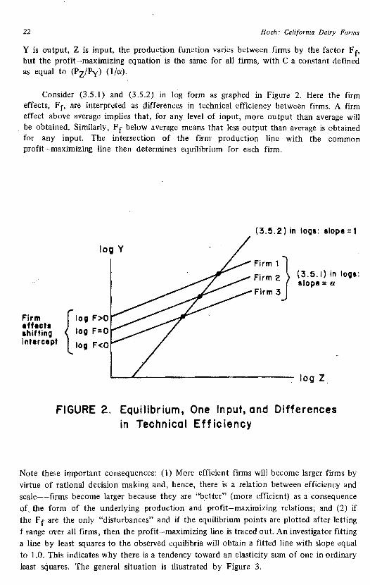
22 Hoch: California Dairy Farms
Y is output, Z is input, the production function varies between firms by the factor Ff, but the profit-maximizing equation is the same for all firms, with C a constant defined as equal to (Pz/Py) (l/a).
Consider (3.5.1) and (3 .5.2) in log form as graphed in Figure 2. Here the firm effects, Ff, are interpreted as differences in technical efficiency between firms. A firm effect above average implies that, for any level of input, more output than average will be obtained. Similarly, Ff below average means that less output than average is obtained for any input. The intersection of the firm production line with the common profit-maximizing line then determines equilibrium for each firm.
(3.5.2) in loQs: slope=1
loc;i Y
Firm 1} ( 3. 5. I) in IOIJS:Firm 2 slope= a
Firm 3
Firm log F>O effects
log F=O1hiftinQ intercept { log F<O
log Z
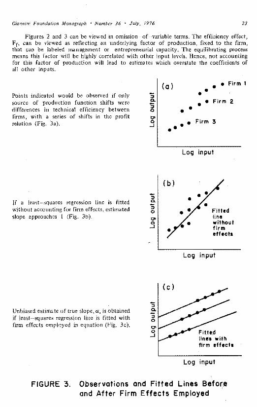
FIGURE 2. Equilibrium, One Input, and Differences in Technical Efficiency
Note these important consequences: (1) More efficient firms will become larger firms by virtue of rational decision making and, hence, there is a relation between efficiency and scale--firrns become larger because they are "better" (more efficient) as a consequence of, the form of the underlying production and profit-maximizing relations; and (2) if the Ff are the only "disturbances" and if the equilibrium points are plotted after letting f range over all firms, then the profit-maximizing line is traced out. An investigator fitting a line by least squares to the observed equilibria will obtain a fitted line with slope equal to 1.0. This indicates why there is a tendency toward an elasticity sum of one in ordinary least squares. The general situation is illustrated by Figure 3.
••
• •
• •
23
(c)
Fitted lines with
Giannini Foundation Monograph • Numba 36 • July, 1976
Figures 2 and 3 can be viewed in omission-of-·variable terms. The efficiency effect, Fr, can be viewed as reflecting an underlying factor of production, fixed to the firm, that can be labeled management or entrepreneurial capacity. The equilibrating process means this factor will be highly correlated with other input levels. Hence, not accounting for this factor of production will lead to estimates which overstate the coefficients of all other inputs.
Points indicated would be observed if only -::I source of production function shifts were -a.
differences in technical efficiency between 0 ::I
firms, with a series of shifts in the profit t:J'I relation (Fig. 3a). 0
..J
-:::> 0.lf a Jeast--squares regression line is fitted -:::>without accounting for firm effects, estimated 0
slope approaches l (Fig. 3b). t:J'I
j
-:::> Unbiased estimate of true a, is obtained a.
:::>if !east-squares regression line is fitted with 0 firm effects employed in equation (Fig. 3c).
0 "' ..J
(a) • • Firm
• •
• • Firm 2
Firm 3
Log input
(b)
• Fitted line without firm effects
Log input
firm effects
Log input
FIGURE 3. Observations and Fitted Lines Before and After Firm Effects Employed
24 Hoch: California Dairy Farms
Finally, Figure 3 can be interpreted in classic analysis-of-covariance terms as exhibiting the difference between interfirm and intrafirm functions. The underlying logic here need not bring in the relation between efficiency and scale by way of profit maximization but merely posit differences in intercepts for different size classes of firm. For example, it could be hypothesized that large firms had smaller intercepts than average, while small firms had larger intercepts. In this case the fitted interfarm function would tend to have a negative slope. The interfirm function, in general, then may be a biased representation of the intrafirm function.
Four previous empirical studies of Cobb-Douglas production functions, using analysis of covariance, obtained results consistent with the theoretical development presented above. A summary of their results appears as Table 6. All of the studies showed a decline in elasticity sum with the introduction of firm effects. Three of the studies had individual farms as units; in those studies, an elasticity sum very close to one was obtained when ordinary least squares was employed. The fourth study, by Timmer, treated each of the 48 contiguous states of the United States as a "farm firm" and found increasing returns using ordinary least squares, but results "changed drastically" when firm effects were introduced with returns to scale dropping below one. 1 Timmer interprets his results as eliminating management bias and points out that the sum of the ordinary least-square1 coefficients is nearly identical to a value reported by Griliches for a similar equation; hence, the conclusion that increasing returns hold for U. S. agriculture, based on the Griliches results, must be shaken. Because the other studies used farms as units, the economic model of the firm developed above is likely to be more relevant, perhaps explaining why most of the ordinary least-squares cases had an elasticity sum close to one. The one exception was Rasmussen's Irish subsistence case; yet, this case could well be consistent with the absence of profit-maximizing equations initially. In Rasmussen's four English cases, the initial elasticity sums ranged from 1.031 to 1.064, while for his four commercial Irish cases, the range was .928 to 1.00 I. After firm effects were introduced, the respective ranges were .466 to .820 for the English cases and .684 to .916 for the Irish. Although the initial English cases showed only slightly increasing returns, the estimated sum was significantly greater than 1.0 because of very low standard errors. A parallel result occurred in the pn::sent study and could be explained as an effect of regulation (see sectfon 4). Possibly the same explanation holds for the English cases.
Although carried out in markedly different agricultural settings, the Mundlak and the Hoch elasticity sums were remarkably similar with a "before".value around 1.00 and an "after" value around 0.80. Mundlak hypothesized that the difference between the two estimates could be interpreted as the elasticity of management.3 To this can be added the additional interrelated explanations of an increase in efficiency with scale and simultaneous equation bias.
Despite the existence of these explanations, some observers question the results. Timmer cites Griliches as suggesting a tendency for analysis of covariance to bias the estimated elasticities downward if there are errors of measurement in the variables, though Timmer adds that "in fact the direction of the bias is part hunch. ,,4 Rasmussen was so
1Timmer, op. cit., pp. 135 and 162.
2Jbid., citing Zvi Griliches, "Research Expenditures, Education, and the Aggregate Agricultural Production Function," American Economic Review, Vol. LIV, No. 6 (December, 1964), p. 966.
3Mundlak, "Empirical Production Function Free of Management Bias," Journal of Farm Economics, Vol. XUII, No. I (February, 1961), pp. 44-56.
"Timmer, op. cit., p. 145.

25 Giannini Foundation Monograph • Number 36 • July, 1976
TABLE 6
Estimated Sums of Elasticities and Coverage in Four Previous Studies by Investigator and Area
Estimated sum of elasticities
Ordinary Analysis Sample Study investigator least of Time span size and
and area covariance covered units~uares
Hoch (Minnesota) 0.991 0.832 1946-1951 63 farms
66 farmsMundlak (Israel) 0.967 0.795 1954-1958
Rasmussen
a 0,6871. 044 1,646 farms Irish commercial
1954-1957English b 0,978 o. 787 1955-1957} 1,139 farms0.763Irish subsistence 0.589 1955-1957
Timmer (United States) 1.168 0.948 1960-1967 48 states
l I
aAverage over four cases with values of 1.032, 1.064, 1.047, and 1.031 in least squares and 0.820, 0.466, 0.783, and 0.678 in analysis of covariance,
bAverage over four cases with values of 1.001, 0.982, 1.001, and 0.928 in least squares and 0.730, 0.817, 0.684, and 0.916 in analysis of covariance.
Sources:
Irving Hoch, "Estimation of Production Function Parameters Combining Time-Series and Cross-Section Data," Econometrica, Vol. 30, No. 1 (January, 1962), pp. 34-53
Yair Mundlak, "Empirical Production Function Free of Management Bias," Journal of Farm Economics, Vol. XLIII, No. 1 (February, 1961), pp. 44-56.
Knud Rasmussen with M. M. Sandilands, Production Function Analyses of British and Irish Farm Accounts, University of Nottingham, School of Agriculture (Loughborough, England, 1962), pp. viii and 116.
C. Peter Timmer, On Measuring Technical Efficiency, Stanford University, Food Research Institute Studies in Agricultural Economics, Trade, and Development, Vol. IX, No. 2 (1970), pp. 99-171.

26 Hoch: California Dairy Farms
concerned about the possibility of errors of measurement causing the elasticity drop that he rejected his analysis of covariance results! Yet, the author examined that possibility by constructing probability limits and found that the bias introduced by measurement error does not change as one moves from ordinary least squares to analysis of covariance. I Further, evidence to be presented in the next section shows that an elasticity sum decline is not universal. For the 12 samples of the present study, all showed a movement away from constant returns to scale; but in 2 samples, this involved an increase in the elasticity sum. The two samples were of small-scale manufacturing milk producers, most plausibly operating in a region of increasing returns to scale. This result squares with the thesis that simultaneous equation bias via neglected firm effects will move the elasticity sum toward constant returns whatever the true sum; i.e., the effect holds for a true elasticity sµm above one as well as below one.2
4. EQUATION I RESULTS
This section presents results and interpretations of those results for Equation I in which milk is regressed on the two inputs--feed in dollars and all other input in dollars. The- discussion is organized as follows: (1) elasticity estimates and inferences on returns to scale, (2) month effects, (3) year effects, (4) DHIA status effect, (5) breed effects, and (6) firm effects.
Elasticity Estimates and Inferences on Returns to Scale
The introduction of the firm dummies was crucial in estimating elasticities. This is shown in Table 7 which lists input elasticity estimates before and after the firm d urnmies were introduced. (All other sets of dummy variables appear in both cases.)
In all of the before cases, the elasticity sum is close to one. For I 0 of 12 cases, the sum is a bit above one. Hence, on this evidence, a hypothesis of (modest) increasing returns could be entertained about as easily as a hypothesis of constant returns to scale.
Marked changes in elasticity sums occur after firm effects are introduced. For each of the I 0 market milk samples, the,elasticity sums drop. For each of the two manufacturing milk samples, the elasticity sums increase. Hence, decreasing returns to scale for market milk and increasing returns to scale for manufacturing milk producers are inferred. The results seem generally consistent with the argument developed in the previous section that the introduction of firm effects, by eliminating simultaneous equation bias, will cause the elasticity sum to diverge from constant returns. Further, it seems worth stressing that an increase occurred in the elasticity sum for the manufacturing cases. As noted in Section 3, this has not been previously reported in the literature, and it tends to contradict the argument that there is a downward bias in analysis of covariance estimates. Certainly, the manufacturing farms are likely to face an institutional situation of relatively low product price and a good deal of fixed input, including human capital. Under these circumstances, increasing returns (or operation in a region of declining average costs) seem plausible.
1Hoch, "Book Review," Journal of the American Statistical Association, Vol. 58, No. 303 (September, 1963), pp. 853-857 (in particular, item 3, p. 855), of Knud Rasmussen with M. M. Sandilands, Production Function Analyses of British and Irish Farm Accounts (Loughborough, England: University of Nottingham, 1962).
2Hoch, "Simultaneous Equation Bias ...," p. 57 5.

TABLE 7
Elasticity Estimates and Coefficients of·Multiple Determination Before and After Firm Effects Introduced by Region and Sample
.
Elasticit:y_ estimates Coefficient of multiple
determinationBefore firm effects introduced After firm effects introduced Before firm After firm A A
Cll Cl2 r&: Cll a2 i:a effects effects
All other Sum of All other Sum of introduced introduced
Re__g_ion and samplea Feed cost it1E_uts Ielasticities Feed cost itlE_uts elasticities ! R2 R2
Sacramento Valley
Market .816 .220 1.036 .330 .477 .807 .893 .953 Man:ufaaturing .813 .270 1.083 .942 .292 1.234 .840 .879 Left survey .379 .632 1.011 .259 .506 .765 .926 .950
Northern and Sierra Mountains .809 .256 1.065 .595 .125 . 720 .873 .921
San Joaquin Valley
NoPthern MaPket .838 .160 .998 .709 .181 .890 .955 .969 SouthePn Mca-ket .884 .132 1.016 .736 .175 .911 .975 .984 Manufaa turing • 766 .278 1.044 .673 .412 1.085 .956 .971
North Coast .888 .055 .943 .510 .392 .902 ,867 .917
Bay Area
NoPthern .661 .409 1.070 .545 .367 .912 .939 .958 Southern .734 .325 1.059 .576 .322 .898 .954 .974
Southern California
CentPaZ .752 .263 1.015 .484 .214 .698 .969 .981 Peripherai .684 .391 1.• 075 .469 .107 .576 .942 .969
Average:
10 market samples
l .745 .284 1.029 .521 .287 .808 .929 .958
2 manufacturing samples .790 .l.
.274 1.064 .808 .352 1.160 .898 .925
aFor geographic coverage, see Table 2, supra, p. 6; for years covered by each sample, see Table 3, supPa, P• 8.

28 Hoch: California Dairy Farms
It is also of interest that the average over the I 0 market milk cases yields an elasticity sum close to one in the before case ahd around .8 in the after case--results which conform to the Hoch (Minnesota) and Mundlak (Israel) study shown in Table 6. There is considerable variation between samples, however. After firm effects are introduced, elasticity sums are around .9 for the Bay Area, North Coast, and San Joaquin Valley market milk samples (5 cases); around .8 for the two Sacramento Valley market milk samples; around .7 for the Southern California (Central) sample; and .6 for the Southern California (Peripheral) sample. The manufacturing milk elasticity sums are around 1.10 for the San Joaquin Valley and 1.20 for the Sacramento Valley.
In all cases, R2 is quite high both before and after firm effects are introduced. The introduction of the firm effects, however, usually explains a good deal of the (small) unexplained variance of the before case. On the average, the finn effects explain three-sevenths of the remaining unexplained variance in the 10 market cases (R2 increases from .93 to .96) and one-fourth in the two manufacturing cases (R2 increases from .9 to .925).
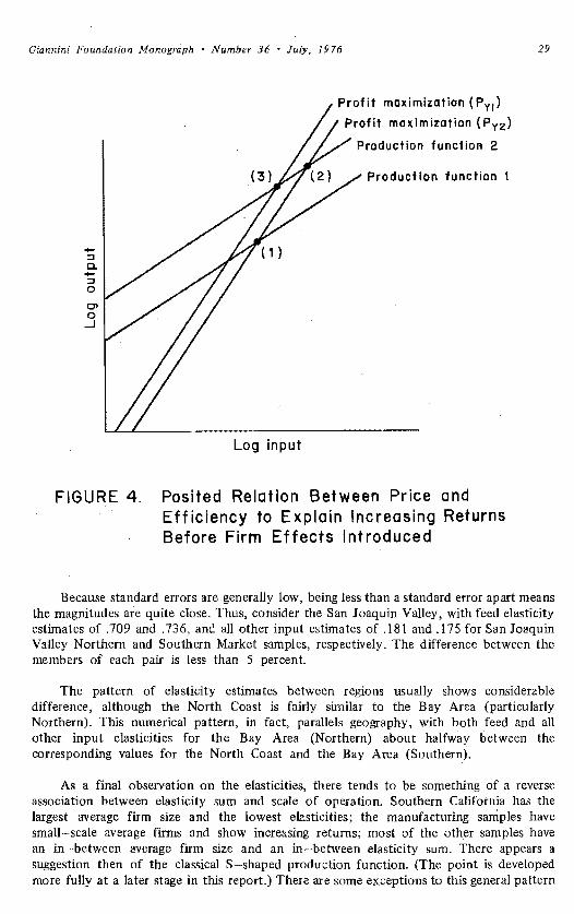
If the suggestion of mildly increasing returns to scale is taken seriously for the before case, some additional hypothesizing becomes necessary. One possibility is that within a sample there is a systematic relation between output price and efficiency, with more efficient firms having somewhat lower prices. To put the hypothesis in simple tenns, consider equation (3.5.2c) with two prices for Py: (I) a lower price, Py 1, that holds for more efficient firms and (2) a somewhat higher price, Py2, for less-efficient firms. The consequence is a profit-maximizing line for each price and a pattern of observed intersections with associated production functions which yields a fitted function exhibiting increasing returns to scale. This may fit the institutional situation prevailing at the time of this study. A dairy farm expanding production received a lower blend price because the increment of production was purchased at a lower price. What might have occurred is shown in Figure 4. The less-efficient firm has its equilibrium point at (1) with Py2. The more efficient firm would like to produce at (2) given a price of Py2; but, as it expands production, its price falls to Py1 so that point (3) is its equilibrium point. A line connecting points (1) and (3) will have a slope above one, i.e., exhibit increasing returns to scale.
Table 8 restates the elasticity estimates and presents the corresponding standard errors of estimate and the t ratios for the "after firm effects introduced" case. (Corresponding statistics for the "before firm effects" case appear in the Statistical Supplement to this report.) In all samples the t ratio for feed is above that for all other input. The t ratio is above the 5 percent level of significance for all the feed cases and for 10 of the 12 cases for all other input.
The feed elasticity is usually greater than that of all other input except in the case of the Sacramento Valley (Market) samples. This can be viewed as reflecting feed's greater share in production iwterms of its share of costs or revenue. (The matter later will be explored in more detail as part of a discussion of allocative efficiency.)
Samples from a given region usually have very similar elasticity estimates. This is clearly the case for the San Joaquin Valley (Northern and Southern Markets) samples and for the Bay Area samples. Corresponding elasticity estimates are less than one standard error apart. There is similarity, too, for corresponding estimates in the Sacramento Valley (Market and Left survey) cases and for corresponding estimates for the Southern California cases.
29 Giannini Foundation Monograph • Number 36 • July, 1976
Profit maximization (Py1)
Profit maximization (Py2 )
Production function 2
Production function
.... ::J a..... ::J 0
C'I 0
_J
Log input
FIGURE 4. Posited Relation Between Price and Efficiency to Explain Increasing Returns Before Firm Effects Introduced
Because standard errors are generally low, being less than a standard error apart means the magnitudes are quite close. Thus, consider the San Joaquin Valley, with feed elasticity estimates of . 709 and . 736, and all other input estimates of .181 and .17 5 for San Joaquin Valley Northern and Southern Market samples, respectively. The difference between the members of each pair is less than 5 percent.
The pattern of elasticity estimates between regions usually shows considerable difference, although the North Coast is fairly similar to the Bay Area (particularly Northern). This numerical pattern, in fact, parallels geography, with both feed and all other input elasticities for the Bay Area (Northern) about halfway between the corresponding values for the North Coast and the Bay Area (Southern).
As a final observation on the elasticities, there tends to be something of a reverse association between elasticity sum and scale of operation. Southern California has the largest average firm size and the lowest elasticities; the manufacturing samples have small-scale average firms and show increasing returns; most of the other samples have an in-between average firm size and an in-between elasticity sum. There appears a suggestion then of the classical S-shaped production function. (The point is developed more fully at a later stage in this report.) There are some exceptions to this general pattern
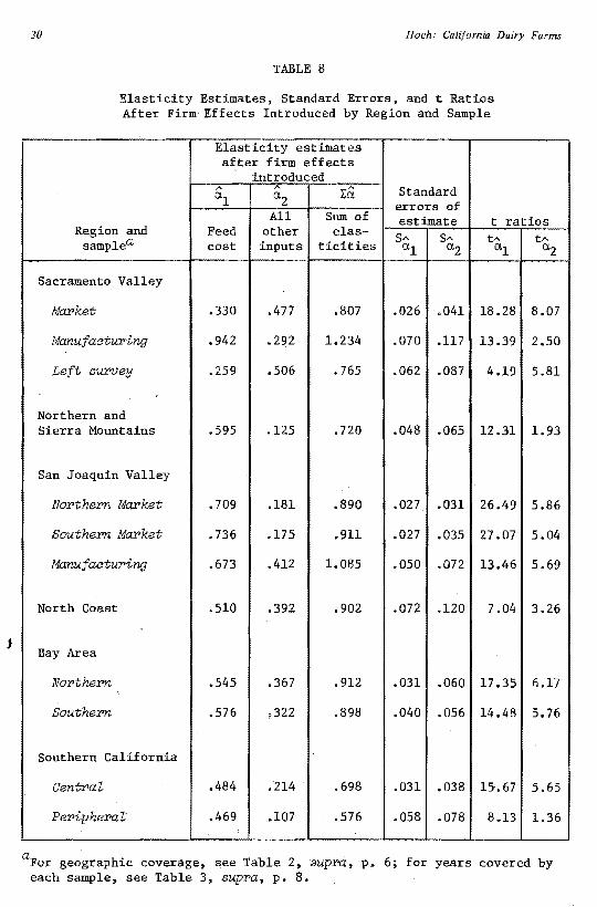
30 Hoch: California Dairy Farms
TABLE 8
Elasticity Estimates, Standard Errors, and t Ratios After Firm, Effects Introduced by Region and Sample
Elasticity estimates after firm effects
introduced
Region and samplea
Sacramento Valley
Market
Manufacturing
Left sUX'Vey
' Northern and Sierra Mountains
San Joaquin Valley
Nor-them Ma:t'ket
Southe:rn Market
Manufaetur-ing
North Coast
Bay Area
Northern
Southern
Southern California
Centl"al
Per-ipheral'
A
a.I
Feed cost
.330
.942
.259
.595
.709
.736
.673
.510
.545
.576
.484
.469
A
a.2 All
other inputs
.477
.292
.506
.125
.181
.175
.412
.392
.367
,322
.214
.107
Ea Sum of elas
ticities
.807
1.234
.765
.720
.890
.9ll
1.085
•9.02
.912
.898
.698
.576
Standard errors of estimate t ratios
SA a.1 s"
a.2 tA tA al a2
.026 '.041 18.28 8.07
.070 .ll7 13.39 2.50
.062 .087 4.19 5.81
.048 .065 12.31 1.93
.027 .031 26.49 5,86
.027 .035 27.07 5.04
.050 .072 13.46 5.69
.072 .120 7.04 3.26
.031 .060 17.35 6.17
.040 .056 14.48 5.76
.031 .038 15.67 5.65
.058 .078 8.13 1.36
aFor geographic coverage, see Table 2, supra, p. 6; for years covered by each sample, see Table 3, supra, p. 8.

31 Giannini Foundation Monograph • Number 36 • July, 1976
for there are three cases with small average firm and relatively low elasticity sum: Sacramento Valley (Left survey), Northern and Sierra Mountains, and North Coast. An attempt to rationalize this might be based on the argument that these three groups were not typical of commercial dairy operations, e.g., many of the dairy farms are probably part-time operations. Thus, a different production function might hold for these exceptional cases. (The evidence in Sections VI and Vil lends some support to this speculation. 1 In particular, the average Northern and Sierra Mountains farm has a high product price but a low output and a low level of technical efficiency.)
Year Effects
The primary source of interest in year effects is to avoid bias due to upward shifts in the production function over time. Thus, if there is an upward shift and if most firms also grow larger over time--either independently of the shift or, more plausibly, because of it (Figure 2)--then production function elasticity estimates can be overstated. In addition, year effects can yield useful clues on the rate of technological change. Admittedly, year-to-year variations in weather can obscure these clues.
Table 9 presents estimates of year effects for each of the samples. The values are in antilog terms, with the 1963 value set equal to 1.000. Hence, the numbers in the table can be interpreted as annual indexes on a given level of input. An index of .96 in 1960 means that for that year only 96 percent as much output was obtained as would be in 1963, given the same input. ·
Estimation of year effects by individual dummies for each year is preferable to the use of a trend term because no pattern is imposed a priori. However, for most of the samples, there appears to be an upward trend over time, that is, the production function appears to be shifting upward, perhaps reflecting technological advance. Hence, cost curves and supply functions should shift downward-rightward during the period under study.
If an average of Table 9 entries is taken over samples for given years, the following values are obtained:
Number of Year AverEM gises
1958 0.783 l 1959 0.884 4 1960 0.940 9 1961 0.985 11 1962 0.976 12 1963 1.000 12 1964 1.032 l I 1965 0.980 5
The 1965 results run against the trend but, perhaps, should be discounted considerably because they were based on a relatively small number of observations for only five samples. (Table 3 exhibits number of observations, with over 1,500 for each of the years 1961 through 1964, and only 155 for 1965 .) Aside from the 1965 result, an upward trend
1Tables 22 and 25, infra, pp. 58 and 68.

32 Hoch: California Dairy Farms
TABLE 9
Estimated Year Effects by Region and Sample (1963 Set Equal to 1.00) 195B-1965a
R..g_ionb and samE_le 1958 1959 1960 1961 1962 1
1963 1964 1965
Sacramento Valley
MarlaJt Manufac:-tu:t>irtg Left survey
c:
.783e .900*
d.9lld
1.065 .956
.963*
.970
.935
.990
.986
.992
1.000 1.000 1.000
1.041* .986
/
\
1.059* .997
Northern and Sierra Mountains .BOBd 1.019 1.015 1.000 1.034 .951
San Joaquin Valley
Northern Ma:I'ket Southern Market Manufac:turing
.903!
.872g
.862g
.960* • 927* • 954
.999
.968* 1.024
.982
.946*
.999
1.000 1.000 1.000
1.051* 1. 024* 1.044
North Coast .892 1.000 1.064
Bay Area
Northern Southern
h• 936h .947
.958
.971* .943* .966*
1.000 1.000
1.035 1.001
Southern California
Central Peripheral
1. 069. .963'
1.015 .986
1.000 1.000
1.047* 1.028
.993
.901*
aFootnotes show that the dummy variable included observations on an earlier year or years as well as the year listed. Aggregation of years was carried out to avoid possible multicollinearity because of limited number of observations.
bFor geographic coverage, see Table 2, supra, p. 6.
aBlanks indicate not covered.
dl960 is the terminal year for the set of observations covering 1955 through 1960; distribution of observations fairly uniform over period.
el958 is the terminal year for the set of observations covering 1955 through 1958; major fraction of observations in 1958.
fA small number of 1958 observations included in 1959.
gA small number of 1957 and 1958 observations included in 1959.
hlncludes a few 1959 observations.
iincludes a few 1960 observations.
*statistically significant at the S percent level. There are 15 significant year effects out of a potential number of 41 cases, rather than 65, because in.all samples the 1963 effect was set equal to 1.000; and the earliest effect was omitted in estimation to avoid collinearity (see Appendix A for more details).

33 Giannini Foundation Monograph • Number 36 • July, 1976
is manifest for all samples except the Sacramento Valley (Manufacturing) and Southern California (Central) cases which exhibit considerable year-to-year variability but no trend.
In six of the samples, the dummy variable labeled as the earliest year also included a small number of observations on the previous year or years. In addition, for the Sacramento Valley and Northern and Sierra Mountains cases, the earliest period was an aggregate of years beginning in 1955 and running to 1958 for the Sacramento Valley (Left survey) sample and to 1960 for Northern and Sierra Mountains samples. Only in this group of four cases are interpretations particularly affected, with the initial year effect listed really applicable to an average over a set of years. In all cases aggregation seemed necessary to prevent possible multicollinearity.
This aggregation seems a partial explanation for the large increase occurring between the initial "year" and succeeding year for the Sacramento Valley (Left survey) and Northern and Sierra Mountains samples. Yet, a graphing of all the data for the samples showing an upward trend suggests an increase at a decreasing rate. Perhaps the impact of a particularly important technological innovation has run its course, e.g., the introduction of holding tanks. But this is quite speculative; it is possible that other factors could be at work, e.g., weather variations.
Samples in a particular region often show very similar patterns of year-to-year changes. For example, in all three San Joaquin Valley samples, there is a decline in the year effect in 1962. Again, both Bay Area samples show a small decline in that same year. A regionwide decline would appear to lend some support to the hypothesis that weather effects are a component of the year effect. However, analysis of data on pasture conditions, presumably indicative of some weather effects on production, appears to yield little in the way of a relation. l .
For example, if an average is taken of the three San Joaquin Valley results for each year (1961, 1962, and 1963) and a comparison made of the averaged year effect to current pasture conditions for the San Joaquin Valley and to pasture conditions lagged one year (assuming preceding year conditions affect hay and green-chop fed the following year), a positive association does not emerge:
Current Lagged Year pasture pasture
Year effect index index
1961 99.7 93.7 85.4 1962 97.6 102.3 91.6 1963 100.0 100.0 100.0
If a comparison is made of the statewide index of pasture conditions to the all-sample average of year effects, with 1963 as the base for each, the following is found:
1Pasture condition data were obtained from Meghnad Desai, "An Index of Pasture Conditions," University of California, Department of Agricultural Economics, Working Paper (Berkeley, 19.65); also from data included in letter from W. Ward Henderson, California Crop and Livestock Reporting Service, June 23, 1965, to M. Desai.
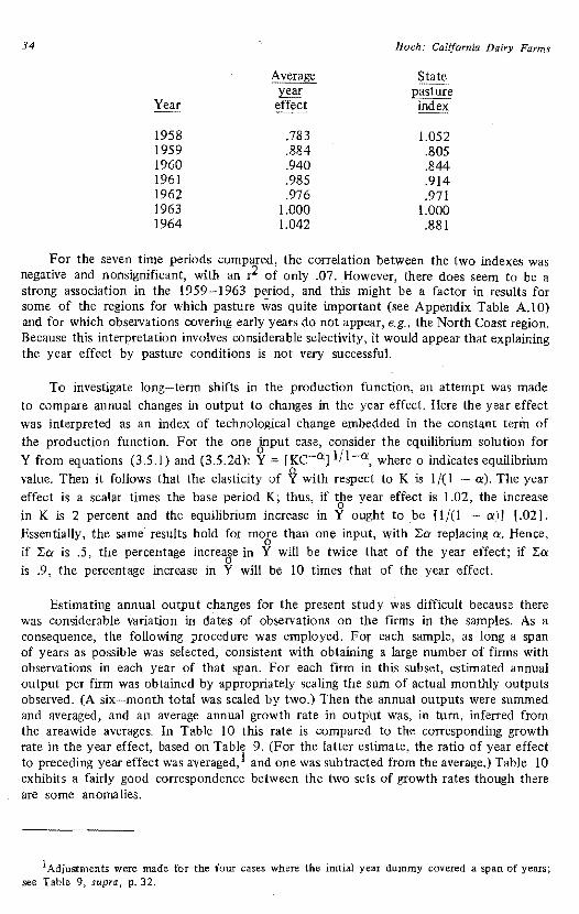
34 Hoch: California Dairy Farms
Average State year pasture
Year effect index
1958 .783 1.052 1959 .884 .805 1960 .940 .844 1961 .985 .914 1962 .976 .971 1963 1.000 1.000 1964 1.042 .881
For the seven time periods compared, the correlation between the two indexes was negative and nonsignificant, with an r2 of only .07. However, there does seem to be a strong association in the 1959-1963 period, and this might be a factor in results for some of the regions for which pasture was quite important (see Appendix Table A. I 0) and for which observations covering early years do not appear, e.g., the North Coast region. Because this interpretation involves considerable selectivity, it would appear that explaining the year effect by pasture conditions is not very successful.
To investigate long-term shifts in the production function, an attempt was made to compare annual changes in output to changes in the year effect. Here the year effect
was interpreted as an index of technological change embedded in the constant term of the production function. For the one input case, consider the equilibrium solution for Y from equations (3.5.1) and (3.5.2d): Y= [KC-a] I/ 1-a, where o indicates equilibrium
value. Then it follows that the elasticity of ~ with respect to K is I/( I - a). The year effect is a scalar times the base period K; thus, if the year effect is 1.02, the increase
0 in K is 2 percent and the equilibrium increase in Y ought to .be [!/(! - ex)] [.02). Essentially, the same results hold for more than one input, with LO'. replacing a. Hence,
0 if LO: is .5, the percentage increase in Y will be twice that of the year effect; if LCX
0 is .9, the percentage increase in Y will be I 0 times that of the year effect.
Estimating annual output changes for the present study was difficult because there was considerable variation in dates of observations on the firms in the samples. As a consequence, the following procedure was employed. For each sample, as long a span of years as possible was selected, consistent with obtaining a large number of firms with observations in each year of that span. For each firm in this subset, estimated annual output per firm was obtained by appropriately scaling the sum of actual monthly outputs observed. (A six-month total was scaled by two.) Then the annual outputs were summed and averaged, and an average annual growth rate in output was, in turn, inferred from the areawide averages. In Table I 0 this rate is compared to the corresponding growth rate in the year effect, based on Table 9. (For the latter estimate, the ratio of year effect to preceding year effect was averaged, 1 and one was subtracted from the average.) Table 10 exhibits a fairly good correspondence between the two sets of growth rates though there are some anomalies.
1Adjustments were made for the four cases where the initial year dummy covered a span of years; see Table 9, supra, p. 32.

35 Giannini Foundation Monograph • Number 36 • July, 1976
TABLE 10
Estimated Annual Growth Rate in Output Compared to Growth Rate for Year Effect by
Region and Sample
aRegion and sample (arranged in order of output growth
rate)
Aspects of estimating procedure for ou1:E_ut growth rate
Number of ! firms in Years Estimated subsam~le covered rate
Growth rate for year
effect (over period of
sam_E_le)
Southern California
Peripheral 20 1961-1964 .012 -.014b
Sacramento Valley
Manuf actur-ing 10 1961-1964 .029 -.01i
Northern and Sierra Mountains 12 1961-1964 .030 .012
Bay Area
Northern 37 1960-1964 .035 .026
Southern California
CentraZ 48 1962-1964 . 039 -.018b•
North Coast 15 1962-1964 .047 .092
Sacramento Valley
Market 44 1961-1964 .053 .023
Bay Area
Southern 23 1960-1964 .054 .014
Sacramento Valley
Left survey 8 1960-1963 .058 .031
San Joaquin Valley
Southern Market Northern Market Manufacturing
43 36 13
1960-1964 1959-:1964
i 1960-1964 l
.058
.063
.072
.035
.031
.040
aFor geographic coverage, see Table 2, supra, p. 6.
bPresumably zero would be a better estimate for long-run forecasts; it is unlikely there is a decline in technology.

36
I
Hoch: California Dairy Farms
Generally, the rate of growth in output appears to roughly reflect the presumed underlying growth rate for the year effect. For the latter, a growth rate below zero might best be replaced with an estimate of zero in terms of long-run forecasting. (It is hardly plausible that there have been technological declines.) For the three samples in this category, the output growth rate was relatively small; but it was positive so the correspondence is limited. All other samples had both growth rates positive, with the output growth rate approximately twice the year effect growth rate. (Omitting the North Coast which is anomalous--perhaps because of the special influence of pasture conditions s4ggested above--the means of the eight remaining cases are exactly 2 to I.) The 2 to ratio is well below the presumed equilibrium ratio of roughly I 0 to I, assuming LC\'. of .9.
It is worth noting that, with LC\'. = .9 and a year effect growth rate of .02, a firm's equilibrium output should compound 20 percent per year, thus doubling every four years. With all firms expanding, it is likely there would be downward pressure on product prices; or if there were institutional constraints on expansion, such constraints would seem even more harsh over time.
The median year effect growth rate in Table 10 is around .02 per year. However, inspection of the scatter diagrams of the year effects yielded the conclusion that a growth rate of about I percent per year is a reasonable estimate for the period 1964 to 1970 for most samples. (This quantifies the previously noted apparent increase at a decreasing rate.) At equilibrium, then, with LC\'. = .9, the average firm would attempt to expand output by about I 0 percent per year.
The estimated growth rate here has not been tied to any specific sources of growth, and a great deal of future effort could and should be addressed to that topic. On the other hand, estimated year effects from production functions for different industries might be useful in the general discussion of productivity change. Certainly, the topic involves a great many unsettled questions. The Denison versus Jorgenson and Griliches controversy is a case in point. I Denison saw a substantial part of postwar growth in national output as due to increases in productivity ascribed to such factors as "advances in knowledge, economies of scale and reallocation of resources." Jorgenson and Griliches initially took the position that almost all of postwar growth was due to an increase in factor inputs. In later work they substantially modified their estimates but nevertheless held that "factor input, not productivity change, predominates in the explanation of the growth of output.'" They initially estimated the growth in factor productivity at 0.30 percent per year but then revised this upward to 1.03 percent per year in contrast to Denison's estimate of 1.3 8 percent per year.
It can be noted in passing that these national estimates add some 'measure of "reasonableness" to the growth rate of I percent, estimated here for the California dairy industry.
Month Effects
Month effects are presented in Table 11 in antilog terms. The geometric meah equals one so that, in a month with a value below one, output for any given input is less than average; with a value above one, output for any given input is above average. A month
!Papers by Edward F. Denison and Dale W. Jorgenson-Zvi Griliches in "The Measurement of Productivity," Survey of Current Business, Vol. 52, No. 5, Part II (May, 1972), I! Ip; quotations and cited material appear on pp. 89, 95, 96, and 111.
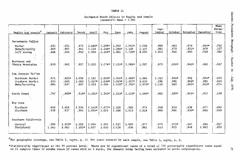
TABLE 11
Estimated Month Effects by Region and Sample (Geometric Mean = 1.00)
Id::_ Ij l Sep-I ~ril 1 ·December i tionI tember October NovemberMa_y Ju!Y_! January June AtigustRt;g_ion ~nd 'salllP.lea MarchFebrua:ry
Sacramento Valley
.042.983 .979 .949"1.058* 1.045 1. 042* 1.040 .995•92.0 .954 .978Market 1.069*
.127.879.978 .831*1. 248* 1.206* 1.137 .965.805 .907 .941 1.116 1.105Manufacti.a>ing
.062.980 .948l.003 1.012 .934.992 1.050 1.144* 1.061 1.120*.886 .906Left si.a>v<Jy
Northern and Sierra Mountains .067.942* .962.910 .962 .957 1. 074* 1.216* 1. 069* 1.007 .975 .910*1.055
San Joaquin Valley
.033.982 .954"1.015 .944*.971 .950* 1.026 1.022 1.059* 1.040* 1.040* 1.004NorthePn Market
.023.966* .9811.000 1.010 .986.953 .985 1.027* l.030* 1.033* 1.037* .996SouthePn Market
.0741.013 1.145* .965 .919*.894 .937 .957 1.054 1.152* 1.075* 1.028 .905*Manufaatu:Ping
.139.816* .910North Coast . 797 .936* 1.243* 1.253* 1.103* .965 .928*.898* 1.201* 1.090*
Bay Area
.049.953 .977.949 1.016 1.034 .974 .948 .958Northern 1.145* 1.077* 1.029 .960
.039.957 .988 .964 .950* .966Sou them .959 .992 1.095* 1.023 1.086 1.013 1.019
Southern California
1.029* 1.024 1.011 .974 .971* .987Central •999 1.020 1.021 1.000 .977 .990 L:J1.037 i 1. 050 1.063 0Peripheral, 1.065 1.016 .9481.042 . 1.102* .936 .862 .953 .955
i I II .
aFor geographic coverage, see Table 2, supra, p. 6; for years covered by each sample, see Table 3, supra, p. B.
*Statistically significant at the 95 percent level. There are 46 significant cases of a total of 132 potentially significant cases equal .co 12 samples times 12 months minus 12 cases with no t ratio, the January dUIIllily having been excluded to avoid collinearity.

38 Hoch: California Dairy Farms
effect of I.OS means that 5 percent more output than the average. is obtained for any level of input.
The seasonal patterris that emerge generally have consistent peaking· in the spring and summer and low levels in fall and winter. There are variations between regions, both in seasonal pattern and amplitude. The manufacturing samples show much greater swings than the corresponding market milk samples. The major market-producing areas of Southern California and the San Joaquin Valley exhibit relatively little variability between months. An index of variability is the mean deviation, ~mIM~ - M* I/ l 2 where M* is the antilog of the month effect, M. The mean deviations, by sample, are presented in Tahle 11. Figure 5 exhibits graphs of the month effects for selected samples.
Correlations of month effects. between pairs of samples are shown for major samples in Table 12 and are indicative of similarity of seasonal pattern between regions. Not too surprisingly, the Sacramento Valley and the two San Joaquin Valley samples are highly correlated with one another; all diverge from the Southern California samples. The Bay Area (Southern) appears to be closer to the Valley pattern, while the Bay Area (Northern) seems somewhat closer to that of Southern California. The Bay Area (Southern), in fact, is more highly correlated with the Valley samples than it is with the Bay Area (Northern).
In terms of supply, the peak months of the year would involve supply shifts to the right, with the reverse movement for the low months. Perhaps these seasonal supply shifts primarily affect the flow into manufacturing milk. However, there may also be some substitution between sources of market milk insofar as alternative regional sources of supply have seasonal cycles that are out of phase.
In supply estimation the month effects are useful in constructing regional or state supply schedules for specific months; setting all month effects equal to one yields an "average" monthly supply, essentially supply on an annual basis.
Membership in Dairy Herd Improvement Association (DHIA)
Table 13 presents antilogs for DHIA status, exhibiting estimates obtained before and after firm effects were introduced into the regression equation.
The basic hypothesis employed was that membership in DHlA would have a positive effect on productivity so that higher output would be obtained for given input. Membership in the DHIA yields management data for a fee; records are obtained on milk and butterfat production and herd condition by tests of each cow every month. The DHIA dummy variable was coded zero for nonmembership and one for membership in DHIA. It was expected the coefficient in the logs would be positive, with the antilog, therefore, above one.
There was some confirmation for this hypothesis. However, the confirmation seemed much stronger before firm effects were introduced, with 11 of the 12 DHIA effects .estimated as above 1, and 7 of these significant at the 5 percent level. After firm effects were introduced, only 8 of the effects were above 1, with 4 significant at the 5 percent level; IO estimates decreased in value and only 2 increased. The average of the 12 samples was 1.046 in the before case and 1.008 in the after case. All of these data can be interpreted to mean that better operators tend to join the DHIA; not accounting for such an association can yield a marked overstatement of the benefits of DHIA membership. This result may have wider implications. It suggests, by analogy, that measured benefits of extension work
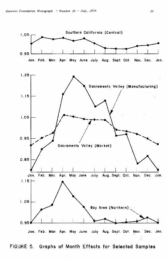
Giannini Foundation Monograph • Number 36 • July, 1976 39
Jan. Feb. Mar. Apr. May June July Aug. Sept. Oct. Nev. Dec. Jan.
I. 25
1.15
I. 05
0.95
0.85
Jan. Feb. Mar.
(Manufacturing)
Sacramento Valley (Market)
Apr. May June July Aug. Sept. Oct. Nev. Dec. Jan.
1.15
I. 05
Bay Area (Northern)
Jan. Feb. Mar. Apr. May June July Aug. Sept. Oct. Nov. Dec. Jan.
FIGURE 5. Graphs of Month Effects for Selected Samples

TABLE 12
Correlations of Month Effects by Region and Sample
Reg_iona and sam12_le
Sacramento : VallEO:L Market
San Jo~uin VallEO:L Northern Southern Market Market
B'!Z_ Area Northern Southern
Southern California Central Peri_.12._heral
Sacramento Valley
Market 1.00 • 77 .91 .57 .84 .18 - .26
San Joaquin Valley
No'I'thern Market Southern Ma.rket
b 1.00 .80 1.00
.47
.56 • 71 .83
.33
.35 - .01 - .08
Bay Area
Northern Southern
1.00 • 71 1.00
.73
.44 .54 .05
Southern California
Central Peripheral I
l I
l I i
I
l
1.00 .70 1.00
aFor geographic coverage, see Table 2, supra, p. 6.
bBlanks indicate value is listed above main diagonal for the specific pair in reverse order.

41 Giarinini Foundation Monograph • Number 36 • July, 1976
TABLE 13
Estimated Effects for Dairy Herd Improvement Association (DHIA) Status Before and After Firm Effects Introduced by Region and Sample
Estimated effect associated with membership in DHIA (antilo_g)
Before firm effects After firm effects R~on and sa!llplea introduced introduced
Sacramento Valley
MaPket 1.008 1.054*
Manufaatu:r>ing 1.052* 0.973
Left SUPVey 1.051 0.923
' Sierra Mountains Northern and
1.031 0.982
San Joaquin Valley
Northern Mctrket 1.0061.119*
Southern MaPket 1.021* 1.018*
1.030* 0.985Manuf aatu.ring
North Coast 1.030 1.029
Bay Area
Northern 0.985 1.030
Southern 1.118* 1.049*
Southern California
Centrat 1.047* 1.032*
1.062* 1.014Peripherai
Average:
12 samples 1.008 10 market samples
1.046 1.047 1.014
aFor geographic coverage, see Table 2, supra, p. 6; for years ·covered by each sample, see Table 3, supra, p. 8,
*Statistically significant at the 5 percent level.
i

42 Hoch: California Dairy Farms
and education may sometimes be overstated. Thus, both the DHIA case and the more general cases of extension work and education can involve a selection process (including self-selection) so that participants in the activity are of higher quality to begin with (before engaging in the activity). Not accounting for the underlying quality difference then yields a form of omission-of-variable bias and leads to overstatement of the benefits attributed to the information service or to the educational process.
In the after case, the four samples having DHIA effect below one also typically had small-scale farms. Perhaps many operators of small farms have a limited budget of time for management decisions, devoting most of their time to furnishing their farm's labor input, so that DHIA participation involves malallocation of management time. It might be simpler to ascribe such negative results to sampling variability; none of the values below one are statistically significant.
Breed Effects
Table 14 presents breed effects by sample, with breeds classified as Guernsey, Holstein, Jersey, and Mixed. A good deal of variability occurs between the breed effects; if the estimates are accepted at face value, there are implications here for dairy farm management. However, only 5 of 32 potentially significant cases, in fact, are significant at the 5 percent level so that some caution seems warranted. It is of interest that Guernsey cattle appear markedly better than other breeds in the Sacramento Valley (Market) and Bay Area (Northern) samples, while Holstein cattle have a strong positive effect in the Bay Area (Southern), in contrast to the Guernsey and Jersey breeds, and a marked negative effect in the Southern California (Peripheral) sample.
Firm Effects
The distributions of firm effects by sample are presented in Table 15. Values are in antilog form. In the usual fashion a firm with an antilog of 1.25 is estimated to obtain 25 percent more output for given input than the average firm (with antilog of 1.00); a firm with an antilog of .75 will obtain only 75 percent of the average output for given input.
Table 15 also presents the aggregated results for all samples combined. Of the 469 firm effects of all the samples,1 220 were significant at the 5 percent level; this is close to 50 percent of all the coefficients.
Figure 6 graphs the distribution of firm effects for all samples combined. It was hypothesized that these observations came from a log-normal distribution. This hypothesis was tested using a chi-square test. In that test the sample mean and variance are assumed to be parameters of a normal distribution, and a set of expected frequencies are generated given the sample size. Then 2:f (Oi Ei)2 /Ei is distributed as chi-square with I 3 degrees of freedom, where 0 is observed frequency, E is expected frequency, i is interval number, and I is number of intervals. The critical chi-square for rejecting the hypothesis of normality was 11.07; a chi-square of 6.96 was obtained, for I = 8 at the 5 percent level. Hence, normality is accepted for the pooled samples.
1This is five less than the number of firms because in five samples the regression program eliminated one firm due to multicollinearity. The eliminated firm, in effect, is combined with the one firm that was eliminated by specification to prevent multicollinearity.
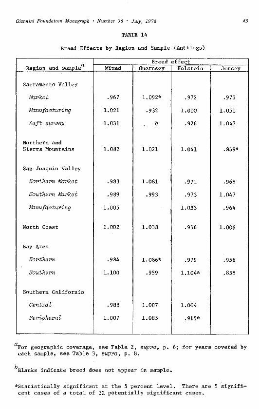
Giannini Foundation Monograph • Number 36 • July, 1976 43
TABLE 14
Breed Effects by Region and Sample (Antilogs)
aReg_ion and sample Mixed Breed effect
GuernsE!Y_ Holstein JersE!Y_
Sacramento Valley
Market
Manufactu:Ping
Left sur•vey
• 967
1.021
1.031
1.092*
.932
b
• 972
1.000
.926
.973
1.051
1.047
Northern and Sierra Mountains 1.082 1.021 1.041 .869*
San Joaquin Valley
Northern Market
Southern Market
Manufactu:Ping
.983
• 989
1.005
1.081
.993
.971
.973
1.033
.968
1.047
.964
North Coast 1.002 1.038 .956 1.006
Bay Area
Northern
Southern
.984
1.100
1.086*
.959
.979
1.104*
.956
.858
Southern California
Central
Peripheral
.988
1.007
1.007
1.085
1.004
.915*
aFor geographic coverage, see Table Z, supra, p. 6; for years covered by each sample, see Table 3, supra, p. 8.
bBlanks indicate breed does not appear in sample.
*Statistically significant at the 5 percent level. There are 5 signifi~ cant cases of a total of 32 potentially significant cases.

TABLE 15
Distribution of Firm Effects by Region and Sample (Antilogs)
firme~.80 .75 .70 Signi
to to o .95 .so
ficant Totalto to to Belowto firms1.00 .95 .90 .85 •70 cases.80 •75 .so
Sacramento Valley
1 1 0 6410 5 4 322 9 2 4 60 4 94 3Market 19°3 0 0 0 0 24 2 10 1 0 1 1 0 3 3Manufaaturing 2121 2 4 0 0 0 l 0 71 2 40 0 3 1Left survey
Northern and Sierra Mountains zs"12 2 1 1 0 173 1 3 32 0 3 30 3
San Joaquin Valley
463 2 0 0 0 267 9 51 1 2 1 5 50 5Northern Market 02 0 5111 4 7 3 4 0 250 8 90 0 0 3Southern Mcu'ket
1 19"0 1 0 01 2 00 0 0 1 3 4 40 3Manufaaturing
3 0 1 0 0 5 291 31 2 0 2 2 4 30North Coast
Bay Area
1 4 0 0 31 676 8 62 7 10 9 540 1 4NoPthern 40"0 14 0 202 7 4 l 01 0 1 6 8 50Southern
Southern California 62(13 I 1 8 1 1 0 416 4 31 6 6 10 71 4Central
1 01 1 3 13 231 1 40 4 02 3 0 1Peripheral 1
220 46960 51 36 30 22 13 9 016 16 15 32 6545 57Total samples 2
'---c----------·~······-····l.--......l"----'----···-'----'----''---·....1.---'----'---···'-----'---'---..l-----'----'---"---...!..----'
aAn intel.'Val runs from the lower value to less than the upper value.
bFor geographic coverage, see Table 2, supra, p. 6; for years covered by each sample, see Table 3, supra, p. 8.
0 one additional firm deleted ex post because of multicollinearity--in effect, combined with firm eliminated ex ante; ex ante elimination always necessary with dummy va4iables.

45 Giannini Foundation Monograph • Number }6 • July, 1976
70
60
50
rn Q)
111 c u
..... 0
.... Q) .a E ::I z
40
30
20
10
0
.--
I-
1-
1-
1-
I-
I-
..-
,......., 1-
.--
1-
.-
I-..-
-I--.-
.-
r T I I D 0.5 0.6 0.7 0.8 0.9 1.0 I. I 1.2 1.3 1.4 1.5 1.6
Value of firm effect
FIGURE 6. Distribution of Firm Effects, All Samples Combined

46 Hoch: California Dairy Farms
Inspection of the data of Table 15 leads to the conclusion that the hypothesis of normality would be accepted for all samples. On an intuitive level, the Northern and Sierra Mountains case seemed the least likely candidate for normality on the basis of its sample distribution. Yet a chi-square test did not lead to rejection of the hypothesis in its case.
In the logs the mean of the pooled sample was, of course, zero; the standard deviation was .0702. This implies that, in the antilogs, 95 percent of all firm effects should fall between .73 and 1.37 and that the range .85 to 1.17 corresponds to ·plus and minus one standard deviation around the mean.
As a check on the reasonableness of the estimated firm effects, the BMS fieldmen were asked to make independent evaluations of the producers in their respective samples in terms of a rating scale on efficiency. A rating scale from -3 to 3 was specified, but each field man followed his own bent in assigning the ratings. In Table 16 the ratings obtained have been classified into low, middle, and high groupings; and the corresponding averages of firm effects are exhibited for each grouping and set of samples for which the ratings were made. A general correspondence does emerge in Table 16.
The ratings were regressed on the firm effects, and relevant results are exhibited in Table 17. The r2's were generally not very high, but t ratios for the coefficients were fairly encouraging. There were four grouped samples, each of which pooled the observations of an individual fieldrnan. All had significant t ratios at the 5 percent level. At the level of the individual sample, five of eight had significant results; the other three had rather low explained variance and t ratio.
On the whole, there seems to be some encouragement for the notion that the firm effects are a fair reflection of reality. In cases where elasticity sums dropp~d substantially, firm effects usually turned out to be highly correlated with average level of output, in line with the interpretation that large firms are better firms. Correlations were low or slightly negative for manufacturing samples, not.- surprising given the increase in elasticity sums for these samples.
As noted in Section 3, the firm effects can be viewed as indexes of entrepreneurial capacity or managerial ability, in effect fixed to the firm. The existence of a fixed factor is consistent with an elasticity sum below one which, in tum, implies positive profits given profit maximization. Profits thus can be interpreted as the return to entrepreneurial capacity. The level of profits reflects the value of the firm effect; better operators will have larger firm effects (by definition) and, hence, larger firms and higher profits (as a consequence of maximizing behavior). Certainly, other factors, such as capital rationing and the inheritance of farms, will make the association between efficiency and scale less than exact. However, evidence to be presented in Section 5 establishes a strong empirical association between firm effects, interpreted as measures of technical efficiency, and various measures of scale. Those results, in turn, are used as a springboard for a general discussion of the sources and further implications of the firm effects.
Testing Statistical Significance of Sets of Dummy Variables
In a given equation the statistical significance of a set of dummy variables can be tested by means of F tests, in effect comparing explained variance before and after the set of dummies is introduced. (It is noteworthy that it is possible to have only a small

TABLE 16
Comparison of Firm Efficiency Estimates Averaged Over Broad Classes
Fieldman estimatea
Sacramento Valleyb
Corresponding avera&e of firm effects San Joaquin Valley Bay Are8!5 and Northern Market North Coast
Southern b California
Low Middle High
.906
. 958 1. 057
.900 1.003 1. 073
• 978 1. 044 1.119
.971 1.040 1.133
number of cases ..
Low 18 4 24 30 Middle 30 12 18 46 High 50 15 8 8
aDefinition of low, middle, and high varied between cases as follows:
Low Middle
Sacramento Valley Below 0 0 Above 0
San Joaquin Valley
Northern Market Below 0 0 Above 0
North Coast and Bay Area -1, 0, 1 +2 +3
Southern California -2, -1, 0 +l +2
bGrouped samples. Sacramento Valley includes Market, Manufacturing, and Left survey. Bay Area includes' North and South Bay. Southern California includes Central and Peripheral.
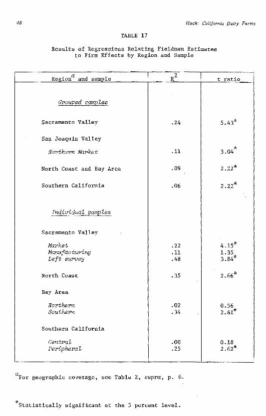
48 Hoch: California Dairy Farms
TABLE 17
Results of Regressions Relating Fieldman Estimates to Firm Effects by Region and Sample
I I t ratio
Grouped sq;rreles
Sacramento Valley 5,43*.24
San Joaquin Valley
.11 3.04*
North Coast and Bay Area
Northern Market
2.22*• 09
Southern California 2.22*.06
Individual samples
Sacramento Valley
Market .22 4.15* Manufac-turing .11 1.35
3.84*Left sUI'Vey • 48
2.66*North Coast .35
Bay Area
Northern .02 0.56 Southern .34 2. 61*
Southern California
Central .oo 0.18 2.62*Peripheral .25
aFor geographic coverage, see Table 2, supra, p. 6.
*statistically significant at the 5 percent level.

49 Giannini Foundation Monograph • Number 36 • July, 1976
number of individual coefficients that are significant and yet have calculated F for the set of coefficients well above the critical level.)
In the present study, time and budget constraints allowed F tests of the firm effects only, and it turned out that calculated F was above critical F at the 5 percent level for all samples. The tests are discussed in detail in Appendix A, and the test results are tabulated in Appendix Table A.15.
For the other sets of dummies, it is possible to present t tests of their statistical significance in the context of all 12 samples as a group by use of the normal approximation to the binomial distribution. The key consideration is that, if all of a set of dummy variables really had zero coefficients, then--in the probability limit--it would be mistakenly inferred that 5 percent of the coefficients were significant. In fact, the percentage of cases that were significant ranged from 15.8 percent for breeds to 47.9 percent for firms. The t statistics calculated, given the observed percentages, were:
Years 9.28 Months 15.68 DHIA 4.49 Breeds 2.79 Firms 42.90
Ail of these test statistics exceed the critical t at the 5 percent level; hence, it can be concluded that all sets of dummies are significant for the study as a whole. The details of procedures employed for the t tests are discussed in Appendix A and summarized in Appendix Table A.16.
S. EQUATION 2 RESULTS
This section presents results for Equation 2 including evidence establishing a strong relation between firm effects and measures of scale and efficiency. Those results, in turn, initiate a discussion of sources and implications of the firm effects.
Equation 2 was developed prior to Equation 1 in terms of chronological order. The models are quite similar, with the only difference being the measurement of feed in terms of dollars in Equation 1 and in terms of TDN in Equation 2.
There were two reasons for the substitution of feed in dollars (Z1) for feed in TDN (X1). First, feed measured in dollars made a number of applications much easier. Cost curves and supply curves are relatively easy to derive using Z 1 but would pose difficulties using X 1. Proper weighting of feed components by respective prices was carried out as a matter of course in defining Z 1. Proper pricing of X1 would be, at best, more complicated and less satisfying. A second reason for the employment of z1 stemmed from some question about the BMS measures of TDN. The BMS estimated TDN as a fraction of weight of feed; the fractions employed implied that a pound of IDN from concentrates cost a good deal more than a pound of TDN from roughage and pasture. The di(ferential was around 50 percent, with the cost of TDN per pound about 3 cents for roughage and pasture and about 4.5 cents for concentrates. If this were indeed the case, it seemed reasonable to aggregate feed in terms of dollars rather than pounds. If this were not the

50 Hoch: California Dairy Farms
case, i.e., if the weights employed by the BMS were biased, the use of dollars would avoid the problem. 1
On the whole, results for Equation 2 turn out to be quite close to those for Equation I. There are some fairly subtle differences which suggest that the TDN measure, X1, could bias some estimates.
Equation 2 parallels Equation 1 in the behavior of elasticities after firm effects are introduced. Before firm effects enter, the average elasticity sum for the 10 market milk samples is 1.06 in Equation 2 and 1.03 in Equation 1; for the two manufacturing samples, it is 1.10 in Equation 2 and 1.07 in Equation I. With the introduction of firm effects, the elasticity sum declines for market milk samples and increases for manufacturing samples in both equations, although the movement away from constant returns is a bit more pronounced in Equation 1. Table 18 compares the elasticities and R2 values obtained after firm effects enter. Results are generally quite close. Some shifts in individual elasticity values occur between the two equations, but this appears to be pronounced only for the Sacramento Valley (Market) milk sample. Elasticity sums are within S percent of one another for all but two cases whose differences are less than 7 percent. All absolute differences are within .OS, with an average difference of .017.
The pattern of general agreement does not hold throughout, however. In particular, firm effects appear to depend on the way in which feed is measured. Firms using a great deal of roughage relative to concentrates will appear with a higher feed input in Equation 2 than in Equation 1 because of differences in weights between the models. Given the same output levels in each case, such firms would be estimated to be lower in efficiency in Equation 2 than in Equation 1. This appears to have occurred for the set of 10 manufacturing firms in the Bay Area (Northern) sample. The following averages for firm effects were obtained:
~quation 2 Equation
Manufacturing (10 firms) .738 .825 Market (57 firms) 1.065 1.044
Under the argument that decision making occurs in terms of dollars, the estimates under Equation 1 seem preferable. Admittedly, the differences here are not particularly pronounced between the equations, though this was not known a priori. (It can be concluded that manufacturing firms are less efficient than market firms.) More generally, dummy variable coefficients were basically similar between equations, indicating this problem had only limited impact. (Proportions of feed components were probably fairly similar between most sets of observations.) Month effects seemed somewhat less extreme (deviated less from the mean), while year and firm effects were somewhat more extreme in Equation 2. But the basic similarity is reflected in the correlations between firm effects for selected samples. For the Sacramento Valley (Market), the Bay Area (Northern), and the two San Joaquin Valley samples, these correlations ranged from .961 to .988.
1Disaggregation of feed is an alternative solution to the problem and was employed here in some applications; see the discussion of Equation 4, infra, p. 75.

TABLE 18
2Comparison of Elasticities and R 's for Equations 1 and 2, with Firm Effects Appearing in Each Case, by Region and Sample
All other input Feed elasticit::y_ elasticities Sum of
R2Equation 2 Equation 1E~uation 2 elasticities~nation 1 Region and samplea Equation 2 Equation 1 Equation 2 Equation 1z2xl z1 z2
dollars dollars
Sacramento Valley
TD~
.341 .477.499 .
. 330 .840 .807 .953 .953MaPket .980 .942 .226 .292 1.207 1.234 .881 .879Manufaatu:Ping
.• 452.345 .506 .797 •765 .950.259 .952Left sum.iey
.651 .113 .125 .765 •720 .924 .9ZlNorthern and Sierra Mountains .595
San Joaquin Valley
.181 .922 .890 .969•736 .709 .186 .969Northern Market • 214 .175 •943 .911 .984Southern Market .729 .736 .983
.412 1.080.625 .673 .455 1.085 .970 .971Manufac tu:Ping
.565 .398 .392 .963 .902 .919 .917North Coast .510
Bay Area
.958.868.597 .545 • 271 .367 .912 .959Northern .898 .974.296 .322 .894 .974Southern .598 .576
Southern California
.214 .695 .698 .981 .981.476 .484 .220CentraZ ,969.107 .969.469 .120 .559 .576PeripheraZ .439
Average:
10 market samples .958.261 .287 .825 .808 .958.564 .521 .352 1.144 1.160 .926 .925.3412 manufacturing samples .803 .808
aFor geographic coverage, see Table 2, supra, p. 6; for years covered by each sample, see Table 3, supra. p. 8. b . Total digestive nutrients.
52 Hoch: California Dairy Farms
Generally high correlations between firm effects and measures of scale and efficiency can be documented further using the data of Equation 2. Table 19 lists correlations between firm effects and (1) average milk produced, (2) average number of cows, and (3) average milk .per cow. Negative correlations with (I) and (2) occur only for Sacramento Valley (Manufacturing), all other scale measure correlations being positive. The amount of correlation generally reflects the amount of change in elasticity sums with the introduction of firm effects. Average milk per cow is often viewed as an index of efficiency; its pattern of correlations furnishes some additional support for the firm effect as a measure of efficiency as well as further confirmation of the positive relation between efficiency and scale of operation.
The confirmation of a generally strong relation between firm effects and efficiency can serve as a point of departure for a discussion of possible sources for and implications of the firm effects.
The hypothesis that firm effects reflect "objective" differences in technical efficiency received support from the comparison of firm effects to independent estimates of firm efficiency by the fieldmen (Table 17). In future work it would seem reasonable, then, to relate the firm effects to such likely explanatory variables as education, experience, age, participation in extension programs, and other institutional factors. Those explanatory variables, or the best of them in terms of explanatory power, should then be introduced into the production function. In the present study it was noted that most of the measured DHIA effect, in the absence of the firm effects, could be attributed to "management" after the firm effects were introduced. That argument has some reverse application as well for, if DHIA were not introduced, it is likely that the firm effects would be somewhat overstated. Accounting for the influence of likely explanatory variables could imply measures of at least some aspects of their effectiveness, in terms of induced shifts in the production function, and the dollar value of those shifts relative to the costs of education, extension, etc. But certainly some residual unexplained effect could be expected, probably best interpreted as a measure of "human quality" or "natural ability." This can be put positively, for the analysis should help to distinguish between the benefits from various forms of measured investment in human capital and the natural ability component of human capital. (It should go without saying that the latter will, perhaps in large part, reflect a host of social and family experiences as well as the influence of any genetic factors.)
Changes over time in variables explaining levels of management should have some impact on the year effects and, in the happiest outcome, would embody what are now disembodied measures of upward shifts in the production function. As a derivative point, the long-term trend to increasing U. S. farm size can be viewed in terms of an upward shift ip the time effect, explainable in terms of increased management input for all farms. (Here apply Figure 2 as denoting shifts over time.)
Some of the implications to be drawn from the occurrence of firm effects can now be considered, including some further aspects of the relation between efficiency and scale. Because production functions vary between firms, given nonequality of the firm effects, there are many supply functions. Individual producers will respond in different fashion to changing conditions. The firm effects are associated with an elasticity sum below one, implying an upward sloping supply function, which seems more realistic than the perfectly elastic supply function implied by constant returns. However, the existence of individual functions implies the need for an averaging process to estimate an areawide function. An approach to this problem is presented in Section 9.

53 Giannini Foundation Monograph • Number 36 • July, 1976
TABLE 19
Correlations of Firm Effects with Measures of Scale and Efficiency (Equation 2) by Region and Sample
Correlations of firm effects with other measures Average
milk produced (3. 8 percent Average
Region and butterfat number of Average milk salll£_lea i:sLuivalent) cows per cow
Sacramento Valley
Market • 823 .678 .609
Manufacturing -.110 -.403 .389
Left survey ,498 .298 .617
Northern and Sierra Mountains .806 .687 .307
San Joaquin Valley
Northern Market .679 .593 .827
Southern Market .686 .526 . 796
Manufacturing .273 .186 .682
North Coast .273 .180 .225
Bay Area
Northern .838 .758 .553
Southern .735 .673 . 776
Southern California
Central .924 .909 .200
Peripheral .956 .938 .654
aFor geographic coverage, see Table 2, supra, p. 6; for years covered by each sample, see Table 3, supra, p. 8,

54 Hoch: California Dairy Farms
The distribution of farm sizes can be explained on the basis of the production elasticities and the finn effects. It can be shown that, as the elasticity sum approaches one, small differences in firm effects lead to much more pronounced differences in size of firm. This is illustrated in Table 20 which shows the ratio of equilibrium output of rirm f to average output as a function of firm effect, Fr, and elasticity sum, .l'a-:i:
TABLE 20
Ratio of Equilibrium Output of Firm to Average Output As Function of Firm Effect and Sum of Elasticitiesa
Value of firm
effect: Ff
I .6 .7
Sum of elasticities:
! .8 .9 !ai
.95 l .99
1.00 1.00 1.00 1.00 1.00 LOO LOO
1.05 1.13 1.19 1.28 1.63 2.65 131.50
I
1.10
1.30
1.50
1.27
1.92
2.76
1.37
2.40
3.86
1.61
3. 71
7.59
2.59
13.78
57.70
6.73
190.00
3,325.00
13,780.00 1011.4
1017.6
aBased on the following relation; let:
0
Yf = equilibrium level of firm output;
then 0
0 y
avg.
0
where F 1.0, and Y is calculated for F avg. avg. avg.
Information on firm effects below the average, 1.0, can be obtained by taking reciprocals. Thus, if Fr I/I.IO = 0.91, then equilibrium output at :Ea-:i = .9 is l /2.59 = 0.39.
It can be inferred from Table 20 that, if :E~ is close to 1.0, then either differences between the Ff are quite small or else differences in firm size are extremely large. These results may be useful in analyzing industry structure in the sense of the distribution of firm size in specific industries. In particular, the results may well suggest why it is that agriculture is a competitive industry (see Tables 8 and 15) and why others tend to be oligopolistic or monopolistic. Put another way, the results suggest that a competitive

55 Giannini Foundation Monograph • Number 36 • July, 1976
industry should not be expected to have firms with both an elasticity sum close to one and even modest differences in firm effects. It seems plausible that a firm with equilibrium output many orders of magnitude above its competitors will dominate the market and will probably drive its competitors out of business well before it reaches equilibrium. Certainly, a firm with large enough levels of output, relative to industry output, will perceive product demand as less ~han perfectly elastic, a condition for oligopoly or monopoly.
Of more immediacy, Table 20 is relevant to the interpretation of production function results. If there are even modest differences in management ability between firms, then an estimated elasticity sum approaching constant returns to scale should be a cause of concern and not of congratulation. Table 20 can be interpreted to mean the simultaneous occurrence of both conditions is implausible, if not impossible. The value of the elasticity sum and the distribution of firm effects, particularly the tails of the distribution, are thus seen to be interrelated.
6. TECHNICAL EFFICIENCY,. BY REGION
Efficiency has two aspects--technical efficiency and economic efficiency. The former refers to level of physical output obtained relative to given input. The latter measures how well the firm allocated its resources in terms of the usual marginal conditions. A comparison of technical efficiency between regions is discussed in this section, while economic efficiency is discussed in the following section.
Some notion of technical efficiency between regions was obtained by two alternative procedures. The first involved estimation of an overall state production function including regional dummy variables. The second involved comparison of output as a function of total cost between samples. Results under the two procedures seemed basically consistent, though some differences did occur.
In the first set of comparisons, output was measured net of firm and time effects. Thus, let Yrfs be milk production of firm f in time period s within region r. Then this production relation is specified as:
z<Xz 2rfs (6.1)
where
K "' constant term
Frf and Srs "' firm effect and time effect, respectively
Rr region effect (or the coefficient of the regional dummy variable)
and
X1 and z2 "' feed and all other inputs as defined in Equation 2.
The Frf and Srs were treated as being equal to the firm and time effects previously estimated in the individual regional regressions under Equation 2. In particular, the time
56 Hoch: California Dairy Farms
effect was the product of month and year effects, that is, Srs = (Tt) (Mm) where t refers to year and m to month for given r. Then
yrfsy" -·--- (6.2)rfs (Frf) (Srs)
was taken as the dependent variable, and its log was regressed on log X 1, log z2, and the regional dummy variables.
This procedure had the virtues of accounting for firm and time effects and of employing a relatively small number of independent variables.
Strictly speaking, firm, time, and regional effects should be estimated simultaneously; however, there were hundreds of individual firms in the combined sample; hence, hundreds of dummy variables would appear in such a regression. This effectively precluded further consideration of simultaneous estimation.
The procedure also specifies that all regions have the same elasticities, ex 1 and Cl'2. This is questionable given the differences between some of the elasticities estimated in the individual samples and the associated small standard errors for these estimates. Nevertheless, the specification was employed at this point in the hope that, by imposing what is in effect an average production function, the regional effects would measure each region's deviation from this overall function and thus yield insights on relative efficiency.
In practice, four of the samples were not employed--the two manufacturing milk, Sacramento Valley (Left survey), and Southern California (Peripheral) samples. The excluded samples were small, in terms of both number of firms and observations, and had individual regression results that diverged most markedly from the general pattern. There was some objective basis for a priori concern about each of the excluded samples. The manufacturing milk producers operated within a different regulatory framework; the Sacramento Valley (Left survey) producers had often left the survey as a consequence of going out of business; and the Southern California (Peripheral) producers operated in the fringe areas of that major market and, hence, were likely to be "outliers" statistically as well as economically. In terms of the results shown in Table 7 above, the manufacturing samples, with increasing returns (presumably reflecting small size of farm), were clearly a case apart. However, results for the other cases, although extreme, nevertheless resembled those obtained for the larger sample in each region--Sacramento Valley (Market) and Southern California (Central), respectively. The extreme results might well be only the consequence of smaller sample size and sampling variability. However, the decision in practice was to let the larger samples carry the full weight of representing their respective region in the combined regression as a way of avoiding any risk of distorted results from inclusion of the smaller samples. The eight samples that were employed yielded a combined sample of 8,040 observations. (The number of observations for each region is shown in Table 3 above.)

57
I
Giannini Foundation Monograph • Number 36 • July, 1976
Table 21 presents input elasticity estimates before and after the regional effects were introduced. A drop in elasticity sum from .94 to .88 occurred after the regional effects were introduced, with the decline most pronounced for the feed input. Thus, the average function is affected by explicit introduction of regional effects.
TABLE 21
Input Coefficients Obtained for Regression Containing Regional Effects
Before regional After regional effects introduced effects introduced
Input Coefficient t ratio Coefficient t ratio
Feed (X )a .651 85.1 87.4.5971
All other inputs (Z2) .290 38.736.7 .282
.941 . 879Total b
R2 .940 .959
ain total digestive nutrients.
bBlanks indicate not applicable.
Table 22 presents the antilogs for the regional effects and the t ratios obtained for the regional effects in the logs, These t ratios were generally quite high--well above the 5 percent level. Regional effects are ordered by magnitude and range from a low of approximately .8 for Northern and Sierra Mountains to a high of 1.11 for Southern California. The San Joaquin Valley regional effects are quite close to this high value, with both northern and southern effects approximately I. I 0.
The drop in elasticity sum with introduction of the regional effect again suggests the association of scale and efficiency. This is reinforced by noting that the rank order of the regional effects in Table 22 is the same as that for milk production per farm, by region, shown in Table 4.
The second approach to interregional comparison involved several stages. As a first step, the individual regional production functions of Equation 1 were converted into output as a function of total money expenditure. This was done by writing each input as a fraction of total expenditure, using the average values that held for each region. The input proportions exhibited a great deal of stability between regions so that essentially the same results would obtain if overall state proportions were applied.
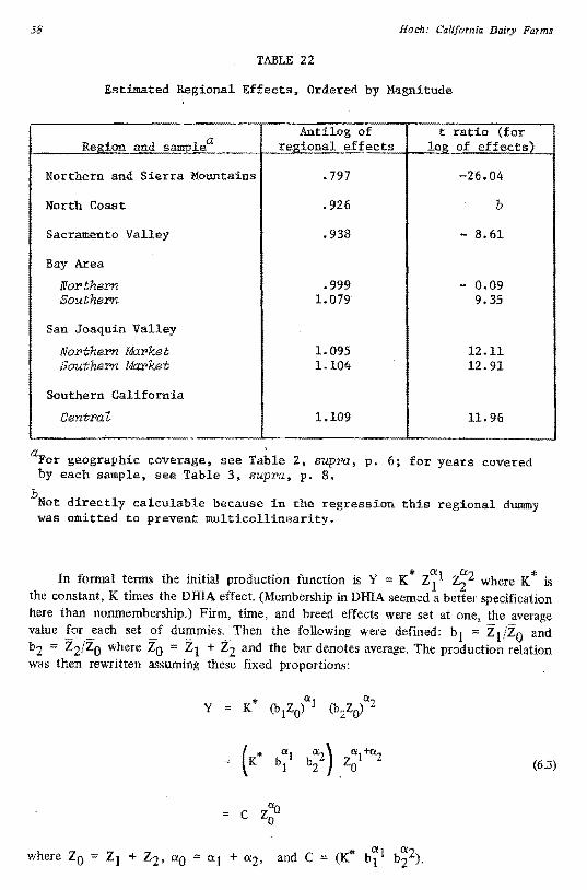
58 Hach: California Dairy Farms
TABLE 22
Estimated Regional Effects, Ordered by Magnitude
Region and sa~lea Antilog of
regional effects t ratio (for l~ of effects)
Northern and Sierra Mountains .797 -26.04
North Coast .926 b
Sacramento Valley • 938 - 8.61
Bay Area
Norther.in Southern
.999 1.079
- 0.09 9.35
San Joaquin Valley
Northern Market Southern Market
1.095 1.104
12.11 12.91
Southern California
Central 1.109 11.96
aFor geographic coverage, see Table 2, supra, p. 6; for years covered by each sample, see Table 3, supra, p. 8.
bNot directly calculable because in the regression this regional dummy was omitted to prevent multicollinearity.
In formal terms the initial production function is Y K* z71 z;2 where K* is
the constant, K times the DHIA effect. (Membership in DHIA seemed a better specification here than nonmembership.) Firm, time, and breed effects were set at one, the average value !_or yach set ~f du~mies:... Then the following were defined: = z1tz andb1 0 b2 "' Z2/Zo where Zo Z1 + z2 and the bar denotes average. The production relation was then rewritten assuming these fixed proportions:
(6.3)
= c z<Xo0

Giannini Foundation Monograph • Number 36 • July, 1976 59
Table 23 exhibits the data and parameter estimates for this transformed function. In all samples the ratio of feed to total expenditure is close to the state average of .584; in like fashion the ratio for all other input relative to the total is close to the state average of .416.
Given the log C and a0 estimates, some inferences were then drawn on comparative regional efficiency using the log version of the production relation: y = c + Cl'() z0, with lower case denoting log values.
In comparing samples, if a0 is approximately the same for a group of regions, then decreasing levels of c can be taken as indexes of decreased efficiency as shown in Figure 7. It can be seen that the plots of San Joaquin Valley (Northern and Southern Markets) are essentially coincident; they are above the Bay Area (Northern), which, in turn, is above the North Coast that, in turn, is above the Bay Area (Southern). This listing then is in order of decreasing efficiency.
Where a0 differs between samples, there are cases where both slope and intercept of region r are above corresponding values of region q so that, at any input level, more output is obtained in r than in q. This is exhibited in Figure 8 which indicates the following descending order of efficiency: San Joaquin Valley (Northern and Southern Markets), Sacramento Valley (Market), Sacramento Valley (Left survey), and Northern and Sierra Mountains.
Complications arise when a0 and c are such that fitted lines intersect. It might be argued that the point of intersection is a demarcation point, with one region more efficient below that point and the other more efficient above it, depending on which production line is higher. But this may well· be too literal an interpretation in a number of cases. Thus, the Sacramento Valley (Manufacturing) line is below most samples in the vicinity of its average level of expenditure; however, at high enough input levels, its line is above all other samples, reflecting its condition of increasing returns to scale. But it seems plausible that a0, in reality, is variable. It can be taken as stable in the vicinity of average input, i.e., within the range of most observations; but outside this range it is likely to change. For the manufacturing samples, average input is low and Cl'() is above one. It seems· likely that increasing input levels would be associated with an (eventual) decline in a0 to some level below one. Similarly, the Southern California samples have high levels of input and a0 well below one. It can be hypothesized that a substantial reduction in input would be associated with some increase in o:0. In short, one can interpret the data of Table 23 as suggestive of the classical S-shaped production function. Consider these figures on expenditure and elasticity sum from Table 23:
Average Sample expenditure Cl'()
Sacramento Valley (Manufacturing) $ 1,666 1.234 Bay Area (Northern) $ 4,033 .912 Southern California (Central) $11,305 .698
The illustration is made more concrete by Figure 9 which~plices together the antilog functions for these three samples.
In an attempt to make regional comparisons despite a (possibly) S-shaped function, samples were compared only "in the vicinity" of theif respective average expenditure using a linked index number approach. Samples were classified into groups based on average
TABLE 23 ct
Data and Parameter Estimates for Output as a Function of Total Expenditure: y z CZ 0
0 by Region and Sample
.Region and samplea
Average amount si>ent All other
Feed cost i'!E_UtS Total il!E_Ut
z1 z2 z0
z z1 + z2 dollars
Ratio to total ~enditure All other
Feed cost inputs
b1 z z/z0 b2 z z2/zo
Parameters of transformed function
l~g rf cxO
Sacramento V~~ley
Market Manufactz.a>ing Left SU!'VeiJ
2,251 970
1,592
1,646 696
1,219
3,897 1,666 2,811
.578
.582
.566
.422
.418
.434
-.538 -. 717 -.540.
,807 1.234
.765
Northern and Sierra Mountains 1,198 999 2,197 .545 .455 -.610 • 720
San Joaquin Valley
Norther>n Market Southern Mal"ket Manufact;uJ:>ing
2,936 2,865 1,221
1,906 2,016
846
4,842 4,881 2,067
.606
.587
.591
.394
.413
.409
-.508 -.516 -.672
.890
.911 1.085
North Coast 1,604 1,184 2,788 .575 .425 -.580 .902
Bay Area
Nor>thern Southern
2,410 3,012
1,623 2,141
4,033 5,153
.598
.585 .402 .415
-.577 -.590
.912
.898
Southern California
CentPaZ Per>ipherai
6, 792 5,672
4,513 3,915
11,305 9,587
.601
.592 .399 .408
-.370 -.271
.698
.576
,Simple average c .584 .416
l aFor geographic coverage, see Table 2, supr>a, p. 6; for years covered by each sample, see Table 3, supra, p. 8.
bLog C derived for fitted production function in which z and z2 were multiplied'by .001; Y was multiplied by .00001.1
cBlanks indicate not calculated.

61 Giannini Foundation Monograph • Number 36 • July, 1976
y 0.4
0.3
0.2
0.1
-0.1
-0.2
-0.3
-0.4
San Joaquin Valley {Southern Market)
San Joaquin Valley {Northern Market)
Bay Area {Northern)
Bay Area {Southern)
-0.6
FIGURE 7. Variations in Technical Efficiency for Cases With Approximately Same Slope for Output on Expenditures
62 Hoch: California Dairy Farms
y 0.4 Son Joaquin Volley
(Sout~ern Market)
Sacramento Volley 0.3 {Market)
Sacramento Valley (Left survey)
0.2
Northern and Sierra Mountains
0.1.
01--~~--'-~~~-'-~~--~--..,____.-+~~---~~~-'-~Zo
0.2 0.4 1.0 1.2
-0.1
-0.2 I
-0.3.
-0.4
-0.5
- 0.6
FIGURE 8. Variations in Technical Efficiency for Cases With Different Slopes and Nonintersecting Production Relations

300
250
200
100
50
Sacramento Valley (Manufacturing) function
2 3 4
Boy Area (Northern) function
5 6 7
Southern California (Central) function
8 9 10 11 12 13 14 15 16 17 18
0 g 150
c
>
FIGURE 9. S-Shaped Production Function Obtained by Combining Three Separate Functions
Zo(in 000)
64 Hoch: California Dairy Farms
input level. Within the group, output was evaluated at this average input level so that output ratios gave efficiency indexes within the group. Then, for between-group comparisons, a member of a given group had its output evaluated at the next higher group's average input level. In like fashion, a member of the higher group had its output evaluated at the lower group input level. An index number linking the two cases would then be defined; this, in turn, was the basis for comparing all members of the two groups.
Formally, let zor and zoq be the input levels for samples r and q, respectively. Then let:
c + Q'.yrr r r zor
Yrq Cf + ll'.r ZOq
Q'. (6.4)+Yqr cq ZOrq
Yqq cq + Q'.q ZQq
+YrrDefine index I
+ r,qYqr Yqq
Link indexes as necessary so that Ir,p = lr,q Iq,p·
Table 24 presents results obtained and indicates the levels of zor and zoq employed and the sample groupings used in constructing the linked indexes. Certainly, there is an arbitrary element in these results. However, there is fair correspondence with the earlier iridexes presented--the regional effects of Table 22. The ordering shown in Figures 7 and· 8 holds within Table 24. Finally, detailed inspection of plotted production lines yields the intuitive judgment that the indexes yield a rather accurate picture.
Inferences can be based on Tables 22 and 24 viewed in conjunction. In particular, it seems highly probable that the San Joaquin Valley regions are at least as efficient as the Southern California regions; and there is some indication that the former is more efficient than the latter.
Some implications of the results of this section are worthy of note. First, production and supply functions for a "large" area, such as a nation or state, can be biased by not accounting for a possible relation between scale and technical efficiency at the sub.area level. Introduction of subarea intercept shifters can account for such a relation, as demonstrated by the state milk production function here, and by the national agricultural output function estimated by Timmer (see Table 6).
Further, the techniques used here in estimating a state production function may have wider applicability. Thus, in estimating a national function, individual state functions might first be estimated employing cross-section and time series data on counties. Then county and time effects could be accounted for as were firm and year effects in equation (6.2). The national equation would then be estimated employing state effects. This recommended

65 Giannini Foundation Monograph • Number 36 • July, 1976
TABLE 24
Index of Efficiency Based on Linked Index Procedure by Region and Samplea
Redo~b and sample Index
Northern and Sierra Mountains .845
Sacramento Valley
Ma.nufrwtu:ring .917
San Joaquin Valley
Marw.factu:t'ing .937
Sacramento Valley
Left survey .938
Bay Area
Southern .963
North Coast .973
Sacramento Valley
Ma:t"ket .974
Bay Area
Northern 1.045
Southern California
Peripheral Centrat
1. 087 1.108
San Joaquin Valley
Northern Market SoutheP"fl Ma:t'ket
1.183 l.200
aSource of linked index:
Sample groupings
1. Sacramento Valley-Manufacturing San Joaquin Ve.J.ley--Manufaaturing
2, San Joaquin Valley--Manu.faaturing Northern and Sierra Mountains Sacramento Valley--Left survey North Coast
3. Sacramento Valley--Left l'!Ul'V'1l/ North Coast Sacramento Valley--Market
4. Sacramento Valley--Market San Joaquin Valley--Northe1'1'1 Market
5. San Joaquin Valley--North131'1'1 and Southern MaPkets Bay Area-Northern and Southe1'1'1
6. San Joaquin Valley--Southern Market Southern California--Central and Peripheral
°For geographic coverage, see Table 2, supra, p, 6.
$1,500 and $ 2,000
$2,000 and $ 3,000
$3,000 and $ 4,000
$4,000 and $ 5,000
$5,000 only
$5,000 and $10,000

66 Hoch: California Dairy Farms
procedure could be qualified if there are marked differences in estimated coefficients between sets of initial equations. In this case slope shifters, as well as intercept shifters, might be introduced. Thus, in the national function a particular slope shifter might be specified as common to a set of states whose coefficient estimates fell within a given range. In general, the suggested stepwise estimating procedure could make economic, or even possible, the fitting of equations with large numbers of dummy variables.
On a substantive level, the estimated differences in technical efficiency by region could be of interest both in marketing applications and in location analysis. There is a tradition of concern with spatial economic relationships in agricultural economicsl as well as in such disciplines as economic geography, regional science, and urban and regional economics. In the present set of results, the range of regional variation is substantial, with the ratio of highest to lowest efficiency index on the order of 1.4 (1.38 is estimated from Table 22 and l.42 from Table 24). This indicates that substantial regional variation in supply response can occur to a given price stimulus.
How can such regional variation be explained? Some speculations can be presented at this point, but serious development and testing of explanatory hypotheses await future effort. The results of Tables 22 and 24 suggest a general tendency for efficiency to increase in a southward direction. This could reflect natural conditions such as climate and topography. Other possible explanations include such factors as proximity to a major market, size of that market, and rate of urbanization. Thus, the Northern and Sierra Mountains and the North Coast region are the furthest from a major market and have the lowest efficiency indexes. Again, the Southern California efficiency index exceeds the Bay Area index, in turn above that of the Sacramento Valley, corresponding to the size of the major market in each case (Los Angeles versus San Francisco versus Sacramento). The San Joaquin Valley cases perhaps do not fit in this array very well since their efficiency approaches that of the Southern California cases; yet, perhaps it is of some significance that the San Joaquin Valley (Southern Market) producers have a slightly higher efficiency index than the San Joaquin Valley (Northern Market) producers, possibly reflecting shipments to the Los Angeles rather than the San Francisco market.
If proximity and size of market are factors explaining regional differentials, how do they come into play? What mechanisms are at work? One likely underlying relationship is an increased capacity for specialization as size of market increases. The part-time nature of northern region operations was noted earlier and illustrates the point since producers there cannot specialize fully to milk production. Again, there may be indivisible capital items that can be properly utilized only with large farm size, in turn a possibility only with a large enough market.
Theodore W. Schultz has hypothesized that efficiency of the farm sector increases with proximity to metropolitan markets.2 His argument is that flows of information improve, and capital and labor markets work better as such proximity increases. The argument was presented as an explanation .for low income in isolated rural pockets, such as Appalachia and Northern Michigan, relative to efficient, high-income areas such as
lThis .is exemplified by Raymond G. Bressler, Jr., and Richard A. King, Markets, Prices and Interregional Trade (New York: John Wiley & Sons, Inc., 1970), 426p.
2Theodore W. Schultz, The Economic Organization of Agriculture (New York: McGraw~Hill Book Company, Inc., 1953), Chapters IX, X, XVII, and XVIII.

Giannini Foundation Monograph • Number 36 • July, 1976 67
Iowa. Perhaps it is of some relevance in the present context as well. It would have to be argued that the presumed institutional factors at work (information and better market organization) show up at the individual farm level as a determinant or component of management, shifting the production function accordingly.
An alternative line of explanation might involve the notion that observed regional differences are the result of an evolutionary process in which there is a greater winnowing out of less-efficient producers or greater selection of more efficient producers, the larger the market. The argument would run: as the market increases, the optimum size of the firm increases, in turn calling for greater entrepreneurial capacity. Hence, better managers will gravitate to the larger markets, and lower quality managers will remain behind or shift back to smaller "hinterland" markets.
Finally, there is a good deal of evidence available that equilibrium wages for any . given occupation increase with metropolitan population size, explainable as compensation for increased cost-of-living with urban size, including the effect of higher land rent with size. I It is conceivable that this cost-of-living differential influences returns in agriculture near metropolitan areas, as well as wages in urban occupations, so that higher returns to farm operators become necessary the larger the nearby urban market.2 Higher returns at equilibrium would be consistent with higher levels of technical efficiency.
The absence of much differential between the San Joaquin Valley and Southern California calls for an explanation, given the previous speculations. An explanation might include the following: ( l) Milk regulation has been less "protectionist" for the San Joaquin Valley region than for Southern California (Section 1 and Table 25), perhaps allowing or even generating greater competitive pressures inducing efficiency in the former region, and (2) urbanization may yield benefits to the entrepreneur and yet impose costs on the enterprise. In particular, a number of dairy farmers in the Southern California sample relocated their enterprises during the period of the survey, having sold the original farms to suburban developers. Such shifts were no doubt profitable to the entrepreneurs, but the dairy enterprises might well have borne some costs of relocation, reducing technical efficiency in the production functions.
These speculations are indicative of the kinds of hypotheses that might be tested, given the evidence on technical efficiency differences by region and their likely relation to proximity, size, and growth of metropolitan markets.
7. PROFITS AND ALWCATIVE EFFICIENCY
The preceding section compared the technical efficiency of production functions between regions. This section will compare the allocative efficiency of the average producer between regions.
1see, for example, Victor R. Fuchs, Differentials in Hourly Earnings by Region and City Size, 1959, National Bureau of Economic Research, :Occasional Paper 101 (New York, 1967); and Hoch, "Income and City Size," Urban Studies, Vol 9, No. 3 (October, 1972), pp. 299-328.
2Gary Elsner and Irving Hoch, Analysis of California Farm Income Relation;hips, University of California, Giannini Foundation Research Report No. 297 (Berkeley, 1968). It was found that per family income of a county's farm population increased with urbanization, measured both by percent of county population that was urban and distance to an urban settlement.

68 Hach: California Dairy Farms
TABLE 25
Average Cost, Revenue, and Profit Per Farm Per Month by Region and Sample 1962-1964 Base
Aver~e...l2_er farm per mon~ All Price
other I Feed input Total Milk Profit/i nu~:;;;aReg;l.on and samplea weicost cost" cost output Revenue Profit revenue
hundred...<:!Qllars dollars
Sacramento Valley
weight
2,251 3, 938 888.0 4.6930 4,167 229 .055M=ket 1,687
970 715 1,685 374.0 3.2490 1,215 - 470 -.387Ma:nufaatwing
1,592 1,255 2,847 579.2 4. 6930Left su:evey 2, 716 - 129 -.047
Northern and Sierra Mountains 1,020 2,218 428.1 5.3694 2,299 811,198 .035
San Joaquin Valley
Nol'the'r'n M=ket 2,936 1,973 1,223.0 4.2218 5,163 254 .0494,909
2,865 2,080 1,219.0 4.2218Southe:t'r! Market 4,945 5,146 201 .039
1,221 889 3.3535Ma.nufr:zaturing 2,110 482.0 1,616 - 494 -.404
North Coast 1,604 1,220 2,824 650.1 4.0786 2,651 - 173 -.065
Bay Area
1,675 1,076.0 4.690cf 5,046 961 .190Northe:t'n 2,410 4,085
3,012 2,189 1,186.0 4.7500Sotdher>i 5,201 5,634 433 .077
' Southern California
6,792 4,586 11,378 2, 371. 0 5.4655 12,959 1,581 .122CentraZ
5,672 3,962 1,876.0 5.4655 10,253 .060PeripheraZ 9,634 619
aFor geographic coverage, see Table 2, ~pra, p. 6; for years covered by each sample, see Table 3, supra, p. 8.
bAverages are geometric meaus. Prices are on a 1962-1964 base.
"Deflated geometric mean of "all other cost" used in regression plus artificial insemination costs calculated as 64 cents times number of cows. The latter item eompr1ses about 4 percent of the other cost figure and about 2 percent of total cost, (Exact amount is the difference between "other cost" here and in Table\23.) "All other cost" in regression was on 1964 price base, deflated here to 1962-1964 base by scalar of .98.
dFrom Bureau of Milk Stabilization data on areawide average prices for 1962, 1963, and 1964. Price refers to milk with 3.8 percent butterfat content.
sample, market milk accounted for 96 percent of total production, and manufacturing milk accounted for 4 percent of total. Price employed is weighted average of niarket milk price ($4.75) and manufacturing milk price ($3.22),
69 Giannini Foundation Monograph • Number 36 • July, 1976
Profits, Factor Shares, and Marginal Returns
Table 25 lists costs, revenue, and profit per month by region and sample, with prices on a 1962-1964 base. Revenue was estimated by multiplying average output by the average milk price listed for the region by the BMS. Table 25 documents the assertion made earlier that there were marked differences in price between manufacturing and market milk and between regions for market milk.
Both manufacturing milk samples had large losses relative to sales. This seems consistent with the estimate of returns to scale above one which occurred in both cases. If producers pay inputs their value of marginal product, then profits will be negative given increasing returns to scale. However, there may have been some overstatement of the cost. of labor and capital on the manufacturing farms. Insofar as these factors are specialized to dairy production, their "salvage" value may be considerably below their acquisition cost. I To put this another way, instead of interpreting negative profit solely as returns
to the entrepreneurial input? it can be viewed as being spread over all factors fixed to the farm including specialized labor and capital as well as the entrepreneur.
The left survey sample of the Sacramento Valley also had negative average profits in contrast to the positive profits for the market milk sample. A number of producers in the former sample left the survey by virtue of selling their farms; it seems plausible that some sold out because of negative profits. The North Coast sample also had negative profits, and this result is not as easy to explain as that of the previous cases. It may be that, because the dairy enterprise was often a part-time occupation here, 'fairly low levels of efficiency prevailed. A related hypothesis is that imputed family wage rates may have been overstated. All other samples had positive profits, with highest profits (both in absolute level and relative to revenue) occurring for the Southern California and Bay Area samples. Estimated profits for the San Joaquin Valley market milk samples were relatively low, probably reflecting the relatively low milk price prevailing in the region.
The cost and revenue data of Table 25 can be employed to obtain estimated production function elasticities, using Klein's factor share method (equation 3.2), which imposes the assumption that profit maximization holds exactly.2 Because profits are generally positive, the factor-share elasticity sum is generally less than one. The factor share elasticities were compared to the before and after firm effect estimates of Table 7. It turned out that the after elasticities were generally closer than the before elasticities;
thus, for the 10 market milk cases, 15 of the 20 comparisons favored the after elasticities. (fhe comparisons ran 9 to 1 for feed and 6 to 4 for other input.) The averag~ deviations between the sets of estimates were:
1For a general discussion of salvage value versus acquisition cost of factors in agriculture, see Dale E. Hathaway, Government and Agriculture: Economic Policy in a Democratic Society (New York: The Macmillan Company, 1963), pp. 118-130.
2Factor share estimates for the five inputs of Equation (5) are presented in Appendix Table B.3, infra, p. 141. The feed elasticity there is exactly that obtained for the feed elasticity here .. The sum of other elasticities is typically .02 to .03 below that for "all other input" here; this occurs because geometric means are used in both applications.

70 Hoch: California Dairy Farms
Feed All other input
Before minus factor share .198 -.117 After minus factor share -.026 -.115
Thus, the after estimates are closer to a situation of profit maximization than are the before estimates, although the shift toward maximization is concentrated in the feed results.
To test for maximization, rather than imposing it by assumption, the equality of "marginal returns" to one is tested. Marginal returns (M$) is defined as value of marginal product divided by factor price; at equilibrium, ma~gin~l returns sho~ld just equal one, i.e., an increment of a dollar's worth of any input will yield $ l .00 of mcremental return.
In fonnal terms,
Pz.l is the VMP equals price. cond~tion for the Cobb:-D~uglas case ~ where Y is output and Zi 1s any mput, and the equat10n.
restates the condition in terms of VMP per dollar of input
Table 26 presents (I) estimates of marginal returns for feed and nonfeed inputs, respectively, by sample; (2) results for tests of the hypotheses that marginal returns equal one for each factor in each region; (3) the 95 percent confidence interval for each marginal returns estimate; and, finally, (4) the ratio of feed and nonfeed marginal returns.
The criterion that marginal returns equal one is a condition for profit maximization only when. returns to scale are below one; in situations of increasing returns to scale, the condition corresponds to profit minimization. Strictly speaking, then, the criterion is not meaningful for the manufacturing milk cases.
The hypothesis that marginal returns equal one was accepted for both feed and nonfeed inputs in only 2 of the 10 market milk cases--North Coast and Bay Area (Southern). It was accepted for feed but rejected for nonfeed inputs for both Southern California samples and for the Northern and Sierra Mountains samples. In all three cases, estimated returns to nonfeed inputs were below one. The opposite result occurred for both Sacramento Valley (Market and Left survey) samples, with the hypothesis accepted for nonfeed but rejected for feed, and with marginal returns for the latter below one. This pattern of acceptance and rejection also held for the Bay Area (Northern); but here the marginal returns to feed were above one. Finally, the hypothesis was rejected for both inputs in the San Joaquin Valley (Northern and Southern Market) samples, with marginal returns to feed above one and marginal returns to nonfeed below one.
The criterion that the ratio of marginal returns equals one is a firm decision rule corresponding to maximization subject to some constraint on output or cost (and is a more general criterion than VMP equals price). This criterion appears to have been met for 5 of the 12 samples.

f5l TABLE 26
Indicators of Allocative Efficiency for Feed and Other Inputs, by Region and Sample
Region and samplea 1
Sacramento Valley
Market Manufaatia-ing Left sl./I"Vey
Northern and Sierra Mountains
San Joaquin Valley
Northern Market Southern Ma:roket Manufaaturinf!
North Coast
Bay Area
Northern Southern
Southern California
Central. Peripheral
Average:
10 market samples
Estimated marginal returns er dollar ex enditureb
M$ (feed)1
0.610' 1.180 0.442
1.142
1
1.247 1.322 0.891
0.843
1.141 1.078
0.923 0.848
0.960
aFor geograph~c coverage, see Table 2, supra, p.
M$ 2 (all other inputs)
1.164 0.520 1.151
0.294
0.500 0.456 0.803
0.896
1.165 0.865
0.627 0.286
0.740
Test of hypothesis of allocative efficienc 0
H [M$1 l] H [M$2 l]
R R R
A
R R A
A
R A
A A
d
A R A
R
R R A
A
A A
R R
(feed)M$1
0.516-0.704 1.008-1.352 0.234-0.650
0.962-1.322
1.154-1.340 1. 227-1. 417 o. 761-1.021
0.610-1.076
1. 013-1. 269 0. 932-1. 224
0.807-1.039 0.642-1.054
0.810-1.110
at
0.957-1.371 0.112-0.928 0.762-1.540
-0.004-0.598
0.331-0.669 0.226-0.636 0.528-1.078
0.359-1.433
0. 790-1. 540 0.570-1.160
0.410-0.844 -0.123-0.695
0.428-1.049
95 percent confidence interval for:
6; for years covered by each sample, see Table 3, supPa, p. 8.
Allocative ro ortions
M$1/M$2
0.524 2.269 0.384
3.884
2.494 2.899 1.110
0.941
0.979 1.246
1.472 2.965
1. 297
a ~
ci1 $;'.;, §6· ;,
~ ;,
~ 01 ].
'.<: $;'.
~
""'~ '"" °' ~ ~ ._ 'O .... °'
bM$ = value of margina1returns divided by price of factor. Thus, let Z1 and Y be input and output and Pzi and Py be respective prices, with ai the Cobb-Douglas e!asticity. Then, M$1 (Y Py/Z1P21) and measures the marginal return to a dollar's worth of input i.a 1
aH [M$ = 1] means test of hypothesis that marginal returns equal 1. "A" denotes accept hypothesis, and "R" denotes reject hypothesis.
dBlanks indicate not applicable.

72 Hoch: California Dairy Farms
As suggested by the factor share results, allocation for the feed input seems generally
better than for nonfeed. This is 'indicated by the average of marginal returns over the
10 market samples, which is close to LOO for feed (.960), and a fair amount below 1.00 for nonfeed (.740). In the IO samples, marginal returns are within .25 of 1.00 for 7 of the feed cases but for only 5 of the nonfeed cases. Only one feed result deviates by more than .40 from 1.00, as opposed to four of the nonfeed cases, with all of these below 1.00. As a general impression, then, it seems that allocation for feed is usually close to optimal, while the levels of nonfeed inputs are often above the optimum, eventuating in low marginal returns.
During the period under study, observers of the dairy market sometimes hypothesized that farms expanded production more than would normally be economic in the expectation of increasing their market milk base in future milk price determination. In short, the individual producer would expect a higher future milk price if he expanded production in the current period; long-run profit maximization would then call for higher levels of input than would be economic at current prices. This hypothesis may have some applicability but, at best, further embellishment seems necessary. Thus, feed is a currently purchased input, while nonfeed includes a number of fixed components. This leads to the speculation that expansion occurred on the basis of past expectations and was no longer supported by current expectations. (If the latter were the case, both feed and nonfeed inputs would be too high.) Low marginal returns are pronounced for the Southern California samples, and it is of interest that Table 10 shows some contraction in output over time for the average firm in those samples which is consistent with movement toward
equilibrium.
A more mundane factor that may be involved in the results is a possible overstatement of the value of family labor and capital. However, in the Southern California samples, most of the labor input is hired labor, so any error in imputation is likely to be unimportant
in those cases.
There is enough variation between regions to suggest that each region operates under somewhat different constraints affecting profit maximization; this interpretation is supported by the consistency of results for pairs of samples from the same region.
On the whole, the pattern of results for marginal returns seems to square fairly well with economic intuition, with a large number of cases "close" to 1.00 and with the remaining cases having fairly plausible magnitudes. This conclusion can be given more substance hy presenting the weighted average deviation from optimality for each sample. For each input, the absolute deviation of marginal returns from one was. multiplied by the fraction of total cost devoted to that input, and the products were then summed. (Over the I 0 market milk samples, the respective fractions averaged .583 for feed and .417 for all other input, with little variation between samples; see Table 23 above.)
For the market milk samples, these average deviations were obtained:

Giannini Foundation Monograph • Number 36 • July, 1976 73
Average deviation
Sacramento Valley (Market) .293 Sacramento Valley (Left survey) .379
Northern and Sierra Mountains .401
San Joaquin Valley (Northern Market) .349 San Joaquin Valley (Southern Market) .415
North Coast .134
Bay Area (Northern) .151 Bay Area (Southern) .102
Southern California (Central) .196 Southern California (Peripheral) .383
'"('he average of the 10 samples was .28; that is, on the average, firms deviated from the optimal position by 28 percent, expressing both situations of too little and of too much input. The range was .102 to .415, with the Bay Area and North Coast having the highest allocative efficiency and the San Joaquin Valley (Southern Market) having the lowest (defined as least and greatest deviation from optimality). The San Joaquin Valley (Northern Market) result is close to the San Joaquin Valley (Southern Market) value; hence, the hypothesized effect of expansion on the basis of past expectations appears to have strongest expression in the San Joaquin Valley region.
Equation 3 Results
Additional inferences on allocative efficiency were based on results for Equation 3 in which output was regressed on the aggregate of feed and nonfeed inputs. The form employed was Y = K* z3<J, where is all input in dollar terms and Cl'() is thez0 corresponding elasticity. (The aggregate of inputs is the arithmetic sum of feed input, z1, and nonfeed input, z2 in dollars; K* includes the constant term and the various dummy variable effects.) The estimates for a0 appear in Table 27 and, not surprisingly, are quite similar to the elasticity sum for Equation 1 as shown in Table 8. However, there is some tendency for o:o to be somewhat above the ~<X of Equation 1. This is so for 10 of the 12 samples; for the market milk samples, Cl'() averages .837 while ~<X averages .808.
Equation 3 permits simple tests1 of the hypothesis of constant returns to scale (or Cl'() = 1).2 The hypothesis was rejected for both manufacturing samples (with returns to scale above one) and for most market milk samples (with returns to scale generally below one), though the hypothesis was accepted for the Bay Area and the San Joaquin Valley (Southern Market) samples.
1Such tests could have been carried out for the two-variable case without much effort given the appropriate inverse matrix. But the inverse matrix was generally of a very large order (up to 100 x 100) and was not obtained explicitly because of its cumbersome features.
2cconstant returns to scale is not consistent with profit maximization, including const~ained profit maximization, unless certain highly restricted price relations hold. Returns to scale below lis consistent with maximization.

74 Hoch: California Dairy Farms
pothesis of constant
Regiona and Elasticity • returns
TABLE 27
Results for Equation 3 (Output on Aggregated Input) by Region and Sample
Test of hy-1 1 Test of by-
allocative returns • efficiency
M$ H [M$ = l]dsample al Sacramento Valley
.844Market 1.425Manuf ac:-turing
. 721 Left SUI'Vey
Northern and Sierra Mountains .806
San Joaquin Valley
.908Northern Market Southern Market . 992
1.115Manufac:turing
North Coast .908
Bay Area
1.022Northern Southern .926
Southern California
Central . 728 .513Peripheral
Average and total:
10 market samples .837 J 2 manufacturing
samples 1. 270 I
a
H Ia = lJc:0
R R R
R
R A R
A
A A
R R
6R, 4A
2R
. Estimates pothesis ofJof marginal •
0.881 R 1.039 A 0.698 R
0.843 R
0.968 A 1.045 A 0.872 R
0.863 A
1.279 R 1.013 A
0.834 R 0.549 R
0.897 6R, 4A
0.956 R, A
For geographic coverage, see Table 2, supra, p. 6. ct°, where z
Test of hypothesis that elasticity, equals 1. "A" denotes accept
bctO is the elasticity in the equation Y = K* z0
gate of all inputs in dollar terms, and K* includes the 0
is the aggreconstant term
and the various dummy variable effects.
c: a 0 ,
hypothesis and "R" reject hypothesis,
dTest of hypothesis that marginal returns equals 1. "A" denotes accept hypothesis and "R" reject hypothesis.

75 Giannini Foundation Monograph • Number 36 • July, 1976
Table 27 also shows estimates of marginal returns and results for tests of the hypothesis that marginal returns equal 1.00. This was seen as a means of posing the question of allocative efficiency for level of total inputs (which disregards the question of input proportions, considered earlier). For the 10 market milk samples, the hypothesis was accepted for four cases: the San Joaquin Valley (Northern and Southern Markets), the Bay Area (Southern), and the North Coast. (If these results are considered in conjunction with those of Table 26, it can be seen that the hypothesis of proper proportions is accepted for the latter two cases whereas, in the San Joaquin Valley cases, too much other input "balances" too little feed.) The Bay Area (Northern) had marginal returns above LOO, indicating total input levels were below the optimum, while the other five samples had marginal returns below 1.00, indicating total input levels above the optimum. For this latter set of cases, the previous discussion (interpreting this result in terms of possible long-run maximization) is again applicable; but the problem seems somewhat less pronounced, reflecting the higher values for relative to :re.: in Equation 1.a0
This section has considered a number of aspects of allocative efficiency. A summary and integration of results can be attempted by ranking the 10 market milk samples in terms of profits and closeness to attainment of optimality. Table 28 presents such rankings for the two measures of profit--total profit and profit relative to revenue--and for four measures of proximity to optimality, each based on how close a marginal return estimate is to one. The last two columns of Table 28 present the mean rankings for profit and optimality, respectively. The Southern California and Bay Area samples show the most profits, while the Bay Area, North Coast, and Southern California (Central) samples are nearest to optimality. Some relatlon between profit and proximity to optimality can be discerned, although the North Coast shows good allocation and poor profits, probably reflecting a relatively low blend price (Table 25) and relatively low technical efficiency (Section 6). Stated more generally, considerable differences in blend price and in technical efficiency between samples will limit the relation between profit and proximity to optimality.
8. SOME SIDE INVESTIGATIONS
A number of side investigations, covering preliminary, experimental, or special situations, were carried out in the course of this work. Some brief mention of results for these cases seems worthwhile, not only in terms of explicit recognition of negative or peculiar results in some of the preliminary efforts but also by way of suggesting future lines of inquiry and developing clues for additional inferences in the present study.
The discussion here will cover Equations 4 through 8. Previous sections have covered results for Equation 1 (viewed as the primary vehicle of investigation) and for Equations 2 and 3 (which yielded information pertinent at earlier points in the report).
Appendix B contains some material supplementing the discussion of the cases in this section, and the statistical supplement to this report con.tains additional tables on the equations of this section.
Equation 4 Results
Equation 4 involves an experimental extension of Equation 1. Feed is disaggregated into two inputs: (I) concentrates and (2) roughage plus pasture, with all inputs in dollar terms. Results were obtained for two major samples of primary interest--San Joaquin Valley (Northern Market) and Southern California (Central). These results were encouraging
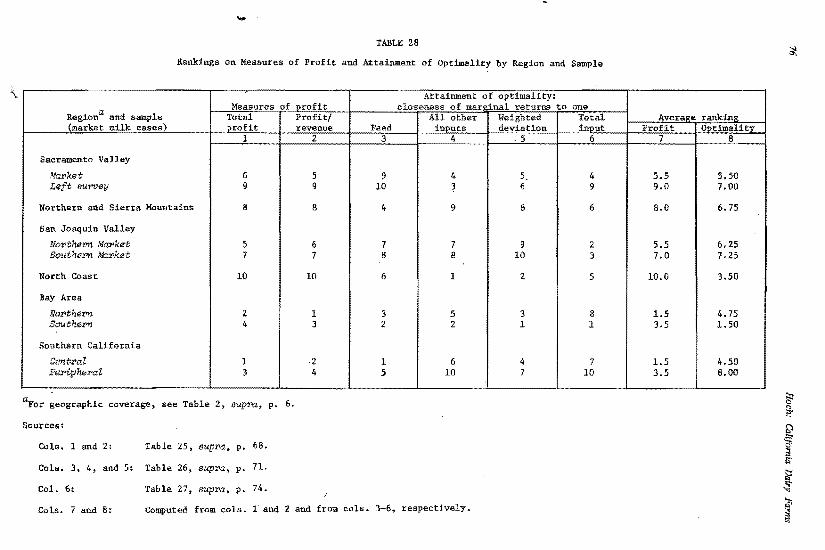
TABLE 28
Rankings on Measures of Profit and Attainment of Optimality by Region and Sample
\ Measures of
Regiona and sample Total (market milk ...<!ases} refit
1
Profi reven
2 4
Sacramento Valley
Market 6 5 9 4 Left 8Urvey 9 9 10 3
Northern and Sierra Mountains 8 8 4 9
San Joaquin Valley
Nol'fhe:rm Ma:Pket 5 6 7 7 Southern Market 7 7 8 8
North Coast 10 10 6 1
Bay Area
NoPthern z 1 3 5 Sau.them 4 3 2 2
Southern California
CentPal l 2 1 6 Periphe:ruZ 3 4 5 10
~or geographic coverage, see Table 2, supPa, p. 6.
Sources:
Cols. 1 and 2: Table 25, sup:ra, P• 68.
Cols. 3, 4, and 5: Table 26, supra, p. 71.
Col. 6: Table 27' supra, p. 74.
5 6
8
9 10
2
3 1
4 7
4 9
6
2 3
5
8 1
1 10
Avera Profit
7
5.5 9.0
8.0
5.5 7.0
10.0
1.5 3.5
1.5 3.5
e rankin timalit
8
5.50 1.00
6.75
6.25 1.25
3.50
4.75 1. 50
4.50 8.00
s: " ~ !? § ~ ;;·
~ ~ ;si
Cols. 7 and 8: Computed from cols. 1 and 2 and from cols. 3-6, respectively. ~

77 Giannini Foundation Monowaph • Number 36 · • July, 1976
and indicate the feasibility of using this equation for other samples and, perhaps, of further disaggregation of the feed input.
Table 29 presents elasticity estimates for Equation 4, before and after firm effects were introduced, and compares the latter to corresponding elasticities obtained for Equation 1. Equation 4 results exhibit the by now usual pattern for the market milk samples of a decline in elasticity sum with the introduction of the firm effects. For that case Equation 4 elasticity sums are about the same as those for Equation 1. In both samples this reflects similar magnitudes for the sum of the feed elasticities of Equation 4 and the feed elasticity of Equation I. Somewhat surprisingly, the elasticity for all other input shows considerable variation betw~en Equations 1 and 4. Part of this may reflect the hi~er standard error for that variable as indicated by the t values shown in Table 30. The R values are the same for the two equations (to three decimal places), but Equation 4 shows an increase in number of significant firm effects relative to Equation l, indicating some improvement in differentiating levels of technical efficiency.
In both samples the roughage and pasture elasticity is greater than the concentrates elasticity, but proportions differ. In the San Joaquin Valley sample, the roughage and pasture elasticity is 1.67 times the concentrates elasticity, but that ratio is only 1.18 for the Southern California sample. This probably reflects differences in production operations between the two areas; for example, there is very little use of pasture in Southern California.
Besides the t values (which are all significant), Table 30 presents marginal returns measures for Equation 4, including estimates, tests for optimality, and confidence intervals. Equation 1 estimates are also presented for purposes of comparison.
The marginal returns estimates for the feed inputs exhibit great consistency within each sample. In the San Joaquin Valley sample, both feeds have estimated marginal returns above 1.00, and there is rejection of the hypothesis that this measure is 1.00 in each case. In the Southern California sample, both feeds have marginal returns very close to LOO, and the hypothesis of equality to l.00 is accepted for both.
In both samples marginal returns for each of the disaggregated feed inputs are of similar magnitude, in turn close to that for aggregate feed in Equation 1. Hence, it can be inferred that feed proportions are at or near optimality and that aggregation caused little or no distortion in these cases. (The equality of the respective marginal returns in each sample is necessary for suboptimizing with respect to feed inputs; the criterion of VMP ratios equal to price relatives is a more familiar statement of the equality of marginal returns condition.)
Finally, in both samples marginal returns for nonfeed inputs are below 1.00, and the hypothesis of equality to LOO is rejected in both cases; these results are the same as those obtained in Equation I.
Equation 5 Results
Equation 5 was the initial equation employed chronologically. Using a Cobb-Douglas form, milk was regressed on feed in TDN, cow service flow, wages, operating cost, and capital service llow. The dollar aggregate of the four nonfeed inputs was the "all other cost" input of Equation 2 and then of Equation I.
Before the firm dummies were introduced, the estimated elasticity sum for Equation 5 was generally quite close to that of Equation 2, with the l 0 market milk samples having

78 Hoch: California Dairy Farms
TABLE 29 ,
2Estimated Elasticities and R Values in Equation 4 Before and After Firm Effects Introduced, and in Equation 1 After Firm
Effects Introduced for Two Major Regions
Re11iona and measure
San Joaguin Vallei
Southern Ma.rket
Elasticities for:
Roughage and pasture Concentrates All other inputs Total feed Total input
R2
Number of significant firm effects
Southern California
Central.
Elasticities for:
Roughage and pastureJ Concentrates All other inputs Total feed Total input
R2
Number of significant firm effects
Eq_uation 4 Before firm
effects introduced
.563
.297
.155
.860 1.015
.974
.456
.375
.190
.831 1.021
.966
After firm
effects introduced
.427
.256
.212
.683
.895
.984
29
• 283 .239 .116 .522 .638
.981
45
Equation 1 After firm
effects introduced
b
.175
.736
.911
.984
25
.214
.484
.698
.981
41
aFor geographic coverage, see Table 2, supra, p. 6; for years covered by each sample, see Table, 3, supra, p. 8.
bBlanks indicate not applicable.

TABLE 30
Estimates of Marginal Returns and t Values in Equation 4 by Region and Input
Regiona and i!!P_ut t value for elasticity
Equation 4
Estimates Test of hyof pothesis of
marginal allocative returns efficienc:_y_
M$ H [M$ = .tJD
95 percent confidence intervals for esti
mated marginal returns
E_g_uation 1 Est:iJllates Test of hy
of pothesis of marginal allocative returns efficiency
M$ H [M$ = lJD
San Joaguin Vallex
Southern Market
Roughage and pasture
Concentrates
20.os*
20.23*
1.328
1.148
R
R
1.199-1.457
1.037-1.259 } 1.322~ R
All other inputs 6.13* 0.541 R 0. 368-0. 714 0.456 R
Southern California
Central
Roughage and pasture
Concentrates
13.09*
11.49*
1.012
1.005
A
A
0.861-1.163
0.834-1.176 } 0.923° A
All. o_ther inputs 3.31* 0.357 R 0.146-0.568 0.627 R ,
aFor geographic coverage, see Table 2, supra, p. 6; for years covered by each sample, see Table 3, supra, p. 8.
bTest of hypothesis that marginal returns equal 1. "A" denotes accept hypothesis, and "R" denotes reject hypothesis.
0 Estimate for total feed (aggregate of roughage and pasture plus concentrates).
*Statistically significant at the 5 percent level.

80 Hach: California Dairy Farms
averages for this sum of 1.049 and 1.056 for Equation 5 and Equation 2, respectively. With the introduction o'f the firm effects, there was a tendency for the elasticity sum to decline in both cases, but this was much less pronounced for Equation 5 than Equation 2, the respective market milk averages here being .977 and .818. Elasticity sums by individual sample are presented in Table 31. It would appear there is greater variability for Equation 5 than for Equation 2 after firm effects are introduced.
The individual elasticity estimates for Equation 5 exhibited a number of peculiarities (including some negative values) and some striking shifts in magnitude given the introduction of the firm effects. Some flavor of the results is given in Table 32 which exhibits the San Joaquin Valley (Southern Market) and Southern California (Central) cases. Appendix Table B. l presents all of the elasticities for Equation 5, and the Statistical Supplement presents corresponding standard errors and t ratios.
The general pattern of results can be inferred from Table 33 which presents averages and aggregates over the 10 market milk samples. With the introduction of the. firm effects, elasticities fell for feed, labor, and operating costs and rose for cow service flow and capital service flow. Before the firm effects, marginal return estimates tended to be at optimal levels for labor and operating costs, somewhat above the optimal for feed, and well below the optimal for cow service flow and capital service flow. The introduction of firm effects reversed relationships, with marginal return estimates for cow and capital service flow very much above optimal levels, while marginal returns for the other three inputs were generally below optimality, with a majority of cases significantly below LOO.
A careful examination of the individual results (as presented in Appendix B and in the Statistical Supplement) suggests there was a pronounced problem of multicollinearity between feed and cow service flow (and, perhaps, capital) after firm effects were introduced. In many of the cases, it can be inferred that part of the feed elasticity has appeared as a component of cow service flow (and, perhaps, of capital as well). Thus, in Equation 5 the elasticity and marginal return for feed is generally below that for Equations 1 and 2. This occurs in 10 of the 12 cases; in 3 of those cases, the feed elasticity in Equation 5 is less than half that of the other two equations. Over the IO market milk samples, the following are the average feed elasticities obtained:
Before After fv:m effects firm-effects
Equation 1 .745 .521 Equation 2 .754 .564 Equation 5 .749 .410
Although the average decline in elasticity in feed is relatively modest, on the order of 25 percent for Equation 5 relative to Equation 2 (with feed measured in TDN in both cases), a shift of the absolute value involved from the feed to the cow and/or capital service flow elasticity would explain the very high marginal returns for the latter factors, given the much lower input level of the latter inputs (as shown in Table 33 and Appendix Tables B.2 and B.3). Further, the hypothesis of multicollinearity is supported by the occurrence of large standard errors and by highly variable estimates between samples for the two service flow variables.
An additional concern is the possibility of an extraneous linear relationship between output and cow service flow, seen as a particular case of raw materials bearing a fixed proportion to output, and becoming of importance here only after firm effects were
81 Giannini Foundation Monograph • Number 36 • July, 1976
TABLE 31
Comparison of Estimated Sums of Elasticities for Equations 2 and 5 Before and After Firm Effects Introduced
by Region and Sample
Estimated sum of elasticities ~uation 5 E_guation 2 ~uation 5 ~uation 2
Before firm effects After firm effects Region and samp1ea introduced introduced
Sacramento Valley
Market 1.032 1.074 1.119 0.840
Manufaaturing 1.138 1.133 1.205 1.207
Left survey 1.045 1.042 0.780 0.734
Northern and Sierra Mountains 1.069 1.082 1.247 0.764
San Joaquin Valley
NortheI'n Ma.I'ket 1.031 1.030 1.059 0.922
Southern Market 1.039 1.044 0.972 0.943
Manufaaturing 1.103 1.096 1.347 1.080 -
North Coast 1.006 0.993 0.958 0.963
Bay Area
Northern 1.094 1.111 0.746 0.868
Southern 1.062 1.089 1.209 0.894
Southern California
Central 1.008 1.017 0.931 0.695
Peripheral 1.103 1.078 0.748 0.559
aFor geographic coverage, see Table 2, supI'a, po 6; for years covered by each sample, see Table 3, supra, po 8,

---
82 Hoch: California Dairy Farms
introduced. This is highly speculative, of course, but it might explain why the elasticity sum here remained close to 1.00 after firm effects were introduced. In any event, the results seemed suspicious enough to justify the substitution of Equation 1 as the primary vehicle of investigation.
TABLE 32
Comparison of San Joaquin Valley (Southern Market) and Southern California (Central) Before and After Firm Effects Introduced
(Equation 5)
San Joaquin Valle_y_a Southern Market
After firmBefore fi'rm effects effects
Southern Californiaa
Central Before firm ! After firm
effects effectsl introducedStatistic introduced introduced introduced
Elasticity estimate for inEut
Feed in total digestive nutrients
Cow service flow
Labor cost
Operating cost
Capital service flow
Sum of elasticities 2
R coefficient of mutual determination
.875
• 016
.126
.046
- .024
1.039
.973
.757
-.005
.081
.060
.079
.972
.983
I
l i
.208• 724 I .069 .445 I .128 .019
.071 .016
.016 . 243
1.008 .931
.984.969
aFor geographic coverage, see Table 2, supra, p. 6; for years covered by each sample, see Table 3, supra, p. 8.
Equation 6 Results
The use of Equation 6 marked a departure from the Cobb-Douglas functional form, with the investigation of a quadratic relationship. Equation 6 had this specification:
where
Y milk production (in 3.8 percent butterfat equivalent)
X1 feed in TON
Z2 dollars of other input
Di general dummy variable covering all the dummies employed
and a, b, and c are the parameters that were estimated.
l

TABLE 33
General Pattern of Results for Equation 5, Aggregating Over 10 Market Samples
Statistics for 10 market samples
Average of dollars spent on input relative to revenue
Feed
.547
Cow service
flow
.057
Labor cost
.178
Operating cost
,085
Capital service
flow
.059
Sum
.926
Average value of elasticit,l
Before firm effects introduced After firm effects introduced
.749
.410 .015 .319
.187
.068 .086 .036
.012
.144 1.049
.977
Average estimated marginal returns
Before firm effects introduced After firm effects introduced
Test of h1Eothesis H [M$ = l]
Before firm effects introduced
Reject, M$ > 1 Accept Reject, M$ < 1
After firm effects introduced
Reject, M$ > 1 Ac.cept Reject, M$ < 1
(M$)
-
1.38 .75
9 0 1
2 2 6
'
.15 s.ss
1 2 7
8 1 1
1.16 .36
number of
3 4 3
0 2 8
1.08 .42
cases
2 5 3
0 4 6
.25 2.52
1 2 7
5 5 0
a
aBlanks indicate not applicable.
Sources: Appendix Tables B.l, B.3, B.4, and B.S.

84 Hoch: California Dairy Farms
Results for Equation 6 were disappointing in several respects. In a number of cases, one of the quadratic terms did not enter when the regression equation was estimated, presumably because of high correlation of independent variables, approaching exact multicollinearity. This occurred in five cases before the introduction and six cases after the introduction of firm effects. One consequence of this is that equations for different samples are not easily comparable. Further, in a number of cases, the signs for some of the coefficients contradict economic intuition. Thus, it was expected that a3 would be positive and that a4 and as would be negative. The former condition corresponds to complementarity of factors, with an increase in input of one factor causing a higher marginal product for the other factor. (Marginal product for X 1 is a 1 + a3Z2 2a4X 1, with a corresponding expression for z2.) The latter condition (a4 and as negative) yields declining marginal productivity (or increasing marginal cost). In practice, a3 was usually negative, a4 was often positive, and as was sometimes positive. These results might be rationalized by citing the strong evidence of multicollinearity noted earlier; both the results and their presumed cause make Equation 6 a relatively inauspicious source of inferences. A summary of results in the form of averages appears in Table 34; Appendix B (Appendix Table B.6) contains the individual coefficient estimates from ,which these averages were derived, and the Statistical Supplement presents corresponding standard errors and t ratios. On the average, a3 and a4 have the wrong signs for the 10 market milk samples; perhaps these are offsetting.
Though Equation 6 seems generally suspect, some plausibility may attach to marginal returns estimates calculated at average values of variables. This is both because (1) these are calculated at average values since the multicollinearity problem is generally more severe with movement away from averages and (2) a number of parameters are involved in the estimates so that errors may be offset. Under these arguments, marginal returns were calculated using the expressions
and
M$z 2J
where the bar denotes average value, and Pz = 1 since z2 was measured in dollars. 2
Table 3 S presents these marginal returns estimates for Equation 6, with comparisons to corresponding estimates for Equation 1, and with both sets of estimates derived after firm effects were introduced. In both cases marginal returns for feed tend to be close to optimal, while marginal returns for all other input tend to be below the optimal. There is fairly good agreement between the two equations at the level of the, individual sample. Defining a case in agreement as one where marginal returns minus 1.00 has the same sign for each equation, 9 of 12 cases in agreement for feed and 8 of 12 cases in agreement for nonfeed input are found. For the San Joaquin Valley (Market) and Southern California samples, there is very good agreement in terms of magnitude as well as in sign of deviation from 1.00.

85 Giannini Foundation Monograph •Number 36 • July, 1976
TABLE 34
Estimates Obtained, Averaged Oller Production Classes (Equation 6)
Production class and case Average: Average:
10 market samples _.I " ~ samples Before firm After firm Before firm ter firm
Estimated effects effects effects effects coefficienta introduced introduc introduced
c -0.083 0.030 -0.141 -0.113
al 0.800 0.743 1.082 1.166
a2 0.216 0.191 0.099 Q.118
a3 -0.033 -0.101 0.097 -0.353
a4 0.119 0.128 -0.544 0.101
a5 -0. 012 -0.003 0.003 0.109
aEquation 6 is of the form:
y
where
Y 3.8 percent butterfat equivalent milk in thousands of hunderweight
xl feed in 1,000 pounds total digestive nutrients
z2 = all other inputs in $1,000
and
D. general dummy variable covering time periods, breeds, Dairyl. Herd Improvement Association membership, and firms.
In forming averages, the coefficients of excluded variables were treated as equal to zero.
Source: Appendix Table B.6.

86 Hoch: California Dairy Farms
TABLE 35
Estimates of Marginal Returns for Equation 6 Versus Equation 1 After Firm Effects Introduced by Region and Sample
~uation 1 ~uation 6 Equation 1 Estimates of
~uation 6 Estimates of
m.arginal returns. marginal returns Region and samplea (_feed) (all other inputs)
1 2 3 4
Sacramento Valley
1.003 0.610 0.807Mm>ket 1.164 0.1751.154 1.180 0.520Manufaaturing
0.442 0.3470.739 1.151Left survey
Northern and Sie.rr.a Mountains 1.203 1.142 0.435 0.294
San Joaquin Valley
1.2471.161 0.511Nor>ther>n Mar>ket 0.500 1.322 0.401Souther>n Mar>ket 1.494 0.456 0.8431.252 0.392 0.803ManufaatuY'ing
1.431 0.843 0.392 0.896North Coast
Bay Area
1.378 1.141 0.488 1.165Northern 1.283 1.078 1.055Southern 0.865
Southern California
0.923 0.7110.978 0.627Central 0.812 0.848 0.536Peripheral 0.288
Average:
10 market samples 1.148 0.960 0.568 0.741
aFor geographic coverage, see Table 2, supr>a, p. 6; for years covered by each sample, see Table 3, supra, p. 8.
Sources:
Cols. 1 and 3: Data in Table 25, supra, p. 68, and Appendix Table B.6, infra, p. 145.
Cols. 2 and 4: Estimates from Table 26, supra, p. 71.
87 Giannini Foundation Monograph • Number 36 • July, 1976
There is fairly good correspondence between results for the two equations before and after firm effects are introduced. This is shown in summary form in Table 36. (Estimates for individual samples appear in Table 35 and Appendix Table B.7.) In both equations the introduction of the firm effects causes a general decline in estimated marginal returns for feed, with the decline somewhat more pronounced for Equation 1 than it is for Equation 6. On the other hand, there is a fairly general decline for all other input in Equation 6 but only a very mild shift in this direction in Equation 1.
The shifts occurring in Equation 6 seem very much in line with the general decline in elasticity sum that occurred for the Cobb-Douglas cases when firm effects were introduced.
On the whole, then, the comparisons made in Tables 35 and 36 reinforce earlier inferences: results for an alternative specification parallel those of the Cobb-Douglas cases.
Equation 7 Results
Equation 7 was an experimental extension of the basic Cobb-Douglas model of Equation 1 through the introduction of slope shifters in addition to the intercept shifters of Equation 1. The slope shifters were firm and time effects which were components of elasticities. In simplifed form Equation 7 may be written explicitly (in the logs) as;
y
(8.1)
where
T t year effect (coefficient of year dummy)
Ff = firm effect
Mm month effect
D = DHlA effect
and y, z1, and z2 are milk, feed, and all other input, respectively, in the usual notation. Each elasticity contains a time and firm component as well as a constant element. The general elasticity form can be written 01.ft = 01.0 + 01.t + Cl'if• i = I, 2; where Cl'it is a slope shifter for year t and Cl'if is a slope shifter for firm f.
Operationally, estimates of the slope shifters can be obtained by multiplying the usual dummy vector of O's and l's by an independent variable and treating the ,product as a new independent variable whose coefficient is the slope shifter. Thus, the fiflT) dummy times z1 yields an independent variable whose coefficient is the firm (slope) effect Cl'lf for the firm in question. In general, the product of two independent variables yields shifting
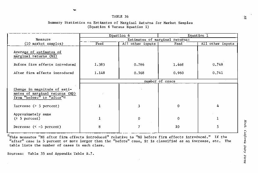
-TABLE 36 Oo
Oo
Summary Statistics on Estimates of Marginal Returns for Market Samples (Equation 6 Versus Equation 1)
Measure (10 market samples) Feed
Equation 6 Equation 1 Estimates of marginal returns:
All other inputs Feed All other inputs
Average of estimates of mar~inal returns (M$)
Before firm effects introduced 1.385 0.786 1.468 0.748
After firm effects introduced 1.148 0.568
number of
0.960
cases I
0.741
Change in magnitude of estimates of marginal returns (M~) from "before" to "after"a
Increase (> 5 percent) 1 403
Approximately same (± 5 percent) 11 0 0
Decrease (< -5 percent) 10 58 7
aThis measures "M$ after firm effects introduced" relative to "M$ before firm effects introduced." If the "after" case is 5 percent or more larger than the "before" case, it is classified as an increase, etc. The table lists the number of cases in each class.
Sources: Table 35 and Appendix Table B.7.

89Giannini Foundation Monograph • Number 36 • July, 1976
slopes and intercepts when one is viewed as fixed; Equation 7 is a special case where one of the independents is a dummy variable.1
In practice, exact multicollinearity is avoided by not forming one of the cross-products for a given set. The omitted case is arbitrary; hence, linear transformations can be carried out afterwards to write:
(8.2)
where am is the overall mean value for the elastici7, and aif and ait are deviations from the mean for specific firm and year, respectively.
The cross-product of the zi and the firm and time dummies generates new sets of independent variables with as many members as are in the original sets of dummies times the number of factors of production. In the present instance, there are twice as many cross-product variables as intercept-shifting dummies. The large number of potential additional variables generates a computer capacity problem as well as possible multicollinearity. Here, the first problem was handled by a large reduction in the number of firms employed, while an attempt to minimize the second problem led to limiting firms selected to those having a relatively large number of observations. Regional samples were developed with about a dozen firms in each, with groupings on the basis of trends in output. Expanding firms had increasing output over time, with 1964 output at least 25 percent above 196 l output in regions having 1961 observations and with 1964 output at least 16 percent above 1962 output for the Southern California case (with limited observations in 1961 ). Some expansion in capital input was also imposed as a necessary condition in sample selection. Nonexpanding producers had output changes below the minimum increase specified for expanding firms, with little or no change in capital, an additional criterion. In the case of Southern California, the nonexpanding group was further stratified into stable producers (with no significant change in output level) and contracting producers (with declines in output level).
1In the general case, say Y a + bX 1 + cX2 + dX1x2 (a + bX1) + (c + dX1) x2 when X is fixed. In the dummy variable situation, say there is only one set of dummies (for simplicity) represente~ by x1, i.e., b, d, and are vectors. Denote a member of the set by m; thenx1 Ym = (a + bm) + (c + dm) X2, with all other members of the set of x 1 equal to zero. The bm and dm are intercept and slope shifters, respectively.
The use of slope-shifting dummies is noted by L Johnston, Econometric Methods (New York: McGraw-Hill Book Company, Inc., 1963), p. 223. Quirino Paris initiated their use in the study of California dairy farm production functions, which inspired their use here.
2The transformed relation is:
where Oif is the ayerage over firms of o:if and o:it is the average over years of o:it· Then

90 Hoch: California Dairy Farms
Results were obtained for l l cases consisting of the 3 Southern California groups formed from the combined initial samples (Central plus Peripheral areas) plus an expanding and a contracting group for each of 4 regions--San Joaquin Valley (Northern Market), San Joaquin Valley (Southern Market), Bay Area (Northern and Southern areas combined), and Sacramento Valley (both market milk samples combined).
Table 37 shows the number of firms and observations in each of the I I samples used for Equation 7 and presents elasticity sums for 4 alternative cases of Equation 7. Case 1 includes both slope and intercept shifters; Case 2 includes only slope shifters; Case 3 includes only intercept shifters; and Case 4 excludes both sets of shifters corresponding to an ordinary regression of output on inputs. The elasticity sum for Cases 3 and 4 is the sum of specified constant elasticities; the elasticity sum for Cases 1 and 2 is the sum of the average elasticities--a 1 and a2. (A detailed listing of coefficients and R 2·s for Cases I and 3 appears in the Statistical Supplement.)
The averages over the 11 samples seem indicative of general patterns. Cases 3 and 4 parallel earlier results, with an elasticity sum a bit over 1.00 prior to an introduction of frrm and time effects and a substantial decline in the elasticity sum after those intercept shifters are introduced. Case 2 introduces slope shifters but omits the intercept shifters, and its elasticity sum (on the average) falls between the extremes of Case I and Case 4. It may be that the slope shifters can account for part, but not all, of the impact of differences in efficiency between firms. Case 1 has both slope and intercept shifters, and some changes in elasticity sum occur relative to Case 3, at the level of the individlial sample. However, the overall average for Case r is essentially the same as that for Case 3, and the individual differences are generally not large, which suggests that the differences are not of much importance.
These results seem encouraging in terms of support for the use of Case 3 (equivalent to Equation l) when the primary goal of an investigation is estimation of average values of elasticities. The rationale for the use of Equation 7 is the possibility of going beyond average elasticities to the investigation of systematic variation in elasticities. For this extended goal, results here appear only mildly encouraging at best. Multicollinearity, even exact multicollinearity, appears a major problem. Table 37 lists the number of omitted independent variables in Case 1 of each sample; this occurs when essentially exact multicollinearity holds. The problem seems particularly severe for the Southern California cases, viewing number of omitted variables as an index of relative severity.
An hypothesized systematic source of variation was behind the decision to organize samples in terms of expansion or nonexpansion of output. It was hypothesized that an expanding firm would move along an S-shaped production function in reality so that the estimated elasticity sum would decline over time. In similar fashion, nonexpanding firms would presumably exhibit no trend in elasticity sum. These hypotheses tended to square with results for the four San Joaquin Valley samples, with the Southern Market expanding group, in particular, very much in line with expectations. However, in the other samples both expanding and nonexpanding groups exhibited a good deal of year-to-year variability with little sign of trend. This is documented in Table 38, which presents the year averages of the elasticity sums for Case l in each sample. Hence, gen~ral confirmation of the hypothesis is rather limited at best.
There is a good deal of variability in the individual elasticities (feed and all other input) which make up the elasticity sum of Table 38. These year averages are averages over firms, of course; further disaggregation to the individual firm again considerably

TABLE 37
Number of Firms and Observatio.ns and Average Sums of Elasticities (Equation 7) by Region, Sample, and Case
R~ion and salll]J_laa
San Joaguin Valley
No:r>thern Ma:r>ket
Expanding Nonexpanding
Southe:r>n Ma:r>ket
Expanding Nonexpanding
Southern California
Expanding Stable Contracting
Bay Area
Expanding Nonexpanding
Sacramento Valley
Ma:r>ket
Expanding Nonexpanding
Average:
11 cases
Averag_e sum of elasticity_ Number of C! shifters in:b ct shifters out:b
Number of observa- F and T in F and T out F and T in F and T out firms tions Case le Case 2c Case 3c Case 4c
14 432 .842 1.084 .899 1.001 12 394 . 714 .782 .794 .952
12 288 .986 1.117 .939 1.0p6 15 376 .905 .988 .817 1.133
11 156 .466 .652 .565 .998 16 258 .263 .519 .360 1.016
9 139 .585 .487 .426 1.119
10 826 .782 .769 .761 1.046 15 373 .449 .942 .680 1.106
14 320 .756 1.006 .785 .954 11 234 .686 .910 .685 .894
d .676 .842 .701 1.026
aFor geographic coverage, see Table 2, sup:r>a, p. 6; for years covered, see Table 38, inf:r>a, p. 92.
Omitted independent variables in Case 1
2 3
2 2
7 5
10
1 2
0 0
b . . ct shifters are firm and year effects in the elasticities, i.e., coefficients for independent variables formed as cross-products of dulllllly variables and factors of production.
°F and Tare firm and year effects in the intercept, i.e., coefficients for usual firm and year dulllllly variables.
dBlanks indicate not applicable. 'O .....
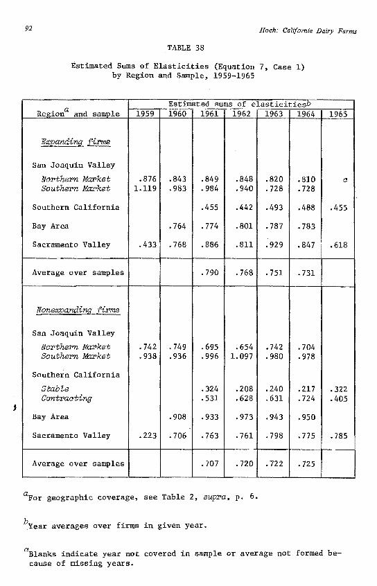
92 Hoch: California Dairy Farms
.TABLE 38
Estimated Sums of Elasticities (Equation 7, Case 1) by Region and Sample, 1959-1965
Reg_iona and salll]2_le 1959 Estimated sums of elasticitiesb 1960 1961 1962 1963 1964 1965
Expanding firms
San Joaquin Valley
NoPthern Market Southern Ma:rket
.876 Lll9
.843
.983 .849 • 984
.848
.940 • 820 • 728
.810
. 728 e
Southern California .455 .442 .493 .488 .455
Bay Area .764 . 774 .801 .787 .783
Sacramento Valley .433 .768 .886 .8ll .929 .847 .618
Average over samples .790 .768 .751 .731
None:x;panding firms
San Joaquin Valley
NorthePn Ma.I>ket Southern Mar>ket
.742 • 938
.749
.936 .695 • 996
.654 1. 097
.742
.980 .704 .978
, Southern California
Stable Contracting
Bay Area .908
.324
.531
.933
.208
.628
.973
.240
.631
.943
.217 • 724
.950
• 322 • 405
Sacramento Valley .223 .706 .763 .761 .798 • 775 .785
Average over samples .707 • 720 • 722 • 725
aFor geographic coverage, see Table 2, supPa, p. 6.
b.Year averages over firms in given year.
eBlanks indicate year not covered in sample or average not formed because of missing years.

93 Giannini Foundation Monograph • Number 36 • July, 1976
increases variability. Negative elasticities are fairly common. The San Joaquin Valley cases exhibit the most stability, but even here a great deal of variability is manifest. This is exemplified in Table 39 which presents year and firm averages for the expanding firm cases for this region. I
It may be that there is considerable variability in reality, but it seems more likely that much of the variability here reflects sampling error and multicollinearity. Deviations in the two input elasticities tend to be of different sign and of roughly the same magnitude, perhaps indicative of multicollinearity~ This can be illustrated by the averages of year estimates over the I 0 samples for years in common; note the stability in elasticity sum with offsetting deviations in individual elasticities:
/
Year o:lt 0:2t Lat
1961 .412 .333 .745 1962 .451 .291 .742 1963 .556 .180 .736 1964 .492 .235 .727
Finally, standard errors generally are so large that little in the way of inference appears possible.
Some notion of the relative contribution of intercept and slope shifters is given in Table 40 in the form of t ratios and F tests. Only about 7 percent of the firm slope shifters are statistically significant, while the firm intercept shifters show a greater proportion of significant cases with 25 percent. On the other hand, about 27 percent of the year slope shifters are significant as are 34 percent of the year intercept shifters.
The F tests of Table 40 can be used to examine two alternative sequences, comparing the cases of Table 37 above. In the first sequence, intercept firm effects are introduced (with intercept time effects already in the regression) and significantly reduce unexplained variance in all cases. Then slope shifters are introduced and significantly reduce variance further in 7 of 11 cases. In the alternative sequence, slope shifters are introduced first and are significant in. all cases; then the firm intercept shifters are brought in and significantly reduce variance further in I 0 of 11 cases.
If one has to choose between intercept shifters and slope shifters, a case can be made for the former. Table 40 shows a somewhat better statistical performance; Table 37 suggests a stronger accounting for the impact of firm differences; and there are fewer variables and, hence, lower costs.
However, further experimentation with slope shifters, in addition to intercept shifters, appears warranted. Limiting the number of such variables will probably be necessary to avoid multicollinearity. The evidence of Table 40 suggests the time slope shifters as likely candidates for inclusion within such a limited number.
lTables in Appendix B present year averages for the other samples and individual estimates by firm and year for one of the San Joaquin Valley samples. The Statistical Supplement lists constant, individual year and firm components of the elasticities, and corresponding standard errors and t ratios for the cases of Table 39.

94 Hoch: California Dairy Farms
TABLE 39
Average Elasticities for Years and Firms for San Joaquin Valley Expanding Firm Cases, 1959-1964
(Equation 7)
J
Yeara
San Jo'!S.uin Valle_y_ Northern Market Southern Market
Feed
All other il!:E_uts Total Feed
All other il!:E_uts Total
' 1959 .834 .042 .876 .391 . 728 1.119
1960 .666 .177 .843 .709 .274 .983
1961 .436 .413 .849 .876 .108 .984
1962 .565 .283 .848 1.007 -.067 .940
1963 .581 • 239 • 820 .896 -.168 • 728
1964 . 557 . 253 .810 . 828 .-.100 . 728
F'irmb
.781 .428 1. 209 • 778 • 666 1.4441
2 .374 .289 .663 . 778 .378 1.156
3 .541 .264 .805 .695 .402 1. 097
4 • 975 -.150 • 825 .909 -.006 .903
5 .642 .208 .850 .683 .293 . 976
6 .781 .408 1.189 .421 .666 1.087
7 . 800 .569 1. 368 .684 .393 1.077
8 .585 .110 .695 .896 -.219 . 677
9 • 365 • 255 .620 .938 .007 . 926
10 .452 -.265 .187 1.184 -.009 1.175
11 .661 .386 1.047 • 779 -.099 .680
12 .514 .007 .507 .682 -.040 .642
13 . 726 • 372 1.098 c
14 . 298 .404 .702
~
aElasticities are averaged over finns for a given year.
bElasticities are averaged over years for a given firm.
"Blanks indicate not applicable; there wer.e 14 firms in the Northern Market sample and 12 in the Southern Market sample.

95 Giannini Foundation Monograph • Number 36 • July, 1976
TABLE 40
Comparisons of Intercept and Slope Shifters in Terms of Statistical Significance
(Equation 7)
Statistic
Number of significant cases relative to
total casesa 4 San Total
Joaquin 6 cases, Valley other 10 samj)les samples sall!Ples
Significant cases
as a fraction of
total ca-s-esa All
samples
t ratios for:
T (year intercept effects) 14/20 4/33 18/53 .340
F (firm intercept effects) 12/47 19/79 31/126 .246
alt (year slope shifter, feed) 9/20 4/31 13/51 .255
().2t (year slope shifter, other input) 7/20 8/30 15/50 .300
a.lf (firm slope shifter, feed) 4/46 2/69 6/115 .052
a.2£ (firm slope shifter, other input) 6/48 5/68 11/116 .095
F tests
From Case 4 to Case 3, introduce F 4/4 7/7 11/11 1.000
From Case 3 to Case 1 given F, introduce
shifters 4/4 3/7 7/11 .636
From Case 4 to Case 2, introduce slope shifters 4/4 7/7 11/11 1.000
From Case 2 to Case 1 given slope shifters, introduce F 4/4 6/7 10/11 .909
aSignificant cases are statistically significant at the 5 percent level.

96 Hoch: California Dairy Farms
9. SUPPLY RELATIONSHIPS
Cost Functions and Supply Functions
. a· Given the Cobb-Douglas production function, Y = K U Zj 1, explicit cost functions
1 can be derived when a relation between inputs is specified. When inputs are in fixed proportion, the derivation is straightforward. In Table 23 above, output as a function of total expenditure was derived through the use of fixed proportions based on average levels of input in each sample. The function was written:
ao y = C z (9.1)0
where
Y output
Zo total expenditures (or total cost)
and
c and ao constants, with ao identical to l:ai (in the present case, a 1 + a2).
An explicit total cost function can be derived by rewriting (9 .1) as
(9.2)
Hence, the data of Table 23 could be employed to generate explicit total cost functions if such were desired. (These would represent the average firm.)
Somewhat different estimated total cost functions would be derived under the assumption of profit maximization. This situation also involves fixed proportions, but the proportions differ somewhat from those used for Table 23 because there was generally some deviation from maximization in the empirical results.
i.tI:owever, it is possible to make some general inferences about supply under either situation, assuming constant elasticity values o:i. In the general case of fixed proportions, marginal cost (MC) can be written:
MC (9.3)
If profit maximization has occurred, then it can be shown that
(9.4)
where the Pz. are factor prices. 1
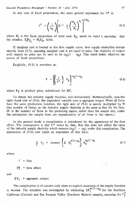
97 Giannini Foundation Monograph • Number 36 • July, 1976
In any case of fixed proportions, the more general expression for C* is:
where Mi is the fixed proportion of total cost, z 0, spent on input i, assuming that the relation, Zlz. = MiZ0 , holds.
I
If marginal cost is treated as the firm supply curve, firm supply elasticities emerge directly from (9.3), assuming marginal cost is set equal to price. The elasticity of output with respect to price can be seen to be (ao/l - a 0). This result holds, whatever the source of fixed proportions.
Explicitly, (9.3) is rewritten as:
y -_ ~(·--1 ) p ] aa/1-ao (9.6)C* y
where Py is product price, substituted for MC.
To obtain the industry supply function, sum horizontally. Mathematically, sum the right-hand side of (9.6); the dependent variable now is aggregate output. When all firms have the same production function, the right side of (9.6) is merely multiplied by N (the number of firms), so the industry supply elasticity is the same as that for the firm. (N is the number of firms in the producing region, rather than the sample size, under the assumption the sample firms are representative of all firms in the region.)
In the present study a complication is introduced by the appearance of the firm effect. The consequence is that C* varies by firm. But this does not affect the value of the industry supply elasticity which remains (a0/l - a 0) under this complication. The summation of (9.6) now yields an expression of this form:
(9.7)
where
f firm
F[ firm effect
and
LYf = aggregate output.
The complication is of concern only when an explicit statement of the supply function
is wanted. The situation was investigated by estimating LFfl/l-ao for the Southern
California (Central) and San Joaquin Valley (Southern Market) samples, assuming the Fr*
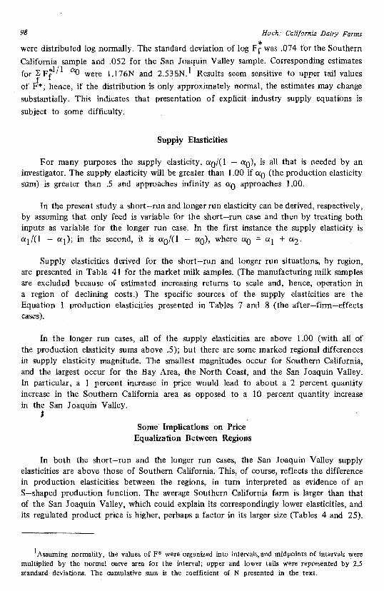
98 Hoch: California Dairy Farms
were distributed log normally. The standard deviation of log Ff* was .074 for the Southern
California sample and .052 for the San Joaquin Valley sample. Corresponding estimates for :3 F[11l--ao were 1. l 76N and 2.538N. 1 Results seem sensitive to upper tail values
f of F*; hence, if the distribution is only approximately normal, the estimates may change
substantially. This indicates that presentation of explicit industry supply equations is
subject to some difficulty.
Supply Elasticities
For many purposes the supply elasticity, a 0/(l - a0 ), is all that is needed by an investigator. The supply elasticity will be greater than 1.00 if a0 (the production elasticity sum) is greater than .5 and approaches infinity as approaches 1.00.a0
In the present study a short-run and longer run elasticity can be derived, respectively, by assuming that only feed is variable for the short-run case and then by treating both inputs as variable for the longer run case. In the first instance the supply elasticity is a 1/(l - a 1); in the second, it is a 0/o - a0), where = a 1 + a2 .a0
Supply elasticities derived for the short-run and longer run situations, by region, are presented in Table 41 for the market milk samples. (The manufacturing milk samples are excludoo because of estimated increasing returns to scale and, hence, operation in a region of declining costs.) The specific sources of the supply elasticities are the Equation l production elasticities presented in Tables 7 and 8 (the after-firm-effects cases).
In the longer run cases, all of the supply elasticities are above 1.00 (with all of the production elasticity sums above .5); but there are some marked regional differences in supply elasticity magnitude. The smallest magnitudes occur for Southern California, and the largest occur for the Bay Area, the North Coast, and the San Joaquin Valley. In particular, a 1 percent increase in price would lead to about a 2 percent quantity increase in the Southern California area as opposed to a IO percent quantity increase in the San Joaquin Valley.
J Some Implications on Price
Equalization Between Regions
In both the short-run and the longer run cases, the San Joaquin Valley supply elasticities are above those of Southern California. This, of course, reflects the difference in production elasticities between the regions, in tum interpreted as evidence of an S-shaped production function. The average Southern California farm is larger than that of the San Joaquin Valley, which could explain its correspondingly lower elasticities, and its regulated product price is higher, perhaps a factor in its larger size (Tables 4 and 25).
1Assuming normality, the values of F* were organized into intervals, and midpoints of intervals were multiplied by the normal curve area for the interval; upper and lower tails were represented by 2.5 standard deviations. The cumulative sum is the coefficient of N presented in the text.
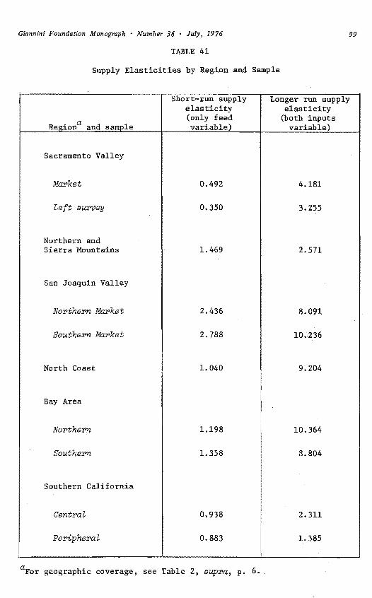
99 Giannini Foundation Monograph • Number 36 • July, 1976
TABLE 41
Supply Elasticities by Region and Sample
Regiona and sam_E_le
Sacramento Valley
Market
Left survey
Northern and Sierra Mountains
San Joaquin Valley
NortheX'n Ma:!'ket
SoutheX'n Ma:rket
North Coast
Bay Area
NortheX'n.
SoutheX'n
Southern California
Short-run supply elasticity (only feed variable)
0.492
0.350
1.469
2.436
2.788
1. 040
1.198
1.358
Longer run supply elasticity
(both inputs variable)
4.181
3.255
2.571
8.091
10..236
9.204
10.364
8.804
Central 0.938 2.311
Peripheral 0.883 1.385
aFor geographic coverage, see Table 2, supra, p. 6.

100 Hoch: California Dairy Farms
The difference in supply elasticities yields some interesting implications under the assumption of a movement toward price equalization between these major supplying regions. If Southem California milk price were reduced and San Joaquin Valley price were increased by the same percentage, there would be a net increase in milk supplied. Stated another way, the quantity effects of a price decline in Southern California could be compensated by a much smaller price increase in the San Joaquin Valley so that average price would fall statewide.
Table 5 shows that Southern California produced 42. 7 percent of 1960 market milk output, while the San Joaquin Valley produced 35.3 percent of the total. Consider the effect of a 5 percent decline in the Southern California price. In the short run, applying a supply elasticity of .9, quantity in the region would decline by 4.5 percent; this would amount to a decline of 1.92 percent in state production. Assuming a San Joaquin Valley short-run elasticity of 2.5, a price increase of 2.18 percent would yield a 5.45 increase in regional quantity, the equivalent of 1.92 of state production to just balance the Southern California decline. In the longer run case, a 5 percent decline in the Southern California price could be balanced by a 1.21 percent increase in the San Joaquin Valley price, applying supply elasticities of 2.0 and 10.0, respectively. (The factor of l.21 is the ratio of Southern California to San Joaquin Valley market milk production initially.)
This discussion can be extended by determining the equilibrating price between the two regions. Fletcher and McCorkle show a transportation cost differential of 45 cents per hundredweight between the two regions, that is, this is the additional cost of shippinf milk from the San Joaquin Valley to the large consuming region of Southern California.
Table 25 shows base year prices of $4.2218 and $5 .4655 per hundredweight for the San Joaquin Valley and Southern California areas, respectively. Given an equilibrating policy, the respective short-run prices would be $4.4218 and $4.8718; the respective longer run prices would be $4.3468 and $4.7968. In both cases total quantity is unchanged, and a transport cost differential of $0.45 holds. 2
1F!etcher and McCorkle, Jr., op. cit., Table 20, p. 67, list transportation and hantlling charges for southern and northern milksheds corresponding to the San Joaquin Valley and Southern California regions here. In both regions, shipment to the local processing plant costs IS cents per hundredweight; and an addij:ional charge of 4 5 cents per hundredweight is shown for transportation from the northern milkshed to C:os Angeles, interpreted here as the additional cost of shipping to the south. Using Bureau of Milk Stabilization terminology, there is a "first haul" charge of 15 cents to the local plant and a "second haul" charge of 45 cents which involves the shipment from the local northern "country" plant to the southern metropolitan plant.
2Let PS represent the initial Southern California price and P J the initial San Joaquin Valley price. It is known that Ps - .05 Ps will have an effect on quantity just balanced by P1 + .0218 P1 in the short run and by P1 + .0121 l'rintheiongerrun. This reasoning can be extended to find equilibrating prices by writing ·
Ps - .05C Ps = PJ + .0218C PJ + .45 (short run)
and
(longer run)
and solving for C. The expression on the left is the new Southern California price and that on the right is the San Joaquin Valley price plus the transport cost differential.

101 Giannini Foundation Monograph • Number 36 • July, 1976
In the short-run case, there is a shift of 4.2 percent of total state production from the Southern California region to the San Joaquin Valley; in the longer run case, the shift is 10.4 percent of state production. On a regional basis, Southern California contracts its production by I 0 percent in the short run and 25 percent in the longer run. The San Joaquin Valley expands its production I 2 percent in the short run and 30 percent in the longer run. The weighted average price of milk for the two regions drops from $4.90 in the initial period to $4.67 in the short mn and $4.59 in the longer run case. These results are summarized in Table 42.
This analysis has involved some simplifying assumptions. Initial prices are averages and, in reality, vary over producers. Jn calculating weighted average prices, it was assumed that all initial San Joaquin Valley production was consumed locally. This assumption does not affect the amounts of price changes, however. Finally, quantity of market milk consumed was assumed invariant by regions and in total.
The analysis as it stands, however, seems a useful first approximation; and perhaps it can be extended to more realistic and complicated models of reality. A retrospective evaluation of supply function estimation may furnish some leads on the construction of more realistic models. That evaluation follows and concludes the present section.
An Evaluation of Supply Function Estimation
Wipf and Bawden have argued that supply curves that are derived from production functions are unreliable; a major elemert of their critique is that elasticities appear too high relative to direct estimation of supply. I
It seems likely that neglect of firm effects has been a major source of overstatement of production elasticities and, of course, that source of bias was avoided here.
Often, economists appear to expect a production function elasticity sum close to one and a supply elasticity substantially below infinity. These are contradictory intuitions--in the long mn, at any event.
Some other factors may cause the industry supply curve to differ from that implied by estimated production function parameters. Some lead to an overstatement and some to an understatement of supply elasticity.
It is generally assumed (and was assumed here) that factor prices are constant. In reality, factor prices are likely to vary with output, with the consequence that the industry supply curve is less elastic than the sum of marginal cost curves. As all firms attempt to expand, factor prices rise, inhibiting the expansion; similarly, contractions are reduced by declining factor prices.
Again, it is plausible that production function elasticities are variable rather than constant. Inferences seem defensible at and near average values of input and output but become increasingly suspect with movement away from the average. Jn the context of
1Larry J. Wipf and D. Lee Bawden, "Reliability of Supply Equations Derived from Production Functions," American Journal of Agricultural Economics, Vol. S 1, No. 1 (February, 1969), pp. 170-178, and, in particular, item B, p. 177.
TABLE 42 ....
Examination of Results of Price Equilibrating Policy for San Joaquin Valley and Southern California Production
Period
_!'_rice Qll!l11tity
Southern California
San Joaquin Valley_
Southern California
San Joaquin Valley
Initial produc
tion
Increment
to Southern Market
Weighted avera_g_ea
Initial production
Increment
to Southern Market
Total produc
ticm
~ dollars_per hundredweight
Initial 5.4655 4.2218 b -
Short run (given price equilibrating policy) 4.8718 4.4218 4. 8718c
Longer run (given price equilibrating policy) 4.7968 4.3468 4.7968c
4.9026
4.6681
4.5931
"E_ercent of state market total
42.7 35.3 35.3
38.5 35.3 4.2 39.5
32.3 35.3 10.4 45.7
aListed prices times corresponding quantities divided by total quantity (78.0). Assumes all of initial San Joaquin Valley production is utilized in that region.
hBlanks indicate not applicable (zero increment in initial period),
cBase price plus 0.45 transport cost to San Joaquin Valley (Southern Market),
10.1 Giannini Foundation Monograph • Number 36 • July, 1976
the empirical appHcation made above, as Southern California output contracts, the area's supply elasticity will probably rise; and, as San Joaquin Valley output expands, that area's supply elasticity will probably decline. This would imply an equilibrium price for the two areas above the estimate derived earlier, with less redistribution of output In general. a variable elasticity S-shaped production function means that supply is less elastic with expansion and more elastic with contraction than constant elasticities indicate. Some approaches to the study of S-shaped functions have been explored in this report and may be of some use in future work.
Length of run has been touched on at several points and is a major consideration in any discussion of supply. Short-run and longer nm cases were developed here, depending on which of the two factors of production were fixed. With a finer breakdown of factors and with differences in the respective periods of factor fixity, there are corresponding differences in length of run. Supply becomes increasingly elastic as length of run increases, allowing additional factors to change from fixed to variable status. The longer run case here implicitly held number of fi1ms constant. A longest run case can be defined as encompassing a variable number of firms. Profits can be viewed as the return to a factor of production labeled "management" or "entrepreneurial capacity." Opportunity costs then equal what the manager can earn in alternative employment. If profits fall below opportunity cost, the rational manager will leave the industry: if profits rise above opportunity cost, new managers will enter the industry. Without specialization to an industry (existence of economic rent either in production or consumption), supply functions would be perfectly elastic in the longest run, as firm output would be replicated at the minimum cost point with as many firms as needed to satisfy demand at price equal to that minimum cost. Given specialization of managers (and firms) to an industry, less than perfectly elastic supply is plausible---even in the longest run. The introduction of firm effects into the production function yields an estimated distribution of returns to management under various conditions, including profit maximization. In conjunction with other data on producer characteristics, these data may be useful in examining actual entry and exit behavior and then in predicting such behavior. Such predictions, in turn, would yield longest run supply implications. Some preliminary work along these lines was carried out here in setting up a separate sample of Sacramento Valley producers who had left the survey, often because they had left the industry. Such producers, as a group, were somewhat less efficient than producers who had remained with the survey (Table 24). Future work might relate exit and entry behavior over a long time period to firm effect and to a variety of other variables, for example, age, education, location, length of time in the industry, etc.
As a final consideration, there is reason to believe the supply function will tend to· shift right over time, reflecting such underlying factors as technological advance, improved management practices, and more and better information--all subsumed under the heading of "advances in productivity." The estimated year effects ,here exhibit an upward time trend (Table 9); and detailed consideration of those effects led to the conclusion that firms might attempt to expand output by about 10 percent per year (see Table l 0 and attendant discussion).
Some attempt to check this could be based on experience since the date of the sample used here. ln addition, the need for more refined work on time effects and sources of productivity increase (noted in Section 4) could be tied to some of the suggestions for additional analyses employing the firm effects (Section 5). Estimated tiJTle effects, as well as firm effects, might be related to hypothesized sources of productiyity gain, with measures of those sources then incorporated into the production function. Timeless
104 Hoch: California Dairy Farms
data on individual producers (such as years of education) might help explain firm effects; aggregate data across producers, or information applying to all producers, might help explain time effects; and variables measured over both time and producers might help explain both sets of effects. The last case includes measures showing the diffusion of new kinds of capital goods or of new technology over individual firms. Then, predictions of changes in the sources of productivity growth would yield corresponding predicted shifts in the supply function.
In the present study the DHIA dummy variable was hypothesized to be such a supply shifter under the interpretation it represented the securing, at a price, of information for management decision. It turned out that there was little change over time in the proportion of firms that were DHIA members (Appendix A); hence, with DHIA omitted, it is not likely there would be much change in the estimated year effects. However, results for the variable supported the supply shifter hypothesis, for DHIA membership had some significant and positive effect on productivity after the firm effects were introduced, thus controlling for all other differences in management. Hence, if DHIA membership, in fact, were increased, corresponding increases in supply would be generated.
These considerations furnish good support for the conclusions that production function estimates are indeed useful in supply application and that there is great potential for refined and extended application.
10. SUMMARY OF RESULTS
This section summarizes the major results obtained in this study and presents some suggestions for future research. The major results can be classified under the headings of methods and subject matter, depending on focus. In the case of methods, the work has involved both ( 1) application and testing of regression analysis using dummy variables~-primarily for the Cobb-Douglas function--extending a body of work carried out over the last two decades and (2) some experimental extension of the technique including the employment of slope shifters as well as intercept shifters. Focusing on subject matter, the work has consisted of a case study of California dairy production in a particular time period. Observations spanned 1955-1965, with about two-thirds of the nearly 10,000 observations occurring in the 1962-1964 period (Table 3 ). The large number of observations employed reflects the detailed coverage of subclasses of California dairy production in terms of regions and milk type. Though specific to time and place, hopefully m;fny of the case study results will have more general applicability. Major topics covered can be catalogued as (I) technical production relationships, (2) measures of technical and allocative efficiency, (3) the impact of institutional arrangements then prevailing, since production was subject to regulatory constraint, and (4) applications to supply analysis. The study may well serve as a benchmark for further work on California dairy farm production; and it may have some applications to other industries as well as in the study of such topics as increases in productivity and regional differences in efficiency.
Because a summary involves a broad brush treatment, there necessarily will be some simplification and limited recognition of caveats and qualifications developed more fully in the text.
Under the heading of method, the impact of firm dummy variables is a major item of interest. The introduction of firm dummies in earlier Cobb-Douglas studies led to a substantial decline in elasticity sum. This indicated that ordinary least-squares estimates were biased because better firms tended to be bigger firms. That conclusion could be
105 Giannini Foundation Monograph • Number 36 • July, J976
enriched by some theoretical underpinning: better firms necessarily would be bigger if all firms were profit maximizers, with the consequence that ordinary least squares would yield an elasticity sum close to 1.00, given the form of the profit-maximizing equations and the simultaneous equation bias involved. Removal of the bias would yield decreasing returns rather than constant returns to scale. With decreasing returns, there are positive profits which can be viewed as returns to an input fixed to the firm, best interpreted as management or entrepreneurial capacity. The long-run level of profit must equal managerial opportunity cost to achieve equilibrium (neither entry nor exit of firms from the industry).
The present study adds a good deal of evidence on the impact of dummy variables on elasticity sums. The major item, of course, is the basic set of results for Equation 1 (Table 7), summarized here as Table 43. With the introduction of firm effects, 10 of 12 cases had a decline in elasticity sum from a previous level of around 1.00. The two exceptions appear to prove the rule. Both were manufacturing milk samples and, for both, the elasticity sum increased; but this seems reasonable, given the size of the typical farm here, and the low product prices it received--about two-thirds to three-quarters of the market milk blend price (Table 25). Operation in a region of increasing returns is hardly surprising for these cases. Simultaneous equation bias can lead to an estimated elasticity sum close to 1.00 in cases of increasing returns if constraints on expansion exist. An increase in elasticity sum, given the analysis of covariance approach, has not been reported previously; such a result is a counter to the intuition that there is a downward bias inherent in analysis of covariance estimation.
There was confirmation of Equation I results for the market milk samples when the alternative quadratic function of Equation 6 was employed. With the introduction of firm effects in Equation 6, marginal return estimates for both feed and other input declined in almost all cases. (Since elasticity times a scalar equals marginal return in the Cobb-Douglas case, this result corresponds to the decline in elasticity sum in Equation I.) This is further evidence supporting a general downward shift in the production function given firm effects and contradicts any suggestion that some quirk of the Cobb-Douglas estimation process is responsible for the shift that occurs. Marginal returns, averaged over 10 market milk samples, were compared in Table 36 and are summarized here:
Before After fun effects firm effects
Equation 1.47 0.96 Equation 6 1.39 1.15
t>.Jl_ other inputs
Equation 0.75 0.74 Equation 6 0.79 0.57
These results furnish some support for a hypothesis that alternative production function forms more or less capture the same underlying reality and that often, perhaps usually,

106 Hoch: California Dairy Farms
TABLE 43
Sums of Elasticities Obtained Before and A£ter Firm Effects Introduced (Equation 1)
by Region and Sample
Sums of elasticities Before firm After firm
effects effects Region and sam_lllea introduced introduced
Sacramento Valley
Market 1.04 0.81
Ma:nufactu:r>ing 1.08 1. 23
Left survey 1.01 0.77
Northern and Sierra Mountains 1.07 0. 72
San Joaquin Valley
Northern Market 1.00 0.89
Southern Market 1.02 0.91
Manufacturing 1.05 1.09
North Coast o. 94 0.90
Bay Area
Northern 1.07 0.91
S~uthern 1.06 0.90
' , Southern California
Central 1.02 o. 70
Pe-riipheraZ 1.08 o. 58
Average:
10 market samples 1.04 0.81
2 manufacturing samples 1.07 1.16
aFor geographic coverage, see Table 2, supra, p. 6.; for years covered by each sample, see Table 3, supra, p. 8,
Source: Table 7,

Giannini Foundation Monograph • Number 36 • July, 1976 107
similar inferences will be obtained whatever the form that is used. I But the hypothesis deserves further testing and is one reason to recommend future explorations with alternative production function forms which can yield additional substantive information as well.
A shift away from constant returns, which occurs with the introduction of firm effects, has a number of ~ncouraging features. At constant returns, output is indeterminate, and profit maximization can occur only for a highly restricted set of product and factor prices; at near-constant returns, differences in technical efficiency between firms must be very small or else extremely wide variations in equilibrium firm size occur; and the corresponding elasticity of supply approaches infinity as the production. elasticity sum approaches one. In contrast, <led-easing returns to scale is consistent with determinate output and profit maximization under any set of prices; an intuitively plausible spread in technical efficiency between firms can occur without extremely wide variation in farm size; and a much more plausible elasticity of supply is obtained.
Another example of dummy variable impact occurred with the introduction of regional effects into the overall state production function estimated from eight pooled samples. Previously estimated firm effects for those samples were included in the dependent variable observations, accounting for firm differences within each region. The introduction of regional effects,' accounting for differences between regions, resulted in a drop in the elasticity sum from .94 to .88 (Table 21). This seems best interpreted as a variant of the original argument on the correlation of efficiency and scale., for the size of the regional effect was positively related to the size of the average farm in the region, as shown in Table 44. The approach used to estimate regional effects yields some suggestions for future work. In terms of method the use in a stepwise procedure of previously estimated firm and year effects for given regions can make possible the fitting of equations with large numbers of dummy variables. For example, state functions could first be estimated using counties as units; then national functions could be estimated using states as units. In terms of content, regional effects in agriculture may be explainable in terms of proximity to and size of the market. Some speculations along these lines were presented and may merit further investiga~ion.
Some experimentation with slope-shifting, as well as intercept-shifting, dummy variables was carried out. Problems of multicollinearity and a very large number of variables limit the usefulness of this approach, though it is capable of yielding a substantial amount of additional information; some success was obtained with its application here.
Averaging over results for 11 samples (Table 37), there is some indication that slope shifters of themselves account for only part of the change in elasticity sum that occurs with intercept shifters. The two types of shifters, in combination, appear to yield the same change that occurs with intercept shifters only. Results were as follows:
1Fabrycy compared Cobb-Douglas results to more flexible but also more complex functions and found that "for a surprisingly large part of the field examined, the Cobb-Douglas function provides results which are not significantly different from the results obtained from ... the mathematically more complex functions"; see Mark Z. Fabrycy, "Cobb-Douglas, CES and Homothetic lsoquant Production Functions: A Comparison," Econometrica, Vol. 38, No. 4 (July, 1970), pp. 106 and 107.

108 Hoch: California Dairy Farms
~~~@.~ _Elastici!}'. Sum 1I Sample_s
Both slope ~~ !f1tercept and interc~ shifters--- shifters No
shifters only !='~ shifters
0.676 0.842 0.701 1.026
TABLE 44
Regional Effects and Average Milk Production Per Farm by Region and Sample
I Average milk pro- I duction per farm
(3.8 percent butter- !
Region and sampL~a Re_g_ional effect fat ~uivalent) 1,000 pounds
_E_er iear
Northern and Sierra Mountains .797 584
.926 915North Coast
.938 1,278Sacramento Valley
Bay Area
.999 1,440Northe:rn 1.079 1,807
San Joaquin Valley
Southern
Northe:rn Ma.rket 1.095 2,176, Southern Ma.rket 1.104 2,017
Southern California
1.109 3,398 i
J aFor geographic coverage, see Table 2, supra, p. 6; for years covered by
each sample, see Table 3, supra, p. 8.
Source: Tables 4 and 22, supra, pp. 9 and 58, respectively.
One source of interest in the slope shifters emerged from the inference that S-shaped production functions held, in reality, for elasticity sums showed some tendency to decline as average farm size increased. The 11 samples here were selected with this hypothesis
109 Giannini Foundation Monograph • Number 36 • July, l 976
in mind; there were 5 samples of farms which had expanded their output over time and 6 samples of farms which were nonexpanding. It was expected that the elasticity sum would decline for the first group (if an S-shaped function held) and remain stable for the second.
This expectation had some modest confirmation as indicated by the following averages. However, at the level of the individual sample, the relationships appeared to hold only for the four San Joaquin Valley cases. The averages of the elasticity sums were:
1961 1962 1963 1964
Expanding firms (five samples) .790 .768 .751 .73 l Nonexpanding firms (six samples) .707 .720 .722 .725
Substantive n:sults of this study illuminated a number of aspects of dairy production, including several technical production relationships.
In developing feed input estimates for a subset of observations, TON fed per day was related to number of cows being milked, number of dry cows, body weight, value of cow per head, breed, year, and region. For all samples combined, the following coefficients were obtained for the first four of these explanatory variables (from Table 6):
Cows milking 26.38 Cows dry 22.37 Body weight (hundred pounds) 94.21 Value of cow per head 2.52
In an extended version of this relationship, expected milk per cow and total expected milk (based on previous production) were introduced (Appendix Table A.8), though their introduction may have added more in complication than in explanation. In any event such relationships may have some applications in farm management; for example, they might be introduced into a linear programming framework to determine herd size and rations.1
Information was developed on the seasonal pattern of production by virtue of the estimated month effects (Table 11 ); distinct regional patterns appeared. Such information may be useful in marketing analyses of the smoothing of peaks and troughs in production to meet consumption requirements.
The effect of membership in the DHIA was generally positive. However, its impact dropped substantially with the introduction of firm effects. On the average, before firm effects, joining the DHIA was estimated to increase output by 6 percent; after firm effects, this estimate dropped to a J percent increase. This suggests that better operators tend to be DHIA members. The selectivity involved here may be meaningful in a wider context, for example, in interpreting returns to education.
This study produced a number of measures and comparisons of both allocative and technical efficiency. In operational terms the former measures how closely VMP approached price of input, while the latter measures the level of the constant term in the Jogged production function, assuming elasticities are the same between cases.
1An example of a linear programming analysis of an optimal dairy feeding prqgram appears in G. W. Dean, D. L. Bath, and S. O!ayide, "Computer Program for Maximizing Income Above Feed Cost from Dairy Cattle," Journal of Dairy Science, Vol. 52, No. 7 (July, 1969), pp. 1009--l016. In that study the constraints involved choice of feed type. Inclusion of additional information, such as that developed here, might expand the coverage of the decision process.
110 Hoch: California Dairy Farms
The comparison of average levels of marginal returns shown above (Equation 1 versus Equation 6) suggests that, in general, feed VMP is greater than or equal to its price, while all other input VMP is below its price.
The percentage deviation from optimality seemed intuitively plausible; for the 10 market milk samples, it averaged only 4 percent for feed and 26 percent for other input. In a majority of cases, VMP deviated by Jess than 25 percent from the optimal level.
At the level of the individual sample, Table 26 indicates that the average farm is quite close to an optimal allocation in the North Coast and Bay Area; it has too much feed and the proper amount of other input in the Sacramento Valley; it has the right amount of feed and too much other input in Southern California; and it has less than enough feed and too much other input in the San Joaquin Valley. ·
These conclusions are reinforced by the evidence of Equation 4. When feed is disaggregated into concentrates and roughage, the VMP of each of these feeds is above the optimal for the San Joaquin Valley sample and optimal for Southern California, while the VMP for other input remains below the optimal level in both cases (Table 30).
If the evidence of Equation 5, based on five inputs, were to be accepted, then it would be concluded that the VMP of feed, labor, and operating cost are generally below optimal levels, while those of capital and cow service flow are generally above optimal levels. But internal evidence strongly suggested that there was collinearity between feed and cow service flow (and, perhaps, capital) and that cow service flow probably had an "outside" linear relationship with output, distorting all of the elasticity estimates of Equation 5 and making their use highly questionable. The aggregation of the nonfeed
· inputs into "all other input" was the solution to the problem that was adopted here. Alternatively, cow service flow might have been subtracted from sales measured in dollars to yield a "net" output as dependent variable. That approach was rejected here because milk blend prices were not available for individual producers; but, in future work, such data might be developed. In addition, there could be exploration of alternative disaggregations of the two inputs of Equation 1. Certainly, the disaggregation of feed seems promising given the results for Equation 4.
As noted above, technical efficiency comparisons between regions indicate a general increase in this measure with increases in average farm size (the average o;:er each region). The San Joaquin Valley and Southern California areas, which produced about 75 percent of the state milk supply, have the highest levels of technical efficiency, ithough it is not ~ertain which of the two is the higher (Table 22 versus Table 24). However, it seems probable that the San Joaquin Valley is at least as efficient as Southern California and could well be more efficient.
There is good evidence that technical efficiency, as measured by the firm effects, is distributed normally between farms, with two-thirds of the firm effects falling between .85 and 1.17 and 95 percent falling between .73 and 1.37--that is, for given input 95 percent of all farms will produce between .73 and 1.37 of average output. However, this is for all samples combined; the distribution may well vary between areas. BMS fieldmen evaluations of individual firm operators were correlated with estimated firm effects; and though r2's were not high, they were generally significant (Table 17).
Some hypotheses were advanced which related certain of the results to institutional constraints prevailing at the time of the study. There was some suggestion of mildly increasing returns to scale before firm effects were introduced; this could be explained if more· efficient farms had somewhat lower product prices which, in turn, could reflect the determination of price as a blend of market and manufacturing milk prices. The allocative results obtained might fit the notion that many farms expanded production
111 Giannini Foundation Monograph • Number 36 • July, 1976
more than would normally be economic in the hopes of increasing their market milk base in future milk price determination. Finally, the marked blend price differences, which prevailed between the San Joaquin Valley and Southern California cases, suggested economic loss may have occurred because of nonequilibration of prices. This hypothesis was supported by the application of results in supply analysis.
Short-run supply elasticities were based on fixity of all other inputs, while longer run elasticities assumed both feed and other input were variable. (Longest run elasticities would treat management as variable, that is, allow exit and entry of firms.) Short-run supply elasticities ranged from about 0.4 to about 2.8, while longer run supply elasticities ranged from 1.4 to I 0.4. Focusing on the matter of possible adjustments between the San Joaquin Valley and Southern California areas, the following inferences were developed (from Table 42). Assuming a price difference at equilibrium of 45 cents per hundredweight, reflecting transport cost and applying estimated supply elasticities, these prices were obtained for initial versus equilibrating situations:
Prices Obtained
Initial ~hort !..U..'!.. h2!1~ run (dollars) (dollars)
San Joaquin Vallt:y 4.22 4.42 4.35
Southern California 5.47 4.87 4.80
The shifts in milk produced, as a percent of total state production, would be about 4 percent in the short run and 1 0 percent in the longer run. Southern California production, as a percent of the state total, would decline from 43 percent to 39 percent in the short run and to 32 percent in the longer run, while the San Joaquin Valley share would rise from 35 percent to 39 percent in the short run and to 46 percent in the longer run. There may be some overstatement in these forecasts because constant elasticities are assumed; but they indicate the potential for substantial adjustments in milk production.
The present case study can 'point the way to a munber of related investigations. For example, in the context of the dairy industry, the levels of technical and allocative efficiency between farms and regions might be checked in future periods for invariance or change over time and for behavioral consequences. It might be asked: How are any changes related to entry and exit behavior of various farm groupings? More generally, the production function approach employed here might be applied to other products or industries; and dummy variable effects might be related to putative explanatory variables. Such work might shed light on industry structure (competition versus monopoly), on changes in productivity and the source of those changes, and on the rastors accounting for differences in efficiency between firms. What is learned can be useful not only in analyzing production relationships but in more general applications of economic theory as well, both in analysis and in policy.

112 Hoch: California Dairy Farms
APPENDIX A
Detail on the Definition and Measurement of Variables
This Appendix amplifies the discussion in Section 2 and part of Section 3 on the definition and measurement of variables. It covers in some detail the development of measures for nonfeed factors of production. 1 feed, and dummy variables. The nonfeed factors include capital service flow, cow service flow, labor, and operating costs. The feed discussion covers two problems: (I) development of independent TON estimates for a subset of observations and (2) converting the TON measure to dollar units. Basic data for the factors of production were derived from the two record forms used by the BMS for each producer. Respectively, these were (I) the field survey sheet (or field sheet) which lists input and output flows on a monthly basis and (2) the investment sheet which lists the stock of capital assets on hand. The discussion of dummy variables covers the distribution of the DHlA status and breed dummy variables and a description of a transformation used to present the dummy coefficients as indexes on a base of 1.00 in the antilogs. The transformation poses some problems in terms of the student t statistic, with particular relevance for the firm effects. The section concludes with F test results which establish the statistical significance for each sample of the firm effects as a group.
Capital
Capital service flow was measured on a sinking-fund basis. Given the life of a particular asset and the market rate of interest, at equilibrium each dollar of asset value should yield a gross internal rate of return consisting of the market interest rate plus a depreciation component. The yearly investment of the depreciation component will yield a compounded sum equal to the original dollar at the expiration of the asset life.
Appendix Table A. I exhibits the gross internal rate of return for assets of different life and for alternative market rates of interest. In the present study an interest rate of 5 percent was applied to capital items, reflecting the long-term market interest rate that held during the period covered by the sample.
Appendix Table A.2 lists the capital items that appear on the BMS investment form. Entries for the individual farm included cost, date of purchase, and asset life for each item on hand. j
The capital items were classified into three categories: ( l) machinery and equipment, (2) buildings and fences, and (3) land. The last was a relatively minor item referring only to land employed for barns and corrals. (Any owned pastured land used in production appeared indirectly in the feed variable in the form of imputed feed from pasture.)
Given classification into a specific category, the dollar amount of a particular capital item was deflated by applying the reciprocal of a price index for that category. The deflators employed appear in Appendix Table A.3 which indicates the somces of the indexes used.
!Quirino Paris made important contributions to the measurement of nonfeed inputs as part of a collaborative effort comprising a phase of the overall project (California Experiment Station Project
MH-2294).

113 Giannini Foundation Monograph • Number 36 • July, 1976
APPENDIX TABLE A.1
Gross Internal Rate of Return for $1.00 of Investment With Different Length of Life and
for Different Interest Rates
Number of iears
1 2 3 4 5
10 15 20 25
30 40 50
Interest rate 7 _p_ercent !5 _p_ercent 4 _percent 6 _p_ercent
1.0701.040 1.050 1.060 .553.538 .545.530 .381.367 .374.360
.275 .282 .289 .295 .244.225 .231 .237
.142.130 .136.123
.110.096 .103.090
.094.080 .087•074 .078 .086.064 .071
.081.065 .072.057
.075.058.051 .066
.072.063.046 .055
Source: C. D. Hodgman, Mathematiaal Tables (11th ed.; Cleveland: Chemical Rubber Publishing Co., 1959).
The deflated dollar value of each asset was then converted to a yearly service flow on the basis of its life and the corresponding internal rate of return. Division by 12 gave a monthly service flow which ran from the date of purchase for purchases in 195 S or later, or from 1955 for purchases prior to 1955. Assigning the date of 1955 to earlier purchases avoided the problem of assets which had zero book value, yet were actually still in place and yielding service. It was assumed that such items were kept in service by virtue of major building repairs; hence, all building repairs prior to 1955 were omitted to avoid double counting. (A separate category labeled repairs was carried on the field survey sheet; such were seen as primarily machinery repairs and were treated as a component of operating costs.)
Given monthly service flows for specific items, aggregation over those items was carried out for each observation date for the individual producer. This aggregate, then, was the capital input employed.
A special problem occurred because of BMS accounting procedure. When a new asset was purchased, the prior asset being replaced had its entry erased from the investment sheet. Hence, it was necessary to account for service flows for such items for any observations prior to the date of replacement. This was done by the use of "obsolete" investment sheets, as available, and by information from the field sheet which listed total investment. A comparison of total investment by date could then be carried 01:1t for field sheet versus investment sheet and inferences made on the value of investment items being replaced.

114 Hoch: California Dairy Farms
I
APPENDIX TABLE A.2
Capital Items Appearing on B'ureau of Milk Stabilization Investment Form
Item number C~ital item and lifea
Item number Cli]2_ital item and lifea
l Land in corrals 29 Bullpen (5) (10) (20)
2 Fences (5) (10) (20) 30 Wagons (10)
3 Paved yards (25) 31 Road (30)
4 Automatic feeders (10) 32 Corrals (5) (10) (20)
5 Concrete tank (20) 33 Hot water heater (10)
6 Milk barn (25) 34 Vacuum pump (10)
7 Milk house (25) 35 Spray (sprinkler system) (10)
8 Shelter (shelters) (10) (25) 36 Tarp (3)
9 Feed barns (30) (40) 37 Green hay chopper (10)
10 Feed rack (10) (15) (25) 38 Well pump (10)
11 Feed tank (25) 39 Sump pits, manure pits (20)
12 Silos (15) (20) 40 Silage loader (10)
13 Water facilities (10) 41 Grain mixer (10)
14 Milking machine and pipeline (10) 42 Mangers (25)
15 Refrigeration (10) 43 Push gate, corral gate (10)
16 Holding tank (10) 44 Pressure system (10)
17 Sterilizer (10) 45 Washing facilities (10)
18 Power unit (and switchboard and rewiring) (10)
46 Tractor and front end loader (10)
19 Manure pump (10) 47 Silage elevator (20)
20 Butane tank (20) 48 Hospital barn and equipment (25)
21 Miscellaneous tools and 49 Bridge (40)
equipment (5) 50 Well (20)
22 Green crop wagon (5) 51 Hay grinder (10)
23 Wagon (flatbed) (10) 52 Aerator (10)
24 Any other equipment (10) 53 Chute (10)
25 Gravel fill and ground leveling improvements (25)
54 Painting (10)
26 Sump pump (10) 55 Harvestore silo (25)
27 Septic tank (10) 56 Tank (not further identified)
28 Underground pipe (10) 57 Major building repairs (same as
building)
aFigures in parentheses indicate life in years; where more than one, figures indicate alternative values which are possible,

115 Giannini Foundation Monograph • Number 36 • July, 1976
APPENDIX TABLE A.3
Deflators of Machinery and Equipment, Buildings and Fences, and Land Used in Constructing the Relative Indexes of Service Flow, 1920-1964 (Base 1964 = l.OO)a
Index Year Machinery and equipment Buildirtgs and fences Land
1 2 3
1964 1.000 1.000 1.000 1963 1.027 .990 1.088 1962 1.045 .990 1.132 1961 1.005 .990 1.172 1960 1.084 .980 1.256
1959 1.115 .980 1.328 1958 1.160 1.010 1.446 1957 1. 208 1.010 1.555 1956 1.275 1.042 1.668 1955 1.333 1.087 1. 785 1954 1.333 1.111 1.872 1953 1.333 1. 099 1.828 1952 1. 333 1.111 1.857 1951 1. 398 1.124 2.115 1950 1.487 1.235 2.437
1949 1.526 1.266 2.355 1948 1.731 1.250 2.262 1947 2.000 1.389 2.240 1946 2.275 1.818 2.431 1945 2.367 2.000 2.856 1944 2.367 2.041 3;410 1943 2.417 2.739 4.154 1942 2.552 2.273 4.861 1941 2.698 2.500 5.440 1940 2.698 2.632 5.440
1939 2.636 2.703 5.314 1938 2.636 2.703 4.706 1937 2.700 2.632 4.760 1936 2.762 2. 778 5.193 1935 2.762 2.703 5.573 1934 2.900 2.703 5.859 1933 2.974 3.030 5. 712 1932 2.900 3.125 4.311 1931 2.762 2.857 3.570 1930 2.700 2.500 3.264
1929 2.700 2.439 3.264 1928 2.700 2.500 3.264 1927 2.700 2.439 3.218 1926 2.700 2.439 3.311 1925 2.700 2.381 3.264 1924 2.700 2.439 3.264 1923 2.762 2.500 3.264 1922 2.900 2.500 3.218 1921 2.578 2.500 3.174 1920 2.572 1.923 3.218
aDeflators are reciprocals of the following indexes: machinery and equipment, buildings and fences, and land.
Sources:
Cols. 1 and 2: u. s. Economic Research Service, Fa:Pm Cost Situation, 1956-1965.
Col. 3: Idtp1, Ag:r>ieuZtu:mZ F~nanee Review, Vol. 24 (Supplement), Tab.le 35, 1963, p. 62. .
This table appears as Table 37 in Quirino Paris, "Estimation of Individual Firm Pro- · duction Functions" (unpublished Ph.D. dissertation, Department of Agric.ultural Economics, University of California, Berkeley, 1966).

116 Hoch: California Dairy Farms
Cow Service Flow
Cow service flow was the measure of the service value per month of the dairy herd. The components of this measqre included O) the purchase price per cow, (2) the salvage value per cow (sales price when the dairy cow was sold by the dairy farm at the end of the cow's productive life), (3) the sales price of calves (usually when a few weeks old), (4) the productive life per cow, and (5) the death rate for cows and calves.
The net capital cost of a cow at date of purchase can be written:
c p -(! + rl (I + rl )
+ (.DIP + .02R) ( I (l +
where
c net capital cost per cow
p purchase price per cow
s salvage value per cow
R value of calf sold
T cow life
and
r interest rate, set at 6 percent (a bit above the 5 percent for capital items),
The factor [ 1 - 1/(1 + r)T] 1/r emerges as the solution to a summation of the form
lf=l 1/(1 + d.
Data on cow purchases and sales and on calf sales were available so that average prices for each farm could be estimated and used in the formula. Data were also available to estimate cull rate per year (number of cows sold relative to average herd size). The reciprocal of the cull rate can be interpreted as the average productive life, T. Death rates were specified as 1 percent for cows and 2 percent for calves for all producers. It was further assumed that each cow produced one calf per year. Appendix Table A.4 lists estimated values for purchase and sales prices and for cow life, averaged over all producers in each sample.
Given C, the present net capital cost per cow, a yearly service flow per cow was obtained as an internal rate of return using the same procedure employed for capital. Because length of life was not a whole number here, interpolation between the values of Appendix Table A. l was carried out. Division by 12 gave a monthly service flow. Multiplication by cows on hand in a given month gave the cow service flow employed in the study.
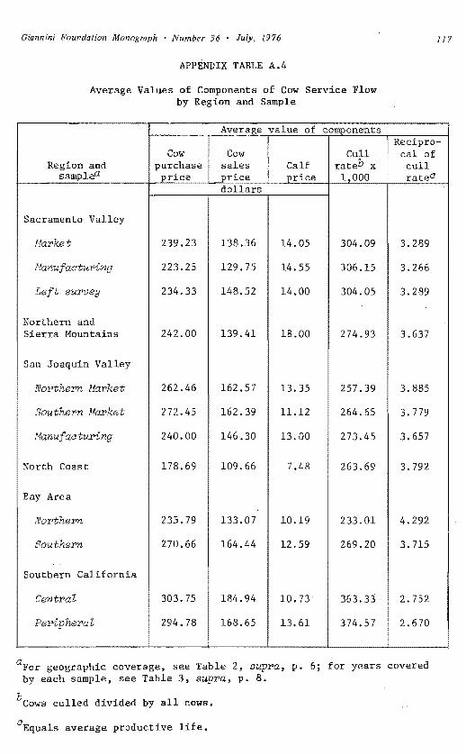
117 Giannini Foundation Monograph • Number 36 • July, 1976
APPENDIX TABLE A.4
Average Values of Components of Cow Service Flow by Region and Sample
Avera_g_e value of c.ol!!£_onents Recipro
Region and samplea
Cow purchase 2rice
Cow sales
J2_rice
T,! i
Calf __E_rice
Cull rateb x
1 000
cal of cull rateC
dollars
Sacramento Valley
Market
t1anufacturing
Left survey
Northern and Sierra Mountains
San Joaquin Valley
Northerra Na:rket
Souther>n Market
Manufacturing
North Coast
Bay Area
Northern
Southern
Southern California
Central
Peripheral
239.23
223.25
234.33
242.00
262.46
2 72. 45
240.00
178.69
235.79
270.66
303. 75
294.78
138.36
129.75
148.52
139.41
162.57
162.39
146.30
109.66
133.07
164.44
184.94
168.65
14.05
14.55
14.00
18.00
13.35
11.12
13.00
7.48
10.19
12.59
10.73
13.61
304.09
306.15
304.05
274.93
257.39
264.65
273.45
263.69
233.01
269.20
363.33
374.57
3.289
3.266
3.289
3.637
3.885
3. 779
3.657
3.792
4.292
3. 715
2.752
2.670
aFor geographic coverage, see Table 2, supra, p. 6; for years covered by each sample, see Table 3, supra, p. 8.
bCows culled divided by all cows.
cEquals average productive life.

118 Hoch: California Dairy Farms
In retrospect, some refinements might have improved the estimate somewhat. Thus, the cow death rate may be somewhat more than I percent. (Shultis, Forker, and Appleman estimate the California cow death rate as l percent to 2 percent per year. 1) Of more importance, artificial insemination charges of $7.00 per cow per year (the BMS estimate) were treated here only as an offset to profit but might have been introduced into cow service flow as an offset to the calf sales price. This would increase the cow service flow estimate by around 15 percent. However, when cow service flow is treated as a component of a nonfeed cost aggregate, as was usually done here, any error from this source will be quite minor.
It seems likely that cow service flow was the major source of difficulty in the disaggregated cost case, i.e., when capital, cow service flow, labor, and operating costs were treated as separate independent variables. Number of cows is highly correlated with measures of feed, so high correlation of independent variables becomes a likely source of large errors of estimate (and possibly peculiar point estimates).2 Further, in production function estimation, there is a common problem of a possible linear relation between output and raw materials, with some raw materials in approximately fixed proportion to output. This relationship can distort regression results. The problem may apply here with number of cows corresponding to raw material. The problem is usually handled by subtracting the value of raw material from output and regressing the net output (or value added) on the remaining inputs. This assumes the proper specification of the production function is:
1-1 y K Il
i=l
so that Y A z1 = Y* becomes the transformed dependent variable to be regressed on the remaining independent variables, Zi, = 1, ... , I - 1, where Z1 is the raw material and Y* is net output or value added.3
This way of handling the problem was precluded here because the milk blend price for the individual producer generally was not known. Further, measurement of output in physical rather than value terms avoids some measurement problems, e.g., the problem of product price deflation.
The aggregation of nonfeed costs then was the device employed to avoid the difficulty of the disaggregated case, whatever its1 cause. In ex post terms it appears to have been
' justified. ,_______ 1Shultis, Forker, and Appleman, op. cit., p. 23.
2Appendix Table B. l, infra, p. 139, exhibits elasticity estimates for the disaggregated cost case (Equation 5). In the 12 samples, cow service flow had a negative coefficient in five cases before firm effects were introduced and in two cases after firm effects were introduced. In the latter analysis, t ratios showed marked variation as documented in the Statistical Supplement to this Monograph.
I a. A z1 i!_l!.'!_ Y = K i~l Zi 1 both hold, it follows that the solution value for Y is
I O:· ] 1/l-a1
y z.1n[ K (+fl I
Ii=J
so that solutions for the a1 can be obtained only if o:1 is known.
119 Giannini Foundation Monograph • Number 36 • July, 1976
Labor
The development of data on total wages was relatively straightforward and consisted of aggregating wages paid to milkers and to laborers, checking, and ,Peflating. The BMS records contained two sources of information on labor, with entries on both the front and back of their field survey sheet. This permitted checking and correcting of errors in the records on the basis of internal evidence. Labor cost was measured in terms of actual input in a given month rather than financial claims paid; thus, there was a prorating through the year of payment to a temporary worker replacing a worker on paid vacation. Wages were deflated to a 1964 base using monthly farm wage indexes. I Examples of the deflators, in the form of month of July values, appear in Appendix Table A.5.
Operating Costs
Operating costs consisted of the sum of utilities (including telephone); veterinary, medicine, and DHIA charges; fees; repairs; tractor and truck expenses; supplies; and other expenses.
DHIA charges refer to payments to the DHIA for testing each cow every month. The tests include mastitis control, butterfat content, and general herd condition. Fees cover payment to producer associations, a state fee to support the state milk stabilization program, and a public health inspection fee. Other expenses include such items as sawdust and gravel for corrals, cow clip and hoof trim, accounting fees, and uniforms.
Tractor and truck expenses in the dairy enterprise were estimated by the BMS and consisted of hours of tractor use times $2.00 per hour and miles of truck use priced at 10 cents a mile for a pickup truck and 15 cents a mile for a larger truck. Since the rates used were invariant over time, there was no need to deflate these dollar values. All other components were deflated, with deflators the reciprocals of monthly price indexes on a 1964 base. A particular index was employed for each component, as indicated in Appendix Table A.5, which presents a subset of the monthly indexes consisting of the July values in each year. The aggregate of the deflated components gave the operating cost variable.
Repairs posed some special problems. If there is $1.00 of repairs every year, the amount to be charged depends on the life of the repairs if the life is greater than one year--i.e.• if making a repair corresponds to investment in an asset. The amount to be charged each year will be TR(T) where T is life and R(T) is the internal rate of return. For example, with an asset of life three years, there is an equilibrium return of .367 each on the investment made this year, last year, and the year before last; so the total return charged per year will be 1.101 (three times .367). Consider this listing of selected values per dollar investment:
T R(T) TR(T)
I 1.050 1.050 2 0.538 1.076 3 0.367 l.101 5 0.231 1.155
10 0.130 1.300
I U. S. Economic Research Service, Farm Cost Situarion, 1956-1964.

c APPENDIX TABLE A.5 ._
"' Price Index.es, 1955-1965
(Base 1964 1. 000)
-Price index for Jul of ear on 1964 base
Consumer Veterinary Farm Year rice index Utilities and medicine Su lies Re airs machiner
1 2 3 5 6
1965 1. 019 0.999 1. 018 1. 010 1.025 1.030
1964 1.002 1.000 1.001 1.000 0.997 0.997
1963 0.991 1. 002 o. 975 0.990 0.985 0.980
1962 0.976 1. 001 0.984 o. 990 0.967 0.954
1961 0.965 0.999 0.973 0.990 0.959 0.940
1960 0.954 o. 992 o. 967 0.980 0.945 0.922
1959 o. 941 0.950 0.955 0.980 0.929 0.900
1958 o. 934 0.930 0.931 0.980 0.898 0.863
1957 0.910 0.893 0.901 0.980 0.886 0.846
1956 0.882 0.889 0.869 0.971 o. 825 0.780
1955 0.863 0.881 0.846 o. 971 D.790 0.750
1. 010 1.050
0.998 1.013
1.002 0.979
1.005 0.954
1.016 0.937
1.015 0.912
1.017 0.895
1.002 0.820
1. 009 0.795
0.960 0.770
o. 910 0.740
Sources:
Cols. 1-3: U. S. Bureau of the Census, SuT'Vey of Cu!'X"ent Business (consumer price index for selected items), monthly issues. For utilities, gas and electricity in.dex was employed; for veterinary and medicine, 50 percent physician index and 50 percent drugs index were used (fees were deflated using general consumer price index); and for repairs, 75 percent farm machinery index plus 25 percent farm buildings index were used).
Cols. 4-8: U. S. Economic Research Service, Farm Cost Situation, November, 1965, p. 2; November, 1964, p. 2; May, 1957, p. 2; and May, 1956, p. 2.
121 Giannini Foundation Monograph • Number 36 • July, 1976
It can be seen that asset life does not affect results markedly, i.e., TR(T) is relatively stable. It was assumed here that the life of the repairs was three years; but results would not be much affected if life were actually two years or five years.
Major building repairs were not included in the repairs category but rather were treated as building investment. Available evidence led to an estimate of repair value as distributed as three-quarters machinery and one-quarter minor building repairs. An assigned life of three years then seemed reasonable for this composite asset.
There was an application of monthly price deflators reflecting the allocation between buildings and machinery. A moving average of annual repairs on a monthly basis was then distributed through time applying the internal rate of return for an asset with a three-year life. In the first and second observed year for any producer, it was assumed the previous two years of repairs were at the same level as that for the first year observed.
Feed
There were two major problems in measuring feed input. The first involved replacing a large subset of feed observations in TDN terms. The second involved transforming feed from a TDN to a dollar measure.
TON Estimates.--The first problem arose because the BMS sometimes estimated feed on the basis of milk produced in a given month. This occurred when pasture was fed or when it was hard to estimate the quantity of a specific roughage. To avoid contradiction of the fundamental assumption of regression analysis that independent variables are truly independent of the disturbance in output, it was necessary to replace these estimates. This was done by regressing feed observations for months when the problem did not occur (labeled the "good" observations) on a set of presumed exogenous variables. The regression results obtained were then used to estimate feed for the months at issue, and the estimates obtained were substituted for the BMS estimates. Ten samples were employed, with a combination of original samples for the Southern California cases and the Sacramento Valley (Market and Manufacturing) cases. The former combination occurred because there were very few "bad" observations; the latter occurred because the Manufacturing sample had a great many bad observations. Linear regression was used in all cases.
The two most important variables employed (as indicated by levels of significance) wen~ number of cows being milked (cows milking) and number of cows not being milked (cows dry). In fact, good explanations for total feed (in TON per day) are obtained when the regression is limited to these variables only, as shown in Appendix Table A.6. The coefficient for cows milking is always above that for cows dry; the averages for the 10 samples employed are 24.9 and 14.5, respectively, which can be interpreted as TON requirements in pounds per cow per day, with the latter figure viewed as the minimum maintenance requirement. The milking cow figure for Southern California is well above that for other areas, perhaps indicating a more intensive feeding pattern in Southern California.
The introduction of a large number of additional variables improved results somewhat in statistical terms; the amount of unexplained variance was generally reduced by around 25 percent, with a reduction in two cases of over 50 percent; and many of the additional variables had statistically significant coefficients.

122 Hoch: California Dairy Farms
APPENDIX TABLE A.6
Results for Feed (Total Digestive Nutrients Per Day) Regressed on Cows Mil~ing and Cows Dry (Linear Regression)
by Region and Sample
Region and samplea
Sacramento Valley
Ma.rket }Manufactu:f>ing Left su:r>Vey
Northern and Sierra Mountains
San Joaquin Valley
No-Ptfiern Ma:Pket Soutfiern Ma.rket Manuf actUPing
North Coast
Bay Area
No-Pthem Southern
j
Southern California
Cent-Pat } Pe-Pipherat
Average:
10 market samples
Number of
"good" observa
tions
567
142
266
560 693 182
66
619 660
1,099
b
Constant
- 27.0
57.6
103.7
-227.1 82.7
-102.8
140.4
136.7 68.9
-143.9
8.9
Coefficient Cows
milking
25.5
26.5
23.1
25.9 24.8 24.2
21.9
23.2 24.4
29.3
24.9
Cows di::y_ Rz
16.3
5.7
.921
.920
12.3 • 927
24.6 13.8
8.7
10. 7
.979
.956 • 978
.888
12.1 21.3
• 957 • 975
19.3 .986
14.5
aFor geographic coverage, see Table 2, supra, p. 6.; for years covered by each sample, see Table 3, supra, p. 8.
bBlanks indicate not relevant.

123 Giannini Foundation Monograph • Number 36 • July, 1976
The additional variables introduced included expected milk per cow, total expected milk produced, average body weight per cow, and cow value per head. Further, several sets of dummy variables were introduced. These included dummies for season (both current and lagged), breed, and year. Explicit definitions follow.
Milk produced in the closest available preceding period was employed in constructing some lagged endogenous variables. Milk was measured in terms of 3.8 percent butterfat content equivalent as defined in the text above. The closest available preceding period was limited to a month in which a "good" observation obtained and occurring within a year preceding the month in question. If these conditions did not hold, the observation in question was deleted from the good sample.
Expected milk per c0w was defined by dividing lagged milk by number of cows milking in the preceding period. Then expected milk for the current period was defined as expected milk per cow times number of cows milking in the current period.
Because seasonal differences might affect results, dummy variables accounting for season were introduced, with one set applying to the season in which the observation occurred (the current season) and one set applying to the preceding period which was the source of the lagged endogenous variables (the preceding season). In each set three dummy variables were defined: (1) "summer" (April through August); (2) "winter" (November through February); and (3) "remaining months" (March, September, and October). Presumed differences in pasture conditions were the source of these seasons.
Body weight and price per head were obtained from the BMS observations for each farm Breeds and years for the good observations were the same as in the overall sample, with the breed categories being Guernsey, Holstein, Jersey, and Mixed.
Linear dependence for sets of dummy variables was eliminated by setting the coefficient of one variable in each set equal to zero, a priori. Variables thereby eliminated included remaining months for season, Holstein for breed, and the earliest year in each sample. Appendix Table A.7 presents some selected results for the 10 regression cases; these include coefficient estimates for the San Joaquin Valley (Southern Market) and the Southern California combined sample. In addition, the number of statistically significant cases and signs for those cases are also listed.
The San Joaquin Valley and Southern California results present two cases: in Case 1 the expected milk variables are excluded, while in Case 2 they are included. It can be seen that the introduction of the expected milk variables causes a drop in the coefficient for cows milking in the San Joaquin Valley case; and this shift occurred in most of the other samples. This can be explained by the appearance of cows milking as one of the components of expected milk total. The results for the Case 2 regressions were used to estimate TDN for the months of concern, and the problem involved was considered solved.
However, it appeared to be of interest to extend the work somewhat and carry out a side investigation by pooling all observations and defining an additional set of dummy variables covering regions. Here all the Sacramento Valley cases are combined into one group, and the 'San Joaquin Valley (Manufacturing) observations are assigned to the San Joaquin Valley (Northern or Southern Market) areas.
Results appear in Appendix Table A.8, and interpretations thereof follow.' Appendix Table A.8 is an extension of Table 6 above which was presented in the text for ease of exposition. Results for the two cases are quite similar.

124 Hoch: California Dairy Farms
APPENDIX TAllLE A. 7
Selected Results for Feed (Total·Digestive Nutrients Per Day) Regressed on Full Set of Explanatory Variables in Linear Regression
i------~-~1[ariab le
Coefficient obtained San Jol!:l..uin Vall~ Southern
Southern Market California Case 1 Case 2 Case 1 Case 2
I Statistically significant
coefficients, all 10 s~les
Number Sigrl_ Case 2
Constant term -1,833.94 -508.03 -3,596.59 -3,522.27 a
Cows milking 24.53* 15 .10* 29.25* 29 .58* 10 plus
Cows dry 15.92* 15.26* 18.44* 18.48* 9 plus
Expected milk per (pounds per day)
cow 5.17 3.81 2 --b
Expected milk, total (hundred pounds per day) 27.57* - o. 77 6 plus
Body weight (hundred pounds) 37. 38* 35 .63* 129 .18* 122 .'66* 5 plus
Value of cow per head (dollars) 6 .93* 2.63* 5.40* 4.96* 6 plus
Dwwrry Variahles
Season
Current su1lllll.er Current winter Past summer Past winter
---
2.42 28.76 54.31
3.09
5.01 8.02
52.19 31.21
50.64 - 12.98
17.84 - 104.17*
- 52.27 11.42 18.32
- 105.11*
2 0 0 1
plus
minus
Breed
Guernsey Jersey Mixed
18.40 - 336.28*
429. 89
-106.93 -276.24* -214.33*
725 .22*
216.59*
- 747.00*
216.16*
5 2 5
minusc
minus minusc
, Year
l
1965 1964 1963 1962 1961 1960 1959
448.96* -498.31* 403.63* -474.83* 344.04* : -342.11*
- 333.96* -363.58* i - 265.61* -405.38*
440.88* 19.49
!65.34 66.85
438.64* 12.80
159.66 61. 79
1 5 4 2 1 1
I
plus minus minus
-minus minus
l .984 .989 .989 .989 l
aBlanks indicate variable not in equation or category not relevant. Case 1 excludes expected milk per cow and total expected milk; Case 2 includes those variables.
bDashes indicate one plus, one minus.
cone case of opposite sign, e.g., of five significant cases for Guernsey, four had minus signs.
*Statistically significant at the 5 percent level.

Giannini Foundation /vJrmogru.pfl · Number 3n • lulx. J 9 76 /~5
APPENDIX TABLE A.8
Results for Feed (Total Digestive Nutrients Per Day) Regressed on All Explanatory Variables All Samples Combined
Average value Variable of variable Coefficient t ratio
Constant term a -770.11 Cows milking 134.13 17.26 52.26* Cows dry 27.72 20.06 46.0l* Expected milk per cow (pounds per day) 36.18 - 13.51 - 9.28* Expected milk, total (hundred pounds per day) 51. 45 22.5.\ 28.67* Body weight (hundred pounds) 12.01 79.97 9. 06* Value of cow per head 254.14 2.33 8.04*
Dummy~b
Season
Current summer • 303 0.14 0.01 Current winter .448 - 1. 93 - 0.11 Past summer . 363 - 2.52 - 0.14 Past winter .348 - 9.22 - 0.60
Breed
Gui;.:rnsey .046 -185.13 - s.10• Jersey .069 91.59 2. 75* Mixed .200 94.58 - 5.60*
Year -
1965 .015 66.14 1. 03 1964 .204 -202.15 - 4.51* 1963 .252 -107.46 - 2.43* 1962 .245 - 53. 79 - 1.21 1961 .162 - 71. 76 - 1. 59 1960 .078 63.00 1.30 1959 .024 81.03 1.42
Region
Sacramento Valley .146 -208.55 - 3. 7 5*
Northern and Sierrn Mountains . 055 -346.57 - 6. 04*
San Joaquin Valley
Northern Market .133 -390.99 - 6.94* Southern Marke·t .162 -316. 96 - 5. 72*
Bay Area
Northerra .128 -358.67 6.26* Southern .136 -256.20 4.31*
Southern California .226 - 70.94 - 1.16
Omitted Dw!1my Va.riableB
Season: Remaining months, current .249 0 remaining months,. past .289 0
Breed: Holstein .685 0 Year: 1958 and earlier .020 0 Region: North Coast .014 0
R2 .985
"Blanks indicate not applicable.
bDumm.y variables take on values of 0 or 1. The average value then is the frequency of occurrence of given dummy. The sum of all averages in a giverl set will total 1.
*Statistically significant at the 5 percent level.

126 Hoch: California Dairy Farms
The coefficient of cows milking is below that of cows dry as noted for Appendix Table A.7. However, if expected milk per cow is fixed at its average of 36.18 pounds per day, the addition of one cow milking contributes 17 .26 pounds of feed directly, and 8.15 pounds of feed indirectly, through the "expected milk total" variable (36.18 x l x .2254). Hence, the amount attributable to one milking cow is 25.41 pounds on the average. In similar fashion, if number of cows is fixed at the average of 134 and expected milk per cow increases by one pound per day, total feed increases by 16.69 pounds (through direct and indirect effects), or about .12 pounds per cow per day. More generally, the expected milk total variable establishes an interaction between cows milking and expected milk per cow. As the latter increases, the linear relation between feed and cows milking increases in slope and decreases in intercept.
The coefficient for cows dry is about 20 in Appendix Table A.8, somewhat above the average figure of Appendix Table A.6. Body weight and value are related positively to feed; an increase in each increases amounts fed. Holstein cows apparently consume more feed (for the same weight and value, presumably) than do the other breeds. The year effects might be interpreted as indicating increased efficiency in feeding, for there is a general negative trend in feed input over time (though 1965 runs counter to it). In similar fashion, the San Joaquin Valley samples might be viewed as having high efficiency in feeding, while the North Coast has the lowest, and Southern California, the next to lowest. However, Appendix Table A.6 results suggested the possibility of a more intensive feeding pattern in Southern California. The seasonal effects appear nil in Appendix Table A.8, but all other results exhibit statistical significance.
Feed Price Estimates.--The second major problem in measuring feed input was that of implementing the decision to transform feed from TDN into dollars. This was carried out by multiplying each major feed category--roughage, concentrates, and pasture--by a corresponding price for each sample.
Pasture prices were based directly on BMS information. Roughage and concentrate prices were estimated in a more involved manner. Prices on a large number of individual feeds were available for a subset of the observations in each sample. These values were averaged over those cases and used to establish average prices for two categories of concentrates and seven categories of roughage. These were converted to prices per 1,000 pounds of TON using BMS data on the fraction of TDN per pound of feed (the TON-feed ratio). Then quantities fed for each of the categories were aggregated by sample;
Jthe fraction of feed in each category of a major feed type was then used as a weight in obtained weighted prices for roughage and concentrates.
Appendix Table A.9 lists the TDN-feed ratio and prices for roughage classes and concentrates. One category of concentrates was a collection of Special Feeds comprising a minor part of the total; it has been aggregated with the other, more general, concentrates category in Appendix Table A.9.
Appendix Table A.10 lists the distribution of feed categories as a fraction of total TDN fed by sample. It can be seen that pasture use is related to farm size and locale, with decreasing pasture use occurring with southward movement and increased average farm size (see Table 4 for average farm-size indicators). There is also some tendency to substitute concentrates for roughage with southward movement and increased size.
Appendix Table A.11 lists the weighted average prices used in practice for the three major categories of feed. Given the time distribution of observations, values for the

APPENDIX TABLE A.9
Total Digestive Nutrients (TDN)-Feed Ratios and Feed Prices by Feed Categories, Regions, and Samples
Other h'!Y_ J Green chop, Feed category, a Alfalfa Lower Higher Beet nonhay Coneen-
r~ion and sample hl!}' priced _p_riced Molasses _ILu],E_ Sil'!i!_e ro'!li_h~ trates TDN-feed ratio
All re8ions
Fraction TDN, per pound of feed .50 .50 .50 .60 .10 .17 .13 .70 to .75b
price of 1,000 _E_ounds of TDN dollars
Sacramento Valley 28.60 21.50 23.70 30.00 22.50 23.50 22.50 45.00
Northern apd Sierra Mountains 28.80 22.50 27 .10 33.40 22.50 23.50 26.90 44.50
San Joaquin Valley
Northern Market 27.90 25.00 25.00 26.70 a 24.70 26.20 44.80 Southern Market 25.80 25.00 25.00 25.90 24.70 20.00 43.10 Manufaaturing 28.00 25.00 25.00 25.00 24.70 22.70 43.00
North Coast 32.50 24.40 27.90 33.40 29.40 34.60 47 .20
Bay Area 30.40 25.20 25.60 25.00 29.40 31.90 44. 70
Southern California 34.70 29.10 31.50 29.20 29.40 29.60 44.40
aFor geographic coverage; see Table 2, supra, p. 6; time span covered is 1959-1965, but feed prices listed are based on a preponderance of observations in the 1962-1964 period.
b"Concentrates" as a general class was assigned a TON ratio of • 75 by the Bureau of Milk Stabilization; concentrates here also include a small amount of other feeds (usually classed as a form of concentrates, e.g., pellets) which causes the variation in TDN ratio. By sample, the following TDN ratios held for this category:
Sacramento Valley (Market): .742 Bay Area (Northern): .739 (Manufacturing): •747 (Southern): .750 (Left survey): • 701 Southern California (Central): • 728
Northern and Sierra Mountains: .741 (Peripheral) : .736
San Joaquin Valley (Northern): • 731 (Southern) : .747 (Manufacturing) : .750
aBlanks indi 0
cate feed category not listed as used by any producer in sample,

- APPENDIX TABLE A.10
Distribution of Feed Categories as Fraction of Total Digestive Nutrients Feda by Region and Sample
Region and sampleb
Sacramento Valley
Alfalfa h!l}' Silage
ROl!JliGreen ch~
h'!J:l_e All
other Total Concentrates Pasture
Market .445 .028 .069 .064 .606 .208 .186
Manufacturing • 432 . 005 .052 .062 .551 .087 • 362
Left BU:MJey .560 .022 .013 .019 • 614 .198 .~88
Northern and Sierra Mountains
San Joaquin Valley
.543 .001 .005 .026 .576 . 210 .214
Northern Market .434 .096 .084 .016 .530 .249 .121
Southern Market .476 .043 .159 • 009 • 687 . 294 .019
Manufacturing .484 .083 .095 • 004 .666 .181 .153
North Coast
Bay Area
.143 .021 .055 .122 • 341 .176 .483
Northern .446 • 013 .018 .036 .513 .336 .151
Southern
Southern California
.587 .043 .054 .009 .693 .265 .042
Central .507 .016 .062 . 014 .599 • 397 .004
Peripheral .418 .043 .177 • 012 .650 .346 .004
aTotal roughage plus concentra·tes plus pasture equal 1. 00.
bFor geographic coverage, see Table 2, supra, p. 6; for years covered by each sample, see Table 3, supra, p. 8.

129 Giannini Foundation Monograph • Number 36 • July, 1976
APPENDIX TABLE A.11
Average Prices Per Pound of Total Digestive Nutrients (TDN) for Major Categories of Feed by Region and Sample
sampleaR~ion and Average prices
Roughage Concentrate Pasture
Sacramento Valley
Market
Manufacturing
Left survey
Northern and Sierra Mountains
San Joaquin Valley
Northern Market
Southern Market
Manufacturing
North Coast
Bay Area
Northern
Southern
Southern California
Central
Peripheml
• 0271
.0274
.0281
• 0286
• 0271
.0243
.0268
.0301
.0301
.0303
.0339
.0329
per __E_ound of TDN
.0450
.0450
.0450
.0445
.0448
.0431
.0430
.0472
.0447
.0447
.0444
.0440
'
.0225
.0225
.0225
.0225
.0250
.0250
.0250
.0240
.0250
.0250
.0290
.0290
aFor geographic coverage, see Table 2, supra, p. 6; for years covered by each sample, see Table 3, supra, p. 8.
130 Hoch: California Dairy Farms
1962-1964 period will have preponderant weight in these averages, but available evidence indicates feed prices were fairly stable over the entire period of the sample.
Dummy Variable for Dairy Herd Improvement Association (DHIA) Status
A dummy variable was used to indicate whether the producer was a member of the DHIA; a value of one indicated membership and zero indicated nonmembership. Some producers were members over all their observations, some were never members, and some were members part of the time. Appendix Table A.12 presents membership status in these terms by sample. It seems clear that participation is most frequent in samples characterized by larger firms, so it is likely that DHIA participation is related to scale of operation.
The question of whether there was a trend in DHIA membership was investigated at both the aggregate level and that of the individual firm. Absence of trend was indicated at each level.
In the first approach, the fraction of firms that were DHIA members in each year was calculated for each sample. Although there was a fair amount of variability, particularly in the small samples, the fraction exhibited no time trend. Readings on the fraction for the seven largest samples (with three subregions aggregated into regional groupings), covering years in common, appear in Appendix Table A.13. The averages over the samples for those years are: 1961--.745; 1962--.753; 1963--.724; and 1964--.763.
Considering patterns for individual firms by focusing on the 141 (out of 474) that were DHIA members part of the time (Appendix Table A.12), 36 were catalogued as having become members during the survey period, 31 as having terminated their membership, with 74, then, having discontinuous membership. Although some of the terminating cases might really be discontinuous, if later data were secured, the pattern suggests a fairly close balance between new members joining and old members withdrawing from the association. Hence, absence of trend is again suggested.
It is possible that more refined measures on DHIA participation might yield additional information. If there is a time lag before DHIA data can be fully utilized, there may be a tendency to understate the ultimate benefits for new members. Hence, information on length of time a producer was a member might be used to test the lag hypothesis.
, In practice, however, such information was not available for producers who were always members during the period observed. Further, the present approach can be viewed as indicating the average payoff to membership and can be rationalized on the basis of estimating average rather than ultimate returns. If there are low benefits initially, a producer should take account of such in his decision to purchase the senrice.
Breed Dummy Variables
Four breed dummy variables were employed: Guernsey, Holstein, Jersey, and Mixed. (The few cases of Ayrshire and Brown Swiss were included in the Mixed category.) Data on breed~farm combinations is presented in Appendix Table A.14. A farm with a change in breed is counted twice; thus, if a farm changes its breed from Holstein to Mixed, one case of each breed is included in the enumeration. Information was not available on the extent of any change so that a change from Holstein to Mixed, for example, might have involved only a few cows.
Giannini Foundation Monograph • Number 36 • July, 1976 131
APPENDIX TABLE A.12
Dairy Herd Improvement Association (DHIA) Participation by Region and Sample
Region and samplea
Sacramento Valley
MaPket
Manuf actuPing
Left survey
Membership in DHIA Always Never Part-
a a time member member member
31 9 24
7 8 5
13 3 5
Total member firms
64
20
21
Northern and Sierra Mountains 4 11 14 29
San Joaquin Valley
Northez>rz Market
Southez>rz Market
Manufaaturing
23
30
3
8
7
12
15
14
5
46
51
20
North Coast 6 12 11 29
Bay Area
Northern
Southe!7!
31
24
20
11
16
6
67
41
Southern California
Central
PeripheT'al
40
9
8
3
15
11
63
23
Total cases 221 112 141 474
aFor geographic coverage, see Table 2, supra, p. 6; for years covered by each sample, see Table 3, 'supra, p. 8.

132 Hoch: California Dairy Farms
APPENDIX TABLE A.13
Evidence on Dairy Herd Improvement Association (DHIA) Participation Over Time by Region and Sample, 1961-1964
Regiona and sample 1961 1962 1963 1964 Firms in DHIA as fraction of all firms
Sacramento Valley
.837Market .792 .745 .734
San Joaquin Valley
Northern Mar>ket} • 732 .742 .742 .784Southern MCU'kBt
Bay Area
Northern} • 660 .656 .625 .676Southern
Southern California
Central } • 796 .778 .783 .877Peripheral
.!verage:
Major samples .745 .753 • 724 .768
Total firms in sa!l!E_le 1'y~ear
Sacramento Valley
48Market 49 59 64
~ San Joaquin Valley
Northern Mar>ket} 97 97 97 97Southern Market
Bay Area
Northern} 94 8890 74Southern
Southern California
Central } 54 72 83 81Peripheral
aFor geographic coverage, see Table 2, supra, p. 6.

133 Giannini Foundation Monograph • Number 36 • July, 1976
APPENDIX TABLE Aol4
Number of Breed-Farm Combinations by Region and Sample
Number of breed-farm combinations
Region and samplea Guernsey Breed
Holstein Jersey Mixed ~otal
ases
Sacramento Valley
Market 7 37 8 18 70
Manufacturing 1 12 4 6 23
Left survey 0 14 4 10 28
Northern and Sierra Mountains 2 20 6 3 31
San Joaquin Valley
Northern Market 2 38 1 19 60
Southern Market 3 39 6 8 56
Manufacturing 3 14 1 7 25
North Co2.st 5 1 15 15 36
Bay Area
Northern 8 34 17 39 98
Southern 1 38 1 20 60
Southern California
Central, 1 58 0 9 68
Peripheral, 2 17 0 11 30
Total 35 322 63 165 585
aFor geographic coverage, see Table 2, supra, p. 6; for years covered by each sample, see Table 3, supra, p. 8,
134 Hoch: California Dairy Farms
The Holstein cases predominate for most samples. The North Coast is an exception, and the Bay Area (Northern) is a partial exception, with much greater employment of Jersey cattle in these cases. Presumably this specialization reflects geographic differences.
Transformation of Dummy Variab1e Results
ln working with dummy variables, a linear constraint must be imposed to avoid linear dependence among explanatory variables. For computational purposes, this was carried out by assigning a value of zero to the coefficient of one dummy variable in each set. For purposes of interpretation, however, it was deemed more useful to present the coefficients (or effects) as deviations from an average of zero in the logs.
This was done by forming the average over a set of effects and then subtracting the average from each effect; the effect set equal to zero initially was included in both steps. Thus, for a given set of dummy variables, write ej, j 1, .. ., n, as the estimated effects obtained as regression results, say, with e1 = _O a priori. Then let ~ =. ~j=l ej/n and ej e Ej, the transformed effect. Clearly, Ej = 0. The average, e, is· added to the constant term in the regression results, so the overall equation is unaffected.
In the antilogs the transformed effect, Ej, is readily interpreted as an index number where the base of l.00 is that of the average effect.
The procedure was employed for all sets of dummy variables except years. In that case the 1963 value for each sample was treated as the base value so that all samples could be easily compared.
The Ej was divided by Sej' the estimated standard error obtained for ej, to yield an adjusted student t value. This was rationalized by viewing e as a constant; tlie addition of a constant leaves the variance and standard deviation unchanged, so that Sej was treated as if it were SEj·
However, a contrary interpretation is to view e as a random variable. Under this argument, SEj would be some complicated function of all the estimated parameters' variances and covariances.
The more e deviated from zero, the greater the distortion likely to be introduced I for, if e equaled zero, then ej = Ej and Sej = SE-. 1 Generally, the most pronounced
deviation of e from zero occurred for the firm efrects, with the Southern California (Peripheral) case the most pronounced of all. To investigate the situation, the Southern California (Peripheral) case was recalculated, now excluding a firm whose transformed firm effect (Ej in the notation employed here) was approximately zero and including the firm omitted 111 the initial calculation. Under this recalculation, the newly derived e was small (approximately zero). The results obtained showed essentially the same pattern as the initial case, though there was some improvemen r in terms of a general decline in standard errors and, hence, a rise in t values. Of the 21 coefficients common to both cases, 13 were significant in the initial calculation; these remained significant and were augmented by two newly significant coefficients in the recalculation. For the 15 significant coefficients, t values averaged 3.9 initially and 5.4 in the recalculated case.
l If the set of e. were independent random variables, each with the same mean, µ, and variance, 202, then the expect
1
ed value of (ej -· e) 2 is O~ = (n - l/n) [a2 + 2µ ] SO that CT~ increases with
the deviation of µ from zero. Though this is a special case, it seems suggestive.

Giannini Foundation Monograph • Number 36 • July, 1976 135
Insofar as this result can be generalized, it suggests the difficulty is not too grave and that the assumption that e is constant may well lead to some understatement of the significance of the results. 1
Tests of Significance of S~ts of Dummy Variables
Given the process sketched out in the previous section, the elimination of one dummy variable from each set to prevent collinearity meant a corresponding reduction in the number of coefficients that were potentially significant. This occurred because t ratios were not computed for omitted variables. In the case of the year effects, an additional reduction in potentially significant cases occurred through the decision to set the 1963 coefficient at 1.000 in the antilogs, making results easily comparable between samples. As a consequence, the 1963 coefficient in the logs was set at zero, with corresponding t ratio of zero, i.e., coefficient relative to standard error.
To test the statistical significance of a given set of dummy variables, an F test is appropriate; in effect, this compares explained variance before and after the set of dummy variables is introduced. Time and budget constraints permitted the carrying out of F tests only for the firm effects. The hypothesis tested was that all firm effects in a given sample are zero. In all 12 samples the hypothesis was rejected at both the 5 percent and the l percent level, employing the data of Equation 1. Calculated F was above critical F in all cases. Results appear in Appendix Table A.15.
For the other sets of dummies, it is possible to apply t tests to the null hypothesis that all members of a given set are zero across all samples by using the normal approximation to the binomial distribution. In the probability limit the null hypothesis implies that 5 percent of the coefficients will test as statistically significant although their effect is really zero, i.e .. that error is made 5 percent of the time by virtue of the initial test procedure. Hence, each reading on significance can be treated as a drawing from a binomial population, with a nonsignificant reading corresponding to failure or zero and a significant reading to success f?r one. Then the ratio of significant to potentially significant cases was taken as a statistic, P, from a binomial population with P, the basic probability, set at .05 under the null hypothesis of inferring significance when false. Finally, a normal approximation to the binomial allowed a t test of the null hypothesis, with test statistic
~
p
where N is the number of drawings, equal to potentially significant cases in the present application. Because the test statistic is approximately normal, a t test using N degress of freedom was deemed appropriate. Appendix Table A.16 lists significant cases, total and potentially significant cases, the ratio of significant to potentially significant cases CP), and the calculated t statistic for each set of dummies. It turns out that all sets of dummies have calculated t above critical t, with lowest t statistic for breeds and highest for firms.
1or course, this runs counter to the plausible hypothesis which initiated the investigation; see footnote I, supra, p. 134.

136 Hoch: California Dairy Farms
APPENDIX TABLE A.15
F Tests for Firm Effects Using Data of Equation 1, by Region and Sample
Regiona and sam2._le
R2 Firm Firm
dummies dummies in- ex-
eluded eluded
Degrees of freedom
m n
Calculated F J_m,n)
Crttical
value of b
F (m,n)
Sacramento Valley
Market .953 .893 42 1,265 37.68 1.45
ManufaetW'ing .879 .840 18 363 6.62 1.65
Left survey .950 .926 19 277 6.90 1.65
Northern and Sierra Mountains .921 .873 28 478 10.38 1.50
San Joaquin Valley
Northern Market .969 • 955 45 1,378 13.69 1.45
Southern Market .984 .975 50 1,159 11.17 1.45
Manufaeturing .971 .956 18 455 13.78 1.65
North Coast .917 .867 27 333 7.32 1.50
~
Bay Area
Northern .958 . 939 66 1,300 9.20 1.30
Southern .975 .954 39 775 16.37 1.45
Southern California
Central .981 .969 40 837 14.17 1.45
Peripheral . 969 .942 22 298 11.84 1.65
aFor geographic. coverage, see Table 2, supra, p. 6.
bTabled F, 5 percent level approximation.
137 Giannini Foundation Monograph • Number 36 • July, 1976
APPENDIX TABLE A.16
t Tests for Significance of All Sets of Dummies Using Normal Approximation to Binomial
Years 1
Months 2
Effects DHIAa
3 Breeds
4 Finns
5
l
Significant cases 15 46 4 5 219
Total cases i !
Potentially signifi- ! cant cases I
! Ratio: significant
Ito potentially significant
65
4lb
.366d
144
132a
.348
12
12
.333
44
32a
.158
469
457°
• 479
Calculated t statistics 9.28 15.68 4.49 2. 75 • 42. 90
aDairy Herd Improvement Association,
b24 less than the total because for each sample (1) the 1963 coefficient is set equal to zero in logs and, hence, to 1.000 in antilogs to make intersample comparisons easy; as a consequence, t ratio for 1963 became zero and (2) the earliest year was eliminated in the original estimation process to avoid collinearity.
0 12 less than the total because one dummy of each set for each sample was eliminated to avoid collinearity. Hence, t statistic was not obtained for that case although the coefficient was obtained as a deviation from the average of included coefficients.
dif omitted cases whose coefficients deviated more from 1.000 than did significant coefficients are also counted, then 21/53 .396 instead of .366 is obtained. The calculated t statistic is then 10.53.
Sources:
Col. 1: Table 9, supra, p. 32.
Col. 2: Table 11, supra. p. 37.
Col, 3: Table 13, supra, p. 41.
Colo 4: Table 14, supra. p. 43.
Col. 5: Table 15, supra, p. 44.

138 Hoch: California Dairy Farms
APPENDIX B
This Appendix presents dt)tailed information on some of the side investigations
reported in the text. The information includes coefficient estimates for Equations 5, 6.
and 7. Corresponding standard errors and t ratios for those equations appear in· the
Statistical Supplement to this Monograph.
Equation 5
Appendix Table B.l presents Equation 5 elasticity estimates and R2's for each sample
before and after firm effects were introduced. Before firm effects were introduced,
estimates for feed, labor, and operating cost seem generally reasonable and consistent,
with variability between samples not very pronounced. The cow service flow and capital
service flow elasticities are often close to zero or even negative, and there is a good deal
of variability between samples. After the firm effects are introduced, feed, labor, and
operating cost elasticities generally show substantial declines, while cow service flow and
capital service flow show substantial increases. The latter two elasticities increase in
variability, with a range from negative values to some individual estimates of around .5.
A comparison of the cases suggests high correlation between feed and cow service flow
has affected results. Thus, the sum of the elasticities of the two variables is fairly close
before and after the firm effects are introduced.
Appendix Table B.2 presents average values for the individual, disaggregated inputs
of Equation 5; the dollar values of Appendix Table B.2 are employed to obtain the "factor
share" estimates of elasticities presented in Appendix Tablee B.3. If allocation is optimal,
then the ratio of dollars of input i to dollars of output will equal the elasticity of input i.
The factor share estimate is then the geometric mean of input relative to the geometric
mean of output, in dollars (see equation 3.2 and attendant discussion). Because profits
ire generally positive, the elasticity sum here is generally below one; the average for the
JO market milk samples is .926, indicating that average profit relative to dollar output
is 1.000 minus .926, or .074.
Appendix Table B.4 presents marginal return estimates, and Appendix Table B.5
presents tests of the hypothesis of allocative efficiency for Equation 5 before and after
firm effects. The high standard errors for cow service flow and capital service flow show
up in the very large range for their respective estimates of marginal returns, running from
a low of -4 to a high of 10. However, tests of hypotheses generally show marginal returns
above optimal levels for these inputs while that for feed is often significantly below the
optimal. This could be an accurate representation of reality, of course; but high correlation
among the three inputs, given the introduction of the firm effects, seems a more plausible
explanation.

139 Giannini Foundation Monograph • Number 36 • July, 1976
APPENDIX TABLE B.l
Elasticity Estimates for Equation 5
Region and samplea
1-
Elasticity estimates for input · xl xz x3 X4 X5
Feed Cow Operat- Capital
ief; service Labor ing service TD flow cost cost flow
Sum of
elasticities
Before firm effects introduced R2
Sacramento Valley
Market Manufanturing Left survey
.783
.816
.406
.015
.068
.162
.249
.199
.279
.094
.023 .079
-.109 .032 .119
1.032 1.138 1.045
.896
.837
.930
Northern and Sierra Mountains .871 -.075 .160 .067 .046 1.069 .884
San Joaquin Valley
Northem Market Southern Market ManufaoturiYl{J
.884 .875 .823
-.005 .016 .034
.094
.126
.109
.049
.046
.082
.009 -.024
.055
1.031 1.039 1.103
.956
.973
.954
North Coast .835 -.098 . 266 .027 -.024 1.006 .891
Bay Area
Northern Southern
• 726 .694
-.021 -.047
.223
.247 .150 .180
.016 -.012
1.094 1.062
.942
.954
Southern California
Centrai Peripherai
.724
.687 .069 .131
.128
.101 I .071
.101 .016 .083
1.008 1.103
.969
.938
After firm effects introduced
Sacramento Valley
Market Manufactu:!'iYl{J Left survey
.259 .885 .202
.530
.161
.479
.007
.042
.099
.079
.045
.052
.244
.072 -.052
1.119 1.205
.780
.958
.881
.956
Northern and Sierra Mountains .514 .249 .DOS .022 .457 1. 247 .929
San Joaquin Valley
Northern Market Southern Market Manufacturing
.307
.757
.475
.602 -.005
.325
.054
.081
.223
.025
.060
.059
.071
.079
.265
1.059 .972
1.347
.971
.983
.970
North Coast .756 -.205 .304 .048 .055 .958 .913
Bay Area
Northern Southern
.506
.298 .248 .567
.068
.083 .035 .012
-.111 .249
.746 1.209
.959
.978
Southern California
i
Centrai Peripherri.1,
.208
.292 .445 .283
.019 -.039
.016
.013 .243 .200
.931
.749 .984 .971
aFor geographic coverage, see Table 2, supra, p. 6; for years covered by each sample, see Table 3, supra, p. 8.
bTotal digestive nutrients.

APPENDIX TABLE B.2
Average Values of Inputs Per Month (Equation 5) by Region and Sample
AYerage vaiueOfii:iillits Feed in
pounds of total
digestive
Feed price per pound of total
digestive Total Cow
service Labor Operating Capital service
flowcostflow costnutrients.b feed costnutrientsR"&ion and sall!!'lea dollars
Sacramento Valley
2462,251758.2 2.97Mwke,t 2.69 970 112360.4ManufactuPin.g
1,592 169538.7 2.96Left survey
1271,198Northern and Sierra Mountains 395.7 3.03
San Joaquin Valley
2832,9363.05963.4Northel'n Market 2,865 334967.0 2.96Southel'n M!Il'ket
1442.82 1,221433.7Manufacturing
1271,6042.87559.9North Coast
Bay Area
2093.22 2,410749.0Northel'n 3,012 .2993.33904.3Southern
Southern California
8113.80 6, 7921,786.4CentraZ 7393.63 5,6721,561. 3Pe?'iphera Z
691 316 575
421
896 918 430
549
795 996
2,069 1,719
404 140 256
231
430 452 146
225
305 446
1,021 886
260 lOJ'i 171
175
250 270 100
240
272 355
502 469
"For geographic coverage, see Table 2, supra, p. 6; for years covered by each sample, see Table 3, supra, p. 8. 0Quantity of feed in pounds of total digestive nutrient~ and total feed cost were given in the sample data. Then feed price per pound
of total digestive nutrients was obtained by dividing the feed cost by quantity.

APPENDIX TABLE B.3
Factor Share Estimates of Elasticities Assuming Value of Marginal Product Equals Pricea (Equation 5) by Region and Sample
Factor share estimates of elasticities Cow Operating Capital
R~onb and sam_E..le Feed service flow Labor cost cost service flow Total
Sacramento Valley
Market .540 .059 .166 .097 .062 .924 Manufaatu:r>ing .798 .092 .260 .115 .088 1.353 Left survey .586 .062 .212 .094 .063 1.017
Northern and Sierra Mountains • 521 .055 .183 .101 .076 .936
San Joaquin Valley
NortheJ"l'l Ma:rket .569 .055 .174 .083 .048 .929 Southern. Market .557 .065 .178 .088 .052 .940 Manufac:tu:r>ing .756 .089 .266 .090 .062 1.263
North Coast .605 .048 .207 .085 .091 1.036
Bay Area
No:!'thsrn. .478 .041 .157 .060 .054 .790 Southern .535 .053 .177 .079 .063 .907
Southern California
Central .524 .063 .160 .079 .039 .865 Peripheral .553 .072 .168 .086 .046 .925
Average·:
10 market samples .547 .057 .178 .085 .059 .926
aFactoi.share estimate is ai. Then a1 (ZiPi)/(Y Py) where i refers to specific input, Z is the geometric average of that input, Y is the
geometric average of output, and Pi and PY are respective prices.
bFor geographic coverage, see Table 2, supra, p. 6.

142 Hoch: California Dairy Farms
APPENDIX TABLE B.4
Estimates of Marginal Returns for Equation 5, Before and After Firm Effects Introduced, by Region and Sample
Estimates of ma~inal returns (M$) M$1 M$2 M$3 M$4 M$5
Cow 1-caprtai:-Operatservice Labor ing service
Reg_ion and sac1np_lea Feed flow cost cost flow Before firm effects introduced
Sacramento Valley
1.45 0.25 1.50 0.97Market -1. 76 1.02 0.74 0.20Manufaaturing o. 77 0.36 0.69 2.61 1.32 0.84 1.89
Northern and Sierra Mountains
Left survey
0.871.67 - 1.36 0.66 0.61
San Joaquin Valley
Northern Ma:Pket 1.55 0.54 0.59- 0.09 0.19 0.25 0.52Sou.them Market 1.57 o. 71 -0.46
1.09 0.410.38 0.91Manuf aotu!'i ng 0.89
North Coast 1.38 1.29 0.32 -0.26
Bay Area
- 2.04
1.52 - 0.51 1.42 2.50Northern 0.30 1.30 1.39 2.28Southern - 0.89 -0.19
Southern California
Central 1.38 1.10 0.80 o. 90 0.41 Pe!'ipher>al I 1.24 1.82 0.60 1.17 1.80
Average:
l I1.38 0.15 1.16 1.0810 market cases 0.25
' .J.
After firm effects introduced Sacramento Valley
0.48 8.98 0.04MaPket 0.82 3.91 0.161.11 0.39Manufacturing 1. 75 0.82 0.47Left SUPVey 0.34 7.68 0.55 -0.83
Northern and Sierra Mountains 4.52 0.03 0.220.99 6.00 , San Joaquin Valley
0.54NorlhePn Market 10.99 0.31 0.30 1.47 1.36 - 0.08SouthePn Mar>ket 0.45 0.68 1.51 0.63 3.65 0.84Manuf aotu!'ing 0.65 4.29
North Coast 1. 25 - 4.30 1.47 0.57 0.61
Bay Area
NorthePn 1.06 6.00 0.43 0.58 -2.06 SouthePn 0.56 10.71 0.47 0.15 3.96
Southern California
o.4oCentral 7.11 0.12 0.20 6.27 Pe:t'ipherai 0.53 3.93 I -0.23 0.15 4.37
Average:
10 market cases o. 75 5.55 0.36 o.42 2.52
~or geographic coverage, see Table 2, GUp:t'a, p. 6; for years covered by each sample, see Tabie 3, supra, p. 8.
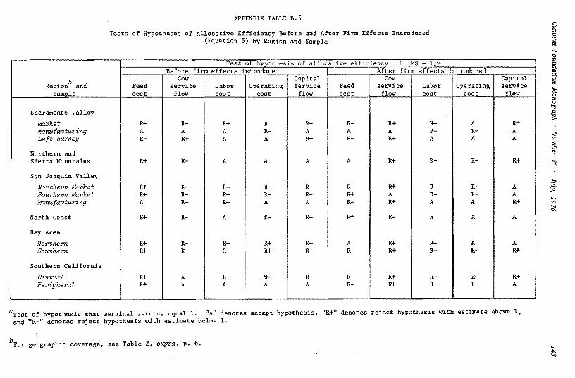
APPENDIX TABLE B.5
Tests of Hypotheses of Allocative Efficiency Before and After Firm Effects Introduced (Equation 5) by Region and Sample
Test of hypothesis of allocative efficiency: HfM$ = l]a: Before firm effects introduced After firm effects introduced
Regionb and Feed Cow
service Labor Operating Capital service Feed
Cow service Labor Operating
Capital service
sa~le cost flow cost cost flow cost flow cost cost flow
Sacramento Valley
Ma:t'ket R+ R R+ A R R R+ R A R+ Manufaoturing A A A R A A A R R A Left survey R R+ A A R+ R R+ A A A
Northern and Sierra Mountains R+ R A A A A R+ R R R+
San Joaquin Valley
Northern Ma:t'ket R+ R R R R R R+ R R A Southern Market R+ R R R R R+ A R R A Manufacturing A R R A A R R+ A A R+
North Coast R+ R A R R R+ R A A A
Bay Area
Northern R+ R R+ R+ R A R+ R A A Southern R+ R R+ R+ R R R+ R R R+
Southern California
Central R+ A R R R R R+ R R R+ Peripheral R+ A A A A R R+ R R A
aTest "Of hypothesis that marginal returns equal 1. "A" denotes accept hypothesis, "R+" denotes reject hypothesis with estimate above 1, and "R-" denotes reject hypothesis with estimate below 1.
bFor geographic coverage, see Table 2, supra, P• 6.
144 Hoch: California Dairy Farms
Equation 6
Appendix Table B.6 presents estimates for Equation 6 by individual sample. Averages
over the 10 market milk samples 'appear in the text as Table 34. Appendix Table B.7
presents estimates of marginal returns for Equation 6 before firm effects were introduced
and compares them to corresponding estimates obtained from Equation I. Table 35 in
the text presents the corresponding comparison after firm effects are introduced.
The R2 values for Equation 6 are generally about the same magnitude as those
obtained for Equation 1 (Table 7). However, a case for Equation 1 can be made on several
grounds. In ex ante terms, dummy variables enter Equation 6 in additive fashion rather
than in multiplicative fashion as in Equation l. The latter seems a preferable assumption.
Again, the quadratic function involves introducing three additional independent variables.
In ex post terms, as noted in the text, there were a number of features of the Equation 6
results that were troublesome: variables sometimes did not enter the regression equations,
and coefficients often had the "wrong" sign, i.e., contrary to expectations. After firm
effects were introduced, the wrong sign occurred for a3 in 6 of 8 cases, for a4 in 7 of 10
cases, and for a5 in 5 of 12 cases. There was some tendency for wrong signs to be associated
and presumably offsetting. The troublesome characteristics suggest that a multicollinearity
problem has occurred.
Equation 7
Appendix Table B.8 presents year elasticities (averages over firms) for feed and all
other input in Equation 7. The table supplements Table 39 in the text which presented
the results for the San Joaquin Valley expanding samples; Appendix Table B.8 exhibits
resljlts for the other samples.
Equation 7 yields specific elasticity estimates for a given firm in a given year. Appendix
Table B.9 exhibits such estimates for the San Joaquin Valley (Northern Market) expa~ding
sample, illustrative (at least) of the tremendous amount of detail inherent in Equation 7.
Of course, the cost of obtaining and handling such detail often may well exceed the
presumed benefits.

145 Giannini Foundation Monograph • Number 36 • July, 1976
APPENDIX TABLE B.6
Estimated Values Before and After Firm Effects Introduced (Equation 6)a by Region and Sample
Estimated value
R~ion and sall!E_leb c al a2 a3 a4 as R2
Before firm effects introduced
Sacramento Valley
Market 0.090* 0.864* -0.054 0.230* -0.167* -0.003 .906 l.fa:nuf aotw>ing -0.172* l.279* 0.274* 0.394 -1.088* -0.125 .823 wft survey -0.165* 0.169 0.471* 0.562* -0.366* -0. 200* .940
Northern and Sierra Mountains -0.074* 0.826* 0.184* -0.260 0.412* 0.008 .908
San Joaquin Valley
Northern Market -0.055 0.498* 0.431* o. 072* 0.048* -0.047* • 968 Southern Market -0.163* 1. 216* 0.158* -0.058* 0.037 Q • 973 Manufaoturing -0.110* 1. 294* -0.076 -0.201* 0.130* • 976
North Coast -0.197* 1. 007* 0.216* -o. 938* 1. 099* 0.144 .879
Bay Area
Northern -0.078 0.994* 0.155* 0.032 -0.003 • 948 Southern -0.046 l. 072* 0.131* 0.127 -0.097 -0. 027 .965
Southern California
Central -0.070 0.573* 0.298* -0.064* 0.164* •967 Peripheral -0.070 o. 778* 0.174* 0.026* 0.007* .968
After firm ef roduced
Sacramento Valley
Market -0.183 o.455* 0.170* 0.029 0.087 -0.006 .958 Manufacturing -0.091 1.159* 0.064 -0.502 0.201 0.122 .895 Left survey 0.238 0.343* 0.053 -0.336 o.494* 0.083 .964
Northern and Sierra Mountains 0.047 0.685* 0.163* -o. 007 -0.041* .944
San Joaquin Valley
Northern Market 0.141* 0.727* 0.185* -0.035* 0.093* -0.008 .982 Southern Market -o. 027 0.957* 0.155* 0.047* -0.015* .984 Ma:nufacturing -0.135* 1.172* 0.171 -o. 204* 0.095* .982
North Coast -0.179 0.834* 0.351* -0.526 0.711* 0.017 .904
Bay Area
Northern 0.004 1. 022* 0.136 -0. 051 -0. 010 .969 Southern -0.256 0.860* o. 333* 0.022 -0.026* .978
<Southern California
Centr>al 0.118 0.955* 0.176* -o. 061* 0.007 .982 PeripheroZ 0.337 o.587*, 0.183 o.os1* -0.117* -o. 021* • 979
aEquation 6 is of the form Y - c + a1 x1 + a2 z2 + a3 cx1 z 2) + a 4 X~ + a5 z; + 1: bi Di
where Y is 3o4 percent equivalent milk in thousands of hundredweight; x1 is feed in thousand pounds of total digestive nutrients; z2 is all other input in thousands of dollars; and Di is a general dummy variable covering time periods, breeds, Dairy Herd Improvement Association, and firms.
bFor geographic coverage, see Table 2, supra, p. 6; for years covered by each sample, see Table 3, supra, p. 8.
aBlanks indicate corresponding variable did not enter regression equation.
*Statistically significant at the 5 percent level.
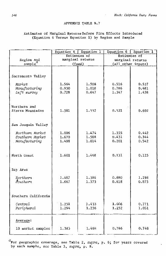
146 Hoch: California Dairy Farms
APPENDIX TABLE B.7
Estimates of Marginal Returns Before Firm Effects Introduced (Equation 6 Versus'Equation 1) by Region and Sample
Equation 1E_q_uation 6 JNuation 6 JNuation 1 Estimates of Estimates of
Region aZ}d marginal returns marginal returns sample (all other i1!E_uts)(feedl
Sacramento Valley
1.564 1.508 0.516 0.537Market 0.7860.930 1.018 0.481Manuf actu:ring
0.647 1.347 1.4380. 728Left SUl'Vey
Northern and Sierra Mountains 1.581 1.552 0.521 0.602
San Joaquin Valley
1.006 1.355 0.442Northern Market 1.474 1.588 0.431 0.344Southern Market 1.670
0.2011.014 0.5421.408Manufaaturing
0.1311.601 1.468 0.125North Coast
Bay Area
1.384 0.6801.487 1.298Northern 0.6181.667 1.373 0.873Jouthem
Southern California
1.006Central 1. 251 1.433 o. 771 1.236 1.252 1.051Peripheral 1.294
Averaf£e:
10 market samples 1.385 1.468 0.786
aFor geographic coverage, see Table 2, supra, p. 6; for years covered by each sample, see Table 3, supra~ p. 8.
0.748

APPENDIX TABLE B.8
Year Elasticities for Feed and All Other Inputs (Equation 7), 1959-1965
San Jo~uin Valley_ Northern Southern Southern California Bay Area Sacramento Valle_x_
Market Market Con- I Nonex- Nonex-Year None~andiI!£ E~1mdin_g_ Stable tracting di!l_g_ E~ndin_g_ _p_andin_g_
Feed elasticity_ estimate
1959 .385 .661 a 1.148 • 764 1960 .027 • 875 .814 .403 .451 .623 1961 .468 . 833 .129 .107 -.048 .646 .427 .361 .295 1962 -.108 .559 • 453 .297 .344 • 789 .360 .260 .439 1963 .414 .903 .508 .387 .339 • 776 .497 .406 .406 1964 .098 .901 .161 .294 .496 .639 .361 .507 .572 1965 .129 -.143 .357 .747 1.078
·-· All other 'input elasticity estimate
1959 .357 .227 - • 715 - .541 1960 •722 .061 -.050 .sos .317 .083 1961 .227 .163 .326 • 217 • 579 .128 .506 .525 .468 1962 • 762 .538 .011 -.089 .284 .012 .613 .551 .322 1963 .328 .077 .015 -.147 .292 .011 .446 .523 .392 1964 .606 .077 .326 -.077 • 228 .144 .589 .340 .203 1965 .326 .465 .048 - .129 - .302
aBlanks indicate year not in sample.

148 Hoch: California Dairy Farms
APPENDIX TABLE B.9
Estimated Individual Elasticities for Specific Firm and Year San Joaquin Valley (Northern Market) Expanding Producers
(Equation 7), 1959-1964
Firm number 1960 1964
~.£. e:last_icity 1959 1961 )2§1 llli
1 1.008 0.840 0.612 0.739 0.755 0.731
2 0.601 0.433 0.205 0.332 0.348 0.324
0.768 0.600 0.372 0.499 0.5153 0.491
1.202 1.034 0.8064 0.933 0.949 0.925
0.869 0.7015 0.473 0.600 0.616 0.592
6 1. 008 0.840 0.612 0.739 0.755 0.131
0.7587 1. 027 0.859 0.631 0.77.4 0.750
8 0.812 0.416 0.5430.644 0.559 0.535
0.592 0.424 0.196 0.323 0.3399 0.315
10 0.679 0.283 0.410 0.4260.511 0.402
11 0.888 0.720 0.492 o.619 0.635 0.611
0.48812 0.741 0.573 0.345 0.472 0.464
0. 953 0.785 0.557 0.68413 0.700 0.676
14 0.525 0.357 0.129 0.256 0.272 0.248
All other in12ut elasticitlI---·
1 0.235 0.370 0.606 o.476 0.432 0.446
2 0.096 0.231 0.3370.467 0.293 0.307 , 3 0.206 0.312o. 071 0.442 0.268 0.282
-0.208 0.028 -0.1024 -0.343 -0.146 -0.132
0.015 0.150 0.386 0.2125 0.256 0.226
0.4120.215 0.350 0.586 0.456 0.4266
0.531 0.767 0.6370.396 0.5937 0.607
-0.083 0.052 0.2888 0.158 0.114 0.128
0.433 0.303 0.2590.062 0.197 0.2739
10 -o. 458 -0.087 -0.217 -0.261-o. 323 -0.247
0.328 0.564 0.43411 0.193 0.390 0.404
12 -0.200 -0.065 0.171 0.041 -0.003 0.011
13 0.179 0.314 0.550 0.420 0.376 0.390
14 0.211 0.346 0.582 0.452 0.408 0.422
149 Giannini Foundation Monograph • Number 36 • July, 1976
ACKNOWLEDGMENTS
This Monograph is the cuhnination of the work on Giannini Foundation Project M-2294 under the author's direction. David Foote and Emilie Lachmann played major roles in the work on the project, carrying out the computer operations phase in the fitting of the regression equations reported; each also assisted greatly in developing and checking the data, in writing computer programs, and in organizing the flow of the work. Project M-2294 was initially a joint project with Quirino Paris, and his Ph.D. dissertation, "Estimation of Individual Firm Production Functions," was an outcome of that association. The work reported here was developed subsequent to that reported in Paris' dissertation; however, he made important contributions to the present effort. Paris directed the development of the data for the San Joaquin Valley sample, helped formulate procedures for measuring inputs, and wrote some computer programs employed in the present study. He initiated the use of production function slope shifters, as well as intercept shifters, in Project M-2294, employing that approach in his dissertation. That approach was subsequently employed here in one of the subsidiary investigations of this study (Equation 7 of Section 8). Mary McMaster and Nina Bienhoff Johnson also made important contributions to the work; the former wrote a number of computer programs and the latter carried out most of the keypunching of data cards.
Data for Project M-2294 were obtained from the California Bureau of Milk Stabilization. The staff of that agency contributed to the effective use of the data; much help was obtained from Mark Temme and John Jarvis, in particular.
A good deal of the time devoted to writing the drafts of this Monograph was made available by Resources for the Future, Inc. Kay Albaugh and Beverly Plater typed the manuscript drafts.
Alain de Janvry, George M. Kuznets, and Gordon A. Rowe served as reviewers of the initial manuscript and made a number of useful comments. Ivan M. Lee reviewed and edited the final manuscript.
Typing of the Monograph and final editorial revisions were carried out by Gertrude Halpern and Amor Bernardino of the Giannini Foundation Word Processing Unit under the direction of lkuko Takeshita.
The project was carried out under the administration of L. L. Sammet and D. A. Clarke, Jr., and both were helpful in its management. The project was of particular interest to Professor Clarke, and he was instrumental in obtaining its funding and in encouraging its completion. This Monograph is dedicated to his memory, in remembrance of his kindness and concern.

150 Hoch: California Dairy Farms
LITERATURE CITED
BRESSLER, RAYMOND G., JR., and RICHARD A. KING 1970. Markets, prices and interregional trade. New York: John Wiley & Sons, Inc.
DEAN, G. W., D. L. BATH, and S. OLAYIDE 1969. Computer program for maximizing income above feed cost from dairy cattle.
Journal of Dairy Science, 52(7): 1009-16.
DENISON, EDWARD F. 1972. The measurement of productivity. Survey of Current Business, 52(5): 111.
DESAI, MEGHNAD 1965. An index of pasture conditions. University of California, Department of
Agricultural Economics, Working Paper. Berkeley.
ELSNER, GARY, and IRVING HOCH 1968. Analysis of California farm income relationships. University of California,
Giannini Foundation Research Report No. 297. Berkeley.
FABRYCY, MARK Z. 1970. Cobb-Douglas, CES and homothetic isoquant production functions: a
comparison. Econometrica, 38(4):106 and 107.
FLETCHER, L. B., and C. 0. McCORKLE, JR. 1962. Growth and adjustment of the Los Angeles milkshed. California Agricultural
Experiment Station Bulletin No. 787.
FUCHS, VICTOR R. 1967. Differentials in hourly earnings by region and city size, 1959. National Bureau
of Economic Research, Occasional Paper IOI. New York.
GRILICHES, ZVI 1964. Research expenditures, education, and the aggregate agricultural production
function. American Economic Review, LIV(6):966.
J HATHAWAY, DALEE.
1963. Government and agriculture: economic policy in a democratic society. New York: The Macmillan Company.
HOCH, IRVING 1958. Simultaneous equation bias in the context of the Cobb-Douglas production
function. Econometrica, 26(4):566-78. 1962. Estimation of production function parameters combining time-series and
cross-section data. Econometrica, 30(1):39-41. 1963. Book review: Journal of the American Statistical Association,
58(303):853-57, of Knud Rasmussen with M. M. Sandilands, Production function of analyses of British and Irish farm accounts. Loughborough, England: University of Nottingham.
1969. Anticipated profit in Cobb-Douglas models. Econometrica, 37(4):720. 1972. Income and city size. Urban Studies, 9(3):299-328.

151 Giannini Foundation Monograph • Number 36 • July, 1976
HODGMAN, C. D. 1959. Mathematical tables. Cleveland Ohio: Chemical Rubber Company. 11th ed.
HOGLUND, C. R., GLENN, L. JOHNSON, CHARLES A. LASSITER, and LON D. McGILLIARD (eds.)
1959. Nutritional and economic aspects of feed utilization by dairy cows. Ames: Iowa State College Press.
JOHNSTON, J. 1963. Econometric methods. New York: McGraw-Hill Book Company, Inc.
JORGENSON,' DALE W., and ZVI GRILICHES 1972. The measurement of productivity. Survey of Current Business, 52(5): 111.
KLEIN, L. R. 1953. A textbook of econometrics. Evanston: Row, Peterson & Co.
MARSCHAK, JACOB, and WILLIAM H. ANDREWS, JR. 1944. Random simultaneous equations and the theory of production. Econometrica,
12(3 and 4):143-205.
MUNDLAK, YAIR 1961. Empirical production function free of management bias. Journal of Farm
Economics, XLIII( 1): 44-56. 1963. On estimation of production and behavioral functions from a combination
of cross-section and time-series data. Measurement in Economics. Ed. Carl Christ. Stanford: Stanford University Press.
MUNDLAK, YAIR, and IRVING HOCH 1965. Consequences of alternative specifications in estimation of Cobb-Douglas
production functions. Econometrica, 3 3( 4): 814-28.
PARIS, QUIRINO 1966. Estimation of individual firm production functions, unpublished Ph.D.
dissertation, Department of Agricultural Economics, University of California, Berkeley.
SCHULTZ, THEODORE W. 1953. The economic organization of agriculture. New York: McGraw-Hill Book
Company, Inc.
SHULTIS, ARTHUR, OLAN D. FORKER, and ROBERT D. APPLEMAN 1963. California dairy management. California Agricultural Experiment Station
Circular 417.
TIMMER, C. PETER 1970. On measuring technical efficiency. Stanford University, Food Research
Institute Studies in Agricultural Economics, Trade and Development, IX(2). Stanford, California.
ULLAH, A., and R. AGARWAL 1972. The exact sampling distribution of generalized Hoch's estimator. Southern
Methodist University, Department of Economics, Working Paper No. 18. Dallas, Texas.
U. S. BUREAU OF THE CENSUS Monthly issues. Survey of Current Business.

, 152 Hoch: California Dairy Farms
U. S. ECONOMIC RESEARCH SERVICE 1963. Agricultural Finance Review, 24 (Supplement). 1956-1964. Farm Cost Situation'.
WIPF, LARRY J., and D. LEE BAWDEN 1969. Reliability of supply equations derived from production functions. American
Journal of Agricultural Economics, 51(1):170-78.
WU, DE-MIN 1973. Estimation of the Cobb-Douglas production function. University of Kansas,
Department of Economics, Research Papers in Theoretical and Applied Economics, 50. Manhattan, Kansas.
ZELLNER, A., J. KMENTA, and J. DREZE 1966. Specification and estimation of Cobb-Douglas production function models.
Econometrica, 34(4):784-95.

GIANNINI FOUNDATION MONOGRAPH SERIES
What it is
The Giannini Foundation Monograph Series is comprised of technical research reports relating to the economics of agriculture. The series, introduced in 1967, is published by the California Agricultural Experiment Station. Similar technical economic research studies formerly were published in Hilgardia.
Each Monograph is a separate report of research undertaken in the California Experiment Station by staff members of the Department of Agricultural Economics and the Giannini Foundation of Agricultural Economics in the University of California. Topics covered range from analyses of farm and processing firms to· broader problems of interregional resource use and public policy.
The Monographs are written in technical terms with professional economists as the intended audience. No attempt is made to reduce the writing to terms understandable to the layman. Each Monograph caries an abstract on the inside front cover.
Monographs are published at irregular intervals as research is completed and reported.
How to obtain copies
In general, copies will be sent free on request to individuals or organizations. The limit to California residents is 20 titles; the limit to nonresidents is 10. There is no distribution through agencies or stores.
A list of available Monographs in the series is published annually and may be obtained by writing to PUBLICATIONS (address below). The list also explains how some out-of-print issues, including reports that formerly appeared in Hilgardia, may be obtained on microfilm or as record prints. To obtain the Giannini Foundation Monograph Series regularly, certain minimum qualifications must be met:
As a gift. Some libraries, educational institutions, or agricultural experiment stations may receive Monographs as issued when there is a definite need for the material and it will be made available to a considerable number of interested economists. Address requests to PUBLICATIONS. Please give particulars.
As an exchange for similar research material. Address requests to Librarian, Giannini Foundation of Agricultural Economics, University of California, Berkeley, California 94720.
With the exception of communications about exchange agreements (see above), address all correspondence concerning the Giannini Foundation Monograph Series to:
PUBLICATIONS University of California Division of Agricultural Sciences 1422 S. 10th Street Richmond, California 94804
Related Documents


