Production Analysis: A Non-Parametric Time Series ...

Int.J.Curr.Microbiol.App.Sci (2019) 8(1): 248-2450

2438

Original Research Article https://doi.org/10.20546/ijcmas.2019.801.257

Production Analysis: A Non-Parametric Time Series

Application for Pulses in Rajasthan

Shirish Sharma and Swatantra Pratap Singh*

ICAR- National Institute of Agricultural Economics and Policy Research,

New Delhi - 110 012, India

*Corresponding author

A B S T R A C T

Introduction

Since the onset of the Green Revolution in the

late 1960s, India has been treading on a path

towards self-sufficiency in food. The

achievements have remained highly skewed

towards wheat and rice on account of

technological as well as policy support

towards these two crops. With high and

assured prices paid through public

procurement encouraging farmers to increase

output, the production of cereals in India has

generally been greater than the domestic

demand since the mid-1990s. The per capita

production of cereals has steadily increased in

each decade from 145 kg during the 1970s to

158 kg during the 2000s. Meanwhile, Per

capita production of pulses in India has

declined from 18.5 kg during 1965-1970 to

about 15 kg during 2011-2014. It touched the

lowest level of 10.5 kg in year 2002-03. Even

with imports, India has not able to meet the

domestic demand for pulses. The per capita

net availability of pulses in the country, after

factoring in for imports and exports, has

declined from 18.15 kg during 1965-70 to

15.4 kg during 2011-14. In India, pulses are

mainly grown under rain-fed and low input

compared to cereal crops (i.e., wheat, maize,

International Journal of Current Microbiology and Applied Sciences ISSN: 2319-7706 Volume 8 Number 01 (2019) Journal homepage: http://www.ijcmas.com

In view of the importance of pulses in Indian dietary system and agriculture sector in state

economy several attempts have been made to study the trends in area and production of

pulses crops which reveal the growth performance. The secondary data were collected for

area and production of pulses for the period of 1979–80 to 2011-12. The study period was

classified as Pre WTO (World Trade Organization) era and Post WTO era. For the

estimation of the trends in area and production and to measure the association in

productivity we use Mann-Kendall test. In the present study correspondence analysis was

applied to contingency table on different level of productivity with districts. It is evident

from the findings that during first and second period of the study Nagaur, Swai Madhopur,

Alwar, Banswara, Bharatpur, Chittoegarh, Jhalawar, Kota, sirohi and Udaipur districts

were show negative trend in area for pulses. However for the first and second period

Bundi, Chittorgarh, Dungarpur, Jhunjhunu, Bikaner, Jaisalmer and Nagaur districts found

positive trend in production for pulses.

K e y w o r d s

Area, Association,

Growth, Pulses and

Trend

Accepted:

17 December 2018

Available Online: 10 January 2019

Article Info

https://doi.org/10.20546/ijcmas.2019.801.257


2439

rice, barley, sorghum and millet), Also,

compared to cereal crops, pulse are grown in

marginal areas where water is a scarce

resource. Moreover, in our countries, because,

pulses are considered as secondary crops, they

do not receive investment resources and

policy attention from governments, as do

cereal crops (e.g., maize, rice, wheat), which

are often considered food security crops and

thus receive priority attention from the

research and policy making communities

(Byerlee and White, 2000). Consequently, the

productivity of pulses is one of the lowest

among staple crops.

Rajasthan, with a geographical area of 3.42

lakh sq. km. is the largest state of the country,

covering 10.4 percent of the total

geographical area of India and it accounts for

5.5 percent of the population of India.

Agriculture plays an important role in

Rajasthan economy. About 70 per cent of the

total population depends on agriculture and

allied activities for their livelihood and

around 30 percent of the state income is

generated by it. Agriculture in the state is

essentially rain fed which is susceptible and

vulnerable of the vagaries of the monsoon.

The northwest region of the state comprising

61 percent of the total area is either desert or

semi desert which absolutely depends on rains

for crop pattern. In view of the importance of

agriculture sector in state economy several

attempts have been made to study the trends

in area and production of pulses crops which

reveal the growth performance. The normal

statistical procedures are obtained as a

measure of growth of output over the period

of a series is to postulate a hypothetical

function which would be adequately

described the series of the outputs over time

and to estimate its parameters which would

offer a measure of growth of output over the

period. The analysis of growth is usually used

in economic studies to find out the trend of a

particular variable over a period of time and

used for making policy decisions. Fitting a

trend to raw data and calculating coefficient

of variation of residuals from the fitted trend

apparently take note of the both the trend and

fluctuations. Though, normally it may be an

adequate procedure but it may not be

workable when fluctuations are huge and

frequent. This is because the estimation of

trend is distorted by fluctuations and neither

the trend nor the fluctuations derived here

may adequately reflect the reality involved

(Rao et al., 1980). For this purpose, the study

has been carried out to on for the years1979–

80 to 2011-12. The paper is divided in two

sections. It begins with an examination of

growth and trend in area of cultivation and

production of pulse crops in Rajasthan. And,

secondly association of productivity of pulses

across districts in Rajasthan.

Materials and Methods

Statistical tools and techniques

Type and sources of data

To study the growth, trend in area and

production and association of productivity of

pulses crops across districts in Rajasthan

during pre and post WTO periods, a reliable

source of secondary data is very essential to

get the real picture. The study was based on

secondary data. The time series data on area

and production of pulses crop was available

from 1979-80 onwards.

The period of study is 1979–80 to 2011-12

which is characterized by wider technology

dissemination. The entire study was split into

two sub periods. The sub period was framed

as period I- 1979-80 to 1994-95, (pre WTO)

period II- 1995-96 to 2011-12 (post WTO).

Data used for the study was collected from

various published sources, like Directorate of

Economics & Statistics, Rajasthan and

Revenue records of area, production and yield

of crops.


2440

Compound annual growth rates

The growth in the area and production under

pulses were estimated using the compound

growth function of the form:

Yt= abt e

ut

Where, Yt = Dependent variable in period t, a

= Intercept, b = Regression coefficient= (1+g)

t = Years and ut = Disturbance term for the

year t

The equation was transformed into log linear

form for estimation purpose. The compound

growth rate (g) in percentage was then

computed using the relationship g = (10^b -

1)*100 (Veena, 1996).

Trend analysis

The distribution-free test for trend used in the

present procedure is the Mann-Kendall test

(Mann 1945 and Kendall 1975). This will

detect presence of negative or positive trends

in time series data set better than the

Spearman’s rho and have similar power (Yue

et al., 2002). This method is based on sign

difference of random variables rather than

their direct values therefore this method is

less affected by outliers. Mann-Kendall test

for trend coupled with the Sen's method for

slope estimation used for identification and

estimation of Trends.

Sen’s slope

This test computes both the slope (i.e. linear

rate of change) and intercept according to

Sen’s method (Hipel 1994). First, a set of

linear slopes is calculated as follows:

for (1 ≤ i < j ≤ n), where d is the slope, X

denotes the variable, n is the number of data,

and i, j are indices. Sen’s slope is then

calculated as the median from all slopes: b =

Median dk. The intercepts are computed for

each time step t as given by

at = Xt − b ∗ t

and the corresponding intercept is as well the

median of all intercepts

Mann-Kendall statistic (S)

This method is also called as Kendall’s Tau.

Tau measures the strength of relationship

between variable X and Y. In other words,

Tau value tells about how X and Y are

correlated. There are two advantages of using

this test. First, it is a non parametric test and

does not require the data to be normally

distributed. Second, the test has low

sensitivity to abrupt breaks due to

inhomogeneous time series. According to this

test, the null hypothesis H0 assumes that there

is no trend (the data is independent and

randomly ordered) and this is tested against

the alternative hypothesis H1, which assumes

that there is a trend.

The Mann-Kendall S Statistic is computed as

follows:

Sing (Tj=Ti) = 1 if Tj-Ti>0

0 if Tj-Ti=0

-1 if Tj-Ti<0

Where

Tj and Ti are the annual values in years j and i,

j > i, respectively.

If n < 10, the value of |S| is compared directly

to the theoretical distribution of S derived by

Mann and Kendall.


2441

For n ≥ 10, the statistic S is approximately

normally distributed with the mean and

Variance as follows:

E(S) = 0

The variance (σ2) for the S-statistic is defined

by:

In which ti denotes the number of ties to

extent i. The summation term in the

numerator is used only if the data series

contains tied values. The standard test statistic

Zs is calculated as follows:

Zs = for S>0

0 for S=0

for S<0

In order to consider the effect of

autocorrelation, Hamed and Rao (1998)

suggest a modified Mann-Kendall test, which

calculates the autocorrelation between the

ranks of the data after removing the apparent

trend. The adjusted variance is given by:

Where, N = number of observations in the

sample, NS = effective number of

observations to account for autocorrelation in

the data and Ps = autocorrelation between

ranks of the observations for lag i, and p is the

maximum time lag under consideration.

Correspondence analysis

Correspondence analysis is a graphical

technique to show which rows or columns of

a frequency table have similar patterns of

counts. In the correspondence analysis plot,

there is a point for each row and for each

column. Use Correspondence Analysis when

you have many levels, making it difficult to

derive useful information from the mosaic

plot. The row profile can be defined as the set

of row wise rates, or in other words, the

counts in a row divided by the total count for

that row. If two rows have very similar row

profiles, their points in the correspondence

analysis plot are close together. Squared

distances between row points are

approximately proportional to Chi-square

distances that test the homogeneity between

the pair of rows.

Algebraic development of correspondence

analysis

Let ‘X’ be a matrix, with elements Xij. Which

is represented as a table of I×J unsealed

frequencies or counts. Here the number of

rows I >J and assume that ‘X’ is of full

column rank J. The rows and columns of the

contingency table ‘X’ correspond to different

categories of two different characteristics.

If ‘n’ is the total of the frequencies in the data

matrix X. A matrix of proportion P = (Pij) is

constructed by dividing each element of X by

number.

Hence,

i = 1, 2, ---------, I

j = 1, 2, ---------, J

The matrix ‘P’ is called the ‘correspondence

matrix’. The vectors of row and column sums


2442

are defined as ‘r’ and ‘c’ respectively. Then,

the diagonal matrices Dr and Dc with elements

of ‘r’ and ‘c’ on the diagonals are formed.

Then the elements ri of Dr are

And the elements of cj of Dc are given by

Dr = diag(r1, r2, --------, rI)

Dc = diag(c1,c2, ---------, cJ)

The scaled version of the matrix is obtained

by,

Where, = rc1

Results and Discussion

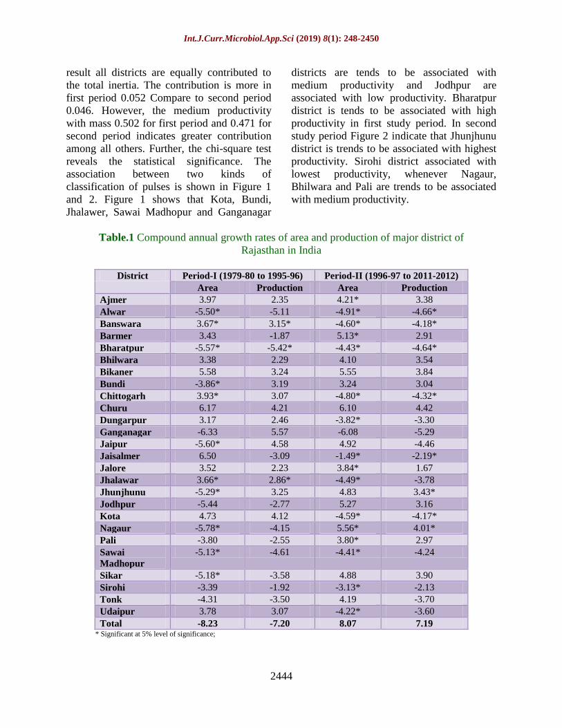
Compound annual growth rate

Analyzing the growth rate trends in the

agricultural area and production across space

and time have remained issues of significant

concern for researchers as well as policy

makers. It has been argued that analysis of the

growth rate trends help us to identifying the

changing pattern of crops and land use pattern

under different crop and rate of change in area

and production of a crop and further help in

designing the appropriate agricultural policy

for the state. The compound annual growth

rate in area and production of pulses crops

during the period 1979-80 to 1995-96 and

1996-97 to 2011-2012 listed in table 1. In the

first period area under pulses crops had

showed highly negative growth rates in

Nagaur district (-5.78%) followed by Jaipur

and Bharatpur districts. During the second

period area under crops showing highly

positive growth rate in Nagaur (5.56%),

followed by Barmer (5.13%) and Jalore

districts (3.84%). In the first period table 1

show that Banswara district (3.15%) have

highly positive growth rate followed by

Jhalawar (2.86%). During the second period

under pulses crops had showed highly

positive Nagaur district of 4.01 per cent,

followed by Jhunjhunu district of 3.43 per

cent growth rate of production. If we see the

state as a whole, growth rate of pulses are

showed positivity growth in both under area

and production (8.07&7.19) respectively.

There are posivte changes in both area and

production growth rate from first study to

second study period. This change might also

be due to the efforts of the research projects at

the national and state level in improving

productivity of pulses over years; availability

of good quality seeds that minimize the

incidence of soil borne diseases and

availability of improved package of practices.

Similar results were found by Acharya et al.,

(2012) in their study.

Identification of trend in area and

production

Area under pulses

The result established in the table 2 indicated

the Tau statistic results from the Mann

Kendall test for the pulses crop area of all

districts. In the first period four district viz.,

Banswara, Bharatpur, Chittogarh and

Jhalawar districts showing statistically

significant increasing trend under cropped


2443

area. Further, only two districts namely

Nagaur and Swai Madhopur districts had a

statistically significant decreasing trend in

area. In remaining districts, eight districts

showing increasing trend as compared to

twelve districts which showing decreasing

trend in pulses area. In the first period (1979-

80 to 1995-96) the analysis of trend in area of

pulses indicates that four districts significant

positive slope coefficients, which indicates

increase in area at Banswara, Bharatpur,

Chittorgarh and Jhalawar districts. In other

hand significant negative slope coefficient at

Nagaur and Swai Madhopur districts indicates

decrease in area.

In the second stuady period (1996-97 to 2011-

12) seven districts viz Ajmer, Bikaner,

Jaisalmer, Jalore, Jodhpur, Nagaur and Pali

showing statistically significantly increasing

trend in area. Further, only eight districts

Alwar, Banswara, Bharatpur, Chittorgarh,

jhalawar, Kota, Sirohi and Udaipur had a


area. In remaining district, five districts

showing increasing trend as compared to six

districts showing decreasing trend in pulses

area. Ajmer, Bikaner, Jaisalmer, Jalore,

Jodhpur, Nagaur and Pali show significant

positively slope coefficients that is indicate

increase in area. In case of Alwar, Banswara,

Bharatpur, Chittorgarh, Jhalawar, Kota, Sirohi

and Udaipur district showed decrease in area

due to significant negative slope coefficients.

The possible reason of increase in area in

some pulses producing districts may be due to

risk taking ability of farmers, i.e. low risk

pulses vs high risk crops in other seasons and

high market prices of produces in last some

years. These results were conformity to the

results of studies conducted by the

Parathasarathy 1984.

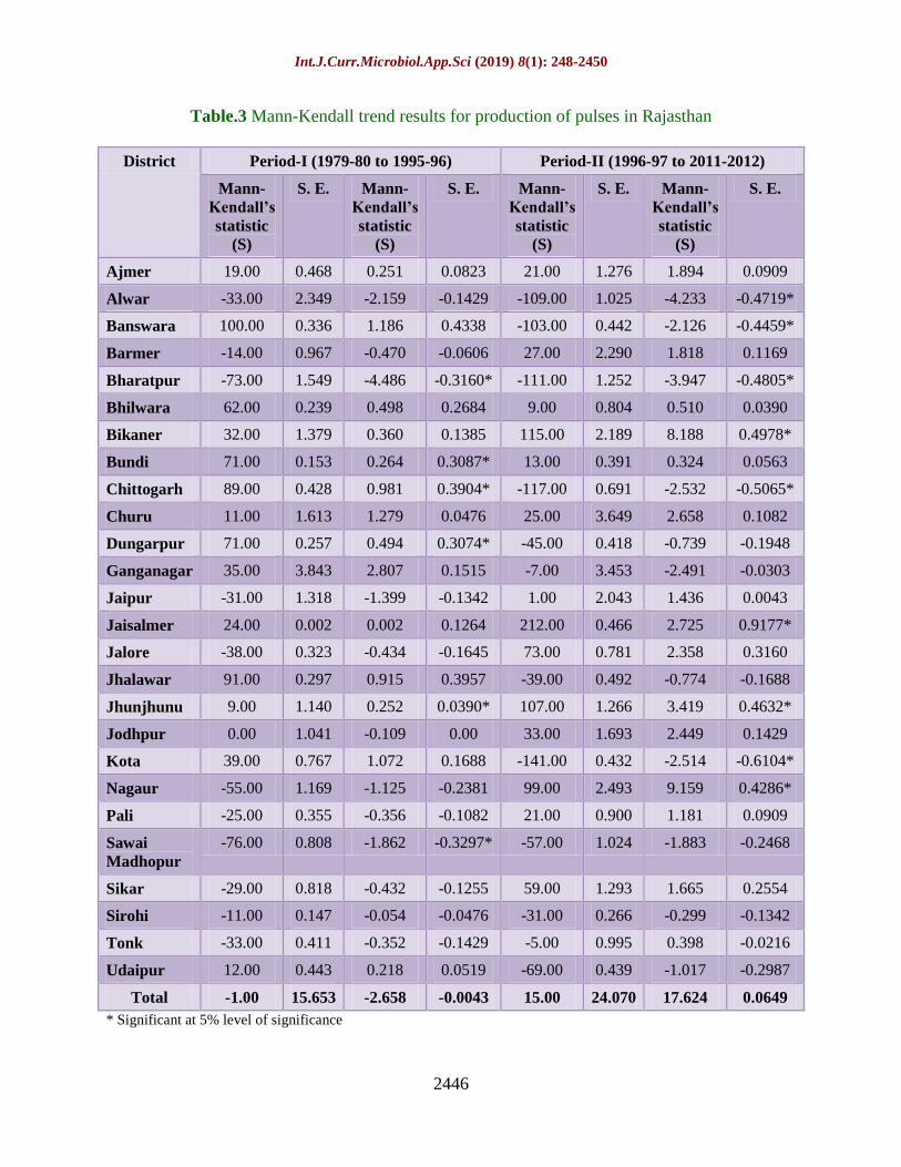
Production of pulses

The result presented in the table 3 indicated

the tau statistic results from the Mann Kendall

test for the production of all districts for the

study period.

In the first period four districts viz Bundi,

Chittorgarh, Dungarpur and Jhunjhunu shows

statistically significant increasing trend in

production. Further, only two districts

Bharatpur and Sawai Madhopur had a


production. In remaining nineteen districts,

ten districts showing increasing trend as a

compared to nine districts showed decreasing

trend in pulses production indicating non-

significant for the first period. In this period

the analysis of trend in production indicate

increase in production at Bundi, Chittorgarh,

Dungarpur and Jhunjhunu and Bharatpur and

Swai Madhopur shows decreasing trend in

production. During the second study period

Bikaner, Jaisalmer, Jhunjhunu and kota

districts showing statistically significant

increasing trend and production. Further, five

districts viz Alwar, Banswara, Bharatpur,

chittorgarh and Kota had a statistically

significant decreasing trend in production. In

remaining seventeen districts, ten districts

showed increasing trend as a compared to

seven districts shows decreasing trend in

pulses production indicating non-significant

for the second period.

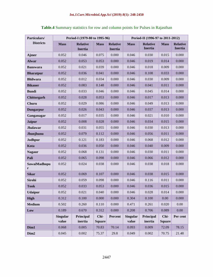
Correspondence analysis

The association between the different levels

of crop yield and different districts,

correspondence analysis is attempted in table

4. The chi-square test for independence

indicated significant association between two

kinds of classification.

The table 4 indicates the mass association and

its inertia of each district and different level

of pulses productivity. From the result, it is

seen that 70.14 per cent and 78.15 per cent of

association can be explained by dimension-1

in first and second period respectively. As a


2444

result all districts are equally contributed to

the total inertia. The contribution is more in

first period 0.052 Compare to second period

0.046. However, the medium productivity

with mass 0.502 for first period and 0.471 for

second period indicates greater contribution

among all others. Further, the chi-square test

reveals the statistical significance. The

association between two kinds of

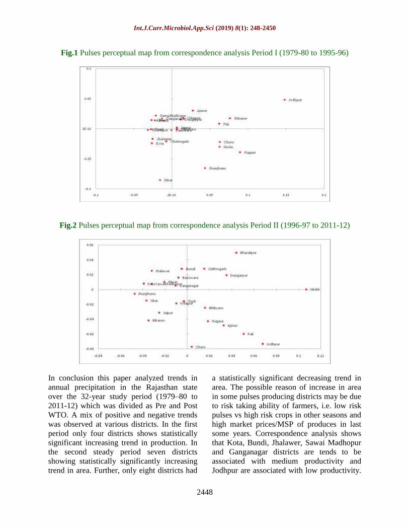
classification of pulses is shown in Figure 1

and 2. Figure 1 shows that Kota, Bundi,

Jhalawer, Sawai Madhopur and Ganganagar

districts are tends to be associated with

medium productivity and Jodhpur are

associated with low productivity. Bharatpur

district is tends to be associated with high

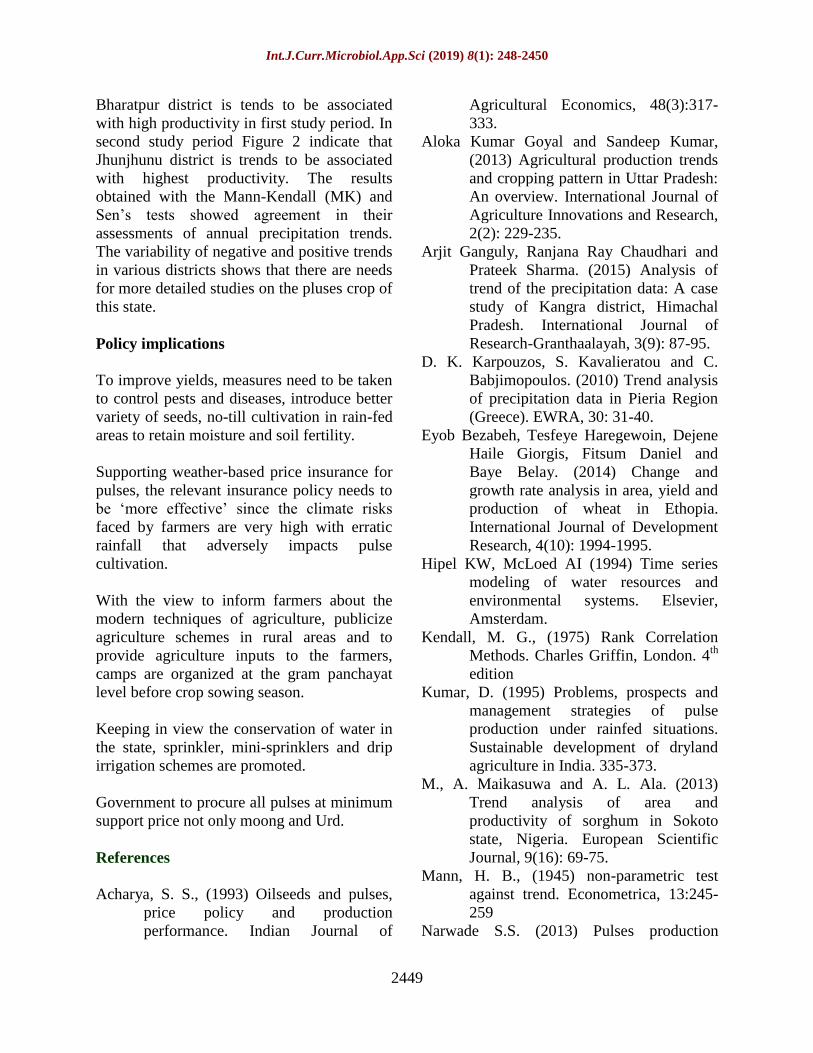
productivity in first study period. In second

study period Figure 2 indicate that Jhunjhunu

district is trends to be associated with highest

productivity. Sirohi district associated with

lowest productivity, whenever Nagaur,

Bhilwara and Pali are trends to be associated

with medium productivity.

Table.1 Compound annual growth rates of area and production of major district of

Rajasthan in India

District Period-I (1979-80 to 1995-96) Period-II (1996-97 to 2011-2012)

Area Production Area Production

Ajmer 3.97 2.35 4.21* 3.38

Alwar -5.50* -5.11 -4.91* -4.66*

Banswara 3.67* 3.15* -4.60* -4.18*

Barmer 3.43 -1.87 5.13* 2.91

Bharatpur -5.57* -5.42* -4.43* -4.64*

Bhilwara 3.38 2.29 4.10 3.54

Bikaner 5.58 3.24 5.55 3.84

Bundi -3.86* 3.19 3.24 3.04

Chittogarh 3.93* 3.07 -4.80* -4.32*

Churu 6.17 4.21 6.10 4.42

Dungarpur 3.17 2.46 -3.82* -3.30

Ganganagar -6.33 5.57 -6.08 -5.29

Jaipur -5.60* 4.58 4.92 -4.46

Jaisalmer 6.50 -3.09 -1.49* -2.19*

Jalore 3.52 2.23 3.84* 1.67

Jhalawar 3.66* 2.86* -4.49* -3.78

Jhunjhunu -5.29* 3.25 4.83 3.43*

Jodhpur -5.44 -2.77 5.27 3.16

Kota 4.73 4.12 -4.59* -4.17*

Nagaur -5.78* -4.15 5.56* 4.01*

Pali -3.80 -2.55 3.80* 2.97

Sawai

Madhopur

-5.13* -4.61 -4.41* -4.24

Sikar -5.18* -3.58 4.88 3.90

Sirohi -3.39 -1.92 -3.13* -2.13

Tonk -4.31 -3.50 4.19 -3.70

Udaipur 3.78 3.07 -4.22* -3.60

Total -8.23 -7.20 8.07 7.19 * Significant at 5% level of significance;


2445

Table.2 Mann-Kendall trend results for area under pulses in Rajasthan


Mann-

Kendall’s

statistic

(S)

S. E. Mann-

Kendall’s

statistic

(S)

S. E. Mann-

Kendall’s

statistic

(S)

S. E. Mann-

Kendall’s

statistic

(S)

S. E.

Ajmer -11.00 0.634 -0.046 -0.0476 99.00 1.413 4.095 0.4286*

Alwar -87.00 1.577 -4.749 -0.3766 -155.00 0.832 -4.731 -

0.6710*

Banswara 141.00 0.361 1.959 0.6104* -161.00 0.345 -2.850 -

0.6970*

Barmer 67.00 1.785 2.262 0.2900 87.00 1.632 5.584 0.3756

Bharatpur -137.00 1.143 -5.866 0.5931* -129.00 0.716 -2.738 -

0.5584*

Bhilwara 35.00 0.286 0.447 0.1515 75.00 0.670 1.440 0.3247

Bikaner 45.00 1.634 1.115 0.1948 111.00 2.692 9.842 0.4805*

Bundi -75.00 0.149 -0.364 -0.3247 29.00 0.424 0.421 0.1255

Chittogarh 102.00 0.885 2.712 0.4416* -153.00 0.594 -3.654 -

0.6623*

Churu 59.00 2.303 0.662 0.2554 25.00 5.862 4.015 0.1022

Dungarpur 59.00 0.259 0.404 0.2554 -82.00 0.272 -1.008 -0.3550

Ganganagar 15.00 3.871 -1.699 0.0649 -47.00 4.182 -6.871 -0.2035

Jaipur -91.00 1.391 -5.139 -0.3939 -9.00 1.671 0.585 -0.0390

Jaisalmer -8.00 0.007 -0.002 -0.0346 217.00 0.618 4.494 0.9394*

Jalore 3.00 0.820 -0.128 0.0130 153.00 0.643 4.533 0.6623*

Jhalawar 141.00 0.436 2.498 0.6104* -113.00 0.522 -2.599 -

0.4892*

Jhunjhunu -90.00 1.345 -3.777 -0.3896 -1.00 1.291 -0.123 -0.0043

Jodhpur -77.00 1.550 -2.971 -0.3333 101.00 1.981 3.084 0.4372*

Kota 57.00 0.525 0.762 0.2468 -161.00 0.535 -3.930 -

0.6970*

Nagaur -99.00 1.557 -5.125 -

0.4286*

151.00 2.020 13.540 0.6537*

Pali -15.00 0.648 -0.318 -0.0649 119.00 0.900 3.866 0.5152*

Sawai

Madhopur

-149.00 0.664 -4.141 -

0.6450*

-91.00 0.735 -2.366 -0.3939

Sikar -85.00 0.927 -2.589 -0.3680 -1.00 0.765 -0.25 -0.0043

Sirohi -3.00 0.370 -0.102 -0.0130 -103.00 0.145 -0.536 -

0.4459*

Tonk -91.00 0.374 -0.954 -0.3939 51.00 1.194 1.734 0.2208

Udaipur -3.00 0.516 0.212 -0.0130 -107.00 0.415 -1.976 -

0.4632*

Total -31.00 18.580 -24.937 -0.1342 39.00 24.061 23.824 0.1688 * Significant at 5% level of significance


2446

Table.3 Mann-Kendall trend results for production of pulses in Rajasthan


Mann-

Kendall’s

statistic

(S)

S. E. Mann-

Kendall’s

statistic

(S)

S. E. Mann-

Kendall’s

statistic

(S)

S. E. Mann-

Kendall’s

statistic

(S)

S. E.

Ajmer 19.00 0.468 0.251 0.0823 21.00 1.276 1.894 0.0909

Alwar -33.00 2.349 -2.159 -0.1429 -109.00 1.025 -4.233 -0.4719*

Banswara 100.00 0.336 1.186 0.4338 -103.00 0.442 -2.126 -0.4459*

Barmer -14.00 0.967 -0.470 -0.0606 27.00 2.290 1.818 0.1169

Bharatpur -73.00 1.549 -4.486 -0.3160* -111.00 1.252 -3.947 -0.4805*

Bhilwara 62.00 0.239 0.498 0.2684 9.00 0.804 0.510 0.0390

Bikaner 32.00 1.379 0.360 0.1385 115.00 2.189 8.188 0.4978*

Bundi 71.00 0.153 0.264 0.3087* 13.00 0.391 0.324 0.0563

Chittogarh 89.00 0.428 0.981 0.3904* -117.00 0.691 -2.532 -0.5065*

Churu 11.00 1.613 1.279 0.0476 25.00 3.649 2.658 0.1082

Dungarpur 71.00 0.257 0.494 0.3074* -45.00 0.418 -0.739 -0.1948

Ganganagar 35.00 3.843 2.807 0.1515 -7.00 3.453 -2.491 -0.0303

Jaipur -31.00 1.318 -1.399 -0.1342 1.00 2.043 1.436 0.0043

Jaisalmer 24.00 0.002 0.002 0.1264 212.00 0.466 2.725 0.9177*

Jalore -38.00 0.323 -0.434 -0.1645 73.00 0.781 2.358 0.3160

Jhalawar 91.00 0.297 0.915 0.3957 -39.00 0.492 -0.774 -0.1688

Jhunjhunu 9.00 1.140 0.252 0.0390* 107.00 1.266 3.419 0.4632*

Jodhpur 0.00 1.041 -0.109 0.00 33.00 1.693 2.449 0.1429

Kota 39.00 0.767 1.072 0.1688 -141.00 0.432 -2.514 -0.6104*

Nagaur -55.00 1.169 -1.125 -0.2381 99.00 2.493 9.159 0.4286*

Pali -25.00 0.355 -0.356 -0.1082 21.00 0.900 1.181 0.0909

Sawai

Madhopur

-76.00 0.808 -1.862 -0.3297* -57.00 1.024 -1.883 -0.2468

Sikar -29.00 0.818 -0.432 -0.1255 59.00 1.293 1.665 0.2554

Sirohi -11.00 0.147 -0.054 -0.0476 -31.00 0.266 -0.299 -0.1342

Tonk -33.00 0.411 -0.352 -0.1429 -5.00 0.995 0.398 -0.0216

Udaipur 12.00 0.443 0.218 0.0519 -69.00 0.439 -1.017 -0.2987

Total -1.00 15.653 -2.658 -0.0043 15.00 24.070 17.624 0.0649

* Significant at 5% level of significance


2447

Table.4 Summary statistics for row and column points for Pulses in Rajasthan

Particulars/

Districts

Period-I (1979-80 to 1995-96) Period-II (1996-97 to 2011-2012)

Mass Relative

Inertia

Mass Relative

Inertia

Mass Relative

Inertia

Mass Relative

Inertia

Ajmer 0.052 0.046 0.075 0.000 0.046 0.030 0.015 0.000

Alwar 0.052 0.053 0.053 0.000 0.046 0.019 0.014 0.000

Banswara 0.052 0.021 0.039 0.000 0.046 0.018 0.009 0.000

Bharatpur 0.052 0.036 0.041 0.000 0.046 0.108 0.033 0.000

Bhilwara 0.052 0.012 0.034 0.000 0.046 0.030 0.009 0.000

Bikaner 0.052 0.083 0.148 0.000 0.046 0.041 0.011 0.000

Bundi 0.052 0.033 0.046 0.000 0.046 0.045 0.014 0.000

Chittorgarh 0.052 0.028 0.053 0.000 0.046 0.017 0.013 0.000

Churu 0.052 0.029 0.086 0.000 0.046 0.049 0.013 0.000

Dungarpur 0.052 0.026 0.043 0.000 0.046 0.037 0.013 0.000

Ganganagar 0.052 0.017 0.035 0.000 0.046 0.021 0.010 0.000

Jaipur 0.052 0.008 0.028 0.000 0.046 0.034 0.015 0.000

Jhalawar 0.052 0.031 0.055 0.000 0.046 0.030 0.013 0.000

Jhunjhunu 0.052 0.079 0.112 0.000 0.046 0.056 0.011 0.000

Jodhpur 0.052 0.121 0.183 0.000 0.046 0.068 0.012 0.000

Kota 0.052 0.036 0.050 0.000 0.046 0.040 0.009 0.000

Nagaur 0.052 0.068 0.131 0.000 0.046 0.030 0.011 0.000

Pali 0.052 0.065 0.098 0.000 0.046 0.066 0.012 0.000

SawaiMadhopu

r

0.052 0.024 0.038 0.000 0.046 0.038 0.018 0.000

Sikar 0.052 0.069 0.107 0.000 0.046 0.038 0.015 0.000

Sirohi 0.052 0.059 0.098 0.000 0.046 0.116 0.011 0.000

Tonk 0.052 0.033 0.053 0.000 0.046 0.036 0.015 0.000

Udaipur 0.052 0.021 0.040 0.000 0.046 0.028 0.014 0.000

High 0.312 0.100 0.000 0.000 0.304 0.100 0.00 0.000

Medium 0.502 0.260 0.110 0.000 0.471 0.261 0.020 0.00

Low 0.189 0.670 0.312 0.000 0.208 0.706 0.089 0.00

Singular

value

Principal

inertia

Chi-

Square

Percent Singular

value

Principal

inertia

Chi-

Square

Per cent

Dim1 0.068 0.005 70.83 70.14 0.093 0.009 72.09 78.15

Dim2 0.045 0.002 75.37 29.8 0.049 0.002 70.75 21.48


2448

Fig.1 Pulses perceptual map from correspondence analysis Period I (1979-80 to 1995-96)

Fig.2 Pulses perceptual map from correspondence analysis Period II (1996-97 to 2011-12)

In conclusion this paper analyzed trends in

annual precipitation in the Rajasthan state

over the 32-year study period (1979–80 to

2011-12) which was divided as Pre and Post

WTO. A mix of positive and negative trends

was observed at various districts. In the first

period only four districts shows statistically

significant increasing trend in production. In

the second steady period seven districts

showing statistically significantly increasing

trend in area. Further, only eight districts had

a statistically significant decreasing trend in

area. The possible reason of increase in area

in some pulses producing districts may be due

to risk taking ability of farmers, i.e. low risk

pulses vs high risk crops in other seasons and

high market prices/MSP of produces in last

some years. Correspondence analysis shows

that Kota, Bundi, Jhalawer, Sawai Madhopur

and Ganganagar districts are tends to be

associated with medium productivity and

Jodhpur are associated with low productivity.


2449

Bharatpur district is tends to be associated

with high productivity in first study period. In

second study period Figure 2 indicate that

Jhunjhunu district is trends to be associated

with highest productivity. The results

obtained with the Mann-Kendall (MK) and

Sen’s tests showed agreement in their

assessments of annual precipitation trends.

The variability of negative and positive trends

in various districts shows that there are needs

for more detailed studies on the pluses crop of

this state.

Policy implications

To improve yields, measures need to be taken

to control pests and diseases, introduce better

variety of seeds, no-till cultivation in rain-fed

areas to retain moisture and soil fertility.

Supporting weather-based price insurance for

pulses, the relevant insurance policy needs to

be ‘more effective’ since the climate risks

faced by farmers are very high with erratic

rainfall that adversely impacts pulse

cultivation.

With the view to inform farmers about the

modern techniques of agriculture, publicize

agriculture schemes in rural areas and to

provide agriculture inputs to the farmers,

camps are organized at the gram panchayat

level before crop sowing season.

Keeping in view the conservation of water in

the state, sprinkler, mini-sprinklers and drip

irrigation schemes are promoted.

Government to procure all pulses at minimum

support price not only moong and Urd.

References

Acharya, S. S., (1993) Oilseeds and pulses,

price policy and production

performance. Indian Journal of

Agricultural Economics, 48(3):317-

333.

Aloka Kumar Goyal and Sandeep Kumar,

(2013) Agricultural production trends

and cropping pattern in Uttar Pradesh:

An overview. International Journal of

Agriculture Innovations and Research,

2(2): 229-235.

Arjit Ganguly, Ranjana Ray Chaudhari and

Prateek Sharma. (2015) Analysis of

trend of the precipitation data: A case

study of Kangra district, Himachal

Pradesh. International Journal of

Research-Granthaalayah, 3(9): 87-95.

D. K. Karpouzos, S. Kavalieratou and C.

Babjimopoulos. (2010) Trend analysis

of precipitation data in Pieria Region

(Greece). EWRA, 30: 31-40.

Eyob Bezabeh, Tesfeye Haregewoin, Dejene

Haile Giorgis, Fitsum Daniel and

Baye Belay. (2014) Change and

growth rate analysis in area, yield and

production of wheat in Ethopia.

International Journal of Development

Research, 4(10): 1994-1995.

Hipel KW, McLoed AI (1994) Time series

modeling of water resources and

environmental systems. Elsevier,

Amsterdam.

Kendall, M. G., (1975) Rank Correlation

Methods. Charles Griffin, London. 4th

edition

Kumar, D. (1995) Problems, prospects and

management strategies of pulse

production under rainfed situations.

Sustainable development of dryland

agriculture in India. 335-373.

M., A. Maikasuwa and A. L. Ala. (2013)

Trend analysis of area and

productivity of sorghum in Sokoto

state, Nigeria. European Scientific

Journal, 9(16): 69-75.

Mann, H. B., (1945) non-parametric test

against trend. Econometrica, 13:245-

259

Narwade S.S. (2013) Pulses production


2450

during post-reform period in India.

Journal of Crop Science, 4(1): 104-

107.

Pack, F. T. and Jolliffe, K. S. (1992)

Correspondence Analysis on Israel,

Applied Statistics, 56:456-475.

Parathasarathy G (1984) Growth rates and

fluctuations of agricultural

production– a district-wise analysis in

Andhra Pradesh. Economic and

Political Weekly 19(26): A74-A84.

Reddy, B.S., Chandrashekhar, S.M., Dikshit,

A.K. and Manohar, N.S. (2012) Price

trend and integration of wholesale

markets for onion in metro cities of

India. Journal of Economics and

Sustainable Development, 3(70): 120-

130.

S. S. Kalamkar, V. G. Atkare and N. V.

Shende. (2002) An analysis of growth

trends of principal crops in India.

Agricultural Science Digest. 22(3):

153-156

Sagar, V. (1980). Decomposition of Growth

Trends and Certain Related Issues.

Indian Journal of Agricultural

Economics, 35(2), 42- 59.

Saraswati Poudel Acharya, H. Basavaraja, L.

B. Kunnal, S. B. Mahajanashetti and

A. R. S. Bhat (2012) Growth in area,

production and productivity of major

crops in Karnataka. Karnataka Journal

of Agriculture Science 25 (4): (431-

436) 2012

Saraswati Poudel Acharya, H. Basavaraja, L.

B. Kunnal, S. B. Mahajanashetti and

A. R. S. Bhat. (2012) Growth in area,

production and productivity of major

crops in Karnataka. Karnataka Journal

of Agricultural Science, 25(4): 431-

436.

Satinder Kumar and Surender Singh. (2014)

Trends in growth rates in area,

production and productivity of

sugarcane in Haryana. International

Journal of Advanced Research in

Management and Social Sciences,

3(4): 117-124.

Sheng Yue, Paul Pilon and George Cavadias,

(2002) Power of the Mann–Kendall

and Spearman's rho tests for detecting

monotonic trends in hydrological

series. Journal of Hydrology,

264(4):262-263

Srivastava, S.C., Sen, C. and Reddy, A.R.

(2003) An analysis of growth of

pulses in eastern Uttar Pradesh.

Agricultural Situation in India 59 (12):

771-775.

Veena, V. M., (1996) Growth dimensions of

horticulture in Karnataka- An

econometric analysis, Ph.D. Thesis,

University of Agricultural Science,

Dharwad (India).

How to cite this article:

Shirish Sharma and Swatantra Pratap Singh. 2019. Production Analysis: A Non-Parametric

Time Series Application for Pulses in Rajasthan. Int.J.Curr.Microbiol.App.Sci. 8(01): 2438-

2450. doi: https://doi.org/10.20546/ijcmas.2019.801.257

https://doi.org/10.20546/ijcmas.2019.801.257

Production Analysis: A Non-Parametric Time Series ...

Documents