Producer Decision Making Two - Variable Inputs and Enterprise Selection Chapter 5

Producer Decision Making Two - Variable Inputs and Enterprise Selection Chapter 5.
Dec 25, 2015
Welcome message from author
This document is posted to help you gain knowledge. Please leave a comment to let me know what you think about it! Share it to your friends and learn new things together.
Transcript
Producer Decision Making
Two - Variable Inputs and Enterprise Selection
Chapter 5
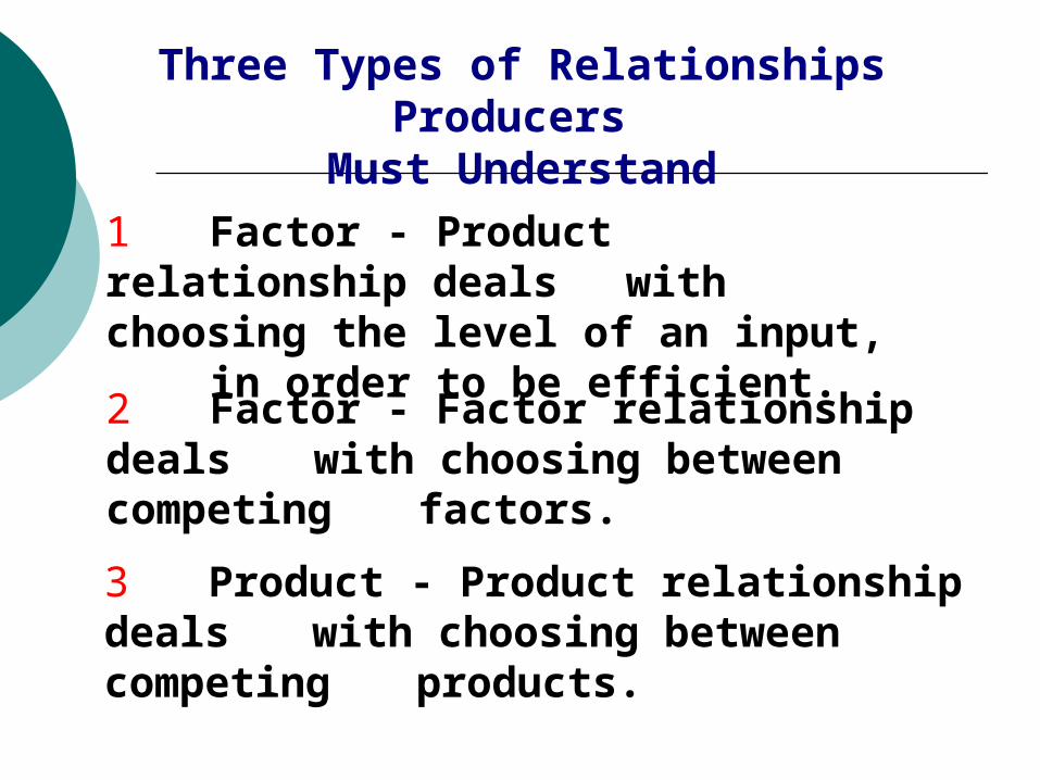
Three Types of Relationships Producers
Must Understand
3 Product - Product relationship deals with choosing between competing products.
1 Factor - Product relationship deals with choosing the level of an input, in order to be efficient. 2 Factor - Factor relationship deals with choosing between competing factors.
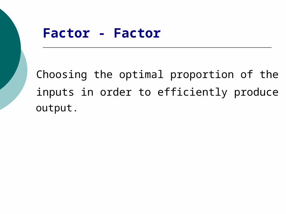
Factor - Factor
Choosing the optimal proportion of the
inputs in order to efficiently produceoutput.
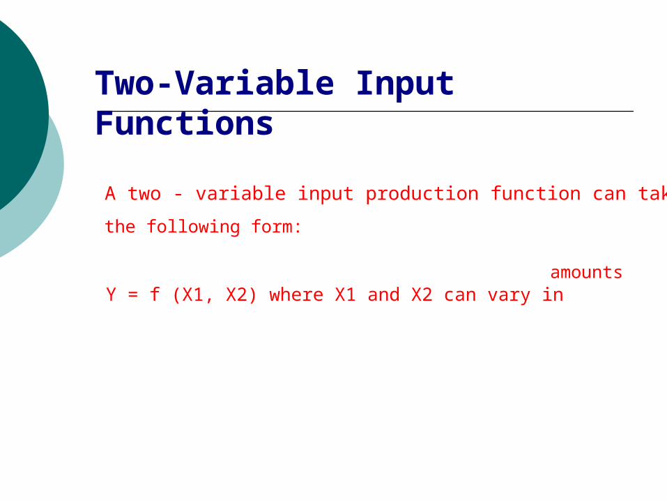
Two-Variable Input Functions
A two - variable input production function can take on
the following form:
Y = f (X1, X2) where X1 and X2 can vary in amounts
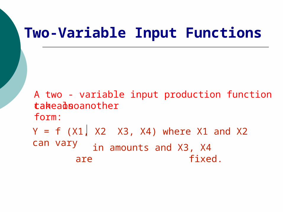
Two-Variable Input Functions
A two - variable input production function can alsotake on another form:
Y = f (X1, X2 X3, X4) where X1 and X2 can vary
in amounts and X3, X4 are fixed.
..
..
.
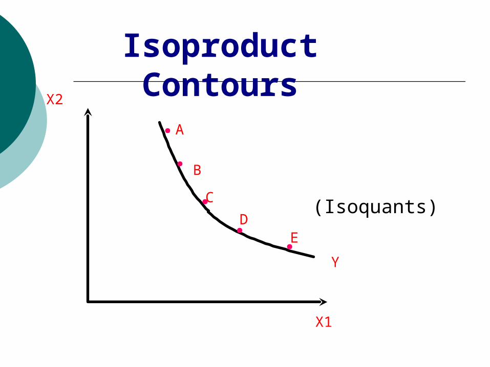
A
B
C
DE
X1
X2
Y
(Isoquants)
Isoproduct Contours
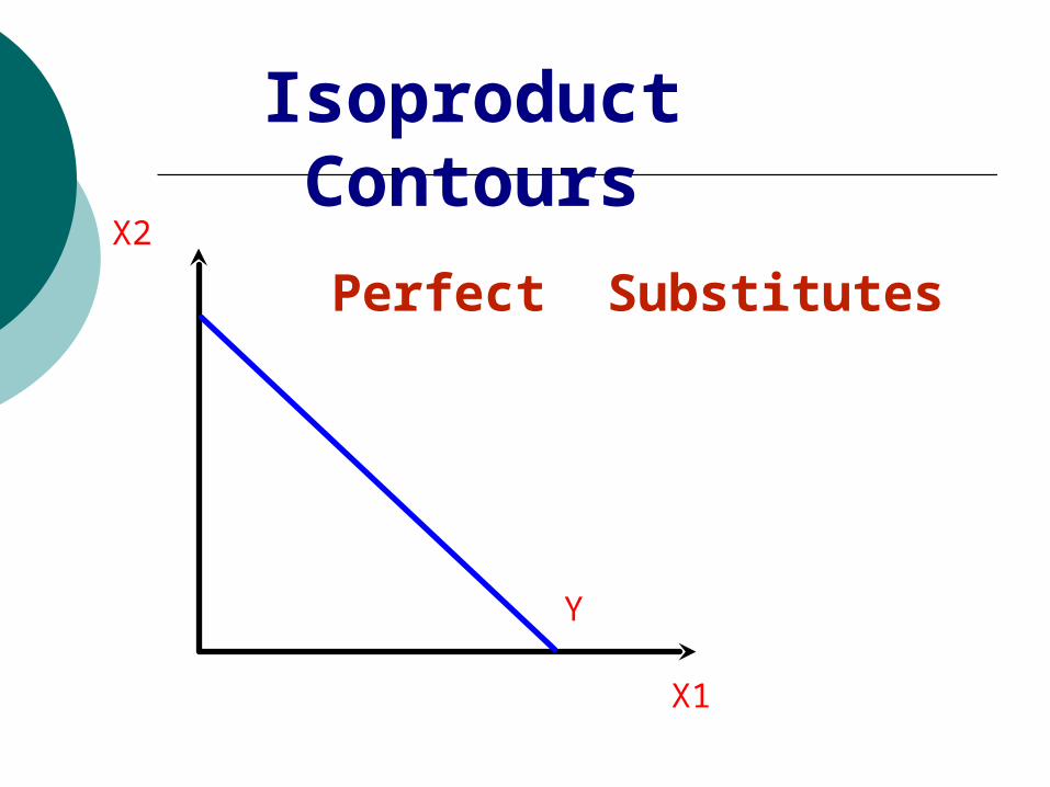
X1
X2
Perfect Substitutes
Y
Isoproduct Contours
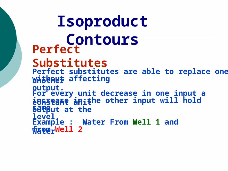
Perfect SubstitutesPerfect substitutes are able to replace one anotherwithout affecting output.For every unit decrease in one input a constant unitincrease in the other input will hold output at thesame level.Example : Water From Well 1 and Water from Well 2
Isoproduct Contours
Isoproduct Contours
X1
X2
Y
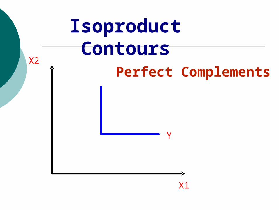
Perfect Complements
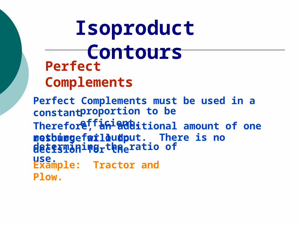
Perfect Complements
Perfect Complements must be used in a constantproportion to be
efficient.Therefore, an additional amount of one resource will donothing for output. There is no decision for thedetermining the ratio of use.Example: Tractor and Plow.
Isoproduct Contours
X1
X2
Y
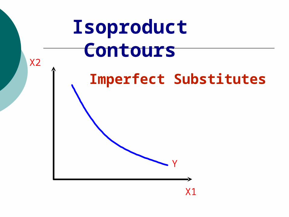
Imperfect Substitutes
Isoproduct Contours
Imperfect Substitutes
The most common problem faced by producers. Factorswill substitute for one another, but not at aconstant rate.Successive equal incremental reductions in oneinput, must be matched by increasingly largerincreases in the other input in order to hold outputconstant.This is what gives the curved shape to the isoquant.
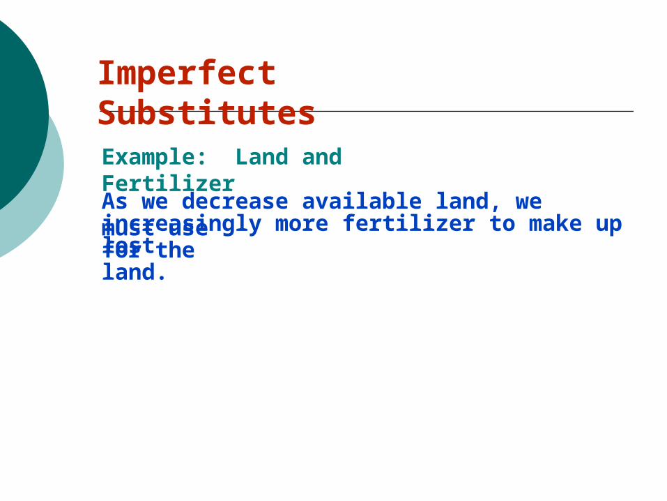
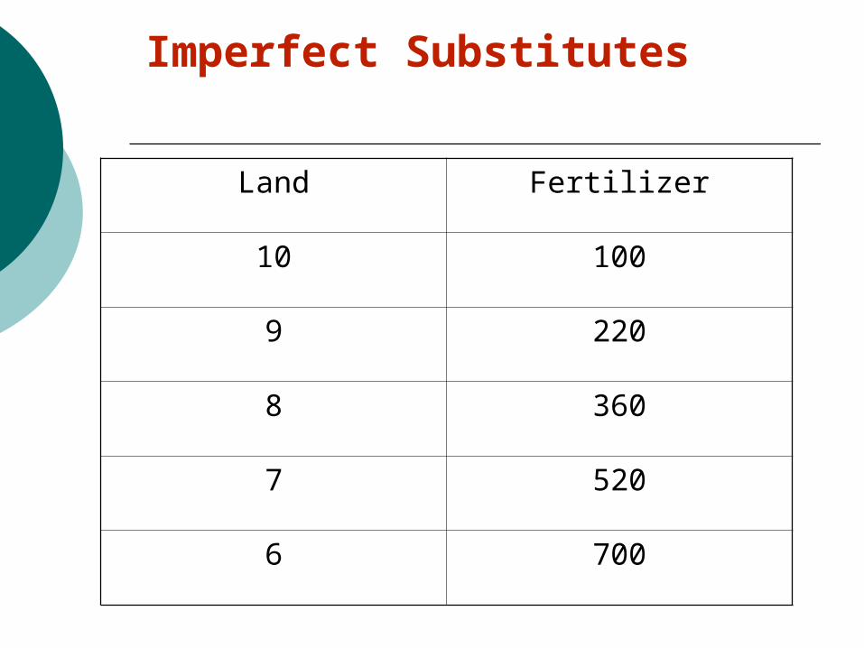
Imperfect SubstitutesExample: Land and FertilizerAs we decrease available land, we must useincreasingly more fertilizer to make up for thelost land.
Imperfect Substitutes
Land Fertilizer
10 100
9 220
8 360
7 520
6 700

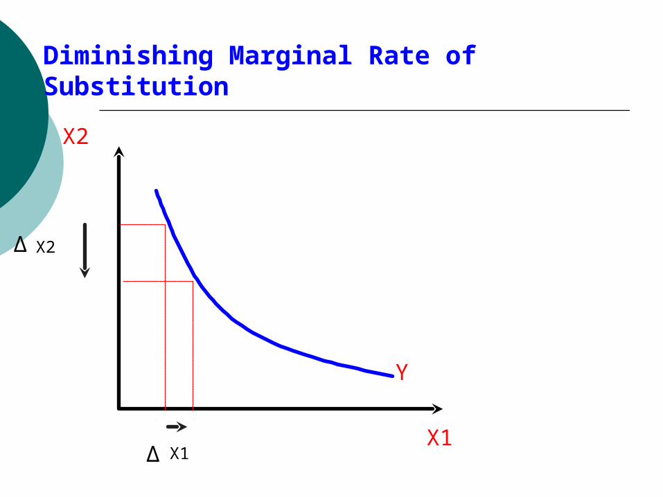
Marginal Rate of Substitution
Is the rate at which resources substitute for
one another.
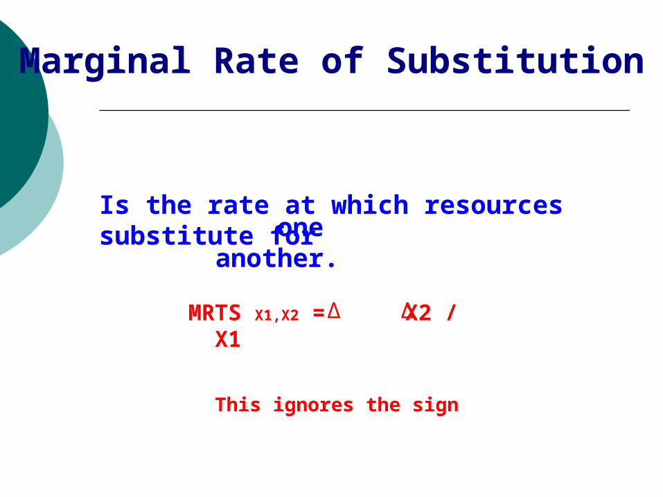
Marginal Rate of Substitution
Is the rate at which resources substitute for one
another.
MRTS X1,X2 = X2 / X1
This ignores the sign
∆ ∆
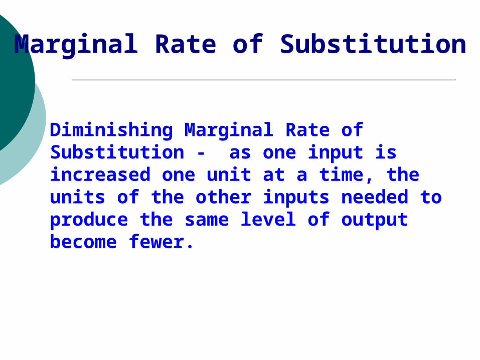
Diminishing Marginal Rate of Substitution - as one input is increased one unit at a time, the units of the other inputs needed to produce the same level of output become fewer.
Marginal Rate of Substitution
X1
X2
Y
X2
X1
Diminishing Marginal Rate of Substitution
∆
∆
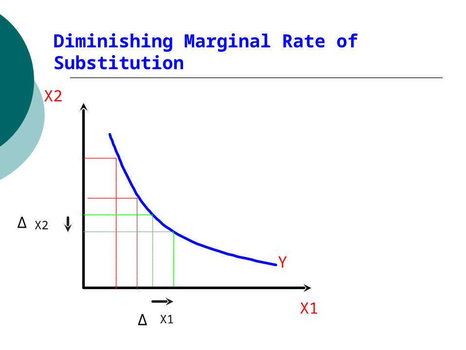
X1
X2
Y
X2
X1
Diminishing Marginal Rate of Substitution
∆
∆
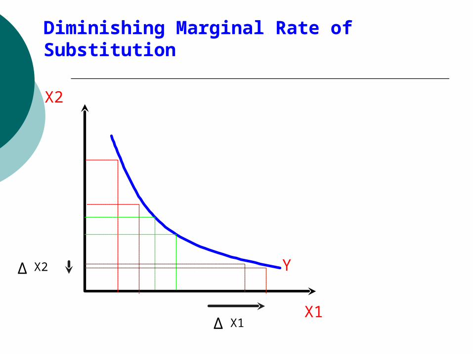
X1
X2
YX2
X1
Diminishing Marginal Rate of Substitution
∆
∆
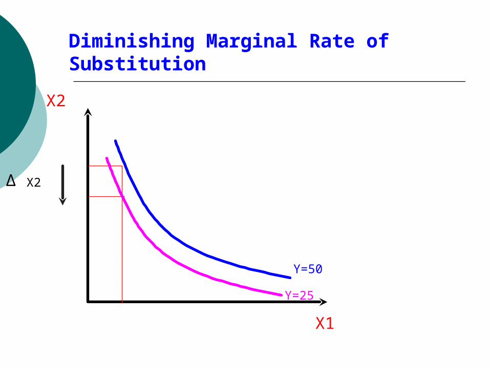
X1
X2
Y=50
X2
Y=25
Diminishing Marginal Rate of Substitution
∆
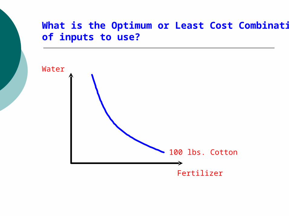
Fertilizer
Water
100 lbs. Cotton
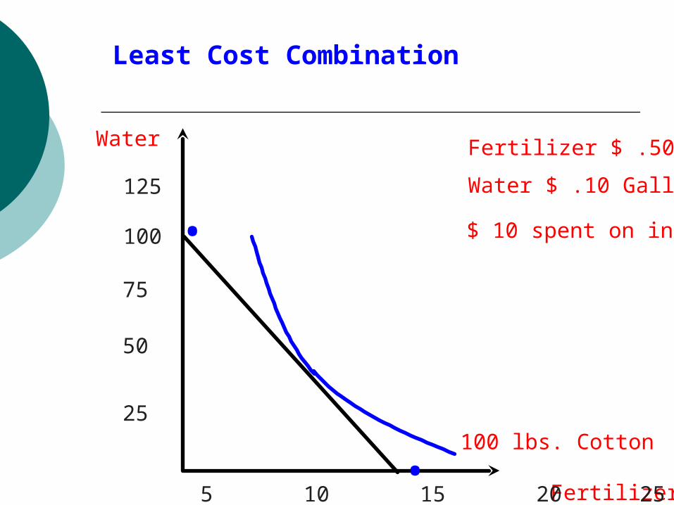
What is the Optimum or Least Cost Combination of inputs to use?
Fertilizer
Water
100 lbs. Cotton
Water $ .10 Gallon
Fertilizer $ .50 lb
$ 10 spent on inputs
5 10 15 20
100
75
50
25
125
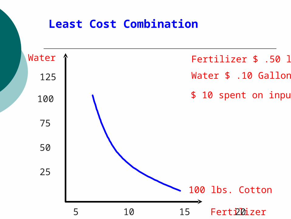
Least Cost Combination
Fertilizer
Water
100 lbs. Cotton
Water $ .10 Gallon
Fertilizer $ .50 lb
$ 10 spent on inputs
5 10 15 20 25
125
100
75
50
25
.
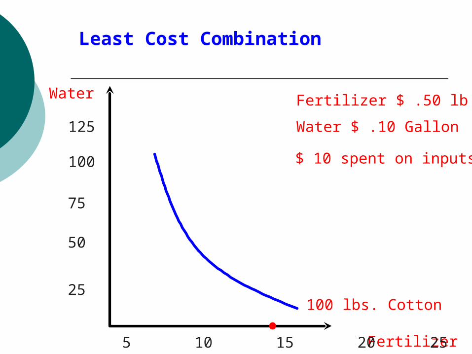
Least Cost Combination
Fertilizer
Water
100 lbs. Cotton
Water $ .10 Gallon
Fertilizer $ .50 lb
$ 10 spent on inputs
5 10 15 20 25
125
100
75
50
25
.
.
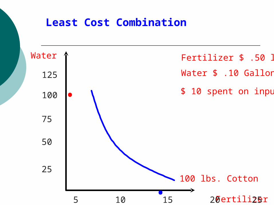
Least Cost Combination
Fertilizer
Water
100 lbs. Cotton
Water $ .10 Gallon
Fertilizer $ .50 lb
$ 10 spent on inputs
5 10 15 20 25
125
100
75
50
25
.
.
Least Cost Combination
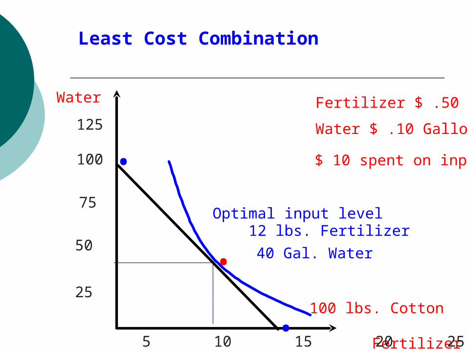
Fertilizer
Water
100 lbs. Cotton
Water $ .10 Gallon
Fertilizer $ .50 lb
$ 10 spent on inputs
5 10 15 20 25
125
100
75
50
25
.
.
.Optimal input level 12 lbs. Fertilizer
40 Gal. Water
Least Cost Combination
Fertilizer
Water
100 lbs. Cotton
Water $ .20 Gallon
Fertilizer $ .50 lb
$ 10 spent on inputs
5 10 15 20 25
125
100
75
50
25
.
.
.
Optimal input level 16 lbs. Fertilizer 10 Gal. Water
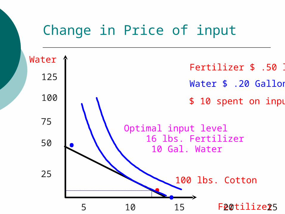
Change in Price of input
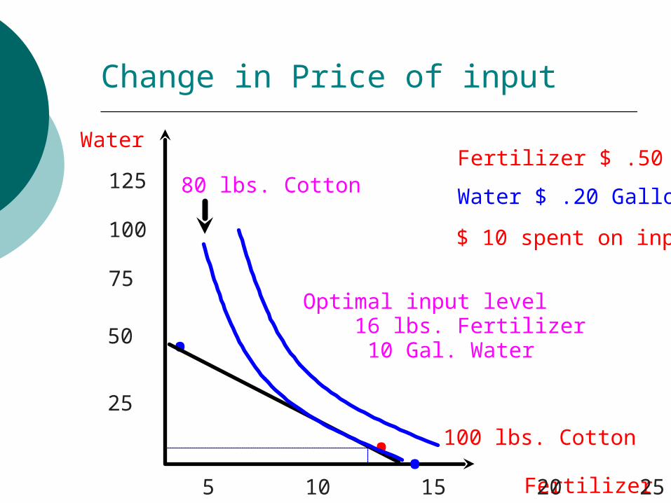
Fertilizer
Water
100 lbs. Cotton
Water $ .20 Gallon
Fertilizer $ .50 lb
$ 10 spent on inputs
5 10 15 20 25
125
100
75
50
25
.
..
Optimal input level 16 lbs. Fertilizer 10 Gal. Water
Change in Price of input
80 lbs. Cotton
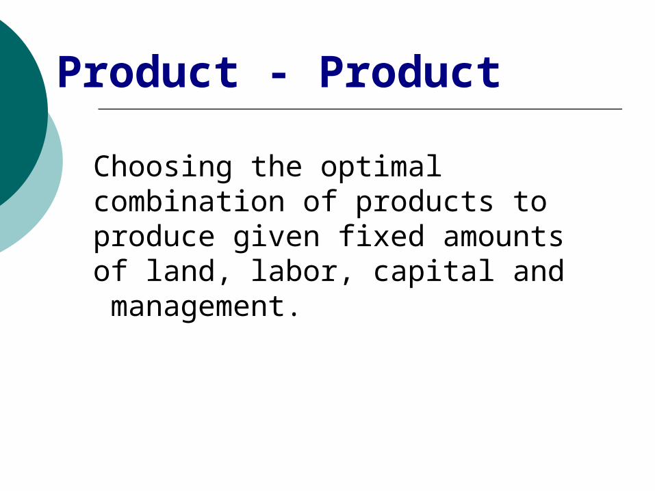
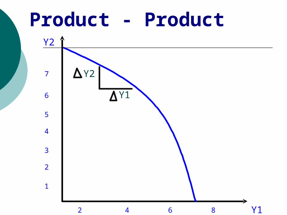
Product - Product
Choosing the optimal combination of products to produce given fixed amounts of land, labor, capital and management.
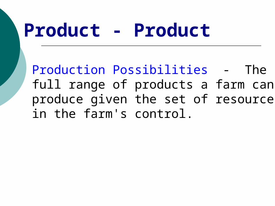
Production Possibilities - The full range of products a farm can produce given the set of resources in the farm's control.
Product - Product
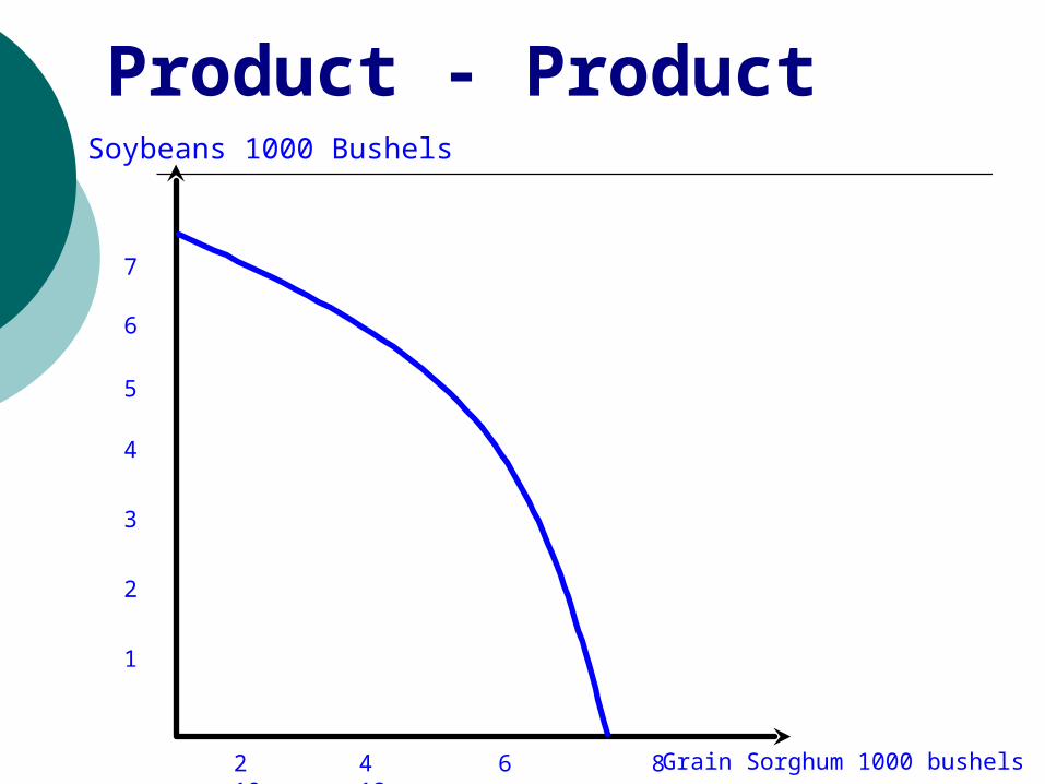
Soybeans 1000 Bushels
Grain Sorghum 1000 bushels
7
6
5
4
3
2
1
2 4 6 8 10 12
Product - Product
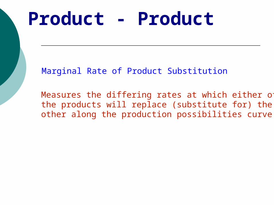
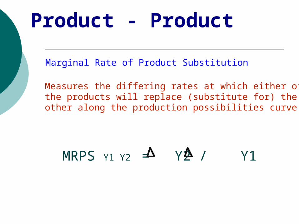
Marginal Rate of Product Substitution
Measures the differing rates at which either ofthe products will replace (substitute for) theother along the production possibilities curve.
Product - Product
Marginal Rate of Product Substitution
Measures the differing rates at which either ofthe products will replace (substitute for) theother along the production possibilities curve.
MRPS Y1 Y2 = Y2 / Y1
Product - Product
Y2
Y1
7
6
5
4
3
2
1
2 4 6 8 10 12
Y2
Y1
Product - Product
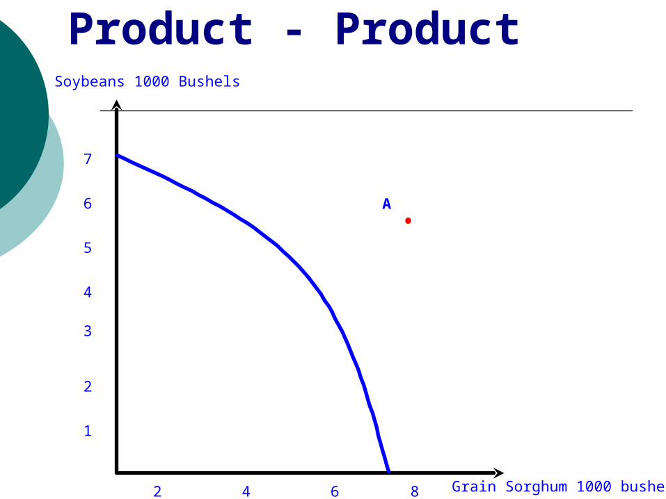
A.
Soybeans 1000 Bushels
Grain Sorghum 1000 bushels
7
6
5
4
3
2
1
2 4 6 8 10 12
Product - Product
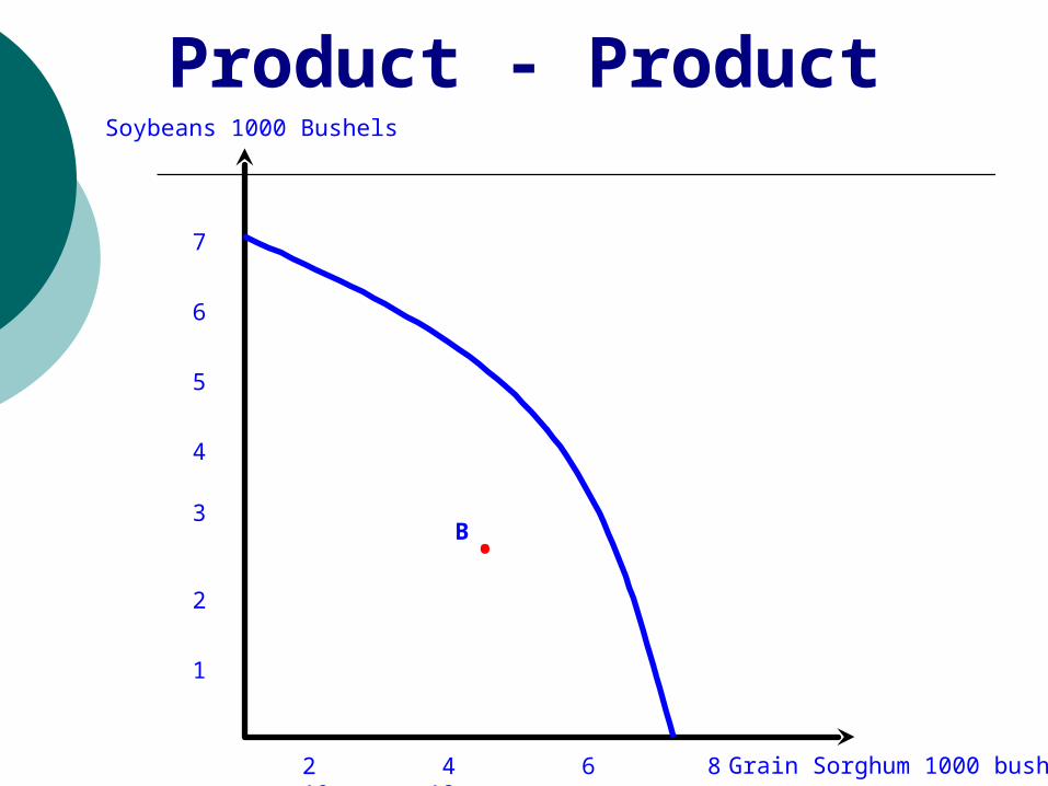
Soybeans 1000 Bushels
Grain Sorghum 1000 bushels
7
6
5
4
3
2
1
2 4 6 8 10 12
B.
Product - Product
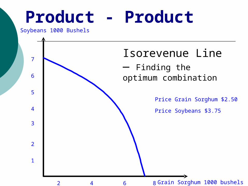
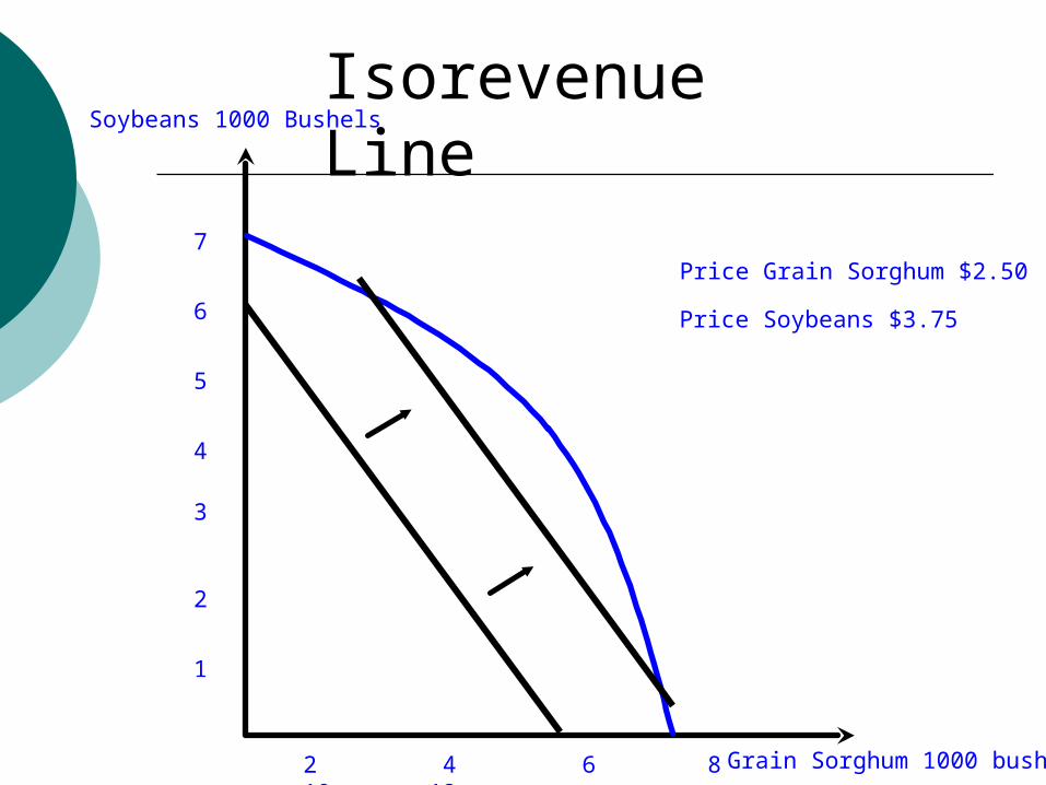
Isorevenue Line— Finding the optimum combination
Price Grain Sorghum $2.50
Price Soybeans $3.75
Soybeans 1000 Bushels
Grain Sorghum 1000 bushels
7
6
5
4
3
2
1
2 4 6 8 10 12
Product - Product
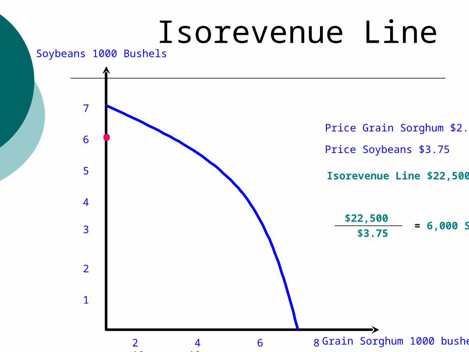
Isorevenue Line
Price Grain Sorghum $2.50
Price Soybeans $3.75
Isorevenue Line $22,500
$22,500 $3.75
= 6,000 SB
Soybeans 1000 Bushels
Grain Sorghum 1000 bushels
7
6
5
4
3
2
1
2 4 6 8 10 12
.
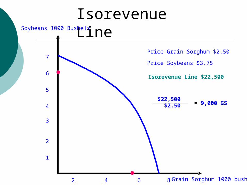
Isorevenue Line
Price Grain Sorghum $2.50
Price Soybeans $3.75
Isorevenue Line $22,500
$22,500 $2.50 = 9,000 GS
Soybeans 1000 Bushels
Grain Sorghum 1000 bushels
7
6
5
4
3
2
1
2 4 6 8 10 12.
.
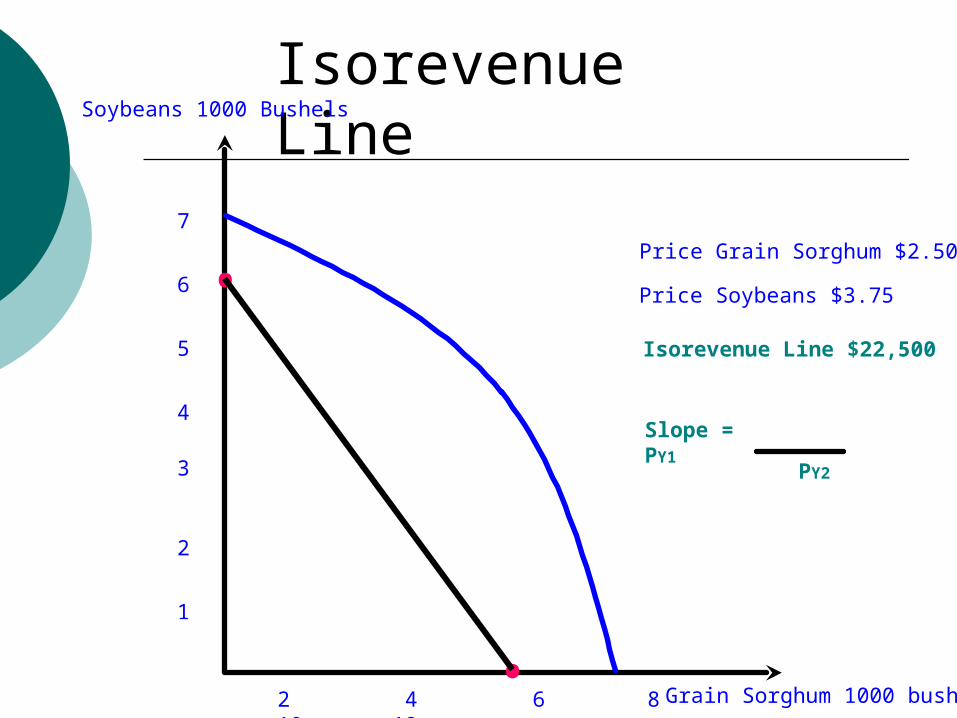
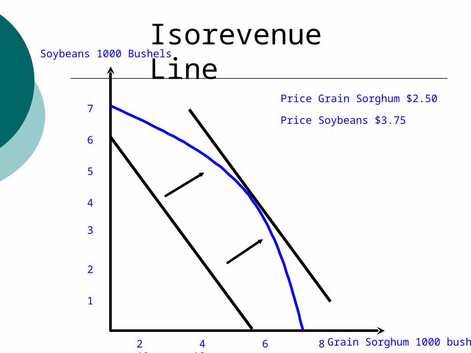
Isorevenue Line
Price Grain Sorghum $2.50
Price Soybeans $3.75
Isorevenue Line $22,500
Slope = PY1
PY2
Soybeans 1000 Bushels
Grain Sorghum 1000 bushels
7
6
5
4
3
2
1
2 4 6 8 10 12
.
.
Isorevenue Line
Price Grain Sorghum $2.50
Price Soybeans $3.75
Soybeans 1000 Bushels
Grain Sorghum 1000 bushels
7
6
5
4
3
2
1
2 4 6 8 10 12
Isorevenue Line
Price Grain Sorghum $2.50
Price Soybeans $3.75
Soybeans 1000 Bushels
Grain Sorghum 1000 bushels
7
6
5
4
3
2
1
2 4 6 8 10 12
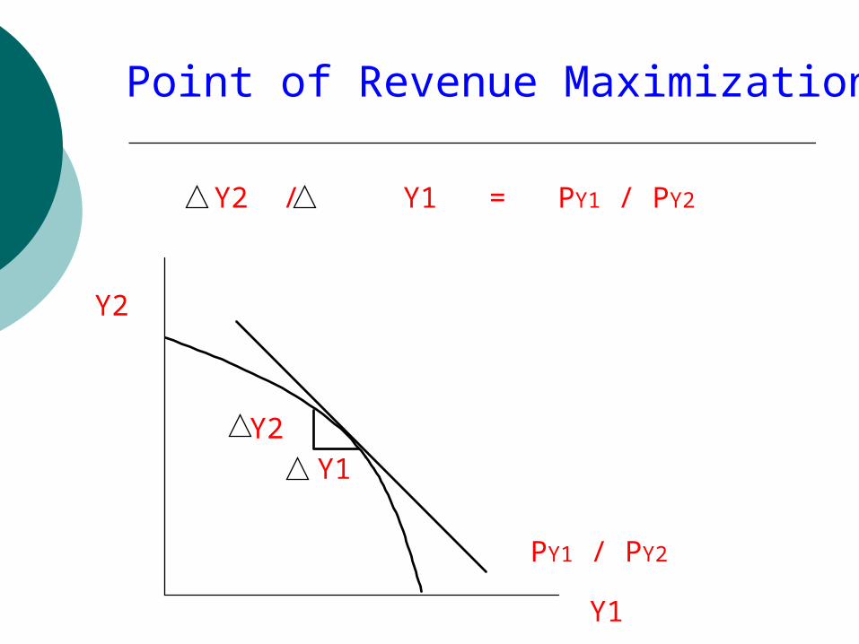
Point of Revenue Maximization
Y2 / Y1 = PY1 / PY2
Y2
Y1
PY1 / PY2
Y2
Y1
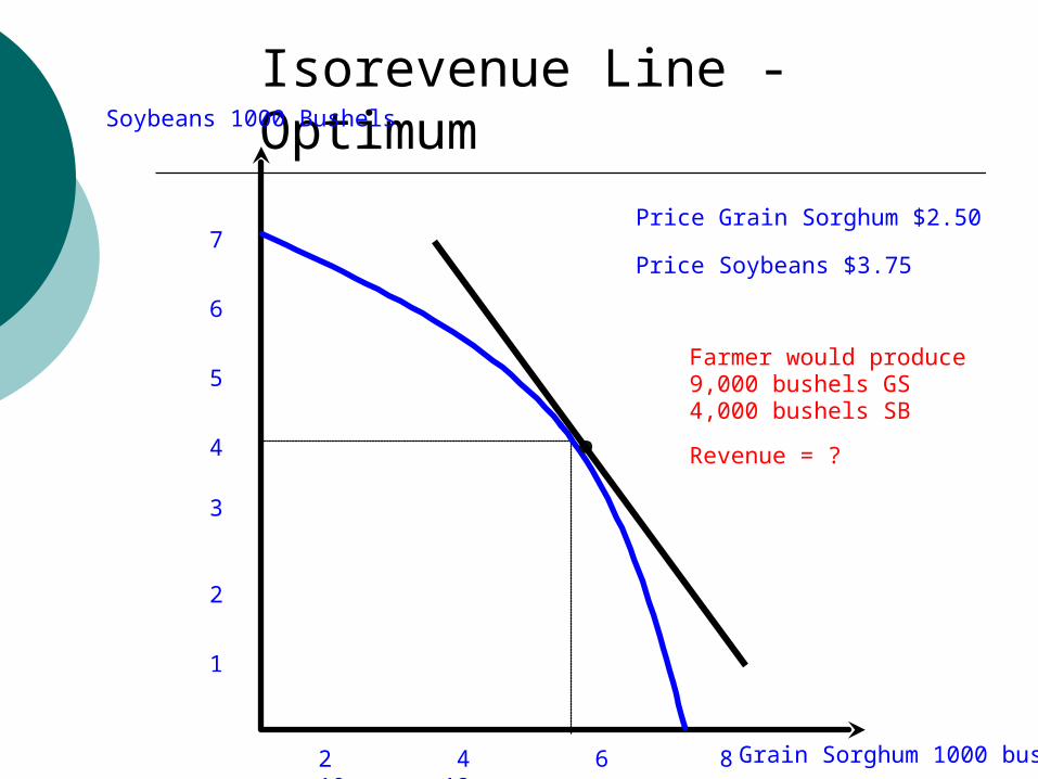
Isorevenue Line - Optimum
Price Grain Sorghum $2.50
Price Soybeans $3.75
Farmer would produce9,000 bushels GS4,000 bushels SB
Revenue = ?
Soybeans 1000 Bushels
Grain Sorghum 1000 bushels
7
6
5
4
3
2
1
2 4 6 8 10 12
.
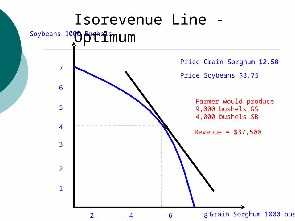
Price Grain Sorghum $2.50
Price Soybeans $3.75
Farmer would produce9,000 bushels GS4,000 bushels SB
Revenue = $37,500
Soybeans 1000 Bushels
Grain Sorghum 1000 bushels
7
6
5
4
3
2
1
2 4 6 8 10 12
.
Isorevenue Line - Optimum
Related Documents


![[XLS]Software Model - Excellence in Financial Management ... files/Financial_model_1.xls · Web viewThe variable inputs in the DETAIL worksheet are designed to accomodate most business](https://static.cupdf.com/doc/110x72/5afd686e7f8b9a814d8d720a/xlssoftware-model-excellence-in-financial-management-filesfinancialmodel1xlsweb.jpg)


