Processing - Forest and Wood Products Australia

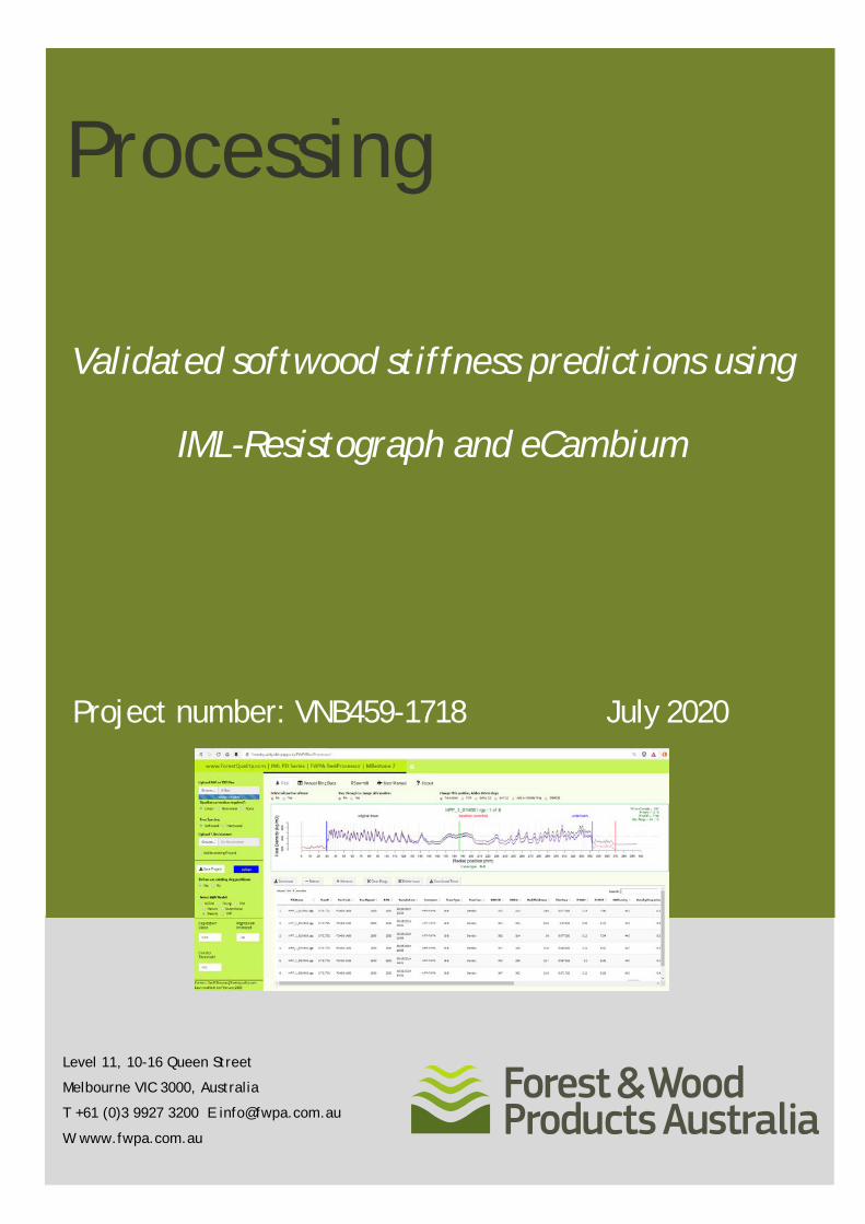
Processing

Validated softwood stiffness predictions using

IML-Resistograph and eCambium

Project number: VNB459-1718 July 2020

Level 11, 10-16 Queen Street

Melbourne VIC 3000, Australia

T +61 (0)3 9927 3200 E [email protected]

W www.fwpa.com.au

Forest & Wood Products Australia Limited Level 11, 10-16 Queen St, Melbourne, Victoria, 3000 T +61 3 9927 3200 F +61 3 9927 3288 E [email protected] W www.fwpa.com.au

Validated softwood stiffness predictions using IML-Resistograph and eCambium

for

Forest & Wood Products Australia

by

Geoff Downes, David Drew and David Lee

mailto:[email protected]

http://www.fwpa.com.au/

Forest & Wood Products Australia Limited Level 11, 10-16 Queen St, Melbourne, Victoria, 3000 T +61 3 9927 3200 F +61 3 9927 3288 E [email protected] W www.fwpa.com.au

Publication: Validated softwood stiffness predictions using IML-Resistograph and eCambium

Project No: VNB459-1718

IMPORTANT NOTICE

This work is supported by funding provided to FWPA by the Department of Agriculture, Water and Environment (DAWE).

© 2020 Forest & Wood Products Australia Limited. All rights reserved.

Whilst all care has been taken to ensure the accuracy of the information contained in this publication, Forest and Wood Products Australia Limited and all persons associated with them (FWPA) as well as any other contributors make no representations or give any warranty regarding the use, suitability, validity, accuracy, completeness, currency or reliability of the information, including any opinion or advice, contained in this publication. To the maximum extent permitted by law, FWPA disclaims all warranties of any kind, whether express or implied, including but not limited to any warranty that the information is up-to-date, complete, true, legally compliant, accurate, non-misleading or suitable.

To the maximum extent permitted by law, FWPA excludes all liability in contract, tort (including negligence), or otherwise for any injury, loss or damage whatsoever (whether direct, indirect, special or consequential) arising out of or in connection with use or reliance on this publication (and any information, opinions or advice therein) and whether caused by any errors, defects, omissions or misrepresentations in this publication. Individual requirements may vary from those discussed in this publication and you are advised to check with State authorities to ensure building compliance as well as make your own professional assessment of the relevant applicable laws and Standards.

The work is copyright and protected under the terms of the Copyright Act 1968 (Cwth). All material may be reproduced in whole or in part, provided that it is not sold or used for commercial benefit and its source (Forest & Wood Products Australia Limited) is acknowledged and the above disclaimer is included. Reproduction or copying for other purposes, which is strictly reserved only for the owner or licensee of copyright under the Copyright Act, is prohibited without the prior written consent of FWPA.

ISBN: 978-1-925213-94-2

Researcher/s: G. Downes (Forest Quality), D. Drew (Forest Forecasting), D. Lee (University Sunshine Coast), M. Lausberg (Wood Quality Consulting), J. Harrington, M. Ivković, (Tree Breeding Australia), S. Elms (HVPlantations), P. Muyambo (Highland Pine), R. Riepsamen (Forest Corporation NSW) and D. Kain (HQPlantations).

This work was also funded by industry contributions from the following companies: HQPlantations, HVP Plantations, Forestry Corporation of NSW, Timberlands, Highland Pine, OneFortyOne Plantations, AKD Softwoods, Norske Skog, GTFP, PF Olsen, Hume Forests and Hyne Timbers.

Page | 1



Page | 2

FWPA Project VNB459-1718: Validated softwood stiffness predictions using IML-Resistograph and eCambium: online automated processing

Geoff Downes, Forest Quality Pty. Ltd. And David Drew, University of Stellenbosch, South Africa.

Project Deliverables The proposal documentation for this project listed the following project deliverables

1. Fully automated algorithm for the prediction of log MOE (AWV) from IML Resistograph tracesusing existing FWPA and NZSWI data sets with algorithms incorporated into web-based URLavailable via secure login for commercial use and featuring

a. Sawing simulator to predict sawn board out turn based on RESI traces from each trace(tree)

b. Ability to allocate annual rings to Resi traces and download growth and wood data forinventory applications

2. Validation datasets from industry partners with measured log MOE from logs sampled usingthe Resistograph across a range of age classes and species (radiata and southern pines)

3. Sawmill validation study relating predicted Resi and eCambium site values to actual milloutput

4. Online version of eCambium featuring automated site and weather data input, and scenariosetup

5. Written reports describing relationships identified in the analysis and also incorporatingnecessary user-manuals

6. Industry workshops to explain and train people in the use of the web-based systems

Page | 3

Table of Contents Project Deliverables ................................................................................................................................ 2

Table of Contents 3

Project Background ................................................................................................................................. 4

Report structure 8

Key Outcomes 9

Deliverable 1. User Guide to the FWPA ResiProcessor web platform .................................................. 12

Deliverable 2 Part 1. The prediction of MOE and AWV in 7-year-old radiata pine .............................. 37

Deliverable 2 Part 2. The prediction of MOE and AWV in 10 year-old southern yellow pine .............. 46

Deliverable 2 Part 3. Evaluation of Resi predicted standing tree wood properties across a range of Pinus radiata sites. ................................................................................................. 60

Deliverable 2 Part 4. Southern Pine assessment of stiffness predictions using IML-Resi PD400 (Experiment 374 SIL) .............................................................................................. 77

Deliverable 3. Predicting sawn timber volumes and quality from preharvest measurements using Resi. .............................................................................................................................. 100

Deliverable 4. Part 1. User Guide for the rCambium web platform ................................................... 120

Deliverable 4. Part 2. Evaluating the performance of the rCambium platform in radiata pine. ........ 133

Deliverable 4. Part 3. Evaluating the performance of the rCambium platform in Southern Pines. ... 152

Page | 4

Project Background The pressure to boost plantation productivity in commercial softwood plantations is ever-present. Typically, productivity increases are assessed as increased volume production over unit time, such that rotation lengths can be reduced (Apiolaza et al. 2013, O’Hehir and Nambiar 2010). Maintaining rotation lengths to increase log volume can be problematic if the processing industry is geared towards a set range of log diameters, as over-sized logs can impact negatively on costs and profitability. Preferably volume gains achieved should not detrimentally affect wood quality. However, all things being equal, shorter rotation rates increase the proportion of lower quality juvenile wood, generally lowering overall log quality (Baltunis, Wu and Powell 2007, Kennedy 1995, Li, Wu and Southerton 2012). Maintaining wood quality while shortening rotations is therefore a significant challenge. If wood quality can be added into the productivity (value) equation from a grower’s perspective, a more balanced approach to volume gains can be achieved that minimises negative impacts on quality.

The main options available to forest managers to increase productivity are genetic improvement and silvicultural adjustments, but they still lack tools by which to understand the potential wood quality implications. At the same time, processors are recognising the importance of understanding and managing wood variability in the timber resource to optimise their operations to achieve the ever-increasing quality demands on their product.

Forest managers can have important effects on wood quality by adjusting management and silvicultural regimes. For example, mid-rotation fertilisation and thinning of radiata pine may increase the proportion of non-juvenile wood without affecting the value recovery (Nyakuengama, Downes and Ng 2003, Downes et al. 2002a, Nyakuengama, Downes and Ng 2002, McGrath, Copeland and Dumbrell 2003). Stocking and weed control have been shown to significantly affect mean wood density and stiffness (Watt et al. 2011, Xue et al. 2013). Site type and climatic variation are both also of major importance in determining wood properties. Wood density varies with temperature (Cown 2005) while other factors, like drought, are also important (Ivković et al. 2013, Nanayakkara et al. 2014, Downes, Wimmer and Evans 2002b).

Over recent decades a range of new tools have been developed that allow wood quality in the standing resource to be measured (Evans et al. 1995, Downes and Lausberg 2016a, Downes et al. 2014, Downes et al. 2012, Mora et al. 2009, Vikram et al. 2011). Increasingly these are being implemented in breeding programs (Gapare et al. 2010, Wu et al. 2008, Chauhan et al. 2013) and to a lesser extent in general resource inventory (Cown et al. 2006, McKinley et al. 2003). The various costs involved vary with the lower-cost technologies being more commonly applied. The process-based model, eCambium (Downes et al. 2016, Pinkard 2016, Drew and Downes 2015), was developed to predict wood properties and stand growth and productivity from inputs of weather data, site characteristics and silviculture. Predictions explained >60% of mean site-average wood density and mean MOE from an initial test set of 53 sites in the Murray Valley basin (Downes et al. 2016). The key novelty of the tool is that it can assist forest managers to forecast potential wood quality implications from management changes or under unprecedented situations, such as new plantation establishment, or a changing climate.

As part of this model development the IML-Resistograph PD400 was assessed as a means of quantifying basic density in individual trees. The key features of this tool are its low cost in field application and the relatively high-resolution data produced. A 400 mm long traces can be taken from a single tree in less than 30 seconds, with tests conservatively showing that over 50 trees per hour can

Page | 5

be sampled. The trace provides a profile of resistance to turning (torque) every 0.1mm and this trace indicates the variation in density (Downes and Lausberg 2016a, Gao et al. 2012). Typically, this instrument has been applied in qualitative studies to identify decay and other defects in trees and poles. Previous work in earlier models had indicated its ability to quantify density variation was limited (Isik and Li 2003) but useful for breeding selection (Eckard et al. 2010). Work in the eCambium study (Downes et al. 2016)indicated that site average values of density obtained from the Resistograph compared with 50mm outerwood cores taken a year previously explained over 80% of the variance in density. Subsequent work in both pines and eucalypts has demonstrated that Resi data typically correlates with basic density at 65-88% variance explained at the individual sample level (Downes unpublished data), and is strongly correlated with pilodyn.

References

Apiolaza, L., S. Chauhan, M. Hayes, R. Nakada, M. Sharma & J. Walker (2013) Selection and breeding for wood quality A new approach. NZJ For, 58, 33.

Baltunis, B. S., H. X. Wu & M. B. Powell (2007) Inheritance of density, microfibril angle, and modulus of elasticity in juvenile wood of Pinus radiata at two locations in Australia. Canadian Journal of Forest Research, 37, 2164-2174.

Chauhan, S. S., M. Sharma, J. Thomas, L. A. Apiolaza, D. A. Collings & J. C. F. Walker (2013) Methods for the very early selection of Pinus radiata D. Don. for solid wood products. Annals of Forest Science, 70, 439-449.

Cown, D. (2005) Understanding and managing wood quality for improving product value in New Zealand. NZJ For. Sci, 35, 205-220.

Cown, D., R. McKinley, G. Downes, M. Kimberley, J. Bruce, M. Hall, P. Hodgkiss, D. McConchie & M. Lausberg (2006) Benchmarking the wood properties of radiata pine plantations: Tasmania. Summary report prepared for the Forest and Wood Products Research and Development Corporation, Australia.

Downes, G. M., D. M. Drew, J. Moore, M. Lausberg, J. Harrington, S. Elms, D. Watt & S. Holtorf. 2016. Evaluating and modelling radiata pine wood quality in the Murray valley region. Melbourne, Australia: Forest and Wood Products Australia.

Downes, G. M., C. E. Harwood, J. Wiedemann, N. Ebdon, H. Bond & R. Meder (2012) Radial variation in Kraft pulp yield and cellulose content in Eucalyptus globulus wood across three contrasting sites predicted by near infrared spectroscopy. Canadian Journal of Forest Research, 42, 1577-1586.

Downes, G. M. & M. Lausberg. 2016a. Evaluation of the RESI Software tool for the prediction of HM200 within pine logs sourced from multiple sites across New Zealand and Australia. 15 New Zealand Solid Wood Innovations.

---. 2016b. User Manual for the software tool for the prediction of Acoustic Velocity (HM200) from traces collected from Pinus radiata using the IML Resistograph PD-400. 15. Forest Quality Pty. Ltd.

Downes, G. M., J. G. Nyakuengama, R. Evans, R. Northway, P. Blakemore, R. L. Dickson & M. Lausberg (2002a) Relationship between wood density, microfibril angle and stiffness in thinned and fertilized Pinus radiata. Iawa Journal, 23, 253-266.

Downes, G. M., M. Touza, C. E. Harwood & M. Wentzel-Vietheer (2014) NIR detection of non-recoverable collapse in sawn boards of Eucalyptus globulus. Eur. J Wood Prod., in press.

Downes, G. M., R. Wimmer & R. Evans (2002b) Understanding wood formation: gains to commercial forestry through tree-ring research. Dendrochronologia, 20, 37-51.

Drew, D. M. & G. Downes (2015) A model of stem growth and wood formation in Pinus radiata. Trees, 29, 1395-1413.

Page | 6

Eckard, J. T., F. Isik, B. Bullock, B. Li & M. Gumpertz (2010) Selection Efficiency for Solid Wood Traits in Pinus taeda using Time-of-Flight Acoustic and Micro-Drill Resistance Methods. Forest Science, 56, 233-241.

Evans, R., G. Downes, D. Menz & S. Stringer (1995) Rapid measurement of variation in tracheid transverse dimensions in a radiata pine tree. Appita journal, 48, 134-138.

Gao, S., X. Wang, B. K. Brashaw, R. J. Ross & L. Wang. 2012. Rapid assessment of wood density of standing tre with nondestructive methods—A review. In Biobase Material Science and Engineering (BMSE), 2012 International Conference on, 262-267. IEEE.

Gapare, W. J., M. Ivković, B. S. Baltunis, C. A. Matheson & H. X. Wu (2010) Genetic stability of wood density and diameter in Pinus radiata D. Don plantation estate across Australia. Tree Genetics & Genomes, 6, 113-125.

Isik, F. & B. Li (2003) Rapid assessment of wood density of live trees using the Resistograph for selection in tree improvement programs. Canadian Journal of Forest Research, 33, 2426-2435.

Ivković, M., W. Gapare, H. Wu, S. Espinoza & P. Rozenberg (2013) Influence of cambial age and climate on ring width and wood density in Pinus radiata families. Annals of forest science, 70, 525-534.

Kennedy, R. (1995) Coniferous wood quality in the future: concerns and strategies. Wood Science and Technology, 29, 321-338.

Li, X., H. X. Wu & S. G. Southerton (2012) Identification of putative candidate genes for juvenile wood density in Pinus radiata. Tree physiology, 32, 1046-1057.

McGrath, J., B. Copeland & I. Dumbrell (2003) Magnitude and duration of growth and wood quality responses to phosphorus and nitrogen in thinned Pinus radiata in southern Western Australia. Australian Forestry, 66, 223-230.

McKinley, R., R. Ball, G. Downes, D. Fife, D. Gritton, J. Ilic, A. Koehler, A. Morrow & S. Pongracic. 2003. Resource evaluation for future profit: wood property survey of the Green Triangle region. CSIRO Client Report.

Mora, C. R., L. R. Schimleck, F. Isik, J. M. Mahon, A. Clark & R. F. Daniels (2009) Relationships between acoustic variables and different measures of stiffness in standing Pinus taeda trees. Canadian Journal of Forest Research, 39, 1421-1429.

Nanayakkara, B., F. Lagane, P. Hodgkiss, M. Dibley, S. Smaill, M. Riddell, J. Harrington & D. Cown (2014) Effects of induced drought and tilting on biomass allocation, wood properties, compression wood formation and chemical composition of young Pinus radiata genotypes (clones). Holzforschung, 68, 455-465.

Nyakuengama, J. G., G. M. Downes & J. Ng (2002) Growth and wood density responses to later-age fertilizer application in Pinus radiata. IAWA J, 23, 431-448.

--- (2003) Changes caused by mid-rotation fertilizer application to the fibre anatomy of Pinus radiata. Iawa Journal, 24, 397-410.

O’Hehir, J. & E. Nambiar (2010) Productivity of three successive rotations of P. radiata plantations in South Australia over a century. Forest Ecology and Management, 259, 1857-1869.

Pinkard, L. (2016) Opportunities for innovation in the forestry sector. Australian Forest Grower, 39, 36.

Vikram, V., M. L. Cherry, D. Briggs, D. W. Cress, R. Evans & G. T. Howe (2011) Stiffness of Douglas-fir lumber: effects of wood properties and genetics. Canadian Journal of Forest Research, 41, 1160-1173.

Watt, M. S., B. Zoric, M. O. Kimberley & J. Harrington (2011) Influence of stocking on radial and longitudinal variation in modulus of elasticity, microfibril angle, and density in a 24-year-old Pinus radiata thinning trial. Canadian journal of forest research, 41, 1422-1431.

Wu, H., M. Ivkovic, W. Gapare, A. Matheson, B. Baltunis, M. Powell & T. McRae (2008) Breeding for wood quality and profit in Pinus radiata: a review of genetic parameter estimates and implications for breeding and deployment. New Zealand Journal of Forestry Science, 38, 56-87.

Page | 7

Xue, J., P. W. Clinton, A. C. Leckie & J. D. Graham (2013) Magnesium fertilizer, weed control and clonal effects on wood stiffness of juvenile Pinus radiata at two contrasting sites. Forest ecology and management, 306, 128-134.

Page | 8

Report structure Given the diverse nature of the deliverables, this report addresses these as a collection of separate reports compiled into a single document to assist the reader in accessing and following each component of interest. Each report can be read as a standalone account.

The reports are presented under the following headings:

Deliverable 1. Web-based Resi trace processing platform. • User manual and overview including appendices as follows

o Resi User Field work guidelines o Protocol for assessing core basic density and calibration of Resi values o Infield measurement of disc green density o Protocol for assessing Resi predictions

Deliverable 2. Resi prediction of log MOE • Part 1 The prediction of MOE and AWV in 7-year-old radiata pine • Part 2 The prediction of MOE and AWV in 10 year-old southern yellow pine • Part 3 Evaluation of Resi predicted standing tree wood properties across a range of Pinus

radiata sites. o Appendix 1: Assessment of HVP calibration data.

• Part 4 Southern Pine assessment of stiffness predictions using IML-Resi PD400 (Experiment 374 SIL)

o Appendix 1: Procedure used to select 11 trees additional to DST trees in Experiment 374 SIL

Deliverable 3. Sawmill validation study • Predicting sawn timber volumes and quality from preharvest measurements using Resi.

Deliverable 4. rCambium web platform • Part 1: User Guide for the rCambium web platform

o Protocol for assessing rCambium predictions o Protocol for soil sampling

• Part 2: Evaluating the performance of the rCambium platform in radiata pine. o Appendix 1: FCNSW trial operational implementation of rCambium model

• Part 3: Evaluating the performance of the rCambium platform in southern pines.

Page | 9

Key Outcomes Deliverable 1. Web-based Resi trace processing platform.

• The web platform has proved accessible and robust in processing Resi traces. • Over the course of the project its functionality has increased according to interest and demand

from industry partners. • Error catching has been progressively improved to minimise errors which cause disconnection

and loss of data. • Various AWV and MOE prediction models have been implemented and are currently being

evaluated by industry partners.

Deliverable 2. Assessment of Resi performance in the prediction of log MOE The attainment of this deliverable is presented as four parts as follows

Part 1: Young radiata pine (7 year old) • ST300 values were moderately correlated with HM200 values with a SEP ~ 0.2 km.sec-1 • Resi-derived basic density values at breast height prior to felling were moderately to strongly

correlated with the basic density of the cross-section disc taken from the small end of the 3 m butt log (r2 = 0.67).

• The “Mature” model of predicted HM200 (PrAWV) from the current Resi processing web platform gave the best predictive performance, but explaining less variance than the ST300 (44% vs 61%).

• Fitting a predictive model to the log HM200 values used 4 Resi predictor variables and explained 44% of the variance in HM200 at the family mean level.

• A fitted model to log MOE values used 2 Resi predictor variables and explained 55% of the variance at the family mean level

• Combining ST300 and Resi in a fitted regression explained 74% of the variance in log MOE compared to 62% using ST300 alone

Part 2: Young Southern pine (10 year old) • ST300 measures of AWV provided the best indicator of log MOE in young southern pines

explaining 68% of the variance with a SEP of 0.45 GPa . • Resi measures of basic density in contrast explained only 26% of the variance. • Resi predictions of log MOE explained 33% of the variance with a SEP of 0.74 GPa. • A fitted regression to predict log MOE using Resi-derived variables explained 42% of the

variance with a SEP of 0.59 GPa. • Combining ST300 and Resi in a fitted regression explained 75% of the variance with a SEP of

0.41 GPa

Part 3: Mature radiata pine • All predicted MOE models explained most of the variance in actual MOE (log and mill board

MOE) across available data • In terms of accuracy and precision the Outerwood and Density models performed with the

greater consistency. • The Mature model performed well in mature stands but less well in younger stands, also

tending to under-predict log MOE and AWV at higher values. • The Young model had significant bias when applied to older stands, tending to markedly

under-estimate the actual MOE in mature stands.

Page | 10

• In terms of general application, the Density model is arguably the better model, and could be refined to give more accurate results over a wider age range.

• Overall the results indicate that the ability of Resi to predict basic density is the main contributor to MOE prediction, with little being gained from the attempts to explain additional variance by extracting other metrics from the Resi trace.

Part 4: Mature southern pine • Resi was good at predicting individual tree basic density and excellent at predicting site

average basic density of a Southern Pine stand, as it explains 89% of the variance. • Combining the ResiProcessor predictions of basic density with the ST300 or HM200 AWV

improves the prediction of tree MOE of both of these tools. • The NZSWI ResiProcessor model for PrAWV explains more of the variance in site average Tree

AWV than other models tested. • The NZSWI ResiProcessor model for PrMOE explains more of the variance in site average Tree

MOE than other models tested. Across three levels of interventions this model explained 66-71% of the Tree MOE.

• Combining the NZSWI PrMOE x stem slenderness explains 80% of the variance in site average Tree MOE. This appears to be the current best option to predict site Tree MOE of the ResiProcessor options tested.

Deliverable 3. Sawmill validation study • Site mean log MOE explained 85% of the variance in site mean board MOE, whereas in the

absence of green density information site mean log AWV explained only 51%.

• Preharvest Resi basic density near breast height explained most of the variance in mean log and board MOE (78% and 88% respectively) and some variance in log AWV (50%) and mean board AWV (39%)

• Resi-derived core density was a better predictor than the Resi-predicted AWV of both board and log MOE and AWV

• Site mean actual outerwood core density explained 85% of the variance in site mean board MOE.

• Three different Resi instruments gave comparable results once each individual instrument was calibrated using actual outerwood core basic density values

• Sites exhibited a large range in the percentage of MGP10 or better boards. Resi values exhibited strong correlations with this metric

• The strength of the relationships between Resi values and log and board data strengthens the commercial value of the use of the Resi as a preharvest assessment tool and the need to develop standard methodologies of application to enhance the communication of data across the value chain.

Deliverable 4. rCambium web platform The attainment of this deliverable is presented as three parts addressing

Part 1. rCambium web platform • The web platform has proved robust in terms of usage allowing hundreds of scenarios to be

run in a single session. The running of each scenario takes 1-2 seconds including the collection of soils and monthly weather data from other web portals.

Page | 11

• It provides a portal for the convenient collection of soils and weather data for a given location within Australia

• Its dependence upon these independent data sets prevents its utilisation outside Australia • In its current form, the web site is openly available to all public users, but could be restricted

by enforcing a username and password login. • Additional functionality can be added if and as its commercial use is found to be of value.

Part 2. Evaluating the performance of the rCambium platform in radiata pine. • The rCambium web platform has performed robustly, processing input data sets defining

hundreds of separate scenarios, processing each scenario in 1-2 secs.

• Using site index as an input to the rCambium model is not advised at this stage. While slightly improving the prediction of tree height, it resulted in poorer predictions of diameter and wood property metrics.

• Measures of tree height were accurate (little bias overall) but imprecise (r2 ~ 20%)

• Measures of under-bark diameter were reasonable in terms of variance explained (r2 ~ 43%) with some tendency to under-predict larger diameter sites.

• Predictions of wood density were best against pith-to-bark or bark-to-bark means, avoiding the confounding effects of diameter growth on outerwood density metrics

• Over the whole data set, rCambium predicted 50% of the variance in Resi-predicted pith-to-bark basic density with a SEP of 20 kg.m-3.

• rCambium predictions of log MOE were strong, explaining 66% of the variance.

• rCambium is intended as a lowest-cost, first-pass assessment of wood quality variance at the estate level. The broad resolution of the input weather data and potential inaccuracy in the publicly available soils data will lead to poor performance at some sites. Thus application across a range of sites where the actual range of wood property values is restricted will result in lower levels of explained variance (r2). SEP values should guide the user with respect to the confidence intervals that can be expected in model predictions.

Part 3. Evaluating the performance of the rCambium platform in southern pines. • rCambium in its present form was not able to predict the actual variance in DBH, tree height,

basic density or Log MOE across the sites available for study • The physiology of Southern Yellow Pines (SYP) and/or growth environment exhibits

fundamental differences to those for radiata pine, which requires a re-evaluation of an appropriate modelling strategy

• SYP on many of these sites are subject to seasonal water-logging; an effect which is not addressed in the rCambium framework

• Sub-tropical growth patterns, in comparison with the temperate patterns of radiata pine, may require some more fundamental investigation to inform an appropriate modelling strategy

• In contrast to radiata pine, southern pines represent a range of species and hybrids (taxa), which contributes to the potential physiological variance. It may be that individual taxa need individual parameterisation.

Page | 12

Deliverable 1. User Guide to the FWPA ResiProcessor web platform

Geoff Downes, Forest Quality Pty Ltd, PO Box 293, Huonville, Tasmania, 7109, Australia

Email: [email protected]

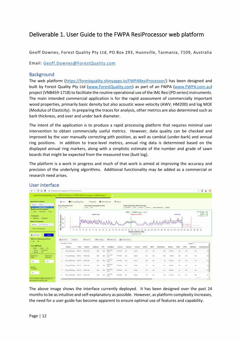
Background The web platform (https://forestquality.shinyapps.io/FWPAResiProcessor/) has been designed and built by Forest Quality Pty Ltd (www.ForestQuality.com) as part of an FWPA (www.FWPA.com.au) project (VNB459-1718) to facilitate the routine operational use of the IML Resi (PD series) instruments. The main intended commercial application is for the rapid assessment of commercially important wood properties, primarily basic density but also acoustic wave velocity (AWV, HM200) and log MOE (Modulus of Elasticity). In preparing the traces for analysis, other metrics are also determined such as bark thickness, and over and under bark diameter.

The intent of the application is to produce a rapid processing platform that requires minimal user intervention to obtain commercially useful metrics. However, data quality can be checked and improved by the user manually correcting pith position, as well as cambial (under-bark) and annual ring positions. In addition to trace-level metrics, annual ring data is determined based on the displayed annual ring markers, along with a simplistic estimate of the number and grade of sawn boards that might be expected from the measured tree (butt log).

The platform is a work in progress and much of that work is aimed at improving the accuracy and precision of the underlying algorithms. Additional functionality may be added as a commercial or research need arises.

User interface

The above image shows the interface currently deployed. It has been designed over the past 24 months to be as intuitive and self-explanatory as possible. However, as platform complexity increases, the need for a user guide has become apparent to ensure optimal use of features and capability.


https://forestquality.shinyapps.io/FWPAResiProcessor/

http://www.forestquality.com/


Page | 13

The bottom left hand corner records the date when the current interface was uploaded. This will change over time as operations that cause errors are corrected, new functionality is added, or back ground algorithms are changed.

The interface contains a sidebar on the left where the major project functions are carried out to load traces or projects, to save a collection of uploaded traces as a project, and to select which model to use for the prediction of AWV. On the right are a series of panels displaying the Resi data in different forms:

• Resi: This panel displays the individual traces and the summary table of metrics derived from their processing upon loading and editing. It provides access to various controls to allow the user to interact with the trace and adjust summary metrics.

• Annual Ring Data: Annual ring locations will be allocated automatically but these can be adjusted manually on the trace displayed on the Resi panel described above. Annual ring level allows the user to use the Resi data to generate annual measures of growth and basic density. If the “Hardwood” option in the sidebar is selected, annual ring boundaries are allocated at 20 mm intervals from the bark, rather than annual boundaries.

• RSawmill: The Resi data is processed to predict AWV which is then used with density to calculate log MOE. The Resi trace can be re-expressed as an MOE trace. This panel displays the MOE trace and the virtual (perfectly circular) log end derived from it. The number and MOE of 100 x 40 mm boards derived from it are estimated. This is not intended as a sophisticated sawing simulator but as a preliminary exploration of expected board numbers and quality. Based on pre-determined thresholds, board MOE is used to allocate to MGP (Machine Graded Pine) classes. The summary table describes these metrics. The same simulator is used in the rCambium platform (https://forestquality.shinyapps.io/rCambium/) which allows an approach to comparing (ground truthing) between the two platforms.

• User Manual: This panel contains a simple PDF Viewer window where this manual can be read and if preferred printed as a hard copy.

• About: An information panel about the web platform and provides contact details of where the user can send grumbles, murmurings of discontent, complaints, praise and suggestions.

Error catching An increasing issue with the platform is catching errors arising from traces that cause problems or have abnormalities in them, or a combination of operations not encountered during development. As the complexity of the web platform increases, the potential for errors increases exponentially.

If an error arises it is important to be able to communicate the causes to the developers such that they can replicate the error and put in place corrective measures.

The intention when an error is encountered by the platform is to:

• Define the error and display a message dialog with a meaningful explanation of the cause • Contain the error so that the web platform does not disconnect.

An uncaught error will typically cause the web platform to disconnect. Disconnection can also occur if there is no user interaction with the site for a prolonged period of time.

https://forestquality.shinyapps.io/rCambium/

Page | 14

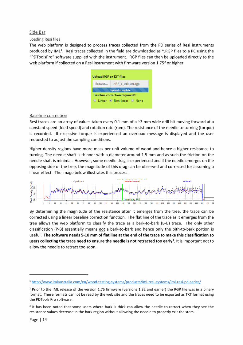
Side Bar Loading Resi files The web platform is designed to process traces collected from the PD series of Resi instruments produced by IML1. Resi traces collected in the field are downloaded as *.RGP files to a PC using the “PDToolsPro” software supplied with the instrument. RGP files can then be uploaded directly to the web platform if collected on a Resi instrument with firmware version 1.752 or higher.

Baseline correction Resi traces are an array of values taken every 0.1 mm of a ~3 mm wide drill bit moving forward at a constant speed (feed speed) and rotation rate (rpm). The resistance of the needle to turning (torque) is recorded. If excessive torque is experienced an overload message is displayed and the user requested to adjust the sampling conditions.

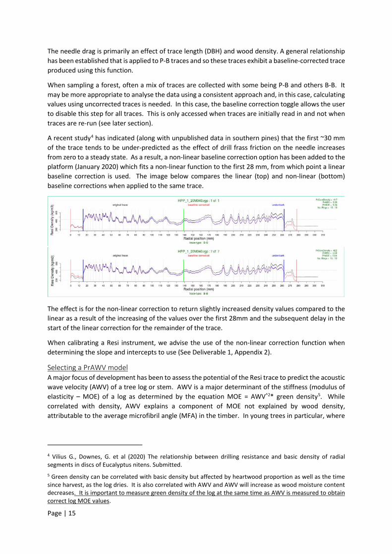
Higher density regions have more mass per unit volume of wood and hence a higher resistance to turning. The needle shaft is thinner with a diameter around 1.5 mm and as such the friction on the needle shaft is minimal. However, some needle drag is experienced and if the needle emerges on the opposing side of the tree, the magnitude of this drag can be observed and corrected for assuming a linear effect. The image below illustrates this process.

By determining the magnitude of the resistance after it emerges from the tree, the trace can be corrected using a linear baseline correction function. The flat line of the trace as it emerges from the tree allows the web platform to classify the trace as a bark-to-bark (B-B) trace. The only other classification (P-B) essentially means not a bark-to-bark and hence only the pith-to-bark portion is useful. The software needs 5-10 mm of flat line at the end of the trace to make this classification so users collecting the trace need to ensure the needle is not retracted too early3. It is important not to allow the needle to retract too soon.

1 http://www.imlaustralia.com/en/wood-testing-systems/products/iml-resi-systems/iml-resi-pd-series/ 2 Prior to the IML release of the version 1.75 firmware (versions 1.32 and earlier) the RGP file was in a binary format. These formats cannot be read by the web site and the traces need to be exported as TXT format using the PDTools Pro software. 3 It has been noted that some users where bark is thick can allow the needle to retract when they see the resistance values decrease in the bark region without allowing the needle to properly exit the stem.

http://www.imlaustralia.com/en/wood-testing-systems/products/iml-resi-systems/iml-resi-pd-series/

Page | 15

The needle drag is primarily an effect of trace length (DBH) and wood density. A general relationship has been established that is applied to P-B traces and so these traces exhibit a baseline-corrected trace produced using this function.

When sampling a forest, often a mix of traces are collected with some being P-B and others B-B. It may be more appropriate to analyse the data using a consistent approach and, in this case, calculating values using uncorrected traces is needed. In this case, the baseline correction toggle allows the user to disable this step for all traces. This is only accessed when traces are initially read in and not when traces are re-run (see later section).

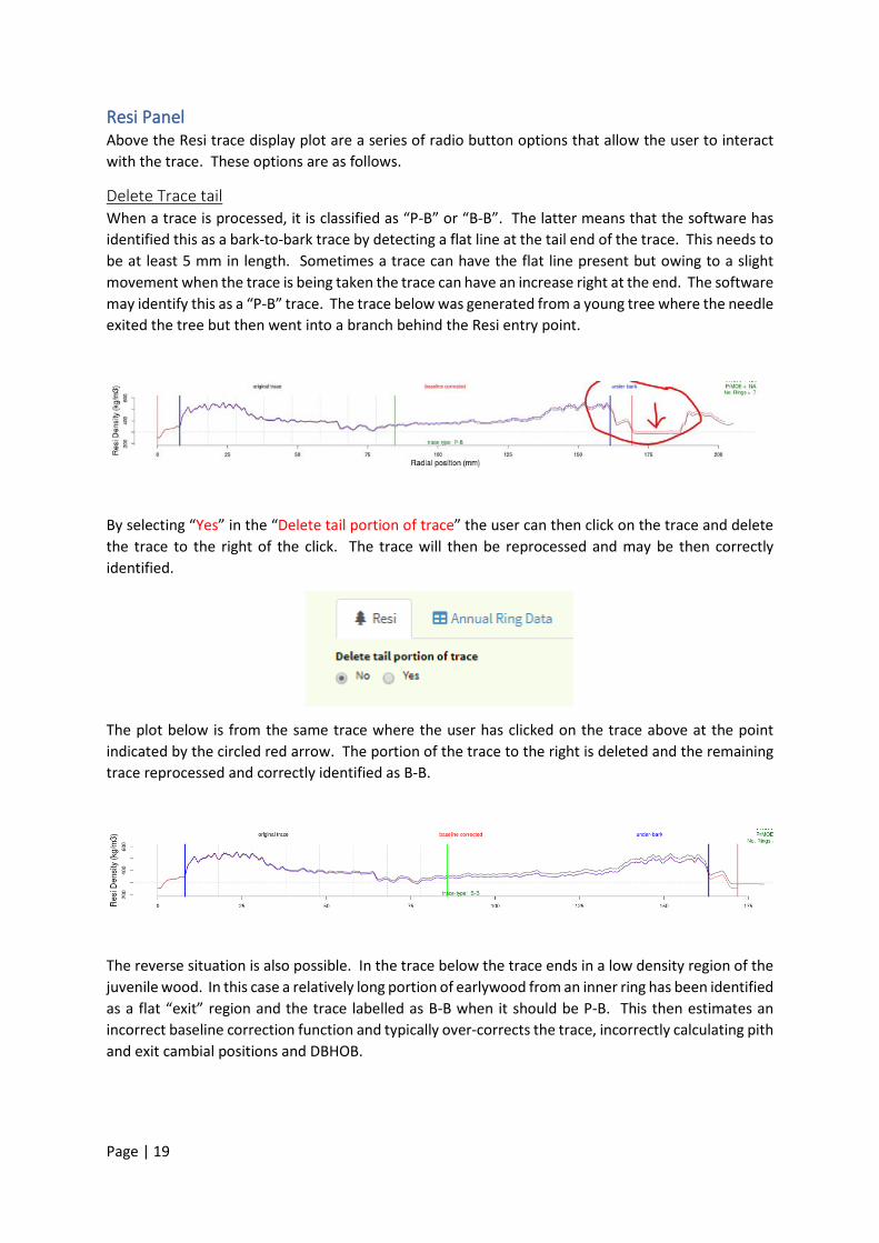
A recent study4 has indicated (along with unpublished data in southern pines) that the first ~30 mm of the trace tends to be under-predicted as the effect of drill frass friction on the needle increases from zero to a steady state. As a result, a non-linear baseline correction option has been added to the platform (January 2020) which fits a non-linear function to the first 28 mm, from which point a linear baseline correction is used. The image below compares the linear (top) and non-linear (bottom) baseline corrections when applied to the same trace.

The effect is for the non-linear correction to return slightly increased density values compared to the linear as a result of the increasing of the values over the first 28mm and the subsequent delay in the start of the linear correction for the remainder of the trace.

When calibrating a Resi instrument, we advise the use of the non-linear correction function when determining the slope and intercepts to use (See Deliverable 1, Appendix 2).

Selecting a PrAWV model A major focus of development has been to assess the potential of the Resi trace to predict the acoustic wave velocity (AWV) of a tree log or stem. AWV is a major determinant of the stiffness (modulus of elasticity – MOE) of a log as determined by the equation MOE = AWV^2* green density5. While correlated with density, AWV explains a component of MOE not explained by wood density, attributable to the average microfibril angle (MFA) in the timber. In young trees in particular, where

4 Vilius G., Downes, G. et al (2020) The relationship between drilling resistance and basic density of radial segments in discs of Eucalyptus nitens. Submitted. 5 Green density can be correlated with basic density but affected by heartwood proportion as well as the time since harvest, as the log dries. It is also correlated with AWV and AWV will increase as wood moisture content decreases. It is important to measure green density of the log at the same time as AWV is measured to obtain correct log MOE values.

Page | 16

MFA is high and density low, the AWV is a more significant contributor to MOE. AWV is also affected by knots, slope of grain, extractives and moisture content.

Various predictive equations (multiple or partial least squares regression) have been developed in an attempt to extract from the Resi trace variables that explain independent variance in AWV related to mean variance in MFA, in addition to those related to basic density.

• NZSWI: Multiple regression model similar to that developed by New Zealand Solid Wood Innovations and embedded in the software tool they developed. It is sensitive to the correct positioning of the pith and annual rings, making it less useful in automatic applications

• Young: Multiple regression model built using variables extracted from traces taken from 7yo radiata pine trees.

• Mid: Not yet developed • Mature: Multiple regression model using variables derived from the pith-to-bark

trace. It is intended as a fully-automatic algorithm completely independent of annual ring positions

• Outerwood: PLS regression that uses variables extracted from the outer 50 mm but includes the length of the trace (radius of stem), as well as the slope and intercept of the Resi used. It is also intended as a fully-automatic algorithm completely independent of annual ring positions.

• Density: It was noted in sawmill studies that basic density was a good predictor of plot or site level log and board MOE in harvest age trees. This algorithm uses a simple multiple regression to convert the core density values (i.e. pith-to-bark mean density) into AWV and MOE units. Thus it is sensitive to density changes related to changing pith and cambial positions as well as the slope and intercept used to convert the Resi trace into density units (see below)6.

Regression coefficients The image below shows the portion of the Web-platform interface where the user can enter in the coefficients needed to convert Resi resistance (torque) values to basic density. Each Resi instrument has slightly different characteristics such that these coefficients will vary between instruments. The degree to which they vary between tree species and / or other conditions is a subject of ongoing study7.

The relationship between Resi units and density is linear, as determined from the measurement of many cores taken as bark-to-bark or 50 mm outerwood cores. As such the calculation of basic density requires only a regression slope and intercept. It is necessary that these values be determined for each

6 When dealing with logs from harvest age trees (with the exception perhaps of the top log which contributes relatively few boards), log MOE is going to be influenced almost entirely by basic density variation. 7 Recent discussion with IML regarding changing coefficients between service events, suggests that where this occurs it is primarily a result of the effect of cleaning the telescope within the instrument. Hence minimising the degree to which cleaning is necessary is important by ensuring that debris is not allowed to build up in the nose cap during field use. Removing this debris every 4-5 trees is advised.

Page | 17

instrument to ensure optimal accuracy in the prediction of AWV and MOE. We also recommend ongoing checks to establish whether and how this relationship might vary over time. The regression and slope values are highly correlated, with higher slope values typically associated with lower intercepts.

Density Threshold In assessing trees within and between forests, users are often interested in the proportion of the stem above a given threshold. Historically the width of the juvenile core expressed as the first 10 rings from the pith, has been used as a surrogate. Resi allows a quantitative approach. The pith-to-bark trace on the entry side is area-weighted (to represent a stem cross-section), heavily smoothed and the length of the trace above the threshold value calculated as a (volume) proportion of the whole trace.

Trace processing All selected traces are uploaded as a batch before any processing begins. When a trace is being processed it is first assessed for its type (CAL8, B-B or P-B). DBHOB is then determined and the baseline correction function defined. The pith location is estimated. For B-B traces the pith location, by default, is placed at the mid-point of the under-bark region. For P-B traces estimating pith location in the current formulation can be quite inaccurate as the structure of the trace as it passes near the pith can be highly variable, making it difficult to define automatically.

The under-bark positions of the cambium at the entry and exit (in B-B traces) ends are automatically determined and positioning is generally quite robust. However, under some conditions they can be allocated to the wrong position. Misplacement can occur when the bark density contains high regions together with some low-density earlywood within 50 mm of the bark. Also, some trees may have voids or resin pockets close to the bark.

Saving traces as a Project Once the selected traces have been uploaded, processed and the results table displayed, they can be saved as a single “*.Resi” file. By selecting the “Save Project” button the file will be saved with an automatically generated name which includes the current data (eg “ResiData_18 Jun 2019.Resi”). Depending on the setting of your web browser, the browser may ask you to choose where you want to save the file, at which time you can change the name to something more meaningful.

8 “CAL” is a new type currently being assessed. It is a trace taken through a small ceramic disc of uniform material with known density and strength.

Page | 18

Saving the projects allows any editing done by the user as described in the following sections to be retained.9

Uploading and combining projects The *.Resi files can be reloaded using the “Upload *.Resi dataset” button.

Underneath this button is a checkbox labelled “Add to existing Project”. This allows the user to combine datasets. For example, if you have uploaded and processed a batch of traces and want to combine them with those from a previously saved project, check the box and upload the previous project. The project traces are appended to those currently loaded. The whole set can then be saved as a new project or by over-writing the existing one.

9 Note: Depending upon the settings of your web browser, a dialog box may or may not appear asking you where to save the Resi file to. The settings on the web browser may default to a “download” folder. You can change the settings to get the browser to ask you to specify the location, at which time you can change the file name to something more meaningful.

Page | 19

Resi Panel Above the Resi trace display plot are a series of radio button options that allow the user to interact with the trace. These options are as follows.

Delete Trace tail When a trace is processed, it is classified as “P-B” or “B-B”. The latter means that the software has identified this as a bark-to-bark trace by detecting a flat line at the tail end of the trace. This needs to be at least 5 mm in length. Sometimes a trace can have the flat line present but owing to a slight movement when the trace is being taken the trace can have an increase right at the end. The software may identify this as a “P-B” trace. The trace below was generated from a young tree where the needle exited the tree but then went into a branch behind the Resi entry point.

By selecting “Yes” in the “Delete tail portion of trace” the user can then click on the trace and delete the trace to the right of the click. The trace will then be reprocessed and may be then correctly identified.

The plot below is from the same trace where the user has clicked on the trace above at the point indicated by the circled red arrow. The portion of the trace to the right is deleted and the remaining trace reprocessed and correctly identified as B-B.

The reverse situation is also possible. In the trace below the trace ends in a low density region of the juvenile wood. In this case a relatively long portion of earlywood from an inner ring has been identified as a flat “exit” region and the trace labelled as B-B when it should be P-B. This then estimates an incorrect baseline correction function and typically over-corrects the trace, incorrectly calculating pith and exit cambial positions and DBHOB.

Page | 20

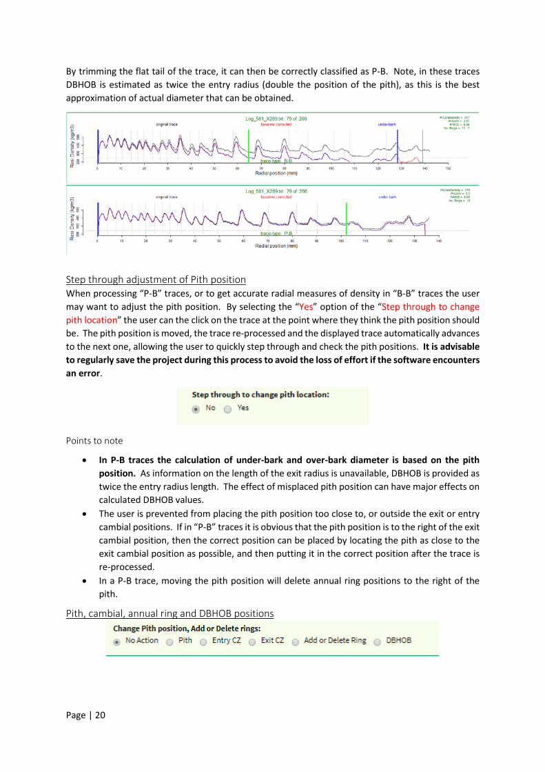
By trimming the flat tail of the trace, it can then be correctly classified as P-B. Note, in these traces DBHOB is estimated as twice the entry radius (double the position of the pith), as this is the best approximation of actual diameter that can be obtained.

Step through adjustment of Pith position When processing “P-B” traces, or to get accurate radial measures of density in “B-B” traces the user may want to adjust the pith position. By selecting the “Yes” option of the “Step through to change pith location” the user can the click on the trace at the point where they think the pith position should be. The pith position is moved, the trace re-processed and the displayed trace automatically advances to the next one, allowing the user to quickly step through and check the pith positions. It is advisable to regularly save the project during this process to avoid the loss of effort if the software encounters an error.

Points to note

• In P-B traces the calculation of under-bark and over-bark diameter is based on the pith position. As information on the length of the exit radius is unavailable, DBHOB is provided as twice the entry radius length. The effect of misplaced pith position can have major effects on calculated DBHOB values.

• The user is prevented from placing the pith position too close to, or outside the exit or entry cambial positions. If in “P-B” traces it is obvious that the pith position is to the right of the exit cambial position, then the correct position can be placed by locating the pith as close to the exit cambial position as possible, and then putting it in the correct position after the trace is re-processed.

• In a P-B trace, moving the pith position will delete annual ring positions to the right of the pith.

Pith, cambial, annual ring and DBHOB positions

Page | 21

At the top right-hand corner above the trace plot window there are a series of radio buttons that control what the user can do for the currently displayed trace. Selecting an option, and then clicking on the trace will adjust the summary data as follows

• Pith: allows the position of the pith to be changed as described previously without advancing to the next trace

• EntryCZ: allows the position of the left-hand cambial position on the entry-side of the trace to be changed

• ExitCZ: : allows the position of the left-hand cambial position on the exit-side of the trace to be changed

• Add or Delete Ring: Adds or deletes an annual ring location depending on the presence or absence of an existing location mark within a defined range of the mouse click. It is best to click slightly to the right of an existing ring to delete it.

• DBHOB: This option over-rides the trace type (P-B) and forces its classification as B-B. By placing the cursor on the black trace at the point where you want DBHOB to be, it will reprocess the trace, and use the y-axis value of the black line for the baseline correction. This is useful if the automatic processing allocates the DBHOB position into the bark resulting in a wrong baseline correction, or more commonly there is insufficient flat line exiting the tree for the software to detect it, but it is obvious to the eye that it did exit.

Other Actions Below the plot window are a range of buttons, the actions of which are described as follows:

• Download: clicking this button will download the summary table as a CSV file that can be opened directly in Excel. Depending on your web browser settings, the file will be saved directly to your download folder as “.csv” or a dialogue box will display asking you where to save the file and allowing you to edit the filename to something more meaningful.

• Retreat: changes the displayed plot to the previous trace • Advance: advances the displayed plot to the next trace • Clear Rings: Removes all annual ring marks from the trace • Delete Trace: Deletes the displayed trace from the project • Area weighted trace: Displays the trace as an area-weighted profile. This action only affects

the displayed trace and has no other effect. The x-axis changes from mm to mm^2 centred on the pith position. Thus, the area to the left of the pith is displayed as negative area. Each point along the x-axis then displays the cross-sectional area it represents in square millimetres. The effect is to compress the inner juvenile wood and expand the outer wood and bark.

• Download Trace: Downloads the current trace as a CSV file imaginatively called “trace.csv”. The first five lines define, in order, the filename, entry-side cambial position, pith position, exit-side cambial position and DBHOB. The first column contains the radial position in mm from the entry-side of the trace, and the second column contains the density values calculated from the (resistance values x regression slope + regression intercept). The idea is to allow users to download a particular trace for use in presentations etc.

Summary Table Once traces are uploaded and processed, the first trace is automatically displayed in the plot window. The summary table displays the calculated metrics for each trace loaded. The user can step through

Page | 22

each trace by selecting the “Advance” button beneath the plot. Similarly, the “Retreat” button will take the user back one trace from the current selection. The user can also navigate to different traces using the summary table below the plot window. Selecting a line will display the associated trace. By default, the table displays 100 rows , with subsequent rows displayed in pages of 100 rows accessible using the next button at the bottom of the table. This default setting can be changed using the “Show entries” drop list in the top left-hand corner of the table.

• The table has scroll bars to allow the user to view all the columns in the table. • Each column can be filtered (sorted) in ascending or descending order. This is useful, for

example, to identify traces which have been mis-classified as “P-B” if you expect all traces to be “B-B”.

Each row in the table summarises the information extracted from a single Resi traces as follows

• FileName: Filename of the trace either as a TXT file or RGP file • TreeID: The information entered into the Resi ID field in the field prior to taking the trace • ResiCode: Serial number of the Resi instrument • FeedSpeed10: Forward feed speed used for trace collection • RPM: Revolutions per minute used trace collection • SampleDate: Date when sample was taken based on Resi instrument date setting • Comment: Comment field from the Resi instrument • TraceType: A binary classification (P-B or B-B) determined from the presence or absence of a flat

line at the tail of the trace where the needle exits the tree. This classification controls how the trace is processed.

• TreeClass: This records the model used in the calculation of PrAWV (see below) • DBHOB: The estimated over-bark diameter at the trace sampling point. In P-B traces it is twice

the entry radius which is defined by the pith position. • UBDIA: The underbark diameter based on the estimated position of the entry and exit bark

thickness. In P-B traces exit bark thickness is assumed to equal entry bark thickness, which is subtracted from the estimated DBHOB (twice the entry radius)

• BarkThickness: The distance from the entry point of the trace to the cambial position at which wood (secondary xylem) starts. Only the entry bark thickness is returned as, given the fissured nature of pine bark, the exit bark position cannot be controlled and may give a biased measure. By taking the trace on a high point on the entry side, the user can control the estimated bark thickness.

• DiscArea: The estimated area of the disc cross section defined by the entry radius. Only the underbark portion of the trace is used in the calculation. In a B-B trace both radii are used, and the mean disc area returned. In P-B traces only the entry-side trace is used

• PrAWV: Predicted Acoustic Wave velocity. This is calculated by a multiple regression or partial least squares model prediction based on a range of variables extracted from the trace as described above. It is a process that is currently a major focus of development and testing and should be considered in that light. An accurate or precise predicted value for an individual trace is not the main objective (although desirable), but the mean

10 Note that in using the Resi values to calculate density, the Resi values are converted to a common range as if they were collected at a feed speed of 200 cm per minute and 2500 rpm using a set of coefficients. Thus if, for example, a trace was sampled at 150 cm per minute and 3500 rpm, the values are converted to 200 cm per min and 2500 rpm equivalents, and density calculated from these values.

Page | 23

predicted value from a defined population of traces is intended to be as accurate and precise as possible

• PrMOE: Predicted Modulus of Elasticity. An estimate of log MOE (or ideally the mean MOE of all sawn timber produced from the log) represented by the trace. It is calculated from the PrAWV2 x CoreDensity x 2. As with PrAWV it is a value currently under development and testing.

• OWDensity: Estimated basic density of the under-bark, outer 50 mm of the entry-side of the trace. It is calculated from the Resi values x rSlope + rIntcpt. Hence the latter two variables are recorded in the table assist in tracking the nature of the estimate.

• DensityProportion: Proportion of the smoothed area-weighted trace greater than the density threshold value.

• CoreDensity: The mean basic density of the trace, equivalent to an increment core density. In B-B traces it is based on the full under-bark, bark-to-bark portion of the trace. In P-B traces it is based on the entry-side pith-to-bark portion of the trace.

• DiscDensity: An area-weighted estimate of the core density trace. In B-B cores each radius (entry and exit) is area-weighted and the mean density calculated, and the mean of these two estimates returned. In P-B traces only the entry-side value is returned

• Decay: In some trees voids have been identified, attributable to decay. Based on a density threshold, the percentage of the trace that is below this threshold is returned.

• EntryRadius: The distance from the outer-bark entry point of the trace to the identified position of the pith. The software does calculate this position automatically but the user can modify the position using the controls described above. In B-B traces pith location is automatically defined as the mid-point of the under-bark portion of the trace. In P-B traces it is estimated based on certain trace smoothing techniques but is typically subject to considerable error given the variability of traces

• EntryDensity: The mean basic density of the under-bark, entry-side radius. • ExitRadius: The distance from the pith position to the identified DBHOB position • ExitDensity: The mean basic density of the under-bark, exit-side radius. • BLCorrDen: A variable used in the baseline correction of the trace. It is not currently used and

recorded here as it may be used in later software developments • rSlope: The regression slope used in converting Resi values to basic density, after the Resi

values have been adjusted to equivalent values for 200 cm per min feedspeed and 2500 rpm.11

• rIntcpt: The regression intercept used in converting Resi values to basic density.

11 . Each instrument has slightly different relationship coefficients which needs to be identified. The degree to which these coefficients vary over time, between servicing events, between species (e.g. softwood and hardwoods) and between wood types (dry vs green) is a subject that needs ongoing monitoring and estimation. Likewise, the degree to which identified difference in coefficients are real, vs random variance for a given calibration data set needs attention. IML are working on a nose cap that may assist in determining instrument-specific coefficients, but at this stage the method is focussed on material strength rather than density.

Page | 24

Annual Ring Panel Based on the annual ring positions marked, the plot window shows two line plots. The blue plot shows the ring width pattern, starting from the pith according to the y-axis on the right-hand side of the plot. The red line shows the selected property (mean basic density by default) selected from the drop list titled “Select Property”.

Different traces can be selected from the right-hand drop list. It is important to note that the summary table contains a row for each annual ring for every trace loaded. Selecting a row performs no action at present12. Displaying different traces can be done using the “Retreat” and “Advance” buttons or by selecting a particular trace from the droplist.

As with the Resi panel, the table can be sorted by each column (ascending or descending) and downloaded using the “Ring Data Download” button. This is allocated a default filename of “RingData.csv” which the user can modify as needed.

12 It will be modified to display the particular trace to which the row belongs.

Page | 25

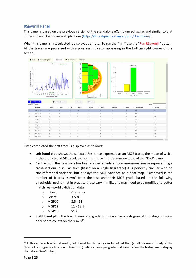
RSawmill Panel This panel is based on the previous version of the standalone eCambium software, and similar to that in the current rCambium web platform (https://forestquality.shinyapps.io/rCambium/).

When this panel is first selected it displays as empty. To run the “mill” use the “Run RSawmill” button. All the traces are processed with a progress indicator appearing in the bottom right corner of the screen.

Once completed the first trace is displayed as follows:

• Left hand plot: shows the selected Resi trace expressed as an MOE trace., the mean of which is the predicted MOE calculated for that trace in the summary table of the “Resi” panel.

• Centre plot: The Resi trace has been converted into a two-dimensional image representing a cross-sectional disc. As such (based on a single Resi trace) it is perfectly circular with no circumferential variance, but displays the MOE variance as a heat map. Overlayed is the number of boards “sawn” from the disc and their MOE grade based on the following thresholds, noting that in practice these vary in mills, and may need to be modified to better match real-world validation data.

o Reject: < 3.5 GPa o Select: 3.5-8.5 o MGP10: 8.5 - 11 o MGP12: 11 - 13.5 o MGP15: >13.5

• Right hand plot: The board count and grade is displayed as a histogram at this stage showing only board counts on the x-axis13.

13 If this approach is found useful, additional functionality can be added that (a) allows users to adjust the thresholds for grade allocation of boards (b) define a price per grade that would allow the histogram to display the data as $/m3 of log


Page | 26

The summary table records the processing output for each trace and selecting on a row will display the corresponding trace. The table records the numbers of boards in each grade along with the mean MOE of all boards as well as the area-weighted mean MOE of the trace (i.e. cross-sectional disc).

The table can be downloaded as a simple CSV file with the generic filename “BoardSummaryData.csv”. The “Retreat” and “Advance” buttons allow the user to navigate through the traces one at a time.

Page | 27

Appendix 1: Resi user field work guidelines

This document suggests a basic protocol to follow to ensure the correct use and maintenance of the Resi instrument. All users need to read the operation manual supplied with each instrument to understand the:

• use of the instrument control panel

• basic mechanical operation of the instrument including how to change needles and chuck and how to clean the brass telescope within the unit.

• Manufacturer’s advice in keeping the instrument clean and operational

• process of transferring the collected traces from the Resi to a PC. It is advised that a small laptop be supplied with each Resi on which is installed the PDTools Pro software supplied with each instrument. This will allow ease of download of the traces from the Resi instrument in the field (if necessary) for compiling and processing.

A small logbook should be included in the case of each instrument and appropriately labelled. Use this to record each day’s operation in terms of the:

o Number of traces collected

o If needles were replaced and at what stage.

If the number of traces collected on a single needle exceeds 1000 trees, replace the needle

o Any issues with the instrument

o Whether it rained during the day and the Resi got wet

o Sites and compartments that were sampled. Preparing for field operation

• Identify which compartments are being sampled and define the sample code to be entered into the ID field of the Resi instrument.14

• Make sure the Resi is operational o Install battery and make sure the instrument turns on o Are there any icons along the bottom of the screen showing, indicating issues with

the instrument? (refer to the user manual) o Make sure any traces in memory have been transferred to a PC and delete from the

Resi instrument ONLY AFTER MAKING SURE ALL NECESSARY DATA HAS BEEN SAFELY BACKED UP.

o Check needle status, and replace if necessary o Extend the needle and check that it is clean o Is the nose cap clean? o Is the correct time and date displayed?

• Make sure batteries are charged

14 The ID field can be used to rename RGP files during the transfer from the Resi to the PC. It is retained with the web-based summary data derived from each trace. If it contains specific information to identify the tree in a standardised way, it facilitates the analysis of the data in subsequent analyses.

Page | 28

• Is there a cloth in the case that has been damped with WD40 or Inox (preferred) and kept in a sealed Ziploc bag? This is needed to clean the needle and nose cap at the end of each day (or plot as necessary) at the field site.

• Is there a plastic bag in the case to protect the Resi if it rains? In rainy conditions the user is responsible to decide whether it is safe to use the Resi. The instrument is water resistant but NOT water proof. It can be used in some light drizzle situations using a plastic bag to cover the instrument screen and controls. But do not risk damaging the instrument. In particular water can enter round the edges of the display screen. Drips from the brim of the user’s hard hat are a particular source of water.

• Are there enough NEW needles in the case if required? If needle stocks are low arrange ordering more.

• Make sure the RESI is in the case when all has been checked, and the case is clean and tidy. • ALWAYS TRANSPORT THE RESI TO THE SITE IN THE CASE. The case is designed to protect the

instrument from damage during transport. If the conditions are wet, the case needs to be protected from the rain.

Arriving at the sampling site

o Take the Resi from the case and insert battery. Make sure it turns on OK and is ready for sampling.

o Check the battery has sufficient charge o Enter the predetermined Site code in the ID field o Additional information can be entered in the comment field (e.g. the Operators name, forest

name) o If travel to the sampling site is a considerable walking distance, a canvas carry bag can be

purchased from IML to make carrying easier. If used disconnect the battery and place Resi in canvas bag.

o One charged 4.0 Amp Hour battery should allow a sampling of over 200 traces.

Collecting traces

o Depending on the sampling approach enter additional information in the ID field to record details such as plot number using a hyphen (“-“) to separate from the site code. Use the hyphen to separate any tree or plot specific codes if that level of detail is needed.

o Look at the sampling point of the tree and avoid places where there are branches, knots or other defects. Check the back of the tree where the needle will emerge to make sure it is clear of knots and loose bark.

o Position the Resi against the tree making sure your head is aligned along the length of the Resi. This helps you estimate the centre of the tree better.

o Try to aim the Resi for the centre of the tree, keeping the Resi horizontal (or perpendicular to the stem if it is leaning. Generally it is preferable to sample perpendicular to the direction of lean to avoid or minimise the reaction wood sampled.

o Take the trace and make sure there is at least 1 cm of trace after the needle exits the tree if the tree is less than 38-39 cm diameter. The exit is evident as a flat line at the end of the trace. The bark will tend to be lower density than the wood so make sure the trace has the exit flat line and don’t stop in the bark.

Page | 29

o Use the red button to start the trace. It is advised to NOT use the red button to stop the trace but to remove the pressure from the Resi so that the switch under the nose cap is released, which automatically starts the needle retraction. Stopping the trace with the red button can sometimes result in a third press which stops the trace from retracting leaving the needle stuck in the tree. Then when pulling the needle out of the tree this can sometimes result in the needle pulling out of the chuck (mainly an issue in hardwoods).

o In this case use the pliers to pull the needle straight back and avoid putting any bends in the needle. If the needle is straight it can be re-inserted in the chuck and used. If it has any kinks or bends, it needs to be replaced.

o Check each trace on the screen immediately after collection. Delete any trace that is not satisfactory straight away. The best place and time to determine whether a trace should be kept is here immediately after sampling. Keeping unnecessary or bad traces will potentially cause confusion or waste time back in the office.

o For routine inventory only collect 1 full diameter (or length if DBH is over 400mm) trace per tree. Other applications may require more traces, but it is better to sample more trees than collect multiple traces per tree as the main application of the Resi is to obtain site-average values.

o If it is raining, or water is dripping from the canopy, water can drop from the brim of the hard hat onto the screen. Be careful to avoid getting water on the screen. Use a plastic bag to cover the screen end of the Resi if required.

o After each 5-10 trees sampled, check the nose cap of the Resi for debris collecting in the needle end. Clean as necessary. This is very important. A clogged nose cap can result in the needle dragging debris into the Resi interior as it retracts, affecting the operation of the telescopic system.

Finishing at the sampling site (end of day) Prior to loading Resi back into its case for transport back to the office, clean the needle and nose cap.

o Record in the log book the number of traces taken for the day and calculate and record the number of traces taken with the current needle. If it has reached 1000 traces remove the needle. Make sure that old needles are not mixed with new needles

o Record the compartment sampled and any additional information that may be useful. o Remove the nose cap o Extend the needle to its full length using the appropriate controls o Take the cloth soaked in WD40 or Inox (IML service technician recommends using Inox) from

the plastic Ziploc bag and wipe the needle to remove any resin and sap. This will apply a light coating of oil to the needle. If not cleaned extractives can corrode the needle surface.

o Retract the needle and clean the brass end of the Resi. A small bristle brush may be useful here.

o Use the same cloth to clean the nose cap and place back onto the Resi o PLACE THE RESI IN THE CASE FOR TRANSPORT IN THE CAR o It is important to keep the Resi clean and organised for ongoing operation.

Page | 30

Laboratory check and storage

o Charge the batteries as required o Store the Resi safely overnight. If the environment is excessively cold or humid, store in an air

conditioned room rather than leave in the back of the vehicle. If necessary leave the case open so the air-conditioned environment can dry out any accumulated moisture in the case and/or instrument, especially if there is evidence of moisture getting in around the edge of the display.

o Keep everything clean and organised.

Maintenance Monthly

o Each month (or more frequently depending on use) clean the telescope of each instrument as per the manufacturer’s instructions. Wipe the brass telescope over with an oiled (Inox) rag to remove any foreign particulates

o Check that the needle supply is sufficient to meet sampling needs for the next few months o Check there are no error icons displaying in the bottom right line of the screen (refer to IML’s

user manual).

Annual

o Every year send each Resi instrument back to IML (Toowoomba, Qld) for service. This makes sure the electronic calibrations in each instrument are within limits and the instrument is functioning correctly. Servicing may need to be more frequent if the instrument receives heavy use.

Page | 31

Appendix 2: Protocol for assessing core basic density for calibration of Resi values Because of the relatively recent application of the Resi technology to the routine estimation of basic density, and the importance of establishing the degree of confidence in the numbers Resi instruments generate, we encourage users to collect ongoing validation / calibration values to maintain a check over density estimates. This addresses the need to answer the following questions:

Does the relationship between Resi generated resistance values for a given basic wood density differ between:

• Instruments • Species (e.g. hardwood vs softwood) • Over time with the same instrument (e.g. before and after annual servicing)

We recommend the maximum moisture content method described by Smith 195415 for calculating basic density. As a starting point and for simplicity, we suggest using the increment cores taken from the outer 50 mm of the stem adjacent to the position (within 1-2 cm) on the entry side of a Resi sampling point. Using the outer 50 mm has become a common commercial practice for routine density sampling, and to facilitate this the Resi web platform generates a value of density called “OWDensity”. Actual 50 mm core density values can be compared with these. Below is a basic protocol.

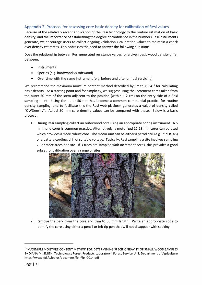
1. During Resi sampling collect an outerwood core using an appropriate coring instrument. A 5 mm hand corer is common practice. Alternatively, a motorized 12-13 mm corer can be used which provides a more robust core. The motor unit can be either a petrol drill (e.g. Stihl BT45) or a battery cordless drill of suitable voltage. Typically, Resi sampling a site involves sampling 20 or more trees per site. If 3 trees are sampled with increment cores, this provides a good subset for calibration over a range of sites.

2. Remove the bark from the core and trim to 50 mm length. Write an appropriate code to

identify the core using either a pencil or felt tip pen that will not disappear with soaking.

15 MAXIMUM MOISTURE CONTENT METHOD FOR DETERMINING SPECIFIC GRAVITY OF SMALL WOOD SAMPLES By DIANA M. SMITH, Technologist Forest Products Laboratory,l Forest Service U. S. Department of Agriculture https://www.fpl.fs.fed.us/documnts/fplr/fplr2014.pdf

Page | 32

3. Place the core in a plastic bag or container. 5mm cores can be fragile and subject to breaking so using a rigid container can help protect the cores.

4. Soak the cores for several days to ensure they are fully saturated. 12 mm cores can take longer than 5 mm cores, especially if there is heartwood present. Use cycles in and out of vacuum to facilitate the saturation process. The vacuum does not need to be extreme.

5. Once the cores are fully saturated (and not floating) measure the green weight using a 3-figure balance.

6. Oven dry the cores for 24 hours at 103oC and place in a sealed chamber with desiccant to avoid them absorbing moisture from the ambient air.

7. Measure the oven-dry weights and use the following formula to calculate basic density. • Basic density = 1000*(1/(((GreenWt-OvenDryWt)/$ OvenDryWt)+1/1.53))

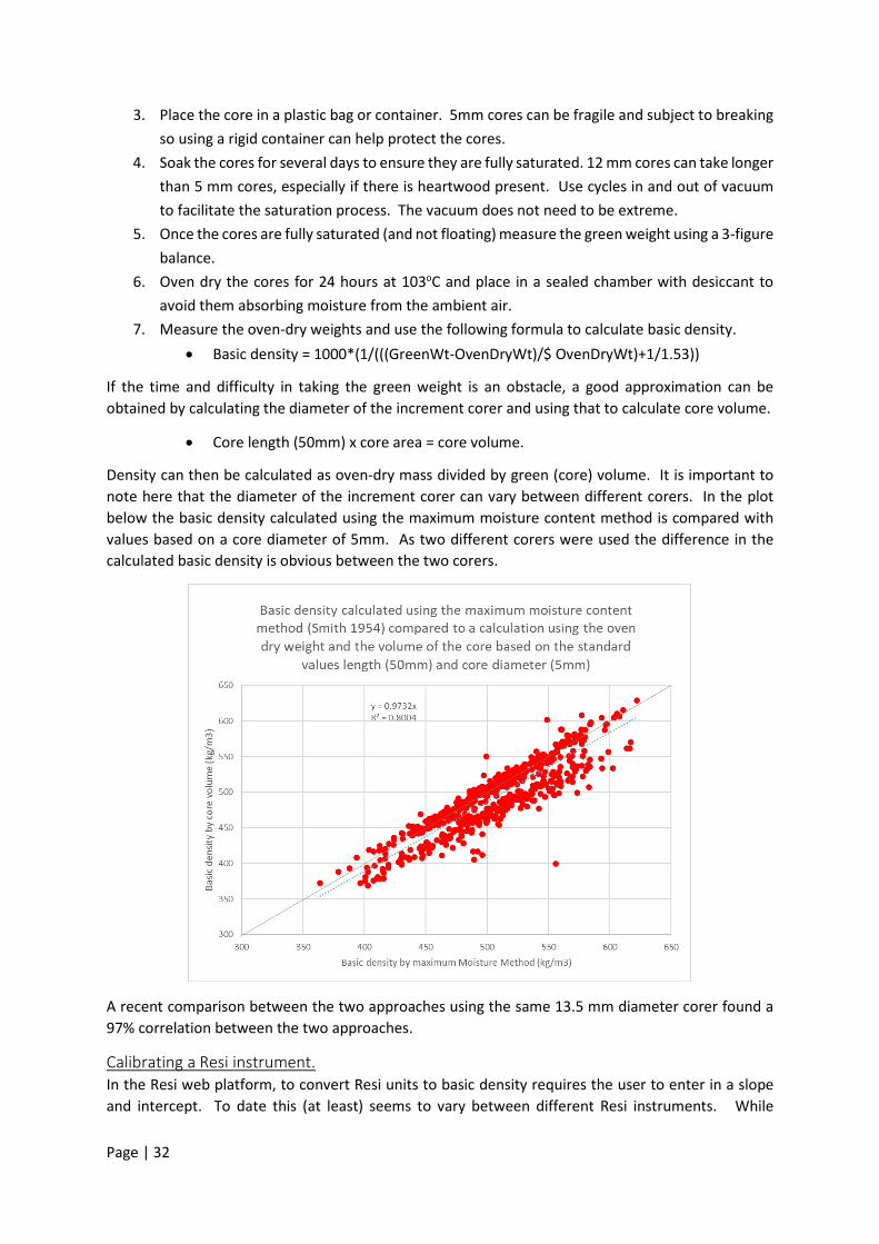
If the time and difficulty in taking the green weight is an obstacle, a good approximation can be obtained by calculating the diameter of the increment corer and using that to calculate core volume.

• Core length (50mm) x core area = core volume.

Density can then be calculated as oven-dry mass divided by green (core) volume. It is important to note here that the diameter of the increment corer can vary between different corers. In the plot below the basic density calculated using the maximum moisture content method is compared with values based on a core diameter of 5mm. As two different corers were used the difference in the calculated basic density is obvious between the two corers.

A recent comparison between the two approaches using the same 13.5 mm diameter corer found a 97% correlation between the two approaches.

Calibrating a Resi instrument. In the Resi web platform, to convert Resi units to basic density requires the user to enter in a slope and intercept. To date this (at least) seems to vary between different Resi instruments. While

Page | 33

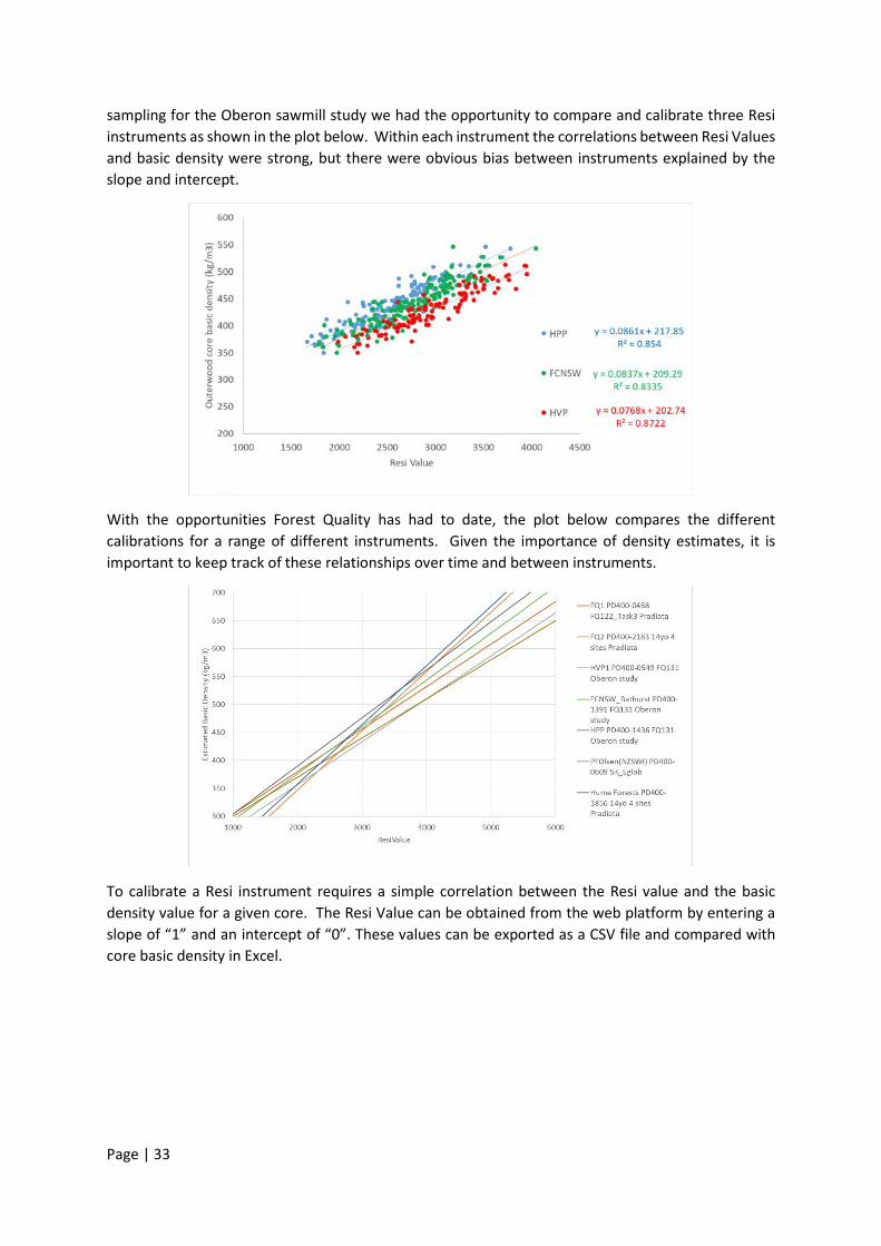
sampling for the Oberon sawmill study we had the opportunity to compare and calibrate three Resi instruments as shown in the plot below. Within each instrument the correlations between Resi Values and basic density were strong, but there were obvious bias between instruments explained by the slope and intercept.

With the opportunities Forest Quality has had to date, the plot below compares the different calibrations for a range of different instruments. Given the importance of density estimates, it is important to keep track of these relationships over time and between instruments.

To calibrate a Resi instrument requires a simple correlation between the Resi value and the basic density value for a given core. The Resi Value can be obtained from the web platform by entering a slope of “1” and an intercept of “0”. These values can be exported as a CSV file and compared with core basic density in Excel.

Page | 34

Appendix 3: Infield measurement of disc green density To estimate log MOE requires the combination of AWV values (eg HM200) and green density according to the following relationship

• (HM200²) * green density = logMOE

The difficulty here is the measurement of log MOE and in particular log weight. An alternative approach is the use of a cross section disc from the small-end diameter (SED).

AWV is a measure of the 'average' speed at which mechanical (acoustic) energy travels along a log. This is affected by green density, which is a function of more than just basic density (moisture content, heartwood proportion, extractives etc). A drier log will have a faster AWV. Thus, when measuring the green density it is important to measure it as close to the conditions when AWV was also measured. For discs this generally requires infield measurement.

Green density in discs can be measured quickly and simply in the field.

1. Remove the bark. Depending on the time of year and field conditions this may require the use of a small hatchet.

2. Record the green weight using a balance. A battery-operated unit accurate to 1 g is sufficient and capable of measuring weight up to 40 kg.

3. Measure disc volume by water displacement. Place a container of water on the balance with sufficient diameter and depth to allow the disc to be fully immersed. If the disc is too large a half or quarter can be used, making sure the green weight is measured only on this same portion. Drive a sharp tool (eg screwdriver ) into the centre of the sample and use a retort stand to clamp the screwdriver handle to allow the balance measure to become stable. This may be difficult if conditions are windy.

4. Divide the green weight by the displacement volume (weight) to obtain green density.

Page | 35

Appendix 4: Protocol for assessing Resi predictions The web-based protocol predicts basic density, acoustic wave velocity (AWV) and modulus of elasticity (MOE) from each Resi trace. These predictions are based on models (relationships) that have been developed over a number of studies. However, they will need to be checked against actual values (especially basic density) to assess their accuracy and precision. Basic density has been addressed in previous protocols. Following is suggested protocol for assessing AWV and MOE predictions.

Objectives:

1. To collect standing-tree Resi and HM200 butt log values to assess the prediction performance of log AWV and MOE from Resi traces

2. To define the instrument-specific relationship between Resi values and basic wood density for the Hume Forests Resi instrument

Background: Resi is being used as a standing tree assessment tool for wood quality. Resi provides a robust assessment of wood basic density at the point of sampling. Basic density typically explains around 50% of the variance in MOE (stiffness) of wood, which is a key commercial wood property defining its value as a sawn product. Another key contributor to wood stiffness is microfibril angle (MFA) in the woody cell wall, which is partially correlated with basic density. Recent work has focussed on the ability to enhance to prediction of stiffness from Resi traces by extracting variables from the trace that are empirically related to AWV variance to provide a stronger prediction of log MOE than that provided by basic density alone.

Site selection Resi predictions are intended to provide site level estimates of wood quality rather than focus on individual tree metrics. Sites would preferably be selected to cover a range of growth conditions e.g. dry and wet sites or low and high elevation sites. To extract the most value from the study site, use the data as a check on the rCambium model also.

• Record Latitude and Longitude of the site • Collect regime information

i. Plant date and stocking ii. Thinning dates and stocking

iii. Fertilisation dates and amounts

Site level workplan

2. Spray a number (1-20) on 20 trees. Avoid multiple leaders of trees with excessive lean or sinuosity.

• Measure and record the DBHOB of each tree • If possible, record tree heights and height to live crown.

3. Collect a single Resi trace from each of 20 trees near breast height. Use a 2 letter site code and a 2 digit number in the ID field to identify the tree

4. Collect a 50 mm long, 12 mm diameter outerwood core from each tree near the Resi sampling point (preferably within 2-3 cm).

5. Fell trees and cut a 4-6 m butt log16

16 Logs from harvest age trees are typically assessed at 6 m lengths as representative of the logs sampled commercially. In younger trees shorter lengths may be more appropriate to minimise the confounding effects of taper and knots.

Page | 36

6. Collect an HM200 value from each log making sure the entered log length is correct to get the correct AWV value.

7. Record LED & LEDHW; SED & SEDHW (useful but not essential data) 8. Remove a ~ 25 mm thick disc from the SED 9. Measure the green weight of the disc (bark removed) (See Appendix 3)

• The back of a ute can serve as a work bench for measuring disc weights. Ideally this would be parked on level ground close to the sampling site. If too large, discs can be cut into halves or quarters using a hatchet.

10. Measure the volume of the disc by water displacement and discard it 11. Ensure the outerwood cores are labelled and stored correctly

Equipment needed

• Appropriate personal protective equipment • Wet weather gear • Resi instruments • Tree marking paint • Diameter tape • Vertex (If tree height is needed) • Chainsaw and tree feller • HM200 (or appropriate acoustic measurement system) • Increment corer (and drill unit for motorised coring) • Battery-operated scales (1 gm resolution) • Retort stand and clamp • 40 litres of water • Container for core storage • Tag pen • Hatchet • GPS • Appropriate data recording (hard copy or iPad equivalent)

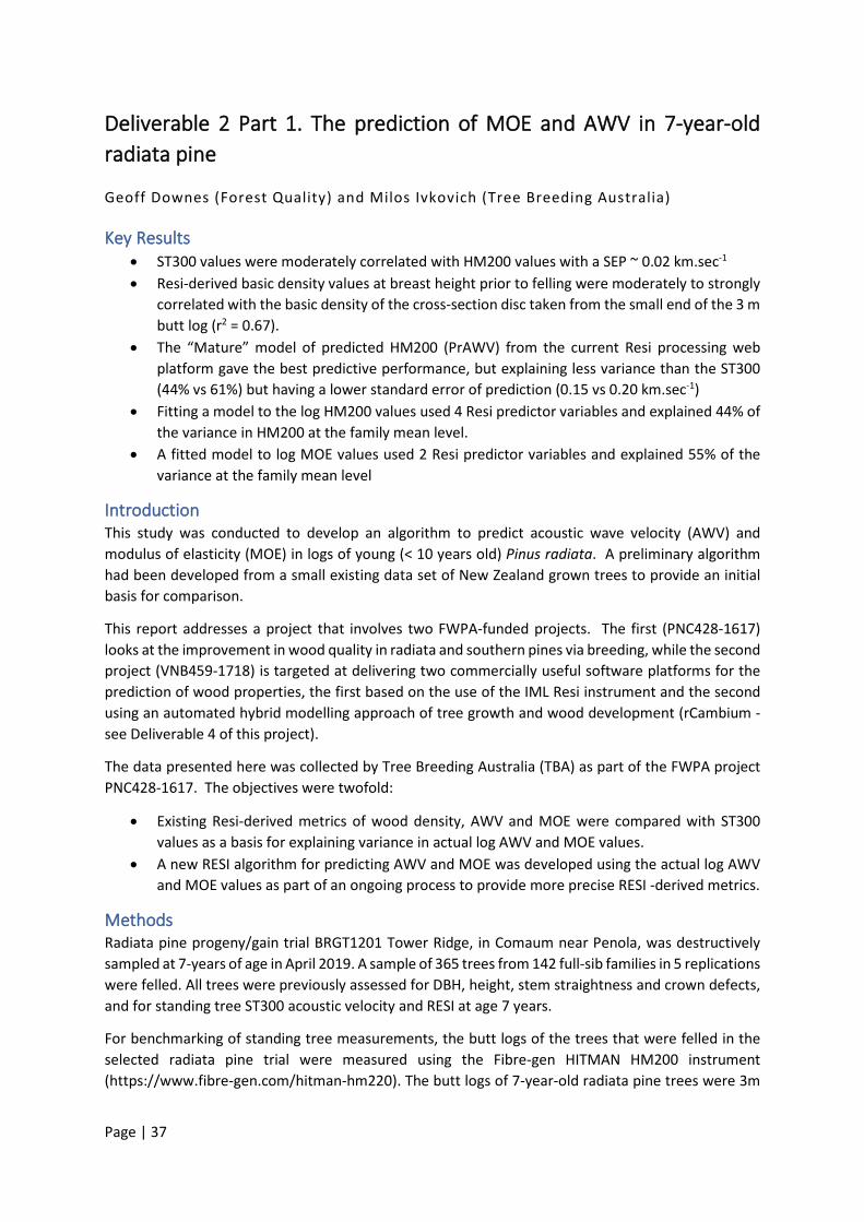
Page | 37

Deliverable 2 Part 1. The prediction of MOE and AWV in 7-year-old radiata pine

Geoff Downes (Forest Quality) and Milos Ivkovich (Tree Breeding Australia)

Key Results • ST300 values were moderately correlated with HM200 values with a SEP ~ 0.02 km.sec-1 • Resi-derived basic density values at breast height prior to felling were moderately to strongly

correlated with the basic density of the cross-section disc taken from the small end of the 3 m butt log (r2 = 0.67).

• The “Mature” model of predicted HM200 (PrAWV) from the current Resi processing web platform gave the best predictive performance, but explaining less variance than the ST300 (44% vs 61%) but having a lower standard error of prediction (0.15 vs 0.20 km.sec-1)

• Fitting a model to the log HM200 values used 4 Resi predictor variables and explained 44% of the variance in HM200 at the family mean level.

• A fitted model to log MOE values used 2 Resi predictor variables and explained 55% of the variance at the family mean level

Introduction This study was conducted to develop an algorithm to predict acoustic wave velocity (AWV) and modulus of elasticity (MOE) in logs of young (< 10 years old) Pinus radiata. A preliminary algorithm had been developed from a small existing data set of New Zealand grown trees to provide an initial basis for comparison.

This report addresses a project that involves two FWPA-funded projects. The first (PNC428-1617) looks at the improvement in wood quality in radiata and southern pines via breeding, while the second project (VNB459-1718) is targeted at delivering two commercially useful software platforms for the prediction of wood properties, the first based on the use of the IML Resi instrument and the second using an automated hybrid modelling approach of tree growth and wood development (rCambium -see Deliverable 4 of this project).

The data presented here was collected by Tree Breeding Australia (TBA) as part of the FWPA project PNC428-1617. The objectives were twofold:

• Existing Resi-derived metrics of wood density, AWV and MOE were compared with ST300 values as a basis for explaining variance in actual log AWV and MOE values.

• A new RESI algorithm for predicting AWV and MOE was developed using the actual log AWV and MOE values as part of an ongoing process to provide more precise RESI -derived metrics.

Methods Radiata pine progeny/gain trial BRGT1201 Tower Ridge, in Comaum near Penola, was destructively sampled at 7-years of age in April 2019. A sample of 365 trees from 142 full-sib families in 5 replications were felled. All trees were previously assessed for DBH, height, stem straightness and crown defects, and for standing tree ST300 acoustic velocity and RESI at age 7 years.

For benchmarking of standing tree measurements, the butt logs of the trees that were felled in the selected radiata pine trial were measured using the Fibre-gen HITMAN HM200 instrument (https://www.fibre-gen.com/hitman-hm220). The butt logs of 7-year-old radiata pine trees were 3m

Page | 38

long17, all branches were removed, and ends cut clean and perpendicular to the log. Log length, large- and small-end diameter (LED and SED) were recorded. Any severe compression wood, sweep, and/or mechanical damage, rot and very large knots, were noted. Three HM200 readings were obtained for each log to make sure that the readings were accurate.

Diameters at both ends of each log were obtained for volume and taper (which is correlated to stiffness). Log sweep was measured by running a builder’s string from one end of the log to the other end and recording the maximum deviation from the straight line. No heartwood was encountered. Discs of approximately 40 mm thickness were cut from the small end. The discs were de-barked, labelled using a permanent marker and stored in sealed zip-lock bag in an esky for gravimetric density and moisture content determination.

The day after felling, discs were weighed in their zip-lock bags, and the standard zip-lock bag mass subtracted (after pre-checking zip-lock bag mass measures were consistent), to obtain green disc mass. Discs were removed from zip-lock bags and green disc volume was measured using the Archimedean method, by submerging the disc in water on a balance. A small amount of detergent mixed into the water reduced the surface tension enough to avoid bubbles on the sample surface inflating its volume. Discs were oven-dried for at least 72 h at 105°C until they reached a constant oven-dry weight. Discs were removed from the oven and cooled for 3 minutes in a sealed desiccator, and oven dry mass recorded. Disc green density was calculated as green disc mass divided by green disc volume. Disc basic density was calculated as oven dry disc mass divided by green disc volume.

Data Metrics The following metrics were available for analysis:

• ST300: Time-of-flight AWV on standing trees • HM200: Resonance AWV on felled logs • LogMOE: HM200^2 * green density • SE disk green and basic Density • Resi predicted values18

o OWD: basic density of the outer 50 mm on the entry-side of the trace o Core density: Mean bark-to-bark basic density o Disc Density: Mean area-weighted density of each of the entry and exit pith-to-bark

traces. o PrAWV: predicted values made from a range of available algorithms listed below o PrMOE: predicted values made from a range of available algorithms listed below

• Resi prediction models o NZSWI: This model is similar to the one used in the previous software tool developed

with support from NZ Solid Wood Innovations o Young: A preliminary multiple regression model produced from a limited data set of

young 8 – 10 year old, New Zealand-grown trees o Mature: Multiple regression model produced for Milestone 5 of the current project

17 In general, log length must be at least 10 times the small-end diameter. 18 All values were derived using the web portal at from the web portal at https://forestquality.shinyapps.io/FWPAResiProcessor/


Page | 39

o Outerwood: PLS model produced for Milestone 5 of the current project focussing on variables from the outer 50mm of the trace

o Density: A recent addition (Aug 2019) of a simple linear regression against pith-to-bark density. Effectively a measure of the predictive ability of density alone.

Results Relationship between ST300 in standing trees and basic density in explaining variance in HM200 and log MOE values Prior to exploring the explanatory power of the Resi data it is necessary to establish the relationships among metrics which have become standard methods of assessment in recent years. As found in other studies, ST300 values were effective in predicting variance in HM200 values (r2=61%; D2P1 Figure 1a&b) and log MOE (r2=63%) at the individual log level in younger trees. In contrast the basic density of a cross-section disc taken from the small end of the log explained only 24% and 40% respectively (D2P1 Figure 1c&d). Of interest is that at the family mean level, disc basic density explained only 5-6% less variance than ST300 (55% vs 61%).

In terms of assessing prediction performance the standard error of prediction (SEP)19 is of interest when considered together with the variance explained (r2) as this indicates the precision of the relationship. In D2P1 Figure 1(b-c), SEP values provided are based on the application of the regression equation shown on the figure, and therefore RMSEP is close to the SEP values. ST300 values have a SEP of 0.2 km.sec-1 in the relationship with HM200 values. Likewise, a simple regression model to predict log MOE from the ST300 values (D2P1 Figure 1c) would have a SEP of 0.58 GPa.

Individual data points were combined into means defined by family ID which contained between 1 and 6 individuals. Bulking of values reduces the standard error of prediction, with some increase in the variance explained. Ideally there would be at least 10 individuals within each family mean to more precisely describe the true mean value. The data shown in D2P1 Figure 1 provides the basis of comparison for Resi-derived metrics.

19 RMSEP (Root Mean Standard Error of Prediction) is a measure of the scatter in the predicted data relative to the 1:1 relationship for the true values. SEP (Standard Error of Prediction), the standard error of the estimate is a measure of the scatter around the regression line. This indicates how well the predicted values rank in the same order as the true (measured) value. If there is no bias (1 to 1 relationship) RMSEP = SEP.

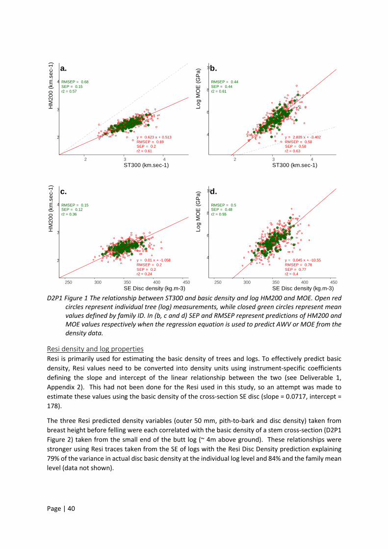
Page | 40

D2P1 Figure 1 The relationship between ST300 and basic density and log HM200 and MOE. Open red

circles represent individual tree (log) measurements, while closed green circles represent mean values defined by family ID. In (b, c and d) SEP and RMSEP represent predictions of HM200 and MOE values respectively when the regression equation is used to predict AWV or MOE from the density data.

Resi density and log properties Resi is primarily used for estimating the basic density of trees and logs. To effectively predict basic density, Resi values need to be converted into density units using instrument-specific coefficients defining the slope and intercept of the linear relationship between the two (see Deliverable 1, Appendix 2). This had not been done for the Resi used in this study, so an attempt was made to estimate these values using the basic density of the cross-section SE disc (slope = 0.0717, intercept = 178).

The three Resi predicted density variables (outer 50 mm, pith-to-bark and disc density) taken from breast height before felling were each correlated with the basic density of a stem cross-section (D2P1 Figure 2) taken from the small end of the butt log (~ 4m above ground). These relationships were stronger using Resi traces taken from the SE of logs with the Resi Disc Density prediction explaining 79% of the variance in actual disc basic density at the individual log level and 84% and the family mean level (data not shown).

a.

y = 0.623 x + 0.513RMSEP = 0.69SEP = 0.2r2 = 0.61

RMSEP = 0.68SEP = 0.15r2 = 0.57

2

3

4

2 3 4ST300 (km.sec-1)

HM

200

(km

.sec

-1)

b.

y = 2.835 x + -3.402RMSEP = 0.58SEP = 0.58r2 = 0.63

RMSEP = 0.44SEP = 0.44r2 = 0.61

4

6

8

10

2 3 4ST300 (km.sec-1)

Log

MO

E (G

Pa)

c.

y = 0.01 x + -1.058RMSEP = 0.2SEP = 0.2r2 = 0.24

RMSEP = 0.15SEP = 0.12r2 = 0.36

2

3

4

250 300 350 400 450SE Disc density (kg.m-3)

HM

200

(km

.sec

-1)

d.

y = 0.045 x + -10.55RMSEP = 0.78SEP = 0.77r2 = 0.4

RMSEP = 0.5SEP = 0.48r2 = 0.55

4

6

8

10

250 300 350 400 450SE Disc density (kg.m-3)

Log

MO

E (G

Pa)

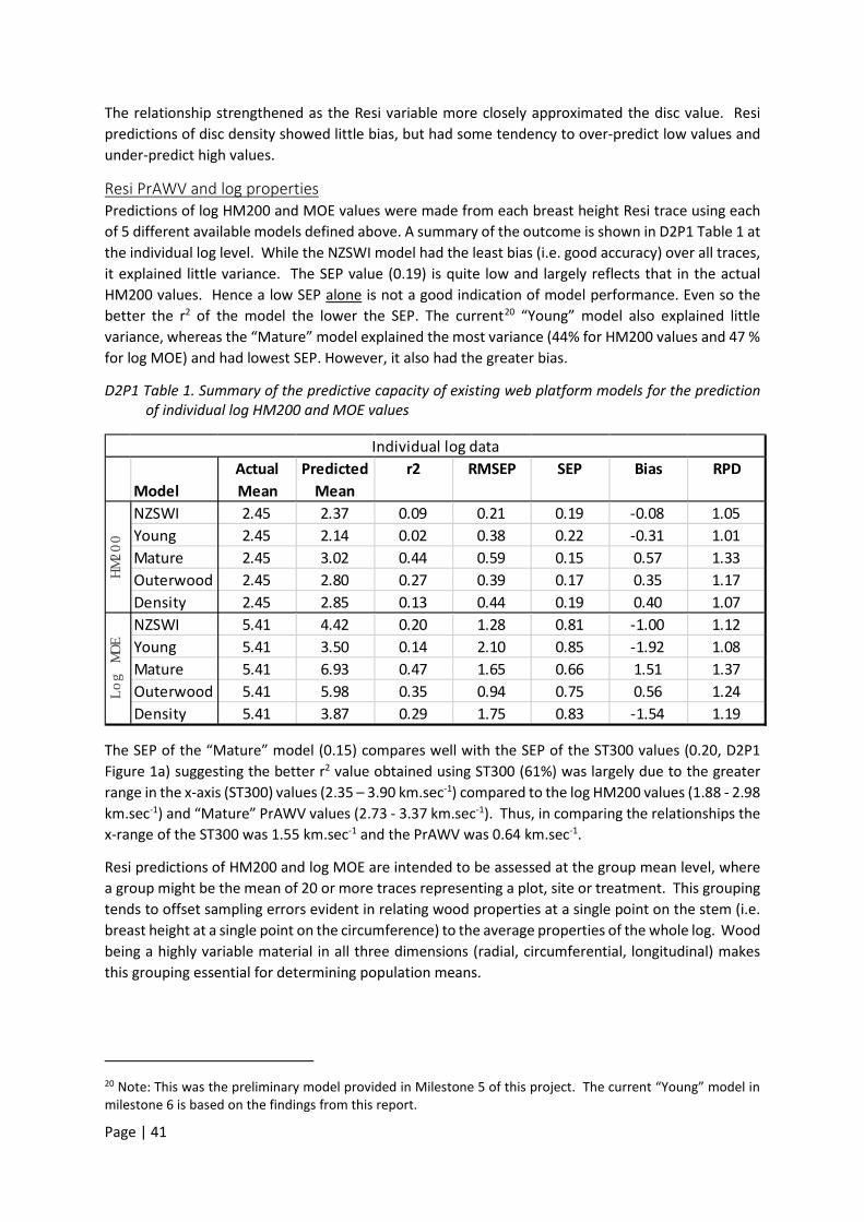
Page | 41

The relationship strengthened as the Resi variable more closely approximated the disc value. Resi predictions of disc density showed little bias, but had some tendency to over-predict low values and under-predict high values.

Resi PrAWV and log properties Predictions of log HM200 and MOE values were made from each breast height Resi trace using each of 5 different available models defined above. A summary of the outcome is shown in D2P1 Table 1 at the individual log level. While the NZSWI model had the least bias (i.e. good accuracy) over all traces, it explained little variance. The SEP value (0.19) is quite low and largely reflects that in the actual HM200 values. Hence a low SEP alone is not a good indication of model performance. Even so the better the r2 of the model the lower the SEP. The current20 “Young” model also explained little variance, whereas the “Mature” model explained the most variance (44% for HM200 values and 47 % for log MOE) and had lowest SEP. However, it also had the greater bias.

D2P1 Table 1. Summary of the predictive capacity of existing web platform models for the prediction of individual log HM200 and MOE values

The SEP of the “Mature” model (0.15) compares well with the SEP of the ST300 values (0.20, D2P1 Figure 1a) suggesting the better r2 value obtained using ST300 (61%) was largely due to the greater range in the x-axis (ST300) values (2.35 – 3.90 km.sec-1) compared to the log HM200 values (1.88 - 2.98 km.sec-1) and “Mature” PrAWV values (2.73 - 3.37 km.sec-1). Thus, in comparing the relationships the x-range of the ST300 was 1.55 km.sec-1 and the PrAWV was 0.64 km.sec-1.

Resi predictions of HM200 and log MOE are intended to be assessed at the group mean level, where a group might be the mean of 20 or more traces representing a plot, site or treatment. This grouping tends to offset sampling errors evident in relating wood properties at a single point on the stem (i.e. breast height at a single point on the circumference) to the average properties of the whole log. Wood being a highly variable material in all three dimensions (radial, circumferential, longitudinal) makes this grouping essential for determining population means.

20 Note: This was the preliminary model provided in Milestone 5 of this project. The current “Young” model in milestone 6 is based on the findings from this report.

ModelActual Mean

Predicted Mean

r2 RMSEP SEP Bias RPD

NZSWI 2.45 2.37 0.09 0.21 0.19 -0.08 1.05Young 2.45 2.14 0.02 0.38 0.22 -0.31 1.01Mature 2.45 3.02 0.44 0.59 0.15 0.57 1.33Outerwood 2.45 2.80 0.27 0.39 0.17 0.35 1.17Density 2.45 2.85 0.13 0.44 0.19 0.40 1.07NZSWI 5.41 4.42 0.20 1.28 0.81 -1.00 1.12Young 5.41 3.50 0.14 2.10 0.85 -1.92 1.08Mature 5.41 6.93 0.47 1.65 0.66 1.51 1.37Outerwood 5.41 5.98 0.35 0.94 0.75 0.56 1.24Density 5.41 3.87 0.29 1.75 0.83 -1.54 1.19

HM200

Log MOE

Individual log data

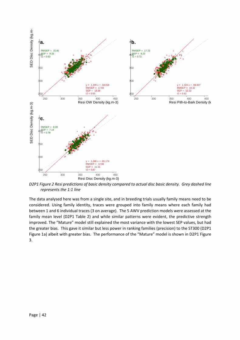
Page | 42

D2P1 Figure 2 Resi predictions of basic density compared to actual disc basic density. Grey dashed line

represents the 1:1 line

The data analysed here was from a single site, and in breeding trials usually family means need to be considered. Using family identity, traces were grouped into family means where each family had between 1 and 6 individual traces (3 on average). The 5 AWV prediction models were assessed at the family mean level (D2P1 Table 2) and while similar patterns were evident, the predictive strength improved. The “Mature” model still explained the most variance with the lowest SEP values, but had the greater bias. This gave it similar but less power in ranking families (precision) to the ST300 (D2P1 Figure 1a) albeit with greater bias. The performance of the “Mature” model is shown in D2P1 Figure 3.

a.

y = 1.209 x + -59.018RMSEP = 17.93SEP = 13.38r2 = 0.55

RMSEP = 15.45SEP = 9.33r2 = 0.63

250

300

350

400

450

250 300 350 400 450Resi OW Density (kg.m-3)

SE

D D

isc

Den

sity

(kg.

m-3

b.

y = 1.324 x + -94.007RMSEP = 19.32SEP = 12.22r2 = 0.62

RMSEP = 17.23SEP = 8.22r2 = 0.72

250

300

350

400

450

250 300 350 400 450Resi Pith-to-Bark Density (kg

c.

y = 1.246 x + -81.174RMSEP = 12.08SEP = 11.31r2 = 0.67

RMSEP = 8.39SEP = 7.14r2 = 0.78

250

300

350

400

450

250 300 350 400 450Resi Disc Density (kg.m-3)

SE

D D

isc

Den

sity

(kg.

m-3

)

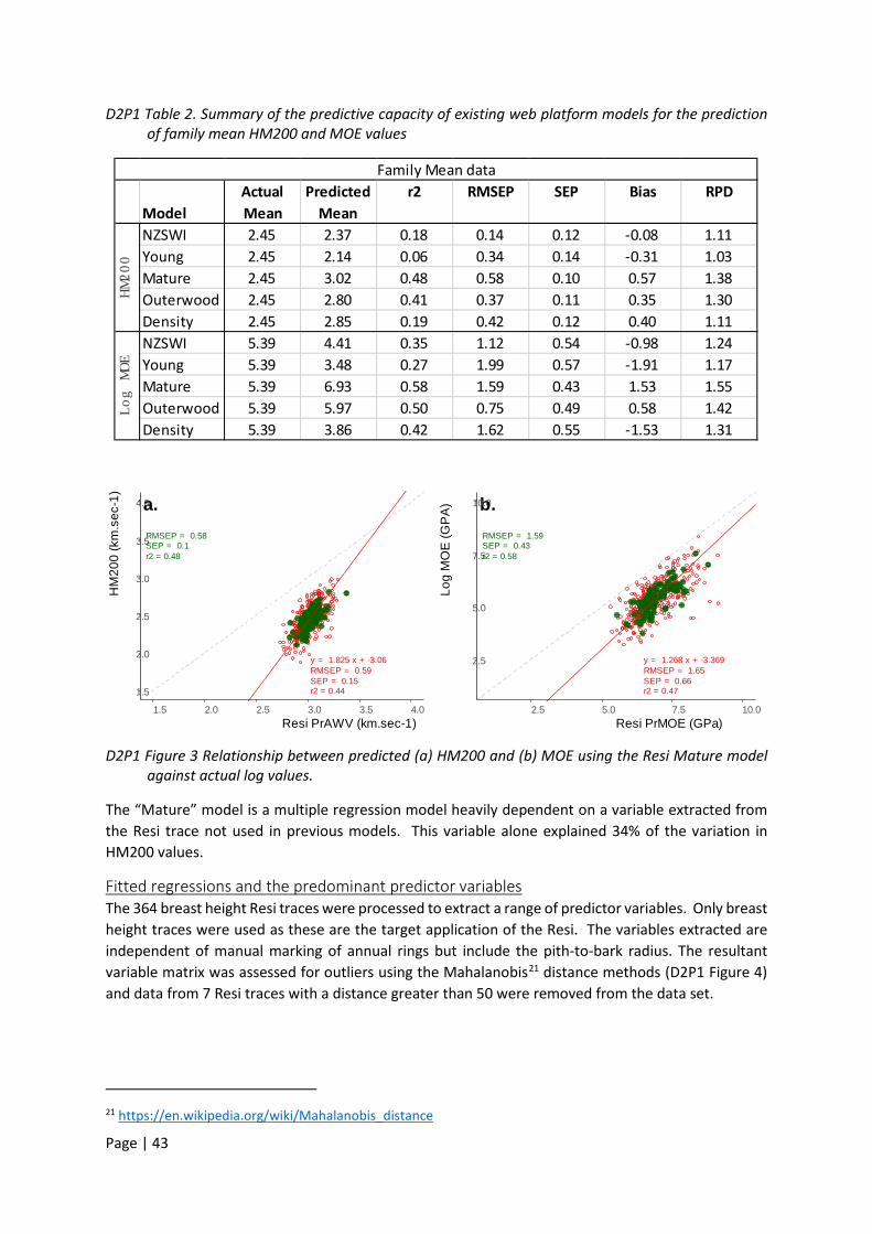
Page | 43

D2P1 Table 2. Summary of the predictive capacity of existing web platform models for the prediction of family mean HM200 and MOE values

D2P1 Figure 3 Relationship between predicted (a) HM200 and (b) MOE using the Resi Mature model against actual log values.

The “Mature” model is a multiple regression model heavily dependent on a variable extracted from the Resi trace not used in previous models. This variable alone explained 34% of the variation in HM200 values.

Fitted regressions and the predominant predictor variables The 364 breast height Resi traces were processed to extract a range of predictor variables. Only breast height traces were used as these are the target application of the Resi. The variables extracted are independent of manual marking of annual rings but include the pith-to-bark radius. The resultant variable matrix was assessed for outliers using the Mahalanobis21 distance methods (D2P1 Figure 4) and data from 7 Resi traces with a distance greater than 50 were removed from the data set.

21 https://en.wikipedia.org/wiki/Mahalanobis_distance

ModelActual Mean

Predicted Mean


NZSWI 2.45 2.37 0.18 0.14 0.12 -0.08 1.11Young 2.45 2.14 0.06 0.34 0.14 -0.31 1.03Mature 2.45 3.02 0.48 0.58 0.10 0.57 1.38Outerwood 2.45 2.80 0.41 0.37 0.11 0.35 1.30Density 2.45 2.85 0.19 0.42 0.12 0.40 1.11NZSWI 5.39 4.41 0.35 1.12 0.54 -0.98 1.24Young 5.39 3.48 0.27 1.99 0.57 -1.91 1.17Mature 5.39 6.93 0.58 1.59 0.43 1.53 1.55Outerwood 5.39 5.97 0.50 0.75 0.49 0.58 1.42Density 5.39 3.86 0.42 1.62 0.55 -1.53 1.31

Family Mean data

HM200

Log MOE

a.

y = 1.825 x + -3.06RMSEP = 0.59SEP = 0.15r2 = 0.44

RMSEP = 0.58SEP = 0.1r2 = 0.48

1.5

2.0

2.5

3.0

3.5

4.0

1.5 2.0 2.5 3.0 3.5 4.0Resi PrAWV (km.sec-1)

HM

200

(km

.sec

-1)

b.

y = 1.268 x + -3.369RMSEP = 1.65SEP = 0.66r2 = 0.47

RMSEP = 1.59SEP = 0.43r2 = 0.58

2.5

5.0

7.5

10.0

2.5 5.0 7.5 10.0Resi PrMOE (GPa)

Log

MO

E (G

PA

)

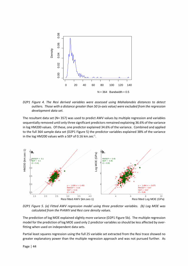
https://en.wikipedia.org/wiki/Mahalanobis_distance

Page | 44

D2P1 Figure 4. The Resi derived variables were assessed using Mahalanobis distances to detect outliers. Those with a distance greater than 50 (x-axis value) were excluded from the regression development data set.

The resultant data set (N= 357) was used to predict AWV values by multiple regression and variables sequentially removed until only three significant predictors remained explaining 36.6% of the variance in log HM200 values. Of these, one predictor explained 34.6% of the variance. Combined and applied to the full 364 sample data set (D2P1 Figure 5) the predictor variables explained 38% of the variance in the log HM200 values with a SEP of 0.16 km.sec-1.

D2P1 Figure 5. (a) Fitted AWV regression model using three predictor variables. (b) Log MOE was calculated from the PrAWV and Resi core density values.

The prediction of log MOE explained slightly more variance (D2P1 Figure 5b). The multiple regression model for the prediction of log MOE used only 2 predictor variables so should be less affected by over-fitting when used on independent data sets.

Partial least squares regression using the full 25 variable set extracted from the Resi trace showed no greater explanatory power than the multiple regression approach and was not pursued further. As

0 20 40 60 80 100 120 140

0.00

0.02

0.04

0.06

0.08

N = 364 Bandwidth = 0.5

Den

sity

a.

y = 1.608 x + -1.493RMSEP = 0.16SEP = 0.16r2 = 0.38

RMSEP = 0.1SEP = 0.1r2 = 0.41

1.5

2.0

2.5

3.0

3.5

4.0

1.5 2.0 2.5 3.0 3.5 4.0Resi fitted AWV (km.sec-1)

HM

200

(km

.sec

-1)

b.

y = 1.494 x + -2.675RMSEP = 0.67SEP = 0.67r2 = 0.45

RMSEP = 0.45SEP = 0.45r2 = 0.55

4

6

8

10

4 6 8 10Resi fitted Log MOE (GPa)

Log

MO

E (G

Pa)

Page | 45

other independent data sets become available the predictive robustness of the PLS versus the multiple regression models can be assessed.

Conclusions • ST300 values explained more phenotypic variance than Resi predictions (PrAWV) • The fitted model uses similar variables to those used in the current “Mature” model. The

slightly less explained variance arose from the exclusion of outliers in fitting the model which should make it more robust.

• At the family mean level, Resi predictions of AWV and MOE did only slightly better than regressions based on Resi predicted disc basic density.

Page | 46

Deliverable 2 Part 2. The prediction of MOE and AWV in 10 year-old southern yellow pine

Geoff Downes (Forest Quality) and Dominic Kain (HQPlantations)

Key Findings • ST300 measures of AWV provided the best indicator of log MOE in the young Southern Pine

trees assessed, explaining 68% of the variance in family means, with a SEP of 0.45 GPa. • Resi measures of basic density in contrast explained only 26% of the variance in family means • Resi predictions of log MOE explained 33% of the variance in family means, with a SEP of 0.74

GPa. • A fitted regression to predict log MOE using Resi-derived variables explained 42% of the

variance with a SEP of 0.59 GPa. • Combining ST300 and Resi in a fitted regression explained 76% of the variance with a SEP of

0.41 GPa

Introduction Genetic improvement of wood quality is gaining importance but remains limited by the cost of assessment tools. HQPlantations have used the Fibre-gen ST300 acoustic tool to assess wood acoustic velocity on young standing trees in progeny trials in its Southern Pine genetic improvement program for over 10 years, with over 25,000 trees assessed. A sawing study (Harding et al. 2007) of 6.8-year old trees found a strong correlation (r=0.89) at the clone mean level between standing tree ST300 measures and sawn board static modulus of elasticity (MoE). This has been treated as an approximate estimate of the genetic correlation between the selection criterion Av_05to07 (acoustic velocity at age 5-7 years) and the breeding objective trait Pred_moe_06 (Predicted MoE at age 6 years) in the Treeplan system for the PEExPCH hybrid. Standing tree acoustic velocity assessments between ages 4 and 10 years are used as measure traits. Predicted genetic gains of 10.2% in corewood MoE were made in a seed orchard established 2015 (Stritzke’s B), which is now providing seed for plantation replanting.

Using the ST300 tool, a single operator can assess around 150-200 trees in a working day. Progress is on the lower side of this range if assessing only a subsample of trees. Subsampling is nearly always necessary due to the high cost of assessing every tree in moderate to large-sized progeny trials (4,000-12,000 trees).

The Resi penetrometer is a handheld device that measures the torque required to drive a high-tensile steel needle through a tree. A single operator can assess around 500 trees in a working day. While the device has been used since 1989 to predict wood density (Rinn 2012), in 2016 a research co-operative in New Zealand (SWI), identified the potential of the Resi to predict wood MoE. This is of particular interest to HQP’s genetic improvement program as our major long-term customer prefers higher wood MoE but lower wood density. While it may be biologically very difficult to achieve this, we want to ensure we are selecting for wood MoE rather than for density alone.

Initial pilot studies in Queensland Southern Pine trees have indicated the potential of the Resi to predict MoE at both the tree and group level in harvest-age trees, but have not studied younger trees at typical selection ages for genetic improvement (4-10 years). Based on Resi assessments to date in Southern Pine genetics trials, the number of trees that can be assessed per day is around double that possible with the ST300. However, the accuracy of MoE prediction using the Resi currently depends

Page | 47

on the identification of growth rings. This is time-consuming to do manually and challenging to automate accurately.

This experiment will assess ST300, Resi, and log MoE on 421 Pinus elliottii var. elliottii × Pinus caribaea var. hondurensis (slash x Caribbean pine hybrid) F2 hybrid trees aged 10 years, sampled from a partial factorial mating design involving 27 parents and 62 families, from 7 replicates of a cloned progeny trial on a single site at Tuan. The data will be used to compare standing tree assessment methods including ST300 previously collected on the same trees at age 4 years (for results including age 4 years, see final report, FWPA project PNC428-1617)22.

Data for this study was collected as part of an HQP study, Experiment 870 TBS “Comparing ST300 at two ages with Resi-predicted wood stiffness as estimators of age 10 butt log MoE in F2 hybrid progeny from Expt. 813B TBS” 23.

The objectives of this analysis, using the 10-year data only, are:

1. Test and compare the 5 currently available Resi-based MoE prediction models with ST300 values for predicting dynamic green buttlog MOE at age 10 years in the slash x Caribbean pine hybrid, at the individual-tree and family mean levels.

2. Fit a model using available Resi-based values to best predict available log MoE data for this experiment with and without ST300 values.

3. Examine the capability of the Resi to predict other relevant variables such as BH disc density and log acoustic wave velocity (AWV).

Methods Genetic material Various experiments were considered as candidates for the study. All had shortcomings but Expt. 813B TBS was judged the most useful. Other trials had either too few trees assessed for early ST300, ST300 assessed at an age of less relevance for the future selection strategy, or the trials were still very young, only having ST300 assessments in recent years. Expt. 813TBS, while having fewer than the ideal number of families and parents, has the following strengths:

• ST300 previously assessed at age 4 years on approx. 1/3 of trees • 27 parents and 63 families, excluding controls (more than most clonal trials ) • Trees now at age 10 years so the value of ST300 measures at age 4y and age 10y can be

compared for predicting log MoE in essentially the entire “juvenile core”. • Trial is fully pedigreed and has material of some interest for future selection.

Of the three sites, Expt. 813B TBS was chosen as it had the highest heritability for growth traits, though this was still low by comparison with other trials. Heritabilities for all other traits were at moderate levels.

Sampling strategy Sampling was restricted to the F2 hybrid only as the F1 crossing matrix was small, sparse and added an additional complication to the trial. There were 63 total F2 families for sampling, of which all had previously been assessed for AWV (ST300) on varying numbers of trees.

22 Link to FWPA web 23 Expt. 870TBS working plan: Resi Genetics study in Expt. 813B TBS by D. Kain and R. Peters (HQP)

Page | 48

An initial sample of replicates was chosen by selecting those with the greatest number of trees previously assessed for ST300 at age 4 years. The previously assessed trees were inspected, and stem straightness was found to be unacceptably poor, with compression wood clearly visible on various trees.

A revised sample of replicates was selected based on both:

1. Prior stem straightness scores (as this was an issue at the trial) 2. The number of families previously sampled in age 4 ST300 assessments in this trial.

The following replicates were chosen as the final sample: 1, 11, 13, 14, 17, 18, 21.

An initial set of nominated trees was chosen for sampling and with reference to this a final set was confirmed and marked in the field. The combined nomination and selection procedure was as follows:

• Choose one tree per 3-tree family line plot in each of the final sample replicates, excluding F1 hybrids

• Choose trees with age 4 acoustic velocity assessments (Av_0404) wherever possible – if there are more than one:

• exclude any that are now judged unacceptable for sampling (due to bends, obvious compression wood, double leaders or large ramicorns or large kinks in or affecting the 4m buttlog).

• Select among acceptable trees at random. • Where no trees were previously assessed for AWV or any trees assessed are now judged to

be unacceptable, randomly select another acceptable tree within the same 3-tree line plot that does not have an AWV assessment.

• Where no trees at all in a line plot are judged acceptable, select none.

The aim was to get to a total of at least 6 trees sampled per F2 full-sib family. In some cases 7 trees were sampled.

Two replicates containing control plots were sampled. Control plots are whole 8Rx9T plots of either Kennedy CSO or Clarke CSO bulk seedlots. 19 trees per control treatment were sampled. While 2 replicates is not ideal for the control treatments, spatial analysis will be used to improve comparisons between treatments across the site.

423 trees were nominated for sampling. Wherever possible, these were trees that had previously been assessed for AWV. Where those trees had unacceptable form (e.g. too bendy, or defect within the 4m butt log) a different tree in the same plot was nominated.

• 421 trees were selected for sampling and paint-marked in the field. • 292 of these trees had been previously assessed for AWV. • 32 nominated trees had to be rejected or substituted because they were not of acceptable

form.

Standing tree assessment procedure The 421 trees for assessment were marked in the field with a paint ring at breast height. On the standing tree and close to the 1.3m point, collect one Resi trace as described below.

1. Entry at ‘clock’ position 6:00, where row start position is 6:00, using SPRCS terminology (see Deliverable 2 Part 4 reference).

Page | 49

2. Change entry position and height where necessary to avoid compression wood, whorls and branches.

3. Note defect codes, following the Resi HQP Standard Operating Procedure. 4. Data to be recorded in the Resi device prior to each trace are: Plot_Row_Tree, Entry

position (O’clock, rounding down so 4:30 = 4), defect code, and entry height (m). 5. Where defect code = 9, note the nature of the defect on the proforma 6. Ensure the Resi goes all the way through the tree so as to extract a bark-to-bark trace for

comparison with DBH measured using a diameter tape.

On the standing tree and centred around the 1.3m point, collect one ST300 reading as described in the ST300 HQP Standard Operating Procedure.

Destructive sampling procedure 1. Fell the tree, keeping stump height to a minimum and avoiding damage to the buttlog. 2. Collect 10 fully expanded fascicle sheaths from at or near the growing tip of the tree. Place

in a paper bag, fold and staple top in two places. Mark bag with Experiment-Plot-Row-Tree, i.e. 813B 10-2-5. For the rest of the day, store in a cool dry place (esky), not directly on ice. At the end of the day place all samples in the dehumidifier, checking the temperature is set to 30 degrees C and humidity to 10%.

3. Cut off uneven wood at the base of the felled stem, making a clean even log end. 4. Cut one 4-metre log measuring from the clean even log end. Ensure any green limbs are

pruned back to the stem, though these are unlikely to be present. 5. Take one HM200 (log hitman) reading at the large end of the log. Record on the proforma

along with any notes (e.g. resin impregnation or other defects and which part of the log is affected).

6. From the breast height point (1.3 metres), obtain a de-barked disc of c. 30mm even width for assessing green and basic densities in the lab. a. If a defect (e.g. resin impregnation, reaction wood around branches) is present at

breast height, take the disc as close as possible to breast height, avoiding the defect. b. Label with a crayon on the disc the Plot-Row-Tree identifier (e.g. 41-2-5). c. Note any issues with the disc on the proforma. d. Enclose the disc entirely in a supplied plastic bag of type 1 or 2 (small or large) as soon

as possible. Exclude excess air from the bag, and tape to prevent moisture loss. Exclude excess air from the bag. Label the outside of the bag with the Plot-Row-Tree identifier using a paint pen. Write and circle the bag type (1 or 2) on the outside of the bag.

e. Store in the shade to avoid disc drying. 7. Arrange transfer of discs to the laboratory as soon as possible, and refrigerate (if to be

assessed within 2 days) or freeze if not.

Laboratory procedure The following properties are to be measured on each disc, in this order:

1. Green mass (g ± 0.1 g) 2. Green volume (cm3 ± 0.5 cm3) 3. Oven dry mass (g ± 0.1 g)

The following step by step procedure is to be used to measure the above properties:

1. If frozen, completely defrost the disc, keeping it inside its plastic bag.

Page | 50

2. Discs that are too large to be submerged in water (limited by container size and balance capacity) should be split preferably in two and re-labelled, appending a 1, 2 (3 or 4 if necessary) to the disc label (for example, a disc labelled 641-1-5 would be re-labelled 641-1-5-1 and 641-1-5-2). Hereon the word disc refers to either a disc or disc segment.

3. Note the plastic bag type (1 or 2) on the proforma. 1. Keeping the disc inside its plastic bag, place it on the balance and record green mass (g ± 0.1

g). 2. Place a protective sheet on the balance (e.g. plastic or cardboard sheet – to protect from

resin) and tare the balance. 3. Wearing gloves, remove the disc from its bag and measure disc green volume (cm3 ± 0.5

cm3), using the Archimedean water displacement method (as instructed by DAF or HQP staff), ensuring the following:

a. Tare the balance prior to immersing the disc b. The disc must be fully submerged at the time of measurement c. The disc must not touch the water vessel at the time of measurement d. Use a small amount of a wetting agent such as Teepol to avoid bubbles e. Wait for the balance to stabilise sufficiently to read the volume to within 0.5 cm3 of

the actual measurement. Note the balance displays in g but is measuring volume (cm3) as long as the disc does not touch the container.

4. Dry discs in the oven at 100⁰-105⁰ Celsius for 3 days, separating discs using stakes to ensure they are not touching. Record the time a batch of discs is added to the oven and when it is removed.

5. Wearing protective clothing to avoid burns, remove the discs from the oven, allow them to cool (and the mass to stabilise) for 3 minutes, and measure oven dry mass (g ± 0.1g). While it will be necessary to process discs in batches for efficiency, try to keep the stabilisation time as constant as possible between discs. The discs take up moisture quite rapidly after removal from the oven. Dessicator storage during this time is desirable but not possible.

6. Store the discs at an HQP-nominated location at room temperature and humidity.

Buttlog green dynamic MoE (MPa) will be calculated as:

MoE = v2.d

Where:

• v2 = the square of buttlog HM200 velocity (km/s) • d = breast height disc green density (kg/m3)

Data Metrics The following metrics were available for analysis,

• ST300: Time-of-flight AWV on standing trees • HM200: Resonance AWV on felled logs • LogMOE: HM200^2 * green density • SE disk green and basic Density • Resi predicted values24

24 All values were derived using the web portal at from the web portal at https://forestquality.shinyapps.io/FWPAResiProcessor/


Page | 51

o OWD: basic density of the outer 50 mm on the entry-side of the trace o Core density: Mean bark-to-bark basic density o Disc Density: Mean area-weighted density of each of the entry and exit pith-to-bark

traces. o PrAWV: predicted values made from a range of available algorithms listed below o PrMOE: predicted values made from a range of available algorithms listed below

• Resi prediction models o NZSWI: This model is similar to the one used in the previous software tool developed

with support from NZ Solid Wood Innovations o Young: Radiata pine model as defined in Deliverable 2 Part 1 o Mature: Multiple regression model produced for Milestone 5 of the current project o Outerwood: PLS model produced for Milestone 5 of the current project focussing on

variables from the outer 50mm of the trace o Density: A recent addition (Aug 2019) of a simple linear regression against pith-to-

bark density. Effectively a measure of the predictive ability of density alone.

Results Relationship between ST300 in standing trees and basic density in explaining variance in HM200 and log MOE values Prior to exploring the explanatory power of the Resi data it is necessary to establish the relationships among metrics which have become standard methods of assessment in recent years. As found in other studies ST300 values were effective in predicting variance in HM200 values (r2=44%; D2P2 Figure 1) and log MOE (r2=43%) at the individual log level in younger trees. In contrast the basic density of a cross-section disc taken from the small end of the log explained only 10% and 13% respectively (D2P2 Figure 1 c&d).

Page | 52

D2P2 Figure 1. The relationship between ST300 and basic density and log HM200 and MOE. Open red circles represent individual tree (log) measurements, while closed circles represent mean values defined by family ID.

The basic density values are unextracted values and hence may be influenced by resin content, though the extent of this influence is uncertain in these young, 10-year old trees in which heartwood formation had not yet commenced. The variance in the basic density – log MOE relationship is greater at higher basic density values, potentially indicating (given previously observed stronger relationships between basic density and MOE in radiata pine) that some higher density discs could be more resin-affected. However, in Southern Pine at age 30-34 years (D2P4 Figure 2), where resin content is expected to be substantially higher, this pattern was not observed. This hints at an alternative cause. Previous studies (reviewed by Harding 2008) have found that time of flight measured using an acoustic tool was the best predictor of MoE in young Southern Pine, with density of lesser importance. The link between density and MoE in Southern Pine at various ages and the impact of resin on this relationship need further investigation.

In terms of assessing prediction performance the standard error of prediction (SEP) is of interest when considered together with the variance explained (r2) as this indicates the precision of the relationship. In D2P2 Figure 1(b-c), SEP values provided are based on the application of the regression equation shown on the plot, and therefore RMSEP values are the same as the SEP values. ST300 values have a SEP of 0.34 km.sec-1 in the relationship with HM200 values. Likewise, a simple regression model to

a.

y = 0.526 x + 0.766RMSEP = 0.19SEP = 0.19r2 = 0.44

RMSEP = 0.07SEP = 0.07r2 = 0.7

y = 0.575 x + 0.594

2

3

4

2 3 4ST300 (km.sec-1)

HM

200

(km

.sec

-1)

b.

y = 3.096 x + -3.477RMSEP = 1.14SEP = 1.14r2 = 0.43

RMSEP = 0.45SEP = 0.45r2 = 0.68

y = 3.483 x + -4.841

4

8

12

2 3 4ST300 (km.sec-1)

Log

MO

E (G

Pa)

c.

y = 0.004 x + 0.462RMSEP = 0.28SEP = 0.27r2 = 0.1

RMSEP = 0.14SEP = 0.14r2 = 0.2

y = 0.005 x + 0.064

2

3

4

400 500 600 700SE Disc density (kg.m-3)

HM

200

(km

.sec

-1)

d.

y = 0.025 x + -5.269RMSEP = 1.57SEP = 1.55r2 = 0.13

RMSEP = 0.77SEP = 0.77r2 = 0.25

y = 0.03 x + -8.051

4

8

12

400 500 600 700SE Disc density (kg.m-3)

Log

MO

E (G

Pa)

Page | 53

predict MOE from the ST300 values (D2P2 Figure 1b) would have a SEP of 1.14 GPa. These are markedly larger than those observed in radiata pine.

Individual data points were combined into means defined by family ID which contained between 4 and 20 individuals. The bulking of values tended to reduce the standard error or prediction, with some increase in the variance explained.

The data illustrated in D2P2 Figure 1 represents the basis of comparison for Resi-derived metrics.

Resi density and log properties Resi is primarily used for estimating the basic density of trees and logs as the:

• Outerwood density: basic density of the outer 50mm of the stem at the sampling point (a common approach when using increment cores)

• Core density: full under-bark diameter similar to a full diameter increment core • Disc Density: area-weighted diameter indicative of the density of the cross-sectional disc.

To effectively predict basic density, Resi values need to be converted into density units using instrument-specific coefficients defining the slope and intercept of the linear relationship between the two. This had not been done for the Resi used in this study, so the Resi predicted values were obtained using the default values on the web processing site (slope = 0.09, intercept = 196).

The three Resi predicted density variables (Outer 50 mm, pith-to-bark and estimated disc density) taken from breast height before felling were each well correlated with the basic density of a stem cross-section (D2P2 Figure 2) taken from the small end of the butt log (~ 4m above ground).

The Resi-predicted density values from BH traces were correlated with the BH disc density values, but the strength of the relationship was less than observed in radiata pine generally, and a similar recently completed assessment of 7yo radiata pine. The increase in the scatter in the individual-tree relationship as density increased is also noticeable, potentially due to resin increasing the laboratory basic density values of some samples. An increase in scatter was not observed at the family-mean level, or in mature Southern Pine (D2P4 Figure 2).

The relationship tended to strengthen as the Resi variable more closely approximated the disc value. Resi predictions of density showed some bias, largely attributable to the absence of instrument specific regression coefficients. The precision of prediction is of most interest in this experiment, and bias will be addressed through calibration in a follow-up experiment.

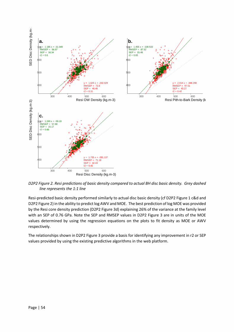
Page | 54

D2P2 Figure 2. Resi predictions of basic density compared to actual BH disc basic density. Grey dashed line represents the 1:1 line

Resi-predicted basic density performed similarly to actual disc basic density (cf D2P2 Figure 1 c&d and D2P2 Figure 2) in the ability to predict log AWV and MOE. The best prediction of log MOE was provided by the Resi core density prediction (D2P2 Figure 3d) explaining 26% of the variance at the family level with an SEP of 0.76 GPa. Note the SEP and RMSEP values in D2P2 Figure 3 are in units of the MOE values determined by using the regression equations on the plots to fit density as MOE or AWV respectively.

The relationships shown in D2P2 Figure 3 provide a basis for identifying any improvement in r2 or SEP values provided by using the existing predictive algorithms in the web platform.

a.

y = 1.625 x + -232.029RMSEP = 72.8SEP = 46.46r2 = 0.31

RMSEP = 56.57SEP = 16.34r2 = 0.6

y = 1.185 x + -31.049

400

500

600

700

300 400 500 600Resi OW Density (kg.m-3)

SE

D D

isc

Den

sity

(kg.

m-3

b.

y = 2.014 x + -348.298RMSEP = 97.51SEP = 43.27r2 = 0.42

RMSEP = 87.52SEP = 15.48r2 = 0.65

y = 1.455 x + -109.533

400

500

600

700

300 400 500 600Resi Pith-to-Bark Density (kg

c.

y = 1.735 x + -281.137RMSEP = 71.18SEP = 42.43r2 = 0.42

RMSEP = 57.68SEP = 15.17r2 = 0.65

y = 1.249 x + -59.19

400

500

600

700

300 400 500 600Resi Disc Density (kg.m-3)

SE

D D

isc

Den

sity

(kg.

m-3

)

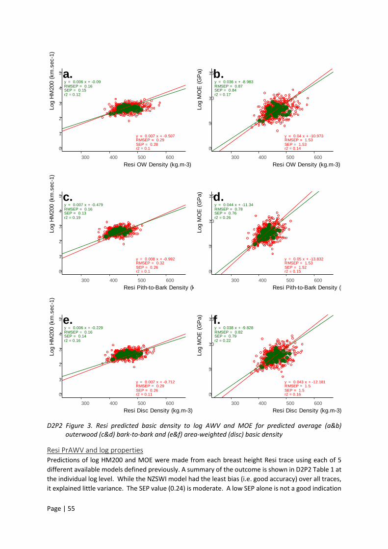
Page | 55

D2P2 Figure 3. Resi predicted basic density to log AWV and MOE for predicted average (a&b) outerwood (c&d) bark-to-bark and (e&f) area-weighted (disc) basic density

Resi PrAWV and log properties Predictions of log HM200 and MOE were made from each breast height Resi trace using each of 5 different available models defined previously. A summary of the outcome is shown in D2P2 Table 1 at the individual log level. While the NZSWI model had the least bias (i.e. good accuracy) over all traces, it explained little variance. The SEP value (0.24) is moderate. A low SEP alone is not a good indication

a.

y = 0.007 x + -0.507RMSEP = 0.29SEP = 0.28r2 = 0.1

RMSEP = 0.16SEP = 0.15r2 = 0.12

y = 0.006 x + -0.09

0

1

2

3

4

5


Log

HM

200

(km

.sec

-1)

b.

y = 0.04 x + -10.973RMSEP = 1.53SEP = 1.53r2 = 0.14

RMSEP = 0.87SEP = 0.84r2 = 0.17

y = 0.036 x + -8.983

0

5

10

15


Log

MO

E (G

Pa)

c.

y = 0.008 x + -0.992RMSEP = 0.32SEP = 0.26r2 = 0.1

RMSEP = 0.16SEP = 0.13r2 = 0.19

y = 0.007 x + -0.479

0

1

2

3

4

5

300 400 500 600Resi Pith-to-Bark Density (kg.m-3)

Log

HM

200

(km

.sec

-1)

d.

y = 0.05 x + -13.832RMSEP = 1.53SEP = 1.52r2 = 0.15

RMSEP = 0.78SEP = 0.76r2 = 0.26

y = 0.044 x + -11.34

0

5

10

15

300 400 500 600Resi Pith-to-Bark Density (k

Log

MO

E (G

Pa)

e.

y = 0.007 x + -0.712RMSEP = 0.29SEP = 0.26r2 = 0.11

RMSEP = 0.16SEP = 0.14r2 = 0.16

y = 0.006 x + -0.229

0

1

2

3

4

5


Log

HM

200

(km

.sec

-1)

f.

y = 0.043 x + -12.181RMSEP = 1.5SEP = 1.5r2 = 0.16

RMSEP = 0.82SEP = 0.79r2 = 0.22

y = 0.038 x + -9.828

0

5

10

15


Log

MO

E (G

Pa)

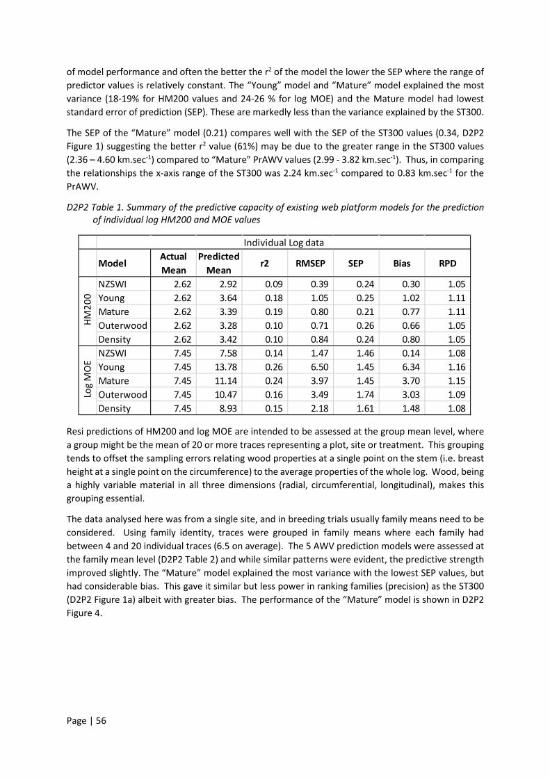
Page | 56

of model performance and often the better the r2 of the model the lower the SEP where the range of predictor values is relatively constant. The “Young” model and “Mature” model explained the most variance (18-19% for HM200 values and 24-26 % for log MOE) and the Mature model had lowest standard error of prediction (SEP). These are markedly less than the variance explained by the ST300.

The SEP of the “Mature” model (0.21) compares well with the SEP of the ST300 values (0.34, D2P2 Figure 1) suggesting the better r2 value (61%) may be due to the greater range in the ST300 values (2.36 – 4.60 km.sec-1) compared to “Mature” PrAWV values (2.99 - 3.82 km.sec-1). Thus, in comparing the relationships the x-axis range of the ST300 was 2.24 km.sec-1 compared to 0.83 km.sec-1 for the PrAWV.

D2P2 Table 1. Summary of the predictive capacity of existing web platform models for the prediction of individual log HM200 and MOE values

Resi predictions of HM200 and log MOE are intended to be assessed at the group mean level, where a group might be the mean of 20 or more traces representing a plot, site or treatment. This grouping tends to offset the sampling errors relating wood properties at a single point on the stem (i.e. breast height at a single point on the circumference) to the average properties of the whole log. Wood, being a highly variable material in all three dimensions (radial, circumferential, longitudinal), makes this grouping essential.

The data analysed here was from a single site, and in breeding trials usually family means need to be considered. Using family identity, traces were grouped in family means where each family had between 4 and 20 individual traces (6.5 on average). The 5 AWV prediction models were assessed at the family mean level (D2P2 Table 2) and while similar patterns were evident, the predictive strength improved slightly. The “Mature” model explained the most variance with the lowest SEP values, but had considerable bias. This gave it similar but less power in ranking families (precision) as the ST300 (D2P2 Figure 1a) albeit with greater bias. The performance of the “Mature” model is shown in D2P2 Figure 4.

ModelActual Mean

Predicted Mean


NZSWI 2.62 2.92 0.09 0.39 0.24 0.30 1.05 Young 2.62 3.64 0.18 1.05 0.25 1.02 1.11 Mature 2.62 3.39 0.19 0.80 0.21 0.77 1.11 Outerwood 2.62 3.28 0.10 0.71 0.26 0.66 1.05 Density 2.62 3.42 0.10 0.84 0.24 0.80 1.05 NZSWI 7.45 7.58 0.14 1.47 1.46 0.14 1.08 Young 7.45 13.78 0.26 6.50 1.45 6.34 1.16 Mature 7.45 11.14 0.24 3.97 1.45 3.70 1.15 Outerwood 7.45 10.47 0.16 3.49 1.74 3.03 1.09 Density 7.45 8.93 0.15 2.18 1.61 1.48 1.08

Individual Log data

HM20

0Lo

g M

OE

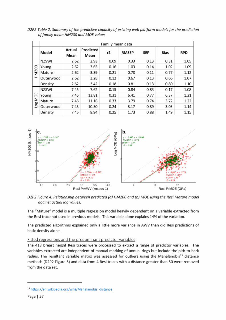
Page | 57

D2P2 Table 2. Summary of the predictive capacity of existing web platform models for the prediction of family mean HM200 and MOE values

D2P2 Figure 4. Relationship between predicted (a) HM200 and (b) MOE using the Resi Mature model against actual log values.

The “Mature” model is a multiple regression model heavily dependent on a variable extracted from the Resi trace not used in previous models. This variable alone explains 14% of the variation.

The predicted algorithms explained only a little more variance in AWV than did Resi predictions of basic density alone.

Fitted regressions and the predominant predictor variables The 418 breast height Resi traces were processed to extract a range of predictor variables. The variables extracted are independent of manual marking of annual rings but include the pith-to-bark radius. The resultant variable matrix was assessed for outliers using the Mahalanobis25 distance methods (D2P2 Figure 5) and data from 4 Resi traces with a distance greater than 50 were removed from the data set.

25 https://en.wikipedia.org/wiki/Mahalanobis_distance

ModelActual Mean

Predicted Mean


NZSWI 2.62 2.93 0.09 0.33 0.13 0.31 1.05 Young 2.62 3.65 0.16 1.03 0.14 1.02 1.09 Mature 2.62 3.39 0.21 0.78 0.11 0.77 1.12 Outerwood 2.62 3.28 0.12 0.67 0.13 0.66 1.07 Density 2.62 3.42 0.18 0.81 0.13 0.80 1.10 NZSWI 7.45 7.62 0.15 0.84 0.83 0.17 1.08 Young 7.45 13.81 0.31 6.41 0.77 6.37 1.21 Mature 7.45 11.16 0.33 3.79 0.74 3.72 1.22 Outerwood 7.45 10.50 0.24 3.17 0.89 3.05 1.14 Density 7.45 8.94 0.25 1.73 0.88 1.49 1.15

HM20

0Lo

g M

OE

Family mean data

c.

y = 1.576 x + -2.717RMSEP = 0.8SEP = 0.21r2 = 0.19

RMSEP = 0.78SEP = 0.11r2 = 0.21

y = 1.708 x + -3.167

1.5

2.0

2.5

3.0

3.5

4.0

1.5 2.0 2.5 3.0 3.5 4.0Resi PrAWV (km.sec-1)

HM

200

(km

.sec

-1)

b.

y = 0.915 x + -2.75RMSEP = 3.97SEP = 1.45r2 = 0.24

RMSEP = 3.79SEP = 0.74r2 = 0.33

y = 0.945 x + -3.098

4

8

12

4 8 12Resi PrMOE (GPa)

Log

MO

E (G

Pa)

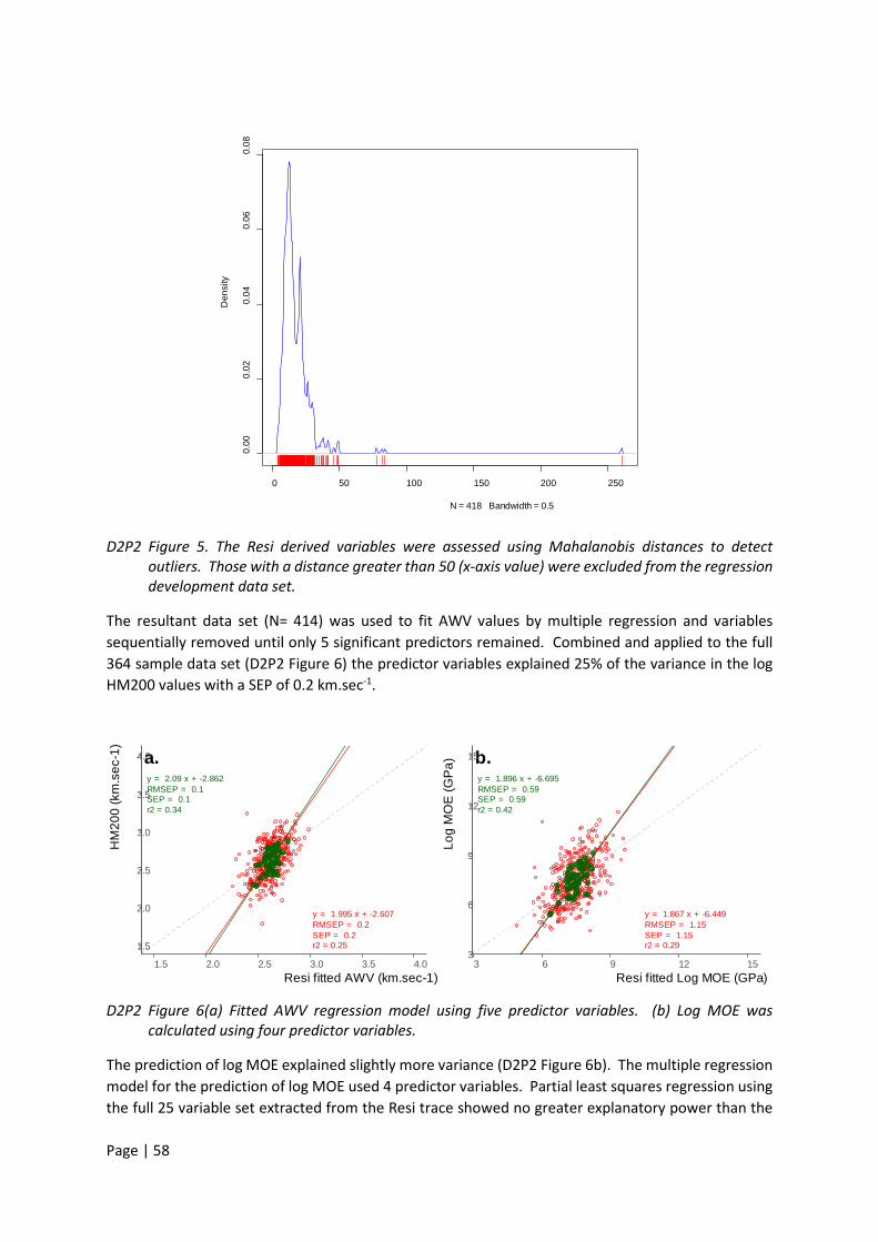
https://en.wikipedia.org/wiki/Mahalanobis_distance

Page | 58

D2P2 Figure 5. The Resi derived variables were assessed using Mahalanobis distances to detect outliers. Those with a distance greater than 50 (x-axis value) were excluded from the regression development data set.

The resultant data set (N= 414) was used to fit AWV values by multiple regression and variables sequentially removed until only 5 significant predictors remained. Combined and applied to the full 364 sample data set (D2P2 Figure 6) the predictor variables explained 25% of the variance in the log HM200 values with a SEP of 0.2 km.sec-1.

D2P2 Figure 6(a) Fitted AWV regression model using five predictor variables. (b) Log MOE was calculated using four predictor variables.

The prediction of log MOE explained slightly more variance (D2P2 Figure 6b). The multiple regression model for the prediction of log MOE used 4 predictor variables. Partial least squares regression using the full 25 variable set extracted from the Resi trace showed no greater explanatory power than the

0 50 100 150 200 250

0.00

0.02

0.04

0.06

0.08

N = 418 Bandwidth = 0.5

Den

sity

a.

y = 1.995 x + -2.607RMSEP = 0.2SEP = 0.2r2 = 0.25

RMSEP = 0.1SEP = 0.1r2 = 0.34

y = 2.09 x + -2.862

1.5

2.0

2.5

3.0

3.5

4.0


HM

200

(km

.sec

-1)

b.

y = 1.867 x + -6.449RMSEP = 1.15SEP = 1.15r2 = 0.29

RMSEP = 0.59SEP = 0.59r2 = 0.42

y = 1.896 x + -6.695

3

6

9

12

15

3 6 9 12 15Resi fitted Log MOE (GPa)

Log

MO

E (G

Pa)

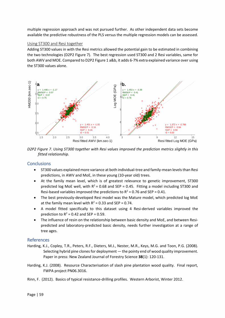
Page | 59

multiple regression approach and was not pursued further. As other independent data sets become available the predictive robustness of the PLS versus the multiple regression models can be assessed.

Using ST300 and Resi together Adding ST300 values in with the Resi metrics allowed the potential gain to be estimated in combining the two technologies (D2P2 Figure 7). The best regression used ST300 and 2 Resi variables, same for both AWV and MOE. Compared to D2P2 Figure 1 a&b, it adds 6-7% extra explained variance over using the ST300 values alone.

D2P2 Figure 7. Using ST300 together with Resi values improved the prediction metrics slightly in this fitted relationship.

Conclusions • ST300 values explained more variance at both individual-tree and family-mean levels than Resi

predictions, in AWV and MoE, in these young (10-year old) trees. • At the family mean level, which is of greatest relevance to genetic improvement, ST300

predicted log MoE well, with R2 = 0.68 and SEP = 0.45. Fitting a model including ST300 and Resi-based variables improved the predictions to R2 = 0.76 and SEP = 0.41.

• The best previously-developed Resi model was the Mature model, which predicted log MoE at the family mean level with R2 = 0.33 and SEP = 0.74.

• A model fitted specifically to this dataset using 4 Resi-derived variables improved the prediction to R2 = 0.42 and SEP = 0.59.

• The influence of resin on the relationship between basic density and MoE, and between Resi-predicted and laboratory-predicted basic density, needs further investigation at a range of tree ages.

References Harding, K.J., Copley, T.R., Peters, R.F., Dieters, M.J., Nester, M.R., Keys, M.G. and Toon, P.G. (2008).

Selecting hybrid pine clones for deployment — the pointy end of wood quality improvement. Paper in press: New Zealand Journal of Forestry Science 38(1): 120-131.

Harding, K.J. (2008). Resource Characterisation of slash pine plantation wood quality. Final report, FWPA project PN06.3016.

Rinn, F. (2012). Basics of typical resistance-drilling profiles. Western Arborist, Winter 2012.

a

y = 1.401 x + -1.05RMSEP = 0.16SEP = 0.16r2 = 0.51

RMSEP = 0.07SEP = 0.07r2 = 0.75

y = 1.446 x + -1.17

1.5

2.0

2.5

3.0

3.5

4.0


HM

200

(km

.sec

-1)

b.

y = 1.372 x + -2.766RMSEP = 0.94SEP = 0.94r2 = 0.53

RMSEP = 0.41SEP = 0.41r2 = 0.76

y = 1.453 x + -3.39

3

6

9

12

15

3 6 9 12 15Resi fitted Log MOE (GPa)

Log

MO

E (G

Pa)

Page | 60

Deliverable 2 Part 3. Evaluation of Resi predicted standing tree wood properties across a range of Pinus radiata sites.

Geoff Downes (FQ)

Contributors: Stephen Elms (HVP), Michael Schofield (NS) and Chris Rhynehart (HF)

Key Findings • All models explained most of the variance in MOE (log and Mill boards) across available data • Overall the results indicated that the ability of Resi to predict basic density is the main

contributor to MOE prediction, with little being gained from the attempts to explain additional variance by extracting other metrics from the Resi trace.

• In terms of accuracy and precision the Outerwood and Density models performed with the greater consistency.

• The Mature model performed well in mature stands but less well in younger stands and tended to under-predict log MOE and AWV at higher values.

• The Young model had significant bias when applied to older stands, tending to markedly under-estimate the actual MOE in mature stands.

• In terms of general application the Density model is arguably the better model, and could be refined to give more accurate results over a wider age range.

• Adding traces from the now available younger stands may improve the Outerwood model. The advantage of the Outerwood and Density models is the minimal user intervention required, with just the pith and cambial zone positions needing to be examined given their impact on radial length and average pith-to-bark density predictions.

Objective: To combine industry partner supplied site level data from a broad range of sites to evaluate the accuracy and precision of Resi-derived predictions of wood density, acoustic wave velocity (AWV), log modulus of elasticity (MOE) in standing trees and the site mean MOE of sawn boards. These data are predominantly independent of data used in the development of the Resi models and constitute a validation study across a wide geographical range as well as exploring the effects of spacing treatments within a similar geographical region.

Introduction The routine commercial implementation of the Resi technology requires that the data it generates is commercially useful and, as importantly, easy and quick to obtain. At a minimum it must be capable of providing accurate and precise measures of wood density at a cost significantly less than current methods to warrant the capital and maintenance costs of the instrument.

Routine commercial use of the Resi typically involves the collection of a single trace from an individual standing tree obtained from clear wood around breast height. Given the known spatial variability of wood within logs, and that log level metrics such as AWV and MOE are an integration over the whole log (including variation contributed by characteristics such as branches, heartwood proportion and grain angle), the relationship between a single Resi trace and the individual log mean properties can be quite poor. Consequently, commercial application has been on the basis of comparing values at the site or plot mean level, where each plot mean represents around 20 or more individual trees.

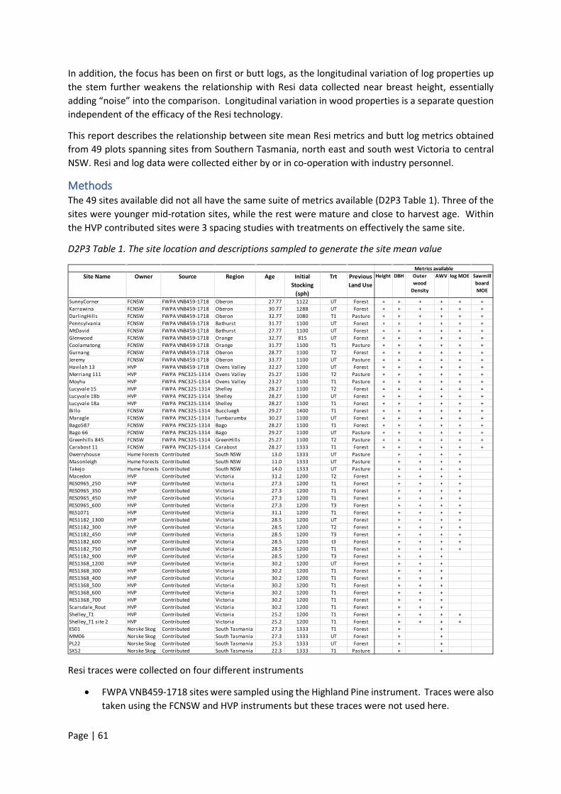
Page | 61

In addition, the focus has been on first or butt logs, as the longitudinal variation of log properties up the stem further weakens the relationship with Resi data collected near breast height, essentially adding “noise” into the comparison. Longitudinal variation in wood properties is a separate question independent of the efficacy of the Resi technology.

This report describes the relationship between site mean Resi metrics and butt log metrics obtained from 49 plots spanning sites from Southern Tasmania, north east and south west Victoria to central NSW. Resi and log data were collected either by or in co-operation with industry personnel.

Methods The 49 sites available did not all have the same suite of metrics available (D2P3 Table 1). Three of the sites were younger mid-rotation sites, while the rest were mature and close to harvest age. Within the HVP contributed sites were 3 spacing studies with treatments on effectively the same site.

D2P3 Table 1. The site location and descriptions sampled to generate the site mean value

Resi traces were collected on four different instruments

• FWPA VNB459-1718 sites were sampled using the Highland Pine instrument. Traces were also taken using the FCNSW and HVP instruments but these traces were not used here.

Site Name Owner Source Region Age Initial Stocking

(sph)

Trt Previous Land Use

Height DBH Outer wood

Density

AWV log MOE Sawmill board MOE

SunnyCorner FCNSW FWPA VNB459-1718 Oberon 27.77 1122 UT Forest + + + + + +Karrawina FCNSW FWPA VNB459-1718 Oberon 30.77 1288 UT Forest + + + + + +DarlingHills FCNSW FWPA VNB459-1718 Oberon 32.77 1080 T1 Pasture + + + + + +Pennsylvania FCNSW FWPA VNB459-1718 Bathurst 31.77 1100 UT Forest + + + + + +MtDavid FCNSW FWPA VNB459-1718 Bathurst 27.77 1100 UT Forest + + + + + +Glenwood FCNSW FWPA VNB459-1718 Orange 32.77 815 UT Forest + + + + + +Coolamatong FCNSW FWPA VNB459-1718 Orange 31.77 1100 T1 Pasture + + + + + +Gurnang FCNSW FWPA VNB459-1718 Oberon 28.77 1100 T2 Forest + + + + + +Jeremy FCNSW FWPA VNB459-1718 Oberon 33.77 1100 UT Pasture + + + + + +Havilah 13 HVP FWPA VNB459-1718 Ovens Valley 32.27 1200 UT Forest + + + + + +Merriang 111 HVP FWPA PNC325-1314 Ovens Valley 25.27 1100 T2 Pasture + + + + + +Moyhu HVP FWPA PNC325-1314 Ovens Valley 23.27 1100 T1 Pasture + + + + + +Lucyvale 15 HVP FWPA PNC325-1314 Shelley 28.27 1100 T2 Forest + + + + + +Lucyvale 18b HVP FWPA PNC325-1314 Shelley 28.27 1100 UT Forest + + + + + +Lucyvale 18a HVP FWPA PNC325-1314 Shelley 28.27 1100 T1 Forest + + + + + +Billo FCNSW FWPA PNC325-1314 Buccluegh 29.27 1400 T1 Forest + + + + + +Maragle FCNSW FWPA PNC325-1314 Tumbarumba 30.27 1100 UT Forest + + + + + +Bago587 FCNSW FWPA PNC325-1314 Bago 28.27 1100 T1 Forest + + + + + +Bago 66 FCNSW FWPA PNC325-1314 Bago 29.27 1100 UT Pasture + + + + + +Greenhills 845 FCNSW FWPA PNC325-1314 GreenHills 25.27 1100 T2 Pasture + + + + + +Carabost 11 FCNSW FWPA PNC325-1314 Carabost 28.27 1333 T1 Forest + + + + + +Dwerryhouse Hume Forests Contributed South NSW 13.0 1333 UT Pasture + + + +Masonleigh Hume Forests Contributed South NSW 11.0 1333 UT Pasture + + + +Takejo Hume Forests Contributed South NSW 14.0 1333 UT Pasture + + + +Macedon HVP Contributed Victoria 31.2 1200 T2 Forest + + + +RES0965_250 HVP Contributed Victoria 27.3 1200 T1 Forest + + + +RES0965_350 HVP Contributed Victoria 27.3 1200 T1 Forest + + + +RES0965_450 HVP Contributed Victoria 27.3 1200 T1 Forest + + + +RES0965_600 HVP Contributed Victoria 27.3 1200 T3 Forest + + + +RES1071 HVP Contributed Victoria 31.1 1200 T1 Forest + + + +RES1182_1300 HVP Contributed Victoria 28.5 1200 UT Forest + + + +RES1182_300 HVP Contributed Victoria 28.5 1200 T2 Forest + + + +RES1182_450 HVP Contributed Victoria 28.5 1200 T3 Forest + + + +RES1182_600 HVP Contributed Victoria 28.5 1200 t3 Forest + + + +RES1182_750 HVP Contributed Victoria 28.5 1200 T1 Forest + + + +RES1182_900 HVP Contributed Victoria 28.5 1200 T3 Forest + + +RES1368_1200 HVP Contributed Victoria 30.2 1200 UT Forest + + +RES1368_300 HVP Contributed Victoria 30.2 1200 T1 Forest + + +RES1368_400 HVP Contributed Victoria 30.2 1200 T1 Forest + + +RES1368_500 HVP Contributed Victoria 30.2 1200 T1 Forest + + +RES1368_600 HVP Contributed Victoria 30.2 1200 T1 Forest + + +RES1368_700 HVP Contributed Victoria 30.2 1200 T1 Forest + + +Scarsdale_Rout HVP Contributed Victoria 30.2 1200 T1 Forest + + +Shelley_T1 HVP Contributed Victoria 25.2 1200 T1 Forest + + + +Shelley_T1 site 2 HVP Contributed Victoria 25.2 1200 T1 Forest + + + +ES01 Norske Skog Contributed South Tasmania 27.3 1333 T1 Forest + +MM06 Norske Skog Contributed South Tasmania 27.3 1333 UT Forest + +PL22 Norske Skog Contributed South Tasmania 25.3 1333 UT Forest + +SX52 Norske Skog Contributed South Tasmania 22.3 1333 T1 Pasture + +

Metrics available

Page | 62

• FWPA PNC325-1314 were collected in 2015 using the NZ Solid Wood innovations (NZSWI) instrument now owned by PF Olsen.

• Seven sites managed by Hume Forests and Norske Skog were sampled using instruments owned by Forest Quality, with the Norske Skog sites sampled in October 2018 with a different instrument than the Hume Forest sites sampled in June 2019.

• The HVP contributed sites were all sampled using the HVP instrument over a 2 year period, during which the instrument was returned for service and /or repair on two occasions. Data from these sites was supplied as site means with processing done within HVP (see Appendix 1 of this report).

Each Resi trace was processed through the web portal (https://forestquality.shinyapps.io/FWPAResiProcessor/) to derive the following values

• DBHOB: Breast height diameter over bark • DBHUB: Breast height diameter under-bark • Basic density as a mean of

o The outer 50 mm on the entry side o The pith-to-bark or bark-to-bark average o An area-weighted estimate of the stem cross-section

• PrAWV: Predicted Acoustic Wave Velocity • PrMOE: Predicted Modulus of Elasticity

Predicted values of AWV and MOE were available via five different predictive algorithms

• NZSWI: Essentially the algorithm used in the NZSWI funded software tool developed in 2016. Most accurate when annual ring boundaries are allocated requiring considerable user intervention

• Young: multiple regression relationship defined in 7 year old radiata pine data contributed by Tree Breeding Australia (see Deliverable 2 Part 1)

• Mature: Multiple regression relationship using variables derived from the pith-to-bark trace independent of annual ring allocation, thus requiring less user intervention

• Outerwood: Partial least square regression relationship defined in milestone 3 and refined for milestone 5 using only variables automatically derived from the outer 50 mm of the radius along with radial length

• Density: A regression based only on the mean pith-to-bark density scaled into units equivalent to AWV (km.sec-1) or MOE (GPa)

For each trace PrAWV and PrMOE was obtained from the entry radius, and in bark-to-bark traces from the exit radius also. In the latter case the mean of the two predictions was returned.

Data Analysis Resi traces for each site were uploaded to the web portal and stored as a project (*.Resi). Traces were checked to ensure assigned pith and cambial positions were correct and that trace type (P-B or B-B) had been correctly identified. Basic density, PrAWV and PrMOE values were determined using the appropriate regression coefficients for the particular Resi instrument. With the HVP instrument some variance over time was observed and identified as related to various service and repair events (see Appendix 1 of this report) and appropriate coefficients used according to the time of sampling.

PrAWV and PrMOE were calculated by rerunning the project for each different model in turn, downloading the summary data table and collating the different model predictions into a single


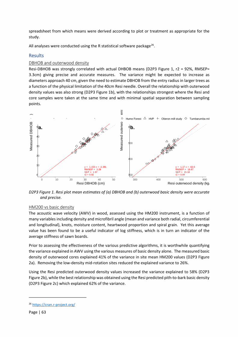
Page | 63

spreadsheet from which means were derived according to plot or treatment as appropriate for the study.

All analyses were conducted using the R statistical software package26.

Results DBHOB and outerwood density Resi-DBHOB was strongly correlated with actual DHBOB means (D2P3 Figure 1, r2 = 92%, RMSEP= 3.3cm) giving precise and accurate measures. The variance might be expected to increase as diameters approach 40 cm, given the need to estimate DBHOB from the entry radius in larger trees as a function of the physical limitation of the 40cm Resi needle. Overall the relationship with outerwood density values was also strong (D2P3 Figure 1b), with the relationships strongest where the Resi and core samples were taken at the same time and with minimal spatial separation between sampling points.

D2P3 Figure 1. Resi plot mean estimates of (a) DBHOB and (b) outerwood basic density were accurate and precise.

HM200 vs basic density The acoustic wave velocity (AWV) in wood, assessed using the HM200 instrument, is a function of many variables including density and microfibril angle (mean and variance both radial, circumferential and longitudinal), knots, moisture content, heartwood proportion and spiral grain. Yet this average value has been found to be a useful indicator of log stiffness, which is in turn an indicator of the average stiffness of sawn boards.

Prior to assessing the effectiveness of the various predictive algorithms, it is worthwhile quantifying the variance explained in AWV using the various measures of basic density alone. The measured basic density of outerwood cores explained 41% of the variance in site mean HM200 values (D2P3 Figure 2a). Removing the low-density mid-rotation sites reduced the explained variance to 26%.

Using the Resi predicted outerwood density values increased the variance explained to 58% (D2P3 Figure 2b), while the best relationship was obtained using the Resi predicted pith-to-bark basic density (D2P3 Figure 2c) which explained 62% of the variance.

26 https://cran.r-project.org/

a.

y = 1.153 x + -2.391RMSEP = 3.29SEP = 1.97r2 = 0.920

10

20

30

40

50

0 10 20 30 40 50Resi DBHOB (cm)

Mea

sure

d D

BH

OB

(cm

)

Hume Forest HVP Oberon mill study Tumbarumba mill study

b.

y = 1.17 x + -62.6RMSEP = 19.87SEP = 15.18r2 = 0.84300

400

500

600

300 400 500 600Resi outerwood density (kg/

Mea

sure

d ou

terw

ood

dens

Hume Forest HVP Oberon mill study Tumbarumba mil

https://cran.r-project.org/

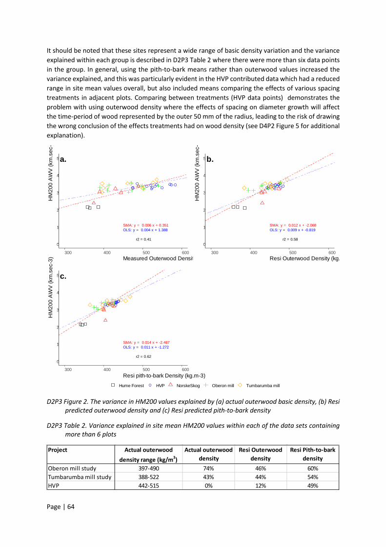
Page | 64

It should be noted that these sites represent a wide range of basic density variation and the variance explained within each group is described in D2P3 Table 2 where there were more than six data points in the group. In general, using the pith-to-bark means rather than outerwood values increased the variance explained, and this was particularly evident in the HVP contributed data which had a reduced range in site mean values overall, but also included means comparing the effects of various spacing treatments in adjacent plots. Comparing between treatments (HVP data points) demonstrates the problem with using outerwood density where the effects of spacing on diameter growth will affect the time-period of wood represented by the outer 50 mm of the radius, leading to the risk of drawing the wrong conclusion of the effects treatments had on wood density (see D4P2 Figure 5 for additional explanation).

D2P3 Figure 2. The variance in HM200 values explained by (a) actual outerwood basic density, (b) Resi predicted outerwood density and (c) Resi predicted pith-to-bark density

D2P3 Table 2. Variance explained in site mean HM200 values within each of the data sets containing more than 6 plots

a.

SMA: y = 0.006 x + 0.351OLS: y = 0.004 x + 1.388

r2 = 0.410

1

2

3

4

5

300 400 500 600Measured Outerwood Density (kg.m-3)

HM

200

AW

V (k

m.s

ec-

b.

SMA: y = 0.012 x + -2.068OLS: y = 0.009 x + -0.819

r2 = 0.580

1

2

3

4

5

300 400 500 600Resi Outerwood Density (kg.

HM

200

AW

V (k

m.s

ec-

c.

SMA: y = 0.014 x + -2.467OLS: y = 0.011 x + -1.272

r2 = 0.620

1

2

3

4

5

300 400 500 600Resi pith-to-bark Density (kg.m-3)

HM

200

AW

V (k

m.s

ec-3

)

Hume Forest HVP NorskeSkog Oberon mill Tumbarumba mill

Project Actual outerwood density range (kg/m3)

Actual outerwood density

Resi Outerwood density

Resi Pith-to-bark density

Oberon mill study 397-490 74% 46% 60%Tumbarumba mill study 388-522 43% 44% 54%HVP 442-515 0% 12% 49%

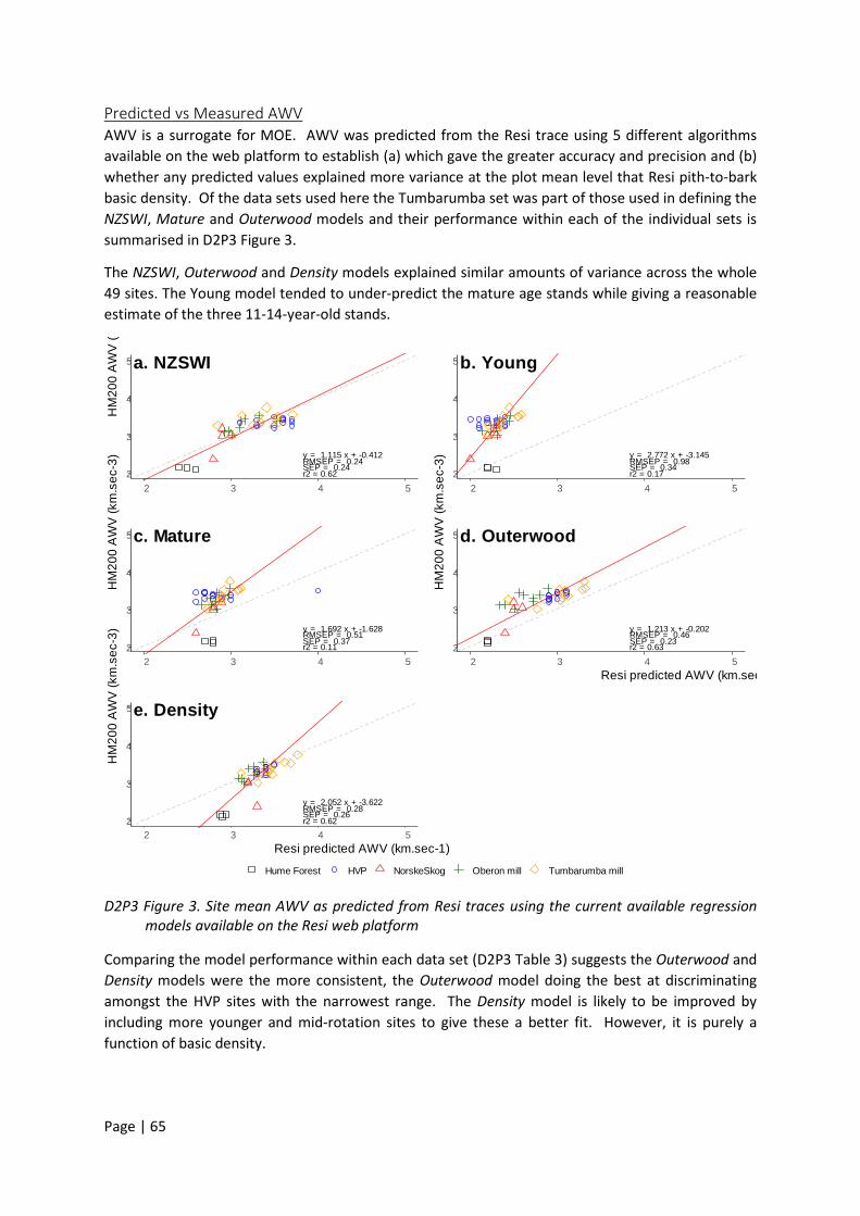
Page | 65

Predicted vs Measured AWV AWV is a surrogate for MOE. AWV was predicted from the Resi trace using 5 different algorithms available on the web platform to establish (a) which gave the greater accuracy and precision and (b) whether any predicted values explained more variance at the plot mean level that Resi pith-to-bark basic density. Of the data sets used here the Tumbarumba set was part of those used in defining the NZSWI, Mature and Outerwood models and their performance within each of the individual sets is summarised in D2P3 Figure 3.

The NZSWI, Outerwood and Density models explained similar amounts of variance across the whole 49 sites. The Young model tended to under-predict the mature age stands while giving a reasonable estimate of the three 11-14-year-old stands.

D2P3 Figure 3. Site mean AWV as predicted from Resi traces using the current available regression models available on the Resi web platform

Comparing the model performance within each data set (D2P3 Table 3) suggests the Outerwood and Density models were the more consistent, the Outerwood model doing the best at discriminating amongst the HVP sites with the narrowest range. The Density model is likely to be improved by including more younger and mid-rotation sites to give these a better fit. However, it is purely a function of basic density.

a. NZSWI

y = 1.115 x + -0.412RMSEP = 0.24SEP = 0.24r2 = 0.622

3

4

5

2 3 4 5

HM

200

AW

V (

b. Young

y = 2.772 x + -3.145RMSEP = 0.98SEP = 0.34r2 = 0.172

3

4

5

2 3 4 5

c. Mature

y = 1.692 x + -1.628RMSEP = 0.51SEP = 0.37r2 = 0.112

3

4

5

2 3 4 5

HM

200

AW

V (k

m.s

ec-3

)

d. Outerwood

y = 1.213 x + -0.202RMSEP = 0.46SEP = 0.23r2 = 0.632

3

4

5

2 3 4 5Resi predicted AWV (km.sec

HM

200

AW

V (k

m.s

ec-3

)

e. Density

y = 2.052 x + -3.622RMSEP = 0.28SEP = 0.26r2 = 0.622

3

4

5

2 3 4 5Resi predicted AWV (km.sec-1)

HM

200

AW

V (k

m.s

ec-3

)


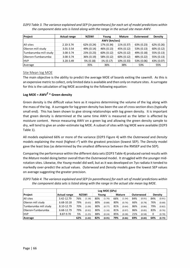
Page | 66

D2P3 Table 3. The variance explained and SEP (in parentheses) for each set of model predictions within the component data sets is listed along with the range in the actual site mean AWV.

Site Mean log MOE The main objective is the ability to predict the average MOE of boards exiting the sawmill. As this is an expensive metric to collect, only limited data is available and then only on mature sites. A surrogate for this is the calculation of log MOE according to the following equation:

Log MOE = AWV2 * Green density

Green density is the difficult value here as it requires determining the volume of the log along with the mass of the log. A surrogate for log green density has been the use of cross-section discs (typically small end). This has been shown to give strong relationships with log green density. It is important that green density is determined at the same time AWV is measured as the latter is affected by moisture content. Hence measuring AWV on a green log and allowing the green density sample to dry, will tend to give an under-estimate log MOE. A subset of sites with log MOE were available (D2P3 Table 1).

All models explained 66% or more of the variance (D2P3 Figure 4) with the Outerwood and Density models explaining the most (highest r2) with the greatest precision (lowest SEP). The Density model gave the least bias (as determined by the smallest difference between the RMSEP and the SEP).

Comparing the performance within the different data sets (D2P3 Table 4) produced varied results with the Mature model doing better overall than the Outerwood model. It struggled with the younger mid-rotation sites. Likewise, the Young model did well, but as it was developed on 7yo radiata it tended to markedly over-predict the actual values. Outerwood and Density models gave the lowest SEP values on average suggesting the greater precision.

D2P3 Table 4. The variance explained and SEP (in parentheses) for each set of model predictions within the component data sets is listed along with the range in the actual site mean log MOE.

Project Actual range NZSWI Young Mature Outerwood Density

All sites 2.10-3.74 62% (0.24) 17% (0.34) 11% (0.37) 63% (0.23) 62% (0.26)Oberon mill study 3.01-3.54 49% (0.14) 46% (0.13) 45% (0.12) 53% (0.13) 60% (0.12)Tumbarumba mill study 3.00-3.74 23% (0.23) 60% (0.12) 62% (0.12) 49% (0.18) 55% (0.13)Oberon+Tumbarumba 3.00-3.74 36% (0.19) 58% (0.12) 60% (0.12) 48% (0.22) 55% (0.13)HVP 3.20-3.49 5% (0.18) 1% (0.17) 10% (0.33) 53% (0.06) 43% (0.07)Average 35% 36% 38% 53% 55%

AWV (km/sec)

Project Actual range All sites 3.42-12.79 76% (1.18) 80% (1.70) 66% (1.54) 84% (0.91) 84% (0.91)

Oberon mill study 6.68-10.18 79% (0.65) 80% (0.88) 80% (0.76) 66% (0.78) 76% (0.68)

Tumbarumba mill study 8.10-12.79 70% (1.09) 80% (0.77) 81% (0.64) 86% (0.86) 79% (0.82)

Oberon+Tumbarumba 6.68-12.79 79% (0.92) 80% (1.16) 81% (0.97) 86% (0.85) 83% (0.76)

HVP 8.87-9.70 5% (1.25) 88% (0.24) 85% (0.38) 21% (0.58) 0 (0.78)

Average 62% (1.02) 82% (0.95) 79% (0.86) 69% (0.80) 64% (0.79)

Log MOE (GPa)NZSWI Young Mature Outerwood Density

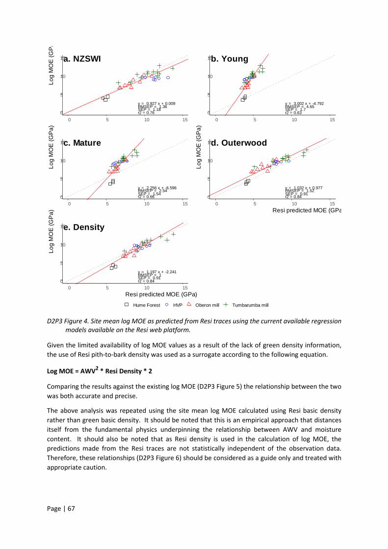
Page | 67

D2P3 Figure 4. Site mean log MOE as predicted from Resi traces using the current available regression models available on the Resi web platform.

Given the limited availability of log MOE values as a result of the lack of green density information, the use of Resi pith-to-bark density was used as a surrogate according to the following equation.

Log MOE = AWV2 * Resi Density * 2

Comparing the results against the existing log MOE (D2P3 Figure 5) the relationship between the two was both accurate and precise.

The above analysis was repeated using the site mean log MOE calculated using Resi basic density rather than green basic density. It should be noted that this is an empirical approach that distances itself from the fundamental physics underpinning the relationship between AWV and moisture content. It should also be noted that as Resi density is used in the calculation of log MOE, the predictions made from the Resi traces are not statistically independent of the observation data. Therefore, these relationships (D2P3 Figure 6) should be considered as a guide only and treated with appropriate caution.

a. NZSWI

y = 0.927 x + 0.009RMSEP = 1.36SEP = 1.18r2 = 0.760

5

10

15

0 5 10 15

Log

MO

E (G

Pa

b. Young

y = 3.002 x + -4.792RMSEP = 4.65SEP = 1.7r2 = 0.630

5

10

15

0 5 10 15

c. Mature

y = 2.256 x + -6.596RMSEP = 2.54SEP = 1.54r2 = 0.660

5

10

15

0 5 10 15

Log

MO

E (G

Pa)

d. Outerwood

y = 1.032 x + 0.977RMSEP = 1.52SEP = 0.91r2 = 0.840

5

10

15

0 5 10 15Resi predicted MOE (GPa

Log

MO

E (G

Pa)

e. Density

y = 1.197 x + -2.241RMSEP = 1SEP = 0.91r2 = 0.840

5

10

15

0 5 10 15Resi predicted MOE (GPa)

Log

MO

E (G

Pa)

Hume Forest HVP Oberon mill Tumbarumba mill

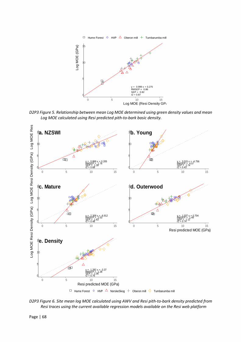
Page | 68

D2P3 Figure 5. Relationship between mean Log MOE determined using green density values and mean Log MOE calculated using Resi predicted pith-to-bark basic density.

D2P3 Figure 6. Site mean log MOE calculated using AWV and Resi pith-to-bark density predicted from Resi traces using the current available regression models available on the Resi web platform

y = 0.999 x + 0.275RMSEP = 0.86SEP = 0.82r2 = 0.870

5

10

15

0 5 10 15Log MOE (Resi Density GPa

Log

MO

E (G

Pa)

Hume Forest HVP Oberon mill Tumbarumba mill

a. NZSWI

y = 0.869 x + 0.205RMSEP = 1.76SEP = 1.39r2 = 0.680

5

10

15

0 5 10 15

Log

MO

E R

es

b. Young

y = 3.015 x + -4.756RMSEP = 4.57SEP = 1.74r2 = 0.430

5

10

15

0 5 10 15

c. Mature

y = 2.309 x + -6.912RMSEP = 2.53SEP = 1.63r2 = 0.480

5

10

15

0 5 10 15

Log

MO

E R

esi D

ensi

ty (G

Pa)

d. Outerwood

y = 1.037 x + 0.704RMSEP = 1.49SEP = 1.12r2 = 0.740

5

10

15


e. Density

y = 1.282 x + -3.37RMSEP = 1.28SEP = 1.06r2 = 0.760

5

10

15


Log

MO

E R

esi D

ensi

ty (G

Pa)


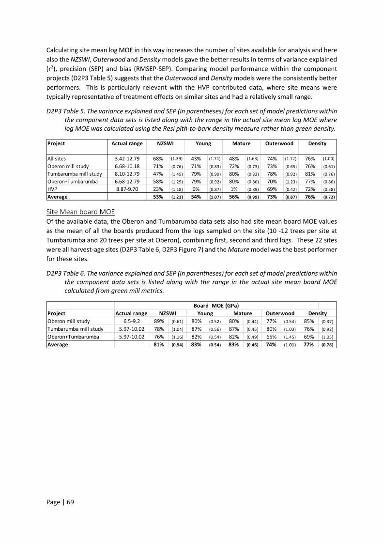
Page | 69

Calculating site mean log MOE in this way increases the number of sites available for analysis and here also the NZSWI, Outerwood and Density models gave the better results in terms of variance explained (r2), precision (SEP) and bias (RMSEP-SEP). Comparing model performance within the component projects (D2P3 Table 5) suggests that the Outerwood and Density models were the consistently better performers. This is particularly relevant with the HVP contributed data, where site means were typically representative of treatment effects on similar sites and had a relatively small range.

D2P3 Table 5. The variance explained and SEP (in parentheses) for each set of model predictions within the component data sets is listed along with the range in the actual site mean log MOE where log MOE was calculated using the Resi pith-to-bark density measure rather than green density.

Site Mean board MOE Of the available data, the Oberon and Tumbarumba data sets also had site mean board MOE values as the mean of all the boards produced from the logs sampled on the site (10 -12 trees per site at Tumbarumba and 20 trees per site at Oberon), combining first, second and third logs. These 22 sites were all harvest-age sites (D2P3 Table 6, D2P3 Figure 7) and the Mature model was the best performer for these sites.

D2P3 Table 6. The variance explained and SEP (in parentheses) for each set of model predictions within the component data sets is listed along with the range in the actual site mean board MOE calculated from green mill metrics.

Project Actual range

All sites 3.42-12.79 68% (1.39) 43% (1.74) 48% (1.63) 74% (1.12) 76% (1.00)

Oberon mill study 6.68-10.18 71% (0.76) 71% (0.83) 72% (0.73) 73% (0.65) 76% (0.61)



HVP 8.87-9.70 23% (1.18) 0% (0.87) 1% (0.89) 69% (0.42) 72% (0.38)

Average 53% (1.21) 54% (1.07) 56% (0.99) 73% (0.87) 76% (0.72)

NZSWI Young Mature Outerwood Density

Project Actual range Oberon mill study 6.5-9.2 89% (0.61) 80% (0.52) 80% (0.44) 77% (0.54) 85% (0.37)



Average 81% (0.94) 83% (0.54) 83% (0.46) 74% (1.01) 77% (0.78)

Board MOE (GPa)NZSWI Young Mature Outerwood Density

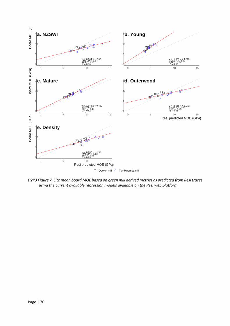
Page | 70

D2P3 Figure 7. Site mean board MOE based on green mill derived metrics as predicted from Resi traces using the current available regression models available on the Resi web platform.

a. NZSWI

y = 0.564 x + 2.62RMSEP = 1.97SEP = 1.16r2 = 0.760

5

10

15

0 5 10 15

Boa

rd M

OE

(Gb. Young

y = 1.433 x + 1.309RMSEP = 3.39SEP = 0.54r2 = 0.820

5

10

15

0 5 10 15

c. Mature

y = 1.076 x + 0.459RMSEP = 1.11SEP = 0.49r2 = 0.820

5

10

15

0 5 10 15

Boa

rd M

OE

(GP

a)

d. Outerwood

y = 0.515 x + 3.972RMSEP = 1.45SEP = 1.45r2 = 0.650

5

10

15


e. Density

y = 0.632 x + 1.95RMSEP = 1.92SEP = 1.05r2 = 0.690

5

10

15


Boa

rd M

OE

(GP

a)

Oberon mill Tumbarumba mill

Page | 71

Appendix 1: Assessment of HVP calibration data. Geoff Downes and Stephen Elms

Background In order to use Resi data to validate the prediction of acoustic wave velocity (AWV) and modulus of elasticity (MOE), or for rCambium predictions (see Deliverable 4 Part 2), its accuracy and precision in the prediction of basic density needs to be acceptable. Any random or unexplained variance arising from the Resi data can affect the evaluation of Resi predictions potentially making them seem less precise because the variance explained is low. Likewise, some of the current algorithms for the prediction of AWV are based on Resi traces after they have been converted to basic density values, in order to compensate for instrument-dependent relationships in basic density prediction.

• HVP have been using their PD-400 Resi since October 2017. • Over the past 2 years they have been assessing trials and comparing Resi values against a

subset of actual density values from 50mm long outerwood cores. • Individual regressions between Resi values and basic density have varied significantly making

the absolute values of density less valuable for comparison over time. • During the past 2 years the Resi has been returned for service and repair on two occasions,

dividing the collected data into 3 classes defined by date A. Pre first service (issues with dirt in the telescope) B. After first service and before the second service (repair) where it was giving overload

messages C. After the third service

Objective To examine the Resi data sets collected by HVP over time and endeavour to identify how Resi regression coefficients may have varied and determine those best used to generate the most accurate predictions of density. These Resi-predictions can then be used with more confidence in evaluating other predictive algorithms consistently between different Resi instruments.

Initial data assessment In D2P3 Figure 8, the various data sets were compared, and a general regression applied across them all to examine the fit. Two types of regression are used in the plot

• Ordinary Least squares (OLS) of the type used in Excel which assumes the y-values (density) are true with no variance

• Standard (reduced) Major Axis regression (SMA)27 which assumes some random variance in both the x and y values.

When comparing Resi values with actual density from cores, errors arise from a number of sources. Firstly, the measurements are not taken from exactly the same wood, no matter how closely aligned they are. The closer the measurement points are spatially, the stronger the correlation between them. Secondly, the portion of the radius extracted from the Resi trace might be slightly different from that used for the core density in terms of the start and stop point for determining the 50 mm length, also slight variances in the length of the actual core, and the orientation of the core with respect to the pith-to-bark direction. In this case it is arguably better to use the SMA regression coefficients. OLS regression tends to reduce the slope and increase the intercept.

27 https://twin.sci-hub.tw/6617/b615c5cebc733901b3cf9a812baaa269/harper2016.pdf

https://twin.sci-hub.tw/6617/b615c5cebc733901b3cf9a812baaa269/harper2016.pdf

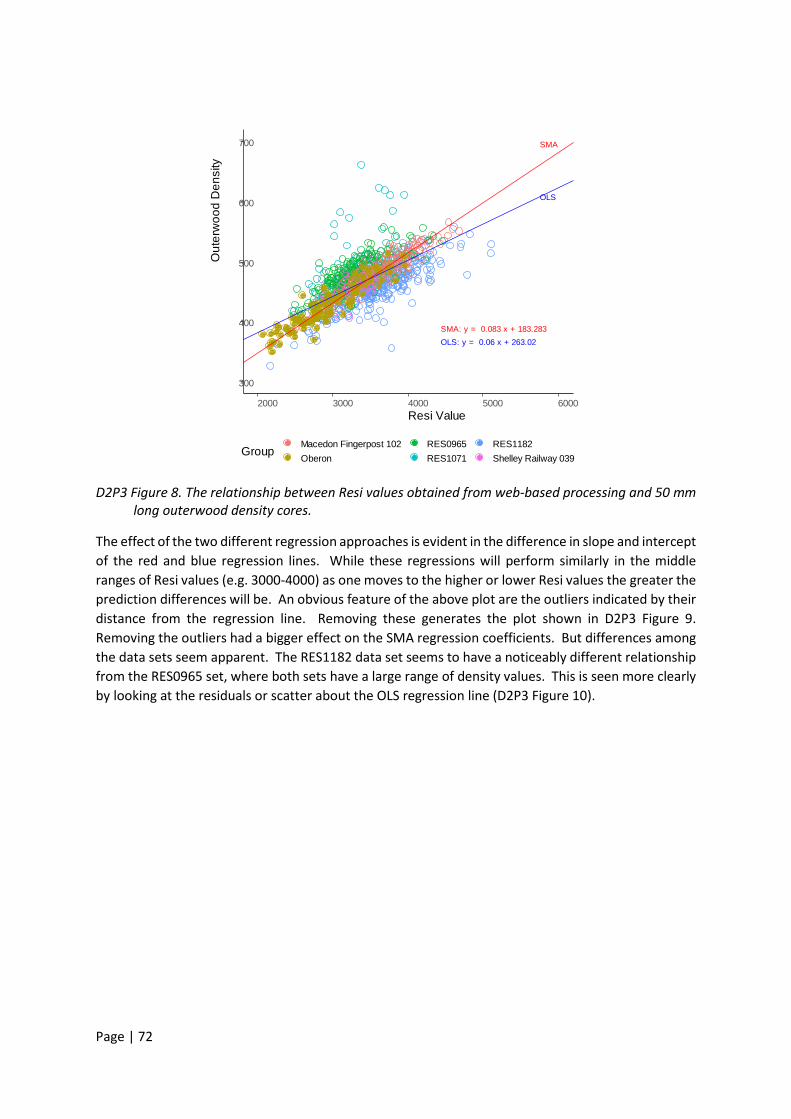
Page | 72

D2P3 Figure 8. The relationship between Resi values obtained from web-based processing and 50 mm long outerwood density cores.

The effect of the two different regression approaches is evident in the difference in slope and intercept of the red and blue regression lines. While these regressions will perform similarly in the middle ranges of Resi values (e.g. 3000-4000) as one moves to the higher or lower Resi values the greater the prediction differences will be. An obvious feature of the above plot are the outliers indicated by their distance from the regression line. Removing these generates the plot shown in D2P3 Figure 9. Removing the outliers had a bigger effect on the SMA regression coefficients. But differences among the data sets seem apparent. The RES1182 data set seems to have a noticeably different relationship from the RES0965 set, where both sets have a large range of density values. This is seen more clearly by looking at the residuals or scatter about the OLS regression line (D2P3 Figure 10).

SMA: y = 0.083 x + 183.283OLS: y = 0.06 x + 263.02

OLS

SMA

300

400

500

600

700

2000 3000 4000 5000 6000Resi Value

Out

erw

ood

Den

sity

GroupMacedon Fingerpost 102Oberon

RES0965RES1071

RES1182Shelley Railway 039

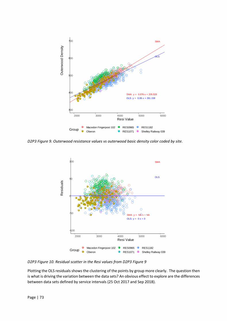
Page | 73

D2P3 Figure 9. Outerwood resistance values vs outerwood basic density color coded by site.

D2P3 Figure 10. Residual scatter in the Resi values from D2P3 Figure 9

Plotting the OLS residuals shows the clustering of the points by group more clearly. The question then is what is driving the variation between the data sets? An obvious effect to explore are the differences between data sets defined by service intervals (25 Oct 2017 and Sep 2018).

SMA: y = 0.076 x + 205.528OLS: y = 0.06 x + 261.159

OLS

SMA

300

400

500

600

700

2000 3000 4000 5000 6000Resi Value

Out

erw

ood

Den

sity


RES0965RES1071


SMA: y = NA x + NAOLS: y = 0 x + 0

OLS

SMA

-100

-50

0

50

100

2000 3000 4000 5000 6000Resi Value

Res

idua

ls


RES0965RES1071


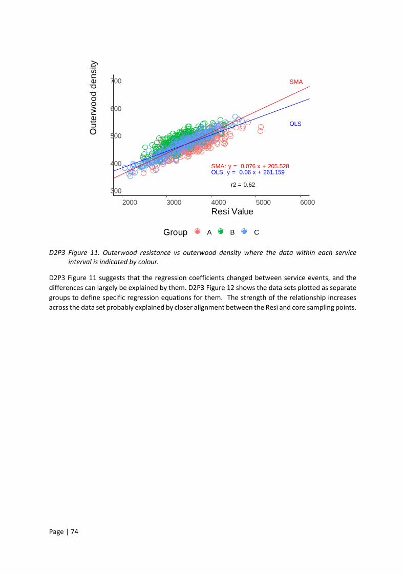
Page | 74

D2P3 Figure 11. Outerwood resistance vs outerwood density where the data within each service interval is indicated by colour.

D2P3 Figure 11 suggests that the regression coefficients changed between service events, and the differences can largely be explained by them. D2P3 Figure 12 shows the data sets plotted as separate groups to define specific regression equations for them. The strength of the relationship increases across the data set probably explained by closer alignment between the Resi and core sampling points.

SMA: y = 0.076 x + 205.528OLS: y = 0.06 x + 261.159

OLS

SMA

r2 = 0.62300

400

500

600

700

2000 3000 4000 5000 6000Resi Value

Out

erw

ood

dens

ity

Group A B C

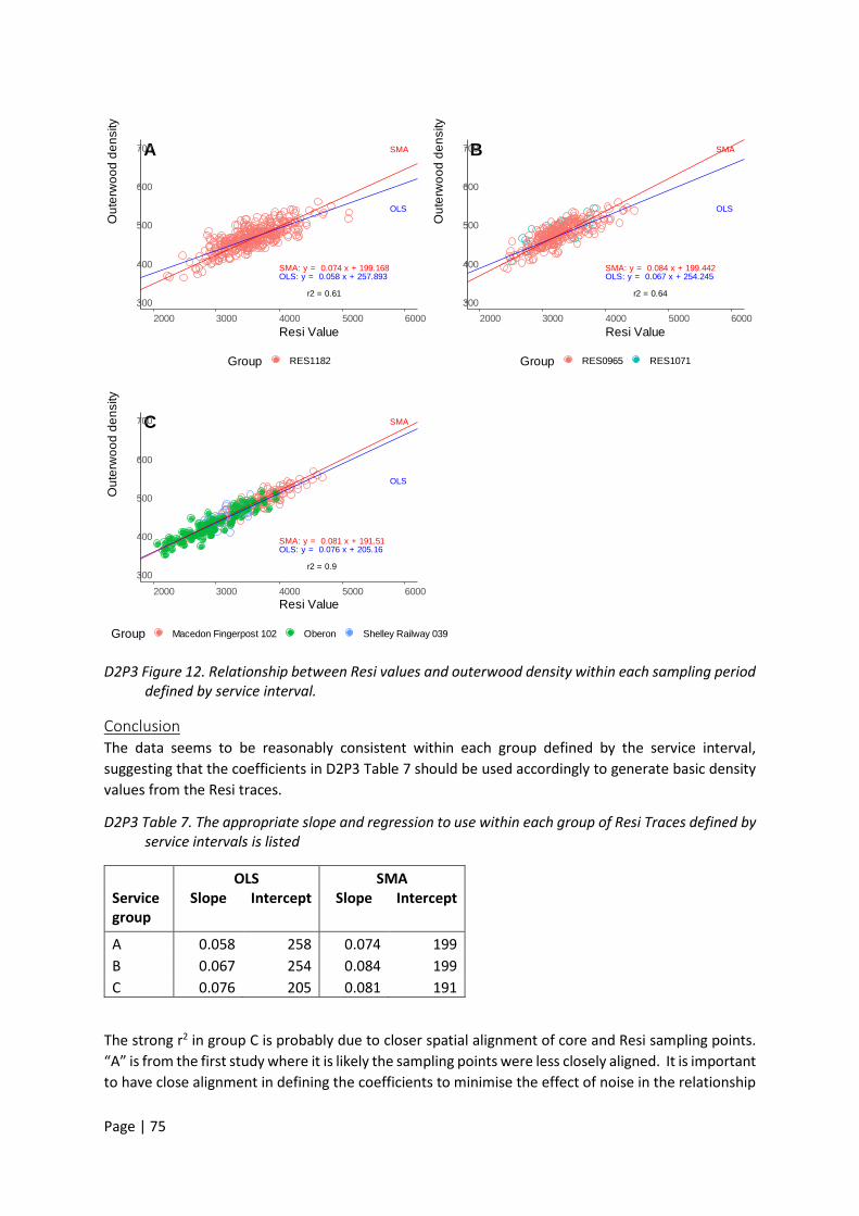
Page | 75

D2P3 Figure 12. Relationship between Resi values and outerwood density within each sampling period defined by service interval.

Conclusion The data seems to be reasonably consistent within each group defined by the service interval, suggesting that the coefficients in D2P3 Table 7 should be used accordingly to generate basic density values from the Resi traces.

D2P3 Table 7. The appropriate slope and regression to use within each group of Resi Traces defined by service intervals is listed

OLS SMA Service group

Slope Intercept Slope Intercept

A 0.058 258 0.074 199 B 0.067 254 0.084 199 C 0.076 205 0.081 191

The strong r2 in group C is probably due to closer spatial alignment of core and Resi sampling points. “A” is from the first study where it is likely the sampling points were less closely aligned. It is important to have close alignment in defining the coefficients to minimise the effect of noise in the relationship

A

SMA: y = 0.074 x + 199.168OLS: y = 0.058 x + 257.893

OLS

SMA

r2 = 0.61300

400

500

600

700

2000 3000 4000 5000 6000Resi Value

Out

erw

ood

dens

ity

Group RES1182

B

SMA: y = 0.084 x + 199.442OLS: y = 0.067 x + 254.245

OLS

SMA

r2 = 0.64300

400

500

600

700

2000 3000 4000 5000 6000Resi Value

Out

erw

ood

dens

ity

Group RES0965 RES1071

C

SMA: y = 0.081 x + 191.51OLS: y = 0.076 x + 205.16

OLS

SMA

r2 = 0.9300

400

500

600

700

2000 3000 4000 5000 6000Resi Value

Out

erw

ood

dens

ity

Group Macedon Fingerpost 102 Oberon Shelley Railway 039

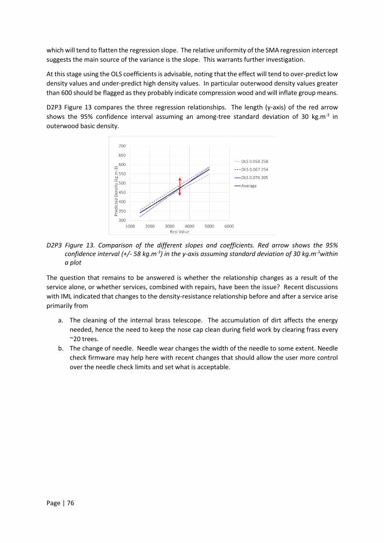
Page | 76

which will tend to flatten the regression slope. The relative uniformity of the SMA regression intercept suggests the main source of the variance is the slope. This warrants further investigation.

At this stage using the OLS coefficients is advisable, noting that the effect will tend to over-predict low density values and under-predict high density values. In particular outerwood density values greater than 600 should be flagged as they probably indicate compression wood and will inflate group means.

D2P3 Figure 13 compares the three regression relationships. The length (y-axis) of the red arrow shows the 95% confidence interval assuming an among-tree standard deviation of 30 kg.m-3 in outerwood basic density.

D2P3 Figure 13. Comparison of the different slopes and coefficients. Red arrow shows the 95% confidence interval (+/- 58 kg.m-3) in the y-axis assuming standard deviation of 30 kg.m-3within a plot

The question that remains to be answered is whether the relationship changes as a result of the service alone, or whether services, combined with repairs, have been the issue? Recent discussions with IML indicated that changes to the density-resistance relationship before and after a service arise primarily from

a. The cleaning of the internal brass telescope. The accumulation of dirt affects the energy needed, hence the need to keep the nose cap clean during field work by clearing frass every ~20 trees.

b. The change of needle. Needle wear changes the width of the needle to some extent. Needle check firmware may help here with recent changes that should allow the user more control over the needle check limits and set what is acceptable.

Page | 77

Deliverable 2 Part 4. Southern Pine assessment of stiffness predictions using IML-Resi PD400 (Experiment 374 SIL)

Lee D.J. (USC), G.M. Downes (FQ) & D.P. Kain (HQPlantations)

Corresponding author: [email protected]

Key Findings. The project has found that the IML Resi PD400 has potential to assist in predicting the wood quality of Southern Pine stands. In particular:

• Resi was good at predicting individual tree basic density and excellent at predicting site average basic density of Southern Pine stands, as it explains 89% of the variance.

• The NZSWI ResiProcessor model for PrMOE explains more of the variance in site average Tree MOE than other models tested. Across three levels of interventions this model explains 66-71% of the Tree MOE.

Background Non-destructive evaluation of wood properties and decay in timber and trees using micro-drill resistance tools have been studied for over 30 years. However, widespread adoption of these resistance tools for wood quality assessments are only reported in the last few years, as the precision of the data collected and algorithms needed to analyse this data have been developed (e.g. Rinn 2013. Downes et al., 2018, Sharapov et al., 2019). These micro-drill resistance tools measure variations in drilling resistance of a thin needle when driven into a tree at a constant force. Sharapov et al. (2019) and Goa et al (2017) have reviewed the application of these tools finding they have been useful to assess wood density, tree growth rings and decay in timber and trees.

In Australia, the most used Resistograph tool is the IML Resi PD400. This Resi generates a ‘trace’ of measurements at 0.1 mm intervals containing detailed information about wood properties and stem diameter of a tree or log. Assessment of a single tree takes less than 10 seconds. Measured variables include: power consumption, torque, depth penetration through time.

Isik and Li (2003), evaluated an older version of the IML Resistograph tool in four 11 year old loblolly pine (Pinus taeda) progeny trials; directly comparing density measured on bark to bark cores to the Resistograph reading (amplitude) and found significant, weak to moderate phenotypic correlations between wood density and the Resistograph amplitude regression equation (r=0.29 to 0.65 across the four sites), however the correlation across all sites was weak (r=0.12). Given this they found a high family mean correlation between density and Resistograph amplitude, leading them to conclude the Resistograph could be used to rank loblolly pine families for wood density. In another study Gantz (2002) found that phenotypic correlations between Resistograph amplitudes and wood density was moderate for four species (two Pinus and two Eucalyptus species), R2 ranging from between 0.30 to 0.78. Recently, strong linear correlations (R2 range 0.66 to 0.87) have been found with the basic density of increment cores of eucalypt species (E. nitens and E. globulus) across 8 sites in southern Australia (Downes et al., 2018).

Flexing of the drill bit during drilling by the operator, air temperature variation (-20°C to +20°C), and presence of knots impact the quality of the Resistograph traces and data from interior spruce (Picea spp.; Ukrainetz and O’Neill, 2010). In addition, moisture content of the wood may affect drilling resistance in a range of species (Lin et al., 2003, Ukrainetz and O’Neill, 2010). Another issue observed


Page | 78

when using micro-drill resistance tools is friction on the drill shaft as the drill penetrates further into the stem, resulting in poorer correlations between the resistance and density (specific gravity) of tropical hardwood species (Nutto and Biechele, 2015) and eucalypt hybrids (Oliveira et al 2017). This however is not considered to be an issue for softwoods (Rinn et al., 1996).

The ability of the IML Resi to predict log MOE and log HM200 acoustic wave velocity (AWV) has been the recent focus of a number of studies with Downes et al. (2016) finding that site average predictions involving 12 sites were moderately to strongly correlated with HM200 AWV (R2=0.47) and actual log MOE (R2=0.66) for P. radiata in a destructive study.

Preliminary studies have been undertaken in HQPlantations’ Southern Pine estate testing the New Zealand Solid Wood Initiative (SWI) Resi-based algorithms for predicting Log MOE and or AWV:

1. A 2016 pilot study, where HM200 AWV was predicted with R2=0.95 at the taxon mean level (Lausberg et al. 2016).

2. The 2018 SPRC28 study that found individual-log dynamic MOE (BING method) was predicted with R2=0.68 with a 9% bias at the tree level (Bailleres et al. 2018). This result is comparable with SWI results at the tree level in radiata pine.

3. The 2018 SPRC site mean study, where a positive relationship was indicated between Resi and core MOE at the site mean level; however, there were issues with Resi under-predicting the MOE of mid rotation age trees (17-24 years old) compared to that measured using ultrasound on cores (Bailleres et al. 2018).

Resi may also be suitable for rapid assessment of underbark diameter. An HQP pilot study (Durocher et al. 2017) found R2=0.99 between tape and Resi measures of underbark diameter in a small sample of 10 trees. The PD400 is limited to stems 40 cm in diameter, though larger models are available.

The aim of this study is to operationalise the use of the Resi for wood quality resource characterisation in HQP’s Southern Pine estate by calibrating the Resi tool against log MOE across a range of sites of varying MOE and site index. This work will be carried out in Experiment 374 SIL (this experiment). This study will also test a range of algorithms that have been developed for the IML Resi including: ‘Outerwood’, ‘Mature’ and the ‘SWI’ models and a range of interventions of the Resi-traces (described in the methods section) to see which of these works best for Southern Pines.

28 FWPA-funded Southern Pine Resource Characterisation Study PNC361-1415 (2015-2018)

Page | 79

Glossary AWV Acoustic wave velocity. Bias A measure of the distance between the value of the measurements and the true value

of the sample. Buttlog Six metre log taken from the bottom of the tree. DBHOB Diameter at breast height over bark. HM200 HM200 (Fibre-gen, New Zealand) resonance acoustic tool. Log2 Six metre log taken above the Buttlog. MOE (modulus of elasticity) infers a material’s resistance against deformation. It is an

important property of a material to any external stress. Pr As in PrMOE is the ResiProcessor predicted MOE. Resi IML Resi PD400 Site Location or plot from which a sample was collected. Slenderness Ratio of tree height / tree DBHOB. ST300 The ST300 (Fibre-gen, New Zealand) time of flight standing tree acoustic tool. Tree The average of the Buttlog and Log2 measurements. It is often used in the form with

another term e.g. Tree MOE = the average MOE of the Buttlog and Log2 MOE USMOE The MOE predicted from the core by integration of the core segments predicted from

ultrasound measurement of MOE at 8% moisture content. This was measured in the Southern Pine Resource Characterisation Project: PNC361-1415.

Materials and methods Data for IML Resi calibration (374 SIL) was collected from the following sources:

• Nine Pinus elliottii var. elliottii (PEE) x Pinus caribaea var. hondurensis (PCH) hybrid pine (F1 or F2 hybrid) permanent growth plots previously assessed in the SPRC, which had been identified for priority detailed sample tree (DST) assessment (D2P4 Table 1).

• Five PCH permanent growth plots previously assessed in the SPRC available for destructive sampling (D2P4 Table 1).

D2P4 Table 1. Details of the 14 sites sampled in this study (9 hybrid sites and 5 PCH sites)

Within plot selection and measurement of trees Approximately 20 trees were assessed per growth plot. The first 9 trees were selected for ‘Detailed Sample Tree’ (DST) assessment by the HQPlantations Resources Group procedures. The remaining 11 were trees focussed on trees previously assessed in the SPRC. The nine trees selected for DST were selected on the basis they are representative of the trees within each selected permanent growth plot, within c. 2 years of clear fall. Over- and under-bark DBH measurements are taken at various

Growth Plot Taxon Lat Long Plant Date Initial stocking Harvest date PCT Post-PCT Stocking Thinning Residual stocking641 F2 -25.9961 152.8219 06/1986 1116 8/02/2019 1990 715 2001 518643 F2 -26.0932 152.8642 05/1987 1058 14/02/2019 1990 733 2005 431634 F2 -25.9977 152.8366 06/1986 1058 13/02/2019 1990 750 2006 435604 PCH -25.8185 152.8405 04/1986 1033 27/02/2019 1988 ? 2007 369239 PCH -25.39 152.3924 5/1989 ̴ ̴ ̴1000 19/03/2019 1993 750 NA 585223 PCH -25.4275 152.4825 5/1988 ̴ ̴ ̴1000 18/03/2019 1990 640-720 2003 331218 F1 -25.4465 152.506 5/1988 925 19/03/2019 1992 750 2005 285220 F2 -25.453 152.502 5/1988 926 18/03/2019 1992 750 2005 330176 PCH -25.4371 152.6469 5/1985 925 19/03/2019 1988 750 2005 369674 PCH -25.7625 152.694 6/1989 1091 28/02/2019 1992 727 2007 369610 F2 -25.7504 152.9254 4/1986 ̴ ̴ ̴1000 7/03/2019 1988 ? 2003 363654 F1 -25.8224 152.7675 6/1988 ̴ ̴ ̴1000 5/03/2019 1990 ? 2008 328658 F2 -25.8859 152.7778 6/1987 1040 20/02/2019 1991 743 2006 51137 F2 -25.8975 152.7499 7/1988 980 18/02/2019 1991 758 2005 387

Page | 80

heights in metres from the base of the tree: 0.2, 0.5, 1.3, 5, and at 3 metre intervals up the stem above this point.

For the remaining 11 trees these were selected following the procedure detailed in Appendix 1.

For all 20 trees the following measurements were undertaken:

1. On the standing tree at 1.3 m or as close as possible avoiding any defects, mark the DBH point and measure DBH over-bark using a diameter tape. The total tree height, height to the first green branch, height to the lowest whorl were measured using a vertex. Assess Crown Classification using PRA guidelines as dominant, codominant, intermediate or suppressed were also recorded.

2. On the standing tree and close to the 1.3 m point, collect one IML Resi PD400 (hereafter called ‘Resi’) trace as described below, first adjusting the Resi to the standard settings for mature Pinus trees: Feed speed 200 cm/min, Rotation speed 2500 rpm. • Entry at ‘clock’ position 4:30, where row start position is 6:00, using SPRC terminology. • Sample far enough away vertically from previous coring points (c. 15 cm) and Resi points (c.

7 cm, where visible, though typically not) to avoid resin-impregnated wood. • Change entry position and height where necessary to avoid compression wood. • Note defect codes, as per the Resi Standard Operating Procedure. • Data to be recorded in the Resi device prior to each trace are: Plot_Row_Tree, Entry position

(O’clock, rounding down so 4:30 = 4), defect code, and entry height (m). • Where defect code = 9, note the nature of the defect on the proforma.

3. Measure out and paint-mark DST sampling points along the felled stem. 4. Cut two 6-metre logs measuring from the clean even large end diameter (LED) of the Buttlog,

ensuring any green limbs are pruned back to the stem, though these were unlikely to be present. Note the Buttlog was taken from above 1.3 m to allow a breast height disc to be taken for density analysis (see below).

5. Take and record one HM200 (log hitman) reading at the large end of each of the two logs (Buttlog and Log2) ensuring this was done prior to any de-barking.

6. From the breast height point (1.3 metres) and at 7.3 m (bottom of the second log) a de-barked disc of around 30mm even width for assessing green and basic densities in the lab was collected. These discs were placed into a plastic bag as soon as possible. Exclude excess air from the bag, and staple to prevent moisture loss. The discs were stored in the shade to avoid disc drying, then frozen at -20°C until data collection in the laboratory.

Disc data collection procedure The following properties were measured on each disc, in this order:

• Green mass (g ± 0.1 g) • Green volume (cm3 ± 0.5 cm3) • Oven dry mass (g ± 0.1 g)

The following step by step procedure was used to measure the above properties:

1. The frozen disc was defrosted inside its plastic bag overnight before data collection. 2. Discs that were too large to be submerged in water (limited by container size and balance capacity)

were split (preferably in two) and re-labelled, appending a 1, 2 (3 or 4 if necessary) to the disc label (for example, a disc labelled 641-1-5A would be re-labelled 641-1-5A1 and 641-1-5A2) and each segment stored in a sealed bag. From hereon the word disc refers to either a disc or disc segment.

Page | 81

3. The balance was then tared with an unused empty plastic bag of the same size. 4. Green mass (g ± 0.1 g) was measured on the disc inside its plastic bag. 5. Disc green volume (cm3 ± 0.5 cm3) of the un-bagged disc was then measured using the Archimedes

water displacement method, ensuring the following: • Tare the balance prior to immersing the disc in a water filled vessel • The disc was fully submerged at the time of measurement • The disc did not touch the water vessel at the time of measurement • A small amount of a wetting agent (e.g. Teepol) was added to avoid bubbles.

6. The discs were dried at 100⁰-105⁰ Celsius for 3 days, separating discs using bamboo sticks or similar to ensure they were not touching.

7. Discs were then removed from the oven, allowed to cool (and the mass to stabilise) for 3 minutes, and oven dry mass measured (g ± 0.1 g).

Wood quality calculations

Tree-level green dynamic MOE (Tree MOE) was calculated based on the average of the two log-level green dynamic MOE estimates (Buttlog MOE and Log2 MOE), each calculated as the square of log HM200 AWV multiplied by green density of the disc at the base of the log (Equation 1). This meant there was three dynamic MOE measurements for each tree. It is noted that density plays a minor role in green MOE estimation compared with AWV (e.g. Wielinga et al. 2009), and that additional density data is expensive to collect because of the laboratory stage.

log𝑀𝑀𝑀𝑀𝑀𝑀 =𝐴𝐴𝐴𝐴𝑉𝑉2 𝑥𝑥 𝑑𝑑𝑑𝑑𝑑𝑑𝑑𝑑 𝑑𝑑𝑑𝑑𝑑𝑑𝑑𝑑𝑑𝑑𝑑𝑑𝑑𝑑 (Equation 1)

The text version of the Resi traces were loaded into the FWPA ResiProcessor (https://forestquality.shinyapps.io/FWPAResiProcessor/) and the data processed in 12 different ways as detailed in D2P4 Table 2.

D2P4 Table 2. Data manipulation in the FWPA ResiProcessor

ResiProcessor data manipulation

ResiProcessor Models Evaluated Mature Outerwood NZSWI

Fully automatic (no intervention)

✓ ✓ ✓

Semi-automatic with pith correction

✓ ✓ ✓

Semi-automatic with pith and cambium correction

✓ ✓ ✓

Manual: correction of pith, cambium and growth rings

✓ ✓ ✓

In total data was collected on 298 trees with a complete dataset available for 184 trees (mainly due to USMOE not being collected on those trees during the SPRC project).

Data analysis The data from the 14 field plots, the outputs from 12 ResiProcessor options detailed in Table 1 and SPRC project’s ultrasound MOE (USMOE) and ST300 acoustic wave velocity were combined to evaluate how well Resi predicted average Basic Density and log/tree MOE at the plot level and at the individual-tree level. To do this we estimated correlations (r2) between measured and predicted data along with


Page | 82

the RMSEP29 and SEP30 from a simple linear regression of Resi-predicted (Pr) Density and MOE against disc density and dynamic MOE, at both the individual-tree level and the plot level.

Regression analysis was undertaken in Rstudio Version 1.2.1555 using the package lmodel2 for the major axis regression.

Results and discussion DBH measurement using the IML Resi PD400 Resi predicted DBHOB were made on 298 trees. In 78 of these trees (26.1%) the Resi DBHOB did not go through the full diameter of the tree using the automatic ResiProcessor setting. Correcting for the pith and cambium reduced the number of trees that did not have the full diameter sampled down to 43. This resulted in 24.8 % of trees having changes in the Resi predicted DBHOB as a result of the semi-automatic correction (data not shown) relative to the automatic (no intervention of the data in the ResiProcessor). The largest change in an individual tree’s DBHOB as a result of this was the diameter increased by 17.4 cm. relative to the automatic intervention (= no changes) of the Resi trace uploaded into the ResiProcessor. The ResiProcessor with no interventions (automatic) explained 60% of the variance of the measured DBHOB. When the manual intervention was used this increased to explain 77.4% of the variance of the measured DBHOB. Neither measure had much bias (i.e. they were close to a 1 : 1 ratio with the measured DBHOB).

Density Un-extracted basic density from the FWPA ResiProcessor models were tested and found to be very similar despite the model used. This is not unexpected as model doesn’t affect the predicted density, only AWV and MOE. PrDensity is only affected by the slope, intercept, position of cambium and in P-B traces, the position of the pith. This is highlighted in D2P4 Figure 1 where PrBasic Disc Density from the Fully Automatic –Mature ResiProcessor model, explained 100% of the variation in the Semi-automatic with pith correction-Mature model basic density at the individual tree and site average (D2P4 Figure 1a). It also explained 95% of the individual tree and 98% of the site average variation in the Manual-Mature model (D2P4 Figure 1b). Based on this the disc PrBasic Density Automatic–Mature model was evaluated against the disc basic density of the Buttlog disc (taken at 1.3 m) and the tree basic density (the average of the Buttlog disc and the disc taken at the LED of the second log). The disc PrBasic Density under-predicted the measured basic density of the Buttlog disc and was moderately correlated (r2 = 0.47-0.5) at the individual trees level. This could be reduced by use of the correction coefficients for the HQP IML PD400. This is lower than that reported elsewhere e.g. in E. nitens (r2 = 0.8) in a study in Tasmania (Downes et al., 2018) and (r2 = 0.7) for Pinus wood piles in Spain (Morales-Conde et al., 2014). This may be due to resin effect : the Southern Pines generally have 5-10 % resin as a portion of oven dried mass with older trees tending to have higher resin levels (Bailleres et al. 2018). Further, the closer to the pith generally the higher the quantities of resin within a tree (range at pith 0.5 – 71%; Hopewell et al. 2017). The disc PrBasic Density was however highly correlated (r2 = 0.84-0.89) at the site average level (D2P4 Figure 1c & d). It is important to note that the slope of the regression lines are 0.78 and 0.71 for the PrBasic Density, at the site level, for the Buttlog and tree

29 RMSEP (Root Mean Standard Error of Prediction) is a measure of the scatter in the predicted data relative to the 1:1 relationship for the true values. 30 SEP (Standard Error of Prediction) the standard error of the estimate is a measure of the accuracy of predictions made with a regression line. This indicates how well the predicted values rank in the same order as the true (measured) value.

Note: If there is no bias (1 to 1 relationship) RMSEP = SEP.

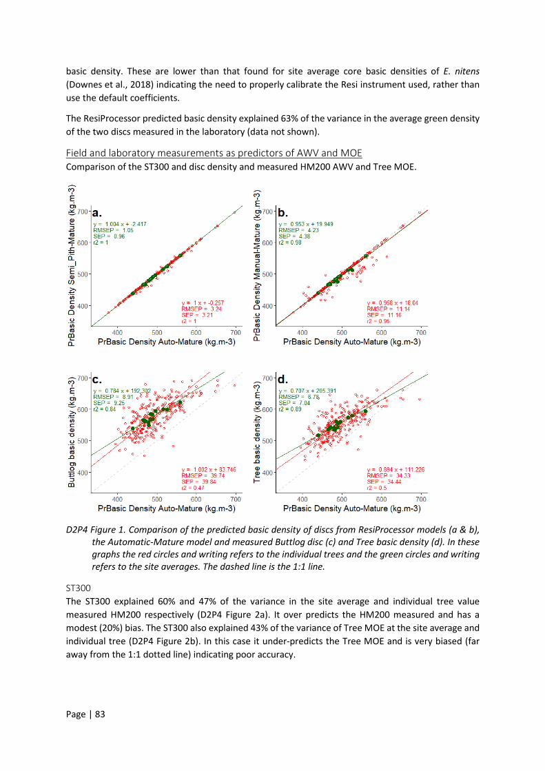
Page | 83

basic density. These are lower than that found for site average core basic densities of E. nitens (Downes et al., 2018) indicating the need to properly calibrate the Resi instrument used, rather than use the default coefficients.

The ResiProcessor predicted basic density explained 63% of the variance in the average green density of the two discs measured in the laboratory (data not shown).

Field and laboratory measurements as predictors of AWV and MOE Comparison of the ST300 and disc density and measured HM200 AWV and Tree MOE.

D2P4 Figure 1. Comparison of the predicted basic density of discs from ResiProcessor models (a & b), the Automatic-Mature model and measured Buttlog disc (c) and Tree basic density (d). In these graphs the red circles and writing refers to the individual trees and the green circles and writing refers to the site averages. The dashed line is the 1:1 line.

ST300 The ST300 explained 60% and 47% of the variance in the site average and individual tree value measured HM200 respectively (D2P4 Figure 2a). It over predicts the HM200 measured and has a modest (20%) bias. The ST300 also explained 43% of the variance of Tree MOE at the site average and individual tree (D2P4 Figure 2b). In this case it under-predicts the Tree MOE and is very biased (far away from the 1:1 dotted line) indicating poor accuracy.

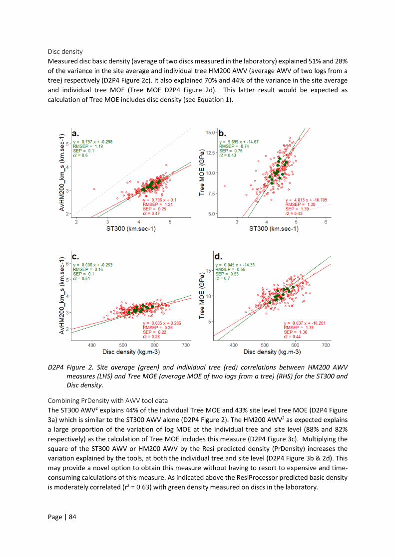
Page | 84

Disc density Measured disc basic density (average of two discs measured in the laboratory) explained 51% and 28% of the variance in the site average and individual tree HM200 AWV (average AWV of two logs from a tree) respectively (D2P4 Figure 2c). It also explained 70% and 44% of the variance in the site average and individual tree MOE (Tree MOE D2P4 Figure 2d). This latter result would be expected as calculation of Tree MOE includes disc density (see Equation 1).

D2P4 Figure 2. Site average (green) and individual tree (red) correlations between HM200 AWV measures (LHS) and Tree MOE (average MOE of two logs from a tree) (RHS) for the ST300 and Disc density.

Combining PrDensity with AWV tool data The ST300 AWV2 explains 44% of the individual Tree MOE and 43% site level Tree MOE (D2P4 Figure 3a) which is similar to the ST300 AWV alone (D2P4 Figure 2). The HM200 AWV2 as expected explains a large proportion of the variation of log MOE at the individual tree and site level (88% and 82% respectively) as the calculation of Tree MOE includes this measure (D2P4 Figure 3c). Multiplying the square of the ST300 AWV or HM200 AWV by the Resi predicted density (PrDensity) increases the variation explained by the tools, at both the individual tree and site level (D2P4 Figure 3b & 2d). This may provide a novel option to obtain this measure without having to resort to expensive and time-consuming calculations of this measure. As indicated above the ResiProcessor predicted basic density is moderately correlated (r2 = 0.63) with green density measured on discs in the laboratory.

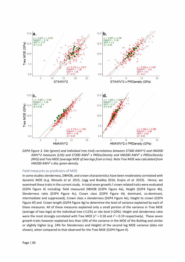
Page | 85

D2P4 Figure 3. Site (green) and individual tree (red) correlations between ST300 AWV^2 and HM200 AWV^2 measures (LHS) and ST300 AWV2 x PRDiscDensity and HM200 AWV2 x PRDiscDensity (RHS) and Tree MOE (average MOE of two logs from a tree). Note Tree MOE was calculated from HM200 AWV2 x disc green density.

Field measures as predictors of MOE In some studies slenderness, DBHOB, and crown characteristics have been moderately correlated with dynamic MOE (e.g. Wessels et al. 2015, Legg and Bradley 2016, Krajnc et al. 2019). Hence, we examined these traits in the current study. In total seven growth / crown related traits were evaluated (D2P4 Figure 4) including: field measured DBHOB (D2P4 Figure 4a), Height (D2P4 Figure 4b), Slenderness ratio (D2P4 Figure 4c), Crown class (D2P4 Figure 4d; dominant, co-dominant, intermediate and suppressed), Crown class x slenderness (D2P4 Figure 4e), Height to crown (D2P4 Figure 4f) and Crown length (D2P4 Figure 4g) to determine the level of variance explained by each of these measures. All of these measures explained only a small portion of the variance in Tree MOE (average of two logs) at the individual tree (<12%) or site level (<20%). Height and slenderness ratio were the most strongly correlated with Tree MOE (r2 = 0.18 and r2 = 0.19 respectively). These seven growth traits however explained less than 10% of the variance in the MOE of the Buttlog and similar or slightly higher (e.g. 24% for Slenderness and Height) of the second log MOE variance (data not shown), when compared to that observed for the Tree MOE (D2P4 Figure 4).

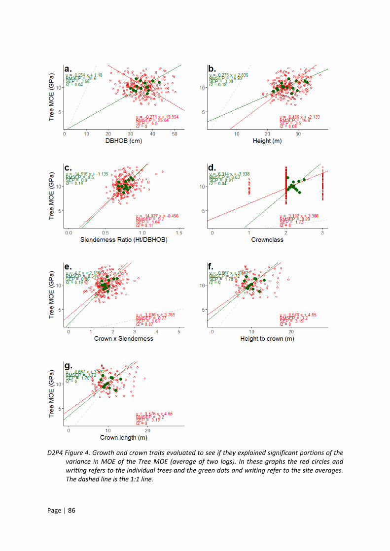
Page | 86

D2P4 Figure 4. Growth and crown traits evaluated to see if they explained significant portions of the variance in MOE of the Tree MOE (average of two logs). In these graphs the red circles and writing refers to the individual trees and the green dots and writing refer to the site averages. The dashed line is the 1:1 line.

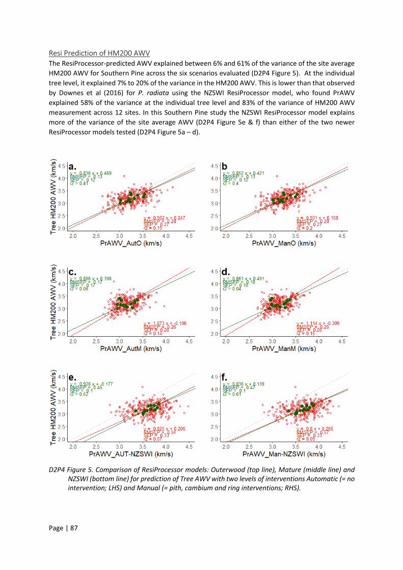
Page | 87

Resi Prediction of HM200 AWV The ResiProcessor-predicted AWV explained between 6% and 61% of the variance of the site average HM200 AWV for Southern Pine across the six scenarios evaluated (D2P4 Figure 5). At the individual tree level, it explained 7% to 20% of the variance in the HM200 AWV. This is lower than that observed by Downes et al (2016) for P. radiata using the NZSWI ResiProcessor model, who found PrAWV explained 58% of the variance at the individual tree level and 83% of the variance of HM200 AWV measurement across 12 sites. In this Southern Pine study the NZSWI ResiProcessor model explains more of the variance of the site average AWV (D2P4 Figure 5e & f) than either of the two newer ResiProcessor models tested (D2P4 Figure 5a – d).

D2P4 Figure 5. Comparison of ResiProcessor models: Outerwood (top line), Mature (middle line) and NZSWI (bottom line) for prediction of Tree AWV with two levels of interventions Automatic (= no intervention; LHS) and Manual (= pith, cambium and ring interventions; RHS).

Page | 88

Resi Prediction of MOE Outerwood and Mature ResiProcessor models

The ‘Outerwood’ ResiProcessor model explained more of the variance of the site average Tree MOE (54-56%) than the ‘Mature’ ResiProcessor model (29-33%). Further, the Outerwood Auto setting (no correction for pith, cambium or growth rings) explains more of the site average Tree MOE variance than the best of the Mature ResiProcessor models (D2P4 Figure 6). When using the Outerwood ResiProcessor model, making corrections to the pith (PrMOE_SemiPO) explains as much of the site average Tree MOE variance as the fully automatic model (PrMOE_AutO), but it reduces the RMSEP and SEP indicating it is a more precise model to predict Southern Pine site average Tree MOE of these two options.

NZSWI ResiProcessor model The NZSWI ResiProcessor model explains more of the site average Tree MOE variance (66%) than either the Outerwood or Mature ResiProcessor model with any level of intervention. It does even better at the site average Buttlog MOE (73-78%; D2P4 Figure 7). Three levels of intervention of the Resi traces were evaluated for the NZSWI model: automatic, semi-automatic (pith correction) and manual intervention (pith, cambial and growth ring correction as needed). The automatic and semi-automatic interventions explained a similar level of variance at both the individual tree (24-25%) and site level (both 66%; D2P4 Figure 8). The manual intervention explained slightly more variance for the individual tree (29%) and site (71%), but the time required to undertake this amount intervention precludes this being done on a regular basis. The semi-automatic approach to processing potentially has an added benefit of allowing a more accurate measure of DBH (both underbark and overbark) than the fully automatic option as it ensures the pith is more accurately identified. During this study, 24.8% of trees had changes in the Resi predicted DBH as a result of the semi-automatic correction (data not shown). The largest change in an individual tree’s DBHOB as a result of this was the diameter increased by 17.4 cm relative to the automatic setting (no correction for pith, cambium or growth rings). Using a generic green density for the two taxon in this study (PCH: unextracted green density of 849.1 kg/m-3; pine hybrids: unextracted green density of 879.5 kg/m-3) based on data from the SPRC project along with NZSWI automatic (no intervention) explained 48%, 53% and 41% of the Tree, Buttlog and Log2 MOE respectively (data not shown).

NZSWI ResiProcessor model combined with growth traits The combination of NZSWI PrMOE multiplied by the slenderness ratio (height divided by DBHOB) of the trees resulted in an index that explained 80% of the site average variance (r2 = 0.8) of Tree MOE, Buttlog (r2 = 0.69) and Log2 MOE (r2 = 0.77) which was more than the NZSWI model by itself (D2P4 Figure 9). When DBHOB or tree height were multiplied by NZSWI model for PrMOE (D2P4 Figure 10) the variance explained was not as high as that explained by the NZSWI x slenderness ratio.

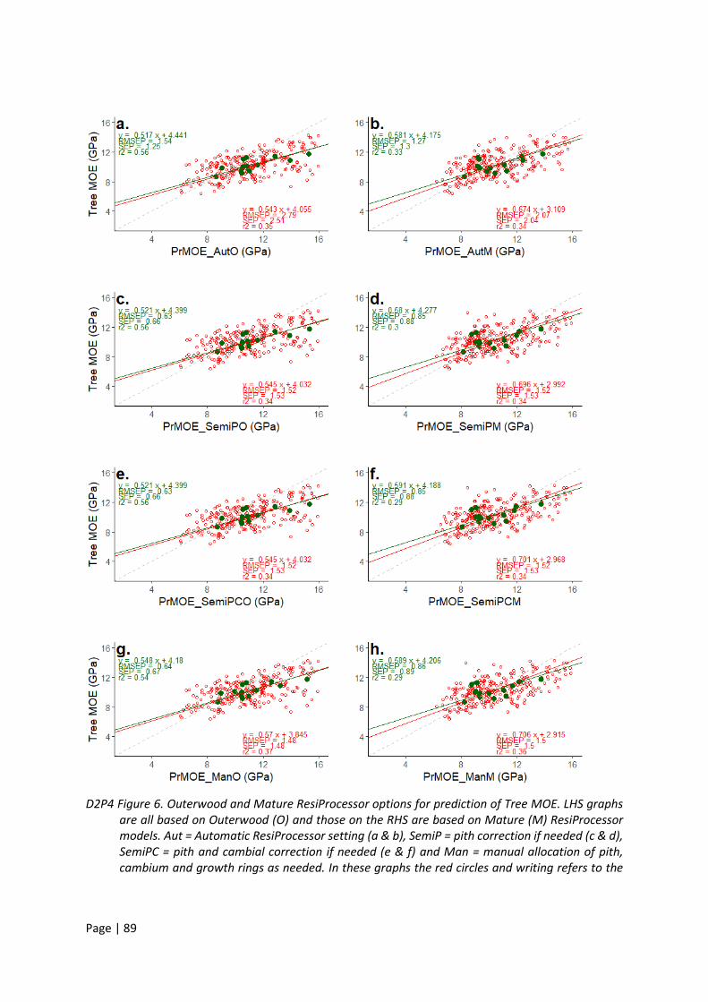
Page | 89

D2P4 Figure 6. Outerwood and Mature ResiProcessor options for prediction of Tree MOE. LHS graphs are all based on Outerwood (O) and those on the RHS are based on Mature (M) ResiProcessor models. Aut = Automatic ResiProcessor setting (a & b), SemiP = pith correction if needed (c & d), SemiPC = pith and cambial correction if needed (e & f) and Man = manual allocation of pith, cambium and growth rings as needed. In these graphs the red circles and writing refers to the

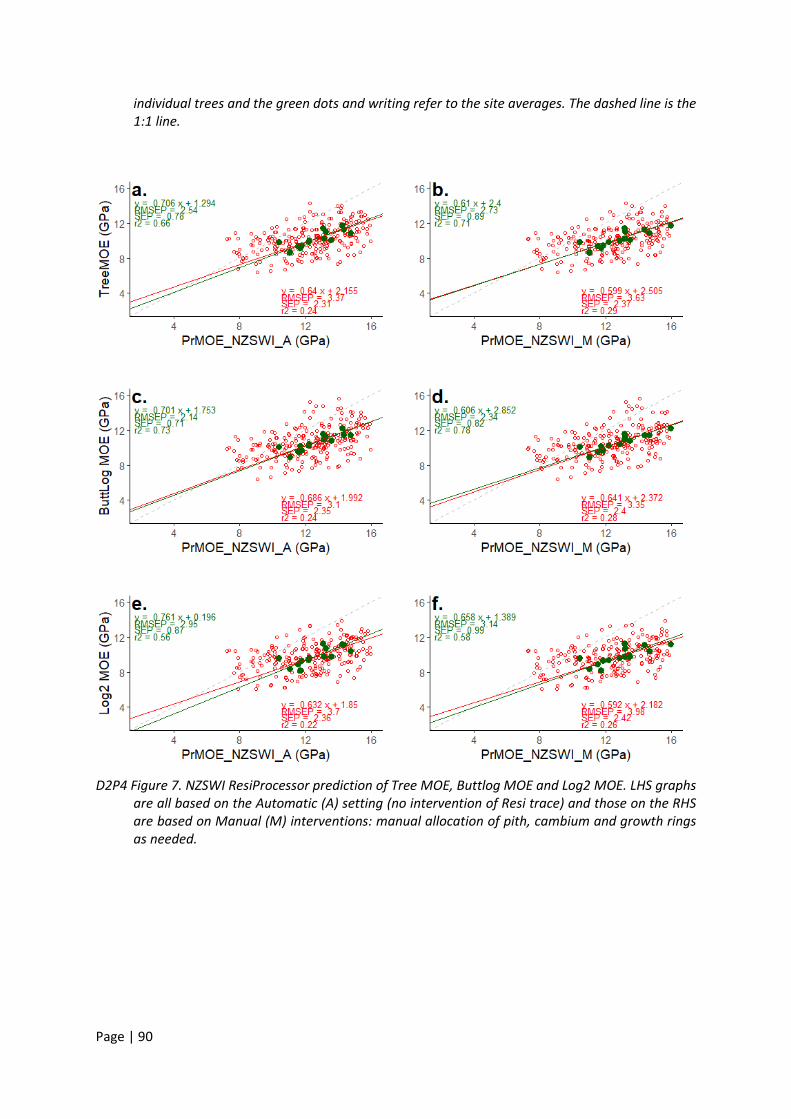
Page | 90

individual trees and the green dots and writing refer to the site averages. The dashed line is the 1:1 line.

D2P4 Figure 7. NZSWI ResiProcessor prediction of Tree MOE, Buttlog MOE and Log2 MOE. LHS graphs are all based on the Automatic (A) setting (no intervention of Resi trace) and those on the RHS are based on Manual (M) interventions: manual allocation of pith, cambium and growth rings as needed.

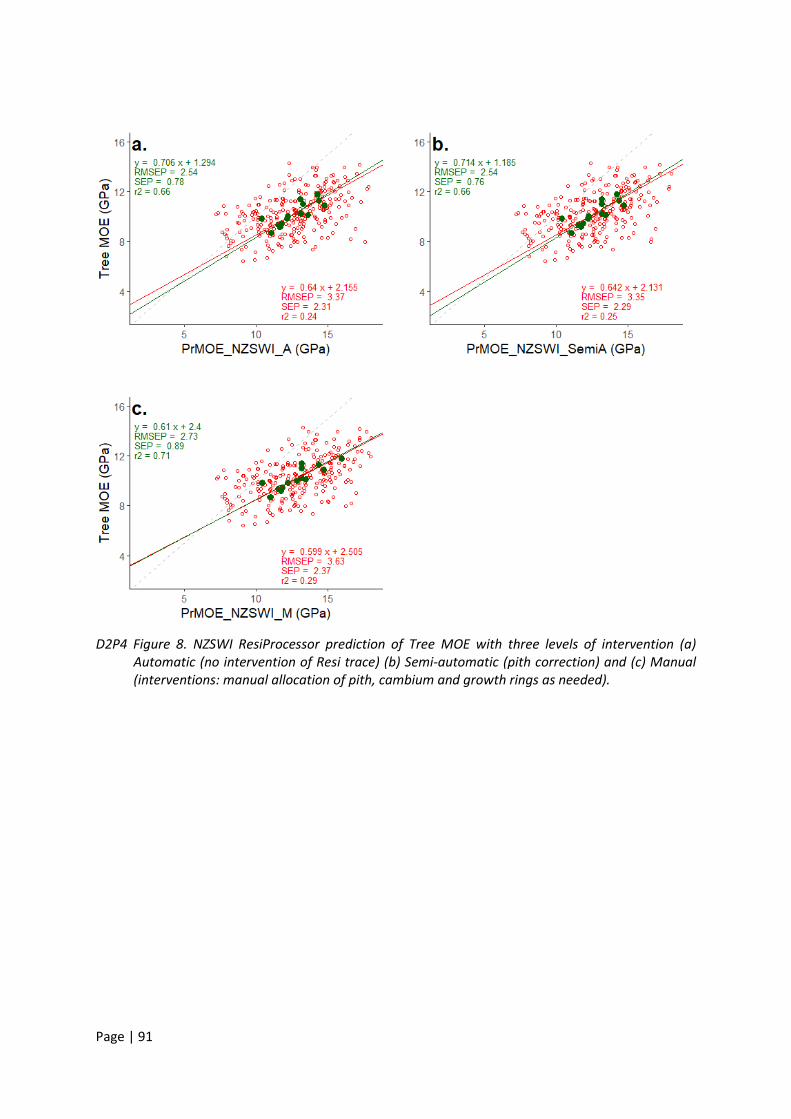
Page | 91

D2P4 Figure 8. NZSWI ResiProcessor prediction of Tree MOE with three levels of intervention (a) Automatic (no intervention of Resi trace) (b) Semi-automatic (pith correction) and (c) Manual (interventions: manual allocation of pith, cambium and growth rings as needed).

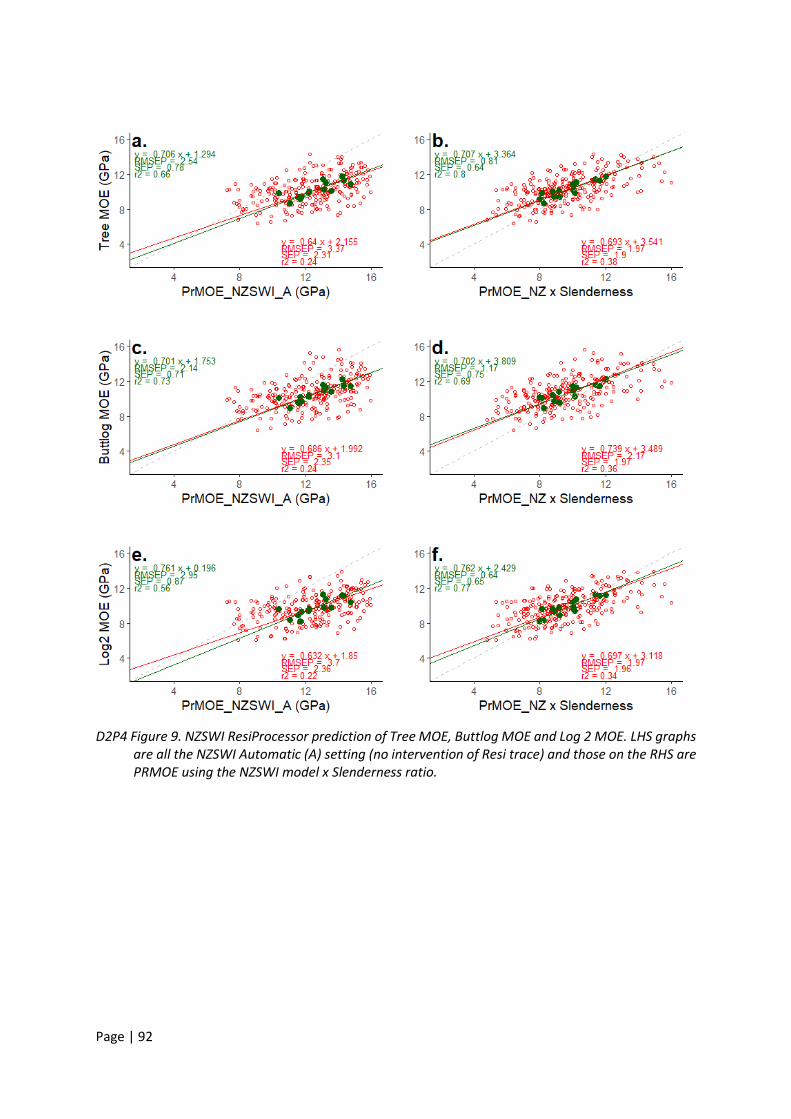
Page | 92

D2P4 Figure 9. NZSWI ResiProcessor prediction of Tree MOE, Buttlog MOE and Log 2 MOE. LHS graphs are all the NZSWI Automatic (A) setting (no intervention of Resi trace) and those on the RHS are PRMOE using the NZSWI model x Slenderness ratio.

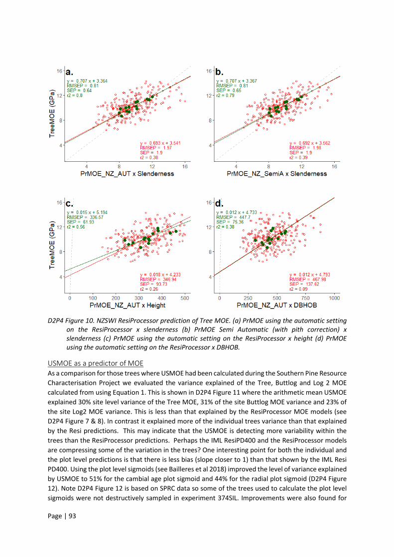
Page | 93

D2P4 Figure 10. NZSWI ResiProcessor prediction of Tree MOE. (a) PrMOE using the automatic setting on the ResiProcessor x slenderness (b) PrMOE Semi Automatic (with pith correction) x slenderness (c) PrMOE using the automatic setting on the ResiProcessor x height (d) PrMOE using the automatic setting on the ResiProcessor x DBHOB.

USMOE as a predictor of MOE As a comparison for those trees where USMOE had been calculated during the Southern Pine Resource Characterisation Project we evaluated the variance explained of the Tree, Buttlog and Log 2 MOE calculated from using Equation 1. This is shown in D2P4 Figure 11 where the arithmetic mean USMOE explained 30% site level variance of the Tree MOE, 31% of the site Buttlog MOE variance and 23% of the site Log2 MOE variance. This is less than that explained by the ResiProcessor MOE models (see D2P4 Figure 7 & 8). In contrast it explained more of the individual trees variance than that explained by the Resi predictions. This may indicate that the USMOE is detecting more variability within the trees than the ResiProcessor predictions. Perhaps the IML ResiPD400 and the ResiProcessor models are compressing some of the variation in the trees? One interesting point for both the individual and the plot level predictions is that there is less bias (slope closer to 1) than that shown by the IML Resi PD400. Using the plot level sigmoids (see Bailleres et al 2018) improved the level of variance explained by USMOE to 51% for the cambial age plot sigmoid and 44% for the radial plot sigmoid (D2P4 Figure 12). Note D2P4 Figure 12 is based on SPRC data so some of the trees used to calculate the plot level sigmoids were not destructively sampled in experiment 374SIL. Improvements were also found for

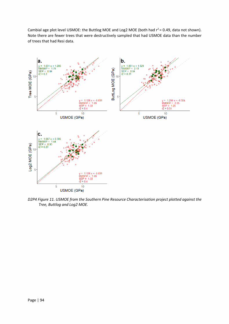
Page | 94

Cambial age plot level USMOE: the Buttlog MOE and Log2 MOE (both had r2 = 0.49, data not shown). Note there are fewer trees that were destructively sampled that had USMOE data than the number of trees that had Resi data.

D2P4 Figure 11. USMOE from the Southern Pine Resource Characterisation project plotted against the Tree, Buttlog and Log2 MOE.

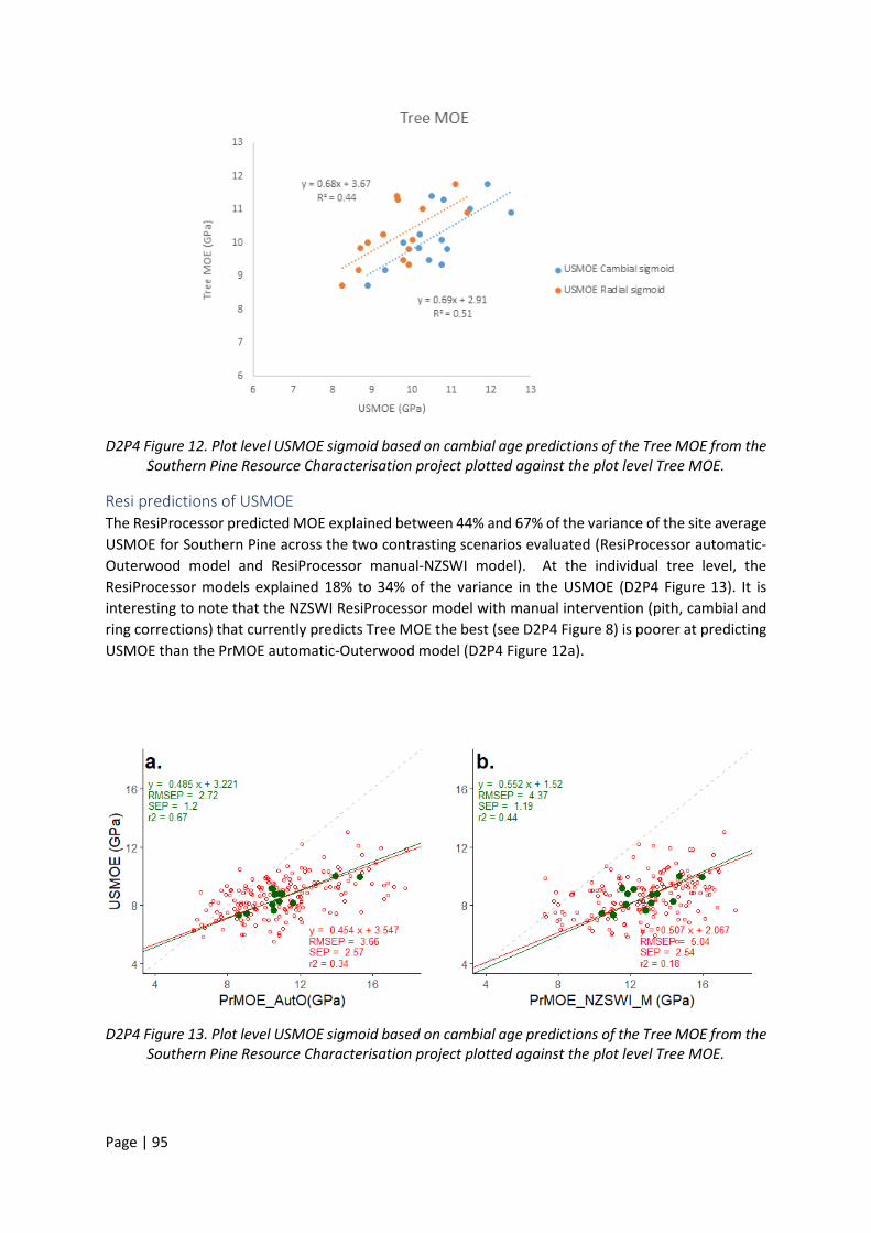
Page | 95

D2P4 Figure 12. Plot level USMOE sigmoid based on cambial age predictions of the Tree MOE from the Southern Pine Resource Characterisation project plotted against the plot level Tree MOE.

Resi predictions of USMOE The ResiProcessor predicted MOE explained between 44% and 67% of the variance of the site average USMOE for Southern Pine across the two contrasting scenarios evaluated (ResiProcessor automatic-Outerwood model and ResiProcessor manual-NZSWI model). At the individual tree level, the ResiProcessor models explained 18% to 34% of the variance in the USMOE (D2P4 Figure 13). It is interesting to note that the NZSWI ResiProcessor model with manual intervention (pith, cambial and ring corrections) that currently predicts Tree MOE the best (see D2P4 Figure 8) is poorer at predicting USMOE than the PrMOE automatic-Outerwood model (D2P4 Figure 12a).

D2P4 Figure 13. Plot level USMOE sigmoid based on cambial age predictions of the Tree MOE from the Southern Pine Resource Characterisation project plotted against the plot level Tree MOE.

Page | 96

Conclusions This component of the project has found that the IML Resi PD400 has potential to assist in predicting wood quality of Southern Pine stands. In particular:

• Resi was good at predicting individual tree basic density and excellent at predicting site average basic density of Southern Pine stands, as it explains 89% of the variance.

• Combining the ResiProcessor predictions of basic density with the ST300 or HM200 AWV improves the prediction of Tree MOE of both of these tools.

• The NZSWI ResiProcessor model for PrAWV explains more of the variance in site average Tree AWV than other models tested.

• The NZSWI ResiProcessor model for PrMOE explains more of the variance in site average Tree MOE than other models tested. Across three levels of interventions this model explains 66-71% of the Tree MOE.

• Combining the NZSWI PrMOE x slenderness explains 80% of the variance in site average Tree MOE. This appears to be the current best option to predict site Tree MOE of the ResiProcessor options tested.

Acknowledgements Chandan Kumar is thanked for provision of plot level sigmoidal predictions of USMOE using the radial and cambial sigmoids and for constructive suggestions in this document. Collection and collation of the data by HQPlantations staff and contractors as well as DAF staff is greatly appreciated.

References Bailleres, H., D. Lee, S. Kumar, G. Hopewell, and L. Brancheriau. 2018. Improving returns from southern pine plantations through innovative resource characterisation. Melbourne: FWPA. pp. 163.

Downes, G., D. Drew, J. Moore, M. Lausberg, J. Harrington, S. Elms, D. Watt, and S. Holtorf. 2016. Evaluating and modelling radiata pine wood quality in the Murray valley region. Melbourne, Victoria: Forest & Wood Products Australia Limited. pp. 154.

Downes, G.M., M. Lausberg, B. M. Potts, D. Pilbeam, M. Bird, and B. Bradshaw. 2018. Application of the IML Resistograph to the infield measurement of basic density, in plantation eucalypts. Australian Forestry 81 (3):177-185.

Durocher, C., D.P. Kain, L. Stamm, I. Last, and P. Keay. 2016. Pilot study - Resi Tool. Comparing methods: measuring under-bark and over-bark diameter: HQPlantations Pty Ltd.

Gantz, C.H. 2002. Evaluating The Efficiency Of The Resistograph To Estimate Genetic Parameters For Wood Density In Two Softwood And Two Hardwood Species. Masters, North Carolina State University, Raleigh, North Carolina.

Gao, S., X. Wang, M.C. Wiemann, B. K. Brashaw, R.J. Ross, and L. Wang. 2017. A critical analysis of methods for rapid and nondestructive determination of wood density in standing trees. Annals of Forest Science 74 (2):27p. doi:10.1007/s13595-017-0623-4.

Hopewell, G., H. Bailleres, A. Hayes, L.. Francis, and D. Lee. 2017. Variation in extractives predicted from core segments. Milestone 6a Project: Improving returns from southern pine plantations through innovative resource characterisation. Brisbane: DAF Queensland. pp. 15.

Krajnc, L., N. Farrelly, and A.M. Harte. 2019. The influence of crown and stem characteristics on timber quality in softwoods. Forest Ecology and Management 435:8-17.

Page | 97

Lausberg, M., K. Harris, W. Green, C. Morris, D. Kain, I. Last, and G. Downes. 2016. Site level lumber stiffness on Slash Pine, Caribbean Pine and their hybrids: SWI

Legg, M., and S. Bradley. 2016. Measurement of stiffness of standing trees and felled logs using acoustics: A review. Journal of the Acoustical Society of America 139 (2):588-604. doi:10.1121/1.4940210.

Lin, C., S. Wang, F. C. Lin, and C. Chui. 2003. Effect of moisture content on the drill resistance value in Taiwania plantation wood. Wood and Fiber Science 35 (2):234-238.

Morales-Conde, MJ, Carmen Rodríguez-Liñán, and J Saporiti-Machado. 2014. Predicting the density of structural timber members in service. The combine use of wood cores and drill resistance data. Materiales de Construccion, 64 (315), 1-11.

Nutto, Leif, and Tobias Biechele. 2015. Drilling resistance measurement and the effect of shaft friction–using feed force information for improving decay identification on hard tropical wood, 19th International Nondestructive Testing and Evaluation of Wood Symposium. pp. 154-161.

R Core Team. 2019. R: A language and environment for statistical computing. URL https://www.R-project.org/. Accessed 2019.

Rinn, F., F. H. Schweingruber, and E. Schär. 1996. RESISTOGRAPH and X-Ray Density Charts of Wood. Comparative Evaluation of Drill Resistance Profiles and X-ray Density Charts of Different Wood Species. Holzforschung - International Journal of the Biology, Chemistry, Physics and Technology of Wood 50 (4):303-311. doi:10.1515/hfsg.1996.50.4.303.

Rinn, Frank. 2013. Practical application of micro-resistance drilling for timber inspection. Holztechnologie 54 (4):32-38.

Sharapov, Evgenii, Christian Brischke, Holger Militz, and Elena Smirnova. 2019. Prediction of modulus of elasticity in static bending and density of wood at different moisture contents and feed rates by drilling resistance measurements. European Journal of Wood and Wood Products 77 (5):833-842. doi:10.1007/s00107-019-01439-2.

Ukrainetz, Nicholas K., and Gregory A. O’Neill. 2010. An analysis of sensitivities contributing measurement error to Resistograph values. Canadian Journal of Forest Research 40 (4):806-811. doi:10.1139/X10-019.

Wessels, C. B., F. S. Malan, T. Seifert, J. H. Louw, and T. Rypstra. 2015. The prediction of the flexural lumber properties from standing South African-grown Pinus patula trees. European Journal of Forest Research 134 (1):1-18. doi:10.1007/s10342-014-0829-z.

Wielinga, B., C. A. Raymond, R. James, and A. C. Matheson. 2009. Genetic parameters and genotype by environment interactions for green and basic density and stiffness of Pinus radiata D. Don estimated using acoustics. Silvae Genetica 58 (3):112-122.

https://www.r-project.org/

https://www.r-project.org/

Page | 98

Appendix 1: Procedure used to select 11 trees additional to DST trees in Experiment 374 SIL There were 3 aims of this selection process:

1) Allow the DST tree selection procedure to be carried out following established protocol (trees are selected in the field immediately prior to felling)

2) Destructively sample as many trees as possible with previous wood quality data from the SPRC 3) Achieve a balanced sample of trees across DBH and MOE classes

The procedure used to select the trees was as follows:

Initial desktop procedure: 1. Collate DBH, ST300 and MOE data for each plot, calculating tree averages where multiple

readings were taken for MOE or ST300 per tree. Include core notes. 2. Sort trees into 2 DBH classes (1=highest 50%, 2=lowest 50%), based on SPRC DBH

measurements on all living trees in the plot. 3. Sort trees into 2 MOE classes (1=highest 50%, 2=lowest 50%), based on SPRC ST300

measurements on 30 trees per plot. 4. Assign USMOE classes based on SPRC increment core USMOE data as follows: assign USMOE

classes to the 15 (or fewer) trees with USMOE data per plot (1=highest 50%, 2=lowest 50%). 5. Adjust the MOE classes based on USMOE data, which is more reliable than ST300 data: if a

tree has USMOE class 1 (or 2), it will be given that MOE class regardless of the ST300 data. 6. From the sample of 15 trees with USMOE data for the plot, select a sample of 11 ‘priority 1’

trees, maintaining a similar balance of DBH and MOE classes. Exclude any trees with problems noted in the SPRC data (e.g. highly resinous cores, parts of cores missing, etc.). Trees with cores noted as ‘heavy resin’ were excluded from sampling, whereas trees noted as ‘resin’ were included as it’s not unusual for there to be some amount of resin impregnation, which can also depend on the sampling location in the stem.

7. Any remaining trees with USMOE data without the above problems should be assigned to ‘priority 2’.

8. Trees with ST300 data but no USMOE data should be assigned ‘priority 3’. 9. Create four ‘DBH/MOE’ classes, shown heuristically in the quadrant diagram below.

In the field: 1. Select 9 trees in the growth plot using DST in-field tree selection processes (see DST manual). Paint-mark these trees on three sides as they are selected, with the numbers 1 to 9. 2. On the proforma, write the numbers of these 9 trees in the ‘Tree paint number in field’ column on the proforma. 3. Select and paint mark a further 11 trees using the procedure below, for a total of 20 trees per growth plot. 11 pre-selected trees have been identified as ‘priority 1’ on the proforma. Inspect each ‘priority 1’ tree, ensuring two 6m logs can be cut from the tree with no major defects. Trees with poor form or double leaders need to be excluded. A replacement must be identified for each ‘priority 1’ tree where:

1. The tree is unsuitable due to defects, or: 2. The tree has been chosen as one of the 9 DST trees Replacements for ‘priority 1’ trees must be identified from the same class where possible (see proforma). The following procedure is suggested to achieve the above:

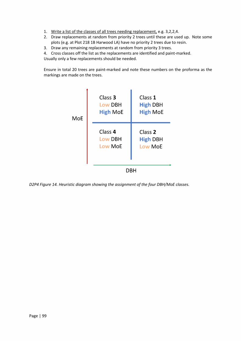
Page | 99

1. Write a list of the classes of all trees needing replacement, e.g. 3,2,2,4. 2. Draw replacements at random from priority 2 trees until these are used up. Note some

plots (e.g. at Plot 218 1B Harwood LA) have no priority 2 trees due to resin. 3. Draw any remaining replacements at random from priority 3 trees. 4. Cross classes off the list as the replacements are identified and paint-marked. Usually only a few replacements should be needed. Ensure in total 20 trees are paint-marked and note these numbers on the proforma as the markings are made on the trees.

D2P4 Figure 14. Heuristic diagram showing the assignment of the four DBH/MoE classes.

Page | 100

Deliverable 3. Predicting sawn timber volumes and quality from preharvest measurements using Resi.

Geoff Downes, Marco Lausberg, Jonathon Harrington, David Drew, Phillip Muyambo, Stephen Elms and Russell Riepsamen.

Key findings • Site mean log MOE explained 85% of the variance in site mean board MOE, whereas in the

absence of green density information site mean log AWV explained only 51%.

• Preharvest Resi basic density near breast height explained most of the variance in mean log and board MOE (78% and 88% respectively) and some variance in log AWV (50%) and mean board AWV (39%)

• Resi-derived core density was a better predictor than the Resi-predicted AWV of both board and log MOE and AWV

• Site mean actual outerwood core density explained 85% of the variance in site mean board MOE.

• Different Resi instruments gave comparable results once each individual instrument was calibrated using actual outerwood core basic density values

• Sites exhibited large range in the percentage of MGP10 or better boards produced. Resi values exhibited strong correlations with this metric

• The strength of the relationships between Resi values and log and board data strengthens the commercial value of the use of the Resi as a preharvest assessment tool and strengthens the need to develop standard methodologies of application to enhance the communication of data across the value chain.

Introduction This report constitutes part of a larger FWPA project (VNB459-1718) directed at assessing preharvest wood quality in softwood plantations using (a) the IML PD-400 Resi instrument and (b) the web-based rCambium modelling platform. The over-arching objective of preharvest assessments is to generate predictions of volumes and properties of sawn boards exiting the dry mill with commercially useful precision.

Where they are undertaken, typically standing tree assessments are related to log level measurements (e.g HM200 Acoustic Wave Velocity (AWV) and stiffness (MOE)), which in turn are less frequently related to green board properties. The opportunity to relate standing tree properties directly through to green board properties is valuable as it minimises the accumulation of errors in the process chain, allowing standing tree metrics to be related directly to board out-turn metrics.

The main objective of this study was to relate site-average MOE predictions from standing trees derived from Resi measurement to site average board MOE at 9 distinct sites in the Bathurst-Oberon region of New South Wales representing a range of site qualities, defined by rainfall, soil type and site index.

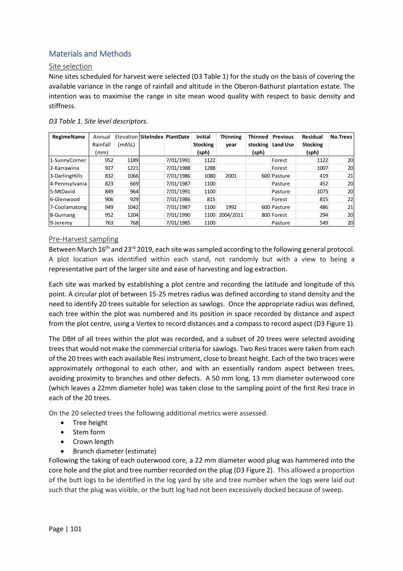
Page | 101

Materials and Methods Site selection Nine sites scheduled for harvest were selected (D3 Table 1) for the study on the basis of covering the available variance in the range of rainfall and altitude in the Oberon-Bathurst plantation estate. The intention was to maximise the range in site mean wood quality with respect to basic density and stiffness.

D3 Table 1. Site level descriptors.

Pre-Harvest sampling Between March 16th and 23rd 2019, each site was sampled according to the following general protocol. A plot location was identified within each stand, not randomly but with a view to being a representative part of the larger site and ease of harvesting and log extraction.

Each site was marked by establishing a plot centre and recording the latitude and longitude of this point. A circular plot of between 15-25 metres radius was defined according to stand density and the need to identify 20 trees suitable for selection as sawlogs. Once the appropriate radius was defined, each tree within the plot was numbered and its position in space recorded by distance and aspect from the plot centre, using a Vertex to record distances and a compass to record aspect (D3 Figure 1).

The DBH of all trees within the plot was recorded, and a subset of 20 trees were selected avoiding trees that would not make the commercial criteria for sawlogs. Two Resi traces were taken from each of the 20 trees with each available Resi instrument, close to breast height. Each of the two traces were approximately orthogonal to each other, and with an essentially random aspect between trees, avoiding proximity to branches and other defects. A 50 mm long, 13 mm diameter outerwood core (which leaves a 22mm diameter hole) was taken close to the sampling point of the first Resi trace in each of the 20 trees.

On the 20 selected trees the following additional metrics were assessed. • Tree height • Stem form • Crown length • Branch diameter (estimate)

Following the taking of each outerwood core, a 22 mm diameter wood plug was hammered into the core hole and the plot and tree number recorded on the plug (D3 Figure 2). This allowed a proportion of the butt logs to be identified in the log yard by site and tree number when the logs were laid out such that the plug was visible, or the butt log had not been excessively docked because of sweep.

RegimeName Annual Rainfall

(mm)

Elevation (mASL)

SiteIndex PlantDate Initial Stocking

(sph)

Thinning year

Thinned stocking

(sph)

Previous Land Use

Residual Stocking

(sph)

No.Trees

1-SunnyCorner 952 1189 7/01/1991 1122 Forest 1122 202-Karrawina 927 1221 7/01/1988 1288 Forest 1007 203-DarlingHills 832 1066 7/01/1986 1080 2001 600 Pasture 419 214-Pennsylvania 823 669 7/01/1987 1100 Pasture 452 205-MtDavid 849 964 7/01/1991 1100 Pasture 1073 206-Glenwood 906 929 7/01/1986 815 Forest 815 227-Coolamatong 949 1042 7/01/1987 1100 1992 600 Pasture 486 218-Gurnang 952 1204 7/01/1990 1100 2004/2011 800 Forest 294 209-Jeremy 763 768 7/01/1985 1100 Pasture 549 20

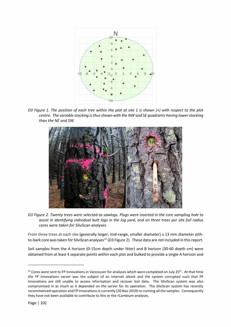
Page | 102

D3 Figure 1. The position of each tree within the plot at site 1 is shown (+) with respect to the plot centre. The variable stocking is thus shown with the NW and SE quadrants having lower stocking than the NE and SW.

D3 Figure 2. Twenty trees were selected as sawlogs. Plugs were inserted in the core sampling hole to assist in identifying individual butt logs in the log yard, and on three trees per site full radius cores were taken for SilviScan analyses.

From three trees at each site (generally larger, mid-range, smaller diameter) a 13 mm diameter pith-to-bark core was taken for SilviScan analyses31 (D3 Figure 2). These data are not included in this report.

Soil samples from the A horizon (0-15cm depth under litter) and B horizon (30-60 depth cm) were obtained from at least 4 separate points within each plot and bulked to provide a single A horizon and

31 Cores were sent to FP Innovations in Vancouver for analyses which were completed on July 25th. At that time the FP Innovations server was the subject of an internet attack and the system corrupted such that FP Innovations are still unable to access information and recover lost data. The SilviScan system was also compromised in as much as it depended on the server for its operation. The SilviScan system has recently recommenced operation and FP Innovations is currently (20 Nov 2019) re-running all the samples. Consequently they have not been available to contribute to this or the rCambium analyses.

-10

-8

-6

-4

-2

0

2

4

6

8

10

-10 -8 -6 -4 -2 0 2 4 6 8 10

N

Page | 103

single B horizon sample per site. These were sent for soil analyses (https://www.swep.com.au/) and will be used in the rCambium evaluation study. Prior to leaving each site, a GoPro video of plot area (Hero 7 black, 125 fps, 4K resolution) to explore potential for generating a point cloud map of the trees. Approximately 6 minutes of footage per site was recorded.

Log-yard assessment Logs from each site were received into the log yard over a period of 2-3 days prior to the mill study, with the harvest of all nine sites spanning only several days. Logs were laid out in site batches on bearers in a level and secluded area of the yard to ensure a safe operating environment and measured prior to processing (D3 Figure 3). Each log was allocated a 3 digit number based on site (first digit 1-9) and sequence in the way they were laid out (1-99 with the maximum number of logs within a site being 58) (e.g. log 207 indicated logs from site 2, and the seventh log in the sequence). Log preparation involved the following

• Individual log codes were sprayed on each end • HM200 data were collected from each log along with log lengths • A cross-section disc was collected from the small end and assessed for green density (volume

by immersion and green weight). Large discs were broken into smaller wedges for this assessment.

• Log diameters and heartwood diameters were measured at the small end • A single Resi trace was taken approximately 1 m from the large end. Two Resi instruments

were used in this process, taking duplicate readings. Where possible these traces were full diameters.

Following preparation, logs were collected as site batches and stored ready for mill processing. To assist in checking the mill operation an additional batch of logs was collected from a regular truck delivery and marked up as site 0. This batch of 44 logs were assessed for AWV and Resi but not green density. They were used as the first batch to go through the mill process to ensure the mill processing was operational.

Mill processing and data collection Prior to processing site batches of logs, the mill was cleared of residual boards. Board acoustic velocity measures were checked and tuned. Additional sensors of log and cant velocity were optimised and the data used to check their operation against the log level HM200 values. Cameras were used to record the log number sequence through the mill (D3 Figure 4) at two different points to allow the alignment of mill data (such as velocity and log shape) to individual log data previously obtained in the log yard.

Cutting patterns were fitted to each log to maximise the production of structural lumber. To maximise recovery thinner boards were produced (25mm thick) where appropriate. MOE values were not calculated for these boards and were excluded from further analysis. The volume of these thinner boards is the difference between total and measured board volume in D3 Table 4.

https://www.swep.com.au/

Page | 104

D3 Figure 3. Logs were laid out in sequence and individual numbers allocated to each. The first digit in the 3 digit code indicates the site number

D3 Figure 4. Logs were processed through the mill as site batches with sufficient time between batches to allow resultant boards to be identified to the site level.

Page | 105

Data collation and analysis All data collected was combined into a single database and stored. Log sequences were checked from the various records and camera sources to allow log sequence at each point in the mill to be determined and aligned with resultant data capture. Collected data was checked and log, cant and board data identified back to (at least) site level.

Data was extracted from the database using R and analysed at the site level to explore site-related differences.

Computed Values The following variables, defined as follows, were used in the analyses

• Log.MOE = Log.AWV^2 * green density

• Resi outerwood density: The estimated basic density of the under-bark outer 50 mm of the stem radius on the entry-side of the trace. Density is estimated from the average of the Resi values multiplied by an instrument-specific slope coefficient and the addition of an instrument specific intercept

o Mean Resi Value * rSlope + rIntcpt

• Resi core density: The estimated basic density of the bark-to-bark trace. In traces where the Resi traces did not measure the full diameter, only the pith-to-bark radius was used and calculated as per the outerwood density metric.

• Resi disc density. The pith-to-bark trace is area-weighted such that the 0.1 mm radial interval of each Resi sampling point is representative of the area it would represent in a cross-section disc. That is, a point 200 mm from the pith represents a much greater cross-sectional area of wood than a point 2 mm from the pith. In a full diameter trace the mean of both radii is calculated. If the trace is not a full diameter, only the entry-side radius is used.

• PrAWV: Predicted AWV value from variables derived from the Resi trace. A range of different predicted models are being assessed for the accuracy and precision in determining site mean values

• PrMOE: PrAWV2 * Resi core density * 2.25

• SED: small end diameter of a log

• SEDHW: small end diameter of the heartwood of a log

Results Preharvest data was collated into site means (D3 Table 2). Across the nine sites, 184 trees were sampled generating 411 logs of which 119 were identified as specific butt logs in the log yard based on the plug inserted at BH prior to harvest (D3 Table 3). The mix of first, second and third logs varies among the sites.

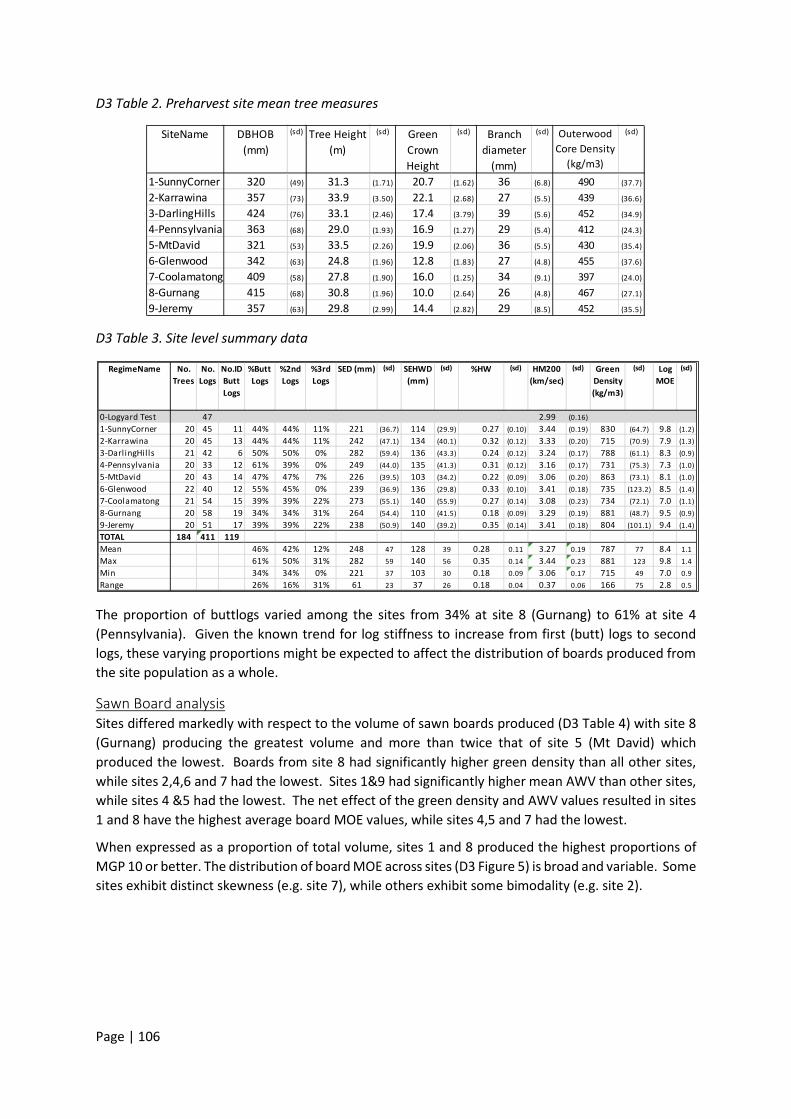
Page | 106

D3 Table 2. Preharvest site mean tree measures

D3 Table 3. Site level summary data

The proportion of buttlogs varied among the sites from 34% at site 8 (Gurnang) to 61% at site 4 (Pennsylvania). Given the known trend for log stiffness to increase from first (butt) logs to second logs, these varying proportions might be expected to affect the distribution of boards produced from the site population as a whole.

Sawn Board analysis Sites differed markedly with respect to the volume of sawn boards produced (D3 Table 4) with site 8 (Gurnang) producing the greatest volume and more than twice that of site 5 (Mt David) which produced the lowest. Boards from site 8 had significantly higher green density than all other sites, while sites 2,4,6 and 7 had the lowest. Sites 1&9 had significantly higher mean AWV than other sites, while sites 4 &5 had the lowest. The net effect of the green density and AWV values resulted in sites 1 and 8 have the highest average board MOE values, while sites 4,5 and 7 had the lowest.

When expressed as a proportion of total volume, sites 1 and 8 produced the highest proportions of MGP 10 or better. The distribution of board MOE across sites (D3 Figure 5) is broad and variable. Some sites exhibit distinct skewness (e.g. site 7), while others exhibit some bimodality (e.g. site 2).

SiteName DBHOB (mm)

(sd) Tree Height (m)

(sd) Green Crown Height

(sd) Branch diameter

(mm)

(sd) Outerwood Core Density

(kg/m3)

(sd)

1-SunnyCorner 320 (49) 31.3 (1.71) 20.7 (1.62) 36 (6.8) 490 (37.7)

2-Karrawina 357 (73) 33.9 (3.50) 22.1 (2.68) 27 (5.5) 439 (36.6)

3-DarlingHills 424 (76) 33.1 (2.46) 17.4 (3.79) 39 (5.6) 452 (34.9)

4-Pennsylvania 363 (68) 29.0 (1.93) 16.9 (1.27) 29 (5.4) 412 (24.3)

5-MtDavid 321 (53) 33.5 (2.26) 19.9 (2.06) 36 (5.5) 430 (35.4)

6-Glenwood 342 (63) 24.8 (1.96) 12.8 (1.83) 27 (4.8) 455 (37.6)

7-Coolamatong 409 (58) 27.8 (1.90) 16.0 (1.25) 34 (9.1) 397 (24.0)

8-Gurnang 415 (68) 30.8 (1.96) 10.0 (2.64) 26 (4.8) 467 (27.1)

9-Jeremy 357 (63) 29.8 (2.99) 14.4 (2.82) 29 (8.5) 452 (35.5)

RegimeName No. Trees

No. Logs

No.ID Butt Logs

%Butt Logs

%2nd Logs

%3rd Logs

SED (mm) (sd) SEHWD (mm)

(sd) %HW (sd) HM200 (km/sec)

(sd) Green Density (kg/m3)

(sd) Log MOE

(sd)

0-Logyard Test 47 2.99 (0.16)1-SunnyCorner 20 45 11 44% 44% 11% 221 (36.7) 114 (29.9) 0.27 (0.10) 3.44 (0.19) 830 (64.7) 9.8 (1.2)2-Karrawina 20 45 13 44% 44% 11% 242 (47.1) 134 (40.1) 0.32 (0.12) 3.33 (0.20) 715 (70.9) 7.9 (1.3)3-DarlingHills 21 42 6 50% 50% 0% 282 (59.4) 136 (43.3) 0.24 (0.12) 3.24 (0.17) 788 (61.1) 8.3 (0.9)4-Pennsylvania 20 33 12 61% 39% 0% 249 (44.0) 135 (41.3) 0.31 (0.12) 3.16 (0.17) 731 (75.3) 7.3 (1.0)5-MtDavid 20 43 14 47% 47% 7% 226 (39.5) 103 (34.2) 0.22 (0.09) 3.06 (0.20) 863 (73.1) 8.1 (1.0)6-Glenwood 22 40 12 55% 45% 0% 239 (36.9) 136 (29.8) 0.33 (0.10) 3.41 (0.18) 735 (123.2) 8.5 (1.4)7-Coolamatong 21 54 15 39% 39% 22% 273 (55.1) 140 (55.9) 0.27 (0.14) 3.08 (0.23) 734 (72.1) 7.0 (1.1)8-Gurnang 20 58 19 34% 34% 31% 264 (54.4) 110 (41.5) 0.18 (0.09) 3.29 (0.19) 881 (48.7) 9.5 (0.9)9-Jeremy 20 51 17 39% 39% 22% 238 (50.9) 140 (39.2) 0.35 (0.14) 3.41 (0.18) 804 (101.1) 9.4 (1.4)TOTAL 184 411 119Mean 46% 42% 12% 248 47 128 39 0.28 0.11 3.27 0.19 787 77 8.4 1.1Max 61% 50% 31% 282 59 140 56 0.35 0.14 3.44 0.23 881 123 9.8 1.4Min 34% 34% 0% 221 37 103 30 0.18 0.09 3.06 0.17 715 49 7.0 0.9Range 26% 16% 31% 61 23 37 26 0.18 0.04 0.37 0.06 166 75 2.8 0.5

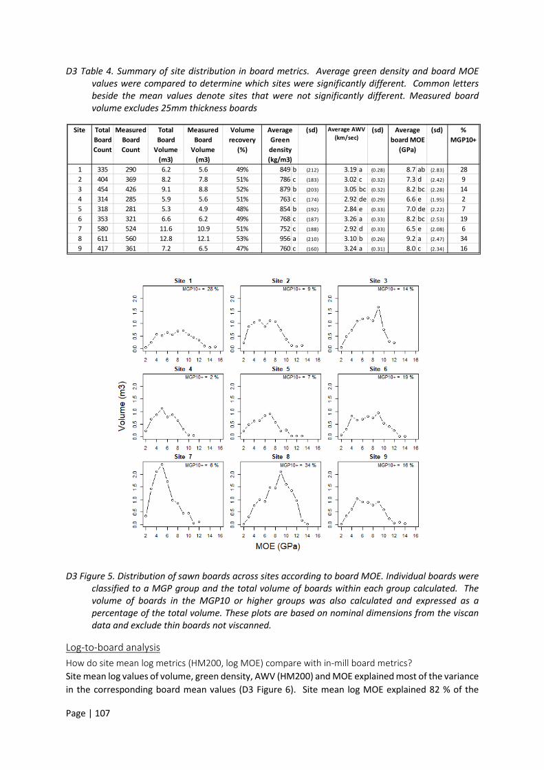
Page | 107

D3 Table 4. Summary of site distribution in board metrics. Average green density and board MOE values were compared to determine which sites were significantly different. Common letters beside the mean values denote sites that were not significantly different. Measured board volume excludes 25mm thickness boards

D3 Figure 5. Distribution of sawn boards across sites according to board MOE. Individual boards were classified to a MGP group and the total volume of boards within each group calculated. The volume of boards in the MGP10 or higher groups was also calculated and expressed as a percentage of the total volume. These plots are based on nominal dimensions from the viscan data and exclude thin boards not viscanned.

Log-to-board analysis How do site mean log metrics (HM200, log MOE) compare with in-mill board metrics? Site mean log values of volume, green density, AWV (HM200) and MOE explained most of the variance in the corresponding board mean values (D3 Figure 6). Site mean log MOE explained 82 % of the

Site Total Board Count

Measured Board Count

Total Board

Volume (m3)

Measured Board

Volume (m3)

Volume recovery

(%)

(sd) (sd) (sd) % MGP10+

1 335 290 6.2 5.6 49% 849 b (212) 3.19 a (0.28) 8.7 ab (2.83) 282 404 369 8.2 7.8 51% 786 c (183) 3.02 c (0.32) 7.3 d (2.42) 93 454 426 9.1 8.8 52% 879 b (203) 3.05 bc (0.32) 8.2 bc (2.28) 144 314 285 5.9 5.6 51% 763 c (174) 2.92 de (0.29) 6.6 e (1.95) 25 318 281 5.3 4.9 48% 854 b (192) 2.84 e (0.33) 7.0 de (2.22) 76 353 321 6.6 6.2 49% 768 c (187) 3.26 a (0.33) 8.2 bc (2.53) 197 580 524 11.6 10.9 51% 752 c (188) 2.92 d (0.33) 6.5 e (2.08) 68 611 560 12.8 12.1 53% 956 a (210) 3.10 b (0.26) 9.2 a (2.47) 349 417 361 7.2 6.5 47% 760 c (160) 3.24 a (0.31) 8.0 c (2.34) 16

Average AWV (km/sec)

Average board MOE

(GPa)

Average Green density (kg/m3)

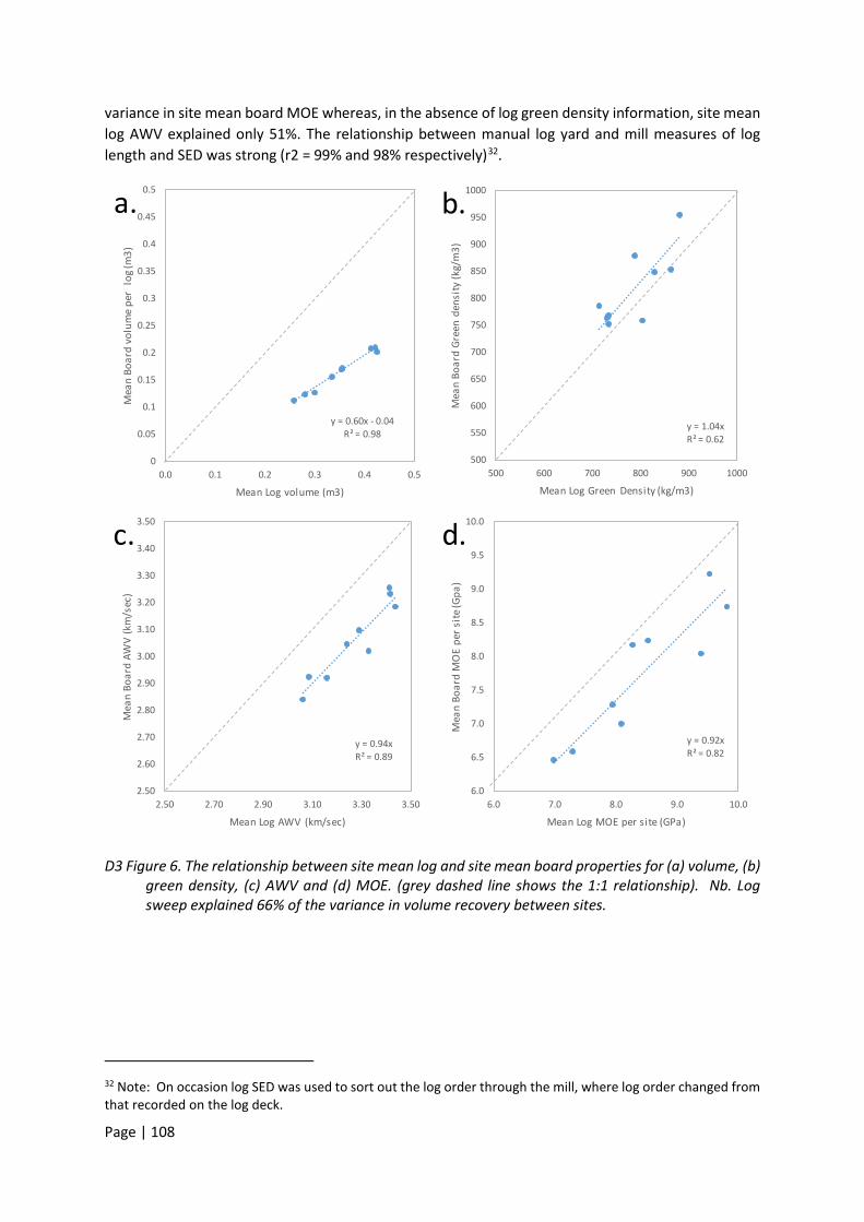
Page | 108

variance in site mean board MOE whereas, in the absence of log green density information, site mean log AWV explained only 51%. The relationship between manual log yard and mill measures of log length and SED was strong (r2 = 99% and 98% respectively)32.

D3 Figure 6. The relationship between site mean log and site mean board properties for (a) volume, (b) green density, (c) AWV and (d) MOE. (grey dashed line shows the 1:1 relationship). Nb. Log sweep explained 66% of the variance in volume recovery between sites.

32 Note: On occasion log SED was used to sort out the log order through the mill, where log order changed from that recorded on the log deck.

y = 1.04xR² = 0.62

500

550

600

650

700

750

800

850

900

950

1000

500 600 700 800 900 1000

Mea

n Bo

ard

Gree

n de

nsity

(kg/

m3)

Mean Log Green Density (kg/m3)

b.

y = 0.94xR² = 0.89

2.50

2.60

2.70

2.80

2.90

3.00

3.10

3.20

3.30

3.40

3.50

2.50 2.70 2.90 3.10 3.30 3.50

Mea

n Bo

ard

AWV

(km

/sec

)

Mean Log AWV (km/sec)

c.

y = 0.92xR² = 0.82

6.0

6.5

7.0

7.5

8.0

8.5

9.0

9.5

10.0

6.0 7.0 8.0 9.0 10.0

Mea

n Bo

ard

MO

E pe

r site

(Gpa

)

Mean Log MOE per site (GPa)

d.

y = 0.60x - 0.04R² = 0.98

0

0.05

0.1

0.15

0.2

0.25

0.3

0.35

0.4

0.45

0.5

0.0 0.1 0.2 0.3 0.4 0.5

Mea

n Bo

ard

volu

me

per

log (

m3)

Mean Log volume (m3)

a.

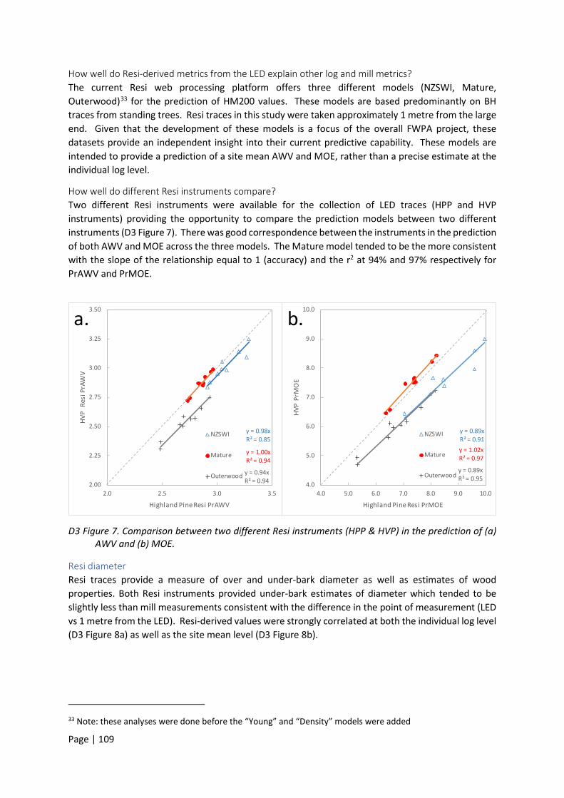
Page | 109

How well do Resi-derived metrics from the LED explain other log and mill metrics? The current Resi web processing platform offers three different models (NZSWI, Mature, Outerwood)33 for the prediction of HM200 values. These models are based predominantly on BH traces from standing trees. Resi traces in this study were taken approximately 1 metre from the large end. Given that the development of these models is a focus of the overall FWPA project, these datasets provide an independent insight into their current predictive capability. These models are intended to provide a prediction of a site mean AWV and MOE, rather than a precise estimate at the individual log level.

How well do different Resi instruments compare? Two different Resi instruments were available for the collection of LED traces (HPP and HVP instruments) providing the opportunity to compare the prediction models between two different instruments (D3 Figure 7). There was good correspondence between the instruments in the prediction of both AWV and MOE across the three models. The Mature model tended to be the more consistent with the slope of the relationship equal to 1 (accuracy) and the r2 at 94% and 97% respectively for PrAWV and PrMOE.

D3 Figure 7. Comparison between two different Resi instruments (HPP & HVP) in the prediction of (a) AWV and (b) MOE.

Resi diameter Resi traces provide a measure of over and under-bark diameter as well as estimates of wood properties. Both Resi instruments provided under-bark estimates of diameter which tended to be slightly less than mill measurements consistent with the difference in the point of measurement (LED vs 1 metre from the LED). Resi-derived values were strongly correlated at both the individual log level (D3 Figure 8a) as well as the site mean level (D3 Figure 8b).

33 Note: these analyses were done before the “Young” and “Density” models were added

y = 0.98xR² = 0.85

y = 1.00xR² = 0.94

y = 0.94xR² = 0.942.00

2.25

2.50

2.75

3.00

3.25

3.50

2.0 2.5 3.0 3.5

HVP

Res

i PrA

WV

Highland Pine Resi PrAWV

NZSWI

Mature

Outerwood

a.

y = 0.89xR² = 0.91y = 1.02xR² = 0.97

y = 0.89xR² = 0.95

4.0

5.0

6.0

7.0

8.0

9.0

10.0

4.0 5.0 6.0 7.0 8.0 9.0 10.0

HVP

PrM

OE

Highland Pine Resi PrMOE

NZSWI

Mature

Outerwood

b.

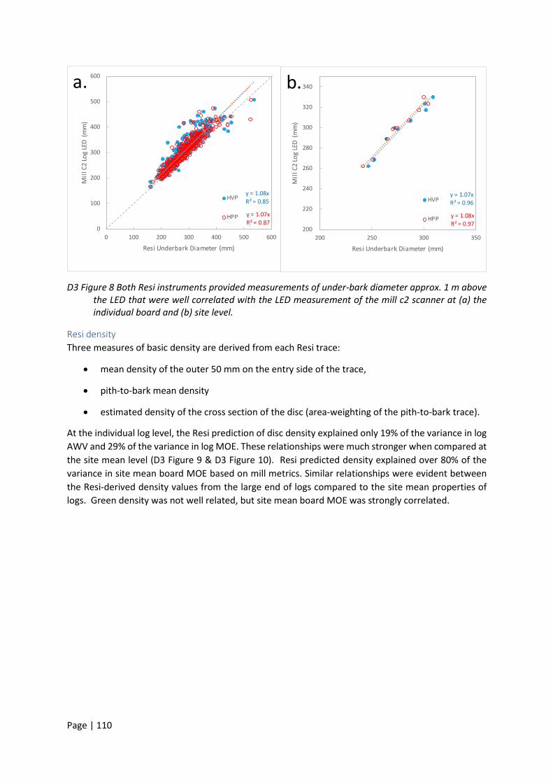
Page | 110

D3 Figure 8 Both Resi instruments provided measurements of under-bark diameter approx. 1 m above the LED that were well correlated with the LED measurement of the mill c2 scanner at (a) the individual board and (b) site level.

Resi density Three measures of basic density are derived from each Resi trace:

• mean density of the outer 50 mm on the entry side of the trace,

• pith-to-bark mean density

• estimated density of the cross section of the disc (area-weighting of the pith-to-bark trace).

At the individual log level, the Resi prediction of disc density explained only 19% of the variance in log AWV and 29% of the variance in log MOE. These relationships were much stronger when compared at the site mean level (D3 Figure 9 & D3 Figure 10). Resi predicted density explained over 80% of the variance in site mean board MOE based on mill metrics. Similar relationships were evident between the Resi-derived density values from the large end of logs compared to the site mean properties of logs. Green density was not well related, but site mean board MOE was strongly correlated.

y = 1.08xR² = 0.85

y = 1.07xR² = 0.87

0

100

200

300

400

500

600

0 100 200 300 400 500 600

Mill

C2

Log

LED

(mm

)

Resi Underbark Diameter (mm)

HVP

HPP

a.

y = 1.07xR² = 0.96

y = 1.08xR² = 0.97

200

220

240

260

280

300

320

340

200 250 300 350

Mill

C2

Log

LED

(mm

)

Resi Underbark Diameter (mm)

HVP

HPP

b.

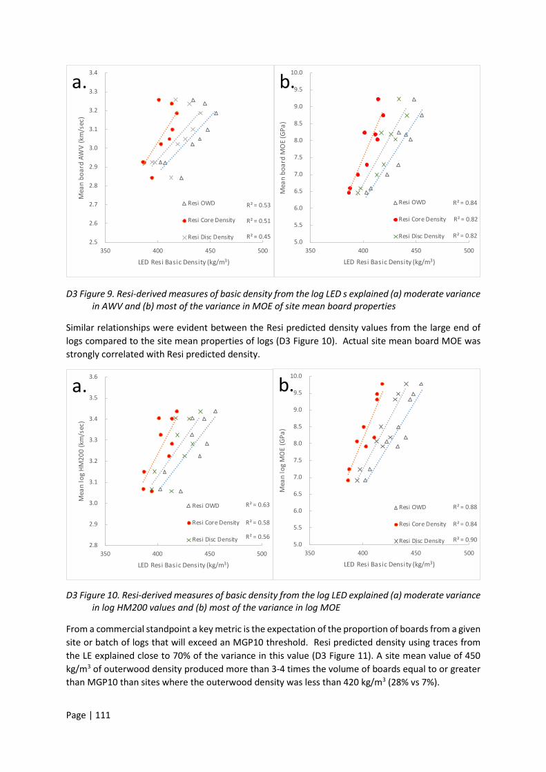
Page | 111

D3 Figure 9. Resi-derived measures of basic density from the log LED s explained (a) moderate variance in AWV and (b) most of the variance in MOE of site mean board properties

Similar relationships were evident between the Resi predicted density values from the large end of logs compared to the site mean properties of logs (D3 Figure 10). Actual site mean board MOE was strongly correlated with Resi predicted density.

D3 Figure 10. Resi-derived measures of basic density from the log LED explained (a) moderate variance in log HM200 values and (b) most of the variance in log MOE

From a commercial standpoint a key metric is the expectation of the proportion of boards from a given site or batch of logs that will exceed an MGP10 threshold. Resi predicted density using traces from the LE explained close to 70% of the variance in this value (D3 Figure 11). A site mean value of 450 kg/m3 of outerwood density produced more than 3-4 times the volume of boards equal to or greater than MGP10 than sites where the outerwood density was less than 420 kg/m3 (28% vs 7%).

R² = 0.53

R² = 0.51

R² = 0.45 2.5

2.6

2.7

2.8

2.9

3.0

3.1

3.2

3.3

3.4

350 400 450 500

Mea

n bo

ard

AWV

(km

/sec

)

LED Resi Basic Density (kg/m3)

Resi OWD

Resi Core Density

Resi Disc Density

a.

R² = 0.84

R² = 0.82

R² = 0.82 5.0

5.5

6.0

6.5

7.0

7.5

8.0

8.5

9.0

9.5

10.0

350 400 450 500

Mea

n bo

ard

MO

E (G

Pa)


Resi OWD

Resi Core Density

Resi Disc Density

b.

R² = 0.63

R² = 0.58

R² = 0.56 2.8

2.9

3.0

3.1

3.2

3.3

3.4

3.5

3.6

350 400 450 500

Mea

n lo

g HM

200

(km

/sec

)


Resi OWD

Resi Core Density

Resi Disc Density

a.

R² = 0.88

R² = 0.84

R² = 0.90 5.0

5.5

6.0

6.5

7.0

7.5

8.0

8.5

9.0

9.5

10.0

350 400 450 500

Mea

n lo

g M

OE

(GPa

)


Resi OWD

Resi Core Density

Resi Disc Density

b.

Page | 112

D3 Figure 11. Resi Density metrics from near the LED are compared with mill board values classified as the percentage for each site greater than or equal to MGP 10

Resi Predicted AWV and MOE

One of the main objectives of the project was to predict average log AWV from a Resi trace, with a greater degree of precision and accuracy than that derived from basic density alone. It is well to keep in mind at this point that AWV is itself a surrogate for MOE, and the precise, accurate prediction of MOE is the commercial goal.

Resi predicted AWV (D3 Figure 12) explained less of the site mean variance in actual AWV in both logs and boards than did Resi predicted density (D3 Figure 9 and 10). The Resi-predicted MOE did better, but no better than did the Resi predicted density values. At the individual log level, Resi PrAWV values explained slightly more (21%) of the variance in actual HM200 values than did basic density (outerwood density: 18%, core density 9%; disc density 19%).

R² = 0.69

R² = 0.66

R² = 0.69 -

5

10

15

20

25

30

35

40

380 400 420 440 460 480 500

% b

oard

s GE

MGP

10


Resi OWD

Resi Core Density

Resi Disc Density

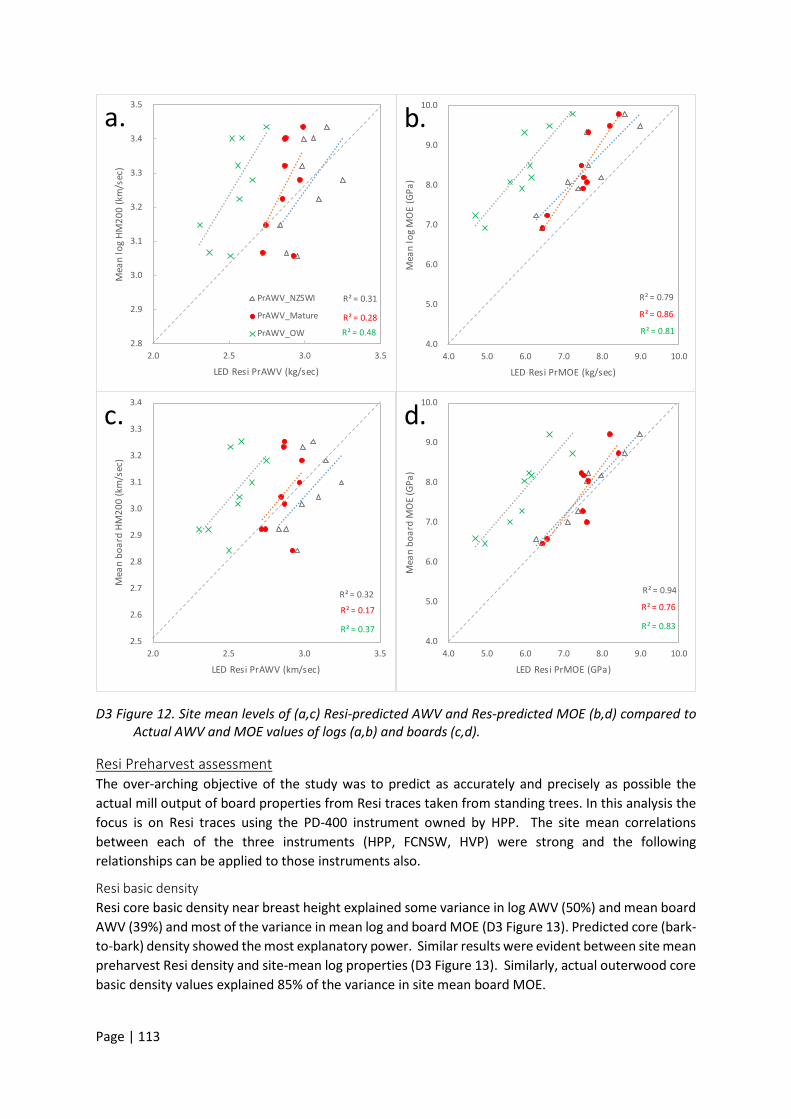
Page | 113

D3 Figure 12. Site mean levels of (a,c) Resi-predicted AWV and Res-predicted MOE (b,d) compared to Actual AWV and MOE values of logs (a,b) and boards (c,d).

Resi Preharvest assessment The over-arching objective of the study was to predict as accurately and precisely as possible the actual mill output of board properties from Resi traces taken from standing trees. In this analysis the focus is on Resi traces using the PD-400 instrument owned by HPP. The site mean correlations between each of the three instruments (HPP, FCNSW, HVP) were strong and the following relationships can be applied to those instruments also.

Resi basic density Resi core basic density near breast height explained some variance in log AWV (50%) and mean board AWV (39%) and most of the variance in mean log and board MOE (D3 Figure 13). Predicted core (bark-to-bark) density showed the most explanatory power. Similar results were evident between site mean preharvest Resi density and site-mean log properties (D3 Figure 13). Similarly, actual outerwood core basic density values explained 85% of the variance in site mean board MOE.

R² = 0.31

R² = 0.28R² = 0.48

2.8

2.9

3.0

3.1

3.2

3.3

3.4

3.5

2.0 2.5 3.0 3.5

Mea

n lo

g HM

200

(km

/sec

)

LED Resi PrAWV (kg/sec)

PrAWV_NZSWI

PrAWV_Mature

PrAWV_OW

a.

R² = 0.79

R² = 0.86

R² = 0.81 4.0

5.0

6.0

7.0

8.0

9.0

10.0

4.0 5.0 6.0 7.0 8.0 9.0 10.0

Mea

n lo

g M

OE

(GPa

)

LED Resi PrMOE (kg/sec)

b.

R² = 0.94

R² = 0.76

R² = 0.83 4.0

5.0

6.0

7.0

8.0

9.0

10.0

4.0 5.0 6.0 7.0 8.0 9.0 10.0

Mea

n bo

ard

MO

E (G

Pa)

LED Resi PrMOE (GPa)

d.

R² = 0.32

R² = 0.17

R² = 0.37 2.5

2.6

2.7

2.8

2.9

3.0

3.1

3.2

3.3

3.4

2.0 2.5 3.0 3.5

Mea

n bo

ard

HM20

0 (k

m/s

ec)

LED Resi PrAWV (km/sec)

c.

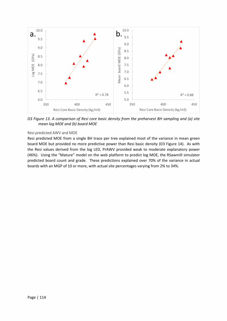
Page | 114

D3 Figure 13. A comparison of Resi core basic density from the preharvest BH sampling and (a) site

mean log MOE and (b) board MOE

Resi predicted AWV and MOE Resi predicted MOE from a single BH trace per tree explained most of the variance in mean green board MOE but provided no more predictive power than Resi basic density (D3 Figure 14). As with the Resi values derived from the log LED, PrAWV provided weak to moderate explanatory power (46%). Using the “Mature” model on the web platform to predict log MOE, the RSawmill simulator predicted board count and grade. These predictions explained over 70% of the variance in actual boards with an MGP of 10 or more, with actual site percentages varying from 2% to 34%.

R² = 0.885.0

5.5

6.0

6.5

7.0

7.5

8.0

8.5

9.0

9.5

10.0

350 400 450

Mea

n b

oard

MO

E (G

Pa)

Resi Core Basic Density (kg/m3)

b.

R² = 0.786.0

6.5

7.0

7.5

8.0

8.5

9.0

9.5

10.0

350 400 450

Log

MO

E (G

Pa)

Resi Core Basic Density (kg/m3)

a.

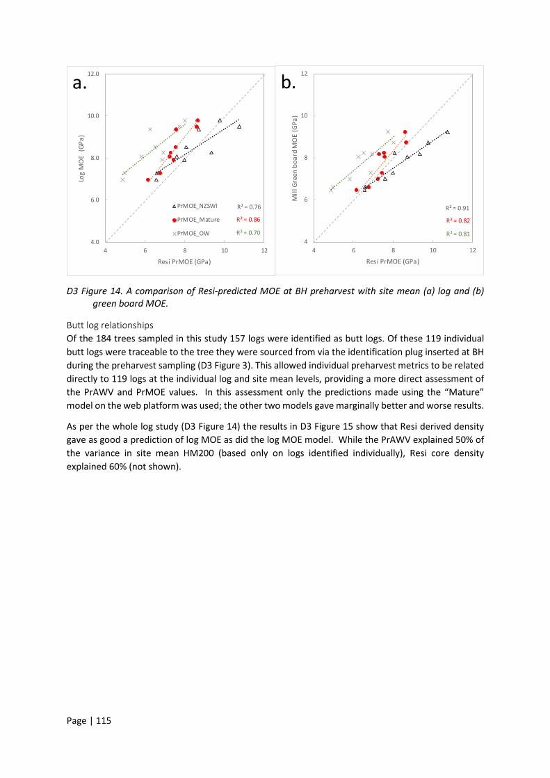
Page | 115

D3 Figure 14. A comparison of Resi-predicted MOE at BH preharvest with site mean (a) log and (b) green board MOE.

Butt log relationships Of the 184 trees sampled in this study 157 logs were identified as butt logs. Of these 119 individual butt logs were traceable to the tree they were sourced from via the identification plug inserted at BH during the preharvest sampling (D3 Figure 3). This allowed individual preharvest metrics to be related directly to 119 logs at the individual log and site mean levels, providing a more direct assessment of the PrAWV and PrMOE values. In this assessment only the predictions made using the “Mature” model on the web platform was used; the other two models gave marginally better and worse results.

As per the whole log study (D3 Figure 14) the results in D3 Figure 15 show that Resi derived density gave as good a prediction of log MOE as did the log MOE model. While the PrAWV explained 50% of the variance in site mean HM200 (based only on logs identified individually), Resi core density explained 60% (not shown).

R² = 0.91

R² = 0.82

R² = 0.814

6

8

10

12

4 6 8 10 12

Mill

Gre

en b

oard

MO

E (G

Pa)

Resi PrMOE (GPa)

b.

R² = 0.76

R² = 0.86

R² = 0.704.0

6.0

8.0

10.0

12.0

4 6 8 10 12

Log

MO

E (G

Pa)

Resi PrMOE (GPa)

PrMOE_NZSWI

PrMOE_Mature

PrMOE_OW

a.

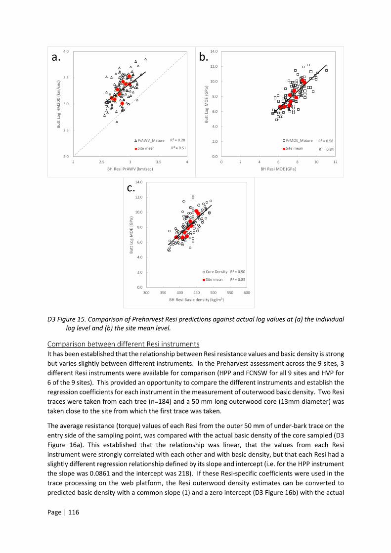
Page | 116

D3 Figure 15. Comparison of Preharvest Resi predictions against actual log values at (a) the individual log level and (b) the site mean level.

Comparison between different Resi instruments It has been established that the relationship between Resi resistance values and basic density is strong but varies slightly between different instruments. In the Preharvest assessment across the 9 sites, 3 different Resi instruments were available for comparison (HPP and FCNSW for all 9 sites and HVP for 6 of the 9 sites). This provided an opportunity to compare the different instruments and establish the regression coefficients for each instrument in the measurement of outerwood basic density. Two Resi traces were taken from each tree (n=184) and a 50 mm long outerwood core (13mm diameter) was taken close to the site from which the first trace was taken.

The average resistance (torque) values of each Resi from the outer 50 mm of under-bark trace on the entry side of the sampling point, was compared with the actual basic density of the core sampled (D3 Figure 16a). This established that the relationship was linear, that the values from each Resi instrument were strongly correlated with each other and with basic density, but that each Resi had a slightly different regression relationship defined by its slope and intercept (i.e. for the HPP instrument the slope was 0.0861 and the intercept was 218). If these Resi-specific coefficients were used in the trace processing on the web platform, the Resi outerwood density estimates can be converted to predicted basic density with a common slope (1) and a zero intercept (D3 Figure 16b) with the actual

R² = 0.28

R² = 0.51

2.0

2.5

3.0

3.5

4.0

2 2.5 3 3.5 4

Butt

Log

HM20

0 (k

m/s

ec)

BH Resi PrAWV (km/sec)

PrAWV_Mature

Site mean

a.

R² = 0.58

R² = 0.84

0.0

2.0

4.0

6.0

8.0

10.0

12.0

14.0

0 2 4 6 8 10 12

Butt

Log

MO

E (G

Pa)

BH Resi MOE (GPa)

PrMOE_Mature

Site mean

b.

R² = 0.50

R² = 0.83

0.0

2.0

4.0

6.0

8.0

10.0

12.0

14.0

300 350 400 450 500 550 600

Butt

Log

MO

E (G

Pa)

BH Resi Basic density (kg/m3)

Core Density

Site mean

c.

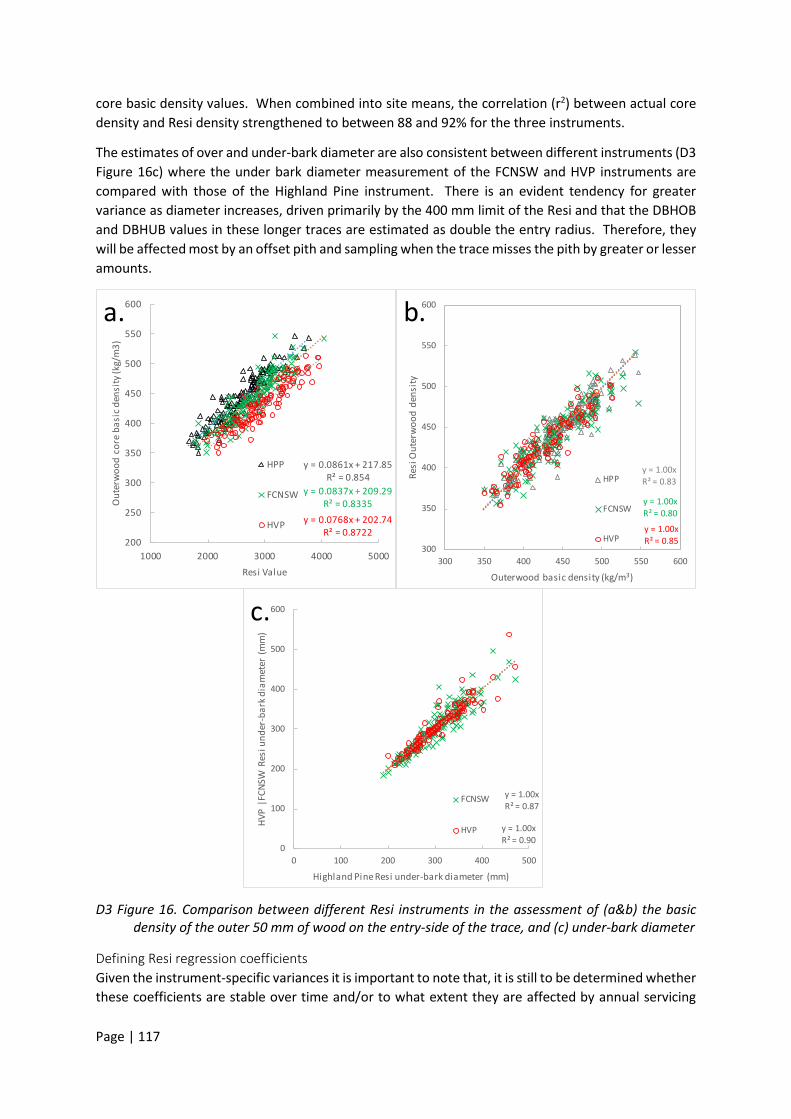
Page | 117

core basic density values. When combined into site means, the correlation (r2) between actual core density and Resi density strengthened to between 88 and 92% for the three instruments.

The estimates of over and under-bark diameter are also consistent between different instruments (D3 Figure 16c) where the under bark diameter measurement of the FCNSW and HVP instruments are compared with those of the Highland Pine instrument. There is an evident tendency for greater variance as diameter increases, driven primarily by the 400 mm limit of the Resi and that the DBHOB and DBHUB values in these longer traces are estimated as double the entry radius. Therefore, they will be affected most by an offset pith and sampling when the trace misses the pith by greater or lesser amounts.

D3 Figure 16. Comparison between different Resi instruments in the assessment of (a&b) the basic density of the outer 50 mm of wood on the entry-side of the trace, and (c) under-bark diameter

Defining Resi regression coefficients Given the instrument-specific variances it is important to note that, it is still to be determined whether these coefficients are stable over time and/or to what extent they are affected by annual servicing

y = 1.00xR² = 0.87

y = 1.00xR² = 0.90

0

100

200

300

400

500

600

0 100 200 300 400 500

HVP

|FCN

SW R

esi u

nder

-bar

k dia

met

er (m

m)

Highland Pine Resi under-bark diameter (mm)

FCNSW

HVP

c.

y = 1.00xR² = 0.83

y = 1.00xR² = 0.80

y = 1.00xR² = 0.85

300

350

400

450

500

550

600

300 350 400 450 500 550 600

Resi

Out

erw

ood

dens

ity

Outerwood basic density (kg/m3)

HPP

FCNSW

HVP

b.

y = 0.0861x + 217.85R² = 0.854

y = 0.0837x + 209.29R² = 0.8335

y = 0.0768x + 202.74R² = 0.8722

200

250

300

350

400

450

500

550

600

1000 2000 3000 4000 5000

Out

erw

ood

core

bas

ic d

ensi

ty (k

g/m

3)

Resi Value

HPP

FCNSW

HVP

a.

Page | 118

required by each instrument and needle wear. There is growing evidence to suggest that they are not affected by moisture content if the wood is above the fibre saturation point34.

It is also important to note that the determination of the slope and intercept values can be affected by the calibration data set. For example in D3 Figure 17, the data for the HPP instrument is considered for the full range of cores and for exactly the same data where the range is limited to cores less than 450 kg/m3. Defining these relationships in Excel is easy and convenient, but the nature of the (ordinary least squares (OLS)) regression approach is to tend to flatten the relationship (i.e. reduce the slope and increase the intercept). OLS regression assumes the y-values (actual core basic density) have no measurement error, and this assumption is not valid in this (or most) relationships.

Therefore, when calibrating the Resi instrument it is important to maximise the range of actual core density which can be done by sampling across a wide range of site types and age classes. In our full range data set, density ranged between 350 and 550 kg/m3. As we include younger material with densities lower than 350, we might expect the slope to increase and the intercept to decrease.

D3 Figure 17. The effect of range on defining regression coefficients is illustrated with a reduced range (red diamonds) giving a flatter relationship than the full range (grey triangles) which will tend to under-predict density in higher density trees.

Conclusions Measurements derived from Resi traces taken from standing tree preharvest were able to explain most of the site mean variance in log properties and green board properties following processing as measured by in-mill equipment. Resi basic density metrics explained as much variance as the other Resi metrics derived from the traces for predicted AWV and MOE.

Resi was effective in assessing log diameters and so can also be used for providing information about expected board volumes. Likewise, the ability of the Resi metrics to predict the proportion of boards with an MGP grading equal to or greater than 10 was also strong.

34 Sharapov et al 2019 “Moisture content had no significant impact on the modulus of elasticity prediction by the drilling resistance measurements, while density can be predicted by linear models for two stages of moisture content variation, below and above fibre saturation.” https://link.springer.com/article/10.1007/s00107-019-01439-2

y = 0.0861x + 217.85R² = 0.854

y = 0.0667x + 259.01R² = 0.6526

200

250

300

350

400

450

500

550

600

650

1000 1500 2000 2500 3000 3500 4000 4500 5000

Out

erw

ood

core

bas

ic d

ensi

ty (k

g/m

3)

Resi Value

Full range

Reduced Range

https://link.springer.com/article/10.1007/s00107-019-01439-2

https://link.springer.com/article/10.1007/s00107-019-01439-2

Page | 119

Individual Resi instruments need to be calibrated for basic density prediction to facilitate the accuracy of the resultant values. Calibration does not affect the precision of the data (for example the ranking of differences between sites).

The ongoing development and implementation of standardised methodologies in the implementation of Resi into routine commercial activity needs to be an ongoing focus.

Page | 120

Deliverable 4. Part 1. User Guide for the rCambium web platform David Drew and Geoff Downes

Overview: This web platform provides access to a simulation system that predicts the monthly stand growth and wood properties in plantation softwoods grown in Australia. The use of the platform is designed to be as intuitive and user-friendly as possible, requiring minimal input from users. For this reason, it is also a very simple system, and should be viewed as such. Based on user-provided information about a particular location (defined by latitude and longitude), the software will extract:

• the relevant soils information from that location from the ASRIS data base, based on an interpolated soils surface for Australia (see http://www.asris.csiro.au/about.html), and

• the monthly weather data from the SILO gridded climatic database (see https://legacy.longpaddock.qld.gov.au/silo/).

Monthly predictions of a range of stand growth and wood property variables are then generated and provided as site-average means for some variables, representing the “mean tree”.

This manual is intended to provide an overview of the operation of this web-based platform, to allow the user to upload regime-specific information and generate model outputs.

Web Platform layout The system is completely online and requires no software to be installed on the user’s local computer apart from an up-to-date internet browser. While not yet fully tested, this system should be accessible from/run correctly in most internet browsers on laptop or desktop computers. Its utility on hand-held devices is currently limited.

The web platform can be accessed at the following web address


The simulation system accesses publicly available data from Australian weather and soil databases, developed only for Australian locations. The model cannot be used, therefore, to simulate forest growth for locations outside Australia.

Scenario panel The opening page for the site includes a linked map object. It is the launch page for the simulation, and the point at which users must provide required data.

http://www.asris.csiro.au/about.html

https://legacy.longpaddock.qld.gov.au/silo/


Page | 121

As a default, to give users an idea of the input data requirements, the web site loads with three locations as described in the table below the map. The position of each of the locations is shown on the map. At this stage, defining this table is the only task requiring or allowing user adjustment of input data. The user can download a proforma spreadsheet-format file (click on the button “Regime download”) and update with their own site information. This can then be uploaded as a comma delimited (*.csv) file (process described below), and run using their locations.

Download Proforma: This button will download the current table which can act as a proforma for the user to populate with location specific information. The user needs to provide the following information indicated in the table columns.

IMPORTANT NOTE: The date formats of the various regime events needs to be defined strictly in YYYY-MM-DD format (e.g. 2001-07-01), with dashes separating year, month and day. The model will not be able to run with dates in any other format.

Upload Regime information Once a CSV file has been prepared with the Regime information in can be uploaded using this button to replace the existing table.

Upload Saved Runs If a set of runs has already been completed, it is possible to save the complete data set (soils, weather, simulated outputs) in a single *.rCambium file. If such a file is available from a prior run, it can be reloaded using this button. This keeps previously collected soil and weather data locally available, the advantage of which is that users can re-run simulations, for example with different parameters, without re-loading weather data, or view data again without re-running.

Run All Scenarios Selecting this button will start the process of working through each regime row in the table, collecting soil and weather data and running the rCambium model to predict growth and wood property

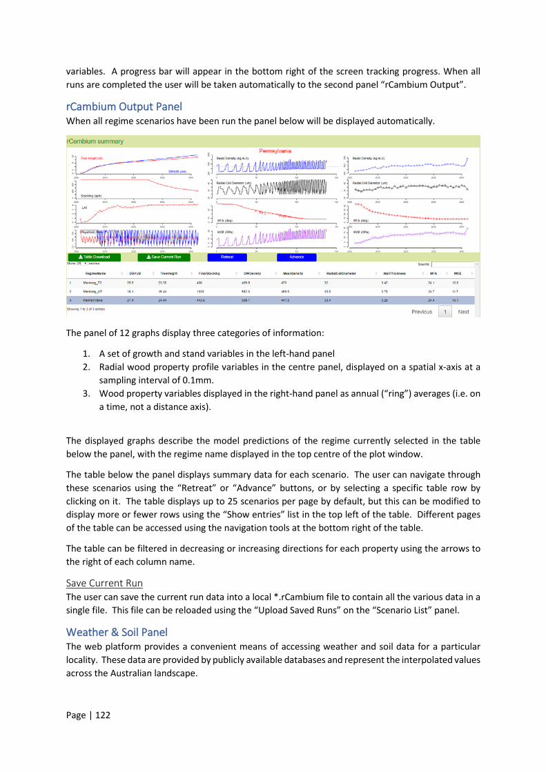
Page | 122

variables. A progress bar will appear in the bottom right of the screen tracking progress. When all runs are completed the user will be taken automatically to the second panel “rCambium Output”.

rCambium Output Panel When all regime scenarios have been run the panel below will be displayed automatically.

The panel of 12 graphs display three categories of information:

1. A set of growth and stand variables in the left-hand panel 2. Radial wood property profile variables in the centre panel, displayed on a spatial x-axis at a

sampling interval of 0.1mm. 3. Wood property variables displayed in the right-hand panel as annual (“ring”) averages (i.e. on

a time, not a distance axis).

The displayed graphs describe the model predictions of the regime currently selected in the table below the panel, with the regime name displayed in the top centre of the plot window.

The table below the panel displays summary data for each scenario. The user can navigate through these scenarios using the “Retreat” or “Advance” buttons, or by selecting a specific table row by clicking on it. The table displays up to 25 scenarios per page by default, but this can be modified to display more or fewer rows using the “Show entries” list in the top left of the table. Different pages of the table can be accessed using the navigation tools at the bottom right of the table.

The table can be filtered in decreasing or increasing directions for each property using the arrows to the right of each column name.

Save Current Run The user can save the current run data into a local *.rCambium file to contain all the various data in a single file. This file can be reloaded using the “Upload Saved Runs” on the “Scenario List” panel.

Weather & Soil Panel The web platform provides a convenient means of accessing weather and soil data for a particular locality. These data are provided by publicly available databases and represent the interpolated values across the Australian landscape.

Page | 123

Weather data are derived from stations managed by the Bureau of Meteorology and consequently subject to any data adjustment they consider necessary. These data were interpolated to a regular grid of 5km x 5km, and provided by SILO. Local weather conditions can vary significantly at finer resolution especially in areas with varying elevation and this source of variance should be born in mind when evaluating model performance.

• https://legacy.longpaddock.qld.gov.au/silo/

Likewise, the soil data is from the ASRIS database hosted by CSIRO as part of Australia’s Terrestrial Ecosystem Research Network (TERN) infrastructure, but provided on a finer grid of approx. 10 m x 10 m. However, soils data in the database is dominated by agricultural soils and the actual soil data from more remote and less productive forest soils may not be well represented.

• http://www.asris.csiro.au/about.html

The weather and soils data can be downloaded using the following two buttons

1. “Weather download”: Download a CSV file to the user’s local PC containing the monthly weather data for each location/scenario run.

2. “Soils download”: Download the table displayed below the plot window.

In the current version of the online system there is no provision for the user to upload their own, locally sourced weather and soils data. This functionality can be added once the performance of the model has been found to be commercially useful. However, it is notable that the fully automated capability provided by the implementation was considered from the outset to be a primary advantage of the rCambium system.

RSawmill Panel The virtual rSawmill functionality in the software is intended to provide a very simple basis for comparing sites and regimes in terms of their expected production of sawn boards in terms of nominal

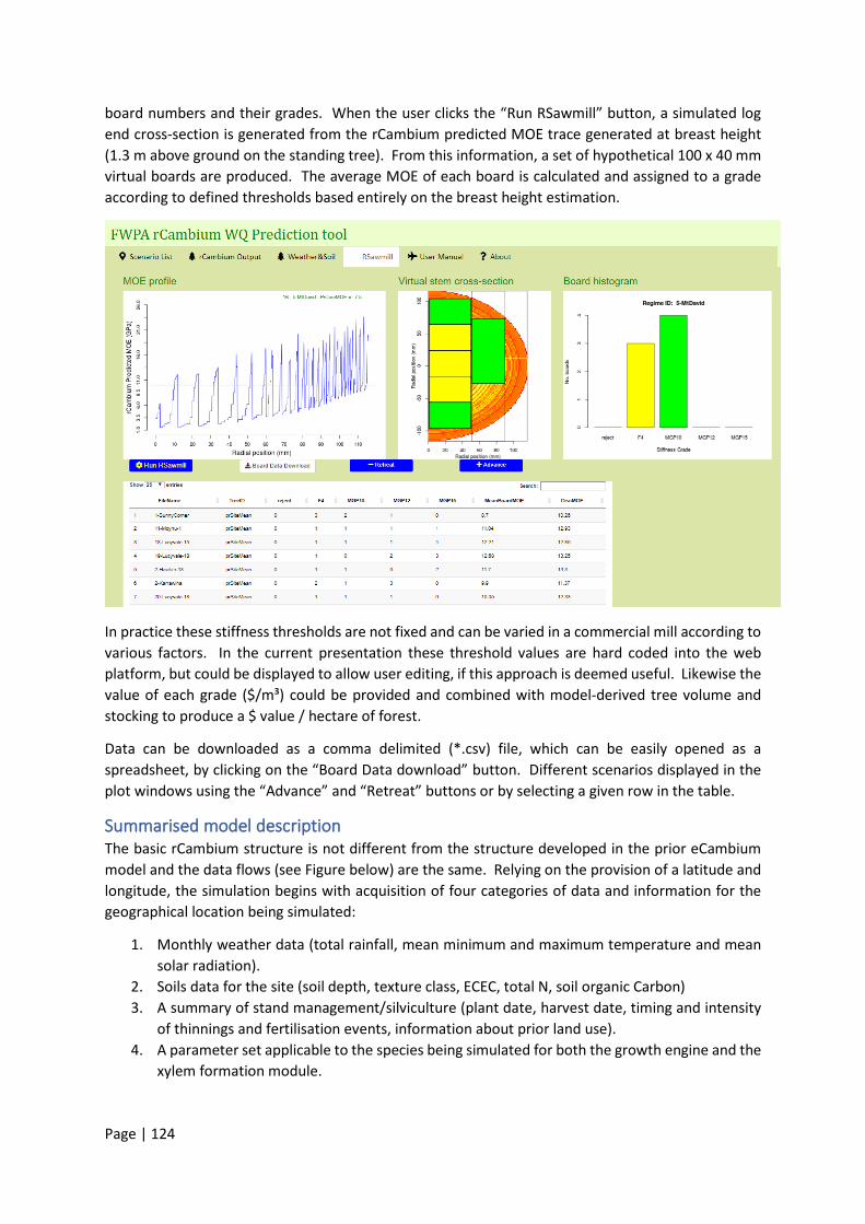
https://legacy.longpaddock.qld.gov.au/silo/

http://www.asris.csiro.au/about.html

Page | 124

board numbers and their grades. When the user clicks the “Run RSawmill” button, a simulated log end cross-section is generated from the rCambium predicted MOE trace generated at breast height (1.3 m above ground on the standing tree). From this information, a set of hypothetical 100 x 40 mm virtual boards are produced. The average MOE of each board is calculated and assigned to a grade according to defined thresholds based entirely on the breast height estimation.

In practice these stiffness thresholds are not fixed and can be varied in a commercial mill according to various factors. In the current presentation these threshold values are hard coded into the web platform, but could be displayed to allow user editing, if this approach is deemed useful. Likewise the value of each grade ($/m³) could be provided and combined with model-derived tree volume and stocking to produce a $ value / hectare of forest.

Data can be downloaded as a comma delimited (*.csv) file, which can be easily opened as a spreadsheet, by clicking on the “Board Data download” button. Different scenarios displayed in the plot windows using the “Advance” and “Retreat” buttons or by selecting a given row in the table.

Summarised model description The basic rCambium structure is not different from the structure developed in the prior eCambium model and the data flows (see Figure below) are the same. Relying on the provision of a latitude and longitude, the simulation begins with acquisition of four categories of data and information for the geographical location being simulated:

1. Monthly weather data (total rainfall, mean minimum and maximum temperature and mean solar radiation).

2. Soils data for the site (soil depth, texture class, ECEC, total N, soil organic Carbon) 3. A summary of stand management/silviculture (plant date, harvest date, timing and intensity

of thinnings and fertilisation events, information about prior land use). 4. A parameter set applicable to the species being simulated for both the growth engine and the

xylem formation module.

Page | 125

The framework is set up in the current implementation so that the predictions from the stand growth simulation feed into the xylem formation simulation month-by-month, and in that way the two modules interact. Tree diameter is calculated from the xylem formation simulation and fed back to the stand simulation, which in turn influences stand model behaviour (e.g. height growth and resource allocation). The key variables required by rCambium are relatively few:

• Net primary productivity (T/ha) and proportional allocation to stem, foliage and roots. • Stand density (trees/ha). • A relative indication of drought as determined by soil and atmosphere. • Mean temperature (deg C). • Tree height (m) and an indication of growth extent (crown length, m).

The model works by first deciding on the properties of the cells which would be expected in a particular month given the environmental conditions, and thereafter calculates how many tracheids with those properties could be formed with the resources (allocated photosynthate) available. The stand-level model is constrained by a set of parameters, and the wood properties model is constrained by a separate set of 23 parameters (see Appendix 1 and 2).

The following steps are followed in the main rCambium module at each timestep:

1. The surface area of the stem of the modelled tree is calculated. 2. A “Crown Control Value” (CCV) is calculated controlling the ontogenetic patterns seen in pine

tracheids over time. a. This is a simple function of the height of the tree and relative size of the crown. b. A tall tree with a short crown will have a larger CCV than a shorter tree or a tree with

a longer crown. 3. Expected tracheid length for the timestep is calculated as a function of the CCV. 4. Expected tracheid radial diameter for the timestep is calculated as a function of the CCV and

the level of drought being experienced by the stand.

Page | 126

5. Expected tracheid wall thickness for the timestep is calculated as a function of the CCV and the cumulative temperature sum, initiated for each year at the winter solstice.

6. From tracheid length, radial diameter and wall thickness (and assuming a constant tangential diameter), the following Tracheid parameters are calculated:

a. Cross sectional area b. Lumen cross-sectional area and wall cross-sectional area c. Volume d. Lumen volume & wall volume

7. Based on the total amount of allocated substrate (an input requirement from the stand-level model) available for the timestep, the surface area of stem over which allocation must be made (conceptually, the area covered by the cambium) and the average tracheid tangential diameter and length, an average cell file specific substrate availability (CFSA) is calculated

8. The CFSA is used to calculate the number of cells with the properties previously determined (step 6) which can be formed with that amount of substrate, assuming a given wall density conversion factor

Page | 127

Table 1: Xylem formation model parameters

PARAMETER CODE DESCRIPTION MAXEWTRD Maximum achievable tracheid radial diameter (micrometres) JUVENILEEWTRD Maximum TRD in the juvenile core (micrometres) MINTRD Mean minimum TRD (not absolute min) (micrometres) KRD Controls shape and slope of P to B TRD MRD Controls shape and slope of P to B TRD KL Controls shape and slope of P to B TL ML Controls shape and slope of P to B TL SENSRDFSW Sensitivity of TRD growth to water deficit MAXWT Maximum tracheid wall thickness in the latewood (micrometres) MINEWWT Minimum tracheid wall thickness in the earlywood (micrometres) MAXEWWT Maximum tracheid wall thickness in the earlywood KWT Controls shape and slope of P to B TWT MWT Controls shape and slope of P to B TWT MINTWOOD The cumulative Minimum temperature above which secondary wall forms (unit

degree months) WALLDENSITY Density of the cell wall in air dried tissue MINTL Minimum tracheid length (in JW, micrometres) MAXTL Maximum tracheid length (micrometres) WALLINCDEGC Rate of wall increment/degree month above minimum MAXJWMFA Average maximum MFA in the juvenile wood (degrees) MINMWMFA Average minimum MFA in the mature wood (degrees) BETAMFA Controls slope of MFA curve B0MOE Multiplier with WD in MOE relationship B1MOE Multiplier with MFA in MOE relationship

Page | 128

Table 2: Stand level growth model parameters

PARAMETER CODE DESCRIPTION MAXAGE Determines rate of "physiological decline" of forest NAGE Empirical parameters in age-modifier RAGE Empirical parameters in age-modifier FULLCANAGE Age at full canopy cover K Radiation extinction coefficient GAMMAR Root turnover rate per month FCALPHA700 Assimilation enhancement factor for 700 ppm atmospheric CO2 FCG700 Assimilation enhancement factor for 700 ppm atmospheric CO2 MAXINTCPTN Max proportion of rainfall intercepted by canopy LAIMAXINTCPTN LAI required for maximum rainfall interception MINCOND Minimum canopy conductance (gc, m/s) MAXCOND Maximum canopy conductance (gc, m/s) LAIGCX LAI required for maximum canopy conductance (See e.g. work by Granier,

Loustau and Breda; 2000) BLCOND Canopy boundary layer conductance, assumed constant COEFFCOND Determines response of canopy conductance to VPD MAXRATESOILEVAP Determines max rate at which water evaporates from bare soil Y Assimilate use efficiency TMAX Critical biological max temperature. TMIN Critical biological min temperature. TOPT Optimal temperature for carbon sequestration and growth KF Number of days production lost per frost days PFS2 Foliage:stem partitioning ratios for D PFS20 Foliage:stem partitioning ratios for D MINCL Minimum crown length (m) MAXCR The maximum rate of crown retreat (m/month) CLINTMOD The relative retarding of crown retreat m per SPH FCC Sensitivity of the "crown control" effect on crown length AWS Stem allometric parameters NWS Stem allometric parameters PRX maximum root biomass partitioning PRN minimum root biomass partitioning RLGROWTHX Max rate of root length growth (m/month) M0 Value of m when FR FN Value of fN when FR FERTDECAY Rate of decay of fertilisation effect (1/month) ALPHACX Canopy quantum efficiency WSX1000 Max tree stem mass (kg) likely in mature stands of 1000 trees/ha THINPOWER Power in self-thinning law MF Leaf mortality fraction MR Root mortality fraction MS Stem mortality fraction GAMMAF1 Coefficients in monthly litterfall rate GAMMAF0 Coefficients in monthly litterfall rate

Page | 129

PARAMETER CODE DESCRIPTION TGAMMAF Coefficients in monthly litterfall rate SLA0 specific leaf area at age 0 (m^2/kg) SLA1 specific leaf area for mature trees (m^2/kg) TSLA stand age (years) for SLA MAXHDRATIO Maximum ratio of height to base diameter (m/cm) MINHDRATIO Minimum ratio of height to base diameter (m/cm) SPHHEIGHTMOD Stand density modifier for height growth HTMULT Multiplier in relationship between height growth and allocation QA intercept of net v. solar radiation relationship (W/m2) QB slope of net v. solar radiation relationship GDM_MOL conversion of mol to gDM MOLPAR_MJ conversion of MJ to PAR

Page | 130

Appendix 1: Procedure for validating rCambium predictions.

David Drew and Geoff Downes

Background This guide attempts to document the process for validating predictions made using the rCambium modelling framework available at

https://forestquality.shinyapps.io/rcambium

The above platform endeavours to predict mean tree growth and wood properties at a monthly time step over the course of a rotation according to user-defined silvicultural regimes. Each scenario is defined by a location (latitude and longitude), planting and harvest dates, initial stocking and the timing and magnitude of thinning and fertiliser events.

The model predicts a range of metrics and these can be compared directly with real values if available. The model was mainly built, however, to predict basic wood density and MOE at breast height (1.3m), along with DBH (underbark) (DBHUB) and tree height.

The present developmental need is to determine the extent to which simulations give commercially useful predictions, with respect to:

• Accuracy: are the predictions close to actual observed values? • Precision: when comparing predictions across a range of sites do the model predictions rank

the sites similarly to the real world data?

Proposed testing and validation procedure As a first test of the success of the modelling framework, we propose that industry partners should pursue the following process where possible.

1. Identify a range of sites across there resource representing the broadest range of site quality (most easily, this can be defined by site index) as possible.

a. Typically, these will be sites of contrasting rainfall, elevation and soil type. b. If this can be done in two age classes (e.g. mid rotation and mature35) that would be

of value, bearing in mind that differing age classes will tend to artificially improve model predictions relative to actual data36.

2. Collect the regime information for each of these sites in the format required for running a simulation on rCambium platform

a. Proforma spreadsheet/CSV file is downloadable on the rCambium platform. 3. Collect the actual site values from each site (over-bark DBH (DBHOB) (cm), Tree height (m),

stocking (trees/ha), Resi traces). a. If possible, collect actual 50 mm long outerwood cores from a subset of trees from

each site to calibrate (check) the Resi-derived values. Cores need to be taken as close to the Resi sampling entry point as possible.

35 At this stage of validation it might be preferred to choose sites where the maximum DBHOB did not exceed 38cm so that a full B-B Resi trace can be obtained. 36 For example choosing 20 sites each at a different age will tend to give better correlations with growth and wood density data as the model will naturally predict smaller, less dense trees at younger ages.

https://forestquality.shinyapps.io/rcambium

Page | 131

4. Process the Resi traces and generate the DBHOB, DBHUB, basic wood density metrics (Outerwood and core) and PrMOE

5. Process the actual outerwood cores to generate basic density values and check / calibrate the Resi-derived values

6. Run the rCambium regimes and download the summary table of predicted values. a. A full user-guide can be found online at

https://forestquality.shinyapps.io/rCambium/. 7. Set up a simple analysis of “predicted” vs “actual” data. We suggest doing this on the sheet

of simulated data downloaded from the rCambium platform after your model run was completed.

a. It is important, when assessing your results to, take note of two things i. The range in the validation data: If the range of actual site values is narrow,

then variance explained will also be less. This is in part a function of the practical precision of a basic model like rCambium.

ii. The variability between the sites/scenarios used. Needless to say, the rCambium platform will not be able to work with the input data provided: it will give very similar predictions for very similar sites!

b. Model performance can be assessed by more than one measure, preferably in concert. We recommend:

i. Use the coefficient of determination (“R-squared”) to give an indication of variance explained

ii. The overall bias: how much were we out in absolute terms? iii. Also use standard errors of prediction (SEP). Contact Geoff Downes for a

simple R script to make this calculation. See here for why this can be useful. iv. Finally, consider the success in ranking. Even if absolute predictions were

out, did the model correctly flag low sites and high sites? 8. Send the data to Geoff Downes and David Drew to assist in improving rCambium

performance and allow the comparison of performance across a larger combined data set.


https://statisticsbyjim.com/regression/standard-error-regression-vs-r-squared/

Page | 132

Appendix 2: Soil Sampling protocol

Page | 133

Deliverable 4. Part 2. Evaluating the performance of the rCambium platform in radiata pine.

Dave Drew (University of Stellenbosch) and Geoff Downes (Forest Quality)

Contributors: Stephen Elms (HVP), Don Aurik (Timberlands), Michael Schofield (NS) and Chris Rhynehart (HF)

Objective: To assess the optimised performance of the rCambium web platform against optimisation and validation data sets, involving site-mean metrics obtained from a total of 160 sites spanning a wide geographical range across Tasmania, Victoria and NSW.

Key Findings • The rCambium web platform has performed robustly, processing input data sets defining

hundreds of separate scenarios, processing each scenario in 1-2 secs.

• Using site index as an input to the rCambium model is not advised at this stage. While slightly improving the prediction of tree height, it resulted in poorer predictions of diameter and wood property metrics.

• Measures of tree height were accurate (little bias over all) but imprecise (r2 ~ 20%)

• Measures of under-bark diameter were reasonable in terms of variance explained (r2 ~ 43%) with a tendency to under-predict larger diameter sites.

• Predictions of wood density were best against pith-to-bark or bark-to-bark means, avoiding the confounding effects of diameter growth on outerwood density metrics

• Over the whole data set, rCambium predicted 50% of the variance in Resi-predicted pith-to-bark basic density with a SEP of 20 kg.m-3.

• rCambium predictions of log MOE were strong, explaining 66% of the variance.

• rCambium is intended as a lowest-cost, first-pass assessment of wood quality variance at the estate level. The broad resolution of the input weather data and potential inaccuracy in the publicly available soils data will lead to poor performance at some sites. Thus application across a range of sites where the actual range of wood property values is restricted will result in lower levels of explained variance (r2). SEP values should guide the user with respect to the expected confidence intervals that can be expect in model predictions.

Page | 134

Introduction The rCambium platform is a simple, but feasible approach to modelling tree growth and wood variability. Relying on the user to only provide location (latitude and longitude) and regime details (plant and harvest dates along with silvicultural interventions), the simulation begins with acquisition of four categories of data and information for the location being simulated:

5. Automated collection of monthly weather data (total rainfall, mean minimum and maximum temperature and mean solar radiation) from the Silo data base (https://www.longpaddock.qld.gov.au/silo/).

6. Automated collection of soils data for the site (soil depth, texture class, ECEC, total N, soil organic Carbon) from the Asris data base (http://www.asris.csiro.au/)

7. User provided summary of stand management/silviculture (plant date, harvest date, timing and intensity of thinnings and fertilisation events, information about prior land use).

8. A parameter set applicable to the species being simulated for both the growth engine and the xylem formation module.

D4P2 Figure 1 diagrams the way this information flows through the model platform. The framework is set up in the current implementation so that the predictions from the stand growth simulation feed into the xylem formation simulation month-by-month, and in that way the two modules interact.

D4P2 Figure 1. Data flows in rCambium

Tree diameter is calculated from the xylem formation simulation and fed back to the stand simulation, which in turn influences stand model behaviour (e.g. height growth and resource allocation). Importantly, the key variables required by rCambium are relatively few. This has the advantage of ensuring the framework is simple and easy to understand and parameterise, while based on broad principles of tree growth which are likely to hold at this level of complexity. The model will not cope with subtle differences between sites which cannot be explained by the relatively small number of input variables.

https://www.longpaddock.qld.gov.au/silo/

http://www.asris.csiro.au/

Page | 135

How it works The model works by first deciding on the properties of the wood cells which would be expected in a particular month given the environmental conditions, and thereafter calculates how many tracheids with those properties could be formed with the resources (allocated photosynthate) available. The stand-level model is constrained by a set of 57 parameters, and the wood properties model is constrained by a separate set of 23 parameters.

The following steps are followed in the main rCambium module at each timestep:

9. The surface area of the stem of the modelled tree is calculated. 10. A “Crown Control Value” (CCV) is calculated controlling the ontogenetic patterns seen in pine

tracheids over time. a. This is a simple function of the height of the tree and relative size of the crown. b. A tall tree with a short crown will have a larger CCV than a shorter tree or a tree with

a longer crown. 11. Expected tracheid length for the timestep is calculated as a function of the CCV. 12. Expected tracheid radial diameter for the timestep is calculated as a function of the CCV and

the level of drought being experienced by the stand. 13. Expected tracheid wall thickness for the timestep is calculated as a function of the CCV and

the cumulative temperature sum, initiated for each year at the winter solstice. 14. From tracheid length, radial diameter and wall thickness (and assuming a constant tangential

diameter), the following tracheid parameters are calculated: a. Cross sectional area b. Lumen cross-sectional area and wall cross-sectional area c. Volume d. Lumen volume & wall volume

15. Based on the total amount of allocated substrate (an input requirement from the stand-level model) available for the timestep, the surface area of stem over which allocation must be made (conceptually, the area covered by the cambium) and the average tracheid tangential diameter and length, an average cell file specific substrate availability (CFSA) is calculated

16. The CFSA is used to calculate the number of cells with the properties previously determined (step 6) which can be formed with that amount of substrate, assuming a given wall density conversion factor

rCambium optimisation Developing a predictive model that explains commercially useful amounts of variance in tree growth and wood properties from publicly available data is a difficult task. The design complexity of living organisms, the genetic and phenotypic sources of variance combined with the relatively coarse spatial resolution of weather and soils data contribute to the difficulty in obtaining consistent patterns of response to silvicultural and environmental changes. The high degree of variance between individual trees within a stand reflects in part the genetic variance as well as the micro-spatial variability in growth conditions.

Publicly available weather data is available on a spatial interval of approx. 5km x 5 km37. The spatial interval of the soils data is down to 10m x 10m, albeit the actual data underlying this interpolated surface is at a much coarser resolution. Obviously, the data is not obtained from actual measurements

37 In the Silo data base the size of each grid cell is 0.05°longitude × 0.05° latitude. Supplied location data at higher resolutions is rounded down.

Page | 136

at a given point but interpolated from a non-random collection of data points. Soils data is typically biased towards agricultural soils.

In adapting the web-based rCambium platform to utilise these public databases (required to make its commercial use feasible) the model parameters need to be optimised to balance the predicted growth and wood formation algorithms to explain the most variance in actual data. This can be a delicate procedure as parameters are inter-connected in the sense that, for example, changing height growth impacts on the carbon allocation, which affects the available carbon for wood formation.

The main objective of rCambium is as a broad-scale wood property assessment tool that allows users to obtain a reasonable indication of how wood quality varies across the landscape. This can then be used to guide actual sampling programs to refine the assessment using approaches such as the Resi instruments. The following optimisation of the rCambium parameters was done using sites from

• 2015 Tumbarumba sawmill study from a previous FWPA project38. o 53 sites with growth and outerwood density; o 12 of the 53 sites with Resi, Log and Sawmill data

• 2019 Oberon sawmill study o 9 sites with growth, outerwood density, Resi, Log and sawmill data

To the extent that rCambium predictions are found to be precise, the model can be used to explore the likely effect of silvicultural interventions.

The main purpose here was to maximise the explained variance in actual board MOE produced which should also optimise the ability to predict actual log MOE. However, because these data are expensive to collect, the ability to predict site mean density values derived from actual coring or from Resi sampling programs is important. These data have been shown to explain most of the variance in actual board properties.

Optimisation performance Growth and wood property metrics were available from a total of 62 sites (D4P2 Table 1) spanning the geographic range from the Benalla region in central Victoria to Oberon in Central New South Wales. The data from these sites was used to identify the model parameters that would give the best balance between accurate and precise predictions of tree growth (height and under-bark DBH) and then wood properties with a focus on outerwood density. We use outerwood density here as it is the most common form of commercial assessment of wood quality. Because of this it is necessary to get the rCambium predictions of DBH as accurate as possible.

rCambium bases a lot of its predictions on carbon balance. Growth (height then diameter) involves the consumption of carbon, and the amount used impacts on what is then available for wood formation (cell number and wall thickness).

38 https://www.fwpa.com.au/images/webinars/2016/PNC325-1314_eCambium_18_May_2016.pdf

https://www.fwpa.com.au/images/webinars/2016/PNC325-1314_eCambium_18_May_2016.pdf

Page | 137

D4P2 Table 1. Optimisation site mean descriptors

RegimeName Region PlantDate HarvestDate Age PlantSPH Trt LandUseFQ131_1-SunnyCorner Oberon 1/07/1991 31/03/2019 27.77 1122 UT ForestFQ131_2-Karrawina Oberon 1/07/1988 31/03/2019 30.77 1288 UT ForestFQ131_3-DarlingHills Oberon 1/07/1986 31/03/2019 32.77 1080 T1 Pasture2FQ131_4-Pennsylvania Bathurst 1/07/1987 31/03/2019 31.77 1100 UT ForestFQ131_5-MtDavid Bathurst 1/07/1991 31/03/2019 27.77 1100 UT ForestFQ131_6-Glenwood Orange 1/07/1986 31/03/2019 32.77 815 UT ForestFQ131_7-Coolamatong Orange 1/07/1987 31/03/2019 31.77 1100 T1 Pasture2FQ131_8-Gurnang Oberon 1/07/1990 31/03/2019 28.77 1100 T2 ForestFQ131_9-Jeremy Oberon 1/07/1985 31/03/2019 33.77 1100 UT Pasture2FQ075-01-HV013 Ovens Valley 1/07/1983 1/10/2014 31.27 1200 UT ForestFQ075-02-HV013a Ovens Valley 1/07/1982 1/10/2014 32.27 1200 UT ForestFQ075-03-BR019 Ovens Valley 1/07/1988 1/10/2014 26.27 1100 UT ForestFQ075-04-ST048 Ovens Valley 1/07/1997 1/10/2014 17.26 1100 T1 ForestFQ075-05-MG001UT Ovens Valley 1/07/1989 1/10/2014 25.27 1250 UT ForestFQ075-06-MG001OP Ovens Valley 1/07/1989 1/10/2014 25.27 1100 T3 ForestFQ075-07-MG001TH Ovens Valley 1/07/1989 1/10/2014 25.27 1100 T2 ForestFQ075-08-ME111 Ovens Valley 1/07/1989 1/10/2014 25.27 1100 T2 Pasture2FQ075-09-NN001 Ovens Valley 1/06/1985 1/10/2014 29.35 1111 T1 Pasture2FQ075-10-HC427 Ovens Valley 1/07/1987 1/10/2014 27.27 1100 T1 ForestFQ075-11-MH001 Ovens Valley 1/07/1991 1/10/2014 23.27 1100 T1 Pasture2FQ075-12-WT001 Ovens Valley 1/07/1988 1/10/2014 26.27 1100 T1 ForestFQ075-13-HL224 Ovens Valley 1/07/1981 1/10/2014 33.27 900 UT ForestFQ075-14-WC158 Ovens Valley 1/07/1985 1/10/2014 29.27 960 T1 ForestFQ075-15-EV002 Ovens Valley 1/07/1987 1/10/2014 27.27 850 UT Pasture1FQ075-16-JN058 Shelley 1/07/1987 1/10/2014 27.27 1100 T1 Pasture2FQ075-17-KO057 Shelley 1/07/1987 1/10/2014 27.27 1100 T2 Pasture2FQ075-18-LV015 Shelley 1/07/1986 1/10/2014 28.27 1100 T2 ForestFQ075-19-LV018b Shelley 1/07/1986 1/10/2014 28.27 1100 UT ForestFQ075-20-LV018a Shelley 1/07/1986 1/10/2014 28.27 1100 T1 ForestFQ075-21-GO024 Shelley 1/07/1988 1/10/2014 26.27 1000 T1 Pasture1FQ075-22-BU019a Shelley 1/07/1988 1/10/2014 26.27 1100 T2 ForestFQ075-23-BU019b Shelley 1/07/1988 1/10/2014 26.27 1100 UT ForestFQ075-24-TR016UT Benalla 1/07/1986 1/10/2014 28.27 900 UT ForestFQ075-25-TR014TH Benalla 1/07/1986 1/10/2014 28.27 900 T2 ForestFQ075-26-GA003 Benalla 1/07/1988 1/10/2014 26.27 900 T2 Pasture1FQ075-27-WB026 Benalla 1/07/1968 1/10/2014 46.28 1650 UT ForestFQ075-28-AR1194 Buccluegh 1/07/1987 1/10/2014 27.27 1100 UT ForestFQ075-29-GC801 Buccluegh 1/07/1987 1/10/2014 27.27 1100 UT ForestFQ075-30-OC1195TH Buccluegh 1/07/1987 1/10/2014 27.27 1100 T2 ForestFQ075-31-OC1195UT Buccluegh 1/07/1987 1/10/2014 27.27 1100 T1 ForestFQ075-32-OC1012UT Buccluegh 1/07/1984 1/10/2014 30.27 1100 UT ForestFQ075-33-OC1012TH Buccluegh 1/07/1984 1/10/2014 30.27 1100 T2 ForestFQ075-34-WJ1151 Buccluegh 1/07/1985 1/10/2014 29.27 1100 T2 ForestFQ075-35-SP1181UT Buccluegh 1/07/1987 1/10/2014 27.27 1100 UT Pasture2FQ075-36-SP1182TH Buccluegh 1/07/1987 1/10/2014 27.27 1100 T1 Pasture2FQ075-37-BI104T1 Buccluegh 1/07/1985 1/10/2014 29.27 1400 T1 ForestFQ075-38-BI133T2 Buccluegh 1/07/1986 1/10/2014 28.27 1100 T2 ForestFQ075-39-MA044UT Tumbarumba 1/07/1984 1/10/2014 30.27 1100 UT ForestFQ075-40-MA053TH Tumbarumba 1/07/1987 1/10/2014 27.27 1100 T1 ForestFQ075-41-BG582UT Bago 1/07/1984 1/10/2014 30.27 1100 UT ForestFQ075-42-BG587T1 Bago 1/07/1986 1/10/2014 28.27 1100 T1 ForestFQ075-43-BG583T2 Bago 1/07/1984 1/10/2014 30.27 1100 T2 ForestFQ075-44-BG066UT Bago 1/07/1985 1/10/2014 29.27 1100 UT Pasture2FQ075-45-GH849UT GreenHills 1/07/1987 1/10/2014 27.27 875 UT Pasture1FQ075-46-GH849T1 GreenHills 1/07/1987 1/10/2014 27.27 875 T1 Pasture1FQ075-47-GH845T2 GreenHills 1/07/1989 1/10/2014 25.27 1100 T2 Pasture1FQ075-48-GH845T1 GreenHills 1/07/1986 1/10/2014 28.27 1100 T1 Pasture1FQ075-49-GH828UT GreenHills 1/07/1984 1/10/2014 30.27 1100 T1 Pasture2FQ075-50-CB001T1 Carabost 1/07/1987 1/10/2014 27.27 1100 T1 ForestFQ075-51-MU206 Muraguldrie 1/07/1979 1/10/2014 35.28 1400 UT ForestFQ075-52-CB011T1 Carabost 1/07/1986 1/10/2014 28.27 1333 T1 ForestFQ075-53-CB018T1 Carabost 1/07/1984 1/10/2014 30.27 1196 T1 Forest

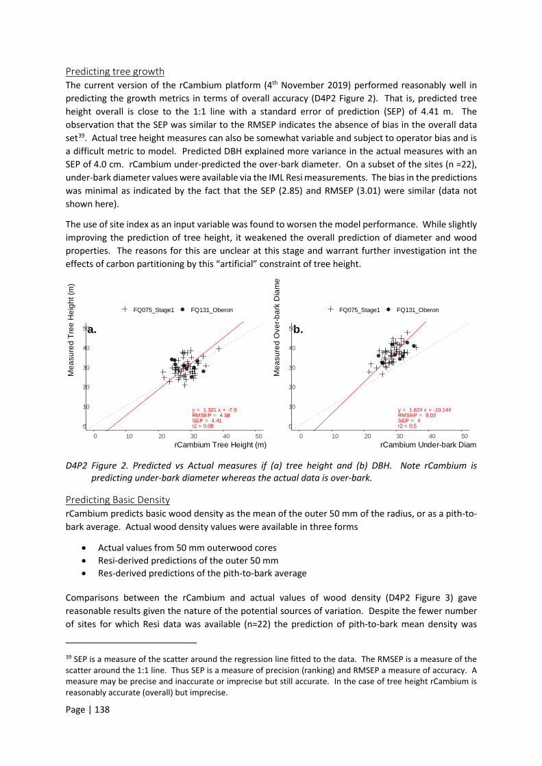
Page | 138

Predicting tree growth The current version of the rCambium platform (4th November 2019) performed reasonably well in predicting the growth metrics in terms of overall accuracy (D4P2 Figure 2). That is, predicted tree height overall is close to the 1:1 line with a standard error of prediction (SEP) of 4.41 m. The observation that the SEP was similar to the RMSEP indicates the absence of bias in the overall data set39. Actual tree height measures can also be somewhat variable and subject to operator bias and is a difficult metric to model. Predicted DBH explained more variance in the actual measures with an SEP of 4.0 cm. rCambium under-predicted the over-bark diameter. On a subset of the sites (n =22), under-bark diameter values were available via the IML Resi measurements. The bias in the predictions was minimal as indicated by the fact that the SEP (2.85) and RMSEP (3.01) were similar (data not shown here).

The use of site index as an input variable was found to worsen the model performance. While slightly improving the prediction of tree height, it weakened the overall prediction of diameter and wood properties. The reasons for this are unclear at this stage and warrant further investigation int the effects of carbon partitioning by this “artificial” constraint of tree height.

D4P2 Figure 2. Predicted vs Actual measures if (a) tree height and (b) DBH. Note rCambium is predicting under-bark diameter whereas the actual data is over-bark.

Predicting Basic Density rCambium predicts basic wood density as the mean of the outer 50 mm of the radius, or as a pith-to-bark average. Actual wood density values were available in three forms

• Actual values from 50 mm outerwood cores • Resi-derived predictions of the outer 50 mm • Res-derived predictions of the pith-to-bark average

Comparisons between the rCambium and actual values of wood density (D4P2 Figure 3) gave reasonable results given the nature of the potential sources of variation. Despite the fewer number of sites for which Resi data was available (n=22) the prediction of pith-to-bark mean density was

39 SEP is a measure of the scatter around the regression line fitted to the data. The RMSEP is a measure of the scatter around the 1:1 line. Thus SEP is a measure of precision (ranking) and RMSEP a measure of accuracy. A measure may be precise and inaccurate or imprecise but still accurate. In the case of tree height rCambium is reasonably accurate (overall) but imprecise.

a.

y = 1.321 x + -7.9RMSEP = 4.58SEP = 4.41r2 = 0.080

10

20

30

40

50

0 10 20 30 40 50rCambium Tree Height (m)

Mea

sure

d Tr

ee H

eigh

t (m

)

FQ075_Stage1 FQ131_Oberon

b.

y = 1.624 x + -10.144RMSEP = 9.02SEP = 4r2 = 0.50

10

20

30

40

50

0 10 20 30 40 50rCambium Under-bark Diame

Mea

sure

d O

ver-b

ark

Dia

met


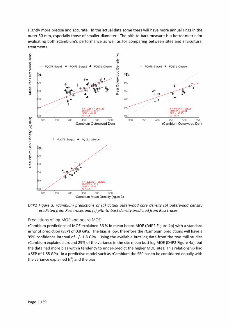
Page | 139

slightly more precise and accurate. In the actual data some trees will have more annual rings in the outer 50 mm, especially those of smaller diameter. The pith-to-bark measure is a better metric for evaluating both rCambium’s performance as well as for comparing between sites and silvicultural treatments.

D4P2 Figure 3. rCambium predictions of (a) actual outerwood core density (b) outerwood density predicted from Resi traces and (c) pith-to-bark density predicted from Resi traces

Predictions of log MOE and board MOE rCambium predictions of MOE explained 36 % in mean board MOE (D4P2 Figure 4b) with a standard error of prediction (SEP) of 0.9 GPa. The bias is low, therefore the rCambium predictions will have a 95% confidence interval of +/- 1.8 GPa. Using the available butt log data from the two mill studies rCambium explained around 29% of the variance in the site mean butt log MOE (D4P2 Figure 4a), but the data had more bias with a tendency to under-predict the higher MOE sites. This relationship had a SEP of 1.55 GPa. In a predictive model such as rCambium the SEP has to be considered equally with the variance explained (r2) and the bias.

a.

y = 0.65 x + 158.133RMSEP = 41.9SEP = 41.67r2 = 0.3300

350

400

450

500

550

300 350 400 450 500 550rCambium Outerwood Density (kg.m-3)

Mea

sure

d O

uter

woo

d D

ensi

FQ075_Stage1 FQ075_Stage2 FQ131_Oberon

b.

y = 0.547 x + 188.75RMSEP = 46.04SEP = 40.15r2 = 0.34300

350

400

450

500

550

300 350 400 450 500 550rCambium Outerwood Dens

Res

i Out

erw

ood

Den

sity

(kg


c.

y = 1.172 x + -76.821RMSEP = 21.2SEP = 20.52r2 = 0.37300

350

400

450

500

550

300 350 400 450 500 550rCambium Mean Density (kg.m-3)

Res

i Pith

-to-B

ark

Den

sity

(kg.

m-3

)


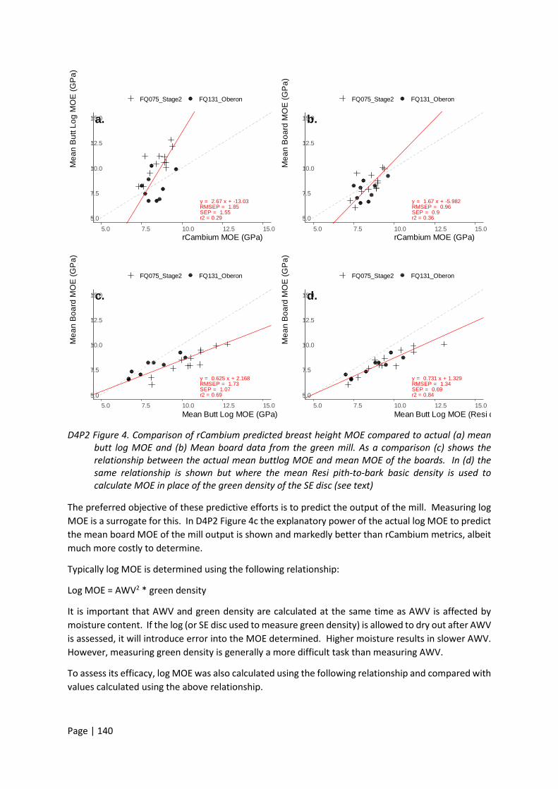
Page | 140

D4P2 Figure 4. Comparison of rCambium predicted breast height MOE compared to actual (a) mean butt log MOE and (b) Mean board data from the green mill. As a comparison (c) shows the relationship between the actual mean buttlog MOE and mean MOE of the boards. In (d) the same relationship is shown but where the mean Resi pith-to-bark basic density is used to calculate MOE in place of the green density of the SE disc (see text)

The preferred objective of these predictive efforts is to predict the output of the mill. Measuring log MOE is a surrogate for this. In D4P2 Figure 4c the explanatory power of the actual log MOE to predict the mean board MOE of the mill output is shown and markedly better than rCambium metrics, albeit much more costly to determine.

Typically log MOE is determined using the following relationship:

Log MOE = AWV2 * green density

It is important that AWV and green density are calculated at the same time as AWV is affected by moisture content. If the log (or SE disc used to measure green density) is allowed to dry out after AWV is assessed, it will introduce error into the MOE determined. Higher moisture results in slower AWV. However, measuring green density is generally a more difficult task than measuring AWV.

To assess its efficacy, log MOE was also calculated using the following relationship and compared with values calculated using the above relationship.

a.

y = 2.67 x + -13.03RMSEP = 1.85SEP = 1.55r2 = 0.295.0

7.5

10.0

12.5

15.0

5.0 7.5 10.0 12.5 15.0rCambium MOE (GPa)

Mea

n B

utt L

og M

OE

(GP

a)


b.

y = 1.67 x + -5.982RMSEP = 0.96SEP = 0.9r2 = 0.365.0

7.5

10.0

12.5

15.0

5.0 7.5 10.0 12.5 15.0rCambium MOE (GPa)

Mea

n B

oard

MO

E (G

Pa)


c.

y = 0.625 x + 2.168RMSEP = 1.73SEP = 1.07r2 = 0.695.0

7.5

10.0

12.5

15.0

5.0 7.5 10.0 12.5 15.0Mean Butt Log MOE (GPa)

Mea

n B

oard

MO

E (G

Pa)


d.

y = 0.731 x + 1.329RMSEP = 1.34SEP = 0.69r2 = 0.845.0

7.5

10.0

12.5

15.0

5.0 7.5 10.0 12.5 15.0Mean Butt Log MOE (Resi d

Mea

n B

oard

MO

E (G

Pa)


Page | 141

Log MOE = AWV2 * Resi predicted core density40 * 2

The use of pith-to-bark basic density multiplied by two as a surrogate for green density resulted in a relationship that explained 80% of the variability in the log MOE calculated normally with a slope of 0.99 (data not shown). This was considered as an acceptable alternative for the calculation of log MOE for the purposes of this study, to be evaluated in other data sets where possible. In D4P2 Figure 4d this metric explained 84% of the variance in the actual mean mill MOE values.

In the above comparisons, the rCambium parameters driving the relationship between actual and predicted values were optimised to give the best overall fit between growth and wood property data. The variance explained in the wood properties could be improved markedly but at the expense of the growth metrics (height and DBH).

The main reasons for poor relationships are

• Model simplicity: Trees are complex well-designed organisms capable of responding to a wide range of growth environments and varying conditions. There is also a lot of genetic variance within the species with different genotypes grown on different sites. The predictive model is a relatively simplistic attempt to simulate the actual tree biology and there are obviously complexities we do not yet understand or cannot model in sufficient complexity with the resources and knowledge available

• The input weather and soil data are from a relatively coarse grid and may not actually represent the point in the landscape from which the measured trees were obtained.

• Real variance in the actual data; measures of tree height for example can vary considerably between operators.

Assessing rCambium performance using outerwood density is also undesirable owing to the confounding effects of diameter growth. This is illustrated in D4P2 Figure 5.

Assuming age is the same, but diameters differ, the outer 50mm the radius will sample a wider range of annual rings in smaller diameter trees, making comparisons invalid and potentially drawing wrong conclusions about treatment and growth effects on wood properties. The extension of the outer 50 mm into the juvenile core of the smaller diameter tree will artificially affect the mean density, invalidating comparisons across treatments. Consequently, using pith-to-bark averages provides a better assessment on the model’s skill, which is reflected in the slightly better r2 value and lower SEP in D4P2 Figure 3c.

Using site collected soils data instead of ASRIS Using the actual soils data for the nine Oberon sites led to a marked improvement in DBH prediction (25% increase in the percentage of variation explained). There was, however no gain or loss in model skill for outerwood density predictions and a small overall reduction whole core density when using the actual soils data (D4P2 Table 2). Note that fertility effects from ex-pasture sites are not necessarily as clear at the end of rotation as they were when the trees were very young. That is, soil fertility in terms of C:N ratio in the soil samples taken in 2018 may not reflect the Nitrogen availability early in the rotation when the juvenile core wood was being formed.

40 It needs to be mentioned that this is an empirical relationship that does not necessarily reflect adequately the physics of the relationship between AWV and green density. Its use here is purely pragmatic.

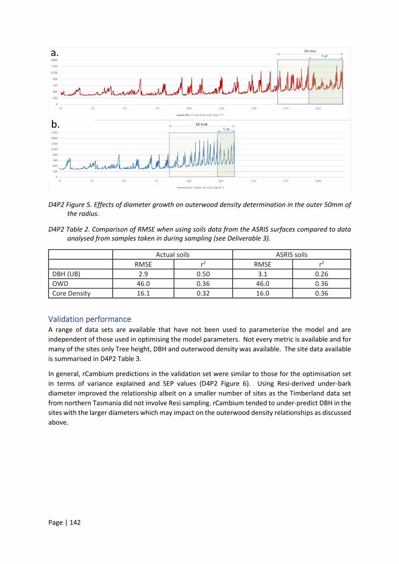
Page | 142

D4P2 Figure 5. Effects of diameter growth on outerwood density determination in the outer 50mm of the radius.

D4P2 Table 2. Comparison of RMSE when using soils data from the ASRIS surfaces compared to data analysed from samples taken in during sampling (see Deliverable 3).

Actual soils ASRIS soils RMSE r2 RMSE r2 DBH (UB) 2.9 0.50 3.1 0.26 OWD 46.0 0.36 46.0 0.36 Core Density 16.1 0.32 16.0 0.36

Validation performance A range of data sets are available that have not been used to parameterise the model and are independent of those used in optimising the model parameters. Not every metric is available and for many of the sites only Tree height, DBH and outerwood density was available. The site data available is summarised in D4P2 Table 3.

In general, rCambium predictions in the validation set were similar to those for the optimisation set in terms of variance explained and SEP values (D4P2 Figure 6). Using Resi-derived under-bark diameter improved the relationship albeit on a smaller number of sites as the Timberland data set from northern Tasmania did not involve Resi sampling. rCambium tended to under-predict DBH in the sites with the larger diameters which may impact on the outerwood density relationships as discussed above.

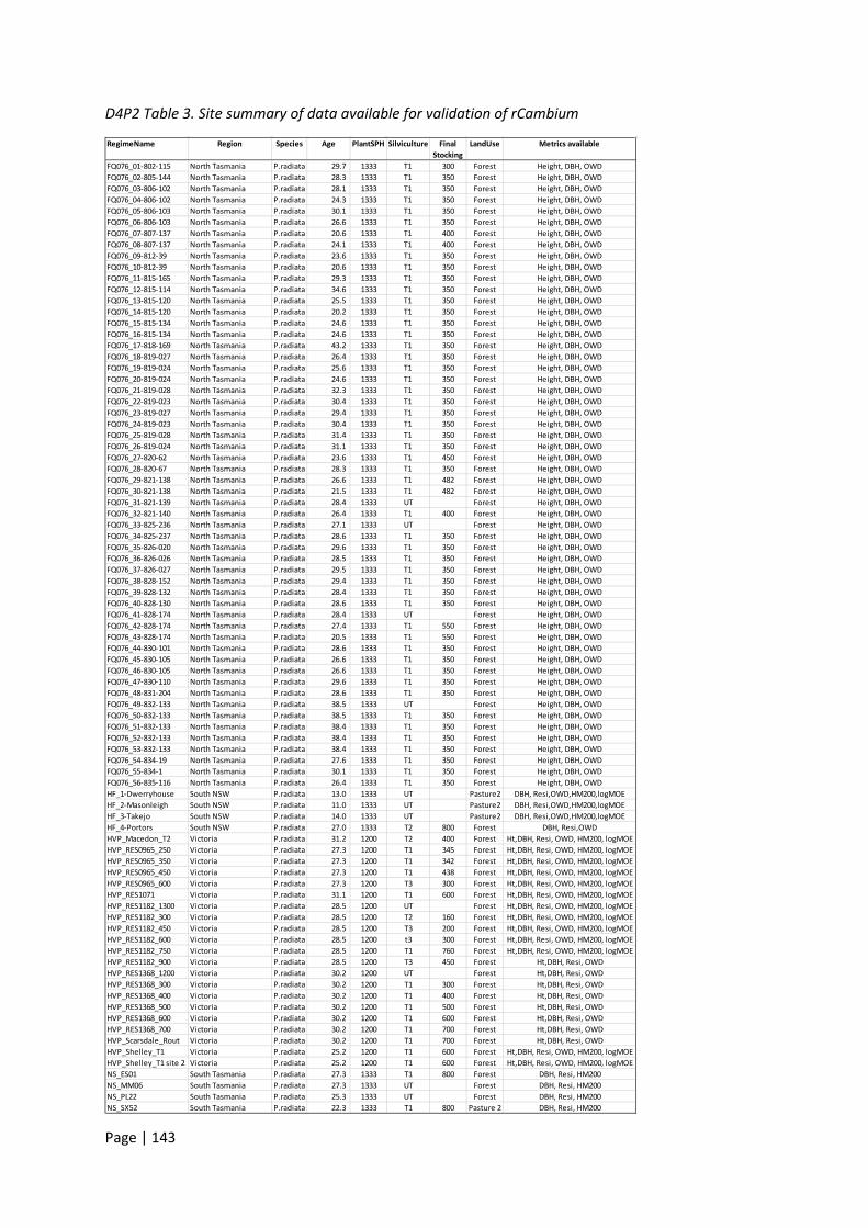
Page | 143

D4P2 Table 3. Site summary of data available for validation of rCambium

RegimeName Region Species Age PlantSPH Silviculture Final Stocking

LandUse Metrics available

FQ076_01-802-115 North Tasmania P.radiata 29.7 1333 T1 300 Forest Height, DBH, OWDFQ076_02-805-144 North Tasmania P.radiata 28.3 1333 T1 350 Forest Height, DBH, OWDFQ076_03-806-102 North Tasmania P.radiata 28.1 1333 T1 350 Forest Height, DBH, OWDFQ076_04-806-102 North Tasmania P.radiata 24.3 1333 T1 350 Forest Height, DBH, OWDFQ076_05-806-103 North Tasmania P.radiata 30.1 1333 T1 350 Forest Height, DBH, OWDFQ076_06-806-103 North Tasmania P.radiata 26.6 1333 T1 350 Forest Height, DBH, OWDFQ076_07-807-137 North Tasmania P.radiata 20.6 1333 T1 400 Forest Height, DBH, OWDFQ076_08-807-137 North Tasmania P.radiata 24.1 1333 T1 400 Forest Height, DBH, OWDFQ076_09-812-39 North Tasmania P.radiata 23.6 1333 T1 350 Forest Height, DBH, OWDFQ076_10-812-39 North Tasmania P.radiata 20.6 1333 T1 350 Forest Height, DBH, OWDFQ076_11-815-165 North Tasmania P.radiata 29.3 1333 T1 350 Forest Height, DBH, OWDFQ076_12-815-114 North Tasmania P.radiata 34.6 1333 T1 350 Forest Height, DBH, OWDFQ076_13-815-120 North Tasmania P.radiata 25.5 1333 T1 350 Forest Height, DBH, OWDFQ076_14-815-120 North Tasmania P.radiata 20.2 1333 T1 350 Forest Height, DBH, OWDFQ076_15-815-134 North Tasmania P.radiata 24.6 1333 T1 350 Forest Height, DBH, OWDFQ076_16-815-134 North Tasmania P.radiata 24.6 1333 T1 350 Forest Height, DBH, OWDFQ076_17-818-169 North Tasmania P.radiata 43.2 1333 T1 350 Forest Height, DBH, OWDFQ076_18-819-027 North Tasmania P.radiata 26.4 1333 T1 350 Forest Height, DBH, OWDFQ076_19-819-024 North Tasmania P.radiata 25.6 1333 T1 350 Forest Height, DBH, OWDFQ076_20-819-024 North Tasmania P.radiata 24.6 1333 T1 350 Forest Height, DBH, OWDFQ076_21-819-028 North Tasmania P.radiata 32.3 1333 T1 350 Forest Height, DBH, OWDFQ076_22-819-023 North Tasmania P.radiata 30.4 1333 T1 350 Forest Height, DBH, OWDFQ076_23-819-027 North Tasmania P.radiata 29.4 1333 T1 350 Forest Height, DBH, OWDFQ076_24-819-023 North Tasmania P.radiata 30.4 1333 T1 350 Forest Height, DBH, OWDFQ076_25-819-028 North Tasmania P.radiata 31.4 1333 T1 350 Forest Height, DBH, OWDFQ076_26-819-024 North Tasmania P.radiata 31.1 1333 T1 350 Forest Height, DBH, OWDFQ076_27-820-62 North Tasmania P.radiata 23.6 1333 T1 450 Forest Height, DBH, OWDFQ076_28-820-67 North Tasmania P.radiata 28.3 1333 T1 350 Forest Height, DBH, OWDFQ076_29-821-138 North Tasmania P.radiata 26.6 1333 T1 482 Forest Height, DBH, OWDFQ076_30-821-138 North Tasmania P.radiata 21.5 1333 T1 482 Forest Height, DBH, OWDFQ076_31-821-139 North Tasmania P.radiata 28.4 1333 UT Forest Height, DBH, OWDFQ076_32-821-140 North Tasmania P.radiata 26.4 1333 T1 400 Forest Height, DBH, OWDFQ076_33-825-236 North Tasmania P.radiata 27.1 1333 UT Forest Height, DBH, OWDFQ076_34-825-237 North Tasmania P.radiata 28.6 1333 T1 350 Forest Height, DBH, OWDFQ076_35-826-020 North Tasmania P.radiata 29.6 1333 T1 350 Forest Height, DBH, OWDFQ076_36-826-026 North Tasmania P.radiata 28.5 1333 T1 350 Forest Height, DBH, OWDFQ076_37-826-027 North Tasmania P.radiata 29.5 1333 T1 350 Forest Height, DBH, OWDFQ076_38-828-152 North Tasmania P.radiata 29.4 1333 T1 350 Forest Height, DBH, OWDFQ076_39-828-132 North Tasmania P.radiata 28.4 1333 T1 350 Forest Height, DBH, OWDFQ076_40-828-130 North Tasmania P.radiata 28.6 1333 T1 350 Forest Height, DBH, OWDFQ076_41-828-174 North Tasmania P.radiata 28.4 1333 UT Forest Height, DBH, OWDFQ076_42-828-174 North Tasmania P.radiata 27.4 1333 T1 550 Forest Height, DBH, OWDFQ076_43-828-174 North Tasmania P.radiata 20.5 1333 T1 550 Forest Height, DBH, OWDFQ076_44-830-101 North Tasmania P.radiata 28.6 1333 T1 350 Forest Height, DBH, OWDFQ076_45-830-105 North Tasmania P.radiata 26.6 1333 T1 350 Forest Height, DBH, OWDFQ076_46-830-105 North Tasmania P.radiata 26.6 1333 T1 350 Forest Height, DBH, OWDFQ076_47-830-110 North Tasmania P.radiata 29.6 1333 T1 350 Forest Height, DBH, OWDFQ076_48-831-204 North Tasmania P.radiata 28.6 1333 T1 350 Forest Height, DBH, OWDFQ076_49-832-133 North Tasmania P.radiata 38.5 1333 UT Forest Height, DBH, OWDFQ076_50-832-133 North Tasmania P.radiata 38.5 1333 T1 350 Forest Height, DBH, OWDFQ076_51-832-133 North Tasmania P.radiata 38.4 1333 T1 350 Forest Height, DBH, OWDFQ076_52-832-133 North Tasmania P.radiata 38.4 1333 T1 350 Forest Height, DBH, OWDFQ076_53-832-133 North Tasmania P.radiata 38.4 1333 T1 350 Forest Height, DBH, OWDFQ076_54-834-19 North Tasmania P.radiata 27.6 1333 T1 350 Forest Height, DBH, OWDFQ076_55-834-1 North Tasmania P.radiata 30.1 1333 T1 350 Forest Height, DBH, OWDFQ076_56-835-116 North Tasmania P.radiata 26.4 1333 T1 350 Forest Height, DBH, OWDHF_1-Dwerryhouse South NSW P.radiata 13.0 1333 UT Pasture2 DBH, Resi,OWD,HM200,logMOEHF_2-Masonleigh South NSW P.radiata 11.0 1333 UT Pasture2 DBH, Resi,OWD,HM200,logMOEHF_3-Takejo South NSW P.radiata 14.0 1333 UT Pasture2 DBH, Resi,OWD,HM200,logMOEHF_4-Portors South NSW P.radiata 27.0 1333 T2 800 Forest DBH, Resi,OWDHVP_Macedon_T2 Victoria P.radiata 31.2 1200 T2 400 Forest Ht,DBH, Resi, OWD, HM200, logMOEHVP_RES0965_250 Victoria P.radiata 27.3 1200 T1 345 Forest Ht,DBH, Resi, OWD, HM200, logMOEHVP_RES0965_350 Victoria P.radiata 27.3 1200 T1 342 Forest Ht,DBH, Resi, OWD, HM200, logMOEHVP_RES0965_450 Victoria P.radiata 27.3 1200 T1 438 Forest Ht,DBH, Resi, OWD, HM200, logMOEHVP_RES0965_600 Victoria P.radiata 27.3 1200 T3 300 Forest Ht,DBH, Resi, OWD, HM200, logMOEHVP_RES1071 Victoria P.radiata 31.1 1200 T1 600 Forest Ht,DBH, Resi, OWD, HM200, logMOEHVP_RES1182_1300 Victoria P.radiata 28.5 1200 UT Forest Ht,DBH, Resi, OWD, HM200, logMOEHVP_RES1182_300 Victoria P.radiata 28.5 1200 T2 160 Forest Ht,DBH, Resi, OWD, HM200, logMOEHVP_RES1182_450 Victoria P.radiata 28.5 1200 T3 200 Forest Ht,DBH, Resi, OWD, HM200, logMOEHVP_RES1182_600 Victoria P.radiata 28.5 1200 t3 300 Forest Ht,DBH, Resi, OWD, HM200, logMOEHVP_RES1182_750 Victoria P.radiata 28.5 1200 T1 760 Forest Ht,DBH, Resi, OWD, HM200, logMOEHVP_RES1182_900 Victoria P.radiata 28.5 1200 T3 450 Forest Ht,DBH, Resi, OWDHVP_RES1368_1200 Victoria P.radiata 30.2 1200 UT Forest Ht,DBH, Resi, OWDHVP_RES1368_300 Victoria P.radiata 30.2 1200 T1 300 Forest Ht,DBH, Resi, OWDHVP_RES1368_400 Victoria P.radiata 30.2 1200 T1 400 Forest Ht,DBH, Resi, OWDHVP_RES1368_500 Victoria P.radiata 30.2 1200 T1 500 Forest Ht,DBH, Resi, OWDHVP_RES1368_600 Victoria P.radiata 30.2 1200 T1 600 Forest Ht,DBH, Resi, OWDHVP_RES1368_700 Victoria P.radiata 30.2 1200 T1 700 Forest Ht,DBH, Resi, OWDHVP_Scarsdale_Rout Victoria P.radiata 30.2 1200 T1 700 Forest Ht,DBH, Resi, OWDHVP_Shelley_T1 Victoria P.radiata 25.2 1200 T1 600 Forest Ht,DBH, Resi, OWD, HM200, logMOEHVP_Shelley_T1 site 2 Victoria P.radiata 25.2 1200 T1 600 Forest Ht,DBH, Resi, OWD, HM200, logMOENS_ES01 South Tasmania P.radiata 27.3 1333 T1 800 Forest DBH, Resi, HM200NS_MM06 South Tasmania P.radiata 27.3 1333 UT Forest DBH, Resi, HM200NS_PL22 South Tasmania P.radiata 25.3 1333 UT Forest DBH, Resi, HM200NS_SX52 South Tasmania P.radiata 22.3 1333 T1 800 Pasture 2 DBH, Resi, HM200

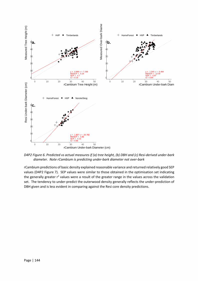
Page | 144

D4P2 Figure 6. Predicted vs actual measures if (a) tree height, (b) DBH and (c) Resi-derived under-bark diameter. Note rCambium is predicting under-bark diameter not over-bark

rCambium predictions of basic density explained reasonable variance and returned relatively good SEP values (D4P2 Figure 7). SEP values were similar to those obtained in the optimisation set indicating the generally greater r2 values were a result of the greater range in the values across the validation set. The tendency to under-predict the outerwood density generally reflects the under-prediction of DBH given and is less evident in comparing against the Resi core density predictions.

a.

y = 0.896 x + 7.288RMSEP = 6.24SEP = 4.7r2 = 0.190

10

20

30

40

50


Mea

sure

d Tr

ee H

eigh

t (m

)

HVP Timberlands

b.

y = 1.545 x + -5.494RMSEP = 12.59SEP = 5.97r2 = 0.540

10

20

30

40

50

0 10 20 30 40 50rCambium Under-bark Diame

Mea

sure

d O

ver-b

ark

Dia

met

HumeForest HVP Timberlands

c.

y = 1.827 x + -16.782RMSEP = 5.82SEP = 4.13r2 = 0.680

10

20

30

40

50

0 10 20 30 40 50rCambium Under-bark Diameter (cm)

Res

i Und

er-b

ark

Dia

met

er (c

m)

HumeForest HVP NorskeSkog

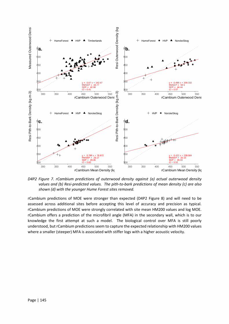
Page | 145

D4P2 Figure 7. rCambium predictions of outerwood density against (a) actual outerwood density values and (b) Resi-predicted values. The pith-to-bark predictions of mean density (c) are also shown (d) with the younger Hume Forest sites removed.

rCambium predictions of MOE were stronger than expected (D4P2 Figure 8) and will need to be assessed across additional sites before accepting this level of accuracy and precision as typical. rCambium predictions of MOE were strongly correlated with site mean HM200 values and log MOE. rCambium offers a prediction of the microfibril angle (MFA) in the secondary wall, which is to our knowledge the first attempt at such a model. The biological control over MFA is still poorly understood, but rCambium predictions seem to capture the expected relationship with HM200 values where a smaller (steeper) MFA is associated with stiffer logs with a higher acoustic velocity.

a.

y = 0.67 x + 142.67RMSEP = 43.77SEP = 42.98r2 = 0.41300

350

400

450

500

550

300 350 400 450 500 550rCambium Outerwood Density (kg.m-3)

Mea

sure

d O

uter

woo

d D

ensi

HumeForest HVP Timberlands

b.

y = 0.488 x + 209.332RMSEP = 59.5SEP = 44.44r2 = 0.57300

350

400

450

500

550

300 350 400 450 500 550rCambium Outerwood Dens

Res

i Out

erw

ood

Den

sity

(kg


c.

y = 0.788 x + 78.672RMSEP = 23.17SEP = 20.36r2 = 0.62300

350

400

450

500

550

300 350 400 450 500 550rCambium Mean Density (kg.m-3)

Res

i Pith

-to-B

ark

Den

sity

(kg.

m-3

)


d.

y = 0.422 x + 239.584RMSEP = 22.13SEP = 20.04r2 = 0.52300

350

400

450

500

550

300 350 400 450 500 550rCambium Mean Density (kg

Res

i Pith

-to-B

ark

Den

sity

(kg.

m-3

)HVP NorskeSkog

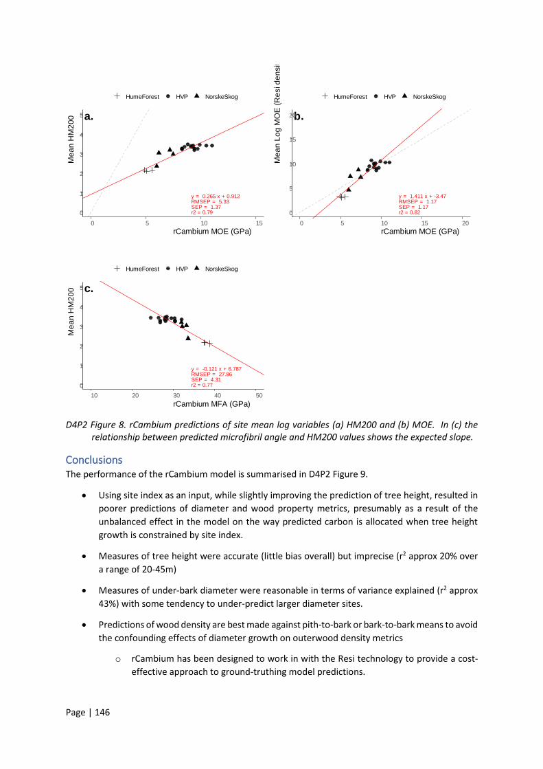
Page | 146

D4P2 Figure 8. rCambium predictions of site mean log variables (a) HM200 and (b) MOE. In (c) the relationship between predicted microfibril angle and HM200 values shows the expected slope.

Conclusions The performance of the rCambium model is summarised in D4P2 Figure 9.

• Using site index as an input, while slightly improving the prediction of tree height, resulted in poorer predictions of diameter and wood property metrics, presumably as a result of the unbalanced effect in the model on the way predicted carbon is allocated when tree height growth is constrained by site index.

• Measures of tree height were accurate (little bias overall) but imprecise (r2 approx 20% over a range of 20-45m)

• Measures of under-bark diameter were reasonable in terms of variance explained (r2 approx 43%) with some tendency to under-predict larger diameter sites.

• Predictions of wood density are best made against pith-to-bark or bark-to-bark means to avoid the confounding effects of diameter growth on outerwood density metrics

o rCambium has been designed to work in with the Resi technology to provide a cost-effective approach to ground-truthing model predictions.

a.

y = 0.265 x + 0.912RMSEP = 5.33SEP = 1.37r2 = 0.790

1

2

3

4

5

0 5 10 15rCambium MOE (GPa)

Mea

n H

M20

0


b.

y = 1.411 x + -3.47RMSEP = 1.17SEP = 1.17r2 = 0.820

5

10

15

20

0 5 10 15 20rCambium MOE (GPa)

Mea

n Lo

g M

OE

(Res

i den

sit


c.

y = -0.121 x + 6.787RMSEP = 27.86SEP = 4.31r2 = 0.770

1

2

3

4

5

10 20 30 40 50rCambium MFA (GPa)

Mea

n H

M20

0


Page | 147

• Over the whole data set, rCambium predicted 50% of the variance in Resi-predicted pith-to-bark basic density with a SEP of 20 kg.m-3. This comparison involved data derived from at least 5 different Resi instruments each requiring appropriate calibration to generate accurate density predictions.

• rCambium predictions of log MOE were excellent explaining 66% of the variance. Log MOE was derived from actual HM200 values combined with Resi-predicted pith-to-bark basic density. The rCambium prediction of MFA seemed to add additional explanatory power to the MOE prediction given the strong observed relationship between rCambium-MFA and actual HM200 values.

• It is important to note that rCambium is intended as a lowest-cost, first-pass assessment of wood quality variance at the estate level. The broad resolution of the input weather data and the potential inaccuracy in the publicly available soils data, with its inherent bias towards more productive agricultural soils, will lead to poor performance at some sites. Thus, application across a range of sites where the actual range of wood property values is restricted will result in lower levels of explained variance (r2). SEP values should be the guide with respect to the expected confidence intervals users can expect in model predictions.

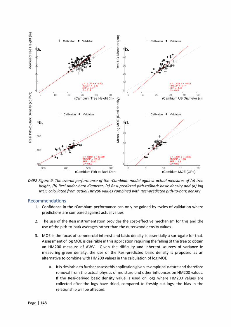
Page | 148

D4P2 Figure 9. The overall performance of the rCambium model against actual measures of (a) tree height, (b) Resi under-bark diameter, (c) Resi-predicted pith-to0bark basic density and (d) log MOE calculated from actual HM200 values combined with Resi-predicted pith-to-bark density

Recommendations 1. Confidence in the rCambium performance can only be gained by cycles of validation where

predictions are compared against actual values

2. The use of the Resi instrumentation provides the cost-effective mechanism for this and the use of the pith-to-bark averages rather than the outerwood density values.

3. MOE is the focus of commercial interest and basic density is essentially a surrogate for that. Assessment of log MOE is desirable in this application requiring the felling of the tree to obtain an HM200 measure of AWV. Given the difficulty and inherent sources of variance in measuring green density, the use of the Resi-predicted basic density is proposed as an alternative to combine with HM200 values in the calculation of log MOE

a. It is desirable to further assess this application given its empirical nature and therefore removal from the actual physics of moisture and other influences on HM200 values. If the Resi-derived basic density value is used on logs where HM200 values are collected after the logs have dried, compared to freshly cut logs, the bias in the relationship will be affected.

a.

y = 1.174 x + -2.401RMSEP = 5.49SEP = 4.77r2 = 0.190

10

20

30

40

50


Mea

sued

tree

Hei

ght (

m)

Calibration Validation

b.

y = 1.421 x + -8.813RMSEP = 4.77SEP = 4.06r2 = 0.430

10

20

30

40

50

0 10 20 30 40 50rCambium UB Diameter (cm

Res

i UB

Dia

met

er (c

m)


b.

y = 0.887 x + 38.999RMSEP = 22.16SEP = 20.42r2 = 0.51300

400

500

600

300 400 500 600rCambium Pith-to-Bark Density (kg.m-3)

Res

i Pith

-to-B

ark

Den

sity

(kg.

m-3

)


d.

y = 1.597 x + -4.608RMSEP = 1.35SEP = 1.3r2 = 0.660

5

10

15

20

0 5 10 15 20rCambium MOE (GPa)

Mea

n Lo

g M

OE

(Res

i den

sity

)Calibration Validation

Page | 149

4. The use of site index to improve model performance requires more attention to see whether the model can be improved by using this additional input metric.

5. The effect of more accurate weather and soils input data warrants further effort to better identify when the model is likely to under-perform.

Acknowledgements Ross Searle, Senior Experimental Scientist, CSIRO Agriculture & Food was very helpful in writing the code needed to extract the weather and soils data from the SILO and ASRIS databases.

Page | 150

Appendix 1: FCNSW trial operational implementation of rCambium model

Duncan Watt, FCNSW

FCNSW have undertaken some preliminary investigaton of the utility of the rCambium software for predicting wood quality across the plantation landscape under a range of different silvicultural regimes and with differing previous land use.

As expected, early modelling results are showing significant variation in predicted wood quality, driven by both silviculture and previous land use.

A work flow has been developed that involves

1. Generating a 1km grid square across the plantation estate as the base modelling unit - this has been selected given that the resolution of the soils input to the model is at this scale

2. For each 1km grid square a suite of 9 standardised model scenarios have been developed that combine

o 3 previous land use types (ex-forest, pasture, improved pasture) o 3 silvicultural regimes (unthinned, single thin, two thin) o A clearfall age of 30 has been assumed

3. Climatic inputs on a 5km grid square have been applied using data from the last 30 years for the analysis, i.e. 1989-2019, although tests of climatic projection into the future have also been tested successfully

4. rCambium analysis for each grid square of 9 scenarios is batch processed at a maxium of 1000 scenarios at a time.

Example results from this process are provided in Figures 10 and 11 below for modelled age 30 mean density values for each 1km grid square. The displayed colour range has lower mean density values in red/orange through to higher values in green.

D4P2 Figure 10 rCambium modelled Mean Density for an assumed second thinned ex-forest site at age 30

Page | 151

D4P2 Figure 11. rCambium modelled Mean Density for an assumed unthinned stand on an improved pasture site at age 30

Next Steps

• Validation work is underway to compare rCambium predictions to our Resi tool sample results • The initial work has been undertaken on a subset of the FCNSW plantation estate however,

once the updated rCambium model is released at the end of October/early November, the plan is to run the equivalent analysis process across the entire FCNSW radiata resource to generate a standardised wood quality surface.

• Investigation will be undertaken in use of rCambium projections of wood quality values as a method to project mid/late rotation Resi sampled data, for example to project an age 23 Resi sample on a site to a predicted value for mean density at age 30 and adding these projected values into stand specific yield tables

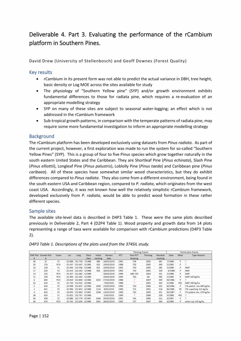
Page | 152

Deliverable 4. Part 3. Evaluating the performance of the rCambium platform in Southern Pines.

David Drew (University of Stellenbosch) and Geoff Downes (Forest Quality)

Key results • rCambium in its present form was not able to predict the actual variance in DBH, tree height,

basic density or Log MOE across the sites available for study • The physiology of “Southern Yellow pine” (SYP) and/or growth environment exhibits

fundamental differences to those for radiata pine, which requires a re-evaluation of an appropriate modelling strategy

• SYP on many of these sites are subject to seasonal water-logging; an effect which is not addressed in the rCambium framework

• Sub-tropical growth patterns, in comparison with the temperate patterns of radiata pine, may require some more fundamental investigation to inform an appropriate modelling strategy

Background The rCambium platform has been developed exclusively using datasets from Pinus radiata. As part of the current project, however, a first exploration was made to run the system for so-called “Southern Yellow Pines” (SYP). This is a group of four to five Pinus species which grow together naturally in the south eastern United States and the Caribbean. They are Shortleaf Pine (Pinus echinata), Slash Pine (Pinus elliottii), Longleaf Pine (Pinus palustris), Loblolly Pine (Pinus taeda) and Caribbean pine (Pinus caribaea). All of these species have somewhat similar wood characteristics, but they do exhibit differences compared to Pinus radiata. They also come from a different environment, being found in the south eastern USA and Caribbean region, compared to P. radiata, which originates from the west coast USA. Accordingly, it was not known how well the relatively simplistic rCambium framework, developed exclusively from P. radiata, would be able to predict wood formation in these rather different species.

Sample sites The available site-level data is described in D4P3 Table 1. These were the same plots described previously in Deliverable 2, Part 4 (D2P4 Table 1). Wood property and growth data from 14 plots representing a range of taxa were available for comparison with rCambium predictions (D4P3 Table 2).

D4P3 Table 1. Descriptions of the plots used from the 374SIL study.

FWP Plot #

Growth Plot #

Taxon Lat Long Plant Date

Initial stocking

Harvest date

PCT Post-PCT Stocking

Thinning Residual stocking

Date What Type Amount

46 37 F2 -25.898 152.750 7/1988 980 18/02/2019 1991 758 2005 387 7/1988 P ?20 176 PCH -25.437 152.647 5/1985 925 19/03/2019 1988 750 2005 369 5/1985 P ?16 218 F1 -25.446 152.506 5/1988 925 19/03/2019 1992 750 2005 285 5/1988 P MAP17 220 F2 -25.453 152.502 5/1988 926 18/03/2019 1992 750 2005 330 6/1988 P MAP13 223 PCH -25.427 152.482 5/1988 18/03/2019 1990 640-720 2003 331 5/1988 P MAP11 239 PCH -25.390 152.392 5/1989 19/03/2019 1993 750 NA 585 5/1989 P MAP 220 kg/ha6 604 PCH -25.819 152.840 4/1986 1033 27/02/2019 1988 ? 2007 369 04/1986 P ?

32 610 F2 -25.750 152.925 4/1986 7/03/2019 1988 ? 2003 363 4/1986 PKC MAP 190 kg/ha5 634 F2 -25.998 152.837 6/1986 1058 13/02/2019 1990 750 2006 435 06/1986 P ITA podsol mix 400 kg/ha1 641 F2 -25.996 152.822 6/1986 1116 8/02/2019 1990 715 2001 518 06/1986 PK ITA superking 312 kg/ha4 643 F2 -26.093 152.864 5/1987 1058 14/02/2019 1990 733 2005 431 05/1987 P ITA podsol mix, 229 kg/ha

38 654 F1 -25.822 152.767 6/1988 5/03/2019 1990 ? 2008 328 6/1988 PKC ?44 658 F2 -25.886 152.778 6/1987 1040 20/02/2019 1991 743 2006 511 6/1987 P ?30 674 PCH -25.762 152.694 6/1989 1091 28/02/2019 1992 727 2007 369 6/1989 P extra sup 120 kg/ha

Thinning Events Fertilisation Events

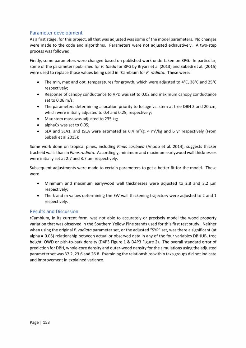
Page | 153

Parameter development As a first stage, for this project, all that was adjusted was some of the model parameters. No changes were made to the code and algorithms. Parameters were not adjusted exhaustively. A two-step process was followed.

Firstly, some parameters were changed based on published work undertaken on 3PG. In particular, some of the parameters published for P. taeda for 3PG by Bryars et al (2013) and Subedi et al. (2015) were used to replace those values being used in rCambium for P. radiata. These were:

• The min, max and opt. temperatures for growth, which were adjusted to 4°C, 38°C and 25°C respectively;

• Response of canopy conductance to VPD was set to 0.02 and maximum canopy conductance set to 0.06 m/s;

• The parameters determining allocation priority to foliage vs. stem at tree DBH 2 and 20 cm, which were initially adjusted to 0.4 and 0.25, respectively;

• Max stem mass was adjusted to 235 kg; • alphaCx was set to 0.05; • SLA and SLA1, and tSLA were estimated as 6.4 m2/g, 4 m2/kg and 6 yr respectively (From

Subedi et al 2015);

Some work done on tropical pines, including Pinus caribaea (Anoop et al. 2014), suggests thicker tracheid walls than in Pinus radiata. Accordingly, minimum and maximum earlywood wall thicknesses were initially set at 2.7 and 3.7 μm respectively.

Subsequent adjustments were made to certain parameters to get a better fit for the model. These were

• Minimum and maximum earlywood wall thicknesses were adjusted to 2.8 and 3.2 μm respectively;

• The k and m values determining the EW wall thickening trajectory were adjusted to 2 and 1 respectively.

Results and Discussion rCambium, in its current form, was not able to accurately or precisely model the wood property variation that was observed in the Southern Yellow Pine stands used for this first test study. Neither when using the original P. radiata parameter set, or the adjusted “SYP” set, was there a significant (at alpha = 0.05) relationship between actual or observed data in any of the four variables DBHUB, tree height, OWD or pith-to-bark density (D4P3 Figure 1 & D4P3 Figure 2). The overall standard error of prediction for DBH, whole-core density and outer-wood density for the simulations using the adjusted parameter set was 37.2, 23.6 and 26.8. Examining the relationships within taxa groups did not indicate and improvement in explained variance.

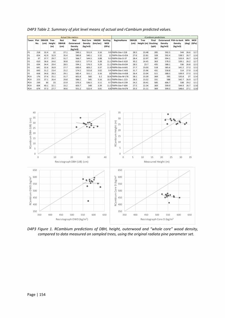
Page | 154

D4P3 Table 2. Summary of plot level means of actual and rCambium predicted values.

D4P3 Figure 1. RCambium predictions of DBH, height, outerwood and “whole core” wood density, compared to data measured on sampled trees, using the original radiata pine parameter set.

Taxon Plot No.

DBHOB (cm)

Tree Height

(m)

Resi DBHUB

(cm)

Resi Outerwood

Density (kg/m3)

Resi Core Density (kg/m3)

HM200 (km/sec)

Buttlog MOE (GPa)

RegimeName DBHUB (cm)

Tree Height (m)

Final Stocking

(sph)

Outerwood Density (kg/m3)

Pith-to-bark Density (kg/m3)

MFA (deg)

MOE (GPa)

F1 218 32.4 22 27.1 590.1 551.9 3.16 9.9 FWPA-Site-I-218 28.5 23.48 285 592.5 544 26.6 12.7F1 654 42.9 32.9 35.4 580.8 540.1 3.32 11 FWPA-Site-G-654 27.6 22.81 328 592.4 538.5 26.7 12.6F2 37 37.7 29.7 31.7 566.7 544.5 3.08 9.3 FWPA-Site-D-37 28.4 22.97 387 594.1 533.9 26.7 12.4F2 610 36.6 24.6 30.8 619.5 577.9 3.28 11.1 FWPA-Site-E-610 30.2 24.45 363 578.3 539.1 26.2 12.7F2 634 34.4 29.4 28.5 594.1 576.3 3.29 11.1 FWPA-Site-B-634 28.5 23.7 435 588.1 536 26.8 12.5F2 641 32.6 26.9 27.7 630.4 603.2 3.37 11.9 FWPA-Site-A-641 27.7 23.03 518 585.6 541.2 27.3 12.5F2 643 31.2 23.4 25.2 574.5 555.8 3.02 9.4 FWPA-Site-C-643 31.7 25.96 431 558.8 514 27.9 11.6F2 658 34.6 28.3 29.1 582.4 551.1 3.16 10 FWPA-Site-H-658 26.4 22.04 511 588.5 539.9 27.3 12.5PCH 176 37.4 25.1 31.7 601.8 560 3.2 10.4 FWPA-Site-M-176 28.1 23.39 369 595 535.8 27 12.4PCH 223 37.1 26.4 29.8 586.2 545 3.16 10.2 FWPA-Site-L-223 28.5 23.52 331 588 542.7 26.9 12.7PCH 239 30 23 22.9 570.3 536.5 3.11 9.7 FWPA-Site-K-239 24.2 20.41 585 606.7 538 29.2 12.1PCH 604 40.1 32.1 33.2 603.7 548 3.39 11.3 FWPA-Site-F-604 27.5 22.34 369 599.9 544.9 26.7 12.8PCH 674 37.3 27.7 30.6 551.2 522.9 3.01 8.8 FWPA-Site-N-674 25.5 21.11 369 599.3 548.6 27.1 12.8

rCambium predictionsActual Site metrics

0

5

10

15

20

25

30

35

40

0 10 20 30 40

RCam

bium

DBH

(UB)

(cm

)

Resistograph DBH (UB) (cm)

0

5

10

15

20

25

30

35

0 5 10 15 20 25 30 35

RCam

bium

Hei

ght (

m)

Measured Height (m)

350

400

450

500

550

600

650

350 400 450 500 550 600 650

RCam

bium

OW

D (k

g/m

3

Resistograph OWD (kg/m3)

350

400

450

500

550

600

650

350 400 450 500 550 600 650

RCam

bium

Cor

e D

(kg/

m3

Resistograph Core D (kg/m3

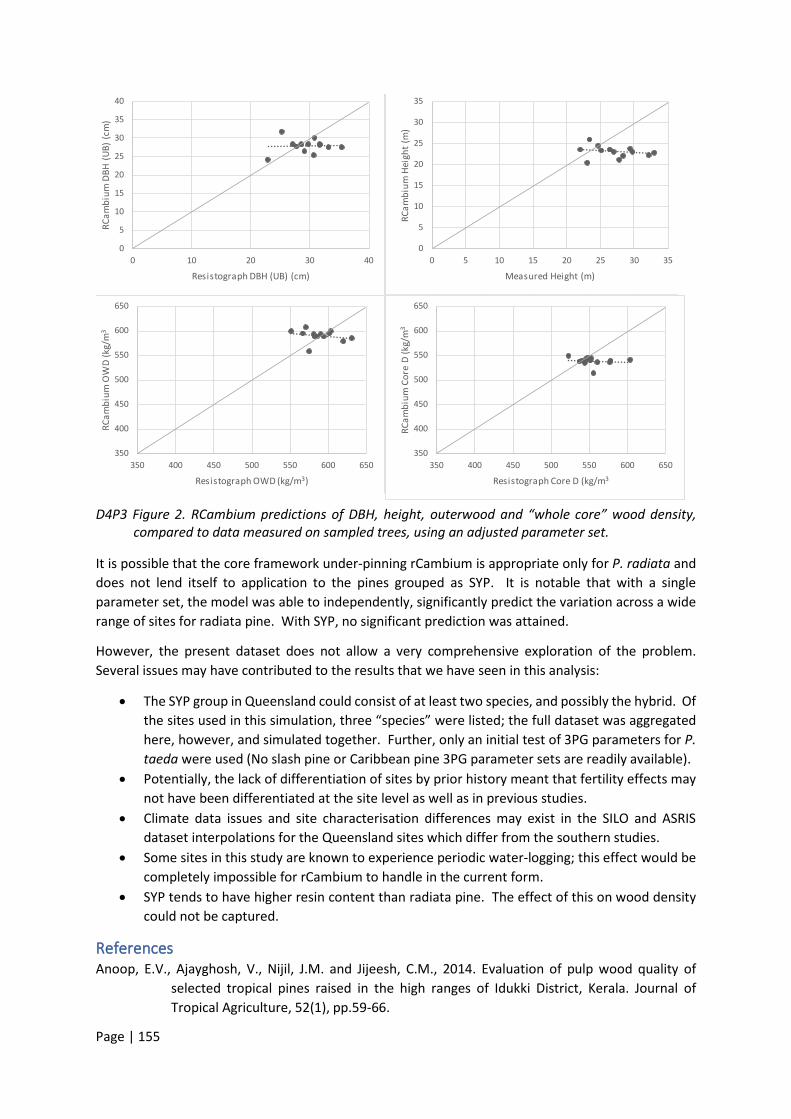
Page | 155

D4P3 Figure 2. RCambium predictions of DBH, height, outerwood and “whole core” wood density, compared to data measured on sampled trees, using an adjusted parameter set.

It is possible that the core framework under-pinning rCambium is appropriate only for P. radiata and does not lend itself to application to the pines grouped as SYP. It is notable that with a single parameter set, the model was able to independently, significantly predict the variation across a wide range of sites for radiata pine. With SYP, no significant prediction was attained.

However, the present dataset does not allow a very comprehensive exploration of the problem. Several issues may have contributed to the results that we have seen in this analysis:

• The SYP group in Queensland could consist of at least two species, and possibly the hybrid. Of the sites used in this simulation, three “species” were listed; the full dataset was aggregated here, however, and simulated together. Further, only an initial test of 3PG parameters for P. taeda were used (No slash pine or Caribbean pine 3PG parameter sets are readily available).

• Potentially, the lack of differentiation of sites by prior history meant that fertility effects may not have been differentiated at the site level as well as in previous studies.

• Climate data issues and site characterisation differences may exist in the SILO and ASRIS dataset interpolations for the Queensland sites which differ from the southern studies.

• Some sites in this study are known to experience periodic water-logging; this effect would be completely impossible for rCambium to handle in the current form.

• SYP tends to have higher resin content than radiata pine. The effect of this on wood density could not be captured.

References Anoop, E.V., Ajayghosh, V., Nijil, J.M. and Jijeesh, C.M., 2014. Evaluation of pulp wood quality of

selected tropical pines raised in the high ranges of Idukki District, Kerala. Journal of Tropical Agriculture, 52(1), pp.59-66.

0

5

10

15

20

25

30

35

40

0 10 20 30 40

RCam

bium

DBH

(UB)

(cm

)

Resistograph DBH (UB) (cm)

0

5

10

15

20

25

30

35

0 5 10 15 20 25 30 35

RCam

bium

Hei

ght (

m)

Measured Height (m)

350

400

450

500

550

600

650

350 400 450 500 550 600 650

RCam

bium

OW

D (k

g/m

3

Resistograph OWD (kg/m3)

350

400

450

500

550

600

650

350 400 450 500 550 600 650

RCam

bium

Cor

e D

(kg/

m3

Resistograph Core D (kg/m3

Page | 156

Bryars, C., Maier, C., Zhao, D., Kane, M., Borders, B., Will, R. and Teskey, R., 2013. Fixed physiological parameters in the 3-PG model produced accurate estimates of loblolly pine growth on sites in different geographic regions. Forest ecology and management, 289, pp.501-514.

Subedi, S., Fox, T. and Wynne, R., 2015. Determination of fertility rating (FR) in the 3-PG model for loblolly pine plantations in the South-eastern United States based on site index. Forests, 6(9), pp.3002-3027.

Processing - Forest and Wood Products Australia

Documents