www.usn.no Faculty of Technology, Natural sciences and Maritime Sciences Campus Porsgrunn FMH606 Master's Thesis 2019 Energy and Environmental Technology Process simulation of CO 2 absorption at TCM Mongstad Sofie Fagerheim

Welcome message from author
This document is posted to help you gain knowledge. Please leave a comment to let me know what you think about it! Share it to your friends and learn new things together.
Transcript
www.usn.no
Faculty of Technology, Natural sciences and Maritime Sciences Campus Porsgrunn
FMH606 Master's Thesis 2019
Energy and Environmental Technology
Process simulation of CO2 absorption at TCM Mongstad
Sofie Fagerheim
www.usn.no
The University of South-Eastern Norway takes no responsibility for the results and
conclusions in this student report.
Course: FMH606 Master's Thesis, 2019
Title: Process simulation of CO2 absorption at TCM Mongstad
Number of pages: 140
Keywords: Absorption, Aspen Plus, Aspen HYSYS, CO2 capture, MEA, simulation, TCM
Student: Sofie Fagerheim
Supervisor: Lars Erik Øi
External partner: CO2 Technology Centre Mongstad (TCM)
Availability: Open
Summary:
Developing robust and predictable process simulation tools for CO2 capture is important for
improving carbon capture technology and reduce man made CO2 emissions.
In this thesis, five different scenarios of experimental data from the amine based CO2 capture
process at TCM have been simulated in rate-based model in Aspen Plus and equilibrium-
based model in Aspen HYSYS and Aspen Plus. The simulations have been compared based
on the prediction reliability for removal grade, temperature profile and rich loading.
In previous work, these five scenarios have been simulated and compared in Aspen HYSYS
and Aspen Plus. Some of the results from earlier work are verified in this thesis.
The main purpose have been to fit the simulated results with performance data from TCM,
and evaluate whether fitted parameters for one scenario gives reasonable predictions at other
conditions. Two new EM-profiles were estimated, and scaled to fit all five scenarios by
developing an EM-factor. From this work the new model with fitted parameters gave a reliable
prediction of removal grade and temperature profile for all scenarios, and predicted more
reliable results than rate-based model with estimated IAF.
The scenarios were also simulated with default EM-profile in Aspen HYSYS, where the
removal grade was fitted to performance data by adjusting number of stages. The scenarios
were also simulated with three different amine packages in Aspen HYSYS, Kent-Eisenberg,
Li-Mather and Acid Gas - Liquid Treating.

Preface
3
Preface This report was written during the spring 2019 as my master thesis, and is part of the master
program in Energy and Environmental technology at the Department of Process, Energy and
Environment at the University of South-Eastern Norway.
The project focus is on performing process simulations of test data from the 2013 and 2015
campaign at TCM in Aspen HYSYS and Aspen Plus, and compare process simulations with
performance data and earlier simulations of the same test data. The main purpose is to fit the
removal grade, temperature profile and rich loading with performance data from TCM. Another
purpose is to evaluate whether fitted parameters for one scenario gives reasonable predictions
at other conditions.
I want to express my gratitude towards my supervisor, Professor Lars Erik Øi, for his
supervision, guidance and great support during this thesis. Especially I appreciate that he made
it possible for me to carry out all the work from Bodø, so that I was able to continue my job at
Multiconsult and be with my family during the duration of this project.
I would also like to thank my family for their help and support during this work. Especially, I
want to show gratitude to my boyfriend, Stefan, for his patience and help taking care of our
son, Philip Edward, who turned two years during this project. I would like to thank him for
giving me the time I needed to complete. Hopefully we will get more time together in the years
to come.
The data-tools used during this project was:
Aspen HYSYS V10, Aspen Plus V10, MS Word 2013, MS Excel 2013 and AutoCAD Plant
3D 2018.
Bodø, 05.05.19
______________________
Sofie Fagerheim
Contents
4
Contents
Preface ..................................................................................................................... 3
Contents ................................................................................................................... 4
Nomenclature ........................................................................................................... 8
1 Introduction ......................................................................................................... 9
1.1 Background ................................................................................................................................ 9 1.2 Outline of the thesis .................................................................................................................... 9
2 Background and problem description ................................................................... 10
2.1 Climate change related to CO2 emission .................................................................................... 10 2.2 Carbon capture technologies ..................................................................................................... 11
2.2.1 Pre-combustion CO2 capture process .................................................................................. 11 2.2.2 Post-combustion CO2 capture process ................................................................................. 11 2.2.3 Oxy-fuel combustion CO2 capture process ........................................................................... 11 2.2.4 Chemical looping CO2 capture process ................................................................................ 11
2.3 Carbon transport and storage .................................................................................................... 11 2.4 Process description at TCM........................................................................................................ 12
2.4.1 Flue gas treatment ............................................................................................................ 12 2.4.2 CO2 capture ....................................................................................................................... 13 2.4.3 Amine regeneration .......................................................................................................... 13
2.5 Chemistry of the process ........................................................................................................... 14 2.5.1 Generally about MEA ........................................................................................................ 14 2.5.2 Advantages and disadvantages of using MEA for CO2 capture ............................................. 14 2.5.3 Reactions of CO2 absorption into MEA ................................................................................ 15
2.6 Earlier work .............................................................................................................................. 16 2.7 Problem description .................................................................................................................. 20
3 Method .............................................................................................................. 21
3.1 Simulation methodology ........................................................................................................... 21 3.1.1 Simulation tools ................................................................................................................ 21 3.1.2 Murphree efficiency .......................................................................................................... 21 3.1.3 Converting Sm3/h to kmol/h .............................................................................................. 23 3.1.4 Calculating composition of lean amine ............................................................................... 23 3.1.5 Calculating CO2 removal grade .......................................................................................... 24
3.2 Suggested method for estimating Murphree efficiency ............................................................... 24 3.2.1 Estimating EM-profile by calculating overall removal efficiency ............................................ 24 3.2.2 Fitting EM to several scenarios by introducing an EM-factor .................................................. 25
3.3 Scenarios .................................................................................................................................. 25 3.3.1 Scenario H14 ..................................................................................................................... 26 3.3.2 Scenario 2B5 ..................................................................................................................... 27 3.3.3 Scenario 6w ...................................................................................................................... 28 3.3.4 Scenario Goal1 .................................................................................................................. 29 3.3.5 Scenario F17 ..................................................................................................................... 30
3.4 Specifications of the simulation tools ......................................................................................... 31 3.4.1 Equilibrium-based model ................................................................................................... 31 3.4.2 Rate-based model ............................................................................................................. 32
Contents
5
4 Results ............................................................................................................... 33
4.1 Verification of earlier work in Aspen HYSYS ............................................................................... 35 4.1.1 Verification of scenario H14 in Aspen HYSYS ....................................................................... 35 4.1.2 Verification of scenario 2B5 in Aspen HYSYS ....................................................................... 37 4.1.3 Verification of scenario 6w in Aspen HYSYS ........................................................................ 38 4.1.4 Verification of scenario Goal1 in Aspen HYSYS .................................................................... 39 4.1.5 Verification of scenario F17 in Aspen HYSYS ........................................................................ 40
4.2 Verification of earlier work in Aspen Plus ................................................................................... 41 4.2.1 Verification of scenario H14 in Aspen Plus .......................................................................... 41 4.2.2 Verification of scenario 2B5 in Aspen Plus........................................................................... 43 4.2.3 Verification of scenario 6w in Aspen Plus ............................................................................ 44 4.2.4 Verification of scenario Goal1 in Aspen Plus ....................................................................... 46 4.2.5 Verification of scenario F17 in Aspen Plus ........................................................................... 47
4.3 Simulation in Aspen HYSYS with estimated EM ............................................................................ 50 4.3.1 Simulation of H14 with estimated EM ................................................................................. 50 4.3.2 Simulation of 2B5 with estimated EM .................................................................................. 51 4.3.3 Simulation of 6w with estimated EM ................................................................................... 52 4.3.4 Simulation of Goal1 with estimated EM ............................................................................... 53 4.3.5 Simulation of F17 with estimated EM .................................................................................. 54
4.4 Simulation in Aspen Plus with estimated EM and IAF ................................................................... 55 4.4.1 Simulation of H14 with estimated EM and IAF ...................................................................... 55 4.4.2 Simulation of 2B5 with estimated EM and IAF ...................................................................... 56 4.4.3 Simulation of 6w with estimated EM and IAF ....................................................................... 57 4.4.4 Simulation of Goal1 with estimated EM and IAF .................................................................. 58 4.4.5 Simulation of F17 with estimated EM and IAF ...................................................................... 59
4.5 Comparison of Rate-based and Equilibrium-based model ........................................................... 60 4.5.1 Comparison of Rate-based and Equilibrium for Scenario H14 ............................................... 60 4.5.2 Comparison of Rate-based and Equilibrium-based for Scenario 2B5 ..................................... 61 4.5.3 Comparison of Rate-based and Equilibrium-based for Scenario 6w ...................................... 62 4.5.4 Comparison of Rate-based and Equilibrium-based for Scenario Goal1 .................................. 63 4.5.5 Comparison of Rate-based and Equilibrium-based for Scenario F17 ..................................... 64
4.6 Simulation with default EM in Aspen HYSYS ................................................................................ 65 4.6.1 Default VS Estimated EM for scenario H14 ........................................................................... 65 4.6.2 Default VS Estimated EM for scenario 2B5 ........................................................................... 66 4.6.3 Default VS Estimated EM for scenario 6w ............................................................................ 67 4.6.4 Default VS Estimated EM for scenario Goal1 ........................................................................ 68 4.6.5 Default VS Estimated EM for scenario F17 ........................................................................... 69
4.7 Comparison of Amine package in Aspen HYSYS .......................................................................... 70 4.7.1 Comparison of amine packages for scenario H14 ................................................................ 70 4.7.2 Comparison of amine packages for scenario 2B5 ................................................................ 71 4.7.3 Comparison of amine packages for scenario 6w .................................................................. 72 4.7.4 Comparison of amine packages for scenario Goal1 ............................................................. 73 4.7.5 Comparison of amine packages for scenario F17 ................................................................. 74
5 Suggested method for estimating EM-factor .......................................................... 75
6 Discussion .......................................................................................................... 77
6.1 Evaluation of verification simulation in Aspen HYSYS.................................................................. 77 6.1.1 Evaluation of scenario H14 verification in Aspen HYSYS ....................................................... 77 6.1.2 Evaluation of scenario 2B5 verification in Aspen HYSYS ....................................................... 77 6.1.3 Evaluation of scenario 6w verification in Aspen HYSYS ........................................................ 78 6.1.4 Evaluation of scenario Goal1 verification in Aspen HYSYS .................................................... 78
Contents
6
6.1.5 Evaluation of scenario F17 verification in Aspen HYSYS ....................................................... 78 6.2 Evaluation of verification simulation in Aspen Plus ..................................................................... 79
6.2.1 Evaluation of scenario H14 verification in Aspen Plus .......................................................... 79 6.2.2 Evaluation of scenario 2B5 verification in Aspen Plus .......................................................... 79 6.2.3 Evaluation of scenario 6w verification in Aspen Plus ........................................................... 79 6.2.4 Evaluation of scenario Goal1 verification in Aspen Plus ....................................................... 80 6.2.5 Evaluation of scenario F17 verification in Aspen Plus .......................................................... 80
6.3 Evaluation of simulation with estimated EM in Aspen HYSYS ....................................................... 81 6.3.1 Evaluation of scenario H14 with estimated EM in Aspen HYSYS ............................................. 81 6.3.2 Evaluation of scenario 2B5 with estimated EM in Aspen HYSYS ............................................. 81 6.3.3 Evaluation of scenario 6w with estimated EM in Aspen HYSYS .............................................. 81 6.3.4 Evaluation of scenario Goal1 with estimated EM in Aspen HYSYS .......................................... 82 6.3.5 Evaluation of scenario F17 with estimated EM in Aspen HYSYS ............................................. 82
6.4 Evaluation of simulation with estimated EM and IAF in Aspen Plus .............................................. 82 6.4.1 Evaluation of scenario H14 with estimated EM and IAF in Aspen Plus .................................... 82 6.4.2 Evaluation of scenario 2B5 with estimated EM and IAF in Aspen Plus .................................... 83 6.4.3 Evaluation of scenario 6w with estimated EM and IAF in Aspen Plus ..................................... 83 6.4.4 Evaluation of scenario Goal1 with estimated EM and IAF in Aspen Plus ................................. 83 6.4.5 Evaluation of scenario F17 with estimated EM and IAF in Aspen Plus .................................... 84
6.5 Evaluation of Comparison between Aspen Plus and HYSYS ......................................................... 84 6.5.1 Evaluation of Comparison for scenario H14 ........................................................................ 84 6.5.2 Evaluation of Comparison for scenario 2B5 ......................................................................... 85 6.5.3 Evaluation of Comparison for scenario 6w .......................................................................... 85 6.5.4 Evaluation of Comparison for scenario Goal1...................................................................... 85 6.5.5 Evaluation of Comparison for scenario F17 ......................................................................... 86
6.6 Evaluation of simulation with default Murphree efficiencies in Aspen HYSYS............................... 87 6.6.1 Evaluation of scenario H14 with default Murphree efficiencies ............................................ 87 6.6.2 Evaluation of scenario 2B5 with default Murphree efficiencies ............................................ 87 6.6.3 Evaluation of scenario 6w with default Murphree efficiencies ............................................. 87 6.6.4 Evaluation of scenario Goal1 with default Murphree efficiencies ......................................... 87 6.6.5 Evaluation of scenario F17 with default Murphree efficiencies............................................. 87
6.7 Evaluation of comparison of different amine packages ............................................................... 88 6.7.1 Evaluation of scenario H14 with different amine packages .................................................. 88 6.7.2 Evaluation of scenario 2B5 with different amine packages .................................................. 88 6.7.3 Evaluation of scenario 6w with different amine packages ................................................... 88 6.7.4 Evaluation of scenario Goal1 with different amine packages ............................................... 89 6.7.5 Evaluation of scenario F17 with different amine packages .................................................. 89
6.8 Comparison between results from this work and results from earlier work ................................. 89 6.9 Further work ............................................................................................................................ 91
7 Conclusion .......................................................................................................... 92
References .............................................................................................................. 93
List of tables and figures .......................................................................................... 96
Appendices ........................................................................................................... 101
Appendix A – Task description ............................................................................... 102
Appendix B – TCM data for scenario H14 ................................................................ 103
Appendix C – TCM data for scenario 2B5 ................................................................. 105
Appendix D – TCM data for scenario 6w .................................................................. 106
Contents
7
Appendix E – TCM data for scenario Goal1 .............................................................. 107
Appendix F – TCM data for scenario F17 ................................................................. 108
Appendix G – Data from verification (HYSYS) .......................................................... 111
Appendix H – Data from verification (Plus) .............................................................. 115
Appendix I – Data from simulation with estimated Murphree efficiency (HYSYS) ....... 120
Appendix J – Data from simulation with estimated Murphree efficiency (Plus) .......... 125
Appendix K – Comparison of Rate-based and Equilibrium-stage in HYSYS and Plus .... 130
Appendix L – Data from simulation with default Murphree efficiency (HYSYS)........... 135
Appendix M – Data from simulation with different Amine Packages (HYSYS) ............ 136
Nomenclature
8
Nomenclature A-G
CCS
Acid Gas - Liquid Treating (Amine package in Aspen HYSYS)
Carbon capture and storage
CHP Combined Heat and Power plant
DCC Direct-Contact Cooler
DEA Diethanolamine
EM
e-NRTL
IAF
Murphree Efficency
Electrolyte non-random two-liquid (Amine package in Aspen Plus)
Interfacial area factor
ID blower Inducted Draft blower
IPCC
K-E
L-M
Intergovernmental Panel on Climate Change
Kent-Eisenberg (Amine package in Aspen HYSYS)
Li-Mather (Amine package in Aspen HYSYS)
MDEA Methyl diethanolamine
MEA Monoethanol amine
NOAA National Oceanic and Atmosperic Administration
RFCC Refinery Residue Fluid Catalytic Cracker
TCM Technology Centre Mongstad
USN University of South-Eastern Norway,
Earlier known as Telemark University College and University
College of Southeast Norway
Lean loading The CO2 low amine entering the absorber
Removal grade Percent of CO2 captured
Rich loading The CO2 rich amine exiting the absorber
9
1 Introduction
1.1 Background
TCM (Technology Centre Mongstad) is the world’s largest facility for testing and improving
CO2 capture, and was started in 2006 when the Norwegian government and Statoil (now
Equinor) made an agreement to establish the world’s largest full scale CO2 capture and storage
project. To be able to predict process behavior, plan campaigns and verify results it is necessary
to have good and robust simulation models.
There have been performed several projects at the University of Southeastern Norway, on
process simulation of amine based CO2 capture processes using Aspen HYSYS and Aspen
Plus. Over the last decade, the MEA based CO2 capture process at TCM have annually been
simulated in master theses.
The focus of this report is on performing a literature review on process simulation of amine
based CO2 capture by absorption. Perform Aspen HYSYS and Aspen Plus simulations of the
MEA based CO2 capture process at TCM, and compare process simulations with performance
data, and do a verification of some of the earlier work on this subject, performed in earlier
master theses at USN.
1.2 Outline of the thesis
In chapter 2, the carbon related climate change, and the carbon capture and storage technology
is briefly described. The Process description of the CO2 capture process at TCM is presented
with a P&ID, followed by the chemistry of MEA and CO2 absorption. A short presentation of
the earlier work on the subject is reviewed. The chapter finishes with a problem description.
In chapter 3, the simulation methodology is presented, introducing different simulation tools,
Murphree efficiency, and necessary calculations. A new method of estimating Murphree
efficiency and fitting Murphree efficiencies with removal grade by introducing an EM-factor is
developed The five scenarios used in this thesis is introduced, with performance data and input
data to simulation. The chapter finishes with specification of simulation tools.
In chapter 4, the earlier theses of Zhu, Sætre and Røsvik is verified in Aspen HYSYS and
Aspen Plus for all five scenarios. The simulations with the new estimated Murphree efficiency
profiles in Aspen HYSYS, and simulations with the new estimated Murphree efficiency
profiles and estimated interfacial area factor in Aspen Plus is presented. Followed by a
comparison of the results from Aspen HYSYS and Aspen Plus. In the end the scenarios have
been simulated with default Murphree efficiencies estimated by Aspen HYSYS, and with three
different amine packages (Kent-Eisenberg, Li-Mather and Acid Gas).
In chapter 5, a method of estimating EM-factor based on performance data is suggested.
In chapter 6, the results from the verification, and different simulations is evaluated. A
comparison between results from earlier work and results from this work is discussed and some
further work is suggested.
Chapter 7 is the conclusion of the thesis.
10
2 Background and problem description This chapter gives a brief introduction to carbon related climate change, CO2 capture
technologies, description of the process at TCM, summary of earlier work on the subject, and
in the end a problem description.
2.1 Climate change related to CO2 emission
When greenhouse gases are released to the atmosphere, they strengthen the greenhouse effect
and trap heat, causing the planet surface to warm. CO2 is the primary greenhouse gas emitted
through human activities, mainly from burning fossil fuel. [1]
The graph in figure 2.1 shows atmospheric CO2 levels measured in ppm at Mauna Loa
Observatory in Hawaii, for a little more than a decade. The circle at the end of the graph shows
the latest measurement from march 2019, where the level had passed 410 ppm. [2]
Figure 2.1: Atmospheric CO2 levels measured at Mauna Loa Observatory, Hawaii. [2]
From the graph, it is clear that the CO2 level in
the atmosphere is increasing and will probably
continue to increase in the years to come, if not
some drastic changes are made. There have been
implemented several protocols to reduce the
global climate changes, the latest one in Paris
2015, where the main mitigation was focused on
reducing emissions.
As mentioned, the largest source of CO2
emissions from human activities comes from
burning fossil fuels for electricity, heat and
transportation. It is therefore implemented
measures for these sources to emission. One
measure is to develop technology to capture CO2
and store it for sufficient time. Figure 2.2: Global greenhouse gas emissions by gas,
based on emissions from 2010. [1]
11
2.2 Carbon capture technologies
According to IPCC (Intergovernmental Panel on Climate Change) One considerable way to
reduce climate change is CCS (Carbon Capture and Storage) [3].
There are mainly four ways to capture CO2 from a combustion process [4, 5].
2.2.1 Pre-combustion CO2 capture process
A pre-combustion system involves converting solid, liquid or gaseous fuel into syngas (a
mixture of H2 and CO2) without combustion. This way the CO2 can be removed from the
mixture before the H2 is used for combustion. Syngas can be produced in several ways e.g.
gasification or pyrolysis.
2.2.2 Post-combustion CO2 capture process
By post-combustion capture, CO2 can be captured from the exhaust of a combustion process
by absorbing it in a solvent. The absorbed CO2 is liberated from the solvent and compressed
for transportation and storage. Post-combustion technology is currently the most mature
process for CO2 capture.
2.2.3 Oxy-fuel combustion CO2 capture process
In the process of oxy-fuel combustion, O2, instead of air, is used for combustion. This oxygen-
rich, nitrogen-free atmosphere results in final flue-gases consisting mainly of CO2 and H2O.
2.2.4 Chemical looping CO2 capture process
The chemical looping process is similar to the oxy-fuel combustion, but a metal oxide is used
as an oxygen carrier for the combustion, instead of pure oxygen. During the process, metal
oxide is reduced to metal while the fuel is oxidized to CO2 and water.
2.3 Carbon transport and storage
After capturing the CO2, it needs to be transported by pipeline, ships, trucks or rail for storage
at a suitable storage facility where it can remain for a long period of time. The transportation
of CO2 is very similar to transportation of natural gas, so the existing technology of
transportation is considered safe [6].
Suited storage sites needs to obtain the pressure and temperature required for the CO2 to remain
in the liquid or supercritical phase. Such sites are typically located several kilometers under the
earth’s surface. Suitable storage sites include former oil and gas fields, deep saline formations
or depleting oil fields where the injected CO2 may increase the amount of oil recovered [4].
12
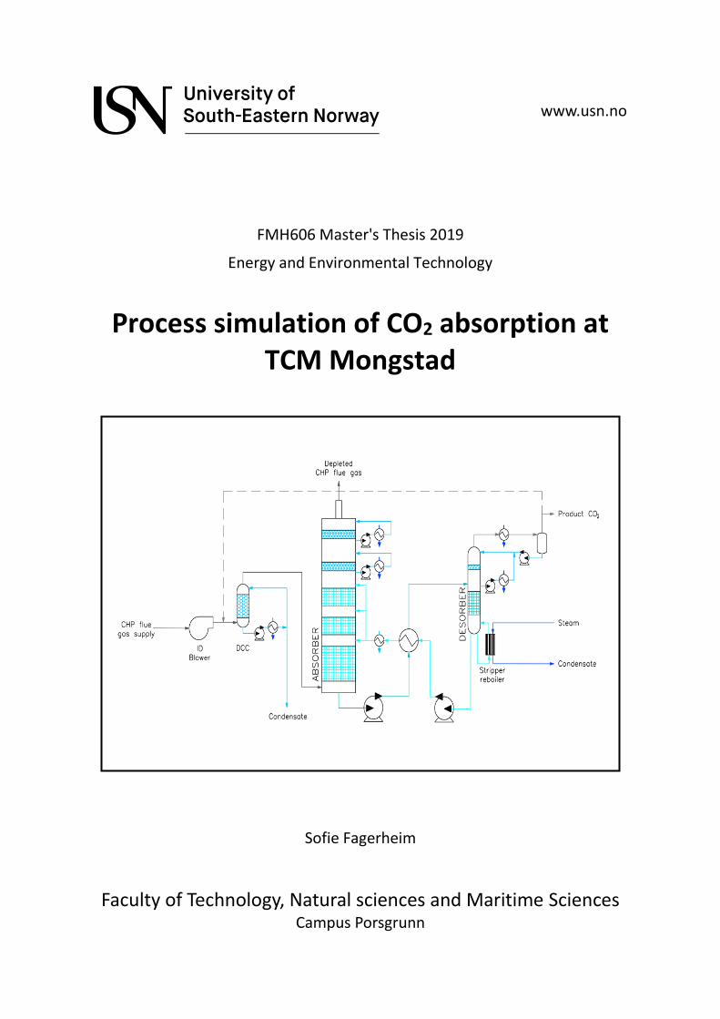
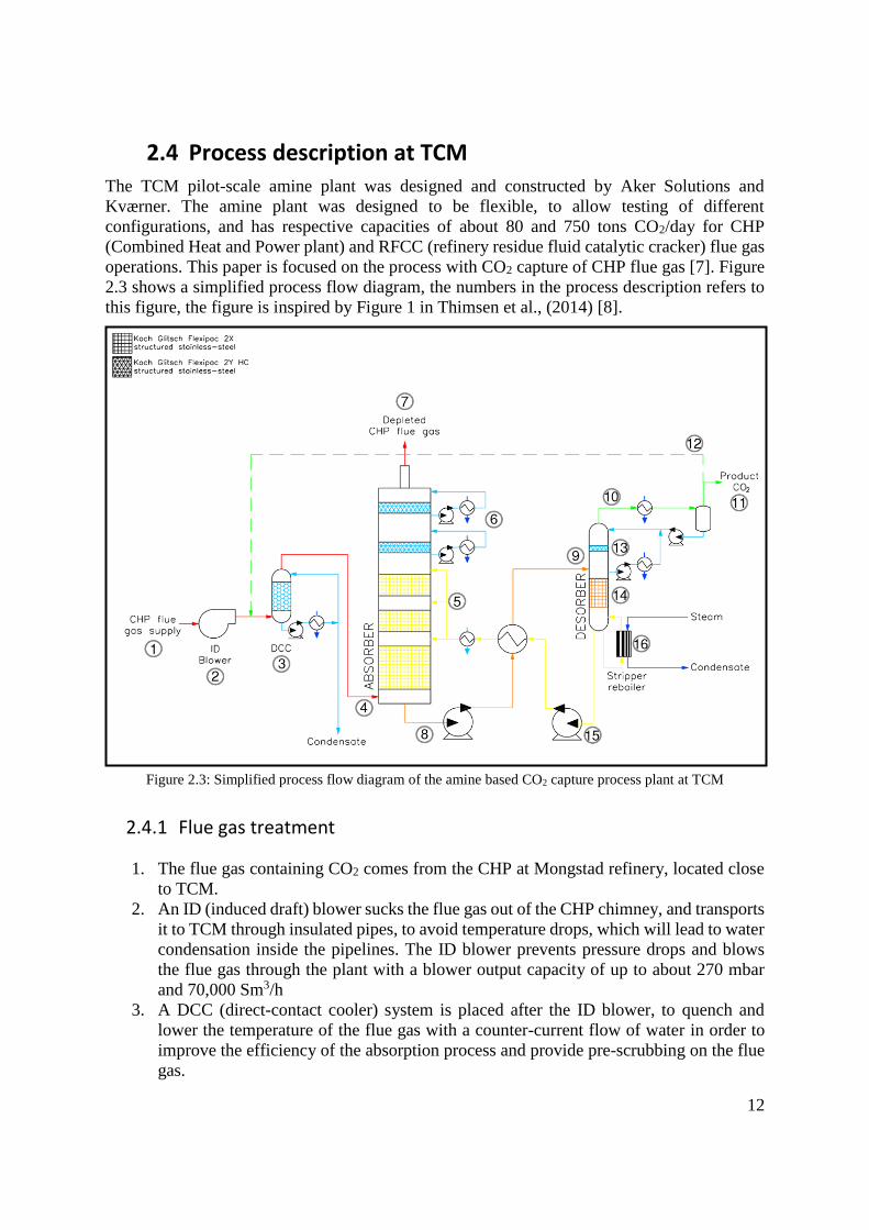
2.4 Process description at TCM
The TCM pilot-scale amine plant was designed and constructed by Aker Solutions and
Kværner. The amine plant was designed to be flexible, to allow testing of different
configurations, and has respective capacities of about 80 and 750 tons CO2/day for CHP
(Combined Heat and Power plant) and RFCC (refinery residue fluid catalytic cracker) flue gas
operations. This paper is focused on the process with CO2 capture of CHP flue gas [7]. Figure
2.3 shows a simplified process flow diagram, the numbers in the process description refers to
this figure, the figure is inspired by Figure 1 in Thimsen et al., (2014) [8].
Figure 2.3: Simplified process flow diagram of the amine based CO2 capture process plant at TCM
2.4.1 Flue gas treatment
1. The flue gas containing CO2 comes from the CHP at Mongstad refinery, located close
to TCM.
2. An ID (induced draft) blower sucks the flue gas out of the CHP chimney, and transports
it to TCM through insulated pipes, to avoid temperature drops, which will lead to water
condensation inside the pipelines. The ID blower prevents pressure drops and blows
the flue gas through the plant with a blower output capacity of up to about 270 mbar
and 70,000 Sm3/h
3. A DCC (direct-contact cooler) system is placed after the ID blower, to quench and
lower the temperature of the flue gas with a counter-current flow of water in order to
improve the efficiency of the absorption process and provide pre-scrubbing on the flue
gas.
13
2.4.2 CO2 capture
4. The cooled flue gas enters an absorber, to remove CO2 from the flue gas using an amine
solvent called MEA (monoethanolamine). The absorber has a rectangular
polypropylene-lined concrete column with a cross section measuring 3.55x2m and a
total height of 62 m.
5. The amine solution contacts the flue gas in the lower region of the column, which
consist of three sections of structured stainless-steel packing of 12 m, 6 m and 6 m of
height.
6. In the upper region of the column, water-wash systems are located to scrub and clean
the flue gas, particularly of any solvent carry over. The water-wash system consists of
two sections of structured stainless-steel packing, both have a height of 3 m. The water-
wash system is also used to maintain the water balance of the solvent by using heat
exchangers to adjust the temperature of the circulating water.
7. The CO2 depleted flue gas exits the absorber column through a stack located at the top
of the absorber.
8. The rich amine exits at the bottom of the absorber, and is from there pumped to the top
of the absorption packing in the stripper. During this transportation, the rich amine
recovers heat from the lean amine exiting the stripper, through a cross-flow heat
exchanger.
2.4.3 Amine regeneration
9. The stripper column recover the captured CO2 and return lean solvent to the absorber.
At TCM there is two independent stripper columns, the column used for CHP flue gas
is cylindrical and has a diameter of 1.3 m and a height of 30 m. The other stripper
column is larger and is utilized when treating flue gases of higher CO2 content.
10. The stripper column has an overhead condenser system where CO2 and water leaving
the stripper is cooled down to separate the water, which is led back to the stripper, by a
reflux drum, condenser and pumps.
11. The cooled and dried CO2 is released in to the atmosphere at a safe vent location.
12. A portion of the product CO2 can also be recycled back to the inlet of the DCC to
increase the concentration of CO2 in the inlet flue gas stream.
13. The upper region of the stripper column consist of a rectifying water-wash section of
structured stainless-steel packing, with a height of 1.6 m.
14. The lower region of the stripper consist of structured stainless steel packing with a
height of 8m.
15. The lean amine exits at the bottom of the desorber, and is pumped through a cross-flow
heat exchanger where it releases energy to the rich amine entering the desorber. The
stripped lean amine is cooled down in another heat exchanger before it enters the
absorber above each of the three absorber packings.
16. A stream of lean amine is re-heated by steam in a stripper reboiler and put back to the
stripper to keep the stripper at desired temperature.
14
2.5 Chemistry of the process
In this subchapter the advantages and disadvantages of using MEA for CO2 capture is weighted
and the chemical reactions of the CO2 absorption is described briefly.
The CO2 is absorbed in a 30/70 wt% mixture of MEA solvent and water. It is absorbed by
direct contact with the solvent-mixture in a 24 meter high packing section, of structured
stainless-steel.
2.5.1 Generally about MEA
MEA (monoethanolamine) is the amine used as solvent for the CO2 absorbation in this paper.
MEA has the formula H2NC2H4OH, and is a primary alkanolamine that often is used for CO2
removal. Other amines that rapidly is used for CO2 removal is the secondary alkanolamine,
DEA (diethanolamine) and the tertiary amine, MDEA (methyl diethanolamine).
When used as solvents, the amines are typically 20-40 wt% solutions in water. MEA in water
solution reacts fast with dissolved CO2 to form carbamate, and has a high CO2 capacity.
Reaction 2.1 shows how MEA reacts as a weak base in water. [9]
𝑀𝐸𝐴 + 𝐻2𝑂 ↔ 𝐻𝑀𝐸𝐴+ + 𝑂𝐻− R(2.1)
2.5.2 Advantages and disadvantages of using MEA for CO2 capture
The advantages of using MEA in CO2 capture is its low molecular weight, which gives the
MEA high capacity even at low concentrations. Another advantage is the high alkalinity of
primary amines. MEA is also considered as a relatively cheap chemical compared with other
amines available for CO2 capture. The toxicity is relatively low and the environmental impact
is less questionable than for other amines, because MEA occurs naturally in living organisms.
The disadvantages of using MEA is the high-energy consumption needed for desorption, which
is a side effect of the high absorption efficiency. Another problem with MEA in contact with
exhaust gas is its tendency to degrade in high temperature and react with oxygen and other
components like sulphur oxides and nitrogen oxides [10, 9]. Another important issue is the CO2
emitted during the production of MEA. When MEA is produced, CO2 is emitted during the
Haber-Bosch process. The regeneration of solvent after the absorption is also an indirect source
of CO2 emission, related to the use of fuels in i.e., combustion for energy supply. The evaluation
of the overall balance of CO2 emitted and captured is essential to determine the efficiency of
the process [11].
15
2.5.3 Reactions of CO2 absorption into MEA
The following reactions describes how CO2 can be absorbed into the mixture of MEA solution
Reaction 2.2 describes how CO2 in a gas can be absorbed in an aqueous liquid. [9]
𝐶𝑂2(𝑔) ↔ 𝐶𝑂2(𝑎𝑞) R(2.2)
Since all the reactions in this system occurs in the aqueous phase, the “aq” notation is skipped.
Reaction 2.3 describes how in the aqueous phase CO2 reacts with hydroxide to bicarbonate.
𝐶𝑂2 + 𝑂𝐻− ↔ 𝐻𝐶𝑂3− R(2.3)
The fast proton transfer reactions (2.4, 2.5 and 2.6) also occur.
Reaction 2.4 describes the ionization of water.
𝐻2𝑂 ↔ 𝐻+ + 𝑂𝐻− R(2.4)
Reaction 2.5 describes the deprotonation of carbonic acid. At equilibrium, the concentration of
H2CO3 is negligible compared to the concentration of free CO2. In a CO2 removal process, with
a pH normally higher than 8.0 this reaction is often neglected because the concentration of
H2CO3 becomes very small.
𝐻2𝐶𝑂3 ↔ 𝐻+ + 𝐻𝐶𝑂3− R(2.5)
Reaction 2.6 describes the deprotonation of the bicarbonate ion to carbonate ion.
𝐻𝐶𝑂3− ↔ 𝐻+ + 𝐶𝑂3
2− R(2.6)
The absorption of CO2 into MEA solution can be described by reaction 2.7, where a protonated
amine ion (MEAH+) and a carbamate ion (MEACOO-) is formed. A carbamate ion is a product
of the reaction of CO2 and amine, when the amine is MEA the carbamate ion has the formula
HN(C2H4OH)COO-.
2𝑀𝐸𝐴 + 𝐶𝑂2 ↔ 𝑀𝐸𝐴𝐻+ + 𝑀𝐸𝐴𝐶𝑂𝑂− R(2.7)
16
Reaction 2.8 describes how a protonated amine ion and bicarbonate (HCO3-) is formed.
𝐶𝑂2 + 𝑀𝐸𝐴 + 𝐻2𝑂 ↔ 𝑀𝐸𝐴𝐻+ + 𝐻𝐶𝑂3− R(2.8)
The total concentration of CO2 is the sum of all the concentrations of the different forms:
𝐶𝐶𝑂2,𝑇𝑂𝑇 = 𝐶𝐶𝑂2 + 𝐶𝐻𝐶𝑂3− + 𝐶𝐶𝑂32− + 𝐶𝐻𝑁(𝐶2𝐻4𝑂𝐻)𝐶𝑂𝑂− (2.1)
The total concentration of amine is the sum of all the concentration of the different forms:
𝐶𝑀𝐸𝐴,𝑇𝑂𝑇 = 𝐶𝑀𝐸𝐴 + 𝐶𝑀𝐸𝐴𝐻+ + 𝐶𝐻𝑁(𝐶2𝐻4𝑂𝐻)𝐶𝑂𝑂− (2.2)
2.6 Earlier work
Some of the relevant earlier work that has been done on simulating CO2 absorption is presented
in this subchapter.
In 2007, Lars Erik Øi (USN) used Aspen HYSYS to simulate CO2 removal by amine
absorption from a gas based power plant. The results showed that adjusting the
Murphree Efficiency outside the simulation tool could be a practical approach when
using Aspen HYSYS to simulate CO2 removal. The paper was published at the
Conference on Simulation and Modelling SIMS2007 in Gøteborg. [12]
In 2007, Finn A. Tobiesen, Hallvard F. Svendsen and Olav Juliussen from SINTEF,
developed a rigorous rate-based model of acid gas absorption, and a simplified absorber
model. They validated the models against mass-transfer data obtained from a 3 month
campaign in a laboratory pilot-plant absorber. It was found that the simplified model
was satisfactory for lower CO2 loading, whiles the rigorous model had a better fit for
higher CO2 loading. [13]
In 2008, Hanne M. Kvamsdal (SINTEF) and Gary T. Rochelle (University of Texas)
studied the effects of temperature bulge in CO2 absorption by MEA. They compared an
Aspen Plus rate based absorber with 4 sets of experimental data from a pilot plant at
the University of Texas, Austin. Several adjustments were made to the model in order
to create a predictable model and to study effects of change in specific parameters. [14]
17
In 2009, Luo et al., from NTNU, compared and validated sixteen data sets from four
different pilot plant studies, with simulations in four different simulation tools (Aspen
Plus equilibrium-based, Aspen Plus rate-based, ProMax, ProTreatTM and CO2SIM).
They concluded that all the simulation tools were able to present reasonable predictions
on overall performance of CO2 absorption rate, while the reboiler duties, concentration
and temperature profiles were less predictable. [15]
In 2011, Espen Hansen worked on his master thesis at USN. Hansen compared Aspen
HYSYS, Aspen Plus and ProMAX simulations of CO2 capture with MEA. He
concluded that Aspen HYSYS and Aspen Plus gives similar results, while the results
from ProMAX deviated from the Aspen tools. Hansen found that Kent-Eisenberg
model in Aspen HYSYS was similar to the Aspen Plus equilibrium-based model for
the absorber, but there was a significant difference in the reboiler duties. [16]
In 2012, Jostein Tvete Bergstrøm worked on his master thesis at USN. Bergstrøm
compared Aspen HYSYS (Kent-Esienberg and Li-Mather), Aspen Plus (Rate-based
and equilibrium) and ProMAX simulations of CO2 capture with MEA. Bergstrøm found
that the models gave similar results, and that the equilibrium-based model in Aspen
Plus and Kent-Eisenberg model in Aspen HYSYS gave coinciding results. [17]
In 2012, Lars Erik Øi (USN) compared Aspen HYSYS and Aspen Plus (rate-based and
equilibrium) simulation of CO2 capture with MEA. Øi found that there was small
deviations in the equilibrium-based model in Aspen HYSYS and Aspen Plus. He found
larger deviations between the equilibrium-based calculations and the rate-based
calculations. [18]
In 2013, Ying Zhang and Chau Chyun Chen simulated nineteen data sets of CO2
absorption in MEA with Aspen rate-based model and the traditional equilibrium-based
model. Their result show that rate-based model yields reasonable predictions on all key
performance measurements, while equilibrium-based model fails to reliably predict
these key performance variables. [19]
In 2013, Stian Holst Pedersen kvam worked on his master thesis at USN. Kvam
compared Aspen Plus (rate based and equilibrium) and Aspen HYSYS (Kent-Eisenberg
and Li-mather) simulations of CO2 capture with MEA. The primary goal was to
compare the energy consumption of a standard process, a process with vapour
recompression and a vapour recompression with split stream, and not to evaluate the
performance of the absorber. [20]
In 2013, Even Solnes Birkelund worked on his master thesis at UIT. Birkelund
compared a standard absorption process, a vapour recompression process and a lean
split with vapour recompression process. He simulated the models in Aspen HYSYS
and used Kent-Eisenberg as thermodynamic model for the aqueous amine solution, and
Peng-Robinson for the vapour phase. All configurations were evaluated due to the
energy cost. The results showed that lean split vapour recompression and vapour
recompression had the lowest energy cost, while the standard absorption process was
simulated to have a much higher energy cost. [21]
18
In 2014, Lars Erik Øi et al, simulated different absorption and desorption configurations
for 85% amine based CO2 removal, from a natural gas based power plant using Aspen
HYSYS. They simulated a standard process, split-stream, vapour recompressions and
different combinations thereof. The simulations were used as a basis for equipment
dimensioning, cost estimation and process optimization. [22]
In 2014, Lars Erik Øi and Stian Holst Pedersen Kvam from USN, simulated different
absorption and desorption configurations for 85% CO2 removal from a natural gas fired
combined cycle power plant, with the simulation tools Aspen HYSYS and Aspen Plus.
In Aspen Plus, both an equilibrium-based model including Murphree Efficiency and a
rate-based model were used. The results show that all simulation models calculate the
same trends in the reduction of equivalent heat consumption, when the absorption
process configuration were changed from the standard process. [23]
In 2014, Inga Strømmen Larsen worked on her master thesis at USN. Larsen simulated
a rate based Aspen Plus model and compared the results to experimental data from
TCM. Larsen found that the Aspen Plus model TCM used was in general agreement
with the experimental data. Larsen found temperature and loading profiles similar to
the experimental data by adjusting parameters. She also did comparison of mass transfer
correlations in Aspen Plus. [24]
In 2014 Espen Steinseth Hamborg et al, published a paper with the results from the
MEA testing at TCM during the 2013 test campaign. The paper reveals CO2 removal
grade, temperature measurement, and experimental data for the process. [7]
In 2015 Espen Steinseth Hamborg from TCM presented some of the results from the
campaign in 2013 and the results from USN-student Inga Strømmen Larsen’s master
thesis from 2014, at the PCCC3 in Canada. A v.7.3 Aspen Plus rate-based model was
compared to the experimental data. The temperature and loading profile from Aspen
Plus presented in this paper gave a good reproduction of the experimental data. [25]
In 2015, Solomon Aforkoghene Aromada and Lars Erik Øi studied how reduction of
energy consumption can be achieved by using alternative configurations. They
simulated standard vapour recompression and vapour recompression combined with
split stream configurations in Aspen HYSYS, for 85% amine-based CO2 removal. The
results showed that it is possible to reduce energy consumption with both the vapour
recompression and the vapor recompression combined with split-stream processes. [26]
In 2015, Coarlie Desvignes worked on a master thesis at Lyon CPE. Desvignes
evaluated the performance of the TCM flowsheet model in Aspen Plus, and compared
with the data obtained in the 2013 and 2014 test campaign at TCM. Desvignes found
that the Aspen Plus model TCM used performed quite well for 30 and 40wt% MEA,
but not for higher flue gas temperature and solvent flowrate. [10]
19
In 2015, Ye Zhu worked on his master thesis at USN. Zhu simulated an equilibrium
model in Aspen HYSYS, Based on the data from TCM 2013 campaign published in
Hamborg et al [7]. Zhu adjusted the Murphree Efficiency to fit the CO2 removal grade
and temperature profile from the experimental results. Zhu found that linear decrease
in Murphree efficiency from top to bottom gave good temperature predictions. [27]
In 2016, Kai Arne Sætre worked on a master’s thesis at USN. Sætre simulated seven
sets of experimental data from the amine based CO2 capture process at TCM, with
Aspen HYSYS (Kent-Eisenberg and Li-Mather) and Aspen Plus (rate-based and
equilibrium). He found that it is possible to fit a rate-based model by adjusting the IAF
and equilibrium-based model by adjusting the EM, both Aspen HYSYS and Aspen Plus
will give good results if there are only small changes in the parameters. [28]
In 2016, Babak Pouladi, Mojtaba Nabipoor Hassankiadeh and Flor Behroozshad,
studies the potential to optimize the conditions of CO2 capture of ethane gas in phase 9
and 10 of south pars in Iran, using DEA as absorbent solvent. They simulated the
process in Aspen HYSYS and found the effect of temperature to be significant. [29]
In 2017, Monica Garcia, Hanna K. Knuutila and Sai Gu, validated a simulation model
of the desorption column built in Aspen Plus v8.6. They used four experimental pilot
campaigns with 30wt% MEA. The results showed a good agreement between the
experimental data and the simulated results. [30]
In 2017, Mohammad Rehan et al., studied the performance and energy savings of
installing an intercooler in a CO2 capture system based on chemical absorption with
MEA as absorption solvent. They used Aspen HYSYS to simulate the CO2 capture
model. The results showed improved CO2 recovery performance and potential of
significant savings in MEA solvent loading and energy requirements, by installing an
intercooler in the system. [31]
In 2017 Leila Faramarzi et al, published a paper with the results from the MEA testing
at TCM during the 2015 test campaign. The paper reveals CO2 removal grade,
temperature measurement, and experimental data for the process. [32]
In 2018, Ole Røsvik worked on his master thesis at USN. Røsvik simulated the TCM
data from the test campaign in 2013, published by Hamborg et al [7]. And the data from
TCM’s test campaign in 2015, published by Faramarzi et al [32] in Aspen HYSYS and
Aspen Plus (equilibrium and rate-based). He found that both Aspen HYSYS and Aspen
Plus will give good results if there are only small changes in the parameters. [33]
In 2018, Lare Erik Øi, Kai Arne Sætre and Espen Steinseth Hamborg, compared four
sets of experimental data from the amine based CO2 capture process at TCM, with
different equilibrium-based models in Aspen HYSYS and Aspen Plus, and a rate based
model in Aspen Plus. The results show that equilibrium and rate-based models perform
equally well in both fitting performance data and in predicting performance at changed
conditions. The paper was presented at the Conference on Simulation and Modelling
SIMS 59 in Oslo. [34]
20
2.7 Problem description
Background
TCM is offered to vendors of solvent based CO2 capture and is mostly running on the vendor’s
solvents and parameters. TCM does not have permission to publish the results conducted at the
vendor’s premises. However, TCM have conducted their own test-campaigns in order to
publish results.
The results from one scenario from TCM’s test-campaign in 2013 was published by Hamborg
et al., (2014) [7], and the result from one scenario from the test-campaign in 2015 was
published by Faramarzi et al., (2017) [32].
USN and NTNU have produced several papers on amine based CO2 capture with different
simulation tools, throughout the last decade. Performance data from the test-campaigns at TCM
have been used in these papers. In addition to the published results some un-published results
have been provided to USN by TCM. The repeated conclusion from these papers have been
that the rate-based model in Aspen Plus, and the equilibrium-based model in Aspen HYSYS
and Aspen Plus perform equally well in both fitting performance data, and in predicting
performance at changed conditions. The model with fitted parameters will give a predictable
simulation only when there are small changes in process parameters [15] [16] [17] [18] [23]
[28] [33] [34].
Another published papers state that the rate-based model yields reasonable predictions on all
key performance measurements, while equilibrium-based model fails to predict reliable
performance variables [19].
Approach
In this thesis the candidate have simulated 5 scenarios from the test-campaigns at TCM from
2013 and 2015. The candidate have tried to further develop the method of estimating Murphree
efficiencies for equilibrium-based models. The candidate have also compared the accuracy of
rate-based model and equilibrium-based model in Aspen Plus and Aspen HYSYS.
Aim of Project
The aim of the project was to contribute to achieve predictable models which gives an accurate
removal grade and satisfactory temperature- and loading profile. The model should be easy to
use for several scenarios with different parameters, and be able to predict reasonable results
even when the parameters are changed.
Another aim of the project was to compare if rate-based model and the equilibrium-based
model will perform equally well in predicting reliable performance data.
21
3 Method In this chapter the method for the simulations, the Murphree efficiency, some necessary
calculations methods and decisions is presented and explained. A new EM-factor is developed.
The experimental data from TCM’s test campaigns is presented with the input data to the
simulations, and specifications of the simulation tools.
3.1 Simulation methodology
The data from TCM is for some cases given in units that needs to be converted to be
implemented in Aspen HYSYS and Aspen Plus. Some necessary decisions and fittings needed
to be done.
Only the absorber is simulated
Experimental data from TCM is converted to units that can be used as parameters in
the simulation program
The pressure loss over the absorber is assumed to be zero
The main goal is to achieve the same CO2 removal grade, temperature profile and rich
loading as in performance data for the five scenarios.
The second goal is to compare the reliability in predicting performance data for
equilibrium-based model with estimated EM-profile and rate-based model with
estimated IAF.
3.1.1 Simulation tools
Several simulation programs can be used to calculate CO2 removal by absorption, such as
Aspen HYSYS, Aspen Plus, Pro/II, ProTreat and ProMax. In this thesis, the process simulation
tool that have been used to perform simulation of CO2 absorption into amine solution are the
equilibrium-based models in Aspen HYSYS and Aspen Plus, and the rate-based model in
Aspen Plus. The equilibrium-based models are based on the assumption of equilibrium at each
stage. By introducing a Murphree efficiency, the model can be extended. Rate-based models
are based on rate expressions for chemical reactions, mass transfer and heat transfer.
3.1.2 Murphree efficiency
There are few tools available for the estimation of stage efficiencies in CO2 absorption
columns. There is a model available for estimation of Murphree efficiency for one plate in a
plate column. The estimation model is based on the work of Tomcej et al., (1987) [35],
modified later by Rangwala et al., (1992) [36]. This model is based on the assumption that a
pseudo first order absorption rate expression is valid. However, there is no model for estimation
of Murphree efficiency for a specific packing section height in a structured packing column.
The calculation of necessary column height for CO2 removal is an important design factor in
CO2 absorption using amine solutions. A simple way to improve the available estimation model
is to use Murphree efficiencies for a specific packing height. In a plate column, an efficiency
value is estimated for each tray based on the ratio of change in mole fraction from a stage to
the next, divided by the change assuming equilibrium. In a packed column, a packing height
22
of e.g. 1 meter could be defined as one tray with a Murphree
efficiency. The Murphree efficiencies can be estimated
outside the simulation program, before it is implemented to
the simulation program. The overall tray efficiency is
defined in equation 3.1, as the number of ideal equilibrium
trays divided by the actual number of trays.
The Murphree tray efficiency related to the gas side for tray
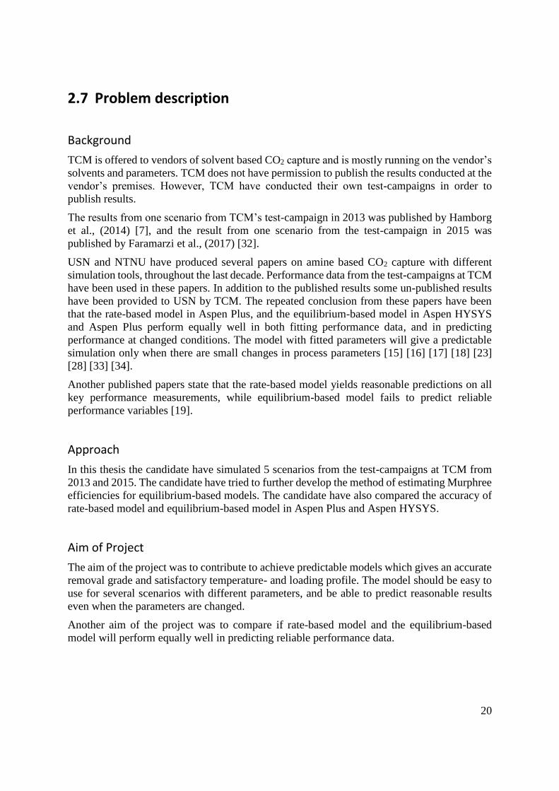
number “n” is traditionally defined by equation 3.2 [37].
Where y is the mole fraction in the gas from the tray, yn+1 is
the mole fraction from the tray below and y* is in
equilibrium with the liquid at tray n. This is illustrated in
figure 3.1.
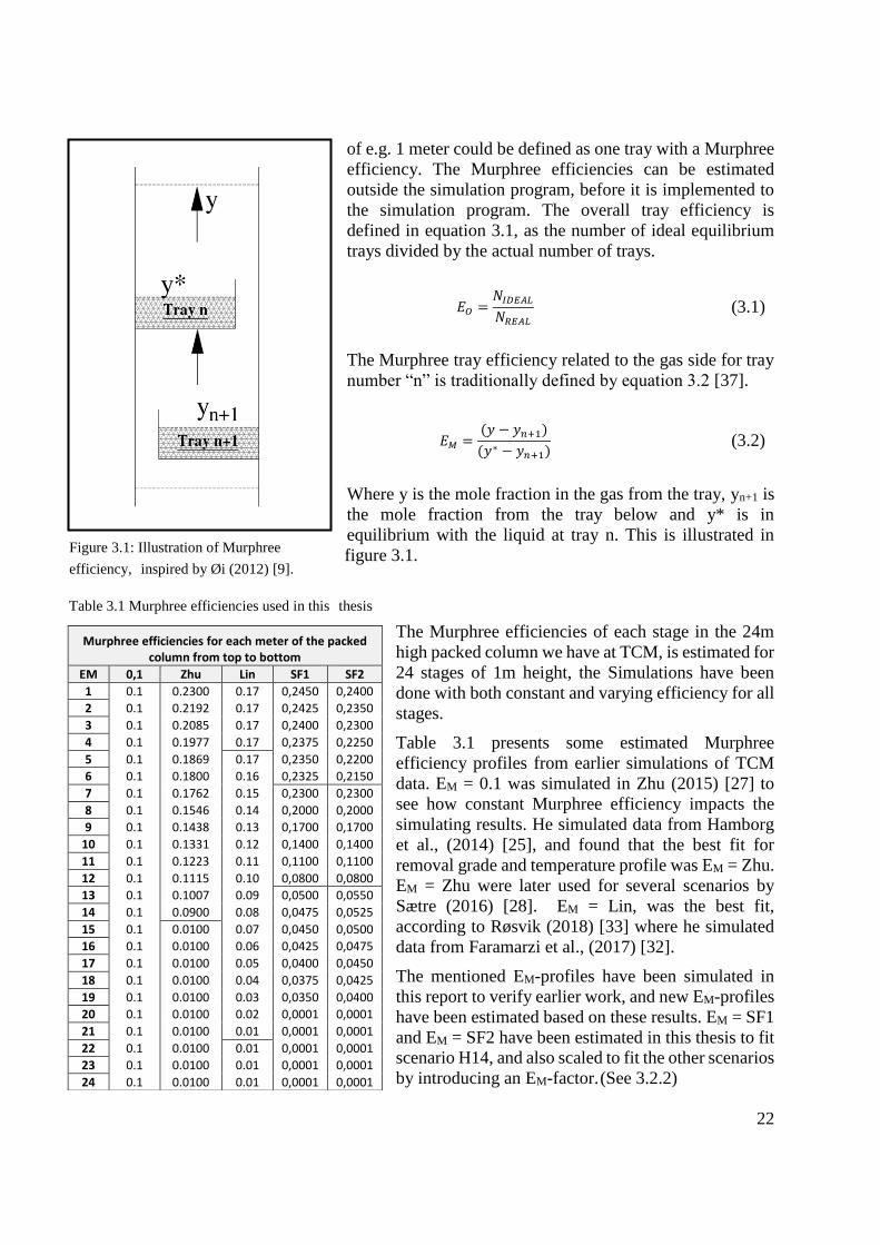
The Murphree efficiencies of each stage in the 24m
high packed column we have at TCM, is estimated for
24 stages of 1m height, the Simulations have been
done with both constant and varying efficiency for all
stages.
Table 3.1 presents some estimated Murphree
efficiency profiles from earlier simulations of TCM
data. EM = 0.1 was simulated in Zhu (2015) [27] to
see how constant Murphree efficiency impacts the
simulating results. He simulated data from Hamborg
et al., (2014) [25], and found that the best fit for
removal grade and temperature profile was EM = Zhu.
EM = Zhu were later used for several scenarios by
Sætre (2016) [28]. EM = Lin, was the best fit,
according to Røsvik (2018) [33] where he simulated
data from Faramarzi et al., (2017) [32].
The mentioned EM-profiles have been simulated in
this report to verify earlier work, and new EM-profiles
have been estimated based on these results. EM = SF1
and EM = SF2 have been estimated in this thesis to fit
scenario H14, and also scaled to fit the other scenarios
by introducing an EM-factor. (See 3.2.2)
𝐸𝑂 =𝑁𝐼𝐷𝐸𝐴𝐿
𝑁𝑅𝐸𝐴𝐿
(3.1)
𝐸𝑀 =(𝑦 − 𝑦𝑛+1)
(𝑦∗ − 𝑦𝑛+1) (3.2)
Murphree efficiencies for each meter of the packed column from top to bottom
EM 0,1 Zhu Lin SF1 SF2
1 0.1 0.2300 0.17 0,2450 0,2400
2 0.1 0.2192 0.17 0,2425 0,2350
3 0.1 0.2085 0.17 0,2400 0,2300
4 0.1 0.1977 0.17 0,2375 0,2250
5 0.1 0.1869 0.17 0,2350 0,2200
6 0.1 0.1800 0.16 0,2325 0,2150
7 0.1 0.1762 0.15 0,2300 0,2300
8 0.1 0.1546 0.14 0,2000 0,2000
9 0.1 0.1438 0.13 0,1700 0,1700
10 0.1 0.1331 0.12 0,1400 0,1400
11 0.1 0.1223 0.11 0,1100 0,1100
12 0.1 0.1115 0.10 0,0800 0,0800
13 0.1 0.1007 0.09 0,0500 0,0550
14 0.1 0.0900 0.08 0,0475 0,0525
15 0.1 0.0100 0.07 0,0450 0,0500
16 0.1 0.0100 0.06 0,0425 0,0475
17 0.1 0.0100 0.05 0,0400 0,0450
18 0.1 0.0100 0.04 0,0375 0,0425
19 0.1 0.0100 0.03 0,0350 0,0400
20 0.1 0.0100 0.02 0,0001 0,0001
21 0.1 0.0100 0.01 0,0001 0,0001
22 0.1 0.0100 0.01 0,0001 0,0001
23 0.1 0.0100 0.01 0,0001 0,0001
24 0.1 0.0100 0.01 0,0001 0,0001
Figure 3.1: Illustration of Murphree
efficiency, inspired by Øi (2012) [9].
Table 3.1 Murphree efficiencies used in this thesis
23
3.1.3 Converting Sm3/h to kmol/h
The inlet gas flow is given in Sm3/h and needs to be given in kmol/h. In 2016, Sætre [28]
created a formula to calculate the mole flow, this is given in equation 3.3. The factor
0.023233 is calculated based on standard conditions chosen by TCM to be 15°C and 1 atm,
and the ideal gas law.
[𝑘𝑚𝑜𝑙
ℎ] = [
𝑆𝑚3
ℎ] ×
1
0,023233[𝑚𝑜𝑙
𝑆𝑚3] (3.3)
He commented that the results from using this formula deviated from measured data for some
of the scenarios, where inlet gas flow was given in both volume flow and molar flow. He
concluded that these deviations probably occurred due to uncertainties in the measured data of
the experimental data at TCM. Therefore he decided to use the calculated molar flow instead
of the measured molar flow, for those scenarios. This decision have also been used for this
thesis.
3.1.4 Calculating composition of lean amine
The lean amine is specified in the reports from TCM [7] [32], by the following parameters:
Lean MEA concentration in water [wt%]
Lean CO2 loading [mol CO2 / mol MEA]
Lean amine supply flow rate [kg/h]
Lean amine supply flow temperature [oC]
Lean amine density [kg/m3]
To get the most accurate result, it is desired to implement the mole fractions of the lean amine
in to the simulations. To accomplish this, some calculation is necessary.
Sætre used a method where he found the molar flow of MEA by using the weight%, mass flow
and molar weight, implemented in equation 3.4.
𝑘𝑚𝑜𝑙 𝑀𝐸𝐴
ℎ=
𝑀𝐸𝐴 [𝑤𝑡% 𝑖𝑛 𝑤𝑎𝑡𝑒𝑟] × 𝑚𝑎𝑠𝑠 𝑓𝑙𝑜𝑤 𝑟𝑎𝑡𝑒 [𝑘𝑔ℎ
]
𝑀𝐸𝐴 𝑚𝑜𝑙𝑎𝑟 𝑤𝑒𝑖𝑔ℎ𝑡 [𝑘𝑚𝑜𝑙𝑘𝑔
]
(3.4)
Following, the H2O molar flow can be found with the same method, shown in equation 3.5.
𝑘𝑚𝑜𝑙 𝐻2𝑂
ℎ=
(1 − 𝑀𝐸𝐴)[𝑤𝑡% 𝑖𝑛 𝑤𝑎𝑡𝑒𝑟] × 𝑚𝑎𝑠𝑠 𝑓𝑙𝑜𝑤 𝑟𝑎𝑡𝑒 [𝑘𝑔ℎ
]
𝐻2𝑂 𝑚𝑜𝑙𝑎𝑟 𝑤𝑒𝑖𝑔ℎ𝑡 [𝑘𝑚𝑜𝑙𝑘𝑔
] (3.5)
24
Finally, the CO2 molar flow can be found by implementing the MEA molar flow and Lean
CO2 loading into equation 3.6.
𝑘𝑚𝑜𝑙 𝐶𝑂2
ℎ= 𝑀𝐸𝐴 𝑚𝑜𝑙𝑎𝑟 𝑓𝑙𝑜𝑤 𝑟𝑎𝑡𝑒 [
𝑘𝑚𝑜𝑙
ℎ] × 𝐶𝑂2 𝑙𝑜𝑎𝑑𝑖𝑛𝑔 [
𝑘𝑚𝑜𝑙 𝐶𝑂2
𝑘𝑚𝑜𝑙 𝑀𝐸𝐴]
(3.6)
When all the tree molar flows are found the molar fractions is easily calculated and can be
implemented to the simulations.
3.1.5 Calculating CO2 removal grade
The CO2 capture efficiency can be quantified in four ways as described in Thimsen et al.,
(2014) [8] and shown in table 3.2, in addition CO2 recovery calculation is given in table 3.2,
and is a measure of the CO2 mass balance [7].
Table 3.2: Methods for calculating CO2 removal grade and CO2 recovery
Method 1 Method 2 Method 3 Method 4 CO2 Recovery
𝑃
𝑆
𝑃
𝑃 + 𝐷
𝑆 − 𝐷
𝑆 1 −
𝑂𝐶𝑂2
1 − 𝑂𝐶𝑂2
(1 − 𝐼𝐶𝑂2)
𝐼𝐶𝑂2
𝐷 + 𝑃
𝑆
S = Flue gas supply OCO2 = Depleted flue gas CO2 content, dry basis
D = Depleted flue gas ICO2 = Flue gas supply CO2 content, dry basis
P = Product CO2
In this report method 3, from table 3.2, is used to calculate removal grade. This method is only
dependent on the CO2 flow in the flue gas supply and the depleted flue gas, the CO2 flow from
the desorber is not included in these calculations. The uncertainty of this method was calculated
to be 2,8% in Hamborg et al., (2014) [7], but it was stated that it might be even higher.
3.2 Suggested method for estimating Murphree efficiency
3.2.1 Estimating EM-profile by calculating overall removal efficiency
To calculate an estimated Murphree efficiency profile the overall removal grade based on the
efficiency of each stage, was calculated with equation 3.7. Where y is the CO2 removal
efficiency of each stage in the absorber packing and n is the number of stages.
25
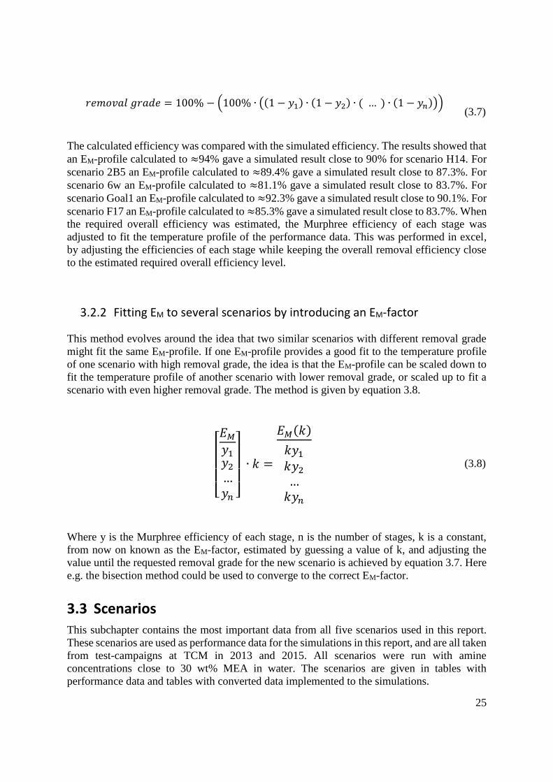
𝑟𝑒𝑚𝑜𝑣𝑎𝑙 𝑔𝑟𝑎𝑑𝑒 = 100% − (100% ∙ ((1 − 𝑦1) ∙ (1 − 𝑦2) ∙ ( … ) ∙ (1 − 𝑦𝑛)))
(3.7)
The calculated efficiency was compared with the simulated efficiency. The results showed that
an EM-profile calculated to ≈94% gave a simulated result close to 90% for scenario H14. For
scenario 2B5 an EM-profile calculated to ≈89.4% gave a simulated result close to 87.3%. For
scenario 6w an EM-profile calculated to ≈81.1% gave a simulated result close to 83.7%. For
scenario Goal1 an EM-profile calculated to ≈92.3% gave a simulated result close to 90.1%. For
scenario F17 an EM-profile calculated to ≈85.3% gave a simulated result close to 83.7%. When
the required overall efficiency was estimated, the Murphree efficiency of each stage was
adjusted to fit the temperature profile of the performance data. This was performed in excel,
by adjusting the efficiencies of each stage while keeping the overall removal efficiency close
to the estimated required overall efficiency level.
3.2.2 Fitting EM to several scenarios by introducing an EM-factor
This method evolves around the idea that two similar scenarios with different removal grade
might fit the same EM-profile. If one EM-profile provides a good fit to the temperature profile
of one scenario with high removal grade, the idea is that the EM-profile can be scaled down to
fit the temperature profile of another scenario with lower removal grade, or scaled up to fit a
scenario with even higher removal grade. The method is given by equation 3.8.
[ 𝐸𝑀
𝑦1𝑦2
…𝑦𝑛 ]
∙ 𝑘 =
𝐸𝑀(𝑘)
𝑘𝑦1
𝑘𝑦2
…𝑘𝑦𝑛
(3.8)
Where y is the Murphree efficiency of each stage, n is the number of stages, k is a constant,
from now on known as the EM-factor, estimated by guessing a value of k, and adjusting the
value until the requested removal grade for the new scenario is achieved by equation 3.7. Here
e.g. the bisection method could be used to converge to the correct EM-factor.
3.3 Scenarios
This subchapter contains the most important data from all five scenarios used in this report.
These scenarios are used as performance data for the simulations in this report, and are all taken
from test-campaigns at TCM in 2013 and 2015. All scenarios were run with amine
concentrations close to 30 wt% MEA in water. The scenarios are given in tables with
performance data and tables with converted data implemented to the simulations.
26
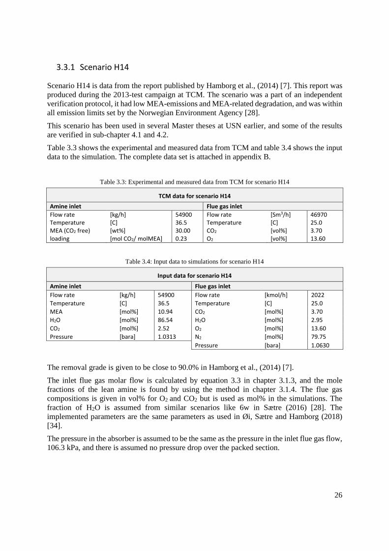
3.3.1 Scenario H14
Scenario H14 is data from the report published by Hamborg et al., (2014) [7]. This report was
produced during the 2013-test campaign at TCM. The scenario was a part of an independent
verification protocol, it had low MEA-emissions and MEA-related degradation, and was within
all emission limits set by the Norwegian Environment Agency [28].
This scenario has been used in several Master theses at USN earlier, and some of the results
are verified in sub-chapter 4.1 and 4.2.
Table 3.3 shows the experimental and measured data from TCM and table 3.4 shows the input
data to the simulation. The complete data set is attached in appendix B.
Table 3.3: Experimental and measured data from TCM for scenario H14
TCM data for scenario H14
Amine inlet Flue gas inlet
Flow rate [kg/h] 54900 Flow rate [Sm3/h] 46970 Temperature [C] 36.5 Temperature [C] 25.0 MEA (CO2 free) [wt%] 30.00 CO2 [vol%] 3.70 loading [mol CO2/ molMEA] 0.23 O2 [vol%] 13.60
Table 3.4: Input data to simulations for scenario H14
Input data for scenario H14
Amine inlet Flue gas inlet
Flow rate [kg/h] 54900 Flow rate [kmol/h] 2022
Temperature [C] 36.5 Temperature [C] 25.0
MEA [mol%] 10.94 CO2 [mol%] 3.70
H2O [mol%] 86.54 H2O [mol%] 2.95
CO2 [mol%] 2.52 O2 [mol%] 13.60
Pressure [bara] 1.0313 N2 [mol%] 79.75
Pressure [bara] 1.0630
The removal grade is given to be close to 90.0% in Hamborg et al., (2014) [7].
The inlet flue gas molar flow is calculated by equation 3.3 in chapter 3.1.3, and the mole
fractions of the lean amine is found by using the method in chapter 3.1.4. The flue gas
compositions is given in vol% for O2 and CO2 but is used as mol% in the simulations. The
fraction of H2O is assumed from similar scenarios like 6w in Sætre (2016) [28]. The
implemented parameters are the same parameters as used in Øi, Sætre and Hamborg (2018)
[34].
The pressure in the absorber is assumed to be the same as the pressure in the inlet flue gas flow,
106.3 kPa, and there is assumed no pressure drop over the packed section.
27
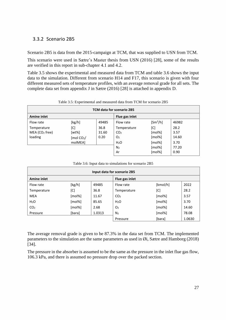
3.3.2 Scenario 2B5
Scenario 2B5 is data from the 2015-campaign at TCM, that was supplied to USN from TCM.
This scenario were used in Sætre’s Master thesis from USN (2016) [28], some of the results
are verified in this report in sub-chapter 4.1 and 4.2.
Table 3.5 shows the experimental and measured data from TCM and table 3.6 shows the input
data to the simulation. Different from scenario H14 and F17, this scenario is given with four
different measured sets of temperature profiles, with an average removal grade for all sets. The
complete data set from appendix J in Sætre (2016) [28] is attached in appendix D.
Table 3.5: Experimental and measured data from TCM for scenario 2B5
TCM data for scenario 2B5
Amine inlet Flue gas inlet
Flow rate [kg/h] 49485 Flow rate [Sm3/h] 46982
Temperature [C] 36.8 Temperature [C] 28.2 MEA (CO2 free) [wt%] 31.60 CO2 [mol%] 3.57 loading [mol CO2/ 0.20 O2 [mol%] 14.60
molMEA] H2O [mol%] 3.70
N2 [mol%] 77.20
Ar [mol%] 0.90
Table 3.6: Input data to simulations for scenario 2B5
Input data for scenario 2B5
Amine inlet Flue gas inlet
Flow rate [kg/h] 49485 Flow rate [kmol/h] 2022
Temperature [C] 36.8 Temperature [C] 28.2
MEA [mol%] 11.67 CO2 [mol%] 3.57
H2O [mol%] 85.65 H2O [mol%] 3.70
CO2 [mol%] 2.68 O2 [mol%] 14.60
Pressure [bara] 1.0313 N2 [mol%] 78.08
Pressure [bara] 1.0630
The average removal grade is given to be 87.3% in the data set from TCM. The implemented
parameters to the simulation are the same parameters as used in Øi, Sætre and Hamborg (2018)
[34].
The pressure in the absorber is assumed to be the same as the pressure in the inlet flue gas flow,
106.3 kPa, and there is assumed no pressure drop over the packed section.
28
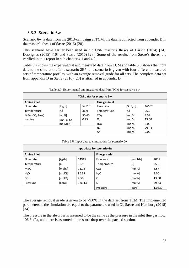
3.3.3 Scenario 6w
Scenario 6w is data from the 2013-campaign at TCM, the data is collected from appendix D in
the master’s thesis of Sætre (2016) [28].
This scenario have earlier been used in the USN master’s theses of Larsen (2014) [24],
Desvignes (2015) [10] and Sætre (2016) [28]. Some of the results from Sætre’s theses are
verified in this report in sub chapter 4.1 and 4.2.
Table 3.7 shows the experimental and measured data from TCM and table 3.8 shows the input
data to the simulation. Like scenario 2B5, this scenario is given with four different measured
sets of temperature profiles, with an average removal grade for all sets. The complete data set
from appendix D in Sætre (2016) [28] is attached in appendix D.
Table 3.7: Experimental and measured data from TCM for scenario 6w
TCM data for scenario 6w
Amine inlet Flue gas inlet
Flow rate [kg/h] 54915 Flow rate [Sm3/h] 46602
Temperature [C] 36.9 Temperature [C] 25.0
MEA (CO2 free) [wt%] 30.40 CO2 [mol%] 3.57 loading [mol CO2/ 0.25 O2 [mol%] 13.60
molMEA] H2O [mol%] 3.00
N2 [mol%] 79.83
Ar [mol%] 0.00
Table 3.8: Input data to simulations for scenario 6w
Input data for scenario 6w
Amine inlet Flue gas inlet
Flow rate [kg/h] 54915 Flow rate [kmol/h] 2005
Temperature [C] 36.9 Temperature [C] 25.0
MEA [mol%] 11.13 CO2 [mol%] 3.57
H2O [mol%] 86.37 H2O [mol%] 3.00
CO2 [mol%] 2.50 O2 [mol%] 13.60
Pressure [bara] 1.0313 N2 [mol%] 79.83
Pressure [bara] 1.0630
The average removal grade is given to be 79.0% in the data set from TCM. The implemented
parameters to the simulation are equal to the parameters used in Øi, Sætre and Hamborg (2018)
[34].
The pressure in the absorber is assumed to be the same as the pressure in the inlet flue gas flow,
106.3 kPa, and there is assumed no pressure drop over the packed section.
29
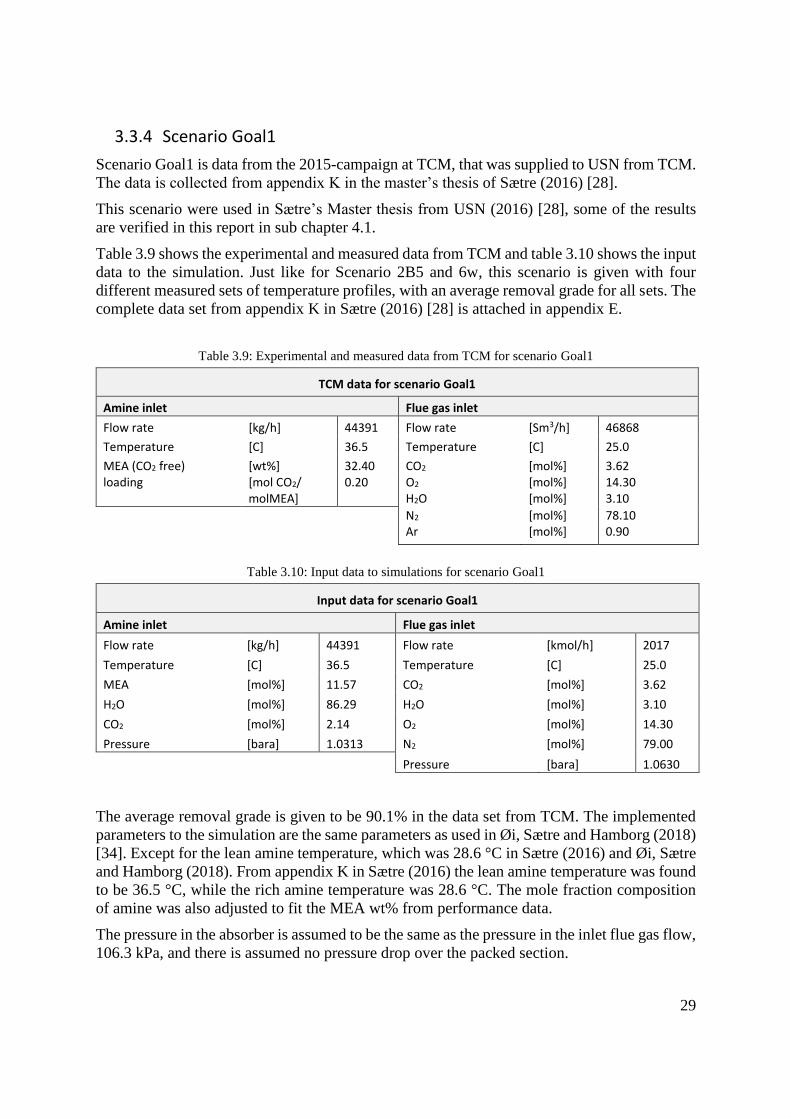
3.3.4 Scenario Goal1
Scenario Goal1 is data from the 2015-campaign at TCM, that was supplied to USN from TCM.
The data is collected from appendix K in the master’s thesis of Sætre (2016) [28].
This scenario were used in Sætre’s Master thesis from USN (2016) [28], some of the results
are verified in this report in sub chapter 4.1.
Table 3.9 shows the experimental and measured data from TCM and table 3.10 shows the input
data to the simulation. Just like for Scenario 2B5 and 6w, this scenario is given with four
different measured sets of temperature profiles, with an average removal grade for all sets. The
complete data set from appendix K in Sætre (2016) [28] is attached in appendix E.
Table 3.9: Experimental and measured data from TCM for scenario Goal1
TCM data for scenario Goal1
Amine inlet Flue gas inlet
Flow rate [kg/h] 44391 Flow rate [Sm3/h] 46868
Temperature [C] 36.5 Temperature [C] 25.0
MEA (CO2 free) [wt%] 32.40 CO2 [mol%] 3.62 loading [mol CO2/ 0.20 O2 [mol%] 14.30 molMEA] H2O [mol%] 3.10
N2 [mol%] 78.10
Ar [mol%] 0.90
Table 3.10: Input data to simulations for scenario Goal1
Input data for scenario Goal1
Amine inlet Flue gas inlet
Flow rate [kg/h] 44391 Flow rate [kmol/h] 2017
Temperature [C] 36.5 Temperature [C] 25.0
MEA [mol%] 11.57 CO2 [mol%] 3.62
H2O [mol%] 86.29 H2O [mol%] 3.10
CO2 [mol%] 2.14 O2 [mol%] 14.30
Pressure [bara] 1.0313 N2 [mol%] 79.00
Pressure [bara] 1.0630
The average removal grade is given to be 90.1% in the data set from TCM. The implemented
parameters to the simulation are the same parameters as used in Øi, Sætre and Hamborg (2018)
[34]. Except for the lean amine temperature, which was 28.6 °C in Sætre (2016) and Øi, Sætre
and Hamborg (2018). From appendix K in Sætre (2016) the lean amine temperature was found
to be 36.5 °C, while the rich amine temperature was 28.6 °C. The mole fraction composition
of amine was also adjusted to fit the MEA wt% from performance data.
The pressure in the absorber is assumed to be the same as the pressure in the inlet flue gas flow,
106.3 kPa, and there is assumed no pressure drop over the packed section.
30
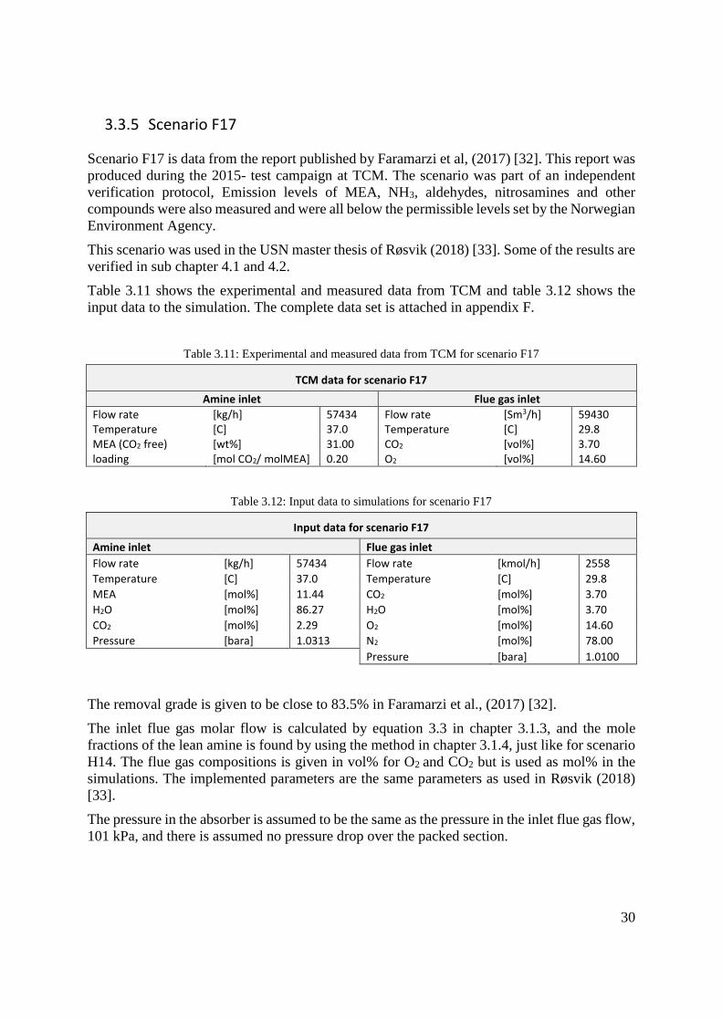
3.3.5 Scenario F17
Scenario F17 is data from the report published by Faramarzi et al, (2017) [32]. This report was
produced during the 2015- test campaign at TCM. The scenario was part of an independent
verification protocol, Emission levels of MEA, NH3, aldehydes, nitrosamines and other
compounds were also measured and were all below the permissible levels set by the Norwegian
Environment Agency.
This scenario was used in the USN master thesis of Røsvik (2018) [33]. Some of the results are
verified in sub chapter 4.1 and 4.2.
Table 3.11 shows the experimental and measured data from TCM and table 3.12 shows the
input data to the simulation. The complete data set is attached in appendix F.
Table 3.11: Experimental and measured data from TCM for scenario F17
TCM data for scenario F17
Amine inlet Flue gas inlet
Flow rate [kg/h] 57434 Flow rate [Sm3/h] 59430 Temperature [C] 37.0 Temperature [C] 29.8 MEA (CO2 free) [wt%] 31.00 CO2 [vol%] 3.70 loading [mol CO2/ molMEA] 0.20 O2 [vol%] 14.60
Table 3.12: Input data to simulations for scenario F17
Input data for scenario F17
Amine inlet Flue gas inlet
Flow rate [kg/h] 57434 Flow rate [kmol/h] 2558
Temperature [C] 37.0 Temperature [C] 29.8
MEA [mol%] 11.44 CO2 [mol%] 3.70
H2O [mol%] 86.27 H2O [mol%] 3.70
CO2 [mol%] 2.29 O2 [mol%] 14.60
Pressure [bara] 1.0313 N2 [mol%] 78.00
Pressure [bara] 1.0100
The removal grade is given to be close to 83.5% in Faramarzi et al., (2017) [32].
The inlet flue gas molar flow is calculated by equation 3.3 in chapter 3.1.3, and the mole
fractions of the lean amine is found by using the method in chapter 3.1.4, just like for scenario
H14. The flue gas compositions is given in vol% for O2 and CO2 but is used as mol% in the
simulations. The implemented parameters are the same parameters as used in Røsvik (2018)
[33].
The pressure in the absorber is assumed to be the same as the pressure in the inlet flue gas flow,
101 kPa, and there is assumed no pressure drop over the packed section.
31
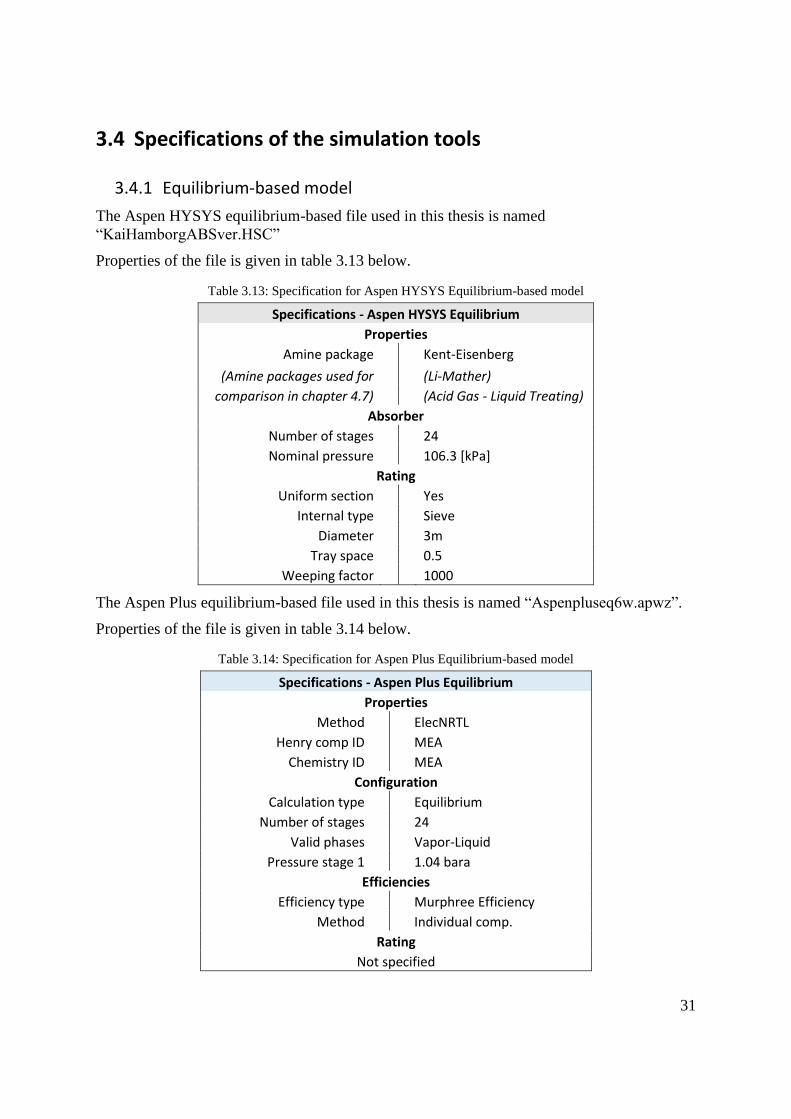
3.4 Specifications of the simulation tools
3.4.1 Equilibrium-based model
The Aspen HYSYS equilibrium-based file used in this thesis is named
“KaiHamborgABSver.HSC”
Properties of the file is given in table 3.13 below.
Table 3.13: Specification for Aspen HYSYS Equilibrium-based model
Specifications - Aspen HYSYS Equilibrium
Properties
Amine package Kent-Eisenberg
(Amine packages used for (Li-Mather)
comparison in chapter 4.7) (Acid Gas - Liquid Treating)
Absorber
Number of stages 24
Nominal pressure 106.3 [kPa]
Rating
Uniform section Yes
Internal type Sieve
Diameter 3m
Tray space 0.5
Weeping factor 1000
The Aspen Plus equilibrium-based file used in this thesis is named “Aspenpluseq6w.apwz”.
Properties of the file is given in table 3.14 below.
Table 3.14: Specification for Aspen Plus Equilibrium-based model
Specifications - Aspen Plus Equilibrium
Properties
Method ElecNRTL
Henry comp ID MEA
Chemistry ID MEA
Configuration
Calculation type Equilibrium
Number of stages 24
Valid phases Vapor-Liquid
Pressure stage 1 1.04 bara
Efficiencies
Efficiency type Murphree Efficiency
Method Individual comp.
Rating
Not specified
32
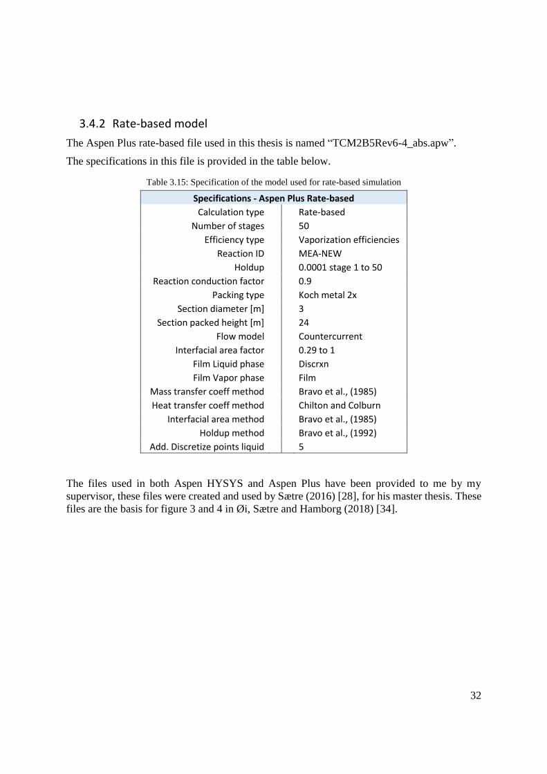
3.4.2 Rate-based model
The Aspen Plus rate-based file used in this thesis is named “TCM2B5Rev6-4_abs.apw”.
The specifications in this file is provided in the table below.
Table 3.15: Specification of the model used for rate-based simulation
Specifications - Aspen Plus Rate-based
Calculation type Rate-based
Number of stages 50
Efficiency type Vaporization efficiencies
Reaction ID MEA-NEW
Holdup 0.0001 stage 1 to 50
Reaction conduction factor 0.9
Packing type Koch metal 2x
Section diameter [m] 3
Section packed height [m] 24
Flow model Countercurrent
Interfacial area factor 0.29 to 1
Film Liquid phase Discrxn
Film Vapor phase Film
Mass transfer coeff method Bravo et al., (1985)
Heat transfer coeff method Chilton and Colburn
Interfacial area method Bravo et al., (1985)
Holdup method Bravo et al., (1992)
Add. Discretize points liquid 5
The files used in both Aspen HYSYS and Aspen Plus have been provided to me by my
supervisor, these files were created and used by Sætre (2016) [28], for his master thesis. These
files are the basis for figure 3 and 4 in Øi, Sætre and Hamborg (2018) [34].
33
4 Results This chapter presents the results from the simulations of all scenarios in Aspen Plus and Aspen
HYSYS. The five scenarios have been used for earlier master theses:
Scenario H14 have been simulated in both Aspen HYSYS and Aspen Plus in earlier
master thesis’s at USN. In 2015 Ye Zhu simulated the scenario in Aspen HYSYS,
for his master thesis. Then in 2016 and 2018, Kai Arne Sætre and Ole Røsvik,
respectively, simulated the same scenario in both Aspen HYSYS and Aspen Plus.
Scenario 2B5 have been simulated in both Aspen HYSYS and Aspen Plus in Kai
Arne Sætre’s master thesis from 2016.
Scenario 6w have been simulated in both Aspen HYSYS and Aspen Plus in earlier
USN master’s theses by Larsen (2014), Desvignes (2015) and Sætre (2016).
Scenario Goal1 have been simulated in both Aspen HYSYS and Aspen Plus in Kai
Arne Sætre’s master thesis from 2016.
Scenario F17 have been simulated in both Aspen HYSYS and Aspen Plus in Ole
Røsvik’s master thesis from 2018.
An introduction and description of the simulations in each sub-chapter is given below:
4.1 Verification of earlier work in Aspen HYSYS
This sub-chapter presents the simulation of the five scenarios compared with results from
earlier work and performance data. All data in this sub-chapter is simulated in equilibrium-
based model in Aspen HYSYS with Kent Eisenberg as amine package.
The simulated temperature profile from Aspen HYSYS compared with simulated results
from earlier theses is attached in appendix G.
4.2 Verification of earlier work in Aspen Plus
This sub-chapter presents the simulation of the five scenarios compared with results from
earlier work and performance data. All scenarios have been simulated in rate-based model
and equilibrium-based model in Aspen Plus with e-NRTL.
The simulated temperature profile from Aspen Plus compared with simulated results from
earlier theses is attached in appendix H.
4.3 Simulation in Aspen HYSYS with estimated EM
Earlier studies have focused on the packed section as one packing with Murphree
efficiencies from top to bottom. The results from these studies showed that a linear decrease
in Murphree efficiency from the top to the lower middle of the packing, followed by a low
constant efficiency for the bottom part of the packing have given the best fit to the
temperature profile, e.g. EM=Zhu.
34
During this project several combinations of Murphree efficiencies have been tested, some
of them based on the idea that the three separated packing sections in the column might
have higher efficiencies at the top of each section, because fresh amine enters at the top of
each section. Based on this theory, two new EM-profiles were estimated with equation 3.7,
EM=SF1 and EM=SF2. Both with linearly decreasing efficiency in each packing section in
the packed column. These two sets was first estimated for Scenario H14, and later scaled
to fit the other scenarios, by introducing the EM-factor in equation 3.8.
In this sub-chapter the five EM-profiles given in table 3.1 in sub chapter 3.1.2, have been
scaled for each scenario to produce requested removal grade in simulation. All simulations
in this sub-chapter have been simulated in equilibrium-based model in Aspen HYSYS with
Kent Eisenberg.
The estimated Murphree efficiency profiles is attached in appendix I, along with the
simulated temperature profiles and important data from simulation.
Some interesting connections between EM-factor and performance data was seen in the
results from these simulations, which led to the calculations in chapter 5.
4.4 Simulation in Aspen Plus with estimated EM and IAF
In this sub-chapter all the EM-profiles used in sub-chapter 4.3 have been scaled to achieve
requested removal grade for all EM-profiles in all five scenarios in Aspen Plus, by adjusting
the EM-factor. The simulations have been simulated in equilibrium-based model in Aspen
Plus with e-NRTL.
The interfacial area factor have been adjusted to achieve requested removal grade for all
scenarios in rate-based model in Aspen plus.
The estimated IAF is attached in appendix J, along with the simulated temperature profiles
and important data from simulation.
4.5 Comparison of Rate-based and Equilibrium-based model
In this sub-chapter the simulated results from sub-chapter 4.3 and 4.4 have been compared.
The simulated temperature profiles and important data from simulation is attached in
appendix K.
4.6 Simulation with default EM in Aspen HYSYS
There is a possibility to get Aspen HYSYS to estimate the Murphree efficiencies, these
efficiencies is from now on called default efficiencies. The method that was used to achieve
the requested removal grade with default efficiencies, was to vary the amount of stages in
the packed column. In this sub chapter the simulations of each scenario with default
efficiencies have been compared with the results from the estimated simulation of EM=SF1
for each scenario.
The default EM-profiles estimated by Aspen HYSYS is attached in appendix L, along with
the simulated temperature profiles and important data from simulation.
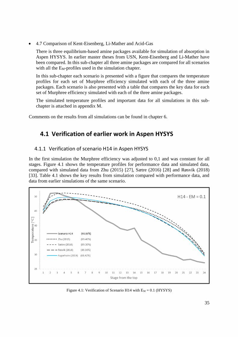
35
4.7 Comparison of Kent-Eisenberg, Li-Mather and Acid-Gas
There is three equilibrium-based amine packages available for simulation of absorption in
Aspen HYSYS. In earlier master theses from USN, Kent-Eisenberg and Li-Mather have
been compared. In this sub-chapter all three amine packages are compared for all scenarios
with all the EM-profiles used in the simulation chapter.
In this sub-chapter each scenario is presented with a figure that compares the temperature
profiles for each set of Murphree efficiency simulated with each of the three amine
packages. Each scenario is also presented with a table that compares the key data for each
set of Murphree efficiency simulated with each of the three amine packages.
The simulated temperature profiles and important data for all simulations in this sub-
chapter is attached in appendix M.
Comments on the results from all simulations can be found in chapter 6.
4.1 Verification of earlier work in Aspen HYSYS
4.1.1 Verification of scenario H14 in Aspen HYSYS
In the first simulation the Murphree efficiency was adjusted to 0,1 and was constant for all
stages. Figure 4.1 shows the temperature profiles for performance data and simulated data,
compared with simulated data from Zhu (2015) [27], Sætre (2016) [28] and Røsvik (2018)
[33]. Table 4.1 shows the key results from simulation compared with performance data, and
data from earlier simulations of the same scenario.
Figure 4.1: Verification of Scenario H14 with EM = 0.1 (HYSYS)
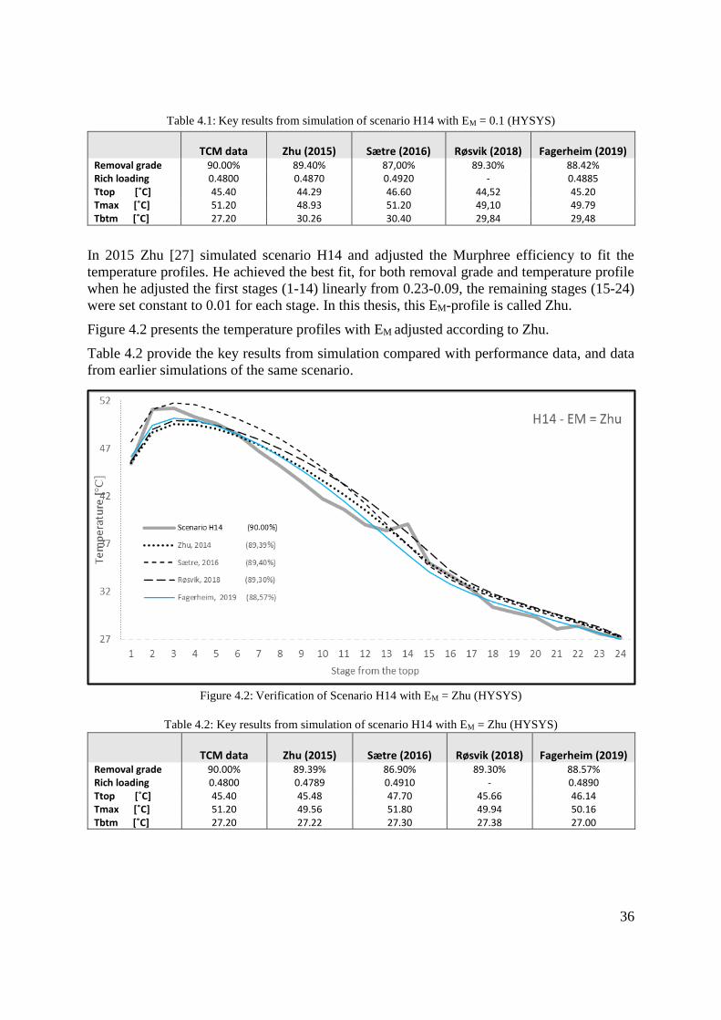
36
Table 4.1: Key results from simulation of scenario H14 with EM = 0.1 (HYSYS)
TCM data Zhu (2015) Sætre (2016) Røsvik (2018) Fagerheim (2019) Removal grade 90.00% 89.40% 87,00% 89.30% 88.42% Rich loading 0.4800 0.4870 0.4920 - 0.4885 Ttop [˚C] 45.40 44.29 46.60 44,52 45.20 Tmax [˚C] 51.20 48.93 51.20 49,10 49.79 Tbtm [˚C] 27.20 30.26 30.40 29,84 29,48
In 2015 Zhu [27] simulated scenario H14 and adjusted the Murphree efficiency to fit the
temperature profiles. He achieved the best fit, for both removal grade and temperature profile
when he adjusted the first stages (1-14) linearly from 0.23-0.09, the remaining stages (15-24)
were set constant to 0.01 for each stage. In this thesis, this EM-profile is called Zhu.
Figure 4.2 presents the temperature profiles with EM adjusted according to Zhu.
Table 4.2 provide the key results from simulation compared with performance data, and data
from earlier simulations of the same scenario.
Figure 4.2: Verification of Scenario H14 with EM = Zhu (HYSYS)
Table 4.2: Key results from simulation of scenario H14 with EM = Zhu (HYSYS)
TCM data Zhu (2015) Sætre (2016) Røsvik (2018) Fagerheim (2019) Removal grade 90.00% 89.39% 86.90% 89.30% 88.57% Rich loading 0.4800 0.4789 0.4910 - 0.4890 Ttop [˚C] 45.40 45.48 47.70 45.66 46.14 Tmax [˚C] 51.20 49.56 51.80 49.94 50.16 Tbtm [˚C] 27.20 27.22 27.30 27.38 27.00
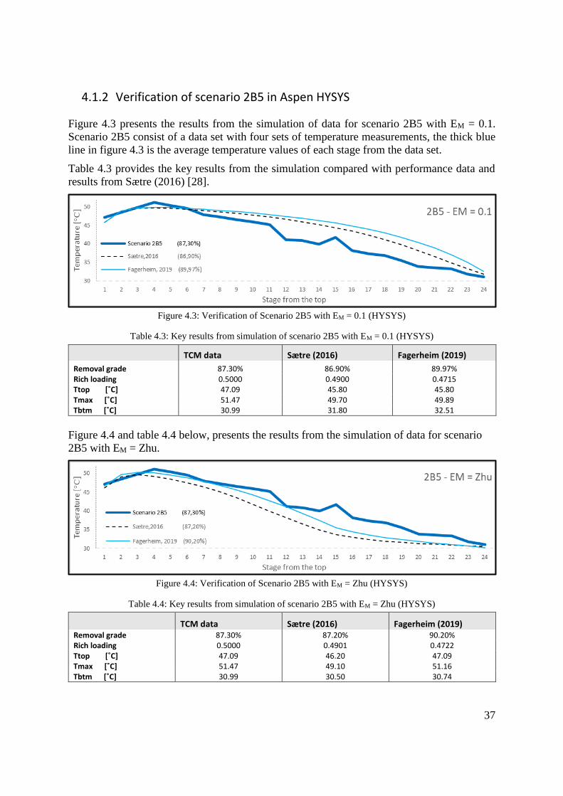
37
4.1.2 Verification of scenario 2B5 in Aspen HYSYS
Figure 4.3 presents the results from the simulation of data for scenario 2B5 with EM = 0.1.
Scenario 2B5 consist of a data set with four sets of temperature measurements, the thick blue
line in figure 4.3 is the average temperature values of each stage from the data set.
Table 4.3 provides the key results from the simulation compared with performance data and
results from Sætre (2016) [28].
Figure 4.3: Verification of Scenario 2B5 with EM = 0.1 (HYSYS)
Table 4.3: Key results from simulation of scenario 2B5 with EM = 0.1 (HYSYS)
TCM data Sætre (2016) Fagerheim (2019)
Removal grade 87.30% 86.90% 89.97% Rich loading 0.5000 0.4900 0.4715 Ttop [˚C] 47.09 45.80 45.80 Tmax [˚C] 51.47 49.70 49.89 Tbtm [˚C] 30.99 31.80 32.51
Figure 4.4 and table 4.4 below, presents the results from the simulation of data for scenario
2B5 with EM = Zhu.
Figure 4.4: Verification of Scenario 2B5 with EM = Zhu (HYSYS)
Table 4.4: Key results from simulation of scenario 2B5 with EM = Zhu (HYSYS)
TCM data Sætre (2016) Fagerheim (2019) Removal grade 87.30% 87.20% 90.20% Rich loading 0.5000 0.4901 0.4722 Ttop [˚C] 47.09 46.20 47.09 Tmax [˚C] 51.47 49.10 51.16 Tbtm [˚C] 30.99 30.50 30.74
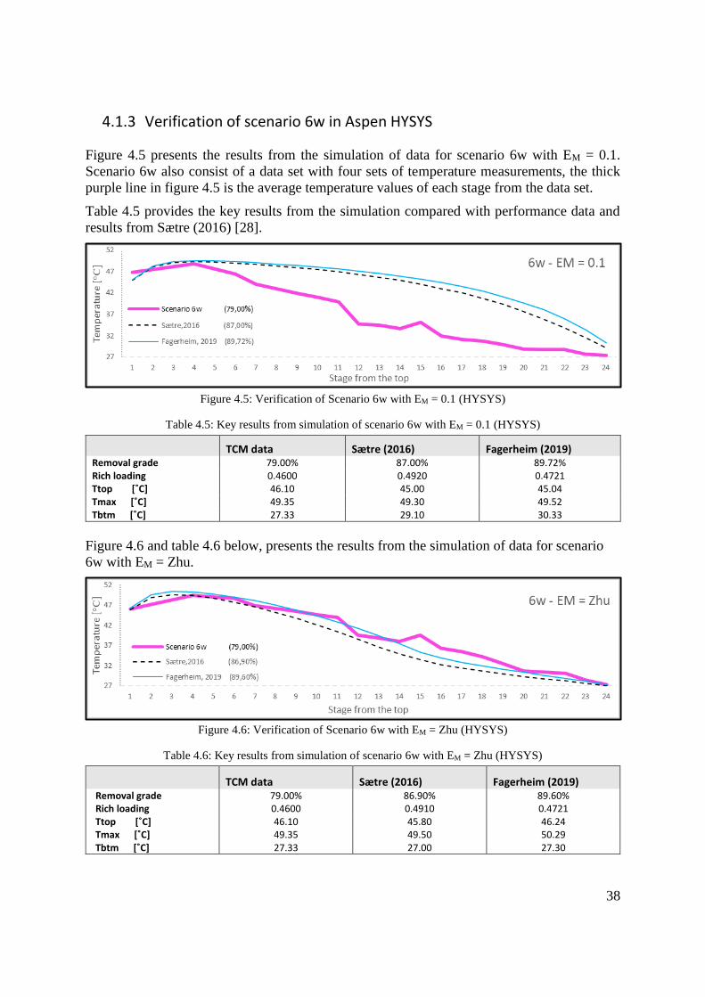
38
4.1.3 Verification of scenario 6w in Aspen HYSYS
Figure 4.5 presents the results from the simulation of data for scenario 6w with EM = 0.1.
Scenario 6w also consist of a data set with four sets of temperature measurements, the thick
purple line in figure 4.5 is the average temperature values of each stage from the data set.
Table 4.5 provides the key results from the simulation compared with performance data and
results from Sætre (2016) [28].
Figure 4.5: Verification of Scenario 6w with EM = 0.1 (HYSYS)
Table 4.5: Key results from simulation of scenario 6w with EM = 0.1 (HYSYS)
TCM data Sætre (2016) Fagerheim (2019) Removal grade 79.00% 87.00% 89.72% Rich loading 0.4600 0.4920 0.4721 Ttop [˚C] 46.10 45.00 45.04 Tmax [˚C] 49.35 49.30 49.52 Tbtm [˚C] 27.33 29.10 30.33
Figure 4.6 and table 4.6 below, presents the results from the simulation of data for scenario
6w with EM = Zhu.
Figure 4.6: Verification of Scenario 6w with EM = Zhu (HYSYS)
Table 4.6: Key results from simulation of scenario 6w with EM = Zhu (HYSYS)
TCM data Sætre (2016) Fagerheim (2019) Removal grade 79.00% 86.90% 89.60% Rich loading 0.4600 0.4910 0.4721 Ttop [˚C] 46.10 45.80 46.24 Tmax [˚C] 49.35 49.50 50.29 Tbtm [˚C] 27.33 27.00 27.30
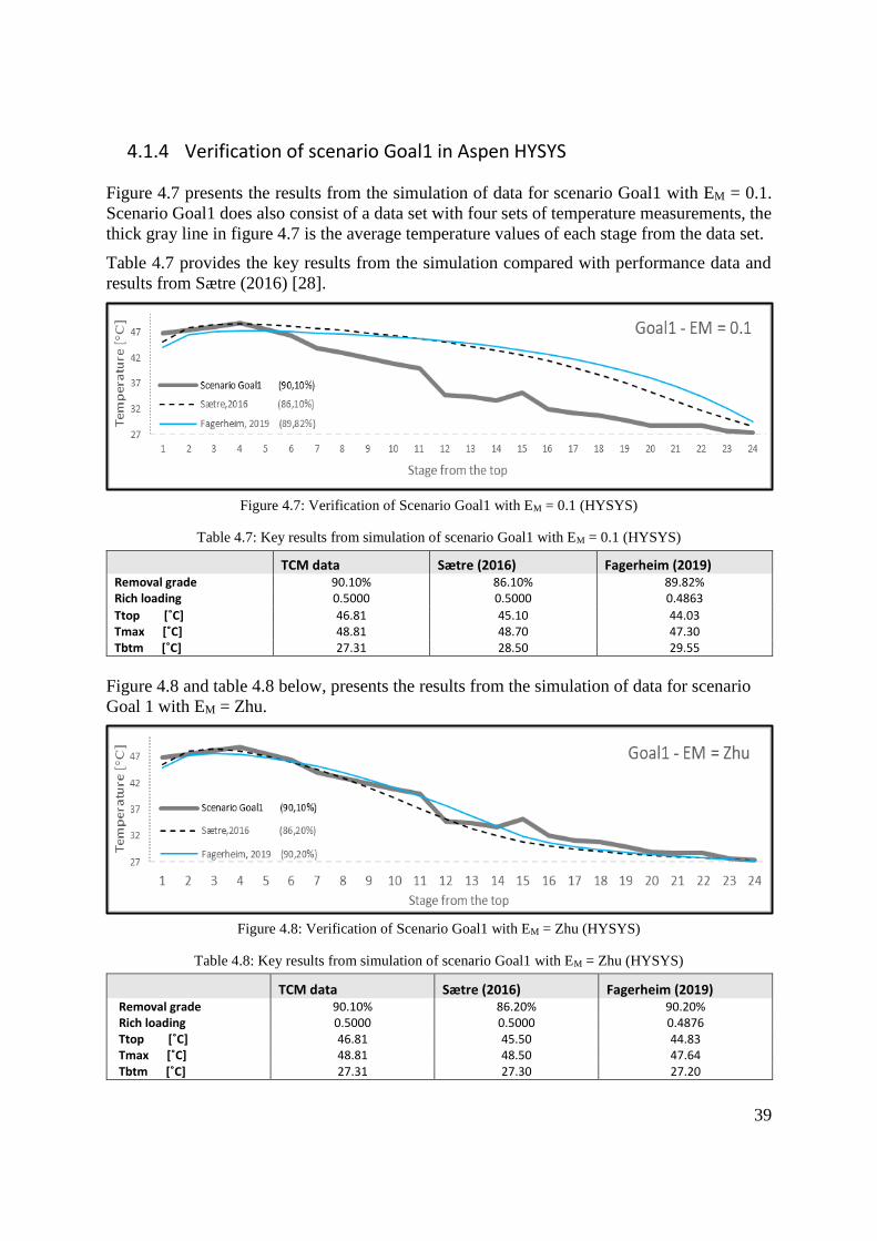
39
4.1.4 Verification of scenario Goal1 in Aspen HYSYS
Figure 4.7 presents the results from the simulation of data for scenario Goal1 with EM = 0.1.
Scenario Goal1 does also consist of a data set with four sets of temperature measurements, the
thick gray line in figure 4.7 is the average temperature values of each stage from the data set.
Table 4.7 provides the key results from the simulation compared with performance data and
results from Sætre (2016) [28].
Figure 4.7: Verification of Scenario Goal1 with EM = 0.1 (HYSYS)
Table 4.7: Key results from simulation of scenario Goal1 with EM = 0.1 (HYSYS)
TCM data Sætre (2016) Fagerheim (2019) Removal grade 90.10% 86.10% 89.82% Rich loading 0.5000 0.5000 0.4863
Ttop [˚C] 46.81 45.10 44.03 Tmax [˚C] 48.81 48.70 47.30 Tbtm [˚C] 27.31 28.50 29.55
Figure 4.8 and table 4.8 below, presents the results from the simulation of data for scenario
Goal 1 with EM = Zhu.
Figure 4.8: Verification of Scenario Goal1 with EM = Zhu (HYSYS)
Table 4.8: Key results from simulation of scenario Goal1 with EM = Zhu (HYSYS)
TCM data Sætre (2016) Fagerheim (2019) Removal grade 90.10% 86.20% 90.20% Rich loading 0.5000 0.5000 0.4876 Ttop [˚C] 46.81 45.50 44.83 Tmax [˚C] 48.81 48.50 47.64 Tbtm [˚C] 27.31 27.30 27.20
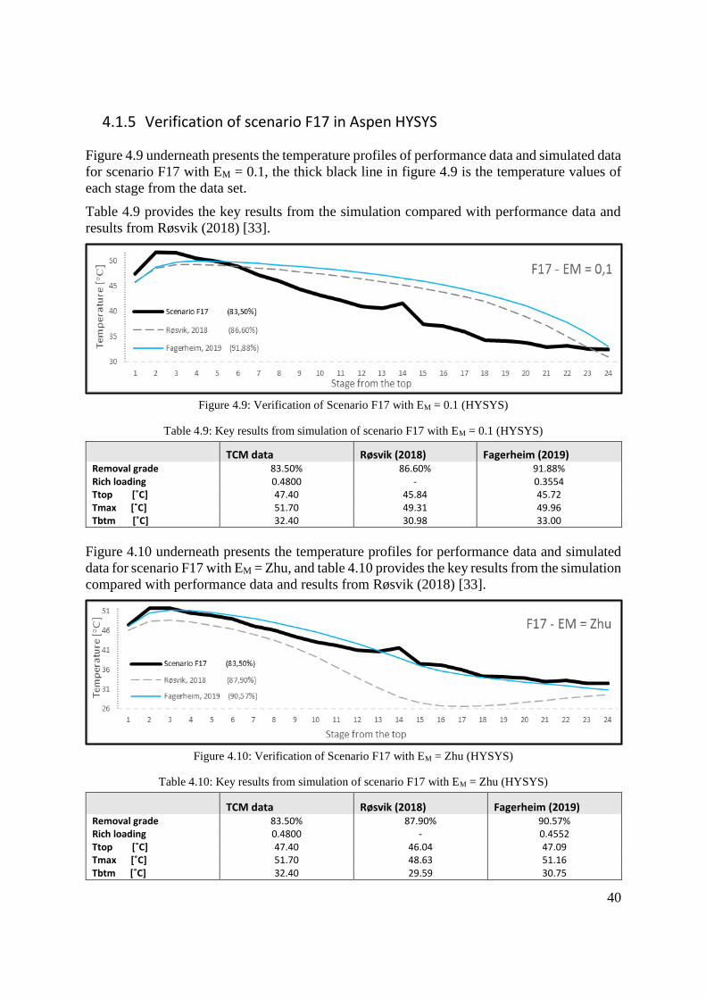
40
4.1.5 Verification of scenario F17 in Aspen HYSYS
Figure 4.9 underneath presents the temperature profiles of performance data and simulated data
for scenario F17 with EM = 0.1, the thick black line in figure 4.9 is the temperature values of
each stage from the data set.
Table 4.9 provides the key results from the simulation compared with performance data and
results from Røsvik (2018) [33].
Figure 4.9: Verification of Scenario F17 with EM = 0.1 (HYSYS)
Table 4.9: Key results from simulation of scenario F17 with EM = 0.1 (HYSYS)
TCM data Røsvik (2018) Fagerheim (2019) Removal grade 83.50% 86.60% 91.88% Rich loading 0.4800 - 0.3554 Ttop [˚C] 47.40 45.84 45.72 Tmax [˚C] 51.70 49.31 49.96 Tbtm [˚C] 32.40 30.98 33.00
Figure 4.10 underneath presents the temperature profiles for performance data and simulated
data for scenario F17 with EM = Zhu, and table 4.10 provides the key results from the simulation
compared with performance data and results from Røsvik (2018) [33].
Figure 4.10: Verification of Scenario F17 with EM = Zhu (HYSYS)
Table 4.10: Key results from simulation of scenario F17 with EM = Zhu (HYSYS)
TCM data Røsvik (2018) Fagerheim (2019) Removal grade 83.50% 87.90% 90.57% Rich loading 0.4800 - 0.4552 Ttop [˚C] 47.40 46.04 47.09 Tmax [˚C] 51.70 48.63 51.16 Tbtm [˚C] 32.40 29.59 30.75
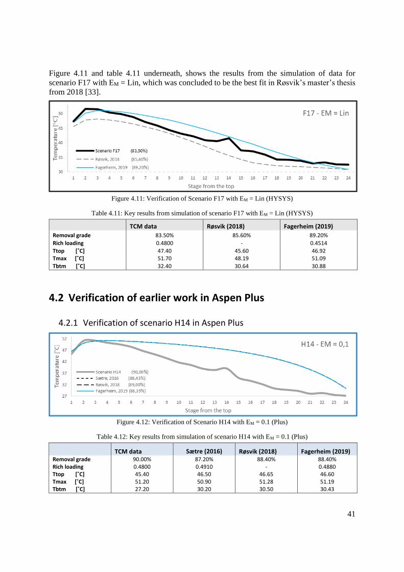
41
Figure 4.11 and table 4.11 underneath, shows the results from the simulation of data for
scenario F17 with EM = Lin, which was concluded to be the best fit in Røsvik’s master’s thesis
from 2018 [33].
Figure 4.11: Verification of Scenario F17 with EM = Lin (HYSYS)
Table 4.11: Key results from simulation of scenario F17 with EM = Lin (HYSYS)
TCM data Røsvik (2018) Fagerheim (2019)
Removal grade 83.50% 85.60% 89.20%
Rich loading 0.4800 - 0.4514
Ttop [˚C] 47.40 45.60 46.92 Tmax [˚C] 51.70 48.19 51.09
Tbtm [˚C] 32.40 30.64 30.88
4.2 Verification of earlier work in Aspen Plus
4.2.1 Verification of scenario H14 in Aspen Plus
Figure 4.12: Verification of Scenario H14 with EM = 0.1 (Plus)
Table 4.12: Key results from simulation of scenario H14 with EM = 0.1 (Plus)
TCM data Sætre (2016) Røsvik (2018) Fagerheim (2019) Removal grade 90.00% 87.20% 88.40% 88.40% Rich loading 0.4800 0.4910 - 0.4880 Ttop [˚C] 45.40 46.50 46.65 46.60 Tmax [˚C] 51.20 50.90 51.28 51.19 Tbtm [˚C] 27.20 30.20 30.50 30.43
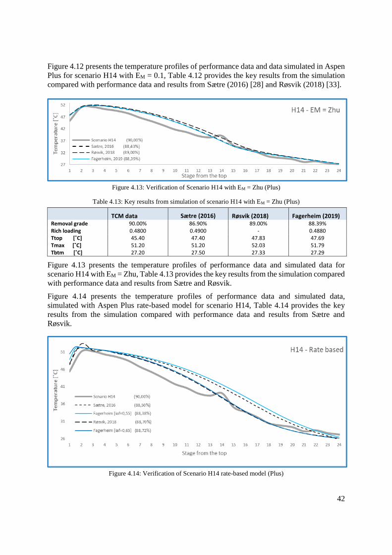
42
Figure 4.12 presents the temperature profiles of performance data and data simulated in Aspen
Plus for scenario H14 with EM = 0.1, Table 4.12 provides the key results from the simulation
compared with performance data and results from Sætre (2016) [28] and Røsvik (2018) [33].
Figure 4.13: Verification of Scenario H14 with EM = Zhu (Plus)
Table 4.13: Key results from simulation of scenario H14 with EM = Zhu (Plus)
TCM data Sætre (2016) Røsvik (2018) Fagerheim (2019) Removal grade 90.00% 86.90% 89.00% 88.39% Rich loading 0.4800 0.4900 - 0.4880 Ttop [˚C] 45.40 47.40 47.83 47.69 Tmax [˚C] 51.20 51.20 52.03 51.79 Tbtm [˚C] 27.20 27.50 27.33 27.29
Figure 4.13 presents the temperature profiles of performance data and simulated data for
scenario H14 with EM = Zhu, Table 4.13 provides the key results from the simulation compared
with performance data and results from Sætre and Røsvik.
Figure 4.14 presents the temperature profiles of performance data and simulated data,
simulated with Aspen Plus rate-based model for scenario H14, Table 4.14 provides the key
results from the simulation compared with performance data and results from Sætre and
Røsvik.
Figure 4.14: Verification of Scenario H14 rate-based model (Plus)
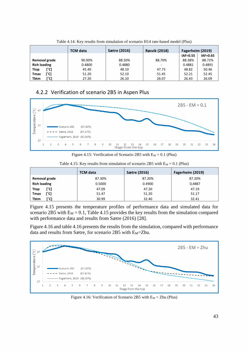
43
Table 4.14: Key results from simulation of scenario H14 rate-based model (Plus)
TCM data Sætre (2016) Røsvik (2018) Fagerheim (2019) Removal grade 90.00%
88.50% 88.70%
IAF=0.55 88.38%
IAF=0.65 88.72%
Rich loading 0.4800 0.4880 - 0.4881 0.4891 Ttop [˚C] 45.40 48.10 47.73 48.82 50.46 Tmax [˚C] 51.20 52.10 51.45 52.21 52.45 Tbtm [˚C] 27.20 26.10 26.07 26.43 26.09
4.2.2 Verification of scenario 2B5 in Aspen Plus
Figure 4.15: Verification of Scenario 2B5 with EM = 0.1 (Plus)
Table 4.15: Key results from simulation of scenario 2B5 with EM = 0.1 (Plus)
TCM data Sætre (2016) Fagerheim (2019)
Removal grade 87.30% 87.20% 87.20%
Rich loading 0.5000 0.4900 0,4887
Ttop [˚C] 47.09 47.20 47.19 Tmax [˚C] 51.47 51.20 51.17
Tbtm [˚C] 30.99 32.40 32.41
Figure 4.15 presents the temperature profiles of performance data and simulated data for
scenario 2B5 with EM = 0.1, Table 4.15 provides the key results from the simulation compared
with performance data and results from Sætre (2016) [28].
Figure 4.16 and table 4.16 presents the results from the simulation, compared with performance
data and results from Sætre, for scenario 2B5 with EM=Zhu.
Figure 4.16: Verification of Scenario 2B5 with EM = Zhu (Plus)
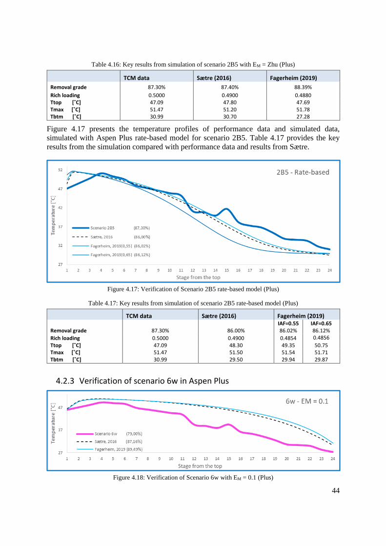
44
Table 4.16: Key results from simulation of scenario 2B5 with EM = Zhu (Plus)
TCM data Sætre (2016) Fagerheim (2019)
Removal grade 87.30% 87.40% 88.39%
Rich loading 0.5000 0.4900 0.4880 Ttop [˚C] 47.09 47.80 47.69 Tmax [˚C] 51.47 51.20 51.78 Tbtm [˚C] 30.99 30.70 27.28
Figure 4.17 presents the temperature profiles of performance data and simulated data,
simulated with Aspen Plus rate-based model for scenario 2B5. Table 4.17 provides the key
results from the simulation compared with performance data and results from Sætre.
Figure 4.17: Verification of Scenario 2B5 rate-based model (Plus)
Table 4.17: Key results from simulation of scenario 2B5 rate-based model (Plus)
TCM data Sætre (2016) Fagerheim (2019)
Removal grade 87.30% 86.00% IAF=0.55 86.02%
IAF=0.65 86.12%
Rich loading 0.5000 0.4900 0.4854 0.4856
Ttop [˚C] 47.09 48.30 49.35 50.75 Tmax [˚C] 51.47 51.50 51.54 51.71 Tbtm [˚C] 30.99 29.50 29.94 29.87
4.2.3 Verification of scenario 6w in Aspen Plus
Figure 4.18: Verification of Scenario 6w with EM = 0.1 (Plus)
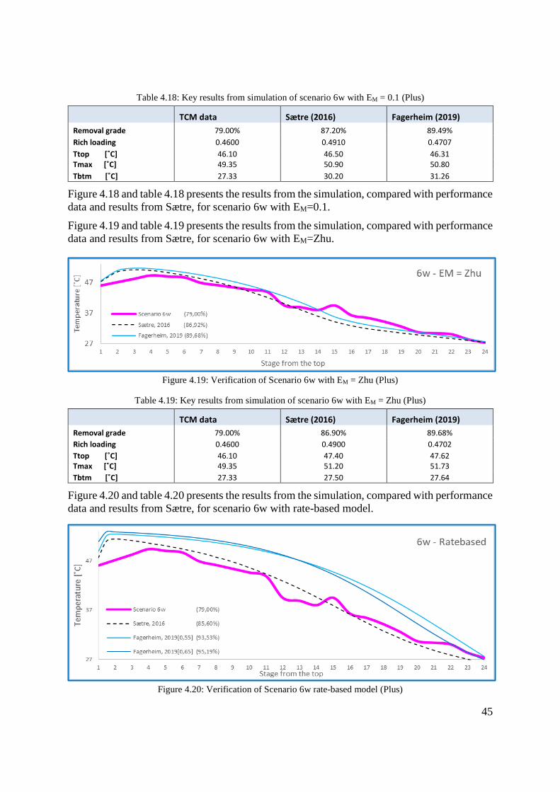
45
Table 4.18: Key results from simulation of scenario 6w with EM = 0.1 (Plus)
TCM data Sætre (2016) Fagerheim (2019)
Removal grade 79.00% 87.20% 89.49%
Rich loading 0.4600 0.4910 0.4707
Ttop [˚C] 46.10 46.50 46.31 Tmax [˚C] 49.35 50.90 50.80
Tbtm [˚C] 27.33 30.20 31.26
Figure 4.18 and table 4.18 presents the results from the simulation, compared with performance
data and results from Sætre, for scenario 6w with EM=0.1.
Figure 4.19 and table 4.19 presents the results from the simulation, compared with performance
data and results from Sætre, for scenario 6w with EM=Zhu.
Figure 4.19: Verification of Scenario 6w with EM = Zhu (Plus)
Table 4.19: Key results from simulation of scenario 6w with EM = Zhu (Plus)
TCM data Sætre (2016) Fagerheim (2019)
Removal grade 79.00% 86.90% 89.68%
Rich loading 0.4600 0.4900 0.4702
Ttop [˚C] 46.10 47.40 47.62 Tmax [˚C] 49.35 51.20 51.73
Tbtm [˚C] 27.33 27.50 27.64
Figure 4.20 and table 4.20 presents the results from the simulation, compared with performance
data and results from Sætre, for scenario 6w with rate-based model.
Figure 4.20: Verification of Scenario 6w rate-based model (Plus)
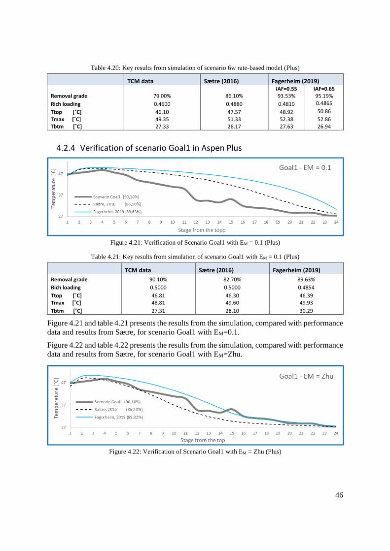
46
Table 4.20: Key results from simulation of scenario 6w rate-based model (Plus)
TCM data Sætre (2016) Fagerheim (2019)
Removal grade 79.00% 86.10% IAF=0.55 93.53%
IAF=0.65 95.19%
Rich loading 0.4600 0.4880 0.4819 0.4865
Ttop [˚C] 46.10 47.57 48.92 50.86
Tmax [˚C] 49.35 51.33 52.38 52.86 Tbtm [˚C] 27.33 26.17 27.63 26.94
4.2.4 Verification of scenario Goal1 in Aspen Plus
Figure 4.21: Verification of Scenario Goal1 with EM = 0.1 (Plus)
Table 4.21: Key results from simulation of scenario Goal1 with EM = 0.1 (Plus)
TCM data Sætre (2016) Fagerheim (2019)
Removal grade 90.10% 82.70% 89.63%
Rich loading 0.5000 0.5000 0.4854
Ttop [˚C] 46.81 46.30 46.39 Tmax [˚C] 48.81 49.60 49.93
Tbtm [˚C] 27.31 28.10 30.29
Figure 4.21 and table 4.21 presents the results from the simulation, compared with performance
data and results from Sætre, for scenario Goal1 with EM=0.1.
Figure 4.22 and table 4.22 presents the results from the simulation, compared with performance
data and results from Sætre, for scenario Goal1 with EM=Zhu.
Figure 4.22: Verification of Scenario Goal1 with EM = Zhu (Plus)
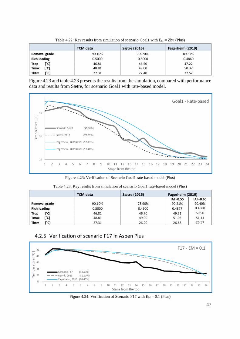
47
Table 4.22: Key results from simulation of scenario Goal1 with EM = Zhu (Plus)
TCM data Sætre (2016) Fagerheim (2019)
Removal grade 90.10% 82.70% 89.82%
Rich loading 0.5000 0.5000 0.4860
Ttop [˚C] 46.81 46.50 47.22 Tmax [˚C] 48.81 49.00 50.37
Tbtm [˚C] 27.31 27.40 27.52
Figure 4.23 and table 4.23 presents the results from the simulation, compared with performance
data and results from Sætre, for scenario Goal1 with rate-based model.
Figure 4.23: Verification of Scenario Goal1 rate-based model (Plus)
Table 4.23: Key results from simulation of scenario Goal1 rate-based model (Plus)
TCM data Sætre (2016) Fagerheim (2019)
Removal grade 90.10% 78.90% IAF=0.55 90.21%
IAF=0.65 90.40%
Rich loading 0.5000 0.4900 0.4877 0.4880
Ttop [˚C] 46.81 46.70 49.51 50.90
Tmax [˚C] 48.81 49.00 51.05 51.11
Tbtm [˚C] 27.31 26.20 26.68 26.57
4.2.5 Verification of scenario F17 in Aspen Plus
Figure 4.24: Verification of Scenario F17 with EM = 0.1 (Plus)
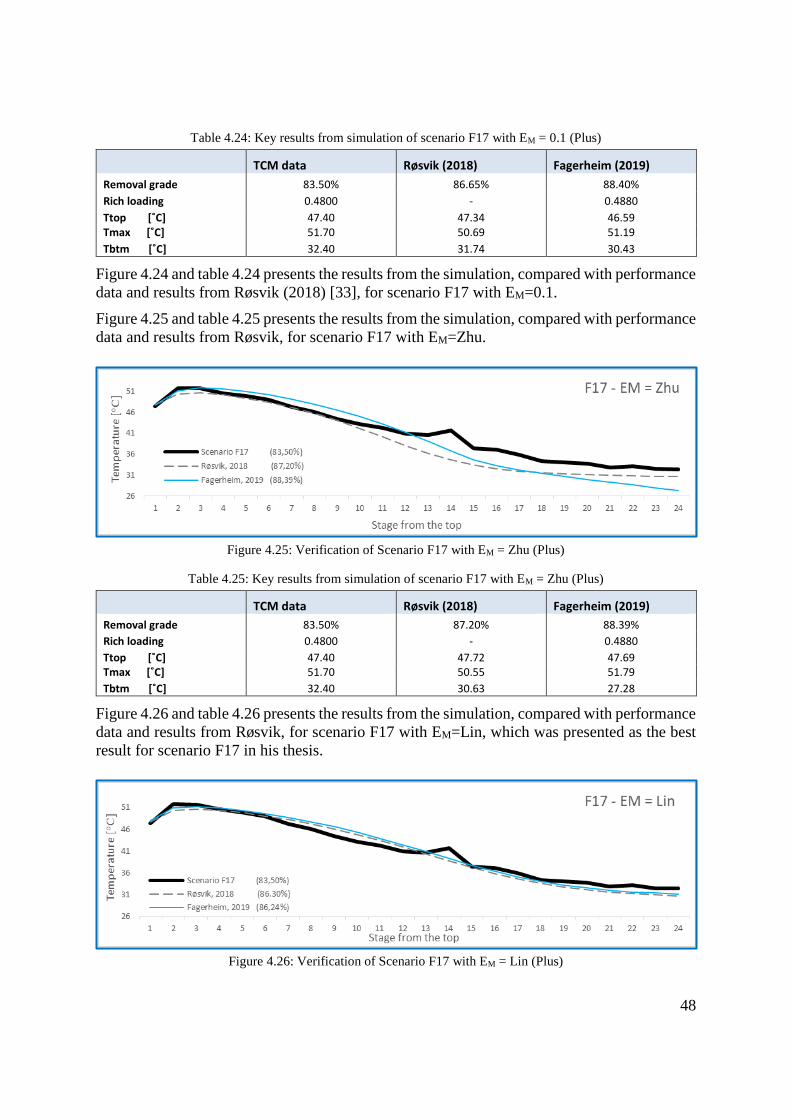
48
Table 4.24: Key results from simulation of scenario F17 with EM = 0.1 (Plus)
TCM data Røsvik (2018) Fagerheim (2019)
Removal grade 83.50% 86.65% 88.40%
Rich loading 0.4800 - 0.4880
Ttop [˚C] 47.40 47.34 46.59 Tmax [˚C] 51.70 50.69 51.19
Tbtm [˚C] 32.40 31.74 30.43
Figure 4.24 and table 4.24 presents the results from the simulation, compared with performance
data and results from Røsvik (2018) [33], for scenario F17 with EM=0.1.
Figure 4.25 and table 4.25 presents the results from the simulation, compared with performance
data and results from Røsvik, for scenario F17 with EM=Zhu.
Figure 4.25: Verification of Scenario F17 with EM = Zhu (Plus)
Table 4.25: Key results from simulation of scenario F17 with EM = Zhu (Plus)
TCM data Røsvik (2018) Fagerheim (2019)
Removal grade 83.50% 87.20% 88.39%
Rich loading 0.4800 - 0.4880
Ttop [˚C] 47.40 47.72 47.69 Tmax [˚C] 51.70 50.55 51.79
Tbtm [˚C] 32.40 30.63 27.28
Figure 4.26 and table 4.26 presents the results from the simulation, compared with performance
data and results from Røsvik, for scenario F17 with EM=Lin, which was presented as the best
result for scenario F17 in his thesis.
Figure 4.26: Verification of Scenario F17 with EM = Lin (Plus)
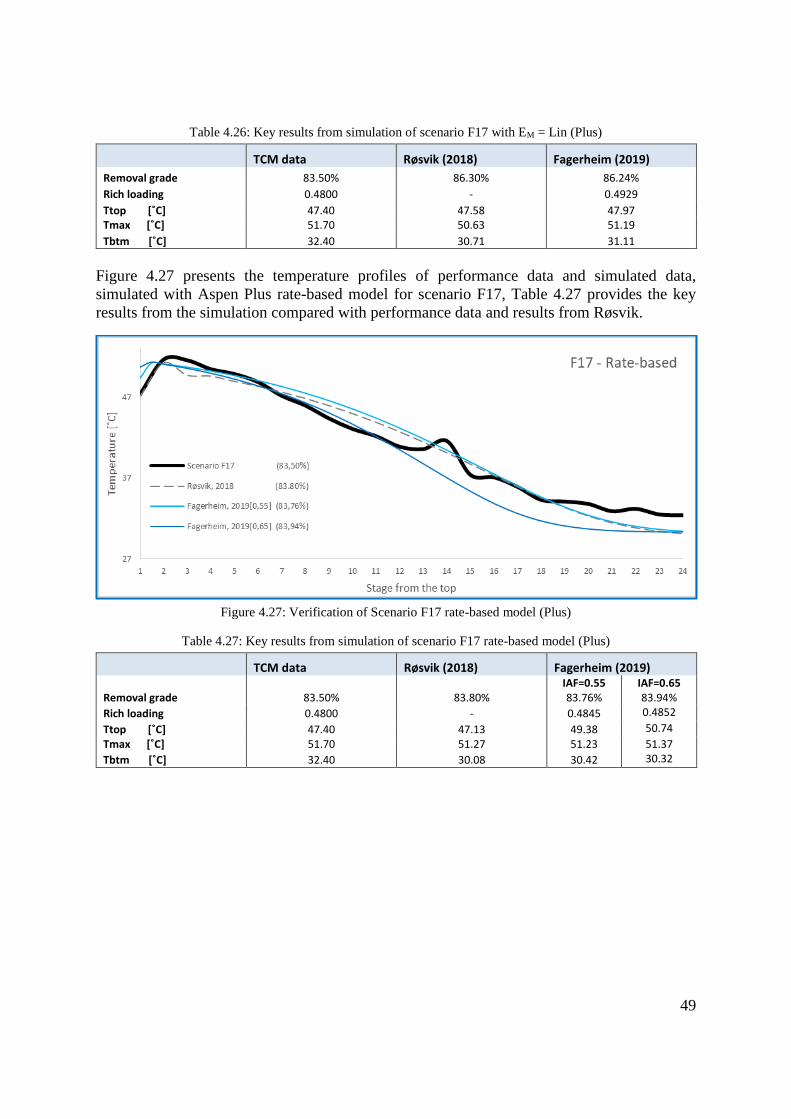
49
Table 4.26: Key results from simulation of scenario F17 with EM = Lin (Plus)
TCM data Røsvik (2018) Fagerheim (2019)
Removal grade 83.50% 86.30% 86.24%
Rich loading 0.4800 - 0.4929
Ttop [˚C] 47.40 47.58 47.97 Tmax [˚C] 51.70 50.63 51.19
Tbtm [˚C] 32.40 30.71 31.11
Figure 4.27 presents the temperature profiles of performance data and simulated data,
simulated with Aspen Plus rate-based model for scenario F17, Table 4.27 provides the key
results from the simulation compared with performance data and results from Røsvik.
Figure 4.27: Verification of Scenario F17 rate-based model (Plus)
Table 4.27: Key results from simulation of scenario F17 rate-based model (Plus)
TCM data Røsvik (2018) Fagerheim (2019)
Removal grade 83.50% 83.80% IAF=0.55 83.76%
IAF=0.65 83.94%
Rich loading 0.4800 - 0.4845 0.4852
Ttop [˚C] 47.40 47.13 49.38 50.74
Tmax [˚C] 51.70 51.27 51.23 51.37
Tbtm [˚C] 32.40 30.08 30.42 30.32
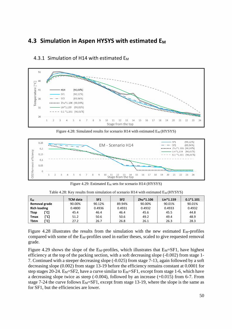
50
4.3 Simulation in Aspen HYSYS with estimated EM
4.3.1 Simulation of H14 with estimated EM
Figure 4.28: Simulated results for scenario H14 with estimated EM (HYSYS)
Figure 4.29: Estimated EM sets for scenario H14 (HYSYS)
Table 4.28: Key results from simulation of scenario H14 with estimated EM (HYSYS)
EM TCM data SF1 SF2 Zhu*1.106 Lin*1.159 0.1*1.101 Removal grade 90.00% 90.12% 89.94% 90.00% 90.01% 90.01% Rich loading 0.4800 0.4936 0.4931 0.4932 0.4933 0.4932 Ttop [˚C] 45.4 46.4 46.4 45.6 45.5 44.8 Tmax [˚C] 51.2 50.6 50.6 49.2 49.4 48.9 Tbtm [˚C] 27.2 26.7 26.8 26.1 26.3 28.3
Figure 4.28 illustrates the results from the simulation with the new estimated EM-profiles
compared with some of the EM-profiles used in earlier theses, scaled to give requested removal
grade.
Figure 4.29 shows the slope of the EM-profiles, which illustrates that EM=SF1, have highest
efficiency at the top of the packing section, with a soft decreasing slope (-0.002) from stage 1-
7. Continued with a steeper decreasing slope (-0.025) from stage 7-13, again followed by a soft
decreasing slope (0.002) from stage 13-19 before the efficiency remains constant at 0.0001 for
step stages 20-24. EM=SF2, have a curve similar to EM=SF1, except from stage 1-6, which have
a decreasing slope twice as steep (-0.004), followed by an increase (+0.015) from 6-7. From
stage 7-24 the curve follows EM=SF1, except from stage 13-19, where the slope is the same as
for SF1, but the efficiencies are lower.
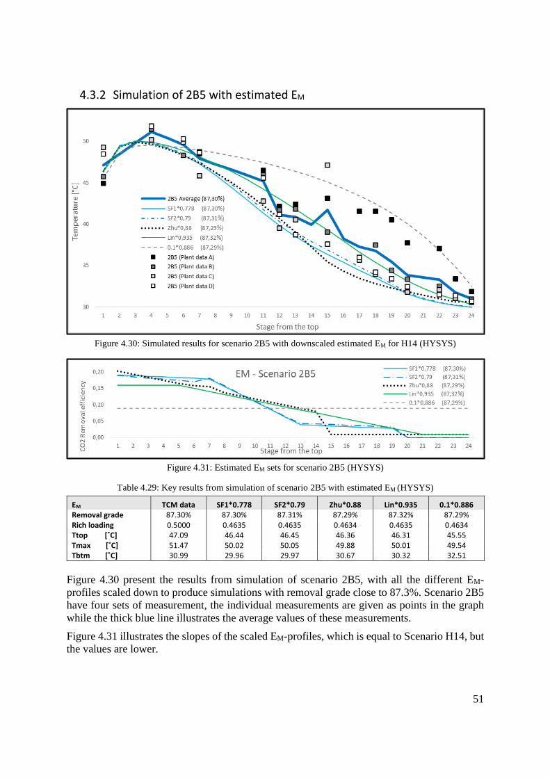
51
4.3.2 Simulation of 2B5 with estimated EM
Figure 4.30: Simulated results for scenario 2B5 with downscaled estimated EM for H14 (HYSYS)
Figure 4.31: Estimated EM sets for scenario 2B5 (HYSYS)
Table 4.29: Key results from simulation of scenario 2B5 with estimated EM (HYSYS)
EM TCM data SF1*0.778 SF2*0.79 Zhu*0.88 Lin*0.935 0.1*0.886 Removal grade 87.30% 87.30% 87.31% 87.29% 87.32% 87.29% Rich loading 0.5000 0.4635 0.4635 0.4634 0.4635 0.4634 Ttop [˚C] 47.09 46.44 46.45 46.36 46.31 45.55 Tmax [˚C] 51.47 50.02 50.05 49.88 50.01 49.54 Tbtm [˚C] 30.99 29.96 29.97 30.67 30.32 32.51
Figure 4.30 present the results from simulation of scenario 2B5, with all the different EM-
profiles scaled down to produce simulations with removal grade close to 87.3%. Scenario 2B5
have four sets of measurement, the individual measurements are given as points in the graph
while the thick blue line illustrates the average values of these measurements.
Figure 4.31 illustrates the slopes of the scaled EM-profiles, which is equal to Scenario H14, but
the values are lower.
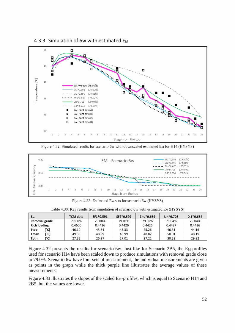
52
4.3.3 Simulation of 6w with estimated EM
Figure 4.32: Simulated results for scenario 6w with downscaled estimated EM for H14 (HYSYS)
Figure 4.33: Estimated EM sets for scenario 6w (HYSYS)
Table 4.30: Key results from simulation of scenario 6w with estimated EM (HYSYS)
EM TCM data SF1*0.591 SF2*0.599 Zhu*0.669 Lin*0.708 0.1*0.664 Removal grade 79.00% 79.00% 79.01% 79.02% 79.04% 79.04% Rich loading 0.4600 0.4426 0.4426 0.4426 0.4427 0.4426 Ttop [˚C] 46.10 45.34 45.33 45.26 46.31 44.16 Tmax [˚C] 49.35 48.99 48.99 48.82 50.01 48.19 Tbtm [˚C] 27.33 26.97 27.01 27.21 30.32 29.92
Figure 4.32 presents the results for scenario 6w. Just like for Scenario 2B5, the EM-profiles
used for scenario H14 have been scaled down to produce simulations with removal grade close
to 79.0%. Scenario 6w have four sets of measurement, the individual measurements are given
as points in the graph while the thick purple line illustrates the average values of these
measurements.
Figure 4.33 illustrates the slopes of the scaled EM-profiles, which is equal to Scenario H14 and
2B5, but the values are lower.
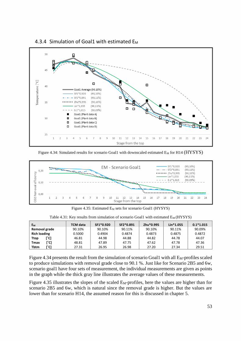
53
4.3.4 Simulation of Goal1 with estimated EM
Figure 4.34: Simulated results for scenario Goal1 with downscaled estimated EM for H14 (HYSYS)
Figure 4.35: Estimated EM sets for scenario Goal1 (HYSYS)
Table 4.31: Key results from simulation of scenario Goal1 with estimated EM (HYSYS)
EM TCM data SF1*0.920 SF2*0.891 Zhu*0.995 Lin*1.055 0.1*1.015 Removal grade 90.10% 90.10% 90.11% 90.10% 90.11% 90.09% Rich loading 0.5000 0.4904 0.4874 0.4873 0.4875 0.4872 Ttop [˚C] 46.81 44.98 44.88 44.82 44.78 44.07 Tmax [˚C] 48.81 47.89 47.75 47.62 47.78 47.36 Tbtm [˚C] 27.31 26.95 26.98 27.20 27.34 29.51
Figure 4.34 presents the result from the simulation of scenario Goal1 with all EM-profiles scaled
to produce simulations with removal grade close to 90.1 %. Just like for Scenario 2B5 and 6w,
scenario goal1 have four sets of measurement, the individual measurements are given as points
in the graph while the thick gray line illustrates the average values of these measurements.
Figure 4.35 illustrates the slopes of the scaled EM-profiles, here the values are higher than for
scenario 2B5 and 6w, which is natural since the removal grade is higher. But the values are
lower than for scenario H14, the assumed reason for this is discussed in chapter 5.
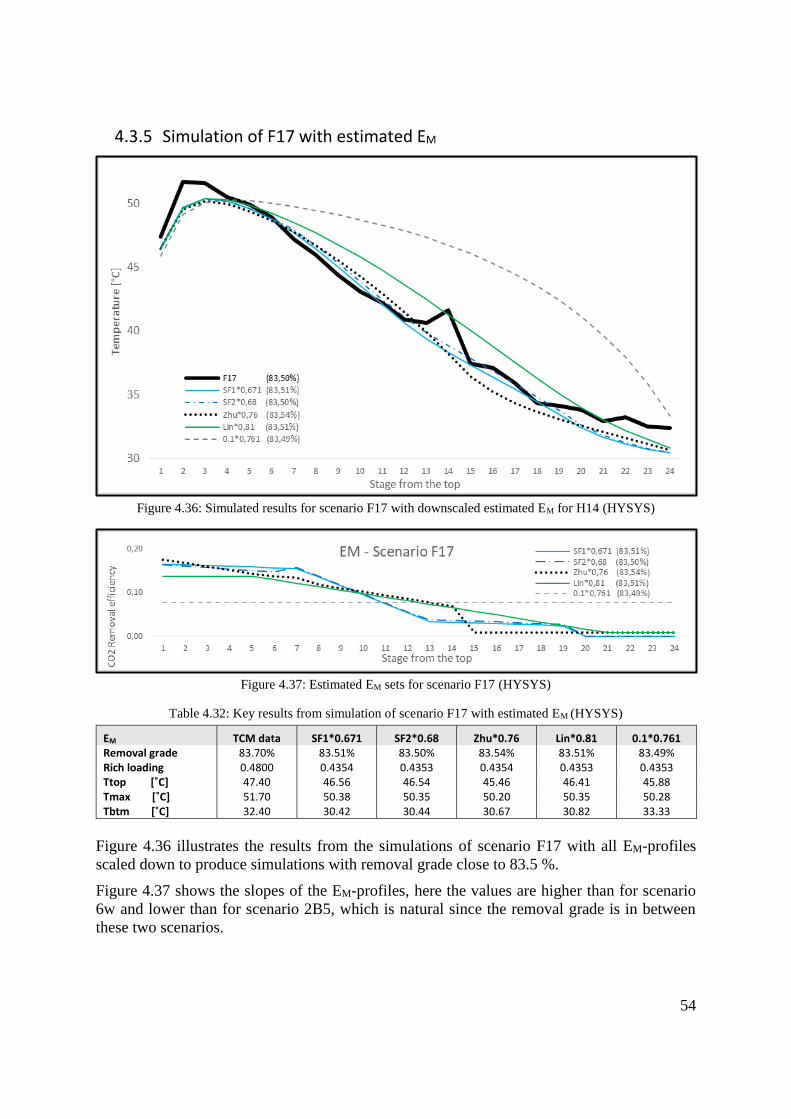
54
4.3.5 Simulation of F17 with estimated EM
Figure 4.36: Simulated results for scenario F17 with downscaled estimated EM for H14 (HYSYS)
Figure 4.37: Estimated EM sets for scenario F17 (HYSYS)
Table 4.32: Key results from simulation of scenario F17 with estimated EM (HYSYS)
EM TCM data SF1*0.671 SF2*0.68 Zhu*0.76 Lin*0.81 0.1*0.761 Removal grade 83.70% 83.51% 83.50% 83.54% 83.51% 83.49% Rich loading 0.4800 0.4354 0.4353 0.4354 0.4353 0.4353 Ttop [˚C] 47.40 46.56 46.54 45.46 46.41 45.88 Tmax [˚C] 51.70 50.38 50.35 50.20 50.35 50.28 Tbtm [˚C] 32.40 30.42 30.44 30.67 30.82 33.33
Figure 4.36 illustrates the results from the simulations of scenario F17 with all EM-profiles
scaled down to produce simulations with removal grade close to 83.5 %.
Figure 4.37 shows the slopes of the EM-profiles, here the values are higher than for scenario
6w and lower than for scenario 2B5, which is natural since the removal grade is in between
these two scenarios.
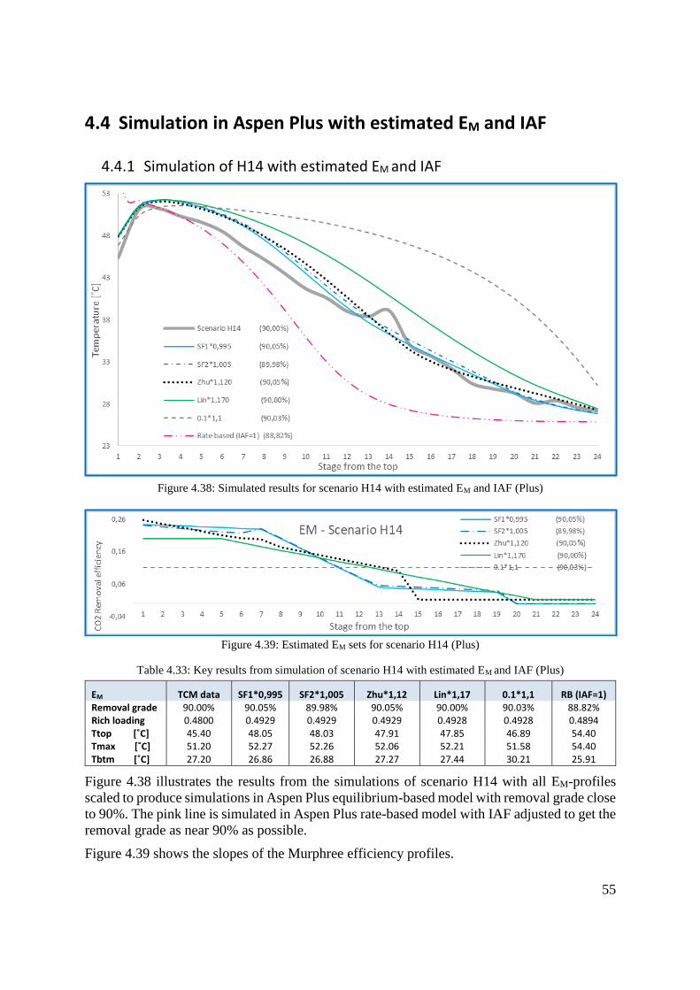
55
4.4 Simulation in Aspen Plus with estimated EM and IAF
4.4.1 Simulation of H14 with estimated EM and IAF
Figure 4.38: Simulated results for scenario H14 with estimated EM and IAF (Plus)
Figure 4.39: Estimated EM sets for scenario H14 (Plus)
Table 4.33: Key results from simulation of scenario H14 with estimated EM and IAF (Plus)
EM TCM data SF1*0,995 SF2*1,005 Zhu*1,12 Lin*1,17 0.1*1,1 RB (IAF=1) Removal grade 90.00% 90.05% 89.98% 90.05% 90.00% 90.03% 88.82% Rich loading 0.4800 0.4929 0.4929 0.4929 0.4928 0.4928 0.4894 Ttop [˚C] 45.40 48.05 48.03 47.91 47.85 46.89 54.40 Tmax [˚C] 51.20 52.27 52.26 52.06 52.21 51.58 54.40 Tbtm [˚C] 27.20 26.86 26.88 27.27 27.44 30.21 25.91
Figure 4.38 illustrates the results from the simulations of scenario H14 with all EM-profiles
scaled to produce simulations in Aspen Plus equilibrium-based model with removal grade close
to 90%. The pink line is simulated in Aspen Plus rate-based model with IAF adjusted to get the
removal grade as near 90% as possible.
Figure 4.39 shows the slopes of the Murphree efficiency profiles.
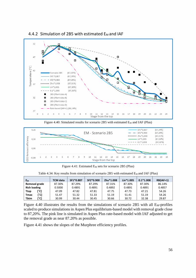
56
4.4.2 Simulation of 2B5 with estimated EM and IAF
Figure 4.40: Simulated results for scenario 2B5 with estimated EM and IAF (Plus)
Figure 4.41: Estimated EM sets for scenario 2B5 (Plus)
Table 4.34: Key results from simulation of scenario 2B5 with estimated EM and IAF (Plus)
EM TCM data SF1*0.887 SF2*0.900 Zhu*1.008 Lin*1.005 0.1*1.008 RB(IAF=1) Removal grade 87.30% 87.29% 87.29% 87.31% 87.30% 87.30% 86.14% Rich loading 0.5000 0.4891 0.4891 0.4892 0.4891 0.4891 0.4857 Ttop [˚C] 47.09 47.82 47.81 47.75 47.73 47.21 54.26 Tmax [˚C] 51.47 51.32 51.33 51.19 51.41 51.19 54.26 Tbtm [˚C] 30.99 30.44 30.45 30.66 30.72 32.38 29.87
Figure 4.40 illustrates the results from the simulations of scenario 2B5 with all EM-profiles
scaled to produce simulations in Aspen Plus equilibrium-based model with removal grade close
to 87,20%. The pink line is simulated in Aspen Plus rate-based model with IAF adjusted to get
the removal grade as near 87.20% as possible.
Figure 4.41 shows the slopes of the Murphree efficiency profiles.
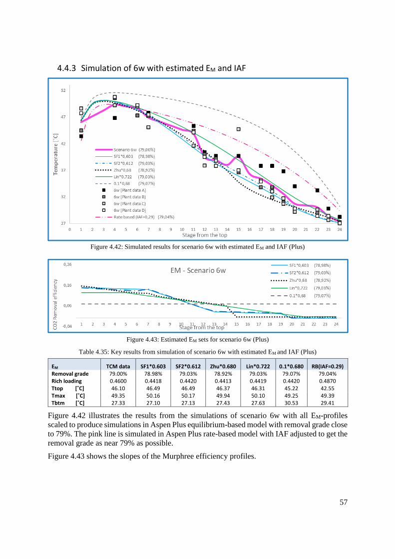
57
4.4.3 Simulation of 6w with estimated EM and IAF
Figure 4.42: Simulated results for scenario 6w with estimated EM and IAF (Plus)
Figure 4.43: Estimated EM sets for scenario 6w (Plus)
Table 4.35: Key results from simulation of scenario 6w with estimated EM and IAF (Plus)
EM TCM data SF1*0.603 SF2*0.612 Zhu*0.680 Lin*0.722 0.1*0.680 RB(IAF=0.29) Removal grade 79.00% 78.98% 79.03% 78.92% 79.03% 79.07% 79.04% Rich loading 0.4600 0.4418 0.4420 0.4413 0.4419 0.4420 0.4870 Ttop [˚C] 46.10 46.49 46.49 46.37 46.31 45.22 42.55 Tmax [˚C] 49.35 50.16 50.17 49.94 50.10 49.25 49.39 Tbtm [˚C] 27.33 27.10 27.13 27.43 27.63 30.53 29.41
Figure 4.42 illustrates the results from the simulations of scenario 6w with all EM-profiles
scaled to produce simulations in Aspen Plus equilibrium-based model with removal grade close
to 79%. The pink line is simulated in Aspen Plus rate-based model with IAF adjusted to get the
removal grade as near 79% as possible.
Figure 4.43 shows the slopes of the Murphree efficiency profiles.
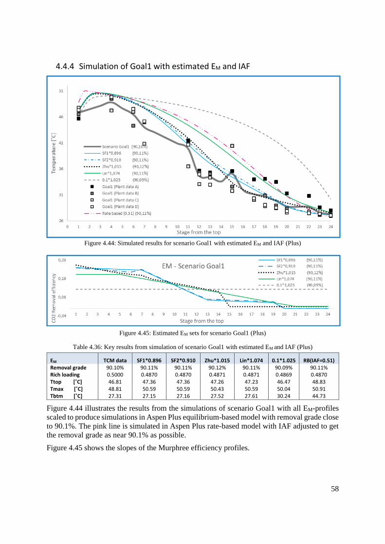
58
4.4.4 Simulation of Goal1 with estimated EM and IAF
Figure 4.44: Simulated results for scenario Goal1 with estimated EM and IAF (Plus)
Figure 4.45: Estimated EM sets for scenario Goal1 (Plus)
Table 4.36: Key results from simulation of scenario Goal1 with estimated EM and IAF (Plus)
EM TCM data SF1*0.896 SF2*0.910 Zhu*1.015 Lin*1.074 0.1*1.025 RB(IAF=0.51) Removal grade 90.10% 90.11% 90.11% 90.12% 90.11% 90.09% 90.11% Rich loading 0.5000 0.4870 0.4870 0.4871 0.4871 0.4869 0.4870 Ttop [˚C] 46.81 47.36 47.36 47.26 47.23 46.47 48.83 Tmax [˚C] 48.81 50.59 50.59 50.43 50.59 50.04 50.91 Tbtm [˚C] 27.31 27.15 27.16 27.52 27.61 30.24 44.73
Figure 4.44 illustrates the results from the simulations of scenario Goal1 with all EM-profiles
scaled to produce simulations in Aspen Plus equilibrium-based model with removal grade close
to 90.1%. The pink line is simulated in Aspen Plus rate-based model with IAF adjusted to get
the removal grade as near 90.1% as possible.
Figure 4.45 shows the slopes of the Murphree efficiency profiles.
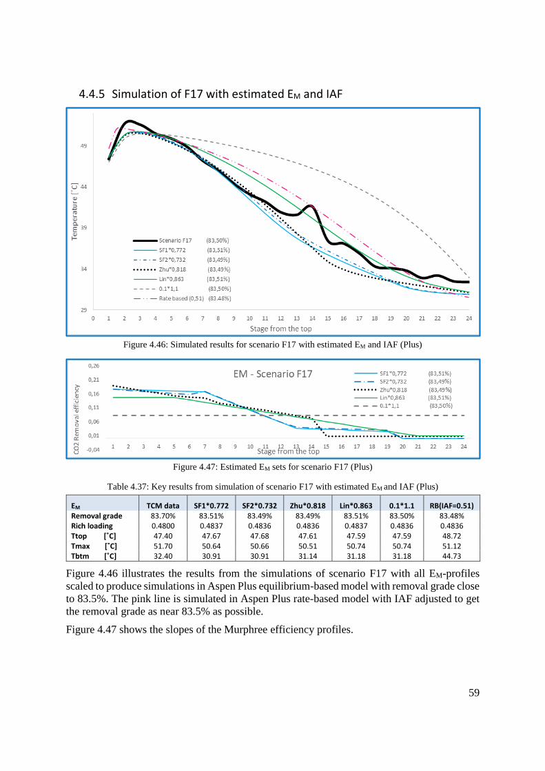
59
4.4.5 Simulation of F17 with estimated EM and IAF
Figure 4.46: Simulated results for scenario F17 with estimated EM and IAF (Plus)
Figure 4.47: Estimated EM sets for scenario F17 (Plus)
Table 4.37: Key results from simulation of scenario F17 with estimated EM and IAF (Plus)
EM TCM data SF1*0.772 SF2*0.732 Zhu*0.818 Lin*0.863 0.1*1.1 RB(IAF=0.51) Removal grade 83.70% 83.51% 83.49% 83.49% 83.51% 83.50% 83.48% Rich loading 0.4800 0.4837 0.4836 0.4836 0.4837 0.4836 0.4836 Ttop [˚C] 47.40 47.67 47.68 47.61 47.59 47.59 48.72 Tmax [˚C] 51.70 50.64 50.66 50.51 50.74 50.74 51.12 Tbtm [˚C] 32.40 30.91 30.91 31.14 31.18 31.18 44.73
Figure 4.46 illustrates the results from the simulations of scenario F17 with all EM-profiles
scaled to produce simulations in Aspen Plus equilibrium-based model with removal grade close
to 83.5%. The pink line is simulated in Aspen Plus rate-based model with IAF adjusted to get
the removal grade as near 83.5% as possible.
Figure 4.47 shows the slopes of the Murphree efficiency profiles.
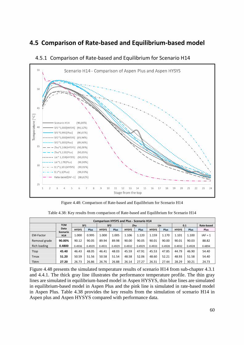
60
4.5 Comparison of Rate-based and Equilibrium-based model
4.5.1 Comparison of Rate-based and Equilibrium for Scenario H14
Figure 4.48: Comparison of Rate-based and Equilibrium for Scenario H14
Table 4.38: Key results from comparison of Rate-based and Equilibrium for Scenario H14
Comparison HYSYS and Plus - Scenario H14
TCM Data
Scenario H14
SF1 SF2 Zhu Lin 0.1 Rate-based
HYSYS Plus HYSYS Plus HYSYS Plus HYSYS Plus HYSYS Plus Plus
EM-Factor 1.000 0.995 1.000 1.005 1.106 1.120 1.159 1.170 1.101 1.100 IAF = 1
Removal grade 90.00% 90.12 90.05 89.94 89.98 90.00 90.05 90.01 90.00 90.01 90.03 88.82
Rich loading 0.4800 0.4936 0.4929 0.4931 0.4929 0.4932 0.4929 0.4933 0.4928 0.4932 0.4928 0.4894
Ttop 45.40 46.43 48.05 46.41 48.03 45.59 47.91 45.53 47.85 44.79 46.90 54.40
Tmax 51.20 50.59 51.56 50.58 51.54 48.58 52.06 48.60 52.21 48.93 51.58 54.40
Tbtm 27.20 26.73 26.86 26.76 26.88 26.14 27.27 26.31 27.44 28.29 30.21 24.73
Figure 4.48 presents the simulated temperature results of scenario H14 from sub-chapter 4.3.1
and 4.4.1. The thick gray line illustrates the performance temperature profile. The thin gray
lines are simulated in equilibrium-based model in Aspen HYSYS, thin blue lines are simulated
in equilibrium-based model in Aspen Plus and the pink line is simulated in rate-based model
in Aspen Plus. Table 4.38 provides the key results from the simulation of scenario H14 in
Aspen plus and Aspen HYSYS compared with performance data.
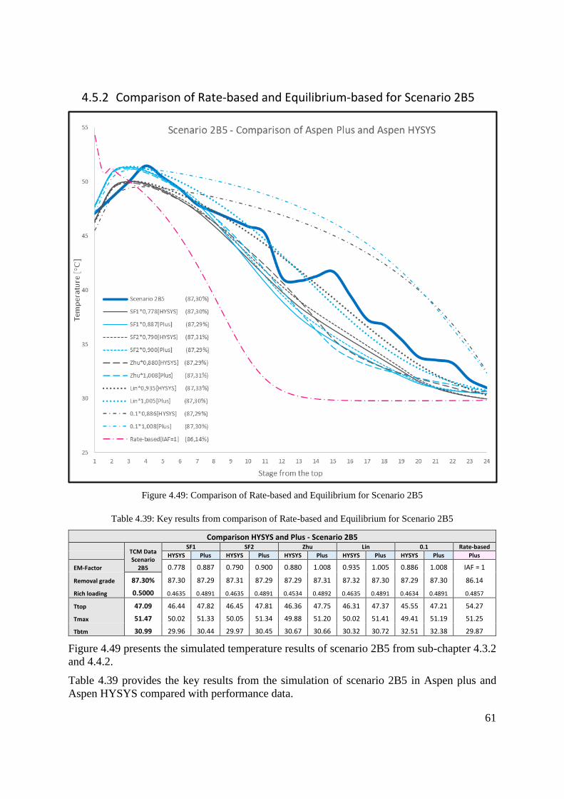
61
4.5.2 Comparison of Rate-based and Equilibrium-based for Scenario 2B5
Figure 4.49: Comparison of Rate-based and Equilibrium for Scenario 2B5
Table 4.39: Key results from comparison of Rate-based and Equilibrium for Scenario 2B5
Comparison HYSYS and Plus - Scenario 2B5
TCM Data Scenario
2B5
SF1 SF2 Zhu Lin 0.1 Rate-based
HYSYS Plus HYSYS Plus HYSYS Plus HYSYS Plus HYSYS Plus Plus
EM-Factor 0.778 0.887 0.790 0.900 0.880 1.008 0.935 1.005 0.886 1.008 IAF = 1
Removal grade 87.30% 87.30 87.29 87.31 87.29 87.29 87.31 87.32 87.30 87.29 87.30 86.14
Rich loading 0.5000 0.4635 0.4891 0.4635 0.4891 0.4534 0.4892 0.4635 0.4891 0.4634 0.4891 0.4857
Ttop 47.09 46.44 47.82 46.45 47.81 46.36 47.75 46.31 47.37 45.55 47.21 54.27
Tmax 51.47 50.02 51.33 50.05 51.34 49.88 51.20 50.02 51.41 49.41 51.19 51.25
Tbtm 30.99 29.96 30.44 29.97 30.45 30.67 30.66 30.32 30.72 32.51 32.38 29.87
Figure 4.49 presents the simulated temperature results of scenario 2B5 from sub-chapter 4.3.2
and 4.4.2.
Table 4.39 provides the key results from the simulation of scenario 2B5 in Aspen plus and
Aspen HYSYS compared with performance data.
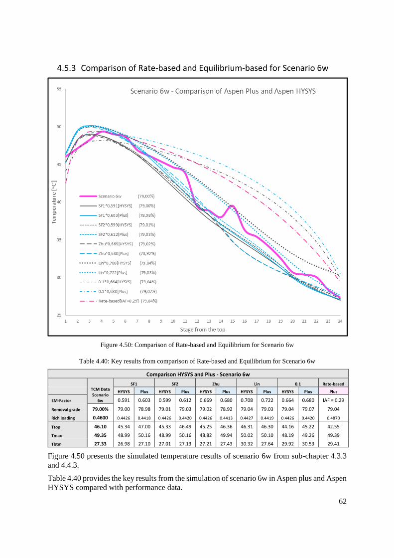
62
4.5.3 Comparison of Rate-based and Equilibrium-based for Scenario 6w
Figure 4.50: Comparison of Rate-based and Equilibrium for Scenario 6w
Table 4.40: Key results from comparison of Rate-based and Equilibrium for Scenario 6w
Comparison HYSYS and Plus - Scenario 6w
TCM Data Scenario
6w
SF1 SF2 Zhu Lin 0.1 Rate-based
HYSYS Plus HYSYS Plus HYSYS Plus HYSYS Plus HYSYS Plus Plus
EM-Factor 0.591 0.603 0.599 0.612 0.669 0.680 0.708 0.722 0.664 0.680 IAF = 0.29
Removal grade 79.00% 79.00 78.98 79.01 79.03 79.02 78.92 79.04 79.03 79.04 79.07 79.04
Rich loading 0.4600 0.4426 0.4418 0.4426 0.4420 0.4426 0.4413 0.4427 0.4419 0.4426 0.4420 0.4870
Ttop 46.10 45.34 47.00 45.33 46.49 45.25 46.36 46.31 46.30 44.16 45.22 42.55
Tmax 49.35 48.99 50.16 48.99 50.16 48.82 49.94 50.02 50.10 48.19 49.26 49.39
Tbtm 27.33 26.98 27.10 27.01 27.13 27.21 27.43 30.32 27.64 29.92 30.53 29.41
Figure 4.50 presents the simulated temperature results of scenario 6w from sub-chapter 4.3.3
and 4.4.3.
Table 4.40 provides the key results from the simulation of scenario 6w in Aspen plus and Aspen
HYSYS compared with performance data.
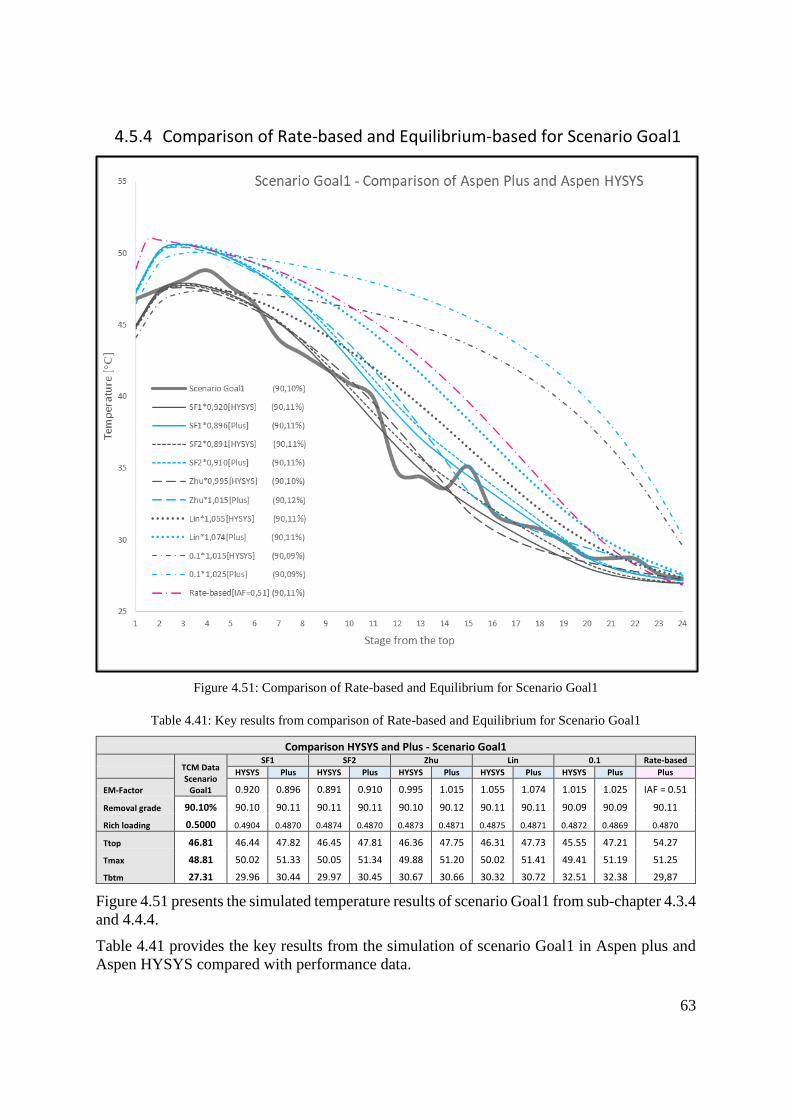
63
4.5.4 Comparison of Rate-based and Equilibrium-based for Scenario Goal1
Figure 4.51: Comparison of Rate-based and Equilibrium for Scenario Goal1
Table 4.41: Key results from comparison of Rate-based and Equilibrium for Scenario Goal1
Comparison HYSYS and Plus - Scenario Goal1
TCM Data Scenario
Goal1
SF1 SF2 Zhu Lin 0.1 Rate-based
HYSYS Plus HYSYS Plus HYSYS Plus HYSYS Plus HYSYS Plus Plus
EM-Factor 0.920 0.896 0.891 0.910 0.995 1.015 1.055 1.074 1.015 1.025 IAF = 0.51
Removal grade 90.10% 90.10 90.11 90.11 90.11 90.10 90.12 90.11 90.11 90.09 90.09 90.11
Rich loading 0.5000 0.4904 0.4870 0.4874 0.4870 0.4873 0.4871 0.4875 0.4871 0.4872 0.4869 0.4870
Ttop 46.81 46.44 47.82 46.45 47.81 46.36 47.75 46.31 47.73 45.55 47.21 54.27
Tmax 48.81 50.02 51.33 50.05 51.34 49.88 51.20 50.02 51.41 49.41 51.19 51.25
Tbtm 27.31 29.96 30.44 29.97 30.45 30.67 30.66 30.32 30.72 32.51 32.38 29,87
Figure 4.51 presents the simulated temperature results of scenario Goal1 from sub-chapter 4.3.4
and 4.4.4.
Table 4.41 provides the key results from the simulation of scenario Goal1 in Aspen plus and
Aspen HYSYS compared with performance data.
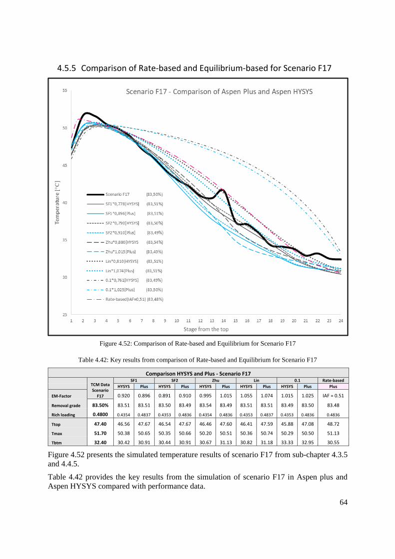
64
4.5.5 Comparison of Rate-based and Equilibrium-based for Scenario F17
Figure 4.52: Comparison of Rate-based and Equilibrium for Scenario F17
Table 4.42: Key results from comparison of Rate-based and Equilibrium for Scenario F17
Comparison HYSYS and Plus - Scenario F17
TCM Data Scenario
F17
SF1 SF2 Zhu Lin 0.1 Rate-based
HYSYS Plus HYSYS Plus HYSYS Plus HYSYS Plus HYSYS Plus Plus
EM-Factor 0.920 0.896 0.891 0.910 0.995 1.015 1.055 1.074 1.015 1.025 IAF = 0.51
Removal grade 83.50% 83.51 83.51 83.50 83.49 83.54 83.49 83.51 83.51 83.49 83.50 83.48
Rich loading 0.4800 0.4354 0.4837 0.4353 0.4836 0.4354 0.4836 0.4353 0.4837 0.4353 0.4836 0.4836
Ttop 47.40 46.56 47.67 46.54 47.67 46.46 47.60 46.41 47.59 45.88 47.08 48.72
Tmax 51.70 50.38 50.65 50.35 50.66 50.20 50.51 50.36 50.74 50.29 50.50 51.13
Tbtm 32.40 30.42 30.91 30.44 30.91 30.67 31.13 30.82 31.18 33.33 32.95 30.55
Figure 4.52 presents the simulated temperature results of scenario F17 from sub-chapter 4.3.5
and 4.4.5.
Table 4.42 provides the key results from the simulation of scenario F17 in Aspen plus and
Aspen HYSYS compared with performance data.
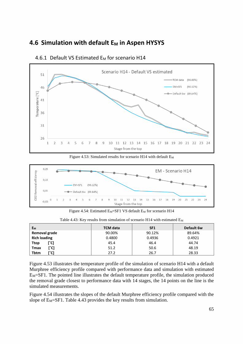
65
4.6 Simulation with default EM in Aspen HYSYS
4.6.1 Default VS Estimated EM for scenario H14
Figure 4.53: Simulated results for scenario H14 with default EM
Figure 4.54: Estimated EM=SF1 VS default EM for scenario H14
Table 4.43: Key results from simulation of scenario H14 with estimated EM
EM TCM data SF1 Default 6w Removal grade 90.00% 90.12% 89.64% Rich loading 0.4800 0.4936 0.4921 Ttop [˚C] 45.4 46.4 44.74 Tmax [˚C] 51.2 50.6 48.19 Tbtm [˚C] 27.2 26.7 28.33
Figure 4.53 illustrates the temperature profile of the simulation of scenario H14 with a default
Murphree efficiency profile compared with performance data and simulation with estimated
EM=SF1. The pointed line illustrates the default temperature profile, the simulation produced
the removal grade closest to performance data with 14 stages, the 14 points on the line is the
simulated measurements.
Figure 4.54 illustrates the slopes of the default Murphree efficiency profile compared with the
slope of EM=SF1. Table 4.43 provides the key results from simulation.
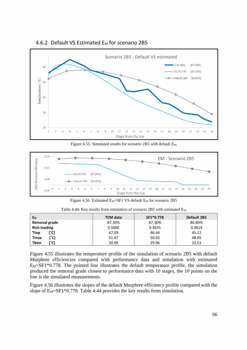
66
4.6.2 Default VS Estimated EM for scenario 2B5
Figure 4.55: Simulated results for scenario 2B5 with default EM
Figure 4.56: Estimated EM=SF1 VS default EM for scenario 2B5
Table 4.44: Key results from simulation of scenario 2B5 with estimated EM
EM TCM data SF1*0.778 Default 2B5 Removal grade 87.30% 87.30% 86.80% Rich loading 0.5000 0.4635 0.4619 Ttop [˚C] 47.09 46.44 45.12 Tmax [˚C] 51.47 50.02 48.05 Tbtm [˚C] 30.99 29.96 33.53
Figure 4.55 illustrates the temperature profile of the simulation of scenario 2B5 with default
Murphree efficiencies compared with performance data and simulation with estimated
EM=SF1*0.778. The pointed line illustrates the default temperature profile, the simulation
produced the removal grade closest to performance data with 10 stages, the 10 points on the
line is the simulated measurements.
Figure 4.56 illustrates the slopes of the default Murphree efficiency profile compared with the
slope of EM=SF1*0.778. Table 4.44 provides the key results from simulation.
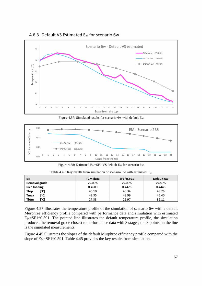
67
4.6.3 Default VS Estimated EM for scenario 6w
Figure 4.57: Simulated results for scenario 6w with default EM
Figure 4.58: Estimated EM=SF1 VS default EM for scenario 6w
Table 4.45: Key results from simulation of scenario 6w with estimated EM
EM TCM data SF1*0.591 Default 6w Removal grade 79.00% 79.00% 79.80% Rich loading 0.4600 0.4426 0.4446 Ttop [˚C] 46.10 45.34 43.26 Tmax [˚C] 49.35 48.99 45.40 Tbtm [˚C] 27.33 26.97 32.11
Figure 4.57 illustrates the temperature profile of the simulation of scenario 6w with a default
Murphree efficiency profile compared with performance data and simulation with estimated
EM=SF1*0.591. The pointed line illustrates the default temperature profile, the simulation
produced the removal grade closest to performance data with 8 stages, the 8 points on the line
is the simulated measurements.
Figure 4.45 illustrates the slopes of the default Murphree efficiency profile compared with the
slope of EM=SF1*0.591. Table 4.45 provides the key results from simulation.
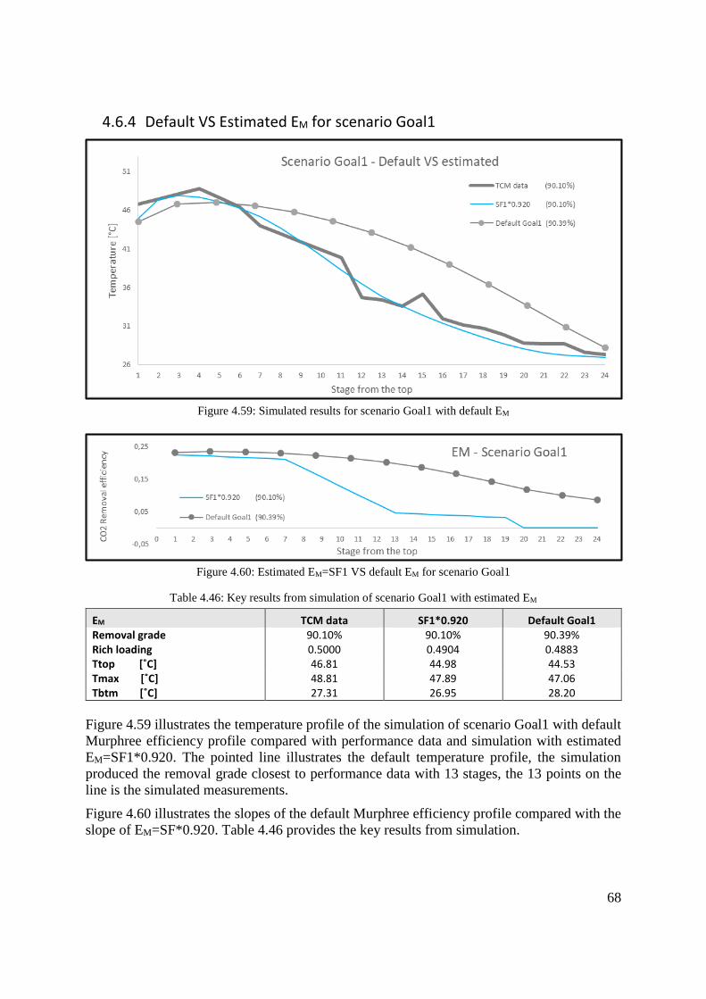
68
4.6.4 Default VS Estimated EM for scenario Goal1
Figure 4.59: Simulated results for scenario Goal1 with default EM
Figure 4.60: Estimated EM=SF1 VS default EM for scenario Goal1
Table 4.46: Key results from simulation of scenario Goal1 with estimated EM
EM TCM data SF1*0.920 Default Goal1 Removal grade 90.10% 90.10% 90.39% Rich loading 0.5000 0.4904 0.4883 Ttop [˚C] 46.81 44.98 44.53 Tmax [˚C] 48.81 47.89 47.06 Tbtm [˚C] 27.31 26.95 28.20
Figure 4.59 illustrates the temperature profile of the simulation of scenario Goal1 with default
Murphree efficiency profile compared with performance data and simulation with estimated
EM=SF1*0.920. The pointed line illustrates the default temperature profile, the simulation
produced the removal grade closest to performance data with 13 stages, the 13 points on the
line is the simulated measurements.
Figure 4.60 illustrates the slopes of the default Murphree efficiency profile compared with the
slope of EM=SF*0.920. Table 4.46 provides the key results from simulation.
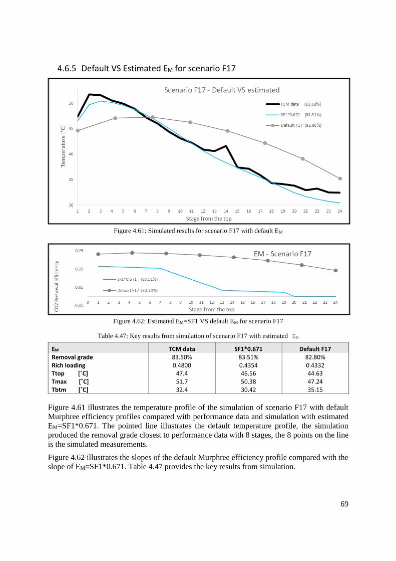
69
4.6.5 Default VS Estimated EM for scenario F17
Figure 4.61: Simulated results for scenario F17 with default EM
Figure 4.62: Estimated EM=SF1 VS default EM for scenario F17
Table 4.47: Key results from simulation of scenario F17 with estimated EM
EM TCM data SF1*0.671 Default F17 Removal grade 83.50% 83.51% 82.80% Rich loading 0.4800 0.4354 0.4332 Ttop [˚C] 47.4 46.56 44.63 Tmax [˚C] 51.7 50.38 47.24 Tbtm [˚C] 32.4 30.42 35.15
Figure 4.61 illustrates the temperature profile of the simulation of scenario F17 with default
Murphree efficiency profiles compared with performance data and simulation with estimated
EM=SF1*0.671. The pointed line illustrates the default temperature profile, the simulation
produced the removal grade closest to performance data with 8 stages, the 8 points on the line
is the simulated measurements.
Figure 4.62 illustrates the slopes of the default Murphree efficiency profile compared with the
slope of EM=SF1*0.671. Table 4.47 provides the key results from simulation.
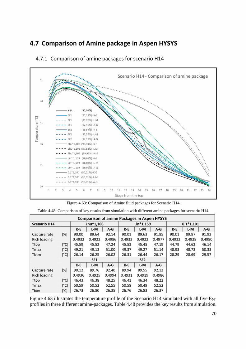
70
4.7 Comparison of Amine package in Aspen HYSYS
4.7.1 Comparison of amine packages for scenario H14
Figure 4.63: Comparison of Amine fluid packages for Scenario H14
Table 4.48: Comparison of key results from simulation with different amine packages for scenario H14
Comparison of amine Packages in Aspen HYSYS Scenario H14 Zhu*1,106 Lin*1,159 0.1*1,101
K-E L-M A-G K-E L-M A-G K-E L-M A-G Capture rate [%] 90.00 89.64 92.14 90.01 89.63 91.85 90.01 89.87 91.92 Rich loading 0.4932 0.4922 0.4986 0.4933 0.4922 0.4977 0.4932 0.4928 0.4980 Ttop [°C] 45.59 45.52 47.24 45.53 45.45 47.19 44.79 44.62 46.14 Tmax [°C] 49.21 49.13 51.00 49.37 49.27 51.14 48.93 48.73 50.33 Tbtm [°C] 26.14 26.25 26.02 26.31 26.44 26.17 28.29 28.69 29.57
SF1 SF2
K-E L-M A-G K-E L-M A-G Capture rate [%] 90.12 89.76 92.40 89.94 89.55 92.12 Rich loading 0.4936 0.4925 0.4994 0.4931 0.4919 0.4986 Ttop [°C] 46.43 46.38 48.25 46.41 46.34 48.22 Tmax [°C] 50.59 50.52 52.55 50.58 50.49 52.52
Tbtm [°C] 26.73 26.80 26.35 26.76 26.83 26.37
Figure 4.63 illustrates the temperature profile of the Scenario H14 simulated with all five EM-
profiles in three different amine-packages. Table 4.48 provides the key results from simulation.
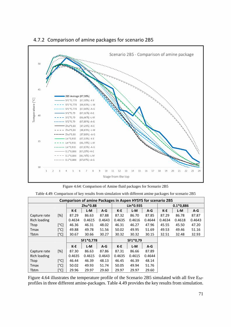
71
4.7.2 Comparison of amine packages for scenario 2B5
Figure 4.64: Comparison of Amine fluid packages for Scenario 2B5
Table 4.49: Comparison of key results from simulation with different amine packages for scenario 2B5
Comparison of amine Packages in Aspen HYSYS for scenario 2B5
Zhu*0.88 Lin*0.935 0.1*0,886
K-E L-M A-G K-E L-M A-G K-E L-M A-G Capture rate [%] 87.29 86.63 87.88 87.32 86.70 87.85 87.29 86.78 87.87 Rich loading 0.4634 0.4615 0.4643 0.4635 0.4616 0.4644 0.4634 0.4618 0.4643 Ttop [°C] 46.36 46.31 48.02 46.31 46.27 47.96 45.55 45.50 47.20 Tmax [°C] 49.88 49.78 51.56 50.02 49.95 51.69 49.53 49.46 51.16 Tbtm [°C] 30.67 30.66 30.27 30.32 30.32 30.15 32.51 32.48 32.93
SF1*0,778 SF1*0,79
K-E L-M A-G K-E L-M A-G Capture rate [%] 87.30 86.63 87.86 87.31 86.66 87.89 Rich loading 0.4635 0.4615 0.4643 0.4635 0.4615 0.4644 Ttop [°C] 46.44 46.39 48.13 46.45 46.39 48.14 Tmax [°C] 50.02 49.93 51.74 50.05 49.94 51.76 Tbtm [°C] 29.96 29.97 29.60 29.97 29.97 29.60
Figure 4.64 illustrates the temperature profile of the Scenario 2B5 simulated with all five EM-
profiles in three different amine-packages. Table 4.49 provides the key results from simulation.
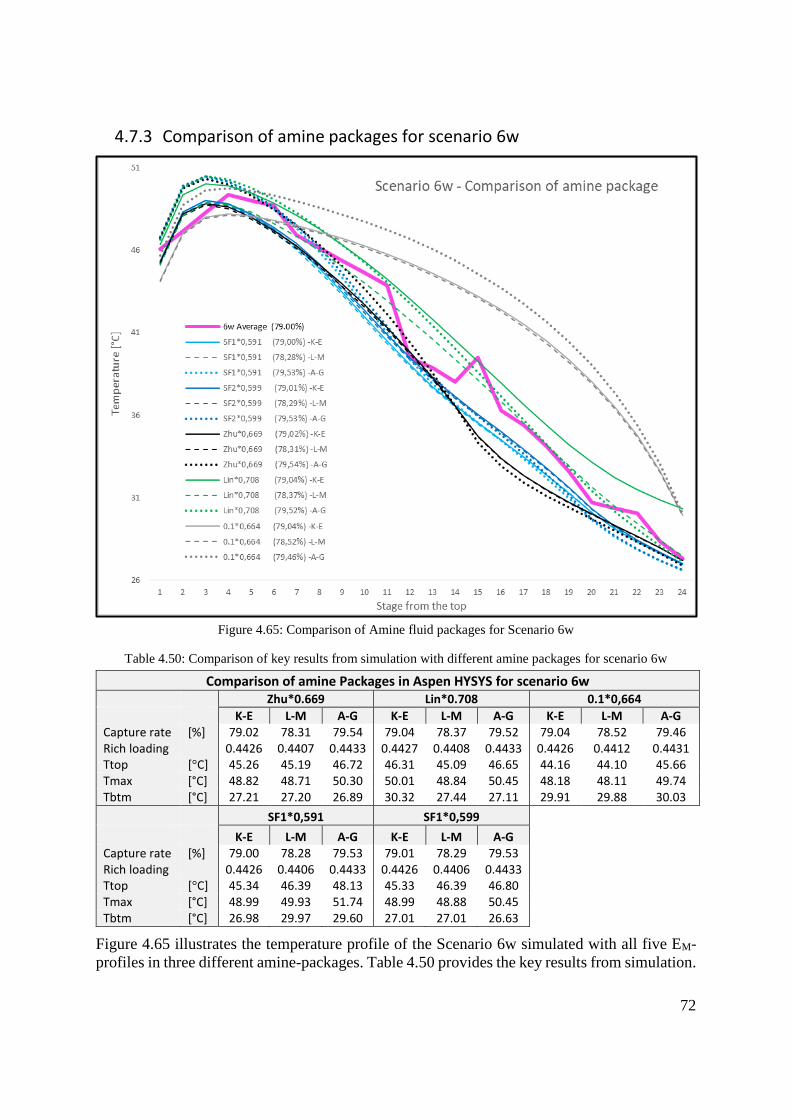
72
4.7.3 Comparison of amine packages for scenario 6w
Figure 4.65: Comparison of Amine fluid packages for Scenario 6w
Table 4.50: Comparison of key results from simulation with different amine packages for scenario 6w
Comparison of amine Packages in Aspen HYSYS for scenario 6w
Zhu*0.669 Lin*0.708 0.1*0,664
K-E L-M A-G K-E L-M A-G K-E L-M A-G Capture rate [%] 79.02 78.31 79.54 79.04 78.37 79.52 79.04 78.52 79.46 Rich loading 0.4426 0.4407 0.4433 0.4427 0.4408 0.4433 0.4426 0.4412 0.4431 Ttop [°C] 45.26 45.19 46.72 46.31 45.09 46.65 44.16 44.10 45.66 Tmax [°C] 48.82 48.71 50.30 50.01 48.84 50.45 48.18 48.11 49.74 Tbtm [°C] 27.21 27.20 26.89 30.32 27.44 27.11 29.91 29.88 30.03
SF1*0,591 SF1*0,599
K-E L-M A-G K-E L-M A-G Capture rate [%] 79.00 78.28 79.53 79.01 78.29 79.53 Rich loading 0.4426 0.4406 0.4433 0.4426 0.4406 0.4433 Ttop [°C] 45.34 46.39 48.13 45.33 46.39 46.80 Tmax [°C] 48.99 49.93 51.74 48.99 48.88 50.45 Tbtm [°C] 26.98 29.97 29.60 27.01 27.01 26.63
Figure 4.65 illustrates the temperature profile of the Scenario 6w simulated with all five EM-
profiles in three different amine-packages. Table 4.50 provides the key results from simulation.
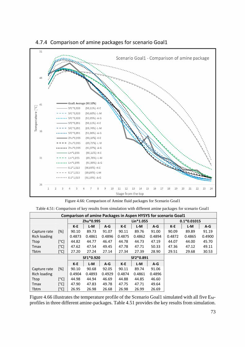
73
4.7.4 Comparison of amine packages for scenario Goal1
Figure 4.66: Comparison of Amine fluid packages for Scenario Goal1
Table 4.51: Comparison of key results from simulation with different amine packages for scenario Goal1
Comparison of amine Packages in Aspen HYSYS for scenario Goal1
Zhu*0.995 Lin*1.055 0.1*0.01015
K-E L-M A-G K-E L-M A-G K-E L-M A-G Capture rate [%] 90.10 89.73 91.07 90.11 89.76 91.00 90.09 89.89 91.19 Rich loading 0.4873 0.4861 0.4896 0.4875 0.4862 0.4894 0.4872 0.4865 0.4900 Ttop [°C] 44.82 44.77 46.47 44.78 44.73 47.19 44.07 44.00 45.70 Tmax [°C] 47.62 47.54 49.45 47.78 47.71 50.33 47.36 47.12 49.11 Tbtm [°C] 27.20 27.24 27.14 27.34 27.39 28.90 29.51 29.68 30.53
SF1*0.920 SF2*0.891
K-E L-M A-G K-E L-M A-G Capture rate [%] 90.10 90.68 92.05 90.11 89.74 91.06 Rich loading 0.4904 0.4893 0.4929 0.4874 0.4861 0.4896 Ttop [°C] 44.98 44.94 46.69 44.88 44.85 46.60 Tmax [°C] 47.90 47.83 49.78 47.75 47.71 49.64 Tbtm [°C] 26.95 26.98 26.68 26.98 26.99 26.69
Figure 4.66 illustrates the temperature profile of the Scenario Goal1 simulated with all five EM-
profiles in three different amine-packages. Table 4.51 provides the key results from simulation.
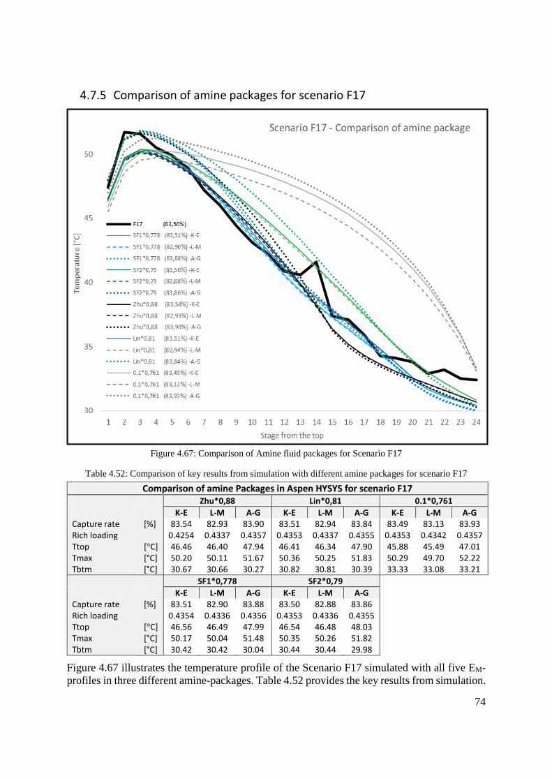
74
4.7.5 Comparison of amine packages for scenario F17
Figure 4.67: Comparison of Amine fluid packages for Scenario F17
Table 4.52: Comparison of key results from simulation with different amine packages for scenario F17
Comparison of amine Packages in Aspen HYSYS for scenario F17
Zhu*0,88 Lin*0,81 0.1*0,761
K-E L-M A-G K-E L-M A-G K-E L-M A-G Capture rate [%] 83.54 82.93 83.90 83.51 82.94 83.84 83.49 83.13 83.93 Rich loading 0.4254 0.4337 0.4357 0.4353 0.4337 0.4355 0.4353 0.4342 0.4357 Ttop [°C] 46.46 46.40 47.94 46.41 46.34 47.90 45.88 45.49 47.01 Tmax [°C] 50.20 50.11 51.67 50.36 50.25 51.83 50.29 49.70 52.22 Tbtm [°C] 30.67 30.66 30.27 30.82 30.81 30.39 33.33 33.08 33.21
SF1*0,778 SF2*0,79 K-E L-M A-G K-E L-M A-G Capture rate [%] 83.51 82.90 83.88 83.50 82.88 83.86 Rich loading 0.4354 0.4336 0.4356 0.4353 0.4336 0.4355 Ttop [°C] 46.56 46.49 47.99 46.54 46.48 48.03 Tmax [°C] 50.17 50.04 51.48 50.35 50.26 51.82 Tbtm [°C] 30.42 30.42 30.04 30.44 30.44 29.98
Figure 4.67 illustrates the temperature profile of the Scenario F17 simulated with all five EM-
profiles in three different amine-packages. Table 4.52 provides the key results from simulation.
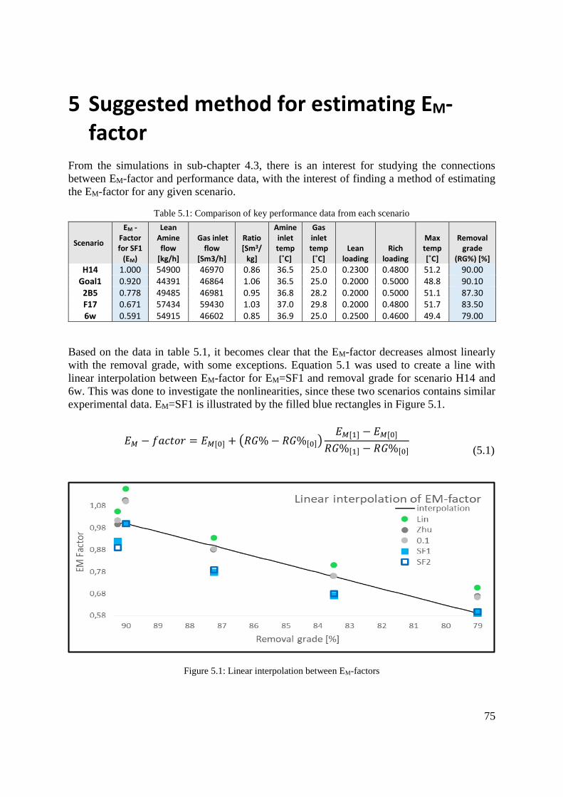
75
5 Suggested method for estimating EM-factor
From the simulations in sub-chapter 4.3, there is an interest for studying the connections
between EM-factor and performance data, with the interest of finding a method of estimating
the EM-factor for any given scenario.
Table 5.1: Comparison of key performance data from each scenario
Scenario
EM -Factor for SF1
(EM)
Lean Amine flow
[kg/h]
Gas inlet flow
[Sm3/h]
Ratio [Sm3/
kg]
Amine inlet temp [˚C]
Gas inlet temp [˚C]
Lean loading
Rich loading
Max temp [˚C]
Removal grade
(RG%) [%]
H14 1.000 54900 46970 0.86 36.5 25.0 0.2300 0.4800 51.2 90.00 Goal1 0.920 44391 46864 1.06 36.5 25.0 0.2000 0.5000 48.8 90.10 2B5 0.778 49485 46981 0.95 36.8 28.2 0.2000 0.5000 51.1 87.30 F17 0.671 57434 59430 1.03 37.0 29.8 0.2000 0.4800 51.7 83.50 6w 0.591 54915 46602 0.85 36.9 25.0 0.2500 0.4600 49.4 79.00
Based on the data in table 5.1, it becomes clear that the EM-factor decreases almost linearly
with the removal grade, with some exceptions. Equation 5.1 was used to create a line with
linear interpolation between EM-factor for EM=SF1 and removal grade for scenario H14 and
6w. This was done to investigate the nonlinearities, since these two scenarios contains similar
experimental data. EM=SF1 is illustrated by the filled blue rectangles in Figure 5.1.
𝐸𝑀 − 𝑓𝑎𝑐𝑡𝑜𝑟 = 𝐸𝑀[0] + (𝑅𝐺% − 𝑅𝐺%[0])𝐸𝑀[1] − 𝐸𝑀[0]
𝑅𝐺%[1] − 𝑅𝐺%[0]
(5.1)
Figure 5.1: Linear interpolation between EM-factors

76
The deviation from the line is calculated for scenario Goal1 (-0.08), 2B5 (-0.12) and F17 (-
0.09). From these results one can assume that the ratio of amine and gas impacts the choice of
EM-factor. It is therefore assumed that if the experimental performance data were closer to the
data for scenario H14 and 6w, the EM-factor could be calculated for any removal grade from
equation 5.1.
If the key data is deviating from the data in scenario H14 and 6w, the suggested method could
be combined with an estimating method e.g. you could calculate the EM-factor with equation
5.1 and simulate with the calculated EM-factor. If the simulated removal grade is higher than
performance removal grade, you could guess a lower value for EM-factor and continue with e.g
the bisection method until an EM-factor which predicts the correct removal grade is found. In
the same way you would guess a higher value for EM-factor if the simulated removal grade is
lower than performance data.
It is assumed that this method will converge to the correct EM-factor quicker than the try and
fail method suggested in sub-chapter 3.2.2.
77
6 Discussion In this chapter, the verification simulations in Aspen HYSYS and Aspen Plus are evaluated.
The simulations with estimated EM-profiles in Aspen HYSYS and estimated EM-profiles and
interfacial area factor in Aspen Plus are evaluated. The comparison between estimated
simulations in Equilibrium-based and rate-based model are evaluated. The simulations with
default EM-profiles compared with estimated EM=SF1 in Aspen HYSYS are evaluated. The
comparison of simulation with different amine packages in Aspen HYSYS are evaluated. And
at last, a comparison of results from this work and results from earlier work is discussed, before
some further work is suggested.
6.1 Evaluation of verification simulation in Aspen HYSYS
6.1.1 Evaluation of scenario H14 verification in Aspen HYSYS
The verification of scenario H14 for Zhu, Sætre and Røsvik was not producing identical
temperature profile with any of their results, but a similar temperature profile for both
scenario H14 with EM = 0.1 and EM = Zhu. The removal grade for EM=0.1 was lower
than performance data (-1.58%), lower than Zhu (-0.98%), higher than Sætre (+1.42%)
and lower than Røsvik (-0.88%). While the rich loading was higher than performance
data (+0.0085), higher than Zhu (+0.0015) and lower than Sætre (-0.0035). The removal
grade for EM=Zhu was lower than performance data (-1.43%), lower than Zhu (-0.82%),
higher than Sætre (+1.67%) and lower than Røsvik (-0.73%). While the rich loading
was higher than performance data (+0.0090), higher than Zhu (+0.0010) and lower than
Sætre (-0.0020).
Zhu got a higher removal grade and a lower rich loading while Sætre got a lower
removal grade and higher rich loading for botm EM=0.1 and EM=Zhu. The reason for
this deviation is assumed to be because Zhu used a lower input flue gas flow than given
by Hamborg et al., (2014) [7] for scenario H14. This assumption gets supported when
the results are compared to Sætre’s verification in his master thesis from 2016 [28],
where he verified Zhu with the same input flue gas flow as Zhu and got a removal grade
and rich loading almost identical with Zhu.
6.1.2 Evaluation of scenario 2B5 verification in Aspen HYSYS
The verification of Sætre’s simulation of 2B5 results in a non-identical but slightly
similar temperature profile for both EM=0.1 and EM=Zhu. The removal grade for
EM=0.1 was slightly higher than Sætre (+3.07%) and performance data (+2.77%) while
the rich loading was lower than Sætre (-0.0200) and performance data (-0.0300). The
removal grade for EM =Zhu was also slightly higher than Sætre (+3.00%) and
performance data (+3%) while the rich loading was lower than Sætre (-0.0200) and
performance data (-0.0300).
78
The reason for these deviations might be caused by uncertainties in measurements,
variations in different versions of simulation programs or unknown differences in
process input variables to simulation.
6.1.3 Evaluation of scenario 6w verification in Aspen HYSYS
The verification on Sætre’s work on scenario 6w also produces a temperature profile
similar but not identical to Sætre, for both EM =0.1 and EM =Zhu. The removal grade
for EM =0.1 were higher than for Sætre (+2.72%) and performance data (+10.72%)
while the rich loading was lower than Sætre (-0.0200) but higher than performance data
(+0.0100). The removal grade of EM =Zhu was also slightly higher than Sætre (+2.70%)
and performance data (+10.60%) while rich loading was lower than for Sætre (-0.0200)
and higher than for performance data (+0.0100).
6.1.4 Evaluation of scenario Goal1 verification in Aspen HYSYS
The verification on Sætre’s work on scenario Goal1 produces a curve fairly similar to
sætre for both EM=0.1 and EM=Zhu. The removal grade for EM =0.1 were higher than
for Sætre (+0.94%) but lower than performance data (-3.06%), while the rich loading
was a little bit lower than both (-0.0070). For EM =Zhu the removal grade was also
higher than Sætre (+1.22%) and lower than performance data (-2.68%), while the rich
loading was lower than both (-0.0060).
6.1.5 Evaluation of scenario F17 verification in Aspen HYSYS
The verification of Røsvik’s simulation of scenario F17, with EM=0.1, produced a
temperature profile similar to Røsvik, but with slightly higher main temperature. The
removal grade deviated from both Røsvik (+5.28%) and performance data (+8.18%).
The verification of Røsvik’s simulation of scenario F17, with EM=Zhu, produced results
that deviated a lot from Røsvik, but fitted the temperature profile for the performance
data better than Røsvik’s simulation. The removal grade on the other hand deviated
from both Røsvik (+2.67%) and performance data (+6.87%). The verification of
Røsviks simulation of scenario F17 with EM=Lin, produced a slightly higher
temperature profile, the removal grade had some deviations from Røsvik (+3.60%) and
the performance data (+5.50%). The simulated rich loading was slightly lower than the
rich loading from performance data for all EM-profiles, EM=0.1 (-0.1200), EM=Zhu (-
0.0200), EM=Lin (-0.0300).
The reason for the deviations is assumed to be for the reason that Røsvik used a much
lower input pressure than given in Faramarzi et al., (2017) [32] for scenario F17. In
addition, the EM-profiles used in this verification will give a removal grade higher than
performance data because they have a too high overall efficiency to be able to fit this
scenario well, this we can also see in scenario 6w which also have a lower removal
grade.
79
6.2 Evaluation of verification simulation in Aspen Plus
6.2.1 Evaluation of scenario H14 verification in Aspen Plus
The verification of scenario H14 for Sætre and Røsvik’s equilibrium-based Aspen Plus
simulation, produced close to identical results for temperature profile for both EM=0.1
and EM=Zhu. The removal grade for EM=0.1 was lower than performance data (-
1.60%), higher than Sætre (+1.20%) and equal to Røsvik. While the rich loading was
higher than performance data (+0.0080), lower than Sætre (-0.0030). The removal grade
for EM=Zhu was lower than performance data (-1.61%), higher than Sætre (+1.49%)
and lower than Røsvik (-0.61%). While the rich loading was higher than performance
data (+0.008) and lower than Sætre (-0.0020).
The rate-based verification of scenario H14 for Sætre and Røsvik, produced close to
identical temperature profiles for Sætre, when IAF was set to 0.55, and Røsvik when
IAF was set to 0.65. The removal grade for IAF=0.55 was lower than performance data
(-1.62%) and lower than Sætre (-0.12%) while the rich loading was higher than
performance data (+0.0091) and higher than Sætre (+0.0001). The removal grade for
IAF=0.65 was lower than performance data (-1.28%) and lower than Røsvik (-0.38%).
6.2.2 Evaluation of scenario 2B5 verification in Aspen Plus
The verification of scenario 2B5 for Sætre’s equilibrium-based Aspen Plus simulation,
produced close to identical results for temperature profile for EM=0.1, while EM=Zhu
had some deviations. The removal grade for EM=0.1 was lower than performance data
(-0.10%) and equal to Sætre. The rich loading was lower than performance data (-
0.0113) and lower than Sætre (-0.0013). The removal grade for EM=Zhu was higher
than performance data (+1.09%), and higher than Sætre (+0.99%). The rich loading was
lower than performance data (-0.0120) and lower than Sætre (-0.0020).
The rate-based verification of scenario 2B5 for Sætre, produced close to identical
temperature profiles when IAF was set to 0.55. The removal grade for IAF=0.55 was
lower than performance data (-1.28%) and higher than Sætre (+0.02%) while the rich
loading was higher than performance data (+0.0146) and lower than Sætre (-0.0046).
6.2.3 Evaluation of scenario 6w verification in Aspen Plus
The verification of scenario 6w for Sætre’s equilibrium-based Aspen Plus simulation,
produced close to identical results for temperature profile for EM=0.1, while EM=Zhu
deviated more.. The removal grade for EM=0.1 was higher than performance data
(+10.49%) and higher than Sætre (+2.29%). The rich loading was higher than
performance data (-0.0107) and lower than Sætre (-0.0203). The removal grade for
EM=Zhu was higher than performance data (+10.68%), and higher than Sætre (+2.78%).
The rich loading was higher than performance data (+0.0102) and lower than Sætre (-
0.0198).
The rate-based verification of scenario 6w for Sætre, produced temperature profiles
with similar curves as Sætre but higher temperatures, both when IAF was set to 0.55
80
and 0.65. The removal grade for IAF=0.55 was higher than performance data (-14.53%)
and higher than Sætre (+7.43%) while the rich loading was higher than performance
data (+0.0219) and lower than Sætre (-0.0061). The removal grade for IAF=0.65 was
higher than performance data (-16.19%) and higher than Sætre (+9.09%) while the rich
loading was higher than performance data (+0.0265) and lower than Sætre (-0.0015).
The removal grade was closer to Sætre for IAF=0.55, while the rich loading was closer
for IAF=0.65, none of them gave a god fit to temperature profile. It is assumed that
Sætre used a lower interfacial area factor.
6.2.4 Evaluation of scenario Goal1 verification in Aspen Plus
The verification of scenario Goal1 for Sætre’s equilibrium-based Aspen Plus
simulation, produced temperature profiles with similar curves as Sætre for both EM=0.1,
and EM=Zhu. The removal grade for EM=0.1 was lower than performance data (-0.47%)
and higher than Sætre (+6.93%). The rich loading was lower than both performance
data and Sætre (-0.0146). The removal grade for EM=Zhu was lower than performance
data (-0.28%), and higher than Sætre (+7.12%). The rich loading was lower than both
performance data and Sætre (-0.0140).
The rate-based verification of scenario Goal1 for Sætre, produced temperature profiles
with similar curves as Sætre, but higher temperatures. The removal grade for IAF=0.55
was higher than performance data (+0.11%) and higher than Sætre (+11.31%) while the
rich loading was lower than performance data (-0.0123) and lower than Sætre (-0.0020).
The removal grade for IAF=0.65 was higher than performance data (+0.30%) and
higher than Sætre (+11.50%) while the rich loading was lower than performance data
(-0.0120) and lower than Sætre (-0.0020).
The removal grade was closer to Sætre for IAF=0.55, while the rich loading was closer
for IAF=0.65, none of them gave a god fit to temperature profile.
6.2.5 Evaluation of scenario F17 verification in Aspen Plus
The verification of scenario F17 for Røsvik’s equilibrium-based Aspen Plus simulation,
produced similar results for temperature profile for EM=0.1, while EM=Zhu had some
deviations. The temperature profile for EM=Lin is close to identical with Røsvik. The
removal grade for EM=0.1 was higher than performance data (+4.90%) and higher than
Sætre (+1.75%). The rich loading was higher than performance data (+0.0080). The
removal grade for EM=Zhu was higher than performance data (+4.89%), and higher
than Sætre (+1.19%). The rich loading was higher than performance data (+0.0080).
The removal grade for EM=Lin was higher than performance data (+2.74%), and lower
than Sætre (-0.06%). The rich loading was higher than performance data (+0.0129).
The rate-based verification of scenario F17 for Røsvik, produced close to identical
temperature profiles when IAF was set to 0.55. The removal grade for IAF=0.55 was
higher than performance data (+0.26%) and lower than Sætre (-0.04%) while the rich
loading was higher than performance data (+0.0450).
81
6.3 Evaluation of simulation with estimated EM in Aspen HYSYS
6.3.1 Evaluation of scenario H14 with estimated EM in Aspen HYSYS
For scenario H14 it was estimated two new EM-profiles, EM=SF1 and EM=SF2. These
two profiles are based on the idea of higher CO2 removal efficiency at the top of each
packing section in the absorber column, and were created by equation 3.7 in sub-chapter
3.2.1. The simulation in figure 4.28 indicates that both these EM’s fit the performance
data well. It looks as EM=SF1 have the best fit for temperature profile, while EM=SF2
have the removal grade closest to performance data. The deviations are small for both
EM=SF1 and EM=SF2. Compared with EM=Zhu, it looks as though the new sets might
have an even better fit for both temperature and removal grade for scenario H14.
6.3.2 Evaluation of scenario 2B5 with estimated EM in Aspen HYSYS
For scenario 2B5, the EM-profiles created for scenario H14 were scaled and fitted to the
performance removal grade for scenario 2B5. 2B5 is a scenario with four different sets
of temperature measurements, and a given average removal grade. In figure 4.30 the
simulation is compared with a blue line of average temperature as well as the measured
temperatures. The simulated results of the new developed EM-profiles, EM=SF1 and
EM=SF2, did not fit well for the average temperature profile based on the average
removal grade, but had a sufficient fit to the temperature profile of plant data C and D.
For this scenario the EM-profile with the best fit to the average temperature profile was
EM=Lin*0.935.
One can see that the measurement in plant data A is slightly higher than for C and D,
while B is in between. The independent removal grade for each data set can be assumed
to vary a lot, as the temperature varies a lot. It is assumed that EM=SF1 and EM=SF2
would fit the average line best if plant data A was neglected.
6.3.3 Evaluation of scenario 6w with estimated EM in Aspen HYSYS
For scenario 6w, the EM-profiles created for scenario H14 were scaled and fitted to the
performance removal grade for scenario 6w just like for scenario 2B5, 6w is also a
scenario with four different sets of temperature measurements, and a given average
removal grade. In figure 4.32 the simulation is compared with a purple line of average
temperature as well as the measured temperatures. The simulated results of the new
developed EM-profiles based on the average removal grade did fit the average
temperature profile better than for scenario 2B5, but was a little too low. Just like for
scenario SB5, EM=SF1 and EM=SF2 had a sufficient fit to the temperature profile of
plant data C and D, but also for B.
If plant data A was removed from the average line the temperature profile would fit
better. Like for scenario 2B5, the independent removal grade for each data set for
scenario 6w can be assumed to vary a lot for these four data sets, as the temperature
varies a lot.
82
6.3.4 Evaluation of scenario Goal1 with estimated EM in Aspen HYSYS
For scenario Goal1, the EM-profiles created for scenario H14 were scaled to fit the
performance removal grade for scenario Goal1, just like for scenario 2B5 and 6w. Goal1
is also a scenario with four different sets of temperature measurements, and a given
average removal grade. In figure 4.34 the simulation is compared with a gray line of
average temperature as well as the measured temperatures. The simulated results for
the new developed EM-profiles based on the average removal grade, did give a sufficient
fit to the average performance data. Just like for scenario SB5, EM=SF1 and EM=SF2
had a sufficient fit to the temperature profile of plant data B, C and D, while A deviated
a lot.
If plant data A was removed from the average line the temperature profile would fit
even better. The independent removal grade for each data set for scenario Goal1 can be
assumed to vary a lot for these four data sets, as the temperature varies a lot.
6.3.5 Evaluation of scenario F17 with estimated EM in Aspen HYSYS
For scenario F17 the EM-profiles created for scenario H14 were used. They were scaled
down and fitted to the removal grade given in the performance data by equation 3.8 in
sub-chapter 3.2.2. As were EM=Zhu and EM=Lin. The simulation in figure 4.36
indicates that the best fit in both temperature profile and removal grade was EM=SF2,
but EM=SF1 and EM=Zhu.
By the results from these simulation it looks like the estimation method of EM-profile by
equation 3.7 and 3.8 gives satisfactory results. EM=Zhu have proven to give a good fit to several
scenarios in earlier master theses, but these results provides better results for EM=SF1 and
EM=SF2. The main difference between Zhu and SF1 & SF2, is that Zhu has constant low
efficiency from stage 13 and down. While SF1 & SF2 have constant low efficiency from stage
20 and down. The fact that SF1 & SF2 fit better than Zhu might deciphering that the bottom
packing have a higher removal efficiency than suggested in earlier theses.
6.4 Evaluation of simulation with estimated EM and IAF in Aspen Plus
6.4.1 Evaluation of scenario H14 with estimated EM and IAF in Aspen Plus
For the equilibrium-based model, the EM-profiles used for simulation of scenario H14
in Aspen HYSYS were scaled to fit the removal grade for scenario H14 in Aspen Plus
by adjusting the EM-factor. From figure 4.38 it is visible that this gave similar
temperature profiles as in Aspen HYSYS with god fit to the performance temperature
for EM=Zhu*1.12, EM=SF1*0.995 and EM=SF2*1.005, while EM=Lin*1.17 and
EM=0.1*1.1 deviated from the performance data. All EM-profiles were easy to fit with
removal grade by adjusting the EM-factor.
83
For the rate-based model, the IAF was adjusted up to give the best fit to removal grade.
For scenario H14 the IAF was not able to fit the removal grade to 90%. The highest
achieved removal grade was for IAF=1, which gave a removal grade of 88.82%. The
temperature profile deviated from performance data and simulations with equilibrium-
based model.
6.4.2 Evaluation of scenario 2B5 with estimated EM and IAF in Aspen Plus
For the equilibrium-based model, the EM-profiles were scaled to fit the removal grade
for scenario 2B5 in Aspen Plus by adjusting the EM-factor. From figure 4.40 it is visible
that this gave similar temperature profiles as in Aspen HYSYS. With the best fit to
average-temperature profile for EM=Lin*1.005.
For the rate-based model, the IAF was adjusted up to give the best fit to removal grade.
For scenario 2B5 the IAF was not able to fit the removal grade to 87.20%. The highest
achieved removal grade was for IAF=1, which gave a removal grade of 86.14%. The
temperature profile deviated from performance data and simulations with equilibrium-
based model. The temperature profile is very similar to the rate-based temperature in
scenario H14.
6.4.3 Evaluation of scenario 6w with estimated EM and IAF in Aspen Plus
For the equilibrium-based model, the EM-profiles were scaled to fit the removal grade
for scenario 6w in Aspen Plus by adjusting the EM-factor. From figure 4.42 it is visible
that this gave similar temperature profiles as in Aspen HYSYS. With the best fit to
average-temperature profile for EM=SF1*0.603 and EM=SF2*0.612. EM=Lin*0.722 fit
the performance temperature better in Aspen Plus than in Aspen HYSYS.
For the rate-based model, the IAF was adjusted up to give the best fit to removal grade.
For scenario 6w the best result was achieved with IAF=0.29, which gave a removal
grade of 79.04%, performance data is 79.00%. The temperature profile deviated from
performance data and simulations with equilibrium-based model, but have a better fit
to the performance temperatures than rate-based for scenario H14 and 2B5.
6.4.4 Evaluation of scenario Goal1 with estimated EM and IAF in Aspen Plus
For the equilibrium-based model, the EM-profiles were scaled to fit the removal grade
for scenario Goal1 in Aspen Plus by adjusting the EM-factor. From figure 4.44 it is
visible that this gave similar temperature profiles as in Aspen HYSYS. Overall the
temperature profiles fit the performance temperature better in HYSYS. The best fit to
average-temperature profile was for EM=Zhu*1.015.
For the rate-based model, the IAF was adjusted to give the best fit to removal grade.
For scenario Goal1 the best result was achieved with IAF=0.51, which gave a removal
grade of 90.11%, performance data is 90.10%. The temperature profile deviated from
performance data, but had a similar profile as EM=Lin*1.074.
84
6.4.5 Evaluation of scenario F17 with estimated EM and IAF in Aspen Plus
For the equilibrium-based model, the EM-profiles were scaled to fit the removal grade
for scenario F17 in Aspen Plus by adjusting the EM-factor. From figure 4.46 it is visible
that this gave similar temperature profiles as in Aspen HYSYS, but in Aspen HYSYS
the best fit was for EM=SF2, EM=SF1 and EM=Zhu. In Aspen Plus the best fit to
performance temperature was for EM=Lin*0.863. Overall the temperature profiles fit
the performance temperature better in HYSYS.
For the rate-based model, the IAF was adjusted up to give the best fit to removal grade.
For scenario F17 the best result was achieved with IAF=0.51, which gave a removal
grade of 83.48%, performance data is 83.50%. The temperature profile had a similar
profile as EM=Lin*0.863, and had an ok fit to the performance temperature.
The results from these simulation indicates that there is small deviations between the
equilibrium-based model in Aspen Plus and Aspen HYSYS. The EM-profiles can easily be
scaled with the EM-factor to fit the removal grade of any scenario, in both Aspen plus and
Aspen HYSYS, but the EM-profile must be adjusted for the simulation tool.
The rate-based method proved to be able to adjust to removal grade for some scenarios, while
other scenario was less adjustable, this is assumed to be because the simulation reaches
equilibrium. For the scenarios where the rate-based simulation was able to predict the requested
removal grade the temperature profile fit the performance data better, but never as good as the
EM-fitted profiles. Typically the temperature profile lays between the fitted EM-profiles and the
EM-profile with constant Murphree efficiency of 0.1.
6.5 Evaluation of Comparison between Aspen Plus and HYSYS
6.5.1 Evaluation of Comparison for scenario H14
For equilibrium-based simulation in Aspen Plus and Aspen HYSYS the results were
very similar. The average temperature for each EM-profile was higher for the
simulations in Aspen Plus than the simulations in Aspen HYSYS. For scenario H14 the
average temperature for EM=SF1 and EM=SF2 was 1.3°C higher in Aspen Plus. The
temperature were 2.4°C, 2.6°C and 2.9°C for EM=Zhu, EM=Lin and EM=0.1
respectively. The rich loading is almost exactly the same for Aspen Plus and Aspen
HYSYS, the small deviations are assumed to be because the removal grade is calculated
with EM-factor of three decimals. If the removal grade was calculated to an accurate
90% for all EM-profiles the deviations between rich loading in Aspen Plus and Aspen
HYSYS is assumed to be 0.0004, because this is the deviation between EM=Zhu
(HYSYS) and EM=Lin (Plus) which both have an accurate removal grade of 90.00%.
Scenario H14 is one of the scenarios where rate-based couldn’t predict accurate removal
grade. With highest predicted removal grade =88.82%, the rate-based model predicted
rich loading of 0.4894, which is closer to performance data than equilibrium-based
model, by 0.0030. The temperature on the other hand, deviates a lot from performance
temperature.
85
For scenario H14 the best fit for temperature profile was EM=SF1 and EM=SF2 in
HYSYS.
6.5.2 Evaluation of Comparison for scenario 2B5
For scenario 2B5 the temperature deviation between Aspen Plus and Aspen HYSYS
less visible than for Scenario H14. For scenario 2B5 the average temperature for
EM=SF1 was 0.07 °C higher in Aspen Plus. The temperature were 0,05°C, 0.2°C, 0.4°C
and 1.1°C for EM=SF2, EM=Zhu, EM=Lin and EM=0.1 respectively. The rich loading is
higher in Aspen Plus than in Aspen HYSYS. If the removal grade was calculated to an
accurate 87.30% for all EM-profiles the deviations between rich loading in Aspen Plus
and Aspen HYSYS is assumed to be 0.0250, because this is the deviation between EM
=SF1 (HYSYS) and EM =0.1 (Plus) which both have an accurate removal grade of
87.30%.
Scenario 2B5 is the other scenario where rate-based couldn’t predict accurate removal
grade. With the highest predicted removal grade =86.14%, the rate-based model
predicted rich loading of 0.4857, which is between equilibrium-based model in Aspen
HYSYS and Aspen Plus, where Aspen Plus is closest to performance data (0.5000).
The temperature profile deviates a lot from performance temperature.
For scenario 2B5 the best fit for temperature profile was EM=Lin in Plus and HYSYS.
6.5.3 Evaluation of Comparison for scenario 6w
For scenario 6w the average temperature for EM=SF1, EM=SF2 and EM=Zhu was 0.06
°C higher in Aspen Plus. The temperature were 1.1°C higher in Aspen Plus for EM=0.1
and 0.06 °C lower in Aspen Plus for EM=Lin. If the removal grade had been calculated
to an accurate 79.00% for all EM-profiles the deviations between rich loading in Aspen
Plus and Aspen HYSYS is assumed to be 0.0007, because this is the deviation between
EM=SF2 & EM =Lin (Plus) and EM =Lin & EM =0.1 (HYSYS) which have an removal
grade of 79.04 and 79.03%.
For Scenario 6w the rate-based model was able to estimate removal grade to 79.04%
and rich loading to be 0.4870. From performance data the rich loading is 0.4600 which
is between equilibrium-based (0.4418) and rate-based (0.4870), where Aspen HYSYS
is closest to performance data. The temperature profile lays between the fitted EM-
profiles and EM=0.1
For scenario 6w the best fit for temperature profile was EM=SF2 and EM=Lin in Plus.
6.5.4 Evaluation of Comparison for scenario Goal1
For scenario Goal1 the average temperature for EM=SF1, EM=SF2 and EM=Zhu was 1.9
°C higher in Aspen Plus. The temperature were 2.0°C and 2.1°C for EM=Lin and
EM=0.1 respectively. If the removal grade had been calculated to an accurate 90.10%
for all EM-profiles the deviations between rich loading in Aspen Plus and Aspen
HYSYS is assumed to be 0.0004, because this is the deviation between EM =Lin in Plus
and HYSYS.
86
For Scenario Goal1 the rate-based model was able to estimate removal grade to 90.11%
and rich loading to be 0.4870. From performance data the rich loading is 0.5000, all
models have very similar values for rich loading but Aspen HYSYS is closest to
performance data, followed by equilibrium-based in Aspen Plus, and rate-based last.
The rate-base temperature profile lays is very close to EM=Lin (Plus).
For scenario Goal1 the best fit for temperature profile was EM=SF1, EM=SF2 and
EM=Zhu in HYSYS.
6.5.5 Evaluation of Comparison for scenario F17
For scenario F17 the average temperature for each EM-profile was higher for the
simulations in Aspen HYSYS than the simulations in Aspen Plus. The average
temperature for EM=SF1 and EM=SF2 was 0.6°C higher in Aspen HYSYS. The
temperature were 0.5°C, 0.4°C and 0.3°C for EM=Zhu, EM=Lin and EM=0.1
respectively. If the removal grade had been calculated to an accurate 83.50% for all EM-
profiles the deviations between rich loading in Aspen Plus and Aspen HYSYS is
assumed to be 0.0500, because this is the deviation between EM=SF2 (HYSYS) and
EM=0.1 (Plus) which both have an accurate removal grade of 83.50%.
For Scenario F17 the rate-based model was able to estimate removal grade to 83.48%
and rich loading to be 0.4836. From performance data the rich loading is 0.4800. For
this scenario Aspen Plus rate-based and equilibrium-based model is very similar and
closest to performance data, while equilibrium-based in HYSYS is off by 0.0400. The
rate-base temperature profile lays is very close to EM=Lin (HYSYS).
For scenario F17 the best fit for temperature profile was EM=SF1 and EM=SF2 in
HYSYS.
By the results from these simulation it looks like there is very small deviations between the
equilibrium-based model in Aspen Plus and Aspen HYSYS. The temperature profiles seem to
have higher average temperatures in Aspen Plus, even though this is not accurate for all EM-
profiles in all scenarios.
The overall best fit for temperature profile have been for equilibrium-based model in Aspen
HYSYS, with EM-profiles EM=SF1, EM=SF2 and EM=Lin. Lin have had the best fit for scenario
2B5 and 6w, but like mentioned earlier, these scenarios have four sets of measurements. And
if data set A had been removed the average line is assumed to fit EM=SF1 and EM=SF2.
The overall best fit for rich loading have been alternately equally good for equilibrium-based
model in Aspen HYSYS and Aspen Plus.
When all factors are added up the best predictions for all parameters where achieved by
equilibrium-based model in Aspen HYSYS.
87
6.6 Evaluation of simulation with default Murphree efficiencies in Aspen HYSYS
The default EM-profiles predicted by Aspen HYSYS was compared to the estimated EM-profile,
EM=SF1, for all scenarios. Since the only adjustable variable in these simulations was the
number of stages, it was harder to achieve the exact removal grade, compared with estimating
the EM-profile by calculation where the results can be just as accurate as requested depending
on the amount of decimals used for the EM-factor.
6.6.1 Evaluation of scenario H14 with default Murphree efficiencies
For scenario H14 the removal grade from both the default simulation (89.64%) and
EM=SF1 (90.12%) was close to performance data (90.00%). The rich loading was
higher for both default (0.0120) and SF1 (0.0130). The best fit for the temperature
profile was for EM=SF1. The only stages where the default is close to performance data
is stage 1, 6 and 24.
6.6.2 Evaluation of scenario 2B5 with default Murphree efficiencies
For scenario 2B5 the removal grade from both the default simulation (86.80%) and
EM=SF1 (87.30%) was close to performance data (87.30%). The rich loading was lower
for both default (-0.0380) and SF1 (-0.0370). The best fit for the temperature profile
was for EM=SF1. The only stages the default is close to performance data is 6, 7 and 8.
6.6.3 Evaluation of scenario 6w with default Murphree efficiencies
For scenario 6w the removal grade from both the default simulation (79.80%) and
EM=SF1 (79.00%) was close to performance data (79.00%). The rich loading was lower
for both default (-0.0150) and SF1 (-0.0170). The best fit for the temperature profile
was for EM=SF1. The only stages the default is near performance data is 8, 9 and 10.
6.6.4 Evaluation of scenario Goal1 with default Murphree efficiencies
For scenario Goal1 the removal grade from both the default simulation (90.39%) and
EM=SF1 (90.10%) was close to performance data (90.10%). The rich loading was lower
for both default (-0.0120) and SF1 (-0.0090). The best fit for the temperature profile
was for EM=SF1. The only stages the default is near performance data is 6 and 24.
6.6.5 Evaluation of scenario F17 with default Murphree efficiencies
For scenario F17 the removal grade from both the default simulation (82.80%) and
EM=SF1 (83.51%) was close to performance data (83.50%). The rich loading was lower
for both default (-0.0470) and SF1 (-0.0450). The best fit for the temperature profile
was for EM=SF1. The only stages the default is near performance data is 7 and 8.
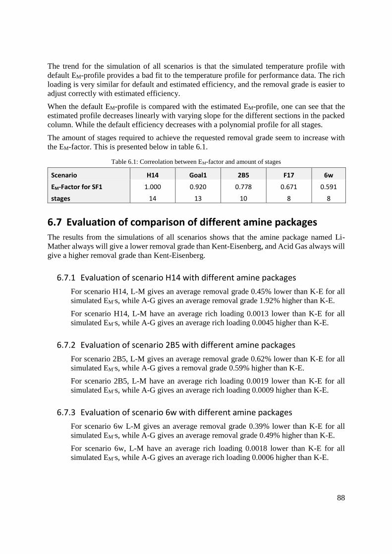
88
The trend for the simulation of all scenarios is that the simulated temperature profile with
default EM-profile provides a bad fit to the temperature profile for performance data. The rich
loading is very similar for default and estimated efficiency, and the removal grade is easier to
adjust correctly with estimated efficiency.
When the default EM-profile is compared with the estimated EM-profile, one can see that the
estimated profile decreases linearly with varying slope for the different sections in the packed
column. While the default efficiency decreases with a polynomial profile for all stages.
The amount of stages required to achieve the requested removal grade seem to increase with
the EM-factor. This is presented below in table 6.1.
Table 6.1: Correolation between EM-factor and amount of stages
Scenario H14 Goal1 2B5 F17 6w
EM-Factor for SF1 1.000 0.920 0.778 0.671 0.591
stages 14 13 10 8 8
6.7 Evaluation of comparison of different amine packages
The results from the simulations of all scenarios shows that the amine package named Li-
Mather always will give a lower removal grade than Kent-Eisenberg, and Acid Gas always will
give a higher removal grade than Kent-Eisenberg.
6.7.1 Evaluation of scenario H14 with different amine packages
For scenario H14, L-M gives an average removal grade 0.45% lower than K-E for all
simulated EM’s, while A-G gives an average removal grade 1.92% higher than K-E.
For scenario H14, L-M have an average rich loading 0.0013 lower than K-E for all
simulated EM’s, while A-G gives an average rich loading 0.0045 higher than K-E.
6.7.2 Evaluation of scenario 2B5 with different amine packages
For scenario 2B5, L-M gives an average removal grade 0.62% lower than K-E for all
simulated EM’s, while A-G gives a removal grade 0.59% higher than K-E.
For scenario 2B5, L-M have an average rich loading 0.0019 lower than K-E for all
simulated EM’s, while A-G gives an average rich loading 0.0009 higher than K-E.
6.7.3 Evaluation of scenario 6w with different amine packages
For scenario 6w L-M gives an average removal grade 0.39% lower than K-E for all
simulated EM’s, while A-G gives an average removal grade 0.49% higher than K-E.
For scenario 6w, L-M have an average rich loading 0.0018 lower than K-E for all
simulated EM’s, while A-G gives an average rich loading 0.0006 higher than K-E.
89
6.7.4 Evaluation of scenario Goal1 with different amine packages
For scenario goal1 L-M gives an average removal grade 0.32% lower than K-E for all
simulated EM’s, while A-G gives an average removal grade 1.19% higher than K-E.
For scenario goal1, L-M have an average rich loading 0.0012 lower than K-E for all
simulated EM’s, while A-G gives an average rich loading 0.0002 higher than K-E.
6.7.5 Evaluation of scenario F17 with different amine packages
For scenario F17, L-M gives a removal grade 0.59% lower than K-E, while A-G gives
a removal grade 0.34% higher than K-E.
For scenario F17, L-M have an average rich loading 0.0016 lower than K-E for all
simulated EM’s, while A-G gives an average rich loading 0.0003 higher than K-E.
Overall the average removal grade for Li-Mather is 0.47% lower than Kent-Eisenberg, and
Acid-Gas is 0.91% higher than Kent-Eisenberg.
The overall average rich loading is also lowest for Li-Mather, which is 0.0016 lower than Kent-
Eisenberg, while Acid-Gas is 0.0013 higher than Kent-Eisenberg.
It is also visible from the graphs in figure 4.63-4.67 that the temperature profiles of Kent-
Eisenberg and Li-Mather are very similar while Acid-Gas keeps a temperature of about 2 °C
higher than K-E and L-M, but the deviation decreases for the lowest stages where all the amine
packages finishes with about the same temperature.
6.8 Comparison between results from this work and results from earlier work
Scenario H14, 2B5, 6w and Goal1 was used in the paper by Øi, Sætre and Hamborg (2018)
[34]. From this paper it was found that an equilibrium-based model with EM=Zhu gave good
predictions to Scenario H14 and Goal1, but not for scenario 2B5 and 6w. They found scenario
2B5 and 6w to be well predicted with a linear decreasing EM-profile with EM=0.192 at top stage
and EM=0.008 at bottom stage.
These results are consistent with the results from this report, except that we have a different
performance removal grade for scenario H14 and 6w. Øi, Sætre and Hamborg used
performance removal grades of 88.50% for both Scenario H14 and 6w. I found the removal
grade for scenario H14 to be about 90.00% from Hamborg et al., (2014) [7] and from appendix
D in Sætre (2016) [28] I found removal grade for scenario 6w to be 79.00%.
It is naturally that Scenario H14 and Goal1 would fit the same EM-profile as they have almost
the same removal grade of 90.00% and 90.10% respectively. This is consistent with the results
from the simulations in this report where the EM-factor used for the EM-profiles in scenario
Goal1 was close to 1 e.g. small scaling factor, and very similar EM-profiles for Scenario H14
and Goal1. It is also naturally that 2B5 and 6w would get good predictions with the same EM-
profile if the removal grades for Scenario 2B5 and 6w was 87.30% and 88.50% as these
90
removal grades are fairly close to each other. But this was not the case in this report where the
removal grades used for scenario 2B5 and 6w was 87.30% and 79.00%.
From figure 2 in Øi, Sætre and Hamborg, for scenario H14, they got a god temperature profile
with the equilibrium-based model in Aspen HYSYS, and an ok temperature profile with the
equilibrium-based model in Aspen Plus. The temperature profile achieved with the rate-based
model in Aspen Plus deviated from the performance data but the deviation was less than 6 °C.
Compared with the results for scenario H14 in this theses, the temperature profiles from the
equilibrium-based model in Aspen Plus and Aspen HYSYS was consistent with their results.
But the temperature profile from the rate-based model in Aspen Plus did not fit the performance
data, and deviated with as much as 11.2 °C. The rate-based simulation in this thesis achieved
removal grade closer to performance data than Øi, Sætre and Hamborg, but it reached
equilibrium and was not able to achieve performance removal grade
From figure 3 in Øi, Sætre and Hamborg, for scenario 6w, they got a god temperature profile
for all simulations. For rate based simulation they used IAF=0.55 to achieve a removal grade
of 86.10%. In this thesis the rate-based simulation used IAF=0.29 to achieve a removal grade
of 79.00%. When the results are compared the temperature profile for their rate-based model
had a better fit to performance data, but not to the removal grade if the correct removal grade
is 79.00%.
From figure 4 in Øi, Sætre and Hamborg, for scenario 2B5, they got a god temperature profile
for all simulations, and a good fit to removal grade for equilibrium-based simulations in Aspen
Plus and Aspen HYSYS. The results from this thesis achieved equally as good temperature
profile and removal grade for the equilibrium-based simulations, but the temperature profile
for the rate-based simulation deviated from the performance data. The rate-based simulation in
this thesis achieved removal grade closer to performance data than Øi, Sætre and Hamborg,
but it reached equilibrium and was not able to achieve performance removal grade.
From figure 5 in Øi, Sætre and Hamborg, for scenario Goal1, they got an ok temperature profile
for all simulations, but none of them achieved a removal grade close to performance data. For
the rate-based simulation Øi et al., used IAF=0.55, and in this thesis the IAF=0.51. In this thesis
all of the simulation tools were able to achieve the requested removal grade. The temperature
profile from equilibrium-based model in Aspen HYSYS fit well for the performance data. The
temperature profile from equilibrium-based model in Aspen Plus was a little too high but had
an ok fit, and temperature profile from rate-based model in Aspen Plus was even higher.
With all these results in mind one can conclude that the EM-factor have been a necessary tool
to easily achieve the right removal grade, and might even be easier to estimate than the IAF
used in rate-based simulation. The EM-factor will always increase linearly with the removal
grade, but this does not always seem to be the case with the interfacial area factor.
Øi, Sætre and Hamborg concluded that the equilibrium-based and rate-based model perform
equally well in both fitting performance data and in predicting performance at changed
conditions. With the new developed EM-factor the equilibrium-based model can predict reliable
performance data at changed conditions. From the simulations in this report the equilibrium-
based model, with estimated Murphree efficiency and EM-factor, predicts more reliable
performance data than the rate-based model with estimated interfacial area factor. The reason
why the equilibrium-based model with estimated EM-profiles gives a better prediction than
rate-based model, is that many parameters can be fitted.
91
6.9 Further work
The estimated EM-profiles SF1 and SF2 gave a god fit to the performance data, but there is
room for improvement. Several fittings of EM profiles should be made, based on the method in
sub-chapter 3.2.1, to get an even better fit for temperature profile. The new estimated EM-sets
should be tested on several scenarios with different removal grades, with the new developed
EM-factor in sub-chapter 3.2.2.
It would also be interesting to test the calculation for estimating EM-factor in equation 5.1, on
different scenarios, and see if there is connections with experimental data and EM-factor based
on linearity of removal grade.
Another interesting topic might be to use the methods developed in this thesis to estimate a
Murphree efficiency profile with another amine package. In this thesis, the removal grade have
always been estimated to fit with Kent Eisenberg as amine package. It might be interesting to
try to fit the removal grade with the amine packages Li Mather or Acid Gas in Aspen HYSYS,
or the equilibrium-based model Electrolyte-NRTL in Aspen Plus, and see if this gives an even
better fit with the temperature profile.
It would also be interesting to compare an equilibrium-based model and a rate-based model.
Results from this work reveals that there is definitely possibilities to fit parameters in
equilibrium-based model. In this work the only parameter that was varied in the rate-based
model was the interfacial area factor. In the rate-based tool in Aspen Plus, there are several
parameters that may be adjusted. In principle any rate-based parameters could be used as
variables to fit performance data, but this may lead to a model with doubtful predictability. One
possibility is to divide the absorption column into 2 or 3 sections with different IAF in each
section.
The fact that the best fit of EM-profiles are the ones with decreasing Murphree efficiency from
the top stage to the bottom stage indicates that the simulation is approaching equilibrium. The
temperature profile flattens out on the lowest stages, and the EM-profile produces a temperature
profile that fits the performance data better, when the Murphree efficiencies are close to zero
on the lowest stages. It would be interesting to do the simulations with an 18 m packing height
and see if the results is consistent with the results from the simulation with 24 m.
It would also be interesting to simulate the entire process with both the absorption and the
desorption column.
92
7 Conclusion The CO2 capture from exhaust gas is an important topic to limit man-made greenhouse gas
emissions. One mature method to capture CO2 is to absorb it in an aqueous amine solution. An
important step in the research to improve the technology is to create simulation tools that is
able to predict the performance of the absorber. There have been developed many calculation
models for process simulation, Aspen HYSYS and Aspen Plus are common tools for simulating
the capture of CO2 in to amine solutions.
In this thesis the amine based CO2 capture process at TCM where CO2 from flue gas is absorbed
into 30wt% MEA solution, have been simulated in Aspen HYSYS and Aspen Plus. The main
purpose of the simulation have been to fit the removal grade, temperature profile and rich
loading to the performance data. The performance data used in this paper is five different
scenarios obtained from test-campaigns at TCM in 2013 and 2015. These scenarios have been
simulated in earlier master theses from USN, and some of the results are verified in this thesis.
The rate-based model in Aspen Plus and the equilibrium-based model in Aspen Plus and Aspen
HYSYS have been compared. The conclusion is that the equilibrium-based model is easier to
adjust to fit the requested parameters. The equilibrium-based model predicts sufficient results
in both Aspen HYSYS and Aspen Plus, but the results from this thesis proved that the most
reliable predictions was achieved in Aspen HYSYS. The result might have been the opposite
if the EM-profile was created for the equilibrium-based model in Aspen Plus, and scaled with
an EM-factor to fit the removal grade in Aspen HYSYS.
An EM-factor was developed in this thesis, this factor made it possible to achieve the requested
removal grade, with an accuracy depending on the amount of decimals used in the EM-factor.
Two methods of estimating the EM-factor have been proposed. The first is a try and fail method
that can be combined with e.g. the bisection-method to converge towards the right answer. The
second method is to estimate the EM-factor based on experimental data. Assuming there is some
linearity between the gas/amine-ratio and the deviation from the linearity of EM-factor and
removal grade. By the linear interpolation equations in chapter 5 the required EM-factor to
achieve the requested removal grade can be calculated. With the interfacial area factor, used to
estimate the removal grade in the rate-based model, the calibration is less predictable, because
the factor does not always seem to be linear with the result.
Some earlier papers have stated that the equilibrium-based model and the rate-based model
perform equally well in fitting performance data and in predicting performance at changed
conditions. Some state that the rate-based model is more reliable than the equilibrium-based
model. From the results in this thesis the equilibrium-based model have proven to predict
reliable results, and can easily be adjusted to predict reliable results even when the conditions
are changed.
The results from this study show that it is possible to fit a rate-based model by adjusting the
interfacial area factor, and to fit an equilibrium-based model by adjusting the Murphree
efficiency for each stage. In this work the equilibrium and rate-based models both predicts
reliable results for removal grade and rich loading, but the equilibrium-based model provides
more reliable results than the rate-based model in predicting temperature profile. Which is
natural as many parameters have been estimated. In addition, with the new developed EM-factor
the equilibrium-based model is able to predict reliable performance at changed conditions.
References
93
References
[1] Contribution of Working Group III to the Fifth Assessment Report of the
Intergovernmental Panel on Climate Change. AR5 Climate Change 2014:
Mitigation of Climate Change. s.l. : IPCC, 2014.
[2] NOAA. NASA Global Climate Change. [Online] April 29, 2019. [Cited: April 30,
2019.] https://climate.nasa.gov/vital-signs/carbon-dioxide/.
[3] Metz B, Davidson O, de Coninck H. C., Loos M, and Meyer L. A. IPCC Special
Report on Carbon Dioxide Capture and Storage. s.l. : Intergovernal Panel on Climate
Change, 2005.
[4] CCSA. What is CCS? [Online] Carbon Capture & Storage Assosiation, 01 25, 2019.
http://www.ccsassociation.org/what-is-ccs/capture/.
[5] Leung Dennis Y.C., Caramanna Giorgio , M. Mercedes Maroto-Valer. An
overview of current status of carbon dioxide capture and storage technologies. s.l. :
Renewable and Sustainable Energy Reviews, V39:426-443, 2014.
[6] Global CCS Institute. Fact sheet: Transporting CO2. 2015.
[7] Hamborg E.S, V Smith, T Cents, N Brigman, O Falk-Pedersen, T De Cazenove,
Milan Chhaganlal, Jane K. Feste, Øyvind Ullestad, Helge Ulvatn, Oddvar Gorset,
Inga Askestad, L. K. Gram, B. F. Fostås, M. I. Shah, A. Maxson, D. Thimsen. Results from MEA testing at the CO2 Technology Centre Mongstad, Part II:
Verification of baseline results. s.l. : Energy Procedia 63:5994 – 6011, 2014.
[8] Thimsen, D.Maxson, A. Smith,V. Cents,T. Falk-Pedersen,O. Gorset,O.
HamborgE.S. Results from MEA testing at the CO2 Technology. s.l. : Energy
Procedia;, 2014.
[9] Øi, Lars Erik. Removal of CO2 from exhaust gas. Porsgrunn : Faculty of Technology,
Telemark University College, PhD, 2012.
[10] Desvignes, Coarlie. Simulation of Post-combustion CO2 capture process with amines
at CO2 Technology Centre Mongstad. s.l. : Lyon CPE, Master Thesis, 2015.
[11] Luis, Petricia. Use of monoethanolamine (MEA) for CO2 capture in a global scenario.
s.l. : Desalination 380:93–99, 2016.
[12] Øi, Lars Erik. Aspen HYSYS Simulation of CO2 Removal by Amine Absorption from
Gas Based Power Plant. Gøteborg : SIMS2007 Conference, 2007.
[13] Tobiesen, Finn A. Svendsen, Hallvard F. Juliussen, Olav. Experimental validation
of a rigorous absorber model for CO2 postcombustion capture. s.l. : AIChE Journal,
Vol 53(4) pp. 846-865, 2007.
References
94
[14] Kvamsdal, Hanne M. Rochelle, Gary T. Effects of the Temperature Bulge in CO2
Absorption from Flue Gas by Aqueous Monoethanolamine. s.l. : Industrial &
Engineering Chemistry Research, Vol 47(3), pp 867-875, 2008.
[15] Luo, X, J.N. Knudsen, D. de Montigny, Sanpasertparnich T. , R. Idem, D.
Gelowitz, R. Notz, S. Hoch, H. Hasse, E. Lemaire, P. Alix, F.A. Tobiesen, O.
Juliussen, M. Köpcke, H.F. Svendsen. Comparison and validation of simulation
codes against sixteen sets. s.l. : Energy Procedia Vol 1, pp. 1249-1256, 2009.
[16] Hansen, Espen. Comparison of Process simulation programs for CO2 removal.
Porsgrunn : Faculty of Technology, Telemark University College, Master Thesis,
2011.
[17] Bergstrøm, Jostein Tvete. Equilibrium based and rate-based simulation of CO2
absorption in monoethanolamine. Porsgrunn : Faculty of Technology, Telemark
University College, Master Thesis, 2012.
[18] Øi, Lars Erik. Comparison of Aspen HYSYS and Aspen Plus simulation of CO2
absorption into MEA from Atmospheric Gas. s.l. : Energy Procedia, Vol 23, pp. 360-
369, 2012.
[19] Ying Zhang, Chau-Chyun Chen. Modeling CO2 absorption and desorption by
aqueous monoethanolamine solution with Aspen rate-based model. s.l. : Energy
Procedia, Vol 37, pp. 1584-1596, 2013.
[20] Kvam, S. H. P. Vapor recompression in absorption and desorption process for CO2
capture. Porsgrunn : Faculty of Technology, Telemark University College, Master
Thesis, 2013.
[21] Birkelund, Even Solnes. CO2 Absorption and Desorption Simulation with Aspen
HYSYS. Tromsø : Faculty of Science and Technology Department of Engineering and
Safety, University of Tromsø, Masters Thesis, 2013.
[22] Øi, L.E. Bråthen,T. Berg,C. Brekne,S.K. Flatin,M. Johansen,R. Moen,I.G.
Thomassen,E. Optimization of configurations for amine based CO2 absorption. s.l. :
Energy Procedia, Vol 51, pp. 224-233, 2014.
[23] Øi, L.E. Kvam, S.H.P. Comparison of energy consumption for different CO2
absorption. s.l. : Energy Procedia, vol 63, pp. 1186-1195, 2014.
[24] Larsen, Inga M. Strømmen. Simulation and validation of CO2 mass transfer
processes in aqueous MES solution with Aspen Plus at CO2 Technology Centre
Mongstad. Porsgrunn : Faculty of Technology, Telemark University College, Masters
Thesis, 2014.
[25] Hamborg E. S., I. M. S. Larsen, M. Shah, T. D. Cazenove, N. Brigman, T. Cents,
et al.,. Simulations and Validations of CO2 mass transfer processes in aqueous
monoethanolamine solutions with Aspen Plus at CO2 Technology Centre Mongstad.
Canada : Presented at the 3rd Post Combustion Capture Conference (PCCC3), 2015.
References
95
[26] Aromada, Solomon Aforkoghene. Øi, Lars Erik. Simulation of Improved
Absorption Configurations for CO2. s.l. : Linköping University Electronic Press,
Linköpings universitet, 2015.
[27] Zhu, Ye. Simulation of CO2 capture at Mongstad using Aspen HYSYS. Porsgrunn :
Faculty of Technology, Telemark University College, Masters Thesis, 2015.
[28] Sætre, Kai Arne. Evaluation of process simulation tools at TCM. Porsgrunn : Faculty
of Technology, University College of Southeastern Norway, Master Thesis, 2016.
[29] Pouladi, B. Hassankiadeh, M.N. Behroozshad, F. Dynamic simulation and
optimization of an industrial-scale absorption tower for CO2 capturing from ethane
gas. s.l. : Energy Reports, Vol 2, pp. 54-61, 2015.
[30] Garcia, M. Knuutila, H.K. Gu, S. ASPEN PLUS simulation model for CO2 removal
with MEA: Validation of desorption model with experimental data. s.l. : Journal of
Environmental Chemical Engineering, Vol 5, pp. 4693-4701, 2017.
[31] Rehan, M. Rahmanian,N. Hyatt,X. Peletiri, S.P. Nizami, A-S. Energy Savings in
CO2 Capture System through intercooling Mechanism. s.l. : Energy Procedia, Vol 142,
pp. 3683-3688, 2017.
[32] Faramarzi, L. Thimsen,D. Hume,S. Maxon,A. Wattson,G. Pedersen,S. Gjernes,E.
Fostås,B.F. Lombardo,G. Cents,T. Morken,A.K. Shah,M.I. T.de Cazenove,
Hamborg,E.S. Results from MEA testing at the CO2 Technology Centre Mongstad:
Verification of baseline results in 2015. s.l. : Energy Procedia 114:1128 – 1145, 2017.
[33] Røsvik, Ole. Process simulation of CO2 capture at Mongstad. Porsgrunn : Faculty of
Technology, University College of Southeastern Norway, Master Thesis, 2018.
[34] Øi, L.E. Sætre,K.A. Hamborg,E.S. Comparison of Simulation Tools to Fit and
Predict Performance Data of CO2 Absorption into Monoethanol Amine at. Oslo :
Proceedings of The 59th Conference on Simulation and Modelling (SIMS 59), 2018.
[35] Tomcej, R.A. Otto,F.D. Ranwala,H.A. Morrell,B.R. Tray design for selective
absorption. Norman, Oklahoma : Gas Conditioning Conference, 1987.
[36] Rangwala, H.A. Morrell,B.R. Mather,A.E. Otto,F.D. Absorption of CO2 into
Aqueous Tertiary Amine/MEA Solutions. s.l. : The Canadian Journal of Chemical
Engineering, Vol 70, pp. 482-490, 1992.
[37] Murphree, E. V. Rectifying Column Calculations – With Particular Reference to N
Component Mixtures. s.l. : Industrial & Engineering Chemistry, Vol 17, pp. 747-750,
1925.
[38] NOAA. Trends in Atmospheric Carbon Dioxide. [Online] December 2018. [Cited:
January 25, 2019.] https://www.esrl.noaa.gov/gmd/ccgg/trends/full.html.
List of tables and figures
96
List of tables and figures
Figure Index:
Figure 2.1: Atmospheric CO2 levels measured at Mauna Loa Observatory, Hawaii. [2] ........ 10
Figure 2.2: Global greenhouse gas emissions by gas, based on emissions from 2010. [1] ..... 10
Figure 2.3: Simplified process flow diagram of the amine based CO2 capture process plant at
TCM ......................................................................................................................................... 12
Figure 3.1: Illustration of Murphree ........................................................................................ 22
Figure 4.1: Verification of Scenario H14 with EM = 0.1 (HYSYS) ........................................ 35
Figure 4.2: Verification of Scenario H14 with EM = Zhu (HYSYS) ....................................... 36
Figure 4.3: Verification of Scenario 2B5 with EM = 0.1 (HYSYS) ......................................... 37
Figure 4.4: Verification of Scenario 2B5 with EM = Zhu (HYSYS) ....................................... 37
Figure 4.5: Verification of Scenario 6w with EM = 0.1 (HYSYS) .......................................... 38
Figure 4.6: Verification of Scenario 6w with EM = Zhu (HYSYS) ......................................... 38
Figure 4.7: Verification of Scenario Goal1 with EM = 0.1 (HYSYS) ...................................... 39
Figure 4.8: Verification of Scenario Goal1 with EM = Zhu (HYSYS) .................................... 39
Figure 4.9: Verification of Scenario F17 with EM = 0.1 (HYSYS) ......................................... 40
Figure 4.10: Verification of Scenario F17 with EM = Zhu (HYSYS) ...................................... 40
Figure 4.11: Verification of Scenario F17 with EM = Lin (HYSYS) ....................................... 41
Figure 4.12: Verification of Scenario H14 with EM = 0.1 (Plus) ............................................. 41
Figure 4.13: Verification of Scenario H14 with EM = Zhu (Plus) ........................................... 42
Figure 4.14: Verification of Scenario H14 rate-based model (Plus) ....................................... 42
Figure 4.15: Verification of Scenario 2B5 with EM = 0.1 (Plus) ............................................. 43
Figure 4.16: Verification of Scenario 2B5 with EM = Zhu (Plus) ........................................... 43
Figure 4.17: Verification of Scenario 2B5 rate-based model (Plus) ........................................ 44
Figure 4.18: Verification of Scenario 6w with EM = 0.1 (Plus) ............................................... 44
Figure 4.19: Verification of Scenario 6w with EM = Zhu (Plus) ............................................. 45
Figure 4.20: Verification of Scenario 6w rate-based model (Plus) ......................................... 45
Figure 4.21: Verification of Scenario Goal1 with EM = 0.1 (Plus) .......................................... 46
Figure 4.22: Verification of Scenario Goal1 with EM = Zhu (Plus) ........................................ 46
Figure 4.23: Verification of Scenario Goal1 rate-based model (Plus)..................................... 47
Figure 4.24: Verification of Scenario F17 with EM = 0.1 (Plus) ............................................. 47
Figure 4.25: Verification of Scenario F17 with EM = Zhu (Plus) ............................................ 48
Figure 4.26: Verification of Scenario F17 with EM = Lin (Plus) ............................................. 48
List of tables and figures
97
Figure 4.27: Verification of Scenario F17 rate-based model (Plus) ........................................ 49
Figure 4.28: Simulated results for scenario H14 with estimated EM (HYSYS) ....................... 50
Figure 4.29: Estimated EM sets for scenario H14 (HYSYS) ................................................... 50
Figure 4.30: Simulated results for scenario 2B5 with downscaled estimated EM for H14
(HYSYS) .................................................................................................................................. 51
Figure 4.31: Estimated EM sets for scenario 2B5 (HYSYS) .................................................... 51
Figure 4.32: Simulated results for scenario 6w with downscaled estimated EM for H14
(HYSYS) .................................................................................................................................. 52
Figure 4.33: Estimated EM sets for scenario 6w (HYSYS) ..................................................... 52
Figure 4.34: Simulated results for scenario Goal1 with downscaled estimated EM for H14
(HYSYS) .................................................................................................................................. 53
Figure 4.35: Estimated EM sets for scenario Goal1 (HYSYS) ................................................. 53
Figure 4.36: Simulated results for scenario F17 with downscaled estimated EM for H14
(HYSYS) .................................................................................................................................. 54
Figure 4.37: Estimated EM sets for scenario F17 (HYSYS) .................................................... 54
Figure 4.38: Simulated results for scenario H14 with estimated EM and IAF (Plus) .............. 55
Figure 4.39: Estimated EM sets for scenario H14 (Plus) .......................................................... 55
Figure 4.40: Simulated results for scenario 2B5 with estimated EM and IAF (Plus) ............... 56
Figure 4.41: Estimated EM sets for scenario 2B5 (Plus) .......................................................... 56
Figure 4.42: Simulated results for scenario 6w with estimated EM and IAF (Plus) ................ 57
Figure 4.43: Estimated EM sets for scenario 6w (Plus) ............................................................ 57
Figure 4.44: Simulated results for scenario Goal1 with estimated EM and IAF (Plus) ........... 58
Figure 4.45: Estimated EM sets for scenario Goal1 (Plus) ....................................................... 58
Figure 4.46: Simulated results for scenario F17 with estimated EM and IAF (Plus) ............... 59
Figure 4.47: Estimated EM sets for scenario F17 (Plus) .......................................................... 59
Figure 4.48: Comparison of Rate-based and Equilibrium for Scenario H14 ........................... 60
Figure 4.49: Comparison of Rate-based and Equilibrium for Scenario 2B5 ........................... 61
Figure 4.50: Comparison of Rate-based and Equilibrium for Scenario 6w ............................. 62
Figure 4.51: Comparison of Rate-based and Equilibrium for Scenario Goal1 ........................ 63
Figure 4.52: Comparison of Rate-based and Equilibrium for Scenario F17 ........................... 64
Figure 4.53: Simulated results for scenario H14 with default EM ........................................... 65
Figure 4.54: Estimated EM=SF1 VS default EM for scenario H14 ........................................... 65
Figure 4.55: Simulated results for scenario 2B5 with default EM ............................................ 66
Figure 4.56: Estimated EM=SF1 VS default EM for scenario 2B5 ........................................... 66
Figure 4.57: Simulated results for scenario 6w with default EM ............................................. 67
Figure 4.58: Estimated EM=SF1 VS default EM for scenario 6w ............................................. 67
List of tables and figures
98
Figure 4.59: Simulated results for scenario Goal1 with default EM ........................................ 68
Figure 4.60: Estimated EM=SF1 VS default EM for scenario Goal1 ........................................ 68
Figure 4.61: Simulated results for scenario F17 with default EM ............................................ 69
Figure 4.62: Estimated EM=SF1 VS default EM for scenario F17 ........................................... 69
Figure 4.63: Comparison of Amine fluid packages for Scenario H14 .................................... 70
Figure 4.64: Comparison of Amine fluid packages for Scenario 2B5 ..................................... 71
Figure 4.65: Comparison of Amine fluid packages for Scenario 6w ...................................... 72
Figure 4.66: Comparison of Amine fluid packages for Scenario Goal1.................................. 73
Figure 4.67: Comparison of Amine fluid packages for Scenario F17 ..................................... 74
Figure 5.1: Linear interpolation between EM-factors ............................................................... 75
Table Index:
Table 3.1 Murphree efficiencies used in this thesis ................................................................. 22
Table 3.2: Methods for calculating CO2 removal grade and CO2 recovery ............................. 24
Table 3.3: Experimental and measured data from TCM for scenario H14 .............................. 26
Table 3.4: Input data to simulations for scenario H14 ............................................................. 26
Table 3.5: Experimental and measured data from TCM for scenario 2B5 .............................. 27
Table 3.6: Input data to simulations for scenario 2B5 ............................................................. 27
Table 3.7: Experimental and measured data from TCM for scenario 6w ................................ 28
Table 3.8: Input data to simulations for scenario 6w ............................................................... 28
Table 3.9: Experimental and measured data from TCM for scenario Goal1 ........................... 29
Table 3.10: Input data to simulations for scenario Goal1 ........................................................ 29
Table 3.11: Experimental and measured data from TCM for scenario F17 ............................ 30
Table 3.12: Input data to simulations for scenario F17 ........................................................... 30
Table 3.13: Specification for Aspen HYSYS Equilibrium-based model ................................ 31
Table 3.14: Specification for Aspen Plus Equilibrium-based model ....................................... 31
Table 3.15: Specification of the model used for rate-based simulation ................................... 32
Table 4.1: Key results from simulation of scenario H14 with EM = 0.1 (HYSYS) ................. 36
Table 4.2: Key results from simulation of scenario H14 with EM = Zhu (HYSYS) ................ 36
Table 4.3: Key results from simulation of scenario 2B5 with EM = 0.1 (HYSYS) ................. 37
Table 4.4: Key results from simulation of scenario 2B5 with EM = Zhu (HYSYS) ................ 37
Table 4.5: Key results from simulation of scenario 6w with EM = 0.1 (HYSYS) ................... 38
Table 4.6: Key results from simulation of scenario 6w with EM = Zhu (HYSYS).................. 38
Table 4.7: Key results from simulation of scenario Goal1 with EM = 0.1 (HYSYS) .............. 39
Table 4.8: Key results from simulation of scenario Goal1 with EM = Zhu (HYSYS) ............. 39
List of tables and figures
99
Table 4.9: Key results from simulation of scenario F17 with EM = 0.1 (HYSYS) .................. 40
Table 4.10: Key results from simulation of scenario F17 with EM = Zhu (HYSYS) .............. 40
Table 4.11: Key results from simulation of scenario F17 with EM = Lin (HYSYS) ............... 41
Table 4.12: Key results from simulation of scenario H14 with EM = 0.1 (Plus) ..................... 41
Table 4.13: Key results from simulation of scenario H14 with EM = Zhu (Plus) .................... 42
Table 4.14: Key results from simulation of scenario H14 rate-based model (Plus) ................ 43
Table 4.15: Key results from simulation of scenario 2B5 with EM = 0.1 (Plus) ..................... 43
Table 4.16: Key results from simulation of scenario 2B5 with EM = Zhu (Plus) .................... 44
Table 4.17: Key results from simulation of scenario 2B5 rate-based model (Plus) ................ 44
Table 4.18: Key results from simulation of scenario 6w with EM = 0.1 (Plus) ....................... 45
Table 4.19: Key results from simulation of scenario 6w with EM = Zhu (Plus) ...................... 45
Table 4.20: Key results from simulation of scenario 6w rate-based model (Plus) .................. 46
Table 4.21: Key results from simulation of scenario Goal1 with EM = 0.1 (Plus) .................. 46
Table 4.22: Key results from simulation of scenario Goal1 with EM = Zhu (Plus) ................. 47
Table 4.23: Key results from simulation of scenario Goal1 rate-based model (Plus) ............. 47
Table 4.24: Key results from simulation of scenario F17 with EM = 0.1 (Plus) ...................... 48
Table 4.25: Key results from simulation of scenario F17 with EM = Zhu (Plus) .................... 48
Table 4.26: Key results from simulation of scenario F17 with EM = Lin (Plus) ..................... 49
Table 4.27: Key results from simulation of scenario F17 rate-based model (Plus) ................. 49
Table 4.28: Key results from simulation of scenario H14 with estimated EM (HYSYS) ........ 50
Table 4.29: Key results from simulation of scenario 2B5 with estimated EM (HYSYS)......... 51
Table 4.30: Key results from simulation of scenario 6w with estimated EM (HYSYS) .......... 52
Table 4.31: Key results from simulation of scenario Goal1 with estimated EM (HYSYS) ..... 53
Table 4.32: Key results from simulation of scenario F17 with estimated EM (HYSYS) ......... 54
Table 4.33: Key results from simulation of scenario H14 with estimated EM and IAF (Plus) 55
Table 4.34: Key results from simulation of scenario 2B5 with estimated EM and IAF (Plus). 56
Table 4.35: Key results from simulation of scenario 6w with estimated EM and IAF (Plus) .. 57
Table 4.36: Key results from simulation of scenario Goal1 with estimated EM and IAF (Plus)
.................................................................................................................................................. 58
Table 4.37: Key results from simulation of scenario F17 with estimated EM and IAF (Plus) . 59
Table 4.38: Key results from comparison of Rate-based and Equilibrium for Scenario H14 . 60
Table 4.39: Key results from comparison of Rate-based and Equilibrium for Scenario 2B5 . 61
Table 4.40: Key results from comparison of Rate-based and Equilibrium for Scenario 6w ... 62
Table 4.41: Key results from comparison of Rate-based and Equilibrium for Scenario Goal1
.................................................................................................................................................. 63
Table 4.42: Key results from comparison of Rate-based and Equilibrium for Scenario F17 .. 64
List of tables and figures
100
Table 4.43: Key results from simulation of scenario H14 with estimated EM ......................... 65
Table 4.44: Key results from simulation of scenario 2B5 with estimated EM ......................... 66
Table 4.45: Key results from simulation of scenario 6w with estimated EM ........................... 67
Table 4.46: Key results from simulation of scenario Goal1 with estimated EM ...................... 68
Table 4.47: Key results from simulation of scenario F17 with estimated EM ......................... 69
Table 4.48: Comparison of key results from simulation with different amine packages for
scenario H14 ............................................................................................................................ 70
Table 4.49: Comparison of key results from simulation with different amine packages for
scenario 2B5............................................................................................................................. 71
Table 4.50: Comparison of key results from simulation with different amine packages for
scenario 6w .............................................................................................................................. 72
Table 4.51: Comparison of key results from simulation with different amine packages for
scenario Goal1 ......................................................................................................................... 73
Table 4.52: Comparison of key results from simulation with different amine packages for
scenario F17 ............................................................................................................................. 74
Table 5.1: Comparison of key performance data from each scenario ..................................... 75
Table 6.1: Correolation between EM-factor and amount of stages .......................................... 88
Appendices
101
Appendices
Appendix A – Task description
Appendix B – TCM data for scenario H14
Appendix C – TCM data for scenario 2B5
Appendix D – TCM data for scenario 6w
Appendix E – TCM data for scenario Goal1
Appendix F – TCM data for scenario F17
Appendix G – Data from verification (HYSYS)
Appendix H – Data from verification (Plus)
Appendix I – Data from simulation with estimated EM (HYSYS)
Appendix J – Data from simulation with estimated EM (Plus)
Appendix K – Data from comparison of Aspen HYSYS and Aspen Plus
Appendix L – Data from simulation with default EM (HYSYS)
Appendix M – Data from simulation with different Amine Packages (HYSYS)

Appendix A – Task description
102
Appendix A – Task description
Appendix B – TCM data for scenario H14
103
Appendix B – TCM data for scenario H14
Appendix B – TCM data for scenario H14
104
Appendix C – TCM data for scenario 2B5
105
Appendix C – TCM data for scenario 2B5 This data is provided to USN from TCM for scenario 2B5, the data table below is
collected from appendix J in Sætre, 2016 [28].
CO2 mol% 0,0357H2O mol% 0,0370O2 mol% 0,1460N2 mol% 0,7720Ar mol% 0,0090
Flue gas inlet flow Sm3/h 46981,61mol/h 1986,40
Flue gas inlet temperature °C 28,20Flue gas inlet pressure kPa 106,30Lean solvent flowrate kg/h 49485,00Lean solvent loading mol/mol 0,20Lean solven temperature °C 36,80MEA wt% (lean, CO2 free) wt% 31,60Rich solvent flowrate kg/h 52064,00Rich solvent loading mol/mol 0,50Rich solvent temperature °C 32,20CO2 recovery % 87,20
Height 24 18 12 0Loading 0,2 0,5
Stage Height [m] Plant data A Plant data B Plant data C Plant data D Average1 23,5 44,93 45,71 49,28 48,47 47,102 23 48,443 22 49,794 21 0,00 51,44 50,16 51,81 51,145 20 50,366 18,5 49,90 48,28 49,89 50,28 49,597 17,5 48,74 48,51 45,81 48,62 47,928 17 47,249 16 46,56
10 15 45,8811 14 46,48 45,94 42,80 45,58 45,2012 12,5 42,15 41,68 39,51 41,18 41,1313 11,5 42,41 41,80 40,54 38,68 40,8614 11 39,9415 9,5 43,10 39,04 47,11 37,56 41,7016 9 38,2017 8 41,54 35,96 35,64 35,98 37,2818 7,5 41,55 37,47 33,93 34,21 36,7919 6 40,53 34,40 33,41 33,38 35,4320 4,5 37,74 33,37 31,82 32,45 33,8421 4 33,5622 3 37,06 32,49 32,04 31,49 33,2723 1,5 33,39 31,12 31,03 31,37 31,7324 0,5 31,84 30,92 30,56 30,65 30,99
TCM DATA for Scenario 2B5
Flue gas composition / absorber inlet
Loading profile
Temperature profileColumn Temperatures
Unit
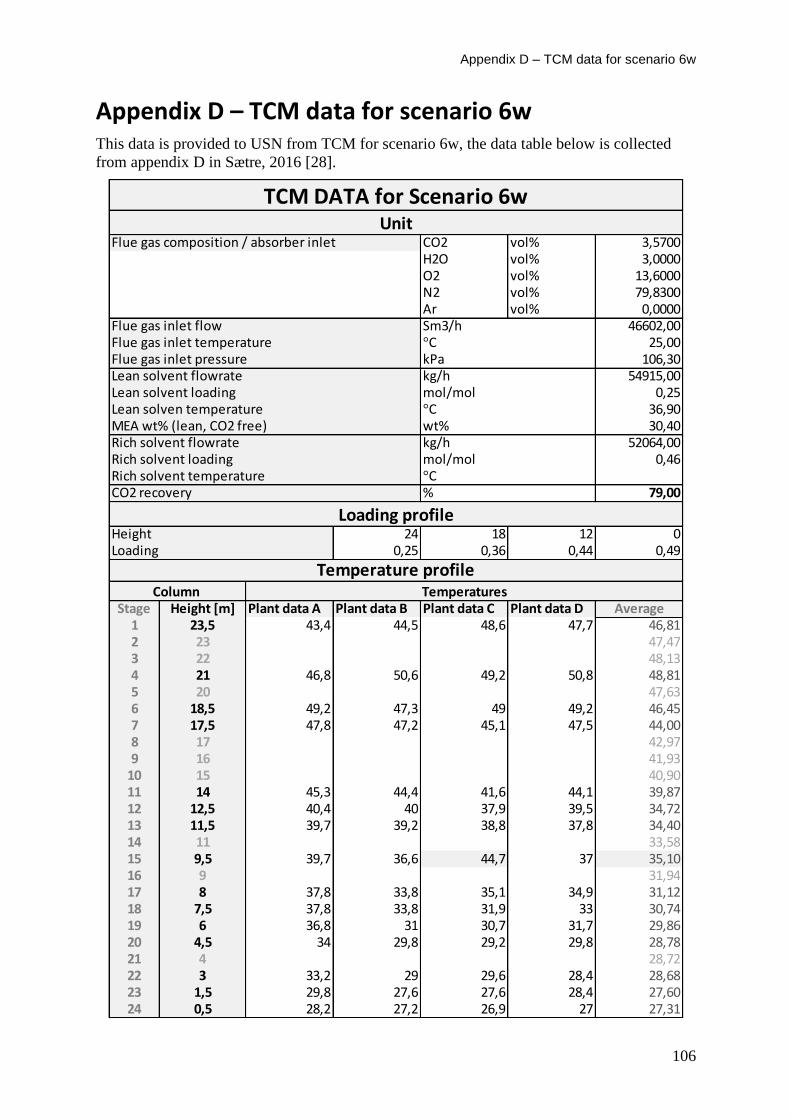
Appendix D – TCM data for scenario 6w
106
Appendix D – TCM data for scenario 6w This data is provided to USN from TCM for scenario 6w, the data table below is collected
from appendix D in Sætre, 2016 [28].
CO2 vol% 3,5700H2O vol% 3,0000O2 vol% 13,6000N2 vol% 79,8300Ar vol% 0,0000
Flue gas inlet flow Sm3/h 46602,00Flue gas inlet temperature °C 25,00Flue gas inlet pressure kPa 106,30Lean solvent flowrate kg/h 54915,00Lean solvent loading mol/mol 0,25Lean solven temperature °C 36,90MEA wt% (lean, CO2 free) wt% 30,40Rich solvent flowrate kg/h 52064,00Rich solvent loading mol/mol 0,46Rich solvent temperature °CCO2 recovery % 79,00
Height 24 18 12 0Loading 0,25 0,36 0,44 0,49
Stage Height [m] Plant data A Plant data B Plant data C Plant data D Average1 23,5 43,4 44,5 48,6 47,7 46,812 23 47,473 22 48,134 21 46,8 50,6 49,2 50,8 48,815 20 47,636 18,5 49,2 47,3 49 49,2 46,457 17,5 47,8 47,2 45,1 47,5 44,008 17 42,979 16 41,93
10 15 40,9011 14 45,3 44,4 41,6 44,1 39,8712 12,5 40,4 40 37,9 39,5 34,7213 11,5 39,7 39,2 38,8 37,8 34,4014 11 33,5815 9,5 39,7 36,6 44,7 37 35,1016 9 31,9417 8 37,8 33,8 35,1 34,9 31,1218 7,5 37,8 33,8 31,9 33 30,7419 6 36,8 31 30,7 31,7 29,8620 4,5 34 29,8 29,2 29,8 28,7821 4 28,7222 3 33,2 29 29,6 28,4 28,6823 1,5 29,8 27,6 27,6 28,4 27,6024 0,5 28,2 27,2 26,9 27 27,31
TCM DATA for Scenario 6w
Loading profile
Temperature profileColumn Temperatures
UnitFlue gas composition / absorber inlet
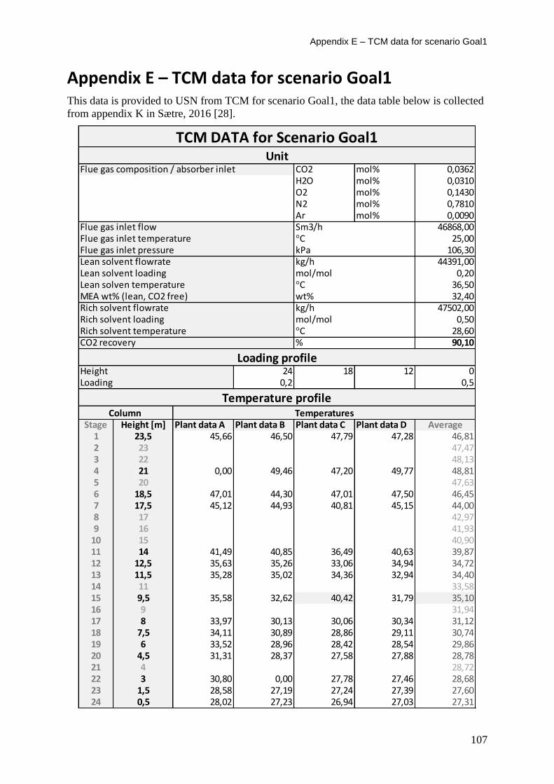
Appendix E – TCM data for scenario Goal1
107
Appendix E – TCM data for scenario Goal1 This data is provided to USN from TCM for scenario Goal1, the data table below is collected
from appendix K in Sætre, 2016 [28].
CO2 mol% 0,0362H2O mol% 0,0310O2 mol% 0,1430N2 mol% 0,7810Ar mol% 0,0090
Flue gas inlet flow Sm3/h 46868,00Flue gas inlet temperature °C 25,00Flue gas inlet pressure kPa 106,30Lean solvent flowrate kg/h 44391,00Lean solvent loading mol/mol 0,20Lean solven temperature °C 36,50MEA wt% (lean, CO2 free) wt% 32,40Rich solvent flowrate kg/h 47502,00Rich solvent loading mol/mol 0,50Rich solvent temperature °C 28,60CO2 recovery % 90,10
Height 24 18 12 0Loading 0,2 0,5
Stage Height [m] Plant data A Plant data B Plant data C Plant data D Average1 23,5 45,66 46,50 47,79 47,28 46,812 23 47,473 22 48,134 21 0,00 49,46 47,20 49,77 48,815 20 47,636 18,5 47,01 44,30 47,01 47,50 46,457 17,5 45,12 44,93 40,81 45,15 44,008 17 42,979 16 41,93
10 15 40,9011 14 41,49 40,85 36,49 40,63 39,8712 12,5 35,63 35,26 33,06 34,94 34,7213 11,5 35,28 35,02 34,36 32,94 34,4014 11 33,5815 9,5 35,58 32,62 40,42 31,79 35,1016 9 31,9417 8 33,97 30,13 30,06 30,34 31,1218 7,5 34,11 30,89 28,86 29,11 30,7419 6 33,52 28,96 28,42 28,54 29,8620 4,5 31,31 28,37 27,58 27,88 28,7821 4 28,7222 3 30,80 0,00 27,78 27,46 28,6823 1,5 28,58 27,19 27,24 27,39 27,6024 0,5 28,02 27,23 26,94 27,03 27,31
TCM DATA for Scenario Goal1Unit
Flue gas composition / absorber inlet
Loading profile
Temperature profileColumn Temperatures
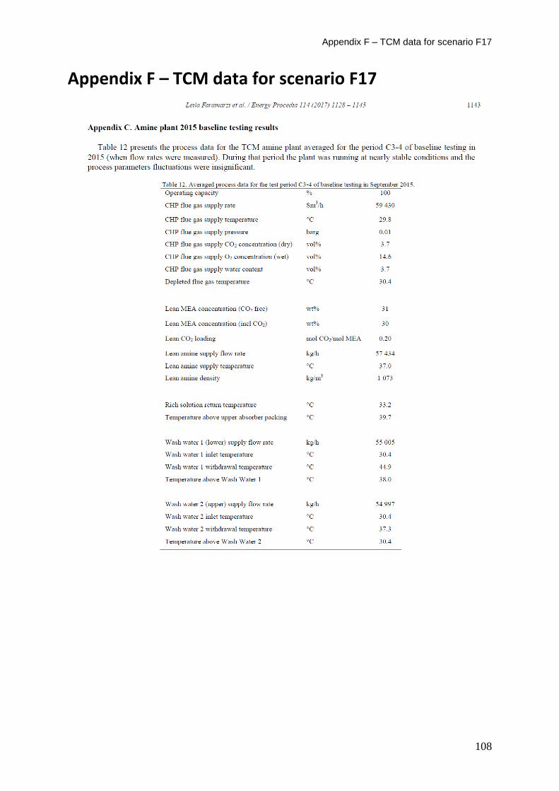
Appendix F – TCM data for scenario F17
108
Appendix F – TCM data for scenario F17
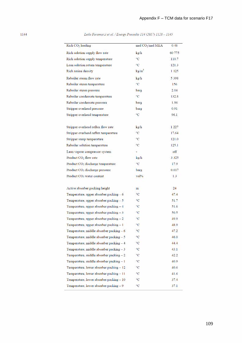
Appendix F – TCM data for scenario F17
109
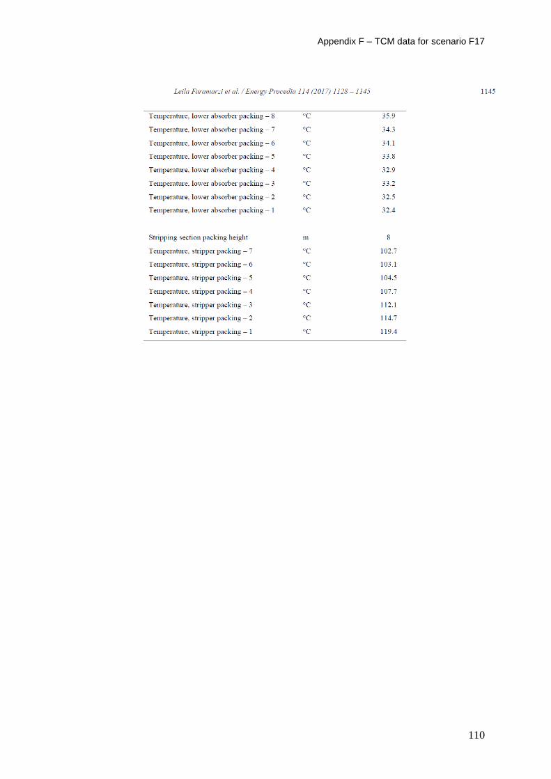
Appendix F – TCM data for scenario F17
110
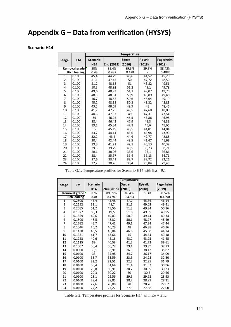
Appendix G – Data from verification (HYSYS)
111
Appendix G – Data from verification (HYSYS)
Scenario H14
Table G.1: Temperature profiles for Scenario H14 with EM = 0.1
Table G.2: Temperature profiles for Scenario H14 with EM = Zhu
Scenario
H14 Zhu (2015)
Sætre
(2016)
Røsvik
(2018)
Fagerheim
(2019)90% 89.4% 89.3% 89.3% 88.42%0.48 0.487 0.478 - 0.4885
1 0.100 45,4 44,29 46,6 44,52 45,202 0.100 51,1 47,45 50 47,72 48,503 0.100 51,2 48,58 51 48,82 49,564 0.100 50,3 48,92 51,2 49,1 49,795 0.100 49,6 48,93 51,1 49,07 49,706 0.100 48,5 48,81 50,9 48,89 49,487 0.100 46,7 48,62 50,6 48,64 49,198 0.100 45,2 48,38 50,3 48,32 48,859 0.100 43,5 48,09 49,9 48 48,46
10 0.100 41,7 47,75 49,5 47,68 48,0311 0.100 40,6 47,37 49 47,31 47,5412 0.100 39 46,92 48,5 46,86 46,9813 0.100 38,4 46,42 47,9 46,3 46,3614 0.100 39,1 45,84 47,3 45,6 45,6515 0.100 35 45,19 46,5 44,81 44,8416 0.100 33,7 44,41 45,6 43,94 43,9317 0.100 32,2 43,5 44,6 42,77 42,8818 0.100 30,4 42,44 43,5 41,47 41,6919 0.100 29,8 41,21 42,1 40,13 40,3220 0.100 29,3 39,79 40,5 38,73 38,7121 0.100 28,1 38,06 38,6 37,1 36,8622 0.100 28,4 35,97 36,4 35,13 34,7123 0.100 27,6 33,41 33,7 32,72 32,2624 0.100 27,2 30,26 30,4 29,84 29,48
Removal gradeRich loading
EMStage
Temperature
Scenario
H14 Zhu (2015)
Sætre
(2016)
Røsvik
(2018)
Fagerheim
(2019)90% 89.39% 89.4% 89.3% 88.57%0.48 0.4789 0.4784 - 0.4890
1 0.2300 45,4 45,48 47,7 45,66 46,142 0.2192 51,1 48,7 51,1 49,02 49,413 0.2085 51,2 49,56 51,8 49,94 50,164 0.1977 50,3 49,5 51,6 49,89 49,955 0.1869 49,6 49,03 50,9 49,44 49,346 0.1800 48,5 48,32 50,1 48,77 48,497 0.1762 46,7 47,41 49,1 47,94 47,448 0.1546 45,2 46,29 48 46,98 46,169 0.1438 43,5 45,04 46,6 45,88 44,74
10 0.1331 41,7 43,66 45 44,64 43,1811 0.1223 40,6 42,18 43,2 43,25 41,4512 0.1115 39 40,53 41,2 41,72 39,6113 0.1007 38,4 38,77 39,1 39,99 37,7314 0.0900 39,1 36,91 36,9 38,12 35,8715 0.0100 35 34,98 34,7 36,17 34,0916 0.0100 33,7 33,59 33,3 34,23 32,8017 0.0100 32,2 32,51 32,2 32,85 31,7918 0.0100 30,4 31,64 31,4 31,82 30,9619 0.0100 29,8 30,91 30,7 30,99 30,2320 0.0100 29,3 30,22 30 30,3 29,5621 0.0100 28,1 29,56 29,3 29,65 28,9322 0.0100 28,4 28,85 28,7 28,99 28,3123 0.0100 27,6 28,08 28 28,26 27,6724 0.0100 27,2 27,22 27,3 27,38 27,00
Removal gradeRich loading
Stage EM
Temperature
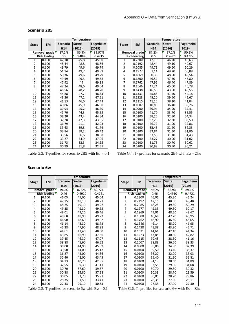
Appendix G – Data from verification (HYSYS)
112
Scenario 2B5
Table G.3: T-profiles for scenario 2B5 with EM = 0.1 Table G.4: T- profiles for scenario 2B5 with EM = Zhu
Scenario 6w
Table G.5: T-profiles for scenario 6w with EM = 0.1 Table G.6: T- profiles for scenario 6w with EM = Zhu
Scenario
H14
Sætre
(2016)
Fagerheim
(2019)87,2% 86.9% 89,97%
0.5 0,4893 0.47151 0.100 47,10 45,8 45,802 0.100 48,44 48,8 48,863 0.100 49,79 49,6 49,744 0.100 51,14 49,7 49,895 0.100 50,36 49,6 49,796 0.100 49,59 49,3 49,587 0.100 47,92 49 49,338 0.100 47,24 48,6 49,049 0.100 46,56 48,2 48,70
10 0.100 45,88 47,7 48,3311 0.100 45,20 47,2 47,9112 0.100 41,13 46,6 47,4313 0.100 40,86 45,9 46,9014 0.100 39,94 45,2 46,3015 0.100 41,70 44,3 45,6216 0.100 38,20 43,4 44,8417 0.100 37,28 42,3 43,9518 0.100 36,79 41,1 42,9319 0.100 35,43 39,8 41,7620 0.100 33,84 38,2 40,4221 0.100 33,56 36,6 38,8822 0.100 33,27 34,9 37,0623 0.100 31,73 33,3 34,9524 0.100 30,99 31,8 32,51
Removal gradeRich loading
Stage EM
TemperatureScenario
H14
Sætre
(2016)
Fagerheim
(2019)87,2% 87,2% 90,2%
0.5 0.4901 0,47221 0.2300 47,10 46,20 46,632 0.2192 48,44 49,10 49,673 0.2085 49,79 49,60 50,294 0.1977 51,14 49,20 50,085 0.1869 50,36 48,50 49,546 0.1800 49,59 47,50 48,807 0.1762 47,92 46,40 47,898 0.1546 47,24 45,00 46,789 0.1438 46,56 43,50 45,55
10 0.1331 45,88 41,70 44,1811 0.1223 45,20 39,90 42,6712 0.1115 41,13 38,10 41,0413 0.1007 40,86 36,40 39,2614 0.0900 39,94 34,90 37,4115 0.0100 41,70 33,70 35,5516 0.0100 38,20 32,90 34,3417 0.0100 37,28 32,30 33,5018 0.0100 36,79 31,90 32,8619 0.0100 35,43 31,60 32,3320 0.0100 33,84 31,30 31,8621 0.0100 33,56 31,10 31,4322 0.0100 33,27 30,90 31,0223 0.0100 31,73 30,70 30,6224 0.0100 30,99 30,50 30,21
Rich loading
Stage EM
Temperature
Removal grade
Scenario
H14
Sætre
(2016)
Fagerheim
(2019)79,0% 87,0% 89,72%0,46 0,4920 0.4721
1 0.100 46,05 45,00 45,042 0.100 47,15 48,10 48,213 0.100 48,25 49,10 49,274 0.100 49,35 49,30 49,525 0.100 49,01 49,20 49,466 0.100 48,68 48,90 49,277 0.100 46,90 48,60 49,028 0.100 46,14 48,30 48,729 0.100 45,38 47,90 48,38
10 0.100 44,61 47,40 48,0011 0.100 43,85 46,90 47,5612 0.100 39,45 46,30 47,0713 0.100 38,88 45,60 46,5214 0.100 38,00 44,90 45,8915 0.100 39,50 44,00 45,1716 0.100 36,27 43,00 44,3617 0.100 35,40 42,00 43,4318 0.100 34,13 40,70 42,3519 0.100 32,55 39,30 41,1120 0.100 30,70 37,60 39,6721 0.100 30,38 35,80 37,9822 0.100 30,05 33,70 35,9123 0.100 28,35 31,50 33,4124 0.100 27,33 29,10 30,33
Removal gradeRich loading
Stage EM
TemperatureScenario
H14
Sætre
(2016)
Fagerheim
(2019)79,0% 86,9% 89,6%0,46 0.4910 0,4721
1 0.2300 46,05 45,80 46,242 0.2192 47,15 48,80 49,483 0.2085 48,25 49,50 50,294 0.1977 49,35 49,30 50,175 0.1869 49,01 48,60 49,676 0.1800 48,68 47,70 48,957 0.1762 46,90 46,60 48,058 0.1546 46,14 45,20 46,959 0.1438 45,38 43,80 45,71
10 0.1331 44,61 42,10 44,3411 0.1223 43,85 40,30 42,8212 0.1115 39,45 38,50 41,1613 0.1007 38,88 36,60 39,3314 0.0900 38,00 34,90 37,3915 0.0100 39,50 33,40 35,3716 0.0100 36,27 32,20 33,9317 0.0100 35,40 31,30 32,8118 0.0100 34,13 30,60 31,8919 0.0100 32,55 29,90 31,0820 0.0100 30,70 29,30 30,3221 0.0100 30,38 28,70 29,5922 0.0100 30,05 28,20 28,8623 0.0100 28,35 27,60 28,1124 0.0100 27,33 27,00 27,30
Removal gradeRich loading
Stage EM
Temperature
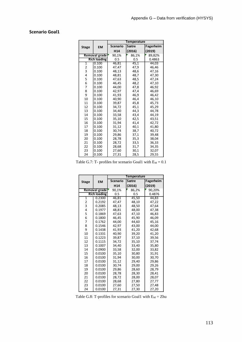
Appendix G – Data from verification (HYSYS)
113
Scenario Goal1
Table G.7: T- profiles for scenario Goal1 with EM = 0.1
Table G.8: T-profiles for scenario Goal1 with EM = Zhu
Scenario
H14
Sætre
(2016)
Fagerheim
(2019)90,1% 86,1% 89,82%
0.5 0.5 0.48631 0.100 46,81 45,1 44,032 0.100 47,47 47,9 46,463 0.100 48,13 48,6 47,164 0.100 48,81 48,7 47,305 0.100 47,63 48,5 47,246 0.100 46,45 48,2 47,107 0.100 44,00 47,8 46,928 0.100 42,97 47,4 46,699 0.100 41,93 46,9 46,42
10 0.100 40,90 46,4 46,1011 0.100 39,87 45,8 45,7312 0.100 34,72 45,1 45,2913 0.100 34,40 44,3 44,7814 0.100 33,58 43,4 44,1915 0.100 35,10 42,5 43,5116 0.100 31,94 41,4 42,7217 0.100 31,12 40,1 41,8018 0.100 30,74 38,7 40,7219 0.100 29,86 37,1 39,4820 0.100 28,78 35,3 38,0421 0.100 28,72 33,5 36,3322 0.100 28,68 31,7 34,3523 0.100 27,60 30,1 32,0724 0.100 27,31 28,5 29,55
Removal gradeRich loading
Stage EM
Temperature
Scenario
H14
Sætre
(2016)
Fagerheim
(2019)90,1% 86,2% 90,20%
0.5 0.5 0.48761 0.2300 46,81 45,50 44,832 0.2192 47,47 48,10 47,223 0.2085 48,13 48,50 47,644 0.1977 48,81 48,00 47,385 0.1869 47,63 47,10 46,836 0.1800 46,45 45,90 46,097 0.1762 44,00 44,60 45,168 0.1546 42,97 43,00 44,009 0.1438 41,93 41,20 42,68
10 0.1331 40,90 39,20 41,2011 0.1223 39,87 37,10 39,5612 0.1115 34,72 35,10 37,7413 0.1007 34,40 33,40 35,8014 0.0900 33,58 32,00 33,8215 0.0100 35,10 30,80 31,9116 0.0100 31,94 30,00 30,7017 0.0100 31,12 29,40 29,8618 0.0100 30,74 29,00 29,2619 0.0100 29,86 28,60 28,7920 0.0100 28,78 28,30 28,4121 0.0100 28,72 28,00 28,0722 0.0100 28,68 27,80 27,7723 0.0100 27,60 27,50 27,4824 0.0100 27,31 27,30 27,20
Removal gradeRich loading
Stage EM
Temperature
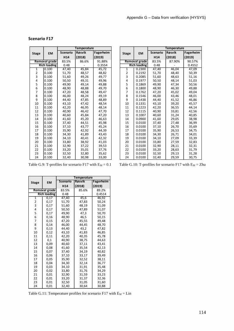
Appendix G – Data from verification (HYSYS)
114
Scenario F17
Table G.9: T-profiles for scenario F17 with EM = 0.1 Table G.10: T-profiles for scenario F17 with EM = Zhu
Table G.11: Temperature profiles for scenario F17 with EM = Lin
Scenario
H14
Røsvik
(2018)
Fagerheim
(2019)83.5% 86.6% 91.88%0.48 - 0.3554
1 0.100 47,40 45,84 45,722 0.100 51,70 48,57 48,823 0.100 51,60 49,26 49,774 0.100 50,50 49,31 49,965 0.100 49,90 49,14 49,886 0.100 48,90 48,88 49,707 0.100 47,20 48,58 49,478 0.100 46,00 48,24 49,199 0.100 44,40 47,85 48,89
10 0.100 43,10 47,42 48,5411 0.100 42,20 46,95 48,1412 0.100 40,90 46,42 47,7013 0.100 40,60 45,84 47,2014 0.100 41,60 45,20 46,6315 0.100 37,40 44,51 45,9816 0.100 37,10 43,77 45,2417 0.100 35,90 42,92 44,3918 0.100 34,30 41,89 43,4319 0.100 34,10 40,41 42,3220 0.100 33,80 38,92 41,0321 0.100 32,90 37,22 39,5322 0.100 33,20 35,01 37,7623 0.100 32,50 32,80 35,6224 0.100 32,40 30,98 33,00
Removal gradeRich loading
Stage EM
TemperatureScenario
H14
Røsvik
(2018)
Fagerheim
(2019)83.5% 87.90% 90.57%0.48 - 0.4552
1 0.2300 47,40 46,04 47,092 0.2192 51,70 48,40 50,393 0.2085 51,60 48,63 51,164 0.1977 50,50 48,14 51,035 0.1869 49,90 47,34 50,566 0.1800 48,90 46,30 49,887 0.1762 47,20 45,02 49,048 0.1546 46,00 43,46 48,019 0.1438 44,40 41,52 46,86
10 0.1331 43,10 39,20 45,5711 0.1223 42,20 36,55 44,1412 0.1115 40,90 33,81 42,5613 0.1007 40,60 31,24 40,8514 0.0900 41,60 29,05 38,9815 0.0100 37,40 27,48 36,9916 0.0100 37,10 26,70 35,6917 0.0100 35,90 26,53 34,7518 0.0100 34,30 26,71 34,0119 0.0100 34,10 27,09 33,3920 0.0100 33,80 27,59 32,8321 0.0100 32,90 28,11 32,3122 0.0100 33,20 28,63 31,7923 0.0100 32,50 29,13 31,2824 0.0100 32,40 29,59 30,75
Removal gradeRich loading
Stage EM
Temperature
Scenario
H14
Røsvik
(2018)
Fagerheim
(2019)83.5% 85.6% 89.2%0.48 - 0.4514
1 0,17 47,40 45,6 46,922 0,17 51,70 47,83 50,243 0,17 51,60 48,19 51,094 0,17 50,50 47,89 51,075 0,17 49,90 47,3 50,706 0,16 48,90 46,5 50,157 0,15 47,20 45,55 49,488 0,14 46,00 44,45 48,709 0,13 44,40 43,2 47,82
10 0,12 43,10 41,83 46,8511 0,11 42,20 40,35 45,7812 0,1 40,90 38,75 44,6313 0,09 40,60 37,11 43,4114 0,08 41,60 35,54 42,1315 0,07 37,40 34,19 40,8216 0,06 37,10 33,17 39,4917 0,05 35,90 32,52 38,1118 0,04 34,30 32,14 36,7719 0,03 34,10 31,91 35,4820 0,02 33,80 31,76 34,2921 0,01 32,90 31,59 33,2322 0,01 33,20 31,37 32,3623 0,01 32,50 31,05 31,6024 0,01 32,40 30,64 30,88
Stage EM
Temperature
Removal gradeRich loading
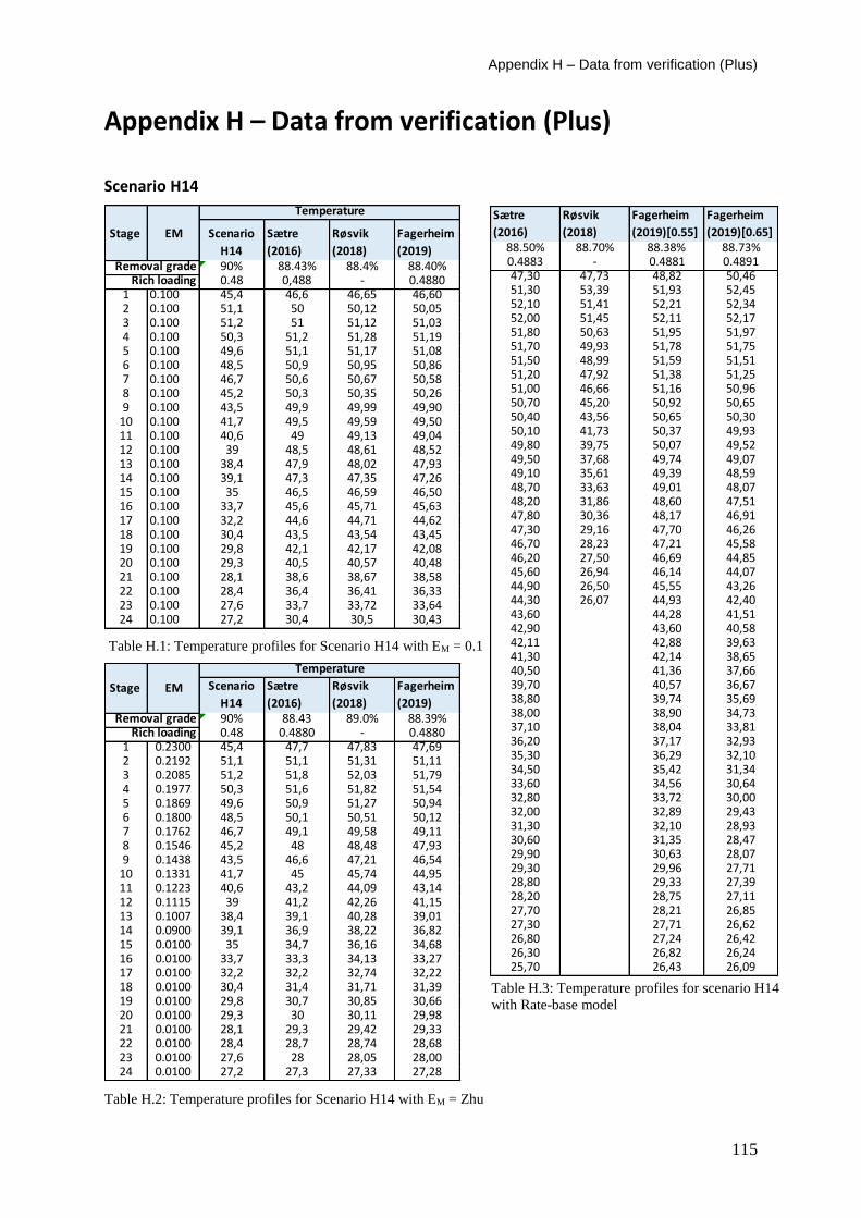
Appendix H – Data from verification (Plus)
115
Sætre
(2016)
Røsvik
(2018)
Fagerheim
(2019)[0.55]
Fagerheim
(2019)[0.65]88.50% 88.70% 88.38% 88.73%0.4883 - 0.4881 0.489147,30 47,73 48,82 50,4651,30 53,39 51,93 52,4552,10 51,41 52,21 52,3452,00 51,45 52,11 52,1751,80 50,63 51,95 51,9751,70 49,93 51,78 51,7551,50 48,99 51,59 51,5151,20 47,92 51,38 51,2551,00 46,66 51,16 50,9650,70 45,20 50,92 50,6550,40 43,56 50,65 50,3050,10 41,73 50,37 49,9349,80 39,75 50,07 49,5249,50 37,68 49,74 49,0749,10 35,61 49,39 48,5948,70 33,63 49,01 48,0748,20 31,86 48,60 47,5147,80 30,36 48,17 46,9147,30 29,16 47,70 46,2646,70 28,23 47,21 45,5846,20 27,50 46,69 44,8545,60 26,94 46,14 44,0744,90 26,50 45,55 43,2644,30 26,07 44,93 42,4043,60 44,28 41,5142,90 43,60 40,5842,11 42,88 39,6341,30 42,14 38,6540,50 41,36 37,6639,70 40,57 36,6738,80 39,74 35,6938,00 38,90 34,7337,10 38,04 33,8136,20 37,17 32,9335,30 36,29 32,1034,50 35,42 31,3433,60 34,56 30,6432,80 33,72 30,0032,00 32,89 29,4331,30 32,10 28,9330,60 31,35 28,4729,90 30,63 28,0729,30 29,96 27,7128,80 29,33 27,3928,20 28,75 27,1127,70 28,21 26,8527,30 27,71 26,6226,80 27,24 26,4226,30 26,82 26,2425,70 26,43 26,09
Table H.3: Temperature profiles for scenario H14
with Rate-base model
Table H.3: Temperature
profiles for scenario H14
with Rate-base model
Table H.3: Temperature
profiles for scenario H14
with Rate-base model
Table H.3: Temperature
Appendix H – Data from verification (Plus)
Scenario H14
Table H.1: Temperature profiles for Scenario H14 with EM = 0.1
Table H.2: Temperature profiles for Scenario H14 with EM = Zhu
Scenario
H14
Sætre
(2016)
Røsvik
(2018)
Fagerheim
(2019)90% 88.43% 88.4% 88.40%0.48 0,488 - 0.4880
1 0.100 45,4 46,6 46,65 46,602 0.100 51,1 50 50,12 50,053 0.100 51,2 51 51,12 51,034 0.100 50,3 51,2 51,28 51,195 0.100 49,6 51,1 51,17 51,086 0.100 48,5 50,9 50,95 50,867 0.100 46,7 50,6 50,67 50,588 0.100 45,2 50,3 50,35 50,269 0.100 43,5 49,9 49,99 49,90
10 0.100 41,7 49,5 49,59 49,5011 0.100 40,6 49 49,13 49,0412 0.100 39 48,5 48,61 48,5213 0.100 38,4 47,9 48,02 47,9314 0.100 39,1 47,3 47,35 47,2615 0.100 35 46,5 46,59 46,5016 0.100 33,7 45,6 45,71 45,6317 0.100 32,2 44,6 44,71 44,6218 0.100 30,4 43,5 43,54 43,4519 0.100 29,8 42,1 42,17 42,0820 0.100 29,3 40,5 40,57 40,4821 0.100 28,1 38,6 38,67 38,5822 0.100 28,4 36,4 36,41 36,3323 0.100 27,6 33,7 33,72 33,6424 0.100 27,2 30,4 30,5 30,43
Stage EM
Temperature
Removal gradeRich loading
Scenario
H14
Sætre
(2016)
Røsvik
(2018)
Fagerheim
(2019)90% 88.43 89.0% 88.39%0.48 0.4880 - 0.4880
1 0.2300 45,4 47,7 47,83 47,692 0.2192 51,1 51,1 51,31 51,113 0.2085 51,2 51,8 52,03 51,794 0.1977 50,3 51,6 51,82 51,545 0.1869 49,6 50,9 51,27 50,946 0.1800 48,5 50,1 50,51 50,127 0.1762 46,7 49,1 49,58 49,118 0.1546 45,2 48 48,48 47,939 0.1438 43,5 46,6 47,21 46,54
10 0.1331 41,7 45 45,74 44,9511 0.1223 40,6 43,2 44,09 43,1412 0.1115 39 41,2 42,26 41,1513 0.1007 38,4 39,1 40,28 39,0114 0.0900 39,1 36,9 38,22 36,8215 0.0100 35 34,7 36,16 34,6816 0.0100 33,7 33,3 34,13 33,2717 0.0100 32,2 32,2 32,74 32,2218 0.0100 30,4 31,4 31,71 31,3919 0.0100 29,8 30,7 30,85 30,6620 0.0100 29,3 30 30,11 29,9821 0.0100 28,1 29,3 29,42 29,3322 0.0100 28,4 28,7 28,74 28,6823 0.0100 27,6 28 28,05 28,0024 0.0100 27,2 27,3 27,33 27,28
Removal gradeRich loading
Stage EM
Temperature
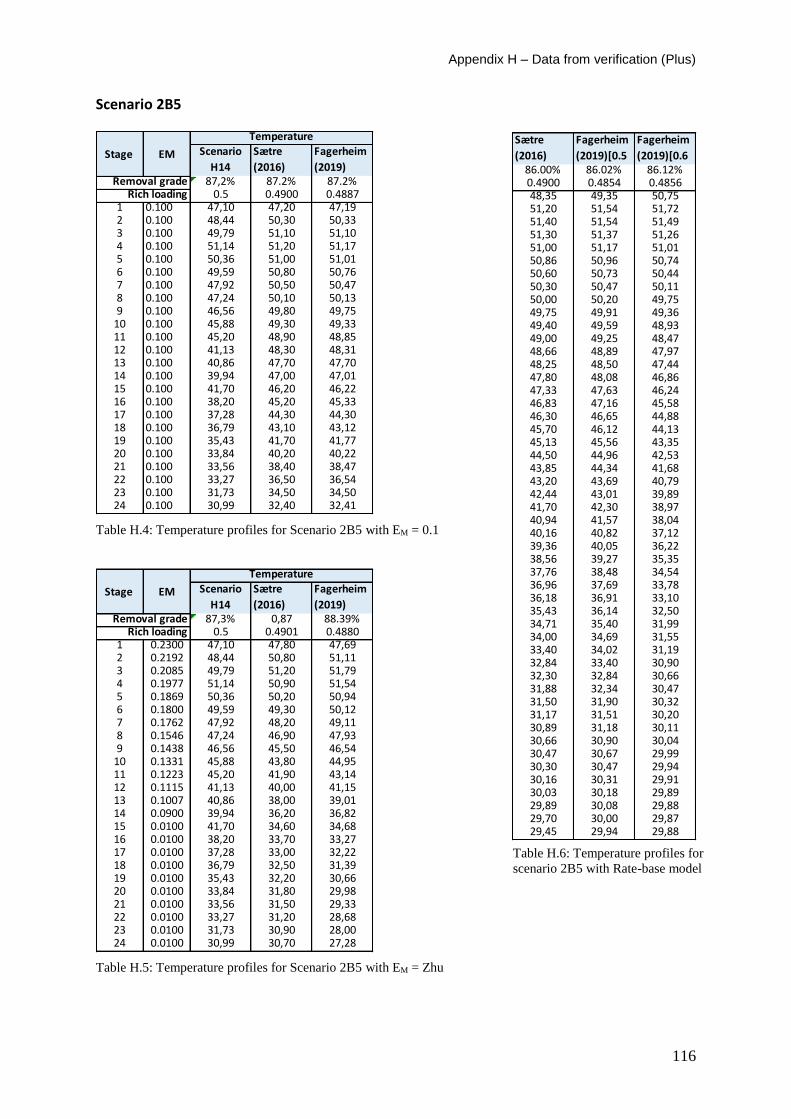
Appendix H – Data from verification (Plus)
116
Table H.6: Temperature profiles for
scenario 2B5 with Rate-base model
Table H.6:
Temperature
profiles for
scenario 2B5 with
Rate-base model
Table H.6:
Temperature
profiles for
scenario 2B5 with
Rate-base model
Table H.6:
Scenario 2B5
Table H.4: Temperature profiles for Scenario 2B5 with EM = 0.1
Table H.5: Temperature profiles for Scenario 2B5 with EM = Zhu
Scenario
H14
Sætre
(2016)
Fagerheim
(2019)87,2% 87.2% 87.2%
0.5 0.4900 0.48871 0.100 47,10 47,20 47,192 0.100 48,44 50,30 50,333 0.100 49,79 51,10 51,104 0.100 51,14 51,20 51,175 0.100 50,36 51,00 51,016 0.100 49,59 50,80 50,767 0.100 47,92 50,50 50,478 0.100 47,24 50,10 50,139 0.100 46,56 49,80 49,75
10 0.100 45,88 49,30 49,3311 0.100 45,20 48,90 48,8512 0.100 41,13 48,30 48,3113 0.100 40,86 47,70 47,7014 0.100 39,94 47,00 47,0115 0.100 41,70 46,20 46,2216 0.100 38,20 45,20 45,3317 0.100 37,28 44,30 44,3018 0.100 36,79 43,10 43,1219 0.100 35,43 41,70 41,7720 0.100 33,84 40,20 40,2221 0.100 33,56 38,40 38,4722 0.100 33,27 36,50 36,5423 0.100 31,73 34,50 34,5024 0.100 30,99 32,40 32,41
Stage EM
Temperature
Removal gradeRich loading
Scenario
H14
Sætre
(2016)
Fagerheim
(2019)87,3% 0,87 88.39%
0.5 0.4901 0.48801 0.2300 47,10 47,80 47,692 0.2192 48,44 50,80 51,113 0.2085 49,79 51,20 51,794 0.1977 51,14 50,90 51,545 0.1869 50,36 50,20 50,946 0.1800 49,59 49,30 50,127 0.1762 47,92 48,20 49,118 0.1546 47,24 46,90 47,939 0.1438 46,56 45,50 46,54
10 0.1331 45,88 43,80 44,9511 0.1223 45,20 41,90 43,1412 0.1115 41,13 40,00 41,1513 0.1007 40,86 38,00 39,0114 0.0900 39,94 36,20 36,8215 0.0100 41,70 34,60 34,6816 0.0100 38,20 33,70 33,2717 0.0100 37,28 33,00 32,2218 0.0100 36,79 32,50 31,3919 0.0100 35,43 32,20 30,6620 0.0100 33,84 31,80 29,9821 0.0100 33,56 31,50 29,3322 0.0100 33,27 31,20 28,6823 0.0100 31,73 30,90 28,0024 0.0100 30,99 30,70 27,28
Rich loading
Stage EM
Temperature
Removal grade
Sætre
(2016)
Fagerheim
(2019)[0.5
Fagerheim
(2019)[0.686.00% 86.02% 86.12%0.4900 0.4854 0.485648,35 49,35 50,7551,20 51,54 51,7251,40 51,54 51,4951,30 51,37 51,2651,00 51,17 51,0150,86 50,96 50,7450,60 50,73 50,4450,30 50,47 50,1150,00 50,20 49,7549,75 49,91 49,3649,40 49,59 48,9349,00 49,25 48,4748,66 48,89 47,9748,25 48,50 47,4447,80 48,08 46,8647,33 47,63 46,2446,83 47,16 45,5846,30 46,65 44,8845,70 46,12 44,1345,13 45,56 43,3544,50 44,96 42,5343,85 44,34 41,6843,20 43,69 40,7942,44 43,01 39,8941,70 42,30 38,9740,94 41,57 38,0440,16 40,82 37,1239,36 40,05 36,2238,56 39,27 35,3537,76 38,48 34,5436,96 37,69 33,7836,18 36,91 33,1035,43 36,14 32,5034,71 35,40 31,9934,00 34,69 31,5533,40 34,02 31,1932,84 33,40 30,9032,30 32,84 30,6631,88 32,34 30,4731,50 31,90 30,3231,17 31,51 30,2030,89 31,18 30,1130,66 30,90 30,0430,47 30,67 29,9930,30 30,47 29,9430,16 30,31 29,9130,03 30,18 29,8929,89 30,08 29,8829,70 30,00 29,8729,45 29,94 29,88
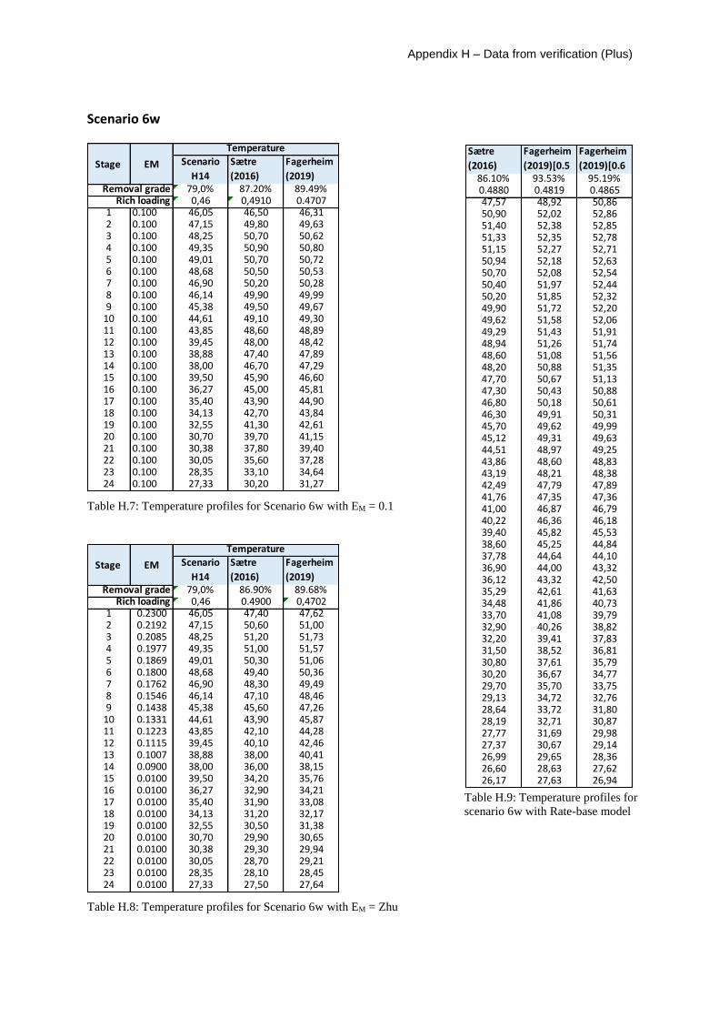
Appendix H – Data from verification (Plus)
117
Sætre
(2016)
Fagerheim
(2019)[0.5
Fagerheim
(2019)[0.686.10% 93.53% 95.19%0.4880 0.4819 0.486547,57 48,92 50,8650,90 52,02 52,8651,40 52,38 52,8551,33 52,35 52,7851,15 52,27 52,7150,94 52,18 52,6350,70 52,08 52,5450,40 51,97 52,4450,20 51,85 52,3249,90 51,72 52,2049,62 51,58 52,0649,29 51,43 51,9148,94 51,26 51,7448,60 51,08 51,5648,20 50,88 51,3547,70 50,67 51,1347,30 50,43 50,8846,80 50,18 50,6146,30 49,91 50,3145,70 49,62 49,9945,12 49,31 49,6344,51 48,97 49,2543,86 48,60 48,8343,19 48,21 48,3842,49 47,79 47,8941,76 47,35 47,3641,00 46,87 46,7940,22 46,36 46,1839,40 45,82 45,5338,60 45,25 44,8437,78 44,64 44,1036,90 44,00 43,3236,12 43,32 42,5035,29 42,61 41,6334,48 41,86 40,7333,70 41,08 39,7932,90 40,26 38,8232,20 39,41 37,8331,50 38,52 36,8130,80 37,61 35,7930,20 36,67 34,7729,70 35,70 33,7529,13 34,72 32,7628,64 33,72 31,8028,19 32,71 30,8727,77 31,69 29,9827,37 30,67 29,1426,99 29,65 28,3626,60 28,63 27,6226,17 27,63 26,94
Table H.9: Temperature profiles for
scenario 6w with Rate-base model
Scenario 6w
Table H.7: Temperature profiles for Scenario 6w with EM = 0.1
Table H.8: Temperature profiles for Scenario 6w with EM = Zhu
Scenario
H14
Sætre
(2016)
Fagerheim
(2019)79,0% 87.20% 89.49%0,46 0,4910 0.4707
1 0.100 46,05 46,50 46,312 0.100 47,15 49,80 49,633 0.100 48,25 50,70 50,624 0.100 49,35 50,90 50,805 0.100 49,01 50,70 50,726 0.100 48,68 50,50 50,537 0.100 46,90 50,20 50,288 0.100 46,14 49,90 49,999 0.100 45,38 49,50 49,67
10 0.100 44,61 49,10 49,3011 0.100 43,85 48,60 48,8912 0.100 39,45 48,00 48,4213 0.100 38,88 47,40 47,8914 0.100 38,00 46,70 47,2915 0.100 39,50 45,90 46,6016 0.100 36,27 45,00 45,8117 0.100 35,40 43,90 44,9018 0.100 34,13 42,70 43,8419 0.100 32,55 41,30 42,6120 0.100 30,70 39,70 41,1521 0.100 30,38 37,80 39,4022 0.100 30,05 35,60 37,2823 0.100 28,35 33,10 34,6424 0.100 27,33 30,20 31,27
Removal gradeRich loading
Stage EM
Temperature
Scenario
H14
Sætre
(2016)
Fagerheim
(2019)79,0% 86.90% 89.68%0,46 0.4900 0,4702
1 0.2300 46,05 47,40 47,622 0.2192 47,15 50,60 51,003 0.2085 48,25 51,20 51,734 0.1977 49,35 51,00 51,575 0.1869 49,01 50,30 51,066 0.1800 48,68 49,40 50,367 0.1762 46,90 48,30 49,498 0.1546 46,14 47,10 48,469 0.1438 45,38 45,60 47,26
10 0.1331 44,61 43,90 45,8711 0.1223 43,85 42,10 44,2812 0.1115 39,45 40,10 42,4613 0.1007 38,88 38,00 40,4114 0.0900 38,00 36,00 38,1515 0.0100 39,50 34,20 35,7616 0.0100 36,27 32,90 34,2117 0.0100 35,40 31,90 33,0818 0.0100 34,13 31,20 32,1719 0.0100 32,55 30,50 31,3820 0.0100 30,70 29,90 30,6521 0.0100 30,38 29,30 29,9422 0.0100 30,05 28,70 29,2123 0.0100 28,35 28,10 28,4524 0.0100 27,33 27,50 27,64
Removal gradeRich loading
Stage EM
Temperature
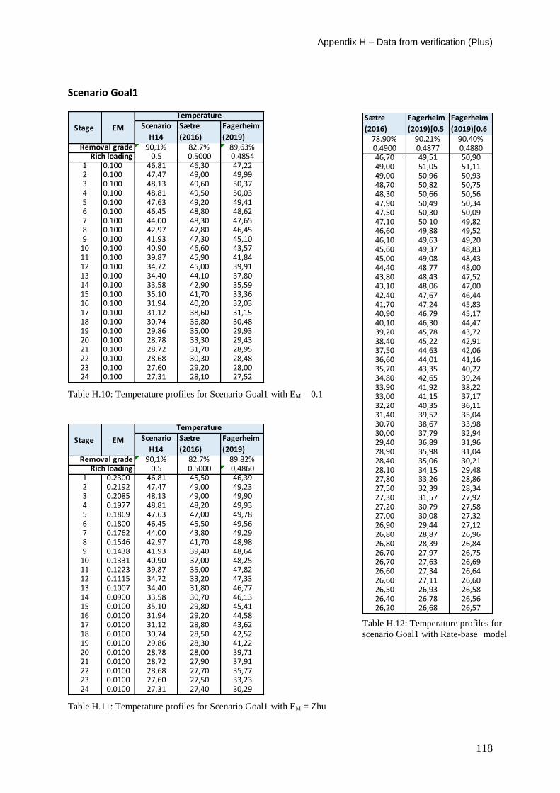
Appendix H – Data from verification (Plus)
118
Table H.12: Temperature profiles for
scenario Goal1 with Rate-base model
Sætre
(2016)
Fagerheim
(2019)[0.5
Fagerheim
(2019)[0.678.90% 90.21% 90.40%0.4900 0.4877 0.488046,70 49,51 50,9049,00 51,05 51,1149,00 50,96 50,9348,70 50,82 50,7548,30 50,66 50,5647,90 50,49 50,3447,50 50,30 50,0947,10 50,10 49,8246,60 49,88 49,5246,10 49,63 49,2045,60 49,37 48,8345,00 49,08 48,4344,40 48,77 48,0043,80 48,43 47,5243,10 48,06 47,0042,40 47,67 46,4441,70 47,24 45,8340,90 46,79 45,1740,10 46,30 44,4739,20 45,78 43,7238,40 45,22 42,9137,50 44,63 42,0636,60 44,01 41,1635,70 43,35 40,2234,80 42,65 39,2433,90 41,92 38,2233,00 41,15 37,1732,20 40,35 36,1131,40 39,52 35,0430,70 38,67 33,9830,00 37,79 32,9429,40 36,89 31,9628,90 35,98 31,0428,40 35,06 30,2128,10 34,15 29,4827,80 33,26 28,8627,50 32,39 28,3427,30 31,57 27,9227,20 30,79 27,5827,00 30,08 27,3226,90 29,44 27,1226,80 28,87 26,9626,80 28,39 26,8426,70 27,97 26,7526,70 27,63 26,6926,60 27,34 26,6426,60 27,11 26,6026,50 26,93 26,5826,40 26,78 26,5626,20 26,68 26,57
Scenario Goal1
Table H.10: Temperature profiles for Scenario Goal1 with EM = 0.1
Table H.11: Temperature profiles for Scenario Goal1 with EM = Zhu
Scenario
H14
Sætre
(2016)
Fagerheim
(2019)90,1% 82.7% 89,63%
0.5 0.5000 0.48541 0.100 46,81 46,30 47,222 0.100 47,47 49,00 49,993 0.100 48,13 49,60 50,374 0.100 48,81 49,50 50,035 0.100 47,63 49,20 49,416 0.100 46,45 48,80 48,627 0.100 44,00 48,30 47,658 0.100 42,97 47,80 46,459 0.100 41,93 47,30 45,10
10 0.100 40,90 46,60 43,5711 0.100 39,87 45,90 41,8412 0.100 34,72 45,00 39,9113 0.100 34,40 44,10 37,8014 0.100 33,58 42,90 35,5915 0.100 35,10 41,70 33,3616 0.100 31,94 40,20 32,0317 0.100 31,12 38,60 31,1518 0.100 30,74 36,80 30,4819 0.100 29,86 35,00 29,9320 0.100 28,78 33,30 29,4321 0.100 28,72 31,70 28,9522 0.100 28,68 30,30 28,4823 0.100 27,60 29,20 28,0024 0.100 27,31 28,10 27,52
Removal gradeRich loading
Stage EM
Temperature
Scenario
H14
Sætre
(2016)
Fagerheim
(2019)90,1% 82.7% 89.82%
0.5 0.5000 0,48601 0.2300 46,81 45,50 46,392 0.2192 47,47 49,00 49,233 0.2085 48,13 49,00 49,904 0.1977 48,81 48,20 49,935 0.1869 47,63 47,00 49,786 0.1800 46,45 45,50 49,567 0.1762 44,00 43,80 49,298 0.1546 42,97 41,70 48,989 0.1438 41,93 39,40 48,64
10 0.1331 40,90 37,00 48,2511 0.1223 39,87 35,00 47,8212 0.1115 34,72 33,20 47,3313 0.1007 34,40 31,80 46,7714 0.0900 33,58 30,70 46,1315 0.0100 35,10 29,80 45,4116 0.0100 31,94 29,20 44,5817 0.0100 31,12 28,80 43,6218 0.0100 30,74 28,50 42,5219 0.0100 29,86 28,30 41,2220 0.0100 28,78 28,00 39,7121 0.0100 28,72 27,90 37,9122 0.0100 28,68 27,70 35,7723 0.0100 27,60 27,50 33,2324 0.0100 27,31 27,40 30,29
Removal gradeRich loading
Stage EM
Temperature
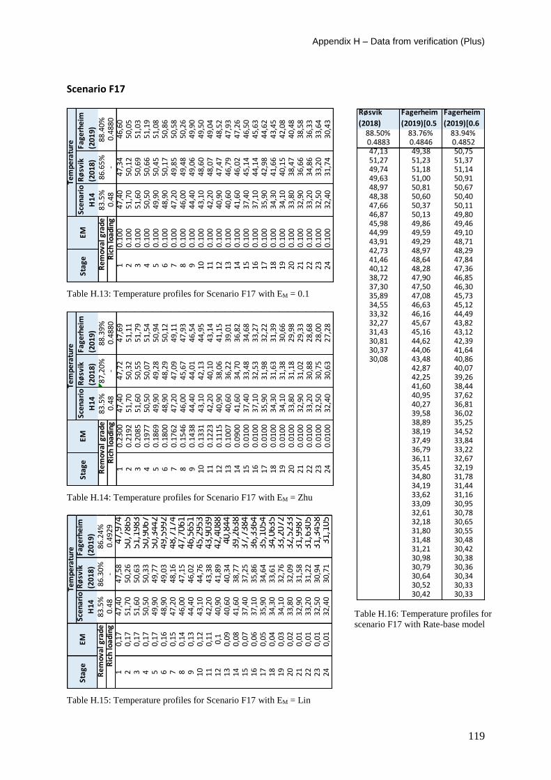
Appendix H – Data from verification (Plus)
119
Røsvik
(2018)
Fagerheim
(2019)[0.5
Fagerheim
(2019)[0.688.50% 83.76% 83.94%0.4883 0.4846 0.485247,13 49,38 50,7551,27 51,23 51,3749,74 51,18 51,1449,63 51,00 50,9148,97 50,81 50,6748,38 50,60 50,4047,66 50,37 50,1146,87 50,13 49,8045,98 49,86 49,4644,99 49,59 49,1043,91 49,29 48,7142,73 48,97 48,2941,46 48,64 47,8440,12 48,28 47,3638,72 47,90 46,8537,30 47,50 46,3035,89 47,08 45,7334,55 46,63 45,1233,32 46,16 44,4932,27 45,67 43,8231,43 45,16 43,1230,81 44,62 42,3930,37 44,06 41,6430,08 43,48 40,86
42,87 40,0742,25 39,2641,60 38,4440,95 37,6240,27 36,8139,58 36,0238,89 35,2538,19 34,5237,49 33,8436,79 33,2236,11 32,6735,45 32,1934,80 31,7834,19 31,4433,62 31,1633,09 30,9532,61 30,7832,18 30,6531,80 30,5531,48 30,4831,21 30,4230,98 30,3830,79 30,3630,64 30,3430,52 30,3330,42 30,33
Table H.16: Temperature profiles for
scenario F17 with Rate-base model
Scenario F17
Table H.13: Temperature profiles for Scenario F17 with EM = 0.1
Table H.14: Temperature profiles for Scenario F17 with EM = Zhu
Table H.15: Temperature profiles for Scenario F17 with EM = Lin
Sce
na
rio
H1
4
Rø
svik
(20
18
)
Fa
ge
rhe
im
(20
19
)8
3.5
%8
6.6
5%
88
.40
%0
.48
-0
.48
80
10
.10
04
7,4
04
7,3
44
6,6
02
0.1
00
51
,70
50
,12
50
,05
30
.10
05
1,6
05
0,6
95
1,0
34
0.1
00
50
,50
50
,66
51
,19
50
.10
04
9,9
05
0,4
55
1,0
86
0.1
00
48
,90
50
,17
50
,86
70
.10
04
7,2
04
9,8
55
0,5
88
0.1
00
46
,00
49
,48
50
,26
90
.10
04
4,4
04
9,0
64
9,9
01
00
.10
04
3,1
04
8,6
04
9,5
01
10
.10
04
2,2
04
8,0
74
9,0
41
20
.10
04
0,9
04
7,4
74
8,5
21
30
.10
04
0,6
04
6,7
94
7,9
31
40
.10
04
1,6
04
6,0
24
7,2
61
50
.10
03
7,4
04
5,1
44
6,5
01
60
.10
03
7,1
04
4,1
44
5,6
31
70
.10
03
5,9
04
2,9
84
4,6
21
80
.10
03
4,3
04
1,6
64
3,4
51
90
.10
03
4,1
04
0,1
54
2,0
82
00
.10
03
3,8
03
8,4
74
0,4
82
10
.10
03
2,9
03
6,6
63
8,5
82
20
.10
03
3,2
03
4,8
63
6,3
32
30
.10
03
2,5
03
3,2
03
3,6
42
40
.10
03
2,4
03
1,7
43
0,4
3
Re
mo
va
l gra
de
Ric
h lo
ad
ing
Sta
ge
E
M
Te
mp
era
ture
Sce
na
rio
H1
4
Rø
svik
(20
18
)
Fa
ge
rhe
im
(20
19
)8
3.5
%8
7,2
0%
88
.39
%0
.48
-0
.48
80
10
.23
00
47
,40
47
,72
47
,69
20
.21
92
51
,70
50
,32
51
,11
30
.20
85
51
,60
50
,55
51
,79
40
.19
77
50
,50
50
,07
51
,54
50
.18
69
49
,90
49
,28
50
,94
60
.18
00
48
,90
48
,29
50
,12
70
.17
62
47
,20
47
,09
49
,11
80
.15
46
46
,00
45
,67
47
,93
90
.14
38
44
,40
44
,01
46
,54
10
0.1
33
14
3,1
04
2,1
34
4,9
51
10
.12
23
42
,20
40
,10
43
,14
12
0.1
11
54
0,9
03
8,0
64
1,1
51
30
.10
07
40
,60
36
,22
39
,01
14
0.0
90
04
1,6
03
4,7
03
6,8
21
50
.01
00
37
,40
33
,48
34
,68
16
0.0
10
03
7,1
03
2,5
33
3,2
71
70
.01
00
35
,90
31
,98
32
,22
18
0.0
10
03
4,3
03
1,6
33
1,3
91
90
.01
00
34
,10
31
,38
30
,66
20
0.0
10
03
3,8
03
1,1
82
9,9
82
10
.01
00
32
,90
31
,02
29
,33
22
0.0
10
03
3,2
03
0,8
82
8,6
82
30
.01
00
32
,50
30
,75
28
,00
24
0.0
10
03
2,4
03
0,6
32
7,2
8
Re
mo
va
l gra
de
Ric
h lo
ad
ing
Sta
ge
E
M
Te
mp
era
ture
Sce
na
rio
H1
4
Rø
svik
(20
18
)
Fa
ge
rhe
im
(20
19
)8
3.5
%8
6.3
0%
86
.24
%0
.48
-0
.49
29
10
,17
47
,40
47
,58
47,9
742
0,1
75
1,7
05
0,2
650
,786
53
0,1
75
1,6
05
0,6
351
,198
34
0,1
75
0,5
05
0,3
350
,906
75
0,1
74
9,9
04
9,7
750
,344
26
0,1
64
8,9
04
9,0
349
,599
27
0,1
54
7,2
04
8,1
648
,717
48
0,1
44
6,0
04
7,1
547
,706
19
0,1
34
4,4
04
6,0
246
,565
11
00
,12
43
,10
44
,76
45,2
953
11
0,1
14
2,2
04
3,3
843
,903
91
20
,14
0,9
04
1,8
942
,408
81
30
,09
40
,60
40
,34
40,8
441
40
,08
41
,60
38
,77
39,2
638
15
0,0
73
7,4
03
7,2
537
,738
41
60
,06
37
,10
35
,86
36,3
364
17
0,0
53
5,9
03
4,6
435
,105
41
80
,04
34
,30
33
,61
34,0
635
19
0,0
33
4,1
03
2,7
633
,207
22
00
,02
33
,80
32
,09
32,5
233
21
0,0
13
2,9
03
1,5
831
,998
72
20
,01
33
,20
31
,22
31,6
305
23
0,0
13
2,5
03
0,9
431
,345
82
40
,01
32
,40
30
,71
31,1
05
Te
mp
era
ture
Re
mo
va
l gra
de
Ric
h lo
ad
ing
Sta
ge
E
M
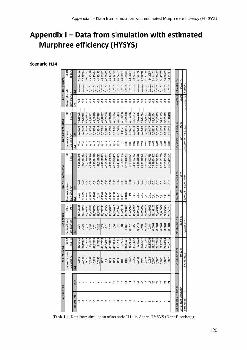
Appendix I – Data from simulation with estimated Murphree efficiency (HYSYS)
120
Appendix I – Data from simulation with estimated Murphree efficiency (HYSYS)
Scenario H14
Table I.1: Data from simulation of scenario H14 in Aspen HYSYS (Kent-Eisenberg)
Re
mo
val g
rad
e90
,12
Re
mo
val g
rad
e89
,94
Re
mo
val g
rad
e90
Re
mo
val g
rad
e90
Re
mo
val g
rad
e90
,01
Ric
h lo
adin
g0,
4936
Ric
h lo
adin
g0,
4931
Ric
h lo
adin
g0,
4933
Ric
h lo
adin
g0,
4885
Ric
h lo
adin
g0,
4427
He
igh
t (m
)St
ep
EMT
EMT
EMEM
TEM
EMT
EMEM
T
241
0,24
546
,434
230,
2446
,411
369
0,23
0,25
46,1
5531
546
0,17
0,19
703
45,1
9928
0,1
0,11
0146
,313
02
232
0,24
2549
,808
190,
235
49,7
8394
80,
2192
0,24
49,4
3573
820,
170,
1970
348
,502
330,
10,
1101
49,3
3061
223
0,24
50,5
9425
0,23
50,5
8154
20,
2085
0,23
50,1
8484
330,
170,
1970
349
,564
530,
10,
1101
50,0
1751
214
0,23
7550
,391
70,
225
50,4
0756
30,
1977
0,22
49,9
8058
266
0,17
0,19
703
49,7
8902
0,1
0,11
0149
,903
49
205
0,23
549
,722
190,
2249
,792
754
0,18
690,
2149
,366
2478
90,
170,
1970
349
,698
990,
10,
1101
49,4
7054
196
0,23
2548
,717
50,
215
48,8
8578
10,
180,
2048
,515
8092
0,16
0,18
544
49,4
7788
0,1
0,11
0148
,854
75
187
0,23
47,3
7409
0,23
47,7
0421
10,
1762
0,19
47,4
6149
473
0,15
0,17
385
49,1
8967
0,1
0,11
0148
,118
53
178
0,2
45,6
4572
0,2
46,1
0333
40,
1546
0,17
46,1
8145
711
0,14
0,16
226
48,8
5018
0,1
0,11
0147
,280
99
169
0,17
43,6
9197
0,17
44,2
5400
30,
1438
0,16
44,7
6568
279
0,13
0,15
067
48,4
6368
0,1
0,11
0146
,349
05
1510
0,14
41,6
0845
0,14
42,2
6245
50,
1331
0,15
43,2
1078
415
0,12
0,13
908
48,0
2784
0,1
0,11
0145
,327
75
1411
0,11
39,5
7541
0,11
40,2
7567
10,
1223
0,14
41,4
9319
485
0,11
0,12
749
47,5
3463
0,1
0,11
0144
,224
69
1312
0,08
37,7
206
0,08
38,4
2410
60,
1115
0,12
39,6
6731
114
0,1
0,11
5946
,982
380,
10,
1101
43,0
4981
1213
0,05
36,1
1771
0,05
536
,799
821
0,10
070,
1137
,789
5623
40,
090,
1043
146
,353
380,
10,
1101
41,8
1853
1114
0,04
7534
,796
780,
0525
35,4
2797
20,
090,
1035
,930
7012
10,
080,
0927
245
,643
060,
10,
1101
40,5
4881
1015
0,04
533
,642
820,
0534
,202
939
0,01
0,01
34,1
5152
262
0,07
0,08
113
44,8
3812
0,1
0,11
0139
,265
51
916
0,04
2532
,597
80,
0475
33,0
7911
40,
010,
0132
,855
5896
60,
060,
0695
443
,921
980,
10,
1101
37,9
3476
817
0,04
31,6
3047
0,04
532
,030
922
0,01
0,01
31,8
4359
623
0,05
0,05
795
42,8
7751
0,1
0,11
0136
,630
35
718
0,03
7530
,719
450,
0425
31,0
4559
80,
010,
0131
,003
7657
70,
040,
0463
641
,685
210,
10,
1101
35,3
7716
619
0,03
529
,852
260,
0430
,106
005
0,01
0,01
30,2
6902
753
0,03
0,03
477
40,3
2256
0,1
0,11
0134
,203
7
520
0,00
0129
,015
570,
0001
29,1
9910
50,
010,
0129
,596
6441
20,
020,
0231
838
,716
540,
10,
1101
33,1
4101
421
0,00
0128
,324
450,
0001
28,4
5505
60,
010,
0128
,957
7120
30,
010,
0115
936
,857
630,
10,
1101
32,2
2497
322
0,00
0127
,728
830,
0001
27,8
1903
80,
010,
0128
,331
5125
80,
010,
0115
934
,711
930,
10,
1101
31,4
9707
223
0,00
0127
,203
740,
0001
27,2
5963
40,
010,
0127
,689
6324
60,
010,
0115
932
,259
690,
10,
1101
30,8
7855
124
0,00
0126
,729
950,
0001
26,7
5623
70,
010,
0127
,014
3577
10,
010,
0115
929
,484
680,
10,
1101
30,3
1713
Cal
cula
ted
eff
icie
ncy
94,8
3380
484
%94
,562
9584
7%
92,4
054
94,5
7074
05%
90,9
5945
94,5
822
%92
,023
3694
,598
36%
sim
ula
ted
eff
icie
ncy
90,1
2%
89,9
4%
9090
%90
90%
90,0
190
,01
%
dif
fere
nce
4,71
3804
836
4,62
2958
470
2,40
538
4,57
0740
490
0,95
9447
4,58
2202
02,
0133
564,
5883
61
0.1
*1.1
01 (
90.0
1%)
Sce
nar
io H
14SF
2 (
89,9
4%)
SF1
(90
,12%
)Zh
u *
1.10
6 (9
0.00
%)
Lin
*1.
159
(90,
00%
)
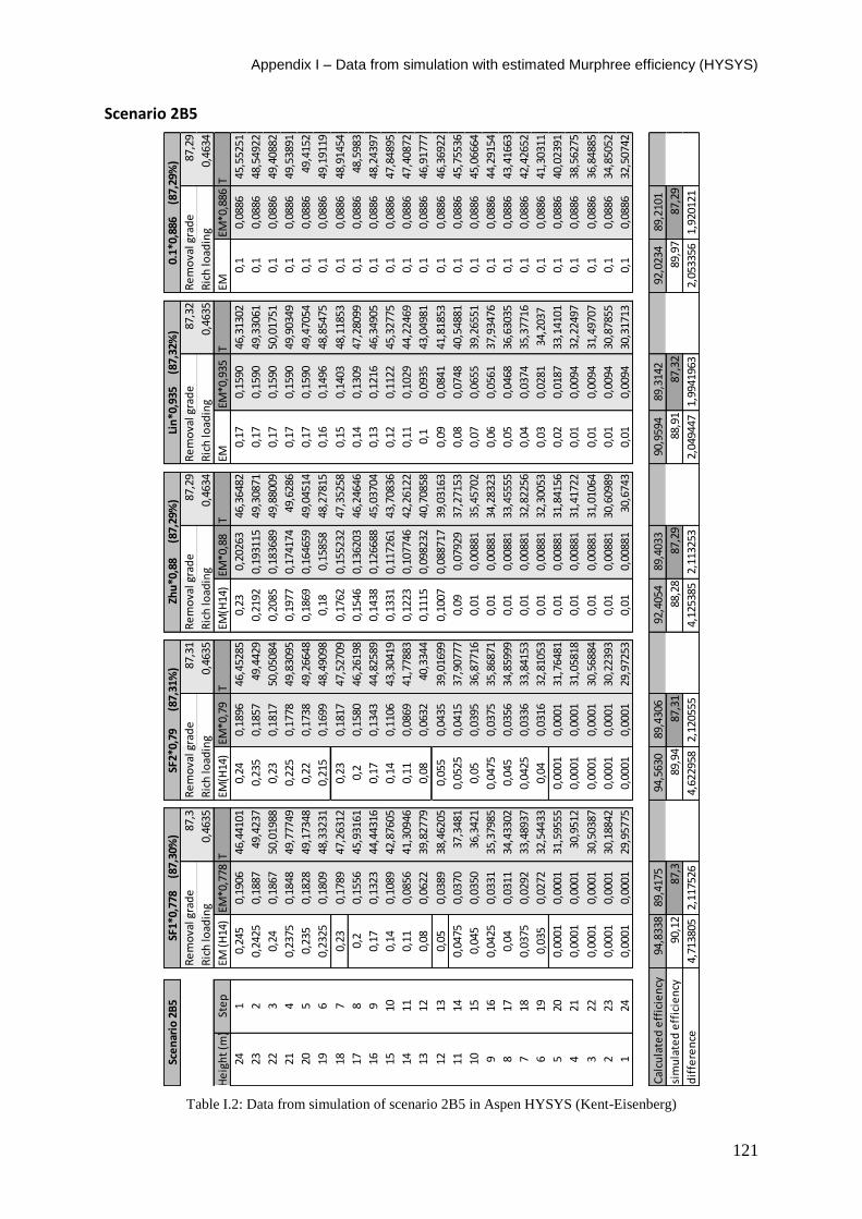
Appendix I – Data from simulation with estimated Murphree efficiency (HYSYS)
121
Scenario 2B5
Table I.2: Data from simulation of scenario 2B5 in Aspen HYSYS (Kent-Eisenberg)
Re
mo
val g
rad
e87
,3R
em
ova
l gra
de
87,3
1R
em
ova
l gra
de
87,2
9R
em
ova
l gra
de
87,3
2R
em
ova
l gra
de
87,2
9
Ric
h lo
adin
g0,
4635
Ric
h lo
adin
g0,
4635
Ric
h lo
adin
g0,
4634
Ric
h lo
adin
g0,
4635
Ric
h lo
adin
g0,
4634
He
igh
t (m
)St
ep
EM (
H14
)EM
*0,7
78T
EM(H
14)
EM*0
,79
TEM
(H14
)EM
*0,8
8T
EMEM
*0,9
35T
EMEM
*0,8
86T
241
0,24
50,
1906
46,4
4101
0,24
0,18
9646
,452
850,
230,
2026
346
,364
820,
170,
1590
46,3
1302
0,1
0,08
8645
,552
51
232
0,24
250,
1887
49,4
237
0,23
50,
1857
49,4
429
0,21
920,
1931
1549
,308
710,
170,
1590
49,3
3061
0,1
0,08
8648
,549
22
223
0,24
0,18
6750
,019
880,
230,
1817
50,0
5084
0,20
850,
1836
8949
,880
090,
170,
1590
50,0
1751
0,1
0,08
8649
,408
82
214
0,23
750,
1848
49,7
7749
0,22
50,
1778
49,8
3095
0,19
770,
1741
7449
,628
60,
170,
1590
49,9
0349
0,1
0,08
8649
,538
91
205
0,23
50,
1828
49,1
7348
0,22
0,17
3849
,266
480,
1869
0,16
4659
49,0
4514
0,17
0,15
9049
,470
540,
10,
0886
49,4
152
196
0,23
250,
1809
48,3
3231
0,21
50,
1699
48,4
9098
0,18
0,15
858
48,2
7815
0,16
0,14
9648
,854
750,
10,
0886
49,1
9119
187
0,23
0,17
8947
,263
120,
230,
1817
47,5
2709
0,17
620,
1552
3247
,352
580,
150,
1403
48,1
1853
0,1
0,08
8648
,914
54
178
0,2
0,15
5645
,931
610,
20,
1580
46,2
6198
0,15
460,
1362
0346
,246
460,
140,
1309
47,2
8099
0,1
0,08
8648
,598
3
169
0,17
0,13
2344
,443
160,
170,
1343
44,8
2589
0,14
380,
1266
8845
,037
040,
130,
1216
46,3
4905
0,1
0,08
8648
,243
97
1510
0,14
0,10
8942
,876
050,
140,
1106
43,3
0419
0,13
310,
1172
6143
,708
360,
120,
1122
45,3
2775
0,1
0,08
8647
,848
95
1411
0,11
0,08
5641
,309
460,
110,
0869
41,7
7883
0,12
230,
1077
4642
,261
220,
110,
1029
44,2
2469
0,1
0,08
8647
,408
72
1312
0,08
0,06
2239
,827
790,
080,
0632
40,3
344
0,11
150,
0982
3240
,708
580,
10,
0935
43,0
4981
0,1
0,08
8646
,917
77
1213
0,05
0,03
8938
,462
050,
055
0,04
3539
,016
990,
1007
0,08
8717
39,0
3163
0,09
0,08
4141
,818
530,
10,
0886
46,3
6922
1114
0,04
750,
0370
37,3
481
0,05
250,
0415
37,9
0777
0,09
0,07
929
37,2
7153
0,08
0,07
4840
,548
810,
10,
0886
45,7
5536
1015
0,04
50,
0350
36,3
421
0,05
0,03
9536
,877
160,
010,
0088
135
,457
020,
070,
0655
39,2
6551
0,1
0,08
8645
,066
64
916
0,04
250,
0331
35,3
7985
0,04
750,
0375
35,8
6871
0,01
0,00
881
34,2
8323
0,06
0,05
6137
,934
760,
10,
0886
44,2
9154
817
0,04
0,03
1134
,433
020,
045
0,03
5634
,859
990,
010,
0088
133
,455
550,
050,
0468
36,6
3035
0,1
0,08
8643
,416
63
718
0,03
750,
0292
33,4
8937
0,04
250,
0336
33,8
4153
0,01
0,00
881
32,8
2256
0,04
0,03
7435
,377
160,
10,
0886
42,4
2652
619
0,03
50,
0272
32,5
4433
0,04
0,03
1632
,810
530,
010,
0088
132
,300
530,
030,
0281
34,2
037
0,1
0,08
8641
,303
11
520
0,00
010,
0001
31,5
9555
0,00
010,
0001
31,7
6481
0,01
0,00
881
31,8
4156
0,02
0,01
8733
,141
010,
10,
0886
40,0
2391
421
0,00
010,
0001
30,9
512
0,00
010,
0001
31,0
5818
0,01
0,00
881
31,4
1722
0,01
0,00
9432
,224
970,
10,
0886
38,5
6275
322
0,00
010,
0001
30,5
0387
0,00
010,
0001
30,5
6884
0,01
0,00
881
31,0
1064
0,01
0,00
9431
,497
070,
10,
0886
36,8
4885
223
0,00
010,
0001
30,1
8842
0,00
010,
0001
30,2
2393
0,01
0,00
881
30,6
0989
0,01
0,00
9430
,878
550,
10,
0886
34,8
5052
124
0,00
010,
0001
29,9
5775
0,00
010,
0001
29,9
7253
0,01
0,00
881
30,6
743
0,01
0,00
9430
,317
130,
10,
0886
32,5
0742
94,8
338
89,4
175
94,5
630
89,4
306
92,4
054
89,4
033
90,9
594
89,3
142
92,0
234
89,2
101
90,1
287
,389
,94
87,3
188
,28
87,2
988
,91
87,3
289
,97
87,2
9
4,71
3805
2,11
7526
4,62
2958
2,12
0555
4,12
5385
2,11
3253
2,04
9447
1,99
4196
32,
0533
561,
9201
21
0.1*
0,88
6
(87
,29%
)
dif
fere
nce
Cal
cula
ted
eff
icie
ncy
sim
ula
ted
eff
icie
ncy
Sce
nar
io 2
B5
SF1*
0,77
8
(87
,30%
)SF
2*0,
79
(
87,3
1%)
Zhu
*0,8
8
(87
,29%
)Li
n*0
,935
(
87,3
2%)
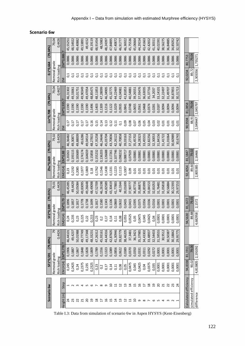
Appendix I – Data from simulation with estimated Murphree efficiency (HYSYS)
122
Scenario 6w
Table I.3: Data from simulation of scenario 6w in Aspen HYSYS (Kent-Eisenberg)
Re
mo
val g
rad
e79
Re
mo
val g
rad
e79
,01
Re
mo
val g
rad
e79
,02
Re
mo
val g
rad
e79
,04
Re
mo
val g
rad
e79
,04
Ric
h lo
adin
g0,
4426
Ric
h lo
adin
g0,
4426
Ric
h lo
adin
g0,
4426
Ric
h lo
adin
g0,
4427
Ric
h lo
adin
g0,
4426
He
igh
t (m
)St
ep
EM (
H14
)EM
*0,7
78T
EM(H
14)
EM*0
,79
TEM
(H14
)EM
*0,8
8T
EMEM
*0,9
35T
EMEM
*0,8
86T
241
0,24
50,
1906
46,4
4101
0,24
0,18
9646
,452
850,
230,
2026
346
,364
820,
170,
1590
46,3
1302
0,1
0,08
8645
,552
51
232
0,24
250,
1887
49,4
237
0,23
50,
1857
49,4
429
0,21
920,
1931
1549
,308
710,
170,
1590
49,3
3061
0,1
0,08
8648
,549
22
223
0,24
0,18
6750
,019
880,
230,
1817
50,0
5084
0,20
850,
1836
8949
,880
090,
170,
1590
50,0
1751
0,1
0,08
8649
,408
82
214
0,23
750,
1848
49,7
7749
0,22
50,
1778
49,8
3095
0,19
770,
1741
7449
,628
60,
170,
1590
49,9
0349
0,1
0,08
8649
,538
91
205
0,23
50,
1828
49,1
7348
0,22
0,17
3849
,266
480,
1869
0,16
4659
49,0
4514
0,17
0,15
9049
,470
540,
10,
0886
49,4
152
196
0,23
250,
1809
48,3
3231
0,21
50,
1699
48,4
9098
0,18
0,15
858
48,2
7815
0,16
0,14
9648
,854
750,
10,
0886
49,1
9119
187
0,23
0,17
8947
,263
120,
230,
1817
47,5
2709
0,17
620,
1552
3247
,352
580,
150,
1403
48,1
1853
0,1
0,08
8648
,914
54
178
0,2
0,15
5645
,931
610,
20,
1580
46,2
6198
0,15
460,
1362
0346
,246
460,
140,
1309
47,2
8099
0,1
0,08
8648
,598
3
169
0,17
0,13
2344
,443
160,
170,
1343
44,8
2589
0,14
380,
1266
8845
,037
040,
130,
1216
46,3
4905
0,1
0,08
8648
,243
97
1510
0,14
0,10
8942
,876
050,
140,
1106
43,3
0419
0,13
310,
1172
6143
,708
360,
120,
1122
45,3
2775
0,1
0,08
8647
,848
95
1411
0,11
0,08
5641
,309
460,
110,
0869
41,7
7883
0,12
230,
1077
4642
,261
220,
110,
1029
44,2
2469
0,1
0,08
8647
,408
72
1312
0,08
0,06
2239
,827
790,
080,
0632
40,3
344
0,11
150,
0982
3240
,708
580,
10,
0935
43,0
4981
0,1
0,08
8646
,917
77
1213
0,05
0,03
8938
,462
050,
055
0,04
3539
,016
990,
1007
0,08
8717
39,0
3163
0,09
0,08
4141
,818
530,
10,
0886
46,3
6922
1114
0,04
750,
0370
37,3
481
0,05
250,
0415
37,9
0777
0,09
0,07
929
37,2
7153
0,08
0,07
4840
,548
810,
10,
0886
45,7
5536
1015
0,04
50,
0350
36,3
421
0,05
0,03
9536
,877
160,
010,
0088
135
,457
020,
070,
0655
39,2
6551
0,1
0,08
8645
,066
64
916
0,04
250,
0331
35,3
7985
0,04
750,
0375
35,8
6871
0,01
0,00
881
34,2
8323
0,06
0,05
6137
,934
760,
10,
0886
44,2
9154
817
0,04
0,03
1134
,433
020,
045
0,03
5634
,859
990,
010,
0088
133
,455
550,
050,
0468
36,6
3035
0,1
0,08
8643
,416
63
718
0,03
750,
0292
33,4
8937
0,04
250,
0336
33,8
4153
0,01
0,00
881
32,8
2256
0,04
0,03
7435
,377
160,
10,
0886
42,4
2652
619
0,03
50,
0272
32,5
4433
0,04
0,03
1632
,810
530,
010,
0088
132
,300
530,
030,
0281
34,2
037
0,1
0,08
8641
,303
11
520
0,00
010,
0001
31,5
9555
0,00
010,
0001
31,7
6481
0,01
0,00
881
31,8
4156
0,02
0,01
8733
,141
010,
10,
0886
40,0
2391
421
0,00
010,
0001
30,9
512
0,00
010,
0001
31,0
5818
0,01
0,00
881
31,4
1722
0,01
0,00
9432
,224
970,
10,
0886
38,5
6275
322
0,00
010,
0001
30,5
0387
0,00
010,
0001
30,5
6884
0,01
0,00
881
31,0
1064
0,01
0,00
9431
,497
070,
10,
0886
36,8
4885
223
0,00
010,
0001
30,1
8842
0,00
010,
0001
30,2
2393
0,01
0,00
881
30,6
0989
0,01
0,00
9430
,878
550,
10,
0886
34,8
5052
124
0,00
010,
0001
29,9
5775
0,00
010,
0001
29,9
7253
0,01
0,00
881
30,6
743
0,01
0,00
9430
,317
130,
10,
0886
32,5
0742
94,8
338
81,1
911
94,5
630
81,1
672
92,4
054
81,1
847
90,9
594
81,0
858
92,0
234
80,7
753
sim
ula
ted
eff
icie
ncy
90,0
279
,00
89,8
879
,01
89,6
079
,02
88,9
179
,04
89,7
279
,04
4,81
3805
2,19
1092
4,68
2958
2,15
722,
8053
852,
1646
62,
0494
472,
0457
972,
3033
561,
7352
71
Sce
nar
io 6
wSF
1*0,
591
(
79,0
0%)
SF2*
0,59
9
(79
,01%
)Zh
u*0
,669
(
79,0
2%)
dif
fere
nce
0.1*
0,66
4
(79
,04%
)
Cal
cula
ted
eff
icie
ncy
Lin
*0,7
08
(7
9,04
%)

Appendix I – Data from simulation with estimated Murphree efficiency (HYSYS)
123
Scenario Goal1
Table I.4: Data from simulation of scenario Goal1 in Aspen HYSYS (Kent-Eisenberg)
Re
mo
val g
rad
e90
,11
Re
mo
val g
rad
e90
,09
Re
mo
val g
rad
e90
,09
Re
mo
val g
rad
e90
,1R
em
ova
l gra
de
90,0
9
Ric
h lo
adin
g0,
4207
Ric
h lo
adin
g0,
4207
Ric
h lo
adin
g0,
4207
Ric
h lo
adin
g0,
4207
Ric
h lo
adin
g0,
4207
He
igh
t (m
)St
ep
EM (
H14
)EM
*0,7
78T
EM(H
14)
EM*0
,79
TEM
(H14
)EM
*0,8
8T
EMEM
*0,9
35T
EMEM
*0,8
86T
241
0,24
50,
1906
46,4
4101
0,24
0,18
9646
,452
850,
230,
2026
346
,364
820,
170,
1590
46,3
1302
0,1
0,08
8645
,552
51
232
0,24
250,
1887
49,4
237
0,23
50,
1857
49,4
429
0,21
920,
1931
1549
,308
710,
170,
1590
49,3
3061
0,1
0,08
8648
,549
22
223
0,24
0,18
6750
,019
880,
230,
1817
50,0
5084
0,20
850,
1836
8949
,880
090,
170,
1590
50,0
1751
0,1
0,08
8649
,408
82
214
0,23
750,
1848
49,7
7749
0,22
50,
1778
49,8
3095
0,19
770,
1741
7449
,628
60,
170,
1590
49,9
0349
0,1
0,08
8649
,538
91
205
0,23
50,
1828
49,1
7348
0,22
0,17
3849
,266
480,
1869
0,16
4659
49,0
4514
0,17
0,15
9049
,470
540,
10,
0886
49,4
152
196
0,23
250,
1809
48,3
3231
0,21
50,
1699
48,4
9098
0,18
0,15
858
48,2
7815
0,16
0,14
9648
,854
750,
10,
0886
49,1
9119
187
0,23
0,17
8947
,263
120,
230,
1817
47,5
2709
0,17
620,
1552
3247
,352
580,
150,
1403
48,1
1853
0,1
0,08
8648
,914
54
178
0,2
0,15
5645
,931
610,
20,
1580
46,2
6198
0,15
460,
1362
0346
,246
460,
140,
1309
47,2
8099
0,1
0,08
8648
,598
3
169
0,17
0,13
2344
,443
160,
170,
1343
44,8
2589
0,14
380,
1266
8845
,037
040,
130,
1216
46,3
4905
0,1
0,08
8648
,243
97
1510
0,14
0,10
8942
,876
050,
140,
1106
43,3
0419
0,13
310,
1172
6143
,708
360,
120,
1122
45,3
2775
0,1
0,08
8647
,848
95
1411
0,11
0,08
5641
,309
460,
110,
0869
41,7
7883
0,12
230,
1077
4642
,261
220,
110,
1029
44,2
2469
0,1
0,08
8647
,408
72
1312
0,08
0,06
2239
,827
790,
080,
0632
40,3
344
0,11
150,
0982
3240
,708
580,
10,
0935
43,0
4981
0,1
0,08
8646
,917
77
1213
0,05
0,03
8938
,462
050,
055
0,04
3539
,016
990,
1007
0,08
8717
39,0
3163
0,09
0,08
4141
,818
530,
10,
0886
46,3
6922
1114
0,04
750,
0370
37,3
481
0,05
250,
0415
37,9
0777
0,09
0,07
929
37,2
7153
0,08
0,07
4840
,548
810,
10,
0886
45,7
5536
1015
0,04
50,
0350
36,3
421
0,05
0,03
9536
,877
160,
010,
0088
135
,457
020,
070,
0655
39,2
6551
0,1
0,08
8645
,066
64
916
0,04
250,
0331
35,3
7985
0,04
750,
0375
35,8
6871
0,01
0,00
881
34,2
8323
0,06
0,05
6137
,934
760,
10,
0886
44,2
9154
817
0,04
0,03
1134
,433
020,
045
0,03
5634
,859
990,
010,
0088
133
,455
550,
050,
0468
36,6
3035
0,1
0,08
8643
,416
63
718
0,03
750,
0292
33,4
8937
0,04
250,
0336
33,8
4153
0,01
0,00
881
32,8
2256
0,04
0,03
7435
,377
160,
10,
0886
42,4
2652
619
0,03
50,
0272
32,5
4433
0,04
0,03
1632
,810
530,
010,
0088
132
,300
530,
030,
0281
34,2
037
0,1
0,08
8641
,303
11
520
0,00
010,
0001
31,5
9555
0,00
010,
0001
31,7
6481
0,01
0,00
881
31,8
4156
0,02
0,01
8733
,141
010,
10,
0886
40,0
2391
421
0,00
010,
0001
30,9
512
0,00
010,
0001
31,0
5818
0,01
0,00
881
31,4
1722
0,01
0,00
9432
,224
970,
10,
0886
38,5
6275
322
0,00
010,
0001
30,5
0387
0,00
010,
0001
30,5
6884
0,01
0,00
881
31,0
1064
0,01
0,00
9431
,497
070,
10,
0886
36,8
4885
223
0,00
010,
0001
30,1
8842
0,00
010,
0001
30,2
2393
0,01
0,00
881
30,6
0989
0,01
0,00
9430
,878
550,
10,
0886
34,8
5052
124
0,00
010,
0001
29,9
5775
0,00
010,
0001
29,9
7253
0,01
0,00
881
30,6
743
0,01
0,00
9430
,317
130,
10,
0886
32,5
0742
94,8
338
0,00
00#
94,5
630
91,6
593
92,4
054
94,1
292
90,9
594
91,6
139
92,0
234
94,0
620
90,3
90,1
1#
90,0
290
,09
90,2
90,0
989
,91
90,1
89,9
790
,09
4,53
3805
-90,
11#
4,54
2958
1,56
9294
2,20
5385
4,03
917
1,04
9447
1,51
3906
2,05
3356
3,97
1972
Sce
nar
io G
oal
1SF
1*0,
854
(90
,11%
)SF
2*0,
886
(90
,09%
)Zh
u*0
,966
(9
0,09
%)
sim
ula
ted
eff
icie
ncy
dif
fere
nce
0.1*
0,97
4
(90,
09%
)
Cal
cula
ted
eff
icie
ncy
Lin
*1,0
29
(90
,10%
)
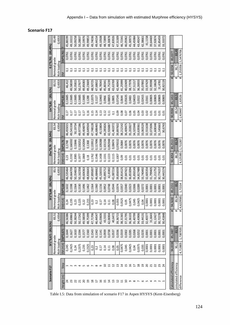
Appendix I – Data from simulation with estimated Murphree efficiency (HYSYS)
124
Scenario F17
Table I.5: Data from simulation of scenario F17 in Aspen HYSYS (Kent-Eisenberg)
Re
mo
val g
rad
e83
,51
Re
mo
val g
rad
e83
,5R
em
ova
l gra
de
83,5
4R
em
ova
l gra
de
83,5
1R
em
ova
l gra
de
83,4
9
Ric
h lo
adin
g0,
4354
Ric
h lo
adin
g0,
4353
Ric
h lo
adin
g0,
4354
Ric
h lo
adin
g0,
4353
Ric
h lo
adin
g0,
4353
He
igh
t (m
)St
ep
EM (
H14
)EM
*0,6
71T
EM(H
14)
EM*0
,68
TEM
(H14
)EM
*0,7
6T
EMEM
*0,8
1T
EMEM
*0,7
61T
241
0,24
50,
1644
46,5
6386
0,24
0,16
3246
,535
464
0,23
0,17
4846
,455
015
0,17
0,13
685
46,4
120,
10,
0761
45,8
8199
232
0,24
250,
1627
49,6
9863
0,23
50,
1598
49,6
6470
90,
2192
0,16
6592
49,5
4133
80,
170,
1368
549
,580
390,
10,
0761
49,1
0222
223
0,24
0,16
1050
,382
440,
230,
1564
50,3
5481
90,
2085
0,15
846
50,1
9734
0,17
0,13
685
50,3
5815
0,1
0,07
6150
,092
58
214
0,23
750,
1594
50,1
7242
0,22
50,
1530
50,1
6235
80,
1977
0,15
0252
49,9
7728
60,
170,
1368
550
,276
770,
10,
0761
50,2
8837
205
0,23
50,
1577
49,5
8039
0,22
0,14
9649
,604
363
0,18
690,
1420
4449
,404
879
0,17
0,13
685
49,8
5083
0,1
0,07
6150
,199
76
196
0,23
250,
1560
48,7
5399
0,21
50,
1462
48,8
3664
30,
180,
1368
48,6
4950
40,
160,
1288
49,2
3669
0,1
0,07
6149
,998
53
187
0,23
0,15
4347
,717
060,
230,
1564
47,8
9500
70,
1762
0,13
3912
47,7
4812
80,
150,
1207
548
,507
250,
10,
0761
49,7
4036
178
0,2
0,13
4246
,445
470,
20,
1360
46,6
8466
20,
1546
0,11
7496
46,6
8646
50,
140,
1127
47,6
8652
0,1
0,07
6149
,441
54
169
0,17
0,11
4145
,036
060,
170,
1156
45,3
2655
50,
1438
0,10
9288
45,5
3804
0,13
0,10
465
46,7
8343
0,1
0,07
6149
,105
08
1510
0,14
0,09
3943
,555
50,
140,
0952
43,8
9571
20,
1331
0,10
1156
44,2
8582
60,
120,
0966
45,8
0341
0,1
0,07
6148
,728
99
1411
0,11
0,07
3842
,069
040,
110,
0748
42,4
5902
0,12
230,
0929
4842
,926
887
0,11
0,08
855
44,7
5239
0,1
0,07
6148
,308
78
1312
0,08
0,05
3740
,647
20,
080,
0544
41,0
8721
60,
1115
0,08
474
41,4
6197
20,
10,
0805
43,6
3769
0,1
0,07
6147
,839
26
1213
0,05
0,03
3639
,367
150,
055
0,03
7439
,856
939
0,10
070,
0765
3239
,897
602
0,09
0,07
245
42,4
6943
0,1
0,07
6147
,313
09
1114
0,04
750,
0319
38,3
1365
0,05
250,
0357
38,8
1412
50,
090,
0684
38,2
1214
20,
080,
0644
41,2
5999
0,1
0,07
6146
,723
41
1015
0,04
50,
0302
37,3
1795
0,05
0,03
4037
,847
421
0,01
0,00
7636
,409
475
0,07
0,05
635
40,0
2409
0,1
0,07
6146
,059
62
916
0,04
250,
0285
36,3
6103
0,04
750,
0323
36,8
5309
40,
010,
0076
35,2
0282
70,
060,
0483
38,7
7978
0,1
0,07
6145
,309
73
817
0,04
0,02
6835
,407
990,
045
0,03
0635
,850
149
0,01
0,00
7634
,325
948
0,05
0,04
025
37,5
1217
0,1
0,07
6144
,459
84
718
0,03
750,
0252
34,4
3906
0,04
250,
0289
34,8
1748
90,
010,
0076
33,6
3936
10,
040,
0322
36,2
6933
0,1
0,07
6143
,492
47
619
0,03
50,
0235
33,4
4131
0,04
0,02
7233
,740
492
0,01
0,00
7633
,063
529
0,03
0,02
415
35,0
7892
0,1
0,07
6142
,386
61
520
0,00
010,
0001
32,4
0377
0,00
010,
0001
32,6
0535
40,
010,
0076
32,5
5163
80,
020,
0161
33,9
7429
0,1
0,07
6141
,115
8
421
0,00
010,
0001
31,6
643
0,00
010,
0001
31,7
9940
50,
010,
0076
32,0
7269
60,
010,
0080
532
,993
980,
10,
0761
39,6
4469
322
0,00
010,
0001
31,1
2427
0,00
010,
0001
31,2
1175
20,
010,
0076
31,6
0834
80,
010,
0080
532
,186
280,
10,
0761
37,9
2874
223
0,00
010,
0001
30,7
2278
0,00
010,
0001
30,7
7415
70,
010,
0076
31,1
4566
30,
010,
0080
531
,478
10,
10,
0761
35,8
5459
124
0,00
010,
0001
30,4
1848
0,00
010,
0001
30,4
4157
40,
010,
0076
30,6
743
0,01
0,00
805
30,8
2119
0,1
0,07
6133
,333
72
94,8
338
85,2
487
#94
,563
085
,215
192
,405
485
,251
3#
90,9
594
85,1
453
#92
,023
485
,037
7
90,1
283
,51
#89
,94
83,5
88,2
883
,54
#89
,54
83,5
1#
90,7
783
,49
4,71
3805
1,73
8703
5#
4,62
2958
51,
7151
44,
1253
851,
7112
87#
1,41
9447
1,63
526
#1,
2533
561,
5476
706
Sce
nar
io F
17
Cal
cula
ted
eff
icie
ncy
sim
ula
ted
eff
icie
ncy
dif
fere
nce
SF2*
0,68
(
83,5
0%)
Zhu
*0,7
6
(83,
54%
)Li
n*0
,81
(
83,5
1%)
0.1*
0,76
1 (
83,4
9%)
SF1*
0,67
1 (
83,5
1%)
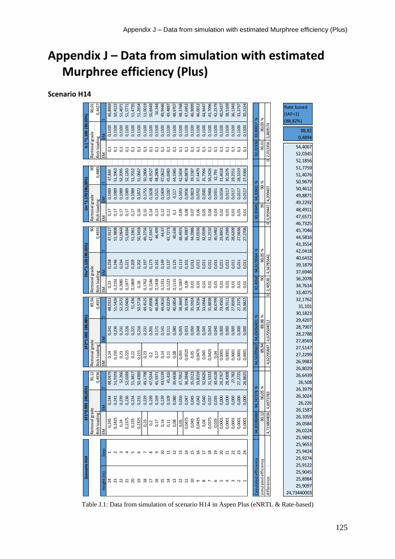
Appendix J – Data from simulation with estimated Murphree efficiency (Plus)
125
Rate based
(IAF=1)
(88,82%)
88,82
0,4894
54,4007
52,0345
52,1856
51,7759
51,4076
50,9679
50,4612
49,8871
49,2292
48,4911
47,6571
46,7325
45,7046
44,5816
43,3554
42,0418
40,6432
39,1879
37,6946
36,2078
34,7614
33,4075
32,1762
31,101
30,1823
29,4207
28,7907
28,2788
27,8569
27,5147
27,2299
26,9983
26,8029
26,6439
26,508
26,3979
26,3024
26,226
26,1587
26,1059
26,0584
26,0224
25,9892
25,9653
25,9424
25,9274
25,9122
25,9045
25,8984
25,9097
24,73440003
Appendix J – Data from simulation with estimated Murphree efficiency (Plus)
Scenario H14
Table J.1: Data from simulation of scenario H14 in Aspen Plus (eNRTL & Rate-based)
Re
mo
val g
rad
e90
,12
Re
mo
val g
rad
e89
,94
Re
mo
val g
rad
e90
Re
mo
val g
rad
e90
Re
mo
val g
rad
e90
,01
Ric
h lo
adin
g0,
4936
Ric
h lo
adin
g0,
4931
Ric
h lo
adin
g0,
4933
Ric
h lo
adin
g0,
4885
Ric
h lo
adin
g0,
4427
He
igh
t (m
)St
ep
EMEM
TEM
EMT
EMEM
TEM
EMT
EMEM
T
241
0,24
50,
244
48,0
479
0,24
0,24
148
,032
20,
230,
258
47,9
127
0,17
0,19
8947
,849
0,1
0,11
0046
,896
9
232
0,24
250,
241
51,5
593
0,23
50,
236
51,5
426
0,21
920,
246
51,3
808
0,17
0,19
8951
,396
30,
10,
1100
50,4
122
223
0,24
0,23
952
,266
0,23
0,23
152
,257
20,
2085
0,23
452
,064
30,
170,
1989
52,2
095
0,1
0,11
0051
,407
1
214
0,23
750,
236
52,0
289
0,22
50,
226
52,0
406
0,19
770,
221
51,8
184
0,17
0,19
8952
,128
30,
10,
1100
51,5
771
205
0,23
50,
234
51,3
817
0,22
0,22
151
,436
0,18
690,
209
51,1
961
0,17
0,19
8951
,701
20,
10,
1100
51,4
735
196
0,23
250,
231
50,4
389
0,21
50,
216
50,5
718
0,18
0,20
250
,345
80,
160,
1872
51,0
667
0,1
0,11
0051
,265
4
187
0,23
0,22
949
,179
80,
230,
231
49,4
525
0,17
620,
197
49,2
756
0,15
0,17
5550
,280
60,
10,
1100
51,0
019
178
0,2
0,19
947
,524
40,
20,
201
47,8
998
0,15
460,
173
47,9
347
0,14
0,16
3849
,352
70,
10,
1100
50,6
949
169
0,17
0,16
945
,597
10,
170,
171
46,0
646
0,14
380,
161
46,4
090,
130,
1521
48,2
808
0,1
0,11
0050
,344
1510
0,14
0,13
943
,513
90,
140,
141
44,0
616
0,13
310,
149
44,6
70,
120,
1404
47,0
622
0,1
0,11
0049
,944
6
1411
0,11
0,10
941
,416
0,11
0,11
142
,022
90,
1223
0,13
742
,727
30,
110,
1287
45,6
983
0,1
0,11
0049
,489
7
1312
0,08
0,08
039
,443
80,
080,
080
40,0
854
0,11
150,
125
40,6
360,
10,
117
44,1
985
0,1
0,11
0048
,970
7
1213
0,05
0,05
037
,705
20,
055
0,05
538
,366
90,
1007
0,11
338
,492
50,
090,
1053
42,5
834
0,1
0,11
0048
,376
8
1114
0,04
750,
047
36,2
848
0,05
250,
053
36,9
196
0,09
0,10
136
,398
70,
080,
0936
40,8
878
0,1
0,11
0047
,695
2
1015
0,04
50,
045
35,0
123
0,05
0,05
035
,592
40,
010,
011
34,3
986
0,07
0,08
1939
,158
70,
10,
1100
46,9
099
916
0,04
250,
042
33,8
159
0,04
750,
048
34,3
256
0,01
0,01
133
,055
60,
060,
0702
37,4
479
0,1
0,11
0046
,001
2
817
0,04
0,04
032
,662
60,
045
0,04
533
,094
40,
010,
011
32,0
599
0,05
0,05
8535
,799
40,
10,
1100
44,9
447
718
0,03
750,
037
31,5
333
0,04
250,
043
31,8
838
0,01
0,01
131
,253
20,
040,
0468
34,2
426
0,1
0,11
0043
,709
6
619
0,03
50,
035
30,4
128
0,04
0,04
030
,679
90,
010,
011
30,5
482
0,03
0,03
5132
,793
0,1
0,11
0042
,257
9
520
0,00
010,
000
29,2
767
0,00
010,
000
29,4
565
0,01
0,01
129
,894
10,
020,
0234
31,4
618
0,1
0,11
0040
,543
7
421
0,00
010,
000
28,4
308
0,00
010,
000
28,5
511
0,01
0,01
129
,258
90,
010,
0117
30,2
676
0,1
0,11
0038
,516
9
322
0,00
010,
000
27,7
820,
0001
0,00
027
,859
30,
010,
011
28,6
209
0,01
0,01
1729
,255
10,
10,
1100
36,1
343
223
0,00
010,
000
27,2
725
0,00
010,
000
27,3
175
0,01
0,01
127
,963
60,
010,
0117
28,3
319
0,1
0,11
0033
,373
7
124
0,00
010,
000
26,8
625
0,00
010,
000
26,8
822
0,01
0,01
127
,270
60,
010,
0117
27,4
366
0,1
0,11
0030
,212
4
Cal
cula
ted
eff
icie
ncy
94,8
3380
484
94,7
4737
8%
94,5
6295
847
94,6
5050
401
%92
,405
494
,617
8564
%90
,959
4594
,209
41%
92,0
2336
93,8
9957
%
sim
ula
ted
eff
icie
ncy
90,1
290
,05
%89
,94
89,9
8%
9090
,05
%90
90%
90,0
190
,03
%
dif
fere
nce
4,71
3804
836
4,69
7378
34,
6229
5847
4,67
0504
012
02,
4053
84,
5678
5642
00,
9594
474,
2094
070
2,01
3356
3,86
9574
0.1
*1.1
00 (
90.0
3%)
Sce
nar
io H
14SF
2*1.
005
(89
,98%
)SF
1*0.
995
(90
,05%
)Zh
u*1
.120
(90
.05%
)Li
n *
1.17
0 (9
0,00
%)
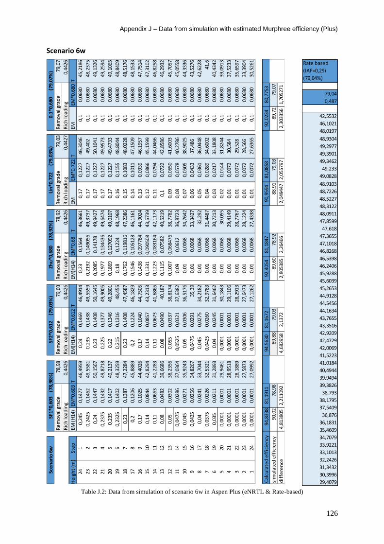
Appendix J – Data from simulation with estimated Murphree efficiency (Plus)
126
Rate based
(IAF=0,29)
(79,04%)
79,04
0,487
42,5532
46,1021
48,0197
48,9304
49,2977
49,3901
49,3462
49,233
49,0828
48,9103
48,7226
48,5227
48,3122
48,0911
47,8599
47,618
47,3655
47,1018
46,8268
46,5398
46,2406
45,9288
45,6039
45,2653
44,9128
44,5456
44,1634
43,7655
43,3516
42,9209
42,4729
42,0069
41,5223
41,0184
40,4944
39,9494
39,3826
38,793
38,1795
37,5409
36,876
36,1831
35,4609
34,7079
33,9221
33,1013
32,2426
31,3432
30,3996
29,4079
Scenario 6w
Table J.2: Data from simulation of scenario 6w in Aspen Plus (eNRTL & Rate-based)
Re
mo
val g
rad
e78
,98
Re
mo
val g
rad
e79
,03
Re
mo
val g
rad
e78
,92
Re
mo
val g
rad
e79
,03
Re
mo
val g
rad
e79
,07
Ric
h lo
adin
g0,
4426
Ric
h lo
adin
g0,
4426
Ric
h lo
adin
g0,
4426
Ric
h lo
adin
g0,
4427
Ric
h lo
adin
g0,
4426
He
igh
t (m
)St
ep
EM (
H14
)EM
*0,6
03T
EM(H
14)
EM*0
,612
TEM
(H14
)EM
*0,6
8T
EMEM
*0,7
22T
EMEM
*0,6
80T
241
0,24
50,
1477
46,4
959
0,24
0,14
6946
,491
40,
230,
1564
46,3
661
0,17
0,12
2746
,304
60,
10,
0680
45,2
186
232
0,24
250,
1462
49,5
581
0,23
50,
1438
49,5
559
0,21
920,
1490
5649
,373
70,
170,
1227
49,4
020,
10,
0680
48,2
375
223
0,24
0,14
4750
,156
70,
230,
1408
50,1
645
0,20
850,
1417
849
,942
70,
170,
1227
50,1
041
0,1
0,06
8049
,132
6
214
0,23
750,
1432
49,8
718
0,22
50,
1377
49,9
005
0,19
770,
1344
3649
,647
40,
170,
1227
49,9
573
0,1
0,06
8049
,259
4
205
0,23
50,
1417
49,2
137
0,22
0,13
4649
,280
10,
1869
0,12
7092
49,0
107
0,17
0,12
2749
,473
30,
10,
0680
49,1
065
196
0,23
250,
1402
48,3
259
0,21
50,
1316
48,4
550,
180,
1224
48,1
968
0,16
0,11
5548
,804
40,
10,
0680
48,8
409
187
0,23
0,13
8747
,228
40,
230,
1408
47,4
587
0,17
620,
1198
1647
,238
60,
150,
1083
48,0
228
0,1
0,06
8048
,517
6
178
0,2
0,12
0645
,888
90,
20,
1224
46,1
829
0,15
460,
1051
2846
,116
10,
140,
1011
47,1
509
0,1
0,06
8048
,153
3
169
0,17
0,10
2544
,402
60,
170,
1040
44,7
505
0,14
380,
0977
8444
,902
40,
130,
0939
46,1
957
0,1
0,06
8047
,751
4
1510
0,14
0,08
4442
,829
40,
140,
0857
43,2
313
0,13
310,
0905
0843
,573
90,
120,
0866
45,1
599
0,1
0,06
8047
,310
2
1411
0,11
0,06
6341
,228
30,
110,
0673
41,6
865
0,12
230,
0831
6442
,117
30,
110,
0794
44,0
466
0,1
0,06
8046
,825
8
1312
0,08
0,04
8239
,668
60,
080,
0490
40,1
870,
1115
0,07
582
40,5
219
0,1
0,07
2242
,858
60,
10,
0680
46,2
932
1213
0,05
0,03
0238
,235
60,
055
0,03
3738
,817
40,
1007
0,06
8476
38,7
782
0,09
0,06
5041
,600
30,
10,
0680
45,7
057
1114
0,04
750,
0286
37,0
364
0,05
250,
0321
37,6
382
0,09
0,06
1236
,872
30,
080,
0578
40,2
786
0,1
0,06
8045
,055
8
1015
0,04
50,
0271
35,9
243
0,05
0,03
0636
,517
60,
010,
0068
34,7
642
0,07
0,05
0538
,902
50,
10,
0680
44,3
336
916
0,04
250,
0256
34,8
267
0,04
750,
0291
35,3
90,
010,
0068
33,3
427
0,06
0,04
3337
,486
0,1
0,06
8043
,527
6
817
0,04
0,02
4133
,704
40,
045
0,02
7534
,218
20,
010,
0068
32,2
920,
050,
0361
36,0
448
0,1
0,06
8042
,622
8
718
0,03
750,
0226
32,5
321
0,04
250,
0260
32,9
783
0,01
0,00
6831
,448
70,
040,
0289
34,6
002
0,1
0,06
8041
,6
619
0,03
50,
0211
31,2
893
0,04
0,02
4531
,646
20,
010,
0068
30,7
213
0,03
0,02
1733
,180
80,
10,
0680
40,4
342
520
0,00
010,
0001
29,9
461
0,00
010,
0001
30,1
843
0,01
0,00
6830
,055
0,02
0,01
4431
,824
40,
10,
0680
39,0
913
421
0,00
010,
0001
28,9
518
0,00
010,
0001
29,1
106
0,01
0,00
6829
,414
90,
010,
0072
30,5
840,
10,
0680
37,5
233
322
0,00
010,
0001
28,1
889
0,00
010,
0001
28,2
913
0,01
0,00
6828
,776
70,
010,
0072
29,5
280,
10,
0680
35,6
597
223
0,00
010,
0001
27,5
873
0,00
010,
0001
27,6
473
0,01
0,00
6828
,122
40,
010,
0072
28,5
660,
10,
0680
33,3
904
124
0,00
010,
0001
27,0
992
0,00
010,
0001
27,1
262
0,01
0,00
6827
,433
80,
010,
0072
27,6
365
0,1
0,06
8030
,526
1
94,8
338
81,1
911
94,5
630
81,1
672
92,4
054
81,1
847
90,9
594
81,0
858
92,0
234
80,7
753
sim
ula
ted
eff
icie
ncy
90,0
278
,98
89,8
879
,03
89,6
078
,92
88,9
179
,03
89,7
279
,07
4,81
3805
2,21
1092
4,68
2958
2,13
722,
8053
852,
2646
62,
0494
472,
0557
972,
3033
561,
7052
71
Sce
nar
io 6
wSF
1*0,
603
(7
8,98
%)
SF2*
0,61
2
(79
,03%
)Zh
u*0
,680
(
78,9
2%)
dif
fere
nce
0.1*
0,68
0
(79
,07%
)
Cal
cula
ted
eff
icie
ncy
Lin
*0,7
22
(7
9,03
%)
Appendix J – Data from simulation with estimated Murphree efficiency (Plus)
127
Scenario 2B5
Table J.3: Data from simulation of scenario 2B5 in Aspen Plus (eNRTL & Rate-based)
Re
mo
val g
rad
e87
,29
Re
mo
val g
rad
e87
,29
Re
mo
val g
rad
e87
,31
Re
mo
val g
rad
e87
,3R
em
ova
l gra
de
87,3
Ric
h lo
adin
g0,
4891
Ric
h lo
adin
g0,
4891
Ric
h lo
adin
g0,
4892
Ric
h lo
adin
g0,
4891
Ric
h lo
adin
g0,
4891
He
igh
t (m
)St
ep
EM (
H14
)EM
*0,8
87T
EM(H
14)
EM*0
,9T
EM(H
14)
EM*1
,008
TEM
EM*1
,004
TEM
EM*1
,008
T
241
0,24
50,
2173
47,8
166
0,24
0,21
6047
,814
60,
230,
2318
447
,753
60,
170,
1707
47,7
309
0,1
0,10
0847
,210
8
232
0,24
250,
2151
50,8
570,
235
0,21
1550
,857
10,
2192
0,22
0954
50,7
561
0,17
0,17
0750
,828
70,
10,
1008
50,3
592
223
0,24
0,21
2951
,328
70,
230,
2070
51,3
379
0,20
850,
2101
6851
,197
80,
170,
1707
51,4
107
0,1
0,10
0851
,132
3
214
0,23
750,
2107
50,9
731
0,22
50,
2025
51,0
041
0,19
770,
1992
8250
,826
60,
170,
1707
51,2
118
0,1
0,10
0851
,193
2
205
0,23
50,
2084
50,2
578
0,22
0,19
8050
,331
70,
1869
0,18
8395
50,1
294
0,17
0,17
0750
,712
70,
10,
1008
51,0
318
196
0,23
250,
2062
49,2
769
0,21
50,
1935
49,4
268
0,18
0,18
144
49,2
305
0,16
0,16
0650
,024
60,
10,
1008
50,7
857
187
0,23
0,20
4048
,011
10,
230,
2070
48,2
927
0,17
620,
1776
148
,133
20,
150,
1506
49,1
988
0,1
0,10
0850
,491
4
178
0,2
0,17
7446
,392
80,
20,
1800
46,7
603
0,15
460,
1558
3746
,789
80,
140,
1406
48,2
450,
10,
1008
50,1
558
169
0,17
0,15
0844
,556
30,
170,
1530
44,9
941
0,14
380,
1449
545
,296
30,
130,
1305
47,1
643
0,1
0,10
0849
,777
5
1510
0,14
0,12
4242
,617
80,
140,
1260
43,1
121
0,13
310,
1341
6543
,631
20,
120,
1205
45,9
579
0,1
0,10
0849
,351
4
1411
0,11
0,09
7640
,709
70,
110,
0990
41,2
412
0,12
230,
1232
7841
,815
90,
110,
1104
44,6
329
0,1
0,10
0848
,871
1
1312
0,08
0,07
1038
,961
0,08
0,07
2039
,508
80,
1115
0,11
2392
39,9
172
0,1
0,10
0443
,204
60,
10,
1008
48,3
286
1213
0,05
0,04
4437
,467
20,
055
0,04
9538
,019
30,
1007
0,10
1506
38,0
378
0,09
0,09
0441
,701
20,
10,
1008
47,7
145
1114
0,04
750,
0421
36,2
999
0,05
250,
0473
36,8
136
0,09
0,09
072
36,2
801
0,08
0,08
0340
,165
10,
10,
1008
47,0
175
1015
0,04
50,
0399
35,2
945
0,05
0,04
5035
,745
90,
010,
0100
834
,689
10,
070,
0703
38,6
479
0,1
0,10
0846
,224
2
916
0,04
250,
0377
34,3
869
0,04
750,
0428
34,7
654
0,01
0,01
008
33,7
252
0,06
0,06
0237
,203
10,
10,
1008
45,3
183
817
0,04
0,03
5533
,552
0,04
50,
0405
33,8
545
0,01
0,01
008
33,0
783
0,05
0,05
0235
,874
80,
10,
1008
44,2
81
718
0,03
750,
0333
32,7
793
0,04
250,
0383
33,0
081
0,01
0,01
008
32,5
978
0,04
0,04
0234
,688
80,
10,
1008
43,0
905
619
0,03
50,
0310
32,0
635
0,04
0,03
6032
,222
70,
010,
0100
832
,206
80,
030,
0301
33,6
571
0,1
0,10
0841
,723
8
520
0,00
010,
0001
31,3
937
0,00
010,
0001
31,4
873
0,01
0,01
008
31,8
647
0,02
0,02
0132
,783
30,
10,
1008
40,1
611
421
0,00
010,
0001
30,9
80,
0001
0,00
0131
,034
40,
010,
0100
831
,549
50,
010,
0100
32,0
726
0,1
0,10
0838
,397
6
322
0,00
010,
0001
30,7
207
0,00
010,
0001
30,7
511
0,01
0,01
008
31,2
491
0,01
0,01
0031
,540
90,
10,
1008
36,4
626
223
0,00
010,
0001
30,5
564
0,00
010,
0001
30,5
718
0,01
0,01
008
30,9
570,
010,
0100
31,1
078
0,1
0,10
0834
,428
9
124
0,00
010,
0001
30,4
448
0,00
010,
0001
30,4
507
0,01
0,01
008
30,6
625
0,01
0,01
0030
,723
30,
10,
1008
32,3
765
94,8
338
89,4
175
94,5
630
89,4
306
92,4
054
89,4
033
90,9
594
89,3
142
92,0
234
89,2
101
90,1
287
,29
89,9
487
,29
88,2
887
,31
88,9
187
,389
,97
87,3
4,71
3805
2,12
7526
4,62
2958
2,14
0555
4,12
5385
2,09
3253
2,04
9447
2,01
4196
32,
0533
561,
9101
21
0.1*
1,00
8
(87
,30%
)
dif
fere
nce
Cal
cula
ted
eff
icie
ncy
sim
ula
ted
eff
icie
ncy
Sce
nar
io 2
B5
SF1*
0,88
7
(87
,29%
)SF
2*0,
900
(87,
29%
)Zh
u*1
,008
(87,
31%
)Li
n*1
,004
(
87,3
0%)
Rate based
(IAF=1)
(86,14%)
86,14
0,4857
54,2651
50,8566
51,2477
50,662
50,2149
49,6563
49,0256
48,3131
47,5079
46,6129
45,6183
44,5307
43,3452
42,076
40,7294
39,3329
37,9102
36,5089
35,1725
33,9602
32,9111
32,0585
31,3961
30,9098
30,558
30,3153
30,144
30,0308
29,9504
29,9002
29,8634
29,8427
29,8261
29,8191
29,8117
29,8109
29,8077
29,8097
29,8084
29,8115
29,8111
29,8148
29,8147
29,8186
29,8187
29,8228
29,8234
29,8291
29,8356
29,865
Appendix J – Data from simulation with estimated Murphree efficiency (Plus)
128
Scenario Goal1
Table J.4: Data from simulation of scenario Goal1 in Aspen Plus (eNRTL & Rate-based)
Re
mo
val g
rad
e90
,11
Re
mo
val g
rad
e90
,11
Re
mo
val g
rad
e90
,12
Re
mo
val g
rad
e90
,12
Re
mo
val g
rad
e90
,09
Ric
h lo
adin
g0,
487
Ric
h lo
adin
g0,
487
Ric
h lo
adin
g0,
4871
Ric
h lo
adin
g0,
4871
Ric
h lo
adin
g0,
4869
He
igh
t (m
)St
ep
EM (
H14
)EM
*0,8
96T
EM(H
14)
EM*0
,91
TEM
EM*1
,015
TEM
EM*1
,074
TEM
EM*1
,025
T
241
0,24
50,
2195
47,3
613
0,24
0,21
8447
,358
70,
230,
2334
547
,259
0,17
0,18
2647
,230
20,
10,
1025
46,4
696
232
0,24
250,
2173
50,1
803
0,23
50,
2139
50,1
790,
2192
0,22
2488
50,0
396
0,17
0,18
2650
,088
50,
10,
1025
49,3
283
223
0,24
0,21
5050
,591
0,23
0,20
9350
,597
30,
2085
0,21
1628
50,4
253
0,17
0,18
2650
,591
10,
10,
1025
49,9
963
214
0,23
750,
2128
50,2
682
0,22
50,
2048
50,2
930,
1977
0,20
0666
50,0
908
0,17
0,18
2650
,400
60,
10,
1025
50,0
36
205
0,23
50,
2106
49,6
335
0,22
0,20
0249
,695
50,
1869
0,18
9704
49,4
752
0,17
0,18
2649
,95
0,1
0,10
2549
,886
1
196
0,23
250,
2083
48,7
625
0,21
50,
1957
48,8
926
0,18
0,18
2748
,683
30,
160,
1718
49,3
323
0,1
0,10
2549
,664
6
187
0,23
0,20
6147
,628
70,
230,
2093
47,8
791
0,17
620,
1788
4347
,712
0,15
0,16
1148
,589
30,
10,
1025
49,4
012
178
0,2
0,17
9246
,153
60,
20,
1820
46,4
849
0,15
460,
1569
1946
,511
10,
140,
1504
47,7
263
0,1
0,10
2549
,100
8
169
0,17
0,15
2344
,440
60,
170,
1547
44,8
462
0,14
380,
1459
5745
,161
0,13
0,13
9646
,740
30,
10,
1025
48,7
614
1510
0,14
0,12
5442
,566
20,
140,
1274
43,0
460,
1331
0,13
5097
43,6
207
0,12
0,12
8945
,628
90,
10,
1025
48,3
781
1411
0,11
0,09
8640
,625
20,
110,
1001
41,1
771
0,12
230,
1241
3541
,873
60,
110,
1181
44,3
906
0,1
0,10
2547
,944
7
1312
0,08
0,07
1738
,737
50,
080,
0728
39,3
561
0,11
150,
1131
7339
,922
70,
10,
1074
43,0
297
0,1
0,10
2547
,453
7
1213
0,05
0,04
4837
,037
90,
055
0,05
0137
,717
10,
1007
0,10
2211
37,7
984
0,09
0,09
6741
,554
90,
10,
1025
46,8
959
1114
0,04
750,
0426
35,6
728
0,05
250,
0478
36,3
452
0,09
0,09
135
35,5
781
0,08
0,08
5939
,984
20,
10,
1025
46,2
602
1015
0,04
50,
0403
34,4
313
0,05
0,04
5535
,057
80,
010,
0101
533
,345
40,
070,
0752
38,3
475
0,1
0,10
2545
,533
2
916
0,04
250,
0381
33,2
390,
0475
0,04
3233
,793
30,
010,
0101
532
,026
0,06
0,06
4436
,685
10,
10,
1025
44,6
98
817
0,04
0,03
5832
,072
30,
045
0,04
1032
,537
60,
010,
0101
531
,143
50,
050,
0537
35,0
484
0,1
0,10
2543
,733
7
718
0,03
750,
0336
30,9
302
0,04
250,
0387
31,2
943
0,01
0,01
015
30,4
785
0,04
0,04
3033
,489
50,
10,
1025
42,6
137
619
0,03
50,
0314
29,8
158
0,04
0,03
6430
,074
10,
010,
0101
529
,922
90,
030,
0322
32,0
556
0,1
0,10
2541
,304
520
0,00
010,
0001
28,7
210,
0001
0,00
0128
,872
20,
010,
0101
529
,421
0,02
0,02
1530
,787
70,
10,
1025
39,7
612
421
0,00
010,
0001
28,0
421
0,00
010,
0001
28,1
303
0,01
0,01
015
28,9
433
0,01
0,01
0729
,722
20,
10,
1025
37,9
31
322
0,00
010,
0001
27,6
113
0,00
010,
0001
27,6
611
0,01
0,01
015
28,4
733
0,01
0,01
0728
,910
90,
10,
1025
35,7
531
223
0,00
010,
0001
27,3
336
0,00
010,
0001
27,3
591
0,01
0,01
015
28,0
020,
010,
0107
28,2
311
0,1
0,10
2533
,184
3
124
0,00
010,
0001
27,1
449
0,00
010,
0001
27,1
549
0,01
0,01
015
27,5
161
0,01
0,01
0727
,61
0,1
0,10
2530
,240
9
94,8
338
91,6
846
#94
,563
091
,659
392
,405
494
,129
290
,959
491
,613
992
,023
494
,062
0
90,3
90,1
1#
90,0
290
,11
90,2
90,1
289
,91
90,1
289
,97
90,0
9
4,53
3805
1,57
4602
#4,
5429
581,
5492
942,
2053
854,
0091
71,
0494
471,
4939
062,
0533
563,
9719
72
Sce
nar
io G
oal
1SF
1*0,
896
(90
,11%
)SF
2*0,
910
(90
,11%
)Zh
u*1
,015
(9
0,12
%)
sim
ula
ted
eff
icie
ncy
dif
fere
nce
0.1*
1,02
5
(90,
09%
)
Cal
cula
ted
eff
icie
ncy
Lin
*1,0
74
(90
,12%
)
Rate based
[0,51]
(90,11%)
90,11
0,487
48,8326
50,8846
50,9133
50,791
50,6474
50,492
50,3213
50,1374
49,9361
49,7194
49,4832
49,2293
48,9537
48,658
48,3383
47,9964
47,628
47,2352
46,8141
46,3664
45,8887
45,3828
44,8453
44,2784
43,6791
43,05
42,3886
41,6981
40,9765
40,2277
39,4508
38,6507
37,8277
36,9884
36,1351
35,276
34,4157
33,5646
32,7293
31,9218
31,1494
30,4241
29,7521
29,1424
28,5971
28,1199
27,7076
27,3593
27,0694
26,837
Appendix J – Data from simulation with estimated Murphree efficiency (Plus)
129
Scenario F17
Table J.5: Data from simulation of scenario F17 in Aspen Plus (eNRTL & Rate-based)
Re
mo
val g
rad
e83
,51
Re
mo
val g
rad
e83
,49
Re
mo
val g
rad
e83
,49
Re
mo
val g
rad
e83
,51
Re
mo
val g
rad
e83
,5
Ric
h lo
adin
g0,
4837
Ric
h lo
adin
g0,
4836
Ric
h lo
adin
g0,
4836
Ric
h lo
adin
g0,
4837
Ric
h lo
adin
g0,
4836
He
igh
t (m
)St
ep
EM (
H14
)EM
*0,7
72T
EM(H
14)
EM*0
,732
TEM
(H14
)EM
*0,8
18T
EMEM
*0,8
63T
EMEM
*1,1
T
241
0,24
50,
1891
47,6
719
0,24
0,17
5747
,668
20,
230,
1881
447
,604
90,
170,
1467
147
,592
90,
10,
1147
,078
9
232
0,24
250,
1872
50,3
556
0,23
50,
1720
50,3
538
0,21
920,
1793
0650
,248
60,
170,
1467
150
,338
70,
10,
1149
,892
4
223
0,24
0,18
5350
,648
70,
230,
1684
50,6
564
0,20
850,
1705
5350
,512
20,
170,
1467
150
,742
10,
10,
1150
,500
8
214
0,23
750,
1834
50,2
124
0,22
50,
1647
50,2
418
0,19
770,
1617
1950
,063
70,
170,
1467
150
,455
40,
10,
1150
,484
4
205
0,23
50,
1814
49,4
706
0,22
0,16
1049
,541
0,18
690,
1528
8449
,344
70,
170,
1467
149
,910
70,
10,
1150
,280
8
196
0,23
250,
1795
48,5
080,
215
0,15
7448
,648
80,
180,
1472
448
,465
30,
160,
1380
849
,204
30,
10,
1150
,006
5
187
0,23
0,17
7647
,312
50,
230,
1684
47,5
710,
1762
0,14
4132
47,4
301
0,15
0,12
945
48,3
859
0,1
0,11
49,6
909
178
0,2
0,15
4445
,830
30,
20,
1464
46,1
598
0,15
460,
1264
6346
,200
50,
140,
1208
247
,467
40,
10,
1149
,339
1
169
0,17
0,13
1244
,182
60,
170,
1244
44,5
710,
1438
0,11
7628
44,8
658
0,13
0,11
219
46,4
524
0,1
0,11
48,9
499
1510
0,14
0,10
8142
,454
80,
140,
1025
42,8
968
0,13
310,
1088
7643
,400
40,
120,
1035
645
,343
40,
10,
1148
,519
2
1411
0,11
0,08
4940
,737
80,
110,
0805
41,2
268
0,12
230,
1000
4141
,803
10,
110,
0949
344
,145
90,
10,
1148
,042
2
1312
0,08
0,06
1839
,134
20,
080,
0586
39,6
610,
1115
0,09
1207
40,0
967
0,1
0,08
6342
,870
90,
10,
1147
,512
8
1213
0,05
0,03
8637
,742
0,05
50,
0403
38,2
994
0,10
070,
0823
7338
,327
30,
090,
0776
741
,534
40,
10,
1146
,923
9
1114
0,04
750,
0367
36,6
599
0,05
250,
0384
37,1
957
0,09
0,07
362
36,5
674
0,08
0,06
904
40,1
60,
10,
1146
,267
1
1015
0,04
50,
0347
35,7
099
0,05
0,03
6636
,196
20,
010,
0081
834
,875
50,
070,
0604
138
,780
90,
10,
1145
,532
4
916
0,04
250,
0328
34,8
276
0,04
750,
0348
35,2
470,
010,
0081
833
,924
80,
060,
0517
837
,434
90,
10,
1144
,707
9
817
0,04
0,03
0933
,992
10,
045
0,03
2934
,334
10,
010,
0081
833
,322
60,
050,
0431
536
,161
90,
10,
1143
,779
3
718
0,03
750,
0290
33,1
994
0,04
250,
0311
33,4
596
0,01
0,00
818
32,8
90,
040,
0345
234
,997
90,
10,
1142
,729
6
619
0,03
50,
0270
32,4
510,
040,
0293
32,6
286
0,01
0,00
818
32,5
415
0,03
0,02
589
33,9
723
0,1
0,11
41,5
387
520
0,00
010,
0001
31,7
397
0,00
010,
0001
31,8
351
0,01
0,00
818
32,2
351
0,02
0,01
726
33,1
047
0,1
0,11
40,1
844
421
0,00
010,
0001
31,3
422
0,00
010,
0001
31,3
931
0,01
0,00
818
31,9
497
0,01
0,00
863
32,4
115
0,1
0,11
38,6
449
322
0,00
010,
0001
31,1
167
0,00
010,
0001
31,1
429
0,01
0,00
818
31,6
747
0,01
0,00
863
31,9
168
0,1
0,11
36,9
079
223
0,00
010,
0001
30,9
873
0,00
010,
0001
30,9
996
0,01
0,00
818
31,4
047
0,01
0,00
863
31,5
235
0,1
0,11
34,9
886
124
0,00
010,
0001
30,9
098
0,00
010,
0001
30,9
142
0,01
0,00
818
31,1
345
0,01
0,00
863
31,1
807
0,1
0,11
32,9
464
94,8
338
85,2
487
#94
,563
085
,215
192
,405
485
,251
3#
90,9
594
85,1
453
#92
,023
485
,037
7
90,1
283
,51
#89
,94
83,4
988
,28
83,4
9#
89,5
483
,51
#90
,77
83,5
4,71
3805
1,73
8703
5#
4,62
2958
51,
7251
44,
1253
851,
7612
87#
1,41
9447
1,63
526
#1,
2533
561,
5376
706
Sce
nar
io F
17
Cal
cula
ted
eff
icie
ncy
sim
ula
ted
eff
icie
ncy
dif
fere
nce
SF2*
0,73
2
(83,
49%
)Zh
u*0
,818
(
83,4
9%)
Lin
*0,8
63
(83
,51%
)0.
1*1,
1 (
83,5
0%)
SF1*
0,77
2 (
83,5
1%)
Rate based
(0,51) (83.48%)
83,48
0,4836
48,7205
51,0303
51,1265
50,9802
50,8001
50,6067
50,3986
50,1777
49,9411
49,6904
49,4227
49,1397
48,8385
48,5208
48,1838
47,8293
47,4547
47,0617
46,6479
46,2152
45,7614
45,2884
44,7941
44,2808
43,7467
43,1944
42,6226
42,0341
41,4283
40,8086
40,1748
39,5311
38,8782
38,2212
37,5618
36,9058
36,256
35,6192
34,9988
34,402
33,8326
33,2975
32,7996
32,3448
31,9337
31,5698
31,2509
30,9776
30,7457
30,5542
Appendix K – Comparison of Rate-based and Equilibrium-stage in HYSYS and Plus
130
Appendix K – Comparison of Rate-based and Equilibrium-stage in HYSYS and Plus
Scenario H14
Table K.1: Comparison of Rate-based (Aspen Plus) and Equilibrium (Aspen Plus & HYSYS) for Scenario H14
HYSYS Plus HYSYS Plus HYSYS Plus HYSYS Plus HYSYS Plus
EM-Factor 1.0 0.995 1.0 1.005 1.106 1.120 1.159 1.170 1.101 1.100
Removal grade[%] 90,12 90,05 89,94 89,98 90 90,05 90,01 90 90,01 90,03
Rich loading 0,4936 0,4929 0,4931 0,4929 0,4932 0,4929 0,4933 0,4928 0,4932 0,4928
Temp-profile 46,43 48,05 46,41 48,03 45,59 47,91 45,53 47,85 44,79 46,90 54,401 29,4
49,81 51,56 49,78 51,54 48,58 51,38 48,60 51,40 47,82 50,41 52,035 28,8
50,59 52,27 50,58 52,26 49,21 52,06 49,37 52,21 48,75 51,41 52,186 28,3
50,39 52,03 50,41 52,04 48,96 51,82 49,30 52,13 48,93 51,58 51,776 27,9
49,72 51,38 49,79 51,44 48,32 51,20 48,86 51,70 48,83 51,47 51,408 27,5
48,72 50,44 48,89 50,57 47,43 50,35 48,20 51,07 48,61 51,27 50,968 27,2
47,37 49,18 47,70 49,45 46,32 49,28 47,37 50,28 48,33 51,00 50,461 27
45,65 47,52 46,10 47,90 44,94 47,93 46,40 49,35 48,00 50,69 49,887 26,8
43,69 45,60 44,25 46,06 43,40 46,41 45,29 48,28 47,62 50,34 49,229 26,6
41,61 43,51 42,26 44,06 41,69 44,67 44,04 47,06 47,19 49,94 48,491 26,5
39,58 41,42 40,28 42,02 39,80 42,73 42,67 45,70 46,70 49,49 47,657 26,4
37,72 39,44 38,42 40,09 37,84 40,64 41,20 44,20 46,13 48,97 46,733 26,3
36,12 37,71 36,80 38,37 35,92 38,49 39,61 42,58 45,49 48,38 45,705 26,2
34,80 36,28 35,43 36,92 34,12 36,40 37,98 40,89 44,76 47,70 44,582 26,2
33,64 35,01 34,20 35,59 32,50 34,40 36,35 39,16 43,92 46,91 43,355 26,1
32,60 33,82 33,08 34,33 31,32 33,06 34,79 37,45 42,96 46,00 42,042 26,1
31,63 32,66 32,03 33,09 30,39 32,06 33,34 35,80 41,85 44,94 40,643 26
30,72 31,53 31,05 31,88 29,63 31,25 32,00 34,24 40,58 43,71 39,188 26
29,85 30,41 30,11 30,68 28,97 30,55 30,79 32,79 39,13 42,26 37,695 26
29,02 29,28 29,20 29,46 28,38 29,89 29,70 31,46 37,40 40,54 36,208 25,9
28,32 28,43 28,46 28,55 27,81 29,26 28,73 30,27 35,42 38,52 34,761 25,9
27,73 27,78 27,82 27,86 27,26 28,62 27,87 29,26 33,21 36,13 33,408 25,9
27,20 27,27 27,26 27,32 26,70 27,96 27,08 28,33 30,82 33,37 32,176 25,9
26,73 26,86 26,76 26,88 26,14 27,27 26,31 27,44 28,29 30,21 31,101 25,9
30,182 25,9
29,421 24,7
Comparison HYSYS and Plus - Scenario H14Rate-basedSF1 SF2 Zhu Lin 0.1
Plus
8882,00 %
IAF = 1
0,4894
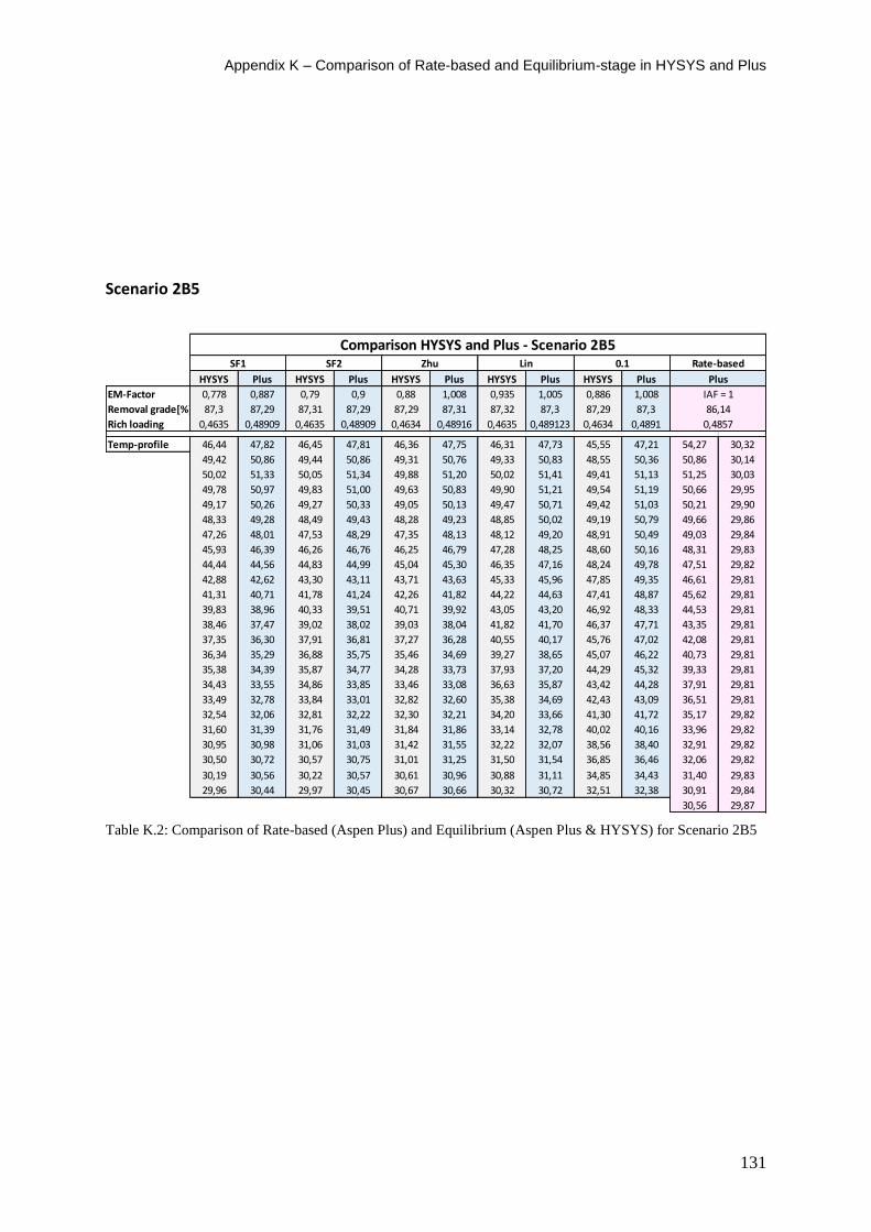
Appendix K – Comparison of Rate-based and Equilibrium-stage in HYSYS and Plus
131
Scenario 2B5
Table K.2: Comparison of Rate-based (Aspen Plus) and Equilibrium (Aspen Plus & HYSYS) for Scenario 2B5
HYSYS Plus HYSYS Plus HYSYS Plus HYSYS Plus HYSYS Plus
EM-Factor 0,778 0,887 0,79 0,9 0,88 1,008 0,935 1,005 0,886 1,008
Removal grade[%] 87,3 87,29 87,31 87,29 87,29 87,31 87,32 87,3 87,29 87,3
Rich loading 0,4635 0,48909 0,4635 0,48909 0,4634 0,48916 0,4635 0,489123 0,4634 0,4891
Temp-profile 46,44 47,82 46,45 47,81 46,36 47,75 46,31 47,73 45,55 47,21 54,27 30,32
49,42 50,86 49,44 50,86 49,31 50,76 49,33 50,83 48,55 50,36 50,86 30,14
50,02 51,33 50,05 51,34 49,88 51,20 50,02 51,41 49,41 51,13 51,25 30,03
49,78 50,97 49,83 51,00 49,63 50,83 49,90 51,21 49,54 51,19 50,66 29,95
49,17 50,26 49,27 50,33 49,05 50,13 49,47 50,71 49,42 51,03 50,21 29,90
48,33 49,28 48,49 49,43 48,28 49,23 48,85 50,02 49,19 50,79 49,66 29,86
47,26 48,01 47,53 48,29 47,35 48,13 48,12 49,20 48,91 50,49 49,03 29,84
45,93 46,39 46,26 46,76 46,25 46,79 47,28 48,25 48,60 50,16 48,31 29,83
44,44 44,56 44,83 44,99 45,04 45,30 46,35 47,16 48,24 49,78 47,51 29,82
42,88 42,62 43,30 43,11 43,71 43,63 45,33 45,96 47,85 49,35 46,61 29,81
41,31 40,71 41,78 41,24 42,26 41,82 44,22 44,63 47,41 48,87 45,62 29,81
39,83 38,96 40,33 39,51 40,71 39,92 43,05 43,20 46,92 48,33 44,53 29,81
38,46 37,47 39,02 38,02 39,03 38,04 41,82 41,70 46,37 47,71 43,35 29,81
37,35 36,30 37,91 36,81 37,27 36,28 40,55 40,17 45,76 47,02 42,08 29,81
36,34 35,29 36,88 35,75 35,46 34,69 39,27 38,65 45,07 46,22 40,73 29,81
35,38 34,39 35,87 34,77 34,28 33,73 37,93 37,20 44,29 45,32 39,33 29,81
34,43 33,55 34,86 33,85 33,46 33,08 36,63 35,87 43,42 44,28 37,91 29,81
33,49 32,78 33,84 33,01 32,82 32,60 35,38 34,69 42,43 43,09 36,51 29,81
32,54 32,06 32,81 32,22 32,30 32,21 34,20 33,66 41,30 41,72 35,17 29,82
31,60 31,39 31,76 31,49 31,84 31,86 33,14 32,78 40,02 40,16 33,96 29,82
30,95 30,98 31,06 31,03 31,42 31,55 32,22 32,07 38,56 38,40 32,91 29,82
30,50 30,72 30,57 30,75 31,01 31,25 31,50 31,54 36,85 36,46 32,06 29,82
30,19 30,56 30,22 30,57 30,61 30,96 30,88 31,11 34,85 34,43 31,40 29,83
29,96 30,44 29,97 30,45 30,67 30,66 30,32 30,72 32,51 32,38 30,91 29,84
30,56 29,87
Plus
IAF = 1
86,14
0,4857
SF1 SF2 Zhu Lin 0.1 Rate-based
Comparison HYSYS and Plus - Scenario 2B5
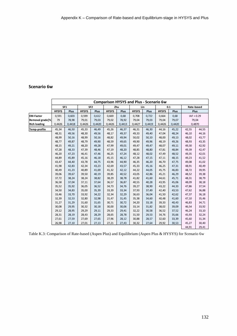
Appendix K – Comparison of Rate-based and Equilibrium-stage in HYSYS and Plus
132
Scenario 6w
Table K.3: Comparison of Rate-based (Aspen Plus) and Equilibrium (Aspen Plus & HYSYS) for Scenario 6w
HYSYS Plus HYSYS Plus HYSYS Plus HYSYS Plus HYSYS Plus
EM-Factor 0,591 0,603 0,599 0,612 0,669 0,68 0,708 0,722 0,664 0,68
Removal grade[%] 79 78,98 79,01 79,03 79,02 78,92 79,04 79,03 79,04 79,07
Rich loading 0,4426 0,4418 0,4426 0,4420 0,4426 0,4413 0,4427 0,4419 0,4426 0,4420
Temp-profile 45,34 46,50 45,33 46,49 45,26 46,37 46,31 46,30 44,16 45,22 42,55 44,55
48,31 49,56 48,30 49,56 48,17 49,37 49,33 49,40 47,04 48,24 46,10 44,16
48,99 50,16 48,99 50,16 48,82 49,94 50,02 50,10 48,00 49,13 48,02 43,77
48,77 49,87 48,79 49,90 48,59 49,65 49,90 49,96 48,19 49,26 48,93 43,35
48,15 49,21 48,20 49,28 47,99 49,01 49,47 49,47 48,07 49,11 49,30 42,92
47,28 48,33 47,39 48,46 47,19 48,20 48,85 48,80 47,81 48,84 49,39 42,47
46,20 47,23 46,41 47,46 46,25 47,24 48,12 48,02 47,49 48,52 49,35 42,01
44,89 45,89 45,16 46,18 45,15 46,12 47,28 47,15 47,11 48,15 49,23 41,52
43,47 44,40 43,78 44,75 43,96 44,90 46,35 46,20 46,70 47,75 49,08 41,02
41,98 42,83 42,34 43,23 42,69 43,57 45,33 45,16 46,25 47,31 48,91 40,49
40,49 41,23 40,89 41,69 41,32 42,12 44,22 44,05 45,75 46,83 48,72 39,95
39,06 39,67 39,50 40,19 39,85 40,52 43,05 42,86 45,21 46,29 48,52 39,38
37,72 38,24 38,24 38,82 38,29 38,78 41,82 41,60 44,61 45,71 48,31 38,79
36,58 37,04 37,11 37,64 36,57 36,87 40,55 40,28 43,95 45,06 48,09 38,18
35,52 35,92 36,05 36,52 34,73 34,76 39,27 38,90 43,22 44,33 47,86 37,54
34,50 34,83 35,00 35,39 33,39 33,34 37,93 37,49 42,40 43,53 47,62 36,88
33,46 33,70 33,92 34,22 32,34 32,29 36,63 36,04 41,50 42,62 47,37 36,18
32,39 32,53 32,80 32,98 31,47 31,45 35,38 34,60 40,48 41,60 47,10 35,46
31,27 31,29 31,60 31,65 30,71 30,72 34,20 33,18 39,33 40,43 46,83 34,71
30,08 29,95 30,32 30,18 30,00 30,06 33,14 31,82 38,02 39,09 46,54 33,92
29,12 28,95 29,29 29,11 29,33 29,41 32,22 30,58 36,52 37,52 46,24 33,10
28,31 28,19 28,43 28,29 28,65 28,78 31,50 29,53 34,76 35,66 45,93 32,24
27,61 27,59 27,69 27,65 27,96 28,12 30,88 28,57 32,60 33,39 45,60 31,34
26,98 27,10 27,01 27,13 27,21 27,43 30,32 27,64 29,92 30,53 45,27 30,40
44,91 29,41
79,04
0,4870
Lin 0.1 Rate-based
Plus
IAF = 0.29
Comparison HYSYS and Plus - Scenario 6wSF1 SF2 Zhu
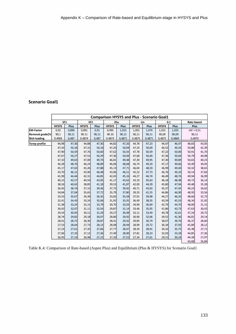
Appendix K – Comparison of Rate-based and Equilibrium-stage in HYSYS and Plus
133
Scenario Goal1
Table K.4: Comparison of Rate-based (Aspen Plus) and Equilibrium (Plus & HYSYS) for Scenario Goal1
HYSYS Plus HYSYS Plus HYSYS Plus HYSYS Plus HYSYS Plus
EM-Factor 0,92 0,896 0,891 0,91 0,995 1,015 1,055 1,074 1,015 1,025
Removal grade[%] 90,1 90,11 90.11 90,11 90.10 90,12 90,11 90,11 90,09 90,09
Rich loading 0.4904 0,487 0.4874 0,487 0.4873 0,4871 0.4875 0,4871 0,4872 0,4869
Temp-profile 44,98 47,36 44,88 47,36 44,82 47,26 44,78 47,23 44,07 46,47 48,83 43,05
47,43 50,18 47,31 50,18 47,20 50,04 47,24 50,09 46,52 49,33 50,88 42,39
47,90 50,59 47,76 50,60 47,62 50,43 47,78 50,59 47,22 50,00 50,91 41,70
47,67 50,27 47,53 50,29 47,36 50,09 47,68 50,40 47,36 50,04 50,79 40,98
47,10 49,63 47,00 49,70 46,81 49,48 47,30 49,95 47,30 49,89 50,65 40,23
46,28 48,76 46,24 48,89 46,06 48,68 46,74 49,33 47,17 49,66 50,49 39,45
45,17 47,63 45,26 47,88 45,13 47,71 46,04 48,59 46,99 49,40 50,32 38,65
43,70 46,15 43,90 46,48 43,96 46,51 45,22 47,73 46,76 49,10 50,14 37,83
41,99 44,44 42,31 44,85 42,65 45,16 44,27 46,74 46,49 48,76 49,94 36,99
40,15 42,57 40,59 43,05 41,17 43,62 43,19 45,63 46,18 48,38 49,72 36,14
38,26 40,63 38,85 41,18 39,53 41,87 42,00 44,39 45,80 47,94 49,48 35,28
36,45 38,74 37,15 39,36 37,73 39,92 40,71 43,03 45,37 47,45 49,23 34,42
34,84 37,04 35,65 37,72 35,79 37,80 39,33 41,55 44,86 46,90 48,95 33,56
33,55 35,67 34,39 36,35 33,82 35,58 37,91 39,98 44,27 46,26 48,66 32,73
32,41 34,43 33,24 35,06 31,92 33,35 36,40 38,35 43,59 45,53 48,34 31,92
31,38 33,24 32,15 33,79 30,70 32,03 34,90 36,69 42,79 44,70 48,00 31,15
30,42 32,07 31,11 32,54 29,87 31,14 33,46 35,05 41,86 43,73 47,63 30,42
29,54 30,93 30,11 31,29 29,27 30,48 32,11 33,49 40,78 42,61 47,24 29,75
28,74 29,82 29,18 30,07 28,80 29,92 30,90 32,06 39,52 41,30 46,81 29,14
28,01 28,72 28,30 28,87 28,41 29,42 29,85 30,79 38,07 39,76 46,37 28,60
27,53 28,04 27,73 28,13 28,08 28,94 28,99 29,72 36,34 37,93 45,89 28,12
27,23 27,61 27,35 27,66 27,77 28,47 28,34 28,91 34,32 35,75 45,38 27,71
27,06 27,33 27,13 27,36 27,49 28,00 27,81 28,23 32,03 33,18 44,85 27,36
26,95 27,14 26,98 27,15 27,20 27,52 27,34 27,61 29,51 30,24 44,28 27,07
43,68 26,84
Plus
IAF = 0,51
90,11
0,4870
SF1 SF2 Zhu Lin 0.1 Rate-based
Comparison HYSYS and Plus - Scenario Goal1
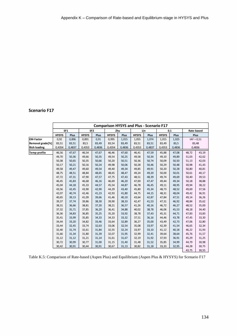
Appendix K – Comparison of Rate-based and Equilibrium-stage in HYSYS and Plus
134
Scenario F17
Table K.5: Comparison of Rate-based (Aspen Plus) and Equilibrium (Aspen Plus & HYSYS) for Scenario F17
HYSYS Plus HYSYS Plus HYSYS Plus HYSYS Plus HYSYS Plus
EM-Factor 0,92 0,896 0,891 0,91 0,995 1,015 1,055 1,074 1,015 1,025
Removal grade[%] 83,51 83,51 83,5 83,49 83,54 83,49 83,51 83,51 83,49 83,5
Rich loading 0,4354 0,4837 0,4353 0,4836 0,4354 0,4836 0,4353 0,4837 0,4353 0,4836
Temp-profile 46,56 47,67 46,54 47,67 46,46 47,60 46,41 47,59 45,88 47,08 48,72 43,19
49,70 50,36 49,66 50,35 49,54 50,25 49,58 50,34 49,10 49,89 51,03 42,62
50,38 50,65 50,35 50,66 50,20 50,51 50,36 50,74 50,09 50,50 51,13 42,03
50,17 50,21 50,16 50,24 49,98 50,06 50,28 50,46 50,29 50,48 50,98 41,43
49,58 49,47 49,60 49,54 49,40 49,34 49,85 49,91 50,20 50,28 50,80 40,81
48,75 48,51 48,84 48,65 48,65 48,47 49,24 49,20 50,00 50,01 50,61 40,17
47,72 47,31 47,90 47,57 47,75 47,43 48,51 48,39 49,74 49,69 50,40 39,53
46,45 45,83 46,68 46,16 46,69 46,20 47,69 47,47 49,44 49,34 50,18 38,88
45,04 44,18 45,33 44,57 45,54 44,87 46,78 46,45 49,11 48,95 49,94 38,22
43,56 42,45 43,90 42,90 44,29 43,40 45,80 45,34 48,73 48,52 49,69 37,56
42,07 40,74 42,46 41,23 42,93 41,80 44,75 44,15 48,31 48,04 49,42 36,91
40,65 39,13 41,09 39,66 41,46 40,10 43,64 42,87 47,84 47,51 49,14 36,26
39,37 37,74 39,86 38,30 39,90 38,33 42,47 41,53 47,31 46,92 48,84 35,62
38,31 36,66 38,81 37,20 38,21 36,57 41,26 40,16 46,72 46,27 48,52 35,00
37,32 35,71 37,85 36,20 36,41 34,88 40,02 38,78 46,06 45,53 48,18 34,40
36,36 34,83 36,85 35,25 35,20 33,92 38,78 37,43 45,31 44,71 47,83 33,83
35,41 33,99 35,85 34,33 34,33 33,32 37,51 36,16 44,46 43,78 47,45 33,30
34,44 33,20 34,82 33,46 33,64 32,89 36,27 35,00 43,49 42,73 47,06 32,80
33,44 32,45 33,74 32,63 33,06 32,54 35,08 33,97 42,39 41,54 46,65 32,34
32,40 31,74 32,61 31,84 32,55 32,24 33,97 33,10 41,12 40,18 46,22 31,93
31,66 31,34 31,80 31,39 32,07 31,95 32,99 32,41 39,64 38,64 45,76 31,57
31,12 31,12 31,21 31,14 31,61 31,67 32,19 31,92 37,93 36,91 45,29 31,25
30,72 30,99 30,77 31,00 31,15 31,40 31,48 31,52 35,85 34,99 44,79 30,98
30,42 30,91 30,44 30,91 30,67 31,13 30,82 31,18 33,33 32,95 44,28 30,75
43,75 30,55
Plus
IAF = 0,51
83,48
0,4836
SF1 SF2 Zhu Lin 0.1 Rate-based
Comparison HYSYS and Plus - Scenario F17
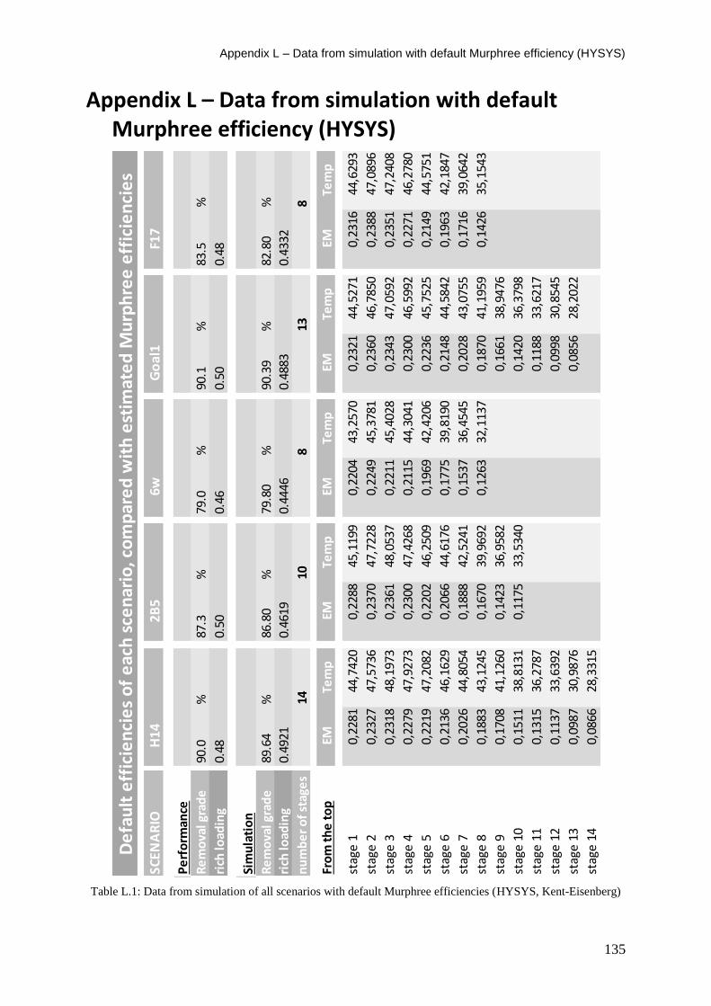
Appendix L – Data from simulation with default Murphree efficiency (HYSYS)
135
Appendix L – Data from simulation with default Murphree efficiency (HYSYS)
Table L.1: Data from simulation of all scenarios with default Murphree efficiencies (HYSYS, Kent-Eisenberg)
SCEN
AR
IOH
14
2B5
6wG
oal
1F1
7
Pe
rfo
rman
ce
Re
mo
val g
rad
e90
.0%
87.3
%79
.0%
90.1
%83
.5%
rich
load
ing
0.48
0.50
0.46
0.50
0.48
nu
mb
er
of
ste
ps
Sim
ula
tio
n
Re
mo
val g
rad
e89
.64
%86
.80
%79
.80
%90
.39
%82
.80
%
rich
load
ing
0.49
210.
4619
0.44
460.
4883
0.43
32
nu
mb
er
of
stag
es
1410
813
8
Fro
m t
he
to
pEM
Tem
pEM
Tem
pEM
Tem
pEM
Tem
pEM
Tem
p
stag
e 1
0,22
8144
,742
00,
2288
45,1
199
0,22
0443
,257
00,
2321
44,5
271
0,23
1644
,629
3
stag
e 2
0,23
2747
,573
60,
2370
47,7
228
0,22
4945
,378
10,
2360
46,7
850
0,23
8847
,089
6
stag
e 3
0,23
1848
,197
30,
2361
48,0
537
0,22
1145
,402
80,
2343
47,0
592
0,23
5147
,240
8
stag
e 4
0,22
7947
,927
30,
2300
47,4
268
0,21
1544
,304
10,
2300
46,5
992
0,22
7146
,278
0
stag
e 5
0,22
1947
,208
20,
2202
46,2
509
0,19
6942
,420
60,
2236
45,7
525
0,21
4944
,575
1
stag
e 6
0,21
3646
,162
90,
2066
44,6
176
0,17
7539
,819
00,
2148
44,5
842
0,19
6342
,184
7
stag
e 7
0,20
2644
,805
40,
1888
42,5
241
0,15
3736
,454
50,
2028
43,0
755
0,17
1639
,064
2
stag
e 8
0,18
8343
,124
50,
1670
39,9
692
0,12
6332
,113
70,
1870
41,1
959
0,14
2635
,154
3
stag
e 9
0,17
0841
,126
00,
1423
36,9
582
0,16
6138
,947
6
stag
e 1
00,
1511
38,8
131
0,11
7533
,534
00,
1420
36,3
798
stag
e 1
10,
1315
36,2
787
0,11
8833
,621
7
stag
e 1
20,
1137
33,6
392
0,09
9830
,854
5
stag
e 1
30,
0987
30,9
876
0,08
5628
,202
2
stag
e 1
40,
0866
28,3
315
De
fau
lt e
ffic
ien
cie
s o
f e
ach
sce
nar
io, c
om
par
ed
wit
h e
stim
ate
d M
urp
hre
e e
ffic
ien
cie
s
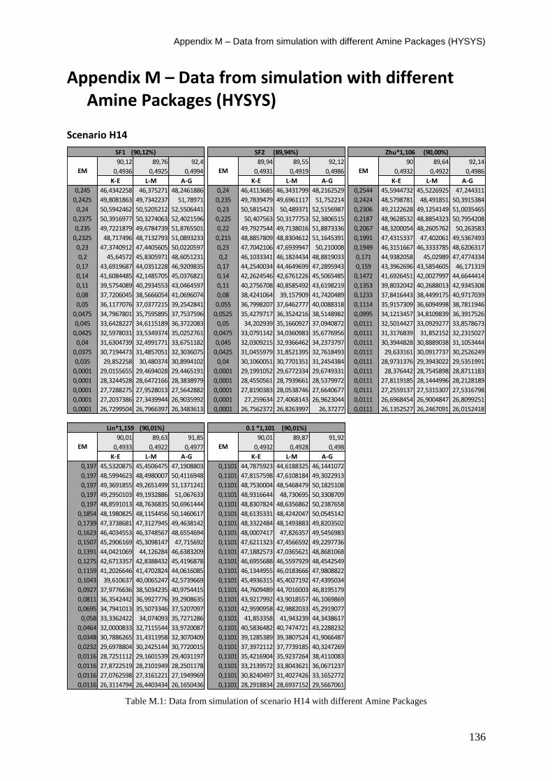
Appendix M – Data from simulation with different Amine Packages (HYSYS)
136
Appendix M – Data from simulation with different Amine Packages (HYSYS)
Scenario H14
Table M.1: Data from simulation of scenario H14 with different Amine Packages
90,12 89,76 92,4 89,94 89,55 92,12 90 89,64 92,14
0,4936 0,4925 0,4994 0,4931 0,4919 0,4986 0,4932 0,4922 0,4986
K-E L-M A-G K-E L-M A-G K-E L-M A-G
0,245 46,4342258 46,375271 48,2461886 0,24 46,4113685 46,3431799 48,2162529 0,2544 45,5944732 45,5226925 47,244311
0,2425 49,8081863 49,7342237 51,78971 0,235 49,7839479 49,6961117 51,752214 0,2424 48,5798781 48,491851 50,3915384
0,24 50,5942462 50,5205212 52,5506441 0,23 50,5815423 50,489371 52,5156987 0,2306 49,2122628 49,1254149 51,0035465
0,2375 50,3916977 50,3274063 52,4021596 0,225 50,407563 50,3177753 52,3806515 0,2187 48,9628532 48,8854323 50,7954208
0,235 49,7221879 49,6784739 51,8765501 0,22 49,7927544 49,7138016 51,8873336 0,2067 48,3200054 48,2605762 50,263583
0,2325 48,717496 48,7132793 51,0893233 0,215 48,8857809 48,8304612 51,1645391 0,1991 47,4315337 47,402061 49,5367493
0,23 47,3740912 47,4405605 50,0220597 0,23 47,7042106 47,6939947 50,210008 0,1949 46,3151667 46,3333785 48,6206317
0,2 45,64572 45,8305971 48,6051231 0,2 46,1033341 46,1824434 48,8819033 0,171 44,9382058 45,02989 47,4774334
0,17 43,6919687 44,0351228 46,9209835 0,17 44,2540034 44,4649699 47,2895943 0,159 43,3962696 43,5854605 46,171319
0,14 41,6084485 42,1485705 45,0376821 0,14 42,2624546 42,6761226 45,5065485 0,1472 41,6926451 42,0027997 44,6644414
0,11 39,5754089 40,2934553 43,0464597 0,11 40,2756708 40,8585492 43,6198219 0,1353 39,8032042 40,2688013 42,9345308
0,08 37,7206045 38,5666054 41,0696074 0,08 38,4241064 39,157909 41,7420489 0,1233 37,8416443 38,4499175 40,9717039
0,05 36,1177076 37,0377215 39,2542841 0,055 36,7998207 37,6462777 40,0088318 0,1114 35,9157309 36,6094998 38,7811946
0,0475 34,7967801 35,7595895 37,7537596 0,0525 35,4279717 36,3524216 38,5148982 0,0995 34,1213457 34,8109839 36,3917526
0,045 33,6428227 34,6115189 36,3722083 0,05 34,202939 35,1660927 37,0940872 0,0111 32,5014427 33,0929277 33,8578673
0,0425 32,5978031 33,5349374 35,0252761 0,0475 33,0791142 34,0360983 35,6776956 0,0111 31,3176839 31,852152 32,2315027
0,04 31,6304739 32,4991771 33,6751182 0,045 32,0309215 32,9366462 34,2373797 0,0111 30,3944828 30,8889038 31,1053444
0,0375 30,7194473 31,4857051 32,3036075 0,0425 31,0455979 31,8521395 32,7618493 0,0111 29,633161 30,0917737 30,2526249
0,035 29,852258 30,480374 30,8994102 0,04 30,1060051 30,7701351 31,2454384 0,0111 28,9731376 29,3943022 29,5351991
0,0001 29,0155655 29,4694028 29,4465191 0,0001 29,1991052 29,6772334 29,6749331 0,0111 28,376442 28,7545898 28,8711183
0,0001 28,3244528 28,6472166 28,3838979 0,0001 28,4550561 28,7939661 28,5379972 0,0111 27,8119185 28,1444996 28,2128189
0,0001 27,7288275 27,9528013 27,5642882 0,0001 27,8190383 28,0538746 27,6640677 0,0111 27,2559137 27,5315307 27,5316798
0,0001 27,2037386 27,3439944 26,9035992 0,0001 27,259634 27,4068143 26,9623044 0,0111 26,6968454 26,9004847 26,8099251
0,0001 26,7299504 26,7966397 26,3483613 0,0001 26,7562372 26,8263997 26,37277 0,0111 26,1352527 26,2467091 26,0152418
90,01 89,63 91,85 90,01 89,87 91,92
0,4933 0,4922 0,4977 0,4932 0,4928 0,498
K-E L-M A-G K-E L-M A-G
0,197 45,5320875 45,4506475 47,1908803 0,1101 44,7875923 44,6188325 46,1441072
0,197 48,5994623 48,4980007 50,4116948 0,1101 47,8157598 47,6108184 49,3022913
0,197 49,3691855 49,2651499 51,1371241 0,1101 48,7530004 48,5468479 50,1825108
0,197 49,2950103 49,1932886 51,067633 0,1101 48,9316644 48,730695 50,3308709
0,197 48,8591013 48,7636835 50,6961444 0,1101 48,8307824 48,6356862 50,2387658
0,1854 48,1980825 48,1154456 50,1460617 0,1101 48,6135331 48,4242047 50,0545142
0,1739 47,3738681 47,3127945 49,4638142 0,1101 48,3322484 48,1493883 49,8203502
0,1623 46,4034553 46,3748567 48,6554694 0,1101 48,0007417 47,826357 49,5456983
0,1507 45,2906169 45,3098147 47,715692 0,1101 47,6211323 47,4566592 49,2297736
0,1391 44,0421069 44,126284 46,6383209 0,1101 47,1882573 47,0365621 48,8681068
0,1275 42,6713357 42,8388432 45,4196878 0,1101 46,6955688 46,5597929 48,4542549
0,1159 41,2026646 41,4702824 44,0616085 0,1101 46,1344955 46,0183666 47,9808822
0,1043 39,610637 40,0065247 42,5739669 0,1101 45,4936315 45,4027192 47,4395034
0,0927 37,9776636 38,5034235 40,9754415 0,1101 44,7609489 44,7016003 46,8195179
0,0811 36,3542442 36,9927776 39,2908635 0,1101 43,9217992 43,9018557 46,1069869
0,0695 34,7941013 35,5073346 37,5207097 0,1101 42,9590958 42,9882033 45,2919077
0,058 33,3362422 34,074093 35,7271286 0,1101 41,853358 41,943239 44,3438617
0,0464 32,0000833 32,7115544 33,9720087 0,1101 40,5836482 40,7474721 43,2288232
0,0348 30,7886265 31,4311958 32,3070409 0,1101 39,1285389 39,3807524 41,9066487
0,0232 29,6978804 30,2425144 30,7720015 0,1101 37,3972112 37,7739185 40,3247269
0,0116 28,7251112 29,1601539 29,4031197 0,1101 35,4216904 35,9237264 38,4110083
0,0116 27,8722519 28,2101949 28,2501178 0,1101 33,2139572 33,8043621 36,0671237
0,0116 27,0762598 27,3161221 27,1949969 0,1101 30,8240497 31,4027426 33,1652772
0,0116 26,3114794 26,4403434 26,1650436 0,1101 28,2918834 28,6937152 29,5667061
EM EM
EM EM EM
Lin*1,159 (90,01%) 0.1 *1,101 (90,01%)
SF1 (90,12%) SF2 (89,94%) Zhu*1,106 (90,00%)
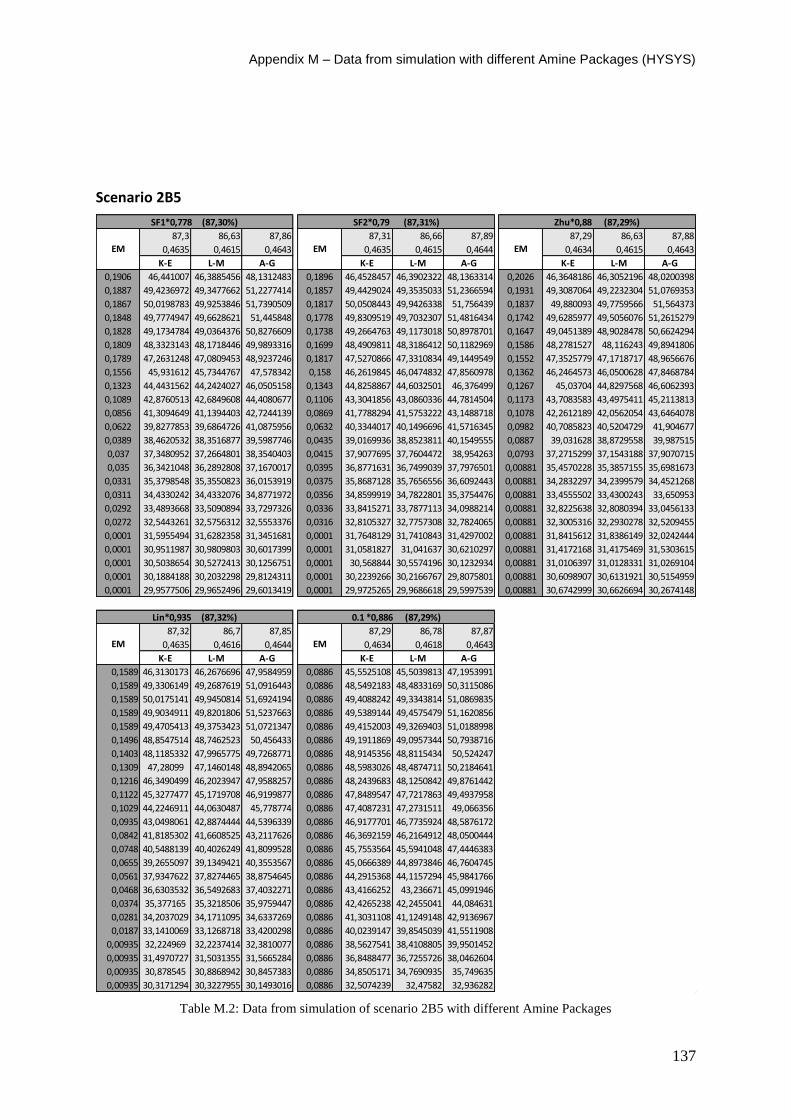
Appendix M – Data from simulation with different Amine Packages (HYSYS)
137
Scenario 2B5
Table M.2: Data from simulation of scenario 2B5 with different Amine Packages
87,3 86,63 87,86 87,31 86,66 87,89 87,29 86,63 87,88
0,4635 0,4615 0,4643 0,4635 0,4615 0,4644 0,4634 0,4615 0,4643
K-E L-M A-G K-E L-M A-G K-E L-M A-G
0,1906 46,441007 46,3885456 48,1312483 0,1896 46,4528457 46,3902322 48,1363314 0,2026 46,3648186 46,3052196 48,0200398
0,1887 49,4236972 49,3477662 51,2277414 0,1857 49,4429024 49,3535033 51,2366594 0,1931 49,3087064 49,2232304 51,0769353
0,1867 50,0198783 49,9253846 51,7390509 0,1817 50,0508443 49,9426338 51,756439 0,1837 49,880093 49,7759566 51,564373
0,1848 49,7774947 49,6628621 51,445848 0,1778 49,8309519 49,7032307 51,4816434 0,1742 49,6285977 49,5056076 51,2615279
0,1828 49,1734784 49,0364376 50,8276609 0,1738 49,2664763 49,1173018 50,8978701 0,1647 49,0451389 48,9028478 50,6624294
0,1809 48,3323143 48,1718446 49,9893316 0,1699 48,4909811 48,3186412 50,1182969 0,1586 48,2781527 48,116243 49,8941806
0,1789 47,2631248 47,0809453 48,9237246 0,1817 47,5270866 47,3310834 49,1449549 0,1552 47,3525779 47,1718717 48,9656676
0,1556 45,931612 45,7344767 47,578342 0,158 46,2619845 46,0474832 47,8560978 0,1362 46,2464573 46,0500628 47,8468784
0,1323 44,4431562 44,2424027 46,0505158 0,1343 44,8258867 44,6032501 46,376499 0,1267 45,03704 44,8297568 46,6062393
0,1089 42,8760513 42,6849608 44,4080677 0,1106 43,3041856 43,0860336 44,7814504 0,1173 43,7083583 43,4975411 45,2113813
0,0856 41,3094649 41,1394403 42,7244139 0,0869 41,7788294 41,5753222 43,1488718 0,1078 42,2612189 42,0562054 43,6464078
0,0622 39,8277853 39,6864726 41,0875956 0,0632 40,3344017 40,1496696 41,5716345 0,0982 40,7085823 40,5204729 41,904677
0,0389 38,4620532 38,3516877 39,5987746 0,0435 39,0169936 38,8523811 40,1549555 0,0887 39,031628 38,8729558 39,987515
0,037 37,3480952 37,2664801 38,3540403 0,0415 37,9077695 37,7604472 38,954263 0,0793 37,2715299 37,1543188 37,9070715
0,035 36,3421048 36,2892808 37,1670017 0,0395 36,8771631 36,7499039 37,7976501 0,00881 35,4570228 35,3857155 35,6981673
0,0331 35,3798548 35,3550823 36,0153919 0,0375 35,8687128 35,7656556 36,6092443 0,00881 34,2832297 34,2399579 34,4521268
0,0311 34,4330242 34,4332076 34,8771972 0,0356 34,8599919 34,7822801 35,3754476 0,00881 33,4555502 33,4300243 33,650953
0,0292 33,4893668 33,5090894 33,7297326 0,0336 33,8415271 33,7877113 34,0988214 0,00881 32,8225638 32,8080394 33,0456133
0,0272 32,5443261 32,5756312 32,5553376 0,0316 32,8105327 32,7757308 32,7824065 0,00881 32,3005316 32,2930278 32,5209455
0,0001 31,5955494 31,6282358 31,3451681 0,0001 31,7648129 31,7410843 31,4297002 0,00881 31,8415612 31,8386149 32,0242444
0,0001 30,9511987 30,9809803 30,6017399 0,0001 31,0581827 31,041637 30,6210297 0,00881 31,4172168 31,4175469 31,5303615
0,0001 30,5038654 30,5272413 30,1256751 0,0001 30,568844 30,5574196 30,1232934 0,00881 31,0106397 31,0128331 31,0269104
0,0001 30,1884188 30,2032298 29,8124311 0,0001 30,2239266 30,2166767 29,8075801 0,00881 30,6098907 30,6131921 30,5154959
0,0001 29,9577506 29,9652496 29,6013419 0,0001 29,9725265 29,9686618 29,5997539 0,00881 30,6742999 30,6626694 30,2674148
87,32 86,7 87,85 87,29 86,78 87,87
0,4635 0,4616 0,4644 0,4634 0,4618 0,4643
K-E L-M A-G K-E L-M A-G
0,1589 46,3130173 46,2676696 47,9584959 0,0886 45,5525108 45,5039813 47,1953991
0,1589 49,3306149 49,2687619 51,0916443 0,0886 48,5492183 48,4833169 50,3115086
0,1589 50,0175141 49,9450814 51,6924194 0,0886 49,4088242 49,3343814 51,0869835
0,1589 49,9034911 49,8201806 51,5237663 0,0886 49,5389144 49,4575479 51,1620856
0,1589 49,4705413 49,3753423 51,0721347 0,0886 49,4152003 49,3269403 51,0188998
0,1496 48,8547514 48,7462523 50,456433 0,0886 49,1911869 49,0957344 50,7938716
0,1403 48,1185332 47,9965775 49,7268771 0,0886 48,9145356 48,8115434 50,524247
0,1309 47,28099 47,1460148 48,8942065 0,0886 48,5983026 48,4874711 50,2184641
0,1216 46,3490499 46,2023947 47,9588257 0,0886 48,2439683 48,1250842 49,8761442
0,1122 45,3277477 45,1719708 46,9199877 0,0886 47,8489547 47,7217863 49,4937958
0,1029 44,2246911 44,0630487 45,778774 0,0886 47,4087231 47,2731511 49,066356
0,0935 43,0498061 42,8874444 44,5396339 0,0886 46,9177701 46,7735924 48,5876172
0,0842 41,8185302 41,6608525 43,2117626 0,0886 46,3692159 46,2164912 48,0500444
0,0748 40,5488139 40,4026249 41,8099528 0,0886 45,7553564 45,5941048 47,4446383
0,0655 39,2655097 39,1349421 40,3553567 0,0886 45,0666389 44,8973846 46,7604745
0,0561 37,9347622 37,8274465 38,8754645 0,0886 44,2915368 44,1157294 45,9841766
0,0468 36,6303532 36,5492683 37,4032271 0,0886 43,4166252 43,236671 45,0991946
0,0374 35,377165 35,3218506 35,9759447 0,0886 42,4265238 42,2455041 44,084631
0,0281 34,2037029 34,1711095 34,6337269 0,0886 41,3031108 41,1249148 42,9136967
0,0187 33,1410069 33,1268718 33,4200298 0,0886 40,0239147 39,8545039 41,5511908
0,00935 32,224969 32,2237414 32,3810077 0,0886 38,5627541 38,4108805 39,9501452
0,00935 31,4970727 31,5031355 31,5665284 0,0886 36,8488477 36,7255726 38,0462604
0,00935 30,878545 30,8868942 30,8457383 0,0886 34,8505171 34,7690935 35,749635
0,00935 30,3171294 30,3227955 30,1493016 0,0886 32,5074239 32,47582 32,936282
EM EM
EM EM EM
Lin*0,935 (87,32%) 0.1 *0,886 (87,29%)
SF1*0,778 (87,30%) SF2*0,79 (87,31%) Zhu*0,88 (87,29%)

Appendix M – Data from simulation with different Amine Packages (HYSYS)
138
Scenario 6w
Table M.3: Data from simulation of scenario 6w with different Amine Packages
79 78,28 79,53 79,01 78,29 79,53 79,02 78,31 79,54
0,4426 0,4406 0,4433 0,4426 0,4406 0,4433 0,4426 0,4407 0,4433
K-E L-M A-G K-E L-M A-G K-E L-M A-G
0,1448 45,3437118 45,2631779 46,7942146 0,1438 45,3322283 45,2652914 46,8029346 0,1539 45,25502 45,1889499 46,7207597
0,1433 48,3076912 48,1960163 49,865542 0,1408 48,2975408 48,2053022 49,8812852 0,1466 48,1695055 48,07833 49,7527581
0,1418 48,991069 48,8630434 50,4320044 0,1374 48,990846 48,8854131 50,4591364 0,1395 48,823279 48,7188827 50,2988355
0,1404 48,7715543 48,6303382 50,1126804 0,1348 48,7920002 48,6755497 50,1595434 0,1323 48,5938195 48,4786321 49,9788395
0,1389 48,1460258 47,9925078 49,4171982 0,1318 48,2034636 48,0760846 49,4972693 0,1250 47,9902671 47,8650401 49,3176562
0,1374 47,2750391 47,1107877 48,4840047 0,1288 47,3928806 47,2548307 48,6162837 0,1204 47,1920118 47,0578482 48,4758725
0,1359 46,19534 46,0237151 47,3273269 0,1378 46,4072978 46,2596449 47,5373351 0,1179 46,2459956 46,104753 47,482228
0,1182 44,8943392 44,7212793 45,9170423 0,1198 45,1646008 45,0128168 46,1716883 0,1034 45,1462898 45,0008109 46,3187206
0,1005 43,4679217 43,2998683 44,3474394 0,1018 43,7840802 43,6343779 44,6419853 0,0962 43,9646225 43,8178943 45,0542222
0,0827 41,9805287 41,8232126 42,6830827 0,0839 42,3390496 42,196992 43,0178905 0,0890 42,6897286 42,5458012 43,6632122
0,0650 40,4917605 40,3494266 40,9938435 0,0659 40,890929 40,7602306 41,3653155 0,0818 41,31775 41,1818853 42,1279489
0,0473 39,0628727 38,9380336 39,3626651 0,0479 39,5031955 39,3845283 39,7636551 0,0746 39,8493473 39,7277874 40,4340609
0,0296 37,7215397 37,6173635 37,8877099 0,0329 38,2443328 38,1338264 38,3087753 0,0674 38,2872102 38,1863032 38,5703815
0,0281 36,5797838 36,4955298 36,6733357 0,0314 37,1120166 37,0100712 37,0778513 0,0602 36,5675692 36,4950325 36,5331441
0,0266 35,5247169 35,461203 35,5601651 0,0300 36,0493776 35,9543076 35,9322039 0,0067 34,7259576 34,6824282 34,3397735
0,0251 34,4962868 34,454081 34,4672481 0,0285 34,9971777 34,9091872 34,798271 0,0067 33,3862389 33,3569268 32,9151299
0,0236 33,4594765 33,4382001 33,350652 0,0270 33,9210665 33,841569 33,6353187 0,0067 32,3396052 32,3170878 31,9059262
0,0222 32,3909416 32,3890547 32,1834049 0,0255 32,7967101 32,7278334 32,4163451 0,0067 31,4696893 31,450551 31,1037173
0,0207 31,270301 31,2851332 30,9425386 0,0240 31,6028618 31,5468692 31,1181409 0,0067 30,7060679 30,6882374 30,3917663
0,0001 30,0780343 30,1054608 29,6107093 0,0001 30,3159409 30,2741906 29,7195629 0,0067 30,0025178 29,9846197 29,7095413
0,0001 29,1162154 29,1502026 28,617918 0,0001 29,2853878 29,2549567 28,6879879 0,0067 29,3258112 29,3094432 29,0243594
0,0001 28,313683 28,3493127 27,8349126 0,0001 28,4301764 28,4083385 27,8762571 0,0067 28,6517656 28,6386793 28,3291446
0,0001 27,6109263 27,6423627 27,186772 0,0001 27,6854437 27,6701914 27,2080248 0,0067 27,9553033 27,9462268 27,6212814
0,0001 26,9770221 26,9954868 26,6276587 0,0001 27,0134156 27,0051424 26,6302252 0,0067 27,2084945 27,2030309 26,8942388
79,04 78,37 79,52 79,04 78,52 79,46
0,4427 0,4408 0,4433 0,4426 0,4412 0,4431
K-E L-M A-G K-E L-M A-G
0,1204 46,3130173 45,0955887 46,6507817 0,0664 44,1550848 44,0969364 45,661799
0,1204 49,3306149 48,0664352 49,772315 0,0664 47,0423852 46,9671529 48,7475005
0,1204 50,0175141 48,8404505 50,4496308 0,0664 48,0020429 47,9215931 49,6357498
0,1204 49,9034911 48,7500155 50,2747684 0,0664 48,1890552 48,105133 49,745914
0,1204 49,4705413 48,2887921 49,7625448 0,0664 48,0670004 47,9790373 49,5772316
0,1133 48,8547514 47,623756 49,0648838 0,0664 47,8113356 47,7187385 49,2967588
0,1062 48,1185332 46,8385712 48,2518386 0,0664 47,486445 47,3889914 48,9589
0,0991 47,28099 45,9643216 47,3440889 0,0664 47,1146521 47,0123662 48,5810842
0,0920 46,3490499 45,0139812 46,3456464 0,0664 46,7023967 46,5953279 48,1675304
0,0850 45,3277477 43,9949632 45,2540518 0,0664 46,2496339 46,1378397 47,7157669
0,0779 44,2246911 42,9136369 44,0675999 0,0664 45,7534053 45,6368019 47,2194375
0,0708 43,0498061 41,7768631 42,7903056 0,0664 45,2089762 45,0872786 46,6684248
0,0637 41,8185302 40,5922545 41,4359688 0,0664 44,6100848 44,4829865 46,0491678
0,0566 40,5488139 39,3700275 40,0271508 0,0664 43,9490777 43,8160184 45,3470561
0,0496 39,2655097 38,1220432 38,58896 0,0664 43,2171802 43,0781125 44,5537955
0,0425 37,9347622 36,8201814 37,1424978 0,0664 42,4040147 42,2605744 43,6840513
0,0354 36,6303532 35,5081354 35,6841558 0,0664 41,4969942 41,3515402 42,721644
0,0283 35,377165 34,1976277 34,2262282 0,0664 40,4802149 40,3351691 41,6425412
0,0212 34,2037029 32,905907 32,7933928 0,0664 39,3325018 39,1908347 40,4176162
0,0142 33,1410069 31,6574102 31,4199383 0,0664 38,0249324 37,8913778 39,0103994
0,0071 32,224969 30,4853055 30,154347 0,0664 36,5183162 36,399074 37,3613211
0,0071 31,4970727 29,435411 29,0680473 0,0664 34,760174 34,6609781 35,3984399
0,0071 30,878545 28,444433 28,0732392 0,0664 32,5989153 32,5277923 33,0121639
0,0071 30,3171294 27,4436153 27,1051908 0,0664 29,9185772 29,8810104 30,0273898
EM EM
SF1*0,591 (79,00%) SF2*0,599 (79,01%) Zhu*0,669 (79,02%)
EM EM EM
Lin*0,708 (79,04%) 0.1*0,664 (79,04%)

Appendix M – Data from simulation with different Amine Packages (HYSYS)
139
Scenario Goal1
Table M.4: Data from simulation of scenario Goal1 with different Amine Packages
90,1 90,68 92,05 90.11 89,74 91,06 90.10 89,73 91,07
0.4904 0,4893 0,4929 0.4874 0.4861 0,4896 0.4873 0,4861 0,4896
K-E L-M A-G K-E L-M A-G K-E L-M A-G
0,2254 44,9779401 44,9379624 46,6847171 0,2138 44,8793681 44,8494604 46,5900126 0,22885 44,8166129 44,7688424 46,4661818
0,2231 47,4347861 47,3783518 49,3250486 0,2094 47,3062286 47,2638402 49,2029522 0,218104 47,2047233 47,1371099 49,0381832
0,2208 47,8960614 47,8286209 49,7752346 0,2049 47,7569433 47,7062133 49,6395975 0,207458 47,6188174 47,5393514 49,4467381
0,2185 47,6653619 47,5876681 49,5617952 0,2005 47,5309706 47,471605 49,4218792 0,196712 47,3584857 47,2683316 49,2056117
0,2162 47,1041637 47,0164426 49,0590056 0,1960 46,9971955 46,9296166 48,9312623 0,185966 46,8068503 46,7036618 48,7051668
0,2139 46,281642 46,1857659 48,327636 0,1916 46,2398449 46,1663058 48,2416008 0,1791 46,0642476 45,9484655 48,034534
0,2116 45,1693562 45,0726728 47,3331033 0,2049 45,2587235 45,180249 47,3343775 0,175319 45,1288884 45,0056676 47,1867441
0,1840 43,7002175 43,6169794 45,9972403 0,1782 43,8981501 43,8269808 46,0623313 0,153827 43,9624416 43,8380935 46,1201796
0,1564 41,9928303 41,9436655 44,4128445 0,1515 42,3061294 42,2572186 44,552207 0,143081 42,6511186 42,5331918 44,9009869
0,1288 40,1505045 40,1591454 42,6500056 0,1247 40,5866815 40,5766388 42,8815258 0,132435 41,1734539 41,0732087 43,4861612
0,1012 38,2616467 38,380063 40,7980861 0,0980 38,8482964 38,8918954 41,1374791 0,121689 39,5345887 39,4673548 41,8508441
0,0736 36,4507913 36,6496654 38,9742742 0,0713 37,1538648 37,2649324 39,4269617 0,110943 37,7260293 37,7155918 39,9809732
0,0460 34,8424734 35,1246358 37,3161229 0,0490 35,6464823 35,822848 37,8735876 0,100197 35,7939369 35,8606674 37,8764188
0,0437 33,5486787 33,9026305 35,9563097 0,0468 34,3887608 34,6229926 36,5454319 0,08955 33,8216876 33,9573291 35,5658971
0,0414 32,413141 32,823603 34,6621803 0,0446 33,2420634 33,5244612 35,2446902 0,00995 31,9173983 32,0746298 33,1324199
0,0391 31,375659 31,8196231 33,3801842 0,0423 32,1532519 32,4691783 33,9121307 0,00995 30,7031359 30,8751988 31,7700644
0,0368 30,4180192 30,8644636 32,0966338 0,0401 31,1094595 31,4374455 32,5436698 0,00995 29,8729591 30,0503208 30,9008938
0,0345 29,5379079 29,950282 30,8095522 0,0379 30,1146925 30,4252931 31,1475882 0,00995 29,2687517 29,4412091 30,2505542
0,0322 28,7376377 29,0768318 29,5226176 0,0356 29,177987 29,4349929 29,7405867 0,00995 28,7976576 28,9628942 29,6923635
0,0001 28,0098154 28,2388844 28,2406836 0,0001 28,3041803 28,4693514 28,339363 0,00995 28,4114933 28,5665053 29,1708518
0,0001 27,5333107 27,6842268 27,4908626 0,0001 27,7273369 27,833722 27,5381895 0,00995 28,0753035 28,2162406 28,6631515
0,0001 27,2322907 27,3285391 27,0548123 0,0001 27,3541989 27,4191801 27,0801659 0,00995 27,770395 27,8878476 28,1610235
0,0001 27,0571941 27,1127452 26,8108132 0,0001 27,1262676 27,1620223 26,8258377 0,00995 27,4864077 27,5728054 27,6600285
0,0001 26,9544896 26,9790573 26,6788942 0,0001 26,984001 26,9988784 26,686691 0,00995 27,1968992 27,2444606 27,1430787
90,11 89,76 91 90,09 89,89 91,19
0.4875 0,4862 0,4894 0,4872 0,4865 0,49
K-E L-M A-G K-E L-M A-G
0,17935 44,775511 44,7260847 47,1860194 0,1015 44,0736494 43,9954806 45,6793363
0,17935 47,2415561 47,1759786 49,7706575 0,1015 46,5170678 46,4198811 48,2937903
0,17935 47,7809333 47,7067805 50,3306534 0,1015 47,2181831 47,1160161 48,9787139
0,17935 47,6762569 47,5942571 50,2119412 0,1015 47,3567212 47,25172 49,1078273
0,17935 47,3001513 47,2093661 49,8058813 0,1015 47,3030662 47,1953142 49,0601213
0,1688 46,7420617 46,6418116 49,2071112 0,1015 47,1692086 47,058352 48,9404138
0,15825 46,0447875 45,9379324 48,4645187 0,1015 46,9866651 46,8725001 48,7770545
0,1477 45,2200932 45,1087207 47,5897003 0,1015 46,7620265 46,6443555 48,5758376
0,13715 44,2692302 44,1575556 46,5862212 0,1015 46,4937481 46,3723165 48,3352229
0,1266 43,1947684 43,0886024 45,4584756 0,1015 46,1767925 46,0520554 48,0507671
0,11605 42,0039218 41,9099724 44,2150209 0,1015 45,8047132 45,6783666 47,7162815
0,1055 40,7095432 40,6355635 42,8705194 0,1015 45,3699629 45,2444144 47,3242209
0,09495 39,3329507 39,2872184 41,4480154 0,1015 44,8634205 44,7387549 46,8652805
0,0844 37,9061285 37,8988587 39,983296 0,1015 44,273304 44,1476778 46,3283199
0,07385 36,3987211 36,4438838 38,4482974 0,1015 43,5864227 43,4623204 45,6994204
0,0633 34,9015766 35,0009348 36,9259863 0,1015 42,7878788 42,672476 44,96148
0,05275 33,4559369 33,6039535 35,4521709 0,1015 41,8596702 41,7565673 44,0930184
0,0422 32,1078435 32,2891812 34,0650862 0,1015 40,7801055 40,6910387 43,0664776
0,03165 30,896945 31,0897785 32,7997163 0,1015 39,5245217 39,4591566 41,8460242
0,0211 29,8514418 30,0343751 31,6862657 0,1015 38,066861 38,0396024 40,3838158
0,01055 28,9923407 29,1500808 30,7533352 0,1015 36,3391925 36,3704924 38,6164847
0,01055 28,3417778 28,4711369 30,0370494 0,1015 34,3241662 34,4321152 36,4600375
0,01055 27,8106674 27,905625 29,4404343 0,1015 32,0255487 32,2006486 33,8095528
0,01055 27,3375407 27,3901138 28,89657 0,1015 29,5100701 29,6789934 30,5339106
Lin*1,055 (90,11%) 0.1*1,015 (90,09%)
EM EM
SF1*0,920 (90,10%) SF2*0,891 (90,11%) Zhu*0,995 (90,10%)
EM EM EM
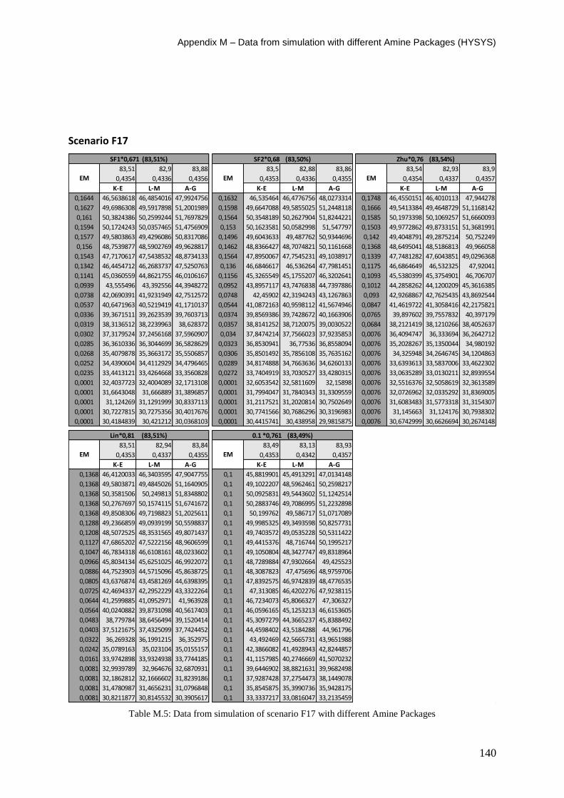
Appendix M – Data from simulation with different Amine Packages (HYSYS)
140
Scenario F17
Table M.5: Data from simulation of scenario F17 with different Amine Packages
83,51 82,9 83,88 83,5 82,88 83,86 83,54 82,93 83,9
0,4354 0,4336 0,4356 0,4353 0,4336 0,4355 0,4354 0,4337 0,4357
K-E L-M A-G K-E L-M A-G K-E L-M A-G
0,1644 46,5638618 46,4854016 47,9924756 0,1632 46,535464 46,4776756 48,0273314 0,1748 46,4550151 46,4010113 47,944278
0,1627 49,6986308 49,5917898 51,2001989 0,1598 49,6647088 49,5855025 51,2448118 0,1666 49,5413384 49,4648729 51,1168142
0,161 50,3824386 50,2599244 51,7697829 0,1564 50,3548189 50,2627904 51,8244221 0,1585 50,1973398 50,1069257 51,6660093
0,1594 50,1724243 50,0357465 51,4756909 0,153 50,1623581 50,0582998 51,547797 0,1503 49,9772862 49,8733151 51,3681991
0,1577 49,5803863 49,4296086 50,8317086 0,1496 49,6043633 49,487762 50,9344696 0,142 49,4048791 49,2875214 50,752249
0,156 48,7539877 48,5902769 49,9628817 0,1462 48,8366427 48,7074821 50,1161668 0,1368 48,6495041 48,5186813 49,966058
0,1543 47,7170617 47,5438532 48,8734133 0,1564 47,8950067 47,7545231 49,1038917 0,1339 47,7481282 47,6043851 49,0296368
0,1342 46,4454712 46,2683737 47,5250763 0,136 46,6846617 46,536264 47,7981451 0,1175 46,6864649 46,532325 47,92041
0,1141 45,0360559 44,8621755 46,0106167 0,1156 45,3265549 45,1755207 46,3202641 0,1093 45,5380399 45,3754901 46,706707
0,0939 43,555496 43,392556 44,3948272 0,0952 43,8957117 43,7476838 44,7397886 0,1012 44,2858262 44,1200209 45,3616385
0,0738 42,0690391 41,9231949 42,7512572 0,0748 42,45902 42,3194243 43,1267863 0,093 42,9268867 42,7625435 43,8692544
0,0537 40,6471963 40,5219419 41,1710137 0,0544 41,0872163 40,9598112 41,5674946 0,0847 41,4619722 41,3058416 42,2175821
0,0336 39,3671511 39,2623539 39,7603713 0,0374 39,8569386 39,7428672 40,1663906 0,0765 39,897602 39,7557832 40,397179
0,0319 38,3136512 38,2239963 38,628372 0,0357 38,8141252 38,7120075 39,0030522 0,0684 38,2121419 38,1210266 38,4052637
0,0302 37,3179524 37,2456168 37,5960907 0,034 37,8474214 37,7566023 37,9235853 0,0076 36,4094747 36,333694 36,2642712
0,0285 36,3610336 36,3044699 36,5828629 0,0323 36,8530941 36,77536 36,8558094 0,0076 35,2028267 35,1350044 34,980192
0,0268 35,4079878 35,3663172 35,5506857 0,0306 35,8501492 35,7856108 35,7635162 0,0076 34,325948 34,2646745 34,1204863
0,0252 34,4390604 34,4112929 34,4796465 0,0289 34,8174888 34,7663636 34,6260133 0,0076 33,6393613 33,5837006 33,4622302
0,0235 33,4413121 33,4264668 33,3560828 0,0272 33,7404919 33,7030527 33,4280315 0,0076 33,0635289 33,0130211 32,8939554
0,0001 32,4037723 32,4004089 32,1713108 0,0001 32,6053542 32,5811609 32,15898 0,0076 32,5516376 32,5058619 32,3613589
0,0001 31,6643048 31,666889 31,3896857 0,0001 31,7994047 31,7840343 31,3309559 0,0076 32,0726962 32,0335292 31,8369005
0,0001 31,124269 31,1291999 30,8337113 0,0001 31,2117521 31,2020814 30,7502649 0,0076 31,6083483 31,5773318 31,3154307
0,0001 30,7227815 30,7275356 30,4017676 0,0001 30,7741566 30,7686296 30,3196983 0,0076 31,145663 31,124176 30,7938302
0,0001 30,4184839 30,421212 30,0368103 0,0001 30,4415741 30,438958 29,9815875 0,0076 30,6742999 30,6626694 30,2674148
83,51 82,94 83,84 83,49 83,13 83,93
0,4353 0,4337 0,4355 0,4353 0,4342 0,4357
K-E L-M A-G K-E L-M A-G
0,1368 46,4120033 46,3403595 47,9047755 0,1 45,8819901 45,4913291 47,0134148
0,1368 49,5803871 49,4845026 51,1640905 0,1 49,1022207 48,5962461 50,2598217
0,1368 50,3581506 50,249813 51,8348802 0,1 50,0925831 49,5443602 51,1242514
0,1368 50,2767697 50,1574115 51,6741672 0,1 50,2883746 49,7086995 51,2232898
0,1368 49,8508306 49,7198823 51,2025611 0,1 50,199762 49,586717 51,0717089
0,1288 49,2366859 49,0939199 50,5598837 0,1 49,9985325 49,3493598 50,8257731
0,1208 48,5072525 48,3531565 49,8071437 0,1 49,7403572 49,0535228 50,5311422
0,1127 47,6865202 47,5222156 48,9606599 0,1 49,4415376 48,716744 50,1995217
0,1047 46,7834318 46,6108161 48,0233602 0,1 49,1050804 48,3427747 49,8318964
0,0966 45,8034134 45,6251025 46,9922072 0,1 48,7289884 47,9302664 49,425523
0,0886 44,7523903 44,5715096 45,8638725 0,1 48,3087823 47,475696 48,9759706
0,0805 43,6376874 43,4581269 44,6398395 0,1 47,8392575 46,9742839 48,4776535
0,0725 42,4694337 42,2952229 43,3322264 0,1 47,313085 46,4202276 47,9238115
0,0644 41,2599885 41,0952971 41,963928 0,1 46,7234073 45,8066327 47,306327
0,0564 40,0240882 39,8731098 40,5617403 0,1 46,0596165 45,1253213 46,6153605
0,0483 38,779784 38,6456494 39,1520414 0,1 45,3097279 44,3665237 45,8388492
0,0403 37,5121675 37,4325099 37,7424452 0,1 44,4598402 43,5184288 44,961796
0,0322 36,269328 36,1991215 36,352975 0,1 43,492469 42,5665731 43,9651988
0,0242 35,0789163 35,023104 35,0155157 0,1 42,3866082 41,4928943 42,8244857
0,0161 33,9742898 33,9324938 33,7744185 0,1 41,1157985 40,2746669 41,5070232
0,0081 32,9939789 32,964676 32,6870931 0,1 39,6446902 38,8821631 39,9682498
0,0081 32,1862812 32,1666602 31,8239186 0,1 37,9287428 37,2754473 38,1449078
0,0081 31,4780987 31,4656231 31,0796848 0,1 35,8545875 35,3990736 35,9428175
0,0081 30,8211877 30,8145532 30,3905617 0,1 33,3337217 33,0816047 33,2135459
0.1 *0,761 (83,49%)
EM EM
Zhu*0,76 (83,54%)
EM
Lin*0,81 (83,51%)
Scenario F17SF1*0,671 (83,51%) SF2*0,68 (83,50%)
EM EM
Related Documents