Process Modeling of Next-Generation Liquid Fuel Production – Commercial Hydrocracking Process and Biodiesel Manufacturing Ai-Fu Chang Dissertation submitted to the Faculty of Virginia Polytechnic Institute and State University in partial fulfillment of the requirements for the degree of Doctor of Philosophy in Chemical Engineering Y. A. Liu, Chair Luke E. K. Achenie Richey M. Davis Preston L. Durrill September 7, 2011 Blacksburg, VA Keyword: model, hydrocracking, biodiesel, process optimization, product design

Welcome message from author
This document is posted to help you gain knowledge. Please leave a comment to let me know what you think about it! Share it to your friends and learn new things together.
Transcript
Process Modeling of Next-Generation Liquid Fuel Production – Commercial
Hydrocracking Process and Biodiesel Manufacturing
Ai-Fu Chang
Dissertation submitted to the Faculty of
Virginia Polytechnic Institute and State University
in partial fulfillment of the requirements for the degree of
Doctor of Philosophy
in
Chemical Engineering
Y. A. Liu, Chair
Luke E. K. Achenie
Richey M. Davis
Preston L. Durrill
September 7, 2011
Blacksburg, VA
Keyword: model, hydrocracking, biodiesel, process optimization, product design
Process Modeling of Next-Generation Liquid Fuel Production – Commercial
Hydrocracking Process and Biodiesel Manufacturing
Ai-Fu Chang
Abstract
This dissertation includes two process modeling studies – (1) predictive modeling of large-scale
integrated refinery reaction and fractionation systems from plant data – hydrocracking process;
and (2) integrated process modeling and product design of biodiesel manufacturing.
1. Predictive Modeling of Large-Scale Integrated Refinery Reaction and Fractionation
Systems from Plant Data – Hydrocracking Processes: This work represents a workflow to
develop, validate and apply a predictive model for rating and optimization of large-scale
integrated refinery reaction and fractionation systems from plant data. We demonstrate the
workflow with two commercial processes – medium-pressure hydrocracking unit with a feed
capacity of 1 million ton per year and high-pressure hydrocracking unit with a feed capacity of 2
million ton per year in the Asia Pacific. This work represents the detailed procedure for data
acquisition to ensure accurate mass balances, and for implementing the workflow using Excel
spreadsheets and a commercial software tool, Aspen HYSYS from Aspen Technology, Inc. The
workflow includes special tools to facilitate an accurate transition from lumped kinetic
components used in reactor modeling to the boiling point based pseudo-components required in
the rigorous tray-by-tray distillation simulation. Two to three months of plant data are used to
validate models’ predictability. The resulting models accurately predict unit performance,
product yields, and fuel properties from the corresponding operating conditions.
2. Integrated Process Modeling and Product Design of Biodiesel Manufacturing: This work
iii
represents first a comprehensive review of published literature pertaining to developing an
integrated process modeling and product design of biodiesel manufacturing, and identifies those
deficient areas for further development. It also represents new modeling tools and a methodology
for the integrated process modeling and product design of an entire biodiesel manufacturing train.
We demonstrate the methodology by simulating an integrated process to predict reactor and
separator performance, stream conditions, and product qualities with different feedstocks. The
results show that the methodology is effective not only for the rating and optimization of an
existing biodiesel manufacturing, and but also for the design of a new process to produce
biodiesel with specified fuel properties.

iv
Dedication
I would like to thank my advisor, Dr. Y. A. Liu, for his support and guidance during my tenure
as a student at Virginia Tech. He provided me opportunities to work closely with the
professionals from SINOPEC and Aspen Tech. I would also like to thank Dr. Luke E. K.
Achenie, Dr. Richey M. Davis, and Dr. Preston L. Durrill for serving on my committee, their
feedback, times and efforts to help me graduate.
I thank my group member, Kiran Pashikanti, for his friendship and support both in and out of the
office. Kiran is a great friend and colleague. We had countless discussions on a wide variety of
topics. I gained different perspectives on topics both related and unrelated to academic work. He
had many creative ideas which helped me to overcome the difficulties I had in research work.
Most importantly, he also served as my English teacher for free by having conversation with me
everyday. He turned me from a guy who did not know how to claim baggage in the airport into a
person who has no problem with discussing both technical and non-technical conversations in
English.
To my parents and my big sister, I can never express enough my sincere love and gratitude to my
parents for their unconditional love and encouragement in my life and studies. To my wife,
I-Chun Lin, for enduring years as the girlfriend, fiancee, and now wife of a Ph.D. student, for
suffering from several lonely summers, Thanksgivings, and birthdays, thank you for your
patience.

v
Format of Dissertation
This dissertation is written in journal format. Chapter 1 describes the motivations of this research
product. Chapters 2 and 3 are self-contained papers that separately describe the literature review,
modeling technology, results, and conclusions for commercial hydrocracking process and
biodiesel manufacturing, respectively. Chapter 4 summarizes the contributions of this research
product.
vi
Table of Contents Chapter 1 Introduction and Dissertation Scope.................................................................- 1 - Chapter 2 Predictive Modeling of Large-Scale Integrated Refinery Reaction and
Fractionation Systems from Plant Data – Hydrocracking Processes................- 4 -
Abstract ..............................................................................................................................- 4 -
2.1 Introduction..................................................................................................................- 5 -
2.2 Aspen HYSYS/Refining HCR Modeling Tool. .........................................................- 11 -
2.3 Process Description....................................................................................................- 18 - 2.3.1 MP HCR Process. .....................................................................................- 18 - 2.3.2 HP HCR Process. ......................................................................................- 20 -
2.4 Model Development...................................................................................................- 21 - 2.4.1 Workflow of Developing an Integrated HCR Process Model...................- 21 - 2.4.2 Data Acquisition........................................................................................- 23 - 2.4.3 Mass Balance. ...........................................................................................- 26 - 2.4.4 Reactor Model Development. ...................................................................- 27 -
2.4.4.1 MP HCR Reactor Model.....................................................................- 28 - 2.4.4.2 HP HCR Reactor Model. ....................................................................- 35 -
2.4.5 Delumping of Reactor Model Effluent and Fractionator Model Development………………...……………………………………………………...- 41 -
2.4.5.1 Apply the Gauss-Legendre Quadrature to Delump the Reactor Model Effluent. ..............................................................................................- 45 -
2.4.5.2 Key Issue of Building Fractionator Model: Overall Tray Efficiency Model............................................................................................................ - 49 -
2.4.5.3 Verification of the Delumping Method ...............................................- 50 - 2.4.6 Product Property Correlation. ...................................................................- 53 -
2.5 Modeling Results of MP HCR Process......................................................................- 55 - 2.5.1 Performance of Reactor and Hydrogen Recycle System..........................- 55 - 2.5.2 Performance of Fractionators....................................................................- 57 - 2.5.3 Product Yields. ..........................................................................................- 59 - 2.5.4 Distillation Curves of Liquid Products. ....................................................- 62 - 2.5.5 Product Property........................................................................................- 65 -
vii
2.6 Modeling Results of HP HCR Process. .....................................................................- 68 - 2.6.1 Performance of Reactor and Hydrogen Recycle System..........................- 68 - 2.6.2 Performance of Fractionators....................................................................- 71 - 2.6.3 Product Yields. ..........................................................................................- 74 - 2.6.4 LPG Composition and Distillation Curves of Liquid Products. ...............- 76 - 2.6.5 Product Property........................................................................................- 79 -
2.7 Model Application – Simulation Experiment. ...........................................................- 82 - 2.7.1 H2-to-oil Ratio vs. Product Distribution, Remained Catalyst Life, and Hydrogen Consumption. ...........................................................................................- 82 - 2.7.2 WART vs. Feed Flow Rate vs. Product Distribution. ...............................- 85 -
2.8 Model Application – Delta-Base Vector Generation..................................................- 87 -
2.9 Conclusion. ................................................................................................................- 92 -
2.10 Workshop 1 – Build Preliminary Reactor Model of HCR Process..........................- 94 -
2.11 Workshop 2 – Calibrate Preliminary Reactor Model to Match Plant Data............- 100 -
2.12 Workshop 3 – Simulation Experiment. ..................................................................- 117 -
2.13 Workshop 4 – Connect Reactor Model to Fractionator Simulation.......................- 125 -
2.14 Acknowledgement..................................................................................................- 136 -
2.15 Nomenclature.........................................................................................................- 136 -
2.16 Literature Cited. .....................................................................................................- 139 - Chapter 3 Integrated Process Modeling and Product Design of Biodiesel Manufacturing ……………………………………………………………………………...- 144 -
Abstract ..........................................................................................................................- 144 -
3.1 Biodiesel Production by Transesterification Process...............................................- 144 -
3.2 Integrated Process Modeling and Product Design. ..................................................- 146 -
3.3 Reaction Kinetics. ....................................................................................................- 148 -
3.4 Characterization and Thermophysical Property of Feed Oil and Biodiesel Fuel. ...- 154 -
viii
3.4.1 Minimum Requirements of Thermophysical Properties.........................- 154 - 3.4.2 Triglycerides. ..........................................................................................- 155 - 3.4.3 Characterization of Feed Oil. ..................................................................- 160 - 3.4.4 FAME......................................................................................................- 165 -
3.5 Thermodynamic Model Selection............................................................................- 166 -
3.6 Fuel Qualities of FAME and Biodiesel Fuel............................................................- 168 - 3.6.1 Density. ...................................................................................................- 169 - 3.6.2 Viscosity..................................................................................................- 170 - 3.6.3 Cetane Number........................................................................................- 173 -
3.7 Rigorous Model of Alkali-catalyzed Transesterification Process............................- 175 - 3.7.1 Selection of Feed Oil Characterization Method......................................- 176 - 3.7.2 Modeling Methodology...........................................................................- 179 - 3.7.3 Lumper/Delumper. ..................................................................................- 181 - 3.7.4 Rigorous Reactor Model. ........................................................................- 183 - 3.7.5 Separation and Purification Units. ..........................................................- 185 - 3.7.6 Product Quality Calculator......................................................................- 186 - 3.7.7 Model Results. ........................................................................................- 187 - 3.7.8 Model Application to Product Design: Feed Oil Selection.....................- 187 -
3.8 Conclusion. ..............................................................................................................- 190 -
3.9 Acknowledgements..................................................................................................- 191 -
3.10 Nomenclature.........................................................................................................- 192 -
3.11 Literature Cited. .....................................................................................................- 193 -
3.12. Appendix A – An Illustration of How to Access NIST TDE When Applying Aspen Plus to Develop a Biodiesel Process Model. ...................................................................- 203 -
3.13. Appendix B – Prediction Methods for Thermophysical Properties. .................…- 205 - Chapter 4 Conclusions and Recommendations........................................................................- 218-
Literature Cited. .............................................................................................................- 221 -
ix
List of Figures Figure 2.1 Flow diagram of a typical single-stage HCR process. ..............................................- 6 - Figure 2.2 Complexity of petroleum oil. ....................................................................................- 7 - Figure 2.3 A three-layer onion for modeling scope ....................................................................- 8 - Figure 2.4 Built-in process flow diagram of Aspen HYSYS/Refining HCR. ..........................- 12 - Figure 2.5 Reaction network of Aspen HYSYS/Refining HCR – paraffin HCR (HCR), ring open,
ring dealkylation and aromatic saturation.............................................................- 16 - Figure 2.6 Reaction network of Aspen HYSYS/Refining HCR – HDS...................................- 17 - Figure 2.7 Reaction network of Aspen HYSYS/Refining HCR – HDN ..................................- 18 - Figure 2.8 The simplified process flow diagram of MP HPR unit ...........................................- 19 - Figure 2.9 The simplified process flow diagram of HP HPR unit............................................- 21 - Figure 2.10 The workflow of building an integrated HCR process model...............................- 22 - Figure 2.11 A spreadsheet for the mass balance calculation of a HCR process. ......................- 27 - Figure 2.12 Relationships among activity factor, catalyst bed and reactor type for hydrotreating
(HT) and hydrocracking (HCR)..........................................................................- 33 - Figure 2.13 The procedure of model calibration.......................................................................- 34 - Figure 2.14 Concept of equivalent reactor................................................................................- 37 - Figure 2.15 A two-lump scheme developed by Qader and Hill ................................................- 38 - Figure 2.16 Hydrocracking rate constant vs. equivalent reactor volume .................................- 39 - Figure 2.17 Construction of equivalent reactor ........................................................................- 39 - Figure 2.18 Model reconciliation by MS Excel........................................................................- 41 - Figure 2.19 Inter-conversion between different ASTM distillation types. ...............................- 43 - Figure 2.20 Relationship between pseudo-component properties and the TBP curve. ............- 44 - Figure 2.21 Discontinuity of C6+ kinetic lump distribution of reactor model effluent............- 45 - Figure 2.22 Demonstration of allocating cut point over TBP curve. ........................................- 47 - Figure 2.23 Relationship between draw rate and draw temperature of heavy naphtha ............- 52 - Figure 2.24 Relationship between draw rate and draw temperature of diesel fuel...................- 52 - Figure 2.25 Relationship between draw rate and distillation curve of diesel fuel ....................- 53 - Figure 2.26 Relationship between draw rate and distillation curve of diesel fuel (Gauss-Legendre
quadrature method) .............................................................................................- 53 - Figure 2.27 Predictions of WART of hydrotreating reactor (MP HCR Process) ......................- 56 - Figure 2.28 Predictions of WART of HCR reactor (MP HCR Process) ................................- 56 - Figure 2.29 Predictions of makeup hydrogen flow rate (MP HCR) .........................................- 57 - Figure 2.30 Prediction of temperature profile of H2S stripper (dataset 1 in MP HCR)............- 58 - Figure 2.31 Prediction of temperature profile of fractionator (dataset 1 in MP HCR).............- 58 -
x
Figure 2.32 Prediction of temperature profile of H2S stripper (dataset 5 in MP HCR)............- 59 - Figure 2.33 Prediction of temperature profile of fractionator (dataset 5 in MP HCR).............- 59 - Figure 2.34 Predictions of light naphtha yield (MP HCR) .......................................................- 60 - Figure 2.35 Predictions of heavy naphtha yield (MP HCR) .....................................................- 61 - Figure 2.36 Predictions of diesel fuel yield (MP HCR)............................................................- 61 - Figure 2.37 Predictions of diesel fuel yield (MP HCR)............................................................- 62 - Figure 2.38 Predictions of distillation curves of liquid products (dataset 1 in MP HCR) ........- 63 - Figure 2.39 Predictions of distillation curves of liquid products (dataset 5 in MP HCR) ........- 63 - Figure 2.40 Comparison between C5+ distribution of plant reactor effluent and model prediction
within the boiling point range of heavy naphtha (Dataset 4 in MP HCR)..........- 64 - Figure 2.41 Comparison between C5+ distribution of plant reactor effluent and model prediction
within the boiling point range of diesel fuel (Dataset 4 in MP HCR)…………………………………………………………………………...- 64 -
Figure 2.42 Comparison between C5+ distribution of plant reactor effluent and model prediction within the boiling point range of bottom oil (Dataset 4 in MP HCR). ...............- 65 -
Figure 2.43 Predictions of diesel fuel’s flash point (MP HCR). ...............................................- 66 - Figure 2.44 Predictions of diesel fuel’s freezing point (MP HCR)...........................................- 66 - Figure 2.45 Predictions of light naphtha’s specific gravity (MP HCR)....................................- 67 - Figure 2.46 Predictions of heavy naphtha’s specific gravity (MP HCR)..................................- 67 - Figure 2.47 Predictions of diesel fuel’s specific gravity (MP HCR). .......................................- 68 - Figure 2.48 Predictions of bottom oil’s specific gravity (MP HCR). .......................................- 68 - Figure 2.49 Predictions of WARTs of hydrotreating and HCR reactors ...................................- 69 - Figure 2.50 Predictions of WARTs of hydrotreating and HCR reactors ...................................- 70 - Figure 2.51 Predictions of makeup hydrogen flow rate (HP HCR)..........................................- 71 - Figure 2.52 Prediction of temperature profiles of fractionators (dataset 1 in HP HCR) ..........- 72 - Figure 2.53 Prediction of temperature profiles of fractionators (dataset 7 in HP HCR) ..........- 73 - Figure 2.54 Predictions of LPG yield (HP HCR) .....................................................................- 74 - Figure 2.55 Predictions of light naphtha yield (HP HCR)........................................................- 75 - Figure 2.56 Predictions of heavy naphtha yield (HP HCR)......................................................- 75 - Figure 2.57 Predictions of jet fuel yield (HP HCR)..................................................................- 76 - Figure 2.58 Predictions of resid oil yield (HP HCR)................................................................- 76 - Figure 2.59 Predictions of LPG compositions (HP HCR) ........................................................- 77 - Figure 2.60 Predictions of distillation curves of liquid products (dataset 1 in HP HCR).........- 78 - Figure 2.61 Predictions of distillation curves of liquid products (dataset 7 in HP HCR).........- 78 - Figure 2.62 Predictions of jet fuel’s flash point (HP HCR). .....................................................- 79 - Figure 2.63 Predictions of jet fuel’s freezing point (HP HCR).................................................- 80 -
xi
Figure 2.64 Predictions of light naphtha’s specific gravity (HP HCR). ...................................- 80 - Figure 2.65 Predictions of heavy naphtha’s specific gravity (HP HCR) ..................................- 81 - Figure 2.66 Predictions of jet fuel’s specific gravity (HP HCR) ..............................................- 81 - Figure 2.67 Predictions of resid oil’s specific gravity (HP HCR) ............................................- 82 - Figure 2.68 H2-to-oil ratios and the corresponding values of H2 partial pressure ....................- 84 - Figure 2.69 H2-to-oil ratios and the corresponding values of H2 partial pressure ....................- 84 - Figure 2.70 The effects of H2-to-oil ratio on H2 consumption and catalyst life .......................- 85 - Figure 2.71 Effect of feed flow rate and WART of HCR reactor on heavy naphtha yield. ......- 86 - Figure 2.72 Effect of feed flow rate and WART of HCR reactor on diesel fuel yield. .............- 87 - Figure 2.73 Effect of feed flow rate and WART of HCR reactor on bottom oil yield. .............- 87 - Figure 2.74 Nonlinear relationship between product distribution & reactor temperature........- 89 - Figure 2.75 Linearization of production yield’s response on process variable.........................- 89 - Figure 2.76 Multi-scenario delta-base vectors in a catalytic reforming process ......................- 90 - Figure 2.77 Delta-base vector of HP HCR process generated in this work..............................- 92 - Figure 2.78 Define reactors in HCR process ............................................................................- 95 - Figure 2.79 Define catalyst bed ................................................................................................- 95 - Figure 2.80 Choose set of reaction activity factors...................................................................- 96 - Figure 2.81 Feed analysis sheet ................................................................................................- 96 - Figure 2.82 Fingerprint type .....................................................................................................- 97 - Figure 2.83 Define flow conditions ..........................................................................................- 97 - Figure 2.84 Assign reactor temperature ....................................................................................- 98 - Figure 2.85 Define hydrogen recycle system ...........................................................................- 98 - Figure 2.86 Catalyst deactivation information..........................................................................- 99 - Figure 2.87 Select algorithm for model convergence ...............................................................- 99 - Figure 2.88 Model results – product yield ..............................................................................- 100 - Figure 2.89 Model results – reactor performance...................................................................- 100 - Figure 2.90 Enter calibration environment .............................................................................- 101 - Figure 2.91 Extract data from simulation ...............................................................................- 101 - Figure 2.92 Input reactor variables .........................................................................................- 102 - Figure 2.93 Input process data ................................................................................................- 102 - Figure 2.94 Define plant cuts..................................................................................................- 103 - Figure 2.95 Input product yields and analyses (light products)..............................................- 103 - Figure 2.96 Input product yields and analyses (heavy products)............................................- 104 - Figure 2.97 Iteration algorithm for model convergence .........................................................- 104 - Figure 2.98 Objective function sheet ......................................................................................- 105 - Figure 2.99 Reaction activity factor sheet ..............................................................................- 105 -
xii
Figure 2.100 Calibration result sheet ......................................................................................- 106 - Figure 2.101 Define objective function (1st bed) ....................................................................- 106 - Figure 2.102 Select tuning activity factor (1st global activity) ...............................................- 107 - Figure 2.103 Calibration result (1st bed) .................................................................................- 107 - Figure 2.104 Fitted activity factor (1st global activity) ...........................................................- 108 - Figure 2.105 Define objective function (all beds) ..................................................................- 108 - Figure 2.106 Select tuning activity factor (all global activities).............................................- 109 - Figure 2.107 Calibration result (all beds) ...............................................................................- 109 - Figure 2.108 Calibration result (product yields).....................................................................- 110 - Figure 2.109 Define objective function (all beds) ..................................................................- 110 - Figure 2.110 Define objective function (all mass yields except for resid) ............................. - 111 - Figure 2.111 Select tuning activity factor (all global activities) ............................................. - 111 - Figure 2.112 Select tuning activity factor (all cracking activities on cracking beds) .............- 112 - Figure 2.113 Calibration results..............................................................................................- 113 - Figure 2.114 Manual calibration.............................................................................................- 114 - Figure 2.115 Calibration results after manual calibration.......................................................- 115 - Figure 2.116 Calibration results of this workshop..................................................................- 116 - Figure 2.117 Export calibrated activity factors and results into simulation ...........................- 117 - Figure 2.118 Deactivation button............................................................................................- 117 - Figure 2.119 Add spreadsheet in Aspen HYSYS....................................................................- 118 - Figure 2.120 Export reactor temperature into spreadsheet .....................................................- 118 - Figure 2.121 Add an increment factor to enable step change .................................................- 119 - Figure 2.122 Export feed flow into spreadsheet .....................................................................- 119 - Figure 2.123 Add equations to allow the three reactor temperatures to be tuned at once ......- 120 - Figure 2.124 Cells are empty until exporting the results ........................................................- 120 - Figure 2.125 Export formula results .......................................................................................- 121 - Figure 2.126 Select the variables to export formula results....................................................- 121 - Figure 2.127 Exported formula results in spreadsheet............................................................- 122 - Figure 2.128 New databook....................................................................................................- 122 - Figure 2.129 Insert the cells of spreadsheet into databook.....................................................- 123 - Figure 2.130 Insert process variables into databook...............................................................- 123 - Figure 2.131 Insert product yields into databook ...................................................................- 123 - Figure 2.132 Variables in databook.........................................................................................- 124 - Figure 2.133 Add a case study ................................................................................................- 124 - Figure 2.134 Define independent and dependent variables in case study ..............................- 124 - Figure 2.135 Define lower and upper bounds of independent variables ................................- 125 -
xiii
Figure 2.136 The results of case study....................................................................................- 125 - Figure 2.137 Open HCR model in Aspen HYSYS environment............................................- 126 - Figure 2.138 Export HCR model result into Aspen HYSYS environment.............................- 126 - Figure 2.139 Insert the template to read stream results ..........................................................- 127 - Figure 2.140 Flowsheet after inserting the template mentioned above ..................................- 127 - Figure 2.141 Delumping spreadsheet .....................................................................................- 128 - Figure 2.142 Stream property of C6+ of HCR reactor effluent ..............................................- 128 - Figure 2.143 Copy stream properties into delumping spreadsheet.........................................- 129 - Figure 2.144 Property template includes stream results from reactor model .........................- 129 - Figure 2.145 Copy essential stream properties into delumping spreadsheet ..........................- 130 - Figure 2.146 Properties of generated pseudo-components .....................................................- 130 - Figure 2.147 Enter basis environment ....................................................................................- 131 - Figure 2.148 Add new component list ....................................................................................- 131 - Figure 2.149 Add light components........................................................................................- 131 - Figure 2.150 Create new hypo list for pseudo-components generated by delumping............- 132 - Figure 2.151 The pseudo-components and relevant properties ..............................................- 132 - Figure 2.152 Enter simulation environment ...........................................................................- 132 - Figure 2.153 Flowsheet for mixing light and heavy parts of reactor effluent ........................- 133 - Figure 2.154 The resulting process flowsheet ........................................................................- 133 - Figure 2.155 Definitions of T-100 ..........................................................................................- 134 - Figure 2.156 Specifications of T-100......................................................................................- 134 - Figure 2.157 Definitions of T-101 ..........................................................................................- 134 - Figure 2.158 Specifications of T-101......................................................................................- 135 - Figure 2.159 Side strippers in T-101.......................................................................................- 135 - Figure 2.160 Pump arounds in T-101......................................................................................- 136 - Figure 3.1 A simplified flowsheet of an alkali-catalyzed transesterification process……..…-145 - Figure 3.2 Chemical structure of triglyceride (TG) ................................................................- 148 - Figure 3.3 Overall reaction scheme of transesterification ......................................................- 150 - Figure 3.4 Stepwise reaction scheme of transesterification....................................................- 150 - Figure 3.5 Saponification of triglyceride with NaOH ............................................................- 151 - Figure 3.6 Saponification of free fatty acid with NaOH.........................................................- 151 - Figure 3.7 Comparison of normal boiling points of pure triglycerides predicted by different methods with experimental data .............................................................................................- 156 - Figure 3.8 Prediction map of thermophysical properties of triglycerides ..............................- 157 - Figure 3.9 Possible profiles of the triglyceride molecules of the lard ....................................- 160 - Figure 3.10 Three ways to characterize the feed oil ...............................................................- 162 -
xiv
Figure 3.11 Four fragments of mixed triglyceride molecule ..................................................- 163 - Figure 3.12 ΔHvap,i vs. carbon number of the fatty acid fragment.........................................- 163 - Figure 3.13 Molecular structure of pseudo-triglyceride molecule..........................................- 165 - Figure 3.14 Density estimation of biodiesel fuel by using Spencer and Danner method.......- 170 - Figure 3.15 Viscosity at 40 of FAME ..............................................................................- 171 - Figure 3.16 Prediction of viscosity at 40 of pure FAME by Eq. (18)................................- 172 - Figure 3.17 Validation of viscosity at 40 prediction of biodiesel fuel by Eq. (18) ............- 173 - Figure 3.18 Variation of the reported viscosity data ...............................................................- 173 - Figure 3.19 Cetane number of FAME (DB = double bond) ...................................................- 174 - Figure 3.20 Prediction of CN of pure FAME by Eq. (20) ......................................................- 175 - Figure 3.21 Validation of CN prediction of biodiesel fuel by Eq. (20) ..................................- 175 - Figure 3.22 Comparison of ΔHvap prediction by different characterization methods .............- 177 - Figure 3.23 Comparison of Pvap prediction by different feed oil characterization methods ...- 178 - Figure 3.24 Comparison of density prediction by different feed oil characterization methods...........................................................................................................................................…..- 178 - Figure 3.25 Comparison of density prediction by different feed oil characterization
methods………………………………………………………………………...- 179 - Figure 3.26 Comparison of density prediction by different feed oil characterization methods
(Grape seed oil, data source: ref.42) ...................................................................- 179 - Figure 3.27 Methodology of the rigorous model ....................................................................- 180 - Figure 3.28 The process model of the alkali-catalyzed transesterification process in............- 181 - Figure 3.29 The structure of pseudo-DG in our example .......................................................- 182 - Figure 3.30 The structure of pseudo-MG in our example ......................................................- 182 - Figure 3.31 The structure of pseudo-FAME in our example ..................................................- 182 - Figure 3.32 The effects of catalyst concentration on conversion ...........................................- 184 - Figure 3.33 The relationships among conversion, reactor volume and residence time..........- 184 - Figure 3.34 The effect of the degree of unsaturation, DB/Nc, of feed oil on product qualities...................................................................................................................................………..- 188 - Figure 3.35 Monotonic trend between viscosity and DB/Nc observed from reported data…- 189 - Figure 3.36 Monotonic trend between cetane number and DB/Nc observed from reported data. .................................................................................................................................................- 190 -
xv
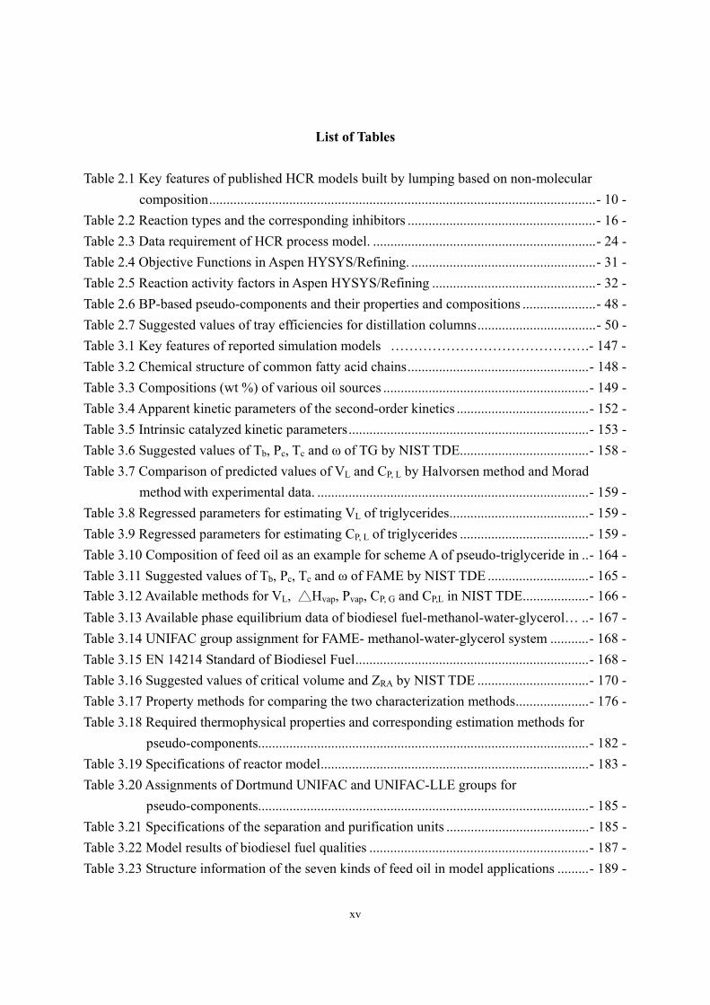
List of Tables Table 2.1 Key features of published HCR models built by lumping based on non-molecular
composition...............................................................................................................- 10 - Table 2.2 Reaction types and the corresponding inhibitors ......................................................- 16 - Table 2.3 Data requirement of HCR process model. ................................................................- 24 - Table 2.4 Objective Functions in Aspen HYSYS/Refining. .....................................................- 31 - Table 2.5 Reaction activity factors in Aspen HYSYS/Refining ...............................................- 32 - Table 2.6 BP-based pseudo-components and their properties and compositions .....................- 48 - Table 2.7 Suggested values of tray efficiencies for distillation columns..................................- 50 - Table 3.1 Key features of reported simulation models …………………………………….- 147 - Table 3.2 Chemical structure of common fatty acid chains....................................................- 148 - Table 3.3 Compositions (wt %) of various oil sources ...........................................................- 149 - Table 3.4 Apparent kinetic parameters of the second-order kinetics ......................................- 152 - Table 3.5 Intrinsic catalyzed kinetic parameters.....................................................................- 153 - Table 3.6 Suggested values of Tb, Pc, Tc and ω of TG by NIST TDE.....................................- 158 - Table 3.7 Comparison of predicted values of VL and CP, L by Halvorsen method and Morad
method with experimental data. ..............................................................................- 159 - Table 3.8 Regressed parameters for estimating VL of triglycerides........................................- 159 - Table 3.9 Regressed parameters for estimating CP, L of triglycerides .....................................- 159 - Table 3.10 Composition of feed oil as an example for scheme A of pseudo-triglyceride in ..- 164 - Table 3.11 Suggested values of Tb, Pc, Tc and ω of FAME by NIST TDE .............................- 165 - Table 3.12 Available methods for VL, Hvap, Pvap, CP, G and CP,L in NIST TDE...................- 166 - Table 3.13 Available phase equilibrium data of biodiesel fuel-methanol-water-glycerol… ..- 167 - Table 3.14 UNIFAC group assignment for FAME- methanol-water-glycerol system ...........- 168 - Table 3.15 EN 14214 Standard of Biodiesel Fuel...................................................................- 168 - Table 3.16 Suggested values of critical volume and ZRA by NIST TDE ................................- 170 - Table 3.17 Property methods for comparing the two characterization methods.....................- 176 - Table 3.18 Required thermophysical properties and corresponding estimation methods for
pseudo-components...............................................................................................- 182 - Table 3.19 Specifications of reactor model.............................................................................- 183 - Table 3.20 Assignments of Dortmund UNIFAC and UNIFAC-LLE groups for
pseudo-components...............................................................................................- 185 - Table 3.21 Specifications of the separation and purification units .........................................- 185 - Table 3.22 Model results of biodiesel fuel qualities ...............................................................- 187 - Table 3.23 Structure information of the seven kinds of feed oil in model applications .........- 189 -
1
Chapter 1 Introduction and Dissertation Scope.
Nowadays, the disparity between raising demand and decreasing discoveries of fossil fuel
sources is increasingly drawing global attention1. People are worried that the slow growth of
crude oil production will not meet global demand’s burst in the near future. Researchers and
scientists are seeking for solutions in three areas – (1) improve the exploration technology to
exploit more fossil fuel and gas; (2) maximize the usage of fossil fuel and gas; and (3) develop
new technology to produce energy from sustainable sources. Chemical engineers are more
interested in the second and third areas since they require good understanding of process system
engineering and relevant chemistry knowledge. The second area includes many different tasks on
improving existing process and/or developing new process to better utilize fossil fuel and gas,
such as recovering more gas oil from atmospheric residue (deep-cut operation in vacuum
distillation unit), improving the production scenario of hydrocracking process to produce better
product distribution and gasifying coal into syngas which can be converted into liquid fuel
through Fischer-Tropsch reaction. On the other hand, the third area is concerned with seeking for
different sustainable sources and transforming those sustainable sources into usable forms of
energy such as bio-ethanol from corns, biodiesel from crops and algae, solar electricity from
sunlight and wind power generation.
This dissertation includes two process modeling studies which improve existing simulation
technologies in both areas – (1) predictive model of large-scale integrated refinery reaction and
fractionation systems from plant data – hydrocracking processes; and (2) integrated process
modeling and product design of biodiesel manufacturing.
In Predictive Model of Large-Scale Integrated Refinery Reaction and Fractionation
Systems from Plant Data – Hydrocracking Processes, the following issues are investigated
and addressed:
2
1. Review of current modeling technologies on plant-wide simulation of hydrocracking process;
2. Identification of the deficiencies in current modeling technologies which are
a. Lack of plant-wide process model verified with long-term process and production data;
b. Unable to connect hydrocracking reactor model with the simulation of downstream
distillation column;
c. Most of the published models are either using complex kinetic lumping model or
simple boiling point lumping model. The former requires detailed molecular
information of feedstock which is not available in daily measurements in a refinery.
The latter is only able to provide good predictions of product yields and can not predict
unit performance and fuel quality.
In Integrated Process Modeling and Product Design of Biodiesel Manufacturing, the
following issues are investigated and addressed:
1. Review of current modeling technologies on biodiesel process;
2. Identification of the deficiencies in current modeling technologies which are
a. Improper representation of feedstock – most models use pure triolein to represent
feedstock which is a complex mixture of various triglyceride molecules;
b. Poor estimation on required physical properties for modeling – none of the published
models discuss the estimation of required physical properties for modeling, particularly
the thermophysical properties of triglyceride molecules which are major components in
feedstock oil;
c. Simplified reaction kinetics in reactor model – most models utilize simplified reaction
kinetics assuming fix reaction conversion regardless of reactor condition;
d. Lack of biodiesel property prediction – none of the model is able to predict fuel
property of biodiesel for product design purpose.

3
Literature Cited
1. Strategic Significance of America’s Oil Shale Resource, Office of Naval Petroleum and Oil
Shale Reserves, U.S. Department of Energy, 2004, Washington D.C.
4
Chapter 2 Predictive Model of Large-Scale Integrated Refinery Reaction and
Fractionation Systems from Plant Data – Hydrocracking Processes.
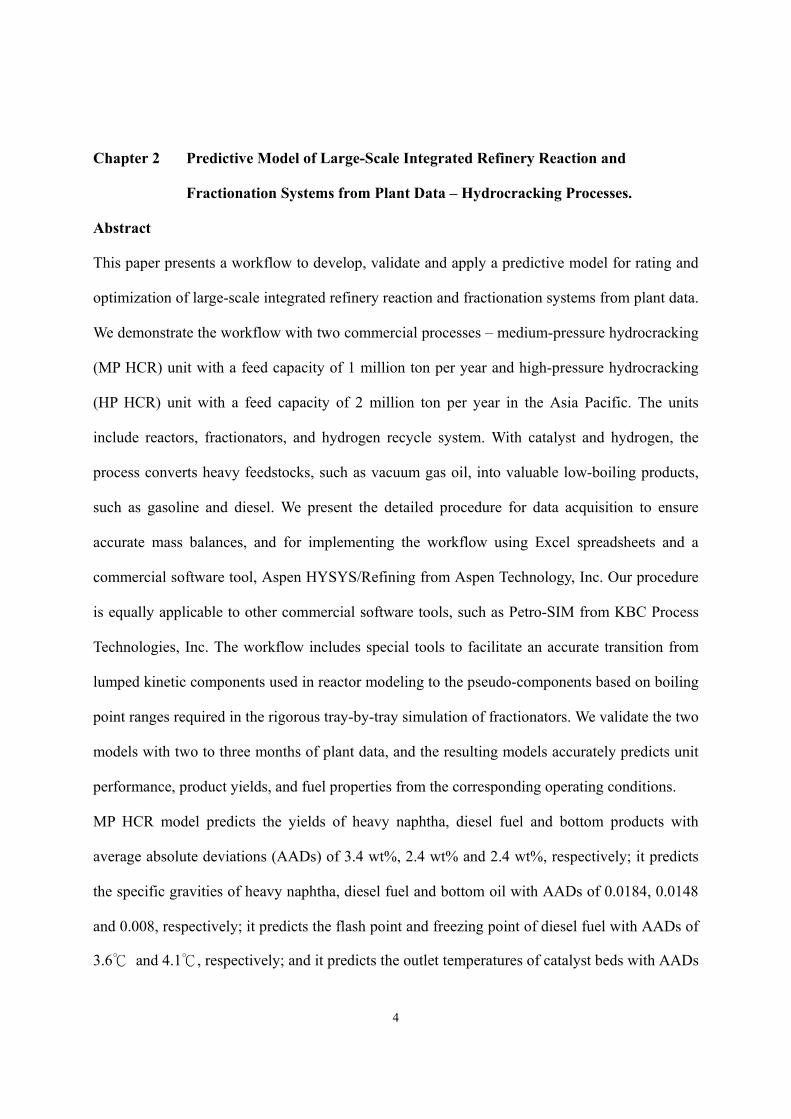
Abstract
This paper presents a workflow to develop, validate and apply a predictive model for rating and
optimization of large-scale integrated refinery reaction and fractionation systems from plant data.
We demonstrate the workflow with two commercial processes – medium-pressure hydrocracking
(MP HCR) unit with a feed capacity of 1 million ton per year and high-pressure hydrocracking
(HP HCR) unit with a feed capacity of 2 million ton per year in the Asia Pacific. The units
include reactors, fractionators, and hydrogen recycle system. With catalyst and hydrogen, the
process converts heavy feedstocks, such as vacuum gas oil, into valuable low-boiling products,
such as gasoline and diesel. We present the detailed procedure for data acquisition to ensure
accurate mass balances, and for implementing the workflow using Excel spreadsheets and a
commercial software tool, Aspen HYSYS/Refining from Aspen Technology, Inc. Our procedure
is equally applicable to other commercial software tools, such as Petro-SIM from KBC Process
Technologies, Inc. The workflow includes special tools to facilitate an accurate transition from
lumped kinetic components used in reactor modeling to the pseudo-components based on boiling
point ranges required in the rigorous tray-by-tray simulation of fractionators. We validate the two
models with two to three months of plant data, and the resulting models accurately predicts unit
performance, product yields, and fuel properties from the corresponding operating conditions.
MP HCR model predicts the yields of heavy naphtha, diesel fuel and bottom products with
average absolute deviations (AADs) of 3.4 wt%, 2.4 wt% and 2.4 wt%, respectively; it predicts
the specific gravities of heavy naphtha, diesel fuel and bottom oil with AADs of 0.0184, 0.0148
and 0.008, respectively; it predicts the flash point and freezing point of diesel fuel with AADs of
3.6 and 4.1, respectively; and it predicts the outlet temperatures of catalyst beds with AADs
5
of 1.9. HP HCR model predicts the yields of LPG, light naphtha, heavy naphtha, jet fuel, and
resid oil with AADs of 0.4 wt%, 0.2 wt%, 0.5 wt%, 0.4 wt%, and 1.7 wt% respectively; it
predicts the specific gravities of light naphtha, heavy naphtha, jet fuel, and resid oil with AADs
of 0.0049, 0.0062, 0.134, and 0.0045, respectively; it predicts the flash point and freezing point
of jet fuel with AADs of 1.6 and 2.3, respectively; and it predicts the outlet temperatures of
catalyst beds of the two hydrocracking reactors with AADs of 1.8 and 3.2 .
We apply the validated plantwide model to quantify the effect of H2-to-oil ratio on product
distribution and catalyst life, and the effect of HCR reactor temperature and feed flow rate on
product distribution. The results agree well with experimental observations reported in the
literature. We also incorporate the model with linear programming production planning by
generating delta-base vector. Our resulting models only require typical operating conditions and
routine analysis of feedstock and products, and appears to be the only reported integrated HCR
models that can quantitatively simulate all key aspects of reactor operation, fractionator
performance, hydrogen consumption, product yield and fuel properties.
2.1 Introduction.
Hydrocracking (HCR) is one of the most important process units in modern refinery. It is widely
used to upgrade the heavy petroleum fraction such as vacuum gas oil. With catalyst and excess
hydrogen, HCR converts heavy oil fractions such as vacuum gas oil (VGO) from crude
distillation unit, into broad range of valuable low-boiling products, such as gasoline and diesel.
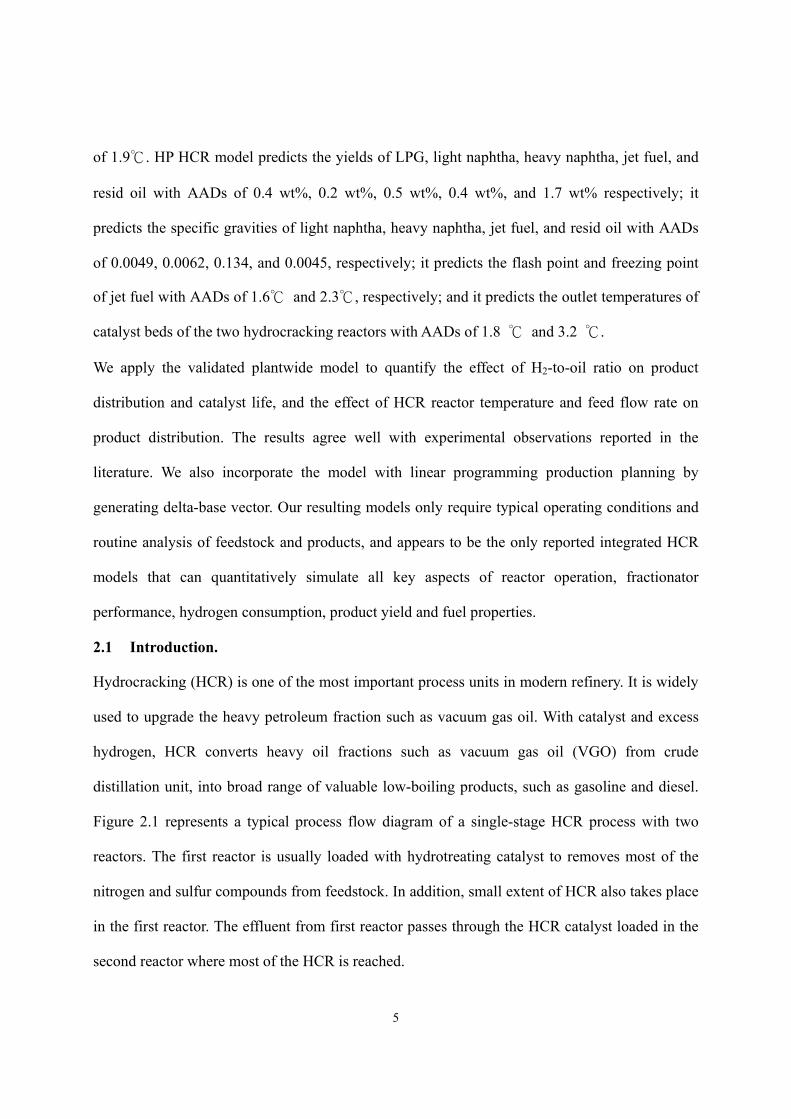
Figure 2.1 represents a typical process flow diagram of a single-stage HCR process with two
reactors. The first reactor is usually loaded with hydrotreating catalyst to removes most of the
nitrogen and sulfur compounds from feedstock. In addition, small extent of HCR also takes place
in the first reactor. The effluent from first reactor passes through the HCR catalyst loaded in the
second reactor where most of the HCR is reached.
6
Figure 2.1 Flow diagram of a typical single-stage HCR process.
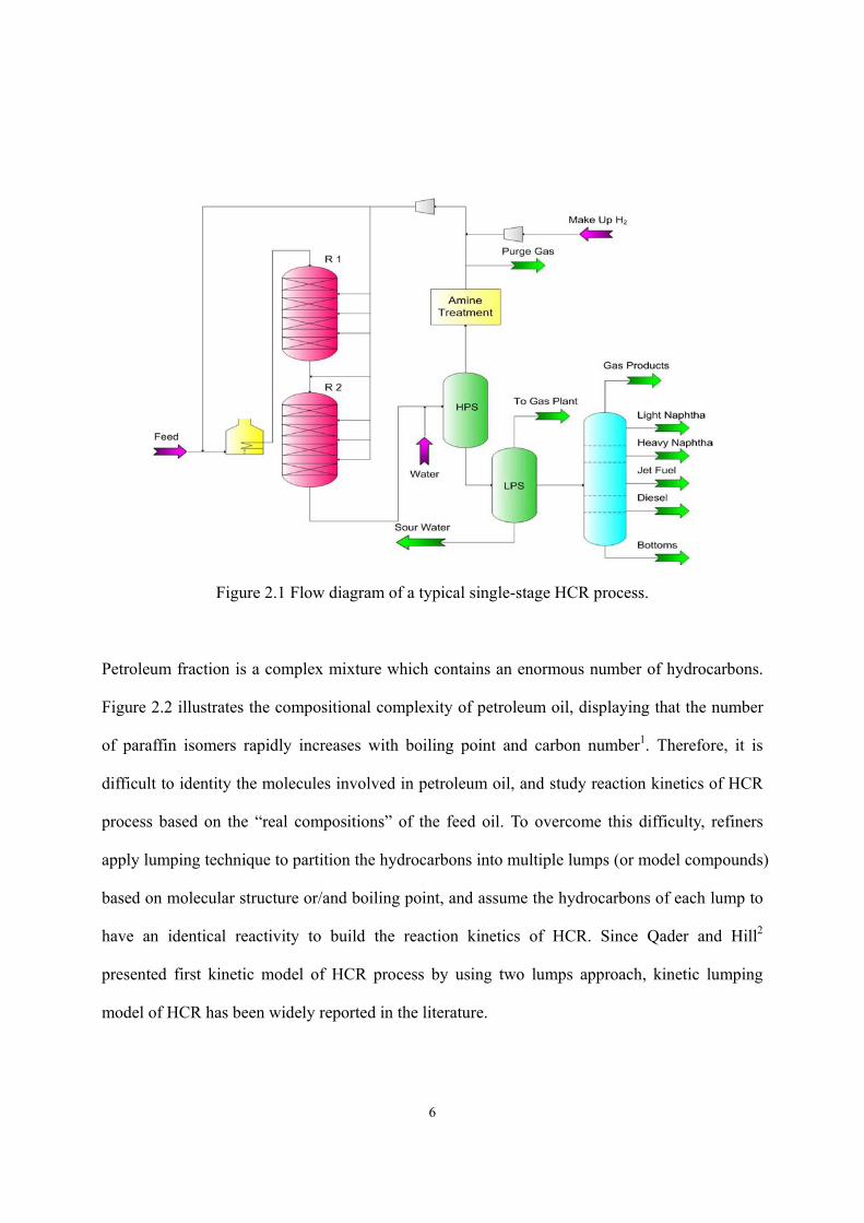
Petroleum fraction is a complex mixture which contains an enormous number of hydrocarbons.
Figure 2.2 illustrates the compositional complexity of petroleum oil, displaying that the number
of paraffin isomers rapidly increases with boiling point and carbon number1. Therefore, it is
difficult to identity the molecules involved in petroleum oil, and study reaction kinetics of HCR
process based on the “real compositions” of the feed oil. To overcome this difficulty, refiners
apply lumping technique to partition the hydrocarbons into multiple lumps (or model compounds)
based on molecular structure or/and boiling point, and assume the hydrocarbons of each lump to
have an identical reactivity to build the reaction kinetics of HCR. Since Qader and Hill2
presented first kinetic model of HCR process by using two lumps approach, kinetic lumping
model of HCR has been widely reported in the literature.
7
Figure 2.2 Complexity of petroleum oil (redraw from ref. [1]).
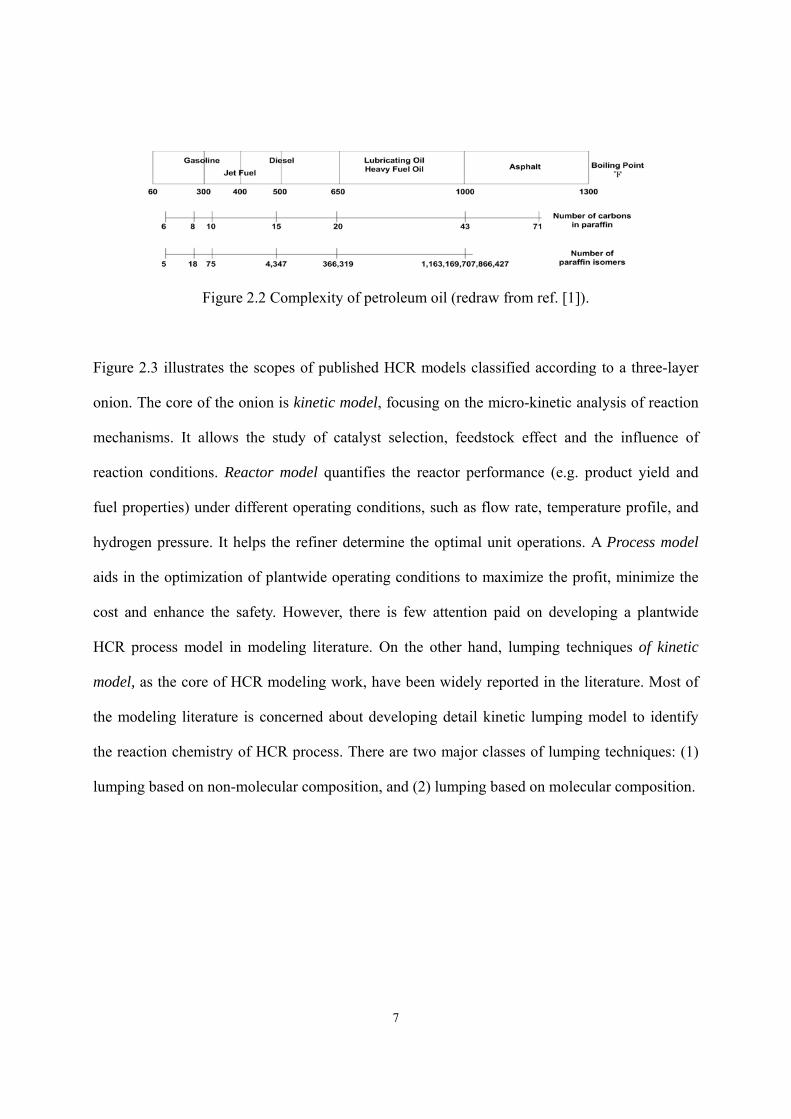
Figure 2.3 illustrates the scopes of published HCR models classified according to a three-layer
onion. The core of the onion is kinetic model, focusing on the micro-kinetic analysis of reaction
mechanisms. It allows the study of catalyst selection, feedstock effect and the influence of
reaction conditions. Reactor model quantifies the reactor performance (e.g. product yield and
fuel properties) under different operating conditions, such as flow rate, temperature profile, and
hydrogen pressure. It helps the refiner determine the optimal unit operations. A Process model
aids in the optimization of plantwide operating conditions to maximize the profit, minimize the
cost and enhance the safety. However, there is few attention paid on developing a plantwide
HCR process model in modeling literature. On the other hand, lumping techniques of kinetic
model, as the core of HCR modeling work, have been widely reported in the literature. Most of
the modeling literature is concerned about developing detail kinetic lumping model to identify
the reaction chemistry of HCR process. There are two major classes of lumping techniques: (1)
lumping based on non-molecular composition, and (2) lumping based on molecular composition.
8
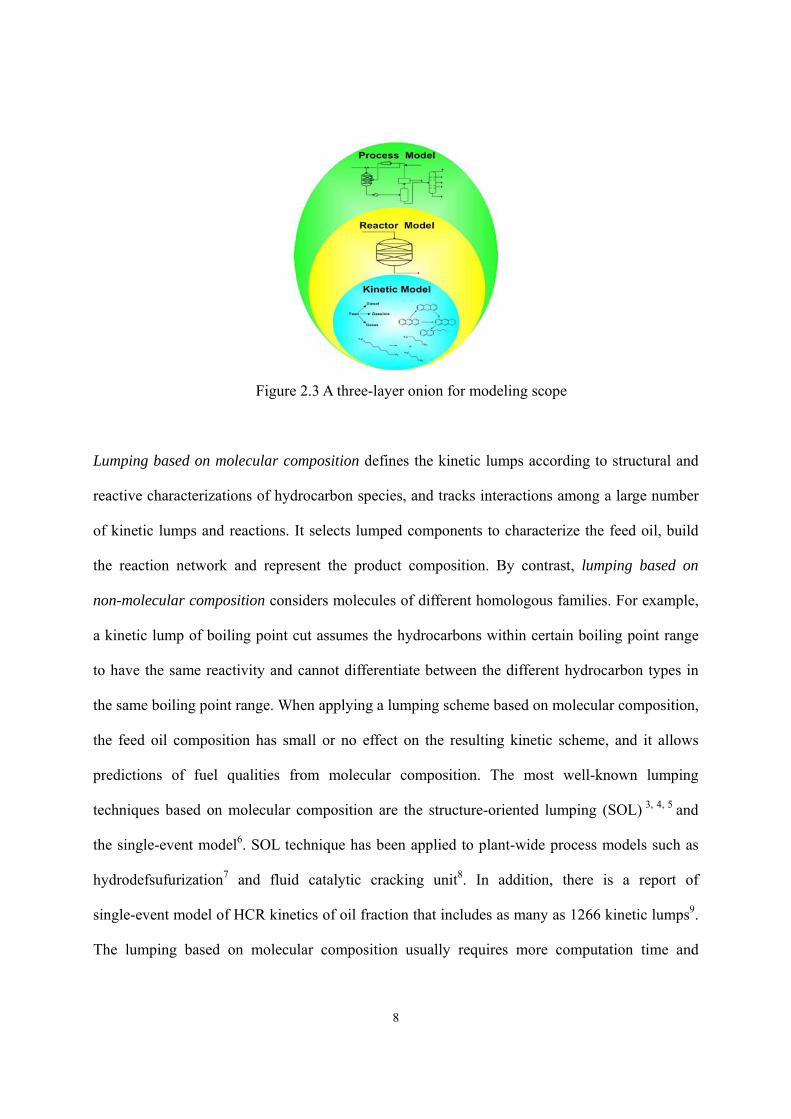
Figure 2.3 A three-layer onion for modeling scope
Lumping based on molecular composition defines the kinetic lumps according to structural and
reactive characterizations of hydrocarbon species, and tracks interactions among a large number
of kinetic lumps and reactions. It selects lumped components to characterize the feed oil, build
the reaction network and represent the product composition. By contrast, lumping based on
non-molecular composition considers molecules of different homologous families. For example,
a kinetic lump of boiling point cut assumes the hydrocarbons within certain boiling point range
to have the same reactivity and cannot differentiate between the different hydrocarbon types in
the same boiling point range. When applying a lumping scheme based on molecular composition,
the feed oil composition has small or no effect on the resulting kinetic scheme, and it allows
predictions of fuel qualities from molecular composition. The most well-known lumping
techniques based on molecular composition are the structure-oriented lumping (SOL) 3, 4, 5 and
the single-event model6. SOL technique has been applied to plant-wide process models such as
hydrodefsufurization7 and fluid catalytic cracking unit8. In addition, there is a report of
single-event model of HCR kinetics of oil fraction that includes as many as 1266 kinetic lumps9.
The lumping based on molecular composition usually requires more computation time and
9
makes it difficult to incorporate equipment simulation such as reactor hydrodynamics. It also
requires more data than what the routine chemical analysis in a refinery can provide. This limits
its application to kinetics and catalyst studies, and can rarely apply to a plantwide process model.
In addition to the SOL and single-event model, however, there are other non-complex lumping
techniques based on molecular composition, such as the approach of Aspen HYSYS/Refining
hydrocracker model (Aspen Technology, Inc. Burlington, Massachusetts) that we will discuss in
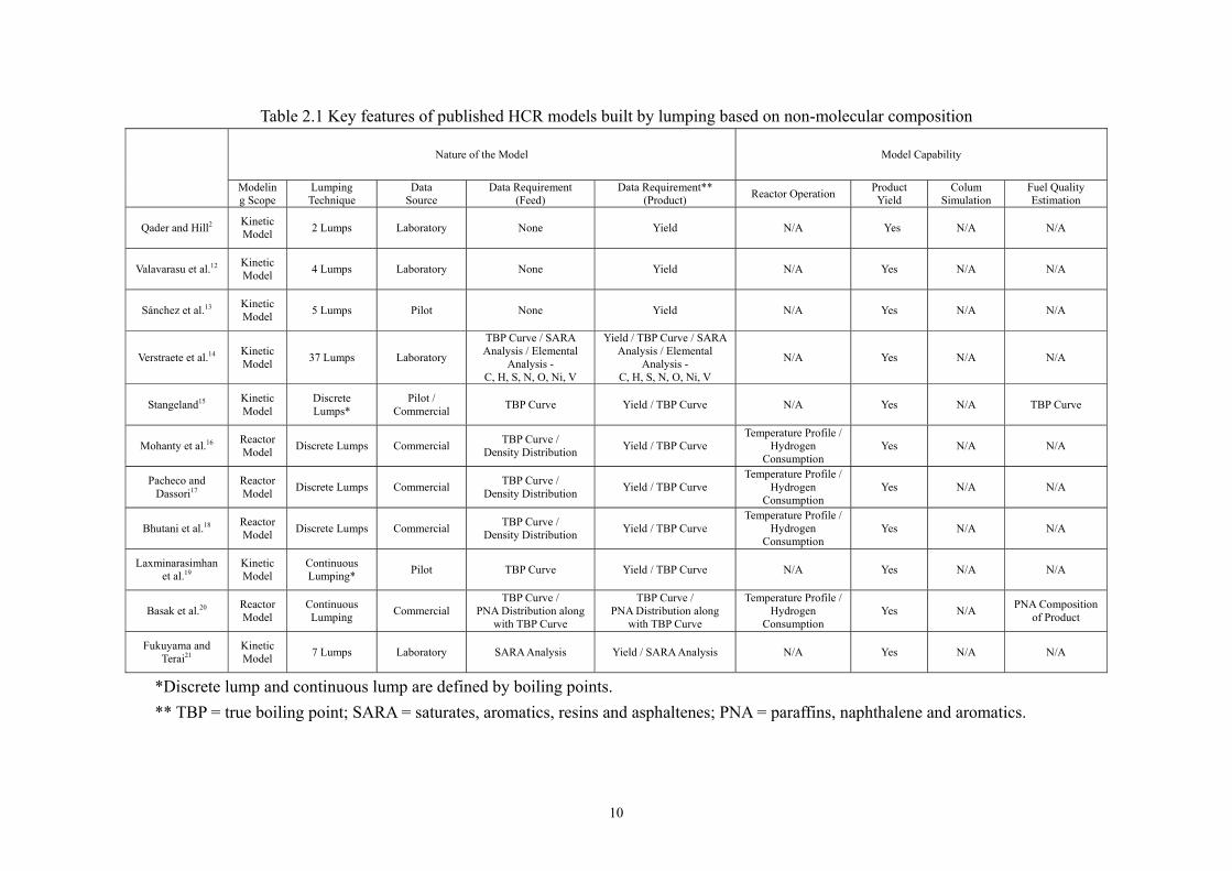
Section 2.2. Table 2.1 summarizes the key features of well-known published HCR models based
on non-molecular composition lumping. For a review and comparison on HCR reactor models,
please see Ancheyta et al.10; and for a review of kinetic modeling of large-scale reaction systems
through lumping, please refer to Ho11.
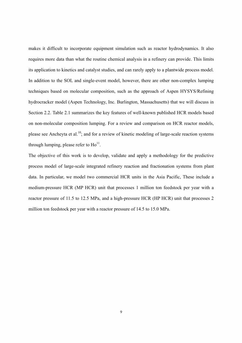
The objective of this work is to develop, validate and apply a methodology for the predictive
process model of large-scale integrated refinery reaction and fractionation systems from plant
data. In particular, we model two commercial HCR units in the Asia Pacific, These include a
medium-pressure HCR (MP HCR) unit that processes 1 million ton feedstock per year with a
reactor pressure of 11.5 to 12.5 MPa, and a high-pressure HCR (HP HCR) unit that processes 2
million ton feedstock per year with a reactor pressure of 14.5 to 15.0 MPa.
10
Table 2.1 Key features of published HCR models built by lumping based on non-molecular composition
*Discrete lump and continuous lump are defined by boiling points. ** TBP = true boiling point; SARA = saturates, aromatics, resins and asphaltenes; PNA = paraffins, naphthalene and aromatics.
Nature of the Model Model Capability
Modeling Scope
Lumping Technique
Data Source
Data Requirement (Feed)
Data Requirement** (Product) Reactor Operation Product
Yield Colum
Simulation Fuel Quality Estimation
Qader and Hill2 Kinetic Model 2 Lumps Laboratory None Yield N/A Yes N/A N/A
Valavarasu et al.12 Kinetic Model 4 Lumps Laboratory None Yield N/A Yes N/A N/A
Sánchez et al.13 Kinetic Model 5 Lumps Pilot None Yield N/A Yes N/A N/A
Verstraete et al.14 Kinetic Model 37 Lumps Laboratory
TBP Curve / SARA Analysis / Elemental
Analysis - C, H, S, N, O, Ni, V
Yield / TBP Curve / SARA Analysis / Elemental
Analysis - C, H, S, N, O, Ni, V
N/A Yes N/A N/A
Stangeland15 Kinetic Model
Discrete Lumps*
Pilot / Commercial TBP Curve Yield / TBP Curve N/A Yes N/A TBP Curve
Mohanty et al.16 Reactor Model Discrete Lumps Commercial TBP Curve /
Density Distribution Yield / TBP Curve Temperature Profile /
Hydrogen Consumption
Yes N/A N/A
Pacheco and Dassori17
Reactor Model Discrete Lumps Commercial TBP Curve /
Density Distribution Yield / TBP Curve Temperature Profile /
Hydrogen Consumption
Yes N/A N/A
Bhutani et al.18 Reactor Model Discrete Lumps Commercial TBP Curve /
Density Distribution Yield / TBP Curve Temperature Profile /
Hydrogen Consumption
Yes N/A N/A
Laxminarasimhan et al.19
Kinetic Model
Continuous Lumping* Pilot TBP Curve Yield / TBP Curve N/A Yes N/A N/A
Basak et al.20 Reactor Model
Continuous Lumping Commercial
TBP Curve / PNA Distribution along
with TBP Curve
TBP Curve / PNA Distribution along
with TBP Curve
Temperature Profile / Hydrogen
Consumption Yes N/A PNA Composition
of Product
Fukuyama and Terai21
Kinetic Model 7 Lumps Laboratory SARA Analysis Yield / SARA Analysis N/A Yes N/A N/A
11
2.2 Aspen HYSYS/Refining HCR Modeling Tool.
Aspen HYSYS/Refining is an add-on program to Aspen HYSYS, a popular process simulation
software tool for refining and chemical businesses. HYSYS/Refining includes several built-in
modeling capabilities for refining process modeling, such as hydrocracker (HCR), catalytic
reformer (CatRef) and fluid catalytic cracking (FCC). In this work, we use Aspen
HYSYS/Refining HCR to model the HCR reactors, and Aspen HYSYS to develop the rigorous
plantwide simulation including fractionation units.
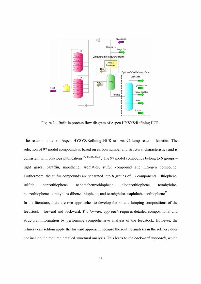
Figure 2.4 represents the built-in process flow diagram of Aspen HYSYS/Refining HCR for a
single-stage HCR process. It can simulate the feed heater, reactor, high-pressure separator,
hydrogen recycle system, amine treatment (optional) and distillation column (optional). To
ensure that the simulation agrees with the real process, users have to configure the process type
(single-stage or two-stage), number of reactors, number of reactor beds for each reactor, and the
operation of each unit. The model of amine treatment is a shortcut component splitter that
separates H2S from the vapor product of high-pressure separator, and the simulation of
distillation column is also based on shortcut calculations22. In addition, the ammonia (NH3)
produced by HDN reactions is split from reactor effluent before its entry into the high-pressure
separator that is modeled by rigorous thermodynamics.
12
Figure 2.4 Built-in process flow diagram of Aspen HYSYS/Refining HCR.
The reactor model of Aspen HYSYS/Refining HCR utilizes 97-lump reaction kinetics. The
selection of 97 model compounds is based on carbon number and structural characteristics and is
consistent with previous publications14, 23, 24, 25, 26. The 97 model compounds belong to 6 groups –
light gases, paraffin, naphthene, aromatics, sulfur compound and nitrogen compound.
Furthermore, the sulfur compounds are separated into 8 groups of 13 components – thiophene,
sulfide, benzothiophene, naphthabenzothiophene, dibenzothiophene, tetrahyhdro-
benzothiophene, tetrahyhdro-dibenzothiophene, and tetrahyhdro- naphthabenzothiophene22.
In the literature, there are two approaches to develop the kinetic lumping compositions of the
feedstock – forward and backward. The forward approach requires detailed compositional and
structural information by performing comprehensive analysis of the feedstock. However, the
refinery can seldom apply the forward approach, because the routine analysis in the refinery does
not include the required detailed structural analysis. This leads to the backward approach, which
13
requires a reference library and only limited analytical data from routine measurement such as
density and sulfur content to estimate kinetic lumping compositions. Brown et al.27 report a
methodology estimating detailed compositional information for SOL-based model and
Gomez-Prado et al.28 develop a molecular-type homologous series (MTHS) representation to
characterize heavy petroleum fractions.
In Aspen HYSYS/Refining the forward approach requires detailed compositional and structural
information by performing comprehensive analysis of the feedstock, including API gravity,
ASTM D-2887 distillation, refractive index, viscosity, bromine number, total sulfur, total and
basic nitrogen, fluorescent indicator adsorption (FIA, total aromatics in vol%), NMR (carbon in
aromatic rings), UV method (wt% of mono-, di-, tri- and tetra- aromatics), HPLC and GC/MS.
With the detailed compositional and structural information, Aspen HYSYS/Refining quantifies
the so-called “fingerprint” (molecular representation) of the feedstock based on 97 kinetic
lumps29. On the other hand, the backward approach of Aspen HYSYS/Refining requires only the
bulk properties (density, ASTM D-2887 distillation curve, and sulfur and nitrogen contents) of
the feedstock. Aspen HYSYS/Refining contains a built-in fingerprint databank for various types
of feedstock, such as light VGO, heavy VGO, FCC cycle oil, etc. The backward approach
assumes that the petroleum feedstock with the same fingerprint type maintains the same generic
kinetic lump distribution as the initial composition. Aspen HYSYS/Refining uses a tool called
“Feed Adjust”29 to skew the kinetic lump distribution of the selected fingerprint type in order to
minimize the difference between the measured and calculated bulk properties of the feedstock.
We use the resulting kinetic lump distribution as the feed condition for the HCR model. If there
is specific concern about compositional information, the user can customize the feed finger print
to match the measurement. For example, the user can change sulfur lump distribution of selected
feed fingerprint manually to ensure the distribution of hindered and non-hindered sulfur
14
compounds match plant measurement.
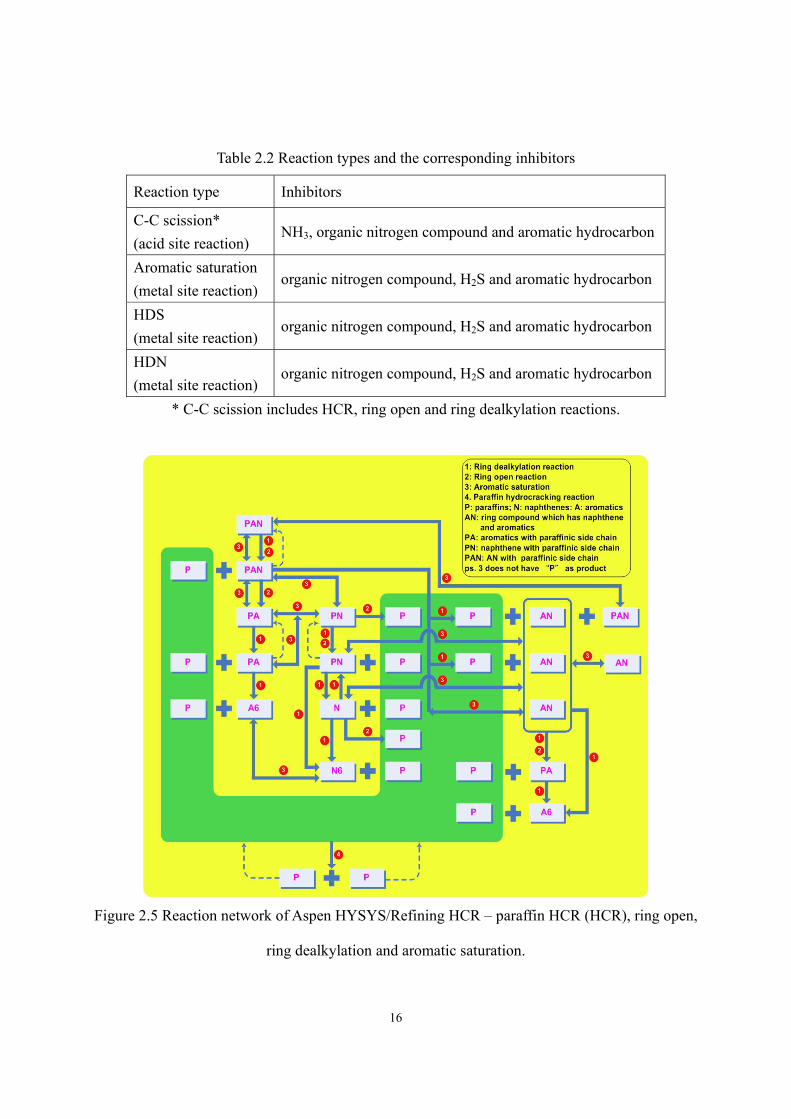
The 97 lumps construct the reaction pathways of 177 reactions, including30 : (1) paraffin HCR;
(2) ring opening; (3) dealkylation of aromatics, naphthenes, nitrogen lumps and sulfur lumps; (4)
saturation of aromatics, non-basic nitrogen lumps and hindered sulfur lumps; (5)
hydrodesulfurization (HDS) of unhindered sulfur lumps; and (6) hydrodenitrogenation (HDN) of
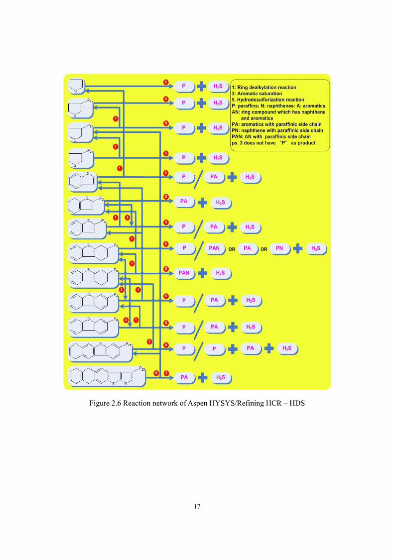
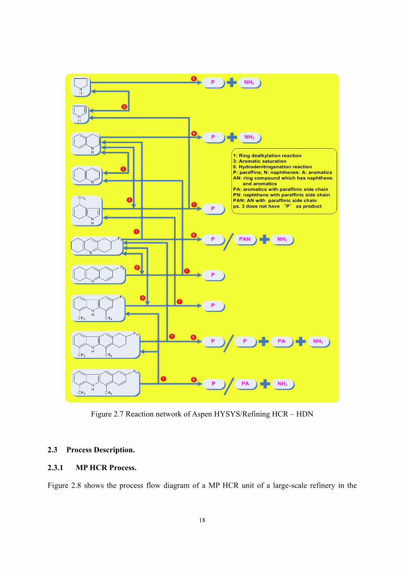
nitrogen lumps. Figure 2.5 to Figure 2.7 illustrate the reaction network. Rate equation of each
reaction is based on Langmuir-Hinshelwood-Hougen-Watson (LHHW) mechanism with both
reversible and irreversible reactions. The mechanism includes30:
Adsorption of reactants to the catalyst surface;
Inhibition of adsorption;
Reaction of adsorbed molecules;
Desorption of products;
The kinetic scheme also includes the inhibition resulted from H2S, NH3 and organic nitrogen
compounds30:
Inhibition of HDS reactions by H2S;
Inhibition of paraffin HCR, ring opening and dealkylation reactions by NH3 and organic
nitrogen compounds;
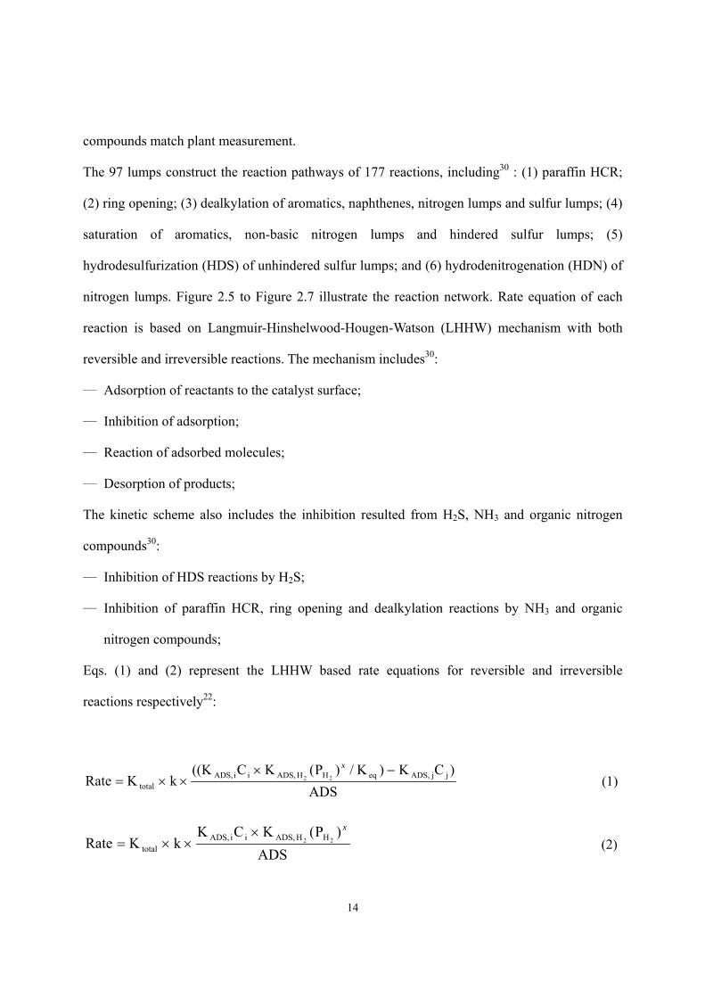
Eqs. (1) and (2) represent the LHHW based rate equations for reversible and irreversible
reactions respectively22:
ADS)CK)K/)P(K C((K
kK Rate jjADS,eqHHADS,iiADS,total
22−×
××=x
(1)
ADS)P(K CK
kK Rate 22 HHADS,iiADS,total
x×××= (2)
15
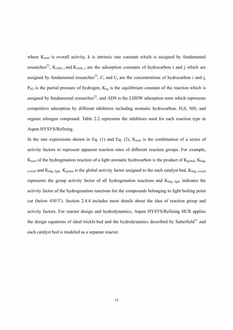
where Ktotal is overall activity, k is intrinsic rate constant which is assigned by fundamental
researches22, KADS, i and KADS, j are the adsorption constants of hydrocarbon i and j which are
assigned by fundamental researches22, Ci and Cj are the concentrations of hydrocarbon i and j,
PH2 is the partial pressure of hydrogen, Keq is the equilibrium constant of the reaction which is
assigned by fundamental researches22, and ADS is the LHHW adsorption term which represents
competitive adsorption by different inhibitors including aromatic hydrocarbon, H2S, NH3 and
organic nitrogen compound. Table 2.2 represents the inhibitors used for each reaction type in
Aspen HYSYS/Refining.
In the rate expressions shown in Eq. (1) and Eq. (2), Ktotal is the combination of a series of
activity factors to represent apparent reaction rates of different reaction groups. For example,
Ktotal of the hydrogenation reaction of a light aromatic hydrocarbon is the product of Kglobal, Khdg,
overall and Khdg, light. Kglobal is the global activity factor assigned to the each catalyst bed, Khdg, overall
represents the group activity factor of all hydrogenation reactions and Khdg, light indicates the
activity factor of the hydrogenation reactions for the compounds belonging to light boiling point
cut (below 430). Section 2.4.4 includes more details about the idea of reaction group and
activity factors. For reactor design and hydrodynamics, Aspen HYSYS/Refining HCR applies
the design equations of ideal trickle-bed and the hydrodynamics described by Satterfield31 and
each catalyst bed is modeled as a separate reactor.
16
Table 2.2 Reaction types and the corresponding inhibitors
Reaction type Inhibitors
C-C scission* (acid site reaction)
NH3, organic nitrogen compound and aromatic hydrocarbon
Aromatic saturation (metal site reaction)
organic nitrogen compound, H2S and aromatic hydrocarbon
HDS (metal site reaction)
organic nitrogen compound, H2S and aromatic hydrocarbon
HDN (metal site reaction)
organic nitrogen compound, H2S and aromatic hydrocarbon
* C-C scission includes HCR, ring open and ring dealkylation reactions.
Figure 2.5 Reaction network of Aspen HYSYS/Refining HCR – paraffin HCR (HCR), ring open,
ring dealkylation and aromatic saturation.
17
Figure 2.6 Reaction network of Aspen HYSYS/Refining HCR – HDS
18
Figure 2.7 Reaction network of Aspen HYSYS/Refining HCR – HDN
2.3 Process Description.
2.3.1 MP HCR Process.
Figure 2.8 shows the process flow diagram of a MP HCR unit of a large-scale refinery in the

19
Asia Pacific. The unit upgrades 1 million tons/yr of VGO from the crude distillation unit (CDU)
into valuable naphtha, diesel and bottom (the feedstock to ethylene plant) by HCR. The VGO
feed from the CDU is mixed with a hydrogen-rich gas and preheated before entering the first
reactor. The first reactor uses hydrotreating catalyst to reduce nitrogen and sulfur contents. The
second reactor uses HCR catalyst to crack heavy hydrocarbons into lighter oils – naphtha, diesel
and bottom. Following the two reactors, a high-pressure separator (HPS) recovers un-reacted
hydrogen and a low-pressure separator (LPS) separates the light gases from the liquid outlet of
HPS. An amine treatment scrubs sour gases from the vapor product of HPS to concentrate the
hydrogen content of the hydrogen recycle stream. To balance the hydrogen in the system, a purge
gas stream is removed from amine treatment. In the fractionation part, a H2S stripper removes
the dissolved H2S from light hydrocarbons and a fractionator with two side strippers produces
the major products – light naphtha, heavy naphtha, diesel and bottom.
Figure 2.8 The simplified process flow diagram of MP HPR unit
20
2.3.2 HP HCR Process.
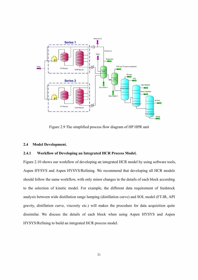
Figure 2.9 shows the process flow diagram of a HP HCR unit of a large-scale refinery in the Asia
Pacific. The unit upgrades 2 million tons/yr of VGO into valuable naphtha, jet fuel and residue
oil by HCR. Unlike a typical HCR unit, this process includes two parallel reactor series and each
series contains one hydrotreating reactor and HCR reactor. The VGO feed is mixed with a
hydrogen-rich gas and preheated before being fed to the first reactors of both reactor series. The
first reactors of both series are loaded with the hydrotreating catalyst to reduce nitrogen and
sulfur contents. The second reactor of both series are loaded with the HCR catalyst to crack
heavy hydrocarbons into more valuable liquid products – LPG, light naphtha, heavy naphtha, and
jet fuel. Following the two reactor series, a HPS recovers un-reacted hydrogen and a LPS
separates the light gases from the liquid outlet of HPS. To balance the hydrogen in the system,
we remove a purge gas stream from the vapor product of HPS. In the fractionation part, the first
fractionator separates light gases and LPG from light hydrocarbons, the second fractionator
produces the most valuable products, namely, light naphtha and heavy naphtha, and the third
fractionator further produces jet fuel and residue oil.
21
Figure 2.9 The simplified process flow diagram of HP HPR unit
2.4 Model Development.
2.4.1 Workflow of Developing an Integrated HCR Process Model.
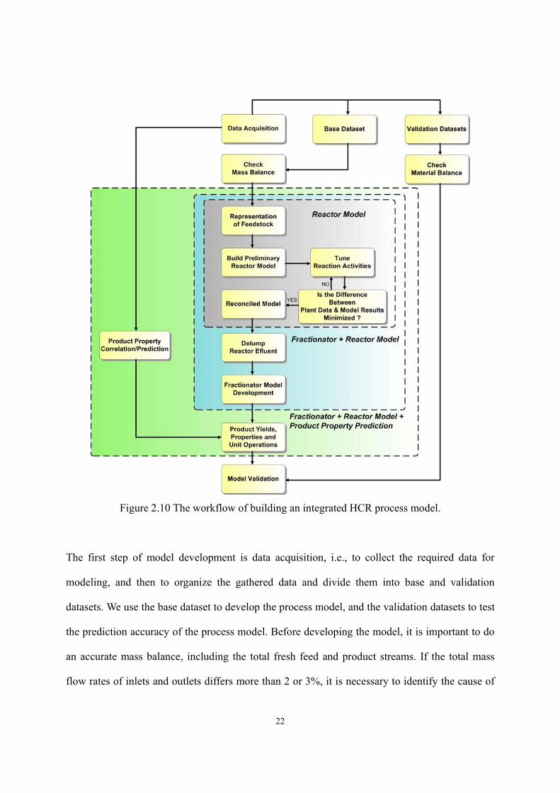
Figure 2.10 shows our workflow of developing an integrated HCR model by using software tools,
Aspen HYSYS and Aspen HYSYS/Refining. We recommend that developing all HCR models
should follow the same workflow, with only minor changes in the details of each block according
to the selection of kinetic model. For example, the different data requirement of feedstock
analysis between wide distillation range lumping (distillation curve) and SOL model (FT-IR, API
gravity, distillation curve, viscosity etc.) will makes the procedure for data acquisition quite
dissimilar. We discuss the details of each block when using Aspen HYSYS and Aspen
HYSYS/Refining to build an integrated HCR process model.
22
Figure 2.10 The workflow of building an integrated HCR process model.
The first step of model development is data acquisition, i.e., to collect the required data for
modeling, and then to organize the gathered data and divide them into base and validation
datasets. We use the base dataset to develop the process model, and the validation datasets to test
the prediction accuracy of the process model. Before developing the model, it is important to do
an accurate mass balance, including the total fresh feed and product streams. If the total mass
flow rates of inlets and outlets differs more than 2 or 3%, it is necessary to identify the cause of
23
the imbalance32.
Following the mass balance is the development of a reactor model. The steps to develop a reactor
model also depend on the selection of kinetic model. The procedures shown in Figure 2.10
correspond to the case using Aspen HYSYS/Refining. The development of a fractionator model
in a HCR process is similar to a crude distillation unit (CDU). The only difference is the
representation of the feed stream to the HCR fractionator, because the HCR reactor effluent is
characterized by kinetic lumps instead of the pseudo-components based on boiling point which
are widely used in a CDU model. Therefore, we use a step called delumping when the chosen
kinetic lumps cannot appropriately characterize the feed stream to a HCR fractionator.
Delumping is the most important step to build a plantwide model of HCR process, because it
needs to capture the key properties of reactor effluent for fractionator simulation during the
component transition process. After completing the fractionator model, we incorporate the oil
property correlations into the process model to calculate fuel properties such as flash point of
diesel fuel. Lastly, we verify the model by comparing the predictions with multiple plant
datasets.
2.4.2 Data Acquisition.
Regardless of the selection of kinetic model, data acquisition is always the first step of model
development. We obtain two months of feedstock/product analysis, production and operation
data from plant, and construct multiple datasets to build and validate the model. It is important to
consult plant engineers about data consistency to ensure each dataset does not include the data in
the period of operation upsets and significant operation changes. Moreover, it is always helpful
to revisit the original data for test run, because test run data are usually adjusted to show perfect
mass and heat balances32.
Data required for modeling purpose is quite sensitive to the selection of kinetic model and the
24
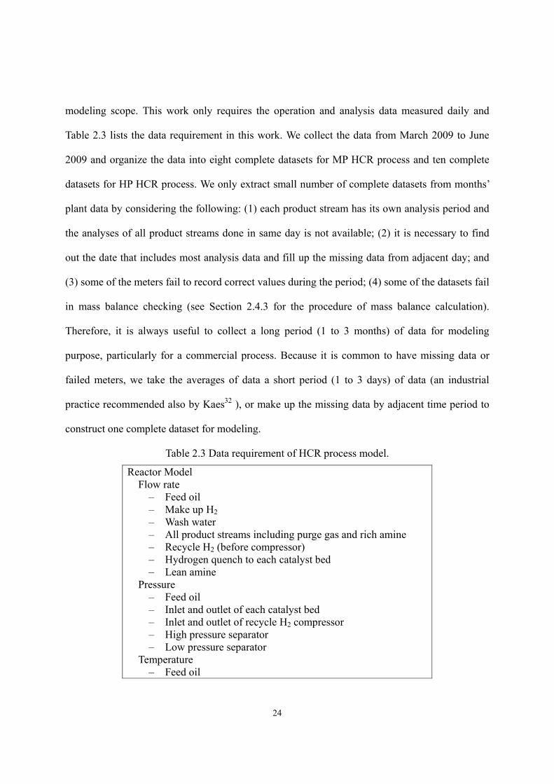
modeling scope. This work only requires the operation and analysis data measured daily and
Table 2.3 lists the data requirement in this work. We collect the data from March 2009 to June
2009 and organize the data into eight complete datasets for MP HCR process and ten complete
datasets for HP HCR process. We only extract small number of complete datasets from months’
plant data by considering the following: (1) each product stream has its own analysis period and
the analyses of all product streams done in same day is not available; (2) it is necessary to find
out the date that includes most analysis data and fill up the missing data from adjacent day; and
(3) some of the meters fail to record correct values during the period; (4) some of the datasets fail
in mass balance checking (see Section 2.4.3 for the procedure of mass balance calculation).
Therefore, it is always useful to collect a long period (1 to 3 months) of data for modeling
purpose, particularly for a commercial process. Because it is common to have missing data or
failed meters, we take the averages of data a short period (1 to 3 days) of data (an industrial
practice recommended also by Kaes32 ), or make up the missing data by adjacent time period to
construct one complete dataset for modeling.
Table 2.3 Data requirement of HCR process model.
Reactor Model Flow rate
– Feed oil – Make up H2 – Wash water – All product streams including purge gas and rich amine – Recycle H2 (before compressor) – Hydrogen quench to each catalyst bed – Lean amine
Pressure – Feed oil – Inlet and outlet of each catalyst bed – Inlet and outlet of recycle H2 compressor – High pressure separator – Low pressure separator
Temperature – Feed oil
25
– Inlet and outlet of each catalyst bed – Inlet and outlet of recycle H2 compressor – High pressure separator – Low pressure separator
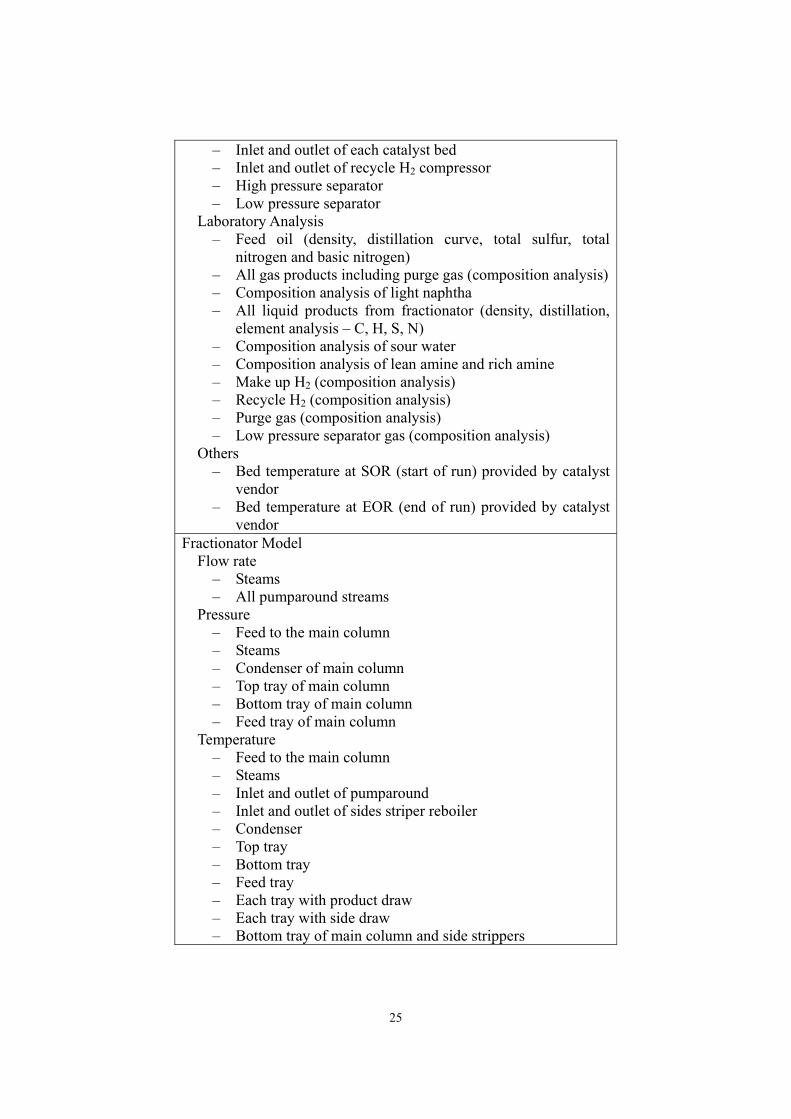
Laboratory Analysis – Feed oil (density, distillation curve, total sulfur, total
nitrogen and basic nitrogen) – All gas products including purge gas (composition analysis) – Composition analysis of light naphtha – All liquid products from fractionator (density, distillation,
element analysis – C, H, S, N) – Composition analysis of sour water – Composition analysis of lean amine and rich amine – Make up H2 (composition analysis) – Recycle H2 (composition analysis) – Purge gas (composition analysis) – Low pressure separator gas (composition analysis)
Others – Bed temperature at SOR (start of run) provided by catalyst
vendor – Bed temperature at EOR (end of run) provided by catalyst
vendor Fractionator Model
Flow rate – Steams – All pumparound streams
Pressure – Feed to the main column – Steams – Condenser of main column – Top tray of main column – Bottom tray of main column – Feed tray of main column
Temperature – Feed to the main column – Steams – Inlet and outlet of pumparound – Inlet and outlet of sides striper reboiler – Condenser – Top tray – Bottom tray – Feed tray – Each tray with product draw – Each tray with side draw – Bottom tray of main column and side strippers
26
2.4.3 Mass Balance.
It is critical to review the collected information to ensure accurate model development,
particularly mass balance. The calculation of mass balance should include all of the inlet streams
(such as feed oil, make up H2, wash water, lean amine and steam in MP HCR process) and the
outlet streams (such as LPS vapor, sour gas, LPG, flare, light naphtha, heavy naphtha, diesel,
bottom, purge gas, sour water, rich amine in MP HCR process). However, the streams around
amine treatment, wash water and sour water streams are not routinely measured, and it is
unlikely to include those streams in the calculation of material balance. Since those streams only
affect the mass balance of sulfur and nitrogen, we recommend doing a separate mass balance of
sulfur and nitrogen by assuming that all of the removed sulfur and nitrogen atoms are reacted
into H2S and NH3.
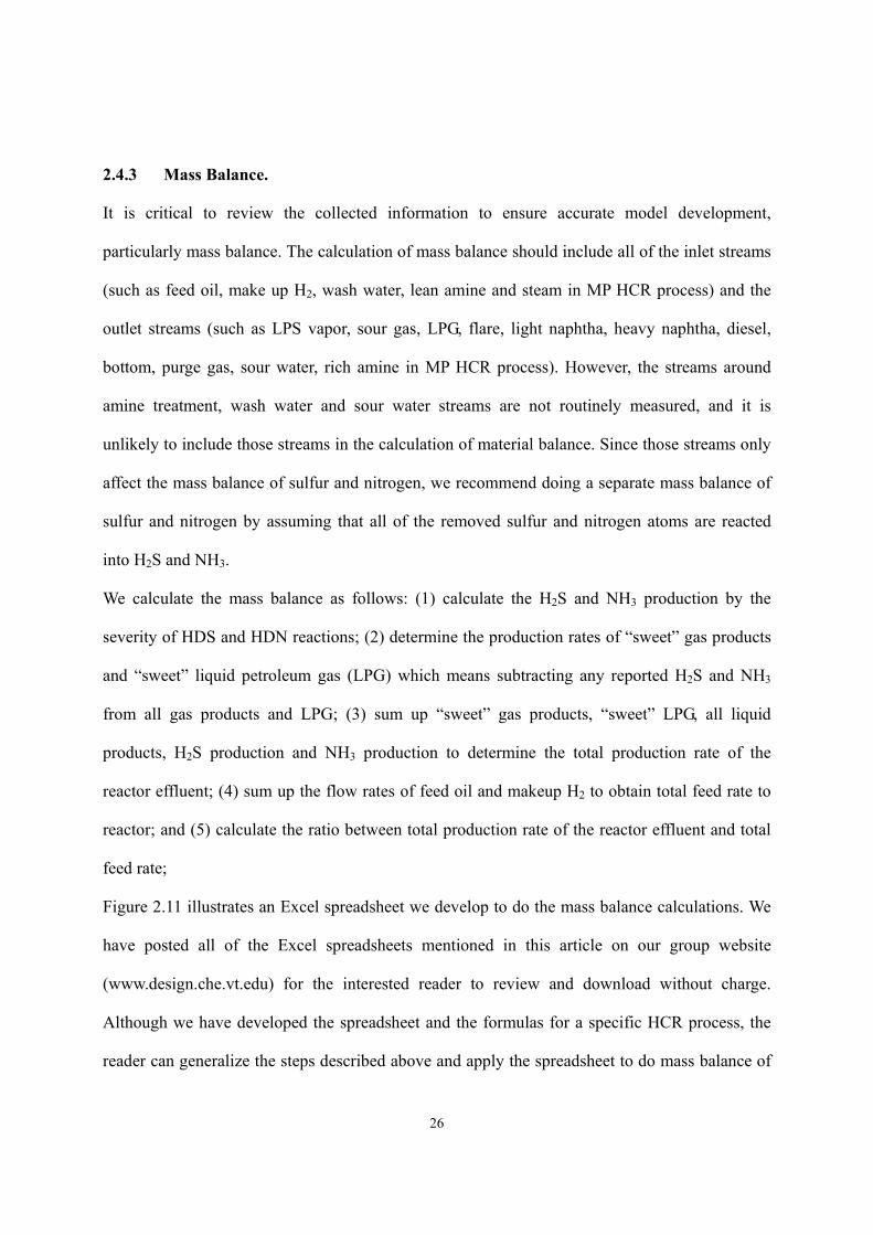
We calculate the mass balance as follows: (1) calculate the H2S and NH3 production by the
severity of HDS and HDN reactions; (2) determine the production rates of “sweet” gas products
and “sweet” liquid petroleum gas (LPG) which means subtracting any reported H2S and NH3
from all gas products and LPG; (3) sum up “sweet” gas products, “sweet” LPG, all liquid
products, H2S production and NH3 production to determine the total production rate of the
reactor effluent; (4) sum up the flow rates of feed oil and makeup H2 to obtain total feed rate to
reactor; and (5) calculate the ratio between total production rate of the reactor effluent and total
feed rate;
Figure 2.11 illustrates an Excel spreadsheet we develop to do the mass balance calculations. We
have posted all of the Excel spreadsheets mentioned in this article on our group website
(www.design.che.vt.edu) for the interested reader to review and download without charge.
Although we have developed the spreadsheet and the formulas for a specific HCR process, the
reader can generalize the steps described above and apply the spreadsheet to do mass balance of
27
any HCR process with only minor changes.
Figure 2.11 A spreadsheet for the mass balance calculation of a HCR process.
2.4.4 Reactor Model Development.
Reactor model development is the core of building a HCR process model. Although the
procedure of building a reactor model depends on the selection of kinetic model, we require the
following tasks in developing a model for most commercial HCR processes: (1) do the feedstock
analysis based on the selected kinetic model; (2) represent the feedstock as a mixture of kinetic
lumps which can be modeling compounds or pseudo-components based on boiling point ranges;
(3) build the reaction network, define rate equations, and estimate rate constants and heat of
reaction; (4) apply the operation data (e.g. reactor temperature, feed rate, etc.) to solve rate
equations and reactor design equations simultaneously; (5) and minimize objective functions
(user-defined indices to represent the differences between model predictions and plant data) by
tuning reaction activity parameters.
28
2.4.4.1 MP HCR Reactor Model.
We describe in Section 2.2 the concept of the backward approach in representing the feedstock
using the Aspen HYSYS/Refining. Since the refinery does not conduct comprehensive analysis
of HCR feedstock routinely, this work applies the backward approach to characterize the
feedstock. We select “LVGO” fingerprint type for both HCR processes because the feeds to both
processes is mainly vacuum gas oil from crude distillation unit and the selected fingerprint type
should be as close to the real feeds as possible. This section will demonstrate the last step of
building reactor model by using Aspen HYSYS/Refining – to minimize the difference between
model predictions and plant data to make the model match plant operation.
Although Aspen HYSYS/Refining assigns the rate constants to the 177 reactions based on
fundamental research, it is necessary to identify the activity factor to match plant operation
because the reactor configuration, catalyst activity and operating conditions vary for different
refineries. The procedure of minimizing the difference between model predictions and plant data
in Aspen HYSYS/Refining is called “calibration”, meaning to calibrate the model to agree with
plant operation.
Table 2.4 lists the 31 optional objective functions and Table 2.5 shows the 48 reaction activity
factors for selection. Aspen HYSYS/Refining combines the input plant product distribution to
construct the reactor effluent, and partition the reactor effluent into C1, C2, C3, C4, C5, and four
“square cuts”, namely, naphtha (C6 to 430 cut), diesel (430 to 700 cut), bottom (700 to
1000) cut and resid (1000+ cut) which are shown in Table 2.4. All of the objective functions
listed in Table 2.4 are either the prediction errors of crucial operations or important product
yields for the HCR process. Aspen HYSYS/Refining allows us to select the desired objective
functions during calibration. After selecting the objective functions, we choose appropriate
activity factors to calibrate the reactor model. Figure 2.12 illustrates the relationships among
29
activity factors, catalyst bed and reactor type and Table 2.5 shows the major effect of each
activity factor on the model performance such as global activity (Kglobal) on the bed temperature
profile to help the selection of activity factors.
The procedure of model calibration depends on the operational mode, product yields and the
precision of plant data. For example, a hydrogen-insufficient refinery might pay more attention
to hydrogen consumption and makeup hydrogen flow. In addition, it is necessary to have high
precision of light-end analysis (C1 to C5) if we desire to have accurate predictions of light gas
yields. For MP HCR process, the most important considerations to the plant management are the
product yields, flow rate of makeup hydrogen, reactor temperature and properties of liquid fuel
products. We note that the reactor model cannot calculate some fuel properties, such as flash
point and freezing point of diesel and jet fuel, because the square cuts defined by Aspen
HYSYS/Refining have different distillation ranges from plant cuts. Therefore, we develop
correlations to estimate such fuel properties (see Section 2.4.6).
Figure 2.13 illustrates the steps to identify activity factors in this work which are divided into
two phases. The first phase is applicable to any Aspen HYSYS/Refining HCR model and the
second phase depends on the modeling priority of the refinery. Since Aspen HYSYS/Refining
assigns small values to Kglobal to ensure the initial convergence, all catalyst beds’ performance is
almost “dead” initially, meaning that the reaction conversion is small. Thus, the first task is to
tune the global activity factor of each catalyst bed to “activate” the reactors. After activating the
reactors, the reaction conversion must increase to some extent and we tune the cracking activity
factors to minimize the difference between predicted and actual liquid product yields.
Because of heat effects of the reactions, the calculated reactor temperature profiles from previous
steps would show deviations from actual plant data. We tune the global activity factors again to
ensure the deviations of reactor temperature predictions are within tolerance. We repeat the
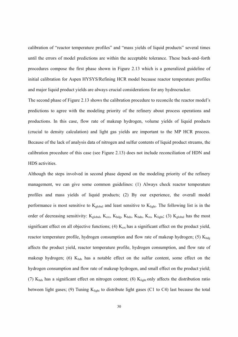
30
calibration of “reactor temperature profiles” and “mass yields of liquid products” several times
until the errors of model predictions are within the acceptable tolerance. These back-and–forth
procedures compose the first phase shown in Figure 2.13 which is a generalized guideline of
initial calibration for Aspen HYSYS/Refining HCR model because reactor temperature profiles
and major liquid product yields are always crucial considerations for any hydrocracker.
The second phase of Figure 2.13 shows the calibration procedure to reconcile the reactor model’s
predictions to agree with the modeling priority of the refinery about process operations and
productions. In this case, flow rate of makeup hydrogen, volume yields of liquid products
(crucial to density calculation) and light gas yields are important to the MP HCR process.
Because of the lack of analysis data of nitrogen and sulfur contents of liquid product streams, the
calibration procedure of this case (see Figure 2.13) does not include reconciliation of HDN and
HDS activities.
Although the steps involved in second phase depend on the modeling priority of the refinery
management, we can give some common guidelines: (1) Always check reactor temperature
profiles and mass yields of liquid products; (2) By our experience, the overall model
performance is most sensitive to Kglobal and least sensitive to Klight. The following list is in the
order of decreasing sensitivity: Kglobal, Kcrc, Khdg, Khds, Khdn, Kro, Klight; (3) Kglobal has the most
significant effect on all objective functions; (4) Kcrc has a significant effect on the product yield,
reactor temperature profile, hydrogen consumption and flow rate of makeup hydrogen; (5) Khdg
affects the product yield, reactor temperature profile, hydrogen consumption, and flow rate of
makeup hydrogen; (6) Khds has a notable effect on the sulfur content, some effect on the
hydrogen consumption and flow rate of makeup hydrogen, and small effect on the product yield;
(7) Khds has a significant effect on nitrogen content; (8) Klight only affects the distribution ratio
between light gases; (9) Tuning Klight to distribute light gases (C1 to C4) last because the total
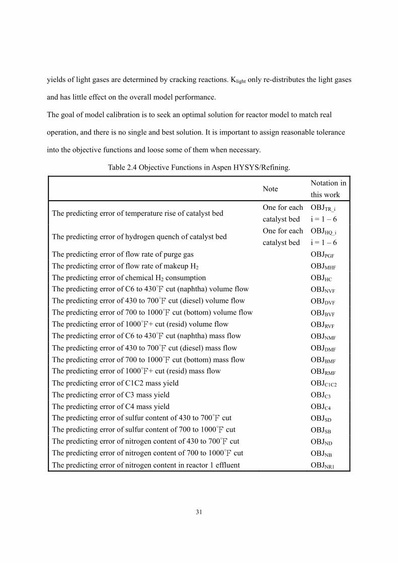
31
yields of light gases are determined by cracking reactions. Klight only re-distributes the light gases
and has little effect on the overall model performance.
The goal of model calibration is to seek an optimal solution for reactor model to match real
operation, and there is no single and best solution. It is important to assign reasonable tolerance
into the objective functions and loose some of them when necessary.
Table 2.4 Objective Functions in Aspen HYSYS/Refining.
Note Notation in this work
The predicting error of temperature rise of catalyst bed One for each catalyst bed
OBJTR_i
i = 1 – 6
The predicting error of hydrogen quench of catalyst bed One for each catalyst bed
OBJHQ_i
i = 1 – 6 The predicting error of flow rate of purge gas OBJPGF
The predicting error of flow rate of makeup H2 OBJMHF
The predicting error of chemical H2 consumption OBJHC The predicting error of C6 to 430 cut (naphtha) volume flow OBJNVF The predicting error of 430 to 700 cut (diesel) volume flow OBJDVF The predicting error of 700 to 1000 cut (bottom) volume flow OBJBVF The predicting error of 1000+ cut (resid) volume flow OBJRVF The predicting error of C6 to 430 cut (naphtha) mass flow OBJNMF The predicting error of 430 to 700 cut (diesel) mass flow OBJDMF The predicting error of 700 to 1000 cut (bottom) mass flow OBJBMF The predicting error of 1000+ cut (resid) mass flow OBJRMF The predicting error of C1C2 mass yield OBJC1C2 The predicting error of C3 mass yield OBJC3 The predicting error of C4 mass yield OBJC4 The predicting error of sulfur content of 430 to 700 cut OBJSD The predicting error of sulfur content of 700 to 1000 cut OBJSB The predicting error of nitrogen content of 430 to 700 cut OBJND The predicting error of nitrogen content of 700 to 1000 cut OBJNB The predicting error of nitrogen content in reactor 1 effluent OBJNR1
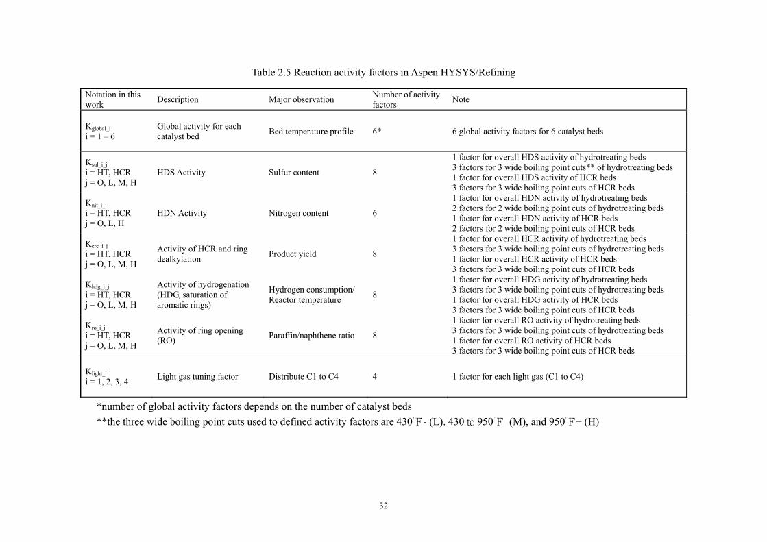
32
Table 2.5 Reaction activity factors in Aspen HYSYS/Refining
*number of global activity factors depends on the number of catalyst beds **the three wide boiling point cuts used to defined activity factors are 430- (L). 430 to 950 (M), and 950+ (H)
Notation in this work Description Major observation Number of activity
factors Note
Kglobal_i i = 1 – 6
Global activity for each catalyst bed Bed temperature profile 6* 6 global activity factors for 6 catalyst beds
Ksul_i_j i = HT, HCR j = O, L, M, H
HDS Activity Sulfur content 8
1 factor for overall HDS activity of hydrotreating beds 3 factors for 3 wide boiling point cuts** of hydrotreating beds 1 factor for overall HDS activity of HCR beds 3 factors for 3 wide boiling point cuts of HCR beds
Knit_i_j i = HT, HCR j = O, L, H
HDN Activity Nitrogen content 6
1 factor for overall HDN activity of hydrotreating beds 2 factors for 2 wide boiling point cuts of hydrotreating beds 1 factor for overall HDN activity of HCR beds 2 factors for 2 wide boiling point cuts of HCR beds
Kcrc_i_j i = HT, HCR j = O, L, M, H
Activity of HCR and ring dealkylation Product yield 8
1 factor for overall HCR activity of hydrotreating beds 3 factors for 3 wide boiling point cuts of hydrotreating beds 1 factor for overall HCR activity of HCR beds 3 factors for 3 wide boiling point cuts of HCR beds
Khdg_i_j i = HT, HCR j = O, L, M, H
Activity of hydrogenation (HDG, saturation of aromatic rings)
Hydrogen consumption/ Reactor temperature 8
1 factor for overall HDG activity of hydrotreating beds 3 factors for 3 wide boiling point cuts of hydrotreating beds 1 factor for overall HDG activity of HCR beds 3 factors for 3 wide boiling point cuts of HCR beds
Kro_i_j i = HT, HCR j = O, L, M, H
Activity of ring opening (RO) Paraffin/naphthene ratio 8
1 factor for overall RO activity of hydrotreating beds 3 factors for 3 wide boiling point cuts of hydrotreating beds 1 factor for overall RO activity of HCR beds 3 factors for 3 wide boiling point cuts of HCR beds
Klight_i i = 1, 2, 3, 4 Light gas tuning factor Distribute C1 to C4 4 1 factor for each light gas (C1 to C4)
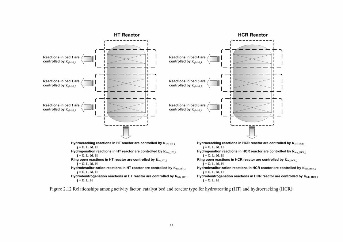
33
Figure 2.12 Relationships among activity factor, catalyst bed and reactor type for hydrotreating (HT) and hydrocracking (HCR).
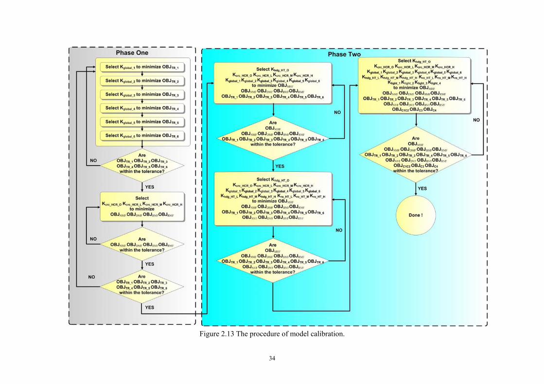
34
Figure 2.13 The procedure of model calibration.
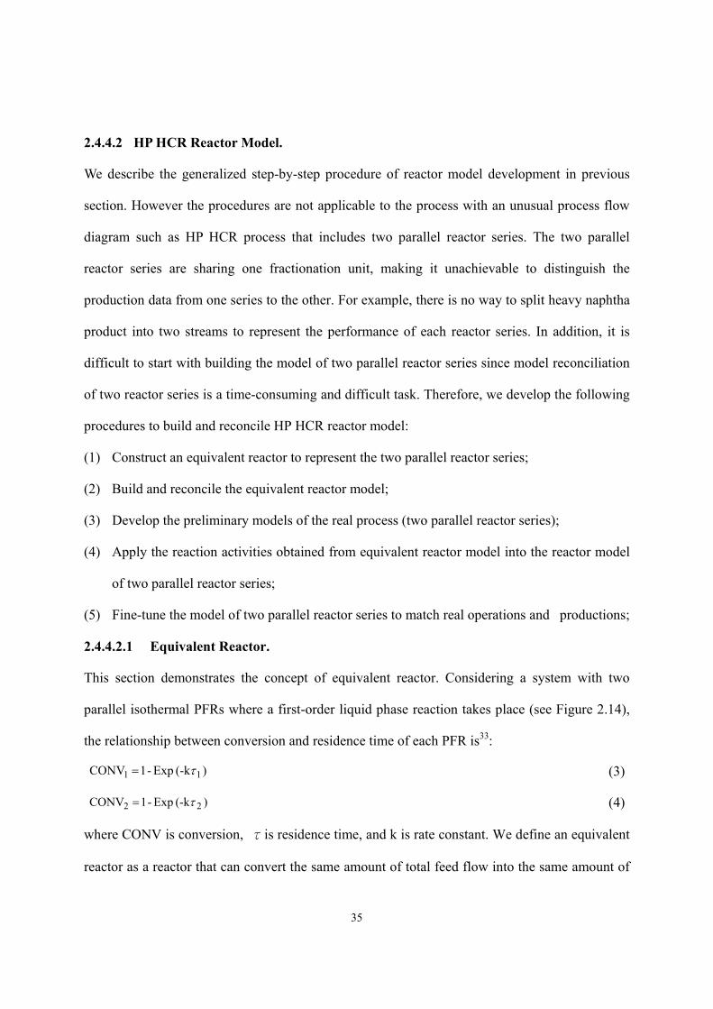
35
2.4.4.2 HP HCR Reactor Model.
We describe the generalized step-by-step procedure of reactor model development in previous
section. However the procedures are not applicable to the process with an unusual process flow
diagram such as HP HCR process that includes two parallel reactor series. The two parallel
reactor series are sharing one fractionation unit, making it unachievable to distinguish the
production data from one series to the other. For example, there is no way to split heavy naphtha
product into two streams to represent the performance of each reactor series. In addition, it is
difficult to start with building the model of two parallel reactor series since model reconciliation
of two reactor series is a time-consuming and difficult task. Therefore, we develop the following
procedures to build and reconcile HP HCR reactor model:
(1) Construct an equivalent reactor to represent the two parallel reactor series;
(2) Build and reconcile the equivalent reactor model;
(3) Develop the preliminary models of the real process (two parallel reactor series);
(4) Apply the reaction activities obtained from equivalent reactor model into the reactor model
of two parallel reactor series;
(5) Fine-tune the model of two parallel reactor series to match real operations and productions;
2.4.4.2.1 Equivalent Reactor.
This section demonstrates the concept of equivalent reactor. Considering a system with two
parallel isothermal PFRs where a first-order liquid phase reaction takes place (see Figure 2.14),
the relationship between conversion and residence time of each PFR is33:
)(-k Exp-1 CONV 11 τ= (3)
)(-k Exp-1 CONV 22 τ= (4)
where CONV is conversion, τis residence time, and k is rate constant. We define an equivalent
reactor as a reactor that can convert the same amount of total feed flow into the same amount of
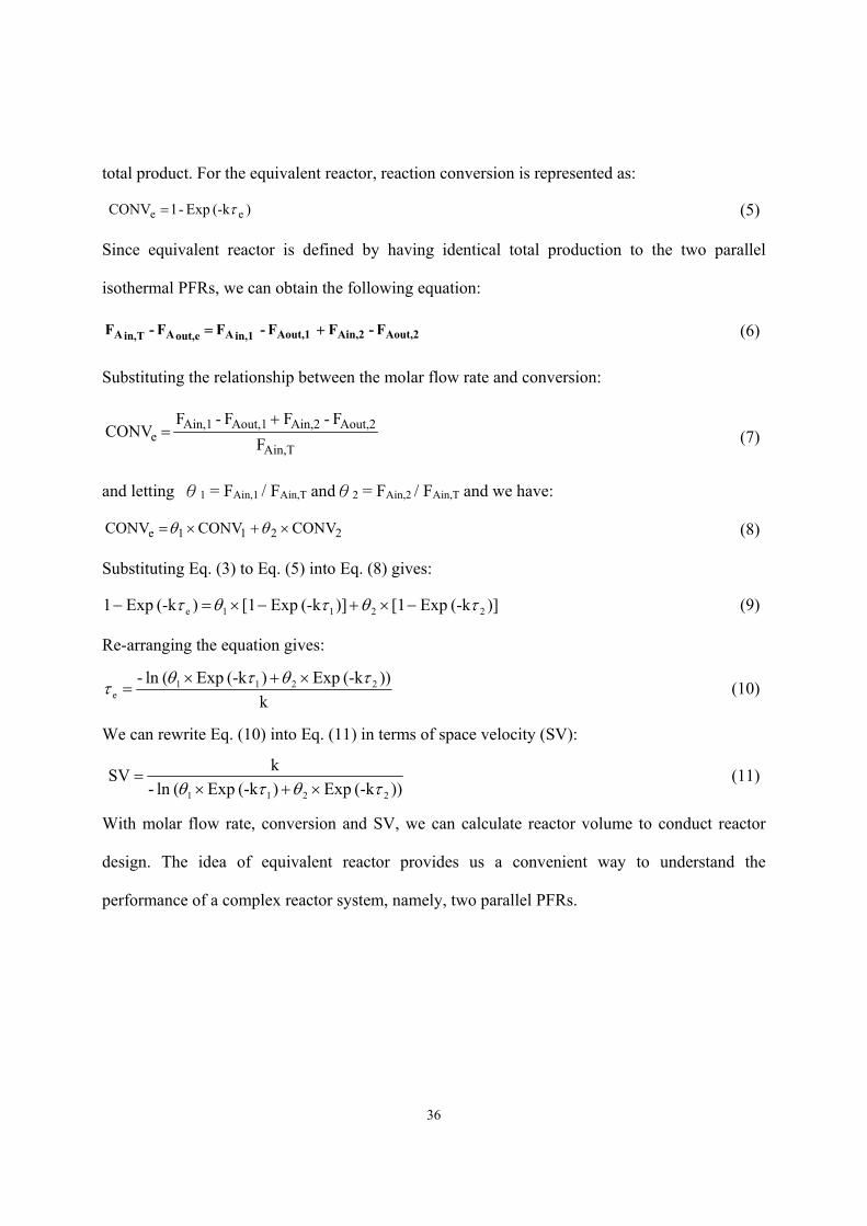
36
total product. For the equivalent reactor, reaction conversion is represented as:
)(-k Exp-1 CONV ee τ= (5)
Since equivalent reactor is defined by having identical total production to the two parallel
isothermal PFRs, we can obtain the following equation:
Aout,2Ain,2 Aout,1 in,1Aout,eATin,A F - F F -F F - F += (6)
Substituting the relationship between the molar flow rate and conversion:
TAin,
Aout,2Ain,2Aout,1Ain,1e F
F - F F - F CONV
+= (7)
and letting θ1 = FAin,1 / FAin,T andθ2 = FAin,2 / FAin,T and we have:
2211e CONV CONV CONV ×+×= θθ (8)
Substituting Eq. (3) to Eq. (5) into Eq. (8) gives:
)](-k Exp [1 )](-k Exp [1 )(-k Exp 1 2211e τθτθτ −×+−×=− (9)
Re-arranging the equation gives:
k))(-k Exp )(-k Exp (ln - 2211
eτθτθτ ×+×
= (10)
We can rewrite Eq. (10) into Eq. (11) in terms of space velocity (SV):
))(-k Exp )(-k Exp (ln -k SV
2211 τθτθ ×+×= (11)
With molar flow rate, conversion and SV, we can calculate reactor volume to conduct reactor
design. The idea of equivalent reactor provides us a convenient way to understand the
performance of a complex reactor system, namely, two parallel PFRs.
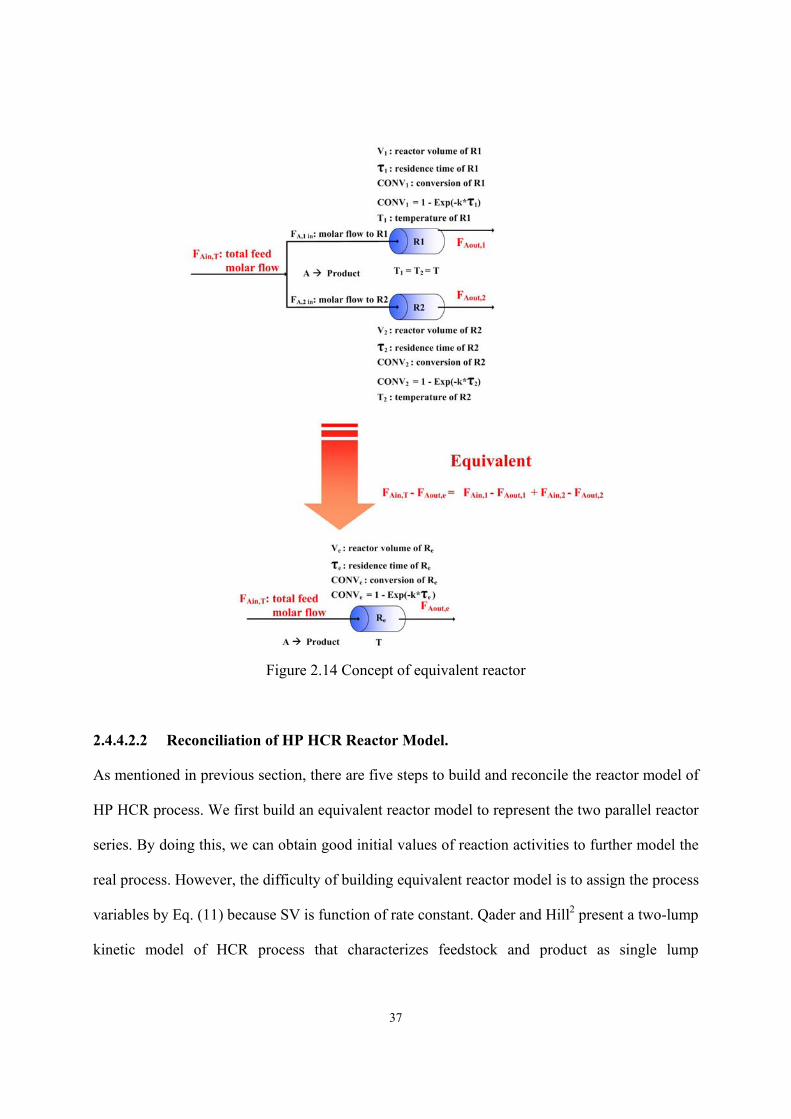
37
Figure 2.14 Concept of equivalent reactor
2.4.4.2.2 Reconciliation of HP HCR Reactor Model.
As mentioned in previous section, there are five steps to build and reconcile the reactor model of
HP HCR process. We first build an equivalent reactor model to represent the two parallel reactor
series. By doing this, we can obtain good initial values of reaction activities to further model the
real process. However, the difficulty of building equivalent reactor model is to assign the process
variables by Eq. (11) because SV is function of rate constant. Qader and Hill2 present a two-lump
kinetic model of HCR process that characterizes feedstock and product as single lump
38
respectively (see Figure 2.15) and apply first-order kinetics to obtain rate constant under
different operating conditions. Eq. (12) represents the rate equation and they apply Arrhenius
equation to correlate experimental data to obtain pre-exponential term and activation energy. Eq.
(13) shows the temperature dependence of rate constant.
oil] [Gask dt
oil] d[Gas- GO ×= (12)
]RT(cal/mole) 21100-Exp[)(h101 )(h k 1-71-
GO ××= (13)
where kGO is rate constant of gas oil HCR reaction. The experimental data were obtained at 10.34
MPa pressure, 400 – 500 , 0.5 – 3.0 h-1 SV, and a constant H2/oil ratio of 500 STD m3/m3.
Since they conduct experiment under similar condition as industrial reactor, it is practical to
utilize kinetic data by Qader and Hill2 to investigate the design of equivalent reactor model. We
apply feed flow rates, reactor volumes, and space velocities from HP HCR process and calculate
reactor volume of equivalent reactor under different rate constants. Figure 2.16 illustrates how
HCR rate constant affects equivalent reactor volume. The y-axis represents the ratio of
equivalent reactor volume to the sum of reactor volumes of the two parallel hydrocracking
reactors (Ve / (V1+V2)). As k approaches zero, the upper limit of 100% is also achieved. This
reflects the physical limitation when no reaction takes place. On the other hand, the value of Ve /
(V1+V2) drops while k increases. Under industrial operating conditions, k value ranges from
0.5 – 3 h-1 (corresponding reactor temperatures are 360 – 430) according to the kinetic data
of Qader and Hill2. Therefore, typical values of Ve / (V1+V2) should be always greater than 90%.
Figure 2.15 A two-lump scheme developed by Qader and Hill2
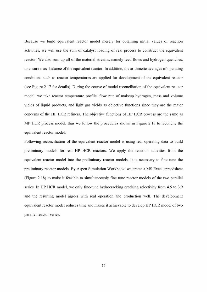
39
Because we build equivalent reactor model merely for obtaining initial values of reaction
activities, we will use the sum of catalyst loading of real process to construct the equivalent
reactor. We also sum up all of the material streams, namely feed flows and hydrogen quenches,
to ensure mass balance of the equivalent reactor. In addition, the arithmetic averages of operating
conditions such as reactor temperatures are applied for development of the equivalent reactor
(see Figure 2.17 for details). During the course of model reconciliation of the equivalent reactor
model, we take reactor temperature profile, flow rate of makeup hydrogen, mass and volume
yields of liquid products, and light gas yields as objective functions since they are the major
concerns of the HP HCR refiners. The objective functions of HP HCR process are the same as
MP HCR process model, thus we follow the procedures shown in Figure 2.13 to reconcile the
equivalent reactor model.
Following reconciliation of the equivalent reactor model is using real operating data to build
preliminary models for real HP HCR reactors. We apply the reaction activities from the
equivalent reactor model into the preliminary reactor models. It is necessary to fine tune the
preliminary reactor models. By Aspen Simulation Workbook, we create a MS Excel spreadsheet
(Figure 2.18) to make it feasible to simultaneously fine tune reactor models of the two parallel
series. In HP HCR model, we only fine-tune hydrocracking cracking selectivity from 4.5 to 3.9
and the resulting model agrees with real operation and production well. The development
equivalent reactor model reduces time and makes it achievable to develop HP HCR model of two
parallel reactor series.
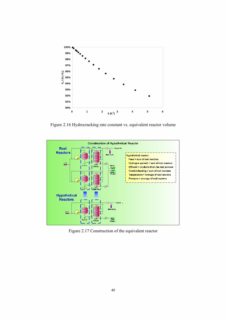
40
90%
91%
92%
93%
94%
95%
96%
97%
98%
99%
100%
0 1 2 3 4 5 6k (h-1)
V e /
(V1+
V 2)
Figure 2.16 Hydrocracking rate constant vs. equivalent reactor volume
Figure 2.17 Construction of the equivalent reactor
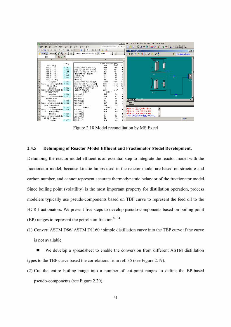
41
Figure 2.18 Model reconciliation by MS Excel
2.4.5 Delumping of Reactor Model Effluent and Fractionator Model Development.
Delumping the reactor model effluent is an essential step to integrate the reactor model with the
fractionator model, because kinetic lumps used in the reactor model are based on structure and
carbon number, and cannot represent accurate thermodynamic behavior of the fractionator model.
Since boiling point (volatility) is the most important property for distillation operation, process
modelers typically use pseudo-components based on TBP curve to represent the feed oil to the
HCR fractionators. We present five steps to develop pseudo-components based on boiling point
(BP) ranges to represent the petroleum fraction32, 34.
(1) Convert ASTM D86/ ASTM D1160 / simple distillation curve into the TBP curve if the curve
is not available.
We develop a spreadsheet to enable the conversion from different ASTM distillation
types to the TBP curve based the correlations from ref. 35 (see Figure 2.19).
(2) Cut the entire boiling range into a number of cut-point ranges to define the BP-based
pseudo-components (see Figure 2.20).
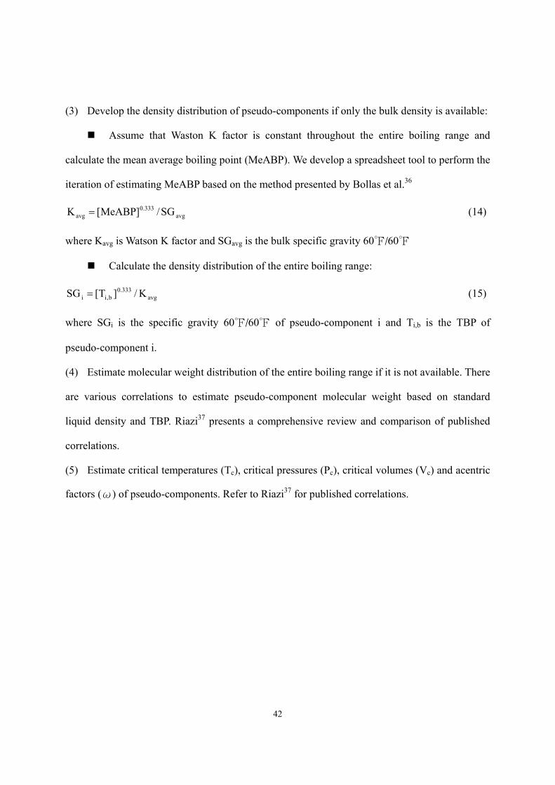
42
(3) Develop the density distribution of pseudo-components if only the bulk density is available:
Assume that Waston K factor is constant throughout the entire boiling range and
calculate the mean average boiling point (MeABP). We develop a spreadsheet tool to perform the
iteration of estimating MeABP based on the method presented by Bollas et al.36
SG/]MeABP[K avg333.0
avg = (14)
where Kavg is Watson K factor and SGavg is the bulk specific gravity 60/60
Calculate the density distribution of the entire boiling range:
K/]T[SG avg333.0
b,ii = (15)
where SGi is the specific gravity 60/60 of pseudo-component i and Ti,b is the TBP of
pseudo-component i.
(4) Estimate molecular weight distribution of the entire boiling range if it is not available. There
are various correlations to estimate pseudo-component molecular weight based on standard
liquid density and TBP. Riazi37 presents a comprehensive review and comparison of published
correlations.
(5) Estimate critical temperatures (Tc), critical pressures (Pc), critical volumes (Vc) and acentric
factors (ω) of pseudo-components. Refer to Riazi37 for published correlations.
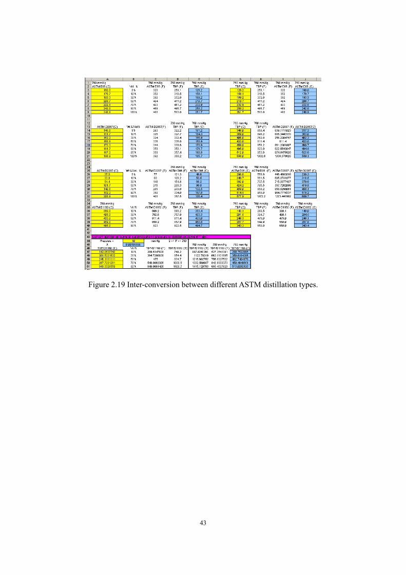
43
Figure 2.19 Inter-conversion between different ASTM distillation types.
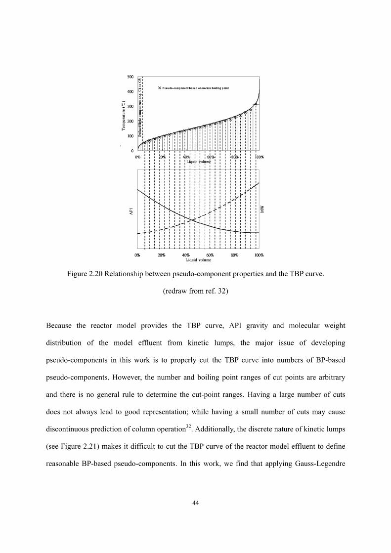
44
Figure 2.20 Relationship between pseudo-component properties and the TBP curve.
(redraw from ref. 32)
Because the reactor model provides the TBP curve, API gravity and molecular weight
distribution of the model effluent from kinetic lumps, the major issue of developing
pseudo-components in this work is to properly cut the TBP curve into numbers of BP-based
pseudo-components. However, the number and boiling point ranges of cut points are arbitrary
and there is no general rule to determine the cut-point ranges. Having a large number of cuts
does not always lead to good representation; while having a small number of cuts may cause
discontinuous prediction of column operation32. Additionally, the discrete nature of kinetic lumps
(see Figure 2.21) makes it difficult to cut the TBP curve of the reactor model effluent to define
reasonable BP-based pseudo-components. In this work, we find that applying Gauss-Legendre
45
quadrature to cut the reactor model effluent into 20 BP-based pseudo-components works well.
The rest of this section will represent the delumping we use to define these pseudo-components,
how to apply tray efficiency model while building the fractionator model, and the sensitivity test
of the fractionator model to verify the delumping method used in this work.
Figure 2.21 Discontinuity of C6+ kinetic lump distribution of reactor model effluent.
2.4.5.1 Apply the Gauss-Legendre Quadrature to Delump the Reactor Model Effluent.
Haynes and Matthews38 apply the Gauss-Legendre quadrature to predict the
vapor-liquid-equilibrium (VLE) of hydrocarbon mixture derived from a continuous
equation-of-state developed by Cotterman et al.39. Later, Mani et al.40 extend the work of Haynes
and Matthews38 to partition the cut-point ranges of TBP curve of a petroleum fraction to define
BP-based pseudo-components, and the predicted VLE satisfactorily matches the experimental
data. Hence, we extend the method represented by Mani et al.40 to delump the reactor model
effluent into BP-based pseudo-components.
In this work, we develop a method with six steps to delump the reactor model effluent into
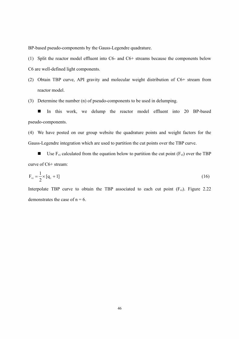
46
BP-based pseudo-components by the Gauss-Legendre quadrature.
(1) Split the reactor model effluent into C6- and C6+ streams because the components below
C6 are well-defined light components.
(2) Obtain TBP curve, API gravity and molecular weight distribution of C6+ stream from
reactor model.
(3) Determine the number (n) of pseudo-components to be used in delumping.
In this work, we delump the reactor model effluent into 20 BP-based
pseudo-components.
(4) We have posted on our group website the quadrature points and weight factors for the
Gauss-Legendre integration which are used to partition the cut points over the TBP curve.
Use Fvi calculated from the equation below to partition the cut point (Fvi) over the TBP
curve of C6+ stream:
]1q[21F ivi +×= (16)
Interpolate TBP curve to obtain the TBP associated to each cut point (Fvi). Figure 2.22
demonstrates the case of n = 6.
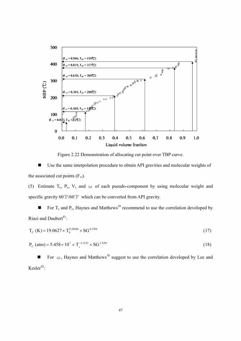
47
Figure 2.22 Demonstration of allocating cut point over TBP curve.
Use the same interpolation procedure to obtain API gravities and molecular weights of
the associated cut points (Fvi).
(5) Estimate Tc, Pc, Vc and ω of each pseudo-component by using molecular weight and
specific gravity 60/60 which can be converted from API gravity.
For Tc and Pc, Haynes and Matthews38 recommend to use the correlation developed by
Riazi and Daubert41:
3596.058848.0bC SGT0627.19)K( T ××= (17)
3201.23125.27C SGT10458.5)atm( P
b×××= − (18)
For ω, Haynes and Matthews38 suggest to use the correlation developed by Lee and
Kesler42:
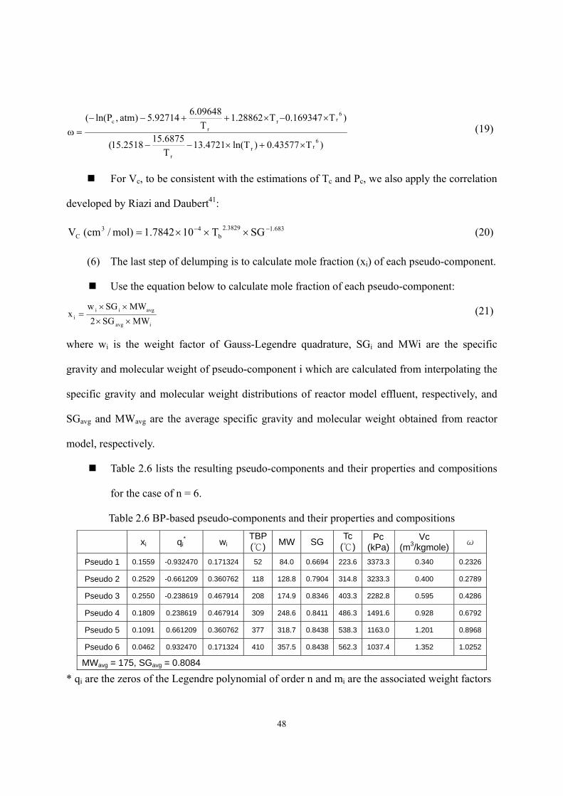
48
)T43577.0)Tln(4721.13T6875.152518.15(
)T169347.0T28862.1T
09648.692714.5)atm ,Pln((
6rr
r
6rr
rc
×+×−−
×−×++−−=ω (19)
For Vc, to be consistent with the estimations of Tc and Pc, we also apply the correlation
developed by Riazi and Daubert41:
683.13829.2b
43C SGT107842.1)mol/cm( V −− ×××= (20)
(6) The last step of delumping is to calculate mole fraction (xi) of each pseudo-component.
Use the equation below to calculate mole fraction of each pseudo-component:
iavg
avgiii MWSG2
MWSGwx
××
××= (21)
where wi is the weight factor of Gauss-Legendre quadrature, SGi and MWi are the specific
gravity and molecular weight of pseudo-component i which are calculated from interpolating the
specific gravity and molecular weight distributions of reactor model effluent, respectively, and
SGavg and MWavg are the average specific gravity and molecular weight obtained from reactor
model, respectively.
Table 2.6 lists the resulting pseudo-components and their properties and compositions
for the case of n = 6.
Table 2.6 BP-based pseudo-components and their properties and compositions
xi qi* wi
TBP () MW SG Tc
()Pc
(kPa)Vc
(m3/kgmole) ω
Pseudo 1 0.1559 -0.932470 0.171324 52 84.0 0.6694 223.6 3373.3 0.340 0.2326
Pseudo 2 0.2529 -0.661209 0.360762 118 128.8 0.7904 314.8 3233.3 0.400 0.2789
Pseudo 3 0.2550 -0.238619 0.467914 208 174.9 0.8346 403.3 2282.8 0.595 0.4286
Pseudo 4 0.1809 0.238619 0.467914 309 248.6 0.8411 486.3 1491.6 0.928 0.6792
Pseudo 5 0.1091 0.661209 0.360762 377 318.7 0.8438 538.3 1163.0 1.201 0.8968
Pseudo 6 0.0462 0.932470 0.171324 410 357.5 0.8438 562.3 1037.4 1.352 1.0252
MWavg = 175, SGavg = 0.8084
* qi are the zeros of the Legendre polynomial of order n and mi are the associated weight factors
49
2.4.5.2 Key Issue of Building Fractionator Model: Overall Tray Efficiency Model.
In building simulation models for fractionators, simulation software users often misunderstand
the concept of “tray efficiency” 32. The theoretical column model based on rigorous
thermodynamics assumes that each tray is in perfect vapor-liquid equilibrium (VLE). However,
real distillation columns do not perform perfectly. The “overall tray efficiency”, defined as
(number of theoretical trays / number of actual trays), indicates the difference of a real column to
a theoretical column. We can apply the overall tray efficiency to the entire column or to specific
separation zones. For example, 20 theoretical trays are required to model an operating column
with 40 actual trays and 50% overall tray efficiency. It is important to remember that all trays in
this column still perform perfect VLE.
There are also tray efficiency models such as the “single tray efficiency” that considers the
separation achieved on each tray independently. The most popular single tray efficiency model is
the Murphree tray efficiency based on either vapor phase or liquid phase. We calculate the
Murphree tray efficiency by the following equation:
1n*n
1nn
1n*n
1nn
xxxxor
yyyyE
+
+
+
+
−−
−−
= (22)
where yn (xn) is the actual composition of vapor (liquid) leaving tray n, yn+1 (xn+1) indicates the
actual composition of vapor (liquid) leaving tray n+1, and *ny ( *
nx ) represents the actual
composition of vapor (liquid) leaving tray n. We note that when applying a single tray efficiency
model, such as the Murphree tray efficiency, the vapor and liquid leaving a tray no longer
achieve VLE in the column model.
However, many simulation software users do not realize that the tray efficiency models
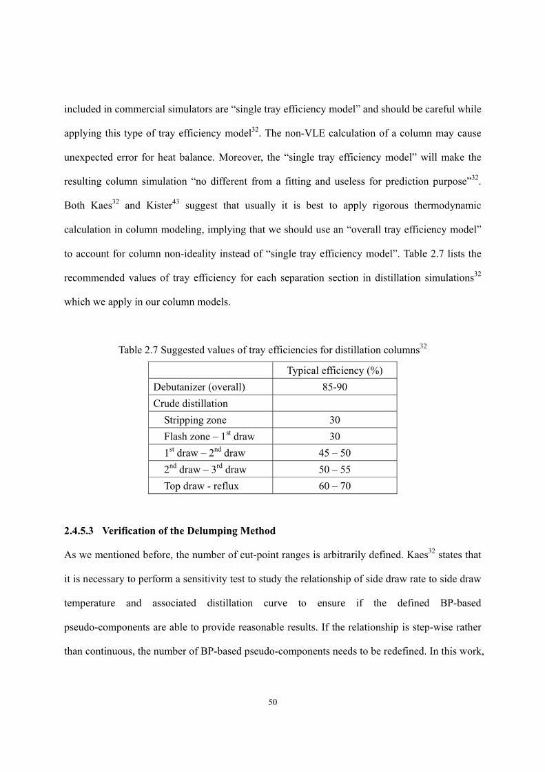
50
included in commercial simulators are “single tray efficiency model” and should be careful while
applying this type of tray efficiency model32. The non-VLE calculation of a column may cause
unexpected error for heat balance. Moreover, the “single tray efficiency model” will make the
resulting column simulation “no different from a fitting and useless for prediction purpose”32.
Both Kaes32 and Kister43 suggest that usually it is best to apply rigorous thermodynamic
calculation in column modeling, implying that we should use an “overall tray efficiency model”
to account for column non-ideality instead of “single tray efficiency model”. Table 2.7 lists the
recommended values of tray efficiency for each separation section in distillation simulations32
which we apply in our column models.
Table 2.7 Suggested values of tray efficiencies for distillation columns32
Typical efficiency (%) Debutanizer (overall) 85-90 Crude distillation Stripping zone 30 Flash zone – 1st draw 30 1st draw – 2nd draw 45 – 50
2nd draw – 3rd draw 50 – 55 Top draw - reflux 60 – 70
2.4.5.3 Verification of the Delumping Method
As we mentioned before, the number of cut-point ranges is arbitrarily defined. Kaes32 states that
it is necessary to perform a sensitivity test to study the relationship of side draw rate to side draw
temperature and associated distillation curve to ensure if the defined BP-based
pseudo-components are able to provide reasonable results. If the relationship is step-wise rather
than continuous, the number of BP-based pseudo-components needs to be redefined. In this work,
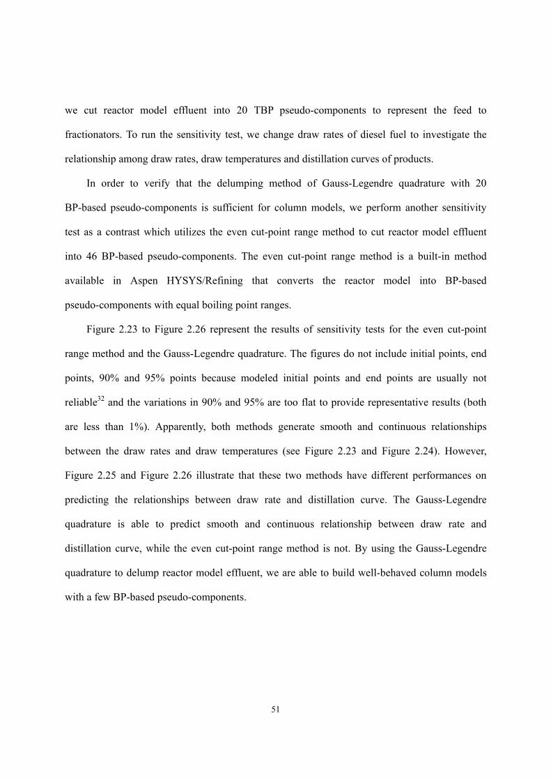
51
we cut reactor model effluent into 20 TBP pseudo-components to represent the feed to
fractionators. To run the sensitivity test, we change draw rates of diesel fuel to investigate the
relationship among draw rates, draw temperatures and distillation curves of products.
In order to verify that the delumping method of Gauss-Legendre quadrature with 20
BP-based pseudo-components is sufficient for column models, we perform another sensitivity
test as a contrast which utilizes the even cut-point range method to cut reactor model effluent
into 46 BP-based pseudo-components. The even cut-point range method is a built-in method
available in Aspen HYSYS/Refining that converts the reactor model into BP-based
pseudo-components with equal boiling point ranges.
Figure 2.23 to Figure 2.26 represent the results of sensitivity tests for the even cut-point
range method and the Gauss-Legendre quadrature. The figures do not include initial points, end
points, 90% and 95% points because modeled initial points and end points are usually not
reliable32 and the variations in 90% and 95% are too flat to provide representative results (both
are less than 1%). Apparently, both methods generate smooth and continuous relationships
between the draw rates and draw temperatures (see Figure 2.23 and Figure 2.24). However,
Figure 2.25 and Figure 2.26 illustrate that these two methods have different performances on
predicting the relationships between draw rate and distillation curve. The Gauss-Legendre
quadrature is able to predict smooth and continuous relationship between draw rate and
distillation curve, while the even cut-point range method is not. By using the Gauss-Legendre
quadrature to delump reactor model effluent, we are able to build well-behaved column models
with a few BP-based pseudo-components.
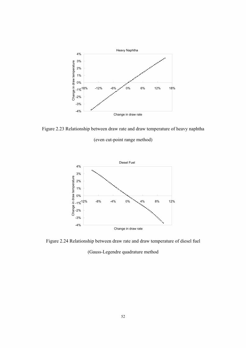
52
Heavy Naphtha
-4%
-3%
-2%
-1%
0%
1%
2%
3%
4%
-18% -12% -6% 0% 6% 12% 18%
Change in draw rate
Cha
nge
in d
raw
tem
pera
ture
Figure 2.23 Relationship between draw rate and draw temperature of heavy naphtha
(even cut-point range method)
Diesel Fuel
-4%
-3%
-2%
-1%
0%
1%
2%
3%
4%
-12% -8% -4% 0% 4% 8% 12%
Change in draw rate
Cha
nge
in d
raw
tem
pera
ture
Figure 2.24 Relationship between draw rate and draw temperature of diesel fuel
(Gauss-Legendre quadrature method
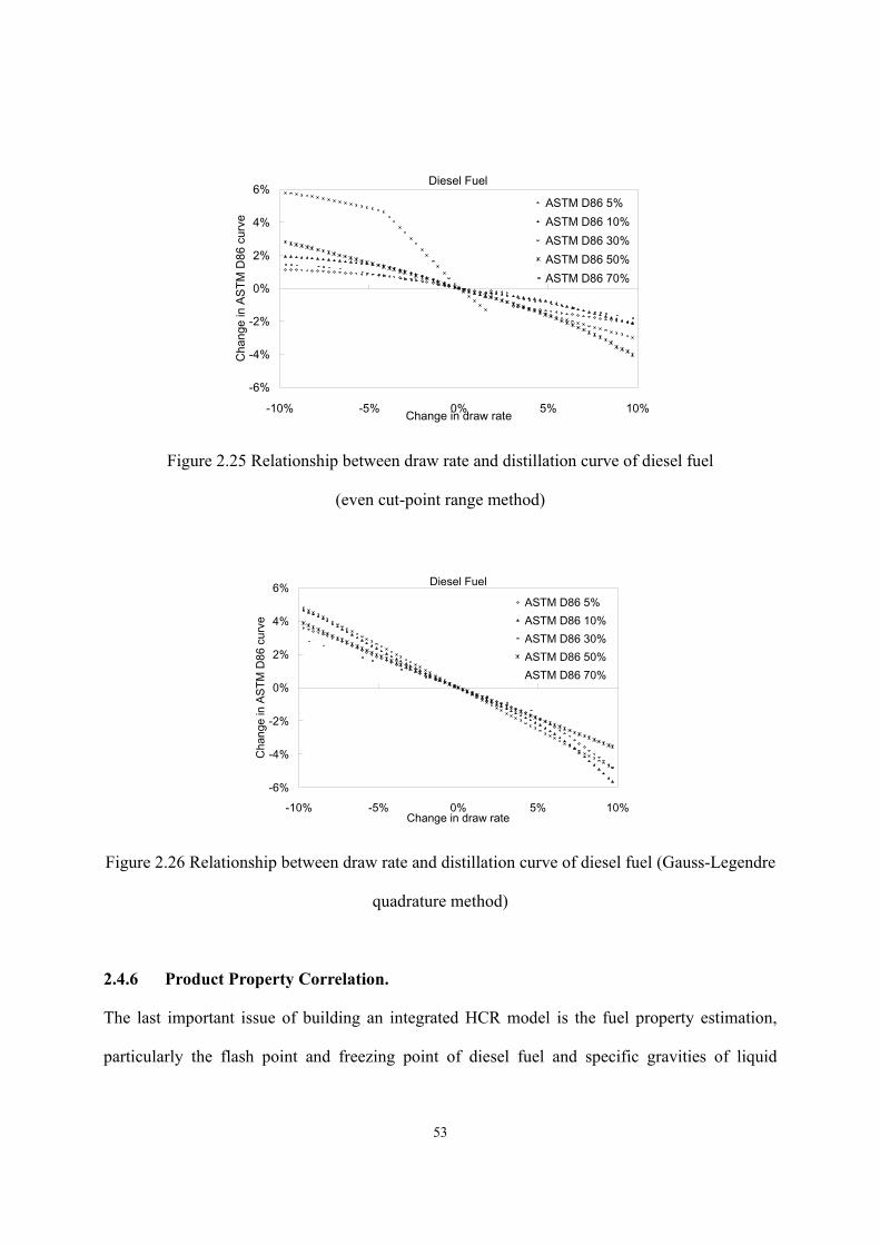
53
Diesel Fuel
-6%
-4%
-2%
0%
2%
4%
6%
-10% -5% 0% 5% 10%Change in draw rate
Cha
nge
in A
STM
D86
cur
ve
ASTM D86 5%ASTM D86 10%ASTM D86 30%ASTM D86 50%ASTM D86 70%
Figure 2.25 Relationship between draw rate and distillation curve of diesel fuel
(even cut-point range method)
Diesel Fuel
-6%
-4%
-2%
0%
2%
4%
6%
-10% -5% 0% 5% 10%Change in draw rate
Cha
nge
in A
STM
D86
cur
ve
ASTM D86 5%ASTM D86 10%ASTM D86 30%ASTM D86 50%ASTM D86 70%
Figure 2.26 Relationship between draw rate and distillation curve of diesel fuel (Gauss-Legendre
quadrature method)
2.4.6 Product Property Correlation.
The last important issue of building an integrated HCR model is the fuel property estimation,
particularly the flash point and freezing point of diesel fuel and specific gravities of liquid
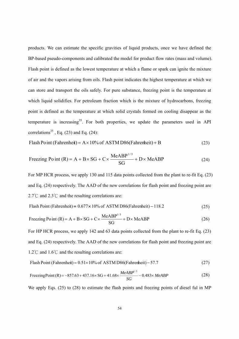
54
products. We can estimate the specific gravities of liquid products, once we have defined the
BP-based pseudo-components and calibrated the model for product flow rates (mass and volume).
Flash point is defined as the lowest temperature at which a flame or spark can ignite the mixture
of air and the vapors arising from oils. Flash point indicates the highest temperature at which we
can store and transport the oils safely. For pure substance, freezing point is the temperature at
which liquid solidifies. For petroleum fraction which is the mixture of hydrocarbons, freezing
point is defined as the temperature at which solid crystals formed on cooling disappear as the
temperature is increasing35. For both properties, we update the parameters used in API
correlations35 , Eq. (23) and Eq. (24):
B heit)D86(Fahren ASTM of %10A t)(Fahrenhei intPo Flash +×= (23)
MeABPDSG
MeABPC SG B A (R) intPo Freezing3/1
×+×+×+= (24)
For MP HCR process, we apply 130 and 115 data points collected from the plant to re-fit Eq. (23)
and Eq. (24) respectively. The AAD of the new correlations for flash point and freezing point are
2.7 and 2.3 and the resulting correlations are:
118.2 heit)D86(Fahren ASTM of 10%0.677 t)(FahrenheiPoint Flash −×= (25)
MeABPDSG
MeABPC SG B A (R) intPo Freezing3/1
×+×+×+= (26)
For HP HCR process, we apply 142 and 63 data points collected from the plant to re-fit Eq. (23)
and Eq. (24) respectively. The AAD of the new correlations for flash point and freezing point are
1.2 and 1.6 and the resulting correlations are:
7.75 heit)D86(Fahren ASTM of %1051.0 t)(FahrenheiPoint Flash −×= (27)
MeABPSG
MeABP×−×+×+−= 483.041.68 SG 16.374 63.857 (R)Point Freezing
3/1
(28)
We apply Eqs. (25) to (28) to estimate the flash points and freezing points of diesel ful in MP
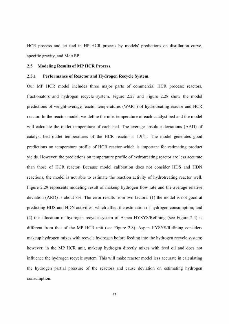
55
HCR process and jet fuel in HP HCR process by models’ predictions on distillation curve,
specific gravity, and MeABP.
2.5 Modeling Results of MP HCR Process.
2.5.1 Performance of Reactor and Hydrogen Recycle System.
Our MP HCR model includes three major parts of commercial HCR process: reactors,
fractionators and hydrogen recycle system. Figure 2.27 and Figure 2.28 show the model
predictions of weight-average reactor temperatures (WART) of hydrotreating reactor and HCR
reactor. In the reactor model, we define the inlet temperature of each catalyst bed and the model
will calculate the outlet temperature of each bed. The average absolute deviations (AAD) of
catalyst bed outlet temperatures of the HCR reactor is 1.9. The model generates good
predictions on temperature profile of HCR reactor which is important for estimating product
yields. However, the predictions on temperature profile of hydrotreating reactor are less accurate
than those of HCR reactor. Because model calibration does not consider HDS and HDN
reactions, the model is not able to estimate the reaction activity of hydrotreating reactor well.
Figure 2.29 represents modeling result of makeup hydrogen flow rate and the average relative
deviation (ARD) is about 8%. The error results from two factors: (1) the model is not good at
predicting HDS and HDN activities, which affect the estimation of hydrogen consumption; and
(2) the allocation of hydrogen recycle system of Aspen HYSYS/Refining (see Figure 2.4) is
different from that of the MP HCR unit (see Figure 2.8). Aspen HYSYS/Refining considers
makeup hydrogen mixes with recycle hydrogen before feeding into the hydrogen recycle system;
however, in the MP HCR unit, makeup hydrogen directly mixes with feed oil and does not
influence the hydrogen recycle system. This will make reactor model less accurate in calculating
the hydrogen partial pressure of the reactors and cause deviation on estimating hydrogen
consumption.
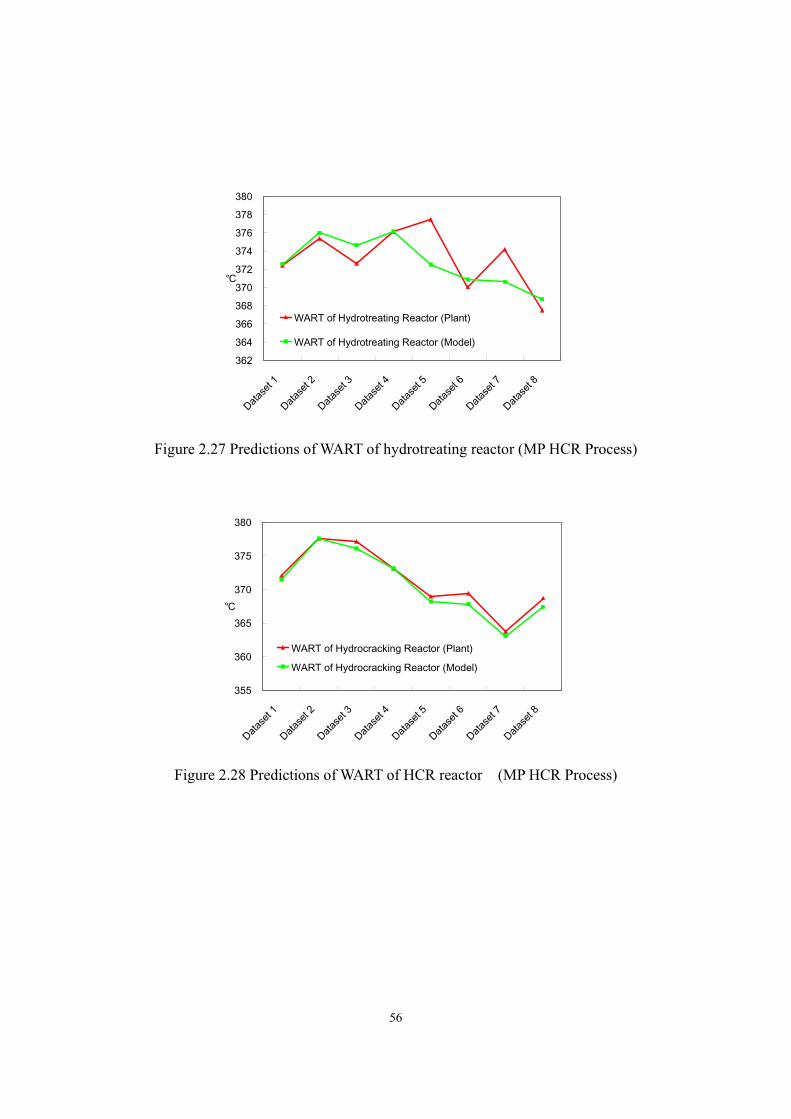
56
362
364
366
368
370
372
374
376
378
380
Datase
t 1
Datase
t 2
Datase
t 3
Datase
t 4
Datase
t 5
Datase
t 6
Datase
t 7
Datase
t 8
WART of Hydrotreating Reactor (Plant)
WART of Hydrotreating Reactor (Model)
Figure 2.27 Predictions of WART of hydrotreating reactor (MP HCR Process)
355
360
365
370
375
380
Datase
t 1
Datase
t 2
Datase
t 3
Datase
t 4
Datase
t 5
Datase
t 6
Datase
t 7
Datase
t 8
WART of Hydrocracking Reactor (Plant)
WART of Hydrocracking Reactor (Model)
Figure 2.28 Predictions of WART of HCR reactor (MP HCR Process)
57
0
10000
20000
30000
40000
Dataset1
Dataset2
Dataset3
Dataset4
Dataset5
Dataset6
Dataset7
Dataset8
STD
m3 /h
MakeUp H2 Flowrate (Plant)MakeUp H2 Flowrate (Model) ARD: 8.0%
Figure 2.29 Predictions of makeup hydrogen flow rate (MP HCR)
2.5.2 Performance of Fractionators.
Temperature profile of distillation column is valuable for evaluating energy consumption,
helping plant operation of cut-point and process optimization. Figure 2.30 to Figure 2.33
illustrate selected modeling results on temperature profiles of distillation columns. Note that we
apply the overall tray efficiency model to column simulations and the resulting tray number of
column model does not correspond to the tray number in the real column. Therefore, we use “top
-> bottom” in Figure 2.30 to Figure 2.33 instead, showing tray number to illustrate temperature
distribution from condenser to bottom of the column. Obviously, the model is able to provide
good predictions on column temperature profiles.
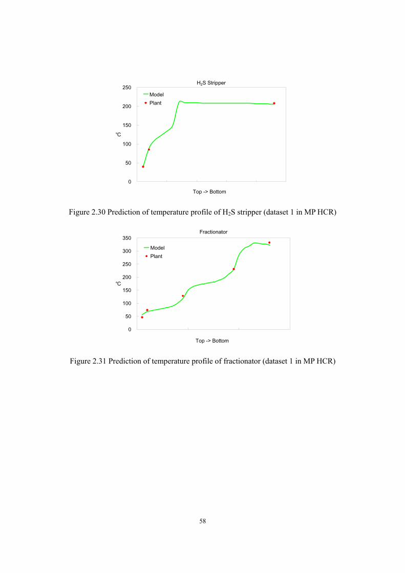
58
H2S Stripper
0
50
100
150
200
250
Top -> Bottom
ModelPlant
Figure 2.30 Prediction of temperature profile of H2S stripper (dataset 1 in MP HCR)
Fractionator
0
50
100
150
200
250
300
350
Top -> Bottom
ModelPlant
Figure 2.31 Prediction of temperature profile of fractionator (dataset 1 in MP HCR)
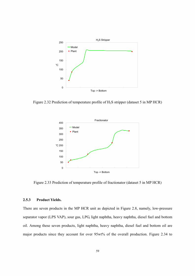
59
H2S Stripper
0
50
100
150
200
250
Top -> Bottom
ModelPlant
Figure 2.32 Prediction of temperature profile of H2S stripper (dataset 5 in MP HCR)
Fractionator
0
50
100
150
200
250
300
350
400
Top -> Bottom
ModelPlant
Figure 2.33 Prediction of temperature profile of fractionator (dataset 5 in MP HCR)
2.5.3 Product Yields.
There are seven products in the MP HCR unit as depicted in Figure 2.8, namely, low-pressure
separator vapor (LPS VAP), sour gas, LPG, light naphtha, heavy naphtha, diesel fuel and bottom
oil. Among these seven products, light naphtha, heavy naphtha, diesel fuel and bottom oil are
major products since they account for over 95wt% of the overall production. Figure 2.34 to
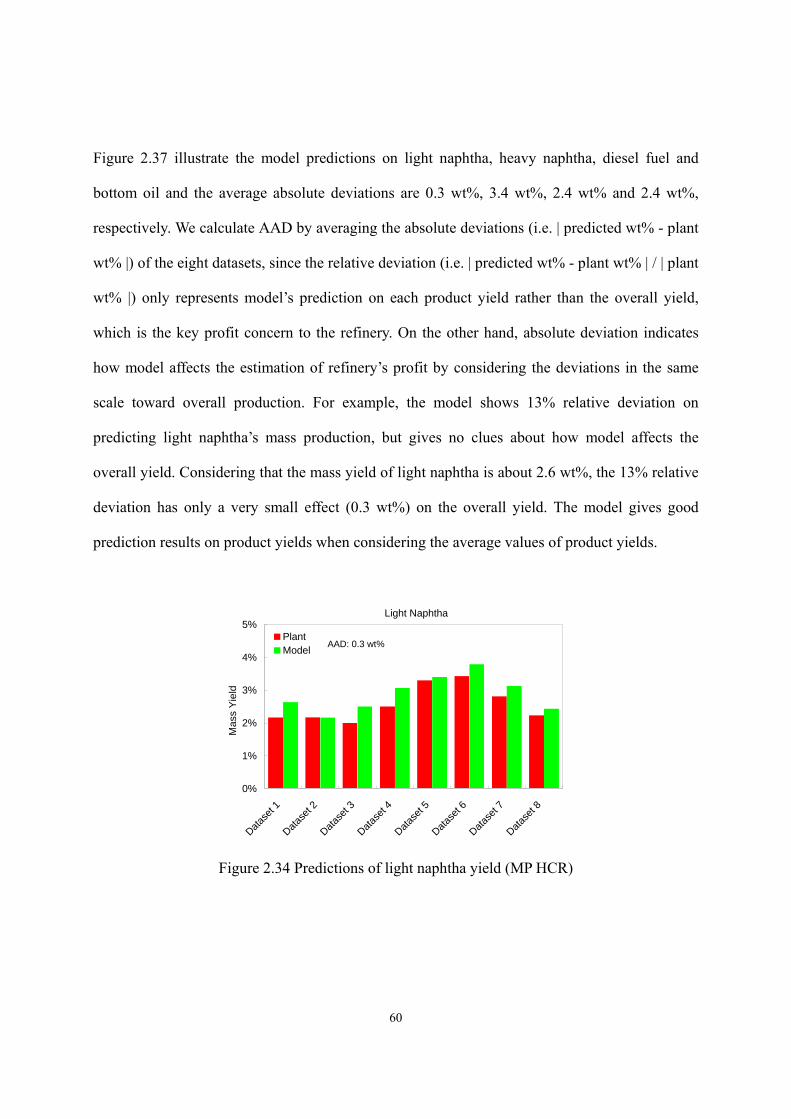
60
Figure 2.37 illustrate the model predictions on light naphtha, heavy naphtha, diesel fuel and
bottom oil and the average absolute deviations are 0.3 wt%, 3.4 wt%, 2.4 wt% and 2.4 wt%,
respectively. We calculate AAD by averaging the absolute deviations (i.e. | predicted wt% - plant
wt% |) of the eight datasets, since the relative deviation (i.e. | predicted wt% - plant wt% | / | plant
wt% |) only represents model’s prediction on each product yield rather than the overall yield,
which is the key profit concern to the refinery. On the other hand, absolute deviation indicates
how model affects the estimation of refinery’s profit by considering the deviations in the same
scale toward overall production. For example, the model shows 13% relative deviation on
predicting light naphtha’s mass production, but gives no clues about how model affects the
overall yield. Considering that the mass yield of light naphtha is about 2.6 wt%, the 13% relative
deviation has only a very small effect (0.3 wt%) on the overall yield. The model gives good
prediction results on product yields when considering the average values of product yields.
Light Naphtha
0%
1%
2%
3%
4%
5%
Datase
t 1
Datase
t 2
Datase
t 3
Datase
t 4
Datase
t 5
Datase
t 6
Datase
t 7
Datase
t 8
Mas
s Yi
eld
PlantModel AAD: 0.3 wt%
Figure 2.34 Predictions of light naphtha yield (MP HCR)
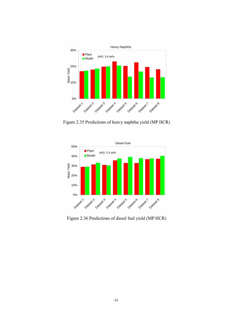
61
Heavy Naphtha
0%
10%
20%
30%
Datase
t 1
Datase
t 2
Datase
t 3
Datase
t 4
Datase
t 5
Datase
t 6
Datase
t 7
Datase
t 8
Mas
s Yi
eld
PlantModel
AAD: 3.4 wt%
Figure 2.35 Predictions of heavy naphtha yield (MP HCR)
Diesel Fuel
0%
10%
20%
30%
40%
50%
Datase
t 1
Datase
t 2
Datase
t 3
Datase
t 4
Datase
t 5
Datase
t 6
Datase
t 7
Datase
t 8
Mas
s Yi
eld
PlantModel
AAD: 2.4 wt%
Figure 2.36 Predictions of diesel fuel yield (MP HCR)
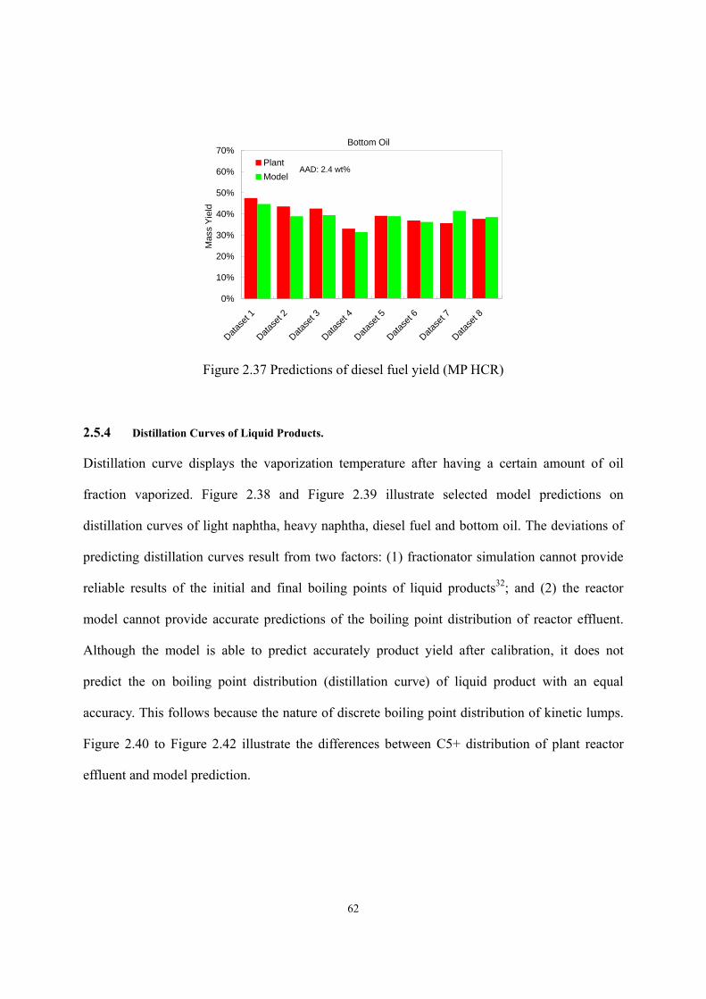
62
Bottom Oil
0%
10%
20%
30%
40%
50%
60%
70%
Datase
t 1
Datase
t 2
Datase
t 3
Datase
t 4
Datase
t 5
Datase
t 6
Datase
t 7
Datase
t 8
Mas
s Yi
eld
PlantModel
AAD: 2.4 wt%
Figure 2.37 Predictions of diesel fuel yield (MP HCR)
2.5.4 Distillation Curves of Liquid Products.
Distillation curve displays the vaporization temperature after having a certain amount of oil
fraction vaporized. Figure 2.38 and Figure 2.39 illustrate selected model predictions on
distillation curves of light naphtha, heavy naphtha, diesel fuel and bottom oil. The deviations of
predicting distillation curves result from two factors: (1) fractionator simulation cannot provide
reliable results of the initial and final boiling points of liquid products32; and (2) the reactor
model cannot provide accurate predictions of the boiling point distribution of reactor effluent.
Although the model is able to predict accurately product yield after calibration, it does not
predict the on boiling point distribution (distillation curve) of liquid product with an equal
accuracy. This follows because the nature of discrete boiling point distribution of kinetic lumps.
Figure 2.40 to Figure 2.42 illustrate the differences between C5+ distribution of plant reactor
effluent and model prediction.
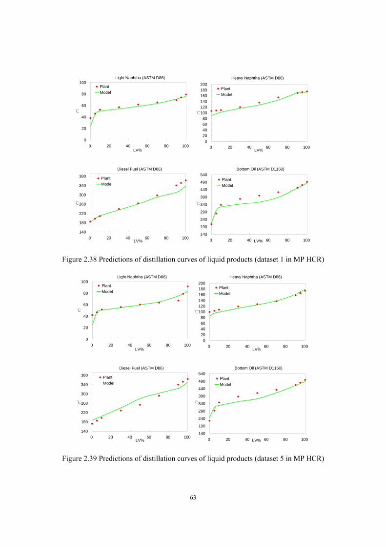
63
Light Naphtha (ASTM D86)
0
20
40
60
80
100
0 20 40 60 80 100LV%
PlantModel
Heavy Naphtha (ASTM D86)
020406080
100120140160180200
0 20 40 60 80 100LV%
PlantModel
Diesel Fuel (ASTM D86)
140
180
220
260
300
340
380
0 20 40 60 80 100LV%
PlantModel
Bottom Oil (ASTM D1160)
140
190
240
290
340
390
440
490
540
0 20 40 60 80 100LV%
PlantModel
Figure 2.38 Predictions of distillation curves of liquid products (dataset 1 in MP HCR)
Light Naphtha (ASTM D86)
0
20
40
60
80
100
0 20 40 60 80 100LV%
PlantModel
Heavy Naphtha (ASTM D86)
020406080
100120140160180200
0 20 40 60 80 100LV%
PlantModel
Diesel Fuel (ASTM D86)
140
180
220
260
300
340
380
0 20 40 60 80 100LV%
PlantModel
Bottom Oil (ASTM D1160)
140
190
240
290
340
390
440
490
540
0 20 40 60 80 100LV%
PlantModel
Figure 2.39 Predictions of distillation curves of liquid products (dataset 5 in MP HCR)
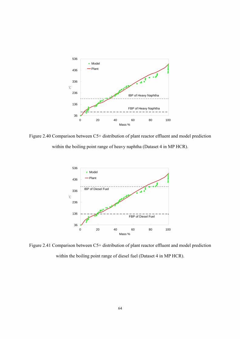
64
36
136
236
336
436
536
0 20 40 60 80 100Mass %
Model
Plant
IBP of Heavy Naphtha
FBP of Heavy Naphtha
Figure 2.40 Comparison between C5+ distribution of plant reactor effluent and model prediction
within the boiling point range of heavy naphtha (Dataset 4 in MP HCR).
36
136
236
336
436
536
0 20 40 60 80 100Mass %
Model
Plant
IBP of Diesel Fuel
FBP of Diesel Fuel
Figure 2.41 Comparison between C5+ distribution of plant reactor effluent and model prediction
within the boiling point range of diesel fuel (Dataset 4 in MP HCR).
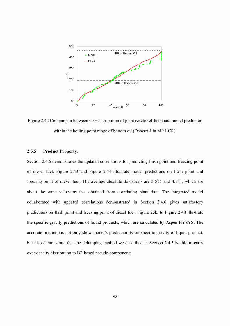
65
36
136
236
336
436
536
0 20 40 60 80 100Mass %
Model
Plant
IBP of Bottom Oil
FBP of Bottom Oil
Figure 2.42 Comparison between C5+ distribution of plant reactor effluent and model prediction
within the boiling point range of bottom oil (Dataset 4 in MP HCR).
2.5.5 Product Property.
Section 2.4.6 demonstrates the updated correlations for predicting flash point and freezing point
of diesel fuel. Figure 2.43 and Figure 2.44 illustrate model predictions on flash point and
freezing point of diesel fuel. The average absolute deviations are 3.6 and 4.1, which are
about the same values as that obtained from correlating plant data. The integrated model
collaborated with updated correlations demonstrated in Section 2.4.6 gives satisfactory
predictions on flash point and freezing point of diesel fuel. Figure 2.45 to Figure 2.48 illustrate
the specific gravity predictions of liquid products, which are calculated by Aspen HYSYS. The
accurate predictions not only show model’s predictability on specific gravity of liquid product,
but also demonstrate that the delumping method we described in Section 2.4.5 is able to carry
over density distribution to BP-based pseudo-components.
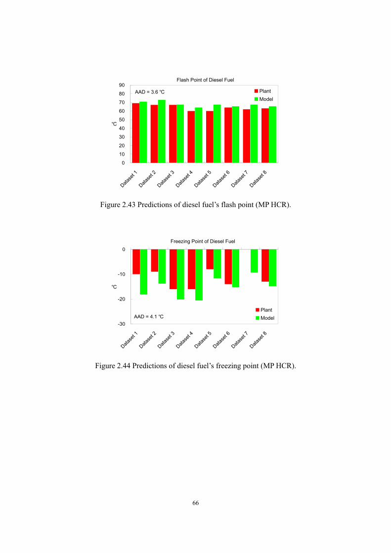
66
Flash Point of Diesel Fuel
0102030405060708090
Datase
t 1
Datase
t 2
Datase
t 3
Datase
t 4
Datase
t 5
Datase
t 6
Datase
t 7
Datase
t 8
PlantModel
AAD = 3.6
Figure 2.43 Predictions of diesel fuel’s flash point (MP HCR).
Freezing Point of Diesel Fuel
-30
-20
-10
0
Datase
t 1
Datase
t 2
Datase
t 3
Datase
t 4
Datase
t 5
Datase
t 6
Datase
t 7
Datase
t 8
PlantModelAAD = 4.1
Figure 2.44 Predictions of diesel fuel’s freezing point (MP HCR).
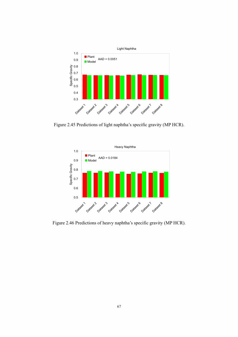
67
Light Naphtha
0.3
0.4
0.5
0.6
0.7
0.8
0.9
1.0
Datase
t 1
Datase
t 2
Datase
t 3
Datase
t 4
Datase
t 5
Datase
t 6
Datase
t 7
Datase
t 8
Spec
ific
Gra
vity
PlantModel
AAD = 0.0051
Figure 2.45 Predictions of light naphtha’s specific gravity (MP HCR).
Heavy Naphtha
0.5
0.6
0.7
0.8
0.9
1.0
Datase
t 1
Datase
t 2
Datase
t 3
Datase
t 4
Datase
t 5
Datase
t 6
Datase
t 7
Datase
t 8
Spec
ific
Gra
vity
PlantModel
AAD = 0.0184
Figure 2.46 Predictions of heavy naphtha’s specific gravity (MP HCR).
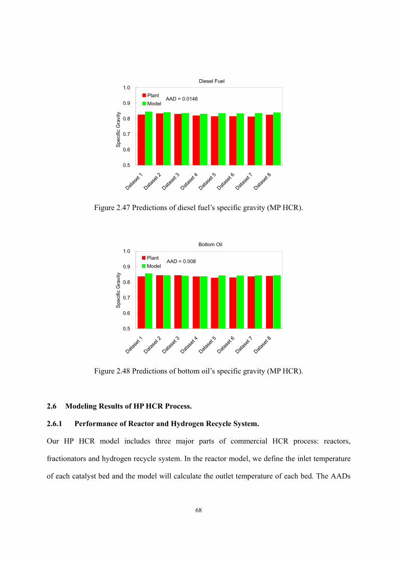
68
Diesel Fuel
0.5
0.6
0.7
0.8
0.9
1.0
Datase
t 1
Datase
t 2
Datase
t 3
Datase
t 4
Datase
t 5
Datase
t 6
Datase
t 7
Datase
t 8
Spec
ific
Gra
vity
PlantModel
AAD = 0.0148
Figure 2.47 Predictions of diesel fuel’s specific gravity (MP HCR).
Bottom Oil
0.5
0.6
0.7
0.8
0.9
1.0
Datase
t 1
Datase
t 2
Datase
t 3
Datase
t 4
Datase
t 5
Datase
t 6
Datase
t 7
Datase
t 8
Spec
ific
Gra
vity
PlantModel
AAD = 0.008
Figure 2.48 Predictions of bottom oil’s specific gravity (MP HCR).
2.6 Modeling Results of HP HCR Process.
2.6.1 Performance of Reactor and Hydrogen Recycle System.
Our HP HCR model includes three major parts of commercial HCR process: reactors,
fractionators and hydrogen recycle system. In the reactor model, we define the inlet temperature
of each catalyst bed and the model will calculate the outlet temperature of each bed. The AADs
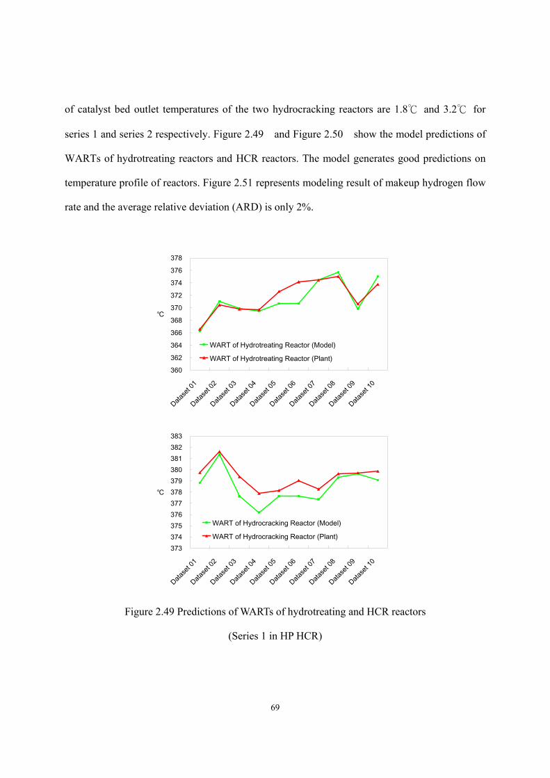
69
of catalyst bed outlet temperatures of the two hydrocracking reactors are 1.8 and 3.2 for
series 1 and series 2 respectively. Figure 2.49 and Figure 2.50 show the model predictions of
WARTs of hydrotreating reactors and HCR reactors. The model generates good predictions on
temperature profile of reactors. Figure 2.51 represents modeling result of makeup hydrogen flow
rate and the average relative deviation (ARD) is only 2%.
360
362
364
366
368
370
372
374
376
378
Datase
t 01
Datase
t 02
Datase
t 03
Datase
t 04
Datase
t 05
Datase
t 06
Datase
t 07
Datase
t 08
Datase
t 09
Datase
t 10
WART of Hydrotreating Reactor (Model)
WART of Hydrotreating Reactor (Plant)
373374375376377378379380381382383
Datase
t 01
Datase
t 02
Datase
t 03
Datase
t 04
Datase
t 05
Datase
t 06
Datase
t 07
Datase
t 08
Datase
t 09
Datase
t 10
WART of Hydrocracking Reactor (Model)
WART of Hydrocracking Reactor (Plant)
Figure 2.49 Predictions of WARTs of hydrotreating and HCR reactors
(Series 1 in HP HCR)
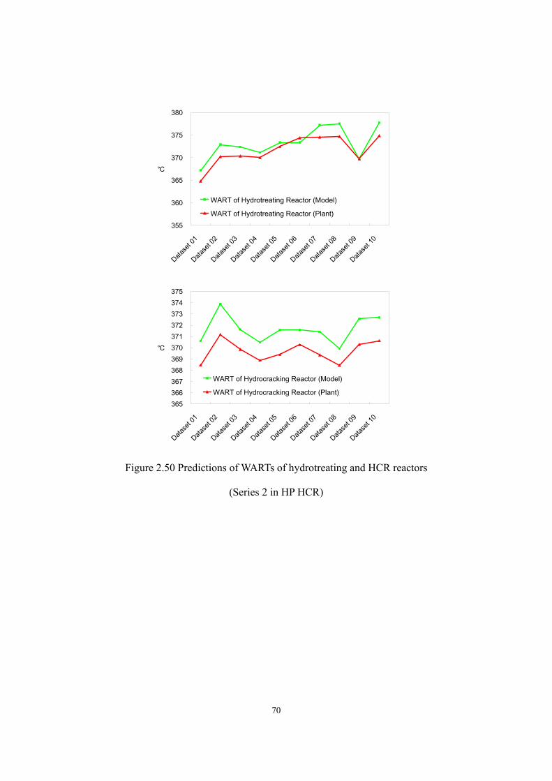
70
355
360
365
370
375
380
Datase
t 01
Datase
t 02
Datase
t 03
Datase
t 04
Datase
t 05
Datase
t 06
Datase
t 07
Datase
t 08
Datase
t 09
Datase
t 10
WART of Hydrotreating Reactor (Model)
WART of Hydrotreating Reactor (Plant)
365366367368369370371372373374375
Datase
t 01
Datase
t 02
Datase
t 03
Datase
t 04
Datase
t 05
Datase
t 06
Datase
t 07
Datase
t 08
Datase
t 09
Datase
t 10
WART of Hydrocracking Reactor (Model)
WART of Hydrocracking Reactor (Plant)
Figure 2.50 Predictions of WARTs of hydrotreating and HCR reactors
(Series 2 in HP HCR)
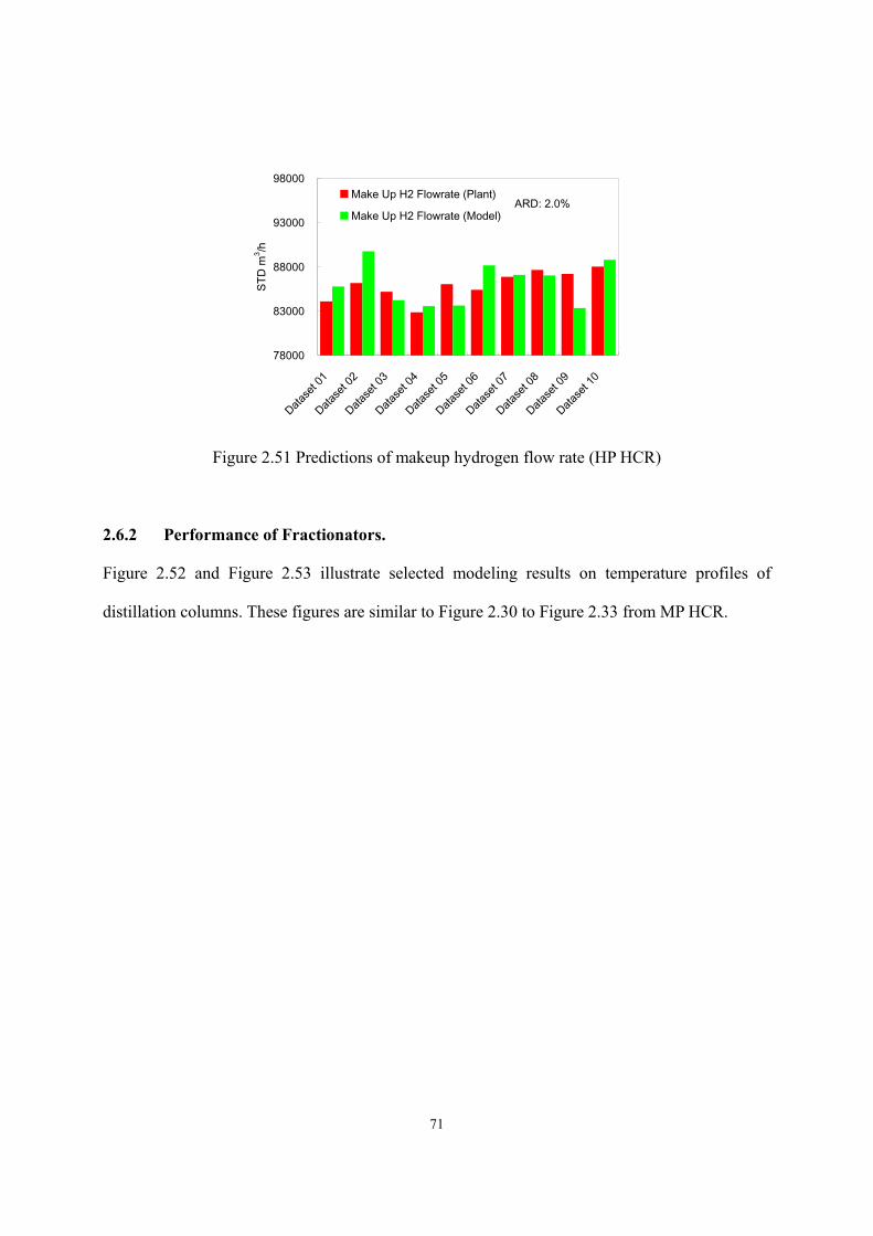
71
78000
83000
88000
93000
98000
Datase
t 01
Datase
t 02
Datase
t 03
Datase
t 04
Datase
t 05
Datase
t 06
Datase
t 07
Datase
t 08
Datase
t 09
Datase
t 10
STD
m3 /h
Make Up H2 Flowrate (Plant)
Make Up H2 Flowrate (Model)ARD: 2.0%
Figure 2.51 Predictions of makeup hydrogen flow rate (HP HCR)
2.6.2 Performance of Fractionators.
Figure 2.52 and Figure 2.53 illustrate selected modeling results on temperature profiles of
distillation columns. These figures are similar to Figure 2.30 to Figure 2.33 from MP HCR.
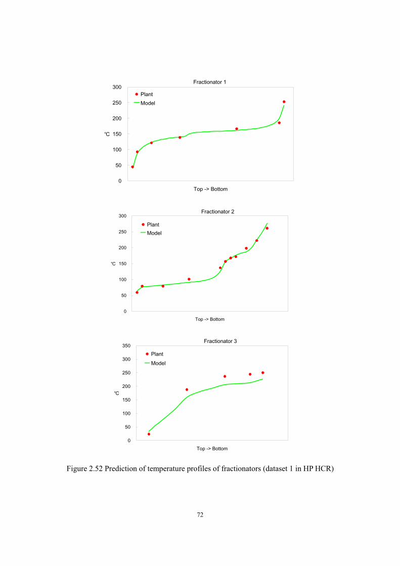
72
Fractionator 1
0
50
100
150
200
250
300
Top -> Bottom
PlantModel
Fractionator 2
0
50
100
150
200
250
300
Top -> Bottom
PlantModel
Fractionator 3
0
50
100
150
200
250
300
350
Top -> Bottom
PlantModel
Figure 2.52 Prediction of temperature profiles of fractionators (dataset 1 in HP HCR)
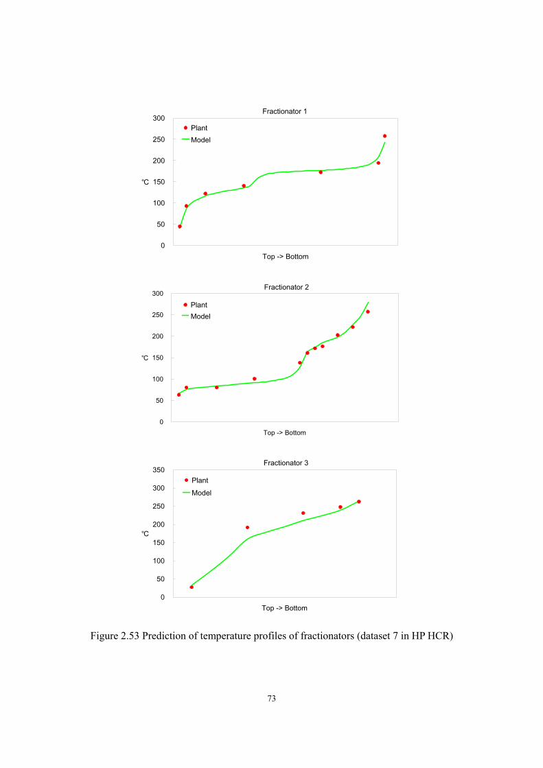
73
Fractionator 1
0
50
100
150
200
250
300
Top -> Bottom
PlantModel
Fractionator 2
0
50
100
150
200
250
300
Top -> Bottom
PlantModel
Fractionator 3
0
50
100
150
200
250
300
350
Top -> Bottom
PlantModel
Figure 2.53 Prediction of temperature profiles of fractionators (dataset 7 in HP HCR)
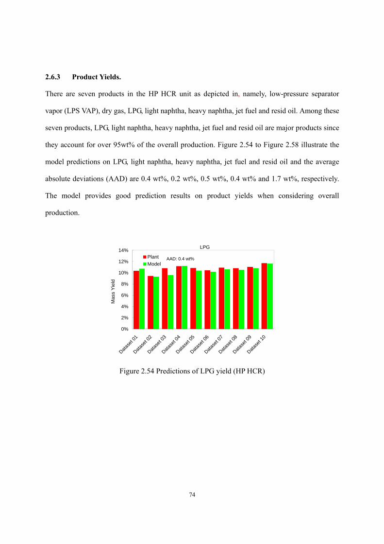
74
2.6.3 Product Yields.
There are seven products in the HP HCR unit as depicted in, namely, low-pressure separator
vapor (LPS VAP), dry gas, LPG, light naphtha, heavy naphtha, jet fuel and resid oil. Among these
seven products, LPG, light naphtha, heavy naphtha, jet fuel and resid oil are major products since
they account for over 95wt% of the overall production. Figure 2.54 to Figure 2.58 illustrate the
model predictions on LPG, light naphtha, heavy naphtha, jet fuel and resid oil and the average
absolute deviations (AAD) are 0.4 wt%, 0.2 wt%, 0.5 wt%, 0.4 wt% and 1.7 wt%, respectively.
The model provides good prediction results on product yields when considering overall
production.
LPG
0%
2%
4%
6%
8%
10%
12%
14%
Datase
t 01
Datase
t 02
Datase
t 03
Datase
t 04
Datase
t 05
Datase
t 06
Datase
t 07
Datase
t 08
Datase
t 09
Datase
t 10
Mas
s Yi
eld
PlantModel
AAD: 0.4 wt%
Figure 2.54 Predictions of LPG yield (HP HCR)
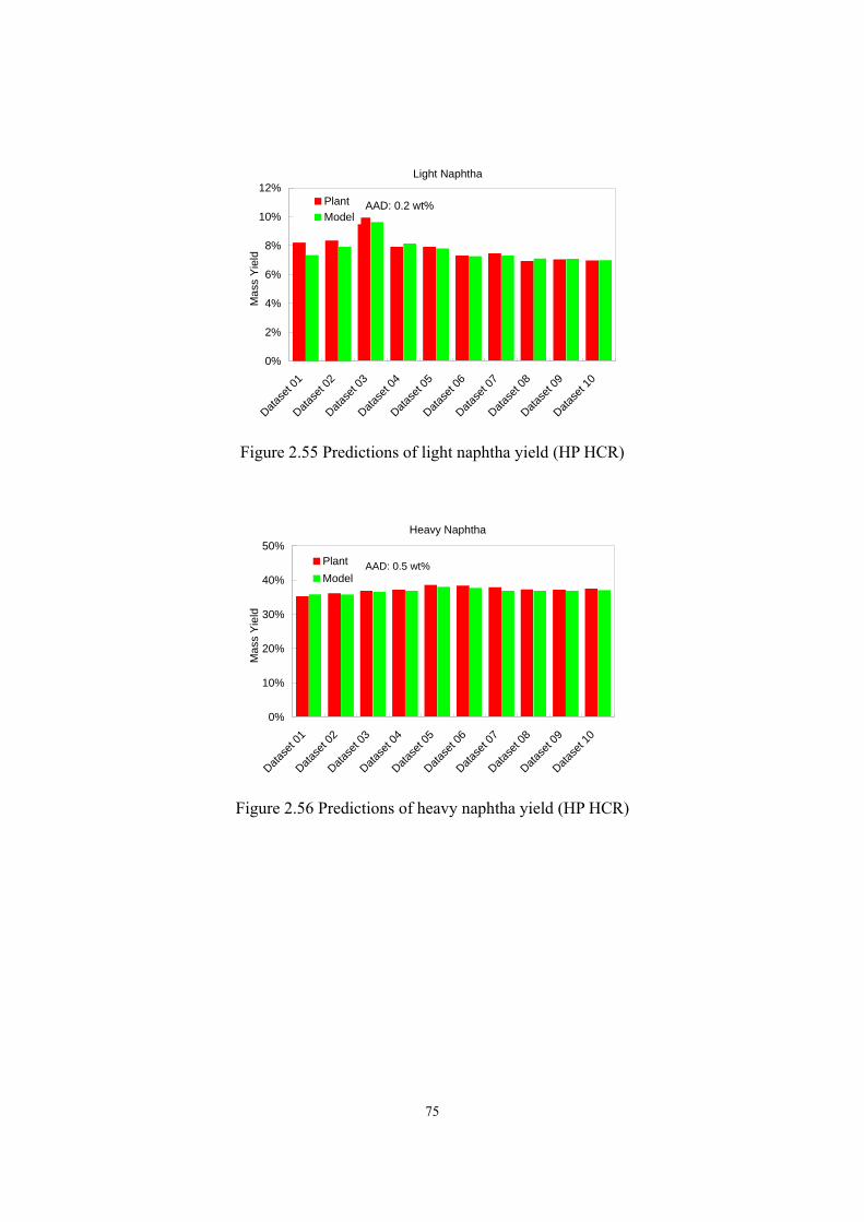
75
Light Naphtha
0%
2%
4%
6%
8%
10%
12%
Datase
t 01
Datase
t 02
Datase
t 03
Datase
t 04
Datase
t 05
Datase
t 06
Datase
t 07
Datase
t 08
Datase
t 09
Datase
t 10
Mas
s Yi
eld
PlantModel
AAD: 0.2 wt%
Figure 2.55 Predictions of light naphtha yield (HP HCR)
Heavy Naphtha
0%
10%
20%
30%
40%
50%
Datase
t 01
Datase
t 02
Datase
t 03
Datase
t 04
Datase
t 05
Datase
t 06
Datase
t 07
Datase
t 08
Datase
t 09
Datase
t 10
Mas
s Y
ield
PlantModel
AAD: 0.5 wt%
Figure 2.56 Predictions of heavy naphtha yield (HP HCR)
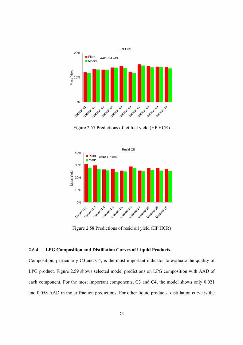
76
Jet Fuel
0%
10%
20%
Datase
t 01
Datase
t 02
Datase
t 03
Datase
t 04
Datase
t 05
Datase
t 06
Datase
t 07
Datase
t 08
Datase
t 09
Datase
t 10
Mas
s Y
ield
PlantModel
AAD: 0.4 wt%
Figure 2.57 Predictions of jet fuel yield (HP HCR)
Resid Oil
0%
10%
20%
30%
40%
Datase
t 01
Datase
t 02
Datase
t 03
Datase
t 04
Datase
t 05
Datase
t 06
Datase
t 07
Datase
t 08
Datase
t 09
Datase
t 10
Mas
s Yi
eld
PlantModel
AAD: 1.7 wt%
Figure 2.58 Predictions of resid oil yield (HP HCR)
2.6.4 LPG Composition and Distillation Curves of Liquid Products.
Composition, particularly C3 and C4, is the most important indicator to evaluate the quality of
LPG product. Figure 2.59 shows selected model predictions on LPG composition with AAD of
each component. For the most important components, C3 and C4, the model shows only 0.021
and 0.058 AAD in molar fraction predictions. For other liquid products, distillation curve is the
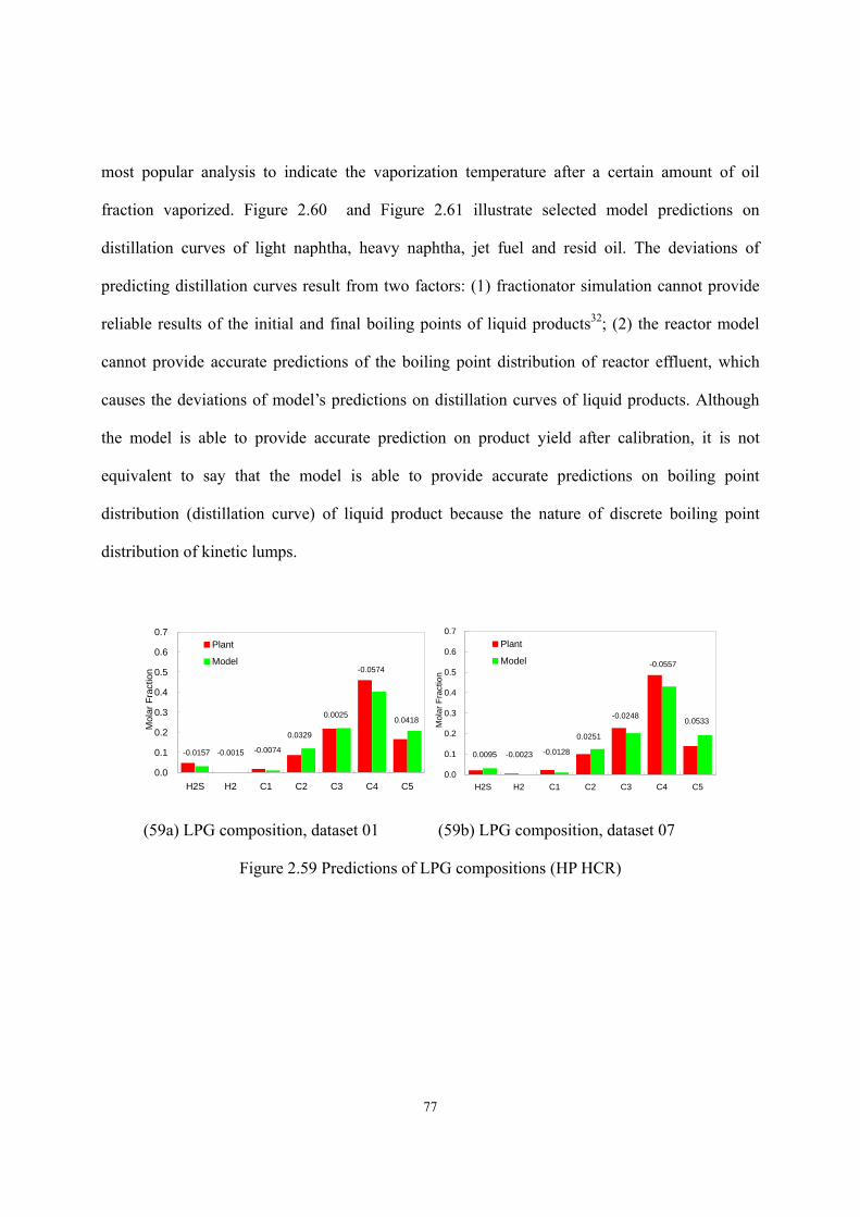
77
most popular analysis to indicate the vaporization temperature after a certain amount of oil
fraction vaporized. Figure 2.60 and Figure 2.61 illustrate selected model predictions on
distillation curves of light naphtha, heavy naphtha, jet fuel and resid oil. The deviations of
predicting distillation curves result from two factors: (1) fractionator simulation cannot provide
reliable results of the initial and final boiling points of liquid products32; (2) the reactor model
cannot provide accurate predictions of the boiling point distribution of reactor effluent, which
causes the deviations of model’s predictions on distillation curves of liquid products. Although
the model is able to provide accurate prediction on product yield after calibration, it is not
equivalent to say that the model is able to provide accurate predictions on boiling point
distribution (distillation curve) of liquid product because the nature of discrete boiling point
distribution of kinetic lumps.
0.0
0.1
0.2
0.3
0.4
0.5
0.6
0.7
H2S H2 C1 C2 C3 C4 C5
Mol
ar F
ract
ion
Plant
Model
-0.0157 -0.0015 -0.0074
0.0329
0.0025
-0.0574
0.0418
0.0
0.1
0.2
0.3
0.4
0.5
0.6
0.7
H2S H2 C1 C2 C3 C4 C5
Mol
ar F
ract
ion
Plant
Model
0.0095 -0.0023 -0.0128
0.0251
-0.0248
-0.0557
0.0533
(59a) LPG composition, dataset 01 (59b) LPG composition, dataset 07
Figure 2.59 Predictions of LPG compositions (HP HCR)
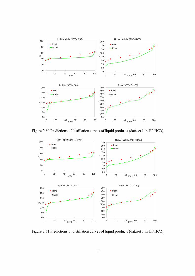
78
Light Naphtha (ASTM D86)
0
20
40
60
80
100
0 20 40 60 80 100LV %
PlantModel
Heavy Naphtha (ASTM D86)
30
50
70
90
110
130
150
170
190
0 20 40 60 80 100LV %
Plant
Model
Jet Fuel (ASTM D86)
50
90
130
170
210
250
290
0 20 40 60 80 100LV %
Plant
Model
Resid (ASTM D1160)
50100150200250300350400450500
0 20 40 60 80 100LV %
Plant
Model
Figure 2.60 Predictions of distillation curves of liquid products (dataset 1 in HP HCR)
Light Naphtha (ASTM D86)
0
20
40
60
80
100
0 20 40 60 80 100LV %
PlantModel
Heavy Naphtha (ASTM D86)
30507090
110130150170190210
0 20 40 60 80 100LV %
Plant
Model
Jet Fuel (ASTM D86)
50
90
130
170
210
250
290
0 20 40 60 80 100LV %
Plant
Model
Resid (ASTM D1160)
50100150200250300350400450500
0 20 40 60 80 100LV %
Plant
Model
Figure 2.61 Predictions of distillation curves of liquid products (dataset 7 in HP HCR)

79
2.6.5 Product Property.
We apply the updated correlations developed in Section 2.4.6 to estimate flash point and freezing
point of jet fuel. Figure 2.62 and Figure 2.63 illustrate model predictions on flash point and
freezing point of jet fuel. The average absolute deviations are 1.6 and 2.3, which are about
the same values as that obtained from correlating plant data. The integrated model collaborated
with updated correlations provides satisfactory predictions on flash point and freezing point of
jet fuel. Figure 2.64 to Figure 2.67 illustrate the specific gravity predictions of liquid products,
which are calculated by Aspen HYSYS. The AADs of the specific gravity predictions for light
naphtha, heavy naphtha, jet fuel, and resid oil are 0.0049, 0.0062, 0.0134, and 0.0045
respectively. The accurate predictions not only show model’s predictability on specific gravity of
liquid product, but also demonstrate that the delumping method we developed in Section 2.4.5 is
able to carry over density distribution to NBP-based pseudo-components.
Flash Point of Jet Fuel
0
10
20
30
40
50
60
Datase
t 01
Datase
t 02
Datase
t 03
Datase
t 04
Datase
t 05
Datase
t 06
Datase
t 07
Datase
t 08
Datase
t 09
Datase
t 10
PlantModel AAD = 1.6
Figure 2.62 Predictions of jet fuel’s flash point (HP HCR).
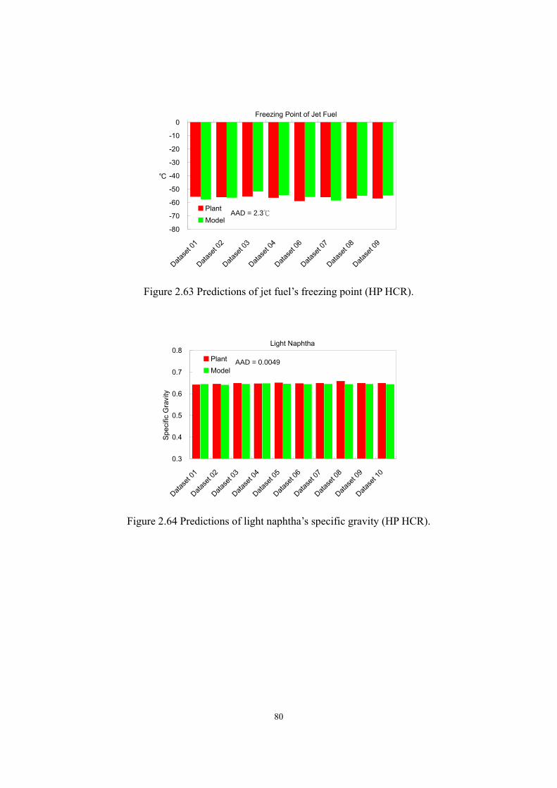
80
Freezing Point of Jet Fuel
-80
-70
-60
-50
-40
-30
-20
-10
0
Datase
t 01
Datase
t 02
Datase
t 03
Datase
t 04
Datase
t 06
Datase
t 07
Datase
t 08
Datase
t 09
PlantModel
AAD = 2.3
Figure 2.63 Predictions of jet fuel’s freezing point (HP HCR).
Light Naphtha
0.3
0.4
0.5
0.6
0.7
0.8
Datase
t 01
Datase
t 02
Datase
t 03
Datase
t 04
Datase
t 05
Datase
t 06
Datase
t 07
Datase
t 08
Datase
t 09
Datase
t 10
Spec
ific
Gra
vity
PlantModel
AAD = 0.0049
Figure 2.64 Predictions of light naphtha’s specific gravity (HP HCR).
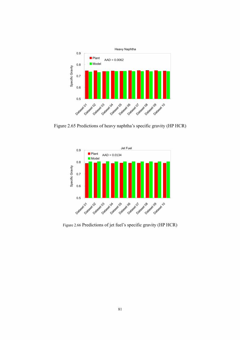
81
Heavy Naphtha
0.5
0.6
0.7
0.8
0.9
Datase
t 01
Datase
t 02
Datase
t 03
Datase
t 04
Datase
t 05
Datase
t 06
Datase
t 07
Datase
t 08
Datase
t 09
Datase
t 10
Spec
ific
Gra
vity
Plant
ModelAAD = 0.0062
Figure 2.65 Predictions of heavy naphtha’s specific gravity (HP HCR)
Jet Fuel
0.5
0.6
0.7
0.8
0.9
Datase
t 01
Datase
t 02
Datase
t 03
Datase
t 04
Datase
t 05
Datase
t 06
Datase
t 07
Datase
t 08
Datase
t 09
Datase
t 10
Spec
ific
Gra
vity
PlantModel
AAD = 0.0134
Figure 2.66 Predictions of jet fuel’s specific gravity (HP HCR)
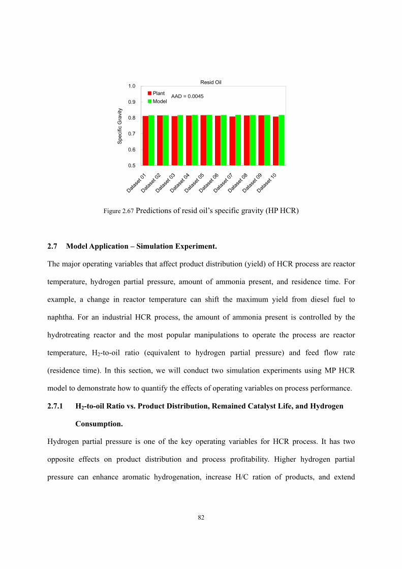
82
Resid Oil
0.5
0.6
0.7
0.8
0.9
1.0
Datase
t 01
Datase
t 02
Datase
t 03
Datase
t 04
Datase
t 05
Datase
t 06
Datase
t 07
Datase
t 08
Datase
t 09
Datase
t 10
Spec
ific
Gra
vity
PlantModel
AAD = 0.0045
Figure 2.67 Predictions of resid oil’s specific gravity (HP HCR)
2.7 Model Application – Simulation Experiment.
The major operating variables that affect product distribution (yield) of HCR process are reactor
temperature, hydrogen partial pressure, amount of ammonia present, and residence time. For
example, a change in reactor temperature can shift the maximum yield from diesel fuel to
naphtha. For an industrial HCR process, the amount of ammonia present is controlled by the
hydrotreating reactor and the most popular manipulations to operate the process are reactor
temperature, H2-to-oil ratio (equivalent to hydrogen partial pressure) and feed flow rate
(residence time). In this section, we will conduct two simulation experiments using MP HCR
model to demonstrate how to quantify the effects of operating variables on process performance.
2.7.1 H2-to-oil Ratio vs. Product Distribution, Remained Catalyst Life, and Hydrogen
Consumption.
Hydrogen partial pressure is one of the key operating variables for HCR process. It has two
opposite effects on product distribution and process profitability. Higher hydrogen partial
pressure can enhance aromatic hydrogenation, increase H/C ration of products, and extend
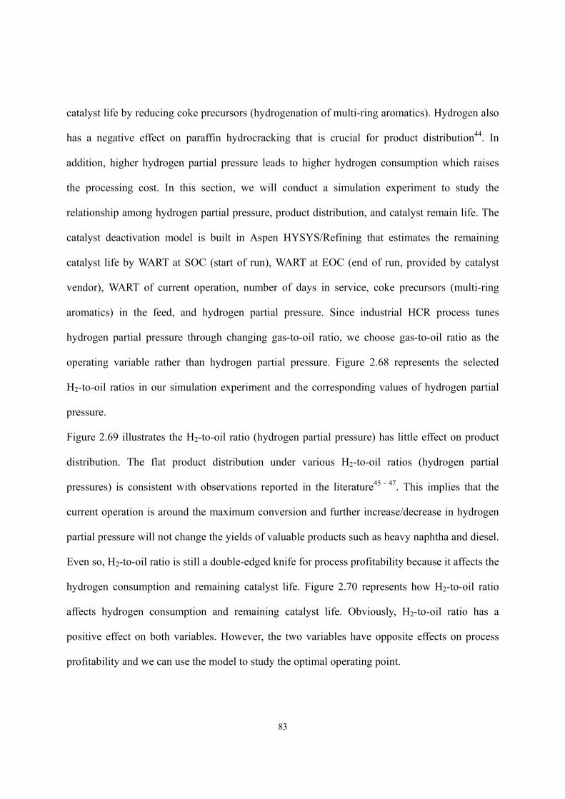
83
catalyst life by reducing coke precursors (hydrogenation of multi-ring aromatics). Hydrogen also
has a negative effect on paraffin hydrocracking that is crucial for product distribution44. In
addition, higher hydrogen partial pressure leads to higher hydrogen consumption which raises
the processing cost. In this section, we will conduct a simulation experiment to study the
relationship among hydrogen partial pressure, product distribution, and catalyst remain life. The
catalyst deactivation model is built in Aspen HYSYS/Refining that estimates the remaining
catalyst life by WART at SOC (start of run), WART at EOC (end of run, provided by catalyst
vendor), WART of current operation, number of days in service, coke precursors (multi-ring
aromatics) in the feed, and hydrogen partial pressure. Since industrial HCR process tunes
hydrogen partial pressure through changing gas-to-oil ratio, we choose gas-to-oil ratio as the
operating variable rather than hydrogen partial pressure. Figure 2.68 represents the selected
H2-to-oil ratios in our simulation experiment and the corresponding values of hydrogen partial
pressure.
Figure 2.69 illustrates the H2-to-oil ratio (hydrogen partial pressure) has little effect on product
distribution. The flat product distribution under various H2-to-oil ratios (hydrogen partial
pressures) is consistent with observations reported in the literature45 - 47. This implies that the
current operation is around the maximum conversion and further increase/decrease in hydrogen
partial pressure will not change the yields of valuable products such as heavy naphtha and diesel.
Even so, H2-to-oil ratio is still a double-edged knife for process profitability because it affects the
hydrogen consumption and remaining catalyst life. Figure 2.70 represents how H2-to-oil ratio
affects hydrogen consumption and remaining catalyst life. Obviously, H2-to-oil ratio has a
positive effect on both variables. However, the two variables have opposite effects on process
profitability and we can use the model to study the optimal operating point.
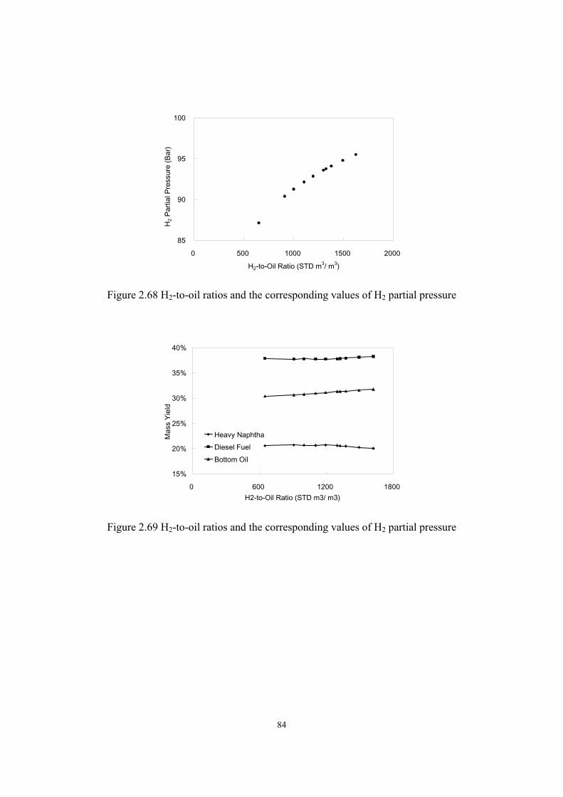
84
85
90
95
100
0 500 1000 1500 2000
H2-to-Oil Ratio (STD m3/ m3)
H2 P
artia
l Pre
ssur
e (B
ar)
Figure 2.68 H2-to-oil ratios and the corresponding values of H2 partial pressure
15%
20%
25%
30%
35%
40%
0 600 1200 1800H2-to-Oil Ratio (STD m3/ m3)
Mas
s Yi
eld
Heavy NaphthaDiesel FuelBottom Oil
Figure 2.69 H2-to-oil ratios and the corresponding values of H2 partial pressure
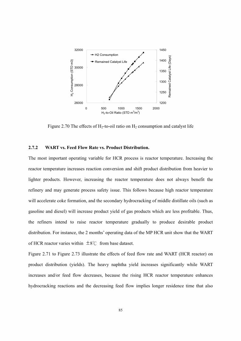
85
26000
28000
30000
32000
0 500 1000 1500 2000H2-to-Oil Ratio (STD m3/m3)
H2 C
onsu
mpt
ion
(STD
m3)
1200
1250
1300
1350
1400
1450
Rem
aine
d C
atal
yst L
ife (D
ays)H2 Consumption
Remained Catalyst Life
Figure 2.70 The effects of H2-to-oil ratio on H2 consumption and catalyst life
2.7.2 WART vs. Feed Flow Rate vs. Product Distribution.
The most important operating variable for HCR process is reactor temperature. Increasing the
reactor temperature increases reaction conversion and shift product distribution from heavier to
lighter products. However, increasing the reactor temperature does not always benefit the
refinery and may generate process safety issue. This follows because high reactor temperature
will accelerate coke formation, and the secondary hydrocracking of middle distillate oils (such as
gasoline and diesel) will increase product yield of gas products which are less profitable. Thus,
the refiners intend to raise reactor temperature gradually to produce desirable product
distribution. For instance, the 2 months’ operating data of the MP HCR unit show that the WART
of HCR reactor varies within ±8 from base dataset.
Figure 2.71 to Figure 2.73 illustrate the effects of feed flow rate and WART (HCR reactor) on
product distribution (yields). The heavy naphtha yield increases significantly while WART
increases and/or feed flow decreases, because the rising HCR reactor temperature enhances
hydrocracking reactions and the decreasing feed flow implies longer residence time that also
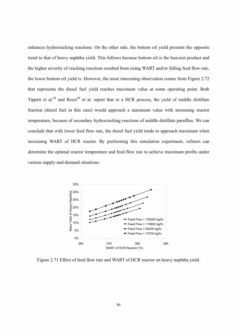
86
enhances hydrocracking reactions. On the other side, the bottom oil yield presents the opposite
trend to that of heavy naphtha yield. This follows because bottom oil is the heaviest product and
the higher severity of cracking reactions resulted from rising WART and/or falling feed flow rate,
the lower bottom oil yield is. However, the most interesting observation comes from Figure 2.72
that represents the diesel fuel yield reaches maximum value at some operating point. Both
Tippett et al.48 and Rossi49 et al. report that in a HCR process, the yield of middle distillate
fraction (diesel fuel in this case) would approach a maximum value with increasing reactor
temperature, because of secondary hydrocracking reactions of middle distillate paraffins. We can
conclude that with lower feed flow rate, the diesel fuel yield tends to approach maximum when
increasing WART of HCR reactor. By performing this simulation experiment, refiners can
determine the optimal reactor temperature and feed flow rate to achieve maximum profits under
various supply-and-demand situations.
0%
5%
10%
15%
20%
25%
30%
35%
360 370 380 390WART of HCR Reactor ()
Mas
s Yi
eld
of H
eavy
Nap
htha
Feed Flow = 129000 kg/hrFeed Flow = 110600 kg/hrFeed Flow = 92200 kg/hrFeed Flow = 73700 kg/hr
Figure 2.71 Effect of feed flow rate and WART of HCR reactor on heavy naphtha yield.
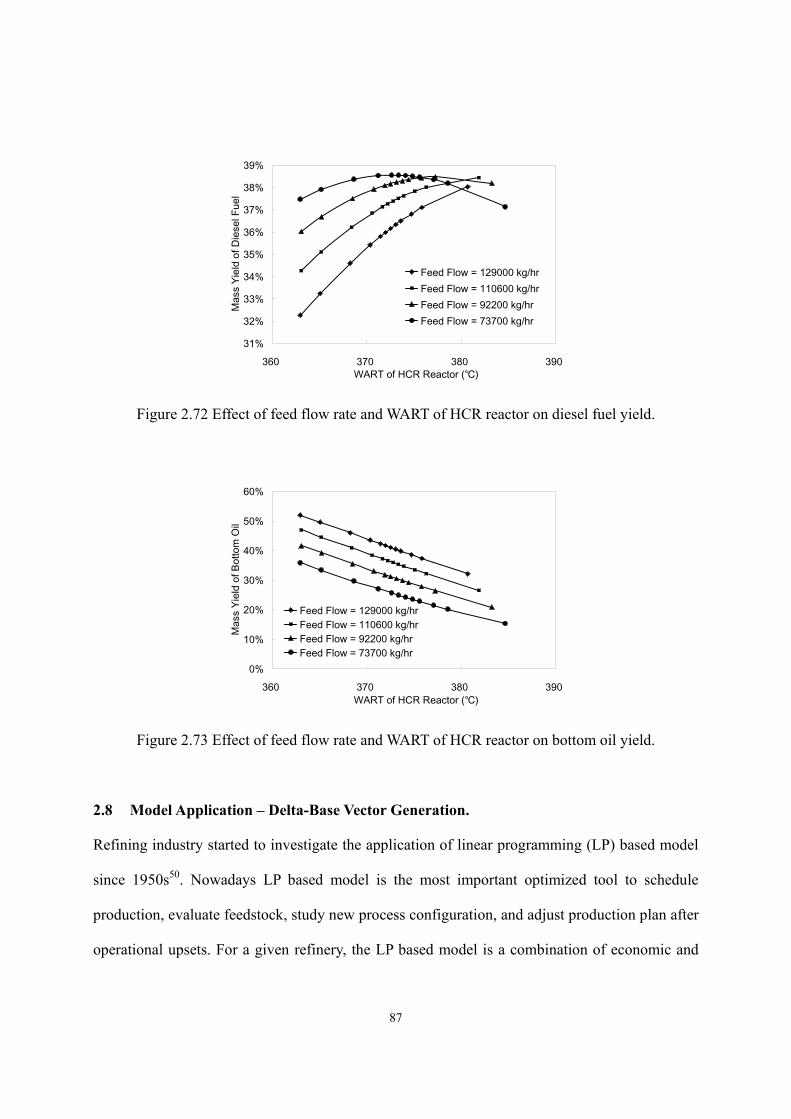
87
31%
32%
33%
34%
35%
36%
37%
38%
39%
360 370 380 390WART of HCR Reactor ()
Mas
s Yi
eld
of D
iese
l Fue
l
Feed Flow = 129000 kg/hrFeed Flow = 110600 kg/hrFeed Flow = 92200 kg/hrFeed Flow = 73700 kg/hr
Figure 2.72 Effect of feed flow rate and WART of HCR reactor on diesel fuel yield.
0%
10%
20%
30%
40%
50%
60%
360 370 380 390WART of HCR Reactor ()
Mas
s Yi
eld
of B
otto
m O
il
Feed Flow = 129000 kg/hrFeed Flow = 110600 kg/hrFeed Flow = 92200 kg/hrFeed Flow = 73700 kg/hr
Figure 2.73 Effect of feed flow rate and WART of HCR reactor on bottom oil yield.
2.8 Model Application – Delta-Base Vector Generation.
Refining industry started to investigate the application of linear programming (LP) based model
since 1950s50. Nowadays LP based model is the most important optimized tool to schedule
production, evaluate feedstock, study new process configuration, and adjust production plan after
operational upsets. For a given refinery, the LP based model is a combination of economic and
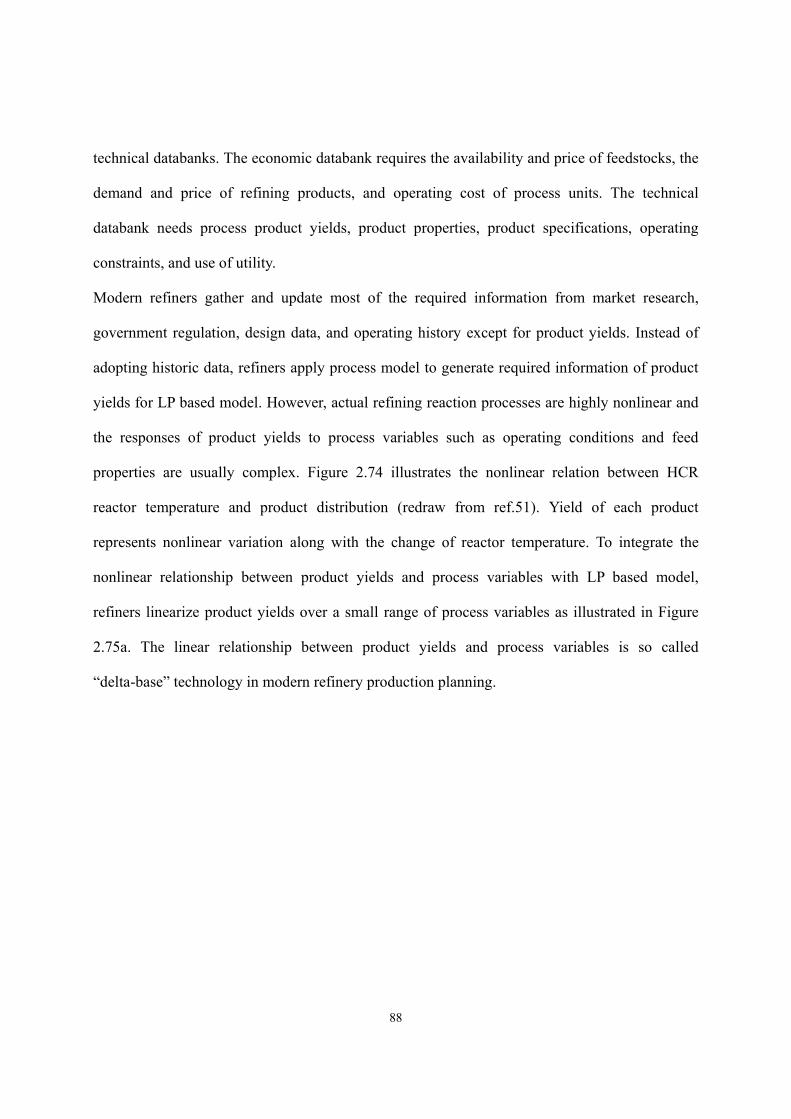
88
technical databanks. The economic databank requires the availability and price of feedstocks, the
demand and price of refining products, and operating cost of process units. The technical
databank needs process product yields, product properties, product specifications, operating
constraints, and use of utility.
Modern refiners gather and update most of the required information from market research,
government regulation, design data, and operating history except for product yields. Instead of
adopting historic data, refiners apply process model to generate required information of product
yields for LP based model. However, actual refining reaction processes are highly nonlinear and
the responses of product yields to process variables such as operating conditions and feed
properties are usually complex. Figure 2.74 illustrates the nonlinear relation between HCR
reactor temperature and product distribution (redraw from ref.51). Yield of each product
represents nonlinear variation along with the change of reactor temperature. To integrate the
nonlinear relationship between product yields and process variables with LP based model,
refiners linearize product yields over a small range of process variables as illustrated in Figure
2.75a. The linear relationship between product yields and process variables is so called
“delta-base” technology in modern refinery production planning.
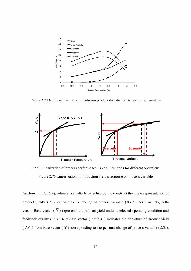
89
0
5
10
15
20
25
30
35
40
380 390 400 410 420 430 440 450 460
Reactor Temperature ()
Mas
s Yi
eld
(%)
Gas
Light Naphtha
Gasoline
Kerosene
Gas Oil
Figure 2.74 Nonlinear relationship between product distribution & reactor temperature
(75a) Linearization of process performance (75b) Scenarios for different operations
Figure 2.75 Linearization of production yield’s response on process variable
As shown in Eq. (29), refiners use delta-base technology to construct the linear representation of
product yield’s ( Y ) response to the change of process variable ( XX-X Δ= ), namely, delta
vector. Base vector ( Y ) represents the product yield under a selected operating condition and
feedstock quality ( X ). Delta-base vector ( XY/ ΔΔ ) indicates the departure of product yield
( Y Δ ) from base vector ( Y ) corresponding to the per unit change of process variable ( XΔ ).
Process Variable
Yiel
d
Scenario Scenario
Y1
Reactor Temperature
Yiel
d Slope = ΔY /ΔT
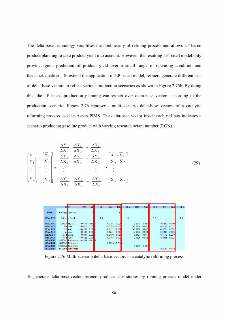
90
The delta-base technology simplifies the nonlinearity of refining process and allows LP based
product planning to take product yield into account. However, the resulting LP based model only
provides good prediction of product yield over a small range of operating condition and
feedstock qualities. To extend the application of LP based model, refiners generate different sets
of delta-base vectors to reflect various production scenarios as shown in Figure 2.75b. By doing
this, the LP based production planning can switch over delta-base vectors according to the
production scenario. Figure 2.76 represents multi-scenario delta-base vectors of a catalytic
reforming process used in Aspen PIMS. The delta-base vector inside each red box indicates a
scenario producing gasoline product with varying research octant number (RON).
⎥⎥⎥⎥⎥⎥⎥
⎦
⎤
⎢⎢⎢⎢⎢⎢⎢
⎣
⎡
•
⎥⎥⎥⎥⎥⎥⎥⎥⎥⎥⎥⎥
⎦
⎤
⎢⎢⎢⎢⎢⎢⎢⎢⎢⎢⎢⎢
⎣
⎡
ΔΔ
ΔΔ
ΔΔ
ΔΔ
ΔΔ
ΔΔ
ΔΔ
ΔΔ
ΔΔ
+
⎥⎥⎥⎥⎥⎥⎥
⎦
⎤
⎢⎢⎢⎢⎢⎢⎢
⎣
⎡
=
⎥⎥⎥⎥⎥⎥
⎦
⎤
⎢⎢⎢⎢⎢⎢
⎣
⎡
nn
22
11
n
m
2
m
1
m
n
2
2
2
1
2
n
1
2
1
1
1
m
2
1
m
2
1
X - X
X - X
X - X
XY
XY
XY
XY
XY
XY
XY
XY
XY
Y
Y
Y
Y YY
M
M
L
MM
MM
L
L
M
M
M
M (29)
Figure 2.76 Multi-scenario delta-base vectors in a catalytic reforming process
To generate delta-base vector, refiners produce case studies by running process model under
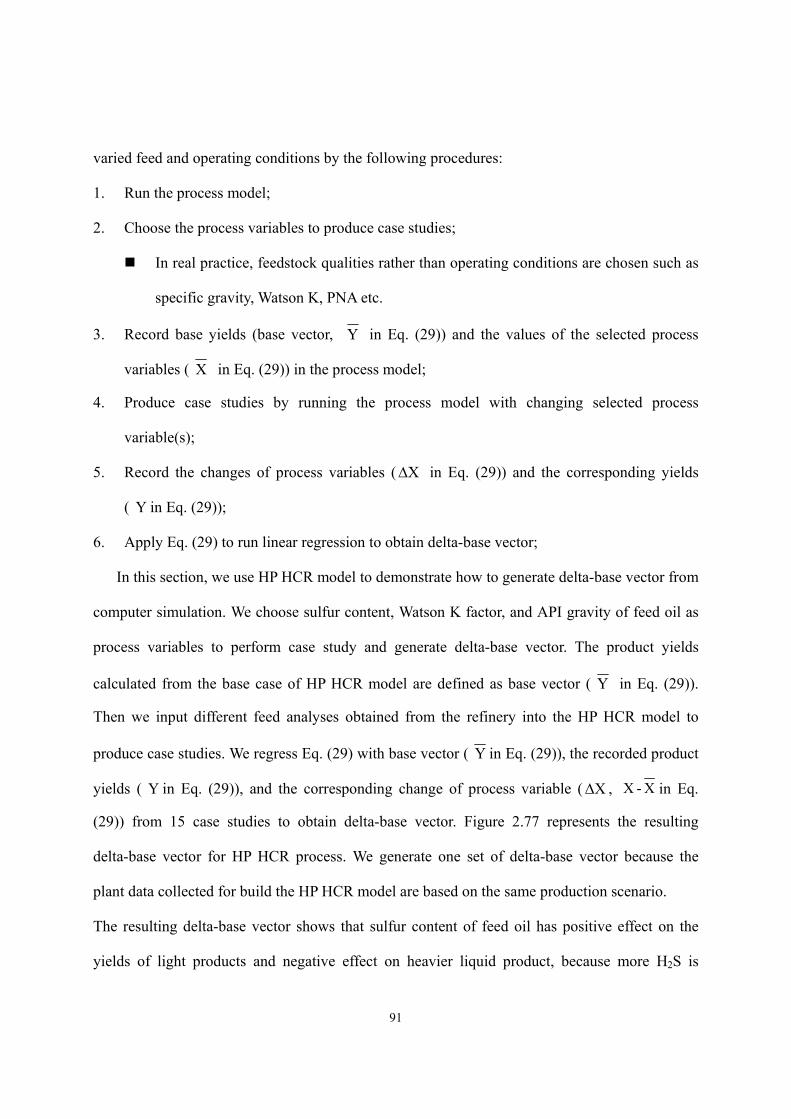
91
varied feed and operating conditions by the following procedures:
1. Run the process model;
2. Choose the process variables to produce case studies;
In real practice, feedstock qualities rather than operating conditions are chosen such as
specific gravity, Watson K, PNA etc.
3. Record base yields (base vector, Y in Eq. (29)) and the values of the selected process
variables ( X in Eq. (29)) in the process model;
4. Produce case studies by running the process model with changing selected process
variable(s);
5. Record the changes of process variables ( XΔ in Eq. (29)) and the corresponding yields
( Y in Eq. (29));
6. Apply Eq. (29) to run linear regression to obtain delta-base vector;
In this section, we use HP HCR model to demonstrate how to generate delta-base vector from
computer simulation. We choose sulfur content, Watson K factor, and API gravity of feed oil as
process variables to perform case study and generate delta-base vector. The product yields
calculated from the base case of HP HCR model are defined as base vector ( Y in Eq. (29)).
Then we input different feed analyses obtained from the refinery into the HP HCR model to
produce case studies. We regress Eq. (29) with base vector ( Y in Eq. (29)), the recorded product
yields ( Y in Eq. (29)), and the corresponding change of process variable ( XΔ , X - X in Eq.
(29)) from 15 case studies to obtain delta-base vector. Figure 2.77 represents the resulting
delta-base vector for HP HCR process. We generate one set of delta-base vector because the
plant data collected for build the HP HCR model are based on the same production scenario.
The resulting delta-base vector shows that sulfur content of feed oil has positive effect on the
yields of light products and negative effect on heavier liquid product, because more H2S is
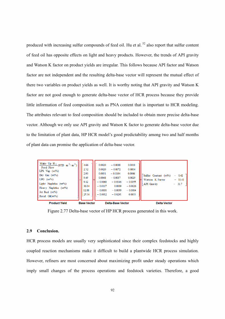
92
produced with increasing sulfur compounds of feed oil. Hu et al. 52 also report that sulfur content
of feed oil has opposite effects on light and heavy products. However, the trends of API gravity
and Watson K factor on product yields are irregular. This follows because API factor and Watson
factor are not independent and the resulting delta-base vector will represent the mutual effect of
there two variables on product yields as well. It is worthy noting that API gravity and Watson K
factor are not good enough to generate delta-base vector of HCR process because they provide
little information of feed composition such as PNA content that is important to HCR modeling.
The attributes relevant to feed composition should be included to obtain more precise delta-base
vector. Although we only use API gravity and Watson K factor to generate delta-base vector due
to the limitation of plant data, HP HCR model’s good predictability among two and half months
of plant data can promise the application of delta-base vector.
Figure 2.77 Delta-base vector of HP HCR process generated in this work.
2.9 Conclusion.
HCR process models are usually very sophisticated since their complex feedstocks and highly
coupled reaction mechanisms make it difficult to build a plantwide HCR process simulation.
However, refiners are most concerned about maximizing profit under steady operations which
imply small changes of the process operations and feedstock varieties. Therefore, a good
93
operating model of refining process only needs to match key product yields, qualities and
process operations under small process changes.
In this work, we develop two operating models of large-scale HCR processes to satisfy the key
considerations of the refiners. The two models only require typical operating conditions, and
routine analysis of feedstock and products. We validate the models’ capabilities of predicting
product yields, product qualities and unit operations with two months of plant data. We also
show key applications of HCR models, namely simulation experiment and delta-base vector
generation. We summarize the key achievements of this work as follows:
(1) We develop two integrated HCR process models which include reactors, fractionators and
hydrogen recycle systems.
(2) We provide the step-by-step guideline of model development that has not been reported in
the literature.
(3) We apply the Gauss-Legendre Quadrature to convert kinetic lumps into pseudo-components
based on boiling point ranges (delumping) for rigorous fractionator simulation.
(4) Our delumping method gives a continuous response to changes in fractionator specification
such as distillate rate.
(5) We update API correlations of flash point and freezing point to plant operation and
production.
(6) The integrated HCR process models are able to predict accurately the product yields,
distillation curves of liquid products, and temperature profiles of reactors and fractionators.
(7) The integrated HCR process models also gives good estimations on liquid product
qualities – density, flash point and freezing point of diesel fuel (MP HCR) and jet fuel (HP
HCR) – by using updated API correlations.
(8) We apply the integrated MP HCR process model to conduct simulation experiment to
94
quantify the effects of operating variables on product yields.
(9) We apply the integrated HP HCR process model to generate delta-base vector for LP based
production planning.
This work represents the workflow to build integrated HCR process model by using Aspen
HYSYS/Refining and only routine measurements for feed characterization in the refinery. We
also use routine measurements of products to calibrate the model. To further improve our models,
we may include Apply SimDist analysis for feed characterization, and to incorporate detailed
molecular information for feed characterization and customize our feed lump distribution if these
measurements are available regularly. We can also to customize the calibration environment to
include product property and product composition as objective functions if detailed molecular
information of product is available.
2.10 Workshop 1 – Build Preliminary Reactor Model of HCR Process.
This workshop provides step-by-step guidelines to demonstrate how to build a preliminary
reactor model of HCR process.
Step 1: Define the process type (single-stage or two-tage), the number of reactors of each stage
and the corresponding reaction beds and the number of high-pressure separators and if amine
treatment is included in the model.
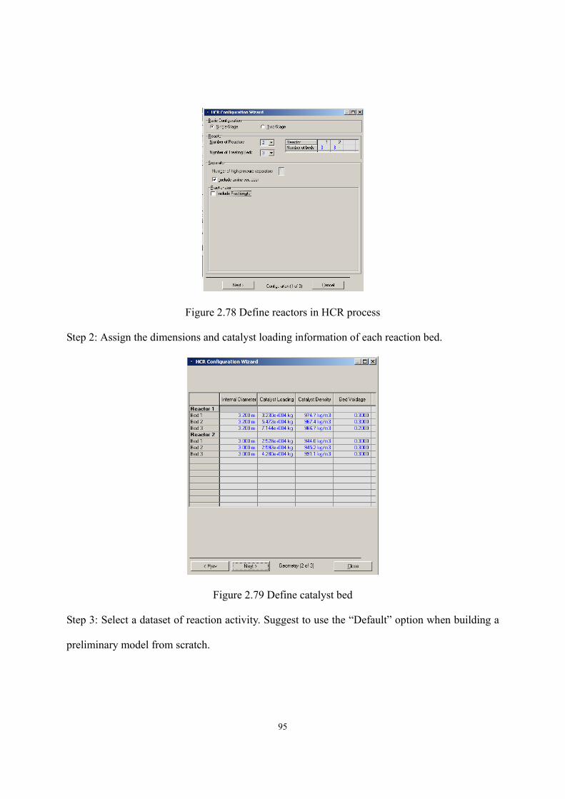
95
Figure 2.78 Define reactors in HCR process
Step 2: Assign the dimensions and catalyst loading information of each reaction bed.
Figure 2.79 Define catalyst bed
Step 3: Select a dataset of reaction activity. Suggest to use the “Default” option when building a
preliminary model from scratch.
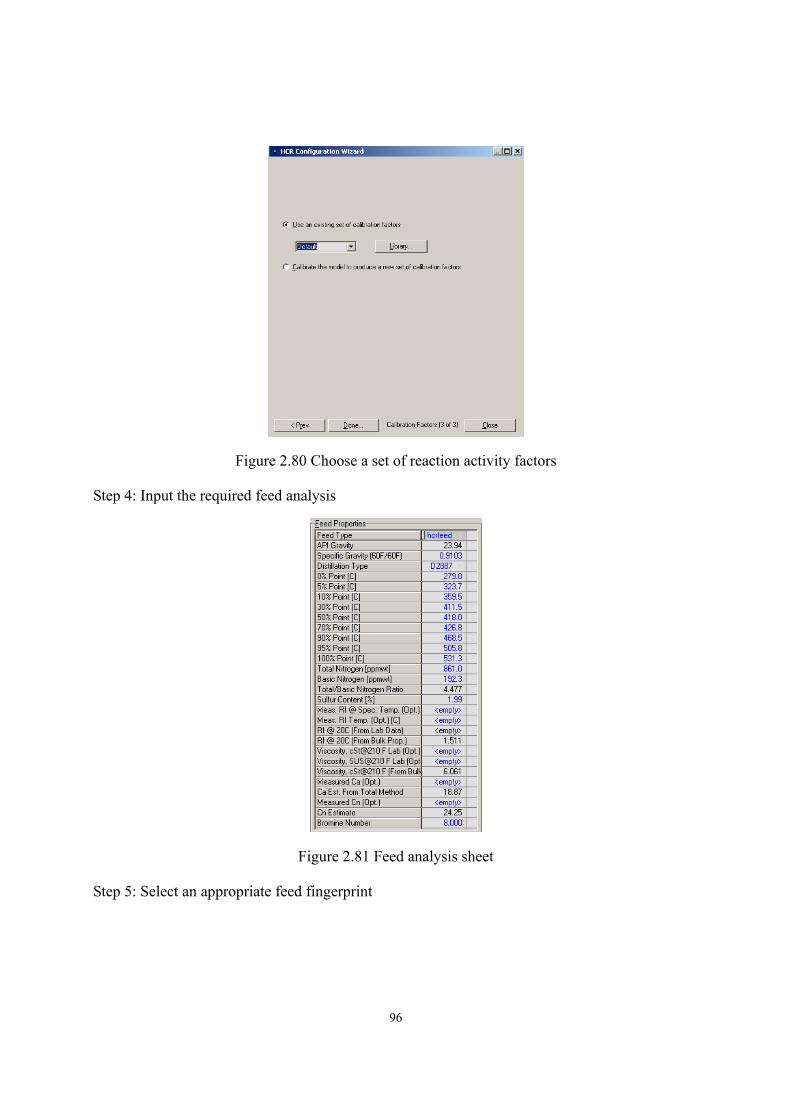
96
Figure 2.80 Choose a set of reaction activity factors
Step 4: Input the required feed analysis
Figure 2.81 Feed analysis sheet
Step 5: Select an appropriate feed fingerprint
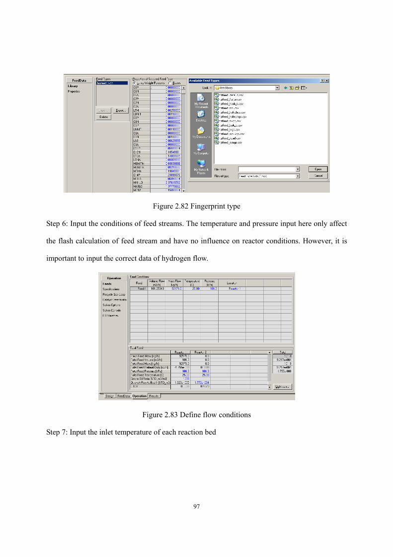
97
Figure 2.82 Fingerprint type
Step 6: Input the conditions of feed streams. The temperature and pressure input here only affect
the flash calculation of feed stream and have no influence on reactor conditions. However, it is
important to input the correct data of hydrogen flow.
Figure 2.83 Define flow conditions
Step 7: Input the inlet temperature of each reaction bed
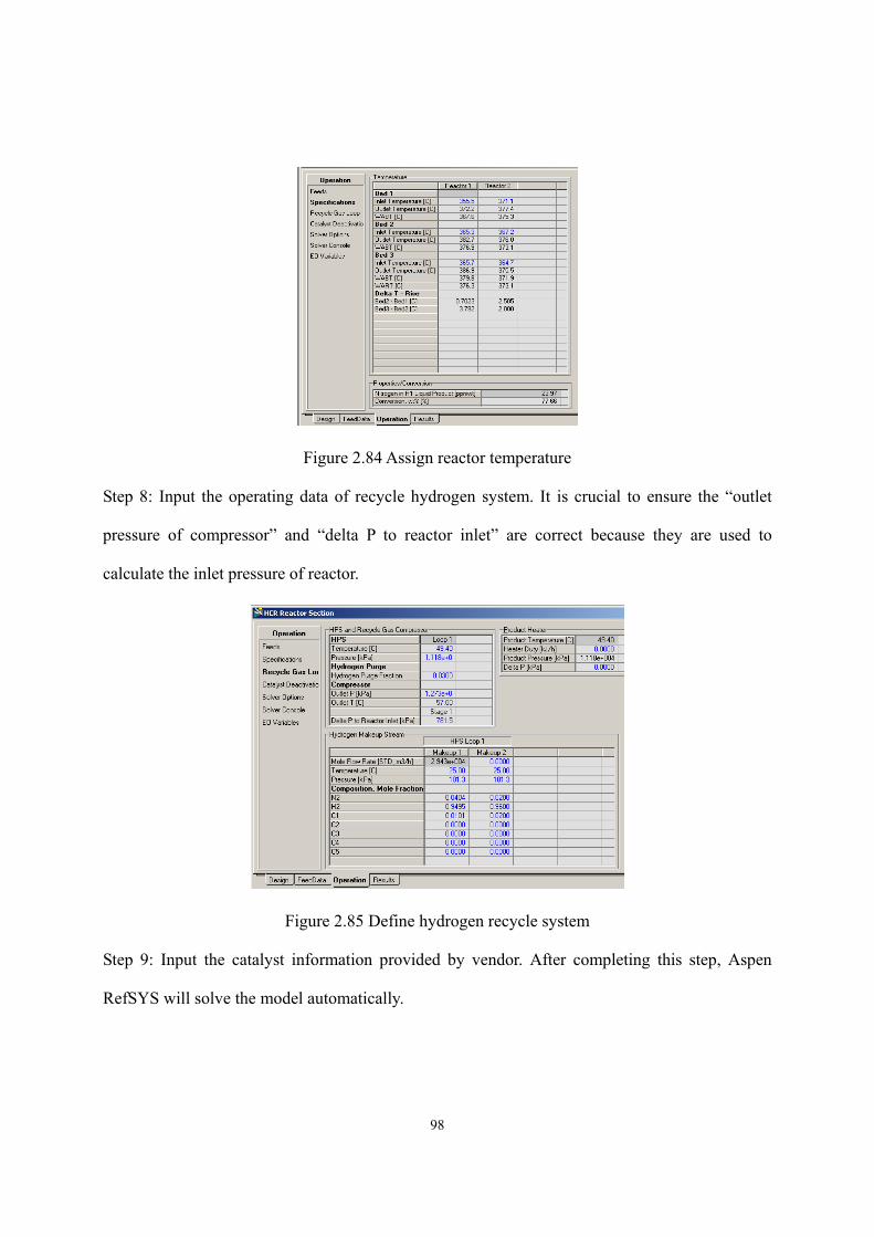
98
Figure 2.84 Assign reactor temperature
Step 8: Input the operating data of recycle hydrogen system. It is crucial to ensure the “outlet
pressure of compressor” and “delta P to reactor inlet” are correct because they are used to
calculate the inlet pressure of reactor.
Figure 2.85 Define hydrogen recycle system
Step 9: Input the catalyst information provided by vendor. After completing this step, Aspen
RefSYS will solve the model automatically.
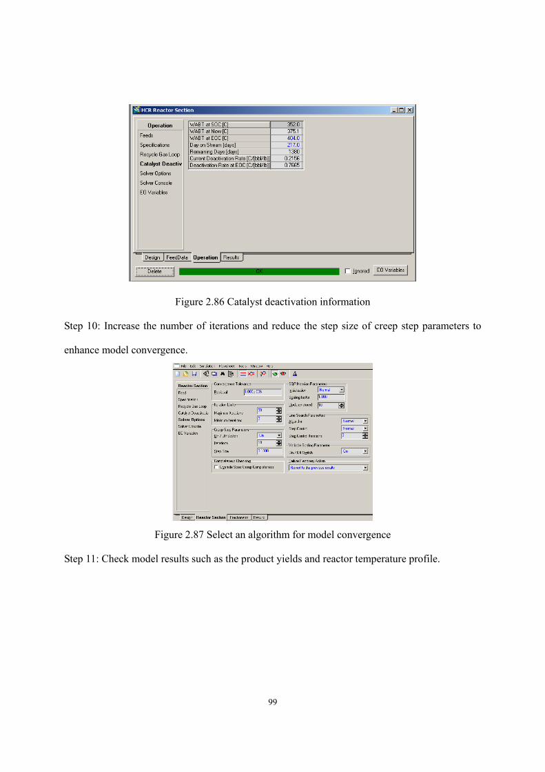
99
Figure 2.86 Catalyst deactivation information
Step 10: Increase the number of iterations and reduce the step size of creep step parameters to
enhance model convergence.
Figure 2.87 Select an algorithm for model convergence
Step 11: Check model results such as the product yields and reactor temperature profile.
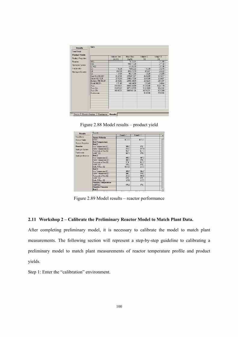
100
Figure 2.88 Model results – product yield
Figure 2.89 Model results – reactor performance
2.11 Workshop 2 – Calibrate the Preliminary Reactor Model to Match Plant Data.
After completing preliminary model, it is necessary to calibrate the model to match plant
measurements. The following section will represent a step-by-step guideline to calibrating a
preliminary model to match plant measurements of reactor temperature profile and product
yields.
Step 1: Enter the “calibration” environment.
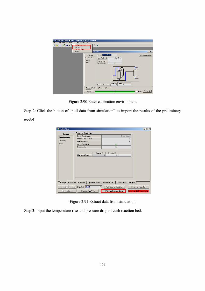
101
Figure 2.90 Enter calibration environment
Step 2: Click the button of “pull data from simulation” to import the results of the preliminary
model.
Figure 2.91 Extract data from simulation
Step 3: Input the temperature rise and pressure drop of each reaction bed.
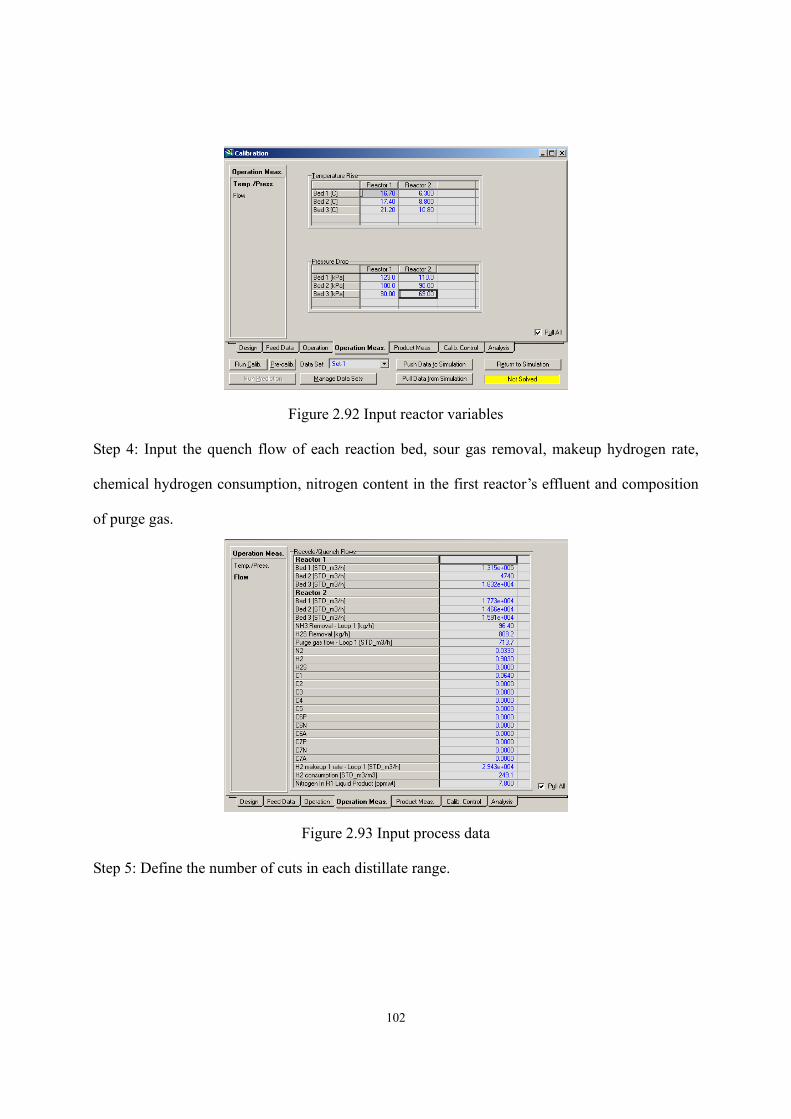
102
Figure 2.92 Input reactor variables
Step 4: Input the quench flow of each reaction bed, sour gas removal, makeup hydrogen rate,
chemical hydrogen consumption, nitrogen content in the first reactor’s effluent and composition
of purge gas.
Figure 2.93 Input process data
Step 5: Define the number of cuts in each distillate range.
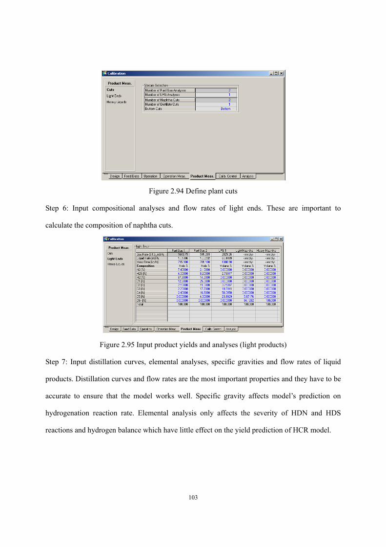
103
Figure 2.94 Define plant cuts
Step 6: Input compositional analyses and flow rates of light ends. These are important to
calculate the composition of naphtha cuts.
Figure 2.95 Input product yields and analyses (light products)
Step 7: Input distillation curves, elemental analyses, specific gravities and flow rates of liquid
products. Distillation curves and flow rates are the most important properties and they have to be
accurate to ensure that the model works well. Specific gravity affects model’s prediction on
hydrogenation reaction rate. Elemental analysis only affects the severity of HDN and HDS
reactions and hydrogen balance which have little effect on the yield prediction of HCR model.
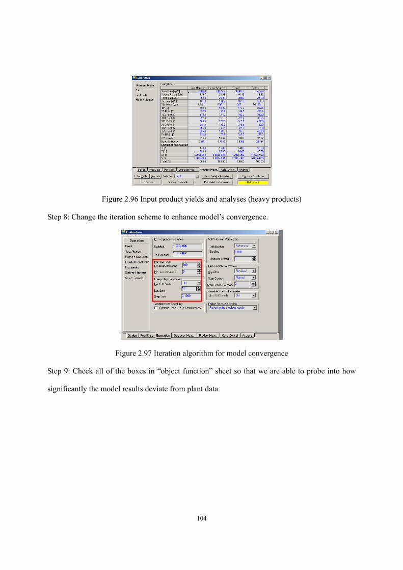
104
Figure 2.96 Input product yields and analyses (heavy products)
Step 8: Change the iteration scheme to enhance model’s convergence.
Figure 2.97 Iteration algorithm for model convergence
Step 9: Check all of the boxes in “object function” sheet so that we are able to probe into how
significantly the model results deviate from plant data.
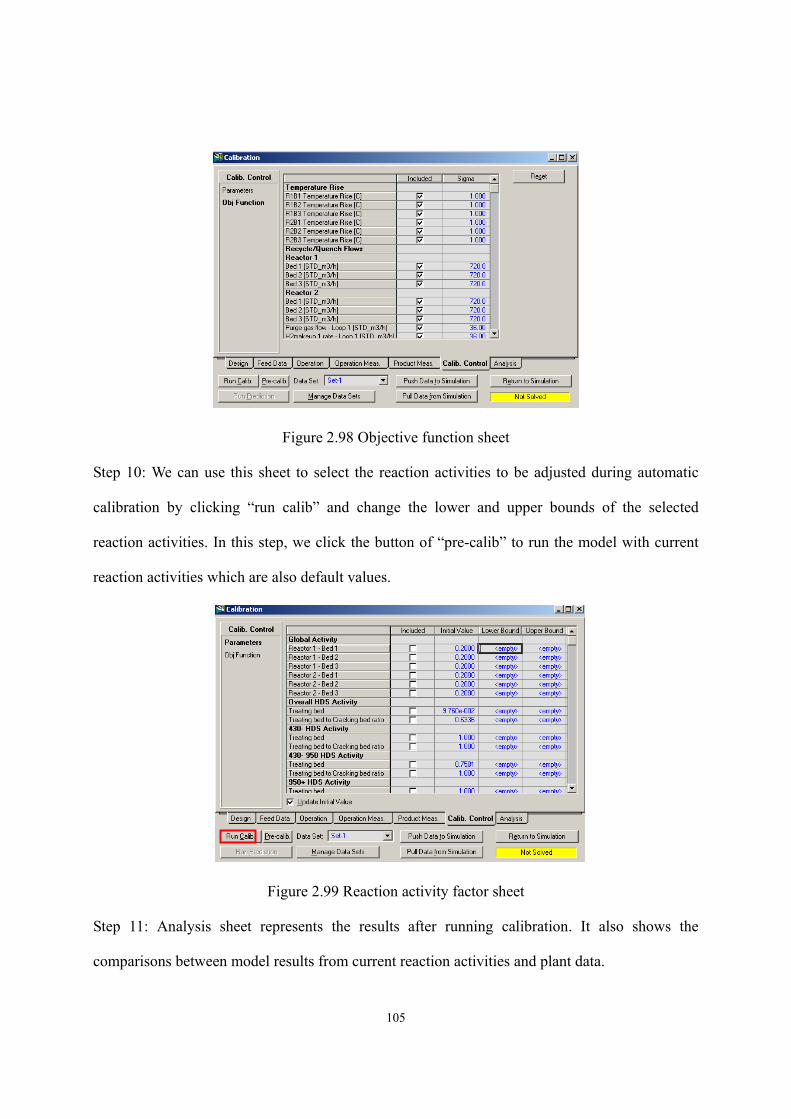
105
Figure 2.98 Objective function sheet
Step 10: We can use this sheet to select the reaction activities to be adjusted during automatic
calibration by clicking “run calib” and change the lower and upper bounds of the selected
reaction activities. In this step, we click the button of “pre-calib” to run the model with current
reaction activities which are also default values.
Figure 2.99 Reaction activity factor sheet
Step 11: Analysis sheet represents the results after running calibration. It also shows the
comparisons between model results from current reaction activities and plant data.
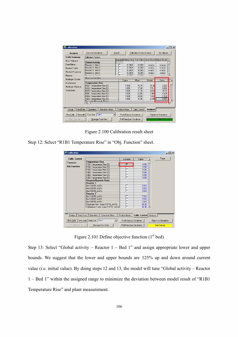
106
Figure 2.100 Calibration result sheet
Step 12: Select “R1B1 Temperature Rise” in “Obj. Function” sheet.
Figure 2.101 Define objective function (1st bed)
Step 13: Select “Global activity – Reactor 1 – Bed 1” and assign appropriate lower and upper
bounds. We suggest that the lower and upper bounds are ±25% up and down around current
value (i.e. initial value). By doing steps 12 and 13, the model will tune “Global activity – Reactor
1 – Bed 1” within the assigned range to minimize the deviation between model result of “R1B1
Temperature Rise” and plant measurement.
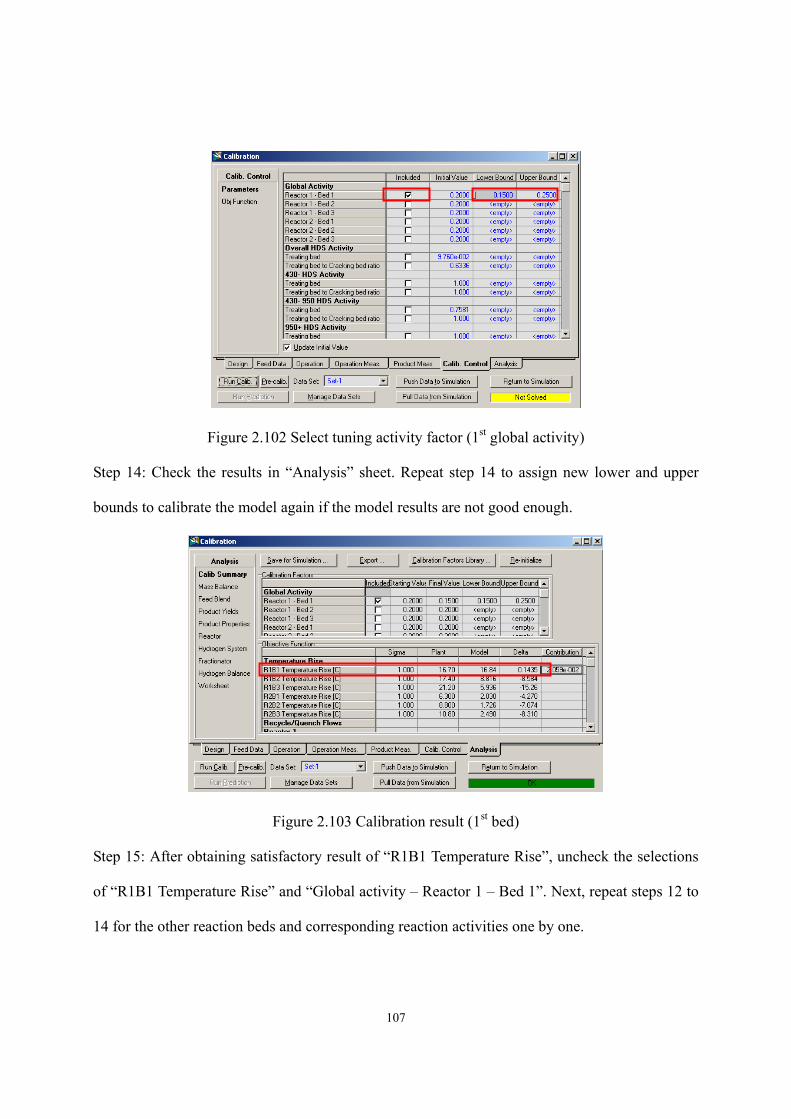
107
Figure 2.102 Select tuning activity factor (1st global activity)
Step 14: Check the results in “Analysis” sheet. Repeat step 14 to assign new lower and upper
bounds to calibrate the model again if the model results are not good enough.
Figure 2.103 Calibration result (1st bed)
Step 15: After obtaining satisfactory result of “R1B1 Temperature Rise”, uncheck the selections
of “R1B1 Temperature Rise” and “Global activity – Reactor 1 – Bed 1”. Next, repeat steps 12 to
14 for the other reaction beds and corresponding reaction activities one by one.
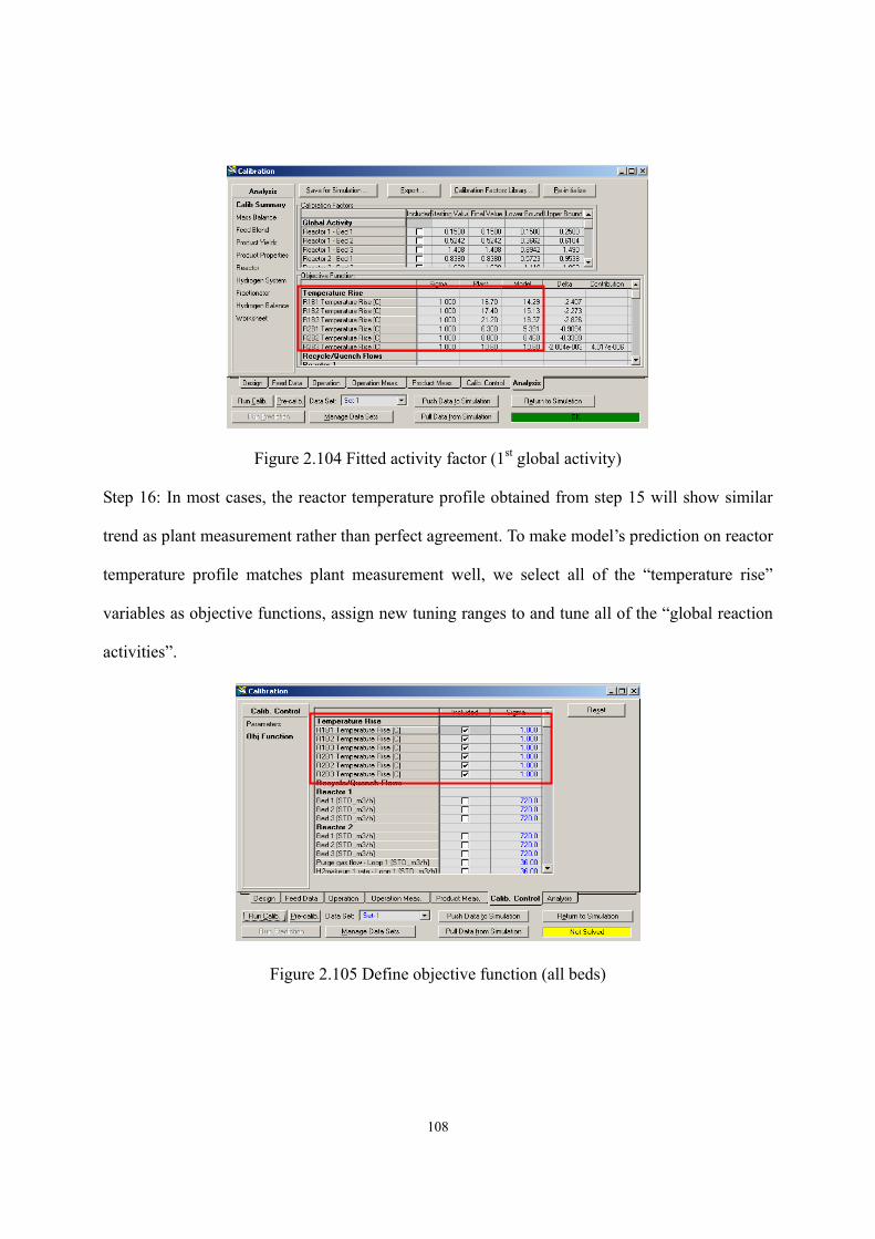
108
Figure 2.104 Fitted activity factor (1st global activity)
Step 16: In most cases, the reactor temperature profile obtained from step 15 will show similar
trend as plant measurement rather than perfect agreement. To make model’s prediction on reactor
temperature profile matches plant measurement well, we select all of the “temperature rise”
variables as objective functions, assign new tuning ranges to and tune all of the “global reaction
activities”.
Figure 2.105 Define objective function (all beds)
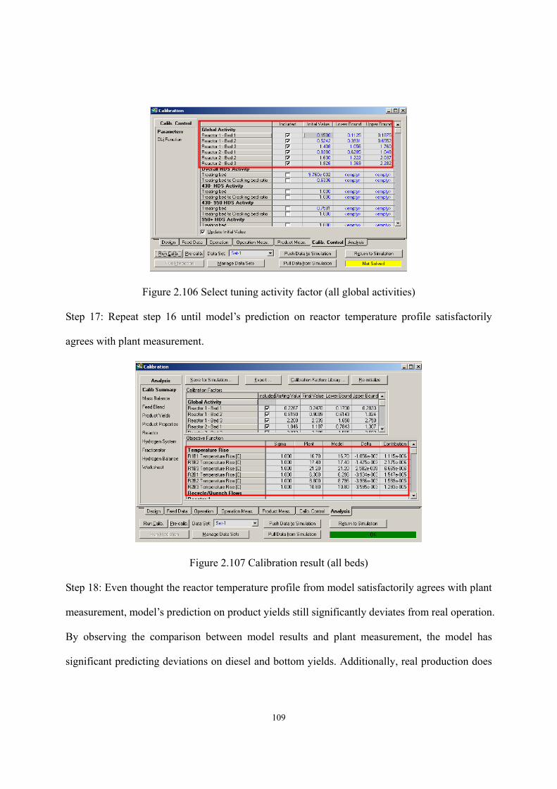
109
Figure 2.106 Select tuning activity factor (all global activities)
Step 17: Repeat step 16 until model’s prediction on reactor temperature profile satisfactorily
agrees with plant measurement.
Figure 2.107 Calibration result (all beds)
Step 18: Even thought the reactor temperature profile from model satisfactorily agrees with plant
measurement, model’s prediction on product yields still significantly deviates from real operation.
By observing the comparison between model results and plant measurement, the model has
significant predicting deviations on diesel and bottom yields. Additionally, real production does
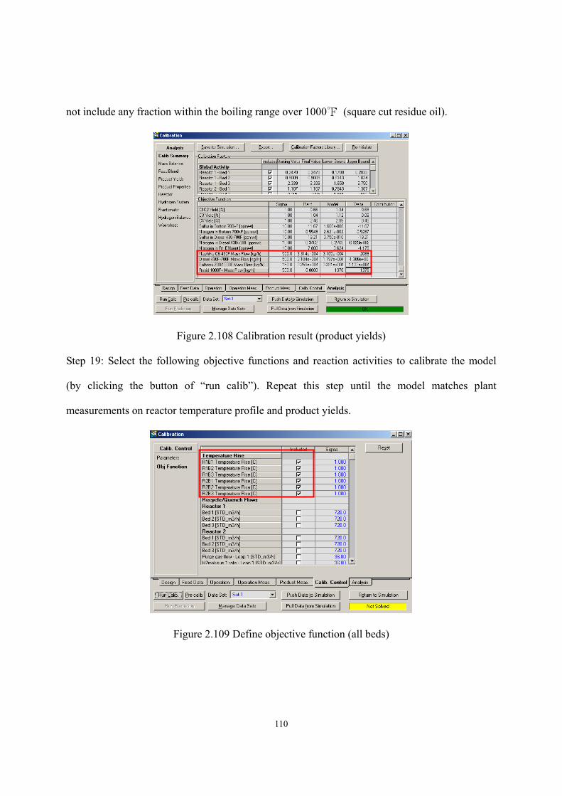
110
not include any fraction within the boiling range over 1000 (square cut residue oil).
Figure 2.108 Calibration result (product yields)
Step 19: Select the following objective functions and reaction activities to calibrate the model
(by clicking the button of “run calib”). Repeat this step until the model matches plant
measurements on reactor temperature profile and product yields.
Figure 2.109 Define objective function (all beds)
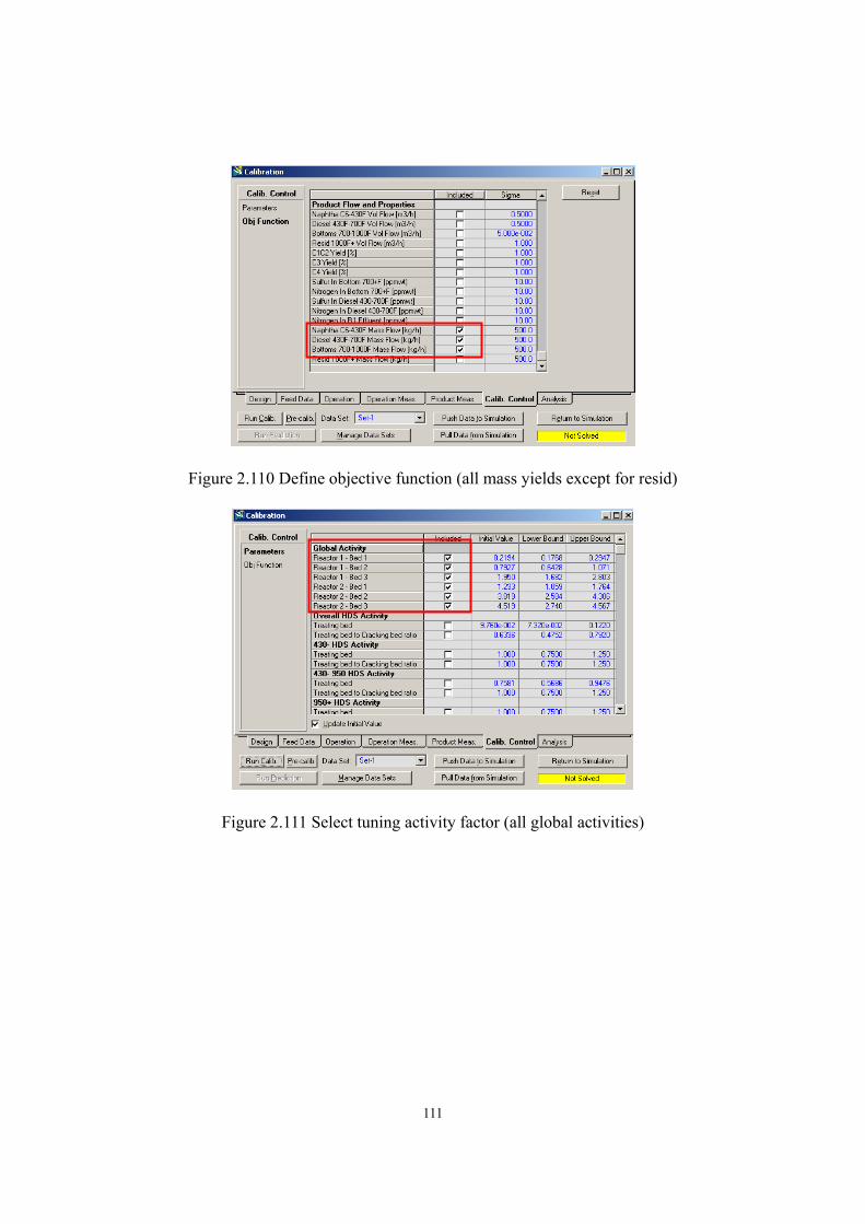
111
Figure 2.110 Define objective function (all mass yields except for resid)
Figure 2.111 Select tuning activity factor (all global activities)
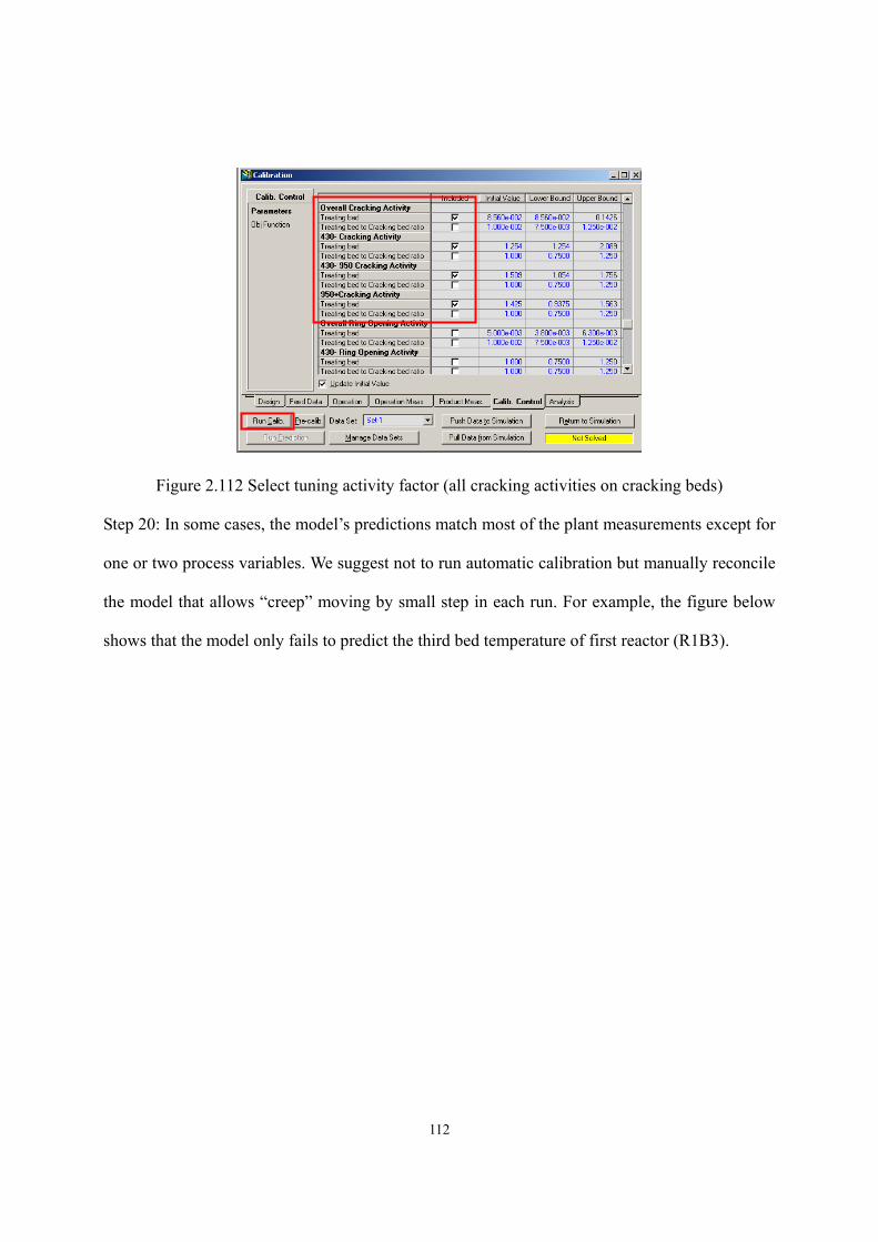
112
Figure 2.112 Select tuning activity factor (all cracking activities on cracking beds)
Step 20: In some cases, the model’s predictions match most of the plant measurements except for
one or two process variables. We suggest not to run automatic calibration but manually reconcile
the model that allows “creep” moving by small step in each run. For example, the figure below
shows that the model only fails to predict the third bed temperature of first reactor (R1B3).
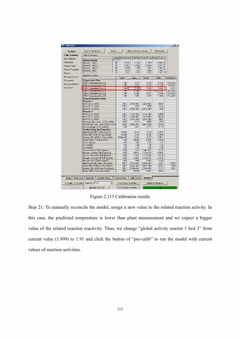
113
Figure 2.113 Calibration results
Step 21: To manually reconcile the model, assign a new value to the related reaction activity. In
this case, the predicted temperature is lower than plant measurement and we expect a bigger
value of the related reaction reactivity. Thus, we change “global activity reactor 1 bed 3” from
current value (1.899) to 1.91 and click the button of “pre-calib” to run the model with current
values of reaction activities.
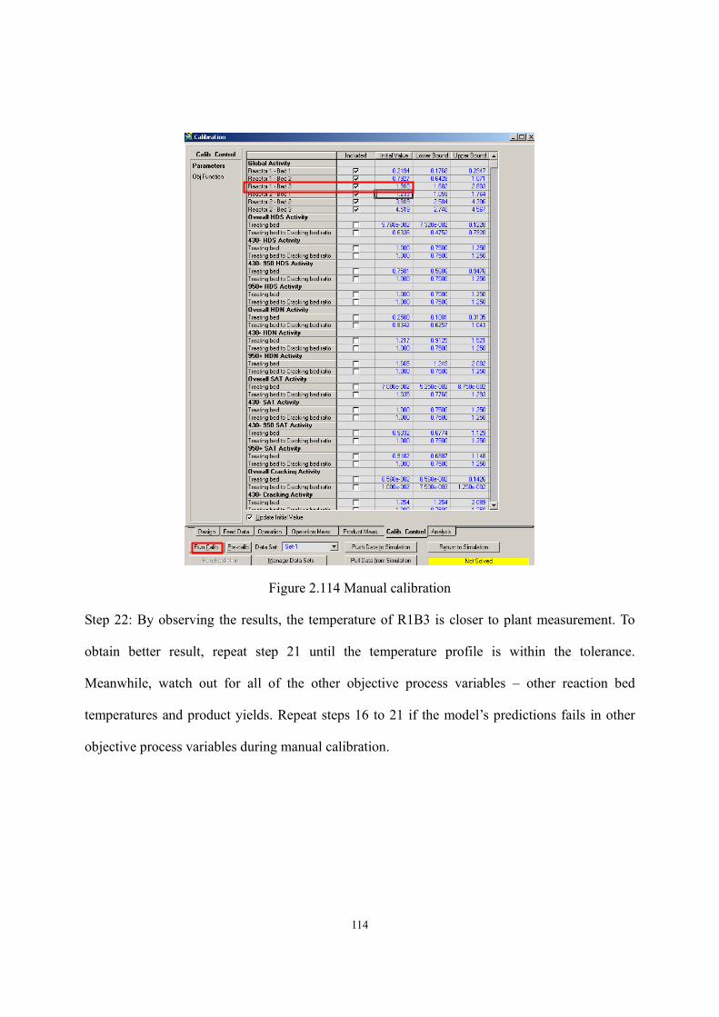
114
Figure 2.114 Manual calibration
Step 22: By observing the results, the temperature of R1B3 is closer to plant measurement. To
obtain better result, repeat step 21 until the temperature profile is within the tolerance.
Meanwhile, watch out for all of the other objective process variables – other reaction bed
temperatures and product yields. Repeat steps 16 to 21 if the model’s predictions fails in other
objective process variables during manual calibration.
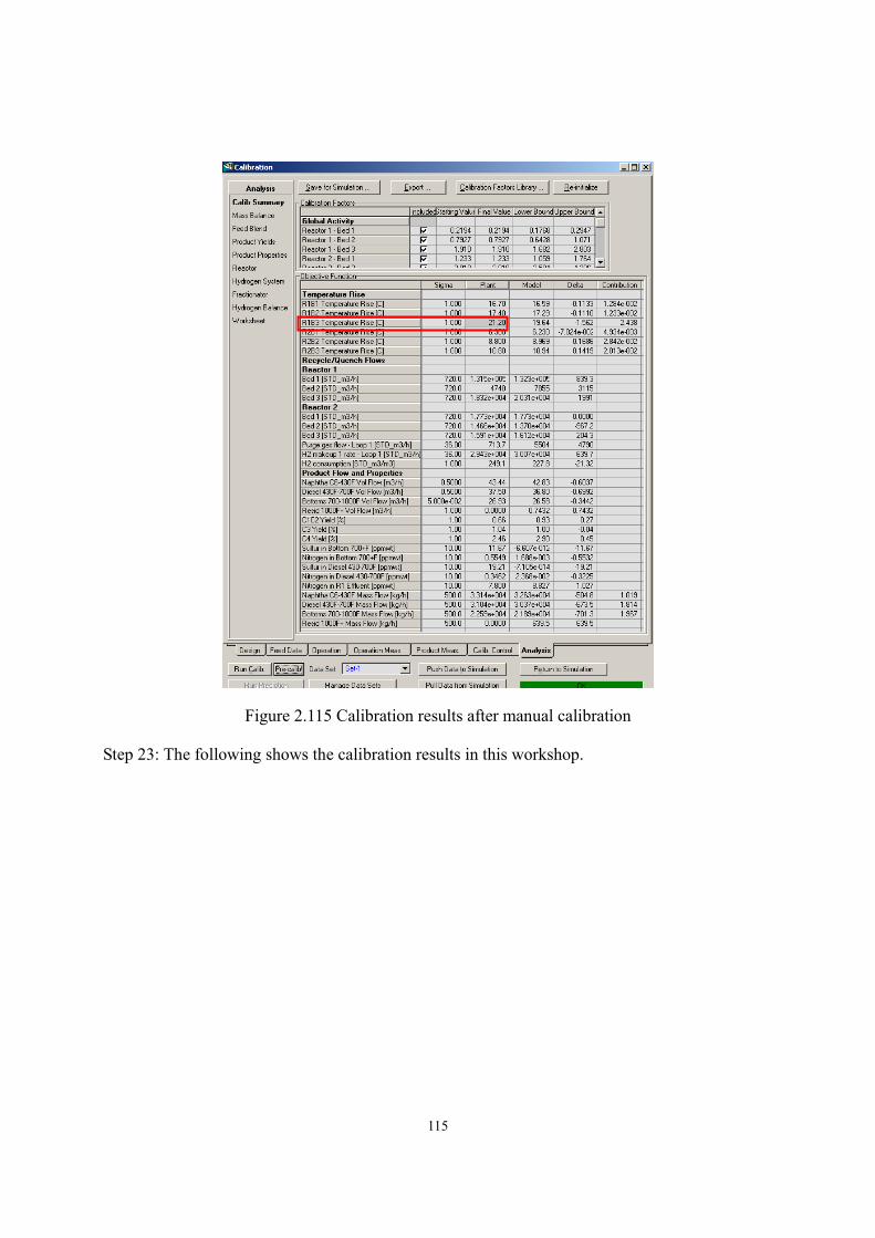
115
Figure 2.115 Calibration results after manual calibration
Step 23: The following shows the calibration results in this workshop.
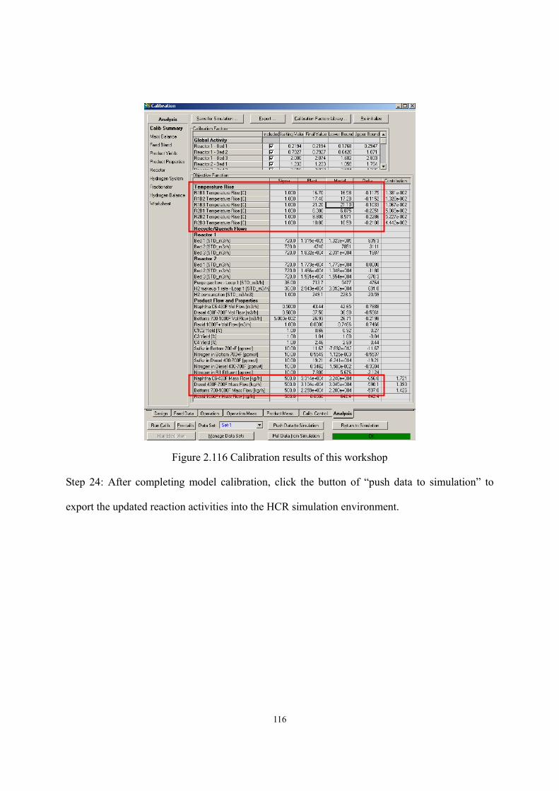
116
Figure 2.116 Calibration results of this workshop
Step 24: After completing model calibration, click the button of “push data to simulation” to
export the updated reaction activities into the HCR simulation environment.
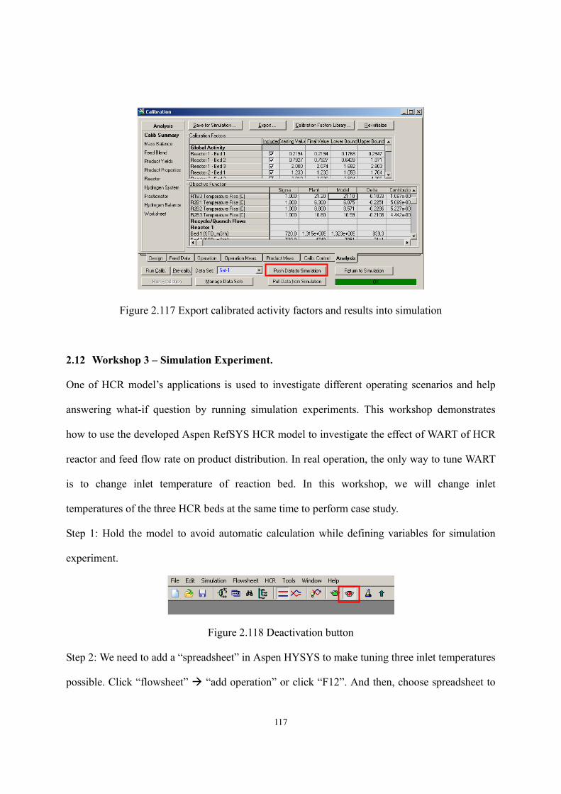
117
Figure 2.117 Export calibrated activity factors and results into simulation
2.12 Workshop 3 – Simulation Experiment.
One of HCR model’s applications is used to investigate different operating scenarios and help
answering what-if question by running simulation experiments. This workshop demonstrates
how to use the developed Aspen RefSYS HCR model to investigate the effect of WART of HCR
reactor and feed flow rate on product distribution. In real operation, the only way to tune WART
is to change inlet temperature of reaction bed. In this workshop, we will change inlet
temperatures of the three HCR beds at the same time to perform case study.
Step 1: Hold the model to avoid automatic calculation while defining variables for simulation
experiment.
Figure 2.118 Deactivation button
Step 2: We need to add a “spreadsheet” in Aspen HYSYS to make tuning three inlet temperatures
possible. Click “flowsheet” “add operation” or click “F12”. And then, choose spreadsheet to
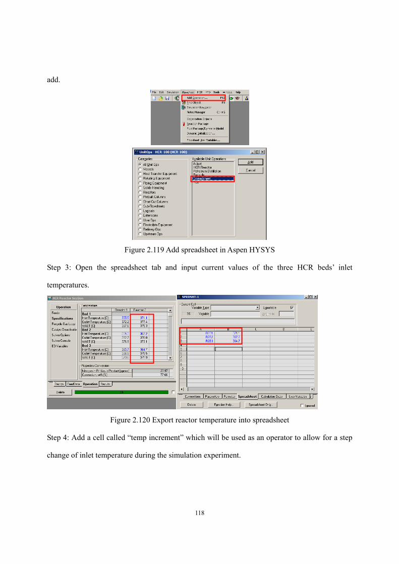
118
add.
Figure 2.119 Add spreadsheet in Aspen HYSYS
Step 3: Open the spreadsheet tab and input current values of the three HCR beds’ inlet
temperatures.
Figure 2.120 Export reactor temperature into spreadsheet
Step 4: Add a cell called “temp increment” which will be used as an operator to allow for a step
change of inlet temperature during the simulation experiment.
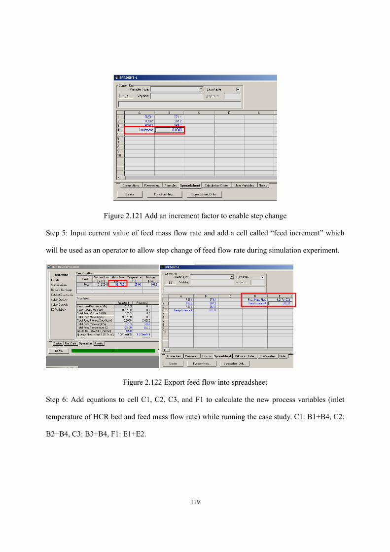
119
Figure 2.121 Add an increment factor to enable step change
Step 5: Input current value of feed mass flow rate and add a cell called “feed increment” which
will be used as an operator to allow step change of feed flow rate during simulation experiment.
Figure 2.122 Export feed flow into spreadsheet
Step 6: Add equations to cell C1, C2, C3, and F1 to calculate the new process variables (inlet
temperature of HCR bed and feed mass flow rate) while running the case study. C1: B1+B4, C2:
B2+B4, C3: B3+B4, F1: E1+E2.
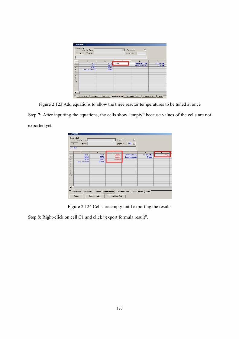
120
Figure 2.123 Add equations to allow the three reactor temperatures to be tuned at once
Step 7: After inputting the equations, the cells show “empty” because values of the cells are not
exported yet.
Figure 2.124 Cells are empty until exporting the results
Step 8: Right-click on cell C1 and click “export formula result”.
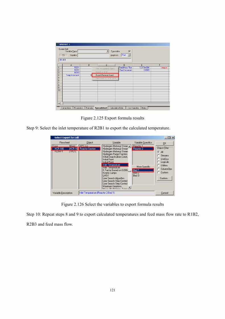
121
Figure 2.125 Export formula results
Step 9: Select the inlet temperature of R2B1 to export the calculated temperature.
Figure 2.126 Select the variables to export formula results
Step 10: Repeat steps 8 and 9 to export calculated temperatures and feed mass flow rate to R1B2,
R2B3 and feed mass flow.
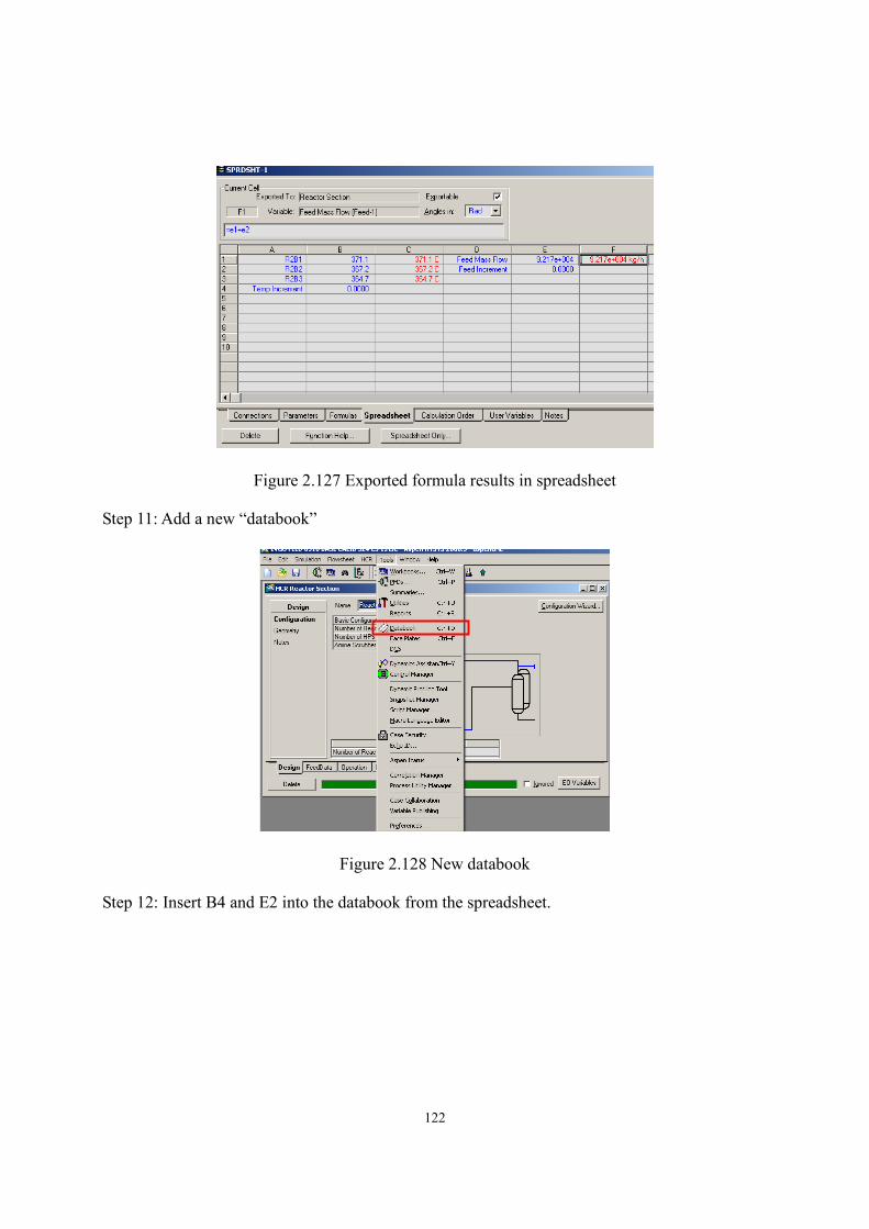
122
Figure 2.127 Exported formula results in spreadsheet
Step 11: Add a new “databook”
Figure 2.128 New databook
Step 12: Insert B4 and E2 into the databook from the spreadsheet.
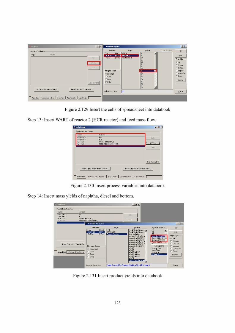
123
Figure 2.129 Insert the cells of spreadsheet into databook
Step 13: Insert WART of reactor 2 (HCR reactor) and feed mass flow.
Figure 2.130 Insert process variables into databook
Step 14: Insert mass yields of naphtha, diesel and bottom.
Figure 2.131 Insert product yields into databook
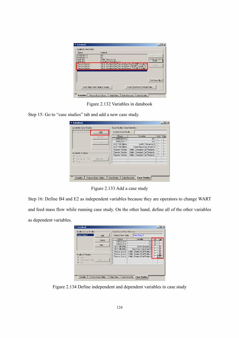
124
Figure 2.132 Variables in databook
Step 15: Go to “case studies” tab and add a new case study.
Figure 2.133 Add a case study
Step 16: Define B4 and E2 as independent variables because they are operators to change WART
and feed mass flow while running case study. On the other hand, define all of the other variables
as dependent variables.
Figure 2.134 Define independent and dependent variables in case study
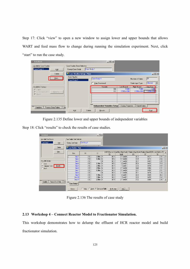
125
Step 17: Click “view” to open a new window to assign lower and upper bounds that allows
WART and feed mass flow to change during running the simulation experiment. Next, click
“start” to run the case study.
Figure 2.135 Define lower and upper bounds of independent variables
Step 18: Click “results” to check the results of case studies.
Figure 2.136 The results of case study
2.13 Workshop 4 – Connect Reactor Model to Fractionator Simulation.
This workshop demonstrates how to delump the effluent of HCR reactor model and build
fractionator simulation.
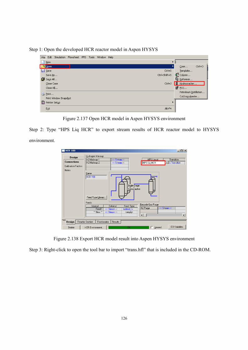
126
Step 1: Open the developed HCR reactor model in Aspen HYSYS
Figure 2.137 Open HCR model in Aspen HYSYS environment
Step 2: Type “HPS Liq HCR” to export stream results of HCR reactor model to HYSYS
environment.
Figure 2.138 Export HCR model result into Aspen HYSYS environment
Step 3: Right-click to open the tool bar to import “trans.hfl” that is included in the CD-ROM.
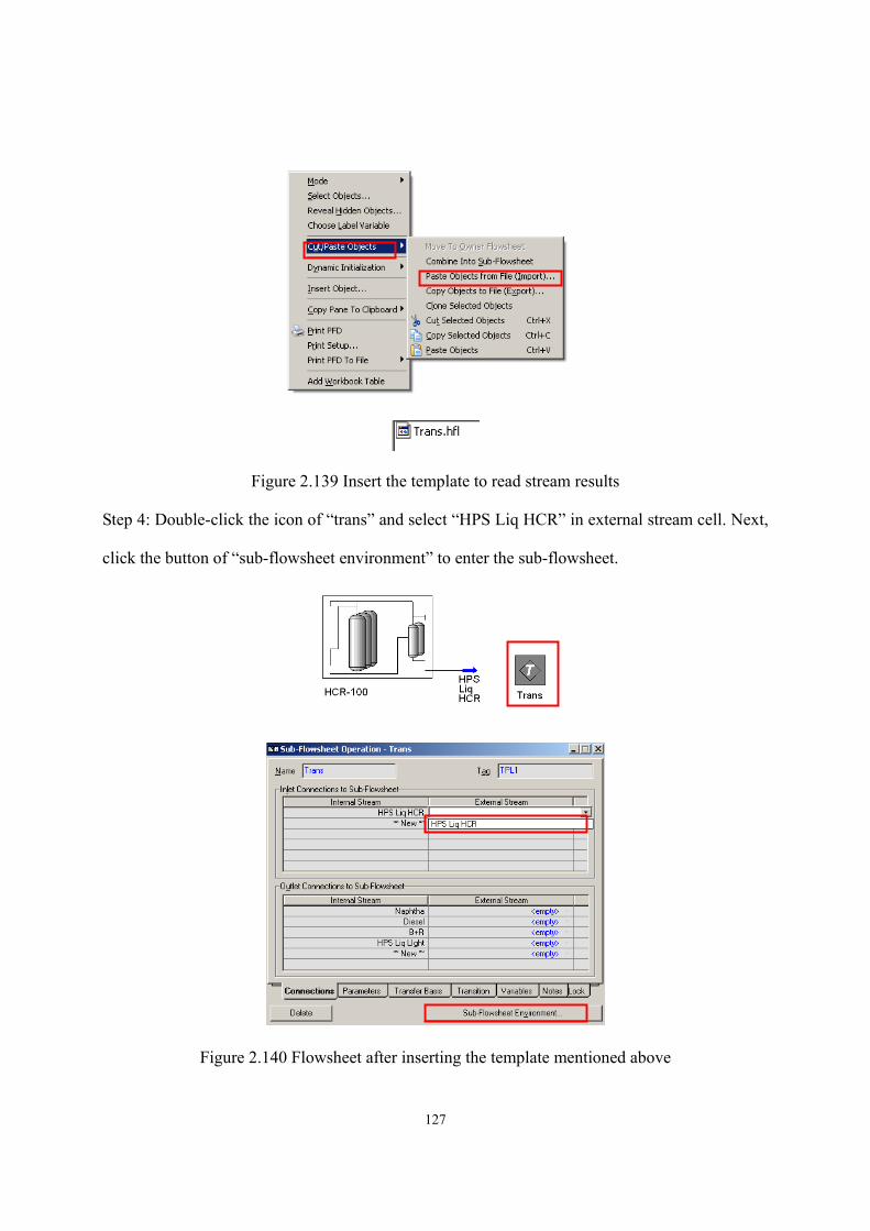
127
Figure 2.139 Insert the template to read stream results
Step 4: Double-click the icon of “trans” and select “HPS Liq HCR” in external stream cell. Next,
click the button of “sub-flowsheet environment” to enter the sub-flowsheet.
Figure 2.140 Flowsheet after inserting the template mentioned above
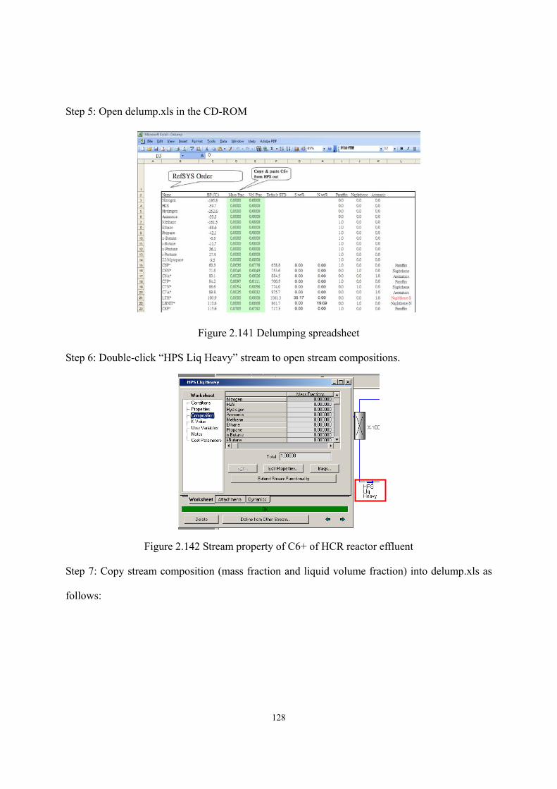
128
Step 5: Open delump.xls in the CD-ROM
Figure 2.141 Delumping spreadsheet
Step 6: Double-click “HPS Liq Heavy” stream to open stream compositions.
Figure 2.142 Stream property of C6+ of HCR reactor effluent
Step 7: Copy stream composition (mass fraction and liquid volume fraction) into delump.xls as
follows:
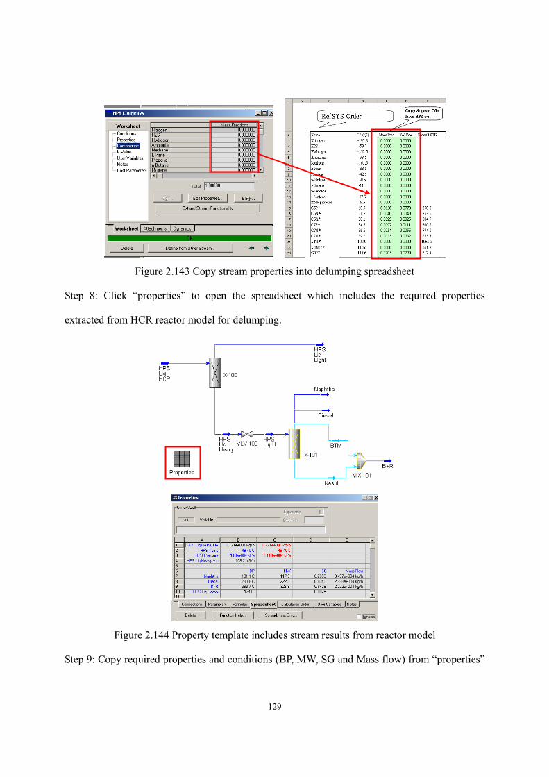
129
Figure 2.143 Copy stream properties into delumping spreadsheet
Step 8: Click “properties” to open the spreadsheet which includes the required properties
extracted from HCR reactor model for delumping.
Figure 2.144 Property template includes stream results from reactor model
Step 9: Copy required properties and conditions (BP, MW, SG and Mass flow) from “properties”
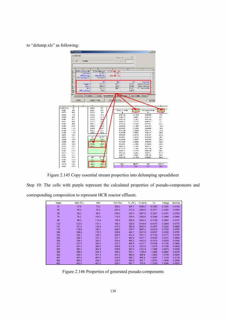
130
to “delump.xls” as following:
Figure 2.145 Copy essential stream properties into delumping spreadsheet
Step 10: The cells with purple represent the calculated properties of pseudo-components and
corresponding composition to represent HCR reactor effluent.
Figure 2.146 Properties of generated pseudo-components
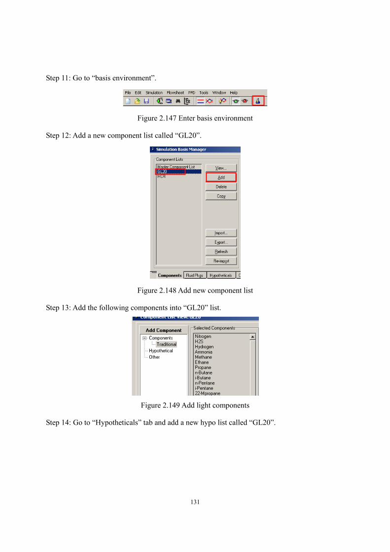
131
Step 11: Go to “basis environment”.
Figure 2.147 Enter basis environment
Step 12: Add a new component list called “GL20”.
Figure 2.148 Add new component list
Step 13: Add the following components into “GL20” list.
Figure 2.149 Add light components
Step 14: Go to “Hypotheticals” tab and add a new hypo list called “GL20”.
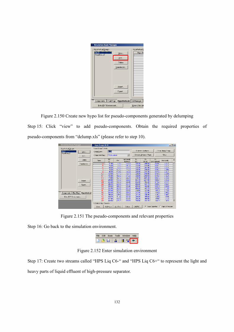
132
Figure 2.150 Create new hypo list for pseudo-components generated by delumping
Step 15: Click “view” to add pseudo-components. Obtain the required properties of
pseudo-components from “delump.xls” (please refer to step 10).
Figure 2.151 The pseudo-components and relevant properties
Step 16: Go back to the simulation environment.
Figure 2.152 Enter simulation environment
Step 17: Create two streams called “HPS Liq C6-“ and “HPS Liq C6+“ to represent the light and
heavy parts of liquid effluent of high-pressure separator.
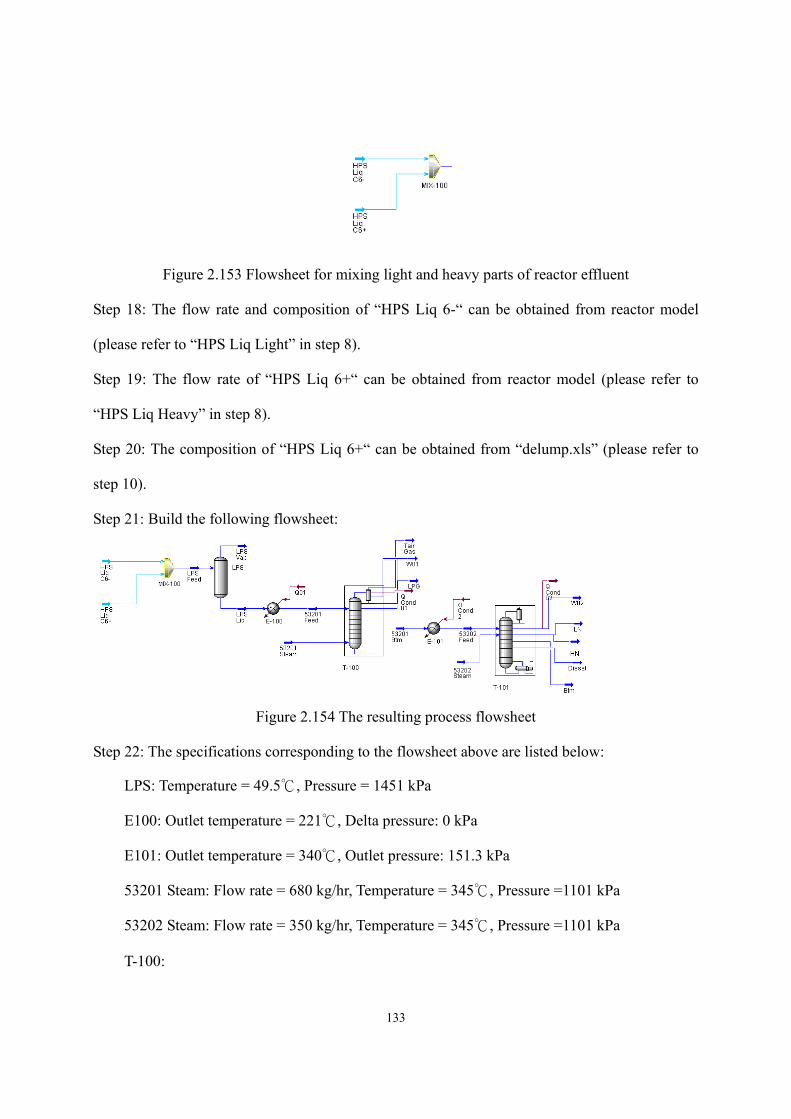
133
Figure 2.153 Flowsheet for mixing light and heavy parts of reactor effluent
Step 18: The flow rate and composition of “HPS Liq 6-“ can be obtained from reactor model
(please refer to “HPS Liq Light” in step 8).
Step 19: The flow rate of “HPS Liq 6+“ can be obtained from reactor model (please refer to
“HPS Liq Heavy” in step 8).
Step 20: The composition of “HPS Liq 6+“ can be obtained from “delump.xls” (please refer to
step 10).
Step 21: Build the following flowsheet:
Figure 2.154 The resulting process flowsheet
Step 22: The specifications corresponding to the flowsheet above are listed below:
LPS: Temperature = 49.5, Pressure = 1451 kPa
E100: Outlet temperature = 221, Delta pressure: 0 kPa
E101: Outlet temperature = 340, Outlet pressure: 151.3 kPa
53201 Steam: Flow rate = 680 kg/hr, Temperature = 345, Pressure =1101 kPa
53202 Steam: Flow rate = 350 kg/hr, Temperature = 345, Pressure =1101 kPa
T-100:
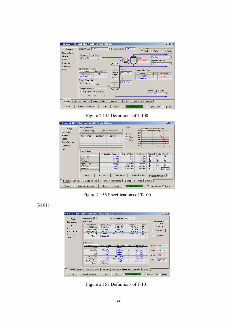
134
Figure 2.155 Definitions of T-100
Figure 2.156 Specifications of T-100
T-101:
Figure 2.157 Definitions of T-101
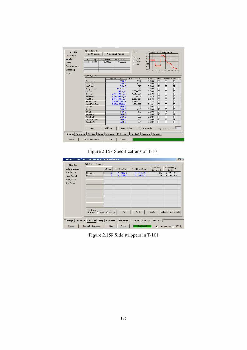
135
Figure 2.158 Specifications of T-101
Figure 2.159 Side strippers in T-101
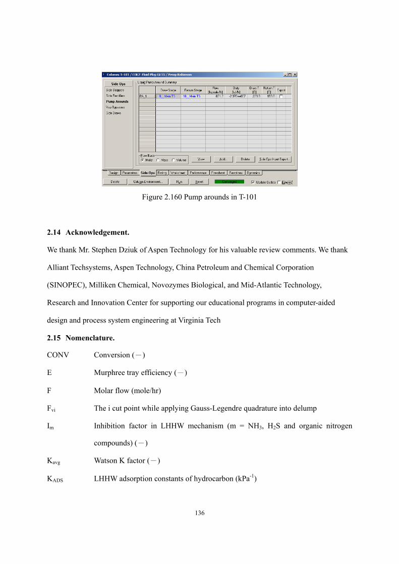
136
Figure 2.160 Pump arounds in T-101
2.14 Acknowledgement.
We thank Mr. Stephen Dziuk of Aspen Technology for his valuable review comments. We thank
Alliant Techsystems, Aspen Technology, China Petroleum and Chemical Corporation
(SINOPEC), Milliken Chemical, Novozymes Biological, and Mid-Atlantic Technology,
Research and Innovation Center for supporting our educational programs in computer-aided
design and process system engineering at Virginia Tech
2.15 Nomenclature.
CONV Conversion (-)
E Murphree tray efficiency (-)
F Molar flow (mole/hr)
Fvi The i cut point while applying Gauss-Legendre quadrature into delump
Im Inhibition factor in LHHW mechanism (m = NH3, H2S and organic nitrogen
compounds) (-)
Kavg Watson K factor (-)
KADS LHHW adsorption constants of hydrocarbon (kPa-1)
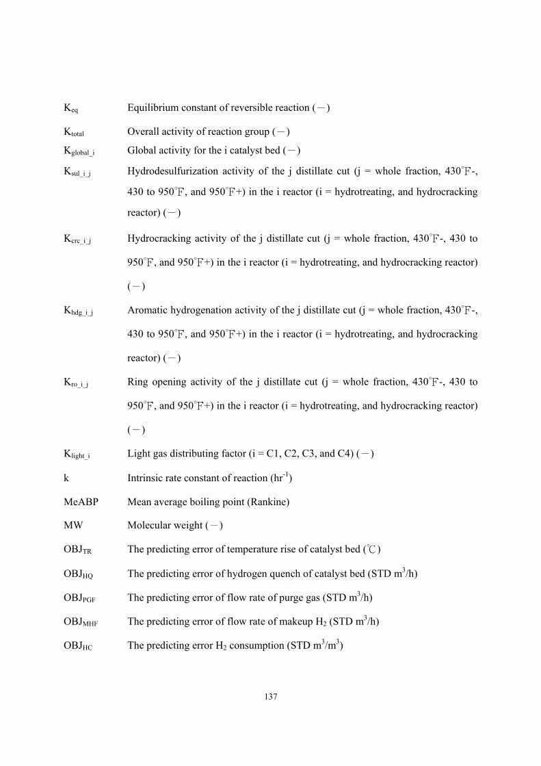
137
Keq Equilibrium constant of reversible reaction (-)
Ktotal Overall activity of reaction group (-)
Kglobal_i Global activity for the i catalyst bed (-)
Ksul_i_j Hydrodesulfurization activity of the j distillate cut (j = whole fraction, 430-,
430 to 950, and 950+) in the i reactor (i = hydrotreating, and hydrocracking
reactor) (-)
Kcrc_i_j Hydrocracking activity of the j distillate cut (j = whole fraction, 430-, 430 to
950, and 950+) in the i reactor (i = hydrotreating, and hydrocracking reactor)
(-)
Khdg_i_j Aromatic hydrogenation activity of the j distillate cut (j = whole fraction, 430-,
430 to 950, and 950+) in the i reactor (i = hydrotreating, and hydrocracking
reactor) (-)
Kro_i_j Ring opening activity of the j distillate cut (j = whole fraction, 430-, 430 to
950, and 950+) in the i reactor (i = hydrotreating, and hydrocracking reactor)
(-)
Klight_i Light gas distributing factor (i = C1, C2, C3, and C4) (-)
k Intrinsic rate constant of reaction (hr-1)
MeABP Mean average boiling point (Rankine)
MW Molecular weight (-)
OBJTR The predicting error of temperature rise of catalyst bed ()
OBJHQ The predicting error of hydrogen quench of catalyst bed (STD m3/h)
OBJPGF The predicting error of flow rate of purge gas (STD m3/h)
OBJMHF The predicting error of flow rate of makeup H2 (STD m3/h)
OBJHC The predicting error H2 consumption (STD m3/m3)
138
OBJNVF The predicting error of C6 to 430 cut (naphtha) volume flow (m3/h)
OBJDVF The predicting error of 430 to 700 cut (diesel) volume flow (m3/h)
OBJBVF The predicting error of 700 to 1000 cut (bottom) volume flow (m3/h)
OBJRVF The predicting error of 1000+ cut (resid) volume flow (m3/h)
OBJNMF The predicting error of C6 to 430 cut (naphtha) mass flow (kg/h)
OBJDMF The predicting error of 430 to 700 cut (diesel) mass flow (kg/h)
OBJBMF The predicting error of 700 to 1000 cut (bottom) mass flow (kg/h)
OBJRMF The predicting error of 1000+ cut (resid) mass flow (kg/h)
OBJC1C2 The predicting error of C1C2 mass yield (wt%)
OBJC3 The predicting error of C3 mass yield (wt%)
OBJC4 The predicting error of C4 mass yield (wt%)
OBJSD The predicting error of sulfur content of 430 to 700 cut (wt%)
OBJSB The predicting error of sulfur content of 700 to 1000 cut (wt%)
OBJND The predicting error of nitrogen content of 430 to 700 cut (ppmwt)
OBJNB The predicting error of nitrogen content of 700 to 1000 cut (ppmwt)
OBJNR1 The predicting error of nitrogen content in reactor 1 effluent (ppmwt)
Pc Critical pressure (kPa)
PH2 Partial pressure of hydrogen (kPa)
qi The zeros of the Legendre polynomial (-)
SG Specific gravity 60/60(-)
SV Space velocity (1/hr)
T Temperature ()
Tb Normal boiling point ()
Tc Critical temperature ()
139
Tr Reduced temperature (-)
V Volume (m3)
Vc Critical volume (m3)
wi Weight factor of Gauss-Legendre quadrature (-)
ω Acentric factor (-)
θ Feed ratio of feed 1 to feed 2 (-)
τ Residence time (hr)
2.16 Literature Cited.
1. Aye, M. M. S.; Zhang, N. A Novel Methodology in Transforming Bulk Properties of
Refining Streams into Molecular Information, Chem. Eng. Sci. 2005, 60, 6702.
2. Qader, S. A.; Hill, G. R. Hydrocracking of Gas Oil, Ind. Eng. Chem. Proc. Des. Dev. 1969, 8,
98.
3. Quann, R. J.; Jaffe, S. B. Structure-Oriented Lumping: Describing the Chemistry of
Complex Hydrocarbon Mixtures, Ind. Eng. Chem. Res. 1992, 31, 2483.
4. Quann, R. J.; Jaffe, S. B. Building Useful Models of Complex Reaction Systems in
Petroleum Refining, Chem. Eng. Sci. 1996, 51, 1615.
5. Quann, R. R. Modeling the Chemistry of Complex Petroleum Mixtures, Environ. Health
Perspect. Suppl. 1998, 106, 1501.
6. Froment, G. F. Single Event Kinetic Modeling of Complex Catalytic Processes, Catal.
Rev.-Sci. Eng. 2005, 47, 83.
7. Ghosh, P.; Andrews A. T.; Quann, R. J.; Halbert, T. R. Detailed Kinetic Model for the
Hydro-desulfurization of FCC Naphtha Energy Fuels 2009, 23, 5743.
8. Christensen, G.; Apelian, M. R.; Karlton, J. H.; Jaffe, S. B. Future directions in modeling the
FCC process: An emphasis on product quality Chem. Eng. Sci. 1999, 54, 2753.
140
9. Kumar, H.; Froment, G. F. Mechanistic Kinetic Modeling of the Hydrocracking of Complex
Feedstocks, Such as Vacuum Gas Oils, Ind. Eng. Chem. Res. 2007, 46, 5881.
10. Ancheyta, J.; Sánchez, S.; Rodríguez, M. A. Kinetic Modeling of Hydrocracking of Heavy
Oil Fractions: A Review, Catal. Today 2005, 109, 76.
11. Ho, T. C. Kinetic Modeling of Large-Scale Reaction Systems, Catal. Rev. Sci. Eng. 2008, 50,
287.
12. Valavarasu, G.; Bhaskar, M.; Sairam, B. A Four Lump Kinetic Model for the Simulation of
the Hydrocracking Process, Petrol. Sci. Technol. 2005, 23, 1323.
13. Sánchez, S.; Rodríguez, M. A.; Ancheyta, J. Kinetic Model for Moderate Hydrocracking of
Heavy Oils, Ind. Eng. Chem. Res. 2005, 44, 9409.
14. Verstraete, J. J.; Le Lannic, K.; Guibard, I. Modeling Fixed-bed Residue Hydrotreating
Processes, Chem. Eng. Sci. 2007, 62, 5402.
15. Stangeland, B. E. A Kinetic Model for the Prediction of Hydrocracker Yields, Ind. Eng.
Chem. Proc. Des. Dev. 1974, 13, 71.
16. Mohanty, S.; Saraf, D. N.; Kunzru, D. Modeling of a Hydrocracking Reactor, Fuel Process
Technol. 1991, 29, 1.
17. Pacheco, M. A.; Dassori, C. G. Hydrocracking: An improved Kinetic Model and Reactor
Modeling, Chem. Eng. Commun. 2002, 189, 1684.
18. Bhutani, N.; Ray, A. K.; Rangaiah, G. P. Modeling, Simulation, and Multi-objective
Optimization of an Industrial Hydrocracking Unit, Ind. Eng. Chem. Res. 2006, 45, 1354.
19. Laxminarasimhan, C. S.; Verma, R. P.; Ramachandran, P. A. Continuous Lumping Model
for Simulation of Hydrocracking, AIChE J. 1996, 42, 2645.
20. Basak, K.; Sau, M.; Manna, U.; Verma, R. P. Industrial Hydrocracker Model Based on
Novel Continuum Lumping Approach for Optimization in Petroleum Refinery, Catal. Today
141
2004, 98, 253.
21. Fukuyama, H.; Terai, S. Kinetic Study on the Hydrocracking Reaction of Vacuum Residue
Using a Lumping Model, Petrol. Sci. Technol. 2007, 25, 277.
22. Aspen HYSYS/Refining Option Guide, AspenTech, Cambridge, MA (2006).
23. Korre, S. C.; Klein, M. T.; Quann, R. J. Hydorcracking of Polynuclear Aromatic
Hydrocarbons. Development of Rate Laws through Inhibition Studies, Ind. Eng. Chem. Res.
1997, 36, 2041.
24. Jacob, S. M.; Quann, R. J.; Sanchez, E.; Wells, M. E. Compositional Modeling Reduces
Crude-Analysis Time, Predicts Yields, Oil & Gas J. 1998, July 6, 51.
25. Filimonov, V.A.; Popov, A.A.; Khavkin, V.A.; Perezhigina, I.Ya.; Osipov, L.N.; Rogov, S.P.;
Agafonov, A.V. International Chemical Engineering 1972, 12, 21.
26. Jacobs, P.A. Hydrocracking of n-Alkane Mixtures on Pt/H-Y Zeolite: Chain Length
Dependence of the Adsorption and the Kinetic Constants, Ind. Eng. Chem. Res. 1997, 36,
3242.
27. Brown, J. M.; Sundaram, A.; Saeger, R. B.; Wellons, H. S.; Kennedy, H. S.; Jaffe, S. B.
Estimating Compositional Information from Limited Analytical Data, WO2009051742,
2009.
28. Gomez-Prado, J.; Zhang, N.; Theodoropoulos, C. Characterization of Heavy Petroleum
Fractions Using Modified Molecular-Type Homologous Series (MTHS) Representation
Energy 2008, 33, 974.
29. Aspen Plus Hydrocracker User’s Guide, AspenTech, Cambridge, MA (2006).
30. Mudt, D. R.; Pedersen, C. C.; Jett, M. D.; Karur, S.; McIntyre, B.; Robinson, P. R.
Refinery-wide Optimization with Rigorous Models, In Practical Advances in Petroleum
Processing, Hsu, C. S.; Robinson, P. R. (Eds.), Springer: New York, NY, 2006.

142
31. Satterfield, C. N. Trickle-Bed Reactors, AIChE J. 1975, 21, 209.
32. Kaes, G. L. Refinery Process Modeling A Practical Guide to Steady State Modeling of
Petroleum Processes; The Athens Printing Company: Athens, GA, 2000.
33. Fogler, H. S. Elements of Chemical Reaction Engineering, 4th ed.; Prentice Hall: Upper
Saddle River, NJ, 2005.
34. Aspen HYSYS Simulation Basis, AspenTech, Cambridge, MA (2006).
35. Daubert, T. E.; Danner, R. P. API Technical Data Book – Petroleum Refining, 6th ed.,
American Petroleum Institute: Washington D.C., 1997.
36. Bollas, G. M.; Vasalos, I. A.; Lappas, A. A.; Iatridis, D. K.; Tsioni, G. K. Bulk Molecular
Characterization Approach for the Simulation of FCC Feedstocks, Ind. Eng. Chem. Res.
2004, 43, 3270.
37. Riazi, M. R. Characterization and Properties of Petroleum Fractions; 1st ed., American
Society for Testing and Materials: West Conshohocken, PA, 2005.
38. Haynes, H. W. Jr.; Matthews, M. A. Continuous-Mixture Vapor-Liquid Equilibria
Computations Based on True Boiling Point Distillations, Ind. Eng. Chem. Res. 1991, 30,
1911.
39. Cotterman, R. L.; Bender, R.; Prausnitz, J. M. Phase Equilibria for Mixtures Containing
Very Many Components. Development and Application of Continuous Thermodynamics for
Chemical Process Design, Ind. Eng. Chem. Proc. Des. Dev. 1985, 24, 194.
40. Mani, K. C.; Mathews, M. A.; Haynes, H. W. Jr. Continuous Approach Optimizes
Vapor-Liquid Equilibrium Calculation, Oil & Gas J. 1993, Feb 15, 76.
41. Riazi, M. R.; Daubert, T. E. Simplify Property Predictions, Hydrocarbon Processing 1980,
Mar, 115.
42. Lee, B. I.; Kesler, M. A. A Generalized Thermodynamic Correlation Based on
143
Three-Parameter Corresponding States. AIChE J. 1985, 31, 1136.
43. Kister, H. Z. Distillation Design; McGraw-Hill, Inc.: New York, NY, 1992.
44. Roussel, M.; Norsica, S.; Lemberton, J. L.; Guinet, M.; Cseri, T.; Benazzi, E.
Hydrocracking of n-Decane on a Bifunctional Sulfided NiW/Silica-Alumina Catalyst:
Effect of the Operating Conditions, Appl. Catal. 2005, 279, 53.
45. Dufresne, P.; Bigeard, P. H.; Bilon, A. New Development in Hydrocracking: Low Pressure
High-Conversion Hydrocracking, Catal. Today 1987, 1, 367.
46. Scherzer, J.; Gruia, A. J. Hydrocracking Science and Technology; Marcel Dekker: New York,
NY, 1996.
47. Hu, Z. H.; Xiong, Z. L.; Shi, Y. H.; Li, D. D. Investigation on the Reaction Pressure of
Hydrocracking Unit, Petroleum Processing and Petrochemicals 2005, 36, 35. (Chinese)
48. Tippett, T. W.; Ward, J. W. Mild Hydrocracking for Middle Distillate Production, National
Petroleum Refiners Association (NPRA) Annual Meeting, 24 Mar 1985, 24 Mar 1985,
AM-85-43.
49. Rossi, V. J.; Mayer, J. F.; Powell, B. E. To Up Hydrocracking Conversion, Hydrocarbon
Processing 1978, Oct 15, 123.
50. Bodington, C. E.; Baker, T. E. A History of Mathematical Programming in the Petroleum
Industry, Interfaces 1990, 20, 117.
51. El-Kady, F. Y. Hydrocracking of Vacuum Distillate Fraction over Bifunctional
Molybdenum – Nickel/Silica – Alumina Catalyst, Indian J. Technol. 1979, 17, 176.
52. Hu, M. C.; Powell, R. T.; Kidd, N. F. Develop LP Models Using a Steady-State Simulator,
Hydrocarbon Processing 1997, 76 (6), 81.
144
Chapter 3 Integrated Process Modeling and Product Design of Biodiesel Manufacturing
Abstract
Biodiesel, i.e., a mixture of fatty acid methyl esters (FAMEs), produced from reacting
triglyceride with methanol by alkali-catalyzed transesterification, has attracted much attention as
an important renewable energy source. To aid in the optimization of biodiesel manufacturing, a
number of published studies have applied commercial process simulators to quantify the effects
of operating conditions on the process performance. Significantly, all of the reported simulation
models are design models for new processes by fixing some level of equipment performance
such as the conversion of transesterification reaction. Most models assume the feed oil as pure
triolein and the biodiesel fuel as pure methyl oleate, and pay insufficient attention to the feed oil
characterization, thermophysical property estimation, rigorous reaction kinetics, phase
equilibrium for separation and purification units, and prediction of essential biodiesel fuel
qualities. This paper presents first a comprehensive review of published literature pertaining to
developing an integrated process modeling and product design of biodiesel manufacturing, and
identifies those deficient areas for further development.
This paper then presents new modeling tools and a methodology for the integrated process
modeling and product design of an entire biodiesel manufacturing train (including
transesterification reactor, methanol recovery and recycle, water wash, biodiesel recovery, and
glycerol separation, etc.). We demonstrate the methodology by simulating an integrated process
to predict reactor and separator performance, stream conditions, and product qualities with
different feedstocks. The results show that the methodology is effective not only for the rating
and optimization of an existing biodiesel manufacturing, and but also for the design of a new
process to produce biodiesel with specified fuel properties.
3.1 Biodiesel Production by Transesterification Process.
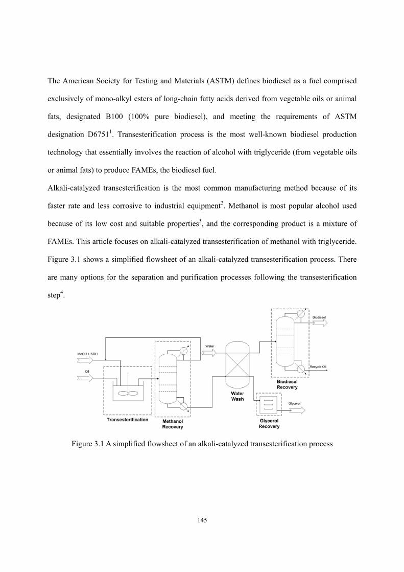
145
The American Society for Testing and Materials (ASTM) defines biodiesel as a fuel comprised
exclusively of mono-alkyl esters of long-chain fatty acids derived from vegetable oils or animal
fats, designated B100 (100% pure biodiesel), and meeting the requirements of ASTM
designation D67511. Transesterification process is the most well-known biodiesel production
technology that essentially involves the reaction of alcohol with triglyceride (from vegetable oils
or animal fats) to produce FAMEs, the biodiesel fuel.
Alkali-catalyzed transesterification is the most common manufacturing method because of its
faster rate and less corrosive to industrial equipment2. Methanol is most popular alcohol used
because of its low cost and suitable properties3, and the corresponding product is a mixture of
FAMEs. This article focuses on alkali-catalyzed transesterification of methanol with triglyceride.
Figure 3.1 shows a simplified flowsheet of an alkali-catalyzed transesterification process. There
are many options for the separation and purification processes following the transesterification
step4.
Figure 3.1 A simplified flowsheet of an alkali-catalyzed transesterification process
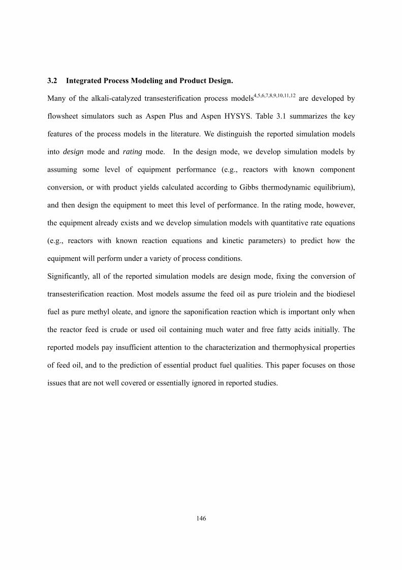
146
3.2 Integrated Process Modeling and Product Design.
Many of the alkali-catalyzed transesterification process models4,5,6,7,8,9,10,11,12 are developed by
flowsheet simulators such as Aspen Plus and Aspen HYSYS. Table 3.1 summarizes the key
features of the process models in the literature. We distinguish the reported simulation models
into design mode and rating mode. In the design mode, we develop simulation models by
assuming some level of equipment performance (e.g., reactors with known component
conversion, or with product yields calculated according to Gibbs thermodynamic equilibrium),
and then design the equipment to meet this level of performance. In the rating mode, however,
the equipment already exists and we develop simulation models with quantitative rate equations
(e.g., reactors with known reaction equations and kinetic parameters) to predict how the
equipment will perform under a variety of process conditions.
Significantly, all of the reported simulation models are design mode, fixing the conversion of
transesterification reaction. Most models assume the feed oil as pure triolein and the biodiesel
fuel as pure methyl oleate, and ignore the saponification reaction which is important only when
the reactor feed is crude or used oil containing much water and free fatty acids initially. The
reported models pay insufficient attention to the characterization and thermophysical properties
of feed oil, and to the prediction of essential product fuel qualities. This paper focuses on those
issues that are not well covered or essentially ignored in reported studies.
147
Table 3.1 Key features of reported simulation models Feed/Product Characterization Reactor Model
Reference Feed/product definition Description of thermophysical property models
Kinetics Saponification
Calculation of Fuel
Properties of Biodiesel
Thermodynamic Model of Biodiesel Purification Unit Program Mode
Myint & El-Halwagi4
Feed: pure triolein + oleic acid Product: methyl-oleate None Yield
model Included None
NRTL (non-random two-liquid) activity coefficient model with RKS (Redlich-Kwong-Soave) equation of state; UNIFAC for estimating missing parameters
Aspen Plus Design
West et al.5 Feed: pure triolein + oleic acid Product: methyl-oleate None Yield
model Not included None
NRTL UNIFAC for estimating missing parameters & fixed efficiency for centrifuge
Aspen HYSYS Design
Zhang et al.6 Feed: pure triolein Product: methyl-oleate None Yield
model Not included None
NRTL UNIFAC for estimating missing parameters & fixed efficiency for centrifuge
Aspen HYSYS Design
Harding et al.7 Feed: pure triolein Product: methyl-oleate None Yield
model Not included None No description Aspen Plus Design
Haas et al.8 Feed: pure triolein Product: methyl-oleate None Yield
model Not included None Fixed efficiency for centrifuge Aspen Plus Design
Tapasvi et al.9 Feed: mixture of simple triglyceridesProduct: mixture of FAMEs None Yield
model Included None Fixed efficiency for centrifuge MS Excel Design
Kapilakarn & Peutong10
Feed: no description Product: no description None Rigorous
model Not included None Fixed efficiency for centrifuge Aspen HYSYS Design
Stiefel & Dassori11Feed: pure triolein Product: methyl-oleate + diolein + monoolein
None Rigorous model Not included None Fixed efficiency Aspen Plus Design
Apostolakou et al.12 Feed: pure triolein Product: methyl-oleate Tang et al.13 Yield
model Not included None
NRTL UNIFAC for estimating missing parameters & Fixed efficiency for centrifuge
Aspen HYSYS Design
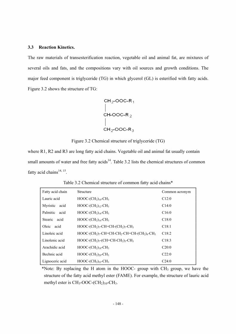
- 148 -
3.3 Reaction Kinetics.
The raw materials of transesterification reaction, vegetable oil and animal fat, are mixtures of
several oils and fats, and the compositions vary with oil sources and growth conditions. The
major feed component is triglyceride (TG) in which glycerol (GL) is esterified with fatty acids.
Figure 3.2 shows the structure of TG:
Figure 3.2 Chemical structure of triglyceride (TG)
where R1, R2 and R3 are long fatty acid chains. Vegetable oil and animal fat usually contain
small amounts of water and free fatty acids14. Table 3.2 lists the chemical structures of common
fatty acid chains14, 15.
Table 3.2 Chemical structure of common fatty acid chains*
Fatty acid chain Structure Common acronym
Lauric acid HOOC-(CH2)10-CH3 C12:0
Myristic acid HOOC-(CH2)12-CH3 C14:0
Palmitic acid HOOC-(CH2)14-CH3 C16:0
Stearic acid HOOC-(CH2)16-CH3 C18:0
Oleic acid HOOC-(CH2)7-CH=CH-(CH2)7-CH3 C18:1
Linoleic acid HOOC-(CH2)7-CH=CH-CH2-CH=CH-(CH2)4-CH3 C18:2
Linolenic acid HOOC-(CH2)7-(CH=CH-CH2)3-CH3 C18:3
Arachidic acid HOOC-(CH2)18-CH3 C20:0
Bechnic acid HOOC-(CH2)20-CH3 C22:0
Lignoceric acid HOOC-(CH2)22-CH3 C24:0
*Note: By replacing the H atom in the HOOC- group with CH3 group, we have the structure of the fatty acid methyl ester (FAME). For example, the structure of lauric acid methyl ester is CH3-OOC-(CH2)10-CH3.
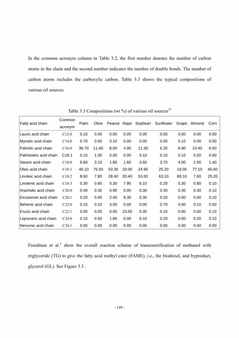
- 149 -
In the common acronym column in Table 3.2, the first number denotes the number of carbon
atoms in the chain and the second number indicates the number of double bonds. The number of
carbon atoms includes the carboxylic carbon. Table 3.3 shows the typical compositions of
various oil sources.
Table 3.3 Compositions (wt %) of various oil sources15
Fatty acid chain Common
acronym Palm Olive Peanut Rape Soybean Sunflower Grape Almond Corn
Lauric acid chain C12:0 0.10 0.00 0.00 0.00 0.00 0.00 0.00 0.00 0.00
Myristic acid chain C14:0 0.70 0.00 0.10 0.00 0.00 0.00 0.10 0.00 0.00
Palmitic acid chain C16:0 36.70 11.60 8.00 4.90 11.30 6.20 6.90 10.40 6.50
Palmitoleic acid chain C16:1 0.10 1.00 0.00 0.00 0.10 0.10 0.10 0.50 0.60
Stearic acid chain C18:0 6.60 3.10 1.80 1.60 3.60 3.70 4.00 2.90 1.40
Oleic acid chain C18:1 46.10 75.00 53.30 33.00 24.90 25.20 19.00 77.10 65.60
Linoleic acid chain C18:2 8.60 7.80 28.40 20.40 53.00 63.10 69.10 7.60 25.20
Linolenic acid chain C18:3 0.30 0.60 0.30 7.90 6.10 0.20 0.30 0.80 0.10
Arachidic acid chain C20:0 0.40 0.30 0.90 0.00 0.30 0.30 0.30 0.30 0.10
Eicosenoic acid chain C20:1 0.20 0.00 2.40 9.30 0.30 0.20 0.00 0.00 0.10
Behenic acid chain C22:0 0.10 0.10 3.00 0.00 0.00 0.70 0.00 0.10 0.00
Erucic acid chain C22:1 0.00 0.00 0.00 23.00 0.30 0.10 0.00 0.00 0.10
Liqnoceric acid chain C24:0 0.10 0.50 1.80 0.00 0.10 0.20 0.00 0.20 0.10
Nervonic acid chain C24:1 0.00 0.00 0.00 0.00 0.00 0.00 0.00 0.40 0.00
Freedman et al.2 show the overall reaction scheme of transesterification of methanol with
triglyceride (TG) to give the fatty acid methyl ester (FAME), i.e., the biodiesel, and byproduct,
glycerol (GL). See Figure 3.3 .
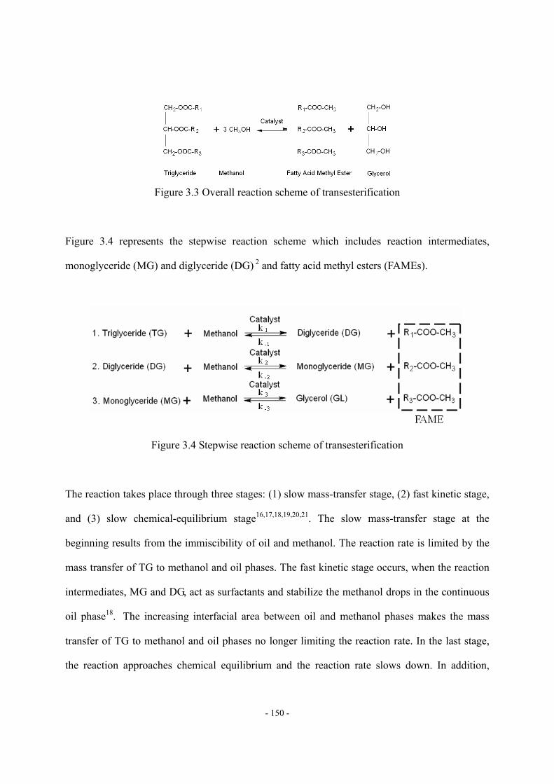
- 150 -
Figure 3.3 Overall reaction scheme of transesterification
Figure 3.4 represents the stepwise reaction scheme which includes reaction intermediates,
monoglyceride (MG) and diglyceride (DG) 2 and fatty acid methyl esters (FAMEs).
Figure 3.4 Stepwise reaction scheme of transesterification
The reaction takes place through three stages: (1) slow mass-transfer stage, (2) fast kinetic stage,
and (3) slow chemical-equilibrium stage16,17,18,19,20,21. The slow mass-transfer stage at the
beginning results from the immiscibility of oil and methanol. The reaction rate is limited by the
mass transfer of TG to methanol and oil phases. The fast kinetic stage occurs, when the reaction
intermediates, MG and DG, act as surfactants and stabilize the methanol drops in the continuous
oil phase18. The increasing interfacial area between oil and methanol phases makes the mass
transfer of TG to methanol and oil phases no longer limiting the reaction rate. In the last stage,
the reaction approaches chemical equilibrium and the reaction rate slows down. In addition,
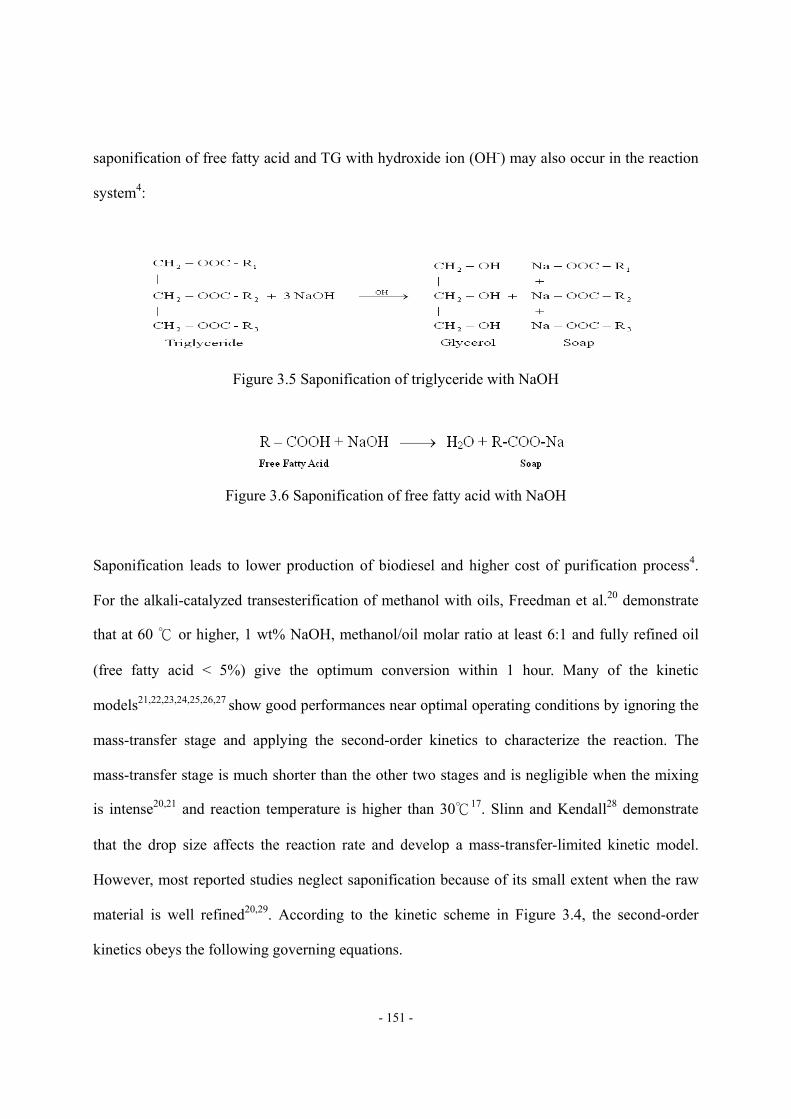
- 151 -
saponification of free fatty acid and TG with hydroxide ion (OH-) may also occur in the reaction
system4:
Figure 3.5 Saponification of triglyceride with NaOH
Figure 3.6 Saponification of free fatty acid with NaOH
Saponification leads to lower production of biodiesel and higher cost of purification process4.
For the alkali-catalyzed transesterification of methanol with oils, Freedman et al.20 demonstrate
that at 60 or higher, 1 wt% NaOH, methanol/oil molar ratio at least 6:1 and fully refined oil
(free fatty acid < 5%) give the optimum conversion within 1 hour. Many of the kinetic
models21,22,23,24,25,26,27 show good performances near optimal operating conditions by ignoring the
mass-transfer stage and applying the second-order kinetics to characterize the reaction. The
mass-transfer stage is much shorter than the other two stages and is negligible when the mixing
is intense20,21 and reaction temperature is higher than 3017. Slinn and Kendall28 demonstrate
that the drop size affects the reaction rate and develop a mass-transfer-limited kinetic model.
However, most reported studies neglect saponification because of its small extent when the raw
material is well refined20,29. According to the kinetic scheme in Figure 3.4, the second-order
kinetics obeys the following governing equations.
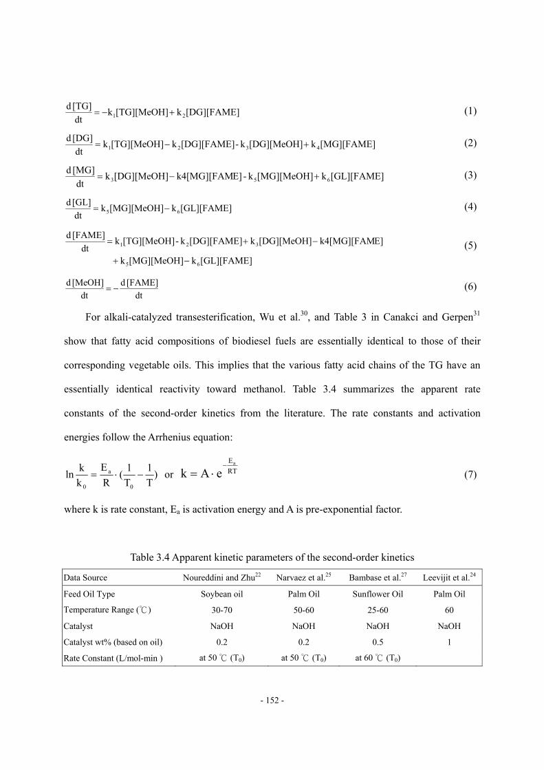
- 152 -
[DG][FAME]k[TG][MeOH]kdt[TG] d
21 +−= (1)
[MG][FAME]k[DG][MeOH]k-[DG][FAME]k[TG][MeOH]kdt
[DG] d4321 +−= (2)
[GL][FAME]k[MG][MeOH]k-E]k4[MG][FAM[DG][MeOH]kdt
[MG] d653 +−= (3)
[GL][FAME]k[MG][MeOH]kdt[GL] d
65 −= (4)
[GL][FAME]k[MG][MeOH]k
E]k4[MG][FAM[DG][MeOH]k[DG][FAME]k-[TG][MeOH]kdt
[FAME] d
65
321
−+
−+= (5)
dt[FAME] d
dt[MeOH] d
−= (6)
For alkali-catalyzed transesterification, Wu et al.30, and Table 3 in Canakci and Gerpen31
show that fatty acid compositions of biodiesel fuels are essentially identical to those of their
corresponding vegetable oils. This implies that the various fatty acid chains of the TG have an
essentially identical reactivity toward methanol. Table 3.4 summarizes the apparent rate
constants of the second-order kinetics from the literature. The rate constants and activation
energies follow the Arrhenius equation:
)T1
T1(
RE
kkln
0
a
0
−⋅= or RTEa
eAk−
⋅= (7)
where k is rate constant, Ea is activation energy and A is pre-exponential factor.
Table 3.4 Apparent kinetic parameters of the second-order kinetics
Data Source Noureddini and Zhu22 Narvaez et al.25 Bambase et al.27 Leevijit et al.24
Feed Oil Type Soybean oil Palm Oil Sunflower Oil Palm Oil
Temperature Range () 30-70 50-60 25-60 60
Catalyst NaOH NaOH NaOH NaOH
Catalyst wt% (based on oil) 0.2 0.2 0.5 1
Rate Constant (L/mol-min ) at 50 (T0) at 50 (T0) at 60 (T0)
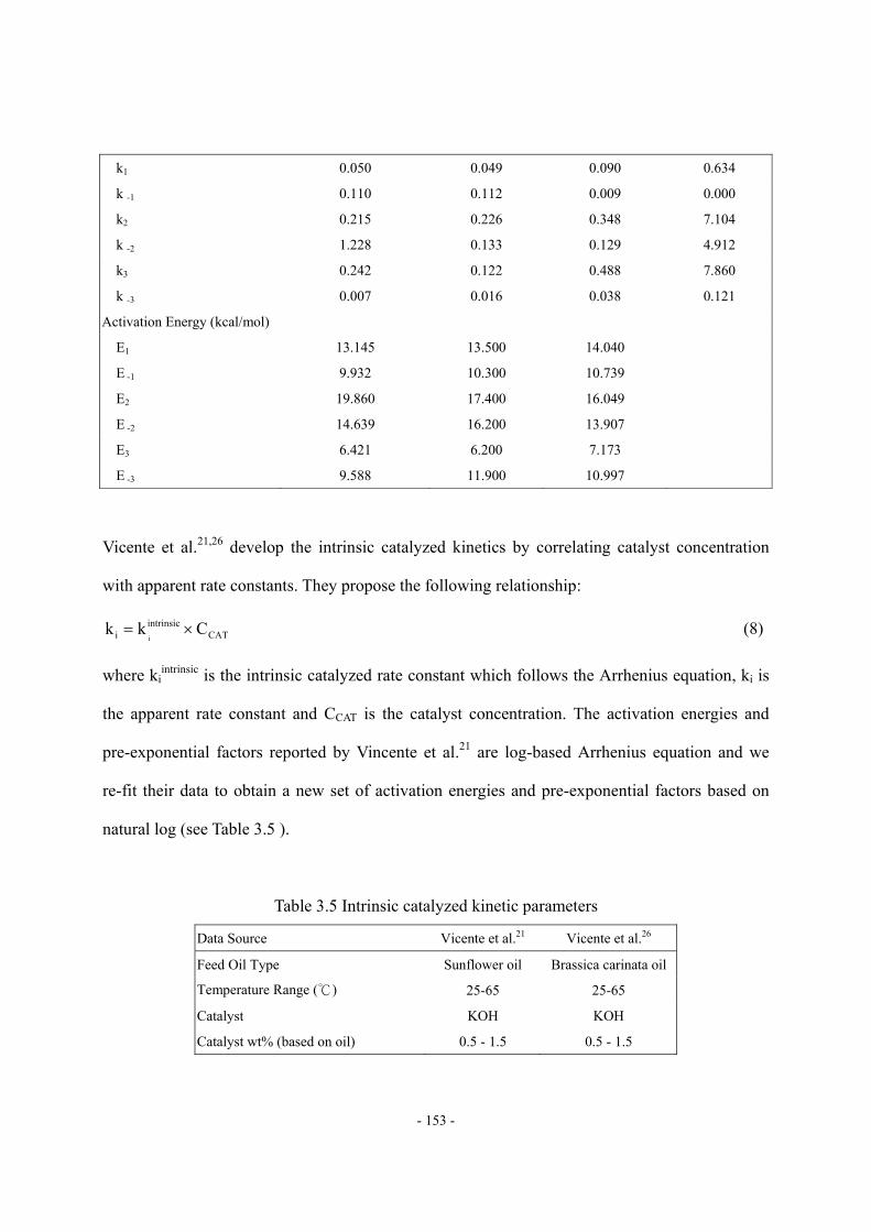
- 153 -
k1 0.050 0.049 0.090 0.634
k -1 0.110 0.112 0.009 0.000
k2 0.215 0.226 0.348 7.104
k -2 1.228 0.133 0.129 4.912
k3 0.242 0.122 0.488 7.860
k -3 0.007 0.016 0.038 0.121
Activation Energy (kcal/mol)
E1 13.145 13.500 14.040
E -1 9.932 10.300 10.739
E2 19.860 17.400 16.049
E -2 14.639 16.200 13.907
E3 6.421 6.200 7.173
E -3 9.588 11.900 10.997
Vicente et al.21,26 develop the intrinsic catalyzed kinetics by correlating catalyst concentration
with apparent rate constants. They propose the following relationship:
CATintrinsic
i Ckki
×= (8)
where kiintrinsic is the intrinsic catalyzed rate constant which follows the Arrhenius equation, ki is
the apparent rate constant and CCAT is the catalyst concentration. The activation energies and
pre-exponential factors reported by Vincente et al.21 are log-based Arrhenius equation and we
re-fit their data to obtain a new set of activation energies and pre-exponential factors based on
natural log (see Table 3.5 ).
Table 3.5 Intrinsic catalyzed kinetic parameters
Data Source Vicente et al.21 Vicente et al.26
Feed Oil Type Sunflower oil Brassica carinata oil
Temperature Range () 25-65 25-65
Catalyst KOH KOH
Catalyst wt% (based on oil) 0.5 - 1.5 0.5 - 1.5
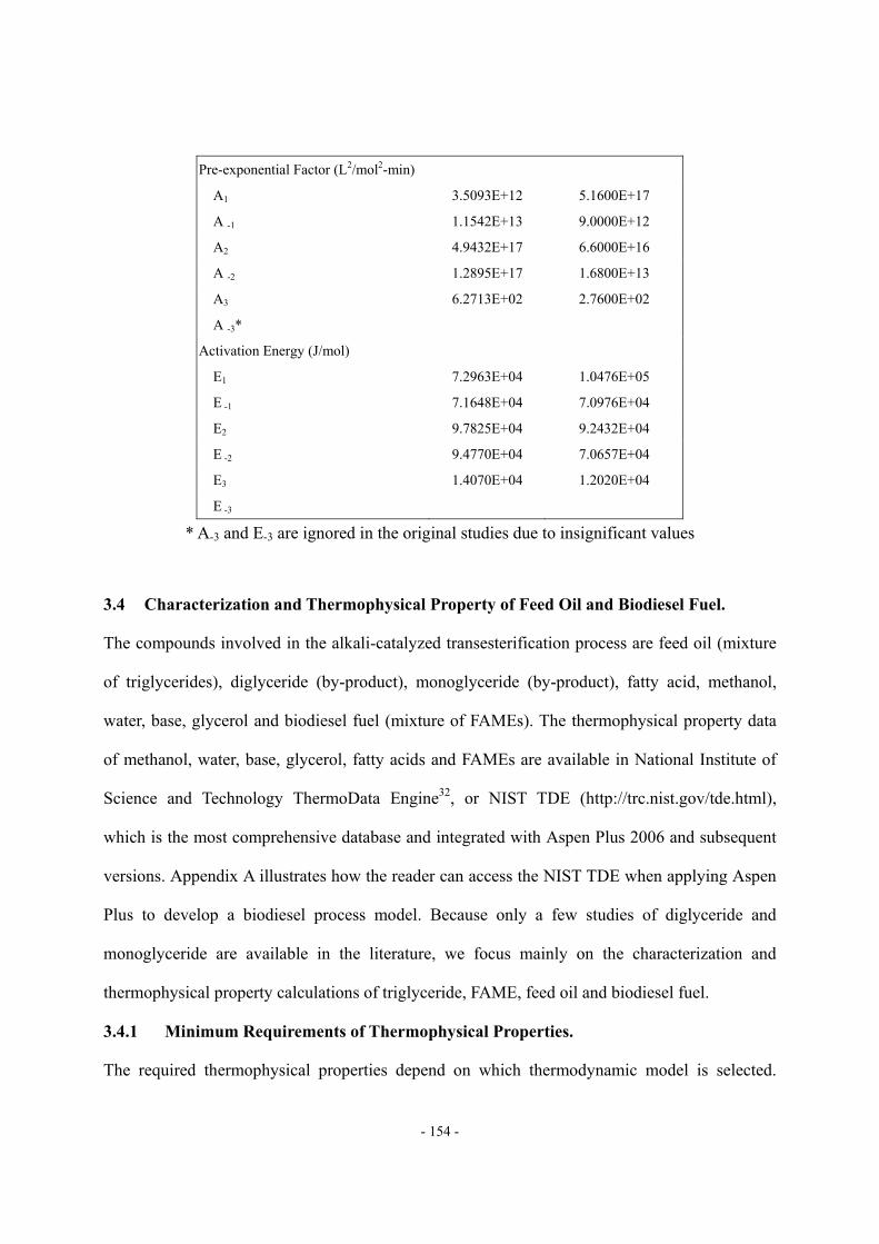
- 154 -
Pre-exponential Factor (L2/mol2-min)
A1 3.5093E+12 5.1600E+17
A -1 1.1542E+13 9.0000E+12
A2 4.9432E+17 6.6000E+16
A -2 1.2895E+17 1.6800E+13
A3 6.2713E+02 2.7600E+02
A -3*
Activation Energy (J/mol)
E1 7.2963E+04 1.0476E+05
E -1 7.1648E+04 7.0976E+04
E2 9.7825E+04 9.2432E+04
E -2 9.4770E+04 7.0657E+04
E3 1.4070E+04 1.2020E+04
E -3
* A-3 and E-3 are ignored in the original studies due to insignificant values
3.4 Characterization and Thermophysical Property of Feed Oil and Biodiesel Fuel.
The compounds involved in the alkali-catalyzed transesterification process are feed oil (mixture
of triglycerides), diglyceride (by-product), monoglyceride (by-product), fatty acid, methanol,
water, base, glycerol and biodiesel fuel (mixture of FAMEs). The thermophysical property data
of methanol, water, base, glycerol, fatty acids and FAMEs are available in National Institute of
Science and Technology ThermoData Engine32, or NIST TDE (http://trc.nist.gov/tde.html),
which is the most comprehensive database and integrated with Aspen Plus 2006 and subsequent
versions. Appendix A illustrates how the reader can access the NIST TDE when applying Aspen
Plus to develop a biodiesel process model. Because only a few studies of diglyceride and
monoglyceride are available in the literature, we focus mainly on the characterization and
thermophysical property calculations of triglyceride, FAME, feed oil and biodiesel fuel.
3.4.1 Minimum Requirements of Thermophysical Properties.
The required thermophysical properties depend on which thermodynamic model is selected.
- 155 -
Because of the presence of polar components (e.g., methanol) in a biodiesel process, we choose
activity coefficient model for modeling thermodynamic equilibrium. Therefore, the minimum
required thermophysical properties are normal boiling point (Tb), critical temperature (Tc),
critical pressure (Pc,), acentric factor (ω), liquid density (ρL) or liquid molar volume (VL), ideal
gas heat capacity (CP, G), liquid heat capacity (CP, L), heat of vaporization (Hvap) and vapor
pressure (Pvap).
3.4.2 Triglycerides.
Triglyerides can be classified into two groups – simple triglyceride and mixed triglyceride. The
simple triglyceride is composed of three identical fatty acid chains, but these fatty acid chains of
mixed triglyceride are not identical. This section focuses on the simple triglyceride. Because
thermal decomposition at high temperature makes the experimental measurements unattainable,
it is necessary to predict Tb, Pc, Tc and ω for long-chain triglycerides. There are many prediction
methods of Tb, Pc, Tc and ω for organic liquids in the literature, but many of the methods are
unsuitable for triglycerides because of their structures and high molecular weights. For example,
Figure 3.7 demonstrates that the Joback method significantly over-estimates the normal boiling
points of pure triglycerides.
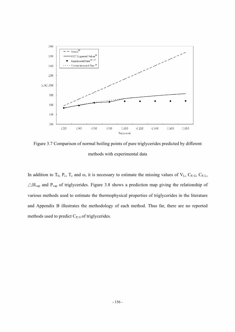
- 156 -
Figure 3.7 Comparison of normal boiling points of pure triglycerides predicted by different
methods with experimental data
In addition to Tb, Pc, Tc and ω, it is necessary to estimate the missing values of VL, CP, G, CP, L,
Hvap and Pvap of triglycerides. Figure 3.8 shows a prediction map giving the relationship of
various methods used to estimate the thermophysical properties of triglycerides in the literature
and Appendix B illustrates the methodology of each method. Thus far, there are no reported
methods used to predict CP, G of triglycerides.
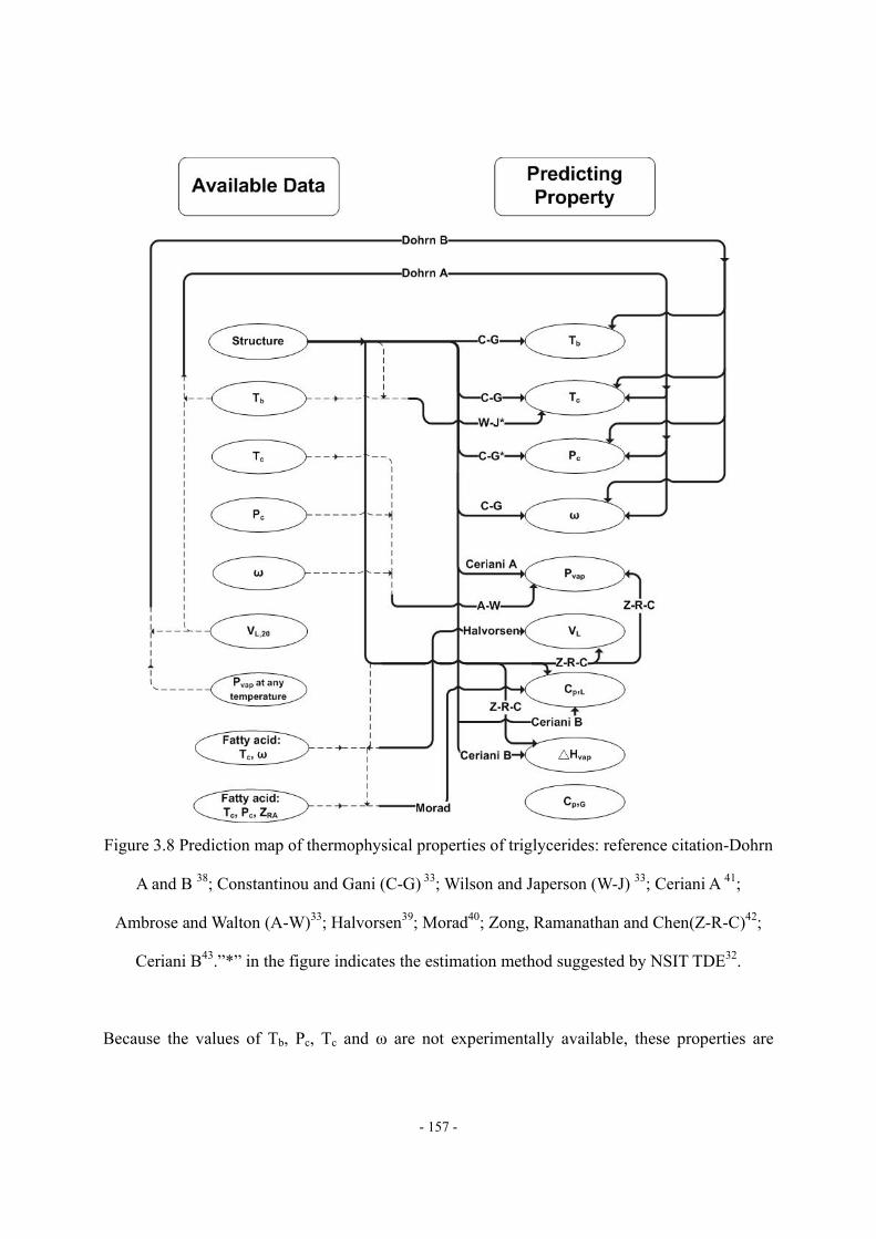
- 157 -
Figure 3.8 Prediction map of thermophysical properties of triglycerides: reference citation-Dohrn
A and B 38; Constantinou and Gani (C-G) 33; Wilson and Japerson (W-J) 33; Ceriani A 41;
Ambrose and Walton (A-W)33; Halvorsen39; Morad40; Zong, Ramanathan and Chen(Z-R-C)42;
Ceriani B43.”*” in the figure indicates the estimation method suggested by NSIT TDE32.
Because the values of Tb, Pc, Tc and ω are not experimentally available, these properties are
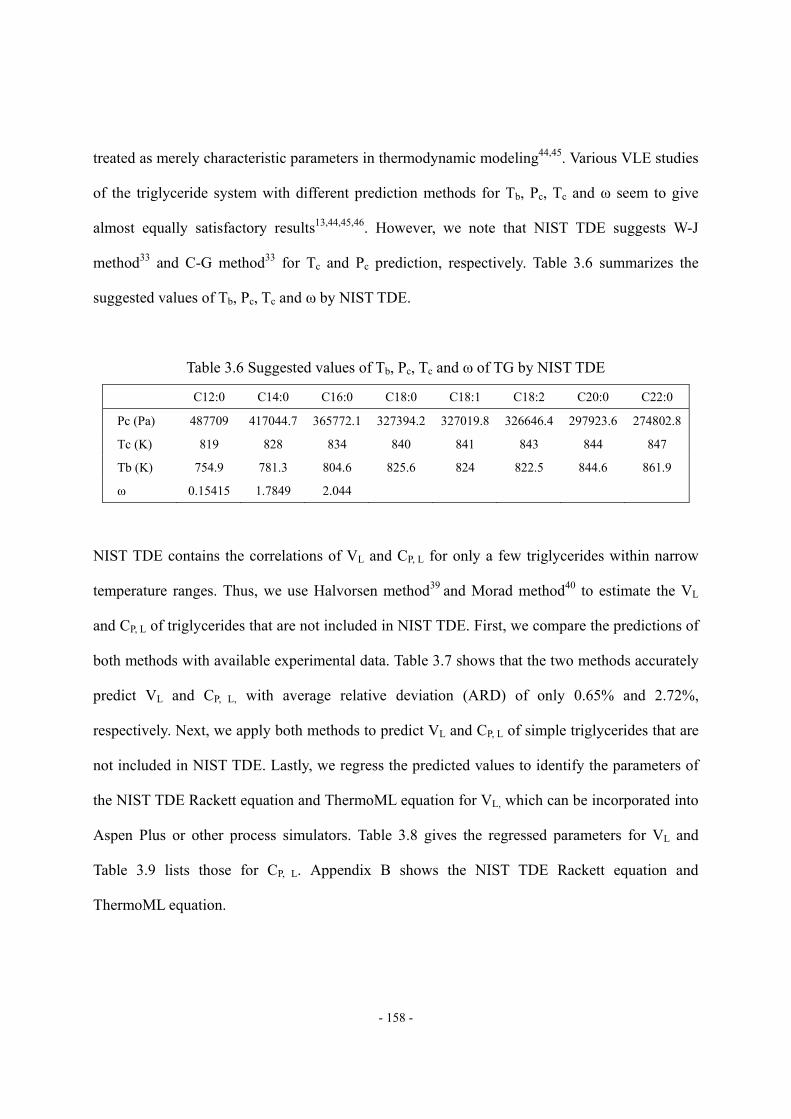
- 158 -
treated as merely characteristic parameters in thermodynamic modeling44,45. Various VLE studies
of the triglyceride system with different prediction methods for Tb, Pc, Tc and ω seem to give
almost equally satisfactory results13,44,45,46. However, we note that NIST TDE suggests W-J
method33 and C-G method33 for Tc and Pc prediction, respectively. Table 3.6 summarizes the
suggested values of Tb, Pc, Tc and ω by NIST TDE.
Table 3.6 Suggested values of Tb, Pc, Tc and ω of TG by NIST TDE
C12:0 C14:0 C16:0 C18:0 C18:1 C18:2 C20:0 C22:0
Pc (Pa) 487709 417044.7 365772.1 327394.2 327019.8 326646.4 297923.6 274802.8
Tc (K) 819 828 834 840 841 843 844 847
Tb (K) 754.9 781.3 804.6 825.6 824 822.5 844.6 861.9
ω 0.15415 1.7849 2.044
NIST TDE contains the correlations of VL and CP, L for only a few triglycerides within narrow
temperature ranges. Thus, we use Halvorsen method39 and Morad method40 to estimate the VL
and CP, L of triglycerides that are not included in NIST TDE. First, we compare the predictions of
both methods with available experimental data. Table 3.7 shows that the two methods accurately
predict VL and CP, L, with average relative deviation (ARD) of only 0.65% and 2.72%,
respectively. Next, we apply both methods to predict VL and CP, L of simple triglycerides that are
not included in NIST TDE. Lastly, we regress the predicted values to identify the parameters of
the NIST TDE Rackett equation and ThermoML equation for VL, which can be incorporated into
Aspen Plus or other process simulators. Table 3.8 gives the regressed parameters for VL and
Table 3.9 lists those for CP, L. Appendix B shows the NIST TDE Rackett equation and
ThermoML equation.
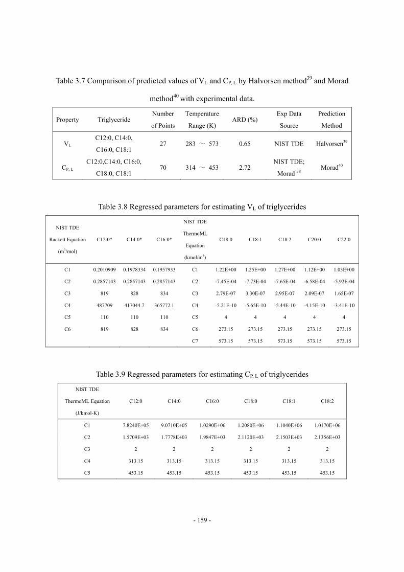
- 159 -
Table 3.7 Comparison of predicted values of VL and CP, L by Halvorsen method39 and Morad
method40 with experimental data.
Property Triglyceride Number
of Points
Temperature
Range (K) ARD (%)
Exp Data
Source
Prediction
Method
VL C12:0, C14:0,
C16:0, C18:1 27 283 ~ 573 0.65 NIST TDE Halvorsen39
CP, L C12:0,C14:0, C16:0,
C18:0, C18:1 70 314 ~ 453 2.72
NIST TDE;
Morad 38 Morad40
Table 3.8 Regressed parameters for estimating VL of triglycerides
NIST TDE
Rackett Equation
(m3/mol)
C12:0* C14:0* C16:0*
NIST TDE
ThermoML
Equation
(kmol/m3)
C18:0 C18:1 C18:2 C20:0 C22:0
C1 0.2010909 0.1978334 0.1957933 C1 1.22E+00 1.25E+00 1.27E+00 1.12E+00 1.03E+00
C2 0.2857143 0.2857143 0.2857143 C2 -7.45E-04 -7.73E-04 -7.65E-04 -6.58E-04 -5.92E-04
C3 819 828 834 C3 2.79E-07 3.30E-07 2.95E-07 2.09E-07 1.65E-07
C4 487709 417044.7 365772.1 C4 -5.21E-10 -5.65E-10 -5.44E-10 -4.15E-10 -3.41E-10
C5 110 110 110 C5 4 4 4 4 4
C6 819 828 834 C6 273.15 273.15 273.15 273.15 273.15
C7 573.15 573.15 573.15 573.15 573.15
Table 3.9 Regressed parameters for estimating CP, L of triglycerides
NIST TDE
ThermoML Equation
(J/kmol-K)
C12:0 C14:0 C16:0 C18:0 C18:1 C18:2
C1 7.8240E+05 9.0710E+05 1.0290E+06 1.2080E+06 1.1040E+06 1.0170E+06
C2 1.5709E+03 1.7778E+03 1.9847E+03 2.1120E+03 2.1503E+03 2.1356E+03
C3 2 2 2 2 2 2
C4 313.15 313.15 313.15 313.15 313.15 313.15
C5 453.15 453.15 453.15 453.15 453.15 453.15
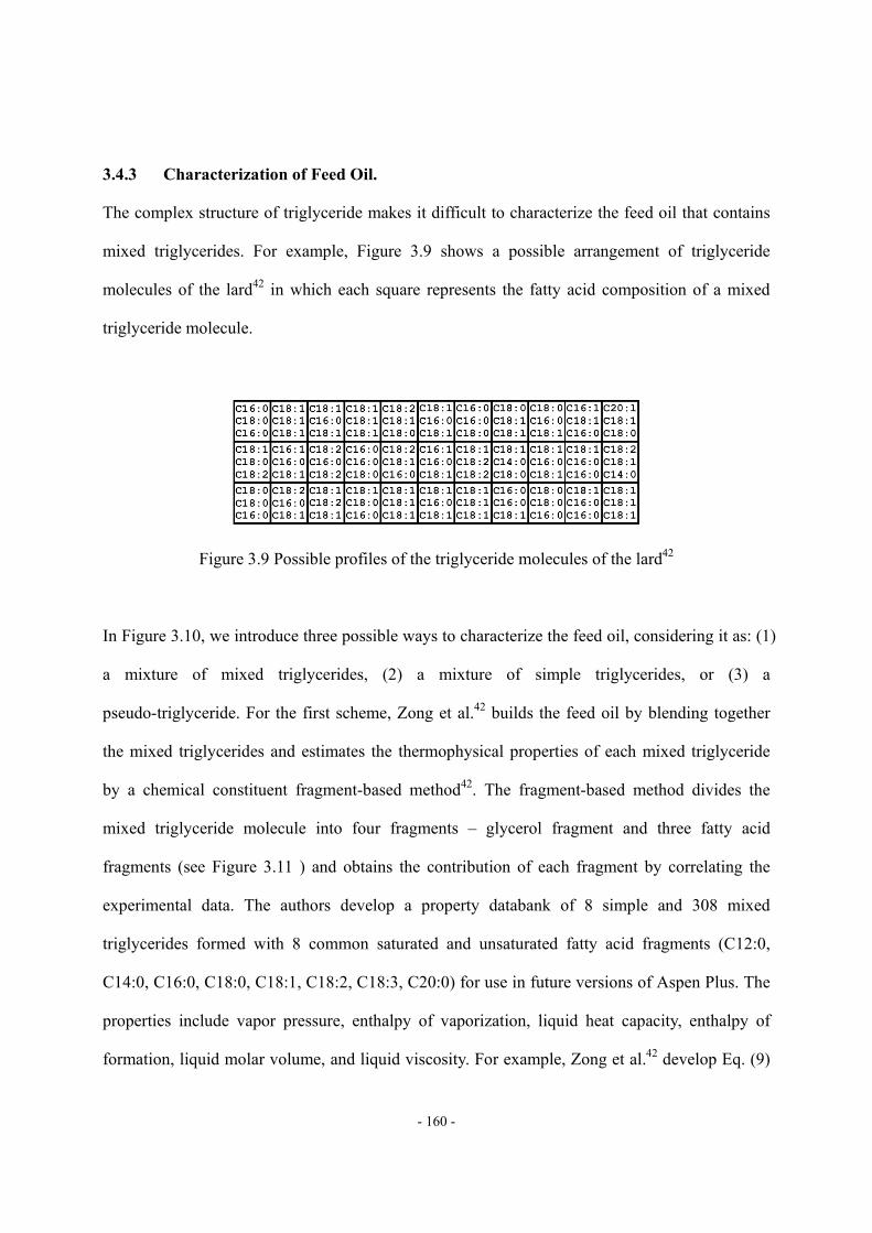
- 160 -
3.4.3 Characterization of Feed Oil.
The complex structure of triglyceride makes it difficult to characterize the feed oil that contains
mixed triglycerides. For example, Figure 3.9 shows a possible arrangement of triglyceride
molecules of the lard42 in which each square represents the fatty acid composition of a mixed
triglyceride molecule.
Figure 3.9 Possible profiles of the triglyceride molecules of the lard42
In Figure 3.10, we introduce three possible ways to characterize the feed oil, considering it as: (1)
a mixture of mixed triglycerides, (2) a mixture of simple triglycerides, or (3) a
pseudo-triglyceride. For the first scheme, Zong et al.42 builds the feed oil by blending together
the mixed triglycerides and estimates the thermophysical properties of each mixed triglyceride
by a chemical constituent fragment-based method42. The fragment-based method divides the
mixed triglyceride molecule into four fragments – glycerol fragment and three fatty acid
fragments (see Figure 3.11 ) and obtains the contribution of each fragment by correlating the
experimental data. The authors develop a property databank of 8 simple and 308 mixed
triglycerides formed with 8 common saturated and unsaturated fatty acid fragments (C12:0,
C14:0, C16:0, C18:0, C18:1, C18:2, C18:3, C20:0) for use in future versions of Aspen Plus. The
properties include vapor pressure, enthalpy of vaporization, liquid heat capacity, enthalpy of
formation, liquid molar volume, and liquid viscosity. For example, Zong et al.42 develop Eq. (9)
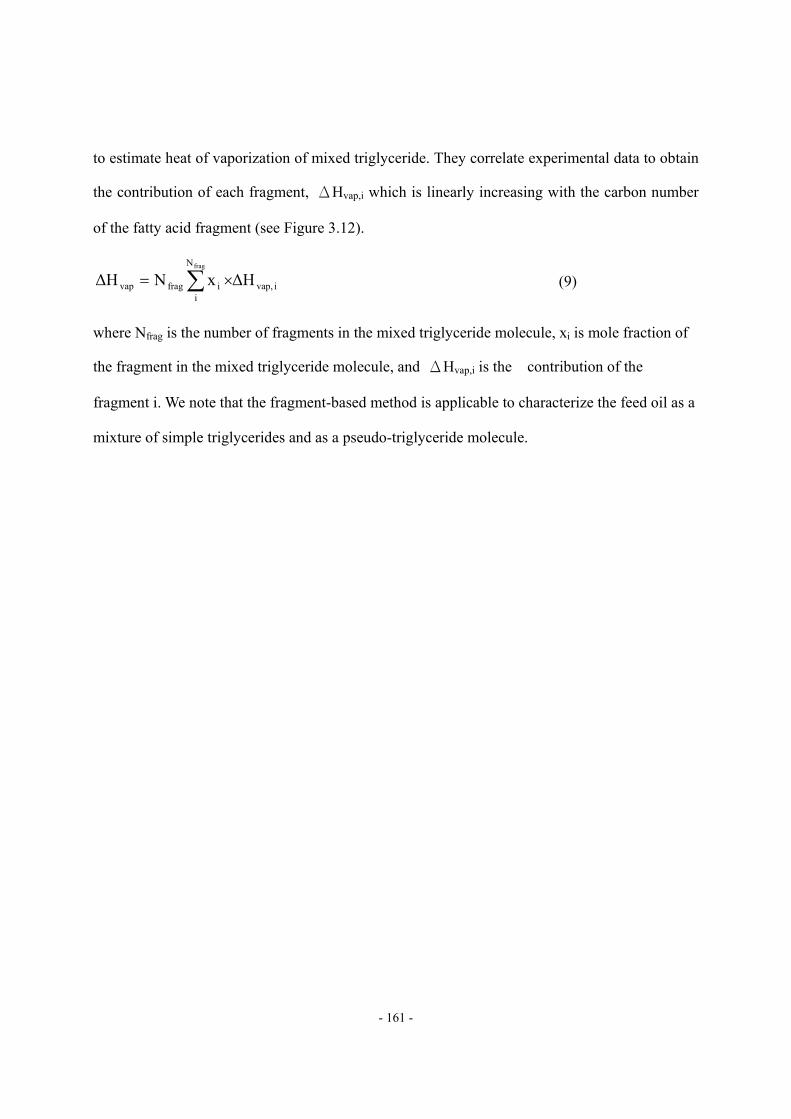
- 161 -
to estimate heat of vaporization of mixed triglyceride. They correlate experimental data to obtain
the contribution of each fragment, ΔHvap,i which is linearly increasing with the carbon number
of the fatty acid fragment (see Figure 3.12).
i vap,
N
iifragvap ΔHxNΔH
frag
∑ ×= (9)
where Nfrag is the number of fragments in the mixed triglyceride molecule, xi is mole fraction of
the fragment in the mixed triglyceride molecule, and ΔHvap,i is the contribution of the
fragment i. We note that the fragment-based method is applicable to characterize the feed oil as a
mixture of simple triglycerides and as a pseudo-triglyceride molecule.
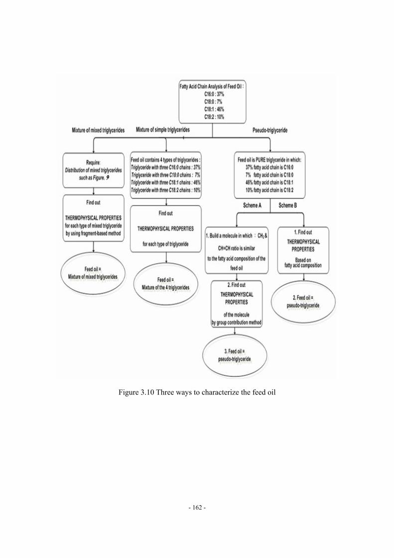
- 162 -
Figure 3.10 Three ways to characterize the feed oil

- 163 -
Figure 3.11 Four fragments of mixed triglyceride molecule42
Figure 3.12 ΔHvap,i vs. carbon number of the fatty acid fragment42
Siang et al.45 model the phase behavior of palm oil by treating the oil as a mixture of simple
triglycerides. They use Dohrn method38 to estimate the critical properties of simple triglycerides
and represent the feed oil by mixing the simple triglycerides based on the fatty acid composition.
Both Ndiaye et al.46 and Espinosa et al.47 apply the pseudo-triglyceride scheme to represent the
feed oil in their phase-equilibrium study. They estimate the critical properties by building a
molecule that has a similar distribution of the functional groups to the feed oil (i.e. scheme A of
- 164 -
pseudo-triglyceride in Figure 3.10). Scheme B of pseudo-triglyceride in Figure 3.10 is identical
to the Halvorsen method39 and Morad method40 for characterizing the oil molecules. Halvorsen et
al.39 validate the method is good for density predictions of 14 vegetable oils and Morad et al.40
validate the method is good for liquid heat capacity predictions of 2 vegetable oils and 6 mixed
triglycerides. We show an example to demonstrate the scheme A of pseudo-triglyceride in Figure
3.10. Table 3.10 shows the fatty acid composition of a given vegetable oil47.
Table 3.10 Composition of feed oil as an example for scheme A of pseudo-triglyceride in
Figure 3.10
Fatty acidxi
mol fraction
ni
number of CH2 group
mi
number of CH= CH group
C16:0 0.067 42 0
C18:0 0.0334 48 0
C18:1 0.2583 42 3
C18:2 0.6391 36 6
C18:3 0.0022 30 9
We calculate the average numbers of CH2 (n) and CH=CH (m) groups in the pseudo-triglyceride
molecule as follows:
54.63xmm
3838.34xnn
iii
iii
≈=×=
≈=×=
∑
∑ (10)
Hence, we could represent the pseudo-triglyceride molecule with 38 CH2 groups and 5 CH=CH
groups in Figure 3.13 .
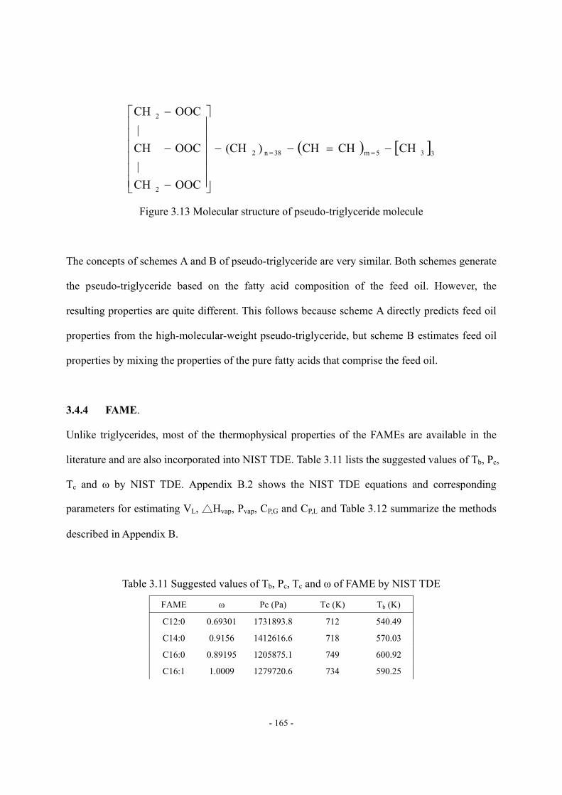
- 165 -
( ) [ ]335m38n2
2
2
CHCHCH)(CH
OOCCH |
OOC CH |
OOCCH
−=−−
⎥⎥⎥⎥⎥⎥
⎦
⎤
⎢⎢⎢⎢⎢⎢
⎣
⎡
−
−
−
==
Figure 3.13 Molecular structure of pseudo-triglyceride molecule
The concepts of schemes A and B of pseudo-triglyceride are very similar. Both schemes generate
the pseudo-triglyceride based on the fatty acid composition of the feed oil. However, the
resulting properties are quite different. This follows because scheme A directly predicts feed oil
properties from the high-molecular-weight pseudo-triglyceride, but scheme B estimates feed oil
properties by mixing the properties of the pure fatty acids that comprise the feed oil.
3.4.4 FAME.
Unlike triglycerides, most of the thermophysical properties of the FAMEs are available in the
literature and are also incorporated into NIST TDE. Table 3.11 lists the suggested values of Tb, Pc,
Tc and ω by NIST TDE. Appendix B.2 shows the NIST TDE equations and corresponding
parameters for estimating VL, Hvap, Pvap, CP,G and CP,L and Table 3.12 summarize the methods
described in Appendix B.
Table 3.11 Suggested values of Tb, Pc, Tc and ω of FAME by NIST TDE
FAME ω Pc (Pa) Tc (K) Tb (K)
C12:0 0.69301 1731893.8 712 540.49
C14:0 0.9156 1412616.6 718 570.03
C16:0 0.89195 1205875.1 749 600.92
C16:1 1.0009 1279720.6 734 590.25
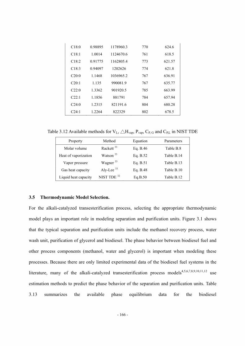
- 166 -
C18:0 0.98895 1178960.3 770 624.6
C18:1 1.0014 1124670.6 761 618.5
C18:2 0.91775 1162805.4 773 621.57
C18:3 0.94097 1202626 774 621.8
C20:0 1.1468 1036965.2 767 636.91
C20:1 1.135 990081.9 767 635.77
C22:0 1.3362 901920.5 785 663.99
C22:1 1.1856 881791 784 657.94
C24:0 1.2315 821191.6 804 680.28
C24:1 1.2264 822329 802 678.5
Table 3.12 Available methods for VL, Hvap, Pvap, CP, G and CP,L in NIST TDE
Property Method Equation Parameters
Molar volume Rackett 33 Eq. B.46 Table B.8
Heat of vaporization Watson 33 Eq. B.52 Table B.14
Vapor pressure Wagner 33 Eq. B.51 Table B.13
Gas heat capacity Aly-Lee 33 Eq. B.48 Table B.10
Liquid heat capacity NIST TDE 32 Eq.B.50 Table B.12
3.5 Thermodynamic Model Selection.
For the alkali-catalyzed transesterification process, selecting the appropriate thermodynamic
model plays an important role in modeling separation and purification units. Figure 3.1 shows
that the typical separation and purification units include the methanol recovery process, water
wash unit, purification of glycerol and biodiesel. The phase behavior between biodiesel fuel and
other process components (methanol, water and glycerol) is important when modeling these
processes. Because there are only limited experimental data of the biodiesel fuel systems in the
literature, many of the alkali-catalyzed transesterification process models4,5,6,7,8,9,10,11,12 use
estimation methods to predict the phase behavior of the separation and purification units. Table
3.13 summarizes the available phase equilibrium data for the biodiesel
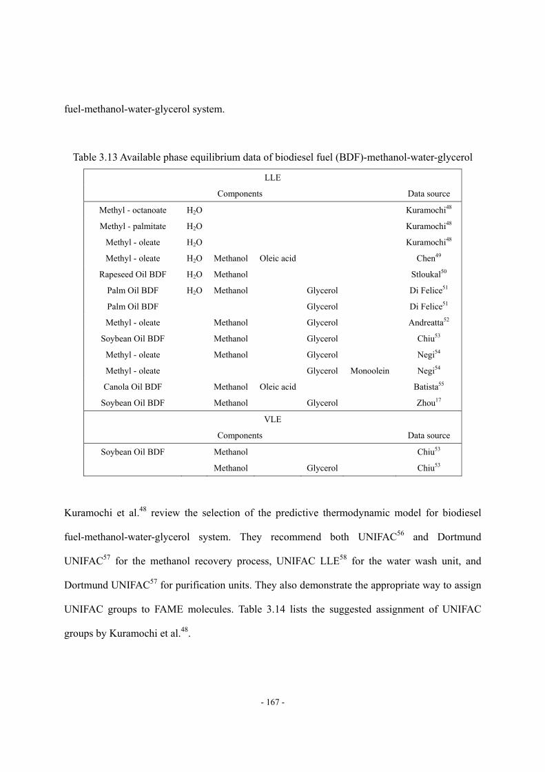
- 167 -
fuel-methanol-water-glycerol system.
Table 3.13 Available phase equilibrium data of biodiesel fuel (BDF)-methanol-water-glycerol
LLE
Components Data source
Methyl - octanoate H2O Kuramochi48
Methyl - palmitate H2O Kuramochi48
Methyl - oleate H2O Kuramochi48
Methyl - oleate H2O Methanol Oleic acid Chen49
Rapeseed Oil BDF H2O Methanol Stloukal50
Palm Oil BDF H2O Methanol Glycerol Di Felice51
Palm Oil BDF Glycerol Di Felice51
Methyl - oleate Methanol Glycerol Andreatta52
Soybean Oil BDF Methanol Glycerol Chiu53
Methyl - oleate Methanol Glycerol Negi54
Methyl - oleate Glycerol Monoolein Negi54
Canola Oil BDF Methanol Oleic acid Batista55
Soybean Oil BDF Methanol Glycerol Zhou17
VLE
Components Data source
Soybean Oil BDF Methanol Chiu53
Methanol Glycerol Chiu53
Kuramochi et al.48 review the selection of the predictive thermodynamic model for biodiesel
fuel-methanol-water-glycerol system. They recommend both UNIFAC56 and Dortmund
UNIFAC57 for the methanol recovery process, UNIFAC LLE58 for the water wash unit, and
Dortmund UNIFAC57 for purification units. They also demonstrate the appropriate way to assign
UNIFAC groups to FAME molecules. Table 3.14 lists the suggested assignment of UNIFAC
groups by Kuramochi et al.48.
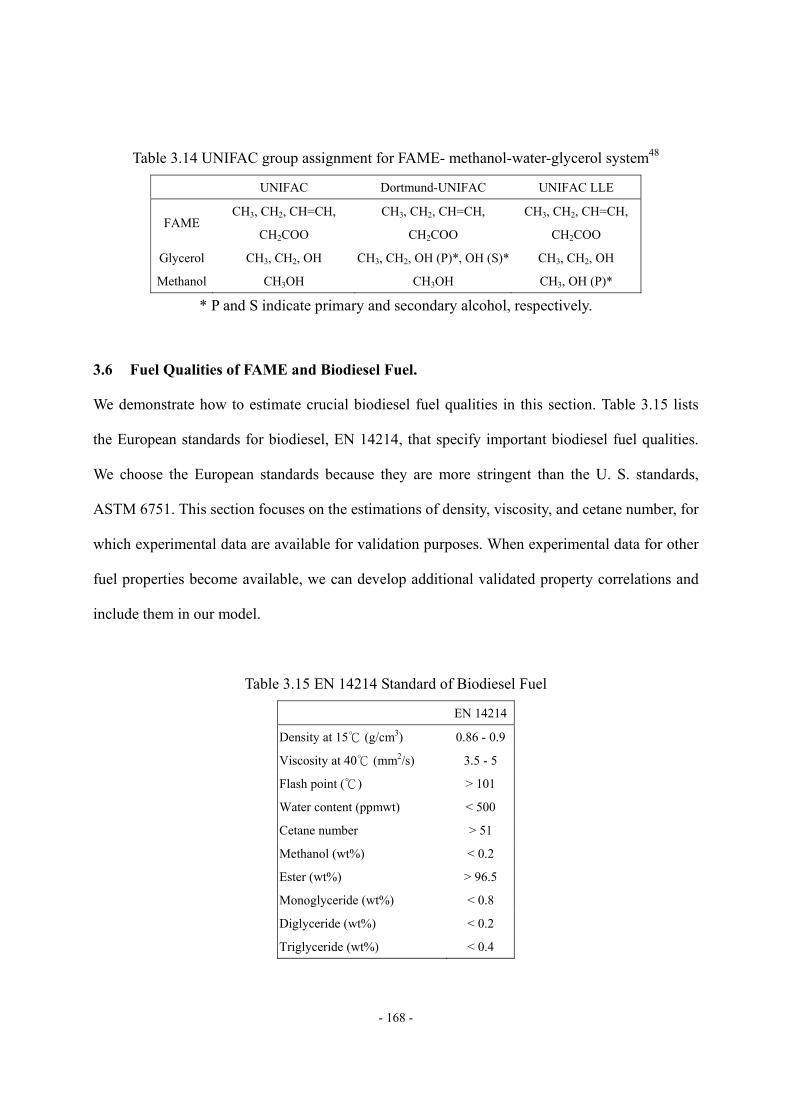
- 168 -
Table 3.14 UNIFAC group assignment for FAME- methanol-water-glycerol system48
UNIFAC Dortmund-UNIFAC UNIFAC LLE
FAME CH3, CH2, CH=CH,
CH2COO
CH3, CH2, CH=CH,
CH2COO
CH3, CH2, CH=CH,
CH2COO
Glycerol CH3, CH2, OH CH3, CH2, OH (P)*, OH (S)* CH3, CH2, OH
Methanol CH3OH CH3OH CH3, OH (P)*
* P and S indicate primary and secondary alcohol, respectively.
3.6 Fuel Qualities of FAME and Biodiesel Fuel.
We demonstrate how to estimate crucial biodiesel fuel qualities in this section. Table 3.15 lists
the European standards for biodiesel, EN 14214, that specify important biodiesel fuel qualities.
We choose the European standards because they are more stringent than the U. S. standards,
ASTM 6751. This section focuses on the estimations of density, viscosity, and cetane number, for
which experimental data are available for validation purposes. When experimental data for other
fuel properties become available, we can develop additional validated property correlations and
include them in our model.
Table 3.15 EN 14214 Standard of Biodiesel Fuel
EN 14214
Density at 15 (g/cm 3) 0.86 - 0.9
Viscosity at 40 (mm 2/s) 3.5 - 5
Flash point ( ) > 101
Water content (ppmwt) < 500
Cetane number > 51
Methanol (wt%) < 0.2
Ester (wt%) > 96.5
Monoglyceride (wt%) < 0.8
Diglyceride (wt%) < 0.2
Triglyceride (wt%) < 0.4
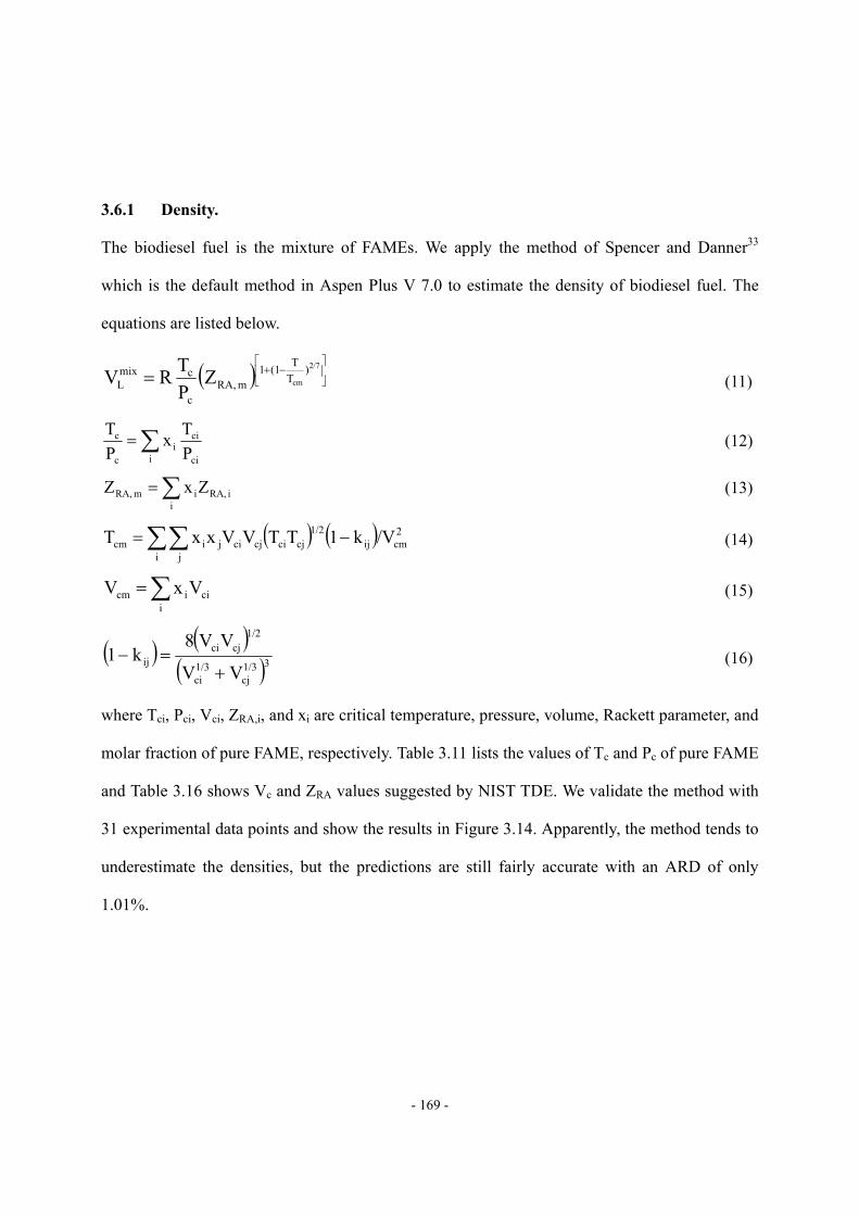
- 169 -
3.6.1 Density.
The biodiesel fuel is the mixture of FAMEs. We apply the method of Spencer and Danner33
which is the default method in Aspen Plus V 7.0 to estimate the density of biodiesel fuel. The
equations are listed below.
( ) ⎥⎦
⎤⎢⎣
⎡−+=
2/7
cm)
TT(11
m RA,c
cmixL Z
PTRV (11)
∑=i ci
cii
c
c
PTx
PT
(12)
∑=i
i RA,im RA, ZxZ (13)
( ) ( )∑∑ −=i j
2cmij
1/2cjcicjcijicm /Vk1TTVVxxT (14)
∑=i
ciicm VxV (15)
( ) ( )( )31/3
cj1/3ci
1/2cjci
ijVV
VV8k1
+=− (16)
where Tci, Pci, Vci, ZRA,i, and xi are critical temperature, pressure, volume, Rackett parameter, and
molar fraction of pure FAME, respectively. Table 3.11 lists the values of Tc and Pc of pure FAME
and Table 3.16 shows Vc and ZRA values suggested by NIST TDE. We validate the method with
31 experimental data points and show the results in Figure 3.14. Apparently, the method tends to
underestimate the densities, but the predictions are still fairly accurate with an ARD of only
1.01%.
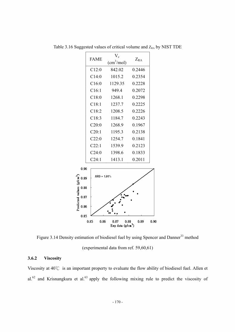
- 170 -
Table 3.16 Suggested values of critical volume and ZRA by NIST TDE
FAME Vc
(cm3/mol)ZRA
C12:0 842.02 0.2446 C14:0 1015.2 0.2354 C16:0 1129.35 0.2228 C16:1 949.4 0.2072 C18:0 1268.1 0.2298 C18:1 1237.7 0.2225 C18:2 1208.5 0.2226 C18:3 1184.7 0.2243 C20:0 1268.9 0.1967 C20:1 1195.3 0.2138 C22:0 1254.7 0.1841 C22:1 1539.9 0.2123 C24:0 1398.6 0.1833 C24:1 1413.1 0.2011
Figure 3.14 Density estimation of biodiesel fuel by using Spencer and Danner33 method
(experimental data from ref. 59,60,61)
3.6.2 Viscosity
Viscosity at 40 is an important property to evaluate the flow ability of biodiesel fuel. Allen et
al.62 and Krisnangkura et al.63 apply the following mixing rule to predict the viscosity of
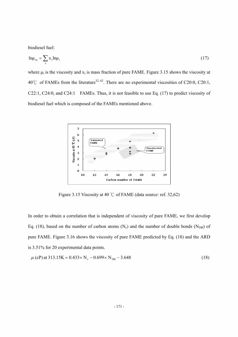
- 171 -
biodiesel fuel:
∑=x
iim lnμxlnμ (17)
where μi is the viscosity and xi is mass fraction of pure FAME. Figure 3.15 shows the viscosity at
40 of FAMEs from the literature32, 62. There are no experimental viscosities of C20:0, C20:1,
C22:1, C24:0, and C24:1 FAMEs. Thus, it is not feasible to use Eq. (17) to predict viscosity of
biodiesel fuel which is composed of the FAMEs mentioned above.
Figure 3.15 Viscosity at 40 of FAME (data source: ref. 32,62)
In order to obtain a correlation that is independent of viscosity of pure FAME, we first develop
Eq. (18), based on the number of carbon atoms (Nc) and the number of double bonds (NDB) of
pure FAME. Figure 3.16 shows the viscosity of pure FAME predicted by Eq. (18) and the ARD
is 3.51% for 20 experimental data points.
648.3N699.0N433.0313.15K at (cP) DBc −×−×=μ (18)
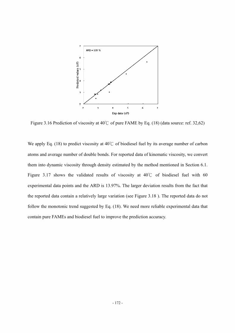
- 172 -
Figure 3.16 Prediction of viscosity at 40 of pure FAME by Eq. (18) (data source: ref. 32,62)
We apply Eq. (18) to predict viscosity at 40 of biodiesel fuel by its average number of carbon
atoms and average number of double bonds. For reported data of kinematic viscosity, we convert
them into dynamic viscosity through density estimated by the method mentioned in Section 6.1.
Figure 3.17 shows the validated results of viscosity at 40 of biodiesel fuel with 60
experimental data points and the ARD is 13.97%. The larger deviation results from the fact that
the reported data contain a relatively large variation (see Figure 3.18 ). The reported data do not
follow the monotonic trend suggested by Eq. (18). We need more reliable experimental data that
contain pure FAMEs and biodiesel fuel to improve the prediction accuracy.
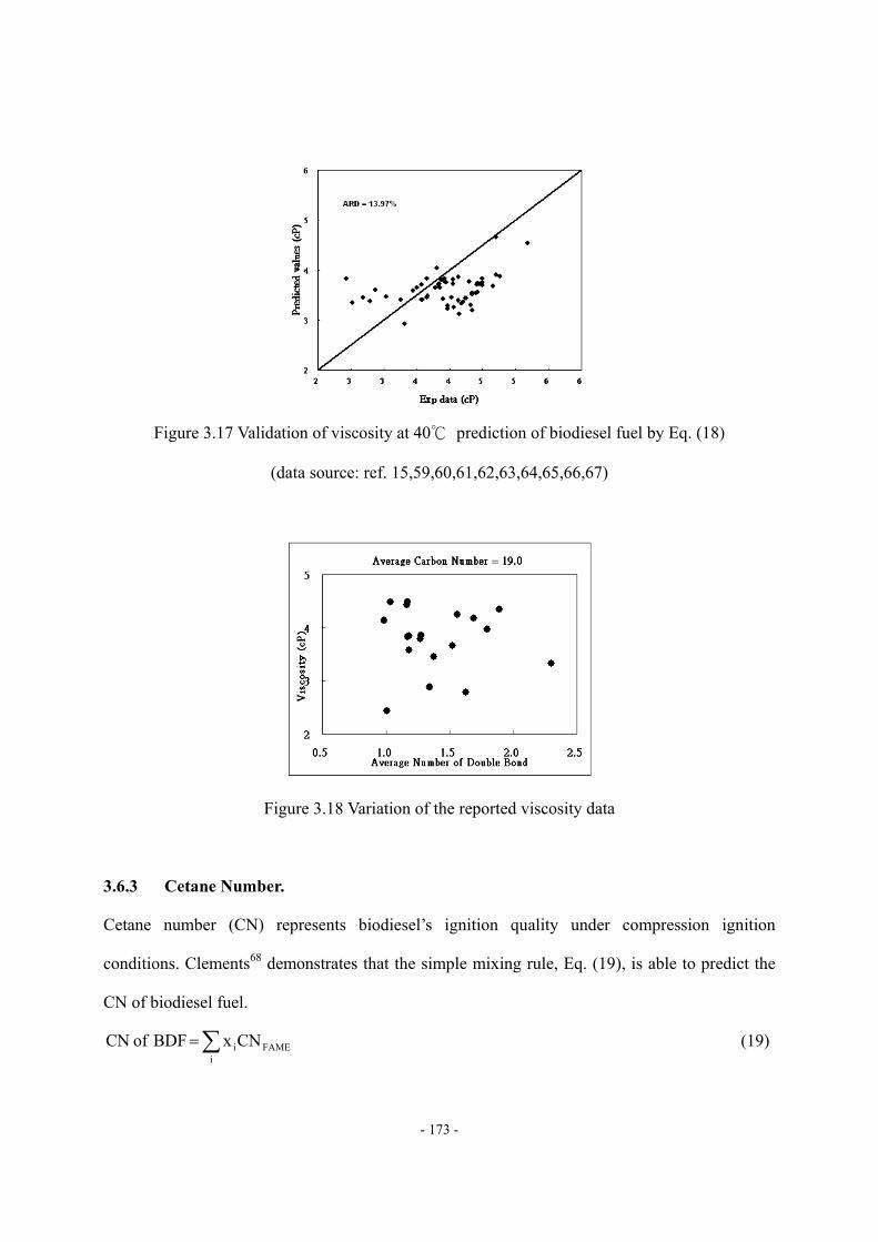
- 173 -
Figure 3.17 Validation of viscosity at 40 prediction of biodiesel fuel by Eq. (18)
(data source: ref. 15,59,60,61,62,63,64,65,66,67)
Figure 3.18 Variation of the reported viscosity data
3.6.3 Cetane Number.
Cetane number (CN) represents biodiesel’s ignition quality under compression ignition
conditions. Clements68 demonstrates that the simple mixing rule, Eq. (19), is able to predict the
CN of biodiesel fuel.
∑=i
FAMEiCNx BDF of CN (19)
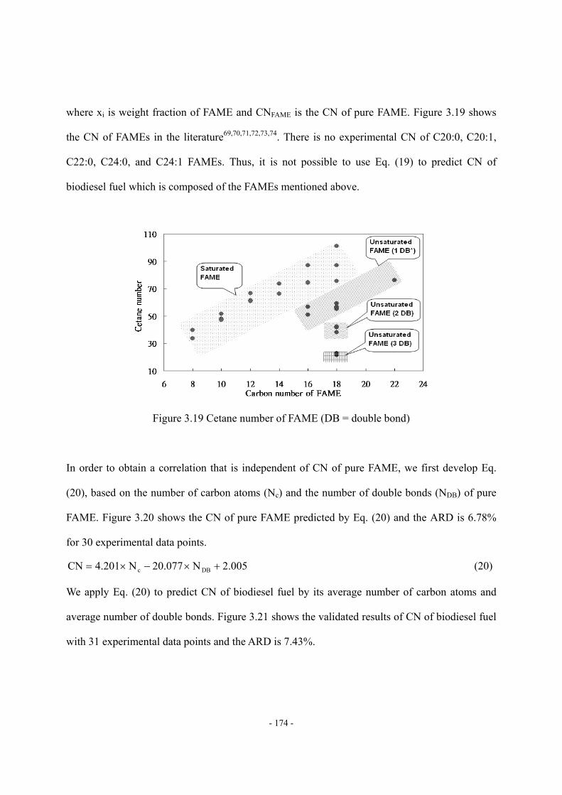
- 174 -
where xi is weight fraction of FAME and CNFAME is the CN of pure FAME. Figure 3.19 shows
the CN of FAMEs in the literature69,70,71,72,73,74. There is no experimental CN of C20:0, C20:1,
C22:0, C24:0, and C24:1 FAMEs. Thus, it is not possible to use Eq. (19) to predict CN of
biodiesel fuel which is composed of the FAMEs mentioned above.
Figure 3.19 Cetane number of FAME (DB = double bond)
In order to obtain a correlation that is independent of CN of pure FAME, we first develop Eq.
(20), based on the number of carbon atoms (Nc) and the number of double bonds (NDB) of pure
FAME. Figure 3.20 shows the CN of pure FAME predicted by Eq. (20) and the ARD is 6.78%
for 30 experimental data points.
2.005N20.077N4.201CN DBc +×−×= (20)
We apply Eq. (20) to predict CN of biodiesel fuel by its average number of carbon atoms and
average number of double bonds. Figure 3.21 shows the validated results of CN of biodiesel fuel
with 31 experimental data points and the ARD is 7.43%.
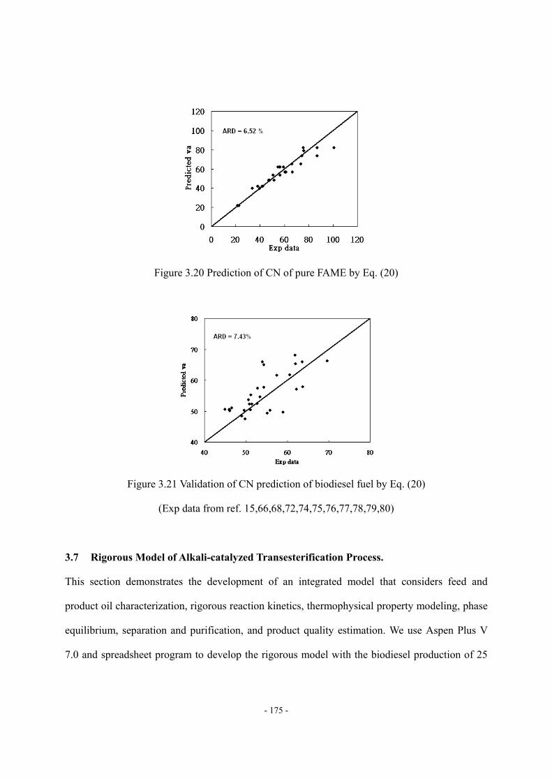
- 175 -
Figure 3.20 Prediction of CN of pure FAME by Eq. (20)
Figure 3.21 Validation of CN prediction of biodiesel fuel by Eq. (20)
(Exp data from ref. 15,66,68,72,74,75,76,77,78,79,80)
3.7 Rigorous Model of Alkali-catalyzed Transesterification Process.
This section demonstrates the development of an integrated model that considers feed and
product oil characterization, rigorous reaction kinetics, thermophysical property modeling, phase
equilibrium, separation and purification, and product quality estimation. We use Aspen Plus V
7.0 and spreadsheet program to develop the rigorous model with the biodiesel production of 25
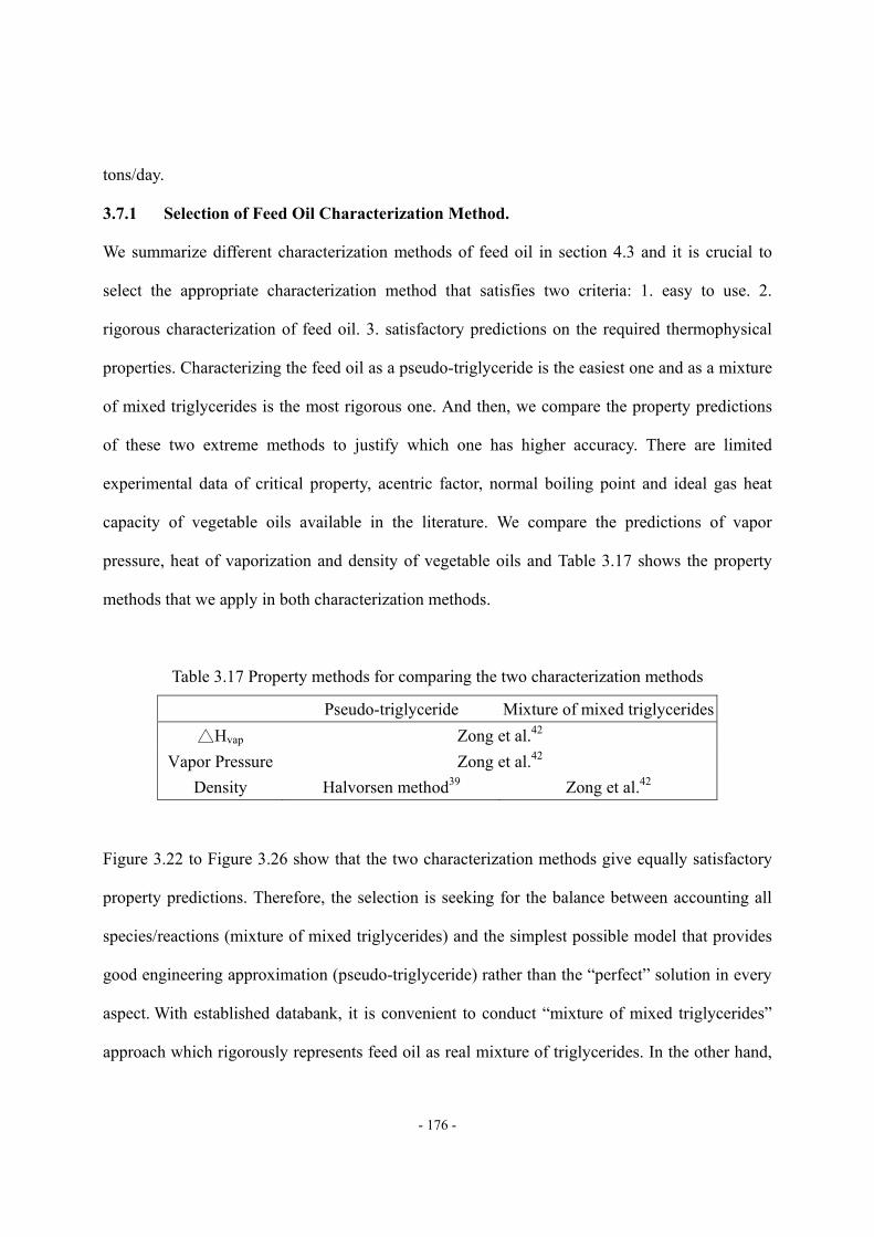
- 176 -
tons/day.
3.7.1 Selection of Feed Oil Characterization Method.
We summarize different characterization methods of feed oil in section 4.3 and it is crucial to
select the appropriate characterization method that satisfies two criteria: 1. easy to use. 2.
rigorous characterization of feed oil. 3. satisfactory predictions on the required thermophysical
properties. Characterizing the feed oil as a pseudo-triglyceride is the easiest one and as a mixture
of mixed triglycerides is the most rigorous one. And then, we compare the property predictions
of these two extreme methods to justify which one has higher accuracy. There are limited
experimental data of critical property, acentric factor, normal boiling point and ideal gas heat
capacity of vegetable oils available in the literature. We compare the predictions of vapor
pressure, heat of vaporization and density of vegetable oils and Table 3.17 shows the property
methods that we apply in both characterization methods.
Table 3.17 Property methods for comparing the two characterization methods
Pseudo-triglyceride Mixture of mixed triglycerides Hvap Zong et al.42
Vapor Pressure Zong et al.42 Density Halvorsen method39 Zong et al.42
Figure 3.22 to Figure 3.26 show that the two characterization methods give equally satisfactory
property predictions. Therefore, the selection is seeking for the balance between accounting all
species/reactions (mixture of mixed triglycerides) and the simplest possible model that provides
good engineering approximation (pseudo-triglyceride) rather than the “perfect” solution in every
aspect. With established databank, it is convenient to conduct “mixture of mixed triglycerides”
approach which rigorously represents feed oil as real mixture of triglycerides. In the other hand,
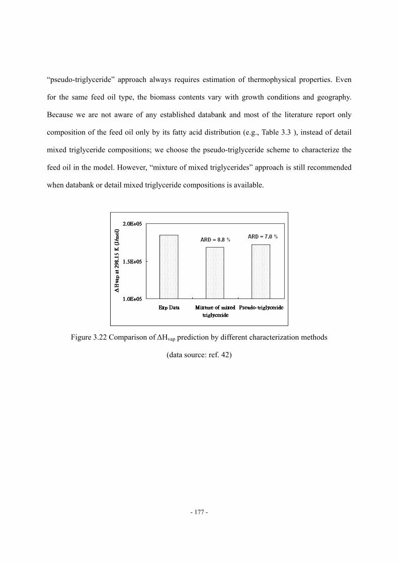
- 177 -
“pseudo-triglyceride” approach always requires estimation of thermophysical properties. Even
for the same feed oil type, the biomass contents vary with growth conditions and geography.
Because we are not aware of any established databank and most of the literature report only
composition of the feed oil only by its fatty acid distribution (e.g., Table 3.3 ), instead of detail
mixed triglyceride compositions; we choose the pseudo-triglyceride scheme to characterize the
feed oil in the model. However, “mixture of mixed triglycerides” approach is still recommended
when databank or detail mixed triglyceride compositions is available.
Figure 3.22 Comparison of ΔHvap prediction by different characterization methods
(data source: ref. 42)
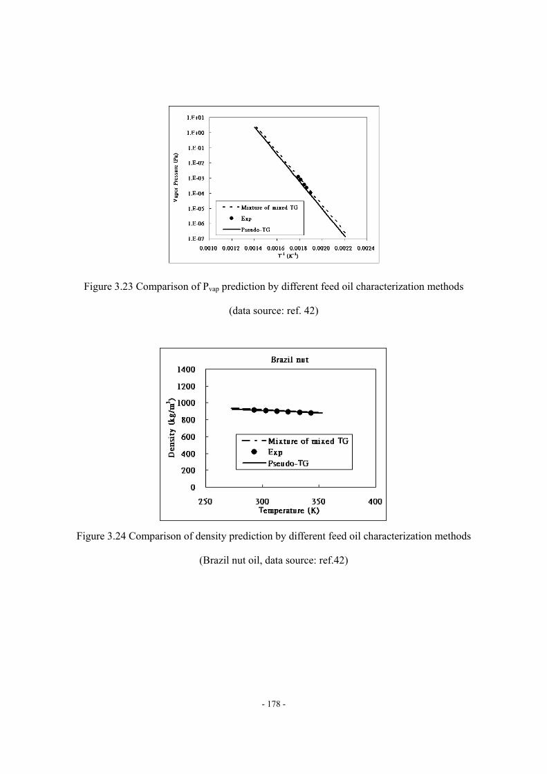
- 178 -
Figure 3.23 Comparison of Pvap prediction by different feed oil characterization methods
(data source: ref. 42)
Figure 3.24 Comparison of density prediction by different feed oil characterization methods
(Brazil nut oil, data source: ref.42)
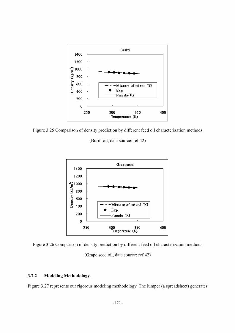
- 179 -
Figure 3.25 Comparison of density prediction by different feed oil characterization methods
(Buriti oil, data source: ref.42)
Figure 3.26 Comparison of density prediction by different feed oil characterization methods
(Grape seed oil, data source: ref.42)
3.7.2 Modeling Methodology.
Figure 3.27 represents our rigorous modeling methodology. The lumper (a spreadsheet) generates
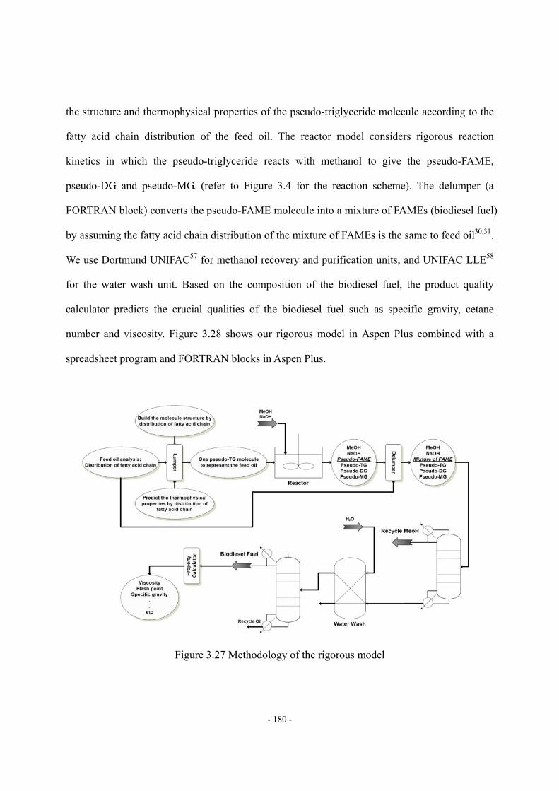
- 180 -
the structure and thermophysical properties of the pseudo-triglyceride molecule according to the
fatty acid chain distribution of the feed oil. The reactor model considers rigorous reaction
kinetics in which the pseudo-triglyceride reacts with methanol to give the pseudo-FAME,
pseudo-DG and pseudo-MG. (refer to Figure 3.4 for the reaction scheme). The delumper (a
FORTRAN block) converts the pseudo-FAME molecule into a mixture of FAMEs (biodiesel fuel)
by assuming the fatty acid chain distribution of the mixture of FAMEs is the same to feed oil30,31.
We use Dortmund UNIFAC57 for methanol recovery and purification units, and UNIFAC LLE58
for the water wash unit. Based on the composition of the biodiesel fuel, the product quality
calculator predicts the crucial qualities of the biodiesel fuel such as specific gravity, cetane
number and viscosity. Figure 3.28 shows our rigorous model in Aspen Plus combined with a
spreadsheet program and FORTRAN blocks in Aspen Plus.
Figure 3.27 Methodology of the rigorous model
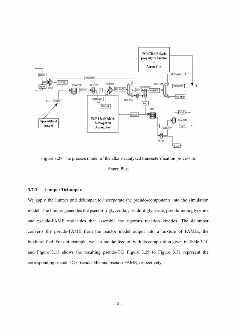
- 181 -
Figure 3.28 The process model of the alkali-catalyzed transesterification process in
Aspen Plus
3.7.3 Lumper/Delumper.
We apply the lumper and delumper to incorporate the pseudo-components into the simulation
model. The lumper generates the pseudo-triglyceride, pseudo-diglyceride, pseudo-monoglyceride
and pseudo-FAME molecules that assemble the rigorous reaction kinetics. The delumper
converts the pseudo-FAME from the reactor model output into a mixture of FAMEs, the
biodiesel fuel. For our example, we assume the feed oil with its composition given in Table 3.10
and Figure 3.13 shows the resulting pseudo-TG. Figure 3.29 to Figure 3.31 represent the
corresponding pseudo-DG, pseudo-MG and pseudo-FAME, respectively.
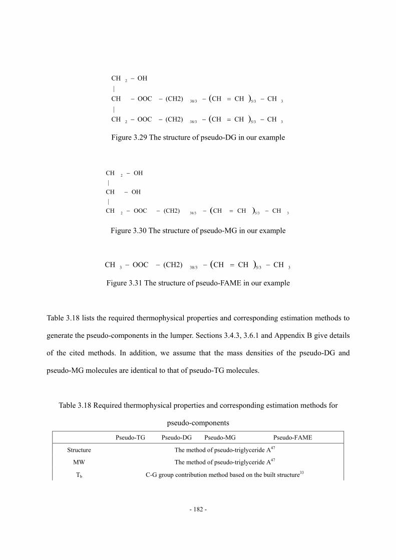
- 182 -
( )
( ) 35/338/32
35/338/3
2
CHCHCH(CH2)OOCCH |
CHCHCH(CH2)OOC CH |
OHCH
−=−−−
−=−−−
−
Figure 3.29 The structure of pseudo-DG in our example
( ) 35/338/32
2
CHCHCH(CH2)OOCCH |
OH CH |
OHCH
−=−−−
−
−
Figure 3.30 The structure of pseudo-MG in our example
( ) 35/338/33 CHCHCH(CH2)OOCCH −=−−−
Figure 3.31 The structure of pseudo-FAME in our example
Table 3.18 lists the required thermophysical properties and corresponding estimation methods to
generate the pseudo-components in the lumper. Sections 3.4.3, 3.6.1 and Appendix B give details
of the cited methods. In addition, we assume that the mass densities of the pseudo-DG and
pseudo-MG molecules are identical to that of pseudo-TG molecules.
Table 3.18 Required thermophysical properties and corresponding estimation methods for
pseudo-components
Pseudo-TG Pseudo-DG Pseudo-MG Pseudo-FAME
Structure The method of pseudo-triglyceride A47
MW The method of pseudo-triglyceride A47
Tb C-G group contribution method based on the built structure33
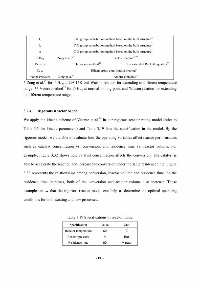
- 183 -
Tc C-G group contribution method based on the built structure33
Pc C-G group contribution method based on the built structure33
ω C-G group contribution method based on the built structure33
Hvap Zong et al.42* Vetere method33**
Density Halvorsen method39 Li's extended Rackett equation33
CP, G Rihani group contribution method81
Vapor Pressure Zong et al.42 Ambrose method33
* Zong et al.42 for Hvap at 298.15K and Watson relation for extending to different temperature range. ** Vetere method33 for Hvap at normal boiling point and Watson relation for extending to different temperature range.
3.7.4 Rigorous Reactor Model.
We apply the kinetic scheme of Vicente et al.26 in our rigorous reactor rating model (refer to
Table 3.5 for kinetic parameters) and Table 3.19 lists the specification in the model. By the
rigorous model, we are able to evaluate how the operating variables affect reactor performances
such as catalyst concentration vs. conversion, and residence time vs. reactor volume. For
example, Figure 3.32 shows how catalyst concentration affects the conversion. The catalyst is
able to accelerate the reaction and increase the conversion under the same residence time. Figure
3.33 represents the relationships among conversion, reactor volume and residence time. As the
residence time increases, both of the conversion and reactor volume also increase. These
examples show that the rigorous reactor model can help us determine the optimal operating
conditions for both existing and new processes.
Table 3.19 Specifications of reactor model
Specification Value Unit
Reactor temperature 60
Reactor pressure 4 Bar
Residence time 60 Minute
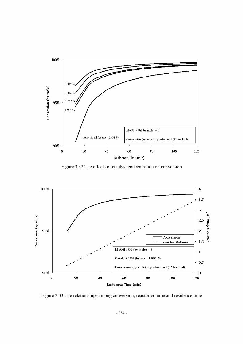
- 184 -
Figure 3.32 The effects of catalyst concentration on conversion
Figure 3.33 The relationships among conversion, reactor volume and residence time
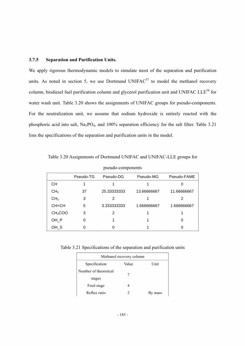
- 185 -
3.7.5 Separation and Purification Units.
We apply rigorous thermodynamic models to simulate most of the separation and purification
units. As noted in section 5, we use Dortmund UNIFAC57 to model the methanol recovery
column, biodiesel fuel purification column and glycerol purification unit and UNIFAC LLE58 for
water wash unit. Table 3.20 shows the assignments of UNIFAC groups for pseudo-components.
For the neutralization unit, we assume that sodium hydroxide is entirely reacted with the
phosphoric acid into salt, Na3PO4, and 100% separation efficiency for the salt filter. Table 3.21
lists the specifications of the separation and purification units in the model.
Table 3.20 Assignments of Dortmund UNIFAC and UNIFAC-LLE groups for
pseudo-components
Pseudo-TG Pseudo-DG Pseudo-MG Pseudo-FAME
CH 1 1 1 0
CH2 37 25.33333333 13.66666667 11.66666667
CH3 3 2 1 2
CH=CH 5 3.333333333 1.666666667 1.666666667
CH2COO 3 2 1 1
OH_P 0 1 1 0
OH_S 0 0 1 0
Table 3.21 Specifications of the separation and purification units
Methanol recovery column
Specification Value Unit
Number of theoretical
stages 7
Feed stage 4
Reflux ratio 2 By mass
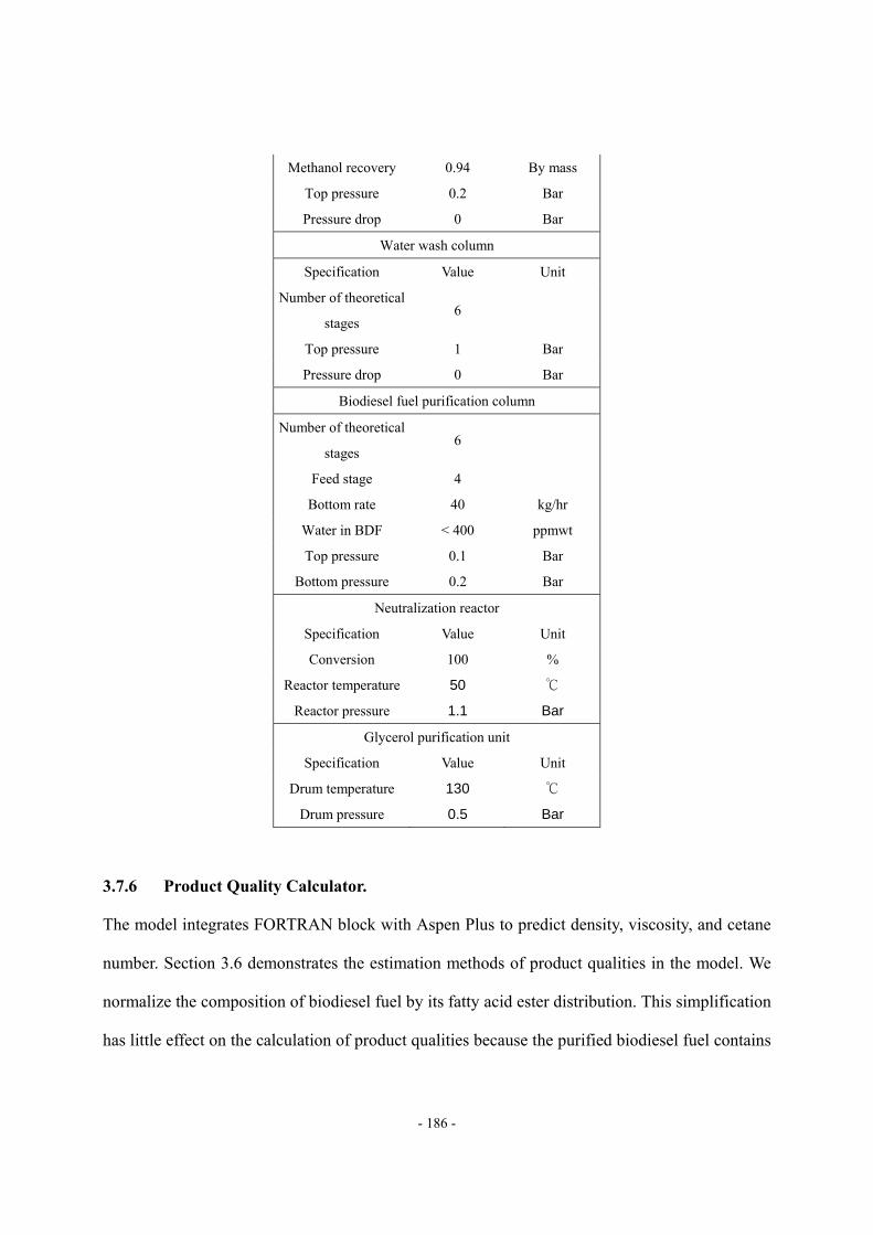
- 186 -
Methanol recovery 0.94 By mass
Top pressure 0.2 Bar
Pressure drop 0 Bar
Water wash column
Specification Value Unit
Number of theoretical
stages 6
Top pressure 1 Bar
Pressure drop 0 Bar
Biodiesel fuel purification column
Number of theoretical
stages 6
Feed stage 4
Bottom rate 40 kg/hr
Water in BDF < 400 ppmwt
Top pressure 0.1 Bar
Bottom pressure 0.2 Bar
Neutralization reactor
Specification Value Unit
Conversion 100 %
Reactor temperature 50
Reactor pressure 1.1 Bar
Glycerol purification unit
Specification Value Unit
Drum temperature 130
Drum pressure 0.5 Bar
3.7.6 Product Quality Calculator.
The model integrates FORTRAN block with Aspen Plus to predict density, viscosity, and cetane
number. Section 3.6 demonstrates the estimation methods of product qualities in the model. We
normalize the composition of biodiesel fuel by its fatty acid ester distribution. This simplification
has little effect on the calculation of product qualities because the purified biodiesel fuel contains
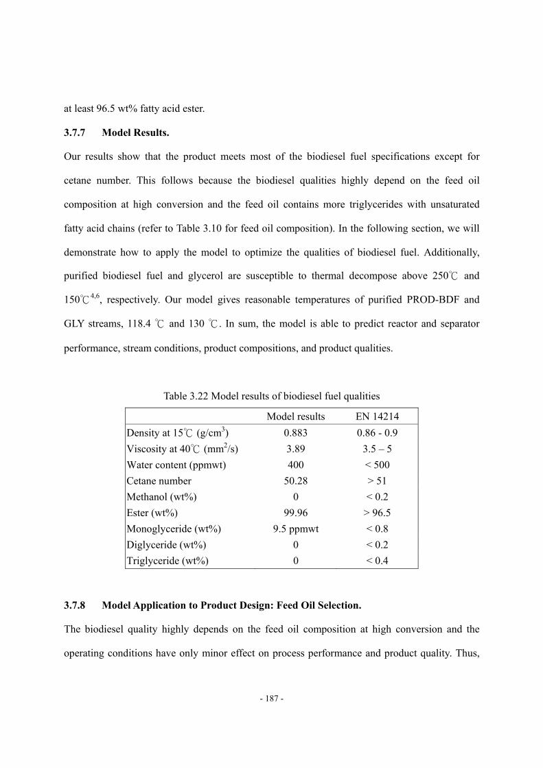
- 187 -
at least 96.5 wt% fatty acid ester.
3.7.7 Model Results.
Our results show that the product meets most of the biodiesel fuel specifications except for
cetane number. This follows because the biodiesel qualities highly depend on the feed oil
composition at high conversion and the feed oil contains more triglycerides with unsaturated
fatty acid chains (refer to Table 3.10 for feed oil composition). In the following section, we will
demonstrate how to apply the model to optimize the qualities of biodiesel fuel. Additionally,
purified biodiesel fuel and glycerol are susceptible to thermal decompose above 250 and
1504,6, respectively. Our model gives reasonable temperatures of purified PROD-BDF and
GLY streams, 118.4 and 130 . In sum, the model is able to predict reactor and separator
performance, stream conditions, product compositions, and product qualities.
Table 3.22 Model results of biodiesel fuel qualities
Model results EN 14214 Density at 15 (g/cm 3) 0.883 0.86 - 0.9 Viscosity at 40 (mm 2/s) 3.89 3.5 – 5 Water content (ppmwt) 400 < 500 Cetane number 50.28 > 51 Methanol (wt%) 0 < 0.2 Ester (wt%) 99.96 > 96.5 Monoglyceride (wt%) 9.5 ppmwt < 0.8 Diglyceride (wt%) 0 < 0.2 Triglyceride (wt%) 0 < 0.4
3.7.8 Model Application to Product Design: Feed Oil Selection.
The biodiesel quality highly depends on the feed oil composition at high conversion and the
operating conditions have only minor effect on process performance and product quality. Thus,
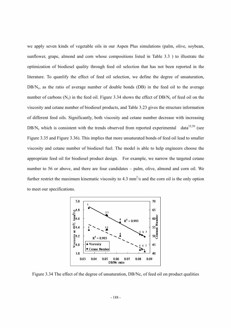
- 188 -
we apply seven kinds of vegetable oils in our Aspen Plus simulations (palm, olive, soybean,
sunflower, grape, almond and corn whose compositions listed in Table 3.3 ) to illustrate the
optimization of biodiesel quality through feed oil selection that has not been reported in the
literature. To quanlify the effect of feed oil selection, we define the degree of unsaturation,
DB/Nc, as the ratio of average number of double bonds (DB) in the feed oil to the average
number of carbons (Nc) in the feed oil. Figure 3.34 shows the effect of DB/Nc of feed oil on the
viscosity and cetane number of biodiesel products, and Table 3.23 gives the structure information
of different feed oils. Significantly, both viscosity and cetane number decrease with increasing
DB/Nc which is consistent with the trends observed from reported experimental data15,59 (see
Figure 3.35 and Figure 3.36). This implies that more unsaturated bonds of feed oil lead to smaller
viscosity and cetane number of biodiesel fuel. The model is able to help engineers choose the
appropriate feed oil for biodiesel product design. For example, we narrow the targeted cetane
number to 56 or above, and there are four candidates – palm, olive, almond and corn oil. We
further restrict the maximum kinematic viscosity to 4.3 mm2/s and the corn oil is the only option
to meet our specifications.
Figure 3.34 The effect of the degree of unsaturation, DB/Nc, of feed oil on product qualities
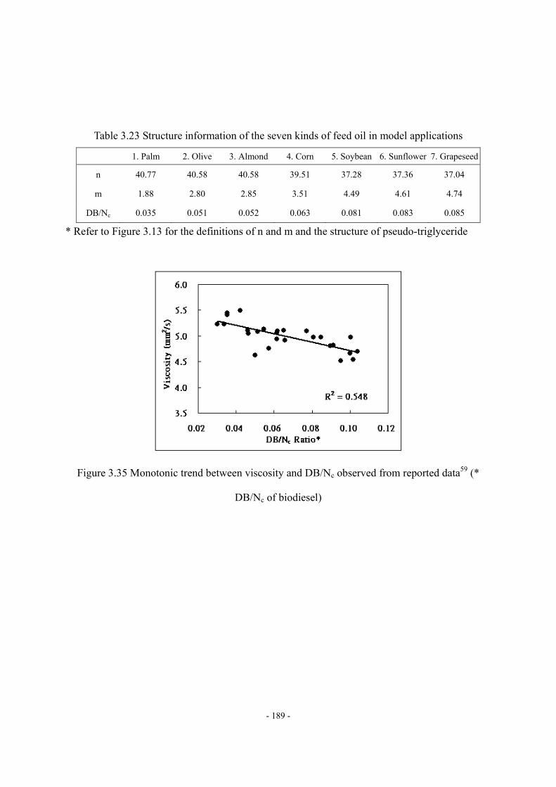
- 189 -
Table 3.23 Structure information of the seven kinds of feed oil in model applications
1. Palm 2. Olive 3. Almond 4. Corn 5. Soybean 6. Sunflower 7. Grapeseed
n 40.77 40.58 40.58 39.51 37.28 37.36 37.04
m 1.88 2.80 2.85 3.51 4.49 4.61 4.74
DB/Nc 0.035 0.051 0.052 0.063 0.081 0.083 0.085
* Refer to Figure 3.13 for the definitions of n and m and the structure of pseudo-triglyceride
Figure 3.35 Monotonic trend between viscosity and DB/Nc observed from reported data59 (*
DB/Nc of biodiesel)
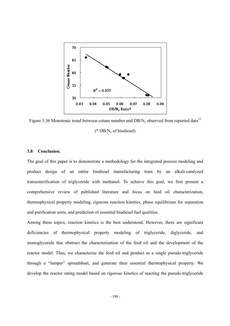
- 190 -
Figure 3.36 Monotonic trend between cetane number and DB/Nc observed from reported data15
(* DB/Nc of biodiesel)
3.8 Conclusion.
The goal of this paper is to demonstrate a methodology for the integrated process modeling and
product design of an entire biodiesel manufacturing train by an alkali-catalyzed
transesterification of triglyceride with methanol. To achieve this goal, we first present a
comprehensive review of published literature and focus on feed oil characterization,
thermophysical property modeling, rigorous reaction kinetics, phase equilibrium for separation
and purification units, and prediction of essential biodiesel fuel qualities.
Among these topics, reaction kinetics is the best understood. However, there are significant
deficiencies of thermophysical property modeling of triglyceride, diglyceride, and
monoglyceride that obstruct the characterization of the feed oil and the development of the
reactor model. Thus, we characterize the feed oil and product as a single pseudo-triglyceride
through a “lumper” spreadsheet, and generate their essential thermophysical property. We
develop the reactor rating model based on rigorous kinetics of reacting the pseudo-triglyceride
- 191 -
with methanol to produce pseudo-diglyceride (DG), pseudo-monoglyceride (MG) and
pseudo-FAME. We then convert the reactor output of pseudo-FAME molecules into a mixture of
FAMEs. i.e., biodiesel, through a FORTRAN block, called a “delumper”. Additionally, there are
only limited studies of the phase equilibrium of the biodiesel fuel-methanol-water-glycerol
system that is important for the simulation of separation and purification units. We apply
Dortmund UNIFAC57 and UNIFAC LLE58 to simulate the separation and purification units. In
order to make the modeling methodology useful to designing biodiesel product with specified
fuel properties, such as density, viscosity, and cetane number, we develop a product fuel property
calculator to predict biodiesel qualities. Throughout this development, we validate all the new
modeling tools with available experimental data, and quantify the percentage of average relative
deviation. The resulting ADR is typically less than 5%.
We then demonstrate a methodology to simulating an integrated process to predict reactor and
separator performance, stream conditions, and product qualities with different feedstocks. We
demonstrate the ease and accuracy of characterizing the feed oil as a pseudo-triglyceride, instead
as a mixture of mixed triglycerides. The results show that the modeling methodology is an
efficient tool not only for evaluating and optimizing the performance of an existing biodiesel
manufacturing, and but also for optimizing the design of a new process to produce biodiesel with
specified fuel properties.
3.9 Acknowledgements.
We thank Dr. Chau-Chyun Chen of Aspen Technology and Professor Mahmoud El-Halwagi of
Texas A and M University for their valuable review comments. We thank Alliant Techsystems
(particularly Mark Matusevich, Vice President; Charles Zisette, Director of Technology), Aspen
Technology (particularly Mark Fusco, President and CEO; Chau-Chyun Chen, Vice President of
Technology; Larry Evans, Founder; Zhiming Huang, Software Director), China Petroleum and
- 192 -
Chemical Corporation (particularly Wang Tianpu, President; Cao Xianghong, Senior Advisor;
Dai Houliang, Senior Vice President), Formosa Petrochemical Corporation (particularly Wilfred
Wang, Board Chairman), and Milliken Chemical (particularly John Rakers, President, and Jean
Hall, Business Manager) for supporting our educational programs in computer-aided design and
process system engineering at Virginia Tech.
3.10 Nomenclature
A
ARD
CN
CCAT
CP, G
CP, L
Ea
Ei
E-i
k
ki
k-i
ko
ki intrinsic
m
Nc
Pre-exponential term in Arrhenius equation, L/min-mol or L2/min-mol2 in
the studies of Vincente et al.
Average relative deviation, %
Cetane number
Catalyst concentration, mol/L
Ideal gas heat capacity, J/mol-K or J/kmol-K
Liquid heat capacity, J/mol-K or J/kmol-K
Activation Energy, cal/mol or J/mol
Forward activation Energy of reaction i, cal/mol or J/mol
Backward activation Energy of reaction i, cal/mol or J/mol
Rate constant, L/mol-min
Forward rate constant of reaction i, L/mol-min
Backward rate constant of reaction i, L/mol-min (ki / k-I represents the
thermodynamic equilibrium constant)
Rate constant at reference temperature, L/mol-min
Intrinsic rate constant in the studies of Vincente et al., L2/min-mol2
Number of CH2 group
Number of carbon atoms
- 193 -
NDB
n
Pc
Pvap
R
T
To
Tb
Tc
Tr
Vc
VL
VL, mix
VL, 20
xi
ZRA
ΔHvap
ω
ρL
μ
Number of double bonds
Number of CH=CH group
Critical pressure, Bar or Pa
Liquid vapor pressure, Bar or Pa
Universal gas constant, 1.987 cal/mol-K or 8.314 J/mol-K
Temperature, K or
Reference temperature in Arrhenius equation, K or
Normal boiling temperature, K or
Critical temperature, K or
Reduced temperature = T/Tc
Critical molar volume, m3/kmol or m3/mol
Molar volume of pure liquid, m3/kmol or m3/mol
Molar volume of liquid mixture, m3/kmol or m3/mol
Liquid molar volume at 20, m3/kmol or m3/mol
Molar fraction or mass fraction
Rackett parameter in Rackett equation
Heat of vaporization, J/mol
Acentric factor
Liquid mass density, kg/m3 or g/cm3
Kinetic viscosity, mm2/s or dynamic viscosity, cP
3.11 Literature Cited.
1. http://www.biodiesel.org/resources/definitions/default.shtm, accessed March 20, 2009.
2. Freedman, B.; Butterfield, R. O.; Pryde, E. H. “Transesterification Kinetics of Soybean
Oil,” Journal of the American Oil Chemists’ Society, 1986, 63, 1375-1380.
- 194 -
3. Fukuda, H.; Kondo, A.; Noda, H. ”Biodiesel Fuel Production by Transesterification of
Oils,” Journal of Bioscience and Bioengineering, 2001, 92, 405-416.
4. Myint, L. L.; El-Halwagi, M. M. “Process Analysis and Optimization of Biodiesel
Production from Soybead Oil,” Clean Technologies and Environmental Policy,
http://www.springerlink.com/content/m673580p1626n12w/fulltext.pdf, accessed May 20,
2009.
5. West, A. H.; Posarac, D.; Ellis, N. “Assessment of Four Biodiesel Production Processes
Using HYSYS. Plant,” Bioresource Technology, 2008, 99, 6587-6601.
6. Zhang, Y.; Dube, M. A.; McLean, D. D.; Kates, M. “Biodiesel Production from Waste
Cooking Oil: 1. Process Design and Technological Assessment,” Bioresource Technology,
2003, 89, 1-16.
7. Harding, K. G.; Dennis, J. S.; von Blottniz, H.; Harrison, S. T. L. “A Life-cycle Comparison
between Inorganic and Biological Catalysis for the Production of Biodiesel,” Journal of
Cleaner Production, 2007, 16, 1368-1378.
8. Hass, M. J.; McAloon, A. J.; Yee, W. C.; Foglia, T. A. “A Process Model to Estimate
Biodiesel Production Costs,” Bioresource Technology, 2006, 97, 671-678.
9. Tapasvi, D.; Wiesenborn, D.; Gustafson, C. “Process Model for Biodiesel Production from
Various Feedstocks,” Transactions of American Society of Agricultural Engineers, 2005, 48,
2215-2221.
10. Kapilakarn, K.; Peugtong, A. “A Comparison of Costs of Biodiesel Production from
Transesterification,” International Energy Journal, 2007, 8, 1-6.
11. Stiefel, S.; Dassori, G. “Simulation of Biodiesel Production through Transesterification of
Vegetable Oils”, Industrial and Engineering Chemistry Research, 2009, 48, 1068-1071.
12. Apostolakou, A. A.; Kookos, I. K.; Marazioti, C.; Angelopoulos, “Techno-economic
- 195 -
Analysis of a Biodiesel Production Process from Vegetable Oils”, Fuel Processing
Technology, 2009, 90, 1023-1031.
13. Tang, Z.; Du, Z.; Min, E.; Gao, L.; Jiang, T.; Han, B. “Phase Equilibria of
Methanol–Triolein System at Elevated Temperature and Pressure,” Fluid Phase Equilibria,
2006, 239, 8-11.
14. Van Gerpen, J.; Shanks, B.; Pruszko, R.; Clements, D.; Knothe, G. “Biodiesel Production
Technology,” National Renewable Energy Laboratory, Golden, CO., Report No.
NREL/SR-510-36244, 2004.
15. Ramos, M. J.; Fernandez, C. M.; Casas, A.; Rodriguez, L.; Perez, A. “Influence of Fatty
Acid Composition of Raw Materials on Biodiesel Properties,” Bioresource Technology,
2009, 100, 261-268.
16. Zhou, W.; Boocock, D. G. B. “Phase behavior of the base-catalyzed transesterification of
soybean oil,” Journal of the American Oil Chemists’ Society, 2006, 83, 1041-1045.
17. Zhou, W.; Boocock, D. G. B. “Phase Distribution of Alcohol, Glycerol, and Catalyst in the
Transesterification of Soybean Oil,” Journal of the American Oil Chemists’ Society, 2006,
83, 1047-1052.
18. Stamenkovis, O. S.; Todorovic, Z. B.; Lazic, M. L.; Veljkovic, V. B.; Skala, D. U. “Kinetics
of Sunflower Oil Methanolysis at Low Temperature,” Bioresource Technology, 2008, 99,
1131-1140.
19. Boocock, D. G. B.; Konar, S. K.; Mao, V.; Lee, C.; Buligan, S. “Fast Formation of
High-Purity Methyl Esters from Vegetable Oils,” Journal of the American Oil Chemists’
Society, 1998, 75, 1167-1172.
20. Freedman, B.; Pryde, E. H.; Mounts, T. L. “Variables Affecting the Yields of Fatty Esters
from Transesterified Vegetable Oils,” Journal of the American Oil Chemists’ Society, 1984,
- 196 -
61, 1638-1643.
21. Vicente, G.; Martinez, M.; Aracil, J.; Esteban, A. “Kinetics of Sunflower Oil Methanolysis,”
Industrial and Engineering Chemistry Research, 2005, 44, 5447-5454.
22. Noureddini, H.; Zhu, D. “Kinetics of Transesterification of Soybean Oil,” Journal of the
American Oil Chemists’ Society, 1997, 74, 1457-1463.
23. Darnoko, D.; Cheryan, M. “Kinetic of Palm Oil Transesterification in a Batch Reactor,”
Journal of the American Oil Chemists’ Society, 2000, 77, 1263-1267.
24. Leevijit, T.; Wisutmethangoon, W.; Prateepchaikul, G.; Tongurai, C.; Allen, M. “A Second
Order Kinetics of Palm Oil Transesterification,” The Joint International Conference on
Sustainable Energy and Environment, Hua Hin, Thailand, 2004. 277-281.
25. Narvaez, P. C.; Rincon, S. M.; Sanchez, F. J. “Kinetics of Palm Oil Methanolysis,” Journal
of the American Oil Chemists’ Society, 2007, 84, 971-977.
26. Vicente, G.; Martinez, M.; Aracil, J. “Kinetics of Brassica Carinata Oil Methanolysis,”
Energy and Fuels, 2006, 20, 1772-1726.
27. Bambase Jr., M. E.; Nakamura, N.; Tanaka, J.; Matsumura, M. “Kinetics of
Hydroxide-Catalyzed Methanolysis of Crude Sunflower Oil for the Production of
Fuel-Grade Methyl Esters,” Journal of Chemical Technology and Biotechnology, 2007, 82,
273-280.
28. Slinn, M.; Kendall, K. “Developing the Reaction Kinetics for a Biodiesel Reactor,”
Bioresource Technology, 2009, 100, 2324-2327.
29. Schwab, A. W.; Bagby, M. O.; Freedman, B. “Preparation and Properties of Diesel Fuels
from Vegetable Oils,” Fuel, 1987, 66, 1372-1378.
30. Wu, M.; Wu, G.; Han, Y.; Zhang, P. “Fatty Acid Composition of Six Edible Vegetable Oils
and Their Biodiesel Fuels,” China Oils and Fats, 2003, 28, 65-67.
- 197 -
31. Canakci, M.; Van Gerpen, J. “A Pilot Plant to Produce Biodiesel from High Free Fatty Acid
Feedstocks”, Transactions of ASAE, 2003, 46, 945-954.
32. National Institute of Science and Technology, ThermoData Engine, NIST TDE
(http://trc.nist.gov/tde.html)
33. Poling, B. E.; Prausnitz, J. M.; O’Connell, J. P. The Properties of Gases and Liquids, 5th ed.,
2000, McGraw Hill, New York.
34. National Institute of Science and Technology, NIST Chemistry WebBook
(http://webbook.nist.gov/chemistry/)
35. Goodrum, J. W. “Rapid Measurements of Boiling Point and Vapor Pressure of Short-Chain
Triglycerides by Thermogravimetric Analysis,” Journal of the American Oil Chemists’
Society, 1997, 74, 947-950.
36. Goodrum, J. W.; Siesel, E. M. “Thermogravimetric Analysis for Boiling Points and Vapor
Pressure,” Journal of Thermal Analysis, 1996, 46, 1251-1258.’
37. Goodrum, J. W.; Geller, D. P. “Rapid Thermogravimetric Measurements of Boiling Points
and Vapor Pressure of Saturated Medium- and Long-Chain Triglycerides,” Bioresource
Technology, 2002, 84, 75-80.
38. Dohrn, R.; Brunner, G. “An Estimation Method to Calculate Tb, Tc, Pc, and ω from the
Liquid Molar Volume and the Vapor Pressure,” Proceedings of the 3rd International
Symposium on Supercritical Fluids, Strasburg, France, 1994, 241-248.
39. Halvorsen, J.D.; Mammel, Jr W.C.; Clements , L.D. “Density Estimation for Fatty Acids
and Vegetable Oils Based on Their Fatty Acid Composition,” Journal of the American Oil
Chemists’ Society, 1993, 70, 875-880.
40. Morad, N. A.; Mustafa Kamal, M. A. A.; Panau, F.; Yew, T. W. “Liquid Specific Heat
Capacity Estimation for Fatty Acids, Triacylglycerols, and Vegetable Oils Based on Their
- 198 -
Fatty Acid Composition,” Journal of the American Oil Chemists’ Society, 2000, 77,
1001-1005.
41. Ceriani, P.; Meirelles, A. J. A. “Predicting Vapor-Liquid Equilibria of Fatty Systems,” Fluid
Phase Equilibria, 2004, 215, 227-236.
42. Zong, L.; Ramanathan, S.; Chen, C. C. “Novel Approach for Estimating Thermophysical
Properties of Fats & Vegetable Oils for Biodiesel Production Processes”, Industrial and
Engineering Chemistry Research (In Pressed)
43. Ceriani. R.; Gani, R.; Meirelles, A. J. A. “Prediction of Heat Capacities and Heats of
Vaporization of Organic Liquids by Group Contribution Methods” Fluid Phase Equilibria,
2009, 283, 49-55.
44. de la Fuente B, J. C.; Fornari, T.; Brignole, E.; Bottini, S. “Phase Equilibria in Mixtures of
Triglycerides with Low-Molecular weight alkanes,” Fluid Phase Equilibria, 1997, 128,
221-227.
45. Siang, L. C.; Manan, Z. A.; Sarmidi, M. R. “Simulation Modeling of the Phase Behaviour of
Palm Oil with Supercritical Carbon Dioxide,” Proceeding of International Conference On
Chemical and Bioprocess Engineering, 27th – 29th August 2003, Universiti Malaysia Sabah,
Kota Kinabatu, 427-434.
46. Ndiaye, P. M.; Franceschi, E.; Oliveira, D.; Dariva, C.; Tavares, F. W.; Oliveira, J. V. “Phase
Behavior of Soybean Oil, Castor Oil and Their Fatty Acid Ethyl Esters in Carbon Dioxide at
High Pressures,” Journal of Supercritical Fluids, 2006, 37, 29-37.
47. Espinosa, S.; Fornari, T.; Bottini, S. B.; Brignole, E. A. “Phase Equilibria in Mixtures of
Fatty Oils and Derivatives with Near Critical Fluids Using the GC-EOS Model,” Journal of
Supercritical Fluids, 2002, 23, 91-102.
48. Kuramochi, H.; Maeda, K.; Kato, S.; Osako, M.; Nakamura, K.; Sakai, S. “Application of
- 199 -
UNIFAC Models for Prediction of Vapor-Liquid Equilibria and Liquid-Liquid Equilibria
Relevant to Separation and Purification Processes of Crude Biodiesel Fuel,” Fuel, 2009, 88,
1472-1477.
49. Chen, F.; Sun, H.; Naka, Y.; Kawasaki, J. “Reaction and Liquid-Liquid Distribution
Equilibria in Oleic Acid/Methanol/Methyl Oleate/Water System at 73 ,” Journal of
Chemical Engineering of Japan, 2001, 34, 1479-1485.
50. Stloukal, R.; Komers, K.; Machek, J. “Ternary Phase Diagram Biodiesel
Fuel-Methanol-Water,” Journal für praktische Chemie Chemiker-Zeitung, 1997, 339,
485-487.
51. De Felice, R.; De Faveri, D.; De Andreis, P.; Ottonello, P. “Component Distribution
between Light and Heavy Phases in Biodiesel manufacturinges,” Industrial and
Engineering Chemistry Research, 2008, 47, 7862-7867.
52. Andreatta, A. E.; Casas, L. M.; Hegel, P.; Bottini, S. b.; Brignole, E. A. “Phase Equilibria in
Ternary Mixtures of Methyl Oleate, Glycerol, and Methanol,” Industrial and Engineering
Chemistry Research, 2008, 47, 5157-5164.
53. Chiu, C.; Goff, M. J.; Suppes, G. J. “Distribution of Methanol and Catalysts between
Biodiesel and Glycerin Phases,” AIChE Journal, 2005, 51, 1274-1278.
54. Negi, D. S.; Sobotka, F.; Kimmel, T.; Wozny, G.; Schomacker, R. “Liquid-Liquid Phase
Equilibrium in Glycerol-Methanol-Methyl Oleate and Glycerol- Monoolein-Methyl Oleate
Ternary Systems,” Industrial and Engineering Chemistry Research, 2006, 45, 3693-3696.
55. Batista, E.; Monnerat, S.; Kato, K.; Stragevitch, L.; Meirelles, A. J. A. “Liquid-Liquid
Equilibrium for Systems of Canola Oil Oleic Acid and Short-Chain Alcohols,” Journal of
Chemical Engineering Data, 1999, 44, 1360-1364.
56. Hansen, H. K.; Rasmussen, P.; Fredenslund, A.; Schiller, M.; Gmehling, J. “Vapor-Liquid
- 200 -
Equilibria by UNIFAC Group Contribution. 5. Revision and Extension,” Industrial and
Engineering Chemistry Research, 1991, 30, 2352-2355.
57. Gmehling, J.; Li, J.; Schiller, M. “A Modified UNIFAC model. 2. Present Parameter Matrix
and Results for Different Thermodynamic Properties,” Industrial and Engineering
Chemistry Research, 1993, 32, 178-193.
58. Magnussen, T.; Rasmussen, P.; Fredenslund, A. “UNIFAC Parameter Table for Prediction of
Liquid-Liquid Equilibriums,” Industrial and Engineering Chemistry Research, 1981, 20,
331-339.
59. Chuck, C. J.; Bannister, C. D.; Hawley, J. G.; Davidson, M. G.; Bruna, I. L.; Paine, A.
"Predictive Model to Assess the Molecular Structure of Biodiesel Fuel," Energy and Fuels,
2009, 23, 2290-2294.
60. Lang, X.; Dalai, A. K.; Bakhshi, N. N.; Reaney, M. J.; Hertz, P. B. "Preparation and
Characterization of Bio-diesel from Various Bio-oils," Bioresource Technology, 2001, 80,
53-62.
61. Benjumea, P.; Aqudelo, J.; Agudelo, A. "Basic Properties of Palm Oil Bio-diesel Blends,"
Fuel, 2008, 87, 2069-2075.
62. Allen, C. A. W.; Watts, K. C.; Ackman, R. G.; Pegg, M. J. “Predicting the viscosity of
biodiesel fuels from their fatty acid ester composition,” Fuel, 1999, 78, 1319-1326.
63. Krisnangkure, K.; Yimsuwan, T.; Pairintra, R. “An Empirical Approach in Predicting
Biodiesel Viscosity at Various Temperature,” Fuel, 2006, 85, 107-113.
64. Moser, B. R. “Influence of Blending Canola, Palm, Soybean, and Sunflower Oil Methyl
Esters on Fuel Properties of Biodiesel,” Energy and Fuels, 2008, 22, 4301-4306.
65. Demirbas, A. “Chemical and Fuel Properties of Seventeen Vegetable Oils,” Energy Sources,
2003, 25, 721-728.
- 201 -
66. Tat, M. E.; Van Gerpen, J. H. “The Specific Gravity of Biodiesel and Its Blends with Diesel
Fuel,” Journal of the American Oil Chemists’ Society, 2000, 77, 115-119.
67. Leung, D. Y. C.; Guo, Y. "Transesterification of Neat and Used Frying Oil: Optimization for
Biodiesel Production", Fuel Processing Technology, 2006, 87, 883–890.
68. Clements, L. D. “Blending Rules for Formulating Biodiesel Fuel,” Proceeding of the Third
Liquid Fuel Conference, American Society of Agricultural Engineers, Nashville, Sep. 15-17,
1996, 44053.
69. Knothe, G. “Dependence of Biodiesel Fuel Properties on the Structure of Fatty Acid Alkyl
Esters,” Fuel Processing Technology, 2005, 86, 1059-1070.
70. Freedman, B.; Bagby, M. O. “Predicting Cetane Numbers of n-Alcohols and Methyl Esters
from Their Physical Properties,” Journal of the American Oil Chemists’ Society, 1990, 67,
565-571.
71. Mccormick, R. L.; Graboski, M. S.; Alleman, T. L.; Herring, A. M.; Tyson, K. S. “Impact of
Biodiesel Source Material and Chemical Structure on Emissions of Criteria Pollutants from
a Heavy-Duty Engine,” Environmental Science and Technology, 2001, 35, 1742-1747.
72. Bamgboye, A. I.; Hansen, A. C. “Prediction of Cetane Number of Biodiesel Fuel from the
Fatty Acid Methyl Ester (FAME) Composition,” International Agrophysics, 2008, 22,
21-29.
73. Knothe, G. “Designer Biodiesel: Optimizing Fatty Ester Composition to Improve Fuel
Properties,” Energy and Fuels, 2008, 22, 1358-1364.
74. Knothe, G.; Dunn, R. O.; Bagby, M. O. “Biodiesel: The Use of Vegetable Oils and Their
Derivatives as Alternative Diesel Fuels,” ACS Symposium Series, 1997, 666, 172-208.
75. Chen, X.; Yuan, Y.; Sun, P. “Effects of Structural Features of the Fatty Acid Methyl Esters
upon the Cetane Number of Biodiesel,” Chemical Engineering of Oil and Gas, 2007, 36,
- 202 -
481-484 (in Chinese).
76. Peterson, C. L.; Taberski, J. S.; Thompson, J. C.; Chase, C. L. “The Effect of Biodiesel
Feedstock on Regulated Emissions in Chassis Dynamometer Tests of a Pickup Truck,”
Transactions of ASAE, 2000, 43, 1371-1381.
77. Yahya, A.; Marley, S. J. “Physical and Chemical Characterization of Methyl Soyoil and
Methyl Tallow Esters as CI Engine Fuels,” Biomass and Bioenergy, 1994, 6, 321-328.
78. Sinha, S.; Agarwal, A. K.; Garg, S. “Biodiesel Development from Rice Bran Oil:
Transesterification Process Optimization and Fuel Characterization,” Energy Conversion
and Management, 49, 1248-1257.
79. Chang, D. Y. Z.; Van Gerpen, J. H.; Lee, I.; Johnson, L. A.; Hammond, E. G.; Marley, S. J.
“Fuel Properties and Emissions of Soybean Oil Esters as Diesel Fuel,” Journal of the
American Oil Chemists’ Society, 1996, 73, 1549-1555.
80. Dunn, R. O.; Bagby, M. O. “Low-Temperature Properties of Triglyceride-Based Diesel
Fuels: Transesterified Methyl Esters and Petroleum Middle Distillate/Ester Blends,” Journal
of the American Oil Chemists’ Society, 1995, 72, 895-904.
81. Rihani, D. N.; Doraiswany. L. K. “Estimation of Heat Capacity of Organic Compounds
from Group Contributions,” Industrial and Engineering Chemistry Fundamentals, 1965, 4,
17-21.
82. Glisic, S.; Skala, D. “The Problems in Design and Detailed Analyses of Energy
Consumption for Biodiesel Synthesis at Supercritical Conditions”, Journal of Supercritical
Fluids, 2009, 49, 293-301.
83. Kiwjaroun, C.; Tubtimdee, C.; Piumsomboon, P. “LCA studies Comparing Biodiesel
Synthesized by Conventional and Supercritical Methanol Methods” Journal of Cleaner
Production, 2009, 17, 143-15.
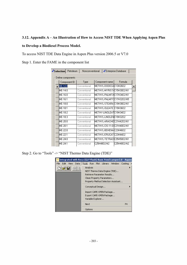
- 203 -
3.12. Appendix A – An Illustration of How to Access NIST TDE When Applying Aspen Plus
to Develop a Biodiesel Process Model.
To access NIST TDE Data Engine in Aspen Plus version 2006.5 or V7.0
Step 1. Enter the FAME in the component list
Step 2. Go to “Tools” -> “NIST Thermo Data Engine (TDE)”
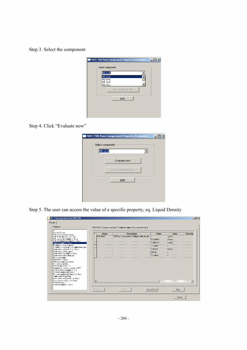
- 204 -
Step 3. Select the component
Step 4. Click “Evaluate now”
Step 5. The user can access the value of a specific property, eq. Liquid Density
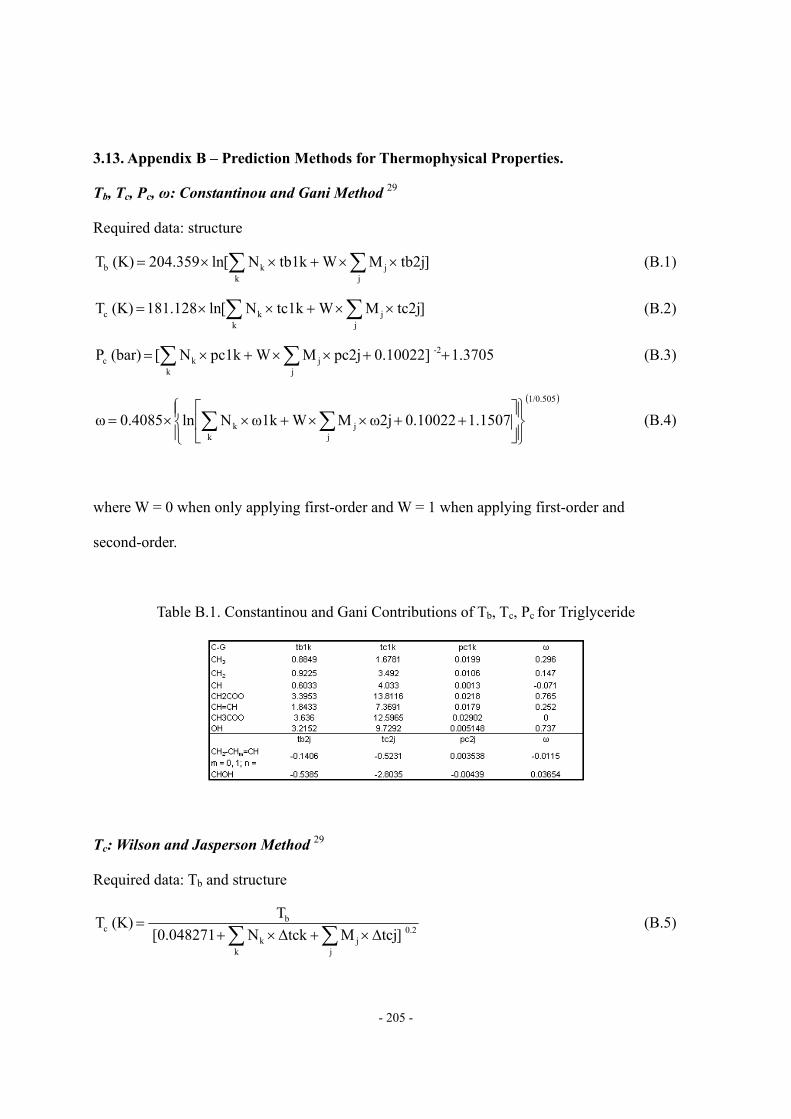
- 205 -
3.13. Appendix B – Prediction Methods for Thermophysical Properties.
Tb, Tc, Pc, ω: Constantinou and Gani Method 29
Required data: structure
]tb2jMWtb1kN[ln204.359 (K) Tj
jk
kb ∑∑ ××+××= (B.1)
]tc2jMWtc1kN[ln128.811 (K) Tj
jk
kc ∑∑ ××+××= (B.2)
3705.1 0.10022] pc2jMWpc1kN[ (bar) P -2
jj
kkc ++××+×= ∑∑ (B.3)
( )1/0.505
jj
kk 1.15070.10022 ω2jMWω1kNln0.4085 ω
⎪⎭
⎪⎬⎫
⎪⎩
⎪⎨⎧
⎥⎦
⎤⎢⎣
⎡++××+××= ∑∑ (B.4)
where W = 0 when only applying first-order and W = 1 when applying first-order and
second-order.
Table B.1. Constantinou and Gani Contributions of Tb, Tc, Pc for Triglyceride
Tc: Wilson and Jasperson Method 29
Required data: Tb and structure
0.2
jj
kk
bc ]tcjMtckN[0.048271
T (K) T∑∑ Δ×+Δ×+
= (B.5)
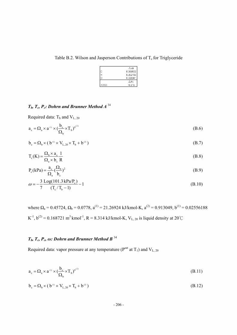
- 206 -
Table B.2. Wilson and Jasperson Contributions of Tc for Triglyceride
Tb, Tc, Pc: Dohrn and Brunner Method A 34
Required data: Tb and VL, 20
)2()1( a
bb
cac )Tb(a a ×
Ω××Ω= (B.6)
)bTVb (b (2)(1)b20 L,bc +×××Ω= (B.7)
R1
baK)(T
ca
cbc ×Ω
×Ω= (B.8)
2
c
b
a
cc )
b(akPa)(P Ω
Ω= (B.9)
1)1T/(T
)kPa/P Log(101.373
bc
c −−
−=ω (B.10)
where Ωa = 0.45724, Ωb = 0.0778, a(1) = 21.26924 kJ/kmol-K, a(2) = 0.913049, b(1) = 0.02556188
K-1, b(2) = 0.168721 m3 kmol-1, R = 8.314 kJ/kmol-K, VL, 20 is liquid density at 20
Tb, Tc, Pc, ω: Dohrn and Brunner Method B 34
Required data: vapor pressure at any temperature (Psat at T1) and VL, 20
)2()1( a
bb
cac )Tb(a a ×
Ω××Ω= (B.11)
)bTVb (b (2)(1)b20 L,bc +×××Ω= (B.12)
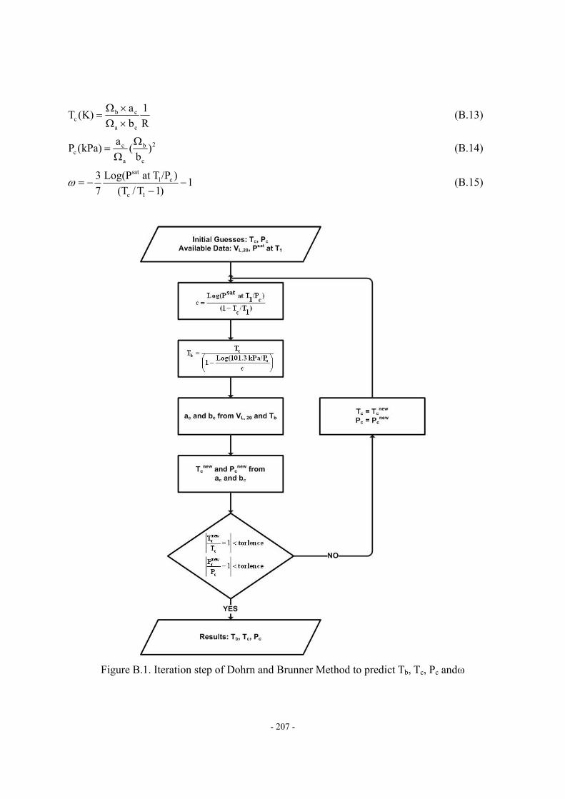
- 207 -
R1
baK)(T
ca
cbc ×Ω
×Ω= (B.13)
2
c
b
a
cc )
b(akPa)(P Ω
Ω= (B.14)
1)1T/(T
)/PTat Log(P73
1c
c1sat
−−
−=ω (B.15)
Figure B.1. Iteration step of Dohrn and Brunner Method to predict Tb, Tc, Pc andω
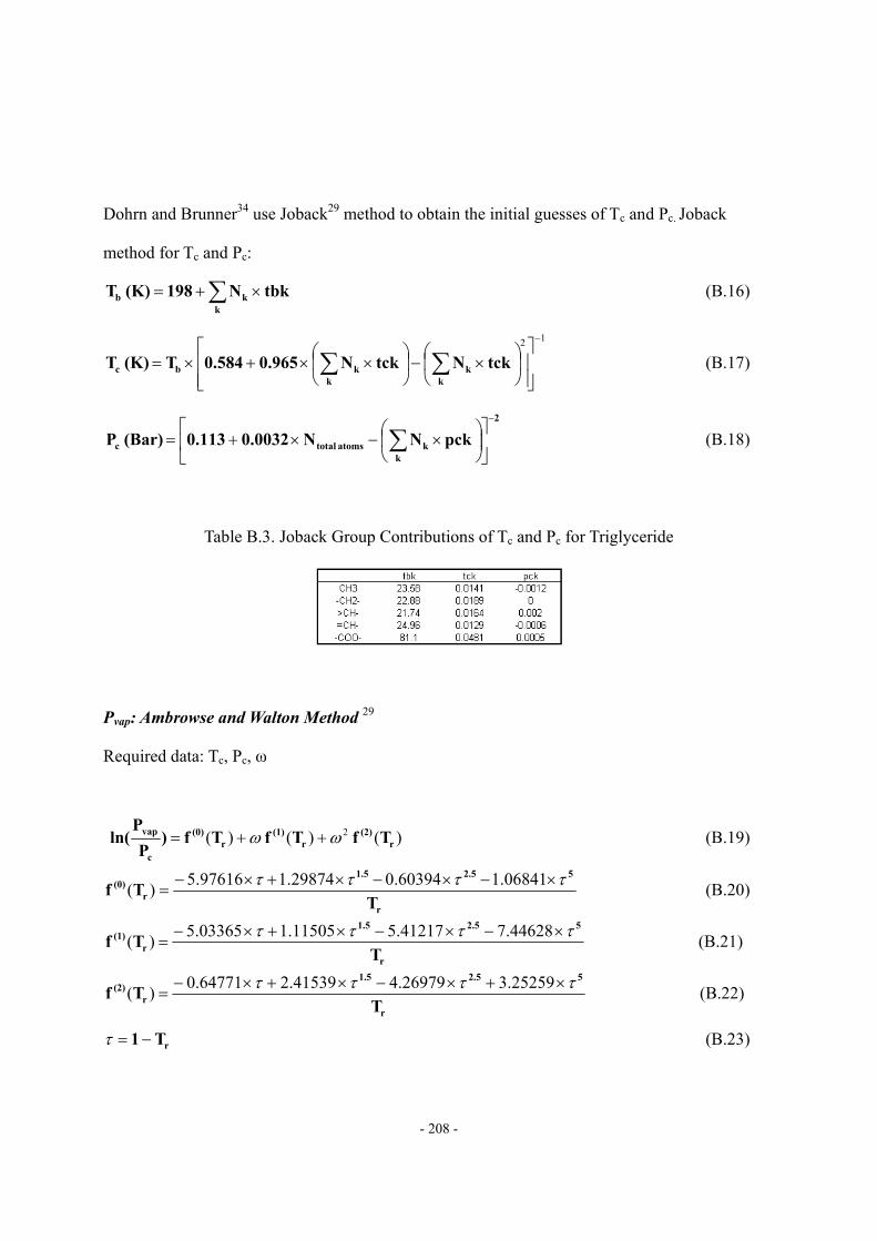
- 208 -
Dohrn and Brunner34 use Joback29 method to obtain the initial guesses of Tc and Pc. Joback
method for Tc and Pc:
tbkN198(K) Tk
kb ∑ ×+= (B.16)
12 −
⎥⎥⎦
⎤
⎢⎢⎣
⎡⎟⎠
⎞⎜⎝
⎛×−⎟
⎠
⎞⎜⎝
⎛××+×= ∑∑
kk
kkbc tckNtckN0.9650.584T (K) T (B.17)
2
kkatoms totalc pckNN0.00320.113 (Bar) P
−
⎥⎦
⎤⎢⎣
⎡⎟⎠
⎞⎜⎝
⎛×−×+= ∑ (B.18)
Table B.3. Joback Group Contributions of Tc and Pc for Triglyceride
Pvap: Ambrowse and Walton Method 29
Required data: Tc, Pc, ω
)()()( 2r
(2)r
(1)r
(0)
c
vap Tf Tf Tf)P
Pln( ωω ++= (B.19)
r
52.51.5
r(0)
TTf ττττ ×−×−×+×−
=06841.160394.029874.197616.5)( (B.20)
r
52.51.5
r(1)
TTf ττττ ×−×−×+×−
=44628.741217.511505.103365.5)( (B.21)
r
52.51.5
r(2)
TTf ττττ ×+×−×+×−
=25259.326979.441539.264771.0)( (B.22)
rT1−=τ (B.23)
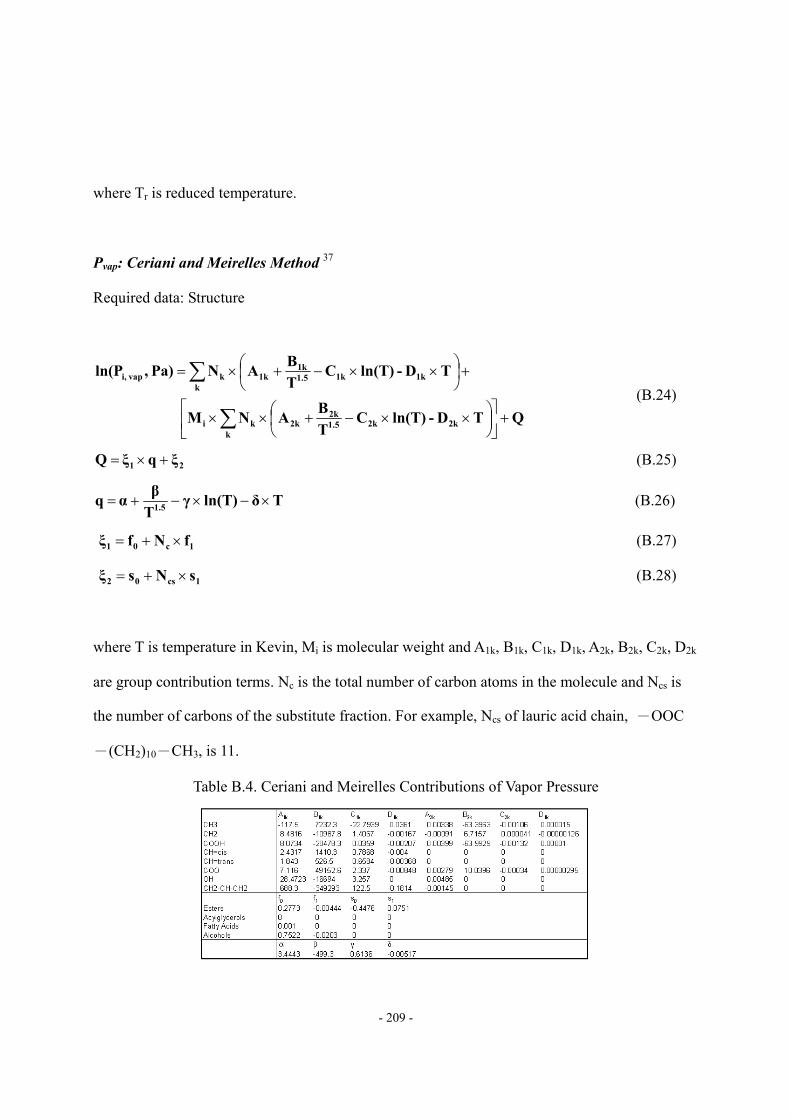
- 209 -
where Tr is reduced temperature.
Pvap: Ceriani and Meirelles Method 37
Required data: Structure
QTD-ln(T)CTBANM
TD-ln(T)CTBANPa) ,ln(P
k2k2k1.5
2k2kki
k1k1k1.5
1k1kkvap i,
+⎥⎦
⎤⎢⎣
⎡⎟⎠⎞
⎜⎝⎛ ××−+××
+⎟⎠⎞
⎜⎝⎛ ××−+×=
∑
∑ (B.24)
21 ξqξ Q +×= (B.25)
Tδln(T)γTβα q 1.5 ×−×−+= (B.26)
1c01 fNfξ ×+= (B.27)
1cs02 sNsξ ×+= (B.28)
where T is temperature in Kevin, Mi is molecular weight and A1k, B1k, C1k, D1k, A2k, B2k, C2k, D2k
are group contribution terms. Nc is the total number of carbon atoms in the molecule and Ncs is
the number of carbons of the substitute fraction. For example, Ncs of lauric acid chain, -OOC
-(CH2)10-CH3, is 11.
Table B.4. Ceriani and Meirelles Contributions of Vapor Pressure
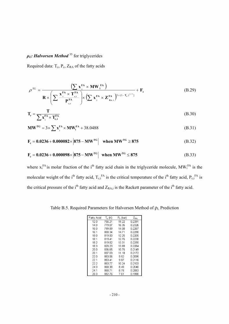
- 210 -
ρL: Halvorsen Method 35 for triglycerides
Required data: Tc, Pc, ZRA of the fatty acids
( )( )
cT FAFA
FA
FAFA
FAi
FA
F
ZxP
T xR
MWx
r
i RA,i
i c,
i c,i
i +
××⎟⎟⎠
⎞⎜⎜⎝
⎛ ××
×=
−+∑∑
∑])1(1[ 7/2
TGρ (B.29)
∑ ×= FA
i c,FAr TxTT
i
(B.30)
0488.383 +××= ∑ FAi
FATG MWxMWi
(B.31)
875MW when MW8750.0000820.0236F TGTGc ≥−×+= (B.32)
875MW when MW8750.0000980.0236F TGTGc ≤−×+= (B.33)
where xiFA is molar fraction of the ith fatty acid chain in the triglyceride molecule, MWi
FA is the
molecular weight of the ith fatty acid, Tc,iFA is the critical temperature of the ith fatty acid, Pc,i
FA is
the critical pressure of the ith fatty acid and ZRA,i is the Rackett parameter of the ith fatty acid.
Table B.5. Required Parameters for Halvorsen Method of ρL Prediction
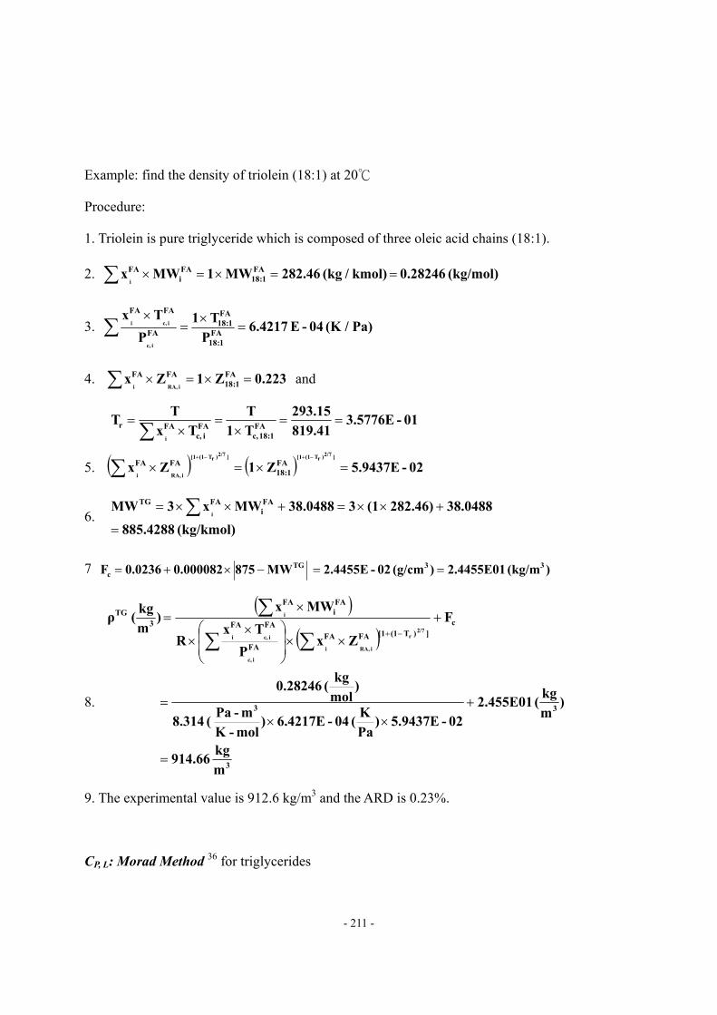
- 211 -
Example: find the density of triolein (18:1) at 20
Procedure:
1. Triolein is pure triglyceride which is composed of three oleic acid chains (18:1).
2. (kg/mol) 0.28246 kmol) /(kg 282.46MW1MWx FA1:18
FAi
FAi
==×=×∑
3. Pa) /(K 04-E 6.4217P
T 1P
T xFA
1:18
FA1:18
FA
FAFA
i c,
i c,i =×
=×
∑
4. 0.223Z1Zx FA1:18
FAFAi RA,i
=×=×∑ and
01-3.5776E819.41293.15
T1T
TxTT FA
1:18 c,FA
i c,FAri
==×
=×
=∑
5. ( ) ( ) 02-5.9437EZ1Zx ]2/7)rT (1[1]2/7)rT (1[1
i RA,i
FA1:18
FAFA =×=×−+−+
∑
6. (kg/kmol) 885.4288
38.0488282.46)(1338.0488MWx3MW FAi
FATGi
=
+××=+××= ∑
7 )(kg/m 2.4455E01)(g/cm 02-2.4455E MW8750.0000820.0236F 33TGc ==−×+=
8.
( )( )
3
33
c])T (1[1FAFA
FA
FAFA
FAi
FA
3TG
mkg 914.66
)mkg( 2.455E01
02-5.9437E)PaK( 04-6.4217E)
mol-Km-Pa ( 8.314
)molkg( 0.28246
F
ZxP
T xR
MWx )
mkg( ρ
2/7r
i RA,i
i c,
i c,i
i
=
+××
=
+
××⎟⎟⎠
⎞⎜⎜⎝
⎛ ××
×=
−+∑∑
∑
9. The experimental value is 912.6 kg/m3 and the ARD is 0.23%.
CP, L: Morad Method 36 for triglycerides
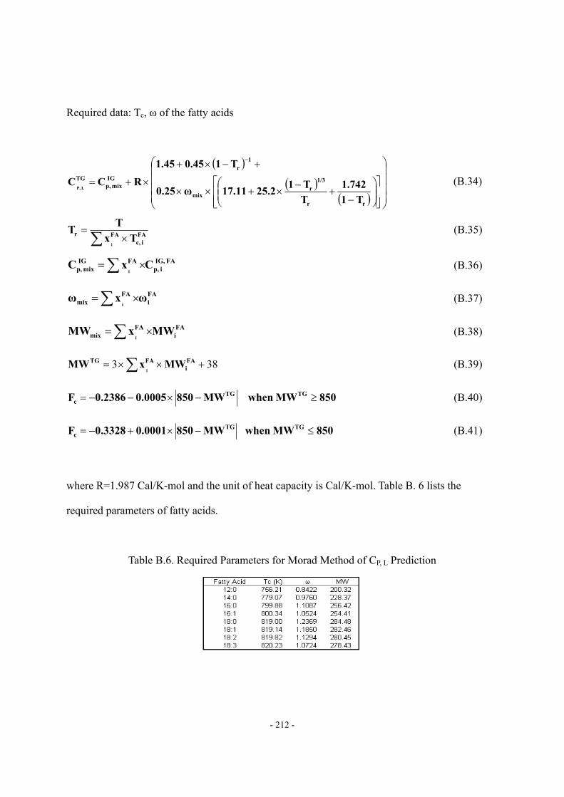
- 212 -
Required data: Tc, ω of the fatty acids
( )( )
( ) ⎟⎟⎟⎟
⎠
⎞
⎜⎜⎜⎜
⎝
⎛
⎥⎥⎦
⎤
⎢⎢⎣
⎡⎟⎟⎠
⎞⎜⎜⎝
⎛−
+−
×+××
+−×+
×+=
−
rr
1/3r
mix
1r
IG mix p,
TG
T11.742
TT125.217.11ω0.25
T10.451.45
RCCL P,
(B.34)
∑ ×= FA
i c,FAr TxTT
i
(B.35)
FA IG, i p,
FAIG mix p, CxC
i∑ ×= (B.36)
FAi
FAmix ωxω
i∑ ×= (B.37)
FAi
FAmix MWxMW
i∑ ×= (B.38)
383 +××= ∑ FAi
FATG MWxMWi
(B.39)
850MW when MW8500.00050.2386F TGTGc ≥−×−−= (B.40)
850MW when MW8500.00010.3328F TGTGc ≤−×+−= (B.41)
where R=1.987 Cal/K-mol and the unit of heat capacity is Cal/K-mol. Table B. 6 lists the
required parameters of fatty acids.
Table B.6. Required Parameters for Morad Method of CP, L Prediction
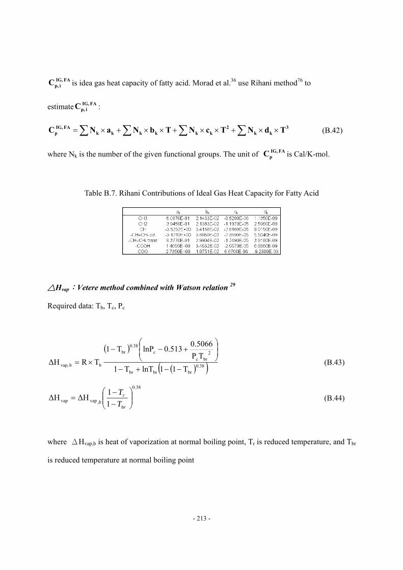
- 213 -
FA IG, i p,C is idea gas heat capacity of fatty acid. Morad et al.36 use Rihani method76 to
estimate FA IG, i p,C :
∑∑∑∑ ××+××+××+×= 3kk
2kkkkkk
FA IG, p TdNTcNTbNaNC (B.42)
where Nk is the number of the given functional groups. The unit of FA IG, pC is Cal/K-mol.
Table B.7. Rihani Contributions of Ideal Gas Heat Capacity for Fatty Acid
Hvap:Vetere method combined with Watson relation 29
Required data: Tb, Tc, Pc
( )
( )( )0.38brbrbr
2brc
c0.38
br
bb vap, T11lnTT1TP
0.50660.513lnPT1TRΔH
−−+−
⎟⎟⎠
⎞⎜⎜⎝
⎛+−−
×= (B.43)
38.0
,vapvap 11ΔHΔH ⎟⎟
⎠
⎞⎜⎜⎝
⎛−−
=br
rb T
T (B.44)
where ΔHvap,b is heat of vaporization at normal boiling point, Tr is reduced temperature, and Tbr
is reduced temperature at normal boiling point
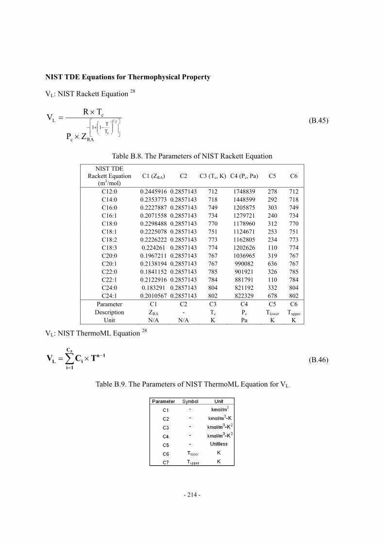
- 214 -
NIST TDE Equations for Thermophysical Property
VL: NIST Rackett Equation 28
⎥⎥
⎦
⎤
⎢⎢
⎣
⎡⎟⎟⎠
⎞⎜⎜⎝
⎛−+−
×
×=
2C
cTT11
RAc
cL
ZP
TRV (B.45)
Table B.8. The Parameters of NIST Rackett Equation NIST TDE
Rackett Equation (m3/mol)
C1 (ZRA) C2 C3 (Tc, K) C4 (Pc, Pa) C5 C6
C12:0 0.2445916 0.2857143 712 1748839 278 712 C14:0 0.2353773 0.2857143 718 1448599 292 718 C16:0 0.2227887 0.2857143 749 1205875 303 749 C16:1 0.2071558 0.2857143 734 1279721 240 734 C18:0 0.2298488 0.2857143 770 1178960 312 770 C18:1 0.2225078 0.2857143 751 1124671 253 751 C18:2 0.2226222 0.2857143 773 1162805 234 773 C18:3 0.224261 0.2857143 774 1202626 110 774 C20:0 0.1967211 0.2857143 767 1036965 319 767 C20:1 0.2138194 0.2857143 767 990082 636 767 C22:0 0.1841152 0.2857143 785 901921 326 785 C22:1 0.2122916 0.2857143 784 881791 110 784 C24:0 0.183291 0.2857143 804 821192 332 804 C24:1 0.2010567 0.2857143 802 822329 678 802
Parameter C1 C2 C3 C4 C5 C6 Description ZRA - Tc Pc Tlower Tupper
Unit N/A N/A K Pa K K
VL: NIST ThermoML Equation 28
1nC
1iiL TCV
5−
=
×=∑ (B.46)
Table B.9. The Parameters of NIST ThermoML Equation for VL
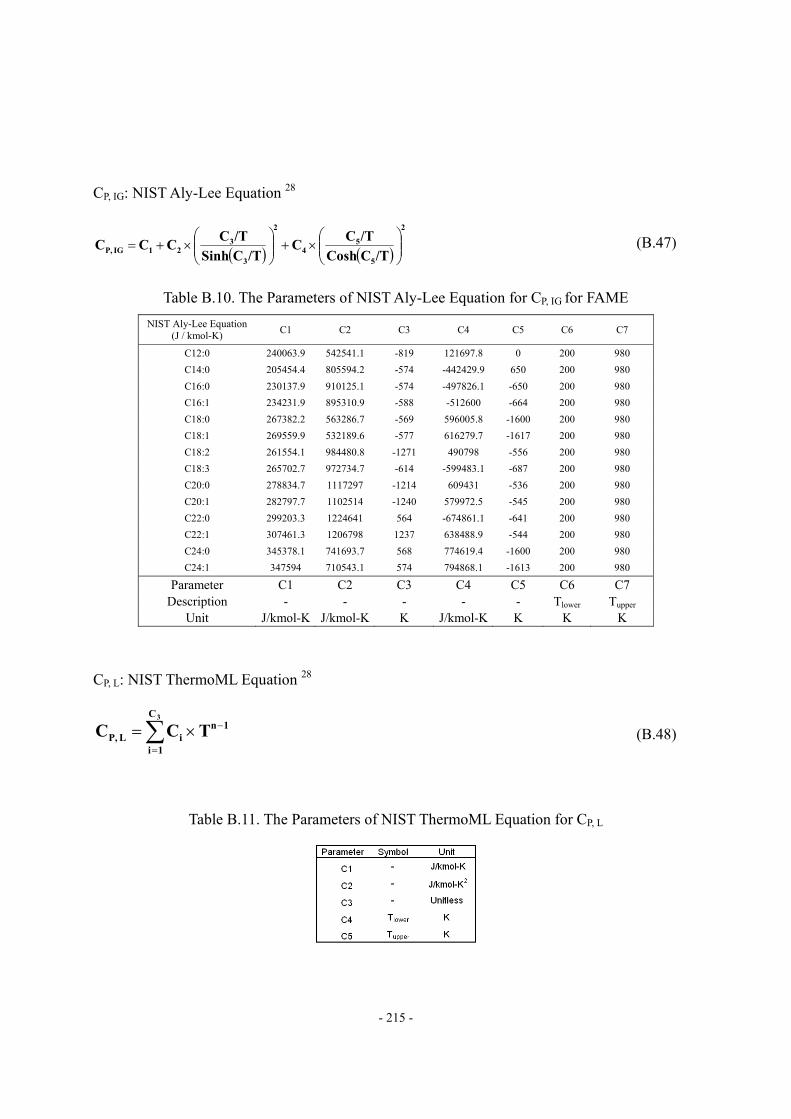
- 215 -
CP, IG: NIST Aly-Lee Equation 28
( ) ( )
2
5
54
2
3
321IG P, /TCCosh
/TCC/TCSinh
/TCCCC ⎟⎟⎠
⎞⎜⎜⎝
⎛×+⎟⎟
⎠
⎞⎜⎜⎝
⎛×+= (B.47)
Table B.10. The Parameters of NIST Aly-Lee Equation for CP, IG for FAME NIST Aly-Lee Equation
(J / kmol-K) C1 C2 C3 C4 C5 C6 C7
C12:0 240063.9 542541.1 -819 121697.8 0 200 980 C14:0 205454.4 805594.2 -574 -442429.9 650 200 980 C16:0 230137.9 910125.1 -574 -497826.1 -650 200 980 C16:1 234231.9 895310.9 -588 -512600 -664 200 980 C18:0 267382.2 563286.7 -569 596005.8 -1600 200 980 C18:1 269559.9 532189.6 -577 616279.7 -1617 200 980 C18:2 261554.1 984480.8 -1271 490798 -556 200 980 C18:3 265702.7 972734.7 -614 -599483.1 -687 200 980 C20:0 278834.7 1117297 -1214 609431 -536 200 980 C20:1 282797.7 1102514 -1240 579972.5 -545 200 980 C22:0 299203.3 1224641 564 -674861.1 -641 200 980 C22:1 307461.3 1206798 1237 638488.9 -544 200 980 C24:0 345378.1 741693.7 568 774619.4 -1600 200 980 C24:1 347594 710543.1 574 794868.1 -1613 200 980
Parameter C1 C2 C3 C4 C5 C6 C7 Description - - - - - Tlower Tupper
Unit J/kmol-K J/kmol-K K J/kmol-K K K K
CP, L: NIST ThermoML Equation 28
1nC
1iiL P, TCC
3−
=
×=∑ (B.48)
Table B.11. The Parameters of NIST ThermoML Equation for CP, L
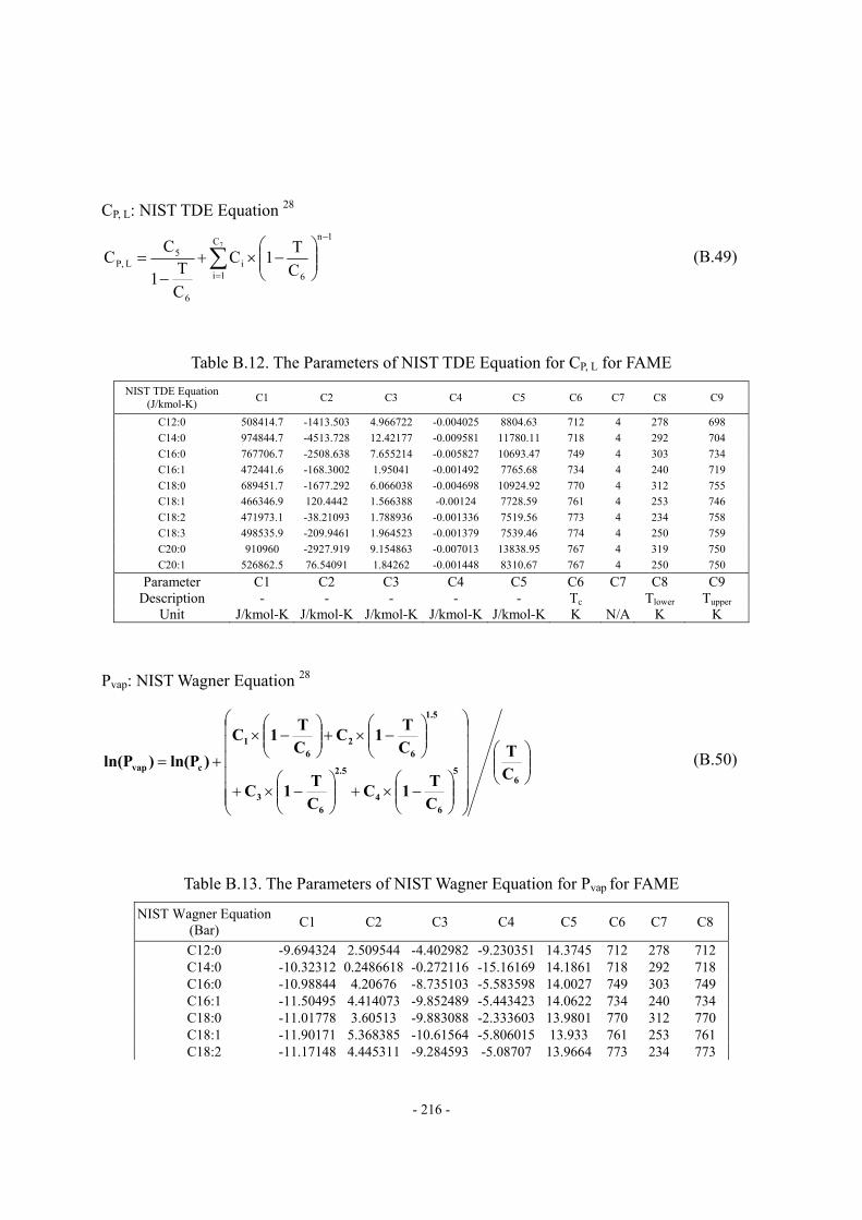
- 216 -
CP, L: NIST TDE Equation 28 1n
6
C
1ii
6
5L P, C
T1C
CT1
CC7
−
=⎟⎟⎠
⎞⎜⎜⎝
⎛−×+
−= ∑ (B.49)
Table B.12. The Parameters of NIST TDE Equation for CP, L for FAME NIST TDE Equation
(J/kmol-K) C1 C2 C3 C4 C5 C6 C7 C8 C9
C12:0 508414.7 -1413.503 4.966722 -0.004025 8804.63 712 4 278 698 C14:0 974844.7 -4513.728 12.42177 -0.009581 11780.11 718 4 292 704 C16:0 767706.7 -2508.638 7.655214 -0.005827 10693.47 749 4 303 734 C16:1 472441.6 -168.3002 1.95041 -0.001492 7765.68 734 4 240 719 C18:0 689451.7 -1677.292 6.066038 -0.004698 10924.92 770 4 312 755 C18:1 466346.9 120.4442 1.566388 -0.00124 7728.59 761 4 253 746 C18:2 471973.1 -38.21093 1.788936 -0.001336 7519.56 773 4 234 758 C18:3 498535.9 -209.9461 1.964523 -0.001379 7539.46 774 4 250 759 C20:0 910960 -2927.919 9.154863 -0.007013 13838.95 767 4 319 750 C20:1 526862.5 76.54091 1.84262 -0.001448 8310.67 767 4 250 750
Parameter C1 C2 C3 C4 C5 C6 C7 C8 C9 Description - - - - - Tc Tlower Tupper
Unit J/kmol-K J/kmol-K J/kmol-K J/kmol-K J/kmol-K K N/A K K
Pvap: NIST Wagner Equation 28
⎟⎟⎠
⎞⎜⎜⎝
⎛
⎟⎟⎟⎟⎟⎟
⎠
⎞
⎜⎜⎜⎜⎜⎜
⎝
⎛
⎟⎟⎠
⎞⎜⎜⎝
⎛−×+⎟⎟
⎠
⎞⎜⎜⎝
⎛−×+
⎟⎟⎠
⎞⎜⎜⎝
⎛−×+⎟⎟
⎠
⎞⎜⎜⎝
⎛−×
+=6
5
64
2.5
63
1.5
62
61
cvap CT
CT1C
CT1C
CT1C
CT1C
)ln(P)ln(P (B.50)
Table B.13. The Parameters of NIST Wagner Equation for Pvap for FAME
NIST Wagner Equation (Bar) C1 C2 C3 C4 C5 C6 C7 C8
C12:0 -9.694324 2.509544 -4.402982 -9.230351 14.3745 712 278 712C14:0 -10.32312 0.2486618 -0.272116 -15.16169 14.1861 718 292 718C16:0 -10.98844 4.20676 -8.735103 -5.583598 14.0027 749 303 749C16:1 -11.50495 4.414073 -9.852489 -5.443423 14.0622 734 240 734C18:0 -11.01778 3.60513 -9.883088 -2.333603 13.9801 770 312 770C18:1 -11.90171 5.368385 -10.61564 -5.806015 13.933 761 253 761C18:2 -11.17148 4.445311 -9.284593 -5.08707 13.9664 773 234 773
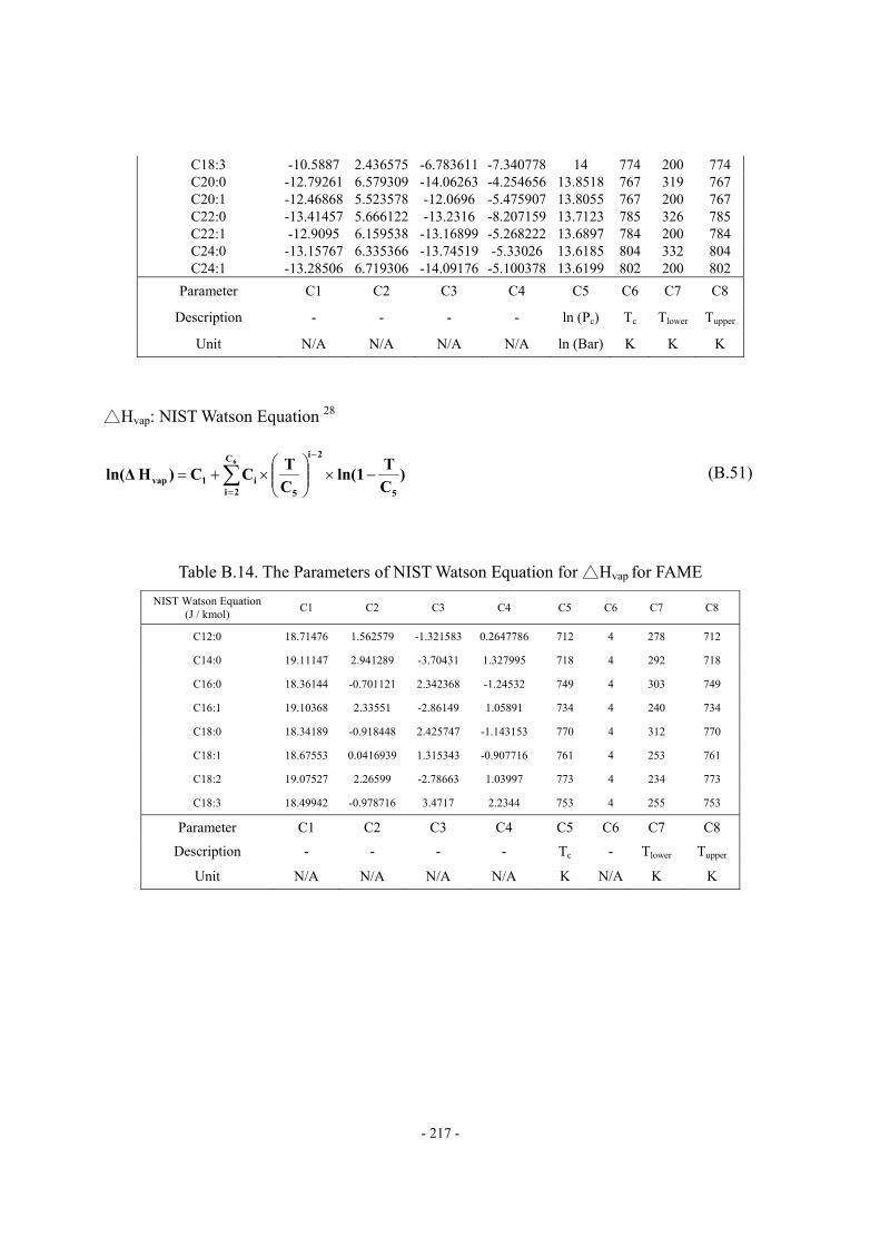
- 217 -
C18:3 -10.5887 2.436575 -6.783611 -7.340778 14 774 200 774C20:0 -12.79261 6.579309 -14.06263 -4.254656 13.8518 767 319 767C20:1 -12.46868 5.523578 -12.0696 -5.475907 13.8055 767 200 767C22:0 -13.41457 5.666122 -13.2316 -8.207159 13.7123 785 326 785C22:1 -12.9095 6.159538 -13.16899 -5.268222 13.6897 784 200 784C24:0 -13.15767 6.335366 -13.74519 -5.33026 13.6185 804 332 804C24:1 -13.28506 6.719306 -14.09176 -5.100378 13.6199 802 200 802
Parameter C1 C2 C3 C4 C5 C6 C7 C8
Description - - - - ln (Pc) Tc Tlower Tupper
Unit N/A N/A N/A N/A ln (Bar) K K K
Hvap: NIST Watson Equation 28
)CTln(1
CTCC)H ln(Δ
5
2iC
2i 5i1vap
6
−×⎟⎟⎠
⎞⎜⎜⎝
⎛×+=
−
=∑ (B.51)
Table B.14 . The Parameters of NIST Watson Equation for Hvap for FAME NIST Watson Equation
(J / kmol) C1 C2 C3 C4 C5 C6 C7 C8
C12:0 18.71476 1.562579 -1.321583 0.2647786 712 4 278 712
C14:0 19.11147 2.941289 -3.70431 1.327995 718 4 292 718
C16:0 18.36144 -0.701121 2.342368 -1.24532 749 4 303 749
C16:1 19.10368 2.33551 -2.86149 1.05891 734 4 240 734
C18:0 18.34189 -0.918448 2.425747 -1.143153 770 4 312 770
C18:1 18.67553 0.0416939 1.315343 -0.907716 761 4 253 761
C18:2 19.07527 2.26599 -2.78663 1.03997 773 4 234 773
C18:3 18.49942 -0.978716 3.4717 2.2344 753 4 255 753
Parameter C1 C2 C3 C4 C5 C6 C7 C8
Description - - - - Tc - Tlower Tupper
Unit N/A N/A N/A N/A K N/A K K
218
Chapter 4 Conclusions and Recommendations.
This dissertation investigates the issues noted in Chapter 1 and provides new methodologies to
properly simulate the two liquid fuel processes – hydrocracking process and biodiesel process.
This section summarizes the achievements and the suggestion to implement our methodologies.
Hydrocracking process:
1. We develop two integrated HCR process models which include reactors, fractionators and
hydrogen recycle systems.
2. We provide the step-by-step guideline of model development that has not been reported in
the literature.
3. We apply the Gauss-Legendre Quadrature to convert kinetic lumps into pseudo-components
based on boiling point ranges (delumping) for rigorous fractionator simulation.
4. Our delumping method gives a continuous response to changes in fractionator specification
such as distillate rate.
5. We update API correlations of flash point and freezing point to plant operation and
production.
6. The integrated HCR process models are able to predict accurately the product yields,
distillation curves of liquid products, and temperature profiles of reactors and fractionators.
7. The integrated HCR process models also gives good estimations on liquid product
qualities – density, flash point and freezing point of diesel fuel (MP HCR) and jet fuel (HP
HCR) – by using updated API correlations.
8. We apply the integrated MP HCR process model to conduct simulation experiment to
quantify the effects of operating variables on product yields.
9. We apply the integrated HP HCR process model to generate delta-base vector for LP based
production planning.
219
Currently, the methodology only requires daily measurements in the refinery to build an
integrated HCR process model. To better implement this model into process integration and
production planning, we suggest a to-do list:
1. Calibrate the model every two to three weeks to ensure that the model always reflects the
latest production and operation scenario.
2. Re-calibrate the model when feedstock is significantly changed from base case
3. Apply SimDist analysis whenever it is available.
To further improve our models, we may include Apply SimDist analysis for feed characterization,
and to incorporate detailed molecular information for feed characterization and customize our
feed lump distribution if these measurements are available regularly. We can also to customize
the calibration environment to include product property and product composition as objective
functions if detailed molecular information of product is available.
Biodiesel process:
1. We present a comprehensive review of published literature and focus on feed oil
characterization, thermophysical property modeling, rigorous reaction kinetics, phase
equilibrium for separation and purification units, and prediction of essential biodiesel fuel
qualities.
2. We characterize the feed oil and product as a single pseudo-triglyceride through a “lumper”
spreadsheet, and generate their essential thermophysical property.
3. We develop the reactor rating model based on rigorous kinetics of reacting the
pseudo-triglyceride with methanol to produce pseudo-diglyceride (DG),
pseudo-monoglyceride (MG) and pseudo-FAME
4. We convert the reactor output of pseudo-FAME molecules into a mixture of FAMEs. i.e.,
biodiesel, through a FORTRAN block, called a “delumper”.
220
5. We develop a product fuel property calculator to predict biodiesel qualities namely density,
viscosity, and cetane number.
6. Our modeling methodology is an efficient tool not only for evaluating and optimizing the
performance of an existing biodiesel manufacturing, and but also for optimizing the design
of a new process to produce biodiesel with specified fuel properties
We use the experimental observation in the literature to develop the methodology. The following
list shows the way to improve the methodology:
1. Current methodology utilizes alkali-catalyzed reaction kinetics with NaOH to model the
reactor. In practice, NaOCH3 is better than NaOH as catalyst because NaOH will react with
free fatty acid into soap and water. With the existence of water, trigleceride will be
hydrolyzed which not only reduce biodiesel yield but also increase the difficulty to purify
the produced biodiesel. Thus, we suggest using the alkali-catalyzed reaction kinetics with
NaOCH3 when it is available.
2. There is a lack of physical property data of triglyceride molecules in the literature. Current
methodology is utilizing predictive methods to estimate required physical properties. Su et
al.1 present a comprehensive review and comparison of different prediction methods based
on all of the available experimental data in the literature. We suggest following their
recommendations if there is no experimental data are available.
3. There are little phase equilibrium data of triglyceride-glycerol-methanol-biodiesel system.
We suggest updating the thermodynamics model to ensure that the phase equilibrium
calculation of separation and purification units match real physics when the data are
available.
4. Currently, biodiesel is sold as biodiesel blend which is blended with petro-diesel in market.
Therefore, predicting fuel properties of biodiesel blend is another interesting issue. There
221
are two ways to address this issue
a. Use pure property data of both biodiesel and petro-diesel to estimate the properties of
biodiesel blend. This approach requires property measurement of both biodiesel and
petro-diesel.
b. Build a databank including property data and compositional analysis of both biodiesel
and petro-diesel. And then, figure out a simple way to predict the fuel property of
biodiesel blend. We could do this by predicting pure property of both biodiesel and
petro-diesel followed by the property estimation of biodiesel blend or predicting
property of biodiesel blend according to its molecular information. Both strategies
require a huge databank which is not available in the literature.
Literature Cited
1. Su, Y.C.; Liu, Y. A.; Diaz Tovar, C. A. and Gani, R, “Selection of Prediction Methods for Thermophysical Properties for Process Modeling and Product Design of Biodiesel Manufacturing”, Industrial and Engineering Chemistry Research, 2011, 50, 6809-6836.
Related Documents