Proceedings of the Workshop on Instream Flow Habitat ...

Proceedings of the Workshop on Instream Flow Habitat Criteria and Modeling

Edited by

George L. Smith

Information Series No. 40

PROCEEDINGS

WORKSHOP IN INSTREAM FLOW

HABITAT CRITERIA AND MODELING

Edited by

George L. SmithAssociate Professor of Civil Engineering

Colorado State University

The Workshop was supported with funds provided by the Officeof Water Research and Technology {P.L. 95-467} and the Officeof Biological Services, U.S. Fish and Wildlife Service, U.S.Department of the Interior.

COLORADO WATER RESOURCES RESEARCH INSTITUTEColorado State University

Fort Collins, Colorado 80523Norman A. Evans, Director

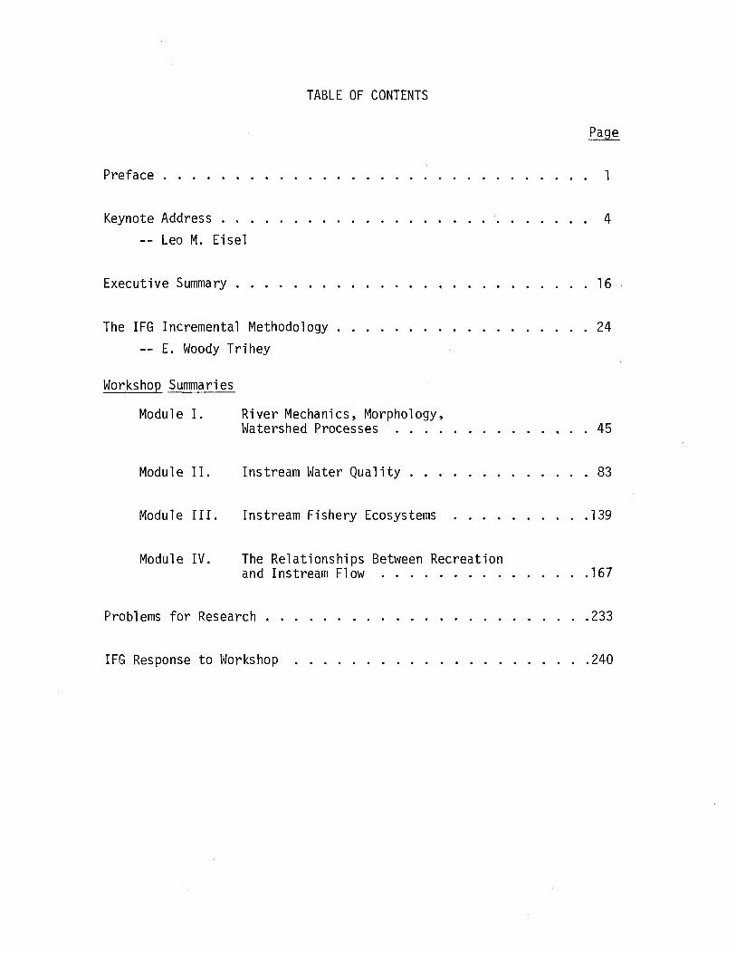
Preface . . . .

Keynote Address-- Leo M. Eisel

Executive Summary .

TABLE OF CONTENTS

1

4

. . • . . • . • . . . • . . . . . . 16

The IFG Incremental Methodology . . . . . . . . . . . . . . .... 24E. Woody Trihey

Workshop Summaries

Module I. River Mechanics, Morphology,Watershed Processes . . . . . . . . . . 45

Modul e I I.

Module III.

Module IV.

Instream Water Quality

Instream Fishery Ecosystems

The Relationships Between Recreationand Instream Flow .

83

.139

.167

Problems for Research ..

IFG Response to Workshop

.233

.240

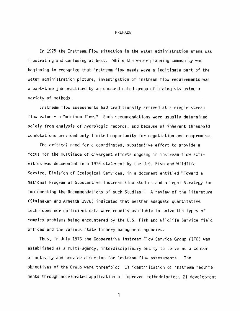
PREFACE

In 1975 the Instream Flow situation in the water administration arena was

frustrating and confusing at best. While the water planning community was

beginning to recognize that instream flow needs were a legitimate part of the

water administration picture, investigation of instream flow requirements was

a part-time job practiced by an uncoordinated group of biologists using a

variety of methods.

Instream flow assessments had traditionally arrived at a single stream

flow value - a "minimum flow. II Such recommendations were usually determined

solely from analysis of hydrologic records, and because of inherent threshold

connotations provided only limited opportunity for negotiation and compromise.

The critical need for a coordinated, substantive effort to provide a

focus for the multitude of divergent efforts ongoing in instream flow acti­

vities was documented in a 1975 statement by the U.S. Fish and Wildlife

Service, Division of Ecological Services, in a document entitled "Toward a

National Program of Substantive Instream Flow Studies and a Legal Strategy for

Implementing the Recommendations of such Studies." A review of the literature

(Stalnaker and Arnette 1976) indicated that neither adequate quantitative

techniques nor sufficient data were readily available to solve the types of

complex problems being encountered by the U.S. Fish and Wildlife Service field

offices and the various state fishery management agencies.

Thus, in July 1976 the Cooperative Instream Flow Service Group (IFG) was

established as a multi-agency, interdisciplinary entity to serve as a center

of activity and provide direction for instream flow assessments. The

objectives of the Group were threefold: 1) identification of instream require­

ments through accelerated application of improved methodologies; 2) development

of guidelines for attaining implementation of instream flow recommendations;

and 3) establishment of an effective communication network pertaining to

instream flow activities, data and information. With this charge, the IFG

undertook development of a comprehensive state-of-the-art methodology for

identification of instream requirements (objective 1) in three steps:

1. Synthesize and transfer to the field of practical quantitative

techniques based on state-of-the-art information for immediate application to

current problems.

2. Promote and direct future research and development of quantitative

techniques and data collection efforts to maximize their usefulness to the

fishery management and water administration agencies.

3. Continually update and improve operational techniques as new tech­

nology is shown to be practical.

By fall of 1977 the IFG had drawn upon experiences of western fishery

biologists and water planners to synthesize a unique state-of-the-art approach

to instream flow assessments. The IFG's Incremental Methodology attempts to

provide for the quantification of the amount of potential habitat available

for a species by life history stage as a function of stream flow.

Initial application of IFG1s methodology to selected western instream

flow questions proved to be very promising. These early successes resulted in

a notable demand for wide scale application, and stimulated considerable

interest in the use of this new tool to address a variety of questions

pertaining to impacts of changes in flow regime or stream channel geometry on

instream fishery resources.

In November 1978 it was both timely and appropriate that the IFG's

methodology be reviewed by user groups and the scientific community to obtain

their assessment of this new tool's ability to do the job it was originally

2

designed to do, and to do those new jobs that many were rapidly coming to

expect it to do. Hence, a group of nationally recognized scientists and

practitioners were invited to an Instream Flow Criteria and Modeling Workshop

conducted by the Colorado Water Resources Center on the Colorado State

University campus.

The express purposes of the workshop were to 1) provide the IFG with a

critique of the existing components of their methodology on both conceptual

and procedural levels; and 2) to assist the IFG in identifying needed

refinement and prioritizing future development. A summary of the workshop

discussion and subsequent recommendations pertaining to present day

application and future research are reported in these Proceedings in reference

to four broad topic areas: River Mechanics and Watershed Processes, Water

Quality, Fishery Ecosystems and Instream Recreation.

3

KEYNOTE ADDRESS

l.eo M. EiselDirector

U. S, Water Resources Council

1 am pleased to have this opportunity to speak to you this evening on

the very important topic of maintaining adequate instream flows. I am also

pleased that the Water Resources Council has had an opportunity over the

past few years to contribute to further work and assistance in the produc­

tion of methodology for determining necessary minimum instream flow

requirements.

Over the past few years, the Water Resources Council, under authorities

contained in Section 13 (a) of the Federal Nonnuclear Act of 1974, has made

funds available to the Fish and Widlife Service and the Cooperative Instream

Flow Service group for various phases of the work. In the course of pre­

paring this speech, I have had the opportunity to review several of the

documents produced by this program and am quite pleased with the results.

The money has been well spent.

I am sure that many of you here tonight have a great deal more experience

and insight into the problems of maintaining adequate minimum stream flows

than I do. I am also sure that many of you have spent a great deal more

time working on this problem and are very familiar with the various technical,

legal and political problems involved. Nevertheless, I would like to ask

all of you to take a step back from the many details involved in your efforts

and to view the problem of maintaining adequate minimum stream flows from

the larger perspective of water resources management.

4

There is no doubt that maintaining minimum flows will be one of the

major water problems over the next few years and that this problem will

probably continue to get worse before it gets better.

For example, the Water Resources Council's Second National Assessment

of the Nation~s Water Resources, which is scheduled to go to the printer

the first of next month, has attempted to make some rather crude ,estimates

of instream flow requirements for the major river basins and sub-basins in

the United States. In the course of this analysis, it was assumed that 60

percent of the average annual flow of a stream would provide a base flow

wh i ch in turn woul d provi de excellent to outstanding habi ta t for most

aquatic life forms during their primary periods of growth and for the majority

of recreation uses. It was further assumed that 30 percent of average annual

flow would provide good survival habitat for most aquatic life forms. Finally,

it was assumed that 10 percent of average flow could sustain only short term

survival habitat for most aquatic life forms. This somewhat crude and general

analysis indicates that nationally, ideal flow levels for preserving instream

uses would total about 1,040 billion gallons per day. With an average daily

flow of 1,242 billion gallons per day in 1975 for all river basins in the

United States, it appears that flows are adequate at present for fish and

wildlife. However, several regions do not reflect such favorable conditions.

For example, the Lower Colorado River has an average daily flow of about

1,550 million gallons per day, while the flow for ideal fish habitat should

be almost 6,900 million gallons per day. Needless to say, these national

and regional estimates are not very useful for purposes of planning water

resources development and the preservation of minimum streamflows for

specific streams. However, they do provi.de some indication of the national

picture.

5

Data from the Second National Assessment as well as other analysis leads

to the general conclusion that conflict over minimum flows is only going to

get worse. The United States currently has no policy on population or economic

, growth and because our economic growth continues at approximately 4 percent

per annum and our population growth continues at something like 1 percent, it

is apparent that there will be increased competition for water and for re­

maining streamflows throughout the United States.

Another major problem which will continue to produce conflicts over

minimum flows is the lack of an adequate water resources planning system

within the United States. A great deal of effort has been made at the

Federal level, as well as State and local levels, to do regional, water

resources planning. The Water Resources Council itself was set up by the

1965 Water Resources Planning Act along with the river basin commissions

for purposes of improving water resources planning. However, these and

other institutions have not yet succeeded in providing the necessary

adequate planning system required for preserving minimum instream flows.

Here, we can draw on an example very close to Ft. Collins -- the Platte

River. Perhaps the Platte River provides an almost stereotypic example of

the shortcoming of our existing planning process. I would imagine most of

you are familiar with the Narrows Reservoir and the controversy surrounding

this project. Without going into the various figures concerning this pro­

ject, it will result in depletion of flows downstream on the Platte River

with possible impact on critical wildlife habitat for whooping and Sandhill

cranes. A similar project, the Grayrocks Reservoir in Wyoming, will also

impact on this same area of wildlife habitat. Unlike the Narrows Reservoir

in Colorado, which would be built by the Bureau of Reclamation, the Gray­

rocks Dam and Reservoir is being constructed by a private entity usi,ng loans

6

guaranteed by the REA. Unlike the Narrows Reservoir project, the Grayrocks

Reservoir is not subject to the Prtnciples and Standards of other Federal

water resources planning requirements. As a consequence, the impact of this

reservoir on a wildlife habitat and flows in the North Platte and main stem

of the Platte River are not really considered in the context of the entire

water resources of the Platte River Basin.

Shortcomings in State water law will also continue to insure inadequate

consideration of low flows in many States.

There have also been recent setbacks in Federal legal decisions. For

example, a recent Supreme Court decision concerning the Rio Membres

essentially indicates that streamflows cannot be preserved for any other

purpose on U.S. Forest Service land beyond the original purposes for which

the land was set aside -- in this case, growing trees.

The point here is that within the near future these many factors -- that

is, continued growth, poor planning, inadequate State and Federal law -­

will produce continued pressure on the preservation of adequate minimum

streamflows.

Probably to most of you here in this room it is obvious that the preser­

vation of minimum streamflows depends on a lot of things. The first is an

adequate system for quantifying the necessary flows. In addition, there

also has to be an adequate planning system and an adequate decisionmaking

system to insure consideration of the required minimum flows.

The first and most basic step in insuring preservation of minimum

streamflows is undoubtedly to put together a procedure which can be used to

quantify the relationship between flow characteristics and the habitat for

a number of species as well as recreational use. This procedure must not

have exceedingly complex computational requirements nor must it demand

7

data which can be gathered only at great cost and effort. In short, the

procedure needs to be as simple and cheap as possible while still providing

information of necessary quality.

Needless to say, this is a big order as many of you here in this room

know. I might draw an analogy between the task you are involved in and

the similar task of mapping floodplains for purposes of floodplain manage­

rnent~ As many of you know, a floodplain management program generally

requires the aerial extent of the area inundated by the 100 year flood to

be estimated since in most cases actual stage readings for the 100 year

flood will at best be available at only a few locations on a stream. During

my experience in the State of Illinois as head of the State water resources

agency, I had a great deal of experience with floodplain management and

quickly learned the need for solid and dependable floodplain mapping. I

believe that a similar requirement exists here for solid and dependable

information concerning the relation between varfous streamflow conditions

for a specific stream and the suitability of wildlife habitat.

Because this is a workshop on instream flow criteria and modeling, most

of you here tonight are primarily concerned about quantifying the relation­

ship between streamflows and wildlife habitat. However, someone must also

worry about the rest of the requirements necessary to insure that adequate

minimum flows will be preserved. Here we are talking about improving systems

for water resources planning as well as changes in State and Federal laws.

Taking the last of these first -- the State water laws -- I think that

this is clearly a State problem in which the Federal government should not

intervene. Last year in the course of the water resources policy review,

the President, as well as Secretary of the Interior Andrus and Vice President

8

Mondale, made it very clear during several trips to the West that the

Federal government would not interfere with State water law~

I do not want to take time tonight to review the various deficiencies

tn State water law where they occur, but the point is that if these State

water laws are to adequately recognize instream flows, the States must

take responsibility for change.

ltd like to spend a little time talking about efforts at the Federal

level to insure that a more realistic planning procedure is in place which

can accommodate the procedures which you are developing for purposes of

considering instream flows. Without a solid water resources planning system,

the procedures that this workshop is concerned with -- will simply not be

used.

As I indicated earlier, existing water resources planning procedures at

the Federal level are not adequate and many problems exist. For example,

the Principles and Standards for the planning of water and related land

resources development do not cover a number of Federal actions. Per

direction of the Water Resources Council, the Principles and Standards

really only cover direct Federal actions; that is, the construction programs

of the Corps of Engineers, the Soil Conservation Service, the Bureau of

Reclamation and TVA and do not cover the so-called uindirect Federal programs"

such as the grants program of U.S. EPA for construction of sewage treatment

facilities.

Another deficiency is the fact that the plans produced by river basin

commissions, interagency coordinating committees, and other entities can be

presently .i gnored by the Federal agenci es and States wi thout any ki nd of

penalty. Another area of defici.ency in the exi.sting planning process is the

almost complete lack of integration of water quality and water quantity

9

planning in the United States. Here I can again draw upon my experience

in the State of Illinois where the Federal government will spend approxi­

mately $17 million for purposes of 208 planning by next spring. All of

this 208 planning is generally based on the 7 day/10 year minimum low flow.

However, because water resources development planning is generally excluded

from 208 planning, and likewise there is little effort to integrate 208

planning into water resources development planning, there really is no guaran­

tee that the 7 day/10 year low flows will be there in the future with that

frequency.

Okay, so much for the problems; now what efforts are being made at the

Federal level to solve some of these problems with our existing water

resources planning system. Most of these efforts are entered in the imple­

meAtation of the water policy review directives which the President issued

last July 12. Maybe I should just take a moment here to give you a capsule

description of the water policy review for those of you who have not been

following this effort closely. In May of 1977, the President directed

OMB, the Council on Environmental Quality and the Water Resources Council

to complete a review of existing Federal water policy and make recommenda­

tions for change. This review was initially to be conducted in 90 days but

stretched on until last July when the President issued directives to a number

of Federal agencies including the Water Resources Council for implementation

of various policy changes.

I'd like to take this opportunity to summarize some of these directives

and point out how I believe they can make a major contribution to insuring

the use of the procedures for estimating low flows that you are concerned

about developing.

10

One of the directives which the President issued went to the Water

Resources Council and directed the Council to modify the Principles and

Standards as well as produce a manual for use by the various Federal

agencies for purposes of improving the implementation of the Principles and

Standards t As many of you here know, the Principles and Standards for

Planning Water and Related Land Resources Projects were originally issued

in 1973. As their name implies, the Principles and Standards are a set of

general principles and standards concerned with water resources planning,

including benefit-cost analysis. The various Federal agencies, such as

the Corps of Soil Conservation Service, develop their own agency rules and

regulations for implementation of the Principles and Standards. As a result,

there is considerable difference between the benefit-cost procedures and

other planning procedures used by the Corps of Engineers, the Soil Conserva­

tion Service, and other Federal development agencies. As a consequence, the

President has directed the Council to prepare a manual to insure more con­

sistency among agencies in benefit-cost analysis and other planning procedures

as well as insuring that the procedures used by the agencies are the best

possible. I think the importance of all of this to you is that by improving

planning and planning procedures, you have more of a guarantee that the pro­

cedures you are presently developing for estimating minimum streamflows will

actually be employed and will not be just left on the shelf someplace.

The initial efforts of the Water Resources Council toward meeting the

President's directive have been primarily concentrated in improving pro­

cedures for benefit-cost analysis. Our present schedule calls for us to

have completed the portion of the manual dealing with benefit-cost analysis

by next July. However, the Principles and Standards are not only concerned

with economic cost and benefits. The P&S also requires an environmental

11

quality plan to be developed and the procedures used by the agencies for

this purpose vary even more and are less sound that those used for traditional

benefit-cost analysis. As a consequence, we plan a second phase to improve

the procedures used by the agencies for developing the environmental quality

account. Procedures for instream flow criteria will be important for the

traditional benefit-cost analyis portion of the manual but will be crucial for

the environmental quality portion. Consequently, as we move into this second

phase after the first of the year, we will be in close contact with you con­

cerning the procedures you are developing. You may ask why the environmental

quality account procedures have been reserved for the second phase. Why is

it not important enough to be in the first phase?

The basic excuse is the age-old one used by bureaucrats of not enough time

and people. The Presidential directive ordered us to have this manual com­

pleted by next July, which requires us to have a draft completed by about

February 1 of next year in order to provide adequate time for publication

in the Federal Register, a gO-day review period, and then development of

the final document. We felt that there was no way we could really adequately

develop definite procedures for the various areas of the environmental

quality account in such a short period of time.

Closely aligned with the P&S manual directive is another directive to

the Water Resources Council to develop an independent review function.

Simply stated, the purpose of this review is one of quality control. The

Water Resources Council will establish a technical group to assure that

agency project plans are done in compliance with the Principles and

Standards, the Fish and Wildlife Coordination Act, and other Federal laws

and regulations. The general objective here is not for the water Resources

12

Council to vote a project up or down, but rather to insure that everyone is

playing the. game by the same rules!

I think that the independent review function will also insure better

planning procedures and more serious consideration of procedures such as

you are developing here for purposes of estimating required minimum

streamfl ows.

There are a number of directives concerned with water conservation. I

donlt want to go into each of these individually, but merely give you some

flavor of what these directives are all about. I believe that the decision

by President Carter to make water conservation a cornerstone of Federal

water policy is definitely a step forward as far as insuring adequate minimum

streamf10ws for purposes of wildlife habitat and other uses. Because of the

increasing future demands for water resulting from increasing economic and

population growth, any successful efforts at reducing overall demand is

bound to reduce the pressure on required minimum streamflows. For example,

one of these directives requires all Federal agencies to review their existing

programs by October 30 of this year and to report to the Water Resources

Council ways that existing programs can be changed to promote water conser­

vation. We are just now beginning to receive the first reports. Other

areas involve things like cost sharing. The President has directed that

legislation be drafted by the Water Resources Council to require 5 and 10

percent cost sharing by States for water resources projects. The purpose of

this cost sharing is to insure more critical review of the need for water

resources projects by States, thereby helping to insure that unnecessary

water development projects will not be built.

Other directives have also concerned cost sharing. For example, the

Bureau of Reclamation recei.ved various directives to promote more adequate

13

pricing of irrigation water with the eventual goal being less wastage of

irrigation water. The President also directed the Water Resources Council

to establish a water conservation technical assistance grants program of

$25 million annually. These funds would go directly to the States for

purposes of assisting them in water conservation. Other directives concerned

the Departments of Interior, HUD and Agriculture, for water conservation

efforts in water short areas as well as water conservation in agricultural

qssistance programs in water short areas. EPA has been directed to essentially

attach water conservation conditions to their loan and grants programs.

I could go on and give a few more examples here but the point is that a

major portion of the President's water policy reform has centered on ways to

reduce demand for future water development! In the past) major emphasis on

Federal water programs has been on increasing supply. In contrast, President

Carter has indicated the need for new emphasis on reducing demand.

Several other areas of reform directed by the President in his July 12

set of directives include increasing an existing State planning grants

program at the Water Resources Council from approximately $5 million to $25

million annually. The purpose of this program is to improve State water

resources planning. Again, we can always be critical of planning, but if

the planning process is not adequate, the type of procedures that you are

concerned about developing here today may not be integrated into decision~

making process for purposes of water resources development and management.

The President also directed more strict enforcement of existing laws such

as the Fish and Wildlife Coordination Act. As many of you know here,

enforcement of the Fish and Wildlife Coordination Act has been somewaht

lax in the past. It has not been appl ied uniformly to water resources

development.

14

There were also some directives which concerned instream flows directly.

I am personally somewhat concerned that these directives are weak and could

have been stronger; however, we were faced with the problem of essentially

what can the Federal government do in the area of instream flows without

becoming entangled in State water law.

Now obviously the question is: How much good are all these directives

going to do? How much water are the water conservation directives going

to save? Will planning be improved sufficiently to really consider the kind

of procedures you were developing here? I am afraid that I cannot adequately

answer any of these questions. We've simply got to wait and see.

I think that the point of all of this once again is that the work you are

doing here is very vital and is absolutely necessary if procedures and

requirements are put into place for insuring future minimum streamflows.

It's just the same as floodplain management. You must first have the maps.

However, these efforts of quantification of required minimum streamflows are

only one part of a very complicated process. Without adequate planning and

decisionmaking processes, your procedures for estimating instream flow needs

will be ignored. Consequently, I have tried to put your work here in the big

picture and demonstrate its importance as well as the importance of other

components of the system.

Thank you for this opportunity to comment.

15

EXECUTIVE SUMMARY

The Cooperative Instream Flow Service Group, U. S. Fish and Wildlife

Service, Fort Collins, Colorado has developed an incremental methodology which

is unique among instream flow habitat assessment procedures. The Instream

Flow Group Incremental Methodology (IFGIM) allows quantification of potential

habitat available to various life history phases of a fish in a given reach of

stream, at different streamflow regimes with different channel configurations

and slopes. It is an emerging technology made necessary by increased public

desire for concious consideration of acceptable habitat for instream biota.

Modifications are constantly being made to improve its utility and this

workshop was designed to accelerate that process.

Discussions were held involving experts in four specific areas relevant

to the basic concepts of the IFG Incremental Methodology. Those areas were:

(1) river mechanics, morphology, and watershed processes; (2) modeling

instream water quality; (3) instream fishery ecosystems; and (4) relationships

between recreation and instream flow. Workshop objectives were: (1)

identification of avenues for improvement or expansion of the incremental

methodology; and (2) identification and establishment of priorities for needed

research and development programs for improvement of the incremental

methodology.

The workshop on river mechanics, morphology, and watershed processes

focused on: (1) an evaluation of current, predictive methodologies involving

mathematical models - regression, lumped parameter, o~ physical process

simulation - and using three mathematical approaches - analytical, finite

difference and finite element; (2) an evaluation of the hydraulic components

16

of the IFGIM that are utilized for determining management aspects of instream

flow needs; (3) identification of possible improvements to the IFGIM's

existing hydraulic simulation models; and (4) making recommendations

pertaining to the addition of sedimentation aspects of instream flow into the

methodology.

Five specific improvements were identified as necessary for increasing

the predictive capability of IFGIM: (1) an improved approach to predictin

watershed response due to duration, quality, and frequency of flow including

consideration of the impacts of forest harvesting, irrigated agriculture,

grazing, mining, and other watershed management activities on the water and

sediment yield from watersheds to stream channel; (2) increased capability of

the spatial resolution of the IFG models to accomodate both upstream

management plans of small watersheds and legal requirements for instream flow

needs, environmental quality, and water resource management for a complete

river basin or subbasin; (3) the models should not be area or regionally

specific; therefore, the models will require site-specific calibration data

and regionally specific species response criteria; (4) the model should be

able to explicitly represent management activities and simulate the system

response resulting from these activities; and (5) increased capability to

assign probabilities to climatic and spatial variables.

In addition to the foregoing improvements the following characteristics

are desired in predictive models: (1) they should be functional within the

constraints of limited data; (2) they should be oriented for use by management

personnel and applicable to specific decision-making processes; (3) they

should possess the capability of making predictions at different levels of

accuracy and resolution depending on purpose of the assessment; (4) the

computer software system should adopt a modular approach; and (5) the models

should be properly documented.17

A hierarchical analytical approach was proposed for IFGIM toward

quantification of watershed processes and sedimentation as integral components

of the riverine ecosystem. The workshop set forth the sequential levels of

analysis required to develop and conduct an integral analysis of watershed

processes and sedimentation. A given level of analysis is to be formulated,

verified and utilized depending on level of accuracy required; available data;

constraints; magnitude of projected channel changes; etc.

The module for instream water quality, recommended that incremental

development be undertaken that would introduce water quality aspects to

instream flow needs assessments. To be useful, such development must be

applicable to the following problems: (1) the redistribution of water over a

year (or periods of years) to increase low flows and/or reduce flood flows;

and (2) the installation of major diversions up stream which decrease

available flows. The context of these problems could be: (1) the need to

establish instream flows as a part of a long range planning process; (2) the

need to make operatinal decisions on f real-time basis to maintain minimum low

flows; and (3) the evaluation of Environmental Impact Statements of projects

that would change instream flows. No limit is specified for the site of a

river system.

This group stressed the introduction of water quality methodologies must

be an evolutionary process that will improve as the IFG staff develops

in-house skills in water quality analyses. The workshop also proposed that

the methodologies be classified according to their cost, required knowledge,

data needs, and ability to resolve a basic low flow/water quality issues.

Four classes were identified: (1) level one - will be to provide low cost,

crude estimates of potential water quality problems. Text book concepts and

heuristic approaches will be used; (2) level two - will estimate changes in

18

temperature and oxygen due to flow alterations within a factor of two. This

level requires limited field studies and textbook level analysis of the fate

of pollutants such as heat, oxygen demand, solids, etc; (3) level three will

expand the set of chemicals to be analyzed and attempt to employ

state-of-the-art technology. This level requires extensive field observations

and mathematical modeling to predict time-dependent fluctuation in heat and

chemical concentrations in a reach; (4) level four involves research and

development concepts that attempt to improve the current state of knowledge of

the fate of toxic pollutants and to define chronic exposure levels that impact

the aquatic ecosystem. This level will seek to add to scientific

understanding as the first priority, and will complicate rather than clarify

most management decisions.

This module's report concludes with examples of methodologies for each

proposed level of analysis.

The workshop on instream fishery ecosystems concentrated on a critique of

the incremental methodology as it pertains to fish, both as a concept and as

an analytical approach.

Two major criticisms were made: (1) the methodology is not a consistent

system of strongly interacting components, but a collection of specific

modules interrelated by stream hydraulics; and (2) the methodology is based on

a narrow set of physical parameters providing necessary, but not sufficient,

conditions for the suitability of stream habitats.

The workshop proposed the development of an ecosystem holistic viewpoint

by IFG to overcome the two major criticisms. The methodology now used should

be expanded to include parameters that reflect chemical and biological

processes of ecosystems. Recommended parameters, in order of importance, are:

(a) depth; (b) velocity; (c) temperature; (d) food supply; (e) riparian cover,

19

and (f) competition. Additional factors of less importance (unranked)

include: (g) predation; (h) substrate; (i) dissolved oxygen; (j) instream

cover; (k) nutrients; (1) stream morphology; and (m) sediment load.

The following avenues for improvement or expansion of the incremental

methodology were identified: (1) an alternative to weighted usable area

should be sought for use in simulation of stream flow phenomena; (2) the

choice of modules in the hierarchical modular approach should be reevaluated

and the modules developed with different data requirements for different

resolution levels; (3) parameters to establish necessary and sufficient

conditions for fish habitats need to be more fully identified; (4) ecological

simulation should be incorporated into the IFG models; (5) both intensive and

extensive validation of the methodology should be sought. (For example,

intensive testing should be undertaken in regions where large data bases

exist,s~ch as salmonid streams of the Pacific northwest. Extensive testing

should cover a range of physiographic provinces, i.e., comparing studies of

eastern salmonid streams with western results, then extending to main stream

rivers and non-salmonid species); (6) documentation of stream ecology over a

broad spectrum of stream types and regions should be stressed; (7) reaches for

study should be selected to ensure statistical reliability of data samples;

(8) the methodology of computing weighted usable area should be replaced by a

method using a histogram of volume units from which mean, median, percent of

volume units with better than 50 percent desirability, etc. could be computed;

(9) a general methodology should be developed by carefully assessing the

variability of data over a range of stream types and geographic regions; (10)

information derived from actual field conditions should replace habitat

criteria now based on LD 50 laboratory tests; (11) a regression approach should

be used to describe behavioral response of a species to cover; (12) the

20

proposed functional classification of macroinvertebrates should include

indicator and keystone species; (13) a substrate index shoudl be used as long

as it does not obscure the primary data; and (14) the present IFG Incremental

Methodology should be modified to incorporate variables of stream biology and

the state of the stream ecosystems as criteria for fish habitat.

To meet the need for understanding relationships between stream flow and

recreation, the work by Anas, et al., 19791 on behavioral demand assessment

was referenced by the instream recreation module. Key concepts extracted from

the work includes: (1) recreation behavior is complex, voluntary, and

discretionary, which suggests that it may be quite sensitive in sometimes

unexpected ways to environmental change; (2) response of recreationists to

stream flow may vary by activity and by market segment; (3) some impacts may

be more important than others depending upon the market setments and

phychological outcomes affected; (4) impact on psychological outcomes may

occur without obvious changes in manifest behavior; and (5) the

state-of-the-art of explaining relationships between environmental conditions

and recreation behavior and benefit is primitive. While hydraulic measurement

and simulation may be well developed in terms of proven theories and standard

methods and measures, this is not so for prediction of recreation behavior.

The workshop raised several questions and criticism of the incremental

methodology. The criticisms are: (1) the attempt to assess the impact of

hydraulic characteristics of stream flow on certain instream recreation

activities is, at present, too narrow in scope; (2) the methodology has been

inadequate in examining the structur of recreation, i.·e., the likelihood that

1 / See reference of Module IV--The Relationships Between Recreation andInstream Flow of this report.

21

for different types of people, there may be different reactions to stream

flow, even for a given activity; (3) the methodology needs a greater

capability of delineating those stream flow variables which affect different

types of activities and kinds of peole; (4) the criterion methodology now used

is the "probability of use II function. However, true probabilities do not

exist in the way the methodology is now constructed and it is not known what

even is being predicted; and (5) the methodology does not include sufficeint

concern for social welfare values.

The strengths of the incremental methodology identified by the workshop

on recreation are: (1) it uses quantitative standard measures which have

general validity and applicability; (2) its approach is based on efficient

description of stream conditions through sampling and simulation; (3) an

analytical approach is used, which promises to allow efficient and rigorous

investigations of the issues; (4) the methodology to be theoretically and

conceptually rigorous has created an articulation of precise questions as well

as demands for specific information and operational definition of terms; (5)

it has generated a new set of questions for tributary disciplines including

recreation scientists, fish biologist water quality experts, and stream

hydrologists; and (6) it has generated a program of developmental education.

However, the IFGIM has not as yet achieved its objective of providing a

capability of (1) assessing the recreation potential of a stream; (2)

specifying instream flow requirements for recreation; and (3) assessing the

impact on recreation potential of instream flow.

To achieve the above objective, the workshop lists four general

components which must be more fully understood: (1) the relationship between

recreation potential and instream flow--the criterion component, (2) the

description and prediction of the instream flow characteristics of a given

22

stream--the resource description component, (3) the user of the criterion

component to measure and interpret the effect on recreation of the instream

flow characteristics described or predicted for a given stream--the evaluation

component, and (4) the practical guestion that needs to be answered--the

application component.

The principle challenge to the incremental methodology is in the

criterion component, where there are inadequacies with respect to (1)

substantive knowledge about recreation, and (2) methods to formulate and apply

criteria. The principle problem is to develop ways to measure and interpret

the meaning of stream flow to recreation. There are five principle needs:

(1) the nature and structure of recreation, vis-a-vis instream flow needs to

be specified; (2) the need for a more rigorous definition of "recreation

potential"; (3) for each recreation "species" there is a need to identify

those parameters of or related to stream flow which are of significance; (4)

the need for a "criterion methodology", i.e., a framework or strategy for

constructing and applying criteria; and (5) the need to understand the

processes by which instream flow affects recreation potential.

In response to the need to establish a more rigorous conceptual framework

of relationships between recreation and instream flow, the workshop includes

as an appendix a paper authored by Dr. George Peterson, entitled, liThe

Relationship Between Recreation and Instream Flow".

23

THE IFG INCREMENTAL METHODOLOGY

E. Woody Triheyl

Cooperative Instream Flow Service Group

Fort Collins, Colorado

Introduction

Instream flow requirements, often called instream flow needs, are the

amounts of stream flow necessary to sustain instream values at an acceptable

level. By instream values we mean the uses made of water within the stream

channel. These include such traditional uses as navigation, hydropower

generation, and waste load assimilation (water quality). In addition to these

more established uses, fish and wildlife needs; riverine based recreation;

compact and treaty requirements at downstream points of diversion; fresh water

recruitment to estuaries, and consumptive requirements of riparian vegetation

and floodplain wetlands are emerging as potent competitors for stream flows.

In addition to satisfying delivery schedules of downstream appropriators

(water right holders), an ideal stream flow management plan should provide an

lI additive flow requirement ll and a II comp limentary instream flow requirement. 1I

Hence the total stream flow requirement for a given stream reach at a

particular time is the sum of (1) the delivery requirement to satisfy

lAssistant Director Idaho Water Resources Research Institute, University ofIdaho, Moscow, Idaho, on assignment under Intergovernmental Personnel ActAgreement 1978-1979.

24

downstream water rights, (2) an additive flow requirement to offset consump­

tive uses enroute, and (3) the complimentary instream flow requirement

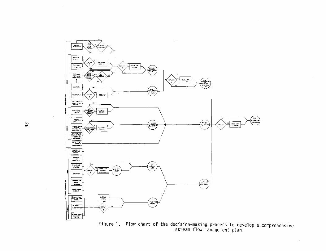
(Fig. 1).

The most desirable total stream flow requirement is one that will satisfy

several uses at once. Understandably, at a given location on a given stream,

only certain uses may be relevant, or preferential consideration may be given

to the use(s) regarded as most important. But in either event stream flow is

apportioned through negotiation and compromise. A paramount concern in these

deliberations is the ability to analyze the acceptability of incremental

changes in stream flow with respect to a particular use.

Instream flow assessments have traditionally arrived at a single thres­

hold value for the fishery resource - lI a minimum flow. II Such an instream flow

recommendation was usually determined solely from an analysis of hydrologic

records, and provided only a limited opportunity for negotiation. This

approach is based on the mistaken assumption that only flows below this

II minimum li will be detrimental to the fishery resource. As a result of the

fallacies and weaknesses associated with traditional fishery assessments it

was apparent that better methods were required.

The IFG incremental methodology is a major advance in this regard for it

attempts to quantify the amount of potential habitat available for each life

history stage of a species as a function of stream flow. This method is

intended to be used as a decision-making tool and is specifically tailored to

demonstrate the impact of incremental changes in stream flow on fishery

habitat potential.

The Incremental Methodology is intended to be used in those instances

where the flow regime is the dominant determinant of the quality of the

instream fishery or recreation resource and where hydraulic conditions are

25

Nm

'.Jf.iTIlI;:'DELivERY

• --<l~FlEOUIREMENT

Figure 1. Flow chart of the decision-making process to develop a comprehensivestream flow management plan.

compatible with the theoretical basis of the models (i.e. steady flow within a

rigid boundary). This method is composed of four basic components: (1) field

measurement of stream channel characteristics using a multiple transect

approach; (2) hydraulic simulation to determine the spacial distribution of

combinations of depths and velocities with respect to substrate and cover

objects under alternative flow regimes; (3) application of habitat suitability

criteria to determine weighting factors; and (4) calculation of weighted

usable area (gross habitat index) for the simulated stream flows based on

physical characteristics of the stream.

Four primary variables can be identified which determine the character of

instream habitat conditions: (1) water chemistry; (2) food web relations; (3)

flow regime; and (4) channel structure. Associated with each of these major

variables are the respective subsets of variables which interact to provide

the myriad of physical-chemical conditions to which the stream biota respond.

These four primary variables also offer a logical division for approaching the

task of quantifying the effects of land and water management decisions on

instream fishery resources.

During the 18 months preceding this workshop the Instream Flow Group·s

efforts concentrated on describing cause-effect relationships between stream

flow alterations and instream fishery habitat potential. In western streams

the most direct relationships (habitat constraints) are attributable to flow

regime and/or channel structure. Consequently, hydraulic simulation modeling

is of central importance to the incremental methodology.

27

Study Site Selection

Time and financial resources are seldom adequate to support the field

work necessary to document stream flow-habitat relationships throughout an

entire stream. Therefore, it is important to select study sites which are

both characteristic of the stream, and capable of providing pertinent informa­

tion. Either of two approaches to study-site selection can be utilized with

the incremental methodology; (1) critical reach, and (2) representative reach.

Under the critical reach concept the study site is selected on the basis

of its restrictiveness, i.e., stream flow characteristics at the critical

reach are limiting attainment of the full potential of the instream resource.

Associated with the critical reach concept is acceptance of the assumption

that adequate stream flow through the critical reach will provide for satis­

factory stream flow conditions throughout the remainder of the stream.

The critical reach concept implies that rather extensive knowledge of

both the stream (hydrology, water-quality, channel geometry) and the instream

resource (species composition, life history, passage requirements) exists.

One must be satisfied that conditions at the selected study site(s) are, in

actuality, limiting the instream resources potential. It should also be

recognized that critical reaches only provide information specific to a

particular set of questions; thus little opportunity would exist to utilize

the critical reach data base to address questions pertaining to other instream

uses.

A fisheries manager might select a critical reach on the basis of migra­

tion blockages, overwintering areas, or essential spawning and rearing

habitat. In the case of endangered species, critical reaches might be

selected on the basis of a unique combination of microhabitat conditions which

28

are quite unrepresentative of the general riverine habitat type. With regard

to instream recreation potential, a critical reach might be chosen on the

basis of safety, access, or passage. The critical reach concept might also be

used to evaluate such other instream concerns as: navigation, waste assimila­

tion, or sediment transport.

The representative reach concept reflects recognition of the importance

of the structure and form of the entire stream in sustaining a particular

instream resource. Application of the representative reach concept is

appropriate when limited life history information is available on the target

species, or when limiting stream channel conditions (critical reaches) cannot

be identified with any degree of certainty. The representative reach concept

is also the more appropriate approach for analysis of species interactions or

complimentary instream uses.

Two essentials of study site selection using the representative reach

approach are homogeneity and randomness. Initially, the stream must be

divided (stratified) into rather homogeneous segments based upon biological

community structure, stream channel morphology, stream flow regime, and human

activities. These stratified river segments are then sub-divided into popula­

tions of candidate representative reaches by either implicit or explicit

zonation techniques (Bovee and Milhous 1978), and three or four candidate

reaches are randomly selected from each of the respective populations of

candidate reaches. Following this office work using maps and aerial photos,

an on-site inspection is made of the candidate reaches to confirm that they

are generally representative of the river segment(s) being evaluated. The

actual study site(s) is then chosen from among the three or four candidate

reaches on the basis of access, manpower and financial resources, and the

limitations and safety of field personnel. What must be kept foremost in mind

29

is that the representative reach is chosen for its ability to provide

pertinent information regarding a given set of questions for the entire stream

segment which it represents. Relationships defined between streamflow and

physical habitat conditions at the study site are considered to be indicative

of interactions existing throughout that river segment.

Application of the Methodology

The incremental methodology is intended to be used in those instances

where the amount of streamflow is the dominant determinant of the abundance of

a target organism and the determination of a streamflow requirement is a

central question. It is also understood that streamflow conditions are

compatible with the theoretical basis of the hydraulic models (i.e., steady

flow within a rigid boundary) and that the habitat suitability curves are

acceptable indications of an individual species preferred habitat conditions.

Once it has been determined that flow regime is the dominant driving

variable and the study site(s) has been selected, standard surveying and

stream measuring techniques are employed to obtain calibration data for IFG1s

hydraulic simulation models. Transects are placed to characterize both

hydraulic and instream resource (fishery habitat) conditions. Detailed

information is obtained on the stream channel geometry and hydraulic

conditions using a multiple transect approach for microhabitat description. A

discussion of the theory and field techniques associated with the Instream

Flow Group's hydraulic simulation models can be found in Bovee and Milhous

(1978).

Computer programs are available which use these data to predict hydraulic

parameters (depth and velocity) with respect to any described substrate

30

condition for any desired flow regime. The hydraulic model is calibrated to

reproduce water surface elevations and horizontal velocity distributions

observed at selective stream flow conditions. The IFG's simulation models

normally use stream channel geometry and velocity data from several cross

sections within a relatively short stream reach. Each transect can be sub­

divided into as many as 100 cells (conveyance areas) to facilitate detailed

analysis of the spacial distribution of depth and velocity combinations. Once

properly calibrated, the computer program will calculate the water surface

evaluation and respective horizontal velocity distribution at each transect

for all desired discharges. The simulated water service elevations and

velocities are then passed from the hydraulic model to IFG's HABTAT model

(Main 1978a).

Within the HABTAT model, the mean depth of each cell is computed by

subtracting stream bed elevations from the simulated water surface elevation.

Surface areas associated with the occurrence of various combinations of

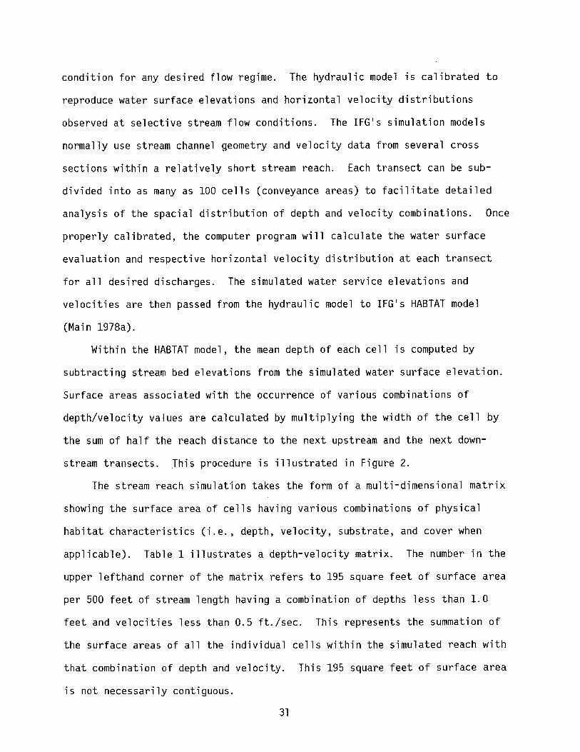
depth/velocity values are calculated by multiplying the width of the cell by

the sum of half the reach distance to the next upstream and the next down­

stream transects. This procedure is illustrated in Figure 2.

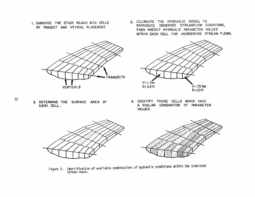
The stream reach simulation takes the form of a multi-dimensional matrix

showing the surface area of cells having various combinations of physical

habitat characteristics (i.e., depth, velocity, substrate, and cover when

applicable). Table 1 illustrates a depth-velocity matrix. The number in the

upper lefthand corner of the matrix refers to 195 square feet of surface area

per 500 feet of stream length having a combination of depths less than 1.0

feet and velocities less than 0.5 ft./sec. This represents the summation of

the surface areas of all the individual cells within the simulated reach with

that combination of depth and velocity. This 195 square feet of surface area

is not necessarily contiguous.

31

V= .75fpsD= I.Oft

WN

I. SUBDIVIDE THE STUDY REACH INTO CELLSBY TRASECT AND VETICAL PLACEMENT.

VERTICALS

3. DETERMINE THE SURFACE AREA OFEACH CELL.

2. CALIBRATE THE HYDRAULIC MODEL TOREPRODUCE OBSERVED STREAMFLOW CONDITIONS,THEN PREDICT HYDRAULIC PARAMETER VALUESWITHIN EACH CELL FOR UNOBSERVED STREAM FLOWS.

4. IDENTIFY THOSE CELLS WHICH HAVEA SIMILAR COMBINATION OF PARAMETERVALUES.

Figure 2. Identification of available combinations of hydraulic conditions within the simulatedstream reach.

Table 1. Occurrance of different combinations of depth and velocity,expressed in square feet of surface area per 500 feet of streamreach. Discharge = 800 cfs.

Depth VELOCITY IN FEET PER SECOND Row(ft. ) Totals

.5 .5-.99 1.0-1. 49 1.50-1.99 2.0-2.49 2.5-2.99 3.0-3.49 3.5

1 195 26 2211.0-1.5 90 47 41 17 6 6 93 3001.5-2.0 29 38 32 44 108 79 38 172 5402.0-2.5 6 29 23 9 111 131 143 175 6272.5-3.0 6 15 55 79 41 64 41 105 4063.0-3.5 9 17 15 12 32 3 149 2373.5-4.0 9 20 17 47 17 82 1924.0-4.5 20 11 50 35 17 1334.5-5.0 11 5 115 20 1515.0-5.5 7 23 15 455.5-6.0 10 31 20 61

ColumnTotals 344 233 125 225 575 390 476 545 2913

In order to translate changes in stream hydraulics into impacts or

effects on fish habitat it is necessary to identify describable relationships

between appropriate hydraulic parameters and the target species or target

group of species. Assemblege of such an information base was undertaken in

1977 by the IFG staff utilizing existing data from the scientific literature

and files of state fishery management agencies. Four techniques were used to

develop a preliminary information base in the form of two dimensional curves

(originally called probability-of-use curves and as suggested during the

workshop now called habitat suitability curves) describing species preference

for a particular stream flow parameter. (Bovee and Cochnauer 1977).

33

These criteria2 were prepared by life history stage for those streamflow

parameters directly influenced by changes in flow regime or channel geometry

and which were considered to most directly affect fish distribution; depth,

velocity, substrate and temperature. Species criteria for the Salmonid fishes

were developed and distributed by the Instream Flow Group in 1978 (Bovee

1978) .

The habitat suitability curves used in conjunction with the IFG metho-

dology are based on the understanding that individuals of a species tend to

select the most favorable conditions available within a stream for habitation,

but will use less favorable conditions with less frequency eventually leaving

an area if possible before conditions become lethal. Subsequently individuals

would be most frequently observed (sampled) in nature inhabiting their most

preferred habitat conditions. Implicit in the use of these criteria is the

assumption that frequency of observation is, in fact, indicative of habitat

preference and the understanding that the data base used to construct the

curves was obtained in an unbiased manner.

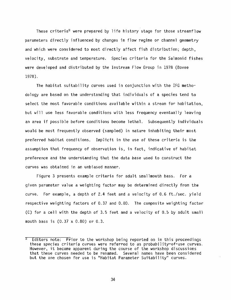
Figure 3 presents example criteria for adult smallmouth bass. For a

given parameter value a weighting factor may be determined directly from the

curve. For example, a depth of 2.4 feet and a velocity of 0.6 ft./sec. yield

respective weighting factors of 0.37 and 0.80. The composite weighting factor

(C) for a cell with the depth of 3.5 feet and a velocity of 0.5 by adult small

mouth bass is (0.37 x 0.80) or 0.3.

2 Editors note: Prior to the workshop being reported on in this proceedingsthese species criteria curves were referred to as probability-of-use curves.However, it became apparent during the course of the workshop discussionsthat these curves needed to be renamed. Several names have been consideredbut the one chosen for use is IIHabitat Parameter Suitabilityll curves.

34

Figure 3. Habitat Suitability Curves for

Adult Smallmouth Bass

(clear water)

5 6234

DEPTH (FT)

/V

JV

J

V

o

CD0::6oI­Uc.o~o

(.!)zv1-0:I:(.!)C\1W~o

oo

a2 3 4

VELOCITY (FT/SEC)

,\

\1\"~o

o a

q

(,!) vZI- 0:I:(,!) C\I

W 03=

40 60 80 100

TEMPERATURE (F)

·

·

· J \

CDerooI­Uc.o~o

(.!)zv1-0:I:(.!)

lLjC\l~o

oo

202 3 4 5 6 7 8

SUBSTRATE w-.J

~II)

~II)-J -.J ~ 0:: UU I- 0 W 0:: W 0

....J Z > ........ 0 0::« « -.J 0

I- en en 0:: w ~ WI.L. (.!) -.J 0 II)0 II) II)en II)

0U

35

J1/.

V

0:: CDo .1- 0U

~c.oo

(,!)Z

I-v:I: 0(,!)

w3=C\1

ooo

I

Substrate and temperature may also be incorporated into this analysis

following similar procedures. If the temperature associated with the above

combination of depth and velocity were 750 F, it would have a weighting factor

of 1.0; were the substrate sand, the numeric index would be 4 and its

associated weighting factor 0.80. The composite weighting for that combina­

tion of depth, velocity, temperature, and substrate would be (0.37 x 0.80 x

1.0 x 0.80) or 0.24.

Weighted usable area is defined as the total surface area having a

certain combination of hydraulic conditions, multiplied by the composite

weighting factor for that combination of conditions. This calculation is

applied to each cell within the multidimensional matrix and is then summed.

This habitat index in its simplest form is described in equation 1.

where:

nWUA = ~

i=lC.A.

1, 1(1)

WUA = weighted usable area

C. = composite weighting factor for usability1

A. = surface area of a cell1

n = total number of cells within the simulated stream reach.

This procedure roughly equates the total surface area of the simulated

reach to an equivalent area of optimal (preferred) habitat. For example, if

1,000 square feet of surface area had the aforementioned combination of depth,

velocity, temperature, and substrate it would have the approximate habitat

value of 240 square feet of optimum habitat (1000 ft 2 x 0.24).

An example of a two-dimensional matrix (depth and velocity) is presented

in Table 2.

36

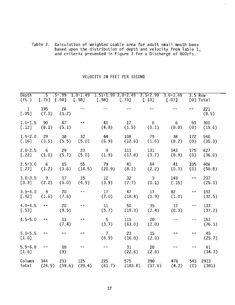
Table 2. Calculation of weighted usable area for adult small mouth bassbased upon the distribution of depth and velocity from Table 1,and criteria presented in Figure 3 for a Discharge of 800cfs.

VELOCITY IN FEET PER SECOND

Depth .5 .5-.99 1.0-1.49 1.51-1.99 2.0-2.49 2.5-2.99 3.0-3.49 3.5 Row(ft. ) [.75J [.90] [.98] [.98] [.73] [.13] [.03J [OJ Total

1 195 26 221[.05] (7.3) (1.2) (8.5)

1.0-1.5 90 47 41 17 6 6 93 300[.12J (8.1) (5.1) (4.8) (1. 5) (0.1) (0.0) (0) (19.6)

1. 5-2. 0 29 38 32 44 108 79 38 172 540[.16J (3.5) (5.5) (5.0) (6.9) (12.6) (1.6) (0.2) (0) (35.3)

2.0-2.5 6 29 23 9 111 131 143 175 627[.22J (1. 0) (5.7) (5.0) (1.9) (17.8) (3.7) (0.9) (0) (36.0)

2.5-3.0 6 15 55 79 41 64 41 105 406[.27J (1. 2) (3.6) (14.5) (20.9) (8.1) (2.2) (0.3) (0) (50.8)

3.0-3.5 9 17 15 12 32 3 149 237[3.3] (2.2) (5.0) (4.9) (3.9) (7.7) (0.1) (.15) (25.3)

3.5-4.0 9 20 17 47 17 82 192[.42J (1. 6) (7.6) (7.0) (14.4) (0.9) (1.0) (32.5)

4.0-4.5 20 11 50 35 17 133[.53J (9.5) (5.7) (19.3) (2.4) (0.3) (37.2)

4.5-5.0 11 5 115 20 151(7.4) (3.7) (63.0) (2.0) (76.1)

5.0-5.5 7 23 15 45[1.0] (6.9) (16.8) (2.0) (25.7)

5.5-6.0 10 31 20 61[1.0] (9) (22.6) (2.6) (34.3)

Column 344 233 125 225 575 390 476 545 2913Total (24.9) (59.6) (29.4) (61. 7) (183.8) (17.6) (4.2) (0) (381)

37

Weighting factors (ref. Fig. 3) for the depth and velocity ranges used in the

matrix are enclosed in brackets. The upper numerals in the matrix refer to

the surface area of the stream per 500 feet of reach which possesses that

combination of depth and velocity (ref. Table 1), while the numerals in

parenthesis refer to the equivalency in weighted usable area (WUA i = CiAi ).

Note that in this example the total surface area per 500 feet of reach

(2913 ft2 ), has been equated to 381 ft2 of surface area possessing most

suitable depth-velocity conditions.

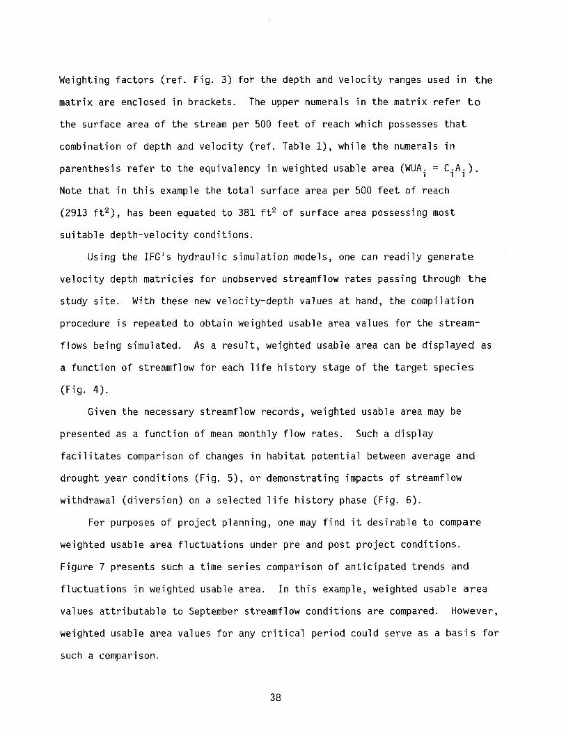
Using the IFG's hydraulic simulation models, one can readily generate

velocity depth matricies for unobserved streamflow rates passing through the

study site. With these new velocity-depth values at hand, the compilation

procedure is repeated to obtain weighted usable area values for the stream­

flows being simulated. As a result, weighted usable area can be displayed as

a function of streamflow for each life history stage of the target species

(Fig. 4).

Given the necessary streamflow records, weighted usable area may be

presented as a function of mean monthly flow rates. Such a display

facilitates comparison of changes in habitat potential between average and

drought year conditions (Fig. 5), or demonstrating impacts of streamflow

withdrawal (diversion) on a selected life history phase (Fig. 6).

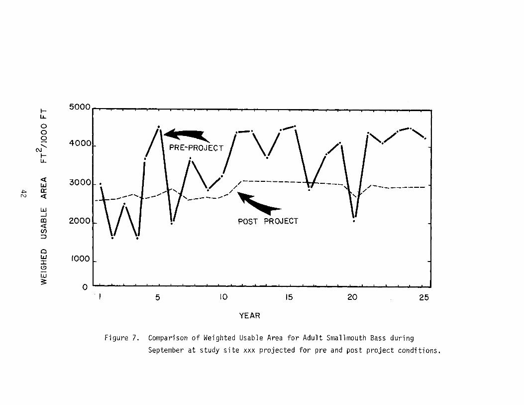
For purposes of project planning, one may find it desirable to compare

weighted usable area fluctuations under pre and post project conditions.

Figure 7 presents such a time series comparison of anticipated trends and

fluctuations in weighted usable area. In this example, weighted usable area

values attributable to September streamflow conditions are compared. However,

weighted usable area values for any critical period could serve as a basis for

such a comparison.

38

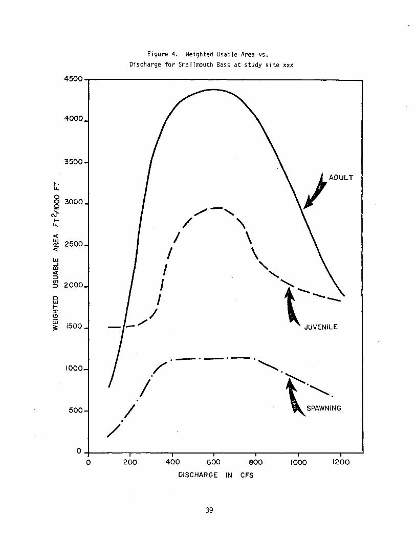
Figure 4. Weighted Usable Area vs.Discharge for Smallmouth Bass at study site xxx

4500..,.-------------------------_ __.

4000

3500

~ I ADULTlL

030000

Q /-,N"~ / "lL

« / \lLJ 25000:« I \I.LJ....J

I,

m« "-::::>C/)

2000 I \--::::>

0 IlLJ~

/::I:C)

JUVEN:w

i500 _/3::

1000

500

.---.---.---.", .

/' .

/ t-°"o/ • \... SPAWNING

/0-t-----,------r----.,.------.r-----.,------r---1

o 200 400 600 800

DISCHARGE IN CFS

1000 1200

39

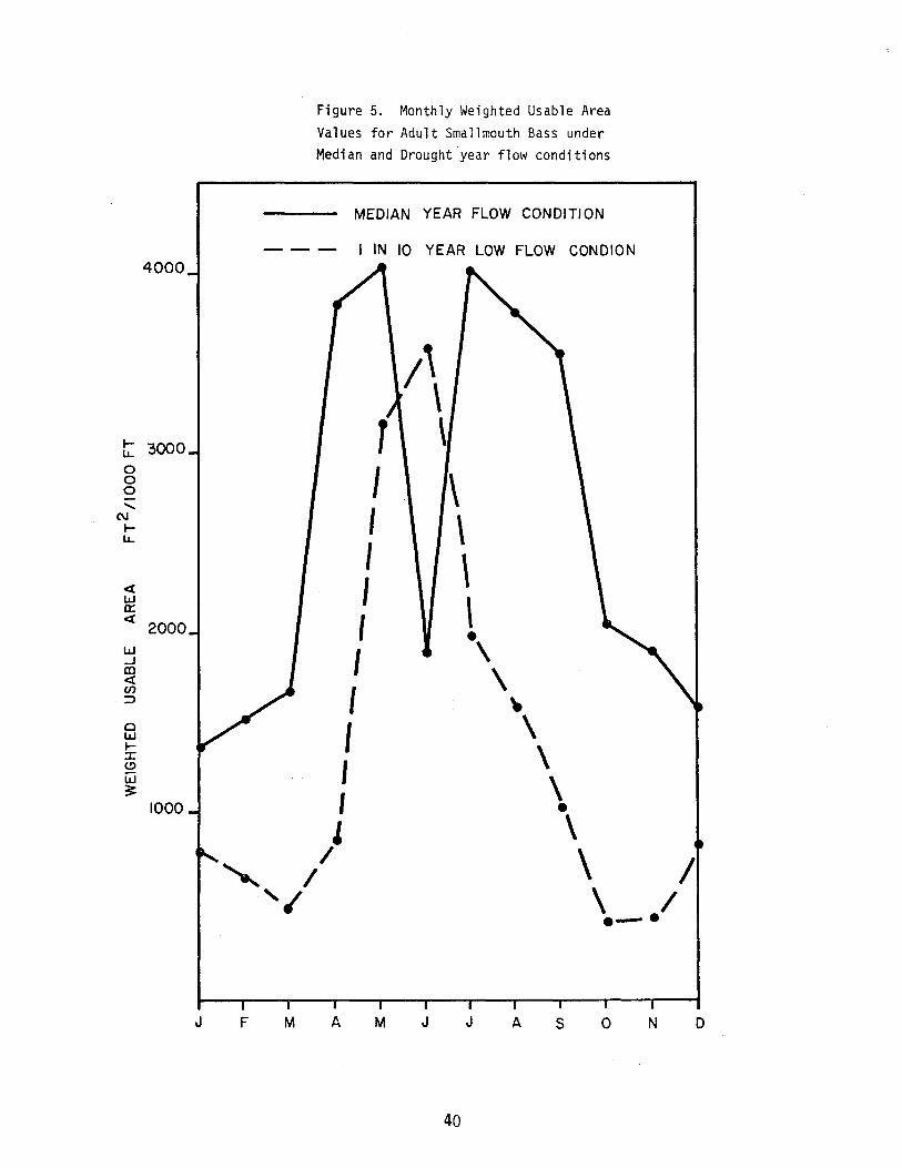
Figure 5. Monthly Weighted Usable AreaValues for Adult Smallmouth Bass underMedian and Drought·year flow conditions

MEDIAN YEAR FLOW CONDITION

- - - I IN 10 YEAR LOW FLOW CONDION4000

/,\

r 3000 1 \LL

0 I \00

"C\J I \rLL

I \« Iw

\a:«

2000 I •w I \.-JCD \«en

I::> ..0 I \wr

\:r(!) Iw \~ ,

1000 •l \

"/ \ //

,~ \ /.-.

J F M . A M J J A s o N D

40

Figure 6. Effect of a constant stream flowwithdrawal on available spawningarea for smallmouth Bass at studysite xxx.

1500 -------------------------..,

t-lL.

000

C\l...... 1000t-lL.

Z

«l&J0::«w-oJCD«:;) 500UJ:;)

0W::I:(,!)

W~

MEDIAN YEAR FLOW CONDITION

- - - MEDIAN YEAR CONDITION WITH CONSTANT

DIVERSION OF 25 CFS

...... I"""""....r,...

/(/ HIGHeV ASSOCiATEDWITH SPRING RUNOFF

/ RESTRICTS SPAWING AREA

/

J/~/ STREAMFLOW WITHDRAWL

tI RESTRICTS SPAWNING PRIORTO INCREASED SPRING RUNOFF

oAPRIL MAY

41

JUNE

o ,! , , , , ! , I , , , , , I , , , I I , , J I , I J I I ,

5000I' , , , , iii iii ii' iii , ii' , i ; • , i , ,

/----------/

.,./........,.

•

./.

•

./\~CT/-·\./-~~. //----------

..... I • /

,----_/ '-POST PR OJ EeT

•

/\•

1000

2000

3000L.

4000

r-l.L.

000"-C\Jr-l.L.

«IJJ

+:> (l:N «

IJJ-lCO«en::::>

0IJJ:I:(!)-W~

5 10 15 20 25

YEAR

Figure 7. Comparison of Weighted Usable Area for Adult Smallmouth Bass duringSeptember at study site xxx projected for pre and post project conditions.

In summary, the IFG Incremental Methodology was developed as a decision-

making tool for use in the water allocation arena. It links various elements

of fisheries behavior science and open channel hydraulics in an attempt to

describe the effects of incremental changes in streamflow on the instream

fishery potential. The methodology may also be used to identify effects of

stream channel alterations on fish habitat conditions or to predict possible

shifts in species composition as a result of flow or channel changes.

The methodology is intended for use in those situations where the flow

regime is the major determinant controlling the fishery resource and field

conditions are compatible with the under-pinning theories and assumptions of

the methodology: 1) steady state flow conditions exist within a rigid channel

and, 2) individuals of a species respond directly to available hydraulic

conditions. If these assumptions can reasonably be made, the methodology has

application to three basic types of questions.

1) Quantification of Instream Flow Requirements

a) Area wide planningb) Reservation or licensing of water rights

2) Negotiation of Water Delivery Schedules

a) Minimum releasesb) Yearly flow regimes (normal vs dry year conditions)

3) Impact Analysis

a) Streamflow depletionb) Streamflow augmentationc) Channel alterations

43

LIST OF REFERENCES

Bovee, K. D. 1978. Probability of use criteria for the family Salmonidae.Instream Flow Information Pater No.4. FWS!OBS-78/07. CooperativeInstream Flow Service Group, Fort Collins, Colorado. 80 pp.

Bovee, K. D. and T. Cochnaur. 1977. Development and evaluation of weightedcriteria, probability-of-use curves for instream flow assessments:fisheries, Instream Flow Information Paper No.3. FWS/OBS-77/63.Cooperative Instream Flow Service Group, Fort Collins, Colorado. 38 pp.

Bovee, K. D., and R. T. Milhous. 1978. Hydraulic simulation in instream flowstudies: theory and techniques. Instream Flow Information Paper No.5.Cooperative Instream Flow Service Group, Fort Collins, Colorado. 131 pp.

Main, R. B. 1978. IFG-4 program users manual. Unpublished manuscript.Cooperative Instream Flow Service Group, Fort Collins, Colorado. 80 pp.

Main, R. B. 1978. HABITAT program users manual. Unpublished manuscript.Cooperative Instream Flow Service Group, Fort Collins, Colorado. 80 pp.

44

MODULE I: RIVER MECHANICS, MORPHOLOGY, WATERSHED PROCESSES

MODULE LEADER: Daryl B. Simons, Associate Deanfor Engineering Research andProfessor of Civil Engineering,Colorado State University,Fort Collins, Colorado

45

IFG WORKSHOP PARTICIPANTSMODULE I

River Mechanics, Morphology, Watershed Processes

Dr. Daryl B. Simons, LeaderDept. of Civil EngineeringEngineering Research CenterFoothills CampusColorado State UniversityFort Collins, Colorado 80523

Mr. Alden BriggsUS Bureau of ReclamationBoulder City, Nevada 89005

Mr. William EmmettUS Geological SurveyWater Resources DivisionBuilding 75Denver Federal CenterDenver, Colorado 80225

Mr. Christopher EstesDepartment of Civil and

Environmental EngineeringWashington State UniversityPullman, Washington 99164

Dr. D. Michael GeeHydrologica Engineering CenterUS Army Corps of Engineers609 Second StreetDavis, California 95616

Dr. Ruh-Ming LiDept. of Civil EngineeringEngineering Research CenterFoothills CampusColorado State UniversityFort Collins, Colorado 80523

Dr. John F. OrsbornDepartment of Civil and

Environmental EngineeringWashington State UniversityPullman, Washington 99164

46

Mr. Ernest PembertonU.S. Bureau of ReclamationEngineering and Research CenterPO Box 25007, ATTN: 753Building 67Denver, Colorado 80225

Mr. Dave Rosgen,US Forest Service240 West ProspectFort Collins, Colorado 80523

Dr. Stanley SchummDepartment of Earth ResourcesNatural Resources BuildingColorado State UniversityFort Collins, Colorado 80523

Dr. H. W. ShenDept. of Civil EngineeringEngineering Research CenterFoothills CampusColorado State UniversityFort Collins, Colorado 80523

Dr. Mostafa A. ShiraziUS Environmental Protection AgencyCorvallis Environmental Research Lab200 SW 35th StreetCorvallis, Oregon 97330

Mr. John B. Stall1601 S. Maple StreetUrbana, Illinois 61801

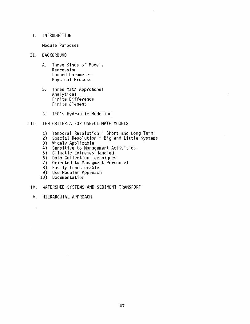
I. INTRODUCTION

Module Purposes

I!. BACKGROUND

A. Three Kinds of ModelsRegressionLumped ParameterPhysical Process

B. Three Math ApproachesAnalyticalFinite DifferenceFinite Element

C. IFG IS Hydraul i c Model i ng

III. TEN CRITERIA FOR USEFUL MATH MODELS

1) Temporal Resolution - Short and Long Term2) Spacial Resolution - Big and Little Systems3) Widely Applicable4) Sensitive to Management Activities5) Climatic Extremes Handled6) Data Collection Techniques7) Oriented to Managment Personnel8) Easily Transferable9) Use Modular Approach

10) Documentation

IV. WATERSHED SYSTEMS AND SEDIMENT TRANSPORT

V. HIERARCHIAL APPROACH

47

I. INTRODUCTION

The river and watershed system is an integral part of the dynamic

ecosystem. Stream flows, sediment transport rates, and channel morphology

reflect the major responses resulting from watershed management and/or river

utilization activities. Knowledge of river mechanics, morphology, and water­

shed management is basic to assessing instream flow needs.

Instream flow issues often result from increased competition for off

stream water uses (agricultural, industrial, urban, and energy developments)

and public concern for environmental quality. Sources of these issues arise

from such development activities as: (1) the redistribution of water over

time and/or space to increase low flows and/or reduce flood flows, (2) the

construction of diversions which decrease natural stream flows, and (3)

changes in land use or other watershed management practices that alter the

water and sediment input to the stream. Such developments affect both water

quantity and quality and in turn change stream morphology, stage-discharge

relationships, substrate distribution, and fish habitat.

When assessing instream flow requirements for fishery habitat and

instream recreation, knowledge of the spatial and temporal distribution of

flow depths and velocities is necessary. Consequently, the Cooperative

Instream Flow Service Group has developed hydraulic simulation techniques for

the determination of the spatial distribution of various combinations of

depths and velocities with respect to substrate for alternative flow regimes

or channel configurations.

The purposes of the Watershed and River Mechanics Module of the Workshop

were to: (1) evaluate current predictive methodologies, (2) evaluate the

hydraulic components of the Instream Flow Group's Incremental Methodology,

48

that are utilized for determining management aspects of instream flow needs,

(3) suggest possible improvements to the IFG1s hydraulic simulation models,

(4) make recommendations pertaining to the analysis of sedimentation aspects

of instream flows, and (5) recommend needed research.

A major objective was to be "critical."

11. BACKGROUND

General

The increasing interest in instream flow as a component of land and water

resource planning has stimulated the development of particular and general

watershed and river system response models. The models, whether physical or

conceptual, are formulated to estimate physical quantities that describe the

major system responses to precipitation such as: water yield, sediment yield,

yields of other water pollutants and stream morphology.

Degradation, aggradation and movement of sediment and other pollutants in

watersheds and river systems are closely related to water movement predictive

streamflow and water routing models have received the most intensive study.

Yet, the ability of the majority of available stream flow and water routing

models to relate wildland management activities in rather unique environments

in such a manner as to account for spatial diversity is not well demonstrated.

There are numerous mathematical models available for predicting the

response of watersheds and river systems. A comprehensive review of nonpoint

source water quality modeling in wildland management was conducted by the U.S.

Forest Service in (1976). An assessment of available methodologies for the

determination of instream flow requirements was made by Utah State University

49

for the U.S. Fish and Wildlife Service (Stalnaker and Arnette, 1976). This

assessment provided an in-depth review of basic stream flow measurements and

relationships, water quality relationships to flow, methodologies for deter­

mining required instream flows for fish and other aquatic life, methodologies

for assessing instream flow requirements for wildlife, and other measurement

techniques for quantifying recreation and aesthetic values. Most of the

methodologies identified in these publications have been studied by the IFG

staff and provide the basis for much of the reasoning behind their Incremental

Methodology.

Mathematical Models

Generally speaking mathematical models can be classified according to

their dominant traits as one of three types: (1) regression, (2) lumped

parameter or IIblack box ll simulation, or (3) physical process simulation.

Regression models are often easy to use and understand but have limited

applicability. A general weakness of regression models is that the variables

representing water and land uses and instream flow conditions are often not

specific enough to reflect the effects of many individual management activi­

ties. In addition, the regression models usually require sufficient observed

data to correlate meaningful relationships. This is often their most serious

drawback. Furthermore, it is very difficult to predict time and space

dependent responses (requisites of any instream flow analysis) using

regression equations. Regression models are very useful, however, for

identifying significant variables in large complex systems.

The lumped parameter or IIblack box simulation type of model interprets

input-output relationships using simplified coefficients and formulae which

50

mayor may not have any physical significance. The classic example of a

lumped parameter model is the rational formula for estimating peak discharge. 1

Such a model is easy to use, but has limited physical meaning and is

often inaccurate. It is impossible to reliably predict the effects of alter-

native mixes and sequences of land management activities occurring in upland

watersheds utilizing lumped parameter models.

Physical process simulation models avoid 1I1 ump ing" physically significant

variables. The overall physical process is separated into component processes

which themselves can be analyzed and refined to meet the needs of the user.

Consequently, as each process component is better understood and upgraded, the

overall model becomes more representative of the physical system. Use of

components also allows input of variables that have physical significance and

meaning to the user. Advantages of physical process simulation models over

other types of models are numerous. But most importantly physical process

models are IIdynamic simulation systems"; the input variables are physically

significant and the model need not be stationary in either time or space.

Methodologies presented in the literature identify three basic types of

mathematical approaches to watershed and river analysis: (1) the analytical

solution, (2) the finite difference method, and (3) the finite-element method.

Hann and Young (1972) and Simons et al. (1977) provide a good summary review

1 Q=CIA where Q is the peak discharge, I is the rainfall input, Ais the drainage area, and C is the runoff coefficient which representsthe major hydrologic processes.

51

of finite difference models using both implicit and explicit solution tech­

niques. Analytical solutions are usually limited by some simplifying assump­

tion (i.e. one dimensional steady flow in rigid boundaries) and are, there­

fore, applicable only to those field conditionsfor which the simplifying

assumptions are valid.

More recently finite-element techniques have been actively applied to

microscopic flow phenomena. Due to the fundamentals of the finite element

formulation, completely arbitrary geometrics can be modeled as well as more

common conditions. In addition, the feature of variable element size can be

used to create a fine mesh of elements in areas of high variable gradient in

order to obtain the desired accuracy and detail in sensitive regions. The

major drawback of the finite-element method is the required computer time.

This constraint will be less significant in the future as numerical techniques

and computer software advancements occur.

IFG's Hydraulic Simulation Efforts

To date the IFG has developed two hydraulic simulation models. The

hydraulic component of the Incremental Methodology is specifically oriented

toward the assessment of riverine fishery conditions on a microhabitat basis.

The models determine spatial distribution of various combinations of veloci­

ties and depths with respect to substrate as a function of either discharge or

cross sectional geometry. Basically, the IFG's hydraulic models are

lIanalyticalli and are based on the assumptions of steady-state flow and rigid

boundary conditions. A major effort is made in determining stage-discharge

relationships and calibrating the Manning roughness coefficient based on site

specific fiedld data (i.e. collected within the representative reach. IGFls

52

hydraulic models represent progressive, state-of-the-art tools for evaluating

instream flow needs. The calibration techniques used are described in two

reports Hydraulic Simulation in Instream Flow Studies (Bovee and Milhous,

1978) and The Calibration of Equations Used to Calculate the Velocity

Distribution in ~ River for Instream Flow Analysis (Milhous, 1977).

The IFG-2 model is an "analytical physical process" model. It is a

modification of the Bureau of Reclamations water surface profile model (Bureau

of Reclamation 1957 and 1968). The IFG model utilizes standard step backwater

computational procedures, but differs from its predecessor in that the stream

channel may be subdivided into as many as ninety-nine conveyance areas rather

than the more traditional "ma in channel"; "r ight and left overbank" subdivi­

sions. Continuity is maintained from transect to transect using the average

velocity and total cross sectional area.

Resistance coefficients (i.e. Manning's "n") are difficult to estimate.

Quite often, the streams of primary interest to fishing managers have channels

in which the resistance coefficients vary marked by. In general, these

coefficients are a function of channel shape, bed material size and distribu­

tion, flow depth and vegetation. Resistance to flow also changes markedly

with discharge as bedform, bed material, or boundary conditions change. To

reduce dependence on properly estimating resistance coefficients, channel

shape, velocity distribution, and water surface elevations are measured in the

field under different flow conditions. These data are then used for site

specific calibration of the hydraulic model.

The IFG-4 model is an "ana lytical regression" model, dependent upon

empiricism. This model is based on a stage-discharge concept and requires

that repetitive depth-discharge and velocity-discharge observations be made at

the study site throughout the entire range of flows of concern. Equations for

53

velocity (V=aQb)and stage (S=cQd stage zero flow) are fitted to the data sets

then used as a basis for interpolating between observed flow conditions.

The watershed and river are integral parts of a dynamic system. Natural

variations and man's activities alike often cause significant shifting of

stage-discharge relationships. These shifts result from: (1) the sediment

movement that modifies the cross section continuously, (2) the dynamic effects

due to the rising and falling of stream discharge, and (3) the alteration of

bed material size and distribution (substrata). The rate of change of

stage-discharge relationships is dependent on the characteristics of the river

system such as: the bed material size, the magnitude and duration of flow,

the channel geometry, the gradient of the channel, and geological or man-made

controls. However, for relatively stable channels the stage-discharge

relationship remains comparatively constant and the IFG-4 model is applicable.

For unstable or dynamic systems, the IFG-4 model is not valid.

The Instream Flow Group's (IFG) efforts have been oriented toward the

development of a hierarchial and modular approach to instream flow studies

utilizing physical process simulation modeling. The modules and various

models available within the modules, should be considered as IIbuilding blocks"

from which an analysis framework can be constructed to evaluate effects of a

wide range of management alternatives. The existing hydraulic models (IFG-2

and IFG-4 represent operational state-of-the-art tools for instream flow

assessment work. Yet, they are applicable only to those field conditions for

which conditional assumptions hold.

54

III. CRITERIA FOR USEFUL MATHEMATICAL MODELS

WITH SPECIFIC COMMENT ON THE IFG INCREMENTAL METHODOLOGY

General Criteria

In order for a methodology to be useful, it should possess the following

attributes:

o (1) Promote clarity, not complexity. Application of complex techniques

to a rather simple problem will confuse rather than clarify the solution.

o

o

o

(2) Produce believable results. The methdology should be based on

accepted state-of-the-art techniques. When complex techniques are

appropriate they should be applied.

(3) Reduce, not compound, the risk and uncertainty associated with

solution alternatives.

(4) Provide understandable results. Results should be presented in a

format that can be understood by user/audience groups alike.

During the course of the workshop this discussion group identified ten

criteria as being descriptive of a useful mathematical model for predicting

cause-effect relationships within watershed and river systems. These criteria

were used to evaluate the IFG1s methodology. A summary follows:

Criteria 1: Temporal resolution of the methodology should be both short- and

long-term. Management practices usually have short- or long- term

55

effects on the environment, and the short-term projects may have

prolonged effects. Therefore, operationally the IFG methodology falls

short of this mark. The hydraulic simulation models being used by the

IFG are based on the assumption of rigid boundary conditions. With

respect to a water-shed response or project-life time frame this assump­

tion is seldom met. It is important to recognize that a river is a

dynamic system. An alluvial river is continuously changing its position

and shape as a consequence of hydraulic forces acting on its bed and

banks. These changes may be slow or rapid and may result from natural

events or from man's activities. Available information and technique for

predicting watershed response due to natural variation and man-made

activities should be incorporated in the methdology.

Response to stream flow is presently based on monthly flows. Month­

ly flows cannot adequately represent the natural variation in most river

systems due to the averaging process. The prediction error caused by the

monthly averaging process is even more pronounced when sediment transport

is evaluated. A better approach to watershed response due to duration,

quality, and frequency of flow is needed to improve prediction. In

addition, the impacts of forest harvesting, irrigated agriculture,

grazing, mining, and other watershed management activities on the water

and sediment yield from watersheds to the stream channel need to be

considered.

Criteria 2: Upland management plans and activities very often occur in small

watersheds while legal and institutional interests in instream flows are

often focused well downstream in the watershed or river basin. As a

56

consequence, the spatial resolution of the IFG models should accommodate

both small and large watersheds and river systems.

As previously stated the current methodology does not consider any

watershed responses. The existing IFG hydraulic models are theoretically

and operationally applicable to both large and small streams. However,

it is not clear how reliable they are in quantifying actual habitat

conditions in large rivers. In part, this is a criteria problem. But it

is also unrealistic to assume that mean column velocity provides suffi­

cient resolution to adequately quantify micro habitat conditions in large

deep rivers. hence, alternative hydraulic models should be developed

which analyize vertical velocity distribution.

Criteria 3: The method should be widely applicable. That is, although the

model parameters may be locally or regionally specific, the model itself

should not be. Conceptually, the IFG's methodology is capable of

providing an appropriate cause effect linkage between management

practices and system response in a variety of geographic locations.

Operationally, the models require site specific calibration data and

regionally specific species response critera. Lack of such a data base

may well impede the transfer and application of the methodology, however,

the same general logic and modeling approach (methodology) would be

applicable from one region to another.

Criteria 4: The model should be sensitive to desired management activities.

It must be possible to explicitly represent management activities and

simulate the system response resulting from these activities.

57

The methodology is intended to be used as a decision making tool and

is specifically tailored to demonstrate the impact of alternative flow

regimes on instream habitat conditions. The method also has application

for evaluating stream channel alteration or relocation proposals. From

an operational standpoint the in~remental methodology can be applied to

three fundamental types of instream flow questions.

1) Quantification of Instream Flow Requirements

a) Area wide planning

b) Reservation or licensing of water rights

2) Negotiation of Water Delivery Schedules

a) Minimum releases

b) Yearly flow regimes (normal vs dry year conditions)

3) Impact Analysis

a) Streamflow depletion

b) Streamflow agumentation

c) Channel alterations

Conceptually the methodology has far greater potential. By develop­

ing modular components discussed under criteria one, it will be possible

to initiate quantification of the effects of numerous land management

activities on instream fishery habitat and recreational potential.

Criteria 5: The uncertainties due to varying climatic and spatial input

should be considered. The simulation must consider variations in both

mean values and extreme events which requires a probabilistic approach to

describe the stochastic structure of model inputs.

58

The existing IFG methodology is capable of handling the full

complement of hydrologic input (streamflow records) available. The

method readily assesses changes in habitat potential attributable to

"incremental" changes in streamflow. Given ample streamflow data the IFG

models are capable of generating stochastic time series plots of corres­

ponding instream fishery habitat conditions.

A notable strength of the method is the ability to describe instream

conditions with respect to local climatic events such as: wet, average

and drought conditions.

Criteria 6: The model should be developed within the constraints of available

data. Models intended for practical applications should not impose

requirements for data that are excessively difficult, costly, or time

consuming to collect or acquire. If a large quantity of data is

required, an effective data storage and retrieval system is necessary.

Calibration data for the hydraulic models may be obtained by

employing routine surveying and stream gaging techniques.

Criteria 7: The model should be oriented for use £y management personnel.

Models intended for use by managers must fit into the specific decision­

making processes and situations for which they are to be employed, if

information resources are to be generated efficiently and used effec­

tively. So, for useable models to be designed and implemented,

developers must be in effective communication with target users through­

out the development process. Involving users in model design helps

insure that the model developer has full knowledge of the decision-making

environment, the actual problems mangers face, and the user's perception

of the situtation being modeled. Such a model will be more relevant and

the user will better trust its validity and capability. The perspective

of the water manager is foremost in the IFG's model development work.

Emphasis is on building a communication tool between the fishery manager

and water-planning community. By involving users in model design IFG

helps insure that the Group has full knowledge of the decision-making

environment, the actual problems both managers face, and the user groups·

perception of the everyday utility of the software being developed.

Criteria 8: It should be possible to easily transfer the model to different

levels of accuracy and resolution. Models operable at several levels of

accuracy and resolution will be required in order to provide the full

range of tools needed for instream, land and river management.

Providing useable and realistic models and guidelines for use by

field level managers in many cases will first require developing and

testing relatively complex process models. Once the processes invloved

are thoroughly understood and the sensitive parameters identified, these

models can then be regionalized and generalized to provide simplified

models and guidelines for field users.

The IFG has incorporated a hierarchial approach within the framework

of its methodology. A very low resolution hydraulic analysis can be per­

formed with extremly limited field data. Investment in the manpower and

materials necessary to obtain real world calibration data over a range of

60

flows will greatly improve the accuracy of the predictions obtained from

the hydraulic models and upgrade considerably the confidence one has in

the hydraulic analysis (i.e. a function of discharge). Depending upon

the financial and temporal resources available a corresponding level of

hydraulic analysis can be performed. Precautions must be taken, however,

not to enter into litigation or important negotiations with a recon­

nassiance grade simulation.

Criteria 9: The model computer software system should adopt the modular

approach. Adopting the modular approach offers an opportunity to build a

coordinated nucleus of standardized system components for use in a wide

spectrum of watershed and river systems. This nucleus would be made up

of components that are necessary for storage and retrieval, analysis, and

display. Modular systems also have the advantage that individual compon­

ents can be updated or replaced as needed without disrupting other com­

ponents of the system. Generalized, all-purpose models are expensive to

develop, usually lack sensitivity to the wide range of management alter­

natives, are difficult to use and control, and have large data require­

ments--all of which tend to detract from their operational utility.

As stated previously the IFG methodology utilizes a modular approach

to assessing instream flow requirements. Although this approach may

appear confusing, and perhaps even ambiguous, to the uninitiated it

possesses several distinct advantages over generalized all purpose

models; even with their standardized data input and crank turning II coo k

book ll instruction.

61

Adopting the modular approach offers an opportunity to build a

coordinated nucleus of standardized system components for use in a wide

spectrum of instream flow situations. This nucleus would be made up of

component "building blocks" that provide for common interfaces for

information transfer between modules that are necessary for storage and

retrieval, analysis, and display. In addition, modular systems have the

great advantage that individual components can be refined, updated, or

replaced as needed without disrupting other components of the system.

Criteria 10: The models should be properly documented. The documentation

should include: i) the sytem level flow chart showing how modules and

files are connected, ii) the flow chart of each module, iii) the descrip­

tion of each file, iv) narrative descriptions showing how the system is

implemented, v) definitions of all variables in each module, and vi)

comments on each program or file that show the purpose of the code.

From an operational standpoint IFG's computer software is not

adequately documented for efficient transfer. In part, this is due to

the lack of documentation which was available for those programs IFG

obtained from outside sources and modified to fit the specific needs of

instream habitat assessment work. As of this writing the IFG has four

major software packages operational. User manuals need to be developed,

flow charts prepared, and variables defied for each program. This is

perhaps the IFG's biggest housekeeping chore.

The philosophy of modeling adopted by the IFG is consistent with

these general attributes and criteria. The methodology is based on

62

accepted state-of-the-art techniques, employing a hierarchial and modular

approach to simulation modeling. Obvious it is the intent of the IFG to

utilize simulation to promote clarity, reduce risk, and otherwise

facilitate decision making.

63

IV. WATERSHED PROCESSES AND SEDIMENT TRANSPORT

State-of-the-Art

Existing sediment models of watershed systems deal mainly with surface

erosion. No process models exist for unstable channel erosion, nor are any

models available for predicting mass wasting and its interaction with

channels. Almost all existing surface erosion models are based on either the

Musgrave approach or the Universal Soil Loss Equation (U.S. Forest Service,

1976). These models are difficult to use because they are insensitive to both

the spatial and temporal variability of management activities. In 1975,

Simons et al. (1975a) developed a numerical model to simulate the physical

processes governing sediment movement on small watersheds. This model can

predict the effects of management activities on sediment yield in both time

and space. However, its applicability is presently limited to surface erosion

on fairly stable land in small watersheds and for a single storm.

Sediment transport is often one of the most important variables needed

for evaluating fishery habitat. The capacity of a stream to transport sedi­

ment depends on hydraulic properties of the stream channel. Such variables as

slope, roughness, channel geometry, discharge, velocity, turbulence, fluid

properties, and size and gradation of the sediment are closely related to the

hydraulic variables controlling the capacity of the stream to carry water, and

are subject to mathematical analysis.

Generally, an alluvial river is continuously changing its position and

shape as a consequence of hydraulic forces acting on its bed and banks. As a

result of the interaction of these forces biological processes within the

64

river environment are in a constant state of flux. These changes may be slow

or rapid and may result from natural events or from man1s activities.

When a river channel is modified locally, the change frequently causes

modification of channel characteristics both up and downstream and can be

propagated for long distances. Many available river routing models either

neglect the dynamic response due to sediment movement or are insensitive to

man's activities. Because bed material is transported as both suspended load

and bed load the different physical laws governing these modes of transport

must be incorporated into any method for predicting total transport of bed

material.

The distinction between bed-material load and wash load is of importance.

Bed material is transported based on availability and the capacity of the

stream. Its transport rate is functionally related to measurable hydraulic

variables. Wash load is not usually transported at the capacity of the stream

and is not functionally related to hydraulic variables. While there is no

sharp demarcation between wash load and bed-material load, one rule of thumb

assumes that the bed-material load consists of sizes equal to or greater than

0.062 mm, the division between sand and silt. Another reasonable criteria is

to choose a sediment size finer than the smallest 10 percent of the bed

material as the point of division between wash load and bed-material load.

Sediment particles that constitute the bed-material load are transported

either by rolling or sliding along the bed (bed load) or in suspension. Again

there is no sharp distinction between bed load and suspended load. A particle

of the bed-material load can move part of the time in contact with the bed or

be suspended by the flow. Generally, the amount of bed-material moving in

contact with the bed of a large sand-bed river is only a small percentage of

the bed material moving in suspension. These two modes of transport follow

65

different physical laws which must be incorporated into any equation for

estimating the bed-material discharge of a river.

Limited quantities of fine material moving as wash load usually will not

pose direct problems inhibiting development activities in the riverine

environment. However, large concentrations of fine materials can influence

fluid viscosity and density, stream bank stability, growth of aquatic plants,

and the biomass of the channel.

For a detailed treatment of currently used suspended and bed-material

load transport theories refer to Vanoni (1976) and Simons and Senturk (1977).

Data on sediment transport in the steep channel systems is generally unavail­

able due to the extreme difficulty associated with collecting data in the

laboratory and field environments. Yet many of the streams with high fishery

and recreation potential are steep turbulent channels. An effort to obtain

more information on sediment transport in the steep channel systems is

warranted.

Hydraulic geometry is a general term applied to alluvial channels to

denote relationships between discharge, the channel morphology, hydraulics and

sediment transport. In self-formed alluvial channels, the morphologic,

hydraulic, and sedimentation characteristics of the channel are determined by

a large variety of factors. In general, these relationships apply to channels

within a physiographic region and can be derived from data available on gaged

rivers. It is understood that hydraulic geometry relationships express the

integrated effect of all the hydraulic, hydrologic, meterorologic, and

geologic variables in a drainage basin.

Geometric relations describing alluvial streams are necessary in river

engineering and river modeling. The forerunners of such relationships are the

regime equations developed to design stable alluvial canals. A generalized

66

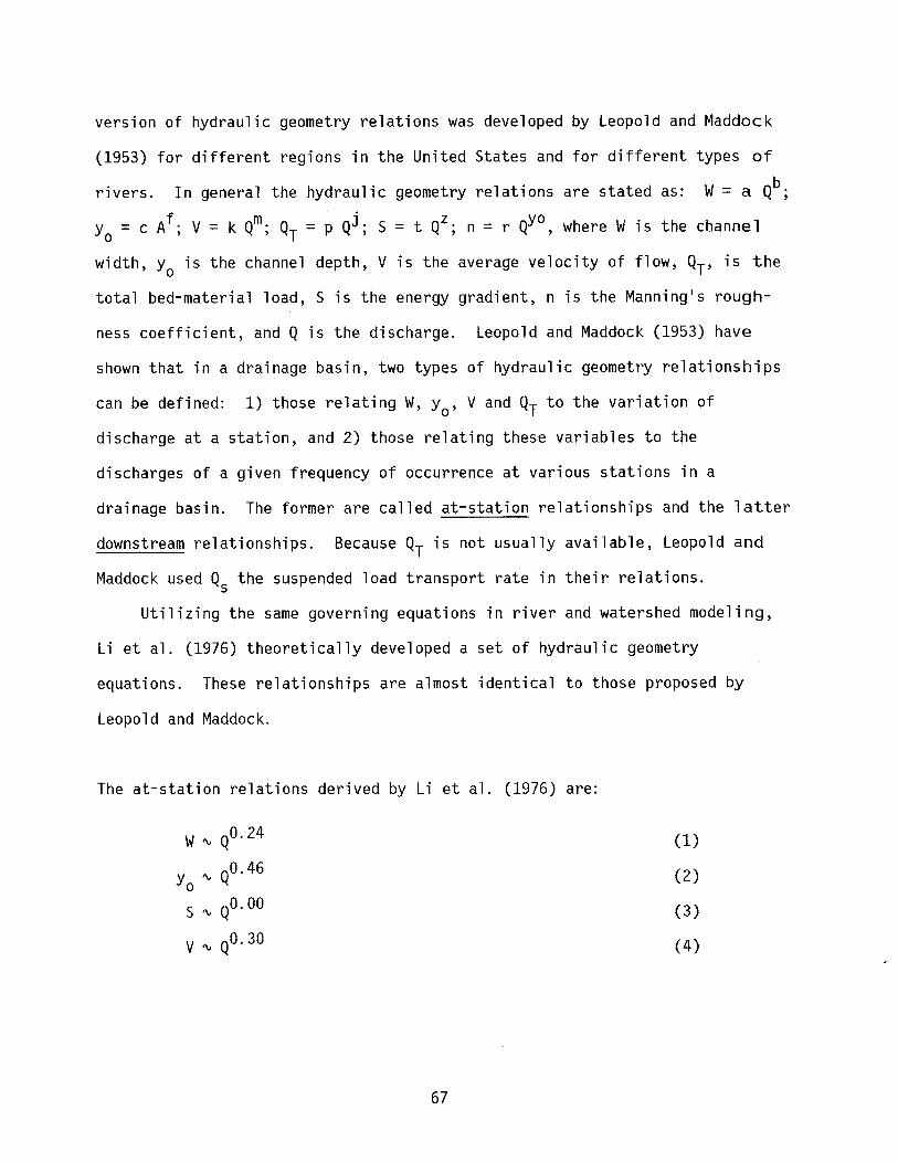
version of hydraulic geometry relations was developed by Leopold and Maddock

(1953) for different regions in the United States and for different types of

rivers. In general the hydraulic geometry relations are stated as: W= a Qb;

Y = c Af . V = k Qm. Q = p Qj. s = t QZ. n = r Qyo where Wis the channelo ' 'T ' " -

width, Yo is the channel depth, V is the average velocity of flow, QT' is the

total bed-material load, S is the energy gradient, n is the Manning's rough-

ness coefficient, and Q is the discharge. Leopold and Maddock (1953) have

shown that in a drainage basin, two types of hydraulic geometry relationships

can be defined: 1) those relating W, Yo' V and QT to the variation of

discharge at a station, and 2) those relating these variables to the

discharges of a given frequency of occurrence at various stations in a

drainage basin. The former are called at-station relationships and the latter

downstream relationships. Because QT is not usually available, Leopold and

Maddock used Q the suspended load transport rate in their relations.s

Utilizing the same governing equations in river and watershed modeling,

Li et al. (1976) theoretically developed a set of hydraulic geometry

equations. These relationships are almost identical to those proposed by

Leopold and Maddock.

The at-station relations derived by Li et al. (1976) are:

w~ QO.24

y ~ QO.46oS ~ QO.OO

V ~ QO.30

67

(1)

(2)

(3)

(4)

Equation (3) implies that slope is constant at a cross section. This is

not quite true except for steep channels. At low flow the effective channel

slope is that of the thalweg that flows from pool through crossing to pool.

At higher stages the thalweg straightens somewhat shortening the path of

travel and increasing the local slope. In the extreme case, river slope

approaches the valley slope at flood stage. It is during high floods that the

flow often cuts across the point bars developing chute channels. This path of

travel verifies the shorter path the water takes and that a steeper channel

prevails during floods.

The derived downstream relations for bank-full discharge are:

0.46Yb ~ Qb (5)

0.46Wb ~ Qb (6)

0.46S ~ Qb (7)

0.08Vb ~ Qb (8)

where the subscript b indicates the bank-full condition. The above theoret­

ically derived hydraulic geometry equations can be utilized to estimate bank­

full discharge and to evaluate channel stability.

For a detailed description of current knowledge of river morphology refer

to Schumm (1978) and Simons and Senturk (1977).

Aggradation, degradation, and the transport of sediment and pollutants in

watersheds and river systems are closely related to water movement. A model

that will predict effects of management activities and represent spatial and

temporal variability of both activities and processes is needed. A great deal

of research has been conducted on various components within the hydrologic

68

cycle. This research in conjunction with stream flow and water routing models

provide necessary ingredients for advanceing our understanding of physical

process simulation for estimating transport rates of sediment and pollutants.

HIERARCHIAL APPROACH FOR ANALYSIS

Both general and specific criteria of useful models applicable to

instream flow analysis have been previewed. This section discusses a multiple

level of analysis approach that can be utilized for achieving selected levels

of resolution. The IFG's methodology should consider watershed processes and

sedimentation as integral components of the riverine ecosystem, and develop an

analytical approach toward quantification. The recommended hierarchial

approach for this analysis is presented by II watershedll and "channel ll submodule

discussion groups. Insight is provided as to the steps required to develop

and conduct an integral analysis of watershed processes and sedimentation.

Watershed Submodule

A watershed submodule would provide water and sediment inflow (magnitude

and timing) information for other components of the analysis. A recommended

approach to multiple levels of analysis follows:

Levell analysis is limited to working with immediately available data

and performing only IIdesk topll analyses. The available information would be

analyzed using several mechanisms such as frequency distribution analysis,

water yield nomographs, the geomorphic description of drainage patterns, etc.

The analysis would then describe the present watershed conditions, with regard

to frequency and duration of various flow volumes, both high and low. Such

69

details regarding the flows would be based on description and evaluation of

basin characteristics, stream patterns, soil types, land-use patterns, etc.

Level 2 analysis would extend and refine the level 1 effort to narrower

confidence bounds and more completely describe the watershed and flow

characteristics. Some field measurements would be required including stream

cross sections, sediment size fraction surveys, and spot checks of stream

flows. More extensive data manipulation and transfer mechanisms would be

applied to obtain more accurate, location specific results.

Level 3 would use state-of-the-art models to perform the data manipu­

lation and system description functions. Additional data specific to the site

of interest would be collected as needed to provide the additional data needed

to improve model accuracy.

Level 4 would involve research to upgrade and/or modify the state-of­

the-art methods to improve the level 3 analysis.

The description of watershed, stream flow and sediment characteristics at

each level of resolution is dependent on the following information: (1)

location of the flow altering facilities within the watershed, (2) the purpose

and methods of operation and impacts on flow imposed by such facilities, (3)

the portion of affected watershed, i.e., to the main stem or to the estuary,

and (4) the time span of alteration of physical and flow conditions.

The following table summarizes the type of information, type of manipu­

lation and results obtainable utilizing the three levels of analysis.

70

Data

Streamflow:

Levell: Approximate Confidence-±50%

Manipulation Results

USGS, county, stateor other agency'sgage data. Waterhydrographs orstage hydrographswith stage-dischargerelationships

Precipitation:

Nearest representa­tive, USNWS gage orgages

Maps:

USGS, county, stateand other entitiestopographic andsoil maps

Areal photos:

Other reports andpersonal communi­cations:

Translation to specificsite, then frequencyanalysis

Translation to siteTP-40 and otherintensity-durationanalysis

Geomorphologicdescription ofdrainage patternWater yield nomo­graphs or computer­ized procedure

Visual inspectionand interpretation

71

Duration curve of dailydischarge, frequencydistribution, bank-fulldischarge (Q), date andduration of peak Q,duration of bank-full Q,

Intensity, frequency,annual precipitationdistribution, meanannual precipitation, etc.

Basin characteristics, area,stream order, length, slopeerosion potential, streampotential, soil typesAverage seasonal normal­ized runoff distribution,i.e., hydrograph basedon 7-day averages

Land use, vegetation,human impacts

Any and all of above

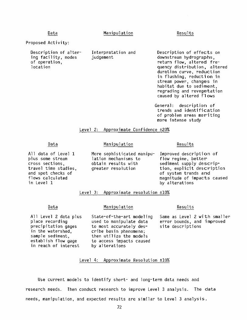
Data

Proposed Activity:

Description of alter­ing facility, modesof operation,location

Manipulation

Interpratation andjudgement

Results

Descri pti on of effects ondownstream hydrographs,return fl ow, altered fre­quency distribution~ altereddurat i on curve, reductionin flushing, reduction instream power, changes inhabitat due to sedi ment,regradi ng and revegetationcaused by altered fl ows

General: description oftrends and identificationof problem areas meritingmore intense study

Level 2: Approximate Confidence ±20%

Data

All data of Levellplus some streamcross sections,travel time studies,and spot checks offlows calculatedin Level 1

Manipulation

More sophisticated manipu­lation mechanisms toobtain results withgreater resolution

Results

Improved descri pt i on offlow regime, bettersediment supply descrip­tion, explicit descriptionof system trends andmagnitude of impacts causedby alterations

Data

Level 3: Approximate resolution ±10%

Manipulation Results

All Level 2 data plusplace recordingprecipitation gagesin the watershed,sample sediment,establish flow gagein reach of interest

State-of-the-art modelingused to manipulate datato most accurately des­cribe basin phenomena;then utilize the modelsto access impacts causedby alterations

Same as Level 2 with smallererror bounds, and improvedsite descriptions

Level 4: Approximate Resolution ±10%

Use current models to identify short- and long-term data needs and

research needs. Then conduct research to improve Level 3 analysis. The data

needs, manipulation, and expected results are similar to Level 3 analysis.

72

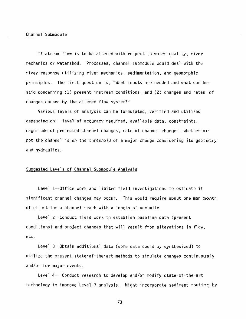
Channel Submodule

If atream flow is to be altered with respect to water quality, river

mechanics or watershed. Processes, channel submodule would deal with the

river response utilizing river mechanics, sedimentation, and geomorphic

principles. The first question is, "What inputs are needed and what can be

said concerning (1) present instream conditions, and (2) changes and rates of

changes caused by the altered flow system?"

Various levels of analysis can be formulated, verified and utilized

depending on: level of accuracy required, available data, constraints,

magnitude of projected channel changes, rate of channel changes, whether or

not the channel is on the threshold of a major change considering its geometry

and hydraulics.

Suggested Levels of Channel Submodule Analysis

Level 1--0ffice work and limited field investigations to estimate if

significant channel changes may occur. This would require about one man-month

of effort for a channel reach with a length of one mile.

Level 2--Conduct field work to establish baseline data (present

conditions) and project changes that will result from alterations in flow,

etc.

Level 3--0btain additional data (some data could by synthesized) to

utilize the present state-of-the-art methods to simulate changes continuously

and/or for major events.

Level 4-- Conduct research to develop and/or modify state-of-the-art

technology to improve Level 3 analysis. Might incorporate sediment routing by

73

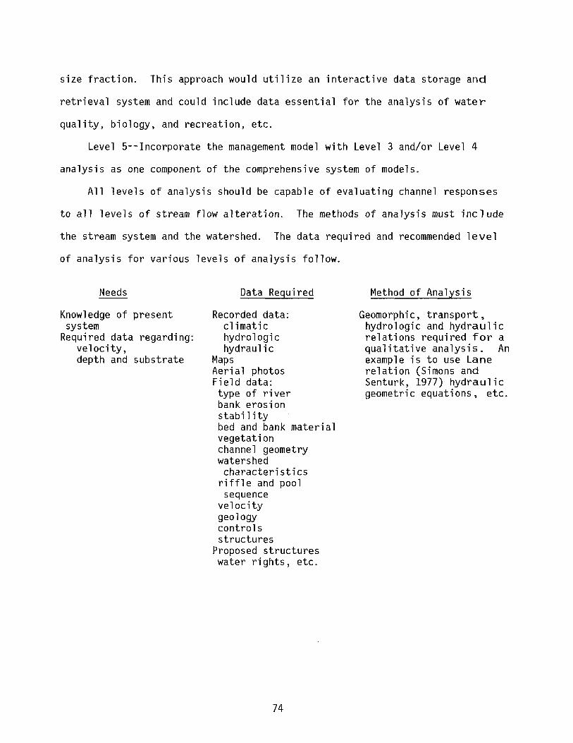
size fraction. This approach would utilize an interactive data storage and

retrieval system and could include data essential for the analysis of water

quality, biology, and recreation, etc.

Level 5--Incorporate the management model with Level 3 and/or Level 4

analysis as one component of the comprehensive system of models.

All levels of analysis should be capable of evaluating channel responses

to all levels of stream flow alteration. The methods of analysis must include

the stream system and the watershed. The data required and recommended level

of analysis for various levels of analysis follow.

Needs

Knowledge of presentsystem

Required data regarding:velocity,depth and substrate

Data Required

Recorded data:climatichydrologichydraulic

MapsAerial photosField data:type of riverbank erosionstabil itybed and bank materialvegetationchannel geometrywatershedcharacteristics

riffle and poolsequence

velocitygeologycontrolsstructures

Proposed structureswater rights, etc.

74

Method of Analysis

Geomorphic, transport,hydrologic and hydraulicrelations required for aqualitative analysis. Anexamp1e is to use Lanerelation (Simons andSenturk, 1977) hydraul i cgeometric equations, etc.

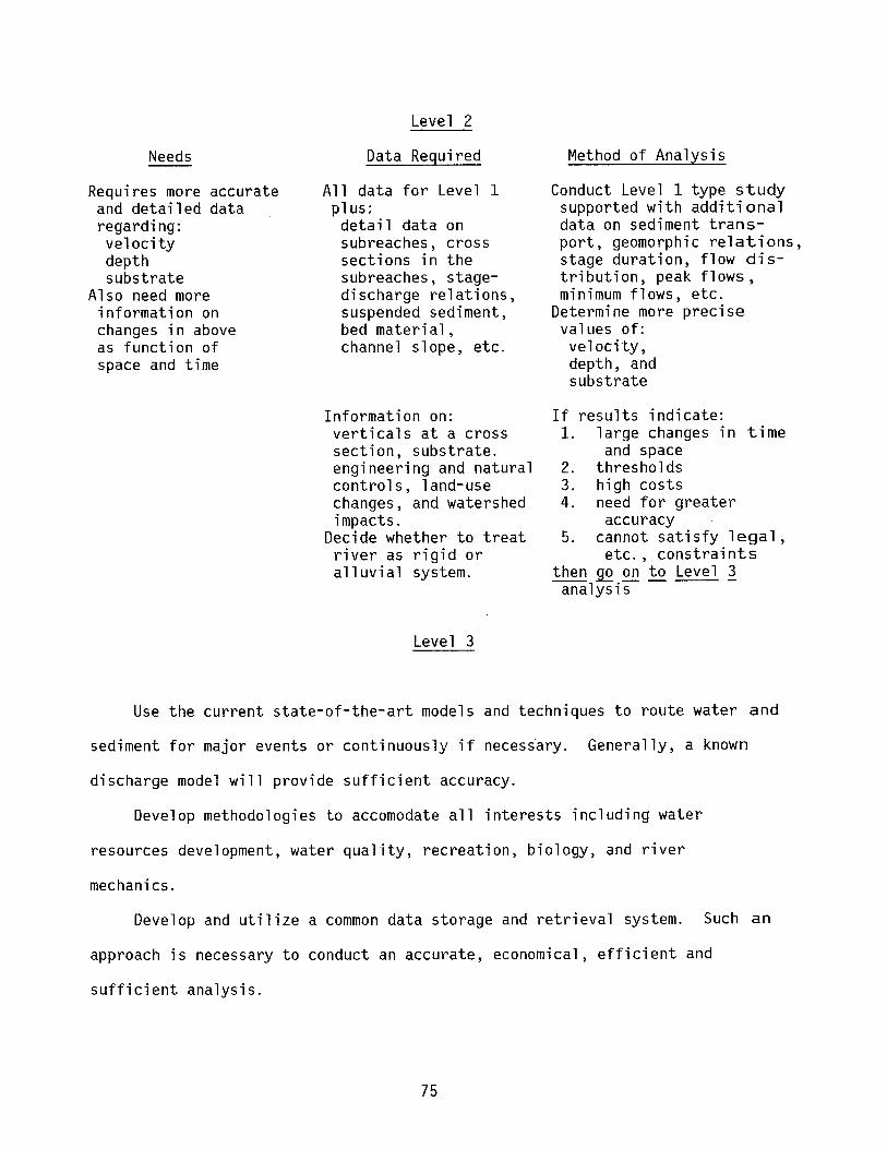
Needs

Requires more accurateand detailed dataregarding:velocitydepthsubstrate

Also need moreinformation onchanges in aboveas function ofspace and time

Level 2

Data Required

All data for Levellplus:detail data onsubreaches, crosssections in thesubreaches, stage­discharge relations,suspended sediment,bed material,channel slope, etc.

Information on:verticals at a crosssection, substrate.engineering and naturalcontrols, land-usechanges, and watershedimpacts.

Decide whether to treatriver as rigid oralluvial system.

Level 3

Method of Analysis

Conduct Level 1 type studysupported with additionaldata on sediment trans­port, geomorphic relations,stage duration, flow dis­tribution, peak flows,minimum flows, etc.

Determine more preciseval ues of:velocity,depth, andsubstrate

If results indicate:1. large changes in time

and space2. thresholds3. hi gh costs4. need for greater

accuracy5. cannot satisfy legal,

etc., constraintsthen ~ on to Level ~

analysis

Use the current state-of-the-art models and techniques to route water and

sediment for major events or continuously if necessary. Generally, a known

discharge model will provide sufficient accuracy.

Develop methodologies to accomodate all interests including water

resources development, water quality, recreation, biology, and river

mechanics.

Develop and utilize a common data storage and retrieval system. Such an

approach is necessary to conduct an accurate, economical, efficient and

sufficient analysis.

75

Level 4

Use current models to identify short- and long-term data needs and

research needs and then conduct research to improve Level 3 type analysis.

One could proceed with a higher level of sophistication involving water

quality, sediment routing by size fraction, two-dimensional modeling and

improve watershed modeling components.

Multistep Development for Analysis

The development and application of a model usually involves the following

steps: spatial design, temporal design, model formulation, mathematical

solution, model calibration, parameter sensitivity analysis, qualitative

examination of physical significance, model simplification, regionalization

and generalization, validation, testing and refinement under operational field

applications and documentation.

The spatial and temporal designs of watershed and river systems are both

requisets for any realistic representation of the space-time structure of the

system simulation models. The spatial design must consider the purposes of

the study. Knowledge of pertinent gaging stations, structures, and

confluences allows development of the spatial design of a large river basin.

The watershed geometry, topography, vegetation and soil distribution may also

be necessary.

The temporal design is used to generate input for evaluating system

response, over time. The temporal design of a system can be made using the

76

historic hydrologic records of the watershed and river basin. Such records

include: historic maximums, minimums; mean precipitation, temperature,

moisture content; river stages, precipitation patterns, flow volumes, and the

effect of man's activities on the system. The temporal design should be

compatible with the spatial design. Therefore, only those records pertinent

to areas included in the spatial design need be analyzed.

After the spatial and temporal designs have been made, the physical

processes governing the response of the system are not difficult to identify,

and a series of partial or total differential equations can be used to

represent the governing processes. The model formulation should consider the

criteria of a useful mathematical model established earlier.

For simulating the dynamic response of water and river systems, perhaps

the most important governing equations include: the continuity equation for

water, the continuity equation for sediment, and the energy equation. These

three equations can be solved simultaneously or can be approximated by solving

the water continuity equation and the momentum equation first and then refine

the solution by using the sediment continuity equation. The second approach

is usually acceptable because the movement of sediment is much slower than

that of water. The numerical solution of these three equations can proceed in

two directions. Either an attempt can be made to convert the original system

of ordinary differential equations by using the method of characteristics

(Chang and Richards, 1971), or one can replace the partial derivatives in the

original system with quotients of finite-differences by using the explicit

method or the implicit method (Amein, 1968; Amein and Fang, 1970, and Chen,

1973).

77

In the mathematical modeling of system respones, the calibration of model

parameters has often relied on an optimization scheme. The dependency on the

optimization technique may be reduced if the model is formulated considering

the physical significance of important processes. For the flood routing

problem, the parameters describing flow resistance are usually unknown, but

their ranges are known from measured data. However, the optimum values of the

parameters which reproduce correct model response are usually not available.

Hence, model calibration is a necessity. The simplest calibration technique

is the trial and error method. Except for models that contain parameters with

very narrow searching ranges, the trial and error procedure is inefficient.

An efficient procedure is apparently needed for the model calibration. There

are many optimization techniques available for the purpose of model calibra­

tion. However, the usefulness of a particular optimization technique is very

dependent on the formulation of the model being calibrated. Rosenbrockls

(1960) optimization technique is usually recommended for finding the optimum

set of parameters because it is by far the most promising and efficient method

for fitting a hydrologic model. Modifications of Rosenbrock's method have

been made by Simons and Li (1976) to increase the efficiency of the method.

After development, the model should be examined by a parameter sensi­

tivityanalysis. This sensitivity analysis facilitates model parameter

calibration, identifies data needs and provides useful information for model

simplification. Another important examination is to examine the model to

assure that it is meaningful considering physical significance and field

experience. Lane's relation (Simons and Senturk, 1977) is very useful for

qualitative analysis of river responses and is often used to provide a guide

for examination of the mathematical model.

78

Simplification is a step backward from the more complicated process

models that deal with time and space. In general, the more complicated

time-space models solve finite difference formulations of the various

processes at each time-space point. The simplified model retreats from this

approach and averages the processes over both time and space. For most cases,

however, the complex procedure provides the better solution.

The main disadvantages of the complex models is that they require

computer applications and knowledge of the mathematical formulations and

assumptions that are often beyond the capability of the average field user.

The limitations of regression type of "black box" models and user restrictions

imposed by the more complex physical process models have made necessary the

development of simplified physical process component models. Such simplified

models can provide the field user with an easy to use, accurate methodology

for estimating system response (Simons et al., 1977b).

In order to facilitate application of the model, the regionalization of

model parameters should be made. This can be achieved by extensive appli­

cation of the model in various geographical areas. After regionalization has

been completed, generalization of the model is possible and it may be applied

to various regions. An example of regionalization and generalization is given

by the Agricultural Research Service (1975).

The refinement of the model is a continuous process. As more field data

becomes available, the model can be improved so that more accurate predictions

are possible. The final step involved in model development is the documen­

tation of the model.

79

REFERENCES

Agricultural Research Service, USDA, 1975. IIControl of Water Pollution fromCropland. II Vol. I-A, Manual for Guideline Development, November.

Amein, M., 1968. IIAn Implicit Method for Numerical Flood Routing. 1I

Water Resources Research, AGU, Vol. 4, No.4, August, pp. 719-726.

Amein, M. and Fang, C. S., 1970. IIImplicit Flood Routing in NaturalChannels. II J. Hyd. Div., ASCE, Vol. 96, No. HY12, Proceedings Paper7775, December, pp. 2481-2500.

Bovee, Ken D. and Milhous, Robert T., 1978. Hydraulic Simulation for InstreamFlow Studies: Theory and Techniques. Instream Flow Information PaperNo.5. Cooperative Instream Flow Service Group, Fort Collins, Colorado.

Chang, F. F. M. and Richards, D. L., 1971. IIDeposition of Sediment inTransient Flow. 1I J. Hyd. Div., ASCE, Vol. 97, No. HY6, Proceedings Paper8191, June, pp. 837-849.

Chen, Y. H., 1973. IIMathematical Modeling of Water and Sediment Routing inNatural Channels. 1I Ph.D. Dissertation, Civil Engineering Department,Colorado State University, Fort Collins, Colorado.

Hann, R., Jr. and Young, P., 1972. IIMathematical Models of Water QualityParameters for Rivers and Estuaries. 1I Technical Report No. 45, WaterResources Institute, Texas A and MUniversity, College Station, Texas.

Hydrologic Engineering Center, Corps of Engineers, U.S. Army, 1976. IIHEC-6Scour and Deposition in Rivers and Reservoirs. User's Manua1. 11

Hydrologic Engineering Center, Corps of Engineers, U.S. Army, 1975. IIWaterSurface Profiles. 1I Vol. 6, Hydrologic Engineering Methods for WaterResources Development.

Kibler, D. F. and Wool hiser, D. A., 1970. liThe Kinematic Cascade as aHydrologic Model. 1I Hydrology Paper No. 39, Colorado State University,Fort Collins, Colorado.

Leopold, L. B. and Maddock, T., Jr., 1953. liThe Hydraulic Geometry of StreamChannels and Some Physiographic Implications. 1I USGS Professional Paper252, 57 p.

Li, R. M., Simons, D. B., Shiao, L. S., and Chen, Y. H., 1976. IIKinematic WaveApproximation for Flood Routing. 1I Rivers 76, Symposium on InlandWaterways for Navigation, Flood Control, and Water Diversions, ColoradoState University, Vol. 1, pp. 377-398.

Li, R. M., Simons, D. B., and Simons, R. K., 1977. IIA Mathematical Model forEvaluating On-Site Soil Erosion. 1I Prepared for USDA Forest Service,Rocky Mountain Forest and Range Experiment Station, Flagstaff, Arizona,February.

80

Li, R. M., Simons, D. B., and Stevens, M. A., 1976. "Morphology of CobbleStreams in Small Watersheds. II J. Hyd. Div., ASCE, Vol. 102, No. HY8~

August, pp. 1101-1117.

Li, R. M., Simons, D. B., and Stevens, M. A., 1975. "Nonlinear Kinematic WaveApproxi mat i on for Water Routing. II Water Resources Research, Vo 1. 11 ~ No.2, April, pp. 245-252.

Rosenbrock, H. H., 1960. "An Automatic Method for Finding the Greatest orLeast Value of a Function." The Computer Journal, Vol. 3, pp. 175-184.

Schumm, S. A., 1977. The Fluvial System. Wiley Interscience, 338 p.

Simons, D. B., Al-Shaikh-Ali, K. S., and Li, R. M., 1978a. "Flow Resistancein Cobble and Boulder Bed Rivers. II Paper approved for publication in theJournal of Hydraulic Division, ASCE.

Simons, D. B. and Li, R. M., 1976. II Procedure for Est imat i ng Model Parametersof a Mathematical Model." Prepared for USDA Forest Service, RockyMountain Forest and Range Experiment Station, Flagstaff, Arizona, April.

Simons, D. B., Li, R. M., Brown, G. 0., Chen, Y. H., Ward, T. J., Duong, N.,and Ponce, V. M., 1978b. "Sedimentation Study of the Yazoo River Basin,Phase I General Report." Prepared for U.S. Army Corps of Engineers,Vicksburg District by Colorado State University, June.

Simons, D. B. and Li, R. M., 1975. "Watershed Segmentation by a DigitalComputer for Mathematical Modeling of Watershed Response. II Prepared forUSDA Forest Service, Rocky Mountain Forest and Range Experiment Station,Flagstaff, Arizona, December.

Simons, D. B., Li, R. M., and Stevens, M. A., 1975b. "Development of Modelsfor Predicting Water and Sediment Routing and Yield from Storms on SmallWatersheds. II Prepared for USDA Forest Service, Rocky Mountain Forest andRange Experiment Station, Flagstaff, Arizona.

Simons, D. B., Li, R. M., and Ward, T. J., 1977. "Simple Procedural Methodfor Est imat i ng On-Site Soil Erosi on. II Prepared for USDA Forest Servi ce,Rocky Mountain Forest and Range Experiment Station, Flagstaff, Arizona,February.

Simons, D. B., Ponce, V. M., Li, R. M., Chen, Y. H., Gessler, J., Ward, 1. J.,and Duong, N., 1977. "Flood Flows, Stages and Damages. II

CER77-78-DBS-VMP-RML-YHC-TJW-ND9, prepared for Land-Use Studies, ColoradoState University Experiment Station, November.

Simons, D. B., Schumm, S. A., Stevens, M. A., Chen, Y. H., and Lagasse, P. F.,1975a. "A Geomorphic Study of Pools 24, 25 and 26 in Upper Mississippiand Lower Illinois Rivers." Prepared for the Waterways ExperimentStation, Vicksburg, Mississippi.

Simons, D. B. and Senturk, F., 1977. Sediment Transport Technology. WaterResource Publications, Fort Collins, Colorado.

81

u.s. Bureau of Reclamation, 1957. Guide for Computing Water Surface Profi les.Sedimentation Section Report, Hydrology Branch, Division of ProjectInvestigations, Denver, Colorado, November.

u.S. Bureau of Reclamation, 1968. Guide for Application of Water SurfaceProfile Computer Program. Sedimentation Section Report, HydrologyBranch, Division of Project Investigations, Denver, Colorado, December.

u.S. Forest Service, 1976. "Non-point Water Quality Modeling in WildlandManagement: A State-of-the-Art Assessment. II USDA Forest ServiceInteragency Agreement No. EPA-IAG-05-0660, Washington, D.C.

Utah State University, 1976. IIMethodologies for the Determination of StreamResource Flow Requirements: An Assessment. II Prepared for U.S. Fish andWildlife Service, Office of Biological Services Western Water Allocation(Editors: Stalnaker and Arnette).

Vanoni, V. A., editor, 1975. IISedimentation Engineering. II ASCE Manual andReport of Engineering Practice, No. 54, prepared by ASCE Task Committeefor the preparation of the Manual of Sedimentation of the SedimentationCommittee of the Hydraulics Division.

82

MODULE II: INSTREAM WATER QUALITY

MODULE LEADER: Brian W. MarEngineering ResearchUniversity of WashingtonSeattle, Washington

83

IFG WORKSHOP PARTICIPANTSModul e II

lnstream Water Quality

Tom BarnwellU.S. Environmental Protection AgencyEnvironmental Research LaboratoryAthens, Georgia 30605

Stanley ZisonTetra Tech, Inc.3700 Mt. Diablo BoulevardLafayette, California 94549

David S. BowlesDept. of Civil and Environmental EngineeringUtah State UniversityLogan, Utah 84322

William J. GrenneyInstream Flow Service GroupU.S. Fish and Wildlife ServiceFort Collins, Colorado 80526

Wa Her G. Hi nesURS Company4th and Vine BuildingSeattle, Washington 98121

G. Fred LeeDept. of Civil EngineeringERC, Foothills CampusColorado State UniversityFort Collins, Colorado 80523

Brian MarOffice of Engineering Research, FH-10University of WashingtonSeattle, Washington 98195

Robert V. ThomannEnvironmental Engineering and Science

Graduate ProgramManhattan CollegeBronx, New York 10471

Kenneth VoosInstream Flow Service GroupU.S. Fish and Wildlife ServiceFort Collins, Colorado 80526

84

TABLE OF CONTENTS

ABstract

Background

General Observations

Existing Methodology

Management Alternatives

Introducing Water Quality Concerns

Hierarchial Framework for Analysis

Appendices

Level 1 Analysis (BOGSAT)

Level 2 Analysis (BOGSAR)

Level 3 Analysis SOA

Level 4 Analysis R&D

References

85

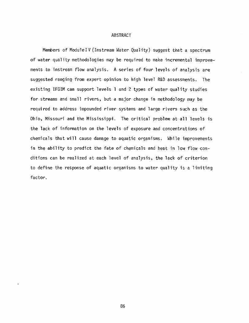
ABSTRACT

MemBers of Module I V (Instream Water Qual ity) suggest that a spectrum

of water quality methodologies may be required to make incremental improve­

ments to instream flow analysis. A series of four levels of analysis are

suggested ranging from expert opinion to high level R&D assessments. The

existing IFGIM can support levels 1 and 2 types of water quality studies

for streams and small rivers! but a major change in methodology may be

required to address impounded river systems and large rivers such as the

Ohio! Missouri and the Mississippi. The critical problem at all levels is

the lack of information on the levels of exposure and concentrations of

chemicals that will cause damage to aquatic organisms. While improvements

in the ability to predict the fate of chemicals and heat in low flow con­

ditions can be realized at each level of analysis! the lack of criterion

to define the response of aquatic organisms to water quality is a limiting

factor.

86

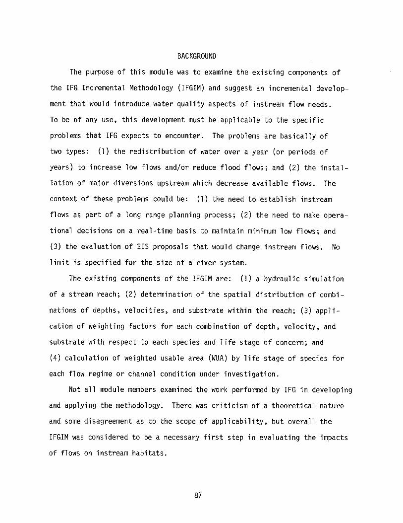
BACKGROUND

The purpose of this module was to examine the existing components of

the IFG Incremental Methodology (IFGIM) and suggest an incremental develop­

ment that would introduce water quality aspects of instream flow needs.

To be of any use, this development must be applicable to the specific

problems that IFG expects to encounter. The problems are basically of

two types: (1) the redistribution of water over a year (or periods of

years) to increase low flows and/or reduce flood flows; and (2) the instal­

lation of major diversions upstream which decrease available flows. The

context of these problems could be: (1) the need to establish instream

flows as part of a long range planning process; (2) the need to make opera­

tional decisions on a real-time basis to maintain minimum low flows; and

(3) the evaluation of EIS proposals that would change instream flows. No

limit is specified for the size of a river system.

The existing components of the IFGIM are: (1) a hydraulic simulation

of a stream reach; (2) determination of the spatial distribution of combi­

nations of depths, velocities, and substrate within the reach; (3) appli­

cation of weighting factors for each combination of depth, velocity, and

substrate with respect to each species and life stage of concern; and

(4) calculation of weighted usable area (WUA) by life stage of species for

each flow regime or channel condition under investigation.

Not all module members examined the work performed by IFG in developing

and applying the methodology. There was criticism of a theoretical nature

and some disagreement as to the scope of applicability, but overall the

IFGIM was considered to be a necessary first step in evaluating the impacts

of flows on instream habitats.

87

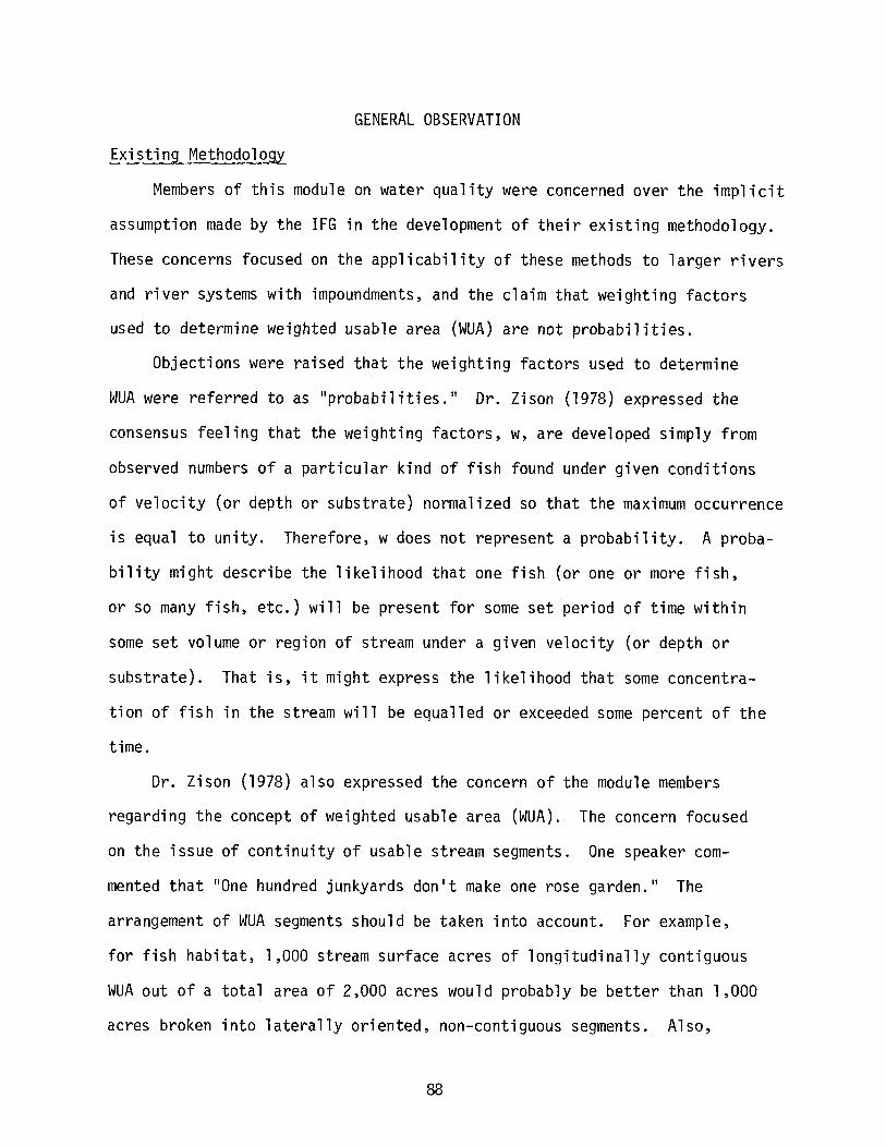
GENERAL OBSERVATION

Existing Methodology

Members of this module on water quality were concerned over the implicit

assumption made by the IFG in the development of their existing methodology.

These concerns focused on the applicability of these methods to larger rivers

and river systems with impoundments, and the claim that weighting factors

used to determine weighted usable area (WUA) are not probabilities.

Objections were raised that the weighting factors used to determine

WUA were referred to as "probabilities." Dr. Zison (1978) expressed the

consensus feeling that the weighting factors, w, are developed simply from

observed numbers of a particular kind of fish found under given conditions

of velocity (or depth or substrate) normalized so that the maximum occurrence

is equal to unity. Therefore, w does not represent a probability. A proba­

bility might describe the likelihood that one fish (or one or more fish,

or so many fish, etc.) will be present for some set period of time within

some set volume or region of stream under a given velocity (or depth or

substrate). That is, it might express the likelihood that some concentra­

tion of fish in the stream will be equalled or exceeded some percent of the

time.

Dr. Zison (1978) also expressed the concern of the module members

regarding the concept of weighted usable area (WUA). The concern focused

on the issue of continuity of usable stream segments. One speaker com­

mented that "One hundred junkyards don't make one rose garden." The

arrangement of WUA segments should be taken into account. For example,

for fish habitat, 1,000 stream surface acres of longitudinally contiguous

WUA out of a total area of 2,000 acres would probably be better than 1,000

acres broken into laterally oriented, non-contiguous segments. Also,

88

10,000 acres of w = 0.1 area (1,000 acres of WUA) may really not be equiv­

alent to 1,000 acres of w = 1.0 area. Just how different they are, of

course, determines how severe problems stemming from the assumption are

likely to be. As values of w for two compared areas become more divergent,

the comparison becomes increasingly tenuous. That is, to equate 8,000

acres of w = 0.9 with 9,000 acres of w = 0.8 is not as bad as 8,000 acres

of w= 0.9 with 72,000 acres of w = 0.1.

Management Alternatives

It may be possible to reduce flows and not change water quality

significantly if proper waste water and land management is observed.

Before a methodology is discussed to predict water quality responses to

flow alterations, an understanding of management alternatives to preserve

water quality is important.

Even when flow is reduced in a river, there may be management actions

that can be taken to maintain water quality. For example, diversion points

could be selected at locations below rather than above waste water dis­

charges. This would provide more water for dilution of waste, but would

degrade the quality of downstream diversions. If a waste discharge of

100 cfs is located in a river with a low flow of 1000 cfs, the waste water

would be diluted 10/1. A diversion of flow below the waste discharge

would not impact water quality of the instream flow as significantly as

if the diversion occurred just above the diversion. In the latter case,

if 900 cfs were diverted, only 100 cfs would remain instream and the waste

would only be diluted 1/1 or a factor of 10 less. The acceptance of this

management alternative could contribute to the maintenance of water quality.

The added cost of treatment to diverters could possibly be balanced by the

reduced losses to instream flow users.

89

Reduction of instream flows will tend to increase water temperatures

since water levels will fall and travel times will increase. In regions

where diversions are for irrigation, return flows will be heated by the

fields and in irrigation ditches and drains. Several management actions

can be taken to compensate for increased exposure to the sun. The first

alternative for small streams would be to increase the shading of the

stream bed with vegetation or physically covering the channel. A recent

experiment using branches to cover stream channels during clearing for high­

way construction was effective in the state of Washington. Another altern­

ative would be to install covered ditches and drains for the last section

of return flow discharges to the river to reduce heating. Finally, if the

instream flows are subject to thermal discharges, it may be possible to

float the hot water on top of the colder water rather than to mix the

thermal discharge with the receiving waters. The higher surface temperature

will dissipate the heat faster than with a mixed stream.

When water is impounded for release at future times, the upper waters

(epilimnium) tend to warm and the lower waters (hypolumnium) tend to be

depleted of oxygen. Some reservoirs may stratify and present water quality

problems. By proper mixing of withdrawals from stratified impoundments,

downstream water quality may be regulated. On the other hand, improper

withdrawal of impounded waters can create severe downstream water quality

problems.

Riparian land use can greatly impact water quality. The clear cutting

of forest will expose streams to rapid heating, the urbanization of water­

sheds without adequate sewage systems will contribute significant amounts

of oxygen demanding wastes and nutrients, and the industrialization of a

river valley can contribute toxic materials in addition to the other wastes

90

of urbanization and agriculture. Policies that preserve a green belt or

natural buffer zone can be significant deterrents to water quality

degradation in spite of flow reductions.

In cases where flow diversions cannot be denied, there are management

practices that can be used to reduce the amount diverted. In certain areas

of the western United States the use of unlined canals requires much more

water than systems with lined canals because of high infiltration rates.

Similarly, covered pipes would reduce evaporation losses. The key to

increased agricultural efficiency of water use is economics. As long as

the cost of water is low, there is not an incentive to install sprinkler

systems or other devices that reduce water application to crops.

Prior to developing a position that flow must be retained to preserve

water quality, all feasible management options must be examined so water

quality enhancement may be an issue to be negotiated in return for instream

flow reductions. It may be feasible to have better water quality in spite

of lower instream flows.

Introduction of Water Quality Concerns

The objective of this module was to suggest means of introducing water

quality aspects into the IFGIM. Historically, water quality analysis has

been a fragmented field with researchers focusing on specific pollutants

and specific aquatic organisms. For a given research effort, it was not

currently possible in most cases to examine the fate of all pollutants on

all compartments of an aquatic ecosystem. Efforts such as IBP encountered

great difficulty in addressing such goals. A survey of methodologies avail­

able or under development indicates that engineers have developed analytical

and empirical methods ranging from crude nomographs to complex computer

models to estimate the fate of pollutants. Aquatic scientists have focused

91

on more mechanistic approaches and tend to conduct two variable studies

rather than holistic ecosystem analyses. These efforts suggest that it is

possible to examine the fate of a single pollutant in great detail, but that

the marginal value of such extensive study may not always be significant in

water resource management studies. On the other hand the use of crude esti­

mates of the fate of many pollutants to provide adequate information for

management studies may receive strong criticism by the scientists conducting

research of such pollutants.

In order for a methodology to be useful to the IFG, it should possess

several attributes.

1) Promote clarity, not complexity. Applying complex techniques to

a simple problem may confuse rather than clarify the solution.

2) Produce believable results. The methodology should be based on

accepted state-of-the-art techniques. When complex techniques are approp­

riate they should be applied.

3) Reduce, not compound, the risk and uncertainty associated with

solution alternatives. The techniques should be consistent with the

objectives of the study and lead to specific conclusions. The study con­

clusions should contain something other than a recommendation for a bigger,

more expensive, follow-on study.

4) Produce understandable results. Results should be presented in

a format that can be understood by the people who need to use them.

There are numerous predictive techniques currently being used to

evaluate water quality problems and they differ greatly in capability.

The capability of a technique is established by two characteristics:

1) the number of constituents that may be included in a water quality

study; and 2) the resolution (i.e., complexity and level of detail) of

92

the analysis for each constituent. The resolution of a technique is related

to the conceptual distribution of the constituent in time and space, and

to the complexity of the mathematical functions representing the physical

and biochemical properties of the constituent.

Dr. Lee expressed the concern that chemical concentration or water

temperature should not be equated to "wa ter quality. II The evaluation of

water quality as defined by Dr. Lee is the final task in the IFG when the

outputs of the water quantity module, the ecosystem module, and this module

are integrated to determine the response of fish to changes in water flow,

chemical concentration, and the aquatic ecosystem. The purpose of this

module is to suggest a series of increasingly precise methods to estimate

water temperature and the concentration of selected chemicals in water.

It is not the purpose of this module to evaluate the environmental signif~

icance of the presence of chemicals in rivers.

93

HIERARCHIAL FRAMEWORK FOR ANALYSIS

The introduction of water quality concerns to the IFGIM must be an

evolutionary process that will improve as the staff develops skills in

water quality analyses advances. While it may be possible to formulate a

highly detailed and complex methodology that may be of great interest to

scientists on the frontiers of water quality research, such a methodology

may be too complex and impractical for operational decision making related

to low flows. The members of this module have attempted to classify

methodologies by their cost, required knowledge, data needs, and ability

to resolve a basic low flow/water quality issue. There are four classes

or levels of resolution suggested for water quality analyses. Tables 1 and

2 summarize the characteristics and utility of each level of resolution

proposed. Level 1 can be classified as methods to provide low cost, crude

estimates of potential water quality problems. These methods rely on text

book concepts and heuristic approaches. They are low in cost and may

stimulate debate among scientists that seek more refined analysis of water

quality problems. Level 2 methodologies are more costly and will estimate

changes in temperature and oxygen due to flow alterations within a factor

of two. Level 3 methodologies expand the set of chemicals to be analyzed

and attempt to employ state-of-the-art technology at still higher costs.

Level 4 methodologies are research and development concepts that are

attempting to improve the current state of knowledge.

While these methodologies are called water quality analyses they

focus on the fate of physical and chemical pollutants in waters. Dr. Lee

was very concerned that this module extend the methodology to speak to the

issue of effects on aquatic organisms, rather than focus solely on fore­

casting that fate of pollutants in the receiving waters. Other members

94

of this module were concerned that Level 4 methodologies are beyond the

capabilities and interest of the IFG and that the thrust of the water

quality efforts be placed on level 2 or 3 type methodologies.

Traditionally the analysis of water quality in a river system requires

knowledge of all upstream activities since pollutants may not be completely

assimilated when they enter a given reach. One of the objectives of a

Level 1 or Level 2 analysis may be to examine an entire river system to

identify reaches where low flow impacts on water quality may be most severe.

Level 3 or 4 methodologies can then be used to improve the estimate of

input in these critical reaches. Some module members favored this screen-

ing approach, while others questioned if such crude approximations were

appropriate.

The resources required to conduct an analysis increase geometrically

with the level of methodology. Level 1 methodology is a simple procedure

to collect expert opinion and perform back-of-the-envelope analysis,

without acquiring new field data. Level 2 methodology requires limited

field studies and text book level analysis of the fate of pollutants such

as heat, oxygen demand, solids, etc. Level 2 studies would require two

to three man-months of effort. Level 3 methodologies are four to eighteen

man-month efforts combining extensive field observations and mathematical

modeling to predict time-dependent fluctuation in heat and chemical

concentrations in a reach. Level 4 methodologies require extensive basic

research to gain understanding of the fate of toxic pollutants and to

define chronic exposure levels that impact the aquatic ecosystem. Level 4-*~methodologies seek to add to scientific understanding as the first priority,

and will complicate rather than clarify most management decisions.

95

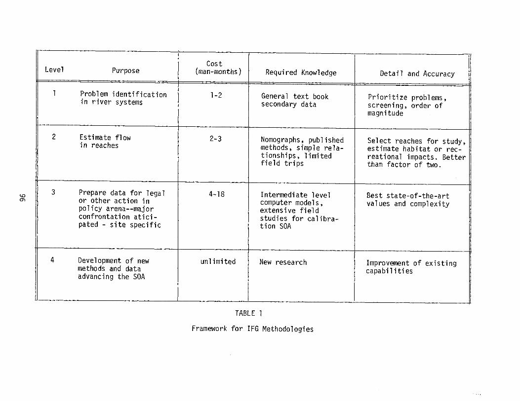
1.00'\

CostLevel Purpose (man-months) Required Knowledge Detail and Accuracy

1 Problem identification 1-2 General text book Prioritize problems,in river systems secondary data screening, order of

magnitude

2 Estimate flow 2-3 Nomographs, published Select reaches for study,in reaches methods, simple rela- estimate habitat or rec-

tionships, limited reational impacts. Betterfield trips than factor of two.

3 Prepare data for legal 4-18 Intermediate level Best state-of-the-artor other action in computer models, values and complexitypolicy arena--major extensive fieldconfrontation atici- studies for calibra-pated - site specific tion SOA

4 Development of new unl imited New research Improvement of existingmethods and data capabi 1iti esadvancing the SOA

TABLE 1

Framework for IFG Methodologies

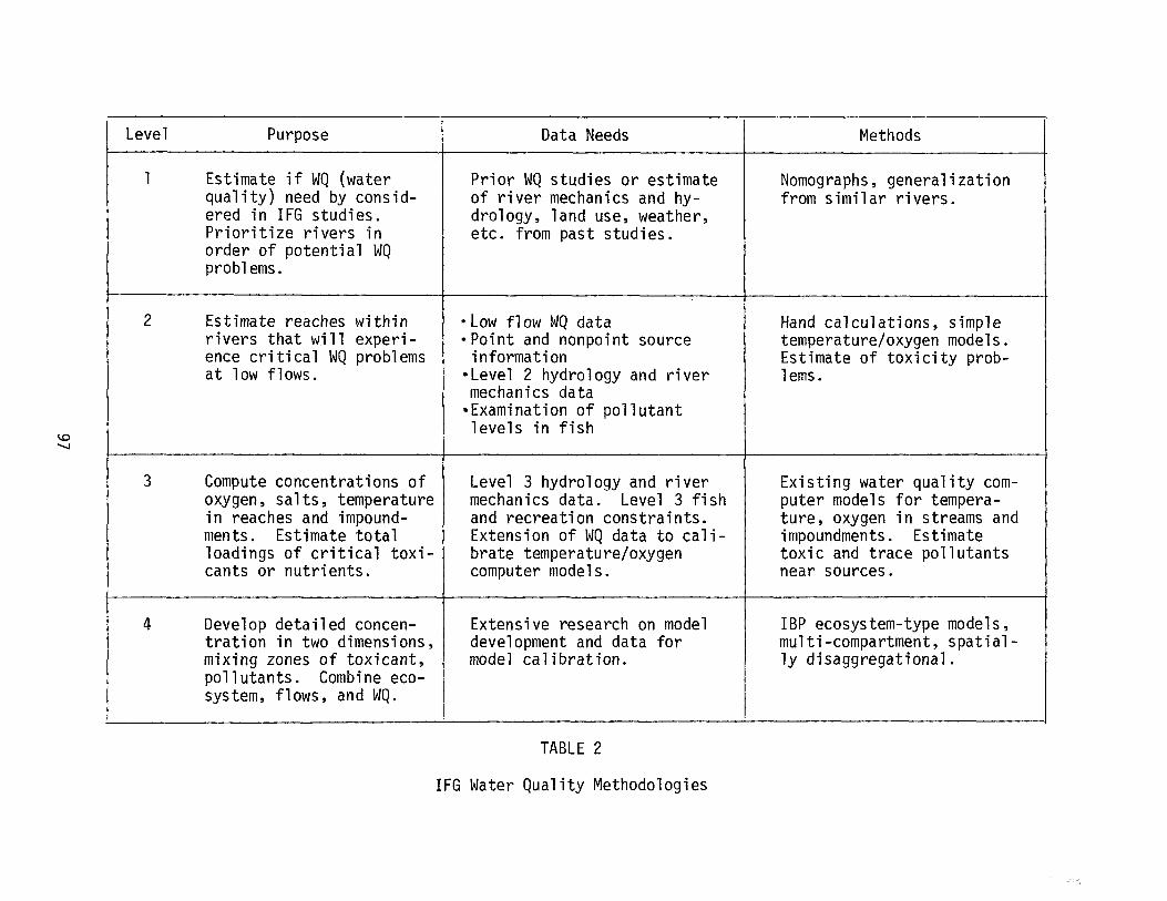
\D""-J

Level

1

2

3

4

Purpose

Estimate if WQ (waterquality) need by consid­ered in IFG studies.Prioritize rivers inorder of potential WQproblems.

Estimate reaches withinrivers that will experi­ence critical WQ problemsat low flows.

Compute concentrations ofoxygen, salts, temperaturein reaches and impound­ments. Estimate totalloadings of critical toxi­cants or nutrients.

Develop detailed concen­tration in two dimensions,mixing zones of toxicant,pollutants. Combine eco­system, flows, and WQ.

Data Needs

Prior WQ studies or estimateof river mechanics and hy­drology, land use, weather,etc. from past studies.

-Low flow WQ data·Point and nonpoint source

information-Level 2 hydrology and rivermechanics data

-Examination of pollutantlevels in fish

Level 3 hydrology and rivermechanics data. Level 3 fishand recreation constraints.Extension of WQ data to cali­brate temperature/oxygencomputer models.

Extensive research on modeldevelopment and data formodel calibration.

TABLE 2

Methods

Nomographs, generalizationfrom similar rivers.

Hand calculations, simpletemperature/oxygen models.Estimate of toxicity prob­lems.

Existing water quality com­puter models for tempera­ture, oxygen in streams andimpoundments. Estimatetoxic and trace pollutantsnear sources.

IBP ecosystem-type models,multi-compartment, spatial­ly disaggregationa1.

IFG Water Quality Methodologies

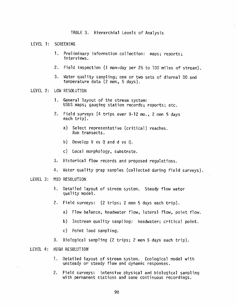
TABLE 3. Hierarchial Levels of Analysis

LEVEL 1: SCREENING

1. Preliminary information collection: maps; reports;interviews.

2. Field inspection (1 man-day per 25 to 100 miles of stream).

3. Water quality sampling; one or two sets of diurnal DO andtemperature data (2 men, 5 days).

LEVEL 2: LOW RESOLUTION

1. General layout of the stream system:USUS maps; gauging station records; reports; etc.

2. Field surveys (4 trips over 9-12 mo., 2 men 5 dayseach trip).

a) Select representative (critical) reaches.Run transects.

b) Develop V vs Q and d vs Q.

c) Local morphology, substrate.

3. Historical flow records and proposed regulations.

4. Water quality grap samples (collected during field surveys).

LEVEL 3: MID RESOLUTION

1. Detailed layout of stream system. Steady flow waterquality model.

2. Field surveys: (2 trips; 2 men 5 days each trip).

a) Flow balance, headwater flow, lateral flow, point flow.

b) Instream quality sampling: headwater; critical point.

c) Point load sampling.

3. Biological sampling (2 trips; 2 men 5 days each trip).

LEVEL 4: HIGH RESOLUTION

1. Detailed layout of stream system. Ecological model withunsteady or steady flow and dynamic responses.

2. Field surveys: intensive physical and biological samplingwith permanent stations and some continuous recordings.

98

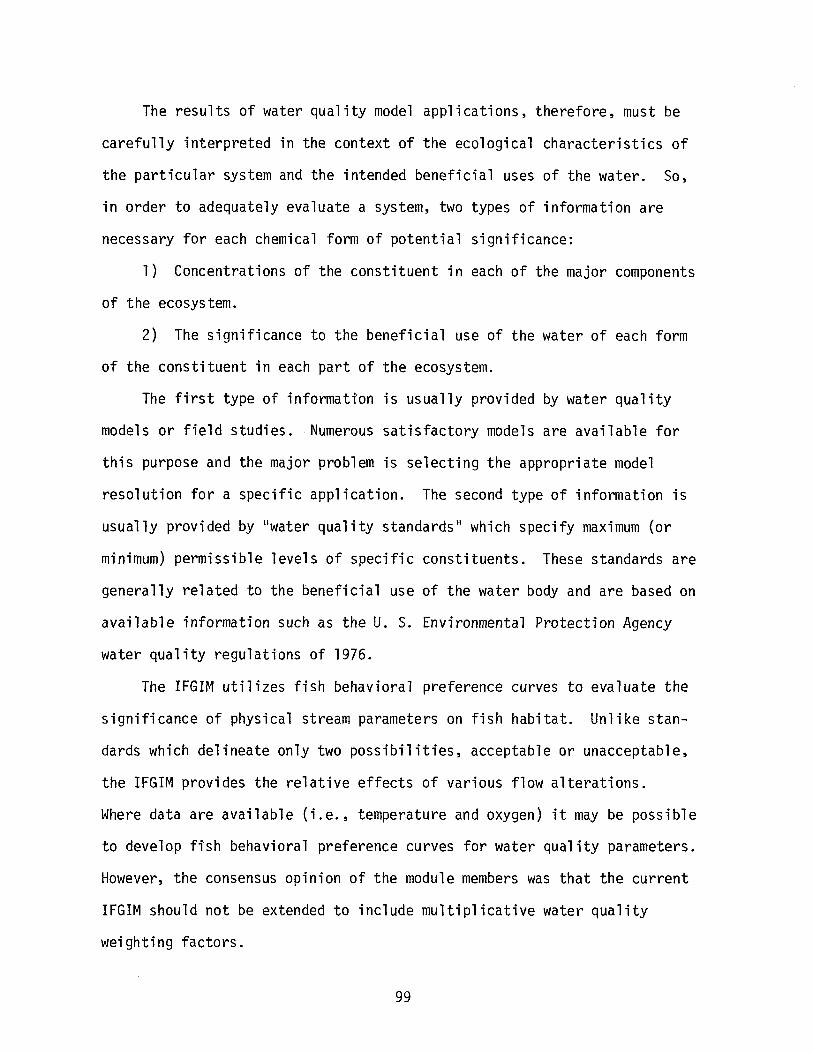
The results of water quality model applications, therefore, must be

carefully interpreted in the context of the ecological characteristics of

the particular system and the intended beneficial uses of the water. So,

in order to adequately evaluate a system, two types of information are

necessary for each chemical form of potential significance:

1) Concentrations of the constituent in each of the major components

of the ecosystem.

2) The significance to the beneficial use of the water of each form

of the constituent in each part of the ecosystem.

The first type of information is usually provided by water quality

models or field studies. Numerous satisfactory models are available for

this purpose and the major problem is selecting the appropriate model

resolution for a specific application. The second type of information is

usually provided by "water qual ity standards II which specify maximum (or

minimum) permissible levels of specific constituents. These standards are

generally related to the beneficial use of the water body and are based on

available information such as the U. S. Environmental Protection Agency

water quality regulations of 1976.

The IFGIM utilizes fish behavioral preference curves to evaluate the

significance of physical stream parameters on fish habitat. Unlike stan­

dards which delineate only two possibilities, acceptable or unacceptable,

the IFGIM provides the relative effects of various flow alterations.

Where data are available (i.e., temperature and oxygen) it may be possible

to develop fish behavioral preference curves for water quality parameters.

However, the consensus opinion of the module members was that the current

IFGIM should not be extended to include multiplicative water quality

weighting factors.

99

Summary

In summary, the water quality methodology should provide guidance

for applying appropriate study intensity. In order to accomplish this,

the methodology should include analytical techniques at several levels of

resolution. The techniques should have state-of-the-art capabilities and

should be directed toward the current needs of the IFG: predicting the

effects of instream flow alterations to fish habitat.

The suggested methodology consists of four levels of resolution. It

is proposed that the entire river system be evaluated using Levell tech­

niques to determine which constituents pose a potential threat to fishery

needs at altered flows. If water quality degradation potential is severe,

the subsequent levels of analysis provide techniques for more price esti­

mates of particular constituents at specific critical sites.

100

APPENDIX

Members of this module have attempted to provide examples of method­

ologies for each level of analysis. These examples are not comprehensive

literature reviews or state-of-the-art presentations, but illustrations to

indicate the type of analysis that could be obtained by increasing levels

of investment. The key to optimizing the level of analysis required in the

IFGIM is knowledge on the response of aquatic organisms to exposure of

various pollutant concentrations. Since ~hronic exposure criterion need

to be developed before such analyses are possible, the IFG will have to

use Levell type analysis to establish such criterion before higher level

water quality analysis can be justified.

101

LEVEL 1 ANALYSIS (BOGSAT)

Levell analysis consists of low-level reconnaissance and screening

and may be characterized as BOGSAT: "A Bunch of Guys Sitting Around the

Table." The first step in assessing water quality at this level is to

identify point and non-point sources of waste. Much of this information

has already been collected for many basins in conjunction with studies

stimulated by P.L. 92-500 (i.e., 303e, 208, 316a, etc.) and state water

quality regulations. The NPDES permits on file with EPA or state agencies

provide useful information on point discharges. When measured data are

not available, loadings may be estimated by standard factors such as these

shown in Tables 4 and 5 for BOD and suspended solids or tables included

in the Environmental Protection Agency·s water quality regulations of 1978.

Fluctuation of water quality with inflows of waste is a significant

factor in allocating waters for waste assimilation. In some cases return

flows may contribute a majority of the downstream volume and management

of return flow quality will become more important than management of

upstream water quality.

Data may also be available on chemical concentrations as, for example,

shown in Table 6 (Finney, et.al, 1977). This type of data is useless unless

accompanied by associated flows as shown in Tables 7 and 8 (Finney, et al,

1977). At this level of analysis, average loading rates and flows are used.

Using the loading and hydraulic data, instream concentrations can be approx­

imated by simple dilution calculations. Instream concentrations at alternate

flows or for different loading patterns (i.e., future scenarios) can be

estimated by the same technique.

The resulting water quality can be compared to instream standards,

102

TABLE 4. Population-Equivalent Conversion Factors for Industrial Wastes

Average Waste/capita Conversion FactorConstituent in waste to PE per1b/capita/day lbs of pollutant

Suspended Solids .250 4

BOD (5 day, 200C) .166 6

Total Phosphorus ,009 110

Total Col Horm 1.6xl08/100 ml

TABLE 5. Populati'on Equivalent Conversion Factors for Specific IndustrialWastes

Population Equivalent/ton of outputPE (BOD) PE (Suspended Solids)

Industry typical Range typical Rangevalue value

Food Processing 300 75-1200 180 6-300

Pulp & Paper - Kraft 700 240-2500 200 80-350

- Sulfite 4000 900-8000 200 80-350

Forest Product ~.l - 3 -Sand & Gravel .4 .3-.6 800 -

Petroleum Refining 6 1-20 100 1-200

Light Mfg. l/employee

Source: Harper, M. S. and B. W. MarA Series of Methodologies for Estimating Low Flow RequirementsBased on Water Quality StandardsState of Washington Water Research Center Report No. 13, June, 1973

103

TABLE 6. Chemical and Biological Characteristics of Selected River Systems

- _. -Ortho- Ult. Bi ochemi Cd1 Dissolved Algae

Description Phosphorusa Oxygen Demanda Ammoniaa Nitratea Oxygena CHL "A"b(mg/1) (mg/1 ) (mg/1 ) (mg/1 ) (mgll ) (mgll )

-

Headwater 0.1 3.0 0.0 0.3 13.5 0.06Reaches 1-4, Lateral Surfa~e Inflow 0.4 8.7 0.0 2.0 7.3 0.0Reaches 1-4, Lateral Ground Inflow 0.0 0.1 0.0 1.9 0.0 0.0

Reaches 5-7, Latel'il1 Surface Inflow 1.4 9.5 0.0 2.0 7.3 0.0Reaches 5-7, Lateral Ground Inflow 0.0 0.1 0.0 2.1 0.0 0.0Reaches 8-14, Lateral Surface Inflow 1.4 8.7e 0.0 2.0 7.6 0.0

Reaches 8-14, Lateral Ground Inflow 0.0 0.1 0.0 2.2 0.0 0.0

Sandy WTP 7.08 101. 22.1 0.19 3.95 0.0

Tri-Community WTP 8.84 74.5 15.7 1.13 3.95 0.0

Little Cottonwood Ck. 0.09 9.01 0.0 0.59 7.00 0.0.....0 Murray IHP 7.45 83.2 13.4 4.45 3.95 0.0~

Big Cottonwood Ck. 0.0 2.48 0.0 1.07 7.90 0.0

Cottonwood WTP 9.06 48.2 18.7 2.64 6.00 0.0

Granger WTP 11.2 88.8 5.62 0.91 6.00 0.0

Salt Lake Sub WTP 9.79 54.2 5.62 4.04 6.00 0.0

r~i 11 Creek . 0.01 2.10 0.0 1.98 7.90 0.0

South Salt Lake WTP 4.16 50.8 3.81 4.95 6.00 0.0

Par" ey, Emmi gratl on and Red Butte Creeks 0.05 4.20 0.0 1.26 7.00 0.0

Ci ty Creek 0.09 1.67 0.0 1. 51 7.90 0.0

South Davis WTP 5.19 47.7 13.7 1.92 3.95 0.0

aSouree: Salt Lake County Council of Governments (1977a)

bSource: Dixon, et al. (1975)cFor reach 13 = 148 mg/l (Bowles, 1977)

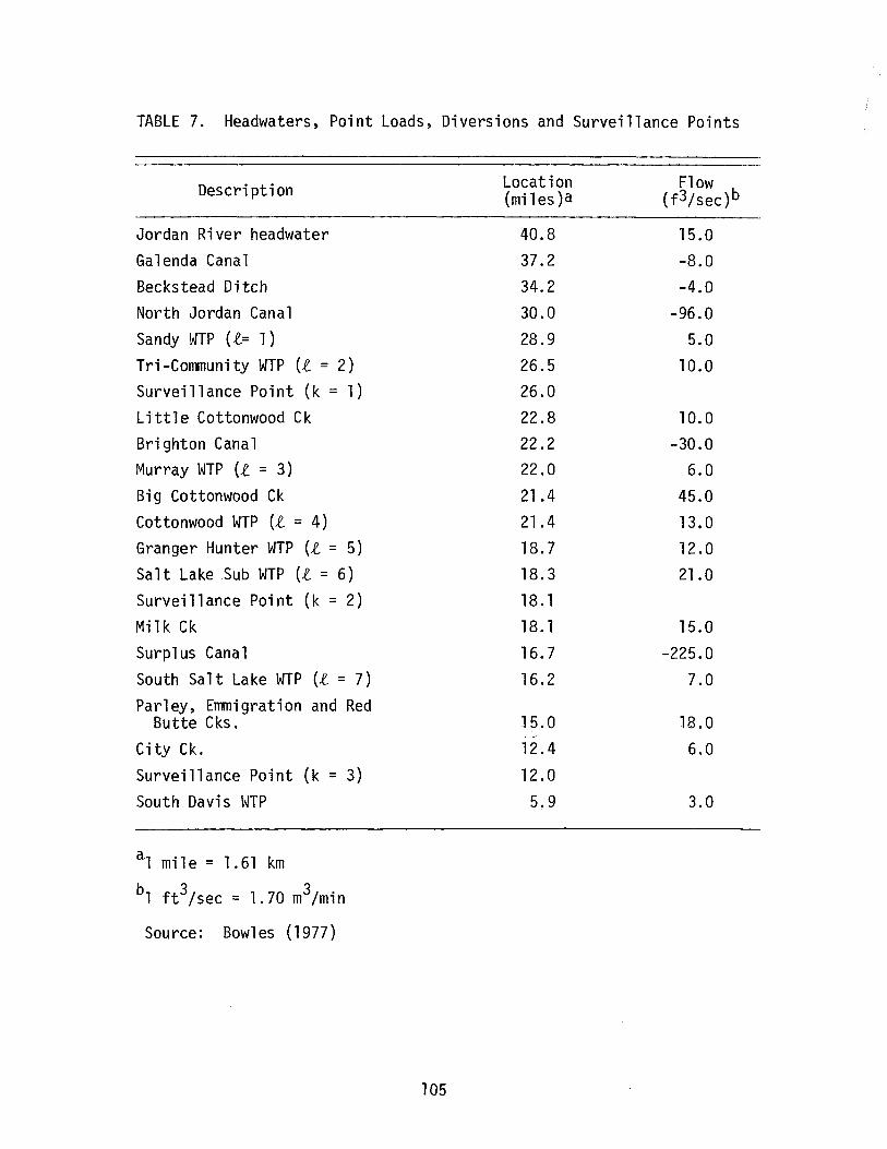
TABLE 7. Headwaters, Point Loads, Diversions and Surveillance Points

Description

Jordan River headwaterGalenda CanalBeckstead DitchNorth Jordan CanalSandy WTP (,e.= 1)

Tri-Community WTP (,e. = 2)

Surveillance Point (k = 1)

Little Cottonwood CkBrighton CanalMurray WTP (,e. = 3)

Big Cottonwood CkCottonwood WTP (,e. = 4)

Granger Hunter WTP (,e. = 5)

Salt Lake Sub WTP (,e. = 6)

Surveillance Point (k = 2)

Mi 1k CkSurplus CanalSouth Salt Lake WTP (,e. = 7)

Parley, Emmigration and RedButte Cks.

City Ck.Surveillance Point (k = 3)South Davis WTP

a, mile = 1.61 km

bl ft3/sec = 1.70 m3/min

Source: Bowles (1977)

105

Location(miles)a

40.837.234.230.028.926.526.022.822.222.021.421.418.718.318.118. 116.716.2

15.012.412.05.9

Flow(f3/sec)b

15.0-8.0-4.0

-96.05.0

10.0

10.0-30.0

6.045.013.012.021.0

15.0-225.0

7.0

18.06.0

3.0

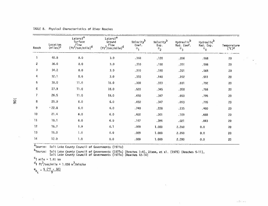
TABLE 8. Physical Characteristics of River Reaches

Latera1 a Lateral aVe10cityb Ve10cityb Hydrau1icb Hydrau1icbSurface Ground

Location Flow Flow d Coef. Exp. Rad. Coef. Rad. Exp. TemperatureReach (miles)C (ft3/sec/mil e)d (ft3/sec/mi1e) °1 °2 8 0 (OC)e3 4

40.8 8.0 3.0 .310 .120 .206 .568 20

2 36.0 8.0 3.0 .310 .150 .201 .588 20

3 34.2 8.0 3.0 .310 .150 .201 .568 20

4 32.1 8.6 3.0 .310 .140 .202 .581 20

5 30.0 11.0 18.0 .300 .333 .031 .792 20

6 27.9 11.0 18.0 .520 .345 .058 .766 20

7 26.5 11.0 18.0 .450 .347 .053 .795 20--I

0 8 25.0 6.0 6.0 .450 .347 .053 .795 200"1

9 · 22.8 6.0 6.0 .740 .228 .235 .400 20

10 21.4 6.0 6.0 .400 .301 .109 .688 20

11 18.1 6.0 6.0 .157 .384 .021 .843 20

12 16.7 1.0 O. 1 .009 1.000 2.200 0.0 20

13 15.0 1.0 0.0 .009 1.000 2.200 0.0 20

14 12.0 1.0 0.0 .009 1.000 2.200 0.0 20

aSource: Salt lake County Council of Governments (1977a)bSource: Salt Lake County Council of Governments (1977a) (Reaches 1-4), Dixon, et a1. (1975) (Reaches 5-11),

Salt Lake County Council of Governments (1977a) (Reaches 12-14)c, mile = 1.61 km

d1 ft3/sec/mile = 1.056 m3/min/km

eo =~- 32)c 9

for example, the U.S. Environmental Protection Agency·s water quality

regulations of 1976, to estimate potential problem constituents and crit­

ical reaches. Since it is difficult to obtain adequate information on

atmospheric conditions, channel characteristics, and sources of wastes to

predict natural water quality closely, the impact of flow alterations can

be simplified if baseline water quality data are available.

Because the initial focus of the water quality effort will be

directed toward fish habitat, dissolved oxygen (DO) and temperature will

be the most important constituents for most reaches. A worst case

estimate of DO in a river with significant BOD content is achieved when

it is assumed that the oxygen deficit equals the ultimate BOD concentration.

The ultimate BOD concentration would be estimated as the total BOD load-

ing dissolved in the average river low flows. If this estimate is near

acceptable levels for fish of interest, then a Level 2 analysis should be

conducted. If oxygen levels estimated by this method are above acceptable

limits, the assumption that oxygen will not be limiting might be made.

Water temperature can be estimated at Levell, knowing latitude,

altitude, river depth, velocity at representative reaches, the time of

year, and the canopy of the river. If the river is completely shaded for

its entire length, temperature will not change as flows are decreased as

much as in an unshaded river. If the river is completely exposed to the

sun, and average cloud cover is small, then flow changes can impact temp­

erature. Water temperature can be estimated at Levell by generalization

from similar conditions in nearby rivers or simplified heat balances for a

representative water column.

As a first approximation water temperature changes are assumed to

increase proportionately with travel time and inversely with the mean

107

depth. Water exposed for a long time to a given set of meteorological

conditions will reach an "equilibrium temperature" (Edinger and Geyer,

1968). For example, the equilibrium water temperature can provide an

estimate of average temperature condition. An average equilibrium water

temperature, Te, can be calculated using average daily meteorological

conditions. By comparing the average daily observed water temperature, To

to Te , the following inference can be made:

1) If T = T . temperature is not sensitive to flow.o e'

2) If To < T . temperature may increase with reduced flow.e'

3) If T > T . temperature may decrease with reduced flow.0 e'

Novotny and Krenkel (1973) have observed that an initial temperature

increase in a stream is dissipated exponentially with time until the

original or natural temperature region is reached and that in some cases

"equilibrium temperatures" are not required to estimate thermal discharge

impacts.

Up to this point only average loadings, flows, and instream concen-

tration have been considered. The temperature or oxygen content of most

rivers and estuaries cannot be characterized by a single observation taken

at a given time of day or place. Diurnal fluctuations can be as great

as : 10°F and :6 ppm of oxygen in a river as large as the Willamette

(Hines, 1977). Figure 1 presents data for oxygen and temperature for

flows of about 5000 cfs reported by Hines. Thus natural flows may have

major temperature and oxygen fluctuations that can be aggravated by reduced

flows.

If data are not available for a diurnal cycle of DO and temperature,

then at least one field trip should be made to collect the data during

108

low flow conditions. The observed diurnal fluctuation can be superimposed

on the average to obtain a first approximation of maximum and minimum

concentrations at other flow conditions.

Data on concentration-duration of exposure relationship that are

detrimental to aquatic organisms are lacking, and should be the thrust of

scientific research to estimate the impact of water quality changes of

beneficial uses that are related to aquatic organisms.

109

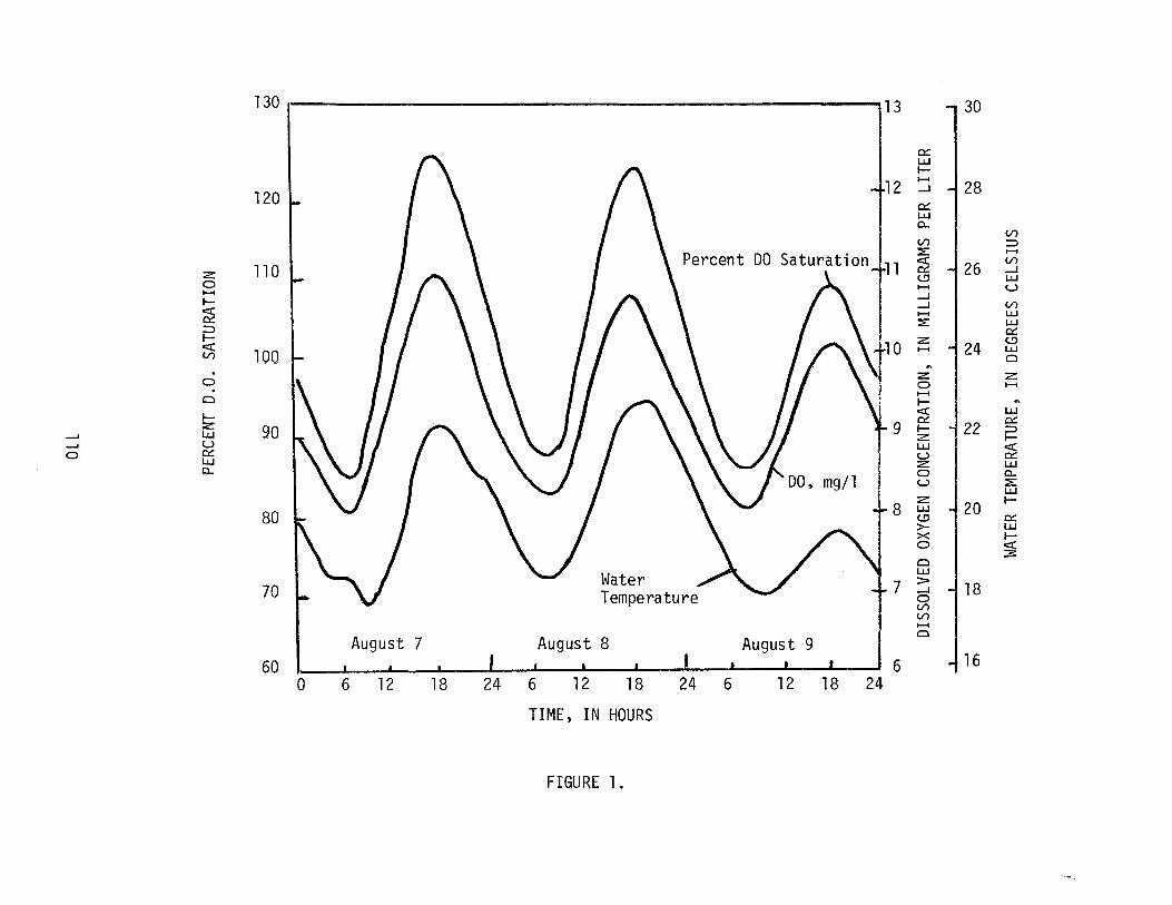
130 • ·13 .., 30

0::lJJI-

T12......

-I 28I \-l

120 L I \ 0::lJJ0..

VlVl :::>

Percent DO Saturation :E: ......11

c:(26

Vl110 0:: -l

2: c..!l lJJ0 ...... u...... -lI- -l Vl

~ ...... lJJ:E: lJJ

:::> 0::I- 2:

24c..!l

c:(

100...... lJJ

Vl Cl". 2: 2:

0 0 ....... ......Cl l- n

c:( lJJI-

90::

220::2: 90 I- :::>..... lJJ , 2: I-..... U I lJJ c:(

0 0:: l u 0::lJJ z: lJJ0.. ~ 0 0..

U :E:lJJ

z:20

I-

b-- - I \ I \ T 8 lJJ80 c..!l 0::

>- lJJX I-0 c:(

:3:Cl

Water ~+7

lJJ:::-

-11870 L \./ -lTemperature 0VlVl......Cl

August 7 August 8 August 9... 1660 I « , ,

• I I I t , f I 6,0 6 12 18 24 6 12 18 24 6 12 18 24

TIME, IN HOURS

FIGURE 1.

LEVEL 2 ANALYSIS (BOGSAR)

The goal of Level 2 is to further evaluate reaches where the effects

of water quality must be included in the evaluation of habitat and may be

characterized as BOGSAR: "A Bunch of Guys Standing Around the River."

Table 9 includes examples of Level 2 analyses.

Level 2 water quality assessment is based on field observation of

water quality at extreme-flow conditions (high and low flows) and at

known waste discharge locations. Knowledge of BOD and temperature at

these conditions will provide data for nomographs or hand calculations

of elementary first order data equations used in oxygen estimations.

Inputs from the IFG Incremental Methodology will provide depth and

velocity to greater detail than this methodology requires. Fishery and

recreation studies (Levels 1 and 2) should define acceptable water quality

conditions, as well as a forecast of human activity and land use that can

be used to estimate pollution loads. General data such as weather, aerial

photographs, soil maps, etc. can provide information on canopy and solar

inputs for temperature calculations using nomographs and generalized data

from existing studies and models.

While methodologies to model other pollutants are not found in common

texts on water quality, there are water quality criteria available for many

other pollutants than temperature and oxygen. The Level 2 analysis should

survey water samples and the flesh of fish for the presence of as many

pollutants as resources permit.

Prediction of Water Temperature

Conceptually, water temperature models have not changed significantly

from the energy balance employed by Raphael (1962). Recent temperature

111

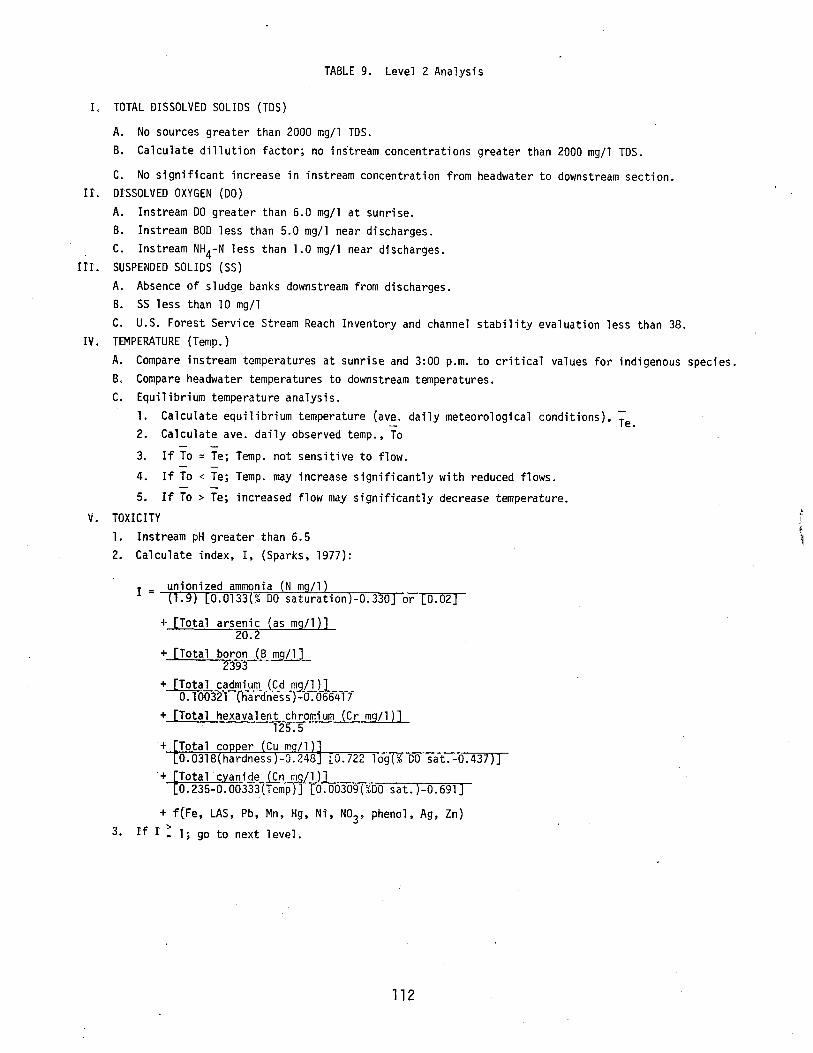
If To > Te; increased flow may significantly decrease temperature.

If To = Te; Temp. not sensitive to flow.

If To < Te; Temp. may increase significantly with reduced flows.

TABLE 9. Level 2 Analysis

I. TOTAL DISSOLVED SOLIDS (TDS)

A. No sources greater than 2000 mg/l TDS.B. Calculate dillution factor; no instream concentrations greater than 2000 mg/l TDS.

C. No significant increase in instream concentration from headwater to downstream section.If. DI'SSOLVED OXYGEN (DO)

A. Instream DO greater than 6.0 mg/l at sunrise.B. Instream BOD less than 5.0 mg/l near discharges.C. Instream NH4-N less than 1.0 mg/l near discharges.

11'1'. SUSPENDED SOLIDS (SS)A. Absence of sludge banks downstream from discharges.B. SS less than 10 mg/lC. U.S. Forest Service Stream Reach Inventory and channel stability evaluation less than 38.

IV. TEMPERATURE (Temp.)A. Compare instream temperatures at sunrise and 3:00 p.m. to critical values for indigenous species.B. Compare headwater temperatures to downstream temperatures.C. Equilibrium temperature analysis.

1. Calculate equilibrium temperature (ave. daily meteorological conditions), Te.2. Calculate ave. daily observed temp., To

3.

4.

5.

V. TOXICITY1. Instream pH greater than 6.52. Calculate index, I, (Sparks, 1977):

I

+ [Total

+ [Total

hexavalent chromium125.5

+ f(Fe, LAS, Pb, Mn, Hg, Ni, N03, phenol, Ag, Zn)

3. If I : 1; go to next 1eve1.

112

models (Novotny and Krenkel, 1973; Brocard and Hardemann, 1976; DeWalle;

1976) continue to employ an energy balance of net solar radiation input

and surface gains or losses by evaporation (condensation), convection,

and back radiation. The advection of water at different temperatures

than that of the main stream is computed by mixing models and heat losses

to the channel bottom are usually neglected. More complex models do not

assume perfect mixing and no heat loss to the channel. These complex

models predict thermal stratification and two or three-dimensional temper­

ature distributions in the waters.

Unless extensive atmospheric data and flow data are available, temper­

ature models cannot be calibrated for a specific reach. Electric utilities

and regulatory agencies responsible for protection of aquatic life forms

from thermal pollution have invested in the development of complex models

for predicting water temperature (Hill and Viskanta, 1976). The task for

this workshop is to extract from this rich literature an effective and

simple methodology to estimate water temperature changes associated with

flow reduction, given local meteorological conditions.

If a body of water of uniform depth is exposed to a sequence of warm­

ing days with identical pattern of diurnal meteorological conditions and

is continually well mixed, the water temperature will follow a trend shown

in Figure 1. As observed by Novotny and Krenkel (1973), no matter what

the initial water temperature may be, the water temperature will seek an

"equilibrium pattern." Since there are many computer models that can

evaluate the water temperature given sequences of meteorological conditions,

it would be possible to prepare charts of water temperature from sequence

of meteorological condition and canopy cover as a function of flow time

and river depth if the initial water temperature is given. While such

113

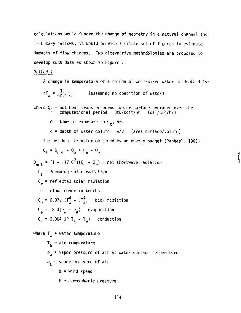
calculations would ignore the change of geometry in a natural channel and

tributary inflows, it would provide a simple set of figures to estimate

impacts of flow changes. Two alternative methodologies are proposed to

develop such data as shown in Figure 1.

Method 1

A change in temperature of a column of well-mixed water of depth dis:

_ Qt ellTw - 62.4 d (assuming no condition of water)

where Q = net heat transfer across water surface averaged over thet computational period Btu/sqft/hr (cal/cm2/hr)

e = time of exposure to Qt' hrs

d = depth of water column ll/V (area surface/volume)

The net heat transfer obtained by an energy budget (Raphael, 1962)

Qt = Qnet - Qb + Qn - Qe

Qnet = (1 - .17 C2)(Qs - Qr > = net shortwave radiation

Qs = incoming solar radiation

Q = reflected solar radiationr

C = cloud cover in tenths

Qb = O.97y (T~ - aT:) back radiation

Qe = 12 U(ew - ea) evaporation

Qn = 0.004 UP(Ta - Tw) conduction

where Tw = water temperature

T = air temperaturea

e = vapor pressure of air at water surface temperaturew

e = vapor pressure of airaU = wi'nd speed

P = atmospheric pressure

114

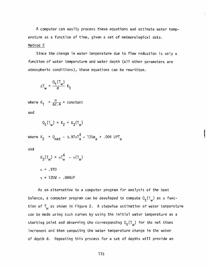
Acomputer can easily process these equations and estimate water temp­

erature as a function of time, given a set of meteorological data.

Method 2

Since the change in water temperature due to flow reduction is only a

function of water temperature and water depth (all other parameters are

atmospheric conditions), these equations can be rewritten.

where Kl

and

e=----- = constant62.4

where K2 = Qnet - S.97crT~ - l2Uea + .004 UPTa

and4K3(T ) = aT - y(T )w w w

a = .970

y = l2UW - .004UP

As an alternative to a computer program for analysis of the heat

balance, a computer program can be developed to compute Qt(Tw) as a func­

tion of Twas shown in Figure 2. A stepwise estimation of water temperature

can be made using such curves by using the initial water temperature as a

starting point and observing the corresponding Qt(Tw) for the net times

increment and then computing the water temperature change in the water

of depth d. Repeating this process for a set of depths will provide an

115

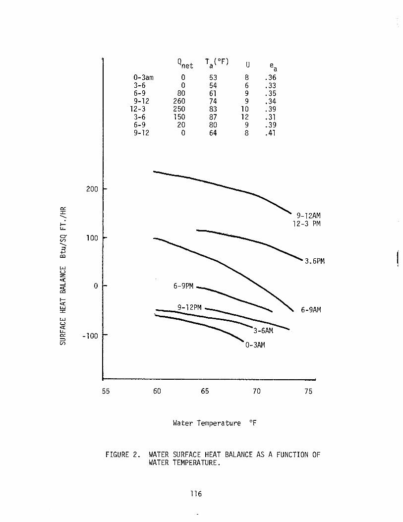
Qnet Ta(OF) U ea0-3am a 53 8 .363-6 a 54 6 .336-9 80 61 9 .359-12 260 74 9 .34

12-3 250 83 10 .393-6 150 87 12 .316-9 20 80 9 .399-12 a 64 8 .41

200

0:::::I: 9-12AM........ 12-3 PMl-lL.

a 100(/).......~

+..>co

3.6PML..L.IuZ~-I a~coI-~L..L.I 6-9AM::I:

L..L.IU~lL.0::: -100::;)(/)

55 60 65 70 75

Water Temperature of

FIGURE 2. WATER SURFACE HEAT BALANCE AS A FUNCTION OFWATER TEMPERATURE.

116

alternative method to generate curves as shown in Figure 1 for any given

set of diurnal atmospheric conditions.

The impact of flow reduction on temperature can be estimated by

selecting a sequence of meteorological conditions (either hourly or three

hourly) and computing the natural variation in water temperature for the

existing water depth and travel time. Knowing the reduction in water

depth or the increase in travel time, the new water temperature can be ob­

tained from curves as shown in Figure 2. For example, if existing condi­

tions in a reach were a depth of six feet and a travel time of 48 hours,

the temperature region would be estimated as 65°-68°F. If flow changes

resulted in depths of three feet and flow times of 96 hours, the tempera­

ture region would be estimated as 68°-72°F from Figure 2.

Since the flow can be stated as a probabilistic distribution of depth

and velocity, these can in turn be used with the water temperature curves

to develop a statement of anticipated water temperatures. The weakest

link in this methodology will be the selection of meteorological condi­

tions. DeWalle (1976) has shown that errors of several degrees Fahrenheit

are commonly associated with normal inaccuracies in wind and vapor pressure.

Prediction of Other Pollutants

There are many other constituents in the waters of streams, lakes,

and estuaries that impact fish and wildlife. Some constituents such as

oxygen content, acids, bases, and salts are of concern when levels are

high enough to stress fish and cause illness or death. Other constituents

which in high enough concentration are lethal are concentrated in fish

even when concentrations in the water are non-lethal. These constituents

such as pesticides and PCB's are of concern since they can contaminate

117

food fish and higher food chain members, including man.

The key to the Level 2 approximation of reduced flow impacts on the

concentration of any pollutant is to have knowledge of the existing con­

centrations of these pollutants in the waters of interest. Unless sources

of these pollutants are known or can be estimated, and the data are avail­

able for ambient concentration of these pollutants in the receiving waters,

there is little basis for prediction of water quality changes associated

with flow reduction. The first step in developing an incremental approach

to water quality impacts of low flows will be to establish the minimum set

of base line pollutant source and water quality data necessary to support

such efforts.

While a simple dilution model is unacceptable to most individuals

knowledgeable in water quality predictions, the dilution model may be a

possible method to classify the magnitude of concern that should be given

to particular low flow reduct10n proposals. Once the priority of the

problem can be estimated, the level of analysis can be defined. The

classical equation for waste oxidation and stream reaeration can be mod­

ified by simple first order rates for benthic demands or contributions.

Since algae contributes significantly to oxygen during daylight periods,

more complex aquatic ecosystem models may become necessary if the waters

are eutrophic. Grenney, et al. (1976) have presented existing model

capabilities and Hines (1977) has shown how such models can be applied

to actual management decision.

The IFG may not need to duplicate such studies, since most agencies

involved in control of water wastes employ such models. If an appreciation

of the sensitivity of such models to changes in depth, velocity, and

temperature can be developed, this may be adequate for instream flow

118

analysis. Models should be used to generate a base line condition, and

then response to alternative flows (with associated depths, velocities,

and temperatures) evaluated. Curves showing the variation in pollution

as a function of river mile will be developed for various flows.

As was discussed earlier, the knowledge of sources of oxygen-demand­

ing waste is a critical input for such calculations. The other major

factor in prediction of pollutants that react with the food web are approp­

riate rate constants for various reactions in each trophic level. Since

these constants must be used by all parties in the evaluation of water

quality, it is suggested that the IFG use constants that have been defined

in the literature for "first cut" analyses.

Many pollutants have been related to sediment loads and simple

models relate concentration of pollutant in water to a multiplier times

sediment loads. This suggests that low flow periods may not be the

critical periods for pollutants since sediment loads increase with flow.

If sediment loads are reduced as a product of instream flow management,

there may be a related lowering of concentration of pollutants associated

with sediment. The interface between the water quality module and the

sediment transport module must be another future task for the IFG if water

models are to be improved.

A simplified model for phosphorus mass balance in lakes has been

suggested by Vollenweider (1975, 1976) and Dillion and Rigler (1974).

They assume lakes can be approximated as a completely mix flow-through

reactor with constant influx of phosphorus and that phosphorus losses

occur through the outflow and sedimentation. The model expresses the

steady state phosphorus concentration in the lake (P) as

P = Po -p­o+p

119

where Po = the inflow concentration of phosphorus

p = flushing rate = annual inflow/lake volume

a = sedimentation rate

Vollenweider (1975) suggests that the sedimentation rate can be expressed

as10

a = -zwhere Z = mean lake depth in meters,

and in 1976 revised this to

a=/-P

thus

P = Po Pp+1p"

If the reduced flows contain the same or lower concentrations of phosphorus,

then the total annual phosphorus load will be reduced. Uttormark (1978)

shows that the

pi

-P- =[

p2 P02

] [ PI + ie.I J1 + PI _Po 1: ,-P-1+.,...P-=2'--:-+-'....--

IP 1 P2

where Po is the concentration of the flushing or withdrawn water and Po2

is the concentration of inflow prior to aeration.

PI = ~ before addition

P2 - ~ the amount added- V2

This simple mixed reaction, first order removal model may be useful

to estimate the fate of other nutrients or materials that are assimilated

by the food web.

Thomann (1978) suggests that the concentration in any trophic level

120

in the food chain can be related to the water concentration by a propor­

tionality constant that is a function of the organism length and uptake,

excretion, respiration, and transfer coefficients.

121

LEVEL 3 SOA (STATE-OF-THE-ART)

Methodologies are available to estimate hourly values of oxygen in

a river to ~l ppm and water temperature with ~loF if adequate information

is known for boundary conditions, BOD loadings and atmospheric conditions,

and river mechanics. Grenney, et al. (1976) have presented a comprehensive

review of SOA methodologies of such water quality models. While the num­

ber of publications on water quality models has been significant since

1976, there have been few significant advances in the fundamental theories. l

The major thrusts of recent water quality modeling efforts are concerned

with the improvement of constants or parameters included in the models,

the development of analytical or numerical techniques to increase computa­

tional efficiencies, or the application of models to specific locations.

Tetra Tech, Inc. (1978) has developed a manual of constants for use in

water quality models funded by EPA. It contains a review of recent data

used in water quality models. Models at this level generally include

some additional level of detail and interactions and, given the present

state-of-the-art, are focused on temperature and diminished oxygen.

The components of the field work and necessary components for the model

are listed below. It should be stressed that not all river problem

settings will require all components, and judgment and experiences

are necessary to proscribe model boundaries and complexity.

It is also assured at this Level 3 that Levels 1 and 2 have also

been essentially completed, i.e., that initial reconnaissance, problem

specification and screening have been accomplished. Following the

lThe Journal of the Water Pollution Control Federation publishes in Juneof each year an annual literature review that includes advances in waterquality models.

122

preliminary steps, the elements listed below would form a "typical"

field program. The completion of the analysis would generally include:

a) compilation and analysis of the field data

b) access to computer program of DO and temperature

c) calibration of data to model one survey set

d) verification of other survey sets to obtain a consistent set

of coordinates

e) projection of input loads and flow regimes

f) simulation of water quality response using verified model

The detailed model specifications are summarized in Table 10, which

summarizes the resolution of models at Level 3. Tables 11 and 12 present

the basic equations and variables that are used in these models.

123

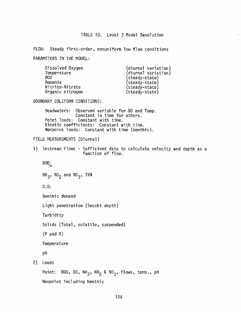
TABLE 10. Level 3 Model Resolution

FLOW: Steady first-order, nonuniform low flow conditions

PARAMETERS IN THE MODEL:

Dissolved OxygenTemperatureBODAll1TloniaNitrite-NitrateOrganic nitrogen

BOUNDARY COLIFORM CONDITIONS:

(diurnal variation)(diurnal variation)(steady-state)(steady-state)(steady-state)(steady-state)

Headwaters: Observed variable for DO and Temp.Constant in time for others.

Point loads: Constant with time.Kinetic coefficients: Constant with time.Nonpoint loads: Constant with time (benthic).

FIELD MEASUREMENTS (Diurnal)

1) Instream Flows - Sufficient data to calculate velocity and depth as afunction of flow.

D.O.

Benthic demand

Light penetration (Secchi depth)

Turbidity

Solids (Total, volatile, suspended)

(P and R)

Temperature

pH

2) Loads

Point: BOD, DO, NH3, N02 &N03, flows, temp., pH

Nonpoint including benthic

124

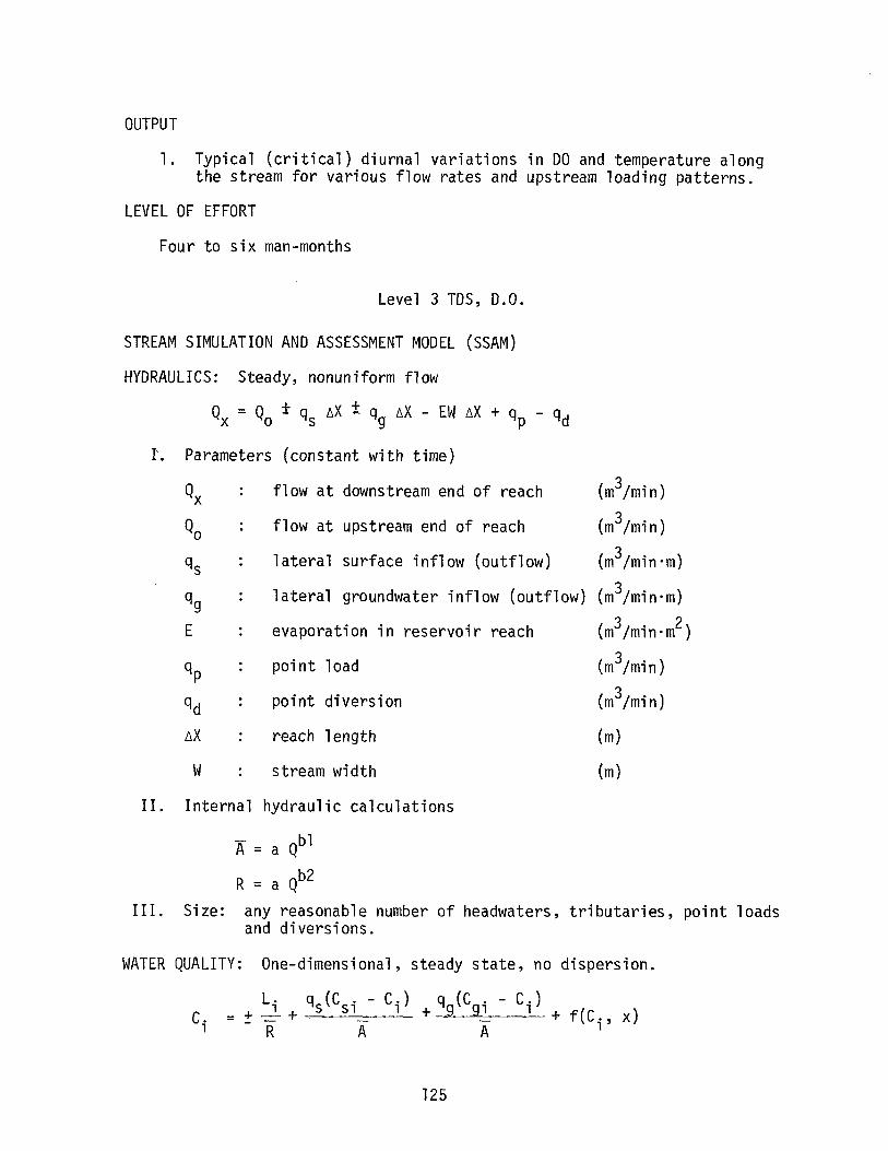
OUTPUT

1. Typical (critical) diurnal variations in DO and temperature alongthe stream for various flow rates and upstream loading patterns.

LEVEL OF EFFORT

Four to six man-months

Level 3 TDS, D.O.

STREAM SIMULATION AND ASSESSMENT MODEL (SSAM)

HYDRAULICS: Steady, nonuniform flow

Q = Q ± q bX ± q bX - EW bX + q - qdx 0 S· 9 P

f. Parameters (constant with time)

W

flow at downstream end of reach (m3/min)

flow at upstream end of reach (m3/min)

lateral surface inflow (outflow) (m3/min·m)

lateral groundwater inflow (outflow) (m3/min·m)

evaporation in reservoir reach (m3/min·m2)

point load (m3/min)

point diversion (m3/min)

reach 1ength (m)

stream width (m)

II. Internal hydraulic cal~ulations

A = a Qbl

R = a Qb2

III. Size: any reasonable number of headwaters, tributaries, point loadsand diversions.

WATER QUALITY: One-dimensional, steady state, no dispersion.

125

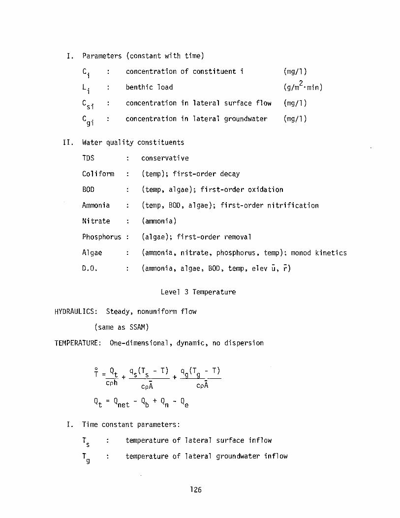
I. Parameters (constant with time)

C. concentration of constituent i (mg/l)1

L. benthic load (g/m2'min)1

Csi concentration in lateral surface flow (mg/l)

C . concentration in lateral groundwater (mg/l)gl

II. Water quality constituents

TDS

Coliform

BOD

Ammonia

Nitrate

Phosphorus

Algae

D.O.

conservative

(temp); first-order decay

(temp, algae); first-order oxidation

(temp, BOD, algae); first-order nitrification

(ammonia)

(algae); first-order removal

(ammonia, nitrate, phosphorus, temp); monod kinetics

(ammonia, algae, BOD, temp, elev u, r)

Level 3 Temperature

HYDRAULICS: Steady, nonuniform flow

(same as SSAM)

TEMPERATURE: One-dimensional, dynamic, no dispersion

T= Qt + qs(Ts - T) + qg(Tg -~cph cpA cpA

Qt = Qnet - Qb + Qn - Qe

I. Time constant parameters:

Ts temperature of lateral surface inflow

Tg temperature of lateral groundwater inflow

126

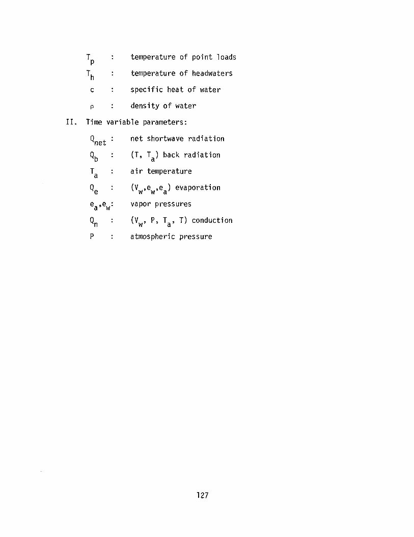
Tp temperature of point loads

Th temperature of headwaters

c specific heat of water

p density of water

II. Time variable parameters:

net shortwave radiation

(T, Ta) back radiation

air temperature

(Vw,ew,ea) evaporation

vapor pressures

(Vw' P, Ta , T) conduction

atmospheric pressure

127

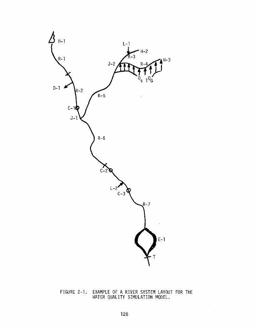
IJ H-1

FIGURE 2-1. EXAMPLE OF A RIVER SYSTEM LAYOUT FOR THEWATER QUALITY SIMULATION MODEL.

128

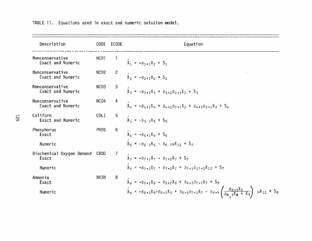
TABLE 11. Equations used in exact and numeric solution model.

Description CODE ICODE Equation

Nonconservative NCOl 1Exact and Numeric Xl = -81'l X1 + 51

Nonconservative NC02 2Exact and Numeric X2 = -S2,l X2 + 52

Nonconservative NC03 3Exact and Numeric X3 = -B3,l X3 + B3,2B2,lX 2 + 53

Nonconservative NC04 4Exact and Numeric X4 = -84,lX4 + S4,282,l X2 + 84,383,lX3 + 54

--' Coliform COLI 5N1..0 Exact and Numeric Xs = -8s lX 5 + 55

Phosphorus PH05 6Exact X6 = -S6,lX 6 + 56

Numeric X6 = -86 lX 6 - 86 2~X12 + 57

Biochemical Oxygen Demand CBOD 7Exact X7 = -87,l X7 - B7,2X7 + 57

Numeric X7 = -S7,l X7 - B7,2X7 + S7,3B12,2X12 + 57

Ammonia NH3N 8Exact Xa = -8a,lXa - BS,2XS + SS,3B7,l X7 + 5a

Numeric X X X ( as, sXs ) ~X12 + 5aXs = -8a'1 S-8Si2 a + 8S,387,1 7 - 8a,4 88,SXs + xi

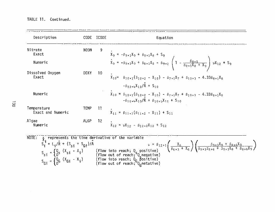
TABLE 11. Continued.

Description CODE ICODE Equation

Nitrate N03N 9Exact Xg = -89'lX 9 + 8S'lXS + 59

Numeric X9 = -69.1X9 + 6a.l Xa - 69.2 (1 -6a.:~;\ X9) J1X 12 + 59

Dissolved Oxygen DOXY 10Exact X10= 810'1(810'2 - X10 ) - 87,lX7 + 810'3 - 4.338s'lXS

--810'4XIO/R + 510

Numeric X10 = 810'1(810'2 - X1o) - 87,l X7 + 810'3 - 4.338s,lXS-810,4X10/R + 810,SX12 + 510

w0

Temperature TEMP 11Exact and Numeric XII = 811,1(811,2 - XII) + 511

Algae ALGP 12Numeric X12 = ~X12 - 812,2X12 + 512

NOTE: x. represents the time derivative of the variable1 - -

S. = L" / R + (S . + SG') / A "'" 8 (X ) ( 8 X Q X )1 1 51 1 1..l - 12'1 6· 9,3 8 + f?S,6 9

5_ {Q (X" - X.) (flow into reach" Q positive) 86'3 + X6 89,38s,6 + 89,3XS + SS,6X9

. - S Sl 1 ' SSl 0 (flow out of reach; Q negative)

S ~ ={QG (XGi - Xi) (flow into reach; QG ~ositive)G, 0 (flow out of reach; QGnetative)

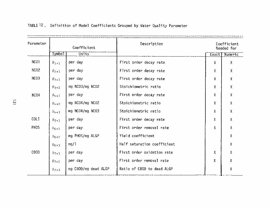
W-...I

TABLE 12. Definition of Model Coefficients Grouped by Water Quality Parameter

Parameter Description CoefficientCoefficient Needed for

Symbol Units Exact Numeric

NCOl 81'1 per day First order decay rate X X

NC02 82, 1 per day First order decay rate X X

NC03 83,1 per day First order decay rate X X

83,2 mg NC03/mg NC02 Stoichiometric ratio X X

NC04 134, 1 per day First order decay rate X X

134,2 mg NC04/mg NC02 Stoichiometric ratio X X

(34,3 mg NC04/mg NC03 Stoichiometric ratio X X

COLI 135,1 per day First order decay rate X X

PHOS (36,1 per day First order removal rate X X

136,2 mg PHOS/mg ALGP Yield coefficient X

136'3 mg/l Half saturation coefficient X

CBQD (37,1 per day First order oxidation rate X X

137,2 per day First order removal rate X X

(37'3 mg CBOD/mg dead ALGP Ratio of CBOD to dead ALGP X

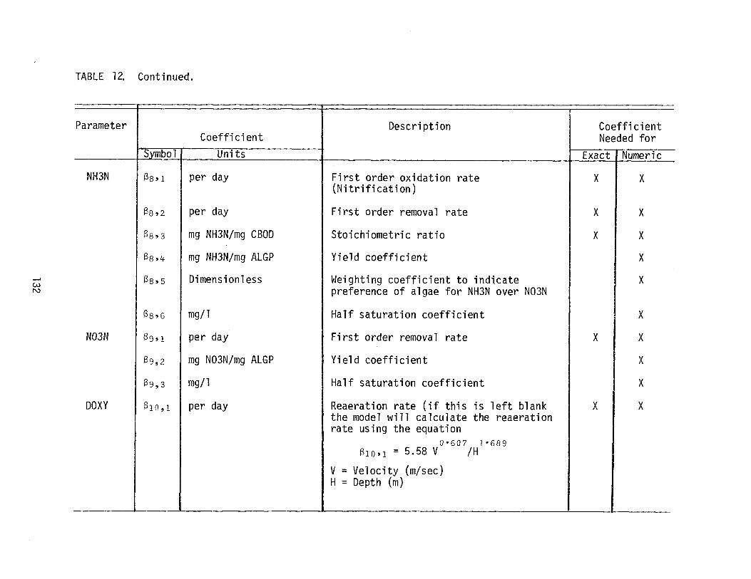
WN

TABLE 12. Continued.

Parameter Description CoefficientCoefficient Needed for

Symbol Units Exact Numeric

NH3N Sa, 1 per day First order oxidation rate X X(Nitrification)

S8,2 per day First order removal rate X X

S8,3 mg NH3N/mg CBOD Stoichiometric ratio X X

S8,4 mg NH3N/mg ALGP Yield coefficient X

138,5 Dimensionless Weighting coefficient to indicate Xpreference of algae for NH3N over N03N

88'6 mg/l Half saturation coefficient X

N03N 89'1 per day First order removal rate X X

89,2 mg N03N/mg ALGP Yield coefficient X

S9,3 mg/l Half saturation coefficient X

DOXY S10,1 per day Reaeration rate (if this is left blank X Xthe model will calculate the reaerationrate using the equation

0-607 1·689610'1 = 5.58 V /H

V = Velocity (m/sec)H = Depth (m)

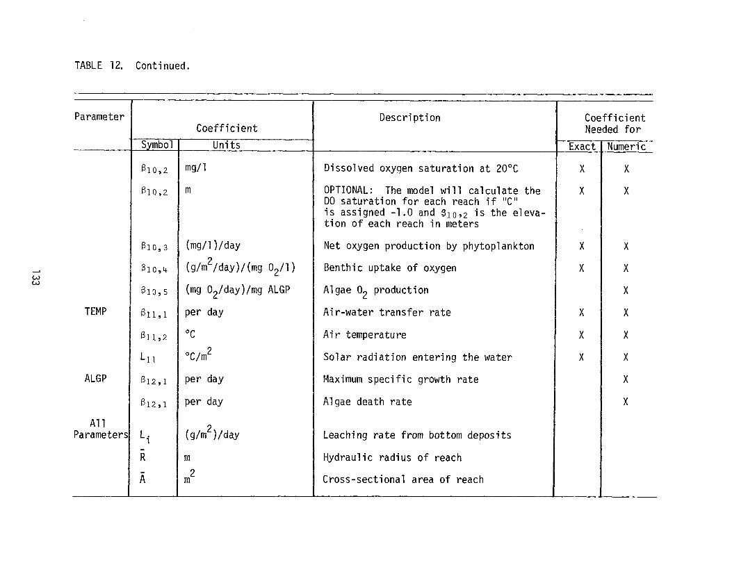
TABLE 12. Continued.

Parameter I Description CoefficientCoefficient Needed for

S mbol Units Exact Numeric

[310,2 mg/l Dissolved oxygen saturation at 20°C I X I X

[310,2 m OPTIONAL: The model will calculate the I X I XDO saturati on for each reach if lie II

is assigned -1.0 and 610'2 is the eleva-tion of each reach in meters

[310,3 (mg/l)/day I Net oxygen production by phytoplankton I X I X

[310,4 (g/m2/day)/(mg °2/1) I Benthic uptake of oxygen I X I Xw ,w

(mg 02/day)/mg ALGP Algae 02 production I IS10,5 XI

TEMP I S11,1 per day Air~water transfer rate I X 1 X

[311,2 °C I Air temperature , X I X

L11 °C/m2 Solar radiation entering the water X X

ALGP I [312,1 per day Maximum specific growth rate X

S12,1 per day Algae death rate X

All I (g/m2)/dayParameters L. I Leaching rate from bottom deposits1

- 1mR Hydraulic radius of reach

A 1m2 Cross-sectional area of reach

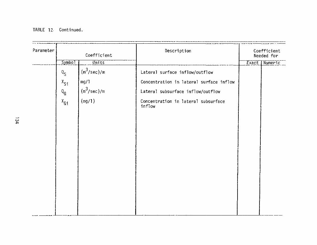
W+::0

TABLE 12· Continued.

Parameter Description CoefficientCoefficient Needed for

Symbol Units Exact Numeric

QS (m3/sec)/m Lateral surface inflow/outflow

XSi mg/l Concentration in lateral surface inflow

QG (m3/sec)/m Lateral subsurface inflow/outflow

XGi (mg/l) Concentration in lateral subsurfaceinflow

I

LEVEL 4 R&D RESEARCH AND DEVELOPMENT

Level 4 would develop a complex interactive ecosystem model that

would synthesize hydrology, river mechanics, water quality, and food chain

dynamics into a unified computer model. There are some knowledge gaps in

creating such a model and basic research is required to provide fundamen­

tal theories to develop these models, as well as to collect adequate data

to calibrate and validate such a model.

While each module can speak to research needs to support the Level 4

methodology development, the water quality module has identified these

following critical research issues:

1) The ability to define the risk and reliability of the information

produced at each level of analysis so tradeoffs can be made between basic

research to improve estimates versus applied research that can devise man­

agement schemes that cope with uncertainty.

2) Even at Level 4, the model and methodology do not include socio­

and economic forces and lack the feedback linkages of human intervention.

Research is needed to determine a hierarchy or framework to introduce these

human factors into the methodology.

3) The ability to model eutrophication in flowing streams is inade­

quate; the shift from phytoplankton to rooted vegetation cannot be modeled.

The drift of species diversity and the resiliency of aquatic ecosystems

needs to be better understood.

4) The response of the food chain to the presence of sublethal con­

centrations of toxic chemicals requires extensive study. Criteria need to

be developed for water quality including such chemicals. The recycling of

these chemicals in the sediments needs to be examined.

135

The details and specifications for large-scale ecosystem models had

to be the subject of another workshop and are beyond the scope of our

module.

136

REFERENCES

Brocard, D. N. and D. R. F. Harleman, "0ne Dimensional TemperaturePrediction in Unsteady Flows," J. of Hyd. Div., Proc. ASCE 102, 227(1976).

DeWalle, D. R., "Effects of Atmospheric Stability in Water TemperaturePredictions for a Thennally Loaded Stream," Water Res. Res., l.0239 (1976)

Dillion, P. J. and F. H. Rigler, "A Test of a Simple Nutrient BudgetModel Predicting the Phosphorus Concentration in Lake Water,"J. Fish Res. Bd. Canada 31:1771 (1974).

Edinger, J. E. and J. C. Geyer, "Heat Exchange and the Environment,"EEl Pub. No. 65, 902 Edison Electric Inst., New York, pp. 259.

Grenney, W. J., D. B. Procella, and M. L. Cleave, "Water Quality Re­lationships to Flow-Streams and Estuaries," in Methodologies for theDetennination of Stream Resources Flow Requirements; An Assessment,Stalnaker, C. B. and J. L. Arnette, eds., Utah State University,Logan, Utah (1976).

Hill, R. G. and R. Viskanta, "Modeling of Unsteady Temperature Distribu­tions in Rivers with Thermal Discharges," Water Res. Res.,JJ, 712(1976).

Hines, W. G., S. W. McKenzie, D. A. Rickert, and F. A. Rinella,"Dissolved Oxygen Region of the Willamette River, Oregon, UnderConditions of Basin-Wide Secondary Treatment," USGC circular 715-1(1977).

Novotny, V. and P. A. Krenke1, "Simplified Mathematical Model of Temper­ature Change in River," JWPLF 45 240 (1973).

Raphael, J. M., "Prediction of Temperature in Rivers and Reservoirs,"J. Power Div., Proc. ASCE, July 1962, pp. 157-181.

Tetra Tech, "Rates, Constants, and Kinetic Formulations in Surface WaterQuality Modeling," prepared for EPA (TC-368a), September 1978.

Thomann, R. V., "Size-Dependent Model of Hazardous Substances in AquaticFood Chain," EPA-600/3-78-036, April 1978.

Uttonnark, P. D. and M. L. Hutchins, "Input/Output Models as DecisiveCriteria for Lake Restoration," Technical Completion Report ProjectC-7232, Water Resources Center, Madison, WI (1978).

Vollenweider, R. A., "Input-Output Models with Special Reference to thePhosphorus Loading Concept in Limnology," Schweiz Z. Hydrol. lZ..:53(1975).

137

Vollenweider, R. A., "Advances in Defining Critical Loading Levels forPhosphorus in Lake Eutrophication," Mem. 1st Hal. Idrobiol. ~:53(1976).

Zison, Stanley, Written comments on the recent IFG workshop, December 13,1978.

Lee, G. F. and R. A. Jones, "Written comments on the recent IFG workshop,December, 1978.

EPA, "Qual ity Criteria for Water," U. S. Environmental Protection Agency,Washington, D. C. 80460, July 1976.

EPA, "Water Quality Assessment: A Screening Method for Nondesignated208 Areas,"Environmental Research Laboratory, Athens, Georgia 30605,August 1977.

138

MODULE III: INSTREAM FISHERY ECOSYSTEMS

MODULE LEADER: Bernard C. PattenDepartment of Zoology andInstitute of EcologyUniversity of GeorgiaAthens, Georgia

139

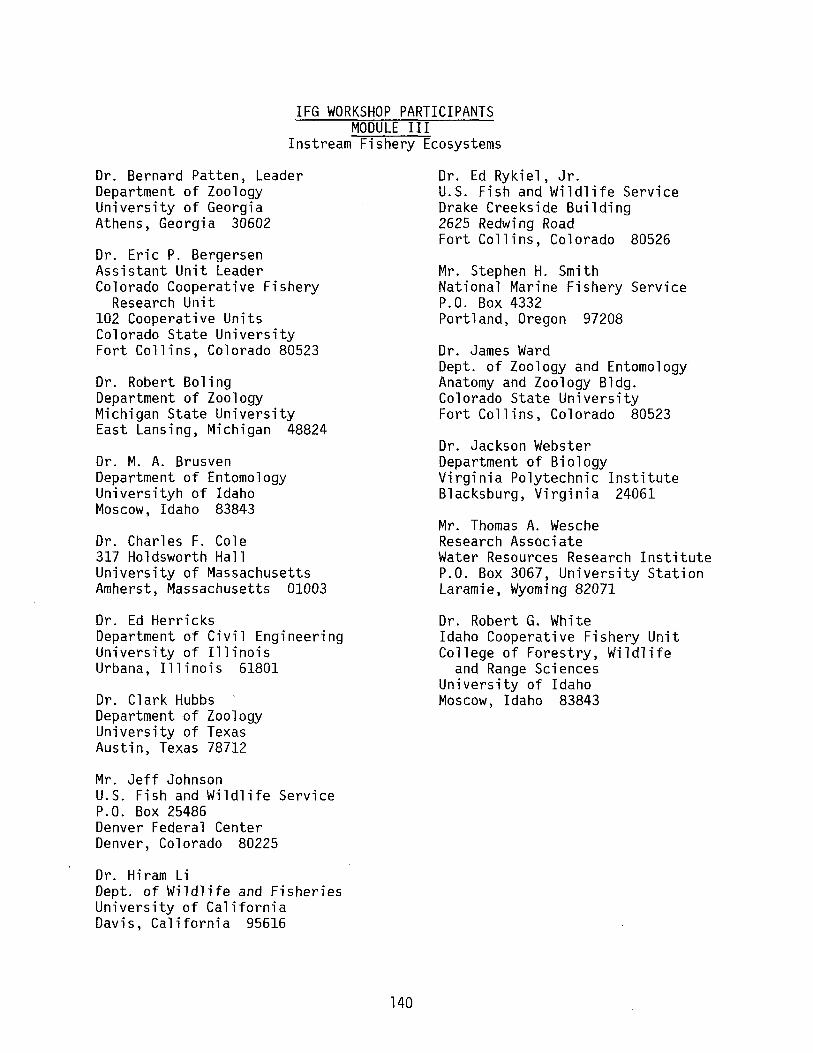
IFG WORKSHOP PARTICIPANTSMODULE III

Instream Fishery Ecosystems

Dr. Bernard Patten, LeaderDepartment of ZoologyUniversity of GeorgiaAthens, Georgia 30602

Dr. Eric P. BergersenAssistant Unit LeaderColorado Cooperative Fishery

Research Unit102 Cooperative UnitsColorado State UniversityFort Collins, Colorado 80523

Dr. Robert BolingDepartment of ZoologyMichigan State UniversityEast Lansing, Michigan 48824

Dr. M. A. BrusvenDepartment of EntomologyUniversityh of IdahoMoscow, Idaho 83843

Dr. Charles F. Cole317 Holdsworth HallUniversity of MassachusettsAmherst, Massachusetts 01003

Dr. Ed HerricksDepartment of Civil EngineeringUniversity of IllinoisUrbana, Illinois 61801

Dr. Clark HubbsDepartment of ZoologyUniversity of TexasAustin, Texas 78712

Mr. Jeff JohnsonU.S. Fish and Wildlife ServiceP.O. Box 25486Denver Federal CenterDenver, Colorado 80225

Dr. Hiram LiDept. of Wildlife and FisheriesUniversity of CaliforniaDavis, California 95616

140

Dr. Ed Rykiel, Jr.U.S. Fish and Wildlife ServiceDrake Creekside Building2625 Redwing RoadFort Collins, Colorado 80526

Mr. Stephen H. SmithNational Marine Fishery ServiceP.O. Box 4332Portland, Oregon 97208

Dr. James WardDept. of Zoology and EntomologyAnatomy and Zoology Bldg.Colorado State UniversityFort Collins, Colorado 80523

Dr. Jackson WebsterDepartment of BiologyVirginia Polytechnic InstituteBlacksburg, Virginia 24061

Mr. Thomas A. WescheResearch AssociateWater Resources Research InstituteP.O. Box 3067, University StationLaramie, Wyoming 82071

Dr. Robert G. WhiteIdaho Cooperative Fishery UnitCollege of Forestry, Wildlife

and Range SciencesUniversity of IdahoMoscow, Idaho 83843

1. INTRODUCTION

II. THE OVERALL METHODOLOGY

III. THE FISHERY MODULE

IV. NEED FOR ECOSYSTEM PARAMETERS

V. RESPONSE TO SPECIFIC QUERIES

141

INTRODUCTION

The IFG incremental methodology endeavors to predict consequences of

streamflow manipulations on various parameters across a broad spectrum of

interests. The methodology is in a state of evolution, therefore it cannot be

evaluated as an operational whole. However, it is possible to examine the

conceptual basis, and the general methodological approach which is under

development. This report concerns the fishery module. Its purpose is to

critique those portions of the IFG methodology pertaining to fishes, both as a

concept and analytical approach, to suggest avenues for improvement or

expansion, and to identify and establish priorities for needed research and

development to improve the present day methodology.

THE OVERALL METHODOLOGY

A common assumption associated with quantification of stream flow

requirements for fish resources is that if instream flows are adequate for

maintenance of healthy fish populations, other instream uses will be generally

protected. This is reasonable because the ichthyofauna as a group is sensitive

to flow variations and changes in related parameters. Fishes are generally in

the upper trophic levels of the aquatic ecosystem, or coupled complexly to

other ecosystem sectors, so that existence of healthy fish stocks implies a

viable ecosystem. Natural fish populations are a sensitive barometer of

ecosystem condition. In addition, fishes are better known ecologically and

biogeographically than other aquatic biota.

Past instream flow methods aimed to establish a single or fixed minimum

flow. Such an approach is founded on a threshold concept, i.e., fish popula­

tions will not be harmed unless stream flows drop below this minimum value.

However, fish and invertebrates are adapted to changing flow regimes;

142

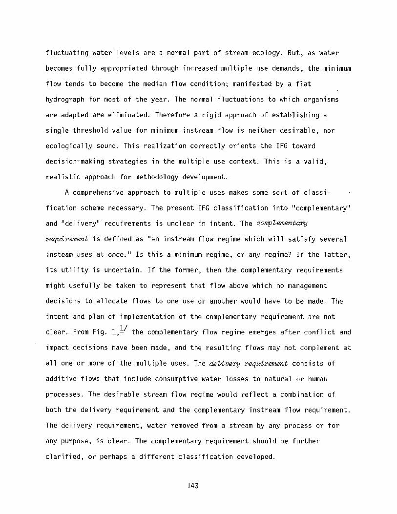
fluctuating water levels are a normal part of stream ecology. But, as water

becomes fully appropriated through increased multiple use demands, the minimum

flow tends to become the median flow condition; manifested by a flat

hydrograph for most of the year. The normal fluctuations to which organisms

are adapted are eliminated. Therefore a rigid approach of establishing a

single threshold value for minimum instream flow is neither desirable, nor

ecologically sound. This realization correctly orients the IFG toward

decision-making strategies in the multiple use context. This is a valid,

realistic approach for methodology development.

A comprehensive approach to multiple uses makes some sort of classi­

fication scheme necessary. The present IFG classification into IIcomplementaryll

and IIdeli veryll requirements is unclear in intent. The ()ompZementary

requirement is defined as lI an instream flow regime which will satisfy several

insteam uses at once. II Is this a minimum regime, or any regime? If the latter,

its utility is uncertain. If the former, then the complementary requirements

might usefully be taken to represent that flow above which no management

decisions to allocate flows to one use or another would have to be made. The

intent and plan of implementation of the complementary requirement are not

clear. From Fig. I,ll the complementary flow regime emerges after conflict and

impact decisions have been made, and the resulting flows may not complement at

all one or more of the multiple uses. The deZivePy requirement consists of

additive flows that include consumptive water losses to natural or human

processes. The desirable stream flow regime would reflect a combination of

both the delivery requirement and the complementary instream flow requirement.

The delivery requirement, water removed from a stream by any process or for

any purpose, is clear. The complementary requirement should be further

clarified, or perhaps a different classification developed.

143

The focus on institutional aspects to the extent of explicitly incorpo-

rating them into the methodology is very positive. Instream flow management is

more than scientific analysis because of the many segments of the user

community it affects. The intent of the IFG to provide service to user groups

is an important step in coupling the technical methodology to applications

within and across institutional frameworks.

As presently conceived the methodology is to be developed in eight

modules, "necessary to complete a simulation of the physical and chemical

dynamics of a stream system. 1I11 The modular concept is necessary in such a

program as this to provide a capability for alternative resolution levels

within modules. A very important stream system may require high resolution

based on extensive data sets, whereas for a lesser system low resolution based

on scant data may be adequate. Each module should have an adaptive resolution

capability based on (1) different intensities of application of a given

approach, (2) different approaches, and (3) different technological

capabilities among scientific disciplines.

The eight modules identified for development are:

1. Delivery and return flow 5. Channel maintenance

2. Fishery 6. Estuarine inflow

3. Recreation 7. Riparian vegetation

4. Water quality 8. Channel design

These modules do not appear to be organized into a framework that constitutes

an ecologically meaningful whole. Modules 1, 5, and 8 pertain to hydrology,

but not all potentially meaningful aspects of hydrology are included. Modules

2 and 7 represent biology but fail to encompass important aspects of stream

ecology. Water quality represents a special aspect of the more basic human

use. The estuarine category is as large a subject as all the rest. The

144

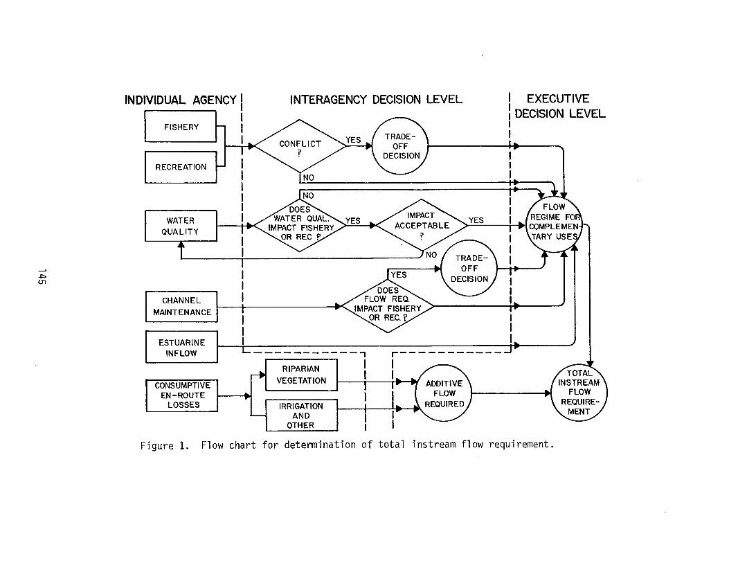
,.J:::.(J"l

INDIVIDUAL AGENCY I

I FISHERY h II

RECREATION

WATERQUALITY

CHANNELMAINTENANCE

INTERAGENCY DECISION LEVEL I EXECUTIVE: DECISION LEVELII

instream flow requirement.

IRRIGATIONAND

OTHER

-----------, r-----------RIPARIAN I I

VEGETATION I I

I

II

Flow chart for determination of total

ESTUARINEINFLOW

CONSUMPTIVEEN-ROUTE

LOSSES

Figure 1.

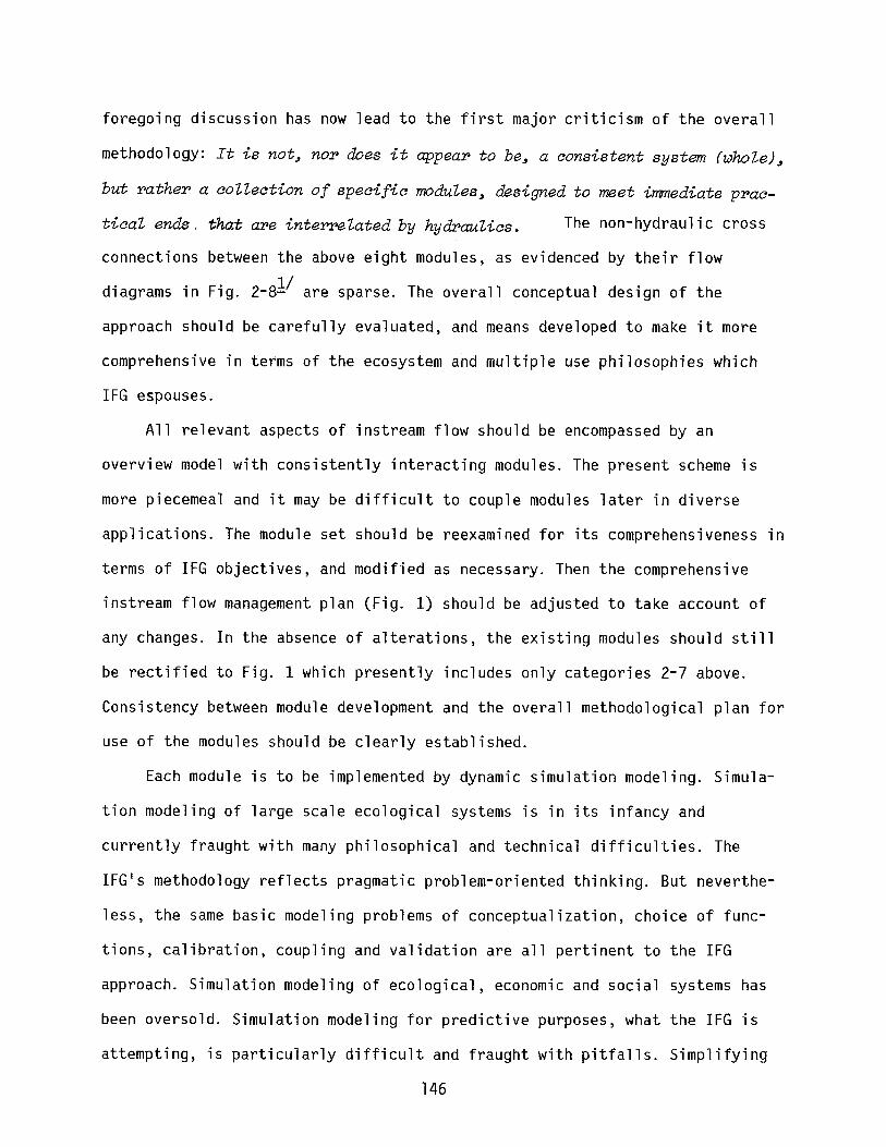
foregoing discussion has now lead to the first major criticism of the overall

methodology: It is not, nor does it appear to be, a consistent system (whole),

but rather a collection of specific modules, designed to meet immediate prac-

tical ends, that are interrelated by hydraulics. The non-hydraulic cross

connections between the above eight modules, as evidenced by their flow

diagrams in Fig. 2-8!/ are sparse. The overall conceptual design of the

approach should be carefully evaluated, and means developed to make it more

comprehensive in terms of the ecosystem and multiple use philosophies which

IFG espouses.

All relevant aspects of instream flow should be encompassed by an

overview model with consistently interacting modules. The present scheme is

more piecemeal and it may be difficult to couple modules later in diverse

applications. The module set should be reexamined for its comprehensiveness in

terms of IFG objectives, and modified as necessary. Then the comprehensive

instream flow management plan (Fig. 1) should be adjusted to take account of

any changes. In the absence of alterations, the existing modules should still

be rectified to Fig. 1 which presently includes only categories 2-7 above.

Consistency between module development and the overall methodological plan for

use of the modules should be clearly established.

Each module is to be implemented by dynamic simulation modeling. Simula­

tion modeling of large scale ecological systems is in its infancy and

currently fraught with many philosophical and technical difficulties. The

IFG's methodology reflects pragmatic problem-oriented thinking. But neverthe-

less, the same basic modeling problems of conceptualization, choice of func­

tions, calibration, coupling and validation are all pertinent to the IFG

approach. Simulation modeling of ecological, economic and social systems has

been oversold. Simulation modeling for predictive purposes, what the IFG is

attempting, is particularly difficult and fraught with pitfalls. Simplifying

146

assumptions must often be made in simulation modeling which compromise

scientific standards. All too~ten, any simulation model that provides even

the most vaguely satisfying solutions is accepted truth.

Accurate prediction of time dynamics in large scale ecological systems is

the most demanding and difficult objective of simulation modeling. Unfortun­

ately, the existing state-of-the-art does not measure up to desired scientific

standards in this regard. Thus, IFG should maintain a focus on the legitimate

uses of modeling, cognizant that any comprehensive methodology is bounded by

numerous state-of-the-art constraints.

Recognizing these present day constraints while still applying this

methodology is within the realm of acceptable scientific behavior. The IFG

effort is not unlike other scientific developments in other fields of

endeavor. That is to say, basic research, further testing, and refinement must

continue; but the present day methodology still has utility as an application

of science in resource policy development and decision-making.

147

THE FISHERY MODULE

The purpose of the fishery module is, lito assess the impacts of altered

streamflow regimes on instream habitats. lIi/ Five streamflow parameters which

directly influence fish distribution are identified: (1) depth, (2) velocity,

(3) temperature, (4) substrate, and (5) cover. Three simulations are involved:

(1) hydraulic conditions, both normal and modified; (2) impact of stream flows

on fishes, invertebrates and other stream biota; and (3) coupling of (1) and

(2). Again, hydraulic modeling is central.

Target fish species are classified into five categories: (1) economic,

(2) indicator, (3) endangered, (4) nongame, and (5) forage forms. The last

group includes also "aquatic invertebrates" which may be important in food

chains. This is a modest, if curious, way to acknowledge the existence of a

stream community which, with depth, velocity, temperature, substrate and

cover, also affects fish populations. The recognition of different functional

classes within a species, such as life history stages, is positive.

The IFG group shows a good sensitivity to assumptions, both expressed and

implied. Three underlying expressed assumptions for the fishery module are:

(1) "that the distribution and abundance of any species [are] not primarily

influenced by any single parameter of streamflow, but related by varying

degrees to all hydraulic parameters;1I (2) "that a species will elect to leave

an area when streamflow conditions become unfavorable;" and (3) IIthat

individuals of a species will tend to select the most favorable conditions in

a stream, but will also use less favorable conditions within a defined range,

with the probability-of-use decreasing as conditions approach the end points

of the total range. lIi/ Thus arises the probabil,ity-of-useaonaept whiah

provides the basis for the IFG Incremental Instream Flow Method.

148

One possible implication of the IFG1s chosen approach leads to a second

major criticism of the methodology. The implication is that the specified

parameters--depth, velocity, temperature, substrate and cover--are sufficient

for determining habitat selection by the fishes. The criticism is that these

factors are necessary" but not sufficient, determinants of fish distribution.

The logical flaw is demonstrated as follows. Let the statement,

"hydraulic parameters are sufficient to specify fish habitats,1I be put in the

form of a conditionaZ statement in propositional logic:

hydraulicparameters

okay

s~ fish====J)~ habi tats~ okay

n

(1)

The double arrow is read "implies," or the statement can be read Hif hydraulic

parameters are okay, then fish habitats are okay. II Hydraulic parameters okay

is sufficient (s) for fish habitats to be okay, and the latter is necessary

(n) for the former. Since the assumption is false, it leads to a false

consequence. The Qo~apo~~ve of the conditional statement holds:

fishhabitatsnot okay

s.~ hydraulic==7'''''' parameters

not okay(2)

The falseness of this statement is obvious; there may not be okay fish

habitats for many reasons other than absence of adequate hydraulics; yet the

absence of fish habitats is implied to be sufficient for poor hydraulics. The

true assumption should be the converse of the original false assumption

149

namely, "hydraulic parameters are necessary to specify fish habitats." In

logical form this is:

fishhabitats

okay

hydraulic-==::;\>,.. parameters

"--.-/ 0 kayn

(3)

The inverse of the original conditional statement,

hydraulicparameters

not okay

s~

)fish

habitatsnot okay

(4)

is a true consequence of the converse. Thus, if the hydraulic parameters are

unsatisfactory, this is sufficient for not okay fish habitats, and the latter

is necessary for not okay hydraulics. Note the difference between statement

(1), which is false, and statement (4), which is true. The IFG incremental

methodology is based on statement (1) when in fact it should be based on

statement (3). Hydraulic parameters are necessary to specification of fish

habitats, but they are not sufficient. The present IFG methodology focuses

heavily on necessary conditions for fish habitats, but does not adequately

incorporate sufficient conditions. To the extent that the present methodology

does nrit establish a basis for impacts of altered streamflow regimes in

"sufficient conditions,1I it is operationally inadequte.

Based on the expressed assumptions, an associational approach to relating

fish distribution to hydraulic conditions is formulated. Of two possible

approaches, (1) establishing causation or (2) observing correlations, the

latter is weaker in the logic of inference. The IFG methodology is correlative

only, and will be less defensible and justifiable in an adversary setting than

would be approaches that gave causal explanations. In the context of resolu-

tion, the correlation approach might be considered a low resolution counterpart

of an eventual high resolution causal method within the fishery module.

150

Probability-oi-Use Curves

The basis for the IFG's incremental methodology lies with its

"probability-of-use" information expressed in a curve format. These curves do

not represent true probabilities, and should, therefore, be renamed. e.g.,

habitat desirability curves. Four types of analyses were employed to formulate

the initial curves. In descending order of the quality of curves produced,

these are: (1) frequency analysis, (2) range and optimum analysis, (3)

parameter overlap, and (4) indirect parameter analysis.if The rationales

underlying these methods, and the methods themselves, constitute a major

positive feature of the IFG methodology given the commitment to a correlation

approach. Each method of curve construction utilizes a specific, objective

procedure consistently employed. FrequenayanaZysis is based on data avail-

able consisting of depth, velocity and substrate at capture or observation

locations for individual fish. The clustering of frequency increments by a

systematic procedure to reduce variance appears reasonable, but statistical

consequences should be evaluated. Range and optimum analysis is based on

range and optimum information when frequency data are not available. Some

subjectivity is involved in IIdrawing ll a bell shaped curve through four data

points, but this is unavoidable. Also, a normal distribution is assumed in

absence of other information. The statistical validity of this choice for the

type of data and systems involved should also be evaluated. Parameter overlap

converts field descriptions of habitats used and avoided to approximate range

and optimum data, and curve construction then follows the same general

procedure as in the previous method. Indipect analysis is, apparently, a set

of ad hoc methods by which information for c~rve construction is drawn

principally from the biologist's intuition and experience.

151

The habitat desirability curves that result from these procedures are

then given a quality rating, based on specific objective criteria. This is an

excellent feature of the methodology that should aid decisions in establishing

instream flow regimes and serve well in proceedings to resolve conflicts.

Methods for obtaining data are described,~ and should also be reviewed

by specialists in sampling theory so that qualifications can become known and

stated.

IFG IncJteme.n-tal Methodology

The incremental methodology based on habitat desirability curves

quantifies the amount of potential habitat available for each species or life

history stage, in a given stream section, under different streamflow regimes,

and with different channel configurations. The method consists of four steps.

(1) Physical stream measurement utilizing multiple transects; (2) Hydraulic

simulation of the stream reach to determine spatial distribution of combina­

tions of depths and velocities associated with bottom and cover types at

different stream flows. (3) For each target species or life stage, a

IIcomposite probabil ity-of-use ll (i .e., c.ompo-6Ue. habUat dubta.bi.h..ty -inde.x) is

calculated for each combination of hydraulic parameters represented in a

stream segment. These composite indices are determined from the individual

habitat desirability curves for the separate parameters as a simple product of

the separate desirabilities. 4/ This procedure introduces an implied assumption

that organisms select among the parameters in a fashion of statistical

independence. Obviously, depth, velocity, substrate and cover are not

independent variables of themselves, and may not be in terms of how fish

select for them. Statistical dependence in selection among parameters should

be a subject of research. Subsequently, the composite desirability indices

should be computed in an analogous manner to joint probabilities between

152

statistically dependent variables. (4) Finally, a weighted usable

area for each reach is calculated for various stream flow levels by species

for life history stage multiplying surface area for each hydraulic combination

(step 2) by the composite desirability index (step 3). The weighted usable

area is accepted as an index of attractiveness of a stream reach in areal

terms for each species or life stage. Weighted usable area plotted against

different flow regimes can be used to identify critical periods for each life

history stage, and availability of limiting habitat for each stage or species.

The incremental method appears sound as a computation procedure, except

for the need to determine interaction effects among depth, velocity, substrate

and cover with respect to the habitat desirability. However, because of the

implications associated with the necessary versus sufficient trap, it is not

generally recommended to determine habitat selection based on hydraulic

parameters alone. The IFG authors state, lfSince changes in hydraulic charac-

teristics will initiate differential species reactions, the incremental method

may be particularly useful in predicting changes in species composition.

Because the output from the incremental method is directly tied to the

physical carrying capacity of the stream, it is possible to determine the

approximate change in standing crop of a given species at different instream

flow regimes.~/ However, until the methodology can be based on a parameter

set--physical, chemical and biological--not only necessary but sufficient to

specify fish production, such application should not be oversold.

153

NEED FOR ECOSYSTEM PARAMETERS

In summary, two major criticisms of the IFG incremental methodology have

been identified:

1. The methodology is not a consistent system of strongly interacting

components, but a collection of specific modules interrelated by stream

hydraulics.

2. The methodology, as presented, is based on a narrow set of physical

parameters providing necessary, but not necessarily sufficient, conditions for

the specification of stream habitats.

These are fundamental conceptual criticisms originating as a result of

the methodology's strong orientation toward water management decision-making.

There is virtually no acknowledgement in the present IFG literature that

stream ecosystems exist or that their status is relevant to the existence and

status of fisheries. This should be remedied. Changes in instream flow regimes

have both direct and indirect effects on fishes. Direct effects are expressed

when flows approach or exceed tolerance limits, hence certain flow character­

istics are necessary for the well being of target populations. But, within the

range of tolerances, habitat desirabilities are determined by other ecosystem

parameters that reflect primary production, trophodynamics, decomposition and

nutrient regeneration. The flow regime affects all ecosystems processes, and

hence under non-extreme conditions its effects are propagated to the fishes

indirectly via ecosystem structure and function. Sufficient parameters to

specify stream fishery habitats therefore reside in the particulars of extant

ecosystems in each stream reach. A rigorous written discussion of these

indirect effects and guides for examining, accepting or rejecting simplifying

assumptions should be developed for IFG methodology users.

154

Although the IFG methodology is portrayed as a general approach, there is

a persistent bias toward the dominance of physical factors which has come from

experience with western stream studies where physical factors are the

principal determinants of fish distribution. Important biological factors in

microhabitats and selection within a stream reach include: (1) keystone

species, (2) trophic dynamics, (3) space competition, and (4) status of

predation. The universal assumption of physical factor dominance is tenuous;

as is the implied assumption that a species in different ecological settings

always behaves similarly. Plasticity in habitat selction is extremely

important. Thus, a fundamental problem with the methodology is the assumption

that fish are physically limited rather than food-chain limited. This also

reflects the western bias. In eastern streams food is often both the ultimate

limit of fish production and the immediate reason for low production. Some

species are limited by external factors such as harvesting. Considering the

entire ichthyofauna, physical factors are seldom limiting under natural

conditions. Under all but extreme natural conditions fish and invertebrates

both tend to be food limited in eastern waters.* Answers to fundamental

questions such as the following need to be built into the methodology: (1)

How are instream nutrients, expecially N03 and P04 , affected by flow modifi­

cations? (2) How does the flow regime influence nutrient effects on primary

production? Nutrients in return flow may be especially important. (3) How is

stream primary production affected by physical factors such as flow,

temperature, sediment load, etc. (4) How important are allochthonous vegeta-

tion inputs to primary production, and how will flow regulation and watershed

* Editor's note: One intended application of the IFG methodology isidentification of those activities of man which would so alter thenatural flow regime as to result in conditions of stress normallyfound only with extreme natural conditions.

155

management influence the quantity and qualtity of allochthonous inputs? (5)

How do physical and chemical factors affect connections between food base

productions and fish production, or detritus decomposition and invertebrate

production?

Implementation of an ecosystem holistic viewpoint by IFG can overcome

both of the two major criticisms. Addition of modules designed to develop

diagnostic information about the state of the stream ecosystem would assure a

more strongly connected set of mutually consistent components for the

incremental methodology, as well as base the methodology on a broader

parameter set to establish sufficient conditions for specifying fishery

habitats. Obviously, full ecosystem information is beyond the' scope and intent

of the IFG methodology. Therefore, the same basic approach as presently used

can continue to be employed, but extended to several additional parameters

that reflect chemical and biological processes of ecosystems.

The following set of parameters incorporate chemical and biological as

well as hydraulic considerations. Seven major parameters, in order of

importance, are:

l. depth 5. riparian cover

2. velocity 6. competition

3. temperature 7. predation

4. food supply

Six additional parameters of lesser significance, unranked, are:

8. substrate

9. dissolved oxygen

10. instream cover

11. nutri ents

12. stream morphology

13. sediment load

Dissolved oxygen and nutrients are constituents of water quality, a graded

approach to which illustrates how other categories might be examined. Water

156

quality could be assessed at several levels of resolution. First is a

screening level in which it is only necessary to establish the absence of

lethal concentrations of toxins. At the second level temperature and dissolved

oxygen concentrations would permit an estimate of stream ecosystem metabolism

for a small additional monitoring investment. Level three would introduce

conductivity and turbidity measurements to assess dissolved and suspended

solids. The fourth level would add to the previous list information about

nitrate, phosphate, other nutrients and perhaps toxicants. Food supply, compe­

tition and predation are biological variables. To assess biotic conditions of

a stream, indicator species, keystone species and species richness (diversity)

should be examined by quick survey techniques. For example, artificial sub­

strates introduced some weeks before sampling would provide diagnostic data on

instream productive potential. Food chain information could also be developed

based on a few relatively simple measurements.

There are four potential food sources in streams:

1. benthic primary production

2. planktonic primary production

3. within-reach allochthonous inputs

4. stream channel allochthonous inputs

Each of these is directly or indirectly affected by instream flows. These

effects and their propagation through food chains to fish abundance can be

evaluated with fairly simple models based almost entirely on parameters

already in the IFG methodology, as outlined below.

Factors needed to estimate benthic primary production are temperature,

nitrogen, phosphorus, light, substrate, and geographic region. Given these

factors a model, perhaps little more than an expansion of Michaelis-Menten

formulation, could be used to estimate benthic primary production. A similar

157

model, using the same factors with the exception of substrate, could be used

for planktonic primary production. Within reach allochthonous inputs could be

generated in a fashion similar to estimation of overstream cover from measured

values of stream and floodplain width, and knowledge of riparian vegetation in

the study reach. Estimation of stream carried allochthonous inputs is a more

difficult problem, one that should be recognized as an area of research need.

Three possible approaches are suggested: (1) From a large number of

particulate organic matter samples, a site-specific model could be developed

and calibrated. (2) It may in the future be possible to develop a predictive

model based on upstream watershed characteristics. (3) Particulate organic

matter could be estimated from predicted or measured levels of total suspended

solids. Based on current lack of information about utilization of dissolved

organic matter, its inclusion in a model is not recommended. Avenues for

refinement of each of these estimations of energy sources should be evident,

for example, breaking down benthic production to diatoms, filamentous algae,

and macrophytes; treating limiting effects of trace nutrients; and partition­

ing particulate organic matter into size fractions.

The next step is to convert energy source estimates to secondary produc­

tion estimates. Again, as a start, a simple two-step procedure might suffice:

(1) determination of the presence of appropriate consumer guilds, i.e.,

benthic grazers, filter feeders, or shredders; and (2) estimation of consumer

production based on trophic efficiences. The approach used to evaluate habitat

desirability for fish could also be applied in general to invertebrate

consumers. One area of modification would be more refined treatment of

substrate classes. For the purposes outlined here, invertebrates could be

lumped into guilds with each guild represented by a broadly tolerant species

since only presence needs to be established. The trophic efficiency technique

158

is probably the weakest step of the suggested procedure, however, no simple

alternative exists. This represents another area of research need, for

example, how do leaf or algal species affect assimilation and respiration? How

efficient are passive filter feeders in capturing suspended organic particles?

Are consumers selective in their feeding?

The end result of these calculations would be an estimate of potential

consumer productions which can be used to complement estimates of weighted

usable area. These outlined procedures also provide a framework for further

development and refinement.

159

RESPONSE TO SPECIFIC QUERIES

A number of questions were posed at the workshop. Responses to many of

these are given below in accordance with the ecosystem philosophy espoused

above.

1. What are the strenghts of the IFG methodology conceptually and

procedurally? Conceptually, the method is geared to provide a service to user

groups, and technical aspects of the problem are coupled meaningfully to

institutional considerations. The modular construction is desirable although

choice of modules and the overall framework within which they are to interact

are issues. Also, several levels of resolution within each module should be

available to adapt the methodology to problems and data sets of different

magnitudes. Procedurally, hydraulic simulation is the obvious strong point of

the methodology. The II probability-of-use ll concept is a normalized index and

not a probability, and should be calculated and interpreted accordingly.

lIWeighted usable area ll is difficult to interpret. For example, 104 ft2 with a

desirability index of .01 is equivalent to 100 ft2 of excellent habitat. If an

adjacent reach has 50 ft2 with a desirability value of 1, that is where the

fish will be. In other words, the use of weighted usable area assumes

additivity of elements of goodness regardless of spatial distribution. An

alternative to weighted usable area should be sought.

2. What are the advantages and disadvantages of the hierarchical,

modular approach of the IFG methodology? The modular approach should be

retained. Choce of modules within a total system framework to overcome the

first major criticism should be reevaluated. Also, modules should be developed

with different data requirements for different resolution levels.

3. In what priority should various physical, chemical and

biological models be pursued? In response to the second major criticism,

160

parameters required to establish sufficient, and not just necessary,

conditions for fish habitats need to be developed. This development should be

integrated, making use of easily measured variables as outlined in the

previous section. With the use of simple models primary variables can be used

to generate derived variables reflecting ecosystem condtion.

4. What state-of-the-art technology is readily available for

adoption or adaptation to instream flow assessments? Multivariate statiscal

analysis has not been explored as a possible alternative to the IFG metho­

dology. These methods should be examined both in their complementary and

alternative resolution aspects. Ecological simulation modeling is sufficiently

well developed to be incorporated judiciously into the IFG approach.

5. What areas of validation research require more emphasis? The

apparent bias of the present methodology toward western stream has been

mentioned. Less is known about lotic systems in the western United States than

in eastern North American and the Mississippi valley. Two kinds of validation

should be sought, intensive and extensive. For intensive, rigorous testing in

regions where large data bases exist should be undertaken, i.e., in salmonid

streams of the Pacific northwest. Extensive testing should cover a broad range

of physiographic provinces, concentrating first on eastern salmonid streams

for comparison with western results, then extending to mainstream rivers and

non-salmonid species. The present physical bias of the methodology may

possibly be acceptable in the west, but in the east, fish habitats will be

determined by other physical and chemical parameters.

6. What other parameters should be added to the methodology? A

total of 13 parameters was indicated in the preceding section 5 to 7 of which

appear to be new.

161

7. What emphasis should be placed on factoring other components

(riparian vegetation, wildlife, estuarine inflows, etc.) into the assessment

method? Considerable. Major criticism number one calls for an integrated,

holistic methodology in which the modules are exhaustive over all significant

problem areas, and meaninfully integrated.

8. What new areas of frontier research are required? The basic

ecology of streams is still a vast unknown, including the biology of even

major aquatic species, their interactions, and ecosystem level relationships.

The IFG methodology can be no better than the knowledge base on which it is

formed. Basic study of stream ecology over a broad spectrum of stream types

and regions should be encouraged. IFG can serve such a purpose through the

data requirements of its alternative modular methodologies, pointing to infor­

mation gaps and defining useful forms of information to be collected.

9. Is the representative reach a valid decision making tool? Yes.

The representative reach is conceptually a stratified random sampling scheme.

The choice of actual study reaches should be in accordance with requirements

of rigorous sampling theory to assure results that can be employed with

confidence at the level of decision-making. Professional statisticians should

be consulted to develop specific criteria.

10. Does the independence of variables influencing species distri­

bution implied by the computation procedure appear to be valid? No. This is a

major technical problem with the present methodology. There are only two

reasons to accept such an assumption: (1) lack of positive reasons to adopt

any other formulation, and (2) the form of available data. It could be argued

that even if only 5% of available data did not conform to the independence

assumption, a multivariate 'analysis would be significantly more reliable than

the IFG methodology. This might be true anyway, and established multivariate

162

methods should be evaluated for instream flow assessment and performance

compared to the IFG approach. As to alternatives, let G be a scalar denoting

habitat desirability of a site. Let f. be a scalar parameter, where i = depth,1

velocity, temperature, etc. spanning the 13 factors listed above. Then

G = $ (f1,f2, ... ,fn), where $ is some integrable function mapping a point

(f1,·.· ,fn) into the scalar value G. IFG has assumed that G = n~=1 gi(fi ),

where g. is some unitless function of factor i (e.g., a frequency distribution1

normalized to 1, a probability function, etc.). Further, since G is computed

*for each habitat subvolume, the aggregated value G is defined as a summation

G* = l~ . G., of the N subvolumes of the study reach, where G. is theJ=l J J

desirability of the j'th subvolume. Two methods to determine G are by power

series,

N. N.G =I' IJ

i=1 j=1Nk fi fjI (1.. k 1 2

k=1 ' J ...

or by discrete approximation. The power series approach is essentially

impossible to parameterize except by a least squares fit to an extensive data

set. Therefore, discrete approximation is recommended. In this approach the

range of each factor f i is segmented. Then an n-dimensional matrix, with each

entry reflecting the utility of a habitat exhibiting each combination of

segmented characteristics, is constructed. Instead of computing weighted

usable area, a histogram of volume units having each value might be construct-

ed, from which mean, median, percent of volume units with better than 50%

desirability, etc. could be computed.~/

11. Is weighted usuable area an adequate concept upon which to

build and defend decisions about instream flows? Even if the computations were

based on sufficient conditions to establish habitat desirability for fishes,

163

weighted usable area would not be an adequate concept. As discussed above, a

large number of units of marginal habitat is not the ecological equivalent of

a small number of units of prime habitat. However, as an interim or low

resolution approach, weighted usable area serves a useful purpose.

12. Is the implicit assumption of the incremental method, that fish

production is a function of "usable habitat,1I valid? Usable habitat could

correspond to used habitat if the former were defined by a sufficient set of

parameters. In other words the assumption is reasonable in principle. The

effort to establish sufficiency will, in general, be geared to the importance

of the specific project.

13. Assuming a known functional relationship between weighted

usable area and fish production, what is the best approach presently available

to relate population dynamics to the IIhabitat dynamics ll produced by the

incr~mental method? Simulation modeling. The previous section outlined an

approach by which information derived from relatively simple to measure

parameters could be extended by simple models to derive parameters reflecting

the state of the stream ecosystem.

14. Should data for the incremental method be collected and

analyzed by region? Should they be catergorized by stream size? Yes. For

development of a general methodology variability over a range of stream types

and geographic regions should be assessed. Delphi approaches to the generation

of II soft li data sets should certainly be used.

15. Would it be desirable to place confidence intervals around the

habitat desirability curves? Certainly, if sufficient data can be obtained to

permit this. The present scheme of quality ratings is a good practical

approach, however.

164

16. Is the traditional approach of developing criteria by LD SOlaboratory test appropriate? No. Extrapolation of laboratory data to the field

should always be done with caution. Information derived under actual field

conditions is most desirable.

17. Is the proposed model for cover, paralleling that for composite

probability of use, adequate to describe the behavioral response of a species

to cover? It would have the same generic problems as discussed for the general

methodology. A regression approach might be more recommendable.

18. Is the proposed functional classification of macroinvertbrates

(shredders, swimmers, burrowers, etc.) satisfactory? Yes. It is probably quite

adequate for even high resolution modules. As stated previously, indicator and

keystone species should be taken into account.

19. Should the above classification be replaced by diversity

indices? No. The functional approach is much to be preferred. However,

diversity measures are diagnostic for stream ecosystem condition and are to be

encouraged provided they do not obscure the primary data (species lists and

abundances) upon which they are based.

20. Is substrate size an adequate descriptor to establish utility

to aquatic invertebrates, and should a substrate index be used? Yes, particle

size is adequate in the necessary sense, but sufficiency still would need ~o

be established in particular cases. Indices are recommended, again so long as

they do not obscure the primary data.

In summary, the present IFG methodology gives incomplete attention to

stream biology and to the state of the stream ecosystem as a requisite for

fish habitat. Subsequent improvements should strive to achieve a strongly

interacting set of modules, holistically derived, and emphasizing the need to

establish sufficient and not merely necessary conditions for stream habitat

specifications.

165

REFERENCES

l/Anon. Methodology development (mimeo). Cooperative Instream FlowService Group, Fort Collins, Colorado. 19 pp.

~/Anon. 1978. SECWATS: A methodology for evaluating watershed impactsof stream modification projects. Ecology Simulations, Inc., Athens,Georgia.

1/Anon. 1976. Guidlines for review of environmental impact statements.Vol. IV. Channelization Projects. U.S. Environmental ProtectionAgency, Washington, D.C.

~/Bovee, K. D. and Cochnauer, T. 1977. Development and evaluation ofweighted criteria, probability-of-use curves for instream flowassessments: fisheries. Instream Flow Information Paper No.3.Cooperative Instream Flow Service Group, Fort Collins, Colorado.39 pp.

~/Boling, R. H., Goodman, E. D., Van Sickle, J. A., Zimmer, J. 0.,Cummins, K. W., Petersen, R. C. and Reice, S. R. 1975. Towarda model of detritus processing in a woodland stream. Ecology56:141-151.

166

MODULE IV: THE RELATIONSHIPS BETWEEN RECREATIONAND INSTREAM FLOW

MODULE LEADER: George PetersonCivil Engineering DepartmentTechnological InstituteNorthwestern UniversityEvanston, Illinois

167

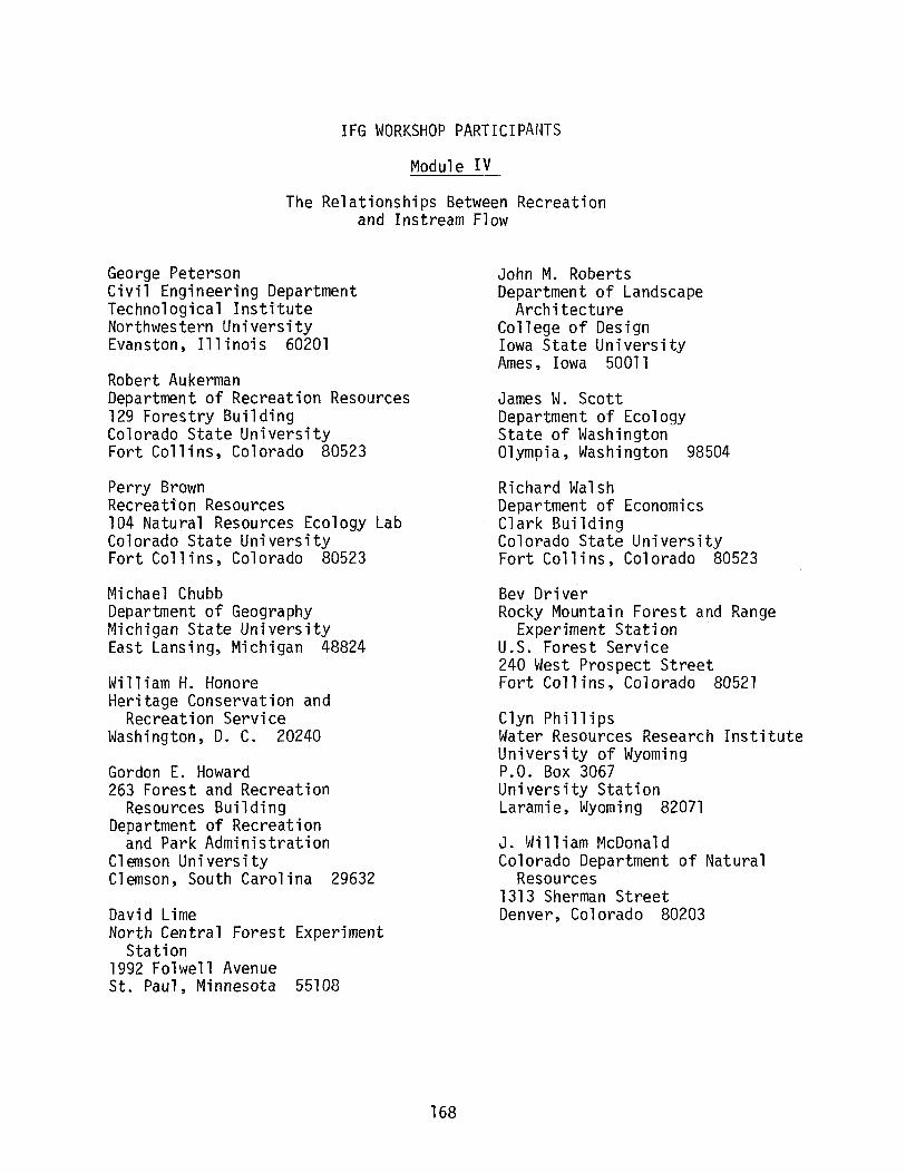
IFG WORKSHOP PARTICI PANTS

Module IV

The Relationships Between Recreationand Instream Flow

George PetersonCivil Engineering DepartmentTechnological InstituteNorthwestern UniversityEvanston~ Illinois 60201

Robert AukermanDepartment of Recreation Resources129 Forestry BuildingColorado State UniversityFort Collins, Colorado 80523

Perry BrownRecreation Resources104 Natural Resources Ecology LabColorado State UniversityFort Collins~ Colorado 80523

Mi chael ChubbDepartment of GeographyMichigan State UniversityEast Lansing, Michigan 48824

William H. HonoreHeritage Conservation and

Recreation ServiceWashington, D. C. 20240

Gordon E. Howard263 Forest and Recreation

Resources BuildingDepartment of Recreation

and Park AdministrationClemson UniversityClemson, South Carolina 29632

David LimeNorth Central Forest Experiment

Station1992 Folwell AvenueSt. Paul, Minnesota 55108

168

John M. RobertsDepartment of Landscape

ArchitectureCollege of DesignIowa State UniversityAmes~ Iowa 50011

James W. ScottDepartment of EcologyState of WashingtonOlympia~ Washington 98504

Richard WalshDepartment of EconomicsClark BuildingColorado State UniversityFort Collins~ Colorado 80523

Bev DriverRocky Mountain Forest and Range

Experiment StationU.S. Forest Service240 West Prospect StreetFort Collins, Colorado 80521

C1yn Ph ill ipsWater Resources Research InstituteUniversity of WyomingP.O. Box 3067University StationLaramie, Wyoming 82071

J. William McDonaldColorado Department of Natural

Resources1313 Sherman StreetDenver, Colorado 80203

TABLE OF CONTENTS

Introducti'on

The CIFSG Mission

Summary of the Proposed Methodology

An Overview of the Problem

The Criterion Component

Resource Description Component

The Application Component

Evaluation Component

Recreation Behavior and the Role of StreamFlow Variables

Questions and Criticisms of the CIFSG Methodologyand Research Needs

The Scope of the Mission

The Structure of Recreation

Criterion Methodology

Hydraulic Simulation

The Weighted Unit Area Concept

Scope of Relevance

Conclusion

Appendix

Toward Conceptual Clarification

Stream Flow

Recreation

Recreation Potential

The Criterion Function Concept

Recreation Requirements for Stream Flow

169

TABLE OF CONTENTS(cont'd)

The Impact on Recreation of Changes in Stream Flow

Assessment of Recreation Potential

A Closer Look at the Use and Misuse of MultiplicativeProbability Models

Methodology for Evaluating and Comparing Streams

Capacity, Recreation Potential and WUA

170

INTRODUCTION

This paper has been written in response to methods proposed by the

Cooperative Instream Flow Service Group (CIFSG) for evaluating the rela­

tionships between the recreation potential of a stream and instream flow.

The purposes are (1) to evaluate the proposed methods, (2) to suggest

specific improvements and/or areas where improvement is needed, and (3)

to identify specific research needs.

The ideas expressed are the responsibility of the authors. The

CIFSG and especially Ron Hyra deserve much credit, however, for raising

the questions in a way that has prompted our effort. We also wish to

acknowledge the important contributions of participants in the November,

1978 CIFSG Workshops in Fort Collins, Colorado. Some of the material

presented here is original and is based on research recently supported by

National Science Foundation Research Applied to National Needs and the

U.S. Forest Service. We also wish to give credit to James S. deBettencourt,

a doctoral student at Northwestern University, for the contributions from

his research on "Util ity Thresho1 d Theory. II

171

THE CIFSG MISSION

As the demands for water grow, the competition for available supplies

intensifies. Water left in streams tends to decrease in quantity as well

as quality, resulting in damage to the recreational and aesthetic uses of

the streams. Because of this increasing competition for water, the dwind­

ling supply of water for stream recreation and the growing demand for

recreation, it is no longer safe to assume that recreation needs will be

served adequately by the water that is left over when other purposes have

been satisfied.

Past efforts to develop methods for evaluating instream flow require­

ments for recreation and related purposes have been inadequate and not widely

accepted. An important effort to address these problems was undertaken

recently by an interagency task force established by the Bureau of Outdoor

Recreation and chaired by William Honore. The task force addressed three

important purposes:

(1) to develop ways to quantify water requirements for instream

recreational use;

(2) to develop methods for evaluating streamflow impacts on recreation;

and

(3) to determine monetary and non-monetary benefits of instream flow

for recreation.

Criteria affecting recreational use of instream water were suggested,

methods for measuring the criteria were established, tested and described;

and a procedure for analyzing the criteria to determine the relationship

to recreation was developed. The results are summarized in a two-volume

report, "Recreation and Instream Flow" (Bureau of Outdoor Recreation 1977).

The "Principles and Standards for Planning Water and Related Land Resources,"

172

developed by the U. S. Water Resources Council and approved by the President

on September 5, 1973, require that "beneficia1 and adverse effects of a

proposed plan should be measured by comparing the estimated conditions with

the plan, with the conditions expected without the p1an " (U.S. Water

Resources Council, 1973). One of the obvious but often neglected effects

of such a plan might be to change the quantity and quality of instream water

available for recreation. This issue becomes even more important in light

of the amount of public money to be used to make waters fishable and swim­

mable under provision of the Clean Water Act of 1977. But, currently avail­

able methods do not allow proper comparison of the recreation benefits of

instream flow with and without a planned project. Therefore, it is difficult

to know where and how much to invest in upgrading stream flow for recreation.

The recent Water Policy Reform message of the President, delivered on

July 6, 1978, emphasized protection of instream flows for recreation, water

quality, aesthetics, and fish and wildlife habitat. His message suggested

Federal or other water programs can create serious problems when they

emphasize agricultural, municipal, and industrial uses of water without

proper consideration of the need to leave water in the stream. One of the

task forces established on July 12, 1978 to implement the provisions of the

Water Policy Message concerned instream flow. The purpose of this task force

was to explore methods for protecting instream uses in the operation and

management of existing water resource projects and to provide for needed

stream flow in proposed project plans. Federal agencies were directed to

provide technical assistance to states to provide for the maintenance of

instream flows.

Against this background the CIFSG is attempting to develop quantitative

methods that will serve the above purposes. To be sure, the work of the

173

CIFSG to date has been somewhat narrow in focus and suffers from several

important weaknesses, which we intend to point out and help to correct.

The work is an important step in the right direction, however, and there

are strengths in the approach as listed below:

(l) The aim is toward quantitative standard methods and measures which

have general validity and applicability.

(2) The approach is based on efficient description of stream conditions

through sampling and simulation.

(3) An analytical approach is used, which promises to allow powerful,

efficient and rigorous investigation of the issues. The use of analytical

language is the hallmark of mature and successful science.

(4) The effort to be theoretically and conceptually rigorous has

created a powerful articulation of precise questions as well as demands for

specific information and operational definition of terms.

(5) Corollary to this last point is the fact that the approach has

generated a new set of questions for tributary disciplines. Recreation

scientists, fish biologist water quality experts, and stream hydrologists

and morphologists are being asked to rearrange their knowledge in very specific

ways.

(6) The effort comprises a program of developmental education. By

attempting to develop rigorous standard methods for analyzing the relation­

ships between recreation and instream flow, the CIFSG has spawned an educa­

tional process. Whether or not the operational goals are achieved, the

contributions to the understanding of the problems and ability to deal with

them will be great.

As we understand it, the mission of the CIFSG vis-a-vis recreation

is to develop methods for analyzing the relationships between recreation

174

and instream flow and to make those methods generally applicable to (1)

assessment of the recreation potential of a stream, (2) specification of

instream flow requirements for recreation, and (3) assessment of the impact

on recreation potential of instream flow. Thus far they have fallen short

of these goals, probably by wise intent, and have chosen to address some

very narrow questions; namely, (1) how to assess the impact on the potential

for certain kinds of instream recreation of changes in depth and velocity,

and (2) how to use representative reaches and hydraulic simulation to

describe the depth and velocity characteristics of a stream.

175

SUMMARY OF THE PROPOSED METHODOLOGY

The recreation assessment methodology is a hybrid of the methods

previously developed by the CIFSG for assessing the impact of flow changes

on fish habitat. In the proposed methodology (Hyra, 1978), depth and

velocity are the only hydraulic variables considered. Two methods are

proposed: (1) the single cross-section method; and (2) the incremental

method. In the single cross-section method, only the critical transect

is measured. This is the cross-section that is most likely to prevent a

given use due to insufficient depth, excessive velocity, insufficient

width, etc.

In the incremental method the quantities of surface area offering var­

ious combinations of depth and velocity are calculated by means of transect

measurement and hydraulic simulation. Criterion functions are also estimated,

showing for various recreational activities the probability that various

combinations of depth and velocity will be acceptable.

The criterion functions and the "hydraulic areas" are then used to

calculate the "weighted usable area" for the stream. This is obtained by

multiplying the surface area of a given combination of (or combination of

ranges of) depth and velocity by the associated probability of use. This

weighted usable area is the criterion measure used to assess capability of

the river to support the type of recreation in question. Obviously, compar­

isons can be made among several different streams or for the same stream at

different rates of discharge.

Alternative methods for assessing the impacts of stream flow changes

on recreation and aesthetics are discussed in Andrews, et al. (1976) and

Masteller, et al.(1976). Other methodologies have been developed which

are not reviewed in this paper or by Hyra (1978) such as Chubb (1976),

176

deBettencourt and Peterson (1977), and deBettencourt (1979). The

deBettencourt and Peterson methodology is closely related to the criterion

functions in the CIFSG methodology, but it is not based on hydraulic

simulation. The aim of the deBettencourt-Peterson paper is to develop a

"probability of acceptabil ityll concept from utility theory and empirical

experimentation. The analysis is not in terms of depth and velocity;

rather, it is in terms of such things as skill level, water quality, level

of use, and degree of development. The functions are based on theory and

methods which allow for tradeoff and interaction among the variables.

177

AN OVERVIEW OF THE PROBLEM

There are four general components in the CIFSG problem. One concerns

the relationship between recreation potential and instream flow--the

criterion component. A second is concerned with the description and pre­

diction of the instream flow characteristics of a given stream--the resource

description component. The third is the use of the criterion component to

measure and interpret the meaning to recreation of the instream flow charac­

teristics described or predicted for a given stream-~this is the evaluation

component. The fourth is the practical question that needs to be answered-­

the application component.

Figure 1 is a flow chart showing how the four components interrelate.

Obviously, each could be dissected in great detail, but the decomposition

of the flow chart into four major components represents our interests, our

beliefs about where the problems are, and our ability to contribute

constructively. The principal challenge to the CIFSG is in the criterion

component, where there may be serious holes in the state-of-the-art with

respect to (1) substantive knowledge about recreation, and (2) methods to

formulate and apply criteria. Consequently, our principal emphasis in

this paper is on the criterion component.

The Criterion Component

The problem is to develop ways to measure and interpret the meaning

of stream flow to recreation. There are at least five serious needs:

(1) The nature and structure of recreation, vis-a-vis instream flow

needs to be specified. In talking about fish habitat we can identify

IIspeciesli with unique habitat requirements, and we can specify at least

some of the parameters that are of concern. What are the recreation

II spec ies?1I

178

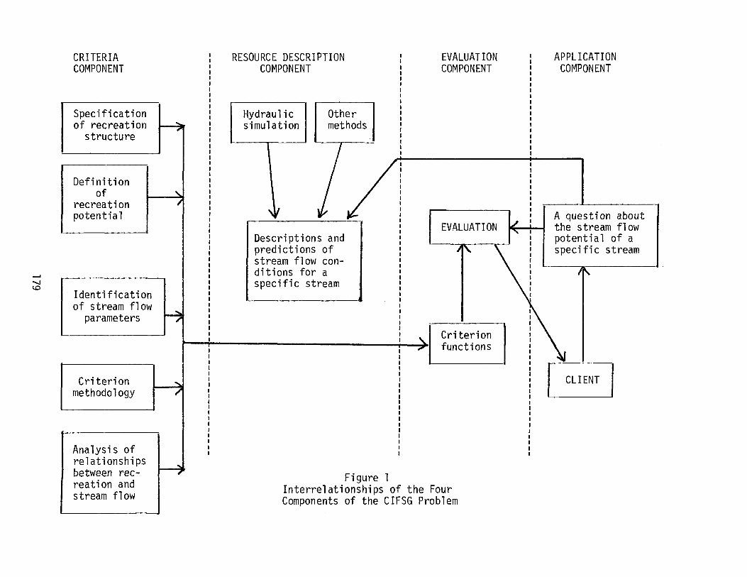
CRITERIACOMPONENT

RESOURCE DESCRIPTIONCOMPONENT

EVALUATIONCOMPONENT

APPLICATIONCOMPONENT

Specification hI Hydraul icit OtherI

of recreation I simulation methods II I J

structure II

.

I. 1II

I II

Definitionof

~Irecreation I

~potentia1 I IV It- i I-~~- i A question aboutI I I

EVALUATION the stream flowI

Descriptions and I i I I potential of aI I

predictions of I I specific streamI I

stream f10w con-ditions for a I

.I \

I If'I I...... I I I specific stream" I I II.D I

Identificationof stream flow

f7.parametersI I

~Criterionfunctions

I i ~ I

Criterion H I I I EJI I I

methodology I I II I I

Analysis ofrelationships ~between rec- ,---,reation andstream flow

Figure 1Interrelationships of the FourComponents of the CIFSG Problem

(2) We need a far more rigorous definition of "recreation potential"

than is presently available. The definition must be strictly operational,

not loosely phrased in glib generalities.

(3) For each recreation "species" we need to identify those parameters

of or related to streamflow which are of significance.

(4) We need a "criterion methodology;" that is, a framework or

strategy for constructing and applying criteria.

(5) Finally, we need to understand the processes by which instream

flow affects recreation potential. Given these five sets of information,

they can be put together into "criterion functions," or rules, possibly

mathematical rules, for measuring the recreational meaning of instream flow.

Resource Description Component

Assuming that the needed criterion functions are available, they will

be written in terms of those variables of the stream and its environment

which are important to recreation potential. To evaluate a specific stream,

it is necessary to measure or describe the stream in terms of those variables.

There are many ways this might be done. The CIFSG has chosen to use an

approach based on measurements of the stream at sampled representative

reaches and hydraulic simulation of the stream flow (Bovee and Milhous,

1978). In addition to the narrowness of the scope of this approach,

there are many questions that need to be examined. They will be identified

in a later section.

The Application Component

This is the practical question that needs to be answered. Somewhere

a client such as a State Department of Natural Resources or a Federal agency

wants to assess the impact of a proposed project on a specific stream; or,

perhaps there is a stream with established recreation use and it is necessary

180

to determine the stream flow requirements for those uses, so that the water

can be used for other purposes to the maximum extent possible without

excessive detriment to recreation.

Whatever the final form taken by the CIFSG methods, there are three

critical questions that should be asked: (1) can the methods answer the

important practi ca1 questions; (2) can they do it cost-effecti vely; and

(3) are they the best methods that might be used?

Evaluation Component

Given the criterion functions, a practical question, and a description

of a stream under the conditions defined by the question, the next step

is to come up with a meaningful answer. Some calculus or framework is

needed for putting all the intricate details together into an understandable

pattern of information. The CIFSG has proposed the "Weighted Usable Area"

as a way to put it all together. The WUA will be discussed in detail later

in this paper.

181

RECREATION BEHAVIOR AND THEROLE OF STREAM FLOW VARIABLES

In order to evaluate the proposed methodology properly, we must first

understand the subject to which it is to be applied. This means that we

need to understand the process by which stream flow variables influence

the recreational use of the stream. We also must separate the important

relationships and changes from those that are unimportant.

Recreation is voluntary behavior. It is people doing what they want

to do during leisure time; time that is not owned by someone else. River

recreation is such voluntary behavior that is dependent in some way upon

the presence and condition of a river.

River recreation may occur in connection with a private sector industry

or a public sector industry. In the private sector, commercial operators

may be offering services, equipment, and facilities with the intention of

maximizing profit. In this regard we are concerned about economic impacts

of changes in stream flow. That is, changes in stream flow may alter the

quality or quantity of the product or service being offered and may change

the firm's ability to attract customers.

There are many reasons why recreational services and facilities are

often provided through a governmental agency. Public investments in

recreation are frequently made, which on face value may appear to be

uneconomical because they (1) provide opportunities for people who would

otherwise be unwilling or unable to pay, (2) divert land and other resources

away from other profitable uses, and (3) promote intangible and sometimes

invisible social and personal benefits which are not readily evaluated.

Such investments are made because society, through political processes, has

182

expressed social welfare objectives which cannot effectively be achieved

through profit-motivated private enterprise. The achievement of these

social objectives in the case of river recreation may be directly related

to stream flow variables. Changes in those variables may interfere with,

magnify, or redistribute the personal and social benefits generated by

public investments in recreation. Because people make numerous private

sector expenditures in connection with their use of public facilities and

services, there will be direct impacts on the private economy as well.

Thus, recreation can be viewed as an instrument whereby personal and

social benefits can be generated and as an industry in which income and

economic activity are generated. Changes in the resource base on which

the instrument and industry so intimately depend can make a lot of IIwaves. II

Prediction of the IIwavesll caused through recreation, by changes in stream

flow, is the task addressed by the proposed methodology. However, as it

now stands the methodology addresses only a small part of the question:

the first-order impacts of changes in depth and velocity on the probability

that people will judge the stream to be acceptable for a given activity.

To answer even this very restricted question, we have to understand the

behavioral process by which people accept or reject river recreation altern­

atives.

A reasonable framework for understanding the relationship between

stream flow and recreation can be obtained from recent work in behavioral

demand assessment (Anas, et al., 1978). The following are major components

in the relationship:

(1) The psychological outcomes are the reasons why people engage in

recreation. These outcomes are defined in terms of the functions performed

by recreation in satisfying personal motives or needs and in generating

183

personal benefits (Driver and Brown, 1975; Driver, 1977; Lancaster, 1966;

Tinsley, 1977).

(2) The activity purposes are the roles and forms taken by recreation.

These are the things the person does in connection with the river, such as

fishing, swimming, boating, camping, etc. One is attracted to a site and/

or activity purpose because of the psychological outcomes expected, but

it is the activity purpose that is apparently the conscious objective.

(3) The activity site includes the lands and facilities where the

activity takes place and upon which it is usually dependent. River

recreation activities generally depend heavily upon site characteristics.

Modification of such things as stream flow variables modifies the site's

ability to attract and support activity purposes, and it changes the ability

of the site and of the activity to deliver psychological outcomes.

(4) The activity attributes are the characteristics of the activity

purpose which enable it to perform the functions which provide psychological

outcomes. If site changes are to be evaluated, the activities must be

described in terms of their relative capability to serve the psychological

outcomes. Description of the relationships, if any, between these activity

attributes and site variables will allow impacts to be traced.

(5) Site variables are the conditions and circumstances of the site

which affect its suitability and attractiveness for various activity

purposes. For river recreation they include stream flow variables as well

as many other things. The activity for which the site is used has site

performance requirements. Some of these relate directly to the psychological

outcomes which the activity is expected to deliver. Considerable work has

been done to try to describe the site performance requirements of various

activities (Hyra, 1978; Chubb, 1976; deBettencourt, 1979; Andrews, et al.,

184

1976). Very little work has been done to explain the process by which

site variables affect recreation.

(6) The personal variables are those individual traits which affect

recreation behavior. They include such things as age, income, sex,

ethnicity, stage in the life cycle, education, occupation, personality,

etc. Such variables modify motives, preferences, and choices in recreation

and help to explain the richness of variation in recreation behavior that

exists among people.

(7) Situational variables include such things as the relative proximity

of the site and the recreation demand, the type, efficiency and cost of

transport linkages, intervening opportunities, etc. To some extent these

variables may modify the impact of stream flow changes on recreation.

They certainly intervene strongly in the overall demand process.

(8) Market segments are categories into which individuals are grouped

in order to simplify the problem of dealing with interpersonal differences.

Such grouping may be done in terms of social or institutional categories

such as income, ethnicity or geographic area. Ideally, market segments

are based on behavioral homogeneity, with people of similar recreational

behavior being grouped together. Different market segments may respond

differently to stream flow changes.

In a behavioral demand model these categories of variables are linked

together by means of mathematical equations which explain the complex inter­

relationships. Knowledge of these relationships would also allow the

specific impacts on recreation of environmental changes to be predicted

for different activities and market segments. The state-of-the-art here

is very primitive, however, and this somewhat superficial exposure of the

various elements of recreation behavior is presented only as a paradigm

185

which will serve as a framework for raising questions about the proposed

stream flow methodology, as well as for guiding constructive improvement.

Key concepts include the following:

(1) Recreation behavior is complex, voluntary, and discretionary,

suggesting that it may be quite sensitive in sometimes unexpected ways to

environmental change.

(2) Response of recreationists to stream flow may vary by activity and

by market segment.

(3) Some impacts may be more important than others, depending upon

the market segments and psychological outcomes affected.

(4) Impact on psychological outcomes may occur without obvious changes

in manifest behavior.

(5) The state-of-the-art of explaining relationships between environ­

mental conditions and recreation behavior and benefit is primitive. While

hydraulic measurement and simulation may be well developed in terms of proven

theories and standard methods and measures, prediction of recreation

behavior is not.

186

QUESTIONS AND CRITICISMS OF THECIFSG METHODOLOGY AND RESEARCH NEEDS

The purpose of this section is to list the questions and criticisms

that have grown out of our deliberations about the CIFSG methodology. These

questions and criticisms define needs for further research. In some cases

what is needed is simply more rigorous definition and conceptual clarifi­

cation. In other cases we may have a need for theoretical development.

But, there are some questions which can only be answered through expensive

and time-consuming empirical research, and there may be state-of-the-art

problems where we aren't even sure what the question is.

In reflecting on these questions, the concept of cost-effectiveness

should be kept "Up front. II We could spend millions of dollars here, and

we need to assess the value of correct answers, and the cost of accepting

less precise answers. The research could be attacked at several levels,

with judgment, common sense and conventional wisdom being the least expensive

and most immediate. However, it is essential to establish a much more

rigorous conceptual framework for the problem before going further with

empirical or methodological research. In the hope of urging this along,

we offer in the Appendix constructive suggestions and examples of what needs

to be done.

The Scope of the Mission

On face value it appears that the CIFSG has taken as its mission to

develop methods for assessing the impacts of changes in depth and velocity

on certain instream recreation activities, with predictions of depth and

velocity being derived from hydraulic simulation and representative reach

sampling. This, we believe, is too narrow. Is it the product of a delib­

erate decision to begin with manageable pieces of the puzzle with the intent

187

to broaden out as problems get solved? Or, is it nearsightedness or

infatuation with pet tools and convenient methods? What are the practical

questions the group is trying to answer, and will their approach lead to

answers to important questions?

The Structure of Recreation

It is obvious that different recreation activities have different

relationships to stream flow, and it is likely that for different types of

people, there may be different relationships to streamflow, even for a

given activity. The CIFSG has not given adequate attention to those ques­

tions. It makes sense to develop methodology in terms of a few important

activities that are convenient to work with. But, to predict impact on

recreation potential, it will be necessary to develop and test the methods

in terms of all recreation activities that are significantly linked to

instream flow. It will also be necessary to understand how person types

and personal variables intervene, or activity specification will be incomplete

and it will not be possible to give proper attention to the social distribu­

tion of costs and benefits.

Stream Flow Variables

Depth and velocity are important to many forms of stream-related

recreation, but they are obviously not the only important variables. It is

natural that the group has begun with depth and velocity, because it follows

directly from prior work on fish habitat, and it is the language of the

hydraulic simulation approach being used. However, there is real danger

that the work on recreation may be going down a long and technical trail

which could lead nowhere.

The overall structure of the recreation problem faced by CIFSG needs

further clarification. What variables are important to which activities

188

for what kinds of people? Given the overall structure, the value of working

with depth and velocity can be assessed and next steps in the research can

be rationally selected.

Criterion Methodology

The criterion methodology being used is the "probability of use"

function. The following specific questions and criticisms must be addressed

before the work proceeds:

(1) Is probability a useful criterion and is it the best way to go?

(2) If so, probability of what? Probability of "use " is dangerous.

because it mixes recreation potential with recreation demand and

profoundly complicates the problem.

(3) The basis for the functions at present is apparently to glean

minimum, maximum, and optimum conditions of depth and velocity

from available literature or by common sense judgment and then to

assume (a) probability is proportional to desirability, (b) probab­

ility is zero at minimum and maximum limits and one at the optimal

condition, and (c) between these points desirability and probabil­

ity vary linearly.

The assumption that probability is proportional to desirability is

a dangerous and fallacious assumption which implies some misleading things.

However, until there is a rigorous definition of the event whose probability

is discussed, nothing can be done. If probability is what is wanted, and

if the event can be rigorously defined, then the assumptions, derivations,

and implications can be explored properly. It will then also be possible to

begin rigorous exploration of relationships between the probability of this

event and the magnitude of stream flow variables. The way the methodology

is now constructed, true probabilities do not exist and it is not known what

189

event is being predicted.

(4) It is incorrect to multiply the "probabilities" to obtain the

"composite probabilities. II Apparently the multiplicative approach

stems from some incorrect assumptions and loose definitions.

(5) Existing literature may be an inadequate source of information

upon which to base the criteria. Complementary sources are

certainly needed, and original basic research may be required.

Hydraulic Simulation

Hydraulic simulation is simply a way to describe and predict the

hydraulic conditions of a river, based on sample measurements at representa­

tive reaches. Regarding the application to the recreation problem, the

following concerns need to be addressed:

(1) Can hydraulic simulation produce the kinds of information needed

for recreation analysis in language appropriate to recreation?

Does recreation need the kind of information hydraulic simulation

can produce? Can the "ges talts" and details that are meaningful

to recreation be adequately represented?

(2) For what activities and under what conditions is the method use­

ful and cost-effective? Under what conditions is it invalid or

inefficient?

(3) How should rivers be classified or segmented to make the method

appropriate?

(4) Is a combined strategy required, using critical reach in some

places and representative reach in others?

(5) What other options are available and have they been adequately

identified and evaluated? Is hydraulic simulation being used

simply because it is something the CIFSG knows how to use, has

190

found useful for the fish habitat problem, and wants to see used?

For example, might recreation analysis be better served through

stream descriptions produced by experienced recreationists who

know the streams, together with judgmental criteria about their

appropriateness for different users?

(6) What other relevant hydraulic parameters might be developed

and simulated? For example, can parameters be theoretically or

empirically derived to describe the power, scale, and regularity

of hydraulic phenomena such as standing waves, backrollers, etc.?

The Weighted Unit Area (WUA) Concept

WUA has come under criticism partly because of inadequate clarification

of what it is, and partly because of incorrect interpretation by the CIFSG.

The following are important concerns:

(1) What is WUA? Does probability times area have any conceptual

meaning? This question has been neglected.

(2) It is invalid to imply that WUA can be used to measure equivalence

or substitutability of streams or sections of streams, without

first specifying exactly what WUA means so that we understand

what about the streams is equivalent or substitutable. To say

that two streams with equal WUA are equally desirable is to pre­

sume that WUA is proportional to desirability. This is a fallacy

on two counts: (a) it is based on the unjustified assumption

that probability is proportional to desirability; and (b) it

fails to recognize that WUA is an expected value and as such is

strictly limited in what it means. These failures lead to the

unfortunate trap where lOa junk yards are concluded to be substi­

tutable for one rose garden. Under very specialized conditions,

191

the interpretation may be correct, such as the example of 100

acres of poor pasture being capable of providing the same quantity

of nutrient for cows as 10 acres of good pasture. With recreation,

however, we may be dealing with a different kind of process, and

the analogy may not be valid.

(3) Are there other methods that might be used instead of or in

addition to WUA that will allow more effective comparison and

evaluation? For example, might it be more meaningful to use a

centile profile to summarize the data so that the disaggregate

richness is preserved, rather than using an aggregate average

where the same "average" can be produced by many drastically

different situations. The use of average measures alone exposes

one to the "statistical deer hunting trip" in which a high miss

and a low miss bags the deer on the grounds that the average is

the same as for two hits.

(4) How is resource carrying capacity related to WUA if at all? The

CIFSG methodology seems to imply that WUA is somehow a measure

of capacity. This is not valid, although WUA may be related to

capacity.

Scope of Relevance

In addition to the questions outlined above, we are concerned that the

CIFSG methodology does not include sufficient concern for social welfare

values. It certainly is important to look at the relationship between stream

flow variables and the suitability of the site for use by individuals for

recreational purposes. This is a major part of the question. However, an

important and neglected part of this question is how to include the distribu­

tion of that suitability for use across different individuals and social

192

classes. Too many quantitative decision criteria, e.g., cost-benefit ratio

and willingness-to-pay are used in ways which are blind to the distribution

of costs and benefits. Policy is not and should not be blind to distribu­

tional questions, and this should be considered by the CIFSG.

Another related deficiency is that we have seen no way for the method­

ology to include "collective" or II poli cy" values that may not be included

in personal choices. For example, historic preservation, natural conserva­

tion, endangered species protection, and protection of options for the

future are collective concerns that may not be reflected in private decisions.

193

CONCLUSION

The purpose of this workshop was to critique the progress to date of

the CIFSG methodology of assessing instream flows for recreation. The

method they have developed has many strengths and many weaknesses, which

have been pointed out. One of the weaknesses, the failure to tackle the

whole problem, is because the problem is larger than the CIFSG mission.

We have attempted to organize the definition of the whole problem, and

have defined the problem which, in the author's opinion, will permit the

group to more fully understand how the portion of the problem they are

wrestling with fits into the big picture. We have taken a close look at

the CIFSG problem, mission, and methodology and have added some needed

background on recreation behavior. In the Appendix which follows, which

is authored by Dr. George Peterson, there is a more detailed discussion

of some of the theoretical and conceptual concepts that were mentioned in

the paper.

194

APPENDIX A

to

The Relationships Between Recreation

and Instream Flow

by

George L. Peterson

195

TOWARD CONCEPTUAL CLARIFICATION

Stream Flow

The primary stream flow concept, as derived from the mission of the

CIFSG and the policy concerns that created that mission, is the quantity

of water flowing in the stream channel. The primary stream flow variables

are therefore Q, the volume of water per unit time flowing through a tran­

sect and dQ/dt, the rate at which the quantity of flow is changing. For

most practical questions it may be possible to confine the analysis to

steady-state conditions in which dQ/dt = O.

The policy question is one of economically efficient and equitable

allocation of water among competing uses or needs. With regard to recrea­

tion, the basic question is, what is the relationship between (a) the

recreation potential of the stream, and (b) the amount of water flowing in

the stream. Ideally we would like to be able to (1) evaluate the recreation

potential of a given stream or stream reach under natural conditions of

stream flow, (2) evaluate the change in recreation potential that would be

caused by specific changes in the amount of water flowing in the stream, and

(3) specify the amount of flow required to support specified levels of

recreation potential. In each of these questions it should be recognized

that IJrecreationlJ must be defined in terms of specific activities.

In addition to the parameter Q, there may be other variables to which

recreation potential is sensitive and which are of concern to recreation in

the context of the stream flow problem because (1) they measure primary

consequences or corollary conditions of stream flow volume (e.g., stage,

depth, velocity, etc.); (2) they measure secondary consequences of stream

flow volume (e.g., turbidity, physical channel and stream bank conditions,

instream vegetation, fish population and behavior, water quality, etc.); or

196

(3) because they intervene to modify the relationship between recreation

potential and stream flow variables (e.g., water quality, climate, gradient

and other physical channel characteristics, location and accessibility,

etc. ) .

The problem here is to define stream flow and its corollary, consequent,

and intervening conditions in terms of the meaning for recreation potential.

Without a model or theory of the processes by which recreation potential is

sensitive to stream flow, it is not possible to be sure that (1) the impor­

tant variables have been specified, and (2) they have been defined in a

meaningful and operational way.

Recreation

In a previous section recreation was defined in general terms as

voluntary play behavior. However, the very complex and diverse reasons why

people do things which we tend to regard as recreation, and the great

diversity of forms taken by recreation lead to the conclusion that while

general definitions are of philosophical interest, they are of little

practical value.

Before we can deal rigorously with recreation potential and the rela­

tionship to stream flow, we need to identify the recreation "species" that

are of interest. This is a two-sided problem. On the one hand is the need

for an appropriate taxonomy of activities. This includes identification of

those kinds of activities which are of interest to the stream flow question,

as well as an understanding of the scale or level of detail with which

activity types need to be specified. On the other hand is a need for an

appropriate taxonomy of people and/or human situations. The meaning of

stream flow conditions for a given kind of recreation may depend on who we

are talking about and what the personal circumstances are at the time.

197

It is also useful to identify several levels of recreational dependence

upon stream flow. At the primary level are activities which occur in or

on the water flowing in the stream (e.g., swimming, boating, wading, fish­

ing, etc.). At the secondary level are activities which are dependent on

or enhanced by the presence of the stream but which do not occur in or on

the water (e.g., sightseeing, photography, camping, picknicking, bird

watching, hunting, etc.). At the tertiary level are those activities which

occur in the vicinity of streams, either by coincidence or because of the

presence of facilities, but which are relatively independent of stream flow

conditions. As a first step it is reasonable to narrow the scope of the

problem to the primary level and deal only with the activities which occur

in or on the water. It must be recognized, however, that it is an incomplete

first step. Camping and picknicking for example may be very sensitive to

changes in stream flow, because the opportunity for water sports makes a

campground or picnic area more attractive to a broader spectrum of people.

Recreation Potential

Assuming that the taxonomies of recreation activities and persons are

available, "recreation potential" will now be defined in rigorous terms.

There may be several different ways to define the concept. Here, we will

use probabi 1ity and the concept of "suitabil ity for use" as the basi s for

the definition. The purpose is to offer a rigorous definition by way of

proposition and illustration. It will be up to the researchers to refine

and/or revise the approach.

The Theoretical Definition: Let it be assumed that the set of all

people of type h who have decided or will decide to engage in activity j

can be identified. Let each of these persons be in the condition of being

at home and having decided to do activity j. Let them be placed with their

198

choice of equipment and accompaniment and at no cost in time, money, effort

or inconvenience for transportation at location l on a stream under specific

conditions of stream flow. At this time let there be no access to, or

awareness of, substitute locations for the activity or to substitute

activities. Let the person then decide whether or not to engage in activity

j at location l. A decision not to engage in the activity at that location

causes the person to be returned home again at no cost. A decision to

engage in activity j at location l exposes the person to whatever risk,

cost, effort, inconvenience or other consequences are associated with the

doing of the activity at that location, except that upon completion of the

activity the return trip home is cost1ess. Indecision is taken to be a

decision not to engage in the activity.

By way of further clarification it must be understood that location l

is a specified point on, in, or adjacent to the river. It is not a region

or locale. For example, the point may be the middle of a wide stream where

the water is ten feet deep and the velocity of the water is 15 ftjsec.

This point is obviously unsuited for wading and few if any people would

decide to do this activity at that point. Although there may be large

areas nearby where the water is one foot deep and virtually motionless,

we have defined this to be irrelevant to the decision regarding the specific

location in question.

Let Nhjl (Accept) be the number of people of type h who accept location

l as a place to do activity j. Let Nhjl (Reject) be the number of people

who· decide not to do the activity. Now define the "Probability that the

site is acceptab1e" as

Phjl (Accept) = Nhjl(Accept)Nhjl(Accept) + Nhjl(Reject)

199

(1) .

This probability is one way to define recreation potential. Simply stated,

it is the likelihood that a point is acceptable for a given activity inde­

pendent of any effects of competing sites, competing activities, or access

costs.

P(Accept) is an indirect measure of recreational quality although the

probability is likely to be a monotonic function of quality. In theory

there is for each individual a utility function in which the magnitude of

utility (satisfaction) derived from the site varies with stream flow para­

meters. However, while such individual utility functions may be measurable

in theory, they are not measurable in practice, at least not at reasonable

cost. Even if they could be measured, they cannot be aggregated into group

utility functions without making invalid political and numerical presump­

tions. However, the P(Accept) concept can be rigorously derived from util­

ity theory with the assumption that there is in the personal utility function

a threshold isoquant dividing the unacceptable stream flow conditions from

those which are acceptable. The threshold utility functions are measurable

and they can be aggregated probabilistically. This approach to the derivation

of P (Accept) is known as Utility Threshold Theory (deBettencourt and

Peterson, 1977; deBettencourt, 1979).

For linear activities such as rafting, canoeing, kayaking, motorboating,

jet boating, etc., the hypothetical "experiment" which defines recreation

potential must be defined in terms of a specified reach of a stream, rather

than at a point. The subject would be placed at an assigned point of

initiation of the activity and would be assigned a point of completion. The

activity would then take place throughout a defined reach. The evaluation

is of the entire reach, not of a point. If the subject accepts the reach,

he must accept all consequences and risks associated with the activity

200

throughout the entire reach. If the reach or point being evaluated is

inaccessible due, for example, to high cliffs or lack of roads, these

conditions apply only while the activity is in progress. The problem of

getting to and from the stream at the points of initiation and conclusion

is irrelevant to recreation potential, though it is not irrelevant to the

actualization of the potential.

In between the point activities and the reach activities are those

which do not require a lengthy reach, but which have no meaning at an

isolated point. There is no joy in wading or swimming at an isolated point.

Thus, there is need for further refinement of the point concept to include

the need for sufficient linkage or proximity to other acceptable points.

It is absolutely necessary to isolate any definition of recreation

potential from the morass of actual recreation participation and demand.

Actual demand is concerned with the sensitivity of actual use to various

conditions of (1) resource quality at the site, (2) proximity of the site to

population, (3) magnitude of accessible population, (4) quality and quantity

of transportation facilities, (5) population awareness of the resource, and

(6) existence, location and quality of competing sites, etc. Demand and

participation include but are vastly more complex than recreation potential.

Ultimately we may want to assess impacts of changes in stream flow on

recreation demand, but at this time it is better to begin with the question

of impact on recreation potential or II site quality. II

A Practical Definition: The theoretical definition of recreation

potential developed above is not very practical. While the theoretical

probability thus defined may exist, it cannot be measured by means of the

hypothetical lIexperimentll used to define it. A practical procedure is

needed whereby the probability can be estimated. Two strategies are available.

201

An empirical or inductive strategy would estimate the probability from

observations of behavior. Because of the need to control demand-related

variables, laboratory experiments or questionnaire methods will have to be

used unless a procedure can be devised to isolate the effects of site quality

variables in actual recreation site choices. At present this is beyond the

state-of-the-art. For an example of questionnaire procedures which simulate

site choice see deBettencourt, 1979; and Peterson, et al, 1973. Also, the

work of Kenneth Hammond (University of Colorado, 1976) on Human Judgment

and Social Interaction utilizes computer graphics techniques which may be

highly effective for extracting P(Accept) functions from representative

individuals.

A deductive strategy would construct a theoretical explanation of the

probability (as a function of stream flow variables from known principles

of human behavior). This is also beyond the state-of-the-art at this time.

Research on this line would have to be aimed at developing and refining the

principles of human behavior.

The Criterion Function Concept

In the previous section we implied, but did not make explicit, the

concept of a criterion function for recreation potential. Assume that there

are four sets or classes of variables to which recreation potential at a

stream is sensitive. Let the first set be the primary and corollary condi­

tions of stream flow such as Q (rate of flow), H (stage), D (depth),

V (velocity) and any others that may be important. To simplify the notation

let these variables be Ql'-------Qn. Let each variable be defined at a

point, i, such that the primary variables are Qli' Q2i'----Qni.

Let the second set of variables be those which help to determine

recreation potential and which are also dependent to some extent upon the

202

primary stream flow conditions. That is, when the amount of water in the

stream changes, these variables (e.g., turbidity stream bank conditions)

change. Let them be separable in the function, i.e., they do not inter­

vene in the relationship between potential and the primary variables. Call

these variables

Xli' X2i'-----------------, Xml·

Let the third set of variables be those which help to determine recrea­

tion potential, but which are independent of stream flow conditions and of

the relationship between potential and stream flow. In other words, they

are independent and separable from the primary stream flow variables (e.g.,

forest type, developed facilities, wildlife, etc.). Call these variables

Let the fourth set of variables be those which intervene in the

re~ationship between recreation potential and any or all of the other

variables. For example, variables describing the physical characteristics

of the stream channel will certainly modify the effect of Q on recreation

potential. A rough channel or a circuitous channel may become dangerous

under some flow conditions while a smooth, straight channel may not. These

variables mayor may not be independent of the other variables. Call these

interveners

Now define the criterion function which determines and measures recre-

ation potential at a point. To simplify notation, we will use vector nota-

tion, where X, for example, represents the set of all XIS.

P (Accept) = Fh (Q,Z) + gh (X,Z) +hjl

Kh (Y,Z)

203

(2)

where f h, gh and Kh are functions which are separable from each other. It

should be recalled that we have defined Y to be independent of Q and, con­

sequently, also of X. We have defined X to be dependent upon Q.

Equation (2) is a criterion function by which Phji might be evaluated,

given values for Q,X,Y, and Z, if the functions f, g, and k could be

specified. The reasons for this somewhat complicated formulation will

become clear in subsequent sections.

Recreation Requirements for Stream Flow

Given a definition of recreation potential as in equation (1) and a

definition of a criterion function as in equation (2), we are now in a

position to define "recreation requirements for stream flow." For simpli­

city of illustration, assume that the recreation activity in question is

sensitive only to depth (0) and velocity (V), both primary stream flow

variables, and that there are no X, Y, or Z variables in the criterion

function. This simplified function can be represented as

(3 )

If depth and velocity were the only variables of concern for swimming,

then the function for person type h might be as in Figure A-l. For wading

it might be as in Figure A-2. These functions are shown graphically as

isoquants or centiles of constant probability. The meaning of the shaded

area will be explained shortly.

Now it is necessary to introduce the concept of "po'licy standard" as

a basis for defining "recreation requirements." Here it is assumed that the

policy question of distribution of benefits among individuals or classes of

individuals can be dealt with adequately by means of the classification h.

In other words, there are no distributional concerns within class h, only

204

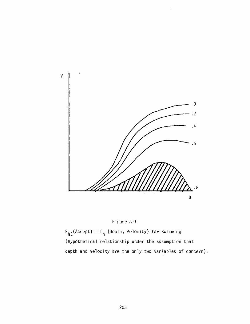
v

o_--.2

.4

.6

D

Figure A-l

Phi(Accept) = f h (Depth, Ve1oc ity) for Swi mmi ng

(Hypothetical relationship under the assumption that

depth and velocity are the only two variables of concern).

205

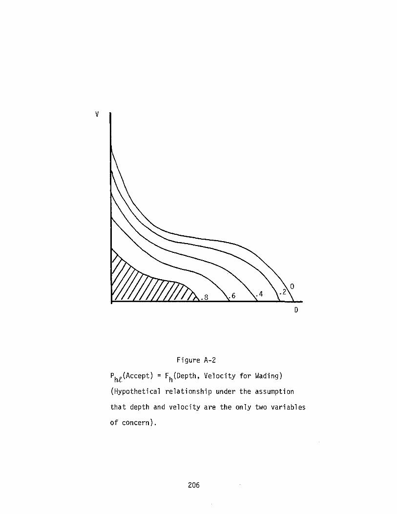
v

o

Figure A-2

Phl(Accept) = Fh(Depth, Velocity for Wading)

(Hypothetical relationship under the assumption

that depth and velocity are the only two variables

of concern).

206

between classes. Otherwise, a more elaborate formulation will be required.

Assume that the policy process has decided that for class h a location

on a stream is of "adequate" recreation quality for a given activity if it

is acceptable to 80 percent of the individuals in the group. (This is not

unreasonable, because a similar concept of "voting" is used to decide

whether a political candidate is acceptable.) However, if the group h is

improperly constructed, this process may cause systematic discrimination

against particular members of the class, say children or handicapped. If

the classes are properly constructed in terms of similarities and differ­

ences between individual utility threshold functions, such systematic

discrimination will not occur.

The shaded area in Figures A-l and A-2 represent the combinations

of depth and velocity which are acceptable to 80 percent or more of the

members of class h. With an 80 percent policy, the requirements for each

activity are that the joint occurrence of depth and velocity must be above

the .80 centile on the criterion function. To judge whether the stream

flow conditions of a specific stream at a particular location satisfy the

requirements for recreation, it is thus necessary to have (1) the criterion

function for each activity and person type of concern, and (2) a policy

standard (e.g., ~80 percent) for each activity and person type. The

magnitudes of the stream flow variables are then entered into the criterion

function and the magnitude (or change in magnitude) of Phji(Accept) is

calculated and tested against the policy standard.

The Impact on Recreation of Changes in Stream Flow

A change in one of the variables in equation (2) will cause a change

in P(Accept) if the criterion function has been correctly specified. A

change in P(Accept) may cause a change in recreational use of the site.

207

Changes in the recreational use of the site will cause changes in the site,

changes in the users themselves, and changes in the economy. The "impact"

on recreation of a change in stream flow is thus a complicated matter,

even if concern is limited only to the significant changes. Clearly the

mission of the CIFSG should aim toward the development of capability to

evaluate this total impact on (or through) recreation caused by a change

in the amount of water in a stream.

However, it makes sense to start with a first step, rather than expect­

ing the group to make the whole trip all at once. While it is true that a

brick house cannot be built only with bricks, it is also true that it cannot

be built without them. The first step, then, is to concern ourselves only

with the impact of stream flow changes on recreation potential, P(Accept).

In other words, if we change a primary stream flow variable (an element

of the set Q, say volume of flow, or stage or velocity, or depth, etc.),

what is the associated change in site quality as measured by Phji(Accept)?

For the sake of simplicity in illustration let us again assume that

depth (0) and Velocity (V) are the only two variables to which P(Accept)

is sensitive. The criterion function then reduces to equation (3). There

are two important questions that must be addressed before the question of

impact can be answered:

(1) Is there interaction between 0 and V in their relationship with

P(Accept)? That is, are their effects on P(Accept) separable?

(2) Is the magnitude of 0 independent of the magnitude of V?

For example, a simple function in which the effects of D and V are

separable is

P(Accept) = C1hj Vi + Shj Df., (4)

where a hj and Shj are coefficients that are specific to the activity and

208

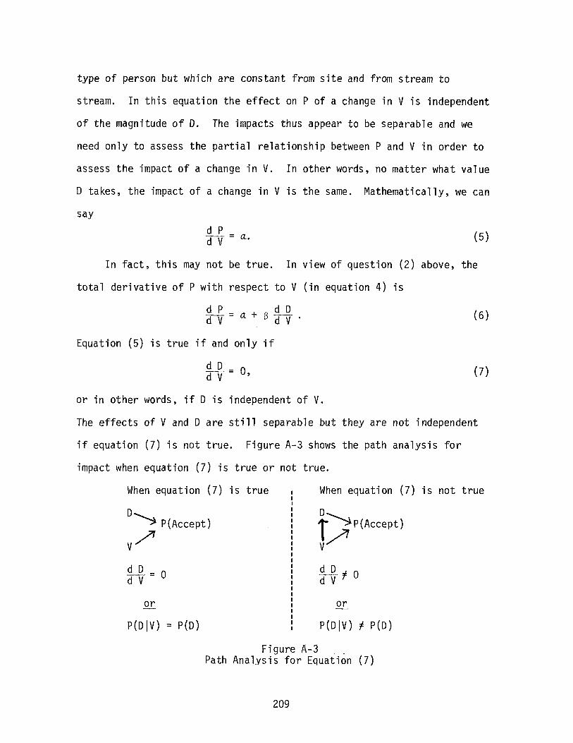
type of person but which are constant from site and from stream to

stream. In this equation the effect on P of a change in V is independent

of the magnitude of D. The impacts thus appear to be separable and we

need only to assess the partial relationship between P and V in order to

assess the impact of a change in V. In other words, no matter what value

D takes, the impact of a change in V is the same. Mathematically, we can

sayd PdV = a. (5)

In fact, this may not be true. In view of question (2) above, the

total derivative of P with respect to V (in equation 4) is

~=a+BdDd V dV·

Equation (5) is true if and only if

d D _dV - 0,

or in other words, if D is independent of V.

(6)

(7)

The effects of V and D are still separable but they are not independent

if equation (7) is not true. Figure A-3 shows the path analysis for

impact when equation (7) is true or not true.

When equation (7) is true

D~ P(Accept)

V?d 0 = 0d V

or

p(DIV) = P(D)

When equation (7) is not true

DT~p(AccePt)v,,/7

~~ 0d V

or

p(Dlv) ~ P(D)

Figure A-3 .Path Analysis for Equation (7)

209

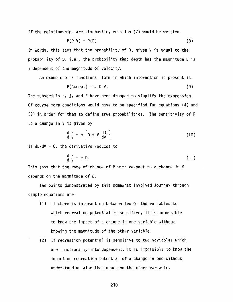
If the relationships are stochastic, equation (7) would be written

P(Dlv) = P(D). (8)

In words, this says that the probabil ity of 0, given V is equal to the

probability of 0, i.e., the probability that depth has the magnitude 0 is

independent of the magnitude of velocity.

An example of a functional form in which interaction is present is

P(Accept) = a 0 V. (9)

The subscripts h, j, and l have been dropped to simplify the expression.

Of course more conditions would have to be specified for equations (4) and

(9) in order for them to define true probabilities. The sensitivity of P

to a change in V is given by

d P _ r dO 1dV - a L0 + V dv J.

If dD/dV = 0, the derivative reduces to

(l0)

(11 )d Pd V = a D.

This says that the rate of change of P with respect to a change in V

depends on the magnitude of D.

The points demonstrated by this somewhat involved journey through

simple equations are

(1) If there is interaction between two of the variables to

which recreation potential is sensitive, it is impossible

to know the impact of a change in one variable without

knowing the magnitude of the other variable.

(2) If recreation potential is sensitive to two variables which

are functionally interdependent, it is impossible to know the

impact on recreation potential of a change in one without

understanding also the impact on the other variable.

210

These conclusions mean that if we desire to assess the impact on recreation

potential of a change in a stream flow variable, say V, then it is absolute­

ly necessary to have complete specification of those parts of the criterion

function which involve interaction or interdependence with V. Other parts

of the criterion function can be ignored, because they are separable from

and independent of V. While such other factors may indeed change, such

changes are irrelevant to the impact of a change in V. It is impossible,

however, to assess the impact of a change in V unless all of those variables

to which P(Accept) is sensitive and which interact or are interdependent

with V are included in the analysis and their parts of the criterion function

are completely specified. Depending on the nature of the interrelationships,

the criterion function may thus have to be a set of simultaneous equations

describing a causal network.

However, while this may be true and necessary in theory, it mayor may

not be important in practice. As always, there is the practical need to

separate the significant from the insignificant. Many of the relationships

may be of lesser orders of magnitude and thus negligible - but this must

be learned, not taken for granted.

In practice it may be possible to measure P(Accept) directly, either

in real situations or in controlled experimental settings and, through

statistical techniques, separate the significant relationships from those

which are negligible. Statistical techniques suitable for estimating such

relationships include, among others, analysis of variance and covariance, and

discriminant analysis. But, they require the observation of P(Accept)

under a meaningful variation of key variables, and they require stratifica­

tion with respect to interactive variables, with separate analysis within

strata.

211

To point out that there may indeed be problems of interaction and

interdependence in assessing the impacts of changes in stream flow conditions

consider the following:

(1) The quantity of flow, stage, velocity, depth, turbulence, and who

knows what other stream flow variables are all important to the recreation

potential for various activities and person types. But, they are strongly

interdependent. As an example, the depth and velocity of water flowing

through a wier (i.e., a critical reach) are hydraulically interrelated.

(2) Depth and velocity interact in their relationship with recreation

potential, at least for some activities. With wading, for example, a

velocity of 10 ft/sec is clearly more acceptable when the depth is three

inches than when the depth is two feet. A depth of two feet may be accept­

able, however, when the velocity is zero.

(3) Class IV and V on the International scale of whitewater difficulty

may be more acceptable to experienced kayakers on an accessible stream where

rescue is readily available than in a remote and inaccessible gorge, where

a dunking would necessitate a perilous swim for several miles through

dangerous white water and a long and perhaps impossible hike out.

(4) Class II and III white water on the same scale as above is clearly

more acceptable to open canoeists when the water is warm than when it is

cold.

Assessment of Recreation Potential

From proceeding sections, recreation potential is the magnitude of

Phjl(Accept). For an activity that can occur at a point, it is the magni­

tude of the probability at a given point. For a linear activity, it is

the magnitude of the probability for a specified reach of the stream. For

an activity that requires an area, it is the magnitude of the probability

212

for a specified section of the stream and/or adjoining lands. Recreation

potential thus is assessed by evaluating the magnitude of Phjl(Accept) for

a point, reach, or section of stream. This is a simple matter if the

criterion function (equation 2) is completely specified. It may be

impossible if the function is not completely specified.

However, if we are evaluating several points on the same stream, then

many of the variables in equation (2) may change very little from point to

point. Likewise, in evaluating several similarly situated streams, many

variables may change very little from stream to stream. In such cases it

may be possible to evaluate differences in recreation potential, knowing

only those parts of equation (2) which pertain to a few key variables which

change significantly. It may also be that if equation (2) were completely

known, there may be some variables to which P(Accept) is very sensitive

and others to which P(Accept) is much less sensitive. In such a case the

less sensitive variables will cause only relatively small and insignificant

changes in P(Accept) even though the changes in the variables themselves

may be great. Such effects may be negligible, and it is often possible to

work with functions which are incompletely specified in terms only of those

variables which change strongly from situation to situation and which have

a very sensitive relationship with P(Accept). Such incomplete functions

can often be obtained by empirical means without having a complete theoret-

ical framework. However, they should be based on a rich range of variation,

and they must not be generalized beyond the range of circumstances repre-

sented by the data.

To illustrate these concepts, consider again the simple relationship

given by equation (4). Let it be assumed that the coefficients have been

estimated empirically as

213

P = O.05Q-O.OOOOl Y (12)

with adequate constraints on Q and Y to disallow values of P outside the

range from 0 to 1. A change of one unit in Qwill be 5000 times as

important as a change of one unit in Y. Even if Y is dependent on Q, it

can be ignored as long as the units of measurement and ranges of variation

for the two variables are roughly equivalent. However, if Q is measured

in kilometers and Y is measured in millimeters and the ranges of variation

are the same, then P is 100 times more sensitive to Y than to Q. If,

however, Q and Yare both measured in the same units and have the same

variance, and if Y were unknown and thus ignored in the empirical analysis

(i.e., incomplete specification), we would find that the function contain­

ing only Qwould explain 99.98 percent of the variance of P. In other

words, with good experimental design which randomizes the effects of

unknown and unspecified variables under actual conditions, the unexplained

portion of the variance of P is a measure of the relative sensitivity of

P to the unspecified variables. For example, if 98 percent of the variance

of P is explained by three conveniently specified variables, then recreation

potential can be evaluated with reasonable confidence, using only those

variables. But, if depth, velocity and turbidity explain only 5 percent

of the variance of P, recreation potential cannot be evaluated with any

confidence. Changes and differences in recreation potential can be evaluated

if it can be assumed that the unknown and unspecified variables remain

constant. However, this may be a very dangerous assumption. In any case, such

empirically estimated criterion functions should never be generalized beyond

the kinds of situations contained in the set of empirical observations.

In summary this line of reasoning suggests that when complete specifi­

cation of the criterion function is not possible, it is reasonable to

214

measure P(Accept) and the predictor variables of interest under a wide

range of conditions, then estimate a plausible functional relationship and

evaluate the completeness of specification. As a result, one1s confidence

in using the relationship to assess recreation potential, by means of the

proportion of the variance of P that has been explained, is increased.

Functions (either mathematical, tabular, or graphical) which are based

on conditional observations of the relationship between P and some other

variable, say V, are of unknown value in assessing recreation potential.

By II conditional ll observation, we mean observations under the condition (or

assumption) that all other variables are held constant. They may be used

to assess partial impact if the estimation is indeed under controlled

conditions and the application is under the same controlled conditions.

However, where two variables are interdependent, and interactive, say for

example a depth and velocity which interact and which may have a hydraulic

interrelationship in a critical reach, it is nonsense to develop a partial

relationship for the one variable under the assumption that the other

remains constant. In such cases, the naturally possible joint occurrences

must be evaluated.

A Closer Look at the Use and Misuse of Multiplicative Probability Models

In Hyra (1978) as in other documents produced by the CIFSG, it is

assumed that separate and independent P(Accept) functions can be obtained

for each instream flow variable of concern, in particular depth and velocity.

The probabilities thus defined are then multiplied to obtain the IIcompositell

P(Accept) function, i.e., the joint probability that the site is acceptable

given the joint conditions of depth and velocity. This approach implies

some things about the probabilities which in turn imply some things about

the human decision process.

215

The rule from probability theory that is apparently being used is

P(Ao.B) = P(A)P(B). (13)

This rule says that the probability of the intersection of the occurrence

of event A and the occurrence of event B (i.e., that both event A and event

B will occur) is equal to the product of the probability that event A will

occur multiplied by the probability that event B will occur. In fact this

is a special case of a more general rule:

P(AQB) = P(A)P(BIA) (14)

where P(B/A) is the conditional probability that event B will occur, given

that event A occurs. If event A and event B are independent, then

P(BIA) = P(B) (15)

and equation (13) is true.

Thus, the CIFSG approach assumes that acceptance of velocity (event A)

and acceptance of depth (event B) are independent events. Assuming that

depth and velocity are the only two variables of concern, this implies

that the person who judges-the suitability of a site for a given activity

looks~ at velocity and decides whether to accept it. It also implies

that he independently looks~ at depth, with absolutely no regard for

what he has decided (or will decide) about velocity, and decides whether to

accept depth. Given a group of individuals who behave in such a fashion,

it would then be correct to say

P(Accept 0 and V) = P(Accept V).P(Accept D). (16)

We must now ask whether it is possible to obtain P(Accept V) and

P(Accept D) such that they are independent events. Consider an experiment

in which a person desiring to do an activity, say wader-fishing, is told

that a site has a depth of four feet and is asked to accept or reject the

depth. His answer will be, lilt depends on what the velocity is. 1I If,

216

without specifying depth, we were to ask if he would accept a velocity of

3 ft/sec, he would say, lilt depends on what the depth is." If we were to

specify that the depth is four feet and ask if he would accept a velocity

of 3 ft/sec, he would be likely to say, "No. 1I If we specify that the depth

is one foot and ask if he would accept a velocity of 3 ft/sec, he would

be likely to say "Yes" (assuming that acceptable conditions of fish species,

size, habitat, and catch habits are also present in all cases).

This says that (in some cases at least) it may be nonsense to ask the

separate questions about depth and velocity, because the consequences on

the person and the two variables are not separable. When the question is

asked to accept or reject velocity, in fact the question being asked is to

accept or reject the consequences of velocity. But those consequences of

velocity are not separable from the consequences of depth. Thus, to present

the questions separately is to ask unanswerable questions. One is willing

and able to answer questions only about the joint occurrence of depth and

velocity and, there may be many more variables as implied by the

definition of equation (2) for which the consequences on the person are

not separable.

However, if depth and velocity are the only two variables, the question

can be asked about different velocities, given that depth is specified, and

vice versa. If such jointly specified questions are answerable, then two

types of P(Accept) functions could be derived for velocity: (1) conditional

curves where P(Accept) = fD(V) is different for each specified value of D,

and (2) a projected distribution function where D is randomized and shows

up as "error" or unexplained variance in P(Accept) = f(V). Figure A-4 shows

a hypothetical situation in which D interacts with P(Accept) = fD(V) but

is not correlated with V.

217

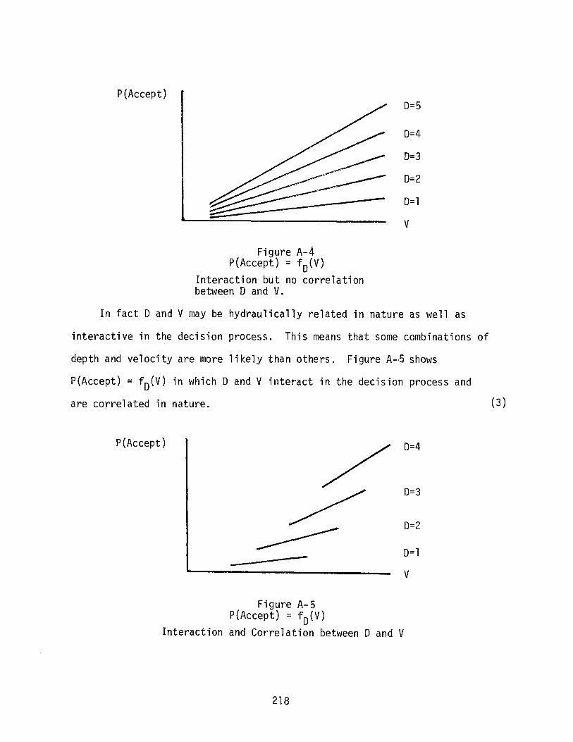
P(Accept)0=5

0=4

0=3

0=2

0=1

V

Figure A-4P(Accept) = fO(V)

Interaction but no correlationbetween 0 and V.

In fact 0 and V may be hydraulically related in nature as well as

interactive in the decision process. This means that some combinations of

depth and vel oci ty are more 1i kely than others. Fi gure A-·5 shows

P(Accept) = fO(V) in which 0 and V interact in the decision process and

are correlated in nature. (3)

-

P(Accept) D=4

0=3

0=2

0=1

V

Figure A- 5P(Accept) = fO(V)

Interaction and Correlation between 0 and V

218

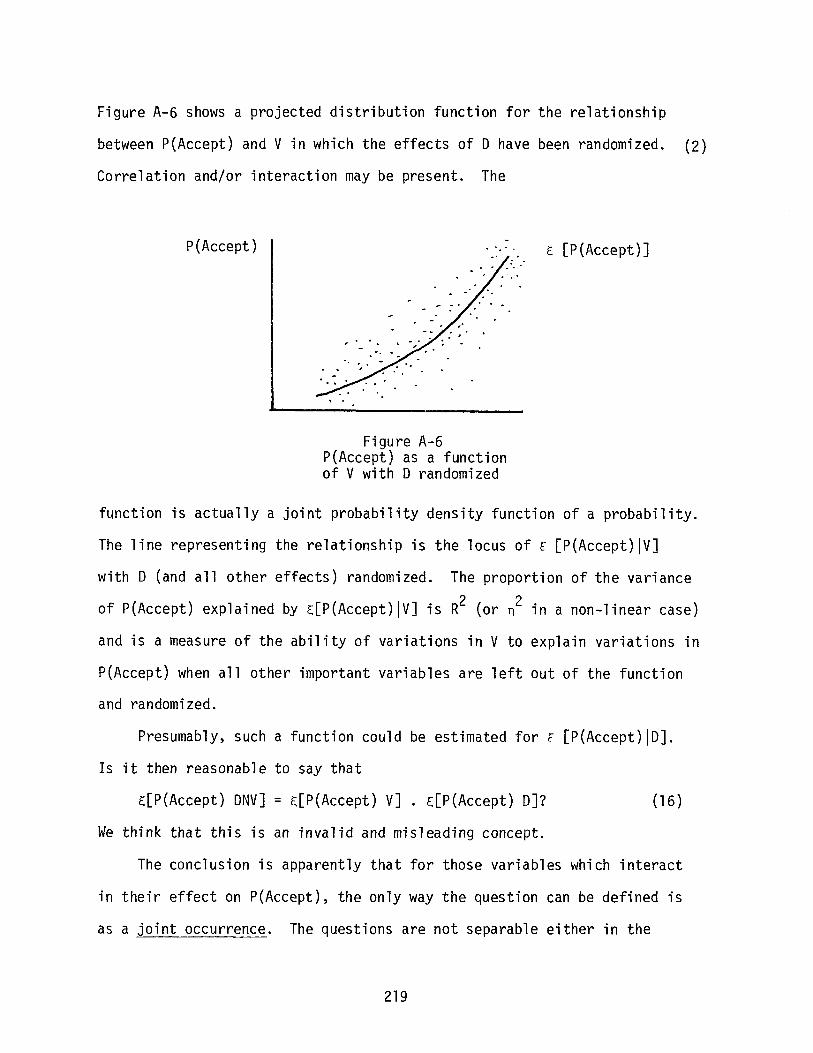
Figure A-6 shows a projected distribution function for the relationship

between P(Accept) and V in which the effects of D have been randomized. (2)

Correlation and/or interaction may be present. The

P(Accept)

Figure A-6P(Accept) as a functionof V with D randomized

E. [P(Accept)]

function is actually a joint probability density function of a probability.

The line representing the relationship is the locus of E. [P(Accept) IV]

with D (and all other effects) randomized. The proportion of the variance

of P(Accept) explained by ~[P(Accept)IV] is R2 (or n2 in a non-linear case)

and is a measure of the ability of variations in V to explain variations in

P(Accept) when all other important variables are left out of the function

and randomized.

Presumably, such a function could be estimated for E [P(Accept)ID].

Is it then reasonable to say that

~[P(Accept) DNV] = F.[P(Accept) V] . ~[P(Accept) D]? (16 )

We think that this is an invalid and misleading concept.

The conclusion is apparently that for those variables which interact

in their effect on P(Accept), the only way the question can be defined is

as a joint occurrence. The questions are not separable either in the

219

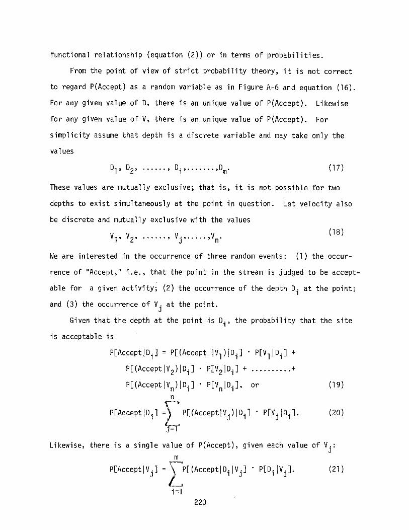
functional relationship (equation (2)) or in terms of probabilities.

From the point of view of strict probability theory, it is not correct

to regard P(Accept) as a random variable as in Figure A-6 and equation (16).

For any given value of D, there is an unique value of P(Accept). Likewise

for any given value of V, there is an unique value of P(Accept). For

simplicity assume that depth is a discrete variable and may take only the

values

07}

These values are mutually exclusive; that is, it is not possible for two

depths to exist simultaneously at the point in question. Let velocity also

be discrete and mutually exclusive with the values

Vl , V2, , Vj , ,V n· (18 )

We are interested in the occurrence of three random events: (1) the occur-

rence of "Accept," i.e., that the point in the stream is judged to be accept­

able for a given activity; (2) the occurrence of the depth Di at the point;

and (3) the occurrence of Vj at the point.

Given that the depth at the point is Di , the probability that the site

is acceptable is

P[AcceptIDi ] = P[(Accept IV1)ID i ] . P[V l ID i ] +

P[(Accept IV 2)IDi ] . P[V2 IDi ] + +

P[(AcceptIVn)IDi] P[VnIDi], or (19)n~

P[AcceptID,'] =\ P[(AcceptIV·)ID.]· P[VJ·ID.]. (20)} J' ,

~

(21). P[D·IV.]., J

Likewise, there is a single value of P(Accept), given each value of Vj :m

P[AcceptIV.] = ~p[(AccePtIDi IVJ.]JLi=l

220

P[Accept/D.nV.] , P[D. Iv.].1 J 1 J

These equations can also be written as follows:n

P[Accept IDi ] = fC---.I

j=l

m

P[Accept IVj ] = [

f=l

This shows that in order to calculate either P[AcceptIVj] or

or P[Accept!Di ] we must know P[AcceptIVjnDi] for all i and j.

Thus

(22)

(23)

and

The formulas

and

P[AcceptIDi] . P[AcceptIVj] = nonsense

Nonsense 1 P[AccePtIVj~Di]

P(AB) = P(A)·P(BIA)

P(AB) = P(A)·P(B) if P(B) = P(BIA)

(24)

(25)

(26)

(27)

are valid when A and B are different events. Equation (27) is true when

they are independent events. But P(Acceptlbi) and P(AcceptjVj ) are not

independent events. Indeed they are the same event under different

conditi ons.

The conclusion is the same whether we look at the problem in terms of

the decision process (equation 2) or in terms of probability theory (equation

22 and 23):

P[AcceptIDi~ViJ must be observed directly.

The multiplicative fallacy has arisen because of the way the events were

defined in the first place. For example, independent and reasonable

questions can be asked: (1) what is the probability that you will eat

brussels sprouts, if offered them; and (2) what is the probability that you

221

will accept a bright green shirt, if offered one? The probability that

you will accept both, if offered both, is simply the product of the two

probabilities (assuming that the decisions are independent)~ Now consider

three very different questions. (1) What is the probability that you will

come to dinner if required to eat brussels sprouts? (2) What is the prob­

ability that you will come to dinner if required to wear a bright green

shirt? (3) What is the probability that you will come to dinner if re­

quired to wear a bright green shirt and eat brussels sprouts? The event

here is II coming to dinner,1I and the probability of that event occurring is

being examined under different conditions which influence the decision.

It is clearly the latter problem we are dealing with, not the former.

Methodology for Evaluating and Comparing Streams

Assuming that the obstacles to definition and measurement of P(Accept)

under the various conditions on which it is dependent can be overcome, the

recreation potential of a stream consists of a matrix Phj1(Accept), or,

given the person type and activity, the recreation potential consists of a

vector of discrete probabilities, Pt(Accept), one for each location being

evaluated. Unfortunately this lIinformation ll is not very lIinformative. II

We can look at a point and say how good it is and we can compare and rank

order points, but we have no way to combine these discrete pieces of infor­

mation into an evaluation of the quality of the overall stream, and there

is no way to compare different streams. A frequency distribution can be

compiled showing the number of points or units of surface area on the stream

at each level of probability. A centile profile could thus be calculated

and the centile profiles could be compared between streams. A centile

profile shows, as with I.Q. or aptitude tests, the proportion of the points

(persons tested) having scores at or below the score in question. Two

222

streams could be compared as in Figure A-7.

~ttl

EttlOJs-~­Vl~

0..OJ OJ

...c U~u

c:(c­oo..

OJ~Vl3. ..- ~ 0~ Cr­Cor- OJOJo.t:J

U 0..s­

4-0o

100

ao

Stream A

Stream B

1•aScore = P(Accept)

Figure A-7Centile Profile Comparison

of Two Streams

The CrFSG methodology bypasses the centile profile concept and goes

one step further to advocate calculation of "weighted unit area." If

Ai is the number of square feet of surface area with P(Accept) = Pi'

thenn

WUA =>i =1

P. A.,1 1

(28)

where n is the number of discrete categories into which probability has

been aggregated. The WUA measure is interpreted as being the equivalent

surface area at a probability of 1.0.

This has come under considerable criticism, mainly on the grounds that

it implies that one hundred junk yards are equivalent to one rose garden.

In fact the concept of WUA as calculated has a valid meaning. The problem

223

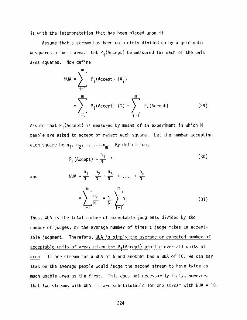
is with the interpretation that has been placed upon it.

Assume that a stream has -been completely divided up by a grid onto

m squares of unit area. Let Pi(Accept) be measured for each of the unit

area squares. Now definem

WUA = \ P. (Accept) (A.)L 1 1

i=lm

=Li=l

m

Pi (Accept) (l) =Ii=l

Pi (Accept) . (29)

Assume that Pi(Accept) is measured by means of an experiment in which N

people are asked to accept or reject each square. Let the number accepting

each square be nl , n2, nm.

n.Pi (Accept) = i

By definition,

(30)

andn

+--.r!!.N

(31)

Thus, WUA is the total number of acceptable judgments divided by the

number of judges, or the average number of times a judge makes an accept­

able judgment. Therefore, WUA is simply the average or expected number of

acceptable units of area, given the Pi(Accept) profile over all units of

area. If one stream has a WUA of 5 and another has a WUA of 10, we can say

that on the average people would judge the second stream to have twice as

much usable area as the first. This does not necessarily imply, however,

that two streams with WUA = 5 are substitutable for one stream with WUA = 10.

224

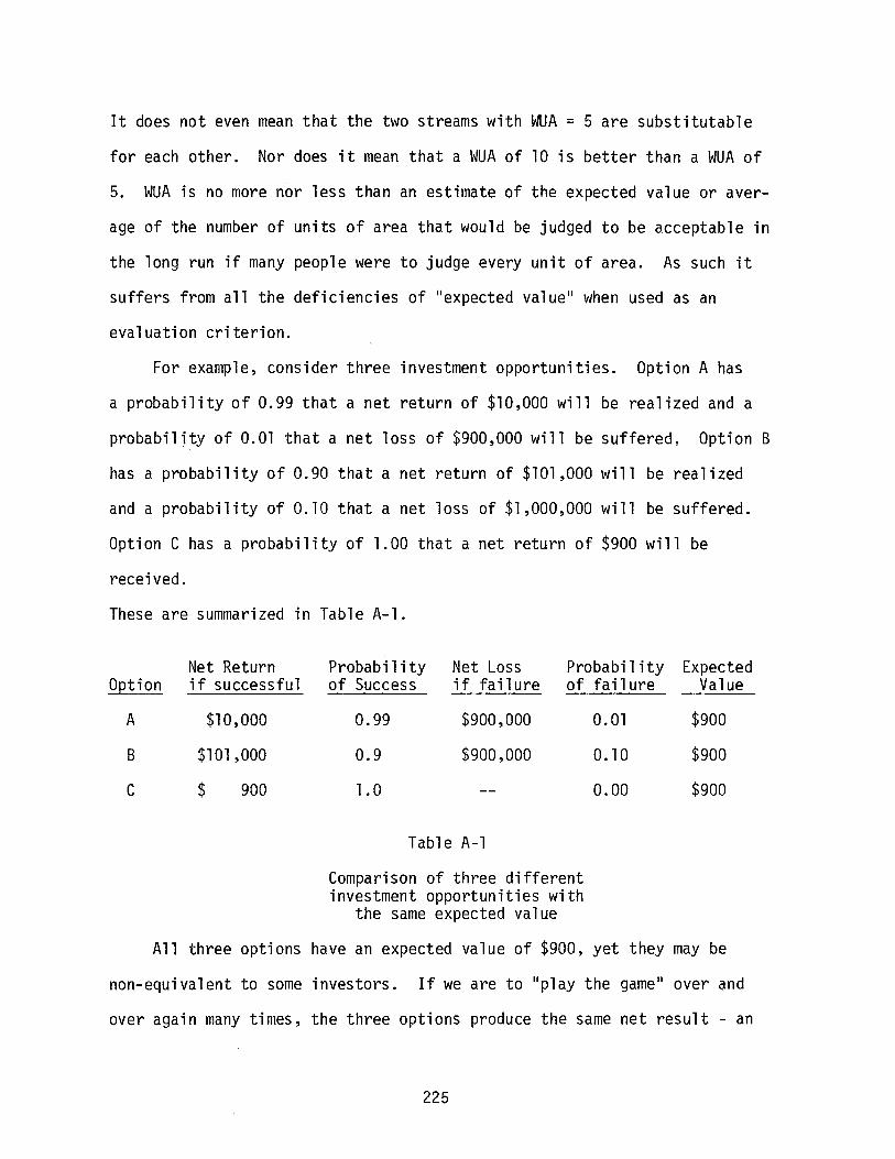
It does not even mean that the two streams with WUA = 5 are substitutable

for each other. Nor does it mean that a WUA of 10 is better than a WUA of

5. WUA is no more nor less than an estimate of the expected value or aver­

age of the number of units of area that would be judged to be acceptable in

the long run if many people were to judge every unit of area. As such it

suffers from all the deficiencies of lIexpected va1ue ll when used as an

evaluation criterion.

For example, consider three investment opportunities. Option A has

a probability of 0.99 that a net return of $10,000 will be realized and a

probability of 0.01 that a net loss of $900,000 will be suffered, Option B

has a probability of 0.90 that a net return of $101,000 will be realized

and a probability of 0.10 that a net loss of $1,000,000 will be suffered.

Option C has a probability of 1.00 that a net return of $900 will be

received.

These are summarized in Table A-l.

Net Return Probability Net Loss Probability ExpectedOption if successful of Success if fai 1ure of failure Value

A $10,000 0.99 $900,000 0.01 $900

B $101 ,000 0.9 $900,000 0.10 $900

C $ 900 1.0 0.00 $900

Tab1 e A-l

Comparison of three differentinvestment opportunities with

the same expected value

All three options have an expected value of $900, yet they may be

non-equivalent to some investors. If we are to lI pl ay the game" over and

over again many times, the three options produce the same net result - an

225

average winning of $900 per play. For a one-shot game, however, a con­

servative small business would go for the sure $900, while a big conglom­

erate with many "games" and a huge capital reserve might prefer option B.

Thus, as an expected value, WUA measures how much adequate stream

area there is on the average over the population as a whole, but it cannot

be applied validly to individual evaluations. Furthermore, it is blind to

the distribution of wins and losses within the population, unless this is

accounted for by segmentation by person type. Finally, the concepts of

P(Accept) and WUA are based on the criterion of "adequacy,1l not optimality.

There is absolutely no reason to assume that the "value in use" of the

site (i.e., the personal utility gained from using the site) is proportional

to the probability that it will be judged to be acceptable. Herein lies

the dilemma that 100 junkyards are not equivalent to one rose garden.

While it may be true that a unit area rose garden will be judged acceptable

100 percent of the time and a unit area junkyard will be judged to be

acceptable one percent of the time, the "value in use" of the rose garden

may be 1,000,000 times as great as the value in use of the junkyard, and

there may be a less desirable rose garden, which is also acceptable 100

percent of the time, but which delivers "value in use" only 1000 times as

great as the junkyard. Thus, WUA is grossly incomplete for recreation

assessments and cannot be used to measure "value in use" (i.e., nothing can

be said about equivalence or substitutability) unless Il va l ue in use ll is

strictly proportional to P(Accept).

Capacity, Recreation Potential and WUA

In this section we ask whether any information about the recreational

capacity of a site can be derived from P(Accept) or WUA. By recreational

capacity we mean the carrying capacity of the site, i.e., the quantity per

226

untt of recreatton activity the site can support. There are two components

to the carrying capacity question: (1) ecological capacity; and (2) social

capacity. Ecological capacity is the maximum quantity of activity that can

be put on the site without unacceptable damage to the site. Social capacity

is the maximum quantity of activity that can be put on the site without

unacceptable damage to the quality of the user's experience. Obviously,

there are second order relationships, i.e., damage to the site may reduce

user satisfaction, so the two kinds of capacity are not clearly separable

in concept. However, in practice, there are usually environmental policy

concerns which define ecological capacity. Social capacity is usually

concerned with the first order effects of congestion - mutual interference

among users.

Ecological capacity may be related to WUA. WUA is the average number

of units of area that will be judged to be acceptable, when a person judges

every unit of area. Thus, it can be viewed as the average "s ize ll of the

resource that is available for use, or the area over which use is likely

to be spread. However, some specific units of area, those with large values

for P(Accept), will be accepted much more frequently than others, and thus

they will be used much more heavily. Also, some units of area will have

much greater value in use than other units of area. Even though two unit

areas may be judged acceptable by a person, the one with the greatest value

in use will be chosen for use~ If, independent of WUA, a policy decision

can be made for the ecological capacity of each unit of area, and if this

policy can be enforced through rationing or price rationing, then WUA may

be a reasonable estimate of the number of units of area available. The

expected number of units of capacity available requires the additional

information about the capacity of each unit of area.

227

Let Ci be the ecological capacity as established by policy for the

i th unit area of a stream. Let Pi(Accept) be the probability that the unit

area is acceptable. Because each unit area has an area of one, WUA is

n

W\JA=~~

i=l

P. (Accept) A.1 J

Pi (Accept).

n

=[i=l

Now define WCA as II we ighted capacity area: II

n

WCA =\' Pi (Accept) Ai CiLi =1

(28)

(29)

WCA is the expected or average number of units of capacity that will be

judged to be acceptable each time a person judges every unit of area. While

this quantity may be useful, it is an lIexpected va1ue ll and suffers from the

weaknesses of expected value and is blind to distributional concerns unless

appropriately segmented by social type.

Social capacity is a much more complex question. It must be defined

from the users' subjective point of view. Given sufficient understanding

of each user's decision criteria, it might be possible to IIfigure out ll

Si' the social capacity of each unit of area, and to establish Si as a

policy. The limiting capacity is then either Ci or Si' whichever is less.

There may be a productive way to define Si using the concept of P

(Accept). For simplicity assume that we are talking about the social

capacity of a room at a cocktail party. Assume that the probability

228

that a person will enter the room or remain there is P, and that P is a

function of the number of people in the room. This defines a simple

stochastic process with three states as in Figure A-7.

o

P

Room

{l-P}

o

{l-P}

ArrivalProcess

Exit

1.0

Figure A-7

Simple Social Carrying Capacity Model

State 1 is the arrival process which delivers people to the entrance

to the room. State 2 is the room. State 3 is an absorbing exit into which

people go and from which they do not return once they have decided to

leave or not to enter State 2, the room. The matrix of probabilities is

P =

o

o

P

P

{l-P}

{l-P} {30}

o 0

229

If the arrival process is some stationary process which delivers a

uniform flow of people to the door of the room and if P decays as the

population of the room increases, there will be some steady-state popula­

tion of the room to which the system will stabilize. If P is P.(Accept)1

and the "room" is a unit of area of a recreation resource, then the steady

state population might be regarded as a definition of social carrying

capacity. This "capacity," however, may depend on the nature of the

arrival process and may not necessarily maximize total value in use. To

maximize value in use we need commensurate individual utility functions.

The same model might be expanded to describe a site with several

different kinds of users. Assume that P(Accept) for each type of user is

some function, perhaps unique to user type, of the number of each type of

user at the site. Presumably there will be a steady-state population for

each type of user, depending on each arrival process and on the way P

(Accept) changes with the population profile at the site.

Given several sites, this model could also be developed into a dis-

placement process describing the invasion and succession that takes place

when some change in the site changes the P(Accept) function of user types

or when the arrival process changes.

230

REFERENCES

Anas, A., F. S. Koppelman, G. L. Peterson, P. R. Stopher, G. Ergun, A. M.Subramanyam (1979), "Prediction of Urban Recreation Demand,1I FinalReport, Grant #APR76-19806, NSF-RANN, Dept. of Civil Engineering,The Technological Institute, Northwestern University, Evanston,Illinois 60201.

Andrews, W. H., et ale (1976), 1I~1easuring the Impact of Changing StreamFlow on Recreation Activity," in C. B. Stalnaker and J. L. Arnette(eds. ). ~~ethodo109i es for the Determinat i on of Stream Reso urceFlow Requirements: An Assessment, U. S. Fish and Wildlife Service.

Bovee, K. D. and R. T. Milhous (1978), "Hydraulic Simulation in InstreamFlow Studies: Theory and Techniques," Instream Flow Service Group,Ft. Collins, Colorado.

Bureau of Outdoor Recreation (1977), Recreation and Instream Flow,Washington, D. C.

Carter, J. (President) (1978), Water Policy Reform Message, July 6th.

Chubb, M. and E. H. Bauman (1976), "Assessing the Recreational Potentialof Rivers,1I 72nd Annual Meeting of the Association of AmericanGeographers, New York.

deBettencourt, J. S. (1979), IIThreshold Theory and Methods for AssessingEnvironmental Performance Capability," Ph.D. Dissertation, Dept.of Civil Engineering, Northwestern University, Evanston, Illinois.

deBettencourt, J. S. and G. L. Peterson (1977), "Standards of EnvironmentalQuality for Recreational Evaluation of Rivers; Proceedings: RiverRecreation Management and Research Symposium, USDA - Forest Service.

Driver, B. L. (1977), "Item Pool for Scales Designed to Quantify the Psycho­logical Outcomes Desired and Expected from Recreation Participation,HUSDA Forest Service, Ft. Collins, Colorado.

Driver, B. L. and P. J. Brown (1975), "A Social Psychological Definitionof Recreation Demand, with Implications for Recreation ResourcePlanning,H in Assessing Demand for Outdoor Recreation, Wash., D. C.

Federal Water Pollution Control Act, as amended in 1977.

Hyra, R. (1978), "Methods of Assessing Instream Flow for Recreation,"Cooperative Instream Flow Service Group, Ft. Collins, Colorado.

Lancaster, K. (1966), IIA New Approach to Consumer Theory," J. of PoliticalEconomy, LXXIV (April).

Masteller, M. B., et ale (1976), 'IMeasurement of Stream Flow AestheticValues," in Stalnaker, C. B. and J. L. Arnette (Eds.) Methodologies

231

REFERENCES(cont'd)

for the Determination of Stream Resource Flow Requirements: AnAssessment, U. S. Fish and Wildlife Service.

Peterson, G. L., R. L. Bishop, R. M. Michaels, and G. J. Rath (1963)IlChildren's Choice of Playground Equipment: Development ofMethodology for Integrating User Preferences into EnvironmentalEngineering," J. of App. Psych., Vol. 58, No.2, 233-238.

Tinsley, H. E. A. (1977), IlLeisure Activities and Need Satisfaction; II J.of Leisure Research, 9 (2): 110-120.

University of Colorado (1976), Program of Research on Human Judgment andSocial Interaction, Institute of Behavioral Science, Boulder,Colorado (Bibliography).

U. S. Water Resources Council (1973), Principles and Standards forPlanning Water and Related Land Resources, Washington, D. C.

232

PROBLEMS FOR RESEARCH

Introduction

This section summarizes research problems which have been identified

by the four modules participating in the IFG workshop on Instream Flow

Criteria and Modeling. The research problems identified are interdisci­

plinary in nature cutting across module subject areas. The following

research problems are not presented according to module subjects but

grouped according to general concerns including: input data {sources and

reliabilitY)t instream flow needs assessment methodologies t and decision

frameworks.

Input Data

As with any approach which depends on both emperical data and existing

baseline data resources the IFG methodology could be vastly improved if

either funding were provided for collection of new data, or data resources

were found which allow direct application of the methodology. Since this

is not the case, a review of problems with input data may be useful.

Lack of short-term and continuous streamflow forecasts in many areas

increase the risk to water managers in making proper adjustments in storage

releases to meet continuous instream flow requirements. Possibilities

exist for changes in streamflow management without interference with legal

water rights. What is needed is a method of forecasting water releases on

a daily basis during critical seasons. Data must provide a basis for

233

determination of regional differences in hydrological conditions (e.g.

west vs east).

Extensive and expensive field data collection is necessary in order

to predict hydraulic habitat parameters. This limits the number of pro­

jections which can be made while there is a need for projections spanning

a wide range of flows (e.g. low flow to flood stage).

The effect of sediment load and characteristics on effective pollutant

load are unknown. This prevents accurate assessment of water quality at

instream habitat locations of interest. Research is needed on the physical­

chemical relationships between sediment and pollutants in the stream.

Generally, sources of specific pollutants in streams are unknown. As

a result, accurate predictions of pollutant loading under various runoff

scenarios cannot be made. Technology is needed for identifying potential

non-point sources of pollutants on various classes of watersheds in various

. geographic areas, and linkage is needed between pollutant yield and both

runoff and sediment yield.

There is incomplete understanding of the relationships of stream

primary production to instream flow. Although it is possible from existing

data to reliably predict benthic production, data on allochthonous pro­

duction is limited and available mainly for low order streams.

Aquatic insect production as a function of habitat conditions is

poorly understood. Therefore, it is impossible to predict the aquatic in­

sect food supply component of the habitat. Research is needed to establish

the relationships between habitat parameters and aquatic insect production.

Sufficient factual data are lacking on fisheries responses, including

behavior and mortality, under various combinations of water quality and

234

physical microhabitat. Although some criteria for minimum and optimum

habitat are available (ref. U.S.E.P.A. Quality Criteria for Water - 1976),

for the most part that data is incomplete. There is a need for research

to determine dose response relationships which reduce the ability of

aquatic organisms to function.

The seasonal and geographic differences for behavior of most fish

species under given habitat conditions are unknown. This represents a

serious constraint to the application of habitat criteria. What is

needed is a clear definition and refinement of "probability of use" curves

for fish species at all life stages by season and geographic region.

There is a lack of factual data on fish biomass production (standing

crop) under various habitat conditions. Therefore, criteria for habitat

suitability are incomplete. Further, the economic effects of habitat

conditions cannot be quantified. What is needed are field observations of

standing crop compared to habitat conditions over a wide range of habitat

parameters.

Along the same lines the degree of flexibility in habitat rejection

by fish is unknown. This is a serious gap in formulating comprehensive

criteria for habitat suitability. Research is needed on fish behavior

responses to a wide range and many combinations of habitat variables.

This is true also for primary and secondary production in the stream.

Factors considered should include physical, chemical, and biological

parameters.

Instream Flow Methodologies

When considering a methodology for instream flow assessment the pre­

requisites include sufficient input data and a reasonably clear understanding

235

of how the output will be used. The methodology can then either be

extremely simple depending on minimal data resources or range through

various levels of complexity dependent on better or more comprehensive

data. The existing IFG methodology attempts to use emperically collected

and existing data, unfortunately this data is incorporated in the

methodology at different levels of precision. Recognizing that predictive. .

tools for environmental assessment and habitat projections must be com-

prehensive even if they are less than perfect leads to the conclusion that

more than one methodology should be available. The different methodologies

might represent a tiered approach dependent on data availability and

decision requirements. The first tier should included a simplified

methodology suitable for the purpose of habitat projections which do not

require extensive field data.

The other tiers which are dependent on more sophisticated data or

decision making procedures can develop from the existing methodology.

The following represent improvements to the existing methodology which

would significantly improve reliability.

A prediction of habitat changes due to changes in streamflow should

represent a substantial length of stream segment. There is uncertainty

whether or not this is accomplished by the IFG method. There is need for

criteria to be established for field study site selection that will yield

representative habitat conditions.

The capability to predict transient channel geometry and bed-particle

size distribtuion during and following unsteady sediment-water discharge

is required for many streams, particularly large rivers. Habitat conditions

under variable discharge cannot be predicted with present state-of-the-art

236

models. Modeling capability is needed for relating microhabitat channel

geometry and bed particle size distribtuion to flow parameters as a

function of time in unsteady flow. This should include moveable bed

characteristics which can be correlated with habitat bed requirements.

The present state-of-the-art does not penmit adequate projections of

flow and geometric characteristics in natural streams. Precision of

estimates of hydraulic variables in natural streams is low. There is need

for projections which incorporate some measure of frequency. Low level

remote sensing technology should be considered for data acquisition.

There is a lack of appropriate methods of water quality projection.

Consequently, the habitat projection method is unable to incorporate

water quality parameters directly. Available water quality models should

be tested to determine their suitability for the IFG model. Promising

models should be adapted to the IFG model.

The technology does not exist for estimating non-point pollutant

yield to streams from the watershed as a function of land management and

land use practices. Consequently, water quality cannot be predicted for

instream habitat purposes. There is need for pollutant yield modules for

various watersheds, land use and management, and runoff combinations.

There is an absence of food chain variables in habitat prediction

models. For example, the relation between habitat suitability for benthic

invertebrates and habitat suitability for target fish species is unknown.

Three particular needs are: (1) an evaluation of chemical and physical

parameters in combinations which define certain limits (lethal, survival,

acceptable, optimum) for various species and life stages of benthic inverte­

brates which can be compared with habitat suitability for target fish

237

species; (2) the impact on a fishery due to given loss of invertebrate

population is needed; and (3) how invertebrate functional groups - collectors,

gatherers, scrapers, and grazers - respond to given habitat conditions and

in turn impact on target fish. Since the same implications of primary

(algae and allochthonous materials) to secondary (aquatic insects) consumers

should be noted, methodologies must be improved to predict ecosystem re­

sponses to changes in flow.

In summary the selection of appropriate methodology to be applied in

predicting hydraulic habitat conditions is often a problem due to con­

straints and limitations of specific methods. Consequently, less than

satisfactory predictions of flow parameters, stream geometry and water

quality on natural streams are being made. There is a need for a classi­

fication system differentiating watershed-stream systems which can be

coupled with decision requirements. Such a system would identify the

tier, its accuracy and provide an estimate of probable costs. Such a

system would be an integral part of IFG use.

Decision Framework

The use of the IFG methodology is dependent on the needs and require­

ments of managers and decisionmakers. If the methodology falls short of

meeting their requirements then it will not be used. At all times the

question IIHow will the results be used ll must be kept in mind. Since the

reliability and versitility of the IFG habitat projection method is not

fully established, there is a lack of confidence and acceptance by potential

users. At the outset it should be clearly understood that the acceptance

of the methodology will be based on how well it meets the requirements of

users. At present the IFG methodology has found only limited application

238

but is being tested throughout the United States. Even before the results

of these tests are in it is possible to identify major decision problems.

There is incomplete understanding of minimum acceptable instream

habitat conditions. Although in many cases the possibility of stream

management improvement exists, lack of well-established criteria for

different levels particularly minimum levels of habitat suitability is a

deterrent to management changes. Improved information is needed for survival

and lethal limits on all critical habitat parameters.

There is a lack of knowledge of river system operational strategies

which would optimize habitat conditions. Instream flow regulations to

preserve aquatic cosystem habitats are therefore not generally accomplished .

. Models for river system management which are applicable to various important

hydrologic systems are needed.

In summary, it appears that a decision framework based on a tiered

methodology is possible. Methodologies which efficiently use data and

fiscal resources will improve utility and decisionmaking.

Sumnary

There is an urgent need to continue the exchange of new advances

among the several disciplines in order to expedite the eventual formulation

of fully suitable models. Further, the research emphasis should be upon

developing comprehensive models which include all necessary and sufficient

parameters (e.g. hydraulic parameters are necessary to specification of

fish habitats, but they are not sUfficient). Once these models are

produced, a decision framework must be available to assure their use.

Since clear requirements for present use exist, the existing IFG methodology

should review its high dependence on "experience" in using empirical

relations for projecting instream flow needs.

239

IFG Response to Workshop

Since the conclusion of the workshop, a number of changes in the

incremental methodology have been made by the Cooperative Instream Flow

Service Group in response to the various suggestions made by the participants.

The workshop was viewed by the IFG as a learning tool and a great deal was

learned. Some changes were made immediately following the workshop, others

have been implemented during the past year, and others are still in the

planning stages. The following statements highlight a number of the ways in

which the Instream Flow Group has benefited from the workshop.

1. Critiques forcefully demonstrate that the IFG must be much more careful

in defining terminology associated with the methodology. For example, the IFG

Incremental Methodology was based on "probability-of-use-curves."

Mathematically, the curves are treated as marginal probability functions;

however, workshop participants pointed out that these curves do not truly

represent probabilities. It is one thing to handle the curves mathematically

as probability functions, yet quite another to assume, or imply, that they are

actual probabilities. Consequently, the IFG is using the term criteria curves

rather than probability-of-use-curves to avoid confusing or misleading users

of the methodology.

2. The IFG has greatly altered its approach to introducing the methodology

to new audiences. In the workshop, participants were given a cursory review

of the methodology and were set to work to provide their critique. A great

deal of misunderstanding ensued because most workshop participants were not

familiar with the historical need for such a methodology, the decision context

240

in which the methodology is intended to be used, or the scientific logic on

which the methodology is based. The numerous misunderstandings that surfaced

during workshop discussions had a great impact on IFG's subsequent training

approaches. Currently, a substantial portion of any training session is spent

on describing the historical need for an lIincremental ll methodology; the type

of uses envisioned for the methodology; the types of uses that are

inappropriate for the methodology; how the methodology relates to prevailing

schools of thought in fishery science; and the assumptions that must be made

in order to apply the methodology correctly. Furthermore, all of these

concerns are reiterated throughout the training setting, along with detailed

descriptions of the application techniques. Thus, while the expected outcome

of the workshop was to focus on the internal logic of the methodology, we

learned a great deal about the process of communicating.

3. Prior to the workshop, the focus was primarily on hydraulic simulation

and the Habitat model. These are but analytical tools within the context of

an overall methodology. Subsequently, the Instream Flow Group has placed a

great deal more emphasis on the entire procedure (methodology) for evaluating

instream impacts. A modular approach is being emphasised to provide users

with a structured format for consciously evaluating the significance and

stability of such components as watershed processes, water chemistry, and food

web relationships before application of any computer model.

In addition guidelines and procedures are being developed to assist users in

determining whether or not their intended application and particular field

situation is consistent with the assumptions of the methodology and its

related computer models. The workshop discussions clearly demonstrated a need

241

for a structured procedure to evaluate underpinning assumptions as part

of the methodology itself.

4. Workshop participants identified the need for further validation and

verification of the various models and assumptions under a variety of

circumstances to strengthen the basic internal logic and to expand application

of the methodology. Such activities are programmed in the Instream Flow Group

budget for Fy 80. Validation studies are programmed which will test the

relationship between weighted usable area and standing crop. Sensitivity

analysis will be conducted to determine the kinds of precision necessary (the

risk of error) for each of several input variables. The intent of the

sensitivity analysis is to make explicity the internal attributes of the

model.

5. We learned from the water quality module that many water quality models

are presently available and that water quality can most generally be assessed on

a macrohabitat basis. As a result, our emphasis will focus on interpretation

of water chemistry parameters with respect to aquatic habitat, rather than on

additional water quality modeling.

6. We learned that we had inadequately described the IFG Incremental

Methodology. At the time of the workshop, a series of information papers were

available which dealt with different aspects of the methodology (such as how

fish criteria curves are derived) but there was no single description of the

methodology. The chapter in this report by E. Woody Trihey is but one attempt

in that direction. It describes what the methodology is, what it does, and

how it should be used. Other reports on the methodology that are currently

242

being developed also contain this kind of information to serve as a point of

contact and to communicate to the reader the methodology that is being

described. Had such a single, brief description been available at the time of

the workshop, participants could have come to the workshop much better

equipped to provide a focused, systematic evaluation.

7. The Instream Flow Group has learned that it is not adequate simply to

identify assumptions. Users are better served by testing whether the

assumptions can normally be justified and whether inaccurate assumptions

really make a difference. As examples, a) the assumption of independence

Utilizing the best data available, a procedure was developed (ref. Module III)

to test for independence among variables. Grenney and Voos found that while

some dependence is present, it is not so significant as to result in a serious

error in the final model output for most applications. This analysis is

presented in the forthcoming paper, Estimation of Parameters for the

Incremental Methodology. b) the assumption of linearity -- Recently the

assumption of a linear relationship between biomass and weighted usable area

has been examined in the western states of Oregon, Wyoming, and Colorado. A

strong positive linear correlation has been found for salmonids. It was also

determined that no linear relationships could be identified between weighted

usable area and density for aquatic insects. A curvilinear relationship

existed in all cases examined which as yet cannot be generalized. c)

the assumption of channel stability -- The Instream Flow Group has recently

contracted for a workshop on sediment transport and channel change. This

workshop will build upon discussions originating in the November 1979 workshop

reported on in these proceedings. The new workshop will bring together a

number of experts on sediment transport modeling to identify the most

243

promising avenues of pursuit for analyzing stream channel hydraulics on a

microhabitat basis in unstable channels.

8. As a result of the discussions within the recreation module, it became

apparent that a separate analytical approach needs to be developed. Instream

flow requirements for many instream recreation pursuits could better be

evaluated on a macro basis (large stream reach) rather than the site-specific

microhabitat approach used for fishery assessments. Although this has yet to

be initiated, the final results will probably be quite similar to suggestions

by James W. Scott in his letter commenting on the review draft of the

recreation model report.

244