3D EM-4 new horizons Proceedings of the 4 th International Symposium on Three-Dimensional Electromagnetics Institute of Geophysics TU Bergakademie Freiberg, Germany September 27–30, 2007

Welcome message from author
This document is posted to help you gain knowledge. Please leave a comment to let me know what you think about it! Share it to your friends and learn new things together.
Transcript

3D
EM-4
new horizons
Proceedings of the4th International Symposium on
Three-Dimensional Electromagnetics
Institute of GeophysicsTU Bergakademie Freiberg, Germany
September 27–30, 2007

ii

Preface
Dear colleagues,
This is now the fourth time we get together to share ourenthusiasm for the mathematical treatment of electromag-netic methods in geophysics. On behalf of the Gerald W.Hohmann Memorial Trust for Research and Teaching inApplied Geophysics we would like to welcome you tothe 4th International Symposium on Three-DimensionalElectromagnetics. We have had three highly successfulmeetings in Ridgefield, CT, USA (1995), Salt Lake City,UT, USA (1999), and Adelaide, Australia (2003). We are,thus, very proud to host 3DEM-4 in Freiberg to continuethis line of important events and hope that this meetingwill be as successful as its predecessors. At the time ofprinting, almost 90 scientists from more than 20 countriesall around the world have registered for 3DEM-4.
We have the impression that right now we are facing avery dynamic phase in the development of EM methodspartially being fueled by economic needs. So, we can feelthe ‘New Horizons’ coming up which has become our at-tribute to 3DEM-4. After focusing on applications in theAdelaide meeting 2003 ‘3D EM at Work’, this meeting,therefore, intends to emphasize the methodological sideagain.
As a participant of the first 3DEM meeting in Ridgefield,I (Klaus) gladly picked up the slogan ‘Equations are wel-come’. However, we extended it to ‘Equations are as wel-come as applications’ to emphasize the importance of bothsides. So, applications, case studies and alternative devel-opments are as numerous in 3DEM-4 as methodologicalcontributions to forward and inverse modeling as well asresolution and data analysis. The symposium, therefore,
represents an interface between modelers and practition-ers, university and economy, developers and users and en-compasses a wide variety of different physical and numer-ical approaches in theory and practice.
This hardcopy printout might appear a little antiquated butsometimes old fashioned things are just practical. It servesas an onsite guide through the meeting (without having tohave your notebook computer on your knees) and reflectsthe most important points of each contribution to keep inmind. After the meeting, just put it in your shelf right nextto the other 3DEM-books to continue this series of sci-entific exchange in EM. Of course, for your conveniencewe offer a state-of-the-art electronic version including col-ored figures in pdf format at our 3DEM-4 homepage fordownload and rapid search.
We hope that you enjoy the morning oral sessions as muchas the afternoon poster sessions. Posters are as importantas orals and are given a large room to underscore theirimportance. We intend to have open discussions after thetalks and beer with the posters to free your mind. More-over, Freiberg’s historical and cultural setting includingthe 82nd Bach Festival of the New Bach Society shouldprovide the right environment to celebrate science.
Finally, we would like to thank the Technical Co-Chairs,the Committee, our student helpers and co-workers, thesponsors and all the attendees and contributors for makingthis symposium a vivid meeting point for the internationalEM community. We hope you enjoy your stay in Saxony.
Klaus Spitzer and Ralph-Uwe BörnerGeneral Co-Chairs
iii

iv

3DEM-4 is sponsored by
KMS Technologies – KJT Enterprises, Houston
EMGS
Metronix
Geosystem, Milan
Zonge
Chinook Geoconsulting, Inc.
Schneider & Berger
v

vi

Contents
Theory – Forward modelling 1
M. Afanasjew, O. G. Ernst, S. Güttel, M. Eiermann, R.-U. Börner, K. SpitzerKrylov subspace approximation for TEM simulation in the time domain . . . . . . . . . . . . . . . . . . . . . . . 3
M. Blome, H. R. MaurerAdvances in 3D geoelectric forward solver . . . . . . . . . . . . . . . . . . . . . . . . . . . . . . . . . . . . . . . 7
R.-U. Börner, O. G. Ernst, K. SpitzerFast 3D simulation of transient electromagnetic fields by model reduction in the frequency domain using Krylovsubspace projection . . . . . . . . . . . . . . . . . . . . . . . . . . . . . . . . . . . . . . . . . . . . . . . . . . . 11
A. Franke, R.-U. Börner, K. Spitzer3D finite element simulation of magnetotelluric fields using unstructured grids . . . . . . . . . . . . . . . . . . . . 15
E. Haber, S. Heldmann, D. W. OldenburgAdaptive mesh refinement for 3D electromagnetic modeling . . . . . . . . . . . . . . . . . . . . . . . . . . . . . 19
T. Hanstein, S. L. Helwig, G. Yu, K. M. Strack, R. Blaschek, A. HördtThe effect of a horizontal axial metallic conductor in marine EM . . . . . . . . . . . . . . . . . . . . . . . . . . . 23
S. Mukherjee, M. E. EverettThree dimensional finite element analysis of electromagnetic induction in geologic formations containing mag-netic bodies . . . . . . . . . . . . . . . . . . . . . . . . . . . . . . . . . . . . . . . . . . . . . . . . . . . . . . . 27
G. A. Oldenborger, D. W. OldenburgFinite-volume time-domain EM modelling for high conductivity . . . . . . . . . . . . . . . . . . . . . . . . . . . 31
D. W. Oldenburg, E. Haber, R. ShekhtmanRapid forward modelling of multi-source TEM data . . . . . . . . . . . . . . . . . . . . . . . . . . . . . . . . . . 35
C. Schwarzbach, K. SpitzerOn the matrix condition number of finite element approximations to the frequency domain Maxwell’s equations . . 39
P. WeideltExact 3D free-decay modes for a uniformly discretized open box . . . . . . . . . . . . . . . . . . . . . . . . . . . 43
M. Zaslavsky, S. Davydycheva, V. Druskin, A. Abubakar, T. Habashy, L. KnizhnermanFinite-difference solution of the 3D EM problem using divergence-free preconditioners . . . . . . . . . . . . . . . 47
Theory – Inversion and resolution analysis 51
A. Avdeeva, D. AvdeevThree-dimensional magnetotelluric inversion using quasi-Newton minimization . . . . . . . . . . . . . . . . . . . 53
M. Berdichevsky, V. DmitrievSussession of partial MT and MV inversions – from 2D to 3D . . . . . . . . . . . . . . . . . . . . . . . . . . . . . 57
M. Braun, U. YaramanciResistivity inversion of magnetic resonance sounding – Assessment of sensitivity and reliability . . . . . . . . . . 62
J. Chen, M. Jegen-Kulcsar, B. HeinckeJoint inversion and topographic correction of geophysical data . . . . . . . . . . . . . . . . . . . . . . . . . . . . 66
J. Kamm, M. Müller-Petke, U. YaramanciModelling of multi-transmitter arrays in magnetic resonance sounding . . . . . . . . . . . . . . . . . . . . . . . . 67
A. Kelbert, G. D. Egbert, A. SchultzNon-linear conjugate gradient inversion for the spherical earth . . . . . . . . . . . . . . . . . . . . . . . . . . . . 71
vii

Contents
P. S. Martyshko, A. L. RoublevOn the electromagnetic inverse problem solving for some models . . . . . . . . . . . . . . . . . . . . . . . . . . . 75
B. J. Minsley, F. D. Morgan3D source inversion of self-potential data . . . . . . . . . . . . . . . . . . . . . . . . . . . . . . . . . . . . . . . 78
M. Müller-Petke, U. YaramanciEfficient datasets – An alternative approach that analyses the data space . . . . . . . . . . . . . . . . . . . . . . . 82
U. SchmuckerA note on the interpretation of EM induction data by multi-dimensional conductivity and resistivity models . . . . 86
Theory – Data analysis 89
M. Berdichevsky, V. Kuznetsov, N. Palshin1. Decomposition of 3D magnetovariational response functions in models of (2D+2D)-type . . . . . . . . . . . . . 91
M. Berdichevsky, V. Kuznetsov, N. Palshin2. Decomposition of 3D magnetovariational response functions in models of (2D+3D)-type . . . . . . . . . . . . . 95
M. Berdichevsky, V. Kuznetsov, N. PalshinMagnetic perturbation ellipses . . . . . . . . . . . . . . . . . . . . . . . . . . . . . . . . . . . . . . . . . . . . . 99
F. E. M. (Ted) Lilley, J. T. WeaverExamples of magnetotelluric data: invariants of rotation, and phases greater than 90 deg. . . . . . . . . . . . . . . 103
Applications – Alternative developments 107
R. Blaschek, A. HördtNumerical modeling of the IP-effect at the pore scale . . . . . . . . . . . . . . . . . . . . . . . . . . . . . . . . . 109
A. N. Kuznetsov, I. P. Moroz, V. M. KobzovaPhysical modeling of seismoelectric effects above three-dimensional heterogeneities of geological environment . . 112
M. Montahaei, M. A. RiahiSimulation of seismoelectric signals generated at an interface . . . . . . . . . . . . . . . . . . . . . . . . . . . . . 114
G. Muñoz, O. Ritter, T. Krings, M. BeckenA new, faster technique of three-dimensional magnetotelluric data acquisition . . . . . . . . . . . . . . . . . . . . 117
F. C. Schoemaker, D. M. J. Smeulders, E. C. SlobLaboratory measurements of electrokinetic phenomena . . . . . . . . . . . . . . . . . . . . . . . . . . . . . . . . 118
J. Schünemann, T. Günther, A. Junge3-dimensional subsurface investigation by means of large-scale tensor-type dc resistivity measurements . . . . . . 122
L. Szarka, A. Franke, E. Prácser, J. KissHypothetical mid-crustal models of second-order magnetic phase transition . . . . . . . . . . . . . . . . . . . . . 126
Applications – Model studies 131
V. C. Baranwal, A. Franke, R.-U. Börner, K. SpitzerUnstructured grid based 2D inversion of plane wave EM data for models including topography . . . . . . . . . . . 133
A. Franke, S. Kütter, R.-U. Börner, K. SpitzerNumerical simulation of magnetotelluric fields at Stromboli . . . . . . . . . . . . . . . . . . . . . . . . . . . . . . 138
N. Han, M. J. Nam, H. J. Kim, T. J. Lee, Y. Song, J. H. SuhA study on the efficient 3D inversion of MT data using various sensitivities . . . . . . . . . . . . . . . . . . . . . 142
G. Li, D. Taylor, B. Hobbs, Z. DzhatievaCalculation of 3D transient responses . . . . . . . . . . . . . . . . . . . . . . . . . . . . . . . . . . . . . . . . . . 146
viii
Contents
R. Logunovich, M. Berdichevsky, D. AvdeevThe effect of 3D anisotropic asthenosphere structures . . . . . . . . . . . . . . . . . . . . . . . . . . . . . . . . . 149
A. Martí, M. Miensopust, A. G. Jones, P. Queralt, J. Ledo, A. MarcuelloTesting dimensionality of inverted models responses using WSINV3DMT code . . . . . . . . . . . . . . . . . . . 152
A. Maxey, L. MacGregor, M. Sinha, V. C. BaranwalBorehole CSEM for offshore hydrocarbon mapping . . . . . . . . . . . . . . . . . . . . . . . . . . . . . . . . . . 155
M. Miensopust, A. G. JonesTesting of the 3D inversion routine engine – the 3D forward algorithm – by comparison with 2D forward mod-elling results . . . . . . . . . . . . . . . . . . . . . . . . . . . . . . . . . . . . . . . . . . . . . . . . . . . . . . . 159
M. Miensopust, A. Martí, A. G. JonesInversion of synthetic data using WSINV3DMT code . . . . . . . . . . . . . . . . . . . . . . . . . . . . . . . . . 163
K. Spitzer, M. Panzner, F. SohlNumerical simulation of a permittivity probe for measuring the electric properties of planetary regolith . . . . . . . 167
R. Streich, J. van der KrukAnalysis of polarization effects of buried pipes in vector-migrated 3-D ground-penetrating radar data . . . . . . . . 172
Applications – Case histories 177
P. Bedrosian, L. Pellerin, S. BoxFitting a round peg in a square hole: 3D inversion of complex MT profile data . . . . . . . . . . . . . . . . . . . . 179
T. Burakhovich, S. Kulik3D geoelectrical model of the Ukrainian shield . . . . . . . . . . . . . . . . . . . . . . . . . . . . . . . . . . . . 183
R. Eso, D. W. Oldenburg3D forward modelling and inversion of CSEM data at the San Nicolás massive sulphide deposit . . . . . . . . . . . 185
M. Gurk, M. Smirnov, A. S. Savvaidis, L. B. Pedersen, O. RitterA 3D magnetotelluric study of the basement structure in the Mygdonian Basin (Northern Greece) . . . . . . . . . . 189
W. Heise, T. G. Caldwell, H. M. Bibby3D inversion of magnetotelluric data from the Rotokawa geothermal field, Taupo Volcanic Zone, New Zealand . . . 193
G. J. Hill, T. G. Caldwell, W. Heise, R. A. F. Cas, J. P. Cull, H. M. BibbyIdentifying and modelling 3-dimensional structure using coordinate invariants of the magnetotelluric phase tensor:Mount St. Helens, USA . . . . . . . . . . . . . . . . . . . . . . . . . . . . . . . . . . . . . . . . . . . . . . . . . 197
D. Kalisperi, G. Romano, D. Rust, F. Vallianatos, J. P. MakrisMagnetotelluric investigation of the crust of western Crete, Greece . . . . . . . . . . . . . . . . . . . . . . . . . . 201
T. J. Lee, S. K. Lee, Y. Song, M. J. Nam, T. UchidaThree-dimensional interpretation of MT data from mid-mountain area of Jeju Island, Korea . . . . . . . . . . . . . 203
V. Maris, P. Wannamaker, Y. SasakiThree-dimensional inversion of magnetotelluric data over the Coso geothermal field, using a PC . . . . . . . . . . 207
T. Ndougsa-Mbarga, A. MeyingEvaluation of marble deposits in the Moulvouday-Kaele area (Far North Cameroon) from a 2D geoelectricalmodelling . . . . . . . . . . . . . . . . . . . . . . . . . . . . . . . . . . . . . . . . . . . . . . . . . . . . . . . . 212
Njignti-Nfor, T. Ndougsa-MbargaDetermination of the dip of the sedimentary-metamorphic contact around the eastern edge of the Douala sedi-mentary basin in Cameroon, based on the audiomagnetotelluric iso-resistivity contour maps . . . . . . . . . . . . . 213
ix

Contents
K. Schwalenberg, C. Scholl, R. Mir, E. C. Willoughby, R. N. EdwardsThree dimensional marine controlled source electromagnetic responses of confined shallow resistive structures:application to gas hydrate deposits in Cascadia, Canada . . . . . . . . . . . . . . . . . . . . . . . . . . . . . . . . 214
S. Thiel, R. Maier, K. Selway, G. HeinsonStatic shift corrected three-dimensional inversion: an example of the Gawler Craton, South Australia . . . . . . . . 217
T. UchidaComparison of 3D inversions of AMT and MT data at Ogiri geothermal field, Japan . . . . . . . . . . . . . . . . . 219
Author index 223
x

Theory – Forward modelling
1

2

4th International Symposium on Three-Dimensional ElectromagneticsFreiberg, Germany, September 27–30, 2007
Krylov Subspace Approximation for TEM Simulation in the Time Domain
Martin Afanasjew1, Oliver G. Ernst1, Stefan Güttel1, Michael Eiermann1,Ralph-Uwe Börner2, and Klaus Spitzer2
1TU Bergakademie Freiberg, Institut für Numerische Mathematik und Optimierung2TU Bergakademie Freiberg, Institut für Geophysik
SUMMARY
Forward transient electromagnetic modeling requires the numerical solution of a linear constant-coefficient initial-valueproblem for the quasi-static Maxwell equations. After discretization in space this problem reduces to a large systemof ordinary differential equations, which is typically solved using finite-difference time-stepping. We compare standardtime-stepping schemes such as the explicit and unconditionally stable Du Fort-Frankel scheme with the more recentRunge-Kutta Chebyshev methods, which are designed specifically for parabolic initial value problems, with Krylov sub-space techniques for the explicit solution of the initial value problem using the matrix exponential. Besides the classicArnoldi/Lanczos approximation we also consider restarted Arnoldi approximations as were recently proposed in (Eier-mann & Ernst, 2006). These restarted schemes have the advantage of requiring only an a priori fixed amount of memorystorage, a significant aspect in the context of 3D simulations.We also present a recent efficient implementation (Afanasjew, Ernst, Eiermann, & Güttel, 2007) of the restarted Arnoldimethod for evaluating the matrix exponential which includes a stopping criterion based on error estimators.
Keywords: quasi-static Maxwell equations, Krylov subspace methods, time-domain, SLDM
INTRODUCTION
The simulation of the forward problem in transient elec-tromagnetic exploration requires the numerical solution ofa linear constant-coefficient initial-value problem for theMaxwell equations in the diffusive limit. After discretiza-tion in space this problem reduces to a large system ofordinary differential equations, which is typically solvedusing finite-difference time-stepping schemes. In recentyears direct exponential propagation schemes based onKrylov subspaces, known in the geophysics literatureas Spectral Lanczos Decomposition Methods (SLDM)(Druskin & Knizhnerman, 1994), have become an attrac-tive alternative to time-stepping. A related approach basedon the restarted Arnoldi process instead of the Lanczosmethod introduced in (Eiermann & Ernst, 2006) promisesto be effective especially for very large discretizations, asit requires a fixed amount of computer storage. In thiswork we compare these various approaches for the timeintegration.
TEM
Geophysical exploration via transient electromagneticfields (TEM) is a technique for inferring properties of thesubsurface by observing the response over time to con-trolled electromagnetic sources. Here we consider the for-
ward problem of computing the electromagnetic field dueto a vertical magnetic dipole, a configuration often used inpractice.The governing equations are the quasi-static Maxwell’sequations
∇×(
1µ∇× e
)+ ∂t σe = −∂t j e, (1)
where
e = e(x , t) is the electric field,µ = µ(x ) is the magnetic permeability,σ = σ(x ) is the electric conductivity andj e = j e(x , t) is the impressed
source current density.
The spatial domain is typically a parallelepiped Ω ⊂ R3
whose upper boundary is either at ground surface levelor above it. In the simplest model, the perfect conductorboundary condition n×e = 0 is imposed on all six facesof ∂Ω.The impressed source current is typically of shut-off type,i.e., of the form
j e(x , t) = q(x )H(−t) (2)
where H denotes the Heaviside unit step function and thevector field q describes the spatial current pattern.
1/4
4th International Symposium on Three-Dimensional ElectromagneticsFreiberg, Germany, September 27–30, 2007
3
Afanasjew, M. et al., 2007, Krylov Subspace Approximation for TEM
YEE DISCRETIZATION
We subdivide the spatial domain Ω into a graded grid withsmall spacing near the source and increasing spacing aswe move away from it. We use a staggered grid (Yee,1966) with electric components at the center of the edgesand magnetic components at the center of the faces, cre-ating a system of elementary electric and magnetic loops,as shown in Figure 1.
y
z
x
ex ex
ex
ey
ey
ey
ez ez
ez
hx
hy
hzex
ex
ez
ez
hy
hy
hz hz
Figure 1: Yee cell and elementary electric/magneticloops.
TIME-STEPPING TECHNIQUES
The reference of our comparison is the well known DuFort-Frankel method proposed in (Wang & Hohmann,1993), which is explicit and solves the coupled first-orderMaxwell’s equations.Given an initial electric field e0 at time t0, and an initialmagnetic field h0 at time t0 + ∆t0/2 we perform a leap-frog iteration. In each step we first compute the electricfield ej from ej−1 and hj−1 and then the magnetic fieldhj from hj−1 and ej . With δmin denoting the smallestmesh size this method is stable if
∆tj = tj+1 − tj < δmin
√µminσmintj
6.
te update:
h update:
ej−1
tj−1
hj−1 ej
tj
hj ej+1
tj+1
hj+1
Figure 2: Leap-frog iteration of the Du Fort-Frankelmethod with time-interleaved electric and magneticfields.
KRYLOV SUBSPACE METHODS
Starting with (1) and omitting the impressed source cur-rent since we are looking at times t > 0 we get
∂te = − 1σ∇×
(1µ∇× e
). (PDE)
The problem is now reduced to the solution of a linearordinary differential equation of first order
∂te = Ae , e(t0) = e0, (ODE)
where the matrix A represents the discrete action of−1/σ∇×(1/µ∇× ·) on the spatial discretization of theelectric field e . The solution of (ODE) is given explic-itly by
e(t) = e(t−t0)A e0.
Therefore the solution can be obtained by evaluating theexponential function for a large sparse matrix times a vec-tor e0. This is what Krylov subspace methods are wellsuited for.
Krylov Subspace Methods for Matrix Functions
Given a square matrix A ∈ RN×N (large and sparse), avector b ∈ RN and a scalar function f(x) which is de-fined in a neighborhood of the eigenvalues of A, then
f(A) := p(A),
where p(·) is a polynomial of degree < N that Hermite-interpolates f in the eigenvalues of A. By Km(A, b) wedenote the m-th Krylov space of b and A, that is
Km(A, b) = spanb, Ab, A2b, . . . , Am−1b.
Since, by definition, f(A) is a polynomial in A of degree< N there holds
f(A)b ∈ KN (A, b).
The idea of Krylov subspace methods for the approxima-tion of matrix functions can be stated briefly as: ChooseKrylov approximations f m = pm(A)b ∈ Km(A, b) suchthat f m ≈ f(A)b .There exist very effective methods that achieve good ap-proximates f m even for fairly small m. Such a method isthe Arnoldi method:
• Generate an orthonormal basis Vm =[v1, v2, . . . , vm] of Km(A, b) using a Gram-Schmidt procedure that satisfies
V TmAVm = Hm,
where Hm ∈ Rm×m is an upper Hessenberg ma-trix.
2/4
Afanasjew et al., Krylov subspace approximation for TEM
4

Afanasjew, M. et al., 2007, Krylov Subspace Approximation for TEM
• The Arnoldi approximation of order m is defined as
f m := ‖b‖Vmf(Hm)[1, 0, . . . , 0]T .
If A is Hermitian then Hm is tridiagonal. Instead oforthonormalizing the vector vm against all precedingv1, . . . , vm−1, there exists a three-term recurrence involv-ing only vm−2, vm−1 and vm. This method is called theLanczos method and in comparison to the Arnoldi method
• computation time decreases rapidly (since only 2orthogonalizations per time-step are necessary),
• the memory requirements reduce to storing only 2vectors of length N for the overall solution process.
Time-Stepped Arnoldi Method
Given e0 at t0 we are interested in evaluating the electricfields e1, e2, . . . , en at times t1 < t2 < · · · < tn from agiven interval [t0, tn].For each time-step j we compute the Arnoldi approxima-tion of order m = m(j)
f mj+1 ∈ Km(A, f mj ) for f(x) = e(tj+1−tj)x,
where f m0 = e0. From error analysis of Krylov subspacemethods it is a well known fact that to guarantee a certainrelative error of the Krylov approximation f mj+1 we shouldchoose
m = m(j) ∼ ‖(tj+1 − tj)A‖1/2.
The drawback of this method is that we build a newKrylov space for each time-step which may be compu-tationally unfeasible.
Arnoldi Method with Recycling
For each time-step j we compute the Arnoldi approxima-tion
f mj ∈ Km(A, e0) for f(x) = e(tj−t0)x,
where we choose m = m(j) ∼ ‖(tj − t0)A‖1/2.Our proposed method reuses the computed basis vectorsv1, v2, . . . , vm(j) for the time-step j + 1, just adding thevectors vm(j)+1, vm(j)+2, . . . , vm(j+1).This approach was found to be most efficient, although thenumber m(j) of required Krylov vectors is slightly largerthan that for the time-stepped Arnoldi method, since thetime-interval is longer.
Restarted Arnoldi Method
If the matrixA cannot be symmetrized, e.g., due to bound-ary conditions, we may easily run out of memory whenusing the Arnoldi method, since m vectors of length Nneed to be stored. To overcome this problem we use arestarted Arnoldi method (Eiermann & Ernst, 2006). Theidea of such a method is to compute an Arnoldi approx-imation f m for a sufficiently small m and to start a newArnoldi method using the last computed basis vector as anew starting vector.
tt0 t1 t2 t2 · · · tn
restarted Arnoldi
time-stepped Arnoldi/Lanczos
Arnoldi/Lanczos with recycling
Figure 3: Considered computational strategies.
NUMERICAL EXPERIMENTS
We present the results of some numerical experiments forthe problem (ODE) obtained from the Yee discretizationof (PDE) where the source is a vertical magnetic dipoleof unit strength located at the origin. Figure 4 shows thecumulative time for the Du Fort-Frankel scheme of (Wang& Hohmann, 1993).
0 5 10 15 20 250
10
20
30
40
Com
puta
tion
time
in s
econ
ds
Time step number
DuFort−Frankel method
overall time in s: 266.2893
Figure 4: Du Fort-Frankel method.
In Figure 5 we give the computing times and the relativeerrors of the Lanczos time stepping scheme using Krylovspaces of various dimensions. We observe that accurateintegration over the entire time interval requires a suffi-ciently large Krylov space.
3/4
Afanasjew et al., Krylov subspace approximation for TEM
5

Afanasjew, M. et al., 2007, Krylov Subspace Approximation for TEM
0 5 10 15 20 250
5
10
15
Com
puta
tion
time
in s
econ
ds
Time step number
Lanczos method with time−stepping
overall time in s: 48.257overall time in s: 88.7387overall time in s: 170.4347overall time in s: 260.1308
dim(K) = 150
dim(K) = 100
dim(K) = 50
dim(K) = 25
10−6
10−5
10−4
10−3
10−3
10−2
10−1
100
101
Time step
Rel
ativ
e er
ror
of K
rylo
v ap
prox
.
dim(K) = 25
dim(K) = 50
dim(K) = 100
dim(K) = 150
Figure 5: Lanczos method with time-stepping. Herem = const. for all time-steps j.
Figure 6 gives a comparison of using the Lanczos schemein time-stepping mode (a new Krylov space every timestep) vs. recycling mode (extending the existing Krylovspace). It is seen that the recucling variant is somewhatmore efficient.Figure 7 shows the computing time and convergence withregard to the number of required matrix-vector productsfor using the restarted Arnoldi method to integrate theproblem in a single time step from t0 = 10−6 to tend =10−3 for different values of the restart length, which isproportional to the required computer storage.
0 5 10 15 20 250
5
10
15
20
25
30
Com
puta
tion
time
in s
econ
ds
Time step number
Lanczos method with time−stepping / recycling
overall time in s: 159.4429
overall time in s: 108.8866
Lanczos with time−stepping
Lanczos with recycling
0 5 10 15 20 250
100
200
300
400
500
600
Dim
ensi
on o
f Kry
lov
spac
e
Time step number
Lanczos with recycling
Lanczos with time−stepping
Figure 6: Lanczos time-stepping vs. recycling.
15 20 25 30 35 40 450
500
1000
1500
Com
puta
tion
time
in s
econ
ds
Restart length
Restarted Arnoldi
0 500 1000 15000
0.2
0.4
0.6
0.8
1
# Matrix vector multiplications
Rel
ativ
e er
ror
of K
rylo
v ap
prox
.
restart length = 15restart length = 20restart length = 25restart length = 30restart length = 35restart length = 40restart length = 45
Figure 7: Large time-step from 10−6 s to 10−3 s usingthe restarted Arnoldi method.
ACKNOWLEDGMENTS
This work was partially supported by the DeutscheForschungsgemeinschaft (DFG).
REFERENCES
Afanasjew, M., Ernst, O. G., Eiermann, M., & Güttel, S.(2007). Implementation of a restarted Krylov sub-space method for the evaluation of matrix functions((submitted)). TU Bergakademie Freiberg, Institutfür Numerische Mathematik und Optimierung.
Druskin, V., & Knizhnerman, L. (1994). Spectral ap-proach to solving three-dimensional Maxwell’s dif-fusion equations in the time and frequency domains.Radio Science, 29(4), 937–953.
Eiermann, M., & Ernst, O. G. (2006). A restarted Krylovsubspace method for the evaluation of matrix func-tions. SIAM J. Numer. Anal., 44(6), 2481–2504.
Wang, T., & Hohmann, G. W. (1993). A finite-difference,time-domain solution for three-dimensional electro-magnetic modeling. Geophysics, 58(6), 797–809.
Yee, K. S. (1966). Numerical Solution of Initial Bound-ary Problems Involving Maxwell’s Equations inIsotropic Media. IEEE Trans. Ant. Prop., AP-14(3),302–309.
4/4
Afanasjew et al., Krylov subspace approximation for TEM
6

4th International Symposium on Three-Dimensional ElectromagneticsFreiberg, Germany, September 27–30, 2007
Advances in 3D geoelectric forward solver
M. Blome1 and H.R. Maurer1
1Institute of Geophysics, ETH Zürich, Switzerland
SUMMARY
The introduction of multi-electrode data acquisition systems during the 1980’s and 1990’s has significantly improved theacquisition speed of geoelectrical surveying, such that relatively large 3-D data sets can now be collected with moderatefield effort. However, despite the seemingly ever increasing power of computers, full 3-D geoelectrical data inversionsremain challenging and time-consuming tasks. We present technical advances in solving the 3D geolectrical forwardproblem, which is the computationally most expensive part of the inversion process. Major problems are typically causedby (i) singularities near the source electrodes and (ii) truncation of the computational domain at the model boundaries.Traditional approaches to overcoming these problems require model discretizations with a large number of grid points.To deal more efficiently with the source electrode singularities, we employ a novel singularity removal scheme based on afast multipole boundary element method, and to cope with inaccuracies due to the limited computational domain, we useinfinite elements. Extensive tests of our new forward solver demonstrate that a high degree of accuracy can be achievedwith modest computational grids.
Keywords: Geoelectric forward solver, finite element method, boundary element method
I NTRODUCTION
During the past decades much effort has been put into thedevelopment of numerical solutions of the 3D geoelectri-cal forward problem. Most published solutions are basedon the finite-difference method (Mufti, 1976; Dey & Mor-rison, 1979) or the finite-element method (Coggon, 1971;Pridmore, Hohmann, Ward, & Sill, 1981). Our forwardsolver is based on the finite-element technique and usesunstructured tetrahedral meshes, thus allowing for the in-corporation of complicated 3-D topographies and varyingmesh densities.
THEORY
Finite-element equations
The governing equation for the geoelectric forward prob-lem is given by the Poisson equation
∇ · (σ∇U) = −I0δ(r − rs) in Ω, (1)
which results from the equation of continuity for a currentdensityI0 injected at a source positionrs into a domainΩwith an arbitrary conductivity distributionσ. By applyingappropriate boundary conditions at the surface(Γs) and atthe computational boundaries in the earth(Γg),
∂U
∂n= 0 on Γs,
∂U
∂n+ νU = 0 on Γg (2)
the electrical potentialU at any positionr in Ω can be de-termined using the finite-element method. A formulationof equation 1 suitable for the finite element method can beobtained by applying Galerkins criterion and Green’s firstidentity:∫
Ω
σ∇U ·∇ωdΩ−∫
Γ
σω∂U
∂ndΓ = −
∫Ω
I0δ(r−rs)ωdΩ,
(3)
whereω represents the shape functions required to ap-proximateU within a finite element (e.g. Kost (1994)).We discretize the computational domain by unstructuredtetrahedral finite elements using linear or quadratic shapefunctions to yield a sparse linear system of equationsthat can be solved effectively with appropriate numericalmethods.
Singularity removal
The solution of the geoelectric forward problem con-tains singularities at the source electrode positions dueto the δ-function in equation 1. Consequently, inaccu-racies that occur close to the source electrode positionscould severely distort the inversion process. An obviousstrategy to handle these inaccuracies is to refine the meshlocally around the source electrode positions. Unfortu-nately, this greatly increases the number of unknowns inthe forward problem, significantly increasing the compu-tational costs. Lowry, Allen, and Shive (1989) presented aprocedure to remove these singularities by separating the
1/4
4th International Symposium on Three-Dimensional ElectromagneticsFreiberg, Germany, September 27–30, 2007
7

M. Blome, H.R. Maurer, 2007, Advances in 3d geoelectric forward solver
singular part of the solution (Un) from the non-singularpart (Ua): U = Ua + Un.To account for the singular part of the potential, an ana-lytical homogeneous halfspace solution withσ0 equal tothe conductivity at the source electrode position, is usu-ally employed. Moving the known singular potential fieldto the right side, equation 1 leads to a modified Poissonequation
∇ · (σ(r)∇Ua) = −∇ · ((σ(r)− σ0)∇Un) (4)
where theδ-function on the right side has vanished. Theproblem is reduced to determining only the non-singularpotential field that results from the conductivity anoma-lies. This technique has been routinely applied to flat-earth models, but it is not applicable in the presence ofpronounced topography. In this case, an analytical ex-pression for the singular potential does not exist. It mustbe computed numerically. Among the available numeri-cal methods, the boundary element method (BEM) is wellsuited for this purpose (see statements concerning equa-tion 6).
Figure 1: (a) A typical surface mesh used in the fast mul-tipole BEM (b) The integration principle.
To derive the boundary integral equation, we use againGalerkin’s criterion (Sauter & Schwab, 2004):∫
Ω
∇ · (σ0∇Uh)ωdΩ = 0, (5)
whereUh is the solution of the homogeneous Poissonequation (Laplace equation) andω is the correspondingGreen’s function. We solve for (Uh) under the modifiedboundary conditions and add the inhomogeneous partUi
(halfspace solution) afterwards to yield the total singular
potentialUn. Applying Green’s first identity twice yieldsthe boundary integral equation∫
Γ
∂Uh
∂nωdΓ−
∫Γ
Uh∂ω
∂ndΓ +
12Uh(r) = 0, (6)
which does not contain volume integrals. Only the bound-ary of the domainΩ needs to be discretized, resulting ina substantial reduction of the number of unknowns in theequations to be solved. Furthermore, the absence of vol-ume integrals permits the underground boundariesΓg tobe moved to infinity (see Figure 1 b). AsUh approaches0at infinity, the boundary integrals alongΓg vanish. Alongthe surface boundary (Γs), the integration can be truncatedafter a limited distance from the source (i.e. where∂Uh
∂napproaches0) and thus only the inner part ofΓs needs tobe discretized. Figure 1 (a) shows an example triangularmesh used for the BEM.To evaluate rapidly the singular potentials, we employ afast multipole BEM (FM-BEM) developed by Hackbuschand Nowak (1989) and implemented by Lage (1995). Inaddition to the standard advantages of the BEM, this im-plementation has almost the same beneficial scaling be-havior of the computational costs as the FE and FD meth-ods.
Open boundary handling via infinite elements
When solving for the potential field unbounded domainsoccur in the geoelectric equations. Commonly, these un-bounded domains are handled by “truncating“ the com-putational domain sufficiently far from the injecting elec-trodes. Mixed type boundary conditions in combinationwith decreasing mesh density towards the undergroundboundaries has proved to be efficient and reasonably ac-curate (Rücker, Günther, & Spitzer, 2006). Nevertheless,a significant fraction of the unknowns in the finite-elementequations is only needed to assure the continuation ofthe potential field towards the underground boundaries.If these additional unknowns could be avoided, signifi-cant reductions of the overall computational costs couldbe achieved.Infinite elements, originally developed in the field ofacoustic radiation (Bettes, 1987), provide a cost-effectiveand elegant alternative to deal with open boundary prob-lems. Instead of truncating the domain at certain distancesaway from the electrodes, a simple mapping technique al-lows the outer domain to be modeled by infinite elementsthat enable the integration to be carried out to infinity inradial directions. Infinite elements feature special shapefunctions that permit the potential to decay in radial direc-tion:
φj = 1/2Si(ξ, η)(1− ν)P (2,0)i (ν), (7)
2/4
Blome et al., Advances in 3D geoeletric forward solver
8

M. Blome, H.R. Maurer, 2007, Advances in 3d geoelectric forward solver
whereP (2,0)i (ν) are Jacobi polynomials,Si(ξ, η) are con-
ventional linear shape functions defined in the plane per-pendicular to the radial direction andξ, η andν are thelocal coordinates in the reference element. We employAstley-Leys elements developed by Astley, Coyette, andCremers (1998). The infinite elements are attached to theboundaryΓg of the FE mesh (see Figure 2).
Figure 2: (a) Cross-section through a 3D FE mesh withinfinite elements attached to the underground boundaries(b) Sketch of a sample infinite element.
NUMERICAL EXAMPLE
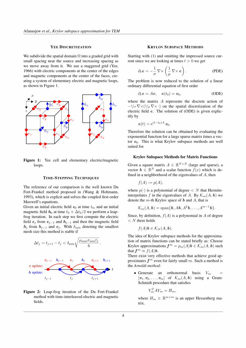
Numerical simulations were carried out for 2 differ-ent conductivity models that include a cuboid-shapedanomaly or a stack of three layers (see Figure 3). Bothmodels are distinguished by substantial topography. Foreach model, we performed calculations on a series ofmeshes with an increasing number of unknowns. All cal-culations were compared to reference solutions that whereobtained on extremely dense FE meshes equipped withsecond-order shape functions (each requiring more than 1million unknowns). Figure 4 shows the median errors rel-ative to the reference solutions together with the25 and75 percentiles (error bars). All calculations where carriedout using first-order shape functions. For the conventionalFE calculations (Figure 4 a), a mixed boundary conditionwas used, whereas for the FE calculations with singularityremoval (Figure 4 c), a dirichlet boundary condition wasconsidered for the non-singular part of the potential.
Figure 3: (a) Cuboid and (b) layered block models. Thesource electrode is located on top of the topographic reliefas indicated by the black arrows.
For the calculations based on the conventional FEM (seeFigure 4 a), the solution for the coarsest mesh shows amedian relative error of≈ 4.7% and≈ 5.5% for thecuboid and layered models, respectively; with an increas-ing number of unknowns the relative error decreases untilit reaches a more-or-less stable value of≈ 1.2 − 1.6%for ≈ 83000 − 86000 unknowns. The error plot for theFE calculations with infinite elements (Figure 4 b) showsquite similar characteristics, but in this case the1.2−1.6%relative errors are achieved with a much smaller numberof unknowns (i.e.≈ 29000− 38000).
The performance of the forward solver is increased sub-stantially when the singularity removal is activated (Fig-ure 4 c). For the cuboid model a relative error of< 1.2%is reached with≈ 7400 unknowns whereas for the layermodel a relative error of< 1.6% is reached with≈ 11000unknowns. Finally, by estimating the singular potentialswith the FM-BEM and applying the infinite elements tocalculate the non-singular potential part, we gain a fur-ther, rather slight increase in the overall solution accuracy(Figure 4 d).
CONCLUSION
Application of BEM-based singularity removal and infi-nite elements improves the efficiency of 3D geoelectri-cal forward modeling substantially. This is primarily dueto the fact that both techniques produce accurate solu-tions with a relatively small number of unknowns. Thisis particularly important, because the computation timerequired for solving the finite-element equations scalesroughly with the square of the number of unknowns.
If the number of unknowns can be kept reasonably low,direct matrix solvers become a very attractive option forsolving the finite-element equations. Once the finite-element system matrix is decomposed, the solutions for
3/4
Blome et al., Advances in 3D geoeletric forward solver
9
M. Blome, H.R. Maurer, 2007, Advances in 3d geoelectric forward solver
Figure 4: Median relative solution errors (in %) for a series of meshes with increasing number of unknowns. For (c) and(d), in which singularity removal has been applied, no local mesh refinement around the source electrodes was used, andfor (b) and (d), in which infinite elements where used, the outer part of the mesh was not discretized.
a multitude of electrode positions can be obtained by sim-ple back substitutions. This will further boost the perfor-mance of our forward solver.
REFERENCES
Astley, R. J., Coyette, J. P., & Cremers, L. (1998, Jan-uary). Three-dimensional wave-envelope elementsof variable order for acoustic radiation and scatter-ing. part ii. formulation in the time domain.JournalOf The Acoustical Society Of America, 103(1), 64–72.
Bettes, P. (1987). A simple wave envelope example.Com-mun. Appl. Numeri. Methods, 3, 77-80.
Coggon, J. H. (1971). Electromagnetic and electricalmodeling by the finite element method.Geophysics,36(1), 132-155.
Dey, A., & Morrison, H. F. (1979). Resistivity modelingfor arbitrarily shaped three-dimensional structures.Geophysics, 44(4), 753-780.
Hackbusch, W., & Nowak, Z. (1989). On the fast ma-trix multiplication in the boundary element methodby panel-clustering.Numerische Mathematik, 54,463-491.
Kost, A. (1994).Numerische methoden in der berechnungelektromagnetischer felder. Springer-Verlag.
Lage, C. (1995).Analyse, Entwurf und Implementation
von Randelementmethoden. Unpublished doctoraldissertation, Inst. f. Prakt. Math., Universitaet Kiel.
Lowry, T., Allen, M. B., & Shive, P. N. (1989). Singular-ity removal: A refinement of resistivity modelingtechniques.Geophysics, 54(6), 766-774.
Mufti, I. R. (1976). Finite-difference resistivity mod-eling for arbitrarily shaped two-dimensional struc-tures.Geophysics, 41(1), 62-78.
Pridmore, D. F., Hohmann, G. W., Ward, S. H., & Sill,W. R. (1981). An investigation of finite-elementmodeling for electrical and electromagnetic data inthree dimensions.Geophysics, 46(7), 1009-1024.
Rücker, C., Günther, T., & Spitzer, K. (2006). Three-dimensional modelling and inversion of dc resis-tivity data incorporating topography - i. modelling.Geophysical Journal International, 166, 495-505.
Sauter, S., & Schwab, C. (2004).Randelementmethoden.Teubner.
4/4
Blome et al., Advances in 3D geoeletric forward solver
10

4th International Symposium on Three-Dimensional ElectromagneticsFreiberg, Germany, September 27–30, 2007
Fast 3D simulation of transient electromagnetic fields by model reduction in thefrequency domain using Krylov subspace projection
R.–U. Börner1, Oliver G. Ernst2, and K. Spitzer1
1TU Bergakademie Freiberg, Institute of Geophysics2TU Bergakademie Freiberg, Institute of Numerical Analysis and Optimization
SUMMARY
We present an efficient numerical method for the simulation of transient electromagnetic fields resulting from magneticand electric dipole sources in three dimensions. The method we propose is based on the Fourier synthesis of frequencydomain solutions at a sufficient number of discrete frequencies obtained using a finite element (FE) approximation ofthe damped vector wave equation, which results after Fourier transforming Maxwell’s equations in time. We assume thesolution to be required only at a few points in the computational domain, whose number is small relative to the numberof FE degrees of freedom. The mapping which assigns to each frequency the FE approximation at the points of interestis a vector-valued rational function known as the transfer function. Its evaluation is approximated using Krylov subspaceprojection, a standard model reduction technique. Computationally, this requires the FE discretization at one referencefrequency and the generation of a sufficiently large Krylov subspace associated with the reference frequency. Once abasis of this subspace is available, a sufficiently accurate rational approximation of the transfer function can be evaluatedat the remaining frequencies at negligible cost. These partial frequency domain solutions are then synthesized to the timeevolution at the points of interest using a fast Hankel transform.
Keywords: Transient electromagnetic modelling, Krylov projection methods
INTRODUCTION
This paper introduces a method based on a FE discretiza-tion in the frequency domain. We avoid the heavy com-putational expense associated with solving a full 3D prob-lem for each of many frequencies by a model reductionapproach. The point of departure is that the transients,which are synthesized from the frequency domain solu-tions, are required only at a small number of receiver lo-cations. After discretization in space, the frequency do-main solution values at the receiver points are rationalfunctions of frequency. Using the model reduction tech-nique of Krylov subspace projection it is possible to ap-proximate this function, known as the transfer function inlinear systems theory, by rational functions of lower or-der. Computationally, the discretized frequency-domainproblem for a suitably chosen reference frequency is pro-jected onto a Krylov subspace of low dimension, yieldingthe desired approximation of the transfer function in termsof quantities generated in the Arnoldi process, which isused to construct an orthonormal basis of the Krylov sub-space. This approximation, the evaluation of which incursonly negligible cost, is then used for all the other frequen-cies needed for the synthesis. After obtaining frequency-domain approximations at the receiver locations for all re-quired frequencies in this way, the associated transients
are synthesized using a fast Hankel transform (cf. (New-man, Hohmann, & Anderson, 1986)). The resulting al-gorithm thus has as its main expense the FE solution atthe reference frequency and the Arnoldi process to con-struct the Krylov space. Since each Arnoldi step requiresthe solution of a linear system with the coefficient matrixassociated with the reference frequency problem, we gen-erate a sparse LU factorization of this matrix using thePARDISO software of Schenk and Gärtner (2004).
THEORY
From the system of Maxwell’s equations we obtain thesecond order partial differential equation
∇× (µ−1∇× e(r, t)) + ∂t σ(r)e(r, t) =−∂t je(r, t) in Ω (1a)
for the electric field, which we complete with the perfectconductor boundary condition
n× e = 0 on Γ,(1b)
at the outer walls of the model. The spatial variable r isrestricted to a computational domain Ω ⊂ R3 bounded by
1/4
4th International Symposium on Three-Dimensional ElectromagneticsFreiberg, Germany, September 27–30, 2007
11

Börner, R.–U. et al., 2007, Fast 3D simulation of transient electromagnetic fields
an artificial boundary Γ, along which appropriate bound-ary conditions on the tangential components of the fieldsare imposed, whereas t ∈ R. The forcing results from aknown stationary transmitter source with a driving currentwhich is shut off at time t = 0, and hence of the form
je(r, t) = q(r)H(−t) (2)
with the vector field q denoting the spatial current patternand H the Heaviside step function. The Earth’s electricalconductivity is denoted by the parameter σ(r). Switch-ing to the frequency domain, we obtain the transformedversion
∇× (µ−1∇×E) + iωσE = q in Ω, (3a)n×E = 0 on Γ, (3b)
of (1a) and (1b) provided that solutions exist for all fre-quencies ω ∈ R. For a given number of discrete frequen-cies, the Fourier representation of the solution e of (1)can be utilized to construct an approximate solution in thetime domain by a Fourier synthesis. Causality allows fora representation of the solution in terms of a sine or co-sine transform of the real or imaginary part of E, resp.(Newman et al., 1986):
e(t) =2π
∞∫0
Re(E)sinωt
ωdω =
2π
∞∫0
Im(E)cos ωt
ωdω.
(4)
In practice, the infinite range of integration is restricted toa finite range and the resulting integrals are evaluated by aFast Hankel Transform (Johansen & Sorensen, 1979). Forthe problems addressed here, solutions for 80 to 150 fre-quencies distributed over a broad spectral bandwidth withf ∈ [10−2, 109] Hz are required to maintain the desiredaccuracy.
SPATIAL DISCRETIZATION
For the solution of boundary value problems in geo-physics, especially for geo-electromagnetic applications,Finite Element (FE) methods offer many advantages. Us-ing triangular or tetrahedral elements to mesh a com-putational domain allows for greater flexibility in theparametrization of conductivity structures without theneed for staircasing at curved boundaries associated withterrain or sea-floor topography. In addition, there is a ma-ture FE convergence theory for electromagnetic applica-tions. Finally, FE methods are much more suitable foradaptive mesh refinement, adding yet further to their effi-ciency.
The Finite Element discretization of (3) finally yields alinear system of equations
(K + iωM)u = f (5)
for the unknown field values expressed as degrees of free-dom u.For a given source vector f determined by the right-handside of (3a), the solution vector u ∈ CN yields an approx-imation of the electric field E we wish to determine.
MODEL REDUCTION
Our goal is the efficient computation of the finite elementapproximation of E in a subset of the computational do-main Ω. To this end, we fix a subset of p N compo-nents of the solution vetor u to be computed.We introduce the discrete extension operator E ∈ RN×p
defined as
[Ei,j ] =
1, if the j-th coefficient has global index i,
0, otherwise.
Multiplication of a coefficient vector v ∈ CN with respectto the finite element basis by E> then extracts the p de-sired components, yielding the reduced vector E>v ∈ Cp
containing the field values at the points of interest.For the solution u, this reduced vector, as a function offrequency, thus takes the form
t = t(ω) = E>(K + iωM)−1f ∈ Cp. (6)
The vector-valued function t(ω) in equation (6) assigns,for each frequency ω, the output values of interest to thesource (input) data represented by the right-hand-side vec-tor f .Computing t(ω) for a given number of frequencies ωj ∈[ωmin, ωmax], j = 1, . . . , Nf , by solving Nf full systemsand then extracting the p desired components from each iscomputationally expensive, if not prohibitive, for large N .To employ model reduction techniques, we proceed byfixing a reference frequency ω0 and rewriting (6) as
t = t(s) = E>[A0−sM]−1f, A0 := K+iω0M, (7)
where we have also introduced the (purely imaginary)shift parameter s = s(ω) := i(ω0 − ω). Setting furtherL := E ∈ RN×p, r := A−1
0 f ∈ CN , and A := A−10 M ∈
CN×N , the transfer function becomes
t(s) = L>(I− sA)−1r. (8)
The transfer function is a rational function of s (and henceof ω), and a large class of model reduction methods con-sist of finding lower order rational approximations to t(s).The standard approach for computing such approxima-tions in a numerically stable way is by Krylov subspace
2/4
Börner et al., Fast 3D simulation of transient electromagnetic fields
12

Börner, R.–U. et al., 2007, Fast 3D simulation of transient electromagnetic fields
projection. For simplicity, we shall consider an ortho-gonal projection onto a Krylov space based on Arnoldi’smethod.Given a matrix C and a nonzero initial vector x, theArnoldi process successively generates orthonormal basisvectors of the nested sequence
Km(C, x) := spanx,Cx, . . . ,Cm−1x, m = 1, 2, . . .
of Krylov spaces generated by C and x, which are sub-spaces of dimension m up until m reaches a unique indexL, called the grade of C with respect to x, after whichthese spaces become stationary. In particular, choosingC = A and x = r, m steps of the Arnoldi process result inthe Arnoldi decomposition
AVm = VmHm+ηm+1,mvm+1e>m, r = βv1, (9)
in which the columns of Vm ∈ CN×m form an orthonor-mal basis of Km(A, r), Hm ∈ Cm×m is an unreducedupper Hessenberg matrix, vm+1 is a unit vector orthog-onal to Km(A, r) and em denotes the m-th unit coordi-nate vector in Cm. In particular, we have the relationHm = V>mAVm.Using the orthonormal basis Vm, we may project the vec-tor r as well as the columns of L in (8) orthogonally ontoKm(A.r) and replace the matrix I−sA by its compressionV>m(I−sA)Vm onto Km(A, r), yielding the approximatetransfer function
tm(s) := (V>mL)>[V>m(I− sA)Vm]−1(V>mr)
= L>m(Im − sHm)−1βe1, (10)
where we have set Lm := V>mL and used the properties ofthe quantities in (9) stated above.Note that computations with large system matrices andvectors with the full number N of degrees of freedom arerequired only in the Arnoldi process, after which the loopacross the target frequencies takes place in a subspace ofmuch smaller dimension m N . As a consequence, thework required in the latter is almost negligible in compar-ison. The most expensive step of the Arnoldi process isthe matrix-vector multiplication with the matrix A−1
0 M.Currently, we compute an LU factorization of A0 in a pre-processing step and use the factors to compute the productwith two triangular solves.
NUMERICAL VALIDATION
To validate of our approach we consider as a model prob-lem a vertical magnetic dipole over a layered halfspace(cf. Fig. 1). The reason for this choice is twofold: First,an analytical solution is available for direct comparison
with the numerical approximation. Second, the huge con-ductivity contrast due to including the air layer in the com-putational domain presents a severe challenge for realisticsimulations. Besides comparison with the analytical so-lution we also check our solution against one obtained bythe Spectral Lanczos Decomposition Method.Fig. 2 shows a comparison of the transient electric fieldat x = 98 m computed with our Arnoldi-based modelreduction approach with that produced by a competingalgorithm for time-dependent TEM-simulation, the Spec-tral Lanczos Decomposition Method (SLDM) of Druskinand Knizhnerman (1988). We observe good agreementof both approximations with the analytic solution. Com-paring the relative errors of both methods, we observe asubstantially larger error of the SLDM approximation es-pecially at early times.
CONCLUSIONS
We have developed an effective algorithm for simulatingthe electromagnetic field of a transient dipole source. Us-ing a Krylov subspace projection technique, the system ofequations arising from the FE discretization of the time-harmonic equation is projected onto a low-dimensionalsubspace. The resulting system can be solved for a widerange of frequencies with only moderate computationaleffort. In this way, computing transients using a Fouriertransform becomes feasible. Numerical comparisons fora model problem have shown the model reduction methodto be more accurate for early simulation times, which isthe more relevant phase of the process in practical appli-cations and inversion calculations.
REFERENCES
Druskin, V. L., & Knizhnerman, L. A. (1988). Spec-tral differential-difference method for numeric so-lution of three-dimensional nonstationary problemsof electric prospecting. Izvestiya, Earth Physics, 24,641-648.
Johansen, H. K., & Sorensen, K. (1979). Fast HankelTransforms. Geophysical Prospecting, 27, 876-901.
Newman, G. A., Hohmann, G. W., & Anderson, W. L.(1986). Transient electromagnetic response of athree-dimensional body in a layered earth. Geo-physics, 51, 1608-1627.
Schenk, O., & Gärtner, K. (2004). Solving unsymmetricsparse systems of linear equations with PARDISO.Journal of Future Generation Computer Systems,20(3), 475–487.
3/4
Börner et al., Fast 3D simulation of transient electromagnetic fields
13

Börner, R.–U. et al., 2007, Fast 3D simulation of transient electromagnetic fields
0 100 200 300200
150
100
50
0
-50
x in m
zin
m
ρ0 = 1014 Ω·m
ρ1 = 100Ω·m
ρ2 = 30Ω·m
ρ3 = 100Ω·m
coil
−2400 2400
−2400
2400
z in m
x in m
Figure 1: Section of the considered conductivity model. The conductive layer is 30 m thick. The dimension of thediscretized model extends to up to ±2400 m in the horizontal and vertical directions.
a)
10−6
10−5
10−4
10−3
10−10
10−8
10−6
10−4
e y in V
/m
ArnoldiSLDM
10−6
10−5
10−4
10−3
−2
0
2
4
6
t in s
rel.
erro
r in
%
ArnoldiSLDM
b)
10−6
10−5
10−4
10−3
10−10
10−5
100
∂ t bz in
µV
/m2
10−6
10−5
10−4
10−3
−20
−10
0
10
20
t in s
rel.
erro
r in
%
ArnoldiSLDM
ArnoldiSLDM
Figure 2: Comparison of transient electric fields (a, top) and associated relative errors (a, bottom) at x = 98 m, andcomparison of transient voltage (∂tbz , b, top) with associated relative errors (b, bottom) for SLDM and Arnoldisolutions at x = 100 m.
4/4
Börner et al., Fast 3D simulation of transient electromagnetic fields
14
4th International Symposium on Three-Dimensional ElectromagneticsFreiberg, Germany, September 27–30, 2007
3D finite element simulation of magnetotelluric fields using unstructured grids
A. Franke, R.-U. Börner and K. SpitzerTU Bergakademie Freiberg, Germany
SUMMARY
The interpretation of an increasing number of three-dimensional data sets requires the simulation of the electromagneticfields in three directions in space. Basing on Maxwell’s equations different boundary value problems can be formulatedin terms of electromagnetic potentials or fields including homogeneous or inhomogeneous boundary conditions.
The formulation of the equation of induction using vector and scalar potentials reduces the number of unknowns tofour instead of six field components. Applying a secondary potential approach allows for the implementation of simplehomogeneous Dirichlet boundary conditions. The boundary value problem is solved by means of the finite elementmethod. We use quadratic Nédélec elements on unstructured tetrahedral grids that are well suited for incorporatingarbitrary model geometries including surface and seafloor topography.
To expand the classic magnetotelluric frequency range towards lower periods (T<10−4 s) used by the Radio and Audio MTmethod for studying shallow conductivity structures displacement currents may need consideration. Beside the electricconductivity and permittivity, the presented finite element approach incorporates the magnetic permeability as modelparameter that can be advantageous e.g. in the case of ore exploration and for studies of the earth’s crust where basalticrocks occur.
Keywords: Magnetotellurics, finite element method, numerical simulation
INTRODUCTION
The propagation of electromagnetic fields is governed byMaxwell’s equations. They can be combined to yield theequation of induction in terms of the vector potential A.The simulation of the secondary potential As minimizesthe computational effort due to its local occurence and thevalidity of homogeneous Dirichlet boundary conditions.
To solve the boundary value problem, we apply a fi-nite element (FE) approach that allows for the efficientparametrization of arbitrary model geometries on unstruc-tured tetrahedral grids. So-called vector or Nédélec ele-ments are well suited to approximate the vector field As
whose tangential components are continuous at elementinterfaces that represent possible jumps in the model pa-rameters. Within one element, the vector potential As isdescribed by polynomials.
The exploration of shallow conductivity structures re-quires the expansion of the classic magnetotelluric (MT)frequency range to shorter periods. Depending on theconductivity distribution the quasistatic approximation ofMaxwell’s equation might not be valid for periods shorterthan 10−4 s. Hence, displacement currents need consider-ation. Furthermore, the presented FE algorithm incorpo-rates the relative magnetic permeability µr as model pa-rameter. By means of model studies we show the influ-
ence of displacement currents and the relative magneticpermeability µr on the apparent resistivity and the phasecomputed analytically for a homogeneous halfspace.
EQUATION OF INDUCTION
Maxwell’s Equations
Assuming the harmonic time dependency eiwt, the behav-ior of the electric and the magnetic fields E and H is gov-erned by Maxwell’s equations of the form
∇×H = j + iωD, (1)∇×E = −iωB, (2)∇ ·D = ρ,
∇ ·B = 0.
The eddy current density j, the displacement current den-sity D, and the magnetic flux density B are combined withthe electromagnetic fields by Ohm’s law and the constitu-tive relations, respectively,
j = σE, D = ε0εrE, and B = µ0µrH, (3)
with the electric conductivity σ, the electric field constantε0 = 8.854 ·10−12As/V m, the relative electric permittivityεr, the magnetic field constant µ0 = 4π · 10−7V s/Am, andthe relative magnetic permeability µr.
1/4
4th International Symposium on Three-Dimensional ElectromagneticsFreiberg, Germany, September 27–30, 2007
15

Franke, A. et al., 2007, 3D FE simulation of MT fields
Electromagnetic Potentials
The divergence-free field B can be expressed as curl ofthe vector potential A
B = ∇×A. (4)
Since
∇× (E + iωA) = 0, (5)
we can introduce the scalar potential V so that
E = −∇V − iωA. (6)
Applying ∇× on eq. (1), inserting Ohm’s law and theconstitutive relations (eqs. 3) yields
∇× µ−1∇×A + (iωσ − ω2ε)A + (σ + iωε)∇V
= 0. (7)
Choosing
A = A−∇Ψ and V = V − Ψ
with the gauge condition Ψ = −iV/ω, we obtain
A = A− i
ω∇V and V = 0 (8)
that determine the same electromagnetic fields as A andV (cf. eqs 4 and 6). Using eq. (8), eq. (7) can be re-arranged into an elliptic second-order partial differentialequation for A
∇× µ−1∇× A + (iωσ − ω2ε)A = 0.
Secondary Potential Approach
The separation of the potential A (in the following: A)into a normal (An) and an anomalous (As) contributionA = An + As results in a differential equation for As
∇× µ−1(∇×As − µsHn) + (iωσ − ω2ε)As
= (σs + iωεs)En (9)
with
ε = εn + εs, σ = σn + σs, µ = µn + µs
and
∇×En = −iωµnHn, ∇×Hn = (σn + iωεn)En.
The normal electromagnetic fields En und Hn are com-puted for a 1D layered halfspace with parameter distribu-tions σn, µn, and εn by Wait’s algorithm (Wait, 1953).
Boundary Value Problem
Considering eq. (9) in the domain Ω with the outer bound-ary ΓD and all internal boundaries Γint for which the con-ditions of continuity for the magnetic field are valid yieldsthe boundary value problem: Find As, so that
∇× µ−1(∇×As − µsHn) + (iωσ − ω2ε)As
= (σs + iωεs)En in Ω, (10)As = 0 on ΓD, (11)
n1 ×H1 − n2 ×H2 = 0 on Γint (12)
with the outward unit normal vectors n1 and n2.
FINITE ELEMENT METHOD
Weak Form
An equivalent formulation of eq. (10) as an inner product(v,u) =
∫Ω
v · u dV with a complex vector-valued testfunction v from the function space V yields the so-calledweak form of the boundary value problem: Find As ∈ U ,so that ∫
Ω
(µ−1(∇×As − µsHn) · ∇ × v
+(iωσ − ω2ε)As · v) dV
+∫
∂Ω
n× (µ−1(∇×As − µsHn) · v dS︸ ︷︷ ︸0
=∫
Ω
(σs + iωεs)En · v dV ∀v ∈ V, (13)
with
U := As ∈ H(curl,Ω) : As ≡ 0 on ΓD,V := v ∈ H(curl,Ω) : v ≡ 0 on ΓD (14)
and
H(curl,Ω) := u ∈ (L2(Ω))3,∇× u ∈ (L2(Ω))3.Applying the boundary conditions in eqs. (11) and (12),the boundary integral in eq. (13) vanishes.
Finite Element Analysis
A discrete approximation Ahs ∈ Uh of As ∈ U arises
from the linear combination of N real vector-valued ba-sis functions φi ∈ Uh (i = 1, ..., N) with the complexcoefficients ai (i = 1, ..., N ):
Ahs =
N∑i=1
aiφi. (15)
Using the discrete test functions vi = φi the boundaryvalue problem can be written as matrix-vector-equation
KAs = L (16)
2/4
Franke et al., 3D FE simulation of MT fields
16

Franke, A. et al., 2007, 3D FE simulation of MT fields
whereas
Ki,j =∫
Ω
(µ−1(∇× φi − µsHn) · ∇ × φj
+ (iωσ − ω2ε)φi · φj)dV,
Li =∫
Ω
(σs + iωεs)En · φi dV. (17)
The domain Ω is decomposed into tetrahedra. On eachtetrahedron piecewise quadratic basis functions φi are as-sumed. Their degrees of freedom are associated with theedges and the faces of the tetrahedral finite element (Fig.1). This type of finite elements, the so-called vector orNédélec elements, is especially suitable for the discretiza-tion of vector fields that show continuity in their tangentialcomponents.
Figure 1: Graphical representation of the degrees of free-dom for quadratic Nédélec elements on a tetrahe-dron.
INFLUENCE OF PERMITTIVITY AND PERMEABILITY
Displacement Currents
Usually, in the simulation of the MT method displace-ment currents are neglected due to the classic frequencyrange not exceeding 1 kHz. To study shallow conductivitystructures, the Radio and Audio MT method applies fre-quencies up to several MHz. Fig. 2 presents the apparentresistivities and phases for a homogeneous halfspace of1000 Ω m (left) and 10000 Ω m (right), respectively, com-puted including (εr = 1, ’o’) and without (quasistatic, ’+’)displacement currents. Significant deviations are obviousfor frequencies higher than 10 kHz especially for the moreresistive halfspace.
Magnetic Rock Properties
So far, the magnetic rock properties have not been incor-porated in electromagnetic applications. However, in ad-dition to the electric conductivity σ, the relative magnetic
permeablity µr might yield geological information espe-cially in the field of ore exploration and studies of regionswhere basaltic rocks occur. Fig. 3 displays the depen-dency of the apparent resistivity and phase on µr. µr > 1results in a higher induced current density (cf. eqs. (2) and(3)) and therefore yields a lower apparent resistivity. Thephase features no anomalous behavior. Note, that there isno frequency dependency at all.
Figure 2: Apparent resistivities and phases for a homoge-neous halfspace of 1000 Ω m (left) and 10000 Ω m(right).
1 1.5 210
2
103
104
µr
ρ a in Ω
m
1 1.5 230
45
60
µr
φ in
deg
rees
Figure 3: Apparent resistivities and phases over µr vary-ing in the range of 1 ≤ µr ≤ 2 for a homogeneoushalfspace of ρ = 1000Ω m.
COMPARISON WITH AN FD APPROACH
We present the simulation results for the 3D-2 COM-MEMI model (Weaver & Zhdanov, 1997) shown in Fig.4. The apparent resistivities ρxy and ρyx as well as thephases φxy and φyx on the earth’s surface at x = 0 com-puted by our FE algorithm and Mackie’s finite difference(FD) code (Mackie, Madden, & Wannamaker, 1993) aredisplayed in Fig. 5.
3/4
Franke et al., 3D FE simulation of MT fields
17

Franke, A. et al., 2007, 3D FE simulation of MT fields
The anomalous resistivities of the two bodies are obvious.The steep slopes in ρyx and φyx (fig. 5, right) are due tothe discontinuity of the normal component of the electricfield whereas the tangential component used to determineρxy and φxy (fig. 5, left) is continuous. The results forboth of the approaches are in good agreement. However,we expect our FE code to yield the more accurate solu-tion concerning the advantages of the FE method approxi-mating electromagnetic fields especially at high parametercontrasts that we have experienced for two-dimensionalsimulations.
x
y
100 Ωm1 Ωm10 Ωm 10 Ωm
0
20 km20 km
40km
z
0 y
0.1 Ωm
100 Ωm
10 Ωm 1 Ωm 100 Ωm 10 Ωm10 km
30 km
Figure 4: COMMEMI model 3D-2.
−50 0 50 10
0
101
102
y in km
ρ xy in
Ωm
FDFE
−50 0 5010
−2
100
102
y in km
ρ yx in
Ωm
FDFE
−50 0 50 20
40
60
80
y in km
φ xy in
deg
rees
FDFE
−50 0 50 20
40
60
80
y in km
φ yx in
deg
rees
FDFE
Figure 5: Apparent resistivities and phases for the COM-MEMI model 3D-2 at a period of T = 100 s.
CONCLUSIONS
The presented secondary potential approach has provento be well suited for the 3D simulation of electromag-netic fields. The local occurence of the anomalous vectorpotential allows for the implementation of homogeneousDirichlet boundary conditions for relatively small mod-els hence minimizing the computational effort in terms ofmemory. However, future efficiency studies will includeformulations of the boundary value problem for the totalpotential and the electromagnetic fields.
The approximation of the magnetic vector potential byquadratic Nédélec elements on unstructured tetrahedralgrids achieves a satisfying accuracy in comparison withother numerical approaches. We intend to improve the ef-ficiency and accuracy of our algortihm by employing anadaptive mesh refinement in connection with an error es-timator function.
Model studies clearly show that the consideration of dis-placement currents is essential for frequencies higher than10 kHz. Additionally, magnetic rock properties, namelyµr > 1, can influence the apparent resistivity and phasesignificantly. This might be of interest with regard to thehypothesis of the second-order magnetic phase transitiontaking place at medium depths of the earth’s crust (Kiss,Szarka, & Prácser, 2005).
REFERENCES
Kiss, J., Szarka, L., & Prácser, E. (2005). Second-ordermagnetic phase transition in the earth. Geophys.Res. Lett., 32(L24310).
Mackie, R. L., Madden, T. R., & Wannamaker, P. E.(1993). Three-dimensional magnetotelluric model-ing using difference equations - theory and compar-isons to integral equation solutions. Geophys., 58,215-226.
Wait, J. R. (1953). Propagation of radio waves over astratified ground. Geophysics, 20, 416-422.
Weaver, J., & Zhdanov, M. (1997). Methods for mod-elling electromagnetic fields. J. Appl. Geophys., 37,133-271.
4/4
Franke et al., 3D FE simulation of MT fields
18

4th International Symposium on Three-Dimensional ElectromagneticsFreiberg, Germany, September 27–30, 2007
Adaptive mesh refinement for 3D electromagnetic modeling
E. Haber1, S. Heldmann1 and D. Oldenburg2
1Emory University2University of British Columbia
SUMMARY
We develop an adaptive mesh refinement technique for the solution of Maxwell’s equations. The method is based onthe discretization of the Maxwell’s equations in its variational form on OcTree meshes. We generate a consistent, secondorder accurate and mimicking discretization and using its mimicking properties we develop a robust solver for the discretesystem.Keywords: Adaptive mesh, Octree mesh, mimicking properties.
INTRODUCTION
The solution of Maxwell’s equations in the quasi-staticregime is important in many practical settings such asgeophysical prospecting, non-destructive testing and eddycurrent simulations. The equations can be formulated as
∇× µ−1∇× ~E + iωσ ~E = iω~s (0.1)
where ~E is the electric field, σ is the conductivity, µ isthe magnetic permeability, ω is the frequency and ~s is asource term. We assume that the equations are given in abounded box with some appropriate boundary conditionson ~E or ∇ × ~E and that the conductivity σ and perme-ability µ have a small number of jumps with compact sup-port. In our typical applications, the frequencies range at1 − 104 Hz, σ ranges from 10−4 − 102 S/m and µ/µ0
ranges from 1−10 (see [14]). For ease of presentation weassume Perfectly Magnetic Conductor (PMC) boundaryconditions which read
~n× ~H = 0 (0.2)
although other boundary conditions can be considered.The solution of Maxwell’s equations is very challengingeven for the static case. There are three main sources ofdifficulties. First, the curl operator has a nontrivial richnull space. Second, in our applications, the conductivitycan have large jumps and finally, boundary conditions atinfinity needs to be dealt with.Common algorithms for Maxwell’s equations use finiteelement or finite volume/difference approximations, andhave been extensionally studied in the last decade; see forexample [4, 6, 9, 8, 1, 12]. Nevertheless, non of the abovework deal with adaptivity.
In this paper we develop an adaptive finite volume tech-nique for the solution of Maxwell’s equations. First,we develop a mimicking discretization technique forMaxwell’s equations on an OcTree grid. Second, usingthe mimicking properties of our discretization, we modifyour previous work [4] that builds on Helmholtz decompo-sitions of the discrete fields in order to stabilize the equa-tions and avoid the null space of the curl. This modifica-tion yields a fast and stable solver for the discrete system.The use of OcTrees in order to locally refine grids in PDEsis not new. In particular it has been used in flow throughporous media and fluid dynamics [2, 3] where cell cen-ter OcTrees with even and odd number of locally refinedgrids are considered. Recently, there has been renewedinterest in local refinement and their applications to com-putational fluid dynamics and computer graphics [11]. Inparticular, the work of Losasso et-al on OcTree discretiza-tion of Poisson equation demonstrates that second orderaccuracy can be obtained. A more general framework forPoisson equation was recently studied in [10]. Other rele-vant work to ours is the recent work of [13] on the solutionof Maxwell’s equations in the hyperbolic regime where nolarge jumps in the coefficients are present.The paper is organized as follows. In section we de-rive the discretization of Maxwell’s equations, reformula-tion of the discrete system and develop an effective linearsolver. In Section we perform numerical experiments thatdemonstrate the effectiveness of our approach and sum-marize the paper.
DISCRETIZATION OF MAXWELL’S EQUATIONS ONOCTREE GRIDS
OcTree discretization
1/4
4th International Symposium on Three-Dimensional ElectromagneticsFreiberg, Germany, September 27–30, 2007
19

Haber, E. et al., 2007, Adaptive mesh for 3D EM . . .
S(:, :, 1) =(
2 0 1 10 0 1 1
)
S(:, :, 2) =(
0 0 1 10 0 1 1
)
Figure 1: An OcTree and its representation as 2× 4× 2 (sparse) array
Figure 2: Discretization of the electric field on the edges of the cell
We consider a fine underlying orthogonal mesh of size2m1 × 2m2 × 2m3 with mesh size h. Our grid is com-posed of m cube cells of different sizes. Each cell canhave a different length which is a power of 2. To make thedata structure easier and the discretization more accuratewe allow only a factor of 2 between adjacent cells. Thedata is then stored as a sparse array. The size of each cellis stored in the upper left corner of the array. This allowsus to quickly find neighbors which is the major operationin the discretization process. This data structure is closelyrelated to the one suggested in [7]. An example of a small3D grid is plotted in Figure .
Discretizing Maxwell’s equations in variational form
In order to discretize Maxwell’s equations on the OcTreegrid, we view the system as a variational problem. It is
possible to show [9] that the electric field ~E is the station-ary point of the following functional
J =∫
Ω
12µ
(∇× ~E)2 +iωσ
2~E2 − iω~s · ~E dx(0.3)
Rather than discretizing Maxwell’s equations directly wediscretize the variational form (0.3). First, we rewrite theintegral as
J =∫
Ω
(·)dx =∑
j
∫Ωj
(·)dx
where Ωj is an OcTree cell in our grid. Thus, the problemis reduced to approximating the integral over each cell.Similar to Yee discretization [15] we place the discrete ~Eon the edges of each cell, see Figure .
Using this discretization is it easy to approximate ∇× ~Eon the face of each box with second order accuracy, usingshort finite differences. This can be written as
(∇× ~E)cell faces = Ce +O(h2)
where C is a finite difference matrix which approximatesthe ∇× and e is a discrete approximation to ~E. Squar-ing and averaging to cell center we obtain a second order
2/4
Haber et al., Adaptive mesh refinement for 3D electromagnetic modeling
20

Haber, E. et al., 2007, Adaptive mesh for 3D EM . . .
approximation to the integral (0.3) which has the form
Jh =12e>
(C>MC + iωS
)e− iωs>e (0.4)
The stationary point of Jh can be found by solving thelinear system(
C>MC + iωS)e = iωs (0.5)
Solving the discrete systems of equations
In order to solve the linear system we use the mimeticproperties of our discretization. It is easy to show [5] thatthe discretization of the curl described above yields is or-thogonal to the conservative discretization of the gradientoperator. Such discretization is obtained by a short differ-ence of the nodes of the OcTree cells.Let G be the gradient matrix. Then we have CG = 0mimicking the equation ∇× ∇ = 0. We can now use thediscrete Helmholtz decomposition. Defining the vectorsa, φ
e = a + Gφ
0 = G>a.
We now substitute the decomposition in (0.5) and use thesame arguments as in [4] to obtain the system(
C>MC + GM0G> + iωS iωSG
G>S G>SG
) (aφ
)=
(s
G>s
)(0.6)
where M0 is a diagonal matrix with the value of µ of eachcell on its diagonal. While the original system suffersfrom ill-conditioning due to the null-space of the curl themodified system is better conditioned. It is therefore pos-sible to develop efficient algorithms such as multigrid forthe solution of this system (see [5]).
NUMERICAL EXPERIMENTS
As a model problem we simulate the electromagnetic re-sponse that evolves from the shape presented in Figure 3(left). The shape is made from a cone with a conductivityof σ1 berried in a half space with conductivity σ0. Insidethis cone there is a cylinder with conductivity σ2 = 10σ1.Our goal is to solve the electromagnetic problem for arange of σ1’s and for low frequencies ω.
Figure 3: The model and its OcTree representation
The OcTree used for the discretization of our object isplotted in Figure 3 (right).We solve the problem using BiCGStab solver precondi-tioned with a multigrid method. We compare the accuracyto uniform-grid solution where our discretization is equiv-alent to the usual Yee’s method. The accuracy of our so-
lution was always within 1% of the uniform grid solution.Nevertheless, our approach reduce the size of the problemin a factor of roughly 20, yielding substantially smallersystems to solve and thus give an order of speed to thecalculations.
σ1/σbg #iter 16 32 128102 3.5 3.5 3.5104 3.5 3.5 3.5
Table 1: BiCGStab iterations for Maxwell’s equations. Each iteration requires 2 preconditioning steps (ω = 103)
3/4
Haber et al., Adaptive mesh refinement for 3D electromagnetic modeling
21

Haber, E. et al., 2007, Adaptive mesh for 3D EM . . .
REFERENCES
[1] D. Alumbaugh, G. Newman, L. Prevost, and J.N.Shadid. Three dimensional wideband electromag-netic modeling on a massively parallel computers.Radio Science, 31:1–23, 1996.
[2] M. Edwards. Elimination of adaptive grid interfaceerrors in the discrete cell centered pressure equa-tion. Journal of Computational Physics, 126:356–372, 1996.
[3] R.E. Ewing, R.D. Lazarov, and P.S. Vassilevski. Lo-cal refinement techniques for elliptic problems oncell-centered grids i, error analysis. Math. Comp.,56:437461, 1991.
[4] E. Haber and U. Ascher. Fast finite volume simu-lation of 3D electromagnetic problems with highlydiscontinuous coefficients. SIAM J. Scient. Comput.,22:1943–1961, 2001.
[5] E. Haber and S. Heldmann. An octree multigridmethod for quasi-static maxwell’s equations withhighly discontinuous coefficients. Journal of Com-put. Phys., page to appear, 2007.
[6] R. Hiptmair. Multigrid method for Maxwell’s equa-tions. SIAM J. Numer. Anal, 36:204–225, 1998.
[7] G. R. Hjaltason and H. Samet. Speeding up con-struction of quadtrees for spatial indexing. TheVLDB Journal, 11:109–137, 2002.
[8] J.J. Hu, R.S. Tuminaro, P.B. Tuminaro, C.J. Garasi,and A.C. Robinson. Towards an h-independent al-
gebraic multigrid method for maxwell’s equation.SIAM J. on Sci. Comp., To Appear, 2006.
[9] J. Jin. The Finite Element Method in Electromagnet-ics. John Wiley and Sons, 1993.
[10] K. Lipnikov, J. Morel, and M. Shashkov. Mimeticfinite difference methods for diffusion equations onnon-orthogonal amr meshes. Journal of Computa-tional Physics, 199:589–597, 2004.
[11] F. Losasso, R. Fedkiw, and S. Osher. Spatially adap-tive techniques for level set methods and incom-pressible flow. Computers and Fluids, 35:457–462,2006.
[12] T. Madden and R. Mackie. Three-dimensional mag-netotelluric modeling and inversion. Proceedings ofthe ieee, 77:318–321, 1989. n2.
[13] Z.J. Wang, A.J. Przekwasb, and Y. Liuc. A fv-td electromagnetic solver using adaptive cartesiangrids. Computer Physics Communications, 148:17–29, 2002.
[14] S.H. Ward and G.W. Hohmann. Electromagnetictheory for geophysical applications. Electromag-netic Methods in Applied Geophysics, 1:131–311,1988. Soc. Expl. Geophys.
[15] K.S. Yee. Numerical solution of initial boundaryvalue problems involving Maxwell’s equations inisotropic media. IEEE Trans. on antennas and prop-agation, 14:302–307, 1966.
4/4
Haber et al., Adaptive mesh refinement for 3D electromagnetic modeling
22

4th International Symposium on Three-Dimensional Electromagnetics Freiberg, Germany, September 27−30, 2007
1/4
The effect of a horizontal thin axial metallic conductor in Marine EM
T. Hanstein1, S.L. Helwig1, G.Yu1, K.M. Strack1, R. Blaschek2, A. Hördt2
1KMS Technologies – KJT Enterprises Inc, Houston, USA 2Technical University Braunschweig, Germany
SUMMARY The frequency and time domain response of a buried axial conductor is simulated with an analytical approach. Pipelines or communication cables are thin and long elongated objects, which are highly conductive because of their metallic parts. The influence on electromagnetic soundings can be very strong and is here analyzed. The thin metallic structure is described by the current generated in the cylinder. The electromagnetic field of this current is determined by several impedance conditions in different steps. First it is assumed that the cylinder is a perfect conductor, this external impedance condition takes into account that the electric fields are zero inside of the cylinder. Although the cylinder is perfect conductive, the current generated by the external electric field is finite and depends beside of the geometry on the conductivity of the environment. The next step is the internal impedance condition which considers the finite conductivity of the metal. Even if the conductivity of metal is 5 to 6 orders higher than the conductive of the sea water, this internal impedance is important and controls the correct decay of the secondary fields in time domain. For a perfect conductor the decay is one order slower than for a realistic conductor. The impedance condition is also expended for a cylindrical shell, which yield to a better description of a pipeline. An further impedance condition can be added, which considers the effect of an isolating coating sheet which covers the cylinder. This analytical approach describes the galvanic effect of this 2-d structure, which is the strongest contribution, and has a large influence on the electromagnetic soundings. The vortex currents which are also analyzed must be closed current loops inside the cylinder and therefore the secondary fields decay one order faster with the distance. Numerical techniques as finite differences with a staggered grid and finite elements are also applied to this kind of problem and compared with the analytical approach. Keywords: Marine EM, axial conductors
INTRODUCTION Marine controlled-source electromagnetic method becomes very important technique for finding hydrocarbons. Beside the exploration for new reservoirs, the method has been applied in production oil fields. Pipelines or communication cables can cross such survey areas. These thin and long elongated objects are highly conductive because of their metallic parts, and the influence on electromagnetic soundings can be very strong and is here analyzed. The high contrast in conductivity to the surrounding environment and the length with a small cross section is challenging for standard numerical techniques. Therefore we have chosen the analytical approach
based on the work from Tsubota and Wait (1980) for an infinite long horizontal cylinder embedded in the conductive medium.
THEORY The electromagnetic fields are separated into two parts:
anan HHHEEE +=+= and
The normal part consists of the fields in a layered medium generated by an external transmitter, e.g. a grounded dipole. The anormal part describes the field in the medium generated by the current in the cylindrical conductor. The current is determined by an impedance condition at the boundary of the cylinder.
4th International Symposium on Three-Dimensional ElectromagneticsFreiberg, Germany, September 27–30, 2007
23

Hanstein, T. et al., 2007, The effect of a horizontal thin axial metallic conductor in Marine EM
2/4
Therefore the fields and the current is transformed along the strike direction into wave number domain, so that the interaction between current and field become a product. We define the Fourier Transform analog to the Laplace Transform
( ) ( )
( ) ( )∫
∫∞
∞−
∞
∞−
−
=
=
ββπ
β
β
β
deIxI
dxexII
xi
xi
~21
~
The field are first simulated in the frequency domain and excited with eiωt, and then transformed to time domain.
Full space In a full space the anomal fields of a line source have a rotation symmetry around the x-axis. There is no magnetic field component parallel to the current. Therefore the fields can be described by a vector potential Ax with a single component along the strike direction. The electrical field is determined by the Faraday law as far as the gradient of a scalar potential. With the Lorentz gauge condition the vector potential meets the inhomogeneous Helmholtz equation
( ) ( ) ( ) ( ).022 zzyxIAk x −−=−∇ δδ
The solution can be given by a horizontal Fourier Transformation into the wave number domain. Some useful integral identities are given in Gradstein (3.354.5, 3.961.2 and 6.726.4). The vector potential for the field of a line current in the full space at the depth z0 is
( )
( )
( ) ( )
( ) ( ) .
~4
1
~8
1
,,
2202
20
∫
∫ ∫
∫ ∫
∞
∞−
∞
∞−
∞
∞−
∞
∞−
∞
∞−
−−
′−′=
+=
=
=
dxxxGxI
dekrKI
ddeeeI
zyxA
xi
xiyizz
x
βββπ
βαλβ
π
β
βλα
In these equations α2=β2+λ2+k2 and k2=iωμσ are the wave numbers for space and frequency, K0 is the modified Bessel function and r2 = y2 + (z-z0)2 the radial distance from the current. The last integral show that in the space domain the solution is a convolution of the current with the Green function of a full space
( ) .zzyxR
eR
zyxG kR
20
222with
4
1),,(
−++=
= −
π
TE- and TM-mode for the anomal field Tsubota and Wait (1980) defined the potential for the line source by two Hertz potential along the strike direction. This yield to coupled system of equations for the boundary condition of a horizontal layer. Here we define two potentials in the vertical direction, so that the field are decoupled in two modes. Similar to Ward and Hohman (1988) divergence free fields can be separated in poloidal and toroidal fields
( ) ( )( ) ( )ME
ME
zzjzzB
σϕϕσ
μσϕϕˆˆ
ˆˆ
×∇×∇+×−∇=
×∇+×∇×∇=
&r
r
The fields are separated in two modes, TE and TM, which are decoupled. The potentials are coupled by the line source and only together they yield to physical fields.
( ) ( )
( ) ( )∫ ∫
∫ ∫∞
∞−
∞
∞−
∞
∞−
∞
∞−
=
=
λβλβπ
ϕ
λβλβπ
ϕ
λβ
λβ
ddeezfzyx
ddeezfzyx
yixiMM
yixiEE
,,4
1,,
,,4
1,,
2
2
The vertical magnetic component is only in the TE-mode, and the TE-potential can be found by comparing
( ) ( ) ( )zyxAzyxH Eyyxxxyz ,, 1,, 22 ϕμ
∂+∂−=−∂=
( ) ( ) ( )zfAizH Exz ,, 1~,,~ 22 λβλβμ
λλβ +=−=
( ) ( ) .2
~,,
0
22 αλββμλλβ
α zz
EeIizf
−−
+−=
The TM-mode can be determined by the horizontal component of the magnetic field which is a combination of both modes
( ) ( )zyxAzyxH MxEyzxzy ,, 1,, 2 ϕσϕμ
∂−∂=∂=
( ) ( ) ( )
( ) ( ) .2
)(~
2
~,,~
0
0
2202
0
Mzz
zzy
fieIzzsign
eIzzsignzH
βσλβ
βλ
βλβ
α
α
−+
−−=
−−=
−−
−−
( ) ( ) ( ).
2
~,, 00
22zz
M ezzsignIizf −−−
+−= α
σλβββλβ
The impedance condition The unknown current in the metallic conductor is determined by a boundary condition on the surface of the cylinder. The external fields are forcing the current. We are assuming that the electric field parallel to the cylinder axis gives the main contribution to the current.
Hanstein et al., The effect of a horizontal thin axial metallic conductor in marine EM
24

Hanstein, T. et al., 2007, The effect of a horizontal thin axial metallic conductor in Marine EM
3/4
The cross section of the conductor is so small that Ex is rotation symmetry. Several impedance conditions are applied for estimating the current. First we assume that the cylinder is perfect conductor. Therefore the electrical field vanishes inside the conductor. The tangential electrical field is continuous and on the boundary
0≡+= ax
nxx EEE
On the boundary the anomal field is opposite to the external normal field and can be presented by the TE and TM potentials in the wave number domain
( ) ( ) ( )[ ]MzEax
nx fifiiEE ∂+−−=−= βλωββ ~~
For an perfect conductor the external normal field an be expressed by the product of an external impedance Ze and the current
( ) ( ) ( ).~ ~ βββ IZE enx =
Although the cylinder is a perfect conductor the current flow in the cylinder is finite and depends on the radius of the cylinder and the conductivity of the environment. For the full space the impedance can be presented in closed form
( ) ( )220
22
2krKkZ ae +
+= β
πσββ .
The current is flowing on the surface of the perfect conductor. The next step is to consider the finite conductivity of a real conductor. The forces ares are the anomal fields. The relation between electric and magnetic anomal field yield to an internal impedance. The current is replaced by the magnetic field on the boundary by the Ampere law
( ) ( ) ( ) ( ) ( )βπββββ HrZIZE aiiax
~2~~ == .
For fields with this rotation symmetry and the strike direction the magnetic field can be expressed by the electric field
( ) ( )ββσ
β axr
aa Ek
H ~~22 ∂
+−=Φ
.
The electric field satisfy the Helmholtz equation in cylinder geometry and the solution for the inside region is the modified Bessel function of the first kind
( ) ( ) ( ).~0 βββ ICE a
x =
Since the ratio of electrical and magnetic field is of interest, the unknown and arbitrary function C(β) will cancel. The internal impedance with the finite conductivity is
( ) ( )( ).2 22
1
220
22
aa
aa
aai
krI
krIr
kZ
+
++=
β
βσπ
ββ
The internal impedance is zero for the limit of a perfect conductor. But even with the very high conductivity of metals this internal impedance is important for the proper decay of the signal in time domain. The internal impedance can be extended straight forward for a cylindrical shell when the core is nonconductive. The last impedance condition considers the case, when the cylinder has a resistive coating sheet. For this case the solution for the electric field Ex need both modified Bessel function for the coating sheet
( ) ( ) ( )( ) ( )22
0
220
~
M
Max
krKB
krIAE
++
+=
ββ
βββ
Since the conductivity of the coating is low, the Bessel function can be approximated by the low argument limit
( ) ( ) ( ) ( )22ln ~M
ax krBAE ++= ββββ .
In the resistive and thin sheet is the current close to zero and the changes in the tangential and continuous electric field is the difference over the thickness. This gives following internal impedance for the coating
( ) ( )( ) ⎟⎟
⎠
⎞⎜⎜⎝
⎛==
=
=Φ a
M
MM
rr
rra
ax
M rr
rHrE
ZM
a
ln2~2
~ 2
σπβ
βπβ
β .
This impedance is independent of the frequency. A complete isolation yield to an infinite impedance and therefore no current will flow in the cylinder. In reality there will be induced currents in a totally isolated conductor due to time variations in the external magnetic field. These induced current are closed field lines, because they are generated by a 3 dimensional extern source. These are effects of higher order, since the currents inside the cylinder flowing in opposite directions and decay one order faster with distance. The total impedance is the summation of external and all internal impedances, because they are quasi serial connected.
Normal fields in layered media The normal fields in a layered media, generated by an extern source as a grounded electrical dipole or an inductive source as a magnetic dipole, has to be Fourier transformed along the cylinder axis – the strike direction. Especially the extern tangential electric field combined with the impedance of the cylinder gives the current inside the conductor.
Hanstein et al., The effect of a horizontal thin axial metallic conductor in marine EM
25

Hanstein, T. et al., 2007, The effect of a horizontal thin axial metallic conductor in Marine EM
4/4
In space domain the fields are expressed by Hankel Transformation integral
( ) [ ] ( )∫∞
+=0
220 . ...,, κκϕ dyxJzyx
The kernel function […] is dependent on the 1-d conductivity model and the wave number κ2=β2+λ2. The Fourier Transform is only applied to the Bessel function J0. The Bessel function J1 can be transformed to J0 by partial derivatives. Since the function is even in x, only a cosine transform is necessary. With the integral given in Gradstein (6.677.3) a general expression can be given
( ) [ ] ( )∫∞
=0
.cos ...2,,~κλλβϕ dyzy
The remaining integral is the Fourier Transform along the y-direction.
Figure 1: DC electric field line of a grounded electrical dipole in full for the total field (solid line) and the undisturbed normal field. The cylinder is a perfect conductor.
CONCLUSIONS
The frequency and time domain response of a thin horizontal axial conductor is simulated with an analytical approach. The anomal fields of this conductor can be simulated by a current line source. The current is varying in space, so that the current can enter and exit the cylinder along the axis (Figure 1). This channelling effect is generated by the galvanic part of the induction process, and occurs if the external medium is conductive. Figure 1 shows the distortion of the DC electric field lines in the presence of a perfect conductor. The cross marks the position for the time derivative of the vertical magnetic field in Firgue 2. The dashed lines and the crosses are negative contributions to the normal field and the solid lines are positive. At late times the positive amplitudes decay with typical power decay of t-5/2 as the normal fields in the layered media. The conductivity of the cylinder is
varied from 1 MS/m to infinity. The perfect conductor decays with 3/2-power law and the amplitude is always negative.
Figure 2: Induced voltage of the anomal vertical magnetic field for different internal impedances. Lines are solution with the impedance condition and the symbols are the exact solution in a full space.
REFERENCES
Gradstein, I.S. & Ryshik I.M. (1981). Tables of series, products, and integrals. Harri Deutsch, Thun. Tsubota, K. & Wait, J.R. (1980). The frequency and time domain response of a buried axial conductor. Geophysics,45, 941-951. Wait, J.R. & Umashankar, K.R. (1978). Analysis of the earth resistivity response of buried cables. Pageoph, 117, 711-742. Ward, S.H. & Hohmann, G.W. (1988). Electromagne-tic theory for geophysical applications, in Nabighian, M.N., Electromagnetic methods in applied geophysics theory, Tulsa.
Hanstein et al., The effect of a horizontal thin axial metallic conductor in marine EM
26

4th International Symposium on Three-Dimensional Electromagnetics Freiberg, Germany, September 27−30, 2007
Three Dimensional Finite Element Analysis of Electromagnetic Induction in Geologic Formations
Containing Magnetic Bodies
Souvik Mukherjee1, and Mark E. Everett1
1 Department of Geology and Geophysics, Texas A&M University, College Station, TX 77843
SUMMARY
The surge of interest in environmental problems has opened new avenues and scope for the application of the controlled source electromagnetic (CSEM) method to near surface geophysical problems. Whilst most naturally occurring geologic materials are non magnetic, near surface geophysics often deals with steel objects such as drums, pipes, sheets, concrete reinforcement bars, and unexploded ordnance (UXO). These materials, in addition to having a high conductivity, sometimes have significant relative magnetic permeability. An additional challenge is introduced when such targets are embedded in a weakly ferrimagnetic medium. The goal of this work is to develop a numerical forward modeling code for computing the CSEM induction response of such ferromagnetic bodies, embedded in a weakly ferrimagnetic medium, using the low frequency approximation of Maxwell’s equations and a finite element method using vector edge basis functions to solve the resulting “diffusive” differential equations. The coupled potential formulation gives rise to an ungauged “curl – curl” formulation leading to an asymmetric coefficient (stiffness) matrix and the possibility of numerically unstable spurious modes. We formulate the problem in terms of edge basis vectors to counter this.
Keywords: Ferrimagnetic, Ferromagnetic, edge elements, three dimensional finite elements, UXO detection.
INTRODUCTION
The surge of interest in environmental problems has opened new avenues and scope for the application of the controlled source electromagnetic (CSEM) method to near surface geophysical problems. While complicated geology can make the interpretation of CSEM data difficult, an additional challenge is introduced in near surface geophysics by the presence of man made debris, such as buried pipes, drums, and unexploded ordnance (UXO).
Whilst most naturally occurring geologic materials are non magnetic, near surface geophysics often deals with steel objects such as drums, pipes, sheets, concrete reinforcement bars, and unexploded ordnance (UXO). These materials, in addition to having a high conductivity, sometimes have significant relative magnetic permeability in the range of 200 – 500 (Eskola et al, 1999). Although there have been efforts at characterizing the CSEM response of buried targets in terms of analytic solutions (eg. Grant and West, 1965), explicit numerical modeling analysis of such targets embedded within an
inhomogeneous geological host is sparse in geophysical literature.
FINITE ELEMENT FORMULATION
We solve for the electric and magnetic fields induced due to a current loop source placed at the air earth interface (AEI) inside a rectangular earth. We define a double half space with an upper non conducting region, Ωn having non conducting boundaries Γn, and a lower conducting region, Ωc having non conducting boundaries Γc. The interface between the two is defined as Γnc (Figure 1). We define a scalar magnetic potential φ in air, while in earth we define a vector magnetic potential A and a scalar electric potential, V. Following Badea et al (2001), it is possible to avoid explicit modeling of the source geometry by defining a set of primary potentials as the response of a background model, usually a homogeneous or layered earth due to excitation by the source. The primary potentials have a well defined analytic or semi analytic solution everywhere in the FE domain. We can thus define,
sVpVV
sp
+=
+=
+=
sApAAφφφ
1/4
4th International Symposium on Three-Dimensional ElectromagneticsFreiberg, Germany, September 27–30, 2007
27

Mukherjee,S and Everett, M.E, 2007,Three Dimensional Finite Element Analysis of Ferromagnetic Targets.
Figure 1: A schematic representation of the earth model excited by an electromagnetic loop source.
Here, the subscript p denotes the primary potential and s denotes the secondary potential in each case. Furthermore, in Ωn,
B−=∇φ . While in Ωc,
BA =×∇ and ( ) EA =∇+− Viω With appropriate choices of the primary potentials, we have the following governing equations: In Ωn, we have,
02 =∇ sφ (1) While in Ωc, we have
( ) ( )( )2psps
pss
iVi
Vii
AAAA ss
ωσωσ
υωσωσυ
−∇−
×∇×−∇=∇++×∇×∇
And
( ) ( ) ( )3pspsss VV ∇+⋅∇=∇+⋅∇− ωσωσωσωσ iAiiAiWhere σ = σp + σs
µ = µp + µs 1/µ = υ = υp + υs and υp = 1/µpHere, the subscript p in each equation denotes respectively, the primary conductivity, the primary permeability, and the primary reluctivity distribution in
the background model, while the subscript s denotes the secondary of each of these physical quantities.
We can discretize the domain such that it is made up of tetrahedral elements following the discretization scheme of Liu and Joe (1996). We use nodal basis functions to describe Φs and Vs and edge basis functions to describe As. For Ωn, above the AEI, let
( ) ni
N
iis pr ψφ ∑
=
=1
1
Where ip = Unknown scalar coefficients.
And, niψ = Scalar nodal basis functions in but not
including nΩ
nΓ , or, ncΓ . In Ωc, below the AEI, but not including Γc, or Γnc, As can be expressed as
( ) iαA ∑=
=M
iis ar
1
Where ia = Unknown scalar coefficients.
And, iα = Vector edge basis functions in but not
including cΩ
nΓ , cΓ , or, ncΓ . The scalar electric potential, Vs, is also defined inside cΩ as
( ) ci
N
iis brV ψ∑
=
=12
1
Where ib = Unknown scalar coefficients.
And, ciψ = Scalar nodal basis functions in but not
including cΩ
nΓ , cΓ , or, ncΓ . With the appropriate choice of test functions, equations (3), (4), and (5) can be discretized as
( ) ( )40,1
1
=∇∇Ω
=∑ n
ni
nj
N
iip ψψ
Γn
ΩnHorizontal current loop with surface
current density k Γn Γn
Γnc
ΓcΓc Ωc
Γc
2/4
Mukherjee et al., Three dimensional finite element analysis of ferromagnetic targets
28
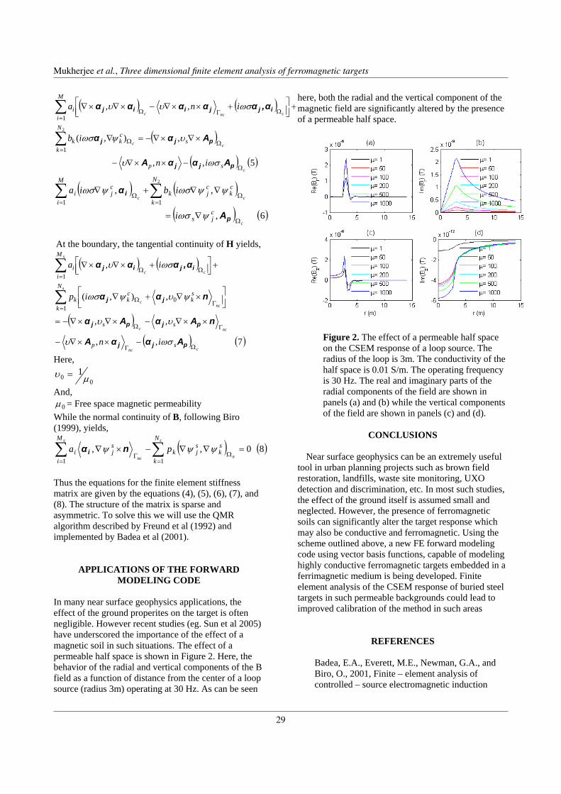
Mukherjee,S and Everett, M.E, 2007,Three Dimensional Finite Element Analysis of Ferromagnetic Targets.
( ) ( )
( )
( ) ( )5,,
,),(
,,
2
1
1
c
cc
cncc
sp
sck
N
kk
M
ii
in
ib
ina
Ω
ΩΩ=
=ΩΓΩ
−××∇−
×∇×∇−=∇
+⎥⎦⎤
⎢⎣⎡ +××∇−×∇×∇
∑
∑
pjj
pjj
ijjiij
AααA
Aαα
α,ααααα
ωσυ
υψωσ
ωσυυ
( ) ( )( ) ( )6,
,,2
11
c
cc
cjs
ck
cj
N
kk
cj
M
ii
i
ibia
Ω
Ω=
Ω=
∇=
∇∇+∇ ∑∑p
i
A
α
ψωσ
ψψωσψωσ
At the boundary, the tangential continuity of H yields,
( ) ( )
( )( ) ( )7,,
,,
,),(
,
10
1
cnc
ncc
s
ncc
s
cc
sp
ss
N
k
sk
ckk
M
ii
in
ip
ia
ΩΓ
ΓΩ
=ΓΩ
=ΩΩ
−××∇−
××∇−×∇×∇−=
⎥⎦⎤
⎢⎣⎡ ×∇+∇
+⎥⎦⎤
⎢⎣⎡ +×∇×∇
∑
∑
pjj
pjpj
jj
ijij
AααA
nAαAα
nαα
α,ααα
ωσυ
υυ
ψυψωσ
ωσυ
Here,
00
1µυ =
And, 0µ = Free space magnetic permeability
While the normal continuity of B, following Biro (1999), yields,
( ) ( )80,,11
=∇∇−×∇Ω
==Γ ∑∑ n
ss
nc
sk
sj
N
kk
M
i
sji pa ψψψ nα i
Thus the equations for the finite element stiffness matrix are given by the equations (4), (5), (6), (7), and (8). The structure of the matrix is sparse and asymmetric. To solve this we will use the QMR algorithm described by Freund et al (1992) and implemented by Badea et al (2001).
APPLICATIONS OF THE FORWARD MODELING CODE
In many near surface geophysics applications, the effect of the ground properites on the target is often negligible. However recent studies (eg. Sun et al 2005) have underscored the importance of the effect of a magnetic soil in such situations. The effect of a permeable half space is shown in Figure 2. Here, the behavior of the radial and vertical components of the B field as a function of distance from the center of a loop source (radius 3m) operating at 30 Hz. As can be seen
here, both the radial and the vertical component of the magnetic field are significantly altered by the presence of a permeable half space.
Figure 2. The effect of a permeable half space on the CSEM response of a loop source. The radius of the loop is 3m. The conductivity of the half space is 0.01 S/m. The operating frequency is 30 Hz. The real and imaginary parts of the radial components of the field are shown in panels (a) and (b) while the vertical components of the field are shown in panels (c) and (d).
CONCLUSIONS
Near surface geophysics can be an extremely useful
tool in urban planning projects such as brown field restoration, landfills, waste site monitoring, UXO detection and discrimination, etc. In most such studies, the effect of the ground itself is assumed small and neglected. However, the presence of ferromagnetic soils can significantly alter the target response which may also be conductive and ferromagnetic. Using the scheme outlined above, a new FE forward modeling code using vector basis functions, capable of modeling highly conductive ferromagnetic targets embedded in a ferrimagnetic medium is being developed. Finite element analysis of the CSEM response of buried steel targets in such permeable backgrounds could lead to improved calibration of the method in such areas
REFERENCES
Badea, E.A., Everett, M.E., Newman, G.A., and Biro, O., 2001, Finite – element analysis of controlled – source electromagnetic induction
3/4
Mukherjee et al., Three dimensional finite element analysis of ferromagnetic targets
29

Mukherjee,S and Everett, M.E, 2007,Three Dimensional Finite Element Analysis of Ferromagnetic Targets.
using Coulomb – gauged potentials, Geophysics, 66, pages 786 – 799. Biro, O., 1999, Edge element formulations of eddy current problems, Computer methods in applied mechanics and engineering, 169, pages 391 – 405. Eskola, L., Puranen, R., and Soininen, H., 1999, Measurement of magnetic properties of steel sheets, Geophysical Prospecting, 47, pages, 593 – 602. Everett, M.E., 2006, Finite element analysis of shallow – water marine controlled – source electromagnetic signals for hydrocarbon exploration, MARELEC – 2006: Marine Establissement, Amsterdam, Netherlands. Freund, R. W., Golub, G.H., and Nachtigal, N.M., 1992, Iterative solutions of linear systems, Acta Numerica edited by A. Iserles, Cambridge University Press, pages 57 – 100. Grant, F.S., and West, G.F., 1965, Interpretation theory in applied geophysics, McGraw – Hill, 584 pages. Liu, A., and Joe, B., 1996, Quality local refinement of tetrahedral meshes based on 8 – subtetrahedron subdivision, Mathematics of Computation, 65, 1183 – 1200. Paulsen, K.D., and Lynch, D.R., 1991, Elimination of vector parasites in finite element Maxwell solutions, IEEE transactions Micro. Theory Tech. 39, pages 395 – 404. Sugeng, F., 1998, Modeling the 3D TDEM response using the 3D full - domain finite – element method based on the hexahedral edge – element technique, Exploration Geophysics, 29, pages 615 – 619. Sun, K., O’Neill, K., Shubitidze, F., Shamatava, I., Paulsen, K.D., 2005, Discrimination of UXO buried under magnetic soil, Detection and Remediation Technologies for Mines and Minelike Tagets X. Edited by Harmon, R.S., Broach, J.T., Holloway, J.H. Jr., Proceedings of the SPIE, v. 5794, pp. 308 – 319.
4/4
Mukherjee et al., Three dimensional finite element analysis of ferromagnetic targets
30
4th International Symposium on Three-Dimensional ElectromagneticsFreiberg, Germany, September 27–30, 2007
Finite-Volume Time-Domain EM Modelling for High Conductivity
G. A. Oldenborger1, and D. W. Oldenburg1
1University of British Columbia
SUMMARY
Numerical solutions of Maxwell’s equations can be problematic for high conductivity contrasts and/or high conductivities.We utilize a time-domain solution based on a potential formulation over a finite-volume staggered grid that accounts forlarge jump discontinuities in electrical conductivity. We test the solution for a variety of plate-type models with variableelectrical conductivity. Good agreement is obtained with the character of the analytical response function and independentthin-plate solutions for contrasts of 10−9 : 100. The 3D vector fields allow for physical interpretation of the EM responseand bolster the modelling results for high conductivity.
Keywords: Electromagnetics, time-domain, finite-volume, high conductivity.
INTRODUCTION
Ultimately, we would like to be able to model and in-vert time-domain electromagnetic (TEM) data for highlyconductive targets such as Sudbury-type nickel sulfide de-posits, or unexploded ordinance. Finite-volume or finite-element methods can ostensibly handle arbitrarily com-plex models with large contrasts in material properties.However, in implementing a numerical TEM solution,we also need to understand its limitations and quantifywhen our results may suffer from inaccuracy. This knowl-edge is crucial when carrying out inversions of field data.For finite-volume (or finite-element) modelling, simulat-ing the TEM response for a plate in freespace is one of themost challenging problems.
The full Maxwell’s equations are modelled using the so-lution of Haber, Ascher, & Oldenburg (2004) in terms ofthe decomposition of the electric field into scaler and vec-tor potentials: E = A + ∇φ. Finite-volumes are chosenfor their more compact formulation and the efficiency ofstoring and solving the sparse matrix system. The numeri-cal algorithm employs a staggered grid with cell-centred φand σ, and face-centred A. Decomposition into potentialsameliorates problems of slow convergence with iterativesolvers, whereas the staggered grid and a weak-form inte-gration allow for piecewise continuous electrical conduc-tivity with large jump discontinuities. Discontinuity of thenormal electric field at cell faces is handled via the defini-tion of the effective current density, and flux conservationis enforced via implementation of harmonic averaging ofconductivity at cell faces. Time-stepping is handled usingan implicit backward-difference formulation (BDF).
Despite careful accounting of the physics of the problemfor strongly discontinuous material properties, numerical
implementation introduces concern with respect to ab-solute conductivity. The difficulty of high-conductivityfinite-volume TEM modelling is encapsulated by theequation for the 1D diffusion distance
δx =√
2t/µσ (1)
where δx represents the distance at which the local elec-tric field reaches a maximum at time t (e.g., Nabighian &Macnae, 1991). Typically, in a numerical modelling con-text, the diffusion distance is used to define a grid spacing∆x such that ∆x <
√2t0/µσ where t0 is some mini-
mum time. As such, we see that high conductivities leadto the expensive requirement of small volume elements.The problem is exacerbated for multi-scale domains withcomplex heterogeneity.
For highly conductive targets, the decay times becomequite long. The characteristic time for a sphere or a 2Dblock conductor is given by Oristaglio & Hohmann (1984)as
τ = µσa2/π2 (2)
which we can substitute into equation (1). At the charac-teristic time, we require a grid spacing
∆xτ <√
2 a/π (3)
which is independent of conductivity. We see that to rep-resent any conductor at its characteristic time, we needonly to discretize at some fraction of the length scale a.Although we may never be able to capture the behaviourof strong conductors at early times, we should be able torepresent them during their decay.
1/4
4th International Symposium on Three-Dimensional ElectromagneticsFreiberg, Germany, September 27–30, 2007
31

Oldenborger, G.A., & Oldenburg, D.W., 2007, TEM Modelling for High Conductivity
SINGLE-PLATE MODELS
To test the TEM solution at high conductivity contrastsand high conductivities, we adopt the plate model illus-trated in Figure 1. We define air or freespace in termsof an electrical conductivity of 10−9 S/m. The transmit-ter signal is a 1 s step-on with magnetic field measure-ments (analogous to a UTEM source with voltage mea-surements). The time range is discretized with 10 stepsper decade from 10−7–100 s. The model volume is dis-cretized with 101 × 78 × 100 cells with 10 m cell widthsover the 50 m-thick plate(s) and 12.5 m cell widths overthe remaining core of the model. Outside of the modelcore, the mesh grows by a factor of
√2 to a point where
the primary field at the boundary is negligible.
10 – 10 S/m
50 × 400 × 400 m
0 4
3
Air
10 S/m-9
Tx
400 × 400 m2
100 m
y
x
z
Not to Scale600 m
50 m
400 m
Air
10 S/m-9
Figure 1: Schematic plate model. Variations involve mul-tiple plates and a conducting halfspace (10−3 S/m).
Figure 2 shows the modelled time decay at the surfacefor a variety of plate conductivities using both the finite-volume solution and the commercial software MAXWELLfor thin plates. For the finite-volume solution, the numer-ical limitation is expressed as the minimum time corre-sponding to a diffusion distance equal to the cell size fora given conductivity. However, we appear to obtain ro-bust solutions for high-conductivity at times less than thelimiting time.
The transient solution of Wait (1951) clearly demonstratesthat for a conductor in a freespace, the magnitude of theresponse function does not vary with conductivity of thetarget. Conductivity alters the decay rate only, but the de-cays are en echelon in log-time with a common asymp-tote. The finite-volume solution exhibits decay consistentwith the analytical response function regardless of con-ductivity. Exponential decay is evidenced by the straight-line sections in log-time, and the transients take approx-imately two orders of magnitude in time to decay from8 pT. As conductivity increases, we do not observe any
obvious manifestation of numerical diffusion due to theBDF discretization that would perturb the apparent timeconstant of the conductor.
10−6
10−4
10−2
100
−2
0
2
4
t (s)
Sec
onda
ry B
x (pT
)
10−6
10−4
10−2
100
0
5
10
t (s)
Sec
onda
ry B
z (pT
)
10−6
10−4
10−2
100
0
1
2
3
t (s)
Sec
onda
ry B
x (pT
)10
−610
−410
−210
00
5
10
t (s)
Sec
onda
ry B
z (pT
)
1 10 100 100010000
Figure 2: Time decays on the surface at x = 700 m for aplate in freespace at the conductivities given by thelegend (S/m). Top: finite-volume solution. Dashedvertical lines indicate the numerical time limitation.Bottom: thin-plate solution.
0 300 600 900 1200 1500
0
5
10
x (m)
Sec
onda
ry B
x (pT
)
0 300 600 900 1200 1500−10
−5
0
5
10
x (m)
Sec
onda
ry B
z (pT
)
0 300 600 900 1200 1500
0
5
10
x (m)
Sec
onda
ry B
x (pT
)
0 300 600 900 1200 1500−10
−5
0
5
10
x (m)
Sec
onda
ry B
z (pT
)0.0001 0.001 0.01 0.1 1
Figure 3: Secondary field profiles for a 10 S/m plate infreespace at the times given by the legend (s). Top:finite-volume solution. Bottom: thin-plate solution.Vertical lines indicate plate centre.
We also observe the finite-volume solutions to be in goodagreement with the thin-plate solutions with some im-
2/4
Oldenborger et al., TEM modelling for high conductivity
32
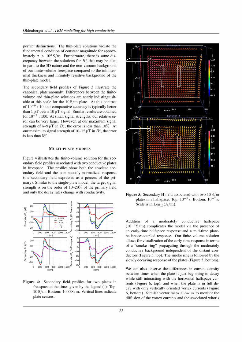
Oldenborger, G.A., & Oldenburg, D.W., 2007, TEM Modelling for High Conductivity
portant distinctions. The thin-plate solutions violate thefundamental condition of constant magnitude for approx-imately σ > 102 S/m. Furthermore, there is some dis-crepancy between the solutions for Bs
x that may be due,in part, to the 3D nature and the non-vacuum backgroundof our finite-volume freespace compared to the infinites-imal thickness and infinitely resistive background of thethin-plate model.
The secondary field profiles of Figure 3 illustrate thecanonical plate anomaly. Differences between the finite-volume and thin-plate solutions are nearly indistinguish-able at this scale for the 10 S/m plate. At this contrastof 10−9 : 10, our comparative accuracy is typically betterthan 1 pT over a 10 pT signal. Similar results are obtainedfor 10−9 : 100. At small signal strengths, our relative er-ror can be very large. However, at our maximum signalstrength of 5–9 pT in Bs
z , the error is less than 10%. Atour maximum signal strength of 10–12 pT in Bs
x, the erroris less than 5%.
MULTI-PLATE MODELS
Figure 4 illustrates the finite-volume solution for the sec-ondary field profiles associated with two conductive platesin freespace. The profiles show both the absolute sec-ondary field and the continuously normalized response(the secondary field expressed as a percent of the pri-mary). Similar to the single-plate model, the target signalstrength is on the order of 10–20% of the primary fieldand only the decay rates change with conductivity.
0 300 600 900 1200 1500
−20
−10
0
10
20
x (m)
Sec
onda
ry B
z (pT
)
0.0001 0.001 0.01 0.1 1
0 300 600 900 1200 1500−25
−20
−15
−10
−5
0
5
x (m)
Sec
onda
ry B
z (%
Fre
espa
ce)
0 300 600 900 1200 1500
−20
−10
0
10
20
x (m)
Sec
onda
ry B
z (pT
)
0 300 600 900 1200 1500−25
−20
−15
−10
−5
0
5
x (m)
Sec
onda
ry B
z (%
Fre
espa
ce)
Figure 4: Secondary field profiles for two plates infreespace at the times given by the legend (s). Top:10 S/m. Bottom: 1000 S/m. Vertical lines indicateplate centres.
Figure 5: Secondary H field associated with two 10 S/mplates in a halfspace. Top: 10−5 s. Bottom: 10−2 s.Scale is in Log10(A/m).
Addition of a moderately conductive halfspace(10−3 S/m) complicates the model via the presence ofan early-time halfspace response and a mid-time plate-halfspace coupled response. Our finite-volume solutionallows for visualization of the early-time response in termsof a “smoke ring” propagating through the moderatelyconductive background independent of the distant con-ductors (Figure 5, top). The smoke ring is followed by theslowly decaying response of the plates (Figure 5, bottom).
We can also observe the differences in current densitybetween times when the plate is just beginning to decaywhile still interacting with the horizontal halfspace cur-rents (Figure 6, top), and when the plate is in full de-cay with only vertically oriented vortex currents (Figure6, bottom). Similar vector maps allow us to monitor thediffusion of the vortex currents and the associated whorls
3/4
Oldenborger et al., TEM modelling for high conductivity
33

Oldenborger, G.A., & Oldenburg, D.W., 2007, TEM Modelling for High Conductivity
of the secondary magnetic field into the conductive platesat later times.
Figure 6: Total current density in and around a 10 S/mplate in a halfspace. Top: 10−4 s. Bottom: 10−2 s.Scale is in Log10(A/m2)
CONCLUDING DISCUSSION
The time-domain solution of Maxwell’s equations viaa potential formulation over a finite-volume staggeredgrid appears robust for high conductivity contrasts andhigh conductivities. Comparison with thin-plate solu-tions gives good agreement for conductivity contrasts of10−9 : 100. Comparison with the analytical responsefunction suggests the capability to model highly conduc-tive targets below the numerical time limit implied by dif-fusion length arguments, and at least during their charac-teristic decay time.
The finite-volume solution does exhibit inaccuracy at veryearly times even for moderate conductivities. Akin to high
frequencies, it proves difficult to obtain and verify solu-tions at very early time due to the presence of a wave so-lution and and the requirement of very fine time stepping.Conversely, thin-plate solutions adopt the simplifying as-sumption of an infinitely resistive background and purediffusion.
For the synthetic models considered here, the target signalstrength represents approximately 10% of the primary ortotal field. As such, modest amounts of noise (numericalor otherwise) may prohibit our ability to invert data suchas these. Our results suggest that the numerical noise,at least, should be manageable at approximately 10% ofthe secondary or 1% of the primary field strength. Never-theless, despite our capability to model high-contrast andhigh-conductivity environments, inversion of the data forhighly conductive targets is an ongoing challenge.
REFERENCES
Haber, E., Ascher, U.M., & Oldenburg, D.W. (2004). In-version of 3D electromagnetic data in frequencyand time domain using an inexact all-at-once ap-proach. Geophysics, 69, 1216–1228.
Nabighian, M.M., & Macnae, J.C. (1991). Time do-main electromagnetic prospecting methods. InM.N. Nabighian (Ed.), Electromagnetic Methodsin Applied Geophysicists, Volume 2, Application(pp. 427–520). Tulsa, OK: Society of ExplorationGeophysics.
Oristaglio, M.L., & Hohmann, G.W. (1984). Diffusionof electromagnetic fields into a two-dimensionalearth: A finite-difference approach. Geophysics,49, 870–894.
Wait, J.R. (1951). A conducting sphere in a time-varyingmagnetic field. Geophysics, 16, 666–672.
4/4
Oldenborger et al., TEM modelling for high conductivity
34

4th International Symposium on Three-Dimensional ElectromagneticsFreiberg, Germany, September 27–30, 2007
Rapid Forward Modelling of Multi-Source TEM Data
D. W. Oldenburg1, E. Haber2 and R. Shekhtman1
1University of British Columbia, Department of Earth & Ocean Sciences2Emory University, Atlanta, GA
ABSTRACT
The availability of matrix factorization software and high performance computing has allowed us to explore the potentialfor solving 3D EM forward modelling problems using direct solvers. This is particularly advantageous when data frommany transmitters need to be simulated. We first formulate Maxwell’s equations in terms of the magnetic field H toprovide a symmetric forward modelling operator. The problem is discretized using a finite volume technique in space anda backward Euler in time. The MUMPS software package is used to carry out a Cholesky decomposition of the forwardoperator, with the work distributed over an array of processors. The forward modelling is then quickly carried out usingthe factored operator. The time savings are considerable and they make the simulations of large ground or airborne datasets feasible and greatly increase our abilities to solve the 3D electromagnetic inverse problem in a reasonable time.Keywords: Electromagnetics, forward modelling, time domain, direct solvers
INTRODUCTION
In previous research (Haber, Oldenburg, & Shekhtman,2006) we developed an inversion algorithm that allowedus to invert data from a single, or a very few, transmit-ters. Unfortunately the computational demands of that al-gorithm were too large to invert typical ground or airbornesurveys acquired from many source locations. The prin-cipal difficulty is the time required to solve the forwardproblem. Simulating data that arise from multi-sourcescan be computationally onerous because each transmitterrequires that Maxwell’s equations be solved. Usually thisis done with iterative (eg. CG-type) algorithms and hencethe computation time increases linearly with the numberof transmitter locations. However, significant increasesin efficiency can be had if the forward modelling matrixis factored. This involves large computations and signifi-cant memory requirements. However, once this is accom-plished, solving the factored system with a different righthand side proceeds very quickly. The idea of decompos-ing the matrix system and solving many right hand sidesfor different sources is not new (Dey & Morrison, 1979),and small problems have been solved in this manner.However, the matrices for 3D TEM problems have gener-ally been considered to be too large to contemplate this ap-proach. Over the last decade however, advances in math-ematics and computing science have resulted in factoriza-tion algorithms that can be implemented on large scalecomputing systems (Amestoy, Guermouche, L’Excellent,& Pralet, 2006). The efficacy of this approach dependsupon the time required to factor the matrix compared tothe time required to solve the matrix system from scratch.
We use the MUMPS codes and distribute the computationover many different processors.
MAXWELL’S EQUATIONS IN THE TIME DOMAIN
The forward model consists of Maxwell’s equations intime where the permeability is fixed but electrical conduc-tivity can be highly discontinuous. To be more specific,we write Maxwell’s equations as
∇× E(i) + µ∂H(i)
∂t= 0, (1a)
∇× H(i) − σE(i) − ε∂E(i)
∂t= s(i)
r (t) (1b)
i = 1, . . . , N (1c)
over a domain Ω × [0, tf ], where E(i) and H(i) are theelectric and magnetic fields that correspond to the sources(i)r , µ is the permeability, σ is the conductivity, ε is the
permittivity and sr is a source. The equations are givenwith boundary and initial conditions:
n×H(i) = 0 (2a)
H(0,x) = H(i)0 (2b)
E(0,x) = 0 (2c)
although other boundary and initial conditions could beused.
1/4
4th International Symposium on Three-Dimensional ElectromagneticsFreiberg, Germany, September 27–30, 2007
35

Oldenburg, D. et al., 2007, Rapid multi-source TEM. . .
Solving the forward problem
As previously discussed in (Haber & Ascher, 2001; Haber,Ascher, Aruliah, & Oldenburg, 2000) consistent dis-cretization of Maxwell’s equation leads to a near-singularsystem. This is due to the rich null space of the curl op-erator. In our previous work we have turned to the A− φformulation to stabilize the system. While this approach ishighly effective for iterative methods, it is not as effectivefor direct methods due to two main difficulties. First, theresulting system is not symmetric thus one is required touse the LU factorization rather than the Cholesky factor-ization; this doubles the amount of memory used for thesolution of the system. Second, the number of unknownsis larger and this adds even more memory to the factoriza-tion. Keeping this in mind, we now work directly with thefields.Using backward Euler discretization in time with step sizeδt we obtain
∇× Ei+1 + µHi+1 −Hi
δt= 0, (3)
∇× Hi+1 − σEi+1 − εEi+1 −Ei
δt= sri+1(4)
Eliminating the electric field Ei+1 from Maxwell’s equa-tions we obtain an equation for the magnetic field Hi+1
∇× (σ + δt−1ε)−1∇× Hi+1 +µ
δtHi+1 = rhsi+1 (5)
The above system can be near-singular when the conduc-tivity is small and the time steps are large. To stabilize itwe recall that we also have ∇ · µH = 0 and therefore wecan rewrite the system as
∇× (σ + δt−1ε)−1∇× Hi+1
−∇µ−1(σ + δt−1ε)−1∇ · (µHi+1)
+µ
δtHi+1 = rhsi+1
The new term∇µ−1(σ+δt−1ε)−1∇· (µHi+1) stabilizesthe system without changing the solution.Upon discretization is space, we obtain the linear system
A(σ)Hi+1 := (C(σ, δt) +M)Hi+1 = rhs (6)
where the matrix C(σ, δt) is a discretization of the differ-ential operator in (6). The matrix is SPD and depends onthe conductivity and the time step δt. The matrix M isdependent on µ and δt.We now make an important observation which motivatesour approach. We note that by using the same time stepsδt, the linear system (6) is identical for all times and allsources. Thus, assuming that we decompose the systeminto
A(σ) = LLT ,
this factorization can be used to solve all the linear sys-tems.Matrix factorization is an expensive computational pro-cess. If the number of sources and/or time steps is smallthen we may not benefit from this work and using itera-tive methods for the solution of the system can be supe-rior. However, when the same forward modelling matrixneeds to be solved many times, the decomposition willbe greatly superior to iterative techniques. The benefitsof this are exacerbated when one proceeds to the inverseproblem since the same factorization can be used for thecomputation of the gradient as well as for the solution ofthe linear system which arises at each Gauss-Newton iter-ation.
Software for Matrix Factorizations
In recent years there has been a growing effort to obtainscalable matrix factorizations on parallel machines. Aftertesting a few packages we have decided to use the pack-age Multi-frontal Massively Parallel Solver (MUMPS) bythe CERFACS group (Amestoy et al., 2006). MUMPS isa package for solving systems of linear equations of theform Ax = b, where the matrix A is sparse and can be ei-ther unsymmetric, symmetric positive definite, or generalsymmetric. MUMPS uses a multifrontal technique whichis a direct method based on either the LU or the LDLTfactorization of the matrix. MUMPS exploits both par-allelism arising from sparsity in the matrix A and fromdense factorizations kernels. The main features of theMUMPS package include the solution of the transposedsystem, input of the matrix in assembled format (dis-tributed or centralized) or elemental format, error analysis,iterative refinement, scaling of the original matrix, and re-turn of a Schur complement matrix. Finally, MUMPS isavailable in various arithmetics (real or complex, singleor double precision). The software is written in Fortran90. The parallel version of MUMPS requires MPI formessage passing and makes use of the BLAS, BLACS,and ScaLAPACK libraries. We have tested MUMPS ona cluster of PCs under Linux. MUMPS distributes thework tasks among the processors, but an identified proces-sor (the host) is required to perform most of the analysisphase, distribute the incoming matrix to the other proces-sors (slaves) in the case where the matrix is centralized,and collect the solution. The system Ax = b is solved inthree main steps:
1. Analysis. The host performs an ordering based onthe symmetrized pattern A + A>, and carries outsymbolic factorization. A mapping of the multi-frontal computational graph is then computed, andsymbolic information is transferred from the host
2/4
Oldenburg et al., Rapid forward modelling of multi-source TEM data
36

Oldenburg, D. et al., 2007, Rapid multi-source TEM. . .
to the other processors. Using this information, theprocessors estimate the memory necessary for fac-torization and solution.
2. Factorization. The original matrix is first distributedto processors that will participate in the numericalfactorization. The numerical factorization on eachfrontal matrix is conducted by a master processor(determined by the analysis phase) and one or moreslave processors (determined dynamically). Eachprocessor allocates an array for contribution blocksand factors; the factors must be kept for the solutionphase.
3. Solution. The right-hand side b is broadcast fromthe host to the other processors. These processorscompute the solution x using the (distributed) fac-tors computed during Step 2, and the solution is ei-ther assembled on the host or kept distributed on theprocessors.
Each of these phases can be called independently and sev-eral instances of MUMPS can be handled simultaneously.
Practical Implementation
To obtain insight regarding the advantages of the decom-position we consider a simple, but generic, problem andrun it on our small cluster of 22 CPU’s. Each processor isa 64 bit Opteron 244 with local memory of 2GB. This isenough memory to solve an EM problem discretized with703 cells. For a numerical example we suppose that thetransmitters are 140m×140m current loops on the surfaceof a homogeneous earth which hosts a conductive prism.The current waveform is a step-off and we are interestedin times between 10−6 and 10−1 seconds. With our orig-inal code, the time increments were equally spaced in logtime and we sampled 6 times per decade. Maxwell’s sys-tem therefore needed to be solved 32 times and this re-quired 12,900 seconds on a single processor. Our im-plementation is "embarassingly parallelizable" over multi-processors since each source can be spawned to its ownprocessor. Thus, on our cluster, we can simulate datafrom 22 transmitters in this same time. We assume thisoptimum case scenario for tabulation of the computationtimes shown in Table I.
Algorithm NTX Np Nδt tf ts P Ttotaloriginal 22 22 32 1.3E4MUMPS 22 22 105 360 0.8 1.8E6MUMPS 22 22 15 360 0.8 5 3.1E3
Table 1: NTX is the number of transmitters; Np is thenumber of processors; Nδt is the number of timesteps needed to solve the full time domain problem;tf is the time required to factor the matrix; ts is thesolution time for a forward problem once the matrixhas been factorized; P is the number of subintervals(each of which requires its own matrix factoriza-tion); Ttotal is the time taken to solve the completeproblem the NTX transmitters.
We now turn to the MUMPS factorization. Our equationsare to be time stepped between times T1 = 10−6 andT2 = 10−1 seconds. The time step δt is determined bythe smallest time needed and is µT1 where µ is a con-stant. Here we use µ = 1 so the number of time stepsis Nδt = (T2 − T1)/δt = 105. The factorization time,tf , depends upon the number of CPU’s and the amount ofavailable memory; for our configuration tf is 360s. Withthe factored system the time required to solve a forwardproblem, tf , is 0.8s. The total number of forward solu-tions is equal to NTX ∗Nδt where NTX is the number oftransmitters. Thus the total time taken to solve our prob-lem is
Ttotal = NTXNδtts + tf (7)
The numbers are listed in Table I. Unfortunately the to-tal time is larger than for the original code. The dif-ficulty arises because of the excessive number of timesteps; keeping the same δt for the entire modelling re-quires 2, 200, 000 forward solutions. This difficulty canbe circumvented by dividing our total time interval into Psubintervals each of which has a constant δt. For our ex-ample we choose P = 5. Each subinterval is one decadein time and Nδt = 15 for each interval. Five factoriza-tions are required and the number of forward solutions isreduced to 1650. As per Table I, this reduces the total for-ward modelling time to 3120s, which is a factor of fourbetter than the original code. This factor can easily be ex-ceeded if NTX/Np increases, as it does in the airbornesurvey. The real benefit however, is for the inverse prob-lem.
Implications for Inversion
Our inverse problem (Haber et al., 2006) is based upona Gauss-Newton procedure where, at each iteration, the
3/4
Oldenburg et al., Rapid forward modelling of multi-source TEM data
37
Oldenburg, D. et al., 2007, Rapid multi-source TEM. . .
equation
(JTJ + βWTW )s = −g (8)
is solved to obtain a perturbation s. W is a sparse reg-ularization matrix, β is a constant, and g is the gradientof the objective function. The sensitivity matrix is avail-able as J = QA−1G where Q is an interpolation matrixthat extracts the simulated data from the computed fieldsor potentials, A is the forward modelling matrix, and Gis a known sparse matrix. The system is solved using apreconditioned conjugate gradient (CG) solver for whichthe matrix on the left must be applied to a vector manytimes. The application of Jv or JT v thus requires thata forward modelling be carried out. The implications ofthe factorization of the forward modelling matrix now be-come apparent. Firstly, the computation of the gradientrequires a forward modelling. Secondly, even with a goodpreconditioner,NCG, the number ofCG iterations neededto get a good solution, is 10-20. Thirdly, once the pertur-bation s is calculated, a line search is required to find thescale factor α to update the model as mn+1 = mn + αs.If NCG = 15 the number of forward modelings is 31 plusany required for a line search. With the numbers outlinedabove, the time to compute a GN step is about 11 hours.This makes the problem doable, especially since anotherfactor of two can be recovered merely by updating ourtwo-year old processors.
CONCLUSIONS
We have demonstrated the benefits of solving multi-sourcetime domain electromagnetic problems by decomposingthe matrix and using direct solvers. The advantages overtraditional approaches that use iterative solvers dependsupon the number of transmitters, the size of the discretizedproblem, the number of processors and the amount ofmemory available. Optimum use of this approach willrequire dividing the global time interval of interest intosubintervals. If the factorization for each subinterval isstored, then Gauss-Newton iterations for the inverse prob-lem can be efficiently carried out. We are currently devel-oping that procedure.
ACKNOWLEDGMENTS
This work was supported by NSERC CRDPJ 340409-06 and by MITEM (Multi-Source Inversion of Time Do-main Electromagnetic Data) consortium partners: New-mont Mining Corp, CAMECO Corp, CRVD, Xstrata Plc,Teck Cominco Ltd, and Barrick Gold Corp.
REFERENCES
Amestoy, P. R., Guermouche, A., L’Excellent, J.-Y., &Pralet, S. (2006). Hybrid scheduling for the parallelsolution of linear systems. Parallel Computing, 32,136-156.
Dey, A., & Morrison, H. F. (1979). Resistivity modelingfor arbitrarily shaped three-dimensional structures.Geophysics, 44, 753-780.
Haber, E., & Ascher, U. (2001). Fast finite volume sim-ulation of 3d electromagnetic problems with highlydiscontinuous coefficients. SIAM Journal of Scien-tific Computing, 22, 1943–1961.
Haber, E., Ascher, U., Aruliah, D., & Oldenburg, D.(2000). Fast simulation of 3d electromagnetic us-ing potentials. Journal of Computational Physics,163, 150–171.
Haber, E., Oldenburg, D., & Shekhtman, R. (2006). In-version of time domain 3d electromagnetic data. ac-cepted Geophysical Journal International.
4/4
Oldenburg et al., Rapid forward modelling of multi-source TEM data
38

4th International Symposium on Three-Dimensional ElectromagneticsFreiberg, Germany, September 27–30, 2007
On the Matrix Condition Number of Finite Element Approximationsto the Frequency Domain Maxwell’s Equations
C. Schwarzbach and K. SpitzerInstitute of Geophysics, TU Bergakademie Freiberg, Freiberg, Germany
SUMMARY
Finite element (FE) approximations to the solution of Maxwell’s equations can be based upon different formulations asboundary value problems. We investigate two different approaches in frequency domain: the classical curl-curl formula-tion and a mixed formulation which explicitly takes into account the equation of continuity for conducting media. Thefrequency dependent condition number of the FE system matrix is computed for a homogeneous medium model problem.It reveals that the mixed approach introduces stability for low frequencies. Additionally, largely unequal weights given tothe two partial differential equations of the mixed formulation significantly affect the matrix condition number.
The study is extended to an anisotropic Perfectly Matched Layer (PML). The resulting coefficients of the partial differ-ential equation (PDE) as a function of frequency can be bounded by introducing a complex frequency shift. However,anisotropy grows with decreasing frequency in the relevant frequency range and, thus, deteriorates the matrix conditionnumber.
Keywords: Finite Element Method, Perfectly Matched Layers, Frequency Domain
INTRODUCTION
Electromagnetic methods in geophysics cover a broadfrequency spectrum. Even at the highest frequenciesused, the damping of electromagnetic waves cannot beneglected because of the inherent electrical conductivitypresent within the earth. Therefore, it is interesting tostudy the damped wave equation over a frequency rangeof several orders of magnitude.
Numerical simulations are a key tool to understandingthe physics of geophysical measurements, interpretingtheir data and improving acquisition techniques. Restrict-ing ourselves to time harmonic fields and Fourier syn-thesizing if required we end up with a system of lin-ear equations which is obtained by the Finite ElementMethod (FEM) from frequency domain Maxwell’s equa-tions (Monk, 2003). This paper presents a numerical ex-periment with different formulations of boundary valueproblems that lead to stable or unstable behaviour of thefrequency dependent FE system matrix condition number.
A MODEL PROBLEM
Consider the unit cube Ω = [0, 1]3 m3 with homogeneousconstitutive parameters magnetic permeability µ = µ0,electric permittivity ε = 8ε0 and electric conductivityσ = 0.01 S/m. µ0 and ε0 denote the free space quan-tities which are related to the vacuum speed of light
c = 1/√
µ0ε0 ≈ 3 · 108 m/s. We will examine the solu-tion of the frequency domain Maxwell’s equations for fre-quencies f = 105 . . . 108 Hz.
The domain Ω is discretized by a regular mesh consistingof 53 hexahedrons of size h = 0.2 m. Maxwell’s equa-tions are numerically solved using FEMSTER (Castillo,Rieben and White, 2003) with a family of quadratic FEbase functions (p = 2). Therefore, a sufficient sampling
105
106
107
108
102
104
106
108
frequency f in Hz
mat
rix
cond
ition
num
ber
κ 1
Dirichlet BCNeumann BC
Figure 1: Frequency dependence of the 1-norm FE sys-tem matrix condition number for the standard curl-curlequation approach with Dirichlet or Neumann bound-ary conditions.
1/4
4th International Symposium on Three-Dimensional ElectromagneticsFreiberg, Germany, September 27–30, 2007
39

Schwarzbach, C., et al., Matrix condition number of FE approximations to Maxwell’s equations
105
106
107
108
102
104
106
108
frequency f in Hz
mat
rix
cond
ition
num
ber
κ 1
α = 0, β = 0α = c, β = 0α = c, β = c2
Figure 2: Frequency dependence of the 1-norm FE sys-tem matrix condition number for the mixed approachwith Dirichlet boundary condition and different valuesfor α and β in equations (5) and (6).
of wavelengths of at least ten samples is provided. Thealgorithm of Higham and Tisseur (Higham and Tisseur,2000) is combined with a direct solver from PARDISO(Schenk and Gärtner, 2004, 2006) to estimate the 1-normFE system matrix condition number κ1.
BOUNDARY VALUE PROBLEMS
Standard curl-curl equation approach
A standard approach of solving Maxwell’s equations infrequency domain is combining them to form a second or-der PDE that reads in terms of the electric field vector Eas
curl(µ−1 curl E)− iω(σ − iωε)E = iωjs. (1)
Here, i denotes the imaginary unit, ω = 2πf the angularfrequency and js an applied source current density. If Eis a sufficiently smooth solution of eq. (1) and ω 6= 0, thedivergence of eq. (1) can be taken, revealing that E alsofulfils the equation of continuity
− div(σ − iωε)E = div js. (2)
To complete the PDE (1) posed on Ω, homogeneousDirichlet or Neumann boundary conditions are applied onthe boundary Γ = ∂Ω,
n×E = 0 (3)
or n× (µ−1 curl E) = 0, (4)
where n is the outward normal vector on Γ.
105
106
107
108
102
104
106
108
frequency f in Hz
mat
rix
cond
ition
num
ber
κ 1
α = 0, β = 0α = c, β = 0α = c, β = c2
Figure 3: Frequency dependence of the 1-norm FE sys-tem matrix condition number for the mixed approachwith Neumann boundary condition and different val-ues for α and β in equations (5) and (6). Note that thematrix is singular for α = c, β = 0.
The condition number κ1 of the resulting FE system ma-trix is depicted in Fig. 1. The kernel of the curl oper-ator causes κ1 to increase exponentially with decreasingfrequency. For small ω, the curl-curl term dominates thezeroth order term and the solution can be spoiled by gra-dients of a scalar function. This behaviour can be avoidedusing a mixed formulation.
Mixed approach
The equation of continuity (2) is explicitly taken into ac-count by extending the system of equations (1) and (2) bya scalar variable V ,
curl(µ−1 curl E)− iω(σ − iωε)E+ α(σ − iωε) grad V = iωjs (5)
−α div(σ − iωε)E + βV = α div js,(6)
where α is a scalar constant and β a scalar function. Theseassumptions ensure that the resulting discrete system hasa symmetric coefficient matrix. The appropriate boundaryconditions read
n×E = 0, V = 0 (7)
or n× (µ−1 curl E) = 0, n · grad V = 0. (8)
Taking the divergence of eq. (5) we learn that V implicitlyfulfils
−α2 div(σ − iωε) grad V + iωβV = 0. (9)
2/4
Schwarzbach et al., Matrix condition number of FE approximations to Maxwell’s equations
40

Schwarzbach, C., et al., Matrix condition number of FE approximations to Maxwell’s equations
10−3
100
103
102
104
106
108
α/c in 1/m
mat
rix c
ondi
tion
num
ber κ 1
f = 105 Hz
f = 106 Hz
f = 107 Hz
f = 108 Hz
Figure 4: Dependence of the 1-norm FE system matrixcondition number κ1 on the weight constant α for theDirichlet boundary condition and β = 0.
The choice β 6= 0 leads to a denser FE system matrixthan β ≡ 0. In the case of the Neumann boundary condi-tion (8), however, the zeroth order term iωβV is crucial: Ifβ ≡ 0, the solution of eq. (9) in terms of V is non-uniqueand κ1 = ∞. For all other cases, a constant κ1 is achievedfor low frequencies using the mixed formulation (Figs 2and 3).The particular value of α is important. It can be inter-preted as giving appropriate weights to both differentialequations and the two unknowns E and V . Fig. 4 illus-trates that the matrix condition number, as a function of α,has a pronounced minimum and is exponentially increas-ing away from the minimum. Note that, for the choice ofPDEs (5) and (6), α is in the order of the vacuum speed oflight c.
EXTENSION TO PERFECTLY MATCHED LAYERS
Most geophysical simulation problems are naturally posedon unbounded domains. Numerical methods like the FEMusually require the restriction to a bounded domain. Theunavailability of appropriate boundary conditions for theauxiliary boundary introduced to obtain a finite simula-tion volume makes attractive the technique of PerfectlyMatched Layers (PML) (Berenger, 1994). Therefore,we extend our model study by a Complex FrequencyShifted (CFS), anisotropic PML (Kuzuoglu and Mittra,1996) which replaces all scalar constitutive parametersη = µ, ε, σ by tensors η diag(1/d, d, d), where
d = 1 + ibxn
ω + iω0(10)
can be considered as a complex valued stretching of thefirst spatial coordinate x. y and z remain unaffected.
105
106
107
108
100
102
104
frequency f in Hz
anis
otro
py f
acto
r ρ
f0 = 1.35⋅105 Hz
Figure 5: Maximum anisotropy factor ρ = |d|2 (x = 1 m)of the CFS PML.
105
106
107
108
103
105
107
109
frequency f in Hz
mat
rix
cond
ition
num
ber
κ 1
α = 0, β = 0α = c, β = 0α = c, β = c2
Figure 6: Frequency dependence of the 1-norm FE sys-tem matrix condition number for the mixed approachCFS PML with Dirichlet boundary condition and dif-ferent values for α and β in equations (5) and (6).
10−3
100
103
102
104
106
108
α/c in 1/m
mat
rix c
ondi
tion
num
ber κ 1
f = 105 Hz
f = 106 Hz
f = 107 Hz
f = 108 Hz
Figure 7: Dependence of the 1-norm matrix conditionnumber κ1 on the weight constant α for the CFS PMLwith Dirichlet boundary condition and β = 0.
3/4
Schwarzbach et al., Matrix condition number of FE approximations to Maxwell’s equations
41

Schwarzbach, C., et al., Matrix condition number of FE approximations to Maxwell’s equations
In particular we choose n = 1, b = 3.45 · 108 Hz/m,ω0 = 8.485 · 105 Hz.
The complex frequency shift iω0 guarantees that the con-stitutive parameters are bounded for low (real) frequenciesω. However, for ω ' ω0, the anisotropy factor, i. e., the ra-tio of the largest and smallest tensor eigenvalues increaseswith decreasing frequency (Fig. 5). A constant level isonly reached at lower frequencies.
Figure 6 shows the FE system matrix condition numberas a function of frequency for different formulations ofthe boundary problem. Comparing the results of the CFSPML with those of the previous section (Fig. 2) the grow-ing anisotropy is clearly seen to considerably enlarge thecondition number for small frequencies. However, thelow frequency behaviour is similar. Exponential growthoccurs for the curl-curl equation formulation while forthe mixed formulation the condition number tends to anasymptotic level since the anisotropy factor is boundedfor low frequencies due to the complex frequency shift.Regarding the mixed formulation (5), (6), the importantrole of the weight constant α observed before in Fig. 4 isconfirmed by Fig. 7.
CONCLUSIONS
Taking explicitly into account the divergence condition,i. e., the equation of continuity, may render stable the re-sulting boundary value problem and its discrete FE equiv-alent when solving the frequency domain Maxwell’s equa-tions for low frequencies. Giving matching weights tothe curl-curl equation and the equation of continuity hasbeen illustrated to be important. An approximately well-balanced formulation can be obtained if eq. (5) is dividedby the vacuum speed of light c and rewritten in terms ofwavenumber k = ω/c instead of the angular frequency ω.
The mixed approach works well for the classical Max-well’s equations. Their anisotropic PML extension intro-duces additional frequency dependencies and a low fre-quency instability. Introduction of a complex frequencyshift to the PML establishes bounds to all coefficients ofthe boundary value problem and its discrete FE equiva-lent. However, the anisotropy, introduced to improve theperformance of boundary conditions, significantly dete-riorates the FE system matrix condition number for lowfrequencies.
REFERENCES
Berenger, J. P. (1994). A perfectly matched layer for theabsorption of electromagnetic waves. Journal of Com-putational Physics, 114, 185–200.
Castillo, P., Rieben, R. N. and White, D. A. (2003). FEM-STER: An object oriented class library of discrete dif-ferential forms. In Proceedings of the 2003 IEEEInternational Antennas and Propagation Symposium(Vol. 2, pp. 972–976). Columbus, OH. (UCRL-JC-150238-ABS)
Higham, N. J., and Tisseur, F. (2000). A block algorithmfor matrix 1-norm estimation, with an application to1-norm pseudospectra. SIAM Journal on Matrix Anal-ysis and Applications, 21(4), 1185–1201.
Kuzuoglu, M., and Mittra, R. (1996). Frequency de-pendence of the constitutive parameters of causalperfectly matched anisotropic absorbers. IEEE Mi-crowave and Guided Wave Letters, 6(12), 447–449.
Monk, P. (2003). Finite element methods for Maxwell’sequations. New York: Oxford University Press.
Schenk, O., and Gärtner, K. (2004). Solving unsym-metric sparse systems of linear equations with PAR-DISO. Journal of Future Generation Computer Sys-tems, 20(3), 475–487.
Schenk, O., and Gärtner, K. (2006). On fast factorizationpivoting methods for sparse symmetric indefinite sys-tems. Electronic Transactions on Numerical Analysis,23, 158–179.
4/4
Schwarzbach et al., Matrix condition number of FE approximations to Maxwell’s equations
42
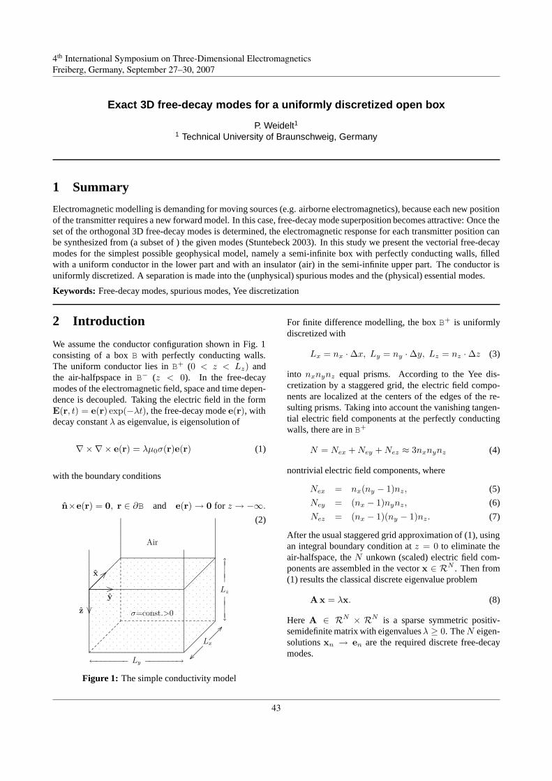
4th International Symposium on Three-Dimensional ElectromagneticsFreiberg, Germany, September 27–30, 2007
Exact 3D free-decay modes for a uniformly discretized open box
P. Weidelt11 Technical University of Braunschweig, Germany
1 Summary
Electromagnetic modelling is demanding for moving sources (e.g. airborne electromagnetics), because each new positionof the transmitter requires a new forward model. In this case, free-decay mode superposition becomes attractive: Once theset of the orthogonal 3D free-decay modes is determined, the electromagnetic response for each transmitter position canbe synthesized from (a subset of ) the given modes (Stuntebeck 2003). In this study we present the vectorial free-decaymodes for the simplest possible geophysical model, namely a semi-infinite box with perfectly conducting walls, filledwith a uniform conductor in the lower part and with an insulator (air) in the semi-infinite upper part. The conductor isuniformly discretized. A separation is made into the (unphysical) spurious modes and the (physical) essential modes.
Keywords: Free-decay modes, spurious modes, Yee discretization
2 Introduction
We assume the conductor configuration shown in Fig. 1consisting of a box B with perfectly conducting walls.The uniform conductor lies in B+ (0 < z < Lz) andthe air-halfpspace in B− (z < 0). In the free-decaymodes of the electromagnetic field, space and time depen-dence is decoupled. Taking the electric field in the formE(r, t) = e(r) exp(−λt), the free-decay mode e(r), withdecay constant λ as eigenvalue, is eigensolution of
∇×∇× e(r) = λµ0σ(r)e(r) (1)
with the boundary conditions
n×e(r) = 0, r ∈ ∂B and e(r) → 0 for z → −∞.
(2)
.......................................................................................................................................................................................................................................................................................................................................................................................................................................................................................................................
.
.
.
.
.
.
.
.
.
.
.
.
.
.
.
.
.
.
.
.
.
.
.
.
.
.
.
.
.
.
.
.
.
.
.
.
.
.
.
.
.
.
.
.
.
.
.
.
.
.
.
.
.
.
.
.
.
.
.
.
.
.
.
.
.
.
.
.
.
.
.
.
.
.
.
.
.
.
.
.
.
.
.
.
.
.
.
.
.
.
.
.
.
.
.
.
.
.
.
.
.
.
.
.
.
.
.
.
.
.
.
.
.
.
.
.
.
.
.
.
.
.
.
.
.
.
.
.
.
.
.
.
.
.
.
.
.
.
.
.
.
.
.
.
.
.
.
.
.
.
.
.
.
.
.
.
.
.
.
.
.
.
.
.
.
.
.
.
.
.
.
.
.
.
.
.
.
.
.
.
.
.
.
.
.
.
.
.
.
.
.
.
.
.
.
.
.
.
.
.
.
.
.
.
.
.
.
.
.
.
.
.
.
.
.
.
.
.
.
.
.
.
.
.
.
.
.
.
.
.
.
.
.
.
.
.
.
.
.
.
.
.
.
.
.
.
.
.
.
.
.
.
.
.
.
.
.
.
.
.
.
.
.
.
.
.
.
.
.
.
.
.
.
.
.
.
.
.
.
.
.
.
.
.
.
.
.
.
.
.
.
.
.
.
.
.
.
.
.
.
.
.
.
.
.
.
.
.
.
.
.
.
.
.
.
.
.
.
.
.
.
.
.
.
.
.
.
.
.
.
.
.
.
.
.
.
.
.
.
.
.
.
.
.
.
.
.
.
.
.
.
.
.
.
.
.
.
.
.
.
.
.
.
.
.
.
.
.
.
.
.
.
.
.
.
.
.
.
.
.
.
.
.
.
.
.
.
.
.
.
.
.
.
.
.
.
.
.
.
.
.
.
.
.
.
.
.
.
.
.
.
.
.
.
.
.
.
.
.
.
.
.
.
.
.
.
.
.
.
.
.
.
.
.
.
.
.
.
.
.
.
.
.
.
.
.
.
.
.
.
.
.
.
.
.
.
.
.
.
.
.
.
.
.
.
.
.
.
.
.
.
.
.
.
.
.
.
.
.
.
.
.
.
.
.
.
.
.
.
.
.
.
.
.
.
.
.
.
.
.
.
.
.
.
.
.
.
.
.
.
.
.
.
.
.
.
.
.
.
.
.
.
.
.
.
.
.
.
.
.
.
.
.
.
.
.
.
.
.
.
.
.
.
.
.
.
.
.
.
.
.
.
.
.
.
.
.
.
.
.
.
.
.
.
.
.
.
.
.
.
.
.
.
.
.
.
.
.
.
.
.
.
.
.
.
.
.
.
.
.
.
.
.
.
.
.
.
.
.
.
.
.
.
.
.
.
.
.
.
.
.
.
.
.
.
.
.
.
.
.
.
.
.
.
.
.
.
.
.
.
.
.
.
.
.
.
.
.
.
.
.
.
.
.
.
.
.
.
.
.
.
.
.
.
.
.
.
.
.
.
.
.
.
.
.
.
.
.
.
.
.
.
.
.
.
.
.
.
.
.
.
.
.
.
.
.
.
.
.
.
.
.
.
.
.
.
.
.
.
.
.
.
.
.
.
.
.
.
.
.
.
.
.
.
.
.
.
.
.
.
.
.
.
.
.
.
.
.
.
.
.
.
.
.
.
.
.
.
.
.
.
.
.
.
.
.
.
.
.
.
.
.
.
.
.
.
.
.
.
.
.
.
.
.
.
.
.
.
.
.
.
.
.
.
.
.
.
.
.
.
.
.
.
.
.
.
.
.
.
.
.
.
.
.
.
.
.
.
.
.
.
.
.
.
.
.
.
.
.
.
.
.
.
.
.
.
.
.
.
.
.
.
.
.
.
.
.
.
.
.
.
.
.
.
.
.
.
.
.
.
.
.
.
.
.
.
.
.
.
.
.
.
.
.
.
.
.
.
.
.
.
.
.
.
.
.
.
.
.
.
.
.
.
.
.
.
.
.
.
.
.
.
.
.
.
.
.
.
.
.
.
.
.
.
.
.
.
.
.
.
.
.
.
.
.
.
.
.
.
.
.
.
.
.
.
.
.
.
.
.
.
.
.
.
.
.
.
.
.
.
.
.
.
.
.
.
.
.
.
.
.
.
.
.
.
.
.
.
.
.
.
.
.
.
.
.
.
.
.
.
.
.
.
.
.
.
.
.
.
.
.
.
.
.
.
.
.
.
.
.
.
.
.
.
.
.
.
.
.
.
.
.
.
.
.
.
.
.
.
.
.
.
.
.
.
.
.
.
.
.
.
.
.
.
.
.
.
.
.
.
.
.
.
.
.
.
.
.
.
.
.
.
.
.
.
.
.
.
.
.
.
.
.
.
.
.
.
.
.
.
.
.
.
.
.
.
.
.
.
.
.
.
.
.
.
.
.
.
.
.
.
.
.
.
.
.
.
.
.
.
.
.
.
.
.
.
.
.
.
.
.
.
.
.
.
.
.
.
.
.
.
.
.
.
.
.
.
.
.
.
.
.
.
.
.
.
.
.
.
.
.
.
.
.
.
.
.
.
.
.
.
.
.
.
.
.
.
.
.
.
.
.
.
.
.
.
.
.
.
.
.
.
.
.
.
.
.
.
.
.
.
.
.
.
.
.
.
.
.
.
.
.
.
.
.
.
.
.
.
.
.
.
.
.
.
.
.
.
.
.
.
.
.
.
.
.
.
.
.
.
.
.
.
.
.
.
.
.
.
.
.
.
.
.
.
.
.
.
.
.
.
.
.
.
.
.
.
.
.
.
.
.
.
.
.
.
.
.
.
.
.
.
.
.
.
.
.
.
.
.
.
.
.
.............................................................................................................................................................................................................................................................................................................................................................................................................................................................................................................................................................................................................................................................................................................................................................................................................................................................................
..
...............................................................................................................................................................
.
.......
........
........
.
.......
........
.
.......
........
........
.
.......
........
.
.......
............ ....... ....... ....... ....... ....... ....... ....... ....... ....... ....... ....... ....... ....... ....... ....... ....... ....... ....... ....... ....... ....... ....... ....... ..............
.
.
.
.
.
.
.
.
.
.
.
.
.
.
.
.
.
.
.
.
.
.
.
.
.
.
.
.
.
.
.
.
.
.
.
.
.
.
.
.
.
.
.
.
.
.
.
.
.
.
.
.
.
.
.
.
.
.
.
.
.
.
.
.
.
.
.
.
.
.
.
.
.
.
.
.
.
.
.
.
.
.
.
.
.
.
.
.
.
.
.
.
.
.
.
.
.
.
.
.
.
.
.
.
.
.
.
.
.
.
.
.
.
................................................................................
................
.
................................................................................
................
Lx
←−−−−−−− Ly −−−−−−−→
↑|||
Lz
|||↓
..
...........................................................................................................
.......................
.............................................................................................................
.......................
.
.
.
.
.
.
.
.
.
.
.
.
.
.
.
.
.
.
.
.
.
.
.
.
.
.
.
.
.
.
.
.
.
.
.
.
.
.
.
.
.
.
.
.
.
.
.
.
.
.
.
.
.
.
.
.
.
.
.
.
.
.
.
.
.
.
.
.
.
.
.
.
.
.
.
.
.
.
.
.
.
.
.
.
.
..
.
.
.
.
.
.
.
.
.
.
.
.
.
.
.
.
.
.
.
.
.
.
.
.
.
.
.
.
.
.
.
.
.
.
.
.
.
.
.
.
.
.
.
.
.
x
y
z
.
.
.
.
.
.
.
.
.
.
.
.
.
.
.
.
.
.
.
.
.
.
.
.
.
.
.
.
.
.
.
.
.
.
.
.
.
.
.
.
.
.
.
.
.
.
.
.
.
.
.
.
.
.
.
.
.
.
.
.
.
.
.
.
.
.
.
.
.
.
.
.
.
.
.
.
.
.
.
.
.
.
.
.
.
.
.
.
.
.
.
.
.
.
.
.
.
.
.
.
.
.
.
.
.
.
.
.
.
.
.
.
.
.
.
.
.
.
.
.
.
.
.
.
.
.
.
.
.
.
.
.
.
.
.
.
.
.
.
.
.
.
.
.
.
.
.
.
.
.
.
.
.
.
.
.
.
.
.
.
.
.
.
.
.
.
.
.
.
.
.
.
.
.
.
.
.
.
.
.
.
.
.
.
.
.
.
.
.
.
.
.
.
.
.
.
.
.
.
.
.
.
.
.
.
.
.
.
.
.
.
.
.
.
.
.
.
.
.
.
.
.
.
.
.
.
.
.
.
.
.
.
.
.
.
.
.
.
.
.
.
.
.
.
.
.
.
.
.
.
.
.
.
.
.
.
.
.
.
.
.
.
.
.
.
.
.
.
.
.
.
.
.
.
.
.
.
.
.
.
.
.
.
.
.
.
.
.
.
.
.
.
.
.
.
.
.
.
.
.
.
.
.
.
.
.
.
.
.
.
.
.
.
.
.
.
.
.
.
.
.
.
.
.
. . . . . . . . . . . . . .
. . . . . . . . . . . . . .
. . . . . . . . . . . . . .
. . . . . . . . . . . . . .
. . . . . . . . . . . . . .
. . . . . . . . . . . . . .
. . . . . . . . . . . . . .
. . . . . . . . . . . . . .
. . . . . . . . . . . . . .
σ=const.>0
Air
Figure 1: The simple conductivity model
For finite difference modelling, the box B+ is uniformlydiscretized with
Lx = nx ·∆x, Ly = ny ·∆y, Lz = nz ·∆z (3)
into nxnynz equal prisms. According to the Yee dis-cretization by a staggered grid, the electric field compo-nents are localized at the centers of the edges of the re-sulting prisms. Taking into account the vanishing tangen-tial electric field components at the perfectly conductingwalls, there are in B+
N = Nex + Ney + Nez ≈ 3nxnynz (4)
nontrivial electric field components, where
Nex = nx(ny − 1)nz, (5)
Ney = (nx − 1)nynz, (6)
Nez = (nx − 1)(ny − 1)nz. (7)
After the usual staggered grid approximation of (1), usingan integral boundary condition at z = 0 to eliminate theair-halfspace, the N unkown (scaled) electric field com-ponents are assembled in the vector x ∈ RN . Then from(1) results the classical discrete eigenvalue problem
Ax = λx. (8)
Here A ∈ RN × RN is a sparse symmetric positiv-semidefinite matrix with eigenvalues λ ≥ 0. The N eigen-solutions xn → en are the required discrete free-decaymodes.
1/4
4th International Symposium on Three-Dimensional ElectromagneticsFreiberg, Germany, September 27–30, 2007
43

Weidelt, P. 2007, Exact 3D free-decay modes. . .
Let ∇ ·v and ∇×v be the staggered grid approximationsof∇ · v and∇× v. Using that ∇ · ∇ × v = 0, we obtainfrom (1)
λ∇ · (σe) = 0. (9)
This equation can be satisfied in two different ways:
1. λ = 0, ∇ · (σe) 6≡ 0: spurious modeThe eigenvalue problem (8) has an Ns-fold eigen-value λ = 0, Ns = (nx − 1)(ny − 1)nz ≈ N/3,where Ns is the number of internal grid points.These Ns eigensolutions are associated with an un-physical divergent current density ∇ · (σe) 6≡ 0and have to be discarded. This is achieved by ap-plying at the Ns internal grid points the solenoidalcondition ∇ · (σe) = 0. Since Ns = Nez [ see eq.(7) ], the solenoidal current condition is satisfied byeliminating via this condition the Nez vertical elec-tric field components. This reduces the dimensionof the problem to Nf := N −Ns ≈ (2/3)N . HereNf is the number of degrees of freedom of the prob-lem. All Nf eigenvalues of the reduced system arepositive.
2. λ > 0, ∇ · (σe) ≡ 0: essential modeThe system (8) has Nf = Nex+Ney positive eigen-values, where Nf is the number of nontrivial hori-zontal electric field components. Only these essen-tial modes are required for the field synthesis.
So far, all considerations are valid for an arbitrary con-ductivity distribution σ(r) > 0, r ∈ B+ and also for anon-uniform product grid.
3 Uniformly discretized open box
Now we consider as special case the uniform box with auniform discretization. For the determination of the Nf
essential eigensolutions we assume the decomposition ofe into a toroidal part eT and poloidal part eP ,
e = eT + eP (10)
with
eT := ∇× (zT ), eP := ∇×∇× (zP ), (11)
such that the solenoidal condition ∇ · (σe) = 0 is auto-matically satisfied. The localization of the potentials inspace and the pertinent boundary conditions are displayedin Figs. 2 and 3. The localization of T agrees with that ofthe vertical magnetic field bz and the localization of P isidentical with that of the vertical electric field ez.
.
.
.
.
.
.
.
.
.
.
.
.
.
.
.
.
.
.
.
.
.
.
.
.
.
.
.
.
.
.
.
.
.
.
.
.
.
.
.
.
.
.
.
.
.
.
.
.
.
.
.
.
.
.
.
.
.
.
.
.
.
.
.
.
.
.
.
.
.
.
.
.
.
.
.
.
.
.
.
.
.
.
.
.
.
.
.
.
.
.
.
.
.
.
.
.
.
.
.
.
.
.
.
.
.
.
.
.
.
.
.
.
.
.
.
.
.
.
.
.
.
.
.
.
.
.
.
.
.
.
.
.
.
.
.
.
.
.
.
.
.
.
.
.
.
.
.
.
.
.
.
.
.
.
.
.
.
.
.
.
.
.
.
.
.
.
.
.
.
.
.
.
.
.
.
.
.
.
.
.
.
.
.
.
.
.
.
.
.
.
.
.
.
.
.
.
.
.
.
.
.
.
.
.
.
.
.
.
.
.
.
.
.
.
.
.
.
.
.
.
.
.
.
.
.
.
.
.
.
.
.
.
.
.
.
.
.
.
.
.
.
.
.
.
.
.
.
.
.
.
.
.
.
.
.
.
.
.
.
.
.
.
.
.
.
.
.
.
.
.
.
.
.
.
.
.
.
.
.
.
.
.
.
.
.
.
.
.
.
.
.
.
.
.
.
.
.
.
.
.
.
.
.
.
.
.
.
.
.
.
.
.
.
.
.
.
.
.
.
.
.
.
.
.
.
.
.
.
.
.
.
.
.
.
.
.
.
.
.
.
.
.
.
.
.
.
.
.
.
.
.
.
.
.
.
.
.
.
.
.
.
.
.
.
.
.
.
.
.
.
.
.
.
.
.
.
.
.
.
.
.
.
.
.
.
.
.
.
.
.
.
.
.
.
.
.
.
.
.
.
.
.
.
.
.
.
.
.
.
.
.
.
.
.
.
.
.
.
.
.
.
.
.
.
.
.
.
.
.
.
.
.
.
.
.
.
.
.
.
.
.
.
.
.
.
.
.
.
.
.
.
.
.
.
.
.
.
.
.
.
.
.
.
.
.
.
.
.
.
.
.
.
.
.
.
.
.
.
.
.
.
.
.
.
.
.
.
.
.
.
.
.
.
.
.
.
.
.
.
.
.
.
.
.
.
.
.
.
.
.
.
.
.
.
.
.
.
.
.
.
.
.
.
.
.
.
.
.
.
.
.
.
.
.
.
.
.
.
.
.
.
.
.
.
.
.
.
.
.
.
.
.
.
.
.
.
.
.
.
.
.
.
.
.
.
.
.
.
.
.
.
.
.
.
.
.
.
.
.
.
.
.
.
.
.
.
.
.
.
.
.
.
.
.
.
.
.
.
......................................................................................................................................................................................................................................................................................................................................................
......................................................................................................................................................................................................................................................................................................................................................
......................................................................................................................................................................................................................................................................................................................................................
......................................................................................................................................................................................................................................................................................................................................................
.
.
.
.
.
.
.
.
.
.
.
.
.
.
.
.
.
.
.
.
.
.
.
.
.
.
.
.
.
.
.
.
.
.
.
.
.
.
.
.
.
.
.
.
.
.
.
.
.
.
.
.
.
.
.
.
.
.
.
.
.
.
.
.
.
.
.
.
.
.
.
.
.
.
.
.
.
.
.
.
.
.
.
.
.
.
.
.
.
.
.
.
.
.
.
.
.
.
.
.
.
.
.
.
.
.
.
.
.
.
.
.
.
.
.
.
.
.
.
.
.
.
.
.
.
.
.
.
.
.
.
.
.
.
.
.
.
.
.
.
.
.
.
.
.
.
.
.
.
.
.
.
.
.
.
.
.
.
.
.
.
.
.
.
.
.
.
.
.
.
.
.
.
.
.
.
.
.
.
.
.
.
.
.
.
.
.
.
.
.
.
.
.
.
.
.
.
.
.
.
.
.
.
.
.
.
.
.
.
.
.
.
.
.
.
.
.
.
.
.
.
.
.
.
.
.
.
.
.
.
.
.
.
.
.
.
.
.
.
.
.
.
.
.
.
.
.
.
.
.
.
.
.
.
.
.
.
.
.
.
.
.
.
.
.
.
.
.
.
.
.
.
.
.
.
.
.
.
.
.
.
.
.
.
.
.
.
.
.
.
.
.
.
.
.
.
.
.
.
.
.
.
.
.
.
.
.
.
.
.
.
.
.
.
.
.
.
.
.
.
.
.
.
.
.
.
.
.
.
.
.
.
.
.
.
.
.
.
.
.
.
.
.
.
.
.
.
.
.
.
.
.
.
.
.
.
.
.
.
.
.
.
.
.
.
.
.
.
.
.
.
.
.
.
.
.
.
.
.
.
.
.
.
.
.
.
.
.
.
.
.
.
.
.
.
.
.
.
.
.
.
.
.
.
.
.
.
.
.
.
.
.
.
.
.
.
.
.
.
.
.
.
.
.
.
.
.
.
.
.
.
.
.
.
.
.
.
.
.
.
.
.
.
.
.
.
.
.
.
.
.
.
.
.
.
.
.
.
.
.
.
.
.
.
.
.
.
.
.
.
.
.
.
.
.
.
.
.
.
.
.
.
.
.
.
.
.
.
.
.
.
.
.
.
.
.
.
.
.
.
.
.
.
.
.
.
.
.
.
.
.
.
.
.
.
.
.
.
.
.
.
.
.
.
.
.
.
.
.
.
.
.
.
.
.
.
.
.
.
.
.
.
.
.
.
.
.
.
.
.
.
.
.
.
.
.
.
.
.
.
.
.
.
.
.
.
.
.
.
.
.
.
.
.
.
.
.
.
.
.
.
.
.
.
.
.
.
.
.
.
.
.
.
.
.
.
.
.
.
.
.
.
.
.
.
.
.
.
.
.
.
.
.
.
.
.
.
.
.
.
.
.
.
.
.
.
.
.
.
.
.
.
.
.
.
.
.
.
.
.
.
.
.
.
.
.
.
.
.
.
.
.
.
.
.
.
.
.
.
.
.
.
.
.
.
.
.
.
.
.
.
.
.
.
.
.
.
.
.
.
.
.
.
.
.
.
.
.
.
.
.
.
.
.
.
.
.
.
.
.
.
.
.
.
.
.
.
.
.
.
.
.
.
.
.
.
.
.
.
.
.
.
.
.
.
.
.
.
.
.
.
.
.
.
.
.
.
.
.
.
.
.
.
.
.
.
.
.
.
.
.
.
.
.
.
.
.
.
.
.
.
.
.
.
.
.
.
.
.
.
.
.
.
.
.
.
.
.
.
.
.
.
.
.
.
.
.
.
.
.
.
.
.
.
.
.
.
.
.
.
.
.
.
.
.
.
.
.
.
.
.
.
.
.
.
.
.
.
.
.
.
.
.
.
.
.
.
.
.
.
.
.
.
.
.
.
.
.
.
.
.
.
.
.
.
.
.
.
.
.
.
.
.
.
.
.
.
.
.
.
.
.
.
.
.
.
.
.
.
.
.
.
.
.
.
.
.
.
.
.
.
.
.
.
.
.
.
.
.
.
.
.
.
.
.
.
.
.
.
.
.
.
.
.
.
.
.
.
.
.
.
.
.
.
.
.
.
.
.
.
.
.
.
.
.
.
.
.
.
.
.
.
.
.
.
.
.
.
.
.
.
.
.
.
.
.
.
.
.
.
.
.
.
.
.
.
.
.
.
.
.
.
.
.
.
.
.
.
.
.
.
.
.
.
.
.
.
.
.
.
.
.
.
.
.
.
.
.
.
.
.
.
.
.
.
.
.
.
.
.
.
.
.
.
.
.
.
.
.
.
.
.
.
.
.
.
.
.
.
.
.
.
.
.
.
.
.
.
.
.
.
.
.
.
.
.
.
.
.
.
.
.
.
.
.
.
.
.
.
.
.
.
.
.
.
.
.
.
.
.
.
.
.
.
.
.
.
.
.
.
.
.
.
.
.
.
.
.
.
.
.
.
.
.
.
.
.
.
.
.
.
.
.
.
.
.
.
.
.
.
.
.
.
.
.
.
.
.
.
.
.
.
.
.
.
.
.
.
.
.
.
.
.
.
.
.
.
.
.
.
.
.
.
.
.
.
.
.
.
.
.
.
.
.
.
.
.
.
.
.
.
.
.
.
.
.
.
.
.
.
.
.
.
.
.
.
.
.
.
.
.
.
.
.
.
.
.
.
.
.
.
.
.
.
.
.
.
.
.
.
.
.
.
.
.
.
.
.
.
.
.
.
.
.
.
.
.
.
.
.
.
.
.
.
.
.
.
.
.
.
.
.
.
.
.
.
.
.
.
.
.
.
.
.
.
.
.
.
.
.
.
.
.
.
.
.
.
.
.
.
.
.
.
.
.
.
.
.
.
.
.
.
.
.
.
.
.
.
.
.
.
.
.
.
.
.
.
.
.
.
.
.
.
.
.
.
.
.
.
.
.
.
.
.
.
.
.
.
.
.
.
.
.
.
.
.
.
.
.
.
.
.
.
.
.
.
.
.
.
.
.
.
.
.
.
.
.
.
.
.
.
.
.
.
.
.
.
.
.
.
.
.
.
.
.
.
.
.
.
.
.
.
.
.
.
.
.
.
.
.
.
.
.
.
.
.
.
.
.
.
.
.
.
.
.
.
.
.
.
.
.
.
.
.
.
.
.
.
.
.
.
.
.
.
.
.
.
.
.
.
.
.
.
.
.
.
.
.
.
.
.
.
.
.
.
.
.
.
.
.
.
.
.
.
.
.
.
.
.
.
.
.
.
.
.
.
.
.
.
.
.
.
.
.
.
.
.
.
.
.
.
.
.
.
.
.
.
.
.
.
.
.
.
.
.
.
.
.
.
.
.
.
.
.
.
.
.
.
.
.
.
.
.
.
.
.
.
.
.
.
.
.
.
.
.
.
.
.
.
.
.
.
.
.
.
.
.
.
.
.
.
.
.
.
.
.
.
.
.
.
.
.
.
.
.
.
.
.
.
.
.
.
.
.
.
.
.
.
.
.
.
......................................................................................................................................................................................................................................................................................................................................................
......................................................................................................................................................................................................................................................................................................................................................
......................................................................................................................................................................................................................................................................................................................................................
.
.
.
.
.
.
.
.
.
.
.
.
.
.
.
.
.
.
.
.
.
.
.
.
.
.
.
.
.
.
.
.
.
.
.
.
.
.
.
.
.
.
.
.
.
.
.
.
.
.
.
.
.
.
.
.
.
.
.
.
.
.
.
.
.
.
.
.
.
.
.
.
.
.
.
.
.
.
.
.
.
.
.
.
.
.
.
.
.
.
.
.
.
.
.
.
.
.
.
.
.
.
.
.
.
.
.
.
.
.
.
.
.
.
.
.
.
.
.
.
.
.
.
.
.
.
.
.
.
.
.
.
.
.
.
.
.
.
.
.
.
.
.
.
.
.
.
.
.
.
.
.
.
.
.
.
.
.
.
.
.
.
.
.
.
.
.
.
.
.
.
.
.
.
.
.
.
.
.
.
.
.
.
.
.
.
.
.
.
.
.
.
.
.
.
.
.
.
.
.
.
.
.
.
.
.
.
.
.
.
.
.
.
.
.
.
.
.
.
.
.
.
.
.
.
.
.
.
.
.
.
.
.
.
.
.
.
.
.
.
.
.
.
.
.
.
.
.
.
.
.
.
.
.
.
.
.
.
.
.
.
.
.
.
.
.
.
.
.
.
.
.
.
.
.
.
.
.
.
.
.
.
.
.
.
.
.
.
.
.
.
.
.
.
.
.
.
.
.
.
.
.
.
.
.
.
.
.
.
.
.
.
.
.
.
.
.
.
.
.
.
.
.
.
.
.
.
.
.
.
.
.
.
.
.
.
.
.
.
.
.
.
.
.
.
.
.
.
.
.
.
.
.
.
.
.
.
.
.
.
.
.
.
.
.
.
.
.
.
.
.
.
.
.
.
.
.
.
.
.
.
.
.
.
.
.
.
.
.
.
.
.
.
.
.
.
.
.
.
.
.
.
.
.
.
.
.
.
.
.
.
.
.
.
.
.
.
.
.
.
.
.
.
.
.
.
.
.
.
.
.
.
.
.
.
.
.
.
.
.
.
.
.
.
.
.
.
.
.
.
.
.
.
.
.
.
.
.
.
.
.
.
.
.
.
.
.
.
.
.
.
.
.
.
.
.
.
.
.
.
.
.
.
.
.
.
.
.
.
.
.
.
.
.
.
.
.
.
.
.
.
.
.
.
.
.
.
.
.
.
.
.
.
.
.
.
.
.
.
.
.
.
.
.
.
.
.
.
.
.
.
.
.
.
.
.
.
.
.
.
.
.
.
.
.
.
.
.
.
.
.
.
.
.
.
.
.
.
.
.
.
.
.
.
.
.
.
.
.
.
.
.
.
.
.
.
.
.
.
.
.
.
.
.
.
.
.
.
.
.
.
.
.
.
.
.
.
.
.
.
.
.
.
.
.
.
.
.
.
.
.
.
.
.
.
.
.
.
.
.
.
.
.
.
.
.
.
.
.
.
.
.
.
.
.
.
.
.
.
.
.
.
.
.
.
.
.
.
.
.
.
.
.
.
.
.
.
.
.
.
.
.
.
.
.
.
.
.
.
.
.
.
.
.
.
.
.
.
.
.
.
.
.
.
.
.
.
.
.
.
.
.
.
.
.
.
.
.
.
.
.
.
.
.
.
.
.
.
.
.
.
.
.
.
.
.
.
.
.
.
.
.
.
.
.
.
.
.
.
.
.
.
.
.
.
.
.
.
.
.
.
.
.
.
.
.
.
.
.
.
.
.
.
.
.
.
.
.
.
.
.
.
.
.
.
.
.
.
.
.
.
.
.
.
.
.
.
.
.
.
.
.
.
.
.
.
.
.
.
.
.
.
.
.
.
.
.
.
.
.
.
.
.
.
.
.
.
.
.
.
.
.
.
.
.
.
.
.
.
.
.
.
.
.
.
.
.
.
.
.
.
.
.
.
.
.
.
.
.
.
.
.
.
.
.
.
.
.
.
.
.
.
.
.
.
.
.
.
.
.
.
.
.
.
.
.
.
.
.
.
.
.
.
.
.
.
.
.
.
.
.
.
.
.
.
.
.
.
.
.
.
.
.
.
.
.
.
.
.
.
.
.
.
.
.
.
.
.
.
.
.
.
.
.
.
.
.
.
.
.
.
.
.
.
.
.
.
.
.
.
.
.
.
.
.
.
.
.
.
.
.
.
.
.
.
.
.
.
.
.
.
.
.
.
.
.
.
.
.
.
.
.
.
.
.
.
.
.
.
.
.
.
.
.
.
.
.
.
.
.
.
.
.
.
.
.
.
.
.
.
.
.
.
.
.
.
.
.
.
.
.
.
.
.
.
.
.
.
.
.
.
.
.
.
.
.
.
.
.
.
.
.
.
.
.
.
.
.
.
.
.
.
.
.
.
.
.
.
.
.
.
.
.
.
.
.
.
.
.
.
.
.
.
.
.
.
.
.
.
.
.
.
.
.
.
.
.
.
.
.
.
.
.
.
.
.
.
.
.
.
.
.
.
.
.
.
.
.
.
.
.
.
.
.
.
.
.
.
.
.
.
.
.
.
.
.
.
.
.
.
.
.
.
.
.
.
.
.
.
.
.
.
.
.
.
.
.
.
.
.
.
.
.
.
.
.
.
.
.
.
.
.
.
.
.
.
.
.
.
.
.
.
.
.
.
......................................................................................................................................................................................................................................................................................................................................................
......................................................................................................................................................................................................................................................................................................................................................
• • • •
• • • •
• • • •
• • • •
• • • •
• • • •
• • • •
x = 0
x = Lx
z = 0
z = Lz
y = 0 y = Ly
y = 0 y = Ly
∂yT = 0∂yT = 0
T = 0
∂yT = 0∂yT = 0
∂xT = 0
∂xT = 0
.
.
.
.
.
.
.
.
.
.
.
.
.
.
.
.
.
.
.
.
.
.
.
.
.
.
.
.
.
.
.
.
.
.
.
.
.
.
.
.
.
.
..
.
.
.
.
.
.
.
.
.
.
.
.
.
.
.
.
.
.
.
.
.
.
.
.
.
.
.
.
.
.
.
T → 0
Figure 2: The toroidal potential T : Localization andboundary conditions.
.
.
.
.
.
.
.
.
.
.
.
.
.
.
.
.
.
.
.
.
.
.
.
.
.
.
.
.
.
.
.
.
.
.
.
.
.
.
.
.
.
.
.
.
.
.
.
.
.
.
.
.
.
.
.
.
.
.
.
.
.
.
.
.
.
.
.
.
.
.
.
.
.
.
.
.
.
.
.
.
.
.
.
.
.
.
.
.
.
.
.
.
.
.
.
.
.
.
.
.
.
.
.
.
.
.
.
.
.
.
.
.
.
.
.
.
.
.
.
.
.
.
.
.
.
.
.
.
.
.
.
.
.
.
.
.
.
.
.
.
.
.
.
.
.
.
.
.
.
.
.
.
.
.
.
.
.
.
.
.
.
.
.
.
.
.
.
.
.
.
.
.
.
.
.
.
.
.
.
.
.
.
.
.
.
.
.
.
.
.
.
.
.
.
.
.
.
.
.
.
.
.
.
.
.
.
.
.
.
.
.
.
.
.
.
.
.
.
.
.
.
.
.
.
.
.
.
.
.
.
.
.
.
.
.
.
.
.
.
.
.
.
.
.
.
.
.
.
.
.
.
.
.
.
.
.
.
.
.
.
.
.
.
.
.
.
.
.
.
.
.
.
.
.
.
.
.
.
.
.
.
.
.
.
.
.
.
.
.
.
.
.
.
.
.
.
.
.
.
.
.
.
.
.
.
.
.
.
.
.
.
.
.
.
.
.
.
.
.
.
.
.
.
.
.
.
.
.
.
.
.
.
.
.
.
.
.
.
.
.
.
.
.
.
.
.
.
.
.
.
.
.
.
.
.
.
.
.
.
.
.
.
.
.
.
.
.
.
.
.
.
.
.
.
.
.
.
.
.
.
.
.
.
.
.
.
.
.
.
.
.
.
.
.
.
.
.
.
.
.
.
.
.
.
.
.
.
.
.
.
.
.
.
.
.
.
.
.
.
.
.
.
.
.
.
.
.
.
.
.
.
.
.
.
.
.
.
.
.
.
.
.
.
.
.
.
.
.
.
.
.
.
.
.
.
.
.
.
.
.
.
.
.
.
.
.
.
.
.
.
.
.
.
.
.
.
.
.
.
.
.
.
.
.
.
.
.
.
.
.
.
.
.
.
.
.
.
.
.
.
.
.
.
.
.
.
.
.
.
.
.
.
.
.
.
.
.
.
.
.
.
.
.
.
.
.
.
.
.
.
.
.
.
.
.
.
.
.
.
.
.
.
.
.
.
.
.
.
.
.
.
.
.
.
.
.
.
.
.
.
.
.
.
.
.
.
.
.
.
.
.
.
.
.
.
.
.
.
.
.
.
.
.
.
.
.
.
.
.
.
.
.
.
.
.
.
.
.
......................................................................................................................................................................................................................................................................................................................................................
......................................................................................................................................................................................................................................................................................................................................................
......................................................................................................................................................................................................................................................................................................................................................
......................................................................................................................................................................................................................................................................................................................................................
.
.
.
.
.
.
.
.
.
.
.
.
.
.
.
.
.
.
.
.
.
.
.
.
.
.
.
.
.
.
.
.
.
.
.
.
.
.
.
.
.
.
.
.
.
.
.
.
.
.
.
.
.
.
.
.
.
.
.
.
.
.
.
.
.
.
.
.
.
.
.
.
.
.
.
.
.
.
.
.
.
.
.
.
.
.
.
.
.
.
.
.
.
.
.
.
.
.
.
.
.
.
.
.
.
.
.
.
.
.
.
.
.
.
.
.
.
.
.
.
.
.
.
.
.
.
.
.
.
.
.
.
.
.
.
.
.
.
.
.
.
.
.
.
.
.
.
.
.
.
.
.
.
.
.
.
.
.
.
.
.
.
.
.
.
.
.
.
.
.
.
.
.
.
.
.
.
.
.
.
.
.
.
.
.
.
.
.
.
.
.
.
.
.
.
.
.
.
.
.
.
.
.
.
.
.
.
.
.
.
.
.
.
.
.
.
.
.
.
.
.
.
.
.
.
.
.
.
.
.
.
.
.
.
.
.
.
.
.
.
.
.
.
.
.
.
.
.
.
.
.
.
.
.
.
.
.
.
.
.
.
.
.
.
.
.
.
.
.
.
.
.
.
.
.
.
.
.
.
.
.
.
.
.
.
.
.
.
.
.
.
.
.
.
.
.
.
.
.
.
.
.
.
.
.
.
.
.
.
.
.
.
.
.
.
.
.
.
.
.
.
.
.
.
.
.
.
.
.
.
.
.
.
.
.
.
.
.
.
.
.
.
.
.
.
.
.
.
.
.
.
.
.
.
.
.
.
.
.
.
.
.
.
.
.
.
.
.
.
.
.
.
.
.
.
.
.
.
.
.
.
.
.
.
.
.
.
.
.
.
.
.
.
.
.
.
.
.
.
.
.
.
.
.
.
.
.
.
.
.
.
.
.
.
.
.
.
.
.
.
.
.
.
.
.
.
.
.
.
.
.
.
.
.
.
.
.
.
.
.
.
.
.
.
.
.
.
.
.
.
.
.
.
.
.
.
.
.
.
.
.
.
.
.
.
.
.
.
.
.
.
.
.
.
.
.
.
.
.
.
.
.
.
.
.
.
.
.
.
.
.
.
.
.
.
.
.
.
.
.
.
.
.
.
.
.
.
.
.
.
.
.
.
.
.
.
.
.
.
.
.
.
.
.
.
.
.
.
.
.
.
.
.
.
.
.
.
.
.
.
.
.
.
.
.
.
.
.
.
.
.
.
.
.
.
.
.
.
.
.
.
.
.
.
.
.
.
.
.
.
.
.
.
.
.
.
.
.
.
.
.
.
.
.
.
.
.
.
.
.
.
.
.
.
.
.
.
.
.
.
.
.
.
.
.
.
.
.
.
.
.
.
.
.
.
.
.
.
.
.
.
.
.
.
.
.
.
.
.
.
.
.
.
.
.
.
.
.
.
.
.
.
.
.
.
.
.
.
.
.
.
.
.
.
.
.
.
.
.
.
.
.
.
.
.
.
.
.
.
.
.
.
.
.
.
.
.
.
.
.
.
.
.
.
.
.
.
.
.
.
.
.
.
.
.
.
.
.
.
.
.
.
.
.
.
.
.
.
.
.
.
.
.
.
.
.
.
.
.
.
.
.
.
.
.
.
.
.
.
.
.
.
.
.
.
.
.
.
.
.
.
.
.
.
.
.
.
.
.
.
.
.
.
.
.
.
.
.
.
.
.
.
.
.
.
.
.
.
.
.
.
.
.
.
.
.
.
.
.
.
.
.
.
.
.
.
.
.
.
.
.
.
.
.
.
.
.
.
.
.
.
.
.
.
.
.
.
.
.
.
.
.
.
.
.
.
.
.
.
.
.
.
.
.
.
.
.
.
.
.
.
.
.
.
.
.
.
.
.
.
.
.
.
.
.
.
.
.
.
.
.
.
.
.
.
.
.
.
.
.
.
.
.
.
.
.
.
.
.
.
.
.
.
.
.
.
.
.
.
.
.
.
.
.
.
.
.
.
.
.
.
.
.
.
.
.
.
.
.
.
.
.
.
.
.
.
.
.
.
.
.
.
.
.
.
.
.
.
.
.
.
.
.
.
.
.
.
.
.
.
.
.
.
.
.
.
.
.
.
.
.
.
.
.
.
.
.
.
.
.
.
.
.
.
.
.
.
.
.
.
.
.
.
.
.
.
.
.
.
.
.
.
.
.
.
.
.
.
.
.
.
.
.
.
.
.
.
.
.
.
.
.
.
.
.
.
.
.
.
.
.
.
.
.
.
.
.
.
.
.
.
.
.
.
.
.
.
.
.
.
.
.
.
.
.
.
.
.
.
.
.
.
.
.
.
.
.
.
.
.
.
.
.
.
.
.
.
.
.
.
.
.
.
.
.
.
.
.
.
.
.
.
.
.
.
.
.
.
.
.
.
.
.
.
.
.
.
.
.
.
.
.
.
.
.
.
.
.
.
.
.
.
.
.
.
.
.
.
.
.
.
.
.
.
.
.
.
.
.
.
.
.
.
.
.
.
.
.
.
.
.
.
.
.
.
.
.
.
.
.
.
.
.
.
.
.
.
.
.
.
.
.
.
.
.
.
.
.
.
.
.
.
.
.
.
.
.
.
.
.
.
.
.
.
.
.
.
.
.
.
.
.
.
.
.
.
.
.
.
.
.
.
.
.
.
.
.
.
.
.
.
.
.
.
.
.
.
.
.
.
.
.
.
.
.
.
.
.
.
.
.
.
.
.
.
.
.
.
.
.
.
.
.
.
.
.
.
.
.
.
.
.
.
.
.
.
.
.
.
.
.
.
.
.
.
.
.
.
.
.
.
.
.
.
.
.
.
.
.
.
.
.
.
.
.
.
.
.
.
.
.
.
.
.
.
.
.
.
.
.
.
.
.
.
.
.
.
.
.
.
.
.
.
.
.
.
.
.
.
.
.
.
.
.
.
.
.
.
.
.
.
.
.
.
.
.
.
.
.
.
.
.
.
.
.
.
.
.
.
.
.
.
.
.
.
.
.
.
.
.
.
.
.
.
.
.
.
.
.
.
.
.
.
.
.
.
.
.
.
.
.
.
.
.
.
.
.
.
.
.
.
.
.
.
.
.
.
.
.
.
.
.
.
.
.
.
.
.
.
.
.
.
.
.
.
.
.
.
.
.
.
.
.
.
.
.
.
.
.
.
.
.
.
.
.
.
.
.
.
.
.
.
.
.
.
.
.
.
.
.
.
.
.
.
.
.
.
.
.
.
.
.
.
.
.
.
.
.
.
.
.
.
.
.
.
.
.
.
.
.
.
.
.
.
.
.
.
.
.
.
.
.
.
.
.
.
.
.
.
.
.
.
.
.
.
.
.
.
.
.
.
.
.
.
.
.
.
.
.
.
.
.
.
.
.
.
.
.
.
.
.
.
.
.
.
.
.
.
.
.
.
.
.
.
.
.
.
.
.
.
.
.
.
.
.
.
.
.
.
.
.
......................................................................................................................................................................................................................................................................................................................................................
......................................................................................................................................................................................................................................................................................................................................................
......................................................................................................................................................................................................................................................................................................................................................
.
.
.
.
.
.
.
.
.
.
.
.
.
.
.
.
.
.
.
.
.
.
.
.
.
.
.
.
.
.
.
.
.
.
.
.
.
.
.
.
.
.
.
.
.
.
.
.
.
.
.
.
.
.
.
.
.
.
.
.
.
.
.
.
.
.
.
.
.
.
.
.
.
.
.
.
.
.
.
.
.
.
.
.
.
.
.
.
.
.
.
.
.
.
.
.
.
.
.
.
.
.
.
.
.
.
.
.
.
.
.
.
.
.
.
.
.
.
.
.
.
.
.
.
.
.
.
.
.
.
.
.
.
.
.
.
.
.
.
.
.
.
.
.
.
.
.
.
.
.
.
.
.
.
.
.
.
.
.
.
.
.
.
.
.
.
.
.
.
.
.
.
.
.
.
.
.
.
.
.
.
.
.
.
.
.
.
.
.
.
.
.
.
.
.
.
.
.
.
.
.
.
.
.
.
.
.
.
.
.
.
.
.
.
.
.
.
.
.
.
.
.
.
.
.
.
.
.
.
.
.
.
.
.
.
.
.
.
.
.
.
.
.
.
.
.
.
.
.
.
.
.
.
.
.
.
.
.
.
.
.
.
.
.
.
.
.
.
.
.
.
.
.
.
.
.
.
.
.
.
.
.
.
.
.
.
.
.
.
.
.
.
.
.
.
.
.
.
.
.
.
.
.
.
.
.
.
.
.
.
.
.
.
.
.
.
.
.
.
.
.
.
.
.
.
.
.
.
.
.
.
.
.
.
.
.
.
.
.
.
.
.
.
.
.
.
.
.
.
.
.
.
.
.
.
.
.
.
.
.
.
.
.
.
.
.
.
.
.
.
.
.
.
.
.
.
.
.
.
.
.
.
.
.
.
.
.
.
.
.
.
.
.
.
.
.
.
.
.
.
.
.
.
.
.
.
.
.
.
.
.
.
.
.
.
.
.
.
.
.
.
.
.
.
.
.
.
.
.
.
.
.
.
.
.
.
.
.
.
.
.
.
.
.
.
.
.
.
.
.
.
.
.
.
.
.
.
.
.
.
.
.
.
.
.
.
.
.
.
.
.
.
.
.
.
.
.
.
.
.
.
.
.
.
.
.
.
.
.
.
.
.
.
.
.
.
.
.
.
.
.
.
.
.
.
.
.
.
.
.
.
.
.
.
.
.
.
.
.
.
.
.
.
.
.
.
.
.
.
.
.
.
.
.
.
.
.
.
.
.
.
.
.
.
.
.
.
.
.
.
.
.
.
.
.
.
.
.
.
.
.
.
.
.
.
.
.
.
.
.
.
.
.
.
.
.
.
.
.
.
.
.
.
.
.
.
.
.
.
.
.
.
.
.
.
.
.
.
.
.
.
.
.
.
.
.
.
.
.
.
.
.
.
.
.
.
.
.
.
.
.
.
.
.
.
.
.
.
.
.
.
.
.
.
.
.
.
.
.
.
.
.
.
.
.
.
.
.
.
.
.
.
.
.
.
.
.
.
.
.
.
.
.
.
.
.
.
.
.
.
.
.
.
.
.
.
.
.
.
.
.
.
.
.
.
.
.
.
.
.
.
.
.
.
.
.
.
.
.
.
.
.
.
.
.
.
.
.
.
.
.
.
.
.
.
.
.
.
.
.
.
.
.
.
.
.
.
.
.
.
.
.
.
.
.
.
.
.
.
.
.
.
.
.
.
.
.
.
.
.
.
.
.
.
.
.
.
.
.
.
.
.
.
.
.
.
.
.
.
.
.
.
.
.
.
.
.
.
.
.
.
.
.
.
.
.
.
.
.
.
.
.
.
.
.
.
.
.
.
.
.
.
.
.
.
.
.
.
.
.
.
.
.
.
.
.
.
.
.
.
.
.
.
.
.
.
.
.
.
.
.
.
.
.
.
.
.
.
.
.
.
.
.
.
.
.
.
.
.
.
.
.
.
.
.
.
.
.
.
.
.
.
.
.
.
.
.
.
.
.
.
.
.
.
.
.
.
.
.
.
.
.
.
.
.
.
.
.
.
.
.
.
.
.
.
.
.
.
.
.
.
.
.
.
.
.
.
.
.
.
.
.
.
.
.
.
.
.
.
.
.
.
.
.
.
.
.
.
.
.
.
.
.
.
.
.
.
.
.
.
.
.
.
.
.
.
.
.
.
.
.
.
.
.
.
.
.
.
.
.
.
.
.
.
.
.
.
.
.
.
.
.
.
.
.
.
.
.
.
.
.
.
.
.
.
.
.
.
.
.
.
.
.
.
.
.
.
.
.
.
.
.
.
.
.
.
.
.
.
.
.
.
.
.
.
.
.
.
.
.
.
.
.
.
.
.
.
.
.
.
.
.
.
.
.
.
.
.
.
.
.
.
.
.
.
.
.
.
.
.
.
.
.
.
.
.
.
.
.
.
.
.
.
.
.
.
.
.
.
.
.
.
.
.
.
.
.
.
.
.
.
.
.
.
.
.
.
.
.
.
.
.
.
.
.
.
.
.
.
.
.
.
.
.
.
.
.
.
.
.
.
.
.
.
.
.
.
.
.
.
.
.
.
.
.
.
.
.
.
.
.
.
.
.
.
.
.
.
.
.
.
.
.
.
.
.
.
.
.
.
.
.
.
.
.
......................................................................................................................................................................................................................................................................................................................................................
......................................................................................................................................................................................................................................................................................................................................................
• • •
• • •
• • •
• • •
• • •
• • •
x = 0
x = Lx
z = 0
z = Lz
y = 0 y = Ly
y = 0 y = Ly
P = 0P = 0
∂zP = 0
P (z = 0+) = 0
P = 0P = 0
P = 0
P = 0
Figure 3: The poloidal potential P : Localization andboundary conditions.
2/4
Weidelt, Exact 3D free-decay modes for a uniformly discretized open box
44

Weidelt, P. 2007, Exact 3D free-decay modes. . .
A simple count shows that there are
NT = (nxny − 1)nz (12)
discrete nontrivial toroidal potentials and
NP = (nx − 1)(ny − 1)nz = Nez (13)
discrete poloidal potentials. The count of the toroidalpotentials takes into consideration that in each level theboundary condition n · ∇T = 0 fixes T only up to anarbitrary additive constant. It is readily checked that
NT + NP = Nf = Nex + Ney. (14)
Therefore we expect NT ≈ N/3 toroidal eigenmodes andNP ≈ N/3 poloidal eigenmodes, all associated with po-sitive decay constants λ.
3.1 Toroidal free-decay modes
The toroidal potential T is sampled at the discrete points(see Fig. 2)
x` = (`− 1/2)∆x, 1 ≤ ` ≤ nx, (15)
ym = (m− 1/2)∆y, 1 ≤ m ≤ ny, (16)
zn = n∆z, 0 ≤ n ≤ nz − 1, (17)
and satisfies the staggered grid eigenvalue equation
∇2T +λµ0σT = 0, z > 0; ∇2T = 0, z < 0 (18)
with the boundary conditions shown in Fig. 2. Moreover,T and the discretized version of ∂zT are continuous atz = 0. Therefore the staggered grid eigenfunctions havethe form
T (r) = NTijk cos
(
iπx`
Lx
)
cos
(
jπym
Ly
)
fijk(z) (19)
with
0 ≤ i ≤ nx− 1, 0 ≤ j ≤ ny − 1, 1 ≤ k ≤ nz (20)
and
fijk(z) =
sin[αijk(1− z/Lz)], z ≥ 0,sin(αijk) exp(sijz), z ≤ 0.
(21)
Moreover, NTijk is a normalization constant and
s2ij :=
(
2
∆x
)2
sin2
(
iπ
2nx
)
+
(
2
∆y
)2
sin2
(
jπ
2ny
)
.
(22)
The values αijk have to be determined from the condi-tion that the discretized version of ∂zT is continuous at
z = 0. Therefore α = αijk is the k-th root of the mildlynon-linear equation
ζ(α) := −nz sin(α/nz) cot α = cij (23)
with
cij := sijLz[ exp(−sij∆z/2) + sij∆z/2 ]. (24)
For cij ≤ 1, eq. (23) has nz real solutions αijk , as shownin Fig. 4 for nz = 4. If cij > 1, there are only nz − 1 realroots and the last root is complex,
αijnz= nzπ + ıβij , (25)
where ı is the imaginary unit and βij is the only positivesolution of eq. (23), which now reads
nz sinh(βij/nz) coth(βij) = cij > 1. (26)
Figure 4: Illustration of the non-linear equation (23)for the case nz = 4. The dots mark the roots. Forc := cij ≤ 1 there are nz real solutions. In the casec > 1, however, the last root is complex.
The tripel (i, j, k), given in eq. (20), subject to the con-straint i + j ≥ 1, defines the set of NT eigenmodes. Thecorresponding toroidal eigenvalues λT
ijk are obtained afterinserting (19) into (18) for z > 0 and solving for λ,
λTijk =
1
µ0σ
[
s2ij +
(
2
∆z
)2
sin2
(
αijk
2nz
)
]
. (27)
3/4
Weidelt, Exact 3D free-decay modes for a uniformly discretized open box
45

Weidelt, P. 2007, Exact 3D free-decay modes. . .
Even if αijk assumes the complex value (25), the corre-sponding eigenvalue is positive, since
sin[ αijnz/(2nz) ] = cosh[ βij/(2nz) ] > 1. (28)
The pertinent eigenfunctions are purely imaginary. As aconsequence of (28), at the upper end of the eigenvaluespectrum there are a few eigenvalues, which are distinctlygreater than the background. They are associated with thecells adjacent to the air-earth interface, where conductivityaveraging leads to a decrease of conductivity and thereforeto a faster decay.
Finally we consider briefly the normalization of the eigen-solutions. Let ν := (i, j, k) be a generic quantum num-ber and let µ := (`, m, n) be a generic sample point,see eqs (15) to (17). Then the normalization constantNT
ijk =: NTν in (19) is determined from the normaliza-
tion condition
σ∆x∆y∆z∑
µ
eTν(µ) · e∗Tν′(µ) = δνν′ , (29)
where eT is defined in eq. (11), ∗ denotes complex conju-gation and δνν′ is the Kronecker symbol. When summing,the sample point n = 0 has the weight 1/2 because ofconductivity averaging. NT
ν can be given in closed form.
3.2 Poloidal free-decay modes
The eigenanalysis for the poloidal free-decay modes,which are associated with a vertical electric field, ismuch simpler, since these modes are decoupled fromthe air-halfspace through the simple boundary conditionP (z = 0+) = 0, i.e. the potential is discontinuous atthe air-earth interface with vanishing values on the con-ductor side (earth) and non-zero values on the insulatorside (air). In the air, eP is a pure potential field.
The poloidal potential P is sampled at the discrete points(see Fig. 3)
x` = `∆x, 1 ≤ ` ≤ nx − 1, (30)
ym = m∆y, 1 ≤ m ≤ ny − 1, (31)
zn = (n− 1/2)∆z, 1 ≤ n ≤ nz, (32)
and satisfies in z > 0 the staggered grid eigenvalue equa-tion
∇2P + λµ0σP = 0, (33)
with the boundary conditions shown in Fig. 3. Thereforethe eigenfunctions have the form
P (r) = NPijk ×
sin
(
iπx`
Lx
)
sin
(
jπym
Ly
)
sin
[
(k − 1/2)πzn
Lz
]
(34)
with
1 ≤ i ≤ nx− 1, 1 ≤ j ≤ ny− 1, 1 ≤ k ≤ nz. (35)
NPijk is a normalization constant, determined in analogy
to (29) via
σ∆x∆y∆z∑
µ
ePν(µ) · ePν′(µ) = δνν′ , (36)
where eP is defined in eq. (11).
The tripel (i, j, k), given in eq. (35), defines the set of NP
poloidal eigenmodes. The corresponding poloidal eigen-values λP
ijk are obtained after inserting (34) into (33) andsolving for λ,
λPijk =
1
µ0σ
s2ij +
(
2
∆z
)2
sin2
[
(k − 1/2)π
2nz
]
. (37)
Since αijk > (k − 1/2)π (see Fig. 4), we infer from (27)and (37) that
λTijk > λP
ijk , i, j ≥ 1. (38)
The (small) differences result from the fact that thetoroidal mode is coupled to the insulating halfspace,which leads to an accelerated decay of the field.
4 Conclusions
We have studied the simplest 3D decay mode problemrelevant in geophysics, namely a semi-infinite box withperfectly conducting walls, occupied with a uniform con-ductor in the lower part and with an insulator (air) in thesemi-infinite upper part. The results lead to an improvedunderstanding of the vectorial eigenvalue problem and canbe used to check numerical codes.
For the discretized model we emphasize the bilance,which exists between the total number N of field compo-nents, the number Ns of unphysical spurious modes andthe number Nf of essential modes, N = Ns + Nf withNs ≈ N/3. Moreover, Ns equals the number of verticalelectric field components and Nf is the number of hori-zontal components. In the present problem, the Nf es-sential modes are most readily obtained by consideringseparately toroidal and poloidal modes.
Reference
Stuntebeck, C., 2003. Three-dimensiional elec-tromagnetic modelling by free-decay mode su-perposition. PhD thesis, Technical Universityof Braunschweig. http//deposit.ddb.de/cgi-bin/dokserv?idn=968911811
4/4
Weidelt, Exact 3D free-decay modes for a uniformly discretized open box
46

4th International Symposium on Three-Dimensional ElectromagneticsFreiberg, Germany, September 27–30, 2007
Finite-difference solution of the 3D EM problem using divergence-freepreconditioners
M. Zaslavsky1, S. Davydycheva1, V. Druskin1, A. Abubakar1, T. Habashy1 and L. Knizhnerman 2
1Schlumberger, USA2Central Geophysical Expedition, Russia
SUMMARY
The marine electromagnetic (EM) problem requires fine gridding to account for sea bottom bathymetry and to modelcomplicated targets. This results in large computational costs using conventional finite-difference (FD) solvers. To cir-cumvent these problems, we employ a volume integral equation (IE) approach for preconditioning and to eliminate thebackground, thus significantly reducing the condition number and dimensionality of the problem. Thus, cost of precondi-tioning is much smaller than in a standard IE. We consider using the divergence free preconditioner based on a magneticfield formulation. The original homogenization technique allows grids that non-conform to interfaces. So-called optimalgrids are used for simulation in infinite domains. Theory and numerical results are presented.
Keywords: finite difference, preconditioners, homogenization
INTRODUCTION
Owing to an increased interest in marine resources, a vari-ety of methods have been developed to remotely measurethe conductivity of the subsurface. For industrial applica-tions, particularly in hydrocarbon exploration and devel-opment, these methods are arguably the most importantgeophysical technology for imaging below the seafloorsince the emergence of 3D reflection seismology some 25years ago.Therefore, an effective and accurate solution ofmarine EM problems is very important; yet, most existingcodes are either slow or not self-consistent.These problems have properties that distinguish themfrom other types of EM problems. First of all, we usu-ally deal with a layered background with several anoma-lies on it. The first anomaly consists of layers of hydrocar-bon reservoirs located under the seabottom. The secondanomaly is caused by curvature of seafloor.In this paper we present our efforts to develop a fast androbust algorithm for solution of 3D marine EM problemsin infinite domains. For discretization, we use Lebedev’sgrid, inside the domain of interest, extended in some di-rections by an optimal grid; see (Davydycheva et al.,2003). The combination of Lebedev’s grid and optimalgrids allows the truncation of error for approximation ininfinite domains.For approximation on a grid that non-conforms to inter-faces, we use a specific homogenization method callednodal homogenization; see (Moskow et al., 1999). It isbased on a continuous and discrete energy-matching con-dition for certain class of functions approximating the ex-
act solution of our problem. For the corresponding linearsystem solution, we use an IE-type preconditioner basedon the 1D background mentioned above. It eliminates thebackground from the iterative process; i.e., all iterationsare performed only within the anomaly. Thus, we can ob-tain a divergence-free solution in a short time.
THEORY
Consider a magnetic field formulation
∇× σ−1∇×H − i ω µ H = ∇× σ−1J ′, (1)
where H is the magnetic field vector induced by externalcurrent J ′, ω is frequency, and µ is magnetic permeabil-ity, which is assumed to be constant all over the wholedomain.
Lebedev’s scheme and optimal grid
Let’s consider the simplest cartesian grid: S =(ih1; jh2; kh3)N
i,j,k=1. Lebedev’s P-grid is defined asa subgrid of S with even numbers of (i + j+ k); the R-gridconsists of the remaining nodes of S. Let all componentsof the magnetic field be defined at the same nodes of the P-grid. In this case, all components of the electric field are atthe same points of R-grid. It allows us to treat anisotropyeffectively. We use Lebedev’s grid with certain grid stepsinside the domain of interest. Ouside the domain of inter-est, we extend our grid in z and y directions by optimalone. It allows to minimize number of grid nodes in thedomain without sources and receivers for given accuracy.
1/4
4th International Symposium on Three-Dimensional ElectromagneticsFreiberg, Germany, September 27–30, 2007
47

M. Zaslavsky et al., 2007, FD solution of 3D EM problems using divergence free preconditioners
In the x direction we use just an equidistant grid inside thedomain.
Lebedev’s scheme and optimal grid
Let’s consider the simplest cartesian grid: S =(ih1; jh2; kh3)N
i,j,k=1. Lebedev’s P-grid is defined asa subgrid of S with even numbers of (i + j+ k); the R-gridconsists of the remaining nodes of S. Let all componentsof the magnetic field be defined at the same nodes of the P-grid. In this case, all components of the electric field are atthe same points of R-grid. It allows us to treat anisotropyeffectively. We use Lebedev’s grid with certain grid stepsinside the domain of interest. Ouside the domain of inter-est, we extend our grid in z and y directions by optimalone. It allows to minimize number of grid nodes in thedomain without sources and receivers for given accuracy.In the x direction we use just an equidistant grid inside thedomain.
Nodal homogenization
Instead of conforming grids, we use material averaging inthe cells intersected by interfaces. For this purpose wecalculate the effective tensor of conductivity. Usually itis fully anisotropic even if the medium of our problem isisotropic. Consider the direct-current equation
−∇ · 1σ∇φ = ∇ · J ′.
We make two assumptions for algorithm construction:
• There exists a determinant direction of coefficientchange: σ = σ(~n · ~r).
• Let 1σ∇φ as well as φ,l, φ,m be smooth enough to
be approximated by a constant locally, where ~m and~l are orthogonal to ~n and to each other.
Due to these assumptions,
1σ (~n · ~r)∂φ
∂n ≈ c1∂φ∂m ≈ c2∂φ∂l ≈ c3
Thus, a solution may be approximated in R-grid cell H bya function from
L(H) = span(φ0 = 1, φ1 = ~l·~r, φ1 = ~m·~r, φ3 =∫ ~n·~r
0
σds)
We define the effective tensor Σij in R-grid cell H usingenergy matching for functions from L(H).
∫H
1σ
φα,i φβ ,j dV = |H|ΣHij φ,αi φ,βj , α, β = 1, 2, 3
Here φ,i are central difference approximations of the gra-dient in cell H, |H| is measure of cell H.
Iterative method
Our system of equation for the magnetic field has a form
AH = S, (2)
where
AH = ∇× σ−1∇×H − i ω µ H,
S = ∇× σ−1J ′.
Let’s apply preconditioner M to both parts of equation 2
MAH = MS, (3)
whereM = (∇×G∇×−i ω µ I)−1
with a symmetric positive-definite matrix function G ∈R3×3 with eigenvalues bounded between σ−1
2 and σ−11 ,
where σ1 and σ2 are, respectively the minimal and maxi-mal eigenvalues of the conductivity, tensor for the wholedomain. Let G be one dimensional, depending just on z.In this case, action of M can be computed using separa-tion of variables. Namely, we perform Discrete FourierTransform (DFT) along x and y and then solve corre-sponding block tridiagonal system along z using sweepmethod.First let’s notice that Krylov subspace
Km =
= spanMS, (MA)MS, (MA)2MS, . . . , (MA)m−1MSis divergence-free, since each vector from its space is justa magnetic field in a medium with conductivity G.If we denote
σ−1 = G + δ,
then equation (3) can be rewritten as
(I + MR)H = MS, (4)
where
R = ∇× δ∇× .
Let ω = 0. Then,
‖MR‖M−1 ≤ maxR3
‖G−1/2δG−1/2‖.
2/4
Zaslavsky et al., FD solution of 3D EM problems using divergence free preconditioners
48
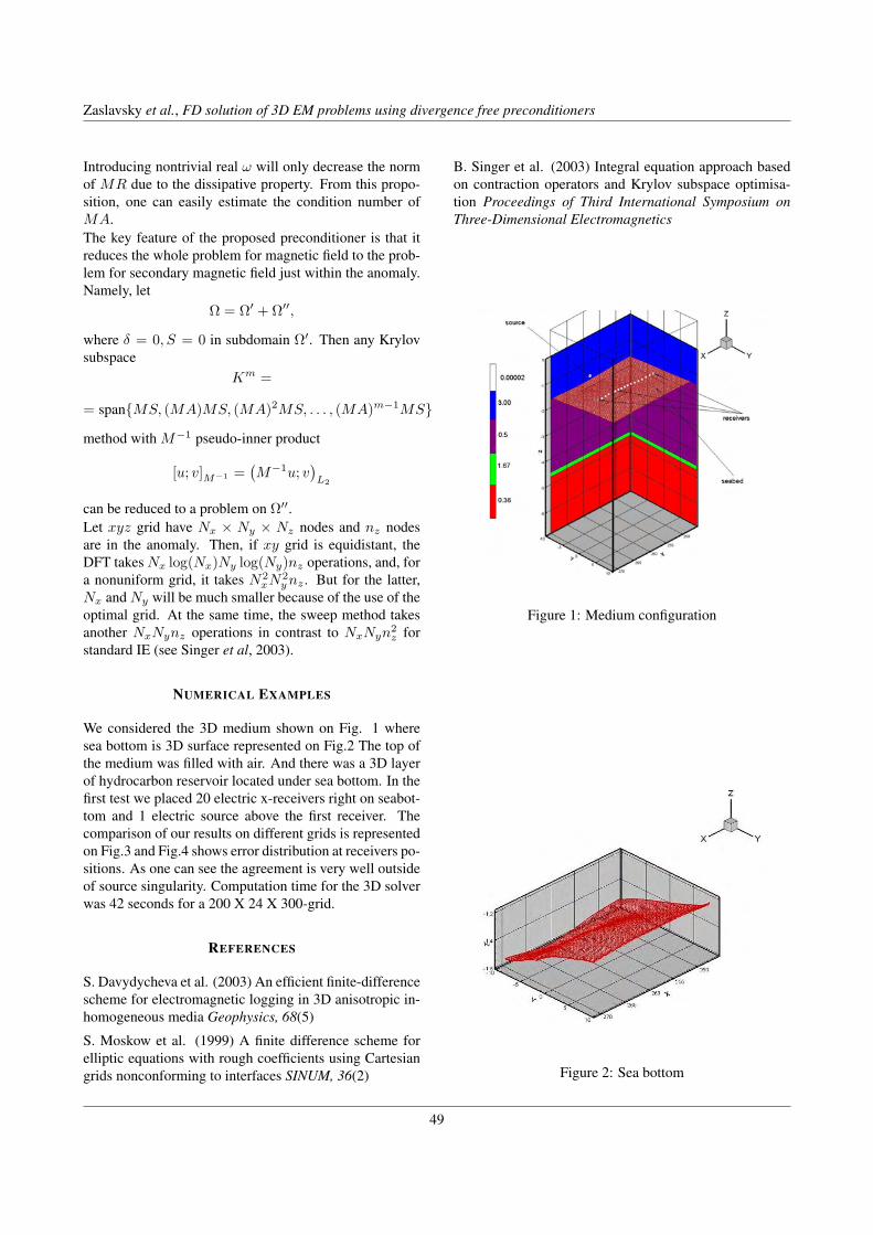
M. Zaslavsky et al., 2007, FD solution of 3D EM problems using divergence free preconditioners
Introducing nontrivial real ω will only decrease the normof MR due to the dissipative property. From this propo-sition, one can easily estimate the condition number ofMA.The key feature of the proposed preconditioner is that itreduces the whole problem for magnetic field to the prob-lem for secondary magnetic field just within the anomaly.Namely, let
Ω = Ω′ + Ω′′,
where δ = 0, S = 0 in subdomain Ω′. Then any Krylovsubspace
Km =
= spanMS, (MA)MS, (MA)2MS, . . . , (MA)m−1MS
method with M−1 pseudo-inner product
[u; v]M−1 =(M−1u; v
)L2
can be reduced to a problem on Ω′′.Let xyz grid have Nx × Ny × Nz nodes and nz nodesare in the anomaly. Then, if xy grid is equidistant, theDFT takes Nx log(Nx)Ny log(Ny)nz operations, and, fora nonuniform grid, it takes N2
xN2y nz . But for the latter,
Nx and Ny will be much smaller because of the use of theoptimal grid. At the same time, the sweep method takesanother NxNynz operations in contrast to NxNyn2
z forstandard IE (see Singer et al, 2003).
NUMERICAL EXAMPLES
We considered the 3D medium shown on Fig. 1 wheresea bottom is 3D surface represented on Fig.2 The top ofthe medium was filled with air. And there was a 3D layerof hydrocarbon reservoir located under sea bottom. In thefirst test we placed 20 electric x-receivers right on seabot-tom and 1 electric source above the first receiver. Thecomparison of our results on different grids is representedon Fig.3 and Fig.4 shows error distribution at receivers po-sitions. As one can see the agreement is very well outsideof source singularity. Computation time for the 3D solverwas 42 seconds for a 200 X 24 X 300-grid.
REFERENCES
S. Davydycheva et al. (2003) An efficient finite-differencescheme for electromagnetic logging in 3D anisotropic in-homogeneous media Geophysics, 68(5)
S. Moskow et al. (1999) A finite difference scheme forelliptic equations with rough coefficients using Cartesiangrids nonconforming to interfaces SINUM, 36(2)
B. Singer et al. (2003) Integral equation approach basedon contraction operators and Krylov subspace optimisa-tion Proceedings of Third International Symposium onThree-Dimensional Electromagnetics
Figure 1: Medium configuration
Figure 2: Sea bottom
3/4
Zaslavsky et al., FD solution of 3D EM problems using divergence free preconditioners
49

M. Zaslavsky et al., 2007, FD solution of 3D EM problems using divergence free preconditioners
Figure 3: Solutions for different grids
Figure 4: Errors for different grids
4/4
Zaslavsky et al., FD solution of 3D EM problems using divergence free preconditioners
50

Theory – Inversion and resolution analysis
51

52

4th International Symposium on Three-Dimensional ElectromagneticsFreiberg, Germany, September 27–30, 2007
Three-dimensional magnetotelluric inversion using quasi-Newton minimization
A. Avdeeva1, and D. Avdeev2,3
1Dublin Institute for Advanced Studies, Ireland2IZMIRAN, Russian Academy of Sciences, Russia
3University of Tokyo, Japan
SUMMARY
In this paper we present recent results for the solution of the three-dimensional (3D) magnetotelluric (MT) inverse prob-lem. Compared with the models considered in our previous work, we are considering a more complicated 3D model. Herewe outline the basics of our solution, and show the results obtained for this model. The results are encouraging, and showthat the software works. However, some unresolved problem remains, as usual. This problem is directly inherent in thephysics of the 3D MT inverse problem, rather than related to some bugs of our solution. We strongly believe that it can besuccessfully resolved, if we apply more constraints on the model parameters, in addition to those imposed by traditionalTikhonov-type regularization.
Keywords: Three-dimensional inversion, magnetotellurics, quasi-Newton optimization
INTRODUCTION
Interestingly, in spite of a hot need for sophisticated three-dimensional (3D) magnetotelluric (MT) inversion soft-ware, only a few developments on such a software arereported (Mackie & Madden, 1993; Mackie et al., 2001;Newman & Alumbaugh, 2000; Newman et al., 2003; Zh-danov & Golubev, 2003; Sasaki, 2004; Siripunvaraporn etal., 2005). It is not very surprising, if one recalls the highlevel of complexity of 3D MT inverse problems.
Mackie & Madden (1993) used a Gauss-Newton op-timization method for coarsely parameterized models.Sasaki (2004) also developed 3D MT inversion, againbased on a Gauss-Newton optimization, with smooth-ness regularization in model space. Siripunvaraporn et al.(2005) successfully developed their 3D inversion, whichis again based a Gauss-Newton approach, but in dataspace. Other authors applied non-linear conjugate gradi-ent (NLCG) methods to solve this problem (Newman &Alumbaugh, 2000; Newman et al., 2003; Mackie et al.,2001; Zhdanov & Golubev, 2003) .
This work is an extension of our previous work (Avdeev& Avdeeva, 2006). In that work we applied a limitedmemory quasi-Newton optimization method to numeri-cally solve the 3D MT inverse problem. As far as weknow, this method has never been applied before to 3DMT problem. However, for completeness we should men-tion work by Haber (2005), where QN methods wereapplied to solve controlled-source EM problems. Herewe first present the basic equations of our solution andthen show and discuss the results obtained for a synthetic
benchmark model.
BASIC EQUATIONS
In our previous paper (Avdeev & Avdeeva, 2006) we pro-posed to solve the 3D MT inverse problem using a limited-memory quasi-Newton minimization method. To solvethis problem numerically, the 3D conductivity model isdiscretized by N = Nx ×Ny ×Nz rectangular cells, andthe conductivities σk (k = 1, . . . , N) of these cells aresought through the minimization of a penalty function
ϕ(σ, λ) = ϕd(σ) + λϕs(σ). (1)
Here ϕd is the data misfit, ϕs is a Tikhonov-type reg-ularization function, λ is the regularization parameter,σ = (σ1, . . . , σN ), where σk is the conductivity of thek-th cell. Our data misfit ϕd has the following unusualform
ϕd =12
NS∑j=1
NT∑i=1
βjitr[AT
jiAji], (2)
where the superscript T means transpose and the upperbar stands for the complex conjugate; NS is the number ofMT sites, rj = (xj , yj , z = 0), where j = 1, ..., NS ; NT
is the number of the periods Ti, where i = 1, ..., NT ; the2× 2 matrices Aji are defined as Aji = Zji −Dji, where
Zji =(
Zxx Zxy
Zyx Zyy
)ji
and Dji =(
Dxx Dxy
Dyx Dyy
)ji
are matrices of the complex-valued predicted Z(rj , Ti)and observed D(rj , Ti) impedances, respectively; βji =
1/4
4th International Symposium on Three-Dimensional ElectromagneticsFreiberg, Germany, September 27–30, 2007
53
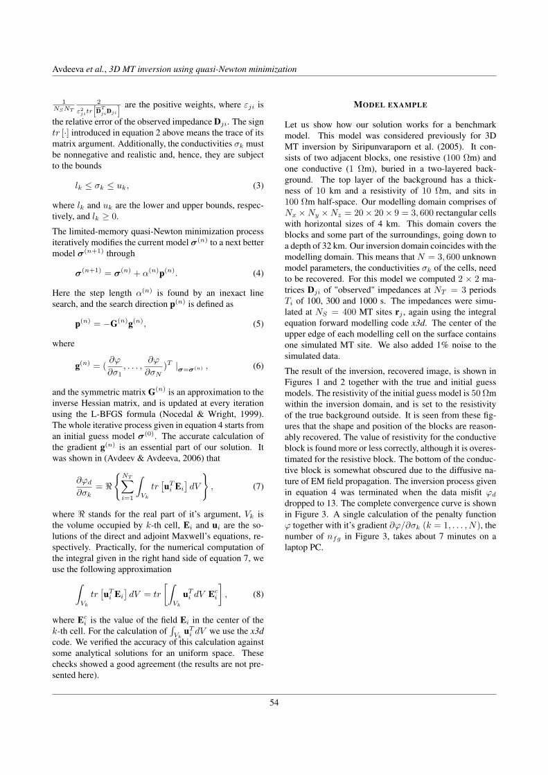
Avdeeva, A., and Avdeev, D., 2007, 3D MT QN inversion . . .
1NSNT
2
ε2jitr
hDT
jiDji
i are the positive weights, where εji is
the relative error of the observed impedance Dji. The signtr [·] introduced in equation 2 above means the trace of itsmatrix argument. Additionally, the conductivities σk mustbe nonnegative and realistic and, hence, they are subjectto the bounds
lk ≤ σk ≤ uk, (3)
where lk and uk are the lower and upper bounds, respec-tively, and lk ≥ 0.
The limited-memory quasi-Newton minimization processiteratively modifies the current model σ(n) to a next bettermodel σ(n+1) through
σ(n+1) = σ(n) + α(n)p(n). (4)
Here the step length α(n) is found by an inexact linesearch, and the search direction p(n) is defined as
p(n) = −G(n)g(n), (5)
where
g(n) = (∂ϕ
∂σ1, . . . ,
∂ϕ
∂σN)T |σ=σ(n) , (6)
and the symmetric matrix G(n) is an approximation to theinverse Hessian matrix, and is updated at every iterationusing the L-BFGS formula (Nocedal & Wright, 1999).The whole iterative process given in equation 4 starts froman initial guess model σ(0). The accurate calculation ofthe gradient g(n) is an essential part of our solution. Itwas shown in (Avdeev & Avdeeva, 2006) that
∂ϕd
∂σk= <
NT∑i=1
∫Vk
tr[uT
i Ei
]dV
, (7)
where < stands for the real part of it’s argument, Vk isthe volume occupied by k-th cell, Ei and ui are the so-lutions of the direct and adjoint Maxwell’s equations, re-spectively. Practically, for the numerical computation ofthe integral given in the right hand side of equation 7, weuse the following approximation∫
Vk
tr[uT
i Ei
]dV = tr
[∫Vk
uTi dV Ec
i
], (8)
where Eci is the value of the field Ei in the center of the
k-th cell. For the calculation of∫
VkuT
i dV we use the x3dcode. We verified the accuracy of this calculation againstsome analytical solutions for an uniform space. Thesechecks showed a good agreement (the results are not pre-sented here).
MODEL EXAMPLE
Let us show how our solution works for a benchmarkmodel. This model was considered previously for 3DMT inversion by Siripunvaraporn et al. (2005). It con-sists of two adjacent blocks, one resistive (100 Ωm) andone conductive (1 Ωm), buried in a two-layered back-ground. The top layer of the background has a thick-ness of 10 km and a resistivity of 10 Ωm, and sits in100 Ωm half-space. Our modelling domain comprises ofNx ×Ny ×Nz = 20× 20× 9 = 3, 600 rectangular cellswith horizontal sizes of 4 km. This domain covers theblocks and some part of the surroundings, going down toa depth of 32 km. Our inversion domain coincides with themodelling domain. This means that N = 3, 600 unknownmodel parameters, the conductivities σk of the cells, needto be recovered. For this model we computed 2 × 2 ma-trices Dji of "observed" impedances at NT = 3 periodsTi of 100, 300 and 1000 s. The impedances were simu-lated at NS = 400 MT sites rj , again using the integralequation forward modelling code x3d. The center of theupper edge of each modelling cell on the surface containsone simulated MT site. We also added 1% noise to thesimulated data.
The result of the inversion, recovered image, is shown inFigures 1 and 2 together with the true and initial guessmodels. The resistivity of the initial guess model is 50 Ωmwithin the inversion domain, and is set to the resistivityof the true background outside. It is seen from these fig-ures that the shape and position of the blocks are reason-ably recovered. The value of resistivity for the conductiveblock is found more or less correctly, although it is overes-timated for the resistive block. The bottom of the conduc-tive block is somewhat obscured due to the diffusive na-ture of EM field propagation. The inversion process givenin equation 4 was terminated when the data misfit ϕd
dropped to 13. The complete convergence curve is shownin Figure 3. A single calculation of the penalty functionϕ together with it’s gradient ∂ϕ/∂σk (k = 1, . . . , N), thenumber of nfg in Figure 3, takes about 7 minutes on alaptop PC.
2/4
Avdeeva et al., 3D MT inversion using quasi-Newton minimization
54

Avdeeva, A., and Avdeev, D., 2007, 3D MT QN inversion . . .
z : 0-1 km 1-2.5 km 2.5-4.5km 4.5-7 km 7-10 km 10-14 km 14-19 km 19-25 km 25-32 km
Figure 1: Comparison with the true model. Each row presents nine horizontal (x − y) slices through the model startingfrom the top (left) to the bottom (right). The depths of the slices are shown above each panel. 1st row correspondsto the initial guess model, 2nd presents to recovered image, and 3rd is the true model. 400 MT sites and 3 periodswere used for this inversion.
Figure 2: Comparison for the central (x-z) cross-section. The left panel presents the recovered image, whereas the rightpanel presents the true model. 400 MT sites and 3 periods were used.
CONCLUSIONS
In addition to the model experiment described above, weperformed a lot of other numerical experiments with thesame 3D model − we inverted the data using several morerefined numerical grids, tried a different number of peri-ods, and we also used coarser coverage of the model byMT sites, etc. The results of these experiments are notpresented here due to obvious space limitations. But insummary, we can say that our feelings about the 3D MTinverse problem solution developed are controversial. Onone side we came up with relatively good images, when
we have dense MT site coverages. Yet, for coarser MTsite coverages our solution sometimes cannot see throughsurface numerical cells, that are not covered by the MTsites. One of our findings is that the Tikhonov-type reg-ularization we included in our inversion solution, is notpowerful enough to suppress non-smoothness of the resis-tivity images (especially for the upper part of the model).Still, we believe that our solution can doubtlessly be usedto recover the resistivity images of the lower part of earthmodels. As for the upper part of the models, it’s proper re-covering depends on many factors, such as the geometryand resistivity of the structures inside the earth, coverage
3/4
Avdeeva et al., 3D MT inversion using quasi-Newton minimization
55
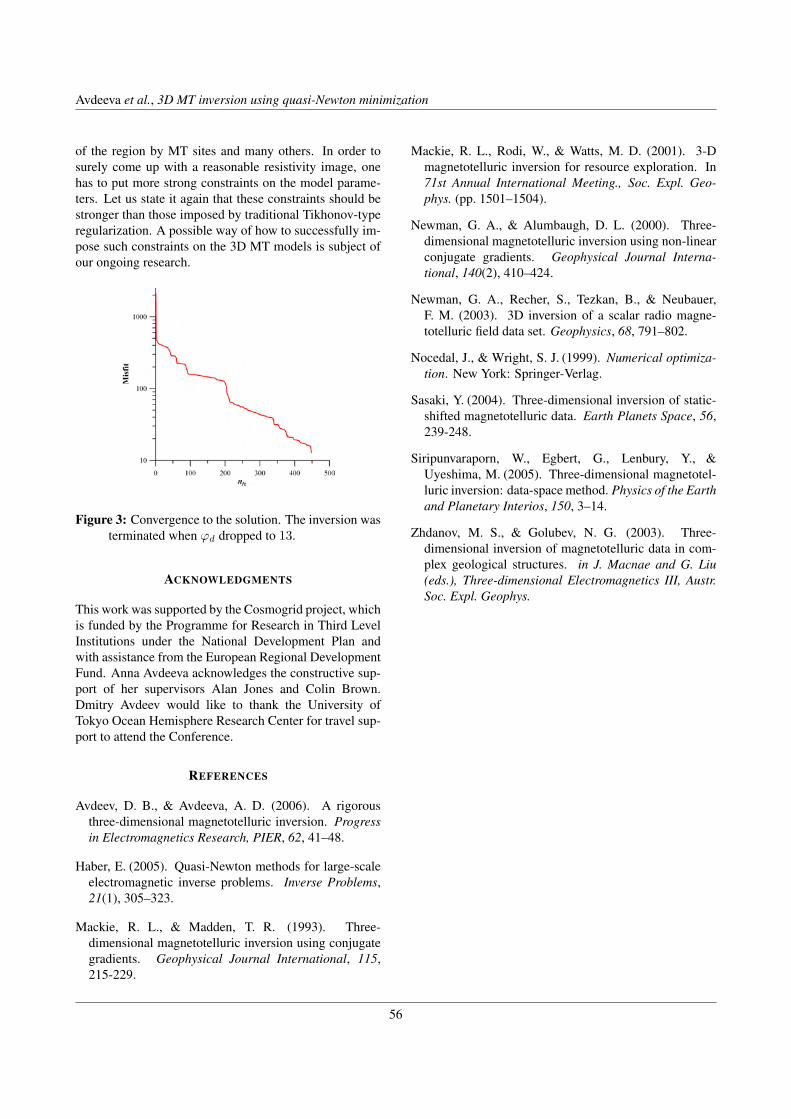
Avdeeva, A., and Avdeev, D., 2007, 3D MT QN inversion . . .
of the region by MT sites and many others. In order tosurely come up with a reasonable resistivity image, onehas to put more strong constraints on the model parame-ters. Let us state it again that these constraints should bestronger than those imposed by traditional Tikhonov-typeregularization. A possible way of how to successfully im-pose such constraints on the 3D MT models is subject ofour ongoing research.
Figure 3: Convergence to the solution. The inversion wasterminated when ϕd dropped to 13.
ACKNOWLEDGMENTS
This work was supported by the Cosmogrid project, whichis funded by the Programme for Research in Third LevelInstitutions under the National Development Plan andwith assistance from the European Regional DevelopmentFund. Anna Avdeeva acknowledges the constructive sup-port of her supervisors Alan Jones and Colin Brown.Dmitry Avdeev would like to thank the University ofTokyo Ocean Hemisphere Research Center for travel sup-port to attend the Conference.
REFERENCES
Avdeev, D. B., & Avdeeva, A. D. (2006). A rigorousthree-dimensional magnetotelluric inversion. Progressin Electromagnetics Research, PIER, 62, 41–48.
Haber, E. (2005). Quasi-Newton methods for large-scaleelectromagnetic inverse problems. Inverse Problems,21(1), 305–323.
Mackie, R. L., & Madden, T. R. (1993). Three-dimensional magnetotelluric inversion using conjugategradients. Geophysical Journal International, 115,215-229.
Mackie, R. L., Rodi, W., & Watts, M. D. (2001). 3-Dmagnetotelluric inversion for resource exploration. In71st Annual International Meeting., Soc. Expl. Geo-phys. (pp. 1501–1504).
Newman, G. A., & Alumbaugh, D. L. (2000). Three-dimensional magnetotelluric inversion using non-linearconjugate gradients. Geophysical Journal Interna-tional, 140(2), 410–424.
Newman, G. A., Recher, S., Tezkan, B., & Neubauer,F. M. (2003). 3D inversion of a scalar radio magne-totelluric field data set. Geophysics, 68, 791–802.
Nocedal, J., & Wright, S. J. (1999). Numerical optimiza-tion. New York: Springer-Verlag.
Sasaki, Y. (2004). Three-dimensional inversion of static-shifted magnetotelluric data. Earth Planets Space, 56,239-248.
Siripunvaraporn, W., Egbert, G., Lenbury, Y., &Uyeshima, M. (2005). Three-dimensional magnetotel-luric inversion: data-space method. Physics of the Earthand Planetary Interios, 150, 3–14.
Zhdanov, M. S., & Golubev, N. G. (2003). Three-dimensional inversion of magnetotelluric data in com-plex geological structures. in J. Macnae and G. Liu(eds.), Three-dimensional Electromagnetics III, Austr.Soc. Expl. Geophys.
4/4
Avdeeva et al., 3D MT inversion using quasi-Newton minimization
56

SUSSESSION OF PARTIAL MT AND MV INVERSIONS - FROM 2D TO 3D Mark Berdichevsky, Vladimir Dmitriev Moscow State Univertsity [email protected] Abstract Method of successive partial inversions of magnetotelluric and magnetovariational
data is successfully employed in 2D interpretation. We assume that this method can be useful in 3D interpretation.
Speaking on development of modern magnetotellurics, we first of all note its main tendency
linked with transition from two-dimensional inversion of the magnetotelluric (MT) and magnetovariational (MV) data to three-dimensional inversion. Here the question arises of whether the philosophy of the two-dimensional inversion, which proved successful in regions with elongate symmetrical geoelectric structures, can be applied for the three-dimensional inversion in regions with asymmetric geoelectric medium. In our paper we try to answer this question.
It is evident that adequate description of 3D media requires a great number of the geoelectric
and geometric parameters. This impairs the inversion stability. We arrive at a conclusion that stronger constraints must be imposed on the three-dimensional inter-pretation model.
The properties of the two-dimensional magnetotelluric field depend on its orientation in reference frame formed by the model strike (to separate the induction and galvanic anomalies, it is enough to orient the magnetotelluric field along and across the model strike). In the three-dimensional asymmetric model such a reference frame is absent. So, we lose that simple physical basis, on which the strategy of two-dimensional inversion separating inductive TE mode and galvanic TM mode has been constructed. It would be helpful to use the experience of two-dimensional interpretation and to create the strategy of multicriterion three-dimensional inversion, which is an analog of multicriterion two-dimensional inversion, but takes into account the properties of the three-dimensional magnetotelluric field. Do the boundaries exist in the three-dimensional field, which divide the inversion according its sensitivity to objective structures and immunity to near-surface distortion? Such boundaries can be drawn between the inversion of the MV functions, the inversion of the MT phase functions and the inversion of the MT functions of apparent resistivities.
The three-dimensional inverse problem as well as the two-dimensional inverse problem is multicriterion ( the conductivity distribution is derived from a set of magnetotelluric and magnetovariational response functions, which have different sensitivity to objective structures and different immunity to near-surface distortions). The simultaneous parallel inversion of all these functions is hardly reasonable since they can conflict with each other. Experience of the two-dimensional interpretation suggests that the best result can be obtained by successive partial inversions, which are connected with each other through the starting models and the stabilizers providing proximity to the starting models (Fig.1). The following succession of two-dimensional partial inversions is applied: 1) TE inversion of the magnetovariational response functions (tipper , horizontal magnetic tensor ) – being free of near-surface static distortions, this inversion yields sufficiently reliable primary image of the geoelectric medium (particularly of its conductive zones), 2) TE inversion of the magnetotelluric phase response functions ( phase of the longitudinal impedance, long-itudinal component of the phase tensor) - at low frequencies this inversion is also free of near-surface static distortions, it controls and edits the magnevariational inversion, increasing the investigation depth ( here the transverse apparent resistivities distorted by static shift are eliminated), 3) TM inversion of the magnetotelluric response functions (transverse apparent resistivity , phase of the transverse impedance) – this inversion is subjected to strong near-surface distortions and has low sensitivity to deep conductive zones, but it can give additional information on the sedimentary cover, state of the faults, galvanic connections in the lithosphere; inversion of , is usually carried out on the background of fixed deep structures obtained by
WM
||ϕ||Φ
⊥ρ ⊥ϕ
⊥ρ ⊥ϕ
1
4th International Symposium on Three-Dimensional ElectromagneticsFreiberg, Germany, September 27–30, 2007
57
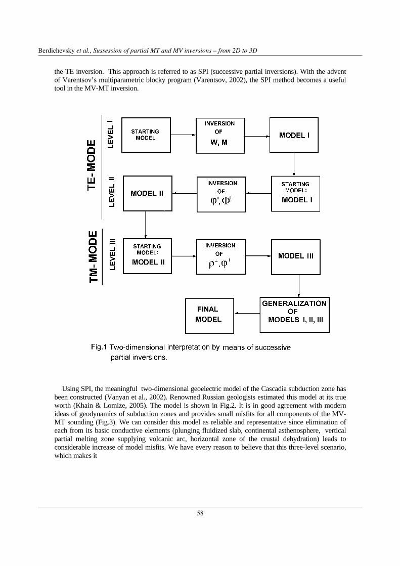
the TE inversion. This approach is referred to as SPI (successive partial inversions). With the advent of Varentsov’s multiparametric blocky program (Varentsov, 2002), the SPI method becomes a useful tool in the MV-MT inversion.
Using SPI, the meaningful two-dimensional geoelectric model of the Cascadia subduction zone has been constructed (Vanyan et al., 2002). Renowned Russian geologists estimated this model at its true worth (Khain & Lomize, 2005). The model is shown in Fig.2. It is in good agreement with modern ideas of geodynamics of subduction zones and provides small misfits for all components of the MV-MT sounding (Fig.3). We can consider this model as reliable and representative since elimination of each from its basic conductive elements (plunging fluidized slab, continental asthenosphere, vertical partial melting zone supplying volcanic arc, horizontal zone of the crustal dehydration) leads to considerable increase of model misfits. We have every reason to believe that this three-level scenario, which makes it
2
Berdichevsky et al., Sussession of partial MT and MV inversions – from 2D to 3D
58

possible to focus inversion on certain objective structures, can form the basis for three-dimensional MV-MT interpretation. Fig.4 is a schematic diagram of the three-dimensional successive partial inversions. It contains basic magnetovariational inversions, which are immune to near-surface distortions (inversion of tipper and horizontal magnetic tensor WM ), and editing magnetotelluric inversions: the phase inversions (inversion of the impedance
phases and the phase tensor ), which can confirm the results of MV sounding and yxϕϕ ,xy Φ
3
Berdichevsky et al., Sussession of partial MT and MV inversions – from 2D to 3D
59

increase its depth, and amplitude inversion of the magnetotelluric apparent resistivities , which can give additional information on sediments, faults and upper layers of the Earth’s crust.
yxxy ρ ,ρ
4. Proceeding from experience of two-dimensional MV-MT interpretation, we assume that the method of three-dimensional successive partial inversions can be efficient provided it is applied in regions with sufficiently simple geoelectric medium (gentle layering, closed conductive zones, absence of faults, fractures, thrusts and etc). It seems that by studying complicated three-dimensional structures, the interpretation should be divided into two sta-ges. The first stage reduces to smoothing MV and phase MT inversions (Occam inversions based on the least-structure principle). This stage results in a primary simplified schematic model of the geoelectric medium. In the second stage, the primary model is examined in some detail. It is correlated with a priory information and with qualitative analysis of MV-MT data. On testing and editing, the primary model is included into a blocky starting model, which
is supplemented with a set of inhomogeneities related to different hypotheses for the medium under investigation. The blocky starting model is limited in number of blocks. Geometry of blocks and their minimum number are adjusted in accord with required detailedness in image of structures. The partition density should be higher in zones, which contain assumed structures, and lower in intermediate (“empty”) zones. The free parameters of the starting model are determined by SPI
4
Berdichevsky et al., Sussession of partial MT and MV inversions – from 2D to 3D
60

method. Hypotheses, which yield the minimum model misfit, are taken as the most plausible. Thus, the successive partial inversions are carried out on the basis of the primary smoothing inversion and are integrated with the hypothesis tests. The idea of the suggested approach can be formulated in the following way. First we construct a primary crude model of the geoelectric medium. Then we detail the medium without going far from the primary crude model. This approach can provide sufficiently stable and detailed three-dimensional interpretation, realized in the model class with rather small number of free parameters. REFERENCES Khain, V.E., Lomize, M.G., 2005, Geotectonics with foundations of geodynamics, Publishing House “Knizhny Mir UNIVERSITET”, pp 559 (in Russian). Vanyan, L.L., Berdichevsky, M.N.,Pushkarev, P.Yu., Romanyuk, T.V.,2002, A Geoelectric Model of the Cascadia Subduction Zone, Izvestia, Physics of the Solid Earth, 38, 10, 798-815. Varentsov, I.M., 2002, A general approach to magnetotelluricdata inversion in a piecewise continuous medium, Izvestia, Physics of the Solid Earth, 38, 11, 913-934.
5
Berdichevsky et al., Sussession of partial MT and MV inversions – from 2D to 3D
61

4th International Symposium on Three-Dimensional Electromagnetics Freiberg, Germany, September 27−30, 2007
Resistivity inversion of Magnetic Resonance Sounding –
Assessment of Sensitivity and Reliability
M. Braun and U. Yaramanci Technical University of Berlin, Germany
SUMMARY The Magnetic Resonance Sounding (MRS) or Surface Nuclear Magnetic Resonance (SNMR) method is used for groundwater exploration and aquifer characterization. MRS provides useful information about water content and hydraulic conductivity of the aquifer. The excitation field of the NMR experiment is generated by a transmitter loop placed on the surface. Due to the electromagnetic attenuation, the magnetic excitation field depends on the resistivity of the subsurface. Therefore, the resistivity has to be taken into account when inverting the MRS data. Neglecting the resistivity causes a biased estimate of the water content distribution. The resistivity information can be given by a priori information or, as newly introduced in the presented inversion scheme here, it can be obtained during the inversion process. Having also the resistivity along with the water content distribution as inversion result, MRS gives information about the salinity of the aquifer and thereby, the quality of the aquifer can be estimated. This is of utmost interest for the further hydrogeological interpretation. This specific information cannot be achieved by geoelectrics alone, because of the nonuniqueness in resistivity concerning water content and salinity. Keywords: magnetic resonance sounding, surface nuclear magnetic resonance, inversion, sensitivity
INTRODUCTION Magnetic Resonance Sounding (MRS, or Surface Nu-clear Magnetic Resonance, SNMR) is used for ground-water exploration and aquifer characterization (Yara-manci and Hertrich, 2006). The NMR experiment is conducted by a transmitter and receiver loop at the sur-face exciting the spin of protons of water molecules in the subsurface with the Larmor frequency of the earth’s magnetic field. Successively increasing the excitation intensity (pulse moment q) yields a complex sounding curve. The initial amplitude E0 of the voltage response in the receiver loop is the integral over the water content f and the complex kernel function K, which comprises parameters depending on the location (e.g. resistivity of the subsurface) and depending on the loop geometry:
dVfqKqE )(),()(0 rr∫= (1)
Explicit expressions and detailed derivation for the ker-nel function are given in Weichman et al., 2000.
The excitation field of the NMR experiment is gener-ated by a transmitter loop placed on the surface. Due to the electromagnetic attenuation, the magnetic excita-tion field depends on the resistivity of the subsurface. Figure 1 shows exemplarily the excitation magnetic field of a circular loop over an electrically homogeneous subsurface (left) and a 2D resistivity structure (right). The axial symmetry of the field disappears using a non-1D subsurface. For the further calculation in MRS, the excitation magnetic field must be known in the entire 3D volume of the subsurface. In the following, 1D conditions of the subsurface are considered. Thus, the axial symmetry of the excitation magnetic field can be exploited when calculating the field. However, only the component perpendicular to the earth’s magnetic field generates the NMR signal. Thus, the 3D MRS kernel function is non-symmetric even for a homogeneous subsurface, except for the case of 90° inclination, i.e. at the poles.
1/4
4th International Symposium on Three-Dimensional ElectromagneticsFreiberg, Germany, September 27–30, 2007
62

Braun, M., Yaramanci, U. , 2007, Resistivity inversion of MRS – Assessment of sensitivity and reliability
Figure 1: Magnitude log10(Bnorm) of the excitation magnetic field of a circular loop (d=100 m, loop centre at the origin of the coordinate system) using f=2043 Hz. Electrical conductivity of the air half-space (z>0 m) is 0 S/m. The subsur-face (z<0 m) is electrically homogeneous with 50 Ωm (left). It consists of a 25 m thick discontinuous layer at 25 m depth with 5 Ωm in a surrounding of 50 Ωm (right). Calculations are performed with Comsol Multiphysics. ESTIMATION OF THE PENETRATION DEPTH
AND EFFECTS OF RESISTIVITY Several ways have been presented in order to calculate the MRS penetration depth. Three approaches of the estimation of the MRS penetration depth are superim-posed on the image of the 1D kernel function versus depth and homogeneous half-space resistivity exemplarily for two pulse moments (Fig. 2). It is clearly visible that estimation via the skin depth is not useful for MRS application, not even for depths smaller than one loop size as proposed in Vouillamoz et al. (2007). The electromagnetic skin depth describes the distance, where a plane wave will be reduced by a factor of 1/e, i.e. it falls to 37 % of its original value. However, the MRS method uses a loop as an active source. Thus, there is also a geometrical attenuation dependent on the inhomogeneity in horizontal direction: the more the field is inhomogeneous in horizontal direction, the more the field is attenuated in vertical direction. The MRS maximum depth detection follows the contour line of 10 nV/m (Legchenko and Shushakov, 1998). Below this depth limit, the water content does not contribute to the measured MRS signal. This is the depth down to which the kernel function should be calculated when inverting the data. The MRS penetration depth using the SVD approach follows the maximum sensitivity (Müller-Petke et al.,
2007). This can be regarded as confidence depth limit down to which the inversion can give a reliable result. It is necessary to point out that the MRS penetration depth depends on various parameters such as loop size, number of turns, resistivity structure of the subsurface, earth's magnetic field strength and inclination. Therefore, the MRS penetration depth must be calculated for each site using the appropriate kernel function.
RESISTIVITY EFFECT IN THE INVERSION The resistivity has to be taken into account when in-verting the MRS data. Neglecting the resistivity causes a biased estimate of the water content distribution. The used resistivity information can be given as a priori or, as newly introduced, in the presented inversion scheme here, it can be obtained during the inversion process (Braun, 2007). Figure 3 shows a comparison of the inversion results of MRS field data, collected in Sardinia (Italy) close to the sea shore. The MRS standard inversion with resistivity as a priori information is shown in Figure 3 (top) as well as MRS with resistivity inversion (bottom). The block inversion is conducted with three layers. The used resistivity distributions are homoge-neous subsurfaces with 50 Ωm and 5 Ωm as well as the resistivity distribution derived from a DC geoelectric measurement at the same site. The low resistivity of the aquifer is caused by salt water intrusion from the sea.
2/4
Braun et al., Resistivity inversion of MRS – Assessment of sensitivity and reliability
63

Braun, M., Yaramanci, U. , 2007, Resistivity inversion of MRS – Assessment of sensitivity and reliability
Figure 2: Image of the amplitude of the 1D MRS kernel function of a pulse moment q=3.4 As and q=18 As for homogeneous half-spaces with resistivities between 1 and 1000 Ωm. The calculated electromagnetic skin depth, MRS penetration depth and MRS maximum detection depth are superimposed. A circular loop is used with a diameter of d=100 m and a magnetic field intensity of 48000 nT as well as 60°N inclination. The dependence of the inversion result on the used re-sistivity is clearly obvious. Thus, using an appropriate resistivity also improves the water content determina-tion. The reliability of the inversion result is shown in Figure 4 in terms of the root-mean-square (rms) error. The rms is calculated between synthetic data, calculated after successively changing water content and resistivity of one layer, and measured MRS data. The fixed layer depths (2 m and 18.5 m) were determined by MRS with resistivity inversion (Figure 3 bottom). Resistivity and water content of one layer are changed while the subsurface parameters of the other two layers are set constant. It is clearly visible that water content and resistivity of the aquifer (Layer 2) is most reliably determined indicated as pronounced minimum of the rms. Even if the minimum is broader for Layer 1 and 3, the possible solutions are narrowed.
CONCLUSIONS A 1D inversion scheme is presented for determining water content and resistivity from MRS. This is the basis for using MRS as a stand-alone method. Also, the determination of the water content is improved when using an appropriate resistivity model. Having the resistivity along with the water content distribution as inversion result, MRS gives information
about the salinity of the aquifer and thereby, the quality of the aquifer can be estimated. This specific informa-tion cannot be achieved by geoelectrics alone, because of the nonuniqueness in resistivity concerning water content and salinity.
REFERENCES Braun, M. (2007). Influence of the resistivity on Mag-
netic Resonance Sounding: 1D inversion and 2D modelling. PhD thesis, Technical University of Berlin.
Legchenko, A., Shushakov, O. (1998). Inversion of surface NMR data. Geophysics 63 (1), 75-84.
Müller-Petke, M., Hertrich, M., Yaramanci, U. (2007). Optimization and resolution studies for Magnetic Resonance Sounding (MRS) using SVD. Submitted to Journal of Applied Geophysics.
Vouillamoz, J., Chatenoux, B., Mathieu, Baltassat, J., Legchenko, A. (2007). Efficiency of joint use of MRS and VES to characterize coastal aquifer in Myanmar. Journal of Applied Geophysics 61, 142-154.
Weichman, P., Lavely, E., Ritzwoller, M. (2000). The-ory of surface nuclear magnetic resonance with applications to geophysical imaging problems. Physical Review E, 62 (1), 1290-1312.
Yaramanci, U., Hertrich, M. (2006). Magnetic Reso-nance Sounding. In: (Ed. Kirsch, R.) Groundwater Geophysics. Springer-Verlag, 253-274.
3/4
Braun et al., Resistivity inversion of MRS – Assessment of sensitivity and reliability
64

Braun, M., Yaramanci, U. , 2007, Resistivity inversion of MRS – Assessment of sensitivity and reliability
Figure 3: MRS field data from Sardinia. The data are collected using a circular loop (d=70 m, 2 turns). Magnetic field intensity 44968 nT, 55°N inclination. MRS standard inversion using the resistivity a priori (top) and MRS with resistiv-ity inversion (bottom).
Figure 4: Contour plots of the rms for amplitude as well as real and imaginary parts changing water content and resis-tivity of one layer. Fixed layer depths (2 m and 18.5 m) are used, determined from the MRS with resistivity inversion. The inversion result is (Figure 3 bottom): 9 vol.%, 16 vol.%, 10 vol.% and 3 Ωm, 0.7 Ωm, 998 Ωm for Layer 1, 2 and 3, respectively.
4/4
Braun et al., Resistivity inversion of MRS – Assessment of sensitivity and reliability
65

Joint inversion and topographic correction of geophysical data
Chen, J., Jegen-Kulcsar, M. (IFM-GEOMAR), Heincke, B. (Norwegian Geological Survey)
Abstract: Different geophysical data such as gravity, seismic and electromagnetic data often contain complementary information and are sensitive to different features of a subduction zone. Since furthermore inversion of geophysical data of any kind is inherently non-unique, i.e. a variety of earth models may fit a particular data set equally well, it is difficult to develop a coherent picture of a geological setting from individual inversion results of different data set. The obvious way of developing a more complete picture of subduction zones and reducing the degree of non-uniqueness is the combination of various geophysical data in a joint inversion approach. By inverting different data sets jointly, an earth model is searched, which fits all data sets in question simultaneously.Here we will present a joint inversion scheme of EM, gravity and seismic data together with joint inversion results or data collected on a passive margin. The results are furthermore compared with individual data type inversion.Subduction zones and passive margins are characterized by large changes in topography on a regional as well as local scale. Topography may have a large impact on geophysical data, e.g. on the gravity data due to the large density contrast between water and rocks, and on EM data due to electrical current distortion. The analysis of the passive margin data showed, that these influences have to be carefully investigated. The first stage we have approached the topography effect on gravity in two ways. (1), Within the model through refined topography modelling. (2) Outside of the model by applying topographic correction to the data. We will present and discuss results for joint inversion with these topographic correction. The second stage dealing with the topographic influence on EM data will be reported next.
4th International Symposium on Three-Dimensional ElectromagneticsFreiberg, Germany, September 27–30, 2007
66

4th International Symposium on Three-Dimensional ElectromagneticsFreiberg, Germany, September 27–30, 2007
Modelling of multi-transmitter arrays in Magnetic Resonance Sounding
J. Kamm, M. Müller-Petke, and U. YaramanciTechnical University of Berlin
SUMMARY
The standard configuration in Magnetic Resonance Sounding (MRS) is coincident transmitter and receiver loop. Mean-while also some efforts have been made to realize separated transmitter and receiver loops. In this paper, we introducemulti-transmitter arrays to enhance model resolution. We present two configurations that are benefecial in particularconditions.
The first one is a symmetric transmitter spreading around the receiver loop. A moderate separation allows a significantimprove regarding 1D sensitivity. In the second approach, concentric counteracting transmitter coils are analysed. Thisapproach is adequate to improve the resolution of near-surface structures. These results are promising in terms of 1Dsensitivity. This is verified via 1D inversion of synthetic data. Multi-transmitter approaches discussed can enhance spatialresolution in several ways at the cost of penetration depth.
Keywords: surface nuclear magnetic resonance, magnetic resonance sounding, multi-transmitter, modelling
INTRODUCTION
In Magnetic Resonance Sounding, the magnetic proper-ties of hydrogen nuclei are exploited to detect water inthe subsurface. It is the only geophysical method that di-rectly leads to the desired physical property, i.e. the wa-ter content distribution. In this view it turns out to be atool especially applicable in hydrogeophysics. The one-dimensional sounding employs a coincident transmitterand receiver loop (see Yaramanci and Hertrich (2006)).Weichman, Lavely, and Ritzwoller (2000) came up witha generalized formulation of the forward problem, whichmade measurements with separated receiver and transmit-ter loops possible. Besides, the theory holds for arbitrarytransmitter and receiver spreads with multiple loops, butwas not exploited up to the present. The first step in thatdirection is done in this work by the introduction and eval-uation of multi-transmitter arrays. Two promising resultsin terms of 1D sensitivity are presented and discussed re-specting favorable sensitivity distributions. This is donewith sensitivity plots as well as 1D inversion of a syntheticdata set.
THE MRS KERNEL FUNCTION
It is necessary to gain some insight on the assembly ofthe kernel function. Weichman et al. (2000) presents anextended formulation of the MRS signal. The initial am-plitude E0 of the voltage response in the receiver loop isthe integral over the water content f and the kernel func-
tion K with respect to the applied pulse moment q:
E0(q) =∫
f(~r)K(~r, q)d3r (1)
where K in the general three-dimensional case is
K(q, ~r) = 2πfL| ~M0| sin(q| ~B+T (~r)|)eiζT (~r)
×2| ~B−R(~r)|eiζR(~r)
×[~bR(~r) ·~bT (~r) + i~b0 ·~bR(~r) ×~bT (~r)].
(2)
~M0 denotes equilibrium magnetization in the magneticfield of the earth ~B0. ~B+
T is the circular polarized partof the transmitter field ~BT co-rotating with spin preces-sion, projected along the direction perpendicular to ~B0
and normalized on a unit current. Similarly ~B−R defines thecounter-rotating part of the virtual unit field of the receiverloop, also projected to the plane orthogonal to ~B0. fL isthe Larmor frequency corresponding to ~B0. ζT and ζR arethe phases of the particular fields. ~b0 is the the unit vec-tor parallel to the earth field direction. The other~b denoteunit vectors pointing in the directions of the componentsorthogonal to the earth field of the indicated fields. Thetwo-dimensional kernel then is obtained by integration
K2D(q, y, z) =∫
K(q, x, y, z)dx (3)
and the one-dimensional kernel follows from
K1D(q, z) =∫ ∫
K(q, x, y, z)dydx, (4)
respectively.
1/4
4th International Symposium on Three-Dimensional ElectromagneticsFreiberg, Germany, September 27–30, 2007
67

Kamm, J. et al., 2007, Multi-transmitter arrays in MRS
Thus, the first line of Eq. 2 merely refers to the transmit-ter and its effect on the hydrogen nuclei in the subsurface,i.e. the excitation. The second line represents the sensi-tivity of the receiver loop alone. The third line relates thepreceding ones geometrically. A detailed discussion ofthese kernel parts concerning the receiver-transmitter sep-aration was carried out by Hertrich, Braun, and Yaramanci(2005), while a review on the influence of resistivity canbe found in Braun, Hertrich, and Yaramanci (2005).
The multi-transmitter approach is used to implement twobasic optimization strategies. Firstly, a superposition oftransmitter fields is associated to the first line of eq. 2.Secondly, the spatial relation of transmitter and receiverrefers to the latter two. In fact, both influences cannotbe analysed separately. Two approaches to enhance one-dimensional resolution were found to be especially favor-able.
In the following, a homogenoues subsurface with a resis-tivity of 100 Ωm and an inclination of the earth field of60N were assumed. The Larmor frequency at 48000 nT is2043.7 Hz.
SYMMETRIC TRANSMITTER SPREAD
The first configuration presented exploits the asymmetricnature of the kernel function due to earth field inclination.Two coils along the north-south-axis match their edges atexactly one point. This is the midpoint of the array aswell as the center of the receiver loop. All loops are 50min diameter (see Fig. 1).
Figure 1: Symmetric Transmitter spread: Two transmit-ters are symmetrically distributed around the mid-point of one receiver loop. All loops are 50m indiameter.
As a reference, the kernel function of a standard coinci-dent loop configuration with the equivalent transmissionenergy is calculated (see Fig. 2). The two separated trans-mitter loops add their effects at intermediate depth levels.The curved northern and southern lobes contribute less tothe signal in the symmetric transmitter spread, because
they are farther off the receiver loop than in the coinci-dent case. The asymmetry decreases as the steepness ofthe focused area of the kernel function is diminished. Os-cillations in the upper part have significantly larger wavelengths than in the coincident loop configuration.
Figure 2: Real parts of two pulse moments (4.03 As,10.97 As) of a 2D kernel function of a coincidentloop array as a reference (left) and the symmetricspread (right). The asymmetry is diminished, thecurved outer lobes of the kernel are less importantand the sensitivity distribution is more confined.
Figure 3: Real parts of the 1D kernel function of thereference coincidence loop sounding (left) and thesymmetric transmitter spread (right). The sensitiv-ity contrast at the upper border of the lowest oscil-lation of the kernel function (focused area) is en-hanced. The distribution is more confined.
Additionally, the 1D-kernel is shown in Figure 3. The firstoscillation above its focused tail is emphasized. Hence,the upper boundary of that crucial part of the kernel ismuch better defined, as the sensitivity contrast there evenyields a continuous negative sign for every pulse moment.The focused part stays more confined even in deeper re-
2/4
Kamm et al., Modelling of multi-transmitter arrays in MRS
68

Kamm, J. et al., 2007, Multi-transmitter arrays in MRS
gions. However, the major drawback of the configura-tion is a loss of penetration depth. The approach highlydepends on local earth field conditions. It favors a non-vertically inclined earth field. The overall signal strengthis not diminished in comparison to the coincident case.
Figure 4: Results of 1D-Inversion (red) of a syntheticmodel (blue) for the coincident case (left) and thesymmetric transmitter spread (right). The respec-tive synthetic data and the fit are displayed aside.Especially the aquiclude and the deep aquifer areresolved significantly better compared to the coin-cident loop configuration.
To demonstrate the improvements coming with the pro-posed configuration, synthetic data calculated for a twoaquifer model was inverted. 10nV of Gaussian noisedistributed noise was added. The estimated model (seeFig. 4) was derived from a single step generalized inver-sion scheme using a truncated singular value decompo-sition with tikhonov regularisation. The tikhonov regu-larisation parameter λ was choosen by generalized crossvalidation while the truncation level σi=truncation is es-timated from the singular value distribution (see Müller-Petke, Hertrich, and Yaramanci (2006)). The symmetrictransmitter sounding resolves the aquiclude layer betweenthe aquifers better than the coincident sounding. Also, thewater content of the aquifers is better approximated. Thisis due to higher signal amplitudes at the high pulse mo-ments.
CONCENTRIC LOOPS
The second approach is a symmetric one, and thus, is lessdependent on the inclination and strength of the earth fieldat the locality. We propose to set up a standard coinci-dent loop setting with a loop diameter of 75m, and addinga counteracting inner loop with a diameter of 2/3 of theouter loop (see Fig. 5).
Figure 5: Concentric loops: A big outer loop with a diam-eter of 75m is used as a transmitter and a receiver atthe same time. Concentrically, a smaller transmitterloop is positioned with a counteracting phase of π,i.e. a reversed sign.
Figure 6: Real parts of 2D kernel functions for two pulsemoments (4.03 As, 10.97 As) of a coincident con-figuration (left) and of the concentric loops configu-ration (right). Compared to the coincident case, thesensitivity distribution is more horizontally aligned,less curved and more confined. The penetrationdepth is considerably decreased.
The current flows with a phase shift of exactly π in theinner loop. The reference again is the standard coinci-dent loop configuration. Compared to it, the 2D kernelof the proposed scheme is more horizontal (see Fig. 6).This corresponds to a generel decrease of north-south-asymmetry. Near the surface, the counteracting transmit-ters cancel each other out partially. This results in slightlyreduced amplitudes in the oscillating upper part of the ker-nel. The focused area is concentrated on a smaller regionand the amplitude there is higher than in the coincidentcase.
Once again, an inversion was carried out to comparethe proposed concentric loops with their reference (seeFig. 8). The model and noise level applied are the same asin the preceding section. Both configurations resolve the
3/4
Kamm et al., Modelling of multi-transmitter arrays in MRS
69

Kamm, J. et al., 2007, Multi-transmitter arrays in MRS
two aquifers, but the inversion using the concetric loopsestimates the actual water content more exactly. Espe-cially in identifying the water content of the aquiclude,the proposed scheme is superior to the standard coincidentsounding.
Figure 7: Real parts of the 1D kernel function of the co-incident loop sounding (left) and of the concentricloops sounding (right). The penetration depth aswell as the high sensitivity at low pulse moments isdamped compared to the coincident case, while athigh pulse moments the focused area is more con-fined.
Figure 8: Results of 1D-Inversion (red) of a syntheticmodel (blue) for the coincident case (left) and theconcentric loops (right). The respective syntheticdata and the fit are displayed aside. Both arrays re-solve the general structure. Nevertheless, the con-centric loops identify the water contents more ex-actly.
CONCLUSIONS
Multi transmitter configurations are successfully intro-duced into MRS and evaluated. They prove to be capa-ble of enhancing the model resolution. The approachespresented are specific to certain conditions and have to beadapted to the locality, i.e. the earth field and the target
of investigation. However, the identified tendencies areexpected to hold under more general circumstances. Ithas been shown, that multi transmitter arrays can be de-signed to improve the resolution of MRS measurements,especially at intermediate depths or near the surface. Pen-etration depth is negatively affected and has to be tradedoff against resolution gain. The technical realization ofmulti-transmitter MRS should considerably improve theexploration.
Further configurations are about to be evaluated. Hereindividual pulse moments/phases for any transmitter aretaken into account.
REFERENCES
Braun, M., Hertrich, M., & Yaramanci, U. (2005). Studyon complex inversion of magnetic resonance sound-ing signals. Near Surface Geophysics, 3(3), 155-163.
Hertrich, M., Braun, M., & Yaramanci, U. (2005). Mag-netic resonance soundings with separated transmit-ter and receiver loops. Near Surface Geophysics,3(3), 131-144.
Müller-Petke, M., Hertrich, M., & Yaramanci, U. (2006).Analysis of magnetic resonance sounding kernelsconcerning large scale applications using svd. InProceedings of SAGEEP 2006, EEGS.
Weichman, P. B., Lavely, E. M., & Ritzwoller, M. H.(2000). Theory of surface nuclear magnetic res-onance with applications to geophysical imagingproblems. Physical Review E, 62(1, Part B), 1290-1312.
Yaramanci, U., & Hertrich, M. (2006). Magnetic reso-nance sounding. In: Ground Water Geophysics (Ed.Kirsch). Springer-Verlag, 253-273.
4/4
Kamm et al., Modelling of multi-transmitter arrays in MRS
70

4th International Symposium on Three-Dimensional Electromagnetics Freiberg, Germany, September 27−30, 2007
Non-Linear Conjugate Gradient Inversion for the Spherical Earth
A. Kelbert1, G. D. Egbert1 and A. Schultz1,2
1 College of Oceanic and Atmospheric Sciences, Oregon State University, 104 COAS Admin Bldg, Corvallis, OR 97331-5503, USA
2 Division of Ocean Science, Room 725, National Science Foundation, 4201 Wilson Blvd., Arlington VA 22230, USA
SUMMARY
We describe development and initial application of a 3-D EM inversion algorithm based on non-linear conjugate gradients. The scheme requires computation of derivatives of the regularized penalty functional. We derive analytical and numerical expressions for these derivatives, and the associated Jacobian. These can be efficiently implemented by generalizing and extending an existing finite difference forward solver.
Keywords: inverse problems, electromagnetic induction, non-linear conjugate gradient, Jacobian, adjoint, 3-D
INTRODUCTION
Very few fully 3-D regional (Koyama et al, 2003) or global (Schultz and Pritchard, 1999) electromagnetic inversions for the spherical Earth exist to date. Here, we present such a technique based on an existing forward modeling code (Uyeshima & Schultz, 2000). We develop a numerical scheme that allows us to evaluate data sensitivities efficiently, and to implement a practical regularized non-linear conjugate gradients (NLCG) inverse solution.
INVERSE PROBLEM
We solve the regularized least squares inverse problem, with the penalty functional defined by
( ) ( )( ) ( )( )H1/ 2 1 1/ 2 Tˆ ˆ ˆ .R ψ ψ−= + − + − +m 0 d m 0m C m m d C C m m d m ˆλ m (1)
Here, are M×1 vectors representing,
respectively, the model parameters and the prior; d is an N×1 data vector;
0ˆ ,m m
ψ are non-linear data functionals; and λ is a damping parameter. Note that the data space is in general complex, while the model space is real. Additionally, and are data and model covariance operators; and the subscript H denotes the Hermitian conjugate transpose. In our analysis, we take
to be diagonal, such that scales by the inverse
of the data error variance. Here, is the square root of the model covariance, which effectively implements smoothing across the layers and down weights higher degree and order structures. After minimizing
dC mC
dC 1−dC
1/ 2mC
( )ˆR m
over , the transformation takes us back into the space of the original model parametrization. Thus, by solving the problem in the space of , we achieve pre-conditioning comparable to that used by Rodi and Mackie (2001) or Haber et al. (2000) at no additional computational cost.
m 1/ 2 ˆ= +m 0m C m m
m
We seek the inverse solution by an iterative process of minimizing ( )ˆR m for a fixed value of λ , then
reducing λ (by a factor of 10) when the data misfit ( )( ) ( )( )H 1ψ ψ−− −dm d C m d stops decreasing. The
process is terminated when the target data misfit is achieved (generally, 1 for the normalized misfit) or when reduction of data misfit stalls.
For a fixed damping parameterλ , the minimization of the penalty functional is achieved by the non-linear Polak-Ribière conjugate gradients technique with line search based on a secant method. The Hessian of the penalty functional is approximated by first derivatives and substituted in the Taylor's expansion to estimate the line search step size parameter (Shewchuk, 1994; Kelbert, 2006).
ADJOINT FORMULATION
The NLCG approach requires evaluation of both the penalty functional and the gradient of the penalty functional with respect to the model parameters at each step of the iterative process. To evaluate the gradient of (1), M+1 forward computations must be performed, where M is the dimension of the model parameter space. This can quickly become unpractical as the model parameterization becomes complicated enough
1/4
4th International Symposium on Three-Dimensional ElectromagneticsFreiberg, Germany, September 27–30, 2007
71

Kelbert, A. et al., 2007, Modular NLCG Inversion for Global EM Induction to accommodate realistic features. However, from (1) it also follows that
( )T H
1 1/ 2 ˆ ˆ2Re 2 .ˆ ˆR ψ ψ λ−
⎛∂ ∂⎡ ⎤ ⎡ ⎤ ⎡ ⎤= +⎜⎢ ⎥ ⎢ ⎥ ⎣ ⎦⎜∂ ∂⎣ ⎦ ⎣ ⎦⎝d m 0C C m m d
m m⎞
− +⎟⎟⎠
m (2)
Here, ˆ/ψ∂ ∂m is the Jacobian of the forward modeling operator, i.e., a complex N×M matrix of data sensitivities. It can be seen from equation (1), that an evaluation of the derivative in its adjoint formulation requires a single calculation of the product of the (adjoint) Jacobian with the normalized residual. Computation of this product does not require the full Jacobian matrix. Representation of the Jacobian as a combination of linear operators and implementation of their adjoints allows for an efficient NLCG search.
2/4
FORWARD PROBLEM
The forward solver (Uyeshima and Schultz, 2000; henceforth U&S) is effectively equivalent to a numerical solution of the vector Helmholtz equation for the magnetic field H,
(3) ( ) 0 0iρ ωμ∇× ∇× + =H H
in a computational domain that includes the resistive air and conductive Earth's oceans, crust and mantle. Here, H denotes the magnetic field, ρ is the electrical resistivity, ω is frequency, and μ0 is the vacuum magnetic permeability. Note that the electrical resistivity of the air is set to a moderately large finite value of 1010 Ω·m (see Mackie and Madden, 1993), so that the Helmholtz equation holds throughout the model domain, while the resulting numerical system remains acceptably well-conditioned. To complete the system, the tangential components of the magnetic field H at the upper and lower boundaries of the domain are specified.
In the U&S formulation, the computational domain is subdivided into curved rectangular prisms, such that the components of H are defined on the edges. The linear system of equations where hi
denotes the magnetic field components in the interior of the domain, b denotes boundary conditions, and Dl is diagonal, is such that the operator
, lρ ω ρ= −iA D h B b
,ρ ωA is symmetric and real everywhere except along the diagonal. A variant of bi-conjugate gradients is used to obtain the solution iteratively. As e.g. in Mackie et al. (1994), a divergence correction is applied as part of the iterative scheme to avoid accumulation of error in the value of
, which should be identically zero. ∇⋅HThe lower boundary is set at or just below the core-mantle boundary (~ 2890 km), where we set the tangential components of H to zero. As in U&S, here
we assume that the equatorial ring current is the primary source of the geomagnetic variations, approximating the inducing sources of stD -type by a
spherical harmonic (e.g., Banks and Ainsworth 1992). The source is specified at the upper boundary of the computational domain, placed at a radial distance from the Earth’s surface of 10 , where is the Earth’s radius. At this distance, secondary magnetic fields induced by the presence of the conductive Earth are damped out to <
01P
EarthR EarthR
310− of the external field intensity and may be considered negligible (U&S, Appendix).
The computation of ( )H/ ρ∂ ∂ih is the core to the (adjoint) sensitivity calculation. Introduce a small perturbation into equation (3) and linearise to obtain
( ) (0iρ δ ωμ δ δρ∇× ∇× + = −∇× ∇×H H )H (4)
Thus, to calculate sensitivities we need to solve the forward problem with a non-zero interior source, which depends on the unperturbed magnetic field H and ρ. The adjoint computations involve a slightly different system of equations, which requires only minimal modifications to the original system. The only complex components of operator ,ρ ωA are due to the
0iωμ− term
on the diagonal. Hence, we may write *, ,ρ ω ρ ω−=A A .
Other linear operators involved in the forward solver computations are easier to transpose (Kelbert et al, 2007). Divergence correction can still be applied after taking any interior forcing F into account (then,
0
iωμ
∇⋅ + ∇ ⋅H F is identically zero). The identity holds
for the magnetic field, hence the result of any intermediate forward computations needs to be multiplied by 1
l−D before divergence correction can be
performed.
RESOLVABILITY AND SENSITIVITY
We have performed a set of computational experiments aimed to assess the resolution of our technique. For these experiments, the logarithmic resistivity perturbation is modeled as a degree and order 6 spherical harmonic expansion in geomagnetic coordinates with 12 layers. Only the upper 8 mantle layers are allowed to be heterogeneous (12.65 – 1600 km depths). From 1600 km depth to the CMB the mantle is assumed to be 1-D. This assumption is justified by the fact that deeper structures, if present, cannot be easily resolved with external EM induction methods due to contamination by secular variations of the Earth's main field. We invert for the 3-D perturbations around a realistic prior 1-D structure, based on Kuvshinov and Olsen (2006). A 12.65 km
Kelbert et al., Modular NLCG inversion for global EM induction
72

Kelbert, A. et al., 2007, Modular NLCG Inversion for Global EM Induction
3/4
sheet of averaged near-surface conductance is included in the prior.
Most of the experiments have been performed with a 36 × 18 × 52 grid, including 7 air layers. This corresponds to 10º × 10º grid cells. This grid size is sufficient to model large-scale mantle inhomogeneities, and at the same time is computationally tractable. The inversions were regularized by smoothing both vertically across the layers and horizontally.
We arrived at the conclusion (Kelbert et al., 2007) that the currently available long-period global geomagnetic observatory data in the period range 5 – 107 days can resolve large-scale (300 - 500 km vertically, thousands of km horizontally) heterogeneities in mantle electrical conductivity reliably at depths ~ 670 – 1600 km. By extending induction response to daily variation periods (0.2 – 5 days), upper mantle structure could also be resolved.
Figure 1 shows an example synthetic inverse model. We start with the Ishii and Tromp (2001) shear wave velocity model, based on seismic normal-mode data and the geoid. This model is parameterized with spherical harmonics to degree and order 6 with Chebyshev polynomials in the vertical. We mapped this to a layered model after rotation of the spherical harmonic coefficients to geomagnetic coordinates. The coefficients in the upper eight layers of the model (12.65 – 1600 km) were then rescaled to correspond to perturbations in log-conductivity via a simple heuristic transformation. The scaling was chosen to make the amplitude of the perturbations realistic, in the sense that the deviation from spherical symmetry in the c responses resulting from this perturbation is comparable to that seen in the Fujii and Schultz (2002) (henceforth F&S) set. The synthetic data, comprised of c and d response ratios, was designed to resemble the global observatory data set compiled by F&S in terms of the observatory distribution and frequency range, as well as in terms of the measurement errors. In order to obtain more realistic errors in the synthetic data, we performed a linear regression analysis of the F&S absolute data errors, converted to the errors in the field ratios. The regression coefficients obtained this way were used to generate the errors in the synthetic data.
The synthetic model was then perturbed by finer scale random features (up to degree and order 14 spherical harmonics) and synthetic data were generated by solving the forward problem on 10º × 5º grid. The synthetic models, with and without the random higher order perturbation, are shown in the first two columns of Figure 1. The period range and observatory
distribution for this experiment was as in F&S. Figure 1, column 3 shows the reconstructed perturbations around the prior, obtained with a restricted degree and order 6 parametrization with vertical and horizontal smoothing. Computations for the inversion were done on the coarse 10º × 10º grid. By comparing the last two columns in Figure 1 we see that the large-scale features of the synthetic model are reasonably well reconstructed at the mid-mantle depths even with the irregular and sparse observatory distribution of F&S. In spite of the presence of smaller scale conductivity perturbations of substantial amplitude in the synthetic model used to generate the data, the inversion reproduced the underlying large scale features reasonably well.
This gives some confidence that inversion of data sets such as that of F&S, and extensions, can reveal at least large scale variations in conductivity near the bottom of the transition zone and top of the lower mantle.
A very preliminary inversion of the F&S c response ratios has been performed with the same parameterization and regularization as used for the synthetic experiment. The resultant inverse solution is plotted on the same scale as the synthetic on Figure 1, column 4. Shown is the perturbation around the prior. Inverting jointly c and d response ratios seems to reveal smaller structures with sharper boundaries, which could be the result of overly optimistic errors in the F&S d responses; this issue needs to be addressed further before any geodynamic interpretation could be suggested.
CONCLUSIONS
An adjoint NLCG inversion technique for global EM has been developed and implemented, based on an existing finite difference forward solution. This technique is computationally tractable at the modest resolution justified by the sparse observatory coverage: an inversion requires 2 – 3 days on a typical desktop workstation to complete. A preliminary inversion of a real data set has been performed.
ACKNOWLEDGEMENTS
The authors acknowledge the UK Natural Environment Research Council EMS programme for its support of A. Kelbert's PhD studentship, the National Science Foundation grant 0345438-EAR for support of G. D. Egbert and the NSF Ocean Science Division for support of A. Schultz. The views expressed in this paper are those of the authors, and do not necessarily represent the views of the National Science Foundation.
Kelbert et al., Modular NLCG inversion for global EM induction
73

Kelbert, A. et al., 2007, Modular NLCG Inversion for Global EM Induction
Figure 1: The inverse solution (column 3) obtained by reconstructing the rescaled and randomly perturbed Ishii and Tromp (2001) SPRD6 S-wave model (column 1), using a degree and order 6 parametrization and observatory distribution of F&S. The corresponding rescaled degree and order 6 SPRD6 model is also shown (column 2). The inverse model fits the corresponding synthetic data sets with RMS values of approximately 1.09 for c response ratios and 1.00 for d response ratios. We have also plotted the results of preliminary inversion of F&S c response ratios (column 4), obtained with a degree and order 6 parametrization. Only deviations from the prior are plotted in all cases.
REFERENCES Banks, R. & Ainsworth, J. (1992), 'Global induction and the
spatial structure of mid-latitude geomagnetic variations', Geophys. J. Int. 110, 251-266.
Fujii, I. & Schultz, A. (2002), 'The 3D Electromagnetic Response of the Earth to Ring Current and Auroral Oval Excitation', Geophys. J. Int. 151(3), 689-709.
Haber, E., Ascher, U. M., & Oldenburg, D. (2000). On optimization techniques for solving nonlinear inverse problems. Inverse Problems, 16, 1263-1280.
Ishii, M. & Tromp, J. (2001), 'Even-degree lateral variations in the Earth's mantle constrained by free oscillations and the free-air gravity anomaly', Geophys. J. Int. 145, 77-96.
Kelbert, A. (2006). Geophysical inverse theory applied to reconstruction of large-scale heterogeneities in electrical conductivity of Earth’s mantle. PhD thesis, Cardiff University.
Kelbert, A.; Egbert, G.D. & Schultz, A. (2007), 'Non-Linear Conjugate Gradient Inversion for Global EM Induction: Resolution Studies', submitted to Geophys. J. Int.
Koyama, T.; Shimizu, H. & Utada, H. (2003),'Three-dimensional electrical conductivity structure beneath North Pacific by using a submarine cable network''. The 3rd International Workshop on', Scientific Use of Submarine Cables and Related Technologies, 101-106.
Kuvshinov, A. & Olsen, N. (2006), 'A global model of mantle conductivity derived from 5 years of CHAMP, Ørsted, and SAC-C magnetic data', Geophys. Res. Lett.
Mackie, R.L. & Madden, T.R. (1993), 3-Dimensional Magnetotelluric Inversion Using Conjugate Gradients Geophys. J. Int., 115, 215-229
Mackie, R.L.; Smith, J.T. & Madden, T.R. (1994), 3-Dimensional Electromagnetic Modeling Using Finite-difference Equations - the Magnetotelluric Example Radio Sci., 29, 923-935
Rodi, W., & Mackie, R. L. (2001). Nonlinear conjugate gradients algorithm for 2-D magnetotelluric inversion. Geophysics, 66(1), 174-187.
Shewchuk, J. R. (1994). An introduction to the conjugate gradient method without the agonizing pain. (Technical report, School of Computer Science, Carnegie Mellon University)
Schultz, A., and G. Pritchard (1999), A three-dimensional inversion for large-scale structure in aspherical domain, in Three Dimensional Electromagnetics, Geophysical Developments Series, vol. 7, pp. 451–476, Society of Exploration Geophysicists.
Uyeshima, M., & Schultz, A. (2000). Geomagnetic induction in a heterogeneous sphere: a new three-dimensional forward solver using a conservative staggered-grid finite difference method. Geophys. J. Int., 140(3), 636-650.
4/4
Kelbert et al., Modular NLCG inversion for global EM induction
74

4th International Symposium on Three-Dimensional Electromagnetics Freiberg, Germany, September 27−30, 2007
1/3
On the electromagnetic inverse problem solving for some models
Peter S. Martyshko and Alexey L. Roublev
Institute of Geophysics UB of RAS, Amundsen Str. 100, 620016 Ekaterinburg, Russia [email protected], [email protected]
SUMMARY We present the original equations of 3-D electromagnetic inverse problems for some model classes: structure boundary and stellar body in halfspace with arbitrary edge between ground and air. Keywords: explicit equations for inverse problem, structure electromagnetic inverse problem.
INTRODUCTION
Inversion of electromagnetic (EM) data in geophysical prospecting involves solution of a nonlinear-operator equation of the first kind (with an implicit ill-conditioned operator). The numerical solution of such equations requires considerable expenditures of computer time. The TIP equations are derived for EM fields satisfying the Helmholtz and diffusion equations. For the theoretical inverse problem (TIP) the author was able to obtain explicit equations for the electrical and magnetic fields, to develop effective algorithms for solving these equations, and construct numerical examples. A TIP is one in which the governing fields are specified explicitly, usually as the field of singular sources lying in a half-space. Solution of a TIP can be the last step of interpretation methods that first approximate observed data with the fields of singular sources. It also makes possible the construction of geologically meaningful equivalents for different classes of singular sources. We constructed some numerical examples solving EM Inverse Problem (for different earth-air boundaries).
EXPLICIT EQUATIONS FOR INVERSE PROBLEM
Assume that in a linear isotropic lower half-space with conductivity 1σ and permeability 1µ , there is an inclusion, a body T with parameters 2σ , 2µ . Also assume that in the medium there are sources of generating electromagnetic fields, 11, EH and 22, EH , outside and inside the conducting inclusion, respectively. We assume that T is a 3-D region, S is
its boundary, L is ground-air boundary, ,, zyxr = is
the radius-vector of a point in R 3 . We have obtained the new inverse problem equations of electromagnetic fields on the base representation for E and H by M. Zhdanov [2]. There are the first generation equations with explicit operators.
Quasi-stationary field
In this case equations have the form
[ ] ( ) [ ]
[ ]( ) ( ) ( )[ ] ( )
[ ] [ ] ( ) ,,
,
,
),(
111111
2
212
121121
21211
1
2
2
112
dldtGEnHnGEn
dsdtEnGHn
GGEnHn
GEnGGEntrE
t
L
dt
Gd
Sd
tGS
ddt
Gt
G
t
S
dSdd
d
d
dd
∫ ∫
∫ ∫
′
∞−∂
∂
∂∂
∂∂
∂∂
′
∞−
∇+×+∇××+
+∇
+×+
+−∇+−×+
+∇××+−∇××=′′
ααα
σσαα
αα
µ
σσµ
µµ(1)
[ ] ( ) [ ][ ]( ) ( ) ( )
[ ] ( )
[ ] [ ] ( ) ∫ ∫
∫ ∫
′
∞−
′
∞−
∇+×+∇××+
+∇
+×+
+−∇+−×+
+∇××+−∇××=′′
t
L
ddd
Sd
dS
dddd
t
S
dsdd
dldtGHnGEnGHn
dsdtHnGGEn
GGHnGGEn
GHnGGHntrH
,,
,
,
),(
1111111
2
2122
12111221
21211
2
1
ααα
µµαα
αα
σ
µµσ
σσ(2)
where dG 2,1 is the fundamental solution for the diffusion equation. If σ2=0, we have equations for seeking insulator boundary:
01][1),(41
112
1 =
′−∇××+
′−∇∫ dS
rrEn
rrEn
S εε
π, (3)
4th International Symposium on Three-Dimensional ElectromagneticsFreiberg, Germany, September 27–30, 2007
75
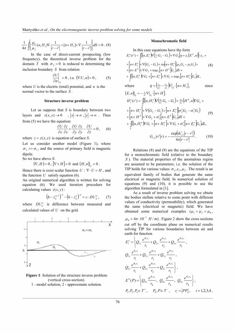
Martyshko, P. et al., 2007, On the electromagnetic inverse problem …
2/3
01][1),(41
112
1 =
′−∇××+
′−∇∫ dS
rrHn
rrHn
S µµ
π. (4)
In the case of direct-current prospecting (low frequency), the theoretical inverse problem for the domain T with 02 =σ is reduced to determining the inclusion boundary S from relation
0=∂∂
SnU , i.e. ( ) 0, =∇ nU , (5)
where U is the electric (total) potential, and n is the normal vector to the surface S .
Structure inverse problem
Let us suppose that S is boundary between two layers and 0),( →yxz , ∞→∞→ yx , . Then from (5) we have the equation:
0=∂∂
−∂∂
∂∂
+∂∂
∂∂
zU
yz
yU
xz
xU , (6)
where ),( yxzz = is equation of surface S. Let us consider another model (Figure 1), where
12 σσ >> , and the source of primary field is magnetic dipole. So we have above S:
( ) 0, =∇ H , [ ] 0=×∇ H and ( ) 0, =S
nH . Hence there is exist scalar function U : HU =⋅∇ , and the function U satisfy equation (6). An original numerical algorithm is written for solving equation (6). We used iteration procedure for calculating values ),( yxz :
( ) ( ) nij
nij
nij DUczhzh ⋅=−−−
−−+ 331 , (7)
where nijDU is difference between measured and
calculated values of U on the grid.
Figure 1: Solution of the structure inverse problem (vertical cross-section).
1 - model solution, 2 - approximate solution.
Monochromatic field
In this case equations have the form ( ) ( ) ( )[ ]
[ ] ( ) [ ]( )[ ] [ ]
( ) [ ] [ ] ,,
/,,)(
1111111
222
11221121
2121211 2
1
dLGHniGEnGEn
dSGHniGEn
GGHniGGEn
nEGGGEnrE
L
aa
SS
aaS
Saa
∫
∫
×+∇××+∇+
+×+∇××+
+−×+−∇××+
++∇+−∇=′
ωµ
ωµ
µµω
εεη
α
εε
(8)
where ( ) [ ]12
2
1
1 HnS
×⋅∇−= ∗∗ σε
σεη , since
( ) [ ]HnnESS
×⋅∇−= σ1, .
( ) ( ) ( )[ ] ( ) [ ]( )[ ] [ ]
( ) [ ] [ ] ∫
∫
×+∇××+∇+
+×+∇××+
−×+−∇××+
+∇+−∇=′
∗
∗
∗∗
L
aa
SS
aaS
Saa
dLGEnGHnGHn
dSGEnGHn
GGEnGGHn
GnHGGHnrH
,,
,,)(
1111111
222
11221121
21211 2
1
2
1
σ
σ
σσ
α
µµ
µµ
(9)
( )rr
rrikrrG
′−
′−−=′
∗
π4exp
)( 2,12,1 . (10)
Relations (8) and (9) are the equations of the TIP
for a monochromatic field (relative to the boundary S ). The material properties of the anomalous region are assumed to be parameters; i.e. the solution of the TIP holds for various values 222 ,, µεσ . The result is an equivalent family of bodies that generate the same electrical or magnetic field. In numerical solution of equations (9) and (10), it is possible to use the algorithm formulated in [1].
As a result of inverse problem solving we obtain the bodies stellate relative to some point with different values of conductivity (permeability), which generated the same (electrical or magnetic) field. We have obtained some numerical examples 021( µµµ == ,
)/104 70 mH−⋅= πµ . Figure 2 show the cross sections
cut off by the coordinate plane on numerical results solving TIP for various boundaries between air and earth for function
++=3
32
21
11
322212
reQ
reQ
reQE
rik
x
rik
x
rik
xa ,
33
22
11
322212
reQ
reQ
reQ
rik
y
rik
y
rik
y ++ ,
++3
32
21
1
322212
reQ
reQ
reQ
rik
z
rik
z
rik
z ,
=4
44
44
4
424242
,,)(r
eQr
eQr
eQPErik
x
rik
x
rik
xS ,
+∈TPPP 321 ,, , −∈TPP ,4 , ii PPr = , 4,3,2,1=i ,
Martyshko et al., On the electromagnetic inverse problem solving for some models
76

Martyshko, P. et al., 2007, On the electromagnetic inverse problem …
3/3
)10,0,0(4P , 3111 === zyx QQQ , 6222 === zyx QQQ , 9333 −=== zyx QQQ , 10444 === zyx QQQ ,
6/1/ 21 =σσ , 100002 ⋅= πω .
Figure 2: Cross-section on the coordinate plane for the inverse problem solutions of Helmholtz equation. S is the contour of the bodies for solutions for different boundaries between air and earth.
CONCLUSIONS On the base original explicit equations we have derived algorithms for solving 3-D electromagnetic inverse problem. Numerical examples for some models have been constructed.
REFERENCES [1] P. S. Martyshko, Inverse Problems of
Electromagnetic Geophysical Fields. “VSP”, Utrecht, The Netherlands, 123 pp, 1999.
[2] M. S. Zhdanov, Integral Transforms in Geophysics. Springer, Germany, 367 pp, 1988.
Martyshko et al., On the electromagnetic inverse problem solving for some models
77
4th International Symposium on Three-Dimensional Electromagnetics Freiberg, Germany, September 27−30, 2007
3D source inversion of self-potential data
Burke J. Minsley1 and Frank Dale Morgan1
1Earth Resources Laboratory, Department of Earth, Atmospheric, and Planetary Sciences Massachusetts Institute of Technology
SUMMARY Self-potential source inversion is formulated as a linear problem by seeking the distribution of source amplitudes within a discretized model that satisfies the measured data. Source inversion is ill-posed and non-unique, which is addressed by incorporating model regularization into the inverse problem. A non-traditional regularization method, sometimes referred to as “compactness” or “minimum support,” is utilized to recover a spatially compact source model rather than one that satisfies more commonly used smoothness constraints. Spatial compactness is often an appropriate form of prior information for the self-potential inverse source problem. Minimum support regularization makes the inverse problem nonlinear however, requiring an iterative solution technique similar to iteratively re-weighted least squares (IRLS) methods. An additional complicating factor is that the measured self-potentials are a function of the earth resistivity structure as well as the unknown sources. The influence of imperfect knowledge of the resistivity in the inverse problem is discussed, and illustrated through synthetic examples. Keywords: self-potential, source inversion, least squares, IRLS, minimum support
INTRODUCTION Self-potentials are the result of coupling between electric and non-electric flows and forces in the earth. Hydraulic, chemical, or thermal gradients produce a source current that must be balanced by a conduction current within the conductive earth structure (e.g. Marshall and Madden, 1959; Sill, 1983). The passive self-potential measurements, which result from this conduction current, are somewhat unique in that they are sensitive to active forcing phenomena in the subsurface. Advances in self-potential acquisition and processing methods have led to a recent resurgence in the application of this technique. In this study, we present an inversion methodology that aims to characterize the spatial distribution and amplitudes of sources that generate a measured self-potential signal. This approach is general in that it is not aimed at any particular forcing mechanism, and is therefore applicable to a wide variety of problems. The methods build on work by Shi (1998), and are documented in more detail by Minsley et al. (2007). This problem is analogous to electroencephalographic (EEG) imaging techniques in the medical community, which utilize passively measured electric potentials on the scalp to infer the location of electrical activity
within the brain due to various stimuli (Michel et al., 2004). Many of the concepts used in EEG source localization are applicable to self-potental source inversion, as both techniques rely on passively measured potentials to locate electrical sources within a heterogeneous volume conductor. As with other potential-field problems, self-potential source inversion is highly non-unique; there are many possible distributions of sources that fit the data equally. Additionally, the self-potential response depends on the medium resistivity structure, which is never perfectly known. These issues are addressed by: (1) utilizing non-traditional inversion constraints that are appropriate for self-potential sources, (2) incorporating available resistivity information into the inversion algorithm, and (3) understanding the effects of uncertainty in the resistivity structure on the source inversion results. Both synthetic and field data examples are studied to illustrate the efficacy of this approach.
SELF-POTENTIAL SOURCE INVERSION The total current density in the earth [A·m-2] is composed of a source current related to the forcing mechanism and a balancing conduction current (e.g. Sill, 1983). Streaming currents due to the drag of excess charge in the pore space of a rock due to
1/4
4th International Symposium on Three-Dimensional ElectromagneticsFreiberg, Germany, September 27–30, 2007
78

Minsley, B. and F.D. Morgan, 2007, Self-potential source inversion
hydraulic gradients are one common example of a source current. Under the quasi-static assumption, the total current density must be conserved, resulting in an elliptic partial differential equation that governs the self-potential response (1). sj sσ ϕ−∇ ⋅ ∇ = ∇ ⋅ = (1) On the left-hand side of this equation, σ [S·m-1] represents the electrical conductivity structure of the medium and ϕ [V] are the measurable self-potentials. The source term, s [A·m-3], on the right-hand side is defined by the divergence of the source current. The measured self-potentials, therefore, can be expressed as ( ) ( ) ( ); ,Gx x x s x dxϕ ϕ σ′ ′= ∫D ′ , (2)
where ϕG represents the Green’s functions that are a function of the conductivity structure and source locations. In discrete form, this can be written as 1−=φ K s , (3) where K is a sparse, banded operator that incorporates model geometry and conductivity structure. The inverse problem involves estimating s by minimizing an objective function that is a combined measure of data misfit (φd) and a weighted model semi-norm (φm)
( ) 2 2122
d m d d mφ λφ λ−Φ = + = +W PK s -φ W s . (4)
Here, φd represents the subset of potentials sampled at the measurement locations, and P selects the corresponding rows from K-1. Wd and Wm are data and model weighting operators, respectively, and λ is a trade-off parameter that controls the relative influence of the two terms. As stated in equation (4), this is a linear inverse problem, which can be solved efficiently using the transmission network analogy and conjugate gradient algorithms (e.g. Zhang et al., 1995). Additionally, we consider two aspects of the inverse problem in more detail: - Choices of Wm that promote model structures
appropriate to the self-potential source inversion problem
- Errors in the source estimate associated with imperfect knowledge of the medium conductivity structure, which is incorporated into K.
COMPACT SOURCE REGULARIZATION
The model regularization term in equation (4) often utilizes a low order differential operator for Wm, which
generally results in ‘smooth’ models. This has the benefit of being a linear operator, and often results in geologically appropriate models. Self-potential sources, however, are often spatially localized as they come from the divergence of a source current, and smoothness is not necessarily an inherent model property. We therefore choose a non-traditional form of model regularization which promotes spatially compact sources. Last and Kubik (1983) applied this ‘compactness’ strategy to gravity inversion, which has been more recently applied to other geophysical problems under the heading ‘minimum support’ (Portniaguine and Zhdanov, 1999). The basic premise is that the minimum spatial region of non-zero parameters should be used to fit the data. This is accomplished by minimizing a volume metric, given by
2
20 1
limM
ke
k k
svolume v
sβ 2β→=
=+∑ . (5)
ve represents the volume of an individual model block or element, which is assumed constant in this case. β is a small number that is introduced to provide stability as sk → 0. In the limit of β → 0, terms in equation (5) evaluate to 1 for any value of sk ≠ 0, and they become 0 for sk = 0. This metric is incorporated into the inverse problem by defining a new diagonal weighting model operator,
(6) ( ) 1/ 22 2m kdiag s β
−= +W
Because this is now a nonlinear function of the model parameters, iteratively reweighted least squares (IRLS) techniques must be utilized to solve the inverse problem (e.g. Farquharson and Oldenburg, 1998). This is accomplished by solving equation (4), then using this source estimate to generate a new Wm according to equation (6), and solving for a new source estimate. This iterative procedure is repeated until a pre-determined stopping criteria is met. The result of this iterative procedure is an ensemble of models that are increasingly spatially compact. This does not remove the inherent non-uniqueness of the problem, but provides the user with a choice of models with varying spatial statistics that all fit the data. One complicating factor is that there are now two regularization parameters (λ and β), which cannot be chosen independently, that control the solution. Figure 1 illustrates synthetic source inversion results using a traditional smoothness constraint (A) and the compact source constraint (B). The true source
2/4
Minsley et al., Self-potential source inversion
79

Minsley, B. and F.D. Morgan, 2007, Self-potential source inversion
locations are depicted with white asterisks, and both solutions fit the data equally. Note that the more compact solution amplitudes are greater, which occurs naturally as the model is required to become more compact.
Figure 1: Source inversion results using a smooth regularization operator (A) and the compact source method (B). The true source locations are depicted by white asterisks. Both solutions fit the synthetic data equally.
INFLUENCE OF THE RESISTIVITY
STRUCTURE As discussed in equation (2), the self-potential reponse is a function of both the unknown sources and the earth resistivity structure. Assumptions about the resistivity structure, which is never perfectly known, must be incorporated into K. Ideally, a resistivity survey can be carried out in conjunction with self-potential measurements, but this is not always practicable. In many cases, a homogeneous resistivity structure is assumed during the self-potential data interpretation. It is therefore important to understand the influence of imperfect knowledge of the resistivity structure on self-potential inversion results. We accomplish this using two different approaches: (1) deriving the sensitivity of the measurable potentials to pertubations in resistivity structure and (2) inverting simple synthetic source geometries using an incorrect resistivity model, and observing how the recovered sources are distorted. The first approach, while more general, is difficult to visualize, and is discussed in more detail by Minsley (2007). To get a feel for the influence of incorrect resistivity assumptions on the inversion results, we perform several synthetic examples. Synthetic data are generated by placing a point source in a known, heterogeneous resistivity model. These data are then
inverted using a homogeneous resistivity assumption built into K. Various 1D, 2D, and 3D resistivity structures are considered. Figure 2 shows results of this synthetic test using one of the 2D resistivity structures. The upper images show the synthetic data (mesh plots) generated from a point source embedded within the known resistivity structure. In (A), a conductive block (10Ω·m) is embedded within the background resistivity (100Ω·m). In (B), the embedded block is more resistive (1000Ω·m) than the background. The bottom images are slices of the source inversion model, which uses a homogeneous resistivity assumption. Distortion of the true point source (white asterisk) is due to the incorrect resistivity structure. Note that the errors in the source inversion for the conductive and resistive cases have very different characteristics. In general, the source inversion errors are most significant when: (1) resistivity errors are near the source, (2) resistivity errors are near the receiver, (3) the magnitude of the resistivity error is large, or (4) the spatial extent of unknown resistivity is large.
Figure 2: Upper images show synthetic data (mesh plots) generated from a point source embedded within known 2D resistivity structures (conductive block – A, resistive block – B). Lower images show slices through the inverted source model, which uses a homogeneous resistivity assumption. Distortion of the true point source (white asterisk) is due to the incorrect resistivity structure.
CONCLUSIONS
Source inversion is an important step in the interpretation of self-potential data. The methods presented here are robust in that they are not specific to any particular forcing mechanism. While compact source regularization is often appropriate, future research will focus on inversion constraints that are derived from the physics or chemistry of the
3/4
Minsley et al., Self-potential source inversion
80

Minsley, B. and F.D. Morgan, 2007, Self-potential source inversion
underlying forcing mechanism. Accounting for the influence of resistivity structure is a critical step in self-potential source inversion and error quantification.
ACKNOWLEDGEMENTS
We thank the Kuwait-MIT Center for Natural Resources and the Environment and the Earth Resources Laboratory Founding Member Consortium for providing support for this research.
REFERENCES Farquharson, C.G., and D.W. Oldenburg (1998), Non-
linear inversion using general measures of data misfit and model structure, Geophys. J. Int., 134 (1), 213-227.
Last, B.J., and K. Kubik (1983), Compact gravity inversion, Geophysics, 48 (6), 713-721.
Marshall, D.J., and T.R. Madden (1959), Induced polarization, a study of its causes, Geophysics, 24 (4), 790-816.
Michel, C.M., M.M. Murray, G. Lantz, S. Gonzalez, L. Spinelli, and R.G. de Peralta (2004), EEG source imaging, Clin. Neurophysiol., 115 (10), 2195-2222.
Minsley, B.J. (2007), Modeling and inversion of self-potential data, Ph.D. thesis, Massachusetts Institute of Technology, Cambridge, Massachusetts.
Minsley, B.J., J. Sogade, and F.D. Morgan (2007), Three-dimensional source inversion of self-potential data, J. Geophys. Res., 112 (B02202), doi:10.1029/2006JB004262.
Portniaguine, O., and M.S. Zhdanov (1999), Focusing geophysical inversion images, Geophysics, 64 (3), 874-887.
Shi, W. (1998), Advanced modeling and inversion techniques for three-dimensional geoelectrical surveys, Ph.D. thesis, Massachusetts Institute of Technology, Cambridge, MA.
Sill, W.R. (1983), Self-Potential Modeling from Primary Flows, Geophysics, 48 (1), 76-86.
Zhang, J., R.L. Mackie, and T.R. Madden (1995), 3-D Resistivity Forward Modeling and Inversion Using Conjugate Gradients, Geophysics, 60 (5), 1313-1325.
4/4
Minsley et al., Self-potential source inversion
81
4th International Symposium on Three-Dimensional ElectromagneticsFreiberg, Germany, September 27–30, 2007
Efficient datasets - An alternative approach that analyses the data space
M. Müller-Petke and U. YaramanciBerlin University of Technology
SUMMARY
The quest and need for optimisation of geophysical data sets is either to improve the resolution or to reduce the field work(or both) is of growing interest for geophysical applications. So far, the task is solved by analysing resolution measuresderived from the model resolution matrix. The dataset is changed iteratively in order to minimise these measures, i.e.improve the resolution.
Here we present a direct method to estimate an efficient dataset. The approach is based on analysing the data space,i.e. calculating the data resolution matrix. Essentially variable quantities of data errors are taken into account to definethe necessary amount of independent unique measurements. Applied to the technique of Magnetic Resonance Sounding(MRS) we show that not only the singular value distribution of the forward operator is improved but also the resolution,i.e. the inversion result of the efficient dataset compared to a logarithmic and linear spaced pulse moment series.
Keywords: MRS, Data Resolution Matrix, Efficient Dataset
INTRODUCTION
The quest and need for optimisation of geophysical datasets is either to improve the resolution or to reduce thefield work (or both) is of growing interest for geophysi-cal applications (triggered mostly by Electrical Resistiv-ity Tomography (Dahlin & Zhou, 2004)). The neces-sity becomes obvious especially when taking 2D and 3Dprospectings into account. So far, the task is solved byanalysing resolution measures derived from the model res-olution matrix, i.e. to adopt a dataset iteratively until con-sideration concerning the model resolution matrix are met(Stummer, Maurer, and Green (2004), Wilkinson, Mel-drum, Chambers, Kuras, and Ogilvy (2006)).
Here we present a direct approach to estimate an efficientdataset using the data resolution matrix. Variable quan-tities of data error (e.g. noise) are included to define theindependent number of measurements. The approach isapplied to the technique of Magnetic Resonance Sound-ing to derive an efficient series of pulse moments that iscompared to linear and logarithmic space series of pulsemoments.
MRS PRINCIPLES
The detected MRS signal is a decay curve at resonancefrequency of the relaxation process of a system of hydro-gen protons at a given excitation intensity. The relaxationis caused by an electromagnetic excitation pulse of a cer-tain amplitude and duration at resonance frequency excit-
ing the magnetic moment of the hydrogen proton out of itsequilibrium state in the earth magnetic field. Since the EMfield is diffusive the degree of excitation depends on thedepths, i.e. hydrogen protons at different depths emit sig-nals of different amplitudes corresponding to the degree ofexcitation (and phase relation). Changing the amplitudeof this excitation pulse (i.e. the energy of the diffusiveEM field) these depth ranges can be changed. The decaycurve carries 3 measures. The relaxation time related tothe pore size and the initial amplitude and phase related tothe subsurface water content and resistivity respectively.Determining a 1D water content the MRSounding curve,i.e. the initial amplitude and phase (or real and imaginarypart) versus the pulse moment is inverted (Yaramanci &Hertrich, 2006).
DATA RESOLUTION MATRIX: COMPLEX DATASET
Besides the model resolution matrix Rm that describes therelation between the true subsurface model and the esti-mated model as a weighting function (Menke, 1984), thedata resolution matrix Rd describes the relation of one da-tum to all other, i.e. the uniqueness of the information ofthis datum. If the corresponding row of Rd for one datumis “delta like” (no off diagonal elements) this datum bearsunique information. The more off diagonal elements ex-ist the more data is weighted inside the inversion to oneinformation.
In a first step we only consider the real part of the mea-surement. This is valid if resitivity does not affect the
1/4
4th International Symposium on Three-Dimensional ElectromagneticsFreiberg, Germany, September 27–30, 2007
82

Müller-Petke, M. and Yaraamnci, U., 2007, Efficient Datasets - An alternative approach that analyses the data space
measurement. Fig.1 shows Rd for 48 m loop radius, maxi-mum pulse moment of 18 As, 1 Ωm and 1000 Ωm groundresistivity, respectively. For large resistivities the imag-inary part obviously contains no information since theelectromagnetic phase vanishes. The same conclusion canbe drawn directly from the singular value distribution. Ifone considers a fixed limit for the ratio of the largest sin-gular value to the smallest included value, the distributionof singular values for 1000 Ωm ground resistivity includesless singular values than for 1 Ωm. The difference is thephase information.
a) b)
c) d)
Figure 1: Data resolution matrix for a complex dataset attwo ground resistivities. a) and c) data resolutionmatrix: loop radius of 48 m b) and d) singular valuedistribution. Depending on the ground resistivitythe imaginary part of the dataset contains signifi-cant information. For the further investigation onlythe real part is taken into account, i.e. insulatingcondition are assumed.
EFFICIENT DATASETS: INDEPENDENTMEASUREMENTS
An efficient dataset can be defined as a dataset includingexclusively measurements with unique information, i.e. adata resolution matrix that contains only elements withthe value of 1 at the main diagonal. The crucial pointis not to find unique measurement but avoid redundancy.Therefore, the first task to solve is: How many indepen-dent measurements exist? This is at least a question of thequantity of data error.
The Picard Plot is a very useful tool to analyse this (Fedi,Hansen, & Poaletti, 2005). The Picard condition that can
be checked visually by the Picard Plot claims that |uTi d|
(uTi : data space eigenvectors; d: data/ pulse moments) de-
cay on average faster then the singular values σi. Since|uT
i d| converges against the quantity of data error the con-dition is satisfied in a first order if σi is above the levelof data error. To retrieve the maximum number of inde-pendent measurements d theoretically the data and modelspace must be a continuous functions, since model anddata space are correlated. As long as the Picard conditionis satisfied the imaging process is stable, or vice versa, theamount of independent measurements is given.
Due to numerical reasons the task is solved inversly. Start-ing with few thick layers and less amount of pulse mo-ments the layer thickness is stepwise decreased, i.e. thenumber of basis layers and the amount of pulse momentsis increased as long as no additional singular values fitthe conditions. Hence in the first step the minimum ba-sis layer thickness concerning a certain noise level issearched. At the time the necessary amount of pulse mo-ments are given to achieve this resolution.
Figure 2: Picard Plot 48 m loop radius, 1000 Ωm groundresitivity, 600 pulse moments from 0.2 As - 18 As.The quantity of data error defines the amount of in-dependent measurements. To estimate this quantitythe model space discretisation is stepwise decreaseduntil the nose level is reached and the independentmeasurement (38) can be found.
Fig.2 shows the Picard Plot calculated for 600 linearspaced pulse moments (min = 0.2 As, max = 18 As)and a linear spaced subsurface model of 2 m, 0.5 m and0.25 m base layer thickness. Concerning 2 m layer thick-ness (blue line) 18 singular value (that correspond to theamount of pulse moments) can be included calculatinga stable inverse. Since the values itself are fairly abovethe level of data error the basis layer thickness can be re-duced. Reducing the base layer thickness requires moredata can be included. The basis layer thickness is reducedas long as no additional singular values (pulse moments)
2/4
Müller-Petke et al., Efficient datasets – An alternative approach that analyses the data space
83

Müller-Petke, M. and Yaraamnci, U., 2007, Efficient Datasets - An alternative approach that analyses the data space
are above the noise level. Reaching a base layer thicknessof 0.25 m some σi are within the level of data error. Con-sequently the smallest layer thickness resolvable duringinversion is reached and corresponds to and amount of 38pulse moments or measurements.
EFFICIENT DATASET: SELECT SEQUENCE MEMBER
Using the Picard Plot the minimum layer thickness of 0.25m and the maximum amount of 38 independent pulse mo-ments are calculated. Concerning this pulse moments ba-sis the data resolution matrix (derived from and TSVDwith a cut-off at σi=38) shows the correlation between allincluded measurements. Since much more data than nec-essary are used Rd is not an identity matrix (Fig. 3a).To retrieve the independent ones, Rd can be analysed rowby row (Fig. 3b). Starting from the smallest pulse mo-ment, the corresponding row of Rd indicates the next in-dependent pulse moment if the weighting value is lowerthan some threshold (here 0.01, according to the numer-ical variances). This scheme is continued until the lastpulse moment.
a) b)
c) d)
Figure 3: Deviation of the efficient dataset. a) data res-olution matrix: loop radius of 48 m, 600 pulse mo-ments, 0.25m base layer thickness, truncation atσi=38; b) row of R for q=3As; c) efficient seriescompared to logarithmic and linear spaced; d) Pi-card plot for these series
The proper functionality of the derived dataset (Fig. 3c)can be checked by analysing the Picard Plot. The singularvalue distribution of the retrieved efficient series of pulse
moments (red line) is compared to a linear (blue line)and a logarithmic (black line) spaced series of the sameamount of measurements, while the smallest and largestpulses are identically. As expected the first few singu-lar values are quite equal for any of the seriess. But isoutstanding that only the efficient series satisfies the Pi-card condition for all singular values (Fig. 3d), i.e. allmeasurements can be included into calculating the inverseoperator.
EFFICIENT DATASET: INVERSION TEST
Finally, the inversion results of the linear, logarithmic andthe efficient series are compared. Both the smooth in-version (Fig. 4) and block inversion (Fig. 5) are basedon the singular value decomposition. The smooth inver-sion is a standard truncated singular value decompositionwith Tikhonov regularisation based minimisation of theL2 − data norm and L2 − model norm. The block in-version is a picewise polynomial truncated singular valuedecomposition (Hansen, 1996) based on minimisation ofthe L2 − data norm and L1 − model norm. As under-lying model a two aquifer case with a thin aquifer closeto the surface and a thicker aquifer at larger depths. Thusthe resolutionfor shallow and deep structures can be con-trolled. The synthetic dataset contains 10 nV Gaussiandistributed noise. The inversion parameters are identicalfor all series (smooth inversion: truncation at σi=38 andλtichonov = 100; block inversion: 10 discontinuities).
The images of all series reproduce the generel modelstructure of the 2 aquifer case (Fig. 4/5). As expected theefficient series shows the best overall results which is indi-cated by the lowest model rms value and smallest averag-ing areas (red bars, derived from the model resolution ma-trix of the smooth inversion for both inversion schemes).Remark that for the block inversion the discontinuities areconstructed from the model null space. Consequently, itappears to be valid to take the resolution properties de-rived from the smooth inversion.
The linear (Fig. 5b) series has less resolution and there-fore higher averaging properties at shallow depths due toless amount of small pulse moments. Consequently boththe boundaries and the watercontent of the shallow aquiferare not met. In contrast the deeper aquifer is resolved bestcompared to the other series. Since the upper boundery ofthe shallow layer cannot be found using the block inver-sion the water content is underestimated. The logarithmic(Fig. 5c) spaced series in contrast shows bad resolutionat large depths that is due to less amount of large pulsesand causes the underestimation of the deep aquifer watercontent. Vice versa the shallow layer can be resolved best.The efficient series (Fig. 5a) now combines the properties
3/4
Müller-Petke et al., Efficient datasets – An alternative approach that analyses the data space
84
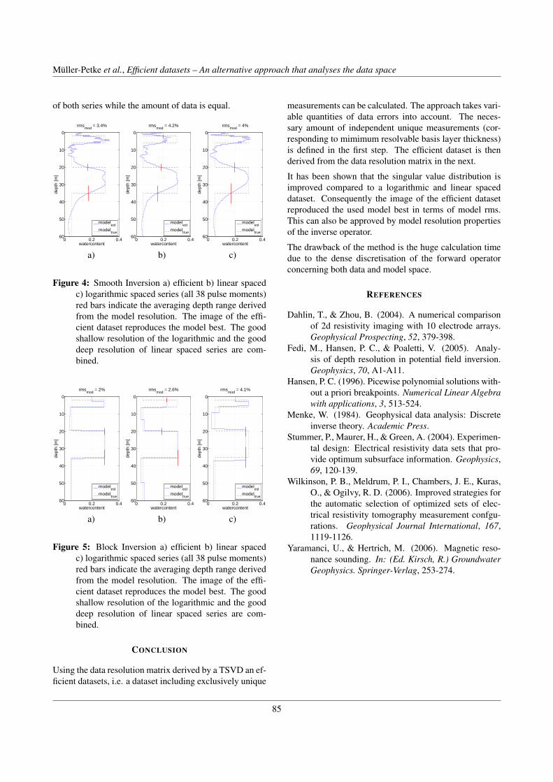
Müller-Petke, M. and Yaraamnci, U., 2007, Efficient Datasets - An alternative approach that analyses the data space
of both series while the amount of data is equal.
0 0.2 0.4
0
10
20
30
40
50
60
rmsmod
= 3.4%
dept
h [m
]
watercontent
modelest
modeltrue
0 0.2 0.4
0
10
20
30
40
50
60
rmsmod
= 4.2%de
pth
[m]
watercontent
modelest
modeltrue
0 0.2 0.4
0
10
20
30
40
50
60
rmsmod
= 4%
dept
h [m
]
watercontent
modelest
modeltrue
a) b) c)
Figure 4: Smooth Inversion a) efficient b) linear spacedc) logarithmic spaced series (all 38 pulse moments)red bars indicate the averaging depth range derivedfrom the model resolution. The image of the effi-cient dataset reproduces the model best. The goodshallow resolution of the logarithmic and the gooddeep resolution of linear spaced series are com-bined.
0 0.2 0.4
0
10
20
30
40
50
60
rmsmod
= 2%
dept
h [m
]
watercontent
modelest
modeltrue
0 0.2 0.4
0
10
20
30
40
50
60
rmsmod
= 2.6%
dept
h [m
]
watercontent
modelest
modeltrue
0 0.2 0.4
0
10
20
30
40
50
60
rmsmod
= 4.1%
dept
h [m
]
watercontent
modelest
modeltrue
a) b) c)
Figure 5: Block Inversion a) efficient b) linear spacedc) logarithmic spaced series (all 38 pulse moments)red bars indicate the averaging depth range derivedfrom the model resolution. The image of the effi-cient dataset reproduces the model best. The goodshallow resolution of the logarithmic and the gooddeep resolution of linear spaced series are com-bined.
CONCLUSION
Using the data resolution matrix derived by a TSVD an ef-ficient datasets, i.e. a dataset including exclusively unique
measurements can be calculated. The approach takes vari-able quantities of data errors into account. The neces-sary amount of independent unique measurements (cor-responding to mimimum resolvable basis layer thickness)is defined in the first step. The efficient dataset is thenderived from the data resolution matrix in the next.
It has been shown that the singular value distribution isimproved compared to a logarithmic and linear spaceddataset. Consequently the image of the efficient datasetreproduced the used model best in terms of model rms.This can also be approved by model resolution propertiesof the inverse operator.
The drawback of the method is the huge calculation timedue to the dense discretisation of the forward operatorconcerning both data and model space.
REFERENCES
Dahlin, T., & Zhou, B. (2004). A numerical comparisonof 2d resistivity imaging with 10 electrode arrays.Geophysical Prospecting, 52, 379-398.
Fedi, M., Hansen, P. C., & Poaletti, V. (2005). Analy-sis of depth resolution in potential field inversion.Geophysics, 70, A1-A11.
Hansen, P. C. (1996). Picewise polynomial solutions with-out a priori breakpoints. Numerical Linear Algebrawith applications, 3, 513-524.
Menke, W. (1984). Geophysical data analysis: Discreteinverse theory. Academic Press.
Stummer, P., Maurer, H., & Green, A. (2004). Experimen-tal design: Electrical resistivity data sets that pro-vide optimum subsurface information. Geophysics,69, 120-139.
Wilkinson, P. B., Meldrum, P. I., Chambers, J. E., Kuras,O., & Ogilvy, R. D. (2006). Improved strategies forthe automatic selection of optimized sets of elec-trical resistivity tomography measurement confgu-rations. Geophysical Journal International, 167,1119-1126.
Yaramanci, U., & Hertrich, M. (2006). Magnetic reso-nance sounding. In: (Ed. Kirsch, R.) GroundwaterGeophysics. Springer-Verlag, 253-274.
4/4
Müller-Petke et al., Efficient datasets – An alternative approach that analyses the data space
85

A note on the interpretation of EM induction data by multi-dimensional conductivity and resistivity models Ulrich Schmucker, Goettingen It is customary to use in this context gradient-type methods, yielding gradual improvements of a starting model. This contribution describes an alternative approach based on integral equations for the anomalous parts na EEE −= and na BBB −= of EM fields on the Earth’s surface. Their normal part nE and nB are the fields in a laterally uniform structure surrounding a laterally non-uniform anomalous domain A. The model parameter to be found will be the laterally variable anomalous part ax of conductivity or resistivity within A. It will be assumed that their solely depth-dependent normal part nx outside A and thereby nE and
nB as functions of depth are known. Denoting with )(rym an anomalous EM datum at surface location r for frequency mω and with )(rx ′ the conductivity or resistivity at location r′ within A , then the integral equation to be solved towards )()()( zxrxrx na ′−′=′ is
')'()',|()( rdrxrrxKry aA
m ⋅= ∫ . (1)
The non-linearity of the arising well-posed inverse problem (after linearization) is expressed by the model dependence of the data kernel mK . Hence, an iterative process is started with an approximated data kernel ),|()0( rrxK nm ′& , depending on the known normal structure only. It leads to a starting model )0(
ax and thereby in ),|( )0()1( rrxxK anm ′+ & to the exact data kernel for this model. Evaluation of eq, (1) with )1(
mK yields a new preliminary model )1(ax , and so on.
Provided the process converges, the data kernels become better and better adapted to less and less changing models. It is terminated, when )( j
mK is sufficiently close to )1( −jmK . Thus, in
every iterative step an entirely new model is derived from the data rather than successive model improvements from data residuals. This allows the assessment of accuracy and resolution of the final model )( j
axv for target point kr′ , that is data errors my∆ can be converted into model errors )( j
axv∆ . Furthermore, from the final data kernel and its inverse the range or “spread” can be specified, over which the true model is averaged in the neighbourhood of kr′ . In case of 2-dimensional model interpretations, the data kernel represents the product of Green’s function for the normal structure (in the appropriate mode) with the internal field, which is ),( zyEx ′′ for E-polarisation and ),( zyBx ′′ for B-polarisation. Since the respective integral equation contains as model parameter ),( zya ′′σ for E-polarisation and ),( zya ′′ρ for B-polarisation, a joint interpretation of data for both polarisations does not exploit fully their information contents. Hence, the interpretation of any of the E-polarisation transfer functions for axE , ayB or azB leads in this approach to a conductivity model, whereas the GDS transfer functions seem to possess the greater resolution power. The same applies to the resistivity model derived from the B-polarisation transfer function for ayE . The cause may be that the respective data kernels involve differentiated Green’s functions with respect to y and z.
4th International Symposium on Three-Dimensional ElectromagneticsFreiberg, Germany, September 27–30, 2007
86

An extension to interpretations with 3-dimensional models is complicated by the fact that their anomalous fields are composed of both the tangential electric TE mode and the tangential magnetic TM mode, which should be interpreted separately: transfer functions for the TE mode towards models in conductivity and those for the TM mode towards models in resistivity. While the anomalous TE surface field is accessible to direct observations, because the magnetic variation field on and above ground is exclusively a TE field, this is not the case for the TM surface field. Noting that aE is a Laplacian potential field in the air space, the expression . +∂∂ xEax / 0|// −=∂−∂=∂∂ zazay zEyE (2) reflects accumulated electric charges within the model and on its surface, and it can be shown that this expression eliminates the TE mode of aE in the air space. It is in analogy to the expression
−∂∂ yEax / azay BixE ω=∂∂ / (3) for the TE mode according to Faraday’s law, only that azB is a readily observed field component, when for laterally quasi-uniform source fields nxB is zero.. The data kernel is now the dyadic product of a Green’s tensor with the internal electric vector field, while the components of aE at the surface serve as data my in eq. (1). The intended use of their derivatives as datum requires again the differentiation of Green’s functions with respect to x and y, and in the combinations of eqs (2) and (3) this eliminates either the TE or the TM mode of aE . The combination of differentiated MT impedances according to (2) is used then to derive a 3-dimensional resistivity model and the GDS transfer functions for azB ,
axB or ayB to obtain a conductivity model. According to the above cited experience with 2-dimensional models, such separately conducted interpretations according to modes may lead for the same reason to better resolved models as with joint interpretations of the undifferentiated MT tensor elements. Obviously, the application of eq. (2) to real data requires arrays with a sufficiently closely spaced network of recording sites.
Schmucker, A note on the interpretation of EM induction data by multi-dimensional conductivity and resistivity models
87

88

Theory – Data analysis
89

90

1. DECOMPOSITION OF 3D MAGNETOVARIATIONAL RESPONSE
FUNCTIONS IN MODELS OF (2D+2D)-TYPE
М. Berdichevsky1 , V. Kuznetsov2 , N. Palshin2
1Мoscow State University, 2 Institute of Oceanology RAS, e-mail: [email protected] Abstract We consider superimposition 3D model of a (2D+2D)-type that contains two 2D struc-tures of different strike and suggest a decomposition method, which divides a 3D anomaly into two independent 2D anomalies.
Let us consider a 3D geoelectric layered medium that contains at different depth two 2D hori-zontal cylinders of arbitrary section and different strike. Such a medium will be referred to as medium of a (2D+2D)-type. The cylinders are separated by sufficiently thick resistive strata so that there is no galvanic connection between them. Assume that at sufficiently low frequency the inductive connec-tion between cylinder is absent too. Under these assumptions each of cylinders manifests itself as in-dependent two-dimensional body and a total effect of both the cylinders is a simple sum of partial 2D effects generated by each cylinder. Assume also that the Earth is excited by a plane vertically incident electromagnetic wave and an areal magnetovariational survey is conducted synchronously with ob-servations at base site characterized by the normal magnetic field.
Determine the Schmucker tipper [ ]zS connecting the anomalous vertical magnetic field
at the observation site with the normal horizontal magnetic field at the base site:
AzH
NτH
[ ] [ ]N
NN ,x
z z z zx zyy
HH S S
HτNτ
⎡ ⎤⎡ ⎤= = = ⎢ ⎥⎣ ⎦ ⎢ ⎥⎣ ⎦
S H S H (1)
and the Schmucker perturbation tensor [ ]τS , connecting the anomalous horizontal magnetic field AτH
at the observation site with the normal horizontal magnetic field at the base site: NτH
[ ] [ ]A N
A N A NA .xx xy x
yx yy y y
S S H HS S H Hτ τ τ τ τ τ N
x⎡ ⎤ ⎡⎡ ⎤= = = =
⎤⎢ ⎥ ⎢⎢ ⎥ ⎥⎢ ⎥ ⎢⎣ ⎦ ⎥⎣ ⎦ ⎣
H S H S H H⎦
(2)
Introduce measurement coordinates ,x y′ ′ with the x′ -axis directed along the strike of cylin-der and coordinates 1P ,x y′′ ′′ with the x′′ -axis directed along the strike of cylinder . Azimuths
,α of cylinders are counted clockwise from the 2P
α′ ′′ 1 2,P P x′ -axis: α =0,α 0′ ′′ ≠ .
Decomposition of the Schmucker tipper [ ]zS
Let the MV-sounding result in tippers [ ]zS reflecting the total 3D effect of cylinders
and induction arrows defining the cylinders strike. We look for partial tippers 1 2,P P
[ ]z′S and [ ]z′′S reflecting
the 2D effect of cylinder in the absence of cylinder and the 2D effect of cylinder in the absence of cylinder .
1P 2P 2P
1PIn coordinates ,x y′ ′ we have:
1
4th International Symposium on Three-Dimensional ElectromagneticsFreiberg, Germany, September 27–30, 2007
91

[ ] cos sin[ ] [0 ] [0 ] [ sin cos ]
sin cosz zy z zy zy zyS S S S .′′ ′′α α⎡ ⎤′ ′ ′′ ′′ ′′ ′′ ′′ ′′= = = − α⎢ ⎥′′ ′′− α α⎣ ⎦
S S α (3)
Inasmuch as the cylinders and do not interact, their total effect is equal to the sum their partial effects. Thus,
1P 2P
[ ] [ ] [ ] [ ] [ ]N N Nz z z z z z z zH H H N
τ τ τ′ ′′ ′ ′′ ′ ′′= + = + = + =S H S H S S H S Hτ , (4)
whence [ ] [ ] [ ]z z z′ ′′= +S S S . (5) With a glance to (3)
sin
cos ,zx zy
zy zy zy
S S
S S S
′′ ′′= − α
′ ′′ ′′= + α (6)
from which
cos sin
sin sinzx zy zx
zy zy
S S SS S
′′ ′′α + α′ ′′=
′′ ′′α α= − (7)
and
[ ] [ ][ ] [ ] [ ]
0 cotα + c α
0 cotα + c α .
z zx zy zx zy zx zx
z zx zy z zx zx
S S S S S S
S S S S
ot
ot
′′ ′⎡ ⎤ ⎡ ⎤= = + −⎣ ⎦ ⎣ ⎦′ ′′ ′′⎡ ⎤= =⎣ ⎦
S
S S
′
′′− (8)
So, with a knowledge of azimuths 0,′ ′′α = α and the total 3D tippers, we get the partial tip-pers [ ]z′S ,[ ]z′′S and divide the 3D anomaly of the vertical magnetic field into two independent 2D anomalies. Decomposition of the Schmucker perturbation tensor [ ]τS
Similarly we can decompose the Schmucker perturbation tensor [ ]τS . Let the MV-sounding
result in tippers [ ]zS reflecting the total 3D effect of cylinders and induction arrows defining
the cylinders strike. We look for partial tippers 1 2,P P
[ ]z′S and [ ]z′′S reflecting the 2D effect of cylinder
in the absence of cylinder and the 2D effect of cylinder in the absence of cylinder . 1P
2P 2P 1PIn coordinates ,x y′ ′ we have:
[ ]
2
2
0 0 0 0cos sin cos sin[ ]
0 0sin cos sin cos
sin sin cos.
sin cos cos
yy yy
yy yy
yy yy
S S
S SS S
τ τ
′′ ′′ ′′ ′′α − α α α⎡ ⎤ ⎡ ⎤⎡ ⎤ ⎡ ⎤′ ′′= =⎢ ⎥ ⎢ ⎥⎢ ⎥ ⎢ ⎥′ ′′′′ ′′ ′′ ′′α α − α⎣ ⎦ ⎣ ⎦⎣ ⎦ ⎣ ⎦′′ ′′ ′′ ′′ ′′⎡ ⎤α − α α
= ⎢ ⎥′′ ′′ ′′ ′′ ′′− α α α⎢ ⎥⎣ ⎦
S Sα
(9)
In the absence of interaction between cylinders and 1P 2P
[ ] [ ] [ ] [ ] [ ] A N N Nτ τ τ τ τ τ τ τ τ′ ′′ ′ ′′Η = = + = +S H S H S H S S HN
τ , (10)
whence
[ ] [ ] [ ]2
2
sin sin cos.
sin cos cosxx xy yy yy
yx yy yy yy yy
S S S SS S S S Sτ τ τ
′′ ′′ ′′ ′′ ′′⎡ ⎤α − α α⎡ ⎤′ ′′= + = ⎢ ⎥⎢ ⎥ ′′ ′′ ′′ ′ ′′ ′′− α α + α⎢ ⎥⎣ ⎦ ⎣ ⎦
S S S (11)
We arrive at a matrix equation for unknown ,yy yyS S′ ′′ . Equations of this linear system are com-patible if cotxy yx xxS S S ′′= = − α . (12) Let (12) be satisfied. Then
2
Berdichevsky et al., 1. Decomposition of 3D MV response functions in models of (2D+2D)-type
92

[ ]
[ ] [ ]
22
2 2
cotsin
cotcot
0 0 cot.
0 cot cot cot
xxyy yy xx yy
xx xy xx xx
yx yy xx yy
xx xx
yy xx xx xx
SS S S a S
S S S SS S S S
S SS S S S
τ
τ τ
′ ′′ ′′= − =′′α′′− α⎡ ⎤ ⎡ ⎤
= =⎢ ⎥ ⎢ ⎥′′− α⎣ ⎦ ⎣ ⎦′′− α⎡ ⎤ ⎡ ⎤
′ ′′= =⎢ ⎥ ⎢ ⎥′′− α ′′− α α′′⎣ ⎦⎣ ⎦
S
S S
(13)
We get the partial tensors [ ]τ′S ,[ ]τ′′S and divide the 3D anomaly of the horizontal magnetic field into two independent 2D anomalies. When studying media of a (2D+2D)- type, the 3D inversion can be reduced to two 2D inversions. Model experiments
As an example we refer to the 3D model shown in Fig.1. It consists of the sedimentary cover ( ), lithosphere (1 1 1ρ =10 Оhm m, ρ =1000 Оhm m, ρ =100 Оhm m′ ′′ ′′′⋅ ⋅ ⋅ 2 2 2ρ =ρ ρ 1000Оhm m′ ′′ ′′′= = ⋅ ) and asthenosphere ( 3ρ 20Оhm m= ⋅ ).The lithospheric layer 2′′′ρ contains the asthenosphere eleva-tion in the form of conductive prism of 5 O1P hm m⋅ resistivity, its thickness, width and azimuth being 50 km, 300 km and 0o respectively. The lithospheric layer 2′ρ contains the crustal zone in the form of conductive prism of 6 O2P hm m⋅ resistivity, its thickness, width and azimuth being 3 km, 100 km and 135o respectively.
Decomposition of the Schmucker tipper [ ]zS has been accomplished by (11) at the periods Т=100, 1000, 10000 s.
Fig.2 displays the pseudo-topographies of Eucleadian norm 22
z zx zS S= +S y of the initial
tipper [ ]z zx zS S⎡= ⎣S y ⎤⎦ and Eucleadian norms 22
z zx zS S y′ ′ ′= +S and 22
z zx zS S′′ ′′ ′′= +S y of
the partial tippers [ ]z zx zS S′ ′⎡ ⎤= ⎣ ⎦S y′ and [ ]z zx zS S y′′ ′′ ′′⎡ ⎤= ⎣ ⎦S . For comparison we present here the
pseudo-topographies of Eucleadian norms 2 2
z zx zS S y′ ′ ′= +S% % % and 2 2
z zx zS S y′′ ′′ ′= +S% % % ′
zy′
y
of the
true partial tipper , obtained in the absence of the prism , and the true strike
partial tipper , obtained in the absence of the prism . Inspecting pseudo-
topography of
z zxS S⎡ ⎤ ⎡ ⎤′ ′=⎣ ⎦ ⎣ ⎦S% % %2P
z zx zS S⎡ ⎤ ⎡ ⎤′′ ′′ ′′=⎣ ⎦ ⎣ ⎦S% % %1P
zS , we find that at 10000sT = the strike of the prism and at the
strike of the prism can be evaluated quite reliably. So, we proceed to decomposition of the Schmucker tipper with knowledge of strikes of the prisms . Comparing pseudo-topographies of
1P 100sT =
2P
1 2,P P
,z z′ ′′S S and ,z z′ ′′S S% % , we conclude that decomposition of the Schmucker tipper separates two-
dimensional effects of asthenospheric and crustal structures with reasonable accuracy. Examining the decomposition of the Schmucker perturbation tensor, we arrive at the same conclusion.
3
Berdichevsky et al., 1. Decomposition of 3D MV response functions in models of (2D+2D)-type
93

Fig.
2 D
ecom
posi
tion
of th
e Sc
hmuc
ker
tippe
r. Th
e ho
rizon
tal s
cale
s are
in k
m.
Fig.
1 3
D m
odel
of t
he (2
D+2
D)-
type
.
4
Berdichevsky et al., 1. Decomposition of 3D MV response functions in models of (2D+2D)-type
94

2. DECOMPOSITION OF 3D MAGNETOVARIATIONAL RESPONSE
FUNCTIONS IN MODELS OF (2D+3D)-TYPE
М.Berdichevsky1 , V.Kuznetsov2 , N.Palshin2
1Мoscow State University 2 Institute of Oceanology RAS, e-mail: [email protected] Abstract We consider a 3D superimposition model of the (3D+2D)-type that contains a 3D elon-gated structure against the 2D background and attempt to divide this model into 3D and 2D models using an approach valid for models of (2D+2D)-type.
Let us consider a 3D geoelectric layered medium that contains a 3D elongated structure against the 2D background. Such a medium will be referred to as medium of the (3D+2D)-type. As-sume that the Earth is excited by a plane vertically incident electromagnetic wave and an areal magne-tovariational survey is conducted synchronously with observations at base site characterized by the normal magnetic field. Our question is whether it is possible to separate effects of the 3D elongated structure and 2D background by means of approach suggested for a 3D model of the (2D+2D)-type. Recall main points of this approach. We considered a 3D medium that contains two 2D horizontal cylinders of different strike and determine the Schmucker tipper 1 2,P P [ ]zS connecting the anoma-
lous vertical magnetic field at the observation site with the normal horizontal magnetic field at the base site:
AzH N
τH
[ ] [ ]N
22N NNx
z z z zx zy z zx zyy
HH S S S S
Hτ τ
⎡ ⎤⎡ ⎤= = = + ⎢⎣ ⎦ ⎢ ⎥⎣ ⎦
S H S S H = ⎥
and the Schmucker magnetic perturbation tensor [ ]τS , connecting the anomalous horizontal magnetic
field at the observation site with the normal horizontal magnetic field at the base site: AτH N
τH[ ]
[ ]
A N
A2 22 2 A N
A N .xx xy xxx xy yx xx
yx yy y y
S S HS S S S
S S H H
τ τ τ
τ τ τ τ
=NxH⎡ ⎤ ⎡⎡ ⎤
= = + + + =⎤
=⎢ ⎥ ⎢⎢ ⎥ ⎥⎢ ⎥ ⎢⎣ ⎦ ⎥⎣ ⎦ ⎣
H S H
S S H H⎦
Here we introduce measurement coordinates ,x y′ ′ with the x′ -axis directed along the strike of cylin-der and coordinates 1P ,x y′′ ′′ with the x′′ -axis directed along the strike of cylinder . Azimuths
, of cylinders are counted clockwise from the 2P
α′ α′′ 1 2,P P x′ -axis: α =0,α 0′ ′′ ≠ . In this model we
look for partial tippers [ ]z′S ,[ ]z′′S and partial perturbation tensors [ ] [ ],τ τ′ ′′S S reflecting the 2D effects
of cylinder in the absence of cylinder and the 2D effects of cylinder in the absence of cyl-
inder . Decomposition of [1P 2P 2P
1P ] [ ],z τS S is performed in assumption that the cylinders do not
interact with each other. The Schmucker tipper 1 2,P P
[ ]zS is decomposed by formulae
1
[ ] [ ] [ ]z z′ ′= +S S S z′ [ ]z zx zS S⎡ ⎤= ⎣ ⎦S y [ ] 0 cotα +z zx zyS S′ ′′ [ ] [ ]⎡ ⎤= ⎣ ⎦S cot αz zx zxS S′′ ′′= −S .
The Schmucker perturbation tensor [ ]τS is decomposed by formulae
[ ] [ ] [ ]τ τ′= +S S Sτ′′ [ ]cot
cotxx xy xx xx
yx yy xx yy
S S S SS S S Sτ
′′− α⎡ ⎤ ⎡ ⎤= =⎢ ⎥ ⎢ ⎥′′− α⎣ ⎦ ⎣ ⎦
S
4th International Symposium on Three-Dimensional ElectromagneticsFreiberg, Germany, September 27–30, 2007
95

[ ] [ ]2 2
0 0 cot.
0 cot cot cotxx xx
yy xx xx xx
S SS S S Sτ τ
′′− α⎡ ⎤ ⎡ ⎤′ ′′= =⎢ ⎥ ⎢ ⎥′′− α ′′ ′′− α α⎣ ⎦⎣ ⎦
S S
In the (2D+2D)-model the symmetric magnetic perturbation tensor meets the condition . This is the necessary condition for decomposition. It is referred to as decom-
position condition. Taking into account a deviation from the (2D+2D)-model, we represent the pertur-bation tensor as [
cotxy yx xxS S S ′′= = − α
] [ ]ˆ[ ]τ τ= +S S δ , where ˆ[ ]τS is the corrected perturbation tensor that satisfies the
decomposition condition, and [ ]δ defines the error of decomposition:
ˆ ˆ cotˆˆ ˆ cot
[ ] xx xy xx xx
xx yyyx yx
S S S SS SS Sτ
⎡ ⎤ ′′− α⎡ ⎤= =⎢ ⎥ ⎢ ⎥′′− α⎢ ⎥ ⎣ ⎦⎣ ⎦
S [ ]0 c
cot 0xy xx
yx xx
S SS S
ot ′′+ α⎡ ⎤δ = ⎢ ⎥′′+ α⎣ ⎦
.
Let us apply such a decomposition to the model of the type (2D+3D) shown in Fig.1. The
model is taken from [Ledo, 2006]. It consists of the sedimentary cover (10 ), lithosphere (1000
Оhm m, 100 Оhm m⋅ ⋅Оhm m⋅ ) and asthenosphere ( 20Ohm m⋅ ).The sediments contain a 2D resistive
ledge of resistivity , its azimuth being 0o, and a 3D horizontal prism of resistivity , its azimuth being 135o. The prism is inserted into the ledge so that both the structures can
electromagnetically interact with each other.
2000 Ohm m⋅4Ohm m⋅
Decomposition of the Schmucker tipper [ ]zS and perturbation tensor [ ]τS has been accom-plished at the periods Т=1, 10, 100 s. Fig.2 displays the pseudo-topographies of Eucleadian norms zS of the initial tipper [ ]zS
and z′S , z′′S of the partial tippers [ ]z′S ,[ ]z′′S . For comparison we present here the pseudo-
topographies of Eucleadian norms z′S% and z′′S% of the true partial tipper z⎡ ⎤′⎣ ⎦S% , obtained in the ab-
sence of the prism , and the true partial tipper 2P z⎡ ⎤′′⎣ ⎦S% , obtained in the absence of the ledge . From
pseudo-topography of 1P
zS we find at 1, 10 sT = the strikes of the ledge and prism . Compar-
ing the pseudo-topographies of 1P 2P
,z z′ ′′S S and ,z z′ ′′S S% % , we see that decomposition of the
Schmucker tipper separates the three-dimensional effect of the prism with reasonable accuracy, while the two-dimensional effect of the ledge is separated with some distortion.
2P
1P The same can be said about decomposition of the magnetic tensor [ ]τZ . Fig.3 shows the
pseudo-topographies of Eucleadian norms τS of the initial tensor [ ]τS , ˆτS of the corrected tensor
and ˆτ
⎡ ⎤⎣ ⎦S τ′S , τ′′S of the partial tensors [ ]τ′S ,[ ]τ′′S , obtained by decomposition of the corrected
tensor as well as ˆτ
⎡ ⎤⎣ ⎦S τ′S% , τ′′S% of the true partial tensors τ⎡ ⎤′⎣ ⎦S% , τ⎡ ⎤′′⎣ ⎦S% . Comparing the pseudo-
topographies of ,τ τ′ ′′S S and ,τ τ′ ′S S% % ′ , we see that decomposition of the Schmucker tensor sepa-
rates the three-dimensional effect of the prism with reasonable accuracy, while the two-dimensional effect of the ledge is separated with some distortion.
2P
1P Summing up, we arrive at conclusion that the suggested decompositions can be useful in analysis and inversion of the magnetovariational superimposition functions. Reference Ledo, J., 2006, 2D versus 3D magnetotelluric data interpretation, Surveys in Geophysics, 27, 111-148..
2
Berdichevsky et al., 2. Decomposition of 3D MV response functions in models of (2D+3D)-type
96

F
ig.2
Dec
ompo
sitio
n of
the
Scm
ucke
r tip
per.
The
horiz
onta
l sca
les a
re in
km
.
X
YPLA
N
CR
OSS
-SE
CT
ION
10 km
35 km
P 1
P 2
10 O
hmm*
20 O
hmm*
100
Ohm
m*
2000
Ohm
m*
1000
Ohm
m*
0.10 1 10 100
km
2 km
6 km
1 km
4
Ohm
m*
F
ig.1
The
Led
o m
odel
.
3
Berdichevsky et al., 2. Decomposition of 3D MV response functions in models of (2D+3D)-type
97

Fig.
3 D
ecom
posi
tion
of th
e Sc
hmuc
ker m
agne
tic te
nsor
. Th
e ho
rizon
tal s
cale
s are
in k
m.
4
Berdichevsky et al., 2. Decomposition of 3D MV response functions in models of (2D+3D)-type
98

MAGNETIC PERTURBATION ELLIPSES
M. Berdichevsky1, V. Kuznetsov2, N. Palshin2 1Moscow State University, 2Institute Oceanology RAS
Сonsidering the Scmucker magnetic tensors [S] and perturbation vectors and q , we
supplement these definitions with the perturbation ellipses which expand our information field. p
The horizontal Schmucker tensor [S] establishes the relation between the anomalous magnetic field at an observation site and the normal field at a base site located in a horizontally homogeneous zone:
AτH N
τH
, Nτ
Aτ [S]HH =
where
. ⎥⎥⎦
⎤
⎢⎢⎣
⎡=⎥
⎦
⎤⎢⎣
⎡=
⎥⎥⎦
⎤
⎢⎢⎣
⎡= N
y
Nx
yyyx
xyxxAy
Ax
HH
SSSS
HH N
τAτ H[S]H
The perturbation vectors p and q define the anomalous magnetic fields that correspond to the unit normal magnetic fields and polarized respectively in the x1 y1 x - and y -directions: yxyx 11q11p yyxyyxxx SSSS +=+=
yxyx
yxyx
11q11p11q11p
yyxyyxxx
yyxyyxxx
SSSSSSSS
ImImImImImImReReReReReRe
+=+=+=+=
.
They indicate intensity and direction of the anomalous magnetic fields depending on polarization of the normal magnetic field. Let us show that vectors p and q can be incorporated into ellipses which give better image of geoelectric structures perturbing the magnetic field.
Introduce the following notations:
N N A A
Re Re Re Re .x y x y
xx xy yx
H X H Y H U H V
a S b S c S d S
= = = =
= = = = yy
In these notations the Schmucker tensor transforms the XY plane into the UV plane:
.
U aX bYV cX dY= += +
It is easy to prove that a circle 2 2 1X Y+ = given in the XY plane (at base site) is transformed into an ellipse
2 2 2 2 2 2( ) 2( ) ( ) (c d U bd ac UV a b V ad bc+ − + + + = − 2)
centered at the origin of the plane UV at observation site. This ellipse is referred to as the real perturbation ellipse. It is an analog of the Doll telluric ellipse applied in the telluric current prospecting.
1
4th International Symposium on Three-Dimensional ElectromagneticsFreiberg, Germany, September 27–30, 2007
99

The transformation of the unit circle into a perturbation ellipse is shown in Fig.1. The perturbation vectors and are transforms of the conjugate radii and of the unit circle. Evidently the vectors and are conjugate radii of the perturbation ellipse. It is seen from presented example that perturbation ellipse reflects the field anisotropy much better than perturbation vectors. What we want to stress is that the minor axis of the perturbation ellipse indicates strength and direction of maximum excess current.
pRe qRe x1 y1pRe qRe
Fig.1 The Schmucker perturbation vectors and are conjugate radii of the magnetic perturbation ellipse.
pRe pIm
In canonical form, the perturbation ellipse equation is
2 2
2 2
( ) ( ) 1,U VA B′ ′
+ =
where
2 2 2 2 2 2 2 2 22
2 2 2 2 2 2 2 2 22
( ) ( )2 4
( ) ( )2 4
a b c d a b c dA ad bc
a b c d a b c dB ad bc
+ + + + + += + −
+ + + + + += − −
−
−
are the major and minor semi-axes of the ellipse. The slope of the major axis is
2
Berdichevsky et al., Magnetic perturbation ellipses
100
2 2 2 2 2 2 2 2 2 2
2 2 2 2 2 2 2 2 2 2
2 2 2 2 2 2 2 2 2 2
2 2 2 2 2 2 2 2 2 2
2( )tan( ) 4( )
( ) 4( )2( )
2( ) ( ) 4( ).
2( ) ( ) 4( )
ac bda b c d a b c d ad bc
a b c d a b c d ad bcac bd
a b c d ac bd a b c d ad bc
a b c d ac bd a b c d ad bc
+α =
+ − − + + + + − −
+ − − − + + + − −=
− +
+ − − + + − + + + − −=
+ − − − + + + + + − −
Similarly we construct the imaginary perturbation ellipse associated with the imaginary perturbation vectors and . To this end we substitute pIm qIm
Im Im Im Im .xx xy yxS S Sa b c d= = = = yyS
By way of illustration let us consider the perturbation ellipses obtained in a model with the 3D graben. The model is shown in Fig.2. The integral conductivity of sediments changes from 5 S outside the graben to 100 S inside the graben. Fig.3 presents the map of the real mag-netic perturbation ellipses covering the IV quadrant of the graben and its vicinity. Two features of this map catch the eye: 1) the perturbation ellipses round the graben edge, 2) in the central part of the graben they are aligned perpendicularly to the graben strike. To get more vivid pattern, we turn to the map of the minor axes of the perturbation ellipses (Fig.4). Here a picture of current channeling emerges: excess currents are concentrated along the graben.
Fig.2 Three-dimensional graben.
3
Berdichevsky et al., Magnetic perturbation ellipses
101
Fig.3 Major and minor axes of the magnetic perturbation ellipses.
Fig.4 Minor axes of the magnetic perturbation ellipses. Schmucker U., 1970, Anomalies of geomagnetic variations in the southwestern United States,
University of California Press, Berkeley-Los Angeles-London.
4
Berdichevsky et al., Magnetic perturbation ellipses
102

4th International Symposium on Three-Dimensional ElectromagneticsFreiberg, Germany, September 27 30, 2007
1/3
Examples of magnetotelluric data: invariants of rotation, and phases greater than 90deg.
F.E.M.(Ted) Lilley1 and John T. Weaver2
1Australian National University2University of Victoria, Canada
SUMMARY
This paper presents a portfolio of analyses of representative magnetotelluric impedance tensors, in terms of invariants ofrotation of the measuring axes. These analyses range from principal value decompositions of the real and quadrature(imaginary) parts taken separately, to the invariants of phase tensor analysis. Attention is paid especially to thoseinvariants which indicate dimensionality.
Some data have phases greater than 90 deg. It is shown that the Mohr circles for these examples do not enclose or“capture” the origin points of their plots.
Keywords: electromagnetic, magnetotelluric, tensor, rotation, phase, decomposition, invariant, Mohr circle
INTRODUCTION
Central to a magnetotelluric study of Earth structure isthe determination, from field observations at an arrayof sites, of values of the magnetotelluric impedancetensors for those sites. Often the interpretation of suchobserved impedance tensors is straight-forward,enabling the magnetotelluric study to proceed tocompletion.
Sometimes, however, individual sites may appearanomalous, and need extra attention and understanding,before their interpretation can proceed. The presentpaper gives graphical analyses of some selectedexamples, where calculating and displaying especiallyinvariants of rotation have been found to be helpful inunderstanding perplexing characteristics.
These examples are discussed against a widerbackground. The procedure for 1D inversion isinvariably based on an invariant (the 1D observedimpedance). Similarly 2D inversion is commonlybased on invariants, the TE (E-pol) and TM (B-pol)impedances. As the subject of magnetotelluricinterpretation advances further into 3D inversion andmodelling, the question of which parameters to invert,from a wide range of possible candidates includingnotably invariants as discussed in this paper, may beexpected to need frequent re-visiting.
INVARIANTS OF ROTATION
At the 3DEM3 meeting in Adelaide in 2003, Weaver etal. (2003) discussed invariants of rotation of themagnetotelluric impedance tensor, and presented threesuch invariants (J1, J2 and J3) which were based on thephase tensor analysis of Caldwell et al. (2004, see alsoBibby et al. 2005). The significance of invariants hasbeen recognized for some time (Ingham, 1988; Parkand Livelybrooks, 1989; Fischer and Masero, 1994,Lilley 1998), and recently Szarka and Menvielle (1997)and Weaver et al. (2000) have investigated sets ofseven invariants which, together with an eighth valuein the form of a geographic bearing, have been neededto fully describe a complex magnetotelluric impedancetensor value of eight elements.
The recognition that just three invariants carry muchimportant information in many practical situations isnow explored further. The present paper offers a rangeof examples, in which these three invariants arecalculated and displayed as functions of period. Forcomparison, a variety of other invariants are alsodisplayed, notably the principal decomposition valuesof Lilley (1998), and the seven invariants of Weaver etal. (2000).
DocumentsPDFComplete
Click Here & UpgradeExpanded Features
Unlimited Pages
4th International Symposium on Three-Dimensional ElectromagneticsFreiberg, Germany, September 27–30, 2007
103
Author, A. et al., 2007, Short title goes here…
2/3
MOHR CIRCLES
Mohr circle diagrams are included in the displays, notonly for the principal value decompositions, but alsofor the phase tensor analysis as described by Weaver etal. (2003). The J1, J2 and J3 invariants have aparticularly simple expression on a Mohr circle.
It is also instructive to examine all Mohr circles (fulltensor, and phase tensor) in such cases, to see whetherthe circles enclose or “capture” the origins of axes. Inthe present examples, they do not do so. .
PHASE VALUES EXCEEDING 90 deg
A related matter is that of magnetotelluric phase valueswhich exceed an expected maximum value of 90 deg.Such cases are often perplexing and need specialattention (for example Heise and Pous, 2003). Thegraphical displays of this paper include exampleswhere observed phase exceeds 90 deg. The figuresexplain simply how other orientations of the observingaxes will produce phases which are less than 90 deg,and in fact show clearly the ranges of observing axesorientation for which anomalous phases will occur.
EXAMPLE FROM AUSTRALIA
The first example is from a sedimentary basin inAustralia. The diagram depicting these data show firstapparent resistivity and phase curves calculated fromthe Zxy and Zyx impedances as observed. The analysisstarts with principal value decomposition of the realand quadrature parts of the impedance tensor takenseparately (Lilley, 1998), and the recombination of thereal and quadrature principal values to give principal-value apparent resistivities and phases, together withvalues of the rotation angles, theta-e and theta-h. Theanalysis then moves to the calculation and presentationof the invariants of rotation of Weaver et al. (2000),and to the phase tensor analysis of Caldwell et al.(2004). Seven invariants (I1 to I7) monitor thedimensionality of the impedance tensor as a function ofperiod, and especially three (J1, J2 and J3) summariseneatly the extent to which the dimensionality is 1D, 2Dor 3D. The angles calculated (alpha, beta and gamma)are auxiliary to the analysis, and the strike angle ispresented as theta-s. Many of the phase tensorquantities are also displayed neatly in a Mohr circle.
EXAMPLE FROM EMSLAB
The second example presents data from the EMSLABexperiment. Again, the data are initially presented asapparent resititvity and phase values, computed fromthe Zxy and Zyx imedance tensor elements, asobserved. Note that the phase for the Zxy tensorelement is at first in the expected quadrant, but that asperiod increases the phase value changes smoothly tobe greater than 90 deg. There is also unusual behavourevident where the apparent resitivity calculated for theZxx element, as observed, is greater than as calculatedfor the Zxy element. Such behaviour may at times beperplexing, but is to some extent resolved by inspectionof the Mohr circles for the data, which are shown.These circles give a full representation of the observedtensor, and demonstrate that the observed behaviour isa distinctive consequence of the particular orientationwhich the observing axes happened to have with thegeologic structure.
CONCLUSIONS
In the routine processing of observations from an arrayof many magnetotelluric stations, any particular stationmay be unlikely to receive undue individual attentionand analysis. However, when results are found for astation which are perplexing, that station may welldeserve extra attention, until its characteristics areunderstood. Adopting analyses such as demonstratedin the present paper may be of assistance in suchperplexing cases, helping the interpreter to understandparticularly some 3D behaviour.
ACKNOWLEDGEMENTS
Many colleagues have helped the authors develop theideas in the present paper, and are thanked for theircomments, criticisms, and discussions. Professor J.R.Booker is thanked for supplying the EMSLAB example(which he first discussed in a presentation at 3DEM1,in 1995).
REFERENCES
Bibby, H.M., Caldwell, T.G. and Brown, C. (2005).Determinable and non-determinable parameters ofgalvanic distortion in magnetotellurics.
Geophys. J. Int., 163 (915-930).
DocumentsPDFComplete
Click Here & UpgradeExpanded Features
Unlimited Pages
Lilley et al., Examples of MT data: invariants of rotation, and phases greater than 90 deg.
104

Author, A. et al., 2007, Short title goes here…
3/3
Caldwell, T.G., Bibby, H.M. and Brown, C. (2004).The magnetotelluric phase tensor.
Geophys. J. Int., 158 (457-469).
Fischer, G. and Masero, W. (1994). Rotationalproperties of the magnetotelluric impedance tensor: theexample of the Araguainha impact crater, Brazil.
Geophys. J. Int., 119 (548-560).
Heise, W and Pous, J. (2003). Anomalous phasesexceeding 90 deg in magnetotellurics: anisotropicmodel studies and a field example.
Geophys. J. Int., 155 (308-318).
Ingham, M.R. (1998). The use of invariant impedancesin magnetotelluric interpretation.
Geophys. J. R. astr. Soc., 92 (165-169).
Lilley, F.E.M. (1998). Magnetotelluric tensordecomposition: 1. Theory for a basic procedure.
Geophysics, 63 (1885-1897).
Park, S.W. and Livelybrooks, D.W. (1989).Quantitative interpretation of rotationally invariantparameters in magnetotellurics.
Geophysics, 54 (1483-1490).
Szarka, L. and Menvielle, M. (1997). Analysis ofrotational invariants of the magnetotelluric impedancetensor.
Geophys. J. Int., 129 (133-142).
Weaver, J.T., Agarwal, A.K. and Lilley, F.E.M. (2000).Characterization of the magnetotelluric tensor in termsof its invariants.
Geophys. J. Int., 141 (321-336).
Weaver, J.T., Agarwal, A.K. and Lilley, F.E.M. (2003).The relationship between the magnetotelluric tensorinvariants and the phase tensor of Caldwell, Bibby andBrown.
In Macnae, J. and Liu, G. (eds), Three-Dimensional Electromagnetics III ,Australian Society of ExplorationGeophysicists, Paper 43 (1-8).
Weaver, J.T. and Lilley, F.E.M. (2004). Using Mohrcircles to identify regional dimensionality and strikeangle from distorted magnetotelluric data.
Exploration Geophysics, 35 (251-254).
DocumentsPDFComplete
Click Here & UpgradeExpanded Features
Unlimited Pages
Lilley et al., Examples of MT data: invariants of rotation, and phases greater than 90 deg.
105

106

Applications – Alternative developments
107

108
4th International Symposium on Three-Dimensional Electromagnetics Freiberg, Germany, September 27−30, 2007
Numerical modeling of the IP-effect at the pore scale
R. Blaschek1, and A. Hördt1
1Technical University Braunschweig
SUMMARY Since nearly fifty years there has been an ongoing discussion about the mechanisms controlling the low-frequency polarization, i.e. the frequency dependence of the complex resistivity. Numerous measurements have been carried out both in the laboratory and at test sites. There also exist various equivalent circuits of the subsurface to explain the effects, but there is a lack of numerical modeling of the processes. We follow the model of Marshall and Madden (1959) who were able to estimate the high-frequency (ac) and low-frequency (dc) limits of the conductivities in 1D cases for sequences of two alternating materials and therefore could also calculate the maximum frequency effect based on their assumptions. We solve the numerical problem in the time domain and can not only calculate a chargeability of our models but also a time constant. Furthermore, a fit to traditional Cole-Cole curves is possible which permits an estimation of the frequency exponent. We extend the studies of Marshall and Madden (1959) by simulating the processes for models that vary in more than one spatial dimension. The numerical modeling proves to be helpful for the understanding of the governing mechanisms in the pore space that lead to frequency-dependent conductivities. Keywords: induced polarization, frequency effect, pore scale
INTRODUCTION Induced polarization (IP) has become a more and more common tool in the applied geophysics. In addition to the early employment in the mineral exploration, the method is today often used for hydrogeophysical applications. It also has the potential to distinguish between sand layers containing salt water as pore fluid and clay layers with the same DC resistivity. Many theories exist to correlate the complex electrical resistivity to the hydraulic conductivity, but no relationships have been obtained that are applicable to more than a few limited types of samples. A better understanding of the relaxation processes and their relationship with geometrical parameters describing the pore space (e.g., grain sizes) would be extremely helpful. Currently, two main theories exist to explain the IP-effect. The first is based on processes within the electrical double layer (EDL) along the boundary between grain surface and pore fluid. An external voltage leads to a charge buildup caused by the excess of ions that are moving at different speeds along the EDL (e.g., Lesmes and Morgan (2001)). As a
consequence, the grain size controls the relaxation time. In the second approach the charge buildup is caused by pore spaces of varying thickness where the narrow passages act as ion-selective membranes (e.g., Titov et al. (2002)). Here, theory suggests that the length of the pore-throat is the decisive parameter controlling the relaxation time. A recent paper by Scott (2006) where gel-filled samples with reduced mobilities in the bulk pore fluid are compared to common water-saturated samples (keeping the ionic composition nearly constant) and only little effect on the relaxation is observed adds interesting aspects. We now want to make a contribution by numerical modeling of the processes.
THEORY To model the mechanisms in the pore space we start with the equations of motion for the ion species (e.g, Marshall and Madden (1959)):
( ) )( ,, pEpDtp
ipip μ⋅∇−∇⋅∇=∂∂
(1)
1/3
4th International Symposium on Three-Dimensional ElectromagneticsFreiberg, Germany, September 27–30, 2007
109

Blaschek and Hördt, 2007, The IP-effect at the pore scale
( ) )( ,, nEnDtn
inin μ⋅∇−∇⋅∇=∂∂
(2)
where p and n are the concentrations of cations and anions, Di the diffusion coefficients (of the ith domain), μi the corresponding mobilities and E the electric field. Additionaly, Poisson’s equation shall be satisfied
( npFE −=⋅∇0ε
2/3
) , (3)
as well as Einstein’s relation
eTkD Bμ
= . (4)
Here, ε0 denotes the permittivity of free space, F is the Faraday constant, kB is Boltzmann’s constant, T denotes temperature and e is unit charge. Equations (1) and (2) control the currents consisting of a diffusion part caused by concentration gradients and another part driven by the electric field. Equation (3) couples the concentrations with the electric field. Equation (4) directly relates the diffusion coefficients to the mobilities. The system of equations is solved using COMSOL multiphysics modeling software.
EXAMPLES In the following models we start to impress a constant voltage at the ends of the pore channel at t = 0 and observe the developing concentration gradients. The software also allows to use time-varying voltages (e.g., a sinusoidal signal or a switch-off). The first example is a 1D-case of two different media alternating every 0.3 mm along the pore channel and an impressed outer electric field of 1V/m. All parameters are constant along the pore except for the anion mobility, which is reduced from the background value of 5E-8 m/s² by a factor of ten in the second medium (right half in figures 1 and 2). We observe a concentration buildup (figure 1) at the boundary between the two media (x = 0.9 mm) ending up in a stationary case (figure 2) with constant concentration gradients. The background concentration of 1 (mol/m³) has been subtracted from the data shown in figures 1 and 2. In a first approximation cation and anion concentrations are equal, as a significant difference leads to huge electric fields that immediately reduce the contrast. Only a very small charge buildup (i.e. p-n) is observed at the boundaries between the two media (here around 1E-8 of the excess concentration) influencing the processes via equation (3). Therefore, the concentrations shown
can either be seen as anion or as cation excess concentrations.
Figure 1: Excess concentration along the pore channel, early times. Between 0.9 and 1.2 mm the anion mobility is reduced.
Figure 2: Excess concentration along the pore channel, late times. Between 0.9 and 1.2 mm the anion mobility is reduced. From the known concentrations and potentials we can calculate a time-dependent resistivity. The dc and ac limits (not shown here) are in very good agreement with the theoretic values of Marshall and Madden (1959). We fit a Cole-Cole model to the resistivities and find a model that fits our data well (figure 3). At the time limits we see that the model (dashed line) can not completely explain our data (solid line) but basically we have the ability the estimate all four Cole-Cole parameters. For this model we obtain a dc-resistivity ρ0
= 181 Ωm, a chargeability m = 0.2, a time constant τ = 12 s and a frequency exponent c = 0.65.
Blaschek et al., Numerical modeling of the IP-effect at the pore scale
110

Blaschek and Hördt, 2007, The IP-effect at the pore scale
Figure 3: Cole-Cole fit (dashed) to numerical results (solid). Resistivity (Ωm) vs. log10(time in s). In the second model we use a 2D geometry decreasing the pore diameter in the sections where the anion mobility is reduced. The stationary case of the excess concentrations is shown in figure 4.
Figure 4: 2D model. Excess concentration, stationary case. As expected, there are obvious geometry effects caused by changes of the concentrations in perpendicular direction to the pore channel. Looking again at the development with time (along the center of the pore channel, figure 5) we see that the steady state is reached earlier than in the 1D example and the concentration gradients do not become constant.
Figure 5: 2D model. Excess concentration, time development.
DISCUSSION AND CONCLUSION
We are able to model the equations of motion of the ion species for all kinds of pore geometries and estimate the time (or frequency) dependent resistivities. Therefore, we can study the correlation of the geometry not only to the expected frequency effect (as in Marshall and Madden (1959) for 1D cases) but also predict the relaxation times or fit the data to existing relaxation models (e.g., Cole-Cole). Potentially, this can give significant insight in the correlation between geologic parameters as e.g., hydraulic conductivity and the measured relaxation response. Besides the geometry the numerical modeling is also flexible concerning the applied electric field. Apart from the shown switch-on response also the switch-off case or other signals (e.g., sinusoidal behavior) can be modelled. Furthermore, surface charges can be modelled to simulate the typical negative boundaries of clay particles. So, we are neither limited to the EDL approach nor to the pore constriction model. In the future we plan to examine more realistic pore geometries and find realistic estimates of the mobilities in the pores and their throates. Subsequently, we can compare our results with artificial samples consisting of only one grain size. Additional calculations could be carried out considering simple chemical reactions between the ions.
REFERENCES Marshall, D. J., and T. R. Madden (1959). Induced Polarization, a Study of its Causes. Geophysics, 24, 790-816. Titov, K., V. Komarov, V. Tarasov, and A. Levitski (2002). Theoretical and experimental study of time domain-induced polarization in water-saturated sands. Journal of Applied Geophysics, 50, 417-433. Lesmes, D. P., and F. D. Morgan (2001). Dielectric spectroscopy of sedimentary rocks. Journal of Geophysical Research, 106, 13329-13346. Scott, J. B. T. (2006) The origin of the observed low-frequency electrical polarization in sandstones. Geophysics, 71, G235-G238.
3/3
Blaschek et al., Numerical modeling of the IP-effect at the pore scale
111

4th International Symposium on Three-Dimensional ElectromagneticsFreiberg, Germany, September 27–30, 2007
Physical modeling of seismoelectric effects above three-dimensionalheterogeneities of geological environment
A. N. Kuznetsov1, I. P. Moroz2 and V. M. Kobzova2
1State federal unitary enterprise All-Russia Research Institute of Geophysical Prospecting, Naro-FominskBranch, Naro-Fominsk, Moscow region
2Carpathian Branch of Institute of Geophysics National Academy of Sciences of Ukraine, L’viv
In the All-Russia Institute of Geophysical Prospecting ofthe Ministry of Natural Resources of Russia and in theCarpathian Branch of Institute of Geophysics NationalAcademy of Sciences of Ukraine, joint laboratory re-search is being conducted into seismoelectric and electro-seismic characteristics of rocks in cores from deep bore-holes drilled in different oil and gas provinces of EasternEurope and Western Siberia; physical modeling of the 3Dheterogeneities of the seismoelectric active environmentin plating bath is being carried out as well. Effects of the1st and 2nd types are studied in detail.
In modeling in the electromagnetic tub, the regularities arestudied of distribution in 3D heterogeneous environmentof electromagnetic field excited by mechanical vibrations(seismoelectric effect of the 2nd type). Porous syntheticmaterials saturated with NaCl aqueous solutions of vari-ous concentrations (cement tile, ceramics) are used as thematerial for modeling. Modeling scale is 1:104. Owingto the fact that it is difficult to formulate similarity cri-terion for heterogeneous environment forming the model,measurements were made in two frequency ranges: ul-trasound of 10–220 kHz and low-frequency range of theorder of (3–5) · 102 Hz. Similar frequency range was usedin laboratory studies of natural samples, core.
Special devices were worked out to conduct the research.Mechanical vibrations for laboratory research and formodeling were excited in two ways: in harmonic and im-pulse conditions. A direct relation was established be-tween the manifestation intensity of seismoelectric effectof the 2nd type and porosity coefficient of rocks understudies for terrigenous collectors of oil and gas (withinKp = 10–20 %); with small values of porosity (1–4 %),inverse relationship is noted in some cases.
From preliminary results of research, the greatest seismo-electric activity is noted above hydrocarbon deposits inlayers overlapping oil deposits where in rock pores mi-cro inclusions of oil and water both occur. Seismoelec-tric activity increases with increasing temperature and de-creases as the salt concentration grows in strata water.With similar coefficients of porosity, the greatest seismo-electric activity in noted in fine-porous rocks, which canbe accounted for by larger specific surface of particles as
compared to coarse-pored environment.Seismoelectric effect of the 1st type (rock resistivity vari-ation under the effect of vibration) for terrigenous rocks(Western Siberia, Volga-Ural region) is not significant andis always characterized with a 10–15 % increase of ρ aftervibration. On the contrary for carbonaceous containers offissure type, manifestation of the effect of the 1st type ismarked with a decrease of resistivity of rocks after vibra-tion, which may reach 50 %.In 3D physical modeling, several problems were dealtwith that were principal for seismoelectric method:
1. Record point position, that is the site of point onthe profile where observed seismoelectric anoma-lies should be referred to;
2. Sensitivity of the method to the heterogeneities ofseismoelectric active environment;
3. The form of observed anomalies and the assessmentof 3D heterogeneous environment lateral influenceson electromagnetic fields; comparison of seismo-electric anomalies and anomalies obtained with theuse of electromagnetic methods;
4. Depth of seismic electric prospecting.
The problems set up were solved for models of horst,graben and a heterogeneity in the form of a rectangularlens having a considerably less acoustic rigidity as com-pared to the basic environment of which models werebuilt. Basic environment is represented with cement plateswith resistivity of the order of 200 Ohm·m, and the hetero-geneity is represented with coarse-pored plate of resistiv-ity of the order of 20 Ohm·m. In the modeling installa-tion, field sources are acoustic transducers with vibrationunits of piezo ceramics cased in a metallic water-proofbody. Frequencies were used from 10 to 220 kHz. Thetransducers were fixed on a massive guide of coordinatesystem and were put in contact with unsaturated solutionof NaCl (M = 20 g/l) that filled a large electrolytic tub(5 × 5 × 0.7 m3) half-full with cement tile permeated withelectrolyte. The receiving part of the installation is repre-sented with two perpendicular lines MN and three induc-
1/2
4th International Symposium on Three-Dimensional ElectromagneticsFreiberg, Germany, September 27–30, 2007
112
Kuznetsov et al., Physical modeling of seismoelectric effects
tion frames to measure orthogonal components of mag-netic field Hx, Hy and Hz .The above-mentioned models were studied as well asthe “normal” section (three-layer horizontal homogeneousenvironment). Besides, the graben was studied with theuse of magnetotelluric sounding.Seismoelectric effect of the 2nd type was measured withvariable and constant r (r is the distance between thesource of acoustic vibrations and the electromagnetic fieldreceiver). The experiments made corroborate the possibil-ity of studying seismoelectric effect of the 2nd type in cer-tain seismic geological and geoelectric conditions in thefield and in the laboratory because the registered signalis sufficiently large and the form of anomalies observedreflects the investigated objects in qualitative sense.Certain analogies can be noted between seismic electricanomalies and anomalies in classical methods frequencysounding (FS), time domain electromagnetic (TDEM)sounding. Thus positive structures of active high-resistance layer are shown by the increase of electric fieldintensities. The form of the observed anomalies, similar tothe case of electromagnetic sounding, is related to the di-rection of electrical field primarily excited and therefore itis different for longitudinal and transversal seismic waves.There are distorting effects that may have similar mani-festations. Thus if the vibrator and the receiver are placedat opposites sides from the active high-resistive uplift,“shadow” effect in noted, i. e. weakening of electric re-sponse. A similar effect is noted in dipole profiling inelectric prospecting. However, there are some differencesas well. Seismoelectric anomalies have a more compli-cated morphology than electric prospecting anomalies.Besides, the plots of anomalous fields are asymmetric;they are characterized by smooth form and commonlythey poorly reflect position of one or other subvertical ge-ological boundary.Record point for seismic electric prospecting is the loca-tion of measuring dipole. Record point for electric andmagnetic FS and TDEM (axial dipoles) is the center ofthe installation. The differences in the form of the anoma-lies are associated with the fact that physical processesthat go on near heterogeneity margins with electric mag-netic sounding and with the registration of seismic electriceffect of the 2nd type differ. With electromagnetic sound-ing, the redistribution of currents takes place, and in caseof seismic electric prospecting, diffraction phenomena arelikely to appear near vertical and subvertical boundaries inseismic fields, which changes and commonly strengthensthe magnetic field and expands the anomalous zone.Evidently in certain seismic geological and geoelectricconditions that most likely are associated with oil and gasin the interior of fissure traps and water-bearing reservoirs
in breccias, seismoelectric research can be a significantaddition to geophysical methods.
2/2
Kuznetsov et al., Physical modeling of seismoelectric effects
113
4th International Symposium on Three-Dimensional Electromagnetics Freiberg, Germany, September 27−30, 2007
1/3
Simulation of seismoelectric signals generated at an interface
M. Montahaei1, and M.A. Riahi1
1Institute of Geophysics, University of Tehran, Iran
SUMMARY Mechanical and electromagnetic perturbations will be coupled in a fluid saturated porous medium. When a seismic pulse propagates through a medium with a specific chemical and elastic properties it causes a relative movement between the solid and fluid. Then this movement will induce an unbalanced situation in the electrical flux. The unbalanced electrical flux will separates the dipoles and multi-poles at the both sides of an interface and makes it possible to record the electromagnetic perturbations at the earth’s surface. In this paper, electroseismic wave propagation have been studied and simulated in a layered and porous medium saturated with liquid. For this purpose the governing equations of Pride (1994), the coupled equations of the Biot and Maxwell’s, were used and for calculating the electroseismic traces, the generalized reflection and transmission matrix method (GRTM) was applied. Keywords electroseismic, electromagnetic perturbations, flux-force transmission, reflection and transmission matrix.
INTRODUCTION A seismic wave propagating through a saturated porous
medium induces a relative fluid-solid motion, which
cause the existing ions in the thin layer around the
grains of the matrix to move. Consequently there is
“streaming “ electrical current that act as a current
source in Maxwell’s equations. As a result, there’s
electromagnetic perturbations which are measurable at
the earth’s surface. Observation of seismoelectric
phenomena reported for the first in the Geophysics
issue 1 (Thompson, 1936), and was closely followed
by Ivanov (1939) in the Russian literature. Thompson
(1936, 1939) observed changes in electrical
conductivity caused by passing a seismic wave,
whereas Ivanov reported the electric field localized
within a compress ional seismic wave. These
contributions initiated the study of effects related to the
interaction of mechanical energy (sound) and
electromagnetic fields. But the experimental work by
Thompson and Gist (1993) that presented a
seismoelectric image of subsurface interfaces along
with associated theoretical modeling, brought
seismoelectric research into the spotlight These
experimental advances were matched by the
development of much-needed seismoelectric theory. In
an important series of publications, Pride (1994), Pride
and Haartsen (1996), and Haartsen and Pride (1997)
derived a complete understanding seismoelectric
phenomenon for fluid-saturated materials based on the
combination of Biot theory (Biot, 1956a,b) and
Maxwell's equations.
.
Discussion In this paper, electromagnetic waves generated from an
incident seismic wave at a mechanical property
(porosity) interface, have been modeled by GRTM
method.
It's assumed that elastic waves in a fluid saturated
medium propagate according to Biot equations and
electromagnetic (EM) effects in a medium are
described by Maxwell equations. Coupled EM and
4th International Symposium on Three-Dimensional ElectromagneticsFreiberg, Germany, September 27–30, 2007
114
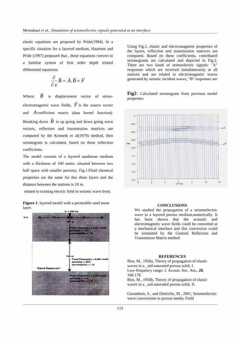
Author, A. et al., 2007, Short title goes here…
elastic equations are proposed by Pride(1994). In a
specific situation for a layered medium, Haartsen and
Pride (1997) proposed that , these equations convert to
a familiar system of first order depth related
differential equations:
FBABz
+=∂∂ .
Where: is displacement vector of stress-
electromagnetic wave fields,
B
F is the source vector
and Acoefficient matrix (data kernel function).
Breaking down in up going and down going wave
vectors, reflection and transmission matrices are
computed by the Kenneth et al(1979) method, then
seismogram is calculated, based on these reflection
coefficients.
B
2/3
The model consists of a layered sandstone medium
with a thickness of 100 meter, situated between two
half space with smaller porosity, Fig.1.Fluid chemical
properties are the same for this three layers and the
distance between the stations is 10 m.
related to existing electric field in seismic wave front. Figure 1: layered model with a permeable sand stone layer.
Using Fig.1, elastic and electromagnetic properties of the layers, reflection and transmission matrices are computed. Based on these coefficients, contributed seismograms are calculated and depicted in Fig.2. There are two kinds of seimoelectric signals: "A" responses which are received simultaneously at all stations and are related to electromagnetic waves generated by seismic incident waves, "B" responses are Fig2: Calculated seismogram from previous model properties
CONCLUSIONS We studied the propogation of a seismoelectric wave in a layered porous medium,numerically. It has been shown that the acoustic and electromagnetic wave fields could be converted at a mechanical interface and this conversion could be simulated by the General Reflection and Transmision Matrix method
REFERENCES Biot, M., 1956a, Theory of propagation of elastic waves in a _uid-saturated porous solid, I. Low-frequency range: J. Acoust. Soc. Am., 28, 168.178. Biot, M., 1956b, Theory of propagation of elastic waves in a _uid-saturated porous solid, II. Garambois, S., and Dietrichz, M., 2001, Seismoelectric wave conversions in porous media: Field
Montahaei et al., Simulation of seismoelectric signals generated at an interface
115

Author, A. et al., 2007, Short title goes here…
3/3
measurements and transfer function analysis: Geophysics, 66, 1417–1430. Haartsen, M. W., and Pride, S. R., 1997, Electroseismic waves from point sources in layered media: J. Geophys. Res., 102, 24745–24769.
Kennett,B. L. N., and N. J. Kerry, 1979, Seismic waves in
stratified half space, Geophys. J. R. Astron. Soc., 57, 557-583.
Kennett, B. L. N., 1983, Seismic Wave Propagation in Stratified Media, 342 pp., Cambridge Univ. Press. Martner, S. T., and Sparks, N. R., 1959, The electroseismic effect: Geophysics, 24, 297-308. Pride, S., 1994, Governing equations for the coupled electromagnetics and acoustics of porous media: Physical Review B, 50, 15678–15696. Pride, S. R., and M.W. Haartsen, 1996, Electroseismic wave properties, J. Acoust. Soc. Am., 100, 1301-1315. Thompson, R. R., 1936, The seismic electric effect, Geophysics, 1, 327 – 335. Thompson, A. H., and Gist, G. A., 1993, Geophysical applications of electrokinetic conversion: The Leading Edge, 12, 1169–1173.
Montahaei et al., Simulation of seismoelectric signals generated at an interface
116
4th International Symposium on Three-Dimensional Electromagnetics
Freiberg, Germany, September 27−30, 2007
1/1
A new, faster technique of three-dimensional magnetotelluric data acquisition
Gerard Muñoz, Oliver Ritter, Thomas Krings, Michael Becken
GeoForschungsZentrum Potsdam
SUMMARY
One of the difficulties for obtaining meaningful three-dimensional magnetotelluric models is getting a sufficient spatial
coverage of the target area. A huge number of stations is required if the target area is large and / or site spacing is dense.
The deployment of a large number of MT stations results in big costs both in terms of time and money. In this work we
present a technique of 3D data acquisition and processing that can reduce the needed setup time. This technique was
used to acquire MT data in a dense grid in the area around the Groß Schönebeck (Germany) geothermal test site. Five
standard MT stations (base stations) were distributed in the studied area of approximately 5 x 15 km and kept recording
for the whole duration of the experiment. In addition, at 158 stations (grid stations) only horizontal electric fields and
the vertical magnetic field were recorded covering the area with a site spacing of 500 x 500 m. Given that the
deployment of horizontal magnetic sensors is not necessary, the setup time of one of these stations is much shorter than
for a standard MT station, thus increasing the number of sites that can be deployed per day.
We applied both standard and remote-reference processing. A reference site was operated on the 250 km distant Island
of Rügen. As a first approach, the impedance tensor and the geomagnetic transfer functions at the grid stations were
calculated by simply using the horizontal magnetic fields measured at the five base stations. The spatial variability of
the horizontal magnetic fields is estimated form horizontal magnetic inter-station transfer functions between the base
sites. If the subsurface is predominantly 1D, as is the case for our short-period data, the anomalous horizontal magnetic
fields are small and the inter-station impedance estimates are close to the local impedances.. For more complex
structures, the transfer functions will be biased by the local variation of the horizontal magnetic field. To interpret these
data, we suggest to (i) modify existing inversion codes to handle inter-station transfer functions and, alternatively, (ii) to
apply techniques to predict the horizontal magnetic fields at the grid stations from the observed vertical magnetic fields,
using some hypothetic event analysis or related decomposition schemes.
Keywords: 3D data acquisition, processing, remote reference
4th International Symposium on Three-Dimensional ElectromagneticsFreiberg, Germany, September 27–30, 2007
117

4th International Symposium on Three-Dimensional Electromagnetics Freiberg, Germany, September 27−30, 2007
Laboratory measurements of electrokinetic phenomena
F.C Schoemaker, D.M.J. Smeulders and E.C. Slob
Delft University of Technology, The Netherlands
SUMMARY Electrokinetics is the area where the interaction between the seismic and electromagnetic effects is studied. We present laboratory measurements of the phenomenological coefficients which are required during the analysis of fluid saturated porous media. Samples consisting of capillary tubes were used. The dynamic permeability which is a measure of the fluid flow response to an applied external oscillating pressure gradient, such as exists in seismic waves, was measured. This measurement is followed by the analysis of the dynamic coupling factor, which is essential for the interaction between seismic and E-M phenomena. The governing electrokinetic theory is also written down and used for the derivation of the characteristic wave velocities. From this analysis it has become clear that the shear wave, in comparison to the other compressional waves, is most sensitive for detecting electrokinetic effects. Keywords: Electrokinetics, streaming potential, experiments
INTRODUCTION Exploration companies are extensively studying the structure of the earth using electro-magnetic (E-M) and seismic techniques. In this way they are capable of finding water, gas and oil reservoirs or minerals. Due to an increased demand for these assets, there is a growing demand for new and improved exploration techniques. Through the years seismic and E-M methods have proven their effectiveness therefore geophysists are now also looking for hybrid methods. Electrokinetics is the area where the interaction between the seismic and electromagnetic effects in saturated porous media is studied. Electrokinetic effects are studied within a wide variety of scientific disciplines, e.g. microsystem industry, medicine, groundwater and waste management, earthquake prediction and monitoring and geophysical prospecting. In this paper our attention is directed towards measure-ment of the frequency-dependency of electrokinetic phenomena. Thereby a short theoretical description is given of the governing equations followed by computed results of the characteristic acoustic waves. A comparison is made of how much the electrokinetic coupling affects the characteristic waves. Thereafter the theory behind the frequency-dependent phenomenological coefficients is shown and compared to experimental results which are obtained with the so-called Dynamic Darcy Cell (DDC). In figure 1 a photo is shown of this set-up.
Figure 1: Laboratory set-up: Dynamic Darcy Cell.
Background
When brine flows through porous rocks two effects play a role. The first is the viscous effect characterized by Darcy’s law. The second is the electrokinetic coupling caused by the relative motion of charges in response to an applied electric field (electro-osmosis) or an applied pressure gradient (streaming-potential). For example, glass immersed in an aqueous solution becomes negatively charged due to the fact that the silane terminals Si-O-H located at the surface of the glass become protonated in the presence of an aqueous
1/4
4th International Symposium on Three-Dimensional ElectromagneticsFreiberg, Germany, September 27–30, 2007
118

F.C. Schoemaker, et al., 2007, Laboratory measurements of electrokinetic phenomena
solution. The mobile charge distribution, within the liquid forms a so-called 'electric double layer' near the immersed surface. This EDL consists of a fixed layer at the surface, the ´Stern layer´, which is a molecular film of counter-ions bonded to the solid by electrostatic interaction. The second layer is a diffuse layer, which extends from the fixed layer into the bulk solution; it is known as the ´Gouy-Chapman diffuse layer´. This diffuse layer results from a statistical equilibrium between thermal and electrical forces. Both the viscous and the electrokinetic coupling effects are strongly frequency-dependent. For low frequencies, the velocity profile is parabolic and Darcy’s law is generally valid. For higher frequencies, the drag that the solid part of the medium exerts on the fluid part, is dominated by inertial effects as the viscous boundary layer decreases. This drag is characterized by the tortuosity or the related formation factor. Similarly the electric coupling is governed by the visco-electric steady-state properties of the fluid-saturated porous medium at low frequencies. For high frequencies, inertia effects will become dominant, as the viscous skin depth decreases.
THEORETICAL FRAMEWORK The governing equations were derived by Pride (1994). Using an i te ω dependence, they can be written as:
( )1 bf si w i vωφρ ω φ ρ τ+ − = ∇ ⋅) ) , (1a)
[ ] ( ) ( )fw v p i v ELφ ωρη
ω⎡ ⎤− = −∇ − +⎣ ⎦k ω )) ) ) ) , (1b)
i p Q v R wωφ− = ∇ ⋅ + ∇ ⋅) ) ) , (1c)
( ) ( )2 2 ijb kk kkij
dede di P Q G R Q Gdt dt dt
εωτ δ⎡ ⎤= + − + + +⎢ ⎥⎣ ⎦, (1d)
with the strain rates given by: 12
ij ji
j i
de vvdt x x
⎛ ⎞∂∂= +⎜⎜ ∂ ∂⎝ ⎠
⎟⎟
)), (1e)
12
ij ji
j i
d wwdt x xε ⎛ ⎞∂∂
= +⎜ ⎟⎜ ⎟∂ ∂⎝ ⎠
)), (1f)
Maxwell’s equations: ( ) fJ E p iL ρωσ ω⎡ ⎤= + −∇ −⎣ ⎦
r rv) ) , (2a)
( )0 ri E Hωε ε = ∇× −r r
Jr
, (2b)
( )0 ri H Eωµ µ = − ∇×r r
(2c) In these equations, v) , w) are the solid and fluid velocity,
is the fluid pressure,p bτ the total stress, φ the porosity, ( )k ω the dynamic permeability,η the fluid viscosity, ρf and ρs are the fluid and solid density, respectively. P, Q and R are the Biot-Gassmann constants, G the shear modulus. In the E-M equations we have 0ε and rε the permittivity in vacuum and the relative permittivity, σ the conductivity, ,H
rEr
, Jr
are
the magnetic field, electric field and electric-current, for more details see (Pride 1994). Setting the coupling coefficient ( )L ω equal to zero, the Biot equation and Maxwell relations decouple and the ordinary Biot waves and Electromagnetic waves are found. Solving the Biot equations results in the prediction of three wave types: two compressional and one shear wave (see e.g. Smeulders, 2005). If the electrokinetic coupling is included ( )0L ≠ (Pride, 1996), the three wave type characteristics are affected by electrokinetic effects, and their phase velocities and attenuation factors are modified. Results are shown in figures 2. In figure 2a the phase speed versus the frequency are plotted as a function of reduced frequency. From the figures we notice that the electrokinetic coupling hardly affects the compressional waves. The shear wave, however, does show coupling effects which will be the subject of further research investigation.
Figure 2a: Phase velocity versus frequency for the characteristic waves..
Figure 2b: Attenuation versus frequency for the characteristic waves.
2/4
Schoemaker et al., Laboratory measurements of electrokinetic phenomena
119

F.C. Schoemaker, et al., 2007, Laboratory measurements of electrokinetic phenomena
Parameter analysis
We now take a look at the phenomenological coef-ficients (colored red in the above governing equations). Dynamic permeability: For a porous medium consisting of an ensemble of parallel tubes (radius R), the dynamic permeability can be computed exactly (Cortis et al, 2003): ( )
( )( )( )
12
0
8 21o
k Jk R JRω
β ββ
⎡ ⎛ ⎞= −⎢ ⎜ ⎟⎜ ⎟⎢ ⎥⎝ ⎠⎣ ⎦
RR
β ⎤⎥
R
, (3a)
with ( ) 20 1/ 8k φ= the steady state permeability, ρf the
fluid density 2 /fiβ ωρ η= − and R the radius of the capillary, J0, J1 are Bessel functions of respectively order zero and one. This is an exact solution derived from the Navier-Stokes equations. The dynamic per-meability for a porous medium of arbitrary shape was later described by Johnson, Koplik and Dashen (Johnson et al, 1987):
( )12
12o c
k Mi ikω
c
ω ωω ω
⎡⎛ ⎞⎢= − −⎜ ⎟⎢ ⎥⎝ ⎠⎢ ⎥⎣ ⎦
⎤⎥
)
, (3b)
where ( 0/c f kω ηφ ρ α∞= is the rollover frequency
describing the transition from low frequency, viscosity dominated flow towards, high frequency, inertia dominated flow. The shape factor M (usually taken 1) describes the ruggedness of the pore morphology, at microscopic scale. For the same sample consisting of parallel tubes also an exact expression for the electrokinetic coupling can be derived. This can be reached by combining the charge transport flux within an individual cylinder and Poisson´s equation for electrostatics (Packard, 1952). For steady state conditions we obtain:
( ) ( )( )
( )( )
1
0
2V JL
P R Jω εξωω ση β β
⎡∇ ⎡ ⎤ −= = ⎢⎢ ⎥∇ ⎣ ⎦ ⎣ ⎦
RR
β ⎤⎥
, (4a)
with ( )V ω∇ the potential gradient, ε the permittivity of the fluid, and σ the fluid conductivity. Like before, this result can be generalized to a porous medium of arbitrary pore structure (Pride, 1994):
( )32
12 2221 1 2 1 f
c
dL i i dM
ωρεξ ωωση ω
−⎡ ⎤⎛⎡ ⎤ ⎛ ⎞⎢= − − −⎜⎜ ⎟⎢ ⎥ ⎜ ⎟⎢ Λ Λ⎝ ⎠⎣ ⎦ ⎝ ⎠⎣
⎞⎥⎟⎥⎦
(4b)
where d is the Debye length and Λ a characteristic pore size parameter representing a weighted volume-to-surface ratio.
Instrumentation At the inlet of the DDC (figure 1) an oscillating pressure is applied. The tube is standing in a vertical position, with the inlet at the bottom. There a vibrating exciter drives a rubber membrane which induces the oscillating pressure. Vibrations are induced in a frequency band ranging from 5 Hz up to 200 Hz. Two identical piezoelectric transducers are used to measure the pressure, one at the inlet and the other at the outlet mounted at the top, just above the porous sample in the electrolyte. On the top and bottom of the porous medium, electrodes are placed from which the potential gradient is measured. The obtained results will be compared with the existing theory. This is necessary because in contrast to the recent advances in the theoretical area, fieldwork and laboratory measurements are still under-exposed. Most of the laboratory measurements, were measured with Direct Current (DC), thereby neglecting frequency effects. The porous sample consists of capillary tubes of glass, which are glued together with an epoxy resin. Use is made of glass tubes, for their simple geometry which allows an easier interpretation of the underlying physics.
RESULTS and CONCLUSIONS In Figure 3a, the real and in Figure 3b the imaginary part of the dynamic permeability are plotted for both the exact solution (equation 3a) and the generalized approximate solution (equation 3b). We notice that both models are almost indistinguishable. At low frequencies (viscosity dominated), the dynamic permeability necessarily tends to its steady-state value, whereas above the rollover frequency a strong decline can be observed (inertia dominated flow). The Imaginary part displays a pronounced maximum at the rollover frequency. In Figure 4, Real and Imaginary parts of the dynamic coupling factor (equation 4a and 4b) are plotted. Here we observe also similar transition as described for the dynamic permeability. In figure 4a a small difference is observed between the exact solution at micro-scale and the approximate solution at macro scale. From our analysis it is possible to conclude, that we can measure the dynamic permeability and electro-kinetic coupling factor in one single experimental set-up. Reducing this way the chance of measurement errors caused by sample handling and manufacturing. The measured dynamic permeability values are in good agreement with the theoretical predictions. The electrokinetic coupling factor can be studied by analyzing the shear waves, due to their larger
3/4
Schoemaker et al., Laboratory measurements of electrokinetic phenomena
120
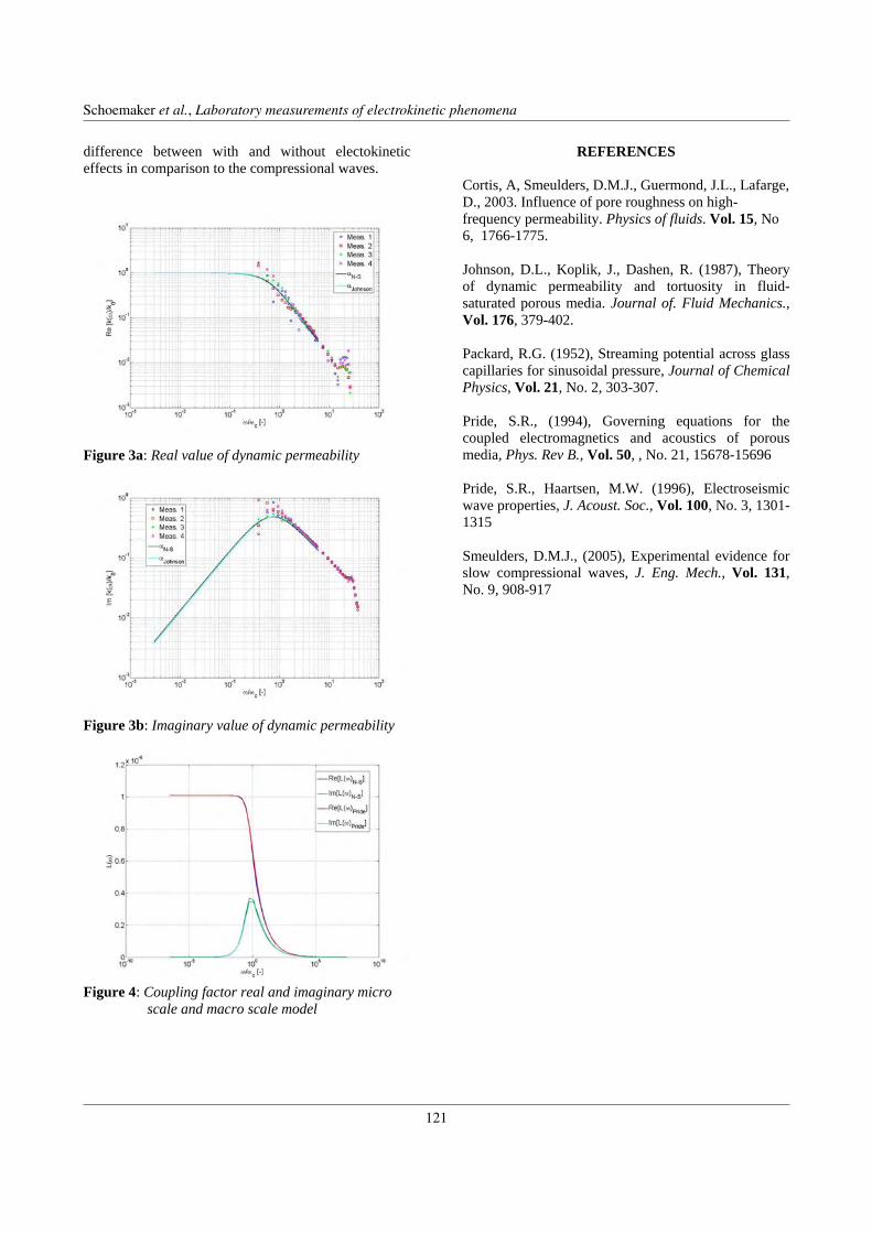
F.C. Schoemaker, et al., 2007, Laboratory measurements of electrokinetic phenomena
difference between with and without electokinetic effects in comparison to the compressional waves.
Figure 3a: Real value of dynamic permeability
Figure 3b: Imaginary value of dynamic permeability
Figure 4: Coupling factor real and imaginary micro scale and macro scale model
REFERENCES Cortis, A, Smeulders, D.M.J., Guermond, J.L., Lafarge, D., 2003. Influence of pore roughness on high-frequency permeability. Physics of fluids. Vol. 15, No 6, 1766-1775. Johnson, D.L., Koplik, J., Dashen, R. (1987), Theory of dynamic permeability and tortuosity in fluid-saturated porous media. Journal of. Fluid Mechanics., Vol. 176, 379-402. Packard, R.G. (1952), Streaming potential across glass capillaries for sinusoidal pressure, Journal of Chemical Physics, Vol. 21, No. 2, 303-307. Pride, S.R., (1994), Governing equations for the coupled electromagnetics and acoustics of porous media, Phys. Rev B., Vol. 50, , No. 21, 15678-15696 Pride, S.R., Haartsen, M.W. (1996), Electroseismic wave properties, J. Acoust. Soc., Vol. 100, No. 3, 1301-1315 Smeulders, D.M.J., (2005), Experimental evidence for slow compressional waves, J. Eng. Mech., Vol. 131, No. 9, 908-917
4/4
Schoemaker et al., Laboratory measurements of electrokinetic phenomena
121

Schünemann, Günther & Junge 2007, Large-scale 3D DC resistivity tensor investigations
3-dimensional subsurface investigation by means of large-scale tensor-type dcresistivity measurements
J. Schünemann1, T. Günther1 and A. Junge2
1Leibniz Institute for Applied Geosciences, Hannover2University of Frankfurt, Institute for Geosciences
SUMMARY
Resistivity is an important parameter for hydrogeophysical characterisation. In order to investigate large-scale structuresthe usual multi-electrode devices cannot be applied. We present a measuring technology with fixed stations and variablecurrent input up to 40 Amperes. Each station consists of three differently oriented dipoles, current is also injected intothree directions.
The interpretation consists of three parts: (i) First the time series have to be pre-processed. A novel approach based ona least squares method is used to correlate current and voltage yielding the resistance and its error. (ii) Then both scalarand tensor apparent resistivities are calculated. The latter are able to illustrate the directional dependence of the measuredelectric fields. (iii) Finally the data are used to find a subsurface model via modeling and inversion. Finite-element basedmethods on unstructured meshes provide best flexibility to handle large-scale and small-scale structures at the same time.
The methodology is applied to data over a buried valley structure in Northern Germany and provides valuable insight intothe subsurface.
Keywords: DC resistivity, apparent resistivity tensor, modeling, inversion
INTRODUCTION
In order to investigate the ground with dc resistivity mea-surements we cannot use the common multi-electrode de-vices due to their spatial limitations. In case of a one-dimensional underground Schlumberger soundings can beapplied. For 3d structures the only choice are dipole-dipole type arrays. However the geometric factor growsheavily with increasing dipole distance. Moreover, evenfor short distances the geometry factor can reach infinityfor a dipole spread along the potential line thus makingthe concept of apparent resistivity inapplicable.To overcome these problems the apparent resistivity ten-sor has been introduced (Bibby, 1986). It is derived bymeasuring the electric field (two voltages) at each site fortwo current injections. The tensor represents the under-ground resistivity distribution and its directional depen-dence. There exist so-called invariants that are mainly in-dependent on the dipole orientation.We will apply this technique to the investigation of aburied valley. Similar to (Bibby, Risk, & Caldwell, 2002)we apply three current injections at each source positionand measure three potential differences at each station.We develop a new methodology of processing the timeseries by means of a least-squares approach. Then prelim-inary results of the study are presented.
TENSOR ANALYSIS
The apparent resistivity is the (scalar) resistivity of theequivalent homogeneous half-space reproducing the mea-sured voltage. Therefore we transform the resistance intoan apparent resistivity ρa = G · U/I by the geometricfactor G, which is derived by the solution of the homoge-neous half-space.Similarly, the apparent resistivity tensor is the propertyof an anisotropic half-space representing a laterally vary-ing isotrope resistivity. For two current injections imply-ing the theoretical current densities ~j1 = [j1x j1y]T and~j2 = [j2x j2y]T , the electric fields ~E1 = [E1x E1y]T and~E2 = [E2x E2y]T are measured by voltage readings. Thedefinition ~Ei = ρa
~ji yields (Bibby, 1986)
ρa =(ρxx ρxy
ρyx ρyy
)=
1j1xj2y − j1yj2x
·(E1xj2y − E2xj1y E2xj1x − E1xj1x
E1yj2y − E2yj1y E2yj1x − E1yj1x
)(1)
representing the distortion of the electric field with respectto the current. The tensor can be imaged by an ellipse il-lustrating the preferential current flow. Furthermore, ro-tational invariants can be derived. P1 = (ρxx + ρyy)/2and P2 = det ρa represent mean resistivities, P3 =(ρxy − ρyx)/2 indicates the skewness.
1/4
4th International Symposium on Three-Dimensional ElectromagneticsFreiberg, Germany, September 27–30, 2007
122

Schünemann, Günther & Junge 2007, Large-scale 3D DC resistivity tensor investigations
THE 3D EXPERIMENT
The area of investigation is located in Northern Germanynear Cuxhaven. The Target is one of the existing buriedglacial valleys, which are of importance for groundwatersupply. Many geophysical methods such as reflection seis-mics or air-borne electromagnetics have been applied sofar (BurVal Working Group, 2006) revealing a complexvalley-like structure with different sediment layers and aclay cap.We chose an area of ≈ 4× 3 km and installed 20 E-fieldsites. Each station consists of a central electrode and threeelectrodes in 0, 120 and 240 directions with dipolelengths of about 75 m as shown in Figure 2. 20 transientrecorders of GEOLORE type, which have been developedfor MT studies (Golden, Roßberg, & Junge, 2004), sam-pled the 3 channels with 8 Hz sampling rate during thewhole experiment, about 2 weeks.
Figure 1: Measuring area, current (black) and poten-tial (red) positions. The boundary of the valley asknown from EM measurements is delineated in red.
In a similar arrangement we set up the source dipoles. At10 sites a square wave signal of up to 40 A was injectedinto the ground using a high voltage generator, ensuringlarge signals at greater distances. In total we have a num-ber of 10 Current Locations × 20 Stations × 3 injectiondirections × 3 measuring directions = 1800 independentdata. Figure 1 shows the measuring area and the used elec-
trode positions.
Figure 2: Setup of transient recorders with the data log-ger at the central reference electrode and three elec-trodes at ≈75 m distance.
PROCESSING OF TIME SERIES
As a first step, the 2 weeks registration have to be split intosegments and associated to the source injections. Timecorrections and resampling had to be applied due to vary-ing sampling frequencies of the current signal. Since thereis noise from different origins in the data, filtering is nec-essary. This includes (i) offset and drift correction, (ii) alow pass in order to remove long-periodic telluric currentsand (iii) a removal of the 50 Hz and 16.7 Hz frequenciesof of anthropogenic origin. Identical filters are applied forboth voltage and current time series to avoid numericallyproduced bias when estimating the resistances.
0 0.5 1 1.5 2
0
0.5
1
Frequency [Hz]
Am
plitu
de
16 18
−2
0
2x 10
−4
Vol
tage
[V]
time in minutes
Figure 3: Section of a square wave signal from a recordedvoltage time series with 50 Hz noise and long-periodic drift (top). In the signal spectrum (below)the fundamental frequency (≈0.1 Hz) and its oddmultiples can be seen.
Figure 3 shows a section of the signal and its Fourier spec-trum. The square-wave signal is represented by the odd
2/4
Schünemann et al., Large-scale 3D DC resistivity tensor investigations
123

Schünemann, Günther & Junge 2007, Large-scale 3D DC resistivity tensor investigations
harmonics of the basic frequency of about 1/9 Hz. On thesquare wave we see high-frequency oscillations from the50 Hz AC mains power, shown at its alias frequency of2 Hz in the spectrum. Furthermore we can observe a long-periodic noise both in the signal as well as in the spectrum.There are different method to estimate the resistance asfraction of voltage and current:
1. stacking of the signals, estimating magnitudes sep-arately
2. estimating the magnitudes in frequency domain
3. estimating the correlation coefficient between cur-rent and voltage
The latter is the most intense but also most accurate ap-proach. It has the advantage of treating an arbitrary cur-rent signal, e.g. breakdowns in the current occurred fre-quently. Cross-correlation methods were used to shift thevoltage signal to match the current signal.We use the following relation to fit the voltage signal
U(t) = R · I(t) +n∑i
aifi(t) + e(t) (2)
and determine the coefficient vector c = [R, a1, . . . , an]T
by a least squares fit
c = (AT A)−1AT U with A = [I, f1, . . . , fn] .
For the functions fi we tried polygonal functionsand long-periodic harmonic functions f2i−1(t) =sin(2iπt/T ) and f2i(t) = cos(2iπt/T ), where T is thesample length, about 20 min. The latter performed best,with a number of about 40 function pairs. Additionallywe are able to obtain an accuracy of the resistance fromthe residual U−AI = e.
SOME RESULTS
From the time series processing we obtain nine resis-tances for each source/receiver combination according tothe three source directions and the three receiver chan-nels. Straightforward we can compute a geometric factorG from the positions and thus produce scalar apparent re-sistivities. In the following we concentrate on source E1and receiver 14, which are quite close to each other in thecentre of the valley. Figure 4 shows the resulting apparentresistivities and their geometric factors for the individualsource/receiver directions.
1 2 3
1
2
3
receiver channel
sour
ce d
irect
ion
37Ωm
ρ=107.0Ωm
G=−2.60e5m
ρ=81.8Ωm
G=3.30e5m
ρ=156.0Ωm
G=9.10e5m
ρ=36.3Ωm
G=4.62e5m
ρ=−17.1Ωm
G=4.86e6m
ρ=31.1Ωm
G=−4.05e5m
ρ=38.7Ωm
G=6.44e5m
ρ=30.2Ωm
G=−3.63e5m
ρ=21.8Ωm
G=9.31e5m
ρ in Ωm
25
32
40
50
63
79
100
130
Figure 4: Apparent resistivities and geometric factors Gfor all combinations at receiver 14 caused by sourceE1.
Only the central apparent resistivity is negative. The rea-son is probably the large geometric factor of about 5e6,whereas the other combinations have absolute G valuesbelow 1e6. From noise measurements yielding a mini-mum voltage of 20µV to be measured we are able to ob-tain reliable ρa’s up to G =3e6. The values for the sourcedirections 2 and 3 vary around 30 Ωm, however the firstinjection yields very differing results. The reason can bea problem in the source signal, electrode positions or astrong lateral inhomogeneity in their vicinity.For each pair of two current injections and voltage read-ings an apparent resistivity tensor can be constructed. Sowe have 9 tensors for each source/receiver pair.
sour- channelsces 1 2 1 3 2 31 36.1 -3.6 33.5 -0.7 34.8 -2.12 -82.3 76.6 -82.2 76.6 -84.6 79.11 27.1 -5.4 30.6 -1.3 28.9 -3.33 68.7 106.8 68.7 106.8 71.8 110.42 31.3 -0.9 32.0 0.1 31.6 -0.43 -1.6 32.2 -1.6 32.2 -1.0 33.1
Table 1: Apparent resistivity tensors in Ωm for all combi-nations of source and receiver orientation.
Table 1 shows the apparent resistivity tensors. Con-sequently the first and second row exhibits unexpected
3/4
Schünemann et al., Large-scale 3D DC resistivity tensor investigations
124

Schünemann, Günther & Junge 2007, Large-scale 3D DC resistivity tensor investigations
tensors with very differing main diagonal and large off-diagonal elements. Only the tensors based on source di-rections 2 and 3 are very similar, their main diagonals aswell as the invariants show values of about 32 Ωm. In or-der to obtain a geometrical overview, the median apparentresistivities due to source E1 of all receivers are computedand displayed in Figure 5 according to the station layout.The source position is located between stations 22 and 14.
10 F1 14 F2 15 F3 11
F4 21 F5 22 F6 F7 −
13 F8 16 F9 18 10 12
ρa in Ωm
2.5 4 6.3 10 16 25 40
Figure 5: Median apparent resistivity values for all sta-tions caused by current injection at station 1.
We observe increased resistivities of 40-60 Ωm in the areawhere the buried valley is situated. Outside the valuesare dropping down to 10 Ωm or below. For the inter-pretation we must also take into account the penetrationdepth which is increasing with growing source-receiverdistance. So the low apparent resistivities could be a resultof the known salt water at depth as well as the product ofnegative near-surface sensitivities. Hence extensive mod-eling and sensitivity studies are required to find subsurfacemodels.
MODELING AND INVERSION
For an accurate prediction of voltages we solve the con-tinuity equation with the finite element method (Rücker,Günther, & Spitzer, 2006). We use unstructured tetra-hedral meshes because they bear the biggest geometricalflexibility to include information from other methods orto create a resolution-dependent mesh for inversion. Asmoothness-constrained Gauss-Newton approach is used(Günther, Rücker, & Spitzer, 2006). To account for thevery different quality of the input resistances the residualsof the least squares estimation are used for weighting theindividual data. We use a combination of forward model-ing and inversion to find a model. This procedure is cur-rently ongoing.
CONCLUSIONS
Tensor measurements represent a costly but valuablemethod to describe the large-scale resistivities in theground by direct current measurements. A high-voltagegenerator and sensitive electrical field loggers are neededto counteract the dipole type arrays. The accurate methodfor determining the resistances showed up to be a a least-squares approach including the current signal and long-periodic harmonic functions.However the whole methodology is sensitive to mistakesand even the tensors are not easy to understand. Yet to bedone are sensitivity studies, extensive modeling and inver-sion in order to fit the data, error propagation analysis andresolution appraisal.
ACKNOWLEDGMENTS
We like to thank the persons involved in the very exhaust-ing field campaign: M. Grinat, T. Grelle, R. Meyer, W.Südekum and T. Agricola.
REFERENCES
Bibby, H. M. (1986). Analysis of multiple-source bipole-dipole resisitivity surveys using the apparent resis-tivity tensor. Geophysics, 51, 972-983.
Bibby, H. M., Risk, G. F., & Caldwell, T. G. (2002).Long offset tensor apparent resistivity surveys ofthe taupo volcanic zone, New Zealand. Journal ofApplied Geophysics, 49, 17-32.
BurVal Working Group. (2006). Groundwater resourcesin buried valleys - a challenge for geosciences(R. Kirsch, Ed.). Hannover: Leibniz Inst. for Appl.Geosc.
Golden, S., Roßberg, R., & Junge, A. (2004). The datalogger geolore and its application in lake bottommagnetotellurics. In 17th workshop on electromag-netic induction in the earth. Hyderabad, India.
Günther, T., Rücker, C., & Spitzer, K. (2006). 3-d mod-eling and inversion of dc resistivity data incorporat-ing topography - part II: Inversion. Geophys. J. Int.,166(2), 506-517.
Rücker, C., Günther, T., & Spitzer, K. (2006). 3-d mod-eling and inversion of dc resistivity data incorporat-ing topography - part I: Modeling. Geophys. J. Int.,166(2), 495-505.
4/4
Schünemann et al., Large-scale 3D DC resistivity tensor investigations
125
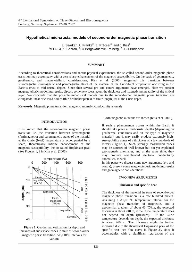
4th International Symposium on Three-Dimensional Electromagnetics Freiberg, Germany, September 27−30, 2007
Hypothetical mid-crustal models of second-order magnetic phase transition
L. Szarka1, A. Franke2, E. Prácser3, and J. Kiss3
1MTA GGKI Sopron, 2TU Bergakademie Freiberg, 3ELGI Budapest
SUMMARY According to theoretical considerations and recent physical experiments, the so-called second-order magnetic phase transition may accompany with a very sharp enhancement of the magnetic susceptibility. On the basis of geomagnetic, geothermic, and magnetotelluric considerations, Kiss et al. (2005) suggested this transition between ferromagnetic/ferrimagnetic and paramagnetic states of the material at the Curie/Néel temperature occurring in the Earth’s crust at mid-crustal depths. Since then several pro and contra arguments have emerged. Here we present magnetotelluric modelling results, discuss some new ideas about the thickness and magnetic permeability of the critical layer. We conclude that the possible mid-crustal models due to the second-order magnetic phase transition are elongated: linear or curved bodies (thin or thicker plates) of finite length just at the Curie depth. Keywords: Magnetic phase transition, magnetic anomaly, conductivity anomaly
INTRODUCTION It is known that the second-order magnetic phase transition i.e. the transition between ferromagnetic (ferrimagnetic) and paramagnetic states of the material at the Curie (Néel) temperature is accompanied by a sharp, theoretically infinite enhancement of the magnetic susceptibility, the so-called Hopkinson peak (See Figures 1, 2 in Kiss et al. (2005).
Figure 1. Geothermal estimation for depth and thickness of subsurface zones in state of second-order
magnetic phase transition. ∆Tc=10oC intervals for various
Earth magnetic minerals are shown (Kiss et al. 2005) If such a phenomenon occurs within the Earth, it should take place at mid-crustal depths (depending on geothermal conditions and on the type of magnetic material), and it may easily produce extremely high-susceptibility zones of a thickness of a few hundreds of meters (Figure 1). Such strongly magnetized zones may be sources of well-known but not-yet explained geomagnetic anomalies, and at the same time, they may produce complicated electrical conductivity anomalies, as well. In this paper we discuss some new arguments (pro and contra), present some magnetotelluric modeling results and geomagnetic considerations.
TWO NEW ARGUMENTS
Thickness and specific heat The thickness of the material in state of second-order magnetic phase transition is a few hundred meters. Assuming a ∆Tc=10oC temperature interval for the magnetic phase transition of magnetite, and a geothermal gradient of about 40 oC/km, the expected thickness is about 240 m, if the Curie temperature does not depend on depth (pressure). If the Curie temperature depends on depth, the expected thickness is about 260 m. The thickness might be further increased due to the theoretical Hopkinson peak of the specific heat (see blue curve in Figure 2), since it accompanies with a significant retardation of the
1/4
4th International Symposium on Three-Dimensional ElectromagneticsFreiberg, Germany, September 27–30, 2007
126
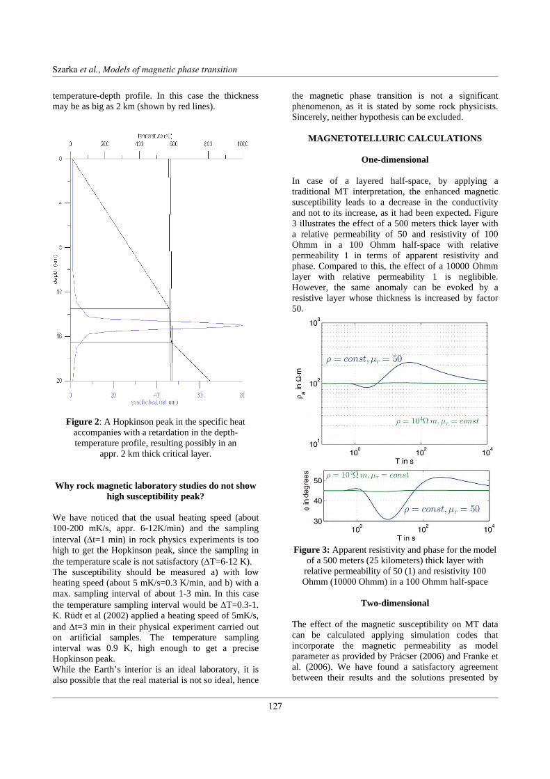
Szarka, L. et al., 2007, Models of magnetic phase transition
temperature-depth profile. In this case the thickness may be as big as 2 km (shown by red lines).
Figure 2: A Hopkinson peak in the specific heat accompanies with a retardation in the depth-temperature profile, resulting possibly in an
appr. 2 km thick critical layer. Why rock magnetic laboratory studies do not show
high susceptibility peak? We have noticed that the usual heating speed (about 100-200 mK/s, appr. 6-12K/min) and the sampling interval (∆t=1 min) in rock physics experiments is too high to get the Hopkinson peak, since the sampling in the temperature scale is not satisfactory (∆T=6-12 K). The susceptibility should be measured a) with low heating speed (about 5 mK/s=0.3 K/min, and b) with a max. sampling interval of about 1-3 min. In this case the temperature sampling interval would be ∆T=0.3-1. K. Rüdt et al (2002) applied a heating speed of 5mK/s, and ∆t=3 min in their physical experiment carried out on artificial samples. The temperature sampling interval was 0.9 K, high enough to get a precise Hopkinson peak. While the Earth’s interior is an ideal laboratory, it is also possible that the real material is not so ideal, hence
the magnetic phase transition is not a significant phenomenon, as it is stated by some rock physicists. Sincerely, neither hypothesis can be excluded.
MAGNETOTELLURIC CALCULATIONS
One-dimensional
In case of a layered half-space, by applying a traditional MT interpretation, the enhanced magnetic susceptibility leads to a decrease in the conductivity and not to its increase, as it had been expected. Figure 3 illustrates the effect of a 500 meters thick layer with a relative permeability of 50 and resistivity of 100 Ohmm in a 100 Ohmm half-space with relative permeability 1 in terms of apparent resistivity and phase. Compared to this, the effect of a 10000 Ohmm layer with relative permeability 1 is neglibible. However, the same anomaly can be evoked by a resistive layer whose thickness is increased by factor 50.
Figure 3: Apparent resistivity and phase for the model
of a 500 meters (25 kilometers) thick layer with relative permeability of 50 (1) and resistivity 100 Ohmm (10000 Ohmm) in a 100 Ohmm half-space
Two-dimensional
The effect of the magnetic susceptibility on MT data can be calculated applying simulation codes that incorporate the magnetic permeability as model parameter as provided by Prácser (2006) and Franke et al. (2006). We have found a satisfactory agreement between their results and the solutions presented by
2/4
Szarka et al., Models of magnetic phase transition
127

Szarka, L. et al., 2007, Models of magnetic phase transition
Rijo (2004). E- and H-polarisation calculations over a 2D dike model (width: 1 km, thickness: 0.5 km, depth of its top: 10 km) embedded in a homogeneous half-space of 100 Ohmm were carried out. Both the magnetic permeability and the electrical conductivity of the model varied in a wide range: permeability contrast „mu”= 50, 100, 200; conductivity contrast= 50, 100, 200 (corresponding to resistivity values of 2 Ohmm, 1 Ohmm, 0.5 Ohmm). The effect of the magnetic permability on MT data in H-polarisation is the same as that of the electrical resistivity (reciprocial conductivity) in E-polarisation. However, it is insignificant in E-polarisation (as well as the effect of conductivity in H-polarisation). Some results are shown in Figure 4.
Figure 4: MT apparent resistivity curves. Top: H-polarisation curves for varying magnetic permeability;
bottom: E-polarisation curves for varying electric resistivity (reciprocial conductivity)
Three-dimensional
3D magnetotelluric calculations (over thin circular plates and cubic structures) show of course less significant anomalies. However, it is not impossible that in case of 2 km thick models and having very high magnetic permeability contrast the 3D effects would become measurable.
MAGNETISM
The origin of a surprisingly large number of magnetic anomalies is unknown. This is also the case in Hungary (see Figure 5). It is usually assumed that they are due to some large-size sources extended down to the Curie-depth. In the magnetic phase transition concept one can assume these magnetic anomalies as consequences of relatively thin bodies just at the Curie-depth. One of the geomagnetic anomalies along the long profile shown in Figure 5 was successfully modeled by assuming a small-size prism at the Curie-depth for magnetite, in case of geothermal gradient of the Pannonian basin (Figure 6).
Figure 5: Geomagnetic ∆Z map of Hungary, with four small sections of individual depth estimation. Location
of the geomagnetic anomaly, where the model calculation in Figure 6 was carried out, is also shown
(Kiss et al. 2005)
Figure 6: Measured and modeled ∆T (total field) geomagnetic anomaly along the profile shown in
Figure 5, together with its possible interpretation (Kiss et al. 2005).
3/4
Szarka et al., Models of magnetic phase transition
128

Szarka, L. et al., 2007, Models of magnetic phase transition
MODELS TO BE EXPECTED If the second-order magnetic phase transition is a real phenomenon in the Earth’s crust, we assume not only thin sheet models (2D plates and 3D “pancake” shapes). They may be even thicker (1-2 km at midcrustal depths). Measurable magnetotelluric effects are expected first of all due to elongated models, where the E-polarisaton anomaly is due to the subsurface electrical conductivity distribution and the H-polarization anomaly is due to the subsurface magnetic permeability distribution. Quasi 2D models, having geometric features of tectonic lines: linear, curvilinear and curved models (as indicated more or less by the geometry of crustal magnetic anomalies in Figure 5) are expected. Have you already seen low apparent resistivity values in E-polarisation, accompanied by high apparent resistivity values in H-polarisation? One of the sources of this field situation might be just the second-order phase transition.
CONCLUSIONS (1) Magnetotelluric anomalies due to the assumed susceptibility (permeability) increase appear in H-polarisation in the same way as the reciprocial conductivity anomalies appear in E-polarisation. In E-polarisation the effect is insignificant as well as conductivity anomalies in H-polarisation; (2) The Hopkinson peaks may be much higher than they are shown in recent rock physics experiments, where the temperature sampling is too rough; (3) The thickness of the material in the magnetic phase transition may be also much larger than expected; (4) In case of quasi circular 3D models the effect of is small, but in case of quasi two-dimensional models: elongated horizontal prisms of finite length, curved, curvilinear models the effect may be significant.
ACKNOWLEDGEMENTS Hungarian Scientific Research Found (OTKA), project number 68475. (The project proposal was submitted in April 2006, accepted on June 29, 2007.)
REFERENCES Cao J., Li X., He Z. (2004). MT inversion including magnetic parameter. 6th China International Geo-electromagnetic workshop, Extended abstracts, pp. 5-8.
Franke A., Boerner R.-U., Spitzer K. (2006). Three-dimensional finite-element simulation of electromanbetic fields using unstructured grids. 18th EMIW, paper S3-13 Kiss J., Szarka L., Prácser E. (2005). Second-order magnetic phase transition in the Earth, Geophys. Res. Lett., 32, L24310 Kiss J.,Szarka L., Prácser E., Ádám, A., Franke A. (2007). Second-order magnetic phase transition in the Earth’s crust: reality or fiction? Paper presented at the IUGG 24th General Assembly, Perugia Kontny, A., de Wall, H. (2000). The use of low and high k(T)-curves for the characterization of magneto-minerological changes during metamorphism. Phys. Chem. Earth, 25, 421-429. Prácser E. (2006). Parametrization to geophysical inversion along profiles. PhD thesis, Miskolc University Rijo, L. (2003), "Magnetic Statics" shift effects on 2-D TE Magnetotelluric Sounding. In: 8th International Congress of the Brasilian Geophysical Society, 2003, Rio de Janeiro, v. 1. p. 1-6. Rüdt, C., P. Poulopoulos, K. Babersche, P. Blomquist, and R. Wäppling (2002), Curie temperature and critical exponent g in a Fe2/V5 superlattice. SCM 2001, Physical Status Solidi (a), 189, 362. Uchida, T. (1993), Smooth 2-D inversion for magnetotelluric data based on statistical criterion ABIC, J. Geomag. Geoelectr., 45, 841-858. Uchida, T., Ogawa, Y. (1993), Development of Fortran code for two-dimensional magnetotelluric inversion with smoothness constraint, Geological Survey of Japan Open-File Report, No. 205, 115p.
4/4
Szarka et al., Models of magnetic phase transition
129

130

Applications – Model studies
131

132

4th International Symposium on Three-Dimensional ElectromagneticsFreiberg, Germany, September 27–30, 2007
Unstructured grid based 2D inversion of plane wave EM data for models includingtopography
Baranwal, V.C.1,2, Franke, A.1, Börner, R.-U.1, Spitzer, K.11 Institute of Geophysics, Technische Universität Bergakademie Freiberg, Freiberg, Germany
2 now at University of Southampton, UK
SUMMARY
We present a 2D damped least-squares inversion code for plane wave electromagnetic (EM) methods using an adaptiveunstructured grid finite element forward operator. Unstructured triangular grids permit efficient discretization of arbitrary2D model geometries and, hence, allow for modeling arbitrary topography. The inversion model is parameterized on acoarse parameter grid which constitutes a subset of the forward modeling grid. We investigate two types of parametergrids: a regular type, however, containing trapezoidal cells and hanging nodes, and an unstructured triangular type.The transformation from parameter to forward modeling grid is obtained by adaptive mesh refinement. Sensitivities aredetermined by solving a modified sensitivity equation system obtained from the derivative of the finite element equationswith respect to the model parameters.Firstly, the inversion of a COPROD2 data set in E-polarization is presented as an example to show that our inversioncode produces reasonable results for real data and flat earth models. Secondly, we demonstrate that surface topographymay induce significant effects on the EM response and the inversion result, and that it cannot be ignored when the scalelength of topographic variations is in the order of magnitude of the skin depth. Finally, we demonstrate the inversion of asynthetic data set from a model with topography.
Keywords: Unstructured grids, finite elements, topography, VLF, MT, inversion
FORWARD MODELING
The forward computations are carried out using an adap-tive unstructured triangular grid finite element algorithm(Franke, Börner and Spitzer, 2004). In the case ofplane, diffusive, time-harmonic electromagnetic fields in2D conductivity structures Maxwell’s equations can becombined to yield two decoupled equations of inductionreading
∂2Ey∂2x2
+∂2Ey∂2z2
= iωµσEy, (1)
∂
∂x
(1σ
∂Hy
∂x
)+
∂
∂z
(1σ
∂Hy
∂z
)= iωµHy (2)
for E- and H-polarizations, respectively, in a right-handedCartesian coordinate system with the positive z-axispointing upwards. Ey is the y-component of the electricfield and Hy is the y-component of the magnetic field. ydenotes the strike direction. ω, µ, i, and σ are angular fre-quency, magnetic permeability, imaginary unit, and elec-trical conductivity, respectively. To solve for the unknownfields, inhomogeneous Dirichlet boundary conditions areapplied that assign the field values of a horizontally lay-ered half-space to the boundaries.
The finite element discretization leads to a system of equa-tions that can be expressed in matrix-vector form as
(K + M) ~u = f, (3)
where ~u is either a column vector of the electric fieldEy or the magnetic field Hy at each node in E- and H-polarization, respectively, and f is the right-hand side. Kand M are referred to as stiffness and mass matrices.The remaining field components Hx, Hz for E-polarization and Ex, Ez for H-polarization can be deter-mined at each grid node by
Hx =1iωµ
∂Ey∂z
, and Hz = − 1iωµ
∂Ey∂x
,
Ex = − 1σ
∂Hy
∂z, and Ez =
1σ
∂Hy
∂x. (4)
The apparent resistivity ρa and the phase φ for E- and H-polarizations (in the case of VLF-R and MT methods) can
1/5
4th International Symposium on Three-Dimensional ElectromagneticsFreiberg, Germany, September 27–30, 2007
133
Baranwal et al., 2006, Unstructured grid based 2D plane wave inversion
be computed as
ρa =1ωµ
∣∣∣∣EyHx
∣∣∣∣2 , φ = tan−1
(imag (Ey/Hx)real (Ey/Hx)
), (5)
for E-polarization,
ρa =1ωµ
∣∣∣∣ExHy
∣∣∣∣2 , φ = tan−1
(imag (Ex/Hy)real (Ex/Hy)
), (6)
for H-polarization.
The real part Re and the imaginary part Im of the mag-netic transfer function in the case of VLF can be computedas
Re = real(Hz
Hx
)· 100%,
Im = imag(Hz
Hx
)· 100% (7)
INVERSION PROCEDURE
We apply a damped least-squares method for the mini-mization of the objective function ψ given by
ψ =(
∆~d− S∆~p)T (
∆~d− S∆~p)
+ λ(∆~pT∆~p− p2
0
),
(8)
where ∆~d = ~dobs − ~dcomp describes the discrepancybetween the observed data ~dobs and the computed data~dcomp. S and ∆~p denote the sensitivity matrix and themodel parameter update, respectively. The logarithm ofthe conductivities are considered as model parameters.The Lagrange parameter λ is introduced to constrain theenergy of the model parameter update to a finite quantityp20. To get the minimum of the objective function ψ, its
partial derivatives ∂ψ/∂∆pj are required to be zero forall model cells j. The resulting normal equation reads(
STS + λI)
∆~p = ST∆~d, (9)
where I is the identity matrix. Equation (9) is solved ap-plying a direct solver at each stage of the iterative inver-sion process. Model parameters are updated in each it-eration. In the first step of our approach, we find that themaximum singular value of STS proves to be a good guessas the starting value for the Lagrange parameter λ. To getfast convergence, λ is decreased by a factor of less thanone (e.g. 0.6) in each iteration.The root mean square (RMS) error and χ2-value can be
calculated by
RMS =
√√√√ 1n
n∑i=1
∆di2,
χ2 =1n
n∑i=1
∆di2
ε2i, (10)
where εi and n denote the standard deviation of the dataand number of the data, respectively. We stop the iterationif one of the following criteria is met: (1) the maximumnumber of iterations is reached, (2) the convergence ofRMS error stagnates, (3) χ2 ≈ 1.
SENSITIVITY CALCULATION
The element Sij of the sensitivity matrix S for the ith ob-servation site and jth model parameter is calculated us-ing the modified sensitivity equation method presented byRodi (1976) which requires (n+1) forward computationsfor each frequency
Sij =
(~ai
~aiT~u
−~bi
~biT~u
)(K + M)−1
(−∂(K + M)
∂(lnσj)
)~u,
(11)
where ~ai and ~bi are column vectors to calculate the electricand the magnetic fields in the case of E-polarization andvice-versa in the case of H-polarization for the ith datumfrom ~u. ~ai is formed by simply keeping 1 at the positionof the ith datum and zeros at the other nodes. If the ob-servation site is not located exactly at grid node then fieldvalues are interpolated by two nearby grid nodes. ~bi isdesigned in such a way that it performs a numerical dif-ferentiation over ~u according to eq. (4).The sensitivities for the logarithm of the apparent resistiv-ity Sln ρa
ij and for the phase Sφij can be computed as fol-lows:
Sln ρa
ij = 2 real(Sij) , Sφij = imag(Sij). (12)
An analogous strategy is used to calculate sensitivitiesfor the real and imaginary parts of the magnetic transferfunction in the case of VLF that corresponds to the E-polarization case. The only difference is that ~ai and ~biboth are now designed to perform numerical differentia-tion over ~u to get Hz and Hx according to eq. (4).For details of these derivations, the reader is referred toRodi (1976) and Farquharson and Oldenburg (1996).
2/5
Baranwal et al., 2D inversion for models including topography
134

Baranwal et al., 2006, Unstructured grid based 2D plane wave inversion
INVERSION OF A FLAT EARTH COPROD2 DATA SET
In this section, we show that our code is basically workingfor real field data, however, for reasons of comparabilityand due to the lack of available examples we restrict our-selves to a flat target area. We therefore invert, as an exam-ple, a COPROD2 data set (Jones, 1993) consisting of 20sites and 4 periods in E-polarization to show that our codeproduces results comparable to other flat earth inversioncodes. Here we have chosen the Occam inversion code bydeGroot-Hedlin and Constable (1993). Fig. 1a shows
(a)
(b)
Figure 1: (a) Model obtained from the inversion of theCOPROD2 data in E-polarization using the inver-sion code presented here. (b) Model obtained froma smoothness-constrained joint inversion of the CO-PROD2 data in E- and H-polarizations according todeGroot-Hedlin and Constable (1993) (modified af-ter Jones, 1993).
our inverted model obtained in 15 iterations starting froma 100 Ω·m half-space. The χ2-value is 1.1 when the er-ror floor is set to 10% in ρa and 2.9 in φ. The presenceof a conductive overburden down to 5 km depth and threedistinct anomalous regions below 10 to 50 km depth areclearly visible. Fig. 1b shows the inverted model usingthe Occam code starting from the same half-space modeland assuming the same error floor, however, consideringthe data from both E- and H- polarizations. Both resultsagree well.
PARAMETERIZATION OF A MODEL INCLUDINGSURFACE TOPOGRAPHY
In the following, we discuss two possibilities of parame-terizing a model whose surface is associated with a vary-
ing topography. We perform the parameterization by seg-mentation either in rectangles and trapezoids (Fig. 2) thatform a rather regular type of grid or in unstructured trian-gular cells (Fig. 3) that closely correspond to the forwardmodeling grid.
Figure 2: Parameterizing the model in rectangles andtrapezoids (red lines). The unstructured forwardmodeling grid is indicated in blue.
The rectangular/trapezoidal grid comprises hanging nodeswhich enhance the flexibility with respect to resolution.Both types are adaptively refined into unstructured trian-gular grids for forward modeling. In Figs 2 and 3, theparameter grid is indicated in red and the first refinementstage of the unstructured triangular forward modeling gridin blue. Note that the latter is further refined using anadaptive refinement strategy to actually perform the simu-lation.
Figure 3: Parameterizing the model in unstructured trian-gular grids (red lines). The forward modeling gridis again outlined in blue.
THE TOPOGRAPHY EFFECT
We now investigate the influence of the topography on theVLF-R and VLF response and the inverse process. Forthis purpose, we disassemble a model in a first step to sep-arately examine its response originating from the subsur-face and from topographic undulations. Since these fea-tures are inductively coupled, both superposed responsesare certainly not giving the total response. However, it
3/5
Baranwal et al., 2D inversion for models including topography
135

Baranwal et al., 2006, Unstructured grid based 2D plane wave inversion
instructively displays the order of magnitude of the asso-ciated effects. In a second step, we take data of a homoge-neous earth model with surface topography and perform aflat earth inversion to point out topography induced arti-facts.
DECOMPOSING THE RESPONSE FROM SURFACETOPOGRAPHY AND SUBSURFACE CONDUCTIVITY
STRUCTURES
The synthetic model displayed in Fig. 4 consists of twoanomalous regions having resistivities of 100 Ω·m and20 Ω·m, respectively, within a 1000 Ω·m half-space witha smooth, but pronounced topography.
Figure 4: Synthetic responses for different models: (a)with topography and conductive regions (b) onlywith topography and (c) only with conductive re-gions within a flat earth.
The observation sites are located at 50 m intervals from−575 m to 575 m and marked by arrows. Synthetic dataare generated for three frequencies in the VLF range: 5,16 and 25 kHz. In Fig. 4a, the total synthetic responseof the complete model is displayed in terms of apparentresistivity and phase according to eq. 6 and real and imag-inary part of the magnetic transfer function according toeq. 7. In Fig. 4b, the perturbing bodies are removed sothat a homogeneous model remains. The response clearlyshows the influence of the topography. In Fig. 4c, the to-pography undulations are replaced by an average flat earthlevel so that the remaining lateral variation in the responseis only due to the perturbing bodies. Note that the orderof magnitude of both effects is comparable.
FLAT EARTH INVERSION OF DATA FROM MODELSWITH TOPOGRAPHY
In this section we investigate how data from a model withtopography influence the results of our inversion algo-rithm if the topography is not taken into account. Forthis purpose, we consider the synthetic VLF-R data setshown in Fig. 4b which is generated for a homogeneous1000 Ω·m model with topography and without anomalousregions. We invert this data set using a flat earth assump-tion. The starting model is a 2000 Ω·m half-space. The in-version result obtained in 11 iterations is shown in Fig. 5.There are clear artifacts associated with the topographyundulations. Conductive structures having resistivities of≈ 500 Ω·m appear below the central valley and the transi-tions from the hills to the planes on the left- and right-handside whereas resistive anomalies around 2500 Ω·m showup beneath the hills. Knowing the true resistivity, the max-imum deviation of the inverted resistivities is more than afactor of 2 in both directions of the resistivity scale.
Figure 5: Flat earth inversion results of VLF-R data gen-erated from a model including topography. For rea-sons of comparison, the original topography is plot-ted at the top.
This example demonstrates that the topography effect maybecome significant. It is therefore necessary to take intoaccount any arbitrary topography for simulation and inver-sion. Approximate data correction schemes then becomeneedless.
INVERSION OF SYNTHETIC DATA FROM MODELSINCLUDING TOPOGRAPHY
To show that our code is able to cope with the problemof topography induced artifacts we take the synthetic dataset from Fig. 4a for both the VLF-R and VLF case and add5 % random noise for each frequency. We invert these datausing both parameterization schemes presented in Figs 2and 3. Starting model is always a homogeneous 2000 Ω·mmodel.
4/5
Baranwal et al., 2D inversion for models including topography
136
Baranwal et al., 2006, Unstructured grid based 2D plane wave inversion
For brevity, we are only going to show here the result-ing models obtained by inversion of VLF-R data (Figs 6and 7). The original rectangular anomalous regions areindicated by dashed lines. Both parameterization schemesrecover the synthetic models satisfactorily after reachingthe χ2-criterion (in 8 to 9 iteration steps).
Figure 6: Inverted model obtained by inversion of VLF-Rdata using the rectangular/trapezoidal parameteriza-tion scheme.
Figure 7: Inverted model obtained by inversion ofVLF-R data using the unstructured parameteriza-tion scheme.
At first glance, the parameterization using rectangles andtrapezoids seems to give better results in comparison withthe parameterization using unstructured grids. This, how-ever, is due to the perfect match of structure and grid. Thefuture strategy is to adapt unstructured grids in each iter-ation step to some arbitrary structure obtained during theinversion process.
CONCLUSIONS
We have developed a 2D inversion code for invertingplane wave EM data from models including topography.At first, we have shown that our inversion code is able tocope with real data in the form of a COPROD2 data set ac-quired in a flat earth environment. Using forward model-ing, we have then demonstrated that the topography effectmay become significant. A flat earth inversion of data gen-erated from a homogeneous model including topography
exhibits characteristic artifacts and, thus, corroborates thenecessity to incorporate the topography into the inversionprocess.After demonstrating the effect of topography, we haveshown by inversion of VLF-R data that our code is ableto resolve anomalous regions in the presence of topogra-phy. Two parameterization schemes are tested for modelsincluding topography. The best inversion results are ob-taimed when the grid is adapted to the structures in theinverse model. Future inversion strategies will thereforeincorporate adaptive parametrization schemes during theinversion process.Concluding, the inversion of models including surfaceor subsurface topography, i.e., seabed topography, voids,mining galleries, tunnels, caves etc. opens up new waysfor field surveys and specific applications and enhancesthe interpretation techniques available at present.
REFERENCES
deGroot-Hedlin, C. and Constable, S. (1993). Occam’s in-version and the North American Central Plains elec-trical anomaly. J. Geom. Geoelec., 45, 985-999.
Farquharson, C. and Oldenburg, D. (1996). Approximatesensitivities for the electromagnetic inverse prob-lem. Geophys. J. Int., 126, 235-252.
Franke, A., Börner, R.-U. and Spitzer, K. (2004).2D finite element modelling of plane-wave dif-fusive time-harmonic electromagnetic fields us-ing adaptive unstructured grids. Extended ab-stract, 17th Workshop on Electromagnetic In-duction in the Earth, Hyderabad, India. www-document. http://www.emindia2004.org., S.2-O.01,1-6.
Jones, A. (1993). The COPROD2 dataset: Tectonic set-ting, recorded MT data and comparison of models.J. Geom. Geoelec., 45, 933-955.
Rodi, W. L. (1976). A technique for improving the accu-racy of finite element solutions for magnetotelluricdata. Geophys. J. R. Astr. Soc., 44, 483-506.
5/5
Baranwal et al., 2D inversion for models including topography
137

4th International Symposium on Three-Dimensional ElectromagneticsFreiberg, Germany, September 27–30, 2007
Numerical simulation of magnetotelluric fields at Stromboli
A. Franke, S. Kütter, R.-U. Börner and K. SpitzerTU Bergakademie Freiberg, Germany
SUMMARY
Stromboli is a small volcanic island in the Mediterranean Sea off the west coast of Italy. It is famous for its characteristicStrombolian eruptions. To get a better understanding of these processes further explorations of the inner structure of thevolcano are essential. By carrying out numerical simulations, we aim at showing that the magnetotelluric method using awide frequency range, e.g. 10−4...104 Hz, is applicable to this task.
To compute accurate electromagnetic fields the geometry of Stromboli volcano and the surrounding bathymetry need tobe considered as detailed as possible. This becomes feasible using 2D and 3D finite element techniques on unstructuredtriangular and tetrahedral grids. First numerical simulations of MT measurements are computed applying a generalizedgeometry: a frustum as the volcano, an underlying halfspace and a layer of sea water surrounding the volcano.
Keywords: magnetotellurics, volcano, numerical simulation
INTRODUCTION
Stromboli volcano is 926 m high and extends down be-neath the sea level to a depth of 2000 m. The first ac-tivities of the Palaeostromboli took place in the youngerPleistocene about 40,000 years ago. The characteristicStrombolian eruptions have proceeded in approximatelythe same manner for at least the last two thousand years.
To get a better understanding of the processes that leadto eruptions further investigations of the inner structure ofthe volcano are essential. As shown by Müller and Haack(2004) the magnetotelluric (MT) method might be appli-cable to this task. In order to calculate highly accurateresults, a detailed description of the geometry of Strom-boli volcano and the surrounding bathymetry is necessary.We apply 2D and 3D finite element techniques on un-structured triangular and tetrahedral to incorporate arbi-trary surface and seafloor topography (Franke, Börner, &Spitzer, 2007).
First numerical simulations of MT measurements arecomputed applying a generalized geometry: a frustum of3000 m height as the volcano, an underlying halfspacewith a thickness of 5000 m and a layer of sea water sur-rounding the volcano. The electromagnetic fields, appar-ent resistivities and phases are calculated numerically atthe seafloor, the slopes, and on top of the volcano. Toresolve the upper structure of the volcano including thechimney as well as the layers underneath the volcano andthe magma chamber, the computations are carried out fora wide frequency range.
Figure 1: Stromboli (picture from “strombolionline”).
MAGNETOTELLURIC METHOD
The behaviour of electromagnetic fields is governed byMaxwell’s equations. Assuming a harmonic time depen-dency eiωt as well as the magnetic and electric fields Hand E as
H = µ−1(∇×A) and E = −iωA,
the equation of induction for the magnetic vector potentialA reads
∇× µ−1(∇×A) + (iωσ − ω2ε)A = 0.
1/4
4th International Symposium on Three-Dimensional ElectromagneticsFreiberg, Germany, September 27–30, 2007
138

Franke, A. et al., 2007, 3D FE simulation of MT boundary value problems
To solve the boundary value problem in the bounded do-main Ω, electric and magnetic insulation are required forboundaries parallel (Γ||) and perpendicular (Γ⊥) to thecurrent flow, respectively:
n×H = 0 on Γ||n×A = 0 on Γ⊥.
Furthermore, the magnetic field values for the top and bot-tom boundaries are calculated analytically for a 1D lay-ered halfspace:
H⊥ = 1Am−1 on Γtop
H⊥ = H(z), on Γbottom.
The conditions of continuity for the magnetic fields arevalid at all interior boundaries representing possible jumpsin the conductivity:
n1 ×H1 + n2 ×H2 = 0 on Γint.
To interpret MT measurements, apparent resistivity andphase are computed from the electromagnetic fields
ρij =1
ωµ| Zij |2 , φij = arg(Zij),
Zij =Ei
Hj, i, j = x, y
where Zij is the impedance for different directions of po-larisation.
THE MODEL
The geometry of Stromboli volcano and the surroundingbathymetry have to be considered as detailed as possibleto obtain results that are close to reality. First 2D simula-tions of MT measurements imply a generalized geometrydepicted in fig. 2 with the following parameters: a frus-tum of 3 km height as the volcano, an underlying halfs-pace with a thickness of 100 km, a layer of sea water andan air layer of 100 km. The electrical conductivities areassigned according to Friedel and Jacobs (1997) and UN-ESCO (1983). Preliminary 3D calculations use an axiallysymmetric model (cf. fig. 3) with a 50×50×17 km sizedrectangular prism surrounding the volcano.
Figure 2: Section of the 2D model including the electri-cal conductivity distribution.
Figure 3: 3D model.
To the 2D simulations, we apply the finite element methodusing unstructured triangular grids and quadratic La-grange elements. In the 3D case, tetrahedral grids andquadratic Nèdèlec elements are employed to computethe electromagnetic fields. These approaches are verywell suited to take into account the steep topography andbathymetry.
MODEL STUDIES
For the first analysis of the behaviour of MT data we havecarried out 2D computations. Figs. 4 and 5 display sound-ing curves of the apparent resistivity on the seafloor atx = 50 km and on top of the volcano at x = 0, re-spectively. On the seafloor, the effect of the volcano i.e.the deviation from the halfspace resistivity of 100 Ω m issmall and limited to the period range of 102...104 s (cf.
2/4
Franke et al., 3D FE simulation of MT boundary value problems
139

Franke, A. et al., 2007, 3D FE simulation of MT boundary value problems
fig. 4). These periods yield a skin depth that is largerthan the thickness of the sea layer and they are suited toregister a lateral effect of the resistive volcano. On topof the volcano, however, as shown in fig. 5 the apparentresistivity shows variations for periods between 10−2 and104 s due to the conductive sea water and the underlyinghalfspace. Hence, the challenge is to simulate the electro-magnetic fields for a wide frequency range that is suitedto yield information about the conductivity distribution ofthe halfspace and the volcano itself.
Figure 4: 2D sounding curve for E-polarisation on theseafloor at x=50km.
Figure 5: 2D sounding curve for E-polarisation on top ofthe volcano at x=0km.
The 3D simulations show a very complex behaviour ofthe apparent resistivity and the phase that are displayedin figs 6 and 7 for the frequency of 10−3 Hz on a pro-file. Towards the model boundaries the apparent resistiv-ity and the phase reflect the value of the halfspace. The
response associated with the volcano, i.e. the central partof the curves, is complicated due to the concurrence oftopography and conductive sea water. Due to the axialsymmetry of the model the calculations for xy- and yx-polarisation show the same results which confirms the cor-rectness of the 3D computations. The calculation of accu-rate 3D sounding curves, however, is very memory andtime consuming.
Figure 6: 3D apparent resistivity for xy-polarisation,f = 10−3 Hz.
Figure 7: 3D phase for xy-polarisation, f = 10−3 Hz.
CONCLUSIONS
We have presented our first promising results for simu-lating MT data at volcano Stromboli. In order to providedetailed information about the interior structure of the vol-cano that is of great interest with regard to eruption pro-cesses the elctromagnetic fields need to be computed for
3/4
Franke et al., 3D FE simulation of MT boundary value problems
140

Franke, A. et al., 2007, 3D FE simulation of MT boundary value problems
a wide frequency range and interpreted on the volcano aswell as on the seafloor. We have applied the finite elementmethod using unstructured triangular and tetrahedral gridsthat are well suited to take into account the topographicand bathymetric effects of the volcano’s slopes. By exam-ining the distribution of the current density and the elec-tromagnetic fields themselves a more fundamental under-standing of the underlying physical phenomena might beachieved. In the future, more detailed model studies aimat resolving rising gas bubbles associated with Strombo-lian eruption processes. Furthermore, to be even closer toreality we intend to use real topography and bathymetrydata of Stromboli in the form of digital elevation models.
REFERENCES
Franke, A., Börner, R.-U., & Spitzer, K. (2007). Adaptiveunstructured grid finite element simulation of two-dimensional electromagnetic fields for arbitrary sur-face and seafloor topography. Geophysical JournalInternational, in press.
Friedel, S., & Jacobs, F. (1997). DFG-Arbeitsbericht(Ja 590/6-1): Geoelektrische Untersuchungen zurErforschung des strukturellen Aufbaus sowie vonvulkanischen Aktivitäten und Vorläuferphänomenenam Dekadenvulkan Merapi (Tech. Rep.).
Müller, A., & Haack, V. (2004). 3-D modeling of the deepelectrical conductivity of Merapi volcano (CentralJava): Integrating magnetotellurics, induction vec-tors and the effects of steep topgraphy. Journalof volcanology and geothermal research, 138, 205-222.
UNESCO. (1983). Algorithms for computation of funda-mental properties of seawater. Unesco Techn. Pap.in Mar. Sci., 44.
4/4
Franke et al., 3D FE simulation of MT boundary value problems
141

4th International Symposium on Three-Dimensional Electromagnetics Freiberg, Germany, September 27−30, 2007
1/4
A study on the efficient 3D inversion of MT data using various sensitivities
N. Han1, M. J. Nam2, H. J. Kim3, T. J. Lee4, Y. Song4, and J. H. Suh5
1Seoul National University, Korea 2The University of Texas at Austin, USA
3Pukyong National University, Korea 4Korean Institute of Geoscience and Mineral Resources, Korea
5Deceased, Formerly Seoul National University, Korea
SUMMARY An efficient algorithm for inverting static-shifted magnetotelluric (MT) data has been developed to produce a three-dimensional (3D) model. In the Gauss-Newton approach, computational costs associated with construction of a full sensitivity matrix usually make 3D MT inversion impractical. This computational difficulty can be overcome with using approximate sensitivities. In this paper, we use four kinds of sensitivities in particular orders in the inversion process. These sensitivities are obtained 1) analytically for an initial, homogeneous earth, 2) exactly for a current model, 3) by the Broyden method, and 4) approximately from the previous sensitivity. Inversion experiments with synthetic and field static-shifted MT data show that inversion results are highly dependent on characteristics of data and thus applying various combinations of sensitivities is helpful for obtaining a good image with reasonable computation time. Keywords: 3D, MT, inversion, sensitivity
INTRODUCTION It is commonly accepted that three-dimensional (3D) magnetotelluric (MT) inversion is too expensive to be used as a practical interpretation tool for MT data. Many studies during past a few decades, however, show that 3D MT inversion can be carried out efficiently by using approximate sensitivities (Smith and Booker, 1991; Sasaki, 2004) or avoiding the calculation of a full sensitivity matrix (Mackie and Madden, 1993; Newman and Alumbaugh, 2000). In this paper, we propose an efficient algorithm for 3D inversion of MT data, which gives both resistivities and static shifts simultaneously. The algorithm is based on the Gauss-Newton approach which requires the evaluation of a sensitivity matrix. To reduce the computation time required for the inversion to a reasonable level, the algorithm evaluates the sensitivity matrix approximately in the inversion process.
INVERSION METHOD An MT inverse problem is iteratively solved since measured MT responses are nonlinear with respect to subsurface electrical properties. This nonlinear MT inverse problem can be linearized as
∆d = J∆m + Gs, (1) where ∆d is a vector of differences between observed and predicted data, ∆m is a model correction vector, J is the sensitivity matrix, s is a vector of static-shift parameters, and G is a matrix which relates s to the observed data (deGroot-Hedlin, 1991). Rather than solving equation (1) directly, which is numerically unstable and nonunique, we solve the corresponding optimization problem minimizing an objective function with constraints φ = ||Wd(J∆m + Gs - ∆d)||2
+ λ2[||Rmk+1||2 + α2||mk+1 - mb||2] + β2||s||2, (2) where Wd is a matrix of weights defined from observation errors, R is a roughening matrix, mb can be a base model or a model of the previous iteration, λ is a Lagrange multiplier, α and β are adjustable constants (Sasaki, 2004), and mk+1 is the (k+1)th model being determined together with s to minimize φ. Static shifts are assumed to have a Gaussian distribution (Ogawa and Uchida, 1996). Minimizing φ is equivalent to solving a system
4th International Symposium on Three-Dimensional ElectromagneticsFreiberg, Germany, September 27–30, 2007
142

Han, N. et al., 2007, A study on the efficient 3D inversion of MT data
2/4
( )dd d1
b
k
kλλα λα
β
+
⎡ ⎤+ Δ⎡ ⎤⎢ ⎥⎢ ⎥ ⎡ ⎤ ⎢ ⎥⎢ ⎥ =⎢ ⎥ ⎢ ⎥⎢ ⎥ ⎣ ⎦ ⎢ ⎥⎢ ⎥⎢ ⎥⎣ ⎦ ⎣ ⎦
W Jm dW J W GR 0 m 0
I 0 s m0 I 0
, (3)
where I is the identity matrix. A modified Gram-Schmidt method is used to solve equation (3) to give mk+1 and s at each iteration. The iteration process continues until a root-mean-square (rms) misfit measure is reduced to an acceptable level. The rms data misfit is defined as
T Td dRN
Δ Δ=
d W W d, (4)
where N is the number of data. In solving equation (3), an optimum value of λ is searched to minimize R at each iteration.
SENSITIVITY The sensitivities of MT fields with respect to the conductivity of an inversion block can be obtained from forward modeling results by an adjoint-equation method (McGillivray et al., 1994). For example, the sensitivity of the x-component of the electric field with respect to the conductivity of the mth block having a volume of V is given by
( ) ( ) ,Jxx
m V
EdV
σ∂
= ⋅∂ ∫E r E r (5)
where E and EJx denote the electric fields due to a plane-wave source and an x-directed unit electric dipole source (Jx) at a measurement site, respectively. Decomposing EJx into primary ( Jx
pE ) and secondary ( Jx
sE ) fields, JxsE can be obtained from
( )x x xJ J J
s s p pi iωμσ ωμ σ σ∇×∇× + = − −E E E , (6) where Jx
pE are calculated for a reference model having a homogeneous conductivity of σp. In a 3D case, constructing the sensitivity matrix requires a huge number of forward calculations even though the reciprocity principle is applied. To reduce the computational burden, Sasaki (2004) used three kinds of sensitivities: the sensitivity calculated analytically for an initial homogeneous half-space (I), the exact sensitivity evaluated for a current model (E),
and the sensitivity updated by the Broyden method (Loke and Barker, 1996) (U), respectively, and proposed two ways of using these sensitivities in a particular order in the iteration process (e.g., IIIII and IIEUU for five iterations).
In this study, we further introduce approximate sensitivities (A). Since evaluation of Jx
sE in equation (6) spends most of computation time in constructing a sensitivity matrix, we replace Jx
sE at the kth iteration to either , 1
Jxs k −E if the exact sensitivity were calculated
at the previous iteration or 0 otherwise. The reference model for calculating the primary field is a homogeneous half-space having either the conductivity of the block of the receiver in the current model or the initial conductivity:
, , 1, ,
,1
Jx Jxp k s kJx Jx Jx
k p k s k Jxp
−⎧≈ +⎪= + ⎨≈⎪⎩
E EE E E
E. (7)
We use a filter proposed by Guptasarma and Singh (1997) to compute Jx
pE efficiently, which is also used in constructing both I and E.
EXAMPLES We test the four kinds of sensitivities (I, E, U and A) in various orders on synthetic and field data, and compare inversion results with each other.
Synthetic data We first apply inversion procedures with three kinds of combinations of sensitivities, IUUUU, IAAAA, and IIEAA, to synthetic static-shifted MT data generated from a 3D model proposed by Sasaki (2004) (Fig. 1), and compare the results with those obtained from IIIII and IIEUU, which are conducted by Sasaki (2004). The model consists of a conductor of 5 ohm-m embedded in a vertical contact of two media of 100 ohm-m and 10 ohm-m. Synthetic data are generated for seven frequencies, ranging from 0.1 Hz to 100 Hz, at 100 stations. Prior to inversion, we added Gaussian random noise with a standard deviation of 1.5 % to the MT impedance. Apparent resistivities were further static shifted using random values from a Gaussian distribution with a mean of zero and a standard deviation of 0.5. We use a homogeneous half-space of 30 ohm-m as an initial model, and set parameters α and β to 0.2 and 0.2, respectively.
Han et al., A study on the efficient 3D inversion of MT data
143

Han, N. et al., 2007, A study on the efficient 3D inversion of MT data
3/4
The five methods effectively reduce the rms data misfit almost up to a noise level of 3.8 %, which is added to the synthetic data (Fig. 2). Using U or A at the second iteration reduces the rms data misfit more effectively than using I. Horizontal slices of reconstructed images at depths of 150, 500, 800 and 2,000 m (Fig. 3) show that both of the vertical contact and the conductor are resolved by all of the five methods. In particular, the methods including A (IAAAA and IIEAA) can give a clear image of the conductor separated from the vertical contact. Approximated or updated sensitivities applied to the inversion processes with (IIEUU and IIEAA) or without (IUUUU and IAAAA) the exact sensitivity gives rise to good images. In addition, both IIIII and IUUUU spend less than one third of computing time of the two methods including E (Table 1).
Field data Next, we test the inversion algorithm on field data obtained in Pohang, Korea (Lee et al., 2007). The MT surveys were conducted for geothermal exploration in 2002 and 2003 (Fig. 4). The survey area is known to have a thick surface layer of semi-consolidated mudstones with resistivities less than 10 ohm-m. MT data at 13 frequencies, ranging from 0.02 to 66 Hz, from 44 stations are used for 3D inversion. We start with a homogeneous half-space of an average value of observed apparent resistivities, and set parameters α and β to 0.2 and 1.0, respectively. We test six kinds of sensitivity combinations, IUUUUUUUUU, IAAAAAAAAA, IEEEEEEEEE, IAEAEAEAEA, IIIIIIIIII, and IIEUUUUUUU, where the last two approaches are proposed by Sasaki (2004). Reconstructed resistivity images are shown in Fig. 5.
CONCLUSIONS To solve an MT inverse problem efficiently, we employ various combinations of four kinds of sensitivities: the sensitivity for an initial, homogeneous half-space, the exact sensitivity, the sensitivity updated by the Broyden method, and the approximate sensitivity which is proposed in this study. Inversion experiments to synthetic data show that the sensitivity for an initial model, and the updated and approximated sensitivities give reasonable results with short computation time compared to the time of the exact sensitivity. In the case of field data, in contrast, inversion experiments indicate that the computation time of the three sensitivities except for the exact sensitivity shows a relatively great difference from that of the exact sensitivity. The subsurface resistivity
image in a deeper part can be reconstructed only by the exact sensitivity because of the existence of the very low resistivity in the surface layer. These results suggest that the effectiveness of the sensitivities depends highly upon the characteristics of data. Applying various combinations of the sensitivities is therefore recommended to obtain reasonable results efficiently from the 3D inversion of MT data.
ACKNOWLEDGEMENTS This work was supported by Basic Research Project of Korea Institute of Geoscience and Mineral Resources (KIGAM) funded by the Ministry of Science and Technology of Korea, and supported by Korea Research Foundation Grant funded by the Korea Government (MOEHRD) (KRF-2006-311-D00985).
REFERENCES deGroot-Hedlin, C., 1991, Removal of static shift in
two dimensions by regularized inversion, Geophysics, 56, 2102-2106.
Guptasarma, D. and Singh, B., 1997, New digital linear filters for Hankel J0 and J1 transforms, Geophys. Prosp., 45, 745-762.
Lee, T. J., Song, Y. and Uchida, T., 2007, Three-dimensional magnetotelluric surveys for geothermal development in Pohang, Korea, Exploration Geophysics, 38; Butsuri-Tansa, 60; Mulli-Tamsa, 10, 44-49.
Lock, M. H. and Barker, R. D., 1996, Practical technique for 3D resistivity surveys and data inversion, Geophys. Prosp., 44, 499-523.
Mackie, R. L. and Madden, T. R., 1993, Three-dimensional magnetotelluric inversion using conjugate gradients, Geophys. J. Int., 115, 215-229.
McGillivray, P. R., Oldenburg, D. W., Ellis, R. G. and Habashy, T. M., 1994, Calculation of sensitivities for the frequency-domain electromagnetic problem, Geophys. J. Int., 116, 1-4.
Newman, G. A. and Alumbaugh, D. L., 2000, Three-dimensional magnetotelluric inversion using non-linear conjugate gradients, Goephys., J. Int., 140, 410-424.
Ogawa, Y. and Uchida, T., 1996, A two-dimensional magnetotelluric inversion assuming Gaussian static shift, Geophys. J. Int., 126, 69-76.
Sasaki, Y., 2004, Three-dimensional inversion of static-shifted magnetotelluric data, Earth Planets Space, 56, 239-248.
Smith, J. T. and Booker, J. R., 1991, Rapid inversion of two- and three-dimensional magnetotelluric data, J. Geophys. Res., 96, 3905-3922.
Han et al., A study on the efficient 3D inversion of MT data
144

Han, N. et al., 2007, A study on the efficient 3D inversion of MT data
4/4
(a) plan view (b) cross-section
Figure 1: Plan (a) and cross-sectional (b) views of a
test model which consists of a conductor of 5 ohm-m in a vertically contacted media of 100 ohm-m and 10 ohm-m. The conductor with a dimension of 400 m × 800 m × 600 m is embedded at a depth of 400 m. Crosses indicate MT stations.
0 0.5 1 1.5Lagrange multiplier
0
0.05
0.1
0.15
rms d
ata
mis
fit
1
23
45
0 0.5 1 1.5Lagrange multiplier
0
0.05
0.1
0.15
rms d
ata
mis
fit
1
2
345
0 0.5 1 1.5Lagrange multiplier
0
0.05
0.1
0.15
rms d
ata
mis
fit
1
2345
(a) IIIII (b) IIEUU (c) IUUUU
0 0.5 1 1.5Lagrange multiplier
0
0.05
0.1
0.15
rms d
ata
mis
fit
1
234
5
0 0.5 1 1.5Lagrange multiplier
0
0.05
0.1
0.15
rms d
ata
mis
fit
1
2
345
(d) IAAAA (e) IIEAA
Figure 2: Lagrange multipliers and rms data misfits
during five different inversions of synthetic MT data generated from the model shown in Fig. 1; (a) IIIII, (b) IIEUU, (c) IUUUU, (d) IAAAA, and (e) IIEAA. Dotted lines show a noise level of 3.8 % added to the synthetic data.
Table 1: Comparison of computing times of the five
inversion procedures Method IIIII IIEUU IUUUU IAAAA IIEAA
Time (min.)
42 159 49 68 157
Figure 3: Horizontal depth slices of reconstructed
images obtained from the five inversions of synthetic data for the model shown in Fig. 1. The images are at depths of 150, 500, 800, and 2,000 m.
Figure 4: Locations of MT sites in the Pohang area.
Figure 5: Horizontal depth slices of reconstructed
images obtained from inversion procedures of (a) IIIIIIIIII, (b) IUUUUUUUUU, (c) IAAAAAAAAA, (d) IEEEEEEEEE, (e) IIEUUUUUUU and (f) IAEAEAEAEA for the field data obtained in Pohang.
Han et al., A study on the efficient 3D inversion of MT data
145

4th International Symposium on Three-Dimensional Electromagnetics
Freiberg, Germany, September 27−30, 2007
1/3
Calculation of 3D transient responses
G. Li, D. Taylor, B.Hobbs and Z. Dzhatieva
MTEM Limited
SUMMARY
This paper presents a means of avoiding the shortcomings of 1-D reflectivity and 3-D perturbation modeling
codes. In the context of simulating transient responses to a series of pulse-coded electrical transient signals,
modeling results are required for a wide range of offsets, survey geometries and source configurations. While
it is attractive to provide all the traces for a survey on the same time base, this presents computational
difficulties. Within a survey, high frequencies may be needed to resolve near-surface properties and arrivals
at small offsets. At large offsets it is time-consuming to obtain correct results at these high frequencies and
difficult to recognize the appearance of errors in a consistent manner. We present a method of estimating the
arrival times and related frequency ranges for offsets in a survey based on the model resistivities and thus
avoid frequencies which are not only inappropriate but which are also liable to give erroneous
Keywords: 3D forward modeling, Transient response, Time range, Frequency range
INTRODUCTION
There are many methods available for TEM field
modeling. There have been numerical solutions for the
transient responses of 3D thin plates in free space
(Annan,1974) and for a 3D prism in an homogenous
half space (SanFilipo et al., 1985). There is an
asymptotic solution for a sphere in a layered earth?
(Lee, 1981). Newman et al. (1986) introduced a new
technique to calculate transient responses for arbitrary
3D anomalous bodies in a layered earth using the
integral equation. Wang and Hohmann(1993)
developed a finitedifference method to calculate the
transient EM field over a 3D structure. Zhdanov et.al
(2000 and 2002) introduced a new integral equation
method (Intem3d) for solving the 3-D problem as a
perturbation of a 1-D reflectivity solution.
Intem3d can calculate transient 3D electrical fields in
complex structures with large-scale conductivity
variations, which we require. The basic code provides
solutions in the frequency domain which we then
transform to the time domain.
We use Intem3d with different frequency ranges for
different offsets to avoid discrepancies, unpredictable
errors in 1-D modelling and associated convergence
failures in the solution of the 3-D integral equations.
DISCREPANCIES IN FREQUENCY DOMAIN
Even for an homogenous half space model, the 1-D
reflectivity method cannot deal with high frequency
components unless a very large number of quadrature
steps are used. The difficulty in compution increases
with offset, with frequency and with condictivity, the
inverse of resistivity.
The discrepencies arising from failure can be clearly
seen in the frequency domain responses for a long
offset shown inFigure 1. The discrepancies distort the
early part of the time domain response. The upper part
of the frequency range in Figure 1 may be appropriate
for complex structures with large-scale conductivity
variations or a shallow target., but it is not appropriate
for the offset used for Figure 1 The results with a
reduced range are shown in Figure 2 There is a clear
need for different frequency ranges for different
offsets within a survey.
4th International Symposium on Three-Dimensional ElectromagneticsFreiberg, Germany, September 27–30, 2007
146
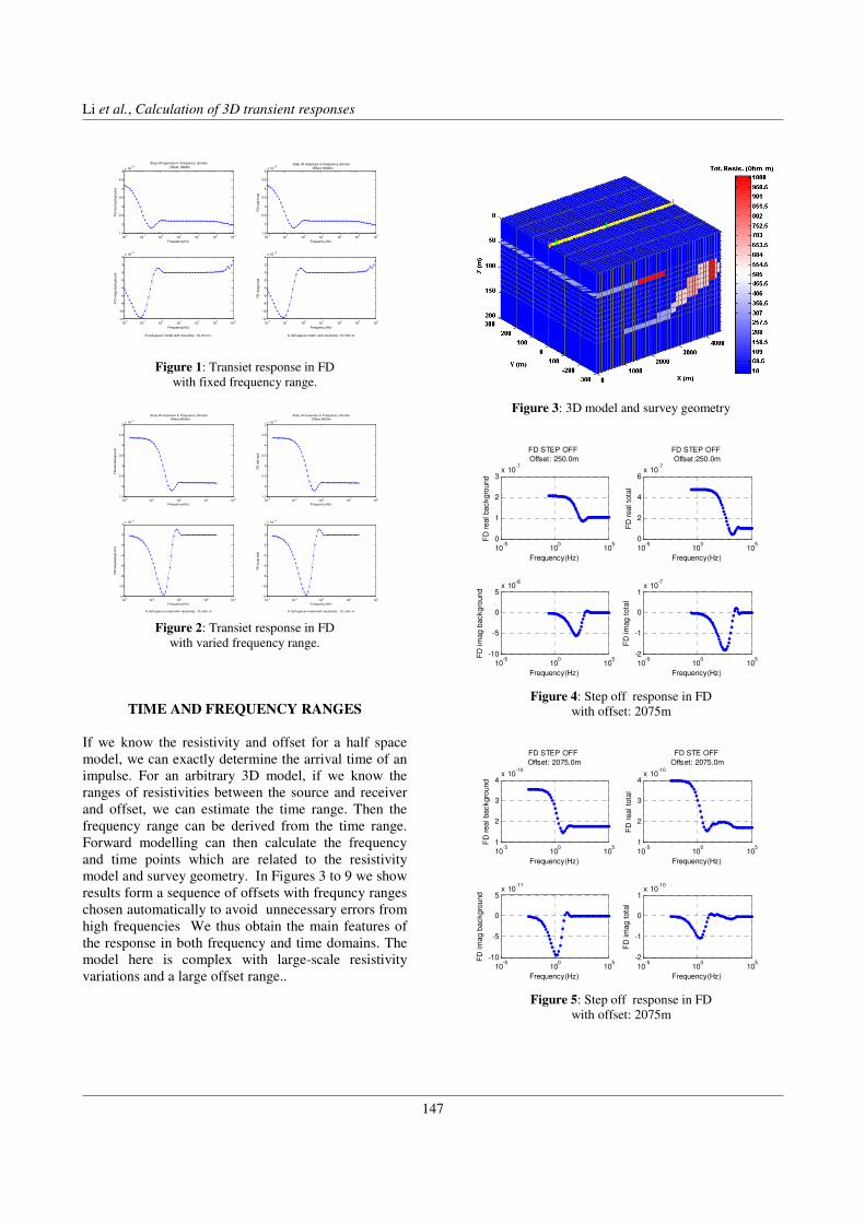
Li, G. et al., 2007, Calculation of 3D transient responses
2/3
10-2
10-1
100
101
102
103
104
1.5
2
2.5
3
3.5
4
4.5
5x 10
-12
Frequency(Hz)
FD
rea
l backgro
un
d
Step off response in Frequency domain
Offset: 9000m
10-2
10-1
100
101
102
103
104
-12
-10
-8
-6
-4
-2
0
2
4x 10
-13
Frequency(Hz)
A half-space model with resistivity: 10 ohm.m
FD
im
ag b
ack
gro
und
10-2
10-1
100
101
102
103
104
1.5
2
2.5
3
3.5
4
4.5
5x 10
-12
Frequency(Hz)
FD
real to
tal
Step off response in Frequency domain
Offset: 9000m
10-2
10-1
100
101
102
103
104
-12
-10
-8
-6
-4
-2
0
2
4x 10
-13
Frequency(Hz)
A half-space model with resistivity: 10 ohm.m
FD
im
ag
tota
l
Figure 1: Transiet response in FD
with fixed frequency range.
10-4
10-2
100
102
104
1.5
2
2.5
3
3.5
4
4.5
5x 10
-12
Frequency(Hz)
FD
real backgro
und
Step off response in Frequency domain
Offset:9000m
10-4
10-2
100
102
104
-12
-10
-8
-6
-4
-2
0
2x 10
-13
Frequency(Hz)
A half-space model with resistivity: 10 ohm.m
FD
im
ag b
ackgro
und
10-4
10-2
100
102
104
1.5
2
2.5
3
3.5
4
4.5
5x 10
-12
Frequency(Hz)
FD
real to
tal
Step off response in Frequency domain
Offset:9000m
10-4
10-2
100
102
104
-12
-10
-8
-6
-4
-2
0
2x 10
-13
Frequency(Hz)
A half-space model with resistivity : 10 ohm.m
FD
im
ag t
ota
l
Figure 2: Transiet response in FD
with varied frequency range.
TIME AND FREQUENCY RANGES
If we know the resistivity and offset for a half space
model, we can exactly determine the arrival time of an
impulse. For an arbitrary 3D model, if we know the
ranges of resistivities between the source and receiver
and offset, we can estimate the time range. Then the
frequency range can be derived from the time range.
Forward modelling can then calculate the frequency
and time points which are related to the resistivity
model and survey geometry. In Figures 3 to 9 we show
results form a sequence of offsets with frequncy ranges
chosen automatically to avoid unnecessary errors from
high frequencies We thus obtain the main features of
the response in both frequency and time domains. The
model here is complex with large-scale resistivity
variations and a large offset range..
Figure 3: 3D model and survey geometry
10-5
100
105
0
1
2
3x 10
-7
Frequency(Hz)
FD
re
al bac
kgro
und
FD STEP OFF
Offset: 250.0m
10-5
100
105
-10
-5
0
5x 10
-8
Frequency(Hz)
FD
im
ag b
ackgro
und
10-5
100
105
0
2
4
6x 10
-7
Frequency(Hz)
FD
real
tota
l
FD STEP OFF
Offset:250.0m
10-5
100
105
-2
-1
0
1x 10
-7
Frequency(Hz)
FD
im
ag
tota
l
Figure 4: Step off response in FD
with offset: 2075m
10-5
100
105
1
2
3
4x 10
-10
Frequency(Hz)
FD
re
al bac
kgro
und
FD STEP OFF
Offset: 2075.0m
10-5
100
105
-10
-5
0
5x 10
-11
Frequency(Hz)
FD
im
ag b
ackgro
und
10-5
100
105
1
2
3
4x 10
-10
Frequency(Hz)
FD
real
tota
l
FD STE OFF
Offset: 2075.0m
10-5
100
105
-2
-1
0
1x 10
-10
Frequency(Hz)
FD
im
ag
tota
l
Figure 5: Step off response in FD
with offset: 2075m
Li et al., Calculation of 3D transient responses
147
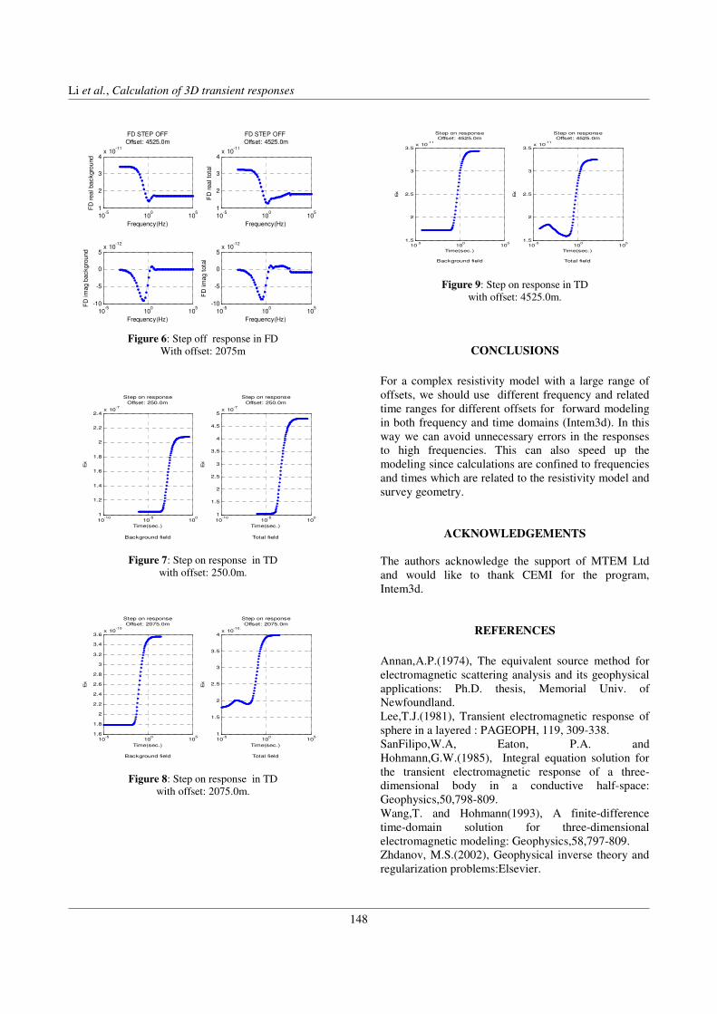
Li, G. et al., 2007, Calculation of 3D transient responses
3/3
10-5
100
105
1
2
3
4x 10
-11
Frequency(Hz)
FD
re
al bac
kgro
und
FD STEP OFF
Offset: 4525.0m
10-5
100
105
-10
-5
0
5x 10
-12
Frequency(Hz)
FD
im
ag b
ackgro
und
10-5
100
105
1
2
3
4x 10
-11
Frequency(Hz)
FD
real
tota
l
FD STEP OFF
Offset: 4525.0m
10-5
100
105
-10
-5
0
5x 10
-12
Frequency(Hz)
FD
im
ag
tota
l
Figure 6: Step off response in FD
With offset: 2075m
10-10
10-5
100
1
1.2
1.4
1.6
1.8
2
2.2
2.4x 10
-7
Time(sec.)
Background field
Ex
Step on response
Offset: 250.0m
10-10
10-5
100
1
1.5
2
2.5
3
3.5
4
4.5
5x 10
-7
Time(sec.)
Total field
Ex
Step on response
Offset: 250.0m
Figure 7: Step on response in TD
with offset: 250.0m.
10-5
100
105
1.6
1.8
2
2.2
2.4
2.6
2.8
3
3.2
3.4
3.6x 10
-10
Time(sec.)
Background field
Ex
Step on response
Offset: 2075.0m
10-5
100
105
1
1.5
2
2.5
3
3.5
4x 10
-10
Time(sec.)
Total field
Ex
Step on response
Offset: 2075.0m
Figure 8: Step on response in TD
with offset: 2075.0m.
10-5
100
105
1.5
2
2.5
3
3.5x 10
-11
Time(sec.)
Background field
Ex
Step on response
Offset: 4525.0m
10-5
100
105
1.5
2
2.5
3
3.5x 10
-11
Time(sec.)
Total field
Ex
Step on response
Offset: 4525.0m
Figure 9: Step on response in TD
with offset: 4525.0m.
CONCLUSIONS
For a complex resistivity model with a large range of
offsets, we should use different frequency and related
time ranges for different offsets for forward modeling
in both frequency and time domains (Intem3d). In this
way we can avoid unnecessary errors in the responses
to high frequencies. This can also speed up the
modeling since calculations are confined to frequencies
and times which are related to the resistivity model and
survey geometry.
ACKNOWLEDGEMENTS
The authors acknowledge the support of MTEM Ltd
and would like to thank CEMI for the program,
Intem3d.
REFERENCES
Annan,A.P.(1974), The equivalent source method for
electromagnetic scattering analysis and its geophysical
applications: Ph.D. thesis, Memorial Univ. of
Newfoundland.
Lee,T.J.(1981), Transient electromagnetic response of
sphere in a layered : PAGEOPH, 119, 309-338.
SanFilipo,W.A, Eaton, P.A. and
Hohmann,G.W.(1985), Integral equation solution for
the transient electromagnetic response of a three-
dimensional body in a conductive half-space:
Geophysics,50,798-809.
Wang,T. and Hohmann(1993), A finite-difference
time-domain solution for three-dimensional
electromagnetic modeling: Geophysics,58,797-809.
Zhdanov, M.S.(2002), Geophysical inverse theory and
regularization problems:Elsevier.
Li et al., Calculation of 3D transient responses
148

4th International Symposium on Three-Dimensional Electromagnetics Freiberg, Germany, September 27−30, 2007
1/3
The effect of 3D anisotropic asthenosphere structures.
R. Logunovich1, M. Berdichevsky2 and D. Avdeev1,3
1IZMIRAN, Russian Academy of Sciences, Troitsk, Russia; 2Moscow State University, Moscow, Russia
3The University of Tokyo, Japan
SUMMARY Recognition of possible anisotropy in crust conductors is one of the important problems in the modern magnetotellurics (MT). In this paper, we numerically investigate conditions under which the MT responses can distinguish whether the conductors are isotropic or anisotropic. In order to do that, we perform a number of numerical experiments with 3-D models that include an isotropic (or anisotropic) crustal conductor of a prismatic shape. To derive these conditions, we compare the responses for model with the isotropic conductor against those obtained for the models with the anisotropic conductor. Keywords: Three-dimensional modeling, magnetotellurics, anisotropic asthenosphere
INTRODUCTION This study is a straightforward continuation of previous works on the effect of anisotropic structures (Pek & Verner, 1997; Bahr & Duba, 2000; Pek & Santos, 2002; Berdichevsky & Pushkarev, 2006). In paper by Berdichevsky & Pushkarev (2006) the authors claim that the effect from two-dimensional (2-D) transversal anisotropic structures is basically the same as the effect from similar, but isotropic structures. They demonstrated that such an equivalence of the isotropic and anisotropic structures is however violated, the same moment as an adjustment distance becomes smaller than the half of the structure width. The adjustment distance is traditionally defined as the square root of the product of the sedimentary conductance times the resistance R of underlying resistive layers. In this work, we consider the same equivalence problem, but our analysis involves three-dimensional (3-D) isotropic and anisotropic models. For these models we numerically simulate the magnetotelluric (MT) responses and compare them to evaluate the anisotropy effect.
MODEL STUDY Our basic 3-D model is presented in Figure 1. It includes an asthenosphere conductive block of 2000×200×50 km3, which sits in a three-layered
background. The top layer of the background has a thickness of 1 km and a resistivity of 3 Ωm. It is underlined by a highly resistive 99-km thick layer of 105 Ωm resistivity. These two layers are sitting on top of 10 Ωm half-space. In our numerical experiments we considered various scenarios, depending on whether the resistivity aρ of the conductor is isotropic or anisotropic. For all the experiments, our modeling domain comprises of Nx×Ny×Nz = 1000×250×8= 2,000,000 rectangular cells with horizontal sizes of 5 km. This domain covers the conductor and some parts of the surroundings. For this model we calculated the MT responses in the period range of 10 to 40,000 s, using an integral equation forward modeling code x3d by Avdeev et al. (1997, 2002). In Figures 2 the responses are shown for an MT site, located just above the center of the conductor. For completeness, in Figure 3 we present the responses calculated for another MT site, which is placed over the middle of the longer side of the conductor. Both locations are shown in Figure 1 as red dots. In Figures 2 and 3 we also compare the responses calculated for a conductor of isotropic resistivity ( a
zay
ax ρρρ == = 9.1 Ωm) with those obtained for an
anisotropic conductor of the same geometry. Two types of possible anisotropy are considered -- longitudinal and transversal. Within the anisotropic conductor, the anisotropy factor yx ρρλ = was set to 0.1 for the
4th International Symposium on Three-Dimensional ElectromagneticsFreiberg, Germany, September 27–30, 2007
149
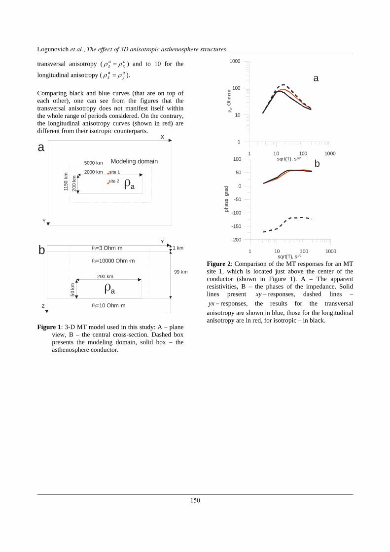
R. Logunovich et al., 2007, The effect of 3D anisotropic asthenosphere structures
2/3
transversal anisotropy ( ax
az ρρ = ) and to 10 for the
longitudinal anisotropy ( ay
az ρρ = ).
Comparing black and blue curves (that are on top of each other), one can see from the figures that the transversal anisotropy does not manifest itself within the whole range of periods considered. On the contrary, the longitudinal anisotropy curves (shown in red) are different from their isotropic counterparts.
XX
Y
2000 km
200
km ρa
Z
200 km
50 k
m ρa
1 km
99 km
ρ1=3 Ohm.m
ρ2=10000 Ohm .m
ρ2=10 Ohm.m
Y
a
b
1150
km
5000 km Modeling domainsite 1
site 2
Figure 1: 3-D MT model used in this study: A – plane
view, B – the central cross-section. Dashed box presents the modeling domain, solid box – the asthenosphere conductor.
1 10 100 1000sqrt(T), s1/2
1
10
100
1000
ρ a,O
hm. m
1 10 100 1000sqrt(T), s1/2
-200
-150
-100
-50
0
50
100
phas
e,gr
ad
a
b
Figure 2: Comparison of the MT responses for an MT site 1, which is located just above the center of the conductor (shown in Figure 1). A – The apparent resistivities, B – the phases of the impedance. Solid lines present −xy responses, dashed lines –
−yx responses, the results for the transversal anisotropy are shown in blue, those for the longitudinal anisotropy are in red, for isotropic – in black.
Logunovich et al., The effect of 3D anisotropic asthenosphere structures
150

R. Logunovich et al., 2007, The effect of 3D anisotropic asthenosphere structures
3/3
1 10 100 1000
1
10
100
1000ρ a
,Ohm
. m
1 10 100 1000
-200
-150
-100
-50
0
50
100
phas
e,gr
ad
a
b
Figure 3: Comparison of the MT responses for an MT site 2, which is located just above the middle of the longer side of the conductor (see Figure 1). The notations are the same as in Figure 2.
CONCLUSIONS In this paper, two different types of the conductor anisotropy were considered – longitudinal and transversal ones. Our results, presented in Figures 2 and 3, along with other results, we obtained for similar models but with different values of the aspect ratio
yx DD (not presented here), suggest that isotropic and transversal anisotropic structures remain practically equivalent, provided that 2yDd ≥ and
10≥yx DD . On the contrary, for longitudinal anisotropic conductors, the equivalency to isotropic ones depends on the anisotropy factor λ and can be significantly violated.
REFERENCES Avdeev, D.B., Kuvshinov, A.V. , Pankratov, O.V. , &
Newman, G. A. (1997). High-performance three-dimensional electromagnetic modelling using modified Neumann series. Wide-band numerical
solution and examples. J. Geomagn. Geoelectr., 49, 1519-1539.
Avdeev, D.B., Kuvshinov, A.V. , Pankratov, O.V. , &
Newman, G. A. (2002). Three-dimensional induction logging problems, Part I: An integral equation solution and model comparisons. Geophysics, 67, 413-426.
Berdichevsky, M. N., & Pushkarev, P. Yu. (2006).
Are the crustal and mantle conductive zones isotropic or anisotropic. Acta Geophysica, 54(4), 333-342.
Bahr, K., & Duba, A. (2000). Is the asthenospere
electrically anisotropic? Earth Planet. Sci. Lett., 87-99.
Pek. J., & Verner, T. (1997). Finite-difference
modeling of magnetotelluric fields in two-dimensional anisotropic media. Geophys J. Int., 128(1), 505-521.
Pek, J., & Santos, F. (2002). Magnetotelluric
impedances and parametric sensitivities for 1-D anisotropic layered media. Comp. Geosci. 28, 939–950.
Logunovich et al., The effect of 3D anisotropic asthenosphere structures
151

4th International Symposium on Three-Dimensional Electromagnetics Freiberg, Germany, September 27−30, 2007
Testing dimensionality of inverted models responses using WSINV3DMT code
A. Martí1, M. Miensopust2,3, A.G. Jones2, P. Queralt1, J. Ledo1 and A. Marcuello1
1Universitat de Barcelona, Spain 2Dublin Institute for Advanced Studies, Dublin, Ireland
3National University of Ireland, Galway, Ireland
SUMMARY The 3D inversion code for magnetotelluric data WSINV3DMT (Siripurnvaraporn et al., 2005) is used in this work to explore the results of several inversions, focusing on the structures and responses of the inverted models and their geoelectric dimensionality. To accomplish this, the synthetic datasets to be inverted were obtained from the model of Ledo et al. (2002), which studied the 3D effects in 2D interpretation of magnetotelluric data, and whose data analysis is well known. These datasets include the direct responses as well as some affected by galvanic distortion. The tests performed show how the choice of the impedance components and the number of sites determine the accuracy of the inversion results, and in which cases the structures and dimensionality can be recovered. Keywords: 3D MT inversion, geoelectric dimensionality, galvanic distortion.
INTRODUCTION The 3D magnetotelluric inversion code WSINV3DMT (Siripurnvaraporn et al., 2005) seeks, for the minimum norm model, to fit observed impedance tensor components. Based on the Occam code (Constable et al., 1987), it works in data space, which significantly reduces the computing times. In this work we use the synthetic model from Ledo et al. (2002) to perform several inversions and compare the responses and dimensionality of the models obtained. The goals are to establish how well the structures can be retrieved from the data responses inverted, what is the weight of the different data components in the inversion, and to test whether it is possible or not to recover galvanic distortion bodies as part of the structure recovered
3D SYNTHETIC MODEL AND RESPONSES
The synthetic model considered, from which the responses to be inverted were generated, consists of a 3D conductive body embedded in a 2D structure (Figure 1). The forward responses of this model were computed using the code RM3D code (Mackie et al., 1993), with a 99x99x50 elements mesh, at 11 periods, from 0.001 s to 1000 s.
Figure 1: 3D electrical conductivity regional model used to generate synthetic responses. Distances are in km. Black line on XY view indicates the position of the profile (From Ledo et al., 2002)
1/3
4th International Symposium on Three-Dimensional ElectromagneticsFreiberg, Germany, September 27–30, 2007
152

Martí et al., 2007, Testing dimensionality using WSINV3DMT
These responses were retrieved as three different datasets: 1) LINE: an EW line with 30 sites distributed along the width of the model (Figure 1); 2) DISTLINE: The same EW line, in which random galvanic distortion C, with site gain g = 1 and without anisotropy, was added to each site. (Both datasets 1 and 2 are coincident with line 1 studied in Ledo et al., 2002). 3) GRID: a rectangular grid with 96 sites covering the model surface (see Figure 2).
Figure 2: Plan view of the synthetic model (central frame with the 96 sites of dataset GRID. The external frame shows the extension of the model to run the inversions.
All the inversions of these datasets were performed using the default inversion parameters provided with the code. Five or eleven periods were inverted (between 0.01 s and 100 s), using either the 4 complex components of the impedance tensor or only the 2 off-diagonal ones. The assumed error was set to 5% in the off-diagonal components and the same value was then applied to the diagonal components (following Siripurnvaraporn et al., 2005, test example). The initial model consisted of a homogeneous half-space. The mesh for inversion was reduced to 28x28x20 cells, given limitations in computing time and space. The lateral cells were extended horizontally (see Figure 2) to avoid problems with the boundary conditions. Although the WSINV3DMT code provides the responses of the inverted model, these were retrieved using RM3D code to make their further analyses and comparisons easier. Dimensionality analysis was carried out using the WALDIM program (Martí et al., 2004), following WAL invariants criteria (Weaver et al., 2000).
LINE AND DISTLINE INVERSIONS Both the original line (LINE) and the distorted one (DISTLINE) were inverted including all the sites, 11 periods and the 4 complex (8 valued) tensor components. In the first case, rms reduced from an initial value of 3.3 to 2.9 by the 5th iteration. Both diagonal and off-diagonal components fits are good, except in the range between 0.0312 s and 3.2 s where the inverted model mesh probably lacks sufficient discretization. Although all four components were inverted, the recovered model is mainly 2D, and not even the structures below the inverted sites are well recovered. Comparison between the dimensionality obtained for the original and inverted datasets shows an agreement at short periods, up to 1 s. At longest periods, the inverted model images as 1D or 2D features that in the original data are seen as 3D. For the distorted dataset, rms started at 129 and significantly reduced to 17 by the 5th iteration, which is still a poor fit. The resulting model shows abrupt resistivity changes at all periods, and the structures extend laterally out of the inverted profile. In order to better characterise the uppermost structure further work will consist of refining the first layers mesh, inverting only the shortest periods with a better resolution, and fixing the resulting model to invert the rest of the periods.
GRID INVERSIONS In order to obtain a better representation of the model, a rectangular grid dataset was created (see Figure 2). A first inversion was performed considering 5 periods between 0.01 s and 10 s, and only 2 components of the impedance tensor. Rms changed from 3.6 in the first iteration to 2.5 by the 7th. Even if only the off-diagonal components were inverted, the shorter spacing between sites allowed for a better retrieval of the original structures in the final inverted model (Figure 3).
Figure 3: Depth slices of the synthetic model and the inverted model at z=2 km.
2/3
Martí et al., Testing dimensionality using WSINV3DMT
153

Martí et al., 2007, Testing dimensionality using WSINV3DMT
As for the model responses computed using RM3D, the diagonal components were significant, and the dimensionality analysis gave results similar to the original dataset: 1D at short periods and 2D and 3D for the rest. The dimensionality information may be used then to invert only 4 components at short periods and 8 components for the others, fixing the uppermost layers of the model.
ERRORS OF THE RESPONSES One of the issues yet to be solved concerns the errors in the diagonal and off-diagonal components. The performed tests show how, when both diagonal and non-diagonal have the same error percentage, the inverted model does seldom change with iteration. Following the same procedure as in the code testrun example (% in the non-diagonals, and same value in the diagonals), the model changes and the responses misfits reduce. However, the diagonal responses have a very low weight, which is almost equivalent to inverting only the off-diagonal components. Even if affected by 3D effects, in general, the diagonal values of the responses are low compared to the non-diagonal. A further test will consist of rotating 45º the responses and the dataset GRID, in order to invert responses with all the components of the same order of magnitude.
CONCLUSIONS The choice of the sites to be inverted seems to be of much more importance in the resulting model than the number of impedance components. When the dataset is dense enough, the model structures are recovered to within a reasonable degree, as shown also in the model responses and dimensionality. Data affected by galvanic distortion must be inverted using a finer grid at the uppermost model layers. Further tests must be performed to solve the error weights.
ACKNOWLEDGEMENTS MM and AGJ would like to acknowledge the Science Foundation Ireland, and AM to the Facultat de Geologia (UB), for the financial support. All authors express their gratitude to Weerachai Siripunvaraporn for making his code available.
REFERENCES Constable, S.C., Orange, A.S., Hoversten, G.M. and
Constable, C.G., 1987. Occam’s inversion: A practical algorithm for generating smoth models from EM sounding data, Geophysics, 63, 816-825.
Ledo, J., Queralt, P., Martí, A. and Jones, A.G. (2002). Two-dimensional interpretation of three-dimensional magnetotelluric data: an example of limitations and resolution, Geophys. J. Int., 150,127-139.
Mackie, R.L., Madden, T.R., and Wannamaker, P. E. (1993). Three-dimensional magnetotelluric modeling using difference equations – Theory and comparisons to integral equations solutions, Geophysics, 58, 215-226.
Martí, A., Queralt, P. and Roca, E. (2004). Geoelectric dimensionality in complex geologic areas: application to the Spanish Betic Chain. Geophys. J. Int., 157, 961-974.
Siripunvaraporn, W., Egbert, G., Lenbury, Y. and Uyeshima, M. (2005). Three-dimensional magnetotelluric inversion: data-space method, Physics of the Earth and Planetary Interiors, 150, 3-14.
Weaver, J.T., Agarwal, A.K. and Lilley, F.E.M. (2000). Characterisation of the magnetotelluric tensor in terms of its invariants, Geophys. J. Int., 141, 321-336.
3/3
Martí et al., Testing dimensionality using WSINV3DMT
154

4th International Symposium on Three-Dimensional Electromagnetics
Freiberg, Germany, September 27−30, 2007
1/4
Borehole CSEM for Offshore Hydrocarbon Mapping
Anna Maxey
1,2, Lucy MacGregor
2, Martin Sinha
1 & Vikas Baranwal
1
1National Oceanography Centre, Southampton, UK
2OHM Ltd, Aberdeen, UK
SUMMARY
Controlled source electromagnetic (CSEM) sounding is increasingly being adopted by the hydrocarbon industry at the
exploration stage (MacGregor et al., 2006). In its current form the method makes use of a deep towed EM source and a
receiver array placed on the sea floor, and is capable of detecting thin hydrocarbon-bearing layers at depths of up to
several kilometres below mudline.
During initial assessment and subsequent development of oil and gas fields, wells are routinely drilled for a variety of
purposes. The boreholes provide a possible means of placing either EM sources or receivers within or beneath the target
reservoir, and this in turn presents the opportunity of applying CSEM methods using a combination of seafloor and
borehole sources and receivers to improve the characterisation and monitoring of the reservoir. The majority of both
theoretical and experimental studies of the use of EM methods to map the interwell region have been for the land case
(for example Wilt and Alumbaugh, 2003). Edwards and Scholl (2006) present a marine borehole comparison to the
standard seafloor to seafloor configuration, with a theoretical study using a downhole vertical electric dipole source and
an array of seafloor receivers. In this paper we consider the advantages a seafloor source with a downhole receiver
affords in the detection and characterisation of buried resistive layers.
Keywords: Exploration, Borehole Methods, CSEM, 3D Modelling
3D MODELLING
To illustrate the interaction of the electric fields with
the reservoir, we show a vertical cross section through
the plane of the modelled horizontal electric dipole
(HED) source (Figure 1). In a simple halfspace earth
with no resistive hydrocarbon layer (Plots A and B),
source fields are rapidly attenuated in the conductive
seawater and 1Ωm background sediments. When a
hydrocarbon layer is included (Plots C and D), field
strengths are increased over the majority of the
modelled space.
CSEM surveys take advantage of the change in fields
at the seafloor due to the presence of a target layer.
Figure 1 shows that greater field variations are
produced beneath the seabed, particularly in near the
target layer itself. This provides an early indication of
the improvement in reservoir characterisation BCSEM
may offer. It is also interesting to note that the
horizontal component fields primarily increase in
strength above and below the target layer, whilst Z-
component fields increase within the layer.
In Figure 2, we directly compare the horizontal radial
field calculated for a single receiver in a conventional
survey geometry, to that which would be recorded by a
downhole receiver positioned beneath the target layer.
The seabed receiver shows the characteristic rapid
decay of fields with range. For this model, target
sensitivity begins at a source-receiver offset of around
2.5km, with the increase in fields due to the layer
reaching 80% at a range of 5km. In contrast, the
borehole receiver sees significantly different fields in
the presence of the target layer over most source
offsets. At short horizontal offsets, fields are attenuated
by the target layer; at longer offsets, higher fields are
recorded in the presence of the layer. Maximum
normalised field strengths dwarf those recorded by a
seabed receiver, reaching 1300% at a horizontal range
of 5km.
We now consider the sensitivity of a downhole receiver
to the physical properties of the target layer, namely
thickness and resistivity. Conventional CSEM is
predominantly sensitive to the transverse resistance
(resistivity, thickness product) of a target layer, but
largely insensitive to the absolute thickness or
resistivity of the target.
4th International Symposium on Three-Dimensional ElectromagneticsFreiberg, Germany, September 27–30, 2007
155
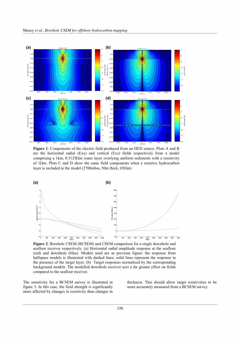
Maxey, A. et al., 2007, Borehole CSEM for offshore hydrocarbon mapping
2/4
The sensitivity for a BCSEM survey is illustrated in
figure 3. In this case, the field strength is significantly
more affected by changes in resistivity than changes in
thickness. This should allow target resistivities to be
more accurately measured from a BCSEM survey.
(a) (b)
Figure 2: Borehole CSEM (BCSEM) and CSEM comparison for a single downhole and
seafloor receiver respectively. (a) Horizontal radial amplitude response at the seafloor
(red) and downhole (blue). Models used are as previous figure: the response from
halfspace models is illustrated with dashed lines; solid lines represent the response in
the presence of the target layer. (b) Target responses normalised by the corresponding
background models. The modelled downhole receiver sees a far greater effect on fields
compared to the seafloor receiver.
Figure 1: Components of the electric field produced from an HED source. Plots A and B
are the horizontal radial (Exx) and vertical (Exz) fields respectively from a model
comprising a 1km, 0.3125Ωm water layer overlying uniform sediments with a resistivity
of 1Ωm. Plots C and D show the same field components when a resistive hydrocarbon
layer is included in the model (2700mbss, 50m thick, 65Ωm).
(c) (d)
(a) (b)
Maxey et al., Borehole CSEM for offshore hydrocarbon mapping
156

Maxey, A. et al., 2007, Borehole CSEM for offshore hydrocarbon mapping
3/4
Whilst the ability to detect vertical changes in the
reservoir using BCSEM has been touched upon above,
this in itself provides little more than a conventional
well logging tool. Greater value will be gained from
borehole CSEM if it can be used to determine reservoir
lateral extent. This information would feed in at the
development stage and aid decisions relating to
optimising the recovery from the reservoir; for
example on the locations of further injection or
production wells. Theoretical studies using 2D
structures to establish the edge detection capabilities of
various EM methods exist in the literature. In one
example, seafloor-to-seafloor CSEM edge detection
has been investigated by Eidesmo et al (2002).
Here, we illustrate one example of the effect that a
reservoir edge has on the fields recorded by a BCSEM
receiver. Figure 4 shows both the horizontal and
vertical fields modelled for a receiver positioned within
a reservoir, and 2km from its edge. The two
components are calculated at different heights relative
to the reservoir in order to show the maximum change
in field strength for each component. For the vertical
component we show the in target response and for the
horizontal component we show the response directly
below the layer. This is directly compared to the same
components modelled for the 1D reservoir case, and
when no reservoir is present. Even at this distance from
the edge, a significant and measurable effect from the
edge can be seen. The on target response is virtually
indistinguishable from the 1D response. As the source
moves off target, there is increased separation between
the 1D and 2D response, with over half an order of
magnitude difference at maximum offset.
CONCLUSIONS
Conventional seafloor CSEM continues to gain
acceptance as an important exploration and appraisal
tool. The greater changes in amplitude measured
downhole provide the potential to detect and monitor
reservoirs which are beyond the current capabilities of
CSEM. The effect that 2D structures have on the
calculated response shows the potential for this method
to detect reservoir edges up to several kilometres from
the borehole location, essential if the technique is to be
used in determining and monitoring reservoir lateral
extents. Coupled with the greater target sensitivity of
BCSEM, detectable features may also include small
hydrocarbon accumulations remaining after the bulk of
the reservoir has been swept. Furthermore, target and
edge sensitivity occurs downhole at shorter source
receiver offsets than at the seafloor, reducing the
overall size (and therefore cost) of potential CSEM
reservoir monitoring techniques.
Figure 3: Sensitivity of a BCSEM survey
geometry to target layer properties. The vertical
component of the electric field within the
resistive target layer is plotted as a function of
layer thickness and layer resistivity. It can be
seen that layer resistivity has a far greater effect
on field strength than thickness.
(a)
(b)
Maxey et al., Borehole CSEM for offshore hydrocarbon mapping
157
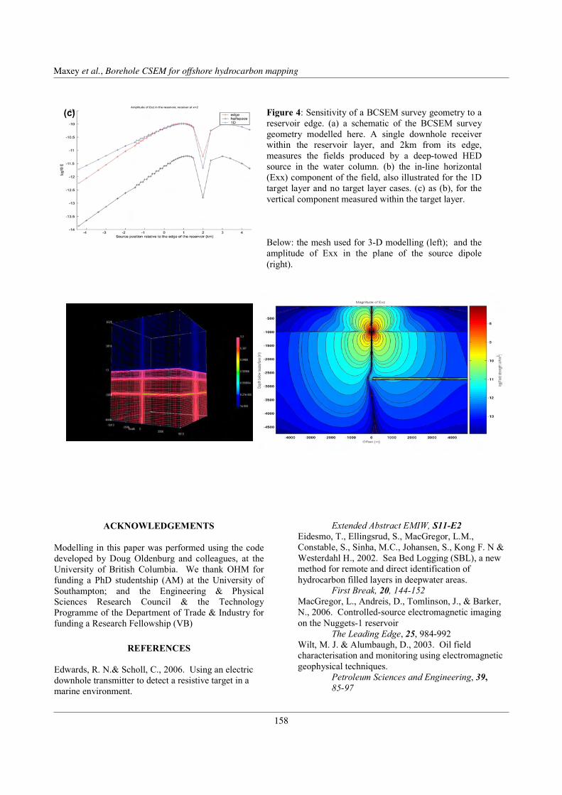
Maxey, A. et al., 2007, Borehole CSEM for offshore hydrocarbon mapping
4/4
ACKNOWLEDGEMENTS
Modelling in this paper was performed using the code
developed by Doug Oldenburg and colleagues, at the
University of British Columbia. We thank OHM for
funding a PhD studentship (AM) at the University of
Southampton; and the Engineering & Physical
Sciences Research Council & the Technology
Programme of the Department of Trade & Industry for
funding a Research Fellowship (VB)
REFERENCES
Edwards, R. N.& Scholl, C., 2006. Using an electric
downhole transmitter to detect a resistive target in a
marine environment.
Extended Abstract EMIW, S11-E2
Eidesmo, T., Ellingsrud, S., MacGregor, L.M.,
Constable, S., Sinha, M.C., Johansen, S., Kong F. N &
Westerdahl H., 2002. Sea Bed Logging (SBL), a new
method for remote and direct identification of
hydrocarbon filled layers in deepwater areas.
First Break, 20, 144-152
MacGregor, L., Andreis, D., Tomlinson, J., & Barker,
N., 2006. Controlled-source electromagnetic imaging
on the Nuggets-1 reservoir
The Leading Edge, 25, 984-992
Wilt, M. J. & Alumbaugh, D., 2003. Oil field
characterisation and monitoring using electromagnetic
geophysical techniques.
Petroleum Sciences and Engineering, 39,
85-97
Figure 4: Sensitivity of a BCSEM survey geometry to a
reservoir edge. (a) a schematic of the BCSEM survey
geometry modelled here. A single downhole receiver
within the reservoir layer, and 2km from its edge,
measures the fields produced by a deep-towed HED
source in the water column. (b) the in-line horizontal
(Exx) component of the field, also illustrated for the 1D
target layer and no target layer cases. (c) as (b), for the
vertical component measured within the target layer.
Below: the mesh used for 3-D modelling (left); and the
amplitude of Exx in the plane of the source dipole
(right).
(c)
Maxey et al., Borehole CSEM for offshore hydrocarbon mapping
158

4th International Symposium on Three-Dimensional ElectromagneticsFreiberg, Germany, September 27–30, 2007
Testing of the 3D inversion routine engine - the 3D forward algorithm - bycomparison with 2D forward modelling results
M. Miensopust1,2 and A.G. Jones1
1Dublin Institute for Advanced Studies, 5 Merrion Square, Dublin 2, Ireland2National University of Ireland, Galway, Ireland
SUMMARY
The importance of 3D forward and inversion codes in electromagnetic interpretation is continuously increasing. As allinversion algorithms are based on a forward calculation, the forward codes are the important basis for all kind of 3Dinterpretation - either for forward modelling itself or integrated in the inversion. Therefore a user must acquaint himselfwith the strengths and weaknesses of the 3D forward code. There are many ways of accomplishing this; the one describedhere is the comparison of 2D and 3D forward modelling responses. The idea behind this kind of testing is that 3D modelresponses become more and more identical to the 2D responses if the extension of the body becomes large, in an inductivescale-length sense, in one direction. The dimensionless ratio of the body length to skin depth at a specific frequency in thehost medium (Jones, 1983) gives a limit for the period range where the agreement of 2D and 3D responses is supposed tobe good - if it is not that can be a hint that there is an issue either with the forward code or its implementation.
INTRODUCTION
Independent of the size of a survey area the subject of in-terest for electromagnetic studies is, very rarely, validlyinterpreted as one-dimensional. Even two-dimensional in-terpretations are often not valid for all frequencies and allsites - which is why three-dimensional modelling toolsare required. For magnetotelluric studies there are al-ready 3D forward modelling codes (e.g., Avdeev, Kuvshi-nov, Pankratov, & Newman, 1997; Mackie, Madden, &Wannamaker, 1993; Mackie, Smith, & Madden, 1994;Siripunvaraporn, Egbert, & Lenbury, 2002; Xiong, Luo,Wang, & Wu, 1986; Xiong, 1992) and more recent also3D inversion codes (e.g. Farquharson, Oldenburg, Haber,& Shekhtman, 2002; Siripunvaraporn, Egbert, Lenbury,& Uyeshima, 2005) are available.
Using 3D inversion codes should never be done withoutbeing aware of the fact that the engines of all 3D inversionprograms are the 3D forward algorithms which are run-ning in the background, and which, in fact, dominate thetime of the 3D inversion run. Therefore, the reliability ofthe used 3D forward routine should be tested thoroughlybefore undertaking extensive 3D inversion. There are dif-ferent ways of testing, the one which we describe here isthe comparison of 3D responses with 2D forward mod-elling results.
WHY ARE 2D AND 3D RESPONSE COMPARABLEAND WHAT ARE THE LIMITS?
Using a one-dimensional subsurface model to calcu-late the 1D, 2D and 3D forward response it is obviousthat all responses should be identical - meaning that theimpedance elements at all frequencies and sites shouldbe Zxx = Zyy = 0 and Zxy = −Zyx, whereas themagnitude of the off-diagonal elements of the 3D forwardresponse should be identical (within acceptable bounds) tothe one of the 1D and the 2D forward modelling. Also fora two-dimensional Earth model the results of the 2D for-ward and 3D forward algorithms must match each otherat specific locations and for specific frequencies. Jones(1983) showed that the difference between data from aprofile over a 3D structure (e.g. a dyke of finite length l)and a real 2D response is dependent on the dimensionlessratio l
δ , where δ is the skin depth at a specific frequency inthe host medium. If this ratio is far greater than 1, then the2D and 3D results should approximately give the sameresistivity structure, whereas if l
δ is smaller than 1 (i.e.either the length l is too short or the frequency is too low)this assumption will not be valid.
This means for the 2D vs. 3D comparison that the highfrequencies (or short periods) will give a good correlationfor a certain range, whereas at lower frequencies (longerperiods) this conformity cannot be expected.
1/4
4th International Symposium on Three-Dimensional ElectromagneticsFreiberg, Germany, September 27–30, 2007
159
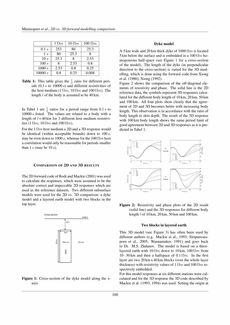
Miensopust and Jones, 2007, 2D vs. 3D forward modelling comparison . . .
1 Ωm 10 Ωm 100 Ωm
0.1 s 253 80 25.31 s 80 25.3 8
10 s 25.3 8 2.53100 s 8 2.53 0.8
1000 s 2.53 0.8 0.2510000 s 0.8 0.25 0.008
Table 1: This table gives the lδ ratio for different peri-
ods (0.1 s to 10000 s) and different resistivities ofthe host medium (1 Ωm, 10 Ωm and 100 Ωm). Thelength l of the body is assumed to be 40 km.
In Tabel 1 are lδ ratios for a period range from 0.1 s to
10000 s listed. The values are related to a body with alength of l = 40 km for 3 different host medium resistivi-ties (1 Ωm, 10 Ωm and 100 Ωm).
For the 1 Ωm host medium a 2D and a 3D response wouldbe identical (within acceptable bounds) down to 100 s,may be even down to 1000 s, whereas for the 100 Ωm hosta correlation would only be reasonable for periods smallerthan 1 s (may be 10 s).
COMPARISON OF 2D AND 3D RESULTS
The 2D forward code of Rodi and Mackie (2001) was usedto calculate the responses, which were assumed to be theabsolute correct and impeccable 2D responses which areused as the reference datasets. Two different subsurfacemodels were used for the 2D vs. 3D comparison: a dykemodel and a layered earth model with two blocks in thetop layer.
Figure 1: Cross-section of the dyke model along the x-axis.
Dyke model
A 5 km wide and 20 km thick dyke of 1000 Ωm is located5 km below the surface and is embedded in a 100 Ωm ho-mogeneous half-space (see Figure 1 for a cross-sectionof the model). The length of the dyke (in perpendiculardirection to the cross-section) is varied for the 3D mod-elling, which is done using the forward code from Xionget al. (1986); Xiong (1992).Figure 2 shows the comparison of the off-diagonal ele-ments of resistivity and phase. The solid line is the 2Dreference data, the symbols represent 3D responses calcu-lated for the different body length of 10 km, 20 km, 50 kmand 100 km. All four plots show clearly that the agree-ment of 2D and 3D becomes better with increasing bodylength. This observation is in accordance with the ratio ofbody length to skin depth. The result of the 3D responsewith 100 km body length shows the same period limit ofgood agreement between 2D and 3D responses as it is pre-dicted in Tabel 1.
Figure 2: Resistivity and phase plots of the 2D result(solid line) and the 3D responses for different bodylength l of 10 km, 20 km, 50 km and 100 km.
Two blocks in layered earth
This 3D model (see Figure 3) has often been used bydifferent authors (e.g. Mackie et al., 1993; Siripunvara-porn et al., 2005; Wannamaker, 1991) and goes backto Dr. M.S. Zhdanov. The model is based on a three-layered earth with 10 Ωm down to 10 km, 100 Ωm from10 - 30 km and then a halfspace of 0.1 Ωm. In the firstlayer are two 20 km x 40 km blocks (over the whole layerthickness) with resistivity values of 1 Ωm and 100 Ωm re-spectively embedded.For this model responses at six different stations were cal-culated and for the 3D response the 3D code described byMackie et al. (1993, 1994) was used. Setting the origin at
2/4
Miensopust et al., 2D vs. 3D forward modelling comparison
160

Miensopust and Jones, 2007, 2D vs. 3D forward modelling comparison . . .
the boundary between the two blocks for x-direction andin the middle of the block in y-direction the site locationsare -25 km, -15 km, -5 km, 5 km, 15 km and 25 km in x-direction and y = 0 for all.
Figure 3: Plan view and cross-section of the used 3Dmodel (redrawn after Mackie, Madden, & Wanna-maker 1993).
Figure 4 shows the resistivity and phase curves for bothoff-diagonal elements at all six sites. The agreement ofthe 2D and 3D results is good down to periods of 10 s -sometimes even down to 100 s. That is in good accor-dance with the expected period range calculated using theratio of length to skin depth of the host (see Table 1).
CONCLUSIONS
For the chosen models and codes the comparison for 2Dand 3D response gave the expected results: good agree-ment for the short period range. Also the increasing ofthe part with reasonable agreement of the 2D and 3Dresponses towards longer periods with increasing bodylength could be seen. For this combination of codes andmodels the comparison can be consider as being success-ful.
Although the experience while testing different codes andmodels showed that there are a few difficulties with the3D forwards codes (not all combinations of chosen mod-
els and codes gave the expected result). Each codes hasweak and strong aspects and it is useful to get an idea ofthem before using a 3D inversion code where the 3D for-ward algorithm is used as engine.
Figure 4: Resistivity and phase plots of the 2D responses(solid and dashed line) and the 3D responses (soliddots and open circles) for all 6 sites over the modelshown in Figure 3.
3/4
Miensopust et al., 2D vs. 3D forward modelling comparison
161

Miensopust and Jones, 2007, 2D vs. 3D forward modelling comparison . . .
ACKNOWLEDGMENTS
Many thanks to Colin Brown for his helpful suggestionsand his assistance while trouble shooting and to Geosys-tem for their effort to help solving problems. We also liketo acknowledge Science Foundation Ireland for the finan-cial support.
REFERENCES
Avdeev, D. B., Kuvshinov, A. V., Pankratov, O. V.,& Newman, G. A. (1997). High-PerformanceThree-Dimensional Electromagnetic Modelling Us-ing Modified Neumann Series. Wide-Band Numer-ical Solution and Examples. J. Geomag. Geoelectr.,49, 1519 - 1539.
Farquharson, C. G., Oldenburg, D. W., Haber, E., &Shekhtman, R. (2002, October). An algorithm forthe three-dimensional inversion of magnetotelluricdata. SEG Int’l Exposition and 72nd Annual Meet-ing, Salt Lake City, Utah.
Jones, A. G. (1983). The problem of current channelling:a critical review. Geophysical Surveys, 6, 79 - 122.
Mackie, R. L., Madden, T. R., & Wannamaker, P. E.(1993, February). Three-dimensional magnetotel-luric modeling using difference equations - The-ory and comparisons to integral equation solutions.Geophysics, 58(2), 215 - 226.
Mackie, R. L., Smith, J. T., & Madden, T. R. (1994).Three-dimensional electromagnetic modeling usingfinite difference equations: The magnetotelluric ex-ample. Radio Science, 29, 923–935.
Rodi, W., & Mackie, R. L. (2001). Nonlinear conjugategradients algorithm for 2-D magnetotelluric inver-sion. Geophysics, 66(1), 174 - 187.
Siripunvaraporn, W., Egbert, G., & Lenbury, Y. (2002).Numerical accuracy of magnetotelluric modeling:A comparison of finite difference approximations.Earth Planets Space, 54, 721 - 725.
Siripunvaraporn, W., Egbert, G., Lenbury, Y., &Uyeshima, M. (2005). Three-dimensional magne-totelluric inversion: data-space method. Physics ofthe Earth and Planetary Interiors, 150, 3–14.
Wannamaker, P. E. (1991). Advances in three-dimensional magnetotelluric modeling using inte-gral equations. Geophysics, 56, 1716 - 1728.
Xiong, Z. (1992). Electromagnetic modeling of 3-D struc-tures by the method of system iteration using inte-gral equations. Geophysics, 57(12), 1556 - 1561.
Xiong, Z., Luo, Y., Wang, S., & Wu, G. (1986).Induced-polarization and electromagnetic modeling
of a three-dimensional body buried in a two-layeranisotropic earth. Geophysics, 51(12), 2235 - 2246.
4/4
Miensopust et al., 2D vs. 3D forward modelling comparison
162

4th International Symposium on Three-Dimensional Electromagnetics Freiberg, Germany, September 27−30, 2007
Inversion of synthetic data using WSINV3DMT code
M. Miensopust1,3, A. Martí2 and A.G. Jones1
1Dublin Institute for Advanced Studies, Dublin, Ireland ([email protected]) 2Universitat de Barcelona, Spain
3National University of Ireland, Galway, Ireland
SUMMARY In recent years 3D inversion of magnetotelluric (MT) data has experienced a significant advance due to the advent of new codes, particularly WSINV3D by Siripurnvaraporn et al. (2005), based on a data-space variant of the Occam approach (Constable et al., 1987), that the authors have made publicly available. In this work we focus on that inversion code. Before applying the code to observed field data, we have undertaken tests using synthetic data to understand how the program works, what its strength and weaknesses are, what values of the parameters are the most suitable for each situation, and what resolution is obtained for the resulting models. To accomplish this, we have used different grids and data sets from simple synthetic models (a cube embedded in a homogeneous medium, and a fault model). After comparing the results obtained from the use of different parameters (e.g. model scale length) and mesh sizing, some statements can be concluded on the smoothness of the inversion model, and the fits between the data and inversion model responses. These are complemented with a list of “open questions” describing issues, which are not completely understood, or at least understood by the authors – we are hoping to receive clarification and solutions from other participants who might have dealt with the same or similar problems. Keywords: 3D MT inversion, synthetic models.
INTRODUCTION The 3D magnetotelluric inversion code WSINV3DMT (Siripurnvaraporn et al., 2005) seeks for the minimum norm model to fit the impedance tensor components. Based on the Occam code (Constable et al., 1987), it works in data space, which reduces significantly the computing times. Before applying the WSINV3DMT code to observed field data and interpreting the resulting models, it was subjected to performance tests using synthetic data. In this paper the tests of synthetic responses retrieved from two simple subsurface models will be presented: a N-S striking fault and a conductive cube embedded in a resistive homogenous host. Aspects of the testing were - amongst others - the behaviour of the code if the synthetic data was generated in different ways and the effects of changes in the inversion parameters (set in the 'startup' file). It was hoped that these tests would give guidelines useful for a later use with real data: what are the strengths and weaknesses of the code, which configuration parameters have to be treated with a lot
of caution and which settings are the most suitable for each kind of dataset.
SIMPLE 2D N-S STRIKING FAULT The first synthetic model is a 2D model. It consists of a vertical N-S striking fault with a 200 Ω·m quarter-space on the west side and 20 Ω·m quarter-space on the east side of the fault. The model has dimensions of 22 km (NS) x 22 km (EW) x 18.2 km (z), with a modeling mesh consisting of 14x14x13 cells, horizontally with a finer grid in the centre (see Figure 1), and increasing thicknesses with depth. At nine periods (from 0.001 s to 10 s, logarithmically distributed) the responses were computed for 36 sites forming a regular square grid, covering both sides of the fault. A 5% error was added to each component of the impedance tensor responses. Prior to the inversion, the datasets were created in four different ways:
1. Default 3D Mackie forward modeling (Mackie et al., 1993 – in the following called
1/4
4th International Symposium on Three-Dimensional ElectromagneticsFreiberg, Germany, September 27–30, 2007
163

Miensopust et al., 2007, Synthetic data inversion using WSINV3DMT
RM3D) for 36 sites centered in the middle of the grid; each line has 3 sites west and 3 sites east of the fault.
2. Default 3D Mackie forward modeling (RM3D) for the 3 southern lines and copying the retrieved responses (mirror-inverted) to the 3 northern lines.
3. Default 3D Mackie forward modeling (RM3D) only for the third line (counting from south) and copied to all the 5 other lines.
4. Using the 2D forward modeling code from Wannamaker et al. (1987): fault in the middle of the profile and large extensions of the model space in E-W direction and depth; responses of this profile were copied to all lines.
These responses were inverted using the WSINV3DMT code with default parameters and a halfspace of 100 Ω·m as the starting model. The expected result of this inversion is a model with a symmetry axis in E-W direction through the center of the grid. However, the result shows instead (e.g. Figure 1) an obvious asymmetric pattern, regardless of how the set of responses was retrieved.
Figure 1: Two depth slices of the model resulting from the inversion of the fault model responses. Both slices show that the inversion result is asymmetric, even if the input was symmetric.
MODEL SCALE LENGTH One of the inversion parameters is the model scale length (δ), which can be defined separately for each direction (x, y and z). For two slightly different datasets – retrieved as described in the previous section at nº1 and nº 2 respectively - the inversion was run once with default (δ = 0.1 for all 3 directions) and once with a changed model scale length. The location of the sites is the same as before, and the initial model was a 100 Ω·m halfspace. For the first dataset, the model scale length was changed only in the x direction (δx = 0.5). Compared to the default inversion the resulting model using the changed model scale length shows features parallel to
the fault to be more continuous/smoothed, which is the direction of the larger model scale length value. The second dataset was inverted with default model scale length and with δ = 1.0 for all 3 directions. As in the test with dataset 1, the model with larger δ (right side of Figure 2) is smoother - in this case for both horizontal directions. It is also smoother in x direction as the result of the first test (δx = 0.5) – which is consistent with the observation of having a smoother model when δ in that direction is larger. However, it seems to be true only for horizontal directions. As can be seen from Figure 3, it is obvious that the result for a changed δ in z-direction does not behave as expected: the model with the larger model scale length in z-direction is not the smoother one. There is no known explanation yet for this surprising observation.
Figure 2: Depth slices of the inversion result using the default model scale length (δ = 0.1 for all 3 directions) on the left and with δ = 1 for all directions on the right hand side.
Figure 3: Sections of the inversion result using the default model scale length (δ = 0.1 for all 3 directions) on the left and with δ = 1 for all directions on the right hand side.
WSINV3DMT TESTRUN MODEL In this section, the forward responses and the consequent inversion results, obtained from RM3D code (Mackie et al., 1993) and the forward modeling implemented in WSINV3DMT, were compared. The synthetic model used as testrun in Siripurnvaraporn et al. (2005) was considered.
2/4
Miensopust et al., Synthetic data inversion using WSINV3DMT
164

Miensopust et al., 2007, Synthetic data inversion using WSINV3DMT
This model consists of a 16 km x 16 km x 5 km block of 1 Ω·m (100 m below the surface) embedded in a 100 Ω·m surrounding. The forward responses were computed using both codes at 5 periods, from 0.1 s to 1000 s, for a set of 36 sites distributed over a regular grid centered on the conductive body. Both sets of responses seem to be quite similar for all sites, with a few variations especially for the longest periods. The inversion was run for both sets of responses with a 5% error, using default parameter settings and a homogeneous halfspace of 50 Ω·m as the initial model. The maximum number of iterations was set to 5. The WSINV3DMT responses finished the inversion by exceeding the maximum number of iterations, whereas the inversion of the Mackie response stopped already after iteration number 4. To compare the results, sections and depth slices are plotted in Figure 4.
Figure 4: Sections and depth slices of the inversion results with WSINV3DMT responses after the final iteration number 5 (= maximum number of iterations) on top, the intermediate result after iteration number 4 in the middle, and the final iteration result (iteration number 4) of the Mackie responses at the bottom.
The top graphs are the final results of the WSINV3DMT responses (iteration step 5) and in the middle is the result after iteration number 4 shown to have a better comparison to iteration step 4 (which is the final result) of the Mackie responses on the bottom. There are only a few small differences between
iteration numbers 4 and 5 of the response set from the WSINV3DMT forward code. However, comparing this result with the one of the other response sets significant differences become obvious. Even if the model scale length for both inversions was set to the default it seems that the Mackie response inversion results are a lot less smooth. With regard to the misfits, both inversion results mostly fit the responses reasonable well but the discrepancies are bigger for the WSINV3DMT responses.
SUMMARY OF OPEN QUESTIONS
The last section of this work summarizes the questions that came up during testing. Some of them are already mentioned in other parts of this paper, one other one is ‘new’ and explained here in more detail. These questions regard the unexpected asymmetry of the inverted models, and the results from changing the model scale length and relaxation time parameter.
Asymmetry. Why do inversion results show asymmetric pattern when starting model and responses were absolutely symmetric? Model scale length. Why does a larger δx or δy result in a smoother model whereas a larger δz seems to make things less smooth? Is there any relation between the model scale length and the grid/cell size? Are there any useful hints of how to use the model scale length correctly? Relaxed vs. default inversion. In Siripunvaraporn et al. (2005) there is a section about changing a few parameter settings to allow the inversion to finish in less time. One of these parameters is the maximum number of iterations for the forward modeling. Just changing that does not result in a faster inversion. It was suggested to change a second parameter: it is not completely understood if the normalized misfit and the normalized residual are the same, and where to change it? Is it one of the parameters in the startup file or has it to be changed somewhere else in the source code? A few minor issues, which are left out here, will be mentioned on the poster itself. All these questions hopefully will encourage discussions, suggestions, ideas, etc. to help understanding the WSINV3DMT and its parameters better and solve problems with which may be a few other users struggled too.
3/4
Miensopust et al., Synthetic data inversion using WSINV3DMT
165

Miensopust et al., 2007, Synthetic data inversion using WSINV3DMT
ACKNOWLEDGEMENTS MM and AGJ would like to acknowledge the Science Foundation Ireland, and AM to the Facultat de Geologia (UB), for the financial support. All authors express their gratitude to Weerachai Siripunvaraporn for making his code available.
REFERENCES Constable, S.C., Orange, A.S., Hoversten, G.M. and
Constable, C.G. (1987). Occam’s inversion: A practical algorithm for generating smooth models from EM sounding data, Geophysics, 63, 816-825.
Mackie, R.L., Madden, T.R., and Wannamaker, P. E., (1993). Three-dimensional magnetotelluric modeling using difference equations – Theory and comparisons to integral equation solutions, Geophysics, 58, 215-226.
Wannamaker, P. E., Stodt, J.A. and Rijo, L. (1987). A stable finite element solution for two-dimensional magnetotelluric modelling, Geophys. J. R. Astr. Soc., 88, 277-796.
Siripunvaraporn, W., Egbert, G., Lenbury, Y. and Uyeshima, M. (2005). Three-dimensional magnetotelluric inversion: data-space method, Physics of the Earth and Planetary Interiors, 150, 3-14.
4/4
Miensopust et al., Synthetic data inversion using WSINV3DMT
166
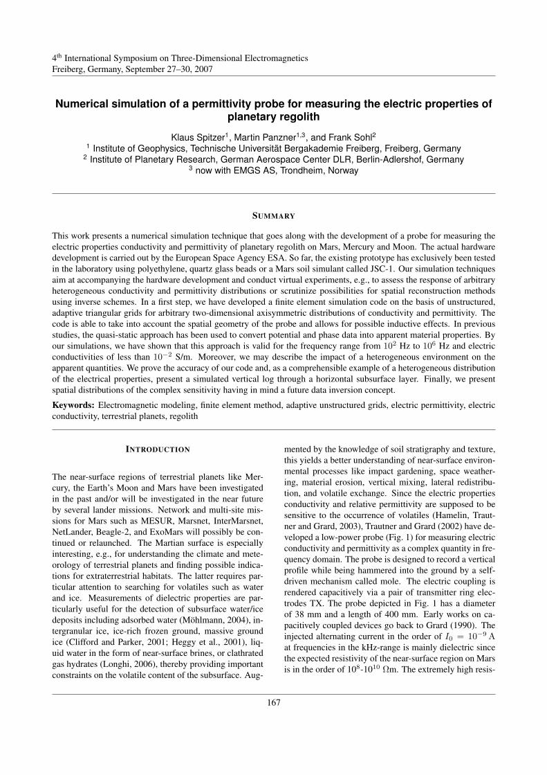
4th International Symposium on Three-Dimensional ElectromagneticsFreiberg, Germany, September 27–30, 2007
Numerical simulation of a permittivity probe for measuring the electric properties ofplanetary regolith
Klaus Spitzer1, Martin Panzner1,3, and Frank Sohl21 Institute of Geophysics, Technische Universität Bergakademie Freiberg, Freiberg, Germany
2 Institute of Planetary Research, German Aerospace Center DLR, Berlin-Adlershof, Germany3 now with EMGS AS, Trondheim, Norway
SUMMARY
This work presents a numerical simulation technique that goes along with the development of a probe for measuring theelectric properties conductivity and permittivity of planetary regolith on Mars, Mercury and Moon. The actual hardwaredevelopment is carried out by the European Space Agency ESA. So far, the existing prototype has exclusively been testedin the laboratory using polyethylene, quartz glass beads or a Mars soil simulant called JSC-1. Our simulation techniquesaim at accompanying the hardware development and conduct virtual experiments, e.g., to assess the response of arbitraryheterogeneous conductivity and permittivity distributions or scrutinize possibilities for spatial reconstruction methodsusing inverse schemes. In a first step, we have developed a finite element simulation code on the basis of unstructured,adaptive triangular grids for arbitrary two-dimensional axisymmetric distributions of conductivity and permittivity. Thecode is able to take into account the spatial geometry of the probe and allows for possible inductive effects. In previousstudies, the quasi-static approach has been used to convert potential and phase data into apparent material properties. Byour simulations, we have shown that this approach is valid for the frequency range from 102 Hz to 106 Hz and electricconductivities of less than 10−2 S/m. Moreover, we may describe the impact of a heterogeneous environment on theapparent quantities. We prove the accuracy of our code and, as a comprehensible example of a heterogeneous distributionof the electrical properties, present a simulated vertical log through a horizontal subsurface layer. Finally, we presentspatial distributions of the complex sensitivity having in mind a future data inversion concept.
Keywords: Electromagnetic modeling, finite element method, adaptive unstructured grids, electric permittivity, electricconductivity, terrestrial planets, regolith
INTRODUCTION
The near-surface regions of terrestrial planets like Mer-cury, the Earth’s Moon and Mars have been investigatedin the past and/or will be investigated in the near futureby several lander missions. Network and multi-site mis-sions for Mars such as MESUR, Marsnet, InterMarsnet,NetLander, Beagle-2, and ExoMars will possibly be con-tinued or relaunched. The Martian surface is especiallyinteresting, e.g., for understanding the climate and mete-orology of terrestrial planets and finding possible indica-tions for extraterrestrial habitats. The latter requires par-ticular attention to searching for volatiles such as waterand ice. Measurements of dielectric properties are par-ticularly useful for the detection of subsurface water/icedeposits including adsorbed water (Möhlmann, 2004), in-tergranular ice, ice-rich frozen ground, massive groundice (Clifford and Parker, 2001; Heggy et al., 2001), liq-uid water in the form of near-surface brines, or clathratedgas hydrates (Longhi, 2006), thereby providing importantconstraints on the volatile content of the subsurface. Aug-
mented by the knowledge of soil stratigraphy and texture,this yields a better understanding of near-surface environ-mental processes like impact gardening, space weather-ing, material erosion, vertical mixing, lateral redistribu-tion, and volatile exchange. Since the electric propertiesconductivity and relative permittivity are supposed to besensitive to the occurrence of volatiles (Hamelin, Traut-ner and Grard, 2003), Trautner and Grard (2002) have de-veloped a low-power probe (Fig. 1) for measuring electricconductivity and permittivity as a complex quantity in fre-quency domain. The probe is designed to record a verticalprofile while being hammered into the ground by a self-driven mechanism called mole. The electric coupling isrendered capacitively via a pair of transmitter ring elec-trodes TX. The probe depicted in Fig. 1 has a diameterof 38 mm and a length of 400 mm. Early works on ca-pacitively coupled devices go back to Grard (1990). Theinjected alternating current in the order of I0 = 10−9 Aat frequencies in the kHz-range is mainly dielectric sincethe expected resistivity of the near-surface region on Marsis in the order of 108-1010 Ωm. The extremely high resis-
1/5
4th International Symposium on Three-Dimensional ElectromagneticsFreiberg, Germany, September 27–30, 2007
167

Spitzer, Panzner, and Sohl, 2006, Numerical simulation of a permittivity probe
tivity yields a voltage signal in the order of mV, which isrecorded by another pair of ring electrodes RX.
Figure 1: Prototype of the permittivity probe accordingto Trautner and Grard (2002). TX are transmittersand RX are receivers.
TX and RX are lined up in a classical equidistant 4-point-arrangement along the cylindrical body of the probe(Fig. 1). Power consumption totals only 80 mW. Thepotential measurements are interpreted in a quasi-staticmode. Using a reference measurement for vacuum theapparent relative permittivity εar and the apparent electricconductivity σa are determined by
εar =|∆V0||∆V |
· cos(φ0 − φ) (1)
σa = −|∆V0||∆V |
ωε0 · sin(φ0 − φ) , (2)
where ∆V0 and φ0 are the reference potential differenceand phase for vacuum and ∆V and φ are the correspond-ing quantities in an arbitrary medium. ω is the angularfrequency and ε0 is the dielectric constant.
GOVERNING EQUATIONS AND NUMERICALFORMULATION
Numerical simulation techniques are helpful for optimiz-ing the experimental setup and investigating physical phe-nomena which occur with the particular design of theprobe. In a first approach, we use high-level programminglanguages (Femlab/Matlab) which take over the majorityof administrative work in coding FE techniques and helpto check out basic simulation strategies.In order to comprehensively describe the nature of thephysical problem we have to take into account the cou-pling of the electric and magnetic fields ~E and ~H .We therefore introduce the magnetic vector potential ~A
giving
~E = −∇V − ∂ ~A
∂t(3)
~H =1
µ0µr∇× ~A , (4)
where µ0 is the free space magnetic permeability, µr therelative magnetic permeability, t the time, and V the elec-tric potential. To completely describe the behavior of lowfrequency electromagnetic fields in a source-free, conduc-tive, and polarizable medium we have to solve Ampere’slaw and the equation of continuity augmented by the di-electric current. In the frequency domain they read
∇ ·~j = 0 = ∇ · [(σ + iωε0εr)∇V ] (5)
∇× ~H = ~j = (σ + iωε0εr)∇V , (6)
where~j is the electric current density, εr the relative elec-tric permittivitty, σ the electric conductivity, and i theimaginary unit. Substituting eqs 3 and 4 into eqs 5 and 6,setting the complex valued conductivity σ = (σ+iωε0εr)and the magnetic permeability µ = µ0µr we obtain thegoverning coupled system of equations
−∇ ·[iωσ ~A+ σ∇V
]= 0 (7)
iωσ ~A+∇×(
1µ∇× ~A
)+ σ∇V = 0 . (8)
Using finite elements we obtain a system of integral equa-tions according to the weak formulation∫
Ω
∇γ ·(iωσ ~A+ σ∇V
)dΩ−
∫Γ
γ jndΓ = 0 (9)
∫Ω
~τ ·[iωσ ~A+ σ∇V
]dΩ+
∫Ω
∇×~τ ·(
1µ∇× ~A
)dΩ+∫
Γ
~τ ·[~n×
(1µ∇× ~A
)]dΓ = 0 , (10)
which forms the basis for the subsequent discretization. γand ~τ are arbitrary scalar or vector test functions, respec-tively. The integration is carried out over the domain Ω.To achieve uniqueness of the solution, a Coulomb gauge∇ · ~A = 0 is applied. The solution for V and ~A aresought such that eqs 9 and 10 hold for all test functionsγ and ~τ . The integrals over the boundary Γ of the do-main Ω are obtained using boundary conditions for thenormal component of the current density jn = ~n · ~j =σ∂nV + iωσ ~A · ~n and the tangential component of themagnetic field ~n × ~H = ~n ×
(1µ∇× ~A
), where ~n is the
outward normal on the boundary. Using mixed bound-ary conditions for the electric potential and the magnetic
2/5
Spitzer et al., Numerical simulation of a permittivity probe
168

Spitzer, Panzner, and Sohl, 2006, Numerical simulation of a permittivity probe
vector potential at the outer boundaries the error propa-gating into the domain could significantly be reduced. Thesource currents are provided by inhomogeneous Neumannboundary conditions for the electric potential at the sur-face of the current electrodes TX.
ACCURACY AND ADAPTIVE GRID
In the contact area of the electrodes large conductivitycontrasts exist (copper/regolith) which produce huge gra-dients of the electric potential. Therefore, in this regionthe unstructured triangular grid has adaptively been re-fined to a high degree (Fig. 2).
Model domainClose-up rangearound electrodes
Probe
Figure 2: Discretization of the model domain. The gridis strongly refined close to the electrodes.
This is of particular concern, because the measurement ofthe potential difference is carried out at the potential elec-trodes RX. We have checked the accuracy of our code bycomparison with the analytic solution for a vertical elec-tric dipole in a homogeneous medium and the frequencyof 1 kHz (Telford, 1990). Fig. 3 shows the orientationof the dipole and field properties (a) and the results forDirichlet and mixed boundary conditions (b). Note thehigh accuracy for the latter except for the region close tothe singularity.In the frequency range 102 Hz < f < 106 Hz the modelresponse has been proved to be stable (not shown here).At the low frequency end, the problem is ill-conditionedfor frequencies f < 102 Hz and, thus, becomes numeri-cally instable. For high frequencies f > 106 Hz the cho-sen approach is not valid anymore because the problemincreasingly becomes a pure wave phenomenon.Through our numerical simulations, the quasi-static ap-proach of eqs 1 and 2 has been verified for con-ductivities σ < 10−2 S/m. The frequency range102 Hz < f < 106 Hz is characterized by low induction
numbers B 1, (Benderitter et al., 1994), where in-ductive effects are negligible. The induction number isdefined by B = L/p with a typical scale length L of themeasurement and the electromagnetic skin depth p.
a)
x
y
z
EErr
HHϕ?
EEθθθ
ϕ
r
VEDL
.
b)
electric field
relative error
analytical
Figure 3: a) Schematic representation of a vertical elec-tric dipole (VED) and corresponding field proper-ties. b) z-component of the electric field ~Ez and itsrelative error in the equatorial plane as a functionof the distance r to the dipole center for (1) mixedboundary conditions and (2) Dirichlet boundaryconditions.
NUMERICAL SIMULATION RESULTS ANDSENSITIVITIES
In the following, we present a simple, but meaningfulmodel of a horizontal layer of anomalous electric proper-ties being penetrated by the probe in the vertical direction(Fig. 4a). While moving downwards, the probe records avertical profile of the complex conductivity comparable toa borehole log. For the sake of simplicity, the probe is keptfixed in the simulation and the layer is moved upwards.The two left-hand subplots of Fig. 4b show the potentialdifference ∆V and phase φ measured at the receivers RX.The signature of the anomalous layer is clearly visible.The two right-hand subplots of Fig. 4b show εar and σa
according to eqs 1 and 2.
3/5
Spitzer et al., Numerical simulation of a permittivity probe
169
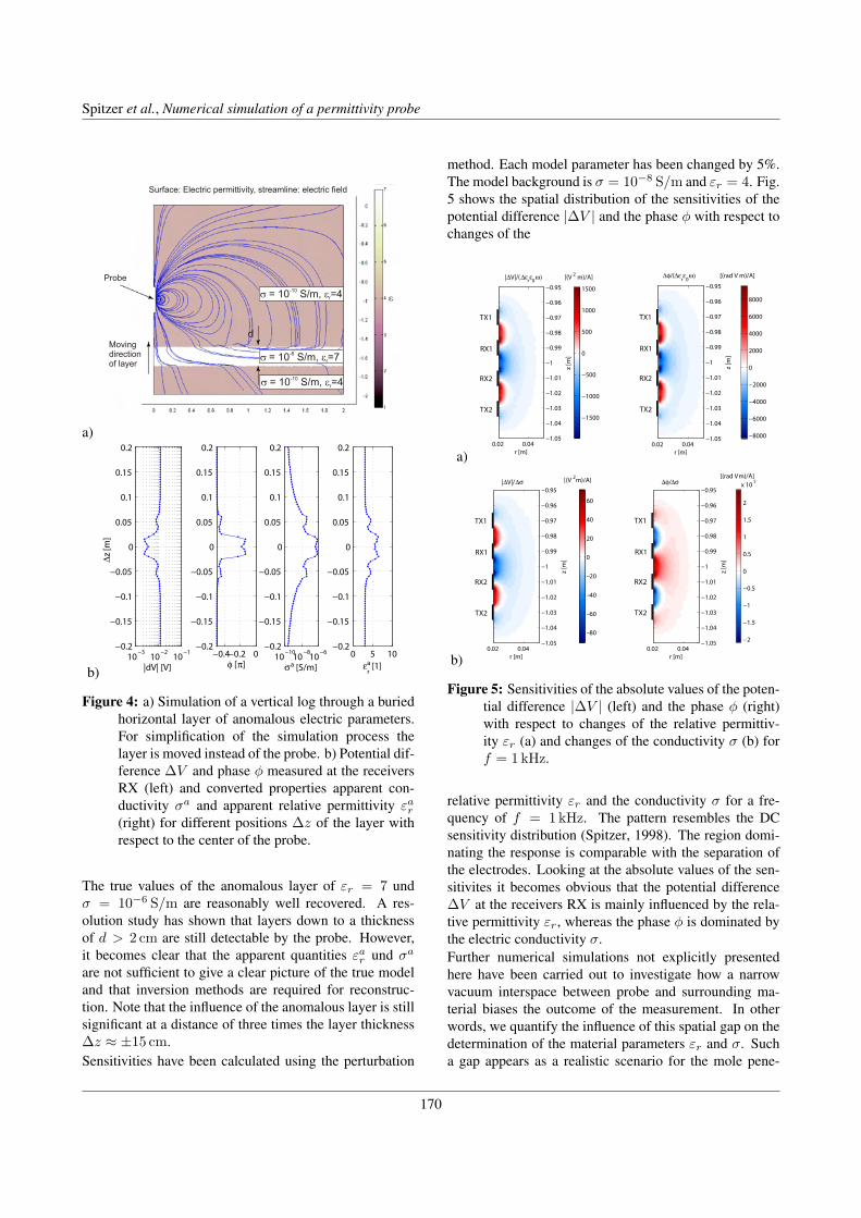
Spitzer, Panzner, and Sohl, 2006, Numerical simulation of a permittivity probe
a)
Probe
Movingdirectionof layer
-6s = 10 S/m, e =7r
-10s = 10 S/m, e =4r
-10s = 10 S/m, e =4r
Surface: Electric permittivity, streamline: electric field
d
b)10
−310
−210
−1−0.2
−0.15
−0.1
−0.05
0
0.05
0.1
0.15
0.2
|dV| [V]
]m[
∆z
−0.4−0.2 0−0.2
−0.15
−0.1
−0.05
0
0.05
0.1
0.15
0.2
φ [π]10
−1010
−810
−6−0.2
−0.15
−0.1
−0.05
0
0.05
0.1
0.15
0.2
σa [S/m]
0 5 10−0.2
−0.15
−0.1
−0.05
0
0.05
0.1
0.15
0.2
εr [1]a
Figure 4: a) Simulation of a vertical log through a buriedhorizontal layer of anomalous electric parameters.For simplification of the simulation process thelayer is moved instead of the probe. b) Potential dif-ference ∆V and phase φ measured at the receiversRX (left) and converted properties apparent con-ductivity σa and apparent relative permittivity εar(right) for different positions ∆z of the layer withrespect to the center of the probe.
The true values of the anomalous layer of εr = 7 undσ = 10−6 S/m are reasonably well recovered. A res-olution study has shown that layers down to a thicknessof d > 2 cm are still detectable by the probe. However,it becomes clear that the apparent quantities εar und σa
are not sufficient to give a clear picture of the true modeland that inversion methods are required for reconstruc-tion. Note that the influence of the anomalous layer is stillsignificant at a distance of three times the layer thickness∆z ≈ ±15 cm.Sensitivities have been calculated using the perturbation
method. Each model parameter has been changed by 5%.The model background is σ = 10−8 S/m and εr = 4. Fig.5 shows the spatial distribution of the sensitivities of thepotential difference |∆V | and the phase φ with respect tochanges of the
a) r [m]
z [m
]
|∆V|/(∆εrε
0ω) [(V 2 m)/A]
0.02 0.04−1.05
−1.04
−1.03
−1.02
−1.01
−1
−0.99
−0.98
−0.97
−0.96
−0.95
−1500
−1000
−500
0
500
1000
1500
r [m]
z [m
]
∆φ/(∆εrε
0ω) [(rad V m)/A]
0.02 0.04−1.05
−1.04
−1.03
−1.02
−1.01
−1
−0.99
−0.98
−0.97
−0.96
−0.95
−8000
−6000
−4000
−2000
0
2000
4000
6000
8000
TX1
TX2
RX1
RX2
TX1
TX2
RX1
RX2
b) r [m]
z [m
]
|∆V|/∆σ [(V 2m)/A]
0.02 0.04−1.05
−1.04
−1.03
−1.02
−1.01
−1
−0.99
−0.98
−0.97
−0.96
−0.95
r [m]
z [m
]
∆φ/∆σ [(rad Vm)/A]
0.02 0.04−1.05
−1.04
−1.03
−1.02
−1.01
−1
−0.99
−0.98
−0.97
−0.96
−0.95
−2
−1.5
−1
−0.5
0
0.5
1
1.5
2
x 105
−80
−60
−40
−20
0
20
40
60
TX1
TX2
RX1
RX2
TX1
TX2
RX1
RX2
Figure 5: Sensitivities of the absolute values of the poten-tial difference |∆V | (left) and the phase φ (right)with respect to changes of the relative permittiv-ity εr (a) and changes of the conductivity σ (b) forf = 1 kHz.
relative permittivity εr and the conductivity σ for a fre-quency of f = 1 kHz. The pattern resembles the DCsensitivity distribution (Spitzer, 1998). The region domi-nating the response is comparable with the separation ofthe electrodes. Looking at the absolute values of the sen-sitivites it becomes obvious that the potential difference∆V at the receivers RX is mainly influenced by the rela-tive permittivity εr, whereas the phase φ is dominated bythe electric conductivity σ.Further numerical simulations not explicitly presentedhere have been carried out to investigate how a narrowvacuum interspace between probe and surrounding ma-terial biases the outcome of the measurement. In otherwords, we quantify the influence of this spatial gap on thedetermination of the material parameters εr and σ. Sucha gap appears as a realistic scenario for the mole pene-
4/5
Spitzer et al., Numerical simulation of a permittivity probe
170
Spitzer, Panzner, and Sohl, 2006, Numerical simulation of a permittivity probe
trating into coarse material. It might be relevant in thesense of weak coupling between electrodes and mediumin strongly heterogeneous ground. For simplicity, the gapencloses the probe completely on its cylindrical shell andis defined by a constant width k. Note that the simulationcode, however, is able to cope with arbitrary cylindricalgeometries. The results exhibit that the relative error in εarand σa is below 2%, and therefore negligible, as long asthe gap is smaller than k = 2 mm. This is particularly in-teresting because the gap is located in the highly sensitiveregion of the probe (see Fig. 5).
CONCLUSIONS AND OUTLOOK
We have developed a 2D adaptive unstructured grid fi-nite element forward modeling software to simulate theresponse of a permittivity probe designed by ESA. With it,we are able to verify the chosen quasi-static approach inthe frequency range 102 Hz < f < 106 Hz for conductiv-ities σ < 10−2 S/m. Moreover, we may carry out a widevariety of virtual experiments taking into account induc-tive effects whenever they occur. This is especially help-ful for studying the physical response in heterogeneousmedia. In perspective, we want to extend our simulationsto 3D, evaluate the possibility of applying spatial recon-struction techniques for the electric material properties,and carry out resolution studies under the following con-straints: 1) The available electric power for planetary fieldsurveys is likely to be very low. 2) The payload is re-stricted to an absolute minimum. Hence, additional elec-trodes have to be positioned well-directedly, e.g., usingthe feet of the landers. This altogether results in surveyswith sparse data sampling and limited spatial range. Still,rocks or ice lumps that are not penetrated directly mightbe resolved in the target area if the survey is designed in-telligently. Concluding, even coarse 3D models revealingstructures within the regolith will provide valuable infor-mation on the near-surface constitution of planetary bod-ies.
REFERENCES
Benderitter, Y., Jolivet, A., Mounir, A. and Tabbagh, A.(1994). Application of the electrostatic quadripoleto sounding in the hectometric depth range. J. Appl.Geophys., 31, 1-6.
Clifford, S. M. and Parker, T. J. (2001). The evolution ofthe Martian hydrosphere: Implications for the fateof a primordial ocean and the current state of thenorthern plains. Icarus, 154, 40–79.
Grard, R. (1990). A quadrupolar array for measuring thecomplex permittivity of the ground: Application to
earth prospection and planetary exploration. Mea-surement Science and Technology, 1, 295–301.
Hamelin, M., Trautner, R. and Grard, R. (2003). Detectionof near-surface ice on Mars with electromagnetictechniques on board future surface vehicles. J. Geo-phys Res., 108, 8045, doi:10.1029/2002JE001893.
Heggy, E., Paillou, P., Ruffie, G., Malezieux, J., Costard,F. and Grandjean, G. (2001). On water detec-tion in the Martian subsurface using sounding radar.Icarus, 154, 244-257.
Longhi, J. (2006). Phase equilibrium in the system CO2-H2O: Application to Mars. J. Geophys. Res., 111,E06011, doi:10.1029/2005JE002552.
Möhlmann, D. T. F. (2004). Water in the upper Martiansurface at mid- and low-latitudes: Presence, state,and consequences. Icarus, 168, 318-323.
Spitzer, K. (1998). The three-dimensional DC sensitivityfor surface and subsurface sources. Geophys. J. Int.,134, 736–746.
Telford, W. (1990). Applied geophysics. Cambridge Uni-versity Press.
Trautner, R. and Grard, R. (2002, 10). Measuring theelectric properties of planetary environments withmutual impedance (MI) probes. Earth-like planetsand moons. Proceedings of the 36th ESLAB Sympo-sium, 105-107.
5/5
Spitzer et al., Numerical simulation of a permittivity probe
171

4th International Symposium on Three-Dimensional ElectromagneticsFreiberg, Germany, September 27–30, 2007
Analysis of polarization effects of buried pipes in vector-migrated 3-Dground-penetrating radar data
R. Streich1,2 and J. van der Kruk1
1Institute of Geophysics, ETH (Swiss Federal Institute of Technology) Zurich, 8093 Zurich, Switzerland2now at SINTEF Petroleum Research, S.P. Andersens vei 15A, 7465 Trondheim, Norway
SUMMARY
Ground-penetrating radar (GPR) data for objects such as utility pipes or wires are influenced both by the vectorial an-tenna radiation patterns and the targets’ scattering properties. In this synthetic study for dielectric pipes, we use recentlydeveloped vector-migration schemes to eliminate the effects of the antenna radiation patterns from the GPR data and thenanalyze scattering effects in the vector-migrated images. Pipe reflection amplitudes in our migrated images agree qual-itatively with those described by other workers, and we find in our images indications of depolarization and systematicphase differences between images of pipes and planar reflectors. This study serves as a starting point for further, morequantitative investigations of pipe scattering properties.
Keywords: Ground-penetrating radar, finite-difference time-domain modeling, vector migration, polarization
INTRODUCTION
The amplitudes and phases of ground-penetrating radar(GPR) data depend on the subsurface reflectivity proper-ties and on the antenna radiation patterns and electromag-netic vector-wave propagation. We have recently devel-oped 3-D vector-migration schemes that practically elim-inate the radiation-pattern and wave-propagation effectsfrom GPR data (Streich and van der Kruk, 2007; Streichet al., 2007). The elimination of radiation-pattern effectshas been demonstrated on synthetic and field data contain-ing dipping planes, which do not exhibit directional scat-tering properties. Vector-images of dipping planes werenearly independent of the antenna-to-plane orientation.
For other objects such as pipes, the data amplitudes arealso influenced by polarization effects that depend on thepolarization and incidence angle of the electromagneticfield relative to the reflecting object. Polarization effectsmay comprise preferential scattering (i.e., variations ofthe scattering amplitudes depending on the polarization ofthe incident field relative to the pipe), and depolarization(i.e., changes of the relative amplitudes of the scatteredfield components compared to the incident field compo-nents). Scattering amplitudes are functions of the relativeantenna-to-pipe orientation, pipe and background proper-ties, scattering angle, and pipe thickness with respect toGPR wavelength. Scattering strengths of pipes as func-tions of the material properties for a fixed antenna-to-pipeorientation have been analyzed by Zeng and McMechan(1997), whereas polarization effects as functions of thematerial properties and antenna-to-pipe orientations have
been investigated, e.g., by Roberts and Daniels (1996) andRadzevicius and Daniels (2000). Their results show:
(i) For metal pipes and dielectric pipes with permittivi-ties larger than that of the surrounding medium, thedirection of preferential scattering is usually alignedwith the pipe orientation (Roberts and Daniels,1996; Radzevicius and Daniels, 2000).
(ii) For dielectric pipes with permittivities lower thanthat of the surrounding medium, the direction ofpreferential scattering depends on the pipe diam-eter (with respect to the dominant GPR wave-lengths) and may be perpendicular to the pipe orien-tation (Roberts and Daniels, 1996; Radzevicius andDaniels, 2000).
(iii) For conducting and dielectric pipes, depolarizationdoes not occur if the incident electric field is ori-ented exactly parallel or exactly perpendicular tothe pipe (Radzevicius and Daniels, 2000).
In this preliminary study, we analyze scattering ampli-tudes in migrated images of synthetic dielectric pipes.We applied our vector-migration algorithms to syntheticdata generated using a 3-D finite-difference time domain(FDTD) modeling algorithm (Lampe et al., 2003). Sincethe migration corrects for the radiation patterns, polariza-tion effects are effectively separated from radiation patternones. In the obtained migrated images, amplitude varia-tions with the relative antenna-to-pipe orientation shouldbe due to scattering effects only. We analyze here theimage amplitudes for different antenna-to-pipe orienta-tions and compare them to theoretically expected ones
1/4
4th International Symposium on Three-Dimensional ElectromagneticsFreiberg, Germany, September 27–30, 2007
172

Streich, R. and van der Kruk, J., 2007, FDTD modeling and vector-imaging of GPR data . . .
(e.g., Radzevicius and Daniels, 2000). Following this ini-tial analysis, further work should be targeted at obtainingquantitative estimates of scattering properties from the mi-grated images.
SYNTHETIC DATA GENERATION
Synthetic GPR data were generated data using the 3-DFDTD algorithm of Lampe et al. (2003). This versatileFDTD modeling tool is second order in space and timeand uses a standard staggering scheme and the generalizedperfectly-matched-layer boundary conditions of Fang andWu (1996).
We simulated a dielectric pipe with a diameter of 0.2 mand a relative permittivity of εr = 4. The pipe was ori-ented parallel to the x2 axis (Figure 1) and embeddedin a homogeneous medium with εr = 8 (correspondingto the situation (ii) listed in the introduction) and its topwas located at a depth of 1.8 m. A constant conductivityof σ = 0.2 mS/m was used for the background mediumand pipe. The sources were infinitesimal dipole antennasemitting a Gaussian wavelet with a center frequency of∼70 MHz. The model dimensions were 7.5 x 7.5 x 5 m.
x1
x2
T1T2 R2
χ11
T2
T1
R1
χ22
pip
e
Figure 1: Geometry for our synthetic surveys of a di-electric pipe: Within each set of antennas (under-lain in gray), Tα and Rβ denote the transmitting andreceiving antennas used to obtain the Eαβ compo-nents. χ11 and χ22 are the images associated withthe different antenna sets. Dashed lines indicatetypical wave-propagation paths.
As in Streich and van der Kruk (2007), we simulatedcommon-offset measurements by modeling a single x1-line of sources oriented both in the x1 and x2 direc-tions. For each source point and orientation, receiverswere placed on a 0.1 x 0.1 m surface grid. From theobtained raw data volumes, we extracted multicomponentcommon-offset data for various antenna offsets (we showhere data and images for an offset of 1 m). The multicom-
ponent data comprise the E11, E21, E12, and E22 compo-nents for antenna offsets both in the x1 and x2 directions(Figure 1 shows the broadside configurations of E11 andE22 and the two corresponding cross-polarized configura-tions used here). To prevent artifacts resulting from theFD model boundaries, the size of the used data volumeswas reduced slightly (e.g., to 6.8 x 7.4 x 5 m for 1 m an-tenna offset).
(a) E11
Tim
e [n
s]
2 4 6
0
40
80
(b) E21
2 4 6
0
40
80
(c) E12
x1 [m]
Tim
e [n
s]
2 4 6
0
40
80
(d) E22
x1 [m]2 4 6
0
40
80
Figure 2: Vertical sections through the multicomponentsynthetic data for the (a) E11, (b) E21, (c) E12 and(d) E22 components (see Figure 1) for an antennaoffset of 1 m. For the same color values, the ampli-tudes in (b) and (c) are 1/4 those in (a) and (d).
Slices through the synthetic data are shown in Figure 2.For the 1-m antenna offset, the data amplitudes are largestin the E11 section and somewhat lower in the E22 section.The amplitudes are practically zero in the cross-polarizedE12 configuration. For this configuration, the electric fieldincident onto the pipe is polarized in the x1 direction (seeFigure 1), and reflection at the pipe does not produce anyenergy detectable by the x2-oriented receiver. In contrast,reflection at the pipe generates a small electric field com-ponent parallel to the x1-oriented receiver for the E21 con-figuration. Here, the electric field incident onto the pipe ispolarized slightly oblique to the x2 axis, and thus a smallportion of the field reflected at the pipe is polarized paral-lel to the x1 axis.
VECTOR-MIGRATION RESULTS
The data were imaged using (i) a multicomponent vector-migration (Streich and van der Kruk, 2007), which cor-rects for exact-field radiation patterns by combining datafrom a co- and a cross-polarized data component intoa migrated image, and (ii) a single-component vector-migration (Streich et al., 2007), which eliminates the vec-
2/4
Streich et al., FDTD modeling and vector-imaging of GPR data
173

Streich, R. and van der Kruk, J., 2007, FDTD modeling and vector-imaging of GPR data . . .
torial radiation-pattern effects from a single co-polarizeddata set. For comparison, we also applied a vector-migration that corrects for far-field radiation patterns (vander Kruk et al., 2003) and a modified Gazdag phase-shiftmigration, which includes a geometrical spreading correc-tion and a 90 phase correction (van der Kruk et al., 2003).
In the employed vector-migrations, scattering objects areassumed to be composed of point scatterers that do notinteract (the first-order Born approximation is used). Mi-grated images for different antenna-to-pipe orientationsand antenna offsets exhibit amplitude and phase variationsdue to variations of the incident electric field polarizationrelative to the pipe.
In Figures 3 and 4, we display results of the modifiedGazdag, single-component far-field vector and exact-fieldmulti- and single-component vector migrations; the vari-ous χ11 and χ22 images were obtained from the E11 andE22 configurations, respectively (see Figure 1). The twoGazdag phase-shift images χmgzd
αα (α∈ 1,2) are some-what less focused than the vector-migrated ones and dif-fer in amplitude and phase as a result of both polarizationand radiation pattern effects (Figures 3a, b and 4a). Thefar-field vector-images χfar,SC
αα show consistent phasesfor the two antenna orientations (Figures 3c, d and 4b).The pipe reflection amplitudes are higher in χfar,SC
22 , forwhich the antennas were oriented parallel to the pipe, thanin χfar,SC
11 , for which the antennas were oriented per-pendicular to the pipe. Conversely, for the exact-fieldmulti- and single-component vector-images χexa,MC
αα andχexa,SC
αα , the pipe reflection amplitudes are ∼22% higherin χexa,MC
11 and χexa,SC11 than in χexa,MC
22 and χexa,SC22
(Figures 3e–h and 4c). This exact-field imaging resultagrees qualitatively with results of Roberts and Daniels(1996) and Radzevicius and Daniels (2000), who alsofound, for comparable models containing low-permittivitydielectric pipes, that scattering amplitudes were largestfor antennas oriented perpendicular to the pipes. Far-fieldimaging has resulted in false indication of polarization ef-fects here.
Comparison of the single-component exact-field images(Figures 3e and f) to the multicomponent ones showed thatthe multicomponent χexa,MC
22 computed from the E22 andE12 components was identical to the single-componentχexa,SC
22 computed from E22 alone. This was expected,because depolarization does not occur for this config-uration (Radzevicius and Daniels, 2000). In contrast,we observed amplitude differences between the multi-and single-component exact-field images χexa,MC
11 andχexa,SC
11 of 0.3%; minor depolarization occurred here. Fora different model with the pipe oriented at 45 to the an-tennas (not shown here), amplitudes between multi- and
single-component images differed by 3.2%.
(a) χ11
Dep
th [m
]
3 4 m
2
3
(b) χ22
3 4 m
2
3
mgzd mgzd
(c) χ11
Dep
th [m
]3 4 m
2
3
(d) χ22
3 4 m
2
3
far,SC far,SC
(e) χ11
Dep
th [m
]
3 4 m
2
3
(f) χ22
3 4 m
2
3
exa,MC exa,MC
(g) χ11
x1 [m]
Dep
th [m
]
3 4
2
3
(h) χ22
x1 [m]3 4
2
3
exa,SC exa,SC
Figure 3: Vertical sections through various images χ11
and χ22 of the dielectric pipe for 1-m offset anten-nas. (a, b) were obtained from modified Gazdagphase-shift migration, (c, d) from far-field single-component vector-migration, (e, f) from exact-fieldmulticomponent and (g, h) from exact-field single-component vector-migration.
Furthermore, the images of the dielectric pipe show dis-tinctly different phase characteristics from images of pla-nar reflectors. After deconvolving the source wavelet,planar reflector images have approximately the expected(van der Kruk et al., 2003) shape of a band-limited delta-function, with the polarity determined by the polarity of
3/4
Streich et al., FDTD modeling and vector-imaging of GPR data
174

Streich, R. and van der Kruk, J., 2007, FDTD modeling and vector-imaging of GPR data . . .
the material contrast. This is illustrated by the tracesshown in Figure 4d, which were extracted from exact-field images of an 18 dipping planar boundary with rela-tive permittivities of 7 above and 10 below (Streich et al.,2007). In contrast, the phases of the exact-field pipe im-ages differ by ∼ 90 from that of a band-limited deltafunction (Figure 4c).
Am
plitu
de
2 2.5 3 3.5−3
−2
−1
0
1
Depth [m]
(d) Dipping plane, χαα
1 1.5 2 2.5
−4−2
024
Depth [m]
(c) Pipe, χαα
1 1.5 2 2.5 m
−4−2
024
(b) Pipe, χαα
Am
plitu
de
1 1.5 2 2.5 m
−4−2
024
(a) Pipe, χαα
χ11 χ22
mgzd far,SC
exa,SC exa,SC
Figure 4: Traces extracted from the dielectric pipe im-ages shown in Figure 3 at x1 = 3.5 m for (a)modified Gazdag phase-shift migration, (b) far-field vector-migration and (c) exact-field single-component vector-migration (multicomponent im-age traces are not shown because their differences to(c) are within the line thickness). For comparison,(d) shows traces extracted from exact-field vector-migrated images of a dipping planar boundary.
CONCLUSIONS AND OUTLOOK
We have delineated various scattering effects for dielec-tric pipes in vector-migrated images practically devoid ofradiation pattern-effects. Whereas previously investigatedvector-images of dipping planes had amplitudes nearly in-dependent of the antenna-to-plane orientation, we observein our pipe images amplitude variations with the relativeantenna-to-pipe orientation, weak depolarization effects,and phases deviating by ∼ 90 from those of planar re-flector images.
For different antenna-to-pipe orientations, exact-fieldvector-migration produced images with scattering am-plitude variations in qualitative agreement with theoreti-cally expected scattering amplitudes. In contrast, far-fieldvector-migration resulted in false indication of polariza-tion effects.
Further work is required to obtain a more quantitative un-derstanding of the observations and infer scatterer proper-ties from the migrated images. Similar synthetic studiesfor different antenna offsets and other models, includingmetallic pipes, and a field study are in progress.
ACKNOWLEDGMENTS
This work was funded by grants from ETH Zurich and theSwiss National Science Foundation.
REFERENCES
Fang, J. and Wu, Z. (1996). Generalized perfectlymatched layer for the absorption of propagating andevanescent waves in lossless and lossy media. IEEETransactions on Microwave Theory and Techniques,44:2216–2222.
Lampe, B., Holliger, K., and Green, A. G. (2003).A finite-difference time-domain simulation tool forground-penetrating radar antennas. Geophysics,68:971–987.
Radzevicius, S. J. and Daniels, J. J. (2000). Ground pene-trating radar polarization and scattering from cylinders.Journal of Applied Geophysics, 45:111–125.
Roberts, R. and Daniels, J. J. (1996). Analysis of GPRpolarization phenomena. American Journal of Environ-mental and Engineering Geophysics, 1:139–157.
Streich, R., van der Kruk, J., and Green, A. G. (2007).Vector-migration of standard co-polarized 3-D GPRdata. Geophysics, in press.
Streich, R. and van der Kruk, J. (2007). Accurate imagingof multicomponent GPR data based on exact radiationpatterns. IEEE Transactions on Geoscience and RemoteSensing, 45:93–103.
van der Kruk, J., Wapenaar, C. P. A., Fokkema, J. T.,and van den Berg, P. M. (2003). Improved three-dimensional image reconstruction technique for multi-component ground penetrating radar data. SubsurfaceSensing Technologies and Applications, 4:61–99.
van der Kruk, J., Wapenaar, C. P. A., Fokkema, J. T., andvan den Berg, P. M. (2003). Three-dimensional imag-ing of multicomponent ground-penetrating radar data.Geophysics, 68:1241–1254.
Zeng, X. and McMechan, G. A. (1997). GPR characteri-zation of buried tanks and pipes. Geophysics, 62:797–806.
4/4
Streich et al., FDTD modeling and vector-imaging of GPR data
175

176

Applications – Case histories
177

178

4th International Symposium on Three-Dimensional Electromagnetics Freiberg, Germany, September 27−30, 2007
1/4
Fitting a round peg in a square hole: 3D inversion of complex MT profile data
Paul Bedrosian1, Louise Pellerin2 and Steve Box3
1US Geological Survey, Denver Colorado, USA 2Green Engineering, Berkeley, California, USA
3US Geological Survey, Spokane, Washington, USA
SUMMARY Magnetotelluric (MT) data are commonly acquired along one or more profiles, regardless of the complexity of the underlying structure, due to logistical and monetary constraints. In addition, transects may not be perpendicular to regional strike because of topography and access. This is the situation for MT data acquired along a 140 km transect crossing the Proterozoic Belt Basin within the Cordilleran foreland of northwest Montana. We present the results of two- (2D) and three-dimensional (3D) inversion of this dataset and two additional sub-parallel profiles. The emphasis is upon structural differences in the resulting models and their dependence on assumptions of dimensionality and choices of regularization. The interpreted structure is largely consistent between 2D models and 3D model slices, with a general shallowing of structure in the 3D model relative to the corresponding 2D model. The 3D inversion of profile data recovers off-profile structure, particularly at greater depths constrained by long-period data. Our findings suggest that a two-stage approach to 3D inversion is appropriate, where results from a smoothing-regularized inversion are used to ‘seed’ a second inversion. Attention must be given to the choice of data and associated errors when inverting the full impedance tensor, because diagonal and off-diagonal tensor elements in quasi-2D strike coordinates may vary by many orders of magnitude. Enforcing an error floor proportional to the square root of the product of the off-diagonal impedance values can easily result in excessive downweighting the 3D data. Keywords: inversion, magnetotellurics, three-dimensional, two-dimensional
INTRODUCTION The Middle Proterozoic Belt Basin, spanning parts of Montana, Idaho, Washington, and British Columbia, is one of the deepest basins in North America. More than 18 km of fine-grained sedimentary strata were deposited rapidly between 1.5-1.4 Ga. The basin was split by rifting during late Proterozoic development of the North American passive margin. Basin strata were relatively undeformed until Mesozoic Cordilleran thrusting and early Eocene extension. Many questions are still outstanding and require an understanding of deep basin structure, including the flexural load of the Basin, its role during Cordilleran deformation, and controls on ore-forming fluids that produced stratabound Cu/Ag and sedimentary exhalative Pb/Zn/Ag deposits within the Basin.
The electrical resistivity of the subsurface spans many orders of magnitude, and reflects variations in lithology, mineralogy and hydrology. As such it records structural information associated with past tectonic events. Magnetotellurics (MT) is sensitive to electrical resistivity and is capable of imaging on scales ranging from 100s of meters to 100s kilometres.
Figure 1: Location of the MT survey superimposed on a gravity map. Long period stations (red dots), the main
profile (bold red line), and broadband stations (white dots) are shown. The black and red boxes depict the 3D
meshes for long-period and broadband data, respectively.
Long-period (1Hz–10,000sec), deep-crustal MT data were collected along a 140 km transect crossing the
4th International Symposium on Three-Dimensional ElectromagneticsFreiberg, Germany, September 27–30, 2007
179

Bedrosian, P. et al., 2007, 3D inversion of complex MT profile data
2/4
central Belt Basin in late summer 2005. Broadband data (100Hz to 350sec) were previously collected along the eastern half of the transect in the 1980s, and new broadband data were collected on the western half in 2005. Station locations are overlain on the intermediate-wavelength isostatic residual gravity map of Mankinen et al. (2004), which illuminates major structural features (Figure 1).
DIMENSIONALITY
The dimensionality of the data was assessed by examining phase tensors (Caldwell et al., 2004) and induction vectors. Changes in strike and dimensionality are evident near fault zones that accommodated significant deformation. As shown in Figure 2 the aggregate statistics of well-defined generalized strike (β < 10º, phase split > 5º) reveal three distinct populations: two are in agreement with surface geology and fault orientations, and a third (N30E) arises mostly from mid-crustal depths that may reflect depositional ‘fabric’ within the deep basin sediments or deep-structural trends. The NW strike population reflects that of the Purcell and Rocky Mountain trenches, while the N population reflects faulting within the Libby thrust Belt.
Figure 2: Aggregate statistics showing several strike directions along the main profile line.
2D INVERSION Although not strictly valid because of three-dimensional (3D) effects, we applied two-dimensional (2D) inversion to the data following rotation to N30W. The transverse electric (TE) mode data were ignored believing that these are more susceptible to contamination by 3D effects (Wannamaker et al.,
1984). A 2D resistivity model was generated along the Main Line from the broadband and long-period data using a two-step process: results using transverse magnetic (TM) mode plus vertical magnetic transfer function (Hz) data and a 100 ohm-m half space starting model were subsequently fed into a TM+Hz inversion in which a basement resistor was added to test a below the belt hypothesis (Figure 3). Note that the TE mode response was calculated and compared to the field data, but was not used in the inversion. Only broadband TM and Hz data were used for the North and South Lines.
Figure 3: 2D inverse models of broadband data to the north and south and broadband plus long-period data
along the center (main) profile. Models were computed using the conjugate gradient method of Rodi and
Mackie (2001). The dashed box outlines an along-strike snapshot for comparison. Data misfits are: TM 2.252, TE 6.12 (20% rho and 10% phase), and Hz - 1.243 +/- 0.05 absolute error on Real and Imaginary
components.
3D INVERSION Two 3D models are presented: one using the long-period data along the main transect, and another using the broadband data from the three profile line data (Figure 1). We used the 3D method of Siripunvaraporn et al. (2005) based on the 2D data space Occam's inversion of Siripunvaraporn and Egbert (2000), which seeks the smoothest, minimum structure models subject to an appropriate fit to the data. A data-space approach, where matrix dimensions depend on the size of the data set rather than the number of model parameters, surmounts the computational demands associated with
Bedrosian et al., 3D inversion of complex MT profile data
180

Bedrosian, P. et al., 2007, 3D inversion of complex MT profile data
3/4
construction and inversion of model-space matrices. The forward modeling is based on the staggered grid finite difference approximation to the second order Maxwell's equations, formulated in terms of the electric field. We have taken a two-stage approach to 3D inversion, using results from an initial smoothing-regularized inversion to ‘seed’ a second inversion with a homogeneous prior model. In this manner, the final inversion stage seeks deviations from 2D or quasi 2D structure that are required by the data. Model regions poorly constrained by the data become homogeneous due to the prior model. Though not as advantageous when inverting for strongly 3D structure, this approach offers a rigorous approach to the problem of inverting MT profile data. Representative model results are presented in plan view (Figure 4 and Figure 5), and as a 1 ohm-m isovolume (Figure 6). Broadband data from forty-four sites is poorly constrained below ~25 km. Long-period data were acquired at 34 sites. The inverse model is best constrained along the main profile and poorly constrained below ~50 km. In the quasi-2D strike coordinates, diagonal and off-diagonal tensor elements may vary by many orders of magnitude. Enforcing an error floor proportional to sqrt(|ZxyZyx*|) can result in downweighting the 3D data so it is no longer meaningful. Misfits can be high, sometimes greater than 25% RMS, but parts of the models not constrained by data revert to a 100 ohm-m half space. The dashed red lines on Figure 5 and Figure 6 roughly indicate the area constrained by the data.
Figure 4: Broadband 3D inversion results at depth
slice of 2.5-3km. The red dashed lines roughly indicate the area constrained by the data. The mesh for the long-
period data (Figure 5) is outlined in black.
Figure 5: Long-period 3D inversion results at depth
slices of 10.5-12.5 km (above) and 24-30 km (below). The mesh for the broadband data (Figure 4) is outlined
in red.
Figure 6: Contour of the 1ohm-m isovolume along
with three intersecting model slices from 3D inversion of the long period data. The stations of the Main Line
denoted with black dots.
Bedrosian et al., 3D inversion of complex MT profile data
181

Bedrosian, P. et al., 2007, 3D inversion of complex MT profile data
4/4
DISCUSSION
Strong conductors are apparent in all data. Indication of structure beneath the strong conductors was only apparent in a few sounding points at a few stations in the broadband data necessitating the need for the long-period survey. The two datasets complement each other well as do the 2D and 3D models. The 2D model of the Main Line is characterized by two sub-horizontal, highly conductive horizons (Figure 3). A shallower horizon at 10-15 km depth begins 10 km west of the Whitefish Range front and continues to the west for 60 km coming to an abrupt end beneath the Sylvanite anticline (Figure 1). A deeper, highly conductive, concave-up layer is seen at a depth of 25-35 km just west of southern Lake Koocanusa and ends abruptly about 20 km east of the Purcell trench. From that point west to the Selkirk Crest, the entire crust is very resistive. The Eocene Purcell trench detachment fault can be traced east dipping 25-30 degrees in that direction and reaching a depth of about 20 km. The expression of this fault flattens abruptly along the base of the shallower conductive layer lying 100 km to the east of the surface trace of the fault (Figure 3). Near-surface (~3 km) structures are seen in the broadband 3D model (Figure 4). The continuity of structures cannot be confidently defined between lines because of the wide spacing of ~40 km. The dashed red line shows the area constrained by data. The conductor along the Rocky Mountain trench is well defined in each line as is a conductor to the east of the Sylvanite Anticline. A shallow feature of the Libby Trench is a resistor. The 2D and 3D broadband models differ in that significant features are shallower in the 3D model. Data are insufficient both spatially and temporally to determine horizontal continuity or resolve features beneath the conductors. Because of these limitations the 3D model does not significantly enhance interpretation of the 2D models. In contrast, 3D modeling of the long-period data refines and improves our understanding of large structures defined by the 2D interpretation. At mid depths (10-12 km) the 3D model delineates a large, primarily 3D conductor (C1), centered on the Libby Tough and south of the Main Line; the northern Sylvanite Anticline is relatively resistive. At depths of 25-30 km the picture has changed greatly and the conductor (C1) has become dominantly 2D defining the length of the Sylvanite Anticline bounded on the west by the Purcell trench and to the east by the Libby trough (Figure 5). The 3D nature of the large-scale
conductors that characterize the Middle Proterozoic Belt Basin is illustrated in Figure 6
CONCLUSIONS
Two- and three-dimensional inversion of MT data reveals the deep structure of the Proterozoic Belt Basin within the Cordilleran foreland of northwest Montana. The interpreted structure is largely consistent between 2D models and 3D model slices, with a general shallowing of structure in 3D model slices relative to the corresponding 2D model. These results suggest that a two-stage approach to 3D inversion is appropriate, using results from a smoothing-regularized inversion to start a second inversion with a homogeneous prior model. Attention must be given to the choice of data and associated errors when inverting the full impedance tensor; diagonal and off-diagonal tensor elements may vary by many orders of magnitude in the quasi-2D strike coordinates. Selecting an error floor proportional to the square of the product of the off-diagonal impedance terms can easily result in seriously downweighting the 3D data. The 3D inversion of profile data permits recovery of off-profile structure, particularly at greater depths constrained by long-period data.
REFERENCES Caldwell, T.G., Bibby, H.M. and Brown, C. (2004).
The magnetotelluric phase tensor. Geophys. Jour. Inter., 158.
Mankinen, E.A., Hildenbrand, T.G., Zientek, M.L., Box, S.E., Bookstrom, A.A., Carlson, M.H., and Larsen, J.C. (2004). Guide to Geophysical Data for the Northern Rocky Mountains and Adjacent Areas, Idaho, Montana, Washington, Oregon, and Wyoming. U.S. Geological Survey, Open-File Report 2004-1413.
Rodi, W. and Mackie, R.L. (2001). Nonlinear conjugate gradients algorithm for 2-D magnetotelluric inversion. Geophysics, 66 (1).
Siripunvaraporn, W. and Egbert, G. (2000). An efficient data-subspace inversion method for 2-D magnetotelluric data. Geophysics, 65 (3).
Siripunvaraporn W., Egbert, G. and Uyeshima, M., 2005, Interpretation of 2-D Magnetotelluric Profile Data with 3-D Inversion: Synthetic Examples. Geophys. Jour. Inter., 160.
Wannamaker, P. E., Hohmann, G.W. and Ward, S.H. (1984). Magnetotelluric responses of three-dimensional bodies in layered earths. Geophysics, 49 (9).
Bedrosian et al., 3D inversion of complex MT profile data
182

3D GEOELECTRICAL MODEL OF THE UKRAINIAN SHIELD
Burakhovich T., Kulik S.
Institute of the Geophysics NASc of the Ukraine
Ukrainian Shield is rich by anomalous objects of high electrical conductivity in the Earth
crust and upper mantle. They were discovered as a result of numerous magnetotelluric and
magnetovariation studies.
We developed a methodology for building geoelectric models, which is based on using the
apparatus of 3D modeling in a low-frequency range of natural electromagnetic fields Mtd3fwd
[Mackie et al., 1994].
Regions of anomalously low magnitudes of electric resistivity were found and their high
depth geoelectric models of the Earth crust and upper mantle of Ukraine were built. They are:
Korosten (Н from 15 to 30 km, ρ = 30 Ohm·m), Gayvoron-Dobrovelichkovo (Н from 0,1 to 10 km,
ρ=10 Ohm·m), Kirovograd (Н from 10 to 30 km, ρ from 1 to 20 Ohm·m), Peryazovyan (Н from 2,5
to 20 km, ρ from 50 to 100 Ohm·m), Volynian (Н from 3 to 6 km, ρ = 20 Ohm·m), Chernovtsy-
Korosten (Н from 3 to 30 km, ρ from 1 to 20 Ohm·m; Н from 70 to 120 km, ρ = 20 Ohm·m).
50 0
ОдесаХерсон
Дн пропетровськi
Запор жжяiДонецьк
30 0 33 0 36 0
36 0
30 0
33 0
27 0
48 0
46 0
48 0
27 0
В нницяi
Ки вi
В-О
ВКр
Пд
Бз
Р
Iнг Дб
ГшзСПд Пр
О-П шз
ДДА
Полтава
С-Пр
К-НI-К
шз
1
3
10
11
2
4
4 6
9
7
78
5
5
30 Омм
20 Омм
5 Омм
1 Омм5 Омм
25 км
50 0
Одеса
Херсон
К ровоградi Дн пропетровськi
Запор жжяi
Донецьк
Черкаси
30 0 33 0 36 0
36 0
30 0
33 0
27 0
48 0
46 0
48 0
27 0
В нницяi
Ки вi
В-О
В
Кр
Пд
Бз
Р
Iнг Дб
Гшз
СПдПр
О-П шз
ДДАПолтава
С-Пр
К-НI-Кшз
30 Омм
20 Омм
5 Омм
1 Омм
5 Омм
10 Омм
1 Омм
5 Омм
10 Омм
20 км
50 0
Одеса
Херсон
К ровоградi
Запор жжяi
Черкаси
30 0 33 0 36 0
36 0
30 0
33 0
27 0
48 0
46 0
48 0
27 0
В нницяi
В-О
В
Кр
Пд
Бз
Р
Iнг Дб
Гшз
СПдПр
О-П шз
ДДАПолтава
С-Пр
К-Н
I-Кшз
30 Омм
20 Омм
10 Омм
5 Омм
5 Омм 30 Омм
50 Омм
1 Омм 1 Омм1 Омм
10 Омм2 Омм
1000 Омм
15 км
50 0
Одеса
Херсон
К ровоградi
Запор жжяi
Черкаси
30 0 33 0 36 0
36 0
30 0
33 0
27 0
48 0
46 0
48 0
27 0
В нницяi
Ки вi
В-О
В
Кр
Пд
Бз
Р
Iнг Дб
Гшз
СПдПр
О-П шз
ДДАПолтава
С-Пр
К-Н
I-Кшз
Житомир
10 Омм
5 Омм
30 Омм
50 Омм
1 Омм 1 Омм1 Омм
10 Омм2 Омм
10 км
50 0
ОдесаХерсон
К ровоградi Дн пропетровськi
Запор жжяi
Черкаси
30 0 33 0 36 0
36 0
30 0
33 0
27 0
48 0
46 0
48 0
27 0
В нницяi
Ки вi
В-О
В
Кр
Пд
Бз
Р
Iнг Дб
Гшз
СПд
Пр
О -П шз
ДДА
Полтава
С-Пр
К-Н I-Кшз
Житомир1
3
10
11
2
4
46
9
7
7 8
5
5
1 Омм
100 Омм
10000 Омм
10 Омм
2,5 км
1000 Омм
1000 Омм
1000 Омм
1000 Омм
1000 Омм
10000 Омм
1000 Омм
1 Омм
2 Омм
5 Омм
10 Омм
20 Омм
30 Омм
50 Омм
100 Омм
1
2
500
Одеса
Херсон
К ровоградi Дн пропетровськi
Запор жжяi
Донецьк
Черкаси
300 330 360
360
300
330
270
480
460
480
270
В нницяi
Ки вi
В-О
В
Кр
Пд
Бз
Р
Iнг Дб
Гшз
СПдПр
О-П шз
ДДА
Полтава
С-Пр
К-Н I-Кшз
Житомир1
3
10
11
2
4
4 6
9
7
78
5
5
25 Омм
70 км
Within Dnieper block of U.Sh. and a part of folding Donbass were found regions of
anomalously high resistivity of rocks in the Earth crust.
We discovered a set of zones, which are characterized by anisotropic properties of specific
electric resistivity. Anisotropy reaches one order of magnitudes in the Earth crust of Volyn, Podol,
Belotserkov-Odessa, Kirovogradian blocks and Golovanevsk suture zone of Ukrainian crystal
shield.
Zones of high electric conductivity that reach the surface are spatially correlated with high
depth fractures of U.Sh. that are determined from geological data – Andrushevsky, Khmelnian,
4th International Symposium on Three-Dimensional ElectromagneticsFreiberg, Germany, September 27–30, 2007
183

Trojanovsky, Zhmerinsky, Obodnovsky Odessa-Talnovian, Gvozdovian, Pervomaysky, Central,
West Ingulian, Krivoy Rog-Kremenchug.
In general, a nature of high anomalous conductivity is caused by combined effect of electron
conductivity of graphite or coals and ionic conductivity of fluids of different origin. The vast extent
of territories occupied by anomalies of electric conductivity points to existence of a broad network of
electric connectivity of different scales – from films on crystal grains inside rocks to network of
cracks and fractures of different topology.
15
20
25
30
Н, км
1
3
4
5
6
10
20
30
1000
Омм·2.5 - 5
13 - 17
20 - 22
25 - 31
Н, км
а) б)
Омм·
1
5
30
32
34
50
48
32
34
50
48
32
34
50
48
32
34
50
48
I
III
II
АБ
В
I
III
II
АБ
В
I
III
II
АБ
В
I
III
II
АБ
В
Кировоград
Кривой Рог
Кировоград
Кривой Рог
Кировоград
Кривой Рог
Кировоград
Кривой Рог
Причерноморская
низменность
ВМДДВ
ДДВВМ
ДДВВМ
ДДВВМ
Причерноморская
низменность
Причерноморская
низменность
Причерноморская
низменность
IV
IV
IV
IV
3D geoelectrical model of the Kirovogradskay
anomaly on the Ukranian Shield.
3D geoelectrical model of the Earth crust of the
Western part of the Ukranian Shield.
3D geoelectrical model of the Earth crust
and upper mantle of the Western part of
the Ukranian Shield.
Burakhovich et al., 3D geoelectrical model of the Ukrainian shield
184
4th International Symposium on Three-Dimensional ElectromagneticsFreiberg, Germany, September 27–30, 2007
3D forward modelling and inversion of CSEM data at the San Nicolás massivesulphide deposit
R. Eso1, and D. Oldenburg1
1Geophysical Inversion Facility, University of British Columbia, Vancouver, Canada
SUMMARY
Scalar CSAMT measurements collected over the San Nicolás massive sulphide deposit are inverted using a 3D frequencydomain inversion methodology. Maxwell’s equations are solved in the frequency domain using finite volumes on astaggered grid, while the inversion is solved using a Gauss-Newton methodology. A corrective-source formulation isused to reduce the large 3D numerical domain required for the CSAMT survey configuration. The resulting conductivityis compared with a 1D interpretation; the 3D inversion model shows an improved recovery of the deposit geometry. Acomparison with a conductivity model obtained using time-domain measurements and a similar inversion methodologyshow a great agreement in the resulting models despite large differences in the survey configurations.Keywords: finite volume, Gauss-Newton, mining
INTRODUCTION
The San Nicolás massive sulphide deposit in central Mex-ico has been host to a vast array of geophysical and ge-ological exploration: gravity, magnetics, airborne EM,ground-based time domain EM, ground-based frequencydomain EM and extensive drilling. The result is a verydetailed 3D geological model of the main deposit bodyand overburden (Philips, Oldenburg, Chen, Li, & Routh,2001). The large amount of prior information makesthe San Nicolás deposit an ideal candidate to evaluate3D forward modelling and inversion of electromagneticmeasurements. Three lines of conventional scalar con-trolled source audio magnetotelluric (CSAMT) measure-ments were collected over the San Nicolás massive sul-phide deposit with a single grounded source situated sev-eral kilometers from the deposit. Interpretation of themeasurements was previously limited to 1D inversion ofeach sounding. Here we invert the measurements in 3D.
FINITE-VOLUME FORWARD MODELLING
Maxwell’s equations in the frequency domain can be writ-ten as
∇× E− ıωµH = 0 (1a)∇× H− (σ − ıωε)E = sr(ω), (1b)
where E and H are the electric and magnetic fields, µ isthe permeability, σ is the electrical conductivity, ε is thepermittivity and sr(ω) is the frequency-dependent sourcecurrent density. The 3D forward problem over a finite dis-crete domain Ω is formulated using a finite-volume for-
mulation on a staggered grid using a Helmholtz decompo-sition such that E = A + ∇φ (Haber, Ascher, Aruliah,& Oldenburg, 2000), (Haber & Ascher, 2001). Boundaryconditions of n ×H = 0 are specified on ∂Ω . Definingσ = σ − iωε, the resulting discrete system of equations is(Lµ + iωMσ iωMσ∇h∇h · Mσ ∇h · Mσ∇h
) (Aφ
)=
(iωsr∇h · sr
)(2)
where ∇h· ,∇h× and ∇h are matrices arising from thediscretization of the corresponding continuous operators,Mσ arises from the operator σ(·) and Lµ is the discretiza-tion of the operator∇× µ−1∇× − ∇µ−1∇· .We write the discrete forward system as a generic linearsystem of equations,A(m)u = q whereA(m) is a sparsediscretization of Maxwell’s equations, u = [A, φ]T con-tains the vector and scalar potentials and q is the dis-cretized source term. The predicted data are then writtenas dpred = Qu where Q is a projection matrix that mapsthe resulting potentials to a field component of the data.The large, sparse linear system of the forward equations issolved using a BiCGSTAB conjugate gradient solver us-ing an iLU pre-conditioner.
Domain reduction
For a numerical solution to equation 2, the volume Ω mustbe large enough to contain the source sr and be of suf-ficient extent that the boundary conditions are satisfied.A CSAMT survey configuration with the source severalkilometers from the receivers results in a large numericaldomain and the resulting forward and inverse problem canbecome prohibitively large. To reduce the domain of inter-
1/4
4th International Symposium on Three-Dimensional ElectromagneticsFreiberg, Germany, September 27–30, 2007
185

Eso, R. et al., 2007, 3D CSEM inversion . . .
est we introduce a correction procedure which has manyelements of a primary/secondary field formulation.
To begin, we generate a reference solution to Maxwell’sequations, Ep, Hp in Ω for a conductivity model σp. Weform a smaller domain around the area of interest Ωs ⊂ Ω,such that the source sr is outside Ωs. The linear systemequation 2 is formed on the domain Ωs for the conductiv-ity model σp. The solution of these fields is then comparedto the reference fields sampled at the discrete locations.The discrepancy is used as a corrective source. The con-sequence is that the solution to equation 2 on Ωs matchesthe reference fields. The corrective source on the smalldomain can be evaluated as
ssr = ∇× hHp − σpEp (3)
ssr is then used in place of sr in equation 2 to solve for thetotal potential u on Ωs for a given conductivity model.
INVERSION
In the inverse problem, we attempt to find a conductivitymodel that matches the observed fields to within a speci-fied misfit while minimizing some measure of the modelssize. To accomplish this, we minimize an objective func-tion
min12‖Wd(Qu−dobs)‖2 +
12β‖Wm(m−mref‖2 (4)
where dobs are the observed electric and magnetic fields,represented as real and imaginary values or amplitude andphases of electric and magnetic fields or the ratios of thefields (impedance); Wd is a diagonal matrix containingthe standard deviation of the measurements and Wm isa model weighting matrix. The solution to the inverseproblem is similar to (Haber, Ascher, & Oldenburg, 2004).A Gauss-Newton approach is used to find the minimizerof equation 4, in which a model perturbation is obtainedthrough
(JTWTd WdJ + βWT
mWm)p = −g(m) (5)
where g(m) is the gradient of the objective function andJ is the sensitivity matrix. In the 3D electromagnetic in-version problem, it is computationally prohibitive to ex-plicitly compute and store the sensitivity matrix. How-ever, the product of the sensitivity times a vector can beefficiently obtained through J = −QA(m)−1G, wherethe matrix G = ∂[A(m)u]/∂m. The step p in equa-tion 5 is solved iteratively using a pre-conditioned conju-gate gradient solver. Updates to the model are obtainedthrough mn+1 = mn + αp where the step-length pa-rameter α is chosen through a polynomial line search
such that the new model mn+1 adequately reduces theobjective function (Kelley, 1999). The tradeoff parame-ter β is reduced through a cooling schedule until the tar-get misfit is achieved. An iterative-Tihkonov regulariza-tion is used in which the reference model is changed dur-ing each change to the regularization parameter such thatmref = mn, so that the smallest model term in the regu-larization is Ws(mn+1 − mn).
Inversion workflow
Interpreting EM data using 3D inversions is challeng-ing, and successful application requires several stages thatmust be done prior to moving onto the next. The imple-mentation of an efficient workflow requires an informedand skilled geophysicist.
The first step in working with EM data is to fully un-derstand the nature of the measurements and their units.Confusion even arises because of differences in the defi-nitions of the x, y, z coordinate systems in the field and theprocessing codes. Although the step of understanding thedata should be trivial, details of the data collection, nor-malization and processing are often dropped as the dataare passed along, or details are poorly documented. Inpractise we have often spent far more time on this stepthan we have in carrying out the inversion. We encouragecompanies and contractors to address this issue.
Forward modelling is a critical component in the inver-sion of EM data and we must be able to model the fieldsquickly and accurately. In order to perform a forwardmodelling it is required to create a background model anda spatial discretization. It may be necessary to revise thebackground model or the discretization as interpretationof the measurements proceeds.
Prescribing uncertainties to the data is difficult yet criticalstep in the inversion process. The final assignment is prob-lem dependent and may involve determining what scaleof features of the data should be reproduced, informationfrom repeat observations, reciprocity checks, estimationof errors in the forward modelling, and interrogating mis-fit maps between the observed and predicted data.
At preliminary stages we want to solve smaller problemsso that turn-around on the inversion is fairly quick. It isrecommended to invert frequencies individually and eval-uate the results in terms of the misfit the resulting model.In the inversions to produce a final model for interpreta-tion, the discretization can be made smaller.
2/4
Eso et al., 3D CSEM inversion
186
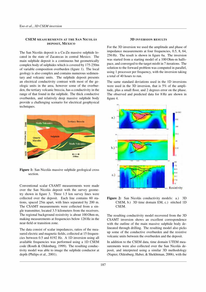
Eso, R. et al., 2007, 3D CSEM inversion . . .
CSEM MEASUREMENTS AT THE SAN NICOLÁSDEPOSIT, MEXICO
The San Nicolás deposit is a Cu-Zn massive sulphide lo-cated in the state of Zacatecas in central Mexico. Themain sulphide deposit is a continuous but geometricallycomplex body of sulphides which is covered by 175-250mof variable composition overburden (figure 1). The localgeology is also complex and contains numerous sedimen-tary and volcanic units. The sulphide deposit presentsan electrical conductivity contrast with most of the ge-ologic units in the area, however some of the overbur-den, the tertiary volcanic breccia, has a conductivity in therange of that found in the sulphide. The thick conductiveoverburden, and relatively deep massive sulphide bodyprovide a challenging scenario for electrical geophysicaltechniques.
Figure 1: San Nicolás massive sulphide geological crosssection.
Conventional scalar CSAMT measurements were madeover the San Nicolás deposit with the survey geome-try shown in figure 3. Three 1.5 km survey lines werecollected over the deposit. Each line contains 60 sta-tions, spaced 25m apart, with lines separated by 200 m.The CSAMT measurements were collected from a sin-gle transmitter, located 3.5 kilometers from the receivers.The regional background resistivity is about 100 Ohm-m,making measurements at frequencies below 128 Hz in thenear-field or transition zone.
The data consist of scalar impedances, ratios of the mea-sured electric and magnetic fields, collected at 15 frequen-cies between 0.5 and 8192 Hz. A 1D inversion using allavailable frequencies was performed using a 1D CSEMcode (Routh & Oldenburg, 1999). The resulting conduc-tivity model was able to image the sulphide conductor atdepth (Philips et al., 2001).
3D INVERSION RESULTS
For the 3D inversion we used the amplitude and phase ofimpedance measurements at four frequencies, 0.5, 8, 64,256 Hz. The result is shown in figure 6a. The inversionwas started from a starting model of a 100 Ohm-m halfs-pace, and converged to the target misfit in 7 iterations. Thesolution to the forward problem was computed in parallel,using 1 processor per frequency, with the inversion takinga total of 40 hours to run.
The same standard deviations used in the 1D inversionswere used in the 3D inversion, that is 5% of the ampli-tude, plus a small floor, and 2 degrees error on the phase.The observed and predicted data for 8 Hz are shown infigure 4.
Figure 2: San Nicolás conductivity models: a.) 3DCSEM, b.) 3D time domain EM, c.) stitched 1DCSEM.
The resulting conductivity model recovered from the 3DCSAMT inversion shows an excellent correspondencewith the outline of the main massive sulphide body de-lineated through drilling. The resulting model also picksup some of the conductive overburden and the resistivevolcanic units between the overburden and the deposit.
In addition to the CSEM data, time domain UTEM mea-surements were also collected over the San Nicolás de-posit, and interpreted using a similar 3D methodology(Napier, Oldenburg, Haber, & Shekhtman, 2006), with the
3/4
Eso et al., 3D CSEM inversion
187

Eso, R. et al., 2007, 3D CSEM inversion . . .
resulting inversion shown in figure 6b. The conductivitymodels in figures 6a and 6b are shown on the same colorscale, and show very similar structure. The stitched con-ductivity model obtained through a 1D inversion is shownin figure 6c. The 1D model shows the conductive sulphidebody at depth, and picks up the conductive overburdenlayer. However, the resulting image of the deposit is notas clear as in the 3D inversion models.
Figure 3: Observed and predicted amplitude and phaseimpedance measurements for 8 Hz
CONCLUSIONS
The CSEM data collected at San Nicolás are from a sin-gle transmitter, and a relatively large spacing between thesurvey lines, the CSAMT dataset over the San Nicolás de-posit is relatively limited dataset when compared to otherelectromagnetic datasets used in 3D inversions (Napieret al., 2006), (Oldenburg, Eso, Napier, & Haber, 2005).However, the resulting 3D interpretation of the CSAMTmodel shows a more defined deposit model when com-pared with the 1D interpretation and is in agreement withan independent 3D EM interpretation. The 1D modelsshow a sulphide resistivity of 20-30 Ohm-m for the mainbody, while the 3D models indicate a more conductive sul-phide, with resistivities in the range of 2-10 Ohm-m.
ACKNOWLEDGMENTS
We would like to thank Scott Napier, Nigel Philips andRoman Shekhtman at UBC-GIF for their help workingwith the San Nicolás field data and geological interpre-tation.
REFERENCES
Haber, E., & Ascher, U. (2001). Fast finite volume sim-ulation of 3d electromagnetic problems with higlydiscontinuous coefficients. SIAM J. Sci. Comput.,22(6), 1943-1961.
Haber, E., Ascher, U., Aruliah, D., & Oldenburg, D. W.(2000). Fast simulation of 3d electromagnetic prob-lems using potentials. J. of Comp. Physics, 163,150-171.
Haber, E., Ascher, U., & Oldenburg, D. W. (2004). In-version of 3d electromagnetic data in frequency andtime domain using an inexact all-at-once approach.Geophysics, 69, 1216-1228.
Kelley, C. (1999). Iterative methods for optimization.SIAM.
Napier, S., Oldenburg, D., Haber, E., & Shekhtman, R.(2006). 3d inversion of time domain data with ap-plication to San Nicolas. SEG Technical ProgramExpanded Abstracts, pp. 1303-1307.
Oldenburg, D. W., Eso, R., Napier, S., & Haber, E. (2005).Controlled souce electromagnetic inversion for re-source exploration. First Break, 23, 41-48.
Philips, N., Oldenburg, D., Chen, J., Li, Y., & Routh, P.(2001). Cost effectiveness of geophysical inver-sions in mineral exploration: Applications at SanNicolas. The Leading Edge, 20, 1351.
Routh, P., & Oldenburg, D. (1999). Inversion of controlledsource audio magnetotelluric data for a horizontallylayered earth. Geophysics, 64, 1689-1697.
4/4
Eso et al., 3D CSEM inversion
188

4th International Symposium on Three-Dimensional Electromagnetics Freiberg, Germany, September 27−30, 2007
1/4
A 3D magnetotelluric study of the basement structure in the Mygdonian Basin
(Northern Greece)
M. Gurk1, M. Smirnov2,3, A.S. Savvaidis1, L. B. Pedersen3 and O. Ritter4
1 Institute of Engineering Seismology and Earthquake Engineering (ITSAK), Greece 2University of Oulu, Finland
3University of Uppsala, Sweden 4GeoForschungsZentrum Potsdam (GFZ), Germany
SUMMARY During 2006 and 2007 a total number of 92 MT/GDS sites have been deployed in the Mygdonian basin (Northern Greece). This EM survey intends to infer the basement structure by means of 2D and 3D MT data inversion and to give information about the the top-of-basement depth for wave propagation models in the frame work of the “Euroseistest Volvi-Thessaloniki” project Keywords: MT, GDS, Mygdonian basin, Volvi area, Euroseistest, top-of- basement, 2D inversion, 3D inversion
INTRODUCTION The Mygdonian basin, situated between the two lakes Volvi and Lagada ca. 45 km northeast of Thessaloniki, is a neotectonic graben structure (5 km wide) with increased seismic activity along distinct normal fault patterns. Fluvioterrestrial and lacustrien sediments (350-400 m thick) are overlying the basement consisting of gneiss with schists. During the project “Euroseistest Volvi-Thessaloniki”, a European Test site for Engineering Seismology was employed in the valley in order to study velocity cross sections across the valley. In this context, the actual EM survey intends to map the top-of-basement to give input parameter for the seismic wave propagation models.
MT/GDS survey During 2006/2007 a total number of 92 MT/GDS sites have been installed in the Mygdonian basin (Fig. 1). The sites were roughly arranged on an orthogonal grid (North-South and East-West) reflecting the predominant East-West orientation of many normal faults in this area. The site spacing on this grid is about 1 km. Some areas in the mountain and around villages are not covered due to the increased EM noise or due to their inaccessibility.
MT and GDS data were collected using three MTU-2000 instruments with Metronix MFS05 coils from Uppsala University. One of these instruments was used as a Remote Reference site during the entire survey. The horizontal electric field components were measured with grounded non-polarisable Pb/PbCl electrodes. If possible, the electrode spacing was extended to a maximum of 100 m using a cross shaped configuration, having ground electrode in the middle of the cross (differential input). Generally, data were recorded in four bands with the sampling frequencies shown in Table 1.
Figure 1: Map of the study area with MT site locations
(triangles) and geological outlines.
4th International Symposium on Three-Dimensional ElectromagneticsFreiberg, Germany, September 27–30, 2007
189
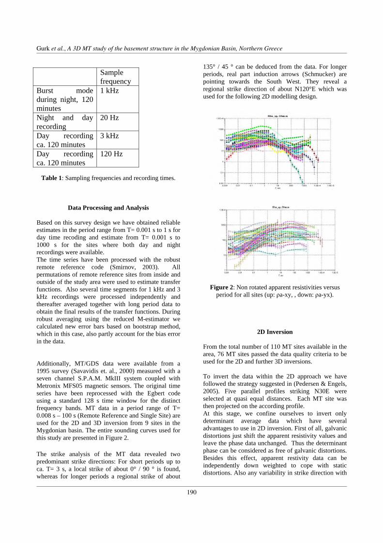
Author, A. et al., 2007, Short title goes here…
2/4
Table 1: Sampling frequencies and recording times.
Data Processing and Analysis Based on this survey design we have obtained reliable estimates in the period range from T= 0.001 s to 1 s for day time recoding and estimate from T= 0.001 s to 1000 s for the sites where both day and night recordings were available. The time series have been processed with the robust remote reference code (Smirnov, 2003). All permutations of remote reference sites from inside and outside of the study area were used to estimate transfer functions. Also several time segments for 1 kHz and 3 kHz recordings were processed independently and thereafter averaged together with long period data to obtain the final results of the transfer functions. During robust averaging using the reduced M-estimator we calculated new error bars based on bootstrap method, which in this case, also partly account for the bias error in the data. Additionally, MT/GDS data were available from a 1995 survey (Savavidis et. al., 2000) measured with a seven channel S.P.A.M. MkIII system coupled with Metronix MFS05 magnetic sensors. The original time series have been reprocessed with the Egbert code using a standard 128 s time window for the distinct frequency bands. MT data in a period range of T= 0.008 s – 100 s (Remote Reference and Single Site) are used for the 2D and 3D inversion from 9 sites in the Mygdonian basin. The entire sounding curves used for this study are presented in Figure 2. The strike analysis of the MT data revealed two predominant strike directions: For short periods up to ca. T= 3 s, a local strike of about 0° / 90 ° is found, whereas for longer periods a regional strike of about
135° / 45 ° can be deduced from the data. For longer periods, real part induction arrows (Schmucker) are pointing towards the South West. They reveal a regional strike direction of about N120°E which was used for the following 2D modelling design.
Figure 2: Non rotated apparent resistivities versus period for all sites (up: ρa-xy, , down: ρa-yx).
2D Inversion From the total number of 110 MT sites available in the area, 76 MT sites passed the data quality criteria to be used for the 2D and further 3D inversions. To invert the data within the 2D approach we have followed the strategy suggested in (Pedersen & Engels, 2005). Five parallel profiles striking N30E were selected at quasi equal distances. Each MT site was then projected on the according profile. At this stage, we confine ourselves to invert only determinant average data which have several advantages to use in 2D inversion. First of all, galvanic distortions just shift the apparent resistivity values and leave the phase data unchanged. Thus the determinant phase can be considered as free of galvanic distortions. Besides this effect, apparent restivity data can be independently down weighted to cope with static distortions. Also any variability in strike direction with
Sample frequency
Burst mode during night, 120 minutes
1 kHz
Night and day recording
20 Hz
Day recording ca. 120 minutes
3 kHz
Day recording ca. 120 minutes
120 Hz
Gurk et al., A 3D MT study of the basement structure in the Mygdonian Basin, Northern Greece
190

Author, A. et al., 2007, Short title goes here…
3/4
period does not affect the results as much as for bi-modal inversion, when the proper mode decomposition is vital. The 2D inversion routine by Siriponvaraporn and Egbert (Siriponvaraporn & Egbert, 2000) including the modifications made by Pedersen and Engels (Pedersen & Engels, 2005) allow for inversion of the determinant of the impedance tensor. Error floors equal to 2% for the impedance phase (corresponding to 1.2°) and 10 % for the apparent resistivities were adopted. Since there was no other information in order to constrain the static shift effect and the site spacing is relatively small, we have chosen a higher error floor for the resistivity data to give the inversion procedure more freedom to compensate for these effects. Finally, a homogeneous halfspace of 100 m was used for the initial and apriori model for all inversions. This procedure resulted in an overall good fit of the data to the model within the error bars (RMS 1).
Figure 3: 2D resistivity model of line B (see Fig. 1)
with RMS = 1, left corner SW, right corner NE, triangles, MT site location.
3D Inversion
The same data set, consisting of 76 pre-selected good quality sites, was used for the 3D inversion (Siriponvaraporn et al., 2005) and was found to be very well suitable for this task. Generally, MT data were measured on a more or less regular grid in the dimension of 12 km x 6 km with an approximately site distance of about 1 km. If necessary, additional high frequencies sites were deployed in between the main grid lines. The model grid itself was designed to have 2 cells between each site. During the first inversion trial we have selected only 3 periods in the frequency range from 1- 100 Hz. The grid therefore was constructed to be a 34 x 34 x 21 matrix including additional 10 horizontal outer cells to extend the grid (60 km) from each side of the grid. The second inversion trial included 8 periods in the frequency range of 0. 1– 100 Hz, using the same model grid, whereas the third inversion trial was characterized
by an increased number of cells in between sites and a better vertical discrimination at target depths (42 x 54 x 26 cells). For the 3D inversion we have used the complete impedance tensor (Zxx, Zxy, Zyx and Zyy) giving 4 complex data values at each site and frequency. For the 3D inversion as well as for the 2D inversion real error bar estimates were provided. After 4 successful iterations of the 3D routine, the RMS fit achieved values of about 10. Figure 4 shows a first example of the 3D model at 150-250 m depth.
Figure 4: 3D resistivity model at 150-250 m depth
CONCLUSIONS The use of MT data arranged on a grid revealed new information about the sediment thickness and the slope of the top-of-basement in the SE part of the investigation area which is of particular importance for the wave propagation model.
ACKNOWLEDGEMENTS
This study is supported by the project of the Marie Curie Action ITSAK-GR (International Transfer of Seismic Advanced Knowledge – Geophysical Research), MTCD-CT-2005-029627. We are greatly indebted to the students from Thessaloniki and Crete who took part in the fieldwork. Finally we would like to thank Lars Dynesius for all his technical help and support during the field measurements.
Gurk et al., A 3D MT study of the basement structure in the Mygdonian Basin, Northern Greece
191

Author, A. et al., 2007, Short title goes here…
4/4
REFERENCES Pedersen, L.B. and Engels, M. (2005). Routine 2D inversion of Magnetotelluric data using the determinant of the impedance tensor. Geophysics 70, G33-G41. Savvaidis, A. Pedersen, L. B., Tsokas, G. N., Dawes, G. J., (2000). Structure of the Mygdonian Basin (N. Greece) inferred from MT and gravity data, Tectonophysics, 317, 171-186. Siripunvaraporn W. and Egbert G, (2000). An efficient data-subspace inversion method for 2-D magnetotelluric data. Geophysics, 65, 791–803. Siripunvaraporn W., G. Egbert, Y. Lenbury and M. Uyeshima. (2005). Three-Dimensional Magnetotelluric: Data Space Method, Physics of the Earth and Planetary Interiors, 150, 3-14. Smirnov, M., (2003). Magnetotelluric data processing with a robust statistical procedure having a high breakdown point, Geophys.J.Int., 152, 1-7.
Gurk et al., A 3D MT study of the basement structure in the Mygdonian Basin, Northern Greece
192

4th International Symposium on Three-Dimensional Electromagnetics Freiberg, Germany, September 27−30, 2007
1/4
3D inversion of magnetotelluric data from the Rotokawa geothermal field, Taupo
Volcanic Zone, New Zealand
Wiebke Heise, T. Grant Caldwell, Hugh M. Bibby GNS Science, Lower Hutt, New Zealand
SUMMARY 3D inverse modelling of 58 magnetotelluric (MT) soundings from a high temperature geothermal system from New Zealand’s Taupo Volcanic Zone has been carried out in order to investigate the deeper structure of the geothermal system. The resulting model shows that the high temperature core of the geothermal system is associated with a resistive feature beneath a cap of highly conductive clays. Phase tensor misfits were used to show the spatial distribution of the misfits and suggest that the model has captured the main features of the data. Keywords: magnetotellurics, geothermal system, phase-tensor, 3D modelling
INTRODUCTION The Taupo Volcanic Zone (TVZ) in the central North Island of New Zealand is a region of young rhyolitic volcanism and rapid crustal extension. This region is characterised by an exceptionally high geothermal heat flow, 4200 MW, which is discharged through 23 high temperature (>200°C) convective hydrothermal systems. The uppermost 1 – 2 km of the TVZ are composed of a mixture of rhyolite lavas, welded and unwelded ignimbrites and volcaniclastic sediment. This material is resistive ( ≥ 300 Ωm) at shallow depth except where it has been hydrothermally altered. However, at deeper levels, this same material becomes conductive (10 – 30 Ωm) at low temperatures due to a diagenetic aging process in which small amounts of conductive clays and zeolites are formed within the rhyolitic volcanics. Thus, outside the geothermal systems, the conductivity-depth structure of the TVZ is characterised by a layer of young, resistive volcanics overlying a layer of much more conductive older volcanics. The basement rocks (greywacke meta-sediments) beneath the volcanics are resistive (300 - 1500 Ωm). The near-surface low resistivities that mark the geothermal fields are caused by the combination of high temperature, saline fluid and hydrothermal alteration of the young volcanics. At depths greater than ~500 m, the resistivity values increase due to decreasing pore space and a change in the type of hydrothermal alteration products (clays) at higher temperatures.
Figure 1. DC apparent resistivity map from Schlumberger array measurements made with an electrode spacing of (AB/2) 500 m. Conductive areas shown in red (<30 Ωm) mark the geothermal systems (Bibby et al. 1995).
MAGNETOTELLURIC DATA
Recently, an MT survey consisting of 64 broadband (0.3 ms – 2000 s) soundings was conducted to investigate the deeper structure of the Rotokawa geothermal field. The distribution of the measurement sites is shown in Figure 2. Site spacings are 200 m - 500 m in the central part of the geothermal field, (i.e. the area characterised by the low Schlumberger apparent resistivity anomaly, Figure 1).
4th International Symposium on Three-Dimensional ElectromagneticsFreiberg, Germany, September 27–30, 2007
193

Heise, W. et al., 2007, 3D inversion of MT data from Rotokawa geothermal system, New Zealand
2/4
Representation of the data as phase tensor maps (Caldwell et al., 2004) provides a distortion free method of visualizing the conductivity gradients of the data and allows identification of main features of the conductivity structure prior to modelling. Phase tensor ellipses at different periods are shown in Figure 2. For periods between 0.1 s and 1 s the mean phase averaged over polarisation direction Φ2 in the centre of the geothermal system is >45º indicating increasing resistivity with depth. At periods >3s the major axis of the phase tensor ellipses become aligned to the NE striking regional conductivity structure known from long offset resistivity studies (Bibby et al. 1998; Risk 2000) and regional MT studies (Ogawa et al. 1999; Heise et al. 2007). The conductivity structure producing this alignment reflects the down faulting of the greywacke basement along the SE margin of the TVZ.
3D MODELLING 3D inverse modelling was carried out using the code WSINV3DMT described by Siripunvaraporn et al. (2005). For the inversion, the data at 58 sites was interpolated at 2 points per decade for a period range of 1-30s. Data was selected carefully, omitting noisy soundings (e.g. sites affected by electric fences) and obvious outliers from the soundings retained for the inversion. A uniform 5 % error was assumed for all impedances. For soundings where the phase tensor analysis identified a 1D section of the sounding curve at short periods, galvanic distortion was removed using the method of Bibby at al. (2005). This method retrieves the shape of sounding curves. The scale of the sounding was set by comparison with TEM soundings made at each location and comparison with the Schlumberger apparent resistivity data. Discretisation in the central part of the model was regular with a cell width of 400m. The inversion reached a minimum rms 5.77 after 6 iterations. Computation time was 8 days on the workstation (Sun Fire X2200 M2 with two Dual-Core AMD Opteron 2214 processors and 12 GB of RAM). The degree and spatial distribution of misfit can be assessed from the phase misfit tensors in Figure 3,
1 1obs mod mod obs( ) / 2− −= − + I ,
where I is the identity matrix. The magnitude of the misfit is indicated by both the size of the ellipse and the colour used to fill the ellipses which indicates the mean of the absolute value of the residual tensor principal axes
max min( ) / 2∆ + ∆ . The ellipse orientation indicates
the polarisation direction in which the maximum difference occurs. Figure 4 shows a 3D view of the resulting conductivity model.
Figure 2. Normalised phase tensor ellipses at each measurement site for periods between 0.01 and 31s. The ellipses are normalised by
maxΦ and the colour
scale shows the geometric mean max min2Φ = Φ Φ which
measures the mean phase averaged over polarisation directions. The high values of
2Φ outside the
geothermal system indicate decreasing resistivity. Note the low phase values in the centre of the geothermal system for 0.31 s indicating a resistor at depth.
Heise et al., 3D inversion of MT data from the Rotokawa geothermal system, New Zealand
194

Heise, W. et al., 2007, 3D inversion of MT data from Rotokawa geothermal system, New Zealand
3/4
Figure 3. Phase misfit tensor at periods between 0.01 and 31s for the model shown in Figure 4.
RESULTS AND DISCUSSION At shallow depth (15 m - 200 m) the geothermal field is characterised by low resistivities (2 - 5 Ωm) caused by relatively high temperatures and conductive clays (smectites) which are the hydrothermal alteration products at these temperatures (~100ºC). With increasing depth the resistivity increases to ~30 Ωm and then decreases again to 10 Ωm at depth >500 m. These changes in resistivity are interpreted to result from the interplay of temperature, fluid chemistry and
porosity which control the nature of the alteration products (clays) inside and at the margins of the geothermal system. Outside the geothermal system the top 500 m of young volcanics are resistive (>300 Ωm) but become more conductive (30 -10 Ωm) below about 600 m. At depths of ~1200 m within the geothermal field the resistivity increases rapidly to values >100 Ωm. This high resistivity body corresponds with the hottest part of the geothermal system, known from drilling. At high temperatures the alteration products formed are less conductive illicitic and chloritic clays.
Figure 4. 3D inversion model of Rotokawa geothermal system. Earthquake hypocentres (Bannister un-published data) shown as black dots correlate with the high resistivity body.
CONCLUSIONS The 3D inversion code WSINV3DMT by Siripunvaraporn et al. (2005) applied to a dense MT dataset gives a geologically consistent model of the conductivity structures. Representation of the model’s misfit as phase misfit tensors shows that the main resistivity features of the data are explained by the model. The most interesting feature of the modelling is the high resistivity body in the central part of the geothermal field. This feature correlates spatially with the area of highest temperature. Earthquake hypocenters concentrate along the margins of the resistive body. Thus it appears that the resistive high temperature (>300ºC) core of the geothermal system
Heise et al., 3D inversion of MT data from the Rotokawa geothermal system, New Zealand
195

Heise, W. et al., 2007, 3D inversion of MT data from Rotokawa geothermal system, New Zealand
4/4
imaged by MT also corresponds to relatively strong material which supports brittle failure.
ACKNOWLEDGEMENTS
We thank the Rotokawa Joint Venture for supplying data and approval to publish.
REFERENCES
Bannister, unpublished data.
Bibby, H.M., Caldwell, T.G., and Brown, C., (2005). Determinable and non-determinable parameters of galvanic distortion in magnetotellurics, Geophysical Journal International, 163, 915-930.
Bibby, H.M., Caldwell, T.G., Davey, F.J. and Webb, T.H., (1995). Geophysical evidence on the structure of the Taupo Volcanic Zone and its hydrothermal circulation. Journal of Volcanology and Geothermal Research, 68, 29-58.
Bibby, H.M., Caldwell, T.G. and Risk, G.F (1998). Electrical resistivity image of the upper crust within the Taupo Volcanic Zone, New Zealand. Journal of Geophysical Research, 103. 9665-9680.
Caldwell, T.G., Bibby, H.M. and Brown, C., (2004). The magnetotelluric phase tensor. Geophysical Journal International, 158, 457-469.
Heise, W., Bibby, H.M., Caldwell, T.G., Bannister, S.C., Ogawa, Y., Takakura, S. and Uchida, T., (2007). Melt distribution beneath a young continental rift: the Taupo Volcanic Zone, New Zealand. Geophysical Research Letters, in press.
Mackie, R.L. and Booker, J. (1999). Documentation for mtd3fwd and d3-to-mt. GSY-USA, Inc.,2261 Market St., Suite 643, San Francisco, CA 94114. User documentation.
Ogawa, Y., Bibby, H.M., Caldwell, T.G., Takakura, S., Matsushima, N., Bennie, S.L., Tosha, T. and Nishi, Y. (1999). Wide-band magnetotelluric measurements across the Taupo volcanic zone: preliminary results. Geophysical Research Letters, 26, 3673-3676.
Risk, G.F., (2000). Electrical resistivity surveys of the Rotokawa geothermal field, New Zealand. p. 121-126 In: Dunstall, M.G.; Morgan, O.E.; Simmons, S.F. (eds.)Proceedings of the 22nd New Zealand Geothermal Workshop 2000. Auckland: University of Auckland.
Siripunvaraporn W., Egbert, G., Lenbury, Y., and Uyeshima, M., (2005). Three-Dimensional
Magnetotelluric: Data Space Method, Phys. Earth Planet. Inter., 150, 3-14.
Heise et al., 3D inversion of MT data from the Rotokawa geothermal system, New Zealand
196
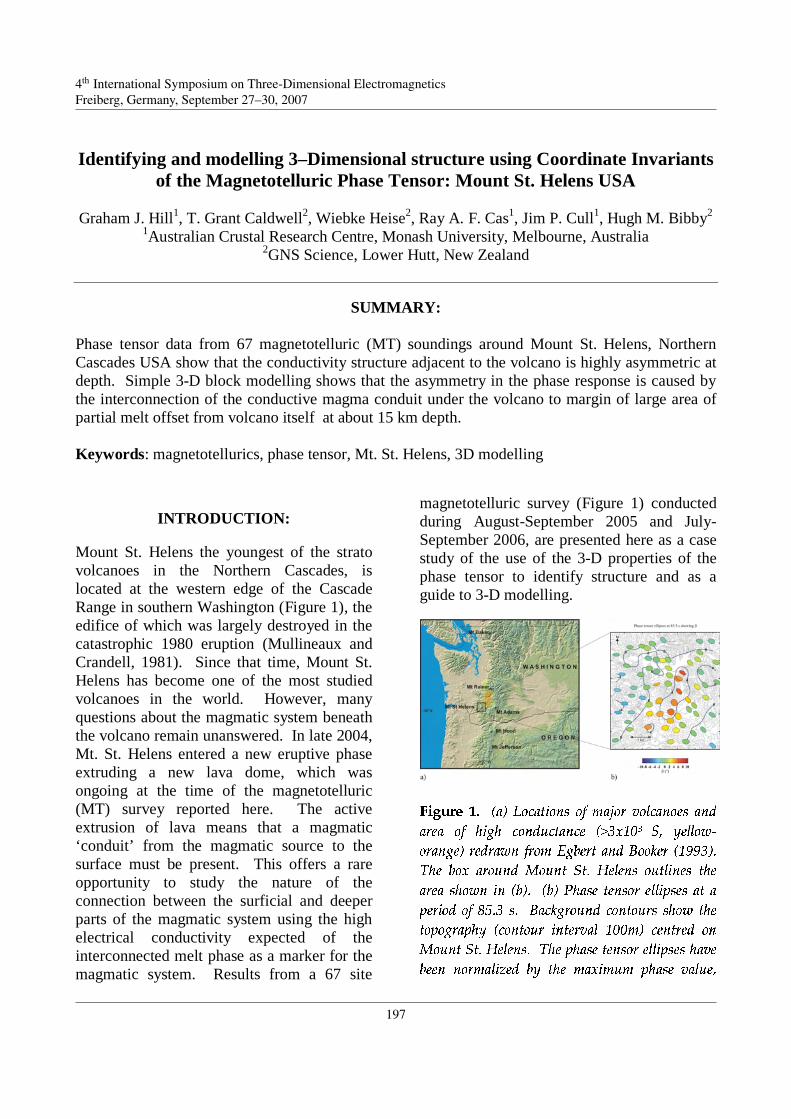
4th International Symposium on Three-Dimensional Electromagnetics Freiberg, Germany, September 27−30, 2007
1/4
Identifying and modelling 3–Dimensional structure using Coordinate Invar iants
of the Magnetotellur ic Phase Tensor : Mount St. Helens USA
Graham J. Hill1, T. Grant Caldwell2, Wiebke Heise2, Ray A. F. Cas1, Jim P. Cull1, Hugh M. Bibby2
1Australian Crustal Research Centre, Monash University, Melbourne, Australia 2GNS Science, Lower Hutt, New Zealand
SUMMARY:
Phase tensor data from 67 magnetotelluric (MT) soundings around Mount St. Helens, Northern Cascades USA show that the conductivity structure adjacent to the volcano is highly asymmetric at depth. Simple 3-D block modelling shows that the asymmetry in the phase response is caused by the interconnection of the conductive magma conduit under the volcano to margin of large area of partial melt offset from volcano itself at about 15 km depth. Keywords: magnetotellurics, phase tensor, Mt. St. Helens, 3D modelling
INTRODUCTION: Mount St. Helens the youngest of the strato volcanoes in the Northern Cascades, is located at the western edge of the Cascade Range in southern Washington (Figure 1), the edifice of which was largely destroyed in the catastrophic 1980 eruption (Mullineaux and Crandell, 1981). Since that time, Mount St. Helens has become one of the most studied volcanoes in the world. However, many questions about the magmatic system beneath the volcano remain unanswered. In late 2004, Mt. St. Helens entered a new eruptive phase extruding a new lava dome, which was ongoing at the time of the magnetotelluric (MT) survey reported here. The active extrusion of lava means that a magmatic ‘conduit’ from the magmatic source to the surface must be present. This offers a rare opportunity to study the nature of the connection between the surficial and deeper parts of the magmatic system using the high electrical conductivity expected of the interconnected melt phase as a marker for the magmatic system. Results from a 67 site
magnetotelluric survey (Figure 1) conducted during August-September 2005 and July-September 2006, are presented here as a case study of the use of the 3-D properties of the phase tensor to identify structure and as a guide to 3-D modelling.
"!#%$'&(*)+-,. /%0 1!- 2345376%8:9"; <9>=6 ?"@"A=B3 ?=5DCEF.GH IKJML.NPORQS S TUWVXYZ [.\]^_Y]`.YaZbc[edYX fhgi\kj]YmlnZ [`poqXXsrt]Yvu*w xxyR^z|.~s k k_~ ~' %%~~.e %¢¡£s¤¥P¡£¤§¦.-¨(m©%©% ªv¨«¬®¯ °±²°%³´¶µk· ¸¹m·¢º¼» ½0¾m¿®° ÀkÁ±½0° Á° À®¹(¹Ã° ÄÅÂÃÆÇÈÇÉÊËÈ"ÌÍÏÎÐÇ ÑÆÇ Ò"ÊÓ%ÑÆÔaÊÕ.Ë Ö×Ø.Ø.ÙcÚpÐÔÑÆÊÔÛÜÇ ÑÝÞ ßàáâáãäåæ åàçmãpèké.åëê"é.ìçå§áåà"çÞí_åæ%æ%î êçåç_é.ìïåðññòóòôõö(÷ø%ù úñûüðsýÏþÿ "ÿ
4th International Symposium on Three-Dimensional ElectromagneticsFreiberg, Germany, September 27–30, 2007
197

Hill, G. J. et al., 2007, Identifying and modelling 3–Dimensional structure using Coordinate Invariants of the Magnetotelluric Phase Tensor: Mount St. Helens USA
2/4
! "$# %& ' ()+*-,/. 02134$5$687-9 5;:'5<6=->"5?9 ='9 5$:'5A@3!6CB4EDGFH3-9 IJKCLCMONQPMLR'S-TVULSXWLRMY?YZLC[\WZN^]-Z_CYN`WNS-YLCMaYbcN[de!f'g hEikjalmhnmohpdCqhdrlsro-t foGuvchwxdefHg hnyz!|~ COE-ECC !! -'- C a H¡¢£ ¤¥¢¦!V§O£¨'¨-§E¢© £¨A£ ¤G¢¦rª$«¬Hª$«§£¨®- H©¢¯8°±°²´³µ¶·¸H±X³2¹'³»º½¼a°¾ °±-¿r³·G³µ°pÀ·±°n· Áµ-à ĵÅÆÇÈ-ÉHÅEÊËÇ'ÅÌÎÍ Ç2ÊÏ!ÌÎÇ-ÆCÐEÊÏÌËÑEÊ»Ò
PHASE TENSOR DATA: The phase relationships inherent in the impedance tensor Z form a second rank 2-D tensor defined by the matrix equation Ó
= X-1Y (1) where X = Re(Z) and Y =Im(Z) (Caldwell et al., 2004). Graphically the phase tensor can be represented as an ellipse, with the principal axes corresponding to the major and minor axes. While the orientation of the ellipse is dependent of the coordinate system, the ellipse radii are coordinate invariant. If the tensor is symmetric the principal axes (i.e. the ellipse size and orientation) completely describe the tensor. However, if the conductivity structure is asymmetric then, in general, Ô will be non-symmetric and an additional (co-ordinate invariant) parameter is required to complete the description of the tensor. This parameter measures the asymmetry of the phase response and is represented by the skew angle Õ defined as Ö = ½ tan-1 ( × xy – Ø yx)/( Ù xx + Ú yy) (2) where Û can be thought of as the amount that the phase tensor principal axes have been rotated away from a corresponding symmetric response.
3D MODELLING OF THE SKEW DATA: The pattern of phase tensor skew near the volcano at T=85 s (Figure 1b) suggests that conductivity distribution at depth is strongly asymmetric in a localised region around the volcano. This asymmetry appears to be the result of a connection between an extensive zone of high conductance known to exist in the mid-crust (Stanley 1983, Egbert and Booker 1993) (Figure 1a) west of Mount St. Helens and a localised zone of high conductivity beneath the volcano itself. We tested this inference using simple 3-D block models (Figure 2) based on preliminary 2-D inverse modelling results.
Ü'Ý»Þßàáâãaäåæç è$éêëç ìê-íîïCìCðñíCðò2è^ìCòéî îç ê!óXô`õíö÷øùûúüCýkþHÿ "!#$%&(')+*$ ,.-/*#'*#0('21 -3)'54768*#0('54:9;)'<&('=>*0('@?ABCEDFGC BIH7JLK MONQPRSNTHURWVG.XYH#X(RZD.[(VCBI\#BGC FA]C_^`Babc(de fhgfiEjkc.ifimlknko(feQp#bqrbcospt;q#uLgvwEx.vy+z|~(v (#r# .:/. .#(_`( LO
Hill et al., Identifying 3D structure using coordinate invariants of the MT phase tensor
198

Hill, G. J. et al., 2007, Identifying and modelling 3–Dimensional structure using Coordinate Invariants of the Magnetotelluric Phase Tensor: Mount St. Helens USA
3/4
The responses of the two different block models shown in figure 2 were calculated using Mackie et al’s (1994) 3-D forward modelling code. In order to reproduce the pattern observed in the skew angle, a model with a conductive conduit connected to conductive block at depth is required; the connection being the crucial element in the model needed to produce the large skew response. The overall response of this oversimplified block model (Figure 2a) does a surprisingly good job of modelling the essential features of the observed phase tensor data (Figure 1) near the volcano itself. However, the models do not reproduce the general NW-SE orientation of the phase tensor ellipse major axes at 85 s (Figure 1). This is a mainly consequence of the boundary of the large conductive zone west of Mount St. Helens (inferred to be a zone of partial melt) extending further southward and trending more SE-NW than modelled in Figure 2. The southward extension and SE-NW trend can be seen directly in observed phase tensor maps (Figure 3) plotting the geometric mean of the phase, i.e. ( min max)
1/2, rather than the skew.
CONCLUSIONS: The models shown in Figure 2 are good examples of how the existence of large 3-D effects in the phase tensor data (i.e. phase tensor skew and lateral changes in principal axes orientation) can be used to make important inferences about the geology directly from the observations and then tested using 3-D forward modelling. Using the observed phase tensor results as a guide, we intend to improve our forward model and this use this model as a check on the reliability of 3-D inverse-modelling results.
"!#%$&$&' (*)&+-,.0/*)"132/45/678:98<;:=>;@?ABCEDF*D&G<H0IJ KLMJONQP"RTSMUVW"XYZRW"Y\[&W"XV]^_`acb_debf`g`hijg_lknmfo`"p\b`"qisr&p\bdit0j"uOvlww0xzy|\~|"*"\~~@|&|M0||~|%&& #0%s ¡z¢"£¤ ¥3¦%§¨©*¡z¢%ª¤¡@«¬¡®¯°±²¯"³&´±¶µ·¹¸»º®¼º®±½±³&³&¸ °¾±¿À"³&À"´Á¸&Ãĸ&¿¾¯:ºf¸&ÃÅƺ®0±ÇÈÉ"ÊzÈMËÌMÍ&ÎÏÊzÈÐ"ÑÓÒÔÖÕ×ÙØ&ÚÜÛÝ0ÞÏßzà%áâ&ßÖãßäà"åæç@è&éè&çÖêçìëíîïðMñ@ò¬íè&óTô¬õö÷¾ð¶ø÷ö"êéù@óö"é\úö"ê÷ïûïíöüýþÿþÿýÿ 3ÿ ÿ ! "#$&%')(*+, % -/.10325476 8 8#%9;:<=#9>%?(#9>6 8@9/A%CBDE/F?GH=DJIKLM NPOQRJS5T=UQVMWNCRXUQNTZY[S>\ O@S/LQV]\^^=Q]_S5M \^`\/OS/LQacbda>bfeghijkml;noh=o?bJl/prqsgjhtl;utlwvZxyozWoh=cl[gl/po|&~= ~=Z/~7 ~@/c~=/W; ?/ r/ ¢¡Z ££ ¤>¥ ¡=¦=§/?=¨ ¡©=ª¬«5®°¯
REFERENCES: Caldwell, T. G., Bibby, H. M., & Brown, C.
The magnetotelluric phase tensor. Geophys. J. Int. 158 457-469 (2004).
Hill et al., Identifying 3D structure using coordinate invariants of the MT phase tensor
199

Hill, G. J. et al., 2007, Identifying and modelling 3–Dimensional structure using Coordinate Invariants of the Magnetotelluric Phase Tensor: Mount St. Helens USA
4/4
Egbert, G. D., & Booker, J. R. Imaging crustal structure in south western Washington with small magnetometer arrays. J. Geophys. Res. 98 (B09) 15967-15986 (1993).
Mackie, R. L., Smith, J. T., & Madden, T. R.
Three-dimensional electromagnetic modelling using finite difference equations: The magnetotelluric example. Radio Science 29 923-935 (1994).
Mullineaux, D. R., & Crandell, D. R. The
eruptive history of Mount St. Helens, U.S. Geol. Surv. Prof. Pap. 1250 3-16 (1981).
Stanley, W. D. Tectonic study of the Cascade
Range and Columbia Plateau in Washington based upon magnetotelluric soundings. J. Geophys. Res. 89 (B06) 4447-4460 (1983).
Hill et al., Identifying 3D structure using coordinate invariants of the MT phase tensor
200
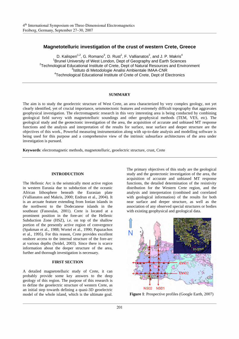
4th International Symposium on Three-Dimensional Electromagnetics Freiberg, Germany, September 27−30, 2007
1/2
Magnetotelluric investigation of the crust of western Crete, Greece
D. Kalisperi1,2, G. Romano3, D. Rust1, F. Vallianatos2, and J. P. Makris4
1Brunel University of West London, Dept of Geography and Earth Sciences 2Technological Educational Institute of Crete, Dept of Natural Resources and Environment
3Istituto di Metodologie Analisi Ambientale IMAA-CNR 4Technological Educational Institute of Crete of Crete, Dept of Electronics
SUMMARY The aim is to study the geoelectric structure of West Crete, an area characterized by very complex geology, not yet clearly identified, yet of crucial importance, seismotectonic features and extremely difficult topography that aggravates geophysical investigation. The electromagnetic research in this very interesting area is being conducted by combining geological field survey with magnetotelluric soundings and other geophysical methods (TEM, VES, etc). The geological study and the geotectonic investigation of the area, the acquisition of accurate and unbiased MT response functions and the analysis and interpretation of the results for surface, near surface and deeper structure are the objectives of this work., Powerful measuring instrumentation along with up-to-date analysis and modelling software is being used for this purpose and a comprehensive view of the intrinsic subsurface architectures of the area under investigation is pursued. Keywords: electromagnetic methods, magnetotelluric, geoelectric structure, crust, Crete
INTRODUCTION The Hellenic Arc is the seismically most active region in western Eurasia due to subduction of the oceanic African lithosphere beneath the Eurasian plate (Vallianatos and Makris, 2000; Endrun et al., 2004). It is an arcuate feature extending from Ionian islands in the northwest to the Dodecanese islands in the southeast (Fassoulas, 2001). Crete is located at a prominent position in the fore-arc of the Hellenic Subduction Zone (HSZ), i.e. on top of the shallow portion of the presently active region of convergence (Spakman et al., 1988; Wortel et al., 1990; Papazachos et al., 1995). For this reason, Crete provides excellent onshore access to the internal structure of the fore-arc at various depths (Seidel, 2003). Since there is scarce information about the deeper structure of the area, further and thorough investigation is necessary.
FIRST SECTION A detailed magnetotelluric study of Crete, it can probably provide some key answers to the deep geology of this region. The purpose of this research is to define the geoelectric structure of western Crete, as an initial step towards defining a quasi-3D geoelectric model of the whole island, which is the ultimate goal.
The primary objectives of this study are the geological study and the geotectonic investigation of the area, the acquisition of accurate and unbiased MT response functions, the detailed determination of the resistivity distribution for the Western Crete region, and the analysis and interpretation (combined and correlated with geological information) of the results for both near surface and deeper structure, as well as the association of any observed special structures or bodies with existing geophysical and geological data.
Figure 1: Prospective profiles (Google Earth, 2007)
4th International Symposium on Three-Dimensional ElectromagneticsFreiberg, Germany, September 27–30, 2007
201

Kalisperi, D. et al., 2007, Magnetotelluric investigation of the crust of western Crete, Greece
2/2
SECOND SECTION
These objectives are being fulfilled by means of a grid MT-survey featuring high density MT-station spacing (~5Km), broad frequency range of the MT-soundings (0.001 to 1000Hz, providing information from shallow to deeper layers), and the complementary use of near surface electromagnetic and electrical geophysical methods. Furthermore, the use of improved instrumentation and modern processing and modelling techniques is anticipated to provide enhanced resolution and more reliable results.
Subsection A careful field procedure is crucial to obtaining successful results, thus site selection and sensor installation are two major factors governing data quality. Four initial MT profiles have been planned for this study and each profile comprises 10 to 15 soundings. Two of them are parallel to each other and they have N-S orientation. They are sited about 5Km and 15Km from the western coast respectively. The other two profiles have W-E orientation and similarly are parallel to each other and they are sited about 5Km and 15Km apart from the southern coast respectively (Fig. 1).
CONCLUSIONS The investigation of West Crete, a very complex area from all points of view, by means of magnetotellurics is the aim of this research. Dealing with the problem involves careful field campaign, use of high performance instrumentation, high quality data collection and advanced analysis, modelling and interpretation. Furthermore, the complementary implementation of near surface electromagnetic and electrical geophysical methods, the correlation with geological information and the combination of the results with existing geophysical and geological data will give insight to a comprehensive understanding of the subsurface deep structure.
ACKNOWLEDGEMENTS This work is supported from the project "Archimedes II: Support of Research Teams of Technological Educational Institute of Crete", sub-project No 2.2.4 entitled: "Combined Technological & Methodological Approach of Geoelectromagnetic Study of Western Crete" in the frame of Operational Programme for
Education and Initial Vocational Training (O.P. "Education") one of the Third Community Support Frameworks Operational Programmes (2000-2006) in Greece, co-financed from European Social Fund (75%) and National Resources (25%).
REFERENCES Enrdun, B., Meier, T., Bischoff, M., and Harjes, H.-P. (2004). Lithospheric structure in the area of Crete constrained by receiver functions and dispersion analysis of Rayleigh phase velocities. Geophys. J. Int. 158: 592-608. Fassoulas C. (2001). The tectonic development of a Neogene basin at the leading edge of the active European margin: the Heraklion basin, Crete, Greece. Journal of Geodynamics 31: 49-70. Papazachos, C. B., Hatzidimitriou, P. M., Panagiotopoulos, D. G., Tsokas, G. N. (1995). Tomography of the crust and upper mantle in southeast Europe. J. Geophys. Res. 100 (B7): 12405-12422). Seidel, M. (2003). Tectono-sedimentary evolution of middle Miocene supra-detachment basins (Western Crete, Greece). Ph.D. Thesis. Universität zu Köln. Spakman, W., Wortel, M. J. R., and Vlaar, N. J. (1988). The Hellenic subduction zone: a tomographic image and its geodynamic implications, Geophys. Res. Lett. 15: 60-63. Vallianatos F. and Makris J. (2000). On the tectonoelectric zonation in the Hellenic Arc, Physics and Chemistry of the Earth, 25/3: 307-313. Wortel, M. J. R., Goes, S. D. B., and Spakman, W. (1990). Structure and seismicity of the Aegean subduction zone, TerraNova. 2: 554-562.
Kalisperi et al., Magnetotelluric investigation of the crust of western Crete, Greece
202

4th International Symposium on Three-Dimensional Electromagnetics Freiberg, Germany, September 27−30, 2007
1/4
Three-dimensional interpretation of MT data from mid-mountain area of Jeju Island,
Korea
Tae Jong Lee1, Seong Kon Lee1, Yoonho Song1, Myung Jin Nam2, and Toshihiro Uchida3
1Korea Institute of Geoscience and Mineral Resources (KIGAM), Korea, [email protected] 2 The University of Texas at Austin, USA
3 National Institute of Advanced Industrial Science and Technology (AIST), Japan
SUMMARY Magnetotelluric (MT) surveys have been performed along five lines in the Jeju volcanic island located at South Sea of Korea. The purposes of the MT surveys are to see if there still remain thermal resources and to see if there exist deeply extended fractures or an aquifer system beneath the mid-mountain region of Mt. Halla in Jeju. By operating far-remote reference site of approximately 480 km apart, we could get MT data of totally 108 sites with very good quality. Because the island is surrounded by electrically conductive sea and has topographic variation, measured MT data in terms of impedance may be seriously biased by distortion of electric fields. A 3D modeling result show that MT data higher than 1 Hz seem to be free from influence of the sea water at most of measurement points in the mid-mountain area. 3D inversion of MT data from 89 measurement sites gives a reasonable estimation of the subsurface structures beneath the island. An induction vector analysis and 3D inversion results commonly indicate the existence of a conductive anomaly extended down to a few-kilometer depth beneath the central part of the island, which can be related to ancient volcanic activities. Keywords: three-dimensional (3D), magnetotelluric surveys, geothermal energy, Jeju Island
INTRODUCTION Jeju Island is a Quaternary volcanic island located in the South Sea of Korea and is one of the most famous tourist spot in Korea. It is 31 km wide and 75 km long in the ENE direction, and 1,800 km2 in area (Fig. 1). It has Mt. Halla (1,950 m high) and more than 360 parasitic cones all across the island. Mt. Halla has gentle slopes in the east and west while steep slopes in the south and north. It lastly erupted in 1007 AD and the last volcanic activity (earthquakes) has been reported in 1570.
Several deep (>800 m) and more than a thousand of shallow boreholes that have been drilled to exploit hot springs and groundwater revealed that basaltic lava flows are underlain by a few hundred of meter thick sedimentary rocks (Seogwipo Formation, SF) the U formation (Unconsolidated sediment formation, UF) of Plio-Pleistocene age, and Cretaceous basement rocks. The basement rocks are mainly welded tuffs and granites, which lie at a depth about 250 ~ 300 m below the sea level. Both SF and UF are marine-based sedimentary layers and are electrically conductive (< 10 ohm-m; Lee et al., 2006).
Though more than a thousand of boreholes have been drilled within the island, most of drillings and geological investigations are concentrated only on the areas at low elevation or near the sea shore, where most of populations are accumulated, for development of groundwater or hot springs. Consequently, geology of the mid-mountain area has not been studied well.
During three years from 2004 to 2006, Korea Institute of Geoscience and Mineral Resources (KIGAM) and National Institute of Advanced Industrial Science and Technology (AIST), Japan performed joint magnetotelluric (MT) surveys at mid-mountain area of the Jeju volcanic island to cover the lack of geological information. The major purpose of the surveys is to figure out the deep geologic structures beneath mid-mountain area, which may be related with a remnant thermal regime associated with volcanic eruption. Because the island is surrounded by electrically conductive sea and has a topographic variation, measured MT data in terms of impedance may be seriously biased by distortion of electric fields. Topography in the mid-mountain area is not very steep as it can affect the MT responses (Song et al., 2006). In
4th International Symposium on Three-Dimensional ElectromagneticsFreiberg, Germany, September 27–30, 2007
203

Lee, T. J. et al., 2007, 3D interpretation of MT data in Jeju Island, Korea
2/4
this study, effects of surrounding sea water are first investigated by performing three-dimensional (3D) modelling using an edge finite element algorithm, which can accommodate topographic variations (Nam et al., 2007). For the modelling, a general one-dimensional (1D) geological model including sea-shore boundary is set up based on the numerous drilling results. Then we perform a 3D inversion of MT data from the mid-mountain area of Jeju Island.
MT DATA ACQUISITION
Figure 1: Location map of MT survey lines. Remote reference for MT band is located in Kyushu, Japan, which is about 480 km apart (RR). MT data from 89 sites within the rectangle (excluding bad quality data) are used for 3D inversion. A total of 108 measurements was made during the three years using Phoenix MTU-5A systems as shown in Fig. 1. Green, red, and blue dots in Fig. 1 indicate locations of MT sites surveyed in the years of 2004, 2005, and 2006, respectively. The five lines surround the mid-mountain area (< 600 m) of Mt. Halla. Four to seven sets of MTU-5A systems are used for the survey, including one set for the far-remote reference in Kyushu, Japan, which is about 480 km apart from Jeju (RR in Fig. 1). MT measurements are performed for 15 hours from 17:00 to 08:00 next morning. Good quality data have been acquired from the MT surveys in the mid-mountain area of Jeju Island. Fig. 2 shows observed MT data in terms of apparent resistivity and phase sounding curves at stations JJW 360 and JJN 561 after remote reference processing. The sounding curves show typical three-layered responses: resistive top layer, conductive middle layer and resistive bottom layer.
Figure 2: Remote reference processed MT responses at stations (a) JJW 360 and (b) JJN 561.
3D MT MODELLING & INVERSION An 1D layered structure as shown in Fig. 3 is assumed to investigate the effect of surrounding seas around Jeju Island based on general stratigraphy based on numerous drilling results for groundwater development (Koh, 1997). The sea water is also assumed to be flat horizontal layer with 90m thick, which is average depth to the seafloor around Jeju Island (Song et al., 2006). Using the 1D resistivity structure with sea shore boundary shown in Fig. 1, 3D MT modelling is performed. Fig. 4 shows the calculated MT sounding curves at the same locations as those considered in Fig. 2. The overall trend of the sounding curves in both observed and calculated data matches fairly well and thus we can conclude that the general geological model shown in Fig. 3 is reasonable. Split of apparent resistivities between different polarizations in calculated data indicates the effect of sea water. Note that the highest frequencies at which the split begins vary site by site, depending on the distance to sea shore boundary of the major axis (ENE). Modelling results at all the sites inside a rectangle shown in Fig. 1 have shown that the split appears at frequencies lower than 1 Hz. This can be assured in induction arrows shown in Fig. 5. One can find that all the induction arrows for frequencies below 1 Hz point to the nearby sea or deep ocean in the south of the island, while to the arbitrary direction or the Mt. Halla at the centre of the island for frequencies above 1 Hz. Note that most of arrows at 1.02 Hz in the mid-mountain area consistently point toward the location of Mt. Halla. Based on the discussions above, we performed 3D inversion with MT data from 89 sites within the rectangle in Fig. 1. A linearized least-squares inversion with optimum regularization and static shift
Lee et al., 3D interpretation of MT data from Jeju Island, Korea
204
Lee, T. J. et al., 2007, 3D interpretation of MT data in Jeju Island, Korea
3/4
parameterization (Sasaki, 2004) was used for the inversion, in which forward modeling was done using a finite-difference method. Weighting, for calculation of the misfit, was based on the measurement errors. A 3% noise floor was assumed. Sixteen frequencies between 0.011 Hz to 780 Hz were used for the inversion. The inversion blocks have a dimension of 2 km x 2 km in horizontal direction, while the vertical dimension varies with depth. The root-mean-square (RMS) error was 5.79 at the final (11th) iteration.
Figure 3: A vertical section of a Jeju model. It consists of four layers whose resistivities are 800, 10, 3,000 and 100 ohm-m from the top to the bottom layer, respectively, and the sea has 3.0 Sm-1. Only the vertical discretization is shown.
Figure 4: Calculated sounding curves at the location of stations (a) JJW 360 and (b) JJN 561.
Figure 5: Induction arrows for observed MT data at various frequencies.
Inversion results (Fig. 6) at the shallow parts appear to be resistive near the measurement location and conductive otherwise. The conductive characteristics in the inversion blocks without the measurement data can be artifacts caused by conductive sedimentary layers (SF & UF) beneath the resistive top layer. Because inversion blocks without any observed data have no information about conductivities of the shallow parts, the blocks must be updated using MT data from the sites nearby. At a depth range of 0.4 ~ 1.0 km, one can find that the island is covered with a very conductive layer which corresponds to the marine-based sedimentary layer (SF & UF). Below the conductive layer, a resistive layer appears again around the island, which is again consistent with drilling results as well as interpretations of observed MT sounding curves. At the depth range between 1.0 ~ 4.0 km there is a conductive anomaly, which is centered at the very position of Mt. Halla at 1 km depth and which migrates to the north-west direction as depth goes down. From this, we may interpret that this anomaly has something to do with the volcanic activities when forming Mt. Halla. Unfortunately, however, we do not have any evidences to support the interpretation so far. Drilling or other geological/geophysical investigation should be followed.
CONCLUSIONS MT surveys have been carried out for three years in Jeju Island to figure out the deep geological structures beneath the island. By operating a far-remote reference site of approximately 480 km apart from the center of Jeju Island, we could get MT data from 108 sites with very good quality. 3D modeling results showed that the sea water distorted the MT responses over different ranges of frequencies, which are dependent on the distance between the sites and the seashore. At most of measurement points in the mid-mountain area, MT data higher than 1 Hz seem to be free from the influence of the sea water. 3D inversion of MT data from 89 measurement sites gave a reasonable estimation of the subsurface structures beneath the island, and is consistent with drilling results to some extent. It is very interesting that the induction vector and 3D inversion results commonly indicated the existence of a conductive anomaly extended down to a few-kilometer depth beneath the central part of the island.
Lee et al., 3D interpretation of MT data from Jeju Island, Korea
205
Lee, T. J. et al., 2007, 3D interpretation of MT data in Jeju Island, Korea
4/4
Because of the sparse distribution of MT measurements, shallow portion of the 3D inversion results couldn’t give satisfactory results near the surface. A special treatment for the inversion blocks without any measured data is required. Additional MT data from several more stations between the mountain top and the mid-mountain area will greatly improve the inversion results. Moreover, 3D inversion with sea water consideration is absolutely needed for further interpretation of the deep geological structures beneath Jeju Island.
ACKNOWLEDGEMENTS This work was supported by 'Deep-Seated Low-Temperature Geothermal Development' project of Korea Institute of Geoscience and Mineral Resources (KIGAM). We thank Mr. Minoru Teshima and Mr. Koichi Matsuo from Nittetsu Mining Consultant Co., Ltd for their efforts to operate the remote reference in Kyushu, Japan.
REFERENCES Koh, G. W., 1997, Characteristics of the groundwater
and hydrogeologic implications of the Seogwipo Formation in Jeju Island, Ph.D Thesis, Busan Nat’l Univ., 326p.
Lee, T. J., Lee, S. K., Song, Y., and Uchida, T., 2006, The deep geological structure of Jeju Island deduced from 2-D interpretation of AMT and MT data, Proceedings of the 8th SEGJ International Symposium,109 ~ 114.
Nam, M. J., Kim, H. J., Song, Y., Lee, T. J., Son, J.-S., and Suh, J. H., 2007. Three-dimensional magnetotelluric modeling including surface topography. Geophysical Prospecting, 55, 277-287.
Sasaki, Y., 2004, Three-dimensional inversion of static-shifted magnetotelluric data, Earth, Planet and Space, 56, 239-247.
Song, Y., Nam, M. J., and Lee, T. J., 2006, Topography and sea effects on MT responses observed in Jeju Island, Korea, Proceedings of the 8th SEGJ International Symposium,121 ~ 124.
Figure 6: Depth slice of the 3D inversion results
Lee et al., 3D interpretation of MT data from Jeju Island, Korea
206

4th International Symposium on Three-Dimensional Electromagnetics Freiberg, Germany, September 27−30, 2007
Three-dimensional inversion of magnetotelluric data
over the Coso geothermal field, using a PC
Virginie Maris1, Phil Wannamaker2, and Yutaka Sasaki3
1University of Utah, Dept. of Geology and Geophysics 717 W.B. Browning Bldg, Salt Lake City, UT 84112 U.S.A.
2University of Utah, Energy & Geoscience Institute 3Kyushu University of Utah, Dept. of Earth Resources Engineering
SUMMARY Magnetotelluric (MT) data from 101 tensor stations over the East Flank of the Coso geothermal field, southeastern Cali-fornia, were inverted on a PC using a 3-D Gauss-Newton regularization algorithm based on a staggered-grid, finite dif-ference forward problem and jacobians. Inversions of the Coso data set were started from a half-space using TM-mode data only; joint TM/TE; and joint TM/TE with static shift estimation. Results are consistent with models from 2-D TM inversions, and from massively parallel 3-D inversion by other workers. In particular, we resolve a steeply west-dipping conductor under the western East Flank tentatively correlated with a zone of high-temperature ionic fluids. Implementa-tion on desktop serial PC’s is an attempt to widen the potential user base. Run times for the Coso data set on a 3.4 GHz desktop are 2-3 days, with the greatest amount of run-time taken up in computing the jacobians explicitly using recip-rocity. Continuing efforts are being made in storage efficiencies, in speeding the jacobian computations, and improved parameter weighting. Recent modifications to our algorithm include the addition of an LU solver to calculate the model parameter update, reducing storage requirements. Keywords: Magnetotellurics, Inversion, Coso, Electrical Resistivity
INTRODUCTION The MT method has been successfully used to image subsurface electrical resistivity in complex geothermal systems, detecting variations related to fluid flow such as increased electrical resistivity contrasts due to high fluid concentrations in fractures, and to conductive al-teration minerals. MT data interpretation is compli-cated by the commonly 3-D nature of the subsurface resistivity, including frequency-independent, apparent resistivity static shifts. Three-dimensional interpreta-tion historically has required large computing resources and long run times (Newman et al., 2005a). The inver-sion algorithm of Sasaki (2004) solves simultaneously for static shift and 3-D subsurface conductivity distri-bution parameters on a personal computer and can handle moderate-sized data sets. One of our goals is to apply the developed algorithm to MT data collected at the East Flank of the Coso geothermal area, a high-temperature power-producing field in southeastern California (Monastero et al., 2005). Just over 100 separated sites plus a dense array
line were collected by Wannamaker et al. (2004) as part of the U.S. Dept of Energy’s Enhanced Geothermal Program research (Sheridan et al., 2003) (Figure 1). This was a difficult operating environment due to strong EM noise from power plant production and a nearby interstate “DC” transmission line, necessitating ultra-distant remote referencing. Interpretation of the Coso MT data has included 2-D stitched vertical slices (Wannamaker, 2004; Newman et al., 2005a), and 3-D inversion using a massively parallel computer (Newman et al., 2005b). An important structure appearing in these interpretations is a high-angle conductor most prominent in the southwest East Flank sector correlated with its producing reservoir. Previously published 3-D inversion results however do not address the removal of static shift, instead opting to reproduce them with fine discretizations, and starting guesses incorporated 2-D inversions rather than a half-space. In this effort, we show that most features of previous interpretations can be resolved with a reduced discretization model on a desktop PC.
1/5
4th International Symposium on Three-Dimensional ElectromagneticsFreiberg, Germany, September 27–30, 2007
207
Maris,V. et al., 2007, 3D MT inversion over the Coso Geothermal Field Area
Figure 1: Map showing locations of MT soundings and dense array profile over the east flank of the Coso geothermal field by the University of Utah/EGI.
INVERSION SCHEME To solve the inverse problem for the subsurface conductivity model parameters m and to constrain the solution, the following objective function is defined (Sasaki, 2004):
( )
212
22
22
2
( aprmm
obspre
mmWCmW
sddW
1 −++
+−=
αλ
βψ
The first term on the right measures the misfit between the observed data dobs, and the predicted data dpre, weighted by W, the reciprocal of the data standard deviation. Observed data consist of apparent resistivity (ρa) and phase (φ) data. Predicted data are calculated by applying the differential form of Maxwell's equations over a staggered finite difference (FD) grid, and solving for the secondary fields using a preconditioned bi-conjugate gradient (BCG) relaxation scheme with divergence correction. The observed ρa can be affected by a frequency-independent vertical shift (static shift, s) which varies with site and source polarization, caused by small-scale, near-surface inhomogeneities; the φ is unaffected. The static shifts are assumed Gaussian distributed with a mean of zero, constrained by the second term. The third term imposes a smoothness constraint, with the roughness (slope) of the subsurface conductivity structure defined by a difference operator C, with damping weighted by diagonal matrix Wm. The fourth term imposes an adherence constraint to an a-priori model, mapr.
The objective function is minimized using a direct Gauss-Newton scheme, operating on the following system of equations (Sasaki, 2004):
( )
⎥⎥⎥⎥
⎦
⎤
⎢⎢⎢⎢
⎣
⎡ −+
=⎥⎦
⎤⎢⎣
⎡
⎥⎥⎥⎥
⎦
⎤
⎢⎢⎢⎢
⎣
⎡
0
0F
00G
0
CF
0
0
1
1
mW
ddmW
sm
I
W
IWW
W00 mm
m
obspre
m
m
αβ
αλ
where m0 is the starting model, the sensitivity Fm is the matrix of derivatives with respect to the resistivity model parameters, G is a matrix of ones and zeros, used to relate corresponding predicted apparent resis-tivity values and static shifts, and I is the identity ma-trix. Premultiplying both sides of the equation by the system matrix transpose results in a symmetric square matrix of dimension equal to the number of parameters only. Solving this system using the LU method requires less computer resources than solving the original over-determined system using the Gram-Schmidt method, allowing the solution of larger problems. In the direct Gauss-Newton approach here, jacobians are computed through imposing fictitious reciprocal sources at all receivers (e.g., deLugao and Wannamaker, 1996; Siripunvaraporn et al., 2005). With iterative solutions, this requires the computation of many equivalent forward problems and is the limiting run-time factor for moderate data sets. Because of the current expense of the BCG sensitivity calculations, rigorous jacobians are calculated for early iterations and the sensitivity matrix on later iterations updated using Broyden's approximation.
INVERSION OF COSO DATA The Coso MT data included in the inversions consist of apparent resistivity and phase measurements of the off-diagonal xy (TE) and yx (TM) impedance elements measured at 13 frequencies ranging from 0.3 Hz to 100 Hz, for 101 stations. Generally, assigned errors for the yx mode were 0.01 log10 units for apparent resistivities and 0.66° for phases and for the xy mode 0.02 log10 units and 1.3°. We discuss three different inversions: 1) TM data only, 2) TM and TE data jointly, with no static shift estimation; and 3) TM and TE data jointly combined with static shift estimation All three inversions used a FD mesh consists of 65 x 57 x 36 nodes in the x, y and z directions. The inversion domain for the TM mode only inversion consists of 27 x 27 x 19 blocks and the joint inversions of 31 x 27 x 17 blocks. Each inversion block contains 2 FD cells in both the x and y directions, with, as much as possible, an extra inversion
2/5
Maris et al., 3D MT inversion over the Coso geothermal field area
208

Maris,V. et al., 2007, 3D MT inversion over the Coso Geothermal Field Area
block between adjacent stations. Where necessary, station positions were shifted so as to fall on the nearest node of the FD mesh at the center of each inversion block. Starting half-space resistivities of 22 Ω.m for the TM mode inversion and 18 Ω.m for the joint inversions were calculated by the program based on averaging the included apparent resistivity data over all sites and frequencies. Models were updated 6 times, with the first 3 updates calculated using rigorous derivatives and the last 3 calculated using approximate derivatives obtained using Broyden's method. Similar regularization parameters were used for all inversions. Final misfits were 4.5 for the TM-mode inversion, 5.3 for the joint inversion with no static shift, and 4.2 for the joint inversion with static shift. To illustrate the fit to the data, pseudo-sections of the observed data for the 9 MT stations along the 2D profile (location shown in Fig. 1) and the predicted data determined from the 3D models are shown in Figure 2. For several stations there exist significant
variations between the YX and XY mode data, particularly for the apparent resistivities. In attempting to fit both modes with the same model, the compromise reached in the inversion results in a poor fit for these stations, resulting in a higher misfit than when inverting only the TM mode. By including static shift estimation in the joint inversion, apparent resistivity offsets are better accounted for and we obtain a model which better fits both modes. Note that although shown is a 2D slice, the models are constrained by data from stations in 3D. From our 3D inversion results, we extract 2D E-W pro-files of the subsurface conductivity along the 2D pro-file line shown in Fig. 1. These profiles are consistent with each other and with previously published results obtained by 2-D stitched inversion of TM mode, E-W subprofiles (Newman et al., 2005a). The most promi-nent features in the models are a low-resistivity struc-ture within the upper 3.5 km interpreted to correlate to the producing reservoir in the southwest East Flank
Figure 2: Observed and predicted apparent resistivity and phase pseudo-sections for the 2D profile shown in Figure 1. The predicted data were extracted from a 3-D inversion applied to the full data. The misfit between data and calculations (nRMS) were scaled by the data weights (errors). As the predicted data approach the observed data to within the data standard deviation, the misfit should approach 1. Colorbars are clipped at 1 Ω.m and 320 Ω.m for the apparent resistivity; 0° and 90° for the phase; 1 and 10 for the misfit.
3/5
Maris et al., 3D MT inversion over the Coso geothermal field area
209

Maris,V. et al., 2007, 3D MT inversion over the Coso Geothermal Field Area
sector of the Coso geothermal field, and a central large resistive horst flanked to the east by an ~1.5 km thick conductor, correlated with sediments of the Coso Wash graben. Inclusion of the TE mode in the inversion yields additional structure in the top 1 km of the model, and less conductive feature beneath 3 km on the west side of the profile. Inclusion of static shift estimation yields a similar structure, but with lower contrasts in the resistivities of adjacent bricks in some near-surface areas.
Figure 3. Vertical slice showing the recovered model parameters beneath the 2-D profile, extracted from the larger model obtained by 3-D inversion. The colorbar is clipped at 1 Ω.m and 1000 Ω.m. The 3D models obtained by TM inversion and by joint inversion with static shift are shown as plan views at different depths in Figure 4. The models show a weak version of the steep conductor extending north through most of the field, consistent with the 2-D TM inversion of the dense array line (Wannamaker, 2004). The TM model shows the low-resistivity zone associated with the reservoir as part of a larger south-southwest
oriented feature, trending towards the main southwest producing area of the geothermal field. This feature, not seen in the joint inversion model, may be because we have not included the xy data or because of edge effects from not extending the inversion domain far enough out laterally. Joint inversion shows more closure of the conductor to the south, consistent with the model of Newman et al. (2005b). We note that ours is the first 3-D inversion to yield the steeply dipping conductor starting from a half-space, and did not utilize an initial guess to seed the structure.
CONCLUSIONS We have produced a 3-D resistivity inversion model of the Coso geothermal system using a PC-based algorithm whose information content is similar to that from massively parallel inversion platforms. Moreover, important features of the model were obtained starting from a half-space rather than an initial guess from stitched 2-D sections. A steeply dipping conductor under the East Flank is imaged and interpreted to be a high permeability zone containing ionic fluids. Further refinement of the model is anticipated by improving parameter regularization, by including the layered background as the a-priori model in the inversion, by increasing the number of rigorous iterations, and by further refining the inversion domain. To speed calculating the sensitivity matrix, we intend to include an integral equations based formulation as an option to replace the rigorous FD sensitivity. Storage will be saved through use of a depth-expanding parameter grid such as we have invoked in 2-D, and through allocatable arrays.
Figure 4. Plan view slices at depths of 0.150, 1.2, and 2.0 km, showing the model parameters recovered from the 3-D inversion of TM data only and joint TM/TE data with static shift estimation. Station locations are shown without topography. The colorbar is clipped at 1Ω.m and 1000 Ω.m.
4/5
Maris et al., 3D MT inversion over the Coso geothermal field area
210

Maris,V. et al., 2007, 3D MT inversion over the Coso Geothermal Field Area
ACKNOWLEDGEMENTS
Inversion development was supported by U.S. Dept. of Energy contract DE-PS36-04GO94001 to the University of Utah/Energy & Geoscience Institute (P. Wannamaker, P. I.), and by the Society of Exploration Geophysicists’ Stan and Shirley Ward, and Charlie and Jean Smith, graduate student scholarships to Maris. Data collection was supported under U.S. Dept. of Energy contract DE-PS07-00ID13913 and Dept. of the Navy contract N68936-03-P-0303 to EGI.
REFERENCES deLugao, P. P., and P. E. Wannamaker, 1996,
Calculating the two-dimensional magnetotelluric Jacobian in finite elements using reciprocity, Geophys. J. Internat., 127, 806-810.
Mackie, R. L., B. R. Bennett, and T. R. Madden, 1988, Long-period magnetotelluric measurements near the central California coast: a land-locked view of the conductivity structure under the Pacific Ocean, Geophys. J. Roy. Astr. Soc., 95, 181-194.
Monastero, F. C., A. M. Katzenstein, J. S. Miller, J. R. Unruh, M. C. Adams, and K. Richards-Dinger, 2005, The Coso geothermal field: a nascent metamorphic core complex, Geol. Soc. Amer. Bull., 117, 1534-1553.
Newman, G. A., M. Hoversten, E. Gasperikova, and P. Wannamaker, 2005a. 3D magnetotelluric characterization of the Coso geothermal field, Proc. 30th Workshop Geothermal Reservoir Engr., Stanford Univ., Stanford, CA, Jan. 26-28, SGP- TR-176.
Newman, G. A., M. Hoversten and E. Gasperikova, 2005b. 3D Magnetotelluric investigation of the Coso Geothermal Field, Geothermal Resources Council Trans., 29, 493-496.
Sasaki, Y., 2004. Three-dimensional inversion of static-shifted magnetotelluric data, Earth Planets Space, 56, 239-248.
Sheridan, J., K. Kovac, P. Rose, C. Barton, J. McCulloch, B. Berard, J. Moore, S. Petty, and P. Spielman, 2003. In situ stress, fracture and fluid flow analysis – east flank of the Coso geothermal system, Proc. 28th Workshop on Geo-thermal Reservoir Engineering, Stanford University, Stanford, CA, Jan. 27-29, SGP-TR-173.
Siripunvaraporn, W., G. Egbert, Y. Lenbury, and M. Uyeshima, 2005. Three-dimensional magneto-telluric inversion: data-space method, Physics of the Earth and Planetary Interiors, v. 150, p. 3-14.
Vozoff, K, 1991. The magnetotelluric method, in Electromagnetic methods in applied geophysics,
ed. by Nabighian, M. N., v. 2B. Soc. Explor. Geophys., Tulsa, p. 641-711.
Wannamaker, P. E., 1999. Affordable magnetotellurics: interpretation in natural environments, in Three-dimensional electromagnetics, ed. by M. Oristaglio and B. Spies, Geophys. Devel. Ser., no. 7, Society of Exploration Geophysicists, Tulsa, Okla., p. 349-374.
Wannamaker, P. E., 2004. Creation of an enhanced geothermal system through hydraulic and thermal stimulation – magnetotelluric surveying and monitoring, Quarterly Project Information and Planning (PIP) Report, July 1 - Sept. 30, 2004, U.S. Dept. of Energy, Geoth. Tech., Enhanced Geoth. Systems Prog. (http://egs.egi.utah.edu).
Wannamaker, P. E., P. E. Rose, W. M. Doerner, B. Berard, J. McCulloch, and K. Nurse, 2004. Magnetotelluric surveying and monitoring at the Coso geothermal area, California, in support of the enhanced geothermal systems concept: survey parameters and initial results, Proc. 29th Workshop Geothermal Reservoir Engr., Stanford University, Stanford, CA, Jan. 26-28, SGP- TR-175.
5/5
Maris et al., 3D MT inversion over the Coso geothermal field area
211

Evaluation of marble deposits in the Moulvouday-Kaele area (Far North Cameroon) from a 2D geoelectrical modelling.
Ndougsa-Mbarga, T.1*, and Meying, A2
1Departement of Physics, Advanced Teacher’s Training College, University of Yaounde I, P.O. Box 47 Yaounde Cameroon
2Departement of Physics, Faculty of Science, University of Yaounde I, P.O. Box 812 Yaounde Cameroon
Abstract:Geophysical prospecting trough the geoelectrical method has been carried out using a scintrex resistivitimeter in the Moulvouday-Kaele area in the Far North Province Cameroon with objective, to evaluate the volume of marble in this region. Five profiles covering a length of 2.78 km each using a schlumberger array and three vertical electrical soundings have been realised and interpreted. The interpretation of data collected has been done by a 2D forward modelling. The contrast of the resistivity observed on the profiles correspond to the contact marble/schisto-quartzitic basement complex. This marble deposit is covering approximately an area of 10000m². The 2D modelling of vertical electrical sounding has permitted us to evaluate the thickness of the marble to approximately 7 m and the extractable volume of the bulk has been evaluated to a minimum of 4520000 m3.
Keywords: geoelectrical sounding, vertical electrical soundings, 2D forward modelling, marble deposit, extractable volume.
4th International Symposium on Three-Dimensional ElectromagneticsFreiberg, Germany, September 27–30, 2007
212
Determination of the dip of the sedimentary-metamorphic contact around the eastern edge of the Douala sedimentary basin in Cameroon, based on
the audiomagnetotelluric iso-resistivity contour maps.
Njignti-Nfor1a and Ndougsa-Mbarga T.1*
1Department of Physics, Advanced Teacher’s Training College, University of Yaounde I, P. O. Box 47 Yaounde, Cameroon *corresponding author: e-mail: [email protected] Personal address: P.O. Box 12529 Yaounde, Cameroon Telephone: (237) 755 85 231a SCS, Advanced Teacher’s Training College, University of Yaounde I,P. O. Box 47 Yaounde, Cameroon
AbstractAudiomagnetotelluric soundings were conducted along two profiles traversing the metamorphic-
sedimentary transition zone around the eastern edge of the Douala sedimentary basin in Cameroon.
From the geometric mean values of apparent resistivity, iso-resistivity contour maps were drawn. On
these maps, a clear resistivity discontinuity along the contour lines could be observed, which
suggested the existence in this area of a contact between two blocks of different lithologies: the
sedimentary and metamorphic formations.
By drawing tangents for each profile along the 20 ( mΩ ) contour line considered as reference
separating the sedimentary from the metamorphic formations, the dip of down dropping under each
station at various depths could be calculated. The values of dip, which have a maximum of 10˚ at a
depth of 1400 m for profile D, and a maximum of 17˚ at a depth of 800 m for profile Y were
suggestive of a pronounced westward lateral spread of the sedimentary formation.
We also used the same method to calculate the values of dip at contact between the sedimentary and
the metamorphic formations at various depths beginning from the surface. The values got which vary
from 58˚ to 73 ˚ for profile Y and from 21˚ to 60˚ for profile D show that the contact is abrupt and
deep-seated with little lateral spread at depth.
The results of our study though at variance with an earlier method of calculating the dip from the same
data, have confirmed the fact that the contact between the metamorphic and sedimentary formations
can be recognised through a sharp and distinct resistivity contrast along each profile as we move from
west to east.
Keywords: audiomagnetotellurics soundings, iso-resistivity contour map, sedimentary-metamorphic
contact, tangent, dip.
4th International Symposium on Three-Dimensional ElectromagneticsFreiberg, Germany, September 27–30, 2007
213

4th International Symposium on Three-Dimensional Electromagnetics Freiberg, Germany, September 27−30, 2007
1/3
Three Dimensional Marine Controlled Source Electromagnetic Responses of
Confined Shallow Resistive Structures: Application to Gas Hydrate Deposits in Cascadia, Canada
K. Schwalenberg (1), C. Scholl(2), R. Mir (2), E.C. Willoughby (2), R.N. Edwards (2)
(1) Federal Institute for Geosciences and Natural Resources (BGR), Hannover, Germany. [email protected]
(2) University of Toronto, Canada. [email protected] Keywords: marine CSEM, gas hydrates, Cascadia, 3D modeling
INTRODUCTION We are developing several controlled source electromagnetic systems (CSEM) to map the seafloor. The proven, common systems consist of transmitting and receiving electric dipoles located on the seafloor. While the responses of one dimensional, layered structures to such an array have existed in the literature for over 25 years, the extension to three dimensions has only appeared relatively recently, with the advent of the keen interest of petroleum exploration companies seeking a complementary method to seismic for petroleum and gas exploration. Only a small number of papers have extended this approach to more shallow structures such as gas hydrate deposits. We examine initially the characteristics of the three dimensional response, using the code by Druskin and Knizhnerman (1994), illustrating the physics through the time evolution of fields through resistive targets following a transient event in the transmitter. We summarize the principal features of the response as a guide to the interpreter seeking to analyze field data.
EM SIGNATURE OF SEISMIC BLANKING The application of the technique is to a deposit in Cascadia off the western shores of Vancouver Island, Canada. Of particular interest are four seismic blank zones (where seismic energy is scattered and coherent images cannot be obtained) with diameters between 80 and 400m which were initially observed on a high resolution 3-D multi-channel seismic section, named Blank zones 1-4. Hydrate was found with a piston corer at different locations within the largest of the blank zones (Blank zone 1, known as the Bullseye vent). There are competing models ((Wood et al., (2002): gas chimney with little hydrate; Zühlsdorff and Spiess (2004): hydraulic fracturing with free gas
bubbles within fractures; Riedel et al. (2002; 2006): hydrate-rich lenses, fractures and conduits) to explain the blanking at Bullseye, revealing the need to complement seismic studies with other geophysical imaging techniques like electromagnetic methods. The seismic data are ambiguous in that there are no measured velocity anomalies despite the inferred presence of gas hydrate (which increases velocity) and/or free gas (which decreases velocity); though they do reveal the 3D structure of the blanking. Riedel et al. (2002) showed the structure of the blank zone at Bullseye suggested gas hydrate formed a cap, or dome, over a roughly cylindrical volume from the base of hydrate stability up to the seafloor; more recently Zykov (2006) showed that this dome is slanted downward along strike. Schwalenberg et al. (2005) collected CSEM data along four profiles, all intersecting at Bullseye. Apparent resistivities along these profiles show very high resistivity anomalies over the vents and otherwise surprisingly uniform background values. Initial attempts to interpret the data using piecewise one dimensional models are limited by the 3D nature of the vents, but do suggest a highly anomalous resistivity structure.
Figure 1:Principle of the bottom-towed electric dipole-dipole system
4th International Symposium on Three-Dimensional ElectromagneticsFreiberg, Germany, September 27–30, 2007
214

Schwalenberg, K. et al., 2007, 3D Marine CSEM Responses of Shallow Structures
2/3
Figure 2: Locations of Blank Zones 1-4, CSEM profiles, and ODP/IODP drill sites on the Cascadia Margin, Western Canada.
Figure 3: Summary or results at Bullseye. Reflection seismic data show 4 seismic blank zones (Riedel et al. 2002). Apparent resistivities are clearly anomalous over the blank zones. Resistivity logs and resistivity at the bit (RAB) data are extremely high in the first 40mbsf at the Bullseye Vent. Coring revealed massive gas hydrate in the same depth interval.
3D MODELING AND TARGET RESOLUTION
Inversion of the data in three dimensions is not easy. The data need to be more plentiful and the lateral coverage greater. We are currently investigating if the inclusion of limited data from other geophysical methods might help. We do compare the response of a model built from non-CSEM data with inferred resistivities based on IODP borehole measurements to the CSEM apparent resistivities. The result is encouraging but not conclusive. A lesson learned from the process of analyzing the seafloor data is its limitation in depth resolution. One obvious solution is through the use of a borehole, employing borehole to seafloor and cross-borehole arrays. These methods have of course the severe practical limitation of obtaining suitable nearby non-cased boreholes. A window of opportunity has opened through project NEPTUNE, an extensive seafloor network through which data may be received and transmitted and from which substantial power may be drawn. We are building the CSEM systems for NEPTUNE including a downhole system to be installed in a prospective future IODP borehole within the Bullseye vent. We present in this paper some of the responses we expect to observe.
Figure 4: 3D model of the Bullseye vent derived from 1D layered modeling.
Schwalenberg et al., 3D marine CSEM responses of shallow structures
215

Schwalenberg, K. et al., 2007, 3D Marine CSEM Responses of Shallow Structures
3/3
We know that a possible limiting factor in a seafloor array is that large offsets between the transmitter and receiver with respect to the target depth are needed. A vertical electric-dipole transmitter would be placed in a borehole deeper than the target, combined with receivers located at the seafloor. Because current must pass through the target, even data recorded at short offsets with respect to target depth should be sensitive to the target. Our analyses show that the data gathered using a downhole transmitter are more sensitive to the resistance between the source and the receiver than those gathered with the seafloor array (Scholl and Edwards, 2007). Model geometry, such as depth to the target, is resolved when a long bipole transmitter is used, extended from below the target layer to a level above it. The data are very sensitive to lateral changes within the target layer. Differences between electric fields simulated at the seafloor for 3D models and a reference model show a correlation to lateral resistivity differences. This finding suggests that the array is suitable for mapping and monitoring resistivity anomalies outward from the borehole.
REFERENCES Druskin, V.L., and L.A. Knizhnerman, 1994, Spectral
approach to solving three-dimensional Maxwell’s diffusion equations in the time and frequency domains: Radio Science, 29, 937–953.
Riedel, M., Spence, G.D., Chapman, N.R., & Hyndman, R.D., 2002, Seismic investigations
of a vent field associated with gas hydrates, offshore Vancouver Island: J. Geophys. Res., 107 (B9), 2200.
Riedel, M., I. Novosel, G.D. Spence, R.D. Hyndman, N.R. Chapman, R.C. Solem, L. Zuehlsdorff, V. Spiess, and T. Lewis. 2006. Geophysical and geochemical signatures associated with gas hydrate related venting at the North Cascadia margin. Geol. Soc. Amer. Bull. 118, 23-38.
Scholl, C., and R.N. Edwards, 2007, Marine downhole to seafloor dipole-dipole electromagnetic methods and the resolution of resistive targets: Geophysics, 72, WA39-WA49.
Schwalenberg, K., Willoughby, E.C., Mir, R. and R.N. Edwards, 2005. Marine gas hydrate electromagnetic signatures in Cascadia and their correlation with seismic blank zones, First Break, 23, 57-63.
Wood, W.T., Gettrust, J.F., Chapman, N.R., Spence, G.D., and Hyndman, R.D., 2002, Decreased stability of methane hydrates in marine sediments owing to phase-boundary roughness, Nature, 420, 656-660.
Zühlsdorff, L., and V. Spiess, 2004. Three-dimensional seismic characterization of a venting site reveals compelling indications of natural hydraulic fracturing: Geology, 32 (2), 101-104.
Zykov, M., 2006, Ph.D. thesis, University of Victoria, Victoria, BC, Canada.
Figure 5: Left: Plan view of the Bullseye vent with the receivers off-site the anomaly (top), and on-site the anomaly (bottom). Right: The respective model responses (black lines) at transmitter separations Tx-Rx1=174m (green) and Tx-Rx2=292m (magenta) show a reasonable fit to data recorded off- and on-site Bullseye.
Schwalenberg et al., 3D marine CSEM responses of shallow structures
216

4th International Symposium on Three-Dimensional ElectromagneticsFreiberg, Germany, September 27–30, 2007
Static shift corrected three-dimensional inversion: an example of the Gawler Craton,South Australia
S. Thiel1, R. Maier1, K. Selway1, and G. Heinson1
1CERG, School of Earth and Environmental Sciences, University of Adelaide, Adelaide, SA 5005, Australia
SUMMARY
We present a three-dimensional (3D) resistivity image of the Proterozoic Gawler Craton, South Australia. Magnetotelluric(MT) data were collected in several stages over the last seven years and covers an area of 800 × 800 km. Impedancetensors were inverted using a 3D code (Siripunvaraporn, Egbert, Lenbury, & Uyeshima, 2005) incorporating static shiftcorrections obtained from prior 2D modelling.
Keywords: 3D inversion, Gawler Craton, static shift
INTRODUCTION
The late Archaean to Palaeoproterozoic Gawler Craton insouthern Australia covers an area of ∼ 530000 km2, al-most the size of France, yet its geological evolution is onlypoorly understood due to its substantial lack of outcropand extensive regolith cover. The Gawler Craton consistsof a central late Archaean to early Palaeoproterozoic core,surrounded by regions of Palaeoproterozoic rock that havebeen interpreted to belong to various tectonic domainson the basis of the limited available geological and geo-physical constraints (Teasdale, 1997). The craton under-went major deformation during the 2.44 Ga SleafordianOrogeny, the 1.73-1.7 Ga Kimban Orogeny and the 1.56-1.54 Kararan Orogeny (Teasdale, 1997). No evidence hasbeen found for major deformation occurring after 1450Ma (Parker, 1993).
There is substantial economic interest in the Gawler Cra-ton due to prosperous mineral deposits such as the ironoxide copper-gold Olympic Dam deposit along the east-ern margin of the craton (Heinson, Direen, & Gill, 2006).The University of Adelaide is currently conducting a largeproject aimed at developing the understanding of the geo-logical evolution and metallogenic potential of the GawlerCraton using geological, geochemical and geophysicaltools, including magnetotellurics (MT). The MT tech-nique provides a regional image of the resistivity distri-bution of the subsurface, allowing important informationon the geometry and therefore evolution of the terranescomprising the Gawler Craton and its surroundings.
MT data were collected between 1998 and 2006 both on-shore and offshore across the Gawler Craton along two-dimensional (2D) lines and arrays. Three-dimensionalforward models and 2D inverse cross-sections of the cen-
tral part of the Gawler Craton suggest a resistive coresurrounded by conductive Proterozoic crust (Maier et al.,2007). Results have shown that many of the major faultsand proposed geological domains correspond to changesin crustal resistivity (Selway, 2006).
The work presented here utilises numerous MT campaignsconducted by the University of Adelaide forming a largecombined data set spanning 800 × 800 km with a 50 −100 km site spacing (Figure 1). MT impedances of the ap-proximately forty MT sites were inverted using a 3D code(Siripunvaraporn et al., 2005).
128˚E
128˚E
132˚E
132˚E
136˚E
136˚E
140˚E
140˚E
36˚S 36˚S
34˚S 34˚S
32˚S 32˚S
30˚S 30˚S
28˚S 28˚S
−3000−2000−1000
0
0
0
−6000
−5500
−5000
−4500
−4000
−3500
−3000
−2500
−2000
−1500
−1000
−500
0
500
1000
1500
2000
2500
3000
m
Figure 1: MT sites on top of digital elevation map of theGawler Craton.
DATA COLLECTION
MT campaigns were undertaken using long-period MTinstruments developed by Adelaide University. Instru-ments were deployed for 3-20 days yielding impedanceresponses for 10 − 30000 s. For the 2D array presentedhere, we have chosen stations from subsets of 2D MT
1/2
4th International Symposium on Three-Dimensional ElectromagneticsFreiberg, Germany, September 27–30, 2007
217

Thiel, S. et al., 2007, 3D resistivity of the Gawler Craton. . .
lines (blue–(Thiel & Heinson, 2006), brown–(Heinson etal., 2006), black–(Selway, 2006), purple–(Thiel, Heinson,& White, 2005)) and 2D arrays (red–(Thiel & Heinson,2006), green–(Maier et al., 2007), yellow–Heinson, col-lected in 1998) (Figure 1).
3D INVERSION
Station impedances using all four components for 30 −5000 s are inverted using a 3D inversion code (Siripunvara-porn et al., 2005). 3D inversion results are compared to2D inverse models cross-cutting the 3D model. In order toimprove data misfit we present a comparison of MT inver-sion with and without static shift correction. The appliedcorrections are obtained from 2D inversions (Hedlin &Constable, 1990; Rodi & Mackie, 2001) of profiles acrossthe entire 2D array, especially where a denser site spacingwas available. These are then incorporated into the 3D in-version by multiplying the impedance tensor componentswith the static shift factors obtained from prior 2D inversemodelling.
ACKNOWLEDGMENTS
We would like to thank Rob Gill, Matthew Scroggs, Bren-dan Coleman, Justin Payne and Magda Nenycz-Thiel fortheir assistence in the field. Primary Industry and Re-sources, South Australia (PIRSA) and Geoscience Aus-tralia have provided financial and logistical support. Fund-ing for research carried out between 2004 and 2007 hasbeen through Australian Research Council Linkage Grant(LP0454301). Wayne Peacock helped to build and modifythe instruments. Aboriginal Land Council and NationalParks, SA have kindly provided access to restricted areas.
REFERENCES
Hedlin, C. deGroot, & Constable, S. (1990). Occam’s in-version to generate smooth, two-dimensional mod-els from magnetotelluric data. Geophysics, 55(12),1613-1624.
Heinson, G. S., Direen, N. G., & Gill, R. M. (2006). Mag-netotelluric evidence for a deep-crustal mineraliz-ing system beneath the Olympic Dam iron oxidecopper-gold deposit, southern Australia. Geology,34(7), 573–576.
Maier, R., Heinson, G., Thiel, S., Selway, K., Gill, R., &Scroggs, M. (2007). A 3D lithospheric electrical re-sistivity model of the Gawler Craton, Southern Aus-tralia. Applied Earth Science, 116, 13-21.
Parker, A. (1993). Geological framework. In J. Drexel,W. Preiss, & A. Parker (Eds.), The geology of South
Australia. (Vols. 1, The Precambrian). GeologicalSurvey of South Australia.
Rodi, W., & Mackie, R. L. (2001). Nonlinear conjugategradients algorithm for 2-d magnetotelluric inver-sion. Geophysics, 66(1), 174-187.
Selway, K. (2006). Magnetotelluric experiments in cen-tral and southern Australia and their implicationsfor tectonic evolution. PhD Thesis, University ofAdelaide, Adelaide.
Siripunvaraporn, W., Egbert, G., Lenbury, Y., &Uyeshima, M. (2005, May). Three-dimensionalmagnetotelluric inversion: data-space method.Physics of The Earth and Planetary Interiors,150(1-3), 3–14.
Teasdale, J. (1997). Methods for understanding poorlyexposed terranes: The interpretive geology andtectonothermal evolution of the western GawlerCraton. Unpublished doctoral dissertation, The Uni-versity of Adelaide.
Thiel, S., & Heinson, G. (2006). A MT array on the edgeof an old Australian craton: first results of strikeanalysis and modelling. In 18th induction workshopabstracts, el vendrell, spain.
Thiel, S., Heinson, G., & White, A. (2005). Tectonicevolution of the southern Gawler craton, South Aus-tralia, from electromagnetic sounding. AustralianJournal of Earth Sciences, 52, 887-896.
2/2
Thiel et al., 3D resistivity of the Gawler Craton, South Australia
218

4th International Symposium on Three-Dimensional Electromagnetics Freiberg, Germany, September 27−30, 2007
1/4
Comparison of 3D inversions of AMT and MT data at Ogiri geothermal field, Japan
Toshihiro Uchida1
1Geological Survey of Japan, AIST
SUMMARY An audiofrequency magnetotelluric (AMT) survey was conducted in 2004 for detailed investigation of the reservoir at the Ogiri geothermal field, southwestern Japan. The AMT stations were arranged with an interval of about 150 m on a grid-like array whose size was approximately 1.5 km x 1.5 km. The number of AMT stations was 66. This survey was targeting an expansion of the currently producing geothermal reservoir to the east. There had been conducted several stages of MT surveys in the same area before. This report presents three-dimensional (3D) inversion of the AMT data, together with comparison with 3D models of the MT data. The resultant 3D models are consistent with the MT models reported in the past. The boundary between the low-resistivity cap layer and the high-resistivity reservoir zone is more complicated in the AMT model than the MT models. This suggests a capability of high-resolution survey by the AMT method. Keywords: audiofrequency magnetotellurics (AMT), MT, three-dimensional, Ogiri, Japan
INTRODUCTION The magnetotelluric (MT) method is one of the major geophysical tools in geothermal exploration. The resistivity structure of a geothermal reservoir is often characterized by a combination of a low-resistivity clay-rich cap layer on top and a relatively high-resistivity reservoir zone beneath. This resistivity structure is usually applicable when clay minerals are dominant hydrothermal alteration in a geothermal field. The penetration depth of the AMT method is smaller than that of MT. However, it may be a good tool for geothermal exploration because of its faster and easier data acquisition in the field surveys than MT. The purpose of this study is to examine how the AMT data can provide sufficient resistivity information for geothermal exploration.
AMT SURVEYS The Ogiri geothermal area is located in the southern part of Kyushu Island, southwestern Japan. A 30-MWe geothermal power plant has been operated by Nittetsu Kagoshima Geothermal Co., Ltd. (NKG) since 1996 (Figure 1). The neighboring Shiramizugoe field is thought to be a promising area for future expansion of steam production. The survey area is situated on a highland whose elevation is from 700 m to 900 m. The area is underlain by Quaternary volcanic rocks with a thickness of 2–3 km. Below this layer is a Mesozoic
metamorphic formation that forms the basement rocks of this region. Three faults trending in a NE-SW direction have been identified in the survey area. From north to south they are the Sakkogawa, Ginyu, and Shiramizugoe faults. The major production zone of the Ogiri geothermal reservoir is associated with the Ginyu Fault (Goko, 2000). This geothermal reservoir is situated at a depth of 500 - 1500 m. A new geothermal resource is being investigated by targeting the Shiramizugoe Fault. The geothermal reservoir in this area is distributed in the Quaternary volcanic layers that mostly consist of tuff and lava erupted from Kirishima Volcano to the east of the area. The New Energy and Industrial Technology Development Organization (NEDO), NKG and Geological Survey of Japan (GSJ) conducted magnetotelluric (MT) surveys from 1996 to 2000 over the Ogiri and Shiramizugoe geothermal fields, at several stages in their exploration and development. The total number of MT stations exceeded 180. A part of 2D and 3D interpretation results of these MT data was reported in Uchida (2005). AMT data were obtained in the center of the area in 2004 by NKG. An average interval of AMT sites was 150 m. The number of AMT sites was 66. The AMT survey covered an area of approximately 1.5 km x 1.5 km. This survey was targeting an eastern expansion of the currently producing Ogiri geothermal reservoir along the Ginyu Fault. In addition, fourteen AMT
4th International Symposium on Three-Dimensional ElectromagneticsFreiberg, Germany, September 27–30, 2007
219

Uchida, T., 2007, 3D inversion of AMT and MT data at Ogiri
2/4
soundings were conducted on one survey line in the studied area by AIST in 2002 (Takakura, 2003). The AMT data acquisition was conducted for 7 or 9 hours during night at each site using Phoenix MTU-5A systems. According to previous studies, AMT data acquisition during night provided better quality for high frequency data above 1 kHz than the measurement during daytime in this area (Takakura, 2003). A remote reference site was set up at approximately 40 km to the south of the survey area. Two examples of AMT apparent resistivity data are shown in Figure 2. Site-914 is located on an alteration zone along Ginyu Fault. Therefore, apparent resistivity is small (below 10 ohm-m) at almost all frequency ranges. Site-955 is located in the center of the AMT survey area, showing a typical apparent resistivity curve; larger than 100 ohm-m at frequencies higher than 100 Hz and reaches about 10 ohm-m below 10 Hz. Data quality was generally fine at frequencies above a few hertz for all sites.
Figure 1: AMT (green dots) and MT (white and orange dots) stations in the Ogiri geothermal field. The background is topography contour. Red dashed lines are estimated faults; large pink ovals indicate areas of geothermal reservoirs; the black open circle indicates location of the power plant; three large rectangles are zones for 3D interpretation.
3D INVERSION 3D inversions were performed for several subsets of the AMT and MT data (Table 1). Case-1 utilized all MT sites in Zone-1 shown in Figure 1. Case-3 utilized AMT sites in Zone-3. For intermediate Zone-2, Case-2b utilized both AMT and MT data, while Case-2a utilized only MT sites for comparison. The impedance was rotated to the direction of the NW-SE survey lines. Directions of x- and y-axes were 150
and 60 degrees clockwise from north, respectively. Off-diagonal components of the impedance (apparent resistivity and phase) were used as the observed data. The inversion scheme was based on the 3D finite-difference forward modeling and the linearized least-squares inversion (Sasaki, 1999, 2004; Uchida and Sasaki, 2003). Topography was not included in the modeling. Static shifts were solved simultaneously in the inversion. For Case-3, for example, the number of AMT sites was 73. the number of frequencies used for the inversion was 13 (from 1.17 Hz to 5200 Hz). A surface cell had a size of 50m (x) x 50m (y) x 25m (z) for the 3D modeling, and the finite difference mesh consisted of 63 (x) x 63 (y) x 38 (z) cells. This mesh created the maximum numerical error of about 2 % in apparent resistivity for a 100 ohm-m homogeneous earth. The number of blocks, whose resistivity values were unknown for the inversion, was 14 (x) x 13 (y) x 16 (z); 2912 blocks in total. The number of observed data was 3660. The noise floor of the observed data was assumed as 1%. The cell sizes on the surface for Zone-1 and Zone-2 were 150 m and 100 m, respectively, to deal with wider modeling areas.
Figure 2: AMT apparent resistivity at Sites 914 and 955. Site 914 is located on an alteration zone along the Ginyu Fault.
Table 1: Settings for 3D inversions of MT and AMT data. Case Zone MT
sitesAMT sites
# Freq
Frequency (Hz)
Case-1 1 164 0 11 0.0703 - 72
Case-2a 85 0 12 0.187 - 384
Case-2b2
85 78 13 0.140 - 640
Case-3 3 0 73 13 1.17 - 5200
Uchida, 3D inversion of AMT and MT data at Ogiri, Japan
220
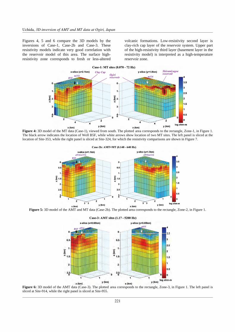
Uchida, T., 2007, 3D inversion of AMT and MT data at Ogiri
3/4
Figures 4, 5 and 6 compare the 3D models by the inversions of Case-1, Case-2b and Case-3. These resistivity models indicate very good correlation with the reservoir model of this area. The surface high-resistivity zone corresponds to fresh or less-altered
volcanic formations. Low-resistivity second layer is clay-rich cap layer of the reservoir system. Upper part of the high-resistivity third layer (basement layer in the resistivity model) is interpreted as a high-temperature reservoir zone.
Figure 4: 3D model of the MT data (Case-1), viewed from south. The plotted area corresponds to the rectangle, Zone-1, in Figure 1. The black arrow indicates the location of Well B5F, while white arrows show location of two MT sites. The left panel is sliced at the location of Site-353, while the right panel is sliced at Site-324, for which the resistivity comparisons are shown in Figure 7.
Figure 5: 3D model of the AMT and MT data (Case-2b). The plotted area corresponds to the rectangle, Zone-2, in Figure 1.
Figure 6: 3D model of the AMT data (Case-3). The plotted area corresponds to the rectangle, Zone-3, in Figure 1. The left panel is sliced at Site-914, while the right panel is sliced at Site-955.
Uchida, 3D inversion of AMT and MT data at Ogiri, Japan
221

Uchida, T., 2007, 3D inversion of AMT and MT data at Ogiri
4/4
Figure 7: Comparison of resistiviy values of the 3D models at (a) Well B5F, (b) AMT site 914 and MT site 353, and (c) AMT site 955 and MT site 324. A thin red line in Panel (a) is the long-normal resistivity data. For Case-3 in Panel (c), two neighboring blocks to Site 955 are shown. These three 3D models correspond well with each other. For the precise delineation of the boundary between the low-resistivity second layer and high-resistivity basement, inclusion of dense AMT data provides more detailed structure. Figure 7 compares block resistivites of the four cases of inversion at a production well B5F, and two AMT and MT sites. Unfortunately the resistivity logging was conducted only for a short depth range in B5F. When we use very high frequency data (above 1 kHz), resistivity of the surface layer is properly determined. It seems to give more reliable resistivity values in the deep layers. However, all the four MT models show similar resistivity profiles at the well location in this case. At Sites 914 and 353 (Figure 7b), Case-1 presents rather high-resistivity for the surface layer because of the lack of high frequency data. Case-2a also shows anomalous low-resistivity layers near the surface and a depth from 300 - 600 meters. Site-914 and 353 are located in an anomalous zone near Ginyu Fault. In such a case, shallow resistivity information by AMT data is necessary. On the other hand, the resistive third layer is expressed almost similar among these models. Therefore, these models do not give significant difference for understanding the high-temperature geothermal reservoirs. This study has suggested that AMT data alone gives almost sufficient resistivity model to interpret down to the top of the geothermal reservoir.
ACKNOWLEDGEMENTS The author is grateful to Nittetsu Kagoshima Geothermal Co., Ltd. and Dr. Shinichi Takakura (AIST) for the permission to use their AMT data in this work.
REFERENCES Goko, K. (2000). Structure and hydrology of the Ogiri
field, West Kirishima geothermal area, Kyushu, Japan. Geothermics, 29, 127–149.
Sasaki, Y. (1999). 3-D inversion of electrical and electromagnetic data on PC. Proc. of 2nd International Symposium on Three-Dimensional Electromagnetics, 128–131.
Sasaki, Y. (2004). Three-dimensional inversion of static-shifted magnetotelluric data. Earth, Planets and Space, 58, 239-248.
Takakura, S. (2003). Advantages and problems of the audio-magnetotelluric method for geothermal exploration., Proc. of SEG Japan 108th (2003 Spring) Conference, 146-149 (in Japanese).
Uchida, T., and Sasaki, Y. (2003). Stable 3-D inversion of MT data and its application to geothermal exploration. in Macnae, J. and Liu, G. (eds.), Three-Dimensional Electromagnetics III, ASEG, 12-1 – 12-10.
Uchida, T. (2005). Three-dimensional magnetotelluric investigation in geothermal fields in Japan and Indonesia, Proc. of World Geothermal Congress 2005, Paper 0752, 1-12.
Uchida, 3D inversion of AMT and MT data at Ogiri, Japan
222

Author index
Abubakar, A., 47Afanasjew, M., 3Avdeev, D., 53, 149Avdeeva, A., 53
Baranwal, V. C., 133, 155Becken, M., 117Bedrosian, P., 179Berdichevsky, M., 57, 91, 95, 99, 149Bibby, H. M., 193, 197Blaschek, R., 23, 109Blome, M., 7Börner, R.-U., 3, 11, 15, 133, 138Box, S., 179Braun, M., 62Burakhovich, T., 183
Caldwell, T. G., 193, 197Cas, R. A. F., 197Chen, J., 66Cull, J. P., 197
Davydycheva, S., 47Dmitriev, V., 57Druskin, V., 47Dzhatieva, Z., 146
Edwards, R. N., 214Egbert, G. D., 71Eiermann, M., 3Ernst, O. G., 3, 11Eso, R., 185Everett, M. E., 27
Franke, A., 15, 126, 133, 138
Günther, T., 122Gurk, M., 189Güttel, S., 3
Habashy, T., 47Haber, E., 19, 35Han, N., 142Hanstein, T., 23Heincke, B., 66Heinson, G., 217Heise, W., 193, 197Heldmann, S., 19Helwig, S. L., 23Hill, G. J., 197
Hobbs, B., 146Hördt, A., 23, 109
Jegen-Kulcsar, M., 66Jones, A. G., 152, 159, 163Junge, A., 122
Kalisperi, D., 201Kamm, J., 67Kelbert, A., 71Kim, H. J., 142Kiss, J., 126Knizhnerman, L., 47Kobzova, V. M., 112Krings, T., 117Kulik, S., 183Kütter, S., 138Kuznetsov, A. N., 112Kuznetsov, V., 91, 95, 99
Ledo, J., 152Lee, S. K., 203Lee, T. J., 142, 203Li, G., 146Lilley, F. E. M. (Ted), 103Logunovich, R., 149
MacGregor, L., 155Maier, R., 217Makris, J. P., 201Marcuello, A., 152Maris, V., 207Martí, A., 152, 163Martyshko, P. S., 75Maurer, H. R., 7Maxey, A., 155Meying, A., 212Miensopust, M., 152, 159, 163Minsley, B. J., 78Mir, R., 214Montahaei, M., 114Morgan, F. D., 78Moroz, I. P., 112Mukherjee, S., 27Müller-Petke, M., 67, 82Muñoz, G., 117
Nam, M. J., 142, 203Ndougsa-Mbarga, T., 212, 213
223

Author index
Njignti-Nfor, 213
Oldenborger, G. A., 31Oldenburg, D. W., 19, 31, 35, 185
Palshin, N., 91, 95, 99Panzner, M., 167Pedersen, L. B., 189Pellerin, L., 179Prácser, E., 126
Queralt, P., 152
Riahi, M. A., 114Ritter, O., 117, 189Romano, G., 201Roublev, A. L., 75Rust, D., 201
Sasaki, Y., 207Savvaidis, A. S., 189Schmucker, U., 86Schoemaker, F. C., 118Scholl, C., 214Schultz, A., 71Schünemann, J., 122Schwalenberg, K., 214Schwarzbach, C., 39Selway, K., 217Shekhtman, R., 35Sinha, M., 155Slob, E. C., 118Smeulders, D. M. J., 118Smirnov, M., 189Sohl, F., 167Song, Y., 142, 203Spitzer, K., 3, 11, 15, 39, 133, 138, 167Strack, K. M., 23Streich, R., 172Suh, J. H., 142Szarka, L., 126
Taylor, D., 146Thiel, S., 217
Uchida, T., 203, 219
Vallianatos, F., 201van der Kruk, J., 172
Wannamaker, P., 207Weaver, J. T., 103
Weidelt, P., 43Willoughby, E. C., 214
Yaramanci, U., 62, 67, 82Yu, G., 23
Zaslavsky, M., 47
224
Related Documents