Proceedings of aConference Held June 11-15, 1990 at t

Intemational Conference on the Roleof the Polar Regions in Global Change:

Proceedings of a Conference Held June 11-15, 1990at the'University of Alaska Fairbanks

Volume II,,

Editedby

GunterWellerCindyL. Wilson

BarbaraA. B. Severin

Published by

Geophysical InstituteUniversity of Alaska Fairbanks

and

Center for Global Change and Arctic System ResearchUniversity of Alaska Fairbanks

Fairbanks, Alaska 99775

December, 1991 "° _' i" ''_

DISTRIBUTION OF THIS DOCUMENT IS UNLIMfTEDgp._ _

ISBN 0-915360-09-8 (Volume II)ISBN 0-915360-10-1 (2-Volume Set)

CONF-9006128--Voi.2

DE92 013653

Section D:

Effects on Biotaand Biological Feedbacks

Chaired by

V. AlexanderUniversity of Alaska Fairbanks

- U.S.A.

G. HempelAlfi-ed-Wegener Institut

Germany

DISCLAIMER

- This report was prepared as an account of work sponsored by nn ager,cy of the United StatesGovernment, Neither the United States Government nor any agency thereof, nor any of theiremployees, makes any warranty, express or implied, or assumes any legal liability or responsi-bility for the accuracy, completeness, or usefulness of any information, apparatus, product, orprocess disclosed, or represents that its use would not infringe privately owned rights. Refer-ence herein to any specific commercial product, process, or service by trade name, trademark,

- manufacturer, or otherwise does not necessarily constitute or imply its endorsement, recom-mendation, or favoring by the United States Government or any agency thereof. The views

_ and opinions of authors expressed herein do not necessarily state or reflect those of theUnited States Govcrnmentor any agency thereof.

Effects of Global Change on Net Ecosystem Carbon Flux of Arctic Tussock Tundra

W. C. OechelDepartmentof Biology,SanDiegoState University,San Diego,California,U.S.A.

ABSTRACT

Arctic ecosystems contain vast quantities of carbon as soil organic matter and,depending on future climatic conditions, have the potential to act as major sourcesor sinks for atmospheric CO2. Cold, moist soils and the presence of permafrostallow increased ecosystem production following global change to be stored on acontinuing basis over long periods of time. Arctic ecosystems ate one of the fewecosystems capable of long-term increased carbon storage. On the other hand,increases in the depth of the active layer, melting of the permafrost, and/ordecreases in soil moisture could result in increased rates of soil decomposition andnet CO2 efflux from the tundra.

Recent evidence indicates that tussock tundra is currently losing substantial car-bon, possibly in response to warming and drying of arctic soils within the last cen-tury. At Toolik Lake, Alaska, the rate of net CO2 loss from the tundra is on theorder of 3 g m-2 d-1. This rate of loss, if occurring over the circumpolar arctic,could account for the net loss of 0.1 to 0.2 x 109 metric tons of carbon per yearfrom tussock tundra alone.

Field manipulations and phytotron experiments indicate that the response of netprimary production or net ecosystem carbon assimilation of tussock tundra to ele-vated CO2 is limited by environmental conditions in the arctic. However, the com-bination of elevated atmospheric CO2 and increased air temperature can result in amajor increase in net primary production and net ecosystem carbon sequestering intussock tundra.

Global change could cause the arctic to contribute up to 55 x 109 metric tons ofsoil carbon to the atmosphere. On the other hand, conditions of elevated CO2 and amoist, poorly aerated soil horizon, could result in long-term carbon sequesteringand negative feedback on the rise of atmospheric CO2. Likely effects depend on thenature of global change and the areas of arctic tundra considered.

369

The Role of Tundra and Taiga Systems in the Global Methane Budget

W. S. Reeburgh and Stephen C. WhalenInstitute of Marine Science, University of Alaska Fairbanks, Fairbanks, Alaska, U.S.A.

g

ABSTRACT

. Tundra and boreal forest soils contain some 30% of the terrestrial soil carbonreservoir. A large fraction of this soil carbon is immobilized in permafrost and peat.

' This soil carbon reservoir could be susceptible to biogeochemical conversion toCO2 and CH4 under warmer, wetter climate. Both of these gases are radiatively

, active, and could be responsible for a positive climate feedback.We performed weekly measurements of CI-14flux at permanent sites to evaluate

the importance of tundra and taiga systems in the present global CH4 budget and to', gain insights into the processes important in modulating emissions under present", and modified climate. Our CI-I4 flux time-series at tundra sites in the UAF Arbo-

retum covers over 3.5 years and indicates that water table level, transport by vas-_, cular plants and microbial oxidation at the water table are important in modulating', tundra CH4 emissions. Emission of CH4 essentially ceases during frozen periods.

Our study at permanent taiga sites covers less than one year. Ali taiga sites con-sumed atmospheric methane in fall 1989, indicating that these soils could be a sinkfor atmospheric CI-I4during part of the year.

Integrated annual emission from the seasonal time-series measurements andresults from a detailed survey along the Trans-Alaska Pipeline Haul Road led toindependent estimates of the global tundra CH4 flux of 19-33 and 38 Tg yr-l,respectively. The road transect estimate for the global taiga CI-t4 contribution is 15

= Tg yr-l.

i

[

L

i

370

_llll ,,

J

iJ

i/

!

I

/

The Influence of Sea Ice on the Structure and Functionof Southern Ocean Ecosystems

C. W. SullivanDepartmentofBiologicalSciences,Universityof SouthernCalifornia,Los Angeles,California,U.S.A.

ABSTRACT

The presence of sea ice and its seasonal dynamics has a profeund influence onplants and animals that inhabit the Southern Ocean. Sea ice is a habitat for organ-isms at ali trophic levels. The ice habitat covers approximately 20 million squarekilometers of the sea surface during the austral winter, but is rapidly and dramat-ically reduced by 80% during the ensuing spring and summer. These dynamic pro-cesses characteristic of the physical environment result in cyclic changes in thehorizontal and vertical distributions of the biomass and activities of organisms.Most notable among these changes are the spatial and temporal characteristics ofproductivity and the coupled process of sedimentation. These changes may in turninfluence both tropho-dynamic relationships and biogeochemical cycles of matterthat are unique to the polar regions of the world ocean. The presumed sensitivity ofthe sea ice ecosystem to global warming suggests that it may be an early indicatorof both physical and biological oceanographic consequences of global change.

r

371

Methane Emissions from Alaska Arctic Tundrain Response to Climatic Change '

Gerald P. Livingston and Leslie A. MorrisseyTGSTechnology,Inc., NASAAmesResearchCenter,EarthSystemsScienceDivision,MoffettField,California,U.S.A.

ABSTRACT

In situ observations of methane emissions from the Alaska North Slope in 1987and 1989 provide insight into the environmental interactions regulating methaneemissions and into the local- and regional-scale response of the arctic tundra to in-terannual environmental variability. Inferences regarding climate change are basedon in situ measurements of methane emissions,regional landscape characterizationsderived from Landsat Multispectral Scanner satellite data, and projected regional-scale emissions based on observed interannual temperature differences and simulat-ed changes in the spatial distribution of methane emissions.

Our results suggest that biogenic methane emissions from arctic tundra will besignificantly perturbed by climatic change, leading to warmer summer soiltemperatures and to vertical displacement of the regional water table. The effect ofincreased soil temperatures on methane emissions resulting from anaerobic de-composition in northern wetlands will be to both increase total emissions and to in-crease interannual and seasonal variability. The magnitude of these effects will bedetermined by those factors affecting the areal distribution of methane emissionrates through regulation of the regional water table. At local scales, the observed4.7°C increase ;.nmid-summer soil temperatures between 1987 and 1989 resulted ina 3.2-fold inc:_ase in the rate of methane emissions from anaerobic soils. The ob-

served linear temperature response was then projected to the regional scale of theAlaska North Slope under three environmental scenarios. Under moderately drierenvironmental conditions than observed in 198% a 4°C mid-summer increase insoil temperatures more than doubled regional methane emissions relative to the1987 regional mean of 0.72 mg m-2 br-1over the 88,408 km2 study area. Wetter en-vironmental conditionsledtoa 4-to5-foldincreaseinmid-summer emissions.These results demonstrate the in_ponance of the interaction between the relativeareal proportion of methane source areas and the magnitude of summer substratctemperatures in determining whether emissions from decomposition processes innorthern ecosystems represent a significant global source and a potential positivefeedback to climatic change.

INTRODUCTION ascarbondioxide(CO2),methane(CH4),andnitrousoxideThe northern high latitudes face a potentially un- 0N20) [Bolinct al., 1986;DickinsonandCicerone,1986;

prcc.edentedrate of climatic warmingas a direct con- Ramanathanct al., 1987].As a directresultof thepastand-_ sequenceof global increasesover the past centuryin the anticipatedcontinuedatmosphericinputsof these "green-

atmosphericconcentrationsof infrared-absorbinggasessuch housegases,"currentglobalcirculationmodelsprojectthat

372

mean annual temperaturesfor the Arctic may increasebe- "Water"at 50 m2 spatialresolution.tween 3--8°C within the next century [Hansen et al., 1988; In situ sample allocations differed between 1987 andPost, 1990]. This climatic change is expected to result in 1989. In 1987 the allocation was defined to regionallyrepre-earlier spring thaws, longer growing seasons, and 2--4°C sent both the Arctic Coastal Plain and Arctic Foothillselevated summer temperatures. Precipitation patterns may physiographic provinces of the North Slope. More specif-.also change, although current projections are still highly un- ically, each land cover class was sampled in proportion to itscertain. If these organic-rich and temperature-limited relative areal representation and to anticipated variances inecosystems [Chapin, 1984] respond to climatic change by emissions at the regional scale. Within each site sampled, areleasing substantially greater quantifies of CO2 and CI-I4, secondary allocation represented the mierotopography andthe climatic warming trend may be enhanced [Lashof, 1989] location of the local water table relative to the surface on aand the global carbon cycle significantly affected [Miller, spatial scale of approximately 9.5 m2. Ten mierotopo-1981; Billings, 1987]. graphic features were identified for sampling, e.g., "low cen-

Empirical and atmospheric modeling studies indicate that ter polygonal basins," "rims,""troughs," "sedge meadows,"the northern high latitude wetlands may represent one of the "highcentered polygonal basins," "frostboils," "sedge tus-largest natural sources of CH4 globally as a result of season- socks," "inter-tussock areas," "lake-ori,_remergent vegeta-al anaerobic microbial decomposition of organic materials tion," and "lake-open water." The location of the water tablein the active thaw layer. More than half of the wetlands area was categorized as "bebw" (z < -5 cm), "at"(-5 • z _;0 cm),of the earth lies in the boreal region north of 500N latitude or "above"(z • 0 cm) the surface. In total, the area of study[Matthews and Fung, 1987; Aselmann and Crutzen, 1989] was represented by 122emissions observations representingand over 20% of the earth's total organics may be stored in 57 spatially independent sites. Additional details of the sam.these ecosystems as frozen or recalcitrant materials in the pie allocation are given in Morrisseyand Livingston [1991].soils and peats [Post et al., 1985; Gorham, 1988]. Seasonal The regional mean rate of CH4 emissions (F) wasCH4 emissions from these ecosystems are estimated to cur- estimated on the basis of a two-tiered stratified approachrently account for 6--10%of ali CHs sources and 16-,53%of [Cochran, 1953] using the relative areal proportions of theali natural wetland sources [Aselmann and Crutzen, 1989]. local and regional categorizations as the weighting terms:If subjected to climatic wanning, these ecosystems may re-spond by releasing substantially greater quantifies of carbon m nto the atmosphere as a consequence of increased rates of de- F = _ _(Pi/_/) (1)composition operating over longer seasons of biological i=lj=l

activity and on increasing quantities of organic materials as where Pij represents the relative areal proportion of landthe permafrost thaws. Examination of arctic methane emis- co_,er class i and local.scale microtopographic feature j, andsions under variable interanntml meteorological conditionsmay provide insight into the response of northern _j the measured rate of el-LIemissions.ecosystems to anticipated climatic change. In 1989, the sample allocation was defined to assess the

In this paper we address observed and projected Cl-h seasonal variability in emissions at anaerobic (waterlogged)emissions from arctic tundra in relation to anticipated cii- organic sites on the Arctic Coastal Plain. Only data from thematically induced changes in soil temperature and water two years that were complemental in time (August 1-14)table position. Our conclusions are based upon measured in were included in this analysis. To estimate regional-scalesitu CI-I4emissions during the summers of 1987 and 1989 emissions for 1989, we initially assumed no net change in

the vegetation or hydrological regimes at the regional scalefrom the North Slope of Alaska, regional land cover char-of the North Slope between 1987 and 1989. As such, in thisacterizations derived from satellite observations, and es-"reference scenario," differences in estimated regional-scaletimated regional-scale emissions derived from observed

interannual temperature differences and simulated changes emissions over the 3-year period reflect only observed inter-annual differences in the rates of emissions at the localin water table position, scale. The 1989 CI-h emission rates for each land cover

METHODS class were thus calculated as:

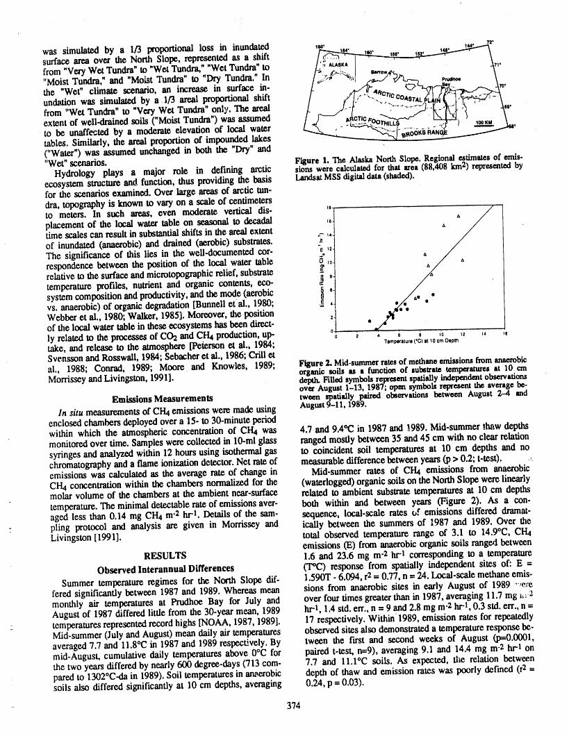
The region of study is an 88,408 km2 area representative _'e1989of the Arctic Coastal Plain and Foothill provinces of the _:1989= \_J (E1987) (2)Alaska North Slope (Figure 1). Estimates of mid-summerregional CI-h emission rates for select climatic scenarioswere derived through integration of satellite-based land where E represents the ecosystem CI-I4emissions rate and ecover characterizations and in situ observations of Cl-h the/n situ emission rate from anaerobic organic soils.emissions from early August of 1987and 1989. The sensitivity of regional CI-14emissions to interaction

At the regional scale, digital classifications of Landsat between the observed interannual differences in the emis-Multispectral Scanner (MSS) data [Morrissey and Ennis, sion rates and changes in the areal _representationof the1981; Walker ct al., 1982] defined the land cover categories metlmne source areas was explored in a simulation exerciseand their relative areal proportions subsequently used to cal- and subsequently interpreted in light of the potential impactsculate regional emission estimates. The spectrally based of climatic change. Two scenarios were examined in addi-classification corresponded to vegetation type and density as tion to the reference scenario described above. "Dry" andwell as to the presence or absence of surface water. These "Wet" environmental conditions were simulated by as-

: land cover classes nominally represented "Dry Tundra," suming arbitrary shifts in the relative areal proportions of"Moist Tundra," "Wet Tundra," "Very Wet Tundra," and the regional land cover classes. The "Dry" climate scenario

373

was simulated by a 1/3 proportional loss in inundawA ,_' '_----_'surface area over theNorth Slope, represented as a shift /_'_-'_-----'?' t_ \from "VeryWet Tundra"to "Wet Tundra,""Wet Tundra"to /_ ALASKA[ -_,1'"Moist Tundra,"and "MoL_tTundra"to "Dry Tundra." In _ . ,-., b,o, -

the .Wet" climate scenario, an increase in surface in" /'___'undation was simulated by a 1/3 areal proportional shift

,ore .Wet Tundra" to "Very Wet Tundra"only. The areal _. _____

extent of well-drainedsoils ("Moist Tundra")was assumedto be unaff_ted by a moderate elevation of local watertables. Similarly, the areal proportion of impounded lakes("Water")was assumedunchangedinbeththe"Dry"and"Wet"scenarios. Figure 1. The AlaskaNorthSlope.Regionalestimatesof emis-

Hydrology plays a major role in defining arctic sions were calculatedfor thatarea (88,408 km2) represented by

ecosystem structureand function, thus providing the basis LandsatMSSdigitaldata(shaded).for the scenarios examined. Over large areasof arctic tun-dm, topography is known to vary on a scale of centimetersto meters. In such areas, even moderate vertical dis- '"placement of the local water table on seasonal to decadal ,,time scales canresult in substantialshifts in the arealextent .._,,of inundated(anaerobic) and drained (aerobic) substrates.The significance of this lies in the well-documented cor- % ,2.respondence between the position of the local water table _ ,0.

relative to the surfaceand microtopographicrelief, substrate _ "A._"temperature profiles, nutrientand organic contents, eco- _ "system composition and productivity,and the mode (aerobic _ "vs. anaerobic)of organic degradation[Bunnell etal., 1980; _ ,! ./4 - •

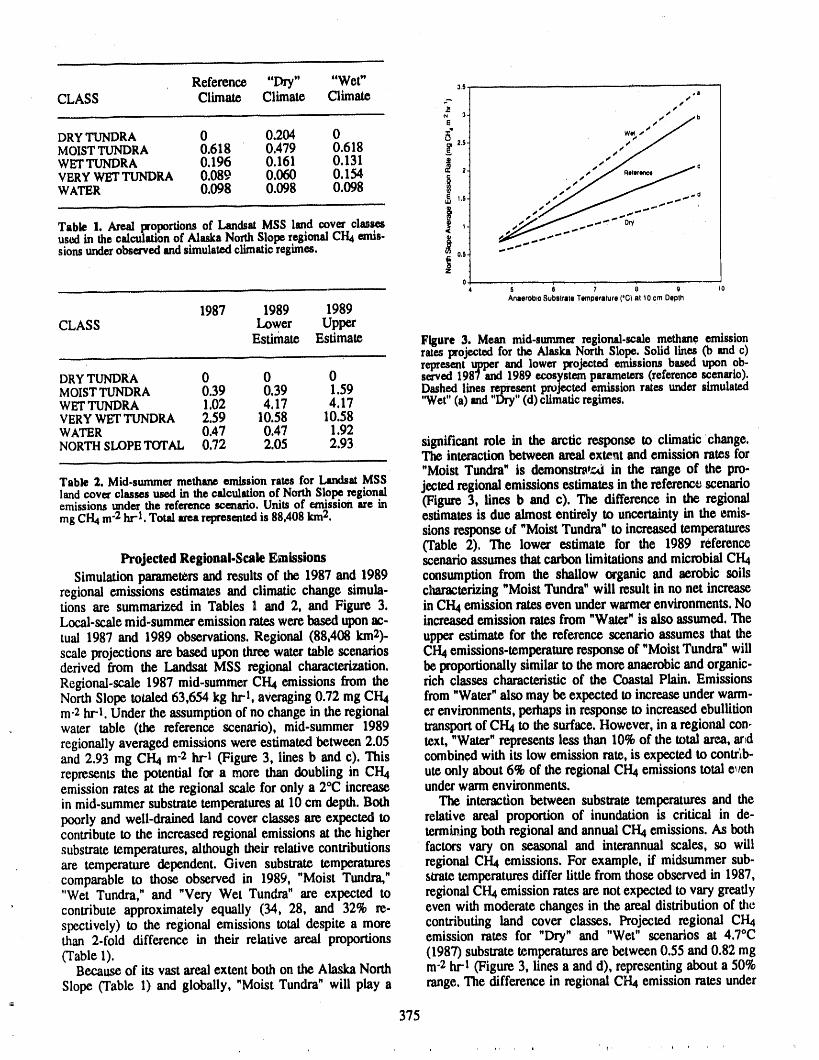
Webber et al., 1980; Walker, 1985]. Moreover, the position 2 Z'"of the local water table in these ecosystems has been direct- o "ly related to the processes of CO2 and CI-I4production,up- 2 , e s ,0 ,2 ,, ,,take, and release to the atmosphere [Peterson et al., 1984; T.mp.,at_,_('c_10_0,_Svenssonand Rosswall, 1984; Sebacheret al., 1986; Crilletal., 1988; Conrad, 1989; Moore and Knowles, 1989; Figure2. Mid-summerratesof methaneemissionsfromanaerobic. organicsoilsasa functionofsubstratetemperaturesatI0cmMorrisseyand Livingston, 1991]. depth.Filledsymbolsrepresent spatially independent observations

over August1-13, 1987;open symbolsrepresentthe averagebe.Emissions Measurements tween spatiallypaired observationsbetween August 2--4 and

In situ measurementsof CH4emissions were made using August 9-11, 1989.enclosed chambers deployed over a 15-to 30-minuteperiodwithin which the atmospheric concentrationof CIG was 4.7 and 9.4°(2 in 1987 and ,_989.Mid-summer thaw depthsmonitoredover time. Samples were collected in 10-ml glass ranged mostly between 35 and 45 cm with no clearrelationsyringes and analyzed within 12 hours using isothermalgas to coincident soil temperatures at 10 cm depths and nochromatographyand a flame ionizationdetector. Net rate of measurabledifference between years (p > 0.2; t-test). ,emissions was calculated as the average rate of change in Mid-summer rates of CH4 emissions from anaerobicCH4 concentration within the chambers normalized for the (waterlogged)organic soils on the North Slope were linearlymolar volume of the chambers at the ambient near-surface related to ambient substrate temperaturesat 10 cm depthstemperature.The minimaldetectable rateof emissions aver- both within and between years (Figure 2). As a con-aged less than 0.14 mg CH4 m"2 hrl. Details of the sam- sequence, local-scale rates of emissions differed dramat-piing protocol and analysis are given in Morrissey and ieally between the summers of 1987 and 1989. Over theLivingston [1991]. total observed temperature range of 3.1 to 14.9°C, CH4

emissions (E) from anaerobic organic soils ranged betweenRESULTS 1.6 and 23.6 mg m-2 ht1 corresponding to a temperature

Observed Interannual Differences (T°C) response from spatially independent sites of: E =

Summer temperature regimes for the North Slope dif- 1.590T - 6.094, r2= 0.77, n = 24. Local-scale methane emis-fered significantly between 1987 and 1989. Whereas mean sions from anaerobic sites in early August of 1989 . ,e.:emonthly air temperatures at Prudhoe Bay for July and over four times greater than in 1987, averaging 11.7 mg _,_-2August of 1987 differed little from the 30-year mean, 1989 ht1, 1.4 std. err., n = 9 and 2.8 mg m-2 hrt, 0.3 std. err., n --temperatures represented record highs [NOAA, 1987, 1989]. 17 respectively. Within 1989, emission rates for repeatedlyMid-summer (July and August) mean daily air temperatures observed sites also demonstrated a temperatureresponse be-averaged 7.7 and 11.8°C in 1987 and 1989 respectively. By tween the Iu'st and second weeks of August (13=0.0001,mid-August, cumulative daily temperatures above 0°C for paired t-test, n=9), averaging 9.1 and 14.4 mg m-2 hrt onthe two years differed by nearly 600 degree-days (713 com- 7.7 and 11.1°C soils. As expected, the relation betweenpared to 1302*C-da in 1989). Soil temperatures in anaerobic depth of thaw and emission rates was poorly defined (r2 --soils also differed significantly at 10 cm depths, averaging 0.24, p =0.03).

374

Reference "Dry" "Wet" _,CLASS Climate Climate Climate .. ,"

S '

o 0.2o4 oDRYTUNDRAMOISTTUNDRA 0.618 0.479 0.618 = "" , ,,,,/WETTUNDRA 0.196 0.161 0.131 _ ,//,_._,_..,.,._oVERYWETTUNDRA 0.089 0.060 0.154 _ 2 ,"WATER 0.098 0.098 0.098 _ ,5 ,,_/"" _/ ,,...,.'0

Table 1. Arealproportionsof LandsatMSS land mv_ classes _ ,//,,-/ _,,.......-'- 0,vusedin thecalculationof Masks NorthSloperegionalEH4emis- * "_;"/ --'""-sionsunderobservedandsimulatedclimaticregimes. _ 0.s ""

Z 0 - , , , ,4 5 6 7 8 9 to

AnaeroOl0 Substrate Tempera_re ('C) at 10 om Depth

1987 1989 1989CLASS Lower Upper

Estimate Estimate Figure 3. Mean mid-summerregional-scalemethane emissionratesprojectedfor the AlaskaNorthSlope.Solid lines (b andc)representupperandlower projectedemissionsbased upon ob-

DRYTUNDRA 0 0 0 served1987and 1989 ecosystemparameters(referencescenario).MOISTTUNDRA 0.39 0.39 1.59 Dashedlines representprojectedemissionratesundersimulatedWETTUNDRA 1,02 4.17 4.17 "Wet"(a)and"Dry"(d)climatlcregimes.VERYWETTUNDRA 2.59 10.58 10.58WATER 0.47 0.47 1.92NORTHSLOPETOTAL 0.72 2.05 2.93 significant role in the arctic response to climatic change.

The interactionbetween areal extent and emission rates for"Moist Tundra"is demonstr_,zd in the range of the pro-

Table 2. Mid-summermethaneemissionratesfor [atmlsatMSS jeeredregionalemissions estimates in the reference scenariolandcov_ classesusedin thecalculationof NorthSloperegionalemissionsunderthe referencescenario.Unitsof emlssionare in (Figure 3, lines b and c). The difference in the regionalmSCH4 m-2hr-I. Totalarearepresentedis 88,408km2. estimates is due almost entirely to uncertaintyin the emis-

sions responseof "Moist Tundra"to increased temperatures(Table 2), The lower estimate for the 1989 reference

Projected Regional.Scale Emissions scenarioassumes thatcarbonlimitations and microbial CH4Simulation parametersand results of the 1987 and 1989 consumption from the shallow organic and aerobic soils

regional emissions estimates and climatic change simula- characterizing"Moist Tundra"will result in no net increasetions are summarized in Tables I and 2, and Figure 3. in CH4emission rateseven underwarmer environments.NoLocal-scale mid-summeremission rates were based uponac- increaseAemission rates from "Water"is also assumed. Thetual 1987 and 1989 observations. Regional (88,408 km2)- upper estimate for the reference scenario assumes that thescale projections arebased upon three watertable scenarios CH4emissions-temperature response of "MoistTundra"willderived _om the Landsat MSS regional characterization, be proportionallysimilar to the more anaerobic and organic-Regional-scale1987 mid-summerCH4 emissionsfzom the rich classescharacteristicof the CoastalPlain.EmissionsNorth Slope totaled 63,654 kg hrl, averaging 0.72 mg CH4 from"Water"also may be expected to increase under warm-m-2 hr-l. Under the assumption of no change in the regional erenvironments, perhaps in response to increasedebullitionwater table (the reference scenario), mid-summer 1989 transportof CH4 to the surface. However, in a regional con-regionally averagedemissions were estimated between 2.05 text, "Water"represents less than 10% of the total area, aridand 2.93 mg CH4 m"2hr-i (Figure 3, lines b and c). This combined with its low emission rate. is expected to contr_b-represents the potential for a more than doubling in CH4 ute only about 6% of the regional CH4emissions total e_rcnemission rates at the regional scale for only a 2°C increase underwarmenvironments.in mid-summersubstratetemperaturesat 10 cm depth. Both The interaction between substrate temperaturesand thepoorlyand well-drained land cover classes are expected to relative areal proportion of inundation is critical in de-contributeto the increased regional emissions at the higher terminingboth regional and annual CH4 emissions. As bethsubstrate temperatures, although their relative contributions factors vary on seasonal and interannualscales, so willare temperaturedependent. Given substrate temperatures regional CIG emissions. For example, if midsummer sub-comparable to those observed in 1989, "Moist Tundra," stratetemperaturesdiffer litde from those observed in 1987,"Wet Tundra," and "Very Wet Tundra" are expected to regional CH4emission rates arenot expected to vary greatlycontribute approximately equally (34, 28, and 32% re- even with moderate changes in the areal distributionof thespectively)to the regionalemissionstotaldespitea more contributingland cover classes.Projectedregional CI-14than 2.fold difference in their relative areal proportions emission rates for "Dry" and "Wet" scenarios at 4.7°C(Table 1). (1987) substratetemperaturesare between0.55 and 0.82 mg

Because of its vast areal extent both on the Alaska North m-2hr-I(Figure 3, lines a and d), representingabout a 50%Slope (Table 1) and globally, "Moist Tundra"will play a range.The difference in regional CH4emission rates under

375

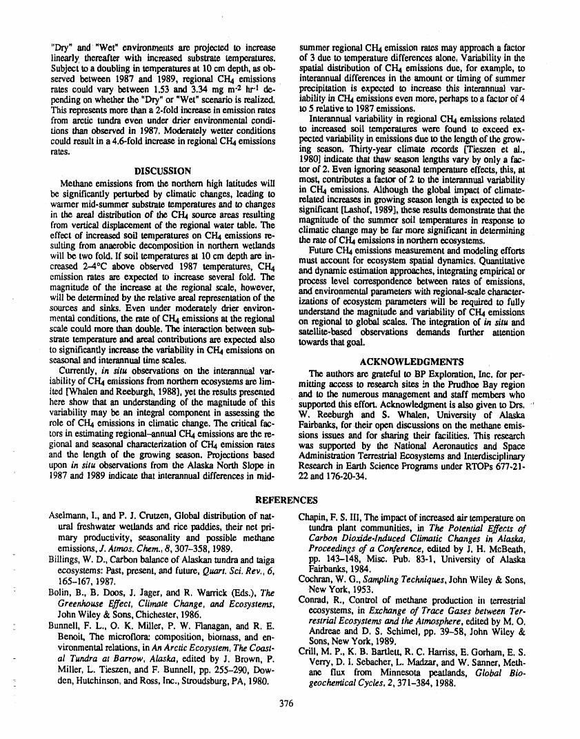
"Dry" and "Wet"environments are projected to increase summer regionalCH4 emission ratesmay approacha factorlinearly, thereafter with increased substrate temperatures, of 3 due to temperaturedifferences alone, Variabilityin theSubjectto a doubling in temperaturesat 10 em depth, as ob- spatial distribution of CI-I4 emissions due, for example, toserved between 1987 and 1989, regional CH4 emissions interannualdifferences in the amountor timingof summerrates could vary between 1.53 and 3.34 mg m"2 hrl de. precipitationis expected to increase this interannual var-pendingon whether the "Dry"or "Wet"scenario is realized, iabillty in CH4emissions even more,perhapsto a factorof 4This represents more thana 2.fold increasein emission rates to 5 relative to 1987 emissions.from arctic tundraoven under drier environmental condi- Interannual,_ariabilityin regional CH4 emissions relateddons than observed in 1987. Moderately wetter conditions to increased soil temperatures were found to exceed ex-could resultin a 4.6-fold increasein regionalCH4 emissions pected variability in emissions due to the length of the grow.rates, ing season. Thirty-year climate records [Tieszen et al.,

1980] indicate that thaw season lengths vary by only a fac-DISCUSSION tor of 2. Even ignoring seasonal temperatureeffects, this, at

Methane emissions from the northern high latitudes will most, contributes a factor of 2 to the interannualvariabilityin CI-h emissions. Although the global impact of climate-

be significantly perturbed by climatic changes, leading to related increases in growing season length is expected to bewazmer mid-summersubstrate temperaturesand to changes significant [Lashof, 1989], these results demonstrate that thein the areal distribution of the CH4 source areas resulting magnitude of the summer soil temperatures in response tofrom vertical displacement of the regional water table. The climatic change may be far more significant in determiningeffect of increased soil temperatures on CH4 emissions re- the rate of CH4emissions in northernecosystems.salting from anaerobic decomposition in northern wetlands Future CH4emissions measurement and modelingeffortswill be two fold. If soil temperaturesat 10 cm depth are in. must account for ecosystem spatial dynamics. Quantitativecreased 2--4°C above observed 1987 temperatures, CH4 and dynamicestimationapproaches,integratingempiricaloremission rates are expected to increase several fold. The process level correspondence between rates of emissions,magnitude of the increase at the regional scale, however, and environmentalparameterswith regional-scale character-will be determinedby the relative arealrepresentationof the izations of ecosystem parameters will be required to fullysources and sinks. Even under moderately drier environ, understandthe magnitude and variabilityof CH4 emissionsmental conditions, the rate of CH4 emissions at the regional on regional to global scales. The integration of/n situ andscale could more than double. The interaction between sub- satellite-based observations demands further attentionstratetemperatureand areal contributions are expected also towardsthatgoal.to significantly increase the variabilityin CH4emissions onseasonalandinterannualtimescales, ACKNOWLEDGMENTS

Currently, in situ observations on the interannual var- The authors are grateful to BP Exploration,Inc. for per-iability of CH4 enlissions from northern ecosystems are lira- mitting access to research sites _ the Prudhoe Bay regionited [Whalen and Recburgh, 1988], yet the results prcseaited and to the numerous management and staff members whohere show that an understandingOf the magnitudeof this supportedthis effort. Acknowledgment is also given to Dis. "'variabilitymay be an integralcomponent in assessing the W. Recburgh and S. Whalen, University of Alaskarole of CH4emissions in climatic change. The critical fac- Fairbanks,for their open discussions on the methane emis-tors in estimatingregional-annual CH4emissions are the re- sions issues and for sharing their facilities. This researchgional and seasonal characterization of CH4emission rates was supported by the National Aeronautics and Spaceand the length of the growing season. Projections based AdministrationTerrestrialEcosystems and Interdisciplinaryupon in situ observations from the Alaska North Slope in Research in Earth Science Programsunder RTOPs 677.21-1987 and 1989 indicate,that interannualdifferences in mid- 22 and 176-20-34.

REFERENCES

Aselmann, I., and P. J. Crutzen, Global distributionof nat- Chapin, F. S. III,The impactof increasedairtemperatureonural freshwaterwetlands and rice paddies, their net pri- tundra plant communities, in The Potential Effects ofmary productivity, seasonality and possible methane Carbon Dioxide4nduced Climatic Changes in Alaska,emissions, J. Atmos. Chem., 8, 307-358, 1989. Proceedings of a Conference, exfitedby J. H. McBeath,-

Billings, W. D., Carbon balance of Alaskan tundra and taiga pp. 143-148, Misc. Pub. 83-1, University of Alaskaecosystems: Past, present, and future, Quart. Sci. Rev., 6, Fairbanks, 1984.165-167, 1987. Cochran, W. G., Sampling Techniques, John Wiley & Sons,

Bolin, B., B. Doos, J. Jager, and R. Warrick (Eds.), The New York, 1953.Greenhouse Effect, Climate Change, and Ecosystems, Conrad, R., Control of methane production in terrestrialJohn Wiley &Sons, Chichesler, 1986. ecosystems, in Exchange of Trace Gases between Ter.

restrial Ecosystems and the Atmosphere, edited by M. O.Bunnell, F. L., O. K. Miller, P. W. Flanagan, and R.E. Andreae and D. S. Schimel, pp. 39-58, John Wiley &

Benoit, The microflora: composition, biomass, and en- Sons, New York, 1989.vironmental relations, in An Arctic Ecosystem, The Coast- CriU, M. P., K. B. Bartlett, R. C. Harriss, E. Gorham, E. S.al Tundra at Barrow, Alaska, edited by J. Brown, P. Verry, D. I. Sebacher, L. Madzar, and W. Sanner, Meth-Miller, L. Tieszen, and F. Bunnell, pp. 255-290, Dow- ane flux from Minnesota peatlands, Global Bio.den, Hutchinson, and Ross, Inc., Stroudsburg, PA, 1980. geocheniical Cycles, 2, 371-384, 1988.

376

b

Diekh_son,R, E., and R. J, Cicerone,Fumn_global warming in the global carbon cycle, EnvironmentalSciences Divi-from atmospheric trace gases, Nature, 319, 109-115, sion Publication No. 3289, Oak Ridge National1986. Laboratory,Oak Ridge, TN, 1990,

Gorham,E., Biotic impoverishmentin northernpeatlands,in Post, W. M,, J. Pastor,P, J. Zinke, and A, G. Stangenberger,Biotic Impoverishment, edited by G. M, Woodwell, Global patternsof soil nitrogen, Nature, 317, 613--616,CambridgeUniversity Press, 1988. 1985.

Hansen, J., I. Fung, A. Lacis, S. Lebedeff, D, Rind, R. Ramanathan,V., L. Callis, R, Cess, J. Hansen, I. Isaksen,Ruedy, G, Russell, and P, Stone, Global climate changes W. Kuhn, A. Lacis, F. Luther,J, Mahlman,R. Reck, andas forecast by theGISS 3-D model, J. Geophys. Res,, 93, M. Schlesinget, Climate.chemical interactions and ef-9341-9364, 1988. fects of changing atmospheric¢ac.e gases, Rev. Geophys.,

Lasher, D. A., The dynamic greenhouseI Feedback pro- 25, 1441-1482, 1987.cesses that may L'lfluence future concentrations of Sebaeher, D. I,, R, C. Harriss, K. B. Bartlett, S. M,atmospheric trace gases and climatic change, Climatic Sebaeher, and S. S. Gric¢, Aunospheric methane sources:Change, 14, 213-.242, 1989. Alaskan tundra bogs, an Alpine fen and a subarctic boreal

Matthews, E., and I. Fung, Methane emission form natural marsh, Tellus, 38, 1-10, 1986.wetlands: Global distribution, area, and environmental Svensson, B. H., andT. Roswall, In situ methane productioncharacteristicsof sources, Global Biogeochemical Cycles, fromacid peat in plant communities with different mois-1,61-86, 1987. ture regimes in a subarctic mire, Oikos, 43, 341-350,

Miller,P. C. (Ed.), Carbon balance in northern ecosystems 1984.and the potential effect of carbon dioxide induced climat- Tieszen, L. L., P. C. Miller, and W. C. Oechel, Photosyn-ic change, Report era Workshop, San Diego, CA, March7-9, 1980, CONF-8003118, U.S. Dept.of Energy,Wash- thesis, in An Arctic Ecosystem, The Coastal Tundra atington, DC, 1981. Barrow, Alaska, edited by J. Brown, P. C, Miller, L. L,

Moore,T. R., and R. Knowles, The influence of water table Tieszen, and F. L. BunneU, pp. 102-139, Dowden,levels on methane and carbon dioxide emissions from Hutchinson,and Ross, Inc.,Stroudsburg,PA, 1980.peatlandsoils, Can. J. Soil Sci., 69, 33-38, 1989. Walker, D. A., Vegetation and environmental gradientsof

Morrissey, L. A., and R. A. Ennis, Vegetation mapping of the Prudhoe Bay region, Alaska, CRREL Report 8514,the National PetroleumReserve in Alaska usingLandsat U.S. Army Cold Regions Research and Engineeringdigital data, U.S. Geological Survey Open File Report 81. Laboratory,Hanover,NH, 1985.315, 25 pp, Reston, VA, 1981. Walker, D. A., W. Acevedo, K. R. Everett, L. Gaydos, J.

Morrissey, L. A., and G, P. Livingston, Methane flux from Brown,and P. J. Webbor,Landsat-assisted environmentaltundra ecosystems in Arctic Alaska; an assessment of mapping in the Arctic National Wildlife Refuge, Alaska,local spatial variability, J. Geophys. Res., 1991, In press. U.S. Cold Regions Researchand Engineering Laboratory,

NOAA, Local climatological data, monthly summary, Hanover,NH, 1982.Environmental Data and InformationService, National Webber, P. J., P. C. Miller, F. S. Chapin HI, and B, H.Climatic Center,Asheville, NC, 1987, 1989, McCown, The vegetation: pattern and succession, in An

Peterson, K. M., W. D. Billings, and N. D. Reynolds, In- Arctic Ecosystem: The Coastal Tundra at Barrow,fluence of water table and atmospheric COg concentra- Alaska, edited by J. Brown, pp. 186-218, Dowden,rien on the carbon balance of Arctic tundra,Arctic and Hutchinson and Ross, Inc., Stroudsburg,PA, 1980.Alpine Research, 16, 331-335, 1984. Whalen, S. C., and W. S. Reeburgh, Methane flux time-

Post, W. M., Report of a workshop on climate feedbacks series for tundra environments, Global Biogeochemicaland the role of peatlands, tundra, and boreal ecosystems Cycles, 2,399--409, 1988.

377

The Toolik Lake P oject.r

Terrestrial and Freshwater Research on Change in the Arctic

/

J. E. Hobble, B. J. Peterson, and G. R. ShaverThe Ecosystems Center, Marine Biological Laboratory, Woods Hole, Massachusetts, U.S.A.

W. J. O'BHenDepartmentofSystematicsandEcology,U_:versityofKansas,Lawrence,Kansas,U.S.A.

ABSTRACT

The Toolik Lake research project in the foothills of the North Slope, Alaska, hascollected data since i975 with funding from the NSFs Division of Polar Prognunsand from the Long Term Ecological Research Program and Ecosys_ms ResearchProgram of the Division of Biotic Systems and Resovxces. The broad goal is tounderstand and predict how ecosystems of tundra, lakes, and streams function andrespond to change.

One specific goal is to understand the extent of control by resources (bottom-upcontrol) or by grazing and predation (top-down control). The processes and re-lationships are analyzed in both natural ecosystems and in ecosystems that haveundergone long-term experimental manipulations to simulate effects of climate andhuman-caused change. These manipulations include the fertilization of lakes andstreams, the addition and removal of lake trout from lakes, the changing of theabundance of arctic grayling in sections of rivers, the exclusion of grazers from tun-dta,andtheshading,fertilizing,andheatingofthetussocktundra.

A secondspecificgoalistomonitoryear-to-yearvariabilityandtomeasurehowrapidlylong-termchangeoccurs.The measurementsinclude:forlakes,measure-mcnts of temperature,chlorophyll,primaryproductivity;forstreams,nutrients,chlorophyllonrifflerocks,insectandfishabundance,and waterflow;and forthetundra,amountofflowering,airtemperature,solarradiation,andbiomass.

A third specific goal is to undderstandthe exchange of nutrients between land andwater. Measurements include the flow of water in rivers, the concentration of nitro-gen and phosphorus in streams, lakes, and soil porewater, and the effect of vegeta-tion on nutrient movement tl'_rough the tundra soils. A dynamic model of nutrientfluxes in the entire upper Kuparuk River watershed is being constructed that willinteract with geographically referenced databases. Eventually the model and pro-cess information will be extrapolated to the larger region; this will allow predictionof the export of nutrients from the whole of the North Slope of Alaska under futureconditions of changed temperature and precipitation.

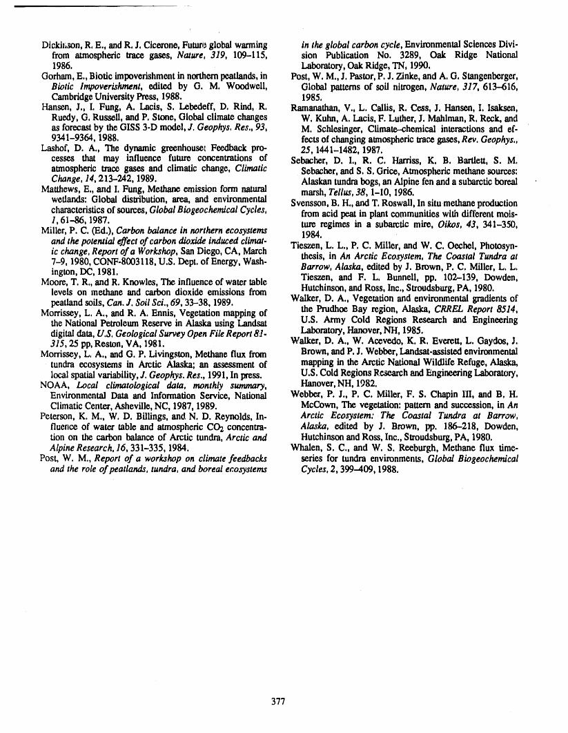
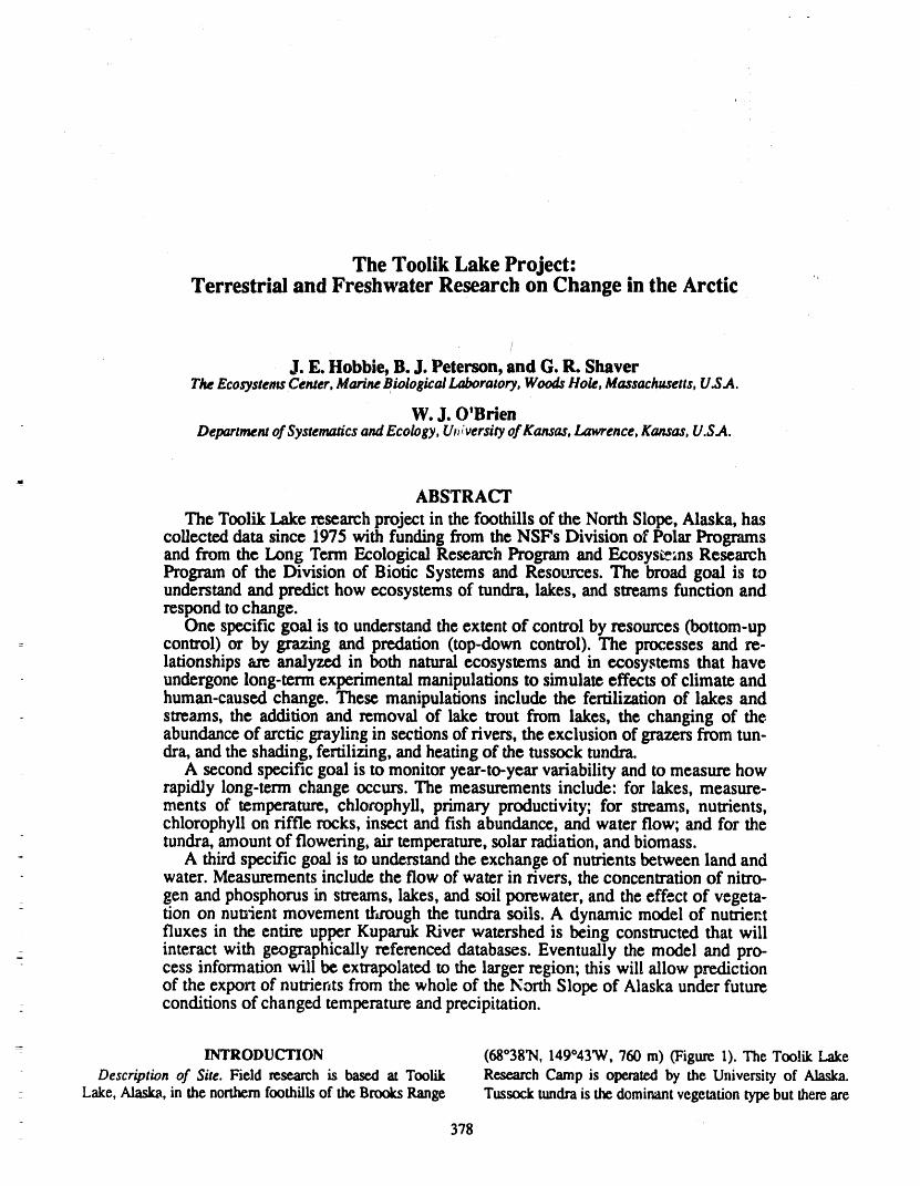
- INTRODUCTION (68°38_1,149°433V,760 m) (Figure1). The ToolikLakeDescription of Site. Field researchis based at Toolik ResearchCampis operatedby the Universityof Alaska.

Lake,Alaska,in thenorthernfoothillsof theBrooksRange Tussocktundrais thedominantvegetationtypebutthereare

378

1989, a monitoringprogramin Oksr_uyik Creek, a slightly

j_. _s_, _ i smaller third-orderstreamabout 15 km to the northeast,was

stray_.'_-._, begun withthe intentionof developing a long-termcompari-\ son andcontrastwith the KuparukRiver.

.... •...... _'F=rt_m,_I ToolikLake has a surfaceareaof 150 ha and a maximum'x:L._ depth of 25 m. Research began in 1975 with surveys of the-7,-_ biota, chemistry, and processes ranging from primary pro-_ASKA ductivity to nulrientbudgets. Dozens of other nearbylakes

LAKE . were _so surveyed. In the 1980s the researchconcentrated... on the question of conuvls of populations,communitystruc-

-- ture,andprocesses. Large (60 m3) plastic bags were set up"J _ """ for manipulations of nutrients and lxedators; entire lakes

-_'" and divided lakes were fertilized and lake trout, the top"--_-_ predator, removed and added to various lakes. More re-

, ..... . '._: cenfly the survey work has been extended to parts of the

N _":f"" ArcticcoastalplainandBrooksRange,aswellasthenorth-/ em foothills region./

l _ Goals of the Toolik Lake Project are:•, ,. .To understand how tundra, streams and lakes func-_'t

tion in the Arctic and to predict how they respond to

•---_. ...'_._,.// changes including climate change.To reachthis objective the projectwill:•Determine year-to-year ecological variability in these

Figure1. Locationof arcticLTERresearchsite atToolikI,eke, systems and measure long-term changes;Alaska. .Understand the extent of control by resources (bot.

tom.up control) or by grazing and predation (top-down control); and

extensive areasof drierheathtundraon ridge tops andother .Measure rates and understand the controls of the ex-well-drained sites as weU as areas of fiver-bottom willow change of nutrients between land and water.communities. Long-term data sets. To keep trackof the observations,

The mean mmual air temperatureis -7°C and the total the Toolik Lake project maintainsa computerizeddatabaseprecipitation250-350 mm. The tundrais snow-free from at the Marine Biological Laboratorywhich contains a widelate May to mid-September while the sun is continuously varietyof long-termdata sets.above the horizon from mid-May until late July. Lakes are Kuparuk River: discharge, NH4, NO3, PO4, temperature,ice-free from mid- to late June until late September. The pH, conductivity, IgSO2,seston(chlorophyll a, particulateentire region is underlain by continuous permafrostwhich C, N, P), epilithon (chlorophyll, primaryproduction),insectexerts a major influence on the distribution,structure,and abundance (Orthocladius, Baetis, Brachycentrus, blackflies, small chironomids,drift density), grayling (growth offunctionof both terrestrialand aquaticecosystems, adults and young, population estimates), rate of N cycling

Terrestrialresearchin the Toolikareabegan in 1976 with with 1SN,majorcationsand anions.descriptive and baseline vegetation studies of many sites Toofik Lake: climate data (temperature,relative humidity,along the length of the Dalton Highway and at Toolik Lake. wind, radiation),rain (volume, chemistry), lake temperature,The next phase, research on the respense of plants to dis- oxygen, light, lake level (continuous record), lake and in-turbanc_,sof pipelineandroadconstruction,led to studiesof flow stream chemistry (NH4, NO3, PO4), sedimentationplant demographyand population dynamics,From 1979 to rates, chlorophylla, primaryproduction,zooplankton(com-1982, plant growth and its controls were analyzed and a position, density), Lymnaea density, fish length and weightnumber of long-term experiments (fertilization, light' tem- (lake trout,sculpin, grayling,white fish).Tundra: soil temperature,rainand runoffnutrients, soil ex-perature)were set up. The presentstudies emphasizethe soil tract,resinbag data, 1SNof plants, biomass (controlplots,element cycling and have the goal of evaluating the lateral fertilize, shade,greenhouseplots), vegetation production.N and P fluxes in soil water moving downslope across thesurface of the permafrost Budgets of N and P for the vail- ECOLOGICAL VARIABILITY AND_us ecosystems through which the water flows have been LONG.TERM CHANGESdevelopedand linked with a hydrologicmodel. Terrestrial research. Can we detect long-term changes

The primaryfocus of the streamsresearch is the Kuparuk in the arctic climate? Are terrestrial ecosystems chang-River, a fourth-order stream where it crosses the Dalton ing in response? These questions are being addressedHighway (Figure 1). Intensive research on the Kuparuk throughlong-term monitoring and manipulation of both cii-River began in 1978, and its water chemistry, flow, and mate and key ecosystem processes. For example, growthmajorspecies populations have been monitoredfor over 10 and flowering of Eriophorum vaginatum, one of the mostyears. For muchof this time, a section of the river has been common and often dominant plant species throughout thefertiliz_I by the continuous additionof phosphate. Recently, Arctic, has been monitored at 34 sites along the climaticthe abundance of the single type of fish in the river, the gradientbetween FairbanksandPrudhoeBay since 1976.arctic grayling, was manipulatedin various sections of the The combination of these approacheshas allowed us toriver to examine the effects of crowding and predation. In distinguish [Shaver et al., 1986] the effects of annual

379

variation in weather from broad regional differences in eli- % OF NPPmate at two time scales: In the long term, we can show that

genetically based, ecotypic variation between populations 'ii CONTROLaccounts for much of the variation in plant size and growth ] Cj_ _ ,

rate that we observe in the field, and that this variation is N E T P _IM A _ Y :I0.lm [] 1 _correlated with long-term average growing-_n tem- _ _ 0 D U C TIe Nperatures. In the short-term, we can show that growth and 250 < ':_rERTILIZED

especially flowering vary uniformly from year to year over -I IImost of Alaska, but these annual fluctuations are not clearly ' '*correlated with annual variation in any climatic variable. 2oo _, __Short-term plant responses to climate must be strongly

"buffered," or constrained, by other limiting factors such as _ 150 '!]GREENHOUSEnutrient availability,and that longer-term responses arecon- E , ,_1_strained genetically. Detection and explanation of multi-year ,_Jlllinking climatic changes to changes in soil nutrient cycling ,... FER]'ILIZEDprocessesandnutrientavailability. 50

Lake Studies.What are the long.term trends in pri-mary productivity of arctic lakes and how are thesetrends related to potential climate changes? In the con- o .... : °'-'--'--"------

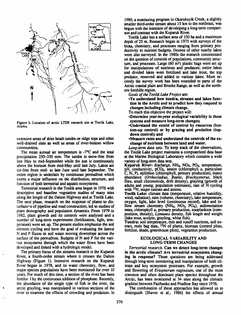
text of climatic change, the master variable for controlling cT F GH GHF SH ':1productivity appears to be temperature.Temperature regu- SHADElates weathering rates, decomposition, andthe depthof thawin terrestrial ecosystems, ali of which alter the flux of nu- 0, I I 1trients through terrestrial landscapes and into lakes. Tem-perature also regulates the strength and extent of thermal _ _stratificationand thus the zone of highest productivityin the _ _ _lake. Fisure2. Effectsof nine-year field treatments on net primarypro-

Under the present climatic regime, algal primary pro- duction and plant growth form composition in moist tussock tundraductivity is controlled by the amount of phosphorus entering at Toolik Lake, Alaska.Symbols:CT = mnu'oi; F = fertilizedthe lakewhich in turnis controlledby the amount of stream- (N+P);GH = greenhouse;GHF = greenhouse+ fertilizer;,SH =flow. In Toolik Lake there was a positive correlation (r2= shaded.Verticallines_-e+ 1S.E.(n = 4).0.52) between 14 years of summer primaryproductivity and

the discharge of the nearby KuparukRiver [Miller ct al., ent availability on terrestrial ecosystems, and howmight1986]. these changes interact? In a series of short- andlong-term

Stream Studies. What is the variability in annual water experiments that began in 1976, we have manipulatedairdischarge and nutrient flux from the Kuparuk temperature by building small greenhouses over the tundra,watershed and is there a discernible tong.term trend re- light intensity by shading, and nutrientavailability by fer-lated to climatic change? The flow of water through the tilizafion. Changes in nutrient availability have effects onlandscape affects many key biogeochemical processes that productivity and composition of tundra vegetation that arewill potentially change if the hydrologic cycle is significant- far greater than changes in either air temperature or lightly changed by either long-term trends or changing annual (Figure 2). The main effect of increased air temperature is tovariability in discharge. For example, increased water flow speed up the changes due to fertilizer alone. Without fertiliz-will likely increase weathering rates of soils in the er the effect of increased temperatures on the vegetation iswatershed and increase the export of dissolved cations, slight even after 9 years, and probably results from small in-anions, nutrients and dissolved organic materials from land creases in soil temperatures and increased nutrient miner-to rivers and lakes. Higher discharge will also lead to greater aliza.ion. These results are consistent with results of ourstreambank erosion which captures peat. When discharge is monitoring studies, and again lead to the prediction that ef-low, the flux of materials from land to water is decreased fects of climate change on nutrient cycling processes are theand the balance between autotrophic and heterotrophic pro- key to understanding climate change in the Arctic.cesses in streams and lakes is probably shifted in favor of Lake Studies. How much of the structure and functionautotrophy. If climatic change does change either the of the lake ecosystem is controlled by resources (bottom.amountof waterflow through arctic watershedsor the tim- up control), such as the rate of nutrient input, and howing of these flows, we expect large changes in nutrientflux- much is controlled by grazing and predation (top-downes and in biotic activity in rivers. Our monitoringpre)gramis control)? To isolate the effects of nutrient availability ondesigned to document these changes, productivity we initiated process-oriented studies on the ef-

fects of fertilization. These studies began in 1983 usingCONTROL BY RESOURCES VS. CONTROL BY large limnocorrals and have been expanded to whole sys-

GRAZING AND PREDATION terns with our current experiments in divided lakes. NutrientTerrestrial Studies. What is the relative importance of additions enhance primary production almost immediately,

changes in air temperature, changes in light intensity but the transferof carbon to higher trophic levels proceeds(due to changes in cloudiness), and changes in soil nutri, more slowly. Additionsof tracer amounts of 15Nto a whole

3RO

5.0 60 -4.0

3.0 o • Doptm/o m/ffdendorff/ono2.o• o Holoped/umg/bberum

-, 0.o 0 " CONTROLo • 50 - SAMPLESc2_

0.5 FERTILIZEDa. • = SAMPLESrr o • !m I_ O.f_" --- 40-

ii/0.05 o 'E• u

0.01 o

0.00 I i // I , ,, = , l ..a 30 -

1976 t977 t983 1984 1985 1986 1987 1988 _-"J ? e% t984 ,YEAR ca.:z: , _ DAY27

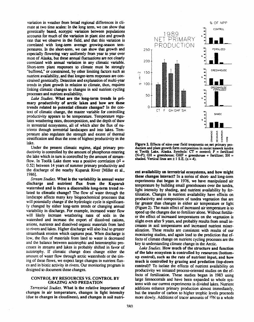
Figure 3. Thenumbersper100litersof two speciesof zcoplank- otoninTooUkLake,1976-1988, -r-

" 20- T

lake alsoindicated a time lag of at least onegrowingseason t, '"-"""_-.__..L

/ _k /

in the incorporationof new phytoplanktonproduction into ;/I' I _. /

the benthic food chain. Thus in the scenario of increased o f98z --1nutrientsupplydueto rising temperaturewe would expect e! DAY38rapidchangesin primaryproductivityanda delayed,more t0 - e,complex response from the higher tmphiclevels. _,

To investigate the higher trophic levels and their inter- /._ 1985 1986DAY20 DAY42

actions with populations below them in the context of /_ k. _T __[climate change, we have been both monitoring and experi- ,.,__ ....z--- Tmentally manipulatinga series of lakes. We have damon _L__'- =

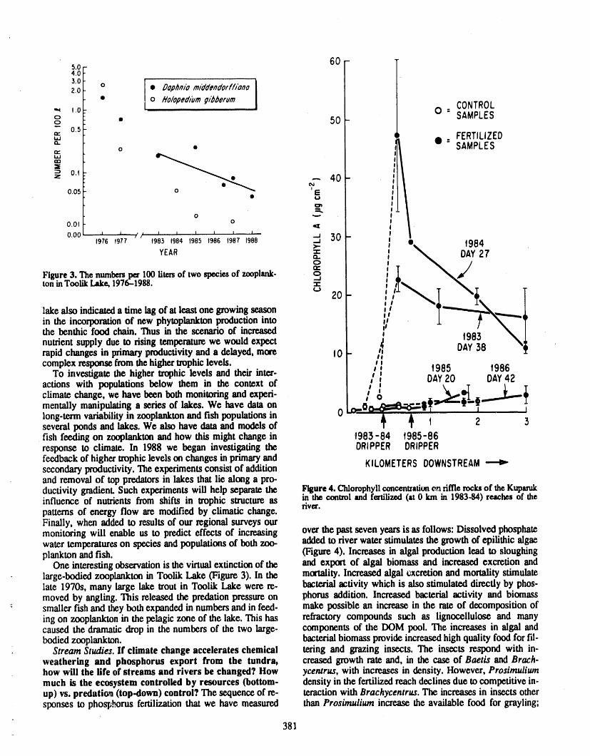
long-termvariabilityin zooplanktonand fish populations in 0 _ _ t Iseveral ponds and lakes. We also have data and models of 2 3fish feedingon zooplanktonand how this mightchangein t983-84 f985-86response to climate. In 1988 we began investigating the DRIPPER DRIPPERfeedbackof highertrophiclevelsonchangesin primaryandsecondaryproductivity.Theexperimentsconsistof addition KILOMETERSDOWNSTREAMandremovalof toppredatorsin lakesthat lie alonga pro-ductivity gradienLSuchexperiments will help separate the Figure4. Chlorophyllconcentrationcn riffle rock of theKuparuk

in theconwol andfertifized(at 0 km in 1983-84)reachesof theinfluence of nutrients from shifts in trophic sU'uctureaspatterns of energy flow are modified by climatic change, riv=.Finally, when added to results of our regional surveys ourmonitoring will enable us to predict effects of increasing over the past seven years is as follows: Dissolved phosphatewater temperatureson species andpopulations of both zoo- added to river water stimulates the growth of epilithic algaeplanktonandfish. (Figure 4). Increases in algal productionlead to sloughing

One interesting observationis the virtualextinction of the and export of algal biomass and increased excretion andlarge-bodiedzooplankton in Toolik Lake (Figure 3). In the mortality. Increased algal t_xcretionand mortality stimulatelate 1970s, many large lake trout in Toolik Lake were re- bacterialactivity which is also stimulated directlyby phos-moved by angling. This released the predationpressure on phorus addition. Increased bacterial activity and biomass

_ smaller fish and they bothexpanded in numbers andin feed- make possible an increase in the rate of decomposition ofing on zooplanktonin the pelagic zone of the lake. This has refractory compounds such as lignocellulose and manycaused the dramaticdrop in the numbers of the two large- components of the DOM pool. The increases in algal andbodiedzooplankton, bacterialbiomass provide increasedhigh quality food for ld-

• Stream Studies. If climate change accelerates chemical tering and grazing insects. The insects respondwith in-weathering and phosphorus export from the tundra, creased growth rate and, in the case of Baetis and Brach-how will the life of streams and rivers be changed? How ycentrus, with increases in density. However, Prosimuliummuch is the ecosystem controlled by resources (bottom- density in the fertilizedreachdeclines due to competitive in-up) vs. predati_u (top-down) control? The sequence of re- teractionwith Brachycentrus. The increases in insects othersponses to pho_rus fertilization that we have measured thanProsimulium increase the available food for grayling;

381

both young-of-the-year and adult grayling grow faster and RATES AND CONTROLS OF THE EXCHANGEachieve better condition in the fertilized reach. In the long OF NUTRIENTS AND ORGANIC MATTERterm, if the experimental nutrient addition wer_ expanded to BETWEEN LAND AND WATERinclude lhe whole river, and barring other overriding but un- Research Question. What controls the fluxes of nu-known population controls, we hypothesize that the fish trlents and water over the arctic landscape and intopopulation would increase. If so, it is possible that predation aquatic ecosystems? This question of land-water inter-by fish would exert increased top-down control over insects actions is fundamental to our understanding of streamsuch as Baetis or Brachycentru_ which are vulnerable to fish ecology and to predictions of climate change on arcticpredation when drifting and emerging. Experimental ecosystems. At the Toolik Lake site we already have manyevidence from bioassays using insecticides indicates that small plot measureanents of nutrients in soil water and theirgrazing insects conlrol algal biomass (also, in Figure 4 the interactions with plants. We also have large-scale dam onlow algal biomass in 1985 and 1986 is due to growth and the flux of nutrients out of entire watersheds. In the next fewgrazing of insects). Finally, increases in epilithic algae and years we will construct a dynamic model of the movementbacteria are responsible in part for uptake of added phos- of nutrients into streams and combine this with a geographicphorus and ammonium and fox uptake oi',aturally abundant information system (GIS) to test our understanding of thenitrate. Thus, the botJom-up effects of added nu_'ients are system and to estimate the nutrient output from larger water-paralleled by several top-down effects of fish on insects, in- sheds.sects on insects, insects on epilithic algae, and epilithon on Terrestrial Research. In tns research our principal aim isdissolved nutrient levels, to evaluate the magnitude and relative importance of lateral

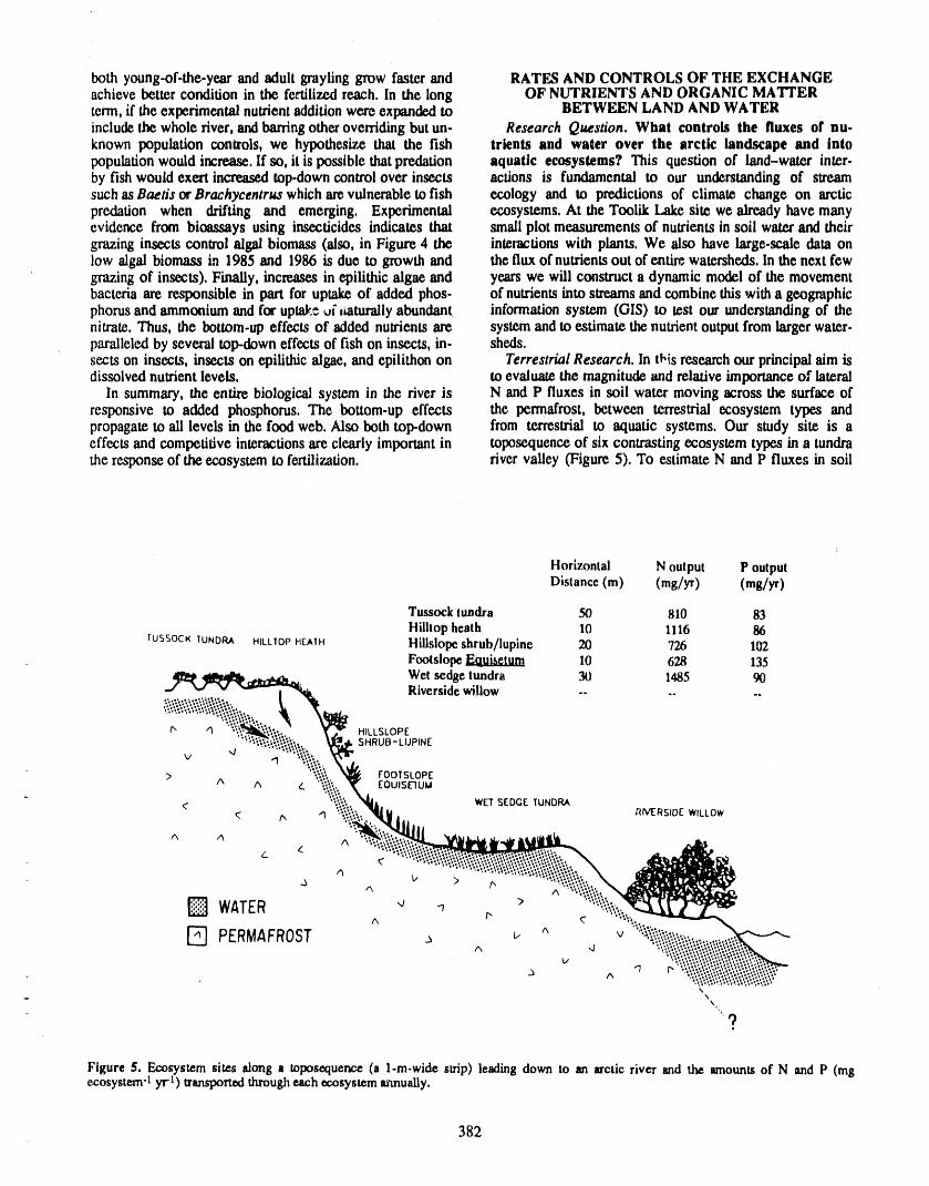
In summary, the entirebiological system in the river is N and P fluxes in soil water moving across the surface ofresponsive to added phosphorus. The bouom-up effects the permafrost, between terrestrial ecosystem types andpropagate to ali levels in the food web. Also both top-down from terrestrial to aquatic systems, Our study site is aeffects and competitive interactions are clearly important in toposequencc of six contrasting ecosystem types in a tundrathe re_onse of the ecosystem to fertilization, river valley (Figure 5). To estimate N and P fluxes in soil

Horizontal N output P outputDistance (m) (mg/yr) (mg/yr)

Tussock tundra 50 810 83Hilltop heath 10 1116 86

IUSSOCK TUNDRA HILLIOPHrLAIH HUlslopeshrub/lupine 20 726 102Footslope _ 10 628 135Wet sedge tundra__ 3o 14a5 90

___ "__ v v "--_0-_ Riverside willow ......

'; _'_i'..:. _lal. SHRUB-LUPINE

-;..%,%> . ":\_:.'.. _ FOOTSLOPE

"= ". _i_"..'-XI. wt_SEDcrTuNoRA"- , _ ".'_:¢..._llll, RIVERSIDEWILLOW

_- _. . ,.,.-?--.?,}j{_.?..

WATER 'J -7 r, ;, ":":":".'i'_-_._._A ¢ ' "",::.

L.U_ PERMAFROST ^ ' L, ^ _" 7"_':::'_.3

_, ''__':.:.._'.:.:..."1 r,' "::::::6:'.:;:::':'._:'::_:';::':"...^ ":':};'::".':i::'."_:':':_':':::':'::':':':_;:':i:':'

= N

',.

9

Figure 5. Ecosystem sites along a toposequence (a 1-m-wide saip) leading down to sn arctic river and the amountsof N and P (ingecosystem-I yrl) transportedthrougheach ecosystem annually.

382

waterat this site we have had to develop and compareover- .What is the specific role of the riparianzone in mod-ali N and P budgets for ali six ecosystems, and to link these ifying the chemistry of water entering rivers and in de-budgetswith a hydrologic model, texmining the amount of allochthonous organic matter

Ourmajor conclusions are that the net uptake of N or P and light in riversand lakes7from moving soil water is small relative to internal fluxes ,What is the role of lakes in retaining and transformingsuch as annual plant uptake or N mineralization.However, organic matter and nutrients as this material moveseach of the six eco, ys_m types has a majorand verydiffer- downstream througha drainage?ent effect on the totalamounts of NO3, NH4, and PO4 in soil ,How do the communities of rivers and lakes change inwater (Figure 5). This has important implications for the in- response to changes in water quantity and qualitycausedputs of these nutrients to aquatic systems. Some ecosystem by various units of landscape, riparian zones and up-types, like tussock tundra and dry heath, are major sources stream lakes?of N to soil water. Other systems, particularly those From our history of experiments on fertilization of lakesoccurring under or below law-thawing snowbanks, are lm- and rivers, we know that both lake and stream biota are veryportant N sinks and P sources to soil water. Poorly drained responsive to both short- or longer-term changes in phos-wet sedge tundra is a P sink with a remarkably high N rain- phorus and nitrogen supply. Thus we have a large amount oferalization rate. information on question #4 and we know from current

We have also learned a great deal about patterns and research on small plots that different terrestrial ecosystemscontrols over N and P cycling processes along our will yield very different quality runoff water. In futuretoposequence. Among our most important discoveries, we research, we will focus on determining the relationships be-have shown that nitrification is much more important along tween larger landscape units (0.1 to 1 km2) and water qual-our toposequence than we suspected based on earlier re- ity of runoff, the role of the riparian zone, and the role ofsearch, and many plant species show high nitrate reductase lakes in determining river water quality.activity. We have strong evidence from stable isotope Scaling to Watershed and Regional Level. The long-termanalyses that different plant species are using isotopic,ally pl_ is to make a model of nutrient processing and transferdifferent N sources, and that these species differences are which would follow nutrients from the interactions in themaintained across sites. The relative amounts of different soil into a stream. This watershed model can be verified byforms of organic and inorganic P in soils also vary dramat- the continuous measurements of nutrient flux from theically across sites, watershed being made at the point where the Kuparuk River

In sum, our work has shown that different terrestrial crosses the single road. Next, the watershed model would beecosystems differ strongly in their chemical interactions calibrated to fit the different environments of northern Alas-with the soil water, and thus have highly variable effects on ka. Finally, the model would be used to characterize the var-the chemistry of water entering aquatic systems. This work iability among Alaskan ecosystems so that statisticalis important in the context of global change, because if extrapolations could be made to the regional scale. The endeither the composition of the landscape mosaic changes, or result would be regional predictions of nutrient fluxes fromland to rivers under various scenarios of climate change.the biogeochemistry of individual landscape units changes,the chemistryof inputs to aquatic systems will also change. The flux from an entire region to the Arctic Ocean could

Land.Water Interactions. To achieve one of our major then be predicted.

long-term objectives of understandingcontrols of water and REFERENCESnutrient flux at the whole watershed and regional levels, weare focusing on four major questions: Miller, M. C., G. R. Hater, P. Spatt, P. Westlake, and D.

•What is the role of various units of landscape in de- Yeakel, Primary production and its control in Tooliktermining the amount and chemistry of water flowing Lake, Alaska, Arch. Hydrobiol./Suppl,, 74, 97-131, 1986.from land to rivers and lakes? Shaver, G. R., N. Fetcher, and F. S. Chapin, Growth and

flowering in Eriophorum vaginatum: Annual and lat-itudinal variation, Ecology, 67, 1524-1535, 1986.

383

Paleolimnologic Evidence of High Arctic LateQuaternary Paleoenvironmental Change:

Truelove Lowland, Devon Island, N.W.T., Canada

R. H. King and I.R. SmithDepartment of Geography, University of Western Ontario, London, Ontario, Canada

. R.B. YoungEnvironmental Applicauona Group Limited, Toronto, Ontario, Canada

ABSTRACT

Truelove Lowland (75°33'N, 84°40'W) Is a small area (43 km2) of relativelyhigh biological diversity in the midst of the more typical Polar Desert of the Cana-dian High Arctic. Much of the Lowland is presently covered by freshwater lakessome of which arc sufficiently deep (7-8.5 m) to contain stratified lake sediments.Sediment cores (= 2 m long) from the larger lakes have been analyzed for diatomsand chemical composition and reveal a stratigraphic record that spans the last10,600 years.

This record indicates that lake development in the Lowland began as a series of

shallow marine lagoons isolatexl from the sea as a result of glacio-isostatic reboundand the progressive emergence of the Lowland from the sea. Following isolation,the timing of which was strongly controlled by elevation and the relative rate of iso-static uplift, the lakes have been flushed with freshwater. Since that time the lakeshave remained oligotrophic and lake sedimentation has be.en dominated by vari-ations in non-biogenic factors and particularly by variations in the influx of alloch-thonous materials from within the lake catchments. Over time, the progressive

_I stabilizationof surfacematerialsand _dogenesis withinthe lakecatchmentshasbccn marked by decreasingamounts of Cr, As and Na in the sedimentsand anincreaseinallochthonousFe and Mn.

INTRODUCTION dm BiomecomponentoftheIntcmation_flBiologicalPro-

Under existing climatic conditions the Canadian High gram (IBP) and the only one outof a total of four majorarc-Arctic is a polar desert, characterized by low biological tic projects that was conducted within the High Arcticdiversity and low productivityand underlainby continuous [Bliss, 1977].permafrost. However, in widely scattered locations small Although a considerableamount of detailed informationareasof relatively high biological diversity andproductivity on the characteristics and performance of this ecosystemoccurasterrestrialoasesinthemidstoftheregionalpolar was amassedby theIBP projectovera fouryearperiod,desert.An exampleofsuchanmca isfileTrueloveLowland 1970-1974,itprovidesonlyasmallpictureofchanges,both(75°3YN,8A°40'W),oneofa seriesoflowlandslocatedon environmentalandecological,experiencedby theLowlandthenortheasterncoastofDevonIsland,N.W.T.(FigureI). sinceithasbccninexistence.What hasbccnlackinguntilBecauseoftheirecologicsignificancethesepolaroases now havebe,cndetailsofthechangesexperiencedby the

havebccn theobjectofconsiderablescientificinterestin Lowlandovertherelativelylongertermofthepostglacialrecentyears.TrueloveLow'landwaschosenasthelocation period.A majorprobleminobtainingsuchinformationhasforoneoffourteenmajorecosystemstudieswithintheTun- bccntheapparentabsenceofa stratigraphicre.c_rdofsuch

384

o l

Tr u e I o ve I n I e t P,oou_,yCartog;zpl_tcSectionDe_rlmenloiG,oomPrly.UW0

84o35'W LonOon,Onta;m

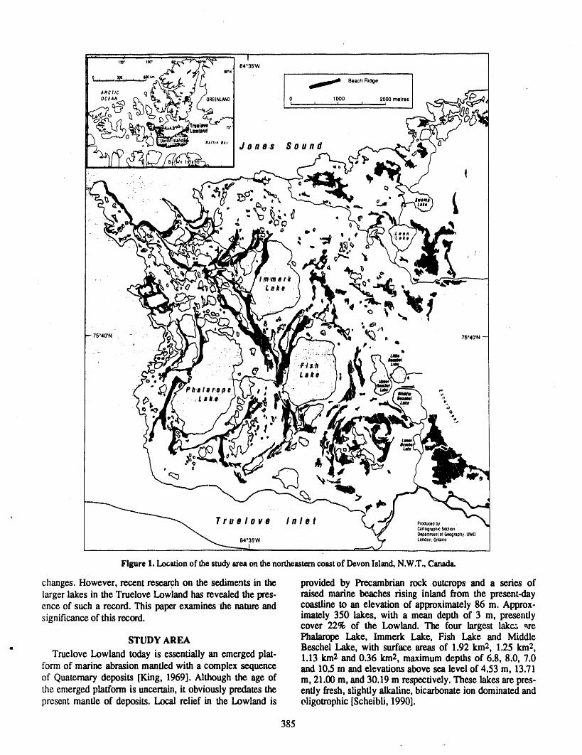
Figure 1. Locationof the studyszeaon thenortheasterncoastof DevonIsland,N,W.T.,Canada.

changes. However, recent researchon the sediments in the provided by Precambrianrock outcrops and a series oflargerlakes in the Truelove Lowland has revealed the Ires. raised marine _aches rising inland from the present.<layence of such a rf_,ord.This paperexamines the natureand coastline to an elevation of approximately86 m. Approx-significance of this record, imately 350 lakes, with a mean depth of 3 m, presently

cover 22% of the Lowland. The four largest lakc_, _reSTUDY AREA Phalarope Lake, Immerk Lake, Fish Lake and Middle

. BeschelLake, with surfaceareasof 1.92 km2, 1.25 km2,Truelove Lowland today is essenfiaUyan emerged plat- 1.13 km2 and 0.36 km:Z,maximumdepths of 6.8, 8.0, 7.0

form of marine abrasion mantled with a complex sequence and 10.5 m and elevations above sca level of 4.53 m, 13.71of Quaternarydeposits [King, 1969]. Although the age of m, 21.00 m, and 30.19 m respectively. These lakes arepres-the emerged platform is uncertain, it obviously predates the ently fresh, slightly alkaline, bicarbonate ion dominated andpresent mantle of deposits. Local relief in the Lowland is oligotrophic [Scheiblt, 1990].

385

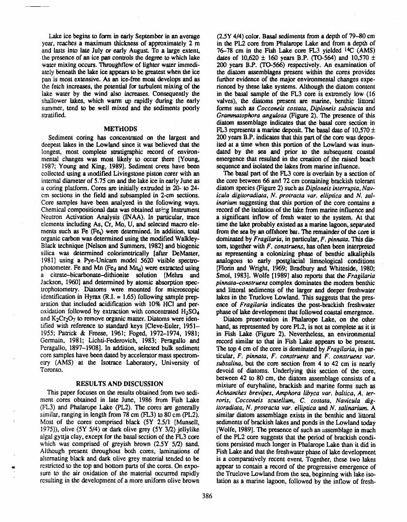
Lake ice begins to form in early Septemberin an average (2.5Y 4/4) color. Basal sediments from a depthof 79--.80emyear, reaches a maximum thickness of approximately 2 m in the PL2 core from Phalarope Lake and from a depth ofand lasts into late July or early August. To a large extent, 76-78 cm in the Fish Lake core FL3 yielded 14C(AMS)thepresence of an ice pan controls the degree to which lake dates of 10,620 4- 160 years B.P. (TO.564) and 10,570 4-watermixing occurs. Throughflowof lighter water immedi- 200 years B.P, (TO-566) respectively. An examinationofately beneath the lake ice appearsto be greatestwhenthe ice the diatom assemblages present within the cores providespan is most extensive. As an ice-free moat develops and as furtherevidence of the majorenvironmentalchanges expe-the fetch increases, the potential for turbulentmixing of the riencedby these lake systems. Although the diatom contentlake water by the wind also increases. Consequently the in the basal sample of the FL3 core is extremely low (16shallower lakes, which warm up rapidly during the early valves), the diatoms present are marine, benthic littoralsummer, tend to be well mixed and the sediments poorly forms such as Cocconeis costata, Diploneis subsincta andstratified. Grammatophora angulosa (Figure 2). The presence of this

diatom assemblage indicates that the basal core section inMETHODS FL3represents a marinedeposit, The basal date of 10,570 4-

Sediment coring has concentrated on the largest and 200 yearsB.P. indicates that this partof the core was depos-deepest lakes in the Lowland since it was believed that the ited at a time when this portion of the Lowland was inun-longest, most complete, stratigraphic record of environ- dated by the sea and prior to the subsequent coastalmental changes was most likely to occur there [Young, emergence that resulted in the creation of the raised beach1987; Young and King, 1989]. Sediment cores have been sequenceand isolatedthe Lakesfrom marineinfluence.collected using a modified Livingstone pistoncorer with an The basalpartof the FL3 core is overlain by a section ofinternaldiameterof 5.75 em and the lake ice in earlyJuneas the core between 66 and 72 cm containingbrackishtoleranta coring platform.Cores are initially extrudedin 20- to 24- diatom species (Figure 2) such as Diploneis interrupta, Nay-cm sections in the field and subsampledin 2-cm sections, icula digitoradiata, N. protracta var. elliptica and N. sal-Core samples have been analyzed in the following ways. inarium suggesting that this portion of the core contains aChemical compositional data was obtainedus_._gInstrument recordof the isolation of the lake frommarineinfluence andNeutron Activation Analysis 0NAA). In particular, trace a significant inflow of fresh water to the system. At thatelements including As, Cr, Mo, U, and selected macro ele- time the lakeprobablyexisted as a marinelagoon, separatedments such as Fe (FeO were determined. In addition, total from the sea by an offshore bar.The remainderof the core isorganic carbon was determinedusing the modifiedWalidey- dominatedby Fragilaria, in particular,F. pinnata. This dia.Black technique [Nelson and Summers, 1982] and biogenic tom, together with F. construens, has often been interpretedsilica was determined colorimetrically [after DeMaster, as representing a colonizing phase of benthic alkaliphils1981] using a Pye-Unicam model 5620 visible speclro- analogous to early postglacial limnologieal conditionsphotometer.Fe and Mn (Fed and Mnd) were extracted using [Florin and Wright, 1969; Bradbury and Whiteside, 1980;a citrate-bicarbonate.-dithionite solution [Mehra and Stool, 1983]. Wolfe [1989] also reports that the FragilariaJackson, 1960] and determined by atomic absorption spec- pinnata--construens complex dominates the modern benthictrophotometry. Diatoms were mounted for microscopic and littoral sediments of Ciaelarger and deeper freshwateridentification in Hyrax (R.I. ---1.65) following sample prep- lakes in the Truelove Lowland. This suggests that the pres-aration that included acidification with 10% HCI and per- ence of Fragilaria indicates the post-brackish freshwateroxidation followed by extraction with concentrated H2SO4 phase of lake development that followed coastal emergence.and K2Cr207 to remove organic matter. Diatoms were iden- Diatom preservation in Phalarope Lake, on the othertiffed with reference to standard keys [Cleve-Euler, 1951- hand, as represented by core PL2, is not as complete as it is1955; Patrick & Freese, 1961; Foged, 1972-1974, 1981; in Fish lake (Figure 2). Nevertheless, an environmentalGermain, 1981; Lichti.Federovich, 1983; Pe_gallo and record similar to that in Fish Lake appears to be present.Peragallo, 1897-1908]. In addition, selected bulk sediment The top 4 cm of the core is dominated by Fragilaria, in par-core samples have been dated by accelerator mass spectrom, titular, F. pinnata, F. construens and F. construens var.etry (AMS) at the lsotrace Laboratory, University of subsalina, but the core section from 4 to 42 cm is nearlyToronto. devoid of diatoms. Underlying this section of the core,

between 42 to 80 cre, the diatom assemblage consists of aRESULTS AND DISCUSSION mixture of euryhaline, brackish and marine forms such as

This paper focuses on the results obtained from two sedi- Achnanthes brevipes, Amphora libyca var. baltica, A. tct-ment cores obtained in late June, 1986 from Fish Lake roris, Cocconeis scutellum, C. costata, Navicula &'g-(FL3) and Phalarope Lake (PL2). The cores are generally itoradiata, N. protracta var. elliptica and N. salinarium. Asimilar, ranging in length from 78 cm (FL3) to 80 cm (PL2). similar diatom assemblage exists in the benthic and littoralMost of the cores comprised black (5Y 2.5/1 [Munsell, sediments of brackish lakes and ponds in the Lowland today1975]), olive (5Y 5/4) or dark olive grey (SY 3/2) jellylike [Wolfe, 1989].The presence of such an assemblage in muchalgal gyttja clay, except for the basal section of the FL3 core of the PL2 core suggests that the period of brackish condi-which was comprised of greyish brown (2.5Y 5/'2) sand. tions persisted much longer in Phalarope Lake than it did inAlthough present throughout boat cores, laminations of Fish Lake and that the freshwater phase of lake developmentalternating black and dark olive grey material tended to be is a comparatively recent event. Together, these two lakes

° restricted to the top and bottom parts of the cores. On expo- appear to contain a record of the progressive emergence ofsure to the air oxidation of the material occurred rapidly the Truelove Lowland from the sea, beginning with lake iso-resulting in the development of a more uniform olive brown lation as a marine lagoon, followed by the inflow of fresh-

386

" ' / ) h. , ,.,, _, _.

._..5 o o o o __.._!3o o o

.... Ii'0

16

25 _ _

30 ._.._ _ 32OkkN

40

51 _ _ 48 , esi'_ "7" ' [i_%%

'":':" =Figure2. Diatomstratigraphyof theFL3corefromFishLakeandthe PL2corefromPhal_ropeLakein percentageof diatom_um.

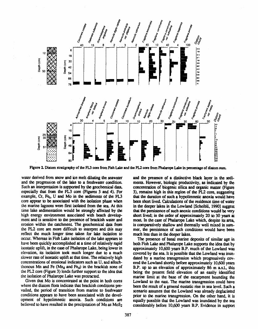
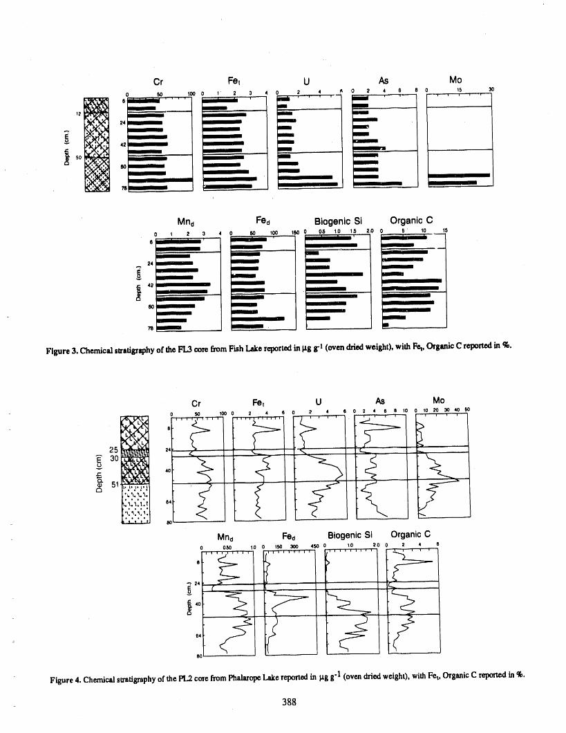
water derived from snow and ice melt diluting the seawater and the presence of a distinctive black layer in the sedi.and the progressionof the lake to a freshwatercondition, merits. However, biologic productivity, as indicated by theSuch an interpretationis supportedby the geochemical data, concentrationof biogenic silica and organic matter(Figureespecially that from the FL3 core (Figures 3 and 4). For 3), remains high in this region of the PL2 core, suggestingexample, Ct, Fe_,U and Mo in the sediments of the FL3 thatthe durationof such a hypolimnetic anoxia would havecore appear to be associated with the isolation phase when been shortlived. Calculagonsof the residence timeof waterthe marine lagoons were f'n'stisolated from the sea. At this in the deeper Lakesin the Lowland [Scheibli, 1990] suggesttime lake sedimentation would be strongly affected by the thatthe persistenceof such anoxic condit/mts would be veryhigh energy environment associated with beach develop- shortlived; in the orderof approximately 20 to 30 years atmentand is sensitiveto thepresenceof brackishwaterand mosLIn thecaseof PhalaropeLakewhich,despiteits area,erosionwithin the catchmenLThe geochemicaldatafrom iscomparativelyshallowand therma/lywell mixed in sum-the PL2 'coreare moredifficult to interpret and this may mer, the persistenceof such conditions would have beenreflect the much longer time taken for lake isolation to muchless thanin the deeper lakes.occur.Whereasin FishLakeL_lationof thelakeappearsto The presenceof basalmarinedepositsof similarageinhave been quickly accomplished at a timeof relativelyrapid both Fish Lake and PhalaropeLake supports the idea thatbyisostatic uplift, in the case of PhalaropeLake, being lowerin approximately 10,600 yearsB.P. much of the Lowland waselevation, its isolation took much longer due to a much covered by thesea. lt is possible thatthe Lowland was inun-slower rateof isostatic uplift at that time. The relativelyhigh dated by a marine transgression which progressively coy-concentrationsof erosional indicatorssuch as U, andalloch- ered the Lowland shortlybefore approximately 10,600 yearsthonous Mn and Fe (Mnd and Fea) in the brackish zone of B.P. up to an elevation of approximately 86 m a.s.l., thisthe PL2 core (Figure3) lends furthersupportto the idea that being the present field elevation of an easily identifiedthe isolationof PhalaropeLake was protracted, marine limit at the base of the escarpment bounding the

Given that Mo is concentrated at the point in both cores Lowland to the east. The marine transgressioncould havewhere the diatom flora indicate that brackish conditions pre- been the result of a general eustatic rise in sea level. Such availed, the period of transition from marine to freshwater scenario assumes that the Lowland was already deglaciatedconditionsaRcars to havebeenassociatedwith the devel- prior to the marinetransgression.On the other hand,it isopment of hypolimnetic anoxia. Such conditions are equally possible that the Lowland was inundated by the seabelieved to have resulted in the precipitationof Mo as MoS2 considerably before 10,600 years B.P. Evidence in support

387

Cr Fet U As Mo0 50 t00 0 t' 2 3 4 0 2 4 _ O 2 4 ....6 8 0 • , 15, , ,, 30

silaimmm .... =mm= ' =mi .... "- m ' '

i __ III i12 - _ iii m

;4_ -- m m

_ -- m m"" d2 -- mim i

m

. so ......... -- -- - .-- ro=m,iOJ_ -- milli mmmmm

II I IIIII , immmm I-- II .-

Mhd Fed Biogenic SI Organic C0 t 2 3 4 0 50 100 t50 0 0.5 1,0 1.5 2,O 0 5' tO 15

.... ' -- __ " 1 I"--6 IZi " " ' _ '

II ,,__

i __ I II

II III i

- 42 I _ ---_ __ lip

= -- I Iq III

60 _ III _ II I _ IIII_ II __ II

Figure 3. Chemical slratigrgphyof theFL3 core fromFish Lakereportedin p.gg-t (oven driedweight), with Fet,OrganicC reportedin %.

Cr Fet U As Mo0 SO 100 2 4 6 0 2 4 6 2 4 6 8 10 0 10 20 30 40 SO

1 | 1 I t ! i 1 I | 1 / '

25 _4 L__r. 4ol

_ 51 ,,a

't '_. _.. '_. _ __

SO

Mna Fea Biogenlc Si Organic C0 0_) 1.0 150 300 450 0 t.O 2.0 0 2 4

o >)

_ ,o ._

L ......8O

Figure 4. Chemical sa'atigraphyof thePL2core fromPhalaropeLakereportedin I_gg-I (oven driedweight), with Fet, OrganicC reportedin %.

388

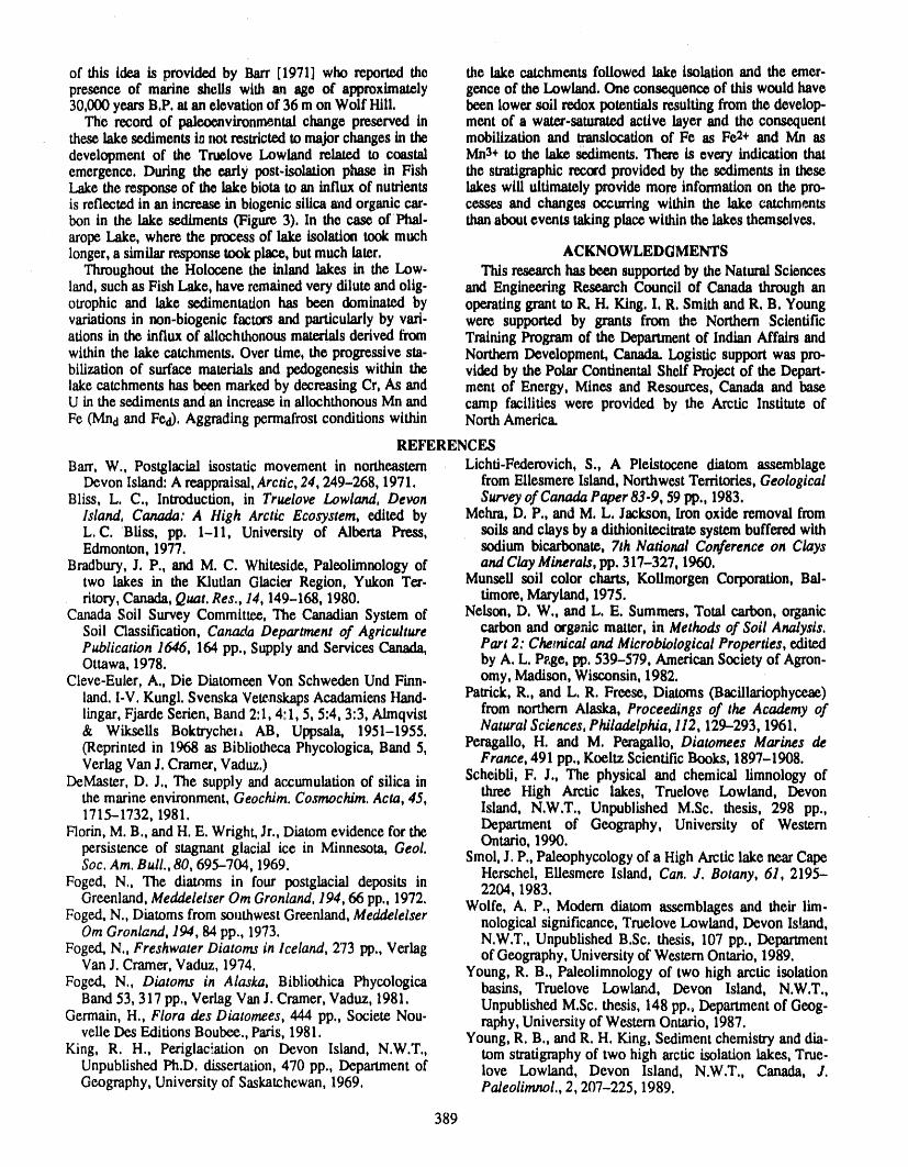
of this idea is provided by Barr [1971] who reported the the lake ca_hments followed lake isolation and the emer-presence of marine shells with an age of approximately gence of the Lowland, One consequence of this would have30,000 yearsB,P. at an elevationof 36 m on Wolf Hill, been lower soil redox potentials resulting from the develop-

The record of paleo_vironmental change preserved in meritof a water.satumwA active layer and the consequentthese lake sedimentsinrmt restrictedto majorchanges in the mobilization and translocationof Fo as 1::¢2+and Mn asdevelopment of the Truelove Lowland related to coastal Mn3+ to the lake Sediments,There is every indication thatemergence, During the early post-isolation phase in Fish the stratigraphicrecordprovided by the sediments in theseLake the response of the lake biota to an influx of nutrients lakes will ultimately provide more informationon the pro..isreflectedinanincreaseinbiogenicsilicaandorganiccar- cessesand changesoccurringwithinthelakecatchmentsben in the lake sediments (Figure 3), In the case of Phai- thanaboutevents takingplace within the lakes themselves.aropeLake, where the process of _ isolation took muchlonger,a similarresponsetook place, butmuch later. ACKNOWLEDGMENTS

Throughout the Holocene the inland lakes in the Low- This researchhas been supportedby theNaturalSciencesland,such as Fish Lake, have remainedvery dilute andolig- and Engine,exing Research Council of Canada through anotrophic and lake sedimentation has been dominated by operating grantto R. H. King. I. R. Smith and R. B. Youngvariationsin non-biogenic factors and particularlyby vm'i- were supported by grants from the Northern Scientifications in the influx of allochthonous materialsderived from Training Programof the Departmentof Indian Affairs andwithin the lake catchments. Over time, the progressive sm- Northern Development, Canada. Logistic support was pro-bilizatton of surface materials and pedogenesis within the vided by the Polar Continental Shelf Projectof the Depart-lakecatchments has been markedby decreasing Cr, As and ment of Energy, Mines and Resources, Canada and baseU inthe sedimentsand an increase in allochthonous Mn and camp facilities were provided by the Arctic Institute ofFe (MII d and Fed). Aggradingpermafrostconditions within North America.

REFERENCES

Barr, W., Postglacial isostatic movement in northeastern Lichti-Fe,derovich, S., A Pleistocene diatom assemblageDevon Island: A re.appraisal,Arctic, 24,249-268, 1971. from Ellesmere Island, NorthwestTerritories, Geological

Bliss, L. C., Introduction, in Truelove Lowland, Devon Survey of Canada Paper 83-9, 59 pp., 1983.Island, Canada: A High Arctic Ecosystem, edited by Mehra, D. P., and M. L. Jackson, Iron oxide removal fromL.C. Bliss, pp. 1-11, University of Alberta Press, soils and clays by a dithionite.citrat¢system buffered withEdmonton, 1977. sodium bicarbonate, 7th National Conference on Clays

Bradbury,J. P., and M. C. Whiteside, Paleolimnology of and ClayMinerals, pp. 317-327, 1960.two lakes in the Klutlan Glacier Region, Yukon Tet. Munsell soil color charts, Kollmorgen Corporation,Bal-ritory,Canada, Quat. Res,, 14, 149-168, 1980. timore, Maryland, 1975.

Canada Soil Survey Commits, The Canadian System of Nelson, D. W., and L. E. Summers, Total carbon, organicSoil Classification, Canada Department of Agriculture carbon and orgardc matter, in Methods of Soil Analysis.Publication 1646, 164 pp., Supply and Services Canada, Part 2: Chemical and Microbiological Properties, editedOttawa, 1978. by A. L. Page, pp. 539-579, American Society of Agron-

Cleve-Euler, A., Die Diatomeen Von Schwcdcn Und Finn- omy, Madison, Wisconsin, 1982.land. I-V. Kungl. Svenska Vetenskaps Acadamiens Hand- Patrick, R., and L. R. Freese, Diatoms (Bacillariophycea¢)lingar, Fjarde Serien, Band 2:1, 4:1, 5, 5:4, 3:3, Almqvist from northern Alaska, Proceedings of the Academy of& Wiksells Boktrychezi AB, Uppsala, 1951-1955. Natural Sciences, Philadelphia, 112, 129-293, 1961.(Reprinted in 1968 as Bibliothcca Phycologica, Band 5, Pcragallo, H. and M. Peragallo, Diawmees Marines deVerlag Van J. Cramer, Vaduz.) France, 491 pp., Kocltz Scientific Books, 1897-1908.

DcMaster, D. J., The supply and accumulation of silica in Scheibli, F. J., The physical and chemical limnology ofthe marine environment, Geochim. Cosmochim. Acta, 45, three High Arctic lakes, Truelove Lowland, Devon1715-1732, 1981. Island, N.W.T., Unpublished M.Sc. thesis, 298 pp.,

Florin, M. B., andH. E. Wright,Jr., Diatomevidence for the Department of Geography, University of Westernpersistence of stagnant glacial ice in Minnesota, Geol. Ontario, 1990.Soc. Am. Bull., 80, 695-704, 1969. Stool, J. P., Paleophycology of a High Arcticlake nearCape

Foged, N,, The diatoms in four postglacial deposits in Herschel, Ellesmere Island, Can, J. Botany, 61, 2195--2204, 1983.Greenland,Meddelelser Om Gronland. 194, 66 pp., 1972. Wolfe, A. P., Modem diatom assemblages and their lira.

Foged, N., Diatoms from southwest Greenland,Meddelelser nological significance, Truelove Lowland, Devon Island,Om Gronland, 194, 84 pp., 1973. N.W.T., Unpublished B.Sc. thesis, 107 pp., Department

Foged, N., Freshwater Diatoms in Iceland, 273 pp., Verlag of Geography, Universityof We.stemOntario, 1989.Van J. Cram_, Vaduz, 1974. Young, R. B., Paleolimnology of two high arctic isolation

Foged, N., Diatoms in Alaska, Bibliothica Phycologica basins, Truelove Lowlaad, Devon Island, N.W.T.,Band53, 317 pp., Verlag VanJ. Cramer,Vaduz, 1981. Unpublished M.Sc. thesis, 148 pp., Departmentof Geog.

Germa/m,H., Flora des Diatomees, 444 pp., Societc Nou- raphy, University of Western Ontario, 1987.velle Des Editions Boube¢., Paris, 1981. Young, R. B., and R. H. King, Sediment chemistry azld dia-

King, R. H., Periglaciation on Devon Island, N.W.T., tom stratigraphyof two high arctic isolation lakes, True-Unpublished Ph.D. dissertation,470 pp., Departmentof love Lowland, Devon Island, N.W.T., Canada, J.Geography, Universityof Saskatchewan, 1969. Paieolimnol., 2,207-225, 1989.

389

Effect of Global Climate Change on Forest Productivity:Control Through Forest Floor Chemistry

K. Van Cleve, J. Yarie, and E. VanceForest Soils Laboratory, University of Alaska Fatrbanks, Alas_, U.S.A.

ABSTRACT

Forest floor chemistry interacts with temperature and moisture to restrict orenhance the supply of nutrients for tree growth. In sub-arctic forests of interiorAlaska, this control of element supply is manifest in dramatically different rates ofnutrient cycling among the principal forest types. Slow-growing forests developingon cold, wet soils produce organic detritus that is slow to decompose because of itschemical composition. Consequently, element supply is restricted in these eco-systems. Productive forests developing on warm, drier soils produce organic detri-tus that decays more rapidly because of favorable chemical composition. Elementsupply is enhanced in these forest ecosystems.

Using the compartment model Linkages, we evaluate several scenarios that pro-pose altered temperature and precipitation regimes for their influence on forestfloor chemistry, element supply and the consequence to forest productivity.

390

The Sensitivity of Ecosystem COz Flux in the Boreal Forestsof interior Alaska to Climatic Parameters

Gordon B. BonanNattc:,_l Centerfor Atmospheric Research, Boulder, Colorado, U.S.A.

ABSTRACT

An eeophysiological model of carbon uptake and release was used to examineCO2 fluxes in 17 mature forests near Fairbanks, Alaska. Under extant climatic con-ditions, ecosystem CO2 flux ranged from a loss of 212 g CO2 m-2 yrl in a blackspruce stand to an uptake of 2882 g CO2 m-2 yr-1 in a birch stand. Increased airtemperature resulted in substantial soil warming. Without concomitant increases innutrient availability, large climatic wanning reduced ecosystem CO2 uptake in aliforests. Deciduous and white spruce stands were still a sink for CO2, but blackspruce stands became, on average, a net source of CO2. With increased nutrientavailability that might accompany soil warming, enhanced tree growth increasedCO2 uptake in conifer stands.

INTRODUCTION biosphereexchange of CO2in boreal forestsand its sensitiv-The circumpolarboreal forest is thelargestreserveof soil ity to climaticparameters.

carbon and is second only to broadieaf humid forests interms of carbon stored in live vegetation [l.,ashof, 1989]. THE MODELNot surprisingly, boreal forests appearto play a significant Bonan [1991b] describes the calculation of the CO2role in the seasonal dynamicsof atmosphericCO2 [D'Arrigo fluxes. The model simulates daily CO2 fluxes duringplantct al., 1987]. With its wide range in site conditions, interior growth and forest floor decomposition (Figure 1). MossesAlaska is a unique location to examine atmosphere- form a significant component of many boreal forestsbiosphere exchange of CO2 in boreal forests. In mature [Oechel and Van Cleve, 1986], and moss photosynthesisforests, above-ground woody biomass ranges from 2.6 kg and respiration are additional CO2 fluxes. Tree photosyn-m-2 in black spruce (Picea mariana (Mill.) B.S.P.) forests thesis is a function of the CO2 diffusion gradient,bulk boun-growing on cold, wet, nutrient-poorsoils to 24.6 kg m-2 in dary layer resistance, stomatal resistance, and mesophyllwhite spruce (Picea glauca (Moench.) Voss) forests grow- resistance. Stomatal resistance is a function of irradiance,ing on warmer, mesic soils [Van Cleve et al., 1983]. Forest foliage temperature, vapor pressure deficit, and foliagefloor mass ranges from an average of 2.2 kg m-2 in mature water potential.Mesophyll resistance includes rate limita-balsam poplar (Populus balsamifera L.) forests to an aver- tions imposed by the diffusion of CO2 within cells and theage of 7.6 kg m-2 in mature black spruce forests [Van Cleve effects of foliage temperature, irradiance, and foliage nitro-et al., 1983]. gen on the biochemical process of photosynthesis. Tree

Interactions among soil temperature, soil moisture, the respiration is partitioned into maintenance and growth res-forest floor, litter q'uality,nutrientavailability and fire con- piration. Maintenancerespiration is an exponential functiontrol stand productivity and organic matterdecomposition in of foliage temperature; growth respiration is a function ofthese forests [Van Cleve and Viereck, 1981; Van Cleve et the efficiency with which tissue is synthesized. Moss photo-al., 1983, 1986]. I have developed a process-oriented, ec- synthesis is limited by irradiance, temperature,and moistureophysiological model of carbon uptake and release that content. Moss respiration is also an exponential function ofquantifies these relationships [Bonan, 1991b]. The purpose temperature and the efficiency with which new tissue is syn-of this paper is to use this model to examine atmosphere,- thesized. Based on data from Schlentner and Van Cleve

391

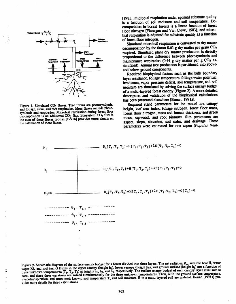
[1985], microbialrespirationunderoptimal substratequalityis a function o_ soil moisture and soil temperature. De.composition in bore_ forests is a linear function of forest

_. _, floor nitrogen [Flanaganand Van Cleve, 1983], and micro-, * ! bial respirationis adjustedforsubstratequalityas a function

" _ fl fm

,_,_ _ __ _ _ of forest floor nitrogen., _.m0_ Simulatedmicrobialrespirationis convertedto drymatter" Idecompositionby lhc factor0.61 g drymatterper gramC02

__ _,_ respired. Simulated plant dry matterproduction is directly_. _ proportional to the difference between photosynthesis andmaintenancerespiration(0.44 g dry matter per g CO2 as-similated).Annual tree productionis partitionedinto alxwe-and below-_ components.

Required biophysical factors such as the bulk boundarylayerresistance, foliage temperature,foliage waterpotential,irmdianc_, vaporpressuredeficit, soil temperature,and soilmoistureare simulatedby solving the surface energy budgetof a multi-layerodforestcanopy (Figure 2). A more detaileddescription and validation of the biophysical calculationshas beenpresentedelsewhexe [Bonan, 1991a].

Figure1. Simulated_ flux_..Tree.fluxesereI_o_syn_. Required stand parameters for the model are canopyand foliage,stem,androotresptrauon.Mou nuxesmcmaeImO height, leaf area index, foliage nitrogen, forest floor mass,synthesis and respiration. MicrobialrespiraLionduring f_est flo_. forest floor nitrogen,moss and humusthickness, and greendecompositionis an additionalCO2flux. Ec_.s.yraemt.u_./2.-t!ux tsthe sumof thesefluxes.Bonan[1991b]provtaesmoreaeta_ on moss, sapwood, and root biomass. Site parameters arethecalculationof thesefluxes, aspect, slope, elevation, soil color, and drainage. These

parameters were estimated for one aspen (Popul_ trem-r

R.[T I Tz,T3]+H[TI,Tz,T3]+IE[TI,Tz'T3]=0HI

Hz R.[TI,Tz,T3] +H [TI 'TZ'T3]+IE[TI'Tz'T3] =0

H3=0 R.[T I,Tz,T3]+HIT I,T z,T3]+IE[T I,Tz,'r3]+G [T3]=0

01, Ts,1-

e z , Ts,Z

0 3 , Ts,3

Figure 2. Schematicdiagramof the surfaceenergybudgetforaforestdividedintothreelayers.ThenetradiationRa, sensibleheatH, water.po, .d.. onu .m of=zero, and these three equatmns are solved snnul_usly tor the uzree untalown tempexamres. I ne_. wire mc 8zuunu _mt t,_.au,_,

_- e.v.apotransl_r,ati.on,andsnow...... ,melt_.,_..kn°wn'__.soll temperatureT, andsoil moistureO in a multi-layered solil are updated.Bonan[1991a1pm-

392

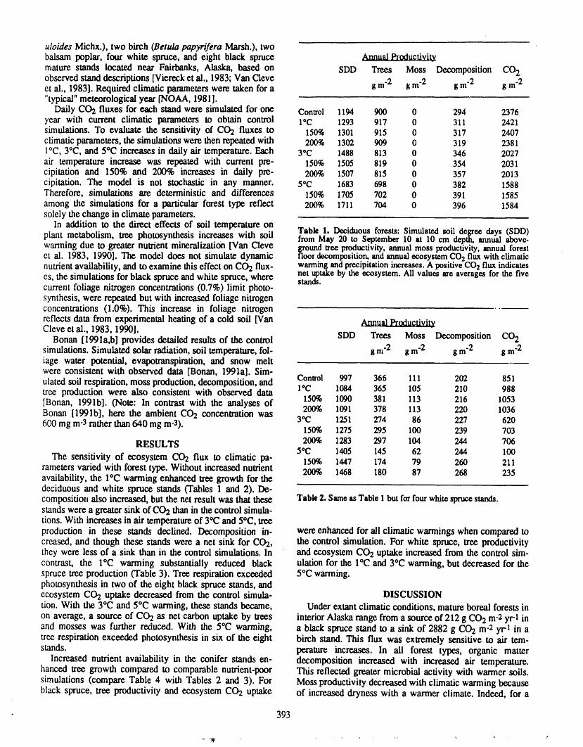
uloides Michx.), two birch (Betula papyrifera Marsh.), twobalsam poplar, four white spruce, and eight black spruce Annual Productivity

mature stands located near Fairbanks, Alaska, based on SDD Trees Moss Decomposition CO2observed stand descriptions [Viereck et al., 1983; Van Cleveet al., 1983]. Required climatic parameters were taken for a $ m'2 g m'2 $m'2 $ m'2"typical"meteorological year [NOAA, 1981].

Daily CO2 fluxes foreach stand were simulated for one Control 1194 900 0 294 2376year with current climatic parameters to obtain control l*C 1293 917 0 311 2421simulations. To evaluate the sensitivity of CO2 fluxes to 150% 1301 915 0 317 2407climatic parameters, the simulations were then repeated with 200% 1302 909 0 319 2381I°C, 3°C, and 5"C increases in daily air temperature. Each 3"C 1488 813 0 346 2027air temperature increase was repeated with current pre- 150% 1505 819 0 354 2031cipitation and 150% and 200% increases in daily pre- 200% 1507 815 0 357 2013cipitation. The model is not stochastic in any manner. 5"C 1683 698 0 382 1588Therefore, simulations are deterministic and differences 150% 1705 702 0 391 1585among the simulations for a particular forest type reflect 200% 1711 704 0 396 1584solely the change in climate parameters.

In addition to the direct effects of soil temperature onTable 1. Deciduousforests:Simulatedsoil degreedays (SDD)

plant metabolism, tree photosynthesis increases with soil from May 20 to September10 at 10 cna depth,annual above.wanning due to greater nutrient mineralization [Van Cleve ground tree productivity,annual moss productivity,annual forestet al. 1983, 1990]. The model does not simulate dynamic floordecomposition,andannualecosystemCO2fluxwithclimaticnutrient availability, and to examine this effect on CO2 flux- warmingand precipitationincreases.A positiveCO2 fluxindicateses, the simulations for black spruce and white spruce, where net uptakeby the ecosystem.Ali values areaveragesfor the fivestands.current foliage nitrogen concentrations (0.7%) limit photwsynthesis, were repeated but with increased foliage nitrogenconcentrations (1.0%). This increase in foliage nitrogenreflects data from experimental heating of a cold soil [Van Annual ProductivityCleve et al., 1983, 1990].

Bonan [1991a,b] provides detailed results of the control SDD Trees Moss Decomposition CO2simulations. Simulated solar radiation, soil temperature, fol- g m"2 g m"2 g m"2 g m"2iage water potential, evapotranspiration, and snow meltwere consistent with observed data [Bonan, 1991a]. Sim-ulated soil respiration, moss production, decomposition, and Control 997 365 111 202 851tree production were also consistent with observed data l*C 1084 365 105 210 988[Bonan, 1991b]. (Note: In contrast with the analyses of 150% 1090 381 113 216 1053Bonan [1991b], here the ambient CO2 concentration was 200% 1091 378 113 220 10363"C 1251 274 86 227 620600 mg m-3rather than 640 mg m-3). 150% 1275 295 100 239 703

RESULTS 200% 1283 297 104 244 70650C 1405 145 62 244 100

The sensitivity of ecosystem CO2 flux to climatic pa- 150% 1447 174 79 260 211rameters varied with forest type. Without increased nutrient 200% 1468 180 87 268 235availability, the I°C warming enhanced tree growth for thedeciduous and white spruce stands (Tables 1 and 2). De-compositio|l also increased, but the net result was that these Table2. SameasTable 1butforfourwhitesprucestands.standswere a greatersinkof CO.2thanin the control simula-tions. With increases in air temperatureof 3°(2and 50C, treeproduction in these stands declined. Decomposition in- were enhanced for ali climatic warmings when compared tocreased, and though these stands were a net sink for CO2, the control simulation. For white spruce, tree productivitythey were less of a sink than in the control simulations. In and ecosystem CO2 uptake increased from the control sim-contrast, the I°C warming substantially reduced black ulation for the l°C and 30C warming, but decreased for thespruce tree production (Table 3). Tree respiration exceeded 5°C warming.photosynthesis in two of the eight black spruce stands, andecosystem CO2 uptake decreased from the control simula- DISCUSSIONtion. With the 3°C and 50C warming, these stands became, Under extant climatic conditions, mature boreal forests inon average, a source of CO2 as net carbon uptake by trees interior Alaska range from a source of 212 g CO2 m-2yr-I inand mosses was further reduced. With the 50C warming, a black spruce stand to a sink of 2882 g CO2 m-2 yr-I in atree respiration exceeded photosynthesis in six of the eight birch stand. This flux was extremely sensitive to air tem-stands, peratare increases. In ali forest types, organic matter

Increased nutrient availability in the conifer stands en- decomposition increased with increased air temperature.hanced tree growth compared to comparable nutrient-poor This reflected greater microbial activity with warmer soils.simulations (compare Table 4 with Tables 2 and 3). For Moss productivity decreased with climatic warming becauseblack spruce, tree productivity and ecosystem CO2 uptake of increased dryness with a warmer climate. Indeed, for a

393

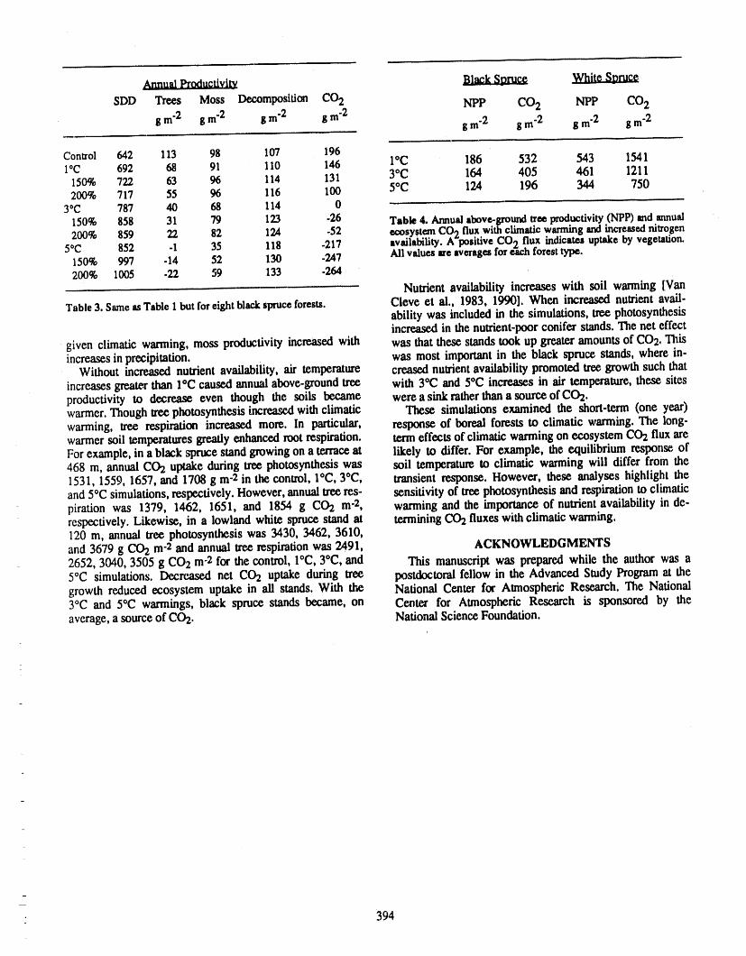
Annual Productiviw _

SDD Trees Moss Decomposition CO2 NPP CO 2 NIP CO2

g m"2 g m"2 g m"2 g m"2 g m"2 g m"2 g m"2 g m"2

Control 642 113 98 107 196I°C 692 68 91 110 146 l°C 186 532 543 1541

150% 722 63 96 114 131 3°C 164 405 461 1211200% 717 55 96 116 100 5°C 124 196 344 750

3°C 787 40 68 114 0150% 858 31 79 123 -26 Table 4. Annualabove-grounda'.eeprod.uctivity.(NPP)md .mmuad200% 859 22 82 124 -52 ecosystem CO2 flux with climaac warming and-met.easedmtro.gen

5oC 852 -1 35 118 -217 availability. A positive CO2 flux indicates uptake Dy vegetauon.150% 997 -14 52 130 .247 Ali values sre averagesfor each forest type.200% 1005 -22 59 133 .264

Nutrient availability increases with soil warming [Van

Table 3. SameasTable 1but foreight blackspruceforests. Cleve et al., 1983, 1990]. When increased nutrient avail-ability was included in the simulations, tree photosynthesisincreased in the nutrient-poor conifer stands. The net effect

given climatic warming, moss productivity increased with was that these stands took up greater amounts of CO2, Thisincreases in precipitation, was most important in the black spruce stands, where in-

Without increased nutrient availability, air temperature creased nutrient availability promoted tree growth such that

increases greater than loC caused ann 'ual above-ground tree with 3°(2 and 5"C increases in air temperature, these sitesproductivity to decrease even though the soils became were a sink rather than a sourceof CO2.warmer. Though tree photosynthesis increased with climatic These simulations examined the short-term (one year)warming, tree respiration increased more. In particular, response of boreal forests to climatic warming. The long-warmer soil temperatures greatly enhanced root respiration, term effects of climatic warming on ecosystem C02 flux areFor example, in a black spruce stand growing on a terrace at likely to differ. For example, the equilibrium response of468 m, annual CO_ uptake during tree photosynthesis was soil temperature to climatic warming will differ from the1531, 1559, 1657, and 1708 g m-2 in the control, I°C, 3°C, transient response. However, these analyses highlight theand 5°C simulations, respectively. However,annualtree res- sensitivityof tree photosynthesis and respirationto climaticpiration was 1379, 1462, 1651, and 1854 g CO2 m"2, warming and the importance of nutrient availability in de-respectively. Likewise, in a lowland white spruce stand at retraining CO2 fluxes with climatic wanning.120 m, annual tree photosynthesis was 3430, 3462, 3610,and 3679 g CO2 m"2 and annual tree respiration was 2491, ACKNOWLEDGMENTS2652, 3040, 3505 g CO2 m-2 for the control, I°C, 3°C, and This manuscript was prepared while the author was a5°C simulations. Decreased net CO2 uptake during tree postdoctoral fellow in the Advanced Study Program at the

growth reduced ecosystem uptake in ali stands. With the National Center for Atmospheric Research. The National3°C and 50C warmings, black spruce stands became, on Center for Atmospheric Research is sponsored by theaverage, a source of CO2. National Science Foundation.

m

394

REFERENCES

Bonan, G. B., A biophysical sm'faceenergy budget analysis Schlenmer, R. E., and K. VanCleve, Relationships betweenof soil temperaturein the boreal forests of interior Alas- CO2evolution from soil, substrateteznperatar¢,and sub-ka, Water Resour. Res., 27, 767-781, 1991a. strate moisture in four mature forest types in interior

Bonan, G. B., Atmosphere--biosphereexchange of carbon Alaska, Can. J. For. Res., 15, 97-106, 1985,dioxide in boreal forests, J. Geophys. Res., 96, 7301- Van Cleve, K., and L. A. Viereck, Forest succession in 1_-7312, 1991b. lation to nutrientcycling in the boreal forest of interior

D'Arrigo, R., G. C. Jacoby, and I. Y. Fang, Boreal forests Alaska, in Forest Succession: Concepts and Application,and atmosphere-biosphere exchange of carbon dioxide, edited by D. C. West, H. H. Shugart, and D, B. Botkin,Nature, 329, 321-323, 1987. pp. 185-211, Spdnger-Verlag, New York, 1981.

Flanagan, P. W., and K. Van Cleve, Nutrient cycling in re- Van Cleve, K., L. Oliver, R. Schlenmer, L. A. Viereck, andlation to decomposition and organic-matter quality in C.T. Dyrness, Productivityand nutrientcycling in tatgataigaecosystems, Can. J. For. Res., 13,795-817, 1983. forest ecosystems, Can. J. For. Res., 13,747-766, 1983,

Lasher,D. A., The dynamicgreenhouse: feedbackprocesses Van Cleve, K., F. S. Chapin,P. W. Flanagan,L. _k.Viereck,that may influence future concentrations of atmospheric and C. T. Dymess, Forest Ecosystems in li_e Alaskantrace gases and climatic change, Climatic Change, 14, Taiga, Springer-Verlag,New York, 1986.213'242, 1989. Van Cleve, K., W. C. Oechel, and J. L. Hem, Response of

NOAA, Typical meteorologicalyear. Hourlysolar radiation black spruce (Picea mariana) ecosystems to soil tem--surface meteorological observations, User's manual TD. perature modification in interior Alaska, Can. J. For.9734, National Climatic Data Center, AsheviUe, NC, Res.,20, 1530--1535,1990.1981. Viereck, L. A., C. T. Dyrness, K. Van Cleve, and M. J.

Oechel, W. C., and K. Van Cleve, The role of bryophytes in Foote, Vegetation, soils, and forest productivity in se-nutrient cycling in the taiga, in Forest Ecosystems in the lectod forest types in interior Alaska, Can. J. For, Res.,Alaskan Taiga, edited by K. Van Cleve, F. S, Chapin, P. 13, 703--720, 1983.W. Flanagan, L. A. Viereck, and C. T. Dyrness, pp.121-137, Springer-Verlag,New York, 1986.

395

Evolutionary History of Polar Regions

J. A. CrameBritishAntarcticSurvey,NaturalEnvironmentResearchCouncil,Cambridge,UnitedKingdom

ABSTRACT

A traditional view of life on earth is that most major groups of plants and ani-mals arose in the tropics and then disseminated to higher latitude regions. In someway, competitively less successful forms are displaced progressively towards mid-and high-latitude regions, with only the most tolerant fomis reaching the poles. Thelatter are frequently cited as refugia.

However, we now know significantly more about the evolutionary history ofpolar regions than was the case when such theories were first promulgated. In par-ticular, it is evident that, for long periods of geological time, vast areas of ice-freecontinent and continental shelf were present in the highest latitudes of both hemi-spheres. These undoubtedly served as the sites of origin for at least some of thecomponents of the distinctive Mesozoic Boreal realm and its austral counterpart.Indeed it is likely that a distinctive biotic realm has characterized the southern highlatitudes, at least intermittently, since the late Paleozoic.

In recent years it has become apparent that West Antarctica and its contiguousregions may have been the center of origin for a range of recent taxa. Here, the lateMesozoic and Cenozoic paleontological record contains the first occurrences of anumber of prominent taxa in living Southern Hemisphere temperate forests. Thesame beds have also yielded fh'st records of living marine invertebrate types such asdecapod crustaceans, echinoids, bivalves, gastropods and brachiopods, lt is evenpossible, at least within the marine realm, that the polar regions are still activelyproviding new taxa. In Antarctica, for example, certain groups of very closelyrelated species (such as pycnogonids, buccinacean gastropods, certain echinodermsand notothenioid fish) seem to be the product of extensive Cenozoic adaptiveradiations.

The polar regions may yet be shown to have been significant contributors to theglobal species pool.

396

r

Possible Impacts of Ozone Depletion on Trophic Interactionsand Biogenic Vertical Carbon Flux in the Southern Ocean

Harvey J. Marchant and Andrew DavidsonAustralian Antarctic Division, Kingston, Tasmania, Australia

ABSTRACT

Among the most productive region of the Southern Ocean is the marginal iceedge zone that trails tY_eretreatingice edge in springandearly summer.The timingof this near-surface phytoplankton bloom coincides with seasonal stratosphericozone depletion when UV irradianceis repon._y as high as in mid-summer, Re-cent investigations indicatethat antarctic marine phy,topl,ank!o,nare presenti_ UVstressed. The extent to which increasing UV radiauon dimlmshes the abihty ofphytoplanktonto fix CO2 and/or leads to changes in their species composition isequivocal. The colonial stage in the life cycle of the alga Phaeocystis pouchetii isone of the major components of the bloom. We have found that this alga producesextracellular products which are strongly UV-B absorbing.When exposed to in-creasing levels of UV-B radiation,survival of antarcticcolonial Phaeocystis wassignificantly greater than colonies of this species from temperatewaters and of thesingle-celled stage of its life cycle which producesnoUV-B-absorbingcompounds.Phaeocystis is apparentlya minor dietary componentof antarctickrill, Euphausiasuperba, and its nutritional value to crustacea is reportedly low. Phytoplankton,principally diatoms, together with fecal pellets and molted exoskeletons of grazerscontributemost of the particulatecarbon flux from the euphoriczone to deep water.If the species composition of antarcticphytoplanktonwas to shift in favor of Phae-ocystis at the expense of diatoms,changes to pelagic trophic interactionsas well asvertical carbon flux are likely°

INTRODUCTION [1990] concluded that antarctic phytoplankton are presently

Stratospheric ozone over Antarctica and the Southern under UV stress and are likely to be seriously affected byOcean is markedly depleted during spring [Stolarski et al., any increase in UV-B radiation as would the higher trophic1986], resulting in UV flux rates similar to mid.summer levels of the Southern Ocean food web. In contrast, Holm-conditions ['Frederickand Snell, 1988]. Solar UV-B radia. Hansen et al. [1989] found that although the rate of photo-tion penetrates oceanic water to depths that are able to in- synthesis by phytoplankton in the top meter of the waterfluence the growth of macrophytes and phytoplankton [Jitts column was depressed by about 30%, organisms at depthset al., 1976; Lorenzen, 1979; Calkins and Thordardottir, greater than 20 m were unaffected by in situ exposure to1980; Won'est, 1983; Maske, 1984; Wood, 1987, 1989]. In UV. They concluded that increased UV irradiation wouldaddition, Trodahl and Buckley [1989] suggest that antarctic have little impact on the phytoplankton and higher trophicsea ice in early spring may be sufficiently transparent to UV levels of the Southern Ocean. Species of phytoplankton dif-for organisms living in and under it to receive levels of ra- fer in their ability, to survive UV irradiation [Calkins anddiation high enough to have biological consequences. Thordardottir, 1980],and Karentz [1991] has argued that the

The effect of UV-B radiation on antarctic marine phy- mostlikely effect of elevated UV irradiation on antarctictoplankton is equivocal [Roberts, 1989]. EI-Sayed et al. marine phytoplankton is a shift in the species composition.

397

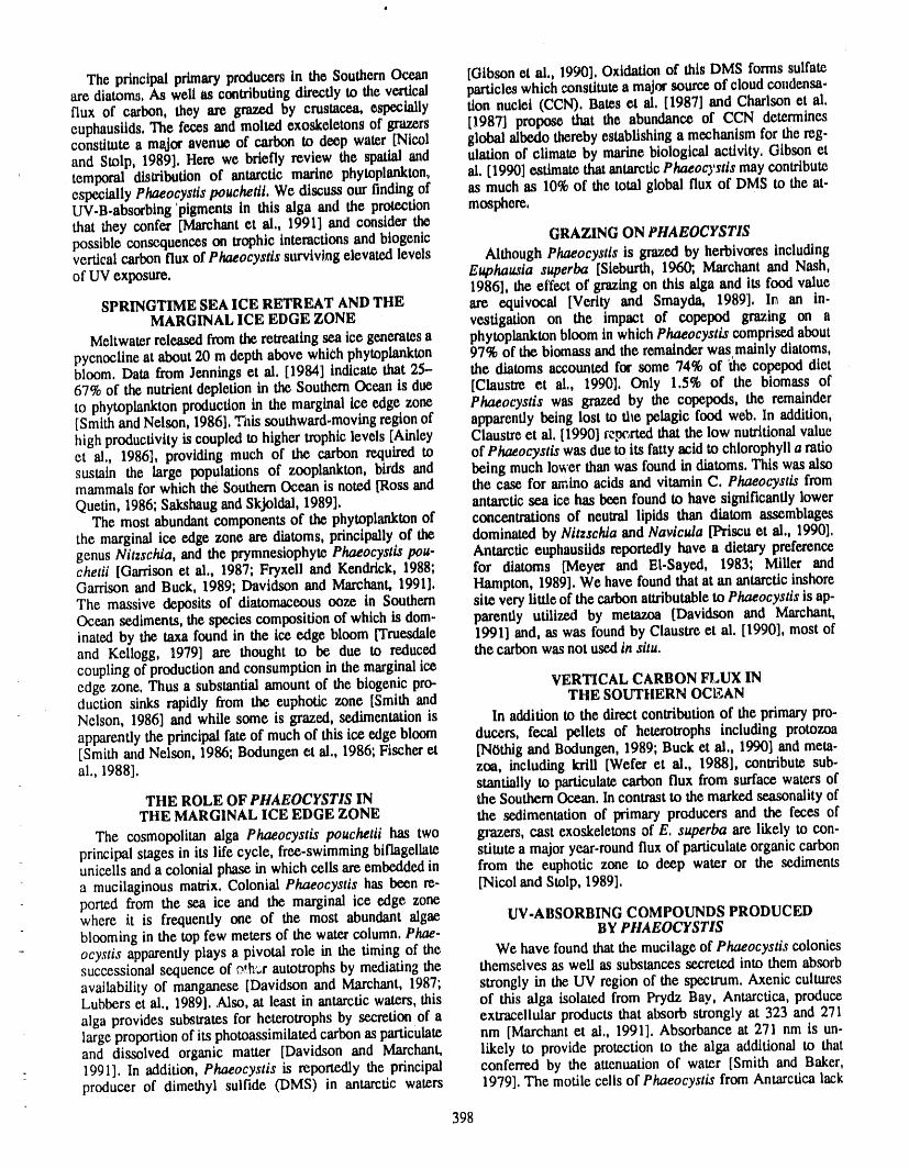
The principal primaryproducers in the Southern Ocean [Gibson ct al., 19901, Oxidation of this DMS forms sulfateare dlatoma, As well as contributing directly to the ve,rrical particles which constitutea major source of cloud condensa-flux of carbon,theyare grazedby crustacea, especially tion nuclei (CCN), Bates et al, [1987] and Charlson et al,euphausiids, The feces and molted exoskeletons of grazers [1987] propose that the abundance of CCN determinesconstitute a mgjor avenue of carbon to deep water [Nicol global albedo therebyestablishing a mechanism for the reg.and Stolp, 1989], Here we briefly review the spatial and ulatton of climate by marine biological activity, Gibson ettemporal distribution of antarctic marine phytoplankton, al. [1990] estimate thatantarcticPhaeocystis may contributeespecially Phaeocystis pouchetii. We discuss our finding of as much as 10%of the total global flux of DMS to the at-UV-B.absorbing 'pigments in this alga and the protection mosphere,that they confer [Marchantet al., 1991] and consider thepossible consequences on trophic interactions and biogenic GRAZING ON PHAEOCYSTISverticalcarbonflux of Phaeocystts surviving elevatedlevels Although Phaeocystis is grazed by herbivores includingof UV exposure. Euphausia superba [Sieburth, 196{Y,Marchant and Nash,

1986], the effect of grazingon this alga and its food valueSPRINGTIME SEAICERETREATANDTHE are equivocal [Verity and Smayda, 1989], In an in-

MARGINAL ICE EDGE ZONE vestigation on the impact of copepod grazing on aMeltwaterreleasedfromthe retreatingsea ice generatesa phytoplankton bloom in which Phaeocystis comprisedabout

pyenocline at about20 m depth above which phytoplankton 97% of the biomass and the remainderwas mainly diatoms,bloom. Data from Jennings et al. [1984] indicate that 25-- the diatoms accounted for some 74% of 'the copepod diet67% of the nutrientdepletion in the SouthernOcean is due [Claustre ct al., 1990], Only 1.5% of the biomass ofto phytoplanktonproductionin the marginal ice edge zone Phaeocystis was grazed by the copepods, the remainder[Smith and Nelson, 1986],_ais southward-movingregion of apparently being lost to tile pelagic food web. In addition,high productivityis coupled to higher trophic levels [Ainley Claustrect al, [1990] ce_,rted that the low nutritionalvaluect al., 1986], providing much of the carbon required to of Phaeocystls was due to its fattyacid to chlorophylla ratiosustain the large populations of zooplankton, birds and being much lower than was found in diatoms. This was alsomammals for which the SouthernOcean is noted [Ross and the case for amino acids and vitamin C. Phaeocystis fromQuetin, 1986;Sakshaugand Skjoldal, 1989]. antarcticsea ice has been found to have significantly lower

The most abundantcomponents of the phytoplanktonof concentrations of neutral lipids than diatom assemblagesthe marginal ice edge zone are diatoms, principally of the dominated by Nitzschia and Navicula [Priscu ct al., 1990].genus Nitzschia, and the prymnesiophytePhaeocystis pou- Antarcticeuphausiids reportedly have a dietary preferencechetii [Garrisonet al., 1987; Fryxell and Kendtick, 1988; for diatoms [Meyer and EI-Sayed, 1983, Miller andGarrison and Buck, 1989; Davidson and Marchant, 1991]. Hampton, 1989].We have foundthat at an antarcticinshoreThe massive deposits of diatomaceous ooze in Southern site very little of the carbonattributableto Phaeocystis is ap-Ocean sediments, the species composition of which is dora- parently utilized by metazoa [Davidson and Marchant,inated by the taxa found in the ice edge bloom [Truesdale 1991] and, as was found by Claustre et al. [1990], most ofand Kellogg, 1979] are thought to be due to reduced the carbonwas not use.din situ.coupling of productionand consumptionin the marginal iceedge zone. Thus a substantial amountof the biogenic pro- VERTICAL CARBON FLUX INduction sinks rapidly from the euphoric zone [Smith and THE SOUTHERN OCEANNelson, 1986] and while some is grazed, sedimentationis In addition to the direct contribution of the primarypro-apparentlythe principalfate of much of this ice edge bloom ducers, fecal pellets of heterotrophs including protozoa[Smith and Nelson, 1986; Bodungen et al., 1986; Fischer et [NOthigand Bodungen, 1989; Buck et al., 1990] and meta-al., 1988]. zea, including krill [Wefer et al., 1988], contribute sub-

stantially to particulatecarbon flux from surface waters ofTHE ROLE OF PHAEOCYSTIS IN the Southern Ocean. In contrastto the marked seasonality of

THE MARGINAL ICE EDGE ZONE the sedimentation of primary producers and the feces of

The cosmopolitan alga Phaeocystis pouchetii has two grazers, cast exoskeletonsof E. superba are likely to con-principal stages in its life cycle, free-swimming biflagellate stitute a majoryear-roundflux of particulateorganic carbonunicells anda colonial phase in which cells areembedded in from the euphoric zone to deep water or the sedimentsa mucilaginous matrix. Colonial Phaeocystis has been re- [Nicol and Stolp, 1989].ported from the sea ice and the marginal ice edge zonewhere it is frequently one of the most abundant algae UV-ABSORBING COMPOUNDS PRODUCEDblooming in the top few meters of the watercolumn. Phae- BYPHAEOCYSTIS

: ocystis apparentlyplays a pivotal role in the timing of the We have found that the mucilageof Phaeocystis coloniessuccessional sequence of _et_:rautotrophs by mediating the themselves as well as substances secreted into them absorbavailability of manganese [Davidson and Marchant, 1987; strongly in the UV region of the spectrum. Axenic culturesLubbers et al., 1989]..Also, at least in antarctic waters, this of this alga isolated from Prydz Bay, Antarctica, producealga provides substrates for heterotrophs by secretion of a extracellular products that absorb strongly at 323 and 271large proportion of its photoassimilated carbon as particulate nm [Marchant et al., 1991]. Absorbance at 271 nm is un-and dissolved organic matter [Davidson and Marchant, likely to provide protection to the alga additional to that

- 1991]. In addition, Phaeocystis is reportedly the principal conferred by the attenuation of water [Smith and Baker,producer of dimethyl sulfide (DMS) in antarctic waters 1979]. The motile cells of Phaeocystis from Antarctica lack

398

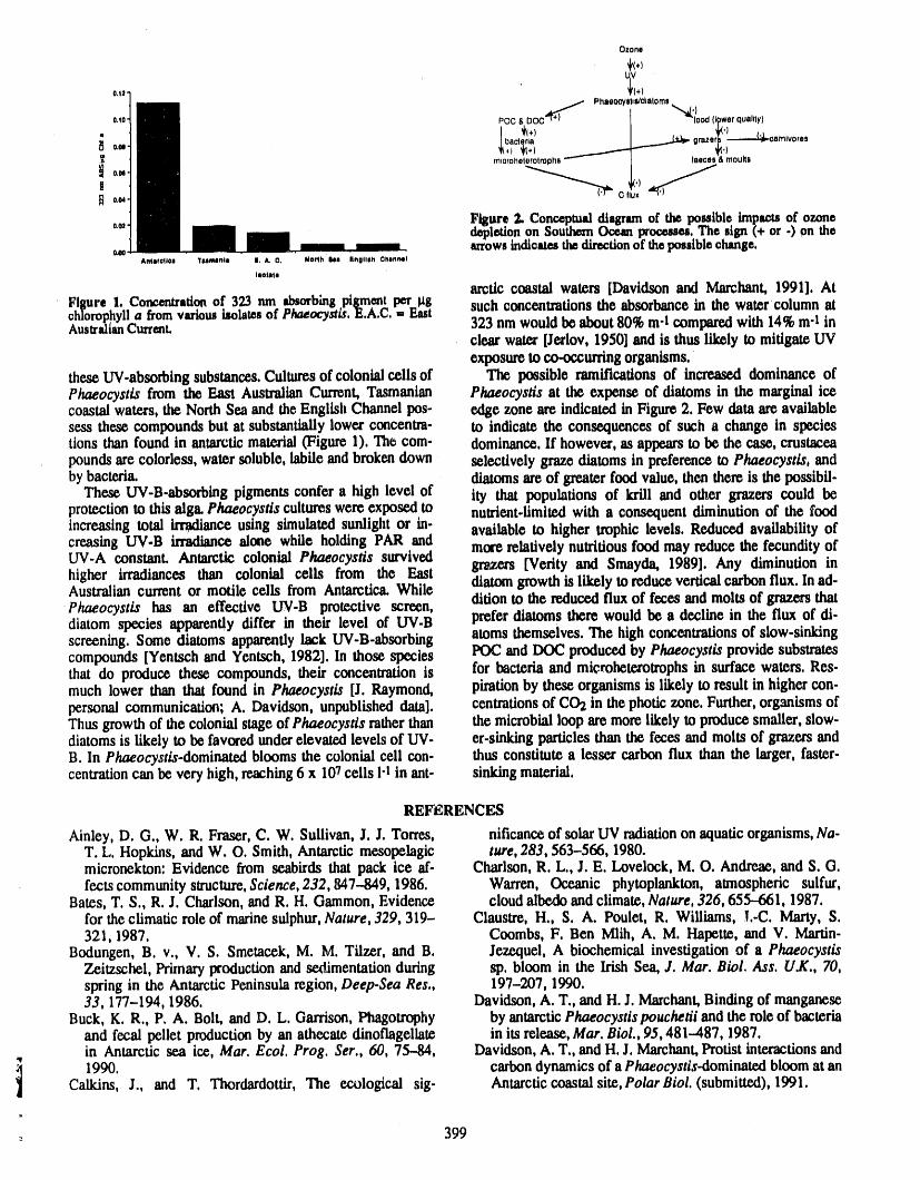
Ozone

4(*), UV

o,u, _(+)

Phaeocystie/dtatoms,_.)o,lo, pocsDOC"t';i''_ I foodO_werqualify)

*(,) ')i0. /-°. I

B ' ')o,o4- " C flux '

Figure 2. Conceptual diagram of the po-Iblo imparts of ozone0=- depletion on SouthernOcean processes. The sign (+ or -) on the0_ arrowsindicates thedtrecUonof thepossible change.

A_aft_tss Teimanim ILk. O, Northks EnglishOhennel

Isolate

arctic coastal waters [Davldson and March=mt' 1991]. At

Filtmre i, Concentration of 323 nm absorbing pigment =per]_ such concentrations the absorbance in the water column atoh]orophyUa fromvarious isolates of Phaeocysfls. E.A.C. EasAustralianCurrent. 323 nm would be about 80% m-1 compared with 14% m-I in

clear water [Jerlov, 1950] and is thus likely to mitigate UVexposure to co-occurring organisms.

these UV-absorbing substances. Cultures of colonial cells of The possible ramifications of increats_ dominance ofPhaeocystis from the East Australian Current, Tasmanian Phaeocystis at the expense of diatoms in the marginal icecoastal waters, the North Sea and the English Channel pos- edge zone are indicated in Figure 2. Few data are availablesessthese compoundsbut at substantiallylower concentra- to indicate the consequencesof sucha change in speciestions than found in antarctic material (Figure 1), The com- dominance. If however, as appears to be the case, crustaceapounds are colorless, water soluble, labile and broken down selectively graze diatoms in preference to Phaeocystis, andby bacteria, diatoms are of greater food value, then there is the possibil-

These UV-B-absorbing pigments confer a high level of ity that populations of krill and other grazers could beprotection to this alga. Phaeocystis cultures were exposed to nutrient.limited with a consequent diminution of the foodincreasing total irradiance using simulated sunlight or in- available to higher trophic levels. Reduced availability ofcreasing UV-B irradiance alone while holding PAR and more relatively nutritious food may reduce the fecundity ofUV-A constant. Antarctic colonial Phaeocystis survivedhigher irradiances than colonial cells from the East gncers [Verity and Smayda, 1989]. Any diminution inAustralian current or motile cells from Antarctica. While diatom growth is likely to reduce vertical carbon flux. In ad-

Phaeocystis has an effective UV.B protective screen, dition to the reduce_ flux of feces and molts of grazers thatdiatom species apparently differ in their level of UV.B prefer diatoms there would be a decline in the flux of di-screening. Some diatoms apparently lack UV-B-absorbing atoms themselves. The high concentrations of slow-sinkingcompounds [Yentsch and Yentsch, 1982]. In those species POC and DOC produced by Phaeocystis provide substratesthat do produce these compounds, their concentration is for bacteria and microhetexotmphs in surface waters. Res-much lower than that found in Phaeocystis [J. Raymond, piration by these organisms is likely to result in higher con-personal communication; A. Davidson, unpublished data], centrations of CO2 in the photic zone. Further, organisms ofThus growth of the colonial stage of Phaeocystts rather than the microbial loop are more likely to produce smaller, slow-diatoms is likely to be favored under elevated levels of UV- er-sinking particles than the feces and molts of grazers andB. In Phaeocystis-dominated blooms the colonial cell con- thus constitute a lesser carbon flux than the larger, faster-centration can be very high, reaching 6 x 107 cells l-I in ant- sinking material.

REFERENCES

Ainley, D. G., W. R. Fraser, C. W. Sullivan, J. J. Torres, nificance of solar UV radiation on aquatic organisms, Na.T. L. Hopkins, and W. O. Smith, Antarctic mesopelagic ture, 283, 563-566, 1980.micronekton: Evidence from seabirds that pack ice at'- Charlson, R. L., J. E. Lovelock, M. O. Andreae, and S. G.fects community structure, Science, 232,847--849, 1986. Warren, Oceanic phytoplankton, almospheric sulfur,

Bates, T. S., R. J. Charlson, and R. H. Gammon, Evidence cloud albedo and climate, Nature, 326, 655--661, 1987.for the climatic role of marine sulphur, Nature, 329, 319- Claustre, H., S. A. Poulet, R. Williams, I.-C. Marry, S.321, 1987. Coombs, F. Ben Mlih, A. M. Hapette, and V. Martin.

Bodungen, B. v., V. S. Smetacek, M. M. Tilzer, and B. Jezequel, A biochemical investigation of a PhaeocystisZeitzschel, Primary production and sedimentation during sp. bloom in the Irish Sea, J. Mar. Biolo Ass. U.K., 70,spring in the Antarctic Peninsula region, Deep-Sea Res., 197-207, 1990.33, 177-194, 1986. Davidson, A. T., and H. J. Marchant, Binding of manganese

Buck, K. R., P. A. Bolt, and D. L. Garrison, Phagotrophy by antarctic Phaeocysttspouchetii and the role of bacteriaand fecal pellet production by an athecate dinoflagellate in its release, Mar. Biol., 95,481-487, 1987.in Antarctic sea ice, Mar. Ecol. Prog. Ser., 60, 75-84, Davidson, A. T., and H. J. Marchant, Protist interactions and

i 1990. carbon dynamics of a Phaeocystis-dominated bloom at anCalkins, J., and T. Thordardottir, The ecological sig- Antarctic coastal site, PolarBiol. (submitted), 1991,

o 399

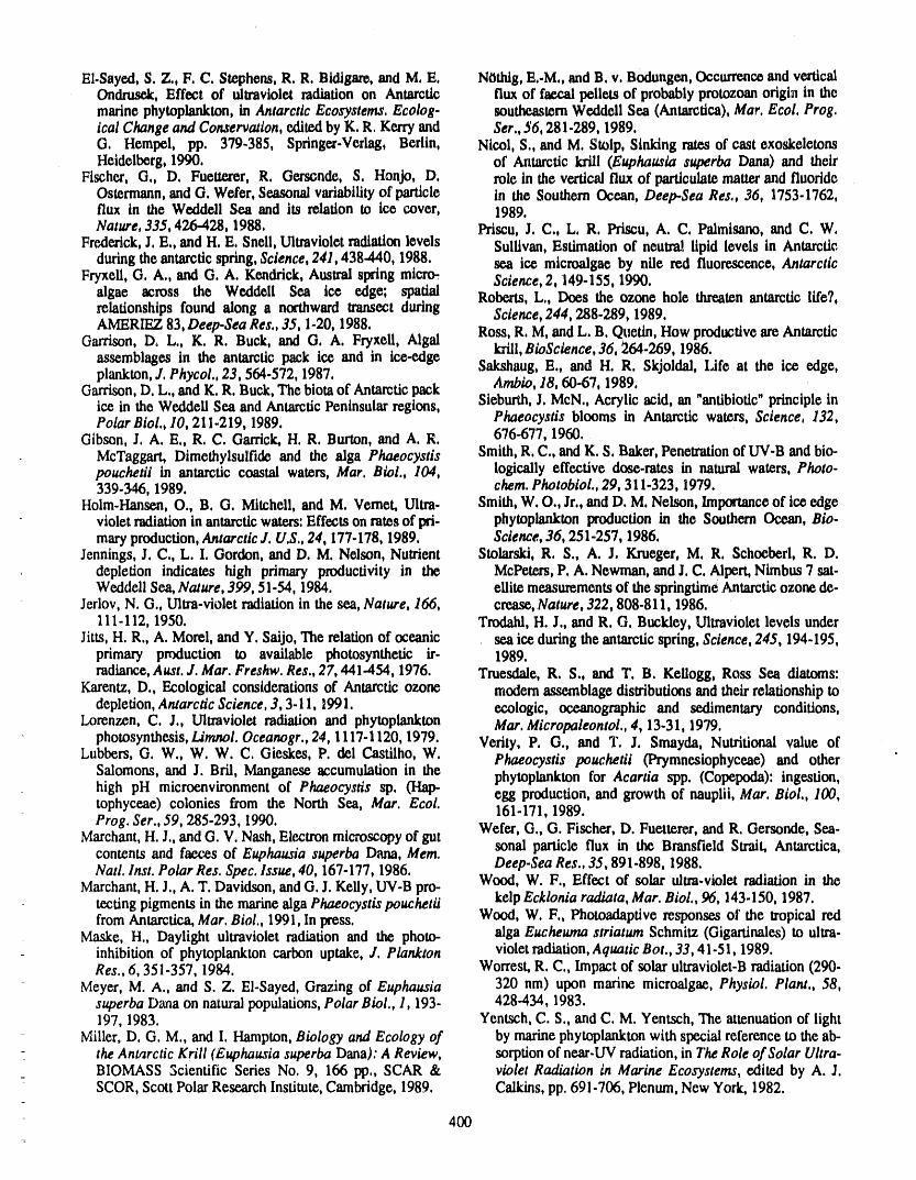
El.Sayed,S,Z.,F.C. Stephens,R.R.Bidigare,andM.E. N6thlg,E,-M,,andB,v.Bodungen,OccurrenceandverticalOndrusek, Effect of ultraviolet radiation on Antarctic flux of faecal pellets of probablyprotozoanorigin in themarine phytoplankton, in Antarctic Ecosystems. Ecolog- southeasternWeddell Sea (Antarctica),Mar. Ecol. Prog.tcal Change and Conservation, editedby K, R. Kerryand Ser., 56, 281-289, 1989,G, Hempel, pp. 379-385, Spdnger-Verlag, Berlin, Nicol, S., and M. Stolp, Sinking rates of cast exoskeletonsHeidelberg, 1990. of Antarctic krill (Euphausta superba Dana) and their

Fischer, G., D. Fuetterer, R. Gersonde, S, Honjo, D, role in the vertical flux of particulatematterand fluorideOstermann,and G, Wefer, Seasonalvariabilityof particle in the Southern Ocean, Deep.Sea Res,, 36, 1753-1762,flux in the Weddell Sea and its relation to ice cover, 1989,Nature, 335, 426-428, 1988, Priscu, J. C., L, R. Priscu, A. C, Palmisano, and C, W.

Frederick,J. E., and H. E, Snell, Ultravioletradiationlevels Sullivan, Estimation of neutral lipid levels in Antarcticduringthe antarcticspring, Science, 241,438-440, 1988. sea ice microalgae by nile red fluorescence, Antarctic

Fryxell, G. A., and G. A. Kendrick, Australspring micro- Science, 2, 149-155, 1990.algae across the Weddell Sea ice edge; spatial Roberts, L., Does the ozone hole threaten antarctic life?,relationships found along a northwardtransect during Science, 244,288-289, 1989.AMERn_7.83, Deep-Sea Res., 35, 1-20, 1988.

Garrison, Dr L,, K. R. Buck, and G, A. FryxeU, Algal Ross, R, M,and L. B. Quetin, How productiveareAntarcticassemblages in the antarctic pack ice and in ice-edge krill,BioScience,36, 264-269, 1986.plankton,J. Phycol., 23, 564-572, 1987. Sakshaug, E., and H. R. Skjoldal, Life at the ice edge,

Garrison,D. L., andK. R. Buck, The biotaof Antarcticpack Ambio, 18, 60-67, 1989,ice in the Weddell Sea and AntarcticPeninsular regions, Sieburth,J. McN., Acrylic acid, an "antibiotic"principleinPolar Biol., 10, 211-219, 1989. Phaeocystis blooms in Antarctic waters, Science, 132,

Gibson, J. A. E., R. C. Garrick,H. R. Burton,and A.R. 676-677, 1960.McTaggart, Dimethylsulfide and the alga Phaeocystis Smith, R. C,, andK. S. Baker,Penetrationof UV-B and bio-.pouchetii in antarctic coastal waters, Mar. Biol., 104, logically effective dose-rates in natural waters, Photo.339.346, 1989. chem. Photobiol., 29, 311-323, 1979,

Holm-Hansen, O., B, G. Mitchell, and M. Vemet' Ultra. Smith, W. O., Jr.,and D. M, Nelson, Importanceof ice edgeviolet radiationin antarcticwaters:Effects on rates of pri- phytoplankton production in the Southern Ocean, Bio-maryproduction,Antarctic J. U.S., 24, 177-178, 1989. Science, 36, 251-257, 1986,

Jennings, J. C., L. I. Gordon, and D. M. Nelson, Nutrient Stolarskt, R. S., A. J. Krueger, M. R, Schoeberl, R. D.depletion indicates high primary productivity in the McPeters,P. A. Newman, andJ. C. Alpert,Nimbus 7 sat-Weddell Sea, Nature, 399, 51-54, 1984. ellite measurementsof the springtimeAntarcticozone de.

Jerlov,N. G., Ultra-violet radiationin the sea, Nature, 166, cre.ase,Nature, 322,808-811, 1986.111.112, 1950. Trodald,H. J., and R. G. Buckley, Ultravioletlevels under

Jitts, H. R., A. Morel, and Y. Saijo, The relation of oceanic sea ice duringthe antarcticspring, Science, 245, 194-195,primary production to available photosynthetic lr- 1989.radiance,Aust. J. Mar. Freshw. Res., 27, 441-454, 1976. Tmesdale, R. S., and T. B. Kellogg, Ross Sea diatoms:

Karentz, D., Ecological considerations of Antarctic ozone modem assemblage distributions and their relationship todepletion, Antarctic Science, 3,3.11, 1991. ecologic, oceanographic and sedimentary conditions,

Lorenzen, C. J., Ultraviolet radiation and phytoplankton Mar. Micropaleontol., 4, 13-31, 1979.photosynthesis, Limnol. Oceanogr., 24, 1117-1120, 1979. Verity, P. G., and T. J. Smayda, Nutritional value of

Lubbers, G. W., W. W. C. Gieskes, P. del Castilho, W. Phaeocystis pouchetii (Prymnesiophyceae) and other "Salomons, and J. Bril, Manganese accumulation in the phytoplankton for Acartia spp. (Copepoda): ingestion,high pH microenvironment of Phaeocystis sp. (Hap- egg production,and growth of nauplii, Mar. Biol., 100,tophyceae) colonies from the North Sea, Mar. Ecol. 161-171, 1989.Prog. Ser.,59, 285-293, 1990. Wefer, G., G. Fischer, D. Fuetterer,and R. Gersonde, Sea-

Mm'chant'H. J,,and G. V. Nash, Electronmicroscopy of gutcontents and faeces of Euphausia superba Dana, Mem. sonal particle flux in the Bransfield Strait, Antarctica,Natl. Inst. Polar Res. Spec. Issue, 40, 167-177, 1986. Deep-Sea Res., 35, 891-898, 1988.

Wood, W. F., Effect of solar ultra-violet radiation in theMarchant,H. J., A. T. Davidson, and G. J. Kelly, UV-B pro..tectingpigments in the marinealgaPhaeocystis pouchetii kelp Ecklonia radiata, Mar. Biol., 96, 143.150, 1987.from Antarctica, Mar. Biol., 1991, In press. Wood, W. F., Photoadaptive responses of the tropical red

Maske, H., Daylight ultraviolet radiation and the photo- alga Eucheuma striatum Schmitz (Gigartinales) to ultra.inhibition of phytoplankton carbon uptake, J, Plankton violet radiation, Aquatic Bot., 33, 41-51, 1989.Res., 6, 351-357, 1984. Worrest, R. C., Impact of solar ultraviolet-B radiation (290-

Meyer, M. A., and S. Z. EI-Sayed, Grazing of Euphausia 320 nra) upon marine microalgae, Physiol. Plant., 58,superba Dana on natural populations, Polar Biol., 1,193- 428-434, 1983.197, 1983. Yentsch, C. S., and C. M. Yentsch, The attenuation of light

Miller, D. G. M., and I. Hampton, Biology and Ecology of by marine phytoplankton with special reference to the ab-the Antarctic Krill (Euphausia superba Dana): A Review, sorption of near-UV radiation, in The Role of Solar Ultra-BIOMASS Scientific Series No. 9, 166 pp., SCAR & violet Radiation in Marine Ecosystems, edited by A. J.

- SCOR, Scott Polar Research Institute, Cambridge, 1989. Calkins, pp. 691.706, Plenum, New York, 1982.

400

Relationships Between Whale Hunting, Human Social Organization, and SubsistenceEconomies in Coastal Areas of Northwest Alaska during Late Prehistoric Times

R. K. HarrittU,S.NationalParkService,AlaskaRegion,Anc&_rage,Alaska,U.S.A.

ABSTRACT

The florescence of' Eskimo whaling on northwest Alaskan coasts during WesternThule rimes, A.D. 10(D-1400, was followed by a shift to a more balanced sub-sistence pattern for human inhabitants of many coastal areas during KotzebuePeriod rimes, from A,D. 1400-1900, The cause of this shift has been identified as achange in the migration routes of whales passing through Bering Strait which pre-sented a circumstance prohibitive to effective whale hunting. Previous inter-pretations of social organization of the large whaling villages of the earlier portionof this period have suggested that whale hunting provided a basis for developmentof social ranking of village inhabitants with the umealik, or whaling captain, assum-ing the role of a chief. Concomitant explanations for the later, more diffuse settle-ment pattern encountered by early European explorers have not been previouslypresented. An alternative position presented here is that prehistoric Eskimo soci-cries retained many egalitarian tenets throughout late prehistoric times. This socialpattern provided flexibility in subsistence economies with nuclear families as thebasic unit transferable from one permanent village to the next, and as a segment ofsociety capable of effectively exploiting sparsely distributed seasonal resources. Inthis interpretation, social status can be construed as a seasonal phenomenon inwhich authority or rank was vested in an individual who had demonstrated specialskills and abilities in organizing and carrying out successful hunts, and other foodprocurement expeditions. This status was relinquished as seasonal requirements forfood acquisition changed.

INTRODUCTION THE PREHISTORYOFWHALING

Differinginterpretationsof socialandsubsistenceaspects The earliestevidenceof a substantialfocus on whalingof whalingby prehistoricandhistoricnativeinhabitantsof was found in Okvik/OldBering sea componentsat thenorthwestAlaskancoasts havebeenpresentedoverthe past Ekvensiteon EastCape,Siberia,datingto the beginningof30 years.HereI presentan alternativeinterpretationto one the first millennium A.D. [Ackerman,1984:108-109;of these;a positiontakenby Sheehan[1985],whosuggests Krupnikct al., 1983:559;Stanford,1976:91-92].A secondthat socialrankingdevelopedin late prehistoricandearly developmentof whalingtechniquesbegan by A.D. 500,historic Eskimo whalingvillages. Sheehanarguesthatan whentechnologynecessaryforhuntinglargewhales,includ-abundanceof food providedby whale harvestingenabled ing togglingharpoonheads,dragfloats andumiaks,wereinfluential individualswho were good whale huntersto obtained by the human inhabitants of Bering Straitobtain and keep authorityover less accomplishedindi- [Bockstoce, 1979:93-95].Evidence of this developmentvidualswithina village.Beforediscussingspecificaspects appearson Siberianshoresby the time of the Punuktradi-of Sheehan's[1985]argumentand my own, it is important tion, sometime around A.D. 600 [Larsenand Rainey,to piace Eskimowhaling in archaeologicaland historical 1948:37-39; Collins, 1964:94; Stanford, 1976:112-114;context. Bockstoce, 1979:86-88; Ackerman, 1984:108-109;

401

n

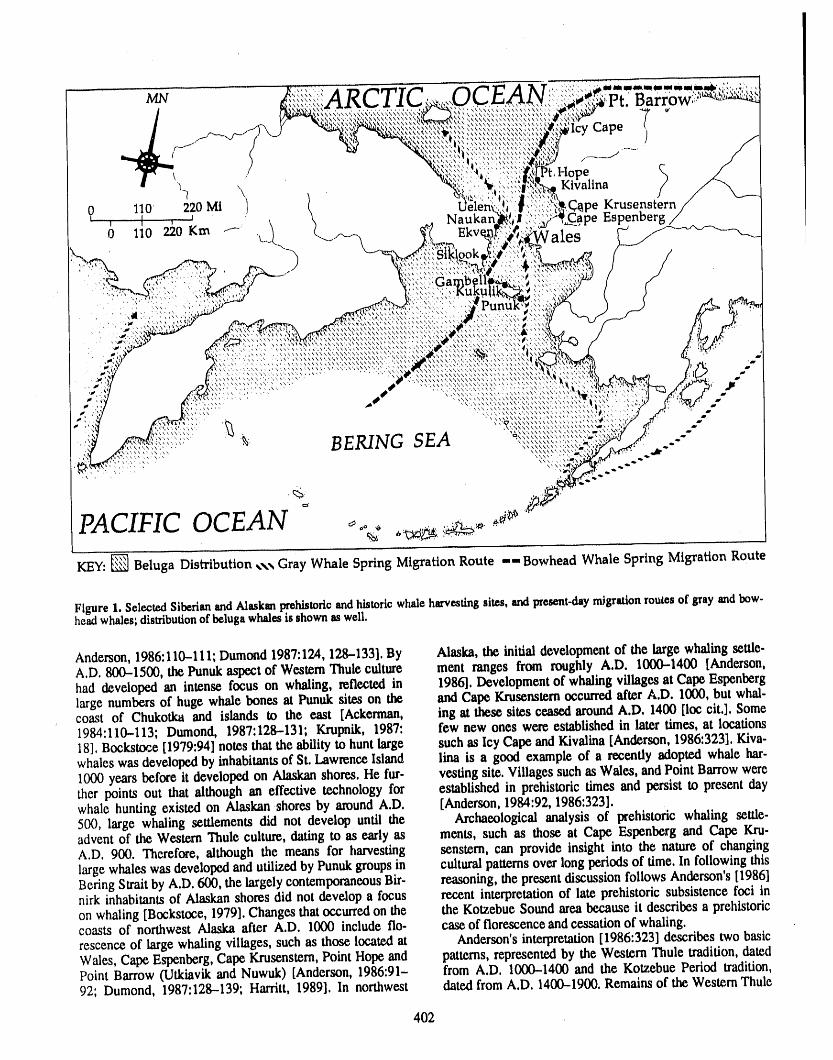
MN ARC'.LC ii Barrow\_"\\\\_ \ \\ _ "\\_ _\"" \ 7'_'_ Cape

_ \ 'alina ?

(_ , 1_0' , 220 Mi / _ EspenbergKrUsenstern

)

.... ,., N\ Nx\,,\,,\',\ ," ', \',' ,

_'' ' '.I' h_ '_\\\\x_'\_x\''''

, , i,,,,\x\\\ \"_\\\"\\\"_\\\ ' '"\ \'_N\"x' \"\'.,, \,, \ ,,,, ,,,,. , , ,_,. ,,\\\\N\\\\\_,,_,\\\\\\\\\_, \" ,\_ ,\\,.\\ ,\

,, ,,, ........... _¢_¢_ , ,'_", ..... _,' ",' ' ' _x\* \\\\,,_.,\\\,\\_\x\ _\_',_"" "

_,"' ' , _,. ,x '._ _ , ', ,, '_l\ \ \ \ _,\\\\\\ \,, \\\\, -,

""...."' BERING SEA "\\\,

', x,, ,

,..._,

PACIFIC OCEAN o

KEY:_ Beluga Distribution _\,_ Gray Whale Spring Migration Route --Bowhead Whale Spring Migration Route

FigureI. SelectedSiberianandAlaskanprehisu_ricandhistoricwhaleharvestingsites,andpresent-daynOgrationroutesof grayandbow-headwhales;distributionofbelugawhalesisshownasweil.

Anderson,1986:110-111;Dumond 1987:124,128-133].By Alaska,theinitialdevelopmentofthelargewhalingsettle-A.D.800-1500,thePunukaspectofWesternThuleculture ment rangesfrom roughlyA.D. 1000-1400[Anderson,haddevelopedan intensefocuson whaling,reflectedin 1986].DevelopmentofwhalingvillagesatCapeEspenbcrglarge numbers of huge whale bones at Punuk sites on the and Cape Krusemtern occurredafter A.D. 1000, but whal-coast of Chukotka and islands to the east [Ackerman, ing at these sites ceased aroundA.D. 1400 [loc cit.]. Some1984:110-113; Dumond, 1987:128-131; Krupnik, 1987: few new ones were established in later times, at locations18]. Bockstoce [1979:94] notes that the ability to huntlarge such as Icy Cape andKivalina [Anderson, 1986:323]. Kiva-whales was developed by inhabitantsof St. LawrenceIsland lina is a good example of a recently adopted whale hat-1000 yearsbefore it developed on Alaskan shores. He fur- vesting site. Villages such as Wales, and Point Barrow werether points out that although an effective technology for established in prehistoric times and persist to present daywhale hunting existed on Alaskan shores by around A.D. [Anderson, 1984:92, 1986:323].500, large whaling settlements did not develop until the Archaeological analysis of prehistoric whaling settle-advent of the Western Thule culture, dating to as early as ments, such as those at Cape Espenberg and Cape Kru-A.D. 900. Therefore, although the means for harvesting senstern, can provide insight into the nature of changinglarge whales was developedand utilized by Punukgroupsin culturalpatternsover long periods of time. In following thisBering Straitby A.D. 600, the largely contemporaneousBir- reasoning, the present discussion follows Anderson's [1986]nirk inhabitants of Alaskan shores did not develop a focus recent interpretationof late prehistoric subsistence foci inon whaling [Bockstoce, 1979]. Changes that occurred on the the Kotzebue Sound area because it describes a prehistoriccoasts of northwest Alaska after A.D. 1000 include ilo- case of florescence and cessation of whaling.rescence of large whaling villages, such as those located at Anderson's interpretation [1986:323] describes two basicWales, Cape Espenberg, Cape Krusenstern, Point Hope and patterns, represented by the Western Thule tradition, datedPoint Barrow (Utkiavlk and Nuwuk) [Anderson, 1986:91- from A.D. 1000-1400 and the Kotzebue Period tradition,92; Dumond, 1987:128--139; Harritt, 1989]. In northwest dated from A.D. 1400-1900. Remains of the Western Thule

402

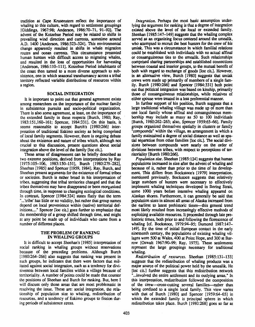
tradition at Cape Krusenstern reflect the importance of Integration, Perhaps the most basic assumption under.whaling to this culture, with regardto settlement groupings lying the argument for ranking is that a degreeof integration[Giddings, 1967:98; Anderson, 1986:70--71, 91-92], The existed above the level of the local or extended family,advent of the Kotzebue Period may be related to shifts in Sheehan [1985:147-149] suggests that the whaling complexprevailing wind direction and currents, sometime around served as an organizing focus centexed around the umeallk,A.D, 1400 [Anderson, 1986:323.-324], This environmental who atmmpted to recruit the best hunters for the crew of hischange apparently resulted in shifts in whale migration umiak, This was a circumstance in which familial relationsroutes and ocean currents, This circumstance presented could be established with individuals with no actual afflnalhuman hunters with difficult access to migrating whales, or consanguineous ties to the umealik, Such relationshipsand resulted in the loss of opportunities for harvesting comprisedsharingpartnershipsand established connections[Anderson, 1986:110-111]. Kotzebue Period inhabitants of between coastal and interiorgroups, to the mutualbenefit ofthe coast then tamed to a more diverse approach to sub- both with regard to exchange of goods [loc cit.], However,sistence, one in which seasonal transhumancyacross a tribal in an alternative view, Butch [1980] suggests that umiakterritoryreflected variable distributionsof resources within crews were made up primarily of members of a single fam.a region, ily. Btu'eh [1980:266] and Spencer [1984:331] both point

out that political integration was based on kinship, primarilySOCIAL INTEGRATION those of consanguineous relationships, while relatives of

It is important to point out that generalagreement exists eitherspouse were treatedin a less preferentialmanner.among researcherson the importanceof the nuclear family In furthersupport of his position, Burch suggests that ain subsistence pursuits and socio-political organization, large traditionalwhaling village was made up of more thanThere is also some agreement,at least, on the importance of one local family whose afflnal and consanguineous mem-the extended family in these respects [Btu.eh, 1980; Ray, bership may include as many as 50 to 100 individuals1983:151,160-.161; Spencer, 1984:331]. On this basis, it [Butch, 1980:262-263; also, Spencer 1959:65--66], Familyseems reasonable to a_ept Butch's [1980:266] inter, groups organized themselves spatially in clusters or familypretation of traditional Eskimo society as being comprised "compounds" within the village, an arrangement in which aof local family segments. However, there is ongoing debate family maintained a degree of social distance as well as spa-about the existence and nature of tribes which, although not tial separation from other families [loc cit.]. The social diel-crucial to this discussion, present questions about social sions between compounds were nearly on the order ofintegration above the level of the family [loc cit.], divisions between tribes, with respect to perceptions of ter.

These areasof disagreement can be briefly described as ritoriality[Burch 1980:.266].two extreme positions, derived from interpretationsby Ray Population size. Sh_ [1985:124] suggests that human[1975:105-106, 1983:150-151], Btu'eh [1980:279-282], populationsincreasedin size after the advent of whaling andSheehan [1985] and Spencer [1959, 1984]. Ray, Butch, and because of it, rather than prior to the time of its develop-Sheehan present arguments for the existence of formal tribes ment. This differ_ from Bockstoee's [1979] interpretation,or societies. Btu.eh is rather broad in his interpretation of mentioned previously. Bockstoee suggests that relativelytribes, suggesting that tribal territories changed and that the large numbers of hunters were necessary to effectivelytribes themselves may have disappeared or been reorganized implement whaling techniques developed in Bering Strait,through time, in response to changing ecological conditions, some 10(X) years before intensive whaling appeared onIn contrast, Spencer [1984:324] states flatly that the term Alaskan shores. Furthermore, it can generally be said that"...'tribe' has little or no validity, but rather that group names population sizes in almost ali areas of Alaska increased fromdepend on local provenience within (native) territorial clef- the earliest to latest prehistoric times--this general trendinitions...." Spencer [loc elL] goes further to emphasize that most likely resulted from increasingly effective methods ofthe membership of a group shifted through time, and might exploiting available resources, lt proceeded through late pre.at any point be made up of individuals who came from a historic times, both prior to and following the florescence ofnumber ofdifferentplaces, whaling [el. Bockstoce, 1979:94--95; Dumond 1987:147-

149]. By the time of initial European contact in the earlyTHE PROBLEM OF RANKING nineteenth century, the populations of existing whaling vii-

IN WHALING GROUPS lages were 500 at Wales, 400 at Point Hope, and 300 at Bar.lt is difficult to accept Sheehan's [1985] interpretation of row [Oswalt 1967:90-99; Ray, 1975]. These settlements

social ranking in whaling groups without reservations represent the large groupings necessary for traditionalbecause of the preceding problems. Although Btu.eh whaling.[1980:264-266] also suggests that ranking was present in Redistribution of resources. Sheehan [1985:131-133]such groups, he indicates that there were factors that mil- suggests that the redistribution of whaling products was aitated against social integration, such as a tendency for divi- major source of the political power held by the umealik. Hesiveness between local families within a village because of [loc cit.] further suggests that this redistribution networkterritoriality. A number of points could be made that counter "...involved the entire settlement and its outlying areas." Inthe positions of Sheehan and Bm.ch for ranking. But, here I this interpretation, redistribution followed the compositionwill discuss only those areas that are most problematic in of the crew--cross-cutting several families--rather thanresolving the issue. These are: social integration, the rela- being confined to a single local family. This view variestionship of population size to whaling, redistribution of with that of Burch [1980] and Spencer [1959:64--65] inresources, and a tendency of Eskimo groups to fission dm'- which the extended family is principal sphere in whiching periods of subsistence stress, redistribution takes place. Burch [1980:268] goes so far as

403

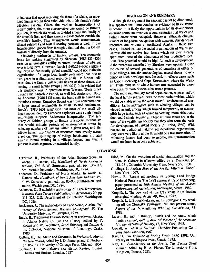
to indicate thatupon receiving his shareof a whale, an unre- DISCUSSION AND SUMMARYlatedhunter would then subdivide this in his family'sredis- Although the argumentforrankingcannot be discounted,tributi0n system, Given the various interpretations of it is apparentthatmore conclusive evidence of its existenceredistribution,the more conservative one would be Butch's is needed, lt is likely that opportunities for its developmentposition, in which the whale is divided amongthe family of occurredsometime over the severalcenturiesthatWales andtheumealikfirst,and thenamong crew.membersoutside the Point Barrow were occupied, However, although circum-umealik's family, This arrangement would accommodate stancesof long.termoccupation withapparentabundanceofdistantrelatives and formal sharing partnersas weil, In this resources are evldent in northwest Alaska in these twointerpretation,goods flow througha familial sharing systetn cases, it is curh_'L_:lhat the social organizationsof Wales andinsteadof directlyfromthe umealik. Barrow did not evolve into forms which set them clearly

Fissioning tendencies of Eskimo groups, The economicbasis for ranking suggested by Sheelmn [1985:131-136] apartfrom those of the inhabitantsof less productive loca-rests on an umealik'sability to controlproductsof whaling tions, The potential would be high for such a development,over a long term,However, Burch [1980:265-266] suggests if the processes describedby Sheehan were operating overthat even an "unusuallygifted umealik"could not maln_n the course of several generations of umeaUks in either oforganizationof a large local family over more than one or these villages, But the archaeologicalrecord shows no evi-two years in a diminished resource crisis. He furtherindt- dence of such developments. Instead, it reflects cases suchcates that the family unit would fission at these times, dis- as Cape Esponberg and Cape Krusenstem where the West-persing in small family groups [1980:274], lt is evident that em Thule remains of whale huntersare succeededby thosethis tendency was in operationfrom We.stemThule times who pursuedmore diverse subsistence patterns.throughthe Kotzebue Period, as well [cf, Anderson,1986]. The more rudimentarysocial organization,represented byAs Anderson[1986:113] notes, the basic shift in humandis- the local family segment, was the most basic division whichtributlonsaroundKotzebue Sound was from concentrations would be viable underthe most sa'essfulenvironmentalcon-in large coastal settlements to small isolated settlements, dttions, Large aggregates such as whaling villages can beButch's [1980:263] suggestion that most of the small vii- viewed as task groups which formed temporarily to accom-lages encounteredby Europeanexplorers were single family plish large tasks, such as whale harvesting, more effectivelysettlements supports Anderson's interpretation. The ten- thancould single segments, These cultural tenets are at thedency of Eskimo groups to fLqsionis a social mechanism core of the egalitarian society but they also form the basisthat would militate periods of environmental stress by for development of ranked society [of, Fried, 1960]. Withreducing numbers of humans within a given area, and dis- respect to traditional Eskimo socio-poUtieal organization,tributehuman exploitation of resources more evenly acrossa region, The splitting up of village inhabitants militates they were very likely at the thresholdof a transformation,Ifagainst formal ranking in a village, beyond any that is militating factors had been overcome, the transformationpresentin each segment,or extended family, would no doubthave been achieved.

CITATIONS

Ackerman, R., Prehlstory of the Asian Eskimo Zone. In Fried, M., On the evolution of social stratification and theArctic. D. Damas, ed., Handbook of North American State, in Culture in History, edited by S. Diamond, pp.Indians, Vol. 5, W. Sturtevant, gen. ed., pp. 106-118, 713-731, Columbia University Press, New York, 1960.Smithsonian Institution, Washington, DC, 1984. Giddings, J., Ancient Men of the Arctic, Alfred A. Knopf,

Anderson, D., Prehistory of North Alaska. In Arctic, D. New York, 1967.Damas, ed., Handbook of North American Indians, Vol. Harritt, R., Recent archaeology in Bering Land Bridge5, W. Sturtevant, gen. ed., pp. 80--93, Smithsonian Insti- National Preserve: The 1988 season at Cape Espenberg,tution, Washington, DC, 1984. paper presented at 16th Annual Meeting of the Alaska

Anderson, D., Beachridge archeology of Cape Krusenstem, Anthropological Association, Anchorage, March, 1989.National Park Service Publications in Archeology 20, pp. Krupnik, I., The bowhead vs. the gray whale in Chukotkan311--325, U.S. Department of the Interior, Washington, aboriginal whaling, Arctic, 40, 16-32, 1987.DC, 1986. Krupnik, I., L. Bogoslovskaya, and L. Botrogov, Gray whal.

Bockstoce, J., The archaeology of Cape Nome, Alaska, Un/- ing off the Chukotka Petdnsula: Past and present status,versity of Pennsylvania, Museum Monograph 38, The Report of the International Whaling Commission, 33,UniversityMuseum, Philadelphia, 1979. 1983.

Burch, E., Traditional Eskimo societies in northwest Alaska, ' Larsen, H., and F. Ralney, Ipiutak and the Arctic whalein Alaska Native Culture and History, edited by Y. hunting culture, Anthropological Papers of the AmericanKotani and W. Workman, Senti Ethnological Studies 4, Museum of Natural History, 42, New York, 1948.

pp. 253-304, National Museum of Ethnology, Osaka, Oswalt, W., Alaskan Eskimos, Chandler Publishing Com-1980. pany, San Francisco, 1967.

Collins, H,, The Arctic and Subarctic, in PreMstortc Man in Ray, D., The Eskimos of Bering Strait, 1650--1898, Uni-the New World, exfitedby J. D. J¢nnings and E. Norbeck, versity of Washington Press, Seattle, 1975.pp. 85-114, University of ChicagoPress, Chicago, 1964. Ray, D., Ethnohistory in the Arctic: The Bering Strait

Dumond, D., The Eskimos and Aleuts, Revised Edition, Eskimo, edited by R. A. Pierce, The Limestone Press,Thames and Hudson, London, 1987. Kingston, Canada, 1983.

404

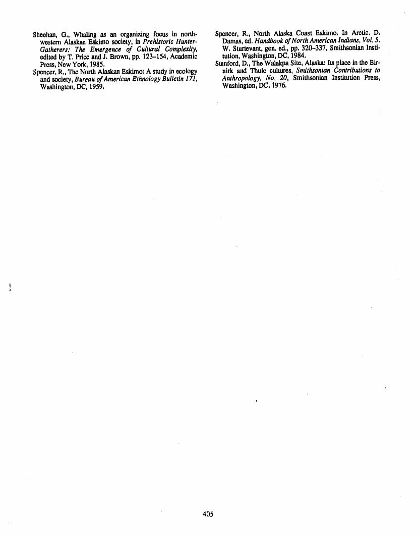
Sheehan, O,, Whaling as an organizing focus in north. Spencer, R,, North Alaska Coast Eskimo, In Arctic, D,western AlaskanEskimo society, in Prehistoric Hunter. Damas,ed, Handbook of North American lndians, Vol,5,Gatherers: The Emergence of Cultural Complexity, W. Sturtevant,gen, ed., pp. 320-337, Smtthsonian Insti-editedby T, Price and J, Brown, pp, 123-154, Academic tution,Washington, DC, 1984,Press, New York, 1985, Stanford,D., The WalakpaSite, Alaska: Its piace in the Bir-

Spencer,R,, The NorthAlaskanEskimo: A studyin ecology nirk and Thule cultures, Smith_onianContrtbu_lons toand society, Bureauof AmertcanEthnology Bulletin 171, Anthropology, No. 20, Smithsonian Institution Press,Washington, DC, 1959, Washington,DC, 1976.

405

The Effect of Climatic Change on Farming and Soil Erosionin Southern Greenland During the Last Thousand Years

Bjarne Holm Jakobsen_.stituteofGeography,UniversityofCopenhagen,Copenhagen,Denmark

ABSTRACT

Soil studies in low-arctic South Greenland often reveal polysequence soil pro-files. The study of these soils, dating of fossil surface horizons, study of land use,and use of paleoclimatic information from studies of ice cores show a complexinterplay between climatic change, soil erosion and agriculun-al land use.

Two periods of agricultural land use are known in Greenlanck From A.D. 985 toabout 1450 Norsemen settled in Greenland, and about 1915 modern sheep breedingstartedinsouthernGreenland.

The Norsemen desertedtheareain late1400,and no exactknowledge existsabouttheirfate.But soilprofilesand largeerosionareasofdesolationtellus abouttheirproblems.Climaticfluctuations,soilerodibilityfactorsand insufficientman-agcmcnt responseon environmentalfeedbacksprobablycausedtheterminationoftheNorse era.

The expandingmodem sheepbreedingindustryisfacingthesame problems astheNorsemen did.In spiteof agriculturalresearchand largeinvestmentsin winterfodderproduction,stablesand infrastructure,itseems difficultto practicea bal-anced landuse asregardscarryingcapacity.Soilerosionaccelerates,and thedev-astationofa uniquelandscapewillbe theconsequence,ifthereallylimitingfactorsforagriculturallanduse arenotrecognized.

INTRODUCTION GEOGRAPHICAL CONDITIONS

In the two periods of agricultural land use in Greenland, The study area covers the ice-free landscape from thethe basis has been grazing of the natural ve&etation. In Davis Straitcoast, throughareas traversedby deep fjords,toSouth Greenland luxuriant vegetation covers large areas in the present marginsof the Inland Ice (ca. 5000 km2).theinnerpartsofthefjordlandscape.Duringthelate1970s The low-arcticclimateshowsa trendfroman oceanicandearly1980sitwasplannedtointensifythesheepbreed- para-arctictypeintheoutercoastareastoa more con-ingindustryintheseareas.At thattimeTheHome Ruleof tinentalpamborealtypeintheinnerregions.Thelowsum-Greenland and The Ministry of Greenland initiated inter- mtr temperaturesof 5-7°(2, and foggy and moist conditionsdisciplinarystudies to evaluate the environmentalimpactof in the areasclose to the Davis Strait arc mainly due to theiccdfift from the Polar Sca with the East Greenland currentthischangeinlanduse.Specialemphasiswaslaidoneffects aroundKap Farvel.Summer temperaturesincreasetoabout

_ onsoilsandvegetation. 10°Cattheheadsofthefjords,andtheyearlyprecipitationThe study of soil profiles gave informationon periods of here decreases to about 600 mm, whereas outer coast areas

serioussoilerosion.The evaluationofconsequencesforthe showanaverageofabout900mm.landscape caused by present-day changes in land use, there- The climatic trend is the main factor for the vegetationalfore, also includes an evaluation of which role substantiated zonation. Dwarf shrub heath, rich in mosses and lichens,climatic fluctuations dmiiig tht_ "'-' _, .... a :_ --I..,: ........ ,h,, _,_n; .... I_e _nfl iehand¢ nf Iha ekeJ'riag land._cane.Z'l-I.JllJla,._il_ IJi_iGYr_4.1 111 Ili_li_l&21_ll _,ql,nv_lo I_llv 1_ -- .................. •

= to soil erosion. Going east the vegetation changes, and in the continental

= 406

.... '_ I

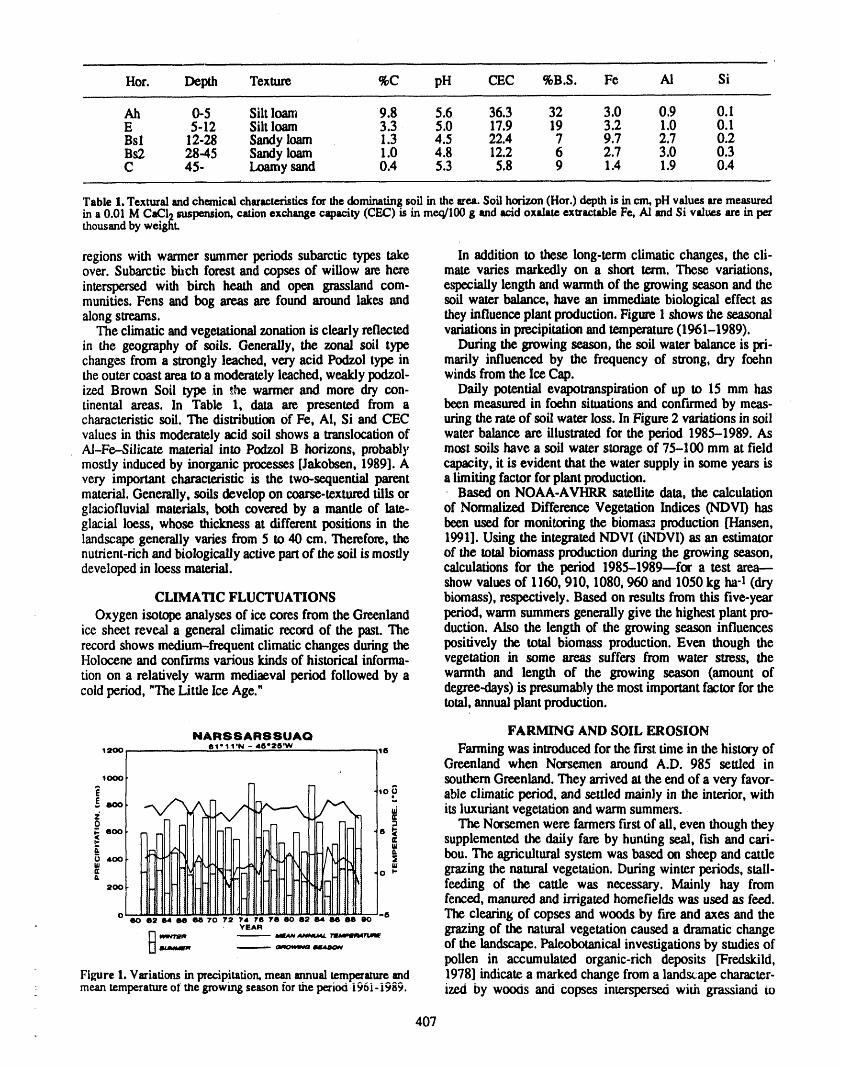
Hor. Depth Texture %C pH CEC %B.S. Fe AI Si

Ah 0-5 Silt loam 9.8 5.6 36.3 32 3.0 0.9 0.1E 5-12 Silt loam 3.3 5.0 17.9 19 3.2 1.0 0.1Bsl 12-28 Sandy loam 1.3 4.5 22.4 7 9.7 2.7 0.2Bs2 28-45 Sandyloam 1.0 4.8 12.2 6 2.7 3.0 0.3C 45- Loamy sand 0.4 5.3 5.8 9 1.4 1.9 0.4

TableI. Texturalandchemicalcharacteristicsfor thedominatingsoilin thearea.Soilh..orlzon (Hor.)depthis incre,pHvaluesaremeasuredina O.01MCaCI2suspension,cationexchangecapacity(CEC)ts inmeq/100g andaetdoxalateexlzactablele, AI madSi valuesareinperthousandbyweight.

regions with warmersummer periods subarctic types take In addition to these long-term climatic changes, the cli-over. Subarctic birch forest and copses of willow are here mate varies markedly on a short term. These variations,interspersed with birch heath and open grassland com- especially length and warmthof the growingseason and themunities. Fens and bog areas are found around lakes and soil water balance, have an immediate biological effect asalongstreams, they influence plantproduction.Figure 1 shows the seasonal

The climatic and vegetational zonationis clearlyreflected variationsin precipitationand temperature(1961-1989).in the geography of soils. Generally, the zonal soil type During the growing season, the soil water balance is pri-changes from a strongly leached, very acid Podzol type in marily influenced by the frequency of strong, dry fuehnthe outer coast areato a moderatelyleached, weakly lxxlzol- windsfrom the IceCap.ized Brown Soil type in ,_hewarmerand more dry con- Daily potential evapotranspirationof up to 15 mm hastinental areas. In Table 1, data are presented from a been measured in foehn situations and confirmed by meas-characteristic soft. The distribution of le, Al, Si and CEC uringthe rate of soil water loss. In Figure2 variationsin soilvalues hl this moderatelyacid soil shows a translocationof water balanceare illustratedfor the period 1985-1989. As

,AI-Fe.-Silicate materialinto Podzol B horizons, probably most soils have a soil water storage of 75-100 mm at fieldmostly inducedby inorganicprocesses [Jakobsen, 1989]. A capacity, it is evident that the watersupply in some years isvery important characteristicis the two-sequential parent a limiting factor forplantproduction.material.Generally. soils develop on coarse-texturedtills or Based on NOAA-AVHRR satellite data, the calculationglaciofluvial materials, both covered by a mantle of late- of Normalized Difference Vegetation Indices (NOV1) hasglacial loess, whose thickness at different positions in the been used for monitoring the biomasz production [Hansen,landscape generally varies from 5 to 40 cm. Therefore, the 1991]. Using the integratedNDVI (iNDVI) as an estimatornutrient-richand biologically active partof the soil is mostly of the total biomass productionduringthe growing season,developed in loess material, calculations for the period 1985-1989--for a test area--

show values of 1160, 910, 1080, 960 and 1050 kg ha-I (dryCLIMATIC FLUCTUATIONS biomass), respectively. Based on results from this five-year

Oxygen isotope analyses of ice cores from the Greenland period, warmsummersgenerally give the highest plant pro-ice sheet reveal a general climatic record of the past. The duction. Also the length of the growing season influencesrecordshows medium-frequentclimatic changes during the positively the total biomass production. Even though theHolocene and confirms various kinds of historical informa- vegetation in some areas suffers from water stress, thetion on a relatively warm mediaeval period followed by a warmth and length of the growing season (amount ofcoldperiod, "The Little Ice Age." degree-days) is presumablythe most importantfactor for the

total,annualplantproduction.

NARSSARSSUAQ FARMING AND SOIL EROSION,_,_, s,-,,.N -,5-2s,,, ,5 Farmingwas introducedfor the faSt time in the history of

J Greenland when Norseznen around A.D. 985 settled in,_ _ southern Greenland.They arrivedat the end of a very favor-,o .8 able climatic period,and settled mainly in the interior, with

E _,o /'_ /" _ its luxuriantvegetation and warmsummers._ The Norsemen were farmers faSt of all, even though they

- eOO -- 5 _- - ,, supplementedthe daily fare by hunting seal, fish and cad-

_ ,co _| _ = bou. The agricultural system was based on sheep and cattle

o _ grazing the natural vegetation. During winter periods, stall-_oo feeding of the cattle was necessary. Mainly hay from

fenced, manured and irrigated homefields was used as feed.o so .2 6, oe sn ,o ,2 ,, re ,, so s2 8, ee ee so -5 The clearing of copses and woods by fire and axes and the

_ Ym,. grazing of the natural vegetation caused a dramatic change- _ __ _...w_ "_'_" of the landscape.Paleobotanicalinvestigations by studies of" pollenin accumulated organic-rich deposits [Fredskild,

Figure1.Variationsin precipitation,meanannualtemperatureend 1978] indicate a marked change from a landscape character-meantemperatureof me growingseasonforthe periodi96i-i989, ized by wooas and copses interspersexi with grassland to

407

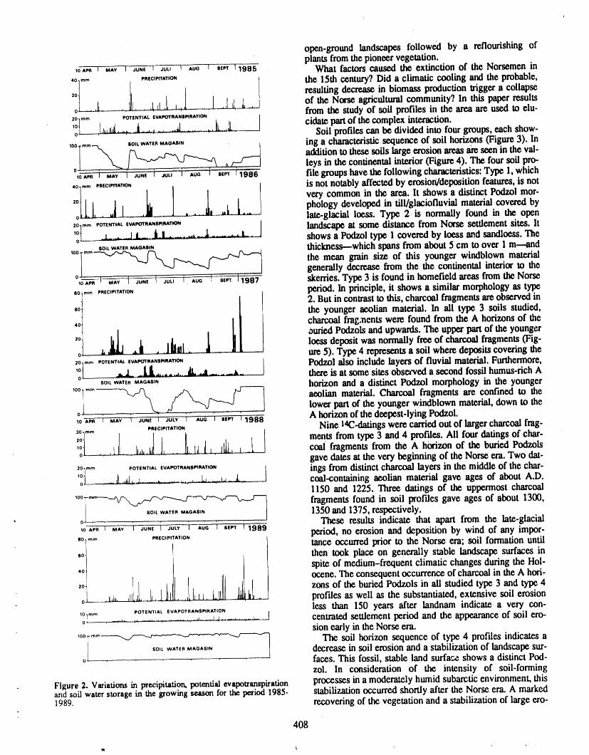
open-ground landscapes followed by a reflourishing ofplantsfromthe pioneervegetation.

,oAn _ MAYI JUNEI XL, I AUO1 S,. 11985 What factorscausedthe extinctionof the Norsemenin

,o _ I resultingdecrease in biomass production triggera collapse1 .It ,Lli [ ,{d J_ of the Norse agriculturalcommunity? In this paperresultso -. _. .... • .... ' _- from the study of soil profiles in therareaare used to elu-

20_mm POTENTIAL EVAPOTRANSPIRATION

ol l,h.,d...... j ...._ _ 11__,[ cidatepartof the complex interaction.,o , , , ........._.' • Soilprofilescanbedividedinto fourgroups,eachshow-,,,...___ SO,.WAT'RMAO",'N , ing a characteristicsequence of soil horizons (Figure 3). In

addition to these soils large erosion areasareseen in the val-leys in the continentalinterior(Figure 4). The foursoil pro-file groupshave the following characteristics:Type 1, which

,o mmPRECI,'rrAT,ON is not notably affectedby erosion/depositionfeatures,is not

1 _ 1 / very common in the area. It shows a distinct Podzol mor-2°[[1 I[_. . , .[ [ phology developed in till/glaciofluvial material covered byo .L . . .. . ...... late-glacialloess.Type 2 is normally found in the open

201mm POTENTIAL EVAPOYRANSPIRAT|ON J landscape at some distance from Norse settlement sites, lt'______t.... l t_ /,I ...... ,_. J,..... L. showsa Podzoltype1 coveredby loess_d sandloess.The

8OILWATERMAOASlN thickness--whichspansfrom about5 cm to over 1 m---and.oom ,..o ofOis,nwi,ow.generallydecreasefrom the the continentalinterior to the

...... skerries.Type 3 is found in homefield areas fromthe Norse80. mm PRECIPITATION p_od,; In principle, it showsa similarmorphologyas type

I 2. But in contrastto this, charcoal fragmentsareobserved in

,o the younger aeolian material. In ali type 3 soils studied,, / charcoalfragmentswerefoundfrom the A horizonsof the

4o I ouriedPodzolsand upwards. The upperpan of the youngero i,., I _,__1 _]hill loess deposit was normally free of charcoal fragments(Fig-, _ ure 5). Type4 representsa soilwheredepositscoveringthe20 mm POTENYIALEVAPOYRAN$1_RAYION Podzo!also includelayersof fluvial material.Furthermore,,o ,,J___Llt .... ..,.. iL J .... •- .. there is at some sites observed a second fossil humus-richA0 [

so,LWATE.MAO._,N horizonand a distinct Podzol morphology in the younger

'°°1mm---------X_ f/_'_'__l aeolianmaterial. Charcoalfragmentsare confinedto thelower part of the younger windblown material, down to theo...... A horizonof the deepest-lying Podzol.10APR l MAY 1 JUNE 1 JULY 1 AUG. I SE_ 11988

PRECIPITATION Nine 14C-datingswerecarriedoutof largercharcoalfrag-

'°t 1. h.,lh.l,l, L .IL.1,1_, ]_-,,-.[ coalfragments from the A horizon of the buried Podzoiso_ - ..... gave dates at the very beginning of the Norse era. Two dat-

20]mm POTENTIAL EV,_OTRANS""T'ON [ ings from distinctcharcoallayers in the middleof thechar-'_I ......,ll._,d_,.........._..................h......._.J._g.... coal-containingaeolianmaterialgaveagesof aboutA.D.1150and 1225.Threedatingsoftheuppermostcharcoal

'°°T_"_'-_ _ fragments found in soil profiles gave ages of about 1300,/ SOiL WATER MAOASIN ] 1350and 1375, respectively.• o These results indicate that apart from the late-glacial

,o APAI *SAY I _USTT"_OLY ! AUO I se_ I 1989 period,no erosion and deposition by wind of any impor-80 mm PRECIPITATION

,o then took place on generally stable landscape surfaces in

t spite of medium-frequentclimatic changes during the Hol-,o ocene. The consequent occurrenceof charcoal in the A hod,

II,h,, ,l_,t _ I I . ,, I11, LIt it o profdcs as well as the substantiated, extensive soil erosiono ' '_ ; ' less than 150 years after landnam indicate a very con-

107m m POTENTIAL EVAPOTR ANSPIRATIONo ...........- .............,.......... •.............'-;.............,..... centratedsettlementperiod and the appearanceof soilero-

sionearlyin theNorseera.,oo,-m__ The soil horizon sequence of type 4 profiles indicates a

: _OILWATE,.AOAS,N ] decreasein soil erosionanda stabilizationof landscapesur-°.---. faces. This fossil, stable land surface shows a distinct POd-zol. In consideration of the intensity of soil-forming

Figure2. Variationsin precipitation,potentialevapotranspiration processes in a moderatelyhumid subarcticenvironment,thisand soil waterstoragein thegrowingseasonforthe period1985- stabilization occurredshortly after the Morseera. A marked1989. recoveringof the vegetation and a stabilization of large ero-

408

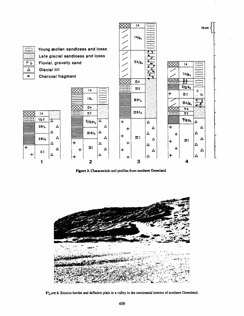
Fl_dl'e 4. Erosion border and deflation plain h_ a valley in the contlne_tal interior of southern Greenlsnd.

4O9

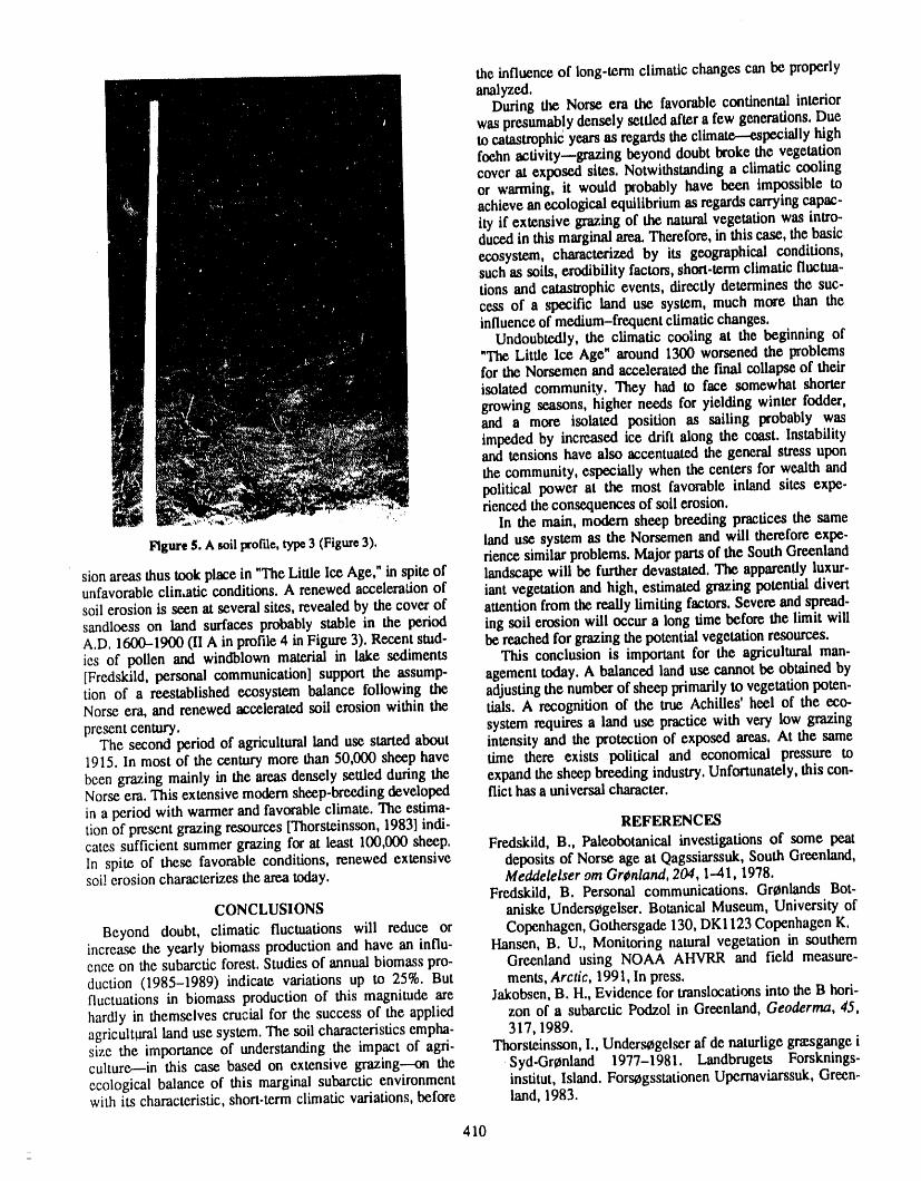
the influence of long-termclimatic changes can be properlyanalyzed.

During the Norse era the favorablecontinental interiorwaspresumablydensely settledaftera few generations,Dueto catastrophicyearsas regardsthe climate.--especially highfoehn activityJgrazing beyond doubt broke the vegetationcover at exposed sites. Notwithstandinga climatic coolingor warming, it would probably have been impossible toachieve anecological equilibriumas regardscarryingcapac-ity if extensive grazing of the naturalvegetation was intro-ducedin this marginalarea.Therefore, in this case, the basicecosystem, characterized by its geographical conditions,such as soils, erodibility factors,short-termclimatic fluctua-tions and catastrophic events, directly determines the suc-cess of a specific land use system, much more than theinfluenceof medium-frequentclimatic changes.

Undoubtedly, the climatic cooling at the beginning of"The Little Ice Age" around 1300 worsened the problemsfor the Norsemen and accelerated the final collapse of theirisolated community. They had to face somewhat shortergrowing seasons, higher needs for yielding winter fodder,and a more isolated position as sailing probably wasimpeded by increased ice drift along the coast. Instabilityand tensions have also accentuatedthe general stress uponthe community, especially when the centers for wealth andpolitical power at the most favorable inland sites expe-riencedtheconsequences of soil erosion.

_: In the main, modern sheep breedingpractices the same

Hgure 5. A soilprof'de,type3 (Figure3). land use system as the Norsemen and will therefore expe-rience similar problems.Majorpartsof the South Greenland

sion areas thus took place in "TheLittle Ice Age," in spiteof landscape will be furtherdevastated. The apparentlyluxur.unfavorableclimatic conditions. A renewed acceleration of iant vegetation and high, estimated grazing potential divertsoil erosion is seen at severalsites, revealed by the cover of attentionfrom the really limiting factors. Severe andspread-sandloess on land surfaces probably stable in the period ing soil erosion will occur a long time before the limit willA.D. 1600-1900 01 A in profile 4 in Figure 3). Recent stud- be reachedfor grazingthe potentialvegetationresources.ies of pollen and windblown material in lake sediments This conclusion is important for the agriculturalman-[Fredskild, personal communication] support the assump- agementtoday. A balanced landuse cannotbe obtained bytion of a reestablished ecosystem balance following the adjustingthe numberof sheep primarilyto vegetationpoten-Norse era, and renewed acceleratedsoil erosion within the rials. A recognition of the true Achilles' heel of the eco-present century, system requires a land use practice with very low grazing

The second period of agricultural land use started about intensity and the protection of exposed areas. At the same1915. In most of the century more than 50,000 sheep have time there exists political and economical pressure tobeen grazing mainly in the areas densely settled during the expand the sheep breeding industry. Unfortunately, this con-Norse era. This extensive modern sheep-breeding developed flict has a universal character.in a period with warmer and favorable climate. The estima-tion of present grazing resources [Thorsteinsson, 1983] indi- REFERENCEScates sufficient summer grazing forat least 100,000 sheep. Fredskild, B., Paleobotanical investigations of some peatIn spite of these favorable conditions, renewed extensive deposits of Norse age at Qagssiarssuk, South Greenland,soil erosion characterizes the area today. Meddelelser om GrCnland, 204, 1.-41, 1978.

Fredskild, B. Personal communications. GrCnlands Bet-CONCLUSIONS aniske Underscgelser. Botanical Museum, University of

Beyond doubt, climatic fluctuations will reduce or Copenhagen, Gothersgade130, DKl123CopenhagenK.increase the yearly biomass production and have an influ- Hansen, B. U., Monitoring natural vegetation in southernence on the subarctic forest. Studies of annual biomass pro- Greenland using NOAA AHVRR and field measure-duction (1985-1989) indicate variations up to 25%. But ments, Arctic, 1991,In press.fluctuations in biomass production of this magnitude are Jakobsen, B. H., Evidence for translocations into the B hori-hardly in themselves crucial for the success of the applied zon of a subarctic Podzol in Greenland, Geoderma, 45,agricultural land use system. The soil characteristics empha- 317, 1989.size the importance of understanding the impact of agri- Thorsteinsson, I., Unders_gelser af de naturlige _gange iculture--in this case based on extensive grazing---on the Syd-Gr¢nland 1977-1981. Landbrugets Forsknings-ecological balance of this marginal subarctic environment institut, Island. Fors_gsstationen Upernaviarssuk, Green-with its characteristic, short-term climatic variations, before land, 1983.

410

Climate and Landscape Perestroykas

S. A. Zimov and V. I. ChupryninPacificInstituteof Geography,Far EastBranchof the U.S.S.R.Academyof Science,Vladivostok,U.S.S.R.

ABSTRACT

Northern moss-lichen wood communities are becoming degraded progressivelyin many regions. That is why the question of their substtufion to grass com-munities, ones less sensitive to mechanical and chemical loads, is widely discussed.The problem of landscape reorganization in Northeast Asia is interesting in thisconnection. Today, territories are over-moist and low productivity moss-lichencovers are distributed everywhere. But, a rich pasture ecosystem existed here in theLate Pleistocene. Many people relate the phenomenon of arid climate mammothsteppes and their destruction to replacement by humid conditions in the Holocene.But in Northeast Asia the climate is arid even now, since the radiation index of dry-ness is more than 1 and even reaches 3. In Lower Kolyma, grasses can evaporate 2-3 times annual rates of precipitation (4--6 times more than mosses and lichens evap-orate). A mathematic model describing relations between various competitive plantcommunities depending on climate and activity of erosive-accumulative processes,pasture loads and CO2 concentration is proposed. It is shown that the influence ofthese factors is more significant than that of climate alone. Maps of northern hemi-sphere plants in the Pleistocene are calculated, as well as maps forecasting plantdistributions arising from future climatic and CO2 changes. The possibilities of arti-ficial regeneration of high-productivity pasture ecosystems are considered.

411

Trajectory Analysis of the Atmospheric Carbon DioxideBimodal Distribution in the Arctic

Kaz Higuchi and Neil B. A. TrivettRAGS Research Section, Atmospheric Environment Service, Downsvlew, Ontario, Canada

ABSTRACTAn examination of detrended atmospheric CO2 time series from two arctic mon-

itoring stations, Alert _d Mould Bay, shows a very prominent seasonal cycle witha very broad maximum In the winter and a very sharp minimum in the late summer.The amplitude of the cycle is about 15 to 16 ppmv (parts per million by volume).This seasonal cycle i:_;,_reflection of the metabolic cycle of the land biota in thenorthern hemisphere. Du:_ -_the period of broad maximum concentration in winter,the time series of CO2 show_, in some years, a bimodal feature, with a relative min-imum in late winter.

The bimodal distribution is difficult to explain in terms of (1) photosynthetic/respiratory cycle of terrestrial biospheric activities in the middle latitudes, and (2)anthropogenic activities. In this paper, we will speculate and discuss the bimodalfeature in terms of the evolution of the atmospheric circulation in the Arctic.

INTRODUCTION [1985], and Wong et al. [1984]. At Alert, the samples are

An examination of detrended atmospheric CO2 con- obtained about once per week using evacuated 2-1iterflasks.centration time series from two arctic monitoring stations, At Mould Bay, the samples are normally coUected twice perAlert and Mould Bay, shows a very prominent seasonal week using 0.5-1iterflasks that axe pumped up to a pressurecycle with a very broad maximum in winter to early spring of 1.5-2 atm.and a very sharp minimum during the late summer. The Nine years (1980-1988) of atmospheric CO2 measure-amplitude of the cycle is about 15 to 16 ppmv (lmm per mil- ments from Alert and Mould Bay were chosen and an-lion by volume), lt is believed that this seasonal cycle is a alyzed. To each of the data sets, we applied the followingreflection of the photosynthetic/decay cycle of the land biota steps:in the northern hemisphere. Composite average of the de- (1) Equally spaced data were obtained by filling gaps intrended seasonal cycle shows a gradual increase in the CO'z data by linear interpolation;concentration from late November to April, falling very rap- (2) A third-degree polynomial was then fitted to the CO2idly thereafter. During this period of broad maximum in time series in a least square sense to remove secular trend;winter, the time series show, in some years at least, a bi- andmodal feature, with a relative minimum in the latter half of (3) A 28-day equally weighted running mean was appliedwinter (Figure la,b). This type of feature can also be seen in to each of the dea'ended time series as a smoothingsuch chemical species as sulphate, procedure.

In this study, we show some preliminary evidence sug- Figure 1 shows the results of the application of thesegesting that the bimodal distribution can be explained, at steps. There is a great deal of interannual variability £-atheleast in part, by changes in the winter atmospheric circula- way the CO2 concentration evolves during the winter sea-tion in the Arctic. son. In particular, in some years there is a relative minimum

lasting about half a month or so during late winter. To ob-PROCEDURE tain an explanation for this phenomenon, we proceeded to

The CO2 flask sampling programs at Alert and Mould examine the statistical distribution of trajectories arriving atBay are described in Higuchi et al. [1987], Komhyer et al. Alert and Mould Bay. This is based on the assumption that

412

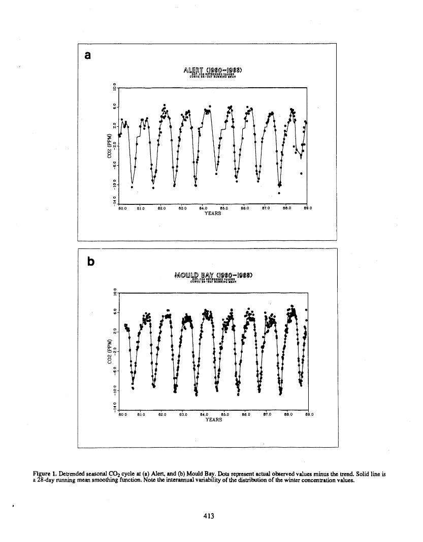
a

° Ile

0

N

_.

°i80.0 BI.O 62,0 8a.O 84,0 86.0 86,0 87.0 88,0 89,0

YEARS

bDOT_COB DK3'IIIeND|D ¥kLUIglt

CURYKJ IS-DAY RUNNING MEAN

o a_ li.. • --°o m • •

o

q

g:.o

_,-

o

7

o

I wBoo Bi,o B_,o 8;,o B,.o 8;,o 8;,o _i.o _6,o ,_.o

YEARS

Figure 1. DetrendedseasonalCO2cycle at (a) Alert,and Co)Mould Ba_. Dots representactualobserved values minus the trend.Solid line isa 28-day nmning meansmoothingfunction.Note the interannualvariabdityof the distributionof thewinter concentrationvalues.

413

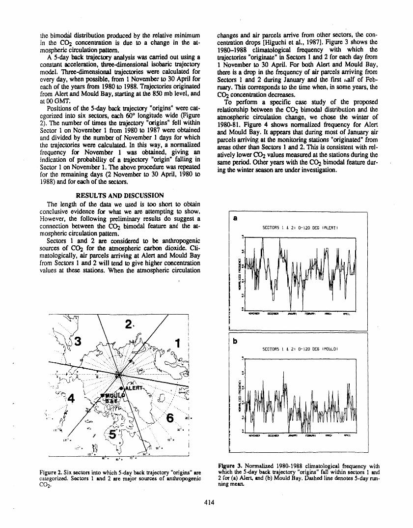
the bimodal distribution produced by the relative minimum changes and air parcels arrive from other sectors, the con-in the CO2 concentration is due to a change in the at- centration drops [Hlguehi et al., 1987], Figure 3 shows themosphcriccirculationpattem. 1980-1988 climatological frequency with which the

A 5-day back trajectory analysis was carried out using a trajectoriea "originate" in Sectors 1 and 2 for each day fromconstant acceleration, three-dimensional isobaric trajectory 1 November to 30 April, For both Alert and Mould Bay,model, Three-dimensional trajectories were calculated for there is a drop in the frequency of air parcels arriving fromevery day, when possible, from 1 November to 30 April for Sectors 1 and 2 during January and the Iu'st .alf of Feb-each of the years from 1980 to 1988, Trajectories originated ruary, Thiscorrespondsto the time when, in some years, thefrom Alert and Mould Bay, starting at the 850 mb level, and CO2 concentration decreases,at00GMT. To perform a specific case study of the proposed

Positions of the 5-day back trajectory "origins" were cat- relationship between the CO2 bimodal distribution and theegorizedintosixsectors,each60° longitudewide (Figure atmosphericcirculationchange,we chose the winterof2),The numberof timesthetrajectory"origins"fellwithin 1980-81.Figm'c4 shows normalizedfrequencyforAlert

Sector1on November I from 1980to1987wereobtained and Mould Bay,ltappearsthatduringmostofJanuaryairand dividedby thenumberof November I daysforwhich parcelsarrivingatthemonitoringstations"originated"fromthe trajectories were calculated. In this way, a normalized areas other than Sectors 1 and 2, This is consistent with rel-

frequency for November 1 was obtained, giving an atively lower CO2 values measured at the stations during theindication of probability of a trajectory "origin" falling in same period. Other years with the CO2 bimodal feature dur-Sector I on November I. The above procedure was repeated ing the winter season are under investigation.for the remaining days (2 November to 30 April, 1980 to1988) and for each of the sectors,

RESULTS AND DISCUSSION

The length of the data we used is too short to obtainconclusive evidence for what we are attempting to show.However, the following preliminary results do suggest a aconnection betw_n the CO,z bimodal feature and the at- srcroRs I _ _, 0-_0 0r_G_nLr_Rr_

mospheric circulation pattern. ,,Sectors1 and 2 are consideredto be anthropogenic

sourcesof CO'zforthe atmosphericcarbondioxide.Cii. :,matologically,airparcelsarrivingatAlertand Mould Bay

fromSectorsIand 2 willtendtogivehigherconcentration i_:_

valuesatthesestations.When theatmosphericcirculation

J

-_]

f ' t..........":,.:Z..., Ciwr, ......-..

Figure 3. Normalized 1980-1988 climatological frequency withFigure 2. Six sectors into which 5-day back trajectory"origins" are which the 5-day back trajectory "origins" fall within sectors 1 andcategorized, Sectors 1 and 2 axe major sources of andu'opogenic 2 for (a) Al='t, and (b) Mould Bay. Dashed line denotes 5-day frm-CO2. ningmean.

414

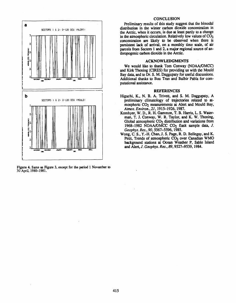
CONCLUSION

a Preliminaryresultsof this study suggest that the bimodalSECTORS I & 2, 0-120 DEG (RLCRTI distributioII in the wintercarbondioxideconcentrationin

the Arctic,whenit occurs,is dueat leastpartlytoa change

Ill parcels from Sectors 1 and 2, a majorregional sourceof an-

ACKNOWLEDGMENTS

; I[[I iiiJii , We would like to thank Tom Conway (NOAA_MCC)

II I I_l// and Kh'k Thoning (CIR S) for providingus with the Mould:j _ .... Bay data, and to Dr,S. M. Daggupaty foruseful discussions.,, _ ,,,,,,, ,,,,,,,,,,, ,,_ ,,,L Additional thanks to Buu Tran and Balbir Pabla for com-

putational assistance.

REFERENCES

b Hlguchi, K., N. B. A. Trivett, and S. M. Daggupaty, AsrCTOR5I : 2, 0-12o0EGtM0ULD_ preliminary climatology of trajectories related to at-

_, mosphericCO2 measurementsat Alert and MouldBay,

=4 Komhyer,W. D., R. H. Gammon,T. B. Harris,L. S. Water-i man, T. J. Conway, W. R. Taylor, and K. W. Thoning,

ilil_ _ Global atmosphericCO2 distributionand variationsfrom

1968-1982 NOAA/GMCC CO2 flask sample data, J.[[ [ Geophys. Res., 90, 5567-5596, 1985.

,__ iii Wong, C. S., Y.-H. Chan, J. S. Page, R. D. Bellegay, andK.

_4 Petit, Trends of atmospheric CO2 over Canadian WMObackground stations at Ocean Weather P, Sable Island

aJ III and Alert,J. Geophys. Res,,89,9527-9539, 1984.s_ml rme_T _ a_tL

I1_ llel

Figure 4. Sameas Figure3, except for theperiod1 Novemberto30 April,1980-1981. '

415

Winter CO2 Flux from Ecosystems in Northeast Asia

S. A. Zimov, G. M. Zimova, U. V. Voropaev, Z. V. Voropaeva, S. P. Davydov,A. I. Davydova, S. F. Prosyannikov, and O. V. Prosyannikova

North-Eastern Scientific Station of Pac_c Institute of Geography, Far East Branch o/the U.S,S.R, Academy of Science,Yakut ASSR, Chersky, Malinovy Yar, U.S,S.R.

ABSTRACT

To provide high concentrations and annual variations of CO2 in the atmosphereat 70°N latitude, the existence of substantial winter sources is required. Winteractivity of microbiota is low, thus a high flux of CO2 from ecosystems is hardly tobe expected. To address this contradiction a program of measurements of local CO2fluxes and CO2 concentrations in soil in the low Kolyma has been initiated. Theenvironments include maritime tundra territories, taiga, mountains, and lowland.An original express-method is proposed.

The analysis of materials demonstrates very high spatial and temporal variationsof local fluxes as well as important contributions to local CO2 variations producedby ecosystems in Northeast Asia.

416

I

Peat Accumulation Rates in Arctic Alaska:Responding to Recent Climatic Change?

D. M. Schell and B. BarnettWaterResearchCenter,UniversityofAlaskaFairbanks,Fairbanks,Alaska,U.S.A.

ABSTRACT

The accumulation of peat in arctic Alaska has left deposits up to 2 meters indepth with basal ages of over 12,000 years B.P. The radiocarbon depressions in thepeat serve as natural tracers of peat carbon movement in ecosystem processes.Many organisms collected from arctic Alaskan lakes and rivers show radiocarbonand stable isotope compositions that indicate that peat is being mobilized and actsas a major energy source to food webs. However, the large inputs of bomb radio-carbon from weapons testing in the late 1950s and early 1960s should be producingelevations in radi_oca:r,bon content, since decomposition of recent vegetation is pre-sumed to be the primary source of particulate and dissolved organic matter instreams. All vegetation produced in the Northern Hemisphere since about 1958 haselevated radiocarbon concentrations. A net radiocarbon depression in consumersimplies that the export of "old" peat carbon vastly exceeds that released from nor-real de_ay of recently grown plant material. Samples of dissolved organic carbonfrom tundra streams now being dated may help ascertain the source of carbonexport.

Upland valley peats show a truncated radiocarbon profile at the top at 1000-2700 years B.P., indicating that peat accumulation has ceased. Cores from thecoastal plain show that accumulation is still continuing, but decreases in soil carboncontent in upper soil horizons imply slower rates. Peat cores were eollected along atransect parallel to the Beaufort Coast near Prudhoe Bay and along a coast-to-foothills transect from Prudhoe Bay to Toolik Lake. Radiocarbon profiles of thesecores are to be dated and should lead to a better understanding of the role of perma-frost peatlands in carbon storage.

417

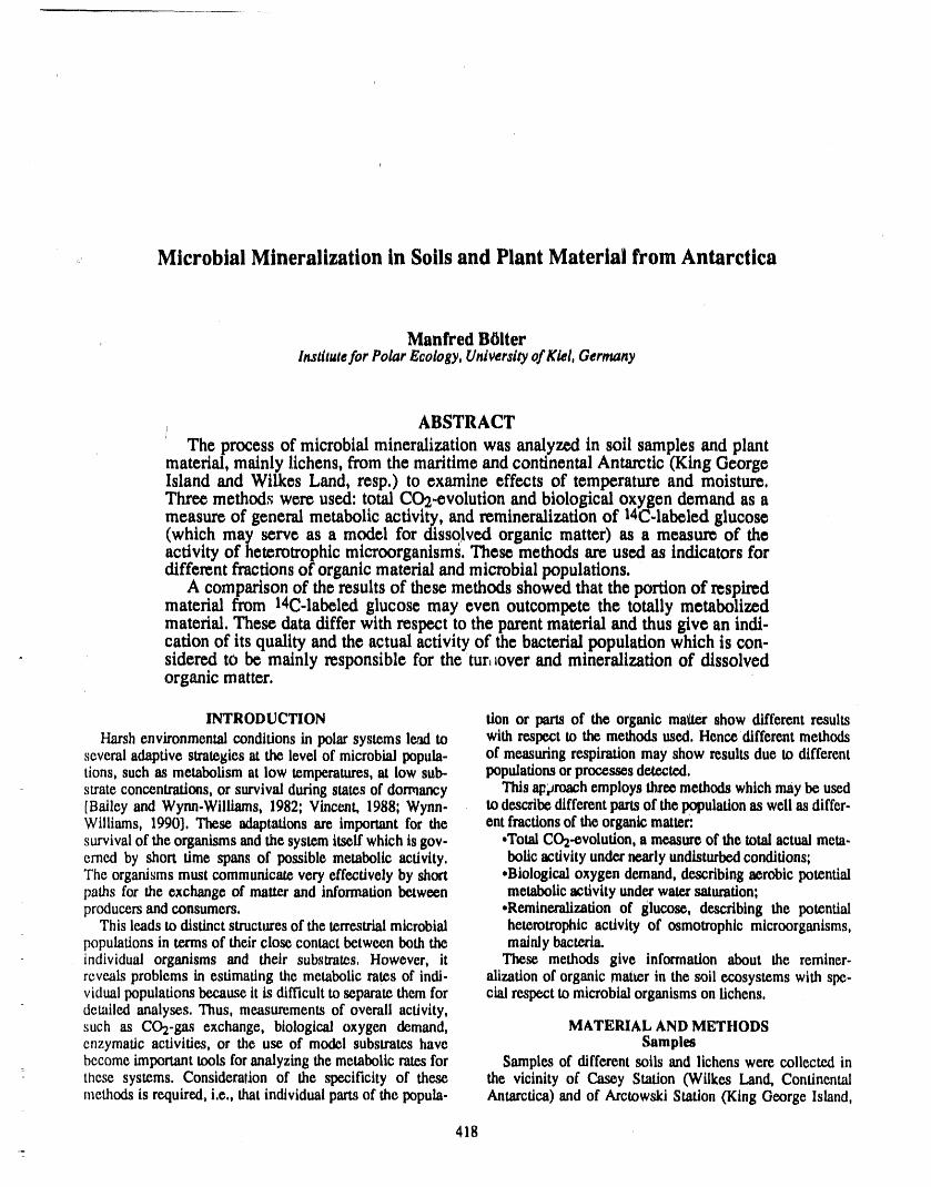
Microbial Mineralization in Soils and Plant Material from Antarctica

, ManfredBIterInstltuteforPolarEcology,UniversityofKiel,Germany

/ ABSTRACTTheprocessof microbialmineralizationwasanalyzedin soil samplesand plant

material, mainly lichens, from the maritime and continental Antarctic (King GeorgeIsland and Wilkes Land, resp.) to examine effects of temperature and moisture.Thre_ methods were used: total CO2.-¢volution and biological oxygen demand as ameasure of general metabolic activitty, and remineralization of 14C.labeled- glucose(which may serve as a model for dissolved organic matter) as a measure of theactivity of hetvrotrophic microorganisms. These methods are used as indicators fordifferent fractions of organic material and microbial populations.

A comparison of the results of these methods showed that the portion of respiredmaterial from 14C-labeled glucose may even outcompete the totally metabolizedmaterial. These data differ with respect to the parent material and thus give an indi-cation of its quality and the actual activity of the bacterial.population which is con-sidered to bc mainly responsible for the tur,_over and mineralization of dissolvedorganic matter.

INTRODUCTION rien or parts of the organic matter show different resultsHarsh environmental conditions in polarsystems lead to with respect to the methods used. Hence different methods

several adaptive strategies at the level of microbial popula- of measuringrespiration may show results due to differenttions, such as metabolism at low temperatures,at low sub- populationsor processes detected.su'atcconcentrations,or survival duringstates of dormancy This _i#roach employs three methods which may _ used[Bailey and Wynn.Willlams, 1982; Vincent, 1988; Wynn- to de,scribe differentpans of the populationas well as differ-Williams, 1990], These adaptations arc important for the ent fractions of the organic matter.survivalof the organismsandthe system itself which is gev- .Total CO-z-evolution,a mcasur©of the total actual meta.creed by short time spans of possible metabolic activity, bolic activity undernearlyundisturbedconditions;The organisms must communical¢very effectively by short .Biological oxygendemand, de.scribingaerobic potcntialpaths for theexchangeof mattedand informationbetween metabolicactivity underwatersaturation;producersandconsumers. .Re.mineralizationof glucose, de.scflbing the potential

This le.adsto distinct structuresof the terrestrialmicrobial hetcmtrophic activity of osmotrophic microorganisms,populations in teamsof theirclosecontact between both the mainly bacteria.individual organisms and their substrates. However, it These methods give information about the reminer-revealsproblemsinestimatingthemetabolicratesofindi- alizationoforganicmatterinthesoilecosystemswithspc-vidual populationsbecause it is difficult to separate them for cial rcslx.t to microbial organisms on lichens,detailed analyses, Thus, measurements of overall activity,suchas CO2-gasexchange,biologicaloxygendemand, MATERIAL AND METIIODSenzymatic activities, or the use of model substrates have Samplesbecome importanttools foranalyzing the metabolic ratesfor Samples of different soils and lichens were collected in

= these systems. Consideration of the specificity of these the vicinity of Cascy Station (Wilkes Land, Continentalmethods is re.quire.d,i.e., that individualpartsof the popula- Antarctica)and of Arctowski Station (King George Island,

418

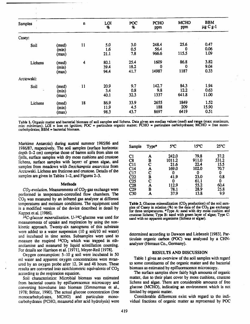
, i

I'

i,

Samples ' n LOI 'FOC PCHO MCHO BBM% % ppm ppm pg C g-1

Casoy:

Soil (med) 11 5,0 3,0 248,4 25.6 0,47(min) 1,6 0,5 56.4 0 0.06(max) 21,1 7,8 966,6 115,5 1,09

Lichens (me,d) 4 80.1 25,4 1609 86.8 3.82(min) 39.4 18.2 0 0 9,1M(max) 94,4 41,7 14987 1187 0,33

Arctowskt:

Soil (med) 11 20,9 9,7 142,7 84,3 1,94(min) 3,4 0,8 9,8 12,2 0,63(max) 40,1 32,3 1337 641,8 i 1,00

Lichens (me,d) 18 86.9 33,9 2655 1849 1,52(min) 11,9 4,5 188 209 15,90(max) 98,3 43,7 8697 64 19 0,51

'Fable I. Organlo matter and bacterial biomass of soil samples and llohem, Data given are median values (med) and range (maxl maximum,

mln: mlnlmt_), LOI= loss on ignition;POC= particulateorganicmatter;PCHO= partloulatee,arbohydrates;MCHO= free menD-carbohydrates,BBM= bacterialbiomass,

Maritime Antarctic) during austral summer 1985/86 and1986/87, respectively. The soil samples (surface horizonts: Sample Type* 50(2 15oc 25°Cdepth 0-2 cm) comprisethose of barrensoils from sites onfjells, surface samples with dry moss cushions and crustose C1 A 242.0 79,8 37,2lichens, surface samples with laye_ of green algae, and C8 B 1011.2 911.0 531,2samples from meadows with Deschampsia antarctica from CI 1 C 21.6 22,4 15.5C14 A 169.0 102,0 70,7Arctowski, Lichens are fruttcos_ and erustos¢, Details of the C17 C 0 0 0samples are given in Tables 1-2, and Figures 2-3, C22 B 41.9 23.0 0,8

C25 C 0 61.1 0Methods C28 A 112.9 55.2 60,4

C02-evolution. Measurements of C02-gas exchange were C29 B 78,1 28,9 25.8performed in temperature.controlled flow chambers, The C30 A 37.9 13.8 9,9CO2 was measured by an infrared gas analyzer at differenttemperatures and moisture conditions. The equipmentused Table2. Glucosemineralization(CO2production)of thesoilsam-

ples of Caseyin relation(%)to thedataof theCO2 gasexchangeis a modified version of the device described in detail by for three temperatures.*TypeA: sandwithdry mo_scushionmadKappet et al, [1986]. crustosolichens;TypeB: sandwithgreen layerof algae;TypeC:

14C-glucose mineralization, U-14C-glucose was used for sandwithno apparentorganisms(lichensor algae),measurements of uptake and respiration by using the non-kinetic approach, Twenty.stx nanograms of this subsWatewere added to a water suspension (10 g soil/10 ml water)and incubated in time series, Subsamples were used to determined according to Dawson and Liebezeit [1983], Par.measure the respired 141202which was trapped in eth. ticulate organic carbon ft'tC) was analyzed by a CHN-anolamine and measured by liquid scintillation counting, analyzer (l-lereausCt., Germany),For details see Harrison et al, [1971], Meyer-Reil [1978],

Oxygen consumption: 5-10 g soil were incubated in 50 RESULTS AND DISCUSSIONml water and apparent oxygen concentrations were mess- Table ! gives an overview of the soil samples with regardured by an oxygen probe after 12, 24 and 48 hours. These to some constituents of the organic matterand the bacterial

' results are converted into stoichiometric equivalents of C02 biomass as estimated by epifluorescence microscopy.according to the respiration equation, The surface samples show fairly high amounts of organic

Soil characteristics: Microbial biomass was estimated matter, due to their plant cover by moss cushions, crustosefrom bacterial counts by epifluorescence microscopy and lichens and algae. There are considerable amounts of freeconverting biovolume into biomass [Zimmerman et al., glucose (MCHO), indicating an environment which is not1978; BOiler, 1990], The actual glucose concentration (free limited by organic matter,monocarbohydrates, MCHO) and particulate mono- Considerable differences exist with regard to the indi-carbohydrates (PCHO, measured after acid hydrolysis) were vidual fractions of organic matter as represented by POC

419

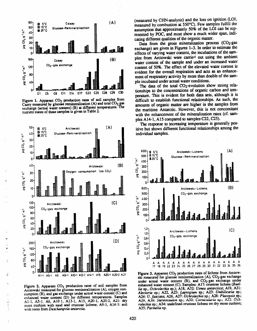
60 0 s'c cos,y (A) (measured by CHN-analysis) and the loss on ignition (LOI,

I measured by combustion at 550°C). Few samples fulfill the

. 50' : _:_ Olucose-Reminerolmofion assumption that approximately 50% of the LOI can be rCp-_- _0 resented by POC, and most show a much wider span, indi-'o, 30-2 caring different qualities of the organic matter.

° 2°'& NI_, 10. $1 I_l Data from the gross mineralization process (C02-gas0. eel ld [_l exchange) are given in Figures 1-3. In order to estimate theeffects of varying water content, the incubations of the sam-

150_ com I {B} pies from Arctowski were caniea out using the ambientwater content of the sample and under an increased water

7:_201 content of 50%. The effect of the elevated water content is'= evident for the overall respiration and acts as an enhance-c_ e°l merit of respiratory activity by more than double of the sam-

_, pieincubatedunderactualwaterconditions.'t The data of the total CO2-¢volution show strong rela-oJ tionships to the concentrations of organic carbon and tem-

C1 C5 ce Cll cii. c17 c22 c25 c28 c29 c30 peJ'ature. This is evident for both data sets, although it isFigure 1. ApparentCO2 prod.ucfion.._ of,soil.sam.pLes bom difficult to establish functional relationships. As such, theCaseymeasuredby glucose renuneral_uon tA) ImOtotalL_>2gas amounts of organic matter are higher in the samples fromexchange (actual watercontent) (B) ,t diffamt temperatures.Thenutrientstates of these smnples is given in Table 2. the maritimeAntarctic.However,this is not concomitant

with the enhancement of the mineralization rates (cf. sam-

pies Al4-1, Al5 compared to samples C22, C25).The response to increasing temperature is generally pos-

lA)501 I_! 5"C Arctowski [_ ! itive but shows different functional relationships among the

_. ';1:;_:_G,ooo--_.o,o.+,-,,oo_ I individualsamples.

ff 2o600"1 § 5"C Arctowski-Lmiaens {A)

_" 100 _ /-005001:2::Cc _ Glucose'Reminer°lis°ti°n I

0tJ I dtll/_'o'l Arc,owsk, (B) _ 3o0

20030_ B L_Oxygen c°nsumph°n (asCO')¥

Oo1 .. ,6001 i Arctowskl- Lmchens (Bl

500"1 I • C02-9OS exchonge •

1201 Arctowski I ) '_ 300o° 200

_ i;1 +1 I J 1 _ 'o ,,_ 0

E 20 1.2] Arctowsk,- Lichens ! lC)

,oot ,,o,o.,,,o, ,o, il II !+ ++, tlJ,i I1,,::l+tt++t++ , +o,+120 E 0,2" __ c_ 1 O.

L_ A A A A A A A A A A A A A A A A A A

_, J 17 18 19 22 23 2/. 25 25 27 28 29 30 31 32 33 _ 35 36

: oJA1-1 A5-1 A6 Ag-1 A10"1 A13-1 A1/--1 A15 A20-1 A20-2 A21 Figure 3. Apparent CO2 productionratesof lichens from Arcmw-ski measured for glucose remineralizadon(A), CO2-gas exchangeunder actual w_" content (B), and CO2-gu exchange under

Figure 2. Apparent CO2 production rat= of soil samplesfzom enhancedwatercontent (C). Samples:Al7: crustos¢ lichens (Buel-Arctowski measuredfor glucose mmineralization(A), oxygen con- lia sp., Ochrolechia sp.); Al8, A32: Usnea antarctica; Al9, A31:sumption(B), andgas exchange under actualwatercontent (C) and Alectoria sp.; A22, A25: Leptogium sp.; A23: Umbilicaria sp.;enhanced water cont_t ('D) for different temperatures. Samples A24: U. fasc/ata; A26, A27: Ochrolechia.sp.': .A28!placops.is_d;

= Al-l, AS-l, A6, Al0-1, Al3-1, Al5, A20-1, A20-2, A21: dry A29, A36: Slereocauion sp.; .,sou: c.ormc,ua+a =+p.;,_-,. v,.,,-: moss cushion with stud and crusto_ lichem; A9-1, AI4-1: soil rolechia sp.; A34: un_f'med crustuse lichens on dry moss cushion;, with roots from Deschampsia antarctia. A35: Parmelia sp.

420-

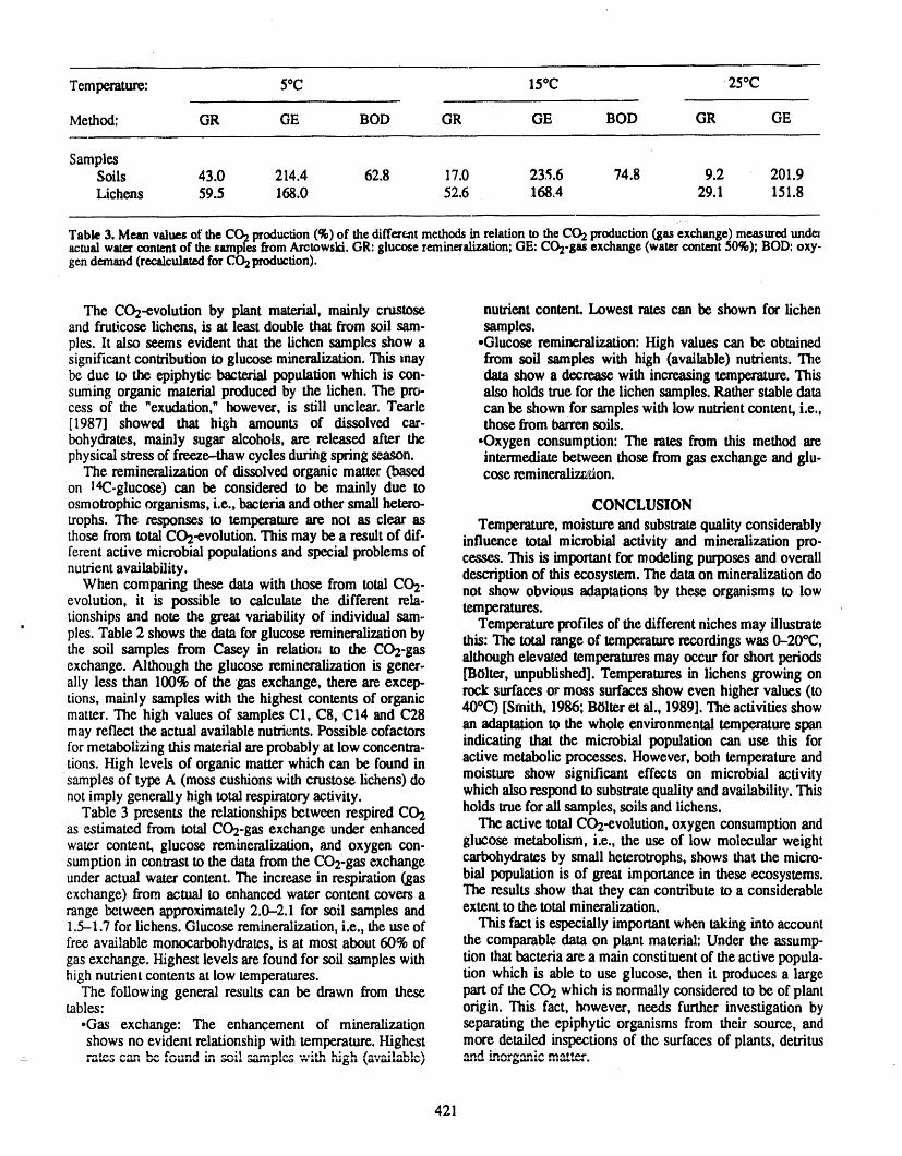
Temperature: 5"C 150C 25°C

Method: GR GE BOD GR GE BOD GR GE

SamplesSoils 43.0 214.4 62.8 17.0 235.6 74.8 9.2 201.9Lichens 59.5 168.0 52.6 168,4 29.1 151.8

Table3. Meanvaluesof theCO2production(%)of thedifferentmethodsinrelationto the CO2production(gas exchange)measuredunde_actualwnte_contentof thesamplesbomArctowski.GR:glucosereminer_r.nlion;GE:CO2-guexchange(watercontent50%);BOD:oxy-gendemand(re_cuhted forCO2production).

The CO2-evolution by plant material, mainly crustose nutrient content. Lowest rates can be shown for lichenand fruficose lichens, is at least double that from soil sam- samples.pies. It also seems evident that the lichen samples show a -Glucose remineralization: High values can be obtainedsignificant contribution to glucose mineralization. This may from soil samples with high (available) nutrients. Thebe due to the epiphytic bacterial population which is con- data show a decrease with increasing temperature. Thissuming organic material produced by the lichen. The pro- also holds true for the lichen samples. Rather stable datacess of the "exudation," however, is still unclear. Tearle can be shown for samples with low nutrient content, i.e.,[1987] showed that high amounts of dissolved car- those frombarrensoils.bohydrates, mainly sugar alcohols, are released after the -Oxygen consumption: The rates fromthismethod arephysical stress of freeze--thaw cycles during spring season, intermediate between those from gas exchange and glu-

The remineralization of dissolved organic matter (based cose reminemlizvJon.on 14C-glucose) can be considered to be mainly due toosmotrophic organisms, i.e., bacteria and other small hetero- CONCLUSIONtrophs. The responses to temperature are not as clear as Temperature, moisture and substrate quality considerablythose from total CO2-evolution.This may be a result of dif- influence total microbial activity and mineralization pro-ferent active microbial populations and special problems of cesses. This is important for modeling purposes and overallnutrient availability, description of this ecosystem. The dam on mineralization do

When comparing these data with those from total CO2- not show obvious adaptations by these organisms to lowevolution, it is possible to calculatethe different rela- temperatures.tionships and note the great variability of individual sam- Temperature profiles of the different niches may illuslrate

" pies. Table 2 shows the data forglucose remineralization by this: The total range of temperaturerecordingswas 0-20"12,the soil samples from Casey in relatiov, to the CO2-gas although elevated temperatures may occur for short periodsexchange. Although the glucose remineralization is gener- lBOlter, unpublished]. Temperatures in lichens growing onally less than 100% of the gas exchange, there are excep-tions, mainly samples with the highest contents of organic rock surfaces or moss surfaces show even higher values (tomatter. The high values of samples C1, C8, C14 and C28 40°C) [Smith, 1986; B01teret al., 1989]. The activities showmay reflect the actual available nutrients. Possible cofactors an adaptation to the whole environmental temperature spanfor metabolizing this material areprobablyat low concentra- indicating that the microbial population can use this fortions. High levels of organic matterwhich can be found in active metabolic processes. However, both temperature andsamples of type A (moss cushions with crustose lichens) do moisture show significant effects on microbial activitynot imply generally high total respiratoryactivity, which also respond to substratequality and availability. This

Table 3 presents the relationships between respired CO2 holds true forali samples, soils and lichens.as estimated from total CO2-gas exchange under enhanced The active total CO2-evolution, oxygen consumption andwater content, glucose remineralization, and oxygen con- glucose metabolism, i.e., the use of low molecular weightsumption in contrast to the data from the CO2'gas exchange carbohydrates by small heterotrophs, shows that the micro-under actual water content. The increase in respiration (gas bial population is of great importance in these ecosystems.

The results show that they can contribute to a considerableexchange) from actual to enhanced water content covers arange between appro_mately 2.0-2.1 for soil samples and extent to the total mineralization.1.5-1.7 for lichens. Glucose remineralization, i.e., the use of This fact is especially important when taking into accountfree available monocarbohydrates, is at most about 60% of the comparable data on plant material: Under the assump-gas exchange. Highest levels are found for soil samples with tion that bacteria are a main constituent of the active popula-high nutrient contents at low temperatures, tion which is able to use glucose, then it produces a large

The following general results can be drawn from these part of the CO2 which is normally considered to be of planttables: origin. This fact, however, needs further investigation by

•Gas exchange: The enhancement of mineralization separating the epiphytic organisms from their source, andshows no evident relationship with temperature. Highest more detailed inspections of the surfaces of plants, detritus

421

REFERENCES

Bailey, A. D., and D. D. Wynn-Williams, Soil micro- Kappen,L., M. BOlter,and A. KUhn,Field measurementsofbiological studies at Signy Island,South OrkneyIslands, net photosynthesis of lichens in the Antarctic, Polar

, Br. Antarct. Surv. Bull., 51,167-191, 1982. Biol., 5,255-258, 1986.B61ter, M., Microbial activity in soils from Antarctica Meyer-Reil,L.-A., Uptakeof glucose by bacteriain the sed-

(Casey Station, Wilkes Land), Proc. NIPR Symp. Polar iment,Mar. Biol., 44,293-298, 1978.Biol., 2, 146-153, 1989. Smith, R. I. L., Plantecological studies in the fellfield eco-

BORer,M., Microbial ecology of soils from Wilkes Land, system near Casey Station, Australian Antarctic Ter-Antarctica: II. Patternsof microbial activity and related ritory,Br. Antarct. Surv. Bull., 72, 81-91, 1986.organic and inol'ganic matter, Proc. NIPR Syrup. Polar Teade, P. V., Cryptogamiccarbohydraterelease and micr_Biol., 3, 120-132, 1990. bial responseduringfreeze-thaw cycles in Antarctic fell-

B61ter, M., L. Kappen, and M. Meyer, The influence ¢3f field fines, SoilBiol. Biochem., 19, 381-390, 1987.microclimatic conciitions on potential photosynthesis of Vincent, W. F., Microbial Ecosystems in Antarctica, Cam.Usnea sphaceiata--a model, Ecol. Res., 4, 297-307, bridgeUniv. Press, Cambridge, 1988.1989. Wynn.WiUiams, D. D., Ecological aspects of Antarctic

Dawson,R., and G. Liebezeit, Determinationof amino acids microbiology,Adv. Microb. Ecol., 11, 71-146, 1990.and carbohydrates, in Methods of Seawater Analysis, Zimmerman,R., R. Iturriaga,and J. Becker-Birck, Simul-edited by K. Grasshoff, M. Ehrhardt,and K. Kremling, taneousdeterminationof the total numberof aquaticbac-pp. 319-346, VerlagChemie, Weinheim, 1983. teria and the number thereof involved in respiration,

Harrison,M. J., R. T. Wright, andR. Y. Mor_ta,Method for Appl. Environ. Microbiol., 36, 926-935, 1978.measuring' mineralisation of lake sediments, Appl.Microbiol., 21,223-229, 1971.

422

Effects of Point Source Atmospheric Pollutionon Boreal Forest Vegetation of Northwestern Siberia

T. M. ViasovaFar North Institute for Agricultural Research, Noril'sk, U.S.S.R,

B. I. KovalevBryansk All.Union Scientific Research Institute, Forest Resources Section, Bryansk, U.S.S.R.

A. N. FilipchukAll-Union Scientific Research I_ _titute,Forest Resources Section, Moscow, U.S.S.R.

ABSTRACT

Atmospheric pollution from the Noril'sk Mining-Metallurgical Complex, in theform of heavy metals and sulfur components, has resulted in damage to plant com-munities in the area. Vegetation on over 550,000 ha has been detrimentally affectedby the pollution fallout, primarily sulfur dioxide. Forests (mainly Larix sibirica)and most lichens have been killed within a 300,000-ha zone around Noril'sk andextending about 50 km to the south and southeast. Less severe damage to lichensand vascular plants extends 170 km to the south and 80 km to the east of the pollu-tion source consistent with prevailing winds during the period of plant growth. Ter-ricolous lichens arc particularly vulnerable to the pollution products and amongvascular plants Larix gmelinii, Picea obovata, Ledum palustre, Calamagrostis sp.,and Salix lanata show least resistance.

INTRODUCTION The NIR has a subarcticclimate with an extended, coldGrowth in industrialproductioncharacterizes the modem winter and a short, cool summer with a vegetation growth

world andhas led to pollution of the environmentwith toxic period of about 60 days. Northerly winds prevail. Dis-substances, causingdeteriorationin the conditionand loss of tributionof a'ee..sis in scattered small units or strips, largecomponents of plantcommunities. Pollution effects on for- stands being infrequent.The average forest cover does notest vegetation may be pronouncedin regions with extreme exceed 40%. The main tree species arc Larix sibirica, shift-climatic conditions--such as at forest ccotones in the Far ing in the cast to L. gmelinii, and also Picea obovata andNorth. A typical example of this phenomenos is furnished Betula pubescens. Forested areasarc concentratedmostly inby the destructionof forest vegetation in the Noril'skindus- river valleys and on watershed slopes. These same water-trialregion (NIR). sheds also include tundravegetation. The forests have a low

density with small tree crowns, about 25% of the forestedTHE STUDY AREA area being represented by open stands. For every unit of

The N_ is located in North Krasnoyarsk Krai, on the plantbiomass there are morephotosynthesizing tissues thanrightbankoftheYcniscyRiver(FigureI).Theforestsstud- inthetruetaiga.icdarethoseatthenortherninterfaceoftaigaandtundra[Parmuzin,1979;Chertovskiiand Semenov,1984].They EMISSIONS PRODUCED BY THE NORIL'SK A.P.providehabitatformammalsandbirdsandtheveryimpor- ZAVENIAGIN MINING AND METALLURGICALrantresourcebaseforreindeerandhuntingeconomies.Bod- INDUSTRIAL COMPLEX 0NMMC)icsof waterintheregionarerichinfishspecies.The The economicand socialdevelopmentand ecologicalecosystemsof suchforesthave littleplasticityand res- stateof theNIR arcdetermincdby theactivitiesof thetorativecapability. NMMC. ltisthebasisofdevelopmentfortheextensive

423

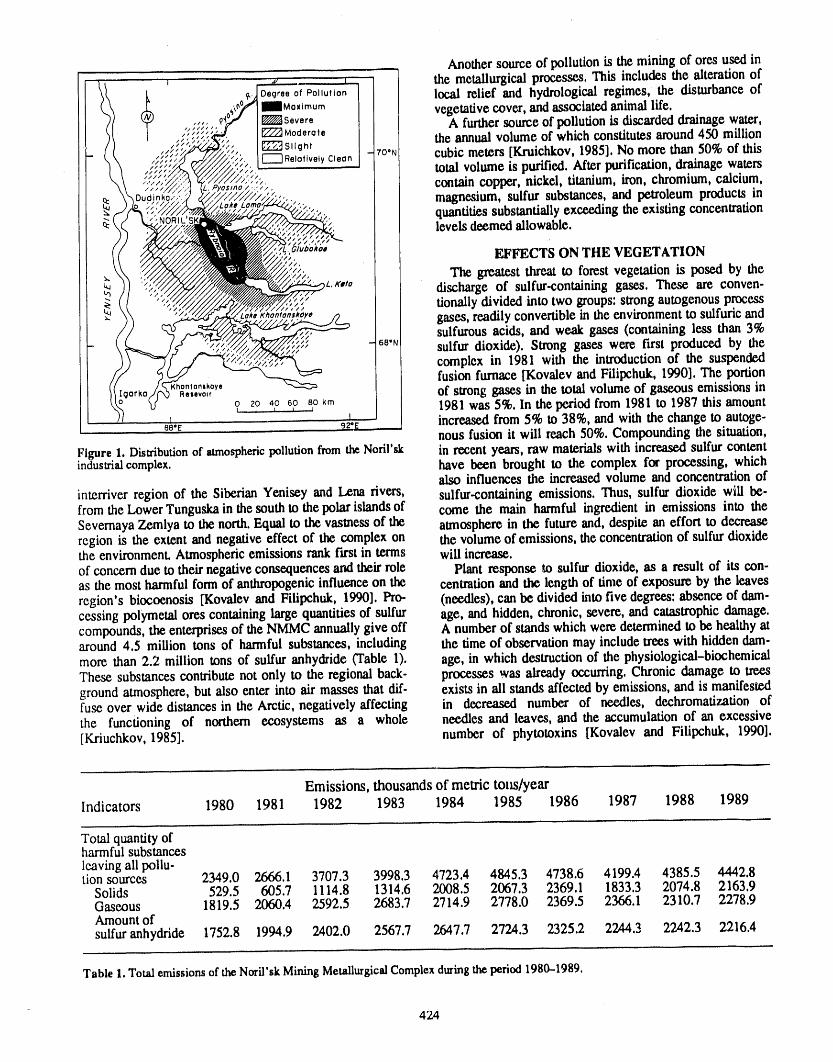
Another source of pollution is the mining of ores used inthe metallurgical processes. This includes the alteration of

I oeqr.eofPollu,lo.I localreliefand hydrologicalregimes,thedisturbanceof

mmMo_,mom I vegetativecover,andassociatedanimal life.[_'P'/_Severe ] A furthersourceofpollutionisdiscardeddrainagewater,_Moderote I_'_Sll0h, / the annual volume of which constitutes around450 million

,_; r---TRe,o,_v**yc_,oo/ cubic meters [Kruichkov, 1985]. No more than 50% of thistotal volume is purified. After purification,drainage waters'" contain copper, nickel, titanium, iron, chromium, calcium,

magnesium, sulfur substances, and petroleum products inquantities substantiallyexcee.dingthe existing concentrationlevels deemed allowable.

_, EFFECTS ON THE VEGETATIONs//,

'_'. The greatestthreatto forestvegetationisposedby the,L,_,ta dischargeof sulfur-containinggases.Theseareconven-

.,_ tionallydivided into two groups:strong autogenous processgases, readily convertible in the environmentto sulfuricandsulfurous acids, and weak gases (containing less than 3%sulfur dioxide). Strong gases were furst produced by thecomplex in 1981 with the introductionof the suspendedfusion furnace [Kovalev and Filipchuk, 1990]. The portion

<hontanskoyeR,,.vo,_ ofstronggasesinthetotalvolumeofgaseousemissionsin? 2o ,_ 67 _o km 1981 was 5%. In the period from 1981 to 1987 this amount

t .L_.._ increased from 5% to 38%, and with the change to autoge-st._ 9__g......_ nous fusion it will reach 50%. Compounding the situation,

Figure 1. Distributionof atmosphericpollutionfrom theNoril'sk in recent years, raw materials with increased sulfur contentindustrialcomplex, have been brought to the complex for processing, which

also influences the increased volume and concentration ofinterriver region of the Siberian Yenisey and Lena rivers, sulfur-containing emissions. Thus, sulfur dioxide will be.from the Lower Tunguska in the south to the polar islands of come the main harmful ingredient in emissions into theSevernaya Zemlya to the north. Equal to the vasmess of the atmosphere in the future and, despite an effort to decreaseregion is the extent and negative effect of the complex on the volume of emissions, the concentration of sulfur dioxidethe environment. Atmospheric emissions rank fast in terms will increase.of concern due to their negative consequences and their role Plant response to sulfur dioxide, as a result of its con-as the most harmful form of anthropogenic influence on the centration and the length of time of exposure by the leavesregion's biocoenosis [Kovalev and Filipchuk, 1990]. Pro- (needles), can be divided into five degrees: absence of dam-cessing polymetal ores containing large quantifies of sulfur age, and hidden, chronic, severe, and catastrophic damage.compounds, the enterprises of the NMMC annually give off A number of stands which were determined to be healthy ataround 4.5 million tons of harmful substances, including the time of observation may include trees with hidden dam-more than 2.2 million tons of sulfur anhydride (Table 1). age, in which destruction of the physiological-biochemicalThese substances contribute not only to the regional back- processes was already occurring. Chronic damage to treesground atmosphere, but also enter into air masses that dif- exists in ali stands affected by emissions, and is manifestedfuse over wide distances in the Arctic, negatively affecting in decreased number of needles, dechromatization ofthe functioning of northern ecosystems as a whole needles and leaves, and the accumulation of an excessive[Kriuchkov, 1985]. number of phytotoxins [Kovalev and Filipchuk, 1990].

Emissions, thousands of metric tom/year

Indicators 1980 1981 1982 1983 1984 1985 1986 1987 1988 1989

Total quantity ofharmful substancesleaving ali pollu-tion sources 2349.0 2666.1 3707.3 3998.3 4723.4 4845.3 4738.6 4199.4 4385.5 4442.8

Solids 529.5 605.7 1114.8 1314.6 2008.5 2067.3 2369.1 1833.3 2074.8 2163.9Gaseous 1819.5 2060.4 2592.5 2683.7 2714.9 2778.0 2369.5 2366.1 2310.7 2278.9Amount ofsulfur anhydride 1752.8 1994.9 2402.0 2567.7 2647.7 2724.3 2325.2 2244.3 2242.3 2216.4

Table 1.Totalemissionsof theNoril'skMiningMetallurgicalComplexduringthe period1980.-1989.

424

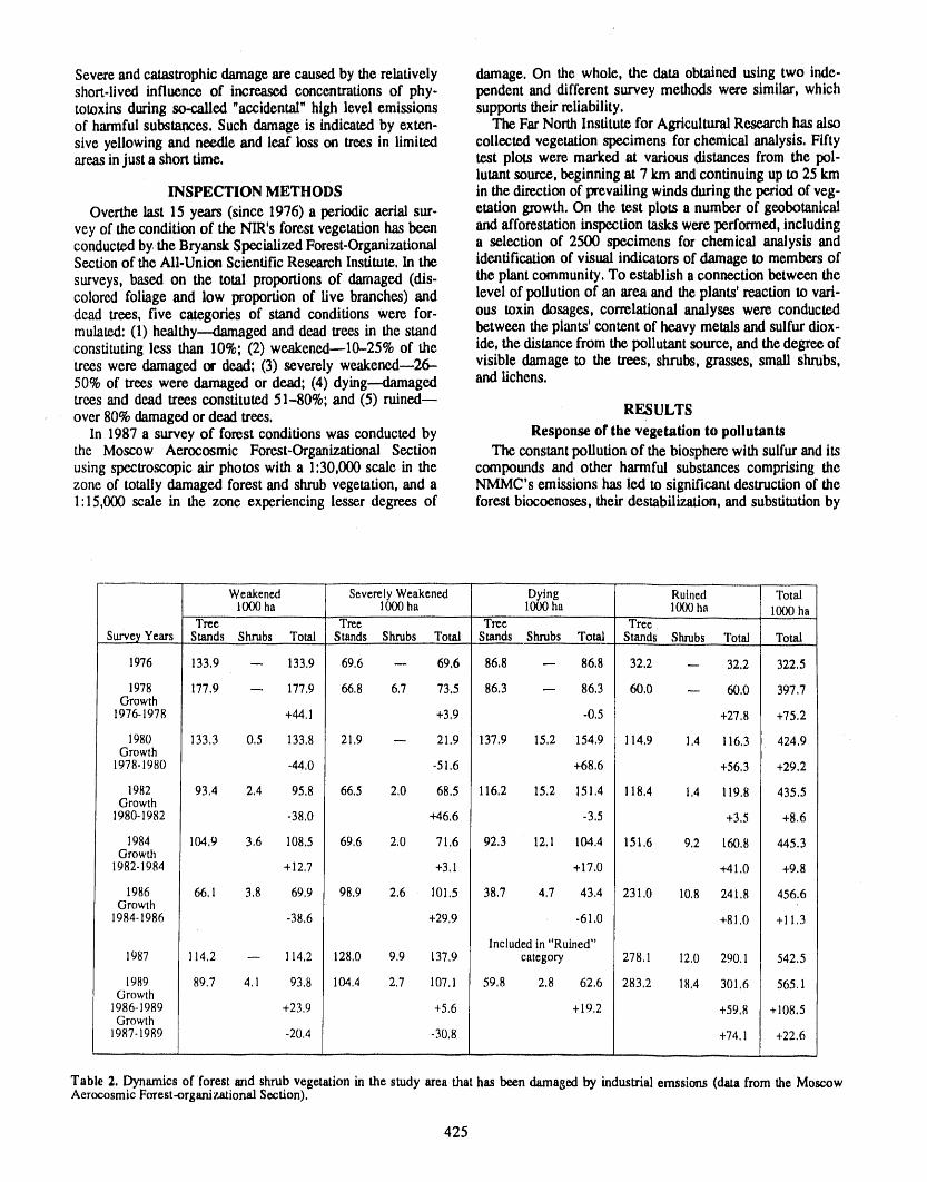
Severe and catastrophic damage are caused by the relatively damage. On the whole, the data obtained using two indc-short-lived influence of increased concentrations of phy- pendent and different survey methods were similar, whichtotoxins during so-called "accidental" high level emissions supports their reliability.of harmful substances. Such damage is indicated by exten- The Far North Institute for Agricultural Re,search has alsosire yellowing and neexlle and leaf loss on trees in limited collected vegetation specimens for chemical analysis. Fiftyareas in just a short time. test plots were marked at various distances from the pol-

lutant source, beginning at 7 km and continuing up to 25 kmINSPECTION METHODS in the direction of prevailing winds during the period of veg-

Overthe last 15 years (since 1976) a periodic aerial sur- etation growth. On the test plots a number of geobotanicalvey of the condition of the NIR's forest vegetation has been and afforestation inspection tasks were performed, includingconducted bythe Bryansk Specialized Forest-Organizational a selection of 2500 specimens for chemical analysis andSection of the MI-Union Scientific Research Institute, In the identification of visual indicators of damage to members of

surveys, based on the total proportions of damaged (dis- the plant community, To establish a connection between thecolored foliage and low proportion of live branches) and level of pollution of an area and the plants' reaction to vari-dead trees, five categories of stand conditions were for- ous toxin dosages, correlational analyses were conductedmulated: (1) healthy--damaged and dead trees in the stand between the plants' content of heavy metals and sulfur diox-constituting less than 10%; (2) weakened--10-25% of the ide, the distance from the pollutant source, and the degree oftrees were damaged or dead; (3) severely weakened--26- visible damage to the trees, shrubs, grasses, small shrubs,50% of trees were damaged or dead; (4) dying---damaged and lichens.trees and dead trees constituted 51--80%; and (5) ruined--over 80% damaged or dead trees, RESULTS

In 1987 a survey of forest conditions was conducted by Response of the vegetation to pollutantsthe Moscow Aerocosmic Forest-Organizational Section The constant pollution of the biosphere with sulfur and itsusing spectroscopic air photos with a 1:30,000 scale in the compounds and other harmful substances comprising thezone of totally damaged forest and shrub vegetation, and a NMMC's emissions has led to significant destruction of the1:15,000 scale in the zone experiencing lesser degrees of forest biocoenoses, their destabilization, and substitution by

Weakened SeverelyWeakened Dying Ruined Total1000ha 1000ha 1000ha 1000ha 1000ha,,

Tree Tree Tree TreeSurveyYears Stands Shrubs Total Stands Shrubs Total Stands Shrubs Total Stands Shrubs Total Total,,, ,,

1976 133.9 m 133,9 69,6 -- 69,6 86,8 -- 86,8 32.2 -- 32.2 322.5

1978 177,9 m 177,9 66,8 6,7 73.5 86.3 -- 86,3 60,0 -- 60,0 397,7Growth

1976-1978 +44,1 +3,9 -0,5 +27,8 +75,2

1980 133,3 0,5 133,8 21,9 -- 21.9 137,9 15.2 154.9 114.9 1.4 116,3 424,9Growth

1978-1980 -44,0 -51,6 +68.6 +56,3 +29.2

1982 93,4 2,4 95,8 66,5 2,0 68,5 116,2 15,2 151,4 118.4 1,4 119,8 435,5Growth

1980-1982 -38,0 +46,6 -3.5 +3.5 +8,6

1984 104,9 3,6 108.5 69,6 2,0 71,6 92.3 12,1 104,4 151,6 9,2 160,8 445.3Growth

1982-1984 +12,7 +3,1 +17.0 +41,0 +9,8

1986 66,1 3,8 69,9 98,9 2,6 101.5 38,7 4,7 43,4 231,0 10,8 241,8 456.6Growth

1984-1986 -38,6 +29,9 -61.0 +81,0 +11,3

Includedin "Ruined"1987 114,2 -- 114,2 128,0 9,9 137,9 category 278,1 12,0 290,1 542.5

1989 89.7 4,1 93,8 104,4 2,7 107,1 59,8 2,8 62,6 283,2 18,4 301,6 565,1Growth

1986-1989 +23.9 +5,6 +19,2 +59,8 +108,5Growth

1987-1989 -20,4 -30,8 +74,1 +22,6..............

Table 2. Dynamics of forest and shrub vegetation in the study area that has been damaged by industrial emssions (datafrom the MoscowAerocosmic Forest-organizational Section).

425

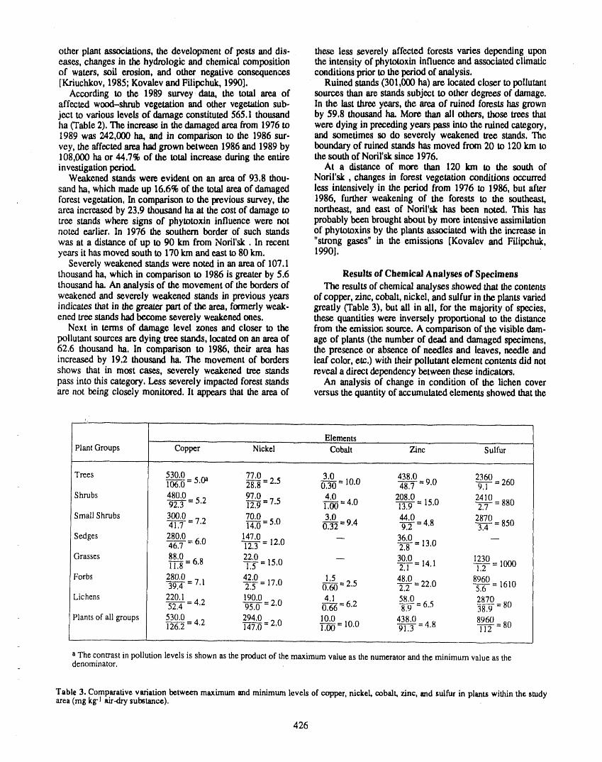
other plant associations, the development of pests and dis- the.,_ less severely affected forests varies depending uponeases, changes in the hydrologic and chemical composition the intensity of phytotoxin influence and associated climaticof waters, soil erosion, and other negative consequences conditions prior to the period of analysis.[Kriuchkov, 1985; Kovalev and Filipchuk, 1990]. Ruined stands (301,000 ha) are located closer to pollutant

According to the 1989 survey _data, the total area of sources than are stands subject to other degrees of damage.affected wood-shrub vegetation and other vegetation sub- In the last three years, the area of ruined forests has grownject to various levels of damage constituted 565.1 thousand by 59.8 thousand ha. More than ali others, those trees thatha (Table 2). The increase in the damaged area from 1976 to were dying in preceding years pass into the ruined category,1989 was _2,000 ha, and in comparisonto the 1986 sur- and sometimes so do severely weakened tree stands. Thevey, the affected area had grown between 1986 and 1989 by boundary of ruined stands has moved from 20 to 120 km to108,000 ha or 44.7% of the total increase during the entire the south of Nodl'sk since 1976.investigation period. At a distance of more than 120 km to the south of

Weakened stands were evident on an area of 93.8 thou- Norirsk, changes in forest vegetation conditions occurredsand ha, which made up 16.6% ofthe total area of damaged less intensively in the period from 1976 to 1986, but afterforest vegetation, In comparison to the previous survey, the 1986, further weakening of the forests to the southeast,area increased by 23,9 thousand ha at the cost of damage to northeast, and east of Noril'sk has been noted, This hastree stands where signs of phytotoxin influence were not probably been brought about by more intensive assimilationnoted earlier, In 1976 the southern border of such stands of phytotoxins by the plants associated with the increase in

was at a distance of up to 90 km from Norirsk. In recent "strong gases" in the emissions [Kovalev and Filipchuk,years it has moved south to 170 km and east to 80 km, 1990].

Severely weakened stands were noted in an area of 107.1thousand ha, which in comparison to 1986 is greater by 5.6 Results of Chemical Analyses of Specimens

thousandha.An analysis of the movement of the borders of The results of chemical analyses showed that the contentsweakened and severely weakened stands in previous years of copper, zinc, cobalt, nickel, and sulfur in the plants variedindicates that in the greater part of the area, formerly weak- greatly (Table 3), but ali in all, for the majority of species,enea tree stands had become severely weakened ones. these quantities were inversely proportional to the distance

Next in terms of damage level zones and closer to the from the emission source. A comparison of the visible dam-pollutant sources are dying tree stands, located on an area of age of plants (the number of dead and damaged specimens,62.6 thousand ha. In comparison to 1986, their area has the presence or absence of needles and leaves, needle andincreased by 19.2 thousand ha. The movement of borders leaf color, etc.) with their pollutant element contents did notshows that in most cases, severely weakened tree stands reveala direct dependency between these indicators.pass into this category, Less severely impacted forest stands An analysis of change in condition of the lichen coverare not being closely monitored, lt appears that the area of versus the quantity of accumulated elements showed that the

ElementsPlant Groups Copper Nickel Cobalt Zinc Sulfur

Trees 530,0 77,0 3.0 438.0 2360106,0 - 5,0a 28,8 - 2.5 - 10.0 9,0 _ = 2600.30 48,7 - 9,1

Shrubs 480,0 97,0 4.0 208.0 241092,3 - 5,2 _ = 7.5 1,00 - 4.0 13,9 - 15.0 2,'-"rf-= 880

Small Shrubs 300,0 70,0 3.0 44,0 287041,7 - 7.2 _ " 5.0 _ = 8500.32 - 9,4 9,2 - 4,8 3,4

Sedges 280,0 147.0 -- 36.046,7 ""6,0 12,-'-_= 12.0 2,8 - 13,0

Grasses 88,0 22,0 -- 30,0 123011,8 -6.8 1.-'-'5"= 15,0 2,-']"= 14.1 1,---_= 1000

Forbs 280,0 42,0 1.5 48.0 896039,4 - 7.1 2,5 - 17.0 - 2.5 _ _ = 16100.60 2,2 " 22.0 5,6

Lichens 220,1 190,0 4,1 58.0 287052,4 - 4,2 95,'----0-= 2,0 0,6-----6--"6.2 8.9 - 6,.'5 38,'----0-= 80

Plants of ali groups 530,0 294,0 10,0 438,0 8960126,2 - 4,2 147,0 - 2,0 1.00 - 10,0 91.3 - 4,8 112 - 80

_

a The conlrast in pollution levels is shown as the product of the maximum value as the numerator and the minimum value as thedenominator,

Table 3. Comparative variation between maximum madminimum levels of copper, nickel, cobalt, zinc, mad sulfur in plants within the studyarea (mg kKI air.dry substance).

426

number of species, the percentage of cover, and the phy- strips which may be more or less extensive, The zones aretomass reserve depends on copper, nickel and sulfur content not constant in terms of time, and their boundaries may[Kriuchkov, 1985]. Depending on the condition of the blend together depending on variation in the volume oflichen cover, five zones characterizing pollution of the area industrial emissions and the self-cleansing capability of nat-were determined within the survey region: (1) areas of maxi- ural communities. In the future, redistribution of the areasmum pollution (lichen desert); (2) severe pollution; (3) aver- may occur both in terms of pollution levels and damage toage pollution; (4) slight pollution; and (5) relatively clean plants.(Figure 1). The pattern of the zones is consistent with thedirection of the pollution plumes, which confirms the impor- CONCLUSIONS AND DISCUSSION

tance of this factor in the transfer of polluted air masses, On The aggregate effect of anthropogenic factors, primarilythe other hand, topographic features are also significant ininfluencing accumulation of pollutants, The terraces of the atmospheric emissions, has led to damage and destruction ofPutorana plateau, for example, prevent the penetration of the vegetative cover on the tundra and forest tundra in Northtoxins to the southeast and east; thus only along river val- Krasnoyarsk Krai In an area of 7,4 million ha [Kriuchkov,leys and lake basins open to the motion of winds blowing 1985]. The total area of dead and damaged forests in thefrom the complex does pollution penetrate into the mountain NIR, which were previously important for hunting, as rein-regions, deer pastures, and as recreational zones for residents of

The zone of maximum pollution (lichen desert) stretches Noril'sk, exceeded 0.5 million ha in 1990. The area of bod-for 50--55 km in a southeasterly direction, encompassing ies of water that have lost their importance for fishingalmost ali of the Rybnala River valley, and towards the exceeds 200,000 ha, including Lake Pyasino and its system.southern area of Lake Pyasino up to 35 km to the northwest. The negative consequences of the atmospheric pollution doThe total area of the zone is around 300,000 ha. The forest not stop with these losses due to the degradation andcover is made up almost entirely of dead trees and strongly destruction of entire plant associations. Active circulation ofdamaged shrubs (up to 60% of the above ground tissues accumulated pollutant microelements in natural mediumsdead). The portion of damaged small shrubs and grasses is along the food chains will create a serious threat to living75%, and 50% of the rhizomes of grasses and sedges are organisms, including man,dead. Lichen cover is absent. A combination of various survey techniques should be

The zone of severe pollution extends 50 km to the north- inco_ted into local forest monitoring programs. Thesewest and southeast 25-30 km beyond the preceding zone, should include geobotanical, floral, and morphologic meas-occnpying approximately 380,000 ha. The vegetation is urements as well as biochemical and physiological analysescharacterized by the prevalence in the forest cover of ruined of plant, soil, air, and water.and dying trees, with 20--50%of the shrubs dying. There are Visual signs of damage appear on the majority of plantsless severe effects than in the preceding zone within thegrass-small shrub layers. The number of damaged plants is with associated concentrations of chemically active harmful40% or less. Lichens appear, but their condition is unsatis- substances following a relatively long period of exposure tofactory, not exceeding 1-5% of the ground cover and with pollutants. Resumption of normal life processes for suchsome species exhibiting morphological changes, plants or conm,:'a!t!ee is often impossible, even with the

The zone of average pollution is located in the northern removal of the pollution source. Therefore, to identify thearea of the Khantayskoye reservoir, and it also occupies the early response of plants to the influence of industrial emis-western portions of lakes Lama, Glubokoe, and Keta. The sions, it is necessary to h,xl suitable biological indicatorszone's total area is about 420,000 ha. The forest cover is dis- that will reflect the presence of damage at different stages.tinguished by the presence of up to 50% dead larch with yel- Arboreal lichens are generally recognized as bioindicatorslowing spruce needles and birch leaves. The conditionof the of pollution levels, but their limited distribution in the NIRshrub and grass-small shrub layers is satisfactory with dam. restricts their use in this capacity. According to the results ofaged plants constituting no more than 10%. Lichens include our research and that of others [Kriuchkov, 1985], it hasup to 34 species and cover ranges from 20--40%. been established that terricolous lichen species and Lark

The zone of slight pollution encompasses a total area of gmelinii are particularly sensitive to pollution. Other plant460,000 ha to the west of the Lontokoisk Rock Range, to species that readily accumulate heavy metals and sulfur aresouth of Lake Khantayskoye, and the eastern areas of lakes Picea obovata, Ledum palustre, Calamagrostis sp,, andLama and Glubokoe. The vegetation is practically without Salix lanata.

signs of damage, and only in the forest canopy are larch The delineation of pollution zones based on the buildupwith yellowing needles noticeable. Lichens are well devel- of harmful microelements in lichens (as determined byoped with plants of average size and cover increasing up to chemical analyses) coincides with the categories of forest70%; more than 34 lichen species were noted.

The boundaries of the weak pollution zone are not estab- conditions determined on the basis of visual indicators.lished, and these pass into a relatively clean zone where the However, only the accumulation of elements in plant tissuesplants show no visible signs of damage; lichen cover is dis- may serve as a reliable indicator of areas of heavy metal andtinguished by considerable s_.cies variety--up to 96 spe- sulfur dioxide pollution. Assessment of atmospheric pollu-cies--and cover reaches 80-90%. Metal content is almost at tion levels according to surface damage indicators may notbackground level, be totally reliable; however, the appearance of damage and

The defined zones have no clear boundaries in terms of apparent outward plant reaction are indicative of unfavor-distance, and between them there are some intermediate able ecological conditions.

427

LITERATURE CITED

Chertovskii,V. G., and B. N. Semenov,PretundraForests of Kriuchkov, V. V., Preservation of the North's Nature, intheUSSR, Forestry, 5, 26-33, (InRussian), 1984. Issues of Anthropogenous Effects on the Environment, pp.

Kovalev, B. I., and A. N. Filipchuk,Forestconditions in the 124--131,Nauka,Moscow, (hi Russian), 1985.zone of the Noril'skMiningand MetallurgicalComplex's Parmuzin,Iu. P., Tu_ra-forests of the USSR, 295 pp., Mos-industrial influence, Forest Management, 5, 1-85 (In cow, (In Russian), 1979.Russian), 1990.

.,a

Manuscript translated from the Russian by David A, Peterson, July 1990.

428

The Natural Background Disturbance in the Soviet Far East

V. P. KarakinPacific Geography Institute of the Far East Division of the U.S.S.R. Academy of Sciences, Vladivostok, U.S,S.R,

A. S. SheinhouseInstitute of Regional Problems and Complex Analysis of the Far East Division of the U.S.S.R. Academy of Sciences,

Khabarovsk, U.S.S.R.

ABSTRACT

The naturalsystem development of the Soviet FarEast dates back to the paleo-lith. It acceleratedmore and more, and strong anthropogenicpressure is now evi-dent.The main partsof the ecosystems appear to have changedas a result.We haveelaboratedspecific methods of ecosystem disturbanceassessment. Measurementofa natural scale was adopted; this scale is based on the period necessary to thechanged landscaperestorationuntilclimax. Assessments for the Amur,Kamchatka,Khabarovsk, Magadan,Prymorie,and Sakhalinregions have been made,

429

Sexual Reproduction of Arctophilafulva and Seasonal Temperature,Arctic Coastal Plain, Alaska

J. D. McKendrickSchoolofAgricultureandLand ResourcesManagement,AgricultureandForestryExperimentStation,

Universityof AlaskaFatrbanks,Palmer,Alaska,U.S.A,

• ABSTRACT

Arctophila fulva is an indigenous grass with circumpolar distribution, lt occursin Alaska's boreal and arctic environments, usually as an emergent aquatic. Anintensive 5-year investigation of Arctophila fulva began in 1985 to determine its lifehistor),, and environmental characteristics. Evaluations of environmental character-istics included recording hourly temperature means of soil/mud, water, and air dur-ing the growing season, Ten Coastal Plain Province sites and one Brooks Rangefoothills site were included in the 1986-1989 temperature monitoring project.Observations in the Alaska Range were done in 1987-1989.

Initial evaluation of sexual reproduction in 1985 indicated no seed formationoccurred in Arctophila fulva colonies on the coastal plain during that year. Floretswere in anthesis at or near the end of growing season. However, sexual repro-duction occurred in the northern foothills of the Brooks Range where seeds maturedbefore the coastal plain plants reached anthesis, Foothill stands of ArctophUa fulvaproduced seed each growing season of our study. Low to no success in sexualreproduction continued for coastal plain stands of Arctophila fulva during 1986 and1987. Seed formation was observed in plants on the coastal plain that were pro-tected by a plexiglas shelter in 1988. During the 1988 growing season, few seedswere found in inflorescences from one natural stand on the coastal plain, and onestand on the margin of the foothills (about 35 miles inland) produced seed. In 1989,25 stands of Arctophila fulva on the coastal plain produced seed, probably due toelevated growing season temperatures and perhaps extension of the growing sea-son. During 1987-1989, sexual reproduction was consistently successful for Arc-tophila fulva growing in the Alaska Range.

Because sexual reproduction success for plants in the Arctic is often poor, plantsin this region are believed to persist mainly by vegetative propagation. The lack ofsexual reproduction may. limit the gene recombination opportunities and geneticdiversity. Also, the scarcity of seeds affects the rate and diversity of species avail-able to colonize barren sites. It appears that wanning of the Arctic could affect thequantity and perhaps the diversity of seed produced by indigenous arctic plants.

430

in the Footsteps of Robert Marshall:Proposed Research of White Spruce Growth and Movement

at the Tree Limit, Central Brooks Range, Alaska

Terry D, DroesslerManTech Environmental Technology, Inc,, US EPA Environmental Research Lab, Corvallis, Oregon, U,S.A,

i

ABSTRACT

The proposed research will quantify white spruce growth and document itslatitudinal stability at the tree limit in the central Brooks Range over the life span ofthe living trees. The goal is to link tree growth and tree position to summer tem-perature and precipitation. Historical records from 1929 to 1938 from work byRobert Marshall have been used to identify tree limit sites and provide informationto interpret the present location of the tree limit,

INTRODUCTION ing to predictions from General Circulation ModelsAltitudinal and latitudinal tree limits represent tem. (GCMs), will probablybe at least twice the glob_2average

pcrature, precipitation or other barriers to species dis. increase [IPCC, 1990],trtbution,Tree limit is defined here as the last living white Several studies of tree limit in the Arctic have shownspruce (Picea glauca, Voss,) tree, regardless of form, that stable to advancing conditions over the last few decadescould be locatedat the farthestnorthernlatitudeor elevation [Densmore, 1980; Goldstein, 1981; Odasz, 1983; Cooper,in selected drainages of the central Brooks Range. The 1986; Lee, 1987]. If temperatures continue to increase andpresenttree limit may indicatethe locationof a temperature moisture is not fimiting, the tree limit may advance in lat-er moisture limitation that prohibits furtherspecies move. itude and altitude until it is once again in equilibrium withment. A knowledge of temperatureand moisturehistoryand temperature, moistureor othercontrolling factors.species movement and growth pat_ms is important for One mechmflsmfor tree limit movement is a change inunderstandingthe establishment andexistence of the present sexual reproductive success, White spruce tree limit on thetree limiL Studying growth and movement rates of trees in south slope and isolated clusters of balsam poplar (Populusthe vicinity of the tree limit will document tree response to balsamOrera,L,) on the north slope of the Brooks Range,temperatureand moisturechange over the life span of living commonly reproduceby vegetative means only [Edwardstrees.Predictingtree growth and tree movement in response and Dtmwiddie, 1985; I.ev, 1987], Increases in temperatureto future temperature and precipitation scenarios may then may allow sufficient time for sexual reproduction to takebe possible based on past tree growth and tree movement place, An increasein temperature would shift the 10°C Julyrelationships to temperature andprecipitation, isotherm northward in latitude and higher in elevation,

Indications of accelerated warming trovebeen reported, Movement rates could dramatically increase because seedJones ct al, [1986] show that the warmest near-surface tem- dispersal distances are far greater than branch or root veg-peratures over the land and oceans of both hemispheres etative reproduction dispersaldistances,between 1861-1984 have occurred since 1980, Jones et al,{1988]show overall rising global surface air temperature for HISTORICAL STUDIES OF TREE LIMIT IN THE1901-1987, Lachenbruch and Marshall [1986] concluded BROOKS RANGEthat the depth to permafrost in the Alaska and Canadian Work by Robert Marshall in the 1930s provides a his-Arctic has increased in recent decades, Houghton and torical basis for a study of tree growth and movement in theWoodwell [1989] state that the greatest warming is expected Brooks Range, Marshall undertook tree growth studies tnto occur at htgher latitudes in winter. The warming, accord, the North Fork of the Koyukuk, Alatna, and John River

431

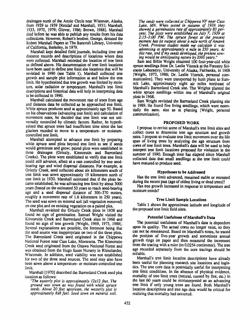
drainages north of the AroticCircle near Wlsoman, Alaska, The seeds were collected at Chippewa NF near cassfrom 1929 to 1939 [Retzlaf and Marshall, 1931; Marshall, Lake, MN, When tested in autumn of 1.938 they1933, 1970, 1979; Olovet, 1986; Brown, 1988], Marshall s/towed a germination rate of approximately 80 per.

died _forc he was able to publishany results from hts data Ce,ht, The plots were establtshedon July 7, 1939 atcollections, However, Robert's brother, George, donated tlm 2,15-3:00 PM, The spruce forest at the presentRobert Marshall Papers to The Bancroft Ltbrm'y,University moment has its outpost about a mile north of AmawkCreek, Previous studies made me calculate it wasof California, Berkeley, tn 1979, advancing at approximately a mile in 250 years, At

Marshall kept dctatled field journals, including time and this rate, and If my seeds developed, the present sow.distance records and descriptions of locations where data ing would Oeanticipating nature by 2000 years,"were collected, Marshall recorded the location of tree limit Sam and Blllte Wright obtained 100 four.year.old whiteas defined above, His documentation of tree limit locations spruceseedlings from Dr, I.aslle Vlereckat theForestry Scl.have been used to define tre_ limit site locations that will be antes Laboratory, University of Alaska, Fatrbanks, in 1968revisited tn 1990 (see Table I), Marshall collected tree [Wright, 1973, 1988_ Dr, l_slte Vlereck, personal com-growth and sample plot Information at and below the tree muntcatlon], They wore transported by bush plane to Sum-ltmlt, He hypothesized that tree growth was limited by mols. mtt Lake, approximately eight a.lr miles northeast oftufa, solar radiation or temperature, Marshall's tree limit Marshall's Barrcnland Creek site, The Wrtghts planted thedescriptionsand historical data will help in interpretingdata whlt_ spruce seedlings within one of Marshall's originalto be collected in 1990, plots tn 1968,

Marshall calculated the movement rate of trees from age Sam Wright _visited the BarronlandCreek planting site_mddistance dam he collected as he approached tree limit, in 1989, He found five living seedlings, which were esscn-White spruce produces seed at approximately age 50, Based tially the same size as at planting [Wright, personalon his observations (advancing tree limit) and calculation of communication],movement rates, he dectded that tree limit was not unl.versally controlled by climatic factors, Rather, he hypoth. PROPOSED WORK

estzed that spruce trees had insufficient ttme since the Inst I propose to revtstt some of Marshall's tre_ limit sites andglaciers re.ce.deAto move to a temperature, or moisture, collect cores to determine tree age structure and growthcontrolled tree limtL rates, I propose to evaluate tree limit movement over the life

Marshall attempted to advance tree limit by preparing span of living trees by analyzing the age structure fromwhite spruce seed plots beyond tree limit to see if seeds cores of tree limit tree,s,Marshall'sdam will be used to helpwould germinateand grow_pairedplots were established in interprettrec limit locations proposed for visitation in thethree drainages (Grizzly, Kinnorutin and Barronland summerof 1990, Enough time has elapsed since MarshallCreeks), The plots were established to verify that tree limit collected data that small seedlings at the tree limit couldcould still advance, albeit at a rate controlled by tree seed. have matured to produce see,d,bearing age and wind dispersal distances, Fm' example, at

GrizzlyCreek,seedcollectedaboutsixkilometerssouthof, HypothesestobeAddressedtrcelimitwas sown approximately19 kilometersnorthof Hasthetreelimitadvanced,remainedstableorretreatedtreelimitin1930,Marshalle,stimatedtlmtiftheplotsbe.

duringtherecentpast(ageofoldestlivingordeadtrees)?came established, he was advancing tree limit by about 3000 Has treegrowth increased in r_"ponse to temperature andyears (based on the estimated 50 years to reach seed.bearing moisture trends?age and a seed dispersal distance of 300-370 meters,roughly a movement rate of 1,6 kilometers in 250 years),The seed was sown on mineral soil (ali vegetation removed) Tree Limit Sample Locationson one plot and on existing vegetation on a paired plot, Table 1 shows the approximate latitude and longitude of

Marshall revisited the Grizzly Creek plots in 1938 and the proposed tree limit field sttes,

found nostgn of germination, Samt_l Wright visited the Potential Usefulness of Marshall's DataKinnorutinCreek and BarrenlandCreek sites in 1966 andfound no sign of tree growth [Wright, 1969, 1973, 1988], The potential usefulness of Marshall'sdam is dependentSeveral explanations are possible, the foremost being that upon its quality, The actual cores no longer exist, so theythe seed source was inappropriate on two of the three plots, can not be reme.asured, Based on Marshall's notes, he tracedThe Barrenland Creek seed originated in the Chippewa the position of five.year growth and sometimes annualNational Forest near Cnss Lake, Minnesota, The Kinnoruttn growth rings on paper and then measured the incrementCreek seed originated from the Ottawa National Forest and from the tracing wlth a ruler (to 0,0254 centimeter), The treewas obtained from the Hugo Sauer Nursery In Rhtnelander, age recorded separately from the core tracings should beWisconsin, In addition, seed viability was not established reliable,/'or two of the three seed sources, The seed may also have Marshall's tree limit location descriptions have alreadybeen sown above a temperattlre- or moisture-controlled tree been useful for planning research site locations and logts-limit, tics, The tree core data ts potentially useful for interpreting

Marshall [1970] described the Barrenland Creek seed plot tree limit conditions, In the absence of physical evidence,location ns follows: mortality of tree limit trees (natural, caused by fire, etc,) in

"The easterly plot is approximately 12x12 feet, The the last 60 years could be misinterpreted as an advancingground was sown as was found with white spruce tree limit if only young trees are found, Both Marshall'sseeds, About 20 feet upstream, the westerly plot is location descriptions and tree age data would be critical forapproximately 8x8 feet, Seed sown on mineral soil, realizing that mortality had occurred,

432

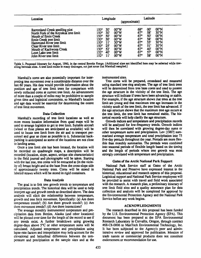
Location Longitude Latitude(approximate)

p

BarronlandCreekseedl!ngplot 1500 30' 00"W 680 00' 00"NNorthForkof the Koyukuktree limit 1500 30' 00"W 670 58' 30"NMouthof EmtoCreek 1500 50' 00"W 670 50' 00"NEmie Creektree limit 150° 50' 00"W 67° 58' 00"NHammondRiver _ limit 1500 11' 30"W 670 55' 30"NClearRivet tree limit 1500 25' 00"W 67° 51' 30"NMouthof KachwonaCreek 1500 52' 00"W 67° 40' 00"NLoon Lake tree limit 1520 40' 00"W 670 57' 00"NJohnRiver tree limit 152o 11' 00"W 67° 58' 00"N

TableI, Pmposf.,dItineraryforAugus_1990,in_ centralBrooksRange,(Additionalsitesnotidentifiedheremaybeselectedwhiletru.oilingbetweensite,s, Atree limitexistsmmanyoramages,notjustareasthatMarshallsampled,)

Marshall'sceres are also potentiallyimportant for inter- instrumentedsites,pretingtree movementover a considerabledistanceover the Tree cores will be prepared, crossdated and measuredlast60 years, His datawould provide informationabout the using standardtree ringanalyses, The age of tree limit treesposition and age of tree limit trees for comparison with will be determinedfrom _ base coves and used to presentnewly cellected cores at currenttrce limit. An advancement the age structure in the vicinity of the trce limit. The ageof more thana couple of miles may be prohibitiveto sample structurewill indicate if trees havebeen advancingor stable,given time and logistical constraints, so Marshall's location For example, if the age structureshows _ trees at the treeand age data would be essential for determining the extent limit are young and that maximum tree age increases in theof tree limit movement, vicinity south of the tree limit, the tree limit has advanced, if

the age structureshows that the maximumtree ageoccursatData Collection the tree limit, the trce limit has remained stable. The his-

Marshall's recording of tree limit locations as well as toflcal recordswill help clarify the age structure.more recent location information from quad maps will be Growth indices and temperatureand precipitation recordsused to arrange logistics to get to tree limit. Suitable aircraft will be analyzed for low-frequency trends. Growth indices(wheel or float planes are anticipated as available) will be will then be correlated with growing degree-day sums orused to locate tree limit from the air and to transportper- other temperaturesums and precipitation. Lev [1987] sum-sonnel and gear as close as possible to it. Substantialback- marized average temperatureand total precipitationinto 73packing is anticipated as some of the locations are not close five.day pentads throughoutthe year.Pentads are moreflex-to landingareas, ible thanmonthly summaries. The pentads were combined

Once a tree limit site has been located, the location will into seasonal periods of flexible length based on the timingbe recorded on quadrangle maps, a description will be and the length of periods where tree growth was mostrecorded(location, slope, aspect, unique site characteristics) strongly correlated with temperatureandprecipitation.in the field journal and photographs will be taken. Startingwith the last tree, treeceres will be extractedat (in the vicin- Gates of the Arctic National Park Supportity of) breastheightand at the base from the cross.slope side National Park Service staff at Gates of the Arcticof approximately twenty trees, Cores will be stored in National Park and Preserve have expressed interest in thelabeled straws which will be storedin rigid containers, historical, educationaland researchaspects of this proposal.

Logistical supportand National ParkService employees willData Analysis be provided to assist with travel and field work associated

The goal is to link tree growth trends to temperatureand with theresearch. A research plan, a preliminaryitineraryofprecipitation trends,The historical datawill be used to help tree limit field sites and a quality assurance plan for datainterpretage andgrowth trends as described above, The data collection and analysis will be completed for approval byanalysis will elicit the relationship between temperature, the EnvironmentalProtection Agency and the NationalParkgrowth and tree lhr.itmovement, Specifically: (a) Are there Service before any workbegins,temperature trends?; (b) Are there growth trends?; (c) Aretheremovement trends?;(d) Are there interactions? ACKNOWLEDGMENTS

The average monthly instrumentedtemperature and pre- The research described in this proposal has been fundedcipitation data from Bettles, Alaska (and other locations) by the U.S. EnvironmentalProtection Agency (EPA). Thiswill be plottedover time for the length of the recordto see if document has been prepared at the EPA Environmentalany trends exist. A further breakdown using growing Research Laboratory in Corvallis, Oregon, through contractdegree-days above 50C or other temperature sums will be #68-C8-0006 to ManTech Environmental Technology, Inc.calculated, Adjusted temperature and precipitation using lt has been subjected to the Agency's peer and attain-lapse.rate factors and interpolation may help account for the istrative review and approved for publication, Mention ofelevational and latitudinal differences between the tem- trade names or commercial products does not constituteperature and precipitation at the sample sites and at the endorsement or recommendation foruse,

433

LITERATURE CITED

Brown, W. E., Gaunt Beauty . . . Tenuous Life, National global warming in the past decade, Nature, 332, 790,Park Service, Gates of the Arctic National Park, 1988. 1988.

Cooper, D. J., Trees above and beyond tree limit in the,Arri- Lachenbruch, A. H., and B. V. Marshall, Changing climate:getch Peaks region, Brooks Range, Alaska, Arctic, 39, Geothermal evidence from permafrost in the Alaskan247-252, 1986. Arctic, Science, 234,689--696, 1986.

Densmore, D., Vegetation and forest dynamics of the upper L.ev, D. J., Balsam poplar (Populus balsamifera) in Alaska:Dietrich River Valley, Alaska, Master's Thesis, 183 pp., Ecology and growth response to climate, Master's Thesis,North Carolina State University, Raleigh, NC, 1980. 69 pp., University of Washington, Seattle, WA, 1987.

Edwards, M. E., and P. W. Dunwiddie, Dendrochrono- Marshall, R., Arctic Village, The Literary Guild, New York,logical and palynological observat;ms on Populus bal- 1933.samifera in northern Alaska, U.S.A., Arctic Alpine Res., Marshall, R., Alaska Wilderness, University of California17, 271-278, 1985. Press, Berkeley and Los Angeles, 1970.

Glover, J. M., A Wilderness Original: The Life of Bob Mar- Marshall, R., The Robert Marshall Papers. The Bancroftshall, The Mountaineers, Seattle, 1986. Library, University of California, Berkeley, 1979.

Goldstein, G. H., Ecophysiological and demographic studies Odasz, A. M., Vegetational patterns at the tree limit ecotoneof white spruce (Picea glauca (Moench) Voss) at treeline in the central Brooks Range of Alaska, Ph.D. Thesis, in the upper Alatna River Drainage of the Central Brooks193 pp., University of Washington, Seattle, WA, 1981. Range, Alaska, Ph.D. Thesis, 224 pp., University of Col-

Houghton, R. A., and G. M. WoodweU, Global climate orado, Boulder, CO, 1983.change, Scientific American, 260, 36--44, 1989. Retzlaf, A., and R. Marshall, Journal of the exploration of

Intergovert_mentalPanel on Climate Change OPCC), Sci- the North Fork of the Koyukuk by Al Retzlaf and Bobentific assessment of climate change. Report for WGI Marshall, pp. 163-175, The Frontier, 1931.

Plenary Meeting, 1990. Wright, B., Four Seasons North, Harper and Row Publish-Jones, P. D., T. M. L. Wigley, and P. B. Wright, Glo0al ers, San Francisco, 1973.

temperature variations between 1861 and 1984, Nature, Wright, S., A letter from the Arctic, The Living Wilderness,322,430--434, 1986. Spring, 4--6, 1969.

Jones, P. D., T. M. L. Wigley, C. K. Folland, D. E. Parker, Wright, S., Koviashuvik, Sierra Club Books, San Francisco,J. K. Angell, S. Lebedeff, and J. E. Hansen, Evidence for 1988.

434

¢

USDA Forest Service Global Change Research:Monitored Ecosystems, Northern Linkages

J

D. V. SandbergForestry Sciences Laboratory, Pacific Northwest Research Station, U.S.D.A. Forest Service, Seattle, Washington, U.S.A.

C. W. SlaughterInstitute of Northern Forestry, Pac_c Northwest Research Siation, U.S.D.A. Forest Service, Fairbanks, Alaska, U.S.A.

ABSTRACT

Foresters and natural resource managers have traditionally based long-term plans(i.e., 100+ year harvest cycles) on the assumption of stable landscapes and climate.Global climate change undercuts these assumptions and may alter or invalidatesome accepted natural resource management practices and paradigms. Possiblechanges in biomass productivity, shifting of forest species' latitudinal or elevationallimits, and rapid changes in forest community species and age class composition,all have major implications for management of the nation's forests.

The USDA Forest Service is undertaking a national research program to assessrates, significant processes, and management implications of possible climaticchange for the nation's forests and related resources. Pacific Region Forest Serviceglobal change research places major emphasis on understanding and monitoringforest processes in the northern boreal forest and the sub-arctic taiga of Alaska,which is potentially "sensitive" to climatic warming and to shifts in precipitationregime. A major terrestrial carbon pool, taiga forests and organic soils may also beimportant in the flux of greenhouse gases between landscape and atmosphere.

Forest Service research emphasizes an ecosystem approach, incorporating land-scape- and watershed-level field research with smaller-scale studies of forest eco-system response mechanisms. Ecological monitoring is critical, and includesestablishment of a monitoring mega-transect from northern latitudinal tree line tomediterranean/dry temperate forest/shrublands. Emphasis is placed on the most crit-ical Pacific Region ecosystems: northern boreal forest (taiga), moist temperate for-est, and mediterranean/dry temperate forest (chaparral/southern Ponderosa pine).

435

r

Changes in the Source/Sink Relationships of the Alaskan Boreal Forestas a Result of Climatic Warming

J. Yarie and K. Van CieveForest Soils Laboratory, University of Alaska Fairbanks, Fairbanks, Alaska, U.S.A.

ABSTRACT

A modifiedversionoftheLINKAGES ecosystemsimulationmodelisusedtoaccessthechangesintheroleofforestsintheinteriorofAlaskatoactasasourceorsinkofcarbonoverafifty-yearperiod.ThestudyareaistheTananaValleyStateForest(TVSF).The TVSF occupiesan mca of5523hectaresalongtheTananaRiverfromtheCanadianBordertotheconfluenceoftheTananaRiverandtheYukonRiver.The currentinventoryfortheTVSF isusedtodevelopa startingstateforthe

modelfortenvegetationclasses.Themodelisrunwiththecurrentclimateuntilthecurrentstandageforthevariousvegetationtypesisreached.Thena5°c increasein

" meanannualtemperatureandadoublinginprecipitationdistributedevenlyovertheyearisgraduallyaddedtothemodel.Themodelwasthenusedtodevelopanaverageestimateoftheatmosphericcar-

bon sequesteringforthecurrentvegetationdistributionoftheproductiveforesttypcsintheTVSF.Thisvaluewasestimatedas392gm-2yr-lfora490,000-hectareareaofinteriorAlaska.

INTRODUCTION thelandscapewhichisderivedfromtraditionalforestin-

The roleofborealforestsintheglobalcarboncycleis vcntoriesofthelandscapeinquestion.unclearatthistime.The bore,alforestcouldeitherbca net Recentinventoriesof thevegetationofinteriorAlaskasourceorsinkforatmosphericCO2.lthasbeensuggested now giveusthepotentialtostarttodevelopprecisees-thattheborealforestcouldrepresenta largesinkfor timatesofthecarbonbudgetoverwideareasofthestate.atmospheric CO2 [Tans ct al., 1990]. Photosynthetic uptake These inventories can be used to define the starting state ofby high arctic vegetation was thought to produce the large ecosystem models. By using actual inventories to define theseasonal amplitude in atmospheric CO2 measured at starting state of the model we should be able to develop aBarrow, Alaska rPeterson et al., 1986]. This uptake by the more realistic estimate of the effect of global change on theliving plant material combined with the relatively slow de- carbon cycle for large land areas of the boreal forest. Recent

_ composition rates found in the arctic and boreal forests forest inventories for interior Alaska have included thetFlanagan and Van Cleve, 1983] could result in high l_titude upper Yukon River drainage [Seizer, 1987], the Tanana Riv-ecosystems acting as a net sink for atmospheric CO2. er drainage [van Hees, 1984], and the Susima River drain-

The problem of estimating the net effect of the boreal for- age [Setzer et al., 1984].: est on the global carbon cycle becomes one of estimating

-1 the net upLalceof carbon in vegetation, the release of carbon METHODSthrough decomposition, and the effect of periodic natural The computer model LINKAGES2 [Pastor and Post,

: disturbance on the uptake/decomposition balance over large 1986] was used to estimate the change in carbon dynamics= land areas. Direct estimates are not viable at this time; there- over a fifty-year period starting ir, approximately 1990 and

-_.t: ......... t. ....... ,,., _ ,I_ I_, .n,_in. in 9f_AI3 Th_ _tarlina climate nf the model wa._ set to

answer. These modeling approaches can then be applied to the long-term average climate for Fairbanks. A linear

436

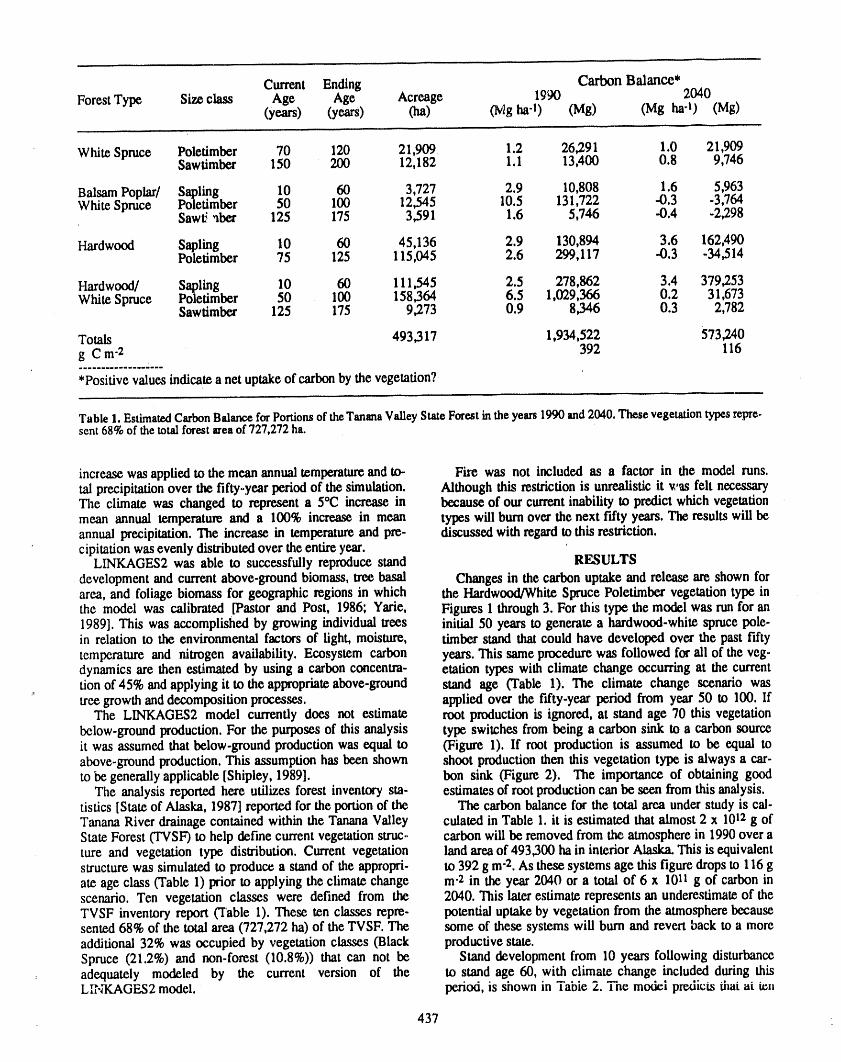
Current Ending Carbon Balance*ForestType Size class Age Age Acreage 1990 2040

(years) (years) (ha) OV gha-t) (Mgha-O O g)

White Spruce Poletimber 70 120 21#09 1.2 26,291 1.0 21,909Sawfimber 150 200 12,182 1.1 13,400 0.8 9,746

Balsam Poplar/ Sapling 10 60 3,727 2.9 10,808 1.6 5,963White Spruce Poletimber 50 100 12,545 10.5 131,722 -0.3 -3,764

Sawt3'iber 125 175 3,591 1.6 5,746 -0.4 -2,298

Hardwood Sapling 10 60 45,136 2.9 130,894 3.6 162,490Poletimber 75 125 115,045 2.6 299,117 -0.3 -34,514

Hardwood/ Sapling 10 60 111,545 2.5 278,862 3.4 379,253White Spruce Poletimber 50 100 158.,364 6.5 1,029,366 0.2 31,673

Sawtimber 125 175 9,273 0.9 8,346 0.3 2,782

Totals 493 ,317 1,934,522 573,240g C m"2 392 116

*Positive values indicate a net uptake of carbonby the vegetation?

Table1. EstimatedCarbonBalanceforPortionsof theTananaValleyStateForestinthe years1990and2040.Thesevegetationtypesrepre.sent68%of thetotal forestareaof 727,272ha.

increase was applied to the mean annualtemperatureand to- Fire was not included as a factor in the model runs.tal precipitationover the fifty-year periodof the simulation. Although this restriction is unrealistic it was felt necessaryThe climate was changed to represent a 5°C increase in because of out currentinability to predict which vegetationmean annual temperature and a 100% increase in mean types will bum over the next fifty years. The resultswill beannual precipitation. The increase in temperatureand pre- discussedwith regardto this restriction.cipitation was evenly distributedover the entire year.

LINKAGES2 was able to successfully reproduce stand RESULTSdevelopment and currentabove-ground biomass, tree basal Changes in the carbon uptake and release are shown forarea, and foliage biomass for geographic regions in which the Hardwood/White Spruce Poletimber vegetation type inthe model was calibrated [Pastor and Post, 1986; Yarie, Figures 1 through3. For this type the model was nut for an1989]. This was accomplished by growing individual trees initial 50 years to generate a hardwood-white spruce pole-in relation to the environmental factors of light, moisture, timberstand that could have developed over the past fiftytemperature and nitrogen availability. Ecosystem carbon years. This same procedure was followed for ali of the veg-dynamics are then estimated by using a carbon concentra- etation types with climate change occurring at the currenttion of 45% and applying it to the appropriate above-ground stand age (Table 1), The climate change scenario was

" tree growth and decomposition processes, applied over the fifty-year period from year 50 to 100. IfThe LIN GES2 model cutrenfly does not estimate root production is ignored, at stand age 70 this vegetation

below-ground production. For the purposes of this analysis type switches from being a carbon sink to a carbon sourceit was assumed that below-ground production was equal to (Figure 1). If root production is assumed to be equal toabove-ground production. This assumption has been shown shoot production then this vegetation type is always a car-to be generally applicable [Shipley, 1989]. bon sink (Figure 2). The importance of obtaining good

The analysis reported here utilizes forest inventory sta- estimates of root production can be seen from this analysis.tistics [State of Alaska, 1987] reported for the portion of the The carbon balance for the total area under study is cal-Tanana River drainage contained within the Tanana Valley culated in Table 1. it is estimated that almost 2 x 1012g ofState Forest (TVSF) to help define current vegetation struc- carbon will be removed from the atmosphere in 1990 over ature and vegetation type distribution. Current vegetation land area of 493,300 ha in interior Alaska. This is equivalentstructure was simulated to produce a stand of the appropri- to 392 g m"2.As these systems age this figure drops to 116 gate age class (Table 1) prior to applying the climate change m-2 in the year 2040 or a total of 6 x 10li g of carbon inscenario. Ten vegetation classes were defined from the 2040. This later estimate represents an underestimate of theTVSF inventory report (Table 1). These ten classes repre- potential uptake by vegetation from the atmosphere becausesented 68% of the total area (727,272 ha) of the TVSF. The some of these systems will burn and revert back to a moreadditional 32% was occupied by vegetation classes (Black productive state.Spruce (21.2%) and non-forest (10.8%)) that can not be Stand development from 10 years following disturbance

= adequately modeled by the current version of the to stand age 60, with climate change included during thisLINKAGES2 model, period, is shown in Tabie 2. Tne model predicts thatat ten

437

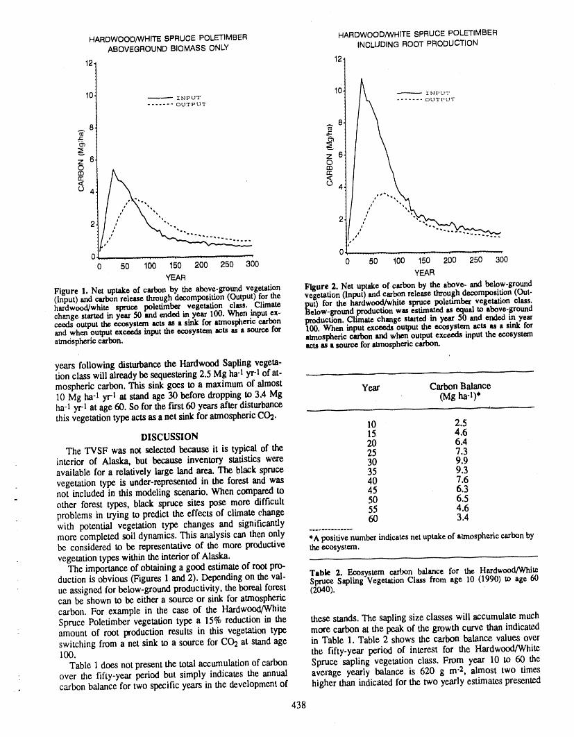
HARDWOOD/WHITE SPRUCE POLETIMBER HARDWOOD/WHITE SPRUCE POLE-TIMBERABOVEGROUND BIOMASS ONLY INCLUDING ROOT PRODUCTION

12_ 12

10 _ INI_UT10 -------- INPUT ....... OUTPUT

....... OUTPUT

Z 6, ZincO

n"< ' o 4

,0 4

2 2

..... 1,,,,.... . , ....., ,,- ..... J ..... ,

0 50 100 150 200 250 300 0 50 100 150 200 250 300

YEAR YEAR

Figure 1. Net uptakeof carbonby the above-poundvegetation Figure2. Net uptakeof carbonby theabove-andbelow-pound(Input) and carbon release through decomposition (Output) for the vegetation (Input) and carbon release thTou.gh.decomposi.tion (,Out-hardwood/whitespruce poletimber,vegetationclass., Cl'unate put) for the hardwood/whitespruce poleUmt_r.vegetauonclass;Below-groundproductionwasestimateoasequalw atmve-grounachangestartedin year50 and ended in year lt_. wn.mampm,ex- production.Climatechangestm_ in year 50 andended '.myem"ceedsoutputtheecosystemactsasa sink for atmosphericcarvon I00. WhminputexceecLsoutputme ecosystemac_.as a smzmrandwhenoutputexcee_ inputthe ecosystemactsas asourceforatmosphericcarbon, atmosphericcarbonandwhenoutputexcems mpmme ecosystemactsasa sourceforatmosphericcarbon.

years following disturbancethe Hardwood Sapling vegeta-tion class will alreadybe sequestering2.5 Mg ha4 yr4 of at-mospheric carbon.This sink goes to a maximum of almost Year CarbonBalance10 Mg ha-1yrl at stand age 30 before dropping to 3.4 Mg (Mg ha-l)*ha-I yr4 at age 60. So for the first60 years after disturbance ,this vegetationtype acts as a net sinkforatmospheric CO2. 10 2.5

DISCUSSION 15 4.620 6.4

The TVSF was not selected because it is typical of the 25 7.3interior of Alaska, but because inventory statistics were 30 9.9available for a relatively large land area. The black spruce 35 9.3vegetation type is under-representedin the forest and was 40 7.6not included in this modeling scenario, When compared to 45 6.3

" other forest types, black spruce sites pose more difficult 50 6.5problems in trying to predict the effects of climate change 55 4.6with potential vegetation type changes and significantly 60 3.4more completed soil dynamics. This analysis can then only *Apositive numberindicatesnet uptake of atmospheric carbon bybe considered to be representative of the more productive theecosys_,em.vegetation types within the interior of Alaska.

The importance of obtaining a good estimate of root pro-duction is obvious (Figures 1 and 2). Depending on the val- Table 2. Ecosystem carbon balance for the Hardwood/WhiteSpruce Sapling Vegetation Class from age 10 (1990) to age 60ue assigned for below-ground productivity, the boreal forest (20,10).can be shown to be either a source or sink foratmosphericcarbon. For example in the case of the Hardwood/WhiteSpruce Poletimber vegetation type a 15% reduction in the these stands. The sapling size classes will accumulate muchamount of root production results in this vegetation type more carbon at the peak of the growth curve than indicatedswitching from a net sink to a source for CO2 at stand age in Table 1. Table 2 shows the carbon balance values over100. the fifty-year period of interest for the Hardwood/White

Table 1 does not present the total accumulation of carbon Spruce sapling vegetation class. From year 10 to 60 theover the fifty-year period but simply indicates the annual average yearly balance is 620 g m"2, almost two timescarbon balance for two specific years in the development of higher than indicated for the two yearly estimates presented

438

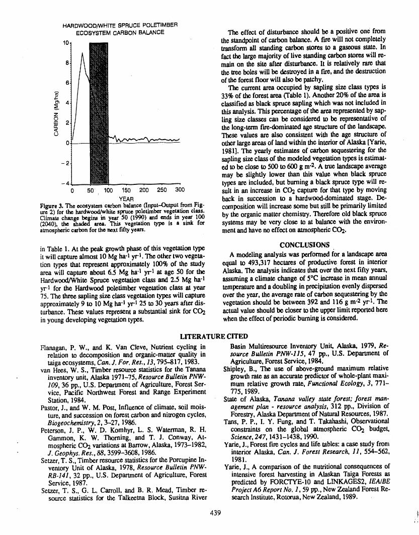
HARDWOOD/WHITE SPRUCE POLETIMBERECOSYSTEM CARBON BALANCE The effect of disturbance should be a positive one from

10, thestandpointof carbonbalance. A fire will not completely. transform ali standing carbon steres to a gaseous state. In

factthe large majority of live standingcarbonstores will re.e main on the site after disturbance, lt is relatively rare that

the treeboleswill bedestroyedin a rue,andthedestructionof the forest floor will also be patchy.

i The currentarea occupied by sapling size class types is33% of the forest area(Table 1).Another20%of the area is

classified as black sprucesapling which was not included in

"-"i __ thisanalysis, This percentageof the arearepresentedby sap-

ling size classes can be considered to be representative ofthe long.term fue..dominatedage structureof the landscape,These values are also consistent with the age structureofotherlarge areas of land within the interiorof Alaska [Yarie,1981]. The yearly estimates of carbon sequestering for thesaplingsize class of the modeled vegetation typesis estimat-ed to be close to 500 to 600 g m-2. A true landscape averagemay be slightly lower than this value when black sprucetypes are included,but burninga black spruce type will re-

0 50 100 i'50 260 250 300 suitin an increasein C02 capturefor thattypeby movingYEAR back in succession to a hardwood-dominated stage.De-

Figure 3. The ecosystemcarbonbalance(Input-Output.fromFig- compositionwill increasesOmebut still be primarilylimitedure2) forthe hardwood/whitesprucepoletimborvegetationcl_s0_Climatechangebeginsin year50 (1990) and ends m yem". by the organic matter chemistry. Therefore old black spruce(2040), the shaded area. _ vegetationtype ts a sink tor systems may be very close to at balance with the environ-atmospheric carbonforthenext fifty years, mentand have no effect on atmosphericCO2.

in Table 1. At the peak growth phaseof this vegetationtype CONCLUSIONSit will capturealmost 10 Mg ha-I yrl. The othertwo vegeta- A modeling analysis was performed for a landscapearearien types that represent approximately 100%of the study equal to 493,317 hectares of productive forest in interiorarea will capture about 6.5 Mg ha-1 yr| at age 50 for the Alaska.The analysis indicates that over the next fifty years,Hardwood/White Spruce vegetation class and 2.5 Mg ha-I assuming a climate change of 5oC increase in mean annualyr-1 for the Hardwoodpoletimbervegetationclassat year temperatureanda doublinginprecipitationevenlydispersed75.Thethreesaplingsizeclassvegetationtypeswill capture overtheyear,theaveragerateof carbonsequesteringbytheapproximately 9 to 10 Mg ha-1 yr I 25 to 30 yearsafterdis- vegetation should be between 392 and 116 g m-2 yr-l. Theturbance.These values represent a substantialsink forCO2 actualvalueshould be closer to the upperlimit reportedhereinyoung developing vegetation types, when theeffect of periodicburningis considered.

LITERATURE CITED

Flanagan, P. W., and K. Van Cleve, Nutrient cycling in Basin Multiresource Inventory Unit, Alaska, 1979, Re-relation to decomposition and organic-matter quality in source Bulletin PNW-II5, 47 pp., U.S. Department oftaigaecosystems, Can. J. For. Res., 13, 795-.817, 1983. Agriculture,Forest Service, 1984.

van Hees, W. S., Timber resource statistics for the Tanana Shipley, B., The use of above-ground maximum relativeinventoryunit, Alaska 1971-75, Resource Bulletin PNW. growthrate as an accurate predictorof whole-plant maxi-109, 36 pp., U.S. Departmentof Agriculture,Forest Ser- mum relative growth rate, Functional Ecology, 3, 771-vice, Pacific Northwest Forest and Range Experiment 775, 1989.Station, 1984. State of Alaska, Tanana valley state forest; forest man-

Pastor, J., and W. M. Post, Influence of climate, soil mois- agernent plan - resource analysis, 312 pp., Division ofture, and succession on forest carbonand nitrogen cycles, Forestry, Alaska Department of NaturalResources, 1987.Biogeochemistry, 2, 3-27, 1986. Tans, P. P., I. Y. Fung, and T. Takahashi, Observational

Peterson, J. P., W. D. Komhyr, L. S. Waterman, R.H. constraints on the global atmospheric CO2 budget,Gammon, K. W. 1"horning, and T. J. Conway, At- Science,247, 1431-1438,1990.mospheric CO2 variations at Barrow, Alaska, 1973-1982, Yarie, J., Forest fire cycles and life tables: a case study fromJ. Geophys. Res., 88, 3599-3608, 1986. interior Alaska, Can. J. Forest Research, 11,554-562,

Setzer, T. S., Timber resource statistics for the Porcupine In- 1981.ventory Unit of Alaska, 1978, Resource Bulletin PNW. Yarie, J., A comparison of the nutritional consequences ofRB.141, 32 pp., U.S. Department of Agriculture, Forest intensive forest harvesting in Alaskan Taiga Forests asService, 1987. predicted by FORCTYE-10 and LINKAGES2, IEAIBE

Setzer, T. S., G. L. Carroll, and B. R. Mead, Timber re- Project A6 Report No. 1, 59 pp., New Zealand Forest Re-source statistics for the Talkeetna Block, Susitna River search Institute, Rolorua, New Zealand, 1989.

439 ,1

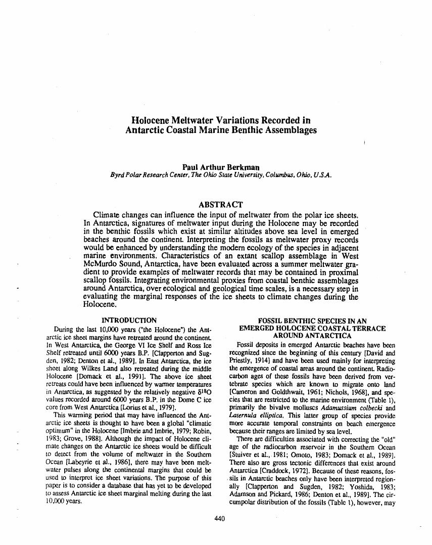
Holocene Meltwater Variations Recorded inAntarctic Coastal Marine Benthic Assemblages

Paul Arthur BerkmanByrd Polar Research Center, The Ohio State University, Columbus, Ohio, U.S.A.

ABSTRACT

Climate changes can influence the input of meltwater from the polar ice sheets.In Antarctica, signatures of meltwater input during the Holocene may be recordedin the benthic fossils which exist at similar altitudes above sea level in emergedbeaches around the continent. Interpreting the fossils as meltwater proxy recordswould be enhanced by understanding the modem ecology of the species in adjacentmarine environments. Characteristics of an extant scallop assemblage in WestMcMurdo Sound, Antarctica, have been evaluated across a summer meltwater gra-client to provide examples of meltwater records that may be contained in proximalscallop fossils. Integrating environmental proxies from coastal benthic assemblagesaround Antarctica, over ecological and geological time scales, is a necessary step inevaluating the marginal responses of the ice sheets to climate changes during theHolocene.

INTRODUCTION FOSSIL BENTHIC SPECIES IN AN

During the last 10,000 years ("the Holocene") the Ant- EMERGED HOLOCENE COASTAL TERRACEarctic ice sheet margins have retreated around the continent. AROUND ANTARCTICAIn West Antarctica, the George VI Ice Shelf and Ross Ice Fossil deposits in emerged Antarctic beaches have beenShelf retreated until 6000 years B.P. [Clapperton and Sug- recognized since the beginning of this century [David andden, 1982; Denton et al., 1989]. In East Antarctica, the ice Priestly, 1914] and have been used mainly for interpretingsheet along Wilkes Land also retreated during the middle the emergence of coastal areas around the continent. Radio-Holocene [Domack et al., 1991]. The above ice sheet carbon ages of these fossils have been derived from ver-retreats could have been influenced by warmer temperatures tebrate species which are known to migrate onto landin Antarctica, as suggested by the relatively negative _i180 [Cameron and Goldthwait, 1961; Nichols, 1968], and spe..values recorded around 6000 years B.P. in the Dome C ice cies that are restricted to the marine environment (Table 1),core from West Antarctica [Lorius et al., 1979]. primarily the bivalve molluscs Adamussium colbecki and

This warming period that may have influenced the Ant- Laternula elliptica. This latter group of species providearctic ice sheets is thought to have been a global "climatic more accurate temporal constraints on beach etnergenceoptimum" in the Holocene [Imbrie and Imbrie, 1979;Robin, because their ranges are limited by sea level.1983; Grove, 1988]. Although the impact of Holocene cii- There are difficulties associated with correcting the "old"mate changes on the Antarctic ice sheets would be difficult age of the radiocarbon reservoir in the Southern Oceanto detect from the volume of meltwater in the Southern [Stuiver et al., 1981; Omoto, 1983; Domack et al., 1989].Ocean [Labeyrie et al., 1986], there may have been melt- There also are gross tectonic differences that exist aroundwater pulses along the continental margins that could be Antarctica [Craddock, 1972]. Because of these reasons, fos-used to interpret ice sheet variations. The purpose of this sils in Antarctic beaches only have been interpreted region-paper is to consider a database that has yet to be developed ally [Clapperton and Sugden, 1982; Yoshida, 1983;to assess Antarctic ice sheet marginal melting during the last Adamson and Pickard, 1986; Denton et al., 1989]. The cir-10,000 years, eumpolar distribution of the fossils (Table 1), however, may

440

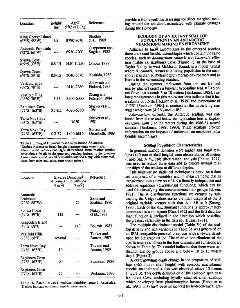
providea framework for assessing ice sheet marginalmelt-Location Heightl Age.2 Reference ing around the continent associated with climate changes

(m) (14CyrB.P.) during the Holocene,

King George Island Shotton ECOLOGY OF AN EXTANT SCALLOP(62°S, 58°W) 3.5 8790-9670 ctal., 1969 POPULATION IN AN ANTARCTIC

NEARSHORE MARINE ENVIRONMENT

AntarcticPeninsula Clappertonand Adjacent to fossil assemblages in the emerged beaches(72oS, 68°90 6930-7200 Sugden, 1982"'" thereareextant benthic assemblages which contain the same

species, such as Adamusstum colbecki and Laternula elltp-Syowa Coast(69°S, 39°E) 0.8-15 1450-10250 emote, 1977 rica (Table 2). Explorers Cove ('Figure 1), at the base of

Taylor Valley in west McMurdo Sound, is a model habitatSyowa Coast where A. colbecki occurs as a living population in the near-(69°S, 39°E) 0.8-15 2040.8370 Yoshida, 1983 shore (less than 30 meters depth) marine environment and as

fossils in the surrounding beaches,Vesffold Hills Adamson and During the summer, meltwater from the sea ice and(68°S, 78°E) .-- 2410-7680 Pickard, 1983 nearby glaciers creates a buoyant hyposaline lens at Explor-

Vesffold Hills Zhang and ers Cove that extends 5 to 10 meters [Berkman, 1988]. Iso-(68°S, 78°E) 3-15 3500-6000 Peterson, 1984 lated measurements in this meltwater lens indicate that it has

a salinity of 1.5 %o[Jackson et al., 1979] and temperature of

Explorers Cove Stuiver et al., -0.2°C [Stockton, 1984] in contrast to the underlying sea-(77°S, 163°E) 0.5-8.1 4620-6350 1981 water which was 34.2 900and -1,8°C.

Adamussium colbecld, the Antarctic scallop, was col-Terra Nova Bay Stuiver et al., leered from above and below the hyposaline lens at Explor-(74°S, 163°E) --- 7020 1981 ers Cove from 3 to 27 meters during the 1986-87 austral

Terra Nova Bay Baroni and summer [Berkman, 1988, 1990]. These scallops provide(74°S, 163°E) 0.2-37 1840-6815 Orombelli, 1989 information on the impacts of meltwater on neat'shore polar

benthic assemblages.

Table 1.EmergedHolocenebeachsitesaroundAntarctica.1Dashesindicatenobeachheightmeasurementsweremade. Scallop Population Characteristics2Uncorrectedradiocarbonages determinedfrom marinebenthic In general, scallop densities were higher and small seal-invertebratefossilsin theemergedbeaches(primarilythebivalves lops (<40 mm in shell height) were absent above 10 metersAdam_sium colbeckiandLaternulaellipticaalongwithothermol-luscs,barnacles and calcareousworm tubes). (Table 3a). A multiple discriminant analysis [Pielou, 1977]

was used to reduce these data and to expose mutual rela-tionships of the scallops at different depths.

This multivariatestatistical technique is based on a dataLocation Bivalve Densitiesl Reference set composed of n variables and m measurements that is

A. colbecld L. elliptica transformed into a new set of k < n lin*_arlyindependent and(#m"2) (# m"2) additive equations (discriminant functions) which can be

used for classifying the measurements into groups [Green,Antarctic 1971]. The A discriminant functions are created by sub-Peninsula Stout and tracting the _. eigenvalues across the main diagonal of the B(72°S, 68°W) -- 75 Shabica, 1970 original variable vectors such that A - kB = 0 [Strang,

1980]. Each of the discriminant functions is approximatelySyowa Coast Nakajima distributed as a chi-square [Rat, 1952] and the first discrim-(69°S, 39°E) 112 --- et al., 1982 inant function is inclined in the direction which describes

Kerguelen Island the greatest variability in thedata set [Buzas, 1971].(49°S, 68°E) .... 140 Beurois, 1987 The multiple discriminant model (Table 3b) of the scal-

lop demity and size variables in Table 3a was generated onVesffold Hills Tucker and an IBM-compatible personal computer with software devel-(78°S, 68°E) several --- Burton, 1987 oped by Statgraphics Inc. The relative contributions of the

coefficients (variables) in the four discriminant functions areTerra Nova Bay Taviani and showr, in Table 3c. This model indicates that there were two

(74°S, 163°E) 10 --- Anmto, 1989 distinct scallop groups above and below 10 to 15 meters

Explorers Cove depth (Figure 2).(77°S, 163°E) 90 Stockton, 1984 A corresponding depth change in the proportion of scal-

lops (>65 mm in shell height) with epizooic macrofaunalExplorersCove species on their shells also was observed above 10 meters(77°S, 163°E) 55 --- Berkman, 1990 (Figure 3). This depth distribution of the epizooic species at

Explorers Cove, including bysally attached small scallopsTable 2. Extant bivalve mollusc densities around Antarctica. which developed from planktotrophic larvae [Berkman et1Dashesindicatenomeasm'ements weremade. al., 1991], may have been influenced by hydrochemical gra-

441

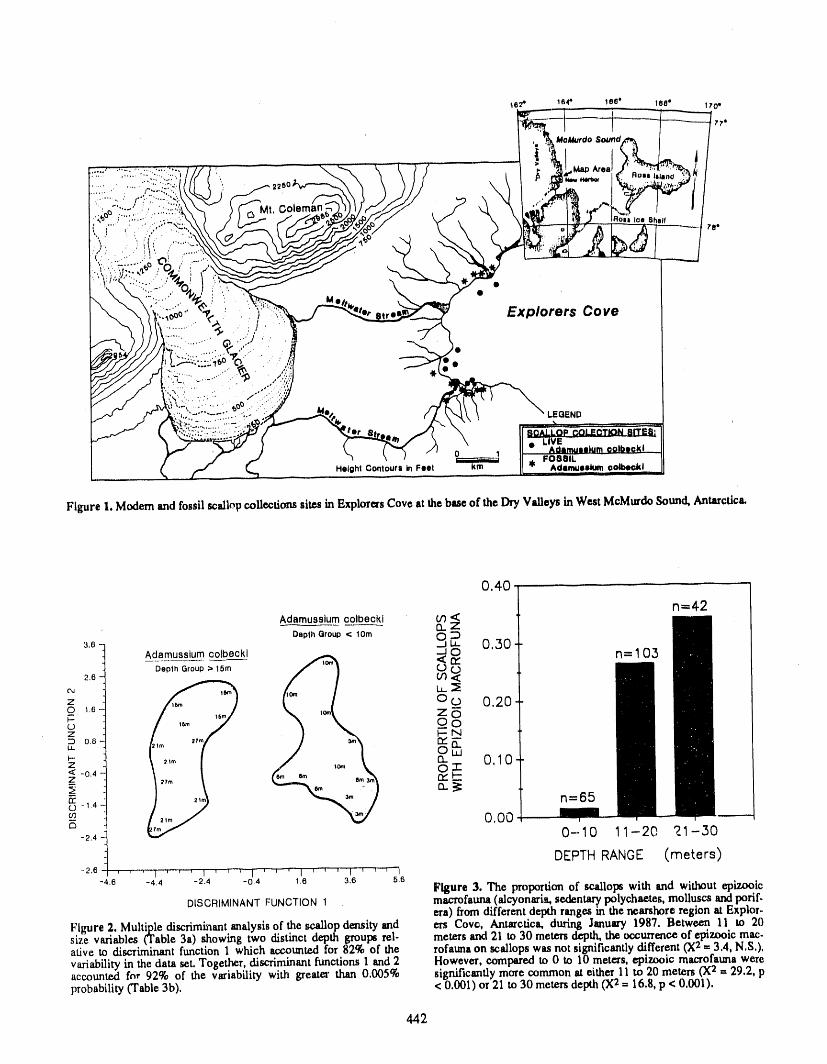
0 1 FO881L

Height Contours in Feet _ $ AdmnNJmmlum ootbookl

Figure 1. Modem and fossil scallopcotlections sites in ExplorersCove at the base of the_ Vslleys in WestMcMurdoSound, Antarctica,

0,40

n=42Adamusslumoolbeokl tj'3

nZDepth Group < 10m

_,,_- o,,p 0.3oAdamusstumc01beokl _ 0 n=103n,"

Depth Group > 15m Q) Q)2.B _ <

c4 b.._z o o 0.20_o _8 z5

GoL) wZ I--N

0.6 rYE"u_ Ou_l_- n 0,10z oT< -0.4z ev.,t--5 n_:

n=65C) -1,4

0,005_2.4 0-10 11-20 ?-1-30

DEPTH RANGE (meters)-2.6 ' ' ' 1 ' ' ' I' ' ' ' I ' ' ' I ' ' ' I / , ,--1

-4.6 -4.4 -2.4 -0,4 1,6 3.6 5,6Figure 3.The proportion of scallops withand withoutepizooic

DISCRIMINANTFUNCTION1 macrofauna (alcyonads, sed_ntar_polychae_s,molluscs andporif.era) fromdifferent depth ranges m thenem'shoreregion at Expior.

Figure2.Multiplediscdminmt analysisofthescallopdensityand ersCove,Antarctica,duringJanuary1987.BetweenI1 to20size variables (Table 3a) showing two distinct depth groups tel- meters and 21 to 30 meters depth, the occurrenceof _epizooicmac.afive to discriminant function 1 which accounted for 82% of the rofaunaon scallops was not significantly different CX2 = 3.4, N.S,),variability in the data seLTogether, discriminant functions 1 and 2 However. compared to 0 to 10 meters, epizoolc macrofauna wereaccounted fnr 92% of the variabBity with greatm' than 0.005% significantly more common at either 11 to 20 meters (X2 = 29.2, pprobability (Table 3b). < 0.001) or 21 to 30 metersdepth (X2= 16.8, p < 0.001).

442

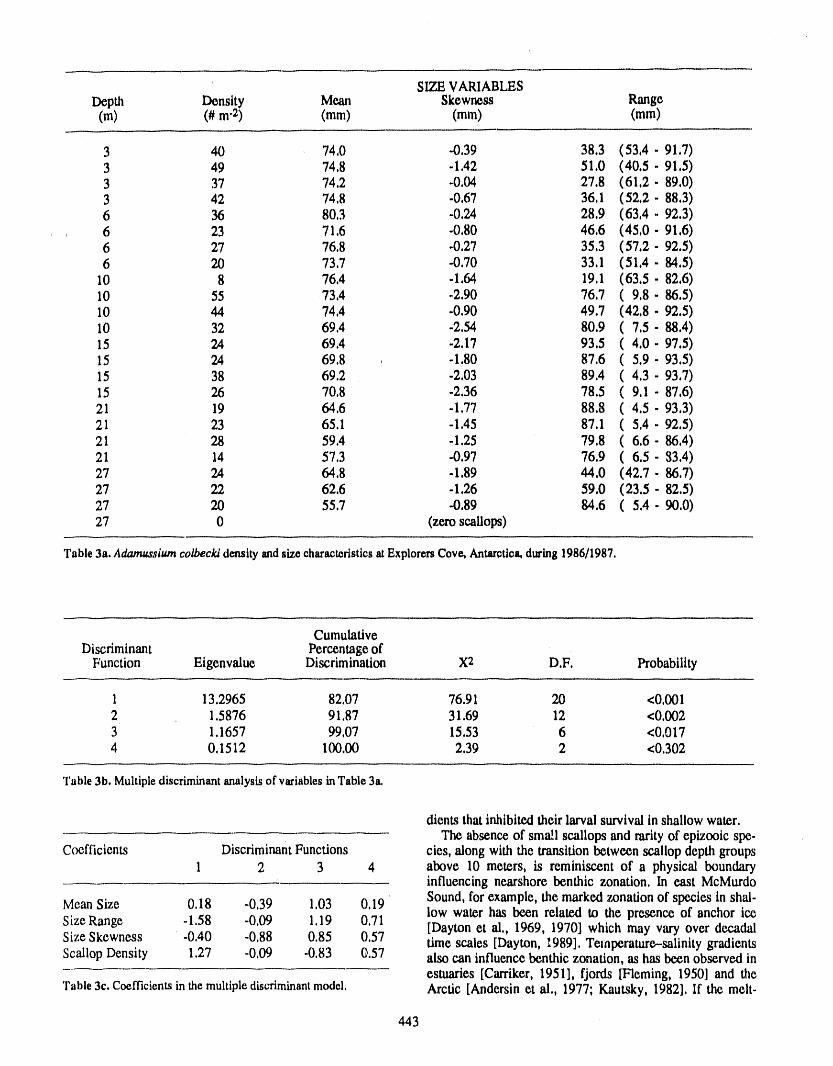
SIZEVARIABLESDepth Density Mean Skewness Range(m) (#m-2) (mm) (mm) (mm)

3 40 74,0 ,0,39 38,3 (53,4- 91,7)3 49 74,8 -1,42 51,0 (40,5-91,5)3 37 74,2 -0,04 27,8 (61,2 - 89,0)3 42 74,8 -0,67 36,1 (52,2 - 88,3)6 36 80,3 -0,24 28,9 (63,4 - 92,3)6 23 71,6 -0,80 46.6 (45,0 - 91,6)6 27 76,8 -0.27 35,3 (57,2 - 92.5)6 20 73,7 -0,70 33,1 (51,4- 84,5)

10 8 76,4 -1,64 19,1 (63,5- 82.6)10 55 73,4 -2.90 76,7 ( 9,8 - 86,5)10 44 74,4 -0,90 49.7 (42,8-92,5)10 32 69.4 -2.54 80.9 ( 7,5- 88.4)15 24 69,4 -2.17 93.5 ( 4,0 - 97,5)15 24 69,8 -1.80 87.6 ( 5,9 - 93,5)15 38 69.2 -2,03 89.4 ( 4,3- 93.7)15 26 70,8 -2.36 78.5 ( 9,1 - 87,6)21 19 64,6 -1,77 88.8 ( 4.5- 93,3)21 23 65,1 -1,45 87.1 ( 5,4- 92,5)21 28 59,4 -1.25 79.8 ( 6.6- 86,4)21 14 57,3 ,0.97 76.9 ( 6.5- 33.4)27 24 64,8 -1.89 44.0 (42.7- 86,7)27 22 62.6 -1.26 59.0 (23.5-82,5)27 20 55.7 -0.89 84.6 ( 5.4- 90,0)27 0 (zero scallops)

Table3a.AdamussiumcolbeckldensityandsizecharacmdsticsatExplorersCove.,Antarctica,during1986/1987,

CumulativeDiscriminant Percentage of

Function Eigenvalue Discrimination X2 D.F, Probability

1 13.2965 82.07 76.91 20 <0,0012 1.5876 91,87 31.69 12 <0,0023 1.1657 99,07 15.53 6 <0,0174 0,1512 100.00 2,39 2 <0,302

Table3b, Multiplediscriminantanalysisof variablesinTable3a.

dients that inhibited their larval survival in shallow water,The absence of small scallops and rarity of epizooic spe-

Coefficients Discriminant Functions cies, along with the transition between scallop depth groups1 2 3 4 above 10 meters, is reminiscent of a physical boundary

influencing nearshore benthic zonation, In east McMurdo

Mean Size 0.18 -0,39 1.03 0,19 Sound, for example, the marked zonation of species in shal-low water has been related to the presence of anchor ice

Size Range -1.58 -0.09 1,19 0.71 [Dayton et al,, 1969, 1970] which may vary over decadalSize Skewness -0,40 -0,88 0.85 0,57 time scales [Dayton, _989], Teinperature-salinity gradientsScallop Density 1,27 -0,09 -0.83 0.57 also can influence benthic zonation, as has been observed in

estuaries [Carriker, 1951], fjords [Fleming, 1950] and theTable3c.Coefficientsin themultiplediscriminantmodel. Arctic [Andersin et al,, 1977; Kautsky, 1982], If the melt-

443

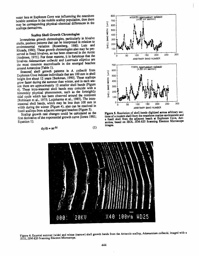
water lens at Explorers Cove was influencing the nearshore BOO MODERN_am_mm _t_lbenthic zonation in the mobilescallop population, then there 700 (4,8oomaeauon)may be corresponding physical.-chemical differences in the _ Booscallops themselves, "" soc

Scallop Shell Growth Chronologies _ 4oo

Invertebrategrowth chronologies, particularlyin bivalve _ 300

shells, producepatternsthat can be interpretedin relation toenvironmental variation [Rosenberg, 1980; Lutz and 200Rhoads, 1980],These growthchronologies also may be pm- Iooserved in fossil bivalves, as has been observed in the Arctic o --.--+--._, .... , : : :.......: : -[Andrews, 1971], For these reasons, it is fortuitousthat the o 5o _oo _so 200 2so 300bivalves Adamussium colbecki and Laternda elllptlca are ARBITRARYBANDNUMBER

the most common macrofossils in the emerged beaches 7oo - -

aroundAntarctica(Table 1), "l FOSSIl.AO_mumaiumSeasonal shell growth patterns in A, colbecki from .-. 600 (4,6gcmaectlon)ExplorersCove indicate Individuals thatare 100 mm in shellheight llve about 12 years [Berkman, 1990], These scallops "_ s°°2grow faster duringthe summer than winter, and in each sea- _ 400

son there are approximately 12 smaller shell bands (Figure I 300

4), These intra-seasonal shell bands may coincide with abimonthly physical phenomenon, such as the fortnightly 200tidal cycle which has been observed around the continent[Robinson et al,, 1975; Lu_jeharmset al,, 1985], The intra- Iooseasonal shell bands, which may be less than 100 mm tn o , 0 , , , , , -: -width during the winter (Figure 4), also can be resolved in o so loo 1so 200 250 300fossil scallops fromadjacent emerged beaches (Figure 5), ARBITRARYBAND NUMBER

Scallop growth rate changes could be calculated as the Figure$. Resolutionof shelt.bamhdigitizedacrossarbitrarysec-firstderivativeof the exponential growth curve [Jones 1981; ttonsof amodemshellfromtheneanhoremarine_vironmentanda fossil shell fromthe adjacentbeth at ExplorenCove, Ant-Equation 1]: arctic.t,basedon JEOLJSM-820Soarming ElectronMicroscope

images,dy/dt = ae"kt (1)

Figure4. Externalsummer(wide)andwinter(narrow)shellgrowthbandsfromtlm Antarcticscallop,Adam_vsiumcolbecld,imagedwith aJEOLJSM.820ScanningElectronMicroscope,

444

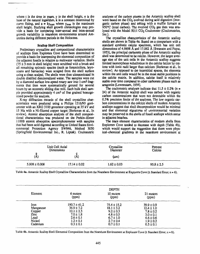
whore t is the time in years, y is the shell height, e is the atudysos of the carbon phases in tl_ Antarotlcscallop shellbase of tl_ natural logarithm,k is a constant determinedby were based on the C02 evolved duringa_id digestion (inor.curve fitting, and a ta kym_ where YmJmis tlm maximtml ganlc carbon phase) and ashing with a muffle furnlmo atshell height, Studying shell growth chronologte.smay pro. 950°C (total carbon), The evolved COg gas then was aria.vide a basis for comparing inter.annual and intra.annual lyzed with the Model 5011 CO: Coulomoter (Coulometrtcs,growth variability in nem'shore environmentsaround Ant. Inc,),arcttcaduringdifferent periods in the Holocene, The crystalline characteristics of rite Antarctic wallop

shells are shown in Table 4a, Based on a compart_n with aScallop Shell Composition standard synthetic calcite specimenj which has unit cell

Preliminary crystalline and compositional characteristics dimensions of 4,9898 A and 17,062 A [Swanson and Fuyat,of _allops from Explorers Cove have been determined to 1953], the principalcarbonatephase of the Antarcticscallopprovidea basis for interpretingthe elemental composition of shell was determinedto becalcite, However, dto largeraver.the adjacent fossils in relation to meltwatervariation,Shells age s'iz¢of the unit cells in the Antarctic scallop suggests(75 :t:5 mm in shell height) were scrubbedwith a brush and limited isomorphous substitutionin the calcite lattice by cat.ali remainingep_ooic species (such as foraminifera,bryo- ions with ionic radii larger than cal¢lwn [Borkmanet al,, Inzoans and barnacles) were scmimd from the shell surface review], As opposed to ti_ interstitialspaces, the elementsusinga clean scalpel, The shells were then ultrasonicatedin within the unit cells would be in the most stable positions indouble distilled demineralized water, The samples were cut the calcite matrix, In addition, calcite itself is relativelyby a diamond surface low.speed rotarysaw into 1.¢m2 frag- stable overtimecomparedtoother carbonate phases such asments that then were systematically ground for several aragonite [Lowenstam, 1954],hours by an eccentric sltdtng disc mill, Each bulk shell sam. The coulometrtc analy,c.,s indicate that 11,5 5:0,2% (n ,-pie providedapproximately 4 em3 of fine grained homoge. 24) of the Antarctic scallop shell was carbon with organicntzed powder foranalysis, carbon concentrations that were not dete_table within the

X.ray diffraction records of the shell crystalline char- 0,3% precision limits of the artalyses, The low organic ear.actertstlcs were produced using a Philips 1316/90 gonl- ben concentrations in the calcttie shells of modem Antarcticometer with an XRG 3100 generator operating at 35 kV and scallops suggest that shell decomposition would be minimal15 Ma with a Ni-filtered copper target [Berkmanet al,, In and that elemental signatures of _nvtronmental variationreview], Atomic absorptionanalysis of the shell compost, may be preservedin the strollsof fossil scallops which occurtlonal characteristics was produced on the Perkln-Elmer tn adjacentbe,aches,l l00B atomic absorption spectrophotometer with samples The trace element c,haractcrlstlcs of modern shells fromthat had been acid digested according to United States Enel. Explorers Cove tended to decrease with depth (Table 4b),ronmental Protection Agency SW846, Method 3050 which would support the suggestion that there were phys.(Springfield Environmental Inc,, R, Liptak), Coulometric ical-ehemical gradients in the nearshore environmentat

Unit Cell Axial Crystalllte PercentDimensions Diameter Calcite

5,008 ± 0,008 17,14 5:0,02 1.62 5:0,03 95,8 :t:2,5

Table4a. AntarcticScallopShellCrystallineCharacteflsttvsfromtheNearshoreEnvironmentatExplorersCove (:t:StandardError;n ffi6),

i

DEPTHElement 6 meters 10 meters 21 meters

(ppm) @pm) (pore)

Iron 190,7 + 41,2 75,4 + 15,2 39,9 ± 0,9Manganese 34,9 5:7,2 18,1 5:3,2 12,4 5:1,0Copper 12,1 + 2,3 9,2 ± 0,3 7,8 + 0,2Zinc 7,0 ± 1,8 4,8 5:0,5 3,0 ± 0,1Lead 2,6 5:0,1 6,7 ± 1,0 4,6 ± 0,6Nickel 1,2 ± 0,1 2,7 5:0,4 1,9 ± 0,2Cadmium 0,3 + 0,1 0,7 ± 0,1 0,5 5:0.1

Table4b, AntarcticScallopShell ElementalCompositionfromtheNearshoreEnvirorunentat ExplorersCove (:i:StandardError;n = 8),

445

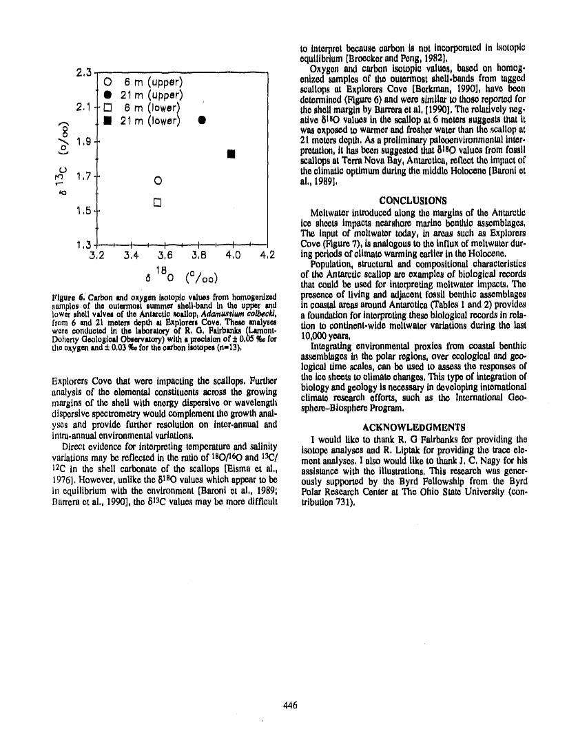
to interpretbecausecarbonis not incorporatedin Isotopicequilibrium[Eroe_kerandPeng,1982],

Oxygen and carbon isotopic valuos, based on homog.2,3 ..... ........ - ....._ _-_ ......,.0 8 m (upper) enizedsamplesof the outermostshell.bandsfrom tagged

s_allopsat ExplorersCove [Berlunan,1990], havebeen• 21 m (upper) determined(FigUre6) andweresimilarto thosereportedfor

2,1 [_ 8 m (lower) ' theshellmarginbyBarreraetal, [1990],Therelativelyhog.Ii 21 m (lower) Q alive 6180 values in the scallop at 6 meters suggests that lt

'_ wasexposedto warmerandfresherwaterthanthe_;_llopat1,9 21 metersdepth,As a preliminarypaleoenvtronmentalintor.

"" l proration,it has been suggested that8lee values from fossilscallops at TerraNova Bay, Antarctica,reflect the impactof

o the cUmatiooptimumduringthe middle Holocene [Baronl ot,--- 1,7 0 al,, 1989],

D CONCLUSIONS1,5 Meltwater introduced along the margins of the Antarctic

ice ,heots impacts nearshoro marine benthic assemblages,Tlm input of meltwater today, in arms such as Explorers

1,3 : : :- I--:--; .....: I...... : --t _ Cove (Figure7), is analogous to the influx of meltwaterdta'-3,2 3,4 3, 6 3,8 4,0 4,2 ing pcdods of climate warming earlierin the Holocene,

Population, structuraland compositional characteristics

180 (O/oo) of the Antarcticscallop are examples of biological recordsthat could be used for interpreting meltwater tmpa_ts, The

Figure6,'Carbonandoxygenlmotopiovaluesfromhomo$enlzed presence of living and adjacent fossil benthic assemblagessamples,of the outermoataummeraholl.bandin the upperand in coastal areas aroundAntarctica(Tables 1 and 2) provideslowershellvalv_ of the Anmotlo _allop, Adamua,viumcolb_ckl, a foundation for interpreting these biological recordsin rela-from 6 and 21 meten depthat EaplorermCove,The_eanalyseswereconductedin the laboratoryof R, G, Ftkbanka([_tmont- i.ion to continent-wide meltwater variations during the lastDohortyGeologicalO_ervat0rY) withltpreoimlonof± 0,05 _ for lO,000 years,theoxy$_ and:t:0,03_, for thecarbontmtopes(n=13), Integrating environmental proxies tivm coastal benthic

as._mblagos h_ the polar regions, over ecological and ge.o-loglc,al time scales, can be used to assess the responses of

Explorers Cove that were impacting the scallops, Further the ice shocksto climate changes, This type of integration ofanalysis of the elemental constituents across the growing biology and geology is necessary in developing international

climate resea_h efforts, such as the International Gee.margins of tlm shell with energy dispersive or wavelength sphere-Biosphere Program.disr,¢rsivoSlxctrometrywould complomentthe growthanal-ys_s and provide further resolution on inter.annual and ACKNOWLEDGMENTS

lntra.annualenvironmentalvariations, I would like to thank R, G Fairbanksfor providing theDire.ctevidence for interpreting temperatureand salinity isotope analyses and R. Liptak for providing the trace ele-

variationsmay be retie, ted in the ratioof 180/160 and l_/ mont analyses. I also would like to thankJ. C. Nagy for hislgC in the shell carbonate of the scallops [Eisma ea al,, assistance with the illustrations, This research was goner.1976], However, unlike the 51sO values which appear to be ously support_ by the Byrd Fellowship from the Byrdin equilibrium with the environment [Baroni ct al,, 1989; Polar Research Center at The Ohio State University (con.Barrcract al,, 1990], the _il3C values may be merc difficult trlbution 731),

446

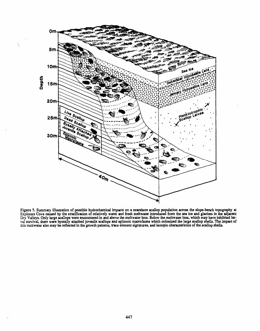
Figure7, Summaryillustrationof possiblohydrochvmtoalimp_ts on a nearshoroscalloppopulationacrossthe slope-benchtopographyatExplororsCove causedby the stratificationof relativelywarmsad freshmeltwatertntmduc_ _om the sca ice and glaciersin theadjacentDryValloys,Onlylargescallopsworeencounteredin andabovethemeltwaterlens,Belowthvmeltwaterlens,whichmayhaw inhibitedlar-valsurvival,therewerebyssalJyattachedjuvenilesoallopsandep.lzooiomacrofaunawhlohcolonizedthelargesoallopshells,Theimpaotofthismoltwat_alsomaybcsr_fl_t_din th_growthpatterns,trac_elementsignatures,andisotopiccharacteristicsof thescallopshells,

447

REFERENCES

Adamson, D., and J. Pickard, Late Quaternary ice move- Scientifique,55, 7-13, 1961.ment across the Vesffold Hi_ls, East Antarctica, in Ant. Carriker, M. _., Ecological observation on the distributionarctic Earth Science, edited by R. L. Oliver, P. R. James, of oyster larvae in New Jersey estuaries, Ecol.and J. B. Jago, pp. 465-.469, Cambridge University Press, Monograph., 21, 19-38, 1951.1983. Clapperton, C. M., and D. E. Sugden, Late Quaternary gla-

Adamson, D., and J. Pickard, Cainozoic history of the Vest- cial history of George VI Sound area, West Antarctica,fold Hills, in Antarctic Oasis: Terrestrial Environments Quat. Res., 18, 243--267, 1982.

and History of the VesC'old Hills, edited by J. Pickard, pp. Craddock, C., Antarctic tectonics, in Antarctic Geology and99-139, Academic Press, New York, 1986. Geophysics, edited by R. J. Adie, pp. 449--455, Uni-

Andersin, A.-B., J. Lassig, and H. Sander, Community versiteasforlaget, Oslo, 1972.structures of soft-bottom macrofauna in different parts of David, T. W. E., and R. E. Priestly, Glaciology, physiog-the Baltic, in Biology of Benthic Organis:"._, edited by raphy, stratigraphy, and tectonic geology of South Vic-B. F. Keegan, P. Oceidigh, and P. J. S. Boaden, pp. 7-20, toria Land, Rep. scient. Invest. Brit. Antarct. Exped.Pergamon Press, New York, 1977. 1907.1909 (Geology), 1, 1-319, 1914.

Andrews, J. T., Recent and fossil growth rates of marine Dayton, P. K., Interdecadal variation in an Antarctic spongebivalves, Canadian Arctic, and Late-Quaternary Arctic and its predators from oceanographic climate shifts,marine environments. Palaeogeogr. Palaeoclimatol. Science, 245, 1484-1486, 1989.Palaeoecol., 11,157-176, 1971. Dayton, P. K., G. A. Robiniard, and A. L. DeVries, Anchor

Baroni, C., and G. Orombelli, Glacial geology and geo- ice formation in McMurdo Sound, Antarctica, and its bio-morphology of Terra Nova Bay (Victoria Land, Ant- logical effects, Science, 163,273-274, 1969.arctica), Mere. Soc. Geol. Ital., 33, 171-193, 1989. Dayton, P. K., G. A. Robilliard, and R. T. Paine, Benthic

Baroni, C., B. Stenni, and A. Longinelli, Isotopic composi- faunal zonation as a result of anchor ice at McMurdotion of Holocene shells from raised beaches and ice Sound, Antarctica, in Antarctic Ecology. Volume i,!;_elves of Terra Nova Bay (Northern Victoria Land, Ant- edited by M. W. Holdgate, pp. 244-258, Scientific Com-z_=tica), 3rd Meeting Scienze Della Terra in Antartide, mittee on Antarctic Research, London, 1970.Siena, 4-6 October 1989, pp. 15-16, 1989. Denton, G. H., J. G. Bockheim, S. C. Wilson, and M.

Barrera, E., J. S. Tevesz, and J. G. Carter, Variations in oxy- Stuiver, Late Wisconsin and Early Holocene glacial his-gen and carbon isotopic compositions and microstructure tory, Inner Ross Embayment, Antarctica, Quat. Res., 31,of the shell of Adamussium colbecld (Bivalvia), Palaios, 151-182, 1989.5, 149-159, 1990. Domack, E. W., A. J. T. Jull, J. B. Anderson, T. W. Linick,

Berkman, P. A., Ecology of the circumpolar Antarctic scal- and C. R. Williams, Application of Tandem Acceleratorlop, Adamussium colbecki (Smith 1902), Doctoral Dis- Mass-Spectrometer Dating to Late Pleistocene-Holocenesertation, 215 pp., University of Rhode Island, 1988. sediments of the East Antarctic continental shelf, Quat.

Berkman, P. A., The population biology of the Antarctic Res., 31,277-287, 1989.scallop, Adamussium colbecki (Smith 1902) at New Hat- Domack, E. W., A. J. T. Jull, J. B. Anderson, and T. W.bor, Ross Sea, in Antarctic Ecosystems: Ecological Linick, Mid-Holocene ice sheet recession from theChange and Conservation, e_ted by N. Kerry and G. Wilkes Land continental shelf, East Antarctica, in Geo-Hempel, pp. 281-288, Springer-Verlag, Heidelberg, logic Evolution of Antarctica, edited by J. A. Crame and1990. J.W. Thomson, pp. 693-698, Cambridge University

Berkman, P. A., T. R. Waller, and S. P. Alexander, Unpro- Press, Cambridge, 1991.tec":.d larval development in the endemic Antarctic scal- Eisma, D., W. G. Mook, and H. A. Das, Shell character-lop, Adamussium colbecid (Mollusca: Bivalvia: Pectin. istics, isotopic composition and trace-element contents ofidae), Antarct. Sci., 3, 151-157, 1991. some euryhaline molluscs as indicators of salinity, Palae-

Berkman, P. A., D. W. Foreman, and J. C. Mitchell, Inter- ogeogr. Palaeoclimatol. Palaeoecol., 19, 39-62, 1976.preting the _ineralogy of antarctic scallop shells based Fleming, C. A., The molluscan fauna of the fjords of West-on X-ray diffraction analysis of their crystalline char- ern Southland, N.Z.J. Sci. Tech.,5, 20--40, 1950.acteristics, Antarct. Res. Ser., American Geophysical Green, R. H., A multivariate statistical approach to theUnion, Washington, DC, In review. Hutchinsonian niche: bivalve m_:lluscs of Central Can-

Beurois, J., Invertebres et algues benthiques exploites ou ada, Ecology,52,543-555, 1971exploitables, in Acres du Colloque sur la Recherches Grove, J. M., The Little Ice Age, 458 pp., Methuen, London,Francaise Darts les Terres Autralies, edited by L. Lauber, 1988.

S. Gauber, and I. Martin, pp. 221-228, Comit_ National lmbrie, J., and K. P. Imbrie, Ice Ages: Solving the Mystery,Franc_s des Recherches Antarctiques, Strasbourg, 1987. 224 pp_,Enslow Publ., Short Hills, 1979.

: Broecker, W. S., and T.-H. Peng, Tracers in the Sea, 690 Jackson, T. L., T. W. Linick, R. L. Michel, and P. M. Wil-pp., Eldigio Press, New York, 1982. lianas, Tritium and carbon-14 distributions in McMurdo

Buzas, M. A., An application of canonical analysis as a Sound, 1977, Antarct. J. U.S., 13, 71-73, 1979.

.... Jt,_u._t'-'a ,,.at- ,_.,,.,_,,_ u. b',,,,¢..... I _aro_¢, I Z nim Erol .__ . _6.. Jones. D. S.. Annual _owth increments in shells of Spisula_. 563--577, 1967. solidissima record marine temperature variability,= Cameron, R. L., and R. D. Goldthwait, The US-IGY con- Science, 211,165-167, 1981.

tribution to Antarctic geology, Union Geodiesie et Geo- Kautsky, N., Growth and size structttre in a Baltic Mytilusphysique, Association Internationale d'Hydrologie edulis population, Mar. Biol., 68, 117-133, 1982.

448

_' ,I , ir iS '' _I '' =_0' ' ' ,l , _ I "' n, , II _ ' =lP _ lr iPl _m ,

Labeyrie,L.D.,J.J.Pichon,M. Labracherie,P.Ippolito,J. Rosemberg,G.D.,An ontogeneticapproachtothe env/ron-Duprat,and J. C. Duplessy, Melting history of Antarctica mental significance of bivalve shell chemistry, in Skeletalduring the past 60,000 years, Nature, 322, 701-706, Growth of Aquatic Organisms, edit_ by D. C. Rhoads1986. and R. A. Lutz, pp. 133--168,Plenum Press, New York,

Lorius, C., L. Merlivat, J. Jouz,',l, and M. Pourchet, A 1980.30,000 yr isotope climatic record from Antarctic ice, Shotlon, F. W., D. J. Blundell, and P_ E. G. Williams, Birm-Nature, 280, 644--648, 1979. ingharn University radiocarbo_da_s III, Radiocarbon,

Lowenstam, H., Factors affecting the aragonite/calcite ratios II, 263-270, 1969.in carbonate-secreting marine organisms, J. Geol., 62, Stockton, W. L., The biology and ecology of the epifaunal284--322, 1954.

Lutjeharms, J. R. E., C. C. Stavropoulos, and K. P. Kol- scallop Adamussium colbecki on the v,est side oftermann, Tidal measurements along the Antarctic coast- McMurdo Sound, Antarctica, Mar. Bio!., 78, 171-178,line, in Oceanology of the Antarctic Continental Shelf, 1984.edited by S. S. Jacobs, pp. 273-289, American Geo- Stout, W. E., and S. V. Shabica, Marine ecological studies atphysical Union, Washington, DC, 1985. Palmer Station and vicinity, Antarct. J. U.S., 5, 134-135,

Lutz, R. A., and D. C. Rhoads, Growth patterns within the 1970.molluscan shell: an overview, in Skeletal Growth of Strang, G., L/near Algebra and Its Applications. 2hd E&'-Aquatic Organisms, edited by D. C. Rhoads and R.A. tion, 414 pp., Academic Press, New York, 1980.Lutz, pp. 203-254, Plenum Press, New York, 1980. Stuiver, M. L., G. H. Denton, T. J. Hughes, and J, L. Fas-

Nakajima, Y., K. Watanabo, and Y. Naito, Diving observa- took, History of the marine ice sheet in West Antarctications of the marine benthos at Syowa Station, Antarctica, during the last glaciation: a working hypothesis, in TheMere. Nat. Inst. Polar Res. Spec. Issue 23, 44-54, 1982. Last Great Ice Sheets, edited by G. H. Denton and T. J.

Nichols, R. L., Coastal geomorphology, McMurdo Sound, Hughes, pp. 319--436, John Wiley and Sons, New York,Antarctica, J. Glaciol., 7, 449--478, 1968. 1981.

Omoto, K., Geomorphic development of the Soya Coast, Swanson, H. E., and R. K. Fuyat, Standard X-ray diffractionEast Antarctica. Chronological Interpretation of raised powder patterns: carbonates, Nat. Bur. Stand. Circ. 539beaches based on levelling and radiocarbon dating, Sci. (II), 51-54, 1953.Rept. Tohoku Univ. 7thSer., 27, 95-148, 1977. Taviani, M., and E. hanato, Diving in Antarctica: Third Ital-

Omoto, K., The problem and significance of radiocarbon ian Expedition in Terra Nova Bay, Boll. Oceano. Teoricageochronology in Antarctica, in Antarctic Earth Science, Applic., 7, 43-53, 1989.edited by R. L. Oliver, P. R. James, and J. B. Jago, pp.450--452, Cambridge University Press, Cambridge, 1983. Tucker, M. J., and H. R. Burton, A survey of the marine

Pielou, E. C., Mathematical Ecology, 384 pp., John Wiley fauna in shallow coastal waters of the Vestfold Hills andand Sons, New York, 1977. Rauer Island, Antarctica, Austral. Nat. Antarct. Res.

Rao, C. R., Advanced Statistical Methods in Biometrical Exped. Res°Notes,55, 1-24, 1987.Research, 390pp., Wiley, New York, 1952. Yoshida, Y., Physiography of the Prince Olav and the

Robin, G. de Q., The Climate Record in Polar Ice Sheets, Prince Harald Coasts, East Antarctica, Mem. Nat. Inst.212 pp., Cambridge University Press, Cambridge, 1983. Polar Res. C, 13, I--83, 1983.

Robinson, E. S., R. T. Williams, H. A. C. Neuberg, C.S. Zhang, Q., and J. A. Peterson, A geomorphology and LateRohrer, and R. L. Ayers. Southern Ross Sea tides, Quaternary geology of the Vesffold Hills, Antarctica,Antarct. J. U.S., 10, 155--157,1975. Austral. Nat. Antarct. Res. Exped. Rept., 133, 1--84,1984.

449

EPOS--A New Approach to International Cooperation

G. HempeiAlfredWegenerInstitutefor PolarandMarineResearch,Bremerhaven,Germany

ABSTRACT

130 marine biologists and oceanographers from 11 Western European countriesparticipated in the European Polarstem Study (EPOS) jointly organized by the Fed-eml Republic of Germany (through Alfred Wegener Institute for Polar and MarineResearch) and the European Science Foundation. The icebreaking research vesselPolarstern operated in the Weddell Sea from October 1988 to March 1989. Each ofthe three legs was headed by a German scientist in charge and by a foreign sci-entific advisor.

The first leg started under late winter conditions and was devoted to the role ofthe sea ice in the pelagic system and to the sea ice biota themselves. Leg 2 studiedthe retreating ice edge end the open water in front of it during spring, particularlythe relation of the phytoplankton blooms to the physical structure and chemistry ofthe surface water and to the grazing by krill. Leg 3 concentrated on taxonomy andeco-physiology of invertebrates and fishes at the sea bed of the eastern Weddell

" Sea.EPOS was meant to provide Antarctic research opportunities to European coun-

tries with little experience in Southern Ocean studies and to foster the exchange ofknowledge and ideas between European marine biologists of different scientificbackground and h_terests. Therefore, the teams of the various projects on boardwere normally multi-national in order to ensure a maximum of interaction. This hasbeen continued in a number of post-expedition workshops and by international

, fellowships.

ll

m

450

Estimation of Matter Fluxes in the River-Sea andOcean-Atmosphere Systems for Okhotsk and Bering Seas

V. V. Anikiev, A. V. Alekseev, A. N. Medvedev, and E. M. ShymilinPacific Oceanological Institute, Far East Branch, Academy of Sciences of the U.S.SJR., Vladivostok, U.S.S2_.

ABSTRACT

The matter fluxes from continental and anthropogenic sources to sea take placeby river discharge and atmospheric precipitation.

The estimation of this flux may be done on the basis of a single concept, but ithas its own specific character in both cases: (1) the time-space changeability of thematter distribution in sea components is conn_texi with the complex gradients ofhydrophysical, physico-chemical and hydrobiological characteristics of the watermass, by name "biological barrier"; (2) the "altitude" and stability of this bio-geochemical barrier are determined by short-period (from seconds up to one year)geochemical processes; and (3) it is very interesting and important to estimate notonly the matter fluxes on the continent under the motion of water and air, but alsothe intensity of accumulation on the biogeochemical barrier.

It is necessary to do the next complex of investigations on the coast and aquatoryof the Okhotsk and Bering Seas. This will include: (1) the synchronous registrationof physical, chemical and biological characteristics in the river-sea and ocean-atmosphere systems to determine the transport and transformation of existing formsof matter, (2) observations of the distribution of natural and pollutant matter (suchas heavy metals, oil and polycyclic aromatic hydrocarbons, artificial radioisotopes,etc.) in the estuaries, atmosphere, shelf zones and open sea regions; and (3) calcula-tions of the matter fluxes between the different components of the sea.

451

Investigations of Scales of Changeabilityof Biogeochemical Processes on the Okhotsk Sea Shelf

V. V. Anikiev, O. V. Dudachev, T. A. Zadonskaya, A. P. Nedashkovski, A. V. Pervushin,S. G. Sagalaev, D. A. Chochlov and V. V. Yarosh

PacificOceanologicalInstitute,Far EasternBranchof the U.S.S.R.Academyof Sciences,Vladivostok,U.S.S.R.

ABSTRACT

Complex investigations of spatial-temporal changeability of biogeochemicalprocesses and parameters were conducted on the north-eastern shelf of Sakhalin.They included: (1) transformation of the size and chemical composition of par-ticulate matter by hydrophysical and biological factors; (2) the shift of equilibriuminto the carbonate system of water masses in relation to variable physico-chemicaland biological parameters; and (3)change of biomass and species phyto-zooplankton and the same amount of primary production connected with fluctua-tions of hydrophysical, physico-chemical and biological characteristics of watermasses.

Observations conducted during the last 3 years in different seasons, apart fromwinter, were by way of polygon survey and daily stations. Mathematical treatmentof the data made it possible to estimate quantitatively the correlation between separ-ate parameters and to identify the influence of several external factors on their spa-tial-temporal changeability: seasonal variations; the significance of the Amur riverdischarge; tidal motion of waters; steady circulation; invasion of CO2 from low-temperature hydrothermal sources on the sea bottom.

The obtained dependencies can be used for forecasting possible ecosystemchanges during the industrial exploitation of the oilfield.

452_

/° 1 __ / , iLong-term ot Arborne Pollen in Alaska and the Yukon:

, t _, '_li, ,' o o

Pog:sib/Implncatlons for Global Change

J. H. AndersonInstituteof ArcticBiology,Universityof AlaskaFairbanks,Fairbar_, Alaska,U.S.A.

ABSTRACT

Airborne pollen and spores have been sampled since 1978 in Fairbanks and 1982in Anchorage and other Alaska-Yukon locations for medical and ecological pur-poses. Comparative analyses of pre- and post-1986 data subsets reveal that after1986 (1) pollen is in the air earlier, (2) the naultiyear average of degree-days pro-moting pollen onset is little changed while (3) annual variation in degree-days atonset is greater, (4) pollen and spore annual productions are considerably higher,and (5) there is more year-to-year variation in pollen production. These changesprobably reflect directional changes in certain weather variables, and there is someindication that they are of global change significance, i.e., related to increasingatmospheric greenhouse gases. Correlations with pollen data suggest that weathervariables of high influence are temperatures during specific periods following pol-len dispersal in the preceding year and the average temperature in April of the cur-rent ),ear. Annual variations in pollen dispersal might be roughly linked to the 11-year sunspot cycle through air temperature mediators. Weather in 1990, apparentpollen production cycles under endogenous control, and the impending sunspotmaximum portend a very severe pollen season in 1991. The existing but unfundedaerospora monitoring program must continue in order to test predictions andhypotheses and as a convenient, economical indicator of effects of climate changeon biological systems and human well-being in the North.

INTRODUCTION stand and manage the significant publichealth problemsThe dominant trees and shrubs and the grasses, sedges posed by pollen and spores as aeroallergens,lt is further

andsomeother herbs in Alaskaand the Yukonreleaselarge enhancedby the _lati_e ease _r_dlow cost of sampliog.Aamountsof pollen for aerial transport.The less conspicuous generalobjectiveof thlisarticle iSto indicatepotentialvaluebutubiquitousmoldsandother fungireleaselargeramounts in the continued long_.t_rmmonitoringof airborne pollenof sporesduringmost of the snow-freeperiod.These micro- andsporesin AlaskaandadjacentCanada.scopic entities, known collectivelyas the aerospora, have Although the multiyear lata set now availablerepresents

only a few years and is only partially analyzed, majorbeen sampled since 1978 in an aerobiologyprogramcon- annual and longer-term variations in the aerospora arecerned with immunological,public health and ecological becomingevident. Specificobjectivesot"this article are (1)issues.A centralecologicalissue is annual pollenand spore to inU'oducesome featuresof the annual variations,(2) todispersalas a functionof certain weathervariablesand an _howchangesin annualvariationsafter 1986, (3) to presentindicatoror predictorof vegetationresponsesto directional a preliminary correlation analysis suggesting specificchangesin those variables,i.e., to climatechange, weather variables influencing pollen dispersal,and (4) to

The aerospora is an important biometeorologicalphe- discusspossibleimplicationsof observedaerosporachangesnomenonand a prime candidatefor long-termmonitoring, for short-term climate changes that might be of globalThis candidacy is enhanced by the need fordata to under- changesignificance.

- 453

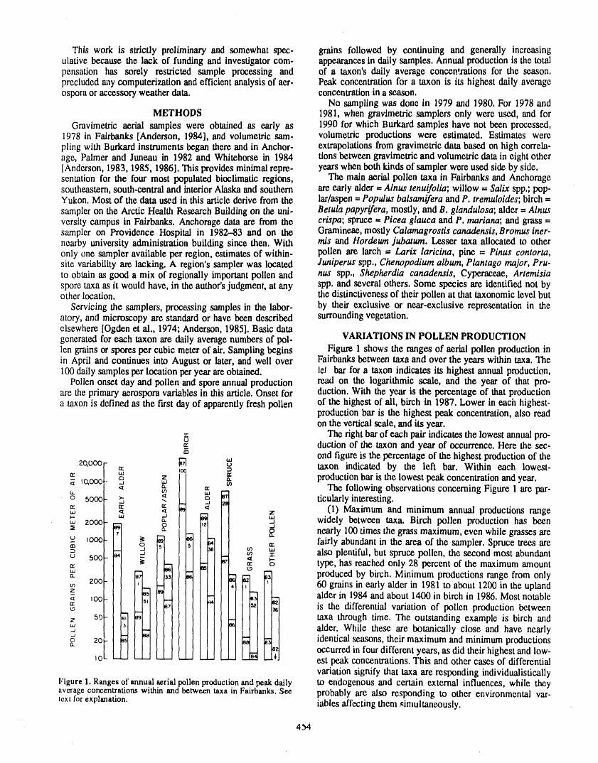
This work is strictly preliminary and somewhat spec- grains followed by continuing and generally increasingulative because the lack of funding and investigator com. appearances in daily samples. Annual production is the totalpensation has sorely restricted sample processing and of a taxon's daily average concen'rations for the season.precluded any computerization and efficient analysis of aer- Peak concentration for a taxon is its highest daily averageospora or accessory weather data. concentration in a season,

No sampling was done in 1979 and 1980. For 1978 andMETHODS 1981, when gravimetric samplers only were used, and for

Gravimetric aerial samples were obtained as early as 1990 for which Burkard samples have not been processed,1978 in Fairbanks [Anderson, 1984], and volumetric sam- volumetric productions were estimated. Estimates werepiing with Burkard instruments began there and in Anchor- extrapolations from gravimetric data based on high correla-age, Palmer and Juneau in 1982 and Whit_horse in 1984 tions between gravimetric and volumetric data in eight other[Anderson, 1983, 1985, 1986]. This provides minimal repre- years when both kitr,clsof sampler were used side by side.sentation for the four most populated bioclimatic regions, The main aerial pollen taxa in Fairbanks and Anchoragesoutheastern, south-central and interior Alaska and southern are early alder = Alnus tenuifolia; willow = Sa//x spp.; pop-Yukon. Most of the data used in this article derive from the lar/aspen = Populus balsamifera and P, tremuloides; birch =sampler on the Arctic Health Research Building on the uni- Betula papyrOrera,mostly, and B. glandulosa; alder = Alnusversity campus in Fairbanks. Anchorage data are from the cr/spa; spruce = Picea glauca and P. mariana; and grass =sampler on Providence Hospital in 1982--83 and on the Gramineae, mostly Calamagrostis canadensis, Bromus iner-nearby university administration building since then. With m/s and Hordeum jubatum. Lesser taxa allocated to otheronly one sampler available per region, estimates of within- pollen are larch = Larix laricina, pine = Pinus contorta,site variability are lacking. A region's sampler was located Juniperus spp., Chenopodium album, Plantago major, Pru-to obtain as good a mix of regionally important pollen and nus spp., Shepherdia canadensis, Cyperaeeae, Artemisiaspore taxa as it would have, in the author's judgment, at any spp, and several others, Some species are identified not byother location, the distinctiveness of their pollen at that taxonomic level but

Servicing the samplers, processing samples in the labor- by their exclusive or near-exclusive representation in theatory, and microscopy are standard or have been described surrounding vegetation.elsewhere [Ogden et al., 1974; Anderson, 1985], Basic datagenerated for each taxon are daily average numbers of Ix)l- VARIATIONS IN POLLEN PRODUCTIONlen grains or spores per cubic meter of air. Sampling begins Figure 1 shows the ranges of aerial pollen production inin April and continues into August or later, and well over Fairbanks between taxa and over the years within taxa. The100 daily samples per location per year are obtained, lel bar for a taxon indicates its highest annual production,

Pollen onset day and pollen and spore annual production r'ead on the logarithmic scale, and the year of that pro-are the primary aerospora variables in this article. Onset for duction. With the year is the percentage of that productiona taxon is defined as the ra.st day of apparently fresh pollen of the highest of all, birch in 1987. Lower in each highest-

production bar is the highest peak concentration, also readon the vertical scale, and its year.

z The right bar of each pair indicates the lowest annual pro-tD

rr duction of the taxon and year of occurrence. Here the sec-ond figure is the percentage of the highest production of the

,2c_ooo- a: _ "''-' taxon indicated by the left bar. Within each lowest-rr t,t.I I00 ::}

" production bar is the lowest peak concentration and year.Io,ooo _ z...j LO tD

- 0. rr The following observations concerning Figure 1 are par-Lt. tD

o 5ooo- _ '_ LO" ticularly interesting._" -J !2[

wrr a:,a a:,t : _ z (I) Maximum and minimum annual productions rangeI-- t,td ...d _ I._LO zooo- - 0. _ widely between taxa. Birch pollen production has been

as _ t2 j, _ nearly 100 times the grass maximum, even while grasses are

tooo- ":: 79 _ _ fairly abundant in the area of the sampler. Spruce trees are03 C) _ _ rv"

= _ _ _[ _ LO= also plentiful, but spruce pollen, the second most abundant

5oo- _.: - 7, _ "0: - o type, has reached only 28 percent of the maximum amountLO -- ml __ _ t) _0. ,, _l _,1 _'] _ ,s produced by birch. Minimum productions range from only_, zoo- , --, - ] ,t , ' 60 grains in early alder in 1981 to about 1200 in the uplandz_ _l as . _ _ alder in 1984 and about 1400 in birch in 1986. Most notable

100, _1 -'_

_ is the differential variation of pollen productionbetween

z 5o-_,"] _ ' ... { ii1 taxa through time. The outstanding example is birch and

_J 3_ ..-, . I _ I alder. While these are botanically close and have nearly--J "-_ Bal I

o 2o- _l 78 J E identical seasons, their maximum and minimum productionsi

to .... _ occurred in four different years, as did their highest and low-........ est peak concentrations. This and other cases of differentialvariation signify that taxa are responding individualistically

Figure 1. Ranges of annual aerial pollen production and peak daily tO endogenous and certain external influences, while theyaverage concentrations within and between taxa in Fairbanks. See probably are also responding to other ertvironmentalvar-

textfor explanation, iables affecting them ,_imultaneously.

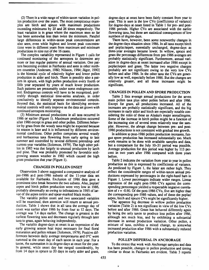
(2) There is a wide range of within-taxon variationin pol- degree-days at onset have been fairly constant from year tolen production over the years. The most conspicuous exam- year. This is seen is the low CVs (coefficients of variance)pies are birch and spruce with maximum productions for degree-days at onset listed in Table 1 for pre. and post.exceeding minimums by 20 and 26 times respectively, The 1986 periods. Higher CVs are associated with the earlierleast variation is in grass where the maximum seen so far flowering taxa, but these are statistical consequences of lowhas been somewhat less than twice the minimum. Parallel numbers of degree-days,large differences in within-taxon peak concentrations are There have, however, been some noteworthy changes inalso seen, even while highest and lowest peak concentra- the degree.days situation since 1986. In ali taxa except birchtions were in different years from maximum and minimum and poplar/aspen, es._ntially unchanged, degree-days asproductions in nine out of the 16 eases, three-year averages became lower. In willow, spruce and

The complex variability represented in Figure 1 calls for grass the percentage differences from pre-1986 averages arecontinued monitoring of the aerospora to determine any probably statistically significant. Furthermore, annual vari-more or less regular patterns of annual variation. One pat- ation in degree-days at onset increased after 1986 except intern becoming evident in Fairbanks and seen in other north- poplar/aspen and grass, The latter two negative changesern countries [Andersen, 1980; Nilsson, 1984; Jltger, 1990] probably are not significant owing to the very low CVsis the biennial cycle of relatively higher and lower pollen before and after 1986. In the other taxa the CVs are gener-production in alder and birch. There is possibly also a pat- ally low as weil, especially before 1986. But the changes aretern in spruce, with high pollen production every fourth or relatively greater, and ali these increases might befifth year separated by years of much lower production, significant.Such patterns are presumably under some endogenous con-trol. Endogenous controls will have to be recognized, prcf- CHANGES IN POLLEN AND SPORE PRODUCTIONerably through statistical time.series analyses, in order Table 2 lists average annual productions for the sevenconclusively to identify separate environmental controls, main pollen taxa plus other pollen before and after 1986.Beyond that, the statistical basis for identifying environ- Except for grass, ali productions increased. All of themental controls will only improve as the data set grows with increases are probably statistically significant, and the bigcontinued aerospora monitoring, increases in early alder and birch are especially notable con-

(3) Minimum annual productions in ali taxa occurred in sidering the roles of these as Alaska's major aeroallergens.1986 or earlier (Figure 1). Maximum productions occurred Some of the increase in birch pollen might be a function ofafter 1986 except in grass and other pollen. Different behav- the increasing size of several trees relatively near the sam-itr by grass from the woody taxa might be expected because pier. However, the abrupt change between pre. and post-its season is later and it is influenced by different environ- 1986 productions is not consistent with gradual tree growth.mental conditions. Other pollen comprises several woody In addition to post-1986 pollen production increases, fun-and herbaceous taxa flowering from early spring to late gus spore production has increased substantially too. Muchsummer and controlled by _veral different preceding- and work remains to be done with available samples and data,current-year variables [Solomon, 1979]. The high other pol- but a comparison for the July 10--31 period was possible.len in 1983 was due largely to unusual production by larch Average production for this period was higher by 113 per-and pine. That was probably promoted by favorable mid- cent in two years after 1986 compared with three yearsgrowing season weather in 1982 which caused the high before.grass production that year (Figure 1). Table 2 indicates the variation from year to year in pollen

production as this is expressed by coefficients of variance.CHANGES IN POLLEN ONSET As predicted by Figure 1, the latter are rather high. They

Observation 3 above suggested a comparative analysis of reflect the considerable ranges of within-taxon annual pro..pre-1986 and post-1986 subsets of the 11-year data set ductions expressed by percentages in the fight-hand bars inavailable for Fairbanks. Exclusion of 1986 data gave a Figure 1. Lower percentages indicate wider ranges. Linearprominent time break between the two subsets. Also, poplar/ regression of the eight post-1986 CVs against the corre-aspen and birch pollen production were very low in 1986, sponding percentages yielded a respectable negative correia-probably abnormally so owing to infestations in 1985 of lm'- tion of r = -0.90. Of the post-1986 CVs, five are higher thanvae of the aspen tortrix and spear-marked black moths, the corresponding pre-1986 values, and of these the poplar/

The variable pollen onset and two associated variables aspen, birch and spruce CVs might be significantly higher.will be examined, then attention will return to annual pro- The apparent big decrease in willow pollen productionduction. Table 1 shows that in ali taxa the average day of variation (Table 2) is not significant in view of the low CVsonset was earlier after 1986 by from four to 12 days. The before and after 1986. Grass has behaved differently againaverage was 7.4 days earlier. The change is greatest in the by being the only taxon to produce less pollen after 1986,earliest flowering taxa and decreases regularly through later although not much less, and by exhibiting a substantialtaxa to grass, again behaving independently, decrease in annual production variation. Other pollen, a

The variable degree-days at onset is an expression of the mixture of taxa, exhibits a mixed change, to somewhatearly growing season heat input necessary for final floral increased production after 1986 with a substantially reducedmaturation and pollen release [Solomon, 1979]. Positive dif- production variation.ferences between daily average temperatures and 0°C weresummed to the onset day of each taxon in each year. For a POLLEN DISPERSAL IN ANCHORAGE'taxon, the summation is its degree-days at onset for the year. To the extent that work with Anchorage samples and dataIn general, while onset day has ranged considerably, by h'as been possible, changes in pollen production and timingfrom 14 days in spruce to 20 days in early alder and grass, _imilar to those in Fairbanks are evident. Table 3 reports

,,, 455 '

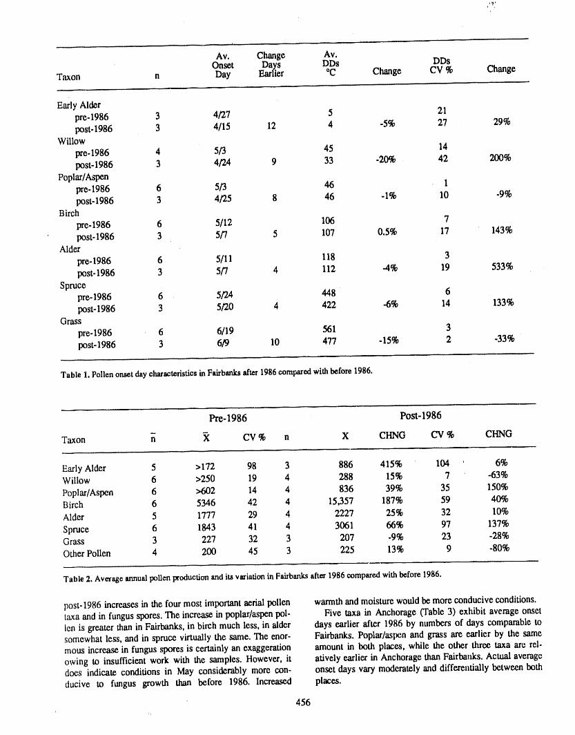
Av. Change Av.Onset Days DDs DDs

Taxon n Day Earlier °C Change ev % Change

Early Alderpre.1986 3 4/27 5 21post-1986 3 4/15 12 4 -5% 27 29%

Willow

pre-1986 4 5/3 45 14post-1986 3 4/24 9 33 -20% 42 200%

Poplar/Aspenpre.1986 6 5/3 46 1post-1986 3 4/25 8 46 -1% 10 -9%

Birch

pre-1986 6 5/12 106 7' post-1986 3 5/7 5 107 0.5% 17 143%

Alder

pre. 1986 6 5/11 118 3post, 1986 3 5/7 4 112 -4% 19 533%

Sprucepre.1986 6 5/24 448 6post- 1986 3 5/20 4 422 -6% 14 133%

Grass

pre-1986 6 6/19 561 3post-1986 3 6/9 10 477 -15% 2 -33%

Table1. PollenonsetdaycharacteristicsinF_tirbanl_after1986comparedwithbefore1986.

Pre- 1986 Post- 1986

Taxon n _( CV % n X CHNG CV % CLING

Early Alder 5 >172 98 3 886 415% 104 6%Willow 6 >250 19 4 288 15% 7 -63%

Poplar/Aspen 6 >602 14 4 836 39% 35 150%Birch 6 5346 42 4 15,357 187% 59 40%

Alder 5 1777 29 4 2227 25% 32 10%

Spruce 6 1843 41 4 3061 66% 97 137%Grass 3 227 32 3 207 -9% 23 -28%Other Pollen 4 200 45 3 225 13% 9 -80%

Table 2. AverageannualpollenproductionanditsvariationinFairbanksafter1986comparedwithbefore1986.

post-1986 increases in the four most important aerial pollen warmth and moisture would be more conducive conditions.taxa and in fungus spores, The increase in poplar/aspen pol- Five taxa in Anchorage (Table 3) exhibit average onsetlen is greater than in Fairbanks, in birch much less, in alder days earlier after 1986 by numbers of days comparable tosomewhat less, and in spruce virtually the same. The enor- Fairbanks. Poplar/aspen and grass are earlier by the samemous increase in fungus spores is certainly an exaggeration amount in both places, while the other three taxa are rel-

owing to insufficient work with the samples. However, it atively earlier in Anchorage than Fairbanks. Actual averagedoes indicate conditions in May considerably more con- onset days vary moderately and differentially between both

ducive to fungus growth than before 1986. Increased places.

' 456

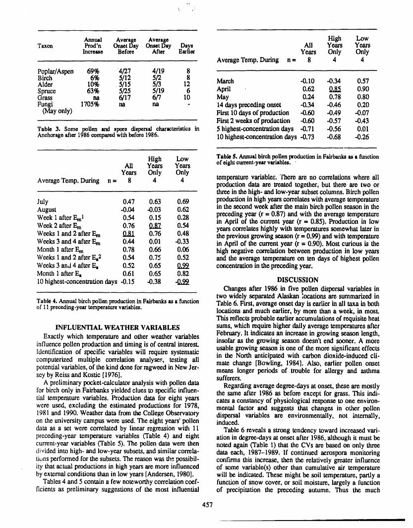
Annual Average Average High LowTaxon Prod'n OnsetDay OnsetDay Days Ali Years Years

Inorease Before After Earlier Years Only OnlyAverageTemp, During n ffi 8 4 4

Poplar/Aspen 69% 4/27 4/19 8Birch 6% 5/12 5/2 8Alder 10% 5/15 5/3 12 March -0,10 -0,34 0,57Spruce 63% 5/25 5/19 6 April 0,62 _ 0,90Grass na 6/17 6/7 10 May 0,24 0,78 0,80Fungi 1705% na na - 14days precedingonset -0,34 -0.46 0.20

(Mayonly) First 10days of production -0,60 -0,49 -0,07First2 weeks of production -0.60 -0.57 -0,43

Table 3. Some pollen and spore dispersaloharacteflstiosin 5 highest-concentrationdays -0.71 -0,56 0,01Anchorageafter1986comparedwithbefore1986, 10highest-concentrationdays -0.73 -0.68 -0,26

Table$. AnnualbirchpollenproductioninFalrbanksasa functionHigh Low of eightcurrent-yearvariables,Ali Years Years

Years Only OnlyAverage Temp. During n = 8 4 4 temperature vaflable_. There are no correlations where ali

productiondata are treated together, but there are two orthreein the high- andlow-year subset columns. Birchpollen

July 0.47 0.63 0.69 productionin high yearscorrelateswith averagetemperatureAugust -0.04 -0.03 0.62 in the second week alter the main birch pollen season in theWeek 1after Em1 0.54 0.15 0.28 preceding year (r = 0.87) and with the average temperatureWeek 2 after Em 0.76 0.87 0.54 in April of the current year (r ffi0.85), Production in lowyears correlates highly with temperatures somewhat later inWeeks 1 and 2 after Em ft,ILl. 0.76 0.48 the previous growing season (r ffi0.99) and with temperatmeWeeks 3 and 4 alter Em 0.44 0.01 -0.33 in April of the current year (r = 0.90). Most curious is theMonth 1 afterEm 0.78 0.66 0.06 high negative correlation between production in low yearsWeeks 1 and 2 _ft_r Ea2 0.54 0.75 0.52 and the average temperature on ten days of highest pollenWeeks 3 and 4 after Ea 0.52 0.65 0.99 concentration in the preeeAing year.Month 1after Ea 0.61 0.65 0.8210highest-concentration days -0.15 -0.38 _ DISCUSSION

Changes after 1986 in five pollen dispersal variables intwo widely separated Alaskan locations are summarized in

Table4. Annualbirch pollenproductlonin Falrbanksasa function Table 6. First, average onset day is earlier in ali taxa in bothof 11preceding-yeartemperaturevariables, locations and much earlier, by more than a week, in most.

This reflects probableearlier accumulationsof requisite heatINFLUENTIAL WEATHER VARIABLES sums, which require higher daily average temperatures after

Exactly which temperature and other weather variables February. lt indicates an increase in growing season length,insofar as the growing season doesn't end sooner. A more

influence pollen production and timing is of central interest, usable growing season is one of the more significant effectsIdentification of specific variables will require systematic in the North anticipated with carbon dioxide-induced cii.computerized multiple correlation analyses, testing ali mate change [Bowling, 1984]. Also, earlier pollen onsetpotential variables, of the kind done for ragweed in New Jet- means longer periods of trouble for allergy and asthmasey by Reiss and Kostic [1976]. sufferers.

A preliminary pocket-calculator analysis with pollen data Regarding average degree-days at onset, these are mostlyfor birch only in Fairbanks yielded clues to specific influen- the same alter 1986 as before except for grass. This indi-tial temperature variables. Production data for eight years cares a constancy of physiological response to one environ.were used, excluding the estimated productions for 1978, mental factor and suggests that changes in other pollen1981 and 1990. Weather data from the College Observatory dispersal variables are environmentally, not Internally,on the university campus were used. The eight years' pollen induced.

data as a set were correlated by linear regression with 11 Table 6 reveals a strong tendency toward increased vari-preceding-year temperature variables (Table 4) and eight ation in degree-days at onset after 1986, although it must becurrent-year variables (Table 5). The pollen data were then noted again (Table 1) that the CVs are based on only threedivided into high- and low-year subsets, and similar ton'eh- data each, 1987-1989. If continued aerospora monitoringtit,ns performed for the subsets. The reason was the possibil- confirms this increase, then the relatively greater influenceity that actual productions in high years are more influenced of some variable(s) other than cumulative air temperatureby external conditions than in low years [Andersen, 1980]. will be indicated. These might be soil temperature, partly a

Tables 4 and 5 contain a few noteworthy correlation eoef- function of snow cover, or soil moisture, largely a functionficients as preliminary suggestions of the most influential of precipitation the preceding autumn. Thus the much

457

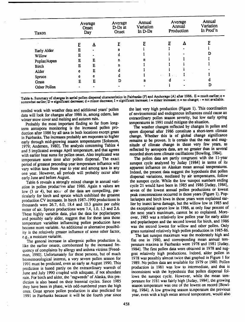
" Average Average Annual Average AnnualOnset D-Ds at Variation Annual Vaflatton

Taxon Day Onset In D-Ds Production In Prod'n

E A F E E A EEarly Alder E - n i I - iWillow E - d I i - D

Poplar/Aspen E E n n i I IBirch E E n I I i IAlder e E d I i i -

Spruce e e d I ,_ I ,, I IGrass E E D n d - dOtherPollen .... i - D

Tableo. Summaryof _anges inaerialpollendispersalcharacteristicsinFalrbanks(10_d ,Mtcho.rage(A),after1986, E = muchearlier;e =somewhatearlier,D = significantdecrease;d = minordecrease;I= significanttnoreue, i = minormca'ease,n = nochange,. = notavailable,

needed work with weather data and additional years' pollen the last very high production (Figure 1). This coordinationdata will took for changes after 1986 in, among others, late of environmental and endogenous influences could cause anwinter snow cover and melting and autumnrain. extraordinarypollen season severity, but low early spring

Probably the most important finding so far from long- temperaturesin 1991could mitigate the situation,term aerospora monitoring is the increased pollen pro- The weatherchanges reflected by changes in pollen andduet.tonafter 1986 by ali taxa in both locationsexcept grass spore dispersal after 1986 constitute a short-termclimatein Fairbanks,The increasesprobablyareresponsesto higher change, Whether Otis is of global change significanceearly throughmid-growing season temperatures [Solomon, remains to be proven, lt is certain that the rate and mag.1979; Andersen, 1980], The analysis concerning Tables 4 nitude of climate change in these very few years, asand 5 implicated average April temperature, and that agrees reflected by aerospora data, are no greater than in severalwith earlierheat sums forpollen onset. Also implicatedwas recordedshort-termclimate oscillations [Bowling, 1984].temperature some time after pollen dispersal. The exact The pollen data are partly congruent with the I l.yearperiod of greatestpreceding-yeartemperature influence will sunspot cycle analyzed by Juday [1984] in terms of itsvary within taxa from year to year and among taxa in any apparent influence on Alaskan mean annual temperatures.one year, However, ali periods will probablyoccur after Indeed, the present data suggest the hypothesis that pollenearly Juneand before August. dispersal variations, mediated by air temperatures, follow

Table 6 reveals a strongly mixed change in annual vari- the sunspot cycle, While the low sunspot numbersendingation in pollen production after 1986, Again n values are cycle 21 would havebeen in 1985 and 1986 [Juday,1984],low (3 or 4), but so_,_,*of the dam are compelling, par. seven of the lowest annual pollen productions or lowestticularly for birch and spruce which exhibited the greatest peak concentrations occurred in those years (Figure 1). Pop-production CV increases, In birch 1987-1990 productions in larlaspen and birch lows in those years were explained ear-thousands were 26.7, 6.0, 18.4 and 10.3 grains per cubic lier by insect larva damage, but the willow low in 1985 andmeter of air. Spruce productions were 7,4, 1.0, 1.3 and 2,6. the exceptional spruce low in 1986, at only four percent ofThese highly variable data, plus the data for poplar/aspen the next year's maximum, cannot be so explained. More-and possibly early alder, suggest that for these taxa those over, 1985 was a relatively low pollen year for early aldertemperature variables influencing pollen production have and poplar/aspen and the second lowest for birch, and 1986become more variable. An additional or alternative possibil, was the seco_adlowest for willow and other pollen. Onlyity is the relatively greater influence of some other factor, grass sustained relatively high pollen production in 1985-86.e.g., a moisture variable. The last sunspot maximum was the moderately high and

The general increase in allergenic pollen production is, fiat one in 1980, and corresponding mean annual tem-like the earlier onsets, corroborated by the increased frc- perature maxima in Fairbanks were 1978 and 1981 [Juday,quency of complaints by allergy and asthma victims [Freed- 1984]. The first pollen data were obtained in 1978 and sug-man, 1990]. Unfortunately for these persons, but of much test relatively high productions. Indeed, alder pollen inbiometeorological interest, a very severe pollen season for 1978 was possibly almost twice that graphed in Figure 1 for1991 must be predicted, even as early as August 1990. This 1989. No pollen data are available for 1979 or 1980. Pollenprediction is based partly on the extraordinary warmth of production in 1981 was low to intermediate, and that isJune and July 1990 coupled with adequate, ii' not abundant inconsistent with the hypothesis that pollen dispersal fol-rain. For birch and alder, the "ragweeds" of Alaska, this pre- lows the sunspot cycle. However, while the mean tem-diction is also based on their biennial cycles. Since 1985 perature for 1981 was fairly high [Juday, 19841,the growing

they have been in phase, with odd-numbered years the high season temperature was one of the lowest on record [Bowl-ones. Great spruce pollen production is also predicted for ing, 1984]. A low growing season teaaperature the previous1991 in Fairbanks because it will be the fourth year since year, even with a high mean annual temperature, would also

458

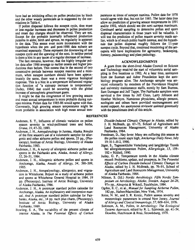
II

haro had mt inhibiting effect on pollen production by birch peratures at times of sunspot numima, Pollen data for 1978and the other woody perennials as is suggested by mo eor- would agree with that, but not for 1981, The latter data titusrelationsin Table4, allow no predictionof growing season temperaturesin 1991

If pollen dispersal follows the sunspot cycle, thtmmare and/or 1992, width should see the next sunspot maxhnum,or less regular increases and decreases in pollen production Continued aerial sampling to determine poUen and sporeand onset day changes should be observed, They are not. dispersal characteristics in those years will be valuable, ltExcept for the probable intz.mally influenced production wIUtest the predictionof pollen season severity made ear.patternsin alder, birchand spruce, no regularityis apparent lier, which is of much public health interest,and the hypoth-in the dam This seems even more inconsistent with the esis tt_ pollen dispersal roughly follows the l l.yearhypothesis when the pre- and post.1986 data subsets are sunspot cycle, Beyond that,continuedmonitoringof the atr-oxaminedseparately,These represent the downswing of one ospora will have implications for agronomy, beekeeping,sunspotcycle andthe upswing of the next. In neitherperiod forestry,palexx_ology and plantpathology,is there a hint in any taxonof a regulardecreaseof increase,

The fact remains, howewr, thatthe highly irrcguiarpol- ACKNOWLEDGMENTSIondata after 1986 averageto earUeronsets andhigher pro-.ductlons than before, This means that in the second of two A grant from the short.lived Alaska Council on Sclcnceconsecutive periods between sunspot maxima and a mini- and Technology enab!ed the start of volumetric aerial sam-mum, when sunspot numbers should have been approx- piing in five locations m 1982, At a later time, assistanceimately the same, there was a more vigorous biological from the Susman and Ashet Foundation kept the acre-response, This is a hint in a temperatureinfluenced vegeta- biology program alive, The Anchorage smnpler was ser-tlon function of "a stairstep increase in temperatures" viced voluntarily by members of the Providence Hospital[Juday, 1984] that could b¢ occurring with the global atm university maintenance staffs, mostly by Sam Btu'ress,increaseof atmosphericgre.enhousogases, Sam DunaganandJeff Tappc, The Fairbankssamplerswere

It might be that the congruence of low growing season serviced a few times by Jeff Conn, Larry Johnson andand mean annual temperaturesis more probableduringsun- Heather McIntyre, Numerous physicians, allergic persons,spot minima. PoUondata for 1985.86 wouldagree with that. ecologists and others have provided encouragement andConversely, high growing season temperatures might be moral support,An anonymous reviewer assisted generouslymerc probable in association with high mean annual tem- with the penultimatedraftof this article,

REFERENCES

Andersen, S, T,, Influcnc_ of climatic variation on pollen Dioxide.lnduced Climatic Changes in Alaska, edited byseason severity in wind-pollinated trees and herbs, J.H. McBeath, pp, 67-75, School of Agriculture andGrana, 19,47-52, 1980, Land Resources Management, University of Alaska i,,

Anderson, J, H., Aeropalynology in Juneau, Alaska. Results Fakbanks, 1984,of the first season's use of a volumetric sampler for aller- Freedman, D,, Hay fever: Many are suffering this season asgenie and other airborne pollen and spores, 33 pp,, (Pho- the pollen count stays high, Anchorage Daily News, Julytocopy), Institute of Arctic Biology, University of Alaska 19: H-l-H-2, 1990,Fairbanks, 1983, J_lger,S,, Tageszeitllche Vertelhmg und langjlthrige Trends

Anderson, J. H., A survey of allergenic airborne pollen and bel allergiekompetenten Pollen, Allergologie, 13, 159-spores in the Fairbanks area, Alaska, Annals of Allergy, 182 + Blldt¢il, 1990.52, 26-31, 1984. Juday, G, P., Temperature Wends in the Alaska climate

Anderson, J. H., Allergenic airborne pollen and spores in record: Problems, update, and prospects, in The PotentialAnchorage, Alat4m, Annals of Allergy, 54, 390-399, Effects of Carbon Dioxide.induced Climatic Changes in1985. Alaska, edited by J, H. McBeath, pp. 76--91, School of

Anderson, J. H., Aeropalynology, allergentcs, and vegeta- Agriculture and Land Resources Management, Universitytion in Whitehorse. Report on a study of airborne pollen of Alaska Fairbanks, 1984.and spores at Whitehorse General Hospital in 1984, 19 Nilsson, S. (Ed.) Nordic Aerobiology. F_fth Nordic Sym-pp. (Photocopy), Ins0tute of Arctic Biology, University posium on Aerobiology, Abisk.o, Sweden, August 24-26,of Alaska Falrbanks, i986. 97+ pp., Almqvist & Wiksell, Stockholm, 1984.

Anderson, J. H., A prototype standard pollen calendar for Ogden, E. C,, et al,, Manual for Sampling Airborne Pollen,Anchorage, Alaska. An explanatory and interpretive man- 182 pp., Hafner/Macmillan, New York, 1974.ual. And A prototype standard pollen calendar for Fair- Reiss, N. M., and S. R. Kostic, Pollen season severity andbanks, Alaska, etc., 14 pp. each plus charts, (Photocopy), meteorologic parameters in central New Jersey, JournalInstitute of Arctic Biology, University of Alaska of Allergy and Clinical.Immunology, 57, 609-614, 1976.Fairbanles, 1989. Solomon, A. M., Pollen, in Aerobiology: The Ecological

Bowling, S. A., The vaJiability of the present climate of Systems Approach, edited by R. L. Edmonds, pp. 41-54,interior Alaska, in The Potential Effects of Carbon Dowden, Hutchimon & Ross, Stroudsburg, 1979.

459

Potential Effects of Global Warming on Calving Caribout

i

WarrenG. EastlandandRobertG. WhiteInstituteof ArcticBiology,Universityof AlaskaFairbank_,Fairbanks,Alaska,U,S.A,

ABSTRACT

Calving grounds of barren-gr0und caribou (Rang(fer tarandus) are often in theportion of their range that remains covered by snow late into spring, We propose

' that global warming would alter the duration of snow cover on the calving groundsand the rate of snowme! t, and thus affect caribou population dynamics. The ration-ale for this hypothesis is based upon the following arguments. For females of thePorcupine Herd, one of the few forages available before and during early calvingare the inflorescenees of cotton grass (Eriophorum vagmatum), which are verydigestible, high in nitrogen and phosphorus, and low in phenols and acid-detergentfiber. The nutritional levels of the inflorescences are highest in the early stages ofphenology and decline rapidly until they are lowest at seed set, about 2 weeks afterbeing exposed from snow cover. The high nutritional level of cotton grass inflor-escences is important to post-paturient caribou attempting to meet nutritionalrequirements of lactation while minimizing associated weight loss. The pattern ofweight regain in summer is important to herd productivity as female body weight atmating influences conception in late summer and calving success in.spring. There-fore, temporal changes in snowmelt may have major effects on nutritional regimesof the female.

INTRODUCTION NUTRITIONALEFFECTSONPlasticityin timingof calvingis a possibleadaptationto CARIBOUPRODUCTIVITY

environmentalchanges suchas temporalchangesin snow- Caribouproductivityis dependentupon rates of preg-melt; however,suchadaptationmaybe quite limited,as tim- nancyand calf survival,both of whtchare dependentuponing of mating in caribou is temporally controlled.This female nutritional levels. One of the primary forages ofsuggests that small changes in snowmeltbecauseof global calvingcaribouis infloresceneesof the tussock.formingcot-warmingcouldhavemultiplicativeeffects on the nutritional tongrass, Eriophorumvaginatum(Figures2,3) [Lent, 1966;regime of the caribou,affectingfemale fecundity,survival Kuropat and Bryant, 1980; Kuropat, 1984]. Immediatelyof calvesand,therefore,herdproductivity, after release from snowcover,Eriophorum inflorescences

Date of snowmeltacrossthe arctic is earlierthaa in the begin to elongate (Table 1). Nutritional levels of intor-past (Figure 1) [Foster, 1989],but it is uncertainwhether eseencesare highestat the onset of elongationand declinethis is attributableto changes in global climate or natural steadilyuntil seed set [Kuropat,1984],whichoccurs withinweather cycles. Timing and duration of snowmelt are of 10day_.Cariboucan takeadvantageof this high-nutritiol,great potential importanceto caribou (Rangifer tarandus forageby calvingin areas of extendedsnowmelt[Fleckandgranti) herdproductivitybecauseit influencesthe timingof Gunn,1982; Eastlandet al., 1989]. Following snowmelt,emergenceand abundanceof forageplantsfor pregnantand earlyfloweringlegumesconstitutean importantdietarypro-lactatingfemales, tein sourcewhich is followedby rapidlyexpandingwillow

460

l_ves(Figure2),Plantbiomassincreasesmarkedlywhichmaxim'Izesfoodintake[WhiteandTrudoll,1980]andcar.

8NOWMELT& POPULATION ibou rapidlychangetheir diet throughoutsummerto take176- 200 advantageof nowgrowthof othervascularplantfoliageaslt

E_A_TEnISLANOSNOWMELr j, becomesavailable,ltlgh levelsof nutritionresult in peak

,7o /_"-"/,Fo,,,r ,uar, / _ milk productionimmediately post calving and, as a con.

/ \ ESTiMATEOPCRPo_,/ 150- se,quence,calf growthrate is maximized[White andLuick16,I " \ \ _ _ 1976, 1984; Rognmo et al,, 1983; Skogland, 1984; White,z 1990], A high body weight of weaned calves enteflng winter

Female caribouam loss likely to conceive unl_ they

:2,51_--_---2---7 'V _..,._=___/ _o_o regainwelght,lostduringwlnt_and ¢ady lactation,In

_. orderto me.t a minimum threshold forconception [Thomas,, o 1982; Reimers, 1983; White, 1983; White andLuick, 1984;

1950 1960 1970 1960 1990 Skogland, 19851Tyler, 1987; tenvik et al., 1988; CameronYEAR et al,, 1991], Therefore thepaRom of post-calving mammal

weight gain is irr,portant, Maximized weight gains through.Figure1, Dat_of completetmowmeltatBarterIsland,Alaskaand out the summer by "plmnological chasing" by caribou instzoof the PorcupineCaribouHard(PCH),Snowmoltdata to 1984 Arctic Alaska has been suggested frequently [Klein, 1970,from Foster[1989],Openoirolesarequestionabledata,solid cir. 1982; Kuropat and Bryant, 1980; White and Trudoll, 1980;¢losrepresentsystematloestimates, White et al., 1981; Kuropat, 1984]; and lt involves fol-

June July Augusti ii i i i i _

WILLOW 50E I '1Ga//x pu/chra % 0

E50

GRAMINOIDS 5o_Floral Parts % 0

Er/ophorum vag/natum 50

Po/2gon/um b/s/orta Leaf Parts ......... _=,,_

Oxytrop/s ma/dell/ana Floral Parts .................

Floral Parts ....Lup/nus arct/cusLeaf Parts ...............

LICHENS % o _7_2.,,'_- .<.z_(Assumed Use)

50

" EClU/setum spp, % o "-- ,5O

_ ._ I I

June July August

Figure2. Relativeamountsof variousforagespeciesusedbycaribouinspringandsummermonths.FromKuropat[19M,Figure3, p.40].

461

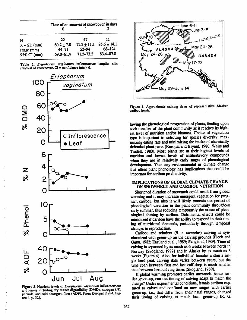
Time afterremovalof snowcover in days __,,---June 6-II

0 1 2 ' _¢___dune 5-8

N 22 47 11 "__i _ _''"_c_'cc'_cL_X+ SD (mm) 60.2 + 7.8 72.2+11.1 85.6+ 14.1 ....range(mm) 44-71 52-94 68-124 _ ,_Z,_;_t-_oy 24-2695% CI(mm) 59.0-61.4 71.2-73.2 83.4-87.8 May 24-26-_-,_ _ CANADA

removalof snowcover.CI= confidenceinterval. ,,.._, ,

Eriophorum

'00180 va_inatum..... IM_ay 29.dune ,4 '__J

__ 60 Figure4. Approximatecalvingdatesof representativeAlaskancaribouh=ds.

o 40lowing the phenological progressionof plants, feeding upon

o_ each memberof the plant community as it reaches its high-

2o F [[ _ est level of nutritionand/or biomass. Choice of vegetation

0 I n f Iore $ce n ce type is important to selecting for species diversity, max-0 , • Le o f imizing eating rate and minimizing the intake of chemically

,,, defendedplantparts [KuropatandBryant, 1980; White andTmdeU, 1980]. Most plants are at their highest levels of

6 r" nutrition and lowest levels of antiherbivory compoundswhen they are in relatively early stages of phenological

4 development. Taus any environmental or climate changeZ ["C__ _ thataltersplant phenology has implications that could be

importantforcaribouproductivity.

O_ 2 IMPLICATIONS OF GLOBAL CLIMATE CHANGE° ON SNOWMELT AND CARIBOU NUTRITION

0 Shorteneddurationof snowmelt could result from globalwarmingand it may increase emergentvegetation for preg-nant caribou, but also it will likely truncate the period of

-- [0 r- phenological variation in the plant community throughout

0 [ early summer,thus reducing temporarilythe extent of phen-t,- ological chasing by caribou. Detrimental effects could beCD¢" 5 I--I minimized if caribouhave the ability torespond in their tim-

t3 [_ ing of nutritional demands, particularlythrough temporalchanges in reproduction.

0 Caribou and reinde_'.z(R. t. tarandus) calving is syn-chronized with green-up on the calving grounds [Fleck andGunn,1982; Eastlandet al,, 1989; Skogland, 1989].Time of

Lt_ 40 [-_ calving is separatedby as much as 6 weeks between herds inNorway [Skogland, 1989] and in Alaska by as much as 3

C3 _ weeks (Figure 4). Also, for individual females within a sin-

<_ 2 0 gle hardpeakcalving date varies betweenyears, but thetime span between fast and last calf-drop is much smaller

O_ 0 I , I [ _ thanbetween-herdcalving times [Skogland, 1989].If global warming promotes earliersnowmelt, hence ear-- Oun dU [ A U g lier green-up,canthetimingof calvingadaptto matchthe

change?Underexperimentalconditions,femalecariboucap-Figure3.Nutrientlevelsof Eriophorwnvaginatwnintlorescencesandleavesincludingdrymatterdigestibility(DMD),nitrogen(N), turedas calvesand conrmedon new rangeswith earlierphenols,andaciddetergentfiber(ADl:).FromKuropat[1984,Fig- green-up, i.e., that differ from their natal ranges, changedure5, p. 52]. their timing of calving to match local green-up [R. G.

462

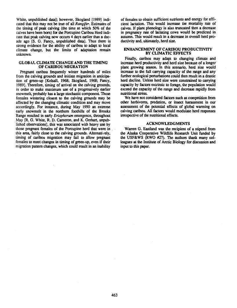
White, unpublished data]; however, Skogland [1989] indi- of females to obtainsufficient nutrients and energy foreffi-cated thatthis may not be trueof ali Rang_fer. Estimatesof cient lactation. This would increase the mortality rate ofthe timing of peak calving (the time at which 50% of the calves. If plant phenology is also mmcated then a decreasecalves havebeen born)for the PorcupineCaribouHerdindi- in pregnancy rate of lactatingcows would be predictedincate that peak calving now occurs 4 days earlier thana dec- autumn.This wouldresult in a decrease in overall herdpro-ade ago [S. G. Fancy, unpublished data]. Thus there is ductivity and, ultimately,herdsize.strong evidence for the ability of caribouto adapt to localclimate change, but the limits of adaptation remain ENHANCEMENT OFCARIBOUPRODUCTIVITYunknown. BY CLIMATIC EFFECTS

Finally, caribou may adapt to changing climate andGLOBAL CLIIVIATECHANGE AND THE TIIVIING increase herdproductivityand herdsize because of a longer

OF CARIBOU MIGRATION plant growing season. In this scenario, herd size wouldPregnant caribou frequently winter hundreds of miles increase to lhc full carrying capacity of the range and any

from the calving groundsand initiate migrationin anticipa- furtherecological perturbationscould then resultin a drastiction of green-up [Kelsall, 1968; Skogland, 1968; Fancy, herd decline. Unless herdsize were constrainedto carrying1989]. Therefore, timing of arrivalon the calving grounds, capacity by factors extrinsic to forage, the populationwouldin order to make maximum use of a progressively earlier exceed the capacity of the range and decrease rapidly fromsnowmelt, probablyhas a large stochastic component.Those nutritionalstress.females wintering closest to the calving grounds may be We havenot consideredfactors such as competition fromaffected by the changingclimatic condition and may move other herbivores, predation, or insect harassment in ouraccordingly. For instance, during May 1990 an extreme assessment of the potential effects of global warming onearly snowmelt in the northern foothills of the Brooks calving caribou. Ali factors would modulate herdresponsesRange resulted in early Eriophorum emergence, throughout irrespectiveof the nutritionaleffects.May [R. G. White, R. D. Cameron, and K. Gerhart,unpub-lished observations], this was associated with heavy use by ACKNOWLEDGMENTSthose pregnant females of the Porcupine herdthat were in WarrenG. Eastlandwas the recipient of a stipend fromthis area, fairly close to the calving grounds. Alternati,_,ely, the Alaska Cooperative Wildlife Research Unit fundedbytiming of caribou migration may fail to allow pregnant the USF&WS (RWO #:27). The authors thank many col-females to meet changes in timing of green-up, even if their leagues at the Instituteof Arctic Biology for discussion andmigrationpatternchanges, which could result in an inability input to this paper.

463

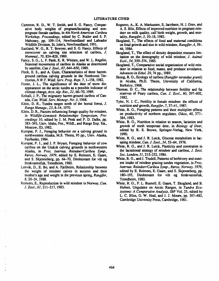
LITERATURE CITED

Cameron,R. D., W. T. Smith, and S. G. Fancy, Compar- Rognmo, A., K. A. Markussen,E. Jacobsen, H. J. Gray,andalive body weights of pregnant/lactating and non- A.S. Blix, Effects of improvednutritionin pregnantrein-pregnantfemale caribou,in 4rhNorth American Caribou deer on milk quality, calf birth weight, growth, and inor-Workshop, Proceedings, e.zfitedby C. Butler and S.P. tality,Rang_er,3, 10-18, 1983.Mahoney, pp. 109--114, Newfoundland and Labrador Skogland, T., The effects of food and maternalconditionsWildlife Division, SL John's,Newfoundland, 1991. on fetal growthand size in wild reindeer,Rang_fer, 4, 39-

Eastland, W. G., R. T. Bowyer, and S. G. Fancy, Effects of 46, 1984.snowcover on calving site selection of caribou, J. Skogland,T., The effect of density dependent resource lira-Mammal., 70, 824--828, 1989. itation on the demographyof wild reindeer, J. Animal

Fancy, S. G., L. F, Pank, K. R. Whitten,and W. L. Regelin, Ecel,, 54, 359--374, 1985.Seasonal movements of caribou in Alaska as determined Skogland, T., Comparativesocial organizationof wild rein.by satellite, Can J. ZooL, 67, 644-.650, 1989. deer in relation to food, mates, and predator avoidance,

Fleck, E. S., and A. Gunn,Characteristicsof three barren- Advances in Ethel. 29, 74 pp., 1989.ground caribou calving grounds in the Northwest Tea- Skoog, R. O., Ecology of caribou(Rang_fertarandus granti)ritories,N.W.T. Wildl. Sere. Prog. Rept. 7, 1-158, 1982. in Attska, Ph.D. Thesis, University of California,

Foster, J. L., The significance of the date of snow dis- Beakei_y,1968.appearanceon the arctic tundraas a possible indicatorof Thomas, D. C., The relationship between fertility and fatclimate change,Arct. Alp. Res., 21, 66-70, 1989. reserves of Peary caribou, Can. J. Zaol., 60, 597--602,

Kelsall, J. P., The migratorybarren-groundcaribouof Can- 1982.ada, Can. Wildl. Serv. Monogr. No. 3, 1968. Tyler, N. J. C., Fertility in female reindeer: the effects of

Klein, D. R., Tundra ranges north of the boreal forest, J.Range Manage., 23, 8-14, 1970. nutritionand growth, Rangifer, 7, 37--41, 1987.

Klein, D. R., Factors influencingforage qualityforre,indeer, White, R. G., Foraging patternsand their multipliereffectsin Wildlife--Livestock Relationships Symposium, Pro- on productivity of northernungulates, Oikos, 40, 377-ceedings I0, edited by J. M. Peek and P. D. Dalke, pp. 384, 1983.383-393, Univ. Idaho, For., Wiidl., and Range Exp. Sta., White, R. G., Nutritionin relation to season, lactationandMoscow, ID, 1982. growth of north temperate deer, in Biology of Deer,

Kuropat, P. J., Foraging behavior on a calving ground in edited by R. E. Brown, Springer-Vealag, New York,northwesternAlaska, M.S. Thesis, 95 pp., Univ. Alaska, 1990.Fairbanks,1984. White, R. G., and J. R. Luick, Glucose metabolism in lac-

Kuropat,P. J., and J. P. Bryant, Foraging behavior of cow taringreindeer, Can. J. Zool., 54, 55-64, 1976.caribou on the Utukok calving grounds in northwestern White, R. G., and J. R. Luick, Plasticity and constraints inAlaska, in Prec. Internat. Reindeer/Caribou Syrup., the lactationalstrategy of reindeer and caribou, J. Zool.Reros, Norway. 1979, exfitedby E. Reimers, E. Game, Soc. London,51,215-232, 1984.and S. Skjenneberg,pp. 64--70, Direktoratetfor vilt og White, R. G., and J. Trudeil,Patternsof herbivoryandnutri-ferskvannsfisk, Trondheim, 1980. ent intake of reindeer grazing tundra vegetation, in Prec.

Lenvik, D,, E. Be, and A. Fjellheim, Relationship between internat. Reindeer/Caribou Syrup.,R¢ros, Norway. 1979,the weight of reindeer calves in autumn and their edited by E. Reimeas, E. Gaare,and S. Skjenneberg,pp.mother's age and weight in the previous spring, Rang_fer, ,180-195, Direktoratet for vilt og ferskvannsfisk,8, 20--24, 1988. Trondheim, 1980.

Reimers, E., Reproduction in wild reindeer in Norway, Can. White, R. G., F. L. Bunnell, E. Gaare, T. Skogland, and B.J. Zool., 61, 211-217, 1983. Hubert, Ungulates on Arctic Ranges, in Tundra Eco-

systems: A Comparative Analysis, IBP Vol. 25, editedbyL. C. Bliss, O. W. Heal, and J. J. Moore, pp. 397-483,CambridgeUniversity Press, Cambridge, 1981.

464

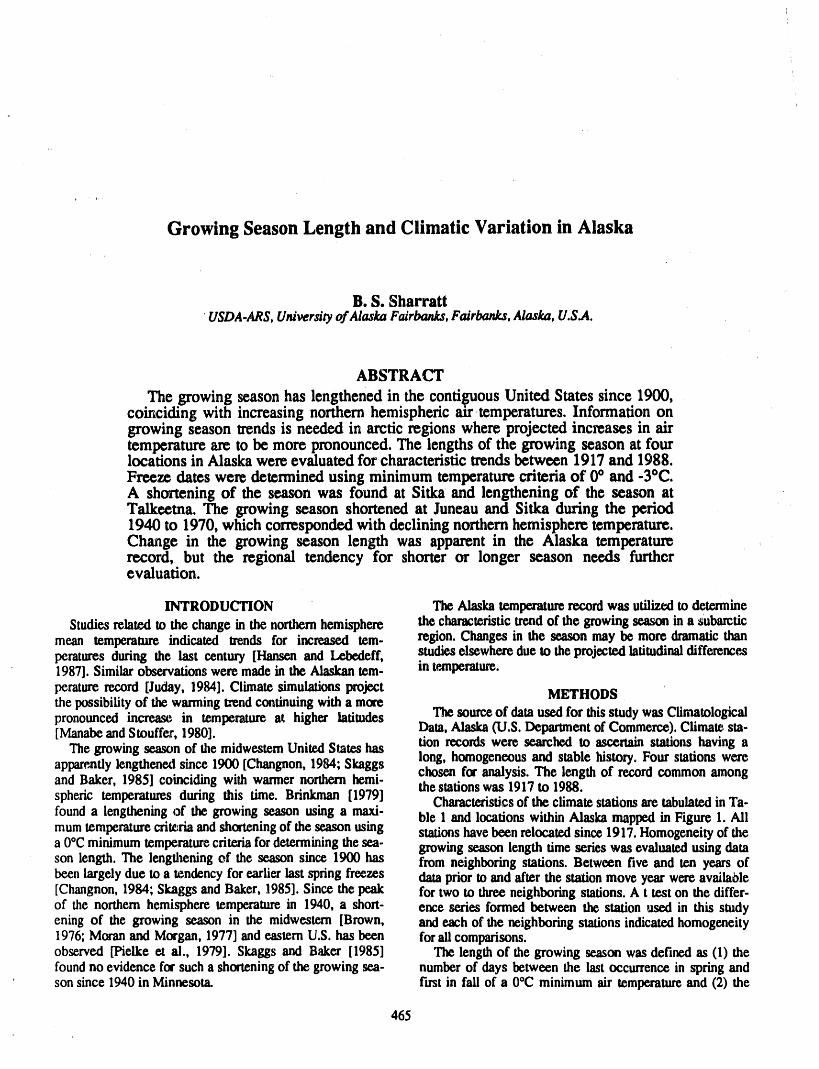
Growing Season Length and Climatic Variation in Alaska

B. S. SharrattUSDA-ARS, Universityof Alaska Fairbanks, Fairbaaka, Alaska, U.S.A.

ABSTRACT

Thegrowingseasonhaslengthenedin the conti.guousUnitedStatessince1900,coincidingwithincreasingnorthernhemisphericatrtemperatures.Informationongrowing seasontrendsisneeded in arcticregionswhere projectedincreasesin airtemperaturearetobe more pronounced.The lengthsof thegrowing seasonatfourlocationsinAlaskawere evaluatedforcharacteristictrendsbetween 1917 and 1988.

Freeze dateswere determinedusingminimum temperaturecriteriaof 0° and -3°C.A shorteningof theseason was found at Sitkaand lengtheningof the season atTalkeetna.The growing season shortenedat Juneau and Sitkaduringthe period1940 to 1970,which correspondedwithdecliningnorthernhemispheretemperature.Change in the growing season lengthwas apparentin the Alaska temperaturerecord,but the regionaltendency for shorteror longer season needs furtherevaluation.

INTRODUCTION The Alaska temperaturerecord was utilized to determine

Studies related to the change in the nortbernhemisphere the characteristictrendof the growing season in a subarcticmean temperature indicated trends for increased tem- region. Changes in the season may be more dramaticthanperatures during the last century [Hansen and Lebedeff, studies elsewhere due to the projected latitudinaldifferences1987]. Similar observationswere made in the Alaskan tem- in temperature.

pcraturerecord [Juday, 1984]. Climate simulations project METHODSthe possibility of the warmingtrendcontinuing with a morepronounced increase in temperature at higher latitudes The sourceof dataused for this study was Climatological[ManabeandStouffer, 1980]. Data, Alaska CO.S.Departmentof Commerce).Climate:sta-

The growing season of the midwestem United States has tion records were searched to ascertain stations having along, homogeneous and stable history. Four stations wereapparentlylengthened since 1900 [Changnon, 19PM;Skaggs

and Baker, 1985] coinciding with wanner northern hemi- chosen for analysis. The length of record common amongthe stations was 1917 to 1988.spheric temperatures during this time. Brinkman [1979] Characteristicsof the climate stations arc tabulated in Ta-found a lengthening of the growing season using a maxi- ble 1 and locations within Alaska mapped in Figure 1. Alimumtemperaturecrite;riaand shortening of the seasonusing stationshave been relocated since 1917. Homogeneity of thea 0°C minimumtemperaturecriteriafordeterminingthe sea- growing season length time series was evaluatedusing datason length. The lengthening of the season since 1900 has from neighboring stations. Between five and ten years ofbeen largely due to a te.ndencyforearlierlast spring freezes datapriorto and after the station move year were availa/)le[Changnon, 1984; Skaggs and Baker, 1985]. Since the peak for two to threeneighboring stations. A t test on the differ-of the northern hemisphere temperaturein 1940, a short- ence series formed between the station ssed in this studyening of the growing season in the midwestem [Brown, andeach of the neighboring stations indicatedhomogeneity1976; Moran and Morgan, 1977] and eastern U.S. has been forali comparisons.observed ['Pielke et al., 1979]. Skaggs and Baker [1985] The length of the growing season was defined as (1) thefound no evidence for such a shortening of the growing sea- number of days between the last occurrence in spring andson since 1940 in Minnesota. first in fall of a 0°C minimum air temperature and (2) the

465

/

/

//

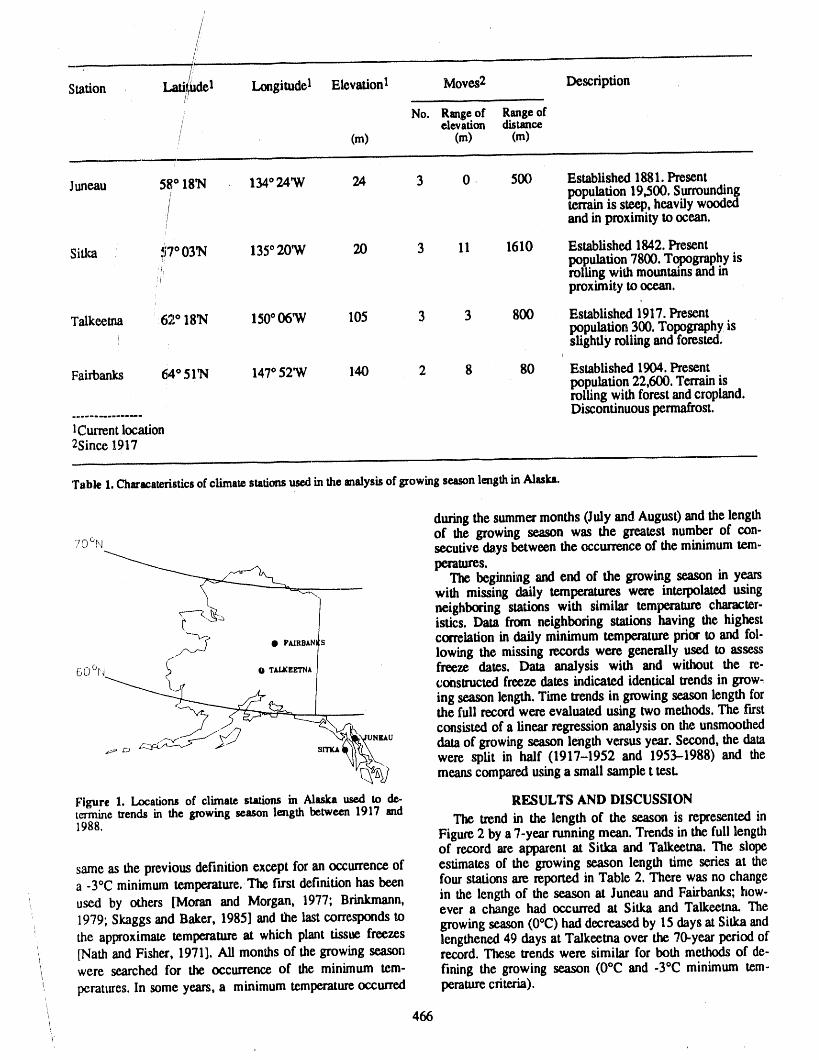
Station de1 Longimdel Elevation1 Moves2 Description

, No. Rangeof Rangeofelevation distance

/ (m) (m) (m)

Juneau 58° 18'N 134° 24'W 24 3 0 500 Established 1881. Present

population 19,500. Surroundingierrainis steep, heavily woodedand in proximityto ocean,

/

Sitka _7°03_1 135° 203V 20 3 11 1610 Established 1842. Presentpopulation 7800. Topographyisrolling withmountainsandinproximity to ocean.

i

Talkeema =62° 18_N 150° 06W 105 3 3 800 Established 1917. Presentpopulation 300. Topographyis

! slightly rollingand forested,

Fairbanks 64° 51'N 147°523V 140 2 8 80 Established 1904. Presentpopulation 22,600. Terrain isrolling with forestandcropland.Discontinuous permafrost.

1Currentlocation2Since 1917

Table1.Characateristicsofclimatestationsusedintheenalysisof growingseasonlengthinAlaska.

duringthe summermonths (July and August) and the lengthof the growing season was the greatest number of con-

/0%J secutive days between the occurrenceof the minimum tem.

__:__ peratures.

The beginning and end of the growing season in yearswith missing daily temperatures were interpolated using

_ / neighboring stations with similar temperaturecharacter-istics. Data from neighboring stations having the highest_-_? , F_SB,.N_s correlation in daily minimum temperatureprior to and foi-

l

l lowing the missing records were generally used to assess

6c_i_._ or,.tr,_,' freeze dates. Data analysis with and without the re-constructedfreeze dates indicated identical trendsin grow-

ing season length. Time trendsin growing season length for

consisted of a linearregression analysis on the unsmoothed_-_':___YJ sm_,,_u"_'u"_u dataof growing season length versus year. Second, the data

"_ -'_I_-_\. were sprit in half (1917-1952 and 1953-1988) and themeans comparedusing a small sample t test.

Figure 1. Locationsofclimatestationsin Alaskaused ta de- RESULTS AND DISCUSSIONterminetrendsin the growingseasonlength between1917 and The trend in the length of the season is represented in1988. Figure 2 by a7-year runningmean. Trendsin the full length

of record are apparentat Sitka and Talkeetna. The slope

same as the previous definition except foran occurrenceof estimates of the growing season length time series at thea -3°C minimum temperature.The first definition has been four stations are reported in Table 2. There was no changeused by others [Moran and Morgan, 1977; Brinkmann, in the length of the season at Juneau and Fairbanks; how-' ever a change had occurred at Sitka and Talkeetna. The

, 1979; Skaggs and Baker, 1985] and the last corresponds to growing season (0°C) had decreased by 15 days at Sitka andt

the approximate temperature at which plant tissue freezes lengthened 49 days at Talkeema overthe70-year period ofi [Nath and Fisher, 1971]. Ali months of the growing season record.These trends were similar for both methods of de-l of the minimum tem- the (O°C and -3°C minimum tem-were searched for the occurrence fining growing season

_ peratt,'es. In some years, a minimum temperatureoccurred peratarecriteria).i

i466

'/

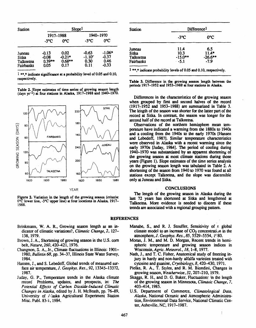
Sration Slope1 Stailon Difference1

1917-1988 1940-1970 .3oC OoC.3°C 0°C -3°C 0°C

Juneau 11.4 6.5Juneau -0.13 0.02 -0.63 .1.06" Sitka 10.3 11.4"Sitka -0.08 -0.21' -1.10_ -0.37 Talkeema -15.0"* -26.6**Talkeema 0.39** 0.68** 0.30 0.46 Falrbanks -5.1 -7.9Fairbanks 0.05 0.17 0.11 -0.33............ 1**,, indicateprobabilitylevelsof 0.05and0.10,respectively.1 **,*indicatesignificanceataprobabilitylevel of0.05 and0.10,

respectively. Table 3. Differencein the growingseason length betweentheperiods1917-1952and1953--198gat fourstationsin Alaska.

Table 2.Slope estimatesof timeseriesof growingseasonlength(daysyr"t)at fourstationsin Alaska,1917-1988and1940-1970.

Differences in the characteristicsof the growing seasonwhen grouped by fast and second halves of the record

__ (1917-1952 and 1953-1988) are summarizedin Table 3.220 The ldilgth of the season was shorterfor the latterpartof the12o record at Sitka. In contrast, the season was longer for the

\\/,..,\..,,,..,...,.,.., second half of therecordatTalkeema..-. / _8o_ Observations of the northern hemisphere mean tem-

9o./"i,1/ ..,\,/ ,..,..,,,"' \ /'"> " ' /"J ', .. peraturehave indicateda warming from the 1880s to 1940s<

_ _ '

oZ 60 1 FAIRBANKS 140_ \'/'V" \,./" [ andanda_eff,coolingfrom1987].thesimilar1940stOtemperaturetheearly 1970Scharacteristics[Hansenwere observed in Alaska with a recent warming since the

_ _ 240_/_ early 1970s [Juday, 1984]. The period of cooling during

12o 1940-1970 was substantiated by an apparent shortening ofz_ the growing season at most climate stations during those

_-_°c_9o i J'"',_KE_./.... ,..,... ZOO] / ,\_. ;.,,,...v,,].,.,, onYears(Figure I). Slopeestimatesof the time seriesanalysiSthegrowingseasonlengthwastabulatedinTable 2. A,,"'",, ..,.,/'" shorteningof theseasonbom 1940to 1970was foundatall60 ,/ , ''J ,6o[ " , _-_'v{_"U] stations except Talkeema, and the slope was discernible1920 ' 1950 1980 1920 1950 19S0 onlyatJuneauandSitka.

YEAR CONCLUSIONSThe length of the growing season in Alaska during the

Figure2. Variationin the lengthof the growingseason(criteria: last 72 years has shortened at Sitka and lengthened at0°C lowerline,-3°Cupperline) atfourlocationsin Alaska,1917- Talkeema. More evidence is needed to discern if these1988. trendsareassociated with a regional grouping pattern.

REFERENCESJ

Brinkmann,W. A. R., Growing season length as an in- Manabc, S., and R. J. Stouffer, Sensitivity of _ globaldicator of climatic variations?,Climatic Change, 2, 127- climate model to an increaseof CO2concentratl,_min the138, 1979. atmosphere,J. Geophys. Res., 85, 5529-5554, 1_'80.

Brown,J. A., Shorteningof growingseason in the U.S. com Moran, J. M., and M. D. Morgan, Recent trends in hemi-belt, Nature, 260, 420-421, 1976. spheric temperature and growing season indices in

Changnon, S. A., Jr., Climate fluctuationsin Illinois: 1901- Wisconsin, Agric. Meteorol., 18, 1--8, 1977.1980, Bulletin 68, pp. 34-37, Illinois State WaterSurvey, Nath, J., and T. C. Fisher, Anatomical study of freezing in-1984. jury in hardy and non-hardyalfalfa varieties treatedwith

Hansen, J., and S. Lebedeff, Global wends of measuredsur- cytosine andguanine, Cryobiology, 8, 420-430, 1971.face air temperature,J. Geophys. Res., 92, 13345-13372, Pielke, R. A., T. Styles, and R. M. Biondini, Changes in1987. growing season, Weatherwise, 32,207-210, 1979.

Juday, G. P., Temperature trends in the Alaska climate Skaggs, R. H., and D. G. Baker, Fluctuation_ _n the lengthrecor_ Problems, updates, and prospects, in: The of the growing season in Minnesota, Climatic Change, 7,Potential Effects of Carbon Dioxide-Induced Climatic 403--414, 1985.Changes in Alaska, e&ted by J. H. McBeath, pp. 76-89, U.S. Department of Commerce, Climatological Data,University of /,,laska Agricultural Experiment Station Alaska, National Oceanic and Atmospheric Administra-Misc. Publ. 83-i, 1984. lion, EnvironmentalData Service, National Climatic Cen-

tea,Asheville, NC, 1917-1987.I

467 i

Ecological Aspects in Construction of West Siberian Oil Field Surface Facilities

I. D. Scvortzov and P. N. CrushinStateScientific-ResearchandDesignInstituteof Oiland GasIndustry,GIPROTYUMENNEFTEGAS,Tyumen,U.S.S.R.

ABSTRACT

The exploitation of arctic regions, where permanently frozen grounds are wide-spread, leads to problems concerning the climate and the geo-cryological environ-ment. One of the most urgent tasks is to minimize effects on the environment,otherwise irreversible, catastrophic processes, the deterioration of permafrost intoswamps, fouling subsoil waters and rivers, ground surface pollution with petroleumproducts, and destruction of fish and birds, may occur.

The measures aimed at providing the environmental ecological equilibrium dur-ing the exploitation of the northern oil deposits of West Siberia are described in thispaper. These measures are worked out during the design stage. Then appropriateengineering decisions and product procedures are chosen, where much prominenceis given to reliability of the oil and gas field facilities.

The paper includes information about developing measures for the preventivesystematic maintenance of the oil pipelines, maintenance schedule, prediction ofaccidents and certain procedures for their rectification.

468

The Effects of Geographical Latitude on the Dynamics of Medical Data

I. v. Naborovisr MoscowMedicalInstitute,GTK,Moscow,U.S.S.R.

T, K. BreusInstituterf SpaceResearch,Moscow,U.S.S.R.

ABSTRACTPolarregionsplayanincreasingsocialandeconomicroleinhumanlife.ltis

alsoknownthattheyarenotthemostfavorableplacesforhumanbeingstolive.Therearesomeexampleswhichshowthatthefrequencyandseriousnessofdiffer-entillnessesincreaseswiththeincreasinggeographicallatitude.Inthenorthernregionsseasonalamplitudesofillnessesarenotablyincreasing.Atthesametimeitwasfoundthatthehigherthelatitude,thehigherthedegreeofsolaractivityinflu-enceonanumberofillnesses,suchascardiovascularandnervediseases,reachingitsmaximum levelataurorallatitudes.Suchgeographicaldistributionsofsicknessratehaveareasonableexplanation.Inaurorallatitudestheinfluenceofcorpuscularradiation(solarwind)ontheEarth'smagnetosphereanditselectrodynamicsisdem-onstratedvividly.Investigationofsimilarinfluenceson biologicalobjectsinpolarregionswithintheprogram"GlobalChange"isnecessaryandmay alsoincludeotherphysicalorsocialfactors.Insuchcasesmedicalemergencydataplayaroleinthesc_chforbiotropicexternalinfluences.

469

The Commons Game: A Lesson in Resources Management

Carla A. KirtsSchool ofAgriculture and Land Resources Management, University ofAlaska Fairbanks, Fairbanks, Alaska, U.S.A.

Mark A. TumeoDepartment of Civil Engineering, University of Alaska Fairbanks, Fairbanks, Alaska, U.S.A.

ABSTRACTThe Commons Game was developed to demonstrate behavioral patterns in-

volved in individual decision-makingregardingcommons propertyand it has beenused in various psychology courses. In this study the game was used to teach uni-versity students the complexities and frustrations of managing commons propertynaturalresources. More specifically the purpose of the study was twofold: to de-termine the extent to which the game, when used in a natural resources man-agement context, meets the teaching objectives of the game as specified by thegame's developer; and to determine whether the game is an effective teaching tool.

The sample population was composed of 36 students enrolled in ALR_QS 193during the Spring 1989, Fall 1989, and Spring 1990 semesters. The team-taughtcourse contains three elements: an introductory lecture, the game, and a postgameanalysis session. Data were obtained from students' opinions of instruction, contentanalyses of students' three- to five-page essays, and observations recorded duringthe postgame analysis/discussion session. A brief description of the game is in-eluded in the paper, but details are intentionally omitted because the game is copy-righted.

The game met its teaching objectives when used in a natural resources man-agement context and in combination with an introductory lecture and postgameanalysis session. Topics discussed in student essays were the best evidence that thegame met the objectives of producing an understanding of social trapping andillustrating trust versus greed. Frustration with the social dilemma was evident ac-cording to faculty observations made during the game conferences and throughoutthe postgame analysis session. From the students' opinions of instruction, the gameappears to be an effective teaching tool. Students rated the game as a valuablelearning experience. From a faculty perspective, the game provides an accurate, r(alistic model of natural resources management and is an effective instructional tool.

Further study is warranted to determine the actual decision-making patternsplayers use in trying to solve the game's dilemma. Associating these patterns ofplay with real world resource decision-making patterns would be an ultimate goal.

INTRODUCTION Its creators "sought a more experiential approach to teachingThe Commons Game [Powers et al., 1983] was de- about social traps" [Powers, 1985/86, p. 3]. lt has been used

veloped to demonstrate behavioral patterns involved in in psychology classes and analyzed from severalindividual decision,making regarding commons property, perspectives [Powers and Boyle, 1983; Powers, 1987]

470

including its effectiveness in promoting students' under- three E's of natural resources management (ecology,standing of the commons dilemma [Powers, 1985/86; Kitts economics, and emotions), and who manages natural re-et al., 1991]. In this study the Commons Game was used to sources in the United States; andteach university students the complexities and frustrations of .concepts pertaining to the commons such as historicalmanaging commons property natural resources, perspectives, the need for management, population ef-

For purposes of this study, "commons property natural re- fects, the role of technical fixes [Hardin, 1968], in-sources" were defined as natural resources which, in theory, dividual rights versus responsibilities, and examples ofare "owned" by everyone but, in reality, "owned" by no one. commons resources and issues.Examples include air, oceans, sunshine, and public lands The postgame discussion outline includes topics such assuch as national parks andnational fcrests. Most often, these trust, greed, individual versus social decision-making, ef-resources are exploited due to human greed and lack of in- fects of uncertainty, the role of reward and incentives/centives to act otherwise [Hardin, 1968; I-Iaefele, 1974; motives, goal perception, values, and application of theHardin and Baden, 1977; Cutter et al., 1985].Effective man. game to the real world of resources management. To cul-agement of public domain resources, particularly on aglobal minate the experience,, students are required to prepare ascale, will be a major concern for future generations. This is three- to five-page essay explaining their final thoughts andespecially evident in light of recent efforts to enhance public conclusions regarding the commons dilemma.participation in decision-making processes affecting public Data were obtained from students' opinions of in-domain natural resources management, struction, a content analysis of essays, and observations

made by faculty during the postgame discussion session.PURPOSE OF THE STUDY The opinion-of-instruction survey was instructor designed.

The purpose of the study was twofold: to determine the Students were asked to place an "X"on a continuum labeledextent to which the CommonsGame, when used in a natural at the end-points from 0 to 10 to indicate his/her rating ofresources management context, meets the teaching ob- nine statements related to the course. Essays were gradedjectives of the game as specified by the game's developer, according to 10 elements, each worth a possible four points:and to determine whether the game is an effective teaching neatness, organization, content documentation, grammar,tool. According to Powers [1985/86], the objectives of the errors, conciseness, analysis, logic/support, and generalgame are: effect.

•to produce an understanding of the social trapping char- Only descriptive statistics are reported in this paperacter of a commons, i.e., that short-term, individual gain because the participants were "captive" and not randomlytends to dominate long-term collective gain; selected [Tuckman, 1978], class sizes varied substantially

•to illustrate the importance of trust when one's gains are (from 4 to 19), and trends instead of comparisons were thedependent not only on what one does but also on what focus of the study. Ali data analyses were performed using aothers do; and Macintosh PC with StatWorks software.

•to allow students to experience the difficulties and frus-trations of attempting to solve the commons dilemma THE GAME---HOW IT IS PLAYEDwith only a small amount of control over others' actions The Commons Game is copyrighted. This description(p. 5). will not contain details such that the game could be repli-

cated. A copy of the game may be purchased from Dr.METHODOLOGY Powers (see References).

The sample population was composed of students en. Ali rules are given via prepared scripts. Four- to six-rolled in Agriculture and Land Resources/Environmental person groups make concealed, individual plays of coloredQuality Science (ALR/EQS) 193--Commons Property cards representing various managementoptions one can ira.Resource Decision Making---duringthe Spring 1989, Fall pose on the commons (Table 1). Points are aw_ded to1989, and Spring 1990 semesters (N=36), at the University individual playersaccording to the card played and its sub-of Alaska Fairbanks. ALR/EQS 193 is a freshman-level sequentvalue (or penalty) derived from the rules or a payoffcourse designed to acquaint students with concepts and matrix developed to represent the currentstate _f the com-issues associated with management of commons property mons (Table 2). As the commons is threatened, the payoffnaturalresources. The course is team-taughtby an environ- matrix reflects fewer point gains, thus indicating loweredmental engineer and a natural resources edu,'.ator,worth one productivity. The more times the exploitation card is played,semester credit, and scheduled to permit three-hour class the faster the payoffs for both exploitation and cooperativesessions, use decline. The state of the commons may be improved by

The course contains three elements: an introductory lec- playing the resource enhancement card, but rehabilitationture, the game, and a postgame discussion session. The occurs more slowly than exploitative decline.three-hour lecture includes: Players are told to accumulate the maximum number of

•definitions (including relationships between and among) points and that the player with the highest number of pointsof natural re.,_urce, management, conservation, and will receive $5. The words "win" or "winner" are never usedcommons; by the game directors. Players are also told the game will

•fundamental management concepts including the con. continue for 60 rounds; however, the game is stopped at 50servation philosophy continuum, the basis of man- rounds to offset possible end-effects such as last-minuteagement, natural resources classification, ecosystems hoarding.and "ecological balances," carrying capacity, sustained Periodic three-minute conferences are allowed during theyield, the tyranny of geography [Bennett, 1983], the game. The group may change any rules of the game with the

471

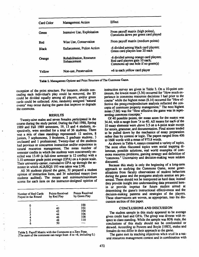
CardColor ManagementActic_t Effect

Green IntensiveUse, Exploitation Frompayoff matrix(high points),• Commonsdown per,green card play_

Red Wise Use, Conservation Frompayoff matrix (mediumpoints)

Black Enforcement,Police Action -6 dividedamongblack card players;Greencardplayerslose 20 each

Orange Rehabilitation,Resource -6 divided amongorangecardplayers;Enhancement Red cardplayersgain 10each; ,

Commons upone hole if no green(s)

Yellow Non-use, Preservation +6 to each yellow cardplayer

Table1. ManagemmtOptionsandPointStructureofTheCommonsGame.

exception of the point structure.For instance, shields con- instructionsurvey are given in Table 3. On a 10-pointcon-cealingeach individual's play could be removed, the $5 tinuum,the lowest mean (3.36) occurredfor "Howmuchex-could be divided equally among ali phyers, and/or green perience in commons resomr.esdecisions I had prior to thecards could be collected. Also, randomlyassigned "natural course"while the highest mean(8.14) oc.ctmcdfor "Howef-events" may occur duringthe game that improveor degrade fective the postg_me/posflectureanalysis reflected the con-thecommons, cepts of commons propertymanagemenL"The next highest

, mean (7.86) was for "How effective the game was in repre-RESULTS sentingcommons concepts."

Twenty-nine males and seven females participatedin the Of 40 possible points, the.mean score for the essays wascourseduring the studyperiod. Duringthe Fall 1988, Spring 34.44, with a range from "_4to 40. Ali means for each of the1989 and Fall 1989 semesters, 19, 13 and 4. students, re- 10 essay elements were Above3.5 on a 4.point scale exceptspectively, were enrolled for a total of 36 students.There forerrors,grammar,and documentation.Final scores tendedwas a mix of class standings represented: 12 seniors, 8 to be pulled down by the mechanics of essay preparationjuniors,7 sophomores, 3 freshmen, 2 graduatestudents, 3 ratherthan by content or logic. The papers ranged from406unclassed and 1 professional. Twenty-four of the studet_ts to 1668 wordswith a mean of 975.8 words.had previous or concurrent instructionand/or experience in As shown in Table 4, essays contained a variety of topics.natm'al resources management. The mean number of The most often discussed topics were social trapping di-semester credits in which the studentswere concurrently en- lemmas, possible solutions, real world examples of com-rolled was 13.49 (a full-time semester is 12 credits) with a mms resources problems, gaming strategy and definition of3.10 semester grade point average (GPA)on a 4-point scale. "commons."Uncertaintyand decision-making were seldomTheir university-career,cumulative GPA up throughthe se- discussed.mesterin which ALR/EQS 193 was takenwas 2.98. Because this study is only the beginning of a long-term

Ali 36 students played the game, 32 prepareda student approach to studying the Commons Game, some goner-opinion of instructionform, and 34 submitted essays (two alizations from faculty observations of student behaviorsstudents audited). The means and minimum/maximum during the game and the postgnme analysis session are pre-scores for each item on the instructor-designed opinion of sentcA. These should not be interpretedas hard data; instead

they provide insight into understanding data presented here-in or provide impetus for future studies aimed atdetermining the game's instructional effectiveness and the

NumberofRedCards PointsReceived PointsReceived decision.making patterns and strategies of the players.Playedin theRound by RedPlay ' by GreenPlay These observationsare woven, as appropriate,into the dis-

cussion section of this paper.o -- 1001 40 102 CONCLUSIONS AND DISCUSSION2 42 1043 44 106 The student sample in this study appearedto be average4 46 108 given credit load and GPA. The group was diverse with re-5 48 110 spect to class standing. While the sample was 80% male, the

_- 6 50 .... conclusions of this study should not be confounded orskewed. According to Powers and Boyle [1983], males and

Table2. PayoffMatrixwiththeCommonsat a Z_o S_te: females do not differ in their approach to the game.(Thestateof thecommonscanrangefrom-8to +Is,including0.) The game met its teaching objectives whe_nu_zd in a nat-

uralresources managementcontext and in combinationwith

472

Statement Mean* Min/Max

How muchknowledge of mural resources I had prior to this course 5.64 1.0/9.0How muchexperienceinnaturalresourcesmanagementI hadpriortothiscourse 4.25 0.0/10.0How much know!edge of commons resources I had priorto this course 4.45 0.0/9.0How much experience incommons resourcesdecisions I had priorto this course 3.36 0.0/9.0How much effortI put into this course comparedto my other courses 5.40 1.0/9.0Howmuch this course challenged me 6.75 3.0/10.0How much I learnedfrom this course 7.37 2.0/10.0How effective the game was in representing commons concepts 7,86 1.5/10.0How effective the postgame/postlectureanalysisreflected the concepts of commons

propertymanagement 8.14 5.0/10.0

*Basedon a10-pointcontinuum.

Table3. Meansandminimum/maxlmumscoresfortheStudentOpinionof Instruction.

an introductory lecture and postgame analysis session. Top- commons improves and the temptation for defaultingon theics discussed in student essays were the best evidence that agreed cooperative arrangement increases. At this point,the game met the objectives of producingan understanding players personally experienced the frustration and complex-of social trapping and illustrating trust versus greed. Frustra- ity of managing a commons.tion with the social dilemma, the third teaching objective, Ending the game at 50 rounds, rather than the 60 playerswas evident according to faculty observations made during were initially told, provides an excellent means of avoiding

an end-effect. Several teams specifically planned for_e endthe game conferences and throughout the postgame analysis of the game and plans tended to reflect a "catch-as-catch-session, can" or "every-man-for-himself"attitude, regardless of the

In every postgame discussion session, students made per- state of the commons. The next generation was seldom con-sonal reference to the frustration and futility of trying to siderecLFurther studies designed to allow one team to beginsolve the commons problem without everyone's coop- where a previous team left off may more realistically sim-eration. General observations support Powers' [1987] con- ulate long-term management. Long-term vision was not aclusion that communication (i.e., conferencing) tends to popular topic in student essays or during the analysis ses-improve cooperation for a while; however, this study sions, while on the other hand, the dilemma of managingrevealed that communication may break down as the commons resources revolves around providing for the next

generation.Another method of providing a time persiw, tive is to

begin the game at a randomly selected starting point--notTopic Frequency* always at zero, a somewhat steady state. After all, most

commons are in trouble because they are not in a steady

Socialtrappingdilemma(individualversussociety) 24 state. Therein lies the management problem.Possiblesolutionstocommonsmanagement 24 From the student opinions of instruction, the game ap-Realworldexamplesof commonsresourceproblems 21 pears to be an effective teaching tool. Students had little ex-StrategyusedtoplayThe CommonsGame 19 perience or knowledge of commons resources managementDefinitionof"commons" 17 and decision.making and, on the student opinion of in-Overpopulationandcarryingcapacity 14Humangreedversustrust 14 struction, rated the game as a valuable learning experience.Individualfightsandfreedom 14 From a faculty perspective, the game provides an ac-Goalof resourcemanagement 10 curate, realistic model of natural resources management andLong/shorttermvisionandplanning 9 is an effective instructional tool. The original objectives ofConceptof "winning" 8 the game can be met when the game is used in a naturalUncertainty 4Decisionmaking 2 resources management context and in conjunction with an................ introductory lecture and postgame analysis. Further study is*N=34;meannumberof topicsperessay,5.35 witha rangeof 2-9. warranted to determine the actual decision-making patterns

players use in trying to solve the game's dilemma.

Table4. Numberof essayscontainingselectedtopics. Associating these patterns of play with real world resourcedecision-makingpatternswould be an ultimategoal.

473

REFERENCES

Bennett,C. F.,ConservationandManagementofNatural Powers,R. B.,The commons game:TeachingstudentsResources in the United States, John Wiley & Sons, New about social dilemmas, Journal of Environmental Educa-York, 1983. tion, 17, 4---10,1985/86.

Cutter,S. L., H. L. Renwick, and W. H. Renwick, Exp/oita- Powers, R. B., Bringingthe commons into a large universitytion, Conservation, Preservation: A Geographic Per- classroom, Simulation and Games: An Internationalspective on Natural Resource Use, Rowman& Allanheld, Journal, 18, 443-457, 1987.Totowa, NJ, 1985. Powers, R. B., and W. Boyle, Generalization from a com-

Haefele, E. T. (Ed.), The Governance of Common Property mms-dilemma game: The effects of a free option,Resources, Johns Hopkins University Press, Baltimore, information, and communication on cooperation and1974. defection, Simulation and Games: An International Jour-

Hardin,G. J., The tragedy of the commons, Science, 162, nal, 14, 253-274, 1983,1243-1248, 1968. Powers, R.B., R. E. Duro;,andR. S. Norton,The commons

Hardin, G. J., and J. Baden (Eds.), Managing the Commons, game. Unpublished numuscript(research version), UtahW. H.Freeman& Co., SanFrancisco, 1977. StateUniversity, Logan, 1983.

Kirts, C. A., M. A. Tumeo, and J. M. Sinz, The commons Tuckman, B. W., Conducting Educational Research, Newgame: Its instructionalvalue when used in a natuiul re- York: HarcourtBraceJovanovich, 1978.sources m_na_ment context, Simulation and Gaming:An Internationac Journal of Theory, Design, and Re- Note: A copy of The Commons Game may be purchasedsearch, 22_5--18, 1991. from Dr. Richard Powers at P.O. Box 307, Oceanside, OR

97134.

474

II' , ,

Section E:

Ice Sheet, Glacier and PermafrostResponses and Feedbacks

Chaired by

M. MeierUniversityof Colorado

U.S.A.

F. RootsEnvironment Canada

Canada

State and Dynamics of Snow and Ice Resources in the Arctic Region Derived fromData in the World Atlas of Snow and Ice Resources

Vladimir M. Kotlyakov and Natalya N. DreyerInstituteof Geography,U.S.S.R.Academyof Sciences,Moscow,U.S.S.R.

ABSTRACT

The compilation of the World Atlas of Snow and Ice Resources has been inprogress in the Soviet Union for more than 15 years. The effort ranks as one of themost important glaciological projects ever undertaken because of its com-prehensiveness and global scope. Several hundred of the most prominent scientistsin the U.S.S.R., including 300 specialists from 40 research institutions, participatedin the work. The United Nations Educational, Scientific and Cultural Organization(UNESCO) and many other researchers from many nations provided broad sci-entific assistance to tile compilers of the Atlas by compiling various datasets, ana-lyzing maps, and giving advice. The Atlas is a major contribution of the U.S.S.R. tothe Hydrological Programme (II-lP) and will also be presented by the Soviet Unionto the International Geosphere-Biosphere Programme (IGBP), because manyparameters associated with change in the cryosphere are included. The Atlaspresents, in a systematic arrangement, comprehensive data and information aboutthe global distribution of snow and ice, compiled since the early 1950s. The Atlasincludes about 1000 maps, ranging in scale from 1:25,000 (local or individualglaciers) to 1:90,000,000. The maps in the Atlas are distributed throughout the 17subject sections.

INTRODUCTION processes,therebydeterminingthe developmentof the sys-The objectiveof the World Arias of Snow and Ice tem and its interactionswith the environment.Separate

Resourcesis to showtheglobaloccurrenceof snowand ice, componentsof a glacio-nivalsystem,forexampleglaciersincludingali types of glacio-nivalphenomena,the var- andsnowcover,mayformindependentsystemsand maybeiabilityof these phenomenain the past,their present.day mappedas such.

Glacio-nivalsystems,and glaciersystemsas a specificregime,anda meansforpredictingtheirfuturedevelopment case, can be characterizedby a cartographicrepresentation[Koflyakov,1976]. thatincludesseveralfundamentalpmameters,in whichthe

The majorityof regionsincludedin theAtlasarelocated generalizedconceptof the distributionof this or thatchar-ateitherhighaltitudesor in thepolarregions,wherethe dis- acteristicof thesystemcan be appliedto a specificregion.tributionof stationsis inadequateand fieldstudiesarelim- The patternsremaincontinuousdespitethe discretenatureited.Comprehensiveresearchwasconductedthroughoutthe of the points of occurrencefromwhichtheyarecomputedprocess of compilation,and several new computational and graphicallyplotted. The cartographicrepresentationmethodsweredevelopedto determinesnowand ice param- presentsa certainabstraction,structuredaccordingto objec-eters,especiallyin thecharacterizationof thenatureof inad- five rules;it emphasizesthe regularitiesof glaciersystemsequatelystudiedregionsOf mountainglaciers.The methods causedby the impactof continuouslydistributedprocesses,werebasedon theconceptof glacio-nivalsystemsadvanced such asclimatic factors,butexcludesthe influenceof ran-recentlyin theU.S.S.R.[KotlyakovandKrenke,1979]. dom,discretefactors,suchas orographicsetting.

A glacio-nivalsystemis a naturalsystemin whichsnow The mainpeculiarityof glacio-nivalobjects is the wideand ice play a dominantrole in its composition and rangein theirspatialdimensions.The prevalenceof small,

477

separatelylocated mountainglaciers and their occurrencein entireregion. The maximum snow storage is mainly deter.small areascaused us to develop different waysof depicting mined by the annual amount of frozen precipitation.Thethemon maps of different scales, including the alre_.dymen- values of snow storage exceed 35--40 cm of water equiv-tioned cartographicrepresentationof glaciersystems, alent only in the crestal zones, while in the internalValleys,

Quantitative as well as qualitative properties of phe. screened by the lateral ranges, where a thin snow covernomena are depicted On small-scale maps in the Atlas. forms,the snow cover thickness is only 15--20cm.Quantitativecharacteristicsmake up the basic content of ali The main regularityin the distributionof maximum snowthe maps, plotted with the use of isolines of temperatures, storage is the decrease when moving from the ocean orprecipitation, snow cover, and runoff. Maps of ice- windwardslope within a mountain massif, and insignificantformation zones, factors associated with avalanche occur- increase with elevation. The altitudinal gradient does notrence, former glaciated areas, permafrost, and mudtlow exceed 5-15 mm of waterequivalent for 100 m. Snow stor-activity depict qualitativeproperties.On some maps qual. age on the windwardslopes usually exceeds snow storageitative categoriesare singled out on the basis of numerical on the leewardslopes by 5-15 cm of waterequivalent.features.Examplesare:thedegreeofavalancheactivityin Thedominatinganticyclonicregimeoftheweatheriritherelationtothedensityofanavalanchenetworkandrecur- winterproducesa minimumyear-m-yearvariabilityofsnowrenceinterval;thenatureofglacierfluctuationswithrespect storage,when comparedwithallothersystems.The vari-tothemagnitudeofglacierterminusfluctuations;andpre- ationcoefficientchangeswithinlimitsof0.15--0.30,andthevailingandaccompanyingtypeofglaciers,includingrefer, meansquaredeviationofsnowstoragefromthemeanIong-encetotherelationshipofglaciersofdifferenttypes,all termvaluesmostfrequentlymakesup only2--6cre.Theexpressed as percentages, duration of the existence of this type of systems is large, on

Rather than discuss maps in ali 17subject sections of the the order of 200-300 days. The variations of the conditionsAtlas, we shall address only three representative sections, of formation and disa_e of snow cover in mountainincluding maps of snow cover, total runoff and meltwater regions are insignificant, reaching 1.5 months only in therunoff, and snow and ice storage. This will demonstrate highest and most humid areas. The latitudinal trend in thegraphically the resource-estimating objectives of the Atlas. change of snow resources' properties is insignificant.

Moving to the south of the polarregionproper,it is worthSNOW COVER MAPS mentioning thatsnow systems of the northerncoastal moun-

To compensate for the paucity of initial data, methods of tains of we,stem and eastern margins of the continent_aregrapho-analytiealcomputationsof the macroscale fields of widespread within the Alaska Range, and the Wrangell,the norms of snow storage and geographo-statistical com- Chugach, and St. Elias Mountains of Alaska and mountain-putation methods of the main properties of snow resources ous regions of Iceland and Scandinavia in northwesternhave been worked ouL Europe. These mountains are located along paths of intense

On the basis of joint interpretationof maps of the maxi- maritimecyclones; thus the amount of frozen precipitationmum waterequivalent content of snow cover, the properties is much greaterhere when compared with previously men-of its time variability, includingdurationof and conditions tioned regions in more continental locations. In the moreassociated with snow cover existence, it becamepossible to southern parts of the mountains, combined with the heatingcharacterize snow systems of the earth [Getker and effect of the nearby ocean, the range of duration of coldlvanovskaya, 1989]. In this paper we would like to analyze period can vary; therefore the maximum snow storage canthe peculiarities of snow systems which exist in polar vary within wide limits. The greatest amount of annualregions and "adjacentregions, snowfall---more than 400 cm water content equivalent--

In the permanent snow systems of Antarctica and higher accumulates in the mountains of southeastern Alaska, and inelevations of Greenland, snow accumulation occurs this region the areas of extreme snow accumulationare verythroughout the year, although annual snowfall amounts extensive. The role of the latitudinal factors in the dis-decrease when moving inland from the coastal areas. Maxi- tribution of snow storage over the coastal windward slopesmum snow storage (expressed in water content equivalent) is insignificant. Thus, at latitude 60*N, on the Aleutianvaries from 20 mm in the interior regions of Antarctica to Ridge and on the western slopes of mountain ranges on700 mm in the coastal mountains of western Antarctica and Vancouver Island, at latitude 49°N, the range of altitudinalsouthwestern Greenland. The annual variability of snow changes of the maximum snow storage is the same, 100-130accumulation in the inland areas is not large; the coefficent eta. Latitudinal zonation is completely manifested only inof variation Cv is 0.2-0.4, with values of norms up to 0.4- the intermontane highlands. The altitudinal gradient of snow0.5, the latter the result of the frequent passage of cyclones, accumulation in the near-crestal zone produces an increase

Snow systems of the northern continental mountains in the annual total up to 10-40 cm for each additional 100membrace ali the mountainous areas of the Arctic and sub- in elevation. The year-to-year variability of the maximumarctic and mountain ranges in the northern part of the tem- snow storage grows abruptly: Cv changes from 0.2 up toperate belt, including those situated under conditions of 0.5, decreasing when moving inland away from the coastextreme continental climate. Typical snow systems are and with decreasing elevation.located in the Brooks and Mackenzie Mountains, on Elles- The dm'ation of snow cover also lengthens with incw.,as.mere Island, the Verkhoyanskiy Range, Byrranga and Cher- ing elevation, from 150 days to a full year (.perennialsnow).sky Mountains, and in the polar Ural mountains. Well- The minimum values are observed at the lower elevations ofpronounced temperature inversions are formed in the lower the "warmest" western coasts, while the maximum valueszones of these mountains; because of the duration of the are located in the accumulation areas of major glaciercold period of 240--330 days varies very little ali over the systems.

478

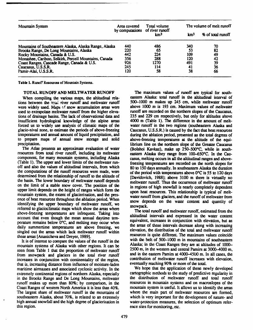
MountainSystem Areacovered Tonalvolume The volume of meltrunoffby computations of riverrunoff

km3 km3 %of totalrunoff

Mountainsof SoutheasternAlaska,AlaskaRange, Alaska 440 486 340 70BrooksRange, De Long Mountains,Alaska 220 65 53 82Rocky Mountains,Canada& U.S. 442 224 109 49Monashee,Cariboo,Selkirk,Percell Mountains, Canada 356 288 120 42Coast Ranges,CascadeRange, Canada& U.S. 926 1270 491 39Caucasus,U.S.S.R. 245 114 41 36Pamir.Alai,U.S.S.R. 120 58 38 66

Table1. RunoffResourcesof MountainSystems.

TOTAL RUNOFF AND MELTWATER RUNOFF The maximum values of runoff are typical for south-When compiling the various maps, the altitudinal vela- eastern Alaska: total runoff in the altitudinal interval of

tions between the _c_ dyer runoff and meltwater runoff 500-1000 m makes up 245 cm, while meltwater runoffwere widely used. Maps wf snow accumulationareas were above 1000 m is 193 cm. Maximum values of meltwaterused to extrapolatemeltwaterrunoff from the highereleva- runoff are recordedon the northernslopes of the Caucasus,tions of drainagebasins. The lackof observationaldataand 235 and 229 cm respectively, but only for altitudes aboveinsufficient hydrological knowledge of the alpine areas 4000 m (Table 1). The difference in the amount of melt-forced us to widely use analysis of climatic maps of the water runoff in the two regions (southeasternAlaska andglacio-nival zone, to estimate the periods of above-freezing Caucasus, U.S.S.R.) is causedby the fact thatheat resourcestemperaturesand annualamountof liquid precipitation,and during the ablation period, presented as the total degreesofto prepare maps of annual snow storage and solid _ above-freezing temperaturesat the altitude of the equi-precipitation, librium line on the northernslope of the GreaterCaucasus

The Atlas presents an approximateevaluation of water (Bolshoi Kavkaz), make up 250-500°C, while in sough-resources from total river runoff, including its meltwater eastern Alaska they range from 100--650°C. In the Cau-component, for many mountain systems, including Alaska casus, melting occurs in ali the altitudinalrangesandabove..(Table 1). The upperand lowerlimits of the meltwaterrun- freezing temperaturesare recordedon the north slopes foroff and also the values of altitudinalintervals, from which 80 to 150 days annually. In southeasternAlaska thedurationthe computations of the runoff resources were made, were of the period with temperaturesabove 0°C is 55 to 120 daysdeterminedfrom the relationshipof runoff to the altitudeof [Davidovich, 1988]; above 3100 m there is virtually nothe basin. The lower boundaryof meltwaterrunoff depends meltwaterrunoff. Thus the occurrenceof meltwater runoffon the limit of a stable snow cover. The position of the in regions of high snowfall is nearly completely dependentupper limit depends on the height of ranges which form the upon heat resources. This relationship is typical of melt-mountain system, the extent of glacierization, and the pres- waterrunoff fromglaciers, andthe runoffof meltwater fromence of heat resom'cesthroughoutthe ablationperiod.When snow depends on the water content and quantity ofidentifying the upper boundary of meltwater runoff, wereferredto glacioclimatic mapswhich show the areaswhere snowpack.The total runoffand meltwater runoff, estimated from theabove-freezing temperatures are infrequent. Taking into altitudinal intervals and expressed in the water contentaccount that even though the mean annual daytime tem-peratureremains below 0°C, and melting may occur when equivalent, increases in conjunction with elevation, but asdaily summertime temperatures are above freezing, we the areas of these intervals decrease along with increasingsingled out the areas which lack meltwater runoff within elevation, the distribution of the tonaland meltwater runoffthese areas [Ananichevaand Dreyer, 1989]. resources is quite different. The maximum values coincide

It is of interest to comparethe values of the runoffin the with the belt of 500-i000 m in mountainsof southeasternmountain systems of Alaska with other regions, lt can be Alaska; in the Coast Ranges ,.heyare at altitudes of 1000-seen from Table 1 that the proportionof meltwaterrunoff 2500 m, in the westem and centralPamirs at 3000-4000 m,from snowpack and glaciers in the total river runoff and in the eastern Pamirs at 4000-4500 m. In ali cases, theincreases in conjunction with confinentality of the region, contribution of meltwater runoff increases with elevation,that is, increasing distancefrominfluence of moisture-laden eventually reaching90% or more of the tonal.maritime airmasses and associated cyclonic activity. In the We hope that the application of these newly developedextremely continentalregions of northernAlaska,especially cartographicmethods to the study of predictive regularityinin the Brooks Range and De Long Mountains, meltwater the distribution of meltwater runoff and total runoffrunoff makes up more than 80%; by comparison, in the resources in mountain systems and on macroslopes of theCoast Ranges of western NorthAmerica it is less than40%. mountainsystem is useful, lt allows us to identify the areasThe largest share of meltwater runoff in the mountainsof where the main part of meltwater resources are formed,southeasternAlaska, about 70%, is related to an extremely which is very importantfor the development of nature-andhighannual snowfall and the high degree of glacierizationin water-protectionmeasures, the selection of optimum refer-this region, ence sites formonitoring,etc.

479

SNOW AND ICE STORAGE glaciefization,volume of glacier ice, specific values of melt-Glacio-nival resources are representedmost completely water from glaciers, and maximumsnow storage, the mean

on the Arias mapsof glaciological zonationand ice storage, thickness of gla_iers, extent of glaciexiz_tion, and the timeStep-by-step zonation of the entire world, including small- interval for ice mass throughoutthe mountains, are shownscale zonation of the earthand medium-scale zonation of on the mapof southeasternAlaska foreach region.particularareas is included in the Atlas. lt is significant for The contentof the mapspresentedandseveralothermapsgeography in generaland is based on a combinationof ore- in the WorldAtlas of Snow and Ice Resourcesmake it pus.graphic, hydrological, and glaciological approaches. The sible to describe numerically the role of precipitationin the

largest mountain-glacier regions of the Northern Hemi-zonationapproach allows us to betterunderstandglaciolog- sphere. Theimportantrole of liquidprecipitationin the heatical peculiaritiesof the earthand to organize the computa- balance of n'awitimeglaciers has been established. Depen-lion of snow and ice resources in specific mural regions dence of global changes in snowfall on the processes of[Koflyakovand Dreyer, 1984]. ' a_mospheric circulation has also been established: the

The maps of natural ice storage on scales from growth of snowiness in the northern and southern hemi-1:1,500,000 to 1:7,500,000, accompanied by summation spheres is related to the prevailing meridional types of cir-tables, give the general idea of the total areas and volumes culation, and its decrease is linked to the zonal type ofof glaciers, the volumes and specific values of their annual circulation. Computations have shown that heat losses onmeltwaterrunoff, and seasonal snow cover and the date of the meltingof seasonal snow cover make the rateof alines-its maximum areal distributionin each of the regions. Dm'- pheric heating threetimes slower than expected, while ore-ing compilationof the maps, evaluationsof mean thickness graphic conditions play a decisive role in the developmentof glaciers in various glacierizedbasins were carried out in of mountainglaciers.conjunction with computationsof the time interval (cycle) The compilation of the mapsof the WorldAtlasof Snowof ice mass throughoutglaciers, an importantindex of gla- and Ice Resources has been completed: Ali maps are nowcier resources, being published in Moscow and in Kiev. Although the vol-

The areaand volume of glaciers and sea ice and specific ume of maps is large,we hope thatthe Atlas will be releasedvalues of maximum snow storage are depicted on the map in 1993 and contribute to a better understandingof globalof the Arctic in water content equivalent. The areas of changeoccurringinglacio-nival phenomenaon earth.

REFERENCES

Ananicheva, M. D., and N. N. Dreyer, Kartograficheskiye Kotlyakov, V. M., Zadachi sozdaniya Allasa snezhno-metody issledovaniya talogo snegovogo i lednikovogo ledobykhresursov mira [']'hemain objectives in creatingstoka gornykh stran [Cartographicmethods of studying the WorldAtlas of Snow and Ice Resom.ces],VestnikANsnow melt and glacier runoff from mountain systems], SSSR, 10, 95-100,1976.Data of Glaciological Studies (DGS), 67, 49-55, 1989. Kotlyakov, V. M., and N, N. Dreyer, Glavniye itogi tabor

Davidovich, N. V., Tepliviye resursy perioda ablyatsii v nad Atlasom snezhno.ledovykhresursovmira [The mainkrupneishikhgorno-lednikovykh stranakh vnepolyarnykh results fromcompilation of World Atlas of Snc",and Iceshirot [Heat resources during the ablation period of the Resources],DGS, 51, 89-95, 1984.largestmountain-glacier systems in non-polarlatitudes], Kotlyakov, V. M., and A. N. Krenke, Nivalno-glyarsialnyeDGS, 64, 134-145, 1988. sistemy Pamirai Gissaro-Alaya [Glacio-nivalsystems of

Getker, M. I., and T. E. Ivsnovskaya, Snezhniy poksov v the Pan'firsand Gissar-Alai], DGS, 35, 25--33, 1979.g0mykh systemakh Zemli (opyt ldassif'tkatsii) [Snowcever in the Earth'smountain systems], DGS, 67, 30-38,1989.

480

//

1

\

Mass Balance of Antarctica and Sea Level Change

s

C. R. BentleyGeophysical and Polar Research Center, University of Wisconsin-Madison, Madison, Wisconsin, U.S,4.

M. B. GiovinettoDepartment of Geography, University of Calgary, Alberta, Canada

ABSTRACT

The overall mass b',dance of the Antarctic ice sheet has been estimated by com-parison of the best available data on input in the form of snowfall with output in theform of ice flux through gates at or near the margin of the ice sheet. Surface melt isa negligible contributor to mass balance and has been ignored. Bottom melt underlarge ice shelves remains a major source of uncertainty. We conclude that there isprobably an excess input of 2-25% of the total input, equivalent to a sea level low-ering of 0.1-1.1 mm yr-1. Although errors remain, it becomes increasingly clearthat an antarctic contribution to current sea level rise is unlikely. We attribute areported iceberg flux that is larger than the mass input to a non-equilibrium break-back of the fronts of the ice shelves.

INTRODUCTION (grounded) ice; systems entirely on an ice shelf, and com-In this paper we have combined ali the informationwe bined systems thatinclude both inland andice shelf ice but

could f'mdabout the net mass balanceof the Antarcticice without memurements at the grounding line. The mostsheet. The approachwe have used is to comparemass input desirablemeasurementin regard to sea level change wouldvalues with correspondingmass output values where both include output flux precisely across a grounding line. inare known,andthento extrapolateto therestof the ice sheet actuality, output is usually measured either some distancein severalways. inlandof the groundingline or at or near the front of an ice

We have used primarilythe nomenclature,mass inputs, shelf. In the lattercase, some interpretationof the regimenand areas of drainage systems given by Giovinetto and of the ice shelf, particularlythe rate of bottom melting, isBentley [1985], modified in minor ways. Values for mass necessaryin orderto estimate the net mass balance inlandofinputs and areas cited without reference are from this the grounding line. The ice shelf systems are, of course,source. Those mass inputs are, we believe, themost accurate irrelevantfor the direct determination of sea level change(as well as the smallest) estimates available for reasons since they are already in the ocean, but they are includedgiven by Giovinetto and Bentley [1985], Oiovinetto and became measurements on ice shelves are an aid to inter-Bull [1987], and Giovinetto et al. [1989]. However, differ- preting the thirdtype of system wherein theoutput is knownences between compilations are not great in most places, only at the,frontof an ice shelf.and where other authors have estimated net mass balances Many geographic names are cited in whis section--toofor particu_r drainage systems (or parts of systems) we many to show on a small map. Ali can be approximatelyusually have used their estiraateswithout modification.The located by the drainage systems in which they occurone majordifference from Giovinetto and Bentley [1985] is (Figures 1-4).in theLambertGlacier drainagebasin, forreasonsexplainedbelow. Inland Ice Only

See Table 1and Figure2.BALANCE MEASUREMENTS Jutulstraumen (in system K°A). The outflow is from Van

In this section the observations are summarized in three Autenboer and Decleir [1978]. The input was found bygroups: systems with input and outflow on the inland multiplying the total estimated input for the encompassing

481

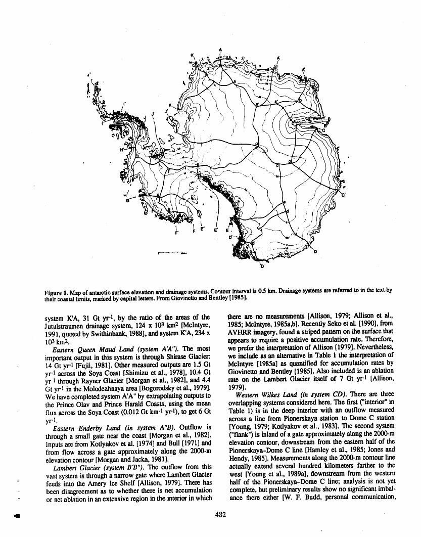
Figure 1. M._ of antarcticsurfaceelevation and &ain_e systems. Contourintervalis 0.5 km. Drainagesystems arereferredto in thetext bytheircoastal limits, markedby capital letters.FromGiovinettoend Bentley [1985].

system K'A, 31 Gt yr-l, by the ratio of the areas of the there arc no measurements [Allison, 1979; Allison ct al.,Jutulstraumcn drainage system, 124 x 103 km2 [Mclntyrc, 1985; Mclntyr¢, 1985a,b]. Recently Seko ct al. [1990], from

1991, quoted by Swithinbank, 1988], and system K'A, 234 x AVHRR imagery, found a stripcxl pattern on the surface that103km2. apgw.arsto requirea positiveaccumulationrate.Therefore,

Eastern Queen Maud Land (system A'A"). The most we prefer the interpretation of Allison [1979]. Nevertheless,important output in this system is through Shim_ Glacier: we include as an alternative in Table 1 the interpretation of14 Gt yr-1 [Fujii, 1981]. Other measured outputs arc 1.5 Ot lVtclntyrc [1985a] as quantified for accumulation rates byyr-I across the Soya Coast [Shimizu etal., 1978], 10.4 Gt Giovinetto and Bentley [1985]. Also included is an ablationyr-I through Rayner Glacier [Morgan ct al., 1982], and 4.4 rate on the Lambert Glacier itself of 7 Gt yr-I [Allison,Gt yr-1 in the Molodezhnaya area [Bogorodsky ct al., 1979]. 1979].We have completed system A'A" by extrapolating outputs to Western Wilkes Land (in system CD). There are threethe Prince Olav and Prince Harald Coasts, using the mean overlapping systems considered here. The fu-st ("interior" in

flux across the Soya Coast (0.012 Gt km-I yr-l), to get 6 Gt Table 1) is in the deep interior with an outflow measured

yrl, acrossa line fromPionerskayastation to Dome C stationEastern Enderby Land (in system A"B). Outflow is [Young, 1979; Kotlyakov et al., 1983], The second system

through a small gate near the coast [Morgan ct al., 1982]. ("flank") is inland of a gate approximately along the 2000-mInputs are from Kotlyakov et al. [1974] and Bull [1971] and elevation contour, downstream from the eastern half of thefrom flow across a gate approximately along the 2000-m Pionerskaya--Dome C line [Hamley et al., 1985; Jones andelevation contour [Morgan and Jacka, 1981]. Hendy, 1985]. Measurements along the 2000-m contour line

Lambert Glacier (system B'B"). The outflow from this actually extend several hundred kilometers farther to the

vast system is through a narrow gate where Lambert Glacier west [Young et al., 1989a], downstream from the westernfeeds into the Amery Ice Shelf [Allison, 1979]. There has half of the Pionerskaya-DomeC line; analysis is not yet

- been disagreement as to whether there is net accumulation complete, but preliminary results show no significant imbal-- or net ablation in an extensive region in the interior in which ance 1her_ either [W. F. Budd, personal communication,

482

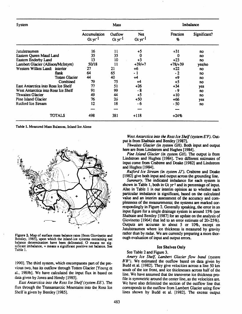
System Mass Imbalance

Accumulation Outflow Net Fraction Significant?Gtyr "1 Gtyr-I Otyr "1 %

Jutulstraumen 16 11 +5 ,,-31 noEastern QueenMaudLand 35 35 0 0 noEasternEnderbyLand 13 10 +3 +23 noLambertGlacier (Allison/Mclntyre) 50/18 11 +39/+7 +78/+39 yes/noWesternWilkes Land: interior 27 21 +6 +22 no

flank 64 65 - 1 .2 noTortenGlacier 44 40 +4 +9 no

Combined 79 75 +4 +5 noEast Antarcticainto Ross Ice Shelf 77 51 +26 +34 yesWest Antarcticainto Ross Ice Shelf 91 99 - 8 - 9 noThwaites Glacier 49 44 +5 + 10 noPine IslandGlacier 76 26 +50 +66 yesRuffordIce Stream 12 18 - 6 - 50 no

TOTALS 498 381 + 118 +24%

Table1.MeasuredMassBalances,InlandIce Alone

WestAntarcticaintotheRossIceShelf(systemE'F).Out-putisfromShabtaieandBentley[1987].ThwaitesGlacier(insystemGH).BothinputandoutputA

_'_b"" " herearefromLindstromandHughes[1984].,•_ ::::=:-_ o ._: Pine Island Glacier (in system GH). The output is from

_/---__"__'" .... Lindstromand Hughes[19841.Two different estimatesof

_'_""' ,' "_'._:_*i". _,_,_,, ...._;.,: inputcome fromCrabtreeandDoake[1982]andLindstrom, / __:i""'\ • x//;-_,,,._., andHughes[1984].

',. '-%,._:_..__._//\ , f _ _ Ru,fordIceStream(insystemJJ').CrabtreeandDoake

'_i %_>_,_ I]- _ T _, [1982] give both inputandoutput acrossthe groundingline.o_ i : __]_ -. ..... .t Summary. The indicated imbalance for each system is

"" ' _" / A L i))_ shownin Table 1,both in Gt yr-! and in percentageof input.

.. ,.__\ -__' AlsoinTable1 isourinterimopinionastowhethereach

._:.::.,+ particularimbalanceissignificant, based on thecalculated• valueandan interimassessmentoftheaccuracyandcom-

., . . ,\_,,,, , ,c. pletenessofthe measurements;the systems are markedcor-

:,'__:2)/)_ restxmdingly in Figure 2. Generallyspeaking,the errorin an

_\_ __/'___''"_-:',:'___3:/i input figure fora single drainagesystem is around 15%(SeeShabtaieand for the"%_ .. Bentley [1987] an updateon analysisof

_' _,._,_ i - ': Giovinetto [1964] that led to an error estimate of 20-25%)."","':_" ° Outputs are accurate to about 5 or 10%, except ono $eea.

° Jutulstraumen where ice thickness is measured by gravityratherthan by radar. We are currentlypreparing a more thor-Figure2. Mapof surfacemassbalancerates [fromGiovinettoand

Bentley,1985],upon whichthe inland-icesystemscontainingnet ough evaluation of inputand output errors.balancedeterminationhave been delineated.O means no sig-nificantimbalance,+ meansa significantpositivenet balance.See Ice Shelves OnlyTable 1. See Table 2 and Figure3.

Amery lee Shelf, Lambert Glacier flow band (systemB'B"). We estimated the outflow based on data given by

1990]. The third system, which encompasses partof the pre- Buddet al. [1982]. They give velocities across a line 50 kmvious two, has its outflow throughTorten Glacier [Young et southof the ice front, and ice thicknesses across half of theal., 1989b]. We have calculated the input flux in based on line. We have assumed that the transverseice thickness pro-data given by Jonesand Hendy [1985]. file is symmetric aroundthe center line, as the velocities are.

East Antarctica into the Ross Ice Shelf (system EE'). The We have also delimited the section of the outflow line thatflux through the TransantarcticMountains into the Ross Ice corresponds to the outflow from LambertGlacier using flowShelf is given by Bentley [1985]. lines shown by Budd et al. [1982]. The excess output

483

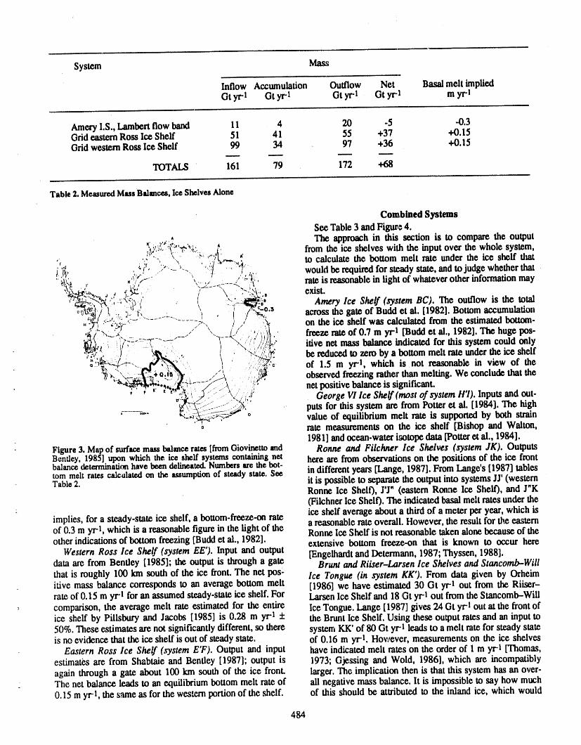
System Mass

Inflow Accumulation Outflow Net Basal melt impliedGtyr-I Gt yr-1 Gt yr-I Gt yr-I m yH

AmeryI.S., Lambertflow band 11 4 20 -5 -0.3GrideasternRoss Ice Shelf 51 41 55 +37 +0.15GridwesternRoss Ice Shelf 99 34 97 +36 +0.15

TOTALS 161 79 172

Table2. MeasuredMassBalances,IceShelvesAlone

Combined SystemsSee Table 3 andFigure 4.

. ,,,_.._., . . The approach in this section is to compare the output_:;,'._'_:q-'_ _:_. _, from the ice shelves with the input over the whole system,

, ,., 4 ", .... _" _'/1

_, , ,, . ,,_,,.,,,_._ tocalculatethebottommeltram undertheiceshelftmr' , .'" ," _'-. :1 ' _ would be requiredfor steadystate, and to judge whetherthat"_._0 _. . ', ./ ,,..._: ....., _-.v rateisreasonablein light of whateverotherinformationmay

_"J"_ " ' / - ", ' _" "_'- eXiSt."_'_: .""_-_...../ . l -,.,...,m_r;-. Amery Ice Shelf (systemBC).The outflow is thetotalr-l, J [ '4 .. \ ! Y_,-- "_v ,,#_4/ , _ >._, , , .f ./_,.• across the gate of Budd et al. [1982]. Bottom accumulation

.-_3._-,%_, /'-, / / '.k. ontheiceshelfwas calculatedfromtheestimatedbottom-.,_ _- , , / "-, I ._ /\, _ .

_:/_---_,,_...... _. ,---- -,--J<.,..,,li_. freezerateof0.7m yrl [Buddetal.,1982].The hugepos-_)'_ i",i/;-'_-_::: !, ".',:_:_:,:z.://,.,i!..:"itiveneamass balance indicated for this systemcould only"_?, .I. .q&.-".., l ' _J:/:i_ bereducedtozeroby a bottommeltrateundertheiceshelf"_i,__.&_-J-:-,;---..._/'_"".,, _ ' '::__. of 1.5m yrl,whichis.notreasonableinviewof the

(i,- v .....4_-_.,-,u- ),i //f', :.._w observed freezingrather than melting, We conclude thai the-_,:_-::--__.,._-,_,.,/ .......A...: netpositivebalanceis significant.

..-'-,/."...-""._L/:,'_. GeorgeVIIceShelf"(mostofsystemH'I).Inputsand out-:,_: .. puts for this system are from Potter et al. [1984]. The high

' _'" . __-_/: ° value of equilibrium melt rate is supportedby bothstraino rate measurements on the ice shelf [Bishop and Walton,

1981] andocean-waterisotope data[Potteret al., 1984].Figure3. Mapof surfacemassbalancerates[fmmGiovinettoand Rwme and Filchner Ice Shelves (system JK). OutputsBentley, 1985] upon which the ice shelf systemscontaining net here are from observations on the positionsof the ice frontbalancedeterminationhavebeendelineated.Numbersare thebot- in differentyears [Lange, 1987].FromLange's [1987] tablestom meltramscalculatedon the assumptionof steadystate.SeeTable2. it is possible to separatethe output into systems JJ' (western

RonneIce Shelf), J'J" (eastern RonneIceShelf), and J"K(FilchnerIce Shelf). The indicatedbasal meltratesunderthe_ceshelf average about a third of a meter per year, which is

implies, for a steady-state ice shelf, a bottom-freeze-on rate a reasonablerate overall. However, the result for the easternof 0.3 m yH, which is a reasonablefigurein the light of the RonneIce Shelf is not reasonabletakenalone because of theotherindicationsof bottom freezing [Buddet al., 1982]. extensive bottom freeze-on that is known to occur here

Western Ross Ice Shelf (system EE'). Input and output [Engelhardtand Determann, 1987; Thyssen, 1988].dataare from Bendey [1985]; the output is througha gate Brunt and Riiser-Larsen Ice Shelves and Stancomb-Willthat is roughly 100 km south of the ice front.The net pos'- Ice Tongue (in system KK'). From data given by Orheimitive mass balance correspondsto an average bottom melt [1986] we have estimated 30 Gt yH out from the Riiser-rateof 0.15 m yrl foran assumed steady-state ice shelf. For LarsenIce Shelf and 18 Gt yrl out from the Stancomb--Willcomparison,theaveragemeltrateestimatedfor the entire IceTongue.Lange[1987]gives24GtyH outatthefrontoficeshelfby PillsburyandJacobs[1985]is0.28m yr-] + the Brunt IceShelf.Usingthese outputratesandan inputto50%.These estimatesare not significantly different, so there system KK' of 80 Gt yr-I leads to a melt rate for steady stateisnoevidencethattheiceshelfisoutofsteadystate, of0.16m yrl. However,measurementson lhc iceshelves

Eastern Ross Ice Shelf (system E'F). Output and input have indicated melt rates on the orderof 1 m yr-I [Thomas,estimates are from Shabtaie and Bentley [1987]; output is 1973; Gjessing and Wold, 1986], which are incompatiblyagain through a gate about 100 km south of the ice front, larger. The implication then is that this system has an over-The net balance leads to an equilibriumbottom melt rate of ali negative mass balance, lt is impossible to say how much0.15m yr-Ithesameasforthewesternportionoftheshelf, ofthisshouldbc attributedtotheinlandice,whichwould

484

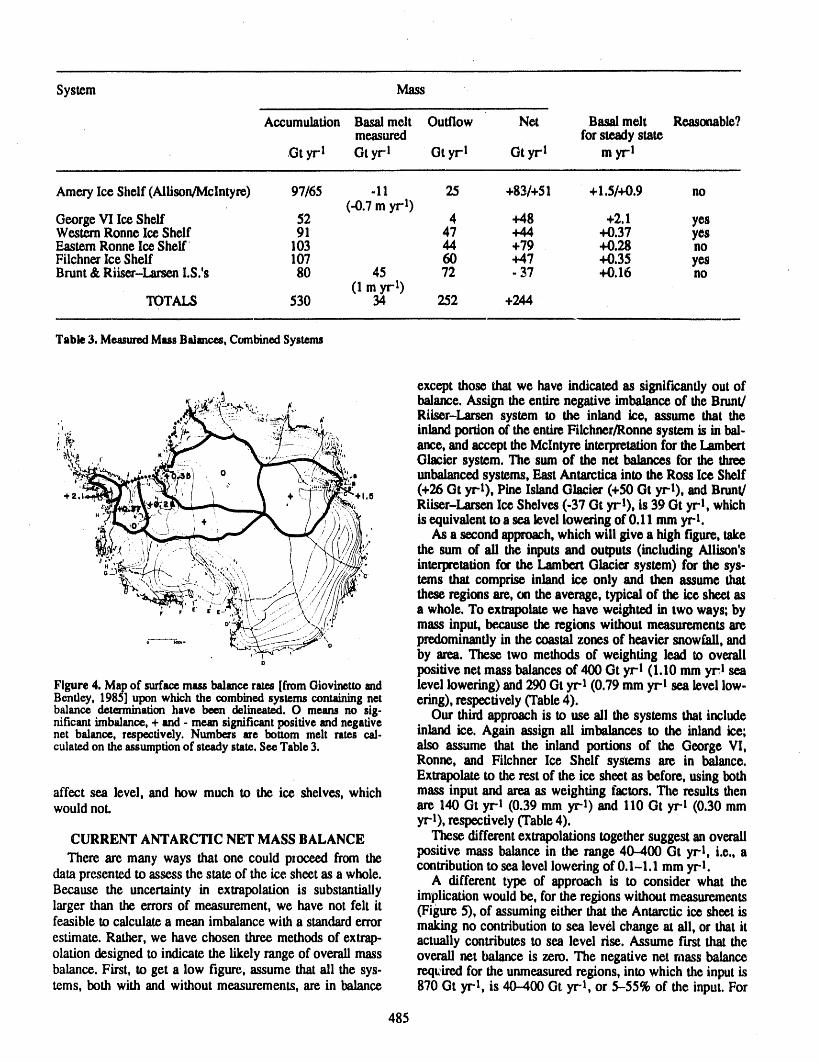
System Mass

Accumulation Basal melt Outflow Net Basal melt Reasonable7measured forsteady state

.Gtyrl Gtyr-1 Otyr-I Gtyrl m yr"I

Amery Ice Shelf (Allison/Mclntyre) 97/65 -11 25 +83/+51 + 1.5/+0.9 no(-0.7 m yr 1)

GeorgeVI IceShelf 52 4 +48 +2,1 yesWesternRonne Ice Shelf 91 47 +44 +0.37 yesEasternRonne IceShelf 103 44 +79 +0.28 noFilchnerIce Shelf 107 60 +47 +0.35 yesBrunt&Riiser-LarsenI.S.'s 80 45 72 - 37 +0.16 no

0 myri)TOTALS 530 34 252 +244

Table3. MeasuredMassBalances,CombinedSysten_

except those thatwe have indicated as significantly out ofA, , _@':-'.}_._.,__,_,, _ balance. Assign the entirenegative imbalanceof the Brunt/

..:__ _::_ <,_,_ ,. Riiser-Larsen system to the inland ice, assume that thei',._ .__._ "_ _ii_/_._. inlandportionoftheentireFilchner/Ronnesystemisinbal-

,,.._ ,_ _ -/_......_/_: anex,andaccepttheMclnty_intex_'etmJonforthel.ami_rt_,'_ ' '___._i Glacier system. The sum of the net balances for the three

1,, B unbalancedsystems, East Antarcticainto the Ross Ice Shelf+z.,_ i/:'_, ;,I_, __ + LT-(_-e,,.+0.e (+26 Ot yr-l), Pine Island Glacier (+50 Ot yrl), and Brunt/

• . _r.z 0 ___ Riiser-l.arsen Ice Shelves (.37 Gt yr-l)i is 39 Gt yrl which

" ' ,_, / _ //_ ')_/_\ ' is equivalentto a sea level lowering of 0.11 mm yr-l.

._..(_. " "_!_ ',,_.._:_'_'?_. __"_//////-'"_y.,_////))_|,:,'{/ As a second approach,which will give a high figure,take•,:.,''.,i.,_I/.....-:_.:i....., '"b_."'_' thesum ofalltheinputsand outputs(includingAllison'so_,__.,_.. ,, _:.,, ,, ////,/;_. interpretationfor the LambertGlacier system) for the sys-

""\_:_'"_"" :::i'_" 1 /.llll/f/_' terns that comprise inland ice only and then assume that"t.. ",.---;+.._-_:_ -_-.'/,_\'_t---- " . '..,',/_//11_'_', theseregionsare,m theaverage,typicalof the ice sheet as

,':" "/Jt"___::;;:;:(:7!_{_, a whole. To extrapolatewe have weighted in two ways; by

°;___-._,(i':--_.._ mass input, because the regions without measurementsare,'._ _'_ predominantlyin the coastal zones of heavier snowfall, and

° _" _ ° by area.Thesetwo methods of weighting lead to overall° positive net mass balances of 400 Gt yr-I (1.10 mm yr_lsea

Figure4. Mapof surfacemassbalancerates[fromGiovinettoand level lowering) and 290 Ot yr-I (0.79 mm yr-I sea level low-Bentley,1985]uponwhichthe combinedsystemscontainingnet ering),respectively (Table4).balancedeterminationhave been delineated.0 means no sig- Our third approachis to use ali the systems thatincludenificantimbalance,+ and- meansignificantpositiveandnegativenet balance, respectively.Numbersare bottommelt ratesca]- inland ice. Again assign ali imbalances to the inland ice;culatedontheassumptionof steadystate.SeeTable3. also assume that the inland portions of the George VI,

Ronne, and Filchner Ice Shelf systems are in balance.Extrapolateto the rest of the ice sheet as before, using both

affect sea level, and how much to the ice shelves, which mass inputand area as weighting factors. The results thenwould not. are 140 Gt yr-I (0.39 mm yr-l) and 110 Gt yr-I (0.30 mm

yr-l), respectively (Table4).CURRENT ANTARCTIC NET MASS BALANCE These different extrapolationstogethersuggest an overall

positive mass balance in the range 40-400 Gt yr-l, i.e., aThere are many ways that one could pxoceed from the contributionto sea level lowering of 0.1-1.1 mm yr-l.

dampresentedto assess the state of the ice sheet as a whole. A different type of approach is to consider what theBecause the uncertainty in extrapolation is substantially implicationwould be, for the regions without measurementslarger than the errors of measurement, we have not felt it (Figure 5), of assuming either thatthe Antarcticice sheet isfeasible to calculatea mean imbalancewith a standarderror makingno contribution to sea level change at all, or thatitestimate. Rather, we have chosen three methods of extrap- actually contributes to sea level rise. Assume first that theolation designed to indicate the likely range of overall mass overall net balance is zero. The negative net mass balancebalance. First, to get a low figure, assume thatali the sys- reqt:iredfor the unmeasuredregions, into which the input isterns, both with and without measurements, are in balance 870 Gt yrl, is 40-400 Ot yrl, or 5-55% of the input. For

485

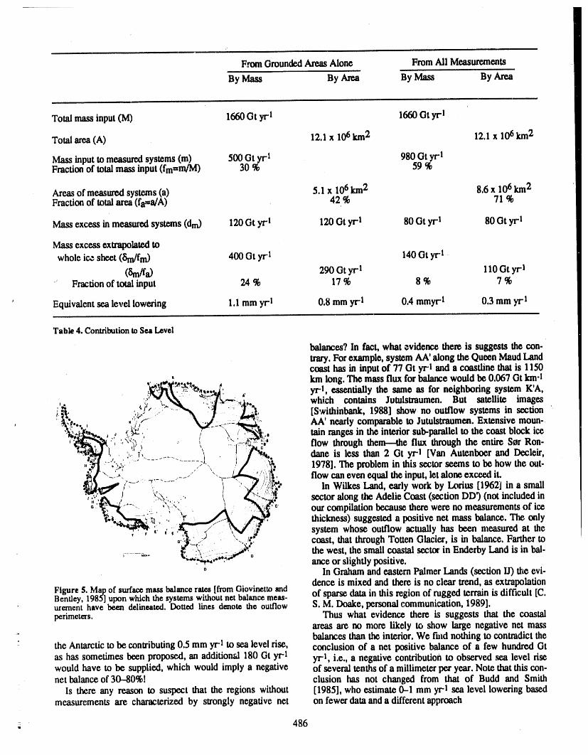
FromGroundedAreasAlone FromAli Measurements

By Mass By Area By Mass By Area

rt ,,, ,i

Totalmassinput(M) 1660 Gt yr'! 1660Gt yr"1

Totalarea(A) 12.1 x 106km2 12.1 x 106 km2

Mass inputto measuredsystems (m) 500 Gtyr'! 980 Gt yr-IFractionof totalmass input(fm=m/M) 30 % 59 %

Areasof measuredsystems(a) 5,1 x 106km2 8,6 x 106km2Fraction of totalarea (ferffia/A) 42 % 71%

Mass excess in measuredsystems (dm) 120Gt yr I 120 Gt yr.l 80 Gt yr"1 80 Gt yr"1

Massexcessextrapolatedtowhole ice sheet (Sm/fm) 400 Gt yr l 140Ot yr l,

(Sm/fa) 290 ot yr4 110 Ot yr-I" Fractionof total input 24 % 17 % 8 % 7 %

' Equivalentsea level lowering 1.1 mm yr I 0.8 mm yrl 0.4 mmyr"1 0.3 mm yr"1

Table4. Con_ibutiontoSeaLevel

balances? In fact, what evidence there is suggests the con-trary.Forexample, system AA'along the QueenMaudLandcoast has in inputof 77 Gt yrl and a coastline that is 1150

kmlong.Themass flux for balance would be 0.067 Ot km-I:!__'s_....,t' yrl essentially the same as for neighboring system K'A,

' , _S -.__-- _+_" '+1"_';' '<:/'V_ .:::;:< ,:_,, which contains Jumlstmumen. But satellite images, ig),+s ?_ -,i '.

i:_%'.. ,,';_'_ + _ I _;: [Swithinbank,1988] showno outflow systemsin section+ _..r .. , /, x:zf_:+---_' As,' nearly comparableto Jutulswaumen.Extensive moun._\ ,'J<.k s ),".,i- "y"-..... \ _.""_,,_++_.._ _ + ,_, , \ + ++_:, rainrangesin the interiorsub-parallelto the coastblockice

' _++_] ' ,,,,t_> + ,, ....), :?I_. flow through them--the flux through the entire Ser Ron-...."_.'O_',' ." " .... ..... . I . t ! _,. dane is less than 2 Ot yr-I [Van Autenboer and Decleir,

."_<J-al•...... :,:+-"' ......... <:_-, +,,+I" _.,,. 1978]. The problemin this sector seems tobehow the out-' \'"" ,-"_,' _/ ".- " ' ' ,','" flow can even equal the input,let alone exceed it,

_i(_.i "?_-'"<.,, ...... "- "_--_. , ,,">i>)!)_",,, In Wilkes Land, early work by Lt,,+ [1962] in a small\_,.". I //!' " "' L _ ,J " "'' '_ _ ', _ + _'_:_ sector along the Adelie Coast (section DD9 (not included in

H '__" -+_ " '"'"; _ " l _' ''_., 7 " - ..... ' '. 'i¢ r'C.:_.... . , <+ +,....... , ourcompilation because there were no measurements of ice

...... :_+., ' thickness) suggested a positive net mass balance. The only

+ "_ , , ,, ": , _p system whose outflow actually has been measured at the, _-- .]_ coast,thatthroughTortenGlacier,isinbalance. Farther to

..........+.. the west, the small coastal sector in EnderbyLand is in bal-ance or slightly positive.

° In Grahamandeastern PalmerLands (section LI)the evi-dence is mixed and there is no clear trend,as extrapolation

Figure5. Mapof surfacemassbalancerates[fromGiovinettoand of sparsedata in this region of rugged terrainis difficult [C.Bentley,1985]uponwhichthesystemswithoutnet balancemeas-urementhave been delineated.Dottedlines denotethe outflow S.M. Doake, personalcommunication, 1989].perimeters. Thus what evidence there is suggests that the coastal

areas are no more likely to show large negative net mass+ balances thanthe interior. We fred nothing to contradictthe

the Antarcticto be contributing0.5 mm yr-Ito sea level rise, conclusion of a net positive balance of a few hundredGtas has sometimes been proposed, an additional 180 Gt yrl yri, i.e., a negative contributionto observed ._a level risewould have to be supplied, which would imply a negative of several tenthsof a millimeterper year. Note thatthis con-net balance of30-80%t clusion has not changed from that of Budd and Smith

Is there any reason to suspect that the regions without [1985], who estimate 0--1 mm yrl sea level lowering basedmeasurements are characterized by strongly negative net on fewerdataand a differentapproach

_. ' 486

ICEBERG FLUX personal communication, 1989]. ShtraseGlacier tongue hasData from a systematicprogramof iceberg observationin broken back in the 1980s [Nishio, 1990]. Williams and

the watersaroundAntarctica,in which nearly ali ships tray- Ferrigno[1988] and Ferrignoet al. [1990] document large-eling to and fromAntarcticaparticipate,have beenanalyzed scale retreator recession in several areas, although theircarefullyby Orheim [1985, 1988, personal communication, study is dominated by the super-gianticebergs that are not1989], taking into account multiple sightings, mean res. included in the iceberg flux calculations, Overall, a generalidence times, and size distributions, His conclusion is that retreat of the floating ice margins of the ice sheet is indi-the totalcalving ratefrom the continent, ignoring the recent cared,but whetherthat retreatis largeenough to accountforgiant icebergs,is at least as large as the totalmass inputonto the excess icebergflux remains problematical,the continent.If meltingunderthe ice shelves is added as anoutput term, the implication is for a negative net mass CONCLUSION

balance. At present the antarctic contribution to sea level changeThe indicated imbalance is equivalent to an average probably is a lowering that lies between 0.1-1.1 mm yr-l.

break-back rate of 1 km yrl along ali the ice.shelf fronts That amounts to 40--400 Gt yrl total excess mass input, or 2around the continent. There is at least qualitative evidenceto indicate that such a break-backis occurring. Zakharov to 25% of the total yearly input. Our estimate is not sig-[1988] has compiled informationfrom maps and satellite nificanfly different from most of those in the past, but theimages on frontal positions of the ice shelves and floating expanding coverage of the ice sheet makes it increasinglyglacier tongues around Antarcticaover the last century. He difficult to attributeany contributionto sea level rise to Ant-found that through the 1970s a larger proportionof the arctic& Excess iceberg flux probably reflects a secularbreakbackof ice shelf fronts.fronts were advancing than at any other time in his cover-age. Unfortunately,his data end in 1980, but it would bereasonable to suppose that aftera periodof unusual advance ACKNOWLEDGMENTSa net break-backwould occur. In the Antarctic Peninsula This workwas supportedby NSF grantDPP86-14011 toregion the Wordie (section H'I), George VI (section H'I), the University of Wisconsin and NSF,RC grantand Larsen Ice Shelves (section I'I") have ali been decaying OGP0036595 to the University of Calgary. This is contribu-in recent years (even aside from the !l,000-km2 calving tion number 514 of the Geophysical and Polar Researchevent from the Larsen Ice Shelf in 1986) lC. S. M. Doake, Center of the University of Wisconsin-Madison.

REFERENCES

Allison, I., The mass budget of the Lambert Glacier drain- Engelhardt, H. F., and J. Detennann, Borehole evidence forage basin, Antarctica, J. Glaciol., 22,223-235, 1979. a thick layer of basal ice in the central Ronne Ice Shelf,

Allison, I., N. W. Young, and T, Medhurst, On reassessment Nature, 327, 318--319, 1987.of the mass balance of the Lambert Glacier drainage Ferrigno, J. G., R. S. Williams, Jr., B. K. Lucchitta, andbasin, Antarctica, J. Glaciol., 31,378--381, 1985. B.F. Molnia, Recent changes in the coastal regions of

Bentley, C. R., Glaciological evidence: The Ross Sea sector, Antarctica documented by landsat images, this volume,in Glaciers, Ice Sheets, and Sea Level: Effects era COz- 1991.Induced Climatic Change, Attachment 10, pp. 178-196, Fujii, Y., Aerophotographic interpretation of surface fea.National Academy Press, Polar Resem'ch Board, Wash. tures and an estimation of ice discharge at the outlet ofington, DC, 1985. the Shirase Drainage Basin, Antarctica, Antarctic Record,

Bishop, J. F., and J. L. W. Walton, Bottom melting under 72, 1-15, 1981,George VI Ice Shelf, Antarctica, J. Glaciol., 27, 429--447, Giovinetto, M. B., and C. R. Bentley, Surface balance in ice1981. drainage system of Antarctica, Antarctic J. U.S., 20, 6--

Bogorodsky, V. V., G. V. Trepov, and A. N. Sheremet'ev, 13, 1985.Use of radio.echo measurements in determining the Giovinetto, M. B., and C. Bull, Summary and analyses ofthickness and velocity of an Antarctic ice sheet, Physics surface mass balance compilations for Antarctica, 1960-of the Solid Earth, 1,5,69--74, 1979. 1985, Byrd Polar Research Center Report No. 1, The

Budd, W. F., and I, N. Smith, The state of balance of the Ohio Stale University, 1987.Antarctic ice she_._ an updated assessment--1984, in Giovinetto, M. B., C. R. Bentley, and C. B. B. Bull, Choos-Glaciers, Ice Sheets, and Sea Level: Effects of a C02- ing between some incompatible regional surface-mass-Induced Climaac Change, Attachment 9, pp. 172-177, balance data sets in Antarctica, Antarctic J. U.S., 24, 7-National Academy Pt'ess, Polar Research Board, Wash- 13, 1989.ington, DC, 1985. Gjessing, Y., and B. Wold, Absolute movement';, mass bal-

Budd, W. F., M. J. Corry, and T. H. Jacka, Results from the ance and snow temperatures of the Riiser-Larsenisen IceAmery Ice Shelf Project, Ann. Glaciol., 3, 36--41, 1982. Shelf, Antarctica, Norsk Polarinstitutt Skrifter, 187, 23-

Bull, C. B. B., Snow accumulation in Antarctica, in 31,1986.Research in the Antarctic, edited by L. O. Quam, pp. Hamley, T. C., I. N. Smith, and N. W. Young, Mass balance367--421, American Association for the Advancement of and ice flow law parameters for East Antarctica, J.Science Publ. No. 93, Washington, DC, 1971. Glaciol,, 31,334-339, 1985.

Crabtree, R. D., and C. S, M. Doake, Pine Island Glacier Jones, D., and M. Hendy, Glaciological measurements inand its drainage basin: results from radio echo sounding, Eastern Wilkes "Land,Antarctica, ANARE Res. Notes, 28,Ann. Glaciol., 3, 65-70, 1982. 164-173, 1985.

487

Kotlyakov, V, M., N. I, Barkov, I, A, Loseva" and B, N, Orhetm,O., Antarcticicebergs- production,distributionandPetrov, Novaiakarta pitaniia lednikovogo pokrova disintegration,Ann, Glaciol,,11, 205,1988.Antarktidy(New map of the accumulationon the Ant- HUsbmy, R, D., and S. S, Jacobs, Preliminaryobservationsarctic Ice Sheet): Institut Oeografii, Adadesila Nauk from long.texm currentmetermooringsnearthe Ross IceSSSR,Materialy Gliatsiologicheskikh Issledovanij, Khro. Shelf, Antarc0,ca,in Oceanology of the Antarctic Con.nika Obsuzhdeniia,24, 248.255, 1974. tinental Shelf, American Geophysical Union, Antarctic

Kotlyakov,V, M., M. B. Dyurgemv, P. A. Korolyev, Accu- Research Series, Vol. 43, edited by S. S, Jacobs, pp, 87-mulation and mass balance of the large ice-catchment 107, 1985.basin in East Antarctica (In Russian), in Materials of Potter,J, R., J, G. Paten, and J. Loynes, Glaciologic_ andglaciological chronicles of discussion 47, pp, 49-61, oceanographiccalculations of the mass balanceand oxy-Academy of Sciences of the U.S.S.R. Soviet Geophysical gen isotope ratio of a melting ice shelf, J, Glaciol,, 30,Committee, 1983. 161-169, 1984,

Lange, M. A., Quantitativeestimates of the mass flux and Seko, K., T. Fm'ukawa,and O, Watanabe,The surfacecon-ice movement along the ice edges in the Eastern and ditlonon the Antarctic ice sheet, this volume, 1991.SouthernWeddell Sea, in The Dynamics of the West Ant. Shabtaie, S,, and C. R. Bentley, West Antarcticice streamsarctic Ice Sheet, editedby J. Oerlemans and C. J. van der draining into the Ross Ice Shelf,'Configurationand massVeen, pp, 57-74, D. Reidel Publishing, Amsterdam, balance,J. Geophys.Res,, 92, 1311-1336, 1987,Netherlands, 1987. Shimizu, H., O. Watanabe, S. Kobayashi, T. Tamada, R.

Lindstrom, D,, mid T, J. Hughes, Downdraw of the Pine Naruse, and Y. Ageta, Glaciological aspects and massIsland Bay drainage basins of the West Antarctic ice budget of the ice sheet in Mizuho Plateau, in Glaciolog-sheet, Antarctic J. U.S., 19, 56-58, 1984. ical Studies in Mizuho Plateau, East Antarctica, 1969-

Loflus, C., Contributionto the knowledge of the Antarctic 1975, Memoirs of National Institute of Polar Research,ice sheet: a synthesis of glaciological measurements in Special IssueNo. 7, pp. 264.274, 1978.TerreAdelie, J. Glaciol., 4, 79-92, 1962. Swithinbank,C. W. M., Antarctica: Satellite image atlas of

Mclntyre, N. F., A reassessmentof the mass balanceof the glaciers of the World, United States Geological SurveyLambert Glacier drainage basin, Antarctica, J. Gla- ProfessionalPaper 1386-B, 1988.ciology, 31, 34-38, 1985a. Thomas, R. H., The dynamics of the BrantIce Shelf, Coats

Mclntyre,N. F., Reply to "Onreassessmentof the massbal- Land, Antarctica, Scient¢'ic Report No. 79, British Ant-ance of the LambertGlacier drainagebasin, Antarctica," arcticSurvey, 1973.J. Glaciol., 31,381-382, 198Ya, Thyssen, F., Special aspects of the centralpartof the Filch-

McIntyre, N. F., Ice sheet drainage basins, balance and ner/RonneIce Shelf, Ann. Glaciol., 11,173-179, 1988.measured ice velocities and sub-glacial water, in Ant- van Autenboer,T., and H. Decleit, Glacier discharge in thearctica: Glaciological and Geophysical Folio, sheet 12, Ser-Rondane,a contributionto the mass balance of Dron.edited by Drewry, D. J., Scott Polar Research Institute, ning Maud Land, Antarctica, Zeitschr_ft fgr Glets-Universityof Cambridge,1991, In press, cherkunde und Glazialgeologie, 14, 1-16, 1978.

Morgan,V. I., and T. H. Jacka,Mass balance studies in East Williams, Jr.,R. S., and J. G. Ferrigno, DocumentationonAntarctica, in Sea Level, Ice, and Climatic Change (Pro- satellite imagery of large cyclical or secular changes inceedings of the Canberra Symposium, December 1979), antarctic ice sheet margin,EO$ (Transactions, AmericanIAHS Publ. No. 131, pp. 253-260, 1981. Geophysical Union), 69, 365, 1988.

Morgan,V. I., T, H. Jacka,G. J. Akerman,andA. L. Clarke, Young, N. W,, Measured velocities of interiorEast Ant-Outlet glacier and mass.budget studies in Enderby, arctica and the state of mass balance within the I,A.G.P.Kemp, and Mac. Robertson Lands, Antarctica, Ann. area,J. Glaciol., 24, 77.87, 1979.Glaciol., 3, 204-210, 1982. Young, N. W., I. D. Goodwin, N. W. J. Hazelton, and R. J.

Nishio, F., Ice front fluctuationsof the Shirase Glacier, East Thwaites, Measured velocities and ice flow in WilkesAntarctica,this volume, 1991. Land, Antarctica,Ann. GlacioL, 12, 192-197, 1989a.

Orheim,O., Iceberg discharge and the mass balanceof Ant- Young, N., P. Malcolm, and P. Mantell, Mass flux andarctica, in Glaciers, Ice Sheets, and Sea Level: Effects of dynamics of Totten Glacier, Antarctica (abstract), Ann.a C02-1nduced Climatic Change, Attachment 12, pp. Glaciol.,12,219, 1989b.210-215, National Academy Press,PolarResearchBoard, Zakharov,V. G., Fluctuations in ice shelves and outlet gla-Washington,DC, 1985. ciers in Antarctica"Polar Geography and Geology, 12,

Orheim, O., Flow and thickness of Riiser-Larsenisen,Ant- 297-311, 1988.arctica,Norsk Polarinstitutt Skrifter, 187, 5-22, 1986.

488

ii i , ,

The Impact of Global Warming on the Antarctic MassBalance end Global Sea Level

W. F. Budd and Ian SimmondsDepartmentofMeteorology,Universityof Melbourne,ParkvUle,Victoria,Australia

ABSTRACT

The onset of global warmingfrom increasing"greenhouse"gases in the atmos-phere can have a numberof importantdifferent impactson the Antarcticice sheet.These include increasingbasalmelt of ice shelves, faster flow of the groundedice,increased surface ablation in coastal regions, and increased precipitationover theinterior. An analysis of these separatetermsby ice sheet modeling indicates that theimpact of increasing ice sheet flow rates on sea level does not become a dominantfactor until 100-200 years after the realization of the warming.For the time periodof the next 100 years the most importantimpact on sea level from the Antarcticmass balance can be expected to result from increasing precipitation minus evap-oration balanceover the groundedice. The present Antarcticnet accumulation andcoastal ice flux each amountto about 2000 km3 yr-1,both of which on their ownwould equate to approximately6 mm yr-i of sea level change. The presentrate ofsea level rise of about 1.2 mm yr-I is therefore equivalent to about 20% imbalancein the Antarcticmass fluxes.

The magnitude of the changes to the Antarctic precipitation and evaporationhave been studied by a series of General Circulation Model experiments, using amodel which gives a reasonablesimulationof the presentAntarcticclimate, includ-ing precipitationand evaporation.The experiments examine the changes in the Ant-arctic precipitation (P) and evaporation (E) resulting sep_u'atelyfrom decreasingincrementallythe Antarcticsea ice concentrationand from global warmingaccom-paniedby decreasedsea ice cover.

For total sea ice removal the changes obtained were P:+23%; E:-8%; (P-E):+48%. For global warming with sea ice reduction by about two thirds thechanges were P:+47%; E:+22%; (P-E):+68%. This latterincrease in mass flux isequivalentto about4 mm yr-1of sea level lowering whichcould provide a small butsignificant offset to the sea level rise expected from ocean thermal expansion andmelting of temperate glaciers.

INTRODUCTION shelvesdiminished.Ontheotherhand,fortheshorterterm,Considerableinteresthas developedin recentyears the effectof increasingprecipitati6nover the Antarctic

regardingthe roleof the Antarcticice sheetin possible wouldhavean/mined/ateimpactincontributingtasealevelfuturechangesof sealevel,lt wasindicatedbyBuddet al. lowering.Table1 showsthecurrentestimatesof Antarctic[1987]andBudd[1988]thatthemajorresponseof theAnt- snowaccumulationin relationta se,a levelchange.Inspitearcticicesheettaglobalwarmingwhichcouldcontributeto of theuncertaintyin theaccumulationestimatesthepresentsealevelr/se,fromincreasediceflow,wouldbedelayedfor Antarcticaccumulationrateisequivalenttoaboutfivetimes

..... ."..... t--°l. *t,--- ,g21__..'___ 2---- ,,,lt.-- _L" l ..... S --!-.. _. ........ !_s.s_

UVV,,.I a q.,_IILUI.i_ IUIIUWUI_ I.illt_ WJnilllilil_t WlilitlO I.il_ ltlU4_t,tli_ it.,_ UIU II,,IJIAIUIII, lil_.U Ut _ IUVUi ii_1_. /b_li _plUI_II'IUIU h-I_,l'_ il-i

489

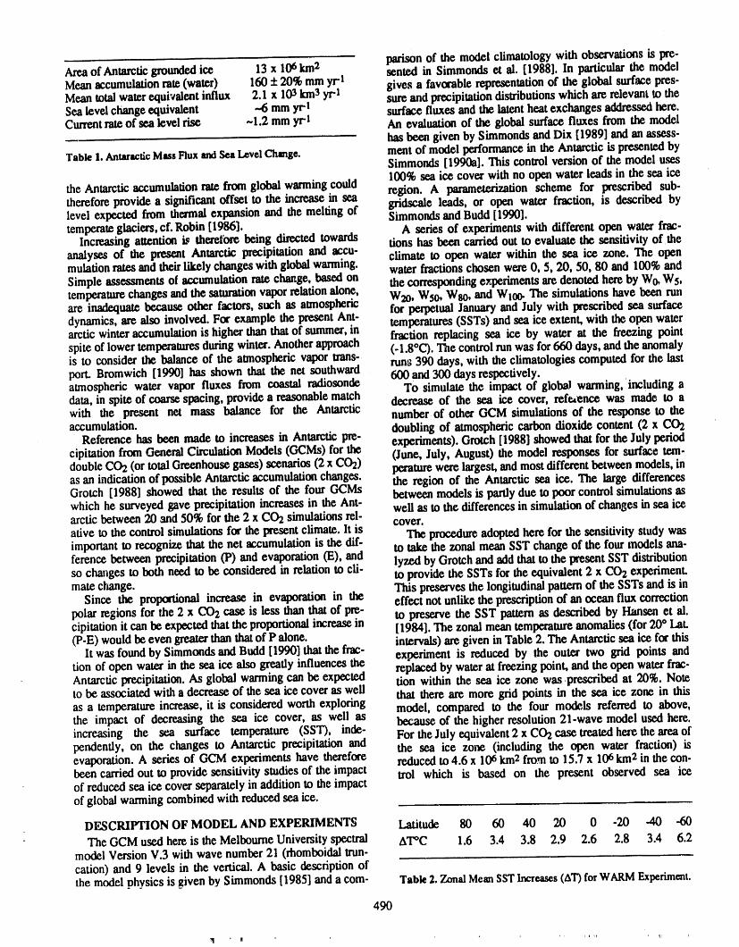
parisonof the model climatology with observations is pre-Areaof Antarcticgroundedice 13 x 106km2 sented in Simmonds et al. [1988]. In particularthe modelMean accumulationrate (water) 160 + 20% mm yrl gives a favorable representationof the global surface pres-Mean totalwaterequivalent influx 2.1 x 103km3yr-l sure andprecipitationdistributionswhich are relevantto theSealevel change equivalent .-6 mm yrl surface fluxes and the latentheat exchanges addressedhere.Currentrateof sea level rise ~1.2 mm yrl An evaluation of the global surface fluxes from the model

has been given by Simmondsand Dix [1989] andan assess-

Table1. AntaracticMassFluxandSeaLevelChange. ment of model performancein the Antarctic is presentedbySimmonds [1990a]. This control version of the model uses100% sea ice cover with no open water leads in the sea ice

the Antarcticaccumulationratefrom global wanning could region. A parameterizationscheme for prescribed sub-thereforeprovide a significant offset to the increase in sea gridscale leads, or open water fraction, is described bylevel expected from thermal expansion and the melting of Simmondsand Budd [1990].temperateglaciers,cf. Robin [1986]. A series of experimentswith different open water frac-

Increasing attention is therefore being directed towards tions has been carriedout to evaluate the sensitivity of theanalyses of the present Antarctic precipitationand accu- climate to open water within the sea ice zone. The openmulafionratesand theirlikely changeswith global warming, water fractionschosen were 0, 5, 20, 50, 80 and 100%andSimple assessments of accumulation rate change, based on the correspondingexperiments aredenotedhereby W0,Ws,temperaturechangesand the saturationvapor relation alone, W2o, Ws0, Wso, and Wl0o. The simulations have been mnare inadequatebecause other factors, such as atmospheric for perpetualJanuary and July with prescribedsea surfacedynamics, are also involved. For example the present Ant- temperatures(SSTs) and sea ice extent' with the open waterarctic winteraccumulation is higher thanthatof summer,in fraction replacing sea ice by water at the freezing pointspite of lowertemperaturesduringwinter. Anotherapproach (-1.8°C). The controlrunwas for660 days,and the anomalyis to consider the balance of the atmospheric vapor trans- runs 390 days, with the climatologies computed for the lastport. Bromwich [1990] has shown that the net southward 600 and 300 days respectively.atmospheric water vapor fluxes from coastal radiosonde TO simulate the impact of global warming,including adata, in spite of coarse spacing, provide a reasonablematch decrease of the sea ice cover, refe,ence was made to awith the present net mass balance for the Antarctic number of other GCM simulations of the response to theaccumulation, doubling of atmosphericcarbon dioxide content (2 x CO2

Reference has been made to increases in Antarctic pre- experiments). Grotch [1988] showed that for the July periodcipitation fromGeneralCirculation Models (GCMs) for the (June, July, August) the model responses for surface tem-doubleCO2(or total Greenhousegases) scenarios(2 x CO2) peraturewere largest, andmost differentbetween models, inasan indicationof possible Antarcticaccumulation changes, the region of the Antarctic sea ice. The large differencesGrotch [1988] showed that the results of the four GCMs between models is partlydue to poor control simulationsaswhich he surveyed gave precipitation increases in the Ant- well as to the differencesin simulation of changes in sea icearctic between 20 and 50% for the 2 x CO2simulations rel- cover.ative to the control simulations for the presentclimate, lt is The procedureadoptedhere for the sensitivity study wasimportantto recognize that the net accumulation is the di/'- to take the zonal mean SST change of the four models ana-ference between precipitation(P) and evaporation(E), and lyzed by Grotehand addthatto the presentSST distributionso changes to both need to be considered in relation to cii- to provide the SSTs for the equivalent 2 x CO2 experiment.matechange. This preservesthe longitudinalpatternof the SSTs and is in

Since the proportional increase in evaporation in the effect not unlike the prescriptionof an ocean flux correctionpolar regions for the 2 x CO2 case is less than that of pre- to preserve the SST patternas described by Hansen et al.cipitationit can be expected thatthe proportionalincreasein [1984]. The zonal mean temperatureanomalies (for 20° Lat.(P-E)would beeven greaterthanthatof P alone, intervals)aregiven in Table 2. The Antarcticsea ice for this

lt was foundby Simmondsand Budd [1990] thatthe frac- experiment is reduced by the outer two grid points andtion of open water in the sea ice also greatly influences the replaced by waterat freezingpoint, and the open waterfrac-Antarcticprecipitation.As global warmingcan be expected tion within the sea ice zone was prescribed at 20%. Noteto be associated with a decrease of the sea ice cover as well that there are more grid points in the sea ice zone in thisas a temperature increase, it is considered worth exploring model, compared to the four mode,Is referred to above,the impact of decreasing the sea ice cover, as well as because of the higher resolution21-wave model used here.increasing the sea surface temperature (SST), inde- For the July equivalent2 x CO2case treatedhere the areaofpendently, on the changes to Antarctic precipitationand the sea ice zone (including the open water fraction) isevaporation. A series of GCM experiments have therefore reducedto 4.6 x 106km2from to 15.7 x 106km2in the con-been carriedout to providesensitivity studies of the impact trol which is based on the present observed sea iceof reducedsea ice cover separatelyin addition to the impactof global wanning combinedwith reducodsea ice.

DESCRIPTION OF MODEL AND EXPERIMENTS Latitude 80 60 40 20 0 -20 -40 -60The GCM used here is the MelbourneUniversity spectral AToC 1.6 3.4 3.8 2.9 2.6 2.8 3.4 6.2

model Version V.3 withwave number 21 (rhomboidaltrun-cation) and 9 levels in the vertical. A basic descriptionofthe model physics is given by Simmonds [1985] and a com- Table2, ZonalMeanSSTIncreases(AT)forWARMExperiment.

490

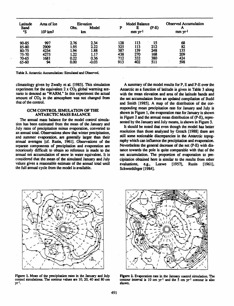
Latitede Area of lee Elevation Model Balance ObservedAccumulationBand Obs. Model P E (P-E) AoS 103km2 km mm yr-I mm yrq

90-85 997 2.76 2.34 I28 113 15 6885-80 2909 1.95 2.22 325 113 212 8280-75 4234 1.94 1.88 387 139 248 13575-70 4273 1.22 1.17 438 270 168 20970-65 1681 0.22 0.36 712 332 380 42465-60 94 0.00 -0.03 913 402 511 598

Table3. AntarcticAccumulation:SimulatedandObserved.

climatology given by Zwally et al. [1983]. This simulation A summaryof the model resultsfor P, E andP-E over theexperimentfor the equivalent 2 x CO2 global warmingsee- Antarcticas a function of latitude is given in Table 3 alongnariois denoted as "WARM."In this experiment the actual with the mean elevatim and areaof the latitudebands andamount of CO2 in the atmospherewas not changed from the net accumulation firoman updatedcompilationof Buddthatof the control, and Smith [1985]. A map of the distributionof the eor-

GCM CONTROL SIMULATION OF THE respondingmean precipitationrate for Januaryand July isANTARCTIC MASS BALANCE shown in Figure 1, the evaporationrateforJanuaryis shown

in Figure2 and the annual meandistributionof (P-E), repre-The annual mass balance for the model control simula-tion has been estimated from the mean of the January and sentedby the Januaryand July means, is shown in Figure 3.July rates of precipitationminus evaporation,converted to lt should be noted that even though the model has betteran annualtotal. Observationsshow thatwinterprecipitation, resolution than those analyzed by Gmtch [1988] there areand summer evaporation, are generally larger than their still somenoticeable discrepancies in the Antarctic topog-annual averages Icf. Rusin, 1961]. Observations of the raphywhich can influence the precipitationand evaporation.separate components of precipitationand evaporation are Nevertheless the general decrease of the net (P-E) with dis-notoriously difficult to obtain so reference is made to the lance towards the pole is quite comparablewith that of theannual net accumulation of snow in waterequivalent, lt is net accumulation. The proportion of evaporation to pre-consideredthat the mean of the simulated Januaryand July cipitafion obtained here is similar to the results from othervalues gives a reasonable estimate of the annual total until evaluations, e.g., Loewe [1957], Ru_in [1961],the full annualcycle from the model is available. Schwerdffeger[1984].

..'-4 "i 't.F-_ _NI / / /F-'-_.z" ,-,,._,,.z.- _ .-.T<"_tm i(;(-- Lf<..Y 2:-7q ]

.I _ /"\

I .:'" " _-'"_",..f-" ' ,":. II" "" I I _ \ / "J

Figure1. Meanof thelmrecipitationratesin theJanuarymd July Figure2. Evepor_on ratein the Januarycontrolsimulation.Thecontrolsimulations.The contourvaluesareI0, 20, 40 and80crn contourintervalis 10 cm yr"1 and the5 cmyr"Icontourisyr-l. shown.

491

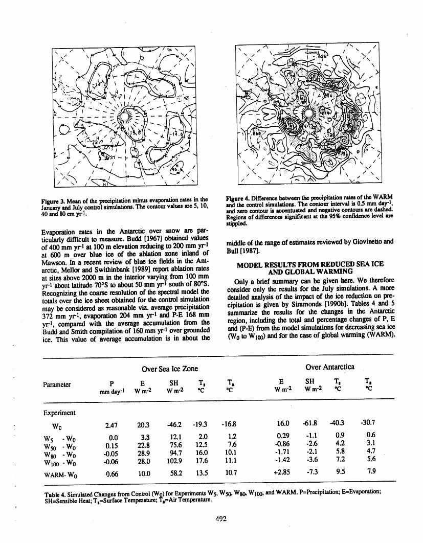
, F _ X . _, _ I /'_ /

/ " " _'I" ", \

_',, _, - , /, a ,

?"_'-_' -_ ,'_ X i H I _..(o

"x " :"""I."- I "-,L_.. _ I l,.'t.\ -_.;.,/K:,,.-":z_i.J /

i',_, ' I ,>:./I._ / - / ""'_ "_\ \ /"

Figure 3. Meanof theprecipiu_'on n_n_usevaporationrates _ the Figure 4. Difference between the precipitationrates of the WARMJanuaryandJuly control simulmons, nne contourwuues are 3, I0, and the controlsimulations. The contourintervalis 0.5 mm day.l;40 and 80 cm yrl. and zero contour is accentuimd and negative contours sre dashed.

Regions of dlffermces significant at the 95% comqdance level arestippled,

Evaporation mms in the Antarctic over snow are par-ticularly difficult to measure. Budd [1967] obtained valuesof 400 mm yr-t at I00 m elevation reducing to 200 mm yr-i middle of the range of estimates reviewed by Giovinetto andat 600 m over blue ice of the ablation zone inland of Bull [1987].Mawson. In a recent review of blue ice fields in the Ant-

arctic, Mellor and Swithinbank [1989] report ablation rates MODEL RESULTS FROM REDUCED SEA ICEat sites above 2000 m in the interior varying from I00 mm AND GLOBAL WARMINGyr-I about latitude 70°S to about 50 mm yri south of 80°S. Only a brief summary can be given here. We thereforeRecognizing the coarse resolution of the spectral model the consider only the results for the July simulations. A moretotals over the ice sheet obtained for the control simulation detailed analysis of the impa_t of the ice reduction on pre-

may be considered as reasonable viz. average precipitation cipitation is given by Simmonds [1990b]. Tables 4 and 5372 mm yri, evaporation 204 mm yri and P-E 168 mm summarize the results for the changes in the Antarcticyri, compared with the average accumulation from the region, including the total and percentage changes of P, EBudd and Smith compilation of 160 mm yri over grounded and (P-E) from the model simulations for decreasing sea iceice. This value of average accumulation is in about the OVo to Wf00)and for the case of global warming (WARM).

Over Sea Ice Zone Over Antarctica

Parameter P E SH T. T. E SH T. T_mm day'l W m"2 W m"2 °C °C W m"2 W m-2 °C °C

Experiment

W0 2.47 20.3 -46.2 -19.3 -16.8 16.0 -61.8 -40.3 -30.7

W5 - Wo 0.0 3.8 12.1 2.0 1.2 0.29 - 1.1 0.9 0.6W50 - Wo 0.15 22.8 75.6 12.5 7.6 -0.86 -2.6 4.2 3.1W8o - Wo -0.05 28.9 94.7 16.0 10.1 -1.71 -2.1 5.8 4.7Wloo - Wo -0.06 28.0 102.9 17.6 11.1 -1.42 -3.6 7.2 5.6

WARM- Wo 0.66 10.0 58.2 13.5 10.7 +2.85 -7.3 9.5 7.9

Table 4. Simulated,Changes fromContzolOV0) for ExperimentsW5, W50, WSO.WIOGand WARM. P=Precipitation;E=Evaporation;SH=SensibleHeat;Ts=SurfaceTemperature;Ts=AirTemperature.

]

AO")-v .J .i,

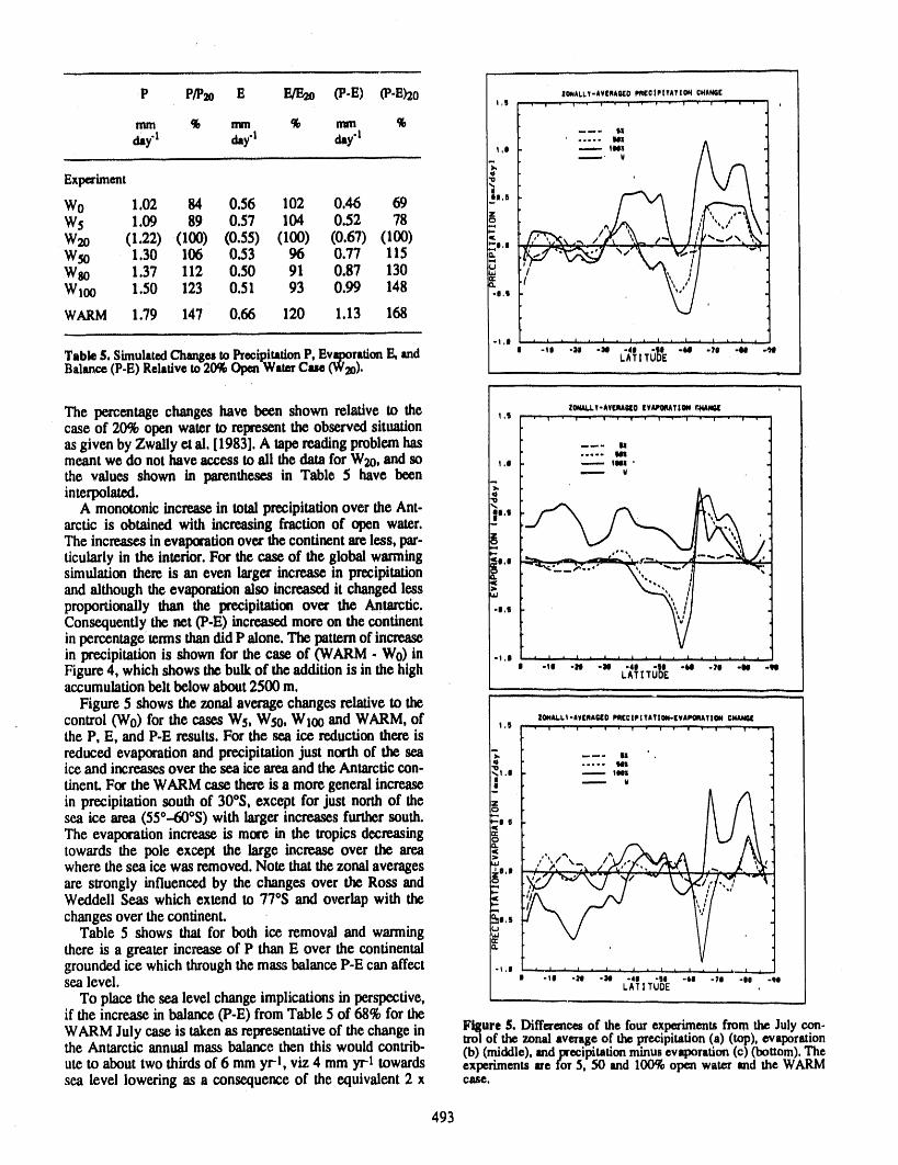
r,

P P/I)_o E _ _-E) (P'E)20 Zo,,LL.,V.,,(O_...,,t_ G,,_(

nun % mn % _ %

daY'l day'I daY'l l,, -.--- ,sos

,* ,,...mm.--.' W

Experiment

W0 1.02 84 0.56 102 0.46 69 ,,,sW5 1.09 89 0,57 104 0.52 78W2o (1.22) (100) (0.55) (lO0) (0.67) (100) :*,* /'_,,., //'

W5o 1.30 106 0.53 96 0.77 115 _" _.'"',.,"_._V_:] "Wso 1.37 112 0.50 91 0.87 130 i ./WI0o 1.50 123 0.51 93 0.99 148 :.,s /

WARM 1.79 147 0.66 120 1.13 168 ' L

J.| ,| * J * I , t , t , l , 1 , J i | I

Table $. Simulated Changes to Precipitation P, Evaporation E, and . .,. .u .N .,, .I. 4, ._Balance (P-E) Relative to 20% Open Water Case (W_0), t.ATl1"t_3_"**

[O*4AI.I.T-AV(IqAUO (W_TlOt4 r_t_IGI

The percentage changes have been shown relative to the ,,s ..... ,,,. , ,,.,, , ,,, .....case of 20% open waterto representthe observed situationas given by Zwally etal. [1983]. A tapereadingproblemhas __. mumeant we do not haveaccess to ali the datafor W20,and so ,,, _._ ,,._.the values shown in parentheses in Table 5 have been ---interpolated.

A monotonic increasein total precipitationover the Ant- _,.sarctic is obtained with increasing fraction of open water.The increasesin evaporationoverthe continentareless, par- iticularlyin the interior.For the case of the global warming i,,, "'" _- 'simulation there is an even larger increase in precipitation 5 "., I "and although the evaporationalso increased it changed less .! ",. :proportionally than the precipitation over the Antarctic. ...s v. tlConsequentlythe net (P-E) increasedmoreon the continentin percentage terms0urndid P alone. The patternof increasein precipitation is shown for the case of (WARM-W0) in .,,, , , , , . , . , , , , , , , , , .Figure4, which shows the bulkof the addition is in the high .,, ._. 4. LATXTU0("',S, -,, -,. -,, -_,accumulationbelt below about2500 m.

Figure 5 shows the zonal average changes relative tO thecontrol (9/0) for the cases WS, W50,Wloo and WARM, of ,s .O,,,,.Lv-,V(MM_O.(:l,l_,Tl_(v,_,._ C_Uthe P, E, and P-E results.For the sea ice reduction there is

reduced evaporation and precipitation just north of the sea -_ f _,_-__. _ •ice and increasesover the sea ice areaand theAntarcticcon- _,.tinent.For the WARM case there is a more generalincreasein precipitation south of 30°S, except for just northof the =Osea ice area (55°--60°S)with larger increases furthersouth. :. sThe evaporation increase is more in the tropics decreasingtowards the pole except the large increaseover the area

where the sea ice was removed.Note thatthe zonalaverages _0,, _"are strongly influenced by the changes over the Ross and _ _.,)/ '_" K,.J iWeddell Seas which extend to 77°S and overlap with the _changes over the continent. _,,s

Table 5 shows that for beth ice removal and warmingthere is a greater increaseofP thanE over the continentalgroundedice which throughthe mass balance P-E can affect ,.,sea level. , -,, -- -_. .,. .s. .- .,. -. .,.LATITUDE

To place the _ level change implications in perspective,if the increase in balance (P-E) from Table 5 of 68%for theWARM July case is takenas representativeof the change in Figure 5. Differencesof the fourexperimentsfrom theJuly con-trol of thezonalaverageof theprecipitation(a) (top),evaporationthe Antarctic annual mass balance then this would contrib- (b) (middle),andprecipitationminusevaporation(c)(bottom).Theute to about two thirds of 6 mm yr-l, viz 4 mm yr-Itowards experimentsarefor 5, 50 and100%open waterandthe WARMsealevel lowering as a consequence of the equivalent 2 x case.

493

CO2global warming. This appears to be about double the rien,are la'oadlyin therangeof estimatespresented in Tableimpact of earlier estimates where the relatively smaller 9.9 of the IPCC [Houghtonct al., 1990]:changesin evaporationwere not adequatelyconsidered Esttm_edsealevelchanges by 2050are:[Houghtonetal., 1990], Oceanthermalexpansion + 300nun

As an example of the possible impact on future sca level Temperate gls_tex melt + 90'

change the following hypotheticalscenaflo is examined. Greenlandice sheetchange 0Suppose an effective doubling of CO2with other gre_. Antaxctiobalancechange . 120

house gases occurs by the year 2030. Suppose a 20-year Totalnetchange + 270mmdelay occurs before the full oceanic warming responds to The increase in Antarcticwecipitation and mass balancethechange and assume a linearincreaseof the changes from can therefore be expecled to providea small but significant1990 to 2050. The following contributions to sea level offset to the increase in sea le'eel resultingfrom ocean ther-change are estimatedand, except for the Antarctic contrtbu, mal expansion and the melting of glaciers over the next

REFERENCES

Bromwich, D. H., Estimates of Antarctic precipitation, MeUor,M., andC. Swithinbank,Airfieldson Antarctiogla-Nature, 343, 627-629, 1990. cier ice, CRREL Report 89.21, 97 pp., U.S. Army Corps

Budd,W. F., Ablation from an Antarctic ice surface, Pro- of Engineers, Cold Regions Research and Engineeringceedings of the International Conference on Low Temper. Laboratory,1989.ate Science, Sapporo1966, pp.431-.446. Instituteof Low Robin, G. deQ., Changing the sea level, Chapter 7 in TheTemperatureScience, Hokkal&, University, 1967, Greenhouse Effect, Climatic Change and Ecosystems,

Budd, W. F., The expected sea level rise from climate edited by B. Bolin ct al., SCOPE, 29, pp. 323-359, J,warming in the Antarctic, in Greenhouse: Planning for Wiley, Chichester, 1986.Climate Change, edited by G. I. Pearman,pp. 74--82, E. Rusin, N. P., Meteorological and Radiational Regime ofJ. BriU, Leiden, 1988. Antarctica, Translated by Israel Program for Scientific

Budd, W. F., and I. N. Smith, The state of balance of the Translation 1964, Office of Technical Services, U.S,Antarctic Ice Sheet, in Glaciers, Ice Sheets and Sea Dept. of Commerce, Washington, DC, 1961.Level: Effect of a C02 induced climatic change, U.S. Schwetdffeger, W., Weather and climate of the Antarctic, inDept. of Energy Report DOE/EV/60235-1, pp. 172-177, Developments in Atmospheric Science 15, 261 pp., Else-1985. viet, Amsterdam, 1984.

Budd, W. F., B. J. Mclnnes, D. Jenssen, and I. N. Smith, Simmonds, I., Analysis of the 'spinup' of a general cireula-Modelling the response of the West Antarctic lee Sheet to tion model, J. Geophys. Res., 90, 5637-5660, 1985.a climatic warming, in Dynamics Jf i,_ West Antarctic Simmonds, I., Improvements in General Circulation ModelIce Sheet, edited by C. J. van der _¢_en, and J. Oerlemans, performance in simulating Antarctic climate, Antarcticpp. 321-358, Reidel, Dordrecht, 1_)87. Science, 2,287-300, 1990a.

Giovinetto M. B., and C. Bull, Summary and analysis of Simmonds, I., Impact of reduced sea ice concentration onsurface mass balance compilations for Antarctica 1960- the Antarctic mass balance, Proceedings of the Centre for85, Report 1, Byrd Polar Research Center, Ohio State Mathematical Analysis, vol. 25, edited by G. A. LathamUniversity, 90 pp., 1987. and J. A. Taylor, pp. 39--48, Australian National Uni-

Grotch, S. L., Regional intercomparisons of general circula- vetsity, 1990b.tion model predictions andhistorical climate data, DOE/ Simmonds, I. and W. F. Budd,A simple parameterization ofNBB-O084, 291 pp., 1988. ice leads in a GCM and the sensitivity of climate to a

Hansen, J., A. Lacis, D. Rind, G. Russell, P. Stone, I.Fung, change in Antarctic ice concentration,Ann. Glaciol., 14,R. Ruedy, and J. Lerner, Climate sensitivity: Analysis of 266--269, 1990.feedback mechanisms, in Climate Processes and Climate Simmonds, 1., and M. Dlx, The use of mean atmosphericSensitivity OVlauriceEwing Series, No. 5), edited by J.E. parameters in the calculation of modelled mean surfaceHansen and T. Takashi, pp. 130--163, American Geo- heat fluxes over the world's oceans, J. Phys. Oceanogr.,physical Union, Washington, DC, 1984. 19, 205-215, 1989.

Houghton, J. T., G. J. Jenkins, and J. J. Ephraums (Eds.), Simmonds, I., G. Trigg, and R. Law, The Climatology oftheClimate Change: The IPCC Assessment, 365 pp., Cam- Melbourne University General Circulation Model, 67bridge University Press, 1990. pp., Publication No. 31, (NTIS PB 88 227491.), Depart-

Loewe, F., Precipitation and evaporation in the Antarctic, in ment of Meteorology, University of Melbourne, 1988.Meteorology of the Antarctic, edited by M. P. van Rooy, Zwally, H. J., J. C. Comiso, C. L. Parkinson, W. J,Weather Bureau, Pretoria, pp. 71--89, 1957. L C_mpbell, F. D. Carsey, and P. Gloersen, Antarctic sea

ice, 1973-1976. Satellite passive-microwave observa-t/ons, 206 pp., NASA Scientific and Technical Informa-

" tion Branch, NASA SY-459, 1983.

494

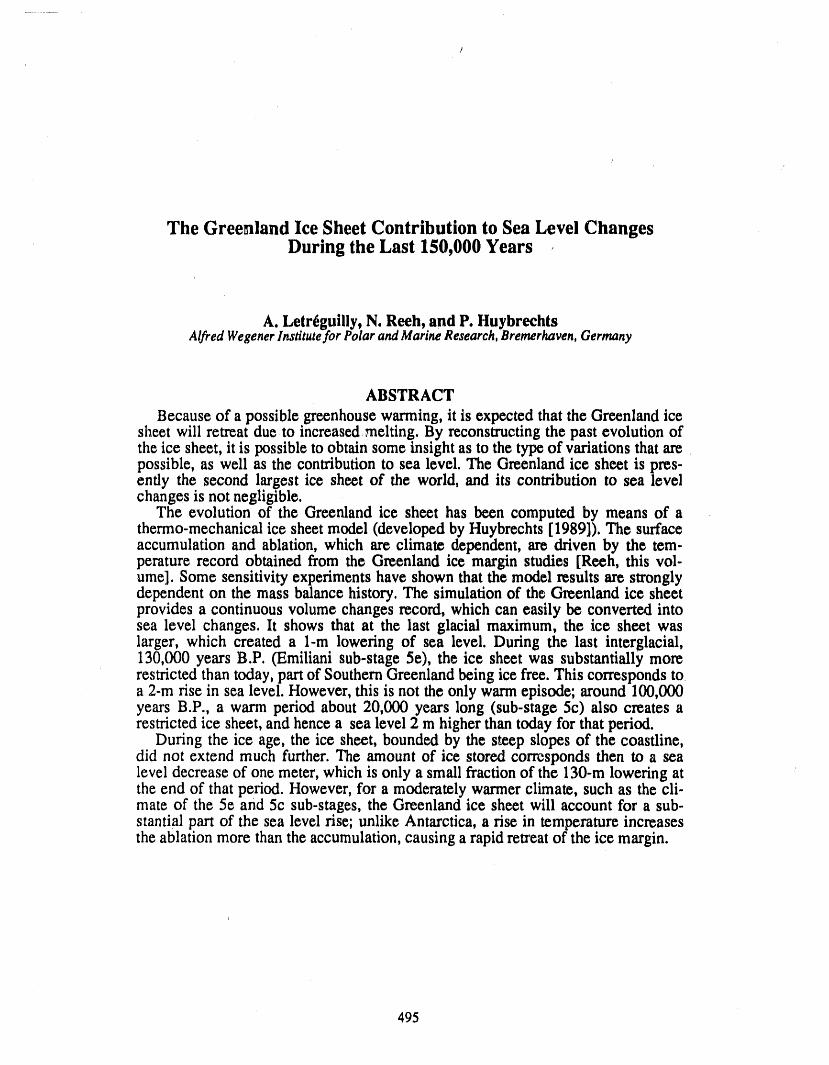
The Greenland Ice Sheet Contribution to Sea Level ChangesDuring the Last 150,000 Years

A. Letr_guilly, N. Reeh,.and P. HuybrechtsAlfred WegenerInstitutefor PolarandMarineResearch,Bremerhaven,Germany

ABSTRACT

Because of a possible greenhouse warming, it is expected that the Greenland icesheet will retreat due to increasedmelting. By reconstructing the past evolution ofthe ice sheet, it is possible to obtain some insight as to the type of variations that arepossible, as well as the contribution to sea level. The Greenland ice sheet is pres-ently the second largest ice sheet of the world, and its contribution to sea levelchanges is not negligible.

The evolution of the Greenland ice sheet has been computed by means of athermo-mechanical ice sheet model (developed by Huybrechts [1989]). The surfaceaccumulation and ablation, which arc climate dependent, are driven by the tem-perature record obtained from the Greenland ice margin studies [Rech, this vol-ume]. Some sensitivity experiments have shown that the model results are stronglydependent on the mass balance history. The simulation of the Greenland ice sheetprovides a continuous volume changes record, which can easily be converted intosea level changes. It shows that at the last glacial maximum, the ice sheet waslarger, which created a 1-m lowering of sea level. During the last interglacial,130,000 years B.P. (Emiliani sub-stage 5e), the ice sheet was substantially morerestricted than today, part of Southern Greenland being ice free. This corresponds toa 2-m rise in sea level. However, this is not the only warm episode; around 100,000years B.P., a warm period about 20,000 years long (sub-stage 5c) also creates arestricted ice sheet, and hence a sea level 2 m higher than today for that period.

During the ice age, the ice sheet, bounded by the steep slopes of the coastline,did not extend much further. The amount of ice stored corresponds then to a sealevel decrease of one meter, which is only a small fraction of the 130-m lowering atthe end of that period. However, for a moderately warmer climate, such as the cli-mate of the 5e and 5c sub-stages, the Greenland ice sheet will account for a sub-stantial part of the sea level rise; unlike Antarctica, a rise in temperature increasesthe ablation more than the accumulation, causing a rapid retreat of the ice margin.

495

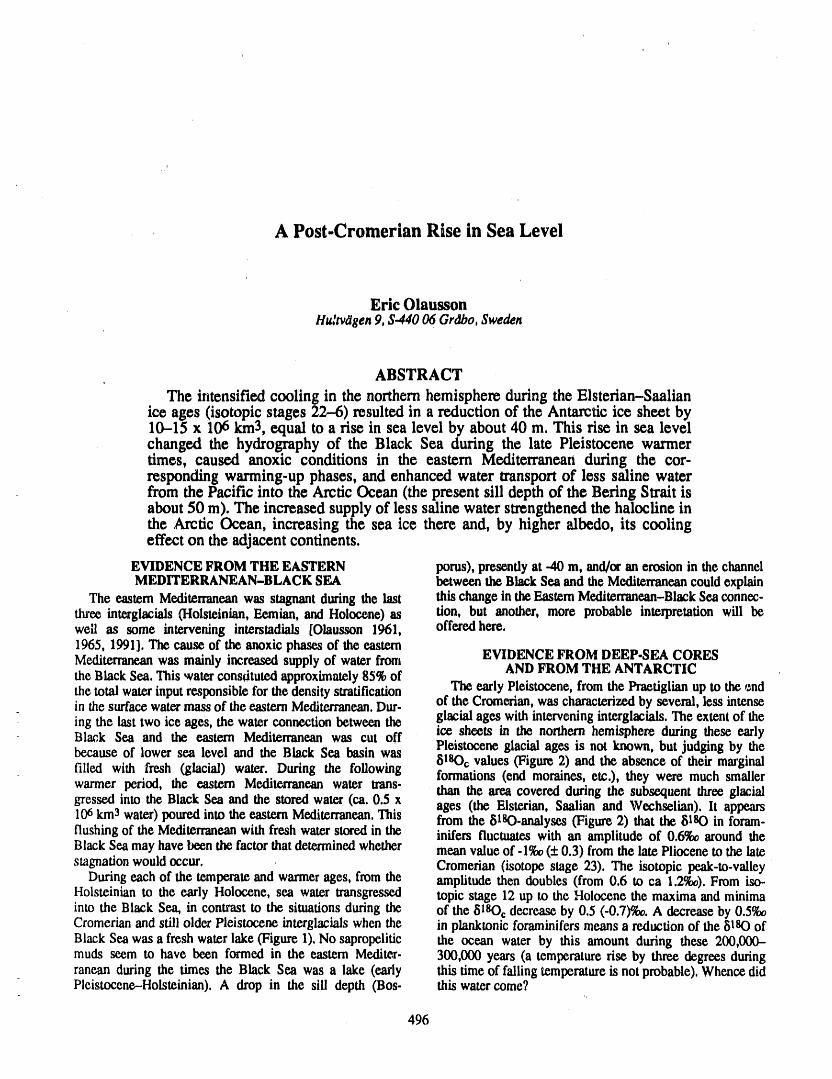
A Post-Cromerian Rise in Sea Level

Eric OlaussonHu'tvdgen9,8.44006Grdbo,Sweden

ABSTRACT

The intensified cooling in the northernhemisphere during the Elsterian-Saaiianice ages (isotopic stages 22-6) resulted m a reduction of the Antarctic ice sheet by10-15 x 106 km3, equal to a rise in sea level by about 40 m. This rise in sea levelchangedthehydrographyoftheBlackSeaduringthelatePleistocenewarmertimes,causedanoxicconditionsintheeasternMediterraneanduringthecor-respondingwarming-upphases,andenhancedwatertransportoflesssalinewaterfromthePacificintotheArcticOcean(thepresentsilldepthoftheBeringStraitisabout50m).TheincreasedsupplyoflesssalinewaterstrengthenedthehaloclineintheArcticOcean,increasingtheseaicethereand,by higheralbedo,itscoolingeffecton theadjacentcontinents.

EVIDENCE FROM THE EASTERN pores), presentlyat -40 m, and/_ an erosion in the channelMEDITERRANEAN-BLACK SEA between the Black Sea and the Mediterraneancould explain

The eastern Mediterraneanwas stagnant during the last this change in theEasternMediterranean-BlackSea connec-three interglacials (Holsteinian, Eemian, and Holocene) as rien, but another, more probable interpretation will bewell as some intervening interstadials [Olausson 1961, offered here.1965, 1991]. The cause of the anoxic phases of the easternMediterranean was mainly increased supply of water front EVIDENCE FROM DEEP-SEA CORESAND FROM THE ANTARCTICthe Black Sea. This waterconstituted approximately85% ofthe total water inputresponsible for the density stratification The early Pleistocene, from the Praetiglian up to the endinthesurfacewatermassoftheeasternMeditearancan.Dm'- oftheCromerian,wascharacterizedby several,lessintenseing the last two ice ages, the water connection between the glacial ages with interveninginterglacials. The extent of theBlack Sea and the eastern Mediterranean was cut off ice sheets in the northern hemisphere during these early

Pleistocene glacial ages is not known,but judging by thebecauseof lowersealeveland theBlackSeabasinwas 81sO¢values(Figure2)andtheabsenceoftheirmarginalfilled with fresh (glacial) water. During the following formations (end moraines, etc.), they were much smallerwarmer period, the eastern Mediterranean water trans- than the area covered during the subsequent three glacialgrossed into the Black Sca and the stored water (ca. 0.5 x ages (the Elsterian, Saalian and Wechselian), lt appears106km3 water)poured into the eastern Mediterranean.This from the 81sO-analyses (Figure 2) that the 8180 in foram-flushing of the Mediterraneanwith fresh waterstored in the inffers fluctuates with an amplitude of 0.6_ around theBlack Sca may havebeen the factor thatdetermined whether mean value of -1%o(+ 0.3) from the late Pliocene to the latestagnationwould occur. , Cromerian (isotope stage 23). The isotopic peak-to-valley

During each of the temperate and warmerages, from the amplitude then doubles (from 0.6 to ca 1.2%o).From iso-Holsteinian to the early Holocene, sca water transgressed topic stage 12 up to the Holocene the maxima and minimainto the Black Sea, in contrast to the situationsduring the of the 81SOcdecrease by 0.5 (-0.7)%0.A decrease by 0.5%0Cromcrianandstill older Pleistocene intcrglacials when the in planktonicforaminifcrsmeansa reductionof the 81sO ofBlack Sca was a fresh water lake (Figure 1). No sapropelitic the ocean water by this amount during these 200,000-muds seem to have been formed in the eastern Meditcr- 300,000 years (a temperaturerise by three degrees duringrancan during the times the Black Sea was a lake (early this timeof falling temperatureis not probable).Whence didPlcistoccne-Holsteinian). A drop in the sill depth (Bcs- this watercome?

496

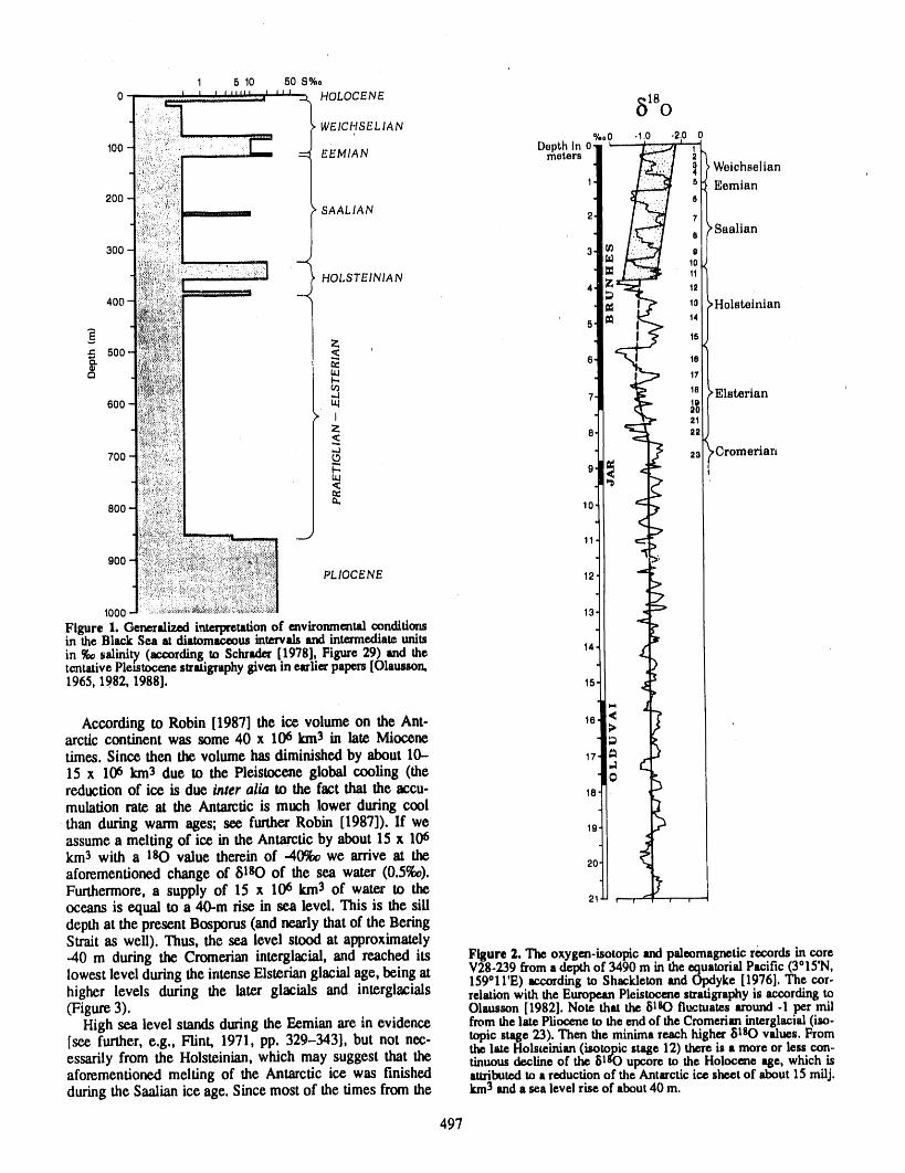
1 5 10 50 S%o0 .... _=---:-.!=.L:.-.!-:!..!_il ....' " ' _ HOLOCENE 18

; • "lm, 5_, . :'% O

.i :.iiii!;_::.: WEICHSELIAN

oo, = o''°° .,o .,oomotors ' _!

.... ;1i.!::/:_Ei_?_:::I!! .::200 ....... _i:i :_;"i"'!_'!:_ SAALIAN

300 3 9

' 4 Z 12:, ..m.............. 7/:.

_"'i '_:_::i_'_i . i_l_ _,, la Holsteinian

= 500 '_:":":!_"_:_::_

6oo ...............i,: _ _{i: I 21

700 _::::::__::":. :i_ .4 ? _s ,Cromerian

uji: < >

b_i!;_i(:.;_TiF:i::!:!;:!:i:

900 ;_/_:!i:.'i;_!_i_:__i_i!i!i;_i_::::_:_i_:!_i!_!_!:i_i'_&_l

. :_.:/ii::_i_:i.i:i:i;::;);i;_ii:._:_:!i:;i;!ii:i1:i:i::;i::_;!;:;_ii!_!ii:_;_::]_:. >;:i:::::i_iii!;;::,::_ii!;;i_!(i_:i:_!_i!:!:!i!:il:!?i;_::ii;i:ii!i_:i_;:i!_/i_,:i:i_i_i:_:i:: - '

1000 :_':::*:::_::_'_*_':_'_'_:_'_::_":_'::::"_:_*__:"_":_:_*_" 13- ,,_Figure I.Generalizedinterpretationof mv_ronm,ental .cpnditio[)s . ;in the BlackSea at diatomaceous interv_ and intermexliate umm 14- _'in %0 salini_ (w.cording to Schrader [1978], Figure 29) and thetentative Ple=tocene stratigraphy given in e_lier papers [Olausson, , )1965, 1982, 1988]. _s 4 b

According to Robin [1987] the ice volume on the Ant- _e >arcticcontinentwas some40 x 106km3 in late Miocene

times. Since then the volume has diminished by about 10- _7 ._ d

15 x 106 km3 due to the Pleistocene global cooling (the oreduction ofice isdue inter alia to the fact that the accu- _smulationrateat the Antarctic is much lower duringcool .than during warm ages; see further Robin [1987]). If we _0. "_I"assume a melting of ice in the Antarctic by about 15 x 106 .km3 with a 180 value therein of -40°/00we arrive at the 20.aforementioned change of iSlSOof the sea water (0.5%o). ,

Furthermore, a supply of 15 x 106 km3 of water to the _ ,. , .oceans is equal to a 40-m rise in sea level. This is the silldepth at the present Bosporus(and nearly thatof the BeringStrait as weil). Thus, the sea level stood at approximately-40 m during the Cromerian interglacial, and reached its Figure2. The oxygen-isotopicandpaleomagneticrecordsin corelowest level during the intense Elsterian glacial age, being at V28-239froma depthof 3490m in theequatorialPacific(3°15'N,159°11'E) according to Shackleton and Opdyke [1976]. The cor-higher levels during the hW.z glacials and interglacials relationwith the EuropeanPleistocenestratigraphyis accordingto(Figure 3). Olausson [1982]. Note that the 51tO fluctuates around -1 pe.r rail

High sea level stands duringthe Eemian are in evidence from the late Pliocene to the end of the Cromerian interglacml (iso-topic stage 23). Then the minima reach highe_ _1_O values. From

[see further, e.g., Flint, 1971, pp. 329-343], but not nec- the late Holsteinian (isotopic stage 12) there ii a more or less con-essarily from the Hoisteinian, which may suggest that the tinuous decline of the _lsO upcore to the Holocene age, which isaforementioned melting of the Antarctic ice was finished attributed to a reduction of the Antarctic ice sheet of about 15 milj.

during the Saalian ice age. Since most of the times from the km3and a sea level rise of about 40 m.

497

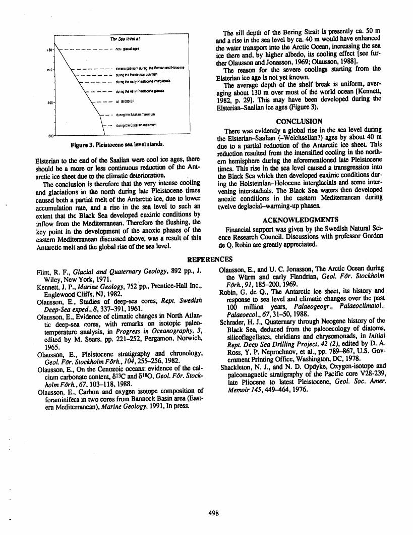
The sill depth of the Bering Strait is presently ca. 50 m_. _. I..1.t anda rise in the sea level by ca. 40 m wouldhave enhanced

.e0 _0o_.Q.. the watertranslx_ into the Arctic Ocean, increasing the seaice thereand. by higheralbedo, its cooling effect [see fur-filerOlaussonandJonasmn, 1969; Olausson.1988].

m0 c,m.,_m_m=n__.e...n._o_.°. The reason for the severe coolings starting from thedunngt_e H_to_nmnopbmum

du,,__,°-,yP,°_o_)_,Q_ Elsterianiceageisnotyetknown.The averagedepthoftheshelfbreakisuniform,aver-

a_,,__°.,,yP_°,s=n_ aging about 130 m over most of the worldocean [Kennett.._oo ,t _8oooBP 1982, p. 29], This may have been developed during the

Elsterian-Saalianice ages (Figure 3).dunngU3oSaal_anmaximum

Ounn9_e Eiste,_/_maximum CONCLUSIONThere was evidently a global rise in the sea level during

.2® the Elsteflan--Saalian(-WeichseiianT) ages by about 40 mFigure3. Plebttx:enesealevelstands, due to a partial reduction of the Antarctic ice sheet. This

reductionresulted from the intensified cooling in the north-Elsterianto the end of the Saallan were cool ice ages, there em hemisphereduring the aforementionedlate Pleistoceneshould be a more or less continuous reductionof the Ant- times. This rise in the sea level causeda transgressionintoarcticice sheet due to the climaticdeterioration, the Black Sea which then developed euxinic conditions dur-

The conclusion is therefore that the very intense cooling ing the Holsteinian-Holocene interglacials and some inter-and glaciations in the north during late Pleistocene times vening interstadials.The Black Sea watersthen developedcausedboth a partialmelt of the Antarcticice, due to lower anoxic conditions in the eastern Mediterraneanduring

' accumulation rate, and a rise in the sea level to suchan twelve deglacial-warming-up phases.extent that th¢ Black Sea developed etvdnic conditions byinflow from the Mediterranean.Thereforethe flushing, the ACKNOWLEDGMENTSkey point irt the development of the anoxic phases of the Financialsupportwas given by the Swedish NaturalSci-eastern Mediterraneandiscussed above, was a result of _his ence Research Council. Discussions with professorGordonAntarcticmeltand the global rise of the sea level, de Q. Robinaregreatlyappreciated.

REFERENCES

Flint, R. F., Glacial and Quaternary Geology, 892 pp., J. Olausson, E., and U. C. Jonas.son,The Arctic Ocean duringWiley, New York, 1971. the Witrm and early Flandrian,Geol. FOr. Stockholm

Kennett' J. P., Marine Geology, 752'pp., Prentice-HaUInc., F6rh., 91,185-200, 1969.Englewood Cliffs, NJ, 1982. Robin, G. de Q., The Antarctic ice sheet, its history and

Olausson, E., Studies of deep-seacores, Rept, Swedish response to sea level andclimatic changes over the pestDeep-Sea exped., 8, 337-391, 1961. 100 million years, Palaeogeogr., Palaeoclimatol.,

Olausson,E., Evidence of climatic changes in North Arian- Palaeoecol.,67, 31-50, 1988.tic deep-sea cores, with remarks on isotopic paleo- Schrader,H. J., QuaternarythroughNeogene history of thetemperature analysis, in Progress in Oceanography, 3, Black Sea, deduced from the paleoecology of diatoms,edited by M. Sears, pp. 221-252, Pergamon, Norwich, silicoflageUates, ebridians and chrysomonads, in initial1965. Rept. Deep Sea Drilling Project, 42 (2), edited by D. A.

Olausson, E., Pleistocene stratigraphy and chronology, Ross, Y. P. Neprochnov, et al., pp. 789-867, U.S. Gev-Geol. FOr.Stockholm F6rh., 104,255-256, 1982. enunent PrintingOffice, Washington, DC, 1978.

Olausson,E., On the Cenozoic oceans: evidence of the cal- Shacideton, N. J., and N. D. Opdyke, Oxygen-isotope andcium carbonatecontent, 513Cand51sO,Geol. F6r. Stock- paleomagnetic stratigraphyof the Pacific core V28-239,holm FiJrh.,67, 103-118, 1988. late Pliocene to latest Pleistocene, Geol. Soc. Amer.

Olausson, E., Carbon and oxygen isotope composition of Memoir 145,449-464, 1976.foraminifera in two cores from BannockBasin area (East-ern Mediterranean),Marine Geology, 1991, In press.

498=

e

Meltwater Runoff Lag from Arctic Glaciers and Ice Caps During Global Warming

W. T. Pfeffer, M. F. Meier, and T. H. IllangasekareUniversityof Colorado,Boulder,Colorado,U.S.4,

ABSTRACT

Predictions of the contribution of glacier wastage to future sea level change inresponse to global warming must consider refreezing of meltwater in cold snow.Runoff from surface melt generated in cold permeable snow is delayed because thewater first percolates locally and refreezes. Calculations to date show that this pro-cess may significantly reduce predicted sea level rise from Greenland and Arcticicecaps over the ne_:t50--150 years.

We present an extended analysis of this process for the circumpolar arctic gla-ciers and ice caps. Calculations are presented which provide estimates of the quan-tity of water refrozen by this process for the entire Arctic (given simple climatechange scenarios) and the consequent effect on predictions of future sea level.

499

Measurement Error and Climate Change Implicationsof Glacier Mass Balance Records from Western Canada

Melinda M. BrugmanNationalHydrologyResearchInstitute,EnvironmentCanada,Saskatoon,Saskatchewan,Canada

ABSTRACT

Trends in temperature, precipitation, insolation and large-scale atmospheric cir-culation have been shown to correlate with glacier mass balances measured in west-ern Canada and elsewhere in North America. In order to understand these apparentcorrelations, a detailed analysis of measurement error is needed. In this paper, theerror issue is examined for Sentinel, Piace, Helm, Woolsey, Peyto and Ram Riverglaciers. Ali these glaciers have experienced a strongly negative cumulative massbalance, except Sentinel, which is located in the western portion of the CoastRanges. Ali the glaciers, even Sentinel, have dramatically retreated throughout themeasurement period at rates of one to five meters per year. Helm and Sentinel gla-ciers are only a few kilometers apart, yet they display markedly different mass bal-ance records. We must a_k, how reliable are the glacier data?

To answer this question, the effects of measurement bias (i.e., error) due to inter-nal accumulation, basal melt, inadequate or improper pole placement, pole move-ment, map inaccuracy, surface slope change, wind and avalanche redistribution ofsnow, albedo change due to changing patterns of crevassing, surface dust and rockcoverings are fast considered. Then, computed errors in summer, winter and netbalance data are compared to that of meteorological parameters obtained for eachglacier site. Observer and technique changes are examined. Errors attributable todata manipulation are detailed.

Cumulative balance error is best computed by remapping the surface of the gla-cier and directly calculating the total volume change since the beginning of themeasurement period. Efforts are presently underway to do this by direct mapping orestimation of changes in glacier volume from stake surveys, radar and seismicsounding of glacier depths and earlier glacier surface maps.

Balance error should be further analyzed with new maps, and observation tech-niques updated to include accurate annual field surveys and remote sensing data.Increased standardization of measurement methods at ali the sites (Canadian andnon-Canadian) should reduce the possibility of error due to observer bias. In sum-mary, regular remapping of surface contours and glacier cross-sectional profiles isnecessary to properly check the accuracy of long-term glacier mass balance data.

5O0I

i

)

Ice Front Fluctuations of the Shirase Glacier, East Antarctica

Fumihiko NishioNationalInstituteof PolarResearch,Tokyo,Japan

ABSTRACT

The Shirase Glacier drainage basin in the Queen Maud Land ice sheet is drained_11a fast-moving ice stream with a flow rate of 2-3 km yr-1 at the mouth of Shirase

acier, in order to predict likely ice sheet responses to future changes in climate, itis essential to understand the controls on ice stream motion.

In the upstream region of the Shirase Glacier drainage basin, the ice sheet hasthinned by approximately 1 m yr-.1 The possible cause of thinning is basal, meltingat the ice,--bedrock interface. Since thinning began, the Shirasc Glacier has beenflowing as a fast-moving lee stream to the mouth of this drainage basin.

At the mouth of the ice stream, the Shirase Glacier crosses the grounding lineand a 15-km-wide fl.oaring ice tongue extends 80 km to the north. At the groundingline the mean velocity is 2.5 km pcr year, the lee thickness is about 500 m and grad-ually decreases towards the front.

The positions of the front of the ice tongue have been determined since 1957 byground survey and recently by LANDSAT MSS and TM, and MOS-1 MESSR sat-ellite images. Since 1957 the ice tongue has b_n retreating to the mouth of ShiraseGlacier and at present there is no ice tongue evident in MOS-1 MESSR imageryobtained in February 1989 by the Multi-purpose Satellite Receiving System atSyowa Station.

In summer, Ltttzow-Holm Bay remains covered with thick landfast sea ice, pre-venting the ice tongue from flowing seaward by ice stream motion. However, since1957 the floating ice tongue has disintegrated three times, in the middle of the1960s, 1980 and 1988, due to the retreat of the fast ice in Ltitzow-Holm Bay.

Annual mean air temperatures at Syowa Station since 1957 have increased byapproximately I°C, and 1980 was 2°C higher than the average annual temperature.This suggests that the fast ice cover in the Liltzow-Holm Bay is probably sensitiveto climate changes in the Antarctic region and is linked to the existence of the icetongue of the Shirase Glacier.

Recent rapid shrinkage of the ice tongue is, therefore, associated with the indica-tion of increasing mean annual t_mperature at Syowa Station, Antarctica.

501 )

Changes in Ice Cover Thickness and Lake Level of Lake Hoare, Antarctica

Robert A. Wharton, Jr.Biological Sciences Center, Desert Research Institute, Reno, Nevada, U.S.A,

Gary D. CIowAstrogeology Branch, U.S. Geological Survey, Menlo Park, California, U,S.A,

Christopher P. McKaySpace Sciences Division, NASA Ames Research Center, Moffett Field, California, U.S.A.

Dale T. AndersenLockheed Engineering and Sciences Co., Washington, D.C., U.S.A.

George M. Simmons, Jr.Department ofBiological Sciences, Virginia Tech, Blacksburg, Virginia, U.S.A.

ABSTRACT

Results from 10 years of ice thicknessmeasurementsat perennially ice-coveredLake Hoare in Southern Victoria Land, Antarcticaare reported. The ice cover ofthis lake thinned appreciably during the period 1979 to 1986 at a rate exceeding 20cm yr-1, from an initial thickness of 5.5 m. Since 1986, the ice cover thicknessseems to have leveled off at about 3.5 m. We suggest that the mode of behavior ofthe ice cover on this lake may have made a transition from (1) a thick "dry" icecover in which sublimation is the dominant form of mass removal from the icecover, to (2) a thinner "wet" ice cover in which near-surface melting and subse-quent percolation of meltwater through the ice becomes at least as important as sub-limation in the removal of mass from the surface of the ice cover. We also discuss aparametric analysis of the response of a model of the thick "dry" ice cover to vari-ous environmental factors, including surface temperature, sunlight, wind speed, andthe amount of light-obscuring surface sediments. This analysis shows that of theabove factors, an increase in mean annual temperature is the most plausible expla-nation for the thinning of the ice cover. Data concerning lake level and degree daysabove freezing are presented to show the relationship between peak summer tem-perature and the volume of glacier-derived meltwater entering Lake Hoare eachsummer. From these latter data and from previous observations by others that thelakes in the dry valleys axe rising, we infer that the peak summer temperatures havebeen above zero for a progressively longer period of time each year since 1973.

502

Thermal and Hydrologic Responses of an Arctic Watershed to Climatic Warming

Larry D. Hinzman and Douglas L. Kane,Water Research Center, University of Alaska Fairbanks, Fairbanks, Alaska, U.S.A.

ABSTRACT

The implicationsof globalwarming reachbeyondwarmer airtemperatures,milderwintersand longersummers.The potentialeffectsofclimaticwarmingonthehydrologicregimeofanarcticwatershedwereexploredwithrespecttophysicalchangesintheactivelayerand theresultantchangesinthecomponentsof theannual water balance and the nature of the hydrologic cycle. With the advent of cli-matic warming, the annual depth of thaw in the permafrost will increase, affectingthe amount of soil moisture storage, the depth to the water table, even the shape ofthe runoff hydrograph. The gradual thawing of the active layer was simulated usingTDHC, a heat conduction model which incorporated phase change. The results offour possible scenarios of climatic warming were input into I-IBV, a hydrologicmodel, to elucidate the effects on the hydrologic regime. The results indicate an ear-lier spring melt event, greater evaporation, greater soil moisture storage, and apotential for severe moisture stress on current vegetation types in early summerunless the precipitation pattern changes. The amount of free water in the soil willlargely depend upon precipitation patterns and amount.

503

i,

Contemporary Climate Change in the Mackenzie Valley, N.W.T,and the Impact upon Permafrost

Alan JudgeTerrain Sciences Division, Geological Survey of Canada, Ottawa, Ontario, Canada

Angus HedleyCanadian Climate Centre, Atmospheric Environment Service, Downsview, Ontario, Canada

Margo BurgessTerrain Sciences Division, Geological Survey of Canada, Ottawa, Ontario, Canada

Kay MacInnesLand Resources Division, Indian and Northern Affairs, Yellowknife, Northwest Territories, Canada

ABSTRACT

Many global change scenarios predict a pronounced wanning of the Arcticregions over the next several decades. The impacts of a possible wanning of severaldegrees on the permafrost environment have important implications locally andglobally.

Although permafrost temperatures may be expected to change in response to anincrease in air temperature, the relationship between air and ground temperature is aresult of complex and poorly known surface energy exchange processes. The mag-nitude, extent and rate of permafrost response to climate change are, therefore, notsimple to predict. A cooperative project was established in 1986 in order to exam-ine and better understand permafrost and climate relationships along the MackenzieValley corridor. Several instrumented sites have been established and graduallyequipped with AES automatic weather stations and GSC/INAC deep ground tem-perature boreholes. Analysis and monitoring of ground temperature and climatedata will provide information on both recent surface temperature changes and onthe ground thermal response to current local climate trends. Analysis of existing airtemperature data from standard meteorological stations yields statistically sig-nificant increases of about 1 K in the past 50 years. In contrast the arctic coastshows some evidence of cooling in the same time-frame.

Preliminary examination of ground temperature profiles from the MackenzieValley provides evidence of recent surface increases of up to 3 K. The presentnorthward decrease of surface temperature in the western arctic is roughly 0.7 K perdegree of latitude and thus the southern margins of permafrost might be expected toretreat northwards by several hundred kilometers over the next century.

- 504

Response of Permafrost to Changes in Paleoclimate

T. E. Osterkamp, J. P. Gosink, T. Fei, and T. ZhangGeophysical l_titute, University ofAlaska Fairbanks, Fairbanks, Alaska, U.S.A.

ABSTRACT

Solutions to the Stefan problemfor the motionof the base of ice-bearingperma-frost in response to changes in paleoclimate wereobtainedusing perturbation,finitedifference, and finite element methods. Paleotemperature models were used toinvestigate the thickness response, compare soludon methods, determine the currentstate of the permafrost, and to determine constraints on the models. The per-turbation and finite difference methods used the approximation of linear tem-perature profiles while the finite element method did not. There was a transientthickness response of about 41 kyr implying that paleotemperature records ofgreater length are needed for models and that the permafrost loses its "memory" ofpast conditions for much longer times. Faster thawing rates, slower freezing rates,and greater variations in thickness were found for the perturbation and finite differ-enee solutions compared to the finite element solution. These appear to be causedby the simplifying assumptions in the former solutions. A lag (20 kyr) existsbetween changes in surface temperature and thickness response and a small thermaloffset is apparent in the finite element solution. Small asymmetries exist in thefreezing and thawing rates and thickness response. Paleotemperature models basedon ice cores predict current permafrost thicknesses that are too large. Models withthe long-term mean surface temperature of permafrost within a few degrees of thecurrent value of- 11°C and with full glacial temperatures no more than 6-8°C lowerare compatible with current Prudhoe Bay conditions. These include models devel-oped for East Siberia, from isotopic profiles in deep sea sediments, and for Barrow,Alaska, modified for Prudhoe Bay. These models predict that the permafrost thick-ness at Prudt...e Bay varied by <10% (<60 m) over the last glacial cycle. Freezingand thawing rates were less than 6 mm yr-l. At present, this permafrost should benear its long-term equilibrium thickness and should be thawing at <1 mm yr-1.

Time males for the thickness response of deep continu- temperature prof'de)under the permafrost. A numerical solu-ous permafrost are of the same order as the periods of recent tion (finite difference method) was constructed using theglaciations (105 years) over the past 106 years. Therefore, it same assumptions. The third solution, which does not useis appropriate to consider the permafrost response to the these assumptions, is a complete numerical scheme usinginferred changes in paleotemperatures associated with these finite flements to numerically integrate the thermal energyglaciations. Three solutions have been obtained to address equation from the permafrost surface, through the phasethis question. An approximate analytical (perturbation) boundary, and deep into the underlying unfrozen materials.method was used to solve the heat balar_ceequation at the Applications of the solution methods to paleotemperaturephase boundary (base of the ice-hearing i_.rmafrost) assum- models at the surface of the permafrost were used to com-ing linear temperature profiles in the permafrost and con- pare the solutions, to investigate the thickness response ofstant geothermal heat flux (which also yields a linear the permafrost, to assess the current state of the permafrost,

505

and to develop general constraints on paleotemperature were greatercompared to permafrost that contained pure icemodels of the surfacetemperature history,Ts, of the perma- (-3.9 mm yr-I< X < 3.8 mm yr-I and 365 m < X < 487 m),frostnearPrudhoeBay, Alaska. These differences are attributed to temperature.dependent

The solution methods were applied to step, linear, sinu- thermal properties,distributed latent heat effects, and thesoidal, and otherpotential paleotemperaturemodels of Ts. conversion of only part of the soil solution to ice near theExcept forthe sinusoidalmodel, these models arenotgener- phaseboundarywhen brine is present in the permafrost.ally periodic. Perturbationsolutions which are polynomials Temperature,profiles in the permafrostare nearly linearin time, t, for models consisting of a seriesof step or linear for the finite element solution, which supports the linearchanges in Ts can be used to approximate any Ts provided assumption used in the perturbation and finite differenceeach step or linear segment is long compared to the time solutions. The long-term variations in paleotemperataresconstant, tc = X2/4D, where X is the permafrost thickness lead to disturbances in the temperature profiles extending toand D its diffusivity. 2 to 3 Ian depthforPrudhoe Bay conditions.

There was a transient response in X for ali solutions Paleotemperaturemodels for the surface temperatureofwhich, for the models and Prudhoe Bay conditions, was permafrost are constrained in that they must predictthe cur-nearly nii after about 200 kyr. For the sine model, the per- rent permafrost conditions at Prudhoe Bay to within theturbationsolution yields a transienttimeconstant, taffihX0/J uncertaintieF Currently,X ,, 600 m, Jl " 55 mW m"2,Ts ffi_,41 kyr,whereh is the volumetric latentheat,X_0the long- -11°C, andX is unmeasuredbut inferredto be close to zero.term periodic mean permafrost thickness (X0 = Xe= KI (Tc The step model of Brigham and Miller [1983] which was

q's B) and J the deep undisturbed geothermal heat flux. developed for the Barrow area was modified for PrudhoeSince the transient response affects the predicted X, then Bay conditions and has Ts ---13.3"C and YCe-739 m withresults obtained from calculations extending over one time -80C > Ts > -150C. lt leads to a prediction of current X ,,constant orless will generally be influenced by the transient. 712 m, which is slightly greater than the uncertainty (aboutWhen Ts is periodic, the transient canbe eliminated by + 15%),with712m<X<755 m,choosing the initial permafrost thickness, Xi, to be the value A normalized SPECMAP curve [Matteucci, 1989] wasfound at the end of two or more cycles. Permafrost at Prod- modified and linked to produce a relatively warm modelhoe Bay loses its "memory" of past conditions for times with _'s "-IIOC, Xe - 600 m, and -80C > Ts > -14°C. Cur-much longerthanone time constant.As a result, the effects rent X - 602 m with562 m g X g 646 m.of possible submergence of some areas at Prudhoe Bay, A paleotemperaturemodel developed for East SiberiaAlaska by high sea levels >45 kyr B.P.cannotbe detected at [Maximova and Romanovsky, 1988] yields predictions inpresent, given the uncertaintiesin the data. excellent agreementwith currentconditions. Thismodel has

Long-term mean permafrost thickness, X, calculated from _'s " -11.3oc, Xe- 616 m, and Ts ranging from -7°C tothe time average of X, usually differed slightly between slightly colder than -17"C. Values of Ts are about 2°Csolutions and withXe. This may be partially a result of small wanner than the modified step model while values for Tscomputational errors but when the thermal conductivity in during glacial periods agree with the estimates of Brighamthe permafrost, Kt, was set equal to that of the underlying and Miller [1983]. Current X - 601 m with 557 m < X <unfrozen material K2, the difference was nearly eliminated, 660 m.suggesting that it was, at least primarily, a result of thermal Predictions based on the East Siberian model, modifiedoffset. SPECMAP model, and on the modified step model indicate

The perturbation and finite difference solutions predicted that the permafrost should be near its equilih'ium thicknessamplitudes for X (513.5 m < X < 686.5 m and 510 m < X < and thawing 0ess than 1 mm yr-t) in response to the warm-685 m respectively for the sine model) which were generally ing since the last glacial period. The predicted current heatgreater than the finite element values (531.5 m < X < 657.5 flow in the permafrost at X is about 58--61 mW m-Z,slightlym for the sine model) by about one fourth to one third, larger than observed, and increasing. This indicates that the

There is a lag between Ts and changes in X. For the sine currently observed value may be slightly greater than themodel, the lag angle, B = arctan(c0ta)- 19 kyr, where cois true heat flow at depth.the frequency. Computations based on paleotemperature models deter-

Small asymmetries exist in X and _: for the numerical mined from the isotopic profile in the Vostok ice core pre-solutions. These are most apparent in the _ine model where, diet current values for X which are much too large. Resultsfor the finite element solution, values of X for thawing are from the Camp Century ice core are expected to be similar.

greater than for freezing which results in changes of X for lt does not seem likely that these models will be useful forthawing which are greater than for freezing. The curve for X interpreting permafrost thickness variations in the Alaskanvs. t is also slightly_wider(in time) compared to a pure sine Arctic.function when X < X and narrower when X > X. The curve lt appears that paleotemperature models for the surfacefor X is slightly wider during freezing and narrower during temperat_ureof permafrost in the Prudhoe Bay area will needthawing, to have Ts within a few degrees of the current Ts (-11°C)

The finite element solution for a sine model of Ts was and minimum temperatures during the last glacial periodused to compare the response of permafrost containing brine within about 6--8°C of current Ts. These conclusions areand ice to that of permafrost containing pure ice. Tem- based on results from a limited number of models. Exceptperatures and phase boundary motion are qualitatively sim- for the step model, these models were developed for otherilar for the two cases. However, for permafrost containing distant regions.

brine, phase bo_dary velocities and thickness variations Modeling of the reslxmse of the permafrost to changes in(-6.0 mm yr-I < X < 5.2 mm yr-I and 345 m _ X < 523 m) the paleoclimate is hampered by the lack of reliable paleo-

-

506

temperaturemodels for the surface temperatureof the per, REFERENCF,Smafrostand informationon the thermalpropertiesand heat Brigham, J, K., and O. H. Miller, Paleotemperature esti-flow in thepermafrost, mates of the AlaskanArctic Coastal Plain duringthe last

125,000 years, Proc. Fourth Intl. Co_f. Permafrost, pp.ACKNOWLEDGMENTS 80--85,National AcademyPress, Washington, DC, 1983,

This researchwas sponsoredby the Earth Sciences Sec- Matteucci, G., Orbital forcing in a stochastic resonancetion, Division of PolarPrograms,National Science Fotmda. model of the l.atte-Pleistc_ne climate variations,Climatelion under Grant Nos. DPP86-19382 and DPP-87-21966, Dynamics, 3, 179-190, 1989,andU.S, Geological SurveyAwardNo. 14-08-001-G1305. Maximova, L. N,, and V. Y. Romanovsky,A hypothesisfor

the Holocene permafrostevolution,Proc, F_fth Intl, Conf.Permaffrost, pp. 102-106, Norwegian Inst. Tech., Trond-helm, Norway, 1988.

_t3_•JU !

The Antarctic Glacial Geologic Record and GCM Modeling: A Test

D. H. ElliotByrdPolarResearchCenterandDepartmentof Geology& Mineralogy,The OhioState University,Columbus,Ohio,U.S.A.

D. H. BromwichByrd PolarResearchCenter,The OhioStateUniversity,Columbus,Ohio,U.S.A.

D. M. HarwoodDepartmentof Geology,Universityof Nebraska,Lincoln,Nebraska,U.S.A.

P.-N. WebbByrdPolarResearchCenterandDepartmentof Geology& Mineralogy,The OhioState University,Columbus,Ohio,U.S.A.

I

ABSTRACT

A recent GCM (General CirculationModel) study of Antarctic glaciation by Oglesbyconcluded that (1) oceanic heat transport is relatively unimportantin the developmentand maintenance of Antarctic glaciation; (2) height andpolar position, not the AntarcticCircumpolarCurrent,have led to thermal isolation; and(3) surface elevation may be cru-cial for glaciation. Model results are here evaluated against the Pliocene geologic recordfor Antarctica.

The Sirius Group,widely distributed in the TransantarcticMountains, contains diatomfloras suggesting open marbleconditions in interiorEast Antarctica as recently as about3m.y. ago. The Sirius deposits also contain a sparse fossil flora including Nothofaguswood, demonstratingsnow-free conditions and elevated summer temperatureswithin 500km of the South Pole. Based on f'Lssiontrack dataand marine sediments, uplift rates forthe TransantarcticMountainsare estimated to average 50-100 m m.y.-1 for the last 10m.y., although rates may have been higher during the last 3 m.y. The continentalinterioris also most unlikely to have changed elevation by more than a few hundredmeters in thelast 3 m.y. If the dating of the Sirius is correct and uplift rates have not been an order ofmagnitude higher, then polar location and elevation cannot be primary controls on theformation andsubsequentfluctuations of the ice sheet.

The cause of this discrepancy between modeling results and observations can besought in limitations to the model (NCAR CCM1) used by Oglesby. It is _own thatatmospheric GCMs generally do not simulate the modem Antarctic climate with grea_realism. This is also true for the NCAR CCM1 as evidenced by deficiencies in simulatedcyclone behavior, cloud cover amounts, air temperaturesandsnowfall rates.Anothersub-stantial limitation is that there is no simulation of ocean dynamics. The ocean does nottransportheat polcward, and appears in the model only via specified sea surface tem-peraturefields. Recent work with a coupled atmosphere-ocean GCM indicates that theatmosphere andocean are strongly linked in these latitudes, and that this interaction is adominant aspect of climatic variation on (at least) the decadal time scale.

Initial results indicate that GCM performancegenerally needs to be enhanced and, inparticular, that realistic interactive atmosphere-ocean models are needed. An improvedgeologic database, particularlywith respect to age determinations and amounts and ratesof uplift, would facilitatemodel validation.

5O8

INTRODUCTION results difficult. Here we examine results of modeling Ant-Concern about the possibility of global climate change arctic conditions [Oglesby, 1989] in the light of inferences

resulting from human activities has given rise to renewed drawnfrom terrestrialdeposits of Late Pliocene age (-.3 Ma)interestin records ofpaleoclimate as measuresof thenatural in Antarctica[Webb et al,, 1984; McKelvey et al,, 1991],variabilityof the earth's climate system. Presentclimate is We choose this Pliocene example for comparisonof modelregardedas an interglacial within the coldest part(last 2-3 results with the geologic record because continental posi-m,y,) of the present Cenozoic Ice Age that started tens of tions were no different than today and no major geographicmillionsof yearsago. Fluctuationsof the climate systemare change has occurredin Antarctica except for the size of theevident in, for instance, the terrestrial record of glacial ice sheets,deposits and the oxygen isotope signal derivedfrom ice anddeep-sea sediment cores. MODELING STUDY OF ANTARCTIC

Numerical modeling of past climate can be viewed in ICE SHEET FORMATIONterms of three different time scales and resolutions. Ice Oglesby [1989] used an atmospheric general circulationcores, tree rings and other recordscan give proxy climate model (GCM) developed by the National Centerfor Atmos.datawith annual resolution and time scales of several thou- pheric Research (NCAR) to evaluate possible mechanismssand years [Wtgley et al., 1981; Bradley, 1983], Ice cores that could lead to the development of ice sheets in Ant-from the EastAntarctic ice sheet give decadal to millennial arctica. The GCM employed was the Community Climateresolutionon time scales of more than 100,000 years, and Model (CCM)which has been used fora wide varietyof cii-can be correlated with the high resolutiondeep sea cores on mate diagnostic and climate change studies [WiUtamson,the basis of oxygen isotope stage chronology [Lofius et al., 1990]. The model code evolves over time as simulations of1985, 1989]. Longer time scales are obtained from most additional processes are added and improved numericaldeep sea cores andfromother geologic databut resolutionis schemes are implemented. Version 1 of the CCM (CCM1),generally limited. Only the last category provides informa- unchangedsince June 1987, was used in Oglesby'sstudy.rien on the full range of naturalvariabilityand therefore is Table 1 summarizes some of the key attributesof themost important in understandingthe frameworkfor any CCM1 simulations carried out by Oglesby [1989]. Thechanges in climate. CCM1 and equivalent models produce global fields of the

Interest in modeling past cli:,_:, is increasing.Results of main climatic variablesby numerical time integration,overresearch on, for instance, Cretal. ,_ (120-65 Ma) and an arrayof gridpoints, of five non-linearpartialdifferentialEocene (-55-40 Ma) climates haw i_n presented by equations (two for momentum and one each for energy,Ban'on [1983] and Cirbus Sloan and Barren [1990]. The mass conservation,and moisture)from specified initial con-inherent limitations of geologic data, which increase with ditions [Williamson et al., 1987]. Typical integrationtimesthe age of the re.cordbeing considered, make evaluation of requiredfor the model atmosphere to approach a state of

ASPECT TREATMENT

PredictiveEquations Conservationofmass,momentum,energyandmoisture.Cloudsarederived.

NumericalDetails Verticalandtimecalculationsarecarriedoutbyfinitedifferences,buthorizontalcomputationsin-volveaspecllal-transformmethod.A sigmavertical(orterrainfollowing)coordina[esystemisused.

TimeStep 30minutes

HorizontalResolution Spectrallytruncatedatrhomboidalwave15CRIb'),about7,5°longitudeby4.5°latitude.At70°S,this correspondsto 280 km x 500 km.

VerticalResolution 12unevenly spacedlevels, 6 of which are below 300 bpa over terrainnear sea level.

Treatmentof the Ocean Representedonly by specified interface conditions; sea surface temperaturesand sea ice distributionareeither assumed or derived frompresentclimatological data. No ocean dynamics (e.g., currents,poleward heat transport,thermohalineconvection) is permitted.

AntarcticTopography Specified from higher resolutiondatawhich are spectrally truncatedto R15.

RadiationModes PerpetaalJanuary (australsummer) andJuly (australwinter). Solar radiationdoes not change fromone simulationday to the next. These constructsareused because of their computationalefficiency,and because the resultsclosely approximate those obtainable from seasonal simulations.

Seasonal (solar radiation varies with calendar day) - includes a calculation of snow accumulation andablation.

Table 1. RelevantCharacteristicsof Oglesby'sNCARCCM1 Simulations(materialexCactedfromOglesby [1989]and Williamsonet al,[1987]),

509

quasi-equilibriumwith the imposed boundaryconditionsare (5) Even with low continental elevations and very warma few hundreddays for perpetualruns and many years for seas (model sea surfacetemperaturesat the Antarcticcoastseasonalnms. In the present context, which deals with phe- during July ffi 14°C) the model is only able to producenomenamanifestedovertime scales of 105to 107years,it is tundra-likeconditions (i.e,, treeless, but without a perma-particularlyimportantto emphasize that only the behavior nentsnow cover),of the atmosphere is modeled, and that no dynamic inter- lt is clear thatthe model wants to form an ice sheet withaction with the ocean or the ice sheets is permitted, The Antarctic geography and bedrock elevations close to thoseocean surface characteristics and the topography of Ant- at present, This result does not necessarily imply a steadyarcticaarespecified boundaryconditionsalthough in reality ice sheet buildup.Fluctuationsin size could arise,forexam-these canvary significantlyover time periodsas short as 103 pie, because of ice flow and varying net mass inputfrom theto 104 years, Another key aspect is that the horizontaland atmosphereas the ice sheet topography changes, However,vertical spacing of the grid points is much too coarse to glaciological scaling calculations [W. A. Jones, personalyield adequate simulationsof the katabaticwind circulation communication, 1990] show that it is very difficult to getwhich probablyplays a central role in the dynamics of the size fluctuationslarge enough to produce the open marinemodem Antarctic atmosphere [e.g., Parish and Bromwich, conditions in the deep interior of the continent which are1991], implied by the glacialgeologic results outlined below. Pos-

Oglesby used a set of 16 CCM1 simulationswith differ- sible causes for model bias are presented in the Discussionent boundaryconditions to evaluatethe impactof two mech- section.anisms upon the developmentof glaciationon the Antarcticcontinentover the last twenty million years or so: opening ANTARCTIC GEOLOGIC RECORD

of the seaway (Drake Passage) between South America and Although the recordof glaciation in Antarcticagoes backAntarctica, and changing the elevation of the continent, to the early Oligocene (ca. 36 Ma) [Barrett et al., 1989;Oceanic conditions prior to the opening of the Drake Pas- Hambreyet al., 1989; Wise et al., 1991] or possibly oldersage were presumed to be characterized by increased [Barron etal., 1991; Birkenmajer, 1991],evidence from theoceanic poleward heat transport in comparison to today Pliocene Sirius Group [Webb et al., 1984; McKelvey et al.,because of the disruptionof the AntarcticCircumpolarCur- 1991] and the correlativePagodromaTiUite [McKelvey andrent. This oceanic change was represented in the model by Stephenson, 1990] provide the most dramaticevidence forspecifying sea surface temperaturesabove freezing at the substantialcontrasts in Antarctic climate and ice sheet con-Antarctic coast duringwinter with the consequentabsence figurationthroughtime.of sea ice. The impact of variations in the height of Ant-

The Siriuscomprisesscatteredglaciallyrelatedsedi-arctica was examinedby comparingsimulationswith eleva- mentary deposits throughout the Ross Sea sector of thelions everywhere less than 200 m with those using the TransantarcticMountains, The Sirius consists of compactmodem high elevation Antarctic topography. Seasonalcycle till deposited directly by ice and interbedded glaciofluvialsimulations with an explicit surface budgeting for snowaccumulation and ablation were carried out; Antarctic grid and glaciolaeustrine sediment. Deposits assigned to the Sir-points were initialized to be free of snow during the first ius are found in a variety of topographic settings, most ofsummer.The goal was to ascertain whetherany combination which are related to present-day glacial drainage through theof sea surface temperatures and continentalelevations could mountains. The most striking aspect of the principaloccur-

fences of the Sirius [Harwood, 1986a] is the presence of rareresult in the complete melting of accumulated winter snowduring subsequent summers. The prescribed continental marine microfossils and "microclasts" of marine biogenicsnow cover forperpetualrunsand the specified atmospheric sediment (these microclasts consist of clumps of diatomCD2 content were also varied, skeletons thatcould not have been transported aerially or by

The following conclusions were obtained by comparing traction currents). These originate from marine sediments inthe CCM1runs: subglacial basins of East Antarctica that were eroded and

(1) The presence or absence of oceanic flow through the transported by the ice sheet to the Transantarctic MountainsDrake Passage has little impact on Antarctic glaciation.The [Webb et al., 1984]. The dominant microfossils are marinesmall impact on simulated glaciation conditions of the pre- diatoms of early Pliocene age, although other fossil groupssumed warmer high latitude sea surface temperatures (that are present and other, older time intervals are also repre-accompany a closed Drake Passage) arises because of the sented [Harwood, 1986a,b].small storm wansIg_ of heat and watervapor into the inter- The marine sediments and associated microfossils reflectior of the continent. The higher sea surface temperatures several episodes of extensive deglaciation when marinemay, in fact, promote ice sheet growth through increased embayments or seaways covered intracratonic basins. Agewinter snowfall, dating for these marine incursions is afforded by application

(2) Antarctica is thermally isolated by its elevation and its of Southern Ocean diatom biostratigraphy (developed overpolarlocation (which results in long periods with little or no 20 years throughdeep sea drilling and piston coring in highsunlight) rather than by the Antarctic CircumpolarCurrent. southern latitudes including McMurdo Sound at 78°S), The

(3) The height of the continent may play an essential role diatomaceous s_ments indicate a deep water (>75 m)in ice sheet formation and maintenance (today, average sur- marine depositional setting that was ice-free for severalface temperatures decrease by about I°C for each 100-m months of the year in order to allow for annual diatom

- increase in elevation), blooms and accumulation of sediment consisting pre-(4) Greatly increased atmospheric CO2 concentrations dominantly of diatom skeletons.

have little impact over the changes resulting from removal I'his scenario of repeated deglaciation and marine incur-: of sea ice and elevated sea surface,temperatures, sion presented by the Sirius data is supported by similar

510

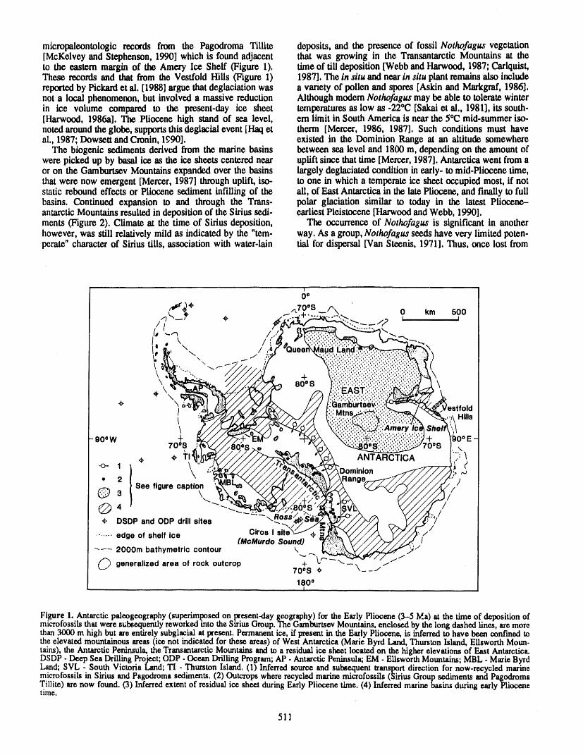
micropaleontologic records from the Pagodroma TilUte deposits, and the presence of fossil Nothofagus vegetation[McKelvey and Stephenson, 1990] which is found adjacent that was growing in the Transantarctic Mountains at theto the eastern margin of the Amery Ice Shelf (Figure 1), time of till deposition [Webb and Harwood, 1987; CarlquiskThese records and that from the Vesffold Hills (Figure 1) 1987]. The in situ and near in situ plant remains also includereported by Pickard et al. [1988] argue that deglaciation was a variety of pollen and spores [Askinand MarkgrM, 1986],not a local phenomenon, but involved a massive reduction Although modem Nothofagus may be able to tolerate winterin ice volume compared to the present-day ice sheet temperatures as low as -22°C [Sakai PAal., 1981], its south-[Harwood, 1986a]. The Pliocene high stand of sea level, ern limit in South America is near the 5°C mid.summer iso-noted around the globe, supports this deglacial event [I-halPA therm [Mercer, 1986, 1987], Such conditions must haveal., 1987; Dowsett and Cronin, 1c,90], existed in the Dominion Range at an altitude somewhere

The biogenic sediments derived from the marine basins between sea level and 1800 m, depending on the amount ofwere picked up by basal ice as the ice sheets centered near uplift since that time [Mercer, 1987]. Antarctica went from aor on the Gamlmrtsev Mountains expanded over the basins largely deglaciated condition in early- to mid-Pliocene time,that were now emergent [Mercer, 1987] through uplift, iso- to one in which a temperate ice sheet occupied most, if notstatic rebound effects or Pliocene sediment infiUing of the all, of East Antarctica in the late Pliocene, and finally to fullbasins. Continued expansion to and through the Trans. polar glaciation similar to today in the latest Pliocene-antarctic Mountains resulted in deposition of the Sirius sedi- earliest Pleistocene [Harwood and Webb, 1990].ments (Figure 2). Climate at the time of Sirius deposition, The occurrence of Nothofagus is significant in anotherhowever, was still relatively mild as indicated by the "tem- way. As a group, Nothofagus seeds have very limited poten-perate" character of Sirius tills, association with water-lain tial for dispersal [Van Steenis, 1971]. Thus, once lost from

!00

,,_r'_, ,,-,.7' 0 km 500

i(, _< I.,, '..o \\ / ,_

\ ,., +\ 8008 \

.,t.k ,. \<

/

\900W 4

7008

_. . TI ANTARCTICA•o- 1 \

• 2 \ Dominion

3 See figureoaptIo_

O 4 :;//DSDPand ODP drill sites \/

....... edge of shelf ice Circa I sit, /(McMurdo Sound) /

-'-_- 2000m bathymetriccontour \

_ generaUzedarea outcrop +of rock70oS _ --\__//

1800I

Figure 1. Antarcticpaleogeography (superimposedon _.esent-day geography)for the Early Pliocene (3-5 Ma) at the time of deposition ofmicrofossils that were st;bsequendyreworkedinto the StriusGroup.The GarnbuttsevMountains,enclosed by the long dashed lines, are morethan3000 m high but are entirely subglacial at present. Permanentice, if presentin the EarlyPliocene, is inferredto have been confined tothe elevated mountainous areas (ice not indicated for these areas) of West Antarctica (Marie Byrd Land, ThurstonIsland, Ellsworth Moun-tains), the Antarctic Peninsula, the TransantarcticMountains and to a residual ice sheet located on the higherelevations of East AntarcticaDSDP. Deep Sea Drilling Project',ODP- Ocean DrillingProgram;AP. AntarcticPeninsula;EM - Ellsworth Mountains;MBL - Marie ByrdLand;SVL - South Victoria Land;TI - ThurstonIsland. (1) Inferredsource and subsequent trans_rt direction for now-recycled marinemicrofossils in Sirius and Pagodmmasediments. (2) Outcropswhere recycled marinemicrofossils (Sirius Groupsediments and PagodromaTiUite) are now found. (3) Inferredextent of residual ice sheet duringEarly Pliocene time. (4) Inferredmarinebasins duringearly Pliocenetime.

511

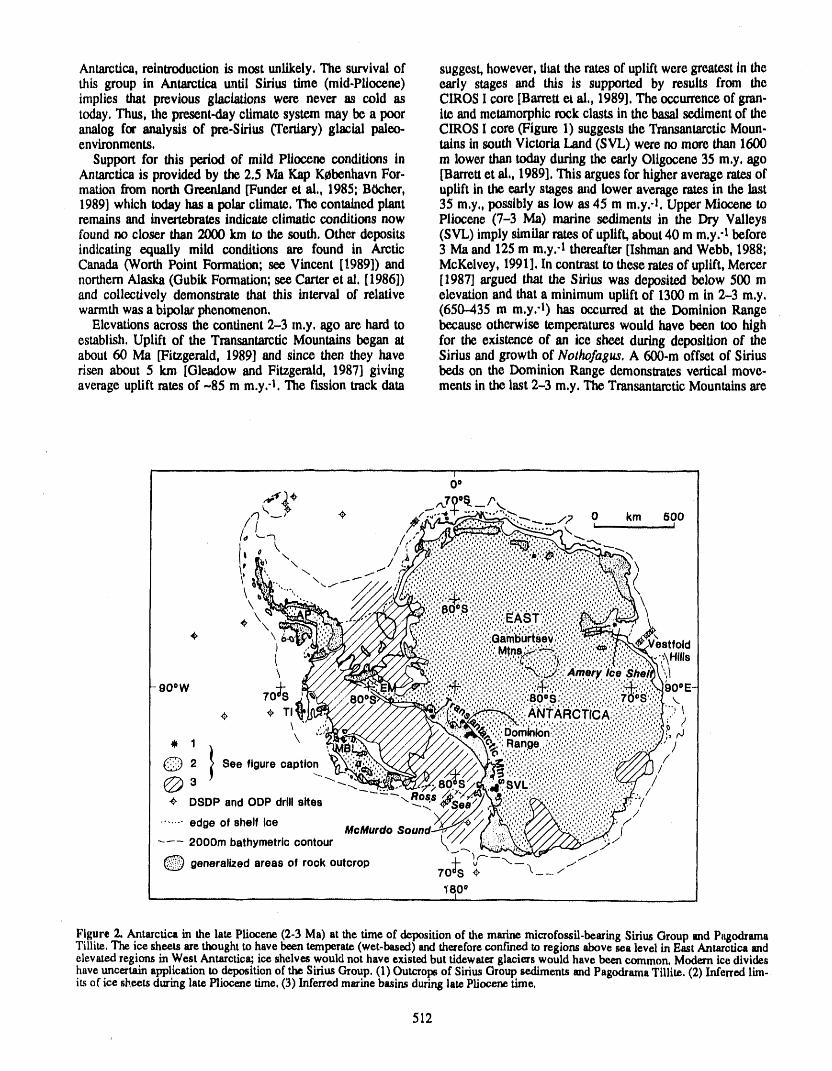
Antarctica, reintroduction is most unlikely. The survival of suggest, however, that the rates of uplift were greatest in thethis group in Antarctica until Sirius time (mid.Pliocene) early stages and this is supported by results from theimplies that previous glaciations wea_ never as cold as CIROS I core [Barrett _ al,, 1989], The occurrence of gran-today. Thus, the present-day climate system may be a poor ite and metamorphic rock clasts in the basal sediment of theanalog for analysis of pre-Sirius (Tertiary) glacial paleo- CIROS I core (Figure 1) suggests the Transantarctic Moun-environments, tatns in south Victoria Land (SVL) were no mote than 1600

Support for this period of mild Plioc,ono conditions in m lower than today during the early Oligocene 35 m.y, agoAntarctica is provided by the 2.5 _ Kap Kebenhavn For- [Barrett et al,, 1989]. This argues for higher average rates ofmarion from north Greenland [Funder et al., 1985; B_her, uplift in the early stages and lower average rates in the last1989] which today has a polar climate. The contained plant 35 m.y., possibly as low as 45 m m.y.-I. Upper Idiocene toremains and invertebrates indicate climatic conditions now Pliocene (7-3 Ma) marine sediments in the Dry Valleysfound no closer than 2000 km to the south, Other deposits (SVL) imply similar rates of uplift, about 40 m m.y.-I beforeindicating equally mild conditions are found in Arctic 3 Ma and 125 m m,y.-I thereaftex [Ishman and Webb, 1988;Canada (Worth Point Formation; see Vincent [1989]) and McKelvey, 1991], In contrast to these rates of uplift, Mercernorthern Alaska (Gubik Formation; see Carter et al, [1986]) [1987] argued that the Sirius was deposited below 500 mand collectively demonstrate that this interval of relative elevation and that a minimum uplift of 1300 m in 2-3 m,y.warmth was a bipolar phenomenon, (650-435 m m,y, "l) has occurred at the Dominion Range

Elevations across the continent 2-3 ro.y, ago are hard to because otherwise temperatures would have been too highestablish, Uplift of the Transantarctic Mountains began at for the existence of an ice shce_ during deposition of theabout 60 Ma [Fitzgerald, 1989] and since then they have Sirius and growth of Nothofagus. A 600.m offset of Siriusrisen about 5 km [Glez_dow and Fitzgerald, 1987] giving beds on the Dominion Range demonstrates vertical move-average uplift rates of -85 m m.y.-l. The fL_siontrack data ments in the last 2-3 m,y. The Transantarctic Mountains are

I0 o

//9 "_-----_-- "_ 0 km 500I I

I -\ I/ \

,.\

.\,

}

\

90°W 70_S

_> _> TI _RCTICA:\

1 \

I "@ 2 See figure oaptlon

Qa /* DSDP andODP drillsites \

/....... edge of shelf ioe /

McMurdoSoun, /_- 2000m bathymetriocontour ;/

generalizedareas of rook o_oropQ 70 ¢ \-- /

1800l

Figure 2, Antarcticain the late Pliocene (2-3 Ma) at the time of deposition of the marinemicrofossil-bearing Sirius Groupand PagodrarnaTillite. The ice sheets arethought to have beentemperate(wet-based) andthereforeconfined to regions above sea level in East Antarcticaandelevatedregions in West Antarctica;ice shelves would not have existed but tidewaterglaciers would have been common. Modernice divideshaveuncertainapplication to depositionof the Sirius Group.(1) Outcropsof SiriusGroupsediments andPagodramaTillite. (2) Inferred lim-itsof ice sheets during late Pliocene time,(3) Inferredmarine basinsduringlate Pliocenetime.

512

)

thought to be a rift shoulder[Stem and ten Brink, 1989] and descriptionof the sea surface conditions, A realisticcoupledthus may exhibit rapid vertical movements, Most of the atmosphere-oceammodel (incorporating, for instance, slm-availableevidence does not support rapid recent movement ulations of sea ice and CO.zvariations) may produce veryalthough high rates (1000 m m,y,-l) are inferred by different results (as illustrated fora different context by theBehrendt and Cooper [1991] and somewhat lower rates workof Stouffer ct al, [1989]),(-500 m ro,y,"1)may be required for the Dominion Range (2) The present location and extent of Antarctica wea'eSirius deposits, Polar climates, in which the freeze-thaw used for ali simulations, For example, no excursions ofmechanism for rock disintegrationis largely inactive,do not warm ocean currents into the continental interior we.relead to rapid denudation of exposed rock in mountain allowed [Oglesby, 1989],ranges, Thus, for the TransantarcticMountains, elevations (3) The strong sensitivity of the modeled net snowmay have been as much as 1500 m lower 3-5 ro,y, ago than buildup to the prescribed snow surface albedo [Oglesby,they are today. This is, however, insufficient to alter major 1991],circulation patterns, e.g., the Transantarctic Mountains (4) The model's inability to reproduce accurately thewould still havebeen an effective barrier,morethan 1.500m present-day characteristics of climatic variables that arehigh, to lowertroposphericairflow, important for this study (especially the seasonal cycle slm-

No comparableevaluation can be made forotherparts of ulations) is also a significant limitation, These include:the continent.An average uplift rate for the last 30 m.y, of (a) Cyclone behavior near Antarctica is not satis-50 m m,y,-1has been argued for the Amory Ice Shelf region factorily simulated. The model's circumpolar low pres-[WellmanandTingey, 1981], No dataexist forQueenMaud sure trough is located too far north, is not deep enough,Land. Marie Byrd Land, however, is dominatedby young and does not have minima at the correct longitudes [seealkaline volcanoes with associated hyaloclastites, and sig. Williamson and Williamson, 1987; Xu et al,, 1990]. Thenificantverticalmovements in the Late Cenozoic have been model may not, as a result,be able to representaccm'atelysuggestedby LeMasurierand Rex [1983]. the horizontal_hcattransportinto the continentby storms

The bedrock elevation of East Antarctica is the key in both for present and altered topographic conditions. Fur-termsof ice sheet growth. Cold polar ice sheets are not par- thermore,the likely inability of the model to resolve sat.ticularlyeffective agents of erosion because, where frozen isfactorily the katabatic wind circulation (the dominantto the bed, movement at the base of the ice sheet is accom- component of the mean meridional mass circulation)modated within the basal ice, not at thecontact. Estimatesof implies that the entire atmospheric heat budget may noterosion by the Laurentide ice sheet of North America be correctlyrepresented.amount to only a few tens of meters for much of the for- Co) Annual precipitation rates over Antarctica pro..morly ice-covered area [Dyke et al,, 1989]. Erosion is duced by the model appearto be two to threetimes largerunlikely to have significantly changed bedrock elevation than observed, althoughthe simulated seasonal cycle issince the mid Pliocene. Most of the interior of East Ant- qualitatively representative [compare Williamson andarcticais a craton and can be expected tDbehave like other Williamson, 1987; Bromwich, 1988]. Clearly,the amountcratonic areas such as the Canadian shield, or Africa: ver- of annual snowfall is centralto the questionof whether atical movements, other than those associated with isostatic shallow, simulated snowfield can survive through thereboundfollowing deglaciation, are likely to be slow (<100 summerablationperiod, and is stronglyinfluenced by them m,y.-l), Mercer [1987], however, suggests a rate of uplift storm transport of water vapor across the coastlineas high as 200 m m.y.-I for the central part of the marine [Bromwich,1988].basin from which the microfossils in the Sirius were (c) Simulated total cloud amounts for July mono-derived. The subglacial Gamburtsev Mountains, possibly a tonically increase from six tenths at 550S to eight tenthsvolcanic edifice like the Tibesti Mountains in the Sahara, at 85°S [Oglesby, 1989] rather than being high over themay be a young geological feature and could play a crucial ocean and falling to around four tenths near South Polerole as a primary center for ice sheet growth. Broad, high [Schwerdffeger, 1970]. This shortcoming means that thebedrock elevations comparable to the Colorado Plateau sth'face conditions over the continent will not be correctlyregion or the Tibetan Plateau, both thought to be significant modeled. Another GCM [Shibata and Chiba, 1990]for northern hemisphere climate [Ruddiman and Raymo, showed a strong sensitivity of the modeled winter Ant-1988; Ruddiman and Kutzbach, 1989], are not part of the arctic climate to cloud cover characteristics over thelate Cenozoic (<10 m.y.) history of Antarctica. continenL

The extremes of Pliocene climatic conditions in Ant- (d) Simulated surface air temperatures from 70--85°Sarctica have occurred with essentially today's geography and are around 8°C warmer than actual during both summerbedrock topography, and winter [compare Taljaard ct al., 1969; Schwerdtfeger,

DISCUSSION 1970; Oglesby, 1989]. Such a warm bias is importantThe glaciated continent indicated by the model results is because summer melting may be simulated to continue

in marked contrast to the very dynamic ice sheet conditions much longer and to be more active than is actually therevealed by the glacial geologic and paleontologic findings case.outlined above. For the Pliocene the continental position and Although, in principle, modeling results cannot be valid(ice-free) topography were essentially those of today, if incompatible with observational data, in reality geologic

Some causes for the apparent model shortcomings could data also have certain limitations. In the geologic argumentinclude: presented here, six uncertainties need to be recognized.

(1) The simulations come solely from an atmospheric (1) The age of the Sirius Group is dependent on how wellmodel. The ocean behavior is specified and limited to a the age of the diatom assemblages can be established and

513

whether Southern Ocean biostratigraphic ages can be Mountainsmay notapplyto the whole of a cross.range trim.directly applied to the continental interior, Diatom bio- sect at that locality, and even if they did, the rates estab-geography suggests that a ixm.Antar_ttc biostrattgraphic ltsbed in thatone sector may not necessarily apply to thescheme applies to both the surrounding ocean and the con- rangeas a whole, Raisedmarinesequences spanningthe lastttnental interior [Harwood, 1991] duringthe Pliocene and 10 m,y, (datedpaleontologicaUyor by radiometricmethods)thatage assignments for the Sirius could not differby more from around the East Antarctic cratoncould provide stg-than 0,5 m,y, from that in the Southern Ocean, Mercer niflcant constraints,as would information on the exposure[1987] provides an analysis of the whole problem of the ages of rockplatforms (provided by cosmogenieally inducedSirius deposits, radionuclides),

(2) Other interpretations of Antarctic glacial history (5) Bedrock topography is poorly known for large partsderived froma varietyof evidence include suggestionsof an of East Antarcticaand therefore uncertaintiesexist in theolder (pre.Pliocene)age for Sirius Groupdeposits [Mercer, location of possible centers of ice sheet initiation and1987], ice sheet overriding of the Transantar_ticMountains growth,[Mayewski, 1975;Dentonet al,, 1984], andonly limitedele- (6) Finally, the rates of erosion are essentially unknownration changes of the TransantarctlcMountains duringthe although widely regardedas very slow,last several million years [Stern and ten Brink, 1989; lt is clearthatan improvedgeologic databasewould sub-McKelvey, 1991], Other aspects of, and perspectives on, stanttallyimprove the ability to validate model results, ThisAntarctic glacial history can be found in Denton et al, should be accompanied by improvements in the per-formanceof the models, so that, at least, I_resent-daycondi-[1991].

(3) The climate tolerances of extant Nothofagus species tions can be simulated with some confidence [compareare well known [Peele, 1987]; however the affinities of the Simmonds, 1990], The most pressing taskappearsto be thepliocene Antarctic Nothofagus from the Sirius have yet to developmentof realisticcoupled atmosphere-ocean modelsbe established definitively, and in any case it is likely to for high southern latitudesaccompanied by incorporationofhave tolerances unique to polar environments. Therefore, more precise paleogeographtc information gained throughalthough qualitative statements can be made, precise tem- geologic records,peratures(mean annual temperature,etc.) andelevationlim-its cannot be drawndirectly for theNothofagus in the Sirius ACKNOWLEDGMENTSsediments, Preparationof this paper was supported by NSF grants

(4) The geologic argument is critically dependent on DPP-8716258 to D, H, Elliot and DPP.8916134 to D, H,knowing the rates and amounts of uplift of the Trans- Bmmwich, Fieldworkand subsequent laboratory studies onantarctic Mountains and the continental interior during the the Siriusdeposits have been supportedby NSF grants DPP-last 5 m.y. Fission-trackdating cannot resolve this, at least 8117889, 8315533 and 8420622, We are grateful for thein part because of the likelihood of episodic uplift. Fur- constructive input from reviewers R. Oglesby and E,thermore, ratesestablished at one site in the Transantarctic Banon, Byrd PolarResearchCentercontribution727,

REFERENCES

Askin, R, A,, and V. Markgraf,Palynomorphsfrom the Sir- B6cher, J., Boreal insects in northernmost Greenland:ius Formation, Dominion Range, Antarctica, Antarct. J. padaeo-entomologicalevidence from the Kap KCbenhavnU.S,, 21, 34-35, 1986. Formation(Pile-Pleistocene), Peary Land, Fauna herr,,

Barrett,P. J., M. J, Hambrey,D. M. Harwood, A. R. Pyne, Ser. B 36, 37-43, 1989.andP, N. Webb,Synthesis, in Antarctic Cenozotc History Bradley, R. S., Quaternary Paleoclimatology, 472 pp.,from the CIROS I drill hole, McMurdo Sound, edited by Allen andUnwin, Boston, 1983.P, J, Barrett,DSIR Bull., 24.5,241-251, 1989. Bromwich, D. H., Snowfall in high southern latitudes,gev.

Bah'on, E. J., A warm, equable Cretaceous: The natureof Geophys,, 26, 149-168, 1988,the problem,Earth Science Reviews, 19, 305-338, 1983. Carlquist,S,, UpperPliocene-lower Pleistocene Nothofagus

Barren,J. A., B. Larsen, and J. G. Baldauf, Evidence for wood from the Transantarcti¢Mountains, Aliso, 11,571-late Eocene-early Oligocene Antarctic glaciation and 583, 1987.observations on Late Neogene glacial history of Ant- Carter,D. L., J. Brigham.Grette,L. Marincovieh,Jr,, V. L.arctica: results fromODP Leg 119, in Proceedings, ODP Pease, and J. W. Hillhouse, Late Cenozoic Arctic OceanScientific Results, 119, edited by J. A. Barren,B. Larsen, sca ice and terrestrialpaleoclimate, Geology, 14, 675-et al., College Station, TX (Ocean Drilling Program), 678, 1986.1991, In press. CirbusSloan, L., and E. J. Barren, "Equable"climates dur..

Behrendt,J., andA. K. Cooper, Evidence of rapidCenozoic ing EarthHistory, Geology, 18, 489-492, 1990.uplift of the shoulder escarpment of the Cenozoic West Denton, G. H., M, L, Prentice, D, E, Kellogg, and T, B.Antarctic rift system and a speculation on possible cii- Kellogg, Late Tertiary history of the Antarctic ice sheet:mate forcing, Geology, 19, 315-319, 1991. Evidence from the Dry Valleys, Geology, 12, 263-267,

Birkenmajer, K., Tertiary glaciation in the South Shetland 1984.Islands, West Antarctica: evaluation of data, in Gee- Denton, G. H., M. L. Prentice, and L. H. Burckle, Cenozoiclogical Evolution of Antarctica, edited by _,I. R.A. history of the Antarctic ice sheet, in Geology of Ant-Thomson, J, A. Crame, and J. W. Thomson, pp. 629--632, arctica, edited by R. J. Tingey, Oxford Univ, Press, 1991,Cambridge University Press, Cambridge, 1991. In press.

514

DowseR, H, J,, and T, M, Cronin, High eustatic sea level The Environmental Record in Glaciers and lee Sheets,during the middle Pliocene: Evidence from the south, editedby H, Oeschger and C, C, Langway, pp, 343-361,eastern U,S, Atlantic Coastal Plain, Geology, 18, 435- john Wiley and Sons, 1989,438, 1990, Mayewski,P, A,, Glacial geology and late Cenozoic history

Dyke, A. _¢.,J,-S. Vincent, I, T, Andrews,L, A, Dridge,and of the Trans,antarcticMountains, Antarctica,Report No.W, R, Cowan, The L,aurentideIce Sheet and an intro. 56, Institute of Polar Studies, Ohio State Univ,, Colum.duction to the Quaternary Geology of the Canadian bus, 168pp,, 1975,Shield, pp, 178-189 in Chapter3 of Quaternary Geology McKelvey, B, C,, The Cainozotc glacial record in Southof Canada and Greenland, edited by R. J. Fulton; The VictoriaLand- A geological evaluationof the McMurdoGeology of North America, Geol, Soc, America,K.1, 837 Sound drilling projects, in Geology of Antarctica, editedpp,, 1989, by R, J, Ttngey, OxfordUniv, Press, 1991, In press,

Fitzgerald,P, G,, Uplift and formationof the Transantarcttc McKelvey, B, C,, and N, C, N, Stephenson, A geologicalMountains:application of apatite fission trackanalysis to reconnaissance of the Radok L_o area, Amery Oasis,tectonic problems, 28th International Geological Con. Prince Charles Mountains, Antarctic Science, 2, 53-.66,gress, Abstracts eel, 1, p, 491, Washington, DC, 1989, 1990,

Funder,S,, N, Abrahamsen, O. Bennike, and R, W. Feyling- McKelvey, B, C,, P,-N, Webb, D, M, Harwood, andHanssen, Forested Arctic: Evidence from North Green. M, C, O, Mabin,The Dominion Range Sirius Group- Aland, Geology, 13,542-546, 1985, record of the late Pliocene-early Pleistocene Beardmore

Glcadow, A, J, W,, and P, G, Fitzgerald,Uplift history and Glacier, in Geological Evolution of Antarctica, edited bystructureof the TransantarcticMountains- new evidence M. R, A, Thompson, J, A. CramP,and J. W, Thomson,from fission trackdatingof basementapatites in the Dry pp, 675.-682, CambridgeUniv, Press, Cambridge, 1991,Valleys area, southern VictoriaLand, Earth Planet. Set, Mercer,J, H., Southernmost Chile: A modernanalog of theLPtr.,82, 1-14, 1987, southern shores of the Ross embaymentduring Pliocene

Hambrey,M, J,, B. Larsen, W. E, Ehrmann,and ODP Leg warmintervals,Antarct. J. U,S., 21,103-105, 1986,119ShipboardParty,Fortymillionyearsof Antarcticgia. Mercer,J. H,, The AntarcticIce Sheet during the late Neo-cial history yielded by Leg 119of the Ocean DrillingPro- gene, in Palaeoecoiogy of Africa and the Surroundinggram, Polar Record, 25, 99-106, 1989, Islands, eel. 18, edited by J. A. Coetzee and E, M, van

Haq, B. U., J. Hardenbol, and P, R. Vail, Chronology of Zinderen Bakker, pp, 21-33, A,A. Balkema, Rotterd,im,fluctuating sea levels since the Triassic, Science, 235, 1987,1156-.1167, 1987. Oglesby, R, J., A GCM study of Antarcticglaciation, CIl-

Harwood, D, M., Recycled siliceous microfossils from the mate Dynamics, 3, 135-156, 1989.SiriusFormation,Antarct.J.U.S.,21,101-103, 1986a. Oglesby, R, J., Sensitivity of glaciation to initial snow

Harwood' D, M., Diatom biostratigraphyand paleoecology cover, CO2, snow albedo, and oceanic roughness in thewith a Cenozoic history of Antarctic ice sheets, Thesis, NCAR CCM, Climate Dynamics, 4, 219-235, 1991,592 pp.,Ohio StateUniversity,Columbus,eH, 1986b, Parish, T, R., and D. H. Bromwich, Continental-scale sim-

Harwood, D, M., Cenozoic diatom biogeography in the ulation of the Antarctic katabatie wind regime, J.southern high latitudes: inferredbiogeographic barriers Climate, 4, 135-146, 1991. .and progressive endemism, in Geological Evolution of Pickard,J., D. A, Adamson, D. M, Harwood,G. H. Miller,Antarctica, edited by M. R. A. Thomson, J. A. Cramp, P. G, Quilty, andR. K. Dell, EarlyPliocene marinesedi-and J. W. Thomson, Cambridge University Press, ments, coastline, andclimate of East Antarctica,Geology,Cambridge, 1991, 16, 158-161, 1988.

Harwood,D, M., and P. N. Webb,Early Pliocene deglacia- Pool:_.,A. L., SouthernBeeches, New Zealand DSIR lqfor-tion of the Antarcticice sheet and late Pliocene onset of marion Series, 162, 148 pp., Science Infornmtion Pub-bipolar glaciation, EOS, Transactions of the American lishing Centre, 1987.Geophysical Union, 71,538-539, 1990. Ruddiman,W. F,, and J. E. Kutzbach, Forcingof Late Cen-

Ishman, S. E., and P. N. Webb, Late Neogene benthic ozoic Northern Hemisphere climate by plateau uplift inforaminiferalrecord from the Victoria Land Basin mar- Southern Asia and the American West, J. Geophys. Res.,gin, Antarctica:application to glacio-eustatic and tectonic 94, 18409-18427, 1989.events, in Benthos '86, Rev. Paleobiol., Vol. Spec. 2,523- Ruddiman, W. F., and M. E. Raymo, Northern Hemisphere551, 1988. climate regimes during the past 3 Ma: possible tectonic

LcMasurier,W. E., and D. C. Rex, Rates of uplift and the connections, Phil. Trans. R. Soc. Lend., B 318, 411-430,scale of ice level instabilitiesrecordedby volcanic rocks 1988.in Marie Byrd Land, West Antarctica,in Antarctic Earth Sakai, A., D. M. Paten, and P. Wardle, Freezing resistanceScience, edited by R. L. Oliver, P, R. James, and J, B. of trees of the south temperate zone, especially subalpineJago, pp. 603--670, Australian Academy of Science, species of Australasia,Ecology, 62,563-570, 1981,Canberra, 1983. Schwerdffeger, W,, The Climate of the Antarctic, Vol. 14,

Lorius, C,, J, Jouzel, C. Ritz, L. Merlivat, N. I. Barkov, edited by S. Orvig, pp. 253-355, World Survey of Clim-Y. S. Korotkevtch, and V. M. Kotlyakov, A 150,000-year atology, edited by H. E. Landsberg, Elsevier, 1970.climatic record from Antarctic ice, Nature, 316, 591-596, Shibata, K., and M. Chiba, Effects of radiation scheme on1985. the surface temperature and wind over the Antarctic and

Lorius, C., G. Raisbeck, J. Jouzel, and D. Raynaud' Long- on circumpolar lows, Proc. NIPR Syrup, Polar Meteorol.term environmental records from Antarctic ice,cores, in Glaciol., 3, 58--78,1990,

515

Simmonds, I., Improvementsin general c_ulatton model Wellman,P,, andR, J. Tingey, Glaciation,erosionandupliftperformance in simulating Antarctic climate, Antarct. over partof East Antarctica,Nature, 291, 142-144, 1981,Science, 2,287-300, 1990. Wigley, T. M.L,, M. J, Ingrain,and G. Farmer,Climate and

Stem, T. S,, and U, S. ten Brink, Flexural uplift of the History, 530 pp,, Cambridge University Press,TransantamttcMountains,J. Geophys. Res., 94, 10315- Cambridge,1981,10330, 1989. Willlamson, D, L., CCM Progress Report - July 1990,

Stoufler, R. J., S. Manabe,and K. Bryan, Intethemispherlc NCARITN.351+PPR, 108 pp., National Center forasymmetryin climate response to a gradualincrease of AtmosphericResearch, Boulder,CO, 1990.atmosphericC02, Nature, 342, 660-662, 1989. Wiiliamson, D. L., J. T. Kiehl, V, Ramanathan, R, E.

Taljaard,J. J,, H, van Loon, H. L. Crutcher,and R. L. Je_ne, Dickinson, and J. J, Hack, Ik_riptton of NeAR Com-Climate of the Upper Air: Southern Hemisphere, Vol. 1, muntty Climate Model (CCM1), NCARITN.285+STRoTemperatures,dew points and heights at selected pres. 112 pp,, National Center for Atmospheric Research,sure levels, NAVAIR-50.1C.55, 135 pp., Chief of Naval Boulder,CO, 1987.Operations,Washington, DC, 1969. Williamson, G. S., and D, L, WiUtamson,Circulationsla-

Van Steents, C. G. G. J., Nothofogus, a key genus of plant tistics fromseasotwAand perpetualJanuaryandJuly sire-geography, in time and space, living and fossil, ecology ulattons with the NCAR Community Climate Modeland phylogeny, Bhmaea, 19, 65-98,1971, (CCM1): Rf5, NCAR/TN.302+STR, 199 pp., National

Vincent, J.-S., Quaternarygeology of the northernCanadian CenterforAtmospheric Research,Boulder, CO, 1987.InteriorPlains, pp. 100-138 in Chapter2 of Quaternary Wise, S. W., Jr., J. Breza, D, M. Harwood, and W. Wei,Geology of Canada and Greenland, edited by R. J. , Paleogene glacial history of Antarctica,in ControversiesFulton; Geol. Soc. Amer,, The Geology of North Amer. in Modern Geology, edited by D. W. Muller,J. A. Mack.tca, K.I, 837 pp., 1989. enzie, and H. Wetssert, pp. 155-171, Academic Press,

Webb, P.-N., and D. M. Harwood,Terrestrialflora of the London,1991.Sirius Formation:Its significance for Late Cenozoic gla- Xu, J.-S., H. von Storch,and H. van Loon,Theperformancecial history, Antarct. J. U.S.,22, 7-11, 1987. of four spectralGCMs in the Southern Hemisphere: theJanuaryand July climatology and the semiannual wave,

Webb, P.-N., D. M. Harwood, B. C. McKelvey, J.H. J. Climate, 3, 53--70, 1990,Mercer,and L. D. Stott, Cenozoic marine sedimentationand ice volume variationon the East Antarctic eraton,Geology, 12, 287-291, 1984.

516

A Search for Short-Term Variations in the Flow of Ice Stream B, Antarctica

W. D. Harrison and K. A. EchelmeyerGeophysicalInstitute,Universityof AlaskaFairbanks,Fairbanks,Alaska,U.S.A,

N. HumphreyDivisionof GeologicalandPlanetarySciences,CaliforniaInstituteof Technology,Pasadena,California,U.S.A.

'ABSTRACT

There is good theoretical and geologic evidence that some ice sheets, both pastand present, arc inherently mechanically unstable to climate or sca level changes,and can disintegrate over short periods of time; exmnples of this behavior in smalltidewater glaciers are well documented. The West Antarctic Ice Sheet, which isgrounded below sea level, is thought to Dc the least stable of the present ice sheets.Recent observations of several investigators have focused attention on the role thatthe large ice streams draining into the Ross Ice Shelf play in the stability of the icesheet. These streams, at least in some cases, appear to bc transient features, out ofbalance with their accumulation areas and subject to large changes; one of them, IceSu'cam C, appears to have stagnated within the last century or so. Another, IceStream B, seems to move largely by the deformation of an underlying till layer.

Given this background of interesting flow behavior, we have be,cn searching forshort-term changes in the flow (which arc often seen on mountain glaciers) as indi-cators of flow mechanisms of Ice Stream B. The measurements began in November1988 and continued to the end of 1989. During the austral field seasons dailymotion studies were conducted with EDM and UHF positioning systems. The 1988data showed the speed near the edge of the ice she.ct to bc constant at 1.00 m d-1within the sensitivity of a few pcr cent. During the 1988 field season meters wereinstalled to measure the horizontal and vertical components of ice strain to a resolu-tion of about 1 pan in 106. Seismic activity in the ice was also monitored. Thesedata were recorded by data loggers for recovery in late 1989, and will be reported.

517

The Velocity Field of Antarctic Outlet GlaciersJ

B.K.LucchittaU.S.GeologicalSurvey,Flagst_f,Arizona,U.S.A.

J.G. Ferrigno,T.R.MacDonald,and R.S.Williams,Jr.u.s.GeologicalSurvey,Reston,Virginia,U.S.A.

ABSTRACT

Climate-induced changes in the area and volume of polar ice sheets mayseverely impact the Earth's densely populated coastal regions; melting of the WestAntarctic ice sheet alone could cause a sea level rise of 3.5 meters. Yet the massbalance (the net gain or loss) of the Antarctic ice sheets is still poorly known, and it

• is not entirely certain whether the Antarctic ice sheets ra'e growing or shrinking.Moreover, the velocity field of most ice streams and outlet glaciers has not yet beenexplored.

An extensive set of Landsat images covering Antarctica was acquired in theearly to middle"1970s. Recently, a program to re-acquire Landsat images over thecoastal regions of Antarctica was initiated by an International Consortium of SCAR(Scientific Committee on Antarctic Research). These later views of the same scenespermit the measurement of outlet-glacier velocities by tracking the translational

. movement of crevasses in the floating part of the glaciers. This technique is preciseenough to establish velocity gradients both along and across glaciers. We appliedthe technique to 15 outlet glaciers around the coast of Antarctica. Preliminaryresults indicate a range in average velocities from a low of 0.1 km per annum to ahigh of 2.2 km per annum. The two highest velocities measured to date are in thePine Island and Land Glaciers in Maria Byrd Land of West Antarctica. As soon asnew image acquisitions permit additional measurements, we will expand our studyto include as much of the Antarctic coastline as possible. We anticipate that thestudy will eventually yield a near-comprehensive view of the outlet-glacier velocityfield of Antarctica.

- 518

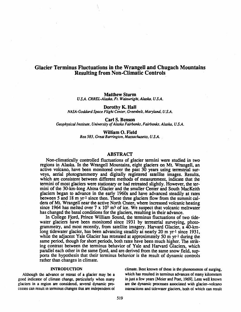
Glacier Terminus Fluctuations in the Wrangell and Chugach MountainsResulting from Non-Climatic Controls

Matthew SturmU.S.A. CRREL.Alaska, Ft. Wainwright, Alaska, U.S.A.

Dorothy K. HallNASA-Goddard Space Flight Center, Greenbelt, Maryland, U.S.A.

Carl S. BensonGeophysical Institute, University of Alaska Fairbanks, Fairbanks, Alaska, U.S.A.

William O. FieldBox 583, Great Barrington, Massachusetts, U.S.A.

ABSTRACT

Non-climatically controlledfluctuations of glacier termini were studied in tworegions in Alaska. In the Wrangell Mountains,eight glaciers on Mt. Wrangell, anactive volcano, have been monitoredover the past 30 years using terrestrialsur-veys, aerial photogrammetry and digitally registered satellite images. Results,which are consistent between different methods of measurement, indicate that _hetermini of most glaciers were stationaryor hadretreatedslightly. However, the ter-mini of the 30-km-long AhtnaGlacier and the smaller Center and South MacKeithglaciers began to advance in the early 1960s and have advanced steadily at ratesbetween 5 and 18 m yr-1since then. These threeglaciers flow from the summitcal-dera of Mt. Wrangell nearthe active NorthCrater,where increased volcanic heatingsince 1964 has meltedover 7 x 107 m3 of ice. We suspect that volcanic meltwaterhas changed the basal conditions for the glaciers,resulting in their advance.

In College Fjord,Prince William Sound, the terminusfluctuationsof two tide-water glaciers have been monitored since 1931 by terrestrial surveying, photo-grammetry, and most recently, from satellite imagery. Harvard Glacier, a 40-km-long tidewaterglacier, has been advancing steadilyat nearly 20 m yr-1since 193I,while the adjacentYale Glacier has ret1_atedat approximately50 m yr-1duringthesame period, thoughfor shortperiods, both rateshave been much higher.The strik-ing contrast between the terminus behavior of Yale and HarvardGlaciers, whichparalleleach other in the same fjord,and arederivedfrom the same snow field, sup-ports the hypothesis that their terminus behavior is the result of dynamic controlsratherthan changes in climate.

INTRODUCTION climate. Best known of these is the phenomenonof surging,Although the advance or retreatof a glacier may be a which has resultedin terminusadvancesof manykilometers

good indicator of climate change, particularlywhen many injust a few years [Meierand Post, 1969].Less well knownglaciers in a region are considered, several dynamic pro- are the dynamic processes associated with glacier-volcanocesses can result in terminuschanges thatare independentof interactionsand tidewater glaciers, both of which can result

519

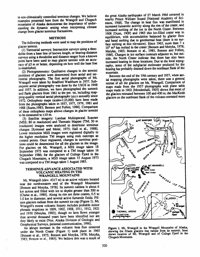
in non-climatically controlled terminuschanges. We believe the great Alaska earthquake of 27 March 1964 centered inexamples presented here from the Wrangell and Chugach nearby Prince William Sound [National Academy of Sci-mountains of Alaska demonstrate the importanceof under- ences, 1968]. The change in heat flux was manifested instanding the dynamic setting when interpreting climate increasedfumarolicactivity along the rim of the crater,andchange fromglacier terminus fluctuations, increasedmelting of the ice in the North Crater.Between1908 [Dunn, 1909] and 1965 this ice-filled crater was in

METHODS equilibrium, with accumulation balanced by glacier flow

The following methods were used to map thepositions of and basal melting due to geothermal heat (there is no sur-face melting at this elevation). Since 1965, more than 7 xglacier termini.

(1) TerresU_alsurveys: Intersection surveys using a theo- 107m3 has melted in the crater [Benson and Motyka, 1978;dolite froma base line of known length, or bearing-distence Motykn, 1983; Benson et al., 1985, Benson and Follett,surveysusing a theodolite end distance rangerfrom aknown 1986]. Changes in ice surface contours adjacent to, but out-side, the North Crater indicate that there has also beenpoint have been used to map glacier termini with an accu-racy of :L5m or better,depending on how well the base line increased heatingin these locations. Due to the local topog-raphy, some of the subglacial meltwater produced by theis established, heatinghasprobablydraineddown the northeastflankof the

(2) Photogrammetry:Qualitative changes in the termini mountain.positions of glaciers were determined from aerial end tea'- Between the end of the 19th century and 1957, when aer-restrial photographs. The fast aerial photographs of Mt.Wrangell were taken by BradfordWashburn in 1937. Sub- ial mapping photographs were taken, there was a generalsequent aerial photography was done by the USGS in 1948 retreatof ali the glaciers on ML Wrangell. Comparison ofand 1957. In addition, we have photographed the summit maps made from the 1957 photographs with plane tablemaps made in 1902 [Mendenhall, 1905] shows that most ofand flank glaciers from 1961 to the pre)'at, including map- the glaciers retreated between 100 and 400 m; the MacKeithping-quality vertical aerial photographs _n annually since glaciers on the northeast flank of the volcano retreated more1972. Orthophoto maps (scale=l:25,000) have been madefrom the photographs taken in 1957, 1977, 1979, 1981 and1988 [Sturm,1983; Benson and Follett, 1986]. Comparisonof these orthopboto maps allows changes in glacier terminito be measured to +10 m.

(3) Satellite imagery: Landsat Multispectral Scanner& _ SANFORD "FIoure 2

(MSS; 80 m resolution) and Thematic Mapper(TM; 30 m \,..,.. ,--_ ]re_lution) images were analyzed to determine terminus : _,_._x., _ .{e_ Ichanges [Krimmel and Meier, 1975; Hall et al., 1988]. , ,¢__: _h[_lLower resolution MSS images were registered digitally to , ,,_the higher resolution TM images using rock outcrops as ' ,, _ _1[ _ dcontrol points. Once registered, changes in terminus posi- , #oRrMOc_E:__'_ _ ]

tions could be determined for all the glaciers in the image. " __,_'__ _/_ r_ _ ' _ _ '

For glaciers on Mt. Wrangell, a MSS image taken 18 _ 6 ,_September 1973 was compared to a VM image taken 16 "- c¢a¢¢_ i

September 1986; for the glaciers of College Fjord in the %'0 .¢t" _ ,, L..' __..,,Chugach Mountains, a MSS image taken 15 August 1973 _ soO_ //was compared to a TM image taken 1 August 1985.

,_W,_ WRANOE|-LTERMINUS ADVANCE ASSOCIATED WITH I[+No._c,_.,

VOLCANIC HEATING IN THE ._ _,, c.,.,WRANGELL MOUNTAINS _" II. "_ %

Mt. Wrangell (elev. 4317 m) is an active volcano located ,r4,,near the northwestern end of the Wrangell Mountains S[BensonandMotyka,1978].Itssummitcalderaisabout6 .'.,, ",'_,-,:km across and Idled with ice to depthsgreaterthan 500 m do'_(,_'_[Clarke et al., 1989]. Along its rim are three craters, 0.5 to ,= I1.0 ian in diameter, and several active fumarole fields. Frf-

teen glaciers radiate from the summit ice cap (Figure 1). ML _Wrangelrs recent volcanic history includes probable minor _ _m,_,phreatic eruptions in 1899, 1902, 1908, 1911, 1912, 1921

• I"and 1930 [Motyka, 1983], though no lava flows younger ._ THERMALAREAS ,

than several thousand years have been identified nor are KILOMETERS ...... /,

they likely to exist [Nye, Alaska Division of Geologic andGeophysical Surveys, personal communication, 1990].

An abrupt increase in the volcanic heat flux centered Figure 1. ML Wrangellin the WrangellMountainsof Alaska,under the North Crater (Figure 1) took place in 1965 showingthe fffteenglaeiers that radiatefrom its summit.Inset[Benson et al., 1975; Benson and Motyka, 1978; Motyka, shows locationof Mt. Wrangell and of College Fjord in the!983; Ben___net al.: 1985]. We believe this was a result of ChugaehMotmtains.

520

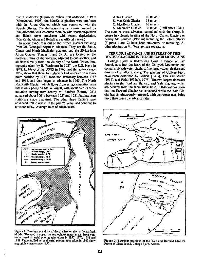
than a kilometer (Figure 2). When first observed in 1902 Ahtna Glacier 10m yr-1[Mendenhall, 1905], the MacKeith glacie_ were confluent S. MacKeith Glacier 18 m yr-1with the Ahtna Glacier, which was connected with the C. MacKeith Glacier 16 m yr-1Betseli Glacier. The deglaciated area is now covered by N. MacKeithG'lacier 6 m yr-1(until about 1981).thin, discontinuous ice.cored morainewith sparse vegetation The start of these advances coincided with the abruptin-and lichen cover consistent with recent deglaciation, crease in volcanic heating of the North Crater.Glaciers on(MacKeith, Ahma and Betseli me unofficial names.) nearby Mt. Sanford (4950 m) including the Betseli GLacier

In about 1965, four out of the Fifteenglaciers radiating (Figures 1 and 2) have been stationary or retreating. Alifrom Mt. Wrangell began to advance. They are the South, other glaciers on Mt. Wrangellare retreating.Center and North MacKeith glaciers, and the 30-km-longAhma Glacier (Figures 1 and 2). Ali are located on the TERMINUSADVANCEAND RETREAT OF TIDE-northeastflank of the volcano, adjacent to one another,and WATERGLACIERS INTHE CHUGACH MOUNTAINSali flow directly fromthe vicinity of the NorthCrater.Pho- College Fjord, a 40-km-long fjord in Prince Williamtographs taken by B. Washburnin 1937, the U.S. Navy in Sound, cuts into the heartof the Chugach Mountainsand1948, L. Mayo of the USGS in 1965, and the authors since contains six tidewaterglaciers, five large valley glaciersand1965, show that these four glaciers had retreatedto a mini- dozens of smaller glaciers. The glaciers of College Fjordmum position by 1937, remainedstationary between 1937 have been described by Gilbert [1903], Tarr and Martinand 1965, and then began to advance in 1965. The North [1914], and Field [1932a,b, 1975]. The two largesttidewaterMacKeith Glacier, which flows from an accumulation area glaciers in the fjord are Harvardand Yale glaciers, whichthatis only partlyon Mt. Wrangell,with about half its accu- are derived from the same snow fields. Observations showmuladon coming from nearby ML Sanford [Sturm, 1983] that the HarvardGlacier has advanced while the Yale Gla-advanced about 300 m between 1957 and 1981, but has been cier has simultaneously retreated,with the retreatratesbeingstationary since that time. The other three glaciers have more thantwice the advance rates.advanced 320 to 480 m in the past25 years, and continue toadvance today. Averageratesof advance are: _

- 521

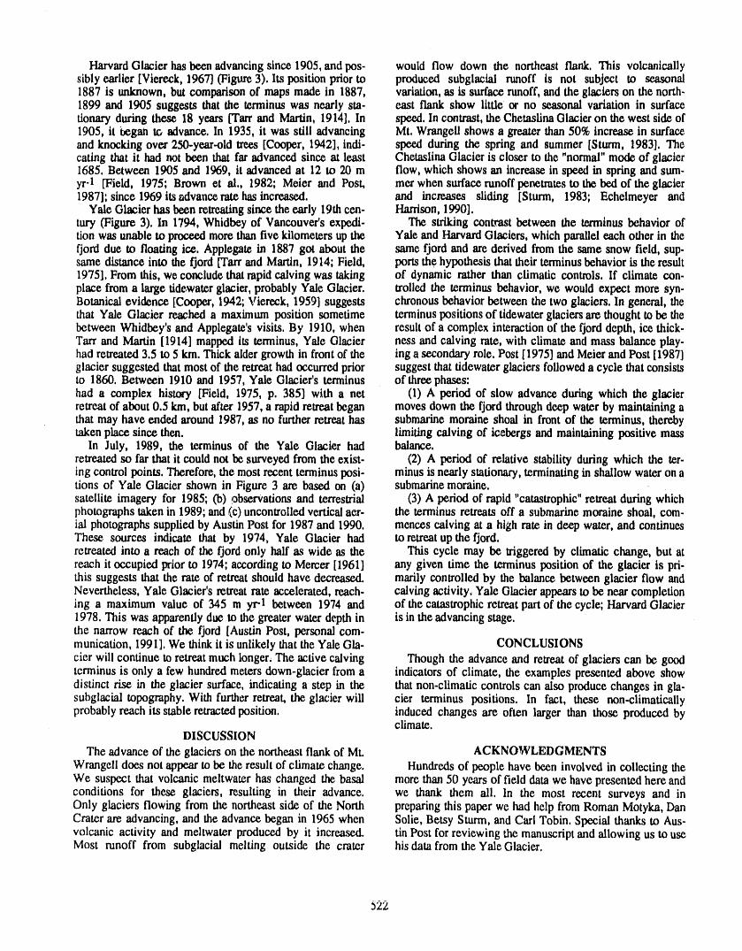
HarvardGlacier has been advancingsince 1905, andlaOS- would flow down the northeast flank. This volcanicallysibly earlier [Viereck, 1967] (Figure3). Its position prior to produced subglacial runoff is not subject to seasonal1887 is unknown, but comparison of maps made in 1887, variation, as is surfacerunoff, andthe glacierson the north-1899 and 1905 suggests that the terminus was nearly sm- east flank show little or no seasonal variation in surfacetionary during these 18 years [Tan'and Martin, 1914]. In speed. In contrast,the ChetaslinaGlacieron the west side of1905, it began t_ advance. In 1935, it was still advancing Mt. Wrangell shows a greater than 50% increase in surfaceand knocking over 250-year-old trees [Cooper, 1942], indi- speed during the spring and summer [Sturm, 1983]. Theeating that it had not been that far advanced since at least Chetaslina Glacier is closer to the "normal" mode of glacier1685. Between 1905 and 1969, it advanced at 12 to 20 m flow, which shows an increase in speed in spring and sum-yr-1 [Field, 1975; Brown et al., 1982; Meier and Post, met when surface runoff penetrates to the bed of the glacier1987];since 1969 its advance rate has increased, and increases sliding [Sturm, 1983; Echelmeyer and

Yale Glacier has been retreating since the early 19111cen- Harrison, 1990].tta), (Figure 3). In 1794, Whtdbey of Vancouver's expedi- The striking contrast between the terminus behavior oftion was unable to pmcee.dmore than five kilometers up the Yale and Harvard Glaciers, which parallel each other in thefjord due to floating ice. Applegate in 1887 got about the same fjord and are derived from the same snow field, sup-same distance into the fjord [Tan' and Martin, 1914; Field, ports the hypothesis that their terminus behavior is the result1975]. From this, we conclude that rapid calving was taking of dynamic rather than climatic controls. If climate con.piace from a large tidewater glacier, probably Yale Glacier. trolled the terminus behavior, we would expect more syn-Botanical evidence [Cooper, 1942; Viereck, 1959] suggests chronous behavior between the two glaciers. In general, thethat Yale Glacier reached a maximum position sometime terminus positions of tidewater glaciers are thought tobe thebetween Whidbey's and Applegate's visits, By 1910, when result of a comPlex interaction of the fjord depth, ice thick-Tarr and Martin [1914] mapped its terminus, Yale Glacier hesSand calving rate, with climate and mass balance play-had retreated 3.5 to 5 kan.Thick alder growth in front of the ing a secondary role. Post [1975] and Meier and Post [1987]glacier suggested that most of the retreat had occurred prior suggest that tidewater glaciers followed a cycle that consiststo 1860. Between 1910 and 1957, Yale Glacier's terminus ofthree phases:had a complex history [Field, 1975, p. 385] with a net (1) A period of slow advance during which the glacierretreat of about 0.5 km, but after 1957, a rapid retreat began moves down the fjord through deep water by maintaining athat may have ended around 1987, as no further retreat has submarine moraine shoal in front of the terminus, therebytaken piace since then. limiting calving of icebergs and maintaining positive mass

In July, 1989, the terminus of the Yale Glacier had balance.retreated so far that it could not be surveyed from the exist- (2) A period of relative stability during which the ter-ing control points. Therefore, the most recent terminus posi- minus is nearly stationary, terminating in shallow water on ations of Yale Glacier shown in Figure 3 are based on (a) submarinemoraine.satellite imagery for 1985; (b) observations and terrestrial (3) A period of rapid "catastrophic" retreat during whichphotographs taken in 1989; and (c) uncontrolled vertical aet- the terminus retreats off a submarine moraine shoal, com-ial photographs supplied by Austin Post for 1987 and 1990. mences calving at a high rate in deep water, and continuesThese sources indicate that by 1974, Yale Glacier had to retreat up the fjord.retreated into a reach of the fjord only half as wide as the This cycle may be triggered by climatic change, but atreach it occupied prior to 1974;according to Mercer [1961] any given time the terminus position of the glacier is pri.this suggests that the rate of retreat should have decreased, madly controlled by the balance between glacier flow andNevertheless, Yale Glacier's retreat rate accelerated, reach- calving activity, Yale Glacier appears to be near completioning a maximum value of 345 m yrl between 1974 and of the catastrophic retreat part of the cycle; Harvard Glacier1978. This was apparently due to the greater water depth in is in the advancing stage.the narrow reach of the fjord [Austin Post, personal com-munication, 1991]. We think it is unlikely that the Yale Gla- CONCLUSIONScier will continue to retreat much longer, The active calving Though the advance and retreat of glaciers can be goodterminus is only a few hundred meters down-glacier from a indicators of climate, the examples presented above showdistinct rise in the glacier surface, indicating a step in the that non-climatic controls can also produce changes in gla-subglacial topography. With further retreat, the glacier will tier terminus positions. In fact, these non-climaticallyprobably reach its stable retracted position, induced changes are often larger than those produced by

climate.DISCUSSION

The advance of the glaciers on the northeast flank of Mt. ACKNOWLEDGMENTSWrangell does not appear to be the result of climate change. Hundreds of people have been involved in collecting theWe suspect that volcanic meltwater has changed the basal more than 50 years of field data we have presented here andconditions for these glaciers, resulting in their advance, we thank them all. In the most recent surveys and inOnly glaciers flowing from the northeast side of the North preparing this paper we had help from Roman Motyka, DanCrater are advancing, and the advance began in 1965 when Solie, Betsy Sturm, and Carl Tobin. Special thanks to Aus-volcanic activity and meltwater produced by it increased, tin Post for reviewing the manuscript and allowing us to useMost runoff from subglacial melting out.side the crater his data from the Yale Glacier.

522

REFERENCES

Benson, C, S., and A. B. FoileR, Application of pho- Field, W. O, (Ed.),Mountain Glacters oftheNorthernHem-togramme_ to the study of volcano-glacier interactions isphere, Vol. 2, 932 pp., U.S.A. Cold Regions Researchon Mt. Wrangell, Alaska, Photogrammetric Engineering and EngineeringLaboratory,1975.and Remote Senaing, 52, 813--827, 1986. Gilbert,G. K., Alaska Harriman Alaska Expedition, Vol. 3.

Benson, C. S., and R. Motyka, Glacier-volcano interactions Glaciers and Glaciation, 231 pp,, Doubleday, Page andof Mt. Wrangell, Al_at, in University of Alaska- Co., New York, 1903.Geophysical Institute Annual Report 1977-1978, pp. 1- Hall, D. K., K. Bayr,and W. M. Kovalick, Determinationof25, 1978. glacier mass balancechange using thematicmapperdata,

Benson, C. S., D. Bingham, and G. Wharton,Glaciological Proceedings of the Eastern Snow Conference, pp. 192-and volcanological studies at the summit of ML Wren- 196, LakePlacid, New York, 1988.gell, Alaska, Snow and Ice Symposium-Proceedings of Krimmel, R. M., and M, F. Meier, Glacier applications ofthe Moscow Symposium, August 1971, IASH-AISHPub- ERTSImages,J. Glaciol., 15,391-402, 1975.licationNo. 104, pp. 95-98, 1975. Meier,M. F., and A. Post,What are glacier surges?,Can. J.

Benson, C. S., R. Motyka, D. Bingham, G. Wharton,P. Earth Sci., 6, 807--817, 1969.MacKeith, and M. Sturm, Glaciological and volcanolog- Meier, M. F., and A. Post, Fast tidewater glaciers, J. Geo-ical studies on Mt. Wrangell, Alaska, in Interaction phys.Res.,92,9051-9058, 1987.between Volcanism and Glaciology, editedby Kotlyakov, Mendenhall,W. C., Geology of the CentralCopper RiverVinogrdov, and Glazovsky, pp. 114-133, Glaciological Region, Alaska, U.S. Geological Survey ProfessionalResearches No. 27, Soviet Geophysical Committee, Paper41, 1905.Academy of Sciences of the USSR, 1985. Mercer, J. H., The response of fjord glaciers to changes in

Brown, C. S., M. F. Meier, and A. Post, Calving speed of the fun limit, J. Glaciol., 3, 850--858, 1961.Alaska tidewater glaciers, with application to Columbia Motyka, R,, Increases and fluctuations in thermalactivity atGlacier, U.S. Geological Survey Professional Paper Mt. Wrangell, Alaska, Ph.D. dissertation, 349 pp., Uni-1258.D, 1982. versityof Alaska Fairbanks, 1983.

Clarke, G. K. C., G. M. Cross, and C. S. Benson, Radar National Academy of Sciences, The Great Alaska Earth-imaging of glaciovoicanic stratigraphy, Mount Wrangell quake of 1964 - Hydrology, Publication 1603, Washing-Caldera, Alaska: interpretation model and results, J. Gee- ton, DC, 1968.phys. Res., 94,7237-7249, 1989. Post, A., Preliminary hydrographic and historic terminal

Cooper, W. S., Vegetation of the Prince William Sound changes of Columbia Glacier, Alaska, U.S. GeologicalRegion, Alaska, with a brief excursion into post- Survey HydrologicallnvestigationsAtlas559, 1975.Pleistocene climatic history, Ecological Monographs, 12, Sturm, M., Comparison of glacier flow of two glacier sys-1-22, 1942. ternson ML Wrangell, Alaska, M.S.Thesis, 186 pp., Uni-

Dunn, R., Conquering our greatest volcano, Harper's versityofAlaskaFairbanks, 1983.Monthly Magazine, 118(706), 497-509, 1909. Tan', R. S., and L. Martin,Alaskan Glacier Studies, 498 pp.,

Echelmeyer, K., and W. D. Harrison, Jakobshavns Isbrae, National Geographic Society, Washington, DC, 1914.West Greenland: seasonal variations in velocity--or lack Viereck, L. A., Unpublished Report of the botanical workthereof,J. Glaciol., 36, 82--88, 1990. done during the 1957 expedition of the American Gee-

Field, W. O., The glaciers of the northernpart of Prince graphicalSociety as partof the IGY, 1959.William Sound, Alaska, Geogr. Rev., 22, 361-388, Viereck, L. A., Botanical dating of recent glacial activity in1932a. western North America, in Arctic and Alpine Environ-

ments, edited by H. E. 'Wrightand W. H. Osburn, pp.Field, W. O., The mountainsand glaciers of PrinceWilliam 189-204, IndianaUniversityPress, 1967.

Sound, Alaska,Am. Alpine J., 1,445-458, 1932b.

523

Radar Mapping of Malaspina Glacier, Alaska,with Applications for Global Change Investigations

John E. Jones and Bruce F. Moiniau.s, GeologicalSurvey,Reston.Virginia,U.S.A.

ABSTRACT

An ongoing radar study by the U.S. Geological Survey has used airborne, sat-ellite, and ice-penetration radarto map glacier-surface features and sub-glacier bed-rock relief of Malaspina Glacier, Alaska. Preliminary results of this study indicatethat it may be possible to develop a model using satellite radar data to estimate thevolume of some ice sheets. This model would be used in mass balance studies forglobal change investigations.

X-band (~3 cm wavelength) airborne radar (1975, 1980, and 1986) and L-band(-24 cm wavelength) Seasat satellite radar (1978) images show complex bright anddark radar backscatter patterns on the surface of Malaspina Glacier. These patterns,0.5 to 10 km in length, resemble bedrock features in nearby mountains, such ascirques and drainage networks. Plane-tablc/a!idade profiles, ice-penetration radar(-.150 m wavelength) soundings, and other field data collected in 1988 and 1989show that many of the radar backscatter patterns c_)rrespond to adjacent topo-graphic highs and lows with a maximum relief of 100 _o on the surface of the gla-cier. Many of the surface features of the glacier mimic the sub-glacier bedrockfeatures at depths greater than 600 m below the ice surface. Preliminary analysisindicates that a relationship exists between the wave amplitude of these ice flowfeatures, the ice flow velocity, and the depth of the ice.

These and other findings resulting from this study indicate that data from theeight international radar satellites planned for launch in the 1990s can be used onsome ice sheets to (1) map landing sites and transportation routes by identifyingcrevassed zones and hummocky surface morphology, and (2) develop a geographicinformation system model of ice flow dynamics, based on wave amplitude, flowvelocity, and areal coverage, to estimate ice volume for global change studies.

524

Climate-Related Research in Svalbard

K. Sand$1NTEFNorwegian HydrotechnicalLaboratory, Trondheim, Norway

J. O. HagenNorwegian Polar Research Institute, Oslo Lufthavn, Norway

K. ReppNorwegian Water Resources and Energy Administration, Oslo, Norway

E. BerntsenNorwegian National Committeefor Hydrology, Oslo, Norway

ABSTRACT

The Svalbard archipelago is located in the Norwegian Arctic, 76-81°N. In theKongsfjord .area, 79°N, on northwest Spitsbergen, there has been increasingresearch activity in several climate-related disciplines over the last few years. Thisresearch will contribute to the global efforts on monitoring and detecting possibleglobal changes. An intensified program monitoring hydrological processes was runfrom 1974 to 1978 and restarted in 1988. One well-equipped station for atmos-pheric research is also established. Four major glaciers are being thoroughly inves-tigated, a program which includes mass balance studies, drainage patterns and coreanalyses. Since 1978 a permafrost station has been operated in Svea, south-centralSpitsbergen. The trend in glacier mass balance analyses shows fairly stable negativeconditions, the net balance is slightly increasing due to a slight increase in the win-ter precipitation. There is no sign of climatic warming through increased melting.The temperature data show a very slight cooling during the ablation period. Areconstruction of mass balance data for the BrCgger glacier shows that the mass bal-ance has been consistently negative since 1918.

INTRODUCTION for the coldest month (March) and the warmest month (July)Svalbard is the geographical name of the archipelago sit- are 11.7°C and +4.7°C, respectively. Precipitation is less

uated between latitudes 76°N and 81°N and longitudes 10°E than 400 mm per year on the west coast of Spitsbergen,and 35°E in the Norwegian Arctic (Figure 1). The total area increasing eastward. Desert areas are found on the north-is about 63,000 km2 of which 60% is covered by glaciers, eastern part of this island.Ice-free land areas have continuous permafrost with thick- This paper gives an overview of present climate-relatedness varying from less than 100 m near sea level up to research carried out in Svalbard within different geophysical500 m in the higher mountains [Liest01, 1977]. Tem- sciences. Most of this research is being carried out in theperatures are high considering the latitude, largely due to the Kongsfjord area, 79°N, on northwest Spitsbergen, whichNorth Atlantic Current (a continuation of the Gulf Stream) over the last few years has become an arctic field laboratory.of which a branch flows toward the west coast of Spits- The scope of this paper is limited to meteorology, perma-bergen. Long-term average temperatures from Isfjord Radio frost, glaciology, hydrology and chemistry of the atmos-

525

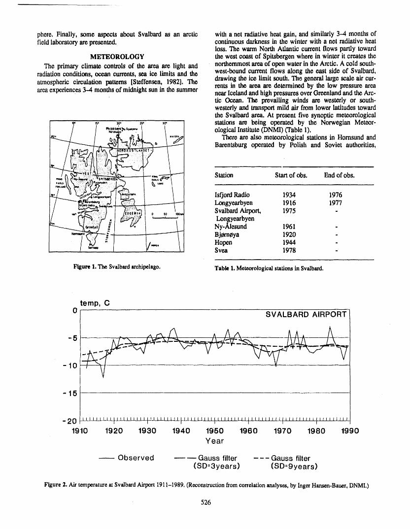
phere, Finally, some aspects about Svalbard as an arctic with a net radiative heat gain, and similarly 3---4months offield laboratory are presented, continuous darkness in the winter with a net radiative heat

loss, The warm North Atlantic current flows partly towardMETEOROLOGY the west coast of Spitsbergenwhere in winter it creates the

The primary climate controls of the area are light and northernmostareaof open water in the Arctic, A cold south-radiation conditions, ocean currents, sea ice limits and the west-bound current flows along the east side of Svalbai_t,atmospheflc circulation patterns [Steffensen, 1982], The drawing the ice limit south, The general large scale air cur-rents in the area are determined by the low pressure areaarea experiences 3-4 months of midnightsun in the summer nearIcelandand high pressuresoverGreenlandand the Arc.

tie Ocean, The prevailing winds arc westerly or south-westerlyand transportmild air fromlower latitudes towardthe Svalbard area, At present five synoptic meteorological

,_, _ _,. ,o. stations are being operated by the Norwegian Meteor-_.,,.s,,._, \ ological Institute (DNMI) (Table 1),

" t_ , _ "'"'_ There are also meteorological stations in Homsund and------- _:_ Barentsburg operated by Polish and Soviet authoflties,

=ili! --_?_o_. / Station Start of obs. Endof obs,

,,' -, IsfjordRadio 1934 1976

_7__ _ij_i_:_vX_ Longyearbyen 1916 1977Svalbard Airport, 1975 -

- _. Ny-Alesund 1961 -

-- _ _ _,, Bjerneya 1920 "Hopen 1944 -

""' "" Svea 1978 -

Figure1. The Svalbardarchipelago. Table1.Meteorologicalstationsin Svalbard.

temp, C

0 SVALBARD AIRPORT

-15

-20 -LL.LL_t-L4-i!j_t_''i_1_tjj_jl1i_t_j______-.LLt-L_LL.t-__ _

1910 1920 1930 1940 1950 1960 1970 1980 1990

Year

Observed _--Gauss filter ---Gauss filter(SD=3years) (SD=9years)

Figure2. AirtemperatureatSvalbardAirport1911-1989.(Rec,omtructionfromcorrelationanalyses,by IngerHamen-Bauer,DNMI.)

526

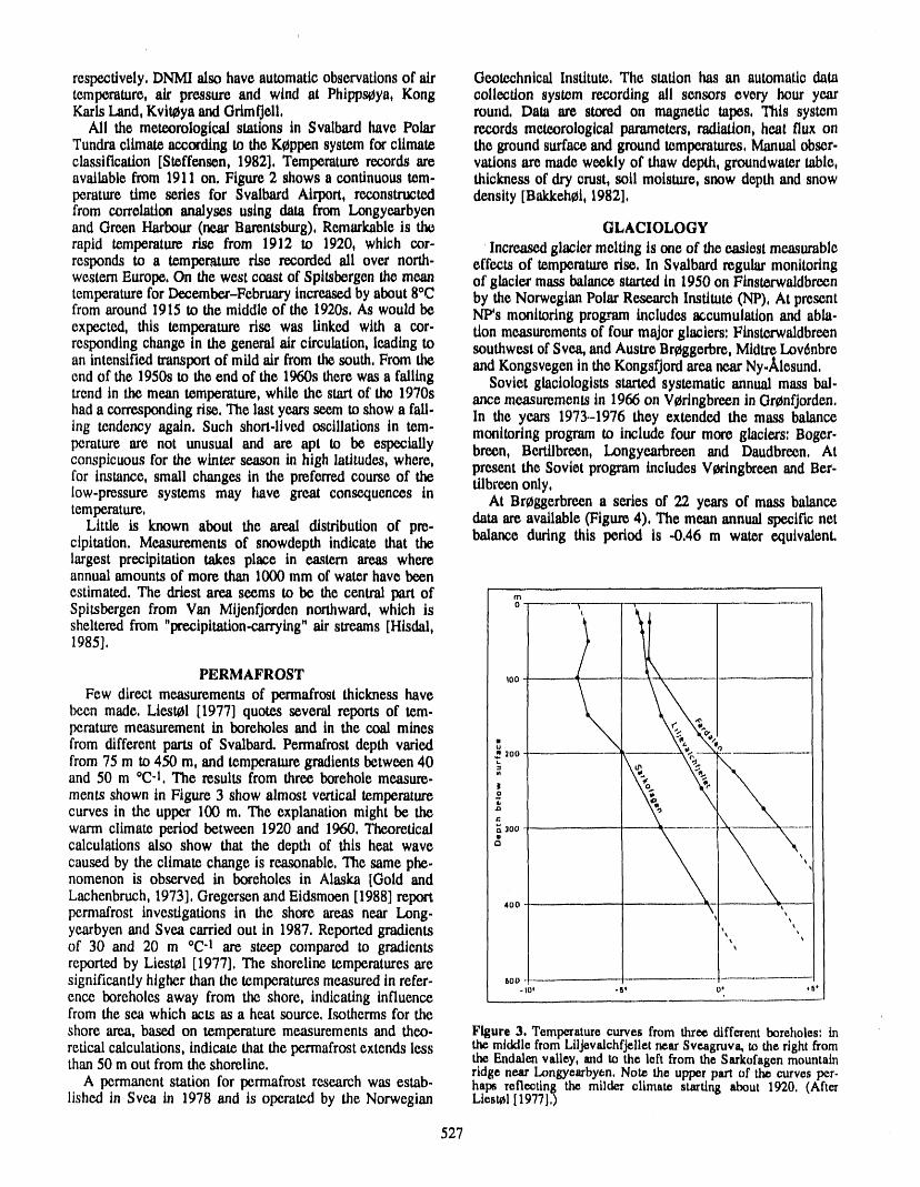
respectively,DNMI also have automaticobservationsof air Gcotechnical Institute, The station has an automatic datatemperature, air pressure and wind at Phtpp_ya, Kong collection system recording ali sensors every hour yearKartsLand,KvitCyaandOrimfjell, round, Data are stored on magnetic tapes, This system

Ml the meteorological stations in Svalbard have Polar records meteorological parameters,radiation, heat flux onTundraclimateaccording to the Keppen system forclimate the groundsurfaceand ground temperatures,Manualobser-classification [Steffensen, 1982], Temperature records are rations are made weekly of thaw depth, groundwatertable,available from 1911 on, Figure 2 shows a continuous tem. thickness of dry crust, soil moistm_, snow depthand snowperature time series for Svalbard Airport, reconstructed density [Bakkeh¢l, 1982],from correlation analyses using data from Longyearbyenand Green Harbour(near Barentsburg), Remarkable is the GLACIOLOGYrapid temperature rise from 1912 to 1920, which c.or. Increased glacier melting is one of the easiest measurableresponds to a temperature rise recorded ali over north, effects of temperaturerise, In Svalbard regular monitoringwesternEurope, On the west coast of Spitsbergen the mean of glacier mass balancestartedin 1950 on FlnsterwaldbreentemperatureforDecember-February increased by about8°C by the Norwegian Polar Research Institute (NP), At presentfromaround 1915 to the middle of the 1920s, As would be NFs monitoring program includes accumulation and abla-expected, this temperature rise was linked with a eor. tton measurements of four major glaciers: Finsterwaldbreenrespondingchange in the general air circulation,leading to southwest of Svea, and AustreBreggerbre, Mldtre Lov6nbrean intensified transportof mild air from the south, From the and Kongsvegen in the Kongsfjord area near Ny.Alesund,end of the 1950s to the end of the 1960s there was a falling Soviet glaciologists started systematic annual mass bal-trend in the mean temperature, while the start of the 1970s arco measurements in 1966 on Veringbreen in Orenfjorden,had a corresponding rise, The last years seem ta show a fall. In the years 1973--1976 they extended the mass balanceing tendency again, Such short-lived oscillations in tem. monitoring program to include four more glaciers: Boger-perature are not unusual and are apt to be especially breen, Bertilbreen, Longyearbreen and Daudbreen, Atconspicuous for the winter season in high latitudes, where, present the Soviet program includes VCringbreenand Ber-for instance, small changes in the preferred course of the tilbreen only,low.pressure systems may have great consequences in At Breggerbreen a series of 22 years of mass balancetemperature, data are available (Figure 4), The mean annual specific netLittle is known about the areal distribution of pre-cipitation, Measurements of snowdepth indicate that the balance during this period is -0,46 m water equivalent,largest precipitation takes place in eastern areas whereannual amounts of more than 1000 mm of water have beenestimated, The driest area seems to be the central part of ,.Spitsbergen from Van Mijenfjorden northward, which issheltered from "precipitation-carrying" air streams [Hisdal,1985],

PERMAFROST

Few direct measurements of permafrost thickness havebeen made, Liest¢l [1977] quotes several reports of tem.perature measurement in boreholes and in the coal minesfrom different parts of Svalbard. Permafrost depth variedfrom 75 m to 450 m, and temperature gradients between 40and 50 m °C-I, The results from three borehole measure-ments shown in Figure 3 show almost vertical temperaturecurves in the upper 100 m, The explanation might be thewarm climate period between 1920 and 1960, Theoreticalcalculations also show that the depth of this heat wavecaused by the climate change is reasonable, The same phe. "nomenon is observed in boreholes in Alaska [Gold andLachenbruch, 1973], Gregersen and Eidsmoen [1988] reportpermafrost investigations in the shore areas near Long. ,,yearbyen and Svea carried out in 1987, Reported gradients ',, ',,of 30 and 20 m °C-Â are steep compared to gradients ',reportedby Liest01[1977],The shorelinetemperaturesaresignificantly higher than the temperatures measured in refer-ence boreholes away from the shore, indicating influence -,o, -v o, __'_'from the sea which acts as a heat source, Isotherms for theshore area, based on temperature measurements and thee- Figure 3. Temperaturecurves from thro_ dtfferentbordloles: inretical calculations, indicate that the permafrost extends less tt_ middlefrom Lilj_valchfjellctrmarSvcagruva,to thefight fromthan 50 m out from the shoreline, the Endalenvalley,and to the left from the Sarkofagenmountain

ridge nearLongyearby_n,Not_ th_ upperpart of th_curvespcr.A permanent station for permafrost research was estab- haps reflecting tlm milder ¢limat_ starting about 1920, (After

lished in Svea in 1978 and is operated by the Norwegian Liest¢111977],)

527

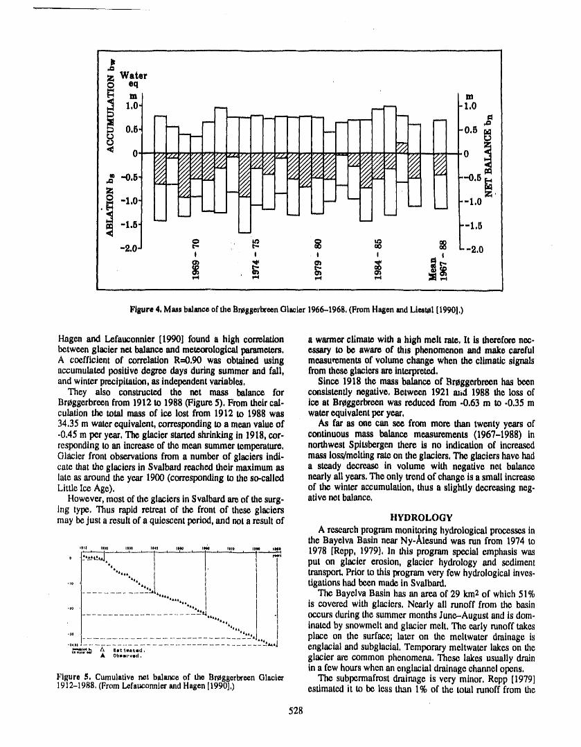
,.QWater

eq

1,0 .- ._ -- 1,0_ _.-=,-, ma.m m,am,m "m'_ ".==., mJ" ,=m,. m..l. ,R,..,=

,=.m. ,==m,m

1--,- -0.5 i --. '0.5

• # • fs-., -/. r#.-#, • i i

.g -.0,5 "rA._ _ ;_ "_'.-.: _ _. _ "" -.O,5g_ ,

-1.0 __. ! -- "" -1.0' i tamm' m"" _ _ /

-1.5 --" -" I'1'5-2.0 ;' '.--2,0

I l l I i

i . i i j

Figure 4, Mass balanc;e of the gr_ggerlxeen Olaoler 1966-.1968, (From Hagen and Ltettal [1990],)

Hagen and Lefauconnler [1990] found a high correlation a wanner climate with a high melt rate, lt is thereforenec-between glacier net balance and meteorological parameters, essary to be aware of this phenomenon and make carefulA coefficient of correlation R=0,90 was obtained using measurements of volume change when the climatic signalsaccumulated positive degree days during summer and fall, from these glaciers are interpreted,and winter precipitation,as independentvariables, Since 1918 the mass balance of Breggerbreen has been

They also constructed the net mass balance for consistently negative, Between 1921 mid 1988 the loss ofBreggerbreen from 1912 to 1988 (Figure5), From their cal- ice at Breggerbroen was reduced from -0.63 m to .0.35 mculatton the total mass of ice lost from 1912 to 1988 was waterequtvalentper year,34.35 m waterequivalent, corresponding to a mean value of As far as one can see from more than twenty years of-0.45 m per year,The glacier startedshrinking in 1918, eor- continuous mass balance measurements (1967-1988) inrespondingtoanincreaseofthemeansummertemperature, northwestSpitsbergenthereisno indicationofincre.ascdGlacier front observations from a numberof glaciers indi. mass loss/melting rateon the glaciers, The glaciershave hadcate that the glaciers in Svalbardreachedtheir maximumas a steady decrease in volume with negative net balancelate as aroand the year 1900 (correspondingto the so-called nearly ali years, The only trendof change is a small tncrea_Little Ice Age), of the winter accumulation, thus a slightly decreasing n_g.

However,most of the glaciers in Svalbard amof the surg- attve net balance,ing type, Thus rapidrctrcatof lhc front of these glaciersmay bcjust a result of a quiescentperiod,and not a result of HYDROLOGY

A re,search programmonitgrtng hydrologicalprocesses inthe Bayelva Basin near Ny-Alcsund was run from 1974 to

, _.,._.eT_. / ,-, 1978 [Rcpp, 1979], In this program special emphasis was

i_ ,, !|[/I''_'[ ,.,._![ ,,. put on glacier erosion, glacier hydrology and sediment

transport,PriortothisprogramveryfewhydrologicalInves.•,o tigattons had been made in Svalbard,

. The Bayelva Basin has an area of 29 km2of which 51%

'° _]i i'_'i:'_'"_,'"'"'""'""", . is covered with glaciers, Nearly ali runoff from the basin

occurs (luringthe summer months June-August and is dora.inatedbysnowmeltandglaciermelt,Theearlyrunofftakes

"" piace on the surface; later on the meltwater drainage is................................... _ .... "4t4dtA4 A

"'_.,,."m t_ e.t_..t.d, englaclal and subglaclal, Temporarymeltwater lakes on the,t o...,,_.., glacier are common phenomena, These lakes usually drain

in a few hours when an englacLaldrainage channel opens,Figure 5. Cumulative net balance of the Br_ggerlxeen Olacter The subpermafrost drainage Is very minor, Repp [1979]1912-1988,(FromLefa_onnler andHagen11990],) estimated it to be less fit,an1% of the total runoff from the

528

SUSp_N0_0 ment of permanent hydrological observation stations inS_Dm_NTLOAD Svalbard, Three researchsites were selected: Bayelva near(_g/i) Ny._esund, DeGeer River north of Longyearbyen, and

100 SSL,0,0Sa_,,o 2,0a9z EndalenBMtn/IsdammenReservoir nearLongyearbyen,," Bayelva Basin was chosen in orderto continue theexten-

t. 09_11 ,, sive work done duringthe 1970s, In addition hydrologicalN. 602 data would increasethe value of this area as an arctic field

10 laboratory for several scientific disciplines, Pemtanent,,i installations for water discharge and sediment transport

,,,, measurementswere pet in the main fiver, Waterconductiv-",', ity sensors will be installed at different sites. A meteor-_' ological station is established on Breggerbreen during the1,0 . ,;

,,, periodlviay--Septemberevery year,,' In the DeGeer River a hydrometrtcstation has been

,_, installed, The drainage area is 78,4 km2, The site wasr' selected primarilybecause only 13% of the basin was gla-

0,1 i, tier covered,,' The _ndalen Basin/IsdammenReservoir is located near

' Longyearbyc_, The Endalselva River feeds the lsdammenReservoir which is the water supply source for Long-

0,01 "' yearbyen (approximately 1200 inhabitants), The area wasselected because hydrological informationis very importantfor properoperationof ritewatersupply reservoir.The mon-itoring programincludes instrumentationfor water balancestudiesof the IsdammenReservoir, sedimenttransportin the

0,001 "/, ' I Endalselva River, groundwatermovements and water qual.

/' [ iW. The stations in the Bayelva Basin andDeGeer Riverare

in operationduring 1990, while the programfor the EndalenBash_sdammen Reservoir has not yet materializeddue toeconomic constraints,

°'°%,ol o,1 1,o 1o lo0WATER,ISHARQE(m'/,) CHEMISTRY OF THE ATMOSPHERE

Toward the end of the 1970s oil exploration onthe con.Figure6, Sedimentcurve1973-1978,('FromRepp[1979],) tinentalshelves started to move furthernorth, In order to

establish a base for evaluation of the concurrentpollutionproblems,a comprehensivestudy of the air pollution situa.

basin, Maximum recorded runoff during the years 1973- tion in the Norwegian sector of the An:tic was carriedout by1978 was 1100 1 s-I km-2 while the mean specific runoff the Norwegian Institutefor Air Re.wau'ch(NILU)during theduringthis periodwas estimated to 321 s-I km-2, 5-year period 1981-1985, Under this program four meas-

The sedhnent transportfrom the basin is quite high; the uring stations were established in the .highArctic with anmaximum suspendedsediment load measuredwas 3830 mg extendedmeasurementprogramin Ny-Alesund [Ottaret al.,1-1.The suspended sediment load is found to be strongly 1986].correlaledwith waterdischarge: The wintertime arctic haze, with concentrationlevels of

man.madepollutants which are comparableto average con.SSL= 0.0534' Q2,o392 (1) central.ionsover the industrLaltzedcontinents, is due to pol.

lutantsemitted from sources within the arctic air mass. InSSL is suspended sediment load and Q is water discharge, late winterand spring, this cold and stable air mass, char.Equation(1) yielded a correlationcoefficient RffiO.95during acterizedby verylow depositionratesandabsence of photo.602 days of observation 1973-1978 (Figure 6), The bottom chemical activity, may engulf large parts of northernload is estimated to be 30%of the total sediment transport Eurasia. Aircraft measurements show that the vertical exten.as an average,The annualsuspendedsedime.nttransportvar- sion of this haze is typically less than2000 m, The presenceted between 6646 tons and 16,558 tons, i,e,, 228 tons km-2 of furtherhaze layers at elevations up to 5000 m or more isto 567 tons km-2, Assuming that sedimenttransportin Bay. due to sources outside the arctic airmass. Also naturalaere.elva reflects the glacier erosion, this indicates an erosion sols are present at high altitudes, in the form of soil dust,intensity of 0,5 mm yr-l, which is significantly more thai] which may have originated from the large deserts in Asia orobserved forwarmerglaciers in Norway. Africa (Figure 7). Local sources in Spitsbergen may also

The hydrological investigations in the Bayelva Basin contributeto the haze layers, but this contributionis limitedwere restarted in 1988 by the Norwegian National Com. to emissions from sources in major settlements in the Sval-mittee for Hydrology. A generalneed for more informadon bard archipelago. The local contamination of air can beandknowledge of hydrologicalprocesses in arctic areas was tracedas high as 1000 m.felt by differentresearch communities in Norway [Hagen ct A large._x,ale multllayer atmospheric dispersion modelal., 1987]. The fh'stphase of this programwas the establish, has been formulated,utilizing the concept of transportalong

529

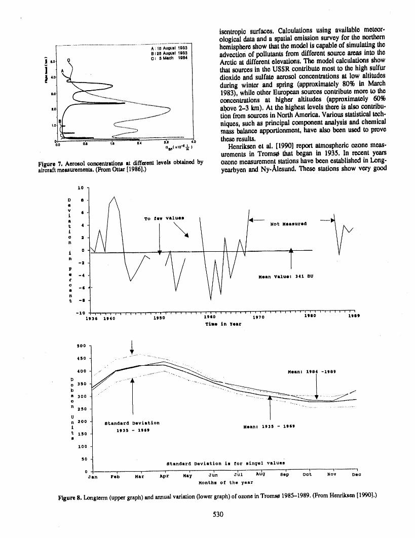
isentropic surfaces, CaLculationsusing available meteor.ological dataand a spatial emission survey for the northern

^_1. ^_,_ 1.._ hemisphereshow that the model is capable of simulatingthe.z2_^_at _u. advection of pollutants from different source areas into the

Lo 9,. o, s Maohtg_ Arctic at differentelevations, The model calculations show

] ^_ that sources in the USSR contribute most to the high sulfur,.o dioxide and sulfate aerosol concentrationsat low altitudes

during winter and spring (approximately 80% in Mar_h._ 1983), while otherEuropeansources contributemoretothe

concentrations at higheraltitudes (approximately 60%

1,o ntques, such as principal component analysis and chemical• mass balanceapportionment,have also boonused to prove:- ...... , ' ::-:"::':".........."" : _::::" 40 theseresults,

°.o o, ,'s ,_4 _s,,(.,o.OX Henriksenet al, [1990] report atmospheric ozone meas-urements in Troms¢ that began in 1935, In recent years

Figure7, Aerosolconcentrationsat differentlevels obtainedby ozone measurementstationshave been established in Long-_vraft metsurements,(FromOtter[1986],) yearbyen and Ny-,/desund. These stations show very good

10

o /,V I$

i ,ro tau valuam

t 0 .... /I

-2

P

t -4_ Mean Valuer 341 DU£

o -6ent -li

-10 _ _! ! v v v v v v' T'! v v v v 'i'v _''1' v _ v v v v v v v v v v v , v v ; v 1 ! v'"f l'"v 'v ¼"i'! v I ! v k

1936 19,10 19ISO 1960 1970 lg80 1989

Ttme In Year

,oo450

, _ _ "._*' .. ' _, .,..

400 .,'" ' ' ..,,f'_'_ .,.,,,_,,.,"*'"__.._"', Meant 19B4 -:1.989

o 350 ' ..............13

a 3000

n 250

U

n 200 Btandard DevLet, ioni Meant 1935 - 1961

1935- 1969t 150a

100

5OBtandard Deviation is tor ningel values

........ v ' '1 ....... __I

0 ----_ , Ha'r ' ' ' Jtal _t_g Bal:) Oat NoV DeeJan Feb p_pr May Oun

Months of the year

Figure 8. Longterm(uppergraph)andannualvariation(lowergraph)of ozoneinTroms¢1985-1989,(FromHem-iksen[1990],)

530

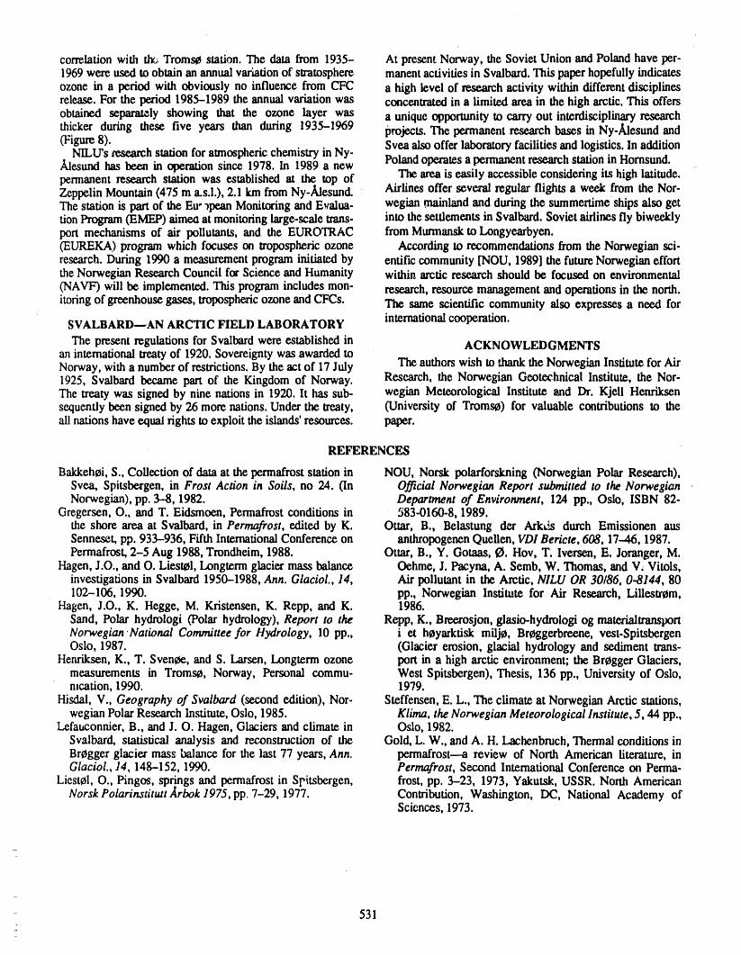
correlationwith tlz_Tmms¢ station. The data from 1935- At present Norway, the Soviet Union and Polandhave pcr-1969were used to obtain an annualvariationof stratosphere manentactivities in Svalbard.This paperhopefully indicatesozone in a period with obviously no influence from CFC a high level of research activity within differentdisciplinesrelease.For the period 1985-1989 the annualvariationwas concentrated in a limited areain the high arctic.This offersobtained separately showing that the ozone layer was a unique opportunity to carryout interdisciplinaryresearchthickerduringthesefiveyearsthanduring1935-1969 projects.ThepermanentresearchbasesinNy-Alesundand(Figure8). Svca also offer laboratoryfacilities and logistics. In additionNILIYsw,,wa_hstationforaunosphericchemistryinNy- PolandoperatesapemmnentresearchstationinHomsund.Alesundhasbeenin rationsince1978 In1989 new

. . apermanentresearchstaUonwas estabhshedatthetopof Theareaiseasilyaccessibleconsideringitshighlatitude.Zeppelin Mountain (475 m a.s.l.). 2.1 km from Ny-_esund. Airlines offer several regular flights a week from the Nor-ThestationispartoftheEu""_peanMonitoringandEvalua- wegianmainlandandduringthesummertimeshipsalsogettion Program(EMFS')aimea at monitoring large-scale trans- into the settlements in Sval'bard,Soviet airlines fly biweeklyportmechanismsof airpollutants,and theEUROTRAC fromMurmansktoLongyearbyen.(EUREKA) programwhichfocuseson troposphericozone AccordingtorecommendationsfromtheNorwegiansci-research. During 1990 a measurementprogram initiated by entitle community [NOU, 1989] the futureNorwegian effortthe Norwegian Research Council fox Science and Humanity within arctic research should be focused on environmental(NAVF)willbe implemented.Thisprogramincludesmon- research,resourcemanagementandoperationsin the north.itoringofgreenhousegases,troposphericozoneandCFCs. The same scientificcommunityalsoexpressesa needfor

internationalcooperation.SVALBARD---AN ARCTIC FIELD LABORATORY

The presentregulationsfor Svalbardwereestablishedin ACKNOWLEDGMENTSan international treatyof1920. Sovereignty wasawardedtoNorway, with a numberof restrictions. By the actof 17July The authors wish to thank the Norwegian InstituteforAir1925,Svalbardbecamepartof theKingdomofNorway. Research,theNorwegianGcotcchnicalInstitute,theNor-Thetreatywassignedby ninenationsin1920.lthassub- wegianMeteorologicalInstituteand Dr.KjeU Henriksenscquentlybeensignedby26morenations.Underthetreaty, (Universityof Troms_)forvaluablecontributionstotheallnationshaveequalrightstoexploittheislands'resources, paper.

REFERENCES

Bakkeh¢i,S.,Collectionofdataatthepermafroststationin NOU, Norskpolarforskning(NorwegianPolarResearch),Svea, Spitsbergen, in Frost Action in Soils, no 24. (In Official Norwegian Report submitted to the NorwegianNorwegian), pp. 3-8, 1982. Department of Environment, 124 pp., Oslo, ISBN 82-

Gregersen, O., and T. Eidsmoen, Permafrost conditions in 583-0160-8, 1989.the shore area at Svalbard, in Permafrost, edited by K. Ottar, B., Belastung der Ark_ dta'eh Emissionen ausSenneset, pp. 933-936, Fifth InternationalConference on anthropogenen QueUen,VDI Bericte, 608, 17--46, 1987.Permafrost, 2-5 Aug 1988, Trondheim, 1988. Ottar, B., Y. Gotaas, _. Hov, T. Iversen, E. Joranger, M.

Hagen, J.O., and O. Liest¢l, Longterm glacier mass balance Oehme, J. Pacyna, A. Semb, W. Thomas, and V_ Vitols,investigations in Svalbard 1950-1988, Ann. Glaciol., 14, Air pollutant in the Arctic, NILU OR 30186, 0-8144, 80102-106, 1990. pp.,NorwegianInstitutefor Air Research, Lillesla'¢m,

Hagen, J.O., K. Hegge, M. Kristensen, K. Repp, and K. 1986.Sand, Polar hydrologi (Polar hydrology), Report to the Repp, K., Breerosjon, glasio-hydrologi og materialtransportNorwegian National Committee for Hydrology, 10 pp., i et h0yarktisk milj¢, Breggerbreene, vest-SpitsbergenOslo, 1987. (Glacier erosion, glacial hydrology and sediment trans-

Henriksen, K., T. SvenCe, and S. Larsen, Longterm ozone port in a high arctic environment; the Bregger Glaciers,measurements in TromsO, Norway, Personal commu- West Spitsbergen), Thesis, 136 pp., University of Oslo,nlcation, 1990. 1979.

Hisdal, V., Geography of Svalbard (second edition), Nor- Steffensen, E. L., The climate at Norwegian Arctic stations,wegian Polar Research Institute, Oslo, 1985. Klima, the Norwegian Meteorological Institute, 5, 44 pp.,

Lefauconnier, B., and J. O. Hagen, Glaciers and climate in Oslo, 1982.Svalbard, statistical analysis and reconstruction of the Gold, L. W., and A. H. Lachenbruch, Thermalconditions inBregger glacier mass balance for the last 77 years, Ann. permafrost----a review of North American literature, inGlaciol., 14, 148-152, 1990. Permafrost, Second International Conference on Perma-

Liest¢l, O., Pingos, springs and permafrost in Spitsbergen, frost, pp. 3-23, 1973, Yakutsk, USSR. North AmericanNorsk Polarinstitutt Arbok 1975, pp_7-29, 1977. Contribution, Washington, DC, National Academy of

Sciences, 1973.

531

Application of Aerial Photographsto Registration of Dynamic Phenomena in Polar Environment

K. Furmanczyk and J. PrajsDepartmentofRemoteSensingandMarineCartography,UniversityofSzczecinoSzczecin,Poland

ABSTRACT

Aerial photographs were taken during the Antarctic expedition of the PolishAcademy of Science. A helicopter was used to make an aerial photographic surveyof the area surrounding Admiralty Bay, King .George Island in the South Shet-land Archipelago. Photographs were taken using a simple, self-constructed, multi-spectral camera. The photographic materials were used to compile a map of thechanges of glacier fronts in Admiralty Bay, to compare with the British Admiraltymap which was made twenty years ago. This map shows areas not covered by snowand ice during the summer.

Apart from long-term changes of extent of glacier fronts, photographs were usedto analyze surface dynamical phenomena in Admiralty Bay. There were manygrowlers, very small icebergs, on the surface of the bay, and these were used tomeasure the velocity and the direction of surface mass drift. Simultaneously, themelt-water on the surface, with a strong concentration of suspended materials, wastreated as an indicator of the tidal cycle in Admiralty Bay.

- 532

Inversion of Borehole Temperature Data for Recent Climatic Changes:Examples from the Alaskan Arctic and Antarctica

G. D. Clow and A. H. LachenbruchU.S.GeologicalSurvey,MenloPark,California,U.S.A.

C. P. McKayNASA,AmesResearchCenter,MoffettField,California,U.S.A.

ABSTRACT

A temperature disturbance at the earth's surface causes a downward-propagatingthermal wave which can be sampled at later times in a geophysical borehole. Thiseffect allows the surface temperature history at a given site to be reconstructed fromprecise temperature measurements at depth within the earth. Continuous permafrostregions are well suited for this type of paleoclimate reconstruction since they lackthe disturbing effects of groundwaterflow.

Application of Backus-Gilbert theory to this inverse problem indicates the high-est temporal resolution that can be obtained for surface disturbances occurring attime -to before present is i-0.40*to. This assumes ideal measurement geometry. Iftemperature measurements are limited to depths less than Zb,temporal resolution isseverely degraded for event times to > Zb2/(18k)where k is the thermal diffusivity.Optimal resolution is retained back to --40 Y.B.P. (160 Y.B.P.) when measurementsto depths of I50 m (300 m) are utilized in the inversion. The resolution of events attime --to is also degraded if the vertical distance between measurements (dz) is >(kto/2)0.5.This is unlikely to cause a problem in practice, except when temperaturedata are acquired from a limited number of fixed thermistors.

We are applying formal inversion techniques to the Alaskan Arctic datasetreported earlier by Lachenbruch and Marshall [Science, 234, 689-696, 1986]. Onthe basis of their data and a forward analysis, they concluded much of the perma-frost surface in this region has warmed 2-4°C during the last century. Applicationof inverse methods to this dataset provides improved estimates of the magnitudeand timing of the recent arctic warming. Inversion of a recent temperature profilefrom the 300-m DVDP hole 11 in Taylor Valley, Antarctica, shows clear evidencefor a I°C warming during the last --15 years. Although it is unclear whether the sig-nal from this isolated hole is due to a climatic disturbance, the inferred warmingdoes coincide with the general rise in lake levels throughout the antarctic dry val-leys during this period.

533

Climate Change and Permafrost Distribution in the Soviet Arctic

Oleg A. AnisimovState Hydrological Institute, Leningrad, U.S.S.R.

Frederick E. NelsonDepartment of Geography, Rutgers University, New Brunswick, New Jersey, U.S.A.

ABSTRACT

Anticipated global warming during the next century will produce many environ-mental changes, including widespread thawing of permafrost in the northern hemi-sphere. The climate change scenario based on the method of paleoclimaticreconstruction developed at the USSR State Hydrological Institute w_,s used todrive a model of permafrost distribution. Results indicate north- and eastwardmovement of permafrost boundmfes, a substantial lengthening of the growing sea-son, and significant soil warming in permafrost areas. Some implications of thesechanges for the Soviet Union are discussed.

534

Permafrozen Temperature Regime Affected by Climate Variability

J

P. A. YanitskyInstitute of Northern Development, Tyumen, U.S.S.R.

ABSTRACT

The paper reports on the numerical-analytical solution for the problem of peri-odically constant heat exchange in permafrost. There are no initial conditions andthe task at issue is based upon the soil conductive heat exchange simulation. Inaddition, at thawing or freezing, the parameters of water/ice transition, geothermaltemperature gradient and the snow cover impact upon the soil heat transition toouter ground have also been taken into account. This solution is governed by thefollowing characteristics: annual air temperature change; winter precipitation accu-mulation; thermo-physical soil properties either in thawed or in frozen state.

Considering the adduced solution the following parameters can be determined:the soil temperature at zero year amplitude level; the frost penetration lower boun-dary depth; and others. The calculated data are presented and compared with theresults of previous field tests. The influence of the quantitative characteristics, suchas variable climate and winter precipitation accumulation, upon the soil temperaturepattern will be shown; in particular, the frost penetration lower boundary depth isvaried by yearly average temperature increase or decrease. The regions where one-two degree yearly average temperature increases result in total permafrost dis-appearance have been located.

535

Computer Simulation of the Retrospective and PerspectiveGeocryological Situations in the Polar Regions

L. S. Garagula, V. E. Romanovsky and N. V. SereginaDepartmentof Geocryology,Facultyof Geology,MoscowUniversity,Moscow,U.S.S.R.

ABSTRACT

We constructed a mathematical model to study the freezing and thawing pro-cesses of soils under temperature fluctuations on the earth's surface. A substantialpart of the model is a computer routine for the numerical solution of a one- or two-dimensional, multi-frontal Stefan's problem. The results were adopted for investiga-tion of the unsteady thermal fields and of freezing-thawing of heterogeneous soilsunder complicated rhythmic changes of the earth's surface temperature. This is aneffective method to simulate the past, present and future geocryological conditionsand to estimate corresponding landscape, engineering and hydrogeological environ-ments, i.e., to detect evolutionary and technogenic trends in the changes.

The method includes the solution of direct and inverse geocryological problems.It is based on the reconstructions of paleoclimatic and significant geological eventsduring the Quaternary (glaciations, sea transgressions and regressions, denudationsand sedimentation velocities), provided by field observations on the structures,compositions, physical properties, thicknesses and thermal field fluctuations of thefrozen soils above different geological and hydrogeological structures. Ali theseparameters are used to describe various natural situations and serve as initial datafor the computer simulation of the permafrost dynamics.

536

Paleotemperature Reconstruction for Freeze-Thaw ProcessesDuring the Late Pleistocene Through the Holocene

V. E. Romanovsky, L. N. Maximova, and N. V. SereginaDepartmentof Geocryology,Facultyof Geology,MoscowStateUniversity,Moscow, U.S.S.R.

ABSTRACT

Variations in ground surface temperatures for different regions of the USSRwere studied using the basic principles of Milankovitch global climate-changetheory and harmonic analysis with cycle periods of 200, 100, 41, 21, and 11 thou-sand years (ka). The amplitude of these cycles has been calculated based on the fol-lowing assumptions: (1) Climatic rhythms are represented as sinusoidal variationsof temperature with periods of 200 (T'), 100 (T1), 41 (T2), 21 (T3) and 11 (T4) ka.(2) Minima of harmonics T and 'I2 occurred between 25 and 26 ka ago, whileminima of period T3 occurred between 22 and 23 ka ago; in addition, maxima ofperiods T1 and T4 were 5 ka ago. (3) Northern hemisphere deviations from present-day temperatures during the last cold epoch were up to 9°C in high latitudes, ice-free areas and 5°C for lower latitudes; during the last warm epoch, these valueswere 4 and 2°C, respectively.

Harmonics T2, T3 and T4 were combined in an attempt to refine the paleo-temperature variations in different regions of the USSR from the late Pleistocene tothe present. This long-term model is tested with a series of computer simulations ofperennial freezing that show good agreement with reconstructions of paleoperma-frost distribution and with its present vertical structure.

A model of surface temperature change is developed for middle- and short-termclimate fluctuations. For this, temperature fluctuations with periods of 2000-1500,300-200, 100-90, 40, 22 and 11 years are assumed. Cycles of 100, 40, 22 and 11years can be studied from meteorological data.

The middle- and short term cycles are the most important for understanding andpredicting permafrost dynamics, especially in the southern extremes of permafrostdistribution. However, 300-200 and 2000-1500 year cycles cannot be studies usingmeteorological data. Fluctuations of mountain glaciers offer a means of studyingthese long-term cycles.

INTRODUCTION The present-daypermafroststructureformed,in general,The difficultywith permafrostpaleoreconstructionsis a during the late Pleistocene and Holocene.Therefore,this

shortageof knowledgeaboutchronologicalsequencesof the time period (approximately100 ka) is the most importantfor the modelingof the historyof the formationof perma-climatic events dm'ingthe late Pleistoceneand Holocene. frost.The mostdifficultproblemis the reconstructionof the

There is not enough data for mathematicalmodelingof the temperatureconditions on the ground surface dta'ingthispermafrostdynamics because of the need to discover cii- time period.However,there presentlyare somefundamentalmatic rhythms and to fully describe such rhythms quart- elaborationsabout global climatic changes that allow this ='titatively(period,amplitude,phase), problem to be solved quantitatively, lt is important to

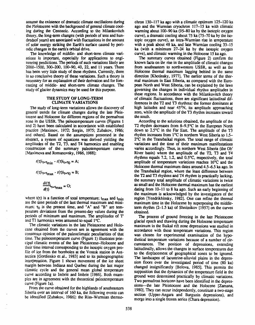
assume the existence of dramaticclimate oscillations during chron 130-117 La ago with a climatic optimum 125-120 Lathe Pleistocenewiththe backgroundof generalclimate cool. ago and the Wurmiancryochron 117-15 La with climaticing during the Cenozoic, According to the Milankovitch warmingabout 100-90 La (95-80 La by the isotopicoxygen

' theory, the long-termchanges (with periodsof tens andhun- curve), a dramaticcooling about 75 La (75-70 La by the iso-dredsofyears) are associated with fluctuations in the amount topic oxygen curve), an intra-Wurmlan rise in temperatureof solar energy strikingthe Earth'ssurface caused by peri. with a peak about 48 La, and late Wurmiancooling 33-15odicchanges in the earth'sorbital drive, La (with a minimum 27-24 La by the isotopic oxygen

The knowledge of middle- and short-term climate vail. curve), and climaticwarmingin the Holocene 15 ka ago,afions is important,especially for applications to engi- The summary curves obtained (Figure 2) confirm theneering predictions,The periods of such variationslikely are known facts on the rise in the amplitudeof climatic changes2000-1500, 300-200, 100-90, 40, 22, and 11 years, There from southeastern to northwestern USSR, as well as thehas been very little study of these rhythms. Currently,there Holocene thermal maximum lagging behind in the sameis no conclusive theory of these variations.Such a theory is direction [Khotinsky, 1977]. The earlier terms of the thor-necessaryforan explanationof theirderivationand for fore. mal maximum in East Siberia, as compared with the Euro-casting of middle- and short-term climate changes. The pean North and West Siberia, can be explained by the lawsstudyof glacierdynamics may be used for this purpose, governing the changes in individual rhythm amplitudes in

these regions.In accordance with the Milankovitch theoryTHE STUDY OF LONG.TERM of climatic fluctuations, there are significant latitudinaldif-

CLIMATE VARIATIONS ferences in the T2 and T3 rhythms: the formerdominatesatThe study of long-term variationsallows the discoveryof high latitudes and near 45°N, its amplitude approaching

general trends for climate changes during the late Pleis- zero, while the amplitude of the T3 rhythm increasestowardtocene and Holocene fordifferent regionsof the permafrost the south.zone in the USSR. The paleotemperaturecurves (Figures 1 According to the solutions obtained, the amplitude of theand 2) have been calculated in accordance with established T2 rhythm decreases from 8--9.5°C in the EuropeanNorthpractice [Maximov, 1972; Sergin, 1975; Zubakov, 1986; down to 2.5°C in the Far East. The amplitude of the T3and others]. Based on the assumptions presented in the rhythm increases from I°C in northernWest Siberia to 1.5-abstract, a system of equations was derived yielding the 20C in the Transbaikalregion. The total range of climaticamplitudes of the T2, T3, and T4 harmonicsand enabling variations and the time of their maximum manifestationsconstruction of the summary paleotemperature curves varies accordingly.Thus, in northern West Siberia (the Ob'[MaximovaandRomanovsky, 1986, 1988]: River basin) where the amplitude of the T2, T3 and 1"4

rhythms equals 7.2, 1.2, and 0.5°C, respectively, the totalt(x)l_--Xmin " t(_)lx.---.v.0--"A; amplitude of temperaturevariations reaches 16°C and the

Holocene thermal maximumdates around4.5-.6.5 ka ago. In

t('01x,--Xmax - t(l:)iv...--x0= B; the TransbaiLalregion, where the least difference betweenthe T2 and T3 rhythms and T4 rhythm is practicallylacking,the summary total amplitude of climatic variationsis twice

at(x),_x--_--Xmax= O; as small and the Holocene thermal maximum has the earliestdating from 10-11 to 8 La ago. Such an early beginning of

the maximum is acknowledged by the investigators of thewhere t(x) is a function of total temperature; tmaxand train region [Yendrikhinsky, 1982]. One can refine the thermalare the time periods of the last thermal maximum and mini- maximum time in the Holocene by superposing the middle-mum; Xo is the present time, and "A" and "B" are tem- term rhythm (2--1.5 La) of Shnitnikov [1957] on the curves

: perature deviations from the present-day values during the obtained.periods of minimum and maximum. The amplitudes of T The process of ground freezing in the late Pleistoceneand T1 harmonics were assumed to equal IoC. glacial epoch and thawing during the Holocene temperature

The climatic variations in the late Pleistocene and Holo- maximum in the Baikal rift zone depressions was studied incene obtained from the curves are in agreement with the accordance with these temperature variations. This regionconsensus opinion of the paleoclimatic peculiarities of that was chosen for experimental examination of the hypo-time. The paleotemperature curve (Figure 1) illustrates prin- thetical temperature variations because of a number of cir-cipal climatic events of the late Pleistocene-Holocene and cumstances. The position of depressions, extendingtheir time interval corresponding to the isotopic oxygen pro- latitudinally, allows the changes in surface temperatures duefile of ice from the boreholes at the Vostok station in Ant- to the displacement of geographical zones to be ignored.arctica [Gordienko et al., 1983] and to its paleogeographic The landscapes of lacustrine-alluvial plains in the depres-interpretation. Figure 1 shows movement of the ice sheet sion floors over the investigated period of time (80 La)margin between Indiana and Quebec during the last major changed insignificantly [Belova, 1985]. This permits theclimatic cycle and the general mean global temperature supposition that the dynamics of the temperature field in thecurve according to Imbrie and Imbrie [1986]. Both exam- ground were determined practically by climatic variations,pies are in agreement with the theoretical paleotemperature Two permafrost horizon,_have been identified in the depres-curve(Figure la). sions---the late. Pleistocene and the Holocene [Zamana,

From the curve obtained for the highlands of southeastern 1980]. They can occur independently, constitute a two-stageSiberia over an interval of 160 ka, the following events can section (Upper-Angara and Barguzin depressions), andbe identified [Zubakov, 1986]: the Riss-Wurmian thermo- merge into a single frozen series (Chara depression).

_

538

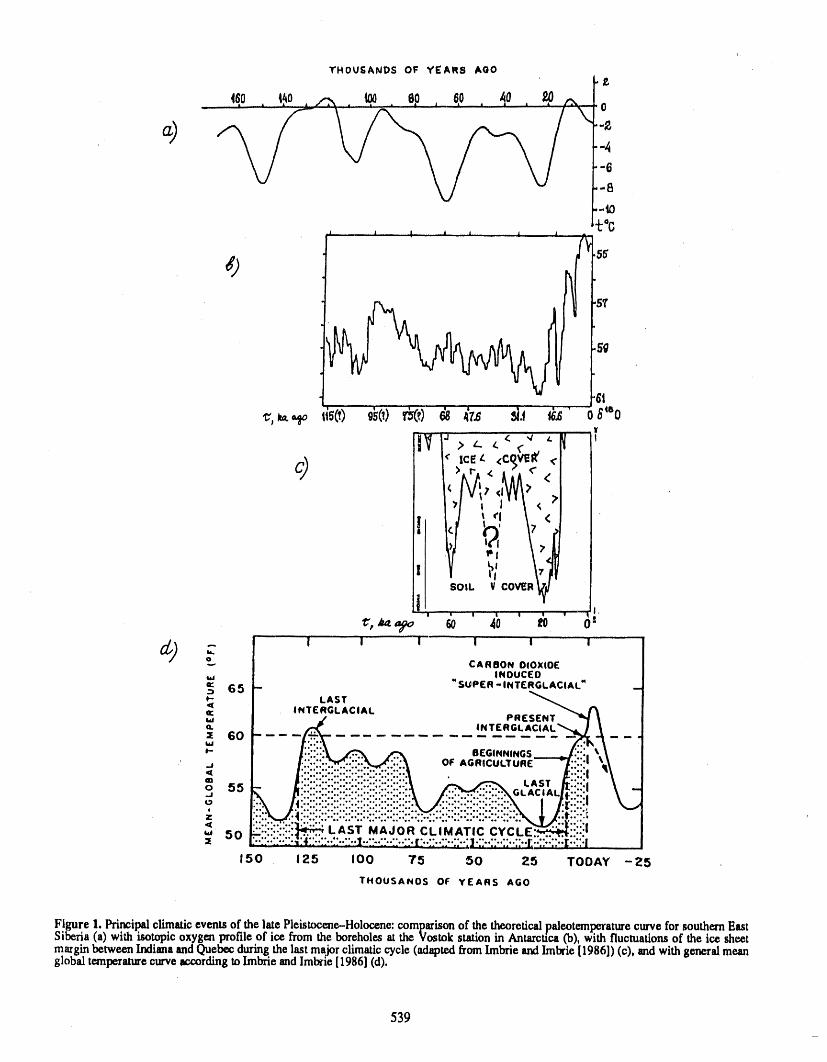
THOUSANDS OF YEARs AO0&

4_o t_o./-:_. _ ep, 60, ._o _ ,,:, o

.'4-6

-.8

._ .. l ! | i , _ J ....

b)

6t

lcEz <CqVi!ff <

/ lt ¢II <_. I , 7

> 7

- I I I '

_',,,,,,,,y_ _o 4b e_ o:

-- ' CARBONDIOXIDE Iw I ,, INDUCED I¢c:) 65 _ SUPER - INTERGLACIAL" _.JP" / LAST _ /,,=(

=: / INTERGLACIAL PRESENT "_ :Q. INTERGL_E 60 ..................*,w

P" | /,.::L_, _ ,_ BEGINNINGS_.._.._.':., _

liii!iii!! iiii!i iiiit li:.iii;;\o 55 - F'___-:::: \ "

o-, (ii!ii!iii::!iiiiiiiiii!!ii::!iii!ii!ili iiiii::iiiiiiiii!iiiiii1/.:ii!!i!l7 lr

< i:"iii!, :!'i!_ LAST MAJOR CLIMATIC CYCLE" iiii:l_" 50=E i'"'..'""__'-.,_4S..".._..'_..I..".."-.'T...". C.."..L'-.::--; ] ,=-.:'..':..;1..£:1:::::1..1_::::'1

150 125 I00 75 50 25 TODAY -215

THOUSANDS OF YEARS AGO

Figure 1. Principal climatic events of the late Pleistocene--Holocene:comparison of the theoreticalpaleotemperaturecurve for southernEastSiberia (a) with isotopic oxygen profile of ice from the boreholes at the Vostok station in AntarcticaCD),with fluctuationsof the ice sheetmargin between Indianaand Quebec duringthe last majorclimatic cycle (adaptedft'oreImbrie andImbrie[1986]) (c), _d with generalmeanglobal temperaturecurve accordingtoImbrie andImbrie[1986] (d).

539

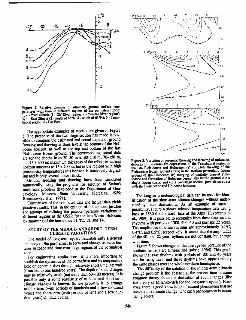
' t ,G ,_,_'!t,.,,,:,,.I,, _,, .,_, ..,,, .,,, :.o i,_ _,

I0 0 (_ z_ 2Jl' I ,, i I . i , L _-- i

//

"-"'"" "° \ "'q.'"""--...L'-. " _ .r0o

•._ ..-- "_ _ .PO0

..v. H.u

Flgure 2. Relative changes of summary ground surface tem. ¢ to-'Fa_s lo 8 6 ,_ 2 o

1, 2- West Sib_'i,, (1- Ob' Riverr6_ion;2- YenisetRive!' region); "-_"-__,60. _// _ "_.._3, 4 - East Siberia(3 - northof 65°N;4 - south of 65 N); 5- Trans- , _--,,,,.,=_..__.____ -.,, -50

baikal region; 6 Fer East. / _

- "_P"'q_" "a_ -_...t..V...v,. ,=_, ..t., .p= .v..._,..e '

-Ioo

The appropriate examples of models are given in Figure3, The presence of the two-stage section has made it pen. ' "_

sible to compare the estimated and actual depths of ground / _/) .,. ,_0freezingand thawingat three levels: the bottom of the Hol- /-0,_ .,..._ .,-."__'_ocene horizon, as well as the top and bottom of the late _-" _-,- ._ _" ...____-0,2_ ?00

Pleistocenefrozenground.The correspondingactttaldata H,_areforthedepthsfrom30-50 m to80-110m, 70-150m,and 130-300m; maximum thicknessoftherelictpermafrost Figure3.Variationofperennialthawingandfreezingofrud_eousdeposits in the mountaindepressions of theTransbaikalregion inhorizon amounts to 150-200 m, but in the regions with high the late Pleistocene and Holocene: (a) complete thawing of thepresent-day temperatures this horizon is intensively degrad- Pleistocene frozen groundstrata;in the section: perennially._o_n

• ing and is only several meters thick, ground of the Holocene; (b) merging of partially thaweo frets-Ground freezing and thawing have been simulated tocene and formationof Holocene perenniallyfrozen groundinto a

numerically using the programs for solution of Stefan's single frozen strata; and(c) a two-stage section permafrost suratawit_ thePleistocene end Holocene horizons.multifront problem developed at the Department of Geo-

cryology, Moscow State University [Seregina, 1989; The long-term meteorological data can be used for iden-Romanovsky et al., 1991]. tification of the short-term climate changes without under-

Comparison of the computed dam and factual data yieldspositiveresults.This,intheopinionoftheauthors,justifies standingtheirderivations,As an example of such athe attempt of refining the paleotemperature variations in possibility, Figure 4 shows selected temperature data datingdifferent regions of the USSR for the late Wurm-Holocene back to 1530 for the north face of the Alps [Huybrechts ctby summing of the harmonics T1, T2, T3, and T4. al., 1989]. lt is possible to recognize from these data severalrhythms with periods of 300, 400, 40 and perhaps 22 years,

STUDY OF THE MIDDLE- AND SHORT- TERM The amplitudes of these rhythms are approximately 0,4°C,CLIMATE VARIATIONS 0.4°C, and 0.5°C, respectively, lt seems that the amplitudes

The model of long-term cycles describes only a general of the 40- and 22-year rhythms are not constant, but changetendency of _,hepermafrost to form and change its main fea- with time.turcsinspaceand timeoverlargeregionsofthepermafrost Figure5 showschangesintheaveragetemperatureofthe

northernhemisphere[Imbrieand Imbrle,1986].Thisgraphzone.

For engineering applications, it is more important to shows that two rhythms with periods of 100 and 40 yearsestablish the dynamics of the permafrost and its temperature can be recognized, and these rhythms have approximatelyfield on concrete sites through relatively short time intervals the same phases over the whole northern hemisphere.(from ten to one hundred years). The depth of such changes The difficulty of the solution of the middle-term climaticmay be relatively small (not more than 50-100 meters), lt is change problem is the absence at the present time of somepossible only if some regularity of middle- and short-term common theory about the derivation of such ckanges (likeclimate changes is known. So the problem is to arrange the theory of Milankovitch for the long-term cycles). How-middle-term (with periods of hundreds and a few thousand ever, there is good knowledge of natural phenomena that are

years) and short-term (with periods of tens and a few hun- sensitive to climate change. One such phenomenon is moun-dred years) climatic cycles, lain glaciers.

540

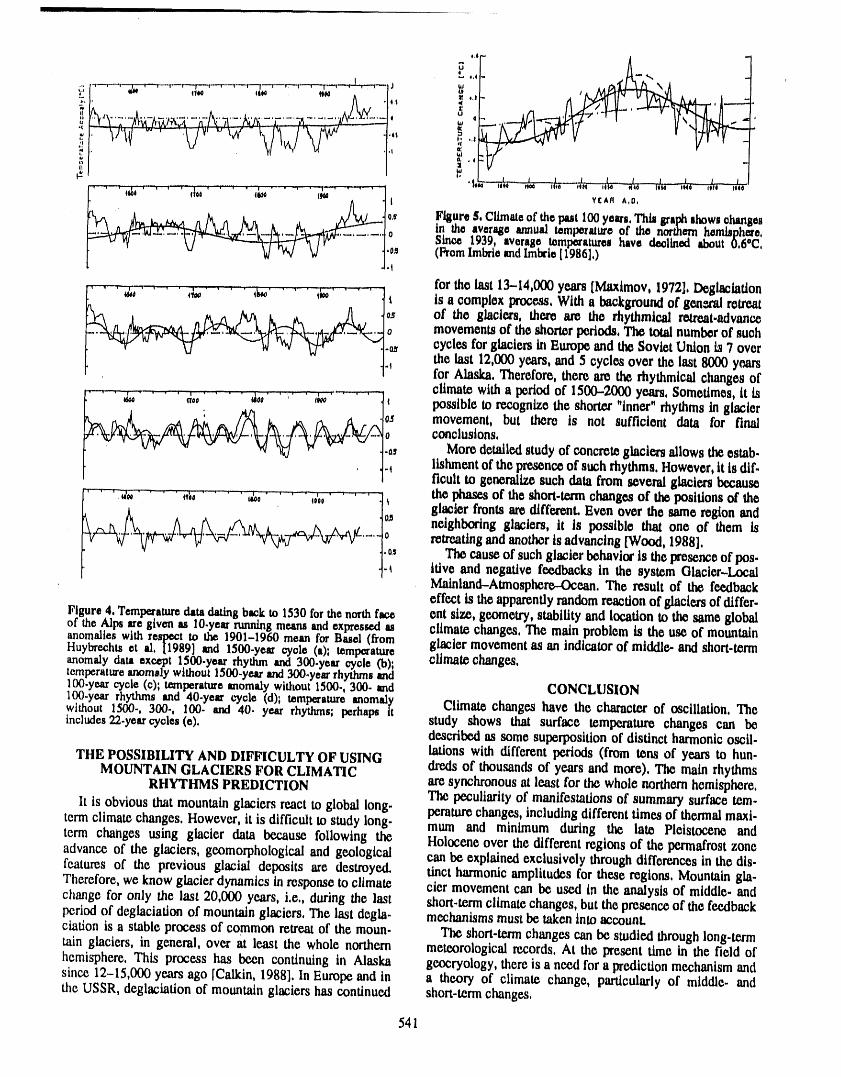
F

- i '.¸,,:,_.;.-:_-_._,-_-j_,,,,hi_-_,-:-__--,::-a , d

, d

_1' 4_ _o0 4_ I_ | I Y( Afl A,U,

the averageannualusmperam'ooi' the nor_ernhomhphero,_J

(FromImCo andIm_te [1986],)Iii" Since1939,.veragetemperatureshavedeclined_out0,6°C,

_' ' ' ',d_"' ' "4_' ' " _ 4;_'--'" 'i forthelast13-14,000years[Maxlmov,1972],Deglaclation/ t is a complex proce,ss, With a backgroundof genmtl retreat0s of the glaciers, there are the rhythmical retreat.advance

.... , .... o movementsof the shorterperiods, The total numberof suchcycles for glaciers ht Europe and the Soviet Union is 7 over

_ the last 12,000 years, and 5 cycles over the last 8000 yearsfor Alaska, Therefore, there are the rhythmical changes of

...... , , . .,....,... .,-.,-.,-._ climatewitha periodof1500-2000years,Sometimes,ltis, _ 4 possibletorecognizetheshorter"inner"rhythmsinglacier

_7 movement, but there is not sufficient data for finalconclusions,

tla, Moredetailed study of concrete glaciers allows the estab.'_ k/ ' , lishmentof the presenceof such rhythms. However, tt is dif-

ficult to generalize such data from several glaciers because-v _ ,J ! , _ " ',, i_ 1, ,"' ; , ....... • ,_ ,v ; , , i i ......

"" ,,0 _0 ,;, t _ the phases of the short.term changes of the positions of the

t_o. glacter fronts aredifferent. Even over the same region and

• 0_ neighboring glaciers, it is possible that one of them is'-' retreatingand another is advancing [Wood, 1988],

The cause of such glacier behavior is the presenceof pos-1._ itive and negative feedbacks in the system Glacier-Local

Mainland-Atmosphew.,-Ocean,The result of the feedbackeffect is theapparentlyrandomreactionof glaciersof differ.

Figure4, Temperaturedatadatingbackto 1530forthenorthface ent size, geometry, stability and location to the same globalof the,Alps_e given u 10.yearrunningmeansandexpressedas climate changes, The main problem is the use of mountainanomaimsw_mrespectto the 1901-1960mean ,f_ Basel (from glacier movementas an indicatorof middle- and short-termHuybrechtset al, [1989] and 1500-year cycle (a), temperature_omaly dataexcep,t 1,500.yearrhythmand300.year eyole (b); climate changes,_mperamreanomalywtmout15ce.yearand300-yearrhythmsandlt2t2-yearcycle (o);temperatureanomalywithout1500.,300. and CONCLUSION

_tn_.yearrhythmsand 40-year cycle (d); temperatureanomaly Climate changes have the characterof oscillation, Thewithout 1500., 300-, 100- and 40- year rhythms;perhapsitincludes22.yearcy¢les (e), study shows that surface temperature changes can be

describedas some superposition of distinct harmonicoscil.THE POSSIBILITY AND DIFFICULTY OF USING lations with different periods (from tens of years to hun.

MOUNTAIN GLACIERS FOR CLIMATIC di'eds of thousandsof years and more). The main rhythmsRHYTHMS PREDICTION aresynchronousat least for the whole northernhemisphere.

The peculiarityof manifestations of summary surface tem.It is obvious that mountainglaciers react to global long. peraturechanges, including different times of thermal maxi-

term climate changes. However, it is difficult to study long- mum and minimum during the late Pleistocene andterm changes using glacier data because following the Holocene over the different regions of the permafrostzoneadvance of the glaciers, gcomorphological and geological can be explained exclusively throughdifferences in the dis.features of the previous glacial deposits are destroyed, tinct harmonicamplitudes for these regions, Mountain gla.Therefore, we know glacier dynamics in response to climate cier movement can be used in the analysis of middle- andchange for only the lasl 20,000 years, i.e,, during the last short-termclimate changes, hutthe presenceof the feedbackperiod of deglaciation of mountain glaciers, The last degla- mechanisms mustbe taken into accounL

elation is a stable process of common retreatof the moun- The short-termchanges can be studied through long-termrain glaciers, in general, over at least the whole northern meteorological records, At the present time in the field ofhemisphere. This process has been continuing in Alaska geocryology, there is a need for a prediction mechanism andsince 12-15,000 years ago rCalkin, 1988]. InEurope and in a theory of climate change, particularly of middle, andthe USSR, deglaciation of mountain glaciers has continued short-termchanges,

541

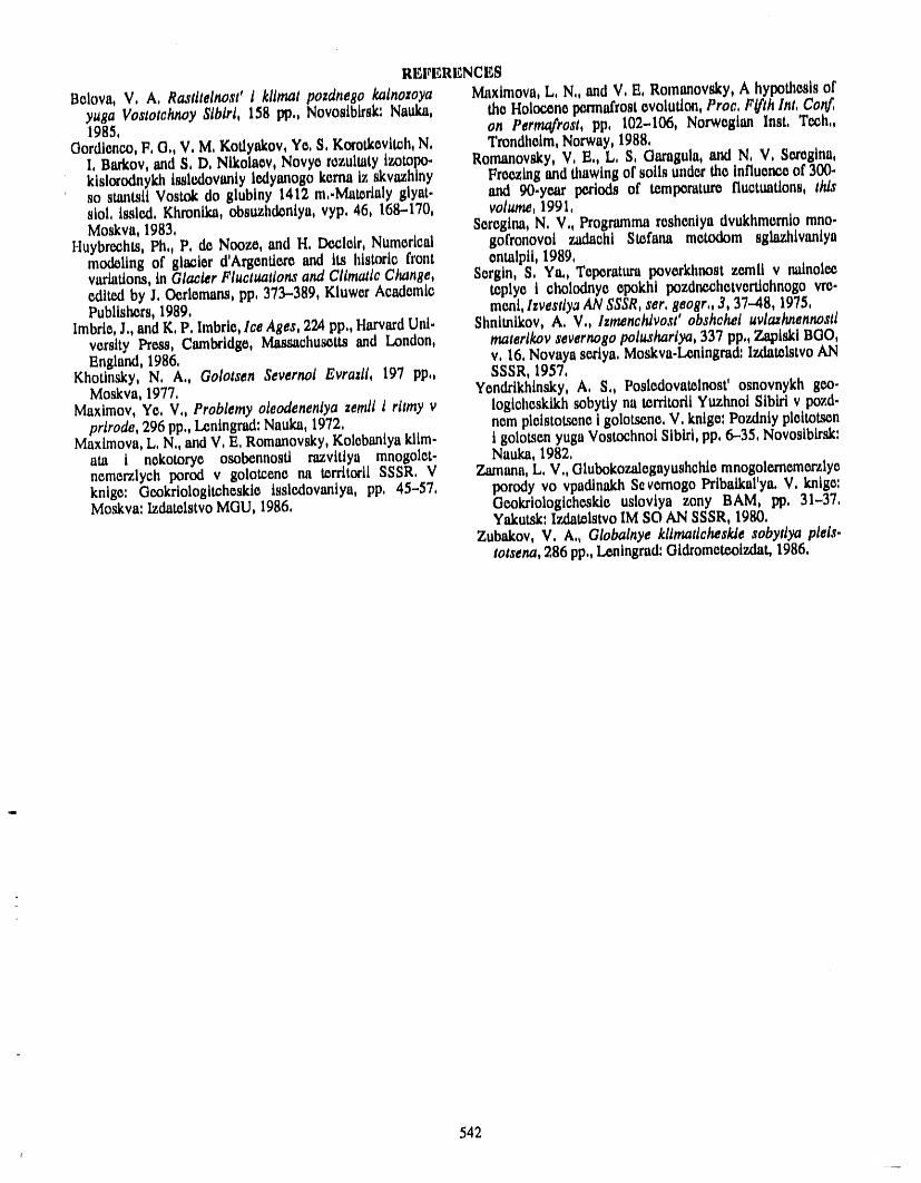
REFERI_NCES

Bolova,V, A, Rastitelno,vt'I kllmatpozdnegokalnozoya Maximova,L,N,,andV,E,Romanovsky,A hypothesisofyugaVostotchnoySibiri,158pp,,Novosibirsk:Naoka, theHolocenepermafrostevolution,Proc,F_fthInt,Co_1985, on Pernu_rost,pp, 102-106,NorwogianInst,Tech,,

Gordionco,F,G,,V,M, Kotlyakov,Yts,S,Korotkovit_h,N, Trondhoim,Norway,1988,I,Barkov,andS,D,Nikolaov,Novyerozultatyizotopo- Romanovsky,V, E,,L, S,Garngula,andN, V, Seregina,kislorodnykh issle,dovaniy ledyanogo korna 17,skvazhiny Freezing and tlmwingof soils underthe influenceof 300-so stantsii Vostok do glubiny 1412 m,.Mat_daly glyat- and 90.ye.ar p_ods of tcmpcratur_ fluctuations, th/sslol, issle,d, Khronika,obsuzhd_niya, vyp, 46, 168-170, volume, 1991,Moskva, 1983, Sorogina,N, V,, Programmaroshontyadvukhmorniomno.

Huybrechts,Ph,, P, do Noozo, and H, De.cloir,Numorical gofronovoi zadaohi Stcfana motodom sglazhivanlyamod_ilng of gln_ier d'Argcntloreand its historio front entalpii, 1989,variations,in Glacier Fluctuations and Cll_ic Change, Scrgin, S, Ya,, Tcporatm'apovorkhnost zemli v nainolece,dit_d by J, O_rlomans,pp, 373-389, Kluwer Acadomic tcplye t cholodnyo opokhi pozdncchctwrttchnogo rrc.Publishers, 1989, mont, lzvestly,_AN SSSR, ser, geogr,, 3, 37.-48, 1975,

Imbrle, J,, and K, P, Imbrte,Ice Ages, 224 pp., HarvardUni. Shnlmlkov, A, V,, Izmenchivost' obshchei uvlazhnennostlvorslty Press, Cmnlxldge, Mas.qachu_tts and London, materlkov severnogo polushartya, 337 pp,, ZaplsklBGO,England, 1986, v, 16, Novaya sertya, Moskva.I.,onlngrad:IzdatolstvoAN

Khotinsky, N, A,, Golotsen Severnot Evrazli, 197 pp,, SSSR, 1957,Moskva, 1977, Yondflkhinsky, A, S,, Poslcdovat_lnost' osnovnykh ge.o.

Maximov, Ye, V,, Probiemy oleodeneniya zemli I ritmy v logicheskikh sobytiy na t_rritofliYuzhnol Sibtri v pozd-prtrode, 296 pp,, Leningrad:Nauka,1972, noraploisto_nc i golotscno, V, knlgo:Pozdniy plettots_n

Maxlmova, L, N,, andV, E, Romanovsky,KolobaniyaIdim- i golotson yuga Vostochnoi Sibiri, pp, 6-35, Novoslbksk:ata i nokotoryo osobcnnostl razviflya mnogolot- Nauka, 1982,nomerzlych porod v golotccno na tcrritoril SSSR, V Zamana,L, V,, Oluboko',udcgayushchiomnogole.rncmcrzlyoknlgo: Gcokrtologltchoskic tssledovantya, pp, 45-57, porody vo vpadlnakhSevornogo Pribaikal'ya,V, knigc:Moskva:Izdat_lstvoMGU, 1986, Ge.okriologicheskto uslovtya zony BAM, pp, 31-37,

Yakutsk:Izdat_lstvoIM SO AN SSSR, 1980.Zubakov, V, A,, Globalnye klimatlcheskie sobytlya piels.

totsena, 286 pp,, Leningrad.'Oidromote.olzdat,1986,

542i

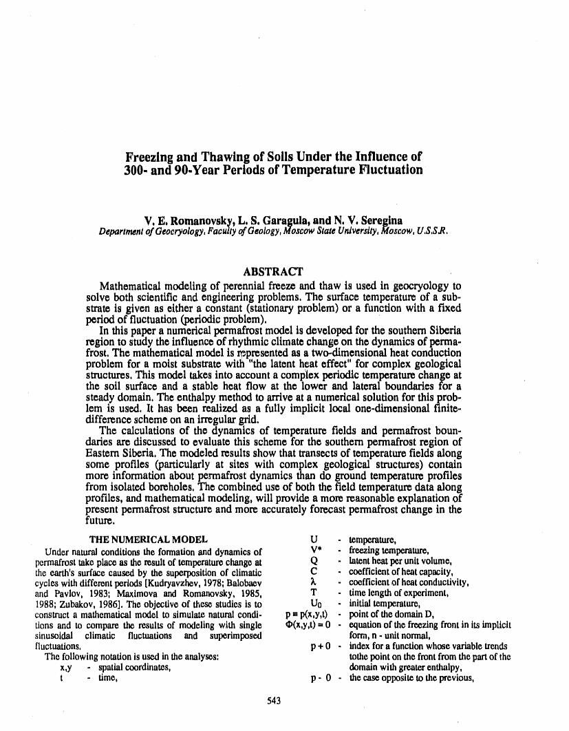
Freezing and Thawing of Soils Under the Influence of300- and 90.Year Periods of Temperature Fluctuation

V. E. Romanovsky,L. S. Garagula,and N. V. SereginaDepartmentof Geocryology,Facultyof Geology,MoscowStateUniversity,Moscow,U,S,S.R,

ABSTRACT

Mathematical modeling of perennial freeze and thaw is used in geocryology tosolve both scientific and engineering problems, The surface temperature of a sub-sl:mm is given as either a constant (stationary problem) or a function with a fixedperiod of fluctuation (periodic problem),

In this paper a numerical permafrost model is developed for the southern Siberiaregion to study the influence of rhythmic climate change on the dynamics of perma-frost, The mathematical model is _presented as a two-dimensional heat conductionproblem for a moist substrate with "the latent heat effect" for complex geologicalstructures. This model takes into account a complex periodic temperature change atthesoilsurfaceand a stableheatflowatthelowerand lateralboundariesforasteadydomain.The enthalpymethodtoarriveata numericalsolutionforthisprob-iem isused.lthasbeenrealizedasa fullyimplicitlocalone-dimensionalfinite-differenceschemeonanirregulargrid.

The calculationsof thedynamicsof temperaturefieldsand permafrostboun-dariesarediscussedtoevaluatethisschemeforthesouthernpermafrostregionofEasternSiberia.The modeledresultsshow thattransectsoftemperaturefieldsalongsome profiles(particularlyatsiteswithcomplex geologicalstructures)containmore informationaboutpermafrostdynamicsthando groundtemperatureprofilesfromisolatedboreholes.The combineduseofboththefieldtemperaturedataalongprofiles,andmathematicalmodeling,willprovidea morereasonableexplanationofpresentpermafroststructureand more accuratelyforecastpermafrostchangeinthefuture.

THE NUMERICAL MODEL U - temperature,Undernaturalconditionsthe formationanddynamicsof V* . freezingtemperature,

permafrosttakepiaceas theresultof temperaturechangeat Q . latentheatperunitvolume,the earth'ssurfacecausedby the superpositionof climatic C - coefficientof heatcapacity,cycleswith differentperiods[Kudryavzhev,1978;Baiobaev _ - coefficientof heatconductivity,and Pavlov, 1983; Maxtmovaand Romanovsky,1985, T - timelengthof experiment,1988;Zubakov,1986]. Theobjectiveof these studies is to U0 . initialtemperature,constructa mathematicalmodel to simulatenaturalcondi, p '_p(x,y,t) - pointof the domainD,tions and to comparetheresultsof modelingwlth single O(x,y,t)= 0 - equationof the freezingfrontin its implicitsinusoidal climatic fluctuations and superimposed form,n - uifltnormal,fluctuations, p + 0 - indexfora functionwhosevariabletrends

The followingnotationis usedin theanalyses: tothepointon the frontfromthepartof thex,y - spatialcoordinates, domainwith greaterenthalpy,t - time, p - 0 - thecaseoppositetothe previous,

543d

At. = tri- tn.l - time step, wheret.+It2 = t. + At./2 - time point,hx,tffixl- xi.l - spatial step in the directionX, 2

yj.. spat in dlr UonY, Ax =hx,+h -0,5h ,i,Yj,discretesolutionat the nth time step,UII

U_I discrete functioncorrespondingto the U1+1,j + U iJ Ul+l ,j - U ijn+1/2 timestep .... 2 --) hx,i+""""'_" _s(Xt- 0,5hx,i,Yj,

Uij2 . discretesolution at the n+l time step,

C, . smooth coefficient of heatcapacity, Ulj+Ul.1 ,j) UlJ-Ui.l,j. smooth coefficient of heat conductivity, , L ..g . geothermalgradient, 2 hx,i ]; (2)

2 [_,s(xi+Yj+l - 0,Shy,j,The model can be representedin the following form in the A2 Uij '_hy,j +H y,j+l-domain

D ffi{0< x < 11,0 < y <12, 0 ¢' t < T} uUII,J+I+Uij Ut,j+l-Uij.

in the X,Y,t- space : 2 ) .......hy,j+l '" _,s(xi,Yj- O,5hy,j,Uij+Ui,j.1 Utj-Ul,j.1

2 ....) hy,j ]'_U._dtv(7,_j,x,y)VU) and (x,y,t)aD,c (u,x,y)

. The boundaryconditions for the first equationof system

U =U (x,y,t) _ V* ' (1) (2) are given as t-in+l/2, and for the second as tffih+l.Forthe scheme (2), the boundaryconditions of the second type

U (x,y,0) ffiU0 (X,y), are approximatedwith the second orderof hx, hy [see, forexample, Seregina, i989] and with the firstorderof At. So

._. _ ._ the approximationorderof the scheme is O (h_2+ hy2+ At),I x=O= _n xffil1, I y-12 =g We used a simple iterationmethod for the solution of thenonlineardiscrete system at each time layer, The solutionfrom theprevious time layer was consideredto be the initial

U (x,0,t)= q_(x,t), approximation of the iterative process. The program waswritten in FORTRAN-IV.The program bisects the time stepU (x,y,t) ffiV* where P (x,y,0 _ • (x,y,t), in the case of iterative divergence at each half of the time

layer,The results of the numerical experiments:after the diel.

sion of the time step, it is more economical not to use theQ(x,y) _t = ((_,VU)ip+O- (_,VU)lp-0, rO), maximum time step; the convergence of the solution of the

initial problem to the solution of the periodic problem de-pends weakly upon the initial temperature function; we

where peO(x,y,t)ffiO, reach the pedodic regime after 4-5 periods. Calculationtime depends greatly upon the upper boundary condition

In order to solve problem (1) we need the initial _x,t); therefore the calculation time in the ease of a 300-temperatureUo(x,y); however, ourmain problemis periodic year period is several times largerthan in the case of the 90-in time, so Uo(x,y) is unknown. FromMeyermanov [1986], yearperiod.we know the solution of problem (1) with a periodic func-tion _x,t) and an arbitraryfunction Uo(x,y) trends to the GEOLOGICAL STRUCTURE, PHYSICALsolution of the periodicequation. PROPERTIES AND CLIMATE DYNAMICS

For a numerical solution of the problem (1), we use the This mathematical model was used for the analysis ofenthalpy method. We smooth the enthalpy function with a permafrostdynamics in the southern regions of Easternfirst-order polynomial. The advantage of this method is that Siberia. Paleogeographers determined in these regions thethe temperature field can be found without knowing the climatic rhythms with periods of about 90 and 300 years andposition of the freezing front at a previous time layer (as, for amplitudes with fluctuations about 2°C and a mean tem-example, in variational-difference method). This is e,spe- perature of approximately 0°C. These temperature valuescially imlxa'tant when we have three or more fronts (as in were used as upper boundary conditions, Lower boundaryour case), conditions were given by the geothermal gradient of 0.01°C

To solve the smoothed differential problem in the m-I at adepthof400m.enthalpy formula we use a fully implicit local one- The geological structure of the study consists of twodimensional finite-difference scheme (always stable): parts. The first part is a layer of alluvial sands with a 10-m

thickness and a sandstone base. The second part is also aC_ (xi,Yj,Ulj1) (Utj1 - Utj)= Atn+lAI UIJ1, layer of alluvial sands, but with a 50-m thickness.

Cs (xi,Yj,UIj2) (Utj2" Uij1) = Atn+lA2UtJ2, Thermal and physical properties of soils are indicated inTable 1.

544-

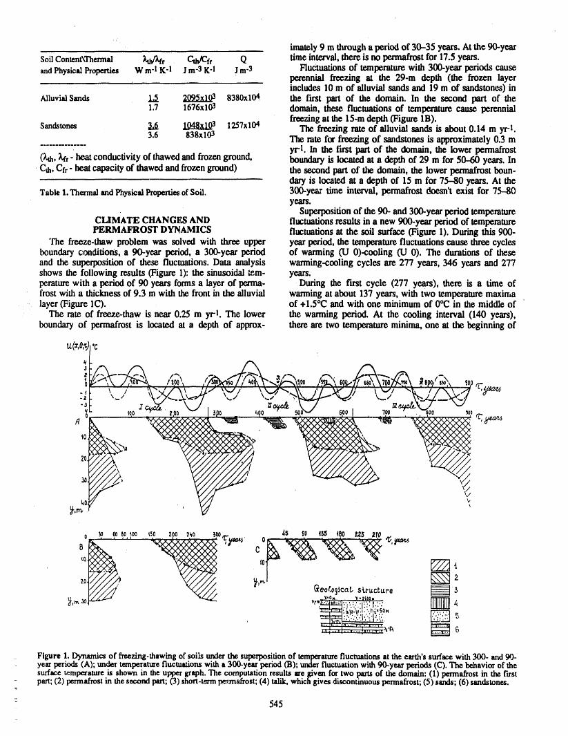
imately9 m througha periodof 30-35 years. Atthe 90-yearSoilConient\Thermal 7,tid14r C,e_fr Q timeinterval,thereis no permafrostfor 17.5 years.andPhysicalProperties W m-tK-I Jm-3K-I Jm-3 Fluctuationsof temperaturewith 300-year periods cause

perennial freezing at the 29-m depth (the frozen layerincludes 10 m of alluvial sandsand 19 m of sandstones) in

AlluvialSands 1.5 _2095x103 8380x104 the first part of the domain. In the second part of the1.7 1676x103 domain, these fluctuations of tempezaturecause perennial

freezing at the 15-m depth (Figure 1B).Sandstones 3.6 1048x103 1257x104 The freezing rate of alluvial sands is about 0.14 m yrl.

3.6 S38x103 The rate for freezing of sandstones is approximately0.3 m3tri. In the first partof the domain, the lower permafrost

0_h, gtr"_heat conductivityof thawedandfrozenground, boundaryis kr.ated at a depth of 29 m for 50-60 years. InCth, Cfr" heat Cal_t:ity of thawed andfrozenground) the second part of the domain, the lower permafrostboun-

daryis located at a depth of 15 m for 75-80 years. At theTablel.Thennal andPhysical Properties ofSoil. 300-year time Interval, permafrost doesn't exist for 75--80

years.Superpositionof the 90- and 300-yearperiod temperature

CLIMATE CHANGES AND fluctuationsresults in a new 900-year periodof temperaturePERMAFROST DYNAMICS fluctuations at the soil surfile (Figure 1). During this 900-

The freeze-thaw problem was solved with three upper yearperiod, the temperaturefluctuations cause three cyclesboundary conditions, a 90-year period, a 300-year period of wanning Ct,l0)-cooling (tj 0). The durations of theseand the superpositionof these fluctuations. Data analysis warming-cooling cycles are 277 years, 346 years and 277shows the following results (Figure 1): the sinusoidal tem- years.peraturewith a period of 90 years forms a layer of perma- During the iu'st cycle (277 years), there is a time offrost with a thickness of 9.3 m with the front in the alluvial wanning at about 137 years, with two temperaturemaxima

: layer(Figure lC). of +1.5°C and with one minimum of 0°(2 in the middle ofThe rate of freeze-thaw is near 0.25 m yrt. The lower the warming period. At the cooling interval (140 years),

boundary of permafrost is located at a depth of approx- there are two temperatureminima, one at the beginning of

u I'c

.li \ / '_",.a'l'_t I/.I xx.d/ \.%,,,.p,",._.\x/,/ ]0"- 11 t x,.// "_¢a !/-X.\ ,// _,_z¢,_

C. lee _ :,oo_ I 5De ,,_o w _oo"-./ 6t I "lee . oo _oo

._ , '/7

J'rl,

7,,__ _--,---- . " ::'.'.','1',:,l.','::....

Figure 1. Dynamicsof freezing-thawingof soils underthesuperpositionof temperaturefluctuationsattheemh's surfacewith300- and90-ye_"periods(A); undvrtemperaturefluctuationswithii 300-yearperiod(Ii); underfluctuationwith90-yearperiods(C).The behaviorof thesurface temperatureis shown in theuppergraph.The computationre_lts ire giv.eaf_. two .partsof thedomain:(1) tm'mafzostin the first

- part;(2) permafrostin thesecondpart;('3)shon-texmpe_.matrost;(4) talik,whichgivesdiscontinuouspermafrost;(5) sands;(6) sandstones.=

545

_

the interval (-1.2°C), and the other at the end (-2oC). In the short-termpermafrostcausesan actualinvariablelocationofmiddleof thecooling interval, there is one maximumwith a permafrostcover during30 years.temperaaimnotgreater than(PC. After thawing of short-termpegnafrost, the thawing of

During the second cycle (364 years), there is a time of soils from above proceeds with a rate of about 0.1 m yrlwarming (208 years).vith three temperature maxima of during the next 35 years, lt ends with the meeting of the+0.7°C, +2.(PC and +0.5oc, and two temperature minima upperandlower fronts.Tt__,end of thawingoccurs when the(-0.3°C and -0.6°C). At the time of cooling (138 years), maxima of the 300- arm90_yearperiods coincide. Twentythere are two temperature minima (-2.0°C and -0.9°C) and years after the end of _J_wing the short-term permafrostone maximum(+0.3'(3). with 6 m thickness is formedand exists for 60 years.

During the third cycle, there is a time of warming(137 At the end of the second cycle, the depth of freezing isyears), with two maxima (+1.8°C and +1.5°C) andone rain- 27-31 m for 150 years. The durationof freezing to a 27-mimum (-0.2°C). At the time following cooling (140 years), depth is equal to 50 years; the rateof freezing is near0.56 mthere are two minima (-1.9°(3 and -1.20C) and one tem- yrl. After that, the freezing front is actually invariable.perature maximum (0oC). The thermal history is opposite Such a position of lowerpermafrost boundary is defined bythat ofthefirstcycle, a temperature maximum of fluctuation with a 90-year

Analysis of the summary temperature curve shows that period.The surface temperature is positive for 20-30 years.total warmingoccurs in the middle of the 900-year period, Talik with thickness near 1.5 m exists over the cover of per-andrids warmingis caused by te,mpcratumfluctuationswith mafrost.Ten years after the freezing of the talk, the lowera 300-year period. The fluctuations with 90-year periods freezing frontfalls to a 3 l-m depth (for30 years).cause a temporary lowering of the surface temperature The third cycle begins with thawing of permafrost frombelow 0°C. above and from below, conditioned by positive surface tem-

The formation and dynamics of permafrost caused by the perature. The rate of thawing from below is about 1.5 mtemperature fluctuations are different with respect to differ- during the 70-year period. The rate of thawing from above isent cycles of 900 years. As shown in Figure 1, simple stable about 0.4 m yrt. After 70 years, the upper and lower frontsconditions of freeze-thaw occur during the first cycle. The meet at a depth of 28 m.maximum thickness of permafrost here is near 45 m. The During the next 70 years, the section consists of thawingexistence of permafrost is near 140 years. During the pre- soils. This is initiated by positive surface temperature. How-vious period of warming, thawed soils exist continuously ever, at the beginning of this time interval, short-term per-during a 55-year period, mafrost is formed with a thickness of about 1 m and remains

Dynamics of freezing are,defined by the positions of the frozen for about 20 years. This short-term permafrost is ini-surface temperature minima The first minimum (connected tiated by negative surface mean temperature. During the lastwith temperature fluctuations with a 90..yearperiod) caused part of the third cycle, there is permafrost for 140 years,the rapid freezing (velocity is near 0.25 m yr-l) of alluvial with a maximum depthhere of 41 m.sands to a depth of 8 m. After that, the rate of freezing Analysis of the processes in the second part of thereduces and the freezing layer with a thickness of 2 m arises domain (with 50 m thickness of alluvial sands) shows thatduring 30 years. At that time. the surface temperature is near differences in the lower boundary of permafrost during time0oc. cycles are insignificant (near 1 m). This is due to the fact

The next 90 years of cooling (coinciding with 300 years that heat for phase changes in alluvial sands is 7 time,sof cooling) cause the freezing of the sandstones at a rate of greater than in sandstones. The first part of the domain (with0.55 m yr-t. The frv,ezing front reaches a depth of 45 m and 10-m thickness of alluvial sands), the lower boundary ofremains at this depth during the 10 years until a change of permafrost, is stable only for a short time (near 10 years).temperature sign on the surface. The position of the upper permafrost boundary, formation

The warming, connected with temperature maximum of of short-term and discontinuous permafrost is similar in thefluctuation with a 90-year period, causes the thawing of first and second parts of the domain. Regularity of forma-soils from the top and bottom. This is the t_'ginning of the tion and duration of the permafrost (with respect to thesecond warming-cooling cycle, upper front) are common for both geological sections at the

During 20 years at the second cycle, the thawing of per- 900-year pedod.mafrost from below occurs at a rate near 0.5 m yrd. Thelower boundary of permafrost rises from 45 to 32 m. After TWO.DIMENSIONAL20 years, the rate of thawing sharply slows, and during the TEMPERATURE FIELD DYNAMICSnext 100 years, the front rises only 4 m. The application of a two-dimensional mathematical

As indicated in Figure 1, the thawing from above (during model also allows the characterization of the anomalies of115 years) is complete at a depth of 30 m in the sandstone, temperature dynamics. The typical positions of isothermsThe rate of thawing is influenced by the soil properties and correspond to a definite stage within the cycles as indicatedtemperature fluctuation,.."at the surface. During the first 20 in Figure 2. There are four stages: the first, from the begin-years, the thawing rate of alluvial sands is near 0.3 m yr-l; ning of freezing until the time the freezing front reaches thethe depth of thawing reaches 7.5 m. During the next 60 sandstones in the second domain; the second, until comple-years, the thawing front actually remains stationary. At the tion of perennial freezing; the third, the time of thawing of._m._.e'dme, )&e s,,_'f.ace !__.mpe._mrefall._ to -0.5°C and oermafrost; the fourth, the time of warming and cooling

_- remains negative for almost 30 years. The short-team perma- without phase changes.frost with a thickness of about 1.5 m is forming. The thaw- The forming of a one-dimensional temperature field is

-_ ing layer with a thickness of 6 m appears. The existence of typical for the first stage (see Figure 2.1). The boundary of

546

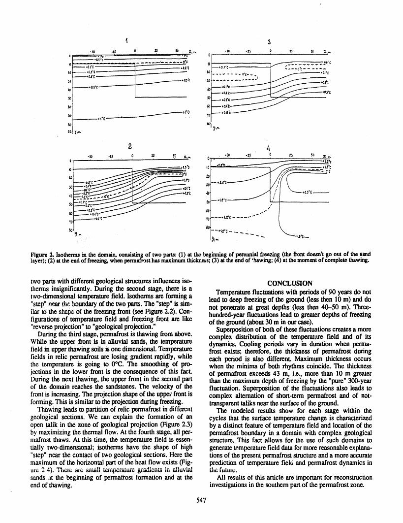
3

._ .15 0 _ _ ,r,_. -50 -_S 0 _ _O _.,_OF+_ , ' *t'c , * I _ "t'C_ 0 * * * " ' '

I+---- -+0.S*c .......... +..,..,..,..,..,.+.O'C 10 *0_'C

=t----" ,o.rc_ u __------.--++_°'c......

I 50'___._l,O_

10 , ,+<'c-- ' __'0,, T0--- ', aO

-_ .t_ 0 _ 50 _,,, -50 -2_ 0 tt_' 50 ¢, _,,,.0 , ,/ i , • 0 . ' ' ' ' ......

-----'--- O.CO 40 .... , _f= +_.S'C

_o + 'c _ ,:_/_';<,o,c-- -O..,+'C -- +2,o'0

---.--+o.l'c-_-_ / +0 / /

u .___- ,,,o,4,c_.-7-_'- .... <,_'c..... "" " L_'ro, __'¢_ 10

80

Figure2. Isothermsin thedomain,consistingof twopm: (1)at thebeginningof perennialfreezing(thefrontdoesn'tgooutof thesandlayer);(2) at theendoffreezing,whmpermafrosthasmaximumthickness;(3) at theendof "_hawing;(4)at themomentof completethawing.

two partswith differentgeological slrucmre.sinfluences iso- CONCLUSION

therms insignificantly. During the second stage, there is a Temperaturefluctuationswithperiods of 90 yearsdo nottwo-dimensional temperaturefield. Isotherms are forminga lead to deep freezing of the ground 0ess then 10 m) and do"step"ne_ the,boundaryof the two parts. The "step"is sim- not penetrate at great depths (less then 40-50 m). Th_-ilar to the sluice of the freezing front (see Figure 2.2). Con- hundred-yearfluctuations lead to greaterdepths of freezingfigurations of temperaturefield and freezing front are like of the ground(about30 m in our case)."reverse projection" to "geological projection." Superpositionof both of these fluctuationscreates a more

During the third stage,permafrostis thawing from above, complex distribution of the temperature field and of itsWhile the upper front is in alluvial sands, the temperature dynamics. Cooling periods vary in duration when perma-field in upper thawingsoils is one dimensional. Temperature frost exists; therefore, the thickness of permafrost duringfields in relic permafrost are losing gradient rapidly, while each period is also differenL Maximum thickness occm,sthe temperature is going to 0°C. The smoothing of pro- when the minima of both rhythms coincide. The thicknessjections in the lower front is the consequence of this facL of permafrost exceeds 43 m, i.e., more than 10 m greaterDuring the next thawing, the upper front in the second part than the maximum depth of freezing by the "pure" 300-yearof the domain reaches the sandstones. The velocity of the fluctuation. Superposition of the fluctuations also leads tofront is increasing. The projection shape of the uppea"front is complex alternation of short-term permafrost and of not-forming. This is similar to the projection during freezing, transparent taliks near the surface of the ground.

Thawing leads to partition of relic permafrost in different The modeled results show for each stage within thegeological sections. We can explain the formation of an cycles that the surface temperature change is chm'acterize.dopen talik in the zone of geological projection (Figure 2.3) by a distinct feature of temperature field and location of theby maximizing the thermal flow. At the fourth stage, ali per- permafrost boundary in a domain with complex geologicalmafrost thaws. At this time, the temperature field is essen- structure. This fact allows for the use of such do,,,_ainstotially two-dimensional; isotherms have the shape of high generate W.mperaturefield data for more reasonable explana-"step" near lhe contact of two geological sections. Here the tions of the present permafrost structure and a more accuratemaximum of the horizontal part of the heat flow exists (Fig- prediction of temperaturefiel6 and permafrost dynamics in

1 ULLIJI_._). m_ :_ttu_utJ W._.I_ULLU_ I_tiatal_ti_

sands +ltthe beginning of permafrost formation and at the Ali results of this article are important for reconstructionend of thawing, investigations in the southernpart of the permafrost zone.

547

REFERENCES

Balobaev,V. T., andA. V. Pavlov, Dinamikakriolitozonyv Meyermanov, A. M., Zadazha Stephana, 239 pp., Nauka,svyazi s izmeneniyami Idimat_ i antropogennym voz- Novosibirsk, 1986.deystviem, V knige: Problemy geokriologii, 184-194, Moiseenko, B. D., and A. A. Samarsky,EkonomizheskayaNauka, Moskva, 1983. schema skvoznogo szheta dlya mnogomernoy zadazhi

Kovalenko,V. D., L. D. Kizim, A. M. Pashestjuk,and V.G. Stephana, Zhunal vyzhisli.telnoy matematiky i mat-Nikolaev, Isslezlovanieprizhin izmenzhivosti klimata, V ematizheskoyfiziki, 5(5), 816-827, 1965.knige: Agroklimati.zheskie resursy Sibiri, 103-113, Izda- Rozanov, M. I,, Parametrygodizhnych kolez derevyev kaktelstvoVASCHNIL, Novosibirsk, 1987. informa-zionnaya osnova dolgosro_nogo prognozir-

Kudrjavzhev,V. A., Obshee merzlotovedenie, 463 pp., Izda- ovanya bioekologizheskich ressursov, V knige: Agrok-telstvoMGU, Moskva, 1978. limatizheskie ressursy Sibiri, 80-102, Izdatelstvo

Maximova, L. N., and V. Ye. Romanovsky, A hypothesis VASCHNIL,Novosibirsk, 1987.for the holocene permafrostevolution, 5th International Seregina,N. V., Nekotorye matematizheskiemodeli zadazhCoqference on Permafrost, ecfitedby K. Senneset, 2-5 geokri-ologii i metody ich zhislennogo reshenya, VAugust 1988, Trondheim,Norway,Vol. 1, pp. 102-106. km'ge: Geokriologizhes-kie issledovanya, 48-54, Izda-

Metody reshenya kraevych i obramych zadazh teplop- telstvoMGU, Moskva, 1989.rovodnosti (.podredakciey A. V. Uspenskogo), 262 pp., Zubakov, V. A., Globalnye klimatizheskie sobytya pleys-IzdatelstvoMGU, Moskva, 1975. tocena, 285 pp., Gidrometeoizdat,Leningr_, 1986.

Maximova, L. N., and V. Ye. Romanovsky, Kolebanyaklimata i nekotorye osobennosty razvitya nog-oletnemerzlychporod v golocene na territoriiSSSR, Geo-kriologizheskie issledovanya, 45-57, Izdatelstvo MGU,Moskva, 1985.

548

Microbiological Weathering of Silicates in Permafrost

T. P. Kolchugina and S. P. FedosovaDepartment of Geocryology, Faculty of Geology, Moscow State University, Moscow, U.S.S.R.

ABSTRACT

Microorganisms are known to degradate soils in temperate regions. Viablemicrobes have been found in permafrost-zone soils, and it is of interest to determineif these organisms can participate in silicate weathering in permafrost at low tem-peratures. The degradation of oligoclase and hornblende when exposed to psych-rophilic bacteria Aeromonas sp. at low and average temperatures was considered inthis study.

A sterile glycerine solution was added to sterilized soil samples to serve as asource of carbon for the bacteria and to prevent the transition of the liquid phase toa solid state. The degradation of the oligoclase at +20, +4, and -1.5°C was exam-ined after 109 days of incubation; the degradation of the hornblende at +20, +4, and-8°C was examined after 360 days.

The bacteria grew in all variants_except the sterile controls. The bacterial num-ber at +20°C was 50 times more than in other non-sterile variants. The bacteria pro-rooted the release of Ca and Na from the oligoclase and did not promote the releaseof Si from this mineral. The content of the Ca in the media exceeded the content ofother elements.

Microbiological weathering of silicates in permafrost is possible even at tem-peratures below zero, if carbon and a liquid phase are present; moreover, the levelsof mineral transformation are comparable with the levels of transformation at mod-erate temperatures.

INTRODUCTION EXPERIMENTAL APPROACH

Microorganisms are known to be capable of degradating Mineral samples were placed in glass vessels and ster-soils in temperate regions [Aristovskayia, 1980]. Because ilized. After the samples were sterilized, 50 ml of a sterileviable microbes have been found in permafrost-zone soils, it glycerine solution was added to each vessel. The glycerineis of interest to determine if these organisms can participate served as the source of carbon for the growing bacteria andin silicate weathering in permafrost at low temperatures, prevented the transition of the liquid phase to a solid state.The results of this study may be of interest not only to soil The degradation of the oligoclase at +20, +4, and -1.5°Cmicrobiologists, but also to specialists in other areas, for was examined after 109 days of incubation; the degradationexample, civil engineering, of the hornblende at +20, +4, and -8°C was examined after

360 days. The experiments were conducted under static con-OBJECTIVES ditions without changing the fluid growth media.

The objective of the study reported herein is to estimate The number of bacteria on the solid starch-ammoniathe level of microbiological weathering of silicates at low medium were counted after incubation. Also, the pH of theand average temperatures. Specifically, the degradation of media was determined. The mineral particles from the fluidoligoclase and hornblende when exposed to psychrophilic phase were separated by filtration through filter paper andbacteria Aeromonas sp. was considered. The bacteria pre- the media was analyzed. The Si, Ca, and Na contents in theviously were isolated from the Kolym lowland permafrost, media in the oligoclase were measured, and the Fe, Ca, and

__ 549

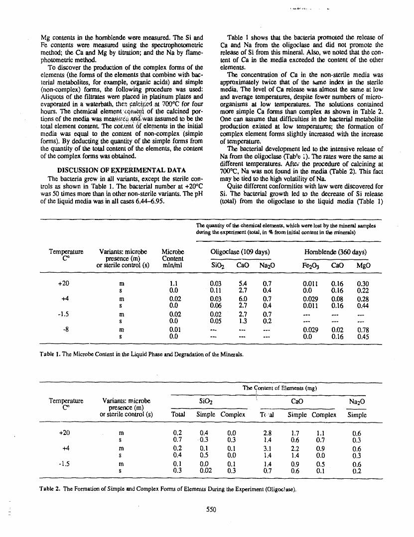
Mg contents in the hornblende were measured. The Si and Table I shows that the bacteriapromoted the release ofPe contents were measured using the spectrophotometric Ca and Na from the oligoclase and did not promote themethod; the Ca and Mg by titration;and the Na by flame- releaseof Si ,fromthis mineral. Also, we noW.xithat the con-photometric method, tent of Ca in the media exceeded the content of the other

To discover the production of the complex forms of the elements.elements (the forms of the elements that combine with bac- The concentration of Ca in the non-sterile media wasterial metabolites, for example, organic acids) and simple approximately twice that of the sdme index in the sterile(non-complex) forms, the following procedure was used: media. The level of Ca release was almost the same at lowAliquots of the filtrates were placed in platinumplates and and average temperatures,despite fewer numbers of micro-evaporated in a waterbath, t,_e.__ale.ii_e4at 709°C for four organisms at low temperatures. The solutions containedhours. The chemical element ct_f(f of the calcined per- more simple Ca forms than complex as shown in Table 2.tions of the media was m_s_S,r_:_!_ii!wasassumedto be,the One can assume that difficulties in the bacterial metabolitetotal element eontenLThe coi',_nt _tfe!e_nentsin the inttial production existed at low temperatures; the formation ofmedia was equal to the content of non-complex (simple complex element forms slightly increased with the increaseforms). By deducting the quantity of the simple forms from of temperature,the quantity of the total content of the elements, the content The bacterial development led to the intensive release ofof the complex forms was obtained. Na from the oligoclase ('rab!e _,).The rates were the same at

different temperatures. AfteJ"the procedure of calcining atDISCUSSION OF EXPERIMENTAL DATA 700°C, Na was not found in the media (Table 2). This fact

The bacteria grew in ali variants, except the sterile con- may be tied to the high volatility of Na.trois as shown in Table 1. The bacterial number at +20°C Quite different conformities with law were discovered forwas 50 times more than inother non.sterile variants. The pH Si. The bacterial growth led to the decrease of Si releaseof the liquid media was in ali cases 6.44--6.95. (total) from the oligoclase to the liquid media (Table 1)

The qtum_ty of tl_ chemical elements, which were lost by the mineral _rnplesduring the cxperirncn_(total, in % from initial oontent in the minerals)

Temperature Variants: microbe Microbe Oligoclase (109 days) Hornblende (360 days)C° presence (m) Content

or sterile control (s) mln/ml Si02 CaO Na20 Fe203 CaO MgO

+20 m 1.1 0.03 5.4 0.7 0.011 0.16 0.30s 0.0 0.11 2.7 0.4 0.0 0.16 0.22

+4 m 0,02 0.03 6.0 0.7 0.029 0.08 0.28s 0,0 0.06 2.7 0.4 0.011 0.16 0.44

-1.5 m 0.02 0,02 2,7 0.7 .........s 0.0 0.05 1.3 0.2 .........

-8 m 0.01 ......... 0.029 0.02 0.78s 0.0 ......... 0.0 0.16 0.45

Table 1.The MicrobeContentin theLiquidPhasemadDegradationof theMinerals.

The _trntent of P.,lcments (rag)

Temperature Variants: microbe SIC)2 CaO Na20C° presence (m)

or sterile control (s) Total Simple Complex Tc,al Simple Complex Simple

+20 m 0.2 0.4 0.0 2.8 1.7 1.1 0.6s 0.7 r0.3 0.3 1.4 0.6 0.7 0.3

+4 m 0.2 0.1 0.1 3.1 2.2 0.9 0.6S 0.4 0.5 0.0 1.4 1.4 0.0 0.3

-1.5 m 0.1 0.0 0.1 1.4 0.9 0.5 0.6s 0.3 0.02 0.3 0.7 0.6 0.1 0.2

Table 2. The Formation of Simple mad Complex Forms of Elements During the Experiment (Oligoc!ase).

=

550

independentof the temperature. In sterile controls, the Si may suppose that the decrease of temperature is followed bycontent was approximately 2-3 times that in the bacterial the mitigation of bacterial metabolite production.variants. An evident dependence between the formation ofdifferent Si forms, the number of bacteria, and the tem- SUMMARY AND CONCLUSIONperature does not appear in the data collected (Table 2). Microbiological weathering of silicates in permafrost is

The bacteriological weathering of the hornblende differed possible even at temperatures below zero, if carbon and afrom that of the oligoclase. The microorganisms did not pro- liquid phase are present; moreover, the levels of mineralmote the release of Ca and Mg from the hornblende to the transformation are comparable with the levels of trans.growth media (Table 1). At the same time, the Ca content in formation at temperate temperatures.the liquid phase was several times less than in the oligoclasevariants. The bacteria influenced the transitionof Fe from ACKNOWLEDGMENTSthe hornblende to the media at ali temperatures considered The bacteria were previously isolated by our colleaguesin the study. A. Siminova, V, Soina and E. Vorobiova, Soil Science

The levels of the bacterial degradation of these minerals Faculty, Moscow State University.were almost the same at low and average temperatures. The The elemental analyses were performed in the Geologicalcharacter of microbiological weathering was different: while Faculty chemical laboratory by M. Yukina, S. Lebedenko,microorganisms promote the release of Ca in the case of L. Semko and V. Kulbery.oligoclase, they don't influence the transition of this elementfrom the hornblende to the media. The hornblende was more REFERENCEresistant to the microbiological weathering (as well as to the Aristovskayia, T. V., Microorganisms as the component ofsterile degradation) compared with the oligoclase. Also, one biogeocenosis, p. 187, Nauka, Moscow, 1980.

551

Anthropogenic Structures in the Geosystems (Landscapes) of the Permafrost Zone

V. P. Antonov.DruzhininLaboratoryof the GeotechnicalSystemsof the ColdRegions,MonitoringTrust,Novy Urengoy,U.S.S.R.

ABSTRACT

Problems created by oil and gas field development in Arctic regions attract muchattention in the discussion of the interaction of civil and industrial buildings andstructures with permafrost.

The investigations carried out must permit the evaluation of changes in the nat-ural environment and single out the anthropogenic component of these changes,must ensure accident-free operation of oil and gas transport units, safety of peopleand environmental control in the mineral resource production regions of the Arctic.

Taking the "pipeline-environment" system example, this report characterizes thespatial-temporal structure of the gas transport geotechnical system as a natural-anthropogenic, physico-geographical object.

The natural subsystem of this object consists of several structures (referred to asareas and zones). These structures are characterized by different dynamics of regen-eration processes of anthropogenic disturbances. It is found that the most negativeecological consequences during the development of the regions at the boundary oftundra and forest-tundra are associated with the disturbances of pre-tundra forests.

The least perceptible ecological changes are typical for anthropogenic trans-formation of bog geo-systems. The anthropogenic structures, which are formedhere, are characterized by a state most similar to the initial conditions and, often, byan increase of biomass in the landscapes.

All these data are presented according to the author's investigations in the perma-frost zone of Western Siberia.

,/552

i1[ ,

Engineering.Geological Monitoring Within the Soviet Global Change Program(the Northern Regions of Western Siberia)

G. I. PushkoTrustof Engineering-GeologicalMonitoring,Novy Urengoy,U.S.S.R.

ABSTRACT

For the purpose of investigation and control of the changes in the natural envi-ronment of the northern regions of Western Siberia, a special service of engi-neering-geological monitoring (IGM) was created within the system of the USSRState Gas Concern.

The engineering-geological monitoring of geotechnical systems involves track-ing, evaluation, analysis and prediction of ongoing changes in their geologic envi-ronment and their negative after-effects for interacting technospher_ objects. Also,scientific and engineering substantiation of preventive and restorative measures andother management decisions as well as technological provisions for their realizationare included.

In addition to observing the state of the geologic environment (settling and dis-placement of buildings, structures and commumcations, causes of deformation andforecasting their further development) the main tasks of this service are the elabora-tion of scientifically grounded recommendations and design concepts for pre-

venfion and elimination, recultivation of damaged landscapes, development ofrepair and restoration work technology and participation in performing responsibleoperations. Most important of the latter are stabilization of damaged soil bases, con-solidation of deformed foundations, curing and recultivation of damaged and pol-luted areas of the geologic environment, recovery of water-intake wells andindustrial effluent-disposal wells.

The leading establishment of this service is the Trust of Engineering-GeologicalMonitoring and Research (TIGMI) in Novy Urengoy. TIGMI maintains close con-tacts with the USSR National Global Change Committee through the GeophysicalCommittee of the USSR Academy of Sciences. The Trust activities are presented inthe f'trst part of the Global Change Data Bank Catalogue.

553-, ,_

i

Section F:

Paleoenvironmental Studies

Chaired by

D. ElliotOhio StateUniversity

U.S.A.

C. LorimLaboratoircdeGlaciologicctGdophysiquc

dcl'EnvironncmentFrance

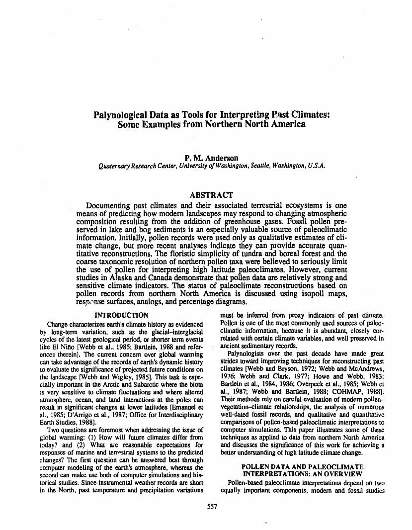
Palynological Data as Tools for Interpreting Past Climates:Some Examples from Northern North America

P. M. AndersonQuaternary Research Center, University of Washington, Seattle, Washington, U,S.A.

ABSTRACT

Documenting past climates and their associated terrestrial ecosystems is onemeans of predicting how modern landscapes may respond to changing atmosphericcomposition resulting from the addition of greenhouse gases, Fossil pollen pre-served in lake and bog sediments is an especially valuable source of paleoclimaticinformation. Initially, pollen records were used only as qualitativ e estimates of cli-mate change, but more recent analyses indicate they can provide accurate quan-titative reconstructions. The floristic simplicity of tundra and boreal forest and thecoarse taxonomic resolution of northern pollen taxa were believed to seriously limitthe use of pollen for interpreting high latitude paleoclimates. However, currentstudies in Alaska and Canada demonstrate that pollen data are relatively strong andsensitive climate indicators. The status of paleoclimate reconstructions based onpollen records from northern North America is discussed using isopoll maps,res p,_nse surfaces, analogs, and percentage diagrams.

INTRODUCTION must be inferredfrom proxy indicators of past climate.Change characterizesearth'sclimate historyas evidenced Pollen is one of the most commonly used sources of paleo.

by long-term variation, such as the glacial-interglacial climatic information, because it is abundant, closely eor-cycles of the latest geological period, or shorterterm events relatedwith certainclimate variables,and well preservedinlike E1 Nifio [Webb et al., 1985; Bartlein, 1988 and refer- ancientsedimentaryrecords.ences therein]. The current concern over global warming Palynologists over the past decade have made greatcan takeadvantage of the recordsof earth'sdynamic history stridestoward improving techniques for reconstructingpastto evaluatethe significa_.e of projected futureconditionson climates [Webb and Bryson, 1972; Webb and McAndrews,the landscape [Webb and Wigley, 1985]. This task is espe- 1976; Webb and Clark, 1977; Howe and Webb, 1983;ciaUy important in the Arctic and Subarctic where the biota Bartlein et al,, 1984, 1986; Ov_k ct al., !985; Webb etis very sensitive to climate fluctuations and where altered al., 1987; Webb and Bartlein, 1988; COHMAP, 1988].atmosphere, ocean, and land interactionsat the poles can Their methods rely on carefulevaluation of modem pollen-result in significant changes at lower latitudes IEmanuel et vegetation--climaterelationships, the analysis of numerousal., 1985; D'Arrigo et al., 1987; Office for Interdisciplinary weft-dated fossil records, and qualitative and quantitativeEarth Studies, 1988]. comparisons of pollen.based paleoclimatic interpretations to

Two questions are foremost when addressing the issue of computer simulations. This paper illustrates some of theseglobal warming: (1) How will future climates differ from techniques as applied to data from northern North Americatoday7 and (2) What axe reasonable expectations for and discusses the significance of this work for achieving aresponses of marine and terrestrial systems to the predicted better understanding of high latitude climate change.changes? The ta'st question can be answered best throughcomputer modeling of the earth'satmosphere, whereas the POLLEN DATA AND PALEOCLIMATEsecond can make use both of computer simulationsand his- INTERPRETATIONS: AN OVERVIEWtorical studies. Since instrumental weather records are short Pollen-based paleoclimate interpretations depend on twoin the North, past temperature and precipitation variations equally important components, modern and fossil studies

557

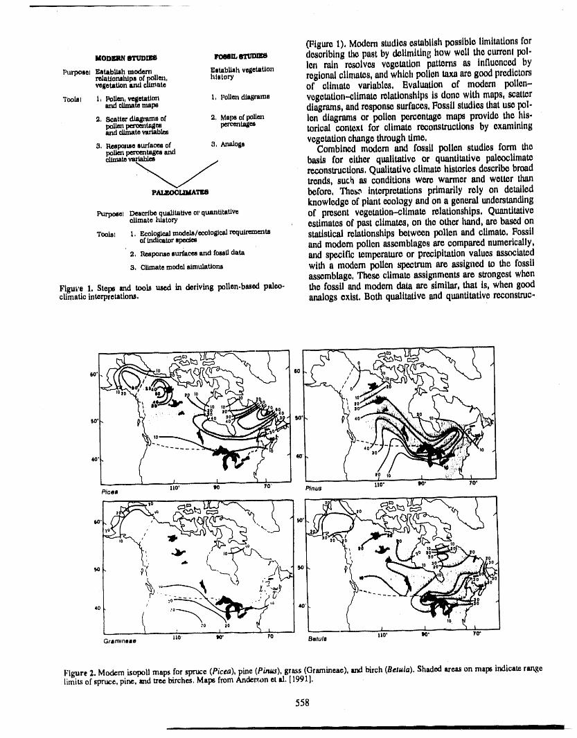
_IguroI),ModernstudiesestablishpossiblelimitationsforMontmsmammt_ mm xtrutru desoriblng the past by d_limtting how well the currentpol-

ptn-potmtIratabliahmodem Eatab_hve_tion len rain resolves vegetation patmrns as influenced byr_uommps pf_tt_, history regionalclimates, and which pollen taxn aregood predictorsvetiemtionandoumate of climate variables, Evaluation of modem poUen-

•rootmtt,_tlm,vegemuon t,pouchdUmmmB vegetation.--climaterolationshlpsisdonewithmaps,scattermxl_a_ mm diagrams,andresponsesurfaces,Fossilstudiesthatusepol.

2, Scatterdta8_ of 2, Marsofpetten len diagrams or pollen percentage maps provide the his-tx_.._._n_, pe_nt,_ toflcal context for climate reconstructions by examiningkndcit/hatevsrm._

_, _,_e ,,urfac_of a, maioSs vegetation change through time,_ttmt_nt_estmo Combinedmodem and fossilpollenstudiesformthecumamvam_m basis for either qualitative or quantitative paleocllmate

reconstructions,Qualitative climate histories describe broadtrends, such as conditions were wanner and wetter thaneat,toc_'nm before,Thes.'_interpretationsprimarilyrelyon detailed

knowledgeofplantecologyandona generalunderstandingPurpmet De_mibe.qualltatiwot'quantRatlw of present vegetation--climam relationships, Quantitative

oamatetmtory estimates of past climates, on the other lured, are based onTools2 1, _,ologkml models/ecological req_tmta statistical relationships between pollen and climate, Fossil

ofindicatoralmCi_s andmodem pollenassemblagesarecomparednumerically,2, R_pome.ur_. andlo.ii data and specific temperatureor precipitationvalues associateda, cttmatemode.imulaUom with a modem pollen spectrum are assigned to the fossil

assemblage, These climate assignments are strongestwhen

Figure 1, Steps _d tools used in derivingpollen.basedpaleo- the fossil and modern data arc similar, that is, when goodclimatictnt.rpretatlom, analogs exist, Both qualitative and quantitative rcconstruc-

. __ --, _ ...... _ _ ....... _,,,_ )

,o. o.. .,,. g

_ i l i t _ lte' _o' 1o'110' tO 70' /:_/1U$Ptoea

' 10' " {::3 "

tto

_.,,,,n... _io m" ,o s._ut, t,o' _' '_

Figure2, Modemisopollmaps forspruce(Picea),plne(P/naa),grass(Gramineae),andbirch(Betula).Shadedareason mapsindicaterangelimitsof spruce,pine, andu'e.¢birches,MapsfromAndre.oneaal. [1991],

558

IIl'l

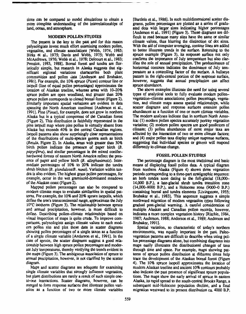
ttons can be compared to model simulations to obtain a [Bartleinet al,, 1986], In such multidimensionalscatterdla.more complete understandingof the interrelationshipsof grams, pollen percentages are plotted as a series of gradu.land,ocean, andatmosphere, ated dots with larger sizes indicating higher percentages

[Andersonet al,, 1991] (Figure 3). These diagramsare dif.MODERN POLLEN STUDIES flcult to read because many sites have the same o1'similar

The present is the key to the past and for this reason climate values, thus blurting the distinction of dot sizes.palynologists invest much effortexamining modernpollen, With the aid of computer averaging,contour lines areaddedvegetation, and climate associations [Webb, 1974, 1985; to better illustrate trends in the surface, Returningto theBirks et al,, 1975; Davis and Webb, 1975; Webb and spruce example (Figure 3), its response surface not onlyMcAndrews, 1976; Webb et al,, 1978; Delcourt etal,, 1983; confirms the importance of July temperature but also olaf.Prentice, 1983, 1988], Boreal forest and tundraare tier. ifles the role of annual precipitation,The predominanceofisttcally simple, but research in Alaska suggests that sig. horizontal contours indicates the dominance of July tem-niflcant regional variationscharacterizeboth plant peratm'e as a controlling factor of the surface, A bullseyecommunities and pollen data [Anderson and Brubaker, pattern in rite fight-central portion of the response surface,1986], For example, the 10%spruce (Ptcea) contour line or however, suggests that annual precipitation can affectisopoll (line of equal pollen percentages) approximatesthe spruce abundance,location of Alaskan treeline, whereas areas with 10-20% The above examples illustrate the need for using severalspruce pollen are open woodland, and greater than 20% types of analytical tools to fully evaluate modern pollen-sprucepollen correspondsto closed boreal forest (Figure 2), vegetation-climate associations; pollen percentage, vegeta.Similarly important spatial variations are evident in data tton, and climate maps assess spatial relationships, whilespanning the North American continent [Anderson et al,, scatter diagrams and response surfaces examine pollen1991], Pine (Ptnus), for example, does not grow in northern abundancesas a function of one or more climate variables,Alaska but is a typical component of the Canadian forest The modem analyses indicate that in northernNorth Amer.(Figure 2), This distributionts faithfully represented in the iea: (1) modernpollen spectra accurately portray vegetationpine isopoll map where pine pollen is virtuallyabsent from variation;(2) modern pollen spectraare good predictorsofAlaska but exceeds 40% in the central Canadian regions, climate; (3) pollen abundances of most major taxa areIsopoll patterns also show surprisinglyclear representations affected by the interaction of two or more climate factors;of the distributions of multi.species genera such as birch and (4) majorpollen taxa display unique response surfaces,(Betula, Figure 2), In Alaska, areas with greater tiara30% suggesting that individual species or gealerawill respondbirch pollen indicate the presence of paper birch (B. differently to climatechange.papyr_fera), and similar percentages in the mixed conifer-hardwoodforests of easternNorth America reflect the pres- FOSSIL POLLEN STUDIESence of paperand yellow birch (B. alleghaniensls), Inter. The percentage diagram is lhc most traditionaland basicmediate percentages of 10% to 20% indicate the tundra means of displaying fossil pollen data. A typical diagramshrub birches (B. 81andulosa/B.nana). Variationwithin tun. from northern Alaska (Figure 4) shows three vegetationdta is also evident, The highest grass pollen percentages, for periods correspondingto a three.partstratigraphicsequence:example, occur in the wet graminoid.dominatedmeadows an herb tundra zone dating to the full.glacial (18,000-of the Alaskancoast (Figure 2). 14,000 BY.), a late.glacial shrub tundra transition zone

Mapped pollen percentages can also be compared to (14,000-9000 B.P,), and a Holocene zone (9(X)O-0B.P.)modem climate maps to evaluate similarities in spatial pat. containing boreal and tundraelements [Livingstone, 1955;terns. For example, the 10% and 20% spruceisopolls, which Brubaker et al., 1983], This sequence suggests a simpledefine the tree'stranscontinentalrange,approximatethe July northward migration of modern vegetation types following10°C isotherm (Figure 3). The relationship between spruce gradual post-glacial warming. A careful considerationofand annual precipitation, however, is more difficult to multiple Alaskan and Canadian pollen records, however,del'me. Describing pollen-climate relationships based on indicates a more complex vegetation history [Ritchie, 1984,visual inspection of maps is quite crude. To improve com- 1987; Anderson, 1988; Andersonet al., 1989; Anderson andparisons, palynologists assign climate values to each mod. Brubaker, 1991].ern pollen site and plot these data in scatter diagrams Spatialvariation,so characteristic of today's northernshowing pollen percentages of a single taxon as a function environments, was equally important in the past. Pale.o.of a single climate variable [Anderson et al., 1991]. In the vegetation patternsare difficult to describe when using 13oi-case of spruce, the scatter diagrams suggest a good vela- len percentage diagramsalone, butcombining diagrams intotionshipbetween highsprucepollen percentages and moder- maps easily illustrates the distributional changes of taxaatc Julytemperatures,thereby verifying the tren_ evident in through time and space. For example, maps showing pat-the maps (Figure 3). The ambiguousassociation of spruce to terns of spruce pollen distribution at different times helpanmml precipitation,however, Lsnot clarified by the scatter trace the development of the Alaskan boreal forest (Figurediagram. 4). The 10% spruce isopoll approximates the locatic,n of

Maps and scatter diagrams are adequate for examining modernAlaskan treelineand ancient 10%contoursprobablysingle climate variables that strongly influence vegetation, also indicate the past presenceof significant spruce popula.but plant distributionsarerarelya result of such simple one. tions. The maps show the early arrival of spruce in easternto-one interactions. Scatter diagrams, however, can be Alaska, its rapidspreadto the south-centralBrooks Range, amerged to form response surfaces that illustratepollen vari- subsequent mid-Holocene population decline, and a finalation as a function of two or more climate variables migration westward to its present distribution ca. 4000 B.P.

559

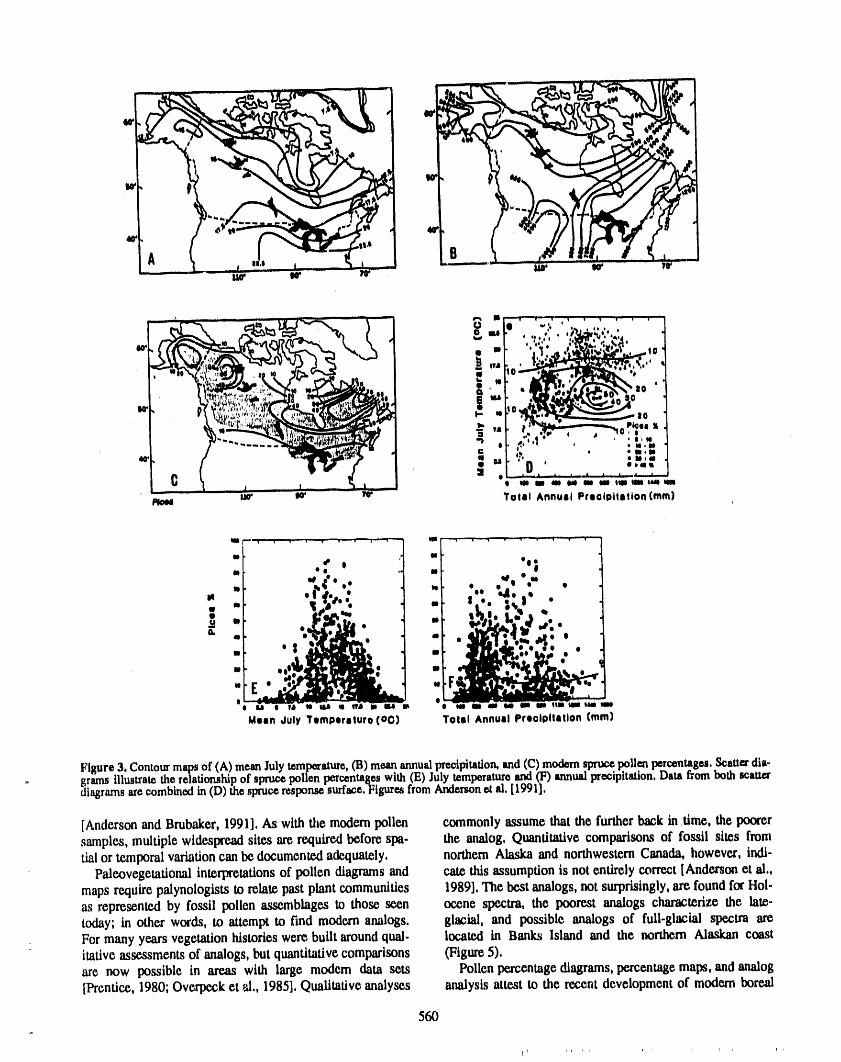
Ii '

Total Annual Praotpitation(mm)

Figure 3, Contourmapsof (A)meanJulytemperature,(Ii) me,an annualprecipitation,and(C)modemsprucepoUml_rCenmSeS,ScaUezdia-gramsillustratetherelationshipof sprucepollenperc_ntag?with.(E)Julytempera._,eand_F)annualprecipitation,Datat_ombothscau_rdiagramsarecombinedin (D) the spruceresponsesurface,lqguresfromAnaersone_m,tl_"JlJ.

[AndersonandBrubaker,1991],Aswithdiemodempollen commonlyassumethatthefurtherbackintime,thepoo_rsamplcs,multiplewidespreadsitesarcre.,quircdbeforespa- theanalog,Quantitativecomparisonsoffossilsimsfronttialortemporalvariationcanbcdocumentedadcquatcly, northernAlaskaandnorthwesternCanada,however,indl-Palcovegetationalinterpretationsofpollendiagramsand carethisassumptionisnotentirelycorrect[Andersonctal,,

mapsrequirepalynologiststorelatepastplantcommunities 1989].Thebe,stanalogs,notsurprisingly,arcfoundforHol-asrepresentedby fossilpollenasscmblagcstothoscsccn occnespectra,thepoorestanalogscharacterizethelate-today;inotherwords,toattempttofindmodernanalogs, glacial,and possibleanalogsof full-glacialspectraarcFormany yearsvegetationhistorieswere,builtaroundqual- locatedin BanksIslandand thenorthernAlaskancoastitativcassessmentsofanalogs,butquantitativecomparisons (Figurc5).arcnow possibleinareaswithlargemodem datasets Pollcnpercentagediagrams,percentagemaps,andanalog[Prentice,1980;Ovcrpcckct_.,1985].Qualitativcanalyses analysisattesttothercccntdcvclopmcntofmodem bore.al

56O

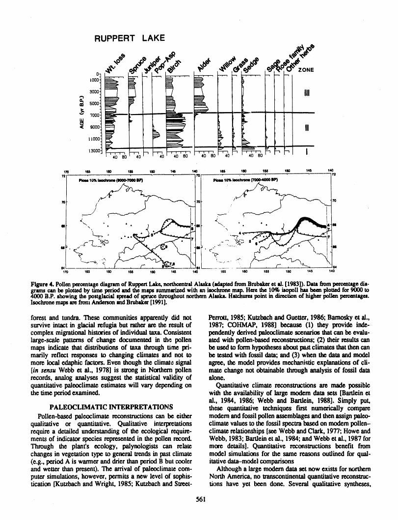
170 165 100 lg4 1ilo 148 140 165 180 lM I10 146 140

/I

170 _65 180 155 1W 145 140 165 160 tSS 150 145 140

Figure 4. Poll_ peroentagediagramof RuppertLake,northoentrslAlaska (adaptedfromBn=bakeret al. [1983]). Dm from percentagedia-grams can be plotted by time periodand the maps summarizedwith an isochnme map. Here the 10% impoll has been plottedfor 9000 to4000 B.P. showing the postglacial spreadof =pnr.e throughoutnorthernAlaska. Hatohurespoint in direction of higher pollen laar.erttages.Isochronemaps arefrmtiAndersonand Brubaker [1991].

forest and tundra. These communities apparently did not Perrott, 1985; Kutzbach and Guetter, 1986; Bamosky et al.,survive intact in glacial refugia but rather are the result of 1987; COHMAP, 1988] because (1) they provide inde-,complex migrational histories of individual taxa. Consistent pendently derived paleoclimate scenarios that can be evalu-large-scale patterns of change documented in _ pollen ated with pollen-based reconstructions; (2) their results canmaps indicate that distributions of taxa through time Iri- be used to form hypotheses about past climates that then canmarily reflect responses to changing climates and not to be tested with fossil data; and (3) when the data and modelmore local edaphic factors. Even though the climate signal agree, the model provides mechanistic explanations of cii-[in se_u Webb et al., 1978] is strong in Northern pollen mate change not obtainable through analysis of fossil datarecords, analog analyses suggest the statistical validity of alone.quantitative paleoclimate estimates will vary depending on Quantitative climate reconstructions are made possiblethe time period examined, with the availability of large modem data sets [Bartlein et

al., 1984, 1986; Webb and Bartl=in, 1988]. Simply put,PALEOCLIMATIC INTERPRETATIONS these quantitative techniques first numerically compare

Pollen-based paleoclimate reconstructions can be either modem and fossil pollen assemblages and then assign paleo-qualitative or quantitative. Qualitative interpretations climate values to the fossil spectra based on modem pollen-require a detailed understanding of the ecological require- climate relationships [see Webb and Clark, 1977; Howe andments of indicator species represented in the pollen record. Webb, 1983; Bartlein et al., 1984; and Webb et al., 1987 forThrough the plant's ecology, palynologists can relate more details]. Quantitative reconstructions benefit fromchanges in vegetation type to general treads in past climate model simulations for the same reasons outlined for qual-(e.g., period A is wanner and drier than periodB but cooler itative data-model comparisonsand wetter than present). The arrival of paleoclimate com- Although a large modern data set now exists for northernpurer simulations, however, permits a new level of sophis- North America, no transcontinental quantitative reconstruc-tication [Kutzbach and Wright, 1985; Kutzbach and Street- tions have yel been done. Several qualitative syntheses,

561

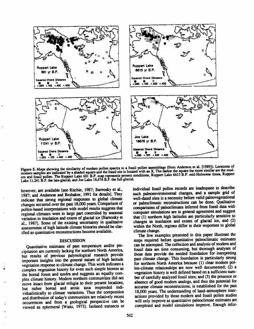
/ Rupp_Lake '_, ' | RuppertIJike '_,

. o1 '=, ....-,........, "" :........-"

, 11241yr6.P. _ _ ;8676yTB.P. _

.... .....

modemsamples_e _-_dJcatedbyashadedsquareandthe;ossus,_ tsJoc_ wtmanA. in©(_rx=m©_um©,,_ernendfossilpollen.TheR_ Lake681B.P.m_aprej_re_mtspreset,t renditions,RuppertLake6615B.P.mid-Holocenetimes,Ruppe_Lake11,241B.P.thelate-glactal,andJoeLakelt;,b_/Otr.t,,menm-gtac_at.

however, are available [see Ritchie, 1987; Barnoskyet al., individual fossil pollen records are inadequateto describe1987; and Anderson and Brubaker,1991 for details]. They such paleoenvironmental changes, and a sample grid ofindicate that strong regional responses to global climate well-dated sites i_ a necessitybefore valid paleovegetationalchanges occurredover thepast 18,000 years. Comparisonof or paleoclimatic reconstructionscan be done. Qualitativepollen-basedinterpretationswith model results suggeststhat comparisonsof l_deoclimates inferredfrom fossil &ttawithregional climates were in large pan controlledby seasonal computer simulationsare in general agreementand suggestvariationin insolationand extent of glacial ice [Barnoskyet that (1) northernhigh latitudes are particulaHysensitive toal., 1987]. Some of the existing uncertaintyin qualitative changes in insolation and extent of glacial ice, and (2)assessments of high latitudeclimatehistoriesshouldbe clar- within the North, regions differ in their responses to globalified as quantitativereconstructionsbecome available, climate change.

The few examples presented in this paper illustratetheDISCUSSION steps required before quantitative paleoclimatic estimates

Quantitative estimates of past temperatureand/or pre- can be attempted. The collection andanalysis of modernandcipitation are currendylacking for northernNorth America, fossil data are time consuming, but thorough analyses ofbut results of previous palynological research provide these data provide the needed foundation for interi_tingimportant insights into the general nature of high latitude past climate change. This foundation is particularlystrongvegetation response to climate change. This workindicates a for northern North America because (1) clear modern pol-complex vegetation historyfor even such simple biomes as Ion-climate relationships are now well documented; (2) athe boreal forest and tundraand suggests an equally com- vegetation h_storyis well definedbased on a sufficient num-plex climate history. Modernnortherncommunities did not ber of carefullyanalyzed fossil sites; and (3) the presenceormove intact from glacial refugia to their present locations, absence of good modernanalogs, and thus the potential forbut rather boreal and arctic taxa responded indi- accurate climate reconstructions,is established for the pastvidualistically to climate variations.Thus the composition 18,000 years. The understandingof land-atmosphere inter-and distributionof today'scommunities arerelatively recent actions provided by these modern and fossil pollen studiesoccurrences and from a geological perspective can be will only improve as quantitativepaleoclimate estimatesare

" viewed as ephemeral [Watts, 1973]. Isolated transects or completed and model simulations improve. Enough infor-

562

marion, however, is available to suggest that the lessons Ritchie, who have been invaluable colleagues in exploringfrom thepast should be kept in mindwhen planningfor the the late Quaternary history of northern North America.future. Researchpresented in this paperwas supportedby the fol-

lowing grants:National Science FoundationDPP8106806_ACKNOWLEDGMENTS DPP8403598 and DPP8619214 to Andersonand Brubaker

This paper has benefited from numerousdiscussions with and ATM8713980 to Bartlein; NSERC grants to GajewskiPat Bartlein, Linch Bmhaker, Konrad Gajewski, and Jim and Ritchie.

REFERENCES

Anderson, P. M., Late Quaternarypolleo records from the Delcourt,H. R., P. A. Delcourt' and T. Webb, IH, DynamicKobuk and Noatak Riverdrainages, northwestern Alaska, plant ecology: the spectrum of vegetational change inQuat. Res., 29, 263-276, 1988. space and time, Quat. Sci. Rev., 1,153-175, 1983.

Anderson,P. M., and L. B. Brubaker,Modern pollen assem- Emanuel, W. R., H. H. Shugart' and M. P. Stevenson, Cii-binges from northern Alaska, Rev. Palaeobot. Palynol., matic change and the broad-scale distribution of ter-46,273-291, 1986. restrialecosystem complexes, Climate Change, 7, 29-43,

Anderson, P. M., and L. B. Brubaker,Vegetation history 1985.and the development of boreal forest in northcentral Howe, S., and T. Webb, III, Calibratingpollen data in cii-Alaska: a mapped summary of late-Quatenuu3,pollen matic terms: improving the methods, Quat. Sci. Rev., 2,data,Ecological Monographs, 1991, Inreview. 17-51, 1983.

Anderson, P. M., P. J. Bartlein, L. B. Brubaker, K. Kutzbach,J. E., andP. J. Guetter,The influence of changingGajewski, and J. C. Ritchie, Modem analogues of late- orbital parameters and surface boundary conditions onQuaternary pollen spectra from the western interior of climate simulations for the past 18,000 years, J. Atmos.North America, J. 8iogeogr., 16, 573-596, 1989. Sci., 43, 1726-1759, 1986.

Anderson, P. M., P. J. Bartlein, L. B. Brubaker, K. Kutzbach,J. E., and F. A. Street-Perrott,Milankovitch forc-Gajewaki, and J. C. Ritchie, Vegetation-pollen-climate ing of fluctuations in the level of tropicallakes from 18 torelationshipsfor the Arcto-Borealregion of North Amer- 0 kyr BP,Nature, 317, 130-134, 1985.ica and Greenland,I. Biogeogr., 1991, In press. Kutzbach,J. E., and H. E. Wright, Jr., Simulation of the cli-

Bamosky, C. W., P. M. Anderson, and P. J. Bartlein, The mateof 18,000 YearsBl':.results for theNorth American/northwestern U.S. duringdeglaciation; vegetational his- North Atlantic/Europeansector and comparison with thetory and paleoclimatic implications, in North America geologic record of North America, Quat. Sci. Rev., 4,and Adjacent Oceans during the Last Deglaciation, 147-187, 1985.edited by W. F. Ruddimanand H. E. Wright, Jr.,pp. 289- Livingstone,D. A., Some pollen profiles fromarctic Alaska,322, Geological Society of America, 1987. Ecology, 36, 587-600, 1955.

Bartlein, P. L, Late-Tertiary and Quaternary paleo- Office for Interdisciplinary Earth Studies, Arctic Inter-environments, in Vegetation History, edited by B. actions RecommendationsforanArcticComponentintheHuntley and T. Webb, III, pp. 113-152, Kluwer Aca- International Geosphere-Biosphere Programme, 41 pp.,demic Publishers, 1988. UCAR, Boulder,CO, 1988.

Bartlein,P. J., T. Webb, III, and E. Fleri, Holocene climatic Overpeck, J. T., T. Webb, III, and I. C. Prentice, Quan-change in the northern Midwest: pollen-derived esti- titative interpretation of fossil pollen spectra: dis-mates, Quat. Res., 22,361-374, 1984. similaritycoefficients and the method of modem analogs,

Bartlein, P. 3., I. C. Prentice, and T. Webb, III, Climatic Quat. Res., 23, 87.-108, 1985.response surfaces from pollen data for some eastern Prentice, I. C., Multidimensional scaling as a research toolNorthAmerican taxa,J.Biogeogr.,13,35--57, 1986. in Quaternary palynology: a review of theory and

Birks, H. J. B., T. Webb, III, and A. A. Berti, Numerical method,Rev. Palaeobot. Palynol., 31, 71-104, 1980.analysis of pollen samples from central Canada:a com- Prentice, I. C., Postglacial climatic change: vegetationparison of methods, Rev. Palaeobot. Palynol., 20, 133-- dynamics and the pollen record,Progr. Phys. Geogr., 17,169, 1975. 273-286, 1983.

Brubaker, L. B., H. L. Garfinkel,and M. E. Edwards, A Prentice, I. C., Records ofvegetation in time and space: thelate-Wisconsin and Holocene vegetationhistory from the principles of pollen analysis, in Vegetation History,central Brooks Range: implications for Alaskan paleo- edited by B. Huntley and T. Webb, III, pp. 17-42,ecology, Quat. Res., 20, 194--214,1983. Kluwet Academic Publishers, 1988.

COHMAP Members, Climatic changes of the last 18,000 Ritchie, J. C., Past and Present Vegetation of the Far North-years: observations and model simulations,Science, 241, west of Canada, University of Toronto Press, Toronto,1043-1052, 1988. 1984.

D'Arrigo,R., G. G. Jacoby, and I. Y. Fung, Boreal forest Ritchie, J. C., Postglacial Vegetation of Canada, Universityand atmosphere-biosphere exchange of carbon dioxide, of CambridgePress, Cambridge,1987.Nature, 329, 321-323, 1987. Watts,W. A., Rates of change and stability in vegetation in

Davis, R. B., and T. Webb, III, The contemporary dis- the perspective of long periods of time, in Quaternarytributionof pollen in eastern North America: a compari- Plant Ecology, edited by H. J. B. Birks and R. G. West,son with the vegetation, Quat. Res., 5,395-434, 1975. pp. 195--206,Blackwell Scientific Publishers, 1973.

563

Webb, T., III, Correslm_dingpatternsof pollen and vegeta- Webb, T., III, and T. M. L. Wigley, Whatpast climatescantion in lower Michigan: a comparison of quantitative indicateabouta warmerworld, in The Potouial Climatedata, Ecology, 55, 17-28, 1974. Effects of Increasing Carbon Dioxide, etfited by M. C.

Webb, T., III, Holocene palynology and climate, Paleo- MacCraeken and F. M. Luther, pp. 239-257, U.S. Depart-climate Analysis and Modeling, eddted by A. D. Hecht, merit of Energy, 1985.pp. 163-197, John Wiley and Sons, 1985. Webb, T., III, R. A. Laseski, and J. C. Benmbo, Sensing

Webb, T., III, and P. J. Bartlein, Late Quaternary climaticchange in eastern North America: the role of modeling vegetation patterns with pollen data: choosing the data,experiments and empirical studies,Bull. Buffalo Soc. Nat- Ecology, 59, 1151-1163, 1978.ural Sci.,33, 3-13, 1988. Webb, T., III, J. E. Kutzbaeh, and F. A. Street-Perrott,

Webb, T., III, and R. A. Bryson, Late- and postglaeial cii- 20,000 years of global climatic change: paleoclimaticmarie change in the northern Midwest, USA: quantitative research plan, in Global Change, edited by T. F. Maloneestimates derived from fossil spectra by multivariate sta- and J. G. Roederer, ICSU Press, 1985.tistical analysis, Quat. Res., 2, 70-115, 1972. Webb, T., III, P. J. Bartlein, and J. E. Kutzbaeh, Postglacial

Webb, T., III, and D. R. Clark, Ca!i'brating micro- climatic and vegetational changes in eastern North Amer-paleontological data in climatic terms: a critical review, iea since 18ka: comparison of the pollen record and cii-Ann. N.Y. Acad. Sci., 288, 93-118, 1977. mate model simulations, in North America and Adjacent

Webb, T., III, and J. H. McAndrews, Ctmesponding pat-terns of contemporary pollen and vegetation in central Oceans during the Last Deglaciation, exited by W. F.North America, Geol. Soc. Amer. Memoir 145, 267-299, Ruddiman and H. E. Wright, Jr., pp. 447--462, Geological1976. Society of America, 1987.

564

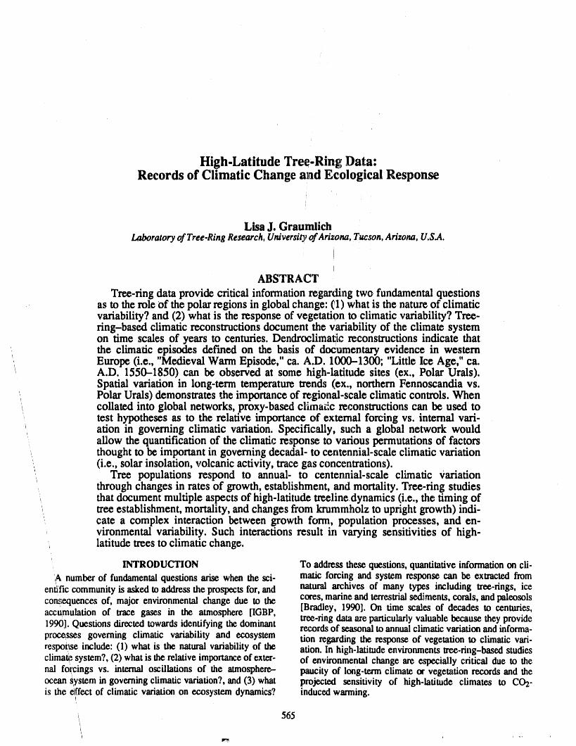
High.Latitude Tree. Ring Data:Records of Climatic Change and Ecological Response

i

Lisa J. GraumlichLaboratory of Tree-Ring Research, University of Arizona, Tucson, Arizona, U.S.A.

ABSTRACT

Tree-ringdataprovide critical informationregardingtwo fundamentalquestionsas to the role Ofthe polarregions in globalchange: (11)what is the natureof climaticvariability? and (2) what is the response of vegetation to climatic variability? Tree-ring-based climatic reconstructions document the v,e_iabilityof the climate systemon time scales of years to centuries. Dendroclimadc reconstructions indicate that

, the climatic episodes clef'reedon the basis of documentary evidence in western,, Europe(i.e., "Medieval Warm Episode," ca. A.D. 1(100-1300; "Little Ice Age," ca./ A.D. 1550-1850) can be observed at some high-latitude sites (ex., Polar Urals).

Spatial variationin long-term temperaturetrends(ex., northernFennoscandia vs.'_ Polar Urals) demonstratesthe importanceof regional-scale climatic controls. When_ collated into global networks, proxy-basedclimaL_,creconstructionscan be used to, test hypotheses as to the relative importance of external forcing vs. internal vail-

ation in governing climatic variation.Specifically, such a global network wouldallow the quantificationof the climatic response to variouspermutations of factorsthought to be importantin governing decadal- to centennial-scale climatic variation(i.e., solar insolation,volcanic activity, trace gas concentrations).

Tree populations respond to annual- to centennial-scale climatic Variationthroughchanges in rates of growth, establishment,and mortality.Tree-ring studiesthat documentmultiple aspects of high-latitudetreelinedynarnics(i.e., the timing oftree establishment, mortality, andchanges from krummholz to uprightgrowth) indi-cate a complex interaction between growth form, population processes, and en-vironmental variability. Such interactions result irt varying sensitivities of high-latitudetrees to climatic change.

, INTRODUCTION Toaddressthesequestions,quantitativeinformationoncli-A number of fundamental questions arise when the sci- malic forcing and system response can be extracted from

entitle community is asked to address the prospectsfor, and natural archives of many types including tree-rings, icecom_equencesof, major environmental change due to the cores, marine and terrestrial sediments, corals, and paleosols

[Bradley, 1990]. On time males of decades to centuries,accumulation of trace gases in the atmosphere [IGBP, tree-ringdataare particularlyvaluable because they provide1990]. Questions direcled towardsidentifying the dominant recordsof seasonal to annual climaticvariationand informa-proce,_ses_governing climatic variability and ecosystem lion regarding the response of vegetation to climatic vari-respoii_e include: (1) what is the naturalvariability of the ation. In high-latitude environments tree-ring-based studiesclimate;system?, (2) what is the relative importanceof exter- of environmental change are especially critical due to thenal foi'cings vs. internal oscillations of the atmosphere- paucityof iong-texm climate or vegetation records and theocean system in governing climatic variation?,and (3) what projected sensitivity of high-latitude climates to CO2-is the effect of climatic variation on ecosystem dynamics? inducedwarming.

', 565

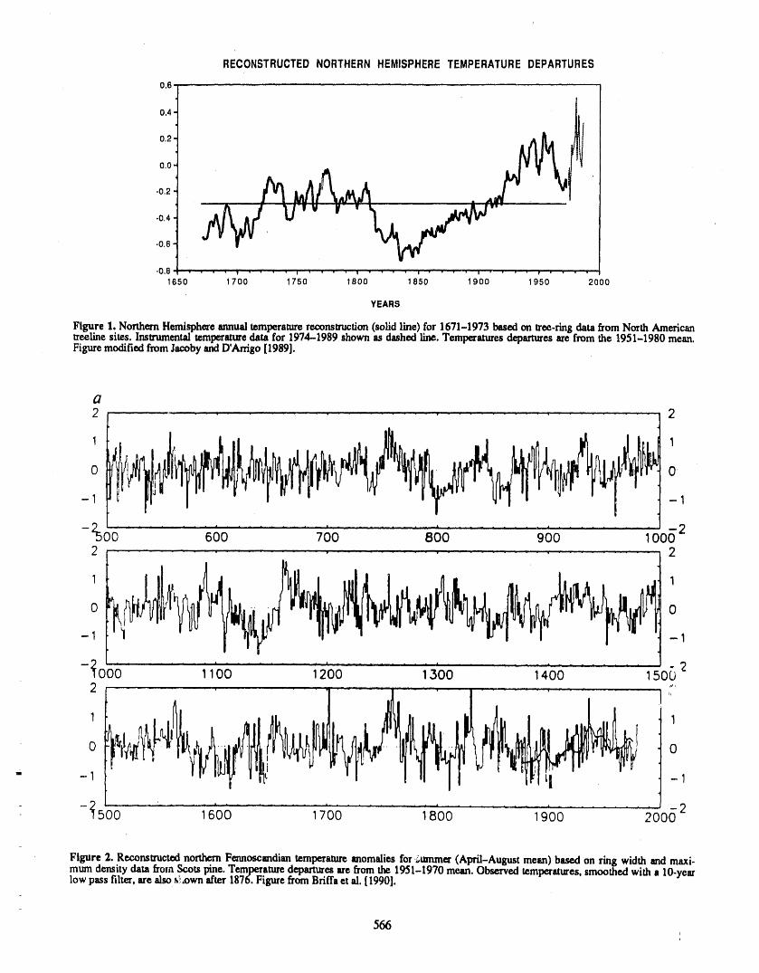
RECONSTRUCTEDNORTHERNHEMISPHERETEMPERATUREDEPARTURES

0,6

0,4

0,2

0,0

-0,2

-0.4

-0,6

-0.8 • • . _ 1" • • • • , '"_' • • .", "'. • , • , .' . • .' r • • .' • r • • , '.1150 1700 1750 1800 1850 1900 1950 2000

YEARS

Figure 1. NorthernHemisphereannualtemperaturereconstruction(solidline) tbr1671-1973basedon tree-ringdatafromNorthAmericantreelinesites.Instrumentaltemperaturedata for1974-1989shownas dashedline.Temperaturesdeparturesarefromthe 1951-1980mean.FiguremodifiedfromJacob),andD'Atrigo[1989].

O2 ............. , .... 2

1 1

0 0

-1 -1

-_00 -600 ....... 760............ 860.......... 960- 100_22 ,' ............. ' 2

0 0

-1 -1

• ........... A _ . . • ........... • ...........

-_000..... i_oo _200 _00 _400 is06.2

1 1

0 0

= -1 -1

-_500 .... '..... i600 1700 1800 1900 2005 2

Figure2. ReconstructednorthernFennoscendiantemperatureanomaliesfor&ummer(April-Augustmen) base,d on ringwidthandmaxi-mumdensitydata from_ts pine.Temperaturedeparturesarefromthe1951-1970mean.Observedtemperatures,smoothedwitha lO-yearlowpass filter,are also_,!,,ownafter1876.FigurefromBriffaetal. [1990].

566

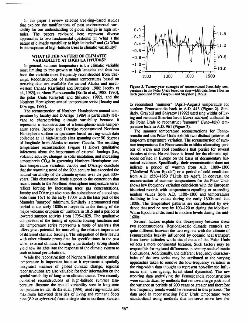
In this paper I review selected tree-ring-based studiesthat explore the ramifications of past environmental vail-

00tudes. The papers reviewed here represent diverse - 11.5approachesto two fundamental questions: (1) What is the -0.2 .

natureof climaticvariabilityat high latitudes?and(2) What -0.4 A _ 11. o

is the responseof high-latitudetreesto climatic variability? -0.6 ." _ /''_/" _'__

WHAT IS THE NATURE OF CLIMATIC -0.8 - 10.5VARIABILITY AT HIGH LATITUDES?

In general, summer temperatureis the climatic variable -1.0- " 10.0most limiting to tree growth at high latitudesand thus has -1.2 , , , , , ,_ , , ,been the variable most frequently reconstructed from tree- 1 ]00 1300 1600 1900rings. Reconstructions of summer temperatures based ontree-ring data are available for central Alaska and north-western Canada [Garfmkel and Brubaker, 1980; Jacoby et Figure3. Twenty-yearaveragesof reconstructedJune-Julytem-

peraturesinthePolarUralsbasedonring-widthdatafromSiberianal., 1985], northernFennoscandia[Briffaet al., 1988, 1990], larch (modified from Graybill and Shiyatov [1992]).the polar Urals [Graybill and Shiyatov, 1992], and the

NorthernHemisphere annualtemperatureseries [Jacobyand to reconstruct "summer"(April-August) temperature forD'Arrigo,1989]. nor,hem Fennoscandia back to A.D. 443 (Figure 2). Sim-The reconstruction of Northern Hemisphereannual tem-peratureby Jacoby and D'Arrigo [1989] is particularlyrcic- ilarly, Graybill and Shiyatov [1992] used ring widthsof liv-vant to characterizing climatic variability because it ing and remnantSiberianlarch (Larixsibirica)collected inrepresentsa reconstruction of a hemispheric-scale temper- the Polar Urals to reconstruct"summer"(June--July)tem-ature series. Jacoby and D'ArrigoreconstructedNorthern peraturebackto A.D. 961 (Figure 3).The summer temperature reconstructions for Fenno-Hemisphere surface temperaturesbased on ring-width data scandia and the Polar Urals exhibit two distinct patternsofcollected at 11 high-latitude sites spanningover 90 degrees long-termtemperaturevariation.The reconstructionof sum-of longitude from Alaska to eastern Canada.The resulting mer temperaturesforFennoscandiaexhibits alternatingpeal-temperature reconstruction (Figure 1) allows qualitative ods of warm and cool conditions that persist for severalinferences about the importance of external forcings (i.e., decades at time. No evidence is found for the climatic epi-volcanicactivity, changes in solarinsolation, and increasing sodes defined in Europe on the basis of documentaryhis-atmospheric CO-z)in governing Northern Hemisphere sur- torical evidence. Specifically, their reconstructiondoes notface temperature variation. Jaeoby and D'Arrigoconclude indicate a period of warmth from A.D. 1000-1300that the warming trendof the 20rh century has exceeded the ("Medieval Warm Epoch") or a period of cold conditionsnatural variability of the climate system over the past 300+ from A.D. 1550-1850 ("Little Ice Age"). In contrast, theyears. This observation lends supportto the contention that reconstructionof summer temperaturesfor the Polar Uralsrecent trendsin the Northern Hemisphere temperatureseries shows low frequency variationcoincident with the Europeanreflect forcing by increasing trace gas concentrations, historical records with temperaturesequallingor exceedingJacoby and D'Arrigo also note the coincidence of a cool epi- modem values from A.D. 1100-1300 and temperaturessode from 1671 to the early 1700s with the later part of the declining to low values during the early 1600s and lateMaunder "sunspot" minimum. Similarly, a pronounced cool 1800s. The temperature patterns are corroborated by evi-period in the early 1800s c_ 'i'esponds to the timing of the dence that treeline rose by 100--120 m during the Medievalmajor volcanic eruption of' iambora in 1815and a period of Warm Epoch and declined to modem levels during the mid-lowered sunspot activity t_om 1795-1825. The qualitative 1600s.comparison of the timing of specific forcing functions and Several factors explain the discrepancy between thesethe temperature series represents a mode of analysis that two reconstructions. Regional-scale climatic controls areoffers great potential for unraveling the relative importance quite different between the tworegions with the climate ofof different climatic forcings. The integration of their results Fennoscandia heavily influenced by oceanic heat transportwith other climatic proxy data for specific times in the past from lower latitudes while the climate of the Polar Uralswhen external climatic forcing is particularly strong should reflects a more continental location. Such factors may beyield new insights into the response of the climate system to responsible for regional differences in century-scale climaticsuch external perturbations, fluctuations. Additionally, the different frequency character-

While the reconstruction of Northern Hemisphere annual istics of the two series may be attributed to the varyingtemperature is important because it represents a spatially approaches taken to remove the low-frequency variation inintegrated measure of global climatic change, regional the ring-width data thought to represent non-climatic influ-reconstructions are also valuable for their information on the ences (i.e., tree ageing, forest stand dynamics). The rawspatial variability of long-term climatic trends. Two recently tree-ring data underlying the Fennoscandia reconstructionpublished reconstructions of high-latitude summer tem- were standardized by methods that remove a large portion ofperature illustrate the spatial variability seen in long-term the variance at periods of 200 years or greater and thereforetemperature trends. Briffa et al. [1990] used ring-widths and low frequency trends would be removed in this process. Themaximum latewood densities of living and remnant Scots data used in reconstructing Polar Urals temperature werepine (Pinus sylvestris) from a single site in northern Sweden standardized using methods that conserve more low frc-

567

quency variationand the resulting reconstructionreflects snow accumulation. At protected sites, upright trees catchthis more conservative approach. Standardizationmethods driftingsnow and accumulatedsnow protects buds and fol-heavily influence the frequency domain characteristicsof iage from abrasion and desiccation during severe winterthe resulting reconstructionsand further attentionneeds to conditions. In such environments sexual reproduction isbe directed towardsmaintainingthe low frequency fidelity more likely to be successful providing a regular supply ofof tree-ringandotherproxy-basedreconstructions, propagules to acceleratepopulation expansion in times ofrelative warmth. In contrast,at exposed sites prostratelow

WHAT IS THE RESPONSE OF HIGH LATITUDE krummholz are unable to control the snow drift environ-TREES TO CLIMATIC VARIABILITY? merit, suffer damage when stems are exposed above the

High-latitude trees respond to climatic variation on snow-air interlace, and rarely reproducesexually. At suchannual time scales through variation in radialgrowth rates sites, population responses lag behind climatic forcing andand on decadaland longer time scales throughphenotypic the vegetation is resilient to climatic change. Ecological fac-changes (i.e., krummholzvs. normalgrowth)andpopulation tots thus complicatethe interpretationof the history of treeexpansions and contractions. Such changes can be quan. morphologic changes inclimate terms.tiffed using dendrochronologic techniques and these data On longer time scales trees respond to changingclimateprovidea critical long-termperspectiveon the natureof eco- throughpopulationexpansionsand contractionsresultinginsystem responseto climatic variationas well as quantitative changes in altitudinalor latitudinal treeline and/or changesinformationthat can be used to develop and test models of in tree density. Dendrochronologically determined ageforestresponse to globalchange [Graumlich,1989]. structures(i.e., dates of tree establishment) and mortality

The effects of climate on annual variation in radial patterns allow the reconstructionof population dynamicsgrowth of white spruce (Picea glauca) growing at or near back in time. Many investigatorstuive found vigorous treetreelinein the Brooks Range of Alaska were analyzedusing regenerationat arctic treeline sites during the 2001century14 tree-ringchronologies [Garfmkeland Brubaker,1980]. that has been attributedto recent warmingtrends [KullmanWhite spruce responds positively to currentsummer and 1983; Payette and Fillion, 1985]. Population responses toprevious autumn temperatures,a finding that is consistent climatic variationexhibit complex spatial and temporalvar-with other studies at nonhero treeline sites [Jacoby,1982]. iability that has been related to such factors as snow accu-In addition, at many of the sites, growth is positively cor- mulation [Payette and Fillion, 1985], fire [layette andrelated with summer precipitation, implying that internal Gagnon 1979;layette and Fillion, 1985], sexual vs. vegeta-waterstressmay limitphotosynthesis when temperaturesare five modes of reproduction [Payette and Gab,non, 1979;high. Ecophysiological studies conducted on trees at the Kullman, 1983], and other life history traits [Kullman,study site indicated that stomatal conductance decreases 1983]. These factorscaninteract to cause a wide variationinsharplyat vaporpressuredeficits similarto thosecommonly the nature of and rates of population response to climaticexperienced in the field during the growing season [Gold- change.stein, 1981]. Precipitationduring the growing season thus Finally, while most tree-ring studies of vegetationfavors growth by reducingvaporpressme deficits andensur- response to climate are concerned with effects on indi-ing ample soil moisture.These findings imply that any pre- viduals or populations,tree.ringdatacan potentiallyprovidedictions of increasing white spruce growth rates due to importantdata on rates of CO2 upltakeat the biome level.rising temperaturesassociated with global wanning must D'Arrigoet _1.[1987] demonstratedthat annualvariationintake into accountlocal moistureconditions, tree growth in the NorthAmericanborealforest is correlated

In addition to changes in radial growth rates, climatic with CO2 drawdown at Point Banow, AK for the periodchange at high latitudescan result in changes in the growth 1971-1982. D'Arrigo and coworkers speculate that theform of trees from krumn_holz to monopodial trees with recent increases in the amplitude of the seasonal CO2 cyclenormal stems. Such phenotypic plasticity has important may be caused, in part,by seasonally enhanced growth ofimplications for populationdynamicsattreeline:whilesex- theborealforest.Thusclimaticallyinducedchangesin com-ual reproduction can occurregularlyin trees,krummholzare position, structureandproductivityof high.latitudenorthernoften unableto produce a large numberof cones and viable forests have importantimplications for of the atmosphere-seeds, layette et al. [1989] demonstratedthat the ability of biosphere exchange of CO2 [Gammon et al., 1985]. Con-black sprucepopulations to respond to climatic change may tinued research efforts directed towards understanding thedepend on growth form at time of climatic change, layette interaction of climate and vegetation processes at scalesand coworkers dated changes in growth form and elevation ranging from individuals to entire ecosystems will beof the snow-air interfacerex_rdedby subfossil black spruce enhanced by the long-term perspective afforded by tree-at a treeline site in northernQuebec. Three periods of con- ring-basedstudies.wasting growth forms were interpretedin termsof climaticforcing:high krummholz (<2 m high) reflected cool condi- CONCLUSIONSlions from AD. 1305-1435, trees and high krummholz Dendroclimatic data will contiinue to be an importantreflected warmt_onditionsfrom A.D. 1435-1570, and low source of informationon global environmental change bykrummholz (<50 era high) reflected cold conditions from elucidating the nature of past climatic variationas well asA.D. 1570 to the present. The s_-or,g interaction between vegetation response.In order to mwavel the separateeffectsphenotype,populationproceeds, and envLronmentalchange of various externalforcings on global climate, the develop-

= is well illustratedby these results. The sensitivity of black ment of networksof multiple proxyclimatic dataneed to besprucepopulationsto climatic change is stronglyaffected by developed [IGBP, 1990]. Towards that end, the global cov-positive feedbacks mediated through vegetative control of erage of climatically sensitive tree-ring chronologies should

568

be extended especially in areaswhere observationaldataare must be inferred from indirect sources such as tree.ring-of short durationor where the climatic system is thought to based recordsof growthvariationand populationdynamics.be particularly sensitive to external forcing. High-latitude In pmticular,furtherstudy of the factorsthat govern the sen-regions fit both criteriaand should thus be given high prior- sitivity or relativeresilience of vegetationto climatic changeit), in future dendtoclimatic research. Similarly, given the needs to be given high priorityff we are to adequatelyantic-long life spansof trees,our knowledge of thecomplex inter- ipate the ecological consequences of CO2-inducedclimaticaction of climate and arboreal vegetation at high latitudes change.

RErRNCBradley, R. S. (Ed.), Global Changes of the Past (Pro- Goldstein, G. H., Ecophysiological and demographicstudies

ceedings of the 1989 Global Change Institute at Snow- of white spruce (Picea glauca [Mcench] Voss) at treelinemass), Publication OIES-6, Office for Interdisciplinary in the central BrooksRange of Alaska"Ph.D. Thesis, Uni-EarthStudies,UCAR, Boulder,CO, 1990. versityof Washington,Seattle, 1981.

Briffa, K. R., T. M. L. Wigley, P. D. Jones, J. R. Pilcher, IGBP, The InternationalGeosphere-Biosphere Programme:and M. K. Hughes, Reconstn_ting summer temperatures A Study of Global Change. The Initial Core Projects,in northern Fennoscandiaback to A.D. 1700 using tree- IGBP Report 12, Stockholm, 1990.ring dam from Scots Pine, Arctic and Alpine Research, Jacoby, G. C., Jr., The arctic, in Climate from Tree Rings,20, 385-394, 1988. edited by M. K. Hughes, P. M. Kelly, J. R. Pilcher, and

Briffa, K. R., T. S. Bartholin,D. Eckstein,P. D. Jones, W. V.C. LaMarche, Jr., Cambridge University Press,Karlen,F. H. Schweingruber,and P. Zetterberg,A 1,400- Cambridge,1982.year tree-ring record of summer temperaturesin Fen- Jacoby, G. C., Jr., and R. D'Arrigo,ReconstructedNorthemnoscandia,Nature,346,434-439, 1990. ' Hemisphere temperature since 1671 based on high-

D'Arrigo, R., and G. C. Jacoby, Jr., Boreal forests and latitude tree-ring data from North America, Climaticalmosphere-biosphere exchange of carbon dioxide, Change, 14, 39.-59, 1989.Nature, 329, 321-323, 1987.

Jacoby, G. C., Jr., E. R. Cook, and L. D. Ulan, Recon-Gammon,R. H., E. T. Sundquist,and P. J. Fraser,History structedsummerdegree days in centralAlaskaand north-of carbondioxide in the almosphere,in AtmosphericCar-

ben Dioxide and the GlobalCarbonCycle, edited by J.R. westernCanadasince 1524, Quat. Res., 23, 18-26, 1985.Trabalka, U.S. Department of Energy, DOE/ER.0238, Kullman, L., Past and present tree-lines of the Hand01anWashington, DC, 1985. Valley, central Sweden, in Tree-Line Ecology, edited by

Garfmkel,H. L., and L. B. Brubaker,Modem climate-tree P. Morisset and S. Payette, pp. 25-45, Centre d'6tudesgrowth relationships and climatic reconstructionin sub- nordiques,Universit6Laval,Qu6bec, 1983.arcticAlaska,Nature, 286, 872-.874, 1980. Payette, S., and L. Fillion, White spruce expansion at the

Graumlich, L. J., The utility of long-term records of tree tree line and recent climatic change, Can. J. Forest Res.,growth for improving forest stand simulation models, in IS, 241-251, 1985.Natural Areas Facing Climatic Change, edited by G.P. Payette, S., and R. Gagnon, Tree-line dynamics in UngavaMalanson, pp. 39-49, SPB Academic, The Hague, 1989. peninsula, northern Quebec, Holarct. Ecel., 2, 239-248,

Graybill, D. A., and S. G. Shiyatov, Dendroclimaticevi- 1979.dence from the northernSoviet Union, in Climate Since Payette, S., L. Fillion, A. Delwaide, and C. Begin, Recon-A29. 1500, edited by R. S. Bradley and P. D. Jones, Rout- sUuction of tree-fine vegetation response to long-term cii.ledge, London, 1992, In press, mate change, Nature, 341,429--432, 1989.

569

Polar Ice Cores: Climatic and Environmental Records

C. LoriusLaboratoirede Giaciologieet G_ophysiquede l'Environnement,St Martind'H_res,France

ABSTRACT

Ice cores from Greenland and Antarctica provide multiple proxy records of cli-matic and environmental parameters. They reveal the anthropogenic impact on aer-osol concentrations in Greenland snow (i.e., SO4 and NO3) and on atmosphericgreenhouse gases. For example, increases over the last 200 years are about 25% forCO2, 8% for N202 and about 200% for CH4. Over the last climatic cycle (i.e., -150Kyr) the glacial-interglacial surface temperature change may be -10°C, with glacialstages generally associated with lower snow accumulation and higher concentra-tions of marine and continental aerosols reflecting enlarged source areas andincreased atmospheric transport. Greenland ice has recorded rapid changes of cli-mate during the last ice age and deglaciation. The 8180 or 5D records from theVostok ice core (Antarctica) strongly suggest the role of insolation orbital forcing,as well as a close relation between temperature and greenhouse gas concentrations.CO2 and CH4 concentrations increase by about 40% and 100% during glacial-interglacial transitions, respectively. It appears likely that fluctuating greenhousegas concentrations have had a significant role in the glacial-interglacial climatechanges by amplifying, together with the growth and decay of the Northern Hemi-sphere ice sheets, the orbital forcing. Climate sensitivity to greenhouse forcing esti-mated from paleo-ice core data is consistent with GCM simulations giving a 3-,4°Cwarming for a future doubled atmospheric CO2.

THEICE CORERECORD linear isotope-temperaturerelationshipis generallyen-: Paleo reconstructionsarenowrecognizedas an imporlant sideredvalidforbothpolar ice sheets[LoriusandMedivat,

elementin climaticandenvironmentalstudiesbecausethey 1977;Johnsenet al., 1989].Thevalidityof usingthepresent(a)allowassessmentof thedegreeof naturalvariabilityand observedrelationshipforpaleotemperaturereconstm:tionispiacecurrentobservedchangesin a broaderperspective;Ca) supportedby variousevidenceincludingatmosphericisc_assist in understandingcausesand mechanismsof change; topemodels.Althoughthereis no doubtthatthe concentra-and(c) contributeto validatingmodelsby thecomparisonof tionof aerosolspeciesinthe airis reflectedinsnowdepositsoutputwith empiricaldatasets. atthesite,quantitativeestimationsof theiratmosphericcon-

Althoughwe cannotexpect to find in naturean ideal centrationsuffersfroman incompleteunderstandingof therecord,ice is a ratherclose approximation,assummarizedin depositionprocesses,such as the relativecontributionofTable1. "wet"and "dry"processes.In contrast,relatinggas concen-

Paleotemperaturereconstructionis based on the present trationsobtainedfromice-corebubblesto the atmosphericcorrelationsbetweenthe ratiosof 2H(D) and lH andof iso valueis quitestraightforwardin sampleswhichdo notcon-and 160 in the snow and the temperatureconditionsboth rainmeltlayers.abovetheinversionlayer,wherethe precipitationis formed,

: andat thesurface.Thesearecorrelatedvia the fractionation TIMESCALESprocessesthat occur in the atmosphericwatercycle and, Forthe upperpartoi the ice sheets the accuracyof thealthoughthese processesdependon severalparameters,a chronologycan be veryhigh.Annuallayerscanbe counted

570

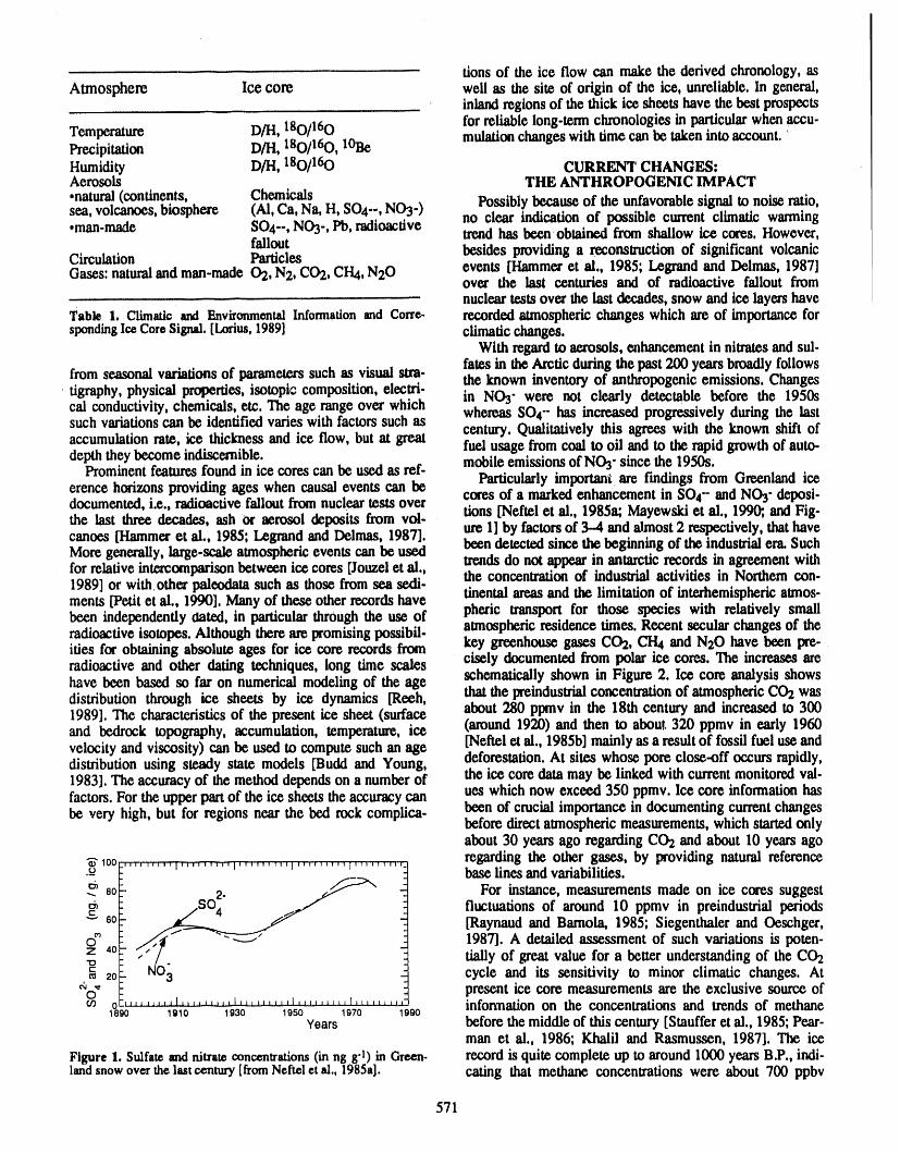
tions of the ice flow can make the derived chronology, asAtmosphere Ice core well as the site of origin of the ice, unreliable. In general,

inlandregionsof the thick ice sheets have the best prospects

Temperature D/I-I,180/160 forreliable long-termchronologies in particularwhen accu-mutationchanges with timecan be takeninto account.Precipitation D/H, 180/160, lOBeHumidity D/H, 180/160 CURRENT CHANGES:Aerosols THE ANTHROPOGENIC IMPACT•natural(continents, Chemicalssea, volcanoes, biosphere (AI,Ca, Na, H, SO4--, NO3-) Possibly because of the unfavorablesignal to noise ratio,•man-made SO4--, NO3-,Ph, radioactive no clear indication of possible current climatic wanningtrendhas been obtained from shallow ice cores, However,

fallout besides providing a reconstruction of significant volcanicCirculation ParticlesGases:naturaland man-made 02, N2, C02, CH4,N20 events [IJaunmeret al., 1985; Legrand and Delmas, 1987]over the last centuries and of radioactive fallout from

nucleartests over the last decades, snow and ice layers haveTable I. Climaticand EnvironmentalInformationand Cone- recordedatmospheric changes which are of importanceforspendingIceCoreSignal.[Lorius,1989] climatic changes.

With regardto aerosols, enhancementin nitrates and sul.fates in theArctic during the past 200 yearsbroadlyfollows

from seasonal variationsof parameterssuch as visual stm- the known inventory of anthropogenic emissions. Changes+tigraphy, physical properties,isotopic composition, electri- in NOy were not clearly detectable before the 1950scal conductivity,chemicals, etc. The age range over which whereas SO4" has increased progressively during the lastsuch variationscan be identified varies with factorssuch as century. Qualitatively this agrees with the known shift ofaccumulationrate, ice thickness and ice flow, but at great fuel usage from coal to oil and to the rapidgrowth of auto-depth theybecome indiscernible, mobileemissions of NO3"since the 1950s.Prominentfeatures found in ice cores can be used as ref.erence horizons providing ages when causal events can be Particularlyimportant+are findings from Greenland icedocumented,i.e., radioactivefallout fromnucleartests over cores of a markedenhancement in SO4- and NOy deposi-the last three decades, ash Or aerosol deposits from vol. tions [Neftel et al., 1985a; Mayewski et al., 1990;,andFig-

ure 1] by factorsof 3--4 and almost 2 respectively, thathavecanoes [Hammer et al., 1985; Legrand and Delmas, 1987]. been detectedsince the beginning of the industrialera.SuchMore generally, large-scale atmospheric events can be usedfor relative intercomparisonbetween ice cores [Jouzelct al., trendsdo not appearin antarcticrecords in agreement withthe concentration of industrial activities in Northern con-1989] or with other paleodata such as those from sea sedi-ments [Petit et al., 1990]. Manyof these other records have tinentalareasand the limitation of interhemisphericatmos-been independentlyaated, in particular through the use of pheric transport for those species with relatively smallradioactiveisotopes. Although there are promisingpossibil- atmosphericresidence times. Recent secular changes of theities for obtaining absolute ages for ice core records from key greenhouse gases CO2, CH4 and N20 have been pre-radioactive and other dating techniques, long time scales cisely documented from polar ice cores. The increases arehave been based so far on numerical modeling of the age schematically shown in Figure 2. Ice core analysis showsdistribution through ice sheets by ice dynamics [Reeh, that the preindustrialconcentrationof atmospheric CO2was1989]. The characteristicsof the present ice sheet (surface about 280 ppmv in the 18rh century and increased to 300and bedrock topography, accumulation, temperature, ice (around 1920) and then to about 320 ppmv in early 1960velocity and viscosity) can be used to compute such an age [Neftel ct al., 1985b] mainly as a resultof fossil fuel use anddistribution using steady state models [Budd and Young, deforestation.At sites whose pore close-off occurs rapidly,1983]. The accuracyof the method dependson a numberof the ice core data may be linked with currentmonitoredval-factors.For the upperpartof the ice sheets the accuracycan ues which now exceed 350 ppmv. Ice core informationhasbe very high, but for regions near the bed rock complica, been of crucial importance in documenting currentchanges

before directatmospheric measurements,which startedonlyabout 30 years ago regarding CO2 and about 10 years ago

1oo.......... , ......... , ......... ]......... I.......... regarding the other gases, by providing natural reference.- base lines andvariabilities.

80 _,,.2.2. _ For instance, measurements made on ice cores suggest/_''4 fluctuations of around 10 ppmv in preindustrial periods

----60 _ _ [Raynaudand Bamola, 1985; Siegenthaler and Oeschger,

_/;_.- "_" 1987]. A detailed assessment of such variations is poten-40 tially of great value for a better understandingof the CO2"I3

m= 20 NO3 cycle and its sensitivity to minor climatic changes. At,* - present ice core measurements are the exclusive source ofO

0:,,,,, .... ",, .... ,' _'',, ..... _", ...... _........ J informationon the concentrations and trends of methane1890 1910 1930 1950 1970 1 _90

Years beforethemiddleof thiscentury[Staufferctal., 1985;Pear-man et al., 1986; Khalil and Rasmussen,1987]. The ice

Figure1. Sulfatemd nitrateconcentrations(in ng g.1)in Green- recordis quite complete up to around 1000 yearsB.P., indi-landsnowoverthelastcentury[fromNefteletal., 1985a]. caring that methane concenU_tions were about 700 ppbv

571

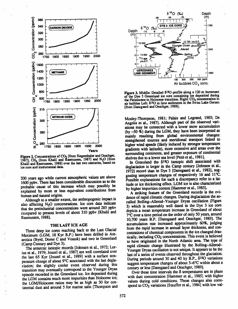
BI"O (%.) Depth•3e .34 .30 (m)

"-" s o (_) ," Depth .IO .8 .e

fd i I I i I I i

1750 1800 1850 1900 1950 2000 lY m'_''" _ _

_ME SEDIMENT,) _-, _l_--i ¢ I I ,-118_0

AirbubblesCO 2cono,

8 e(x)_ _ _ __,,_h,ere3.Middle'.DetailedSnO__vrofi]ealonga120m increment" eoo[ , , , , , , , ' ' - of_ Dyo3C__ icoco,,,_ _._..8 [_ _po,t_ du,_,g"I"

O.. t750 1800 1850 1900 1950 2OOO thePleistoceneto Holocene_ramition,Kilt: UU2eoneen_rmonmair bubblesLeft:81s0 in lime sedimentsinthe SwissLakeOerzen

> 310 , , , , , , , _ , [fromDansgaardandOeschger,1989]. ,,

Mosley-Thompson, 1981; Palais and Legrand, 1985; De

Angelis et al., 1987]. Although part of the observed vari-ations may be connected with a lower snow accumulation(by .-50 %) duringthe LGM, they have been interpretedasmainly resulting from global environmental changes:strengthened sources and meridional transport linked to

O_280 i l, t i , I i i ,Z 1750 1800 1850 1900 1950 2000 higher wind speeds (likely induced by strongertemperature

Years gradientswith latitude), more extensive aridareasover thesurroundingcontinents, and greaterexposure of continental

Figure2.Concmtrationsof CO2[fromSiegenthalerandOeszhger,1987],CI-14[fromKhalilandRasmussen,1987]_ N_O[_om shelves due to a lower sea level [Petitet al., 1981],KhalilandRasmussen,1988]ov_ thelasttwocentunes,oasea on In Greenland the {its0 isotopic shift associated withice core and instnmaentti data. deglaciation is bxger in the Camp century [Johnsenet al.,

1972] record than in Dye 3 [Dansgaardet al., 1982], sug-

200 years ago while currentatmospheric values are above gesting temperaturechanges of respectively 16 and 11"(2.1600 ppbv. There has been considerablediscussion as to the Possible explanations for such a discrepancy refer to a lat-probable cause of this increase which may possibly be itade or ice thickening effect. LGM ice is also characterizedexplained by more or less equivalent contributions from by higher impemtiescontent [Hammeret al., 1985].humanandmural origins. A striking feature of the Greenland records is the evi-

Although to a smallerextent, theanthropogenicimpact is dence of rapidclimatic changes. During deglaciation the so-also affecting N20 concentrations, lee core data indicate called Bolling-Allerod-Younger Dryas oscillation (Figurethat the preindustrialconcentrationswere around285 ppbv 3) which is reasonably well dated in the Dye 3 ice corecompared to present levels of about 310 ppbv [Khalil and depictsa mean temperatureincrease in Greenlandof about7°C over a time periodon the orderof only 50 years, aroundRasmussen, 1988]. I0,700 years B.P. [Dansgaardand Oeschger, 1989]. The

THE LAST ICE AGE accumulation rate increased approximately 60%, judging

Threedeepice coresreachingback to the Last Glacial fromthe rapidincreasein annuallayerthickness,andcon-- Maximum (LGM, 18 Kyr B.P.) have been drilled in Ant- centrationsof chemicalcompo.entsin the ice changeddras-

arctica (Byrd, Dome C and Vostok) and two in Greenland tically, including CO2 concentrations.This event is believed(CampCentury and Dye 3). to have originated in the North Atlantic area. The type of

The antarctic isotopic lecords [Johnsenet al., 1972; tor- rapid climatic change illustrated by the Bolling-Allerod-ius et al., 1979; Jouzel et al., 1987] are well correlatedover Younger Dryas oscillationis not unique, lt appearsto be thethe last 65 Kyr [Jouzel et al., 1989] with a surface tem- last of a seriesof events observed throughoutthe glaciation.perature change of about 9°C associated with the last degla- During periods around 30 and 40 ky B.P., 81sO variationsciation; the slightly cooler event observed during this suggest temperature changes of about 5---6°Cwithin about atransition may eventually correspond to the YoungerDryas century or less [Dansgaard and Oeschger, 1989].episode recorded in the Greenlandice. Ice deposited during Over these time intervals the 8 temperaturesare in phasethe LGM contains much more impurities than Holocene ice; with dust concentration [Hammer et al., 1985] with higherthe LGM/Holoeene ratios may be as high as 30 for con- values during cold conditions. These changes also corre-tinental dust and around 5 for marine salts [Thompson and spond to CO2 variations [Stauffer et al., 1984] with low val-

-

572

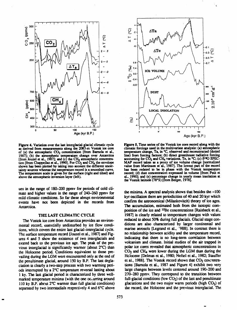
i

".... 300 o- _4_ _

. _IATa ,

Q. -.-.. -2-

oo " '._. <_ .4- _ IO 25O t'-

o j-,\ -o,_2- _ ATe .0.3o°

- .0.5 I--

200 0- 0 o.e .0.7 <]

-2 -- -3 ....

_ mC) 0.0'"- -0.4

•-4---6 c,O-0.8

- LA,700 .6- .9 UST _

-" 600 __.4

500 I LOCAL INSOLATION 0

300 " ;0 50 100 150

Age (kyrB.P.) o _ ,= ,soAge(kyr B.P.)

Figure4.Variationoverthelastinterglacial-glacialclimaticcycle Figure$.TimeseriesoftheVostokioe¢x_rerecordalongwiththeasderivedfrommessurementsalongthe2083-mVostokicecore climaticforcingsusedinthemultivariate=malysis:(a)atmosphericof (a) the atmospimricCO2 conoenlration[from Barnolaez al., temperaturechange,Ta, in °C, observedandreconstructed(dotted1987]; (b) the amm_t_ric temperm_echangeover Anm_tica line) f_ forcingfactors;Co)directgreenhoue_radiativeforcing[bom Jouzel el al., 1987];and (c) the CH4atmosphericconcenera- aocountingfor CO2 and C1-14variations,"re, in eC; (c) 81_ SPEC-tion[from Chappellzzel al., 1990]. For CO2andCH4the envelope MAP recordtakm as a proxy of ice volume change [normalizedshownhasbeenplottedby takinginto accounttlm differentuncer- value fromMarfinsonel al., 1987]. The lowest part of the recordtainty=omr,eswhereasthetemperanererecordis •smoothedcurve, hasbeenredatedtabe inphasewiththeVostoktemperatureThe temperaturescale is given for the surface(rightand tilted)and record; (d) dust _lxation expressed in volume [from Petit elabovethe atmospberkinversionlay=' (left). al., 1990]; and (e) percentagechange in y_=rly mean insolation at

theVostok latiagie (78°S) [fromBerger, 1978].

ues in the range of 180-200 ppmv for periods of cold cli-mate and higher values in the range of 240-260 ppmv for the minima. A spectral analysis shows tl_t besides the -100mild climatic conditions.So far theseabruptenvironmental kyr oscillation thereare periodicitiesof,tO and20 kyr whichevents have not been depictedin the records from confirm the astronomical(Milankovitch) theory of ice ages.Antarctica. The accumulation, estimated both fTom the isotopic com-

position oftheiceand mBe concentrations [Raisbccket al.,THE LAST CLIMATIC CYCLE 1987] is clearly related to temperature changes with values

The Vostok ice core from Antarctica provides an environ- w.Auced to about 50% during full glacials. Glacial stage con-mentalrecord,essentiallyundisturbedby iceflowcondi- ditionsare alsocharacterizedby larl_ercontinentalanddons,which covers the entire last glacial-interglacial cycle, marine aerosols[Legrand ct al., '988]. In contrast there isThe surface temperature record [Jouzel et al., 1987] and Fig- no relationship between acidity and the temperature record,ures 4 and 5 show the existence of two interglacials and indicating that there is no long-term correlation betweenextend back to the previous ice age. The peak of the pre- volcanism and climate. Initial studies of the air trapped invious interglacial is significantly wanner (about 2°C) than polar ice cores revealed that atmosphericconcentrations inthe Holocene period. Conditions equivalent to those pm- CO2 and CH4 were lower during the LGM than during thevailing during the LGM were encountered only at the end of Holocene [Delmas el al., 1980; Neftel et al., 1982; Staufferthe penultimate glacial, around 150 ky B.P. The last degla- ez ai., 1988]. The Vostok record shows that CO2 cohcentra-ciation is clearly a two-step process with two warming peri- tions [Barnola et al., 1987 and Figure 4] exhibit two veryods interrupted by a 2°C temperature reversal lasting about _-ge changes between levels centered around 190-200 and1 ky. The last glacial period is characteri_ by three well- 270-280 ppmv. They correspond to the Iransition betweenmarked temperature minima (with the one oc,.urring around full-glacial conditions flow CO2) of the last and penultimate110 ky B.P. alx'mt 2"12 warmer than full glacial conditions) glaciations and the two major warm periods (high CO2) ofseparatedby two intersmdialsrespectively 4 and 6°C above the record, the Holocene and the previous interglacial. The

. 573

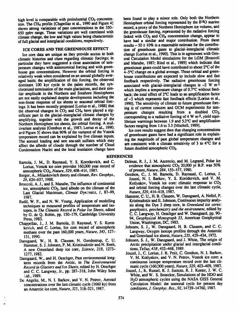
high level is comparablewith preindustrialCOg concentra- been found to play a minor role. Only both the Northerntion. The CH4 profile [ChapeUazet al., 1990 and Figure 4] Hemisphereorbital forcing representedby the 81sO marineshows strong variations of past concentrations in the 350- record,a proxy of the Northem Hemisphereice volume, and650 ppbv range. These variations are well conelated with the greenhouse forcing, represented by the radiative forcingclimatechange, the low and high values being characteristic linked with CO2 and CH4 concentrationchange, appeartoof full glacialand interglacialconditions,respectively, have had a similar and major contribution. From these

results - 50 + 10% is a reasonableestimate for the contribu-ICE CORES AND THE GREENHOUSE EFFECT tion of greenhouse gases to glacial-interglacial climaticIce core data are unique as they provide access to both change [Loriuset al., 1990]. This is in agreementwith Gen-

climatic histories and clues regarding climatic forcings; in eml Circulation Model simulations for the LGM [Broccoliparticularthey have suggested a close association of tem- and Manabe, 1987; Rind et al., 1989] which indicate thatperaturechanges with astronomicalforcing and with green- greenhousegases could havecontributedto about2°C of thehouse gas concentrations. However the orbital forcing is 4--5°Cchange on a global average.These orbitalandgreen-relativelyweak whenconsideredon an annualglobally aver- house contributions are expected to include slow and fastaged basis; the amplification of this forcing, the observed feedback respectively. The radiative greenhouse forcingdominant 100 kyr cycle in the paleo records, the syn- associated with glacial-interglacial changes is .-2 W m-2chronized terminationof themain glaciations,and their slm- which implies a temperaturechange of 0.7°C without feed-ilar amplitude in the Northern and Southern Hemispheres back; the total effect of 2°C leads to an amplification factorare noteasily explained despite developmentsincluding the of --3 which relxesents fast feedback effects [Lodus et al.,non-linear response of ice sheets to seasonal orbital fore- 1990], The sensitivityof climate to futuregreenhouseforc-ings. lt has been recently proposed[Loriuset al., 1988] thatthe observed changes in COg and CH4 have played a sig- ing is of currentconcem and GCM experiments for tem-nificant part in the glacial-interglacial climate changes by peramre changes resulting from a doubled C02,amplifying, together with the growth and decay of the correspondingto a radiative forcing of 4 W m-2,yield equi-NorthernHemisphere ice sheets, the orbital forcing. A mul- librium warmings between 1.9 and 5.2°C andamplificationtivariateanalysis [Genthon et al., 1987; Loriuset al., 1990; factors rangingfrom 1.6 to 3.5 [Mitchell, 1989]._d Figure5] shows that 90% of the variance of the Vostok Ice core results suggest then that changing concentrationstemperaturerecord can be explained by five climate inputs, of greenhousegases have had a significant role in explain-The aerosol loading and non sea-salt sulfates which may ing the magnitude of past global temperaturechanges andaffect the albedo of clouds throughthe numberof Cloud are consistent with a climate sensitivity of 3 to 4°C for aCondensation Nuclei and the local insolation change have fulme doubledatmosphericCO2.

REFERENCES

Bamola, J. M., D. Raynaud, Y. S. Korotkevich, and C. Delmas, R. J., J. M. Ascencio, and M. Legrand, Polar iceLorius,Vostok ice core provides 160,000 year record of evidence thatatmospheric COg 20,000 yr B.P. was 50%atmosphericCOg,Nature, 329, 408-414, 1987. of present,Nature, 284, 155-157, 1980.

Berger,A., Milankovitch theory andclimate, Rev. Geophys., Genthon, C., J. M. Bamola, D. Raynaud, C. Lorius, J.26, 624-657, 1988. Jouzel, N. I. Barkov, Y. S. Korolkevich, and V. M.

Broccoli, A. J., and S. Manabe,The influence of continental Kotlyakov, Vostok ice core: climatic response to COgice, atmospheric CO2, land albedo on the climate of the and orbital forcing changes over the last climatic cycle,I.ast Glacial Maximum, Climate Dyn:_wics, I, 87-99, Nature,329,414-418, 1987.1987. Hammer,C. U., H. B. Clausen,W. Dansgam'd,A. Neftel, P.

Budd, W. F., and N. W. Young, Application of modelling Kfistinsdottirand E. Johnson, Continuousimpurity analy-techniques to measuredprofdes of temperatureand iso- sis along the Dye 3 deep core, in Greenland ice cores:topes,inTheClimaticRecordinPolarIceSheets,edited geophysics,geochemistryandtheenvironment,exfitedbyby G. deQ. Robin,pp.150-179,CambridgeUniversity C.C.Langway,H.OeschgerandW. Dansgaard,pp.90-Press, 1983. 94, Geophysical Monograph 33, American Geophysical

Chappellaz, J., J. M. Bamola, D. Raynaud, Y. S. Korot- Union, Washington, DC, 1985.kevich, and C. Lorius, Ice core record of atmospheric Johnsen, S. J., W. Dansgaard,H. B. Clausen, and C. C.methane over the past 160,000 years, Nature, 345, 127- Langway, Oxygen isotope profdes through the Antarctic131, 1990. andGreenlandice sheets,Nature, 235,429--434, 1972.

Dansgaard, W., H. B. Clausen, N. Gundestrup, C.U. Johnsen, S. J., W. Dansgaard,and J. White, The origin ofHammer,S. J. Johnsen, P. M. Kristinsdottirand N. Reeh, Arctic precipitation under glacial and interglacial condi-A new Greenland deep ice core, Science, 218, 1273- tions, Tellus,41B, 452-468, 1989.1277, 1982. Jouzel, J., C. Lorius, J. R. Petit, C. Genthon, N. I. Barkov,

Dansgaard,W., and H. Oeschger,Past environmentallong- V.M. KoOyakov, and V. N. Petrov, Vostok ice core: aterm records from the Arctic, in The Environmental continuous isotope temperature record over the last cii-Record in Glaciers and Ice Sheets, e_ted by H. _hger malic cycle (160,000 years), Nature, 329, 403-409, 1987.and C. C. Langway, Jr., pp. 287-318, John Wiley Sons Jouzel, J., R. Russel, R. J. Suozzo, R. J. Koster, J. W. C.Ltd., 1989. White, and W. S. Broecker, Simulationsof the HDO and

De Angelis, M., N. I. Barkov, and V. N. Petrov, Aerosol H20 atmospheric cycles using the NASA GISS Generalconcenwations over the last climaticcycle (1660 ky) from Circulation Model: the seasonal cycle for present dayan Antarctic ice core, Nature, 325, 318-321, 1987. conditions, J. Geophys. Res., 92, 14739-14760, 1987.

574

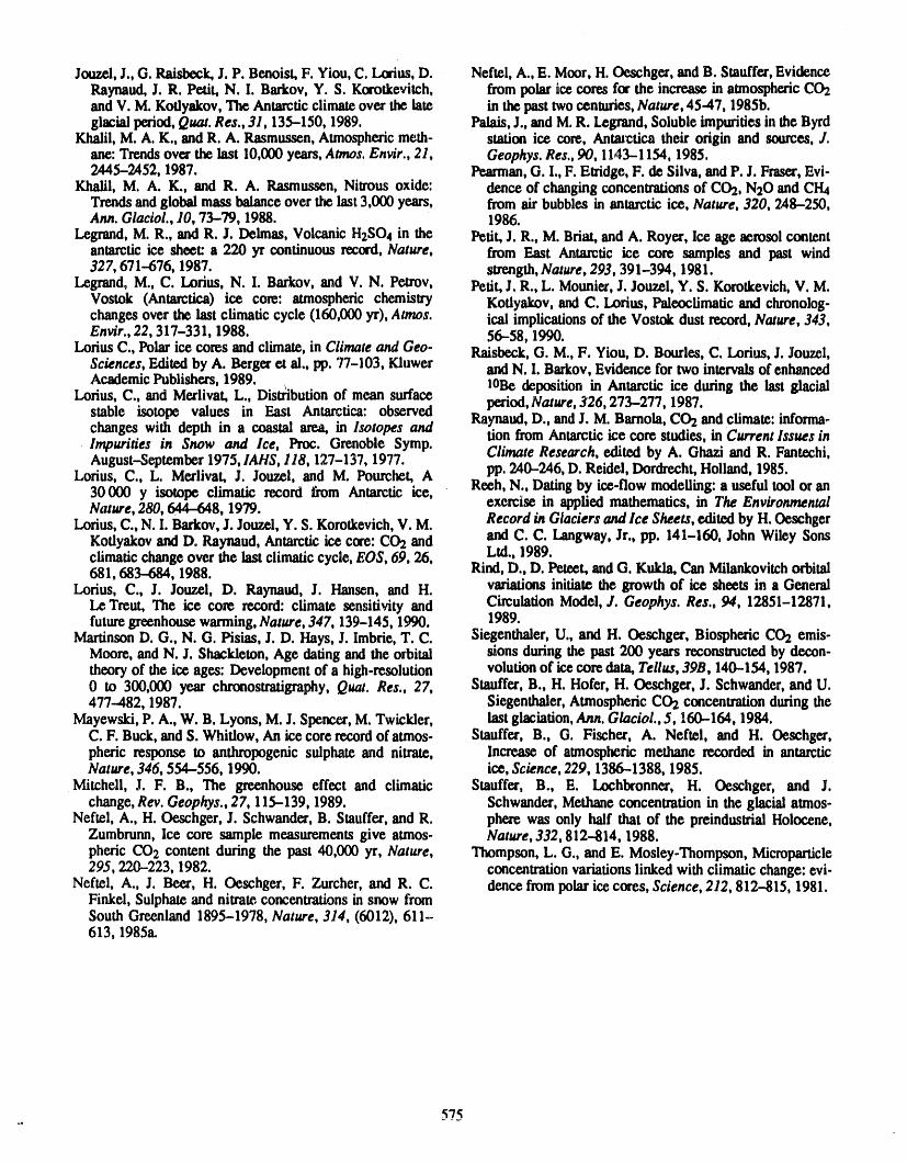
Jouz_l,J., G. Ralsbeck, J. P. Benoist, F. Yiou, C. Lorius, D. Neftel, A., E. Moor, H. Oeachger, and B. Stauffer,EvidenceRaynaud,J. R. Petit, N. I. Barkov, Y. S. Korotkevitch, frompolar ic_ cores for the incre.ascin atmospheric CO2and V. M. Kotlyakov, The Antarcticclimate over the late in the past two centuries,Nature, 45-47, 1985b.glacialperiod,Quat. Res., 31,135-150, 1989. Palais, J., andM. R. Legnmd,Soluble impuritiesin the Byrd

Khalil, M. A. K., and R. A. Rasmussen,Atmospheric moth- station ice core, Antm'ctica their origin and sources, J.ane: Trendsover the last 10,000 years,Atmos. Envir., 21, Geophys. Res., 90, 11,43-1154, 1985.2445-2452, 1987. Pearman,G. I., F. Etridge, F. de Silva, and P. J. Fraser,Evi-

Khalil, M, A. K., and R. A. Rasmussen, Nilrous oxide: dence of changing concentrationsof CO2, N20 and CH4Trendsandglobal mass balance over the last3,000 years, from air bubbles in antarctic ice, Nature, 320, 2,48-250,Ann. Glaciol., lO, 73-79, 1988. 1986.

Legrand,M. R., and R. J. Delmas, Volcanic H2SO 4 in the Petit, J. R., M. Briat, and A. Royer, Ice age aerosol contentantarcticice sheet: a 220 yr continuous record,Nature, from East Antarctic ice core samples and past wind327, 671-676, 1987. strength,Nature, 293, 391-394, 1981.

Legrand, M., C. Lorius, N. I. Barkov, and V. N. Petrov, Petit,J. R., L. Mounier,J. Jouzel, Y. S. Korotkevich,V. M.Vostok (Antarctica) ice core: atmospheric chemistry Kotlyakov, and C. Lorius, Paleoclimatic and chronolog-changes over the last cfimatic cycle (160,000 yr), Atmos. ical implicationsof the Vostok dust record,Nature, 343,Envir., 22, 317-331, 1988. 56-58, 1990.

LoriusC., Polarice cores and climate, inClimate and Geo- Raisbeck, G. M., F. Yiou, D. Bourles, C. Lorius, J. $ouzel,Sciences, Editedby A. Bergeret al., pp. 77-103, Kluwer and N. I. Barkov,Evidence for two intervals of enhancedAcademicPublishers, 1989. 10Be deposition in Antarctic ice during the last glacial

Lorius, C., and Merlivat, L., Dis_bution of mean surfacestable isotope values in East Antarctica: observed period, Nature,326,273-277, 1987.Raynaud,D., andJ. M. Barnola, CO2and climate: informa.changes with depth in a coastal area, in Isotopes and tion from Antarcticice core studies, in Current Issues inImpurities in Snow and Ice, Proc. Grenoble Symp.August-September1975, IAHS, 118, 127-137, 1977. Climate Research, edited by A. Ghazi and R, Fantechi,

Lorius, C., L. Merlivat, J. Jouzel, and M. Pourchet, A pp. 240-246, D. Reidel, Dordrecht,Holland, 1985.30 000 y isotope climatic record from Antarctic ice, Reeh, N., Datingby ice-flow modelling: a useful tool or anNature, 280, 644--648, 1979. exercise in applied mathematics, in The Environmental

Lorius, C., N. I. Barkov,J. Jouzel, Y. S. Korotkevich,V.M. Record in Glaciers and Ice Sheets, ecfitedby H. OeschgerKotlyakov and D. Raynaud, Antarctic ice core: CO2 and and C. C. Langway,Jr., pp. 141-160, John Wiley Sonsclimatic changeover the last climatic cycle, EOS, 69, 26, Ltd., 1989.681,683-684, 1988. Rind, D., D. peteet, and G. Kukla, Can Milankovitchorbital

Lorius, C., J. Jouzel, D. Raynand, J. Hansen, and H. variations initiate the growth of ice sheets in a GeneralLe Treut, The ice core record: climate sensitivity and Circulation Model, J. Geophys. Res., 94, 12851-12871,futuregreenhousewanning, Nature, 347, 139-145, 1990. 1989.

MartinsonD. G., N. G. Pisias, J. D. Hays, J. Imbrie,T.C. Siegenthaler,U., and H. Oeschger, Biospheric CO2 emis-Moore, and N. J. Shackleton, Age dating and the orbital stons duringthe past 200 years reconslructodby decon-theory of the ice ages: Development of a high-resolution volutionof ice core data,Tellus, 39B, 140--154, 1987.0 to 300,000 year chronostratigraphy,Quat. Res., 27, Stauffer, B., H. Hofer, H. Oeschger, J. Schwander, and U.477-482, 1987. Siegenthaler,Atmospheric CO2concentrationduring the

Mayewski,P. A., W. B. Lyons, M. J. Spencer,M. Twickler, lastglaciation, Ann. Glaciol., 5, 160--164, 1984.C. F. Buck, and S. Whitlow, An ice core recordof atmos- Stauffer, B., G. Fischer, A. Neftel, and H. Oeschger,pheric response to anthropogenic sulphate and nitrate, Increase of atmospheric methane recorded in antarcticNature, 346, 554-556, 1990. ice, Science, 229, 1386-1388, 1985.

Mitchell, J. F. B., The greenhouse effect and climatic Stauffer, B., E. Lochtx'onner, H. Oeschger, and J.change,Rev.Geophys., 27, 115-139, 1989. Schwander,Methaneconcentration in the glacial atmos-

Neftel, A., H. Oeachger, J. Schwander, B. Stauffer,and R. phere was only half that of the preindustrialHolocene,Zumbrunn, Ice core sample measurementsgive atmos- Nature, 332,812-814, 1988.pheric CO2 content during the past 40,000 yr, Nature, Thompson, L. G., and E. Mosley-Thom_n, Microparticle295,220-223, 1982. concentration variationslinked with climatic change: evi-

Neftel, A., J. Beer, H. Oeschger, F. Zurcher, and R.C. dence frompolarice cores, Science, 212, 812-815, 1981.Finkel, Sulphateand nitrate,concentrationsin snow fromSouth Greenland 1895-1978, Nature, 314, (6012), 611-613, 1985a.

575=.

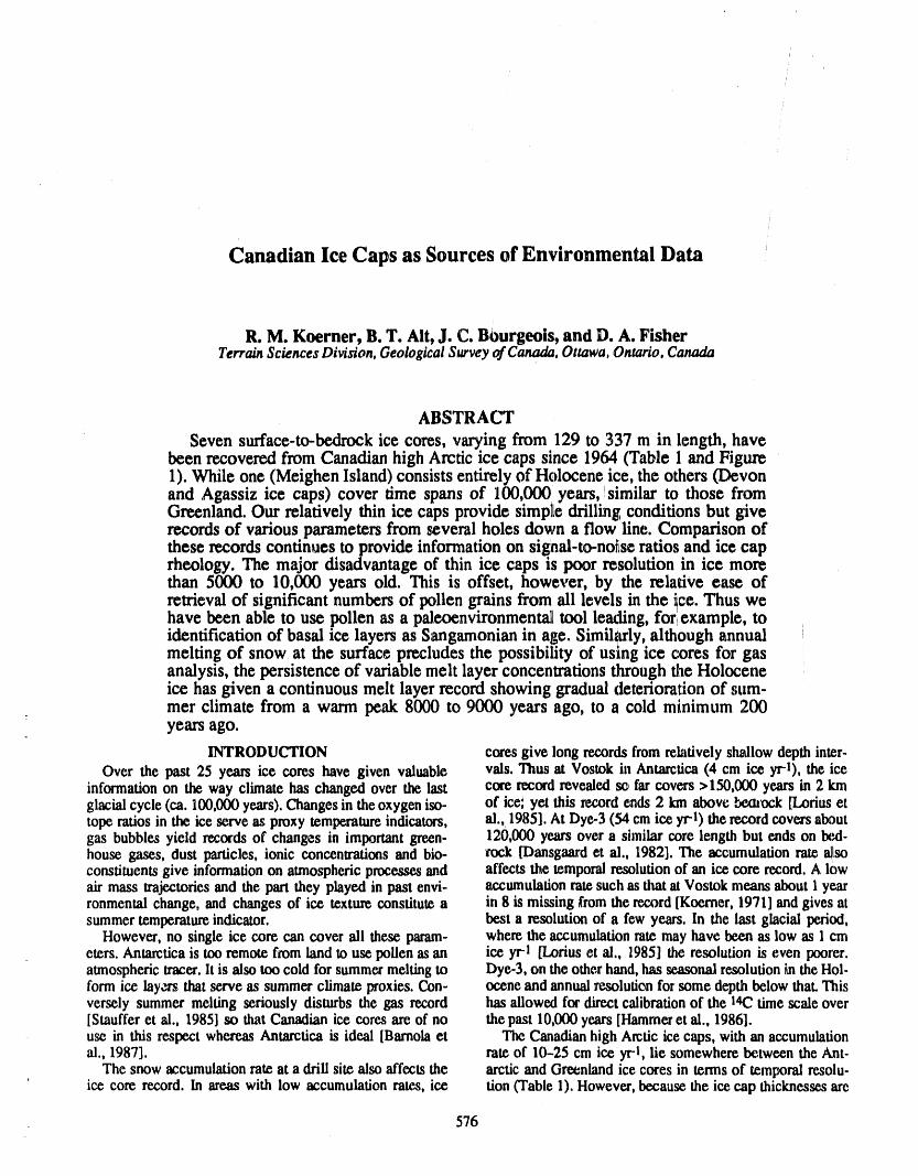
J

Canadian Ice Caps as Sources of Environmental Data

R. M. Koerner, B. T. Alt, J. C. BOurgeois, and D. A. FisherTerrainSciencesDivision,GeologicalSurveyof Canada,Ottawa,Ontario,Canada

ABSTRACT

Seven surface-to-_k ice cores, varying from 129 to 337 m in length, havebeen recovered from Canadian high Arctic ice caps since 1964 (Table 1 and Figure1). While one (Meighen Island) consists entirely of Holocene ice, the others (Devonand Agassiz ice caps) cover time spans of 100,00 0 years, similar to those fromGreenland. Our relatively thin ice caps provide simplte drilling conditions but giverecords of various parameters from several holes down a flow line. Comparison ofthese records continues to provide information on signal-to-nolse ratios and ice caprheology. The major disadvantage of thin ice caps is poor resolution in ice morethan 5000 to 10,000 years old. This is offset, however, by the relative ease ofretrieval of significant numbers of pollen grains from ali levels in the ice. Thus wehave been able to use pollen as a paleoenvironmen_l tool leading, for_example, toidentification of basal ice layers as Sangamonian in age. Similarly, although annualmelting of snow at the surface precludes the possibility of using ice c:ores for gasanalysis, the persistence of variable melt layer concentrations through tl_eHoloceneice has given a continuous melt layer record showing gradual deterioration of sum-mer climate from a warm peak 8000 to 9000 years ago, to a cold minimum 200.

years ago.

INTRODUCTION coresgive longrecordsfromrelativelyshallowdepthinter-Over the past 25 years ice cores have given valuable vals. Thusat Vostokin Antarctica(4 cm ice }x-l), the ice

informationon theway climatehas changedoverthe last corerecordrevealedso farcovers>150,000yearsin 2 kmglacialcycle (ca. 100,000years).Changesintheoxygeniso- of ice; yet this recordends2 km abovebe_ck [Loriusettoperatiosin the ice serveas proxytemperatureindicators, al., 1985].AtDye-3(54cmiceyrl) the recordcoversaboutgas bubblesyield recordsof changes in importantgreen- 120,000yearsovera similarcorelengthbutends on I_',d-house gases, dust particles,ionic concentrationsandbio- rock [Dansgaardet al., 1982].The accumulationratea_lsoconstituentsgive informationon atmosphericproc_ and affectsthe temporalresolutionof an ice core record.A lowairmass trajectoriesand the partthey playedin pastenvi- accumulationratesuchas thatatVostokmeansaboutI yearronmentalchange,and changesof ice textureconstitutea in 8 is missingfromthe record[Koexner,1971]andgivesatsummertemperatureindicator, besta resolutionof a few years.In the last glacialperiod,

However,no single ice core can coverali these param- wheretheaccumulationratemayhavebeenas low as 1 cmeters.Antarcticais too remotefromlandto usepollenasan ice yrl [Loriuset al., 1985]theresolutionis even poorer.atmospherictracer,lt is alsotoocold forsummermeltingto Dye-3,on the otherhand,hasseasonalresolutioniu theHol-formice laye_ thatserve as summerclimateproxies.Con- oceneandannualresolutionforsomedepthbelowthat.Thisverselysummermeltingseriouslydisturbsthe gas record Imsallowedfordirectcalibrationof the 14Ctimescaleover[Staufferet al., 1985]so thatCanadianice coresareof no thepast 10,000years[Hammeret al., 1986].use in thisrespectwhereasAntarcticais ideal [Barnolaet TheCanadianhighArcticicecaps, with an accumulational., 1987]. rateof 10-25 cmice yri, lie somewherebetweenthe Ant-

Thesnowaccumulationrateata drillsite alsoaffectsthe arcticand Greenlandice coresin terms of temporalresolu-' ice core record.In areaswith low accumulationrates,ice tion(Table1).However,becausethe icecap thicknessesare

576

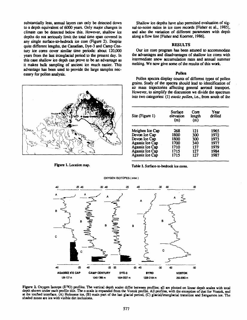
substantiallyless, annuallayers can only be detected down Shallow ice depths have also permittedevaluation of sig-to a depth equivalent of 6000 years. Only majorchanges in ,ud-to-noise ratios in ice core records [Fisher et al., 1985],climate can be detected below this. However, shallow ice and also the variation of different parameterswith depthdepths do not seriously limit the total time span covered in alonga flow line [Fisherand Koerner,1986].any single surface-to-_k ice core (Figure 2). Despitequite differentlengths, the Canadian,Dye-3 andCamp Cen- RESULTStury ice cores cover similar time periods: about 120,000 Our ice core program has been attunedto accommodateyears from the last interglacialperiod to the present day. In the advantagesand disadvantagesof shallow ice cores withthis case shallow ice depth can prove to be an advantage as intermediatesnow accumulation rates and annual summerit makes bulk sampling of ancient ice much easier. This melting.We now give some of the resultsof this work.advantagehas been used to provide the large samples nec-essary forpollen analysis. Pollen

Pollen spectradisplay counts of differenttypes of pollengrins. Study of the speclra should lead to identification ofair mass trajectories affecting general aerosol transport.

_) However, to simplify the discussion we divide the spectrum

___,_.__ lk _ __, .,' into two categories: (1)exoticpollen, i.e., from south of the! Surface Core Year

_<i_L__ Site (Figure 1) elevation length drilled• .¢_.j, ,_ ."'" (m) (m)

'l _' _-_ k "('_ Devon Ice Cap ,1800 300 1972

_,"_.,_i.:_,_,, _o _ - Devon Ice Cap 1800 300 1973: __, ....... . . _" Agassiz Ice Cap 1700 340 1977/ ........,_,_:_..- " ....." _._ AgassizIceCap 1710 137 1979\ , _..,_C_-. _ AgassizIceCap 1715 127 1984

AgassizIceCap 1715 127 1987

Flgure1. Locationmap. Table 1.Surface-to-bedrockice ceres.

OXYGEN ISOTOPES(o/oo)

-40 .25-45 .30 40 .25 -45 .30 .eO .50

-B B

B

C

40 .25 40 .25 45 .20 .45 .30 ,SO .50

AGASSIZ ICECAP CAMP CENTURY DYE-3 BYRD VOSTOK

126-137m 1040-1388m 1694-20_7m 1238-2164m 250.2083m

Figure 2. OxygenIsotope(8IS0.)profiles.The v.erticaddepthscalesdifferbetweenprofiles;ali areplottedon lineardepthscaleswithtotaldepthshownundereachprordeude.Theo-scaletsexpandedfromtheVostokpmrde.Ali pretties,wtththeexceptionof thatforVostok,endat theice/bedinterface.(A) Holoceneice, (B) ras.inpartof the lastglacialperiod,(C)glacial/interglaclaltransitionandSangamonice.Theshadedzonesareice withvisibledirtinclusions.

577

% %

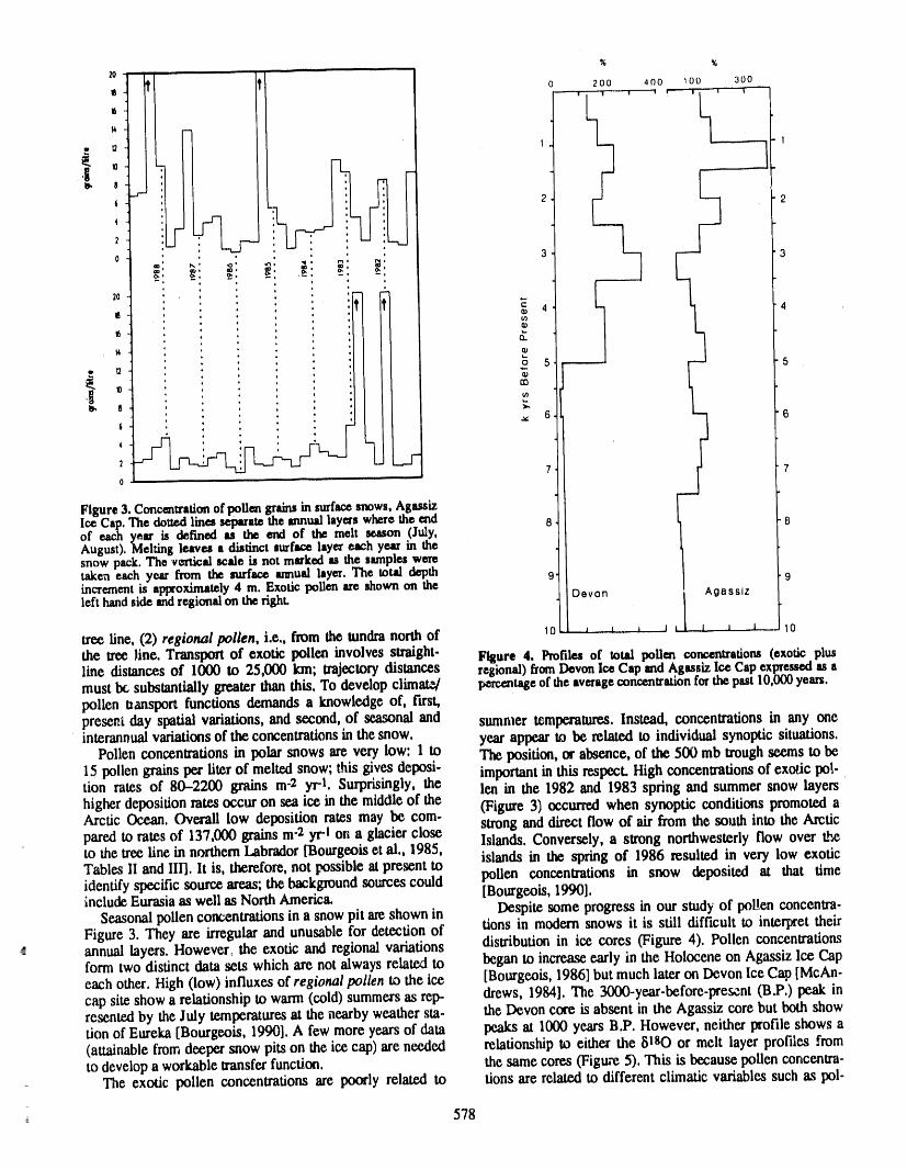
20

'I 0 I iR,_ur,n200 400 100 300z

IB -- 1 , , "I ,

. to _ I I

6 "I- 2 2

4

2 ,

0 3 3_0 _. - -. -,

o ,5 5

'[ e >" B

6

, _A" 7o

Figure 3. Concm_rafionof pollen grgm in surfacesnows, AgusizIce Cap.The dottedlines separatethe snmud layerswhere the end 8of each year is defined as the end of the melt season (July,August). Melting leaves a distinct surface layer each year in thesnow pack. The vm'ilealscsle is not msrked as the samples weretaken each year from the surface annual layer. The total depth 9increment is approximately4 m. Exotic pollen are shown on the

left handside sad regional on the riEhL II -v''''

tree line, (2) regional pollen, i.e., from tlm tundra north of l o_ othetrceline. Transport of exotic pollen involves straight- Figure 4. Profiles of total pollm cotw.en_atlom (exotic plusline distances of 1000 to 25,000 km; trajectory distances regional) fromDevon Ice Cap md Agassiz ice Capexpremmdas amust Ix: substantially greaterthanthis.To develop climate/ lint,enrageof the averageconcen_atlon forthe past10,000 years.

pollen transport functions demands a knowledge of, first,present day spatial variations,and second, of seasonal and sumntertemperatures.Instead,concentrationsin any oneintcrannual variations of the concentrations in the snow. year appear to be related to individual synoptic situations.

Pollen concentrations in polar snows are very low: 1 to The position, or absence, of the 500 mb trough seems to be15 pollen grains pcr liter of melted snow; this gives deposi- important in this respect.Highconcentrationsof exotic pol-rien rates of 80-2200 grains m-2 yrl. Surprisingly, the Iea in the 1982 and 1983 spring and summer snow layershigher deposition rates occur on sca ice in the middle of the (Figure 3) occurred when synoptic conditions promoted aArctic Ocean. Overall low deposition rates may be com- strong and direct flow of air from the south into the Arcticpared to rates of 137,000 grains m-2 yrl on a glacier close Islands. Conversely, a strong northwesterly flow over theto the tree line in northernLabrador [Bourgeois ct al., 1985, islands in the spring of 1986 resulted in very low exoticTable,s II and III]. lt is, therefore, not possible at present to pollen concentrations in snow deposited at that timeidentify specific source areas; the background sources could [Bourgeois, 1990].include Eurasia as well as North America.

Seasonalpollen concentrations in a snow pit are shown in Despite some progress in our study of pollen concentra-Figure 3. They are irregular and unusable for detection of tions in modern snows it is still difficult to interpret theirannual layers. However., the exotic and regionalvariations distribution in ice cores (Figure 4). Pollcn concentrationsform two distinct data sets which arc not always related to beganto increase early in the Holocene on Agassiz Ice Capeach other. High (low) influxes of regional pollen to the ice [Bourgeois, 1986] but much later on Devon Ice Cap [McAn-cap site show a relationship to warm (cold) summers as tcp.. drews, 1984]. The 3000-ycar-before-presant (B.P.) peak inresented by the July temperatures at the nearby weather sta- the Devon coreisabsent in the Agassiz core but both showrien of Eureka [Bourgeois, 1990]. A few merc years of data peaks at 1000 years B.P. However, neither profile shows a(attainable from deeper snow pits on the ice cap)are needed relationship to either the 8180 or melt layer profiles fromto develop a workable transfer function, the same cores (Figth-e 5), This is because pollen concentra-

The exotic pollen concentrations are poorly related to lions arc related to different climatic variables such as pol-

578z

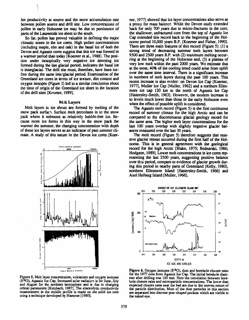
len produc_vity at sourceand the snow accumulation rate net, 1977] showed that ice layer concentrationsalso serveasbetween polien somr.eand drill site. Low concentrationsof a proxy for mass balance.While the Devon study extendedpollen in early Holocene ice may be due to persistence of back for only 700 yearsdue to micro-fracturesin the core,partsof theIaturentide ice sheet to the south, the shallower, unfracturedcore from the top of Agassiz Ice

So far, pollen has proved valuable in defining the major Cap extendedthis recordback to the beginning of the Hol-climatic zones in the ice cores, High pollen concentrations ocene period 10,000 yearsB.P, [Kocmer and Fisher, 1990].(including maple, elm and oak) in the basal ice of both the There are threemain featuresof this record(Figure 5): (1) aDevon and Agassiz cores suggest thatthis ice was formed in strong trend of decreasing summer ntelt layers betweena warmerperiodthantoday[Koemer et al,, 1988].The posi- 9500 and 2500 yearsB.P. with(2) maximummeltingoccur-don under isotopically very negative ice denoting ice ring at the beginning of the Holocene and, (3) a plateau offormedduringthe last glacial period, indicates the basal ice very low melt within the past 2000 years. We estimate thatis interglacial.The drill site must, therefore, have been ice- at the most, 40%of the cooling trendcould arise from upliftfree duringthe same inte,,glacialperiod.Examinationof the over the same time interval. There is a significant increaseGreenlandice cores in terms of ice texture, din content and in numbers of melt layers during the past 100 years. Thisoxygen isotopes (Figure2) led to a similarconclusion ebout recent increase is also evide_'0on Devon Ice Cap [Koerner,the time of origin of th_ Greenlandice sheet in the location 1977], Muller Ice Cap [Muller, 1962] and a northernElles-

mete ice cap 120 km to the north of Agassiz Ice Capof the drill sites [Ko,'_,a-ner,1989]. [Hattersley-Smith, 1963]. However, the modem increase is

to levels much lower than those in the early Holocene evenMe.llLayers when the effect of possible uplift is considered.

Melt layers hi ice sheets are formed by melting of the The Agassiz melt record(Figure 5) is the fast continuoussnow pack surfac-,.Surfacemelt percolates in to the snow record of summer climate for the high Arctic and can bepack where it refieezes as relatively bubble-free ice. Be- compared to the discontinuous glacial geology record forcause more ice forms in this way in the snow pack the the same area.The highermelt layer concentrationsfor thewarmerthe summer, the changingconcentrationwith depth last 100 years overlap with slightly negative glacier bal-of these ice layers serves as an indicatorof past summercii- ances measuredover the last30 years.mate. A study of this naturein the Devon ice cores [Koer- The melt record(Figure 5) therefore suggests that mas-

sive glacier retreatoccurredduring the first half of the Hol.ocene. This is in general agreement with the geological

,o '"" '_'o..... _" . ,o_o0 record for the high Arctic [Blake, 1975; Bednarski, 1986;

.'- ..... __t,. Hodgson, 1989]. Lower melt concentrationsin ice cores =ep-t

resenting the last 2500 years, suggesting positive balanceover tha;.period, compareto evidence of glacier growth dur-

: .i : ing this period in nearbyparts of Greenland [Kelly, 1980],

" m -; northern Ellesmere Island [Hattersley-Smith, 1966] and

"' ; Axel HeibergIsland [Muller,1966].

i I kGASSIZICECkP,ELLESMEREISLANO........... 324 326 328 330 332 334 336 338

•300 _ ' ' ' J i , t < I , , , .20

: 6(_o)i

_, t I)l_lllllit

. _-

,_ I(_ -4_

ia_ i , ,r LA,• 0 ---' _ 40324 ,,126 328 330 332 -134 _

; DEPTHi

ICEAGEANDEARLIER

0 8,00 lO000

6. Oxygenisotopes 8180_dustandboreholeclo_urerates,.... ,.,.,., ...... Figure o '-- ( "forthe1977corefl m AgassizIceCap.Theinitialboreholediam.

Figure5. Meltlayerconcentration,volcanismandoxygenisotopes eterafterdrillingwas 160mm.Notethecorrele_ionbotweenbore-(61sO),AgassizIceCap.Increasedsolarradiationis forJune,July hole closureratesandmicroparticleconcentrations.TlmlowerthanandAugustfor the northernhomisphereand is due to changing expectedclosureratesne&thebedaredueto the unevennatureoforbitalparameters[Kutzbaeh,1987].Theelectrolyticconductivity theparticledistribution.Mostof the dustparticlesin thissectionmeasurementin the middlepro/deis madeon die solid ice core are sel_aratedintodiscretepear-shapedpocketswhicharevisibleusingatechniquedevelopedbyHamm="[1980]. then_leoeye.

579

Rheology rapidboreholeclosure ratesoccurin the latterice, The bore-

Because they are relatively thin (100-500 m of ice), holes and cores fromAgassiz Ice Cap haveshown the sameCanadianice caps are suited to the study of ice dynamics characteristics [Fisher and Koemer, 1986]. The differentand ice rheology. For example, four surface-to-bedrock rheological and, hence, dynamic propertiesof the ice havecores drilled from the top of Agassiz ice cap and down the been partlyattributedto differences in the concentrationsofflowline, requiredonly 728 m of drilling. Yet each core coy- microparttclesin each type of ice [Koemer and Fisher,ers a complete glacial cycle, including soft glacial-periodice, stiff Holocene ice and sections with unique micro- 1979;Fishar and Koerner,1986] although this has be_ con-particle and ionic signatm'es. Studies on Devon Ice Cap tested by Dural and Lorius [1980]. Furtherwork on this,[Paterson, 1977] showed differences between the rheolog- andother problemsof ice dynamicsis continuing [Wadding-ical properties of Holocene and glacial period ice; more ton etal., 1985].

580

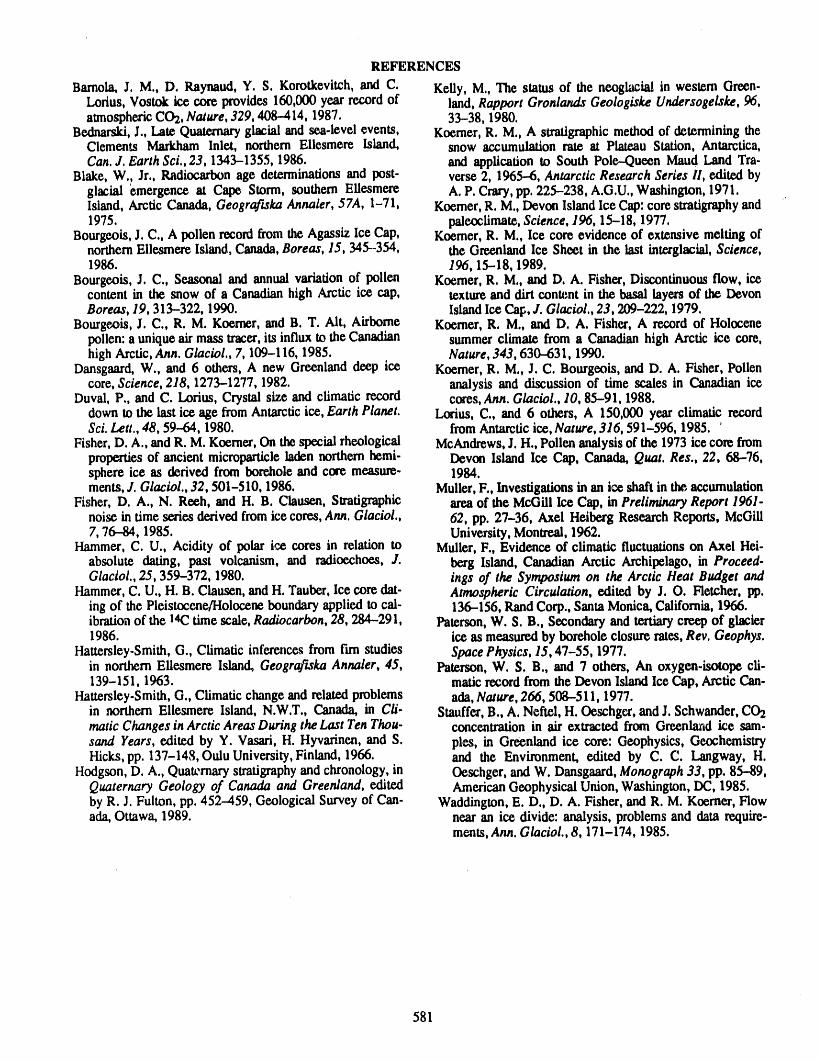
REFERENCES

Barnola, J. M., D. Raynaud, Y. S. Korotkevitch, and C. Kelly, M., The status of the neoglacial in western Green-Lorius,Vostok ice core provides 160,000 year record of land, Rapport Gronlands Geologiske Underso&elske, 96,atmosphericCO'z,Nature, 329, 408-414, 1987. 33-38, 1980.

Bednarski,J., Late Quaternaryglacial and sea.level events, Koemer, R. M., A stratigraphicmethod of determining theClements Markham Inlet, northern Ellesmere Island, snow accumulation rate at Plateau Station, Antarctica,Can. J. Earth Sci., 23, 1343-1355, 1986. and application to South Pole.Queen Maud Land Tta-

Blake, W., Jr., Radiocarbon age determinations and post- verse 2, 1965--6,Antarctic Research Series H, edited byglacial 'emergence at Cape Storm, southern Ellesmere A.P. Crary,pp. 225-238, A.G.U., Washington, 1971.Island, Arctic Canada,Geografiska Annaler, 57A, 1-71, Koemer, R. M., Devon Island Ice Cap:core stratigraphyand1975. paleocfimate,Science, 196, 15-18, 1977.

Bourgeois, J. C., A pollen record fxom the Agassiz Ice Cap, Koemer, R. M., Ice core evidence of extensive melting ofnorthernEllesmere Island, Canada,Boreas, 15, 345-354, the Greenland Ice Sheet in the last interglacial,Science,1986. 196, 15-18, 1989.

Bourgeois, J. C., Seasonal and annual variation of pollen Koemer,R. M., and D. A. Fisher, Discontinuous flow, icecontent in the snow of a Canadianhigh Arctic ice cap, textureand dirt content in the basal layers of the DevonBoreas, 19, 313-322, 1990. IslandIce Ca_, J. Glaciol., 23,209-222, 1979.

Bourgeois, J. C., R. M. Koerner,and B. T. Alt, Airborne Koerner,R. M., and D. A. Fisher, A record of Holocenepollen:a uniqueairmass tracer,its influx to the Canadian summerclimate from a Canadian high Arctic ice core,high Arctic,Ann. Glaciol., 7, 109-116, 1985. Nature, 343, 630-631, 1990.

Dansgaard,W., and 6 others, A new Greenland deep ice Koerner,R. M., J. C. Bourgeois, and D. A. Fisher, Pollencore,Science, 218, 1273-1277, 1982. analysis and discussion of time scales in Canadian ice

Duval, P., and C. Lorius, Crystal size and climatic record cores,Ann. Glaciol., 10, 85-91, 1988.down to the [ast ice age from Antarcticice, Earth Planet. [.orins, C., and 6 others, A 150,000 year climatic recordSci. Lett., 48, 59--64, 1980. from Antarctic ice, Nature, 316, 591-596, 1985. '

Fisher, D. A., and R. M. Koerner,On the specialrheological McAndrews,J. H., Pollen analysisof the 1973 ice core fromproperties of ancient microparticleladen northern hemi- Devon Island Ice Cap, Canada, Quat. Res., 22, 68-76,sphere ice as derived from borehole and core measure- 1984.ments,J. Glaciol., 32,501-510, 1986. Muller,F., Investigations in an ice shaft in the,accumulation

Fisher, D. A., N. Reeh, and H. B. Clausen, Stratigraphic areaof the McGill Ice Cap, in Preliminary Report 1961-noise in time series derived from ice cores, Ann. Glaciol., 62, pp. 27-36, Axel Heiberg Research Reports, McGill7, 76-84, 1985. University, Montreal, 1962.

Hammer, C. U., Acidity of polar ice cores in relation to Muller,F., Evidence of climatic fluctuationson Axel Hei-absolute dating, past volcanism, and radicechoes, J. berg Island, Canadian Arctic Archipelago, in Proceed-Glaciol., 25,359-372, 1980. ings of the Symposium on the Arctic Heat Budget and

Hammer, C. U., H. B. Clausen,and H. Tauber,Ice core dat- Atmospheric Circulation, edited by J. O. Fletcher, pp.ing of the Pleistocene/Holocene boundaryapplied to cal- 136-156, RandCorp., Santa Monica, California,1966.ibrafionof the 14(2time scale, Radiocarbon, 28, 284-291, Paterson, W. S. B., Secondary and tertiarycreep of glacier1986. ice as measuredby borehole closure rates,Rev. Geophys.

Hattersley-Smith,G., Climatic inference,_from tim studies Space Physics, 15, 47-55, 1977.in northern Eilesmere Island, Geografiska Annaler, 45, Paterson, W. S. B., and 7 others, An oxygen-isotope cli-139-151, 1963. matic recordfrom the Devon Island Ice Cap, Arctic Can-

Hattersley-Smith,G., Climatic change and related problems ada, Nature, 266, 508-511, 1977.in northernEllesmere Island, N.W.T., Canada, in Cii- Stauffer,B., A. Neftel, H. Oeschger,and J. Schwander, CO2matic Changes in Arctic Areas During the Last Ten Thou. concentration in air extracted from Greenland ice sam-sand Years, edited by Y. Vasari, H. Hyvafinen, and S. pies, in Greenland ice core: Geophysics, GeochemistryI-ticks,pp. 137-148, Oulu University,Finland,1966. and the Environment, edited by C. C. Langway, H.

Hodgson, D. A., Quaternarystratigraphyand chronology, in Oeschger, andW. Dansgaard,Monograph 33, pp. 85-89,Quaternary Geology of Canada and Greenland, edited AmericanGeophysical Union, Washington, DC, 1985.by R. J. Fulton, pp. 452-459, Geological Surveyof Can- Waddington,E. D., D. A. Fisher, and R. M. Koerner, Flowada,Ottawa, 1989. near an ice divide: analysis, problems and data require-

meats, Ann. Glaciol., 8, 171-174, 1985.

581

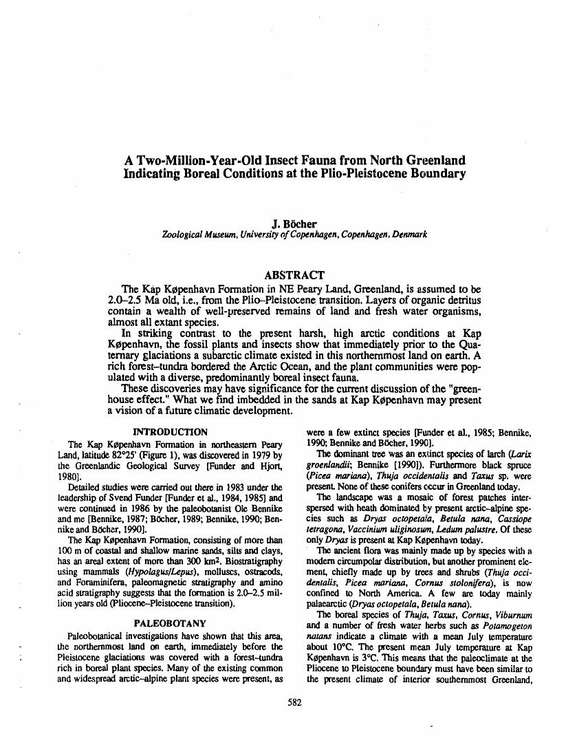
A Two-Million.Year.Old Insect Fauna from North GreenlandIndicating Boreal Conditions at the Plio.Pleistocene Boundary

J. B6cherZoological Museum, Universityof Copenhagen, Copenhagen, Denmark

ABSTRACT

The Kap Klapcnhavn Formation in NE Peary Land, Greenland, is a,ssumed to be2.0-2.5 Ma old, i.e., from the Plio-Pleistocene transition. Layers of organic detrituscontain a wealth of well-preserved remains of land and fresh water organisms,almost ali extant species.

In striking contrast to the present harsh, high arctic conditions at KapKCpcnhavn, the fossil plants and insects show that immediately prior to the Qua-ternary glaciations a subarctic climate existed in this northernmost land on earth. Arich forest-tundra bordered the Arctic Ocean, and the plant communities were pop-ulated with a diverse, predominantly boreal insect fauna.

These discoveries may have significance for the current discussion of the "green-house effect." What we f'md imbedded in the sands at Kap K_penhavn may presenta vision of a future climatic development.

INTRODUCTION were a few extinct species [Funderet al., 1985; Bennike,The Kap K_penhavn Formation in northeasternPeary 199(_,BennikeandBtcher, 1990].

Land,latitude82025, (Figure 1), was discovered in 1979 by The dominant tree was an extinct species of larch(Lar/xthe Greenlandic Geological Survey [Funder and Hjort, groenlandii; Bennike [1990]). Furthermore black spruce1980]. (Picea mariana), Thuja occidentalis and Taxus sp. were

Detailed studies were carriedout there in 1983 under the present.None of these conifers cr,._urin Greenlandtoday.leadershipof Svend Funder [Funderet al., 1984, 1985] and The landscape was a mosaic of forest patches inter-were continued in 1986 by the paleobotanistOle Bennike spersed with heath dominated by present arctic-alpine spe-and me [Bennike, 1987; BOchex, 1989; Bennike, 1990; Ben- cies such as Dryas octopeta_Lz,Betula nana, Cassiopehike andB0cher, 1990]. tetragona, Vaccinium uliginos_, Ledum palustre. Of these

The Kap KCpcnhavnFormation,consisting of more than only Dryas is presentat Kap Kepenhavn today.100 m of coastal and shallow marine sands,silts and clays, The ancient flora was mainly made up by species with ahas an areal extent of more than 300 km2. Biostmtigraphy modem circumpolardistribution,but another prominentele-using mammals (HypolaguslLepus), molluscs, ostracods, ment, chiefly made up by trees and shrubs (Thuja occi-and Foraminifera, paleomagnetic stratigraphyand amino dentalis, Picea mariana, Comus stolonifera), is nowacid stratigraphysuggests that the formationis 2.0-2.5 mit- confined to North America. A few are today mainlylion yearsold (Pliocene-Pleistocene Wansition). palaea_tic (Dryas octopetala, Betula nana).

The boreal species of Thuja, Taxus, Comus, ViburnumPALEOBOTANY and a number of fresh water herbs such as Potamogeton

Paleobotanical investigations have shown that this area, natans indicate a climate with a mean July temperaturethe northernmostland on earth, immediately before the about 10°C. The present mean July temperatureat KapPleistocene glaciations was covered with a forest-tundra K0penhavn is 3°C. This me_ls that the paleoclimate at therich in boreal plant species. Many of the existing common Pliocene to Pleistoceneboundary must have been similartoand widespreadarctic--alpineplant species were present, as the present climate of interior southernmost Greenland,

582

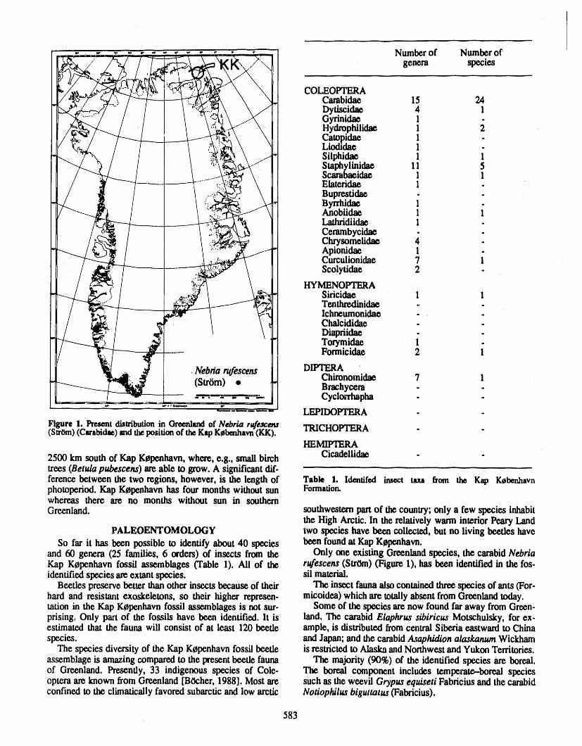
COLEOPTERACarabidae 15 24Dytiscidae 4 iGyrinidae , I -Hydrophilidae I 2Catopidae I -Liodidae 1 -Silphidae 1 1Staphyiinidae 11 5Scarabaeidae 1 1Elateridae 1 .Buprestidae . -Byrrhidae 1 -Anobiidae I 1Lathridiidae 1 -Cerambycidae . .Chrysomelldae 4 -Apionidae 1 -Curculionidae 7 1Scolytidae 2 -

HYMENOPTERASiricidae 1 1Tenthredinidae ., .Ichneumonidae . -Chalcididae . -Dlapriidae . .Torymidae 1 .Formicidae 2 I

Nebrla ntfescens DIPTERAChironomidae 7 1

(Str6m) • Brachycem - -" I[ " "[J: 1 _ Cyclondmpha - -

•0. v f tmm,,_ lm

LEPIDOPTERA - -

Figure 1. Presentdistributionin Greenlandof Nebria rufescens(StrOm)(Carabidae)andthepositionof theKapK_benhavn(KK). TRICHOPTERA . -

HEMIFTERA

2500 km south of Kap KCpenhavn,where, e.g., small birch Cicadellidae - -trees (Betula pubescens) areable to grow. A significant dif-ference between the two regions, however, is the length of Table 1. Identifed insect taxa from the Kap Kebenhavnphotoperiod.Kap KCpenhavnhas four months without sun Formation.whereas there are no months without sun in southernGreenland. southwestern partof thecountry;only a few species inhabit

the High Arctic. In the relatively warm interiorPeary LandPALEOENTOMOLOGY two species have been collected, but no living beetles have

So far it has been possible to identify about 40 species been foundat KapKepenhavn.and 60 genera (25 families, 6 orders) of insects from the Only one existing Greenlandspecies, the carabidNebriaKap KCpenhavn fossil assemblages (Table 1). Ali of the r_escens (StrUm)('Figure1), has been identified in the fos-identified species areextantspecies, sil material.

Beeries preservebetter thanother insects because of their The insect faunaalso contained threespecies of ants (For-hard and resistant exoskeletons, so their higher represen, micoidea) which are totallyabsent fromGreenlandtoday.ration in the gap K_penhavnfossil assemblages is not sur- Some of the species are now found far away from Green-prising. Only part of the fossils have been identified, lt is land. The carabidElaphrus sibiricus Motschulsky, for ex-estimated that the fauna will consist of at least 120 beetle ample, is distributedfromcentralSiberia eastwardto Chinaspecies, and Japan;and the carabid Asaphidion alaskanum Wickham

The species diversity of the Kap KCpenhavn fossil beetle is restricted to Alaska and Northwest and Yukon Territories.assemblage is amazing comparedto the present beetle fauna The majority (90%) of the identified species are boreal.of Greenland. Presently, 33 indigenous species of Cole- The boreal component includes temperate-boreal speciesoptera are known from Greenland [B0cher, 1988]. Most are such as the weevil Grypus equiseti Fabriciusand the carabidconfined to the climatically favored subarctic and low arctic Notiophilus biguttatus ('Fabricius).

583

Many species are associated with fresh water biotopes, holarctlc while the remainder are nearctic (30%) andliving in damp, luxuriantplaces close to the water (e,g., the palaearctic(15%).carabidgeneraNebrla and Patrob_). Others, however, live The paleontological and paleobotanlcal inte.rpretationson open, sandy or gravelly shores and banks of lakes and based on Kap Kepeahavn Formation fossils are in agree-streams. These are generally thermophilous, diurnal and meat. The environment2 million years ago was biologicallyhighly active predators,hunting by means of vision and, highly varied, in contrastto the presentdesert-like,high arc-accordingly,depeadenton a high incidenceof sunshinedur- tic conditions.

ing the active season (species of the carabid genera Cictn-dela, Elaphr_, AsapMdion, Bembidion, Notiophilus and the CONCLUSIONSstaphylinidgenus Stenus). Studies during the last three decades, primarily in the

Few limnic species have been identified, but the largenumberof unidentifiedwaterbeetles (more than 20 species) UK. and North Amexica, have shown that subfossil insectplus manylarvalfragmentsof caddisflies (Trichoptera)and assemblages, especially beetles, are a highly effective teelmidges (Chironomidae) indicate the presence of an abun- for the reconstruc0onof ancientenvironments [e.g., Coopo,dance of different freshwaterbiotopes in the ancient land- 1975, 1979, 1986; Matthews, 1977, 1988]. A method forscape. The occurrenceof the dytiscid beetle Agabus bifarias quantifyingpaleoclimatteinformationfrom the presentgee.(Kirby)is especially interestingbecause its presenthabitatis graphicrangesof beetles has been utilized to producepaleo-stated to be shaded, temporaryponds in rough fescue (Pea) temperature curves in the United Kingdom [Atkinson ct al.,prairiein NorthAmerica [Larson, 1975]. 1987].

Other species indicate dune areas (Aegialia), open tundra The Kap K0peahavn Formationis well dated at 2 millionand fairlyxericheatldand, years ago. During its deposition the position of the con-

A number of species and genera such as the carabid tinents andoceans, the orientationof the earth's axis, and thegenus Dromius, the "death watch beetle" (Hadrobregmus position of the North Pole were ali similar as today.pertinax (L.)), woodliving weevils (Pissodes), bark beetles The fossils from the Kap Kl_penhavnFormation at the(Scolytus, Pityophthorus) and the carpenter ant (Cam- Plio--Pleistocene boundary imply a climate, 800 kin fromponotus herculeanus (L.)) are intimately connected with the North Pole, that was significantiy warmer, allowingtrees and thus represent further evidence of the existence of trees to grow on the beaches of the Arctic Ocean.in situ forest when the Kap KCpenhavn sediments weredeposited. Fly holes and galleries in fossil wood reveal the The Kap Kopenhavn Formation thus presents---to citeexistence of still more arbofieolous forms such as Bupres- Russell Coopo (in litt.)----"ascenario that may indicate thetidae, Cerambycidae 0onghorn beetles) and the giant tree possible consequences of global warming on a world whosewasp, Urocerus #gas (L.). geography is much as we see it today, but a scenario that has

Similar to the biogeography of the fossil flora, the major- no equivalent at the present day or in later Pleistoceneity (55%) of the identified insect species are circumpolar or interglacials."

REFERENCES

Atkinson, T. C., K. R. Briffa, and G. R. Coope, Seasonal Coope, G. R,, Coleoptera analysis, in Handbook of Hal.temperatures in Britain during the past 22,000 years, ocene Palaeoecology and Palaeohydrology, exYitedbyreconstructed using beetle remains, Nature, 325, 587- B.E. Berglund, pp. 703-713, John Wiley & Sons,592, 1987, Chichester, 1986.

Bennike, O., News from the Kap K_penhavn Formation, Funder, S., and C. Hjort, A reconnaissance of the Qua-Plio-Pleistocene, North Greenland, Polar Research, 5, ternary geology of Eastern North Greenland, GrCnlands339-340, 1987. Geologiske UndersCgelse,Rapport, 99, 99--105, 1980.

Bennike, O., The Kap K0penhavn Formation: stratigraphyand palaeobotany of a Plio-Pleistocene sequence in Peary Funder, S., O. Bennike, G. S. Mogeasen, B. Noe-Nygaard,Land, North Greenland, Meddelelserom GrCnland, Geo- S.A.S. Pedersen, and K. S. Petersea, The Kapscience 23, 85 pp,, 1990. KCpenhavn Formation, a late Cainozoic sedimentary

Bennike, O., and J. B_cher, Forest--tundra neighbouring the sequence in North Greenland, GrCnlands GeologiskeNorth Pole: Plant and insect remains from the Plio- Undersegelse, Rapport, 120, 9-18, 1984.Pleistocene Kap KCpenhavn Formation, North Green- Funder, S., N. Abrahamsen, O. Bennike, and R. W. Feyling-land, Arctic, 43,331-338, 1990. Hansen, Forested Arctic: Evidence from North Green-

B0cher, J., The Coleoptera of Greenland, Meddelelser am land, Geology, 13, 542-546, 1985.GrCnland,Bioscience 26, 100pp., 1988. Larson, D. J., The predacious water beetles (Coleoptera:

B0cher, J., 1989, Boreal insects in northernmost Greenland: Dytiscidae) of Alberta: Systematics, natural history andpalaeo-entomological evidence from the Kap KOpenhavn distribution, Quaestiones Entomologicae, 11, 245--498,Formation (Plio-Pleistocene), Peary Land, Fauna nor. 1975.vegica, Ser. B, 36, 37.-43, 1989,

Coope, G. R., Climatic fluctuations in Northwest Europe Matthews, J. V., Coleopterafossils: their potential value forsince the last interglacial, indicated by fossil assemblages dating and correlation of late Cenozoic sediments, Can. J.of Coleoptera, in Ice Ages, Ancient and Modem, edited Earth Sci., 14, 2339--2347, 1977.by A. E, Wright and F. Mosely, pp. 153-168, Geological Matthews, J. V., Late Tertiary arctic environments: A visionJournal, Special Issue 6, 1975. of the future?, Geos, 18, 14-18, 1989.

584

Late Quaternary Paleoceanography and Paleoclimatologyfrom Sediment Cores of the Eastern Arctic Ocean

U. Pagels and S. K6hlerGEOMAR,ResearchCenterfor MarineGeosciences,Kiel,Germany

t

ABSTRACT

Box cores recovered along a N-S transect in the Eurasian Basin allow theestablishment of a time scale for the LateQuaternary history of the Arctic Ocean,based on stable oxygen isotope stratigraphy and AMS 14C dating of planktonicforaminifers (N. pachyderma 1.c.). This high resolution stratigraphy, in combinationwith sedimentological investigations (e.g., coarse fraction analysis, carbonatecontent, productivity of foraminifers), was carried out to reconstruct the glacial andinter-glacial Arctic Ocean paleoenvironment.

The sediment cores, which can be correlated throughout the sampling area in theEastern Arctic Ocean, were dated as representing oxygen isotope stages 1 to 4/5.The sedimentation rates varied between a few mm ka-1 in glacials andapproximately one cm ka-I during the Holocene. The sediments allow a detailedsedimentological description of the depositional regime and the paleoceanographyof the Eastern Arctic Ocean.

Changing ratios of biogenic and lithogenic components in the sediments reflectvariations in the oceanographic circulation pattern in the Eurasian Basin during theLate Quaternary. Carbonate content (1-9wt.%), productivity of foraminifers (highin interglacial, low in glacial stages) and the terrigenous components are in goodcorrelation with glacial and interglacial climatic fluctuations.

585

The Record of Global Change in Circum.Antarctic Marine Sediments

d,

P. F. Barker, C. J. Pudsey, and R. D. LarterBritishAntarcticSurvey(NaturalEnvironmentResearchCouncil),Cambridge,England

*j

ABSTRACT

Sediment drilling, using rigs located on sea ice inshore, and Ocean IMilHng Pro..gram facilities farther offshore, have described the stepwise cooling of Antarcticathrough the Cenozoic, setting the scene for more detailed studies of short-period,recent change. Such studies will not be easy. The virtual absence of carbonate sedi-ments and the strength of bottom currents in some regions are fundamental limita-tions. Nevertheless, Antarctic ocean sediments contain a recoId of global changewhich complements the record of the ice sheet, and extends it back m time. Pelagicand hemipelagic sediments of the ocean basins record changes in primary pro-ductivity, dissolution, sea ice extent and the strength of deep ocean circulation, andin the volume of the main circum-Antarctic water masses. Prograded sediments ofthe Antarctic continental shelf and slope contain a record of glacial/interglacialchanges in ice sheet volume. Modern piston-coring techniques are capable ofrevealing changes over the last glacial cycle in some detail, in suitably expandedsections. At lower sediment accumulation rates, a less detailed but longer recordcan be obtained. It can already be shown that, at and around glacial maximum, (a)grounded ice sheets extended to the Antarctic continental shelf edge, (b) the mar-ginal sea ice zone lay up to 5° farther north, and (c) Weddell Sea Bottom Waterflow was far slower than at present. These have implications for the carbon cycle in

° the oceans, which is of considerable importance in global change.

INTRODUCTION transport,involveiceshelves,sea ice andbottomwaterfor-Theprincipalelementsof thecircum-Antarcticclimatic marionandthevigorandaxialpositionof the ,ACC.

regimeare the continentalice sheet and its fringingice The circum-Antarcticmarinesedimentaryrecord,sam-shelves,sea ice andthe two maincomponentsof Southern pied principallyby DSDPandODP drilling,containsevi-Ocean circulation,AntarcticBottom Water (AABW)and, denceof the long-termdevelopmentof the presentregime,boundingthe Antarcticregion in the north, the Antarctic which sets the scene for the studyof short-term(glacial/CircumpolarCurrent (ACC). These are ali potentially interglacial)change.For example,althoughpaleomagneticimportantto any assessmentof global climate change,not measurementsshow Antarcticato have lain over the southonly as sensitiveindicatorsof change but also as parts of poleformore than90 Ma [e.g.,NortonandSclater,1979],apowerfulclimaticfeedback mechanisms.For example,ice continentalice sheetappears to haveextended to sea levelsheetmelt,sea level rise, ice sheet/shelfflotationandbreak- (as demonstratedby glacial diamictites and by ice-raftedout (with shelf encroachmentof warmer water), lossof ice debris in marine sedimentsof Oligoceneand youngeragesheet support and enhanced flow form a potent positive [see Schlich,Wise et al., 1989; Kennettand Barker, 1990feedback loop [Bentley, 1984; Fastook, 1984; Potter and for example])only during the last 40 Ma. The details ofParen, 1985]. Another such is ice sheet/shelfand sea ice waxingand waningof the ice sheet since then are disputedmelting and global albedo reduction [e.g., ShhJe et al., [e.g., Miller et al., 1987; Shackleton, 1987; Prenticeand1984].Other loops,affectingbiogenicproductivityandCO2 Matthews, 1988], but oxygen isotopic measurementson

586

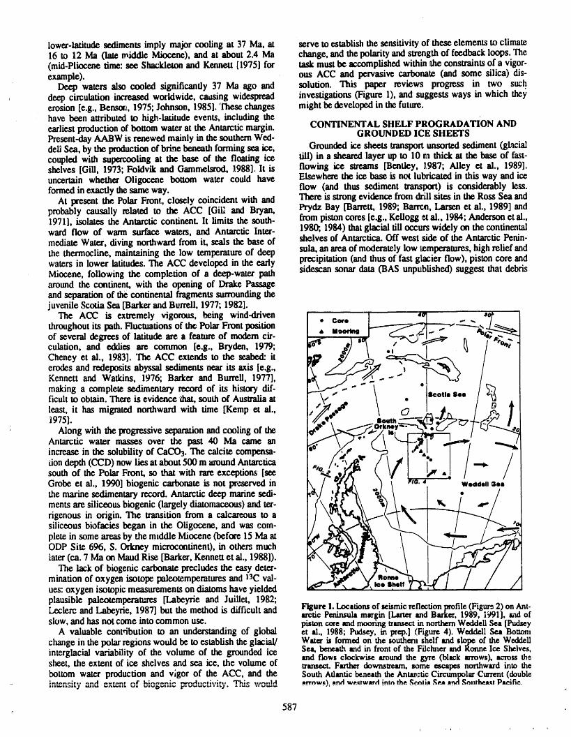
lower-latitudesediments imply majorcooling at 37 Ma, at serve to establishthe sensitivityof these elements to climate16 to 12 Ma (late middle Miocene), and at about 2.4 Ma change, and the polarityand strengthof feedbackloops. The(mid-Pliocenetime: see Sha_idetonand Kennett [1975] for task mustbe accomplishedwithin the constraintsof a vigor-example), ous ACC and pervasive carbonale (and some silica) dis-

Deep waters also cooled significantly 37 Ma ago and solution. This paper reviews progress in two such, deep circulation increased worldwide, c_dsing widespread investigations (Figure 1), and suggests ways in which they

erosion [e.g., Ben.¢_, 1975;Johnson, 1985].These changes might bedeveloped in the futm'e.have been attributedto high-latitude events, including theearliestproductionof bottom water at the Antarcticmargin. CONTINENTAL SHELF PROGRADATiON ANDPresent-dayAABW is renewed mainly in the southernWed- GROUNDED ICE SHEETSdeUSea, by the productionof brinebeneath formingsea ice, Groundedice sheets transportunsortedsediment (gt_ialcoupled with supercooling at the base of the floating ice till) in a shearedlayer up to 10 m thick at the base of fast-shelves [Gill, 1973; Foldvik and Gammelsrod, 1988], lt is flowing ice streams [Bentley, 1987; Alley el al., 1989].uncertain whether Oligocene bottom water could have Elsewhere the ice base is not lubricatedin this way and iceformedin exactly thesame way. flow (and thus sediment translxa't) is considerably less.

At present the Polar Front, closely coincident with and There is strongevidence,from drill sites in the Ross Sea andprobably causally related to the ACC [GiII and Bryan, Prydz Bay [Barrett, 1989; Barton, Larsen et al., 1989] and1971], isolates the Antarcticcontinent, lt limits the south- frompistoncores [e.g., Kellogg (_ al., 1984;Andersonet al.,ward flow of warm surface waters, and Antarctic Inter- 198_, 1984) thatglacial fill occurs widely on the continentalmediateWater, diving northwardfrom it, seals the base of shelves of Antarctica. Off west side of the AntarcticPenin-the thermocline, maintaining the low temperatureof deep sula, an areaof moderatelylow temperatures,high relief andwaters in lower latitudes. The ACC developed in the early precipitation(and thus of fast gYtacierflow), piston core andMiocene, following the completion of a deep-water path side,wan sonar data (BAS unputblished)suggest that debrisaround the continent, with the ofening of Drake Passageandseparationof the continental fragmentssurroundingthejuvenile Scotia Sea [Barkerand Burrell, 1977; 1982].

The ACC is extremely vigorous, being wind-driven Com

throughout its path.Fluctuationsof the PolarFrontposition uee,t,_of several degrees of latitude are a featureof modem cir-culation, and eddies are common [e.g., Bryden, 1979;Cheney et al., 1983]. The ACC extends to the seabed: iterodesand redepositsabyssal sediments near its axis [e.g.,Kennel/ and Walkins, 1976; Barker and Burr,II, 1977],

I,

making a complete sedimentary record of its hLqory dif- I_otia Semficult to obtain. There is evidence that, south of Australiaatleast, it has migrated northward with time [Kemp el al.,i975].

Along with the progressiveseparationandcooling of theAntarctic water masses over the past 40 Ma came anincreasein the solubility of CaCO3. The calcite compensa-tion depth (CCD) now lies atabout 500 m aroundAntarcticasouth of the Polar Front, so that with rareexceptions [seeGrobe et al., 1990] biogenic carbonate is not preserved inthe marine sedimentaryrecord. Antarctic deep marinesedi-ments aresiliceous biogenic (largelydiatomaceous)and ter-rigenous in origin. The transition from a calcareous to asiliceous biofacies began in the Oligocene, and was com-plete in some areasby the middle Miocene (before 15 Ma atODP Site 696, S. Orkney microcontinent),in other_muchlater(ca. 7 Ma on MaudRise [Barker,Kenne_tet al., 1988]).

The lack of biogenic carbonateprecludes the easy deter-minationof oxygen isotope paleotemperaturesand 13Cval-ues: oxygen isotopic measurementson diatomshave yieldedplausible paleotemperamres [Labeyrie and Juillet, 1982;

Figure1. Locationsof seismicreflectionprofile(Figure2) onAnt-Lecle_ andLabeyrie, 1987] but the method is difficult and arcticPeninsulamm'gin[LanerandBarker,1989, 1991],_d ofslow, andhas not come into common use. pistoncoreandmooring transect innorthernWeddellSea [Pudsey

A valuable contribution to an understandingof global et al., 1988; Purls,y,in prep.]_Figure4). WeddellSea Bottomchange in the polarregions would be to establish the glacial/ Water is formedon the southernshelf andslope of the Weddellinterglacial variability of the volume of the grounded ice Sea, beneathandin frontof the FiichnerandRonneIce Shelves,

and flows clockwise around the gyre Col_k arrows), across thesheet, the extent of ice shelves and sea ice, the volume of transect.Fartherclow_trean_ro)meescapes northwardinto thebottom water production and vigor of the ACC, and the SouthAtlanticbeneaththeAntarcticCircumpolgr Current (double

_ ;.,_,A,-..4,.... ,4 ,...,_.,_, ,,f 1.4,_,,z.,_;,- vw-r_l),..t;,.;).., '1[_;0 u,,..)l,4 arrnwg_ mru'lw_gtward intn lho.._cntiJ ._eJkJm¢lSnntheard Pacific.

587

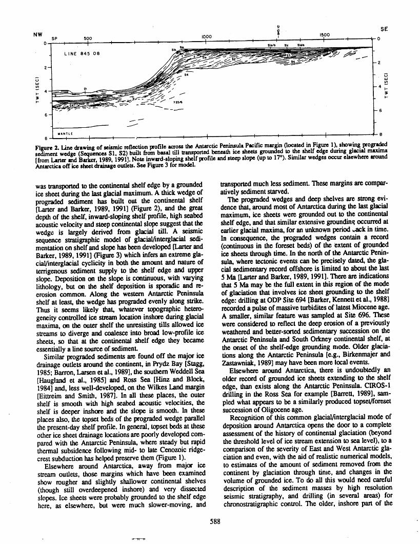
.__ SENWI000 I I I_' I 15001 , I ',SP 500 0

o , t ' ' ' ' t 'l S_ _/11 s sto0

slbLINE 84508

, U

w _

m 4 b

F-

- .._ _... _- ._. _-- ' 6

6 _

WANTLE

I, , _ , ' I I , , ' I , ., 88 I i

Figure2. Linedrawingof seismicreflectionprofileacrossthe AntarcticPeninsulaPacificmargin(locatedin Figure1), showingprogradedsedimentwedge(SequencesSI, $2) builtfrombasaltill tranRx>rmdbeneathice sheetsgroundedto theshelfedgeduringglacialmaxima[fromLatterandBarker,1989,1991].Note inward-slopingshelfprofile andsteepslope(upto 17% SimilarwedgesoccurelsewherearoundAntarcticaoff ice sheetdrainageoutlets.See Figure3 formodel.

wastransportedto thecontinentalshelfedgebya grounded transportedmuchlesssediment.Thesemarginsarecompar-ice sheet duringthe last glacial maximum.A thick wedge of atively sedimentstarved.prograded sediment has built out the continental shelf The progradedwedges and deep shelves are strong evi-[Latter and Barker,1989, 1991] (Figure 2), and the great dence that,aroundmost of Antarcticaduring the last glacialdepthof the shelf, inward-slopingshelf profile, high seabed maximum,ice sheets were groundedout to the continentalacoustic velocity and steep continentalslope suggest thatthe shelf edge, and that similar extensive groundingoccurredatwedge is largely derived from glacial till. A seismic earlierglacial maxima, for an unknownperiod _ackin time.sequence stratigraphic model of glacial/interglacial sedi- In consequence, the prograded wedges contain a recordmentationon shelf and slope has beendeveloped [L,arterand (continuous in the foreset beds) of the extent of groundedBarker,1989, 1991] (Figure 3) which infersan extremegla- ice sheets throughtime. In the north of the AntarcticPenin-cial/interglacial cyclicity in both the amount and natureof sula, where tectonic events can be precisely dated, the gla-terrigenous sediment supply to the shelf edge and upper cial sedimentaryrecord offshore is limited to about the lastslope. Deposition on the slope is continuous, with varying 5 Ma [Latterand Barker, 1989, 1991]. There are indicationslithology, but on the shelf deposition is sporadic and re- that 5 Ma may be the full extent in this region of the modeerosion common. Along the western Antarctic Peninsula of glaciation that involves ice sheet grounding to the shelfshelf at least, the wedge has progradedevenly along strike, edge: drillingat ODP Site 694 [Barker,Kennett et al., 1988]Thus it seems likely that, whatever topographic hereto- recordeda pulse of massive turbiditesof latest Miocene age.geneity controlled ice streamlocation inshore duringglacial A smaller, similar feature was sampled at Site 696. Thesemaxima, on the outer shelf the unresisting tills allowed ice were considered to reflect the deep erosion of a previouslystreams to diverge and coalesce into broad low-profile ice weatheredand better-sortedsedimentarysuccession on thesheets, so that at the continental shelf edge they became Antarctic Peninsula and South Orkney continental shelf, atessentially a line sourceof sediment, the onset of the shelf-edge grounding nlode. Older glacla-

Similar progradedsediments are found off the major ice tions along the Antarctic Peninsula [e.g., Birkenmajer anddrainageoutlets around the continent, in Prydz Bay [Stagg, Zastawniak,1989] may havebeen more local events.1985; Barron,Larsenet al., 1989], the southernWeddell Sea Elsewhere around Antarctica, there is undoubtedly an[Haugland et al., 1985] and Ross Sea [Hinz and Block, older recordof grounded ice sheets extending to the shelf1984] and, less well-developed, on the Wilkes Landmargin edge, than exists along the AntarcticPeninsula. CIROS-I[Eittreim and Smith, 1987]. In ali these places, the outer drilling in the Ross Sea for example [BarteR, 1989], sam-shelf is smooth with high seabed acoustic velocities, the pied what appearsto be a similarly produced topset/foresetshelf is deeper inshore and the slope is smooth. In these successionof Oligocene age.places also, the topset beds of the progradedwedge parallel Recognition of this common glacial/interglacial mode ofthe present-dayshelf profile. In general, topset beds at these depositionarouad Antarctica opens the door to a completeother ice sheet drainage locationsare poorlydevelopedcom- assessment of the history of continental glaciation (beyondparedwith the AntarcticPeninsula,wheresteadybut rapid thethresholdlevelof ice streamextensiontosealevel),to athermal subsidence following mid- to late Cenozoic ridge- comparison of the severity of East and West Antarctic gla-crest subduction has helpedpre.servethem (Figure 1). elation andeven, with the aid of realistic numerical models,

Elsewhere around Antarctica, away from major ice to estimates of the amount of sediment removed from thestreamoutlets, thosemarginswhichhavebeenexamined continentby glaciationthrough time, and changesin theshow rougher and slightly shallower continental shelves volume of grounded ice. To do ali this would need careful(though still overdeepened inshore) and very dissected description of the sediment masses by high resolutionslopes.Ice sheetswereprobablygroundedto theshelfedge seismic stratigraphy,and drilling (in severalareas) forhere, as elsewhere,but were much slower-moving,and chronostratigraphiccontrol. The older, inshorepartof the

588

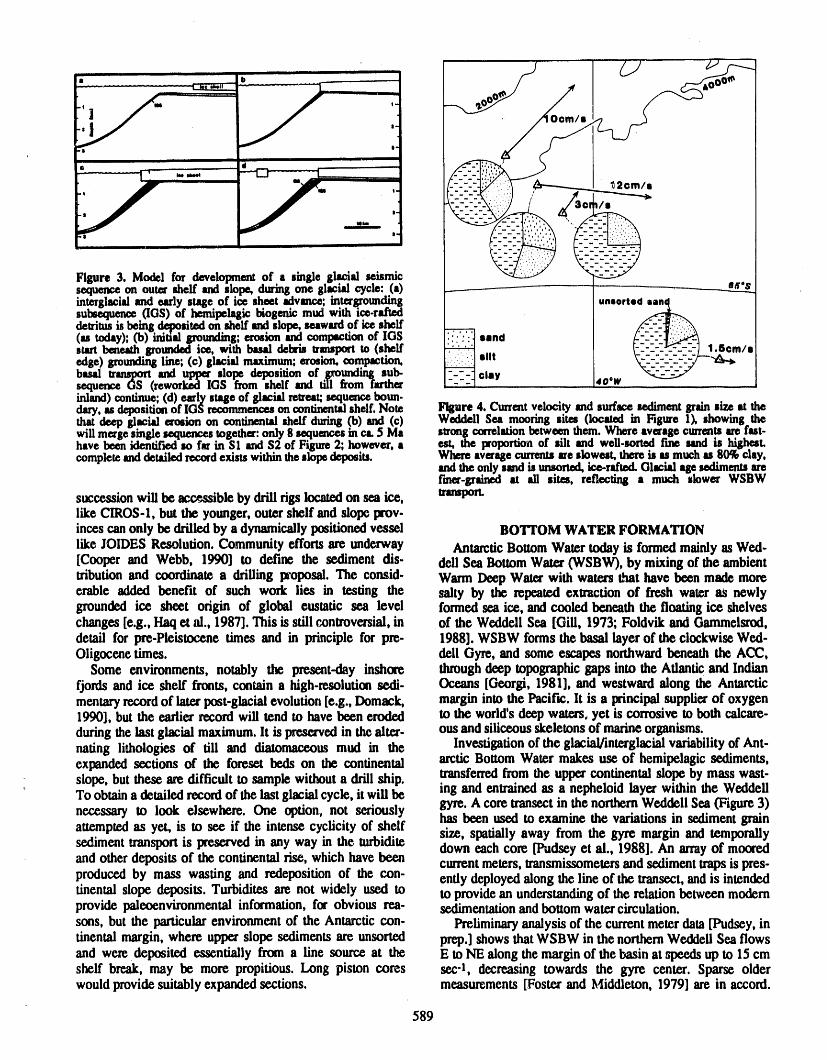
i|, _/d

, |.

Figure 3. Model for developmentof a single glacial seismicsequenceon outershelf andslope,duringone glacial cycle:.(a)interglacialandearly stageof ice sheet advance;in_'groun_g unsorted uanqsubsequen_ riGS)of hemipelaglcbiogenkmudwith ice-talceddetritusis being.d_?slu_don shelfandslope,seawardof ice shelf

(as wday);(b) inibalgrounding;erosionandcompactionof IGS _ sand _:_-::--___:__-._l_mstartbeneathgroundedice, withbasaldebristrmsport to (shelf /sedge)groundingline; (c) glacialmaximum;erosion,compaction, siltbasal transportand uppe¢slope depositionof IFoundingsub- _ claysequence GS (reworkedIGS from shelf and till from farther 4o°winland)centinue;(d) earlysuse of glacitlretreat;sequ=_ houri.dary,,tsdepositionof IGSrecommenceson continentalshelf.Note Figure4. Currentvelocityandsurfacesedimentgrainsize at thethatdeepglacial erosionon continentalshelf during(b) and (c) WeddellSea mootingsites (located in Figure 1), showingthewillmergesingleuxluex¢_ together:only8sequmcesin ca.5 Ma strongcorrelationbetweenthem.Whereaveragecurrmtsarefast-havebeenidentifiedm far in Sl and$2 of Figure2; however,a est, the proportionof silt and weU.mrtedfine und is highest.completeanddetailedrecordexistswithintheslopedeposits. Whereaveragecurrentsareslowest,thereis asmuchas 80%clay,

andtheonlysandis crooned,ice-rafted.Glacialagesedimentsarefreer-grainedat ali sites, reflecting a much slower WSBW

successionwill be accessible by drillrigs located on sea ice, tmeqxnt.like CIROS-I, but the younger, outershelf and slope prov.inces can only be drilled by a dynamicallypositionedvessel BOTTOM WATER FORMATIONlike JOIDES Resolution. Community effortsare underway AntarcticBottom Watertoday is formed mainly as Wed-[Cooper and Webb, 1990] to define the sediment dis- dell Sea Bottom WaterOVSBW),by mixing of the ambienttributionand coordinate a (hilling proposal. The consid- Warm Deep Water with waters that have been made moreerable added benefit of such work lies in testing the salty by the repeated exwaction of fresh water as newlygrounded ice sheet origin of global eustatic sea level formed sea ice, and cooled beneath the floating ice shelveschanges [e.g., Haq et al., 1987]. This is still conuoversial, in of the Weddell Sea [Gill, 1973; Foldvik and Gammelarod,detail for pre-Pleistocene times and in principle for pre- 1988]. WSBW forms the basal layer of the clockwise Wed-Oligocenetimes, dell Gyre, and some escapes northwardbeneath the ACC,

Some environments, notably the present-day inshore throughdeep topographic gaps into the Atlanticand Indianfjords and ice shelf fronts, contain a high-resolutionsedi- Oceans [Georgi, 1981], and westward along the Antarcticmentaryrecordof latexpost-glacialevolution [e.g., Domack, margininto the Pacif¢. lt is a principal supplierof oxygen1990], but the earlier record will tend to have been eroded to the world's deep waters, yet is corrosive to both calcare-duringthe last glacial maximum,lt is preservedin the alter- ous and siliceous skeletons of marineorganisms.nating lithologies of till and diatomaceous mud in the Investigation of the glacial/interglacialvariabilityof Ant-expanded sections of the foreset beds on the continental arctic Bottom Water makes use of hemipelagic sediments,slope, but these are difficult to sample withouta drill ship. transferredfrom the upper continental slope by mass wast-To obtaina detailed record of the last glacial cycle, it will be ing and entrained as a nepheloid layer within the Weddell

gyre. A core transectin the northernWeddell Sea (Figure3)necessary to look elsewhere. One option, not seriously has been used to examine the variations in sediment grainattemptedas yet, is to see if the intense cyclicity of shelf size, spatially away from the gyre margin and temporallysediment transportis preserved in any way in the turbidite down each core [Pudseyet al., 1988]. An arrayof mooredand other deposits of the continental rise, which have been currentmeters, transmissometersand sediment trapsis pres-produced by mass wasting and redeposition of the con- ently deployed along the line of the transect,andis intendedtinental slope deposits. Turbidites are not widely used to to providean understandingof the relation between modemprovide paleoenvironmental information, for obvious rea- sedimentationandbottom water circulation.sons, but the particularenvironment of the Antarctic con- Preliminaryanalysis of the currentmeter data[Pudsey, intinentalmargin, where upper slope sediments are unsorted prep.] shows thatWSBW in the northernWeddell Sea flowsand were deposited essentially from a line source at the E to NE along the marginof the basin at speeds up to 15 cmshelf break, may be more propitious. Long piston cores see-l, decreasing towards the gyre center. Sparse olderwould providesuitablyexpandedsections, measurements[Foster and Middleton, 1979] are in accord.

589

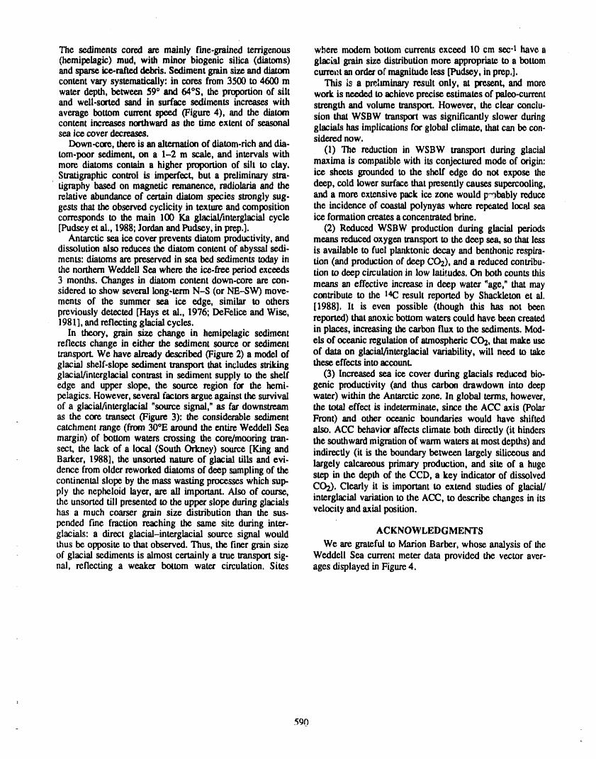
The sediments cored are mainly fine-grained terrigenous where modern bottom currentsexceed 10 cm sec-I have a(hemipelagic) mud, with minor biogenic silica (diatoms) glacL_lgrainsize distributionmore appropriateto a bottomand sparseice-rait_ debris.Sedimentgrainsize anddiatom currentanorderof magnitudeless [Pudsey, inprep.].content vary systematically: in cores from 3500 to 4600 m This is a p_hminary result only, at present, and morewater depth, between 59° and 64°S, the proportionof silt work is needed to achieve precise estimates of paleo-currentand well-sorted sand in surface sediments increases with strength and volume transport.However, the clear conclu-average bottom current speed (Figure 4), and the diatom sion that WSBW lransportwas significantly slower duringcontent increasesnorthwardas the time extent of seasonalsea ice cover decreases, glacials has implicationsfor global climate, that can be con.

Down-core, there is an alternationof diatom.richanddia- sidered now.tom-poor sediment, on a 1-2 m scale, and intervals with (1.) The reduction in WSBW transport during glacialmore diatoms contain a higher proportionof silt to clay. maxtma is compatible with its conjectured mode of origin:Stratigraphiccontrol is imperfect, but a preliminary stra. ice sheets grounded to the shelf edge do not expose thetigraphy based on magnetic remanence,radiolaria and the deep, cold lower surfacethat presently causes supercooling,relative abundanceof certain diatom species strongly sug- and a more extensive pack ice zone would t_,'_bablyreducegests that the observedcyclicity in textureand composition the incidence of coastal polynyas where repeated local seacorresponds to the main I00 Ka glacial/interglacial cycle ice formationcreates a concentratedbrine.[Pudseyet al., 1988;JordanandPudsey,in prep.]. (2) Reduced WSBW production during glacial periods

Antarcticsea ice cover prevents diatomproductivity,and means reducedoxygen transportto the deep sea, so that lessdissolution also reduces the diatomcontent of abyssal sedi. is available to fuel planktonicdecay and benthonic respira.ments: diatoms arepreserved in sea bed sediments today in tion (and productionof deep CO2),and a reducedcontribu-the northernWeddell Sea where the ice-free period exceeds riento deep circulationin low lathudes. On both counts this3 months. Changes in diatom content down-core are con- means an effective increase in deep water "age," that maysidered to show several long-term N-S (or NE--SW)move- contribute to the 14C result reported by Shacideton ct al.ments of the summer sea ice edge, similar to otherspreviously detected [Hays et al., 1976; DeFelice and Wise, [1988]. lt is even possible (though this has not been1981], and reflecting glacialcycles, reported)that anoxic bottomwaterscould have beencreated

In theory, grain size change in hemipelagic sediment in places, increasing thecarbonflux to the sediments.Mod-reflects change in either the sediment source or sediment els of oceanic regulationof atmosphericC02, thatmake usetransport.We have alreadydescribed (Figure2) a model of of data on glacial/interglacialvariability,will need to takeglacial shelf-slope sediment transportthat includes striking these effects intoaccount.glacial/interglacialcontrast in sediment supply to the shelf (3) Increased sea ice cover during glacials reduced bio-edge and upper slope, the source region for the hemi- genic productivity (and thus carbon drawdown into deeppelagics. However, several (actors argue against the survival water) within the Antarcticzone. In global terms,however,of a glacial/interglacial "sourcesignal,"as far downstream the total effect is indeterminate,since the ACC axis (Polaras the core transect(Figure 3): the considerable sediment Front) and other oceanic boundaries would have shiftedcatchment range (from 30°E around the entire Weddell Sea also. ACC behavioraffects climate both directly (it hindersmargin) of bottom waters crossing the core/mooring Wan. the southward migrationof warmwaters at most depths) andsect, the lack of a local (South Orkney) source [King and indirectly (it is the boundarybetween largely siliceous andBarker, 1988], the unsorted natureof glacial tills and evi- largely calcareous primaryproduction, and site of a hugedence fromolder reworkeddiatoms of deep samplingof the step in the depth of the CCD, a key indicator of dissolvedcontinental slope by the mass wasting processes which sup- CO2). Clearly it is importantto extend studies of glacial/ply the nepheloid layer, are ali important. Also of course,the unsortedtill presented to the upperslope duringglacials interglacialvariationto the ACC, to describe changes in itshas a much coarser grain size distribution than the sus. velocity and axial position.pended free fraction reaching the same site during inter-glacials: a direct glacial-interglacial source signal would ACKNOWLEDGMENTSthus be opposite to that observed.Thus, the finer grainsize We aregrateful to MarionBarber, whose analysis of theof glacial sedimentsis almost certainlya true transIx_ sig- Weddell Sea currentmeter data provided the vector aver-nal, reflecting a weaker bottom water circulation. Sites ages displayed in Figure4.

REFERENCES

Alley, R. B., D. D. Blankenship, S. T. Rooney, and C, R, arctic continental margin: geology and geophysics of off-Bentley, Sedimentation beneath ice shelves: the view shore Wilkes Land, edited by S, L. Eittrcim and M, A.fromIce StreamB, Mar. Geol., 85, 101-120, 1989, Hampton,Circum.Pacifie Council for Energy and Mtn.

Anderson, J. B,, D. D. Kurtz, E. W, Domack, and K, M. eral ResourcesEarth Science Series, 5A, 15-43, Houston,Balshaw, Glacial and glacial marine sediments of the Texas, 1987.Antarcticcontinental shelf, J, Geol., 88, 399-414, 1980. Fastook, J. L,, West Antarctica, the sea-level--controUcd

Anderson, J. B., C. F. Brake, and N. C. Myers, Sedl- marine instability: past and future, AGU Geophysicalmentation on the Ross Sea continental shelf, Antarctica, Monograph 29, 275-287, 1984:Mar. Geol,, 57, 295-333, 1984. Foldvik, A., and T. Gammelsrod,Notes on Southern Ocean

Barker,P. F., and J, Burrell,The openingof DrakePassage, hydrography,sea.ice and bottom-waterformation,Palae-Mar. Geol., 25, 15-34, 1977. ogeogr., Palaeoclim,, Palaeoecol., 67, 3-17, 1988.

Barker, P. F,, and J. Burrell, The influence on Southern Foster,T. D., and J. H, Middleton,Variabilityin the bottomOcean circulation,sedimentationand climate of the open- water of the Weddell Sea, Deep.Sea Res., 26, 743-762,1979.ing of DrakePassage, in Antarctic Geoscience, edited by Georgi, D, T., Circulationof bottom waters in the south-C, Craddock, pp. 377-385, Univ. Wisconsin Press, western South Atlantic, Deep-Sea Res., 28, 959-79,Madison, 1982. 1981.

Barker,P. F., J. P. Kennettct al., Proc. ODP, Init. Repts.,113, Ocean DrillingProgram,College Station, TX 1988. Gill, A. E., Circulationand bottom water production in the' Weddell Sea, Deep-Sea Res., 20, 111-140, 1973.

Barrett,P. J., AntarcticCenozoic history from the CIROS-I Gill, A. E., and K, Bryan, Effects of geometry on the cir-drillhole, McMurdoSound, DSIR Bulletin, 245, 251 pp., culation of a three-dimensional southern-hemisphereWellington,New Zealand, 1989. ocean model, Deep.Sea Res., 18, 685-721, 1971.

Bah'on,J., B. Larsen ct al., Prec. ODP, lnit. Repts., 119, Grebe, H., A. Mackensen, H.-W. Hubberten,V. Spiess, andOcean DrillingProgram,College Station, TX, 1989. D.K. Fuctterer,Stable isotope and Late Quaternarysed.

Benson, R. H., The origin of the psychrosphereas recorded imentation rates at the Antarctic continental margin, inin changes in deep-sea ostracodassemblages, Lethaia, 8, Geological History of the Polar Regions: Arctic versus69-83, 1975. Antarctic, edited by U. Bleil and J. Thiede, pp, 539-572,

Bentley, C. R., Some aspects of the cryosphere and its role KluwerAcad. Publ.,Dordrecht,1990.in climatic change, AGU Geophysical Monograph 29, Haq, B. U., J. Hardenbol, and P. R. Vail, Chronology of207-220, 1984. fluctuating sea levels since the Triassic, Science, 235,

Bentley, C. R., Antarctic ice streams:a review, J. Geophys. 1156-1167, 1987.Res., 92, 8843-8858, 1987. Haugland, K., Y. Kristoffersen, and A. Velde, Seismic

Birkenmajer,K., and E. Zastawniak,Late Cretaceous-early Investigations in the Wedde'.l Sea Embayment,Tertiary floras of King George Island, West Antarctica: Tectonophysics, 114, 293-313, 1985.their stratigraphicdistribution and palaeoclimatic sig- Hays, J. D., J. A. Lozano, N. J. Shacldeton, and G. Irving,nificance, in Origins and Evolution of the Antarctic Reconstruction of the Atlantic and eastern Indian OceanBiota, edited by J. A. Crame,Geol. Soc. Sp. Publ., 47, sectors of the 18,000 B.P. Antarctic Ocean, Geol. Soc.227-240, 1989. Amer, Mem. 145,337-372, 1976.

Brydcn, H. L., Poleward heat flux andconversion of avail- Hinz, K., and M. Block, Results of geophysical investiga-able potential energy in Drake Passage,J. Mar. Res., 37, tions in the Weddell Sea and in the Ross Sea, Antarctica.1-22, 1979. Exploration in New Regions, Eleventh World Petroleum

Cheney, R., J. G. Marsh,and B. D. Beckley, Global meso- Congress, London. PD 2(1), pp. 1-13, 1983.scale variability from colinear tracksof SEASAT altim- Johnson, D. A., Abyssal teleconnections II. Initiation ofeter data,J. Geophys. Res., 88, 4343-4354, 1983. AntarcticBottom Water flow in the southwestern Arian-

Cooper, A. K., and P. N. Webb, InternationalWorkshopon tic, in South Atlantic Paleoceanography, K. J. Hsu and H.AntarcticOffshore Seismic Stratigraphy(ANTOSTRAT): J. Weissert, pp. 243-281, CambridgeUniv Press, 1985.Overview and Extended Abstracts, U.S. Geol. Surv. Kellogg, T. B., R. S0 Tmesdale, and L. E. Osterman, LateOpen-File Report 90-309, 130-4, 1990. Quaternaryextent of the West Antarctic ice sheet, new

DcFelice, D. R., and S. W. Wise, Jr., Surface lithofacies, evidence from Ross Sea cores, Geology, 7, 249-253,biofacies and diatom diversity patterns as models for 1979.delineation of climatic change in the southeast Atlantic Kemp, E. M., L. A. Frakes,and D. E. Hayes, Paleoclin_aticOcean, Mar. Micropal., 6, 29-70, 1981. significance of diachronous biogenic facies, Leg 28,

Domack, E. W., Late Quaternaryand pre-glacial strati- Deep Sea Drilling Project, in lnit. Repts., DSDP. 28,graphic sequences along the East Antarctic margin: the D.E. Hayes, L. A Frakes,and others, pp. 909-918, U.S.record from inner shelf basins, in Intemation',dWorkshop Govt. PrintingOffice, Washington, DC, 1975.on Antarctic Offshore Seismic Stratigraphy Kennett, J. P., and P. F. Barker, Latest Cretaceous to Cen-(ANTOSTRAT): Overview and Extended Abstracts, ozoic climate and oceanographic developments in the

, A.K. Cooper and P. N. Webb, conveners, U.S. Geol. Weddell Sea, Antarctica: an Ocean-Drilling perspective,Surv. Open-File Report 90-309, 130-4, 1990. in Proc ODP, Sci. Results, 113, P. F. Barker, J. P. Ken-

Eittreim, S. L., and G. L. Smith, Seismic sequences and nett, and others, pp. 937-960, Ocean Drilling Program,their distribution on the Wilkes Landmargin,in The Ant- College Station, 'IX, 1990.

591

Kennctt,J.P.,and N. D. Watldns,Regionaldeep-sca Potmr,j,R.,andJ.O.Paren,Interactionbetweeniceshelfdynamicprocessesrecordedby !_tcCenozoicsediments and oceanin GeorgeVI Sound, Antarctica,inOcea.ofthesoutheasternIndianOcean,Geol,Soc,Amer,Bull,,' nologyoftheAntarcticContinentalShelf,editedbyS,S,87,321-339,1976, Jacobs,Anlarct,Res,Ser,43,pp,35--58,Amex,Ocophys,

Klng_E. C., and P. F. Barker,The margins of the South Union, Washington,DC, 1985.Orkney microcontinent, J Geol, Soc,, 145, 317-331, Prentice, M, L., and R. K. Matthews, Cenozoic ice volume1988, history: development of a composite oxygen isotope

Latter,R. D., and P. F, Barker,Seismic stratigraphyof the record, Geology, 16, 963-966, 1988.AntarcticPeninsulaPacific margin:a recordof Pliocene- Pu,'lsey,C, J., P. F, Barker,and N. Hamilton, Weddell SeaPleistocene ice volume and paieoclimaw, Geology, 17, _byssal sediments: a record of Antarctic Bottom Water73!-734, 1989, flow, Mar, Geol,, 81,289-314, 1988,

Latter,R, D,, and P, F. Barker,Neogene interactionof tec- Schlich, R., S, W, Wise, Jr,, et al,, Proc, ODP, Intt, Repts, otonic and glacial proceases at the Pacific margin of the 120, Ocean Drilling Program,College Station,TX, 1989.Antarctic Peninsula, in Sea Level Change at Acave Plate Shackleton, N. J,, Oxygen isotopes, ice volume and sea-Margins, exltte,d by D, I. M. Macdonald, Oxford Uni- level, Quaternary Science Reviews, 6, 183-190, 1987,

Shackleton, N, J,, and J. P, Kennett, Palaeotemperature his-versity Press, 1991, In press, tory of the Cenozoic and the initiation of Antarcticglaeia-

Labcyrie,L.D,,andA. Juillct,Oxygenisotopeexchange- don:oxygenandcarbonisotopeanalysesinDSDP site,ability of diatom valve silica; interpretation and conse- 277,279 and 281, in lnit. Repts, DSDP, 29, J. P, KennetLquences for paleoclimatlc studies, Geoctu'm.Cosmochim. R. E, Houtz, et al., pp. 743--755, U,S. Govt, PrintingActa, 46, 967-975, 1982. Office, Washington, DC, 1975.

Leclere, A. J., and L. l.,abeyrie, Temperature depetdence of Shackleton, N. J., J.-C. Duplessy, M, Arnold, P, Maurice,the oxygen isotopic fractionationbetween diatom silica M, A. Hall, and J. Cartlidge, Radiocarbonage of last gin-andwater,Earth Planet, Set, Lett,, 84, 69-74, 1987, cial Pacificdeep water,Nature, 335,708--711, 1988,

Miller,K, G,, R. O. Fairbanks,and G, S. Mountain,Tertiary Shine, K. P,, A, Henderson-Sellars, and R. G, Barry,oxygen isotope synthesis, sea-level history and conti. Albedo-climate feedback: the importance of cloud andnental margin erosion, Paleoceanography, 2, 1-19, 1987. cryospheric variability, in New Perspectives iv Climate

Norton, I. O., and J. O. Sclater, A model for the evolution of Modelling, edited by A. Bergex and C, Nicolis, pp. 135-the Indian "Oceamand the breakup of Gondwanaland, J. 155, Elsevier, 1984.Geophys, Res,, 84, 6803-6830, 1979, Stagg, H. M. J., The structureand origin of Prydz Bay and

MacRobextson Shelf, East Antarctica, Tectonophysics,114,315-340, 1985.

592_ -

Eolian Sediments in Arctic Alaska as Sources of Paleoenvironmental Data

L. David CarterU,S,GeologicalSurvey,Anchorage,Alaska,U.S.A,

ABSTRACT

Eolian sand, silt, and associated fluvial and lacustrine sedimentsare widespreadin Alaska north of the Brooks Range. These sediments and intercalated paieosolsrecord late Quaternary episodes of widespread,eolian sediment transport separatedby l?enods of relative landscape stability and the growth of organic soils. The eoliansediments represent paleoenvironments much different from the modem one, in

G • i 0

which eolian sediment transport is pnn.cipally hmlted to area_,;adjacent to sedimentsources, such as flood plains. Information about these paleocnvironments and theircontemporary climates can be obtained by studying the moff,hology, distribution,and sedlmento!ogy of the sediments, and the fossil fauna and flora they contain. Forexample, eolian sedimentary structures and facies relations can provide informationabout past wind directions, snow cover, and summer surface moisture conditionsand gradients. Fossils such as beetles and ostracods contained in the fluvial andlacustrine sediments can yield information regarding summer temperature andchanges m evaporation/precipitation ratios. Futhermore, the sediments andpaleosols can be dated by thermoluminescence and radiocarbon to provide achronology of paleoclimatic and pale-environmental change. Present data suggestthree major episodes of widespread eolian sediment movement during the latestglacial/inter-glacial cycle: (1) a long period coincident with the Wisconsin glacia-tion during which climate was cooler and drier than today and much of the NorthSlope was a polar desert; (2) an interval during the latest Pleistocene and earlyHolocene in which climate was wanner and surface moisture conditions were drierthan today; and; (3) one or more brief late Holocene intervals during which climatewas probably cooler and drier than today. These eolian sediments and intercalatedpaleosols are being studied in detail as part of the USGS Climate Change Programin order to understand how past environments in arctic Alaska have responded toclimatic change. In particular, the paleoenvironment of the latest Pleistocene--earlyHolocene warm period is being examined as a possible analog for the environmentthat could result from future climatic warming.

593

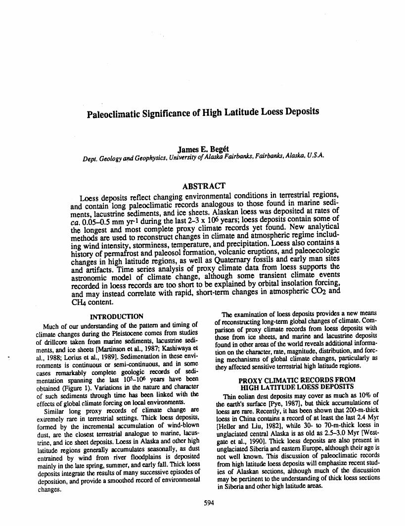
Paleoclimatic Significance of High Latitude Loess Deposits

James E. Beg_tDept,Geologyand Geophysics,UniversityofAlaskaFairbanks,Fairbanks,Alaska,U.S.A.

ABSTRACT

Loess deposits reflect changing environmental conditions in terrestrial regions,and contain long paleoclimatic records analogous to those found in marine sedi-ments, lacustrine sediments, and ice sheets. Alaskan loess was deposited at rates ofca. 0.05-0.5 mm yr-1 during the last 2-3 x 106 years; loess deposits contain some ofthe longest and most complete proxy climate records yet found. New analyticalmethods are used to reconstruct changes in climate and atmospheric regime includ-ing wind intensity, storminess, temperature, and precipitation. Loess also contains ahistory of permafrost and paleosol formation, volcanic eruptions, and paleoecologicchanges in high latitude regions, as well as Quaternary fossils and early man sitesand artifacts. Time series analysis of proxy climate data from loess supports theastronomic model of climate change, although some transient climate eventsrecorded in loess records are too short to be explained by orbital insolation forcing,and may instead correlate with rapid, short-term changes in atmospheric CO2 andCH4 content.

INTRODUCTION The examinationof loessdeposits providesa new meansMuch of ourunderstandingof the patternand timingof of reconstructinglong-termglobalchangesof climate.Com-

climatechangesduringthe Pleistocenecomes fromstudies parison of proxyclimaterecordsfromloess depositswithof drillcoretakenfrom marinesediments,lacustrinesedi- those fromice sheets, andmarineand lacustrinedepositsments,andice sheets [Martinsonet al., 1987;Kashiwayaet foundin otherareasof theworldrevealsadditionalinforma-

- al., 1988;Loriuset al., 1989].Sedimentationin theseenvi- tionon thecharacter,rate,magnitude,distribution,andforc-ronmentsis continuousor semi-continuous,and in some ing mechanismsof globalclimatechanges,particularlyascases remarkablycomplete geologic records of sexli- theyaffectedsensitiveterrestrialhigh latituderegions,mentation spanning the last 105-106 years have been PROXYCLIMATICRECORDSFROMobtained(Figure1). Variationsin the natureandcharacter HIGHLATITUDELOESSDEPOSITSof such sedimentsthroughtime has been linkedwith the Thineoliandustdepositsmaycoveras muchas 10%ofeffectsof globalclimateforcingon local environments, the earth'ssurface [Pye, 1987],butthick accumulationsof

Similar long proxy rewordsof climate change are loessarerare.Recently,it hasbeen shown that200-m-thickex_emely rarein terrestrialsettings.Thick loess deposits, loess in Chinacontainsa recordof at least the last2.4 Myrformed by the incrementalaccumulationof wind-blown [HellerandLiu, 1982], while 30- to 70-m-thick loess indust, are the closest terrestrialanalogueto marine,lacus- unglaciatedcentralAlaskais as old as 2.5-3.0 Myr[West-trine,andice sheetdeposits.Loessin Alaskaand otherhigh gate et al., 1990].Thickloess depositsare also presentinlatituderegionsgenerallyaccumulatesseasonally,as dust unglaciatedSiberiaandeasternEurope,althoughtheirageisentrainedby wind from fiver floodplainsis deposited not well known.This discussionof paleoclimaticrecordsmainlyin the latespring,summer,andearlyfall.Thickloess fromhigh latitudeloessdepositswillemphasizerecentstud-depositsintegratetheresultsof manysuccessiveepisodesof ies of Alaskansections,althoughmuchof the discussiondeposition,and providea smoothedrecordof environmental maybepertinentto the understandingof thickloesssectionschanges, in Siberiaandotherhighlatitudeareas.

594

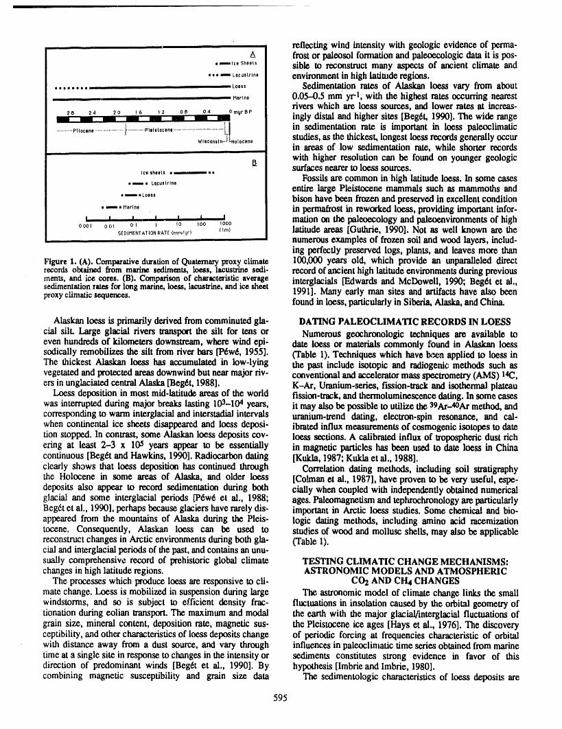
, reflecting wind intensity with geologic evidence of perma-A frost or paleosol formationand paleoecologic data it is pos-

.---,_, sheets sible to reconstruct many aspects of ancient climate and.... L.co,t_.0 environmentin high latituderegions.

...... .._ ,,Loe,s Sedimentation rates of Alaskan loess vary from about-- --Mo,_e 0,05-0.5 mm yr-l, with the highest rates occurring nearest

rivers which are loess sources, and lower rates at inereas-20 24 2o 16 12 o0 0,4 0mrr.,P ingly distal and higher sites [Beg6t, 1990], The wide range

..........PI,0c,,,...................t...........P_e,,toc,,.................................._[ in sedimentation rate is important in loess paleoclimaflcw,ec0,,,,-.IL,o_0c,,, studies, as the thickest, longest loess records generally occur_. in areas of low sedimentation rate, while shorter records

' ' with higher resolution can be found on younger geologic!_ surfaces nearerto loess sources.

Ice sheets • __ -- • •

Fossils are common in high latitude loess. In some eases.--. L,cu,t,,,, entire large Pleistocene mammals such as mammoths and

"--"_°'" bison have been frozen and preserved in excellent condition• --. ,,,,,e in permafrost in rewotked loess, providing important infer-

, , , , I I I marion on the paleoecology and paleoenvironments of highooo, oo, o, , ,o ,oo ,oooSED,,ENTAT,0NRAT_(,,_/_,) (,m> latitude areas [Outhrie, 1990]. Not as well known are the

... . numerous examples of frozen soil and wood layers, includ-ing perfectly preserved logs, plants, and leaves more than

Figure1. tA). Comparativedurationof Quaternaryproxyclimate 100,000 years old, which provide an unparalleled directrecordsobtainedfrom marinesediments,loess, lacustrinesedi- record of ancient high latitudeenvironments during previousments, and ice cores. (B). Comparisonof char.aet_'isticaverage interglacials [Edwards and McDowell, 1990; Beg6t et al.,sedimentationratesfor longmarine.,loess,lacustrine,andice sheet 1991]. Many early man sites and artifacts have also beenproxyclimaticsequences.

found in loess, particularly in Siberia, Alaska, and China.

Alaskan loess is primarilyderived from comminuted gla- DATING PALEOCLIMATIC RECORDS IN LOESS

cial sill Large glacial rivers transportthe silt for tens or Numerous geochronologic techniques are available toeven hundreds of kilometers downstream, where wind epi- date loess or materials commonly found in Alaskan loesssodically remobilizes the silt fromriver bars [P6w6, 1955]. (Table I). Techniques which have _.en applied to loess inThe thickest Alaskan loess has accumulated in low-lying the past include isotopic and radiogenic methods such asvegetated andprotected areas downwindbut near major riv. conventional and accelerator mass speetromearytAMS) 14t2,ers in unglaciatedcentral Alaska [Beg6t, 1988]. K-At, Uranium-series, fission-trackand isothermal plateau

Loess deposition in most mid-latitude areas of the world fission-track, and thermoluminescence dating. In some easeswas interrupted during major breaks lasting 103-104 years, it may also be possible to utilize the agAr-4OArmethod, andcorresponding to warm interglacial and interstadial intervals uranium.trend dating, electron-spin resonance, and cal-when continental ice sheets disappeared and loess deposi- ibmted influx measurements of cosmogenic isotopes to datetion stopped. In contrast, some Alaskan loess deposits eev- loess sections. A calibrated influx of tropospheric dust richering at least 2-3 x 10-s years appear to be essentially in magnetic particles has been used to date loess in Chinacontinuous [Beg6t and Hawkins, 1990]. Radiocarbon dating [Kukla, 1987; Kukla ct al., 1988],clearly shows that loess deposition has continued through Correlation dating methods, including soil stratigraphythe Holocene in some areas of Alaska, and older loess [Colman et al., 1987], have proven to be very useful, espe-deposits also appear to record sedimentation during both cially when coupled with independently obtained numericalglacial and some interglacial periods [P6w6 ct al., 1988; ages. Paleomagnetism and tepta'ochronology are particularlyBeg& ct al., 1990], perhaps because glaciers have rarely dis- important in Arctic loess studies. Some chemical and bio-appeared from the mountains of Alaska during the Pleis- logic dating methods, including amino acid racemizationtocene. Consequently, Alaskan loess can be used to studies of wood and mollusc shells, may also be applicablereconstruct changes in Arctic environments during both gla. (Table 1).cial and interglacial periods of the past, and contains an unu-sually comprehensive record of prehistoric global climate TESTING CLIMATIC CHANGE MECHANISMS:changes in high latitude regions. ASTRONOMIC MODELS AND ATMOSPHERIC

The processes which produce loess are responsive to cii- CO2 AND CI-14CHANGESmate change. Loess is mobilized in suspension during large The astronomic model of climate change links the smallwindstorms, and so is subject to efficient density frac- fluctuations in insolation caused by the orbital geometry oftionation during eolian transport.Themaximum and modal the earth with the major glacial/interglacial fluctuations ofgrain size, mineral content, deposition rate, magnetic sus- the Pleistocene ice ages [Hays et al., 1976]. The discoveryceptibility, and other characteristics of loess deposits change of periodic forcing at frequencies characteristic of orbitalwith distance away from a dust source, and vary through influences in paleoclimatic time seriesobtained from marinetime at a single site in responseto changes in the intensity or sediments constitutes strong evidence in favor of thisdirection of predominant winds [Beg6t et al., 1990]. By hypothesis [Imbrieand Imbrie, 1980].combining magnetic susceptibility and grain size data The sedimentologic characteristics of loess deposits are

595

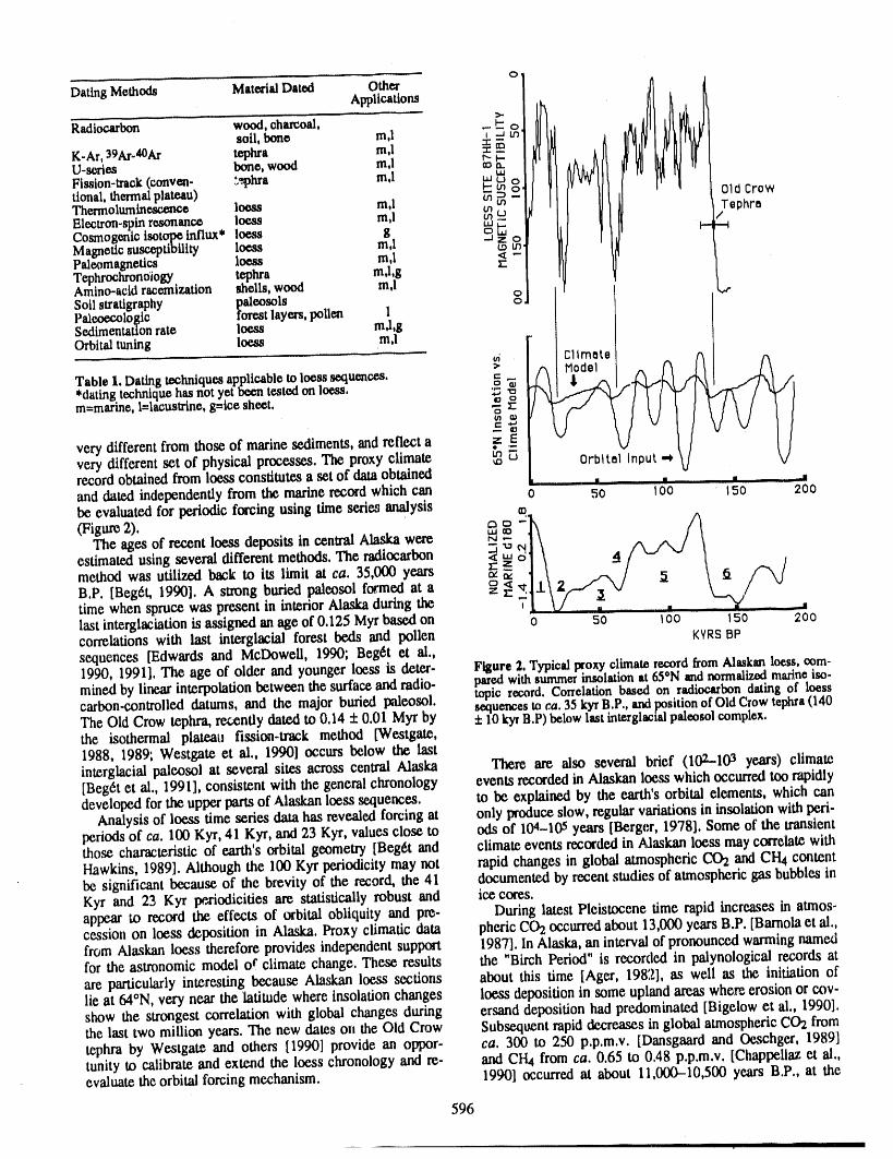
o

DatingMethods MaterialDated OtherApplicatlons

Radiocarbon wood,oharcoal,soil,bone m,l T _ _n

U-s_'ies bone,wood m,lFission-I_ck(conven- .'.._hra m,l _I.u_ OldCrowdonal,thermalplateau) cnThermoluminescence loess m,l tn tn JephraElectron-spinresonance loess m,l ,,,_Cosmogenicisotopeinflux* loess g

Magnetic_scepflbility loess m,l _paleomagnetics loess m,lTephrochronoiogy tephra m,l,gAmino-acidracemization shells,wood m,1 _,.Soilstratigraphy !_deosolsPaleoecologic lOre.stlayers,pollen 1Sedimentationrate loess m,l,g IOrbitaltuning loess m,1 I

v/ ClimateI f_I rx:" ,_ Model _1/I [\

Table 1. Datingtechniquesapplicableto loesssequences, =*datingtechniquehasnotyetbeentestedon loess. '_ \ro=marine,l=lacustrtne,g=icesheet. _, .__=©

very different front those of marinesediments, and reflect a z Every different set of physical processes. The proxy climate, _ _ p t _ V Vrecord obtained from loess constitutes a set of dataobtained L • . • ----"and datedindependentlyfrom the marinerecord which can o 50 100 150 200be evaluated for periodic forcing using time seriea analysis m

(Figure 2). t_ _ "= _ ____

The ages of recent loess deposits in centralAlaska were _ - 4//_estimated using several different methods, The radiocarbon _ '_ /method was utilized back to its limit at ca. 35,000 years _ _"_ 4B,P, [Beg6t, 1990]. A strong buried paleosol formed at a z z:time when spruce was present in interior Alaska during the q: , __1last interglaciation is assigned an age of 0.125 Myr based on o 50 I0o 15o 2oocorrelations with last intergLacial forest beds and pollen KYRS eP

sequences [Edwards and McDowell, 1990; Beg6t et al.,1990, 1991]. The age of older and younger loess is deter- Figure2. TypicalixoxyclimaterecordfromAlaskanloess,com-minedby linearinterpolationbetween the surfaceandradio- paredwith summerinsolationat 650Nandnormalizedmarineiso-topic record.Conelationbased on radiocarbondating of loesscarbon-controlled datums, and the major buried paleosol. sequencesto ca.35kyr B.P.,_ p?sitionof OldCrowtephra(140The Old Crow tephra, recently dated to 0.14 :t:0.01 Myr by + 10kyrB.P)belowlast intergiactsapateosoicomplex.the isothermal plateau fission-track method [Westgate,1988, 1989; Westgate et al., 1990] occurs below the lastinterglacial paleosol at several sites across central Alaska There are also several brief (102-103 years) climate[Beg6t et al., 1991], consistent with rite general chronology events recorded in Alaskan loess which occurred too rapidlydeveloped for the upper partsof Alaskan loess sequences, to be explained by the earth's orbital elements, which can

Analysis of loess time series data has revealed forcing at only produce slow, regular variations in insolation with peri-periods of ca. 100 Kyr, 41 Kyr, and 23 Kyr, values close to eds of 104-105 years [Berge,r, 1978]. Some of the transientthose characteristic of earth's orbital geometry [Beg6t and climate events recorded in Alaskan loess maycorrelate withHawkins, 1989]. Although the 100 Kyr periodicity may not rapid changes in global atmospheric CO2 and CI-14contentbe significant because of the brevity of the record, the 41 documented by recent studies of atmospheric gas bubbles inKyr and 23 Kyr periodicities are statistically robust and ice cores.appear to record the effects of orbital obliquity and pre- During latest Pleistocene time rapid increases in atmos-cession on loess deposition in Alaska. Proxy climatic data pheric CO2 occurred about 13,000 years B.P. [Barnola et al.,from Alaskan loess therefore provides independent support 1987]. In Alaska, an interval of pronounced warming namedfor the astronomic model or climate change. These results the "Birch Period" is recorded in palynological records atare particularly interesting because Alaskan loess sections about this time [Ager, 1982], as well as the initiation oflie at 64°N, very near the latitude where insolation changes loess deposition in some upland areas where erosion or coy-show the strongest correlation with global changes during ersand deposition had predominated [Bigelow et al., 1990].the last two million years. The new dates on the Old Crow Subsequent rapid decreases in global atmospheric CO2 fromtephra by Westgate and others [1990] provide an oppor- ca. 300 to 250 p.p.m.v. [Dansgaard and Oeschger, 1989]tunity to calibrate and extend the loess chronology and re- and CI-I4from ca. 0.65 to 0.48 p.p.m.v. [ChappeUaz et al.,evaluate the orbital forcing mechanism. 1990] occurred at about 11,000-10,500 years B.P., at the

596

time of the dramatic"YoungerDryas"cooling in northern to those of modern values, However, dramatic growth ofEurope,However, theatmosphere is chemically well mixed, permafrost and high wind intensities recorded in centraland global climate models show that decr_ in the Alaskan loess of mid-Wisconsinage suggests a particularly"Greenhou__eEffect" due to reductions in atmospheric CO2 cold climatic interval [Hamilton et al,, 1988; Beget, 1990],and CI-I4concentrations,such as occurredduring the latest The transienthigh latitude cooling may reflect an intervalPleistocene, cannot be restrictedto one region of theplanet, centered at 42 Kyr when atmospheric CO2 composition

Some evidence suggests widespread climate changes decreased to ca, 180-200 p,p,m,v, and CI-14dropped to ca.occurred at this time, particularly in high latitude regions of 0,40 p,p.m,v., values similar to those reached during thethe southern hemisphere [Heusser and Rabassa, 1987;Heus- peak of full glacial conditions [Barnola et al., 1987; Chap-ser, 1989; Chappellaz et al., 1990], Mlcrofaunal and isotopic pellaz et al., 1990],marine data from the northwest Pacific Ocean also show The apparent links between transient intervals of atmos-clear evidence for latest Pleistocene cooling [Kallel ct al,, phertc CO_ increase, and episodes of significant warming,1988], Loess data from Alaska suggest wind intensity permafrostdegradation,and generally lower wind intensitiesbriefly increased at this time, together with transient recorded in Alaskan loess during the Birch Period at ca, 13decreases in regional pollen influx rates [Bigelow et al,, Kyr and the Fox Thermal Event at ca, 30 Kyr, are stg-1990], perhaps due to the cooling of the northwest Pacific nificant for out understanding of the effects of the modemOcean or perhaps in response to changes in atmospheric anthropogenic increase in global atmospheric CO.2,The dis-CCh and CI-I4 content, covery that brief, natural fluctuations in atmospheric CO2 in

During the mid-Wisconsin a similar relationship seems to the past have been associated with intervals of climateexist between intervals of high and low wind intensity and change in high latitude areas provides support for Green-transient atmospheric CO2 and CH4 changes as delineated house models of climate change. These data support globalby ice core studies, A significant interval of climatic warm- climate models which suggest atmospheric CO-2and CH4ing and permafrost degradation at ca. 30,000 years is content plays a very important role in modulating globalrecorded in several areas of Alaska [Hamilton et al., 1988], climate.This episode, named the "Fox Thermal Event," is also If natural short-term changes in atmospheric CO.2haverecorded as an interval of low wind intensity in multiple produced significant climate changes in high latitudeloess sections [Beg6t, 1990], and correlates well with a tran- regions, as is suggested by recent studies of paled.sient interval of high atmospheric CO2 and CI-14content climatologic records in Alaskan loess, then it seems likely[Chappellaz et al., 1990], The mid-Wisconsin, ca, 33--45 that the large increase in atmospheric C02 occurring duringKyr, is an interval of relatively high insolation values, when this century due to modern use of fossil fuels may also haveorbital parameters would produce summer insolation close a significant effect on climate in high latitude regions,

REFERENCES

Ager, T., Vegetational history of western Alaska during the Chappellaz,J., J. Barnola, D. Raynaud,Y, Korotkevich, andWisconsin glacial interval and the Holocene, in Paled- C. Lorius, Ice.core record of atmospheric methane overecology of Beringia, edited by D. Hopkins, J. Mathews, the past 160,000 years, Nature, 345,127-131, 1990.C. Schweger, and S, Young, pp. 75-93, Academic Press, Colman, S, M., K. L. Pierce, and P. W. Birkeland, Sug-New York, 1982. gested terminology for Quaternarydatingmethods, Quat.

Bamola, J., D, Raynaud, Y, Korotkevich, and C. Lorius, Res.,28, 314-319, 1987.Vostok ice core provides 160,000 year record of atmos- Dansgaard,W., and H. Oeschger, Past environmental long-pheric CO2,Nature, 329, 408--414, 1987, term records from the Arctic, in The Environmental

Beg6t, J,, Tephras and sedimentology of frozen loess, Fifth Record in Glaciers and Ice Sheets, edited by H, OeschgerInternational Permafrost Conference Proc., Vol. 1,, and C. Langway, pp. 287-318, Wiley, New York, 1989,edited by K. _Senneset,pp. 672.-677, Tapir, Trondheim, Edwards, M., and P. McDowell, Interglacial deposits at1988. Birch Creek, northeast interior Alaska, Quat. Res,, 35,

Beg6t, J., Mid-Wisconsinan climate fluctuations recorded in 41-52, 1990,central Alaskan loess, Geographie Physique et Quater- Guthrie, R. D., Frozen Fauna of the Mammoth Steppe: Thenaire,44, 3-13, 1990. story of Blue Babe, 323 pp,, University of Chicago,

Beg6t, J., and D. Hawkins, Influence of orbital parameters Chicago, IL, 1990.on Pleistocene loess deposition in central Alaska, Nature, Hamilton, T., J. Craig, and P. Sellman, The Fox permafrost337, 151-153, 1989. tunnel: A late Quaternary geologic record in central

Bcg6t, J., D, Stone, and D, Hawkins, Paleoclimate forcing Alaska, Geol. Soc. Am. Bull., 100, 948--969, 1988,of magnetic susceptibility variations in Alaskan loess, Hays, J., J. lmbrie, and N. Shackleton, Variations in theGeology, 18, 40-43, 1990, earth's orbit: pacemaker of the ice ages, Science, 194,

Beg6t, J,, M. Edwards, D. Hopkins, M, Keskinen, and G. 1121-1132, 1976.Kukla, Old Crow tephra found at the Palisades of the Heller, F., and T. S. Liu, Magnetostratigraphical dating ofYukon, Quat. Res., 34,291-297, 1991. loess deposits in China, Nature, 300, 431--433, 1982.

Berger, A., Long-term variations of caloric insolation result- Heusser, C., Late Quaternary vegetation and climate ofing from the earth's orbital elements, Quat. Res., 9, 139- southern Tierra del Fuego, Quat. Res., 31, 396--406,167, 1978. 1989.

Bigelow, N., J. Beg6t, and R. Powers, R., Increase in latest Heusser, C,, and J. Rabassa, Cold climatic episode ofPleistocene wind intensity recorded in eolian sediments Younger Dryas age in Tierra del Fuego, Nature, 328,from central Alaska, Quat. Res., 34, 160--168, 1990. 609--611, 1987,

597

Imbrio,J,,and J, Z, Imbrie,ModolUngthe climaticresponse Marttnson,D., N, Pistas, J, Hays, J, hnbrio, T, Moore, andto orbitalvariations,Science,207, 942-953, 1980, N, Shacklers, Age dating and the orbital theory of lhc

KaUol,N,, L, Labeyrie, M, Arnold, H, Okada, W, Dudley, ice ages: dev_!opmentof a high re_luflonl to 300,000and J,.C, Duplessy, Evidence of cooling during the yearchronostradgraphy,Quat, Res,,z/, l-.._, 1987,younger Dryas in the western North Pacific, Oceanolog. P6w6, T., Origin of the uplandsilt near Fairbanks,Alaska,ica Acta, 11,369-375, 1988, Geol, Soc, Am, Bull,, 66, 699-724, 1955,

Kashiwaya,K,, A, Yamamoto, and K, Fukuyama,Statistical P6w6, T,, QuaternaryGeology of Alaska, 145 pp,, U,8,analysis of grain size distribution in Pleistocene sedi- Geol, Survey Prof, Paper 835, 1975,merits from Lake Biwa, Japan, Quat. Res,, 30, 12-18, Pye, K,, Aeolian Dust and Dust Deposits, 334 pp,, Aca-1988, demic Press,London, 1987,

Kukla, G,, Loess stratigraphyin central China, Quat, 8cl, Wostgate,J,, Isothermalplateau fission-trackage of the lateRoy,,6, 191-219, 1987, Pleistocene Old Crow tephra, Alaska, Geophys, Res,

Kukla, G,, F, Holler, X, M. Liu, F, C, Xu, J. S, Ltu, and Left., 15,376-379, 1988,Z, A, An, Pleistocene climates in China dated by mag- Westgate, J,, Isothermal plateau fission-track ages ofnettcsusceptlbility, Geology, 16, 811-814, 1988, hydrated glass shards from silicic tephra beds, Earth

Lorius, C,, J, Jouzel, C, Ritz, L, Morlivat, N, Barker, Y, Planet, 8ct, Lett,, 95,226-234, 1989,Korotkevich, and V, Kotlyakov, A 150,000 yearclimatic Wostgate,J,, B, Stemper, and T, P6w6, A 3 m,y, recordofrecordfrom Antarcticice, Nature,316, 591-596, 1989, Pliocene-Pleistocene loess in interior Alaska, Geology,

18, 858-861, 1990,

598

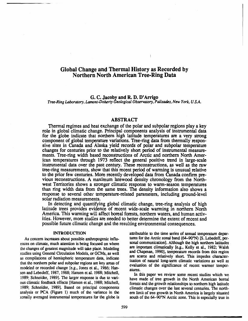
Global Change and Thermal History as Recorded byNorthern North American Tree-Ring Data

G. C. Jacoby and R. D. D'ArrigoTree.RingLaboratory,Lamont.DohertyGeologicalObservatory,Palisades,NewYork,U,S.A,

ABSTRACT

Thermal regimes and heat exchange of the polar and subpolar regions play a keyrole in global climatic change. Principal components analysis of instrumental datafor the globe indicate that northern high latitude temperatures are a very strongcomponent of global temperature variations, Tree-ring data from thermally respon-sive sites in Canada and Alaska yield records of polar and subpolar temperaturechanges for centuries prior to the relatively short peri.odof instrumental measure-ments. Tree-ring width based reconstructions of Arcttc and northern North Amer-ican temperatures through 1973 reflect the general positive trend in large-scaleinstrumental data over the past century, These reconstructions, as well as the rawtree-ring measurements, show_thatthis recent period of warming is unusual relativeto the prior few centuries. More recently developed data from Canada confirm pre-vious reconstructions. A maximum latewood density chronology from the North-west Territories shows a stronger climatic response to warm-season temperaturesthan ring width data from the same trees. The density information also shows aresponse to several other temperature-related parameters, including ground-levelsolar radiation measurements.

In detecting and quantifying global climatic change, tree-ring analysis of highlatitude trees provides evidence of recent wide-scale warming in northern NorthAmerica. This wanning will affect boreal ft)rests, northern waters, and human activ-ities. However, more studies are needed to better determine the extent of recent andpossible future climatic change and the resulting environmental consequences.

INTRODUCTION attributableto thetimeseriesof annualtemperaturedepar.Asconcernincreasesaboutpossibleanthropogenicinflu- turesfortheArcticzonalband(64-900N)[S.Lebedeff,per.

encesonclimate,muchattentionis beingfocusedonwhere sonalcommunication].Althoughthehighnorthernlatitudesthechangesof greatestmagnitudewilltakeplace.Modeling are importantclimatically[e.g.,Kellyet al., 1982;Walshstudiesusing General Circulation Models,orGCMs,aswell andChapman,1990],temperaturerecordsfromthis regionas compilationsof hemispherictemperaturedam,indicate are scarceand relativelyshort.This impedes character-izationof naturallong.termclimaticvariationsas wellasthatthenorthernpolarandsubpolarregionsarekeyareasof evaluationof the significanceof recent warmertemper.modeledor recordedchange[e.g.,Joneset al., 1986;Hart- atures.senandLebedeff,1987,1988;Hansenetal. 1988;Mitchell, In thispaperwe reviewsomerecentstudieswhichwe1989;Schneider,1989].Thelargerresponseis due to vari- havemadeof tree growthin the NorthAmericanborealousclimaticfeedbackeffects[Hansenctal., 1988;Mitchell, forestsandthegrowthrelationshipsto northernhighlatitude1989;Schneider,1989].Basedon principalcomponents climaticchangesoverthe last severalcenturies.Thenorth-analysisor PCA (Figure1) muchof the variancein the ernlimitof treegrowthinNorthAmericaislargelysituatedzonallyaveragedinstrumentaltemperaturesfortheglobeis southof the64-90°NArcticzone.This is especiallytruein

599

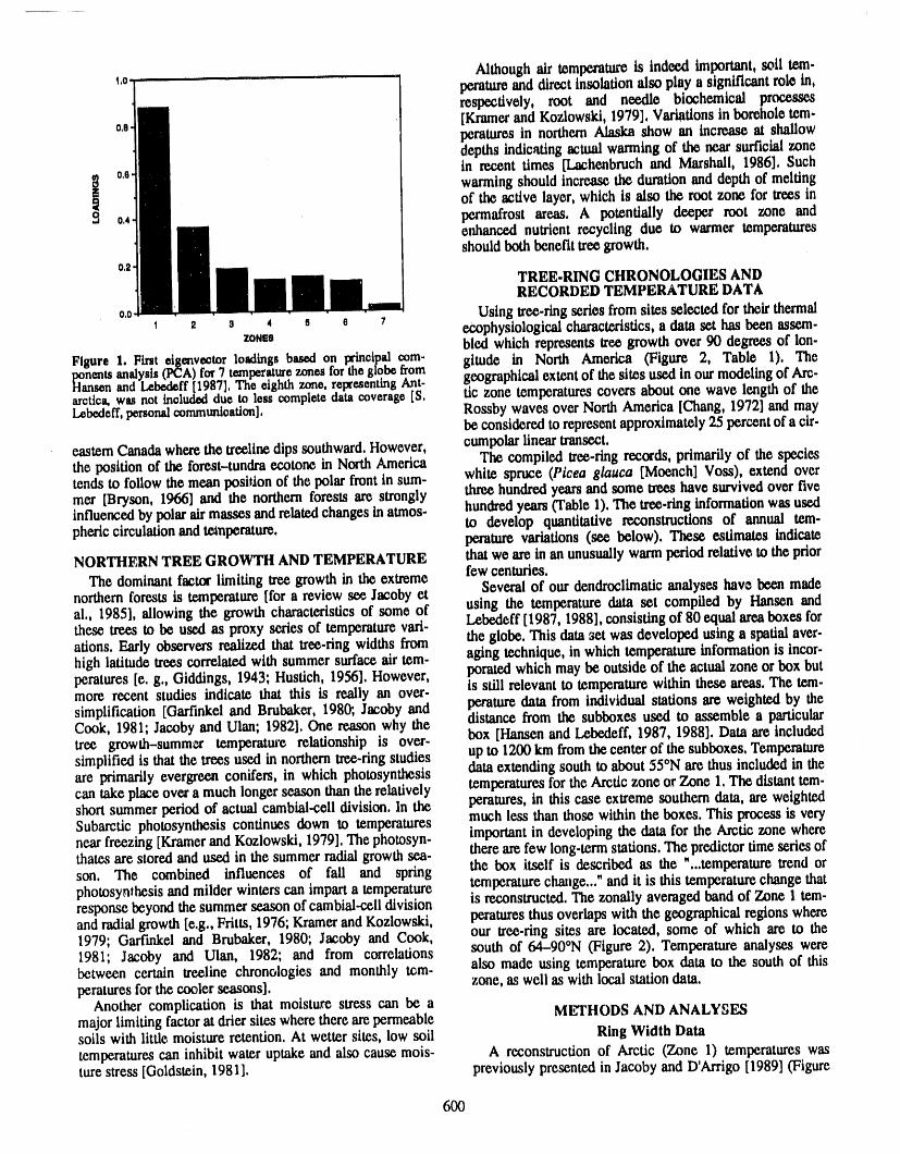
_ Althoughairtemperatureisindeedimportant,soiltem-1'°"i peraturoanddirect insolation also play a significant role in,

/ respectively, root and needle biochemical processes[KramerandKozlowski, 1979]. Variationsin borehole tem-

o,e, peraturesinnorthernAlaskashowan increaseatshallowdepths indicatingactualwarming of the near surficial zonein recent times [Lachenbruch and Marshall, 1986], Such

0.e warming should increasethe durationand depth of meltingof the active layer, which is also the root zone for trees inS 0.4 permafrost areas, A potentially deeper root zone and

enhanced nutrient recycling due to warmer temperaturesshouldboth benefittree growth.

o.= TREE-RING CHRONOLOGIES ANDRECORDED TEMPERATURE DATA

o,o Using tree-ringseries fromsites selected for their thermal1 2 s 4 . e 7 ecophysiological characteristics,a dataset has been assem-

zos_s bled which represents tree growth over 90 degrees of Ion-Figure 1. First eige_veetorloadingsbased on principalmm- gitude in North America (Figure 2, Table 1). The_nents analysis(P_A)for 7 temperaturezonesfortheglobefrom geographicalextentof thesites used in ourmodelingof Arc.tlansenand_ff[1987]. The eighthzone, representingAnt-arottca,wasnot includeddue to leas completedatacoveraget_. tic zone temperaturescovers about one wave length of theLebedeff,personalcommunioation]. Rossby waves over North America [Chang, 1972] andmay

be considered to representapproximately25 percentof a cir-

easternCanadawherethe treeline dipssouthward. However, cumpolarlineartransect.the position of the forest-tundraecotone in North America The compiled tree-ring records, primarilyof the speciestends to follow the mean position of the polar frontin sum- white spruce (Picea glauca [Moench] Voss), extend overthreehundredyears and some trees have survived over fivemer [Bryson, 1966] and the northern forests are stronglyinfluencedby polar airmasses and relatedchanges in atmos- hundredyears (Table1). The tree-ringinformationwas usedto develop quantitative reconstructions of annual tem.phericcirculationand teanperature, perature variations (see below). These estimates indicateNORTHERN TREE GROWTH AND TEMPERATURE thatwe are in an unusuallywarmperiod relative to the prior

few centuries.The dominantfactor limiting tree growth in the extreme Several of our dendroclimaticanalyses have been made

northern forests is temperature[for a review see Jacoby etal., 1985], allowing the growth characteristicsof some of using the temperature data set compiled by I-lansenandthese trees to be used as proxy series of temperature vari- Lebedeff [1987, 1988],consisting of 80 equal areaboxes forthe globe. This data3et was developed using a spatialaver-ations. Early observers realized that tree-ring widths from aging technique, in which temperatureinformationis intor-high latitudetrees correlatedwith summersurfaceair tem-peratures[e. g., Giddings, 1943; Hustich, 1956]. However, poratedwhich may be outside of the actualzone or box butmore recent studies indicate that this is really an over- is still relevant to temperaturewithin these areas. The tem-simplification [Garfinkeland Brubaker,1981>,Jacoby and peraturedata from individual stations are weighted by theCook, 1981; Jacoby and Ulan; 1982]. One reason why the distance from the subhoxes used to assemble a particulartree growth-summer temperature relationship is over- box [Hansen and _eff, 1987, 1988], Data are includedsimplified is that the trees used in northerntree-ringstudies up to 1200 km fromthe center of the subboxes, Temperatureare primarilyevergreen conifers, in which photosynthesis dataextending south to about 55°N are thus included in thecan takepiace over a much longerseason thanthe relatively temperaturesfor the Arctic zone or Zone 1. The distanttem-short summerperiod of actual cambial-cell division. In the peratures, in this case extreme southern data, are weightedmuch less than those within the boxes. This process is verySubarctic photosynthesis continues down to temperatures importantin developing the data for the Arctic zone wherenearfreezing [Kramerand Kozlowski, 1979].The photosyn- there are few long-termstations. The predictortimeseriesofthates are storedand used in the summerradial growth sea- the box itself is described as the "...temperaturetrend orson. The combined influences of fall and spring temperaturechange..."and it is this temperaturechange thatphotosynthesis and milder winters can imparta temperatureresponsebeyond the summer season of cambial-cell division is reconstructed.The zonally averaged bandof Zone 1 tem-andradialgrowth [e.g., Fritts, 1976; Kramerand Kozlowski, peraturesthus overlaps with the geographicalregions where1979; Garfmkel and Brubaker, 1980; Jacoby and Cook, our tree-ringsites are located, some of which are to the1981; Jacoby and Ulan, 1982; and from correlations southof 64-90°N (Figure 2). Temperature analyses werebetween certain treeline chronologies and monthly tem- also made using temperature box data to the south of thisperatures for the cooler seasons], zone, as well as with local stationdata.

Another complication is that moisture stress can be a METHODS AND ANALYSESmajorlimitingfactorat driersites wherethere arepermeablesoils with little moisture retention. At wetter sites, low soil Ring Width Datatemperaturescan inhibit water uptake and also cause mois- A reconstructionof Arctic (Zone 1) temperatures wasturestress [Goldstein, 1981], previouslypresentedin Jacoby and D'Arrigo[1989] (Figure

6OO

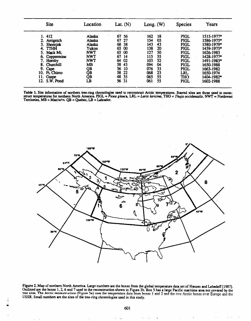
Site Location Lat. (N) Long. (V/) Species Years

I.412 Alaska 67 56 162 18 PIGL 1515-1977"2. Arrige_h Alaska 67 27 154 03 PIGL 1586-1,975"3. Sheenjek Alaska 68 38 143 43 PIGL 1580-1979'4. TTHI-I Yukon 65 00 138 20 P1GL 1459-1975"5. MackMt. NWT 65 00 127 50 PiIGL 1626-19836. _ine NWT 67 14 115 55 PIGL 1428-1977"7. Hobby NWT 64 02 103 52 PIGL 1491-1983"8. Churchill MB 58 43 094 04 PIGL 1650-19889. Cape QB 56 10 076 33 PIGL 1663-1982

10. Ft.Chimo QB 58 22 068 23 LRL 16,50-197411. Gaspe QB 48 35 065 55 THO 1404-1982"12. S.W. Pond LB 56 31 061 55 PIGL 1602-1988

Table 1. Site informatkm of northern tree-ring chronologi.m used lo recomlruct Arctic..u_mp__auu_. Starred sites are those used to recon-

struct temp_atures for nonhero North America. PIGL = Pu:e.a g/auca, LRL = Lar/z/aru:ma, THO = Thuja occ/denta//s. NWT = I%nhwestTerritmies, MB= Mm_mb._ QB = Quebec, I.B = L_ador.

180qV

_OON

Figure2.Map ofnorthernNorthAmerica.Largenumbersaretheboxes fromtheglobaltemperaturedatasetofHensen endLebodeff[1987].OutlinedaretheboxesI,2,6 and 7 usedinthereconslructionshown inFigure3b.Box 5 has,,largePacificmm'itime_ea notcovezedby thetree _it_.The Arctic recrm_tn_tmn (Fimn'p._J_ ._._ tl,_. !_._..,w_'mmr,.,4atJ F,_m t_w.e 1 .,v_9 ,,.,,4 tl_,,.,,,,,,, A._,;_. k......... c .... ._ ,k.

_ USSR. Small numbersarethesitesofthetree-ringchronologiesusedinthisstudy._

i

601

RECONSTRUCTED ARCTIC ANNUAL TEMPERATURES2 ' • ' - • ' " ' ' ""

= o0

I,t,i

WQ -2

-3 - ' , - ' "_ - v - , - . ' '1600 1650 1700 1750 1800 1850 1go0 1950 2000

RECONSTRUCTEDANNUAL TEMPERATURESFOR NORTHERNNORTH AMERICA2

1

ow• U

_ -1w

_ -2D

-3

1600 1650 1700 1750 1800 1850 1900 1950 2000

YEARS

Figure3. Annualtemperaturereconsuucdonsfornorthernlatitudes,a: ReconstructedannualAn:dcor ZoneI temperatures[as in JacobymdD'Arrigo,1989].b: ReconstructedannualtemperaturesfornorthernNorthAmericafromboxes 1, 2. 6 and7 fromHansenand Lebedeff[1987];as in D'ArrigoandJacoby[1992].

3a). The reconstruction shows a cooler period around the in Figure 2. lt encompasses four temperatureboxes (1, 2, 6time of the Maunder Minimum, a relative warming in the and 7) as delimited by Hansen and Lebedeff [1987, 1988]

_. 1700s, an abruptcooling in the early 1800s and a gradual which cover muchof northernNorth America.The locationswarming trend over the past century (Figure 3a). In more of the seven tree sampling sites used are contained withinrecentmodeling we improvedthe spatialcoverage and data this four-box area (these sites are starred in Table 1). Theby addinga chronologyfrom northernLabrador,anareaof longertree-ringdatasetenablesusto producea reconslxuc-relativelyweakcoverage(Figure2, Table1).Also,thechro- tion backto A.D. 1600 and is very similarto the Arctic

= nology fiom Churchill, Manitoba (Figure 2, Table 1) was reconstruction.The trendsfor thecommon period aregener-modified to include data with more low-frequency climatic ally the same. For the earlier period of 1600 to 1671, thisinformation (Scott, P. A., personal communication). The reconstructionshows an extendedcool interval for the earlystandardizationof the raw uee-ring widths for the two new 1600s andsome moderationin the mid-1600s.chronologies was done to preserve both high and low fre-quency variance in the resulting chronologies [Jacoby and Density StudiesD'Arrigo, 1989].The reconstructionusing the two new chro- An important method which is only now being usednologies is essentially the same as the previous one shown extensively in dendroclimatology is densitometric analysisin Figure 3a [Jacobyand D'Arrigo,1989] but the calibration of tree.-r_Jigsamples [Schweingruberet al., 1978; Hughes PAand verificationfordifferent time periods are improved, al., 1984; Conkey, 1986; Yanosky and Robinove, 1986;

- In addition to the reconstruction for the Arctic we also Briffa PAal., 1988; Jacoby PAal., 1988; Schweingruber,= selected a subset of seven of the longest chronologies in 1988; Thefiord PAal., 1991]. Briefly, the densitompAricdata+ orderto reconstructannual temperaturesfor nonhem North from trees can provide a much better indic_3r of inter-

-" America [-u'Arrigoand .;acoby, """" "I3-_isiegioii is -" ....]y_.j. -,. ..... I *,.I;m,t;,., ,,'.knnoa tt,;th 0h,, _,,_o,,,, ht" etmng rliroj-f_|IUWIi l;l,llUllltJt4_Jt _ltJti|lggtlklt_ _,llt4gt4tt_t_,* t v_ alma M=_.,' _m_._**= __ _ --.

602

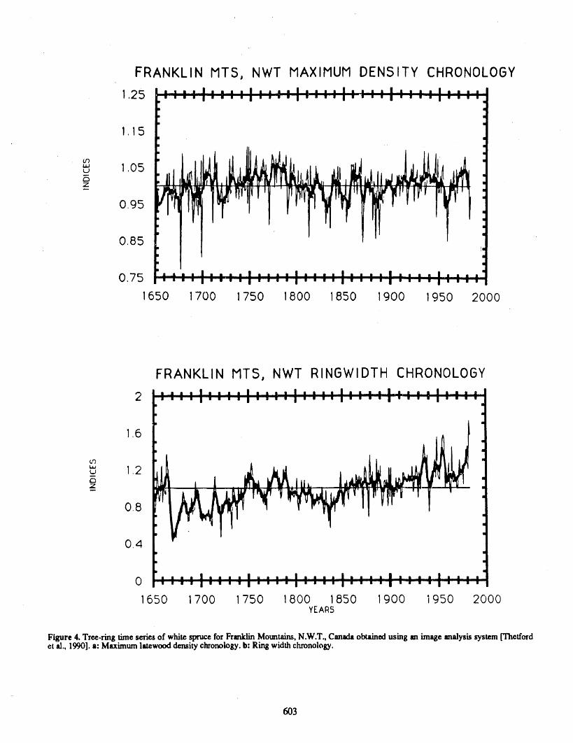
FRANKLIN MTS, NWT MAXIMUM DENSITY CHRONOLOGY

125 I III; II • : • I • • • • II • I l j

I I I I:II'' I'' ' I '' " " I'''''::'ii:::,

I1,15

0.85

0 75 n a I I I I • a I I I I I n I • I " I I I I " • I • n I R I m I I I, " • i • l • I • • l • • I • I I I • • I • I • I I I I . . l I I • I

1650 1700 1750 1800 1850 1900 1950 2000

FRANKLIN MT5, NWT RINGWIDTH CHRONOLOGY

2 IIIIIlIIIIllIIIlII:lInlI|II:IIIII::' ' I ' I'" ' " I " •'" I " " I" " " ' I " ' " ' "

1,6

u 1,2t .. .iii,. _

0,4

i I i i i i _

' | I i'| I II " i ' i'" ' "I ' : :'Ii . .. . '

1650 1700 1750 1800 1850 1900 1950 2000YEARS

Figure4.Tree-ringtimeseriesofwhitespruceforFranklinMountains,N.W.T.,Canadaobtainedusinganimageanalysissystem[Thetfordel al., 1990]. a: Maximum latewood density chronology, b: Ring width chronology.

603

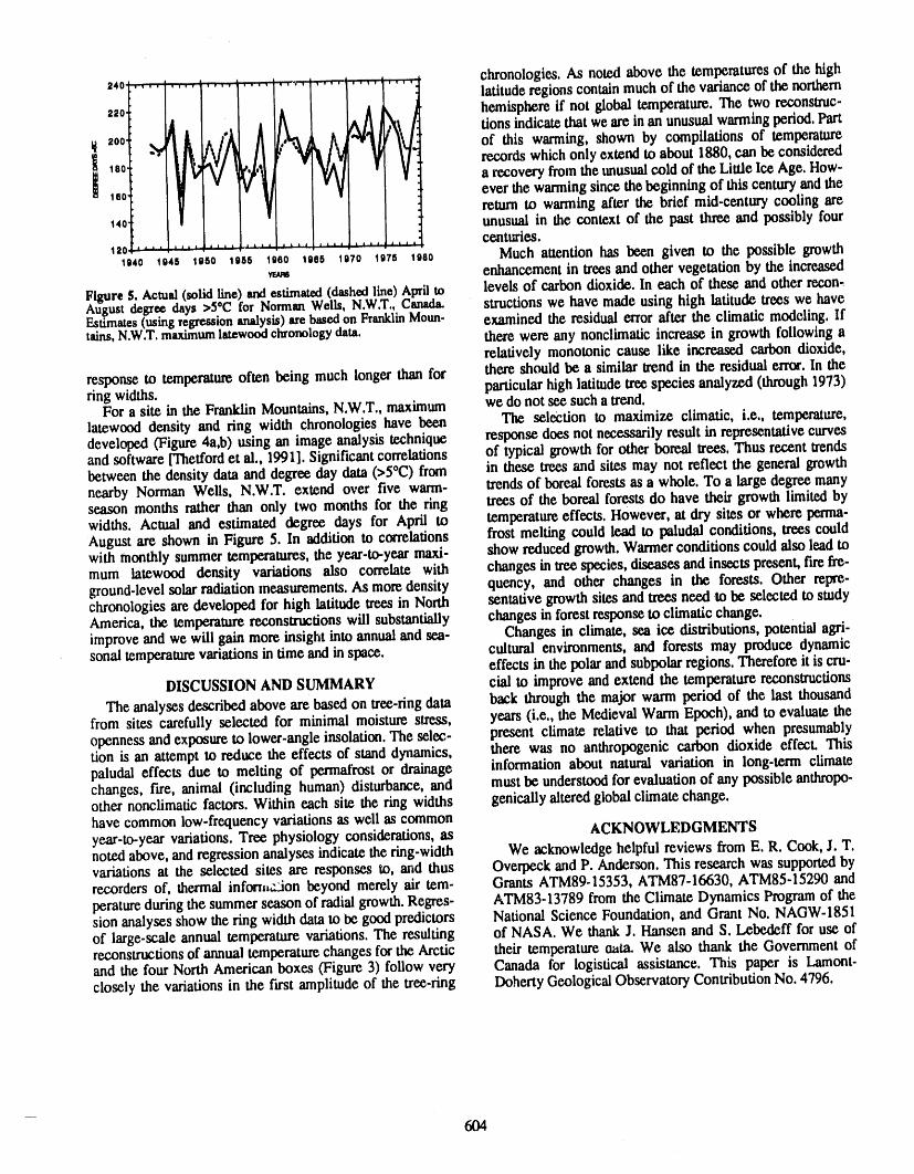
chronologies,As notedabovethetemperaturesofthehigh

,40[_ ..... 1.... ' ...... " ..... "_' .... i latituderegionscontain much of the variance of the northern2_o i hemisphereifnotglobaltemperature.The tworen_nstruc-

(_/t_ , I._ _ ",_ tions indicatethat we are inan unusual warmingperiod.Part_o0 of this warming, shown by compilations of temperature

_ records which only extend to about 1880, can be considered

_,,o ,])_1, r_1'_i a recovery from the unusualcold of the Little Ice Age. How",,ol ever the wanning since the beginning of this centuryandthe

- return to warming after the brief mid.century cooling are

4o unusual in the context of the past three and possibly four1

_20 ........... [" .......... centuries.ls4o lo4e 1see 1see 1see 1see ls7o 10rs lse0 Much attention has been given to the possible growth

enhancement in treesand other vegetation by the increased

FigureS.Actual (solidline) andestimated(dashedline)Aprilto levels of carbon dioxide. In each of these and other recon-August degree days >50C for NormanWells, N.W.T.,Canada. structions we have made using high latitude trees we haveEstimates(usingregressionanalysis)arebasedon FranklinMoun- examined the residual error after the climatic modeling. Ifrains,N.W.T.maximumlatewoodchronologyclam. there were any nonclimaticincrease in growth following a

relatively monotonic cause like increased carbondioxide,

response to temperatureoften being much longer than for there should be a similartrend in the residual error.In theparticularhigh latitudetree species analyzed (through1973)ringwidths.

For a site in the FranklinMountains,N.W.T., maximum we do not see sucha trend.latewood density and ring width chronologies have been The selection to maximize climatic, i.e., temperature,developed (Figure 4a,b) using an image analysis technique response does not necessarilyresult in representativecurvesand software [Thetfordet al., 1991]. Significantcorrelations of typical growth for other boreal trees. Thus recent trendsbetween the density data and degree day data(>5°C) from in these trees and sites may not reflect the general growthnearby Norman Wells, N.W.T. extend over five warm- trendsof boreal forestsas a whole. To a large degree manyseason months rather than only two months for the ring trees of the boreal forests do have their growth limited bywidths. Actual and estimated degree days for April to temperature effects. However, at dry sites or where perma-August are shown in Figure 5. In addition to correlations frost melting could lead to paludal conditions, trees couldwith monthly summer temperatures, the year-to-year maxi- show reduced growth. Warmer conditions could also lead tomum iatewood density variations also correlate with changes in tree species, diseases and insects present, fire fre-ground-level solar radiation measurements. As more density quency, and other changes in the forests. Other repre-chronologies are developed for high latitude trees in North sentative growth sites and trees need to be selected to studyAmerica, the temperaturereconstructions will substantially changes in forest responseto climatic change.improve and we will gain more insight into annual and sea- Changes in climate, sea ice distributions, potential agri-sonal temperature variations in time and in space, cultural environments, and forests may produce dynamic

effects in the polar and subpolar regions. Therefore it is ga'u-DISCUSSION AND SUMMARY cial to improve and extend the temperaturereconstructions

The analyses described above are based on tree-ring data back through the major warm period of the last thousandfrom sites carefully selected for minimal moisture stress, years (i.e., the Medieval Warm Epoch), and to evaluate theopenness and exposure to lower-angle insolation. The selec- present climate relative to that period when presumablytion is an attempt to reduce the effects of stand dynmnics, there was no anthropogenic carbon dioxide effect. Thispaludal effects due to melting of permafrost or drainage information about natural variation in long.term climatechanges, fire, animal (including human) disturbance, and must be understoodfor evaluation of any possible anthropo-other nonclimatic factors. Within each site the ring widths genitally altered global climate change.

have common low-frequency variations as well as common ACKNOWLEDGMENTSyear-to-year variations. Tree physiology considerations, asnoted above, and regression analyses indicate the ring-width We acknowledge helpful reviews from E. R. Cook, J. T.variations at the selected sites are responses to, and thus Overpeck and P. Anderson. This research was supported byrecorders of, thermal inforn,,z_ion beyond merely air tem- Grants ATM89-15353, ATM87-16630, ATM85-15290 andperature during the summer season of radial growth. Regres- ATM83-13789 from the Climate Dynamics Program of thesion analyses show the ring width data to be good predictors National Science Foundation, and Grant No. NAGW-1851of large-scale annual temperature variations. The resulting of NASA. We thank J. Hansen and S. Lebedeff for use ofreconstructionsof annual temperature changes for the Arctic their temperature oata. We also thank the Government ofand the four North American boxes (Figure 3) follow very Canada for logistical assistance. This paper is Lament-closely the variations in the fast amplitude of the tree-ring Doherty Geological Observatory Contribution No. 4796.

604

REFERENCES

Briffa, K. R., P. D. Jones, J. R. Ptlcher, and M. K. Hughes, Jacoby, G. C., and R. D. D'Arrigo,Reconstructed NorthernReconstructing summer t_aperatures in northernFen- Hemisphere annual temperature since 1671 based onnoscandinaviaback to AD 1'/00 using tree-ringdatafrom high-latitude tree-ring data from North America, Clim.Scots pine,Arctic Alpine Rese _ch, 20, 385-394, 1988. Change, 14, 39-59, 1989,

Bryson, R. A., Air masses, streamlines,and the boreal for- Jacoby, G. C., and L. D. Ulan, Reconstructionof past iceest, Geographical Bull., 8, 228-269, 1966. conditions in a Hudson Bay estuary using tree-rings,

Chang, J. H., Atmospheric Circulation Systems and Cii- Nature, 298, 637-639, 1982.mates, OrientalPubl. Co., Honolulu, 326 pp., 1972. Jacoby, G. C., E. R. Cook, and L. D. Ulan, Reconstructed

Conkey, L. E., Red spruce tree.ringwidths and densities in summerdegree days in central Alaska and northwesterneastern North America as indicators of past climate, Canadasince 1524, Quat. Res,,23, 18-26, 1985.Quat. Res., 26, 232-243, 1986. Jacoby, G. C., I. S. Ivanciu, and L. D. Ulan, A 263-year

D'Arrigo,R. D., and G. C. Jscoby, Dendroclimaticevidence record of summer temperature for northern Quebecfrom northernNorth America,in Climate since AD 1500, reconslnlcted fromtree-ring dataand evidence of a majoredited by R. S. Bradleyand P. D. Jones, Routledge,Lon- climatic shift in the early 1800's, Palaeogeogr., Paiaeo.don, 1992, In press, climatol., Palaeoecol., 64, 69-78, 1988.

Fritts,H. C., Tree-Rings and Climate, Academic Press, New Jones,P. D., S, C. B. Raper,R. S. Bradley,H. F. Diaz, P. M,York, 1976. Kelly, and T. M. L. Wigley, Northern Hemisphere sur.

Garf'mkel,H. L., and L. B. Brubaker,Modern climate-.tree face air temperature variations, 1851-1984, J. Clim,growth relationships and climatic reconstructionin sub- Appl. Meteorol., 25, 161-179, 1986.Arctic Alaska,Nature,286, 872-874, 1980. Kelly, P. M., P. D. Jones, C. B. Sear, B, S. G. Cherry, and

Giddings, J. L., Some climatic aspects of tree growth in R.K. Tavukol, Variation_ in surface air temperatures:Alaska, Tree.Ring Bulletin, 4, 26-32, 1943. Part2: Arctic regions, 1881-1980, Mon. Wea. Rev., 110,

Goldstein,G. A., Ecophysiologicaland demographicstudies 71-83, 1982.of white sprUce(Picea glauca [Moench] Voss) at treeline Kramer,P. J., and T. T. Kozlowski, t"hysiology of Woodyin the central Brooks Range of Alaska, Ph.D. thesis, 193 Plants, 811 pp., Academic Press, Orl_ldo, FL, !o79.pp., University of Washington,Seattle, 1981. Lachenbruch,A. H., and B. V. Marshall,Changing climate: :

Hansen, J., and S. Lebedeff, Global trendsof measuredsur- geothermalevidence frompermafrostin the Alaskan Arc,.face air temperature,J. Geophys. Res., 92, 13345-13372, tic,Science, 234,689-696, 1986.1987. Mitchell, J. F. B., The "greenhouse" effect and climate

Hansen, J,, and S. Lebe_ff, Global surface air tem- change,Rev. Geophys,, 27,115-139,1989.peratures:update through 1987, Geophys. Res. Lett., 1.5, Schneider, S. H., The greenhouseeffect: science andpolicy,323-326, 1988. Science, 243, 771-781, 1989.

Hansen, J., I. Fung, A. Lacis, S. Lebedeff, D. Rind, R. Schweingruber,F. H., Tree Rings. Basics and ApplicationsRuedy, G. Russell, and P. Stone, Global climate changes of Dendrochronology, 276 pp.,Reidel, Dordrecht,1988.as forecast by the GISS 3-D model, J. Geophys. Res., 93, Schweingruber, F. H., H. C. Fritts, O. U. Braker, L. G.9341-9364, 1988. Drew, and E. Schar, The x-ray technique as applied to

Hughes, M. K., F. H. Schweingruber,D. Cartwright,and dendroclimatology,Tree-RingBulletin, 38, 61-91, 1978.P.M. Kelly, July-August temperature at Edinburgh Thefford, R. D., R. D. D'Arrigo, and G. C. Jacoby, Anbetween 1721 and 1975 from tree-ring density and width image analysis system for generating densitometric anddata, Nature, 308, 341-344, 1984. ring width time series, Can. J. Forest Res., 1991, In

press.Hustich, I., Correlation of tree-ring chronologies of Alaska, Walsh, J. E., and W. L. Chapman, Short-term climatic var-

Labrador and Northern Europe, Acta Geograptu'ca, 15,3-26, 1956. lability in the Arctic, J. Clim., 3,237-250, 1990.

Yanosky, T. M., and C. J. Robinove, Digital image measure-Jacoby, G. C., and E. R. Cook, Past temperature variations ment of the area and anatomical structure of tree-rings,

as inferred from a 400-year tree-ring chronology from Can. J. Bot., 64, 2896-2902, 1986.Yukon Territory, Canada, Arctic Alpine Res., 13, 409-418, 1981.

_5

Spatial and Temporal Characteristics of the Little Ice Age:The Antarctic IceCore Record

Ellen Mosley.Thompson and Lonnie G. ThompsonByrd Polar Research Center, The Ohio State University, Columbus, Ohio, U.S.A,

ABSTRACT

Recently, ice core re,cords from both hemispheres, in conjunction with otherproxy records (e.g., tree rings, speleothems and corals), have shown that the LittleIce Age (LIA) was spatially extensive, extending to the Antarctic. This paper exam-ines the temporal and spatial characteristics of the dust and 8180 information fromAntarctic ice cores. Substantial differences exist in the records. For example, a 550-year record of 81_,O and dust concentrations from Siple Station, Antarctica suggeststhat warmer, less dusty conditions prevailed from A.D. 1600 to 1830. Alternately,dust and 5180 data from South Pole Station indicate that opposite conditions (e.g.,cooler and more dusty) were prevalent during the LIA. Three additional Antarctic_5180 records are integrated with the Siple and South Pole histories for a more com-prehensive picture of LIA conditions. The records provide additional support forthe LIA temperature opposition between the Antarctic Peninsula r_gion and EastAntarctica. In addition, periods of strongest LIA cooling are not temporally syn-chronous over East Antarctica. These strong regional differences demonstrate that asuite of spatially distributed, high resolution ice core records will be necessary tocharacterize the LIA in Antarctica.

INTRODUCTION A.D. 1450-1880; (3) of maximum data coverage; (4) forThe broad spectrum of chemical and physical data pre- which multi-proxy reconstructions are possible; (5) when

servedwithin ice sheets and ice capsprovidea multifaceted annualand decadal resolution is possible so that leads andrecordof both the climatic and environmentalhistoryof the lags in the system can be studied; and (6) when causes ofearth.Over the last three decades, ice cores have provided these changes remain undetermined.In the last decade icenew details about the magnitude,direction,and rate of cii- cores have been recognized increasingly as sources of verymarie change during the last 160,000 years. These histories highly resolved paleoenvironmental time series. Here weserve as comprehensive case studies that can improve our examine the characteristics of the most recent neoglacialunderstandingof future changes in the global environment, periodor Little Ice Age as it is preserved in Antarctic ice

Clarification of the course of future climatic changes cores.requires understanding the origin of the natural variabilitywithin the environmental system on time scales ranging ANTARCTIC ICE CORE RECORDSfrom decades to centuries [IGBP, 1989]. The Holocene The histories discussed below originated from differentrecord (--last 10,000 years) offers the temporal and spatial areasof the Antarctic(Figure 1) which arecharacterizedbydetail necessaryto characterizethat variability.The last soy- quite disparatenet balances, mean annual temperatures,sur-eral thousandyearsof the Holocene provide the best oppor- face climatologies, and ice flow regimes. Dating of ice coretunity to study decadal, andcentennial-scale processes as it recordsis the first, critical step in paleoclimatic re,construe-is the period (1) most relevant to human activities, both rienand dating precision varies widely among these records.present and future: (2) of extremes within the Holocene The net annual accumulation and temperatureof a site, aswarm period including the "Little Ice Age" period from well as the sample sizes selected for individual analyses,

_

6O6

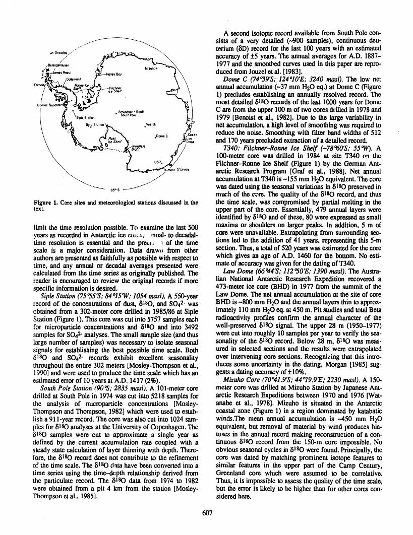
A second isotopic recordavailable from South Pole con-f .... ------_--__ sists of a very detailed (-900 samples), continuous deu-

../" _ texium(SD) record for the last 100 years with an estimated,,-o,co+o,/ _.._ .._

/ ,_=¢'- __ _ accuracy of :t:5 years, +_e annual averages for A.D. 1887-/B,,,,¢_,_, ,-'_ + -,-'--_.._\ 1977 and the smoothed curves used in this paperare repro-

.+/t / Ai r Miz_. - "'_\+.i_2''j'_' m'' 'i_L-m,,.,_, { \ ducedfromJouzelelai.[1983]."8_:,x,• /t_,,,o,,[ \ \ Dome C (74°39°S;124°I0'E;3240 masl).The lownet

,. %).. , If;,s_ " annualaccumulation (-37 mm H20 eq.) at Dome C (FigureT 1) precludes establishing an annually resolved record. The

a_,, N_,-_ :d._v_.'_ _ / most detailed 8180 recordsof the last 1000 years for Dome[ ] 'x_'_ . A_.:,,:sco,, "_I C are from the upper 100 m of two cores drilled in 1978and/ J_ \s,_.m.,= - so_,,_. /(:t 1979 [Benoist et al,, 1982]. Due to the large variability in/ _._t._, _o_-_.... .vo,,o_ :'_1:' net accumulation, a high level of smoothing was requiredto\ _-',:,'¢_ " )"M,. " /_/ reduce the noise. Smoothing with filter band widths of 512

\ _ ,k__._+,+N_ ,,:#,,_ .o_,c _Q_,_, and 170yearsprecludedextractionof a detailed record.' . ..... ,._"_ ,(-/ T340: Filchner-Ronne Ice Shelf (-78"60'S; 55"W). A

t, ,q,_, 100-meter core was drilled in 1984 at site TM0 on the"_ 1/ _._.+ Filchner-Ronne Ice Shelf (Figure 1) by the German Ant-

,.,..,% ,.,,..<,,_.._r-_,_ / DU,,+,, arctic Research Program [Oraf et al., 1988]. Net annual

' __"_- es.s .__ accumulation at T340 is -155 mm H20 equivalent.The corewas datedusing the seasonal variations in 8180 preserved inmuch of the c_re. The quality of the 81SO record, and thus

Figure 1. Coresitesandmeteorologicalstatlo_sdiscussedin the the time scale, was compromised by partialmelting in thetext. upper partof the core. Essentially, 479 annual layers were

identified by 81SOand of these, 80 were expressed as small

limit the time resolution possible. To examine the last 500 maxima or shoulders on larger peaks. In addition, 5 m ofyears as recorded in Antarctic ice co_u_;, ,nual. to decadal- core were unavailable. Extrapolating from surrounding sec-time resolution is essenlial and the prec,:. _ of the lime tions led to the addition of 41 years, representing this 5-mscale is a major consideration. Data draw, from other section. Thus, a total of 520 years was estimated for the coreauthors are presented as faithfully as possible with respect to which gives an age of A.D. 1460 for the bottom. No esti-

mate of accuracy was given for the dating of TM0.time, and any annual or decadal averages presented werecalculated from the time series as originally published. The Law Dome (66°44'S; I12°50'E; 1390 masl). The Austra-reader is encouraged to review the original records if more lian National Antarctic Research Expedition recovered aspecific information is desired. 473-meter ice core (BHD) in 1977 from the summit of the

Siple Station (75°55'S; 84°15'W; 1054 masl). A 550-year Law Dome. The net annual accumulation at the site of corerecord of the concentrations of dust, 8180, and SO42"was BI-IDis -800 mm H20 and the annual layers thin to approx-obtained from a 302.meter core drilled in 1985/86 at Siple imately 110 mm H20 eq. at 450 m. Pit studies and total BetaStation (Figure 1).This core was cut into 5757 samples each radioactivity prof'fles confirm the annual character of thefor microparticle concentrations and 8180 and into 3492 well-preserved _ilso signal. "Ihe upper 28 m (1950--1977)samples for SO42" analyses, The small samples'ize(and thus were cut into roughly 10 samplesper year to verify the sea-large numberof samples) was necessary to isolate seasonal sonality of the _sO record. Below 28 m,/ilsO was meas-signals for establishing the best possible time scale. Both ured in selected sections and lhc results were extrapolated_180 and SO42" records exhibit excellent seasonality over intervening core sections. Recognizing that this intro-throughout the entire302 meters [Mosley-Thompson et al., duces some uncertaintyin the dating, Morgan [1985] sug-1990] and were used to produce the time scale which has an gests a dating accuracy of+10%. ,estimated error of 10years at A.D. 1417 (2%). Mizuho Core (70°41.9'S; 44019.9'E; 2230 masl). A 150-

South Pole Station (90°S; 2835 masl). A 101-meter core meter core was drilled at Mizuho Station by Japanese Ant-drilled at South Pole in 1974 was cut into 5218 samples for arctic Research Expeditions between 1970 and 1976 [Wat-the analysis of microparticle concentrations [Mosley- anabe et al., 1978]. Mizuho is situated in the AntarcticThompson and Thompson, 1982] which were used to estab- coastal zone (Figure 1) in a region dominated by katabaticlish a 911-year record.The core was also cut into 1024 sam- winds.The mean annual accumulation is .-450 mm H20pies for _StBOanalysesat the University of Copenhagen. The equivalent, but removal ofmaterial bywind produces hia-_i_SOsmnples were cut to approximate a single year as tuses in the annual record making reconstructionof a con-defined by the currentaccumulation rate coupled with a tinuous 8180 record from the 150-m core impossible. Nosteady state calculation of layer thinning with depth. There- obvious seasonal cycles in/ii so were found. Principally, thefore, the 8_sO record does not contribute to the refinement core was dated by matching prominent isotope featm'es toof the time scale. The 5_0 data have been converted into a similar features in the upper part of the Camp Century,time series using the time--dt_pthrelationship derived from Greenland core which were assumed to be correlative.the particulate record. The 5_80 data from 1974 to 1982 Thus, it is impossible to assess the quality of the time scale,were obtained from a pit 4 km from the station [Mosley- but the error is likely to be higher than for other cores con-Thompson et al., 1985]. sidered here.

6O7

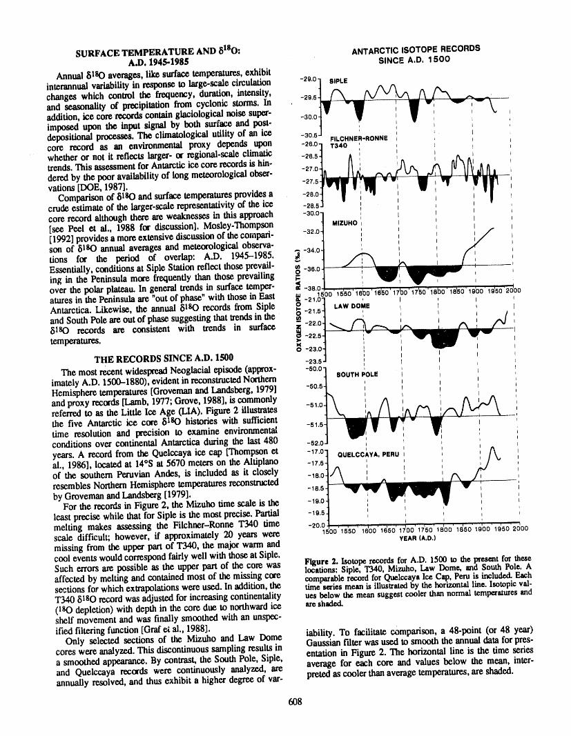
SURFACE TEMPERATURE AND 8180: ANTARCTICISOTOPERECORDSA.D. 194.5-198S SINCE A.D, 1500

Annual 8lsO averages, like surfacetemperatures,exhibit

int_rannualvariability/alresponseto large-scalecirculation -20,ol SlPLE /__ Achanges which control the frequency, duration, intensity, 51 _ _'20' _ -r --

and ,seaso,nality of precipitation from cyc!on!c storms.In , ,addition, ice core r_is contain glaciologcaJ noise super- -30.o L ,imposed upon the input signal by both surface and post- , ,depositional processes. The clinmtologicalutility of an ice -3o.5 FILCHNER-RONNEI

com record as an environmentalproxy dependsupon -26'01 T340 , I

whetheror not it refloctslarger-or regional-scaleclimatic-2e.s_ _ '_f_w_wf_k_ wV_,___

trends.This assessment forAntarcticice corerecordsis hin- -27.o_._ ' i _

dcredby the pooravailabilityoflongmcteomlogical obser- -2"5_V_r Wvations [DOE, 1987]. -28.o_ |Comparison of 5150 and surface temperatures providesacrude estimate of the larger-scalerepresentativityof the ice -28.5Jcorerecordalthoughtherearcweaknessesin thisapproach -3o.o.[see Peel ct al,, 1988 for discussion].Mosley-Thompson MIZUHO[1992] provides a moreextensive discussion of the compari- -a2.o.son of 8tsO annual averages and meteorological observa-

tions for the period of overlap: A.D. 1945-1985. _-34.OEssentially, conditions at Siple Station reflect those prevail- _ -35.o -',ing in the Peninsula more frequently than those prevailing _ ,over the polar plateau. Ingeneral trends in surfacetemper- = -35'_500'15'50'le_o'ie'80'17'00'17_0'Isb0'15'50'19'0019'_02d00atm'es in the Peninsula are"out of phase" with those in East [ -21,ol , i ,Antarctica.Likewise,the annual8IsO recordsfrom Siple o _..1 LAWDOME t t Iand South Pole areoutof phase suggesting thai trendsin the o -_1.0-1 L , ' I ,

8150 records are consistent with trends in surface i -22'°i__'O

THE RECORDS SINCE A.D. 1500 . t I

The most recent widespreadNcoglacial episode (approx- -5o.ot , 'imately A.D. 1500-1880), evident in reconstructedNorthern SOUTH POLE I II

Hemispheretemperatures[Gmveman and Landsberg, 1979] -5°'5"I " 'I t I

and proxy records [Lamb,1977; Grove, 1988], is commonly _ , ^ _ A i A-51.0.4 _ I / I i _ _ I _ j.vreferred to as the Little Ice Age (LIA). Figure 2 illustrates _ _-_ i/_ [ I _,A /-\ ,/"XJ _ \ _,

the five Antarctic ice core 8IsO histories with sufficient -s"5__ rv _'" V', ':dme resolution and precision to examine environmentalconditionsovercontinentalAntarcticaduringthelast480 -52.o] _', ', 'years.A recordfrom tic Quelccayaice cap [Thompsonct -17.o- OUELCCAYA, PERU ' ', /\.

al., 1986],locatedat 14°Sat 5670 meterson the Altiplano -17.s- ^ ', '_ _ -J_ ' ' ,'_ li

of tic southern Peruvian Andes, is included as it closely -18.oi \ , ,, _ / \ j.,

resembles NorthernHemisphere temperaturesreconstructed -18.5 _ V'by Gmveman and Landsberg [1979]. , I

For the records in Figure 2, the Mizuho time scale is the -19.oleast precise while thatfbr Siple is the most precise. Partial -lo.5_ 'I I q I

I *i t

melting makes assessingthe Filchncr-RonneI"340 time -2°'°50_'is'so'16t00 ' 1650'17'00'17'50'18_00' 1850'10'00'1950'2'(_00scaledifficult; however,if approximately 20 yearswere YEAR (A.D.)

missingfrom tic upperpartof T340, the majorwarmandcooleventswouldcorrespondfairlywellwith thoseatSiple.Such errors are possible as the upper part of the core was Figure 2. Isotope recordsforA.D. 1500m the presentfor theselocations:Siple, 'V340,Mizuho,Law Dome, and South Pole. Aaffected by melting and contained most of the missing core comparablerecordforQuelccayaIce Cap, peru is included.Eachs_tions for which extrapolationswere used. In addition,the timeseriesmeanis illustratedby thehorizontalline.Isotopicval-T340 5180 recordwas adjusted for increasing continentality ues belowthe meansuggestcoolerthannormaltemperaturesand(isO depletion) with depth in the core due to northwardice areshaded.shelf movement and was finally smoothed with an unspec-

ified filteringfunction [Grafet al., 1988]. lability. To facilitate comparison, a 48-point (or 48 year)Only selected sections of timMizuhoand Law Dome

cores were analyzed. This discontinuous sampling results in Gaussian filter was used to smooth the annual data forpres-a smoothed appearance.By contrast, the South Pole, Siple, entation in Figure 2. The horizontal line is the time seriesand Quelccaya records were continuously analyzed, are average for each core and values below the mean, inter-pwaed as cooler thanaveragetemperatures, are shaded.annually resolved, and thus exhibit a higher degree of var-

6O8

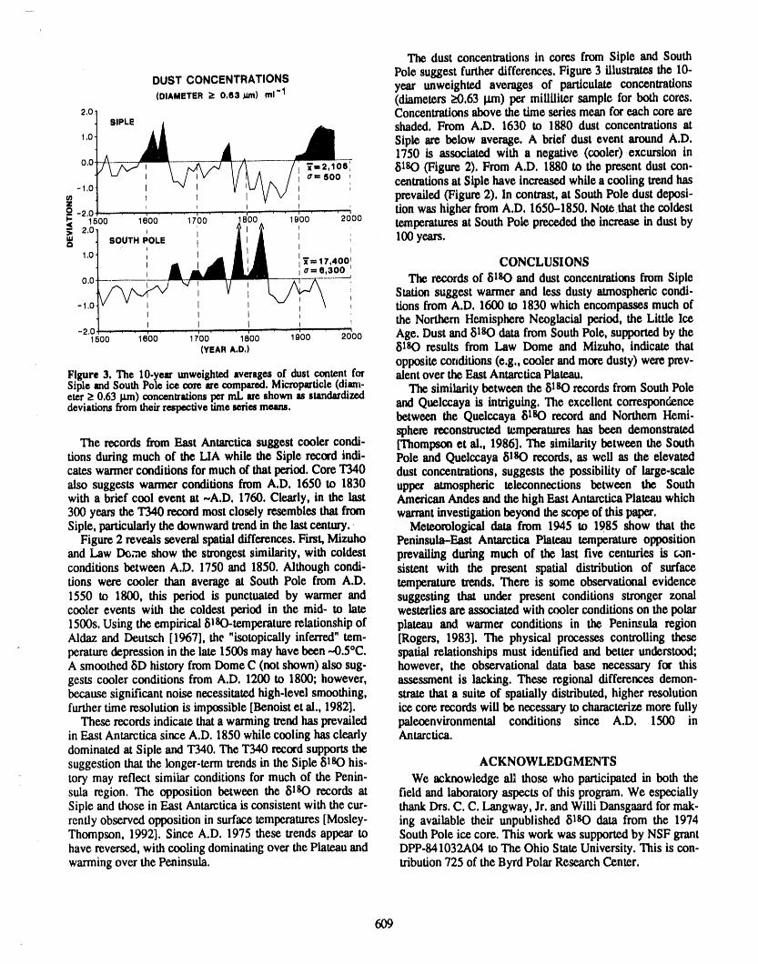
The dust concentrations in cores from Siple and South

DUSTCONCENTRATIONS Polesuggestfurtherdifferences,Figure3 illustratesthe 10-year unweighted averages of particulate concentrations

(DIAMETER 2 O,63jml) ml"1 (diameters L>0,63I.Un)pcr millilitersamplefor bothcores,2,0 Concentrationsabovethetimeseriesmeanforeachcoreare

• StoLE AA _ shaded,From A.D. 1630 to 1880 dust concentrationsat

1,0" _ ml Stplearc below average.A brief dusteventaroundA.D,• __A _o-e- 1750 is associatedwith a negative(cooler)excursionin-A--_-7r---_ 81so (Figure 2). From A.D. 1880 to the present dust con-

°'°" b' v" _gP'IV V _ _=]5'_ c_dons at Slplehavein_ whtlea cooling l_.,nd_-1,0'

_ prevailed(Figure 2). In contrast,at SouthPoledust depost-z ' _ , ton was higher from A,D. 1650-1850. Note that the coldest

-2.0 ........ , . ' "11500 1600 1700 .830" ' '1900' ' '20002,0] , _ I temperaturesatSouthPole precededtheincreasein dustby

I,OI , I ., I' tt "_: e,aoo ' CONCLUSIONSo,o .... m_t-_-T- A Tlm records of 61ILOand dust concentrationsfrom Siple

Station suggest warmer and less dusty atmosphericcondi-tons from A.D. 1600 to 1830 which encompasses much of

', the Northern Hemisphere Neoglacial period, the Little Ice1500 1600 1700 1800' ' 19'00 _2000 Age. Dust and 81sO data from South Pole, supported by the

(YEARA.O.) 61sOresults from Law Dome and Mizuho, indicate thatoppositeconditions(e.g,,coolerandmoredusty)wereprey-

Figure3. The 10-yearunweightedswragea of dust content for alentover the East AntarcticaPlateau.Siplemd SouthPoleice core arecompared.Microparticle(diam- The similaritybetween the 81sO records from South Poleeter> 0.63 p.m)concentration,permL_reshownas standardizeddeviation,fromtheirrespectivetimeseriesmeans, and Quelccaya is intriguing. The excellent correspon_nce

between the Quelccaya 61_3 record and Northern Hemi-sphere reconsmctod temperatures has been demonstrated

The records from East Antarctica suggest cooler condi- tThompson et al., 1986]. The similaritybetween the Southtions duringmuch of the LIA while the Siple record indi- Pole and Quelccaya 8180 records, as well as the elevatedcates warmerconditions formuch of that period.Core TM0 dust concentrations, suggests the possibility of large-scalealso suggests wanner conditions from A.D. 1650 to 1830 upper atmospheric teleconnectons between the Southwith a brief cool event at -A.D. 1760. Clearly, in the last AmericanAndes and the high East Antarctica Plateau which300 years the "1340recordmost closely resemblesthatfrom warrantinvestigationbeyond the scope of this paper.Siple, particularly the downward trend in the lastcentmT. Meteorological data from 1945 to 1985 show that the

Figure 2 reveals severalspatialdifferences. First,Mizuho Peninsula-East Antarctica Plateau temperatureoppositionand Law Dome show the su'ongestsimilarity, with coldest prevailing during much of the last five centuries is con-conditions between A.D. 1750 and 1850. Although condi- sistent with the present spatial distribution of surfacedons were cooler than average at South Pole from A.D. temperaturetrends. There is some observationalevidence1550 to 1800, this period is punctuated by warmer and suggesting that under present conditions stronger zonalcooler events with the coldest period in the mid- to late westerlies are associated with cooler conditions on the polar1500s. Using the empirical 8tsO-temperaturerelationship of plateau and warmer conditions in the Peninsula regionAldaz and Deutsch [1967], the "isotopicaUyinferred"tem- [Rogers, 1983]. The physical processes controlling thesepemturedepression in the late 1500s may have been -0.5°C. spatial relationships must identified and better understood;A smoothed 6D lustoryfrom Dome C (not shown) also sug- however, the observational data base necessary for thisgests cooler conditions from A.D. 1200 to 1800; however, assessment is lacking. These regional differences demon-because significant noise necessitated high-level smoothing, strate that a suite of spatially distributed, higher resolutionfurther time resolution is impossible [Benoistct al., 1982]. ice core records will be necessary to characterize more fully

These records indicate that a warming trend has prevailed paleoenvironmental conditions since A.D. 1500 inin East Antarctica since A.D. 1850 while cooling has clearly Antarctica.dominated at Siple and T340. The T340 record supports thesuggestion that the longer-term trends in the Siple 61sO his- ACKNOWLEDGMENTStory may reflect similar conditions for much of the Penin- We acknowledge ali those who participated in both thesula region. The opposition between the 51sO records at field and laboratory aspects of this program. We especiallySiple and those in East Antarctica is consistent with the cur- thank Drs. C. C. Langway, Jr. and Willi Dansgaard for mak-rently observed opposition in surface temperatures [Mosley- ing available their unpublished _il80 data from the 1974Thompson, 1992]. Since A.D. 1975 these trends appear to South Pole ice core. This work was supported by NSF granthave reversed, with cooling dominating over the Plateau and DPP.841032A04 to The Ohio State University. This is con-warming over the Peninsula. tribution 725 of the Byrd Polar Research Center.

6O9

REFERENCES

Aldaz, L., and S. Deutsch, On a relationship between air Mosley-Thompson, Paleoenvironmental conditions in Ant-temperatureand oxygen isotope ratio of snow and fire J.n arctica since A.D, 1500: ice core evidence, in Climatethe South Pole region, Earth Planet. Set. Lett., 3, 2667- Since Ag). 1500, edited by R, S. Bradleyand P, D, Jones,2674, 1967. Routledge,London, 1992, Inpress,

Benoist, J. P., J. Jouzel, C, Lorius, L, Merlivat, and M, Mosley.Thompson,E,, and L, G Thompson, Nine centuriesPourchet, Isotope climatic record over the last 2.5 KA of microlxtrticledeposition at the SouthPole, Quat, Res,,fromDome C, Antarctica,Ann, Glaclol,, 3, 17- 22, 1982, 17, 1-13, 1982,

Departmentof Energy, A data bank of Antarctic surface Mosley-Thompson, E., P, D, K uss, L, G, Thompson, M,temperatureand pressure data, DOS Technical Report Pourchet, and P, Grootes, Sr,_w stratigraphtcrecord at038, 1987, South Pole: potentialfor pa_xx:limatlc reconstruction,

Graf, W., H. Mos_, H. Oerter,O. Reinwarth,andW. Stich- Ann. Glaciol., 7, 26-33, 1985.lcr, Accumulationand ice-core studies on the Filchnet- Mosley.Thompson, E., L. G. Tho_ pson, P, M, Grootes,andRonne Ice Shelf, Antarctica,Ann, Glactol,, 11, 23-31, N, Gundestrup, Little lee A'e _eoglacial) paleo-1988, environmental conditions at Siple Station, Antarctica,

Grove,J. M., The Little Ice Age, 498 pp., Methuen, London, Ann. GlacioL, 14, 199-204, 1990.1988. Peel, D. A., R. Mulvaney, and B. M. Davison, Stable iso-

Groveman,B. S., and H. E. Landsberg,SimulatedNorthern tope/air-temperaturerelationships in ice cores fromHemisphere temperature departures: 1579-1880, Gee. Dolleman Island and the PalmerLandPlateau, Antarcticphys. Res. Lett., 6, 767-769, 1979. Peninsula,Ann. Glaciol., 10, 130-136, 1988,

IGBP, Global changes of the past, Global Change Report Rogers, J. C., Spatial variability of Antarctic temperatureNo, 6, 39 pp., 1989. anomalies and their association with the southernhemi-

Jouzel, J.,L. Merlivat, J. R, Petit, and C. Lorius, Climatic spheric circulation,Ann. Assoc. Am. Geog., 73, 502-518,informationover the last centurydeducedfroma detailed 1983,isotopicrecordin the South Pole snow, J. Geophys, Res., Thompson,L, G., E. Mosley-Thompson, W. Dansgam'd,and88, 2693--2703, 1983. P, M. Grootes,The Little Ice Age as recordedin the stra-

Lamb,H. H., Climate: Present, Past and Future, Volume 2: tigraphyof the tropicalQuelccaya ice cap, Science, 234,Climatic History and the Future, 835 pp., Methuen, 361-364, 1986.London,1977. Watanabe,O., K. Kate, K. Satow, and F. Okuhira, Strati-

Morgan,V. I., Anoxygen isotope-climatic recordfromLaw graphic analyses of fun and ice at Mlzuho Station,Dome, Antarctica,Climatic Change, 7, 415-426, 1985, Memoirs of the National Institute of Polar Research, Spe.

cialIssue 10, 25-47, 1978.

610

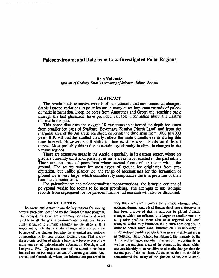
Paleoenvironmental Data from Less-Investigated Polar Regions

ReinVaikmtieInstituteof Geology,EstonianAcademyof Sciences,Talllnn,Estonia

ABSTRACT

The Arctic holds extensive records of past climatic and environmental changes.Stable isotope variations in polar ice are in many cases important records of paleo-climatic information. Deep ice cores from Antarctica and Greenland, reaching backthrough the last glaciation, have provided valuable information about the Earth'sclimate in the past.

This paper discusses the oxygen-18 variations in intermediate-depth ice coresfrom smaller ice caps of Svalbard, Severnaya Zemlya (North Land) and from themarginal area of the Antarctic ice sheet, covering the time span from 1000 to 8000_ears B.P. Ali profiles studied clearly reflect the main climatic events during thistime interval. However, small shifts in time exist between details on differentcurves. Most probably this is due to certain asynchronity in climatic changes in thevarious regions.

There are extensive areas in the Arctic, especially in its eastern sector, where noglaciers cur_nfly exist and, possibly, in some areas never existed in the past either.These are the areas of permafrost where several forms of ice occur within theground. The source water for most types of ground ice originates from pre-cipitation, but unlike glacier ice, the range of mechanisms for the formation ofground ice is very large, which considerably complicates the interpretation of theirisotopic characteristics.

For paleoclimatic and paleopermafrost reconstructions, the isotopic content ofpolygonal wedge ice seems to be most promising. The attempts to use isotopicrecords from segregated ice for paleoenvironmental research will also be discussed.

INTRODUCTION very thick ice sheets covers the climatic changes whichThe Arctic and Antarcticare the key regionsforsolving occurredduringhundredsof thousandsof years.However,it

severalproblemsidentifiedby the GlobalChangeprogram, has been discovered that in addition to global climaticThe ecosystems there are extremely sensitive and react changeswhichare reflected to a largeror smallerextent inquickly to ali changes in environmentalconditions.Espe- ali glacier prof'fles,there also exist regional and localcialiy sensitiveto climatic changes are the glaciers,lt is changes,which may influencethe picture considerably.Inimportantto note that climatic changes alter not only the order to obtain more exact informationit is necessarytobalance of the glaciers but also the chemicaland isotopic study isotopicprofilesof glaciers in asmany differentareascompositionof the precipitationfeeding them.That is why as possible.These include,for instance, the majorityof thethe isotopicprofilesof glaciershavenowbecomeoneof the Arctic archipelagos,mountainglacierson the continents,asmain sources of paleoclimaticinformation[Oeschgerand well as the marginalareas of the Antarcticice sheet,whic,hLangway, 1989].Up to now most of the attentionhas been are considerablymore sensitiveto climaticchangesthanthefocusedon the two majorcentersof currentglaciation,Ant- centralpart of the icesheet, At the same time, it shouldbearctica and Greenland,where the informationpreserved in rememberedthat manyof the glaciers of the Arctic archl-

611

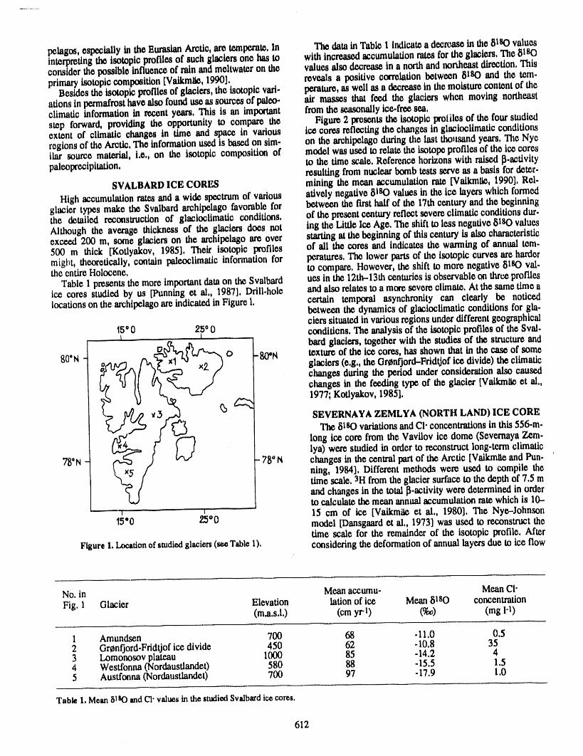
pelagos, especially in the Emaslan Arctic, arc temperate,in The data in Table I indicatea decrease in the8180 valuesinterpretingtheisotopicprofilesofsuchglaciersonehasto withincreasedaccumulationratesfortheglaciers,The61sOconsiderthepossibleinfluenceofndnandmeltwateronthe valuesalsod_rea_ ina northandnortheastdirection,Thisprimaryisotopic composition[Valkmll_, 1990], rewals a positive cen'elation between 61110and the tem-

Besides the isotopicprofiles of glaciers, the isotopicvat- petatare, as well as a decrease in the moisture content of theations in permafrosthave also found useas sources of paleo- air masses that feed the glaciers when moving northeastclimatic infommtion in recent years, This Is an important fromthe seasonallytee-free sea,step forward, providing the opportunity to compare the Figure 2 presents the isotopic proliles of the four studiedextent of climatic changes in time and space in various ice cores reflecting the changes in glacioclimatic conditionsregionsof the Arctic, The informationused is _ on slm- on the archipelagoduring the last thousandyears, The Nycliar source material, i,e,, on the isotopic composition of model was used to relatethe L_tope profiles of the ice cores

to the time scade, Reference horizons with raised [3.a_tivitypaieoprecipitatlon, resulting from nuclear bomb tests serve as a basis fordeter.

SVALBARD ICE CORES mining the mean accumulation rate t'Valkmll_,1990], RoI.

High accumulationrates and a wide spectrumof various atively negative 8180 values in the ice layers which formedglacier types make the 8valbard archipelago favorable for between the firsthalf of the 17th century and the beginningthe detailed reconstruction of glacloclimatic conditions, of the present century reflect severe climatic conditionsdur.Although the average thickness of the glaciers does not ing the LittleIce Age, The shift to less negative 6180 valuesexceed 200 m, some glaciers on the archipelago are over startingat the beginning of this century is also characteristic500 m thick [Koflyakov, 1985], Their isotopic profiles of ali the cores and indicates the wanning of annual tem.might, theoretically, contain paleoclimattc information for peratures, The lower parts of the isotopic curves are harderthe entireHolocene, to compare, However, the shift to more negative 61R3 val.

Table 1 presents the moreimportantdataon the Svalbard ues in the 12th-13th centuries is observableon threeprofilesice cores studied by us [Punning et al,, 1987], Drill.hole andalso relates to a more severe climate, At the same time alocations on the archipelago are indicated in Figure 1, certain temporal asynchronlty can clearly be noticed

between the dynamics of glactoclimatic conditions for gla.tiers situatedin various regions under different geographical

15° 0 2500 condttiens, The analysisof the isotopic profiles of the Seal.I t bard glaciers, together with the studies of the structure and19

80"N o -80*N texture of the ice cores, 'hasshown that in the case of someglaciers (e,g,, the Grenfjord-Fridtjofice divide) the climaticchanges during the period under consideration also causedchanges in the feeding type of the glacier [Vaikmlleet al,,

(_ _ 1977; Kotiyakov, 1985],SEVERNAYA ZEMLYA (NORTH LAND) ICE CORE

The 8i 8(3variationsandCI-concentrationsin this 556-m-long ice core from the Vavilov lee dome (Severnaya Zem-lya) were studied in order to reconstruct long-term climatic

78'N - 78° t_ changes in the central part of the Arctic [Vaikmlte and Pun.ning, 1984], Different methods were used to compile thetime scale, 3H fromthe glaciersurfaceto the depthof7,5 mandchangesinthetotal13-actlvityweredeterminedinordertocalculatethemeanannualaccumulationratewhichis10-

_ 15 cm of ice [Vaikmile et al,, 1980], The Nye--Johnson15"0 25°0 model [Dansgaard et al,, 1973] was used to reconstruct the

time scale for the remainder of the isotopic profile. AfterFigure1. Locationofstudiedglaciers(seeTable1), considering the deformationof annual layers due to ice flow

No.in Mean accumu- Mean CI-Fig, 1 Glacier Elevation lationof ice Mean81R3 concentration

(m.a.s,l,) (cm yrt) (%) (ing 1-))

1 Amundsen 700 68 -11,0 0.52 Grenfjord-Frldtjof ice divide 450 62 -10,8 353 Lomonosov plateau 1000 85 -14.2 44 Wesffonna (Nordaustlandet) 580 88 -15.5 1.55 Austfonna (Nordaustlandet) 700 97 -17.9 1.0

Table1. Mean81SOandCI"valuesin thestudiedSvalbm'dicecores.

612

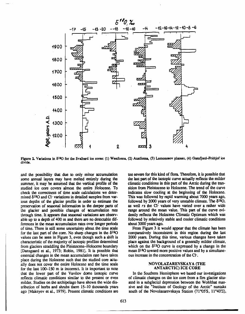
-4_' -45 -49-20 --48 -46-40 -I_ -4_-I0-4_-I_-40-8"6

,J J | I I1_ , i i1_ | ........ -- | ,,11|

egO0 =_

18oo

4600

t500 =Ey:=

4400

_ 4 2 zzz_3

Figure2. Variationsin 8iso for theSvalbzrdice cores:(I) Wesffonna,(2) Austfonna,O) Lomonosovplateau,(4) Gmnfjord.-Ffldtjoficedivide,

and the possibility that due to only minor accumulation too severe for this kind of flora.Therefore,it is possible thatsome annual layers may have melted entirely during the the lastpartof the isotopic_urve actuallyreflects the mildersummer, it may be assumed that the vertical profile of the climaticconditionsin this partof the Arctic during the mm-studied ice core covers almost the entire Holocene. To sition from Pleistocene to Holocene. The trendof the curvecheck the correcmess of dme scale calculations we deter, indicates slow cooling at the beginning of the Holocene.mined 81sO and CI-variationsin detailed samplesfrom var. This was followed by rapidwarming about 7000 years ago,ieus depths of the glacier profile in order to estimate the followed by 2000 yearsof very unstable climate. The 81sO,preservationof seasonal information in the deeper partsof as well rs the Cl" values have varied over a rather widethe glacier and possible changes of accumulation rate range around the mean value. This part of the curve evi-throughtime. It appearsthat seasonal variationsareobserv- denfly reflects the Holocene Climatic Optimum which wasable up to a depth of 400 m and thereare no detectabledfr. followed by relatively stableand cooler climatic conditionsferences in the mean accumulationratesover longer periods about3000 yearsago.of time. There is still some uncertaintyabout the time scale From Figure 3 it would appear that the climate has beenfor the last partof the core. No sharpchanges in the 8180 comparatively inconsistent in this region dta'ing the lastvalues can be seen in Figure 3, even though such a shift is 2000 years. During this time, various changes have takencharacteristicof the majorityof isotopicprofiles determined place against the backgroundof a generally milderclimate,fromglaciers straddlingthe Pleistocene-Holocene boundary which on the 8130 curve is expre_ by a change in the[Dansgaardet al., 1973; Robin, 1981]. lt is possible that mean 81sO toward morepositive values and by a simultane-essential changes in the mean accumulationrate have taken ous increasein the concentrationof the CI-.piace during the Holocene such that the studied core actu-ally dees not cover the entire Holocene and the dme scale NOVOLAZAREVSKAYA (THEfor the last 100-1.50 m is incorrecLlt is importantto note ANTARCTIC) ICE COREthat the lower part of the Vavilov dome isotopic curve In the SouthernHemisphere we based our investigationsreflects climatic conditions similar to the present or even of climatic changes on the ice core from a fun glacier situ-milder.Studies on the archipelago have shown the wide dis. ated in a subglacial depression between the Wohlthat mas-tributtonof herbs and shrubs there 1,5--10thousands years sive and the "Institute of Geology of the Arctic" nuntaksago [Makeyev et al., 1979]. Present climatic conditions are south of the Novolazarevskaya Station (71°05'S, 11°40_),

613

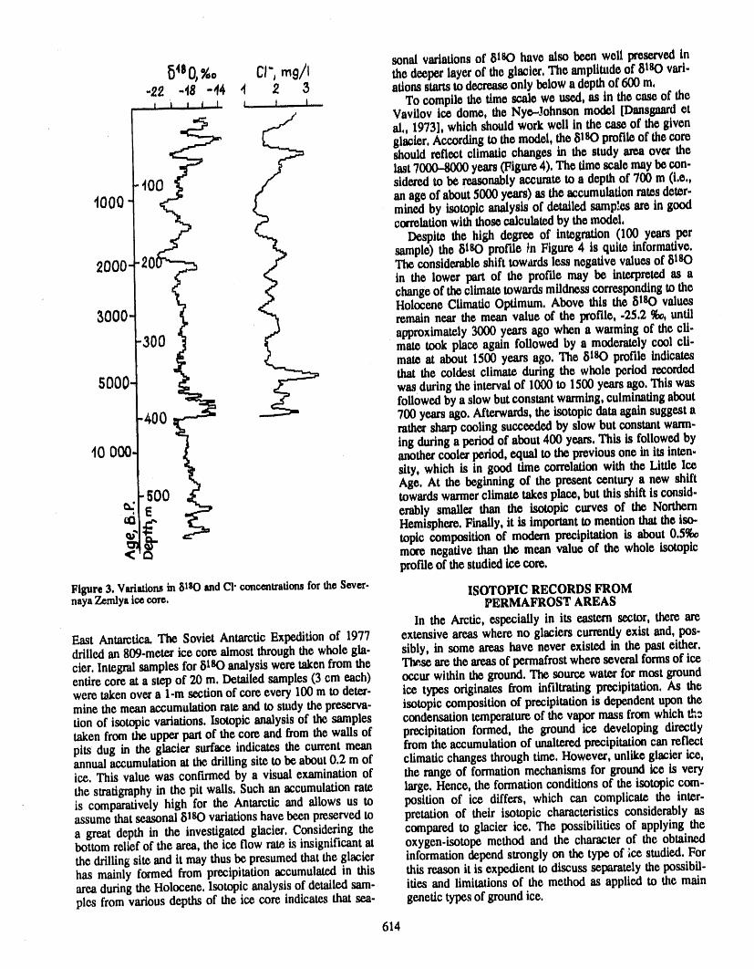
sonal variationsof 8180 have also been well preservedin

_4S0_ %o Cl", mg/I the deeper layerof the glacier, The amplitudeof 8180 vari--£2 ..48 "44 4 2 3 ations startsto decreaseonly below a depth of 600 m,

i t t To compile the time scale we used, as in the case of theVavilov ice dome, the Nye-Johnson model [Dansgnardetal,, 1973], which should work well in the case of the givenglacier,According to the model, the 81SOprofile of the coreshould reflect climatic changes in the study area over thelast 7(X)0-8(X)0years(Figure 4), The timescale may be con-sidered to be reasonablyaccurate to a depth of 700 m (i,e,,

t000 an age of about5000 years) as the accumulationratesdeter-mined by isotopic analysis of detailed samples are in goodcorrelationwith those calculatedby the model,

Despite the high degree of integration (100 years persample) the 8lso profile _n Figure 4 is quite informative.The considerableshift towards less negative values of 81sOin the lower pert of the profile may be interpretedas achangeof the climatetowards mildness correspondingto theHolocene Climatic Optimum, Above this the 6180 values

_000 remain near the mean value of the profile, .25,2 %o,until' approximately3000 years ago when a wmming of the cii.

•300 mate took place again followed by a moderatelycool cii.mate at about 1500 years ago. The 81SOprofile indicatesthat the coldest climateduring the whole period recorded

500{ was duringthe interval of 1000 to 1500 yearsago, This wasfollowed by a slow butconstantwarming,culminatingabout

40 0 700 yearsago. Mtexwards, the isotopic dataagain suggestarathersharpcooling succeeded by slow but constantwann-ing duringa period of about 400 years. This is followed by

10 0{30. another cooler period, equal to the previous one in its inten-sity, which is in good time correlationwith the Little IceAge. At the beginning of the present century a new shift

SO0 towards wannerclimate takes place, but this shift is consid-_." erably smaller than the isotopic curves of the Northern

.rf' Hemisphere.Finally, it is importantto mentionthat the iso-

qi' _. topic composition of modern precipitationis about 0.5_< mote negative than the mean value of the whole isotopicprofileof the studiedice core.

Figure3. Variationsin 8nO andC1-concentrationsfortheSever- ISOTOPIC RECORDS FROMnayaZemlyaice core, PERMAFROST AREAS

In the Arctic, especially in its eastern sector, there are

East Antarctica.The Soviet Antarctic Expedition of 1977 extensive areaswhere no glaciers currentlyexist and, pos-drilled an 809-meterice core almost throughthe whole gla- sibly, in some areas have never existed in the past either.cier. Integralsamples for 5180 analysiswere takenfrom the These are the areasof permafrostwhere several formsof iceentirecore at a step of 20 m. Detailed samples (3 cm each) occur within the ground.The source water for most groundwere takenovera l-m section of core every 100 m to deter- ice types originates from infiltratingprecipitation. As themine the meanaccumulation rateand to study the preserva- isotopic composition of precipitationis dependentupon therien of isotopic variations.Isotopic analysisof the samples condensation temperatureof the vapormass fromwhich t._,_,taken fromthe upperpartof the core and from the walls of precipitation formed, the ground ice developing directlypits dug in the glacier surface indicates the current mean fromthe accumulation of unalteredprecipitationcan reflectannualaccumulation at the drilling site to be about0.2 m of climaticchanges through time. However, unlike glacier ice,ice. This value was confu'med by a visual examinationof the range of formation mechanisms for ground ice is verythe stratigraphyin the pit walls, Such an accumulationrate large. Hence, the formationconditions of the isotopic com-is comparativelyhigh for the Antarctic and allows us to position of ice differs, which can complicate the inter-assume thatseasonal 81SOvariationshavebeen preserved to pretation of their isotopic characteristics considerably asa great depth in the investigated glacier. Considering the compared to glacier ice. The possibilities of applying thebottom relief of the area, the ice flow raW.is insignificantat oxygen-isotope method and the character of the obtainedthe drilling site and it may thus be presumed that the glacier information depend strongly on the type of ice studied. Forhas mainly formed from precipitationaccumulated in this this reason it is expedient to discuss separately the possibil-area during the Holocene. Isotopicanalysis of detailed sam- ities and limitations of the method as applied to the mainpies from various depths of the ice core indicates that sea- genetic types of groundice.

614

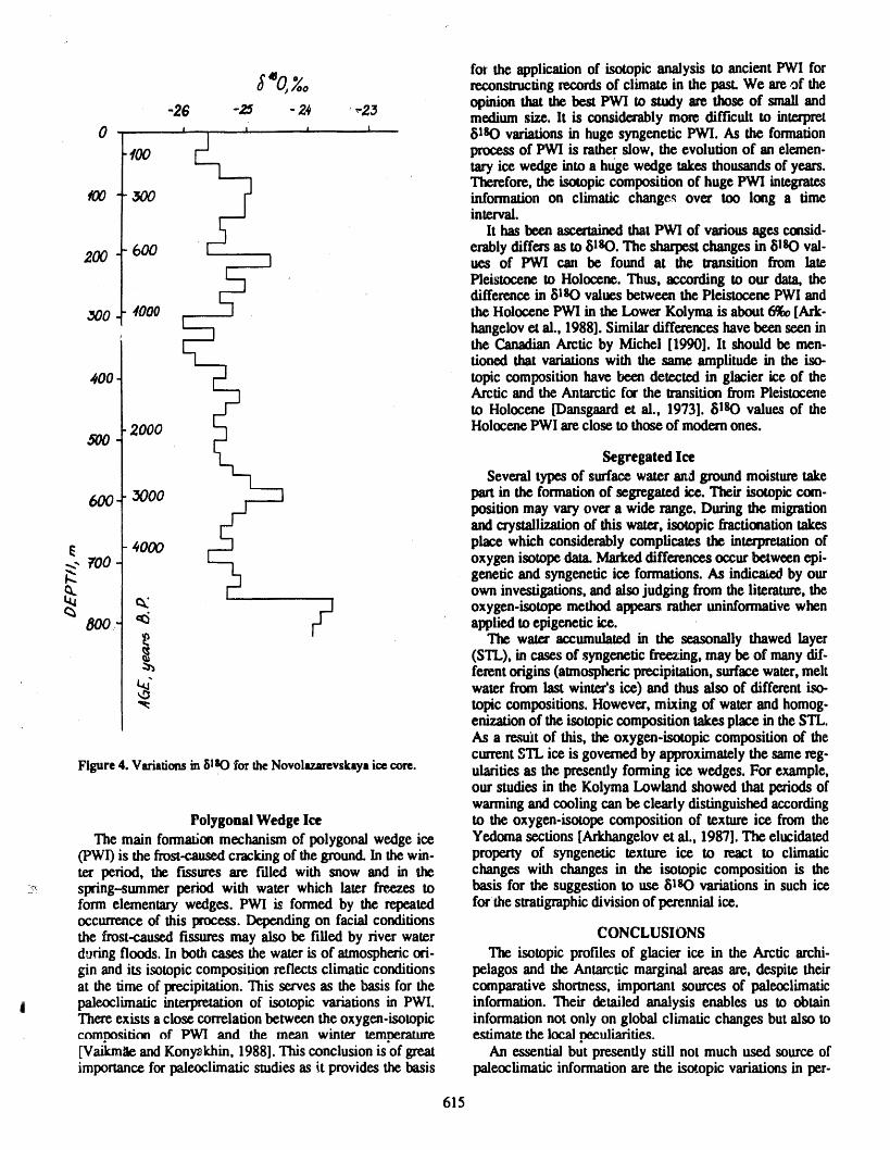
for the applicationof isotopic analysis W ancient PWI for's0j _oo reconstructingrecordsof climate in the past. We areof the

opinion that the best PWI to study are those of small and-26 -25 -2,_ ' ,--23 medium size. lt is considerably more difficult to interpret

0 {StsOvariationsin huge syngenetic PWl. As the formationprocess of PWI is ratherslow, the evolution of an elemen-taw ice wedge into a huge wedge takes thousandsof years.Therefore, the isotopic composition of huge PWI integrates

400 information on climatic change_ over too long a timeinterval.

lt has been asc.emined that PWI of various ages consid-erably differs as to 81sO. The sharpestchanges in 8IsO val-

200 i ues of PWI can be found at the transition from latePleistocene to Holocene. Thus, according to our data, thedifference in 8IsO values between the Pleistocene PWIand

_00 the Holocene PWI in the Lower Kolyma is about 6_ [Ark.L___] hangelovet al., 1988]. Similardifferences have been seen in

' _-- the Canadian Arctic by Michel [1990]. lt should be men-]_ tioned that variations with the same amplitude in the iso-

#00 topic composition have been detected in glacier ice of theArctic and the Antarctic for the transitionfrom Pleistoceneto Holocene [Dansgaardet al., 1973]. 81_) values of the

2000 Holocene PWIare close to those of modernones.Segregated Ice

Several types of surface water and groundmoisture take

_X)0 j_._] partin the formationof segregated ice. Their isotopic com-6OOposition may vary over a wide range. During the migration

l- andcrystallizationof this water, isotopic fractionationtakes#000 place which considerably compficates the interpretationof

_- ?'00 _--'_ oxygen isotope data.Markeddifferences occur betweenepi-genetic and syngenetic ice formations. As indica_ by ourF own investigations, and also judging from the literature, the

_ l oxygen-isotope method appearsrather uninformativewhen

800 _ f appliedto epigenetic ice.

The water accumulated in the seasonally thawed layer(SIT,), in cases of syngenetic freezing, may be of many dif-ferent origins (atmosphericprecipitation, surface water,melt

" water from last winter's ice) and thus also of different iso-topic compositions. However, mixing of waterand homog-enization of the isotopic composition takes place in the STL.As a resuit of this, the oxygen-isotopic composition of thecurrentS'IT,ice is governedby approximately the same reg-

Figure4. Variationsin 51sOfortheNovolazarevskayaice core. ularities as the presendy forming ice wedges. For example,our studies in the Kolyma Lowland showed that periods ofwarmingand cooling can be clearly distinguished according

Polygonal Wedge Ice to the oxygen-isotope composition of texture ice from theThe main formationmechanism of polygonal wedge ice Yedoma sections [Arkhangelovet al., 1987]. The elucidated

(PWI) is the frost-causedcracking of the ground.In the win- property of syngenetic texture ice to react to climatictea"period, the fLssuresare fdled with snow and in the changes with changes in the isotopic composition is the

_ spring--summer period with water which later freezes to basis for the suggestion to use St sO variations in such iceform elementary wedges. PWI is formed by the repeated for the stratigraphicdivision of perennial ice.occurrence of this process. Depending on facial conditionsthe frost-caus_ fissures may also be filled by river water CONCLUSIONSd_dng floods. In boot cases the wateris of atmosphericori- The isotopic profiles of glacier ice in the Arctic archi-gin and its isotopiccomposition reflects climatic conditions pelagos and the Antarctic marginalareas are, despite theirat the time of precipitation.This serves as the basis for the comparative shormess, important sources of paleoclimatic

| paleoclimatic interpretationof isotopic variations in PWI. information. Their detailed analysis enables us to obtainThere exists a close correlationbetween the oxygen-isotopic information not only on global climatic changes but also tocomnosifitm of PW] and the mean winter temneramre estimate the local neculiarifies.

[Vaikmae and Kony'zkhin, 1988]. This conclusion is of great An essential but presently still not much used source ofimportance forpaleoclimatic studies as it provides the basis paleoclimatic information are the isotopic variations in per-

615

mafrost. Comparative analysis of the isotopic profiles of precipitation on a circumpolar as well as global scale.glaciers with the latter gives a good opportunity to estimate This work is a contribution to the IGCP Project 253 "Ter-the distribution of the isotopic composition of paleo- mination of thePleistocene."

REFERENCES

Arkhangelov, A. A., R. A. Vaikmae, M. A. Konjakhin, and Punning, J.-M., R. Vaikmae, and K. T6ugu, Variations ofD. V. Mikhaljov, Oxygen isotopic composition of ground 51BO and CI- in the ice cores of Spitslx._gen, J. Phys.ice and surface waters in Kolyma Lowland (in Russian), Colloq., C148, 619-624, 1987.16 pp., VINITI, Moscow, 1988. Robin, G. de Q., The Climatic Record in Polar Ice Sheets,

Arkhangelov, A. A., R. A. Vaikmlte, D. V. Mikhaljov, 212 pp., Cambridge University Press, Cambridge, 1981.J.-M. K. Punning, and V. I. Solomatin, Slratigraphic divi- Vaikm_, R. A., and M. A. Konyakhin, Formation of Oxy-sion of permafrost in Kolyma Lowland using the oxygen gen Isotope Composition of Current Polygonal Iceisotope method (in Russian), in New Data in Quaternary Wedges (in Russian), 21 pp., VINITI, Moscow, 1988.Geochronology, pp. 143-149, Nauka Publ., Moscow, Vaikm_, R., Isotope variations in the temperate glaciers of1987. the Eurasian Arctic, Int. J. Radiat. Appl. lnstrum. Part E,

Dansgaard, W., S. J. Johnsen, H. B. Clausen, and N. Gun- Nucl. Geophys., 4, 45-55, 1990.destrup, Stable isotope glaciology, Medd. Grenlancl. 197, Vaikmae, R. A., F. G. Gordijenko, V. S. Zagoro_ov, V. I.6-53, 1973.

Kotlyakov, V, M. (Ed.), Glaciology of Spitsbergen (in Rus- Mikhaljov, J.-M. K Punning, and R. A. Rajamae, Isotopegeochemical and stratJgraphic studies on the ice-divide ofsian), 199 pp., Nauka, Moscow, 1985. Gr_nfjord and Fridtjof glaciers (West Spitsbergen) (inMakeyev, V. M., H. A. Arslanov, and V. E. Garutk The ageof mammoths of Severnaya Zemlya and some problems Russian), Data of Glaciological Stud. No. 30, 77-87,of the paleogeogr'0.phy of the Late Pleistocene (in Rus- 1977.sian), Proc. USSR Acad. Sci., 245, 173-177, 1979. Vaikm_, R., and J.-M. Punning, Isotope-geochemical

Michel, F. A., Isotopic composition of ice-wedge ice in investigations on glaciers in the Eurasian Arctic, in Cor-Northwestern Canada, in Permafrost Canada. Proc. of relation of Quaternary Chronologies, exited by W. C.the F_fth Canadian Permafrost Conference, pp. 5-9, Mahaney, pp. 385-393, Norwich, 1984.NRCC, 1990. Vaikm_, R. A., J.-M. K. Punning, V. V. Romanov, and

Oeschger, H., and C. C. Langway, Jr. (Eds.), The Environ- N.I. Barkov, Stratigraphy of the Vavilov Ice Dome,mental Record in Glacier and Ice Sheets, Dahlem Work- Sevemaya Zemlya, wi_, the help of isotope-geochemicalshop on the Environmental Record in Glaciers and Ice methods(in Russian), Data of Glaciological Stuch'es, 40,Sheets, Berlin, 1988, 393 pp., Wiley Interscience 1989. 82-87, 1980.

l

- 616

Little Ice Age Glaciation in Alaska:A Record of Recent Global Climatic Change

Parker E. Calkin and Gregory C. WilesDepartmentof Geology,Universityat Buffalo,Buffalo,New York,U.S.A.

ABSTRACT

General global cooling and temperature fluctuation accompanied by expansionof mountain glaciers characterized the Little Ice Age of about A.D. 1200 throughA.D. 1900. The effects of such temperature changes appear f'urstand are strongest athigh latitudes. Therefore the Little Ice Age record of glacial fluctuation in Alaskamay provide a good proxy for these events and a test for models of future climaticchange. Holocene expansions began here as early as 7000 B.P. and locally show aperiodicity of 350 years after about 4500 years B.P.

The Little Ice Age followed a late Holocene interval of minor ice advance and asubsequent period of ice margin recession lasting one to seven centuries. The tim-ing of expansions since about A.D. 1200 have often varied between glaciers, butthese are the most pervasive glacial events of the Holocene in Alaska and fre-quenOy represent ice marginal maxima for this interval. At least two major expan-sions are apparent in forefields of both land-terminadng and fjord-calving glaciers,but the former display the most reliable and detailed climatic record. Major maxima

. occurred by the 16th century and into the mid-18th century. Culmination ofadvances occurred throughout Alaska during the 19th century followed within afew decades by general glacial retreat. Concurrently, equilibrium line altitudes havebeen raised 10(0-400 m, representing a rise of 2-3°C in mean summer temperature.

INTRODUCTION The Little Ice Age occurredin late Holocenetimefol-Anintervalof generallycoolerclimatespanningthe 13rh lowinga briefintervalof temperateclimatecalledthe"Med-

throughthe 19rh centuries called the "LittleIce Age" ievalOptimum"or"MedievalWarmPeriod"precededby anintervalof EarlyMedievalglacialadvances[Lamb,1977;[Grove,1988]mayprovideone of the bestopportunitiesta

testand ref'memodels thatmaydiscriminatebetweennat- WilliamsandWigley, 1983]. lt was a timeof drasticin-ural and human-inducedglobal climaticchanges.For no crease in weathervariabilityas well as cooler climateotherintervalof globalclimaticchangearebaselinecondi- [Lamb,1977].The nameis appropriatebecauseduringthisLittle Ice Age interval, the world-wideextent of ice intions so well known,noris resolutionso readilyavailable mountainglaciersand inotherformsattaineda maximumasforthetimesc_esof decadesto centuriesthataredemanded

greatas, orinsomecasesgreaterthan,thatatany timesinceforthestudyof key climaticinteractions[internationalGeo- theendof thePleistocene[Grove,1988].sphere-BiosphereProgram(IGBP),1988]. Theobjectiveof thispaperis ta summarizethe LittleIce

Historicaland recentinstrumentalrecordsstronglysug- Agerecordas displayedby mountainglacierfluctuationsingest thatstudiesof climateproxydatainthe northernhemi- AlaskasinceaboutA.D. 1200. Alaska'smountainglacierssphere,and particularlyin the Arctic,arecritical.It is here display marginaladvanceor retreatwithina few years towhereglobalclimaticchangeshavefast appeared(bya cen- decadesof climaticchanges.Thereforethey may be goodturyta decades)andwherethe range,amplitude,andeffect indicatorsof any man-inducedwarming[e.g., Oerlemans,of changeshasbeen in thepast,andis expectedta be in the 1986].Inadditionthesemountainglaciersarea majorcom-

.

617 :--

_

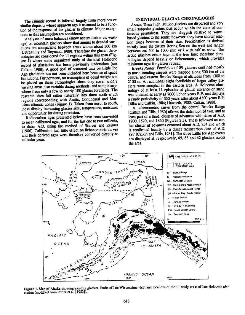
The climatic record is inferred largely from moraines or INDIVIDUAL GLACIAL CHRONOLOGIESsimilardeposits whose apparentage is assumedto be a func- Arctic. These high latitudeglaciers aredispersedand verytion of the response of the glacier to climate. Major excep- small subpolarglaciers that occur within the zone of con-tions to this assumptionareconsidered, tinuous permafrost. They are sluggish relative to warm-

Analysesof mass balances (snow accumulationvs. wast- based glaciers to the south; however, they have shorterreac-age) on mountainglaciers show thatannual to decadalvari- tion times because of their size. Precipitation is derivedations are comparablebetween areas within about 500 km mostly from the distant Bering Sea on the west and ranges[Letreguillyand Reymmd, 1989].Therefore the glacial chro- between ca. 500 to 1000 mm yrl with haft as snow. Thenolo#es areconsideredfor 11 regions within this span (Fig- arctic glaciers occur beyond the tree line; therefore chro-ure 1) where some organized study of the total Holocene nologies depend heavily on lichenometry, which providesrecord of glaciation has been previously undertaken [see minimumages forglacier retreat.Calkin, 1988]. A good deal of scattered data on Little Ice Brooks Range. Forefieids of 89 glaciers confined mostlyAge glaciationhas not been included herebecause of space to north-trendingcirques were mapped along 500 km of thelimitatiom. Furthermore,no assumptionof equal weight can central and easternBrooks Range at altitudes from 1300 tobe placed on these chronologies since they cover widely 2100 m. An additional eight forefields of largervalley gla-varyingareas,use variabledating methods, and sampleany- ciers were sampled in the eastern area. A Holocene chro-where from only a few to nearly 100 glacier forefields.The nology of at least 11 episodes of glacial advance or standresearch sites fall rather naturally into three north-_'uth was initiatedas early as 7600 lichen years B.P. anddisplaysregions correspondingwith Arctic, Continental and lvLar- a crude periodicityof 350 yearsafter about4500 ye.arsB.P.itime climatic zones (Figure 1). Taken from northto south, [Ellis andCalkin, 1984; Haworth,1988, Calkin,1988].these display increasingglacier size, temperature,moisture, A lichenometric curve from the central Brooks Rangeandopportunityfor dating precision. [Calkin andEllis, 1980] allows the definition of two, andat

Radiocarbonages presented below have been converted least partof a third,clusters of advances with dates of A.D.to meancalibratedages, and for the lastone to two millenia, 1200, 1570, and 1860 (Figures 2,3). These followed an ear-to dates A.D. using the method of Stuiver and Reimer lier clusterof advances centered about A.D. 854 and which[1986], Calibrationhad little effect on lichenometriccurves is confirmed locally by a direct radiocarbon date of A.D.and their derived ages were therefore converted directly to 897 [Calkinand Ellis, 1981]. The threeLittleIce Age eventscalendar years, are displayed at, respectively, 45, 85 and 42 glaciers across

the area.

' ' ' ' _ .... * ' [_ EXISTINGGLACIERS(GIii1700 160o _ 1500 140

' N,,/ ARCTIC F---I DRIFrOFLATEi I_...-.J WISCONSINAGE

_,_ .,' J . ._G_ _,_,.i_\_,".r' /-'- E}F_00KS __" _.""-'> , B..B_..anQe

NS . Norll'_asl St Elias

. -. WC- West.CentralAlaskaRange

_ ] _ PENINSULA _L_,.Ol_ Lx_._ tt GB • GlacierBay. BradyGlacier

" C_ LI • Juneau IcelleldK/'__ //__ER t E t't Iy • icyBay - YakutatBay

._ ) /0_' WC_ tI PW.Prince WilliamSound

BO" d ° _ ) F- q'- _T-, _ _-_ i 0 500 km

-.ii'. ii_'_./4_, ... Co

",. . 4)

. ¢. k,__ >JJ..., a.,;. rl_ ,!;. 17 J, _lr,_.,_ %1\, r"O %_,_.r..,',,*'11ql:"_,

Ix , t_,,,_ll,_

__ PACIFIC OCEAN

Figure 1. Map of Alaska showing existing glaciers, limits of late Wisconsinan drift and locations of the 11 study areas of late Holocene gla-ciation (modifiedfromPorteret al. [1983]).

618

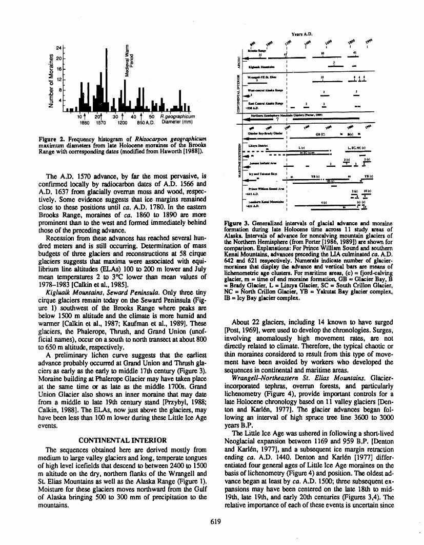
Years_D.

24: _ ,dm.,=., i i J i3! 4_j U 4;i

'_ le _ ,4-.=-...=- ---'--- -0

I ,, __L .L_L

JD ._i= 2 ,,,,=_,

E 4_Z --=t,__ _u_ u=,_ 2-+_141&.D, ,.. u,,,. m,

I0 50 R, geographlcum L _ _ _ _ _' _), i: ? I t1860 1570 1200 850A,O, Diameter(mm) , ,

(_¢=e{_hy,,_y O*=d_ l OB (C) u IKe) m

Figure 2. Frequmoy histogram of Rhizocarpon geographicum - ' '

maximum diameters from late Holocene moraines of the Brooks _ I u,.,.o,,_. ', L,()Range with corresponding dates (modified from Haworth [1988]), _ _ _'......', • _ ,,,,. : L,s_,c <,)=mm,

The A.D. 1570 advance, by far the most pervasive, is _, k,,,.,v=.,.,=, ,3El I en YB(¢) YI (¢)..q,,,,,=., m L

__. , ""lg(siconfirmed locally by radiocarbondates of A.D. 1566 and , _

I Z(c) li (¢)

A.D. 1637 from glacially overrun moss and wood, respec- {.....,_"="'^", 2".I."t-"tively. Some evidence suggests that ice margins remained i_._._..,_., .close to thesepositions until ca. A.D. 1780. In the eastern I "=''=. " 4<" <')<',t""h

I m =...=,

Brooks Range, moraines of ca. 1860 to 1890 are moreprominent thanto the west and formedimmediatelybehind Figure3. Generalizedintervalsof glacial advanceand morainethose of the precedingadvance, formationduringlate Holocenetime across 11 study areasof

Recession from these advances has reached several hun- Alaska.Intervalsof advancefornoncalvingmountainglaciersoftheNorthernHemisphere(fromPorter[1986,1989])=reshownfor

tired meters and is still occurring. Determination of mass comparison.Explanations:ForPrinceWilliamSoundandsouthernbudgets of three glaciers and reconstructionsat 58 cirque KenalMountains,advancesprecedingthe HA culminatedca.A.D.glaciers suggests that maxima were associated with equl- 642 end 621 respectively.Numeralsindicatenumberof glacier-librium line altitudes (ELAs) 100 to 200 m lower andJuly morainesthatdisplaytheadvanceand verticalban aremeansoflichenometricase clusters.Formaritimeareas,(c) = fjord-calvingmean temperatures 2 to 3°C lower than mean values of glacier,m = timeof endmoraineformation,GB = GlacierBay,B1978-1983 [Calkinet al., 1985]. = BradyGlacier,L = LituyaGlacier,SC= SouthCrUlonGlacier,

Kigluaik Mountains, Seward Peninsula. Only three tiny NC = NorthCriUonGlacier,YB ffiYakutatBay glaciercomplex,cirque glaciers remain today on the SewardPeninsula (Fig- IB= IcyBay 8laciercomplex.ure 1) southwest of the Brooks Range where peaks arebelow 1500 m altitude and the climate is more humidandwarmer[Calkin et al., 1987; Kaufmanet al., 1989]. These About 22 glaciers, including 14 known to have surgedglaciers, the Phalerope, Thrush, and Grand Union (tmof- [Post, 1969], were used to develop the chronologies. Surges,ficial names), occuron a south to northtransectat about800 involving anomalously high movement rates, are notto 650 m altitude,respectively, directlyrelated to climate. Therefore, the typical chaotic or

A preliminary lichen curve suggests that the earliest thin moraines considered to result from this type of move-advanceprobablyoccurredat GrandUnion and Thrush gla. ment have been avoided by workers who developed theciers as early as the early to middle 17th century (Figure3). sequences in continentaland maritimeareas.Moraine building at Phalerope Glacier may have taken place Wrangell--Northeastern St. Elias Mountains. Glacier-at the same time or as late as the middle 170(0. Grand inco_ted tephras, overrun forests, and particularlyUnion Glacier also shows an inner moraine that may date lichenometry (Figure 4), provide important controls for afrom a middle to late 19th century stand [Przybyl, 1988; late Holocene chronology based on 11 valley glaciers [Den-Calkin, 1988]. The ELAs, now just above the glaciers, may ton and Karl,, 1977]. The glacier advances began fol-have been less than 100 m lower during these Little Ice Age lowing an interval of high spruce tree line 3600 to 3000events, years B.P.

The Little Ice Age was ushered in following a short-livedCONTINENTAL INTERIOR Neoglacial expansion between 1169 and 959 B.P. [Denton

The sequences obtained here are derived mostly from and Karl6n, 1977], and a subsequent ice margin retractionmedium to large valley glaciers and long, temperate tongues ending ca. A.D. 1440. Denton and Karl6n [1977] differ-of high level icefields that descend to between 2400 to 1500 entiated four general ages of Little Ice Age moraines on them altitude on the dry, northern flanks of the Wrangell and basis of lichenometry (Figure 4) and position. The oldest ad-St. Elias Mountains as well as the Alaska Range (Figure 1). vance began at least by ca. A.D. 1500; three subsequent ex-Moisture for these glaciers moves northward from the Gulf pansions may have been centered on the late 18th to mid-of Alaska bringing 500 to 300 mm of precipitation to the 19th, late 19th, and early 20th centuries (Figures 3,4). Themountains, relativeimportanceof each of these events is uncertain since

619

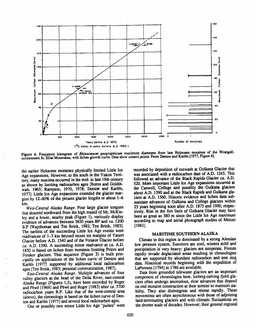
iloilo

//

/ 14o'14o , r.

l-_e_tO IIIi20 f

; .... ,oo ;

_oo /

EI

: so • ,o_u

,- V. ,-

e / _c-+.,.+ _ so _.:1 / J NI4111iI_ IlkE I0

. / > ,s.Q• l

> 4O_ ,

>

>

, !0 _ _ 10

, _ , 0

_oo )oo Isoo zooo zsoo sooo ssoo z 0

Years before A.D, 1970 Number of moroines

{14C dotes in yeors before A,D, 1950 )

Figure 4. Frequency histogram of Rhiwcarpon. &eographicum maxin_um diameters from late Holocene moraines of the Wrangell-northeastern SL Elias Mountains, with lichen growm curve, Dots snow corm'orpoints. From Denton and Karl_n [1977, Figure 4].

the earlier Holocene moraines physically limited Little Ice recordedby deposition of outwash at GulkanaGlacier thatAge expansions. However, to the southin the YukonToni- was associated with a radiocarbondate of A.D. 1245. Thistory, manymaximaoccurredin the mid- to late 19111century followed an advance of the Black Rapids Glacier ca. A.D.as shown by limiting radiocarbonages [Borns and Goldth- 520. More importantLittle Ice Age expansions occurredatwait, 1965; Rampton, 1970, 1978; Denton and Karl6n, the Canwell, College and possibly the Gulkana glaciers1977]. LittleIce Age expansions extended the glacier mar- aboutA.D. 1390 and at the Black Rapids and Gulkanagla-gins by 12-60% of the presentglacier lengths or about 1-6 ciers at A.D. 1560. Historic evidence and lichen data sub-km. stantiate advances of Gulkanaand College glaciers withinWest.CentralAlaskaRange.Fourlargeglaciertongues 25 yearsbeginningsoonafterA.D.1875and1900,respec-

that descend northward from the high massif of Mt. McKin- tively. Rise in the fun limit of Gulkana Glacier may haveIcy and a lower, nearbypeak (Figure 1), variously display been as great as 380 m since the Little Ice Age maximumevidence of advances between 5850 yearsBP and ca. 1200 according to map and aerial photographstudies of MercerB.P [Waythomas and Ten Brink, 1982; Ten Brink, 1983]. [1961].The earliest of the succeeding Little Ice Age events werereadvancesof 1-3 km beyond recent ice margins of Yanert MARITIME SOUTHERN ALASKAGlacier before A.D. 1540 and of the Foraker Glacier before Climate in this region is dominated by a strong Aleutianca. A.D. 1590. A succeeding minor readvance at ca. A.D. low pressure system. Summers are cool, winters mild and1850 is based on lichen from moraines fronting Peters and precipitation iS very heavy; glaciers are temperate. ForestsForaker glaciers. This sequence (Figure 3) is built prin- rapidly invade deglaciated areas resulting in chronologiescipally on applications of the lichen curve of Denton and that are supported by abundant radiocarbon and tree ringKarl6n [1977] supported by additional local radiocarbon data. Historical records beginning with the expedition ofages [Ten Brink, 1983; personal communication, 1987]. LaPerouse [1794] in 1786 are available.

East.Central Alaska Range. Multiple advances of four Data from grounded tidewater glaciers are an importantvalley glaciers at the head of the Delta River, east-central component of chronologies here. Iceberg-calving fjord gla-Alaska Range (Figures 1,3), have been recorded by Reger tiers often undergo anomalous, slow advances that dependand P6w6 [1969] and P6w6 and Reger [1983] after ca. 5700 on end moraine construction at their termini to maintain sta-radiocarbon years B.P. Like that of the west-central area bility. They also disintegrate and retreat rapidly. These(above), the chronology is based on the lichen curve of Den- movements are often asynchronous with those of adjoinington and Karl6n [1977] and several local radiocarbon ages. land-terminating glaciers and with climatic fluctuations on

One or possibly two minor Little Ice Age "pulses" were the shorter scale of decades. However, their general regional

620

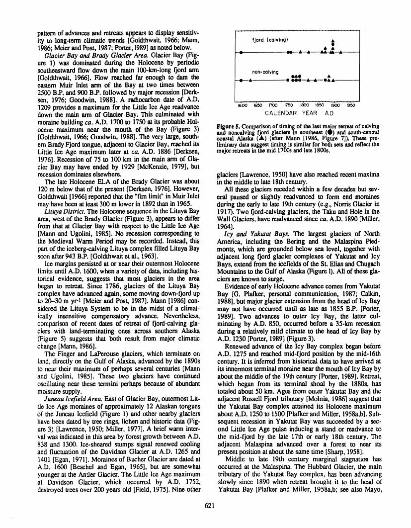
patternof advancesand retreatsappearsto display scnsitiv- _.........................................

ity to long-lerm climatic trends [Goldthwait, 1966; Mann, fjord (0ajving)1986; MeierandPost, 1987;Porter,1989]as notedbelow, A •

Glacier Bay and Brady Glacier Area. Glacier Bay (Fig. _ __ ,,--_m,,,_,,,_A_ure 1) was dominated during the Holocene by periodicsoutheastwardflow down the main 100-km-longfjord ann non-colvlng

qM_O A[Goldthwait, 1966]. Flow re.ached far enough to dam the -e--A -.NO--A--A--O_,A_--eastern Muir Inlet arm of the Bay at two times between2500 B.P. and 900 B.P. followed by major recession [Derbsen, 1976; Goodwin, 1988]. A radiocarbon date of A.D.1209providesa maximumfor theLittle Ice Age re,advance igO° g_ "i_x_"iz_0__b° ;d_0_i_:_ _down the main ann of Glacier Bay, This culminated with CALENDAR YEAR AD

morainebuildingca. A.D. 1700 to 1750 at its probableHol- FigureS.Comparisonof timingof th_last majorretreatof ¢alvtng.ocene maximum near the mouth of the Bay (Figure 3) and noncalvingf_rd glaciersin southout (Q) and south..ccntraJ[Goldthwait, 1966; Goodwin, 1988]. The very large, south- coastalAlaska(A) (aftra"Mann [1986, Figure7]). The.sepre-ernBradyFjordtongue, adjacent to Glacier Bay, reached its liminarydatasuggesttimingis similarforbothsets andreflecttheLittle Ice Age maximum later at ca. A.D. 1886 [Derksen, majorteta'oatsin themid1700sandlat_1800s.1976]. Recession of 75 to 100 km in the main arm of Gla-cier Bay may have ended by 1929 [McKenzie, 1979], butrecessiondominates elsewhere, glaciers [Lawrence, 1950] have also reached recent maxima

The late Holocene ELA of the Brady Glacier was about in the middleto late 18th century.120 m below that of the present [Derksen, 1976]. However, Ali these glaciers receded within a few decades but sev-Goldthwait [1966] reported that the "fun limit"in MuirInlet eral paused or slightly re.advanced to form end morainesmayhave been at least 300 m lower in 1892 than in 1965. during the early to late 19rhcentury (e.g., NorrisGlacier in

Lituya District. The Holocene sequence in the LituyaBay 1917). Two fjord-calving glaciers, the Taku and Hole in thearea, west of the Brady Glacier (Figure 3), appears to differ Wall Glaciers, have re,advanced since ca. A.D. 1890 [Miller,from that at Glacier Bay with respect to the Little Ice Age 1964].[Mann and Ugolini, 1985]. No recession corresponding to Icy and Yakutat Bays. The largest glaciers of Norththe Medieval Warm Period may be recorded. Instead, this America, including the Bering and the Malaspina Pied-part of the iceberg.calving Lituya complex filled Lituya Bay monts, which are grounded below sea level, together withsoon after 943 B.P. [Goldthwait et al., 1963]. adjacent long fjord glacier complexes of Yakutat and Icy

Ice margins persisted at or near their outermost Holocene Bays, extend from the icefields of the SLElias and Chugachlimits until A.D. 1600, when a variety of data, including his- Mountains to the Gulf of Alaska (Figure I). Ali of these gla-torical evidence, suggests that most glaciers in the area tiers are known to surge.began to retreat. Since 1786, glaciers of the Lituya Bay Evidence of early Holocene advance comes from Yakutatcomplex have advanced gain, some moving down-fjord up Bay [G. Platker, personal communication, 1987; Calkin,to 20-30 m yr-! [Meier and Post, 1987]. Mann [1986] con- 1988], but major glacier extension from the head of Icy Baysidered the Lituya System to be in the midst of a climat, may not have occurred until as late as 1855 B.P. [Porter,it.ally insensitive compensatory advance. Nevertheless, 1989]. Two advances to outer Icy Bay, the latter cul-comparison of recent dates of retreat of fjord-calving gla- minating by A.D. 850, occurred before a 35-km recessionciers with land-terminating ones across southern Alaska during a relatively mild climate to the head of Icy Bay by(Figure 5) suggests that both result from major climatic A.D. 1230 [Porter, 1989] (Figure 3).change [Mann, 1986]. Renewed advance of the Icy Bay complex began before

The Finger and LaPerouse glaciers, which terminate on A.D. 1275 and reached mid-fjord position by the mid-16thland, directly on the Gulf of Alaska, advanced by the 1890s century, lt is inferred from historical data to have arrived atto near their maximum of perhaps several centuries [Mann its innermost terminal moraine near the mouth of Icy Bay byand Ugolini, 1985]. These two glaciers have continued about the middle of the 19th century [Porter, 1989].Retreat,oscillating near these termini perhaps because of abundant which began from its terminal shoal by the 1880s, hasmoisture supply, totaled about 50 km. Ages from outer Yakutat Bay and the

Juneau Icefield Area. East of Glacier Bay, outermost Lit- adjacent Russell Fjord tributary [Molnia, 1986] suggest thattie Ice Age moraines of approximately 12 Alaskan tongues the Yakutat Bay complex attained its Holocene maximumof the Juneau Icefield (Figure 1) and other nearby glaciers about A.D. 1_0 to 1500 [Plafker and Miller, 1958a,b]. Sub-have been dated by tree rings, lichen and historic data (Fig- sequent recession in Yakutat Bay was succeeded by a sec-ure 3) [Lawrence, 1950; Miller, 1977]. A brief warm inter- end Little Ice Age pulse inducing a stand or readvance toval was indicated in this area by forest growth between A.D. the mid-fjord by the late 17th or early 18th century. The838 and 1300. Ice-sheared stumps signal renewed cooling adjacent Malaspina advanced over a forest to near itsand fluctuation of the Davidson Glacier at A.D. 1265 and present position at about the same time [Sharp, 1958].1401 [Egan, 1971]. Moraines of Bucher Glacier are dated at Middle to late 19th century marginal stagnation ImsA.D. 1600 [Beschel and Egan, 1965], but are somewhat occurred at the Malaspina. The Hubbard Glacier, the mainyounger at the Antler Glacier. The Little Ice Age maximum tributary of the Yakutat Bay complex, has been advancingat Davidson Glacier, which occurred by A.D. 1752, slowly since 1890 when retreat brought it to the head ofdestroyed trees over 200 years old [Field, 1975]. Nine other Yakutat Bay [Plafker and Miller, 1958a,b; see also Mayo,

621

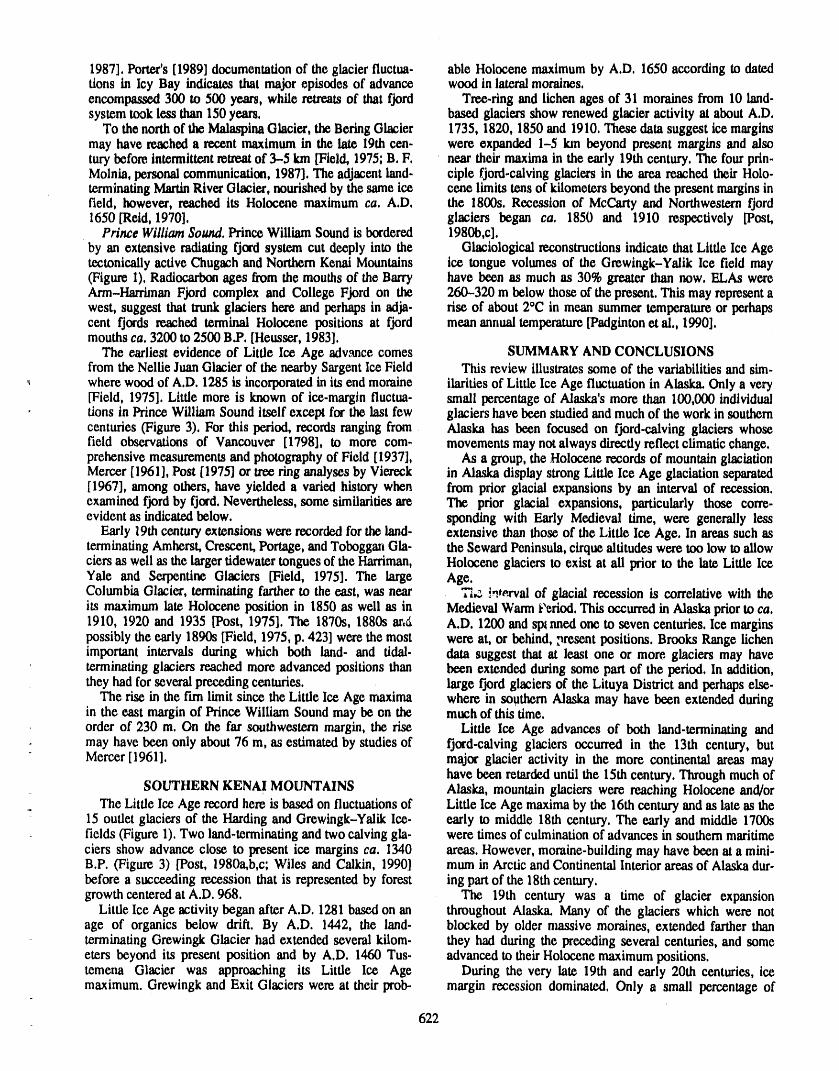
1987]. Porter's[1989] documentationof the glacier fluetua- able Holocene maximumby A.D. 1650 according to datedtions in Icy Bay indicates that majorepisodes of advance wood in lateralmoraines.encompassed 300 to 500 years, while retreatsof thatfjord Tree-ringand lichen ages of 31 moraines from 10 land-system tookless than 150years, based glaciers show renewed glacier activity at about A.D.

To the northof the MalaspinaGlacier, the BeringGlacier 1735, 1820, 1850 and 1910. These data suggest ice marginsmay have re,ached a recent maximumin the late 19111cen- were expanded 1-5 ian beyond present margins and alsotury before intermittentretreatof 3-5 km [Field, 1975; B.F. near their maxima in the early 19th century. The four prin.Molnla, personal communication, 1987]. The adjacentland. ciple fjord-calving glaciers in the area reached their Holo-terminatingMartinRiverGlacier, nourishedby the same ice cene limits tens of kilometersbeyond the present marginsinfield, however, reached its Holocene maximum ca. A.D. the 1800s. Recession of McCarty and Northwesternfjord1650[Reid, 1970]. glaciers began ca. 1850 and 1910 respectively [Post,

Prince William Sound. PrinceWilliam Sound is bordered 1980b,c].by an extensive radiatingfjord system cut deeply into the Glaciological reconstructionsindicate thatLittle Ice Agetectonically active Chugach and NorthernKenai Mountains ice tongue volumes of the Grewingk-Yalik Ice field may(Figure 1). Radiocarbonages from the mouthsof the Barry have been as much as 30% greaterthan now. EL.AswereArm-Harriman Fjord complex and College Fjord on the 260--320 m below those of the preseztt.This may representawest, suggest that trunkglaciers here and perhaps in adja- rise of about 2°C in mean summer temperatureor perhapscent fjords reached terminal Holocene positions at fjord mean annual temperature[Padgintonetal., 1990].mouths ca. 3200 to 2500 B.P. [Heusser,1983].

The earliest evidence of Little Ice Age advice comes SUMMARY AND CONCLUSIONSfromthe Nellie JuanGlacier of the nearbySargentIce Field This review illustratessome of the variabilitiesand sim-wherewood of A.D. 1285 is incorporated in its end moraine ilaflties of Little Ice Age fluctuationin Alaska.Only a very[Field, 1975]. Little more is known of ice-margln fluctua- small percentage of Alaska's more than 100,000 individualtions in Prince William Sound itself except for the last few glaciers have been studiedand much of the workin southerncenturies (Figure 3). For this period, records ranging from Alaska has been focused on fjord-calving glaciers whosefield observations of Vancouver [1798], to more com- movements maynotalways directly reflect climatic change.prehensive measme.mentsand photographyof Field [1937], As a group, the Holocene recordsof mountainglaciationMercer [1961], Post [1975] or tree ringanalyses by Viereck in Alaska display strongLittle Ice Age glaciation separated[1967], among others, have yielded a varied history when from prior glacial expansions by an interval of recession.examined fjordby fjord. Nevertheless, some similarities are The prior glacial expansions, particularly those corm-evidentas indicated below, spending with Early Medieval time, were generally less

Early 19thcentury extensions were recordedfor theland- extensive than those of the Little Ice Age. In areas such asterminatingAmherst, Crescent' Portage,andToboggan Gla- the SewardPeninsula,cirque altitudes were too low to allowciers as well as the largertidewater tonguesof the Harriman, Holocene glaciers to exist at ali prior to the late Little IceYale and Serpentine Glaciers [Field, 1975]. The large Age.Columbia Glacier, terminatingfartherto the east, was near '7i,:._-yerval of glacial recession is correlative with theits maximum late Holocene position in 1850 as well as in Medieval Warmr'eriod.This occurredin Alaska priorto ca.1910, 1920 and 1935 [Post, 1975]. The 1870s, 1880s ar,fi A.D. 1200 andSl_nned one to seven centuries. Ice marginspossibly the early 1890s [Field, 1975, p. 423] were the most were at, or behind, _'_resentpositions. Brooks Range lichenimportant intervals during which both land. and tidal, data suggest that at least one or mo_ glaciers may have

' terminatingglaciers reached more advanced positions than been extended duringsome part of the period. In addition,they had for severalprecedingcenturies, large fjord glaciers of the Lituya District and perhapselse-

The rise in the firn limit since the Little Ice Age maxima where in southern Alaska may have been extended duringin the east marginof PrinceWilliam Sound may be on the muchof this time.order of 230 m. On the far southwestern margin, the rise Little Ice Age advances of both land-terminating andmay have been only about76 m, as estimated by studies of fjord-calving glaciers occurred in the 13th century, butMercer [1961]. major glacier activity in the more continental areas may

have been retarded until the 15th century. Through much ofSOUTHERN KENAI MOUNTAINS Alaska, mountain glaciers were reaching Holocene and/or

The Little lee Age record here is based on fluctuationsof Little Ice Age maxima by the 16th century and as late as the15 outlet glaciers of the Harding and Grewingk-Yalik Ice- early to middle 18th century. The early and middle 1700sfields (Figure 1). Two land-terminating and two calving gla. were times of culmination of advances in southern maritimeciers show advance close to present ice margins ca. 1340 areas. However, moraine-building may have been at a mini-B.P. (Figure 3) [Post, 1980a,b,c; Wiles and Calkin, 1990] mum in Arctic and Continental Interior areas of Alaska dur-before a succeeding recession that is represented by forest ing part of the 18thcentury.growth centered at A.D. 968. The 19th century was a time of glacier expansion

Little lee Age activity began after A.D. 1281 based on an throughout Alaska. Many of the glaciers which were notage of organics below drift. By A.D. 1442, the land- blocked by older massive moraines, extended farther thanterminating Grewingk Glacier had extended several kilom, they had during the preceding several centuries, and someeters beyond its present position and by A,D. 1460 Tus. advanced to their Holocene maximum positions.temena Glacier was approaching its Little Ice Age During the very late 19rh and early 20th centuries, icemaximum. Grewingk and Exit Glaciers were at their prob., margin recession dominated, Only a small percentage of

622

glacier ice marginshaveremainedat their 19rhcenturymax. ACKNOWLEDGMENTSima andthese were in areasof high precipitation.Recession This material is based upon work supported by thefrom Little Ice Age maximahas been on the orderof 0.2 km National Science Foundation under Grants DPP 7619575,formanycirqueglaciers, butup to severaltens of ldlometers 7819982, 8412897 and 8922696, Logistic supporthas beenfor the fjordglaciers, providedby several groups includingALASCOM, the U.S.

Glacierequilibriumlines arepresently 100-200 m higher Geological Survey, Alaska Division of Geological and Geo-in the Arctic and up to 400 m higher in the Maritimeareas physical Surveys, the National Park Service, Alaska Statethan they were through much of the Little Ice Age, This Parks, and the Pratt Museum of Homer. T. D. Hamilton,may reflect a late 19th or early 20rh centuryrise in mean A.S. Post, Bud Rice, and R. P, Goldthwait providedhelp insummer temperatureon the order of 2-3°C (about 1-20C diverse ways, as did fellow researchers J. M. Ellis, L. A.mean annual change) and/or changes in the precipitation Haworth,and B. J. Przybyl.regime [e.g., Lamb, 1977; Williams and Wigley, 1983;Mayo andMarch, 1990].

623

REFERENCES

Beschel,R.,andC.P.Egan,Oeobotanicalinvestigationsof New Yoi'katBuffalo,Buffalo,NY, 1988,a 16rhcentury moraine on the Bucher Glacier, Juneau Housser, C, J,, Holocene vegetation history of the PrinceIcefield, Alaska, Proceedings 16rh Alaska Science Con. William Soundregion, south-central Alaska, Quat, Res,,ference, pp, 114-115, American Association for the 19,337-355, 1983,Advancementof Science, 1965, IGBP, Global change, a plan of action, in Global Ctumge

Borns, H, W,, Jr,, and R, P. Goldthwait, Late-Pleistocene Report 4, IGBPSecretariat,Stockholm, Sweden, 1988,fluctuationsof Kaskawulsh Glacier,southwesternYukon Kaufman,D, S,, P, E, Calkin, W, B, Whifford,B, J, Przybyl,Territory,Canada,Am, J, Sci,, 264,600--619, 1966, D. M, Hopkins, B, J, Peck, and R, E, Nelson, Surficial

Calldn, P. E., Holocene glaciation of Alaska(and adjoining geologic map of the Kigluaik Mountains area, SewardYukon Territory, Canada), Quat, Scl, Rev,, 7, 159-184, Peninsula, Alaska, U,S, Geological Survey, Mlscella.1988. neous Field Studies Map MF.2074, Scale 1:3360, 1989,

Calkin,P. E,, and J, M. Ellis, A lichenometflc datingcurve Lamb,H. H., Climate: Present, Past atm Future, Vol, 2, 835andits applicationto Holocene glacial studies in the cen. pp,, Methuen, London, 1977,tral Brooks Range, Alaska,Arctic Alpine Res., 12, 245- LaPerouse, J, F, O, Dc, Voyage Round the World, Per-264, 1980. formed in the Years 1785, 1786, 1787, and 1788 by the

Calkin,P. E., and J. M, Ellis, A cirqueglacier chronology Boussole and Strolabe, Vol, I, pp, 364-416, and Ariasbased on emergent lichens and mosses, J. Glaciol,, 27, (Translationfrom French), A, Hamilton,London, 1799.512-515, 1981. Lawrence, D, B., Glacier fluctuation for six centuries in

Calkin,P. E,, J. M. Ellis, L. A. Haworth,and P. E. Burns, southeasternAlaskaand its relationto solaractivity,Get.Cirqueglacier regime and Neoglaciation, Brooks Range, graphical Rev,, 40, 191-223, 1950,Alaska, Zeitschrift far Gletscherkunde und Glazial. Letregutlly,A,, and L, Reynaud, Spatial patternsof mass.geologie, 21,371-378, 1985. balance fluctuationsNorthAmerican glaciers, J. Glaclol.,

Calkin,P. E., B. J, Przybyl, and D. 5. Kaufman,Latest Qua. 35, 163-168, 1989.ternary glaciation, Kigluaik Mountains, northwestern Luckman,B. H., Global change and the recordof the past,Alaska, Geol. Soc. America Abstracts with Programs, 19 Geos, 18), 1--8,1989.(1), 8, 1987. Mann,D. H., Reliability of a fjord glacier'sfluctuationsfor

Denton, G. H., and W. Karl_n, Holocene glacial and trce- paleoclimatic reconstructions, Quat, Res., 25, 10-PA,line variationsin the White RiverValley and Skolat Pass, 1986.Alaska and Yukon Territory, Quat, Res., 7, 63-111, Mann,D. H., and F, C, Ugolint, Holocene glacial history of1977. the Lituya district, southeast Alaska, Can. J, Earth Sci.,

Derksen,S. J., Glacial geology of the BradyGlacier region, 22,913-928, 1985.Alaska, Ohio State University, Institute of Polar Studies Mayo, L., Advanceof HubbardGlacier andclosure of Rus-Report,60,97pp.,1976. sellFjord,Alaska:Environmentaleffectsandtmzardsin

Egan,C.P.,ContributiontothelateNeoglacialhistoryof theYakutatarea,U.S.GeologicalCircular1016,pp.4-theLynnCanalandTakuValleysectionsoftheAlaska 16,1987,BoundaryRange,Ph.D.Dissertation,200pp.,StateUni- Mayo,L.R.,andR, S.March,Airtemperatureandpre-versity,EastLansing,Michigan,1971. cipitationatWolverineGlacier,Alaska;Glaciergrowth

Ellis, J. M., and P. E. CaUdn, Chronology of Holocene gla- 1'_a warmer,wetter climate, Ann, Glaciol., 14, 191-194,ciation, central Brooks Range, Alaska, Geol. Soc. Am. 1990.Bu11.,95,897-912, 1984. McKenzie, G. D., Glacier fluctuations in Glacier Bay,

Field, W. O., Observations on Alaskan coastal glaciers in Alaska, in the past 11,000 years, Proceedings of the First1935, Geographical Rev., 27, 63-81, 1937. Conference on Scient_c Research in the National Parks,

Field, W. O., Mountain Glaciers of the Northern Hemi. Vol. 2, New Orleans, 1976, edited by R. M. Linn, pp.sphere, Cold Regions Research and EngineeringLabor- 809-813, 1979.atory, Hanover,NH, 1975. Meier, M. F., Contribution of small glaciers to global sea

Goldthwait, R. P., Glacial history, in Soil development and level, Science, 226, 1418-1421, 1984.ecological succession in a deglaciateAareaof MuirInlet, Meier,M. F., and A. S. Post,Fast tidewaterglaciers, J. Get-southeast Alaska, Part 1, edited by A. Mh.sky,pp. 1-18, phys. Res., 92, 9051-9058, 1987.The Ohio State University, Institute of Polar Studies Meier,M. F., W. V. Tangbom, L. R. Mayo, and A. 5. Post,Report, 20, 1966. Combined ice and water balances of Gulkanaand Wol-

Goldthwait, R. P., I. C. McKeller, and C. Cronk, Fluctua- verine glaciers, Alaska, and South Cascade Glacier,tions of Crillon Glacier system, southeast Alaska, Bull. Washington, 1965 and 1967 hydrologic years, U.S. Get-Int. Assoc. Scientific Hydrol., 8, 62-74, 1963. logical Survey Professional Paper 715.A, 23 pp., 1971.

Goodwin, R. G., Holocene glaciolacustrine sedimentation in Mercer, J. H., The estimation of the regimes and former timMuir Inlet and ice advance in Glacier Bay, Alaska, limit ofaglacier, J. Glaciol.,3,850--858, 1961.U.S.A.,Arctic and Alpine Research, 20, 55--69, 1988. Miller, M. M., Inventory of terminal position changes in

Grove, J. M., The Little lee Age, 498 pp., Methuen, London, Alaskan coastal glaciers since the 1750's, Proc. Am. Phil-1988. osoptu'calSoc., 108, 257-273, 1964.

Haworth, L. H., Holocene glacial chronologies of the Miller, M. M., Quaternary erosional and stmtigraphicBrooks Range, Alaska and their relationship to climate sequences in the Alaska-Canada Boundary Range, inchange, Ph.D. Dissertation, 260 pp., State University of Quaternary Stratigraphy of North America, edited by

624

W, C, Mahaney, pp, 463-492, Halstead Press, Wiley and Post, A, S,, Preliminarybathymetry of Aialik Bay and Nee-Sons,New York, 1977, glacial changes of ALalikand Pederson Glaciers, Alaska,

Molnla, B, F,, Glacial history of the northeasternGulf of U,S, Geological Survey Open.File Report, 80.423,Alaska. A synthesis, in Glaciation in Alaska. The gee. 1980c,logic record, edited by T, D, Hamilton, K, M, Reed, and Przybyl,B, J,, The regimenof GrandUnion Glacier and theR, M, Thorson,pp, 219-236, Alaska Geological Society, glacial geology of the northeasternKlglualk Mountains,Anchorage,1986, SewardPeninsula,Alaska, Master'sThesis, 106 pp,, State

Oerlemans, J,, Gladers as indicators of carbon dioxide University of New York at Buffalo, Buffalo, New York,warming,Nature, 320, 607.-.609,1986, 1988,

Padginton,C, H,, P, E, Calkin, and G, C, Wiles, and V, E, Rampton, V, N,, Neoglacial fluctuation of the NatzhatandRomanovsky,Reconstructionof icefield glaciers and Lit- Klutlan Glaciers, YukonTerritory, Canada,Can, J, Earthtie ice Age climatic change, southern Kenai Mountains, Scl,, 7, 1236-1263, 1970,Alaska, Geol, Soc, Am,, Abstracts with Programs, 22(4), Rampton,V, N,, Holocene glacial andtree.line variationsinAbstr,No, 177, p, 20, 1990, the White River valley and Skolat Pass, Alaska and Yu-

P6w6, T, L,, and R, D. Reger, Delta River area, Alaska ken Territory: A discussion, Quat, Res,, 10, 130-134,Range, in Guidebook topermafrost and Quaternary geol. 1978,ogy along the Richardson and Glenn Highways between Reger, R, D,, and T, L, P6w6, Lichenomettic dating in theFairbanks and Anchorage, Alaska, edited by T, L, P6w6 central Alaska Range, in The Pertglaclal Environment:and R, D, Reger, pp, 47-135, Alaska Division of Gee- Past and Present, edited by T, L, P6w6, pp, 223-247,logical andGeophysical Surveys, Guidebook1, 1983, McGill.QueensUniv, Press, Montreal,Canada, 1969,

Plafker, G., and D, J, Miller, Recent history of glaciation in Reid, J, H,, Late Wisconsin and Neoglaeial history of thethe Malasptnadistrict and adjoining bays, Alaska, Sci. MartinRiver Glacier, Alaska, Geol, Soc, Am, Bull,, 81,ence in Alaska, 1957, Proceedings 8rh Alaskan Science 3593-3604, 1970,Coherence, pp, 132-133, 1958a. Sharp,R, P,, The latestmajoradvanceof MalasptnaGlacier,

Platker, G,, and D, J. Miller, Glacial featuresand surficial Alaska, GeographicalRev,, 48, 16--26,1958,deposits of the Malasptna district, Alaska, U.S. Gee. Stuiver,R., andP. J. Reimer, A computerprogramforradio-logical Survey Miscellaneous Geological Investigations carbon age calibration, Radiocarbon, 28, 1022-1030,Map 1.271, scale 1:125,000, 1958b. 1986.

Porter,S. C., Patternand forcing of Northern Hemisphere Ten Brink,N, W., Glaciationof the northernAlaska Range,glacier variationsduring the last millennium, Quat. Res., in Glaciation in Alaska . Extended Abstracts from a26, 27-48, 1986. Workshop, editedby R. M, Tborson,and T. D. Hamilton,

Porter,S. C., Late Holocene cycles of advance andretreatof pp. 82-90, University of Alaska Museum Occasionalthe fjordglacier system in Icy Bay, Alaska, Arctic Alpine Paper,2, Falrbanks,Alaska, 1983.Res., 21,364-379, 1989. Vancouver, G., Voyage of Discovery to the North Pacific

Porter,S. C., K. L. Pierce, and T. D. Hamilton, Late Wis- Ocean in the Years 1790-1795, Vol 3, Printedfor G. G.consin mountainglaciation in lhe western United States, Robinson, J. Robinson, and J. Edwards, London, 1798.in Late Quaternary Environments of the United States, Viereck, L, A,, Botanicaldating of recent glacial activity inI/ol, I, The Late Pleistocene, edited by S, C, Porter, pp, western North America, in Arctic and Alpine Environ.71-111, Univ, of Minnesota,Minneapolis, MN, 1983, ments, editedby H, E, Wright, Jr, andW, H, Osburn, pp,

Post, A, S,, Distribution of surging glaciers in western North 189-204, IndianaUniv, Press, Bloomington, IN, 1967,America, J. Glaciol., 8, 229-240, 1969, Waythomas, C. F. and N. W. Ten Brink, Glacial geology of

Post, A. S,, Preliminary hydrography and historic terminal the Swift Fork, Hen'on and Foraker River Valleys,changes of Columbia Glacier, Alaska, U.S, Geological Alaska, Unpubl. report submitted to the National ParkSurvey Hydrographic Investigations Atlas, 559, 1975, Service and National Geographic Society, 76 pp,, 1982,

Post, A. S., Preliminary bathymetry of McCarty Glacier, Wiles, G. C., and P. E. Calktn, Neoglaciatlon in the southernAlaska, U.S, Geological Survey Open-File Report 80. Kenal Mountains, Alaska, Ann. Glaciol,, 14, 319-322,424, 4 sheets, 1980a. 1990.

Post, A. S., Preliminary bathymetry of Northwestern Fjord Williams, L, D,, and T, M. L, Wlgley, A comparison of evt-and Neoglacial changes of Northwestern Glacier, Alaska, dence for late Holocene summer temperature variationsU.S. Geological Survey Open.File Report, 80-414, 2 in the Northern Hemisphere, Quat, Res., 20, 286-307,sheets, 1980b. 1983,

625

I

The Greenland Ice Sheet Margin as a Source of Paleoenvironmental Data

N. Reeh, H. Oerter, A. Letr_gullly, and H. MillerA_fredWegenerl_tltute for PolarandMarineResearch,Bremerhaven,Germany

ABSTRACT

Oxygen-18 records measured on surface ice samples from Greenland ice sheetmargins show that ice of pr_-Holocene age is present at many_locations alon8 theice margin. Several records have been obtained from West, North, and NortheastGreenland. At all locations where pre-Holocene ice is found, it constitutes a bandrunning parallel to the ice edge. However, the width of the band varies greatly fromone location ta another, ranging between 30 m and 1500 m,

So far, the most detailed oxygen-18 record has been obtained from a WestGreenland ice margin location. It spans the last glacial (the Wisconsinan), the lastinterglacial (Sangamon, Eem), and part of the previous glacial (the Illinoian). Acorrelation with the oxygen-18 records from the Greenland d_ep ice cores from

Camp Centu_ and Dye-3 indicates that neither of these records reach back to theprevious glacial, probably due to substantial thinning and retreat of the ice sheet inNorth and South Greenland in the Eemian interglacial.

The oxygen-18 record has been translated into a Greenland temperature recordcovering the past 150,000 years. The isotopic temperatures indicate largetemperature variations in marine isotopic stage 5, with a climate warmer than atpresent not only in sub-stage 5e, but also in sub-stage 5c and in a short period ofsub-stage 5a.

The ice margin studies indicate that Greenland ice sheet margins have a largepotential as sources of paleoenvironmental information. Large volumes of ice caneasily be mined, e.g., for Carbon-14 dating and other measurements that requirelarge amounts of ice. Therefore, ice mar_in studies are an important supplement todeep drilling programs in the interior regions of the ice sheet.

626

The History of the Climate of the Northern Polar Regionin the Holocene and Recent Millennia from Proxy and Historical Data

E, P. Borlsenkov and V, M. PasetskyMainGeophysicalObservatory,Leningrad,U.S,S.R,

ABSTRACT

All data available on the reconstruction of the climate of the northern polarregion in different Holocene periods are presented. Primary attention is given to thedata on the polar region climate on the USSR European and Asian territory. Thepossible natural causes responsible for creating the climatic conditions of the Holo-cene warm and cold epochs in polar regions are analyzed, as well as circulationfeatures of these epochs, The historical data available on the polar region climateare generalized tor the past two thousand years and in particular the recentmillennium.

It is shown that during the recent millennium the climatic conditions of thenorthern polar region were very different, which influenced ice conditions and polarnavigation, It is also shown that most of the above periods of climate warming andcooling were related to climatic changes in other regions of Europe and Asia. It isinferred that these changes depend to a considerable extent on circulation processes.In this conaection an analogy is given between the Arctic warming in the 1930S and1940s and similar climate warming in other epochs, in particular in the earlysixteenth century, Their similarity in clmulation processes is shown.

627

Two Late Quaternary Pollen Records from the Upper Kolyma Region,Soviet Northeast: A Preliminary Report

P.M. Andersonand L.B.BrubakerQuaternaryResearchCenter,Universityof Washington,Seattle,Washington,U,S.A,

A. A. AndreevLaboratoryof ealeogeography,Instituteof Geography,Moscow,U,S,S.R.

B. I. Chernenky, I. N. Federova, L. N. Kotova, A. V. Lozhkin, A. I. Polujan, and L. G. RovakoNorthEast InterdisciplinaryResearchInstitute,Magadan,U.S.S.R,

J

P. A. Colinvaux and W. R. EisnerByrd PolarResearchCenter,The OhioStateUniversity,Columbus,Ohio,U.S.A.

D. M. HopkinsAlaskaQuaternaryCenter,Universityof AlaskaFairbanks,Fatrbanks,Alaska, U.S.A.

M. C. MillerDepartmentof BiologicalSciences,Universityof Cincinnati,Cincinnati,Ohio,U.S.A.

ABSTRACT

Pollen records from Sosednee and Elikchan Lakes provide the first continuouslate Quaternary vegetation history for the upper Kolyma drainage of the SovietNortheast. Full-glacial spectra at these sites are similar to those from Eastern Berin-gia, with high percentages of grass, sedge, and wormwood pollen indicative of herbtundra. In the Elikchan area at approximately 12,500 B.P., herb tundra was replacedby a stone pine-larch forest, perhaps similar to modern forests in the region. In con-trast, the herb tundra near Sosednee Lake was succeeded by a birch-aider shrubtundra followed by a larch woodland, Stone pine increased in the region after larchand prior to 8600 B.P. A Holocene decline in stone pine, which is evident at Elik-chan Lake, is less marked or absent at Sosednee Lake. The differences in these pol-len records is somewhat surprising given the proximity of the two sites. Suchdifferences indicate that numerous well-dated sites will be needed to describe thevegetation and climate histories of Western Beringia.

INTRODUCTION [Gitermanet al,, 1982; Giterman, 1984; Lozhkin, 1984;Lacustrinepollen recordsprovide much of the data for Savvinova, 1984], trans-Beringian plant migrations

interpretinglate Quaternaryclimatic and vegetational [Yurtsev,1982, 1984] andpaleoclirnates[Lozhkin,1984],changesfor the easternsideof the BeringLandBridge[e.g., Although usingslightly differentdata bases and analyticalLivingstone, 1955; Colinvaux,1964; Agerand Brubaker, techniques,bothsets of scientistshavenotedthatBeringiais1985;Ritchie,1987;Barnoskyet al., 1987].Researchersin a key area for understandingthe ruleof climate in shapingWesternBeringia, who rely more on pollen preserved in the modern arctic and subarctic flora. Today's BeringiannonLacustrinesettings,have also beenconcernedwith such biomes will be particularly susceptibleto future climaticpaleoenvironmentalhistoriesas that of the Pleistoceneflora warming resulting from increased concentration of

628

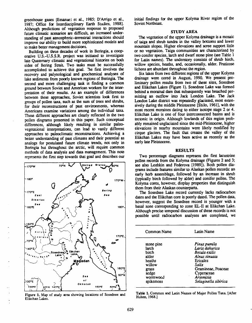
greenhouse gases [Emanuel et al., 1985; D'Arrigo et al., initial t'mdings for the upper Kolyma River region of the1987; Office for Interdisciplinary Earth Studies, 1988]. Soviet Northeast.Although predictions of vegetation response to proposedfuture climatic scenarios are difficult, an increased under- STUDY AREAstanding of past atmospl_cric-terrestrialinteractionsshould The vegetationof the upper Kolymadrainageis a mosaicimprove our ability to build more sophisticatedmodels and of taiga and shrubtundrain the valley bottoms and lowerto make bettermanagementdecisions, mountain slopes. Higher elevations and scree support little

Building on three decades of work in Beringia, a coop- or no vegetation. Taiga communities are characterized byerative U.S.-U.S.S.R. project was initiated to investigate two conifer species, larch and dwarf stone pine (see Table 1late Quaternaryclimatic and vegetational histories on both for Latin names). The understory consists of shrub birch,sides of Bering Strait. Two tasks must be successfully willow species, heaths, and, occasionally, alder. Fruticoseaccomplished to achieve this goal..'he first involves the lichens are abundantthroughoutthe region.recovery and palynological and geochemical analyses of Six lakes fromtwo differentregions of the upperKolymalake sediments frompoorly known regions of Beringia. The drainage were cored in August, 1990. We present pre-second and more challenging task is finding a common liminary pollen results from two of these sites, Sosedneegroundbetween Soviet and American workers for the inter- and Elikchan Lakes (Figure 1). Sosednee Lake was formedpretation of their results. As an example of differences behinda morainaldam that subsequentlywas breachedper-between these approaches, Soviet scientists look lust to mitting an outflow into Jack London Lake. The Jackgroupsof pollen taxa, such as the sum of trees and shrubs, London Lake districtwas repeatedly glaciated, most exten-for their reconstructions of past environments, whereas sively duringthe middle Pleistocene [Shilo, 1961], with theAmericans examine variations among the individual taxa. most recent moraines dating to either isotope stage 2 or 4.These different approachesare clearly reflected in the two Elikchan Lake is one of four interconnected basins and ispollen diagramspresented in this paper. Such conceptual tectonic in origin. Although lowlands of this region prob-differences, although likely resulting in similar paleo- ably remainedunglaciatedsince the mid-Pleistocene, highervegetational interpretations, can lead to vastly different elevations in nearby mountains were likely modified byapproaches to paleoclimatic reconstructions. Achievu,g a cirque glaciers. The fault that creates the valley of thebetter understanding of past climates and their potential as Elikchan Lakes may have been active as recently as theanalogs for postulated future climate trends, not only in early latePleistocene.Beringia but throughou_the arctic, will require commonmethods of data analysis and data management. This note RESULTSrepresents the ftr,st step towards that goal and describes our Two percentage diagrams represent the Iu'st lacustrine

pollen records from the Kolyma drainage (Figures 2 and 3;

_ro.w ro;N IJ" _u_¶,, '"U" -_o'N seealso Lozhkin andFedemva[1989]). Both pollen dia---- 0 grams include features similar to Alaskanpollen records:an

early herb assemblage, followed by an increase in shrub_o. l ro.w- (typically birch followed by alder) and conifer pollen. The

• Kolyma cores, however, display properties that distinguishthem from their Alaskan counterparts.Bering

The Sose_aee Lake record currently lacks radiocarbon£est Sem

dates and the Elikchan core is poorly dated. The pollen data,s.,.,,,, however, suggest the Sosednee record is younger with aSe,

_eo"E . _eo*. basalzone corresponding to zone EL-IIat Elikchan Lake.•= _" Although precise temporal discussion of these records is notj_. . possible until radiocarbon analyses are completed, we

/

'_ Common Name Latin Nameoi

o ,, 170"E,

f q ="_' stone pine Pinus pumila

larch Larix dahurica

c t,. "__ So, . El_chan birch Betula exilis"*,, ,.o °" . =, alder Alnus sinuata

_ Ma heaths Ericaleswillow Salix

,eo._ grass Gramineae,PoaceaeCypcraceaewormwood Artemisia

. sO,l sedge'_'_ 0' / spikemoss Selaginellasibirica:,0 :"i o,,o,.,

1 :_ / _, : ,_t ,, ? .I I

FlgureI.Map ofstudyareashowingIocatiomofSosedneeand TableI.Common andLatinNamesofMajorPollenTaxa.[AfterEIikchanLakes. Hulten,1968.]

J

629

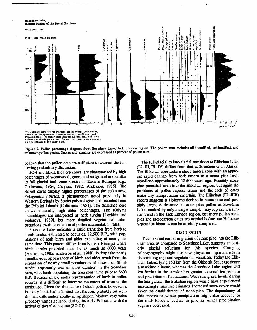
I_l_tednee La/le,

Kolyms Re,on oi' the Soviet Northeast

50

100

i o,i150 P _ b )

iso.ll

I0 30 I0 lO -it)

t_Lrl cm a x I04

The category Other Herbs includes the following: Composltae,Cruclferae, Polyganaceae. Chenopodiaceae, Umbellll'erae. andPapaveraceae. The pollen sum includes all identified, unt-nown,and unldentl/iable pollen taxa. Spores and aquaUcs are expressedas a percentage of the pollen sum.

Figure 2. Pollen percentage diagram f_om Sosednee Lake, Jack London region. The pollen sum includes all identified, unidentified, andunknown pollen grains. Spores and aquatics are expressed as percent of pollen sum,

believe that the pollen data are sufficient to warrant the Col- The full-glacial to late-glacial transition at Elikchan Lakelowing preliminary discussion. (EL-Ill, EL-IV) differs from that at Sosednee or in Alaska.

SO-I and EL,II, the herb zones, are characterized by high The Elikchan core lacks a shrub tundra zone with an appar-percentages of wormwood, grass, and sedge and are similar ent rapid change from herb tundra to a stone pine--larchto full-glacial herb zone spectra in Eastern Beringia [e.g., woodland approximately 12,500 years ago. Possibly stoneColinvaux, 1964; Cwynar, 1982; Anderson, 1985]. The pine preceded larch into the Elikchan region, but again theSoviet cores display higher percentages of the spikemoss, problems of pollen representation and the lack of datesSelaginella sibirica, a phenomenon noted previously in make any interpretation uncertain. The Elikchan (EL-IIIB)Western Beringia by Soviet palynologists and recorded from record suggests a Holocene decline in stone pine and pos-the Pribilof Islands [Colinvaux, 1981]. The Sosednee core sibly larch. A decrease in stone pine pollen at Sosedneeshows unusually high alder percentages. The Kolyma Lake, marked by only a single sample, may represent a slm-assemblages are interpreted as herb tundra [Lozhkin and ilar trend in the Jack London region, but more pollen sam-Federova, 1989], but more detailed vegetational inter- pies and radiocarbon dates are needed before the Holocenepretations await calculation of pollen accumulation rates, vegetation histories can be carefully compared.

Sosednee Lake indicates a rapid transition from herb toshrub tundra, estimated to occur ca. 12,500 B.P., with pop- DISCUSSIONulations of both birch and alder expanding at nearly the The apparent earlier migration of stone pine into the Elik-same time. This pattern differs from Eastern Beringia where chart area, as compared to Sosednee Lake, suggests an east-birch shrubs preceded alder by as much as 6000 years erly glacial refugium for this species. Changing[Anderson, 1985; Anderson et al., 1988]. Perhapsthe nearly paleogeography might also have played an important role insimultaneous appearances of birch and alder result from the determining regional vegetational variation. Today the Elik-expansion of nearby small populations of these taxa. Shrub chan Lakes, lying 150 km from the Ohkotsk Sea, experiencetundra apparently was of short duration in the Sosednee a maritime climate, whereas the Sosednee Lake region 250area, with larch popul_aJn_!ithe area some. time priorto 8600 km further in the interior has greater seasonal temperatureB.P. Because of the under-representation of larch in pollen and precipitation fluctuations. With rising sea levels duringrecords, it is difficult to interpret the extent of trees on the the late glacial, the Elikchan region would have experiencedlandscape. Given the abundance of shrub pollen, however, it increasingly maritime climates. Increased snow cover wouldis likely larch had a limited distribution, probably on well- favor the establishment of stone pine. The dependency ofdrained .qoil.qand/or south-facing slopes. Modern vegetation this si3ecies on winter precipitation might also account forprobably was established during the early Holocene with the the mid-Holocene decline in pine as winter precipitationarrival of dwarf stone pine (SO-III). regimes decreased.

630

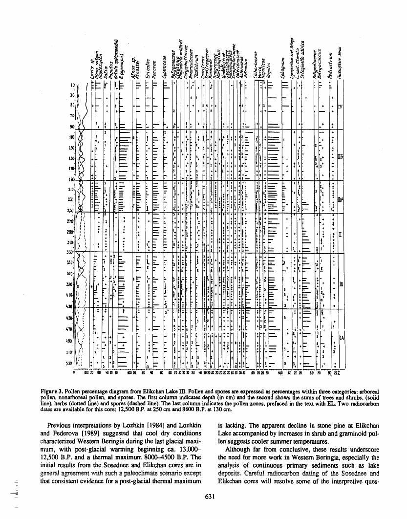
Figure 3. Pollen percentagediagramfrom F3ikchanLake [II. Pollen andspores areexpressed as percentageswithin threecategories: arborealpollen, nonarborea]pollen, and spores. The first colunm indicatesdepth (in cre) and the second shows the sums of trees and shrubs, (soiidline), herbs (dotted line) and spores (dashed line). The last column indicates the pol]e_ zones, prefsced in the text with EL. Two radiocarbondates arc available for thiscore: 12,.500B.P.at 2.50cm and 8600 B.P. at 130 cre.

Previous interpretations by Lozhkin [1984] and Lozhkin is lacking. The apparent decline in stone pine at Elikchanand Feclerova [1989] suggcs_,:d that cool dry conditions Lake accompanied by increases in shrub and gramir,oid pol-characterized Western Beringia during the last glacial maxi- len suggests cooler summer temperatures.mum, with post-glacial warming beginning ca. 13,000- Although far from conclusive, these results underscore

12,500 B.P. and a thermal maximum 8(X30--4500 B.P. The the need for more work in Western Beringia, especially theinitial results from the Sosednee and Elikchan cores are in analysis of continuous primary sediments such as lake_"_'_ "'¢:r"w'''_''_" *''_* _"'"" "* It" ,it_. writ ._ ...., _.,,._, _,v_a,.*_.,_.. s*.**._

that consistent evidence for a post-glacial thermal maximum Elikchan cores will resolve some of the interpretive ques-

_-- 631

tions posed above. The differences in the pollen records ACKNOWLEDGMENTSfrom these two nearbyregions strongly argue that the late This project is fundedby the North East InterdisciplinaryQuaternaryvege_tion history of Western Beringiais com- ResearchInstitute,Far EasternBranch, Academy of Scienceplex and thata gridsampling design, similar to that used in and the National Science Foundation (ATMS 8915415 tonorth-centralAlaska [Anderson et al., 1988], is required. Ohio State Universityand University of Washington),TheThe long.termgoal of this projectis thecollection andanal- authors would like to thank Tom Ager and Tom Hamiltonysis of such a suite of sites in ,order to provide a fuller forhelpful reviews of the manuscript.understanding of the late Quaternary climatic history ofBeringia.

REFERENCES

Ager, T. A., andL. B. Brubaker,Quaternarypalynologyand C.E. Sehweger, and S. B. Young, pp. 43-74. Academicvegetationalhistoryof Alaska, in Pollen Records of Late. Press, New York, 1982.Quaternary North American Sediments, edited by V. Grichuk, V. P., Changes in species composition of flora ofBryant, Jr. and R. G. Holloway, pp. 353--384,American northeastern Eurasia in the late Cenozoic, in Beringia dnAssociation of Stratigraphic Palynologists Foundation, the Cenozoic Era, edited by V. L. Kontrimavichus, pp.Dallas, TX, 1985. 188--200, Amerind Publishing Co. Pvt. Ltd., New Delhi,

Anderson, P. M., Late Quaternary vegetational change in (Translated from Russian), 1984.the Kotzebue Sound area, northwestern Alaska, Quat. Hulten, E., Flora of Alaska and Neighboring Territories,Res., 24, 307-321, 1985. Stanford University Press, Stanford, CA, 1968.

Anderson, P. M., R. E. Reanier, and L. B. Brubaker, Late Livingstone, D. A., Some pollen profiles from arctic Alaska,Quaternary vegetational history of the Black River region Ecology, 36, 587--600, 1955.in northeastern Alaska, Can. J. Earth Sci., 25, 84-94, Lozhkin, A. V., Late Pleistocene and Holocene vegetation1988. in western Bering land, in Beringia in the Cenozoic Era,

Bamosky, C. W,, P. M. Anderson, and P. J. Bartlein, The edited 'oy V. L Kontrimavichus, pp. 88--95, Amerindnorthwestern U.S. during deglaciation: vegetational his- Publishing Co. Pvt. Ltd., New Delhi, (Translated fromtory and paleoclimatic implications, in North America Russian), 1984.and Adjacent Oceans during the Last Deglaciation, Lozhkin, A. V., and I. N. Federova, Late Pleistocene andedited by W. F. Ruddiman and H. E. Wright, Jr., pp. 289- Holocene Vegetation and Climate of Northeastern321, Geological Society of America, Boulder, CO, 1987. U.S.S.R. Based on Data from Lake Sediments. Topog-

Colinvaux, P. A., The environment of the Bering Land raphy and Corresponding Deposits, NortheasternBridge, Ecological Monographs, 34, 297-325, 1964. U.S.S.R., pp. 3-9, Paper of the North East Interdisci-

Colinvaux, P. A., Historical ecology in Beringia: The south plinary Research Institute, Far East Branch Academy ofland bridge coast at St. Paul Island, Quat. Res., 16, 18-- 36, 1981. Science, 1989.

Cwynar, L. C., A late-Quaternary vegetation history from Ritchie, J. C., Postglacial Vegetation of Canada, UniversityHanging Lake, northern Yukon, Ecological Monographs, of Toronto Press, Toronto, Canada, 1987.52, 1-24, 1982. Savvinova, G. M., Pleistocene and Holocene vegetation on

D'Arrigo, R., G. C. Jacoby, and I. Y. Fung, Boreal forests the upper reaches of the Indigirka and Kolyma Rivers, inand atmosphew.,-biosphere exchange of carbon dioxide, Beringia in the Cenozoic Era, edited by V. L.Nature, 329, 321-323, 1987. Kontrimavichus, pp. 211--213, Amerind Publishing Co.

Emanuel, W. R., H. H. Shugart, and M. P. Stevenson, Cii- Pvt. Ltd., New Delhi, (Translated from Russian), 1984.marie change and the broad-scale distribution of tea- Shilo, N. A., Quaternary Deposits of the Yano-Kolymarestrial ecosystem complexes, Climatic Change, 7, 29- Gold Belt of Northeast Asia, Publication of the North43, 1985. East Interdisciplinary Research Institute, Far East Branch

Giterman, R. E., Kolyma lowland vegetation in the Pleis- Academy of Sciences, Magadan, 1961.tocene cold epochs and the problem of polar Beringia Yurtsev, B. A., Relicts of the xerophyte vegetation of Berin-landscapes, in Beringia in the Cenozoic Era, edited by gia in northeastern Asia, in The Paleoecology of Berin-V.L. Kontrimavichus, pp. 214-221, Amerind Publishing gia, edited by D. M. Hopkins, J. V. Matthews, Jr., C° E.Co. Pvt. Ltd., New Delhi, (Translated from Russian), Schweger, and S. B. Young, pp. 157-178, Academic1984. Press, New York, 1982.

Giterman, R. E., A. V. Sher, and J. V. Matthews, Jr., Com- Yurtsev, B. A., Beringia and its biota in the late Cenozoic: aparison of the development of steppe--tundra environ- synthesis, in Beringia in the Cenozoic Era, edited byments in west and east Beringia: pollen and macrofossil V.L. Kontrimavichus, pp. 261-279, Amerind Publishingevidence from key sections, in The Paleoecology of Co. Pvt. Ltd., New Delhi, (Translated from Russian),Beringia, edited by D. M. Hopkins, J. V. Matthews, Jr., 1984.

- 632

Vegetation, Climate, and Lake FormationDuring Interglacial Periods in Northeast Interior Alaska

M. E. EdwardsDepartmentof Geologyand Geophysics,Universityof Alaska,Fairbanks,Alaska,U.S.A.

ABSTRACT

In sediment records from the loess-covered southern Yukon lowland (northeastinterior Alaska), the onset of interglacial conditions ca. 10,000 years ago is cor-related with the development of lakes, probably by deep thawing of ice-rich silt. AtBirch Creek, a river cut exposes 12 m of lacustrine sediments and peat with loessabove and below. The underlying loess contains the 150,000-year old Old CrowTephra. By analogy with Holocene records, the lacustrine sequence probablyrepresents a thaw-lake that formed in the previous interglaciation (isotope sub-stage5e, ca. 125,000 years B.P.).

Sub-stage 5e was probably warmer than any part of the present interglacial andis an important analog for possible future greenhouse climates. Picea (spruce)pollen is more abundant in the interglacial sediments than in comparable Helocenesediments, and values of other pollen types also differ between interglacial andHolocene. This suggests that vegetation and climate were unlike those of today.Comparison of the interglacial pollen with modern pollen spectra may allowestimation of vegetation and climate in northeast Alaska during isotope stage 5e.

As future climatic warming may be expected to affect permafrost, furtherinformation is needed on the vegetational and climatic conditions that favor ice-melting and the formation of thaw lakes in loess.

633

Deglaciation and Latest Pleistocene and Early Holocene Glacier Readvances on theAlaska Peninsula: Records of Rapid Climate Change Due to Transient Changes in

Solar Intensity and Atmospheric CO2 Content?

DeAnne S. Pinney and James E. Beg_tDept. of Geology and Geophysics, University of Alaska Fairbanks, Fairbanks, Alaska, U.S.A.

ABSTRACTGeologic mapping near Windy Creek, Katmai National Park, identified two sets

of glacial deposits postdating late-Wisconsin Iliuk moraines and separated fromthem by volcaniclastic deposits laid down under ice-free conditions. Radiocarbondating of organic material incorporated in the younger Katolinat till and in adjacentpeat and lake sediments suggests that alpine glaciers on the northern Alaska Penin-sula briefly expanded between ca. 8500 and 10,000 years B.P. Stratigraphic rela-tionships and radiocarbon dates suggest an age for the older Ukak drift near thePleistocene--Holocene boundary between ca. 10,000 and 12,000 years B.P.

We suggest that rapid deglaciation following deposition of the Iliuk driftoccurred ca. 13,000--12,000 years B.P. in response to large increases in globalatmospheric "greenhouse gas" content, including CO2. Short-term decreases inthese concentrations, as recorded in polar ice cores, may be linked with brief peri-ods of glacier expansion during the latest Pleistocene and early Holocene. A tran-sient episode of low solar intensity may also have occurred during parts of the earlyHolocene. Rapid environmental changes and glacial fluctuations on the AlaskaPeninsula may have been in response to transient changes in the concentration ofatmospheric greenhouse gases and solar intensity.

INTRODUCTION Thousand Smokes, site of one of the largest volcanic erup-

Prior to the Quaternary the southwestern end of the tions of historic times (Figure 1).Detailed geologic mappingAlaska Peninsula consisted of a string of volcanic islands near lower Windy Creek (Figure 2) has yielded a record of[Detterman, 1986]. The Pleistocene saw these islands con- late Quaternary glacial events on the Alaska Peninsula,nected fast by ice, then by the deposits the glaciers left including periods of latest Wisconsin and early Holocenebehind. Immediately adjacent to moisture sources in the ice expansion recorded by two previously unrecognized setsnorthwest Pacific Ocean and Gulf of Alaska, the Alaska of glacial drift deposits.Peninsula was ideally situated to produce large glaciers[P6w6, 1975; Detterman, 1986].Pleistocene glacial deposit.,; LATE QUATERNARY GLACIALrecognized on the Alaska Peninsula include an unnamed AND VOLCANIC DEPOSITSpre-Wisconsin drift; pre-Wisconsin Johnston Hill drift; Three sets of glacial deposits preserved in the Windyearly-Wisconsin Mak Hill drift; and late-Wisconsin Brooks Creek study area are of significance to the question of lateLake drift, subdivided into the Kvichak, lliamna, Newhalen, Quaternary climate of the Alaska Peninsula: the Iliuk, Ukakand Iliuk Stades [Muller, 1952, 1953; Muller et al., 1954; and Katolinat drifts. The late-Wisconsin Iliuk deposits areDetterman and Reed, 1973; Detterman, 1986] (Table 1). stratigraphically separated from the two younger deposits by

The Windy Creek study area is located on the northern an extensive suite of volcanogenic deposits known col-Alaska Peninsula immediately west of the Valley of Ten lectively as the "Lethe volcaniclastics."

634

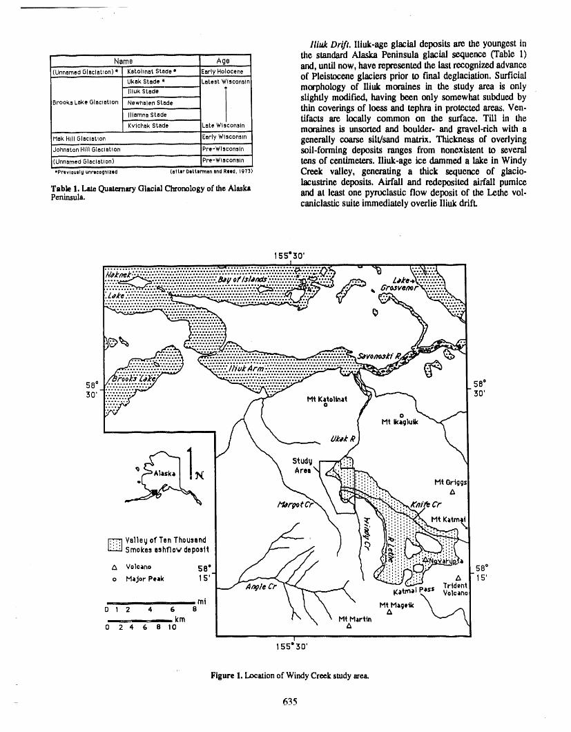
lli_ Drift. Iliuk-age glacial deposits are the youngest in..... the standard Alaska Peninsula glacial sequence (Table 1)

Name Age and, until now, have represented the last recognized advance-U'n_'amed G!actatlon)" Kat'ohnat Stade. Early Holocene of Pleistocene glaciers prior to final deglaciatton, SurfictalUkakStade' LatestWisconsin

--Illuk Stade ' morphology of Iliuk moraines in the study area is only- slightlymodified,having been only somewhat subdued byBrooksLakeGlaclatlonNewhalenStade

_- - thin coverings of loess and tephra in protected areas, Ven-IllamnaSta.de t_ac_ arc locally common on the surface. Till in the

KvlchekStade LateWisconsin moraines is unsorted and boulder- and gravel-rich with aMa'k'HillGlaciation Early Wisconsin generally coarse silt/sand matrix. Thickness of overlyingJohnstonHill81eclair'on...... Pre-Wisconsin soil.forming deposits ranges from nonexistent to several(Unnamed Glaclatlon} PM-Wisconsin tens of centimeters, lliuk-age ice dammeda lake in Windy*Pravl0uslgunrlcogmz.d (aft.r0.tt.rmanandR..d, 197_) Creek valley, generating a thick sequence of glacio-

lacustrine deposits. Airfall and redeposited airfall pumiceTable 1, Late Quaternary Glacial C'hronologyof the Alaska and at least one pyroclastic flow deposit of the Lethe vol-Peninsula. caniclastic suite immediately overlie Iliuk drift.

Wuk Arm ......................... _

58* 58*30' 30'

Ht Katoltnato

oMt Ikaglulk

Ukak

__ Study

Area

Ht Origg;A

_ YalleLjof TenThousandSmokesashflo',vdeposit

A Volcano 58" 58 °

o Major Peak 15' A 15

Angle Cr gatrnalpass TridentYoloano

-mJ Mt Magetk0 1 2 4 6 8 A,,, - km Mt Martin

0 24 6 810 A

155"30'

Figure 1. Location of Windy Creek study area.

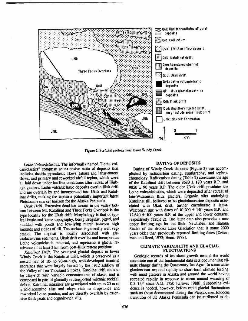
Fl_ure 2. SurficiWgeology ne_ lower WindyCre,ek.

Lethe Volcaniclastics. The informally named "Lethe vol- DATING OF DEPOSITScaniclastics" comprise an extensive suite of deposits that Dating of Windy Creek deposits (Figure 3) was accom-includes dacilJc pyroclastic flows, lahars and lahar-runout plished by radiocarbon dating, stratigraphy, and tephro-flows, and primary and rcworked airfaU tephra, which were chronology. Radiocarbon dating (Table 2) constrains the ageali laid down under ice-fmc conditions after retreat of Iliuk- of the Katolinat drift between 8680 + 170 years B.P. and

age glaciers. Lethe volcaniclastic deposits overlie Iliuk drift 9850 + 90 years B.P. The older Ukak drift postdates theand are overlain by and incorporated into Ukak and Katol- Lethe volcaniclastics, which were deposited after retreat ofinat drifts, making the tephra a potentially important latest late-Wisconsin Iliuk glaciers. Organic silts underlyingPleistocene marker horizon for the Alaska Peninsula. Katolinat till, believed to be glaciolacustrine deposits asso-

Ukak Dr_t. Extensive dead-ice terrain in the valley bor- ciated with Ukak drift, further corroborate a latest-tom between ML Katolinat and Three Forks Overlook is the Wisconsin age with dates of 10,200 + 140 years B.P. and

type locality for the Ukak drift. Morphology is that of typ- 12,640 + 100 years B.P. at the upper and lower contacts,ical ketfle-and-kame topography, being irregular, pitted, and respectively (Table 2). The latter date also provides a newstudded with ponds and low-lying marsh between high upper limiting age for the Iliuk, Newhalen, and Illamnamounds and ridgesof till. The surface is generally well veg- Statics of the Brooks Lake Glaciation that is some 2000etated. The deposit is locally associated with gla- years older than previously reported limiting dates [Detter-ciolacustrine sediments. Ukak drift overlies and incorporates man and Reed, 1973; Henn, 1978].Lethe volcaniclastic material, and represents a glacial re-advance of at least 3 km from post-lliuk retreat positions. CLIMATE VARIABILITY AND GLACIAL

Katolinat Dr_t. The youngest glacial deposit in lower FLUCTUATIONSWindy Creek is the Katolinat drift, which is preserved as a Geologic records of ice sheet growth around the worldnested pair of 10- to 20-m-high, well-developed terminal constitute one of the fundamental data sets documenting cii-moraines that were largely buried by the 1912 ashflow of mate change during the Quaternary Ice Ages. In some casesthe Valley of Ten Thousand Smokes. Katolinat drift tends to glaciers can respond rapidly to short-term climate forcing,be clay-rich with variable concentrations of clasts, and is with most glaciers in Alaska and around the world havingcomposed in part of glacially retransported volcanic rockfall retreated rapidly in response to mean annual warming ofdebris. Katolinat moraines are associated with up to 20 m of 0.5--1.0 ° since A.D. 1750 [Grove, 1988]. Supporting evi-

glaciolacustrine silts and clays rich in dropstones and dence is needed, however, before rapid glacial fluctuationsreworked Lethe pumice, and are directly overlain by exten- such as those documented during the Pleistocene/Holocenesive thick peats and organic-rich silts, transition of the Alaska Peninsula can be attributed to cli-

636

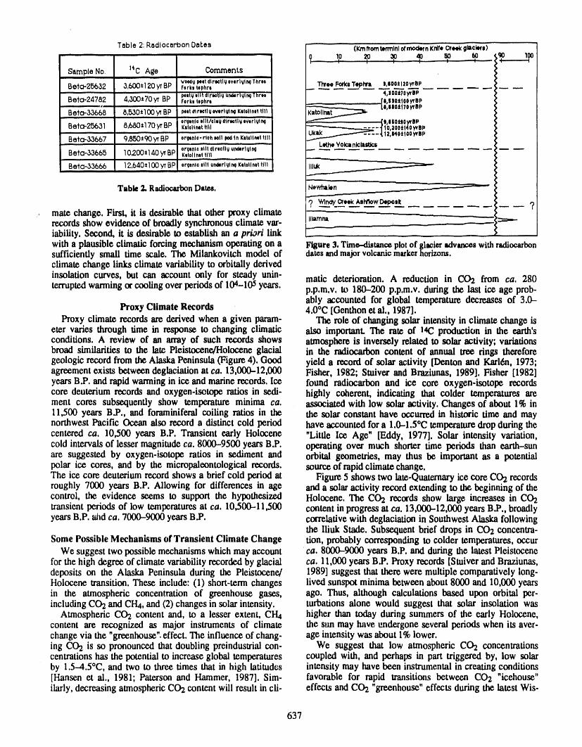
Table 2:Radiocarbon Dat.ea 10 (Kmltornlmmlnlotmod,fnKnlf,or_glac_=) .90 190.... 10 2o ,= ..-,'" ' I '"!.....

Secnp[e No. 14C A_e CommenLsilll

Vood¢p**tdir,=tl_ovorlvtNThree ThreeForksTephrl !,100:1:120yrBPBe?o-2F:_32 3,6OO_120yrBP fork,tophrl' ' p, sty =ll}("dlr_tl_ urvi4rl_tM Th'r'H 4,]00=70yrBP

Be_o.24782 4,300,70 _ BP Fork, (ephro [|,|$0*I00yrDP,' Lil,llO,lTOWBp

Betc_88668 8,580,"1O0yYBP _,,_r.tlu owrl_ x,toiln,t_111orgont©hilt/airydtrNtl_ovorlVtN .(|,OSO_OyrBPBeta-2563] 8,680:170yrBP Kt*01in=trill . -- -- "1'10,3001140YTBP

I_eto-33667 9,850,90yrBP er_tnlo-'HohNrl' 'pod|n KotollMttill J__- _ 12,1HO*IOOyrBPorgontoii'ltdlrodlqund,rlql_ LM.heYok_nl¢It=tJ¢#

Beta-33665 I0200,140yrBP x,t,l,,,t tm

Beia-33666 12,640=I00yrBP organicsilt und,rivInqKttoltnittill llluk ='--"

Table 2. RadiocarbonDates. [Newhal,n

,, mate change. First, it is desirable that otherproxy climaterecordsshow evidence of broadlysynchronousclimatevar- I I,=mn= _ _--lability. Second, it is desirableto establish an a priori link _-with a plausible climatic forcing mechanismoperatingon a Figure3. Time-distanceplotof glacier=dvlw.eswithradiocarbonsufficiently small time scale. The Milankovitch model of datesandmajorvolcanicrnarkerhorizons,climatechangelinks climatevariabilityto orb,tally derived

insolationcurves,but can accountonly for steadyunin- malic deterioration.A reduction in CO2 from ca. 280terruptedwarmingorcoolingoverperiodsof 104-105years, p.p.m.v,to 180-200p.p.m.v,duringthelastice ageprob-

ably accountedfor global temperaturedecreasesof 3.0-Proxy Climate Records 4.0°C [Genthonetal., 1987].

Proxy climate recordsare derived when a given param- The role of changing solar intensity in climate change iseter varies through time in response to changing climatic also important. The rate of 14(2production in the earth'sconditions.A review of an arrayof suchrecordsshows atmosphereis inverselyrelatedto solaractivity;variationsbroad similarities to the late Pleistocene/Holocene glacial in the radiwatrboncontent of annual tree rings thereforegeologic recordfrom the AlaskaPeninsula (Figure4). Good yield a record of solar activity [Denton and KarMn, 1973;agreement exists betweendeglaciationat ca. 13,000-12,000 Fisher, 1982; Stuiver and Braziunas, 1989]. Fisher [1982]yearsB.P. and rapidwarmingin ice and marinerecords. Ice found radiocarbon and ice core oxygen-isotope recordscore deuterium recordsandoxygen-isotoperatiosin sedi- highly coherent,indicatingthat colder temperaturesarement coressubsequentlyshow temperatureminima ca. associatedwith lowsolaractivity.Changesof about1% in11500 years B.P., and foraminiferal coiling ratios in the the solar constant have occurredinhistoric time and maynorthwest Pacific Ocean also record a distinct cold period have accounted fora 1.0-1.5°C temperaturedrop duringthecentered ca. 10,500 years B.P. Transient early Holocene "Little Ice Age" [Eddy, 1977]. Solar intensity variation,cold intervalsof lesser magnitude ca. 8000-9500 years B.P. operating over much shorter time periods than earth-sunare suggested by oxygen-isotope ratios in sediment and orbital geometries, may thus be important as a potentialpolar ice cores, and by the micropaleontological records, sourceof rapid climate change.The ice core deuteriumrecord shows a brief cold period at Figure5 shows two late-Quaternaryice core CO2 recordsroughly 7000 years B.P. Allowing for differences in age anda solaractivity recordextending to the beginning of thecontrol, the evidence seems to support the hypothesized Holocene. The CO2 records show large increases in CO2transientperiods of low temperaturesat ca. 10,500-11,500 content in progressat ca. 13,000-12,000 years B.P., broadlyyearsB.P. m_dca. 7000-9000 yearsB.P. correlativewith deglaciation in Southwest Alaska following

the lliuk Stade. Subsequent brief drops in CO2 concentra-Some Possible Mechanisms of Transient Climate Change tion, probablycorresponding to colder temperatures, occur

We suggest two possible mechanisms which may account ca. 8000-9(X)0 years B.P. and duringthe latest Pleistocenefor the high degree of climate variabilityrecordedby glacial ca. 11,000 yem_ B.P. Proxy records[Stuiver andBraziunas,deposits on the Alaska Peninsula during the Pleistocene/ 1989] suggest that themwere multiple comparatively long-Holocene trans,Lion.These include: (1) short-term changes lived sunspot minima between about8000 and 10.000 yearsin the atmospheric concentration of greenhouse gases, ago. Thus, although calculations based upon orbital per-includingCO2 and CH4,and (2) changes in solar intensity, turbations alone would suggest that solar insolation was

Atmospheric CO2 content and, to a lesser extent, CI-14 higher than today during summers of the early Holocene,content are recognized as major instruments of climate the sun may have undergone several periods when its aver-change via the "greenhouse".effect. The influence of chang- age intensity was about 1% lower.ing CO2 is so pronounced that doubling preindustrial con- We suggest that low atmospheric CO2 concentrationscentrations has the potential to increase global temperatures coupled with, and perhaps in part triggered by, low solarby 1.5-4.5°C, and two to three times that in high latitudes intensity may have been instrumental in creating conditions[Hansen et al., 1981; Paterson and Hammer, 1987]. Sim- favorable for rapid transitions between CO2 "icehouse"ilarly, decreasing atmospheric CO2 content will result in cii- effects and CO2 "greenhouse" effects during the latest Wis-

637

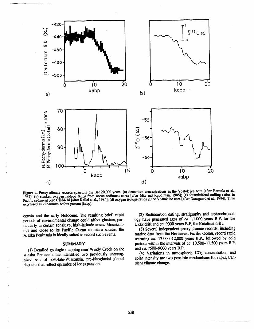
i ii --

1

' _I0 0-440

E -460

t_ -480

_' -50(

0 10 20 0 1'0 2O

a) kabp b) kabp

._ 70 .O

E -52.

O -56"EI _ o• ro -

u o -60"EL CS.

:_ 100 ....... I0 5 0 I'(3 20

kabp kabpc) d)

Figure 4. Proxy climate records_m_tng_the lut 20,000.years:(a) d_u.t_riumeoneenyatiqmin th.e.Vos._k,te_e?reotd_ B__no!a_.et_._,1987); (b) stacked oxygen isotope ratios from ocean s_iment cores I.alterMtx _?o Kueamam},' *')¢3J; tcJ z____'n__!%m_.c_mn_oS_,_lPacific sedimentcoreCHM-14 [afterKallel et al., 1984];(d) oxygenssOtOl_rauosmme vostog teecoret_t_r umasg_tru_aai., z_,_], t,,,_expressedaskilo_mum beforepresent(ka_).

consin and the early Holocene. The resulting brief, rapid (2) Radiocarbon dating, stratigraphy and tephrochronol-

periods of environmental change could affect glaciers, par- olD, have generated ages of ca. 11,000 years B.P. for theticularly in certain sensitive, high.latitude areas. Mountain- Ukak drift and ca. 9000 years B.P. for Katolinat drift.ous and close to its Pacific Ocean moisture source, the (3) Several independent proxy climate records, including

Alaska Peninsula is ideally suited to record such events, marine data from the Northwest Pacific Ocean, record rapidwarming ca. 13,000-12,000 years B.P., followed by cold

SUMMARY periods within the intervals of ca, 10,500-11,500 years B.P,

(1) Detailed geologic mapping near Windy Creek on the and ca. 7500-9000 yeats B.P.Alaska Peninsula has identified two previously unrecog- (4) Variations in atmospheric C02 concentration and

nized sets of post-late-Wisconsin, pre-Neoglacial glacial solar intensity are two possible mechanisms for rapid, tran-deposits that reflect episodes of ice expansion, sient climate change.

638

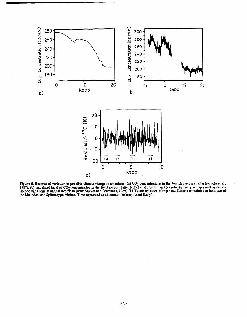
, i i i i _ ii1,,i i ii ii iiiii

> 280_ _ 300--260 e 280

= o= 280o 240- =

_ 240•,-, 2201,..(_ • 220

o o= 200 =0 0

_ 200

N 180 N 180OCD

(..I "' '"'" (.J " ' " i"' '" "'

0 10 20 5 i O 15 20

a) kabp b) k_bp

i iii i i

20

-10_2o.lT -

I ' ' "_ ' '1 ' '

0 5 10

c) kabp

Figure $. Recordsof variationin possible climatechsnge mechanisms: (i) CO_ concentrations in tha Vostok ice coze [afterBarnola el al,,1987); (b) calculamdbandof CO2concentrationin the Byrd ice core [afterNeftel et al,, 1988]; snd (c) soi_ intemity m express_ by carbonisotope variations in mmual tree rings [afterStuiver andBraziunas, 1989], TI-T4 are episodes of tripleoscillations containingat least two oltheMaunder-endSp6rer.typeminima.Time expressedas klloennumbefore prcsent(kabp),

639

REFERENCES CITED

Bamola, J, M,, D, Raynaud, Y, $, Korotkevich,and C, Henn,W,) ArtSae.ologyon tile Alaska Penlnst)la:Tile Ugu-Lorius, VoStok lee core provides 160,000.year re,c_rd of shlk drainage, 1973-1975, University of Oregon Anthro.atmospheric CO2,Nature, 329, 408-414, 1987, pological Papers, 14, 183 pp,, 1978,

Dansgaard, W,, S, J, Johnson, H, B, Clauson, D, Dahl. Kallol, N,, L, D, Laboyrle, M, Arnold, H, Okada, W, C,Jonson,N, Oundostrup,and C, U, H_unmer,North Arian- Dudley, and J,.C, Duplossy, Evidence of cooling duringtic climatic oscillations reveaded by deep Greenland lee the Yotmgor Dryas in the western North Paoiflc, Ocea.cores, inAGU Monograph 29, extltedby J, E, Hansonand ngl, Acta, 1I, 369-375, 1988,T, Takahaskl, pp, 288-298, 1984, Mix, A, C,, and W, F, Ruddilnan, Sttuctw'0 and timing of

Denton, G, H,, and W, Karl6n, Holocene climatic varLa, the last doglaclation:oxygen.isotope evldt_n_, Quat, Sol,tions--thotr pattea'nand possible cause, Quat, Res,, 3, Rev,, 4, 59-108, 1985,155-205, 1973, Muller, E, H,,Glacial history of tht_Naknek District, Alaska

Dettonnan, R, L,, Glaciation of the Alaska Peninsula, tn Peninsula, Alaska (abs), Geol, Soc, Am, Bull,, 63, 12_,Glaciation in Alaska: The Geologic Record, edited by 1952,T, D, Hanlllton, K, M, Reed, and R, M, Thorson, pp, MuUor,E, H,, NorthernAlaska Peninsula and eastern Ktl.151-170, AlaskaGeol, Soc,, 1986, buk Mountains, Alaska, United States Geol, Surv, Circ,,

Dettorman, R, L,, and B, L, Reed, Surflclal _poslts of the 289, 2-3, 1953,Iltamna qtmdrangle, Alaska; United States Geol, Surv. Muller, E, H., W, Juhle, and H, W, Coulter, Current vgl.Bull, 1368-A, 64 pp,, 1973, canto activity in Katmal National Monument, Science,

Eddy, J, A,, Cllmalz and [he changing sun, Climatic I19,310-321, 1954,Cl_ange,1,173-190, 1977, Neftel, A,, H, Oeschger, T, Staffelbach, and B, Stauffer,

Fisher, D, A,, Carbon.14 productioncompared to oxygen CO-zrecordin tlmByrd lee com 50,000-5,000 years B,P,,isotope records from Camp Century, Greenland and Nature, 331,609-.611, 1988,Devon Island, Canada, Climatic Change, 4, 419-.426, Pearson, W,, and C, Hammer,Ice core and otherglaclolog-1982, ical data, in North America and Adjacent Oceans During

Genthon, C,, J, M, Barnola, D, Raynaud, C, Lorius, J, the LastDeglactation, The Geology ofNorthAmerica, K.Jouzel, N. I, Barker, Y. S, Koroti_vtch, and V, M, Kot- 3, edited by W, Ruddlman,and H, Wright, pp, 91-109,lyakov, Vostok ie_ core: Climatic response to CO2 and Geol, Soc. America, Boulder, CO, 1987,orbital forcing over the last climatic cycle, Nature, 329, P6w6, T. L., Quaternary geology of Alaska, United States414--418, 1987. Geol. Surv. Prof Paper835, 145 pp,, 1975.

Grove, J, M., The Little Ice Age, 498 pp,, Methuen Pub,, Stulver, M,, and T, F, Brazttmas, Atmospheric 14C andLondon, 1988, century-scale solar oscillations, Nature, 338, 405--408,

Hansen, J,, D, Johnson, A. Lacts, S. Lebedeff, P, Leo, D, 1989,Rind, and G, Russell, Climate impact of increasingatmospheric carbon dioxide, Science, 213, 957-966,1981,

640

An Algorithm of Approximate Paleotemperature Calculation of the Earth Surfaceby Temperature Measurements in Deep Boreholes

N. A. Baranova and S. F. KhroutskyDepartmentof Geocryology,GeologicalFaculty,MoscowUniversity,Moscow,U,S,S.R,

ABSTRACT

The proposed algorithm of paleotemperature calculation is an independentanalytical method of global climatic change in the Upper Pleistocene and Holocene.It is based on construction of determined and non-determined heat exchangemodels in rocks, i,e,, a system approach to the problem.

The determined model of the process is expressed by a mixed marginal problemfor the heat conductivity equation. Unknown paleotemperatures of the earth surfaceas piecemeal-continuous time functions are determined in order to reach theconclusion of a mixed marginal problem of paleotemperature close (in the sense ofminimum mean quadratic errors) to modern temperature profiles in deep boreholes.The temperature algorithm is also used to calculate geothermal gradients and the

time homogeneity intervals of these quantities. Input data are the heat physicalparameters of rocks and the number of discontinuity points of sought-for functions.

A numerical experiment was carried out for a period of about 20,000 yearsaccordt:ng to real temperature measurements in deep boreholes for a 400-m-thickstratum, As a result, eight "steps" of the group-average of marginal temperature andgeothermal gradient were restored. The algorithm is presented as a FORTRAN-IVlanguage program, The transformation of two measured masses into one measuredmass is the key feature of the program,

641

Arctic Environments and Global Change:Evidence in Deep Permafrost Temperatures, Canadian Arctic Archipelago

Alan TaylorTerrainSciencesDivision,GeologicalSurveyof Canada,Ottawa,Ontario,Canada

ABSTRACT

In considering the role of the polar regions in future global change, one maylook toward these regions for evidence of past environmental change. Deep groundtemperatures provide one window on past surface temperatures, which may beinterpreted in terms not only of past climate but also of past environmentalconditions.

Across the Canadian Arctic Archipelago, there is no consistent curvature in deepground temperature profiles that can be modeled in terms of warty,ing of the pastcentury. This contrasts with the result reported by Lachenbruch et al. [1986] for thePrudhoe Bay area of Alaska and may be a consequence of the much larger regionand wider well spacing considered in the Canadian case. Any curvature present var-ies from well to well and may be interpreted in terms of surface temperaturechanges of the order of 1-3 K on the scale of decades to centuries.

However, there is some evidence that these surface temperature histories mayarise from long-term changes in paleoenvironmental factors as well as climate. Forinstance, the paleocl_matederived from oxygen isotope data at the Agassiz Ice Caphas been compared with the geothermal signature at a well some 180 km to thewest. For the Little Ice Age (LIA), the Agassiz paleoclimate explains only half themeasured variation in ground temperatures at the geothermal site; the remainingvariation may be due to other environmental effects, such as an increase in snowcover following the LIA. This is consistent with extrapolated surface temperatures7 K higher than other Arctic sites and the unusually deep snow cover observedtoday.

642

Glacial Marine Sediments from the Antarctic Peninsula:

A Record of Climate Change and Glacial Fluctuations During the Late Holocene

E. W. Domack and L. BurkleyGeologyDepartment,HamiltonCollege,Clinton,New York, U.S.A.

ABSTRACT

Present climate conditions along the western side of the Antarctic Peninsula varyfrom subpolar, in the north, to polar in the south. Thus, the region provides an idealsetting in which to study the relationship between climate and glacial marineprocesses in Antarctica. Physical oceanographic measurements (211 CTDT casts)and bottom sediment samples (>104) provide the data base for the followingconclusions. Subpolar glacial regimes in the South Shedand Islands are dominatedby extensive surface melting, elevated equilibriur,_ lines (EL,A) and efficientconduction of surface meltwater to the terminus of tidewater and terrestrial glaciers.These conditions control sedimentary processes in the marine maim by the efficientand widespread dispersal of suspended sediment by overflow plumes. Terrigenousfacies, therefore, dominate throughout the 0ord system.

The transition to polar conditions within glaciers along the Danco Coast andPalmer Archipelago is characterized by lower ELA (near sea level), limited surfacemelting and dynamic sea ice conditions. Basal melt processes appear to dominate,especially where subglacial marine ca,.,ities exist beneath glacial termini. Mostterrigenous sediment is transported by ice-r',ffting or by cold, mid-water plumes,which spread horizontally until restricted by bathymetric features. Biogenic (dia-tom) muds and ice-rafted debris dominate sedimentation in outer bay settings; theformer is enhanced by warmer temperatures, increased sunlight, and minimal dis-turbance of surface layers within the fjords.

These facies transitions are well constrained statistically by regression analyseso_ textural and compositional variations with respect to distance from sedimentsources (glacial termini). Correlation trends within individual ice drainage systems

can be applied to marine sediment core,s which contain a record spanningapproximately the last 3000 years (based upon accelerator 14C _:ld 210Pbchronologies). A period of enhanced terrigenous (surface meltwater) input follow-ing more extensive glacier ice is documented in Hughes Bay on the northern DancoCoast. By analogy with modern conditions it is presumed that mean summertemperatures around 700 to 1000 years B.P. were at least 2°C wanner than atpresent. A number of depositional cycles are recognized from fjords further southbut these require additional study before interpretations are forthcoming.

643

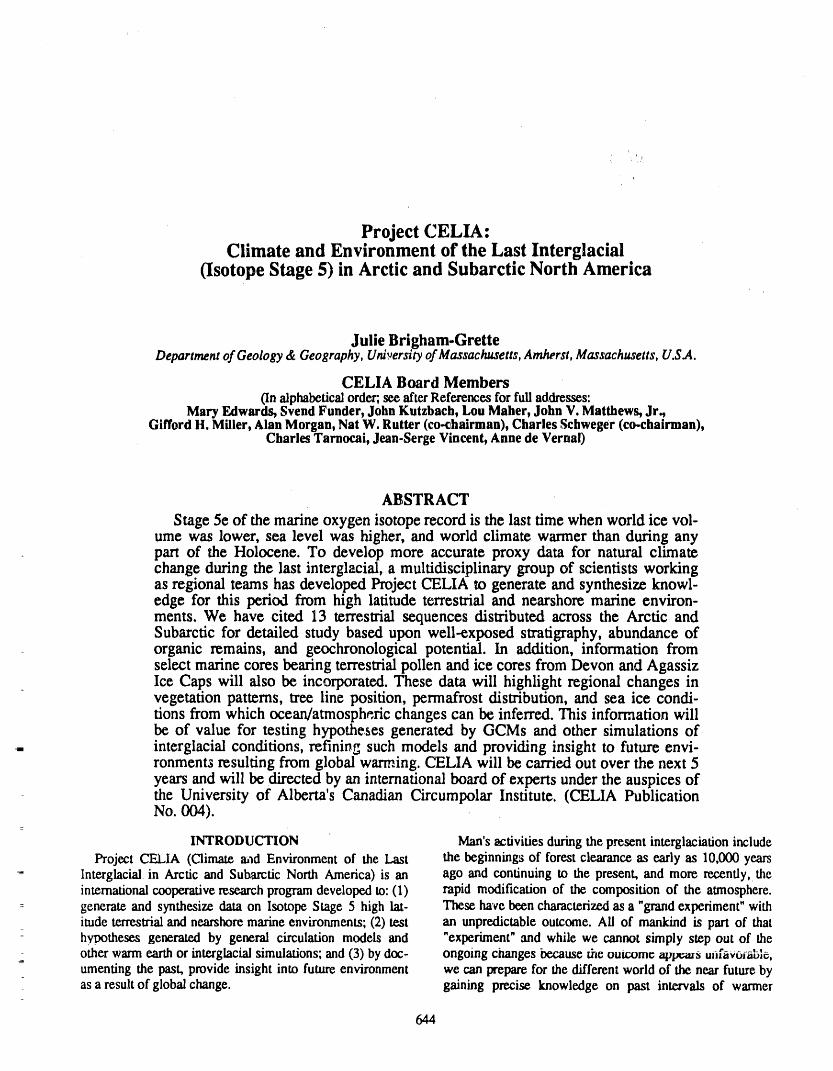
i

b

Project CELIA:Climate and Environment of the Last Interglacial

(Isotope Stage 5) in Arctic and Subarctic North America

Julic Brigham.GretteDepartmentof Geology& Geography,UniversityofMassachusetts,Amherst,Massachusetts,U.S.A.

CELIA Board Members(Inalphabeticalorder;seeafterReferencesforfulladdresses:

MaryEdwards,SvendFunder9JohnKutzbach,LouMaher,JohnV.Matthews,Jr.,GiffordH. Miller,AlanMorgan,NatW. Rutter(co-chairman),CharlesSchweger(co-chairman),

CharlesTarnocai,Jean-SergeVincent,Annede Vernal)

ABSTRACT

Stage 5e of the marine oxygen isotope record is the last time when world ice vol-ume was lower, sea level was higher, and world climate warmer than during anypart of the Holocene. To develop more accurate proxy data for natural climatechange during the last interglacial, a multidisciplinary group of scientists workingas regional teams has developed Project CELIA to generate and synthesize knowl-edge for this period from high latitude terrestrial and nearshore marine environ-ments. We have cited 13 terrestrial sequences distributed across the Arctic andSubarctic for detailed study based upon well-exposed stratigraphy, abundance oforganic remains, and geochronological potential. In addition, information fromselect marine cores bearing terrestrial pollen and ice cores from Devon and AgassizIce Caps will also be incorporated. These data will highlight regional changes invegetation patterns, tree line position, permafrost distribution, and sea ice condi-tions from which ocearffatmosphcric changes can be inferred. This information willbe of value for testing hypotheses generated by GCMs and other simulations of

. interglacial conditions, refining such models and providing insight to future envi-ronments resulting from global warming. CELIA will be carried out over the next 5years and will be directed by an international board of experts under the auspices ofthe University of Alberta's Canadian Circumpolar Institute. (CELIA PublicationNo. 004).

INTRODUCTION Man'sactivitiesduringthepresentinterglaciationincludeProjectCELIA (Climateand Environmentof the Last the beginningsof forestclearanceas earlyas 10,000years

-- Interglacialin Arcticand SubarcticNorth America)is an ago and continuingto the present,and more re,c,enfly, theinternationalcooperativeresearchprogramdevelopedto:(I) rapidmodificationofthecompositionoftheatmosphere.

: generate and synthesizedata on IsotopeStage 5 high lat- Thesehavebeencharacterizedas a "grandexperiment"withitude terrestrialand nearshoremarineenvironments;(2) test an unpredictableoutcome.Ali of mankind is part of thathypotheses generated by general circulationmodels and "experiment"and while we cannot simply step out of theotherwarmearthor interglacialsimulations;and(3)by doc- ongoingchangesbecausethe outcomeapw.msum'avorable,umentingthe past, provideinsight into futureenvironment we can preparefor the differentworldof the near futurebyas a resultof globalchange, gaining precise knowledge on past intervals of warmer

644

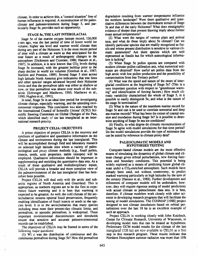
climate. In order to achieve this, a "controlsituation"free of degradation resulting from warmer temperatures influencehuman influences is required. A reconstruction of the paleo- the northern landscape? Were there qualitative and quan-climate and paleoenvironment during Stage 5, and par- titative differences between the thermokarst terrain of Stageticularly Stage 5e, provides such an opportunity. 5e and that of the early Holocene? What does stratigraphic

evidence of deeper than present thawing imply about formerSTAGE _, THE LAST INTERGLACIAL mean annual temperatures?

3tage 5e of the marine oxygen isotope record, 126,000 (2) What were the ranges of various plant and animalyt.ars ago, was the last period of time of lower world ice taxa, and what do these imply about 5e climate? Can wevolume, higher sea level and wanner world climate than identify particular species that are readily recognized as fos-during any part of the Holocene. lt is the most recent period sils and whose present distribution is sensitive to various eli-of time with a climate as warm as that anticipated for the malic parameters? Are there species which are wellnem" future as a result of anthropogenic changes to the represented as fossils but for which autecological informa-atmosphere [Dickinson and Cicerone, 1986; Hansen et al., tion is lacking?1987]. In addition, it is now known that CO2 levels during (3) When Stage 5e pollen spectra are compared withStage 5e increased, with the greatest buildup prior to the modem climate--pollen calibration sets, what numerical esti-sharp decline in world ice volumes [Genthon et al., 1987; mates are obtained? How useful are pollen data from theBartlein and Prentice, 1989]. Several Stage 5 sites across high arctic with low pollen productionand the possibility ofhigh latitude North America give indications that tree lines contamination from late Tertiary pollen?and other species' ranges advanced beyond their Holocene (4) What was the speed and nature of the onset of inter-limits and that the permafrost table was either as shallow as glacial conditions at the beginning of Stage 5e? (This is anow, or that permafrost was absent over much of the sub- very important question with respectto "greenhouse warm-arctic [Schweger and Matthews, 1985; Matthews et al., ing" and identification of forcing factors.) How much eli-1990; Hughes et al., 1991]. malic variability characterized the whole of Stage 5, is it

In total, Stage 5e is an ideal time period for investigating possible to easily distinguish 5e, and what is the nature ofclimate change, especially warming, and the attending envi- the stage 5e termination?ronmental responses. This conclusion w_s also re.ached by (5) What is the nature of the nearshore marine record forthe International Council of Scientific Unions' (ICSU) Sci- Stage 5e and can it be used to correlate terrestrial and deepentitle Steering Committee on Global Changes of the Past, seamarine records? What has been the extent of coastal ero-which identified study of the last interglacial as an inter- sion and inundation during Stage 5e? Is it possible to deter-national research prio_i_yo mine anything of Stage 5e sea ice conditions?

(6) Finally, to what degree do Climaticreconstructions ofPROJECT CELIA: OBJECTIVES Stage 5e agree with model simulations for that time period?

A prime objective of project CELIA is the recovery and Do the model simulations provide the type of estimates thatsynthesis of qualitative and quantitative information on the can be tested by reference to climate proxy data?climate and environment during the last interglacial. Thiswill be accomplished through field and laboratory research PALEOCLIMATIC MODELS ANDon selected high latitude sites where a variety of paleo- HYPOTHESES TESTINGecological and prt_xy climate methods (e.g., fossil pollen, Computer-based climate models are the most effectiveinsects, seeds, soils properties, stable isotopes) will be means of simulating the dynamics of global climate and cii-employed. Qualitative information should be important in mate change given orbital perturbations, new forcing rune-supplementing and enriching the quantitative data sets. As a tions and boundar.¢ conditions. This potential is beingresult of these qualitative and multidisciplinary inputs, widely explored as a means of predicting future global cii-CELIA will provide a broader and more complete view of mate under a CO2-enriched atmosphere. Such models havethe paleoenvironment of the last interglacial than has here- already been used, not without controversy, to predicttofore been possible, marked warming particularly at high latitudes by the turn of

Project CELIA will deal only wiLh the arctic and sub- the century [Hansen et al., 1988]. Further development andarctic regions of North America and Greenland. This is refinement of computer models will be undertaken; how-appropriate, as northern regions are to be the first to expe- ever, they will require rigorous testing of model predictionsrience futare warming and it is here that warming is with actual climate or paleoclimatic data sets. lt is best,expected to be greatest. As weil, the cold climate of the arc- therefore, if climate modelers work closely with other sci-tic/subarctic ensures optimal fossil preservation, frequently entist in developing research programs that will facilitate theenabling identification of fossil insects or seeds to the spe- testing of model simulations. The COHMAP [1988] projectcies level, lt is in the arctic/subarctic that many species designed to test climate simulations based on orbital per-including trees meet their present-day climatic limits, and turl_ations over the last 18 ka is an excellent example ofpermafrost, or sporadic permafrost, is widespread. These such an approach.important environmental discontinuities and thresholds Project CELIA is working closely with John Kutz,bach,ensure that sensitive and accurate paleoenvironmental Center for CIL,natic Research, University of Wisconsin, inrecords can be established, developing model runs that can be treated as hypotheses.

The objectives of CELIA may be framed in terms of the Preliminary GCM model results for the climate of the last

(1) WL Ltwas the distribution of continuous and dis- step in this research program. These results indicate thatcontinuous permafrost during Stage 5e? How did permafrost Northern Hemisphere summer radiation was more than 10%

645

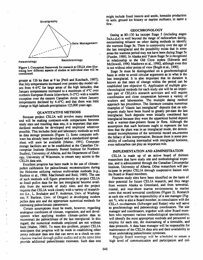
mightincludefossil insectsandseeds,hematiteproductionStratigraphy in soils,groundicehistoryor marinemolluscs,to namea

few.GEOCHRONOLOGY

Dating at 80-130 ka isotope Stage 5 (including stages5a,b,c,d,e) is well beyond the range of radiocarbon dating,

Data Management necessitatingrelianceon other datingmethodsto identifythe warmest Stage 5e. There is controversy over the age ofthe last interglacial and the possibility exists that in someareas the warmest period may not have been during Stage 5e[Funder, 1989]. In Alaska and Yukon Stage 5e is recognized

Paleontology Geochronology in relationship to the Old Crow tephra [E,dwards andMcDowell,1990;Matthewset al., 1990],althougheventhis

Figure1.ConceptualframeworkforresearchatCELIAsites illus- is notwithout other points of view [Begdt ct al., 1990].trating howdifferentaspectsof studiesat individualsite.swill be Stage 5e must be distinguished on a geochronologicalcoordinated, basisin order to avoid circular argumentsas to what is the

greater at 126 lm than at 9 lm [Prell and Kutzbach, 1987]; last interglacial, lt is also important that its duration isthat July temperatures increased over present-day model val- known so that rates of change within the period can beues from 4-6"12 for large areas of the high latitudes; that established (see objective 4). Application of multiple geo-January temperatures increased to a maximum of 40C over chronological methods for each study site will be an impor-northern European Russia (elsewhere, 0--2"C)with a notable rant part of CELIA's research activities and will requireexception over the eastern Canadian Arctic where January coordination and close cooperation between a variety oftemperatures declined by 4--6*(2; and that there was little workers and laboratories. The multiple dating methodchange in high latitude precipitation 125,000 years ago. approach has precedence. The literature contains numerous

examples of "classic last interglacial" deposits that on sub-

QUANTITATIVE METHODS sequent study have been found to greatly pre-date the last

Because project CELIA will involve many researchers interglacial. Such deposits were initially considered lastand will be making continent-wide comparisons between interglacialbecause they were the uppermost buried depositstudy sites and resulting data sets, it is importantthat start- with a warmer-than-presentfauna or flora. Although thedardized methods be developed at_d employed wherever assumption that such horizons ought to represent the lastpossible. This includes field and laboratorymethods as well time that the plant was in an interglacial mode, the demon-as data storage protocols (Figure 1). Some computer soft- strated incompleteness of the terrestrial record unherscoresware has already been developed and a standardized spread- the fallacy of this interpretation. Because there is some pos-sheet will soon be available [Maher, 1991]. Computer sibility of confusing interstadial with interglacial horizons,storage facilities are to be established at the Canadian Cir- even radiocarbon can play an important role.cumpolar Institute (formerly Boreal Institute for NorthernStudies), Universityof Alberta,and the Departmentof Geol- IMPLEMENTATION AND ADMINISTRATIONogy, University of Wisconsin, to ensure easy access to the CELIA is made up of an active board of thirteenCELIAdata sets. researchers that have study site and methodological exper-

Excellent progress has been made in the 'useof climate,- tise, and is administered through the Canadian Circumpolarpollen calibration for paleoclimatic reconstructions during Institute, University of Alberta. Other researchers will par-the Holocene utilizing various multivariate methods [e.g., ticipate in project CELIA through cooperative liaison withBartlein ct al., 1986; MacDonald and Reid, 1989]. The use the Board or Board members.of such methods will figure prominently in project CELIA Fourteen study sites have been identified on the basis ofas fossil polle,n data for the last interglacial become avail- their potential for future CELIA research, and they rangeable from the network of study sites; and the project from western Alaska to Greenland, and from terrestrial,requires that CELIA work closely with a variety of research- coastal, and near-shore marine environments to marineers (i.e., L. Brubaker and P. Anderson, Univ. of Washing- cores that record terrestrial conditions (Figure 2). Researchton; P. Bartlein, Univ. of Oregon) in developing modern at each site will be the responsibility of a site manager (Fig-pollen data sets and the appropriate numerical methods for ure 3), who is also a Board member, in consultation with theestimating paleoclimatic parameters. CELIA co-chairmen (Schweger and Rutter) who will serve

- Certain assumptions must be made, however, regarding as geochronology and paleoecology coordinators. The siteanalogous conditions of climate, vegetation, and soil devel- manager and coordinators, together with other Board mem-

-- opment when spplying modern climate--pollen data to bers who represent various methodological specializations,reconstruct the paleoclirnate of the last interglacial. In this will identify the most appropriate methods and personnel toregard, the numerical methods employed are not without employ for each site, the maintaining of a timetable, andfault [Maher, 1989]. To meet this problem, project CELIA data protocols. A data base manager will be responsible foranticipates that progress will be made in establishing other maintenance of the CELIA data sets and their availability toproxy indicator data sets that can serve as a check on con- those undertaking paleoclimatic syntheses.ulusiuII_ ..... L-J .L ..... t-.--_t! ...... ,4: .... A n* th,_ ,',,'_,_n,= _'*,_,,, Dtan,,lar l:lrmrrl rn_,otino¢ will hP. e._.hPa'hlle.d tO a.q.qure, allF_di/_ilr..4.1 IIilIUU_ll I.A-III I_li _l.l_ I.MI_ at, MIV L_.alllV I_ V "_*0" 'Ct" ................

provide additional paleoclimatic estimates. Such data sets high level of communication and participation and col-

646

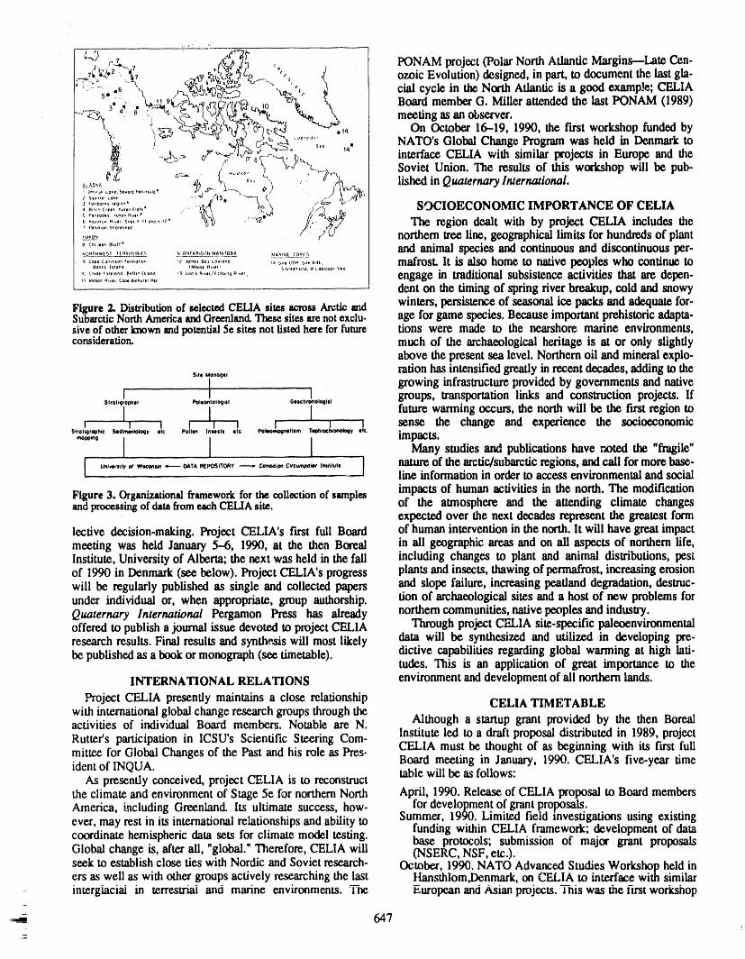
i • ' cr''

[ ,--.7 :.7 <_"_" PONAM project (Polar North Atlantic Margin_--Late Cen-j._ _. , 17 ,,,_,_._J _.:- l _ ozoic Evolution) designed, in part.to document the last gla-[ - ,, .6 \ :_'_,_._ _ .,. _ cial cycle in the North Atlantic is a good example; CELIA/ _ : 4" • _-_9__'_('_,, _o _ _ Board member G. Miller attended the last PONAM (1989)I-.-_ .C,_, ' ' O ; '% ":-_ _1 '_ I. _ ".-. _'l_e. "%._ ',.

I L ', _",, ,4 On October16-19, 1990, the first workshop funded by\,_ - _ _ ,, _ .... NATO's Global Change Programwas held in Denmarktop_ ,..___;>_ _,.-eb"0c--:--._,¢. interfaceCELIA withsimilarprojectsinEuropeandthe_'_, , / \ _:_"'"L. Soviet Union. The results of this workshop will be pub-

_,,.,"'" v. _ ,o, '. :....:_ fishedinQuaternaryInternational,

o_...._..........,,o,,. ,. _,k_, --;_ ::_ _. SOCIOECONOMIC IMPORTANCE OFCELIAo...... .. ,_.' ..... ,...... i2._" :/"<'L_:_")_ol_.u. ,+ ,.* t_ . _, - .. /

.........._.......... %'_ ://../(;, The regiondealtwithby projectCELIA includesthe,u,o, < ::-- northerntree line, geographicallimits for hundredsof plant"_......_'°"" and animal species and continuous and discontinuous per-NO.t___,wr.s._ t_Li",__2._o_s, P.tO__t_._._"l_O./_.____ll_QJ).__ u_,_t co,ts

,,,............................. ,................... ,....... mafmst, lt is alsohome to native peoples who continue toOon_l l$10ed (U00)lft,vie' SGtel_IO'_O,W tobeado,See

..................,.....,......,.........:............. engageintraditionalsubsistenceactivitiesthataredepen-iq t.lol0_, I:l,_t,. Cool Bolnutt) Pin

denton the timing of springriverbreakup,coldandsnowy

Figure2.DistributionofselectedCELIAsitesacrossArcticand winters,persistenceofseasonalicepacksandadequatefor-SubarcticNorthAmericaandGreenland.Thesesitesarenotexclu- ageforgamespecies.Becauseimportantprehistoricadapta.siveofotherknownandpotential5esitesnotlistedhereforfuture lionsweremade tothenearshommarineenvironments,consideration, much ofthearchaeologicalheritageisatoronlyslightly

abovethepresentsealevel.Northernoilandmineralexplo-rationhasintensifiedgreatlyinrecentdecades,addingtothe

Sill ionOOlt

growing infrastructureprovided by governments and nativei i groups, transportation links and construction projects. If

Sl¢ollg¢ilphlt POIIO_IOIoQIII OtOChrO_OlO_lll

I I I future wanning occurs, the north will be the first region to) v"' i _ l .L _I ,,,. i .L sense the change and experience the socioeconomic

giioilmohl S*dlm_k_l, ,i¢. Po, lm ,o.¢,, _._..,m,, impacts.m°pOinO I

Many studies and publications have noted the "fragile"

I ,,,,..,.,_,.._..,,..-- _r__,ro_, --- c_,_ c,,.._., ,.,,,.,. ] nature of the arctic/subarcticregions, andcall formorebase-line informationin order to access environmentaland social

Figure 3. Organizational framework for the collection of samples impacts of human activities in the north.The modificationandprocessingofdatafi'omeachCELIA site. of the atmosphere and the attendingclimate changes

expectedoverthenextdecadesrepresentthegreatestformlectivedecision-making.ProjectCELIA'sfirstfullBoard ofhumaninterventioninthenorth,ltwillhavegreatimpact,meetingwas heldJanuary5-6,1990,atthethenBoreal inallgeographicareasandon allaspectsofnonherolife,Institute,UniversityofAlberta;thenextwasheldinthefall includingchangestoplantand animaldistributions,pestof1990inDenmark(seebelow).ProjectCELIA'sprogress plantsandinsects,thawingofpermafrost,increasingerosionwillbe regularlypublishedas singleandcollectedpapers andslopefailure,increasingpeatlanddegradation,destmc-underindividualor,when appropriate,groupauthorship, lionofarchaeologicalsitesanda hostofnew problemsforQuaternaryInternationalPergamon Presshas already northerncommunities,nativepeoplesandindustry.offeredtopublishajournalissuedevotedtoprojectCELIA ThroughprojectCELIA site-specificpaleoenvironmentalresearchresults. Final results and synthesis will most likely data will be synthesized and utilized ,in developing Ixe-be publishedas a book or monograph(see timetable), dictive capabilities regarding global warming at high lati-

tudes. This is an application of great importance to theINTERNATIONAL RELATIONS environmentand developmentof ali northernlands.

Project CELIA presently maintains a close relationship CELIA TIMETABLEwith internationalglobalchange researchgroups throughtheactivities of individual Board members. Notable are N. Although a startup grant provided by the then Bore.alRutter's participation in ICSU's Scientific Steering Com- Institute led to a draft proposal distributed in 1989, projectmittee for Global Changes of the Past and his role as Pres- CELIA must be thought of as beginning with its rh'Stfull

Boardmee_g in January, 1990. CELIA's five-year timeidentof INQUA. table will be asfollows:

As presendy conceived, project CELIA is to reconstructthe climate and environment of Stage 5e for northernNorth April, 1990. Release of CELIA proposal to Board membersAmerica, _ncludingGreenland. Its ultimate success, how- for developmentof grantproposals.ever, may rest in its international relationships and ability to Summer, 1990. Limited field investigations using existing

funding within CELIA framework; development of datacoordinate hemispheric data sets for climate model testing, base protocols; submission of major grant proposalsGlobal change is, after all, "global." Therefore, CELIA will (NSERC, NSF, etc.).seek to establish close ties with Nordic and Soviet research- October, 1990. NATO Advanced Studies Workshop held iners as well as with other groups actively researching the last Hansthlom,Denmark, on CELIA to interface with similarinterglaciai in terrestrial and marine environments. I--he European and Asian projects. This was the first workshop

-

647

to be funded under NATO's new Global Change researchersto begin process of synthesisand testing.initiative. Winter, 1992/1993. Laboratory research and synthesis of

April, 1991. Release of database protocols',planning for results.summerfield workat designatedCELIAsites. Summer, 1993. Limited field work, otherwise laboratory

Summer, 1991. Field and laboratoryresearch;CELIA par- researchand synthesis of results.ticipationat INQUA meetings. November, 1993. CELIA Board meeting to begin final syn-

November, 1991, CELLAr Board meeting to report on thesisand preparationforpublication-f final results,progressandresults and publications. Winter, 1993/1994. Final laboratory resultsand completion

Winter, 1991/1992. Laborato_ research,planning for sum- of final synthesis,mea"fieldwork andpublicationofresults, June, 1994. Final CELIA Board meeting to edit final

Summer,1992. Field and laboratoryrese,u_)!. paleoclimate publication.November, 1992. CELIA Board rt#..,,,_'_,gji¢_th' i :'/ REFERENCES

Bartlein, P. J., and I. C. Prentice, 0tbi_ variations, climate, Dimensional Model, J. Geophys. Res, 93, 9341-9364,and paleoecology, Trends in Ecology (TREE), 4, 195- 1988.

Hughes, O. L., C. Tarnocai, and C. E. Schweger, Testing199, 1989.Bartlein, P. J., I. C. Prentice, and T. Webb, III, Climate interglacial climate: Pleistocene stratigraphy, paleopedol-

response surfaces from pollen data for some eastern ogy, and paleoecology, Little Bear River section, westernNorth American taxa, J. Biogeogr., 13, 35--57, 1986. Mackenzie District, Can. J. Earth Sci., 1991, In review.

COHMAP members, Climatic changes of the last 18,000 MacDonald, G. M., and R. T. Reid, Pollen--climate distantyears: observations and model simulations, Science, 241, surfaces and the interpretation of fossil pollen assem-1043-1052, 1988. blages from western interior of Canada, J. Biogeogr., 16,

Dickinson, R. E., and R. J. Cicerone, Future global warming 403--412, 1989.from atmospheric trace gases, Nature, 319, 109-115, Maher, L. J., Quaternary palynology: Key to the past or the1986. emperor's new suit?, Geol. Soc. Am. Abstracts with

Edwards, M. E., and P. F. McDowell, Interglacial deposits Programs, 21(6), A211, 1989.at Birch Creek, northeast interior Alaska, Quat. Res., 35, Maher, L. J., Pollen software. Geology Department, Uni-41-52, 1990. versity of Wisconsin, Madison, 1991, In preparation.

Funder, S. (Ed.), Late Quaternary stratigraphy and gla- Matthews, J. V., Jr., C. E. Schweger, and J. E. Janssens, Theciology in the Thule area, Northwest Greenland, Med- last (Koy-Yukon) interglaciation in the northern Yukondelser om Gronland, Geoscience, 22, 3-63, 1990. Territory: evidence from Unit 4 at Ch'ijee's Bluff expo-

Genthon, C., J. M. Barnola, D. Raynaud, C. Lorius, J. sure, Bluefish Basin, G_ographie physique et Quater-Jouzel, N. I. Barkov, Y. S. Korotkevich, and V.M. naire, 44, 341-362, 1990.Kotlyakov, Vostok ice core: climate response to CO2 and PONAM members, European program on Polar Northorbital forcing changes over the last climatic cycle, Atlantic margins---late Cenozoic evolution. EuropeanNature, 329, 414--418, 1987. Science Foundation Proposal, 1989.

Begtt, J. E., D. B. Stone, and D. B. Hawkins, Paleoclimatic PreU, W. L., and J. E. Kutzbach, Monsoon variability overforcing of magnetic susceptibility variations in Alaskan the past 150,000 years, J. Geophys. Res., 92,841 I--8425,loess during the late Quaternary, Geology, 18, 40--43, 1987.1990. Schweger, C. E., and J. V. Matthews, Jr., Early and middle

Hansel], J., I. Fung, A. Lacis, D. Rind, S. Lebedeff, R. Wisconsinan environments of eastern Beringia: strati-Ruedy, and G. Russell, Global climate changes as fore- graphic and paleoecological implications of riteOld Crowcast by Goddard Institute for Space Studies Three- tephra, Gdographie physique et quaternaire, 39, 275--

290, 1985.

CELIA Board Members:JULIE BRIGHAM-GRETrE, Department of Geology & Geography, University of Massachusetts, Amherst, MA 01003 USAMARY EDWARDS, Department of Geology & Geophysics, University of Alaska, Fairbanks, AK 99775 USASVEND FUNDER, Geological Museum, University of Copenhaugen, Oster Voldgatk, 5-7, DK. 1350, Copenhaugen, Denmark

JOHN KUTZBACH, Center forClimatic Research,.Unive .rsityo.fWi_.o.nsin, .Madison,,W1.5;3706USA,LOU MAHER, Department of Ge01o_y&_Geophystc.cs,Untversny.oJ,w.tsconsm.,..rya_,_n, w[__/_x_._, _._....... t-_,,_,, u', aJOHN V. MA'VHIEWS, JR., Geologtcal Survey oi _anaaa, t errata :_ctencest.,tv_ston,t_,t _,aom ..... ..._,,,,,,,, ,.,,,,,_,v ....0E8 CanadaGIFFORD H. MILLER, INSTAAR & Department of Geological Sciences, University of Colorado, Boulder, CO 80309 USAALAN MORGAN, Department of Earth Sciences, University of Waterloo, Waterloo, Ontario N2L 3G1CanadaNAT W. R_R, Board Co-Chairman, Department of Geology, University of Alberta, Edmonton, Alberta T6G 2E3 CanadaCHARLES SCHWEGER, Board Co-Chairman, Department of Anthropology, University of Alberta, Edmonton, Alberta TtG2H4 CanadaCHARLES TARNOCAI, Agriculture Canada, Land Resources Research Institute, K.W. Neatby Building, Ottawa, OntarioK1A 0C6 CanadaJEAN-SERGE VINCENT, Geological Sm'vey of Canada, Terrain Sciences Division, 601 Booth Street, Ottawa, Ontario KIA0E8 CanadaANNE DE VERNAL University of Quebec at Montreal, Laboratory GEOTOP, 1200 Alexander Street, P.O. 8888, Succ. "A",Montreal, Quebec H3C 3P8 Canada

648

A Proxy Late Holocene Climatic RecordDeduced from Northwest Alaska Beach Ridges

Owen K. Mason and James W. JordanAlaska Quaternary Center, University of Alaska Fairbanks, Fairbanks, Alaska, U.S.A.

ABSTRACTA climatically sensitive, oscillatory pattern of progradation and erosion is

revealed in late Holocene accretionarysand ridge and barrierisland complexes ofSeward Peninsula, northwestAlaska. Archaeological and geological radiocarbondates constrain our chronology for the Cape Espenbergbeach ridge plain and theShishmaref barrierislands, 50 km to the southwest. Cape Espenberg, the deposi-tional sink for the northeastwardlongshore transportsystem, contains the oldestsedimentarydeposits: 3700 :i:90 B.P. (1_-2317!_)old grassfrom a paleosol in a lowdune. The oldest date on the Shishmaref barrierislands is 1550 + 70 B.P. (13-23183)and implies that the modern barrieris a comparativelyrecent phenomenon. LateHolocene sedimentation along the Seward Peninsula varied between intervals ofrapidprogradationanderosion. Rapid progradationpredominatedfrom 4000-3300B.P. and from 2000-1200 B.P., with the generationof low beach ridges withoutdunes, separatedby wide swales. During erosional periods higher dunes built atopbeach ridges: as between 3300-2000 B.P. and intermittently from 1000 B.P. to thepresent. Dune formation correlates with the Neoglacial and Little Ice Age glacialadvances and increased alluviation in northern and central Alaska, while rapid pro-gradation is contemporaneous with warmer intervals of soil and/or peat formationatop alluvial terraces, dated to 4000-3500 and 2000-1000 B.P. In the last 1000years, dune building is linked with heightened storminess, as reflected in weatheranomalies such as spring dust storms and winter thunderstorms in East Asia andEuropean glacial expansions.

INTRODUCTION in northwest Alaska. Warm conditions prevailed about 4000Beach Ridge Archaeology originated as an archaeologi- to about 3300 14Cyears B.P. and from 2000-1200 14(2years

cal survey stratagem to assist in deciphering the tempo of B.P., resulting in the progradation of the shoreline. Trans-prehistoric technological changes [Giddings and Anderson, gressive dunes built between 3300--2000 14(2years B.P. and1986]. J. Louis Giddings [1966; Giddings and Anderson, during the last 1200 years, as a consequence of heightened1986] ,_u'.linedover 4000 years of prehistory in northwest storminess and coastal erosion during climatic conditionsAlaska ush_grelative beach ridge position as a chronologi- producing world-wide glacial expansion. To piace ourcal marker, but he did not correlate deposits from mo_ethan paleoclimatic record in context, we examine the boundaryone beach ridge complex or examine the internal patterning conditions influencing beach ridge deposition in northwestof individual beach ridge sets to obtaia paleoenvironmental Alaska.data. However, paleoclimatic conditions may be inferred bycombining archaeological radiocarbon dates with geological OCEANOGRAPHIC AND GEOLOGIC SETTING OFevidence. THE SOUTHEAST CHUKCHI SEA

Our recent (1986--1989) geoarchaeological studies sug- The Chukchi Sea is an arm of the Arc0,c ocean form_ bygest the following sequence of late Holocene paleoclimate the shores of northwest Alaska and northeast Siberia (Figure

= 649

!

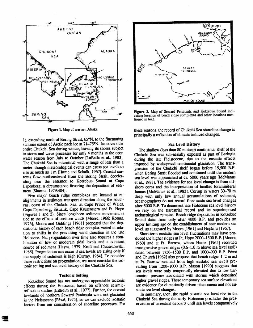
174e llll e IQ_ 0! I !

ARCTICOCEAN

,, 10o

,iCHUKCHI ALASKA

SEA

SIBER

KA! ,KOIZEBUE

pENIN SEWARD '" SOUND' seeULA

_NORTONSOUND

0 _00

K., Figure 2. Mapof SewardPeninsulaand KotzebueSoundindi-BERING eP caringlocationofbeachridgecomplexesandoth_ locationsmc-n-SEA tionedin texL

114 161 16

Figure1.Mapof westernAlaska. these reasons, the record of Chukchi Sea shoreline change is' principallya reflectionof climate-induced changes.

1), extending northof Bering Strait,65°N, to the fluctuatingsummer extent of Arcticpack ice at 71-75°N. Ice covers the Sea Level HistoryentireChukchi Sea duringwinter, leaving its shores subject The shallow 0ess than80 m deep) continentalshelf of theto stormand wave processes for only 4 months in the open Chukchi Sea was sub-aeriaUyexposed as part of Beringiawater season from July to October[t,aBelle ct al., 1983]. during the late Pleistocene, due to the eustatic effectsThe Chukchi Sea is microtidal with a range of less than a imposed by widespread continental glaciation. The trans-meter, though meteorological events can cause sea levels to gression of the Chukchi shelf began before 15,500 B.P.rise as much as 1 m [Hume and Schalk, 1967].Coastal cur- when Bering Strait flooded and continued until the modernrents flow northeastward from the Bering Strait, deceler- scalevel wasapproachedat ca 5000 yearsago [McManusating near the entrance to Kotzebue Sound at Cape et al., 1983]. The evidence for sea level change is from off-Espenberg, a circumstance favoring the deposition of seri- shore cores and the interpretation of benthic foraminiferalment [Sharma, 1979:404]. faunas [McManus et al., 1983]. Coring in waters 30-70 m

Five major beach ridge complexes are located at re- deep with only low annual accumulations of sediment,alignments in sediment transport direction along the south- oceanographers do not record finer scale sea level changeseast coast of the Chukchi Sea, at Cape Prince of Wales, after 5000 B.P. To document late Holocene sea level historyCape Espenberg, Sisualik, Cape Krusenstern and Pt. Hope we rely on the terrestrial record and its superimposed(Figures 1 and 2). Since longshore sediment movement is archaeological remains. Beach ridge deposition in Kotzebuetied to the effects of onshore winds [Moore, 1966; Komar, Sound dates from only after 4000 B.P. and provides an1976], Moore and Giddings [1961] proposed that the dep- upper limiting age on the establishment of near modern seaositional history of each beach ridge complex varied in rela- level, as suggested by Moore [1961] and Hopkim [1967].tion to shifts in the prevailing wind direction in the late Short-term eustatic sea level fluctuations may have pro-Holocene. Net progradation over time also requires a com- duced the higher ridges at Pt. Hope 20(O-1500 B.P. [Moore,bination of low or moderate tidal levels and a constant 1960] and at Pt. Barrow, where Hume [1965] recordedsource of sediment [Hayes, 1979; Kraft and Chrzastowski, transgressive gravel ridges (0.6-1.0 m above sea level (asi))1985]. Progradation can occur if sea levels are rising only if dated between 1750-1500 B.P. and 1000-900 B.P. Pdw6the supply of sediment is high [Curray, 1964]. To cx}nsider and Church [1962] also propose that beach ridges 1-2 m asithese restrictions on progradation, we must consider the tec- at Pt. Barrow resulted from high eustatic sea levels pre-tonic setting and sea level history of the Chukchi Sea. vailing from 1200--1000 B.P. Mason [1990] suggests that

sea levels were only temporarily elevated due to low bar-Tectonic Setting ometric pressure associated with stormswhich depositeg_

Kotzebue Sound has not undergone appreciable tectonic higher gravel ridges. These temporary _ surfaceelevationseffects during the Holocene, based on offshore seismic- are evidence for climatically driven phenomena and not eu-reflection studies IEittreim et al., 1977]. Further, the coastal static sea level changes.lowlands of northern Seward Peninsula were not glaciated In summary, then, the rapid eustatic sea level rise in thei._the Pleistocene [P6w6, 1975], so we can exclude isostatic Chukchi Sea during the early Holocene precludes the pres-factors from our consideration of shoreline processes. For ervation of terrestrial deposits until sea levels comparatively

650 ,'

. ,

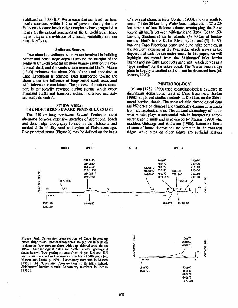
stabilized ca, 4000 B,P, We assume that sea level tats been of erosional characteristics [Jordan, 1988], moving south tonearly constant, within 1-2 m of present, during the late north: (1) the 30-km-long Wales beach ridge plain', (2) a 20-Holocene because beach ridge complexes have prograded at km stretch of late Holocene dunes overtopping the Pleis-nearly ali the critical headlands of the Chukchi Sea, Hence tocene silt bluffs between Mitletavik and Ikpek; (3) the 150-higher ridges are evidence of climatic variability and not km-long Shishmaref barrier islands; (4) 30 km of tundra-eustatic effects, covered bluffs in the Kitluk River region; and (5) the 30-

km.long Cape Espenberg beach and dune ridge complex, atSediment Sources the northern extreme of the Peninsula, which serves as the

Two abundant sediment sources are involved in building depositional sink for the entire coast. In this paper, we willbarrier and beach ridge deposits around the margins of the highlight the record from the Shishmaref Inlet barriersouthern Chukchi Sea: (a) offshore marine sands on the con- islands and the Cape Espenberg sand spit, which serves as atinental shelf, and Co) sands within terrestrial bluffs. Mason "typesection" for the entire coasL The Wales beach ridge[1990] estimates _hat about 90% of the sand deposited at plain is largely unstudied and will not be discussed here [ct'.Cape Espenberg is offshore sand transported toward the Mason, 1990],shore under the influence of long-period swell associatedwith fairweather conditions. The process of onshore trans- METHODOLOGYport is temtxa'arily reversed during storms which erode Mason [1987, 1990] used geoarchaeological evidence tomainland bluffs and transport sediment offshore and sub- distinguish depositional units at Cape Espenberg. Jordansequently downdrift. [1990] employed similar methods at Kividluk on the Shish-

maref barrier islands. The most reliable chronological dataSTUDY AREA: are 14(2dates on charcoal and temporally diagnostic artifacts '

THE NORTHERN SEWARD PENINSULA COAST from archaeological sites. The cultural chronology of north-The 250-km-long northwest Seward Peninsula coast west Alaska plays a substantial role in interpreting chron.

alternates between extensive s:relches of accretional beach ostrattgraphic units and is reviewed by Mason [1990] whoand dune ridge topography formed in the Holocene and modifies Giddings and Anderson [1986]. Extensive lineareroded cliffs of silty sand and tephra of Pleistocene age. clusters of house depressions are common in the youngestFive principal zones (Figure 2) may be defined on the basis ridges while sites on older ridges are surficial scatters

UNITI UNIT II UNIT IU UNIT IV

22851-90 440£-60 100t-902340:1:80 700:t:70 200:t:702500190 1300:t:70 720:t:70 210:).-602530_130 1360i-90 730z'-90 300:1:50 240±70

2660:t:110 141Oz'-60 7904-70 730:/:1O0 260:f:5027904-80

19 17 14 12 8 o,.

)'"' "°1 '" ,o o3700:f:90 1640:t:80 820±70 1500:/:603750±8O

Figure 3(a). Schematic cross.section of Cape Espenberg __ 170±70beach ridge plain. Radiocarbondates _e plotted in relation g, 290z_60

to distancefrommodemshorewithdel:xsitionalunitsshown _ 470±70

above,Archaeologicaldatesareplottedabove;geological _ _ I _datesbelow.Two geologicdatesfromridgesE-4andE-5 '°" _are on marineshell and requirea correction of 500 years [cf. _ -- I o

Mason and Ludwig, 1991]. Laboratory numbers in Mason ;.,,- [ o[1990]. (b). Schematic Cross-section of Kividluk Island,Shishmarefbarrier islands.Laboratorynumbersin Jordan 080±70 320z_60[ 19901. 1550±70 48o±so

520-)70640±701070±80

' 651

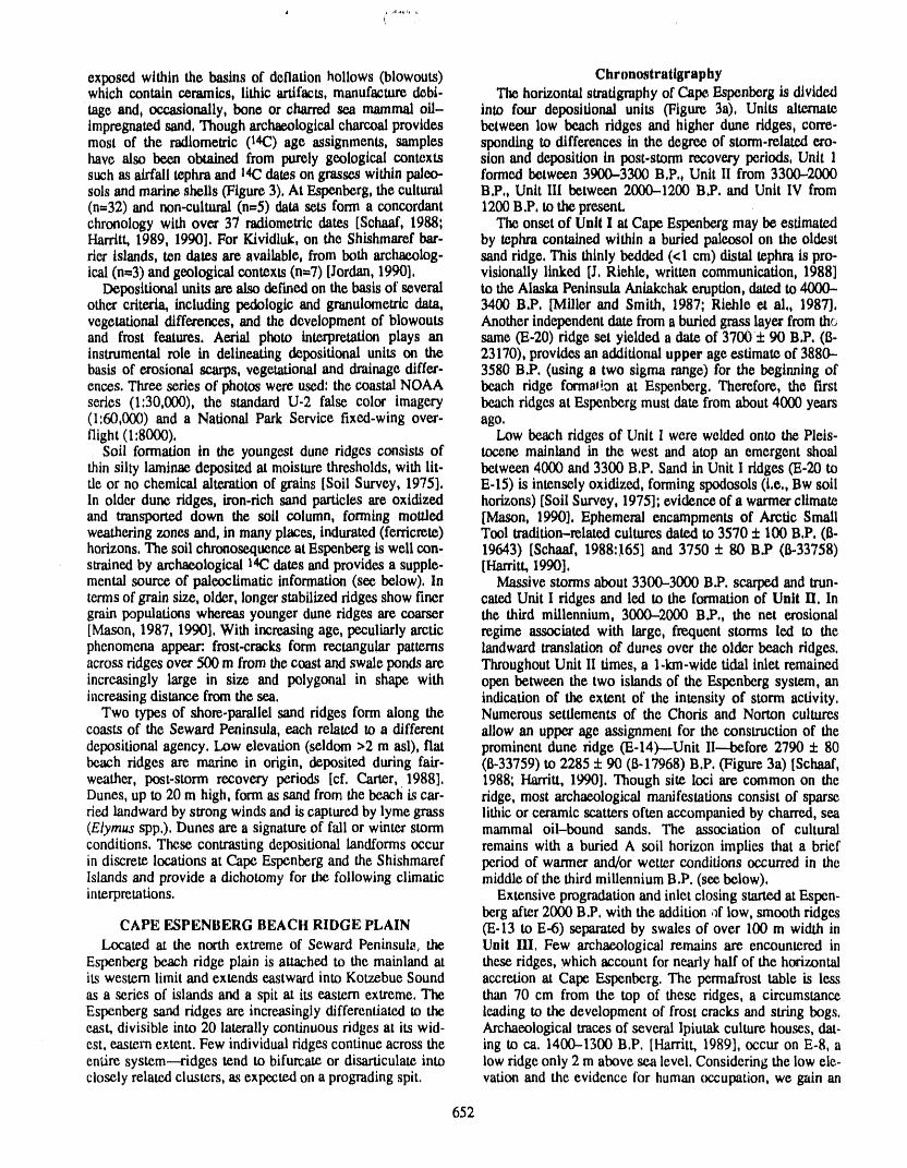
exposed within the basins of deflationhollows (blowouts) Chronostratlgraphywhich contain ceramics, lithic artifacts,manufactured_bi- The horizontal stratigraphyof Cape Esponbergis dividedrage and, occasionally, bone or charred sea mammaloil- into four deposittonal units (Figme 3a), Units alternateimpregnatedsand, Though archaeologicalcharcoalprovides between low beach ridges and higher dune ridges, terre-most of the radiometric (t4C) age assignments, samples spon(llng to differences in the degree of storm.relatextere-have also been obtained from purely geological contexts sion and deposition in post-storm recovery periods, Unit 1such as airfall tephraand 14(2dams on grasses within paleo., formed between 3900-3300 B,P,, Unit II from 3300-2000sols and marine shells (Figure3), At Espenberg, the cultural B.P,, Unit III between 2000-1200 B.P, and Unit IV from(n=32) and non-cultural (n=5) data sets form a concordant 1200 B.P. to the pre.w_Lchronology with over 37 radiometricdates [Schaaf, 1988; The onset of Unit I at Cape Espenberg may be estimatedHarritt, 1989, 1990]. For Kividluk, on the Shishmaref bar- by tephra contained within a buried paleosol on the oldesttier islands, mn dates are available, from both archaeolog- sand ridge. This thinly bedded (<1 em) distal tephra is pro-ical (n=3) and geological contexts (n--7) [Jordan, 1990], visionally linked [J, Riehle, written communication, 1988]

Depositional units are also defined on the basis of several to the Alaska Peninsula Aniakchak eruption, dated to 4000-other criteria, including pedologic and granulometricdata, 3400 B.P, [Miller and Smith, 1987; Riehle ea al,, 1987],vegetational differences, and the development of blowouts Another independentdate from a buriedgrass layer from theand frost features. Aerial photo interpretationplays an same (E-20) ridge set yielded a date of 3700 ± 90 B.P. (B-instrumental role in delineating depositional units on the 23170), provides an additional upper age estimate of 3880-basis of erosional scarps, vegetationaland drainagediffer- 3580 B.P. (using a two sigma range) for the beginning ofences, Three series of photos were used: the coastal NOAA beach ridge formation at Espenberg, Therefore, the Iu'stseries (1:30,000), the standardU-2 false color imagery beach ridges at Espenbergmust date fromabout4000 years(1:60,000) and a National Park Service fixed-wing over- ago,flight (1:8000). Low beach ridges of Unit I were welded onto the Pleis-

Soil formation in the youngest dune ridges consists of tocene mainland in the west and atop an emergent shoalthin silty laminae deposited at moisture thresholds, with lit- between 4000 and 3300 B.P. Sand in Unit I ridges (E-20 tofie or no chemical alteration of grains [Soil Survey, 1975], E-15) is intensely oxidized, forming spodosols (i.e., Bw soilIn older dune ridges, iron.rich sand particles are oxidized horizons) [Soil Survey, 1975]; evidence of a warmer climateand transported down the soil column, forming mottled [Mason, 1990]. Ephemeral encampments of Arctic Smallweathering zones and, in many places, indurated (ferricrete) Teel tradition-related cultures dated to 3570 ± 100 B.P. (B-horizons. The soil chronosequence at Espenberg is well con- 19643) [Schaaf, 1988: !65] and 3750 ± 80 B.P (B-33758)strained by archaeological 1412dates and provides a supple- [Harritt, 1990].mental source of paleoclimatic information (see below). In Massive storms about 3300-3000 B.P. scarped and trun-terms of grain size, older, longer stabilized ridges show finer cated Unit I ridges and led to the formation of Unit H. Ingrain populations whereas younger dune ridges are coarser the third millennium, 3000-2000 B.P., the net erosional[Mason, 1987, 1990]. With increasing age, peculiarly arctic regime associated with large, frequent storms led to thephenomena appear:, frost-cracks form rectangular patterns landward translation of duoes over the older beach ridges,across ridges over 500 m from the coast and swale ponds are Throughout Unit II times, a l.km-wide tidal inlet remainedincreasingly large in size and polygonal in shape with open between the two islands of the Espenberg system, anincreasing distance from the sea. indication of the extent of the intensity of storm activity.

Two types of shore-parallel sand ridges form along the Numerous settlements of the Choris and Norton culturescoasts of the Seward Peninsula, each related to a different allow an upper age assignment for the construction of thedepositional agency. Low elevation (seldom >2 m asi), flat prominent dune ridge (E-14)---.Unit II---before 2790 + 80beach ridges are marine in origin, deposited during fair- (B-33759) to 2285 :t:90 (B-17968) B.P. (Figure 3a) [Schaaf,weather, post-storm recovery periods [cf. Carter, 1988]. 1988; Harritt, 1990]. Though site loci are common on theDunes, up to 20 m high, form as sand from the beach is car. ridge, most archaeological manifestations consist of sparsefled landward by strong winds and is captured by lyme grass lithic or ceramic scatters often accompanied by charred, sea(Elymus spp.). Dunes are a signature of fall or winter storm mammal oil--bound sands. The association of culturalconditions. These contrasting depositional landforms occur remains with a buried A soil horizon implies that a briefin discrete locations at Cape Espenberg and the Shishmaref period of warmer and/or wetter conditions occurred in theIslands and provide a dichotomy for the following climatic middle of the third millennium B.P. (see below).interpretations. Extensive progradation and inlet closing started at Espen-

berg after 2000 B.P. with the addition ,-fflow, smooth ridgesCAPE ESPENBERG BEACH RIDGE PLAIN (E-13 to E-6) separated by swales of over 100 m width in

Located at the north extreme of Seward Peninsula, the Unit Ill. Few archaeological remains are encountered inEspenberg beach ridge plain is attached to the mainland at these ridges, which account for nearly half of the horizontalits western limit and extends eastward into Kotzebue Sound accretion at Cape Espenberg. The permafrost table is lessas a series of islands and a spit at its eastern extreme. The than 70 cm from the top of these ridges, a circumstanceEspenberg sand ridges are increasingly differentiated to the leading to the development of frost cracks and string bogs.east, divisible into 20 laterally continuous ridges at its wid- Archaeological traces of several Ipiutak culture houses, rat-est, eastern extent. Few individual ridges continue across the ing to ca. 1400-1300 B.P, [Harritt, 1989], occur on E-8, aentire system--ridges tend to bifurcate or disarticulate into low ridge only 2 m above sea level. Considering the low ele-closely related clusters, asexpected on a prograding spit. vation and the evidence tbr human occupation, we gain an

652

appreciationof the infrequency and lessened intensity of progradatlonfollowed in the 500 yearsafterthe stabilizationmassivestormsduringthe p_iod between 2000-1000 B.P, of the barrierplatform,Thus, slow verticalaccretionaccom-

In Unit IV, high dunes built up to 20 m above sea level partiedrelatively rapid horizontal progradation,forming aduring an erosiorad regime beginning about 1200 B,P, The thin, seaward-thiclmningwedge of ovorwash and eolianhigh dunes of this pexiod choke off several of the cross, sanddepositedbetween 1600 and 1000 B,P,cutting channels in the low-lying Unit III fldges, Radio. Shoreface erosion, landward migration of transgressivemetric determinationsfrom buried archaeological horizons dunes and the transferof marine se,dimcnts through inletsassociatedwith thewesternThule andold Kotzebuecultures and surge channels characterizes barrierdynamics for thereveal thatdune-buildingoccurredbefore 8(D--6_ and 300- past 1000 years (Figure 3b), Landwardretreatof extensive200 B.P. [Harflt,,1989] or A.D. 1000-1100 and A.D. 1500- transgressivedune deposits has provided sediments to beth1600, in calibratedages [Mason, 1990]. The ,seawardaspect offshore and backshore environments. Backbarriermarshof the dunes is eroding, as indicated by a prominent scarp has expanded onto washthrough flats built above the inter-andphotogrammetricmeasurementsthat 8 to 13m of retreat tidalzone at Ktvidlukisland [cf, Godfrey et al,, 1979],occurredfrom 1949-1976 [Jordan,1988], The barrierisland archaeological record is abundantfor

In summary, dune-building activity is concentrated in the period from about 500 B.P, to present and is preservedthree periods at Espenberg: (a) 3300-2000 B.P,, Co) from in eoliml settings, particularly in transgressive backbeach1200--600 B,P,, and (c) with lessened intensity from 250 dunes which provide sufficient topographicrellef above theB,P, to the present. Assuming that dune building is eor. water table, Prehistoric houses are found atop or in the leerelative with increased storminess, as in the North Sea of high transgressive dunes, while low.elevation beach[Jelgersmact al., 1970; Lamb, 1988] and Australia [Them, ridges contain only prehistoric and historic cache features,1978], then the ridges at Espenberg are a proxy climatic Archaeological loci exposed in dune scarps at Ktvidlukareindicator, Plana_ror beach ridge progradationpresumably dated at470 :t:70 B.P, (B-M772), 290 :t:70 B.P, (5-17958),occurredduring "fairweather"post-storm recovery cond[, and 170+ 70 B.P, (_17973) [Schaaf, 1988; Jordan,1990],tions dominated by high pressure conditions as in July/ The situation on the Shishmaref barrierislands parallelsAugust [cf. Carter,1986]. During the time periodswithless that of Espenberg during the last 2000 years; however,intenseand longer storm recurrenceintervals, beach ridges deposits earlier than 2000 B.P, are not known from the bar-would be low (0.7-1.0 m asi) and more likely to be pre. rier islands. Rapid progradationcharacterizes the barrierserved, In times with intense storms, beach ridges formed island sedimentary regime during the period 1700-1100higher in elevation above sea level (1,0-1,7 m asi), During B.P, However, at about 1100 B.P, a high dune ridge beganthe winter, these higher storm-elevated beach ridges were to buildon the barrierislandsand subsequentlyhas migratedmore susceptibleto eolian deflation, forminglow dunes and landward under the influence of shoreface erosion. Thesusceptible to further incorporation by growing beach grass Shishmarefbarriersand Espenbergspit contain varyingper-duringsummer[cf. Carter, 1986;He,sp, 1988]. tions of the late Holocene sedimentaryrecord,but both con-

rainsimilar deposits from the last 2000 years. DifferencesSHISHMAREF BARRIER ISLANDS betwee._the two areas from 4000 to 2000 B.P. reflect vari-

The Shishmaref barrier islands, located 50 km updrift ation in sediment sources, currentstrength and location infrom Cape Espenberg,extend for over 125 km andseparate the longshore transport system. "['he Shishmaref barriersShishmaref Inlet frou: Lb,e Chukchi Sea. The islands are low may yet provide similar evidence for the transgressive,in elevation and con_,, of a single, scarpedhigh dune ridge stormy interval 3300-2000 B.P. in subsurface deposits orbacked by 13-20 low beach ridges or washover flats separ- evidence of older barrier island deposits may exist as pal-ated by numerous abandoned surge channels. Descriptions impsests offshore.of the sedimentaryenvironments on the Shishmarefbarrierscan be foundin Jordan [1990]. Geological and archaeologi- DISCUSSION: CROSS-CORRELATIONS WITHcal radiocarbondates provide constraints on the history of OTHER NORTH AMERICAN ARCTIC LOCALITIES

barrierisland development. Morphologic comparison with The sequence of storm cycles recorded at Cape Espen-well-dated deposits at Cape Espenberg allows a relative age berg and the Shishmaref barriers correlates with other beachestimate to be made for barrier formation, ridge complexes in western Alaska (i.e., Cape Krusenstem,

Wales, SL Lawrence Island and Sisualik) and with otherChronostratigraphy proxy climatic records from northwest Alaska (Figure 4).

Prior to the progradational phase which began at some Temporal parallels in erosion and progradation at othertime after 2000 B.P., the Shishmaref barriers probably were northwest Alaska beach ridge complexes are related to thefrequently flooded, consisting of washover flats, numerous particular trajectories of North Pacific weather systems andsurge or tide channels, with only limited or episodic sub- the resultant effects on waves and longshore transport on theaerial exposure. A geologic date of 1550 + 70 B.P. (B- nearshore zone of western Alaska [Mason, 1990; Mason and28183) was obtained from a basal organic peat horizon Ludwig, 199I]. Ultimately, the patterns of precipitationexposed in a lagoon-margin trench at Kividluk. This date leading to glacial expansion and alluvial floods are alsoindicates that marsh vegetation had stabilized the local tidal linked to the same synoptic patterns.flat or barrier platform surface, and provides a minimum Progradational regimes at northwest Alaska 'beachridgedate for the beginning of beach ridge progradation at Kivid- complexes leflect warmer mid-summer climatic conditionsluk and the barrier islands to the west. A basal date of 1070 from 4000-3000 and 2.000-1200 B.P. In the former case,_+80 B.P. (B-28181) on exhumed shoreface peat on the med- paleosols or stable surfaces dated to 400(03750 B.P. areem beach at Kividluk reveals that nearly 1 km of horizontal reported from isolated localities _cross northernAlaska and

653

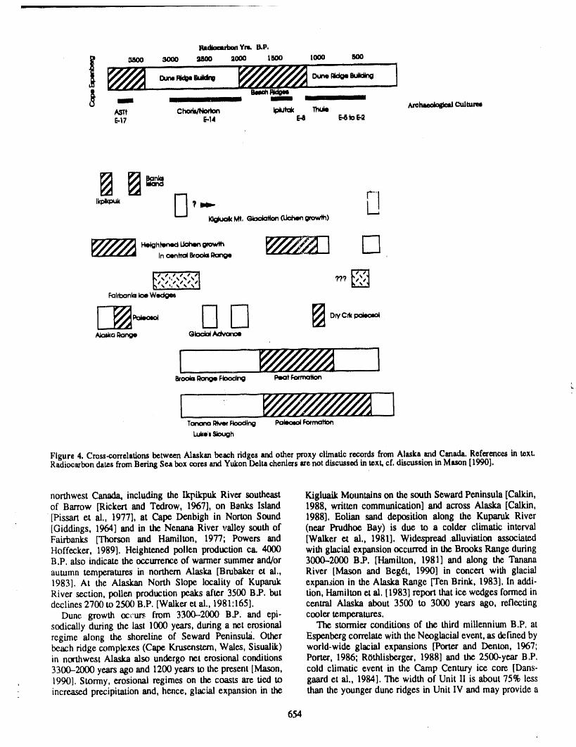
RadlomrtxmYnk B,P,

I 1000 I000 600

_17 (-14 (-4 [.-6tor_

ince_tm4eroo_aRange

Tonana_ Ftoodlog PaleeeolF_maflonL_e'l Sk:)ugh

Figure4. Cmss-c.orrelatio_betweenAlaskanbeachridgesandother climaticrecordsfromAlaskaandCanada.Referencesin text.Radiocarbondates_omBeringSe.aboxooresandYukonDdta cheni_rsPr_ot discuss_ intext,el. dis_.lssioninMason(1_)0],

northwest Canada, including the I_ikpuk River southeast Kigluaik Mountainson the south SewardPeninsula [Calkin,of Barrow FRickerl and Tedrow, 1967], on Banks Island 1988, written communication] and across Alaska [Calkin,

[Pissart ct al., 1977]0 at Cape Denbigh in Norton Sound 1988]. Eolian sand deposition along the KuFmrukRiver[Giddings, 1964] and in the Nenana River valley south of (near Prudhoe Bay) is due to a colder climatic intervalFairbanks [Thorson and Hamilton, 1977; Powers and [Walker ct al., 1981], Widespread .alluviation associatedHoffecker, 1989]. Heightened pollen production ca. 4000 with glacial expansionocctm'ed in the Brooks Range duringB.P. also indicate the occurrence of wanner summer and/or 300(02000 B.P. [Hamilton, 1981] and along the Tanana

autumn temperatures in northern Alaska [Brubaker ct al., River [Mason and Beg6t, 1990] in concert with glacial1983]. At the Alaskan North Slope locality of Kuparuk expansion in the Alaska Range [Ten Brink, 1983], In addi-River section, pollen production peaks after 3500 B.P. but tion, Hamilton et al. [1983] report that ice wedges formed indeclines 2700 to 2500 B.P. [Walker et al., 1981:165]. central Alaska about 3500 to 3000 years ago, reflecting

Dune growth occurs from 3300-2000 B.P. and epi- cooler temperatures.sodicaUy during the last 1000 years, during a net erosional The stormier conditions of the third millennium B.P. atregime along the shoreline of Seward Peninsuhi. Other Espenberg correlate with the Neoglacial event, as defined bybeach ridge complexes (Cape Kzmenstern, Wales, Sisualik) world-wide glacial expansions [Porter and Denton, 1967;in northwest Alaska also undergo net erosional conditions Porter, 1986; ROthlisberger, 1988] and the 2500-year B.P.3300-2000 years ago and 1200 years to the present [Mason, cold climatic event in the Camp Century ice core [Dans-1990]. Stormy, erosional regimes on the coasts are tied to gaard et al., 1984]. The width of Unit II is about 75% lessincreased precipitation and, hence, glacial expansion in the than the younger dune ridges in Unit IV and may provide a

654

relative measure of storm recurrence intervals in tlm third that treoline expanded to higher altitu_s during a warmermillennium B,P,, i,e,, larger storms probably occurred in periodbetween 2200-1200 B,Pmorerapidst_cession, as comparedto the last 1000 years, For the last 1000 years the sedimentary record of the

The buried soil dated at 2800-2500 B,P, on the Unit II Seward Peninsula coast may be compared with hlstork_ridges is evidence of increase.d precipitation or of a tem- records from China because similar weather phenomenaporarypause in the general trend of climatic cooling, Quite affect both east Asia and Boring Strait, Mason [1990] pro-significantly, the record of Espenberg paleosols correlates poses that dune formation at Cape Bsponberg is linked towell with Sorensen and Knox's [1974] reconst.rtmtionfor tlm synoptic phemomonain Siberia which produce anomalouslate Holocene displacementof the forest/tundraboundaryin winter thunderstorms and dust storms in Beijing, both ct'north.central Canada, which shows northern advances of which indicate colder conditions, Th0 onset of cold condi-treellne (andpalcosols) at 3500 and 1600-111)13B.P,, with a lions at Espenberg around 1200-1000 B.P, parallelsthe ovl-slight advance at2600-2200 B.P, and a southwardretreat at dealce presented by Porter [1986] for glacial expansions2900, 1800and 800 B,P, throughout the northern hemisphere, Thus, the proxy cit-

The Espenberg paleosol record reflects a particular com. lnattc record from Alaskazi beach ridges corresponds closelyblnation of climatic and ecological factors, The primary stg- With hlstortc records from both east Asia and Europe, pro-nal is one_of stabilized, shrub vegetation and the absence of vtdtng a means with which to reconstruct paieoclimate tn agrasses and appreciable eolian deposition, which indicates region lacking meteorological records prior to A,D, 1800,the prevalence of increased precipitation coupled withweaker winds, The stablll',ted surfaces occur during lhc ACKNOWLEDGMENTSstormy, cold intervals of Units II and IV, implying thatshort-termdecr_ in wind and/orstorm intensitypunctu. We thank the NationalPark Service and theUniversity ofated these otherwise stormy pededs, Alaska Oeist Fund for monies to field our studies, radio-

The period between 2000-1000 B,P, contains almost half carbon date samples and obtainaerial photographs, In addi-of the progradattonat Espenbergand correlateswith a slm. tion, we both benefited fromparticipationin archaeologicalilar progradationalregime on the Shishmaref barrierislands surveys conducted by the NPS, The unstinting support of1500-1000 yearsago [Jordan, 1989, 1990], Peat formation Dr, D, M, Hopkins was instrumental in completing ouratop alluvial terraces is widespread between 2000-1000 research, Jeanne Schaaf and Dr, Roger Hardtt of the NPSB,P. in north-central Alaska [Hamilton, 1981] and Seward played a critical role in furthering our research, Fteld andPeninsula [Kaufman et al,, 1989]. In the White Mountains, lab assistance by Stefanle Ludwig, Dale Vin_t)),and Marknear the Yukon Territory, Denton and Earl6n [1977] report Moore are also greatly appreciated.

LITERATURE CITEDBrubaker, L. B., H. L. Garfinkel,and M. E. Edwards, Late Alaska,Science, 153, 127-135, 1966,

Wisconsin and Holocene vegetation change in the Walker Giddlngs, J, L,, and D. D, Anderson, Beach Ridge Arehae-Lake/Alatna valley region of the Brooks Range, Quat, elegy of Cape Krusenstern: Eskimo and pre.Eskimo set-Res.,20, 194-214, 1983, tlements around Kotzebue Sound, Publications in

Calkin, P., Holocene glaciation of Alaska (and adjoining Archaeology No, 20, National Park Service, Washington,Yukon Territory, Canada), Quat. Sci. Roy., 7, 159-184, 1986,1988, Godfrey, P. J., S. F, Leatherman, and R. Zaremba, A gee-

Carter, R. W. G., The morphodynamics of beach.ridge for- botanical approach to classification of barrier beach sys- ,marion: Magilltgan, northern Ireland, Marine Geol., 73, terns, in Barrier Islands from the Gulf of St, Lawrence to191-213, 1986, the Gulf of Mexico, edited by S, P, Leatherman, pp. 99-

Carter, R, W, G,, Coastal Environments, Academic Press, 126, Academic Press, New York, 1979.New York, 1988. Hamilton, T, D., Episodic Holocene alluviatton tn the cen-

Curmy, J. R., Transgressions and regressions, in Papers in tral Brooks Range: chronology, correlations and climaticMarine Geology, edited by R. L. Miller, pp. 175-203, implications, In U,S, Geological Survey in Alaska,MacMillan, New York, 1964. Accomplishments during 1979, edited by N, R. D, Albert

Dansgaard, W., S. J. Johnson, H. B. Clausen, D. Dahl- and T. Hudson, pp. 21-24, U.S. Geological Storey Circ.Jensen, N, Gundestrup, and C. U. Hammer, North Arian- 823.b, 1981.tic climatic oscillations revealed by deep Greenland ice Hamilton, T, D,, T. A. Ager, and S, W. Robinson, Late Hol-cores, Am. Geophys. Union Monogr. 29, 288--298, 1984. ocene ice wedges near Fairbanks, Alaska, U.S.A,: Envi-

Denton, G. H. and W. Kari6n, Holocene glacial and tree-line ronmental setting and history of growth, Arctic andvariations in White River and Skolai Pass, Alaska and Alpine Research, 15, 157-168, 1983.Yukon Territory, Quat. Res., 7, 63-111, 1977. Harritt, R. K,, Recent archaeology in Bering Land Bridge

Eittreim, S., A. Grantz, and O. T. Whimey, Tectonic National Preserve: the 1988 Field season at Cape Espen-imprints on sedimentary deposits in Hope basin, in The berg, paper presented at 16th annual meeting, AlaskaU.S. Geological Survey in Alaska: Accomplislunents dur- Anthropological Assoc,, Anchorage, March 3--4, 1989,ing 1976, edited by K. M. Blean, pp. 100-103, United Harritt, R. K., Recent archaeology in Bering Land BridgeStates Geological Survey Circular 751-B, 1977. National Preserve: the 1989 Field season at Cape Espen-

Giddings, J. L., The Archaeology of Cape Denbigh, Brown berg and in the Ikpek area, paper presented at 171tiannualUniversity Press, Providence, 1964, m_ting, Alaska Anthropological Association, Fairbanks,

Giddings, J. L., Cross-dating the archeology of northwestern March 9-10, 1990.

655

Hayes, M, O,, Barrier island morphology as a function of Mason, O, K, and S, L, Ludwig, ResurrectingBeach Ridgetidalandwave r_glme, in Barrier Islands from the Gu!fof Archaeology: Parallel Depositional Histories from SLSt, Lawrence to the Gulf of Mexico, editedby S, P, Leath. Lawrence Island and Cape Krusenstern, Alaska, Gee.ennan, pp, 1-29, AcademicPress, New York, 1979, archaeology, 1991, Inpress,

Hesp, P, A,, Morphology, dylmmics and internal strati- McManus, D, A,, J. S, Creager, R, J, Eeh_ls, and M, L,flcatton of some established foredunes in southeast Aus- Holmes, The Holocene transgressionon the Arctic flanktralta,Sedimentary Geol,, 55, 17-41, 1988, of Bedngttu Chukchi valley to Chukchi estuaryto Chuk.

Hopkins, D, M,, Quatenmry marine transgressions in ehi Sea, in Quaternary Coastlines and Marine Archae.Alaska, in The Bering Land Bridge, edited by D, M, elegy: ?bwartLs' a Prehlstory of Landbrldges andHopkins, pp, 47-90, StarffordUniversityPress, Stanford, Continents, edited by P, M, Masters and N, C, Fleming,CA, 1967, pp, 365-388, Academic Press, New York, 1983,

Hume,J, D,, Sea level changes during the last 2000 years at Miller, T, P,, and R, L, Smith, Late Qtmtemary caldera-Point Barrow,Alaska,Science, 150, 1165-1166, 1965, forming eruptions in tho eastern Aleutian arc, Alaska,

Hume,J, D., and M, Schalk, Shoreline processes near Bar- Geology, 15,434-438, 1987,row, Alaska: A comparison of rite normal and the cat- Moore, G, W,, Recent eustatic sea.level fluctuationsastrophlc, Arcttc, 20,86-103, 1967, recorded by Arctic beach ridges, Geological Survey

Jelgersma, S,, J, de Jong, W, H. Zagwijn, and J, F, van Research 1960, U,S. Geological Survey ProfessionalRegter_n Air,na, The coastal dunes of western Nether. Paper 400 B335-7, 1960,lands: geology, vegetational history and archeology, Moore, G, W,, Arctic beach sedimentation, io EnvironmentMededelingen Rtjks Geologische Dlenst, Nieuwe Ser,, 21, of the Cape Thompson Region, Alaska, edited by N,93-167, 1970, Wilimovsky and J, N, Wolfe, pp, 587.-608, Atomic

Jordan, J, W,, Erosion characteristics and retreat rates along Energy Commission, Oak Ridge, TN, 1966,the north coast of Seward Peninsula, in Bering Land Moore, O, W,, and J, L, Olddtngs, Record of 5000 years ofBridge National Preserve: An Archaeological Survey, Arctic wind direction recorded by Alaskan beach ridges,edited by J, Schaaf, pp, 322-362, National Park Service, Abstract, Special U.S, Geological Soc. Papers, 68, 1961.Alaska Region, Res, Management Rep, No, 14, 1988. Pemtrovlch & Nottingham, Inc., Shishmaref Erosion Con.

Jordan, J, W,, Late Holocene evolution of barrier islands tn trol Engineering Studies, State of Alaska, l_pt. of Trans-the southern Chukchi Sea, Alaska, Unpublished Master's portationand Public Facilities, Anchorage, 1982,Thesis, Quaternary Studies, University of Alaska, P6w6, T, L,, Quaternarygeology of Alaska, United StatesFalrbanks,1990. Geological Survey Professional Paper 835, 1975.

Kauflnan,D, S,, P. E. Calkin,W, B. Whifford,B. J. Przybyl, P6w6, T, L., and R, E, Church, Age of the spit at Barrow,D. M, Hopkins, B, J. Peck, and R. E. Nelson, Smficial Alaska,Bull. Geol. Soc. Am,, 73, 1287-1291, 1962,geologic map of the Kiglualk Mountains Area, Seward Pissart' A,, J. S, Vincent, and S, A, Edlund, D6pots etPeninsula, Alaska, United States Geological Survey Mis- phenom_nes 6oliens sur l'ile de Banks, Terdtoires ducellaneous Field Studies Map MF.2074, 1989. Nord-Ouest,Canada, Can. J. Earth Set,, 14, 2462-2480,

Komar, P. D., Beach Processes and Sedimentation, Pren. 1977,rice-Hall,Englewood Cliffs, NJ, 1976, Porter, S. C,, Pattern and forcing of Northern Hemisphere

Kraft, J. C., and M. J. Chrzastowski, Coastal strattgraphtc glaciervariationsduringrite Last Millennium,Quat. Res.,sequences, in Coastal Sedimentary Environments, edited 26, 27-48, 1986.by R, A. Davis, pp. 625-664, Spdnger Verlag, New Porter, S. C., and G. H. Denton, Chronology of Nee..York, 1985, glaciation in the North American Cordillera, Am. J. Sci.,

La Belle, J. C., J. L. Wise, R. P. Voelker,R. H. Schulze, and 255,177-210, 1967.G. M. Wohl, Alaska Marine ice Atlas, Arctic Environ. Powers, W. R,, and J. F. Hoffecker, Late Pleistocene settle-mental Information and Data Center, Univ, of Alaska, merit in the Nenana valley, central Alaska, AmericanAnchorage, 1983, Antiquity, 54, 263-287, 1989.

Lamb,H. H., Climate in historical times and transgressions Pye, K., Models of transgressive coastal dune building epi-of the sea, storm floods and other coastal changes, in sodes and their relationship to Quaternary sea levelWeatturr, Climate and Human Affairs, edited by H.H. changes: a discussion with reference to evidence fromLamb, pp, 78-103, Routledge, London, 1988. eastern Australia, in Coastal Research: UK Perspectives,

Mason, O. K., The Sedimentology and Relative Dating of edited by M. W. Clark, pp. 81-104, Gee-Books,the Saud Ridge Complexes of the northern Seward Penin- Cambridge, 1984.sula, Bering Land Bridge National Preserve, Final Report Rickert, D. A., and J. C. F. Tedrow, Pedologic investiga-te National Park Service, Alaska Regional Office, tions on some aeolian deposits of northern Alaska, SoilAnchorage, 1987. Science, 104,250--262, 1967.

Mason, O. K., Beach ridge geomorphology of Kotzebue Riehle, J. R., C. E. Meyer, T. A. Ager, D, S. Kaufman, andSound: Implications for paleoclimatology and archae- R.E. Ackerman, The Aniakchak tephra deposit, a lateelegy, Unpublished Ph.D. Dissertation, Quaternary Sci- Holocene marker horizon in Alaska, in Geologic Studiesence, University of Alaska Fairbanks, 1990. in Alaska 1986, edited by T. D. Hamilton and J. P. Gallo-

Mason, O. K., and J. E. Beg6L Late Holocene changes in way, pp. 19-24, U.S. Geological Survey Circular 998,flood frequency at the Tanana River, Alaska, paper 1987.presented at the 17th annual meeting of the Alaska R0thlisberger, F., 10 000 Jahre Gletschergeschichte derAnthropological Association, 1990. Erde, Verlag Sauerlltnder, Aarau, 1986.

656

Schaaf, J., The Bering land bridge:An brchaeological sur- Ten Brink,N. W., Glaciationof lhc northernAlaska Range,vey, National Park Service, Alaska Region, Resources in Glaciation in Alaska, R. M. Thorson and T. D.Management Report No. 14, Anchorage,Alaska, 1988. Hamilton,pp. 82-91, Alaska QuawanaryCenter,Univ. of

Sharma, G. D., The Alas_ Shelf, Springer-Verlag,New Alaska Museum Occasional Paper No. 2, 1983.York, 1979. Them, B. G., Coastal sanddeposition in southeastAustralia

Soil Survey Staff, Soil taxonomy, Agriculture Handbook during the Holocene, in Landform Evolution in Aus-No. 436, U.S. Dept. of Agriculture, Washington, DC, tralasia, ecfitedby J. L. Davies and M. A. J. Williams, pp,1975. 197-214, AustralianNationalUniversity Press, Canberra,

Sorenson, C. S., and J. C. Knox, Paleosols and paleo- 1978.climates related to late Holocene fcxest/tundraborder Thorson, R. M., and T. D. Hamilton, Geology of the Drymigrations: Mackenzie and Keewatin, N.W.T., Canada, Creek Site: a stratifiedearly Man site in interiorAlaska,in International conference on Prehistory and Paleo- Quat. Res., 7, 149-176, 1977.ecology of western North American.:4rctic and Subarctic, Walker, D. A., S. K. Short,J. T. Andrews, and P. J. Weber,pp. 187-203, Archaeological Association, Univ. of Cal. Late Holocene pollen and present day vegetation, Prud.gary, Calgary, 1974. hoe Bay and Atigun River, AlaskanNorth Slope, Arctic

and Alpine Research, 13, 153-172, 1981.

657

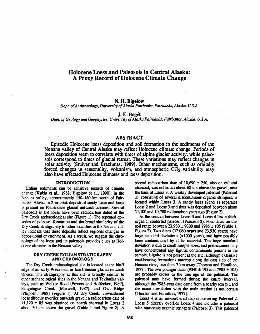
Holocene Loess and Paleosols in Central Alaska:A Proxy Record of Holocene Climate Change

N. H. BigelowDept. of Anthropology, University of Alaska Fairbanks, Fairbanks, Alaska, U.S.A.

J. E. Beg_t ,,Dept. of Geology and Geophysics, University ofAlaska Fairbanks, Fairbanks, Alaska, U.SA.

ABSTRACTi

Episodic Holocene loess deposition and soil formation in the sediments of theNenana valley of Central Alaska may reflect Holocene climate change. Periods ofloess deposition seem to correlate with times of alpine glacier activity, while paleo-sols correspond to times of glacial retreat. These variations may reflect changes insolar activity [Stuiver and Braziunas, 1989]. Other mechanisms, such as orbitallyforced changes in seasonality, volcanism, and atmospheric CO2 variability mayalso have affected Holocene climates and loess deposition.

INTRODUCTION second radiocarbondate of 10,690 + 250, also on culturalEolian sediments can be sensitive records of climate charcoal, was collected about 60 cm above the gravel, near

change [Kukla et al., 1988; Bigelow et al., 1990]. In the the base of Loess 3. A weakly developed paleosol (PaleosolNenana valley, approximately 150-180 km south of Fair- 1), consisting of several discontinuousorganic stringers,isbanks,Alaska, a 2-m-thick deposit of sandy loess and loess located within Loess 3. A sandy loess (Sand 1) separatesis present on Pleistocene glacial outwash texraces. Several Loess 2 andLoess 3 and thus was deposited between aboutpaleosols in the loess have been radiocarbondated at the 11,100 and 10,700 radiocarbonyears ago ('Figure2).Dry Creekarchaeological site (Figure 1). The repeatedepi- At the contact between Loess 3 and Loess 4 lies a thick,sodes of paleosol formation and the broadsimilarity of the organic, contortedpaleosol (Faleosol 2). Fourdates on thisDry Creekswatigraphyto other localities in the Nenanaval- soil range between 23,930 ± 9300 and7985 + 105 (Table 1,ley indicate that these deposits reflect regional changes in Figure 2). Two dates (12,080 yearsand 23,930 years) havedepositional environment. As a result,we suggest the chro- large standarddeviations (>1000 years), and have possiblynology of the loess and its paleosols provides clues to Hol- been contaminated by older material. The large standardocene climates in theNenana valley, deviation is due to small samplesizes, andpre_ent may

have concentratedany lignitic contaminants present in theDRY CREEK EOLIAN STRATIGRAPHY sample.Lignite is not presentat the site, although extensive

AND CHRONOLOGY coal-bearing formations outcrop along the east side of theThe Dry Creek archaeological site is located at the bluff Nenanariver, less than 7 km away [Thorsonand Hamilton,

edge of an early Wisconsin or late Illinoianglacial outwash 1977].The two younger dates (9340 ± 195and 7985 ± 105)terrace.The stratigraphy at this site is broadly similar to are probably closer m the true age of the paleosol. Theother archaeological sites in the Nenanaand Teidanikaval- paleosol may have formed during the entire interval,leys, such as Walker Road [Powers and Hoffecker, 1989], although the 7985-year date came from a nearbytestpit, andPanguingue Creek [Maxwell, 1987], and Owl Ridge the exact correlation with the main section is not certain[Phippen, 1988] (Figure 1). At Dry Creek, unweathered [ThorsonandHamilton, 1977].

= loess directlyoverlies outwash gravel;a radiocarbondate of Loess 4 is an unweathered deposit covering Paleosol 2.11,120 ± 85 was obtained on hearth charcoal in Loess 2 Loess 5 directly overlies Loess 4 and includes a paleosolabout 30 cm above the gravel (Table 1 and Figure 2). A withnumerous organic stringers(Paleosol 3). This paleosol

658

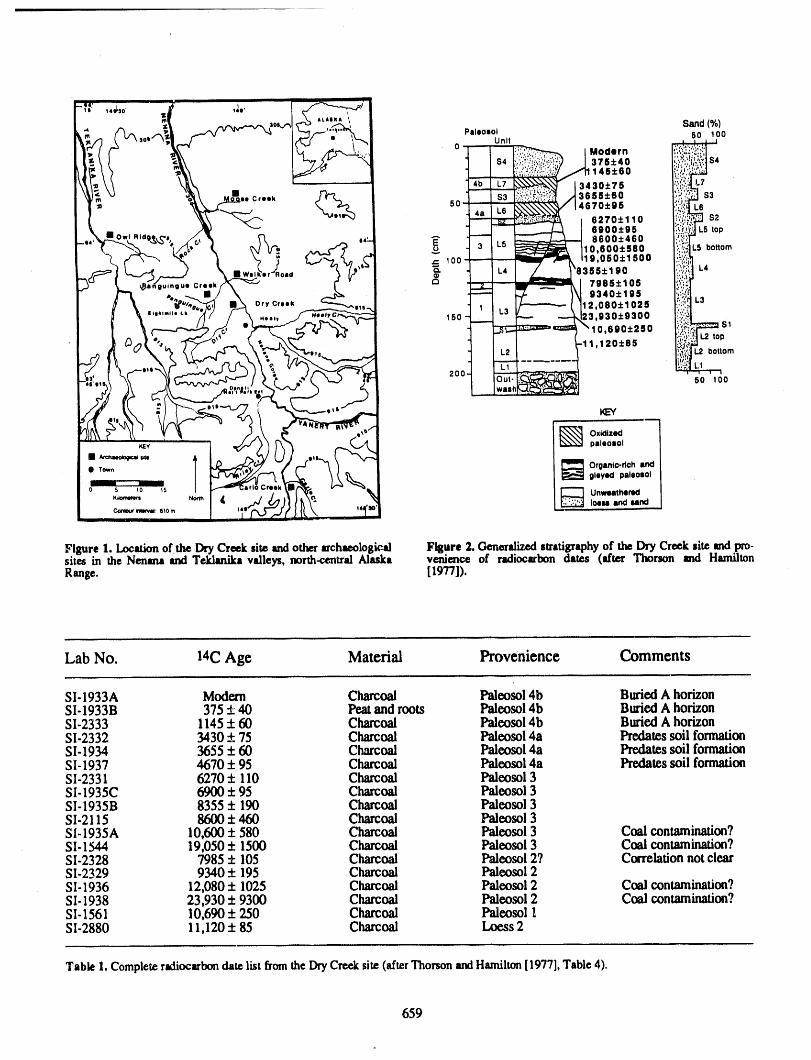
Figure I. Location of the DryCreek site and other archaeological Flgure 2. Generalized slradgraphyof the Dry Creek site and pm-sites in the Nemma and Teklanikmvalleys, north-cemralAlaska venience of radiocarbon dates (after Thorson and HamiltonRange. [1977]).

Lab No. 14C Age Material Provenience Comments

S1-1933A Modem Charcoal Palcosol 4b Buried A horizonSI-1933B 375:k40 Peatand roots Paleosol4b BuriedA horizonSI-2333 1145± 60 Charcoal Paleosol4b BuriedA horizonSI-2332 3430± 75 Charcoal Paleosol4a PredatessoilformationSI-1934 3655 ± 60 Charcoal Paleosol 4a Predates soil formationSI-1937 4670 ± 95 Charcoal Paicosol4a Predates soil formationSI-2331 6270± II0 Charcoal Paleosol3SI-1935C 6900± 95 Charcoal Paleosol3SI-1935B 8355± 190 Charcoal Paleosol3SI-2115 8600± 460 Charcoal l_Jeosol3Sl-1935A 10,600 ± 580 Charcoal Paleosol3 Coalcontamination?SI-1544 19,050± 1500 Charcoal Paleosol3 Coalcontamination?SI-2328 7985± 105 Charcoal Paleosol2? CorrelationnotclearSI-2329 9340 ± 195 Charcoal Paleosol 2SI-1936 12,080± 1025 Charcoal Paleosol2 Coalcontamination?SI-1938 23,930± 9300 Charcoal Palcosol2 Coal contamination?SI-1561 10,690 ± 250 Charcoal Paloosol !SI-2880 11,120 ± 85 Charcoal Logss 2

Table 1. Complete radiocarbondate list fromthe DryCreeksite (afterThorson andHamilton[1977], Table 4).

659

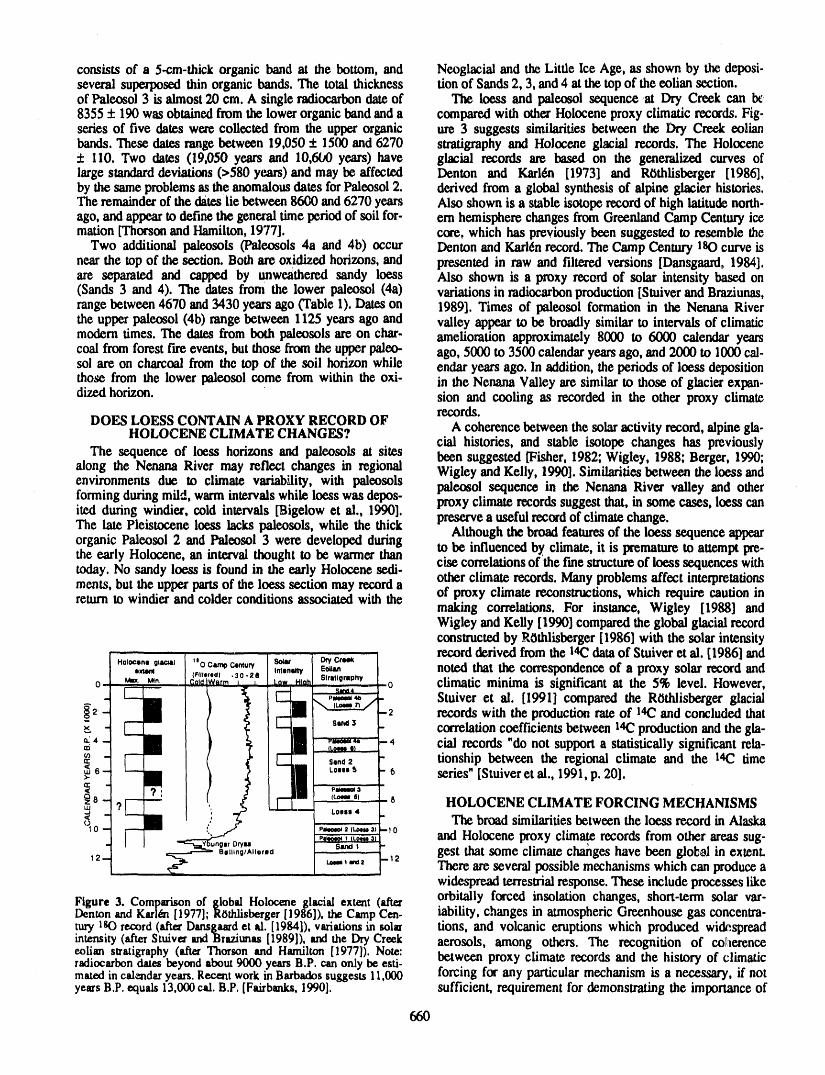
consistsofa 5-cre-thickorganicbandatthebottom,and NeoglacialandtheLittleIceAge,asshownby thedeposi-severalsuperposedthinorganicbands.The totalthickness tionofSands2,3,and4 atthetopoftheeoliansection.ofPaleosol3 isalmost20 cm.A singleradiocaubondateof The loessand paleosolsequenceatDry CreekcanIx.8355+ 190wasobtainedfromthelowerorganicbandanda comparedwithotherHoloceneproxyclimaticrec(xds.Fig-series of five dates were collected from the upper organic ure 3 suggests similarities between the Dry Creek eolianbands.These datesrange between 19,050 + 1500 and 6270 stratigraphyand Holocene glacial records. The Holocene

110. Two dates (19,050 years and 10,600 years) have glacial records are based on the generalized curves oflarge standarddeviations (>580 years) and may be affected Denton and Karl6n [1973] and R6thlisberger [1986],by the same problemsas the anomalousdates forPaleosol2. derived from a global synthesis of alpine glacier histories.The remainderof the dateslie between 8600 and 6270 years Also shown is a stable isotope recordof high latitudenorth-ago, and appearto definethe generaltime periodof soil for- em hemispherechanges from GreenlandCampCentury icemarion[Thorsonand Hamilton, 1977]. core, which has previously been suggested to resemble theTwo additionalpaleosols(Paleosols4a and4b)occur DentonandKarl6nrecord.TheCamp CenturyIsOcurveis

near the top of the section. Both are oxidized horizons, and presented in raw and filtezod versions [Dansgaard, 1984].are separated and capped by unweathered sandy loess Also shown is a proxy record of solar intensity based on(Sands 3 and 4). The dates from the lower paleosol (4a) variationsin radiocarbonproduction[StuiverandBraziunas,range between4670 and 3430 years ago (Table 1). Dateson 1989]. Times of paleosol formation in the Nenana Riverthe upper paleosol (4b) rangebetween 1125 years ago and valley appear to be broadly similar to intervals of climaticmodern times. The dates from both paleosols are on char. amelioration approximately 8000 to 6000 calendar yearscoal from forest f'n'eevents, bet those from the upperpaleo- ago, 5000 to 3500 calendaryearsago, and 2000 to 1000 cabsol are on charcoal from the top of the soil horizonwhile endaryears ago. In addition, theperiods of loess depositionthose from the lower paleosol come from within the oxi- in the Nenana Valley are similar to those of glacier expan-dized horizon, sion and cooling as recorded in the other proxy climate

records.DOES LOESS CONTAIN A PROXY RECORD OF A coherence between the solaractivity record,alpine gla-HOLOCENE CLIMATE CHANGES?

cial histories, and stable isotope changes has previouslyThe sequence of loess horizons and paleosols at sites been suggested [Fisher,1982; Wigley, 1988; Berger, 1990;

along the Nenana River may reflect changes in regional Wigley and Kelly, 1990]. Similaritiesbetween the loess andenvironments due to climate variability, with paleosols paleosol sequence in the Nenana River valley and otherformingduringmild, warmintervalswhile loess was depos-ited during windier, cold intervals [Bigelow et al., 1990]. proxyclimate records suggest that, in some cases, loess canpreservea useful recordof climate change.The late Pleistocene loess lacks paleosols, while the thick Although the broad featuresof the loess sequence appearorganic Paleosol 2 and Paleosol 3 were developed duringthe early Holocene, an interval thought to be warmer than to be influenced by climate, it is prematureto attempt ixe-today. No sandy loess is found in the early Holocene sedi- cise correlationsof'the free structureof loess sequences with

otherclimate records. Many problemsaffect interpretationsments, but the upperpartsof the loess section may recordareturnto windier and colder conditions associated with the of proxy climate reconstructions,which require caution in

making correlations. For instance, Wigley [1988] andWigley and Kelly [1990] compared the global glacial recordconstructedby ROthlisberger[1986] with the solar intensity

,o,_,. 0*._, %c,_oc,_,_ so_ _ c_.._ recordderived from the 14Cdata of Stuiver et al. [1986] and•,,,_ _,t.,_ e,_ noted that the correspondenceof a proxy solar record and(Ffllerea! • _0 • 218 Stratigraphyo- _ _, co,diw.,,, Lo..,o, -0 climatiC minima is significant at the 5% level. However,

I_ __IBil ..__actf_._

- _-- -- p,,,-,, / Stuiver et al. [1991] compared the ROthlisberger glacial_2 x (_" '_/ -2 records with the productionrate of 14Cand concluded that

, _ -....-..,_...., 4 cia] records "do not supporta statistically significant rela-_' - - tionship between the regional climate and the 14C timen- Send 2

_ 6- [] -o-s - 6 series" [Stuiver et al., 1991, p. 20].

;__ _ .....,_o...,, 8 HOLOCENE CLIMATE FORCING MECHANISMS

_s ------ Lo.,.• The broad similarities between the loess record in Alaska?

o p,,,.J2t_,..._)-10,,,o,_,,L__, andHoloceneproxyclimaterecordsfromotherareassug-

- , ),.,, ..s,_, - gestthatsomeclimatechahgeshavebeenglob_1inextent.t2- _.,,,,_-_2 Thereareseveralpossiblemechanismswhichcanproducea

widespreadterrestrialresponse.Theseincludeprocesseslike

Flgure3.ComparisonofglobalHoloceneglacialextent(after orbitallyforcedinsolationchanges,short-termsolarvar-DentonandKarl_[1977];R6thlisberger[1986]),theCampCen- lability,changesinatmosphericGreenhousegasconcentra-furyIsOrecord(afterDansgaardetal.[1984]),variationsinsolar tions,and volcaniceruptionswhichproducedwi_spreadintensity(afterStuiva andBraziunas[1989]),andthe DryCreek aerosols, among others. The recognition of coherenceeolian stratigraphy(after Thorsonand Hamilton [1977]). Note: between proxy climate records and the history of climaticradiocarbondatesbeyondabout9000yearsB.P. canonly beesti-matedincalendaryears.RecentworkinBarbadossuggests11,000 forcing for any particular mechanism is a necessary, ff notyearsB.P.equals 13,000cal. B.P.[Fairbanks,1990]. sufficient, requirementfor demonstrating the importance of

66O

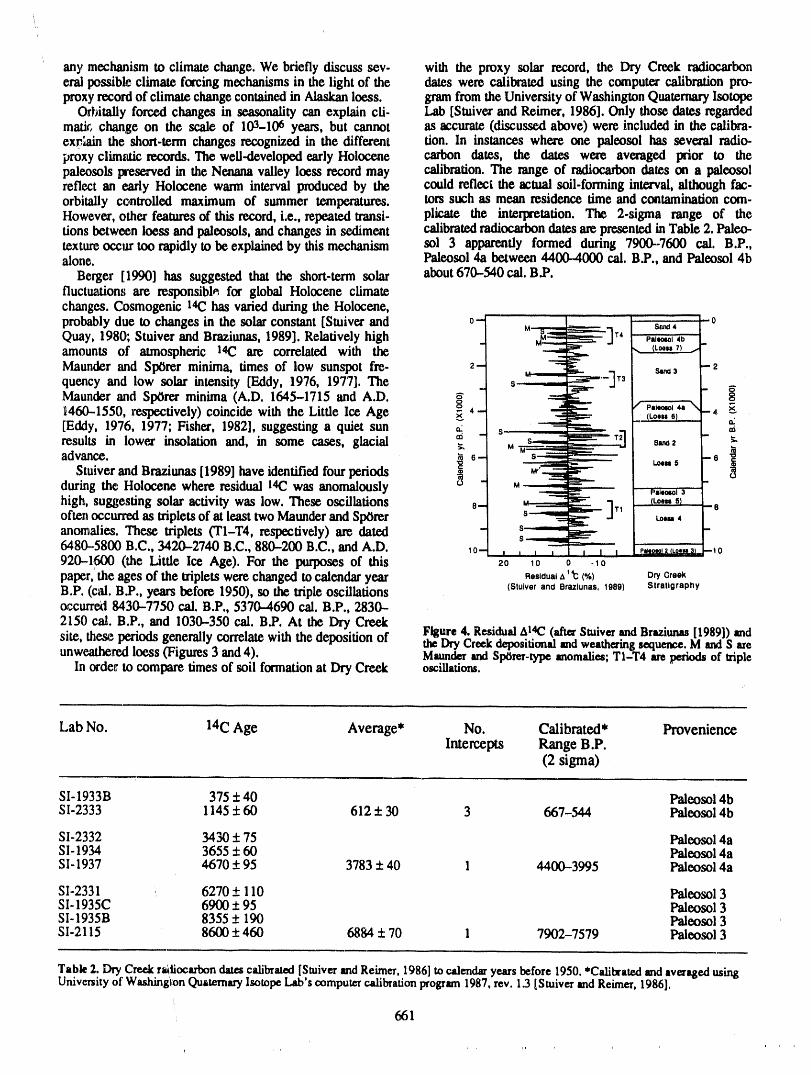
any mechanism to climate change. We briefly discuss sev- with the proxy solar record, the Dry Creek radiocarboneml possible climate forcing mechanisms in the light of the dates were calibrated using the computercalibration pro-proxyrecordof climatechangecontainedin Alaskanloess, gramfrom the University of WashingtonQuaternaryIsotope

Orbitally forced changes in seasonality can explain cfi- Lab [Smiver and Reimer, 1986]. Only those dates regardedmarie change on the scale of 103-106 years, but cannot as accurate(discussed above) were included in the calibra-explain the short-termchanges recognized in the different tion. In instances where one paleosol has several radio-proxyclimatic records. The well-developed early Holocene carbon dates, the dates were averaged prior to thepaleosols preserved in the Neaana valley loess record may calibration. The range of r_liocatr_n dates on a paleosolreflect an early Holocene warm interval produced by the could reflect the actual soil-forming interval, although fac-orbitally controlled maximum of summer temperatures, tors such as mean residence time and contaminationcom-However, other featuresof this record, i.e., repeatedtransi- plicate the interpretation. The 2-sigraa range of thetions between loess and paleosols, and changes in sediment calibratedradiocarbondates arepresentedin Table 2. Paleo-textureoccm"too rapidly to be explained by this mechanism sol 3 apparently formed during 7900-7600 cal. B.P.,alone. Paleosol 4a between 4400-4000 cal. B.P., and Paleosol 4b

Berger [1990] has suggested that the short-term solar about670-540 cal. B_P.fluctuations are responsible, for global Holocene climatechanges. Cosmogenic 14Chas varied duringthe Holocene,probablydue to changes in the solarconstant [Smiver and o- s,_, -oQuay, 1980; Stuiver and Brazianas, 1989]. Relatively high M-_ __r, P..._=,bamounts of atmospheric 14(2 are correlated with the " ---'-2--._- ,. _L**,,71_.-

Maunderand Sp6rer minima, times of low sunspot fie- 2- _"=_ s,_3 -2quency and low solar intensity [Eddy, 1976, 1977]. The s-------,_'-]r3 _

_ - -Maunder and Sp6rer minima (A.D. 1645-1715 and A.D. o "__ / _=,_o,A \M60-1550, respectively) coincide with the Little IceAge 8 4-[Eddy, 1976, 1977; Fisher, 1982], suggesting a quiet sun _ '--'--'"---" _'td

results in lower insolation and, in some cases, glacial '_ - . s.-.._ - _

advance.Stuiver and Braziunas[19891 haveidentified fourperiods _ ,_ _._.._ .

during the Holocene where residual 14(2was anomalously u_ _. P=.==3"'

high, suggesting solar activity was low. These oscillations 8- _ __- ]r_ I_" 51 -eoften occurredas tripletsof at least two Maunderand Sl_rer s_ __ Lo..,anomalies. These triplets ('I'1-'1"4,respectively) are dated - s---.----. _ -s

6480-5800 B.C., 3420-2740 B.C., 880-200 B.C., and A.D. 10- , _ , , I J t _ -10920-1600 (the Litre Ice Age). For the purposes of this 2o _o o -_opaper, the ages of the triplets were changed to calendar year ..=o_= A'_ (%) DryCreekB.P. (cal.B.P., years before1950), so the tripleoscillations (Stulver antiBraziunas.1989) Stratigraplly

occurr=t 8430-7750 cal.B.P., 5370-4690cal.B.P., 2830-2150 cal. B.P., and 1030-350cal. B.P. At theDry Creek

FIsure 4. ResidualA14C(after SmiverandBraziun_[1989])andsite, these periods generally correlatewith the deposition of theDryCreekdepositionalandweathea'ingUXluence.M andS areunweathered loess (Figures 3 and4). MaunderandSpOrer-typeanomalies;T1-T4 areperiodsof triple

In orde_rto compare times of soil formationat Dry Creek oscillations.

Lab No. 14C Age Average* No. Calibrated* ProvenienceIntercepts Range B.P.

(2 sigma)

SI-1933B 375 + 40 Paleosol 4bSI-2333 1145 4.60 612 4-30 3 667-544 Paleosol 4b

SI-2332 3430 + 75 Paleosol 4aSI-1934 3655 4.60 Paleosoi 4aSl-1937 4670 ± 95 3783 4. 40 I 4400--3995 Paleosol 4a

SI-2331 , 6270 + 110 Paleosol 3SI-1935C 6900 4.95 Paleosol 3SI-1935B 8355 4. 190 Paleosol 3SI-2115 8600 4-460 68844-70 1 7902-7579 Paleosol 3

Table2. DryCreekrtatiocarbondatescalibrated[SmiverandReimer.1986]tocalendaryearsbefore1950.*Calibratedandavea,egedusingUniversityof Washingi'.onQuaternaryIsotopeLab'scomputercalibrationprogram1987,tev. 1.3[SmiverandReimer,1986].

!

661

After calibrating lhc available radiocarbondates on the lion of atmospheric Greenhouse gases [Hansen and Lacis,Dry Creek paleosols, the apparent soil-forming intervals 1990], arid large volcanic eruptions [Vogel et al., 1990;seem to broadly fall between the times of triple oscillations Beg6t et al., 1901], although detailed Holocene recordsof(Figure4), although Paleosols 3 and 4b overlap with Trip- these forcing mech,_sms arenot well known.It is also pos-lets 1 and4. sible that there are other important mechanisms not con-

Although the proxy climate record from loess and the sidered here.proxy solar record of Stuiver and Brazitmas [1989] show

some agreement,thereare importantdifferences in the tim- ACKNOWLEDGMENTSing and duration of events. Although Berger [1990] hasargued that the short-term solar intensity variations of We acka_owledgediscussions about the Nenana ValleyStuiver and Braziunas must have strongly influenced Hol- sequence with Dr. Roger Powers, Dr. David Hopkins, Dr.ocene climates, it is likely that other mechanismsmodulated Robert Tho_'son, and Dr. Thomas Hamilton. We are alsoits effects. Other important sources of climatic forcing dm'- grateful for careful reviews of this manuscript by Dr.ing the Holocene may have been changes in the concentra- George Kukla and Dr. RichardReger.

REFERENCES

Beg6t, J., O. Mason, and P. Anderson, Age and extent of the Phippen, P. G., Archaeology at Owl Ridge: a Pleistocene--ca. 3400 BP Aniakchaktephra, western Alaska, The Holocene boundary age site in centralAlaska, Unpub-Holocene, 1, 1991, Irtpress, lished Master's Thesis, University of Alaska Fairbanks,

Berger, R., Relevance of medieval, Egyptian and American Fairbanks, hd(, 1988.dates to the study of climatic and radiocarbon variability, Powers, W. R., and J. F. Hoffecker, LatePleistocene settle-Phil. Trans.R. Soc. Lend. A, 330, 517-527, 1990. ment in the Nenana valley, central Alaska, American

Bigelow, N. H., J. Beg_t, and W. R. Powers, Latest Pleis- Antiquity, 54, 263-287, 1989.tocene increase in wind intensity recorded in eolian sedi- ROlhlisberger,F., 10 000 Jahre Gletschergeshichte derments from central Alaska, Quat. Res., 34, 160--168, Erde, VerlagSauerlander,Aaran, 1986.1990. Stuiver, M., and T. F. Braziunas, Atmospheric i4C and

Dansgaard, W., S. J. Johnsen, J. B. Clausen, and C.C. century-scale solar oscillations, Nature, 338, 405-408,Langway, Jr., North Atlantic climatic oscillations 1989.revealed by deep Greenland ice cores, in Climate Pro- Stuiver, M., and P. D. Quay, Changes in atmosphericcesses and Climate Sensitivity, edited by J. E. Hansenand Carbon-14attributedto a variablesun, Science, 207, li-T. Takahashi,pp. 288-298, Geophysical Monograph 29, 19, 1980.AmericanGeophysical Union, Washington,DC, 1984. Stuiver,M., and P. J. Reimer, A computerprogramfor radi-

Denton, G. H., and W. Karl6n, Holocene climatic earl- ocarbon age calibration, Rach'ocarbon, 28, 1022-1030,ations---lheir pattern and possible cause, Quat. Res., 3, 1986.155-205, 1973. Stuiver, M., G. W. Pearson, and T. F. Braziunas, Radio-

Eddy, J. A., The Maunder minimum, Science, 192, 1189- carbon age calibration of marine samples back to 90001202, 1976. eal yr B.P., Radiocarbon, 28, 980-1021, 1986.

Eddy, J. A., Climate and the changing stm, Climagic Stuiver, M., T. F. Braziunas, and B. Becker, Climatic, solar,Change, 1,173-190, 1977. oceanic, and geomagnetic influences on Late-Glacial and

Fairbanks, R. G., The age and origin of the "Younger DE/as Holocene atmospheric 14C/12Cchange, Quat. Res., 35,Climate Event" in Greenland ice cores,Paleo- 1-24,1991.oceanography, 5, 937-948, 1990. Thorson, R. M., and T. D. Hamilton, Geology of the Dry

Fisher, D. A., Carbon-14 production compared to oxygen Creek site: a stratified early man site in interior Alaska,isotope records from Camp Century, Greenland and Quat. Res., 7, 149-176, 1977.Devon Island, Canada, Climatic Change, 4, 419--426, Vogel, J. S., W. Cornell, D. E. Nelson, and J. R. Southon,1982. Vesuvius/Avellino, one passible source of seventeenth .

Hansen, J. E., and A. A. l..acis, Sun and dust versus green- century B.C. climatic disturbances, Nature, 334, 534--house gases: an assessment of their relative roles in glo-- 537, 1990.bal climate change, Nature, 346, 713-719, 1990. Wigley, T. M. L., The climale of the past 10,000 years and

Kukla, G., F. Helle.r, X. M. Liu, T. C. Xu, T. S. Liu, and the role of the sun, in Secular Solar and GeomagneticZ.A. An, Pleistocene climates in China dated by mag- Variations in the Last 10,000 Years, ecfited by F. R.netic susceptibility, Geology, 16, 811-814, 1988. Stephenson and A. W. Wolfendale, pp. 209-224, Kluwer,

Maxwell, H. E., Archeology and Panguingue Creek: a Late 1988.Pleistocene/Early Holocene-aged site in central Alaska, Wigley, T. M. L., and P. M. Kelly, Holocene climaticUnpublished Master's Thesis, University of Alaska Fair- change, 14C wiggles and variations in solar irradiance,banks, Fairbanks, AK, 19_o7. Phil. Trans.R. Soc. London A, 330, 547-560, 1990.

662

Comparisons of Late Quaternary Climatic DevelopmentBetween the Arctic and Antarctic Through Calcareous Nannofossils

G.GardDepartmentof Geology,UniversityofStockholm,Stockholm,Sweden,U.S.A.

J. A. CruxBPExplorationInc.,Houston,Texas,U.S.A.

ABSTRACTThe content of calcareous nannofossils (_mnants of microscopic planktonic

algae) have been documentedin numeroussediment cores from the NorwegianandGreenland Seas and in ODP Hole 704A from the subantarcticSouth Atlantic.Worldwide species extinctions, inceptions and distinct abundancevariations havebeen used to correlateand date the studied cores, which comprise the last 500,000years. The biostratigraphyhas been correlatedto oxygen isotope stratigraphywhichshows thatintervalsrichin nannofossils represent interglacialtime periods.

The calcareous nannofossils indicatethat duringthe timeperiod studied, climaticfluctuationswere similar in characterand timing in both the subarcticand the sub-antarctic South Atlantic. Abundance patternsof warm water species suggest thatsurfacewaters were warmerthan todayonly duringoxygen isotope substage 5e (thelast interglacial). The environmentwas interglacialalso duringisotope stages 9, 1I,and 13, while stages 3 arid8 may have been characterizedby intermediateglacialconditions. A significa!) rl_ycolder environmentthan at present prevailed in isotopestages 2, 4, 6, I0 and _2. Isotope stage 7 appearsto have been fully interglacial inthe subantarctic South 'Atlantic,but intermediate glacial in the Norwegian sea.

663

Japanese Ice Core Studies in the Polar Regions

O. Watanabe, Y. Fujii, an!_ F. NishioNational Institute of Polar Research, Tokyo, Japan

H. NaritaInstitute of Low Temperature Science, Hokkaido University, Sapporo, Japan

M. NakawoNagaoka Institute of Snow and Ice Studies, National Research Center for Disaster Prevention,

Science and Technology Agency, Nagaoka, Japan

H. ShojiFaculty of Science, Toyama University, Toyama, Japan

ABSTRACT

A 2500-m-deep ice core drilling project is planned by Japanese glaciologists atthe top of the ice sheet in Queen Maud Land, the second highest dome of the Ant-arctic ice sheet. The deep drilling will be carried out during 1993-1995 at a newinland base (77°22'S, 39°37'E, 3807 m a.s.l.), I000 km away from Syowa Station(69°00'S, 30°35'E).

The purpose of this project is to reconstruct climatic and environmental recordsduring the past 15-20K years and also to obtain glaciological data relating to the icesheet formation and the mass balance processes.

This deep drilling is a project developed from a series of drilling projects startedat Mizuho Station in 1971. In August 1984, drilling at Mizuho Station reached adepth of 700.6 m. This core is estimated to cover the last 9400 years.

Ice core drilling in the Arctic and also in the third polar region, i.e., theHimalayas and Kunlun Mountains, was also carried out in recent years. In 1983,

: glacier drilling to a depth of 70 m at 5400-m elevation in the Himalayas, and 86-m-deep drilling to the bottom in Svalbard were accomplished in 1987. A 205-m-deepdrilling was carried out in southern Greenland in 1989.

In this paper, the results obtained by these drilling projects will be reviewed andthe prospect of our new drilling projects will be introduced.

664

Onthe Development in Elaboration of Polar Ice Core Gas Content Analysis

J. P. SemiletovPacific Oceanological Institute, Far Eastern Branch of the U.S.S.R. Academy of Sciences, Vladivostok, U.S.S.R.

ABSTRACT

Differences between CO2 concentrations in ice cores measured by "dry" or"wet" methods are attributed to carbonate contamination of the ice core surfaces[Raynaud et al., 1982]. However, the contribution of natural carbonates in CO2content may amount to-.20 Mg kg-I of ice [Neftel et al., 1982] which correspondsto ~100 ppm CO2. TIC valuesdiffer from the CO2 concentration in the case ofslow wet extraction (~1 h). These differences may be partly connected withfractionation in the system gas-ice+gas hydrate when an ice core sample is crushedimperfectly [Barnola et al., 1983]. In the estimation of CO2 presence in the CO2-ice matrix, the contribution of total gas content (VG) is also needed, lt depends onthe level of transformation, waterdrop,snowflake.

For the Antarctic coastal regions these levels correspond to atmosphericpressures of about 700-800 mbar and for continental sites, for example Vostok,~600--650 mbar. There, precipitation is connected with the entry of snow by strato-spheric genesis in the central Antarctic. In this case, snow CO2 content is aboutzero and more "rich" coastal snow contains about 70-80% from equilibriumconcentration nem"sea level. In consequence, the maximal contribution in VGvalues is about 15-20%. The detailed investigation of this question may beeffective for obtaining more precise data on VG stratifications in ice cores.

A new head-space technique of CO2 and other gas content investigations in icecore is elaborated. Data obtained in 34 Soviet Antarctic Expeditions and in laborat-ory experiments are discussed.

665

Evolution of Southern Indian Ocean Surface and Deep WatersDuring the Paleogene as Inferred From Foraminiferal Stable Isotope Ratios

E. BarreraDepartmen!ofGeologicalSciences,TheUniversityof Michigan,AnnArbor,Michigan,U.S.A.

B. T. HuberDepartmentofPaleobiology,SmithsonianInstitution,Washington,D.C.,U.S.A.

ABSTRACT

During ODP Leg 119, the southernmost pelagic record of carbonate sedi-mentation of Neogene-Paleogene age in the southernIndian Ocean was recoveredat Site 744 (61°34.6'S, 80°35.46'E;water depth2307 m) and Site 738 (62°42.54'S,82°47.25'E; water depth 2252 m) in the southern part of the Kerguelen-HeardPlateau. Site 744 late Eocene-Miocene sequence and Site 738 Late Cretaceous-early Oligocene sequences contain continuous records of climatic events in EastAntarctica during this time.

Oxygen isotopic ratios of planktonic and benthic foraminifera suggest thefollowing climatic changes: (1) a cool Paleocene, although with highertemperatures than those inferred from published Pacific and southern SouthAtlantic 8180 records; (2) the early Eocene was characterized by the warmest deepand surface waters of the Cenozoic, which were similar in temperature to thosefrom low latitude areas; (3) cooling began in the early- middle Eocene and contin-ued through the remainder of the Eocene (Eocene Cibicidoides 8180 values are notvery different from those of low-latitude sites); (4) a rapid increase in Cibicidoides_5180 values (1-1.5%o) occurred in the early Oligocene of Site 744. Ice-raf_ddebris, f'ast recorded in sediments just below the _5180maximum, are also fountl inthe early Oligocene sequence. Oligocene-early Miocene Cibicidoides _il80 valuesof about 2%0 and the presence of ice-rafted debris are considered evidence forglacial conditions in Antarctica.

Planktonic foraminiferal assemblages indicate a similar climatic trend. Speciesdiversity was highest during the latest Paleocene and earliest Eocene. It declinedduring the middle-late Eocene and the low diversity Oligocene faunas were domin-ated by a few globigerine taxa that are long-ranging and morphologicallyconservative.

F

666

' ' r_,, , nlr ,

Surface Currents in the Arctic Ocean During the Last 250 ka:Composition of Ice.Rafted Detritus (IRD) as a Key for Ice Drift Directions

i

M. Kubisch and R. F. SpielhagenGeomar,Forschungszentrumfiir MarineGeowissenschaften,Kiel,Germany

ABSTRACT

Eleven long sediment cores from the Arctic Ocean and Fram Strait (78°.86°N)documenting more than 250,000 years of sedimentation history show distinct vari-ations in the composition of coarse sand (500 gin).

Ice-rafted coal fragments deposited during glacial oxygen isotope stages 6 (186-128ka) and 8 (303-245ka) are evidence for ice drift from the Eastern Arctic Oceanthrough Fram Strait to the Norwegian Sea.

The dominating lithologies, with a high amount of sedimentary rock fragmentsin the IRD from interglacial stages (7, 5, 1), indicate a similar current pattern astoday.

Crystalline rock fragments in glacial sediments decrease from the Barents Shelfmargin to the Nansen-Gakkel Ridge where they are replaced by quartzites andcherts.

667

Sediment.Laden Sea Ice in the Arctic Ocean:Implications for Climate, Environment and Sedimentation

I. R. WollenburgGEOMAR, Research Center for Marine Geosciences, Kiel, Germany

S. L. PfirmanLamont-Doherty Geological Observato_, Palisades, New York, U.S.A.

M. A. LangeAlfred Wegener Institut for Polar- and Marine Research, Bremerhaven, Germany

ABSTRACTSediments in sea ice were first describedby F. Nansen duringhis famous "Fram

expedition (1893-1896). Many researchersobserved and recorded sediment-ladenor "dirty" sea ice in the CentralArctic, but the originand incorporationmechanismsarepoorly understoodand were never the object of detailed studies. Sea ice-raftedsediments are importantfactors for the albedo and for the ecology and productivityof marineorganisms, because of the absorptionof solar radiationand lowered lighttransmission.

Beginning in 1987 in the EasternArctic Basin and continuing in 1988, 1989 and1990 in Fram Strait, Barents Sea and Greenland Sea we conducted a multi-disciplinary sea ice project "on the role and importanceof sea ice-rafted sedimentsfor sedimentation in the Arctic Ocean."During the field work very high sedimentaccumulations were observed and sampled(up to 560 g sediment/kg ice). Most ofthe materialwas concentratedin small patches of 1-10 m in diameter, but in someareas, especially in the Eastern Arctic, they covered up to 80% of the ice surfaceand formed layersof puremud, 2-3 cm thick.

First estimations of the observed concentrations, the annual ice flow throughFram Strait,and the average sedimentationratein this area show that the necessarysediment flux can be obtained only by sea ice. Thus, sea ice-rafting seems to be themost important input mechanism of fine grained terrigenous (biogenic andterrigenic) sediment into the ice-covereddeep sea regions.

668

Environmental Marine Geology of the Arctic Ocean

P. J. MudieGeologicalSurveyCanada,AtlanticGeoscienceCentre,Dartmouth,Nova Scotia,Canada

ABSTRACT

The Arctic Ocean and its ice cover are major regulators of Northern Hemisphereclimate, ocean circulation and marine productivity. The Arctic is also very sensitiveto changes in the global environment because sea ice magnifies small changes intemperature, and be,cause polar regions are sinks for air pollutants. Marine geologystudies are being carried out to determine the nature and rate of these environmentalchanges by study of modem ice and sea bed environments, and by interpretation ofgeological records imprinted in the sea floor _diments. Sea ice camps, an iceisland, and polar icebreakers have been used to study both western and easternArctic Ocean basins. Possible early warning signals of environmental changes inthe Canadian Arctic are die-back in Arctic sponge reefs, outbreaks of toxicdinoflagellates, and pesticides in the marine food chain. Eastern Arctic ice andsurface waters are contaminated by freon and radioactive fallout from Chernobyl.At present, different sedimentary processes operate in the pack ice-coveredCanadian polar margin than in summer open waters off Alaska and Eurasia. Thegeological records, however, suggest that a temperature increase of 1-4°C wouldresult in summer open water throughout the Arctic, with major changes in oceancirculation and productivity of waters off Eastern North America, and morewidespread transport of pollutants from eastern to western Arctic basins. More stud-ies of longer sediment cores are nee4_d to confirm these interpretations, but is isnow clear that the Arctic Ocean has been the pacemaker of climate change duringthe past 1 million years.

669

Section G:

Aerosols/Trace Gases

Chaired by

L. BarrieAtmospheric EnvironmentService

Canada

G. ShawUniversity of Alaska Fairbanks

U.S.A.

Chemical Changes in the Arctic Troposphere at Polar Sunrise

L. A. BarrieAtmosphericEnvironmentService,Ontario,Canada

ABSTRACT

At polar sunrise, the Arc,ric troposphere (0 to -8 km) is a unique chemicalreactor influenced by human activity and the Arctic Ocean. It is surrounded byindustrialized continents that in winter contribute gaseous and particulate pollution(Arctic haze), lt is underlain by the flat Arctic Ocean from which it is separated bya crack-ridden ice membrane 3 to 4 m thick. Ocean to atmosphere exchange of heat,water vapor and marine biogenic gases influence the composition of the reactor.From 21 September to 21 December to 21 March, the region north of the Arcticcircle goes from a completely sunlit si'marion to a completely dark one and thenback to light. At the same time the lower troposphere is stably stratified. This hin-ders vertical mixing.

In this environment, chemical reactions involving sunlight arc much slower thanfurther south_ Thus, it would not be surprising to find a high abundance of photo-chemically reactive compounds in the atmosphere at polar sunrise. Between com-plete dark in 'February and complete light in April, a number of chemical changes inthe lower troposphere are observed. Perhaps the most sensational is the destructionof lower tropospheric ozone accompanied by production of fdterable bromine andiodine. The latter are likely of marine origin, although their production may involveanthropogenic compounds. Another change is the shift in the fraction of total sulfurin its end oxidation state (VI) from 50% to 90%. Several gaseous hydrocarbonsdisappear from the atmosphere at this time. Preliminary observations also indicate amaximum in total non-black carbon on paniculate matter. This is consistent withthe formation of non-volatile organics from photochemically induced reactions ofgas phase organics. Results of the Canadian Polar Sunrise Experiment 1988 arepresented.

013

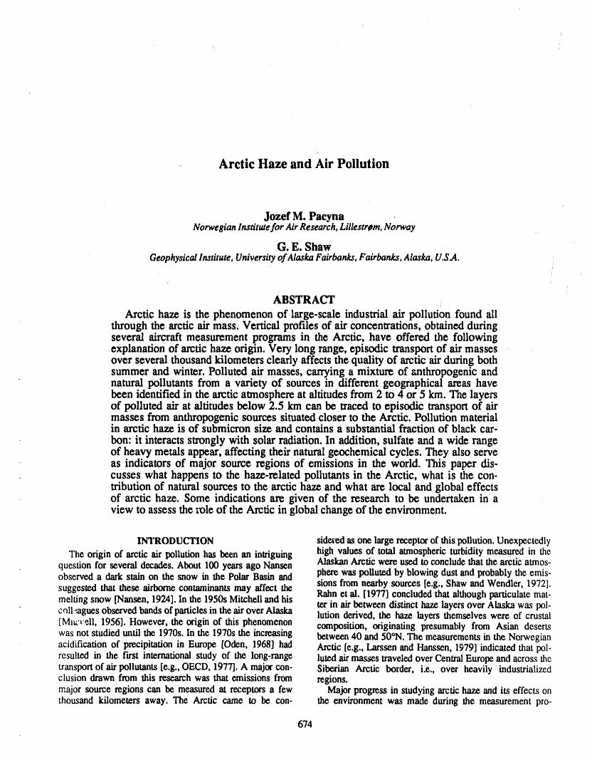
Arctic Haze and Air Pollution

Jozef M. PacynaNorwegian Institute for Air Research, Lillestrem, Norway

G. E. ShawGeophysical Institute, University of Alaska Fairbanks, Fairbank$, Alaska, U.S.A.

ABSTRACTArctic haze is the phenomenon of large-scale industrial air pollution found ali

through the arctic air mass. Vertical profiles of air concentrations, obtained duringseveral aircraft measurement programs in the Arctic, have offered the followingexplanation of arctic haze origin. Very long range, episodic transport of air massesover several thousand kilometers clearly affects the quality of arctic air during bothsummer and winter. Polluted air masses, carrying a mixture of r,nthropogenic andnatural pollutants from a variety of sources in different geographical areas havebeen identified in the arctic atmosphere at altitudes from 2 to 4 or 5 km. The layersof polluted air at altitudes below 2.5 km can be traced to episodic transport of airmasses from anthropogenic sources situated closer to the Arctic. Pollution materialin arctic haze is of submicron size and contains a substantial fraction of black car-bon: it interacts strongly with solar radiation. In addition, sulfate and a wide rangeof heavy metals appear, affecting their naturalgeochemical cycles. They also serveas indicators of major source regions of emissions in the world. This paper dis-cusses what happens to the haze-related pollutants in the Arctic, what is the c0n-tributionof naturalsources to the arctic haze and what are local and global effectsof arctic haze. Some indications are given of the research to be undertakenin aview to assess the role of the Arcticin global change of the environment.

INTRODUCTION sideaedas one large receptor of this pollution. Unexpectedly

The origin of arctic air pollution has been an intriguing high values of total atmosphericturbidity measured in thequestion for several decades. About 100 years ago Nansen AlaskanArctic were used to conclude that the arctic atmos-observed a dark stain on the snow in the Polar Basin and phere was polluted by blowing dust and probably the emis-

sions from nearby sources [e.g., Shaw and Wendler, 1972].suggested that these airborne contaminants may affect the Rahn et al. [1977] concluded that although particulatemat-melting snow [Nansen, 1924]. In the 1950s Mitchell and his terin airbetween distinct haze layers over Alaska was pol-colleagues observed bandsof particlesin the air over Alaska lution derived, the haze layers themselves were of crustal[Mi_'i.'ell, 1956]. However, the origin of this phenomenon composition, originating presumably from Asian desertswas not studied m_dlthe 1970s. In the 1970s the increasing between40 and 50°N. The measurementsin the Norwegianacidification of precipitation in Europe [Oden, 1968] had Arctic [e.g., Larssenand Hanssen, 1979] indicated that pol-resulted in the Fast international study of the long-range luted air masses traveled overCentral Europe and across thetransport of air pollutants [e.g.,OECD, 1977]. A major con- Siberian Arctic border, i.e., over heavily industrializedclusion drawn from this research was that emissions from regions.major source regions can be measured at receptors a few Majorprogress in studying arctic haze and its effects onthousand kilometers away. The Arctic came to be con- the environment was made during lhc measurement pro-

674_

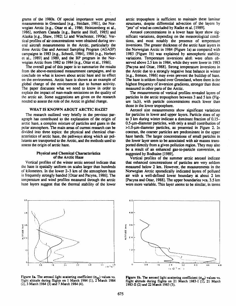
h

grams of the 1980s. Of special importance were ground arctic troposphere is sufficient to maintain these laminarmeasurements in Greenland [e.g., Heidam, 1981], the Nor- structures, despite differential advection of the layers bywegian Arctic [e.g., Ottar et al., 1986; Heintzenberg et al., "jets"of wind asconcluded by Radke et al. [1989].1986], northern Canada [e.g., Barrie and Hoff, 1985] and Aerosol concentrations in a lower haze layer show sig-Alaska [e.g., Shaw, 1982; Li and Winchester, 1990a]. Vet- nificant variations, depending on the meteorological condi-tical prof'flesof airconcentrations were obtainedduring sev- tions, and most notably the presence of temperatureeral aircraft measurements in the Arctic, particularly the inversions. The greater thickness of the arctic haze layers inthree Arctic Gas and Aerosol Sampling Program (AGASP) the Norwegian Arctic in 1984 (Figure la) as compared withcampaigns in 1983 [e.g., Schnell, 1984], 1986 [e.g., Herbert 1983 (Figure lb) was explained by atmospheric stabilityet al., 1989] and 1989, and the BP program in the Nor- variations. Temperature inversions aloft were often ob-wegian Arctic from 1982 to 1984 [e.g,, Ottar et al., 1986]. served above 2.5 km in 1984, while they were lower in 1983

The overall goal of this paperis to summarize the results [Pacyna and Ottar, 1988]. Strong temperature inversions infrom the above-mentioned measurement campaigns, and to the Arctic due to a strongly negative heat balance in winterconclude on what is known about arctic haze and its effect [e.g., Benson, 1986] may even prevent the buildup of haze.on the environment. Arctic haze is shown as an example of The haze is seldom found over Greenland, where there is theglobal change of the environment due to human activity, highest frequency of inversion gradients, stronger than thoseThe paper discusses what we need to know in order to measured in other parts of the Arctic.explain the impact of man-made emissions on the quality of The measurements of vertical profiles revealed layers ofthe arctic air. Some suggestions are given on the research particles in the arctic troposphere between 3 and 5 km (Fig-needed toassess the role of the Arctic in global change, use la,b), with panicle concentrations much lower than

those in the lower troposphere.WHAT IS KNOWN ABOUT ARCTIC HAZE? Aerosol size measurements show significant variations

The research outlined very briefly in the previous par- for particles in lower and upper layers. Particle sizes of upagraph has contributed to the explanation of the origin of to 3 km during winter indicate a dominant fraction of 0.15-arctic haze, a complex mixture of particles and gases in the 0.5-I.tm-diameterparticles, with only a small contribution ofpolar atmosphere. The main areas of current research can be > 1.0-1am-diameterparticles, as presented in Figure 2. Individed into three topics: the physical and chemical char- contrast, the coarser particles are predominant in the upperacteristics of arctic haze, the pathways along which air pol- haze bands. The larger concentrations of small particles inlutants are transported to the Arctic, and the methods used to the lower layer seem to be associated with air masses trans-assess the origin of arctic haze. ported directly from a given pollution region. They may also

be a result of an enhanced gas-to-particle conversion, asPhysical and Chemical Characteristics suggestedby Bodhaine[1989].

of the Arctic Haze Vertical profiles of the summer arctic aerosol indicateVertical profiles of the winter arctic aerosol indicate that that enhanced concentrations of particles are very seldom

the haze is spatially uniform on scales larger than hundreds measured below 2 km. However, the measurements in theof kilometers. In the lower 2-3 km of the atmosphere haze Norwegian Arctic sporadically indicated layers of pollutedis frequently strongly banded [Ottar and Pacyna, 1986],The air with a well-clefmed lower boundary at about 2 kmtemperature and wind profiles measured through the arctic [Pacyna and Ouar, 1988]. The upperboundaries >ca. 3.5 kmhaze layers suggest that the thermal stabili.ty of the lower were more variable. This layer seems to be similar, in terms

60. 60

8 \(, ) 48

\ ...,°°..'°°""\\ o.,.o....'""

', \_ ....'"'

_36. _ 3,6 ' 3

! "".. 2 ",, .......... f/._ ', / /..../

12 (

"" ,., "''t'"".... "' (_t.1_.... ................ .2 ..:..._0 O'B 1'6 214 312 t4'O t,'t, 8 0 0 fl 1.6 2 4 3 ? 4 0 4 4 4 8

, 10"_ m-t

1_I0-_ m '' )

Figure la. The eerosollight scatteringcoefficient(ota) valuesvs. Figurelb. Theaerosollight scatteringcoefficient(ota) valuesvs.flightaltitudeduringflightson 1 March1984 (1), 2 March1984 flightaltitudeduringflights on 21 March 1983-I(1), 21 March(2),3 March1984(3) and7 March1984 (4). 1983-II(2) and22March1983 (3).

675

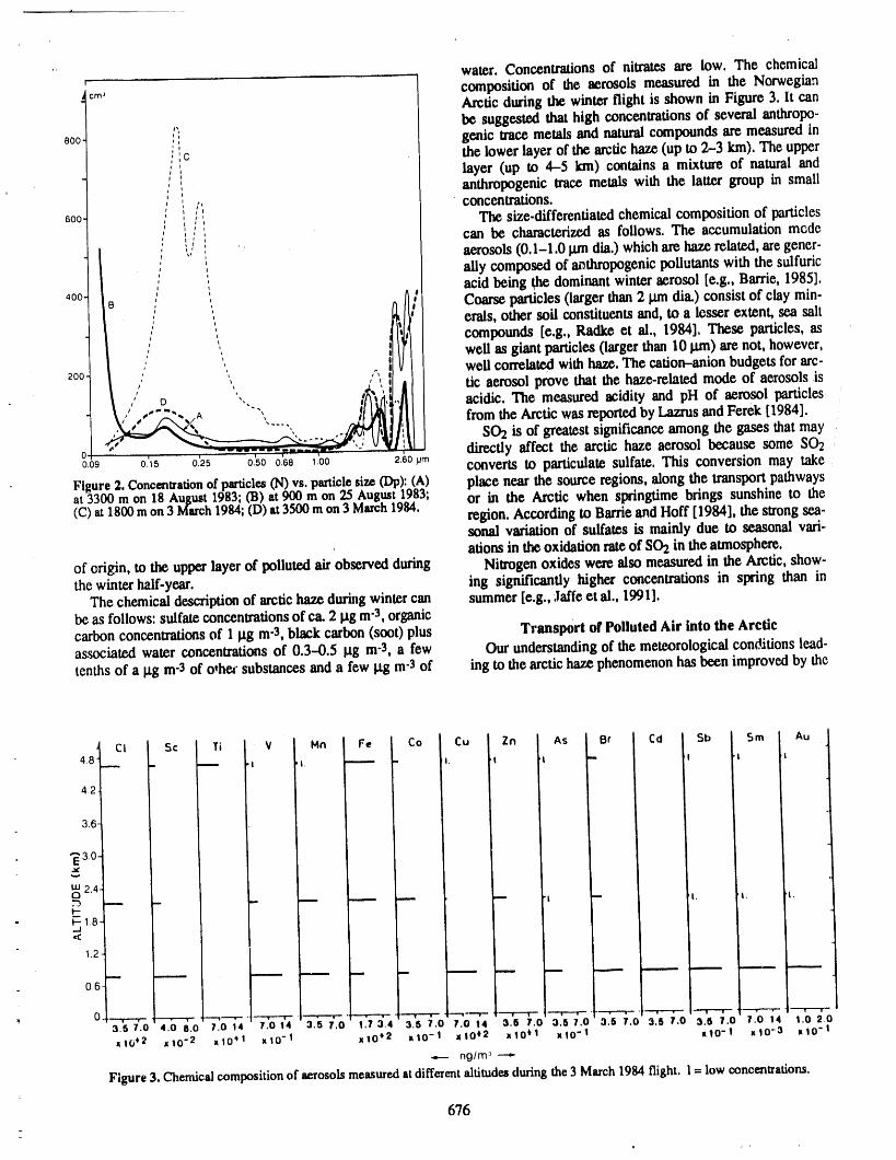
water. Concentrations of nitrates are low. The chemicalcomposition of the aerosols measured in the Norwegian

cre, Arctic duringthe winter flight is shown in Figure 3. lt canbe suggested that high concentrationsof several anthropo-

soo- , genic trace metalsand naturalcompounds are measured ini c the lower layer of the arctichaze (up to 2-3 km). The upper: layer (up to 4-5 km) contains a mixture of natural andi anthropogenic trace metals with the latter group in small

concentrations.i ,,'_ The size-differentiatedchemical composition of particlesj

600 : ,: , ,: can be characterized as follows. The accumulation mode

: ',,' aerosols(0.I-I.0Ixmdia.)whicharehazerelated,aregener-

: ', ally composed of ai_thropogenicpollutants with the sulfuric', acid being the dominantwinteraerosol [e.g., Barrie, 1985].

,_00 : ', ^ I ', ,,, Coarse particles (largerthan2 _undia.) consist of clay min-

B ,' , li I, [I' erals, other soil constituentsand, to a lesser extent, sea salt', I,I compounds [e.g., Radke ct al., 1984]. These panicles, as

" ", 'i well as giant particles (largerthan 10 pjn) arenot, however,20 , ,-, I wellcorrelatedwithhaze.Thecation-anionbudgetsforarc-

'"' ' ' ' I tic aerosol prove that the haze-relatedmode of aerosols is,,' D , -.. ....... acidic. The measured acidity and pH of aerosol particles,,, "2-, A ', ._J/l_ ' from the Arctic was reportedby Lazrusand Ferek[1984].

,_ /'_ ..... ' ,,)_'_ I SO2 is of greatestsignificanceamong the gases that mayL,_ ",---=_,C ' :ll diw_fly affect the arctic haze aerosol because some SO2..... =-.-...-.---oo9 o'_s o'2s oso 068 Ioo 28o,m converts to particulate sulfate. This conversion may take

Figure2. Concentrationof particles(N)vs.particlesize (Dp):(A) piace near the source regions, along the transportpathwaysat 3300m on 18 August1983;(B) at 900ra on 25 August1983; or in the Arctic when springtime brings sunshine to the(C) at1800mon 3 March1984;(D)at3500raon3 March1984. region. Accordingto Barde and Heft [1984], the strong sea-

sonal variation of sulfates is mainly due to seasonal vari-ations in the oxidation rateof SO2 in the atmosphere.

of origin, to the upperlayer of polluted air observed during Nitrogen oxides were also measuredin the Arctic, show-the winterhalf-year, ing significantly higher concentrations in spring than in

The chemical descriptionof arctichaze duringwintercan summer[e.g., Jaffe ctal., 1991].be as follows: sulfateconcentrationsof ca. 2 I.tgm"z,organiccarbon concentrationsof 1 _tg m-Z,black carbon (soot) plus Transport of Polluted Air into the Arcticassociated water concentrationsof 0.3-0.5 ttg m-Z, a few Our understandingof the meteorological conditions lead-tenths of a I_gm-3of o*he_-substances and a few I.tgm-3of ing to the arctic haze phenomenonhas been improvedby the

Cd Sb Sm AuCI Sc Ti V Mn Fe Co Cu Zn As Br

48 _ .._ l --- -

4,2

3.6,

_ao-e I

m2'4 _-

C3 ------ _ t -- t. t. t.t-

• t-- 1.8-_J< I

0.6

__ 0 3._7.0''4.0 8,0' 7;0i4 . -'_%3.s1.7a.4 3,'5_.0T.014 _.s 1.0 a.57.0 .si.o s:si,o _.67.0 _,0_4 _,0_,0x10_2 xl0 -2 xl0 '_1 xlO -1 _tlO +2 _10-1 xlOt2 xlO tl x10"1 xlO'l x10"3 _10 "1

ng/m _ --*

Figure3. Chemicalcompositionof aerosolsmeasuredatdifferentaltitudesduringthe3 March1984 flight. 1= low concentrations.

676

_

introduction of the quasi-isentropic trajectory concept by metal production, combustion of coal and oil to produceCarlson [1981] and Iversen [1984]. Two interpretationsof electricity and heat, and steel and iron manufacturing.Con-long-range transportof polluted air to the Arctic areoffered, sumptionof gasoline containing at least 0.4 g Pb l-I adds toIversen [1989] suggests that regional blocking is a basic the formation of small particles which are subject to long-flow phenomenon causing this transport.Regional blocking range transport. The emissions from the Urals and theis conditioned by interferencebetween stationaryplanetary Norilsk areaseem to be more importantfor the contamina-waves forced by orography and ground level heating, and tion of air over Alaska and the CanadianArctic, while thelow frequency transient waves created by baroclinic sources on the Kola Peninsula contributemore to the Nor-instability, wegian Arctic. The contributionof Europeanemissions to

Raatz and Shaw [1984] suggested that anticyclones play the Arctic aerosol is lower than that from the Russianthe dominantrole in providing theproper conditions for the sources, particularly in Alaska and the Canadian Arctic.trans,9ortof air pollutants to the Arctic.The authors suggest Duringsporadicsummer transportof pollutants to the Arcticthe following sequence of events: (a) a period of accumula- at altitudes below 2-3 km, emissions from sources intion of aerosols over the source region, (13)a synoptic situa- Europe seem to be more important than those from thetion of acceleratedair flow towards the Arctic,and (c) rapid Soviet Union. The North American source contribution intransportacross the Arctic, summer is also evident. Pollutedair masses,carryinga mix-

ture of anthropogenic and natural air pollutants from aOrigin of the Arctic Air Pollution varietyof sources in different geographicalareas, have been

Majorprogress in studying the originof the arcticair pol- identified in the Arctic at altitudesof 4 to 5 km duringbothlutionwas made when the informationon the chemical com- summerand winter.Facyna and Ottar[1989] concluded thatposition of the arctic aerosol became available. Rabn and long-rangetransportof airborneloess from deposits in Asiacolleagues [e.g., Lowenthal and Rabn, 1985] have devel- and Africa can reach the Arctic at these altitudes. Furtheroped the chemical fingerprinting system which uses the con- information summarizing the results of the arctic hazecentration ratios of various anthropogenic trace metals to research is available from reports by Barrie [1985] anddistinguish between contributions from various source Shaw andKhalil[1989].regions to the contamination of the arctic air.

Various dispersion and receptor models were used to WHAT INFORMATION ON ARCTIC HAZEdetermine the origin of arctic aerosols. A trajectoryLagran. IS MISSING?gian model of long-range transportof airpollutants has been Although there has been significant progress in under-applied to study the origin of the aerosols in the Norwegian standingthe features of arctic haze, some aspects need fur-Arctic [e.g., Pacyna et al., 1985]. A chemical translx_ ther explanation. These unanswered questions can bemodel was developed to study the flux of anthropogenic sd- grouped into three major subjects: (1) what happens to thefur into the Arctic from mid-latitudesusingobserved winds, haze-related pollutants in the Arctic?, (2) what is the con-precipitation and pollutant mixing depths as well as SO2 tributionof natural sources to arctic haze?, cad (3) what areemissions in Eurasia and North America [Barrie et al., local and global effects of arctic haze?1989].

Maenhaut et al. [1989] applied the absolute principal Removal of Haze-Related Pollutants in the Arcticcomponent analysis (APCA) and the chemical mass balance The meteorological conditions in the Arctic duringwinter(CMB) to assess the contributionof emissions from various do not favor the deposition of pollutants. There are fewersource regions to the arctic aerosol.Further improvementof and smaller cloud droplets or ice crystals for the haze par.the receptor modeling method was obtained by applying titles to collide with or to diffuse to and attach in the polarAPCA to aerosol elemental concentrationmeasurements in air mass. Dynamic stability in the arctic air mass is greatseparateparticle size frections [Li and Winchester, 1990b]. and laminar flow is the rule. Washout of pollution is lowThe APCA method was also applied to the sets of data throughout most of the polar air mass. Stable stratificationobtained from the scanning electron microsco_ (SEM) in winter prevents strong vertical mixing. The lack of sun-analysis [e.g., Sheridan, 1989; Anderson et al., 1990]. The light in mid-winter results in a greatly reduced rate of trans-anthropogenic part of the arctic aerosol was studied with the formation of SO2 to tiny droplets of sulfuric acid [e.g.,help of information on the concentrations of not only trace Barrie, 1985]. Under such conditions, pollutants transportedmetals but also radioisotopes [e.g., Sturges and Barrie, to the Arctic can be trapped there for several weeks and the1o87], halogens [e.g., Sturges and Barrie, 1988], graphitic residence time of aerosol in the atmosphere may be as longcarlx)n [e.g., Heintzenberg, 1982; Rosen and Hansen, 1984] as several weeks. Indeed, the episode of "megahaze" in theand organic compounds [Pacyna and Oehme, 1988]. Arctic in the late winter of 1986 seems to confirm this sug-

Summarizing the results of the above studies, the fol- gestion [Li and Winchester, 1989]. On some occasions,lowing explanation of the origin of the arctic aerosol can be however, the episodes last not more than a few hours. Thus,offered. Emissions from anthropogenic sources are the main is the deposition process efficient enough to retain smallcontributors to the arctic haze observed up to 2-3 km of the particles within the Arctic region, or are they carried out ofatmosphere in the winter. ,Theemissions from sources in the the region with the air masses? Although the answer to thisnorthern Soviet Union are a major source (at least two question has a fundamental meaning when assessing thethirds) of the pollution measured in the Arctic during winter, impact of industrialization on the quality of the environmentThree major source regions in the northern Soviet U,ion in polar regions, there are only a few measurements of wetinclude the Urals, the Kola Peninsula and the Norilsk area. deposition in the Arctic and even fewer of dry deposition.The major source categories in th_seregions are non-ferrous Summarizing the results obtained by Davidson for Green-

677

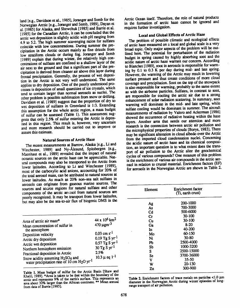
land [e.g., Davidson et al., 1985], Joranger and Semb for the Arctic Ocean itself. Therefore, the role of mural productsNorwegianArctic [e.g., Joranger and Semb, 1989], Dayan et in the formation of arctic haze cannot be ignored andal, [1985] forAlaska, and Shewchuk [1985] and Barrieel al. requiresfurtherinvestigation.{1985] for the Canadian Arctic, it can be concluded that thearctic wetdeposition is slightly acidic with pH ranging from Local and Global Effects of Arctic Haze4.9 to 5.2. The high summer scavenging ratios for sulfates The problem of possible climatic and ecological effectscoincide with low concentrations. During summer the pre- of arctic haze measured on _alocal and global scale is a verycipitation in the Arctic occurs mainly as fine drizzle from broad topic. Only majoraspects of the problemwill be out-low stratiform clouds or during fog. Joranger and Semb lined here. The potential for perturbation of the radiation[1989]explainthatduringwinter,therelativelyhighcon- budgetinspringcausedby highlyabsorbingsootandthecentrationsofsulfatesareconfinedtoa shallowlayerofthe acidicnatureofarctichazewarrantourconcern.According

toBlanchet[1989],sootinaerosolsisresponsibleforwarm-airnexttothegroundandthata significantpartofthepre-cipitationisderivedfromcleanerairabovethislayerduring ingby 0.1to0.3K perday duringmid-andlatespring.frontalprecipitation.Generally,theprocessofwetdeposi- However,thewarmingoftheArcticmay resultinloweringrienintheArcticisnotverywellunderstood.The same surfacepressureandthuscreateconditionsofmorecloudappliestodrydeposition.One ofthepoorlyunderstoodpro- coverageandprecipitation.Sootonthetopofthesnowpackcesses is deposition of small quantities of ice crystals, which is also responsiblefor warming, probably to the same extenttend to contain larger than normal aerosols as nuclei. The as with the airborne particles. Sulfates, in contrast to soot,other problemis possible sublimation from snow or drifting, are responsible for cooling the arctic air due to a strongDavidson et al. [1989] suggest that the proportionof dry to enhancement of solar radiation scattering. In summary,sootwet deposition of sulfates in Greenland is 1:3. Extending warming will dominate in the mid- and late spring, whilethis assumption for the whole arctic region, a mass budget sulfate cooling would be dominant in summer.The aircraftof sulfur can be assessed (Table 1). This assessment sug- measurementsof radiation by Valero and Ackerman [1986]gests that only 2.5% of sulfur entering the Arctic is depos- showed the occurrence of radiative heating within the hazeited in this region. This result is, however, very uncertain layers. Another area that needs our attention and moreand more research should be carried out to improve or research is the connection between arctic air pollution andassure this estimate, the microphysicalpropertiesof clouds [Borys, 1983]. There

may be significant alteration in cloud albedo over the ArcticNatural Sources of Arctic Haze from the imported cloud condensation nuclei. Concerning

The recent measurements at Barrow, Alaska [e.g., Li and the acidic nature of arctic haze and its chemical composi-Winchester, 1989] and Ny-Alesund, Spitsbergen [e.g., tion, an important question is to what extent does the trans-Maenhaut et al., 1989] revealed that the impact of natural port of air pollution to the Arctic alter the geochemicaloceanic sources on the arctic haze can be appreciable.Nat- cycles of various compounds? One measure of this problemural compounds may also be transported to the Arctic from is the enrichment of various air compounds in the arctic aer-lower latitudes. According to Li and Winchester [1989], osol in relation to crustal material. Enrichment factors (EF)most of the carboxylic acid anions, accounting for 20% of foraerosols in the Norwegian Arctic are shown in Table 2.the total aerosol mass, can be attributed to natural sources atlower latitudes. As much as 20% non-sea salt sulfates inaerosols can originate from gaseous marine sources. Thesources and so'ca'ceregions for natural sulfates and other Element Enrichment factorcomponents of the arctic aei osol from natural sources are (Ti, earth crust)poorly recognized, lt may be transport from lower latitudes,but may also be the sea-to-air flux of biogenic DMS in the Ag 200-1000

As 700-3000Cd 5OO-6OOOCr 30-100

Area of arctic air mass* 44 x 106km2 Cu 30-100Mean concentration of suffur in 470 Ixgm"3 Ga 8-20

the atmosphere In 40-200Deposition velocity 0.03 cm s'l Mo 60-150Arctic dry deposition 0.19 Tg S yr"1 Ni 30-80Arctic wet deposition 0.57 Tg S yr"1 Pb 2500-4000Northern hemisphere emission 30 Tg S yr"1 Sb 1000-3200Fractional deposition in Arctic 2.5% S 2500-15000Snow acidity assuming H2SO4 and 10.3 la.eq 1-1 Se 3700-36000

water precipitation rate of 10cm H20 yr"1 V 35-50W 20-130Zn 300-900

Table I. Mass budgetof sulfurfor the ArcticBasin [ShawandKhaliL1989].*Areais taken to be that wi:hintheboundaryof thearcticandrepresents9% of the earth'ssurface.Thisrepresentsan Table 2. Enrichmentfactorsof tracemetalson particles<1.0gmareaabout30% largerthan the Africancontinent.**Meanannual diameterin the NorwegianArcticduringwinterepisodesof long-fromdataof Barrie[1985]. rangel_ansportof air pollution.

678

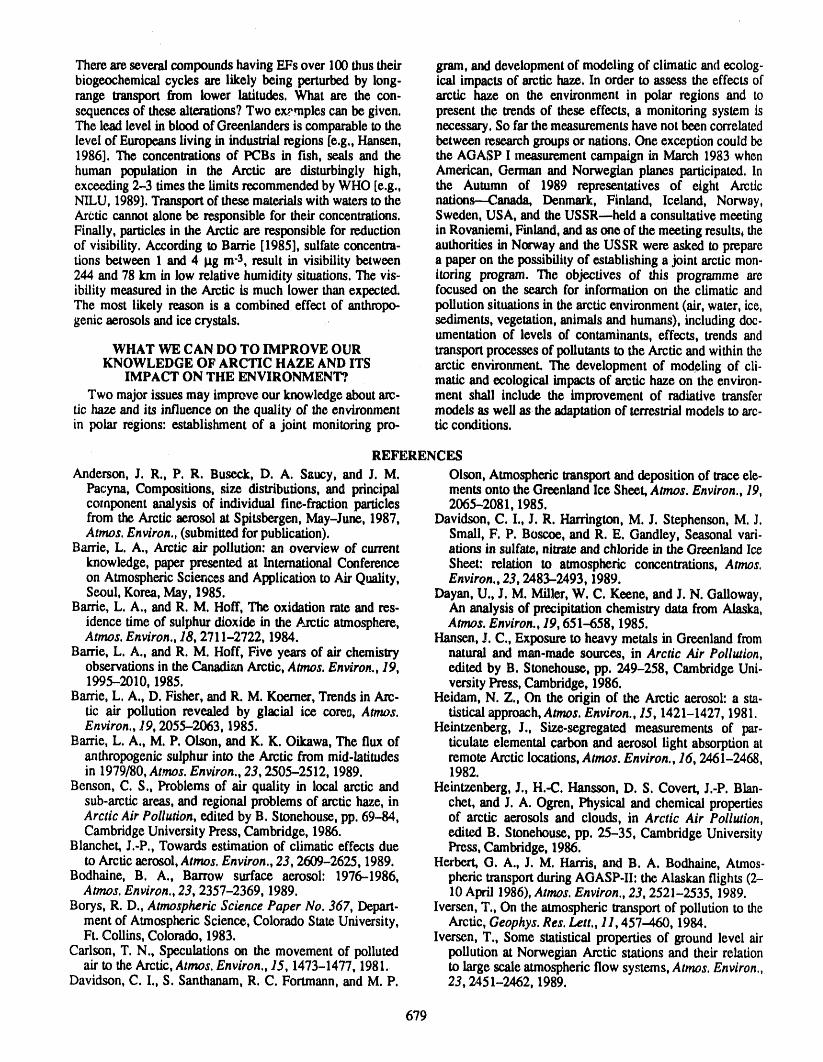
ThereareseveralcompoundshavingEFsover100thustheir gram,anddevelopmentofmodelingofclimaticandecolog.biogeochemical cycles are likely being perturbedby long- ical impacts of arctic haze. In order to assess the effects ofrange transportfrom lower latitudes. What are the con- arctic haze on the environment in polar regions and tosequences of these alterations?Two examples can be given, present tile trends of these effects, a monitoring system isThe lead level in blood of Greenhmders is comparableto the necessary. So far the measurementshave not been correlatedlevel of Europeansliving in industrialregions [e.g., Hansen, between lesearch groupsor nations. One exception could be1986]. The concenlrations of PCBs in fish, seals and the the AGASP I measurementcampaign in March 1983 whenhuman population in the Arctic are disturbingly high, American, German and Norwegian planes participated.Inexceeding 2-3 times the limits recommendedby WHO [e.g., the Autumn of 1989 representatives of eight ArcticNILU, 1989].Transportof these materialswith watersto the nations--Canada, Denmark, Finland, Iceland, Norway,ArCticcannot alone be responsible for their concentrations. Sweden, USA, and the USSR--held a consultative meetingFinally, particlesin the Arctic areresponsible for reduction in Rovaniemi, Finland, and as one of the meetingresults,theof visibility. According to Barrie [1985], sulfate concentra- authorities in Norway and the USSR were asked to preparelions between 1 and 4 I.tgm-3, result in visibility between a paperon the possibilityof establishing a joint arcticmen-244 and 78 km in low relative humidity situations. The vis- itoring program. The objectives of this programme areibility measuredin the Arctic is much lower thanexpected, focused on the search for information on the climatic andThe most likely reason is a combined effect of anthropo- pollutionsituations in the arcticenvironment (air,water,ice,genic aerosols and ice crystals, sediments, vegetation, animals and humans), including doc.

umentation of levels of contaminants, effects, trends andWHAT WE CAN DO TO IMPROVE OUR transportprocesses of pollutants to the Arctic and within the

KNOWLEDGE OF ARCTIC HAZE AND ITS arctic environment. The development of modeling of cii-IMPACT ON THE ENVIRONMENT? matic and ecological impacts of arctic haze on the environ-

Two majorissues may improveour knowledge aboutarc- ment shall include the improvement of radiative transfertic haze and its influence on the quality of the environment models as well as, the adaptationof terrestrialmodels to arc-in polar regions: establishment of a joint monitoringpro- tic conditions.

REFERENCES

Anderson, J. R., P. R. Buseck, D. A. Saucy, and J.M. Olson, Atmospherictransportand deposition of traceele-Pacyna, Compositions, size distributions, and principal ments onto the GreenlandIce Sheet,Atmos. Environ., 19,component analysis of individual fine-fraction particles 2065-2081, 1985.from the Arctic aerosol at Spitsbergen, May-June, 1987, Davidson, C. I., J. R. Harrington,M. J. Stephenson, M. J.Atmos. Environ., (submittedforpublication). Small, F. P. Boscoe, and R. E. Gandley, Seasonal vari-

Battle, L. A., Arctic air pollution: an overview of current ations in sulfate,nitrateand chloride in the GreenlandIceknowledge, paperpresented at InternationalConference Sheet: relation to almospheric concentrations, Atmos.on Atmospheric Sciences and Application to .MrQuality, Environ., 23, 2483-2493, 1989.Seoul, Korea,May, 1985. Dayan, U., J. M. Miller, W. C. Keene, and J. N. Galloway,

Ban'ie, L. A., and R. M. HolT,The oxidation rateand res- An analysis of precipitationchemistry data from Alaska,idence time of sulphur dioxide in the Arctic atmosphere, Atmos. Environ., 19, 651--658, 1985.Atmos. Environ., 18, 2711-2722, 1984. Hansen, J. C., Exposure to heavy metals in Greenlandfrom

Barrie, L. A., and R. M. Heft, Five years of air chemistry natural and man-made sources, in Arctic Air Pollution,observationsin the CanadianArctic, Atmos. Environ., 19, edited by B. Stonehouse, pp. 249-258, CambridgeUni-1995-2010, 1985. versifyPress, Cambridge,1986.

Ban'ie, L. A., D. Fisher, and R. M. Koemer, Trendsin Arc- Heidam, N. Z., On the origin of the Arctic aerosol: a sta.tic air pollution revealed by glacial ice cores, Atmos. tistical approach,Atmos. Environ., 15, 1421-1427, 1981,Environ., 19, 2055-2063, 1985. Heintzenberg, J., Size-segregated measurements of par-

Battle, L. A., M. P. Olson, and K. K. Oikawa, The flux of ticulate elemental carbon and aerosol light absorptionatanthropogenic sulphur into the Arctic from mid-latitudes remote Arctic locations,Atmos. Environ., 16, 2461-2468,in 1979/80, Atmos. Environ., 23, 2505-2512, 1989. 1982.

Benson, C. S., Problems of air quality in local arctic and Heintzenberg, J., H.-C. Hansson, D. S. Covert, J.-P. Blan-sub-arcticareas, and regional problems of arctichaze, in chet, and J. A. Ogren, Physical and chemical propertiesArctic Air Pollution, e,dited by B. Stonehouse, pp. 69-84, of arctic aerosols and clouds, in Arctic Air Pollution,CambridgeUniversityPress, Cambridge, 1986. edited B. Stonehouse, pp. 25-35, Cambridge University

Blancher, J.-P., Towards estimation of climatic effects due Press,Cambridge, 1986.to Arctic aerosol,Atmos. Environ., 23, 2609-2625, 1989. Herbert,G. A., J. M. Harris,and B. A. Bodhaine, Atmos-

Bodhaine, B. A., Barrow surface aerosol: 1976-1986, pheric transport during AGASP-II: the Alaskan flights (2-Atmos. Environ,, 23, 2357-2369, 1989. 10 April 1986),Atmos. Environ., 23, 2521-2535, 1989.

Borys, R. D., Atmospheric Science Paper No. 367, Depart. Iversen, T., On the atmospheric transport of pollution to thement of Atmospheric Science, Colorado State University, Arctic, Geophys. Res. Lett., 11,457--460, 1984.Ft. Collins, Colorado, 1983. Iversen, T., Some statistical properties of ground level air

Carlson, T. N., Speculations on the movement ofpolluted pollution at Norwegian Arctic stations and their relationair to the Arctic, Atmos. Environ., 15, 1473-1477, 1981. to large scale atmospheric flow systems, Atmos. Environ.,

Davidson, C. I., S. Santhanam, R. C. Fortmann, and M.P. 23, 2451-2462, 1989.

679

Jaffe, D. A., R. E. Honrath,J. A. Herring, and S.-M. Li, Pacyna,J. M., andB. Ottar,Verticaldistributionof aerosolsMeasurementof nitrogen oxides at Barrow, Alaska dm'- in the Norwegian Arctic, Atmos. Enviro_l., 22, 2213-ing Spring: Evidence for regional and northern beret- 2222, 1988.spheric sources of pollution,J. Geophys. Res., 96, 7395-- Pacyna,J. M., and B. Ottar,Originof naturalconstituentsin7405, 1991. theArctic aerosol,Atmos. Environ., 23, 809.-815, 1989.

Joranger,E., and A, Scrub, Major ions and scavenging of Pacyna,J. M., B. Ottar,U. Tomza,and W. Maenhaut,Long.sulphate in the Norwegian Arctic, Atmos. Environ., 23, range transportof trace elements to Ny Adlesund,Spits.2463-2469, 1989. bergen,Atmos. Environ., 19, 857-865, 1985.

Larssen,S., and J. E. Hanssen, Annual variationand origin Raatz,W, E., and G. E. Shaw, Long-rangetransportof pol.of aerosol components in the Norwegian Arctic- lutionaerosols into the AlaskanArctic, J. Climatol, Appl.Subarctic region, paperpresentedat the WMO Technical Meteorol., 23, 1052-1064, 1984.Conference on Regional and Global Observation of Radke, L. F., J. H. Lyons, D. A, Hegg, P. V. Hobbs, andAtmosphericPollution Relative to Climate,Boulder, Col- I.H. Bailey, Airborneobservations of Areltc aerosols. I.orado,20-24 August, lY79. Characteristicsof Arctic haze, Geophys. Res. Lett., 11,

Lazrus,A. L., and R. J. Ferek, Acidic sulfate particlesin the 393-396, 1984.winterarctic atmosphere, Geophys. Res. Lett., 11,417- Radke, L,. F., C. A. Brock, J. H, Lyons, P. V. Hobbs, and419, 1984. R.C. Schnell, .Aerosol and lidar measurements of hazes

Li, S..M., and J. W. Winchester,Geochemistry of organic in mid-latitude andpolar air masses, Atmos. Environ., 23,and inorganic ions of late winter arctic aerosols, Atmos. 2417-2430, 1989.Environ., 23, 2401-2415, 1989. Rahn, K. A., R. Borys, andG. E, Shaw, The Asian sourceof

Li, S.-M., and J. W. Winchester,Particle size distributionof Arctic hazebands,Nature, 268, 713-715, 1979.late winter Arctic aerosols, J. Geophys. Res., 95, 13897- Rosen, H. and A. D, A. Hansen, Role of combustion.13908, 1990a. generated carbonparticles in the absorptionof solar radJ.

Li, S.-M., and J. W, Winchester, Haze and other aerosol ation ;.nthe Arctic haze, Geophys. Res. Lett,, 11, 461-components in late winter Arctic Alaska, 1986, J. Gee- 464, 1984.phys. Res., 1797-1810, 1990b. Schnell, R.C., Arctic haze and the Arctic Gas and Aerosol

Lowenthal, D. H., and K. A. Rahn, Regional sources of pol- Sampling Program (AGASP), Geophys. Res. Lett., 11,iution aerosol at Barrow, Alaska during winter 1979-80 361-364, 1984.as deduced from elemental tracers, Atmos. Environ., 19, Shaw, G. E., Evidence for a central Eurasian source area of2011-2024, 1985. Arctic haze in Alaska,Nature, 299, 815--818, 1982.

Maenhaut, W,, P. Cornille, J. M. Pacyna, and V. Vitols, Shaw, G. E., and G. Wendler, Atmospheric turbidity meas.Traceelement compositionand origin of the atmosphericaerosol in the Norwegian Arctic, Atmos. Environ., 23, urements at McCall Glacier in northeast Alaska, paper

presented at the Conference on Atmospheric Radiation,2551-2569, 1989. Fort Collins, Colorado. Prec. Amer. Met. Soc., Boston,

Mitchell, M., Visual rang¢_in the polar regions with par- 181-187, 1972.titular reference to the Alaskan Arctic, J. Atmos. Terr.Phys. (Special supplement),195-211, 1956. Shaw, G. E., and M. A. K. Khalil, Arctic haze, in The Hand.

Nansen,F., Blandt Sel og BjOrn, Dywad, Oslo, 1924. book of Environmental Chemistry, Volume 4/Part B,edited by O. Hutzinger, pp. 69-111, Sp_'mger, Berlin,NILU, Forurensningen av Arktis med klorerte pesticider og

polyklorerte bifenyler, Norwegian Institute for Air 1989.Research, Rept. RR 8189,(in Norwegi,'m),May, 1989. Sheridan, P. J., Characterization of size segregated particles

Oden, S., Nederbordens oeh Luftens Forsurning, dess collected over Alaska and the Canadian High Arctic,orsaker, Forlopp, och Verkan i Olika Miljoer. Statens AOASP-H flights 204--206,Atmos. Environ., 23, 2371-Naturvetenskapeliga Forskningsr_td (Ekologikommitteen, 2386, 1989.Bull. No. 1), (in Swedish), Stockholm, 1968. Shewchuk, S. R., Acid deposition sensitivities within the

OECD, The OECD programme on long-range transport of Northwest Territories and current depositions to theair pollutants, measurements and findings, Organization snowpack and small lakes chemistry of a selected area offor Economic Co-operation and Development, Paris, the Mackenzie District, Proc. Int. Conf. on Arctic Water1977. Pollution Research: Applications of Science and/

Ottar, B, end J. M. Pacyna, Origin and characteristics of aer- Technology, YeUowknife, 28 April-I May, 1985.osols in the Norwegian Arctic, in Arctic Air Pollution, Stm.ges, W. T., and L. A. Battle, Lead 206/207 isotopeedited by B. Stonehouse, pp. 53--67, Cambridge Uni, ratios in the atmosphere of North America as tracers ofversityPress, Cambridge, 1986. US and Canadian emissions, Nature, 329, 144-146,

Ottar, B., Y. Gotaas, O. Hov, T. lversen, E. Joranger, M. 1987.Oehme, J. M. Paeyna, A. Scrub, W. Thomas, and V. Sturges, W. T., and L. A. Barrie, Chlorine, bromine andVitols, Air pollutants in the Arctic, NILU OR Rept. No. iodine in Arctic aerosol, Atmos. Environ., 22, 1179-1194,30/86, The Norwegian Institute for Air Research, 1988.Lillestrem, Norway, 1986. Valero, F. P. J., and T. P. Ackerman, Arctic haze and the

Pacyna, J. M., and M. Oehme, Long-range transport of some radiation balance, in Arctic Air Pollution, edited by B.organic compounds to the Norwegian Arctic, Atmos. Stonehouse, pp. 121.133, Cambridge University Press,Environ., 22, 243-257, 1988. Cambridge, 1986.

680

A Polar Climate Iteration?

A. HoganU.S. Army Cold Regions Research and Engineering Laboratory, Hanover, N_w Hampshire, U.S.A.

D. RileyDepartment of Natural Resources, Waterbury, Vermont, U.S.A.

,' B.B. MurpheyWhiteface Mountain Observatory, ASRC, Wilmington, New York, U.S.A.

S. C. Barnard and J. A. SamsonASRC, State Univ. of New York, Albany, New York, U.S.A.

ABSTRACTThe antarctic continental (cA) air mass is rarely displaced from the South Polar

Plateau, but it is frequently modified by exchange with Antarctic maritime (mA) airadvected from the ice shelves or frozen seas or with polar maritime (mP) airadvected from the Southern Ocean. Because the eA air mass resides over an unin-habited and relatively static ice-covered surface, the concentration of aerosol par-ticles in this unique air mass may reflect aerosol variation in the global atmosphere.

A continuous series of surface observations began at South Pole in 1974 andhave continued to the present. Although a large seasonal variation in aerosol con-centration is present, little year-to-year variation in mean seasonal aerosol con-centration occurred prior to 1982. During the mid-1980s, a consistent diminution ofmean annual aerosol concentration was observed, and a concurrent reduction insodium concentration in snow and fun was reported. The decrease in aerosol con-centration was greatest in late winter and spring, concurrent with decreases in meanair temperature and mean wind speed.

This paper describes concurrent aerosol and meteorological data collected atSouth Pole from 1974 through 1987 and presents several analyses attempting toverify if these changes do reflect a persistent variation in the properties of the cAair mass. Additional analyses, using upper air and automatic weather station data,attempt to identify circulation changes related to these changes in aerosolconcentration.

INTRODUCTION the aerosol properties of the cA air mass are modified coin-

A cold dry air mass is permanently resident over the Ant- eidentally [Hogan et al., 1982; Riley, 1987; Hogan et al.,arctic Plateau. The elevation of the plateau, the radiation 1990]. The uniformity of the surface of the polar plateau,deficit afforded by its permanent snow cover, and the stabil- the absence of continental antarctic aerosol sources, theity of the air, prevent the Antarctic continental (cA) air mass unique stability of the cA air mass, and the relative slownessfrom being displaced by surrounding Antarctic maritime of Antarctic meteorological variation cumulatively provide(mA) or polar maritime (mP) air masses. The cA air mass is Lettau's [1971] "test tube" for examining meteorologicalwarmed by advective exchange with these air masses, and theories.

681

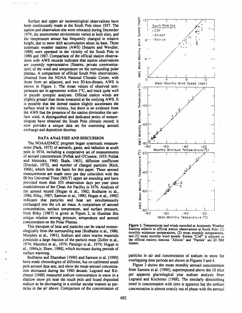
Su.f oo, ]been continuously made at the South Pole since 1957. The _ Soulh Pole Sla' "t3 _ 0 O

station and observation site were relocatedduring December o '- , c AF _ -a.i

1974, the anemometer environment varied at both sites, and t. :, Allison ithe temperature sensor has frequently changed in relative _, 8_-_ Potrick '. --_height, due to snow drift accumulation about its base. Three ._ :/, ,, ,,.automatic weather stations (AWS) [Steams and Wendler, ,. / ',,.

1988] were operated in the vicinity of the South Pole in z i /

1986 and 1987, Comparison of the official station observa- _o "

tions with AWS records indicates that station observations _:= 4 '- //m'e currently representative [Steams, private communica- a,_'

tion] of the wind and temperature on the surrounding polar _ _/ -"plateau. A comparison of official South Pole observations, _:obtained from the NOAA National Climatic Center, with ,_ _ I J I I I0 4 8 12those from an adjacent,and two 30-km.distant,AWS is .-, Meon Monthly Wind Speed (mph)

t.9

shown in Figure 1. The mean values of observed tem- o--2o _r------] _ I Iperatures are in agreement within I°C, and track quite well _ _ //

in pseudo synoptic analyses, Official station winds are "_ -slightly greater than those measured at the outlying AWS. ltis possible that the domed station slightly accelerates the Esurface wind in the vicinity, but there is no evidence from _.-4o- ._..the AWS that the presence of the station diminishes the sur- _ of""//face wind. A distinguished and dedicated series of meteor- _E - _ ,:ologists have obtained the South Pole climatic record; it _:now provides a unique data set for examining aerosol _-6o "exchange and deposition theories. _=

o

DATA ANALYSIS AND DISCUSSION

The NOAA/GMCC program began systematic measure- _-so - _ I t Imerit [Pack, 1973] of aerosols, gases,and radiation at south -so -6o -4o -20

Monlhly Minimum Temperature (*C)pole in 1974, including a cooperative set of measurements _-2 o ' , I _ i , A 1of aerosolconcentration [Pollak and O'Connor, 1955;Pollak "_ ' o/' !

and Metnieks, 1960; Skala, 1963], diffusion coefficient __ _ / ._'[Sinclair, 1972], and number of charged particles [Rich,1966], which form the basis for this paper.These aerosol _. _._"

E -40 ....... /measurements are made once pet day coincident with the _.

00 hrs Universal Time [00UT] upperair sounding and have =__ ,_._ 2provided more than 355 observation days per year since _ _/_-_.establishment of the Clean Air Facility in 1976. Analysis of ,?, ,,_,the aerosol record [Hogan et al., 1982; Bodhaine et al., _-6o _ --_1986; Riley, 1987; Samson ct al,, 1990; Hogan ct al., 1990] _ _ Iindicates that particles and heat are simultaneously _ - ./ -Iexchanged into the cA air mass. A comparison of aerosol t_ Iconcentration, surface temperature, and surface pressure, <-8o L _L_____J___I__L ....... J.......from Riley [1987] is given in Figure 2, to illustrate this -so -6o -4o -ztunique relation among pressure,temperatureand aerosol MeanMonthly Temperature (°C)concentrationon thePolarPlateau.

This translx_ of heat and particles can be traced meteor- Figure1, Temperatm'ea and windsrexx)rde.dat AutomaticWeatherStationsrelativeto officialsialon observationsat South Pole:(1)

ologically from the surrounding seas [Bodhaine ct al., 1986; monthlyminimumtemperatures,(2) mean monthly temperatures,Murphey et al., 1991]. Sodium and other marine materials and (3) meanmonthlywind speeds.Station "CAF"is adjacenttoconstitute a large fraction of the particle mass [Zoller et al., th_ official station; stations "Allison"and "Patrick" are 20 NM1974; Maenhut et al., 1979; Parungo et al,, 1979;Hogan et distant.al., 1984a,b; Shaw, 1988], which increases during periods of

surface warming, particles in air and concentration of sodium in snow forBodhaine and Shanahan [1990] and Samson et al. [1990]-_ have made chronologies of different, but co-calibrated south overlapping time periods are shown in Figures 3 and 4.

pole aerosol data sets, and show the mean aerosol concentre. Figure 3 shows the mean monthly aerosol concentrationtion decreased dta'ing the 1980 decade. Legrand and Kit. from Samson et al. [1990], superimposed above the 10 slicechener [1988] measured sodium concentration in snow in a per apparent glaciological year sodium analysis fromshallow snow pit near the south pole and found deposited Legrand and Kirchener [1988]. The similarly diminishingsodium to be decreasing in a similar secular manner as par- trend in concentration with time is apparent but the sodiumticles in the ai,"above. Comparison of the concentration of concentration is almost exactly out of phase with the aerosol

682

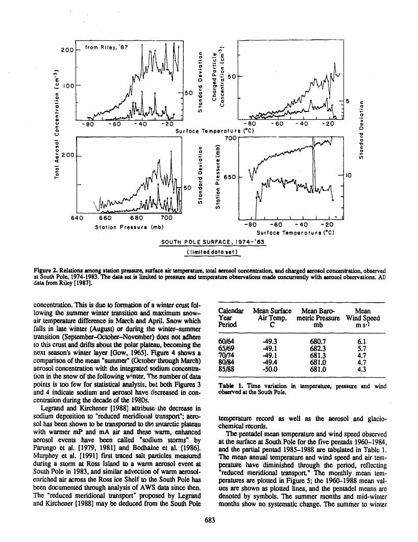
fromRJiey,'87 ! _ | it

==0o

u I00 _ ,. =0

,- g _4--

== .;==cu - 80 - 60 - 40 - 20 - 80 " 60 - 40 - 20 =_

Surface Temperature (°C) c3

..... .-. 700 _ ,_°

o 200 = _ ..,,.-- D

._, ,-=lI/I

_/_ _ _ _ 650 --I0

640 660 680 700 .. .j f I * i ! I. t_',

Station Pressure (mb) -80 -60 -40 -20

Surface Temperature (=C)

SOUTH POLE SURFACE, 1974-'8:5

(llmited data set)

Figure 2. Relationsamongstationpressure,surfaceairtemperature,mudaerosolconcentration,andchargedaerosolconcentration,observedatSouthPole,1974-1983,Thedamset is limitedto pressureandtemperatureoi_ervationsmadeconcurrentlywithaerosolobservations,AlldatafromRiley[1987].

concentration.This isdueto formationof a wintercrustfol-lowingthe summerwinter transitionandmaximumsnow- Calendar MeanSurface MeanBare- Meanair temperaturedifferencein MarchandApril. Snowwhich Year Air Temp. metricPressure Wind SpeedPeriod C mb m s-]falls in late Winter (August) or during the winter-summer

transition(September-October-Noventber) does not adhere 60/64 .49.3 680.7 6.1to this crust anddrifts aboutthe polarplateau,becoming the 65/69 .49.1 682.3 5.7next season's winter layer [Cow, 1965]. Figure 4 shows a 70/74 .49.1 681.3 4.7comparisonof the mean "summer"(OctoberthroughMarch) 80/84 .49.4 681.0 4.7aerosolconcentrationwith the integratedsodiumconcentra. 85/88 -50.0 681.0 4.3tion in the snow of,the following winter.The number of data

points is too few for statistical analysis, bt_tboth Figures 3 Table 1. Time variationin temperature,pressureand windand 4 indicate sodiumand aerosol have,d-.creased in con- obm_ed atthe SouthPole.centrationduring thedecade of the198(_.=

Legrand and Kirchener [1988] attributethe decrease insodiumdeposition to "reducedmeridioxudU_mspon";aere- temperature record as well as the aerosol and glacio-sol hasbeen shown to be transportedto 'the a_tmrcticplateau chemical records.with warmermP and mA air and the_ warm, enhanced Thepentadelmeantemperatureandwindspeedobservedaerosol events have been called "_dium storms" by at the surface at South Pole for the five pentads 1960-1984,Parungo ct al. [1979, 1981] and Bodtudne et al. [1986]. and the partialpentad 1985-1988 are tabulatedin Table 1.Murphey ct al. [1991] first traced salt particles measured The mean annual temperatureand wind speed and air tem-during a storm at Ross Island to a warm aerosol event at perature have diminished through the period, refittingSouth Pole in 1983, and similar advectionof warmaerosol- "reduced meridional transport."The monthly mean tem-enriched air across the Ross ice Shelf to the South Pole has peraturesare plotted in Figure 5; the 1960-1988 mean val-been documented throughanalysis of AWS data since then. ues are shown as plotted lines, and the pentadel means areThe "reducedmefldional lzansport"Ixoposedby Legrand denotedby symbols.The summermonthsand mid.winterandKh'chener[1988]maybededucedfromthe SouthPole monthsshowno systematicchange.The summerto winter

683

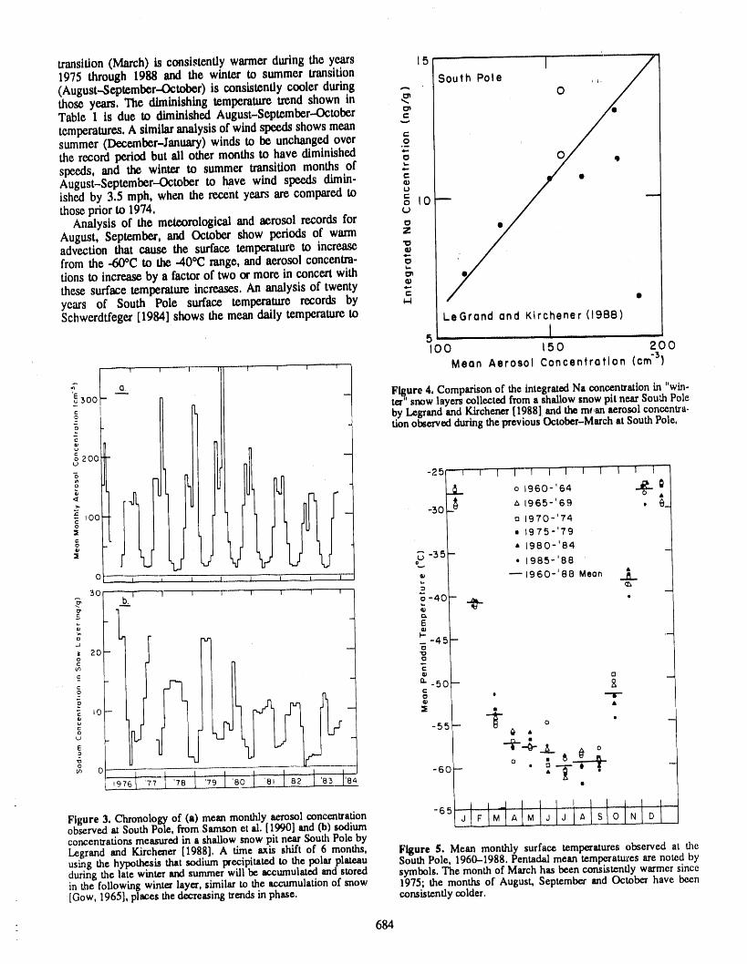
transition (March) is consistently warmer during the years 15 I '

1975 through 1988 and the winter to summer transition South Pole 0(August-September-October) is consistently cooler during .-.those years. The diminishing temperature trend shown in ZTable 1 is due to diminished August-September-October ,-.°'temperatures. A similar analysis of wind speeds shows mean "=summer (December-January) winds to be unchanged over ,9

the record period but ali other months to have diminished _ 7 • •speeds, and the winter to summertransitionmonths ofAugust-September--October to have wind speeds dimin- = /u

ishedby 3.5 mph, whentherecentyearsarecomparedto g lOthose prior to 1974, u

Analysis of the meteorological and aerosol records for v

August, September, and October show peflods of warm z 7advection that cause the surface tempermure to increase _=from the -60°C to the -40°C range, and aerosolconcentre-dons to increase by a factor of two or more in concert withthese surface temperature increases. An analysis of twentyyears of South Pole surface temperaturerecords bySchwerdffeger [1984] showslhc mean daily temperature to LeGrand and Klrchener (1988)

s IlO0 150 200

__ , , _ , , ,, , ,, ..... Moon Aorosol Concentrotlon (cre"_}[

L o _ Figure 4. Comparison of the integratedNaJ oono_ntratlon in Ilwt.n.

'__300. -- torIIsnow layers collected from a shallow snow pit near South Poleg ] by L,cgrandand Kirchener [1988],and ttm mc,anaerosol concentra-= rienobservedduring the previousOctober-Marchat South Pole,O

U¢-

o 200 -U

"_ -25- I l 1 I I 1 I I I 1 I I I

o .._E, n ..L o 1960-'64 o act

-" [ _ ' -30 - _ ,', 1965- 69 , O_£ _00 o 1970-'74g

"_ 1 I • 1975-'79

g • 1980-'84

_ -35 - -= j J _ • ,98_-'880 _ i l I i li. ii I _ -- 1960 -188 Moon .JL.

- "_ -40 - "

E

_" _ _ -45 --r

V} g {3 --

=- Q"-50 - R

lD •

-55 - oL)

o -6c- --f ' : -

5 2 I I IFigure 3. Chronology of (a) mean monthly aerosol concentration -6 J F M A M d d A S 0 N D

observed at South Pole, from Samson et al. [1990] and (b) sodium I

concentrations measuredinashallowsnowpit near SouthPolebyLegrand and Kirchener [1988], A time axis shift of 6 months, Figure 5. Mean monthly surface temperatures observed at theusingthehypothesisthatsodiumprecipitatedtothepolarplateau SouthPole,1960-1988.Pentadalmeantemperaturesarenotedbyduringthelatewinterandsummerwillbeaccumulatedandstored symbols.The monthofMarchhasbeenconsistentlywarmersinceinthefollowingwinterlayer,similartotheaccumulationofsnow 1975;themonthsofAugust,SeptemberandOctoberhavebeen[Gow, 1965], places the decreasing trendsin phase, consistently colder,

- 684

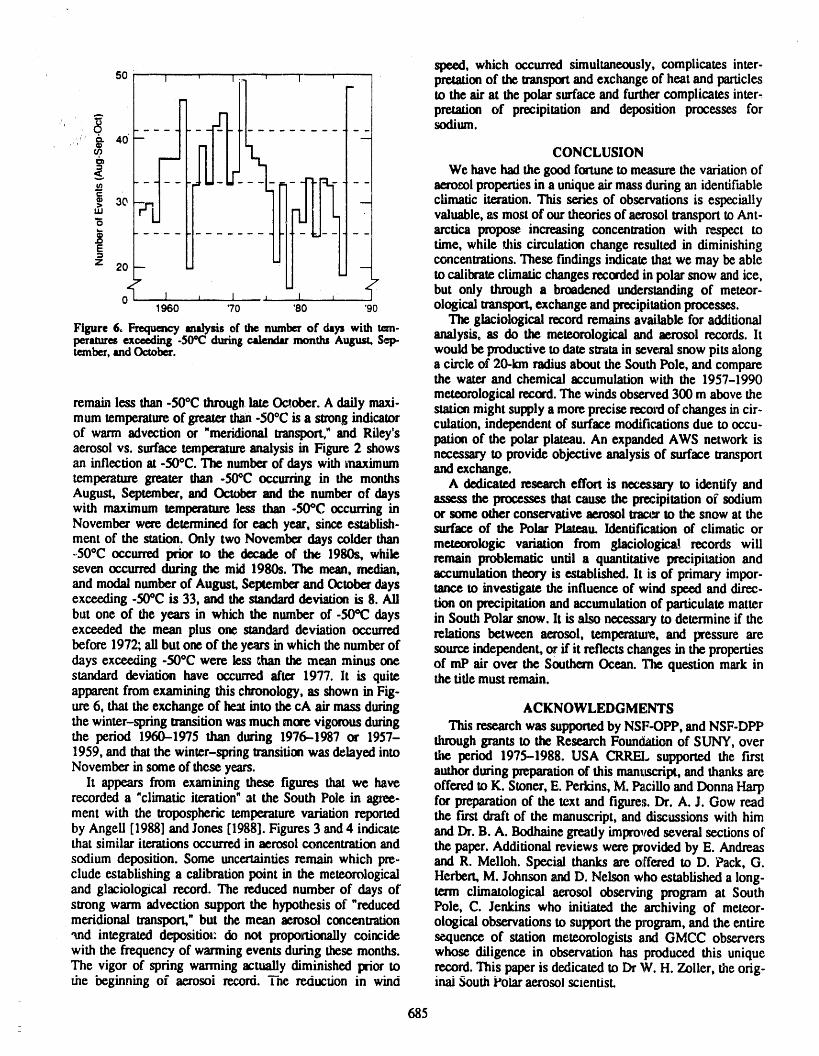
speed, which occurred simultaneously, complicates inter-so, , , 'ii ' ' ' = pretationofthetranslx_andexchangeofheatandlxmicles

II totheairatthepolarsurfaceandfurthercomplicatesinter-,.-. _ pretation of precipitation and deposition processes for

' - - .... 1 _= sodium,, ,

' u) i CONCLUSION

F I We have hadthe good fortuneto meast_rethe variationof

<_-_ _-" "4"1"_"- - - I aeroml propertiesin a unique airmassduring an identif'mble

c

® 3o _ climatic iteration. This series of observations is especially>

uJ "-1 I valuable, as mostof ourtheoriesof aerosoltransportto Ant-

....... _- -1 -t arctica propose increasing concentration with respect to

time, while this circulation change resulted in diminishing= concentrations.These findings indicate tha_we may be ablez 20 - to calibrateclimatic changesrecordedin polarsnow and ice,7"

"_ but only through a broadened understandingof meteor-0 [ 1 I 1 ,_ 1 I1960 70 'SO '90 ological transport,exchangeandprecipitationprocesses.

Figure 6, Frequencyanalysisof the numberof dayswith tem- The glaciological recordremains available for additionalperaun'esexceeding-50°CduringcalendarmonthsAugust,Sep- analysis, as do the meteorological and aerosol records, lttember,andOctober. would be productiveto date stratain severalsnow pits along

a circle of 20-km radiusabout the South Pole, and comparethe water and chemical accumulation with the 1957-1990meteorological record.The winds observed300 m above the

remain less than-50°C throughlate Oc_ober.A daily maxi- station mightsupply a more preciserecordof changes in cir-mum temperatureof greaterthan-50oc is a strongindicator culation, independentof surface modifications due to occu-of warm advection or "meridionaltransport,"and Riley's pation of the polar plateau. An expanded AWS network isaerosol vs. surface temperatmeanalysis in Figure 2 shows necessary to provideobjective analysis ofsurface transportan inflection at -50°C. The numberofdayswith maximum andexchange.temperature greater than -RrC occurring in the months A dedicated research effort is nece_uu'y m identify andAugust, September, and October and the number of days assess the processes that cause the prc:ipitation of sodiumwith maximum temperatureless than -50°C occurring in or some otherconservative aerosol tra_t to the snow at theNovember were determined for each year, since establish- surface of the Polar Plateau. Identification of climatic ormerit of the station. Only two November days colder than meteorologic variation from glaciologica_ records will-5O°C occurred prior to the dec.adeof the 1980s, while remain problematic until a quantitative precipitation andseven occurredduring the mid 1980s. The mean, median, accumulation theory is established, lt iisof primary impor-and modal numberof August, Septemberand Octoberdays lance to investigate the influence of wind speed and direc.exceeding -50°C is 33, and the standarddeviation is 8. Ali tion on precipitationand accumulation of particulate matterbut one of the years in which the number of -50°C days in South Polar snow. lt is also necessaJTto determineif theexce_ed the mean plus one standarddeviation occurred relations between aerosol, teanperatme,and pressure arebefore 1972; ali but one of the years in which the numberof source independent, or if it reflects changes in the propertiesdays exceeding-50°C were less _han the mean minus one of mP air over theSouthern Ocean. The question mark instandard deviation have occuned after 1977. lt is quite the tide mustremain.apparentfrom examining this chronology, as shown in Fig-ure 6, thatthe exchange of heatinto thecA air mass during ACKNOWLEDGMENTS

the winter-spring transitionwas muchmore vigorous during This researchwas supportedby NSF-OPP, and NSF-DPPthe period 1960-1975 than during 1976--1987 or 1957- throughgrants to the Research Foundation of SUNY, over1959, and thatthe winter-springtransitionwas delayed into the period 1975-1988. USA CRREL supported the firstNovember in some of these years, authorduring preparationof this man_Lscript,and thanks are

lt appears from examining these figures that we have offered to K. Stoner, E. Perkins,M. l_cillo and Donna Harprecordeda "climatic iteration"at the South pole in agree- for preparationof the text and figures. Dr. A. J. Gow readment with the tropospheric temperaturevariation reported the first draft of the manuscript, and discussions with himby Angell [1988] and Jones [1988]. Figures3 and 4 indicate and Dr. B. A. Bodhainegreatlyimproved several sections ofthatsimilar iterationsoccurredin aerosol concentrationand the paper.Additional reviews were provided by E. Andreassodium deposition. Some uncertainties remain which pre- and R. Melloh. Special thanks are offered to D. Pack, G.clude establishing a calibrationpoint in the meteorological Herbert,M. Johnsonand D. Nelson who established a long-and glaciological record. The reduced number of days of term climatological aerosol observing program at Southstrong warm advection support the hypothesis of "reduced Pole, C. Jenkins who initiated the archiving of meteor-meridional transport,"but the mean aerosol concentration ological observations to supportthe wogram, and the entire•rod integrated depositiot: do not proportionally coincide sequence of station meteorologists and GMCC observerswith thefrequencyof warming eventsduring these months, whose diligencein observationhas ,producedthis uniqueThe vigor of spring warming actually diminished prior to record. This paperis dedicated to Dr W. H. Zoller, the orig-the beginning of aerosol record. The reduction in wind inai South Polaraerosol scientist.

685

REFERENCES

Angell, J. K., Variations and fiends in troposphericand ConvergentLight Beam, Tech Note 9, School of Cosmicstratosphericglobaltemperatures,J.Climate,1,1296- Physics,DublinInstituteforAdvancedStudy,Dublin,1313, 1988. Ireland,1960.

Bodhaine, B. A., Aerosol measurementsat fourbackground Pollak, L. W., and T. C. O'Connor, A Photo Electric Con-sites,J. Geophys. Res., 88,.10753-10768, 1983. densationNucleus Counterof high precision, Geol. Pura

Bodhaine, B. A., J. J. DeLuisi, J. M. Harris, P. Houmere, e Appl., 32,139-146, 1955.andS. Bauman,Aerosol measurementsat the South Pole, Rich, T. A., Apparatusand method formeasuringthe size ofTellus,38B, 223-235, 1986. aerosols,J. Rech. Atmos., 11, 79--85, 1966.

Bromwich, D. H., Snowfall in high southern latitudes, Rev. Riley, D. C., A study of the relationship between the vari-Geophys., 26, 149-168, 1988. ation of aerosol and meteorological parameters at South

Dalrymple, P., A physical climatology of the Antarctic pla- Pole on synoptic, seasonal, and climatological timeteau, in Studies in Antarctic Meteorology, pp. 195-231, scales, ASRCPub. 1122, SUNY, Albany, NY, May _987.AGU, 1966. Samson, J. A., Some characteristics of the south polar

Gow, A. J., On the accumulation and seasonal stratification atmosphere, M.S. Thesis, SUNY Albany, Albany, NY,of snow at the South Pole, Y. Glaciol., 40, 461--477, 1965. May 1983.

Hogan, A. W., S. C. Bamard, J. A. Samson, and W. Win- Samson, J. A., S. C. Btu'nard, J. S. Obermski, D. C. Riley,ters, The Transport of heat, water vapour and particulate J.J. Black, and A. W. Hogan, On the systematic variationmaterialto the south polar plateau,J. Geophys. Res., 87, of surfaceaerosol concentrationat the South Pole, Atmos.4287--4292, 1982. Res., 25,385-396, 1990.

Hogan,A., et al., Particleconcentrationsat the South Pole, Schwerdffeger,W., The climate of Antarctica, in Climateson meteorological and climatological time scales; is the of the Polar Regions, edited by S. Orvig, pp. 253-322,difference important?,Geophys. Res. Lett., 10, 850-853, Elsevier,New York, 1970.1984a.

Hogan, A. W., J. A. Samson,K. Kebschull, R. Townsend,S. Schwerdffeger,W., Weather and Climate of the Antarctic,Barnard,and B. Murphey,On the Interactionof Aero_l Elsevier,New York, 1984.With Meteorology,J. Rech. Atmos., 18, 41--67, 1984b. Shaw, G. E., Antarctic aerosols: A review, Rev. Geophys.,

Hogan, A. W., W. G. Egan, J. A. Samson, S. C. Bamard, 26, 89-112, 1988.D. M. Riley, and B. B. Murphey, Seasonal variation of Sinclair, D., A portable diffusion battery,Am. Ind. Hygienesome constituents of Antarctic tropospheric air, Geophys. Assoc. J., 33, 729-735, 1972.Res. Lett., 17, 2365--2368, 1990. Sinclair, M.R., Recordhigh temperaturesin theAntarcticm

Jones,P. D., Hemispheric surfaceairtemperaturevariations: A synoptic case study,Mon. Wea. Rev., 109, 2234-2242,recent trendsand an updateto 1987, J, Climate, 1,654- 1981.

1 660, 1988. Skala, G. F., A new instrument for measurement of con-Legrand,M., and S. Kirchener, Polar atmospheric circula- densationnuclei, Anal. Chem., 35,702-705, 1963.

Stearns C. R., and G. Wendler, Research results fromAuto-tion and chemistry of recent (1957--83) south polar pre--- cipitation,Geophys. Res. Lett., 15,879-882, 1988. malic WeatherStations, Rev. Geophys., 26, 45-61, 1988._ Lettau, H. H., Antarctic atmosphere as a test tube for mete- Tuncell, G., N. K. Ares, and W. H. Zoller, Temporal vari-

orological theories, in Research in the Antarctic, edited ations and sources of elements in the south polar atmos-by L. O. Quam, pp. 443--476, AAAS Pub. 93, Washing- phere: 1. Non enriched and moderately vnfichedton, DC, 1971. elements, J. Geophys. Res., 94, 13025--13038, 1989.

Maenhut, W., W. H. Zoller, R. A. Duce, and G. L. Hoffman, Vali, G., Nucleation terminology, Bulletin AMS, 66, 1426--Concentration and size distribution of particulatetrace 1427, 1985.elements in the south polar atmosphere, J. Geophys. Res., Van Loon, H., Pressure in the Southern Hemisphere, in84,2421-PA31, 1979. Meteorology of the Southern Hemisphere, edited by

Murphey, B. B., T. Hare, A. W. Hogan, K. Lie.ser, J. C.W. Newton, Meteorol. Monographs, 13, 59-86, 1972.Toman, and T. Woodgates, Vernal atmospheric mixing in Voskresenskii, A. I., Condensation nuclei in the Mirniithe Antarctic, J. Appl. Meteorol., 30, 494-507, 1991. region, (in Russian only, _bstract translated in Antarctic

Pack, D. H., Geophysical monitoring for climatic change, bibliography), Tr. Soy. Antarkt. Eksped., 38, 194--198,Antarctic J. U.S., 1,253-254, 1973. 1968.

Parungo, F., E. Ackerman, W. CaldweU, and H. K. Weick- Warburton, J. A., and G. O. Linkletter, Atmospheric pro-mann, Individual particle analysis of Antarctic aerosols, cesses and the chemistry of the snow on the Ross Ice

I Tellus, 31,521-529, 1979. Shelf, Antarctica, J. Glaciology, 20, 149-162, 1978.Parungo, F., B. A. Bodhaine, and J. C. Bortiniak, Seasonal Weller, G., Advances in antarctic geophysical sciences from

variation of Antarctic aerosol, J. Aerosol Sci., 12, 491- the IGY to the present, AntarcticJ. U.S., 21, 1-12, 1986.504, 1981. Zoller, W. H., E. S. Gladney, and R. A. Duce, Atmospheric

Pollak, L. W., and A. L. Memieks, Intrinsic calibration of concentrations and sources of trace metals at the Souththe Photo Electric Nucleus Counter model 1957 with Pole, Science, 183, 198-200, 1974.

686

]I _ ......

The Role of the Polar Regions in the Global Carbon Cycleand Related Climatic Changes

E. P. BorisenkovMain Geophysical Observatory, Leningrad, U.S.$2¢.

ABSTRACT

Empirical data are examined which characterize the role of the polar regions inthe global carbon cycle, and the role of polar oceans as atmospheric carbon sinks isdiscussed. The dependence of the annual variation of atmospheric CO2 content onlatitude is analyzed. Natural and anthropogenic sources of CO2 are studied, as wellas their manifestation in polar regions. The results of carbon cycle numerical mod-

eling with linear and non-linear box models for different scenarios of anthropogenicCO2 growth are presented. The role of oceanic, biospheric and anthropogenicsources in carbon cycle dynamics is analyzed. The results of modeling the climateand its changes are discussed for different scenarios of energetics development withmodels of different complexity. Possible causes of climate wanning and cooling areconsideredfor the polar regions.

INTRODUCT]ION approximate consideration of the dynamics of the ocean

The global carboncycle and climate change are now the mixing layer.problem_ of prime importance. They are most completely A number of studies show an important role of deepdescribed in the report preparedby WMO/UNEP [1990], ocean in the global carbon cycle. This effect is most fullybut also in manyother publications. A generalizeddescrip- describedby Bacastow andMaier-Reimer [1990]_tion of the problemof the global carbon cycle relative to cii- Feedbacks proved to be of no less importance, primarilymate changes is presentedin the monographby Borisenkov in the case of lowercloud layerincrease.andKondratiev [1988], with an extensive bibliography. Polar regions are of special importance for studying the

It should be mentioned that despite the exceptional global carbon cycle. These regions, particularly the southimportance,of the problem a quite simple assumptionhas polar region, are powerful sinks of carbon absorbed bybeen laid down so far that CO2concentration will double in oceanic water.the near future, resulting in global climate warming with This flow in one dh'ectioncan reach 80-100 Gigatons ofmaximum warming in the high latitudes of both hemi- carbon per year, which is far larger than the anthropogenicsphereoo,and accompaniedby a rise of the world ocean level sourcedue to fossil fuel combustion, which is equal to moreby approximately 76 cm by the late 21st century, than 5.5 Gt per year.

Basedon numericalexperiments,ManabeandWetherald On the other hand, analysis of ice cores takenfromthe[1975] determined that sudden CO2 doublh_gwould cause Greenland and Antarctica glaciers enables us to reconstructmean warming of approximately 2-3°C, and in polar areas the content of atmospheric carbon approximately for theof 6-8°C. past 160,000 years [Barnola et al., 1987]. Similar variation

These results have been conf'a'rned in many studies, with time in paleodata is traced for another greenhouse gas,although the range of temperature changes in different rood- methane [Chappellaz et al., 1990].els was between 0.2"C and 9.60C. lt should be stressed that Analysis of samples in the cores of continental ice showsali these numerical experiments were made at a given tem- periods of a considerable decrease in CO2 content down toperature of sea surface (so-called swamp ocean) or with approximately 200 ppm and less, and periods of increased

687

CO 2 content reaching 300--310 ppm and, from the data of .__Shackleton et al. [1983], to 330-350 ppm. Glacial epochs at = Y.(KijNI-KJiNi)+nlwith a cold climate approximately 20,000 and 150,000 years i=l (1)ago correspond to low CO2 content. Warm epochs eor- j_irespond to high CO2content.

The above CO2 changes were by no means related to Here Ni is carbon content in l-rh reservoir, Ki_and Kj.'iareanthropogenic effects. Numerousdata indicate that the peri. coefficients of exchange between reservoirs characterizingods of recession and extension of continental ice are well the rate of carbon flux from i-th to j-th reservoirs (K/i) andcorrelated with periods of change in the Earth's orbit param- from j-th to i-th reservoirs (Kji), ni is the anthrop6geniceters, and modeling results eonf'u'mthis [Budd and Rayner, source in the i.th reservoir. This source exists now only for1990]. lt is natural to assume that, if we cannot simulate the the atmosphere.CO2 concentration variations with a numerical model of the In this ease at each time momentcarbon cycle, and cannot explain them, we have no reason nto trust in modeling results when estimating future CO2 con- NI+N2+N3+...+N n= _N10+Ni (2)centrations and corresponding climate changes, i---I

According to model estimates, the time of CO2 concen-tration doubling varies between early in the next century and Here N10 is carbon content in the i-th reservoir at the initialthe middle of the 22hd century [Bodsenkov and Kondratiev, dme moment. The beginning of the industrial period (1860)1988]. In view of the discussion of the greenhouse effect, it is usually taken as the initial time moment.is also important to answer the question of whether paleo- When linear models are integrated over a long periodanalogues (warm periods of the middle Holocene, 5000- they come to a quasistationary regime depending on the8000 years ago; the recent interglacial period-Mikhulinsky rates of CO2 exchange between reservoirs and the dynamicsOptimum, 125,000 years ago; and Pliocene, 3.-4 million of the anthropogenic CO2 source. In the absence of anthro-years ago) could be used for constructingfuture climate sca- pogenic sources only the rates of exchange processes cannarios. This problem is discussed in the scientific literature change carbon cycle dynamics.as weil. lt is well known from theory and experiment that carbon

Since according to some results of model calculations flows between the ocean and the atmosphere depend to aCO2 doubling will result in maximum warming in the polar considerable extent on ocean temperature, and carbon flowsregions, which should lead to the decrease of interlatitudinal between the atmosphere and the biosphere depend also,temperature contrasts and circulation change, this problem though to a lesser extent, on atmosphere temperature.is critical for future climate changes. Since the cumulative concentration of nonorganic carbon

In view of the above the author made it his aim to give a in the ocean (_C) is determined by carbon dioxide dis-critical analysis of the C02 problem and to propose several solved in the ocean (CO2), carbonate ions (I-ICO3) andproblems for discussion with an attempt to provide possible bicarbonate ions (CO32-),we haveanswers to them.

There is no reason to argue against the data on C02 con-tent in the Greenland and Antarctica continental ice cores _ C=[CO2]+[I-ICO3"]+[CO2"] (3)and the coincidence of warm climate periods with the con-tinental ice minimum amount on the planet, extension of The partial pressure of carbon dioxide dissolved in watersnow cover line to the poles, rise of world ocean level, and which affects CO2 exchange with the atmosphere dependsincrease of incoming insolation due to the change of the in a complicated way on the process occurring in the ocean.Earth's orbit parameters as a result of gravitational inter.action between the planets. Similarly the cold climate peri- _ C

ods (ice epochs) are sufficiently well documented and are Thus PCO2 --" L p... KoKIK2 (4)related to the increase of continental ice amount, extension Ko + [H+] + lH+2]of snow cover line to the equator of world ocean level, anddecrease in incoming insolation.

There is some difference in the absolute values obtained In this case

for C02 content for the Mikhulinsky Optimum 125,000 K1years ago. According to the data in Shackleton et al. [1983] [CO2]+[H20].._[HCO3] _ [HCO'3]+the CO2 content then was about 330--350 ppm. The report ofthe WMO/UNEP working group [1990], referring to Bar- K2nola et al. [1987], gives the values 330--310 ppm. [H+]+[HCO3]__. [H+]+[CO,2] (5)

PARAMETERIZATION OF THE RELATIONSHIP where [H+] is hydrogen ion activity, Ko is the factor of car-BETWEEN THE MECHANISM OF ATMOSPHERE- bon dioxide solubility in sea water, K1 and K2 are the first

OCEAN CO2 EXCHANGE AND TEMPERATURE and the second constants of carbon dioxide dissociation sup-If one assumes that the experimental data providing ported by reaction (5).

answers to items I and 2 of Table 1 are reliable enough, we 1 _should be able to model the past changes in CO2 concentra- Denoting .... KoK1 KoK1K2 - t_

tion which are not of anthropogenic origin. Ko + _+ lH+]2For simulating the carbon cycle, linear models of the fol-lowing type are generally used:

688

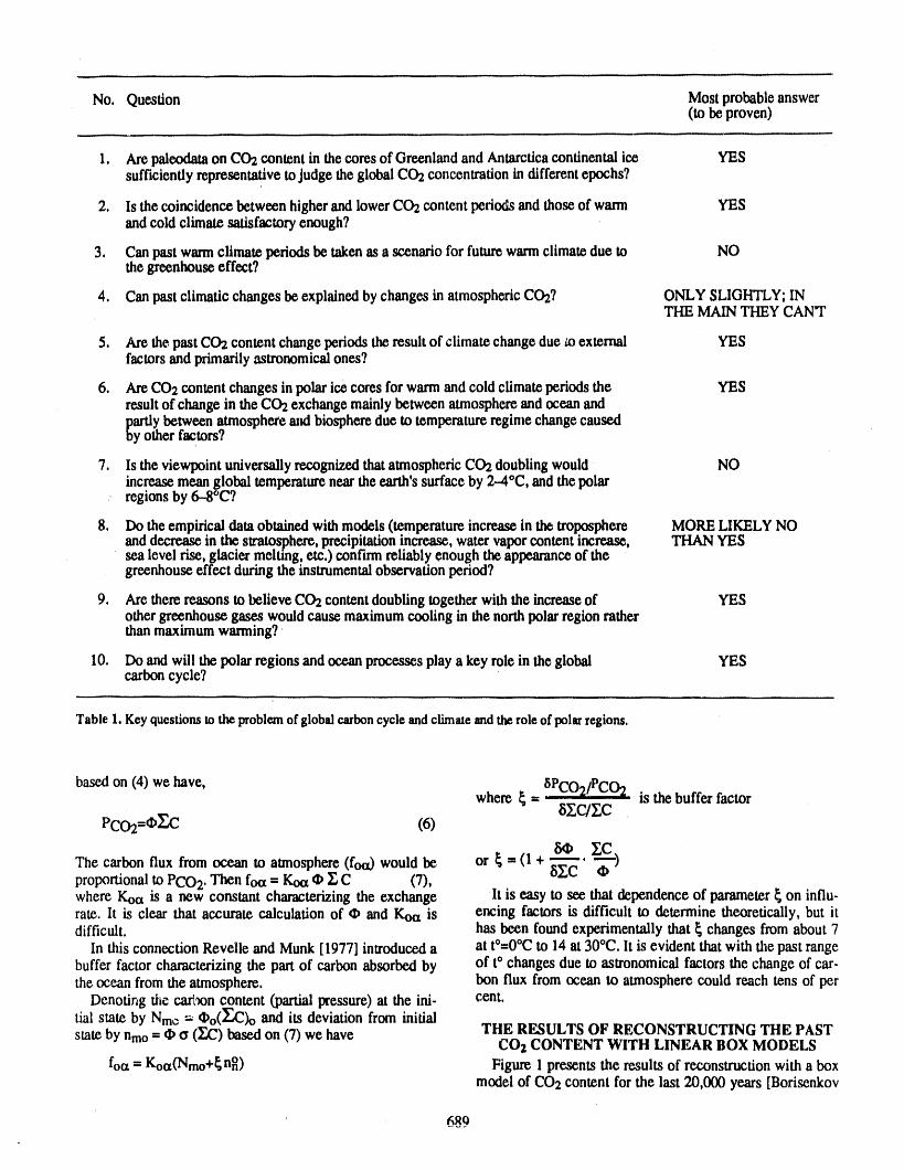
No. Question Most probable answer(to beproven)

1. Arepaleodataon CO2content in thecoresof Greenlandand Antarcticacontinentalice YESsufficientlyrepresentativeto judge the global CO2concentrationin differentepochs7

2. Is the coincidence between higherand lowerCO2content periodsand those of warm YESand cold climate satisfactoryenough?

3. Can pastwarmclimate periodsbe takenas a scenario for futurewarmclimate due to NOthe greenhouseeffect?

4. Canpastclimaticchangesbe explainedby changes in atmospheric CO2? ONLY SLIGHTLY;INTHE MAINTHEYCANT

5. Are the past CO2content change periodstheresult of climate change due Loexternal YESfactorsand primarilyastronomicalones?

6. AreCO2content changes in polar ice cores for warmand cold climate periods the YESresultof change in the CO2exchange mainlybetween atmosphereand oceanandpartlybetween atmosphere aIKibiospheredue to temperatureregimechangecausedby other factors?

7. Is the viewpoint universallyrecognized thatatmospheric CO2doublingwould NOincrease meanglobal temperaturenear theearth's surface by 2-40C, and the polarregionsby 6-8°C?

8. Do the empirical dataobtained with models (temperature increasein thetroposphere MORELIKELYNOanddecreasein the stratosphere,precipitationincrease, watervaporcontentincrease, THAN YESsea level rise, glacier melting,etc.) confh'mreliablyenough theappearanceof thegreenhouseeffect during the instrumentalobservationperiod?

9. Are there reasons to believe CO2contentdoubling together with the increaseof YESother greenhousegases wouldcause maximumcooling in the northpolarregionratherthan maximumwanning? '

10. Do andwill the polar regions and ocean processesplay a key role in the global YEScarboncycle7

Table1. Keyquestionstotheproblemof globalcarboncycleandclimateandtheroleof polarregions.

based on (4) we have,where _ =8PCO_/Pco2 is the buffer factor

8Ec/ cPco2-- Ec (6)

y.cThe carbon flux from ocean to atmosphere (fovOwould be or _ - (1 + ---.proportionalto PCO2.Then foot- Koa • _ C (7), 8Y.C "_-)where Koct is a new constant characterizing the exchange lt is easy to see that dependence of parameter_ on influ-rate. lt is clear that accurate calculation of • and Ko_ is encing factors is difficult to determine theoretically, but itdifficult, has been found experimentally that _ changes fromabout 7

In this connection ReveUeand Munk [1977] introduced a at t°=0°Cto 14 at 30°C. It is evident that with the past rangebuffer factor characterizing the pan of carbonabsorbedby of t° changes due to astronomicalfactors the change of car-theocean from the atmosphere, bon flux from ocean to atmosphere could reach tens of per

Denoting the cartooncontent (partial pressure) at the ini- cent.tial state by Nine = _o(_2)o and its deviation from initialstate by nino= _ a (_C) based on (7) we have THE RESULTS OF RECONSTRUCTING THE PAST

CO2 CONTENT WITH LINEAR BOX MODELS

foct= Koa(Nmo+_ nn) Figure 1 presents the results of reconstruction with a boxmodel of CO2 content for the last 20,000 years [Borisenkov

689

and Kondratiev, 1988], using a 4-box linear model of Bor. To calculate ocean t° more exactly, the model of zeroisenkov andAlttmin[1991] which includes atmosphere,bio- dimensioncan be acceptedof the type,sphere, andactive anddeep oceanic layers, The model was

integrated for 20,000 years back with a time step of 500 dAT1years. The exchange coefficient (the product of Koo¢;in for- c1 -"_= AQ- _,12(AT1-AT2)- LAT1mula (8)) was given in piecewise linear interpolationdepending on paleotemperature. The Figure shows that the

dAT2model reproduces quite well the minimum CO.2content dur- C2 _,12(AT1-AT2) - _.23(AT2-AT3)ing the recent ice epoch. The CO2 concentration variation "_= (9)follows that of paleotemperature.

Figure 2 gives the results of integrating the more sophis- dAT3 _.23(AT2-AT3)ticated 8.box model of Altunin and Borisenkov [1991] for C3 dt =140,000 years, The paleotemperatures were taken from Lot-ius et al. [1985],

The 8-box model of the global carbon cycle includes here C1 = 0.45 W yr m"2°C'I is the atmospheric heat capac-atmosphere, land biota, humus, oceanic inorganic carbon, ity factor;,C2 = 10 W yr m"2°c'l; C3 ffi100 W yr m"2°C'Iphytoplankton, oceanic dissolved organic substance, oceanic are heat capacity factors of the active layer of ocean and ofsediment carbonate rock, and continental sediment rock. deep ocean respectively; Z.= 2,4 W m'2-°C "1 is the param-The rates of exchange between the atmosphere and land eter of climatic feedback; k12 = 45 W m"2 °C-1 is thebiota and humus depend to some extent on temperature. The energy exchange factor between ocean and atmosphere; Z,23rate of exchange between the,,atmosphere and the ocean, in - 4 W m"2 °C'I is the energy exchange factor betweenparticular the box of oceanic inorganic carbon, depends active and deep oceanic layers; AT1, AT2, AT3 are antra-mainly on temperature. These exchange rates are taken from alies of the mean to of atmosphere, acti,_:eand deepoceanicexperimental data. The(i!tt;ivenversion of box model was layers respectively. At theinttial time moment (1860),interpolated backward over 140,000 years with a time stepof 100 years, AT1 = AT2 ffiAT3= 0

Since paleotemperature gives air temperature repro-duction, and our calculations required ocean t°, it was

assumed that ocean t° anomalies were 10% less than the eor- with t _ **AT1 = AT2 = AT3 = ATeq = A._Q_.Qrespondingair t° anomalies. Z.

The water t° anomalies reconstructed in this way are

shown in Figure 2,a. where ATe.qis the equilibrium atmospheric t°, and Q is theNumerical experimental data have shown that if the anthropogenic source. Figure 3 presents the results of model

dependence of exchange coefficient t° is not considered, simulations described by the system of equations (9), for theCO2 concentration remains practically the same over the scenario of anthropogenic source AQ using the data of Bor-whole 140,000-year time interval, which should be isenkov and Kondratiev [1988], lt was taken that the equi-expected, librium t°

If one disregards the dependence of CO-2 exchange

between atmosphere and ocean (box of oceanic inorganic ATm AT(2xC02) • lnlN l(t)/N10] (10)carbon) on t°, but includes that between atmosphere and bio- = ' 1n2sphere (boxes of land biota and humus), weak variations inCO2 content are observed which repeat t° variations (curve lt is clear that atmospheric t° is several decades behind2 in Figure 2b), However CO2 variation amplitudes are far the equilibrium t° due to the thermal inertia of the ocean.from real ones. When the dependence of CO2 exchange Further, behind CO.2 concentration variation are sea t°coefficients between atmosphere and ocean on t° is con- changes which influence the exchange between atmospheresidereal, the agreement between measurements of CO2 con- and ocean. These time periods are tens of years, and consid-tent (solid curve in Figure 2b) and values calculated from erable changes can take place in the oc_ a for this time.the model (dots with crosses) proves to be quite satisfactory, Results mentioned in the WMO/UNEP report [1990]

This gives reason to assume theI the past CO2 content indicate that this is the case. This report contains much evi-changes were determined most likely by natural processes dence showing that consideration of ocean leads to the lagand resulted from climate changes rather than vice versa, of atmospheric and sea t° changes from respective equi-

In this connection one should very carefully estimate the librium temperature. In the model under study for the atmos-possibilities of constructing scenarios of future climate phere, Model t° changes by 2000-2030 years are about 55%caused by CO2 content change on the basis of past warm of equilibrium t° changes ATm(t). This conclusion is inepoch paleoclimates since absolutely different causes act good agreement with the results of other authors, in par-here. lt is worth mentioning that this conclusion does not ticular with the results of a recent study by Schlesinger anticonuadict the conclusions of Broecker and Denton [1990] Jiang [1990].and of other authors that CO2 changes could explain notmore than 50% of climate changes which took piace. What DYNAMICS OF GREENHOUSE GASis more important is that climatic changes which were ANTHROPOGENIC SOURCEScaused by astronomical factors determined CO2 changes in lt is important to determine which dynamics of thethe atmosphere, anthropogenic source AQ should be prescribed in the model.

690

Many uncertaintiesand extremelyhigh values of AQeor- greenhouseeffect, methane 17%, stratosphericwater vaporrespondingto a maximumemission of anthropogeniccarbon 6%, N20 4%, ali freons CFCn 12%. The picture changedof up to 80-100 Gt yrl in theneardecades have led to over- somewhat for 1980-1990 and this would characterize theestimated values for Q. There several tens of scenarios at future. Thus the CO2 contributionwas only 55%, the. con-present for energetics development which are analyzed in tributionsOfCH4, stratosphericwatervapor,N20 and CFCnBorisenkovand Kondratiev[1988]. were 11, 4, 6 and24% respectively, In otherwords, to con-

The most realistic scenarios are determined by vela- sider completely the greenhouse effect, CO2 growth oftionshipsof the type: about 1% per yearcan be taken,

"_dORo(l" Q"Q THE INFLUENCE OF DEEP OCEAN ON THEnl (0 GREENHOUSE EFFECT

One approaches for modeling the carbon cycle and its

Q_)n CO2 manifestationstn the cltmate system seems to be pre-nl(t) = _Ro[1 -( ]'Q (11) scribing a gradtmlincreaseof CO2ata rate of 1% per year,andits suddendoubling, as was done earlier.Besides, as wesaw, the deep ocean processes should be included in the

d._ffiRo.Qn.e.mt models. This should be done because, using real data, onenl(t)OI

cannot yet identify with assurancethe global manifestationHere Q is the amountof carbonreleased to the atmosphere, of the greenhouseeffect in the climaticsystem components.Qo, is carbonreserves, Ro is a parametercharacterizingthe These manifestations of the greenhouse effect could berate of carbon growth, and n and m are some empirical tropospheric t° rise and stratospheric t° fall, continental iceparameters, melting, sea level rise, and increase of atmospheric moisture

The scenarios of CO2 emission dynamics determined content. Among these components we can best distinguishfrom (11) depend first of ali on the s_narios of energetics the really observed positive trend of mean t° near the earth'sdevelopment. The maximum value _ in some scenarios surface.reached 80-100 Gt yr-t,which is notreat_isttc. However, as is shown above, according to ali model estt.

In most scenarios proposed,max (:'a_amounts to 20-30 matesthe t° trendin the atmosphereandeven more so in theGt of carbonper year, falling in the middle of the next cen- _ _houldbe behind the CO2growth trend.Actually thetury. The scenarios estimated in (11) depend to a consid- reverse tookpiace. Tbe positive t° trendstartedat the begin.erable extent on parametersRo, n ,usa mn. The value Q, ningof the currentcentury and reachedits maximumin thecorresponds to the forecasted _upply of conventional fuel 1930s. At that thne the CO2 trend was small. But in theand was assumed equal to 600 GL The above three param- 1940s when the positive trend of CO2 concentrationeters were selected assu_g that at tffi110(this corresponds increased abruptly t° startedfalling. This gives reason toto 1970) (_'-130 GL and "_tffi5 Gt yr-t. These estimates are believe thatthe positive t° trend in the 1930s and 1940s waswell confirmed experimentally.The parametern was a var- not related to CO2 growth, and that it cannot be taken intoled one and was selected depending on scenariosof energet- accountwhen attributingthe observed t° trendto the green.ics development. In this case it was assumed that the house effect. EUsaesser [1984] has the same viewpoint. Thismaximum emission falls on 2030 and is 30 Gt yr-l. Under is even more evident ff one takes into consideration thatthese conditions Ro=0.02, mnffil.25andnffil, such warming periods in the history of climate, took place

Figure 4 gives the results of simulating the atmospheric several times, forexample, in the firsthalf of the 16rhcen-carbon content on the basis of seven types of box models, fury [Borisenkov and Pasetsky, 1988]. These periods,beginning with a linear 9-box model and a nonlinear 7-box including those in the 1930s and 1940s, were related tomodel and with sufficiently realistic scenarios tbr the atmospheric circulation changes. If one subUacts the 1930s/dynamics of source nl(t), from Borisenkov and Altunin 1940s temperature trend from the total, the remaining trend[1985]. This scenario is close to the scenario of the Institute shows a very weak component at noise level which does notof Applied System Analysis (Vienna). correspond to temperature changes which should have taken

The Figure shows that the range of possible CO2 changes piace according to model (9). The actual t° trend after thein the atmosphere is rather narrow. Maximum CO2 con- 1930s and 1940s and up to the mid-1970s is opposite to thecentrations in the atmosphere according to this model data CO2 trend. Ali this allows us to say that there are no reliablewould not exceed 2.0 to 2.5 times the pre.industrial level of indications of greenhouse effect manifestations in the sur-1860. Double CO2 concentration is reached at the end of the face t° field. Nor are these indications found in other climate21st century or even the beginning of the 22nd century, not characteristics. Though some sections of the WMO/UNEPearly in the 21st. This effect in the model is explained by report [1990] are inconsistent, Wigley and Barnett [1990],considerable absorption by the ocean, the authors of section 8 of the report, stated clearly that

Bearing in mind that this model gtves sufficiently good there are no reliable indications of greenhouse effect man-agreement between calculated CO2 concentration for the ifestationsfromobservations.industrial period of 1860-1960 and the past 130 years, one This should not make the problem of the greenhousecan hope that the above estimates should be relied upon. effect and society's concern about its consequences less

lt should be borne in mind that the greenhouse effect is interesting. The question is whether we know reliably whatinfluenced by other anthropogenlc pollutants as weil. As the climatic consequences of a greenhouse effect would begiven in the WMO/UNEP report [1990], for the period and whether the future warming of climate with maximum1765-1990 CO2 yielded 61% of the contribution to the warming in high latitudes is an accurate scenario.

691

/J

I/

One of these consequences, as mentionedabove, is pos. talcingpreventive measures and is not unexpected in the /sible climate warming, on the average by 2-4°(2, and in lightof the preceding discussion. Thereforeali contrarysee-:polarregions by 6-80C. Although this viewpoint was most _arios of future climate relative to the greenhouse effectpopular until recently, some scientists criticized it [Idso, should be carefully analyzed and checked before pl_nntng1982; Elisaesser,1984',Borisenkov and Kondratiev, 1988]. preventivemeasures.For example,based on thescenarios ofRecent numerical experiments made by Washington and climate change toward wanning, in the USSR suggestionsMeehl [1989] and Washington [1989] have shown that this were made to stop building ice.breakerssince ice conditionsgenerally accepted scenario of future climate could hardly in the Arctic would become less severe. Dangerous warn-be considered reliable. Inclusion of deep ocean in model inis are made regarding melting permafrostzones whictlintegrationover 30 years with gradualyearly CO2 increase occupy ex_isive areas in the USSR.of I% leads to quite different scenarios of future climatecompared to scenarios from models with sudden C02 dou- CONCLUSIONbling and disregarding deep ocean. These results are pre- Ali the above gives reason to believe thatscience has notsented in Figure 5. When COz increases by a factor of yet reliably providedconclusions on the manifestationof theapproximately 1.6-1.8 over the preindustrial level for 30 greenhouseeffect, and its climatic and social consequences,years the ocean is reconstructed so considerablythatdue to For this, furtherstudies of the problemare necessary on anfeedbacks weaker t° rise (by 2,--30C)occurred over con- interdisciplinarybasis. Society would have to pay a highttnents. Over the north polar area, particularlyin the Atlantic price for ungroundedrecommendations.region, maximum toc decrease by 6--8°C is observed (to But in ali cases it is evident that the focus of uncertainty10-11°F) rather than maximum increase. In the southern in regional terms shifts to polar regions. In this connectionhemispheret ° regime changes are insignificant. In this see- the role of the polar regions in studying the given problemnario the sea ice thickness increases by approximately shouldbethe leadingone.0.5 m. The southernboundaryof polar ice shifts to the equa- In conclusion it should be noted that the author did histor.Climate instabilityincreases sharply, best and tried to provide the answers to the questions in

This result radically changes the idea of climatic con- Table 1, understandingthat the discussion of them cannotbesequences of the greenhouse effect andrecommendationson consideredfinished.

REFERENCES

Altunin,I. V., and E. P. Borisenkov, Descriptionof atmos- Lorius, C., et al., A 150000 year climate record from Ant-pheric CO2 dynamics on the time scale of 10 years (in arcticice, Nature, 316, 591-596, 1985.Russian), Acad. Sci. USSR Papers, 316, 574--576, 1991. Manabe,S., andR. T. Wetherald,The effect of doubling/the

Bacastow, R., and E. Maier-Reimer, Ocean-circulation CO2 concentrationon the climate of a general circulationmodel of the carbon cycle, Clim. Dynamics, 4, 95-125, model, J. Alines. Sci., 32, 3-15, 1975.1990. Revelle, R., and W. Munk, The carbon dioxide cycle and the

Bamola, J. M., D. Raynaud, Y. S. Korotkevich, and C. biosphere, J. Energy and Climate, 140--158, 1977.Lorius, Vostok ice core: 160000 year record of atmos- Schlesinger, M. E., and X. Tiang, Simple model repre-phericCO2,Nature, 329, 408-414, 1987. sentation of atmosphete,-ocean GCMS and estimationof

Borisenkov, E. P., and I. V. Altunin, Atmospheric CO2 the time scale, J. Climate,3, 1297-1315, 1990.growth and its effect on climate (in Russian), Acad. Sci. Shackleton, N. I., et al., Carbon isotope data in core V9-30.USSR Papers, 281,559--661, 1985. Confirm reduced carbon dioxide concentration in the age

Borisenkov, E. P., and K. Ya. Kondratiev, Carbon cycle and atmosphere, Nature, 306, 319-322, 1983.climate. L., (in Russian), Gidrometeoizdat, 1988. Washington, W. M. Where's the heat?, Natural History, No.

Borisenkov, E. P., and V. M. Pasetsky, Thousand-year 3,69-72, 1990.chronicle of extraordinary natural phenomena. M. (in Washington, W. M., and G, A. Meehl, Characteristics ofRussian), Mysl, 1988. coupled atmosphere,-xw.ezuaCO2 sensitivity experiments

Broecker, W. S., and G. N. Denton, What drives glacial with different ocean formulations, 58 pp., PreIn'int,cycles?, ScientbqcAmerican, 202, 1990.

Budd W. F., and P. Rayner, Modelling global ice and eli- NCAR, Boulder, Colorado, 1989a.mate changes through the ice ages, Ann. Glaciol,, 14, 1- Washington, W. M., and G. A. Meelfl, Climate sensitivitydue to increased CO2. Experiments with a coupled atmos-17, 1990.

Chappellaz, J. J., J. M. Barnola, D. Raynaud, E. C. Korot- phere and ocean general circulation model, Clim. Dynam-kevich, and C. Lorius, Ice core record of atmosphere ics, 4, 1-38, 1989b.methane over the past 160000 years, Nature, 345, 127- Wigley, T. M. L., and T. P. Barnett, Detection of the green-131, 1990. house effect in the observations. J. Rep. Scientific

Ellsaesser, H. W., The climatic effect CO2: a different view, Assessment of Climate Change. Rep. for IPCC Work.Atmos. Environ., 431-434, 1984. Group 1. WMOAJNEP, 245-260, 1990.

Idso, S. B.0 Carbon Dioxide: Friend or Foe? 92 pp., IBR WMO/UNEP, Scientific assessment of climate change.Press, Tempe, Arizona, 1982. Report prepared by working group 1, 1990.

692

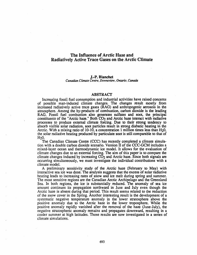
The Influence of Arctic Haze andRadiatively Active Trace Gases on the Arctic Climate

J..P. BlanchetCanadianClimateCnte, Ontado,C, ,aa

ABSTRACTIncreasing fossil fuel consumption and industrial activities have raised concerns

of possible man-induced climate changes. The changes result mostly fromincreased radiatively active trace gases (RAG) and anthropogenicaerosols in theatmosphere. Among the by-productsof combustion, carbon dioxide is the leadingRAG. Fossil fuel combustion also generates sulfates and soot, the pflncipalconstituents of the "Arctic haze." Both CO'2and Arctic haze interact with radiativeprocesses to produce external climate forcing. Due to their strong tendency toabsorb visible solar radiation, soot particles result in strong diabatic heating in theArctic. With a mixing ratio of 10-10, a concentration 1 million times less than H20,the solarradiative heating produced by particulate soot is still comparable to that ofH20.

The Canadian CLimateCentre (CCC) has recently completed a climate simula-tion with a double carbon dioxide scenario. Version II of the CCC-GCM includes amixed-layer ocean and thermodynamic ice model. It allows for the evaluation ofclimate changes due to an external forcing. The aim of this paper is to compare theclimate changes induced by increasing CO2 and Arctic haze. Since both signals arcoccurring simultaneously, we must investigate the individual contributions with aclimate model.

A preliminary sensitivity study of the Arctic haze (February to May) withinteractive sea ice was done. The analysis suggests that the excess of solar radiativeheating leads to increasing rates of snow and ice melt during spring and summer.The most sensitive regions are the Canadian Arctic Archipelago and the GreenlandSea. In both regions, the ice is substantially reduced. The anomaly of sea iceamount continues its propagation northward in June and July even though theArctic haze is absent during that period. This result seems related to the reductionof the snow cover in the Spring. Another interesting result is the development of asystematic negative temperature anomaly in the lower stratosphere above thepositive anomaly due to the Arctic haze in the lower troposphere. While thepositive anomaly rapidly vanished after the removal of the haze (June-July), thenegative stratospheric anomaly remains and propagates downward, resulting in acooler summer at high latitudes. Those results are now investigated in a series ofclimate simulations.

693

AGASP-IH, Polar Lows andCEAREX Norwegian Arctic Flight Program, Spring 1989

R. C. Schnell and P. J. SheridanCooperativeInstitutefor Researchin EnvironmentalSciences,Universityof Colorado/NOAA,Boulder,Colorado,U.S.A,

J. D. KahlDepartmentof Geosciences,Universityof Wisconsin.Milwaukee,Milwaukee,Wisconsin,U.S.A.

ABSTRACT

The third Arctic Gas and Aerosol Sampling Program (AGASP) intensiveairborne research program was successfully conducted in the Norwegian Arctic,March-April 1989. Flying from Bode, Norway, the NOAA WP-3D was utilized tc,study (1) two separatePolar Low systems that developed in the GreenlandSea; (2)the tta,nsfer of energy from the atmosphere to the ice over permanent packice noelof Spitsbergen;.(3) the transfer of wind and heat energy along the ice edge; and (4)Arctic haze (atr pollution) and solar radiation distributions east of Spitsbergen.Participants were from three NOAA laboratories, three National laboratories,NASA, and nineteen universities, with representation from five countries.

These flights were coordinated with surface measurements at the Ny A,lesundNorwegian baseline station on Spitsbergen and the Office of Naval Research(ONR) Coordinated Eastern Arctic Experiment (CEAREX) "O" and "A" ice campsnorthwest of Svalbard.

In these latter flights, AGASP scientists continued their study of the photolyticdestruction of tropospheric ozone in the Arctic spring boundary layer. A source forthe Br molecule involved in the ozone destruction reaction has been suggested asbeing of under-ice origin released to the atmosphere as bromoform and bromo-dichloromethane. A marine or ice algae may be responsible.

From aircraft data on these flights, it was observed that the ozone destructionphenomenon may be capped by as little as a 0.2°C temperature inversion. Ozonedestruction in the marine boundary layer over open water was not observed even ondays when such destruction was observed 100 km further north over theArctic icepack.

694

Comparison of Measurements of Aerosol Black Carbonat Barrow, Alaska, and Wrangel Island, USSR:

An Approach to Estimating the Deposition of Soot to Snow and Ice Surfaces

A. D. A. HansenLawrenceBerkeleyLaborawry,Universityof CalC'ornia,Berkeley,CalOrornia,U,8,4.

R. C. SchneliNOAA/CIRE$,Boulder,Colorado,U.S.A.

J. D. KahlDepartmentof Geosciences,Universityof Wisconsin-Milwaukee,Milwaukee,Wisconsin,U.8,4.

B. A. BodhaineNOAA/GMCC,Boulder,Colorado,U.S.A.

V. N. KapustinInstituteof AtmosphericPhysics,Moscow,U.S.S.R.

ABSTRACT

During late spring 1989 (and 1990, in planning), measurements of aerosol"black" carbon were made on Wrangel Island in the Soviet Arctic to complement

the routine measurements at the NOAA/GMCC Barrow Observatory of th!scombustion-derived pollutant. The results are compared during time intervals mwhich trajectories led from Barrow to Wrangel Island, with typical transit times ofone day. The inte.rvening surface is entirely frozen ocean, without land masses'topography to complicate air flow, nor any human habitation combustion sources.Aerosol black carbon is chemically unreactive, and so any losses in transit will bedue to deposition onto the frozen ocean surface. This species is strongly opticallyabsorbing, and a small aerosol deposition from the Arctic haze may reduce thesurface albedo sufficiently to increase the absorption of solar radiation in spri.ngandlead to premature thawing. We shall discuss the possible effects of the deposition of"soot" from the Arctic haze onto high latitude snow and ice cover in terms ofclimate change.

695

A Review of Arctic Gas Hydrates as a Source of Methane in Global Change

Keith A. Kvenvoldenu,s. GeologicalSurvey,MenloPark,California,U.SA.

ABSTRACT

Atmospheric concentrations of methane are currently increasing at rates of aboutone percent per year, leading to a concern that methane, a "greenhouse" gas, willbecome an increasingly significant factor in global warming. One potential sourceof enormous volumes of methane is natural gas hydrates, which are solids com-posed of cages of water molecules that contain gas molecules, mainly methane. Gashydrates are stable only within certain ranges of temperature and pressure; outsidethese ranges, the cages break down and the gas molecules escape. The Arctic is par-ticularly well endowed with gas hydrates because conditions for their occurrenceare met in three distinct regions: (1) offshore in segments of the outer continentalmargin, at water depths between about 400 and 2800 m, where the base of the zoneof gas hydrate stability ranges from about 300 to 700 m below the sea floor; (2)onshore m areas of continuous permafrost, where the zone of gas hydrate stabilityranges in subsurface depth from about 200 to 1200 m; and (3) on the nearshore con-tinental shelf, where relict perm",..fi'osthas persisted since times of lower sea levelwhen the present shelf was exposed to cold subaerial temperatures. Because gashydrates occur close to the earth's surface in these three regions, they are affectedby surficial changes in pressure and temperature, mid thus destabilized gas hydratesmay be sources of atmospheric methane. Under the present climatic regime, the gas

hydrates of the nearshore continental shelf may, be the most vulnerable to chang.e.The time needed for thermal change to destabilize gas hydrates m this region ismeasured in thousands or tens of thousands of years. Because the latest major Arc-tic marine transgression may have been in progress for about 27,000 years, somegas hydrates associated with nearshore permafrost probably have already becomeunstable, releasing methane to the atmosphere. The rate of current release is esti-mated to be about 3 x 1012 g of methane carbon per year.

INTRODUCTION mussenand Khalll,1984].ContemporaryconcentrationsofMethane is the most abundant gaseous organic com- atmosphericmethaneare at levels that exceed any values

ponent of the earth's atmosphere.The globallyaveraged observedfor the last 160,000years of geologictime [Ray-atmosphericmethaneconcentrationat presentis about 1.70 naudet al., 1988;Staufferet al., 1988].ppm by volume [summarizedby Ciceroneand Oremland, Methane is an important greenhouse gas due to its1988],whichtranslatesto about3.6 Gt (gigatons= 1015g) infraredadsorptionproperties.Atmosphericmethaneexertsof methanecarbon in the atmosphere.The amountof meth- directand indirectinfluenceson the earth's climatesystem,ane that is in the atmosphereis currentlyincreasingat a rate and the predicted future increasein atmosphericmethaneof about 0.03 Gt yr-I of methanecarbon,and the increase concentrationsis likely to contributemore to futureclimatebeganabout 200 years ago as demonstratedby analysesof change thanany other gas exceptcarbondioxide [Ciceroneair trappedin ice cores fromGreenlandandAntarctica[Ras- andOremland,1988].

696

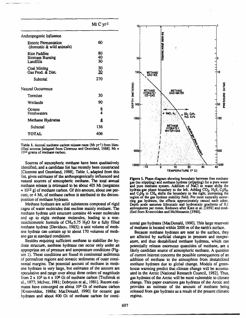
MtCyrl 10 ,) , .... , , , I

Anthropogenlc Influence I[ -EntedcFermentation 60(domestic & wild animals) ) _

Rice Paddies 80 _ -

Biomass Burning 40 _0 _ =5Landfills 30

Coal Mining 30

Prod.DLt. 30Subtotal 270

Natural Occurrence !Termites 30

Wetlands 90 _ • 1_501 - 50 _.Oceans 8 o .Freshwaters 4 " co,,e,H,,

t_S,C)H,Methane Hydrates 4 ioo0 .: .:, loo

Subtotal 136 " METi_ANE"".•HYOClATE+'WATER+OAS

TOTAL 406

Table1.Annualmethanecarbonreleaserates (Mtyrl) fromiden. - I " : " " " ' :"tiffedsources[adaptedfromCiceroneandOremland,1988],Mt = I:. " :._"'1012 gramsof methanecarbon, 500_ ,. :,f : : ..:_:: ... . : 500

:t .... •" !''i;::" ..,_/' , ,- ,.,.,. , :

Sourcesof atmospheric methane have been qualitatively 10000 40)000identified, and a candidatelist has recemflybeen constructed -lo o lo 2o 30[Cicerone and Oremland, 1988]. Table 1, adaptedfrom this TEMPERATURE(" O)

list, gives estimates of the anthropogenically influenced and Figure1. Phasediagramshowingbouadan/betweenfreemethanenatural sources of amaosphericmethane. The total annual gas (nostippling)andmethanehydrate(stippling)forapurewatermethane release is estimatedto be about 405 Mt (megatons andpuremethanesystem,Additionof NaCl to watershifts the= 1012g) of methanecarbon.Of this amount,about one per- hydrate-gasp_h_.• boundaryto the left, Addin$CO?,H2S,, C2H6,cent, or 4 Mt, of methane carbonisattributed to the decom- and C3H8 to O14 shifts the boundaryto me nglat, increasingmc

regionof thegas hydratestabilityfield.Formostnaturallyoccur.position of methane hydrates, ring gas hydrates,the effects approximatelycancel each other,

Methane hydrates are solid substancescomposed of rigid Depthscale assumesltthostaticand hydrostaticgradientsof 0,1cages of water molecules that enclose mainly methane,The atmospherespermeter,RedrawnafterKatzet al. [1959]andmod.methane hydrateunit structurecontains 46 water molecules ifiedfromKvenvoldenandMeMenamin[1980].and up to eight methane molecules, leading to a non-stoichiometric formula of CH4,5.75 H20 for a fully filled nentalgas hydrates[MacDonald, 1990]. This large reservoirmethane hydrate [Davidson, 1983]; a unit volume of moth. of methane is located within 2000 m of the earth's surface,ane hydrate can contain up to about 170 volumes of moth, Because methane hydrates are near to the surface, theyane gas at standard conditions, are affected by surficial changes in pressure and temper-

Besides requiring sufficient methane to stabilize the hy. ature, and thus destabilized methane hydrates, which candrate structure, methane hydrates canoccuronly under an potentially release enormous quantities of methane, are aappropriate set of pressure andtemperature conditions (Fig- likely candidate source of atmospheric methane. A questionure 1), These conditions are found in continental sediments of current interest concerns the possible consequences of anof permafrost regions and oceanic sediments of outer conti- addition of methane to the atmosphere from destabilizednental margins. The potential amount of methane in meth. methane hydrates due to global change. Models of green-ane hydrates is very large, but estimates of the amount are house warming predict that climate change will be accentu-speculative and range over about three orders of magnitude ate,d in the Arctic [National Research Council, 1982]. Thus,from 2 x 103 to 4 x 106Gt of methane carbon [Trofimuk et gas hydrates of the Arctic will be most vulnerable to climateal., 1977; Mclver, 1981; Dobrynin ct al., 1981]. Recent esti- change. This paper examines gas hydrates of the Arctic andmates have converged on about 104Ot of methane carbon provides an estimate of the amount of methane being[Kvenvolden, 1988a; MacDonald, 1990] for oceanic gas released from gas hydrates as a result of the presentclimatichydrates and about 400 Ot of methane carbon for conti- regime.

697

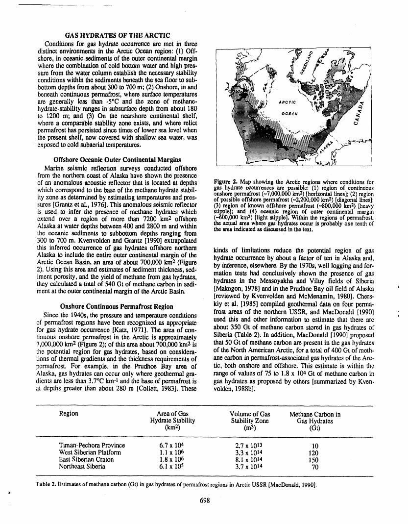
GAS HYDRATES OF THE ARCTIC

Conditions for gas hydrat_ occurrence are met in three

distinct environments in the Arctic Ocean region: (1) Off- ff,_._,._ ./ f ,_ _ -shore, in oceanic sediments of the outer continental margin 'xi f__,dwhere the combination of cold bottom water and high pres- _'_/ _/_,.

sure from thewater column establish the necessarystability " / _ibottom depths from about 300 to 700 m; (2) Onshore, in and

hydrate-stabilityrangesin subsurfacedepth from about 180 '(_ iOOE_,N

to 1200 m; and (3) On the nearshore continental sl_lf, _: .... ., '

where a comparable stability zone exists, and where relict _ ,,,,,.,/_, .._permafrost has persisted stnce times of lower sea level when '' _.....the present shelf, now covered with shallow sea water, was __..,exposed to cold subaerial temperatures, __#- _" y-_ "

Offshore Oceanic Outer Continental Margins _.,_Marine seismic reflection surveys conducted offshore

from the northerncoast of Alaska have shown the presenceof an anomalousacoustic reflector that is located at depths Figure 2. Map showing the Arcticregions where conditionsfor

gas hydrateoccurrenoesare possible:(1) region of continuouswhich correspond to the base of the methane hydrate stabil- ,onshorepermafrost(~7,000,000km2)[horizontallines];(2) regionity zone as determined by estimating temperatures and pres- of possibleoffshorepermafrost(-2,200,000krn2)[diagonallines];sures [Grantz et al,, 1976], This anomalous seismic reflector (3) region of known offshorepermafrost(-800,000 km2) [heavy

is used to infer the presence of methane hydrates which stipple]; and/4) oceanic region of outer continentalmarginextend over a region of more than 7200 km2 offshore (.-600,000km ) [light stipple].Withinthe regions of permafrost,Alaska at water depths between 400 and 2800 m and within the actualarea wheregas hydratesoccur ts probablyone tenthoftheareaindicatedasdiscussedinthetext.the oceanic sediments to subbottom depths ranging from300 to 700 m. Kvenvolden and Grantz [1990] extrapolated

this inferred occurrence of gas hydrates offshore northern kinds of limitations reduce the potential region of gasAlaska to include the entire outer continental margin of the hydrate occurrence by about a factor of ten in Alaska and,Arctic Ocean Basin, an area of about 700,000 km2 (Figure by inference,elsewhere. By the 1970s, well logging and for-2). Using this area and estimates of sediment thickness, sed- matlon tests had conclusively shown the presence of gasiment porosity, and the yield of methane from gas hydrates,they calculated a total of 540 Gt of methane carbon in sedi. hydrates in the Messoyakha and Viluy fields of Siberiament at the outer continental marginof the Arctic Basin, [Makogon, 1978] and in the Prudhoe Bay oil field of Alaska L

[reviewed by Kvenvolden and McMenamin, 1980]. Chers-

Onshore Continuous Permafrost Region kiy ct al. [1985] compiled geothermal data on four perma-frost areas of the northernUSSR, and MacDonald [1990]

Since the 1940s, the pressure and temperature conditions used this and other information to estimate that there are 'of permafrost regions have been recogn_ed as appropriate about 350 Gt of methane carbon stored in gas hydrates offor gas hydrate occurrence [Katz, 1971]. The area of con-tinuous onshore permafrost in the Arctic is approximately Siberia (Table 2). In addition, MacDonald [1990] proposed7,000,000 km2 (Figure 2); of this area about 700,000 km2 is that 50 Gt of methane carbon are present in the gas hydratesthe potential region for gas hydrates, based on considera- of the North American Arctic, for a total of 400 Gt of meth-tions of thermal gradients and the thickness requirements of ane carbon in permafrost-associated gas hydrates of the Arc-permafrost. For example, in the Prudhoe Bay area of tic, both onshore and offshore. This estimate is within theAlaska, gas hydrates can occur only where geothermal gra- range of values of 75 to 1.8 x 104 Gt of methane carbon indients are less than 3.7°C km-I and the base of permafrost is gas hydrates as proposed by others [summarized by Keen-at depths greater than about 280 m [Collett, 1983]. These volden, 1988b].

Region Area of Gas Volume of Gas Methane Carbon inHydrate Stability Stability Zone Gas Hydrates

(km2) (m3) (Gt)

Timan-Pechora Province 6.7 x 104 2.7 x 1013 10West Siberian Platform 1.1 x 106 3.3 x 1014 120East Siberian Craton 1,8 x 106 8,1 x 1014 150Northeast Siberia 6.1 x 105 3.7 x 1014 70

Table2. Estirrtatesof methanecarbon(Ot)in gashydratesof permafrostregionsinArcticUSSR[MacDonald,1990].•

698

The presenceof gas hydratesin the North American Arc. permafrost and about 120 Gt of methane carbon to beric ims been demonstrated.Well-log responses, consistent present in the entire region where offshore permafrost iswith the presence of gas hydrates, were obtained in the knownor was possible in therecentpast.MackenzieDelta [Bily and Dick, 1974;Judge, 1982]; Sver-drupBasin, Arctic Platformand Arctic Islands [Davidson et GLOBAL CHANGEal., 1978; Judge, 1982]; andon the North Slope of Alaska The total reservoirof methane carbon sequestered in gas[Collett' 1983].Detailed reviews of weU logs, well histories, hydrates of the Arctic is about 940 GL with 400 Gtdrilling reports,core de_'riptions, andproduction tests from [MacDonald, 1990] associated with permafrost and 540 Gtthe NorthSlope of Alaska reveal gas hydratesin a restricted [Kvenvolden and Grantz,1990] in outercontinentalmarginregion of the Prudhoe Bay-Kuparuk River oil field area sediments. Of the 400 Gt of methanecarbonassociated with[ColleCtet al., 1989]. Most of the gas hydratesare patchy permafrost, about 120 Gt are associated with offshore per-and occur in six laterally continuous sandstone and con- mafrost.Obviously these numbersare very speculative, butglomer'ateunits ranging in thickness from 2 to 28 m. The they provide a basis for attemptingto judge theimpacts ofamount of methane present in the Prudhoe Bay-Kuparuk gas hydratesresulting fromglobalchange.River area is estimated to be about 0.6 Gt of methane Because gas hydratesoccur so near the surface, their sta-carbon, bility is affected by pressureand temperaturechanges at the

surface. Increases in pressure and decreases in temperatureNearshore Continental Shelf Relict Permafrost Region will tend to stabilize the gas hydrates, whereas the opposite

The amount of relict permafr_ and associated gas changes, that is, a decrease in pressureand an increase inhydrates beneath the shelf today depends apon d_eregres- temperature,will destabilize the gas hydratestructure.Meth-sion _mdtransgression history, initial distributionof tem- ane hydrates in each of the three distinct Arctic environ-pcratures, ice content, gas content, and salinity in the ments (offshore, onshore, and nearshore)are vulnerabletosediment at the time of inundation.Offshore permafrost is global change, but they are vulnerable to different extentsknown to occur on the BeaufortSea shelf of Canada[Neave dependingon their settings.ct al., 1978; Weaver and Stewart, 1982]. Also offshore per- Evidence alreadyexists that warmingof onshore perma-mafrostoccupies a partof the vast continental shelf of Sibe- frost is currently taking place. Lachenbruchand Marshallria [Vigdorchik, 1980]. Studies by Rogers and Morack [1986] showed anomalous temperatureprofiles in the upper[1980] on subseapemmfrostand sea level history lead to the 100 m of permafrostin northernAlaska. They believe thatinference thatoffshore permafrostmay persist beneathany these profiles indicate a varying but widespread secularpartof the Arctic shelf inshorefromabout the90 m isobath, warmingof 2--4°Cof the permafrostsurface duringthe 20thBased on this inference, the area of potential offshore per- century. These thermal changes will eventually penetratemafrost is estimated to be about 3,000,000 km2, and within deep enough to destabilize gas hydrateswithin and beneaththis region thereareabout 800,000 km2where offshoreper- the permafrost, but because of heat transfer propertiesasmafrostis known to be present(Figure 2). About one tenth discussed in detail by MacDonald [1990], the time_de foroftheseareasisassumedtocontaingashydratesbasedon thesethermalchangesisverylarge,requitingthou,gandsofconstraintsimposedby geothermalgradientsand require- yearsbeforeallgashydratesaredestroyed.Forthepresent,ments for minimum thicknesses of permafrost,as discussed however, gas hydrates associated with onshore permafrostpreviously, have probablynot felt the effect of permafrostwarming.

Evidence that gas hydrates are associated with offshore Offshore, the outer continental margin sediments con-permafrostcomes from theMackenzieRiverdeltaarea mininggashydratesareundera columnofverycoldwaterwherewelllogsfromoffshoredrillingindicated thepres- (near0°C)atpressuresequivalentto400-2800m ofwater.ence of both permafrost and gas hydrates [Judge et al., Over the last 27,000 years the pressures on the offshore gas1987]. The observationof gas hydrates in this region sug- hydrates have probably slowly increased due to rising scagests that gas hydratesare also Isesent in other areaswhere levels of about 100 m. Evidence for such a sea level rise hasoffshore permafrostoccurs. The distributionof gas hydrates been obtained from boreholes in the Canadian Beaufortassociated with offshore permafrost is probably similar to shelf [Hill et al., 1985]. Because circulationof Arctic Oceanthat of gas hydratesassociatedwith permafrostonshore; that water into the Canada Basin is restricted [Aagaard et al.,is, the gas hydratesare restricted,patchy, and confined to 1985], this reslliction may provide insolation against ther-porous sedimentary units as in the Prudhoe Bay-Kuparuk mal changes in bottom waters at least for the present time.River area [Colleu et al., 1989]. The amountof methane in Therefore, these offshore gas hydrates, experiencing in-gas hydratesassociated with offshore permafrostcan be esti- creased pressure and minimal temperature changes, arcmatedby utilizingthevalueof400Gt ofmethanecarbon, probablystable,andarea sinkformethaneandnotasource.determinedby MacDonald[1990],asthetotalamountof Evenifsmallamountsofmethanewerebeingreleasedfrommethaneinpermafrost-associatedgas hydrates,bothon- thesegashydrates,much ofthisgaswouldlikelybe dis-shoreandoffshore.Theamountofmethaneinoffshoregas solvedinthewatercolumnorbeoxidizedtocarbondioxide.hydrates is assumed to be proportionalto the inferred area The one environment of the Arctic where gas hydratesof gas hydrate occurrence in the known offshore permafrost are currently vulnerable to global change is the region ofregion (80,000 km2) and the potential offshore permafrost offshore permafrost [Kvenvolden, 1988b]. Gas hydratesregion (300,000 km:') relative to the total potentialarea of present within and under offshore permafrost are probablygas hydrateoccurrenceivArcticpermafrost(I,000,0C0 becomingunstableatleast inpart.The basiccauseofthekm2).t"-nus,about32Gt of_:_ethanecarbonisesdmaw.,dm destabiiizadonisfilemarinewansgressionthathastaken

presentingashydratesassociatedwithknownoffshore placesincethelasticeage.On theBeaufortshelf,forexam-

699

pie, and probablyon othercontinental shelves of the Arctic that the released methane is not trapped within the sedi-Ocean, sea level has risen significantly during the past menll but ratherescapes to the atmosphere. This rate is27,000 years [Hill et al., 1985] bringing cold water to an slightly smallerthanthe "placeholder"estimate of 4 Mt yr-Ieven colder surface. Before the marine transgression, the (Table 1) of Cicerone and Oremland [1988]. Although thisshelf was exposed to low subaerial temperaturesof about amount of methane is small relative to most of the other-10oc [Lachenbruch, 1957], and these low temperatures candidate sources of atmospheric methane, the point to bepromoted the development of permafrost.As the shelf is emphasizedis thatthis methane release is just the tip of aninundatedby the advancing sea, the surface temperatureof immense iceberg. That is, the large gas hydrate reservoirtheshelf increasesby about 10"(2.The result is that the per. holds enormous quantifiesof methane which underacceler-mafrostandany associatedgas hydratesslowly degradeas a ated temperatureconditions could release amounts of meth-covsequence of heat conducted downward from the sea ane that will contributesignificantly to the atmosphere. If,floor and upward from the earth's interior at time scales for example, the time scale for release of methanefromoff-measuredin thousandsof years,lt is presumed,basedon the shore permafrost-associatedgas hydrates was only 2000work of Rogers andMorack [1980], thatpermafrostand gas years instead of 20,000 years, then the calculated rate ofhydrates were once present beneath the coastal shelf ex- release of methane would increaseby an orderof magnitudeposed during the last low-stand of sea level at about 90 m to about30 Mt yr-l. This value would piace gas hydratesasbelow present. Although rising sea level would have in- one of the importantcandidatesources of atmosphericmeth-creased the pressure on the gas hydratesby about9 atm,.this ane. With global warming, onshore gas hydrates will even-pressure increase is more than offset by the 10°C tem- tually be affected,creatinga sourceof methane thatis aboutperature increase, leading to gas hydrate destabilization. a factorof two largerthan that found in the nearshoreenvi-Therefore, gas hydratesassociated with offshore permafrost ronment.Even the gas hydratesin offshoreouter continentalare currently being dissociated with a greater release of margin sediments will ultimately experience the thermalmethane taking place farther offshore where the oceanic effects of global warming, creatinga largerpotentialsourcewaters have warmed the colder shelf for a longer period of of methane.time. With global warming, the temperature of shelfalwaters will likely increaseand thusexacexbatethe release of SUMMARY

methane from gas hydratesassociatedwith offshore perma. This papercontends that Arctic gas hydratesassociatedfrost. Clarke et al. [1986] suggested that cold plumes, seenon NOAA satellite photographsof Bennett Island in the with offshore permafrostare presently more vulnerable toSoviet Arctic shelf, resulted from methanereleased by the global climate change than are continental gas hydratesbreakupof offshore permafrostandassociatedgas hydrates, onshore er oceanic gas hydratesin outercontinentalmargin

sediments. Offshore permafrost-associatedgas hydratesareGiven the present information concerning Arctic gashydrates,it is not possible to calculateaccuratelythe current undergoing significant global change caused by the wans-rate of release of methane or to Ise&ct the future release gression of marine waters over a previously exposed con-expected due to global warming. Nevertheless, it is instruc, tinental shelf, lt is estimated that about 3 Mt yrl of methanetive to try to place some limits on gas hydratesas a source carbon is released from these gas hydrates to the atmos-of atmosphericmethane.Itisassumedthatgashydrates phere.Thisrateofreleaseofmethanecanbeconsideredasassociated with offshore permafrostare most vulnerable to the background contribution of methane hydrates to theglobal change and thatabout 120 Gt of methane carbonare atmosphere. With any increase in global warming, this con-available in these gas hydrates. Of this amotmt, 32 Gt of tribution will increase, although at long time scales, untilmethane carbon are associated with known offshore perma- eventually ali gas hydrates occurrences will be affected.frost. If during the last 27,000 years, 88 Gt (the difference Because the totalamount of methane in the gas hydrate res-between 120 and 32 Gt)of methane carbon were released ervoir is so large, it is obvious that, wherever possible,from decomposing gas hydrates, then the rate of release efforts should be undertaken to minimize global trendswould be about 3.3 Mt yr-l of methane carbon. It is assumed which tend to destabilize these substances.

REFERENCES

Aagaard, K., H. H. Swift, and E. C. Carmack, Thermohaline Assoc. Petrol. Geol. Bull., 70, 574, 1986.circulation in the Arctic Mediterranean Sea, J. Geophys. Collett, T. S., Detection and evaluation of natural gasRes., 90, 4833-4846, 1985. hydrates from well logs, Prudhoe Bay, Alaska, 78 pp.,

Bily, C., and J. W. L. Dick, Naturally occurring gas hydrates M.S. thesis, University of Alaska, 1983.in the Mackenzie Delta, N.W.T., Bull. Can. Petrol. Geol., Collett, T. S., K. J. Bird, K. A. Kvenvolden, and L. B.32,340-352, 1974. Magoon, The origin of natm'al gas hydrates on the North

Cherskiy, N. V., V. P. Tsarev, and S. P. Nikitin, Investiga- Slope of Alaska, in Geologic Studies in Alaska by thetion and prediction of conditions of accumulation of gas U.S. Geological Survey, 1988, edited by J. H. Dover andresources in gas-hydrate pools, Petrol. Geol., 21, 65-89, J.P. Galloway, pp. 3-9, U.S. Geological Survey Bulletin1985. 1903, 1989.

Cicerone, R. J., and R. S. Oremland, Biogeochemical Davidson, D. W., Gas hydrates as clathrate ices, in Naturalaspects of atmospheric methane, Global Biogeochem. Gas Hydrates: Properties, Occurrence and Recovery,

" Cycles, 2,299-327, 1988. edited by J. Cox, pp. 1-16, Butterworth, Wolbm'n, Mass.,- Clarke. J. W., P. St. Amand, and M. Matson, Possible cause 1983.

of plumes from Bennett Island, Soviet Far Arctic, Am. Davidson, D. W., M. K. Ei-L)elrawy, M. O. Fugiem, and

700

A. S. Judge,Natural gas hydrates in northern Canada,in MacDonald, G. J., Role of methane clathrates in past andProceedings Third International Conference on Perma- futureclimates, Climatic Change, 16, 247.281, 1990.frost, 1978, v. 1, pp. 938-943, NationalResearchCouncil Makogon,Y. F., Hydrates of Natural Gas (Translatedfromof Canada"Ottawa,Ontario,1978. Russian by W. Cieslewicz), 237 pp., Penn Weil, Tulsa,

Dobrynin,V. M., Y. P. Korotajev,and D. V. Plyuschev, Gas Oklahoma, 1978.hydrates: a possible energy resource, in Long.term McIver, R. D., Gas hydrates, in Long.term EnergyEnergy Resources, v, I, edited by R. F. Meyer and J.C. Resources, v. I, ecYltedby R. F. Meyer and J. C. OIson,Olson, pp. 727-729, Pitman, Boston, Mass., 1981. pp. 713-726, Pitman,Boston, Mass., 1981.

Grantz,A., G. Boucher, and O. T. Whimey, Possible solid National ResearchCouncil,Carbon Dioxide and Climate: Agas hydrate and naturalgas deposits beneath the conti- Second Assessment, 72 pp., National Academy Press,nentalslope of the BeaufortSea, U.S. Geological Survey Washington,DC, 1982.Circular 733, 17 pp., 1976. Neave, K. G., A. S. Judge, J. A. Hunter, and H. A.Hill, P. R., P. J. Mudie, K. Moran, and S. M. Blasko, A sea-level curve for the CanadianBeaufortshelf, Can. J. Earth MacAulay,Offshore permafrostdistributionin the Beau-Sci.,22, 1383-1393, 1985. fort Sea as determined from temperature and seismic

Judge, A., Natural gas hydrates in Canada, in Proceedings observations, Geological Survey of Canada, CurrentFourth Canadian Permafrost Conference, 1981, Roger Research, Part C, Paper 78-1C, pp. 13-18, 1978,J. E. Brown Memorial Volume, edited by M. H. French, Rasmussen, R. A., and M. A. K. Khalil, Atmosphericmeth-pp. 320-328, National Research Council of Canada, ane in the recent and ancient atmospheres: concentra-Ottawa,Ontario, 1982. tions, trends, and interhemispheric gradient,J. Geophys.

Judge, A. S., Permafrost base and distribution of gas Res.,89,11599-11605,1984.hydrates, in MarineScience Atlas of the Beaufort Sea--- Raynaud, D., J. ChappeUaz,J. M. Barnola, Y. S. Korot-Geology and Geophysics, edited by B. R. Pelletier,p. 39, kevich, and C. Lorius, Climatic and CH4 cycle implica-Geological Survey Canada, Misc. Report 40, 1987. tions of glacial-interglacial CI-I4change in the Vostok ice

Katz, D. L., Depths to which frozen gas fields (gas hydrates) cote, Nature, 333,655-657, 1988.maybe expected,J. Petrol. Technol., 23,419-423, 1971. Rogers, J. C., and J. L. Morack, Geophysical evidence of

Katz, D. L., D. Cornell, R. Kobayashi, F. H. Poettmann, shallow .earshore permafrost, Prudhoe Bay, Alaska, J.J. A. Vary,J. R. Elenblass,and C. F. Weinaug,Handb_ok Geophys. Res., 85, 4845-4853, 1980.of Natural Gas Engineering, 802 pp., McGraw-Hill, New Stauffer, B., E. Lochbronner, H. Oeschger, and J.York, 1959. Schwander, Methane concentration in the glacial atmos-

Kvenvolden,K. A., Methane hydtates--a majorreservoirof phere was only half that of the pre-industrialHolocene,carbon in the shallow geosphere?, Chem. Geol., 71, 41- Nature, 332,812-814, 1988.51, 1988a. Trofimuk, A. A., N. V. Cherskiy, and kV. P. Tsarev, The

Kvenvolden, K. A., Methane hydrates and global climate, role of continental glaciation and hydrate formation onGlobal Biogeochem. Cycles, 2,221-229, 1988b.

Kvenvolden, K. A., and A. Grantz,Gas hydrates of the Arc- petroleum occurrences, in Future Supply of Nature-madetic Ocean region, in The Arctic Ocean Region, edited by Petroleum and Gas, e_ted by R. F. Meyer, pp. 919-926,A. Grantz,L. Johnson, and J. F. Sweeney, pp. 539-549, Pergamon,New York, 1977.The Geology of NorthAmerica, vol. 50, Geological Soci- Vigdorchik, M. E., Arctic Pleistocene History and theety of America,Boulder,Colorado, 1990. Development of Submarine Permafrost 0Vestview Spe-

Kvenvolden, K. A., and M. A. McMenamin, Hydratesof cial Studies in Earth Sciences), 286 pp., Westview Press,naturalgas: a review of their geological occurrences,U.S. Boulder,Colorado, 1980.Geological Survey Circular 825, 11 pp., 1980. Weaver,J. S., and J. M. Stewart, In situ gas hydratesunder

Lachenbruch,A. H.,Thermal effects of the ocean on perma- the Beaufort Sea shelf, in Proceedings Fourth Canadianfrost, Geol. Soc. Am. Bull., 68, 1515-1529, 1957. Permafrost Conference, 1981, Roger J. E. Brown Memo-

Lachenbruch,A. H., and B. V. Marshall,Changir- climate: rial Volume, exited by M. H. French, pp. 312-319,geothermal evidence h'ompermafrost in the AlaskanArc- National Research Council of Canada, Ottawa, Ontario,tic, Science, 234, 689-696, 1986. 1982.

701

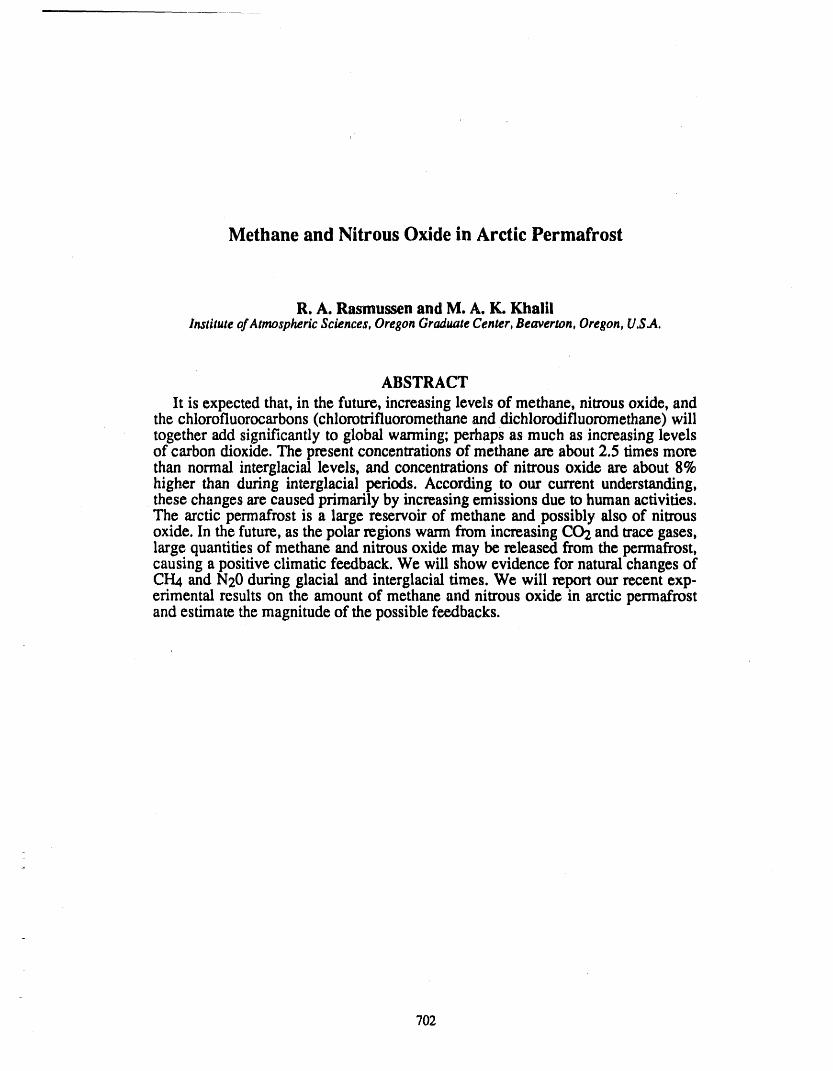
Methane and Nitrous Oxide in Arctic Permafrost

R. A. Rasmussen and M. A. K. KhalilInstituteofAtmosphericSciences,OregonGraduateCenter,Beaverton,Oregon,U.S.A.

ABSTRACT

lt is expected that, in the future, increasing levels of methane, nitrous oxide, andthe chlorofluorocarbons (chlorotrifluoromethane and dichlorodifluoromethane) willtogether add significantly to global warming; perhaps as much as increasing levelsof carbon dioxide. The present concentrations of methane am about 2.5 times morethan normal interglacial levels, and concentrations of nitrous oxide arc about 8%higher than during interglacial periods. According to our cun'ent understanding,these changes are caused primarily by increasing emissions due to human activities.The arctic permafrost is a large reservoir of methane and possibly also of nitrousoxide. In the future, as the polar regions warm from increasing CO2 and trace gases,large quantifies of methane and nitrous oxide may be released from the permafrost,causing a positive climatic feedback. We will show evidence for natural changes ofCI_ and N20 during glacial and interglacial times. We will report our recent exp-erimental results on the amount of methane and nitrous oxide in arctic permafrostand estimate the magnitude of the possible feedbacks.

702

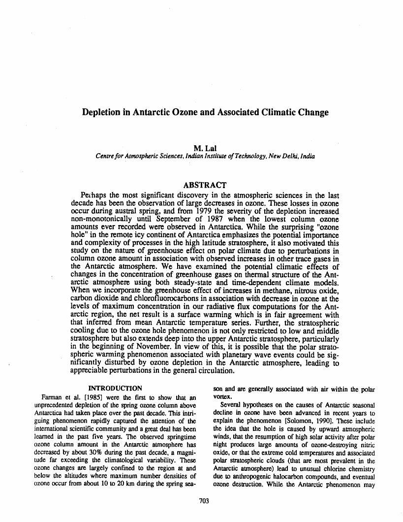
Depletion in Antarctic Ozone and Associated Climatic Change

M. LalCentrefor Atmospheric Sciences, Indian Institute of Technology, New Delhi, India

ABSTRACTPex'hapsthe most significant discovery in the atmosphericsciences in the last

decade has been the observationof large decreases in ozone. These losses in ozoneoccur during australspring, and from 1979 the severity of the depletion increasednon-monotonically until September of 1987 when the lowest column ozoneamounts ever recordedwere observed in Antarctica.While the surprising"ozonehole" in the remote icy continentof Antarcticaemphasizes the potential importanceand complexity of processes in the high latitude stratosphere,it also motivated thisstudy on the natureof greenhouseeffect on polar climate due to perturbations incolumn ozone amount in associationwith observed increases in other tracegases inthe Antarctic atmosphere. We have examined the potential climatic effects ofchanges in the concentration of greenhouse gases on thermal structure of the Ant-arctic atmosphere using both steady-state and time-dependent climate models.When we incorporatethe greenhouseeffect of increases in methane, nitrousoxide,carbon dioxide and chlorofluorocarbonsin associationwith decrease inozone at thelevels of maximum concentrationin our radiative flux computations for the Ant-arctic region, the net result is a surface warming which is in fair agreement withthat inferred from mean Antarctic temperature series. Further, the stratosphericcooling due to the ozone hole phenomenon is not only restricted to low and middlestratospherebut also extends deep into theupper Antarcticstratosphere,particularlyin the beginning of November. In view of this, it is possible that the polar strato-spheric warmingphenomenon associated with planetary wave events could be sig-nificantly disturbed by ozone depletion in the Antarctic atmosphere, leading toappreciable perturbationsin the generalcirculation.

INTRODUCTION son and are generally associated with air within the polarFarman ct al. [1985] were the first to show that an vortex.

unprecedenteddepletion of the spring ozone column above Several hypotheses on the causes of Antarctic seasonalAntarcticahad taken place over the past decade.This intri- decline in ozone have been advanced in recent years toguing phenomenon rapidly captured the attention of the explain the phenomenon [Solomon, 1990]. These includeinternationalscientific community and a greatdealhas been the idea that the hole is caused by upward atmosphericlearned in the past five years. The observed springtime winds, that the resumptionof high solar activity after polarozone column amount in the Antarctic atmosphere has night produces large amounts of ozone-destroying nitricdecreased by about 30% during the past decade, a magni- oxide, or thatthe extreme cold temperaturesand associatedrude far exceeding the climatological variability. These polar stratosphericclouds (that are most prevalent in theozone changes are largely confined to the region at and Antarctic atmosphere) lead to unusual chlorine chemistrybelow the altitudes where maximum numberdensities of due to anthropogenic halocarboncompounds, and eventualozone occur from about 10 to 20 km duringthe spring sea- ozone destruction.While the Antarctic phenomenon may

703

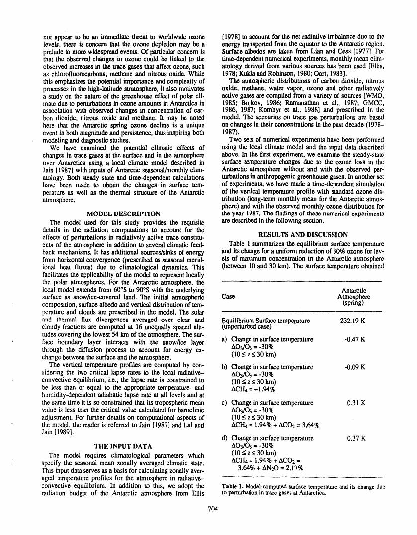
not appearto be an immediate threat to worldwide ozone [1978] to account for the net radiative imbalancedue to thelevels, there is concern that the ozone depletion may be a energy transportedfrom the equatorto the Antarcticregion,preludem more widespread events, Of particular concern is Surface albedos are taken from Lian and Cess [1977], Forthat the observed changes in ozone could be linked to the time-dependentnumerical experiments, monthly meanclim-observed increases in the trace gases that affect ozone, such atology derived from various sources has been used [Ellis,as chlorofluorocarbons,methane and nitrous oxide, While 1978;KuklaandRobinson, 1980; tort, 1983],this emphasizes the potential importanceand complexity of The atmospheric distributionsof carbon dioxide, nitrousprocesses in the high-latitude stratosphere,it also motivates oxide, methane, water vapor, ozone and other mdiativelya study on the natureof the greenhouse effect of polarcii. active gases are compiled from a varietyof sources [WMO,mate due to perturbations in ozone amounts in Antarctica in 1985; Bojkov, 1986; Ramanathan ct al,, 1987; GMCC,association with observed changes in concentration of car. 1986, 1987; Komhyr et al., 1988] and prescribed in thebon dioxide, nitrous oxide and methane, lt may be noted model. The scenarios on trace gas perturbations are basedhere that the Antarctic spring ozone decline is a unique on changes in their concentrations in the past decade (1978-event in both magnitudeand persistence, thus inspiring both 1987),modeling and diagnostic studies. Two sets of numerical experiments have been performed

We have examined the potential climatic effects of using the local climate model and the input data describedchanges in trace gases at the surface and in the atmosphere above. In the fast experiment, we examine the steady-stateover Antarctica using a local climate model described in surface temperature changes due to the ozone loss in theJain [1987] with inputs of Antarctic seasonal/monthly clim. Antarctic atmosphere without and with the observed per-atology. Both steady state and time-dependent calculations turbations in anthropogenic greenhouse gases. In another sethave been made to obtain the changes in surface tem- of experiments, we have made a time-dependent simulationperature as well as the thermal structure of the Antarctic of the vertical temperature profile with standard ozone dis-atmosphere, tribution (long-term monthly mean for the Antarctic atmos-

phere) and with the observed monthly ozone distribution forMODEL DESCRIPTION the year 1987. The findings of these numerical experiments

The model used for this study provides the requisite are described in the following section.details in the radiation computations to account for theeffects of perturbations in radiatively active trace constitu- RESULTS AND DISCUSSIONents of the atmosphere in addition to several climatic feed. Table 1 summarizes the equilibrium surface temperatureback mechanisms, lt has additional sources/sinks of energy and its change for a uniform reduction of 30%ozone for lcr-from horizontal convergence (prescribed as seasonal merid, els of maximum concentration in the Antarctic atmosphereional heat fluxes) due to climatological dynamics. This (between 10 and 30 km). The surface temperature obtainedfacilitates the applicability of the model to represent locallythe polar atmospheres. For the Antarctic atmosphere, thelocal model extends from 60% to 90°S with the underlying Antarcticsurface as snow/ice-covered land. The initial atmospheric Case Atmospherecomposition, surface albedo and vertical distribution of tem. (spring)perature and clouds are prescribed in the model. The solarand thermal flux divergences averaged over clear and Equilibrium Surfacetemperature 232.19 Kcloudy fractions are computed at 16 unequally spaced alti- (unperturbed case)tudes covering the lowest 54 km of the atmosphere. The sur.face boundary layer interacts with the snow/ice layer a) Change in surface temperature -0.47 Kthrough the diffusion process to account for energy ex- AO3/O3=-30%change between the surface and the atmosphere. (10 < z < 30 km)

The vertical temperature profiles are computed by con- b) Change in surface temperature -0.09 Ksidering the two critical lapse rates to the local radiative- AO3/O3=-30%convective equilibrium, i.e., the lapse rate is constrained to (10 <;z < 30 km)be less than or equal to the appropriate temperature- and ACI-I4= +1.94%humidity-dependent adiabatic lapse rate at ali levels and atthe same time it is so constrained that its tropospheric mean c) Change in surface temperature 0.31 Kvalue is less than the critical value calculated for barociinic AO3/O3= -30%adjustment For further details on computational aspects of (10 ,; z < 30 km)the model, the reader is referred to Jain [1987] and Lal and ACH4= 1.94% + ACO2= 3,64%

Jain [1989]. d) Change in surface temperature 0.37 KTHE INPUT DATA AO3/O3= -30%

The model requires climatological parameters which (10 <:z < 30 km)specify the seasonal mean zonally averaged climatic state. ACI-I4= 1.94% + ACO2=

3.64% + AN20 = 2.17%This input data serves as a basis for calculating zonally aver-aged temperature profiles for the atmosphere in radiative-

convective equilibrium. In addition to this, we adopt the Table 1. Model-computedsurfacetemperatureand its changedueradiation budget of the Antarctic atmosphere from Ellis to perturbation in tracegases at Antarcttca.

7_

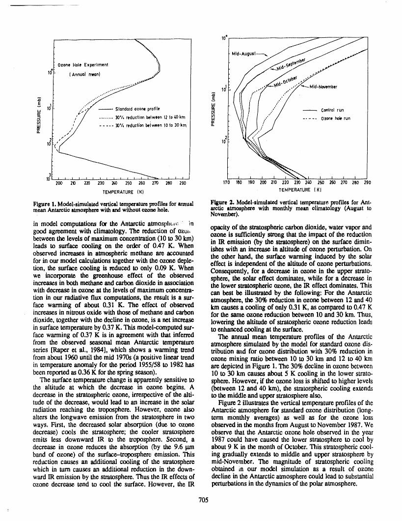
,0200 210 220 230 240 250 260 270 280 290 170 180 190 200 210 220 230 260 250 260 270 2_0 290

TEMPERATURE(K) TEMPERATURE(K)

Figure 1. Model-simulated vertical temperature profiles for annual Figure 2. Model-simulated vertical temperature profiles for Ant.mean Antarctic atmosphere with and without ozone hole. arctic atmosphere with monthly mean climatology (August to

November),

in modelcomputationsfor theAntarcticatmosphere in opacityof thestratosphericcarbondioxide,watervaporandgood ag_cment with climatology. The reduction of ozu. ozone is sufficiently strong that the impact of the reductionbetween the levels of maximumconcentration(10 to 30 km) in lR emission (by the stratosphere)on the surface climin-leads to surface cooling on the order of 0.47 K. When ishes with an increase in altitude of ozone perturbation.Onobserved increases in atmospheric methane are accounted the other hand, the surface warming induced by the.solarfor in our model calculationstogether with the ozone deple- effect is independentof the altitude of ozone perturbations.rien, the surface cooling is reduced to only 0.09 K. When Consequently, for a decrease in ozone in the upper strato-we incorporate the greenhouse effect of the observed sphere, the solar effect dominates, while for a decrease inincreases in both methane and carbondioxide in association the lower stratosphericozone, the IR effect dominates. Thiswith decrease in ozone at the levels of maximum concentra- can best be illustrated by the following: For the Antarcticdon in our radiative flux computations,the result is a sur- atmosphere, the 30%reduction in ozone between 12 and 40face wanning of about 0.31 K. The effect of observed km causes a cooling of only 0.31 K, as compared to 0.47 Kincreases in nitrous oxide with those of methane and carbon for the same ozone reductionbetween 10 and 30 km. Thus,dioxide, togetherwith thedeclinein ozone,is a net increase loweringthe altitudeof stratosphericozonereductionleadsin surface temperatureby 0.37 K. This model-computed sur- to enhanced cooling at the surface.face warming of 0.37 K is in agreement with that inferred The annual mean temperature profiles of the Antarcticfrom the observed seasonal mean Antarctic temperature atmosphere simulated by the model for standard ozone dis.series [Raper et al., 1984], which shows a warming trend tribution and for ozone distribution with 30% reduction infrom about 1960 until the mid 1970s (a positive linear trend ozone mixing ratio between 10 to 30 km and 12 to 40 kmin temperature anomaly for the period 1955/58 to 1982 has are depicted in Figure 1. The 30%decline in ozone betweenbeen reportedas 0.36 K for the spring season). 10 to 30 km causes about 5 K cooling in the lower strato.

The surface temperature change is apparentlysensitive to sphere.However, ff the ozone loss is shiftedto higherlevelsthe altitude at which the decrease in ozone begins. A (between 12 and 40 km), the stratosphericcooling extendsdecrease in the stratospheric ozone, irrespective of the alti- to the middleand upper stratospherealso.tude of the decrease, would lead to an increase in the solar Figure 2 illustrates the vertical temperature profiles of theradiation reaching the troposphere. However, ozone also Antarctic atmosphere for s_ldard ozone distribution (long.alters the longwave emission from the stratosphere in two term monthly averages) as well as for the ozone lossways. First, the decreased solar absorption (due to ozone observed in the months from August to November 1987, Wedecrease) cools the stratosphere; the cooler stratosphere observe that the Antarctic ozone hole observed in the yearemits less downward IR to the troposphere. Second, a 1987 could have caused the lower stratosphere to cool bydecrease in ozone reduces the absorption (by the 9.6 t.tm about 9 K in the month of October. This stratospheric cool-band of ozone) of the surface--troposphere emission. This ing gradually extends to middle and upper stratosphere byreduction causes an additional cooling of the stratosphere mid-November. The magnitude of stratospheric coolingwhich in mm causes an additional reduction in the down- obtained in our model simulation as a result of ozonewardIR emission by the stratosphere. Thus the lR effects of decline in the Antarcticatmosphere could lead to substantialozone decrease tend to cool the surface. However, the IR perturbationsin the dynamics of the polaratmosphere.

705

REFERENCES

Bojkov, R, D,, The 1979-1985 ozone decline in the Ant- L.al,M., and A. K. Jain, Increasing anthropogenlc constitu-arctic as reflected in ground-kased observations, Gee. ents in the atmosphere and associated climatic changes,phys. Res. Lett,, 13, 1236-1239, 1986, in Encyclo. Environ. Cont. Technol,, Vol. 2, edited by

Ellis, J, S,, Cloudiness, the planetaryradiationbudget and P, N, Chcremisionoff,pp. 735--762, 1989,climate, Ph,D, Thesis, 240 pp,, Colorado State Uni- Llan, M, S,, andR, D, Cess, Energybalanceclimate models:versity,Ft. Collins, CO, 1978, A reappraisalof ice--albedo feedback,J, Atmos. Sci., 34,

Farman, J. C., B, G. Gardiner, and J, D. Shanklin,Large 1058-1062, 1977,losses of total ozone in the Antarctic reveal seasonal Oort,A. H., Global atmosphericcirculationstatistics:1958-CLOx/NOxinteraction,Nature, 315,207-210, 1985. 1973,NOAA Prof. Paper 14, 180 pp., 1983.

GMCC, Geophysical monitoring for climatic change, Raper,S. C., T. M. L. Wigley, P. R. Mayer,P. D. Jones, andNOAA/ERL Summary Report 1985, No. 14, 146 pp., M.J. Salinger, Variations in surface air temperature, It.edited by R, C. Schnell, 1986. 3: The Antarctic; 1957-82, Men. Wen. Rev., 112, 1341-

GMCC, Geophysical monitoring for climatic change, 1353, 1984.NOAA/ERL Summary Report 1986, No. 15, 155 pp., Ramanathan, V., L. Callis, R. Cess, J. Hansen, I. Isaksen,edited by R. C. Schnell, 1987, W. Kuim, A. Lacts, F. Luther, J. Mahlman, R. Reck, and

Jaln, A. K., Climate sensitivity studies with radiative,- M. Scl'desinger, Climate--chemical interactions and el-convective models, Ph.D. Thesis, 199 pp., Centre for fects of changing atmospheric trace gases, Rev. Geophys.,Atmospheric Sei., Indian Inst. of Technology, New 25, 1441-1482, 1987.Delhi, India, 1987, Solomon, S., Antarctic Ozone--progress towards a quan-

Komhyr, W. D., P. R. Franchois, S, E. Kuester, P. J. Reitel- titative understanding,Nature, 347, 347-354, 1990.bach, and M. L. Fanning, ECC Ozone.sondeobservations WMO, Atmospheric ozone: Assessment of our under-at South Pole, Antarctica during 1987, NOAA Data Rep. standing of rite processes controlling its present dis-ERL/APL-15,319 pp., 1988, tribution and change, Rep. 16, Global Ozone Res. and

Kukla, O., and D. Robinson, Annual cycle of surface Moni, Proj.,pp. 88--100,Geneva, 1985.albedo, Mon. Wea. Rev., 108, 56-68, 1980.

706

J

Contamination of the Arctic Air During the Megahaze Vent in Late Winter, 1986

M. DjupstrHomDepartmentofPhysics,ChalmersUniversityof Technology,Gothenburg,Sweden

J. M. PacynaNorwegianInstitutefor AirResearch,Lillestrem,Norway

G. E. ShawGeophysicalInstitute,UniversityofAlaskaFairbanks,Fairbanks,Alaska,U.S.A.

J. W. WinchesterDepartmentof Oceanography,FloridaStateUniversity,Tallahassee,Florida,U.S.A.

S.-M. LiNationalCenterfor AtmosphericResearch,Boulder,Colorado,U.S.A.

ABSTRACTThe Arctic offers an opportunityto study the alterationsof geochemical cycles

of ,:arious compounds by human activity. The potential of the compounds toaccumulate in the environment is a significant factor when studying thesealterations.

Three measurementcampaignswere carded out in variouspartsof the Arctic atPoker Flat, Alaska; Barrow, Alaska; and Ny Alesund, Spitsbergenduring the latewinter of 1986. Enhanced concentrationsof several components were measured atall these stationsfor periodslasting froma few days to several weeks. The chemicalcomposition of aerosols and analyses of the meteorologicalconditions during theseperiods have revealed a coherent picture pointing to potential sources of thesecompoundsin Eurasia, and particularlyin the northernSoviet Union, and probabletransport pathways. The pathways can be indicated by surge events across theSoviet Arctic coast towards Barrowandreturnflows towardsSpitzbergen.

Evenly distributed concentrations of anthropogenic compounds suggest theirratherlimiteden-routedepositionin the arcdc winter.However, due to the extendedtime of the episodes and their intensity, some compoundsmay accumulate in theArctic environment. Very high enrichment factors of As, Cd, Pb, Sb, Se, and Zn inthe Arctic seem to indicate that the geochemical cycles of these compounds havebeen alteredon a global scale.

707

Individual Particle Analysis of the Springtime Arctic Aerosol, 1983-1989

Patrick J. Sheridan and Russell C. SchnellCooperative Institute for Research in Environmental Sciences, University of Colorado/NOAA, Boulder, Colorado, U,S.A.

Jonathan D. KahlDepartment of Geosciences, University of Wisconsin.Milwaukee, Milwaukee, Wisconsin, U,S.A.

ABSTRACT

During the springs of 1983, 1986 and 1989, the Arctic Gas and Aerosol Sam-pling Program (AGASP) conducted major aircraft-based field experiments overmuch of the western Arctic. As part of the AGASP research efforts, several regionsof the springtime Arctic atmosphere were probed by the NOAA WP-3D Orionresearch aircraft. These included the marine boundary layer over open water, thesurface inversion layer over the pack ice, the "background" free troposphere, thefrequently encountered Arctic haze layers, 'and the lower stratosphere.

Size segregated aerosol samples were collected from these air masses using athree-stage cascade impactor mounted on the aircraft. Individual particle analysisusing analytical electron microscopy was performed on each collection substrate toreveal particulate morphology, size distribution and elemental composition infor-mation. Results of our studies show that (1) Arctic haze layers are composedlargely of sulfates and anthropogenic particles, (2) the synoptic meteorology is animportant factor which influences the magnitude of the pollution component in thehaze, and (3) the stratospheric aerosols are predominantly H2SO4 droplets, with theexception of those collected in 1983, which showed relatively high crustal particleconcentrations due to volcanic debris.

INTRODUCTION sol physics and radiative effects of Arctic haze. The pro-Air pollution in the Arctic, especially during the spring- gramsconsistedof airbornegas, aerosol, radiationandmete-

time, is now a familiarand well-documented phenomenon, orology measurements fled to similar baseline stationand one that has been intensively studied since the mid- measurementsat PLBarrow, Alaska; Alert, NorthwestTer.1970s (see reviews by Rahn [1985] and Barrie [1986]). ritories;and Ny Alesund, Spitsbergen. During peak opera-Results from many of these studies show that these Arctic tions, the AGASP project included over 150 people fromhaze aerosols undergoperiodic fluctuationsin concentration governmentresearch agencies and universities in the Unitedand composition, which have been linked to episodic trans- States, Canada,Norway, Sweden, Denmarkand the Federalport from the middle latitudes [Barrie et al., 1981; Low- Republic of Germany[Schnellet al., 1989].enthal and Rahn, 1985; Raatz, 1985]. Chemical analyses of The results presentedin this paper focus primarily on thethe aerosols suggest a strong pollution component to the anthropogenic pollution component in Arctic haze layers.haze, one which may be capable of significantly disturbing However, aerosol samples collated within the Arctic strato.the radiativebalance in the Arctic [Valero et al., 1984;Wen- sphere, free troposphere (not in haze layers) and above-icedling et al., 1985; Blancher,1989]. surface inversion layers are also discussed. When appropri.

The major purpose of the international Arctic Gas and ate, meteorological analyses have been presented to showAerosol Sampling Program (AGASP) research expeditions long-range transport of haze associated with mid-latitudewas to determinethe distribution,transport, chemistry, aero- sources.

, 708

METHODS 2, along with their respectivex-ray spectra.

Atmospheric aerosols were sampled during the three Meteorological and air trajectoryanalyses indicated thatAGASP field experimentsusing a three-stage,single orifice organized translx_ episodes occurred which moved aircascade impactor,The orientationand operation of this sam- from within the Soviet Union and Central Europe to theplerhave been described in detailelsewhere [Sheridanand Alaskan and Norwegian research areas prior to and duringMusselman, 1985; Sheridan, 1989a,b], Typical sampling our operations there [Harris, 1984; Raatz, 1985], The Eur-periodswere 10-15 rain., permittingsufficient temporaland asian areas targetedas source regions by the trajectoriesarespatialresolution of discrete airmasses, consistent with the type of Arctic aerosol source areas we

Particles were deposited onto thin formvar films sup- would expect, since they are highly industrializedwith littleported by 200-mesh TEM grids, which were positioned pollution control and are usually situated north of thedirectly behind the jet nozzle on each impactor stage. The springtime Eurasian polar front. During most Arctic winters/manufacturer'sstated aerodynamic cutoff diameters (ACDs) springs, the synoptic meteorology responsible for this cfff.for the three stages are: Stage 1 - 4 mm; Stage 2 - 1 mm; cient tropospheric transportbecomes a quasi-persistent fea.Stage 3 - 0.25 mm. Under sampling conditions of flow and ture [Raatz, 1989], "Atypical" years (such as that of winter/pressure similar to those encounteredin the field, laboratory spring 1989), and how they may affect atmospheric trans-tests show that efficient collection of particles down to port and Arctic aerosol concentrations, will be discussed0,1 mm in diameter was realized, below,

Particles were analyzed using a Japan Electron Optics Stratospheric aerosol samples were collected anytime theLaboratory (JEOL) 200 kV analytical electron microscope aircraft flew above the relatively low Arctic tropopau_, The(AEM) interfaced to an ultrathin window (UTW) x-ray stratospheric aerosols collected during AGASP-I showed aspectrometer, multichannel analyzer and dedicated micro- distinct bimodal size distribution, The fine particle mode,computer, The positions of ali particles in a given field-of- which dominated the number-size distribution, was centeredview (FOV) were recorded, so that subsequent x.ray analy- at 0,3-.0,4 mm diameter, and was composed almost totallyses of ali particles could be performed before continuing to of liquid H2SO4droplets, The coar_ particle mode was cen-another FOV, The UTW detector permitted elemental analy- tered at 1-2 mm diameter, and the particles appeared bysis down to B (7_,=5);thus the interesting light elements C, N morphology and composition to be predominantly of crustaland O were detectable in individual particles, In addition to origin. Several researchershave attributedthese coarse crus-particulate chemistry information, the AEM also provided tal.type particles in the stratosphere to the El Chichon eel-valuable morphological and mineralogical data, which were canic eruption, which occurredapproximately one year priorquite useful wh,,nproposing sourcesfor the aerosol. As with to AGASP-I sampling [Shapiro et al., 1984; Raatz et al.,the sampler, details of the analytical instrumentation and 1985;Winchester etal., 1985].procedures have been reportedpreviously [Sheridan andMusselman, 1985; Sheridan, 1989a,b]. AGASP.II

The first three flights of the AGASP-II experiment wereRESULTS conducted in the Alaskan Arctic, The research area_ for

The approximate flight tracks for the three AGASPs are these flights were out over the Beaufort Sea, north andshown in Figure 1. The AGASP-I (1983) field experiment northeast of Barrow, Alaska. During the first flight, anwas the largest of the three in terms of flight hours and areal extremely dense haze layer was encountered, heavier thancoverage, spending significant time in both the North Amer- those observed during any of the AGASP field experiments.lean and European Arctic. The AGASP-II (1986) project Within this haze event, condensation nuclei (CN) countswas based in Anchorage, Alaska and Thule, Greenland, and exceeded 10,000 cm"3, aerosol scattering extinction coef-was conducted solely in the North American Arctic. The ficients (bsn) were >80 x 10-6 m-t, and SO2 concentrationsAGASP-III (1989) experiment was an extensive European reached 15 pptv [Herbert et al., 1989;Thornton et al., 1989].Arctic mission conducted out of Bode, Norway. Most of the fine aerosol particles were H2SO4, probably

being formed in situ during transport [Herbert et al., 1989].AGASP-I Meteorological analyses, along with surface air quality

Arctic haze layers encountered during AGASP-I flights measurements in Norway, suggest that the haze originatedgenerally showed a stronger and fresher pollution com- in CentralEurope ten days earlier [Bridgman et al., 1989].ponent than did those from the more recent missions (with The transportpathway followed a pattern characteristic ofthe exception of haze observed on the first AGASP.II spring haze transport in the Arctic [Raatz, 1989].flight). Fine liquid (i.e., not significantly unneutralized) Haze layers observed on the second and third AGASP-IIH2SO4droplets were observed in numbers several orders of flights were much lighter and the pollution constituents lessmagnitude higher than other particle types. Both combustion concentrated than on the fast flight. Trajectories for these(,soot)and non-combustion (,probably organic) varieties of flights showed no direct, organized transport from the usualcarbonaceous particles were identified. Spherical particles source regions. Instead, the trajectories originated or spentand aggregates of probable combustion origin were encoun- significant time over the Central Arctic Basin or the Cana-tered with likely sources (based on composition) being non- dian Archipelago [Herbert et al,, 1989],ferrous smelters, heavy industry, incinerators, coal- and oil- One aerosol sample collected in the troposphere overfired combustion, and possibly wood smoke, Other particle south-central Alaska was found to contain high concentra-types, including crustal and marine paa'ticles,also suggested tions of soil-derived particles, with little associated H2SO4distant sources for the haze aerosol. Several types of par- [Sheridan, 1989a]. This aerosol was probably a pocket ofticles observed in AGASP-I haze layer,,;are shown in Figure suspended ash from Mt. Augustine volcano in southern

709

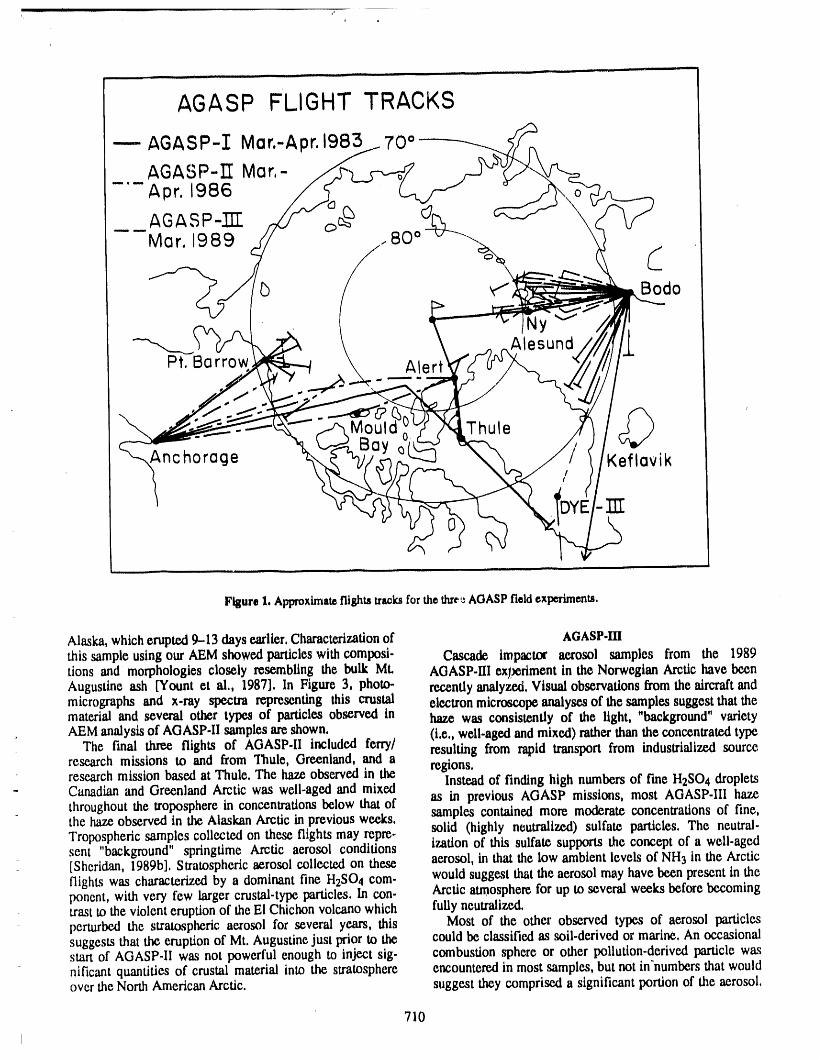
, , i i iii, ,, i iii i

AGASP FLIGHT TRACKS

--- AGASP-I Mar.-Apr.198"5 70*

AGASP-II Mar,-'- Apr. 1986

AGASP-TIT _ __

---Mar. 1989 .80 °

C) v/ Bodo

Alesund

Pr. Barrow . Alert

s

0 'Mould Thule

Anc borage Keflavik!I

Trr

FigureI.Ap1_oxlmsteflightsu'a_ksforthelJu'e,_AOASP fieldexpm'Iments,

Alaska,whicherupted9-13daysearlier.Characterizationof AGASP.mthissampleusingourhEM showedparticleswithcomposi- CascadeImpactoraerosolsamplesfrom the 1989lionsand morphologlescloselyresemblingthebulkMt. AGASP-IIIexperimentintheNorwegianArctichavebeenAugustineash [Yountetal.,1987].In Figure3,photo- recentlyanalyzed.Visualobservationsfromtheaircraftandmicrographs and x-ray spectra representing this crustal electronmicroscopeanalyses of the samplessuggest that thematerial and several other types of particles observed in haze was consistently of the light, "background"varietyAEM analysisof AGASP-II samplesarcshown. (i.e., well-aged and mixed) rather than the concentratedtype

The final three flights of AGASP-II included ferry/ resulting from rapid transport from industrialized sourceresearch missions to and from Thule, Greenland, and a regions,research mission based at Thule. The haze observed in the Instead of finding high numbers of fine H2SO4 droplets

= Canadian and Greenland Arctic was well-aged and mixedthroughout the troposphere in concentrations below that of as in previous AGASP missions, most AGASP-III hazethe .hazeobserved in the Alaskan Arctic in previous weeks, samples contained more moderate concentrations of fine,Tropospheric samples collected on these flights may repre- solid (highly neutralized) sulfate particles. The neutral-sent "background" springtime Arctic aerosol conditions ization of this sulfate supports the concept of a well-aged[Sheridan, 1989b], Stratospheric aerosol collected on these aerosol, in that the low ambient levels of NH3 in the Arcticflights was characterized by a dominant fine H2SO4 com- would suggest that the aerosol may have been present in theponent, with very few larger crustal-type particles. In con- Arctic atmosphere for up to several weeks before becomingtrast to the violent eruption of the El Chtchon volcano which fully neutralized.perturbed the stratospheric aerosol for several years, this Most of the other observed types of aerosol particlessuggests that the eruption of Mt. Augustine just prior to the could be classified as soil-derived or marine. An occasionalstart of AGASP-II was not powerful enough to inject sig- combustion sphere or other pollution-derived particle wasnificant quantities of crustal material into the stratosphere encountered in most samples, but not in'numbers that wouldover the North American Arctic. suggest they comprised a significant portion of the aerosol.

710

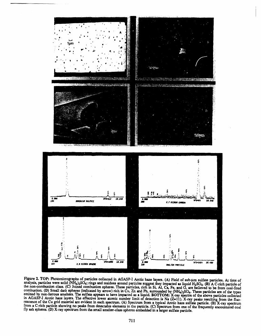
Figure 2, TOP: Photomicrogr_hs of particlescollected in AGASP-I Arctichaze layers, (A) Field of sub-km sulfate particles, At time ofanalysis, particleswere solid (NH4)2SO4;rings and residuesmoundparticlessugsest they impactedas liquid H2SO4, (B) A C-rich particle ofthe non-combustionclass, (C) Joined combustion spheres, These panicles, ri(_hm SL AL Ca, Fe, and O, are believed to be from coal-firedcerebra..rien.(D) Small darkspheres (Ind.icatedby arrow)rich in Cu, Zn and Pb, surroundedby (NI-14)2SO4, These particles are of the types_n_mAt_A_.non-i.e_,oussmelters,£ne,u_a_apl_U_tohaveimputed.asa llgu!d.BOTTOM, X-rayspectraoftheaboveparticlescollectedres_,,_r:_ .,,,a'cucn.a_. say,s: *l.e effective lower ,uom|c numt_. limit oi detection is Na (Z=I1). X-ray peaks resulting from the flue.frocerite ox me _u gno maumm are evto_mtmeach specu'um,tA) a,.pgctrum.troma.t3_picalArctic haze sulfate particle. (B) X-ray spectrum,.,.In a _-rtcn p_.uyt.esnowing no _atcs .m3moet_tao!e elementsm me p.a_cte. _u) _pectrum from one of the frequently encounteredcoalt_yash spheres, tul A-ray spectrmntromme sma. smelter-crassslmeresembeddedin a larger sulfate particle.

711

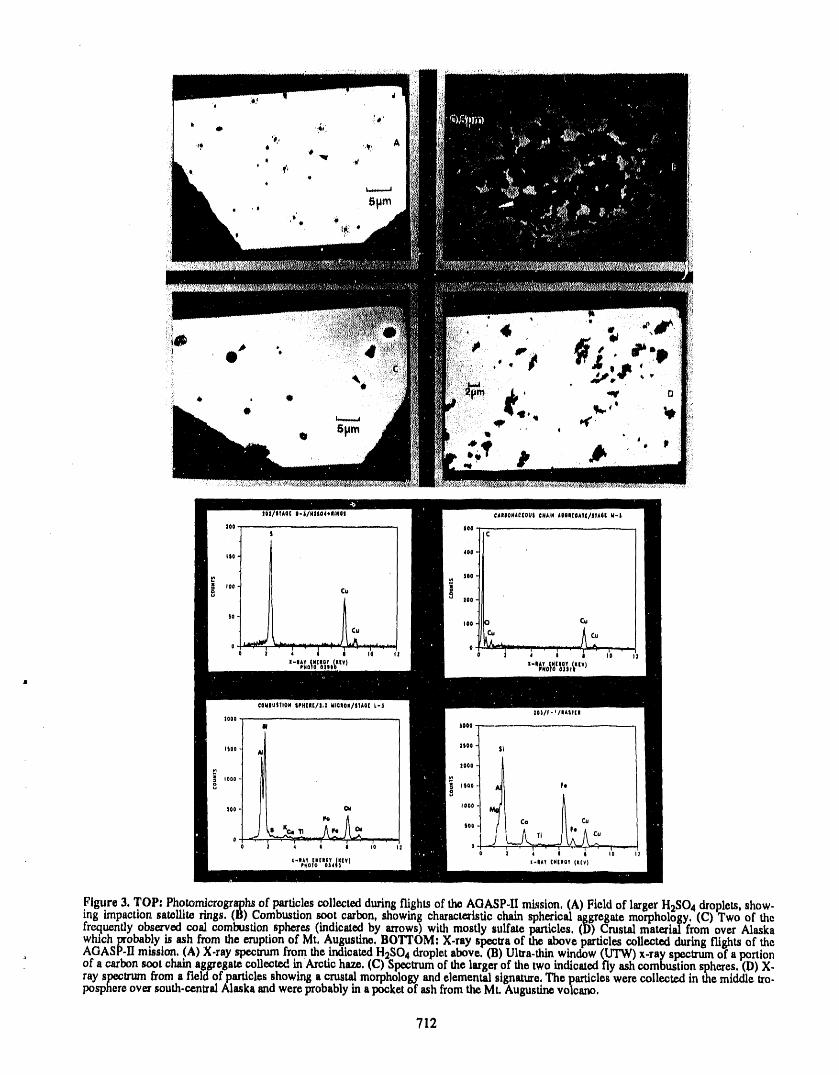
Figure 3, TOP: Photomicrographsof particlescollected duringflights of the AGASP-IImission, (A) Field of larger H2SO4 droplets,show.ing tmpacttonsat_m_ rings, (13)comousuon soot carbon, showing charactertstic chain spherical aggregate morphology, (C) Two of thefrequentlyobserved coal combustion spheres (indicated by arrows)w!th mostly sulfateparticles. (D) Crustal material from over AlaskaWG_Ch_obably.is_h .fromthe eruptionof M!, Augustine, BOTTOM. X-ray spectraof the above particles collected during flights of theo ,_ _._-u mmmon,,tA) A-rayq3ecu'um,zm,m.me ro?teatedH2SO 4 droplet above. (13)Ullra.thin window (L._W) x-ray specl_un of a portioneza c,ar_on soot cnamaggregme couectec m Arcuc haze, (C) Spectrumor the larger of the two indicated fly ash combustion spheres. (D) X-ray speclnun froma field of panicles showing a crustalmorphology and elemental signature,The particleswere collected inthe middle U'o-posphereover south-central Alaska andwere probablyin apocket of ash fromthe Mt. Augustinevolcano,

712

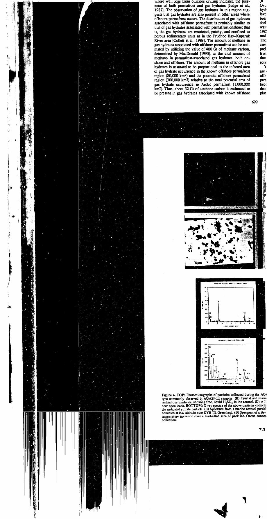
_ waere we,..ogs kTomo1._s.lorec.n,dng mc.lca_,¢..Lie pres- _n,

i ence of both permafrost and gas hydrates [Judge et al,, Ov¢1987]. The observationof gas hydrates.Anthis regionsug- hyd,i

i gests thatgas hydratesare also present in otherareas where lev(i offshore permafi'ost occurs. The distribution of gas hydrates bee:! associated with offshore permafrost is probably similar to shel

thatof gas hydratesassociatedwith permafrostonshore;that wattis, the gas hydrates are restricted, patchy, and confined to 198_

! porous sedimentary units as in the Prudhoe Bay-Kuparuk malRiver area [Collett et al., 1989]. The amountof methanein TI_:gas hydratesassociated with offshore permafrostcan be esti- cre___mated by utilizing the value of 400 Gt of methanecarbon, pro!

determined by MacDonald [1990], as the total amount of Eye_ methane in permafrost-associatedgas hydrates, both on- the.,,

shore and offshore. The amountof methane in offshore gas solv_ hydrates is assumed to be proportional to the inferred area '1

of gas hydrate occurrence in the known offshore permafrost are,region (80,000 km2) and the potentialoffshore permafrost off._region (300,000 km2) relative to the total potentialarea of pre._

_ gas hydrate occurrence in Arcdc permafrost (1,000,000 bcc(il _ km2). Thus, about 32 Gt of t._ethanecarbon is estimated to dest

_ be present in gas hydrates associated with known offshore pl_-

: 699

%

Figure 4. TOP: Photomicrographsof particlescollected duringthe AGItype commonly observed in AGASP-III samples. (13)Crustal _d marh_restrialdust particles,showing free, liquid H2SO4 in theaerosol. (D) A 1_near open leads. BOTTOM: X-ray spectraof theabove particlescollect(the indicated sulfate particle. (B) Specmm_froma marineaerosolparticl

' collected at low akirudeoverD3f_-u.t, _.rr_ni_i. (D) 5pecum_ of a Br<temperatureinversion over a lead-f'dleciarea of pack ice. Ozone conce_collection.

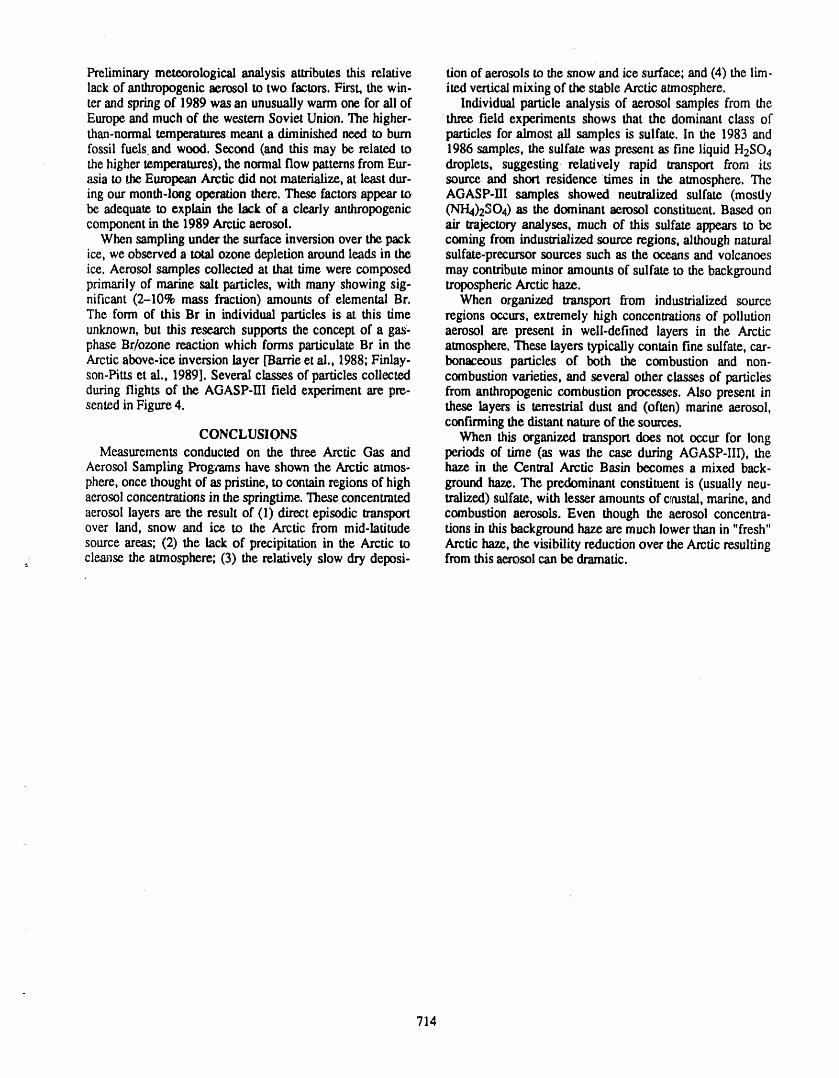
Preliminary meteorological analysis attributes this relative tion of aerosols to the snow and ice surface; and (4) the lira-lack of anthropogenic aerosol to two factors. First, the win- ited vertical mixing of the stable Arctic atmosphere.ter and spring of 1989 was an unusually warm one for ali of Individual particle analysis of aerosol samples from theEurope and much of the western Soviet Union. The higher- three field experiments shows that the dominant class ofthan-normal temperatures meant a diminished need to bum particles for almost ali samples is sulfate. In the 1983 andfossil fuels and wood. Second (and this may be related to 1986 samples, the sulfate was present as fine liquid H2SO#the higher temperatures), the normal flow patterns from Eur- droplets, suggesting relatively rapid transport from itsasia to the European Arctic did not materialize, at least dur- source and short residence times in the atmosphere. Theing our month-long operation there, These factorsappearto AGASP-III samples showed neutralized sulfate (mostlybe adequate to explain the lack of a clearly anthropogenic (NH4)2SO4) as the dominant aerosolconstituent. Based oncomponent in the 1989 Arctic aerosol, air trajectory analyses, much of this sulfate a_s to be

When sampling under the surface inversion over the pack coming from industrialized source regions, although naturalice, we observed a total ozone depletion around leads in the sulfate-precursor sources such as the oceans and volcanoesice. Aerosol samples collected at that time were composed may contribute minor amounts of sulfate to the backgroundprimarily of marine salt particles, with many showing sig- tropospheric Arctic haze.nificant (2-10% mass fraction) amounts of elemental Br. When organized transport from industrialized sourceThe form of this Br in individual particles is at this time regions occurs,extremely high concentrations of pollutionunknown, but this research supports the concept of a gas- aerosol are present in well-defined layers in the Arcticphase Br/ozone reaction which forms particulate Br in the atmosphere. These layers typically contain fine sulfate, car-Arctic above-iceinversion layer [Barrieetal., 1988;Finlay- bonaceous particles of both the combustion and non-son-Pills ct al., 1989]. Several classes of particles collected combustion varieties, andseveral other classes of particlesduring flights of tile AGASP-III field experiment are pre- from anthropogenic combustion processes. Also present insented in Figure 4. these layers is terrestrial dust and (often) marine aerosol,

confirming the distant nature of the sources.CONCLUSIONS When this organized transport does not occur for long

Measurements conducted on the three Arctic Gas and periods of time (as was the case during AGASP-III), theAerosol Sampling Programs have shown the Arctic atmos- haze in the Central Arctic Basin becomes a mixed back-phere, once thought of as pristine, to contain regions of high ground haze. The predominant constituent is (usually neu-aerosol concentrations in the springtime. These concentrated tralized) sulfate, with lesser amounts of crcustal,marine, andaerosol layers are the result of (1) direct episodic transport combustion aerosols. Even though the aerosol concentra-over land, snow and ice to the Arctic from mid-latitude tions in this background haze are much lower than in "fresh"source areas; (2) the lack of precipitation in the Arctic to Arctic haze, the visibility reduction over the Arctic resulting

, cleanse the aunosphere; (3) the relatively slow dry deposi- from this aerosol can be dramatic.

714

REFERENCES

Barrie, L. A., Arctic air pollution: an overview of current Schnell, R. C., T. B. Watson, and B. A. Bodhaine, NOAAknowicdge,Atmos. Environ.,20, 643-663,1986. WP-3D instrumentation and flight operations on

Barde, L. A., R. M. Hoff, and S. M. Daggupaty,The influ- AGASP-II,J. Atmos. Chem., 9, 3-16, 1989.ence of mid-latitudepollution sources on haze in the Shapiro,M. A., R. C. SchneU,F. P. Parungo,S. J. Oltmans,CanadianAtctic, Atmos. Environ.,15, 1407-1419, 1981. and B. A. Bodhaine, El Chichon volcanic debris in an

BarrieL. A., J. W. Bottenheim, R. C. Schnell, P. J. Crutzen, Arctic tropopausefold, Geophys. Res. Lett., I1,421-424,and R. A. Rasmussen, Ozone destruction and photo- 1984.cheraical reactions at polar sunrise in the lower Arctic Sheridan, P. J., Analytical electron microscope studies ofalmosphere, Nature, 334, 138--141, 1988. size segregated particles collected during AGASP-II,

Blanche[, J.-P., Towardestimationof climatic effects due to flights 201-203, J. Atmos. Chem., 9, 267-282, 1989a.Arctic aerosols,Atmos. Environ., 23, 2609-2625, 1989. Sheridan,P. J., Characterizationof size segregated particles

Bridgman, H. A., R. C. Schnell, J. D. Kahl, G. A. Herbert, collected over Alaska and the Canadian high Arctic,and E. Joranger,A major haze event near Point Barrow, AGASP-II flights 204--206, Atmos. Environ., 23, 2371-Alaska:analysisof probablesourceregions and translx_ 2386, 1989b.pathways,Atmos. Environ., 23, 2537-2549, 1989. Sheridan, P. J., and I. H. Mussclman, Characterizationof

Finlayson-Pitts, B. J., F. E. Livingston, and H. N. Berko, aircraft-collectedpanicles present in the Arctic aerosol;Ozone destructionandbromine photochemistryat ground AlaskanArctic, spring 1983, Atmos. Environ., 19, 2159-level in the Arctic spring,Nature, 343, 622-625, 1989. 2166, 1985.

Harris,J. M., Trajectories during AGASP, Geophys. Res. Thornton,D. C., A. R. Bandy, and A. R. Driedger, III,Sul-Lett.,11,453-456, 1984. fur dioxide in the North American Arctic, J. Atmos.

Herbert, G. A., R. C. Schnell, H. A. Bridgman, B. A. Bod- Chem., 9, 331-346, 1989.haine, S. J. Oltmans, and G. E. Shaw, Meteorology and Valero, F. P. J., T. P. Ackerman, and W. J. Y. Gore, Thehaze stnleture during AGASP-II, part l:Alaskan Arctic absorption of solar radiation by the Arctic atmosphereflights, 2-10 April1986, J. Atmos. Chem.,9, 17-48, 1989. during the haze season and its effects on the radiationbal-

Lowenthal, D. H., and K. A. Rahn, Regional sourcesof pol- ance, Geophys. Res. Left., 11,465-468, 1984.lution aerosol at Barrow, Alaska duringwinter 1979-80 Wendling, P., R. Wendling, W. Renger, D. S. Covert, J.as deduced from elemental tracers, Atmos. Environ., 19, Heintzenberg, and P. Moerl, Calculated radiative effects2011-2024, 1985. of Arctic haze during a pollution episode in spring 1983

Raatz, W. E., Meteorological conditions over Eurasia and based on ground-based and airborne measurements,the Arctic contributing to the March 1983 Ar_.tic haze Atmos. Environ., 19, 2181-2193, 1985.episode, Atmos. Environ., 19, 2121-2126, 1985. Winchester, J. W., R. C. Schnell, S.-M. Fan, S.-M. Li, B. A.

Raatz, W. E., An anticyclonic point of view on low-level Bodhaine, P. S. Naegele, A. D. A. Hansen, and H. Rosen,tropospheric long-range transport, Atmos. Environ., 23, Particulate sulfur and chlorine in Arctic aerosols, spring2501-2504, 1989. 1983, Atmos. Environ., 19, 2167-2173, 1985.

Raatz, W. E., R. C. Schnell, M. A. Shapiro, S. J. Oltmans, Yount, M. E., T. P. Miller, and B. M. Gamble, The 1986and B. A. Bodhaine, Intrusions of stratospheric air into eruptions of Augustine Volcano, Alaska: hazards andAlaska's troposphere, March 1983, Atmos. Environ., 19, effects, exlited by T. D. Hamilton and J. P. Galloway,2153-2158, 1985. U.S. Geological Survey Circular 998, pp. 4-13, 1987.

Rahn, K. A., Progress in Arctic air chemistry, 1980--1984,Atmos. Environ., 19, 1987-1994, 1985.

!

- 715_

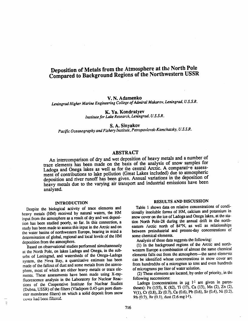
Deposition of Metals from the Atmosphere at the North PoleCompared to Background Regions of the Northwestern USSR

V. N. AdamenkoLeningrad Higher Marine Engineering College of Admiral Makarov, Leningrad, U.S.S.R;

K. Ya. KondratyevInstitute for Lake Research, Leningrad, U.S.S.R.

S. A. SinyakovPacific Oceanography and Fishery Institute, Petropavlovsk-Kamchatsky, U.S.S.R.

ABSTRACT

An intercomparisonof dry and wet depositionof heavy metals and a numberoftrace elements has been made on the basis of the analysis of snow samples forLadoga and Onega lakes as well as for the central Arctic. A comparati,'e assess-ment of contributions to lake poUution (Great Lakes included) due to atmosphericdeposition and river runoff has been given. Annual variations in the deposition ofheavy metals due to the varying air transportand industrial emissions have beenanalyzed.

INTRODUCTION RESULTS AND DISCUSSION

Despite the biological activity of mace elements and Table 1 shows data on relative concentrations of condi-heavy metals (HM) received by natural waters, *.heHM tionally insoluble forms of HM, calcium and potassium ininput from the atmosphereas a resultof dry and wet deposi- snow cover on the ice of LadogaandOnega lakes, at the sta-tion has been studied poorly, so far. In this connection, a tion North Pole-28 during the annual drift in the north-study has been made to assess this input in the Arctic andota eastern Arctic north of 84°N, as well as relationshipsthe water basins of northwestern Europe, bearing in mind a between preindustrial and present-day concentrations ofdetermination of global, regional and local levels of the HM some chemical elements.deposition from the atmosphere. Analysis of these data suggests the following:

Based on observational studies performed simultaneously (1) In the background regions of the Arctic and north-at the North Pole, on lakes Ladoga and Ortega, in the sub- _,estern Europe a combination of almost the same chemicalurbs of Leningrad, and watersheds of the Onega--Ladoga elements falls out from the atmosphere---the same elementssystem, the Neva Bay, a quantitative estimate has been can be identified whose concentrations in snow cover aremade of the fallout of dust and some metals from the atmos- from hundredths of a microgram to tens and even hundreds

phere, most of which are either heavy metals or trace ele- of micrograms per liter of water solution.ments. These assessments have been made using X-ray- (2) These elements are located, by orderof priority, in thefluorescence analysis in the Laboratory for Nuclear Reac- following successions:tions of the Cooperative Institute for Nuclear Studies Ladoga (concentrations in [tg 1-1are given in paren-(Dubna, USSR) of the filters (Vladipore 0.45-I.tmpore diam- theses): Fe (155), K (82), Ti (17), Ca (13), Mn (2), Zn (2),eter membrane f'dters) on which a solid deposit from snow V(1), Cr (0.8), Zr (0.7), Ca (0.6), Pb (0.6), Sr (0.4), Ni (0.2),

.......... t':, .... .I Rb (0:_); Br (l').l); dust (2.6 mg 1-1).UUVU_I iii:ILl _il lltII,UIt,;4.I.-,

_

716

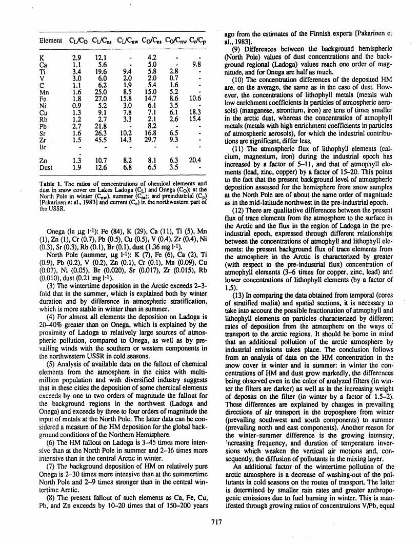
ago from the estimates of the Finnish experts [Pakarinen etElement CL/Co Ct/Cn_ Ct/Cnw CO/Cn, CoK2nwCe/Cp al., 1983].

(9) Differences between the background hemisphericK 2.9 12.1 - 4.2 - - (North Pole) values of dust concentrations and the back-Ca 1.1 5,6 5.0 - 9,8 ground regional (l..adoga) values reach one order of mag-Ti 3.4 19,6 9.4 5.8 2.8 - nitude,and for Onega are half as much.V 3,0 6.0 2.0 2,0 0.7 - (10) The concentration differences of the deposited HMC 1.1 6.2 1.9 5.4 1,6 - are, on the average, the same as in the case of dust. How-Mn 1.6 25.0 8.5 15,0 5.2 -Fe 1.8 27,0 15.8 14.7 8.6 10.6 ever, the concentrations of lithophyll metals (metals with

low enrichment coefficients in particles of atmospheric aero-Ni 0.9 5.2 3.0 6.1 3,5 -Cu 1.3 9.1 7.8 7.1 6,1 18.3 sols) (manganese, strontium, iron) are tens of times smallerRb 1.2 2.7 3.3 2.1 2,6 15.4 in the arctic dust, whereas the concentration of atmophyllPb 2.7 21.8 . 8.2 - - metals (metals with high enrichment coefficients in particlesSr 1.6 26.3 10.2 16.8 6.5 - of atmospheric aerosols), for which the industrial contribu-Zr 1.5 45.5 14,3 29.7 9.3 - tions are significant, differ less.Br ..... (11) The atmospheric flux of lithophyll elements (cal-

Zn 1.3 10.7 8.2 8.1 6.3 20,4 eium, magnesium, iron) during the industrial epoch hasincreased by a factor of 5-11, and that of atmophyll ele-Dust 1.9 12.6 6.8 6.5 3.5 -ments (lead, zinc, copper) by a factor of 15-20, This points

Table 1. The ratiosof eoneentzationsof chemicalelements and to the fact that the present background level of atmospheric, dust in snowcoveron LakesLadoga(CL) andOnega(Co); at the deposition assessed for the hemisphere from snow samples

NorthPolein winter (Cnw), summer (Ct=); and preindustrial (Cp) at the North Pole are of about the same order of magnitude[Pakarinenet al,, 1983]andcurrent(Ca)in thenorthwesternpartof as in the mid-latitudenorthwest in the pre-industrial epoch.theUSSR. (12) There are qualitative differences between the present

flux of trace elements from the atmosphere to the surface inthe Arctic and the flux in the region of Ladoga in the pre-

Onega (in I.tg 1"1):Fe (84), K (29), Ca (11), Ti (5), Mn industrial epoch, expressed through different relationships(1), Zn (1), Cr (0.7), Pb (0.5), Cu (0.5), V (0.4), Zr (0.4), Ni between the concentrations of atmophyU and lithophyll ele-(0.3), Sr (0.3), Rb (0.1), Br (0.1), dust (1.36 mg 1-1). ments: the present background flux of trace elements from

North Pole (summer, _tg 1-1):K (7), Fe (6), Ca (2), Ti the atmosphere in the Arctic is characterized by greater(0.9), Pb (0.2), V (0.2), Zn (0.1), Cr (0,1), Mn (0.09), Cu (with respect to the pre-industrial flux) concentration of(0.07), Ni (0.05), Br (0.020), Sr (0.017), Zr (0.015), Rb atmophyll elements (3--6 times for copper, zinc, lead) and(0.010), dust (0.21 mg !-1). lower concentrations of lithophyll elements (by a factor of

(3) The wintertime deposition in the Arctic exceeds 2-3- 1.5).fold that in the summer, which is explained both by winter (13) In comparing the data obtained from temporal (coresduration and by difference in atmospheric stratification, of stratified media)and spatial sections, it is necessary towhich is more stable in winter than in summer, take into account the possible fractionation of atmophyll and

(4) For almost ali elements the deposition on Ladoga is lithophyll elements on particles characterized by different20--40% greater than on Onega, which is explained by the rates of deposition from the atmosphere on the ways ofproximity of Ladoga to relatively large sources of atmos- transport to the arctic regions, lt should be borne in mindpheric pollution, compared to Onega, as well as by pre- that an additional pollution of the arctic atmosphere byvailing winds with the southern or western components in industrial emissions takes piace. The conclusion followsthe northwestern USSR in cold seasons, from an analysis of data on the HM concentration in the

(5) Analysis of available data on the fallout of chemical snow cover in winter and in summer: in winter the con-elements from the atmosphere in the cities with multi- centrations of HM and dust grow markedly, the differencesmillion population and with diversified industry suggests being observed even in the color of analyzed f'flters(in win-that in these cities the deposition of some chemical elements ter the filters are darker) as well as in the increasing weightexceeds by one to two orders of magnitude the fallout for of deposits on the filter (in winter by a factor of 1.5-2).the background regions in the northwest (l..adoga and These differences are explained by changes in prevailingOnega) and exc.eexlsby three to four orders of magnitude the directions of air transport in the troposphere from winterinput of metals at the North Pole. The latter data can be con- (prevailing southwest and south components) to summersidered a measure of the HM deposition for the global back- (prevailing north and east components). Another reason forgrourtdconditions of the Northern Hemisphere. the winter-summer difference is the growing intensity,

(6) The HM fallout on Ladoga is 3--45 times more inten- "ncreasing frequency, and duration of temperature inver.sive than at the North Pole in summer and 2-16 times more sions which weaken the vertical air motions and, con-intensive than in the central Arctic in winter, sequenfly, the diffusion of pollutants in the mixing layer.

(7) The background deposition of HM on relatively pure An additional factor of the wintertime pollution of theOnega is 2-30 times more intensive than at the summertime arctic atmosphere is a decrease of washing-out of the pol-North Pole and 2-9 times stronger than in the central win- lutants in cold seasons on the routes of transport. The lattertertime Arctic. is determined by smaller rain rates and greater anthropo-

(8) The present fallout of such elements as Ca, Fe, Cu, genie emissions due to fuel burning in winter. This is man-Pb, and Zn exceeds by 10-20 times that of 150-200 years ifested through growing ratios of concentrations V/Pb, equal

717

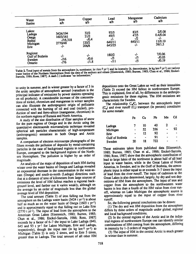
Water Iron Copper Lead Manganese CadmiumBasins a;o _ a/b afo a/b

Lakes:Ladoga 34241194 32/2 93/5 83/5 2/0,08

B_ 1603/161 21/2 49/5 47/5 0.4/0,04./16,318 ./0,4 -/- "/2 "/"Michigan 2770/48 120/2 640/11 640/11 11/0,19Erie ./. 206/8 645/25 ./. 39/1,5

Regions:GulfofBothnia -/- 4- 180/2 -/- 7/0.06Sweden ./16 ./0.6 -/3 -/3 -/0,05Ontario ./'76 ./1,8 -/11 -/5 -/0.19

Table2. Totalinputofmetalsfromtheatmosphere(a,nominator,int km-2yrl) anditsintensityCo,denominator,inkgkm-2yrl) on variouswaterbasinsof theNorthernHemispherefromthedataof theauthorsandothers [Eisemelch,1980;Burn,s, 1985;Ch_ et al., 1986;Enokel-Sarcola,1986;Ross,,1987],A dash(-)indicates"noinformation."

to unity in summer,and in winter greaterby a factorof 3 in depositions onto theGreat Lakes as well as their intensitiesthe arctic samples of atmosphericaerosol (vanadiumis the (Table 2) exceed the HM fallout in northwesternEurope,principal indicatorof emissions by power stationsoperating This is explained, first of all, by differences in the anthropo-on oil products). A considerable increase of the concentra- genie emissions for these regions. The HM emissions aredons of nickel, chromiumand manganese in winter samples characteristic for Sweden.can also illustrate the anthropogenic origin of pollutants The relationship C_/Cr between the atmospheric inputconnected with the burning of oil and coal (nickel), pro- (Ct) and river runoff (Cr) transport (in percent) constitutesducfion of steel and ferro-alloys (manganese, chromium) in for some metals:the northernregions of Eurasia andNorth America.

A study of the size distribution of filter samples of snow Fe Cu Pb Mn Cdfor the pure regions of Onega and in the Arctic using thequantitative eleetrosonde microanalysis technique revealed Ladoga 7 10 40 2 -spherical ash particles characteristic of high.temperature Michigan - 52 356 - 92(anthropogenic) emissions in both Ortega and Arctic Erie - 12 92 - -samples. Gulf of Bothnia - - 91 - -

A comparison of electron microscope photographs of the Sweden 20 18 722 - -filters reveals the pollution of deposits by metal-containingparticles in the case of background regions in northwestern These estimates taken from published data [Eisenreich,Europe, compared to the background regions of the North- 198ff, Burnes, 1985; Chan et al., 1986; Enckel-Sarcola,ern Hemisphere. The pollution is higher by an order of 1986;Ross, 1987] show that the atmospheric contribution ofmagnitude, lead to large lakes of the northwest is about half of ali lead

An analysis of the maps of deposition of each HM during input to water basins, while in the Great Lakes of Northwinter over the water basins of Onega and Ladoga revealed America, in Sweden, and in the Gulf of Bothnia, the atmos-

an exponential decrease in the concentration in the west-to- pheric input is either equal to or exceeds 3-7 times the inputeast (Onega) and south-to-north 0..adoga) directions such of lead from the river runoff. The input of cadmium to thethat at a distance of tens of kilometers from large sources of Great Lakes is also determined, largely, by dry and wet dep-emissions the level of HM fallout reaches a regional back- ositions of HM from the atmosphere. The input of iron andground level, and farther out it varies weakly, although on copper from the atmosphere to the northwestern waterthe average by an order of magnitude less than the global basins is less than a fourth of the HM value from riverrun.average level of HM deposition, off, whereas on Lake Michigan the atmospheric source is

The total amount (Table 2) of iron falling out from the approximately equal to the input of copper from river

atmosphere on the Ladoga water basin (3424 t yr-l) is about runoff.half as much as on the water basin of Onega (1603 t yr-l) So, the following general conclusions can be drawn:and is approximately equal to that falling out on Lake Erie (1) The dry and wet HM deposition from the atmosphere(2770 t yr-l). The input of lead from the atmosphere to the differs by three orders of magnitude under global, regionalAmerican Great Lakes [Eisenreich, 1980; Burnes, 1985; and local background conditions.Chan et al., 1986; Enckel-Sarcola, 1986; Ross, 1987] (2) In the central regions of the Arctic and in the indus-exceeds by a factor of 6-7 the input to Lake Ladoga (640, trial regions of northwestern Europe one can identify similar645 and 93 t yr-I for Lakes Michigan, Erie and Ladoga, combinations of HM coming from the atmosphere, differingrespectively), though the input rate (in kg km-2 yr-l) to in intensity by l-2 orders of magnitude.Michigan (Table 2) is only 2 times, and to Erie 5 times, (3) The input of HM in the central Arctic is much greater

-_ greater than to Ladoga. The total amount of ali other HM in winter than in summer.

718

(4) The spatial variations of HM deposition follow the rto..-1982, Water, Air and Soil Pollution, 29, 373-389,exponential law of reduction tn the direction of prevailing 1986,transports from their principal sources. Eisenretch, S, J,, Atmospheric input of trace metals to Lake

(5) The present level of HM deposition in the north- Michigan, Water, Air and Soil Pollution, 13, 287-301,western part of the USSR is about 1-2 orders of magnitude 1980,

less than that observed 100-150 years ago and an order of Enckel-Sar_ola, E,, The pollutant load Imposed on the Gulfmagnitude more than that typical of the central Arctic, of BothnlawA survey, Proc, 3rd Finntsh--Swedlsh Senn'.

(6) lt is Important to monitor HM deposition from theatmosphere because it constitutes from 25% to 300-700% nar on the Gu_ofBothnia, Aug, 20--21, 1984, pp, 55-59,of that entering the water basins through fiver runoff, Helstnkl, 1986,

Pakarinen, P,, K, Tolonen, S, Hetkklnen, and A, Nurmi,REFERENCES Accumulation of metals in Finnish raised bogs, Environ,

Burnes, N, M,, Erie: The Lake that Survived, p, 320, Row- Biogeochem, Proc, 5th Int, Syrup.JSEB, Stockholm, 1-5man and Allenheld, 1985, June, 1981, pp, 377-382, Stockholm, 1983.

Chan, W, H., J, S, Tang, H. S. Chang, and M, A. Lusis, Ross, H, B,, Trace metals in precipitation in Sweden, Water,Concentration and deposition of trace metals in Onta- Air and SoilPollution, 36, 349-363, 1987,

'7113

Seasonal Change and Chemical State of Polar Stratospheric Aerosols

Y. Iwasaka and M. HayashiSolar Terrestrial Environment Laboratory, Nagoya Umversity, Toyokawa, Japan

A. NomuraDepartment of Engineering, Shinshu University, Wakasato, Nagano, Japan

Y. KondohSolar Terrestrial Environment Laboratory, Nagoya University, Toyokawa, Japan

S. Koga and M. YamatoWater Research Institute, Nagoya University, Chikusa-ku, Nagoya, Japan

P. AimedieuService d'Aeronomie, CNRS, Verrieres le Buisson, France

W. A. MatthewsDSIR/PEL Lauder, Central Otago, New Zealand

ABSTRACT

Winter enhancement of stratospheric aerosols was measured at SyowtLStation,Antarctica by a lidar. Electron microscope observation of individual particles col-lected in the winter Arctic stratosphere with a balloon-borne impactor suggestedthat particles containing nitric acid were formed during the cold winter season, andthe appearance of such particles was an important process causing the winterenhancement of polar stratospheric aerosols. An externally mixed state of nitricacid and sulfate particles was observed in the region of 18.8--19.6 km (the upperregion of the sulfate particle layer) during the measurements of January 31,, 1990.One possible explanation of this is nitric acid particle sedimentation, whmh hasbeen speculated as being an important process causing denitrification of the polarstratosphere and polar ozone depletion.

INTRODUCTION arctica [e.g., Iwasaka et al., 1985]. Satellite measurements

Dramatic ozone depletion during Antarctic spring (ozone showed winter enhancement of stratospheric aerosols in thehole) was Iu'st observed by Farman et al. [1985], who sug- Antarctic and Arctic regions [e.g., McCormick et al., 1982].gested an increase in chlorofluorocarbon content in the Formation of ice particles and/or nitric acid trihydrate par-atmospheric as one of the most important processes causing titles was suggested as the main cause of winter enhance-the ozone hole. The potential contribution of heterogeneous ment of polar stratospheric aerosols from thermodynamicalprocesses to the ozone hole was pointed out by Solomon et studies [e.g., McEkoy et al., 1986; Toon et al., 1986; Han-al. [1986] and others, since such a large ozone depletion sen and Mauersberger, 1988]. Formation of such particlesduring Antarctic spring cannot be explained only by gas can seriously dehydrate and denitrify the stratosphere [e.g.,phase chemical reactions. Crutzen and Arnold, 1986]. In addition, these particles' sur-

Lidar measurements showed noticeable ¢nhancement of faces are expected to serve as catalysts for surface-catalyzedstratospheric aerosols during winter at Syowa Station, Ant- reactions, converting reactive nitrogen gases to HNO3 and

720

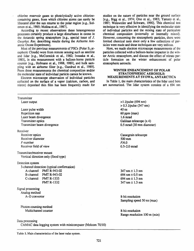
chlorine reservoir gases to photolytically active chlorine- studies on the nature of particles near the ground surfacecontaining gases, from which chlorine atoms can easily be [e,g,, Btgg et al,, 1974; tnt et al,, 1983; Yamato et al.,liberated after the stm returns to the polar region [e.g,, Sol- 1987; Weisweiler and Schwarz, 1990], This chemtcal testomon et al,, 1985; Molina et al,, 1987], technique is very effective in identifying the molecular state

According to recent observations these heterogeneous of individual particles and the mixing state of particuklteprocesses certainly produce a large disturbance in ozone in chemical composition (externally or internally mixed).the Antarctic spring stratosphere [e,g,i special issue of J, However, concerning the stratospheric particles, there wereGeophys. Res. describing results during the Airborne Ant- limited chemical tests since only a few collections of par-arctic Ozone Experiment], ticles were made and these techniques are very tedious.

Most of the previous measurements of PSCs (Polar S_,a_.- Here, we made electron microscope measurements of theospheric Clouds) were from remote sensing such as satellite particles collected with a balloon-borne impactor in the win-and lidar [e,g., McCormick et al., 1982; Iwasaka et al., ter Arctic stratosphere, and discuss the effect of nitrate par-1985], in silJameasurement with a balloon-borne particle ticle formation on the winter enhancement of polarcounter [e,g., Hofmann et al., 1988, 1989], and bulk sam- stratospheric aerosols.piing with an airborne f'dter [e.g., Gandrud et al,, 1989],From these measurements the chemical composition and/or WINTER ENHANCEMENT OF POLARthe molecular state of individual particle cannot be known. STRATOSPHERIC AEROSOLS:

Electron microscope observation of individual particles MEASUREMENTS AT SYOWA, ANTARCTICAcollected on the surface of a vapor (calcium, carbon, and In Table 1, the main characteristics of the lidar used herenitron) deposited thin film has been frequently made for are summarized. The li'dm"system consists of a 694 nm

Transmitter

Laser output > 1J/pulse (694 nm)> 0,3 J/pulse (347 nm)

Laser pulse width 40 nsRepetition rate 60 ppm (max)Laser beam divergence 1.6 mradTransmitter optics Galilean telescope (x 4)Transmitter beam divergence 0.5 mrad (30 mm diameter)

Receiver

Receiver optics Cassegrain telescopeReceiver diameter 500 mmF-number F/4.0Receiver field of view 0.5-2.0 mrad

Transmitter/receiver mountVertical direction only (Votedtype)

Detection system3-channel detection (typical confirmation)

A-channel PMT R-943-02 347 nm+ 1.3 nmB-channel PMT R-943-02 694 nm+ 0.5 nmC-channel PMTR-1333 694 nm+ 1.3 nm

PMT R- 1332 347 nm+ 1.3 nm

Signal processingAnalog method

A-D converter 8-bit resolution

Sampling speed 50 ns (max)

Photon counting methodMultichannel counter 8-bit resolution

Range resolution 100 m (min)

Data processingCAMAC data logging system with minicomputer (Melcom 70/10)

Table 1. Maincharacteristicsof thelaserradarsystem.

721

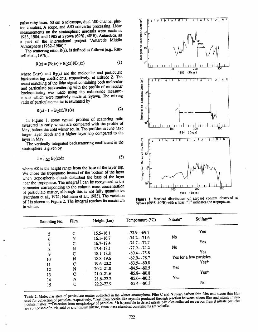
pulse ruby laser, 5tom,telescope, dual lO0-channolpho- _ !j i F i Mi A'I'M l'j t j I A I S ) O i N iton counters, A scope, andA/I)converter processing, Lidarmeasurements on the stratospheric aerosols were made in

a part of the international project "Antarctic Middle

Atmosphere (1982-1986)." _,6' __ I---_[_//_The scattering ratio, R(z), is defined as follows [e.g., Rus-

sell et al., 1976], ._

R(z) = [Bl(z)+B2(z)]/Bl(z) (1) 16'l l)l ******************************1tO 200 300

where Bl(z) and B2(z) are the molecular and particulate 190_ (Day.)backscattering coefficients, respectively, at altitude Z. The ....usual matching of the lidar signal containing both molecular _ _J , F J _' ^ ,M I j , j i A i s , o _N)and particulate backscattering with the prorde of molecularbackscattering was made using the radiosonde measure- _ 16:ments which were routinely made at Syowa. The mixingratio of particulate matter is estimated by ._

R(z) 1 B2(z)/Bl(Z) (2) _ '°_ /L_ J, ," _ _ NO DATA

8' FIn Figure 1, some typical profiles of scattering ratio -_measured in early winter are compared with the profile of ld' iii )1 i1,, Ill I ii , iii It Ill I ii ) ,I, ),May, before the cold winter set in. The profiles in June have 100 200 300larger layer depth and a higher layer top compared to the 1004 (boy,)layer in May. -'-"

The vertically integrated backscattering coefficient in the _=: f j i F I Mi A lM , J , J i A _ S ,' o i N ,stratosphere is given by

,,J

"_ 16;

I= I ria:B2(z)dz (3)

where AZ is the height range from the base of the layer top. _ 163We chose the tropopause instead of the bottom of the layerwhen tropospheric clouds disturbed the base of the layer

the tropopause. The integral I can be recognized as the 16'_nearparametercorresponding to the column mass concentration F_ ii ii, l,) I1] it[ , , I I_ [ , I t t tof particulate matter, although this is not fully quantitative loo 200 aoo[Northam et al., 1974; Hofmann et al., 1983]. The variation 19as (Day,)of I is shown in Figure 2. The integral reaches its maximum Figure 1. Vertical distribution'T"°faerosol content observed atSyowa(69"S,40*E)witha lidar, indicatesthetropopause.in winter.

Sampling No. Film Height (km) Temperature (°C) Nitrate* Sulfate**

5 C 15.5-16.1 -72.9- -69.7 Yes6 N 16.1-16.7 -74.2- -71.6 No7 C 16.7-17.4 -74.7- -72.7 Yes8 N 17.4-18.1 -77.9- -74.2 No9 C 18.1-18.8 -80.4- -75.8 Yes

10 N 18.8-19.6 -82.9- -78.7 Yes for a few particles11 C 19.6--20.2 -83.5- -80.8 Yes+12 N 20.2-21.0 -84.9- -80.5 Yes13 C 21.0--21.6 -85.8-- -80.8 Yes+14 N 21.6-22.2 -85.6- -80.3 Yes15 C 22.2-22.9 -85.4- -80.3 No

Table 2. Molecularstateof particulatemattercollectedin the winterstratosphere.FilmC _d N meancarbonthin film andnitron thin filmused for collectionof particles,respectively.*Testfrom.n_+ie.-likeca2/stalsproducedthroughreactionbetweennitronfilm andnitrateinpar-r **Detectionfromm 11o10 of arucles lt ts possible toticulatematte. ' orp gy p ' . detectnitrateparticlescollectedoncarbonfilm if nitrateparticlesarecomposedofnitricacidor ammoniumnitrate,sincethesechemicalconstituentsarevolatile.

722

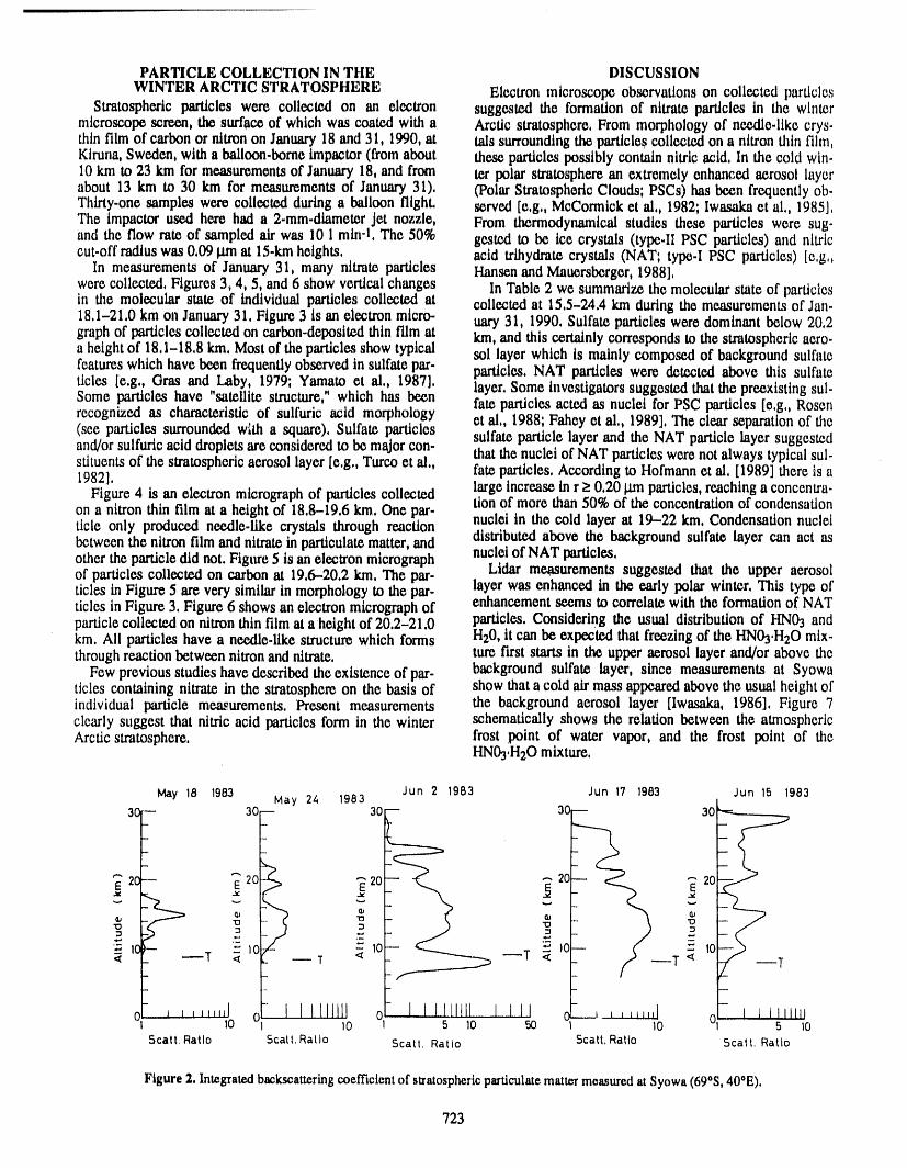
PARTICLE COLLECTION IN THE DISCUSSIONWINTER ARCTIC STRATOSPHERE Electron microscope observationson collected particles

Stratospheric particles were collected on an electron suggested the formation of nitrate particles in the wintermicroscope screen, the surface of which was coated with a Arctic stratosphere, From morphology of needle.like crys.thin film of carbon or nitron on January18 and 31, 1990, at tals surroundingthe particles collected on a nttron thin film,Kiruna, Sweden, with a balloon.borne tmpactor (fromabout these particles possibly contain nitric acid, In the cold win-10 km to 23 km for me.asuromentsof January 18, and from tor polar stratosphere an extremely enhanced aerosol layerabout 13 km to 30 km for measurements of January 31), (Polar Stratospheric Clouds; PSCs) has been frequently ob-Thirty-one samples were collected during a balloon flight, served [e,g,, McCormick ct al,, 1982; lwasaka et al,, 1985j,The impactor used here had a 2-mm-diameter jet nozzle, From thcrmodynamical studies these particles were sug-and the flow rate of sampled air was 10 1 rain-l, The 50% gested to be ice crystals (type-II PSC particles) and nitriccut-offradius was 0,09 [ma at 15.km heights, acid trihydmte crystals (NAT; typ¢-I PSC particles) le,g,,

In measurements of January 31, many nitrate particles Hanson and Mauorsborgor,1988],worecollected. Figures 3, 4, 5, and 6 show vertical changes In Table 2 we summarize the molecular state of particlesin the molecular state of individual particles collected at collected at 15,5-24,4 km during the measurements of Jan-18,1-21,0 km on January 31. Figure3 is an electron micro- uar), 31, 1990. Sulfate particles were dominant below 20,2graph of particles collected on carbon.deposited thin film at km,and this certainly corresponds to the stratospheric aero-a height of 18,1-18,8 km. Most of the particles show typical sol layer which is mainly composedof background sulfatefeatures which have been frequentlyobserved in sulfate par- particles. NAT particles were detected above this sulfateticles [e.g,, Gras and Laby, 1979; Yamato ct al,, 1987], layer. Some investigators suggested that the preexisting sul-Some particles have "satellite structure,"which has been fate particles acted as nuclei for PSC particles [e,g,, Rosenrecognized as characteristic of sulfuric acid morphology ct al,, 1988; Fahey et al,, 1989], The clear separation of the(see particles surrounded w:th a square), Sulfate particles sulfate particle layer and the NAT particle layer suggestedand/orsulfuricacid dropletsareconsideredto be majorcon- that the nuclei of NAT particles were notalways typical sul-stttuentsof the stratosphericaerosol layer [e,g,, Turco et al,, fate particles,According to Hofmann et al, [1989] there is a1982],

Figure 4 is an electron mtcrograph of particles collected large increase in r > 0,20 Ian particles, reaching a concentra-tion of more than 50% of the concentration of condensationon a nitron thin film at a hetght of 18,8-19,6 km, One par-ticle only produced needle.like crystals through reaction nuclei in the cold layer at 19--22 km, Condensation nucleibetween the nitron film and nitrate in particulate matter, and distributed above the background sulfate layer can act asother the particle did not. Figure 5 is an electron mierograph nuclei of NAT particles,

Lidar measurements suggested that the upper aerosolof particles collected on carbon at 19.6-20.2 km. The par-ticles in Figure 5 are very similar in morphology to the par- layer was enhanced in the early polar winter, This type ofticles in Figure 3. Figure 6 shows an electron micrograph of enhancement seems to correlate with the formation of NATparticle collected on nttron thin film at a height of 20.2-21,0 particles, Considering the usual distribution of HN03 andkm. Ali particles have a needle.like structure which forms Hz0, it can be expected that freezing of the HNOyH20 mix-through reaction between nitron and nitrate, ture first starts in the upper aerosol layer and/or above the

Few previous studies have described the existence of par- background sulfate layer, since measurements at Syowaticles containing nitrate in the stratosphere on the basis of show that a cold air mass appeared above the usual height ofindividual particle measurements. Present measurements the background aerosol layer [Iwasaka, 1986], Figure 7clearly suggest that nitric acid particles form in the winter schematically shows the relation between the atmosphericArctic stratosphere, frost point of water vapor, and the frost point of the

HN0.yH20 mature,

May 18 1983 May 24 1983 Jun 2 1983 Jun 17 1983 Jun 15 198330 30 -- 330-- r-- 30

-.

E 2 E 20 20 20 E 20

z lC- "_ 10 --' 1 --T Io,_ --T _, I(3 -,,,.. --T _ _ _ --T _ ,_

o,, j _,,,,,,I o I l IIIIIIi o I I IIIIIII I III OU---,,,,,,,,I 010 10 5 10 50 1 10 lO

Scatt, Ratio Scarf, Ratio Scarf, Ratio 5catt, Ratio 5catt, Ratio

Figure2. lntegratezlbackscatteringcoefficientof stratosphericparticulatemattermeasuredat Syowa(690S,40OE),

723

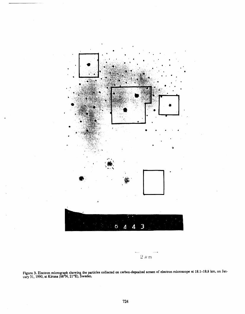
_............. 4

Figure3. Electronmicrographshowingthe particlescollectedon carbon-depositedscreenof electronmicroscopeat 18,1-18,8km,on Jan-uary31, 1990,at Kiruna(68°N,21"E),Sweden.

724

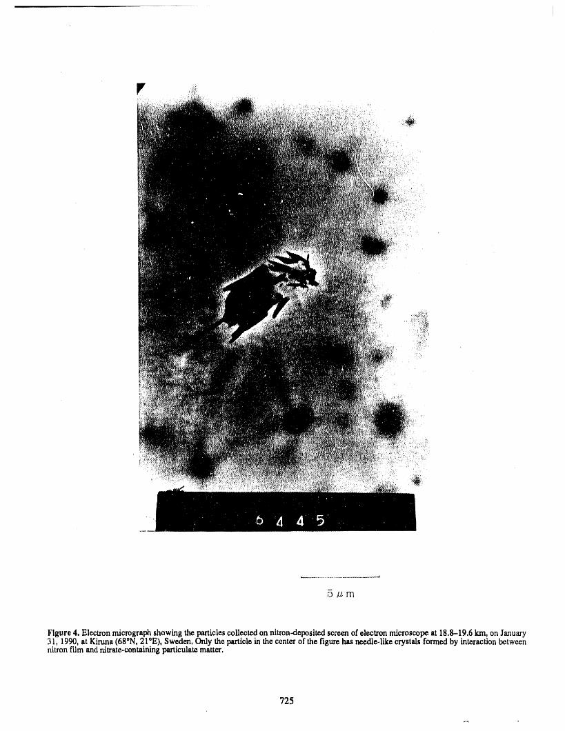
5_m

Figure4.Electronmicrographshowingtheparticlescollectedonnitron-.deposite.clsc_-eenofelectronmicroscopeat18,8--19,6km,onJanuary31, 1990,at Kiruna(68'N, 210E),Sweden,Only tileparticlein the centerof thefigurehas needle.likecrystalsformedby interactionbetweennitronfilmand nitrate-containing particulatematter,

725

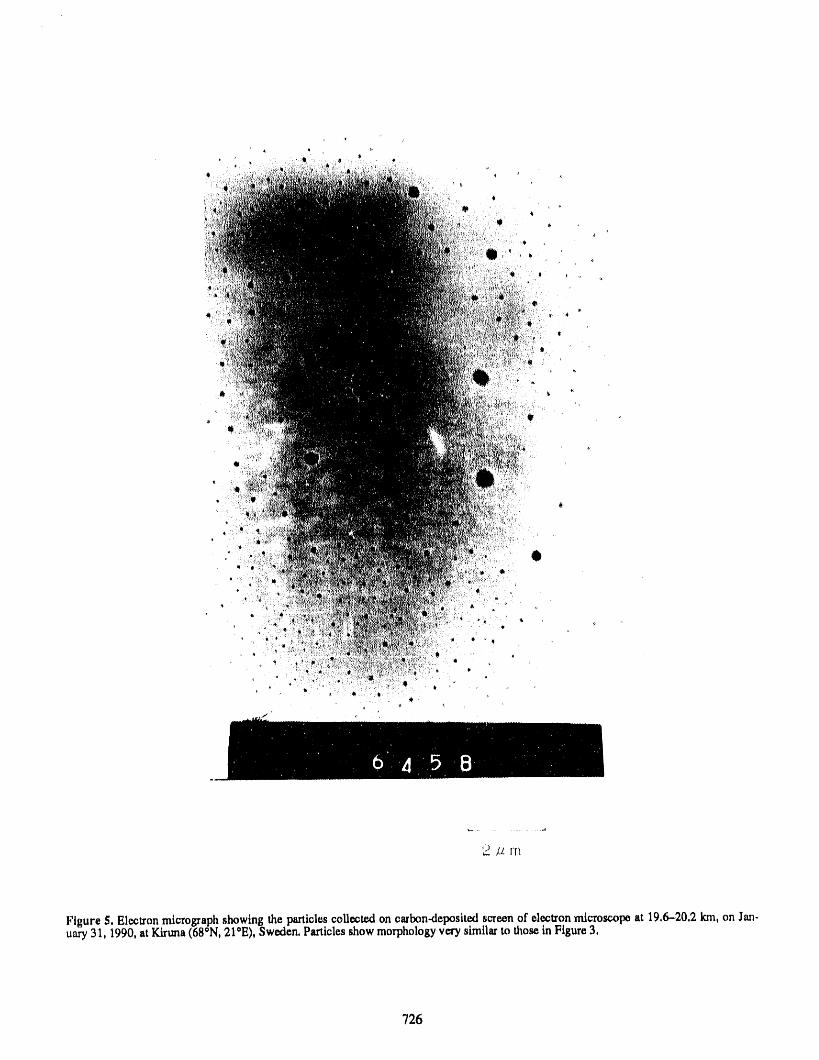
Figure5, Electronmicrographshowingthe particlescollectedon carbon.depositedscreenof electronmicroscopeat 19,6-20,2km, on Jan.uary31, 1990,atKiruna(680N,21'E), Sweden,Particlesshowmorphologyverysimilarto thosein Figure3,

726

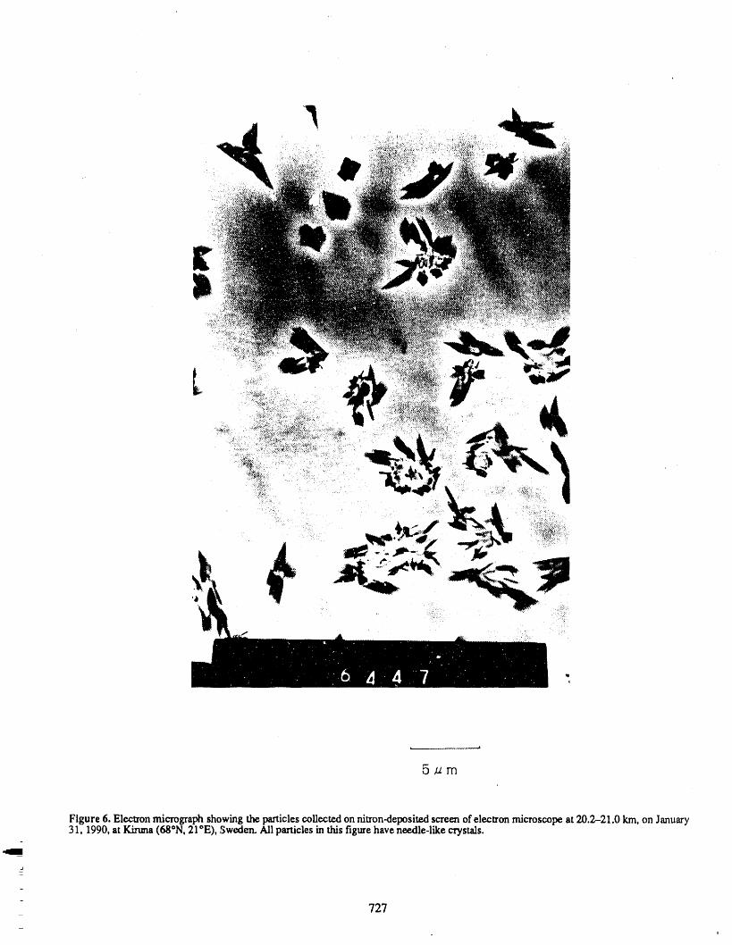
"I

5,urn

Figure 6. Electron micrograph showing the particles collected on nitron-depositext screen of electron microscope at 20.2-21.0 km, on January31, 1990, at gJnma (68°N, 21°E), Sweden. All particles in this figure have needle-like crystals.

-

J_

_

727--

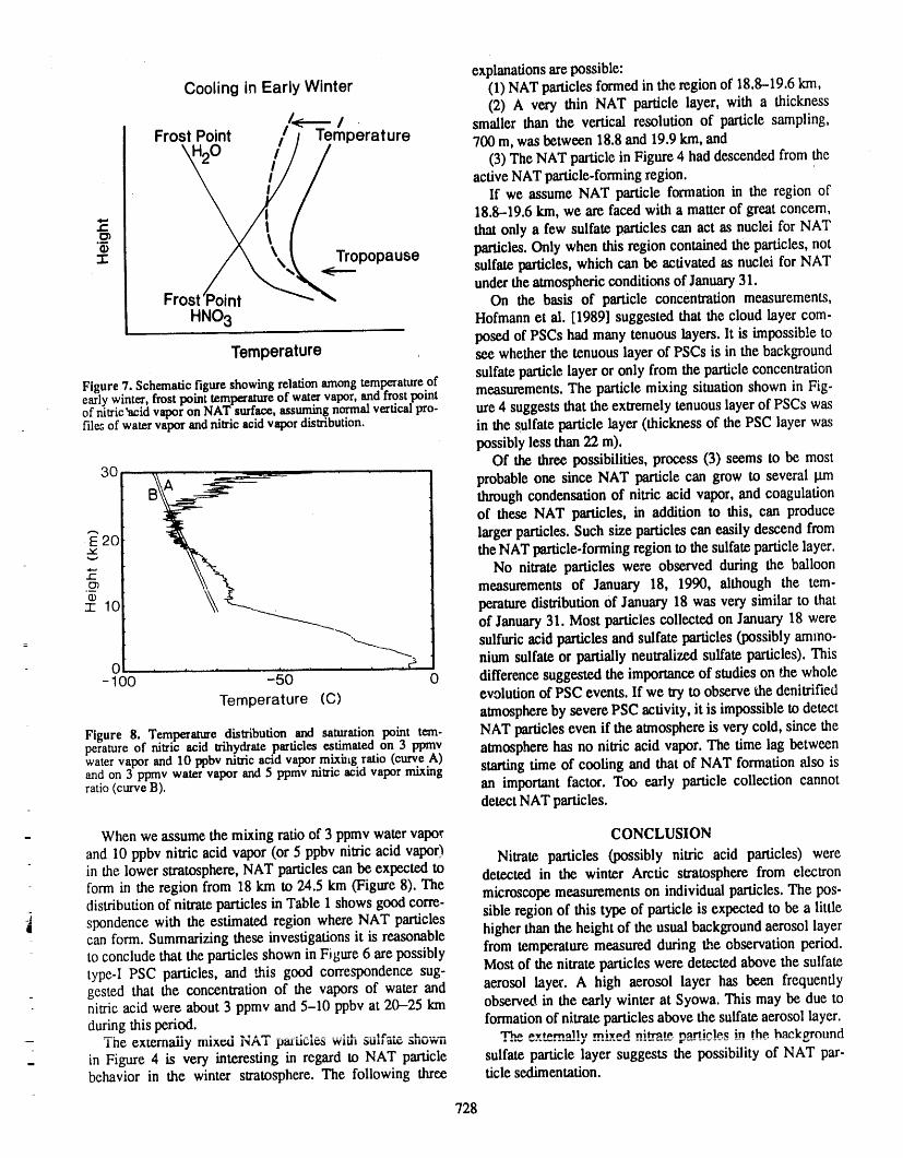
explanations arepossible:Cooling in Early Winter (1) NAT particles formed in the region of 18.8-19,6 km,

(2) A very thin NAT particle layer, with a thickness/<---- / • smaller than the vertical resolution of particle sampling,

Frost Point / I Temperature 700m,wasbetween18,8and 19.9km, and

_20 / / / (3) The NAT particle in Figure 4 had descended from the

If we assume NAT particle formation in the region of18.8--19.6km, we are faced with a matter of great concern,that only a few sulfate particles can act as nuclei for NATc_

"_ particles. Only when this region contained the particles, not

-1- _ Tropopause sulfate particles, which can be activated as nuclei31,for NAT'_'-" under the atmospheric conditions of JanuaryFrost/Point On the basis of particle concentration measurements,

HNO 3 Hofmann et al. [1989] suggested that the cloud layer com-posed of PSCs had many tenuous layers, lt is impossible to

Temperature see whether the tenuous layer of PSCs is in the backgroundsulfate particle layer or only from the particle concentration

Figure7. Schematicfigureshowingrelationamongtemperatureofearlywinter,frostpoint temperatureof watervapor,_d frost.point measurements. The particle mixing situation shown in Fig-of nitric'acidvaporon NATsurface,assumingnormalverticalpro- ure 4 suggests that the extremely tenuous layer of PSCs wasfilet,of watervaporandnitricacidvapordistribution, in the sulfate particle layer (thickness of the PSC layer was

possibly less than 22 m).Of the three possibilities, process (3) seems to be most

30 A " " - --_ probableone sinceNAT particlecangrowtoseverallainthroughcondensationofnitricacidvapor,andcoagulationof theseNAT particles,inadditiontothis,canproduce

_. larger particles. Such size particles can easily descend from.E20,-" the NAT particle-forming region to the sulfateparticle layer.

No nitrate particles were observed during the balloonc--

.__ measurements of January 18, 1990, although the tem-a_:t: 10 perature distribution of January 18 was very similar to that

of January 31. Most particles collected on January 18 were: ,--.. sulfuric acid particles and sulfate particles (possibly ammo-

nium sulfate or partially neutralized sulfate particles). This(3 ........... c_

- 100 -50 0 difference suggested the importance of studies on the whole

Temperature (C) evolution of PSC events. If we try to observe the denitrifiedatmosphere by severe PSC activity, it is impossible to detect

Figure 8. Temperaturedistribution and saturation point tem- NAT particles even if the atmosphere is very cold, since theperatureof nitric acid trihydrateparticlesestimatedon 3 ppmv atmosphere has no nitric acid vapor. The time lag betweenwatervaporand 10 ppbvnitric acidvapormixhlgratio (curveA) starting time of cooling and that of NAT formation also isand on 3 ppmvwatervapor and 5 ppmvnitric acid vapormixingratio(curve B). an important factor. Too early particle collection cannot

detect NAT particles.

= When we assume the mixing ratio of 3 ppmv watervapor CONCLUSION

and 10 ppbv nitric acid vapor (or 5 ppbv nitric acid vapor) Nitrate particles (possibly nitric acid particles) werein the lower stratosphere, NAT particles can be expected to detected in the winter Arctic stratosphere from electronform in the region from 18 km to 24.5 km (Figure 8). The microscope measurements on individual particles. The pos-distribution of nitrate particles in Table 1 shows good corre- sible region of this type of particle is expected to be a little

j spondence with the estimated region where NAT particlescan form. Summarizing these investigations it is reasonable higher than the height of the usual background aerosol layerto conclude that the particles shown in Figure 6 are possibly from temperature measured during the observation period.type-I PSC particles, and ,.his good correspondence sug- Most of the nitrate particles were detected above the sulfategested that the concentration of the vapors of water and aerosol layer. A high aerosol layer has been frequentlynitric acid were about 3 ppmv and 5-10 ppbv at 20-25 km observed in the early winter at Syowa. This may be due toduring this period, formation of nitrate particles above the sulfate aerosol layer.

The externally mixed NAT .........' ..... ,.,_ _..,v .... I. .... Wh_ _v)_msl!y miY@d nitrnm parlial_.qin lhc hacktrroundp_ll LIU 1_7,._ Wll,Ii _iilL/W II .........

= in Figure 4 is very interesting in regard to NAT particle sulfate particle layer suggests the possibility of NAT par-behavior in the winter stratosphere. The following three ticle sedimentation.

728

REFERENCES

Bigg, E. K., A. Ono, and J. A. Williams, Chemical tests for Iwasaka, Y., T. Hirasawa, and H, Fukunishi, Lidar measure-individual submicron aerosol particles, Atmos. Environ., ments on the Antarctic stratospheric aerosol layer, I, Win-8, 1-i3, 1974. ter enhancement, J. Geomagn. Geoelectr., 37, 1087-

Crutzen, P. J., and F. Arnold, Nitric acid cloud formation in 1095, 1985.the cold Antarctic stratosphere: A major cause for the McCormick, M. P., H. M. Steele, P. Hamill, W. P. Chu, andspringtime "ozone hole,"Nature,324,651--655, 1986. T.J. Swissler, Polar stratospheric cloud sightings by

Fahey, D. W., K. K. Kelly, G. V. Ferry, L. R. Poole, J.C. SAM II, J. Atmos. Sci., 39, 1387-1397, 1982.Wilson, D. M. Murphy, M. Lowenstein, and K. R. Chan, McElroy, M. B., R. J. Salawitch, and S. C. Wofsy, AntarcticIn situ measurements of total reactive nitrogen, total 03: Chemical mechanism for the spring decrease, Geo-water, and aerosol L,aa polar stratospheric cloud in the phys. Res. Lett., 13, 1296-1299, 1986.Antarctic, J. Geophys. Res.,94, 11299-11351, 1989. Molina, M. J., T. Tso, L. T. Molina, and F. C. Y. Wang,

Farman, J. C., B. G. Gardiner, and J. D. Shanklin, Large Antarctic stratospheric chemistry of chlorine nitrate,losses of total ozone in Antarctica reveal seasonal CIOx/ hydrogen chloride, and ice release of active chlorine,NOx interaction, Nature, 315,207-210, 1985. Science, 238, 1253--1257, 1987.

Gandrud, B. W., P. D. Sperry, L. Smaford, K. K. Kelly, Ono, A., M. Yamato, and M. Yoshida, Molecular state ofG. V. Ferry, and K. R. Chen, Filter measurement results sulfate aerosols in the remote Everest highlands, Tellus,from the airborne Antarctic ozone experiment, J. Geo- 35B, 197-205, 1983.phys. Res.,94, 11179-11738, 1989. Rosen, J. M., D. J. Hofmann, and J. W. Harder, Aerosol

Gras, J. L., and J. E. Laby, Southern hemisphere strato- measurements in the winter/spring Antarctic stratosphere,spheric aerosol measurements 1, Simultaneous impactor 2, Impact on polar stratospheric cloud theories, J. Geo.and in situ single-particle (light scatter) detection, J. Geo- phys. Res,, 93, 677--686, 1988.phys. Res., 83, 1869-1874, 1979. Russell, P. B., W. Viezee, R. D. Hake, Jr., and R. T. H.

Hansen, D., and K. Mauersberger, Laboratory studies of the Collis, Lidar observations of the stratospheric aerosol:nitric acid trihydrate: Implications for the south polar California, October 1972-March 1974, Q. J. Roy. Mete-stratosphere, Geophys. Res. Lett., 15,855---858,1988. orol. Soc., 102, 675-695, 1976.

Hofmann, D. J., J. M. Rosen, J. W. Harder, and J. V. Here- Solomon, S., R. R. Garcia, F. S. Rawland, and D. J. Waeb-ford, Balloon-borne measurements of aerosol, condensa- bles, On the depletion of Antarctic ozone, Nature, 321,tion nuclei, and cloud particles in the stratosphere at 755--758, 1986.McMurdo station, Antarctica, during the spring of 1987, Toon, O. B., P. ttamill, R. P. Turco, and J. Pinto, Condensa-J. Geophys. Res., 94_16527-16536, 1989. tion of HN03 and HCI in the winter polar stratospheres,

Hofmann, D. J., J. M. Rosen, and J. W. Harder, Aerosol Geophys. Res. Lett., 13, 1284-1287, 1986.measurements in the winter/spring Antarctic stratosphere, Turco, R. P., R. C. Whitten, and O. B. Toon, Stratospheric1, Correlative measurements with ozone, J. Geophys. aerosols: Observation and theory, Rev. Geophys., 20,Res., 93, 665--676, 1988. 233--279, 1982.

Hofmann, D. J., J. M. Rosen, R. Reiter, and H. Jager, Lidar- Weisweiler, W. K., and B. U. Schwarz, Nature of ammo-and balloon-borne particle counter comparisons fol- nium containing particles in an urban site of Germany,lowing recent volcanic eruptions, J. Geophys. Res., 88, Atmos. Environ., 24B, 107-114, 1990.3777-3782, 1983. Yamato, M., Y. Iwasaka, A. Ono, and M. Yoshida, On the

Iwasaka, Y., Non-spherical particles in the antarctic polar sulfate particles in the submicron size range collected atstratosphere---increase in particulate content and strato- Mizuho station and in East Queen Maud Land, Ant-spheric water vapor budget, Tellus, 38B, 364-374, 1986. arctica, Proc. NIPR Symp. Polar Meteorol. Glaciol., No.

1_82-90, 1987.

729

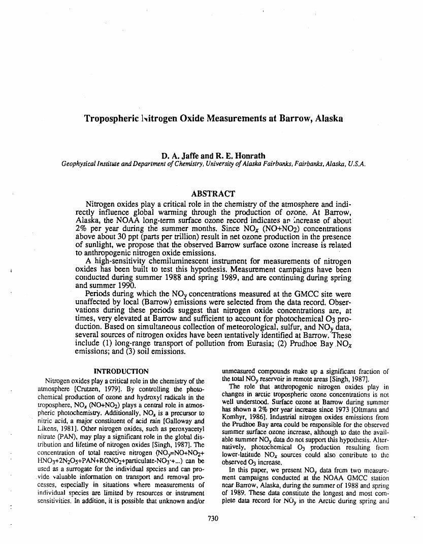
Tropospheric Nitrogen Oxide Measurements at Barrow, Alaska

D. A. Jaffe and R. E. HonrathGeophysicalInstituteandDepartmentof Chemistry,Universityof AlaskaFairbanks,Fairbanks,Alaska,U.S.A.

ABSTRACT

Nitrogen oxides play a critical role in the chemistry of the atmosphere and indi-rectly influence global warming through the production of ozone. At Barrow,Alaska, the NOAA long-term surface ozone record indicates ap increase of about2% per year during the summer months. Since NOx (NO+NO2) concentrationsabove about 30 ppt (parts per trillion) result in net ozone production in the presenceof sunlight, we propose that the observed Barrow surface ozone increase is relatedto anthropogenic nitrogen oxide emissions.

A high-sensitivity chemiluminescent instrument for measurements of nitrogenoxides has been built to test this hypothesis. Measurement campaigns have beenconducted during summer 1988 and spring 1989, and are continuing during springand summer 1990.

Periods during which the NOy concentrations measured at the GMCC site wereunaffected by local (Barrow) emissions were selected from the data record. Obser-vations during these periods suggest that nitrogen oxide concentrations are, attimes, very elevated at Barrow and sufficient to account for photochemical 03 pro-duction. Based on simultaneous collection of meteorological, sulfur, and NOy_data,several sources of nitrogen oxides have been tentatively identified at Barrow. Theseinclude (1) long-range transport of pollution from Eurasia; (2) Prudhoe Bay NOxemissions; and (3) soil emissions.

INTRODUCTION unmeasuredcompoundsmake up a significant fraction ofNitrogenoxidesplaya criticalrole in the chemistryof the thetotal NOyreservoirin remoteareas [Singh,1987],

atmosphere [Crutzen, 1979]. By controlling the photo- The role that anthropogenicnitrogen oxides play inchemicalproductionof ozone and hydroxylradicals in the changes in arctic troposphericozone concentrationsis not

well understood.Surface ozone at Barrow during summertroposphere,NOx (NO+NO2)playsa centralrole in atmos- has showna 2%per year increasesince 1973 [Oltmansandpheric photochemistry.Additionally,NOx is a precursorto Komhyr, 1986]. Industrialnitrogenoxides emissionsfromnitric acid, a majorconstituentof acid rain [Gallowayand the PrudhOeBayarea could be responsiblefor the observedLikens, 1981].Other nitrogenoxides, such as peroxyacetyl summersurfaceozone increase,althoughto date the avail-nitrate (PAN),mayplay a significantrole in the globaldis- able summerNOydatado notsupportthis hypothesis.Alter-tributionand lifetimeof nitrogenoxides [Singh, 1987]:The natively, photochemical O3 production resulting fle,mconcentrationof total reactivenitrogen (NOy=NO+NO2+ lower-latitudeNOx sources could also contribute to theHNO3+2N2Os+PAN+RONO2+particulate-N03-+...)can be observed03 increase.used as a surrogatefor the individualspecies and can pro- In this paper, we present NOydata from two measure-

vide valuable informationon transportand removal pro- ment campaignsconductedat the NOAA GMCC stationcesses, especially in situations where measurements of near Barrow,Alaska,during the summerof 1988and springindividual stw_ciesare limited by resources or instrument of 1989.These data constitutethe longest and most com-sensitivities.In addition,it is possiblethatunknownand/or plete data recordfor NOy in the Arctic during spring and

730

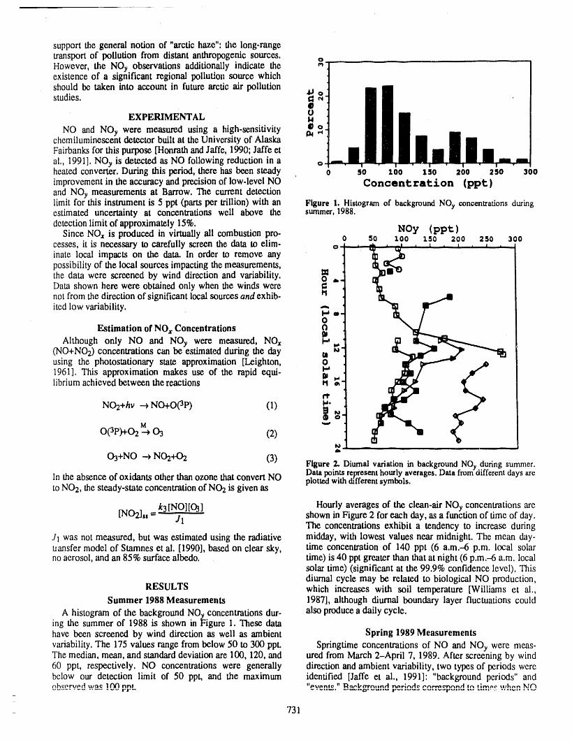
support the general notion of "arctic haze": the long-rangetransport of pollution from distant anthropogenic sources. O

However, the NOy observations additionally indicate theexistence of a significant regional pollution source whichshould be taken into account in future arctic air pollutionstudies. '_ g

41EXPERIMENTAL U14

@oNO and NOy were measured using a high-sensitivity _

chemiluminescent detector built at the University of AlaskaFairbanks for this purpose [Honrath and Jaffe, 1990; Jaffe etal., 1991]. NOy is detected as NO following reduction in a oheated converter. During this period, there has been steady , o so loo zso 2o0 2so _ooimprovement in the accuracy and precision of low-level NO Concentration (ppt)and NOy measurements at Barrow. The current detectionlimit for this instrument is 5 ppt (parts per trillion) with an Figure 1. Histogram of background NOy concentrationsduringestimated uncertainty at concentrations well above the summer,1988.

detection limit of approximately 15%. NOy (ppt)Since NOx is produced in virtually ali combustion pro- o _s0 _.oo _.5o 2o0 2s0 300

cesses, it is necessary to carefully screen the data to elim- oinate local impacts on the data. In order to remove anypossibility of the local sources impacting the measurements,the data were screened by wind direction and variability. O_ d,.Data shown here were obtained only when the winds were =not from the direction of significant local sources and exhib- tS

ited low variability. "_ m.O

Estimation of NOx Concentrations ¢1etl

Although only NO and NOy were measured, NOx _(NO+NO2) concentrations can be estimated during the day tt _using the photostationary state approximation [Leighton, 01961]. This approximation makes use of the rapid equi-librium achieved between the reactions ts

rr

NO2+hv -.-+NO+O(3p) (1) _"W

0(3P)+02_+03 (2)

O3+NO -o NO2+O2 (3)Figure 2. Diurnalvariationin backgroundNO, during summer.Datapointsre_esent hourlyaverages.Data from'differentdays are

In the absence of oxidants other than ozone that convert NO plottedwithdifferentsymbols.to NO2, the steady-state concentration of NO2 is given as

k3 lNO][O3] Hourly averages of the clean-air NOy concentrations are[NO2],, : "' J1 shown in Figure 2 for each day, as a function of time of day.

The concentrations exhibit a tendency to increase duringJl was not measured, but was estimated using the radiative midday, with lowest values near midnight. The mean day-transfer model of Stamnes et al. [1990], based on clear sky, time concentration of 140 ppt (6 a.m.--6 p.m. local solarno aerosol, and an 85% surface albedo, time) is 40 ppt greater than that at night (6 p.m.--6 a.m. local

solar time) (significant at the 99.9% confidence level). Thisdiurnal cycle may be related to biological NO production,

RESULTS which increases with soil temperature [Williams et al.,Summer 1988 Measurements 1987], although diurnal boundary layer fluctuations could

also produce a daily cycle.A histogram of the background NOy concentrations dur-ing the summer of 1988 is shown in Figure 1. These datahave been screened by wind direction as well as ambient Spring 1989 Measurementsvariability. The 175 values range from below 50 to 300 ppt. Springtime concentrations of NO and NOy were meas-The median, mean, and standard deviation are 100, 120, and urea from March 2-April 7, 1989. After screening by wind60 ppt, respectively. NO concentrations were generally direction and ambient variability, two types of periods werebelow our detection limit of 50 ppt, and the maximum identified [Jaffe et al., 1991]: "background periods" andnhuprvod uy_le IrW_ nnt "Psyt_nlo " ]2_,'_nltt'rrA,inrlr_rbr;rsAo nnr'i-,_ol'Xt_nrlt_ tim¢*o szJhr_n l_l('_

--

731

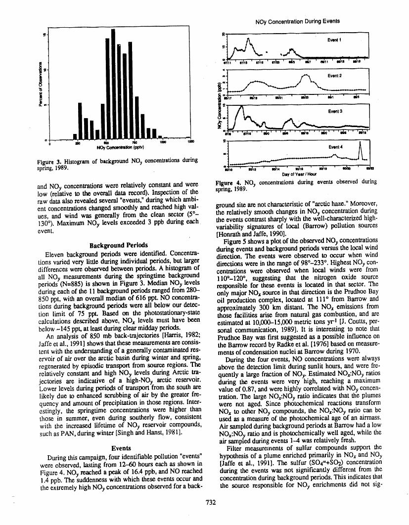
NOyConcentrationDuringEvents

_" _t /1_ ' Eventl

.... I ii= _ ' =h ' =1. ' _ m,_s' =¢_,'

I" "4 I,,, Event 2

" ' '.... Event3 .... I

I_ --_:___ ,._°d'-4' ' '_s' ' '.1_' ' '_ ' '_.' ' '_' ' '=14' ' '_.'

NOy_t_o_ (p_tv)m

Figure 3. Histogram of background NOy concentrations during _ ..................spring, 1989. lt ' _, ' =_t, ' _t= ' m_= '-

Dayof Year / Hour

Figure 4. NOy concentrations during events observed duringand NOy concentrations were relatively constant and werelow (relative to the overall data record). Inspection of the spring, 1989.raw data also revealed several "evealts,"during which ambi-ent concentrations changed smoothly and reached high val- ground site are not characteristic of "arctic haze." Moreover,ues, and wind was gem,-ally from the clean sector (5 °- the relatively smooth changes in NOy concentration during130°). Maximum NOy levels exceeded 3 ppb during each the events contrast sharply with the well-characterized high-variability signatures of local (Barrow) pollution sourcesevent. , [Honrath and Jaffe, 1990].

Background Periods Figure 5 shows a plot of the observed NOy concentrationsduring events and background periods versus the local wind

Eleven background periods were identified. Concentra- direction. The events were observed to occur when windtions varied very little during individual periods, but larger directions were in the range of 980-233 °, Highest NOy con-differences were observed between periods. A histogram of centrations were observed when local winds were fromali NOy measurements during the springtime background 110°-120 °, suggesting that the nitrogen oxide sourceperiods (N=885) is shown in Figure 3. Median NOy levels responsible for these events is located in that sector. Theduring each of the 11 background periods ranged from 280-- only major NO:=source in that direction is the Prudhoe Bay850 ppt, with an overall median of 616 pOt. NO concentra- oil production complex, located at 111° from Barrow andtions during background periods were ali below our detec- approximately 300 km distant. The NOx emissions fromtion limit of 75 ppt. Based on the photostationary-state those facilities arise from natural gas combustion, and arecalculations described above, NOx levels must have been estimated at 10,000-15,000 metric tons yr-I [J. Coutts, per-below -145 pot, at least during clear midday periods, sonal communication, 1989]. lt is interesting to note that

An analysis of 850 mb back-trajectories [Harris, 1982; Prudhoe Bay was first suggested as a possible influence onJaffe et al., 1991] shows that these measurements are consis- the Barrow record by Radke et al. [1976] based on measure-tent with the understanding of a generally contaminated res- ments of condensation nuclei at Barrow during 1970.

ervoir of air over the arctic basin during winter and spring, During the four events, NO concentrations were alwaysregenerated by episodic transport from source regions. The above the detection limit during sunlit hours, and were fre-

relatively constant and high NOy levels during Arctic tra- quenfly a large fraction of NOy. Estimated NOx:NOy ratiosjectories are indicative of a high-NOy arctic reservoir, during the. events were very high, reaching a maximumLower levels during periods of transport from the south are value of 0.87, and were highly correlated with NOy concen-

likely due to enhanced scrubbing of air by the greater fm- tration. The large NOx:NOy ratio indicates that the plumesquency and amount of precipitation in those regions. Inter- were not aged. Since photochemical reactions transform

estingly, the springtime concentrations were higher than NOx to other NOy compounds, the NOx:NOy ratio can bethose in summer, even during southerly flow, consistent used as a measure of the photochemical age of an airmass.with the increased lifetime of NOy reservoir compounds, Air sampled during background periods at Barrow had a lowsuch as PAN, during winter [Singh and Hanst, 1981]. NOx:NOv ratio and is photochemically well aged, while the

air sampled during events 1-4 was relatively fresh.Events Filter measurements of sulfur compounds support the

During this campaign, four identifiable pollution "events" hypothesis of a plume enriched primarily in NOx and NOywere observed, lasting from 12-60 hours each as shown in [Jaffe et al., 1991]. The sulfur (SO4=+SOz) concentration

Figure 4. NOy reached a peak of 16.4 ppb, and NO reached during the events was not significandy different from the1.4 ppb. The suddenness with which these events occur and concentration during background periods. This indicates thatthe extremely high NOy concentrations observed for a back- the source responsible for NOy enrichments did not sig-

732

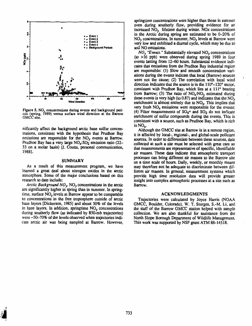
springtimeconcentrations were higher thanthose in summereven during southerly flow, providing evidence for an

' increasedNOy lifetimeduringwinter.NOx concentrations

i ,.eventl intheArcticduringspringareestimatedtobe 0-20% of

..e_mt2 NOy concentrations.Insummer,NOy levelsatBarrowwerex.event3 verylowandexhibitedadiurnalcycle,whichmay beduetoo• Event4.. _a_g_ poa,_ soil NO emissions.

'_ NOy "Events." Substantially elevated NOy concentrations,,_, (to >16 ppb) were observed during spring 1989 in fourevents lasting from 12--60hours. Substantial evidence lndl-

,_, cate..sthat emissions from the Prudhoe Bay industrial region.. are responsible: (1) Slow and smooth concentration vari-

_ ations during the events indicate that local (Barrow) sources_ o. ?* were not the cause; (2) The correlation with local wind,, directionindicatesthatthesourceisinthe110°-120°sector,,_[_=_,aCN" consistent with Prudhoe Bay, which lies at a 111° bearing

i 'T"gl,_ __,0"rlk. _ from Barrow; (3) The ratio of NOx:NOy estimated during ., . ,,, ,,, ,,, ii, ,, these events is very high (to 0.87) and indicates that the NOy

w_ _ , enrichment is almost entirely due to NO:,. This implies thatvery fresh NOx emissions were responsible for the events;

Figure 5. NO v concentrations during events and background peri-ods (spring, I989) versus surface wind direction at the Barrow (4) Filter measurements of SO4 = and SO2 do not indicateGMCCsite. enrichment of sulfur compounds during the events. This is

consistent with a source, such as Prudhoe Bay, which is richin NO_.

nificantly affect the background arctic haze sulfur concen. Although the GMCC site at Barrow is in a remote region,trations, consistent with the hypothesis that Prudhoe Bay it is affected by local., regional-, and global-scale pollutantemissions are responsible for the NOy events at Barrow. sources. In order to differentiate between these sources, damPrudhoe Bay has a very large NOx:SO.zemission ratio (22- collected at such a site must be selected with great care so33 on a molar basis) [J. Coutts, personal communication, that measurements are representative of specific, identif'table1988]. air masses. These data indicate that atmospheric transport

processes can bring different air masses to the Barrow siteSUMMARY ona time scale ofhours. Daily, weekly, or monthlymeans

As a result of this measurement program, we have may therefore not be adequate to discriminate between dif-learned a great deal about nitrogen oxides in the arctic ferent air masses. In general, measurement systems whichatmosphere. Some of the major conclusions based on this provide high time resolution data will provide greaterresearch to date include: insight into complex atmospheric processes at a site such as

Arctic Background NO r NOyconcentrations in the arctic Barrow.are significantly higher in spring than in summer. In spring-time, surface NOy levels at Barrow appear to be comparable ACKNOWLEDGMENTSto concentrations in the free troposphere outside of arctic Trajectories were calculated by Joyce Harris (NOAAhaze layers [Dickerson, 1985] and about 50% of the levels GMCC, Boulder, Colorado). W. T. Sturges, S.-M. Li, andin haze layers. In addition, springtime NO concentrations the staff of the Barrow GMCC station helped with sampleYduring southerly flow (as indicated by 850:mb trajectories) collection. We are also thankful for assistance from thewere -50-70% of the levels observed when trajectories indi. North Slope Borough Department of Wildlife Management.cate arctic air was being sampled at Barrow. However, This work was supported by NSF grant ATM 88-14518.

|

.:)_ 733

REFERENCES

Crutzen, P, J,, The role of NO and NO-2in the chemistry of Leighton, P, A,, Photochemistry of Air Pollution, Academicthe troposphere and stratosphere, Ann, Rev, Earth Plan- Press, New York, 1961,etary Science, 7, 443--472, 1979, Oltmans, S,, and W, P. Komhyr, Surface ozone distributions

Dlckerson, R, R., Reactive nitrogen compounds in the Arc- and variations from 1973-1984: measurements at thetic, J. Geophys. Res,,90, 10739-10743, 1985, NOAA Geophysical Monitoring for Climatic Change

Galloway, J. N,, and G, E. Likens, Acid precipitation: the baseline observatories, J, Geophys, Res,, 91, 5229-5236,importance of nitric acid, Atmos, Ehv,, 15, 1081-1085, 1986.1981. Radke, L, F., P, V, Hobbs, and J, E. Ptnnons, Observations

of cloud condensation nuclei, sodium-containing par-Harris,J. M., The GMCC atmospheric trajectoryprogram,NOAA technical memo ERL ARL.116, Air Resources titles, ice nuclei and the light-scattering coefficient nearLaboratory, Rockville, Maryland, 1982, Barrow, Alaska, J. Appl, Met,, 15,982-995, 1976,

l-tonrath,R, E,, and D. A, Jaffe, Measurements of nitrogen Singh, H, B,, Reactive nitrogen in the troposphere, Env. Sci,oxides in the arctic, Geophys. Res, Lett,, 17, 611--614, Tech,,21,320--327, 1987.1990. Singh, H, B., and P, L, Hanst, Peroxyacetyl nitrate (PAN) in

Jaffe, D. A., R, E, Honrath, J. A. Herring, and S,-M, Li, the unpolluted atmosphere: an important reservoir forMeasurement of nitrogen oxides at Barrow, Alaska dur- nitrogen oxides, Geophys, Res, Lett., 8, 941-944, 1981,ing Spring: Evidence for regional and northern hemi- Stamnes, K., and S,-C, Tsay, Optimum spectral resolutionspheric sources of pollution, J. Geophys. Res,, 96, 7395-- for computing atmospheric heating and photodissociation7405, 1991. rates, Planet, Space Sci., 38, 807--820, 1990,

Williams, E. J., D.'D. Parrish, and F, C, Fehsenfeld, Deter-Kahl, J, D., J. M. Harris, G. A. Herbert, and M, P. Olson, mination of nitrogen oxide emissions from soils: results

Intercomparison of three long-range trajectory models from a grassland site in Colorado, United States, J, Geo.applied to arctic haze, Tellus, 41B, 524-536, 1989, phys, Res., 92, 2173-2179, 1987.

'7_A

Observation of Ozone and Related Quantitiesby the Japanese Antarctic Research Expedition

H. Kanzawa and S. KawaguchiNationalInstituteof PolarResearch,Tokyo,Japan

ABSTRACT

Total ozone observations with a Dobson spectrophotometer, routinely carried outat Syowa Station (69°S, 40°E) since 1966, contributed to the discovery andconf'wmation of the Antarctic ozone hole. Routine meteorological sonde observa-tions since the IGY period and ozone sonde observations since 1966 at Syowa Sta-tion gave useful information on the cause of the formation of the Antarctic ozonehole. Other observations at Syowa Station during the Middle Atmosphere Programperiod (1982-1985) also gave much information on the Antarctic ozone layer.

The "spring" total ozone at Syowa Station showed record low values in 1987 and1989. In 1988, the following phenomenon was observed over Syowa Station. Thereoccurred a large, sudden stratospheric warming in late winter 1988, competing insuddenness and size with major mid-winter warmings in the northern Hemisphere.Associated with the dynamical phenomenon of the sudden warming, total ozonesuddenly increased. The sudden warming, as well as other warmings, whichfollowed it made "spring" total ozone amount higher.

Meridional distributions of ozone were obtained with ozone sonde observationsmade by the Japanese Antarctic Research Ship, Shirase, on the way from Japan toSyowa Station, at intervals of about every 5 degrees for November throughDecember in 1987 and 1988. Characteristics of interest may be summarized asfollows: south of about 60°S, partial pressure of ozone shows low values in thealtitude range of 10-18 km, while large values occur at 20-25 km; there was atropopause gap around 30-35°S through which ozone seems to intrude from thestratosphere to the troposphere.

One or two balloons will be launched under the Polar Patrol Balloon (PPB)project in September 1991 at Syowa Station to measure in situ ozone, aerosol, andtemperature for about two weeks along the track of the balloon on the 50 mb levelover Antarctica. Data acquisition and balloon positioning will be made using theARGOS system. Since the PPB observation is a Lagrangian type observation, theozone measurement can detect the chemical source/sink of ozone more directlythan other types of observation, and the aerosol measurement will give muchinformation on the role of Polar Stratospheric Clouds (PSCs) in the formation of theAntarctic ozone hole.

735

Ozone Evolution Peculiarities in the Polar Regions:Analysis of Observational Data and Results of Modeling

Igor I. MokhovInstituteo./AtmosphericPhysics,Academyof Sciencesof the U.S.SJ¢,,Moscow,U.S.S.R.

ABSTRACT

Analysis of ozone evolution peculiarities in intra-annual evolution of latitude-altitude and latitude-longitude atmospheric ozone concentration fields was cardedout using a special method of amplitude-phase characteristics, The TOMS satelliteozone data for the period 1978-1987 were used in the analysis, Comparison wasmade with results of analysis of total ozone evolution based on data obtained fromthe World Data Center for Ozone (Toronto) and from the Main Geophysical Obser-vatory 0.,eningrad) for the period 1973-1985 at 133 Northern and Southern hemi-sphere stations. Latitude-altitude peculiarities of the evolution of ozoneconcentrations from different satellite data are compared with results of simulationsusing a two-dimensional photochemical model of the atmosphere. There are largedifferences in ozone evolution in polar latitudes of the Northern and Southern hemi-spheres in different stratospheric layers and for different seasons. Particularly it wasnoted that the "ozone hole" phenomenon is more pronounced in the Antarctic thanin the Arctic. Comparison with results of standard harmonic analysis was also car-ried out.

There have been many climatologicalstudies of atmos- cessingTeam.The 5°x5° ozonedata set was preparedbyK.pheric ozone distribution,a number of which have been Bowman,) The results of this analysis are interestingtobased on a harmonic analysis of ozone annual variations, compare with results of the standard harmonicanalysisofHowever, a formal separation by certain modesdoes not the TOMSdataftr4 years[BowmanandKrueger,1985].alwaysgivea clearunderstandingof the real processes. Study of the amplitude characteristics[Mokhov,1985;

Analysisof the ozoneevolutionpeculiaritiesin the intra- Gruzdevand Mokhov,1987]of the TO seasonalevolutionannualevolutionfor latitude--longitudeand latitude-altitude revealedchangesof boundariesof regions with the TO (X)ozoneconcentrationfieldsin theatmospherewascardedout decrease of AX---20DU compared with March and Sep-using a special method of amplitude--phasecharacteristics tember (Figure 1). In the high NH latitudeson the TOMS[Mokhov,1985;Gruzdevand Mokhov,1988].The purpose data the largestvaluesof TO occurredin March(>480DUDof using this method is to minimize our prescription(for and the smallestvalues in September-October(<260DUD.example,by the fixed mode representation)ofthe evolution In the SH high latitudes the smallest values of TO wereof differentfields, noted in March-April(<260 DU) and the largest valuesin

TOMS (TheTotal Ozone MappingSpectrometer)satel- October (>400 DU) in subantarcticlatit_des. So the ozonelite data fromNimbus7 [Bowman,1989]forthe totalozone changesin the annualcyclecomparedwith ,Marchare char-content(TO) in the atmosphereduring1979--1987werearm- acterizedin the NH high latitudesby a TO decrease(in thelyzed. (TOMS ozone data were providedby the National SH by an increase)on the whole. The appropriateozoneSpaceScienceDataCenterat GoddardSpaceFlightCenter. changescomparedwith Septemberare characterizedin theThe originalTOMSdataprocessingwascarriedout by A.J. NH high latitudes by a TO increase (in the SH by aFleig, D. Heath,A. J. Kruegerand the NimbusOzonePro- decrease)on the whole.

736

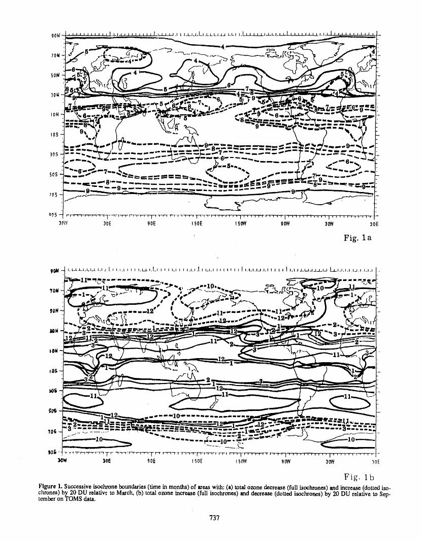
, u, mlmll ii I

"-_+ ---_O; .... - ..... :......-

...... 10 -.+_. ++__.,._..L,_

)Og "

30E 90_, i90E 150W 90W 30W )oE

Fi_,IbFigure 1. Successive isochtone boundaries (time in months) of areas with: (a) total ozone de_ease (full isochtone_) and increas_ (dotted iso-chroncs) by 20 DU reladw. _o Mm'ch, CD)total ozone increase (full isochxones) and decrease (dotted isochron_s) by 20 DU relative to S_p-temb_r on TOMS data,

737

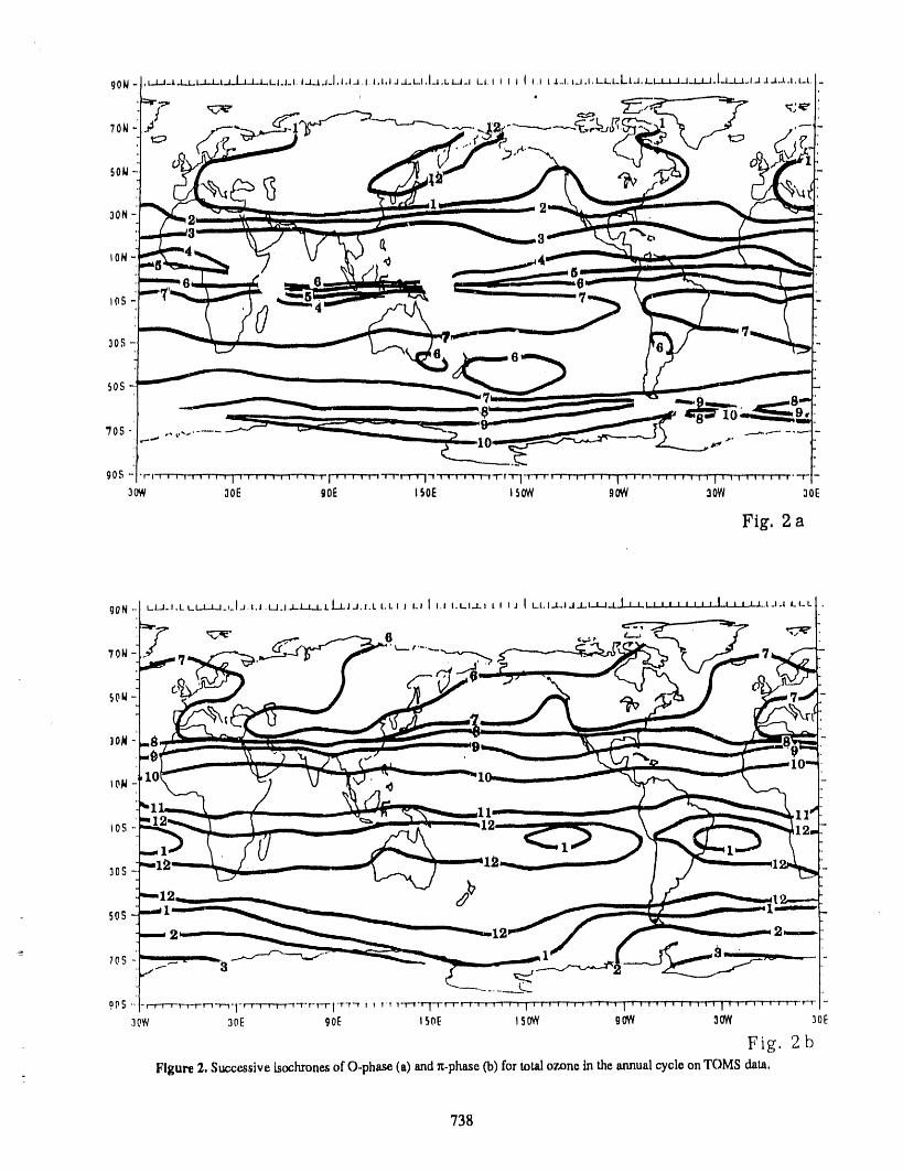
738

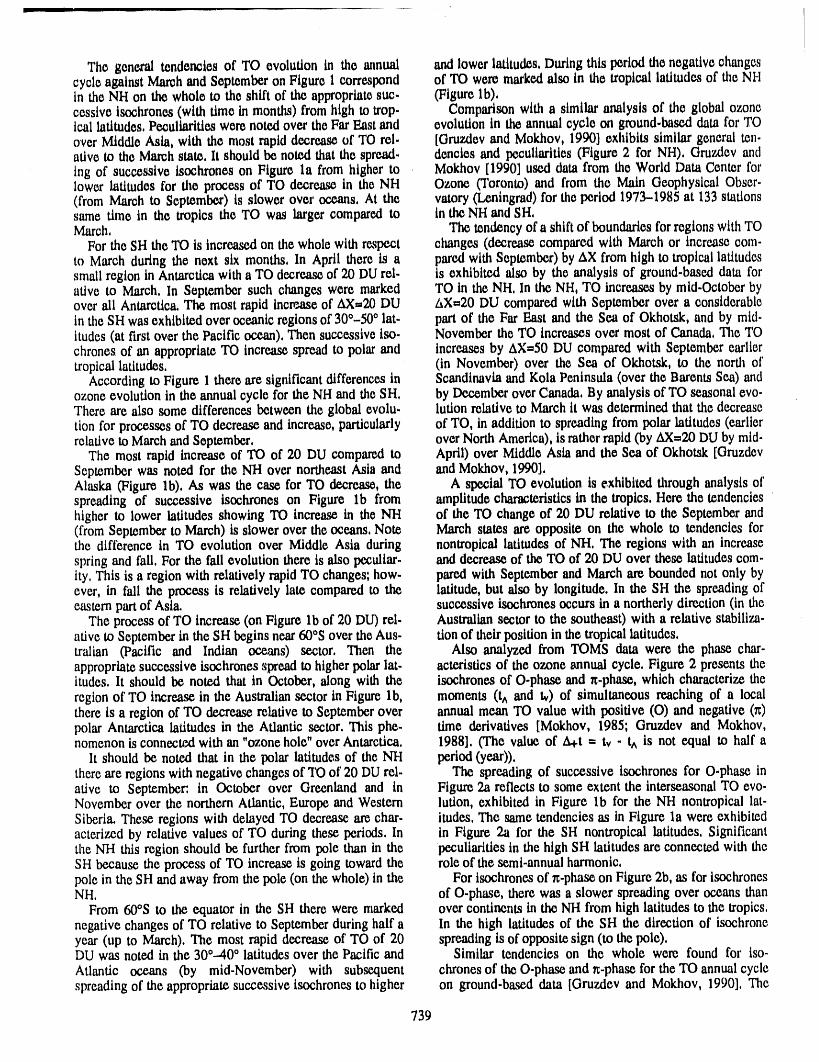
The general tendencies of TO evolution in the annual and lower latitudes,During this period the negative changescycle against March and September on Figure 1 correspond of TO were marked also in the tropical latitudes of the NHin the Nii on the whole to the shift of the appropriatesue- (Figure lb),cessivo isochrones (with time in months) from high to uop- Comparison with a similar analysis of the global ozoneteallatitudes,PeculiaritieswerenotedovertheFarEastand evolutionin theannualcycleoa ground.baseddataforTOover MiddleAsia,withthemostrapid decrease of TO rel. [Oruzdovand Mokhov, 1990] exhibits similar general ten.ative to the March state, lt should be noted that the spread, dencies and peculiarities (Figure 2 for NH), Gruzdev anding of successive tsochrones on Figure la from higher to Mokhov [1990] used data from the World Data Center forlower latitudes for the process of TO decrease in the NII Ozone (Toronto) and from the Main Geophysical Obser-(from March to September) is slower over oceans, At the vatory (Leningrad) for the period 1973-1985 at 133stationssame time in the tropics the TO was larger compared to in the NH and SH,March, The tendency of a shift of boundariesfor regions with TO

For the SH the TO is increased on the whole with re,,spect changes (decrease compared with March or increase com-to March during the next six months, In April there is a paredwith September)by AX from high to tropical latitudessmall region in Antarcticawith a TO de,crease of 20 DU rel. is exhibited also by the analysis of ground-based data forative to March, In September such changes were marked TO in the NH, In the NH, TO increases by mid.October byover ali Antarctica. The most rapid increase of AX=20 DU AX=20 DU compared with September over a considerablein the SH was exhibited over oceantc regions of 300-500 lab part of the Far East and the Sea of Okhotsk, and by mid-ttudes (at first over the Pacific ocean), Then successive iso. November the TO increases over most of Canada, The TOchrones of an appropriate TO increase spread to polar and Increases by AX,,,50DU compared with September earliertropical latitudes, (In November) over the Sea of Okhotsk, to the north of

According to Figure 1 there are significant differences in Scandinavia and Kola Peninsula (over the Barents Sea) andozone evolution in the annual cycle for the NH and the SH, by December over Canada, By analysts of TO seasonal eve-There are also some differences between the global evolu, lutlon relative to March lt was determined that the decreasetion for processes of TO decrease and increase, particularly of TO, in addition to spreading from polar latitudes (earlterrelative to March and September, over North America), is rather rapid (by AX=20 DU by mid-

The most rapid increase of TO of 20 DU compared to April) over Middle Asia and the Sea of Okhotsk [OruzdevSeptember was noted for the NH over northeast Asia and and Mokhov, 1990].Alaska (Figure lb), As was the case for TO decrease, the A special TO evolution is exhibited flwough analysts ofspreading of successive tsochrones on Figure lb from amplitude characteristics in the tropics, Here the tendencieshigher to lower latitudes showing TO increase in the NII of the TO change of 20 DU relative to the September and(from September to March) is slower over the oceans, Note March states are opposite on the whole to tendencies forthe difference in TO evolution over Middle Asia during nontroplcal latitudes of NH, The regions with an increasespring and fall, For the fall evolution there is also peculiar, and decrease of the TO of 20 DU over these latitudes com-ity, This is a region with relatively rapid TO changes; how- pared with September and March are bounded not only byever, in fall the process is relatively late compared to the latitude, but also by longitude. In the SH the spreading ofeastern pan of Asia, successive isochrones occurs in a northerly direction (in the

The process of TO increase (on Figure lb of 20 DU) rel. Australian sector to the southeast) with a relative stablliza-ative to September in the SH begins near 60°S over the Aus. tion of their position in the tropical latitudes,traltan (Pacific and Indian ocer.ms) sector, Then the Also analyzed from TOMS data were the phase char-appropriate successive isochrones spread to htgher polar lat. acteristics of the ozone annual cycle, Figure 2 presents theitudes, lt should be noted that in October, along with the isochrones of O-phase and n-phase, which characterize theregion of TO increase in the Australian sector in Figure lb, moments (tA and tr) of simultaneous reaching of a localthere is a region of TO decrease relative to September over annual mean TO value with positive (O) and negative (g)polar Antarctica latitudes in the Atlantic sector. This phe. time derivatives [Mokhov, 1985; Gruzdev and Mokhov,nomenon is connected with an "ozone hole" over Antarctica, 1988]. (The value of A+t ffi tv - tA is not equal to half a

lt should be noted that in the polar latitudes of the NII peter (year)).there are regions with negative changes of TO oi' 20 DU tel. The spreading of successive isochrones for O-phase inalive to September in October over Greenland and in Figure Za reflects to some extent the interseasonal TO eve-November over the northern Atlantic, Europe and Western lution, exhibited in Figure lb for the NH nontroptcal lat-Siberia. These regions with delayed TO decrease are char. itudes. The same tendencies as in Figure la were exhibitedacterized by relative values of TO during these periods. In in Figure 2a for the SH nontropical latitudes, Significantthe NH this region should be further from pole than in the peculiarities in the high SH latitudes are connected with theSH because the process of TO increase is going toward the role of the semi-annual harmonic,pole in the SH and away from the pole (on the whole) in the For isochrones of n-phase on Figure 2b, as for isochronesNH, of O-phase, there was a slower spreading over oceans than

From 60°S to the equator in the SH there were marked over continents in the NH from high latitudes to the tropics,negative changes of TO relative to September during half a In the high latitudes of the SH the direction of isoehroneyear (up to March). The most rapid decrease of TO of 20 spreading is of opposite sign (to the pole),DU was noted in the 30"--40° latitudes over the Pacific and SimiLar tendencies on the whole were found for Iso-Atlantic oceans (by mid-November) with subsequent thrones of the O-phaseand n-phase for the TO annual cyclespreading of the appropriate successive isochrones to higher on ground-based data [Oruzdev and Mokhov, 1990], The

739

boundaries of n-phase and minimum-phase (m.phase) for In the nontropical SH latitudes both for the model (withthe TO annual cycle over North America according to [q]=mol]cm3) and on the basis of satellite data (with[Oruzdev and Mokhov, 1990] extetld on the whole from [q]=ppmv) there was a descent of the O.phase and rg.phasehigh to low latitudes, In Eurasia there were regions over the isochronesin the middle and lowerstratosphere, On satelliteFar East and Middle Asia with an earlier reaching of the data [Keeting and Young, 1985] the O.phase tsochrones areappropriate phases, The peculiarities of these regions were shifted from the middle stratosphere layers higher than 35noted also for the maximum.phase(M-phase) and O-phai, km, while the level of the rg.phase isochrones forming inOver North America the earlier reaching of the M.phase and March ts remarkably lower (near 30 Ian), For the model, asO-phase states was marked in the vicinity of 50°--600 lat. for the data, there is a shift of the successive O- and rg.phaseltudes. In Oruzdev and Mokhov [1990] tt was noted that O- Isochrones in the lower SH stratosphere from lower to polarphase, rg-phase,M-phase and m-phase states of the TO intra, latitudes, The boundary of the rg.phase reaches the trope-annual evolution differ considerably over certain regions, pause by October, The boundary of the O-phase reaches bySome of these peculiarities of evolution are difficult to October the level near 22 km in the 600 SH latitude,sand byexhibit by analysis using the fixed mode decomposition March-April the tropopause level,(specifically, by the standard harmonic analysis). Unlike the SH, in the NH stratosphere for q there ts no

The phase characteristics on different satellite data [Keet- genel_ delay of reaching of the O- and n-phase states tning and Young, 1985] were also determined for the zonal comparison with lower latitudes, The region with reachtngmean TO [Oruzdev and Mokhov, 1990], On the whole ali of the O.phase state ts extended from polar latitudes In thethe phase isoehrones have a tendency to shift with time from lower NII stratosphere above 20 km and below 16 km thethe north to the south, In riteSH there Is a tendency of the tendency of the shift to pole is exhibited,tsochrones to shift from ..-40°S to the equator, For the m. The appropriate peculiarities of the ozone content evolu-phase there are dtqcontlnuities at ~I0"S and at 60-65°S, The lion in tlm SH and NH stratosphere are exhibited also by anforming of the "ozone hole" structure over Antarctica in the analysis of the amplitude characteristics of the q annualSH spring is connected with noted peculiarity, The spring cycle. In Oruzdev et al. [1988] the peculiarities for Iso.TO minimum forms first (tri August) at -60°S and then in thrones of boundaries of regions with increase and decreasehigher latitudes (occurring at 75°S in the middle of Sep- of the ozone content in the annual cycle relative June andtember). The sequence of the TO maximum isoehrone shift December are noted,(and the sequence of "hole" filling) also has a direction from The noted peculiarities of the ozone annual cycle char-lower to higher latitudes. This corresponds to "ozone hole" actedze, in particular, the mechanisms of forming and fill.filling at the middle stratosphere levels, ing of the atmosphere ozone deficit ("ozone holes") In the

The noted peculiarities of the TO evolution in polar polar atmosphere. As shown by the direction of latitudinalregions are connected with peculiarities of the ozone content displacement of successive isochrones, different ozone

'(q) evolution in different atmospheric layers and latitudinal regimes are reached later ht Antarctica than in neighboringbelts [Oruzdev and Mokhov, 1988, 1989]. Oruzdev et al, latitudes, due to relative dynamical isolation of the Antarctic[1988] compared the intra-annual evolution of the ozone hat- atmosphere. On the other hand, the seasonal ozone evolu-itude--longitude fields from satellite data with results of a lion in the Arctic is characterized on the whole by dis-two-dimensional photochemical model of the atmosphere, placement of successive tsochrones from high latitudes.On the whole there was qualitative agreement, although These results indicate that the "ozone hole" phenomenon tsthere are also the remarkable quantity differences, more pronounced in the Antarctic than in the Arctic.

REFERENCES

Bowman, K, P., Global patterns of the quasi-biennial oscil- Onmdev, A. N., and I, I, Mokhov, Peculiarities of intra-lation in total ozone, J, Atmos, Sci., 46, 3328-3343, 1989. annual global dynamics of total ozone content, Meteor, i

Bowman, K. P., and A. J. Krueger, A global climatology of Gidrol., 7, 1990.total ozone from Nimbus 7 total ozone mapping SlX_- Gruzdev, A, N., I. L. Karol, A. P. Kudryavtsev, and I. i.trometer, J. Geophys. Res., 90, 7967-7976, 1985. Mokhov, Diagnostics of atmospheric ozone dynamics in

Gruzdev, A. N., and I. I. Mokhov, Diagnostics of strato- annual cycle from empirical data and in photochemicalspheric and mesospheric dynamics in annual cycle with model, Conf. on Atmospheric Ozone (2--6 October, 1988,amplitude-phase characteristics method, Preprint of the Suzdal), CAO, Dolgoprudny, 1988.Institute of Atmospheric Physics. Moscow, 1987. Keeting, G, M., and D. F. Young, Interim reference ozone

Gruzdev, A. N., and I. I. Mokhov, Evolution of stratospheric models for the middle atmosphere, Handbook for MAP,ozone annual dynamics from satellite data, Issledovanie 16,205-229, 1986.Zemli iz Cosmosa, 2, 3-10, 1988.

740

Uncertainties in Total Ozone Amounts Inferred from Zenith Sky Observations:Implications for Ozone Trend Analyses

K. Stamnes and S. PegauGeophysicalInstituteandDepartmentof Physics,Universityof AlaskaFairbanks,Fairbanks,Alaska,U.S.A.

J. FrederickDepartmentof GeophysicalSciences,Universityof Chicago,Chicago,Illinois,U.S.A.

ABSTRACT

in an effort to determine ozone measurement uncertainties associated with zenithsky radiation observations we have used radiative transfer calculations to simulateozone inference by the Dobson procedure. Synthetic zenith sky charts are computedfor the commonly used AD wavelength pairs by a procedure ft,at simulates theconstruction of empirical charts. By using a comprehensive radiative transferalgorithm, a model atmosphere and a suitable set of ozone absorption crosssections, we may simulate the effects of cloud optical depth, cloud altitude, verticaldistribution of ozone, temperature profile and surface albedo on the total amount ofozone inferred by the Dobson procedure from zenith sky observations. Our simula-tions indicate that attempts to determine small changes in total ozone amounts frommeasurements of zenith sky intensity are fraught with difficulties. These findingsimply that what appears to be a trend in total ozone could conceivably be due tochanges in (1) ozone profile, (2) effective temperature, or (3) incorrect estimates ofthe effects of clouds or surface albedo. We discuss possible means of rectifying thisozone measurement problem by invoking computer simulations to determinepossible sources and magnitudes of errors incurred in zenith sky measurements toinfer total ozone. In particular, we suggest that construction and use of syntheticcorrection tables for any particular station may alleviate difficulties encountered inthe creation o7 empirical correction tables, since it avoids problems related to (1)time lapse between measurements, and (2) diffuse radiation from forward scatteringin clouds influencing the direct sun measurements. Instrumental effects can beaccounted for by comparing the theoretical charts with direct sun measurementsunder clear sky conditions.

741

Permafrost-Associated Gas Hydrates of Northern Alaska:A Possible Source of Atmospheric Methane

T. S. CollettU.S. Geological Survey, Menlo Park, California, U.S.A.

ABSTRACT

Atmospheric methane, a potential greenhouse gas, is increasing at such a ratethat the current concentrations (=1.7 ppm) will probably double in the next 50years. Analysis of gases trapped in ice cores indicates that the contemporaryatmospheric methane concentrations and their rate of increase are unprecedentedover the last 160,000 years. Numerous researchers have suggested that destabilizedgas hydrates may be contributing to this buildup in atmospheric methane. Little isknown about the geologic or geochemical nature of gas hydrates, even though theyare known to occur in numerous arctic sedimentary basins.

Because of the abundance of available geologic data, our research has focusedon assessing the distribution of gas hydrates within the onshore regions of northernAlaska; currently, onshore permafrost-associated gas hydrates axe believed to beinsulated from most atmospheric temperature changes and are not at this time animportant source of atmospheric methane. Our onshore gas hydrate studies,however, can be used to develop geologic analogs for potential gas hydrateoccurrences within unexplored areas, such as the thermally unstable nearshorecontinental shelf.

On the North Slope, gas hydrates have been identified in 36 industry wells byusing well-log responses calibrated to the response of an interval in one well wheregas hydrates were recovered in a core by an oil company. Most gas hydrates weidentified occur in six laterally continuous Upper Cretaceous and lower Tertiarysandstone and conglomerate units; ali these hydrates are geographically restricted tothe area overlying the eastern part of the Kuparuk River Oil Field and the westernpart of the Prudhoe Bay Oil Field. Stable carbon isotope geochemical analysis ofwell cuttings suggests that the identified hydrates originated fi'om a mixture ofdeep-source thermogenic gas and shallow microbial gas that was either directly

J converted to gas hydrate or Iu'st concentrated in existing traps and later convertedto gas hydrate. We postulate that the thermogenic gas migrated from deeper res-ervoirs along the faults thought to be migration pathways for the large volumes of

" shallow, heavy oil found in the same area.

742=

The Role of Natural Gas Hydrates in Global Changes

Y. F. MakogonOiland GasResearchInstitute,Academyof ScienceU.S.SJ_.,Moscow,U.S.S.R.

ABSTRACT

Natural gas hydrates, a mineral widely spread on earth and on many space bod-ies in the Universe, have been known since the 1960s. The hydrates made aconsiderable contribution to the formation of the earth's atmosphere and hydro-sphere at the early period of existence. They presently play a great role inaccumulation of hydrocarbons in the sedimentary cover of the earth's crust on landand under the sea. Hydrates exert considerable influence on the thermal balance ofthe earth's surface, R_ climate, ecology and geography of the arctic shores.

The main features of gas hydrates which produce global changes are: structureand composition of hydrates, heat of the phase transition and of accumulation anddecomposition (about 420 ld kg-1), the change of the water specific volume (26-32%) under its transition to the hydrate state, and the electric impulse formationbetween the two phases during the phase transitions of systems. One volume ofwater contains 70-200 volumes of gas in hydrate state. Gas pressure in the crystallattice of hydrate is hundreds, even thousands MPa.

The hydrate formation zone is associated with frigid areas of Earth sedimentaryrocks; on the landl near the polar regions, in the sea, at any latitude at depths >200,500 m. Methane hydrate resources make up about 104 Gt, 99% of them under thesea. The explored resources are 500 Gt.

Hydrate methane is, undoubtedly, the energy potential of mankind for the nextcentury, but the rates of the free methane outflow into the atmosphere and theirinfluence on the global climate, ecology, geography, etc. need to be taken intoaccount. The current amount of methane in the atmosphere is about 4.8 Gt. Thus,the ave _ge Earth surface temperature is increased by 1.3 K. The annual increase ofmethane in the atmosphere is 1%.

Natural gas hydrates, their spreading and features may cause blowouts of freemethane to the atmosphere, much greater than the current biochemical andtechnogenic sources. Methane may flow from the top and from the bottom of thelayer as well under changing thermodynamic conditions, such as decreasingpressure, increase of the geothermal gradient, neotectonic shifts, changing of thehydrate deposits, electric potential. The free methane provides for an increase ofCO2, H20, 03 concentration. The heating effect of methane can be equal to orexceed that of C02.

- 743

Volcanic Eruption Events and the Variations in Surface Air Temperatureover High Latitude Regions

Jia PengqunPolar Meteorological Laboratory, Academy of Meteorological Science, State Meteorological Administration,

Beijing, Peoples' Republic of China

ABSTRACT

The numerical experiments of our study suggest that volcanic eruptions cause acooling of the surface temperature. Special attention will be given to the climaticfluctuation tied to the cooling in summer in high latitudes resulting from the erup-tions occurring in spring or summer in high latitudes in the Northern Hemisphere.

INTRODUCTION canic dust is expressed as a functionof the opticaldepthandVolcanic eruptions are magnificent naturalphenomena, aerosol size distribution and a simple model of the latitu-

The early studies on volcanic dust by Humphreys [1940] dinal distributionof aerosol optical thickness as a functionsuggested that there is some relationbetween the pollution of time is developed. The sensitivityexperimentresultscon-of theatmosphereenvelope andclimate variation.In the late cerning the high latitude regions are described below, fol-1950s, a perennial aerosol layer--the Junge Layer--was lowed by a discussion of the reasonsfor these results.found in the lower stratosphere.It has been shown that theJunge Layer is substantiallyincreased for a couple of years THE MODELfollowing majoreruptions [WMO,GARP, 1975]. Based on The Ci|mate Modelthese facts, some authors suggestedvolcanic eruptionsto be The climate model used in this study is an improvementone of the reasons for climatic variation [Mitchell, 1975; of the one first developed by Sellers [1973]. The latitude-Pollack et al., 1976; Xiangon et al., 1985; Angell et al., me,an surface temperatureT_ is determined by the energy-1985; Pengqun, 1989]. balanceequationforeach 10° band with a 6-day time step:

Climate modeling is useful in estimating the climatic __T dMeffect of volcanic eruptions. Sellers [1973] and Pollack et al.[1976] separately used an energy balance model and a radi- I: _t =Q (I-a) - Al-div(F) + L_t" (1)ative-convective model to simulate the climatic effects of a where t is time, C is the thermal inertia, Q is the incidentstratospheric aerosol layer and the volcanic dust. In their radiation, o_is the planetary albedo, AI is the net loss causedstudies the changes of the aerosol layer were indicated only by,4_ng-wave radiation, div(F) is the energy dissipation andby allowing the optical depth of the air to vary, but the LT is the latent heat change due to phase transformationchanges in the other optical properties were neglected. The of ice and snow wher:; M is the amount of ice and snow, Lanalyses by King et al. [1984] concluded that the strato- is the latent heatofcondensation.spheric aerosol layer undergoes some important changes fol- The characteristics of our model that are different fromlowing major volcanic eruptions. The resulting variations of the early one are as follows: (a) The time of the latent heatthe optical and radiative properties of the stratospheric aero- change by phase transformation of ice and snow is added to

: sol layer were discussed and a radiative parameterization for describe the effect of the phase transformation process onthe stratospheric aerosol layer was developed by King et al. the surface temperature field over high latitude regions. This[1984]. is done also to try to improve the early model in fitting with

In this study the radiative parameterization is used to the observations over high latitude regions which are not asforce a one.-dimen._innalglobal climate model based on the good as over low and middle latitude regions. (b) In ourenergy balar_ceof the earth-atmosphere system, to present model, the land temperatures and the sea temperatures insome interesting results. In the model the effect of the vol- one latitude band are not distinguished but are substituted by

744

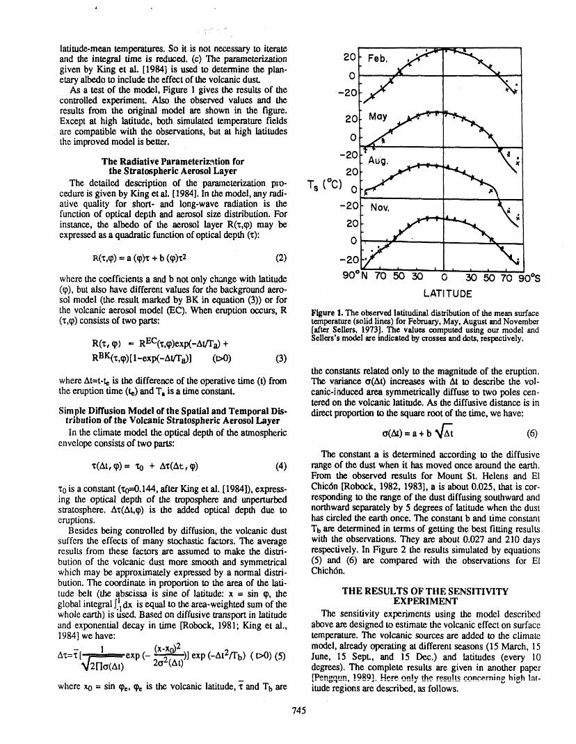
lafitllde-m_sn t_ml_ratllre_o So it is not ne_t_ss_'y to iter_t_ f of __ .......

and the integral time is reduced. (c) The parameterization 20 Feb. _given by King et al. [1984] is used to determine the plan-

etary albedo to include the effect of the volcanic dust. 0 _ ,/t, %,As a test of the model, Figure 1 gives the results of the _201. ,/_.

controlled experiment. Also the observed values and the

results from the original model are shown in the figure, oy ,__ _"m-t_.Except at high latitude, both simulated temperature fields 20 M

"Aare compatible with the observations, but at high latitudesthe improved model is better. 0 _,¢-4t

ali,The Radiative Parameteriz.'_tionfor -20 _ A ' . x- .

the Stratospheric Aerosol Layer o 20 __ __/_o

The detailed description of the par'aneterization pzt- Ts (C) 0cedure is given by King et al. [1984]. In the model, any radi-

v foro wv• /____.,function of optical depth and aerosol size distribution. Forinstance, the albedo of the aerosol layer R(x,cp) may be 20

expressed as a quadratic function of opticaldepth (x): 0 , . , '

R(X,CP)= a (q))x+ b (cp)x2 (2) -20_ , , , , , ,where the coefficients a and b not only change with latitude 90 ° N 70 50 50 0 50 50 70 90°S

(q)),but also have different values for the background aero- LATITUDEsolmodel(theresultmarkedby BK inequation(3))orfor

the volcanic aerosol model (EC). When eruption occurs, R Figure1.The observedlatitudinaldistributionof the meansurface(1:,(I))consists of two parts: temperature(solidlines)for February,May,AugustandNovember

[afterSellers, 1973].The valuescomputedusingour model andSellers'smodelareindicatedby crossesanddots,respectively.

RO:,CP)= REC(%CP)exIX-At/Ta)+

RBK(x,CP)[1-exp(-at/Ta)] (t>O) (3)

the constants related only to the magnitude of the eruption.where At=t-tc is the difference of the operative time (t)from The variance ¢_(At)increases with At to describe the vol-the eruption time (tc) and T,, is a time constant, canic-iaduced area symmetrically diffuse to two poles cen-

tered on the volcanic latitude. As the diffusive distance is inSimple Diffusion Model of the Spatial and Temporal Dis- directproportionto the squareroot of the time, we have:

tribution of the Volcanic Stratospheric Aerosol LayerIn the climate model the optical depth of the atmospheric a(At) = a + b '_ (6)

envelope consists of two parts:The. constant a is determined according to the diffusive

x(At, cp)= Xo + Ax(At, cp) (4) range of the dust when it has moved once around the earth.From the observed results for Mount St. Helens and El

1:0is a constant (xo---0.144,after King et al. [1984]), express- Chic6n [Robock, 1982, 1983], a is about 0.025, that is cor-ing the optical depth of the troposphere and unperturbed responding to the range of the dust diffusing southward andstratosphere. Ax(At,CP)is the added optical depth due to northward separately by 5 degrees of latitude when the dusteruptions, has circled the earth once. The constant b and time constant

Besides being controlled by diffusion, the volcanic dust Tb are determined in terms of getting the best fitting resultssuffers the effects of many stochastic factors. The average with the observations. They are about 0.027 and 210 daysresults from these factors are assumed to make the distri- respectively. In Figure 2 the results simulated by equationsbution of the volcanic dust more smooth and symmetrical (5) and (6) are compared with the observations for Elwhich may be approximately expressed by a normal distri- Chich6n.bution. The coordinate in proportion to the area of the lati-tude belt (the abscissa is sine of latitude: x = sin cp, the THE RESULTS OF THE SENSITIVITYglobal integral _ltdx is equal to the area-weighted sum of the EXPERIMENTwhole earth)is iJsed. Based on diffusive transport in latitude The sensitivity experiments using the model describedand exponential decay in time [Robock, 1981; King et al., above are designed to estimate the volcanic effecton surface1984] we have: temperature. The volcanic sources are added to the climate

model, already operating at different seasons (15 March, 15A't=x'[)"", _! = exp (- (x'x°)2 _]exp (-At2/Tb) (t>0) (5) June, 15 SepL, and 15 Dec.) and latitudes (every 10

2cr2(At)/'%/2I-l_(At) degrees). The complete results are given in another paperrP_=nonttrt IORO] l-lP.rp. nnlv lh_. r___.lt_: rnnr.ernln_ hiEh I,ql-t .... C:_"l--"" t .............. d ..................

where xo = sin (Pe,(Peis the volcanic latitude, x and Tb are itude regions are described, as follows.

745

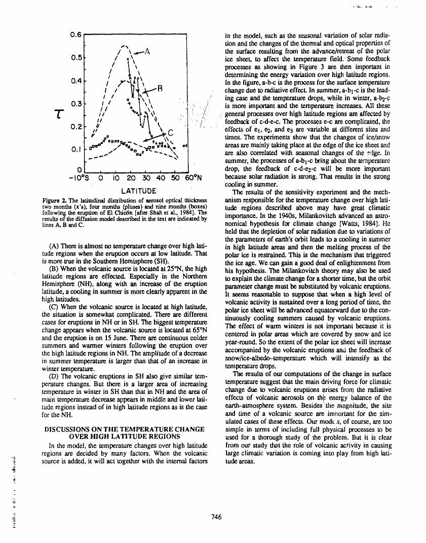
0.6 in the model, such as the seasonal variation of solar radia-

,..,, tion and the changes of the thermal and optical properties of/ _ _-.--A the surface resulting from the advance/retreat of the polar

0.5 [/ __ ice sheet, to affect the temperature field. Some feedback, processes as showing in Figure 3 are then important in/ determining the energy variation over high latitude regions,

O,4 / sr"_ I _ r_ In the figure, a-b-c is the process for the surface temperature

/ , _,_, _._ n change due to radiative effect. In summer,a-bl-C is the lead-

0.3 //' _ l ', _, , ',' /// ing case and the temperature drops, while in winter, a-b2-c,/: is more important and the temperature increases. Ali these2- , general processes over high latitude regions are affected by

'/,, feedback of c-d-e-c. The processes e-e are complicated, the0,2, I_ C I effects of el, e.2,and e3 are variable at different sites and

.*****,.... ._-¢._x, I times. The experiments show that the changes of ice/snowO. I t_*_ //'_,_ -._,',_,k_, *¢1 areas are mainly taking piace at the edge of the ice sheet and

_...-" **" ""-._X I are also correlated with seasonal changes of file edge, In" "- - " I summer, the processesof a-bt-c bring about the temperature

0 , , , , _ _, , _l drop, the feedback of c-d-e2-c will be more important-IO°S 0 I0 20 30 40 50 600N becau_solarradiationis strong.That resultsin the strong

coolingin summer.LATITUDE The restilts of the sensitivityexperimentandthemech-

Figure2. The latitudinaldisn'ibutionof aerosolopticalthickness anism responsible for the temperature change over high lati-twomonths(x's), four months (pluses)and nine months(boxes) tude regions described above may have great climaticfollowingthe eruptionof El Chio6n[afterShahet al., 1984].The importance. In the 1940s, Milankovitch advanced an astro-resultsof thediffusionmodeldescribedin the textare indicatedbylinesA,B andC. nomical hypothesis for climate change [Watts, 1984]. tte

held that the depletion of solar radiation due to variations ofthe parameters of earth's orbit leads to a cooling in summer

(A) There is almost no temperature change over high lati- in high latitude areas and then the melting process of thetude regions when the eruption occurs at low latitude. That polar ice is restrained. This is the mechanism that triggeredis more true in the Southern Hemisphere (SLD. the ice age. We can gain a good deal of enlightenment from

03) When the volcanic source is located at 25°N, the high his hypothesis. The Milankovitch theory may also be usedlatitude regions are effected. Especially in the Northern to explain the climate change for a shorter time, but the orbitHemisphere (NlD, along with an ;.ncrease of the eruption parameter change must be substituted by volcanic eruptions.latitude, a cooling in summer is more clearly apparent in the lt seems reasonable to suppose that when a high level ofhigh latitudes, volcanic activity is sustained over a long period of time, the

(C) When the volcanic source is located at high latitude, polar ice sheet will be advanced equatorward due to the con-the situation is somewhat complicated. There are different tinuously cooling summers caused by volcanic eruptions.cases for eruptions in NH or in SH. The biggest temperature The effect of warm winters is not important because it ischange appears when the volcanic source is located at 65°Nand the eruption is on 15 June. There are continuous colder centered in polar areas which are covered by snow and icesummers and warmer winters following the eruption over year-round. So the extent of the polar ice sheet will increasethe high latitude regions in NH. The amplitude of a decrease accompanied by the volcanic eruptions and the feedback ofin summer temperature is larger than that of an increase in snow/ice-albedo-temperature which will intensify as thewinter temperature, temperature drops.

(D) The volcanic eruptions in SH also give similar tem- The results of our computations of the change in surfaceperature changes. But there is a larger area of increasing temperature suggest that the main driving force for climatictemperature in winter in SH than that in NH and the area of change due to volcanic eruptions _sises from the radiativemain temperature decrease appears in middle and lower lati- effects of volcanic aerosols on th{; energy il_ance of thetude regions instead of in high latitude regions as is the case earth-atmosphere system. Besides'the magnitude, the sitefor the NH. and time of a volcanic source are important for the sim-

ulated cases of these effects. Our modt,s, of course, are tooDISCUSSIONS ON THE TEMPERATURE CHANGE simple in terms of including full physical processes to be

OVER HIGH LATITUDE REGIONS used for a thorough study of the problem. But it is clearIn the model, the temperatm'e changes over high latitude from our study that the role of volcanic activity in causing

regions are decided by many factors. When the volcanic large climatic variation is coming into play from high lati-source is added, it will act together with the internal factors tude areas.

_

=_

= 746

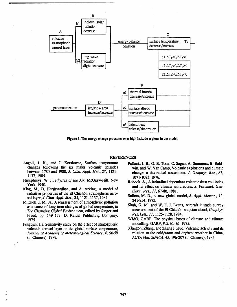
B

i i ,i C

stratospheric energ_balance surface temperature Tsaerosollayer equation decrease{increase

92_lorlg-wave _ e 1:A'I_<0/ATs>0

radiationslight decrease e2:_Ts<0/_Ts>0

i rl

e3:_Ts>0/_Ts<0

E

e__ thermal inertia1--'-!

decreasefmcreaseD i I

Ie3 Ilatent heat--_ release/absorption [

Figure 3.The energychangeprocessesoverhighlatituderegionsin themodel.

REFERENCES

Angell, J. K., and J. Korshover, Surface temperature Pollack, J. B., O. B. Toon, C. Sagan, A. Summers,B. Bald-changes following the six major volcanic episodes win, and W. Van C_tmp,Volcanic explosions andclimatebetween 1780 and 1980, J. Clim. Appl. Met., 23, 1121- change: a theoretical assessment, J. Geophys. Res., 81,1137, 1985. 1071-1083, 1976.

Humphreys, W. J., Physics of the Air, McGraw-Hill, New Roboek, A., A latitmfinal dependent volcanic dust veil indexYork, 1940. and its effect on climate simulations, J. Volcanol. Geo.

King, M., D. Harshvardhan, and A. Arking, A model of therm.Res., 11, 67-80, 1981.radiative properties of the El Chich6n stratospheric aero-sol layer, J. Clim. Appl. Met., 23, 1121-1137, 1984. Sellers, M. D.,/, new global model, J. Appl. Meteor., 12,

Mitchell, J. M., Jr., A re.assessmentof atmospheric pollution 241-254, 1973.as a cause of long-term changes of global temperature, in Shah, G. M., and W. F. J. Evans, Aircraft latitude surveyThe Changing Global Environment, ecfitedby Singer and measurement of the El Chich6n eruption cloud, Geophys.Freed, pp. 149-173, D. Reidel Publishing Company, Res.Lett.,11, 1125-1128, 1984.1975. WMO, GARP, The physical bases of climate and climate

Pengqun, Jia, Sensitivity study on the effect of stratospheric modelling, GARP, P.S. No.16, 1975.volcanic aerosol layer on the global surface temperature, Xiangon, Zhang, and Zhang Fuguo, Volcanic activity and itsJournal of Academy of Meteorological Science, 4, 50-59 relation to the cold/warm and dry/wet weather in China,(in Chinese), 1989. ACTA Met. SINICA, 43, 196-207 (in Chinese), 1985.

747

Satellite and Slow-Scan Television Observations of the Rise and Dispersionof Ash.Rich Eruption Clouds from Redoubt Volcano, Alaska

Juergen KienleGeophysical Institute, University ofAlaska Fairbanl_, Fairbanks, Alaska, U.S.A.

A. W. WoodsInstitute of Theoretical Geophysics, Dept. ofApplied Mathematics and Theoretical Physics, Silver Street, Cambridge, England

S. A. Estes, K. Ahlnaes, K. Dean, and H. TanakaGeophysical Institute, University ofAlaska Fairbanks, Fairbanks, Alaska, U.S.A.

ABSTRACT

Polar-orbiting NOAA 10 and 11 weather satellites with their Advanced VeryHigh Resolution Radiometer (AVHRR) imaging sensors and the Landsat 4 and 5satellites have provided over 30 images of the 1989/90 eruptions of Redoubt Vol-cano. Between December 14 and April 21, about 20 major explosive eruptionsoccurred with ash plumes rising to heights of 10 km or more, most of them pene-trating the tropopause. The ash severely impacted domestic and international airtraffic in Alaska with a near disaster on December 15, 1989, when a KLM 747-400

jet aircraft with 247 people aboard intercepted an ash plume and temporarily lost alifour engines. Fortunately, the engines were eventually restarted after severalattempts and the plane landed safely in Anchorage. We have used satellite and alsoslow-scan television (TV) observations to study the dynamics and thermodynamicsof rising eruption plumes in order to better understand plume dispersal.

SATELLITE DATA these data with radiosonde measurements of atmosphericWe have used satellite imagery of eruption plumes to temperature versus altitude we could derive details of plume

map ash dispersal into the far field from the volcano. The top topography, important for the study the dynamics ofpervasive snow cover that existed near Redoubt Volcano plume rise and dispersion in the atmosphere.from December 1989 to April 1990 preserved even micron- The infrared (IR) bands of the AVHRR of the NOAA I0thin ash layers. For example, a NOAA 10 satellite image of and 11 satellites have proven especially useful to detectApril 21, 1990 shows three ash trajectories on the snow to eruptions at night or in overcast conditions, a common con-distances of over 400 km from the vent. Dispersal areas for dition for the 1989/90 eruptive cycle of Redoubt Volcano,these three plumes of Redoubt eruptions of March 23, April which occurred in mid-winter. Even though the volcano wasi2 and April '15 range from about 4000 to 21,000 km2. A often not visible from the ground, we could still track thenumerical simulation of the ash dispersal involving calcula- high altitude plumes above overcasts or at night, using the

, tions of the 3-D windfield, 3-D diffusion, and gravitational IR channels.fallout and satellite images of the ash dispersals suggest thatdiffusion was not an important process. The ash on the snow SLOW.SCAN TELEVISION OBSERVATIONSformed three narrow undispersed fallout patterns that looked Real-time slow-scan TV observations of volcanic erup-like spokes radiating from the volcano, tions at Redoubt Volcano have also been most useful for

Satellite iinat_ery of eruptive plumes was also used to supplemenling the satellite observations for warnings to themap radiometric plume top temperatures. By convolving public. On December 16, 1989, within 48 hours of the first

748

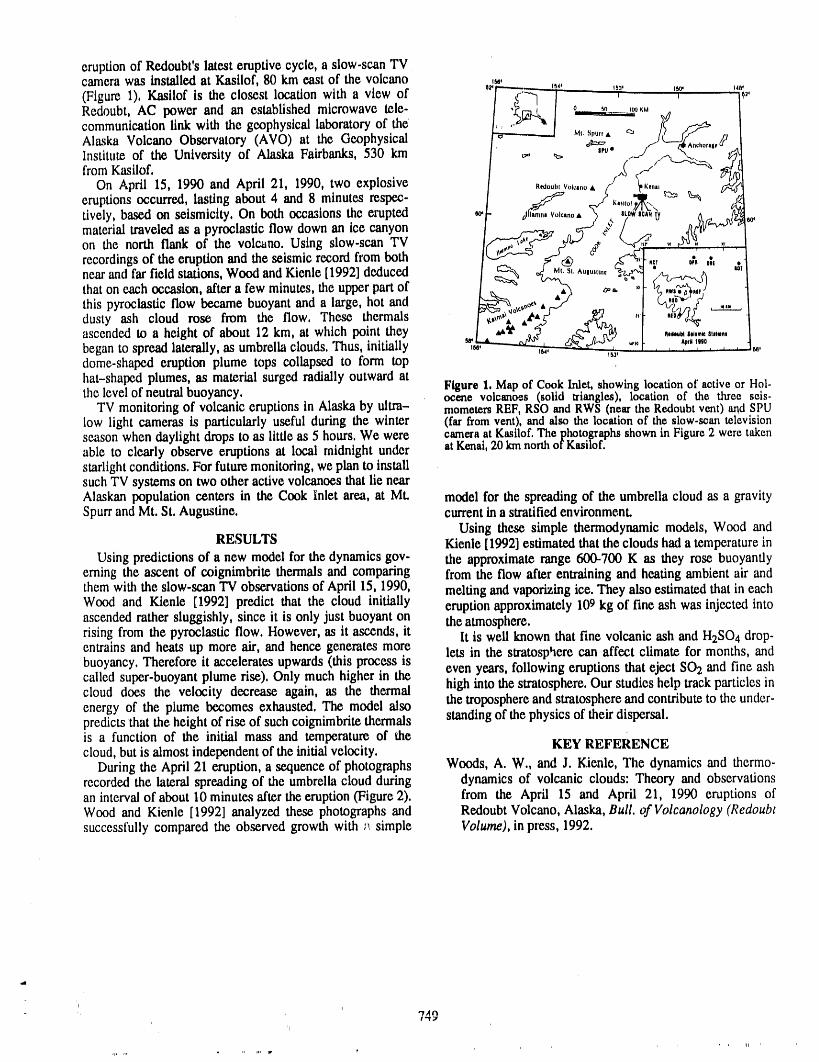
eruption of Re.doubt's latest eruptive cycle, a slow-scan TVcamera was installed at Kasilof, 80 km east of the volcano ,_,

6_ ["-,------_ 1_4_ 1531 tW 148_

communication link with the geophysical laboratory of the M,s,.,,,A

Alaska Volcano Observatory (AVO)at the Geophysical / _ ._ _s,0, _J1.."_._'"°""dTv..jqInstitute of the University of Alaska Fairbanks, 530 km

from Kasllof. / ;_'( f-//" ""-'_:_'_ _IOn April 15, 1990 and April 21, 1990, two explosive I R,do,.b,Vo_,,oA/" _,K,,,, ,_'_

eruptions occurred, lasting about 4 and 8 minutes respec- ] _ _.d_ K,,,,o,_1....r-_ _ v_tively, based on seismicity. On both occasions the erupted "'t- _,_,_,,vo,,,o, ._ ,t0wl0ANtV ^ i_,_

material traveled as a pyroclastic flow down an ice canyon I_ v'-_on the north flank of the volcano. Using slow-scan TV ,_

recordings of the eruption and the seismic record from both ]_ _3-@ e ,_[,i I " _i oi,' .tnear and far field stations, Wood and Kienle [1992] deduced I _% _ M,_t,,,,,,,, ".%e_ -_ -- A "'1that on each occasion, after a few minutes, the upper part of I _ _ ,.,.-_-. [ (_ ,,o_..%)_,,) -Ithis pyroclastic flow became buoyant and a large, hot and _-'_ ._oo, "_? - - [ ??_'i_'4,_r"_ Idusty ash cloud rose from the flow. These thermals I *"".A.A'Lt3" _,^ "I _'°_d-._ ]ascended to a height of about 12 km, at which point they I _'_" ,_ ,.._z ',,_ I ,,_,,,_,,,,,,,,, Ibegan to spread laterally, as umbrella clouds. Thus, initially _,,,'r'L---'_. _--V_"°_',. _l . , .'*"',"°, , . 1_,dome-shaped eruption plume tops collapsed to form top

hat-shaped plumes, as material surged radially outward at Flgur_ 1. Mapof Cook Inlet, showinglocationof activeor Hol.the level of neutral buoyancy. oeene voleano,_s(solid triangles), location of the three sels-TV monitoring of volcanic eruptions in Alaska by ultra- mometen REF,RSO and RWS (nearthe Redoubtvent) and SPU

low light cameras is particularly useful during the winter (far fromvent), and also the locationof the slow-scantelevisionseason when daylight drops to as little as 5 hours. We were cameraat Kasilof.The photographsshownin Figure2 were takenable to clearly observe eruptions at local midnight under atKenai,20kmnorthof Kastlof.starlight conditions. For future monitoring, we plan to installsuch TV systems on two other active volcanoes that lie nearAlaskan population centers in the Cook Inlet area, at Mt. model for the spreading of the umbrella cloud as a gravitySpurr and Mt. St. Augustine. current in a stratified environment.

Using these simple thermodynamic models, Wood andRESULTS Kienle [1992] estimated that the clouds had a temperature in

Using predictions of a new model for the dynamics gov- the approximate range 600-700 K as they rose buoyantlyerning the ascent of coignimbrite thermals and comparing from the flow after entraining and heating ambient air andthem with the slow-scan TV observations of April 15, 1990, melting and vaporizing ice. They also estimated that in eachWood and Kienle [1992] predict that the cloud initially eruption approximately 109 kg of fine ash was injected intoascended rather sluggishly, since it is only just buoyant on the atmosphere.rising from the pyroclastic flow. However, as it ascends, it lt is well known that fine volcanic ash and H2SO4 drop-entrains and heats up more air, and hence generates more lets in the stratosphere can affect climate for months, andbuoyancy. Therefore it accelerates upwards (this process is even years, following eruptions that eject SO2 and fine ashcalled super-buoyant plume rise). Only much higher in the high into the stratosphere. Our studies help track particles incloud does the velocity decrease again, as the thermalenergy of the plume becomes exhausted. The model also the troposphere and stratosphere and contribute to the under-predicts that the height of rise of such coignimbrite thermals standing of the physics of their dispersal.is a function of the initial mass and temperature of thecloud, but is almost independent of the initial velocity. KEY REFERENCE

During the April 21 eruption, a sequence of photographs Woods, A. W., and J. Kienle, The dynamics and thermo-recorded the lateral spreading of the umbrella cloud during dynamics of volcanic clouds: Theory and observationsan interval of about 10minutes after the eruption (Figure2). from the April 15 and April 21, 1990 eruptions ofWood and Kienle [1992] analyzed these photographs and Redoubt Volcano, Alaska, Bull. of Volcanology (Redoubtsuccessfully compared the observed growth with _ simple Volume), in press, 1992.

d

. , ii , _

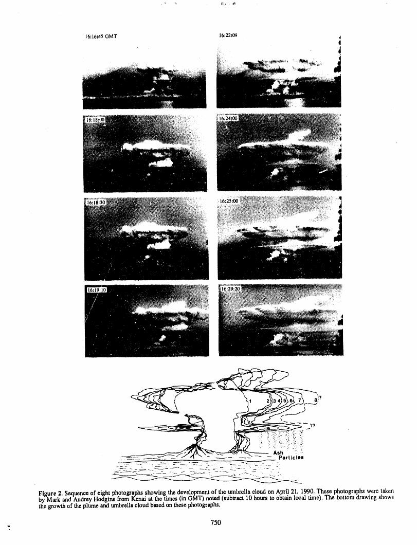
16:16:45GMT 16:22:09

Figure2,Sequenceof_ightphotographsshowingth¢d_v_lopm_ntofth_ullibt_llncloudon April21,1990.Thes_photographsw_r_takenby Mark and Audrey Hodgins from Kenai at the times (in GMT) noted (sub_'act 10 hours to obtain local time). The bottom drawing showsthe growth of the plume and umbrella cloud based on these photographs,

750

Bromine and Surface Ozone Atmospheric Chemistry _at Barrow, Alaska During Spring 1989

WoT. Sturges and R. C. SchnellCooperative Institute for Research in Environmental Sciences, University of Colorado, Boulder, Colorado, U.S.A.

S. LandsbergerDepartment of Nuclear Engineering, University of111inoisoUrbana, Illinois, U.S.A.

ABSTRACT

Measurementswere madeof surfaceozone, particulatebromineandorganicgas-eous bromine species at Barrow, AlaskaduringMarch and April 1989 with a viewto examining the causesof surfaceozone destructionduringthe arcticspring.It wasfound that duringmajor ozone depletion events (03 < 25 ppbv) concentrationsofparticulatebromine and the organic brominatedgases bromoform and dibromo-chloromethane were elevated. A fast productionrate of particulatebromine wasshown by irradiatingambient nighttime air at Barrow in a chamber with actinicradiation that simulated midday conditions for that season and latitude.Such rapidreactionsare not in keeping with gas phase photolysis of bromoform,but furtherstudies showed evid,', f:_ for a substantialfractionof organic brominein the par-ticulatephase, thus heterogenousreactions may be important.

INTRODUCTION form in the Arctic (perhaps the highest atmospheric con-It has been well documentedthat following first light in centrationsmeasured anywhere in the world to date), which

the Arctic, ozone concentrationsmeasured at ground level declines in antiphase to increasingsolarflux following polarbegin to exhibit large negative excursions from wintertime sunrise [Oltmans ct al., 1989]. At the same time large quan-maximumvalues [Barrieet al., 1988; Oltmans etal., 1989]. tities of f'dterable (presumably particulate) bromine areOzone levels can be reduced to effectively zero within a formed, suggesting that some conversion process of bromo-matterof hours. These destructionevents occurmostly dur- form is indeed operating. Filterable bromine levels (f-Br)ing Marchand Aprilandcease aroundMay or June.Aircraft are observed to be strongly ant,icon'elated with ozone. Themeasurements [Oltmans et al., 1989] have shown that the origin of the bromoform is thought to be biogenic, possiblyozone loss occurs entirely below the low level inversion, from arcticice microalgae [Stm'geset al., 1991a].which forms a temporary barrierto downmixing of ozone- In the second hypothesis [Finlayson-Pitts et al., 1990],rich air. dinitrogen pentoxide reacts with sea salt particles, releasing

The cause of this ozone loss remains a mystery. There are nitryl bromide which then photolyses to bromine atoms.currently two favored hypotheses, both of which rely on This hypothesis requires the presence of sea salt aerosolsmonatornic bromine radicals attacking ozone, which can be transported from non-frozen oceans south of the ice mar-simplified to: gins, and pollution-derived oxides of nitrogen. Indeed, both

Br + 03 _ BrO + 02 sea salt aerosol and long range transported pollution are at amaximum in the late winter in the Arctic [Sturges and

The h? potheses differ in the origin of the bromine radicals. Barrie, 1988].In the version put forward by Barrie et al, [1988], photolysis The measurement of the key nitrogen species required toof bromoform gas (CI-IBr3)releases bromine radicals. This evaluate the dinitrogen pentoxide route to ozone loss wasis supported by the observation of high wintertime bromo- beyond the scope of this work: we focus here on an exam-

751

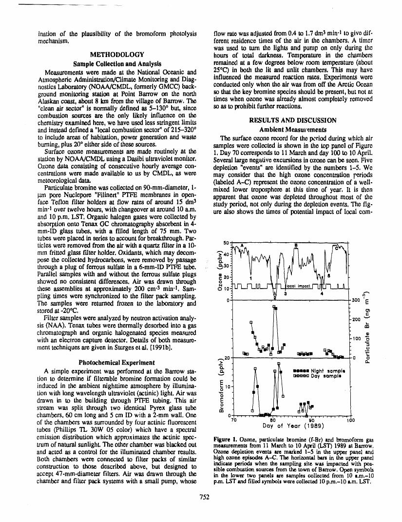
lnation of the plausibility of the bromoform photolysis flow ratewas adjusted from0,4 to 1,7 dm3mind to give dif-mechanism, ferent residence times of the air in the chambers, A timer

was used to turn the lights and pump on only during riteMETHODOLOGY hours of total darkness, Temperature in the chambers

Sample Collection and Analysis remained at a few degrees below room temperature (aboutMeasurements were made at the National Oceanic and 25%') in both the lit and unlit chambers, This may have

AtmosphericAdminlstration/ClimateMonitoflng and Diag- influenced the measured reaction rates, Expeflments werenostics Laboratory(NOAA/CMDL, formerlyGMCC) back. conducted only when the air was from off the Arctic Oceanground monitoring station at Point Barrow on the north so that the key bromine species should be present,but not atAlaskan coast, about 8 km from the village of Barrow. The times when ozone was already almost completely removed"clean air sector"is normally defined as 5-130 ° but, since so as to prohibit furtherreactions,combustion sources are the only likely influence on thechemistryexamined here, we have used less stringent limits RESULTS AND DISCUSSIONand instead defined a "localcombustion sector" of 215-3200 Ambient Measurements

to include areas of habitation, power generationand waste The surface ozone record for the period during which airburning, plus 20° either side of these sources, samples were collected is shown in the top panel of Figure

Surface ozone measurements are made routinely at the 1, Day 70 corresponds to 11March and day 100 to 10April,stationby NOAA/CMDL usinga Dasibi ultravioletmonitor, Several large negative excursions in ozone can be seen, FiveOzone data consisting of consecutive hourly average con- depletion "events"are identified by the numbers 1-5, Wecentrations were made available to us by CMDL, as were may consider that the high ozone concentration periodsmeteorological data, (labeled A.-C) represent the ozone concentration of a well-

Particulate bromine was collected on 90.mm.diameter, 1- mixed lower troposphere at this time of year, lt is thenI.tm pore Nuclepore "Filinert" PTFE membranes in open- apparent that ozone was depleted throughout most of theface Teflon filter holders at flow rates of around 15 dm3 study period, not only during the depletion events, The fig-min-1over twelve hours, with changeover at around 10 a.m. ure also shows the times of potential impact of local com-and l0 p,m. LST. Organic halogen gases were collected byabsorption onto Tenax GC chromatography absorbent in 4-mm-lD glass tubes, with a filled length of 75 mm. Twotubes were placed in series to account for breakthrough. Par-ticles were removed from the air with a quartz filter in a lt)- s0,

mm flitted glass filter holder. Oxidants, which may decom- '_'4o.pose the collected hydrocarbons, were removed by passage 0.through a plug of ferrous sulfate in a 6-mm-ID PTFE tube. ,._30.

Parallel samples with and without the ferrous sulfate plugs _ 20showed no consistent differences. Air was drawn through ,qthese assemblies at approximately 200 cm-3 min-1. Sam- o topiing times were synchronized to the filter pack sampling, a ,4The samples were returned frozen to the laboratory and 0 , ,_oo 'r:stored at -20°C.

Filter samples were analyzed by neutron activation analy- 200 "-"sis (NAA). Tenax tubes were thermally desorbed into a gas _ a_chromatograph and organic halogenated species measuredwith an electron capture detector, Details of both measure- ,loo _t3

ment techniques are given in Stm'geset al. [1991b]. t_ / _

Photochemical Experiment ,_.20 -_o_, ra

-0.

A simple experiment was performed at the Barrow sm- 0. ¢ tt_mQmNight sample

induced in the ambient nighttime atmosphere by illumina- IoPill

lion with long wavelength ultraviolet (actinic) light, Air was _'

drawn in to the building through PTFE tubing. This air Estream was split through two identical Pyrex glass tube otr_

chambers, 60 cm long and 5 cm lD with a 2-mm wall. One o ,-,--,-ofthe chambers was surrounded by four actinic fluorescent 70 ao so cotubes (Phillips TL 30W 05 color) which have a spectral Day of Year (1989)

emission distribution which approximates the actinic spec- Figure 1. Ozone, particulatebromine(f-Br) and bromoformgastrum of natural sunlighLThe other chamber was blacked out measurementsfrom 11 Marchto 10 April(LST) 1989 at Barrow.and acted as a control for the illuminated chamber results. Ozone depletionevents are marked 1-5 in the upper panel andBoth chambers were connected to filter packs of similar high ozoneepiuxle_A..-C,The horizontalbarsin theupperpanel

indicateperiodswhen the samplingsite was impactedwith pos-construction to those described above, but designed to siblecombustion_urces fromthe townof Barrow.Opensymbolsaccept 47-mm-diameter filters. Air was drawn through the in the lowertwo panels aresamplescollectedfrom I0 a.m,-10chamber and filter pack systems with a small pump, whose p.m.LSTand filledsymbols were collected10p,m.-10 Lm. LST,

752

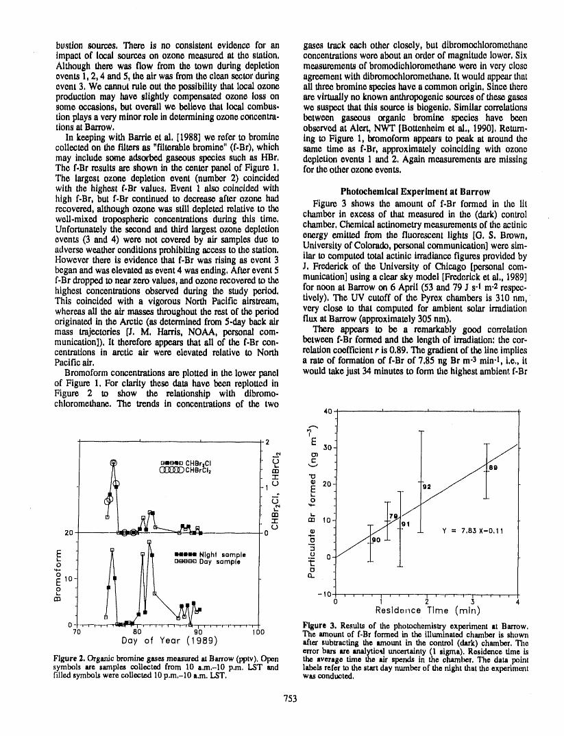
bvstton sources, There is no consistent evidence for an gases track each other closely, but dlbromochloromethanoimpact of local sources on ozone measured at the station, concentrations wore about an order of magnitude lower, SixAlthough them was flow from the town during depletion measurements of bromodichloromethan_ wore in very closeevents 1, 2, 4 and 5, the air was from the clean sc_,torduring agreement with dibromochloromcthano, It would appear thatevent 3, We cannut rule out the possibility that local ozone ali flu'e_bromine species have a common odgin, Since thereproduction may have slightly compensated ozone loss on arcvirtually no knownanthropogenie sour_s of these gasessome occasions, but overall we believe that local combus, wo suspect that this some is biogeni¢, Similar correlationstion plays a very minor role indetermining ozone coneentra- between gaseous organic bromine spccie,s have beenttons atBarrow, observedat Aim, NWT [Bottcnh_lm ct al,, 1990], Return.

In keeping with Barrioct al, [1988] we refer to bromine ing to Figure 1, bromoform appears to peak at around thecoUectedon the filters as "filterablebromine" (f.Br), which same time as f-Br, approximately coinciding with ozonemay include some adsorbed gaseous species such as IBr, depletion events 1 and 2, Again measurements are missingThe f-Br results are shown in the center panel of Figure 1, for the other ozone events,The largest ozone depletion event (number 2) coincidedwith the highest f.Br values, Event 1 also coincided with Photochemical Experiment at Barrowhigh f.Br, but f-Br continued to decrease after ozone hadrecovered, although ozone was s011depleted relative to the Figure 3 shows the amount of f.Br formed in the litwell.mixed tropospheric concentrations during this time, chamber in excess of that measured in the (dark) controlUnfortunately the second and third largest ozone depletion chamber, Chemical acttnometry me,asur_montsof the actinicevents (3 and 4) were not covered by air samples due to energy emitted from the fluorescent lights [O, S, Brown,adverseweatherconditions prohibitingaccess to the station, Universityof Colorado,personal¢ommunic.ation]were stm.However there is evidence that f.Br was rising as event 3 liar to computed total actinic irradiancefigures providedbybegan and was elevated as event 4 was ending, After event 5 J, Fredeflck of the University of Chicago [personal com-f-Br dropped to near zero values, and ozone recovered to the munteation] using a clear sky model [Fredeflck ct al,, 1989]htghest concentrations observed during the study period, for noon at Barrow on 6 April (53 and 79 J s-I m.2 respec.This coincided with a vigorous North Pacific atrstream, tively), The UV cutoff of the Pyrex chambers ts 310 nm,whereas ali the air masses throughout the rest of the period very close to that computed for ambtent solar irradiationoriginated in the Arctic (as determined from 5-day back air flux at Barrow (approximately305 nm),mass trajeetofles [L M, Harris, NOAA, personal com. There appears to be a remarkably good correlationmunication]), lt therefore appears that ali of the f.Br con. between f-Br formed and the length of Irradiation: the cor-centrations in arctic air were elevated relative to North relation coefficient r is 0,89. The gradient of'the line implies

' 1Pacific air, a rate of formation of f-Br of 7,85 ng Br m-3 mm-, t,e,, itBromoform concentrations are plotted in the lower panel would take just 34 minutes to form the highest ambient f-Br

of Figure 1, For clarity these data have been replotted inFigure 2 to show the relationship with dibromo-chloromethane, The trends in concentrations of the two

40 ' ' '

?' -,--------_ 2 E

_FJ CHBr_CI _ C:(I]_ CHBrCI2 rn v eg

-r- "13

1 _ Ew 20 b2

m _ 10-r"

20 -0 _ Y = 7,83X-0,110

E _ mnm Night sample0

_*- 13o nEl00_- -10 , d , , , , ,

o t ,, ....3 4

Residence Time (mln)

0 _ _ Figure 3. Resultsof the photochemistryexperimentat Barrow,70 80 90 100 The amountof f-Brformedin the illuminatedchamberis shown

Day of Year (1989) aft= subtractingtheamotmtin thecontrol (dark) chamber.Theerrorbarsare analyticaluncertainty(1 sigma),Residencetime ks

Figure2. Organicbrominegasesmeasuredat Barrow(pptv),Open the averagetime the air spends in the chamber.The data pointmbols are samples collected from 10 a,m,-lO p.m, L.ST and labelsrefer tothe startdaynumberof thenightthattheexpeflmentled symbolswerecollected10p.m,-10a.m,LST. wascondt_ted,

753

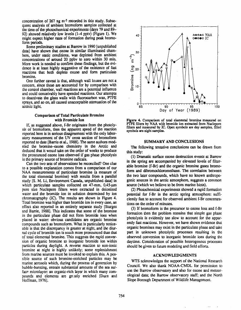
concentrationof267ng m "3recordedinthisstudy,Subse-quentanalysis of ambient bromoformsamplea collected at , ,___the timeof thephotochemicalex_dment_ (days79 and89-92) showed relatively low levels (1-4 pptv) (Figure 1), We 4o _ NAAmight expect higher ratesof formationduring peak bromo- oooeo IC

formperiods, _l

Some preliminarystudies at Barrowin 1990 [unpublisheddam] have shown that ozom in similar illuminated chain. _obers, under static conditions, was depleted from ambient ..--'-.concenttatlonsofaround20 ppbvtozerowithin30 rain, ?More work is needed to confirm these findings, but file ovi- Edonee is at least highly suggestive of the existence of fast = 20

reactions that both deplete ozone and form particulate '-_bromine, •t-

One furthercaveat is that, although wall losses arenot a '_concern,sincetheseareaccountedforby comparisonwith o lothe control chamber, wall reactions arc a potential influence mand could conceivably have speeded reactions, Our attemptsto deactivate the glass walls with fluorocarbon wax, PTFEsprays,andsoon,allcausedunacceptableattenuationofthe o --,-,.,,,,'T'L_,,,,'-_,''actinic ltghL as 9o 9s Ioa

Day of Year (1989)Comparison of Total Particulate Bromine

with Bromide fen Flgure 4. Comparbonof totaldemental brominemeasuredon

If, as suggested above, f.Br oflglnates from the photoly- PTFEfiltersby NAA withbromideion extraoteAfromNu_leporefiltersandmeasuredby lC, Opensymbolsareday samples,filledsis of bromoform, then the apparent spe.ed of th_ reaction symbolsare night samples,reportedhemis in seriousdisagreementwith theonlylabor-atory measurementof the UV crosssectionof bromoformreported to date [Battlect al,, 1988], The same authorsmad- SUMMARY AND CONCLUSIONSclcd the bromine-ozone chemistry in the Arctic and Tlm following tentative conclusions can be drawn fromdeduced that it would takeon the order of weeks to produce this study:thepronouncedozonelossobservedifgasphasephotolysis (I)DramaticsurfaceozonedestructioneventsatBarrowis the primarysource of bromineradicals, in the spflng are accompanied by elevated levels of filter-Can thetwosetsofobservationsbereconciled?One cluetoa possibleexplanationcomesfroma comparisonofour ablebromine(f-Br)andtheorganicbrominegasesbromo-NAA measurementsofparticulatebromine(ameasureof= formand dibmmochloromethane.The correlationbetweenthe total elemental bromine) with results from a parallel the two later compounds, which have no known anthropo-study [S. M. Li, Environment Canada, unpublished data] in genie sources in the arctic atmosphere, suggests a commonwhichparticulatesamplescollectedon 47-mm,0.45-tun source(whichwe believetobefrommarinebiota).poresizeNucleporefilterswere extractedin dcionlzcd (2)Photochemicalexperimentsshowed a rapidformationwater and the bromide ion in solution determined by ion potential for f.Br in the arctic spring atmosphere: suffi-chromatography (IC), The results are shown in Figure 4, cienfly fast to account for observed ambient f.Br concentra-Total bromine was higher than bromide ion in every case, an tions on the order of minutes,effectalsoreportedinan entirelyseparatestudy[SturgesandBattle,1988].Thisindicatesthatsomeofthebromine (3)Ifbromoformistheprecursortoozonelossandf.Brintheparticulatephasedidnotformbromideionswhen formationthentheproblemremainsthatsimplegasphaseplaced in water, obvious candidates are organic bromine photolysis is evidently too slow to account for the appar-compounds such as bromoform. What is particularly notice- enfly fast reactions, However, we have shown evidence thatable is that the discrepancy is greater at night, and the dlur- organic bromines may exist in the particulate phase and takenal cycle of bromide ion is nmch more pronounced than that part in unknown photolytic processes resulting in theof total elemental bromine, This suggests the rapid conver- obsc,rved conversion to inorganic bromide ions during thesion of organic bromine to inorganic bromide ion within daytime. Consideration of possible heterogenous processesparticles during daylight, A reverse reaction to non-ionic should be given to future modeling and field efforts,bromine at night is highly unlikely; some replenishmentfrom marine sources must be invoked to explain this, A pos- ACKNOWLEDGMENTSsible source of such bromine-enriched particles may bemarine aerosols which, during the process of generation by WTS acknowledges the support of the National Researchbubble-bursting, entrain substantial amounts of the sea sur. Council, We also thank NOAA-CMDL for permission to

use the Barrow observatory and also for ozone and meteor-face microlayer: an organic-rich layer in which many com-pounds and elements are gr(atly enriched [Duce and ological dam; the Barrow observatory staff; and the NorthHoffman, 1976], Slope Borough Department of Wildlife Management.

754

REFERENCES

BarrieL. A., J. W. Bottenheim, R. C. Schnell, P. J. Crutzen, Oltmans, S. J., R. C. Schnell, P. J. Sheridan,R. E. Peterson,and R. A. Rasmussen, Ozone destruction and photo- S.M. Li, J. W. Winchester, P. P. Tans, W. T. Sturges,chemical reactions at polar sunrise in the lower Arctic J.D. Kahl, and L. A. Barrie, Seasonal surfaceozone andatmosphere,Nature, 334, 138-141, 1988. filterablebrominerelationshipin the High Arctic,Atmos.

Bottenheim, J. W., L. A. Barfie, E. Atlas, L. E. Heidt, H. Environ., 23, 2431-2441, 1989.Niki, R. A. Rasmussen,and P. B. Shepson, Depletion of Stm'ges,W. T., and L. A. Barrie, Chlorine, bromine andlowertroposphericozone duringArctic spring:The Polar iodine in Arctic aerosols, Atmos. Environ., 22, 1179-SunriseExperiment 1988, J. Geophys. Res., 95, 18555- 1194, 1988.18568, 1990. Sturges W. T., R. C. Schnell, S. l_andsberger,S. J. Oltmans,

Duce, R. A., and E. J. Hoffman, Chemical fractionationat J.M. Harris,and S.-M. Li, Chemical and meteorologicalthe air-sea interface, Ann. Rev. Earth Planetary Sci., 4, influences on surface ozone destruction at Barrow,187-228, 1976. Alaska, during spring 1989, Atmos. Environ., 1991, In

Finlayson-PittsB. J., F. E. Livingstone, and H. N. Berko, press_Ozone destructionandbrominephotochemistryat ground Sturges, W. T., C. W. Sullivan, R. C. Schnell, L. E. Heidt,level in the Arctic spring,Nature, 343, 622--625, 1990. W.H. Pollack, and D. J. Hoffman, Biogenic bromine

Frederick, J. E., H. E. Snell, and E. K. Haywood, Solar gases at McMurdo: Ice algal production, atmosphericultravioletradiation at the Earth's surface, Photochem. concentrations,and potential influence on surface ozone,Photobiol., 50, 443-450, 1989. Syrup.Tropospheric Chemistry of the AntarcticRegion,

June 3-6, 1991, Boulder, Colorado, U.S. Army ColdRegions Research and Engineering Laboratory, SpecialReport 91-10, and Tellus, 1991, submitted.

755

PANEL DISCUSSIONS

PANEL DISCUSSIONS:SUMMARY AND RECOMMENDATIONS

On the final day of the conference three panels met to discuss problems and priorities in polar research.

Panel 1 (chaired by Luis Proenza), dealing with research coordination, identified the following toppriorities: better international cooperation involving scientists from ali countries with polar interests;establishment of joint observational systems and networks, including satellites and long-term monitoringsites; information exchange through a common clearinghouse; addressing education and manpower needs;and closer ties between arctic and antarctic researchers.

Panel 2 (chaired by Oran Young), addressing societal problems of global change, recomrraended the estab-lishment of an international program of social sciences in global change; a reexamination of the scenarios ofclimate change in the polar regions, as they affect social change; the inclusion of social scientists to a greaterextent in future global change planning efforts; and the development of suitable curricula on global change at'alleducational levels.

Panel 3 (chMred by Douglas Posson), addressing polar data and information problems, recommended theestablishment of a weU-organized polar data directory building on present efforts of all the countries; freeexchange of data with other countries having polar data sets; use of improved technologies, e. g., CD,ROM;retrieval of endangered data sets of retiring scientists through funding to the latter, perhaps through sabbaticalleaves; and improving the quality of data sets.

Specific recommendations were made as follows:

Panel 1:

(1) Develop Arctic-wide observational systems and networks which can guarantee the availability of long-term data sets.

(2) Foster international cooperation.

(a) Find mechanisms to ensure that cooperation is sufficiently inclusive of interested scientiststhroughout the world. It was recognized that polar science efforts exist within a highly distributedsystem of resources across nations and within nations. Neither countries nor scientists should beexcluded.

(b) Develop a truly bi-polar approach to science to facilitate coordination of appropriate problems, com-parison of contrasts between the two polar regions, and integration of resources.

(c) Integrate and coordinate logistical resources to create a visible polar research system that is largerthan the sum of the parts. This includes joint planning for the next generation of polar researchplatforms.

(d) Combine informational resources, and create an international information clearinghouse, or intema-tional data directories.

(e) Focus attention on educational issues to ensure the development of a new cadre of polar scientists,and the development of a new academic curriculum of global change.

(f) Erase disciplinary lines and develop mechanisms to move students and scientists across national,institutional, and disciplinary boundaries.

(3) Develop a set of new "tools" essential to the scale of global change problems. This included satellites,ground-truth observatories and automated stations, and numerical models.

759

(4) Keep the research priorities on polar problems in global change flexible to allow new avenues of researchto be pursued as we learn about the earth system (e.g., antarctic ozone hole).

(5) Organize an International Polar Year some time in the future.

Footnote: Several panelists stressed the need to be comprehensive when dealing with the topic of globalchange, not overlooking the need for social science research, nor forgetting that the upper atmosphere is partof the earth system, Some felt strongly, and the audience agreed, that there is too much emphasis on planningandreports and that we need more time for actual science. Linkages between scientists and policy makers wasseen as a difficult area that needed attention. One opinion was that two "conceptual revolutions" wereunderway and converging----one dealing with the emerging science of global change, the other a bureaucraticrevolution by which agency "cross,,.cuts" are beginning to enable agencies and budget offices to work togetheron large and complex program elements.

(Editor's Note: International mechanisms for global change research coordination in the polar regions arebeginning to emerge for both the Antarctic and the Arctic. In the Antarctic, SCAR, the Scientific Committeeon Antarctic Research, has established a global change committee and is in the process of defining a regionalprogram for Antarctica. In the Arctic, IASC, the newly formed (1990) International Arctic Science Committeeis pursuing a similar course).

Panel 2:

(1) Structure future conferences and discussions of the role of the polar regions in global change deliberatelyto improve communications between scientists and policy makers at ali levels, including those in grass-roots organizations.

(2) Establish an international program of joint collaborative studies on the social impacts of global change inthe polar regions, and on the role of the polar regions in shaping human responses to global change.

(3) Organize future discussions of the role of the polar regions in global change around cross-cutting themes(for example, indicators of global change, feedback mechanisms, etc.) rather than conventional disci-plinary categories, to enhance interactions among physical scientists, life scientists, and social scientists.

(4) Modify the curricula of schools at ali levels to incorporate concepts, tools, and analytical skills relevant tounderstanding the earth as an interactive system, and to increase understanding of the interactionsbetween physical, biological, and social phenomena.

(5) Critically reexamine models and scenarios of future climate changes in the polar regions, in order to beable to assess reali,_tically the likely consequences to humans.

Panel 3:

(I) Establish a well-supported polar data directory (or directories) linked with global change directories,which will be the main source for information on the polar regions.

(2) Initiate a dater set cataloging process that will identify endangered data and information (e.g., retiringscientists' data). This could be done through sabbatical leave programs or through other formal links tothe library community.

(3) Ask agencies giving grants and contracts to scientists to request a plan on data disposition as part of thegrant or contract.

(4) Build on successes (e.g., the Canadian ocean data) to improve the quality of data set documentation.

(5) Increase data managers' participation in conferences, interaction between scienlists and data managers,and user feedback.

760

(6) Publicize information about data sets and investigate innovative methods to distribute data and metadata(e.g., digital data serial publications).

(7) Prepare selected polar area CD-ROMs with actual data.

(8) Seek opportunities for programmatic exchanges of data and information with other nations working inthe Arctic (particularly USSR, Canada, etc.).

(9) Insist on citations and connecting names of the original data collector with any data set, as a recognitionof the work done.

(10) Define the types and quantities of numerical model data input and output that the data systems must orga-nize, document, and preserve.

t

761

Photo Captions.

1. Prof. Garth Paltridge from the University of Tasmania sent 11 Australian graduate students to the con-ference, shown here with Cindy Wilson (second from left, front row), chair of the local organizingcommittee.

2. Baerbel Lucchitta of the USGS explains her poster to Juergen Kienle of the University of AlaskaFairbanks.

3. Two wise old polar hands, Joe Fletcher of Fletcher's Ice Island fame, and Ned Ortenso, both fromNOAA, talk with Gunter Weller during the riverboat cruise on the Tanana River.

4. Doug Posson (USGS) chairs the panel on polar data and information.

5. Prof. Juan Roederer, chairman of the U.S. Arctic Research Commission, and Prof. E. Borisenkov ofthe Main Geophysical Observatory in Leningrad renew their acquaintance.

6. Victor Romanovsky, a permafrost researcher from Moscow State University, with an unidentifiedfriend.

7. Prof. V. M. Kotlyakov from Moscow talks with Gunter Weller, the conference chairman, during theopening reception.

8. "Fritz" Koerner of the Geological Survey of Canada comments on the poster of Jesse Ford (back tothe camera) while Len Barrie and another participant look on.

'i

763

ADDRESSES OF PRIMARY AUTHORS(For countries other than the U,S. and Canada, country codes are in parentheses before telephone numbers)

Aagard, K, Barrie, L. A.NOAA/PMEL AtmosphericEnvironmentService7600SandPointWay N.E. 4905DufferinStreetSeattle,Washington98115-0070,U.S.A. NorthYork,OntarioM3H 5T4,CanadaPhone206-526-6806 Phone416-739-4868;Fax416-739-4224

GTE Telemail: K.Aagard Beg_t, James E.Adamenko, V. N. (SEE Kondratyev) Dept. Geology and Geophysics

University ofAlaskaFairbanksAlekseyev,G.V. Fairbanks,Alaska99775-9760,U.S.A.The Arctic and Antarctic Research Institute Phone 907-474.7565Department of Ocean/Atmosphere InteractionLeningrad, U.S.S.R. Belchansky, G. I.

Institute of Evolutionary Animal Ecology and MorphologyAnderson, J.H. U.S.S.R. Academy of Sciences

Institute of Arctic Biology Lenin Avenue, 33- University of Alaska Fan'banks Moscow 117071. U.S.S.R.

Fairbanks, Alaska 99775-0180. U.S.A.Phone 907-474-7640 Bentley, C.R.

Geophysical and Polar Research CenterAnderson, L.G. Department of Geologic and GeophysicsDepartment of Analytical and Marine Chemistry Umversity of Wisconsin-MadisonUmversity of Goteborg Madison, WI 53706-1692, U.S.A.and Chalmers University of Technology Phone 608-262-1921; Fax 608-262-0693S-412 96 Goteberg, SwedenOmnet: L.Anderson.Goteborg Berkman, Paul Arthur

Byrd Polar Research CenterAnderson, P.M. The Ohio State UniversityQuaternary Research Center AK-60 103 Mendenhall LaboratoryUniversity of Washington Columbus, Ohio 43210-1308, U.S.A.Seattle, Washington 98195, U.S.A. Phone 614-292.6639; Fax 614-292-4697Phone 206-543-0570

Bessis, Jean-LucAnikiev, VoV. Service Argos, Inc.Pacific Oceanological Institute 1801 McCormick Dr., Suite #10Far East Branch of the U.S.S.R. Academy of Sciences Landover, Maryland 20785, U.S.A.7 Radio St. Phone 301.925..4411; Fax 301-925-8995Vladivostok 590032, U.S.S.R. Telemail: A. SHAW/CCI

Anisimov, O. A. (SEE Nelson) Bigelow, N. H.Dept. ofAnthropology

Barker,P.F. UmversityofAlaskaFairbanksBritish Antarctic Survey Fairbanks, Alaska 99775-0160, U.S.A.High Cross Phone 907-474-6756Madingley RoadCambridge, England CB3 0ET Blancher, J..P.Phone (44) 223-61188; Fax (44) 223-62616 Canadian Climate Centre/CCRN

4905 Dufferin St.Antonov.Druzhinin, V.P. Downsview, OntarioM3H 5T4, CanadaLaboratory of the Geotechnical Systems of the Cold Regions Phone 416-739-4414; Fax 416-739-4521Monitoring Trust626718, Novy Urengoy, 3-56-60, U.S.S.R. B6cher, J.

Zoological Museum, University of CopenhagenBaranova, N.A. Universitetsparken 15Department of Geocryology, Geological Faculty DK 2100 Copenhagen, DenmarkMoscow University Phone (45) 31354111Moscow 119899, U.S.S.R.

B61ter, M.Barnett, B. Institute for PolarEcologyWater Research Center University of KielUniversity of Alaska Fairbanks Olshausenstr. 40Fairbanks, Alaska 99775-1760, U.S.A. D-2300 Kiel 1, GermanyPhone 907-474-7115 Phone (49) 431-880-4561; Fax (49) 431-880-4284

Barrera Bonan, Gordon B.Department of Geological Sciences National Center for Atmospheric Research1006 C. C. Little Building, The Un;iversity of Michigan P.O. Box 3000Ann Arbor, Michigan 48109-1063, U.S.A. Boulder, Colorado 80307, U.ILA.Phone 313-764-1435; Fax 313-763-4690 Phone 303-497-1000; Fax 303-497-1137

765

Borisenkov, E.P. COllett, T. S.Main Geophysical Observatory U,S. Geological SurveyKaarbysheva Street,7 345 Middlefield Road, MS 999Leningrad 194018, U.S.S.R. Menlo Park, California 94025, U.S.A.Phone (812) 247-01-03 Phone 415.354-3009

Bowling, S.A. Colony, R.Alaska Climate Research Center, Geophysical Institute Polar Science Center, University of WashingtonUniversity of Alaska Fairbanks Seattle, Washington 98105, U,S.A.Fairbanks,Alaska99775-0800,U,S.A, Phone206-543-6615Phone 907-474-7456; Fax 907-474-7290 Telemail: polar science

Breitenberger, E. Crame, J. A.Geophysical Institute British Antarctic SurveyUniversity of Alaska Fatrbanks High CrossFairbanks, Alaska 99775-0800, U.S.A. Madingley RoadPhone 907-47,4-7360; Fax 907-474-7290 Cambridge CB3 0ET, United Kingdom

Phone (44) 223-61188; Fax (44) 223-62616

Brlgham-Grette, JulieDepartment of Geology & Geography Dean, K. G.University of Massachusetts Geophysical InstituteAmherst, Massachusetts 01003-0026, U.S.A. University of Alaska FairbanksPhone 413-545-4840; Fax 413-545-1200 Fairbanks, Alaska 99775-0800, U.S.A.E-Mail: [email protected] Phone 907-474-7364; Fax 907-474-5195

Bromwich, D.H. DjupstrHom, M. (SEE Pacyna)Byrd Polar Research CenterThe Ohio State University Domack, E. W.Columbus, Ohio 43210, U.S.A. Geology DepartmentPhone 614-292-6531; Fax 614-292..4697 Hamilton CollegeOmnet: Byrd.Polar Clinton, New York 13323, U.S.A.Phone 315-859-4711

Brugman, Melinda M.National Hydrology Research Institute, Environment Canada Doronin, N. Yu.11 Innovation Blvd. Arctic and Antarctic Research InstituteSaskatoon, Saskatchewan, S7N 3H5 Canada Leningrad, U.S.S.RPhone 306-975-5143

Droessler, Terry D.Budd, W.F. ManTech Environmental Technology, Inc.Department of Meteorology US EPA Environmental Research Lab

200 SW 35113St.University of MelbournePark_,ille, Victoria 3052, Australia Corvallis, Oregon 97333, U.S.A.Phone (61) 3-344-6912; Fax (61) 3-347-2091 Phone 503-757.4664; Fax 503-757-4799

Calkin, Parker E. Eastland, Warren G.Delgartment of Geology Institute of Arctic BiologyUnlversity at Buffalo University of Alaska Fatrbanks415 Fronczak Hall Fairbanks, Alaska 99775-0180, U.S.A.Buffalo, New York 14260, U.S.A. Phone 907-474-7028Phone 716-636-6100; Fax 716-636-3999

Edwards, M. E.Carter, L.D. Department of Geology and GeophysicsU.S. Geological Survey University of Alaska Fairbanks4200 University Drive Fairbanks, Alaska 99775-0760, U.S.A.Anchorage, Alaska 99508-4667, U.S.A. Phone 907-474.5014

Phone 907-786-7441 Elliot, D. H. (SEE Bromwich)Cheng GuodongLanzhou Institute of Glaciology and Geocryology Ferrigno, J. GAcademia Sinica U.S. Geological SurveyLanzhou 730000, Peoples Republic of China Reston, Virginia 22092, U.S.A.

Phone 703-648-6360

Ciow, G. D.U.S. Geological Survey Fletcher, J. O.345 Middlefield Rd., MS 946 NOAA Environmental Research LaboratoriesMenlo Park, Califomia 94025, U.S.A. Boulder, Colorado 80303-3228, U.S.A.Phone 415-329-5179 Telemail: J.Fletcher

Cohen, S.J. Ford, JesseCanadian Climate Centre NCASI, c/o U.S. EPA Environmental Research LaboratoryAtmospheric Environment Service 200 SW 35th St.4905 Dufferin St. Corvallis, Oregon 97333, U.S.A.Downsview, Ontario M3H 5T4, Canada Phone 503-753-622 I; Fax 503-757-4335Phone 416-739-4389; Fax 416-739-4521

766

Furmanczyk, K. (SEE Prajs) Higuchi, Kaz ,Clinmte Diagnostic Research Gr_ p

Garagula, L.S. Atmospheric Environment Service4905 Duffertn St.Depar_ent of Geocryology, Faculty of Geology

Moscow State University Downsview, Ontario M3H 5T4, CanadaMoscow, 119899, U.S.S.R. Phone 416-739-4452; Fax 416-739-5704Phone (7) 939-1459

Hinzman, Larry D.George, Tom , Water Resee_h CenterAlaski SAR Facility, Geophysical Institute University of Alaska FairbanksUniversity of Alaska Falrbanks Falrbanks, Alaska 99775, U.S.A.Falrbanks, Alaska 99775-0800, U.S.A. Phone 907-474-7331Phone 907-474-7621; Fax 907-474-5195Onmet: T.George Hobble, J. E.

The Ecosystems CenterGloersen, Per Marine Biological LaboratoryLaboratory for Oceans, Code 971 Woods Hole, Massachusetts 02543, U.S.A.NASA Goddard Space Flight Center Phone 508-548-3705; 508-457-1548Greenbelt, Maryland 20771, U.S.A, Omnet: J.HobbiePhone 301-286-6362; Fax 301.286-2717Omnet: P.Gloersen Hogan, A.

Atmospheric Research, Geochemical Sciences BranchGordon, Arnold L. U.S.A. CRRF_Lamont-Doherty Geological Observatory 72 Lyme Rd.Palisades, New York 10964, U.S.A. Hanover, New Hampshire 03755-1290, U.S.A.Phone 914-359-2900,ext.325;Fax914-365-0718 Phone603-646-4364;Fax603-646-4644Onmet:A.Gordon TelemalhA.Hogan

Graumlich, Lisa J. Holt, BenjaminLaboratoryof Tree-Ring Research Jet Propulsion LaboratoryUniversity of Arizona, Bldg. #58 California Institute of Technology, MS 300-323Tucson, Arizona, 85721 U.S.A. Pasadena, California 91109, U.S.A.Phone 602-621.6469; Fax 602-621-8229 Phone 818-354-5473; Fax 818-393-6720

UN:BHOLT, SITE:NASAMAILGroves, J. F.,.Geophysical Institute Hunkins, KennethUniversity of Alaska Falrbanks Lamont-Doherty Geological ObservatoryFairbanks, Alaska 99775-0800, U.S.A. Palisades, New York 10964, U.S.A.Phone 907-474-7870; Fax 907-474-5195 Phone 914-359-2900, ext. 383

Hakkinen, S. Hus, L.Princeton University Department of Remote Sensing and Marine CartographyP.O.Box CN 7I0 UniversityofSczcecinPrinceton, New Jersey 08544-0710, U.S.A. 71-412 Sczcecin, Felczaka 3A, PolandPhone 609-258-1317 Telemail: L.Hus

Harrison, W.D. lwasaka, Y.Geophysical Institute Research Institute of AtmosphericsUniversity of Alaska Falrbanks Nagc_,a UniversityFairbanks"Alaska 99775-0800, U.S.A. Honohara, Toyokawa 442, JapanPhone 907-474-7706; Fax 907-474-7290 Phone (81) 5338-6-3154; Fax (81) 5338-5-0811

Harritt, R.K. Jacka, T. H.U.S. National Park Service, Alaska Region Australian Antarctic Division2525 Gambell St., Rra. 106 Channel HighwayAnchorage, Alaska 99503-2892, U.S.A. Kingston, Tasmania 7050, AustraliaPhone 907-257-2546 Phone (61) 2.29-0209; Fax (61) 2-29-3335

Hempel, G. Jacoby, G. C.Alfred Wegener Institute for Polar and Marine Re,arch Tree-Ring LaboratoryP.O. Box 12 61 Lamont-DohertyGeologicalObservatoryD.2850 Bremerhaven, Germany Palisades, New York 10964, U.S.A.Phone (49) 471-4831.. 100; Fax (49)471-4831-149 Phone 914-359-2900; Fax 914-365-3046Telemail: AlfrecLWegener OmneC GJacoby

E-malh druid_ LAMONT._.COLUMBIA.EDUHerbert, GaryClimate Monitoring and Diagnostics Laboratory Jaffe, D. A.Environmental Research Laboratories, NOAA Geophysical Institute and Department of Chemistry325 Broadway University of Alaska FairbanksBoulder, Colorado 80303-3328, U.S.A. Falrbanks, Alaska 99775-0800, U.S.A. 'Phone 303-497-6842; Fax 303-497-6290 Phone 907-474-7010; Fax 907-474-7290

Bitnet: FFDAJ@ ALASKA

767

t

Jakobsen, Bjarue Holm Kienle, JuergenInstitute of Geography Geophysical InstituteUniversity of Alaska Fairbanks

UniversitYosterVoldgade°fCopenhagen10 Fairbanks,Alaska 99775-0800, U.S.A.DK.1350 Copenhagen K, Denmark Phone 907-474-7467; Fax 907-474-7 90

Phone (45) 33 132105; Fax (45) 33 148105 King, R. H.

Jeffries, Martin O, Department of Geography .UniversitY of Western On,moGeophysical Institute

UniversitY of Alaska Falrbanks London, Ontario N6G lT4, CanadaPhone 519-679-2111, ext. 5006; Fax 519-661-3868Fairbanks,Alaska 99775-0800, U.S.A.Phone 907.474-5257; Fax 907-474-5195 E-mall: [email protected]

Jenne, Roy L. Kitts, Carla A.Scientific Computing Division, Data Support Section School of Agriculture and Land Resources ManagementNational Center for Atmospheric Research 301 O'Neill Resources BuildingP.O. Box 3000 UniversitY of Alaska FairbanksBoulder, Colorado 80307, U.S.A. Fairbanks, Alaska 99775-0100, U.S.A.Phone 303.497-1215; Fax 303.497-1137 Phone 907.474-7471; Fax 907-474-7439

Omnet: r.jenne Kodama, K.

Jezek, Kenneth C. Instituteof Low TemperatureScienceByrd Polar Research Center Hokl_ido UniversitYThe Ohio State UniversitY Sapporo 060, JapanColumbus, Ohio 43210, U.S.A. Phone (81) 11-716-2111Phone 614-292-6531Omnet: K.Jezek K0erner, R.M.

TerrainSciences Division

Jones, E. Peter Geological Survey of CanadaDepartmentof Fisheries and Oceans 601 Booth St.Bedford Institute of Oceanography Ottawa, Ontario K 1A 0E8, CanadaP.O. Box 1006 Phone 613-996-7623 ; Fax 613-996-9990Dartmouth, Nova Scotia B2Y 4A2, CanadaPhone 902.426-3869 Kolchugina, T. P.

Department of Goocryology, FacultY of GeologyJones, John E. Moscow State UniversitYU.S. Geological Survey Moscow, 119899, U.S.S.R.521 National Center Phone (7) 939-2961; Fax (7) 939.0126Reston,Virginia22092,U.S.A.Phone 703.648.4138; Fax 703-648-5585 Kondratyev, K. Ya.

Institute for Lake Research

Juday, G.P. U.S.S.R. Academy of ScienceSchool of Agriculture and Land Resources Management Sevastyanov str,, 9UniversitY ofAlaskaFairbanks 196199_grad, U.S.S.R.Fairbanks,Alaska99775,U.S.A. Phone(812)231-77-73Phone907.474-6717

K6nig-Langlo,G.

Judge, Alan Aifred-Wegener-InstimteTerrainSciences Division ColumbustrasseGeological Survey of Canada 2850 Bremerhaven, Germany601 Booth St. Fax (49) 471-4831149Ottawa, Ontario K1A 0E8, CanadaPhone 613.996-9323; Fax 613-992-2468 Kotlyakov, Viadimir M.

Institute ofGeography

Kahl, Jonathan D. U.S.S.R. Academy of SciencesDepartment of Geosciences Staromonemy Per. 29UniversitY of Wisconsin-Milwaukee 109017 Moscow, U.S.S.R.Milwaukee, Wisconsin 53201, U.S.A. Phone (7) 238-86-10

Phone 414-229.4561 Kubisch, M.

Kanzawa, H. GEOMAR, Research Center for Marine GeosciencesNational Institute ofPolarResearch Wischhofstr. 1-31-9-10 Kaga, Itabashi-ku D-2300 Kiel, Germany

Phone (49) 431-7297191; Fax (49) 431-725650Tokyo 173, JapanPhone (81) 3-962-4611; Fax (81) 3-962-2529Telemail: C3258 [email protected] Kvenvolden, Keith A.

U.S. Geological SurveyKarakin, V.P. 345 Middlefied Rd., M/S 999PacificC,e,,,ographyInstitute MenloPark,California 94025, U.S.A.FarEastDivisionoftheU.S.S.R.AcademyofSciences Phone415-354-3213;Fax415-354-31917 Radio St.Vladivostok 690032, U.S.S.R.

768

Lal, M. Marchant, Harvey J.Centre for Atmospheric Sciences Australian Antarctic DivisionIndianInstituteof Technology Channel HighwayNew Delhi 110 016, India Kingston, Tasmania 7050, AustraliaPhone (91) 656197 Phone (61) 2-32-3209; Fax (61) 2.32-3351

Lange, M.A. Martinson, Douglas G.Alfred.Wegener-Instimte for Polar- and Marine Research Lamont-Doherty Geological ObservatoryPostfach 12 01 61 Palisades, New York 10964, U.S.A,Columbusstrasse Phone914-359-2900;Fax914-365-0718D.2850 Bremerhaven, Germany Omnet: D.MartinsonPhone (49) 471-4831-217/349; (49) 471-4831 -149 Internet: [email protected]

Ledley, Tamara Shapiro Mason, Owen K.Department of Space Physics and Astronomy Alaska Quaternary CenterRice University University of Alaska FalrbanksP,O. Box 1892 Fatrbanks, Alaska 99775, U.S.A.Houston, Texas 77251, U.S.A. Phone 907-474-6293Phone 713-527-8101, ext. 3594; Fax 7.13-285-5143E.mall: Internet: [email protected] Milkovich, Mary F.

Imtimte of Marine ScienceLetr_guilly, A. University ofAlaskaFairbanksAlfred Wegener Institute for Polar andMarine Research Fairbanks, Alaska 99775-1080, U.S.A.Columbusstrasse Phone 907-474-7931D-2850 Bremerhaven, GermanyPhone (49) 471-4831-194; Fax (49) 471-4831-149 Mokhov, I. I,

InstituteofAtmospheric PhysicsLingle, Craig S. 3,PyzhevskyGeophysical Institute Academy ofSciences oftheU.S.S.R.University of Alaska Fairbanks Moscow 109 017, U.S.S.R.Fairbanks, Alaska 99775-0800, U.S.A. Phone (7) 231-64-53; Fax (7) 200-22-16, 200-22-17Phone 907-474-7679; Fax 907-474-5195

Molnia, Bruce F.Livingston, Gerald P. U.S. Geological SurveyTGS Technology, Inc.. NASA Ames Research Center 917 National CenterEarthSystems Science Division, SGE:239-20 Reston, Virginia 22092, U.S.A.Moffett Field, California 94035-1000, U.S.A. Phone 703-648-4120Phone 415-604-3232; Fax 415-604-3954

Mosley.Thompson, EllenLorius, C. Byrd Polar Research CenterLaboratoire de Olaciologie et Gdophysique de The Ohio Slate UniversityrEnvironnement 103 Mendenlmll LaboratoryB.P. 96 Columbus, Ohio 43210-1308, U.S.A.38402 St Martin d'Hbres cedex, France Phone 614-292-6531; Fax 614-292-4697Phone (33) 76 82 42 00; Fax (33) 76 82 42 01 Omnet: E.Mosley.Thompson

Lucchitta, B.K. Mudie, P. J.U.S. Geological Survey Geological Survey Canada, Atlantic Geoscience Centre2255 North Gemini Dr. Box 1006Flagstaff, Arizona 86001, U.S.A. Dartmouth, Nova Scotia B2Y 4A2, CanadaPhone 602-527-7176 Phone 902-426-8720; Fax 902-426-4104

McKendrick, J.D. Mysak, L. A.School of Agriculture and Land Resources Manage_ent Centre for Climate and Global Change ResearchAgriculture and Forestry Experiment Station and Dept. of MeteorologyUniversity of Alaska Fairbanks McGill Univ.533 East Fireweed 805 Sherbrooke St. W.Palmer, Alaska 99645, U.S.A. Montreal, P.Q. H3A 2I(6, CanadaPhone 907-745-3257 Phone 514-398-3759; Fax 514-398-6115

McLaren, A.S. Naborov, I. V.University of Colorado/CIRES 1st Moscow Medical InstituteCampus Box 449 GTKBoulder, Colorado 80309, U.S.A. Moscow, U.S.S.R.Phone 303-492-1272 Phone (7) 284-75-33

Makogon, Y.F. Nelson, Frederick E.Oil and Gas Research Institute Department of GeographyAcademy of Science U.S.S.R. Rutgers UniversityMoscow, U.S.S.R. New Brunswick, New Jersey 08903, U.S.A.

Phone 201-932-4103; Fax 201-932-2175

769

Nishio, Fumihiko Pinney, DeAnne S.National Institute of Polar Research Dept. of Geology andGeophysics9-I0,Kaga,Itabashilm UmversityofAlaskaFairbanksFairbanks,Alaska99775-97_9,U.S.A.Tokyo173,JapanPhone(8I)3-962-471I;Fax (8I)3-962-2529 Phone907-474-7565

Oechel, W.C. Polyakova, A. M.PacificOceanologieal InstituteDepartment of Biology

San Diego StateUniversity FarEastern Branch U.S.S.R. .Academy of SciencesSan Diego, California 92182-0057, U.S.A. 7 Radio St.Phone 619_594-4818; Fax 619-594-5642 Vladivostok 590032, U.S.S.R.

Olausson, Erk Posson, D. R.Hultvllgen 9 U.S. Geological Survey, MS :801S-440 06 Grebe, Sweden Reston, Virginia 22091, U.S.A.Phone (46) 0302-400 82 Phone 703-648-7106

Onmet: D.Posson

Olmsted, CoertAlaskaSAR Facility,GeophysicalInstitute Prajs,J.UniversityofAlaskaFairbanks DepartmentofRemoteSensingandCartographyFairbanks,Alaska99775-0800,U.S.A. UniversityofSzczecinPhone907-474-7475;Fzx90'7-474-5195 Felczake3A

71-412Szezecin,Poland

Osterkamp, T.E. Telemail: J.PrajsGeophysical InstituteUniversity of Alaska Fairbanks Proshutinsky, A. Yu.Falrbanks, Alaska 99775-0800, U.S.A. The Arctic and Antarctic Research InstitutePhone 907-474-7548; Fax 907-474-7290 Leningrad, U.S.S.R.

Pacyna, J.M. Radok, UweNorwegian Institute for Air Research University of Colorado/CIRESP.O. Box 64 Campus Box 4492001 Lillestrom, Norway Boulder, Colorado 80309, U.S.A.Phone (47) 6-814170; Fax (47) 6-819247 Phone 303.492-5562

Pagels, U. Rasmussen, R. A.GEOMAR, Research Center for Marine Sciences Institute of Atmospheric ScienceWisch.hofstr. 1-3 Oregon Graduate CenterD-2300 Kiel 14, Germany 19600 N.W. Von Neumann DrivePhone (49) 431-7202114 Beaverton, Oregon 97006, U.S.A.

Phone 503-690-1093

Parish, T. R.Department of Atmospheric Sciences Reeburgh, W. S.Umversity of Wyoming Institute of Marine ScienceLaramie, Wyoming 8207 I_ U.S.A. University of Alaska FairbanksPhone 307-766-5153 Falrbanks, Alaska 99775-1080, U.S.A.

Phone 907-474-7830

Parkinson, Claire L. Telemail: W.ReeburghOceansandIceBranch,Code 971GoddardSpace FlightCenter Reeh, N.Greenbelt, Maryland 20771, U.S.A. Alfred Wegener Institute f_ Polar and Marine ResearchPhone 301-286-6507 ColumbusstrasseOmnet: C.Parkinson D.2850 Bremerhaven, Germany

Phone: (49) 471-483-1174

Pengqun, JiaPolar Meteorological Laboratory Rogachev, K. A.Academy of Meteorological Science Pacific Oceanological InstituteState Meteorological Administration Far Eastern Branch of the U.S.S.R. Academy of SciencesBeijing, 100081, Peoples Republic of China Vladivostok 690032, U.S.S.R.

Phone (86) 8312277-2296 Romanovsky, V. E.Pettr_, P. Department ofGeocryology, FacultyofGeologyCentre National de Recherches M_t6orologiques Moscow State University42 Av. Coriolis Moscow, 119899, U.S.S.R.31057 Toulouse Cedes, France Phone (7) 939-1453Phone (33) 61 07 93 62; Fax (33) 61 07 96 00

Royer, T. C.Pfeffer, W.T. Institute of Marine Sciew.eUniversi.ty of CoI_ado/INSTAAR University of Alaska FairbanksCampus Box 450 Falrbanks, Alaska99775, U.S.A.Boulder, Colorado 80309,U.S.A. Phone 907-474-7835Phone 303-492-3480 Telemail: T.ROYERemail: [email protected]|orado.edu

770

Sand, K. Stearns, Charles R.SINTEF Norwegian Hydrotechnical Laboratory .Depar_.ent of MeteorologyKlaebuveien 153 Umversity of Wisconsin.MadisonN-7034 Trondheim, Norway 1225 West Dayton St.Phone (47) 7-592300; Fax (47) 7-592376 Madison, Wisconsin 53706, U.S.A.Onmet: J. Saetnan Phone 608-262-2828

Onmet: AWS.MADISON

Sandberg, D. V. (SEE Slaughter) Steele, Michael

ScheU, D. M. (SEE Barnett) Polar Science Center, Applied Physics LabUniversity of Washington

Schnell, R.C. 1013 NE 40rh St.Cooperative Institute for Research in Environmental Sciences Seattle, Washington 98105, U.S.A.University of Colorado/NOAA Phone (206) 543-6586Boulder, Colorado 80309-0449, U.S.A.Phone 303-497-6661 Stephens, Graeme L.

Department of Atmospheric ScienceScvortzov, I.D. Colorado State UniversityState Scientific-Research andDesign Institute of Oil and Gas Ft. Collins, Colorado 80523, U.S.A.Industry Phone (303) 491-8541; Fax (303) 491-8449Respubliki St., 62 Omnet: G.STEPHENS

Tyumen 625000, U.S.S.R. Stewart, R. E.Seko, Katsumoto Cloud Physics Research DivisionWater Research Institute, Nagoya University Atmospheric Environment Service4905 Du_erin St.C_ilam-laiNagoya 464, Japan Toronto, Ontario M3H 5T4, CanadaPhone (81) 52-781-5111, ext. 5727; Fax (81) 52-781-3998 Phone 416-739-4608; Fax 416-739-4211

Omnet: R.Stewart.AES

Semiletov, I. P.PacificOceanological Institute Stocker, Thomas F.Far Eastern Branch of the U.S.S.R. Academy of Sciences Lamont-Doher_ Geological Observatory7 Radio St. Palisades, New York 10964, U.S.A.Vladivostok 690032, U.S.S.R. Phone 914-359-2900, ext. 705; Fax 914-365-3183

Sharratt, B.S. Stone, Robert S.USDA-ARS Cooperative Institute for Research in Environmental Sciences309O'NeillBuilding University of ColoradoUniversity of Alaska Fairbanks Boulder, Colorado 80306, U.S.A.Fairbanks, Alaska 99775, U.S.A. phone 303-497-6056

Phone 907-474-7187 Sturges, W. T.Shasby, M.B. University of Colorado/CIRESU.S. Geological Survey/EROS Field Office Campus Box 216Anchorage,Alaska99508-4664, U.S.A. Boulder, Colorado 80309-0126, U.S.A.Phone 907-271-4065 phone 303_92-1143; Fax 303-492-1149

Sheridan, Patrick J. Sturm, MatthewCooperative Institute for Research in Environmental Sciences U.S.A. CRREI_AlaskaUniversity of Colorado/NOAA Building 4070Boulder, Colorado 80309-0449, U.S.A. Ft. Wainwright, Alaska 99703-7860, U.S.A.Phone 303-497-6672; Fax 303-497-6290 Phone 907-353-5149; Fax 907-353-5142

Simmonds, Ian Sullivan, C. W.Department of Meteorology Department of Biological SciencesUniversity of Melbourne University of Southern CaliforniaParkville, Victoria 3052, Australia Los Angeles, California 90089-0371, U.S.A.Phone (61) 3-344-6912; Fax (61) 3-347-2091 Phone 213-743-6904

Omnet: C.Sullivan

Slaughter, C. W.InstituteofNorthernForestry Tanaka,H. L.PacificNorthwestResearchStation InstituteofGeoscienceUSDA Forest Service University of Tsukuba308 Tanana Drive Tsukuba, Ibaraki305, JapanFairbanks, Alaska 99775, U.S.A.Phone 907-474-3311 Taylor, Alan

Terrain Sciences DivisionStamnes, K. Geological Survey of CanadaGeophysical Institute 601 Booth St.University of Alaska Fairbanks Ottawa, OntarioK1A 0E8, CanadaFairbanks, Alaska 99775-0800, U.S.A. Phone 613-996-9324Phone 907-474-7368; Fax 907-474-7290

771

Turner, J. Wettlaufer, J. S.British Antarctic Survey Polar Science Center and Geophysics ProgramUniversity of WashingtonHigh CrossMadin_ley Road Seattle, Washington 98105, U.S.A.Phone 206-543-2824; Fax 206-543-0308Cambndge CB3 0ET, U.K.Phone (44) 223-61188; Fax (44) 223-62616 Omnet: Polar.Science

Wharton, R. A., Jr.Untersteiner, N. Biological Sciences CenterDepartmentof Atmospheric Sciences AK-40 De,sen Research InstituteUmv_'sity of Washington Rmo, Nevada 89506, U.S.A.Seattle, Washington 98195, U.S.A. Phone 702-673-7323Phone 206-543-4250

Telemail: N.Untersteiner WDliams, R. S., Jr.U.S. Geological Survey

Vaikmtie, Rein 927 National CenterInstituteof Geology Reston, Virginia 22092, U.S.A.Estonian Academy of Sciences Phone 703-648-6388; Fax 703-648-42277 Estonia puiestee200 101 Tallinn, Estonia Wollenburg, I. R.phone 7.0142-444189; Fax 7-0142-523624 GEOMAR, Research Center for Marine Geosciences

Wischhofstr. 1-3, Bdg. 4Vinje, Torgny D-2300 Kiel 14, GermanyNorwegian Polar Research Institute Phone (49) 431-7202114Post Office Box 158

1330 Oslo Lufthavn, Norway Yanitsky, P. A.Phone (47) 2-123650; Fax (47) 2-123854 Institute of Northern Development

Box 3004

Vlasova,T.M. Tyumen-3I,625031U.S.S.R.FarNorthInstituteforAgriculturalResearch Phone296818or290172Reindeer Department

663302 Noril'sk, U.S.S.R. Yarie, J.Forest Soils Laboratory

Wadhams, Peter Agriculturaland Forestry Experiment StationScott Polar Research Institute University of Alaska FairbanksUniversity of Cambridge Fairbanks, Alaska 99775Lensfield Road phone 907-474-6714Cambridge CB2 1ER, England Internet:[email protected] (44) 223-336542; Fax (44) 223-336549 bimet: FFJAY@AI_SKATelemail: P.Wadhams

Zimov, S. A.Walsh, Johiz E. Pacific Institute of GeographyDept. of Atmospberic Sciences Far East Branch of the U.S,S.R. Academy of ScienceUniversity of Illinois Radio St. 7Urbana, Illinois 61801, U.S.A.Phone 217.333-7521 Vladivostok 590032, U.S.S.R.

Zwagy, H. JayWay, JoBea Oceans andIceBranchJet Propulsion Laboratory NASA Goddard Space Flight Center4800 Oak Grove Dr., MS 300-233 Greenbelt, Maryland 20771, U.S.A.Pasadena, California 91109, U.S.A. phone 301-286-8239Phone 818-354-8225

Weaver, R,, L.National Snow and Ice Data Center, CIRESUniversity of Colorado, BoulderBoulder. Colorado 80309-0449, U.S.A.Phone 303-492-762,4Omnet: R.WEAVER

Weidner, George A.Devartment of MeteorologyUniversity of Wisconsin.MadisonMadison, Wisconsin 53706. U.S.A.Phone 608-262-4882

Wendler, GerdGeophysical InstituteUniversity of Alaska FairbanksFairbanks, Alaska 99775-0800, U.S.A.Phone 907-474-7378; Fax 907-474-7290

,-i.wA

IIZ

AUTHOR INDEX

AUTHOR INDEX

Aagaard, K. 248 Chociov, D.A. 452Adamenko, V.N. 716 Christensen, N. 93Ahlnaes, K. 748 Chuprynin, V.I. 411Aimedieu, 720 Ciow, G.D. 502, 533Aiekseev, A.V. 451 Cohen, S.J. 200Aiekseyev, G.V. 158, 317 Colinvaux, P.A. 628Ait, B.T. 576 Coilett, T.S. 7429Andersen, D.T. 502 Colony, R. 290Anderson, J.H. 453 Comiso, J.C. 22Anderson, L.G. 340, 355 Crame, J.A. 396Anderson, P.M. 557, 628 Crushin, P.N. 468Andreev, A.A. 628 Crux, J.A. 663Anikiev, V.V. 451,452 Curlander, J. 80Anisimov, O.A. 534Antonov-Druzhinin, V.P. 553 D'Arrigo, R.D. 599

Davidson, A. 397Baranova, N.A. 641 Davydov, S.P. 416Barker, P.F. 586 Davydova, A.I. 416Barnard, S.C. 681 Dean, K. 133, 338,748Barnett, B. 417 D_qu_, M. 236Barrera, E. 666 DiMarzio, J.P. 35Barrie, L.A. 673 DjupstrHom, M. 707Beg_t, J.E. 594, 634, 658 Dobson, C. 93Beichansky, G.I. 47, 112 Domack, E.W. 643Benson, C.S. 519 Doronin, N. Yu. 205, 310Bentley, C.R. 481 Dreyer, N.N. 477Berkman, P.A. 440 Droessler, T.D. 431Berntsen, E. 525 Dudachev, O.V. 452Be&sis,J.-L. 126Bigelow, N.H. 658 Eastland, W.G. 460Binnian, E.F. 46 Echelmeyer, K.A. 517Blanchet, J.-P. 693 Edwards, M.E. 633, 644B6cher, J. 582 _ Eisner, W.R. 628Bodhaine, B.A. 695 Elliot, D.H. 508B61ter, M. 418 Estes, S.A. 748Bonan, G.B. 391Borisenkov, E.P. 627, 687 Federova, I.N. 628Bourgeois, J.C. 576 Fedosova, S.P. 549Bourke, R.H. 79 Fei, T. 505Boukvareva, E.N. 112 Ferrigno, J.G. 44, 88, 518Bowling, S.A. 206 Field, W.O. 519Breitenberger, E. 320 Filipchuk, A.N. 423Brigham-Grette, J. 644 Fisher, D.A. 576Brenner, A.C. 35 Fletcher, J.O. 149Breus, T.K. 469 Ford, J. 102Bromwich, D.H. 190, 237, 508 Frederick, J. 741Brubaker, L.B. 628 Fujii, Y. 664Brugman, M.M. 500 Funder, S. 644Budd, W.F. 63, 256, 489 Furmanczyk, K. 532Burgess, M. 504 Furukawa, T. 238Burkley, L. 643

Garagula, L.S. 90, 536, 543Calkin, P.E. 617 Gard, G. 663Campbell, W.J. 28 George, T. 133Carmack, E.C. 248 Giovinetto, M.B. 481Carsey, F. 80 Gloersen, P. 28Carter, L.D. 593 Gordon, A.L. 249Cavalieri, D. 43 Gosink, J.P. 338, 505Cheng, G. 243 Graumlich, L.J. 565Chernenky, B.I. 628 Groves, J.E. 357

775

Hagen, J.O. 525 Kondoh, Y. 720Hakkmen, S. 339 Kondratyev, K. Ya. 3, 716Hail, D.K. 519 K6nig-Langio, G. 325Hansen, A. D.A. 695 Kotlyakov, V.M. 477Hanson, C. $. 120 Kotova, L.N. 628Harrison, W.D. 517 Kovalev, B.I. 423Harritt, R.K. 401 Kubisch, M. 667Harwood, D.M. 508 Kutzbach, j. 644Hayashi, M. 720 Kvenvoiden, K.A. 696Hedley, A. 504 Kwok, R. 80, 93Hempel, G. 450

Herbert, G.A. 159 Lai, M. 703Higuchi, K. 164, 412 Lachenbruch, A.H. 533Hinzman, L.D. 503 Landers, D.H. 102Hobble, J.E. 378 Landsberger, S. 751Hogan, A. 681 Lange, M.A. 275,668Holt, B. 80 Latter, R.D. 586Honrath, R.E. 730 Ledley, T.S. 321Hopkins, D.M. 628 Letr_guilly, A. 495, 626Huber, B.T. 666 Li, S.-M. 707Humphrey, N. 517 Lin, C.A. 164, 227Hunkins, K. 304 Lingle, C.S. 35Hus, L. 87 Livingston, G.P. 372Huybrechts, P. 495 Lomakin, A.F. 319

Lorius, C. 570lllangasekare, T.H. 499 Lozhkin, A.V. 628Ishikawa, N. 199 Lucchitta, B.K. 88, 518Ivanov, B. 325lwasaka, Y. 720 MacDonald, T.R. 518

MacInnes, K. 504Jacka, T.H. 63 McDonald, K. 93Jacoby, G.C. $99 McKay, C.P. 502, 533Jaffe, D.A. 730 McKendrick, J.D. 430Jakobsen, B, H. 406 McLaren, A, S. 79Jeffries, M.O. 332 Makogon, Y.F. 743Jenne, R.L. 107 Maher, L. 644Jerk, K.C. 43 Manak, D.K. 2'84Jor_es,E.P. 340 Marchant, H.J. 397Jrmes, J.E. 524 Marsden, R.F. 284Jones, M.O. 106 Martinson, D.G. 269Jordan, J.W. 649 Mason, O.K. 649Juday, G.P. 45 Matthews, J. V., Jr. 644Judge, A. 504 Matthews, W.A. 720

Maximova, L.N. 537Kahl, J.D. 119, 184, 694, 695, 708 Maxwell, J.B. 200Kane, D.L. 503 Medvedev, A.N. 451Kanzawa, H. 735 Meier, M.F. 499Kapustin, V.N. 695 Mellor, G.L. 339Karakin, V.P. 429 Milkovich, M.F. 210Kawaguchi, S. 735 Miller, G.H. 644Khalil, M. A.K. 702 Miller, H. 626Khroutsky, S.F. 641 Miller, J. 133Kienle, J. 748 Miller, M.C. 628King, R.H. 384 Mokhov, I.I. 176, 736Kitts, C.A. 470 Molnia, B.F. 88, 89, 524Knox, J.L. 164 Morgan, A. 644Kobayashi, D. 199 Morrissey, LoA. 372Kodama, K. 199 Mosley.Thompson, E. 606Koerner, R.M. 576 Mudie, P.J. 669Koga, S. 720 Murphey, B.B. 681K6hler, S. 585 Musgrave, D. 338Kolchugina, T.P. 549 Mysak, L.A. 284, 291

776

Naborov, I.V. 469 Seko, K. 238Nakawo, M. _ 664 Semiletov, I.P. 356, 665Narita, H. 664 Seregina, N.V. 536, 537, 543Nedashkovskl, A.P. 452 Shabbar, A. 164Nelson, F. E. ' $34 _ Sharratt, B.S. 465Nishio, F. 501,664 Shasby, M.B. 46Nomura, A. 720 Shaver, G.R. 378

Shaw, G.E. 674, 707O'Brlen, W.J. 378 Sheinhouse, A.S. 429Oechel, W.C. 369 Sheridan, P.J. 119, 694, 708Oerter, H. 626 Shoji, H. 664Olausson, E. 496 Shymilin, E.M. 451Olmsted, C. 141 Simmons, G. M., Jr. 502Osterkamp, T.E. 505 Simmonds, I. 256, 489 ..

Sinyakov, S.A. 716Pacyna, J.M. . 674, 707 Slaughter, C. 93, 435Pagels, U. 585 Smith, L R. 384Parish, T.R. 191 Spielhagen, R.F. 667Parkinson, C.L. 17, 71 Stanmes, K. 741

Pasetsk_v, V.M. 627 Stearns, C.R. 58, 220, 223Pegau, _. "_41 Steele, M. 330Pengqun, J. 744 Stephens, G.L. 151Pervushin, A.V. 452 Stewart, R.E. 227Peterson, B.J. 378 Stocker, T.F. 291Pettr_, P. 236 Stone, R.S. 184Petrosyan, V.G. 112 Stringer, W.J. 357Pfeffer, W.T. 499 Sturges, W.T. 751Pfirman, S.L. 668 Sturm, M. 519Pichugln, A.P. 47 Sullivan, C.W. 371Pinney, D.S. 634Polujan, A.I. 628 Tanaka, H.L. 170, 748Polyakov_ I.V. 347 Tarnocai, C. 644Polyako_,a, A.M. 318 Taylor, A. 642Posson, D.R. 106 Thompson, L.G. 606Prals, J. 532 Trivett, N. B.A. 412Proshutinsky, A. Yu. 296, 310, 347 Troisi, V.J. 120Prosyannikov, S.F. 416 Tumeo, M.A. 470Prosyannikova, O.V. 416 Turner, J. 14Pudsey, C.J. 586

Untersteiner, N. 247, 331Radok, U. 192Rasmussen, R.A. 702 Vaikm/ie, R. 611Reeburgh, W.S. 370 Van Cleve, K. 390, 436Reeh, N. 495, 626 Vance, E. 390Repp, K. 525 Vernal, A. de 644Rogachev, K.A. 319 Viereck, L. 93Roujansky, V.E. 90 Vincent, J.-S. 644Reynolds, G. 133 Vinje, T. 23Riley, D. GI03 Viasova, T.M. 423Romanovsky, V.E. 536, 537, 543 Voropaev, U.V. 416Rovako, L.G. 628 Voropaeva, Z.V. 416Royer, T.C. 150Rutter, N.W. 644 Wadhams, P. 4

Wakahama, G. 199Sagalaev, S.G. 452 Walsh, J.E. 22, 263Samson, J.A. 681 Watanabe, O. 238, 664Sand, K. 525 Way, J. 93Sandberg, D.V. 435 Weatherly, J.W. 263Scheli, D.M. 417 Weaver, R.L. 79, 120Schnell, R.C. 119, 694, 695, '_08, 751 Webb, P.-N. 508Schweger, C. 644 Weidner, G.A. 58, 220, 223Scvortzov, I.D. 468 Weingartner, T. 338

777

Wendler, G. 192, 231,320Wettlaufer, J.S. 331Whalen, S.C. 370Wharton, R. A, Jr. 502White, R.G. 460Wiles, G.C. 617Williams, R. S., Jr. 44, 88, 518Winchester, J.W. 707Wollenburg, L R. 668Woods, A.W. 748Wright, D.G. 291

Xie, Z. 243

Yamato, M. 720Yanitsky, P.A. 535Yarie, J. 390, 436Yarosh, V.V. 452Young, R.B. 384

Zablotsky, G.A. 205Zachek, A. 325Zadonskaya, T.A. 452Zhang, T. 505Zimov, S.A. 411,416Zimova, G.M. 416Zwally, H.J. 22, 35, 263

778

PI................................................................................................