Proceedings - GeoINFO

Proceedings

Laercio M. Namikawa and Vania Bogorny (Eds.)

Dados Internacionais de Catalogação na Publicação

SI57a Simpósio Brasileiro de Geoinformática (11. : 2012: Campos do Jordão,SP)

Anais do 13º Simpósio Brasileiro de Geoinformática, Campos do Jordão, SP, 25 a 27 de novembro de 2012. / editado por Laércio Massaru Namikawa (INPE), Vania Bogorny (UFSC) – São José dos Campos, SP: MCTI/INPE, 2012. CD + On-line ISSN 2179-4820

1. Geoinformação. 2.Bancos de dados espaciais. 3.Análise Espacial. 4. Sistemas de Informação Geográfica ( SIG). 5.Dados espaço-temporais. I. Namikawa, L.M. II. Bogorny, V. III. Título.

CDU: 681.3.06

Preface

This volume of proceedings contains papers presented at the XIII Brazilian Symposium on Geoinformatics, GeoInfo2012, held in Campos do Jordao, Brazil, November 25-27, 2012. The GeoInfo conference series, inaugurated in1999, reached its thirteenth edition in 2012. GeoInfo continues to consolidate itself as the most important referenceof quality research on geoinformatics and related fields in Brazil.

GeoInfo 2012 brought together researchers and participants from several Brazilian states, and from abroad. Thenumber of submissions reached 41, with very high quality contributiuons. The Program Committee selected 18papers submitted by authors from 15 distinct Brazilian academic institutions and research centers, representing 20different departments, and by authors from 4 different countries. Most contributions have been presented as fullpapers, but both full and short papers are assigned the same time for oral presentation at the event. Short papers,which usually reflect ongoing work, receive a larger time share for questions and discussions.

The conference included special keynote presentations by Tom Bittner and Markus Schneider, who followedGeoInfo’s tradition of attracting some of the most prominent researchers in the world to productively interact withour community, thus generating all sorts of interesting exchanges and discussions. Keynote speakers in past GeoInfoeditions include Max Egenhofer, Gary Hunter, Andrew Frank, Roger Bivand, Mike Worboys, Werner Kuhn, StefanoSpaccapietra, Ralf Guting, Shashi Shekhar, Christopher Jones, Martin Kulldorff, Andrea Rodriguez, Max Craglia,Stephen Winter, Edzer Pebesma and Fosca Giannotti.

We would like to thank all Program Committee members, listed below, and additional reviewers, whose workwas essential to ensure the quality of every accepted paper. At least three specialists contributed with their reviewfor each paper submitted to GeoInfo. Special thanks are also in order to the many people that were involved in theorganization and execution of the symposium, particularly INPE’s invaluable support team: Daniela Seki, Janeteda Cunha and Luciana Moreira.

Finally, we would like to thank GeoInfo’s supporters, the European SEEK project, the Brazilian Council forScientific and Technological Development (CNPq), the Brazilian Computer Society (SBC) and the Society of LatinAmerican Remote Sensing Specialists (SELPER-Brasil), identified at the conference’s web site. The BrazilianNational Institute of Space Research (Instituto Nacional de Pesquisas Espaciais, INPE) has provided much of theenergy that has been required to bring together this research community now as in the past, and continues toperform this role not only through their numerous research initiatives, but by continually supporting the GeoInfoevents and related activities. Florianopolis and Sao Jose dos Campos, Brazil.

Vania BogornyProgram Committee Chair

Laercio Massaru NamikawaGeneral Chair

Conference Commitee

General Chair

Laercio Massaru NamikawaNational Institute for Space Research, INPE

Program Chair

Vania BogornyFederal University of Santa Catarina, UFSC

Local Organization

Daniela SekiINPE

Janete da CunhaINPE

Luciana MoreiraINPE

Support

SEEK - Semantic Enrichment of trajectory Knowledge discovery Project

CNPq - Conselho Nacional de Desenvolvimento Cientefico e Tecnologico

SELPER-Brasil - Associacao de Especialistas Latinoamericanos em Sensoriamento Remoto

SBC - Sociedade Brasileira de Computacao

Program committee

Laercio Namikawa, INPELubia Vinhas, INPEMarco Antonio Casanova, PUC-RioEdzer Pebesma, IifgiArmanda Rodrigues, Universidade Nova de LisboaJugurta Lisboa Filho, Universidade Federal de VicosaValeria Times, UFPEWerner Kuhn, ifgiSergio Faria, UFMGStephan Winter, Univ. of MelbournePedro Ribeiro de Andrade, INPEKarla Borges, PRODABELChristopher Jones, Cardiff UniversityLeila Fonseca, INPETiago Carneiro, UFOPCamilo Renno, INPERenato Fileto, UFSCAna Paula Afonso, Universidade de LisboaGilberto Camara , INPEValeria Goncalves Soares, UFPBClodoveu Davis Jr., UFMGRicardo Torres, UNICAMPRaul Queiroz Feitosa, PUC-RIOMarcelino Pereira, UERNFlavia Feitosa, INPELuis Otavio Alvares, UFRGSMarcus Andrade, UFVClaudio Baptista, UFCG

Leonardo Azevedo, UNIRIOAntonio Miguel Vieira Monteiro, INPEFrederico Fonseca, Pennsylvania State UniversityAngela Schwering, ifgiRicardo Rodrigues Ciferri, UFSCARVania Bogorny, UFSCJoachim Gudmundsson, NICTARalf Guting, University of HagenNatalia Andrienko, Fraunhofer Institute IAISMatt Duckham, University of MelbourneBart Kuijpers, Hasselt UniversityNico van de Weghe, Universiteit GentJin Soung Yoo, Indiana University - Purdue UniversityPatrick Laube, University of ZurichSanjay Chawla, University of SydneyMonica Wachowicz, University of New BrunswickNikos Mamoulis, University of Hong KongMarcelo Tilio de Carvalho, PUC-RioAndrea Iabrudi, Universidade Federal de Ouro PretoHolger Schwarz, University of StuttgartChristian Freksa, University of BremenJorge Campos, Universidade SalvadorSilvana Amaral, INPEJoao Pedro C. Cordeiro, INPESergio Rosim, INPEJussara Ortiz, INPEMario J. Gaspar da Silva, Universidade de Lisboa

vi

Contents

Challenges of the Anthropocene Epoch – Supporting Multi-Focus Research,Andre Santanche, Claudia Medeiros, Genevieve Jomier, Michel Zam 1

A Conceptual Analysis of Resolution,Auriol Degbelo, Werner Kuhn 11

Distributed Vector Based Spatial Data Conflation Services,Sergio Freitas, Ana Afonso 23

Estatıstica de Varredura Unidimensional para Deteccao de Conglomerados de Acidentes de Tran-sito em Arruamentos,Marcelo Costa, Marcos Prates, Marcos Santos 30

Geocodificacao de Enderecos Urbanos com Indicacao de Qualidade,Douglas Martins Furtado, Clodoveu A. Davis Jr., Frederico T. Fonseca 36

Acessibilidade em Mapas Urbanos para Portadores de Deficiencia Visual Total,Simone Xavier, Clodoveu Davis 42

TerraME Observer: An Extensible Real-Time Visualization Pipeline for Dynamic Spatial Models,Antonio Rodrigues, Tiago Carneiro, Pedro Andrade 48

Um Framework para Recuperacao Semantica de Dados Espaciais,Jaudete Daltio, Carlos Alberto Carvalho 60

Ontology-Based Geographic Data Access in a Peer Data Management System,Rafael Figueiredo, Daniela Pitta, Ana Carolina Salgado, Damires Souza 66

Expansao do Conteudo ue um Gazetteer: Nomes Hidrograficos,Tiago Moura, Clodoveu Davis 78

M-Attract: Assessing the Attractiveness of Places by Using Moving Objects Trajectories Data,Andre Salvaro Furtado, Renato Fileto, Chiara Renso 84

A Conceptual Model for Representation of Taxi Trajectories,Ana Maria Amorim, Jorge Campos 96

GeoSTAT - A System for Visualization, Analysis and Clustering of Distributed SpatiotemporalData,Maxwell Oliveira, Claudio Baptista 108

vii

Georeferencing Facts in Road Networks,Fabio Albuquerque, Ivanildo Barbosa, Marco Casanova, Marcelo Carvalho 120

Data Quality in Agriculture Applications,Joana Malaverri, Claudia Medeiros 128

Proposta de Infraestrutura para a Gestao de Conhecimento Cientıfico Sensıvel ao Contexto Ge-ografico,Alaor Rodrigues, Walter Santos, Corina Freitas, Sidnei Santanna 140

GeoSQL: Um Ambiente Online para Aprendizado de SQL com Extensoes Espaciais,Anderson Freitas, Clodoveu Davis Junior, Thompson Filgueiras 146

Determinacao da Rede de Drenagem em Grandes Terrenos Armazenados em Memoria Externa,Thiago Gomes, Salles Magalhaes, Marcus Andrade, Guilherme Pena 152

Index of authors 158

viii

Challenges of the Anthropocene epoch – supportingmulti-focus research

Andr e Santanche1 , Claudia Bauzer Medeiros1 , Genevieve Jomier2 , Michel Zam2

1Institute of Computing, UNICAMP, Brazil , LAMSADE - UniversiteParis-IX Dauphine, France

Abstract. Work on multiscale issues presents countless challenges that havebeen long attacked by GIScience researchers. Most results either concentrateon modeling or on data structures/database aspects. Solutions go either to-wards generalization (and/or virtualization of distinct scales) or towards link-ing entities of interest across scales. However, researchers seldom take intoaccount the fact that multiscale scenarios are increasingly constructed coop-eratively, and require distinct perspectives of the world. The combination ofmultiscale and multiple perspectives per scale constitutes what we callmulti-focusresearch. This paper presents our solution to these issues.It builds upona specific database version model – the multiversion MVBD – which has alreadybeen successfully implemented in several geospatial scenarios, being extendedhere to support multi-focus research.

1. IntroductionGeological societies, all over the world, are adopting the term ”Anthropocene” to desig-nate a new geological epoch whose start coincides with the impact of human activities onthe Earth’s ecosystems and their dynamics.

The discussion on the Anthropocene shows a trend in multidisciplinary researchdirectly concerned with the issues raised in this paper – scientists increasingly need tointegrate results of research conducted under multiple foci and scales. Anthropocenicresearch requires considering multiscale interactions – e.g., in climate change studies, thismay vary from the small granularity (e.g., a human) to the macro one (e.g., the Earth).To exploit the evolution and interaction of such complex systems, research groups (anddisciplines) must consider distinct entities of study, submitted to particular time and spacedynamics. Multiscale research is not restricted to geographic phenomena; this paper,however, will consider only two kinds of scales – temporal and geographic.

For such scenarios, one can no longer consider data heterogeneity alone, but alsothe heterogeneity of processes that occur within and acrossscales.This is complicated bythe following: (a) there are distinct fields of knowledge involved (hence different datacollection methodologies, models and practices); and (b) the study of complex systemsrequires complementary ways of analyzing a problem, looking at evidence at distinctaggregation/generalization levels – amulti-focusapproach. Since it is impossible to workat all scales and representations at once, each group of scientists will focus on a given(sub)problem and try to understand its complex processes. The set of analyses performedunder a given focus has implications on others. From now on, this paper will use the term

∗Work partially financed by CAPES-COFECUB (AMIB project), FAPESP-Microsoft Research VirtualInstitute (NavScales project), and CNPq

Proceedings XIII GEOINFO, November 25-27, 2012, Campos do Jordao, Brazil. p 1-10.

1

”multi-focus” to refer to these problems, where a ”focus” isa perspective of a problem,including data (and data representations), but also modeling, analysis and dynamics of thespatio-temporal entities of interest, within and across scales.

This scenario opens a wide range of new problems to be investigated[Longo et al. 2012]. This paper has chosen to concentrate on the following challenges:

• How can GIScience researchers provide support to research that is characterizedby the need to analyze data, models, processes and events at distinct space andtime scales, and represented at varying levels of detail?

• How to keep track of events as they percolate bottom-up, top-down and acrossspace, time and foci of interest?

• How to provide adequate management of these multi-focus multi-expertise sce-narios and their evolution?

A good example of multi-focus Anthropocene research in a geographic context ismultimodal transportation. At a given granularity, engineers are interested in individualvehicles, for which data are collected (e.g., itineraries). Other experts may store andquery trajectories, and associate semantics to stops. At a higher level, traffic plannersstudy trends - the individual vehicles disappear and the entities of study become clustersof vehicles and/or traffic flow – e.g., [Medeiros et al. 2010].A complementary focuscomes from climate research (e.g., floods cause major trafficdisturbances) or politicalupheavals. This can be generalized to several interacting granularity levels. In spite ofadvances in transportation research, e.g., in moving objects, there are very few results inrepresentation and interaction of multiple foci.

Environmental changes present a different set of challenges to multi-focus work.Studies consider a hierarchy of ecological levels, from community to ecosystem, to land-scape, to a whole biome. Though ecosystems are often considered closed systems forstudy purposes, the same does not apply to landscapes, e.g.,they can include rivers thatrun into (or out of) boundaries1. A landscape contains multiple habitats, vegetation types,land uses, which are inter-related by many spatio-temporalrelationships. And a studymay focus on vegetation patches, or in insect-plant interactions.

In agriculture – the case study in this paper – the focus varies from sensors tosatellites, analyzed under land use practices or crop strains and lifecycles. Each of thedisciplines involved has its own work practices, which require analyzing data at severalgranularity levels; when all disciplines and data sets are put together, one is faced with ahighly heterogeneous set of data and processes that vary on space and time, and for whichthere are no consensual storage, indexation, analysis or visualization procedures.

Previous work of ours in traffic management, agriculture andbiodiversity broughtto light the limitations of present research on spatio-temporal information management,when it comes to supporting multi-focus studies. As will be seen, our work combinesthe main solution trends found in the literature, handling both data and processes in ahomogeneous way, expanding the paradigm ofmultiversion databases, under the modelof [Cellary and Jomier 1990]. We have recently extended it to support multiple spatialscales [Longo et al. 2012], and here explore multiple foci and interactions across scales.

1Similar to studies in traffic in and out of a region...


2

2. Related workResearch on multiscale data management involves state-of-the-art work in countlessfields. As pointed out in, for instance, [Spaccapietra et al.2002], multiple cartographicrepresentations are just one example of the need for managing multiple scales. In cli-mate change studies, or agriculture, for instance, a considerable amount of the data aregeospatial – e.g., human factors.

Present research on multiscale issues has several limitations in this broader sce-nario. To start with, it is most frequently limited to vectorial data, whereas many domains,including agriculture, require other kinds of representation and modeling (including rasterdata) [Leibovicia and Jackson 2011]. Also, it is essentially concerned with the represen-tation of geographic entities (in special at the cartographic level), while other kinds ofrequirements must also be considered.

The example reported in [Benda et al. 2002], concerning riverine ecosystems, isrepresentative of challenges to be faced and which are not solved by research on spatio-temporal data management. It shows that such ecosystems involve, among others, anal-ysis of spatio-temporal data and processes on human activities (e.g., urbanization, agri-cultural practices), on hydrologic properties (e.g., precipitation, flow routing), and on theenvironment (e.g., vegetation and aquatic fauna). This, inturn, requires cooperation of (atleast) hydrologists, geomorphologists, social scientists and ecologists.

Literature on the management of spatio-temporal data and processes at multiplescales concentrates on two directions: (a) generalizationalgorithms, which are mostlygeared towards handling multiple spatial scales via algorithmic processes; and (b) multi-representation databases (MRDBs), which are geared towards data management at mul-tiple spatial scales. These two approaches respectively correspond to Zhou and Jones’[Zhou and Jones 2003] multi-representation spatial databases and linked multi-versiondatabases2. Most solutions, nevertheless, concentrate on spatial ”snapshots” at the sametime, and frequently do not consider evolution with time or focus variation.

Generalization-based solutions rely on the construction of virtual spatial scalesfrom a basic initial geographic scale - for instance, [Oosterom and Stoter 2010] in theirmodel mention that managing scales require ”zooming in and out”, operations usu-ally associated with visualization (but not data management). Here, as pointed outby [Zhou and Jones 2003], scale and spatial resolution are usually treated as one sin-gle concept. Generalization itself is far from being a solved subject. As stressed by[Buttenfield et al. 2010], for instance, effective multiscale representation requires that thealgorithm to be applied be tuned to a given region, e.g., due to landscape differences. Gen-eralization solutions are more flexible than MRDBs, but require more computing time.

While generalization approaches compute multiple virtual scales, approachesbased on data structures rely on managing stored data. Options may vary from main-taining separate databases (one for each scale) to using MRDBs.The latter concern datastructures to store and link different objects of several representation of the same entityor phenomenon [Sarjakoski 2007]. They have been successfully reported in, for instance,urban planning, or in the aggregation of large amounts of geospatial data and in cases thatapplications require data in different levels of detail [Oosterom 2009, Gao et al. 2010,

2We point out that our definition ofversionis not the same as that of Zhou and Jones


3

Parent et al. 2009]. The multiple representation work of [Oosterom and Stoter 2010]comments on the possibility of storing the most detailed data and computing other scalesvia generalization. This presents the advantage of preserving consistency across scales(since all except for a basis are computed), but multiple foci cannot be considered.

The previous paragraphs discussed work that concentrates on spatial, and some-times spatio-temporal issues3. Several authors have considered multiscale issues from aconceptual formalization point of view, thus being able to come closer to our focus con-cept. An example is [Spaccapietra et al. 2002], which considers classification and inher-itance as useful conceptual constructs to conceive and manage multiple scales, includingmultiple foci. The work of [Duce and Janowicz 2010] is concerned with multiple (hier-archical) conceptualizations of the world, restricted to spatial administrative boundaries(e.g., the concept of rivers in Spain or in Germany). While this is related to our problem(as multi-focus studies also require multiple ontologies), it is restricted to ontology con-struction. We, on the other hand, though also concerned withmultiple conceptualizationsof geographic space, need to support many views at several scales – e.g., a given entity,for the same administrative boundary, may play distinct roles, and be present or not.

We point out that the work of [Parent et al. 2006] concerning the MADS model,though centered on conceptual issues concerning space, time and perspective (which hassimilar points with our focus concept), also covers implementation issues in a spatio-temporal database. Several implementation initiatives are reported. However, a perspec-tive (focus) does not encompass several scales, and the authors do not concern themselveswith performance issues. Our extension to the MVBD approach,discussed next, coversall these points, and allows managing both materialized andvirtual data objects withina single framework, encompassing both vector and raster data, and letting a focus covermultiple spatial or temporal scales.

3. Case study

Let us briefly introduce our case study - agricultural monitoring. In this domain, phe-nomena within a given region must be accompanied through time. Data to be monitoredinclude, for instance, temperature, rainfall, but also soil management practices, and evencrop responses to such practices. More complex scenarios combine these factors witheconomic, transportation, or cultural factors.

Data need to be gathered at several spatial and temporal scales – e.g., from chem-ical analysis on a farm’s crop every year, to sensor data every 10 minutes. Analyses areconducted by distinct groups of experts, with multiple foci– agro-environmentalists willlook for impact on the environment, others will think of optimizing yield, and so on.

We restrict ourselves to two data sources, satellite images(typically, one imageevery 10 days) and ground sensors, abstracting details on the actual data being produced.From a high level perspective, both kinds of sources give origin to time series, sincethey periodically produce data that are stored together with timestamps. We point outthat these series are very heterogeneous. Sensor (stream) series data are being studiedunder distinct research perspectives, in particular data fusion and summarization e.g.,

3The notion of scale, more often than not, is associated with spatial resolution, and time plays a sec-ondary role.


4

[McGuire et al. 2011]. Some of these methods are specific for comparing entire timeseries, while others can work with subsequences. Satelliteimages are seldom consideredunder a time series perspective: data are collected less frequently, values are not atomic,and processing algorithms are totally different – researchon satellite image analysis isconducted within remote sensing literature – e.g., [Xavieret al. 2006]. Our multi-focusapproach, however, can treat both kinds of data source homogenously.

Satellite time series are usually adopted to provide long-term monitoring, and topredict yield; sensor time series are reserved for real timemonitoring. However, datafrom both sources must be combined to provide adequate monitoring. Such combinationspresent many open problems. The standard, practical, solution is to aggregate sensordata temporally (usually producing averages over a period of time), and then aggregatethem spatially. In the spatial aggregation, a local sensor network becomes a point, whosevalue is the average of the temporal averages of each sensor in the network. Next, Voronoipolygons are constructed, in which the ”content” of a polygon is this global average value.Finally, these polygons can be combined with the contents ofthe images. Joint time seriesevolution is not considered. Our solution, as will be seen, allows solving these issueswithin the database itself.

4. Solving anthropocenic issues using MVDBsOur solution is based on the Multiversion Database (MVDB) model, which will beonly introduced in an informal way. For more details the reader is referred to[Cellary and Jomier 1990]. The solution is illustrated by considering the monitoring ofa farm within a given region, for which time-evolving data are: (a) satellite images(database object S); (b) the farm’s boundaries (database object P), and (c) weather sta-tions at several places in the region, with several sensors each (database object G).

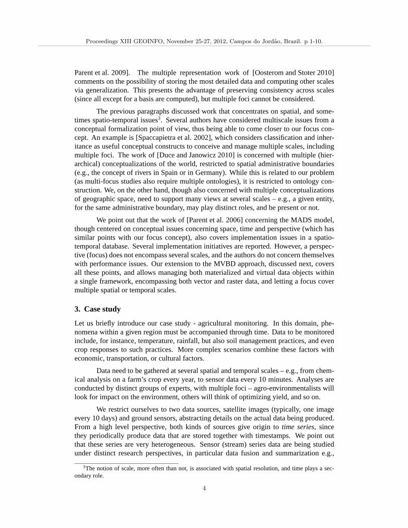
4.1. Introducing MVBDIntuitively, a given real world entity can correspond to many distinct digital items express-ing, for example, its alternative representations, or capturing its different states along time.Each of these ”expressions” will be treated in this work as aversionof the object. Con-sider the example illustrated in Figure 1. On the left, thereare two identified databaseobjects: a satellite image (Obj S) and a polygon to be superimposed on the image (ObjP). delimiting the boundaries of the farm to be monitored.

As illustrated by the table on the right of the figure, both objects can change alongtime, reflecting changes in the world, e.g., a new satellite image will be periodically pro-vided, or the boundaries of the farm can change. For each realworld entity, instead ofconsidering that these are new database objects, such changes can be interpreted as manyversions of the same object4. This object has a single, unique, identifier – called an ObjectIdentifierOid5.

A challenge when many interrelated objects have multiple versions is how togroup them coherently. For example, since the satellite image and the farm polygonchange along time, a given version of the satellite image from 12/05/2010 must be relatedwith a temporally compatible version of the farm polygon. This is the central focus of

4Here, both raster and vector representations are supported. An MVDB object is a database entity5Oids are artificial constructs. The actual disambiguation of an object in the world is not an issue here


5

the Multiversion Database (MVDB) model. It can handle multiple versions of an arbi-trary number of objects, which are organized indatabase versions - DBVs. A DBV is alogical construct. It represents an entire, consistent database constructed from a MVDBwhich gathers together consistent versions of interrelated objects. Intuitively, it can beinterpreted as acomplex viewon a MVDB. However, as shall be seen, unlike standarddatabase views, DBVs are not constructed from queries.

Figure 1. Practical scenario of a polygon over a satellite im age.

To handle the relation between an object and its versions, the MDBV distinguishestheir identifications by using object and physical identifiers respectively. Each object hasa single object identifier (Oid), which will be the same independently of its multipleversions. Each version of this object, materialized in the database by a digital item – e.g.,an image, a polygon etc. – will receive a distinct physical version identifierPVid. In theexample of Figure 1, there is a singleOid for each object – satellite image (Obj S) andthe farm boundaries (Obj P). Every time a new image or a new polygon is stored, it willreceive its ownPVid.

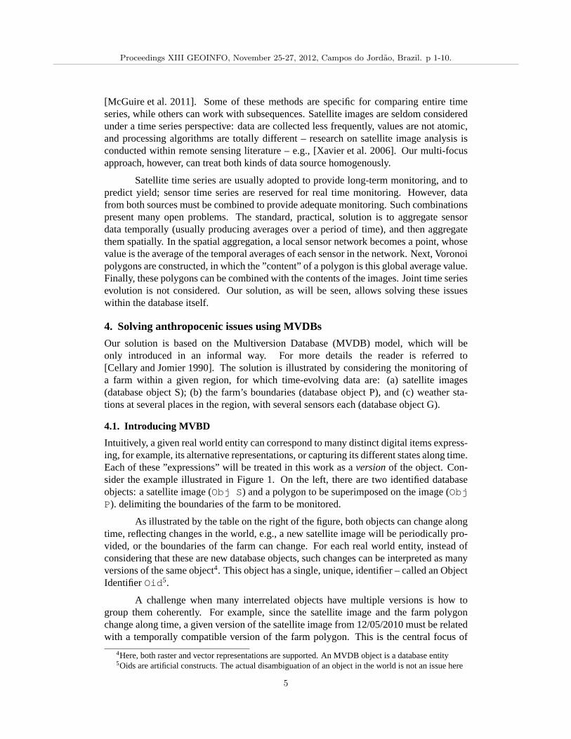
DBVs are the means to manage the relationship between anOid (say,S) and agivenPVid (of S). Figure 2 introduces a graphical illustration of the relationship amongthese three elements:DBV, Oid andPVid. In the middle there are two DBVs identifiedbyDBVids –DBV 1 andDBV 1.1 – and represented as planes containing logical slices(the ”views”) of the MVDB. The figure shows that each DBV has versions ofP andS,but each DBV is monoversion (i.e., it cannot contain two different versions of an object).The right part of the figure shows the physical storage, in which there are two physicalversions ofS (identified byPh1 andPh9), and just one version ofP.

DBV 1 relatesS with a specific satellite image andP with a specific polygon,which form together a consistent version of the world. Notice that here nothing is beingsaid about temporal or spatial scales. For instance, the twosatellite images can correspondto images obtained by different sensors aboard the same satellite (e.g., heat sensor, watersensor), and thus have the same timestamp. Alternatively, they can be images taken indifferent days. The role of the DBV is to gather together compatible versions of its objects,under whichever perspective applies.

Since DBVs are logical constructs, each object in a DBV has its own logical iden-tifier. Figure 2 shows on the left an alternative tabular representation, in whichDBVidsidentify rows andOids identify columns. Each pair (DBVid, Oid) identifies the logicalversion of an object and is related to a singlePVid, e.g.,(DBV 1, ObjS)→Ph1. Theasterisk in cell (DBV 1.1, Obj P) means that the state of the object did not changefrom DBV 1 to DBV 1.1, and therefore it will address the same physical identifierPh5.


6

Figure 2. The relationship between DBVs, logical and physic al identifiers.

4.2. DBV Evolution and Traceability

DBVs can be constructed from scratch or from other DBVs6. The identifier of a DBV(DBVid) indicates its derivation history. This is aligned tothe idea that versions are notnecessarily related to time changes, affording alternative variations of the same source, aswell as multiple foci – see section 5.

The distinction between logical and physical identifications is explored by anMVDB to provide storage efficiency. In most of the derivations, only a partial set ofobjects will change in a new derived DBV. In this case, the MVDBhas a strategy inwhich it stores only the differences from the previous version. Returning to the examplepresented in Figure 2 on the left table,DBV 1.1 is derived fromDBV 1, by changingthe state ofObj S. Thus, a newPVid is stored for it, but the state ofObj P has notchanged – no new polygon is stored, and thus there is no newPVid.

The evolution of a DBV is recorded in a derivation tree of DBVids. To retrievethe properPVid for each (virtual) object in a DBV, the MVDB adopts two strategies:provided and inferred references7, through navigation in the tree. This allows keepingtrack of real world evolution. We take advantage of these concepts in our extension of theMVDB model, implemented to support multiple spatial scales[Longo et al. 2012]. First,we create one tree per spatial scales, and all trees grow and shrink together. Second, thenotion of object id is extended to associate the id with the scale in which that object exists- (Oid, Scaleid). This paper extends this proposal in two directions: (1) we generalizethe notion of spatial scale to that of focus, where a given spatial or temporal scale canaccomodate multiple foci, and the evolution of these foci within a single derivation tree;(2) we provide a detailed case study to illustrate the internals of our solution.

5. From Multiversion to Multi-focusThis paper extends the MVDB model to support the several flavors of multi-focus. Thisimplies in synthesizing the multiple foci which can be applied to objects – scales, rep-resentations etc. – as specializations of versions. Figure3 illustrates an example of thisextension. There are three perspectives within the logicalview - see the Figure.

In the Physical perspective, there are three objects – two versions of satellite im-age S (with identifiersPh1 andPh2), and one version of a set of sensor data streams,corresponding to a set of weather stations G – global identifierPh7). Satellite image and

6DBV derivation trees, part of the model, will not be presented here.7For the logical version (DBV 1.1, Obj P), the reference will be inferred by traversing the chain of

derivations.


7

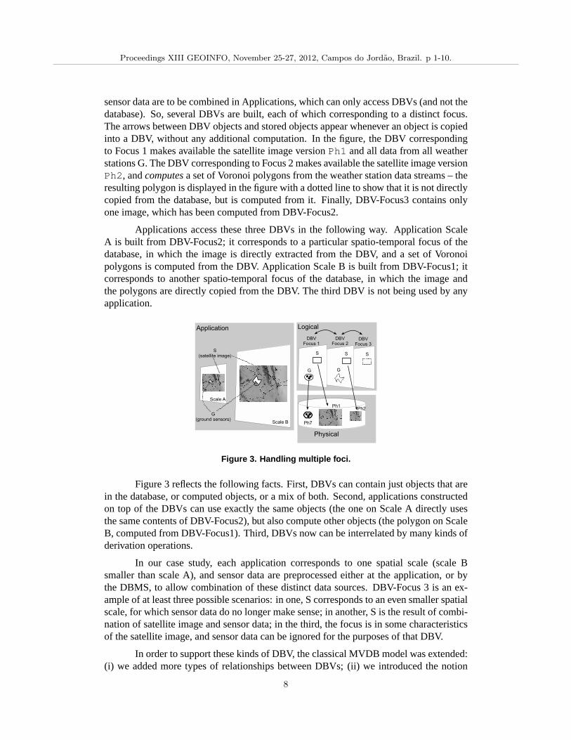
sensor data are to be combined in Applications, which can only access DBVs (and not thedatabase). So, several DBVs are built, each of which corresponding to a distinct focus.The arrows between DBV objects and stored objects appear whenever an object is copiedinto a DBV, without any additional computation. In the figure,the DBV correspondingto Focus 1 makes available the satellite image versionPh1 and all data from all weatherstations G. The DBV corresponding to Focus 2 makes available the satellite image versionPh2, andcomputesa set of Voronoi polygons from the weather station data streams – theresulting polygon is displayed in the figure with a dotted line to show that it is not directlycopied from the database, but is computed from it. Finally, DBV-Focus3 contains onlyone image, which has been computed from DBV-Focus2.

Applications access these three DBVs in the following way. Application ScaleA is built from DBV-Focus2; it corresponds to a particular spatio-temporal focus of thedatabase, in which the image is directly extracted from the DBV, and a set of Voronoipolygons is computed from the DBV. Application Scale B is built from DBV-Focus1; itcorresponds to another spatio-temporal focus of the database, in which the image andthe polygons are directly copied from the DBV. The third DBV is not being used by anyapplication.

Figure 3. Handling multiple foci.

Figure 3 reflects the following facts. First, DBVs can containjust objects that arein the database, or computed objects, or a mix of both. Second, applications constructedon top of the DBVs can use exactly the same objects (the one on Scale A directly usesthe same contents of DBV-Focus2), but also compute other objects (the polygon on ScaleB, computed from DBV-Focus1). Third, DBVs now can be interrelated by many kinds ofderivation operations.

In our case study, each application corresponds to one spatial scale (scale Bsmaller than scale A), and sensor data are preprocessed either at the application, or bythe DBMS, to allow combination of these distinct data sources. DBV-Focus 3 is an ex-ample of at least three possible scenarios: in one, S corresponds to an even smaller spatialscale, for which sensor data do no longer make sense; in another, S is the result of combi-nation of satellite image and sensor data; in the third, the focus is in some characteristicsof the satellite image, and sensor data can be ignored for thepurposes of that DBV.

In order to support these kinds of DBV, the classical MVDB model was extended:(i) we added more types of relationships between DBVs; (ii) weintroduced the notion


8

of scale to be part of an OID. In the classical MVDB the only relationship between twoDBVs is the derivation relationship, explained in the previous section. Our multi-focusapproach requires a wider set of relationships. Therefore,now the relationship betweentwo DBVs becomes typed: generalization, aggregation etc. This typing system is exten-sible, affording new types. This requires that new information be stored concerning eachDBV, and that the semantics of each object be stored alongsidethe object, e.g., usingontologies.

Returning to our example in Figure 3 consider an application that will accessthe contents ofS in DBV-Focus3. Since there is no explicit reference to it in theDBV-Focus2, the only information is that the state of S in the third focushas been de-rived in some kind of relationship with the state of S in the second DBV. Let us considerthat this is a generalization relationship, i.e., the stateof S in the third DBV is a carto-graphic generalization of the state of S in the DBV-Focus2. Inorder to use this logicalversion of S in an application, the construction of DBV-Focus3 will require an algorithmthat will: (1) verify that the type of the relationship is generalization; therefore,S must betransformed to the proper scale; (2) check the semantics ofS, verifying that it is a satelliteimage, and therefore generalization concerns image processing, and scaling.

6. Conclusions and ongoing work

This paper presents our approach to handling multi-focus problems, for geospatial data,based on adapting the MDBV (multiversion database) approachto handle not only mul-tiple scales, but multiple foci at each scale. Most approaches in the geospatial field con-centrate on the management of multiple spatial or temporal scales (either by computingadditional scales via generalization, or keeping track of all scales within a database vialink mechanisms). Our solution encompasses both kinds of approach in a single environ-ment, where anad hocworking scenario (the focus) can be built either by getting togetherconsistent spatio-temporal versions of geospatial entities, or by computing the appropriatestates, or a combination of both. Since a DBV can be seen as a consistent view of the mul-tiversion database, our approach also supports construction of any kind of arbitrary workscenarios, thereby allowing cooperative work. Moreover, derivation trees allow keepingtrack of the evolution of objects as they are updated, appearor disappear across scales.

Our ongoing work follows several directions. One of them includes domain on-tologies, to support communication among experts and interactions across levels and foci.We are also concerned with formalizing constraints across DBVs (and thus across scalesand foci).

References

Benda, L. E. et al. (2002). How to Avoid Train Wrecks When Using Science in Environ-mental Problem Solving.Bioscience, 52(12):1127–1136.

Buttenfield, B., Stanislawski, L., and Brewer, C. (2010). Multiscale Repreentations ofWater: Tailoring Generalization Sequences to Specific Physiographic Regimes. InProc. GIScience 2010.

Cellary, W. and Jomier, G. (1990). Consistency of Versions in Object-Oriented Databases.In Proc. 16th VLDB, pages 432–441.


9

Duce, S. and Janowicz, K. (2010). Microtheories for SpatialData Infrastructures – Ac-counting for Diversity of Local Conceptualizations at a Global Level. In Proc. GI-Science 2010.

Gao, H., Zhang, H., Hu, D., Tian, R., and Guo, D. (2010). Multi-scale features of urbanplanning spatial data. InProc 18th Int. Conf. on Geoinformatics, pages 1 –7.

Leibovicia, D. G. and Jackson, M. (2011). Multi-scale integration for spatio-temporalecoregioning delineation.Int. Journal of Image and Data Fusion, 2(2):105–119.

Longo, J. S. C., Camargo, L. O., Medeiros, C. B., and Santanche, A.(2012). Usingthe DBV model to maintain versions of multi-scale geospatialdata. InProc. 6th In-ternational Workshop on Semantic and Conceptual Issues in GIS (SeCoGIS 2012).Springer-Verlag.

McGuire, M. P., Janeja, V. P., and Gangopadhyay, A. (2011). Characterizing SensorDatasets with Multi-Granular Spatio-Temporal Intervals.19th ACM SIGSPATIAL In-ternational Conference on Advances in Geographic Information Systems.

Medeiros, C. B., Joliveau, M., Jomier, G., and Vuyst, F. (2010). Managing sensor trafficdata and forecasting unusual behaviour propagation.Geoinformatica, 14:279–305.

Oosterom, P. (2009). Research and development in geo-information generalisation andmultiple representation.Computers, Environment and Urban Systems, 33(5):303–310.

Oosterom, P. and Stoter, J. (2010). 5D Data Modelling: Full Integration of 2D/3D Space,Time and Scale Dimensions. InProc. GIScience 2010, pages 310–324.

Parent, C., Spaccapietra, S., Vangenot, C., and Zimanyi, E. (2009). Multiple Represen-tation Modeling. In LIU, L. and OZSU, M. T., editors,Encyclopedia of DatabaseSystems, pages 1844–1849. Springer US.

Parent, C., Spaccapietra, S., and Zimanyi, E. (2006).Conceptual Modeling for Traditionaland Spatio-Temporal Applications - the MADS Approach. Springer.

Sarjakoski, L. T. (2007). Conceptual Models of Generalisation and Multiple Representa-tion. In Generalisation of Geographic Information, pages 11–35. Elsevier.

Spaccapietra, S., Parent, C., and Vangenot, C. (2002). GIS Databases: From Multiscaleto MultiRepresentation. InProc. of the 4th Int. Symposium on Abstraction, Reformu-lation, and Approximation, SARA ’02, pages 57–70.

Xavier, A., Rodorff, B., Shimabukuro, Y., Berka, S., and Moreira, M. (2006). Multi-temporal analysisof MODIS data to classify sugarcane crop.International Journal ofRemote Sensing, 27(4):755–768.

Zhou, S. and Jones, C. B. (2003). A multirepresentation spatial data model. InProc8th Int. Symposium in Advances in Spatial and Temporal Databases – SSTD, pages394–411. LNCS 2750.


10

A Conceptual Analysis of Resolution

Auriol Degbelo and Werner Kuhn

Institute for Geoinformatics – University of Muenster Weseler Strasse 253, 48151, Muenster, Germany

{degbelo, kuhn}@uni-muenster.de

Abstract. The literature in geographic information science and related fields contains a variety of definitions and understandings for the term resolution. The goal of this paper is to discuss them and to provide a framework that makes at least some of these different senses compatible. The ultimate goal of our work is an ontological account of resolution. In a first stage, resolution and related notions are examined along the phenomenon, sampling and analysis dimensions. In a second stage, it is suggested that a basic distinction should be drawn between definitions of resolution, proxy measures for resolution, and notions related to resolution but different from it. It is illustrated how this distinction helps to reconcile several notions of resolution in the literature.

1. Introduction

Resolution is arguably one of the defining characteristics of geographic information (Kuhn 2011) and the need to integrate information across different levels of resolution pervades almost all its application domains. While there is a broader notion of granularity to be considered, for example regarding granularity levels of analyses, we focus here on resolution considered as a property of observations. We further limit our scope to spatial and temporal aspects of resolution, leaving thematic resolution and the dependencies between these dimensions to future work.

Currently, there is no formal theory of resolution of observations underlying geographic information. Such a theory is needed to explain how, for example, the spatial and temporal resolution of a measurement affects data quality and can be accounted for in data integration tasks. The main practical use for a theory of resolution, therefore, lies in its enabling of information integration across different levels of resolution. Specifically, the theory should suggest and inform methods for generalizing, specializing, interpolating, and extrapolating observation data. Turning the theory into an ontology will allow for automated reasoning about resolution in such integration (as well as in retrieval) tasks.

The literature in GIScience has not reached a consensus on what resolution is. Here are some extracts from previous work, each touching upon a definition of resolution:

“Resolution: the smallest spacing between two displayed or processed elements; the smallest size of the feature that can be mapped or sampled” (Burrough & McDonnell, 1998, p305).


11

“Resolution refers to the amount of detail in a representation, while granularity refers to the cognitive aspects involved in selection of features” (Hornsby cited in (Fonseca et al. 2002)).

“Resolution or granularity is concerned with the level of discernibility between elements of a phenomenon that is being represented by the dataset” (Stell & Worboys 1998).

“Resolution: smallest change in a quantity being measured that causes a perceptible change in the corresponding indication” (The ontology of the W3C Semantic Sensor Network Incubator Group)1.

“The capability of making distinguishable the individual parts of an object” (a dictionary definition cited in (Tobler 1987)).

“Resolution refers to the smallest distinguishable parts in an object or a sequence, ... and is often determined by the capability of the instrument or the sampling interval used in a study” (Lam & Quattrochi 1992).

“The detail with which a map depicts the location and shape of geographic features” (a dictionary definition of ESRI2).

“Resolution is an assertion or a measure of the level of detail or the information content of an object database with respect to some reference frame” (Skogan 2001).

This list exemplifies a variety of definitions for the term ‘resolution’ and shows that some of them are conflicting (e.g. the 2nd and 3rd definition in the list). The remark that “[r]esolution seems intuitively obvious, but its technical definition and precise application ... have been complex” made by Robinson et al. (2002) in the context of remote sensing is pertinent for GIScience as a whole. Section 2 analyzes some notions closely related to resolution and arranges them based on the framework suggested in (Dungan et al. 2002). Section 3 suggests that resolution should be defined as the amount of detail of a representation and proposes two types of proxy measures for resolution: smallest unit over which homogeneity is assumed and dispersion. Section 4 concludes the paper and outlines future work.

2. Resolution and related notions

In a discussion of terms related to ‘scale’ in the field of ecology, Dungan et al. (2002) suggested three categories (or dimensions) to which spatial scale-related terms may be applied. The three dimensions are: (a) the phenomenon dimension, (b) the sampling dimension, and (c) the analysis dimension. The phenomenon dimension relates to the (spatial or temporal) unit at which a particular phenomenon operates; the sampling dimension (or observation dimension or measurement dimension) relates to the (spatial or temporal) units used to acquire data about the phenomenon; the analysis dimension relates to the (spatial or temporal) units at which the data collected about a phenomenon

1 See a presentation of the ontology for sensors and observations developed by the group in (Compton et al. 2012). The ontology is available at http://purl.oclc.org/NET/ssnx/ssn (last accessed: July 20, 2012). 2 See http://support.esri.com/en/knowledgebase/GISDictionary/search (last accessed: July, 20, 2012).


12

are summarized and used to make inferences. For example, if one would like to study the change of the temperature over an area A, the phenomenon of interest would be ‘change of temperature’. Data can be collected about the value of the temperature at A, say every hour; one hour relates to the sampling dimension. The data collected is then aggregated to daily values and analysis or inferences are performed on the aggregated values; this refers to the analysis dimension. This paper will reuse the three dimensions introduced in the current paragraph to frame the discussion on resolution and related notions. Although the roots of the three dimensions are in the field of ecology, they can be reused for the purposes of the paper because GIScience and ecology overlap in many respects. For instance:

issues revolving around the concept of ‘scale’ have been identified as deserving prime attention for research by both communities (see for example (UCGIS 1996) for GIScience, and (Wu & Hobbs 2002), for ecology);

both communities are interested in a ‘science of scale’ (see for example (Goodchild & Quattrochi 1997) for GIScience, (Wu & Hobbs 2002), for ecology);

there exists overlaps in objects of studies (witness for example the research field of ‘landscape ecology’ introduced in (Wu 2006; Wu 2008; Wu 2012), and the research field of ‘ethnophysiography’ presented in (Mark et al. 2007));

there are overlaps in underlying principles (Wu (2012) mentions for example that “[s]patial heterogeneity is ubiquitous in all ecological systems” and Goodchild (2011a) proposed spatial heterogeneity as one of the empirical principles that are broadly true of all geographic information).

One notion related to ‘resolution’ is ‘scale’. Scale can have many meanings, as discussed for example in (Förstner 2003; Goodchild 2001; Goodchild 2011b; Goodchild & Proctor 1997; Lam & Quattrochi 1992; Montello 2001; Quattrochi 1993). Like in (Dungan et al. 2002), we consider resolution to be one of many components of scale, with other components being extent, grain, lag, support and cartographic ratio. Dungan et al. (2002) have discussed the matching up of resolution, grain, lag and support with the three dimensions of phenomenon, sampling and analysis. The next paragraph will briefly summarize their discussion. It will touch upon four notions, namely grain, spacing, resolution and support. After that, another paragraph will introduce discrimination, coverage, precision, accuracy, and pixel.

According to Dungan et al. (2002), grain is a term that can be defined for the phenomenon, sampling and analysis dimensions. Sampling grain refers to the minimum spatial or temporal unit over which homogeneity is assumed for a sample3. Another term that applies to the three dimensions according to Dungan et al. (2002) is the term lag or spacing4. Sample spacing denotes the distance between neighboring samples. Resolution was presented in (Dungan et al. 2002) as a term which applies to sampling

3 The definition is in line with (Wu & Li 2006). Grain as used in the remainder of this paper refers to sampling (or measurement or observation) grain. 4 The use of the term spacing is preferred in this paper over the use of the term lag. Spacing as used in the remainder of the paper refers to sampling (or measurement or observation) spacing.


13

and analysis rather than to phenomena. Finally it was argued in (Dungan et al. 2002) that support is a term that belongs to the analysis dimension. Although Dungan et al. (2002) limit support to the analysis dimension, this paper argues that it applies to the sampling or measurement dimension as well. This is in line with (Burrough & McDonnell 1998, p101) who defined support as “the technical name used in geostatistics for the area or volume of the physical sample on which the measurement is made”. The matching up of resolution, grain, spacing and support with the phenomenon, sampling and analysis dimensions is summarized in figure 1.

Lam & Quattrochi (1992) claim that “[r]esolution refers to the smallest distinguishable parts in an object or a sequence, ... and is often determined by the capability of the instrument or the sampling interval used in a study”. This definition points to two correlates of resolution. One of them relates to the sampling interval and was already covered in the previous paragraph under the term spacing; the second relates to the capability of the instrument, and is called here (after Sydenham (1999)) discrimination. The term discrimination is borrowed from the Measurement, Instrumentation, and Sensors Handbook and refers to the smallest change in a quantity being measured that causes a perceptible change in the corresponding observation value5. A synonym for discrimination is step size (see (Burrough & McDonnell 1998, p57)). Discrimination is a property of the sensor (or measuring device) and therefore belongs to the sampling dimension.

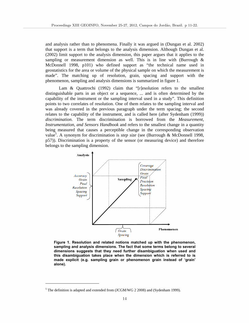
Figure 1. Resolution and related notions matched up with the phenomenon, sampling and analysis dimensions. The fact that some terms belong to several dimensions suggests that they need further disambiguation when used and this disambiguation takes place when the dimension which is referred to is made explicit (e.g. sampling grain or phenomenon grain instead of ‘grain’ alone).

5 The definition is adapted and extended from (JCGM/WG 2 2008) and (Sydenham 1999).


14

Besides the discrimination of a sensor, coverage is another correlate of resolution. Coverage is defined after Wu & Li (2006) as the sampling intensity in space or time. For that reason, coverage is a term that applies to the sampling dimension of the framework (see figure 1). Synonyms for coverage are sampling density, sampling frequency or sampling rate. Figure 2 illustrates the difference between sampling grain, sampling coverage and sampling spacing for the spatial dimension.

Precision is defined after JCGM/WG 2 (2008) as the “closeness of agreement between indications or measured quantity values obtained by replicate measurements on the same or similar objects under specified conditions”. Precision belongs therefore to the sampling (or observation) dimension of the framework. On the contrary, accuracy, the “closeness of agreement between a measured quantity value and a true quantity value of a measurand” (JCGM/WG 2 2008) is a concept which belongs to the analysis dimension. In order to assign an accuracy value to a measurement, one needs not only a measurement value, but also the specification of a reference value. Because the specification of the reference value is likely to vary from task to task (or user to user), it is suggested here that accuracy is classified as a concept belonging to the analysis level. The last correlate of resolution introduced in this section is the notion of pixel. The pixel is the “smallest unit of information in a grid cell map or scanner image” (Burrough & McDonnell 1998, p304). It is also, as indicated by Fisher (1997), the elementary unit of analysis in remote sensing. As a result, pixel belongs to both the sampling and the analysis dimension.

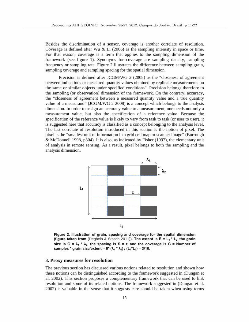
Figure 2. Illustration of grain, spacing and coverage for the spatial dimension (figure taken from (Degbelo & Stasch 2011)). The extent is E = L1 * L2, the grain size is G = λ1 * λ2, the spacing is S = ε and the coverage is C = Number of samples * grain size/extent = 6* (λ1 * λ2) / (L1*L2) = 3/10.

3. Proxy measures for resolution

The previous section has discussed various notions related to resolution and shown how these notions can be distinguished according to the framework suggested in (Dungan et al. 2002). This section proposes a complementary framework that can be used to link resolution and some of its related notions. The framework suggested in (Dungan et al. 2002) is valuable in the sense that it suggests care should be taken when using terms


15

belonging to several dimensions as synonyms. Wu & Li (2006) mention, for example, that in most cases, grain and support have quite similar meanings, and thus have often been used interchangeably in the literature. Such a use is fine in some cases because, at the analysis or sampling level, the distinction between the two terms becomes blurred. On the contrary, the use of phenomenon grain and support as synonyms might not always be appropriate, since phenomenon grain might differ from analysis or sampling grain (= support).

3.1. A unifying framework for resolution and related notions

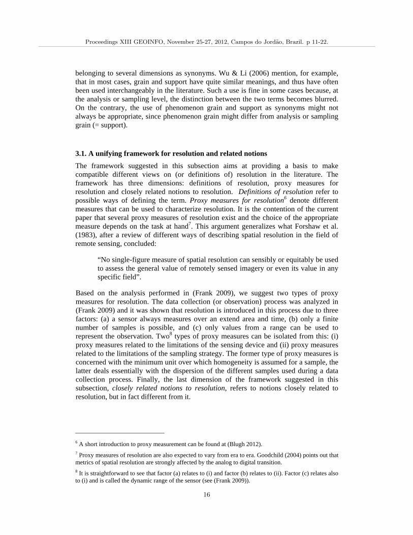
The framework suggested in this subsection aims at providing a basis to make compatible different views on (or definitions of) resolution in the literature. The framework has three dimensions: definitions of resolution, proxy measures for resolution and closely related notions to resolution. Definitions of resolution refer to possible ways of defining the term. Proxy measures for resolution6 denote different measures that can be used to characterize resolution. It is the contention of the current paper that several proxy measures of resolution exist and the choice of the appropriate measure depends on the task at hand7. This argument generalizes what Forshaw et al. (1983), after a review of different ways of describing spatial resolution in the field of remote sensing, concluded:

“No single-figure measure of spatial resolution can sensibly or equitably be used to assess the general value of remotely sensed imagery or even its value in any specific field”.

Based on the analysis performed in (Frank 2009), we suggest two types of proxy measures for resolution. The data collection (or observation) process was analyzed in (Frank 2009) and it was shown that resolution is introduced in this process due to three factors: (a) a sensor always measures over an extend area and time, (b) only a finite number of samples is possible, and (c) only values from a range can be used to represent the observation. Two8 types of proxy measures can be isolated from this: (i) proxy measures related to the limitations of the sensing device and (ii) proxy measures related to the limitations of the sampling strategy. The former type of proxy measures is concerned with the minimum unit over which homogeneity is assumed for a sample, the latter deals essentially with the dispersion of the different samples used during a data collection process. Finally, the last dimension of the framework suggested in this subsection, closely related notions to resolution, refers to notions closely related to resolution, but in fact different from it.

6 A short introduction to proxy measurement can be found at (Blugh 2012). 7 Proxy measures of resolution are also expected to vary from era to era. Goodchild (2004) points out that metrics of spatial resolution are strongly affected by the analog to digital transition. 8 It is straightforward to see that factor (a) relates to (i) and factor (b) relates to (ii). Factor (c) relates also to (i) and is called the dynamic range of the sensor (see (Frank 2009)).


16

3.2. Using the framework suggested

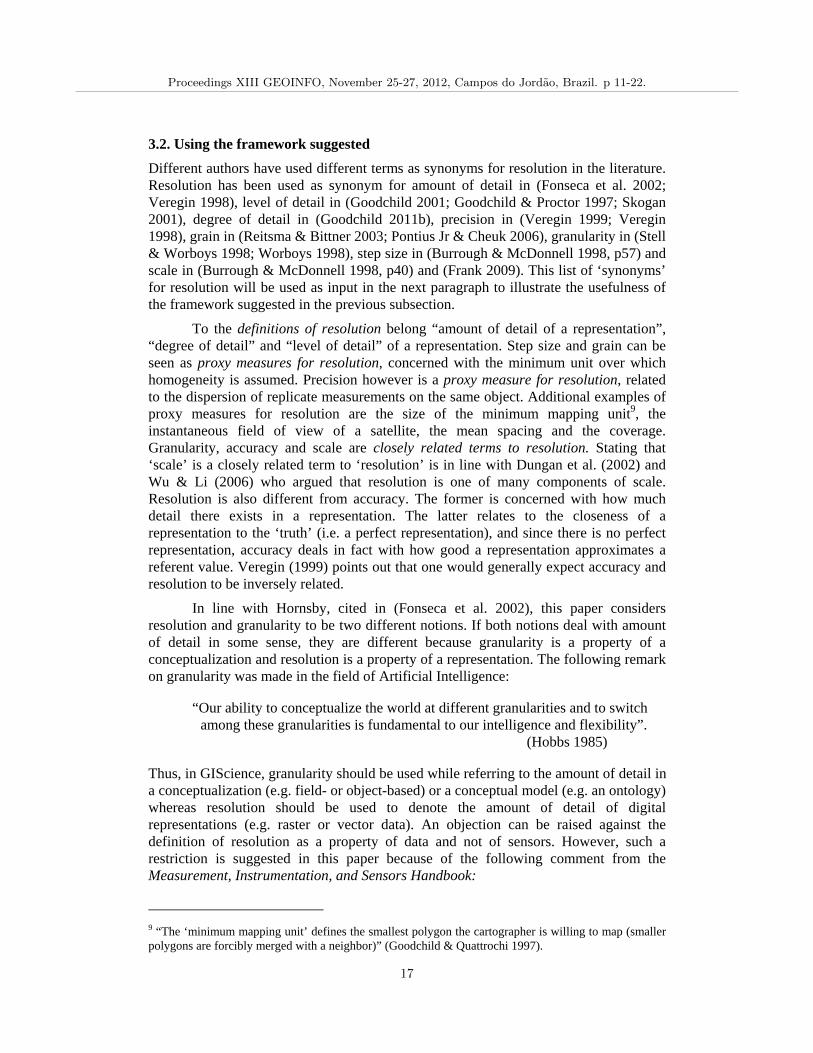
Different authors have used different terms as synonyms for resolution in the literature. Resolution has been used as synonym for amount of detail in (Fonseca et al. 2002; Veregin 1998), level of detail in (Goodchild 2001; Goodchild & Proctor 1997; Skogan 2001), degree of detail in (Goodchild 2011b), precision in (Veregin 1999; Veregin 1998), grain in (Reitsma & Bittner 2003; Pontius Jr & Cheuk 2006), granularity in (Stell & Worboys 1998; Worboys 1998), step size in (Burrough & McDonnell 1998, p57) and scale in (Burrough & McDonnell 1998, p40) and (Frank 2009). This list of ‘synonyms’ for resolution will be used as input in the next paragraph to illustrate the usefulness of the framework suggested in the previous subsection.

To the definitions of resolution belong “amount of detail of a representation”, “degree of detail” and “level of detail” of a representation. Step size and grain can be seen as proxy measures for resolution, concerned with the minimum unit over which homogeneity is assumed. Precision however is a proxy measure for resolution, related to the dispersion of replicate measurements on the same object. Additional examples of proxy measures for resolution are the size of the minimum mapping unit9, the instantaneous field of view of a satellite, the mean spacing and the coverage. Granularity, accuracy and scale are closely related terms to resolution. Stating that ‘scale’ is a closely related term to ‘resolution’ is in line with Dungan et al. (2002) and Wu & Li (2006) who argued that resolution is one of many components of scale. Resolution is also different from accuracy. The former is concerned with how much detail there exists in a representation. The latter relates to the closeness of a representation to the ‘truth’ (i.e. a perfect representation), and since there is no perfect representation, accuracy deals in fact with how good a representation approximates a referent value. Veregin (1999) points out that one would generally expect accuracy and resolution to be inversely related.

In line with Hornsby, cited in (Fonseca et al. 2002), this paper considers resolution and granularity to be two different notions. If both notions deal with amount of detail in some sense, they are different because granularity is a property of a conceptualization and resolution is a property of a representation. The following remark on granularity was made in the field of Artificial Intelligence:

“Our ability to conceptualize the world at different granularities and to switch among these granularities is fundamental to our intelligence and flexibility”. (Hobbs 1985)

Thus, in GIScience, granularity should be used while referring to the amount of detail in a conceptualization (e.g. field- or object-based) or a conceptual model (e.g. an ontology) whereas resolution should be used to denote the amount of detail of digital representations (e.g. raster or vector data). An objection can be raised against the definition of resolution as a property of data and not of sensors. However, such a restriction is suggested in this paper because of the following comment from the Measurement, Instrumentation, and Sensors Handbook:

9 “The ‘minimum mapping unit’ defines the smallest polygon the cartographer is willing to map (smaller polygons are forcibly merged with a neighbor)” (Goodchild & Quattrochi 1997).


17

“Although now officially declared as wrong to use, the term resolution still finds its way into books and reports as meaning discrimination” (Sydenham 1999).

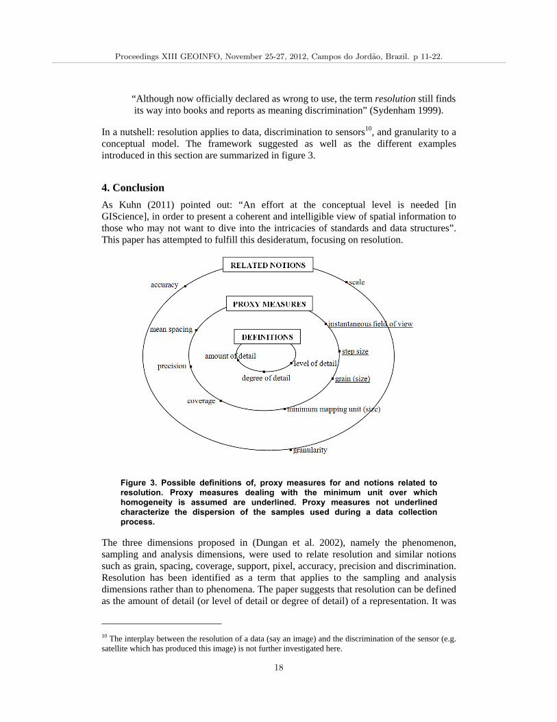
In a nutshell: resolution applies to data, discrimination to sensors10, and granularity to a conceptual model. The framework suggested as well as the different examples introduced in this section are summarized in figure 3.

4. Conclusion

As Kuhn (2011) pointed out: “An effort at the conceptual level is needed [in GIScience], in order to present a coherent and intelligible view of spatial information to those who may not want to dive into the intricacies of standards and data structures”. This paper has attempted to fulfill this desideratum, focusing on resolution.

Figure 3. Possible definitions of, proxy measures for and notions related to resolution. Proxy measures dealing with the minimum unit over which homogeneity is assumed are underlined. Proxy measures not underlined characterize the dispersion of the samples used during a data collection process.

The three dimensions proposed in (Dungan et al. 2002), namely the phenomenon, sampling and analysis dimensions, were used to relate resolution and similar notions such as grain, spacing, coverage, support, pixel, accuracy, precision and discrimination. Resolution has been identified as a term that applies to the sampling and analysis dimensions rather than to phenomena. The paper suggests that resolution can be defined as the amount of detail (or level of detail or degree of detail) of a representation. It was

10 The interplay between the resolution of a data (say an image) and the discrimination of the sensor (e.g. satellite which has produced this image) is not further investigated here.


18

also argued that two types of proxy measures for resolution should be distinguished: those which deal with the minimum unit over which homogeneity is assumed for a sample (e.g. grain or minimum mapping unit), and those which revolve around the dispersion of the samples used during the data collection process (e.g. spacing and coverage). Finally, the paper pointed to notions related to resolution but different from it (e.g. scale, granularity and accuracy). The second author, in his work on core concepts of spatial information, has meanwhile chosen granularity as the core concept covering spatial information, with resolution being the more specialized aspect referring to data (Kuhn 2012). The paper intentionally does not choose a particular definition of resolution, nor does it add a new one to the literature. Instead, the distinction between definitions of, proxy measures for, and notions related to resolution aims at making several perspectives on the term compatible.

The next step of this work will be a formalized ontology of this account of resolution. Such an ontology will extend previous ontologies of observations and measurements (e.g. (Janowicz & Compton 2010; Kuhn 2009; Compton 2011; Compton et al. 2012)) presented and applied in the context of the Semantic Sensor Web.

Acknowledgements

Funding from the German Academic Exchange Service (DAAD A/10/98506), the European Commission through the ENVISION Project (FP7-249170), and the International Research Training Group on Semantic Integration of Geospatial Information (DFG GRK 1498) is gratefully acknowledged. Discussions with Kathleen Stewart helped in the process of clarifying the distinction between granularity and resolution.

References

Blugh, A. (2012) Definition of proxy measures (http://www.ehow.com/facts_7621616_definition-proxy-measures.html; Last accessed July 31, 2012).

Burrough, P.A. & McDonnell, R.A. (1998) Principles of geographical information systems, New York, New York, USA: Oxford University Press.

Compton, M. (2011) What now and where next for the W3C Semantic Sensor Networks Incubator Group sensor ontology. In K. Taylor, A. Ayyagari, & D. De Roure, eds. The 4th international workshop on Semantic Sensor Networks. Bonn, Germany: CEUR-WS.org, pp.1–8.

Compton, M., Barnaghi, P., Bermudez, L., García-Castro, R., Corcho, O., Cox, S., Graybeal, J., Hauswirth, M., Henson, C., Herzog, A., Huang, V., Janowicz, K., Kelsey, W.D., Phuoc, D. Le, Lefort, L., Leggieri, M., Neuhaus, H., Nikolov, A., Page, K., Passant, A., Sheth, A. & Taylor, K. (2012) The SSN ontology of the W3C semantic sensor network incubator group. Web Semantics: Science, Services and Agents on the World Wide Web.


19

Degbelo, A. & Stasch, C. (2011) Level of detail of observations in space and time. In Poster Session at Conference on Spatial Information Theory: COSIT’11. Belfast, Maine, USA.

Dungan, J.L., Perry, J.N., Dale, M.R.T., Legendre, P., Citron-Pousty, S., Fortin, M.J., Jakomulska, A., Miriti, M. & Rosenberg, M.S. (2002) A balanced view of scale in spatial statistical analysis. Ecography, p.pp.626–640.

Fisher, P. (1997) The pixel: a snare and a delusion. International Journal of Remote Sensing, 18 (3), p.pp.679–685.

Fonseca, F., Egenhofer, M., Davis, C. & Câmara, G. (2002) Semantic granularity in ontology-driven geographic information systems. Annals of Mathematics and Artificial Intelligence, 36 (1), p.pp.121–151.

Forshaw, M.R.B., Haskell, A., Miller, P.F., Stanley, D.J. & Townshend, J.R.G. (1983) Spatial resolution of remotely sensed imagery A review paper. International Journal of Remote Sensing, 4 (3), p.pp.497–520.

Frank, A. (2009) Why is scale an effective descriptor for data quality? The physical and ontological rationale for imprecision and level of detail. In W. Cartwright, G. Gartner, L. Meng, & M. P. Peterson, eds. Research Trends in Geographic Information Science. Springer Berlin Heidelberg, pp.39–61.

Förstner, W. (2003) Notions of scale in geosciences. In H. Neugebauer & C. Simmer, eds. Dynamics of Multiscale Earth Systems. Springer Berlin Heidelberg, pp.17–39.

Goodchild, M. & Quattrochi, D. (1997) Introduction: scale, multiscaling, remote sensing, and GIS. In D. Quattrochi & M. Goodchild, eds. Scale in remote sensing and GIS. Boca Raton: Lewis Publishers, pp.1–11.

Goodchild, M.F. (2011a) Challenges in geographical information science. Proceedings of the Royal Society A, 467 (2133), p.pp.2431–2443.

Goodchild, M.F. (2001) Metrics of scale in remote sensing and GIS. International Journal of Applied Earth Observation and Geoinformation, 3 (2), p.pp.114–120.

Goodchild, M.F. (2011b) Scale in GIS: an overview. Geomorphology, 130 (1-2), p.pp.5–9.

Goodchild, M.F. (2004) Scales of cybergeography. In E. Sheppard & R. B. McMaster, eds. Scale and geographic inquiry: nature, society, and method. Malden, MA: Blackwell Publishing Ltd, pp.154–169.

Goodchild, M.F. & Proctor, J. (1997) Scale in a digital geographic world. Geographical and environmental modelling, 1 (1), p.pp.5–23.

Hobbs, J.R. (1985) Granularity. In A. Joshi, ed. In Proceedings of the Ninth International Joint Conference on Artificial Intelligence. Los Angeles, California, USA: Morgan Kaufmann Publishers, pp.432–435.


20

JCGM/WG 2 (2008) The international vocabulary of metrology - Basic and general concepts and associated terms (VIM).

Janowicz, K. & Compton, M. (2010) The Stimulus-Sensor-Observation ontology design pattern and its integration into the semantic sensor network ontology. In K. Taylor, A. Ayyagari, & D. De Roure, eds. The 3rd International workshop on Semantic Sensor Networks. Shanghai, China: CEUR-WS.org.

Kuhn, W. (2009) A functional ontology of observation and measurement. In K. Janowicz, M. Raubal, & S. Levashkin, eds. GeoSpatial Semantics: Third International Conference. Mexico City, Mexico: Springer Berlin Heidelberg, pp.26–43.

Kuhn, W. (2012) Core concepts of spatial information for transdisciplinary research. International Journal of Geographical Information Science, (Special issue honoring Michael Goodchild), in press.

Kuhn, W. (2011) Core concepts of spatial information: a first selection. In L. Vinhas & C. Davis Jr., eds. XII Brazilian Symposium on Geoinformatics. Campos do Jordão, Brazil, pp.13–26.

Lam, N.S.N. & Quattrochi, D.A. (1992) On the Issues of Scale, Resolution, and Fractal Analysis in the Mapping Sciences*. The Professional Geographer, 44 (1), p.pp.88–98.

Mark, D., Turk, A. & Stea, D. (2007) Progress on Yindjibarndi ethnophysiography. In S. Winter, M. Duckham, L. Kulik, & B. Kuipers, eds. Spatial information theory - 8th International Conference, COSIT 2007. Melbourne, Australia: Springer-Verlag Berlin Heidelberg, pp.1–19.

Montello, D.R. (2001) Scale in geography N. Smelser & P. Baltes, eds. International Encyclopedia of the Social and Behavioral Sciences, p.pp.13501–13504.

Pontius Jr, R.G. & Cheuk, M.L. (2006) A generalized cross-tabulation matrix to compare soft-classified maps at multiple resolutions. International Journal of Geographical Information Science, 20 (1), p.pp.1–30.

Quattrochi, D.A. (1993) The need for a lexicon of scale terms in integrating remote sensing data with geographic information systems. Journal of Geography, 92 (5), p.pp.206–212.

Reitsma, F. & Bittner, T. (2003) Scale in object and process ontologies. In W. Kuhn, M. F. Worboys, & S. Timpf, eds. Spatial Information Theory: Foundations of Geographic Information Science, COSIT03. Ittingen, Switzerland: Springer Berlin, pp.13–30.

Robinson, J.A., Amsbury, D.L., Liddle, D.A. & Evans, C.A. (2002) Astronaut-acquired orbital photographs as digital data for remote sensing: spatial resolution. International Journal of Remote Sensing, 23 (20), p.pp.4403–4438.


21

Skogan, D. (2001) Managing resolution in multi-resolution databases. In J. T. Bjørke & H. Tveite, eds. ScanGIS’2001 - The 8th Scandinavian Research Conference on Geographical Information Science. Ås, Norway, pp.99–113.

Stell, J. & Worboys, M. (1998) Stratified map spaces: A formal basis for multi-resolution spatial databases. In T. Poiker & N. Chrisman, eds. SDH’98 - Proceedings 8th International Symposium on Spatial Data Handling. Vancouver, British Columbia, Canada, pp.180–189.

Sydenham, P.H. (1999) Static and dynamic characteristics of instrumentation. In J. G. Webster, ed. The measurement, instrumentation, and sensors handbook. CRC Press LLC.

Tobler, W. (1987) Measuring spatial resolution. In Proceedings, Land Resources Information Systems Conference. Beijing, China, pp.12–16.

UCGIS (1996) Research priorities for geographic information science. Cartography and Geographic Information Systems, 23 (3), p.pp.115–127. Available at: http://www.ncgia.ucsb.edu/other/ucgis/CAGIS.html.

Veregin, H. (1998) Data quality measurement and assessment. NCGIA Core Curriculum in Geographic Information Science, p.pp.1–10.

Veregin, H. (1999) Data quality parameters. In P. A. Longley, D. J. Maguire, M. F. Goodchild, & D. W. Rhind, eds. Geographical information systems: principles and technical issues. New York: John Wiley and Sons, pp.177–189.

Worboys, M. (1998) Imprecision in finite resolution spatial data. GeoInformatica, 2 (3), p.pp.257–279.

Wu, J. (2008) Landscape ecology. In S. E. Jorgensen & B. Fath, eds. Encyclopedia of Ecology. Oxford, United Kingdom: Elsevier, pp.2103–2108.

Wu, J. (2012) Landscape ecology. In A. Hastings & L. Gross, eds. Encyclopedia of Theoretical Ecology. University of California Press, pp.392–396.

Wu, J. (2006) Landscape ecology, cross-disciplinarity, and sustainability science. Landscape Ecology, 21 (1), p.pp.1–4.

Wu, J. & Hobbs, R. (2002) Key issues and research priorities in landscape ecology: an idiosyncratic synthesis. Landscape Ecology, 17 (4), p.pp.355–365.

Wu, J. & Li, H. (2006) Concepts of scale and scaling. In J. Wu, B. Jones, H. Li, & O. Loucks, eds. Scaling and uncertainty analysis in ecology: methods and applications. Dordrecht, The Netherlands: Springer, pp.3–16.


22

Distributed Vector based Spatial Data Conflation Services

Sérgio Freitas, Ana Paula Afonso

Department of Computer Science – University of Lisbon

Lisbon, Portugal.

[email protected], [email protected]

Abstract. Spatial data conflation is a key task for consolidating geographic

knowledge from different data sources covering overlapping regions that were

gathered using different methodologies and objectives. Nowadays this

research area is becoming more challenging because of the increasing size

and number of overlapping spatial data sets being produced. This paper

presents an approach towards distributed vector to vector conflation, which

can be applied to overlapping heterogeneous spatial data sets through the

implementation of Web Processing Services (WPS). Initial results show that

distributed spatial conflation can be effortlessly achieved if during the pre-

processing phase disjoint clusters are created. However, if this is not possible

further horizontal conflation algorithms are applied to neighbor clusters

before obtaining the final data set.

1. Introduction

The ability to combine various datasets of spatial data into a single integrated set is a

fundamental issue of contemporary Geographic Information Systems (GIS). This task is

known in scientific literature as spatial data conflation and is used for combining spatial

knowledge from different sources in a single mean full set.

Till recent years automatic spatial data conflation research has been primarily

concerned with algorithms and tools for performing conflation as single thread

operations on specific types of datasets, primarily using geometry matching techniques

[Saalfeld 1988] and lately semantic matching has been identified has a key element of

the conflation problem [Ressler et al. 2009]. With the advent of Web based maps an

increasing number of community and enterprise generated knowledge is being produced

using heterogeneous techniques [Goodchild 2007].

The increasing size of data sets is a central aspect that spatial data conflation

algorithms have to overcome and the demand to perform on the fly operations in an

Internet environment. To overcome these constraints it is fundamental that conflation

operations can be distributed between several computing instances (nodes) in order to

complete fusion operations in satisfactory time for very large data sets.

The overall spatial conflation process is composed by five main sub-processes,

analysis and comparison, preprocessing, matching, fusion and post-processing

[Wiemann and Bernard 2010]. Analysis and comparison evaluates if each data set is a

candidate for conflation and if further preprocessing is needed to make each data set

compatible (e.g. coordinate system conversion, map alignment, generalization); after

this task the matching process is used to find similar features, a combination of


23

geometrical, topological, semantic similarity measurements are used to find similar

features and afterwards fusion is performed between candidate features; finally post-

processing is applied to perform final adjustments.

A fundamental aspect for implementing geographic services is the use of Open

Geospatial Consortium (OGC) standards that will allow existing GIS software packages

that implement these standards to easily interact with the services being implemented.

MapReduce is a programming model developed by Google that is widely

adopted for processing large data sets on computer clusters [Dean and Ghemawat 2004].

MapReduce is composed by the Map and Reduce steps. Map is responsible to sub-

divide the problem and distribute to worker nodes, and then worker nodes process the

smaller data set and return the results to the master node. Reduce is responsible to

collect the results and combine them according to a predefined process.

In order to achieve distributed conflation, spatial clustering algorithms are

applied in the preprocessing phase to each input data set so each output cluster can be

matched and fused in autonomous nodes (Map). At last results from each computing

instance are merged in post-processing phase in order to reach the desired final output

(Reduce).

Spatial conflation service prototypes are currently being developed through the

implementation of Web Processing Services (WPS) standard defined by the OGC

[OGC 2007]. Apache Hadoop MapReduce framework is invoked by the WPS engine

(PyWPS) to perform distributed and scalable spatial conflation. The base software

components are all open source projects (PyWPS, GDAL/OGR, GEOS and

PostgreSQL/PostGIS). This is a key aspect of this work because the usage of open

source solutions allows the full control of each task performed and a greater knowledge

of the inner works of each software component. Our initial results show that distributed

spatial conflation can be easily achieved if during the preprocessing phase disjoint

clusters are created ensuring that throughout the post-processing phase there is no need

to apply horizontal conflation algorithms (e.g. edge-matching) to merge features that are

placed on the edge of each cluster. If this is not possible further horizontal conflation

algorithms have to be applied during the Reduce step before obtaining the final data set.

This paper presents an approach towards distributed vector to vector conflation,

which can be applied to overlapping heterogeneous vector spatial data sets. The

conflation methodologies are geared towards detecting data clusters that can be

computed in independent nodes and subsequently merged.

2. Related Work

Spatial data conflation is a specialized task within geoinformatics that is mainly used for

detection change, integration, enrichment of spatial data sets and updating

[Yuan and Tao 1999]. Conflation is commonly classified as Horizontal or Vertical

[MacMaster 1986]. Horizontal conflation is used to define conflation applied to adjacent

spatial data sets, and vertical conflation is concerned with overlapping data sets

[Beard and Christman 1986].

A comprehensive mathematical context for automated conflation process was

firstly proposed by Saalfeld [Saalfeld 1988]. This initial work was focus on performing


24

feature geometries alignment between data sets. The first step of this process is to

recognize similar geometries, check if matching is correct using quality control points,

and apply feature geometry alignment using geometric interpolation and space

partitioning algorithms. This process is applied recursively until no similar geometries

were found on each data set. The main conclusion of Saalfeld’s work is that Delaunay

triangulation is the best fit for partitioning space and these partitioning arrangements

certify that independent liner transformations (e.g. scaling and rotation) could be

performed to geometries in order to align data sets inside each triangle.

This technique is described in the conflation literature as rubber-sheeting and is

still widely used for performing alignment operations between data sets using control

points that can be automatically calculate by matching features between data sets or

using humans to determine common control points on each data set [White 1981].

Conflation can be applied to raster and vector data sets, and can be categorized

as raster to raster, raster to vector and vector to vector conflation. Each category uses

different algorithms and techniques. Raster conflation implies the use of image analysis

techniques [White 1981], raster to vector involves image analysis and comparison with

feature geometries, and vector to vector is focused on the analysis of geometry and

feature attributes [Saalfeld 1988].

Current conflation process is composed of several sub-tasks

[Wiemann and Bernard 2010]. Firstly, input data sets have to be analyzed and compared

to ensure fitness for further processing tasks. This includes analyzing metadata or

inferring geometrical, topological and semantic properties. Data gathered during the

previous step is feeded to the pre-processing task which determines if further map

alignment, coordinate system conversion or generalization has to be performed. After

this task feature matching is computed using a wide range of techniques that compute

geometric, topologic and semantic feature similarity. This is an important task in the

conflation process. If this step is not able to achieve unambiguous mapping the whole

process can be compromised or in some systems, humans are used to disambiguate

uncertainty. Afterwards the fusion task is responsible for merging matched features,

which includes full or partial merging of the geometric and attributes. Finally post

processing is performed to attain the final output data set.

Feature matching has evolved through the years. Initially, the main focus was

geometric and topology similarity [Saalfeld 1988] using simple geometrical metrics as

distance, length, angle or linearity [McMaster 1986]. Afterwards attribute based feature

matching was proposed using a role based approach [Cobb et al. 1998]. Lately feature

matching has evolved to measure semantics similarity [Giunchiglia el al. 2007] based on

attributes, geo-ontologies or data structures [Janowicz et al. 2011].

The usage of distributed spatial conflation services was proposed by

[Wieman and Bernand 2009] using the WPS standard. However, these authors did not

describe the distribution methodology and they only briefly refer that the use of Web

Services is advantageous in the implementation of spatial conflation.


25

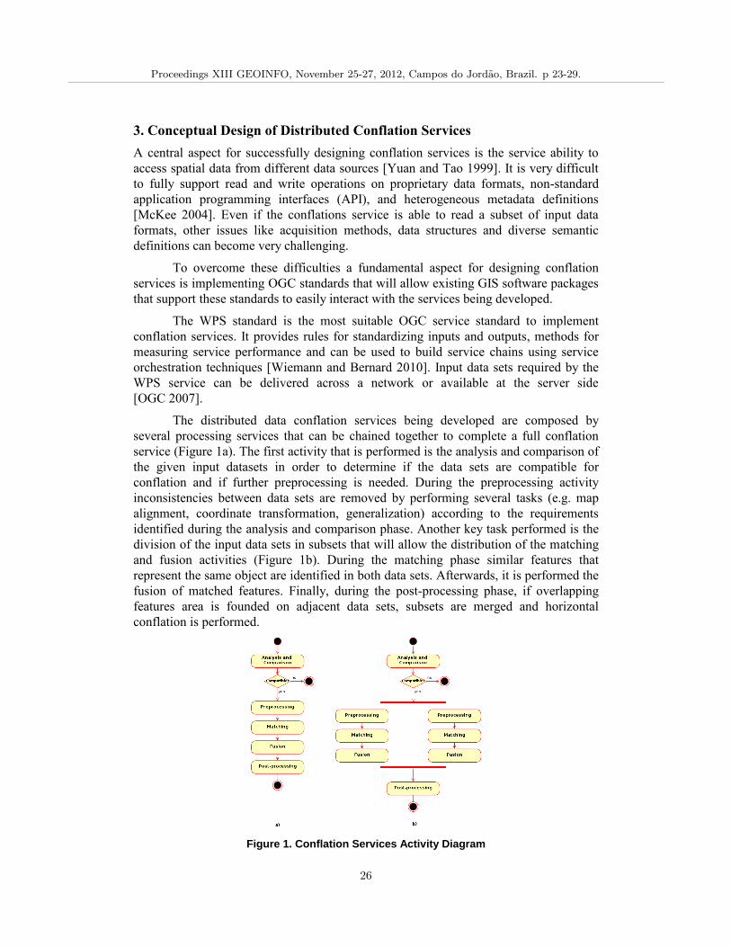
3. Conceptual Design of Distributed Conflation Services

A central aspect for successfully designing conflation services is the service ability to

access spatial data from different data sources [Yuan and Tao 1999]. It is very difficult

to fully support read and write operations on proprietary data formats, non-standard

application programming interfaces (API), and heterogeneous metadata definitions

[McKee 2004]. Even if the conflations service is able to read a subset of input data

formats, other issues like acquisition methods, data structures and diverse semantic

definitions can become very challenging.

To overcome these difficulties a fundamental aspect for designing conflation

services is implementing OGC standards that will allow existing GIS software packages

that support these standards to easily interact with the services being developed.

The WPS standard is the most suitable OGC service standard to implement

conflation services. It provides rules for standardizing inputs and outputs, methods for

measuring service performance and can be used to build service chains using service

orchestration techniques [Wiemann and Bernard 2010]. Input data sets required by the

WPS service can be delivered across a network or available at the server side

[OGC 2007].

The distributed data conflation services being developed are composed by

several processing services that can be chained together to complete a full conflation

service (Figure 1a). The first activity that is performed is the analysis and comparison of

the given input datasets in order to determine if the data sets are compatible for

conflation and if further preprocessing is needed. During the preprocessing activity

inconsistencies between data sets are removed by performing several tasks (e.g. map

alignment, coordinate transformation, generalization) according to the requirements

identified during the analysis and comparison phase. Another key task performed is the

division of the input data sets in subsets that will allow the distribution of the matching

and fusion activities (Figure 1b). During the matching phase similar features that

represent the same object are identified in both data sets. Afterwards, it is performed the

fusion of matched features. Finally, during the post-processing phase, if overlapping

features area is founded on adjacent data sets, subsets are merged and horizontal

conflation is performed.

Figure 1. Conflation Services Activity Diagram


26

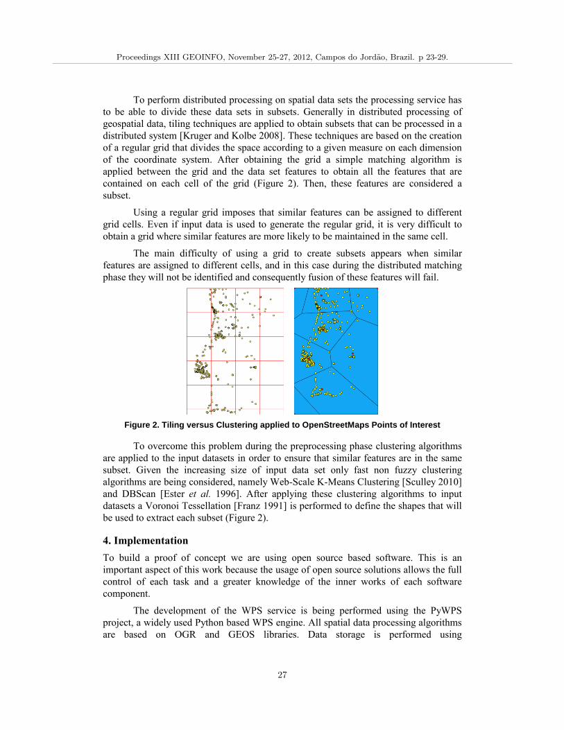
To perform distributed processing on spatial data sets the processing service has

to be able to divide these data sets in subsets. Generally in distributed processing of

geospatial data, tiling techniques are applied to obtain subsets that can be processed in a

distributed system [Kruger and Kolbe 2008]. These techniques are based on the creation

of a regular grid that divides the space according to a given measure on each dimension

of the coordinate system. After obtaining the grid a simple matching algorithm is

applied between the grid and the data set features to obtain all the features that are

contained on each cell of the grid (Figure 2). Then, these features are considered a

subset.

Using a regular grid imposes that similar features can be assigned to different

grid cells. Even if input data is used to generate the regular grid, it is very difficult to

obtain a grid where similar features are more likely to be maintained in the same cell.

The main difficulty of using a grid to create subsets appears when similar

features are assigned to different cells, and in this case during the distributed matching

phase they will not be identified and consequently fusion of these features will fail.

Figure 2. Tiling versus Clustering applied to OpenStreetMaps Points of Interest

To overcome this problem during the preprocessing phase clustering algorithms

are applied to the input datasets in order to ensure that similar features are in the same

subset. Given the increasing size of input data set only fast non fuzzy clustering

algorithms are being considered, namely Web-Scale K-Means Clustering [Sculley 2010]

and DBScan [Ester et al. 1996]. After applying these clustering algorithms to input

datasets a Voronoi Tessellation [Franz 1991] is performed to define the shapes that will

be used to extract each subset (Figure 2).

4. Implementation

To build a proof of concept we are using open source based software. This is an

important aspect of this work because the usage of open source solutions allows the full

control of each task and a greater knowledge of the inner works of each software

component.

The development of the WPS service is being performed using the PyWPS

project, a widely used Python based WPS engine. All spatial data processing algorithms

are based on OGR and GEOS libraries. Data storage is performed using


27

PostgreSQL/PostGIS, and Apache Hadoop MapReduce framework is invoked by the

WPS engine to perform distributed and scalable spatial conflation.

Distributed conflation services deployment is performed on the Amazon Web

Services (AWS) cloud based environment. The ability to create new computing

instances on demand is used to create nodes to perform Map/Reduce operations on the

Hadoop MapReduce framework.

A simple distributed point conflation service was developed using the software

stack described above. This first service implementation uses fast k-means for data

clustering, Euclidean distance for measuring geographic similarity and string based

attribute comparison for attribute matching. Features fusion is achieved using the

average between each similar feature spatial position and a full merge of feature

attributes.

This service will be further developed to support lines and polygons using

clustering algorithms adapted to this type of features and different distance calculations

techniques.

5. Conclusions

The developed concept and the simple implementation of point conflation service has

demonstrated that distributed vector based conflation services are feasible and the use of

clustering algorithms to create subsets can improve the performance of the feature

matching and fusion process on a distributed conflation service.

The definitions of the WPS service interface are important to achieve a greater

abstraction and independence between the service being developed and the clients. This

allows a greater interoperability because changing the underlying development and

deployment methods does not affect service usage.

Initial results show that distributed spatial conflation can be effortlessly achieved

if during the pre-processing phase disjoint clusters are created. However, if this is not

possible further horizontal conflation algorithms are applied to neighbor clusters before

obtaining the final data set.

The developed distributed conflation services will be used to evaluate if the

presented approach is better fitted to perform distributed conflations than using gridding

techniques to create subsets.

Current research is focused on reaching a base conflation service design that can

be used to perform distributed conflation on a cloud based environment. After this

initial phase each service activity will be further developed to increase the overall

conflation performance.

References

Kruger, A. Kolbe, T. (2008). “Mapping spatial data infrastructures to a grid environment

for optimized processing of large amounts of spatial data”, The International

Archives of the Photogrammetry, Remote Sensing and Spatial Information Sciences.

Vol. XXXXVII, Beijing, China.


28

Cobb, M. Chung, M. Miller, V. Foley, H. Petry F., and Shaw K (1998). “A Rule-Based

Approach for the Conflation of Attribute Vector Data”, GeoInformatica, 2(1), 7-35.

Dean, J. and Ghemawat, S. (2004) “MapReduce: Simplified Data Processing on Large

Clusters”, In: 6th

Symposium on Operating Systems Design and Implementation, San

Francisco, USA.

Ester M. Kriegel, H. S, J. and Xu X. (1996) “A density-based algorithm for discovering

clusters in large spatial databases with noise”. In: Proceedings of 2nd

International

Conference on Knowledge Discovery and Data Mining.

Franz A. (1991) “Voronoi diagrams – A Survey of a Fundamental Geometric Data

Structure”. In: ACM Computing Surveys 23(3), 345-405.

Giunchiglia, F. Yatskevich, M. and Shvaiko P. (2007) “Semantic Matching: Algorithms

and Implementation” In: Journal on Data Semantics IX, Springer-Verlag, Berlin, 1-

39.

Goodchild M. (2007) “Citizen and sensors: the world of volunteered geography”.

GeoJournal 69, p. 211-221. Springer Science+Bussiness Media.

Janowicz K., Raubal M. and Kuhn W. (2011) “The Semantics of Similarity in

Geographic Information Retrieval”, In: Journal of Spatial Information Science, 2, 29-

57.

McKee, L. (2004) “The Spatial Web”, White Paper, Open GIS Consortium.

McMaster, R. (1986) “A Statistical Analysis of Mathematical Measures for Linear

Simplification”, In: The America Cartographer, 13, 103-116.

OGC (2007). “OpenGIS Web Processing Services”. Open Geospatial Consortium

Editions, Version 1.0.0.

Ressler J., Freese E. and Boaten V. (2009) “Semantic Method of Conflation”. In: Terra

Cognita 2009 Workshop In Conjunction with the 8th

International Semantic Web

Conference. Washington, USA.

Wiemann S., Bernard L. (2010) “Conflation Services within Spatial Data

Infrastructures”. In: 13th

Agile International Conference on Geographic Information

Science 2010. Guimarães, Portugal.

White, M. (1981). The Theory of Geographical Data Conflation. Internal Census Bureau

draft document.

Saalfield, A. (1998) “Conflation: Automated Map Compilation”. International Journal

of Geographic Information Systems, 2(3), 217-228.

Sculley, D. (2010) “Web-scale K-Means Clustering”. In: Proceedings of WWW 2010 .


29

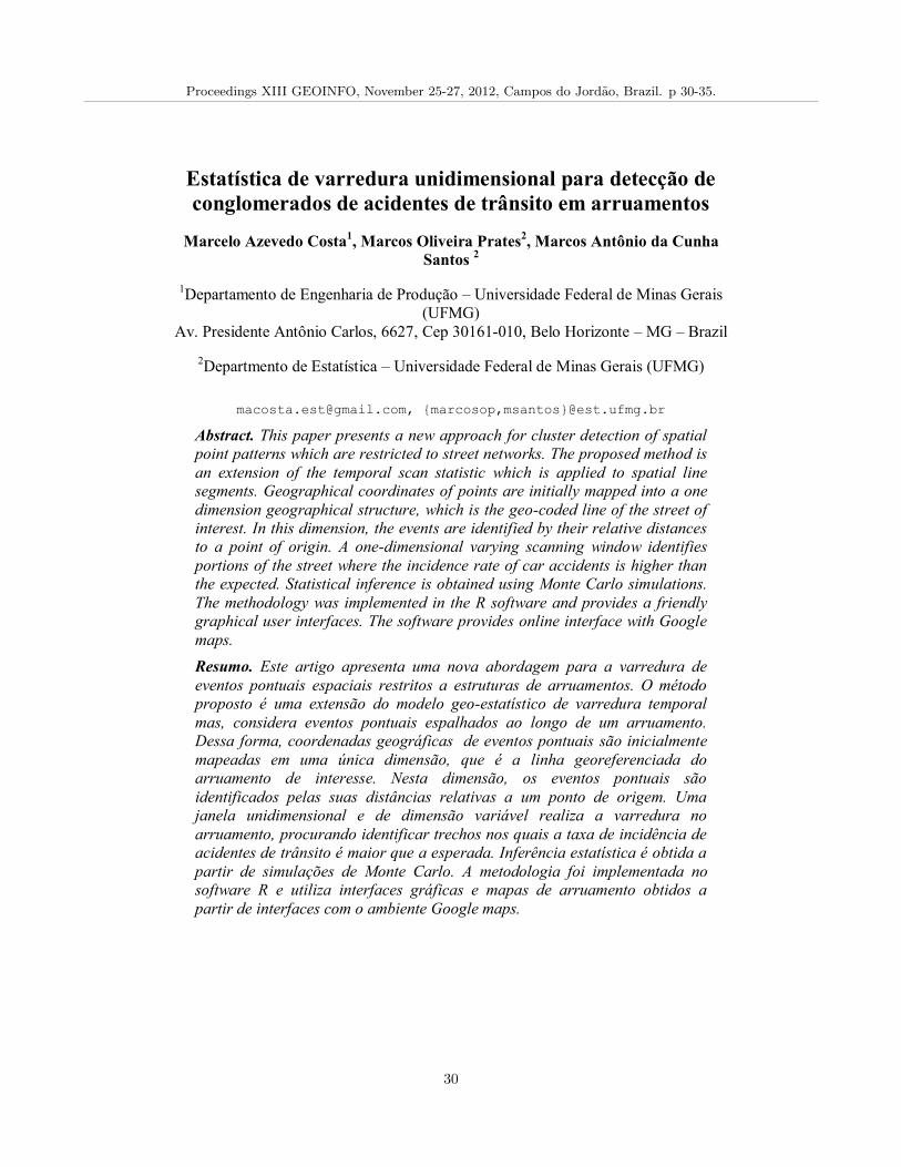
Estatística de varredura unidimensional para detecção de

conglomerados de acidentes de trânsito em arruamentos

Marcelo Azevedo Costa1, Marcos Oliveira Prates

2, Marcos Antônio da Cunha

Santos 2

1Departamento de Engenharia de Produção – Universidade Federal de Minas Gerais

(UFMG)

Av. Presidente Antônio Carlos, 6627, Cep 30161-010, Belo Horizonte – MG – Brazil

2Departmento de Estatística – Universidade Federal de Minas Gerais (UFMG)

[email protected], {marcosop,msantos}@est.ufmg.br

Abstract. This paper presents a new approach for cluster detection of spatial

point patterns which are restricted to street networks. The proposed method is

an extension of the temporal scan statistic which is applied to spatial line

segments. Geographical coordinates of points are initially mapped into a one

dimension geographical structure, which is the geo-coded line of the street of

interest. In this dimension, the events are identified by their relative distances

to a point of origin. A one-dimensional varying scanning window identifies

portions of the street where the incidence rate of car accidents is higher than

the expected. Statistical inference is obtained using Monte Carlo simulations.

The methodology was implemented in the R software and provides a friendly

graphical user interfaces. The software provides online interface with Google

maps.

Resumo. Este artigo apresenta uma nova abordagem para a varredura de

eventos pontuais espaciais restritos a estruturas de arruamentos. O método

proposto é uma extensão do modelo geo-estatístico de varredura temporal

mas, considera eventos pontuais espalhados ao longo de um arruamento.

Dessa forma, coordenadas geográficas de eventos pontuais são inicialmente

mapeadas em uma única dimensão, que é a linha georeferenciada do

arruamento de interesse. Nesta dimensão, os eventos pontuais são

identificados pelas suas distâncias relativas a um ponto de origem. Uma

janela unidimensional e de dimensão variável realiza a varredura no

arruamento, procurando identificar trechos nos quais a taxa de incidência de

acidentes de trânsito é maior que a esperada. Inferência estatística é obtida a

partir de simulações de Monte Carlo. A metodologia foi implementada no

software R e utiliza interfaces gráficas e mapas de arruamento obtidos a

partir de interfaces com o ambiente Google maps.


30

1. Introdução

A estatística de varredura espacial, proposta por Kulldorff (1997), permite a

identificação de conglomerados espaciais a partir de eventos pontuais ou eventos de

áreas. Dessa forma, a metodologia permite delinear regiões no espaço onde a

intensidade da ocorrência de um evento é maior, ou menor que o esperado. Esta

metodologia se tornou muito popular, em diversas áreas do conhecimento, como

demonstra Costa e Kulldorff (2009). Como consequência, novas abordagens tem sido

propostas, como extensões para detecção de conglomerados puramente temporais ou

espaço-temporal [Kulldorff et al. 1998; Kulldorff, 2001; Kulldorff et al., 2005]. Além

de novas metodologias que exploram variações na geometria espacial e espaço-temporal

da janela de varredura [Alm, 1997; Kulldorff, 2006; Duczmal and Assunção, 2004;

Costa et al., 2012].

Em particular, este trabalho apresenta uma nova variação da estatística de

varredura desenvolvida, a princípio, para a análise de eventos pontuais cuja ocorrência é

restrita a estruturas de arruamentos. Análises de conglomerados puramente espaciais

aplicados a dados de trânsito podem ser encontrados na literatura [Huang et al., 2009].

Entretanto, uma análise puramente espacial não permite identificar localmente, isto é, ao

longo de um arruamento específico, regiões de alta ou maior incidência de eventos

pontuais. Por um lado, um cluster puramente espacial poderá abranger diversos

arruamentos, sem que haja qualquer diferenciação com relação à contribuição dos

eventos de cada arruamento. Como consequência, um trecho de um arruamento poderá

ser caracterizado como crítico simplesmente porque a análise de conglomerado não faz

distinção quanto a esta característica. É o caso, por exemplo, de um arruamento paralelo

à uma avenida que apresenta alta incidência de eventos pontuais. Em particular, a

caracterização de trechos críticos de ruas e avenidas permitirá aos órgãos responsáveis a

criação de políticas de restrição como radares e melhorias de sinalização.

A metodologia apresentada foi desenvolvida a partir um projeto de pesquisa

envolvendo o Centro de Estudos de Criminalidade e Segurança da UFMG (CRISP) e a

Empresa de Transporte e Trânsito de Belo Horizonte (BHTRANS). Utilizando dados

georeferenciados provenientes de acidentes de trânsito ocorridos no período de 2004 a

2011, foi desenvolvida uma plataforma para consulta, visualização e análises de dados

em ambiente R. A plataforma, denominada RBHTrans possibilita ao usuário a consulta

total ou parcial da base de dados e, a partir dos dados selecionados, disponibiliza

funcionalidades de análise de mapas de kernel, moda espacial, análise descritiva de

eventos de arruamentos e a estatística de varredura linear, denominada street scan. A

plataforma utiliza os pacotes RgoogleMaps e Rgooglevis que possibilitam o acesso

online a mapas da plataforma Google maps, além da possibilidade de exportar atributos

georeferenciados para visualização em ambiente browser, como o Google Chrome ou

Mozilla Firefox. Utilizando esta plataforma, o usuário pode realizar análises de

arruamentos e visualizar os dados georeferenciados de acidentes sobrepostos a mapas de

arruamento, satélite, ou mesmo visualizações utilizando o ambiente street view do

Google maps.

2. A Estatística de Varredura Unidimensional

Seja 𝑠𝑖 um par de coordenadas espaciais, 𝑠𝑖 = (𝑥𝑖 ,𝑦𝑖), atribuídas a um 𝑖-ésimo evento

pontual espacial. Seja também 𝑖 ∈ {1, … ,𝑁}, onde 𝑁 é o número total de eventos

pontuais em um determinado arruamento. Como exemplo, a Figura 1(a) mostra as


31

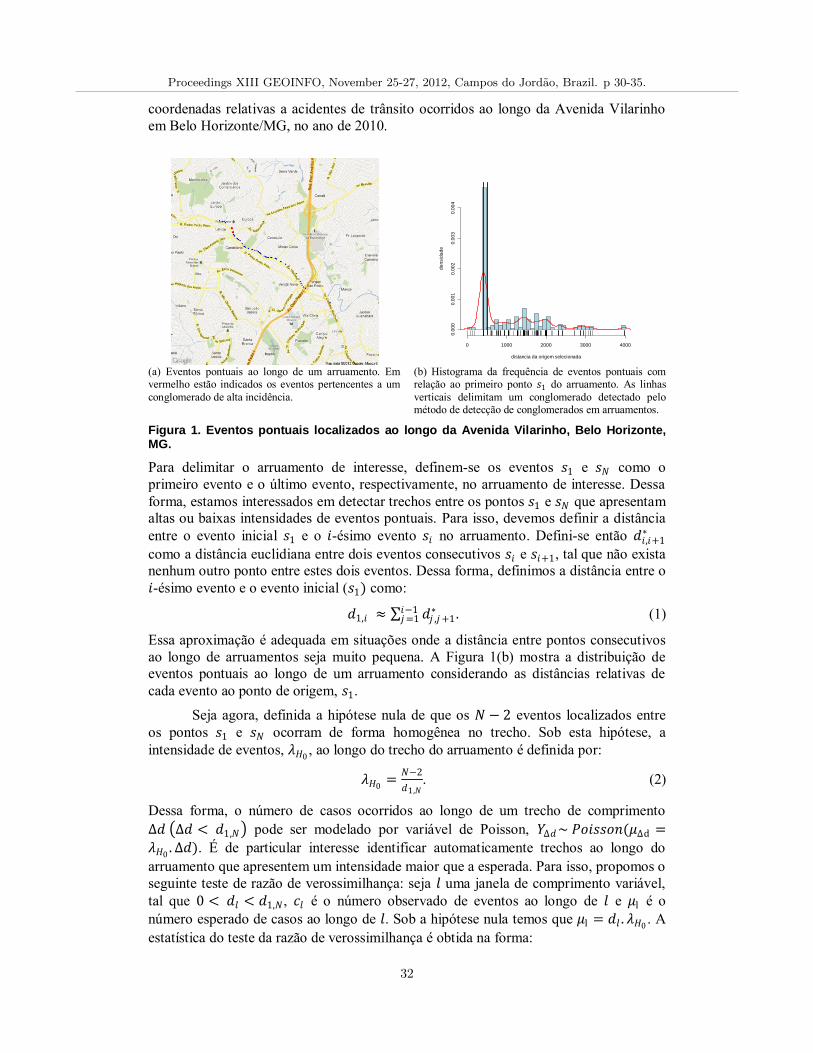
coordenadas relativas a acidentes de trânsito ocorridos ao longo da Avenida Vilarinho

em Belo Horizonte/MG, no ano de 2010.

(a) Eventos pontuais ao longo de um arruamento. Em vermelho estão indicados os eventos pertencentes a um

conglomerado de alta incidência.

(b) Histograma da frequência de eventos pontuais com relação ao primeiro ponto 𝑠1 do arruamento. As linhas

verticais delimitam um conglomerado detectado pelo método de detecção de conglomerados em arruamentos.

Figura 1. Eventos pontuais localizados ao longo da Avenida Vilarinho, Belo Horizonte, MG.

Para delimitar o arruamento de interesse, definem-se os eventos 𝑠1 e 𝑠𝑁 como o

primeiro evento e o último evento, respectivamente, no arruamento de interesse. Dessa

forma, estamos interessados em detectar trechos entre os pontos 𝑠1 e 𝑠𝑁 que apresentam

altas ou baixas intensidades de eventos pontuais. Para isso, devemos definir a distância

entre o evento inicial 𝑠1 e o 𝑖-ésimo evento 𝑠𝑖 no arruamento. Defini-se então 𝑑𝑖,𝑖+1∗

como a distância euclidiana entre dois eventos consecutivos 𝑠𝑖 e 𝑠𝑖+1, tal que não exista

nenhum outro ponto entre estes dois eventos. Dessa forma, definimos a distância entre o

𝑖-ésimo evento e o evento inicial (𝑠1) como:

𝑑1,𝑖 ≈ 𝑑𝑗 ,𝑗+1∗𝑖−1

𝑗=1 . (1)

Essa aproximação é adequada em situações onde a distância entre pontos consecutivos

ao longo de arruamentos seja muito pequena. A Figura 1(b) mostra a distribuição de

eventos pontuais ao longo de um arruamento considerando as distâncias relativas de

cada evento ao ponto de origem, 𝑠1.

Seja agora, definida a hipótese nula de que os 𝑁 − 2 eventos localizados entre

os pontos 𝑠1 e 𝑠𝑁 ocorram de forma homogênea no trecho. Sob esta hipótese, a

intensidade de eventos, 𝜆𝐻0, ao longo do trecho do arruamento é definida por:

𝜆𝐻0=

𝑁−2

𝑑1,𝑁. (2)

Dessa forma, o número de casos ocorridos ao longo de um trecho de comprimento

Δ𝑑 Δ𝑑 < 𝑑1,𝑁 pode ser modelado por variável de Poisson, 𝑌Δ𝑑~ 𝑃𝑜𝑖𝑠𝑠𝑜𝑛(𝜇Δd =

𝜆𝐻0. Δ𝑑). É de particular interesse identificar automaticamente trechos ao longo do

arruamento que apresentem um intensidade maior que a esperada. Para isso, propomos o

seguinte teste de razão de verossimilhança: seja 𝑙 uma janela de comprimento variável,

tal que 0 < 𝑑𝑙 < 𝑑1,𝑁, 𝑐𝑙 é o número observado de eventos ao longo de 𝑙 e 𝜇l é o

número esperado de casos ao longo de 𝑙. Sob a hipótese nula temos que 𝜇l = 𝑑𝑙 . 𝜆𝐻0. A

estatística do teste da razão de verossimilhança é obtida na forma:

distancia da origem selecionada

de

nsid

ad

e

0 1000 2000 3000 4000

0.0

00

0.0

01

0.0

02

0.0

03

0.0

04


32

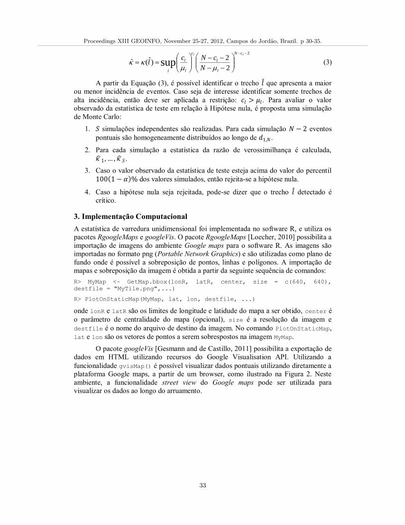
2

2

2)ˆ(ˆ sup

ll cN

l

l

c

l

l

lN

cNcl

(3)

A partir da Equação (3), é possível identificar o trecho 𝑙 que apresenta a maior

ou menor incidência de eventos. Caso seja de interesse identificar somente trechos de

alta incidência, então deve ser aplicada a restrição: 𝑐𝑙 > 𝜇𝑙 . Para avaliar o valor

observado da estatística de teste em relação à Hipótese nula, é proposta uma simulação

de Monte Carlo:

1. 𝑆 simulações independentes são realizadas. Para cada simulação 𝑁 − 2 eventos

pontuais são homogeneamente distribuídos ao longo de 𝑑1,𝑁 .

2. Para cada simulação a estatística da razão de verossimilhança é calculada,

𝜅 1 ,… , 𝜅 𝑆.

3. Caso o valor observado da estatística de teste esteja acima do valor do percentil

100 1 − 𝛼 % dos valores simulados, então rejeita-se a hipótese nula.

4. Caso a hipótese nula seja rejeitada, pode-se dizer que o trecho 𝑙 detectado é

crítico.

3. Implementação Computacional

A estatística de varredura unidimensional foi implementada no software R, e utiliza os

pacotes RgoogleMaps e googleVis. O pacote RgoogleMaps [Loecher, 2010] possibilita a

importação de imagens do ambiente Google maps para o software R. As imagens são

importadas no formato png (Portable Network Graphics) e são utilizadas como plano de

fundo onde é possível a sobreposição de pontos, linhas e polígonos. A importação de

mapas e sobreposição da imagem é obtida a partir da seguinte sequência de comandos:

R> MyMap <- GetMap.bbox(lonR, latR, center, size = c(640, 640),

destfile = "MyTile.png",...)

R> PlotOnStaticMap(MyMap, lat, lon, destfile, ...)

onde lonR e latR são os limites de longitude e latidude do mapa a ser obtido, center é

o parâmetro de centralidade do mapa (opcional), size é a resolução da imagem e

destfile é o nome do arquivo de destino da imagem. No comando PlotOnStaticMap,

lat e lon são os vetores de pontos a serem sobrespostos na imagem MyMap.

O pacote googleVis [Gesmann and de Castillo, 2011] possibilita a exportação de

dados em HTML utilizando recursos do Google Visualisation API. Utilizando a

funcionalidade gvisMap() é possível visualizar dados pontuais utilizando diretamente a

plataforma Google maps, a partir de um browser, como ilustrado na Figura 2. Neste

ambiente, a funcionalidade street view do Google maps pode ser utilizada para

visualizar os dados ao longo do arruamento.


33

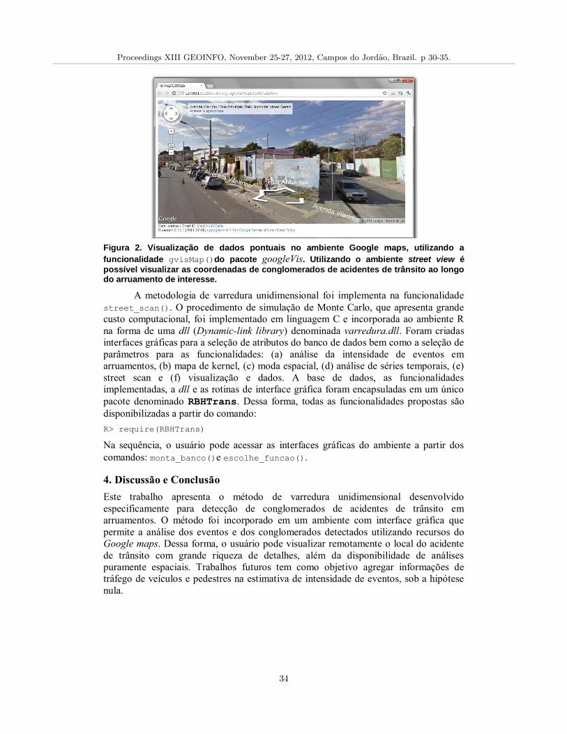
Figura 2. Visualização de dados pontuais no ambiente Google maps, utilizando a

funcionalidade gvisMap()do pacote googleVis. Utilizando o ambiente street view é

possível visualizar as coordenadas de conglomerados de acidentes de trânsito ao longo do arruamento de interesse.

A metodologia de varredura unidimensional foi implementa na funcionalidade

street_scan(). O procedimento de simulação de Monte Carlo, que apresenta grande

custo computacional, foi implementado em linguagem C e incorporada ao ambiente R

na forma de uma dll (Dynamic-link library) denominada varredura.dll. Foram criadas

interfaces gráficas para a seleção de atributos do banco de dados bem como a seleção de

parâmetros para as funcionalidades: (a) análise da intensidade de eventos em

arruamentos, (b) mapa de kernel, (c) moda espacial, (d) análise de séries temporais, (e)

street scan e (f) visualização e dados. A base de dados, as funcionalidades

implementadas, a dll e as rotinas de interface gráfica foram encapsuladas em um único

pacote denominado RBHTrans. Dessa forma, todas as funcionalidades propostas são

disponibilizadas a partir do comando:

R> require(RBHTrans)

Na sequência, o usuário pode acessar as interfaces gráficas do ambiente a partir dos

comandos: monta_banco()e escolhe_funcao().

4. Discussão e Conclusão

Este trabalho apresenta o método de varredura unidimensional desenvolvido

especificamente para detecção de conglomerados de acidentes de trânsito em

arruamentos. O método foi incorporado em um ambiente com interface gráfica que

permite a análise dos eventos e dos conglomerados detectados utilizando recursos do

Google maps. Dessa forma, o usuário pode visualizar remotamente o local do acidente

de trânsito com grande riqueza de detalhes, além da disponibilidade de análises

puramente espaciais. Trabalhos futuros tem como objetivo agregar informações de

tráfego de veículos e pedestres na estimativa de intensidade de eventos, sob a hipótese

nula.


34

Bibliografia

Alm, S. E. (1997). On the distributions of scan statistics of a two dimensional Poisson

process, Advances in Applied. Probability, vol. 29, pages 1–18.

Costa, M. A. and Kulldorff, M. (2009). In Scan statistics: methods and applications.

Birkkäuser: Statistics for Industry and Technology, pages 129–52 [chapter 6].

Costa, M. A. and Assunção, R. A. and Kulldorff, M. (2012). Constrained spanning tree

algorithms for irregularly-shaped spatial clustering. Computational Statistics and

Data Analysis. vol. 56, pages 1771–1783.

Duczmal, L. and Assunção, R. A. (2004). Simulated annealing strategy for the detection

of arbitrarily shaped spatial clusters, Computational Statistics and Data Analysis,

vol. 45, pages 269–286.

Gesmann, Markus and de Castillo, Diego (2011). Using the Google Visualisation API

with R. The R Journal. vol. 3, n. 2, pages 40–44.

Huang, L. and Stinchcomb, D. G. and Pickle, L. W. and Dill, J. (2009). Identifying

clusters of active transportation using spatial scan statistics. American Journal of

Preventive Medicine. vol. 37, n. 2, pages 157–166.

Kulldorff, M. (1997). A spatial scan statistic. Communications in Statistics: Theory and

Methods, vol. 26, pages 1481–1496.

Kulldorff, M. and Athas, W. and Feuer, E. and Miller, B. and Key, C. (1998).

Evaluating cluster alarms: A space-time scan statistic and brain cancer in Los

Alamos. American Journal of Public Health, vol. 88, pages 1377–1380.

Kulldorff, M. (2001). Prospective time-periodic geographical disease surveillance using

a scan statistic. Journal of the Royal Statistical Society, vol. A164, pages 61–72.

Kulldorff, M. and Heffernan, R. and Hartman, J. and Assunção, R. M. and Mostashari,

F. (2005). A space-time permutation scan statistic for the early detection of disease

outbreaks. PLoS Medicine, vol. 2, pages 216–224.

Kulldorff, M. and Huang, L. and Pickle, L. and Duczmal, L. (2006). An elliptic spatial

scan statistic. Statistics in Medicine, vol. 25, pages 3929–3943.

Loecher, Markus (2010). Plotting on Google Static Maps in R. Technical Report,


35

Geocodificação de endereços urbanos com indicação de qualidade

Douglas Martins1, Clodoveu A. Davis Jr.1, Frederico T. Fonseca2 1Departamento de Ciência da Computação – Universidade Federal de Minas Gerais

Av. Presidente Antônio Carlos, 6627 – 31270-010 – Belo Horizonte – MG

2College of Information Sciences and Technology – The Pennsylvania State University 332 IST Building – 16802-6823 – University Park – PA – USA [dougmf,clodoveu]@dcc.ufmg.br, [email protected]

Abstract. Urban addresses are one of the most important ways to express a geographic location in cities. Many conventional information systems have attributes for addresses in order to include an indirect reference to space. Obtaining coordinates from addresses is one of the most important geocoding methods. Such activity is hindered by frequent variations in the addresses, such as abbreviations and missing components. This paper presents a geocoding method for urban addresses, in which address fragments are recognized from the input and a reference geographic database is searched for matching addresses for the corresponding coordinates. Output includes a geographic certainty indicator, which informs the expected quality of the results. An experimental evaluation of the method is presented.

Resumo. Endereços urbanos são uma das principais formas de expressão da localização geográfica em cidades. Muitos sistemas de informação incluem atributos para receber endereços e, assim, contam com uma referência espacial indireta. A obtenção de coordenadas a partir de endereços é um dos métodos de geocodificação mais importantes, mas é dificultada por variações comuns no endereço, como abreviações e omissão de componentes. O artigo apresenta um método de geocodificação de endereços urbanos, que reconhece fragmentos do endereço na entrada e realiza buscas em um banco de dados geográfico de referência, para retornar coordenadas. O resultado é acompanhado de um indicador de certeza geográfica, que indica a expectativa de acerto. Uma avaliação experimental do método é apresentada.

1. Introdução A utilização de sistemas digitais para serviços de pesquisa, visualização de mapas, localização espacial em tempo real, está se tornando cada vez mais comum. Usuários com diversos níveis de conhecimento têm acesso fácil e rápido a esses tipos de sistemas. Esse fato traz alguns desafios para o desenvolvimento e manutenção desses sistemas, pois o ambiente, antes restrito, necessita acomodar diversos tipos de usuários com diferentes concepções sobre como realizar e buscar referências espaciais. Dentre os diversas tipos de referências espaciais, destaca-se a realizada através de endereços postais ou urbanos. Esses endereços são compostos de fragmentos com significados diversos, como tipo do logradouro (rua, avenida, etc.), nome do logradouro,


36

número da edificação, bairro ou região, cidade, estado, país, código postal, etc. O uso de endereços na remessa de correspondências e na localização de pontos de interesse é rotineiro e amplamente conhecido, especialmente em cidades. Por esse motivo, endereços são usualmente incluídos como atributos em sistemas de informação convencionais. Existindo a possibilidade de obter coordenadas geográficas a partir de endereços, numa atividade conhecida como geocodificação (Goldberg, Wilson et al. 2007), tais sistemas de informação podem passar a ser geográficos. Nem todos os sistemas de informação convencionais criam atributos diferenciados para os componentes do endereço, e é comum que o endereço seja armazenado como uma expressão textual livre (Eichelberger 1993; Davis Jr., Fonseca et al. 2003). Apesar da referência espacial por endereços urbanos seguir um padrão, não existem regras rígidas sobre a ordem que os componentes devem ser apresentados ou sobre elementos de separação (Rhind 1999). Isso gera dois problemas: identificação dos fragmentos de um endereço e realização de buscas a partir dos dados identificados para encontrar os resultados mais relevantes em um banco de dados de referência. Considerando esses fatores de incerteza e possíveis causas de erros (abreviações, erros de grafia, variações de formato, entre outras), é importante que o processo de geocodificação incorpore uma medida do grau de certeza que se tem quanto ao resultado. O presente trabalho implementa e avalia um método de geocodificação de endereços urbanos proposto anteriormente (Davis Jr. and Fonseca 2007), que não apresenta uma implementação nem uma análise experimental da consistência dos resultados. O artigo está organizado da seguinte forma. A Seção 2 apresenta trabalhos relacionados, com ênfase no método de geocodificação implementado. A Seção 3 apresenta detalhes sobre a implementação e técnicas utilizadas para torná-la computacionalmente mais eficiente. A Seção 4 traz uma avaliação experimental do método. Finalmente, a Seção 5 apresenta conclusões e trabalhos futuros.

2. Trabalhos relacionados Geocodificação é um conjunto de métodos capazes de transformar descrições em coordenadas geográficas. Essas descrições são, em geral, nomes de lugares, expressões de posicionamento relativo ou endereços, que constituem o caso mais comum. No caso de nomes de lugares, dicionários toponímicos (ou gazetteers) são utilizados para reconhecimento, desambiguação e localização (Hill 2000; Goodchild and Hill 2008; Machado, Alencar et al. 2011). Expressões de posicionamento relativo relacionam um lugar alvo a um lugar conhecido (ponto de referência), utilizando termos em linguagem natural (Delboni, Borges et al. 2007), como, por exemplo “hotel próximo à Praça da Liberdade, Belo Horizonte”. No caso de endereços, existe uma expectativa de detalhamento hierárquico, com componentes que indicam o país, o estado, a cidade, o bairro e o logradouro, além de um código postal que sumariza esses dados. O formato de apresentação desses componentes varia de país para país, e em muitas situações, alguns componentes são intencionalmente omitidos ou simplificados. Para contornar essa variabilidade na formação dos endereços, uma solução consiste na divisão do método em três passos ou estágios, conforme proposto por Davis e Fonseca (2007), sendo que cada estágio possui tarefas e interfaces de entrada e saída bem definidas. O primeiro estágio, chamado de parsing, consiste na análise léxica que leve em conta as peculiaridades da estrutura de endereços do local ou país e posterior


37

conversão da entrada textual contendo o endereço em uma estrutura de dados genérica. Essa estrutura de dados contém um número finito de atributos, que correspondem a cada componente do endereço. O segundo estágio, chamado de matching, recebe a estrutura de dados e realiza buscas em um banco de dados de referência, comparando valores por casamento exato ou aproximado de strings e valores numéricos, e definindo a melhor solução em caso de casamento parcial. O estágio seguinte, denominado locating, consiste em recuperar as referências obtidas e extrair delas as coordenadas desejadas. Um problema na geocodificação de endereços é medir a precisão dos resultados obtidos ao fim dos três estágios. O Geocoding Certainty Indicator (GCI) (Davis Jr. and Fonseca 2007), representa um método para calcular a precisão e realizar a classificação dos resultados de forma a atender as necessidades do usuário do sistema. Esse índice é composto por três índices, um para cada estágio do processo de geocodificação: Parsing Certainty Indicator (PCI), Matching Certainty Indicator (MCI) e Locating Certainty Indicator (LCI). Em cada estágio, esses índices recebem um valor entre 0 e 1, em que 0 representa total incerteza no resultado, enquanto 1 representa máxima certeza. Esse valor é baseado em várias regras, envolvendo casamento aproximado de componentes do endereço com bonificação de acertos e desconto de erros dentre os resultados pesquisados. O GCI final é obtido através do produto dos indicadores de cada estágio.

3. Implementação da geocodificação com avaliação da qualidade Seguindo o objetivo do presente trabalho, foi implementado o método de geocodificação proposto por Davis e Fonseca (2007), seguindo o modelo de três estágios, e utilizando o GCI para calcular o grau de certeza quanto aos resultados encontrados. As subseções a seguir descrevem detalhes sobre a implementação de cada etapa. Para maiores informações sobre o método em si, consultar o artigo original.

3.1 Estágio de Parsing O estágio de parsing consiste em um método para identificar componentes de endereços e organizá-los em uma estrutura de dados apropriada. Para o trabalho, o método foi implementado de forma a reconhecer e estruturar entradas textuais de endereços no formato de endereço utilizado no Brasil. Esse formato possui os seguintes componentes: tipo de logradouro, nome do logradouro, número da edificação dentro de um logradouro, nome do bairro, região ou subseção de um município ou distrito, município, estado, país e código postal. Existem ainda outros atributos, tais como o nome do edifício e complementos de um endereço, porém esses atributos não estão comumente presentes ou não têm muita relevância para efeito de localização. Para realizar o reconhecimento dos campos, o método utiliza um analisador léxico juntamente com uma análise sintática sobre os tokens produzidos. Essa análise procura padrões textuais que se encaixem com os campos tipo de logradouro, nome do logradouro, número da construção dentro de um logradouro e nome de região ou subseção. A análise conta com três tabelas auxiliares, que contêm um conjunto de valores usuais para tipos de logradouros, de regiões e de identificadores numéricos utilizados no endereçamento brasileiro. Além de reconhecer esses componentes, o método supõe que o restante dos tokens representem localizações genéricas, que podem ser bairros, municípios, estados e países, mas a interpretação desses campos é deixada a cargo do estágio de matching. Ao fim do processo, o parsing produz uma estrutura de


38

dados organizada contendo os componentes de endereços identificados na entrada textual.

3.2 Estágio de Matching Em seguida, passamos ao estágio de matching, que consiste em pesquisar o valor dos campos identificados em um banco de dados de endereços a fim de realizar o melhor casamento entre os valores identificados e os dados presentes no banco de dados. O estágio foi subdividido em quatro etapas: reconhecimento de termos de localização genéricos não classificados ou não identificados no estágio de parsing; busca primária no banco de dados por valores que casem com campos identificados; busca complementar no banco de dados para acertar e acrescentar valores aos campos da estrutura; e aplicação de filtros numéricos sobre os resultados das etapas anteriores. A primeira etapa do estágio de matching procura, dentro dos atributos de localização genérica, valores que casem com os nomes de regiões, bairros e municípios (e respectivos estados) presentes no banco de dados. Conforme o caso, os dados genéricos são transformados em nome de região ou subseção (bairros). Após o reconhecimento desses componentes, a estrutura de endereços estará completamente identificada, restando obter o casamento do nome de logradouro. A segunda etapa consiste em realizar busca no banco de dados utilizando casamento aproximado de strings sobre o atributo de nome do logradouro. O algoritmo para classificar os resultados utiliza dois métodos conhecidos na literatura: distância de Levenshtein (ou distancia de edição) e shift-and aproximado (Navarro 2001). Ambos os métodos são combinados para realizar o casamento aproximado de palavras para nomes pessoais ou geográficos. Ao fim dessa etapa, um conjunto de candidatos são obtidos para prosseguir para próxima etapa. A terceira etapa recebe esses candidatos e complementa o restante dos atributos não preenchidos na busca primária com valores vindos do banco de dados. A quarta etapa consiste em determinar valor numérico mais aproximado para o número do imóvel, caso este não tenha sido localizado. Ou seja, esta etapa realiza um filtro sobre todos os números de um logradouro e escolhe aquele que possui menor distância numérica entre o valor informado e os valores existentes. Ao longo das quatro etapas, dois indicadores que compõem o GCI são calculados. Na segunda etapa é calculado o MCI, que mede o nível de aproximação entre entrada e resultado decorrente do casamento aproximado dos strings. Na terceira etapa, após complementar os dados dos candidatos, é calculado o PCI, utilizando o casamento aproximado de palavras para cada campo do candidato em relação ao campo presente na estrutura de dados resultante do estágio de parsing.

3.3 Estágio de Locating O estágio de locating consiste em receber os resultados do estágio matching e extrair coordenadas correspondentes do banco de dados de referência. Como o método apenas transforma os dados, o indicador desse estágio sempre tem valor LCI = 1 nesta implementação, e portanto o valor final do GCI é igual ao produto de PCI e MCI.

4. Avaliação experimental Um conjunto de dados contendo entradas textuais de endereços não padronizados da cidade de Belo Horizonte foi utilizado para verificar a eficácia da implementação do


39

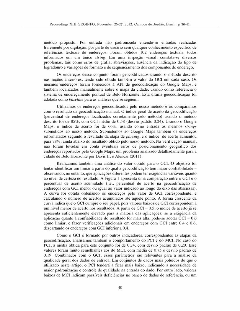
método proposto. Por entrada não padronizada entende-se entradas realizadas livremente por digitação, por parte de usuário sem qualquer conhecimento especifico de referências textuais de endereços. Foram obtidos 102 endereços textuais, todos informados em um único string. Em uma inspeção visual, constata-se diversos problemas, tais como erros de grafia, abreviações, ausência da indicação do tipo de logradouro e variações de formato e de sequenciamento dos componentes do endereço. Os endereços desse conjunto foram geocodificados usando o método descrito nas seções anteriores, tendo sido obtido também o valor do GCI em cada caso. Os mesmos endereços foram fornecidos à API de geocodificação do Google Maps, e também localizados manualmente sobre o mapa da cidade, usando como referência o sistema de endereçamento pontual de Belo Horizonte. Esta última geocodificação foi adotada como baseline para as análises que se seguem. Utilizamos os endereços geocodificados pelo nosso método e os comparamos com o resultado da geocodificação manual. O índice geral de acerto da geocodificação (percentual de endereços localizados corretamente pelo método) usando o método descrito foi de 85%, com GCI médio de 0,58 (desvio padrão 0,24). Usando o Google Maps, o índice de acerto foi de 66%, usando como entrada os mesmos strings submetidos ao nosso método. Submetemos ao Google Maps também os endereços reformatados segundo o resultado da etapa de parsing, e o índice de acerto aumentou para 78%, ainda abaixo do resultado obtido pelo nosso método. Na verificação manual, não foram levadas em conta eventuais erros de posicionamento geográfico dos endereços reportados pelo Google Maps, um problema analisado detalhadamente para a cidade de Belo Horizonte por Davis Jr. e Alencar (2011). Realizamos também uma análise do valor obtido para o GCI. O objetivo foi tentar identificar um limiar a partir do qual a geocodificação tem maior confiabilidade – observando, no entanto, que aplicações diferentes podem ter exigências variáveis quanto ao nível de certeza no resultado. A Figura 1 apresenta uma comparação entre o GCI e o percentual de acerto acumulado (i.e., percentual de acerto na geocodificação de endereços com GCI menor ou igual ao valor indicado ao longo do eixo das abscissas). A curva foi obtida ordenando os endereços pelo valor de GCI correspondente, e calculando o número de acertos acumulados até aquele ponto. A forma crescente da curva indica que o GCI cumpre o seu papel, pois valores baixos de GCI correspondem a um nível menor de acerto nos resultados. A partir de GCI = 0,5, o índice de acerto já se apresenta suficientemente elevado para a maioria das aplicações; se a exigência da aplicação quanto à confiabilidade do resultado for mais alta, pode-se adotar GCI = 0,6 como limiar, e fazer verificações adicionais em endereços com GCI entre 0,4 e 0,6, descartando os endereços com GCI inferior a 0,4. Como o GCI é formado por outros indicadores, correspondentes às etapas da geocodificação, analisamos também o comportamento do PCI e do MCI. No caso do PCI, a média obtida para este conjunto foi de 0,74, com desvio padrão de 0,20. Esse valores foram muito semelhantes aos do MCI, com média de 0,75 e desvio padrão de 0,19. Combinados com o GCI, esses parâmetros são relevantes para a análise da qualidade geral dos dados de entrada. Em conjuntos de dados mais poluídos do que o utilizado neste artigo, o PCI tenderá a ficar mais baixo, indicando a necessidade de maior padronização e controle de qualidade na entrada do dado. Por outro lado, valores baixos de MCI indicam possíveis deficiências no banco de dados de referência, ou um


40

acúmulo de dificuldades com nomes de logradouros ambíguos. Os valores do GCI indicam a composição desses fatores no resultado final da geocodificação.

Figura 1 - GCI versus índice de acerto

5. Conclusões O presente artigo apresentou uma implementação do método de geocodificação com verificação de confiabilidade (Davis Jr. and Fonseca 2007), acompanhada de uma verificação experimental do comportamento dos indicadores de qualidade. Os resultados foram comparados com a geocodificação oferecida na API do Google Maps, e aferidos por verificação manual. Pela análise realizada, os indicadores de qualidade da geocodificação são úteis e relevantes para as aplicações, cumprindo o papel indicado no artigo que os propôs. Trabalhos futuros envolvem a realização de avaliações mais aprofundadas, utilizando dados de entrada de qualidade variável e em maior quantidade, e a aplicação do método em situações reais, frequentemente encontradas em áreas tais como saúde pública, epidemiologia, logística e outras.

Referências Davis Jr, C.A. and Alencar, R.O. (2011). "Evaluation of the quality of an online geocoding resource in the

context of a large Brazilian city." Transactions in GIS 15(6): 851-868. Davis Jr., C.A., Fonseca, F. and Borges, K.A.V. (2003). A flexible addressing system for approximate

urban geocoding. V Simpósio Brasileiro de GeoInformática (GeoInfo 2003), Campos do Jordão (SP):em CD-ROM.

Davis Jr., C.A. and Fonseca, F.T. (2007). "Assessing the Certainty of Locations Produced by an Address Geocoding System." Geoinformatica 11(1): 103-129.

Delboni, T.M., Borges, K.A.V., Laender, A.H.F. and Davis Jr., C.A. (2007). "Semantic Expansion of Geographic Web Queries Based on Natural Language Positioning Expressions." Transactions in GIS 11(3): 377-397.

Eichelberger, P. (1993). The Importance of Addresses - The Locus of GIS. URISA 1993 Annual Conference, Atlanta, Georgia, URISA:200-211.

Goldberg, D.W., Wilson, J.P. and Knoblock, C.A. (2007). "From Text to Geographic Coordinates: The Current State of Geocoding." URISA Journal 19(1): 33-46.

Goodchild, M.F. and Hill, L.L. (2008). "Introduction to digital gazetteer research." International Journal of Geographic Information Science 22(10): 1039-1044.

Hill, L.L. (2000). Core Elements of Digital Gazetteers: Placenames, Categories, and Footprints. 4th European Conference on Research and Advanced Technology for Digital Libraries:280-290.

Machado, I.M.R., Alencar, R.O., Campos Junior, R.O. and Davis Jr, C.A. (2011). "An ontological gazetteer and its application for place name disambiguation in text." Journal of the Brazilian Computer Society 17(4): 267-279.

Navarro, G. (2001). "A Guided Tour to Approximate String Matching." ACM Computing Surveys 33(1): 31-88.

Rhind, G. (1999). Global Sourcebook of Address Data Management: A Guide to Address Formats and Data in 194 Countries Gower.


41

Acessibilidade em mapas urbanos para portadores de

deficiência visual total

Simone I. R. Xavier, Clodoveu A. Davis Jr.

Departamento de Ciência da Computação – UFMG

Belo Horizonte, MG – Brasil

[simone.xavier, clodoveu]@dcc.ufmg.br

Resumo. Um dos Grandes Desafios para a Computação brasileira é garantir

o acesso participativo e universal do cidadão brasileiro ao conhecimento. No

entanto, ainda hoje, a maior parte das informações geográficas contidas em

mapas na Web está disponível apenas através de imagens, que não são

acessíveis para pessoas com deficiência visual total. Tais pessoas contam com

recursos, tais como síntese de voz e leitura de textos na tela, que não são

facilmente adaptáveis para o conteúdo geográfico. Este artigo apresenta um

sistema em desenvolvimento que tem como principal objetivo tornar as

informações contidas em mapas de ruas e avenidas acessíveis para essas

pessoas, possibilitando que elas explorem o conteúdo geográfico e naveguem

no espaço urbano de acordo com o seu interesse.

1. Introdução

No mundo há 314 milhões de pessoas com deficiências visuais (PCDVs) e cerca de 45

milhões de pessoas incapazes de enxergar [OMS, 2010]. No Brasil, de acordo com o

Censo 2010 do Instituto Brasileiro de Geografia e Estatística (IBGE), esses números

também são significativos: há 6,5 milhões de pessoas com algum grau de deficiência

visual e, entre elas, 528 mil são não enxergam. Entretanto, essas pessoas ainda

encontram uma série de dificuldades para utilizar sistemas informatizados e ter acesso

aos recursos que estão disponíveis para aqueles que não possuem essa deficiência.

Tendo em vista a importância do incentivo a pesquisas que contribuam para essa área, a

Sociedade Brasileira de Computação (SBC) incluiu essa questão dentro do quarto

Grande Desafio para a pesquisa em Ciência da Computação para a década de 2006 a

2016 [SBC, 2006], que trata do “Acesso participativo e universal do cidadão brasileiro

ao conhecimento”.

Atualmente os mapas fazem parte do cotidiano das pessoas, estando presentes na

televisão, em jornais, revistas e na Internet. Isso contribuiu fortemente para a

popularização do acesso à informação geográfica [Nogueira, 2010]. As PCDVs podem

utilizar o computador de forma independente com o auxílio de sistemas leitores de tela.

Esses programas permitem que o usuário interaja com o computador utilizando apenas o

teclado, e sua principal função é fazer uma síntese do som correspondente ao texto que é

exibido ao usuário, retornando todo o feedback em áudio. No entanto, quando

informações são exibidas apenas através de imagens, sem um texto correspondente, os

sites e aplicativos se tornam inacessíveis para essas pessoas. Isso é o que acontece com

os mapas na Web. Como são renderizados, em geral, por meio de imagens, mesmo o

texto contido nos mapas é inacessível para os leitores de tela.


42

Considerando esse contexto, este trabalho apresenta a implementação de uma forma

alternativa para apresentação de mapas na Web [Xavier e Miranda, 2010], na qual as

informações geográficas são também exibidas de forma textual, sendo, portanto,

acessíveis para os usuários de leitores de tela. A proposta consiste na utilização de

recursos da Web para proporcionar uma experiência interativa, permitindo que o usuário

possa se aprofundar nas informações geográficas de acordo com seu interesse. Este

artigo descreve a implementação de um protótipo de um sistema Web, utilizando um

banco de dados geográfico contendo ruas e avenidas da cidade de Belo Horizonte (MG),

que permite a navegação pelo mapa. Naturalmente, o conceito pode ser estendido a

outras cidades, bastando apenas acrescentar dados do arruamento.

O objetivo do aplicativo apresentado é contribuir para aumentar o acesso às informações

contidas em mapas para PCDVs. A ideia principal do sistema é possibilitar que uma

PCDV interaja com o mapa informando um endereço inicial e explorando as ruas e

avenidas próximas de forma livre. O software apresenta uma contribuição de caráter

informativo, reorganizando e apresentando de forma acessível o conhecimento que seria

equivalente a “olhar para o mapa”, no caso de uma pessoa sem deficiência.

O artigo está organizado da seguinte forma. A Seção 2 apresenta trabalhos relacionados.

Em seguida, a Seção 3 traz detalhes sobre o aplicativo desenvolvido. Na Seção 4 são

explicadas as medidas tomadas para tornar o sistema acessível. Por fim, na Seção 5 é

feita a conclusão e apresentadas possibilidades de trabalhos futuros.

2. Trabalhos relacionados

Em um estudo anterior [Xavier e Miranda, 2010], foi realizada uma pesquisa com

proposta semelhante, porém ao invés do uso de um banco de dados geográfico próprio,

foi utilizada a Application Program Interface (API) do Google Maps1 para obtenção de

dados urbanos. No entanto, para obter os dados necessários para possibilitar ao usuário

a navegação no mapa a cada cruzamento utilizando essa API, foi necessária a utilização

de uma heurística, e em vários casos o sistema não apresentava as informações

corretamente. Outra dificuldade encontrada é que era necessário tratar o texto retornado

pela API para apresentação dos dados de forma significativa para o usuário, e qualquer

mudança que ocorresse na API quanto ao formato de retorno do texto poderia acarretar

no mau funcionamento do sistema. Nesse estudo a interface passou por vários

validadores de acessibilidade automáticos e ainda pelo teste com dois usuários,

confirmando que a interface era acessível.

Wasserburger et al. (2011) apresentaram também uma proposta parecida, que consistia

em mapas para PCDVs na Web apresentados de forma textual e interativa, utilizando

OpenStreetMaps como fonte de dados. Porém, no trabalho não foram abordados

detalhes nem da implementação e nem da interface, sendo apresentado apenas uma

visão geral do que foi desenvolvido. Com exceção do estudo apresentado por Xavier e

Miranda (2010), esse foi o único artigo encontrado que trata de mapas na Web para

PCDVs. O uso de texto para apresentar informações geográficas também foi abordado

em uma investigação preliminar apresentada por Thomas (2012), porém não foi tratada

a possibilidade de uso desse recurso de forma interativa na Web.

1 http://code.google.com/intl/pt-BR/apis/maps/documentation/javascript/


43

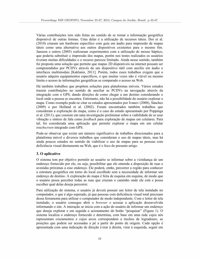
Várias contribuições tem sido feitas no sentido de se tornar a informação geográfica

disponível de outras formas. Uma delas é a utilização de recursos táteis. Doi et al.

(2010) criaram um hardware específico com guia em áudio para impressão de mapas

táteis como uma alternativa aos outros dispositivos existentes para o mesmo fim.

Jansson e outros (2005) realizaram experimentos com a utilização de mouse háptico,

que poderia substituir a impressão dos mapas, porém nos testes realizados os usuários

tiveram muitas dificuldades e o recurso pareceu limitado. Ainda nesse sentido, também

foi proposta uma solução que permite que mapas 2D disponíveis na internet possam ser

compreendidos por PCDVs através de um dispositivo tátil com auxílio em áudio e

interfaces multimodais [Kaklanis, 2011]. Porém, todos esses trabalhos exigem que o

usuário adquira equipamentos específicos, o que muitas vezes não é viável ou mesmo

limita o acesso às informações geográficas se comparado o acesso na Web.

Há também trabalhos que propõem soluções para plataformas móveis. Vários estudos

trazem contribuições no sentido de auxiliar as PCDVs na navegação através da

integração com o GPS, dando direções de como chegar a um destino considerando o

local onde a pessoa se encontra. Entretanto, não há a possibilidade do usuário explorar o

mapa. Como exemplo pode-se citar os estudos apresentados por Ivanov (2008), Sánchez

(2009) e por Holland et al. (2002). Foram encontrados também trabalhos que

consideram a exploração do mapa, como é o caso do estudo apresentado por Poppinga

et al. (2011), que consiste em uma investigação preliminar sobre a viabilidade de se usar

vibração e síntese de fala como feedback para exploração de mapas em celulares. Para

tal, foi considerada uma aplicação que permite explorar o mapa em um celular

touchscreen integrado com GPS.

Pode-se observar que existe um número significativo de trabalhos direcionados para a

plataforma móvel e diversos trabalhos que consideram o uso de mapas táteis, mas há

ainda poucos estudos no sentido de viabilizar o uso de mapas para as pessoas com

deficiência visual diretamente na Web, que é o foco do presente artigo.

3. O aplicativo

O sistema tem por objetivo permitir ao usuário se informar sobre a vizinhança de um

endereço fornecido por ele, ou seja, possibilitar que ele entenda a disposição de ruas e

avenidas próximas a esse endereço. Ele poderá, então, percorrer a região para conhecer

a estrutura geográfica em torno do local escolhido sem a necessidade de informar um

endereço de destino. A exploração do mapa é feita de esquina em esquina, de modo que

o usuário possa perceber todas as ruas que cruzam o caminho onde ele está e possa

escolher qual delas deseja percorrer.

Para utilização do sistema, o usuário já deverá possuir um leitor de tela instalado no

computador, o que é algo esperado, já que pessoas com deficiência visual total precisam

dessa ferramenta para utilizar o computador de modo independente. Com o leitor de tela

instalado, o usuário consegue abrir o browser e acessar a aplicação desenvolvida

informando o site. A interação se inicia com a ação do usuário de informar um endereço

que deseja explorar e em seguida o acionamento do botão “pesquisar” (Figura 1). O

sistema localiza o endereço fornecido e determina, com base em uma rede cujos nós

representam cruzamentos e cujos arcos correspondem a trechos de logradouro, as

posições que podem ser acessadas a pé a partir do ponto de origem. Cada opção é

apresentada com uma indicação de direção (virar à direita, virar à esquerda, seguir em


44

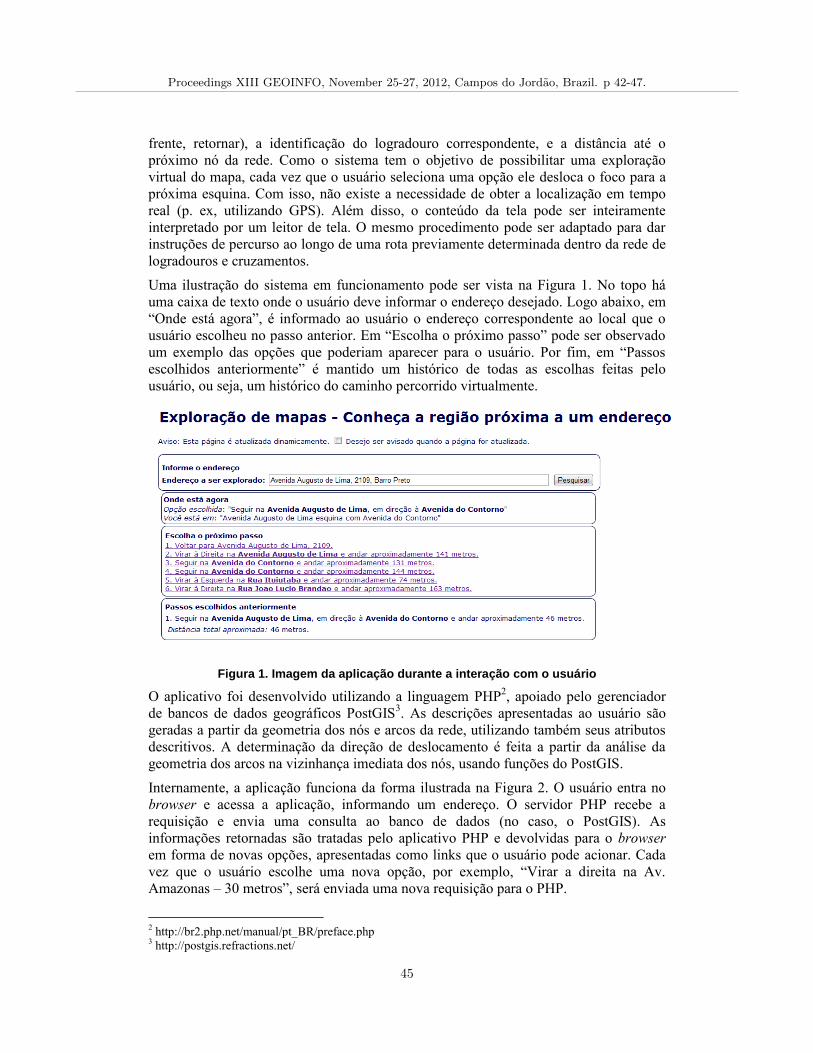
frente, retornar), a identificação do logradouro correspondente, e a distância até o

próximo nó da rede. Como o sistema tem o objetivo de possibilitar uma exploração

virtual do mapa, cada vez que o usuário seleciona uma opção ele desloca o foco para a

próxima esquina. Com isso, não existe a necessidade de obter a localização em tempo

real (p. ex, utilizando GPS). Além disso, o conteúdo da tela pode ser inteiramente

interpretado por um leitor de tela. O mesmo procedimento pode ser adaptado para dar

instruções de percurso ao longo de uma rota previamente determinada dentro da rede de

logradouros e cruzamentos.

Uma ilustração do sistema em funcionamento pode ser vista na Figura 1. No topo há

uma caixa de texto onde o usuário deve informar o endereço desejado. Logo abaixo, em

“Onde está agora”, é informado ao usuário o endereço correspondente ao local que o

usuário escolheu no passo anterior. Em “Escolha o próximo passo” pode ser observado

um exemplo das opções que poderiam aparecer para o usuário. Por fim, em “Passos

escolhidos anteriormente” é mantido um histórico de todas as escolhas feitas pelo

usuário, ou seja, um histórico do caminho percorrido virtualmente.

Figura 1. Imagem da aplicação durante a interação com o usuário

O aplicativo foi desenvolvido utilizando a linguagem PHP2, apoiado pelo gerenciador

de bancos de dados geográficos PostGIS3. As descrições apresentadas ao usuário são

geradas a partir da geometria dos nós e arcos da rede, utilizando também seus atributos

descritivos. A determinação da direção de deslocamento é feita a partir da análise da

geometria dos arcos na vizinhança imediata dos nós, usando funções do PostGIS.

Internamente, a aplicação funciona da forma ilustrada na Figura 2. O usuário entra no

browser e acessa a aplicação, informando um endereço. O servidor PHP recebe a

requisição e envia uma consulta ao banco de dados (no caso, o PostGIS). As

informações retornadas são tratadas pelo aplicativo PHP e devolvidas para o browser

em forma de novas opções, apresentadas como links que o usuário pode acionar. Cada

vez que o usuário escolhe uma nova opção, por exemplo, “Virar a direita na Av.

Amazonas – 30 metros”, será enviada uma nova requisição para o PHP.

2 http://br2.php.net/manual/pt_BR/preface.php

3 http://postgis.refractions.net/


45

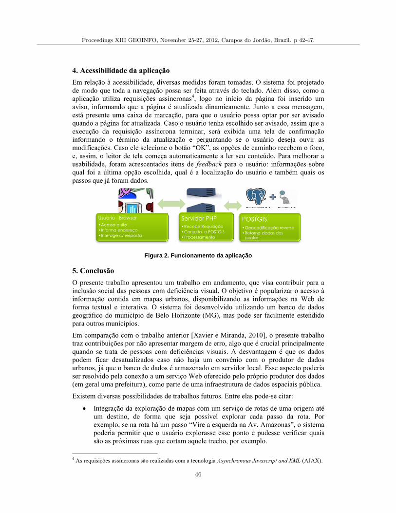
4. Acessibilidade da aplicação

Em relação à acessibilidade, diversas medidas foram tomadas. O sistema foi projetado

de modo que toda a navegação possa ser feita através do teclado. Além disso, como a

aplicação utiliza requisições assíncronas4, logo no início da página foi inserido um

aviso, informando que a página é atualizada dinamicamente. Junto a essa mensagem,

está presente uma caixa de marcação, para que o usuário possa optar por ser avisado

quando a página for atualizada. Caso o usuário tenha escolhido ser avisado, assim que a

execução da requisição assíncrona terminar, será exibida uma tela de confirmação

informando o término da atualização e perguntando se o usuário deseja ouvir as

modificações. Caso ele selecione o botão “OK”, as opções de caminho recebem o foco,

e, assim, o leitor de tela começa automaticamente a ler seu conteúdo. Para melhorar a

usabilidade, foram acrescentados itens de feedback para o usuário: informações sobre

qual foi a última opção escolhida, qual é a localização do usuário e também quais os

passos que já foram dados.

Figura 2. Funcionamento da aplicação

5. Conclusão

O presente trabalho apresentou um trabalho em andamento, que visa contribuir para a

inclusão social das pessoas com deficiência visual. O objetivo é popularizar o acesso à

informação contida em mapas urbanos, disponibilizando as informações na Web de

forma textual e interativa. O sistema foi desenvolvido utilizando um banco de dados

geográfico do município de Belo Horizonte (MG), mas pode ser facilmente estendido

para outros municípios.

Em comparação com o trabalho anterior [Xavier e Miranda, 2010], o presente trabalho

traz contribuições por não apresentar margem de erro, algo que é crucial principalmente

quando se trata de pessoas com deficiências visuais. A desvantagem é que os dados

podem ficar desatualizados caso não haja um convênio com o produtor de dados

urbanos, já que o banco de dados é armazenado em servidor local. Esse aspecto poderia

ser resolvido pela conexão a um serviço Web oferecido pelo próprio produtor dos dados

(em geral uma prefeitura), como parte de uma infraestrutura de dados espaciais pública.

Existem diversas possibilidades de trabalhos futuros. Entre elas pode-se citar:

Integração da exploração de mapas com um serviço de rotas de uma origem até

um destino, de forma que seja possível explorar cada passo da rota. Por

exemplo, se na rota há um passo “Vire a esquerda na Av. Amazonas”, o sistema

poderia permitir que o usuário explorasse esse ponto e pudesse verificar quais

são as próximas ruas que cortam aquele trecho, por exemplo.

4 As requisições assíncronas são realizadas com a tecnologia Asynchronous Javascript and XML (AJAX).

Usuário - Browser

•Acessa o site

•Informa endereço

•Interage c/ resposta

Servidor PHP

•Recebe Requisição

•Consulta o POSTGIS

•Processamento

POSTGIS

•Geocodificação reversa

•Retorna dados dos pontos


46

Incluir informações de pontos de interesse. tais como padarias e farmácias, pois

pessoas com deficiência visual conseguem reconhecer esses tipos de

estabelecimentos pelo olfato, e os utilizam como ponto de referência.

Investigar quais os tipos de informação seriam interessantes para acrescentar no

mapa de forma a tentar aumentar a segurança para as PCDVs, informando, por

exemplo, se o passeio é estreito ou se tem muitos buracos.

Referências

Doi, K., Toyoda, W., Fujimoto, H. (2010) “Development of tactile map production

device and tactile map with multilingual vocal guidance function”, In: Proceedings

of the 12th international ACM SIGACCESS conference on Computers and

accessibility.

Holland, S., Morse, D. R., Gedenryd, H. (2002) “AudioGPS: Spatial Audio Navigation

with a Minimal Attention Interface”, In: Personal Ubiquitous Comput. 6, 4 (2002),

253-259.

Ivanov, R. (2008) “Mobile GPS Navigation Application, Adapted for Visually Impaired

people”, In: Proceeding of International Conference Automatics and Informatics’08

Jansson, G., Pedersen, P. (2005) “Obtaining Geographical Information from a Virtual

Map with a Haptic Mouse”, In: Proc. XXII International Cartographic Conference.

Kaklanis, N., Votis, K, Moschonas, P., Tzovaras, D. (2011) “HapticRiaMaps: towards

interactive exploration of web world maps for the visually impaired”, In:

Proceedings of the International Cross-Disciplinary Conference on Web

Accessibility.

Nogueira, R. (2010). “Mapas como facilitadores na inclusão social de pessoas com

deficiência visual”, In: Com Ciência: revista eletrônica de jornalismo científico.

OMS, Organização Mundial de Saúde. 2010

http://www.who.int/mediacentre/factsheets/fs282/en/, Acessado em Julho de 2012.

Poppinga, B., Magnusson, C., Pielot, M., Rassmus-Gröhn, K. (2011) “TouchOver map:

audio-tactile exploration of interactive maps”, In: MobileHCI '11.

Sánchez, J. (2009). “Mobile Audio Navigation Interfaces for the Blind”, In: UAHCI '09.

SBC. 2006. “Grand Challenges for Computer Science Research in Brazil 2006-2016,

workshop report”, 2006.

Thomas, K. E., Spripada, S., Noordzij, M. L. (2012) “Atlas.txt: exploring linguistic

grounding techniques for communicating spatial information to blind users”, In:

Universal Access in the Information Society. Volume 11, Número 1 (2012), 85-9.8

Wasserburger, W., Neuschmid, J., Schrenk, M. (2011) Web-based City Maps for Blind

and Visually Impaired”, In: REAL CORP 2011.

Xavier, S. I. R, Miranda Junior, P. O. (2010). “Implementação de uma interface

interativa para exploração de mapas por pessoas com deficiência visual”, Trabalho

de diplomação apresentado na PUC-MG.


47

TerraME Observer: An extensible real-time visualization

pipeline for dynamic spatial models

Antônio José C. Rodrigues1, Tiago G. S. Carneiro

1, Pedro R. Andrade

2

1 TerraLAB – Earth System Modeling and Simulation Laboratory,

Computer Science Department, Federal University of Ouro Preto (UFOP)

Campus Universitário Morro do Cruzeiro – 35400-000

Ouro Preto – MG– Brazil

2 Earth System Science Center (CCST), National Institute for Space Research (INPE)

Avenida dos Astronautas, 1758, Jardim da Granja – 12227-010

São José dos Campos – SP– Brazil

[email protected], [email protected], [email protected]

Abstract. This paper presents ongoing research results of an extensible

visualization pipeline for real-time exploratory analysis of spatially explicit

simulations. We identify the software requirements and discuss the main

conceptual and design issues. We propose a protocol for data serialization, a

high performance monitoring mechanism, and graphical interfaces for

visualization. Experiments for performance analysis have shown that

combining multithreading and the BlackBoard design pattern reduces the

visualization response time in 50%, with no significant increase in memory

consumption. The components presented in this paper have been integrated in

the TerraME modeling platform for simulation of terrestrial systems.

1. Introduction

Computer modeling of environmental and social processes has been used to carry on

controlled experiments to simulate the effects of human actions on the environment and

their feedbacks (Schreinemachers and Berger, 2011). In these studies, simulated

scenarios analyze issues related to the prognosis of amount and location of changes,

which may support decision-making or public policies. Computer models are in general

dynamic and spatially explicit (Sprugel et al., 2009; Wu and David, 2002), using remote

sensing data and digital maps as inputs.

Dynamic spatially explicit models to study nature-society interactions,

hereinafter referred as environmental models, are capable of generating a huge amount

of spatiotemporal data in each simulation step. In addition, before any experiment,

models need to be verified in order to fix logic faults. The sooner such errors are found,

the sooner the implementation can be completed. Model verification and interpretation

of simulation results can be more efficiently performed with the support of methods and

tools capable of synthesizing and analyzing simulation outcomes.

Visualization components of environmental modeling platforms differ in the

way they gather, serialize, and transmit state variable values to graphical interfaces.

Such platforms may provide high-level languages to implement models or may be


48

delivered as libraries for model development in general purpose programming

languages. In the latter situation, as in Swarm and RePast platforms, state variable

values are available within the same runtime environment of graphical interfaces (Minar

et al., 1996; North et al., 2006), making data gathering easier and faster. In the platforms

that provide embedded languages, as NetLogo and TerraME, state variables are stored

in this language memory space and need to be copied to the memory space where the

graphical interfaces are defined (Tisue and Wilensky, 2004; Carneiro, 2006), i.e., to the

memory space of a simulation core responsible for model interpretation and execution.

This way, once collected, data needs to be serialized and transmitted according to a

protocol that can be decoded by the graphical interfaces. As environmental modelers

use to be specialists in the application domains (biologists, ecologists, etc) and do not

have strong programming skills, this work focuses on modeling platforms that follow

the second architecture.

As environmental simulations may deal with huge amounts of data, there might

also be a huge amount of data that need to be transferred, which in turn can make the

tasks of gathering, serializing, and transmitting data very time consuming. Land use

change modeling studies discretize space in thousands or millions of regular cells in

different resolutions, whose patterns of change need to be identified, analyzed and

understood (Moreira et al., 2009). In these cases, the simulation could run on dedicated

high-performance hardware, with its results being displayed on remote graphical

workstations. Therefore, it might be necessary to transfer data from one process in this

pipeline to the next through a network.

The main hypothesis of this work is that combining software design patterns and

multithreading is a good strategy to improve visualization response times of

environmental models, keeping the platform simple, extensible, and modular. This work

presents the architecture of a high performance pipeline for the visualization of

environmental models. It includes high-level language primitives for visualization

definition and updating, a serialization protocol, a monitoring mechanism for data

gathering and transmission, and several graphical interfaces for data visualization. This

architecture has been implemented and integrated within the TerraME modeling and

simulation platform (Carneiro, 2006).

The remainder of the paper is organized as follows. TerraME modeling

environment is discussed in Section 2. Related works are presented in Section 3. Section

4 describes the architecture and implementation of the system, while experiments

results are presented in Section 5. Finally, in Section 6, we present the final remarks and

future work.

2. TerraME modeling and simulation platform

TerraME is a software platform for the development of multiscale environmental

models, built jointly by the Federal University of Ouro Preto (UFOP) and the National

Institute for Space Research (INPE) (Carneiro, 2006). It uses multiple modeling

paradigms, among them the theory of agents, the discrete-event simulation theory, the

general systems theory, and the theory of cellular automata (Wooldridge and Jennings,

1995; Zeigler et al., 2005; von Bertalanffy, 1968; von Neumann, 1966). Users can

describe TerraME models directly in C++ or in Lua programming language

(Ierusalimschy et al., 1996). TerraME provides several types of objects to describe


49

temporal, behavioral, and spatial features of models. Cell, CellularSpace, and

Neighborhood types are useful to describe the geographical space. Agent, Automaton

and Trajectories types represent actors and processes that change space properties.

Timer and Event types control the simulation dynamics. During a simulation, the Lua

interpreter embedded within TerraME activates the simulation services from the C++

framework whenever an operation is performed over TerraME objects. The TerraLib

library is used for reading and writing geospatial data to relational database

management systems (Câmara et al., 2000). The traditional way to visualize the

outcomes of a simulation in TerraME is by using the geographical information system

TerraView1. However, TerraView cannot monitor the progress of simulations in real-

time.

3. Related Works

This section compares the most popular simulation platforms according to services

related to graphical interfaces to visualize simulation outcomes, including the

extensibility of such interfaces. Major environmental modeling platforms provide

graphical interfaces for visualization. However, their visualization components work as

black boxes and their architectural designs have not been published. Swarm and Repast

are multi-agent modeling platforms delivered as libraries for general purpose

programming languages (Minar et al., 1996; North et al., 2006). They provide specific

objects for monitoring and visualization. New graphical interfaces can be developed by

inheritance. Their monitoring mechanism periodically updates interfaces in an

asynchronous way, i.e., simulation runs in parallel with visualization interfaces; it does

not stop waiting for interface updating.

NetLogo is a framework that provides tools for multi-agent modeling and simulation

(Tisue and Wilensky, 2004). Models are described in a visual environment focused in

building graphical user interfaces by reusing widget components in a drag-and-drop

fashion. Rules are defined in a high-level programming language. Model structure and

rules are translated into a source code in a general purpose programming language,

which is finally compiled. Communication between simulation and graphical interfaces

is also asynchronous. Graphical interfaces can be periodically updated or explicitly

notified by the implementation.

4. Architecture and Implementation

This section describes computer systems and methods employed to achieve our goals.

We identify the main requirements of an environmental model visualization pipeline,

discuss the design of visualization pipeline and graphical interfaces, present the high-

level language primitives used to create visualizations and to associate them to model

state variables, formally define the serialization protocol, and detail the object oriented

structure of the monitoring mechanism.

4.1. Software requirements

Some requirements have been considered essential to a visualization pipeline for real-

time exploratory analysis of spatially explicit dynamic models.

1 http://www.dpi.inpe.br/terraview/


50

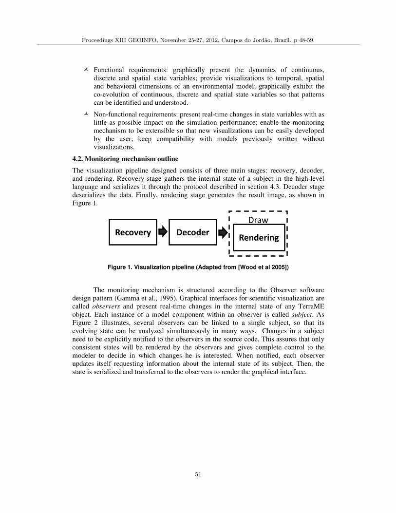
� Functional requirements: graphically present the dynamics of continuous,

discrete and spatial state variables; provide visualizations to temporal, spatial

and behavioral dimensions of an environmental model; graphically exhibit the

co-evolution of continuous, discrete and spatial state variables so that patterns

can be identified and understood.

� Non-functional requirements: present real-time changes in state variables with as

little as possible impact on the simulation performance; enable the monitoring

mechanism to be extensible so that new visualizations can be easily developed

by the user; keep compatibility with models previously written without

visualizations.

4.2. Monitoring mechanism outline

The visualization pipeline designed consists of three main stages: recovery, decoder,

and rendering. Recovery stage gathers the internal state of a subject in the high-level

language and serializes it through the protocol described in section 4.3. Decoder stage

deserializes the data. Finally, rendering stage generates the result image, as shown in

Figure 1.

Figure 1. Visualization pipeline (Adapted from [Wood et al 2005])

The monitoring mechanism is structured according to the Observer software

design pattern (Gamma et al., 1995). Graphical interfaces for scientific visualization are

called observers and present real-time changes in the internal state of any TerraME

object. Each instance of a model component within an observer is called subject. As

Figure 2 illustrates, several observers can be linked to a single subject, so that its

evolving state can be analyzed simultaneously in many ways. Changes in a subject

need to be explicitly notified to the observers in the source code. This assures that only

consistent states will be rendered by the observers and gives complete control to the

modeler to decide in which changes he is interested. When notified, each observer

updates itself requesting information about the internal state of its subject. Then, the

state is serialized and transferred to the observers to render the graphical interface.

Recovery Decoder

Draw

Rendering


51

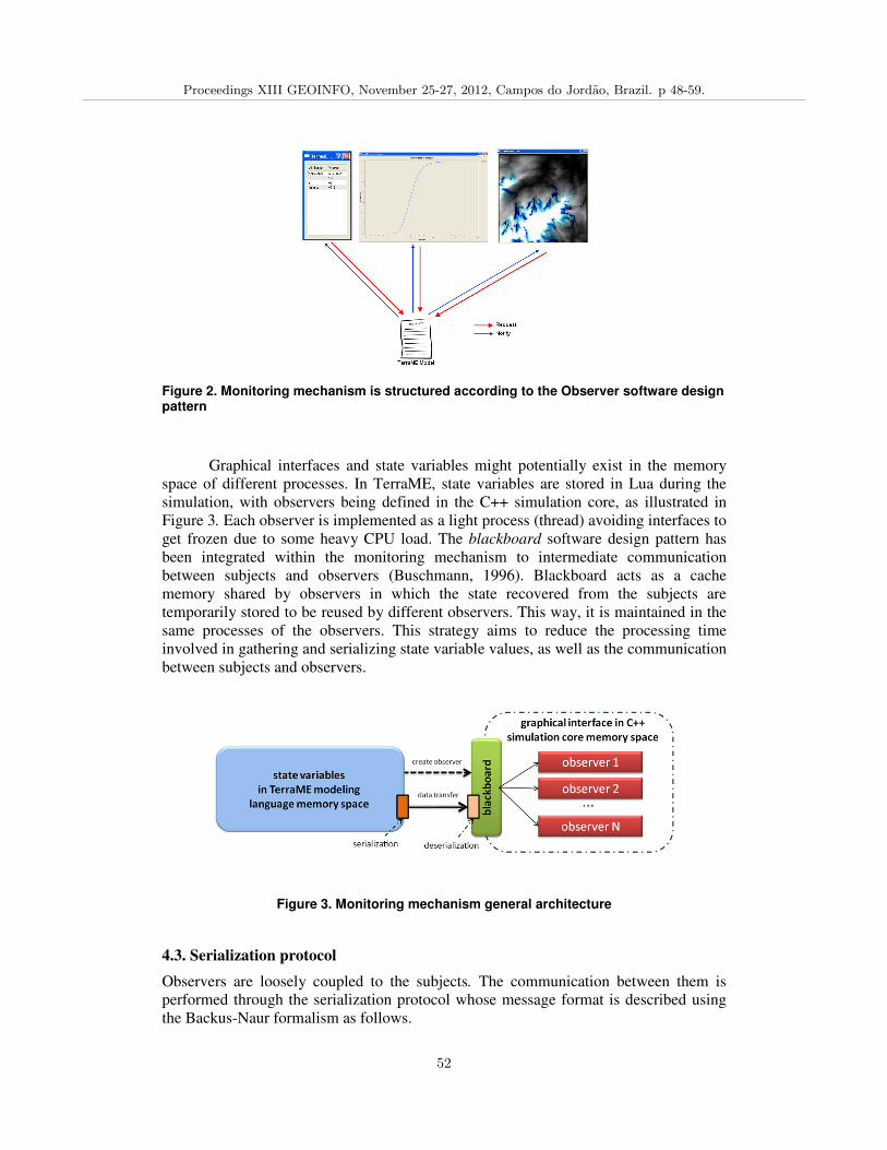
Figure 2. Monitoring mechanism is structured according to the Observer software design pattern

Graphical interfaces and state variables might potentially exist in the memory

space of different processes. In TerraME, state variables are stored in Lua during the

simulation, with observers being defined in the C++ simulation core, as illustrated in

Figure 3. Each observer is implemented as a light process (thread) avoiding interfaces to

get frozen due to some heavy CPU load. The blackboard software design pattern has

been integrated within the monitoring mechanism to intermediate communication

between subjects and observers (Buschmann, 1996). Blackboard acts as a cache

memory shared by observers in which the state recovered from the subjects are

temporarily stored to be reused by different observers. This way, it is maintained in the

same processes of the observers. This strategy aims to reduce the processing time

involved in gathering and serializing state variable values, as well as the communication

between subjects and observers.

Figure 3. Monitoring mechanism general architecture

4.3. Serialization protocol

Observers are loosely coupled to the subjects. The communication between them is

performed through the serialization protocol whose message format is described using

the Backus-Naur formalism as follows.


52

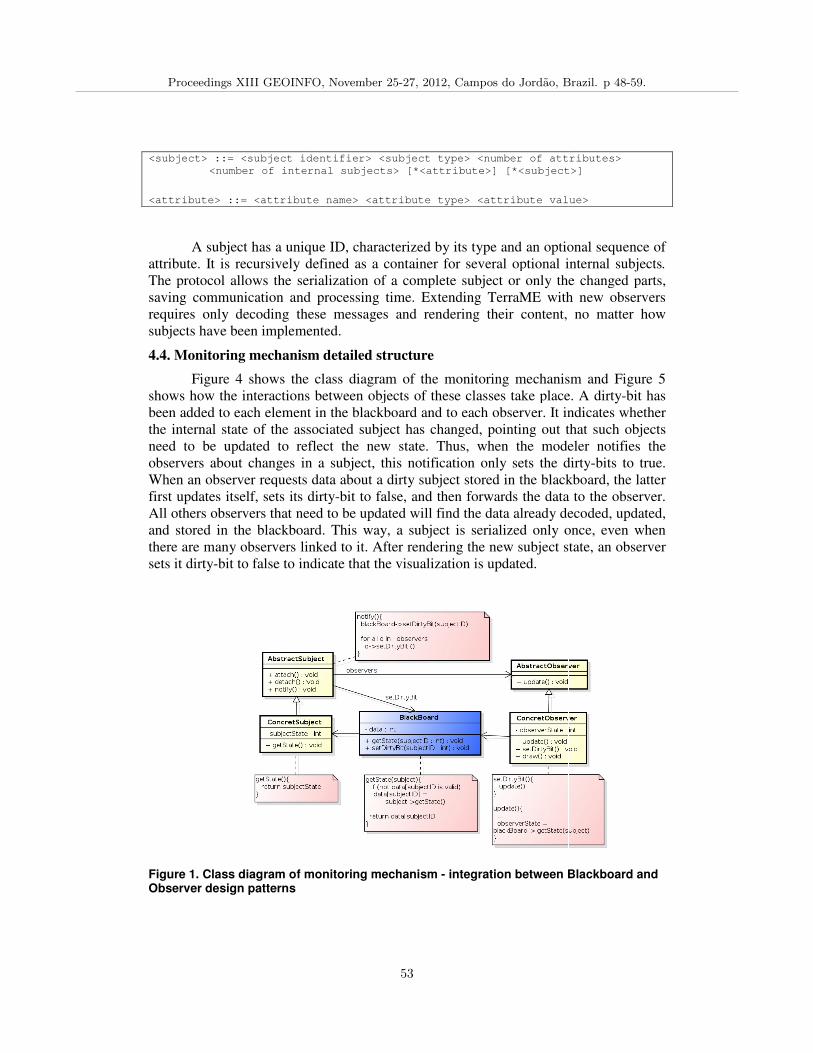
<subject> ::= <subject identifier> <subject type> <number

<number of internal subjects> [*<attribute>] [*<subject>]

<attribute> ::= <attribute name> <attribute type> <attribute value>

A subject has a unique I

attribute. It is recursively defined as a container for several optional internal

The protocol allows the serialization of a complete

saving communication and processing time.

requires only decoding thes

subjects have been implemented.

4.4. Monitoring mechanism

Figure 4 shows the class diagram of the monitoring mechanism and Figure 5

shows how the interactions between objects of these

been added to each element in the

the internal state of the associated

need to be updated to reflect

observers about changes in a

When an observer requests

first updates itself, sets its dirty

All others observers that need to be updated will find the data already

and stored in the blackboard

there are many observers linked to it. After rendering the new subject state, an observer

sets it dirty-bit to false to indicate

Figure 1. Class diagram of monitoring Observer design patterns

<subject identifier> <subject type> <number of attributes>



unique ID, characterized by its type and an optional

defined as a container for several optional internal

The protocol allows the serialization of a complete subject or only the changed parts,

saving communication and processing time. Extending TerraME with new observers

decoding these messages and rendering their content, no matter how

subjects have been implemented.

mechanism detailed structure


interactions between objects of these classes take place

been added to each element in the blackboard and to each observer. It indicates whether

the internal state of the associated subject has changed, pointing out that such

need to be updated to reflect the new state. Thus, when the modeler notifies the

about changes in a subject, this notification only sets the dirty

requests data about a dirty subject stored in the blackboard

ts dirty-bit to false, and then forwards the data to the

All others observers that need to be updated will find the data already decoded,

blackboard. This way, a subject is serialized only once, even when

linked to it. After rendering the new subject state, an observer

to indicate that the visualization is updated.

Class diagram of monitoring mechanism - integration between Blackboard and

attributes>



n optional sequence of

defined as a container for several optional internal subjects.

the changed parts,

Extending TerraME with new observers

content, no matter how


place. A dirty-bit has

It indicates whether

, pointing out that such objects

new state. Thus, when the modeler notifies the

, this notification only sets the dirty-bits to true.

blackboard, the latter

bit to false, and then forwards the data to the observer.

decoded, updated,

only once, even when

linked to it. After rendering the new subject state, an observer

Blackboard and


53

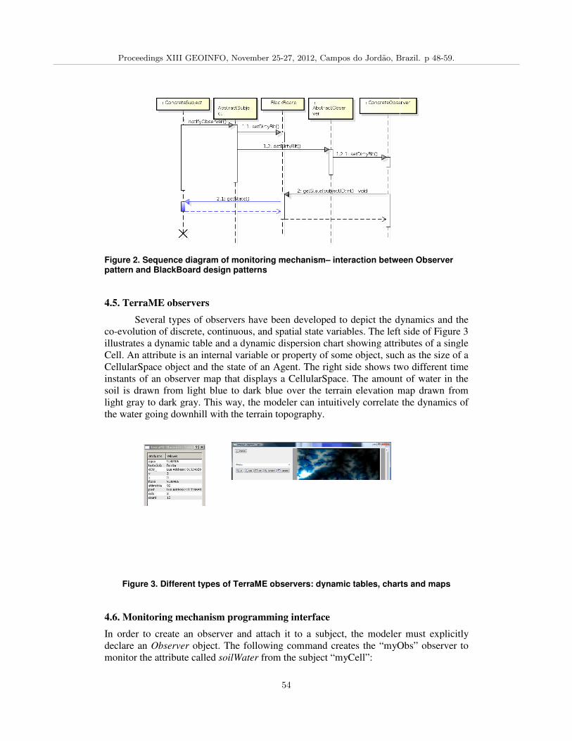
Figure 2. Sequence diagram of monitoring pattern and BlackBoard design patterns

4.5. TerraME observers

Several types of observers

co-evolution of discrete, continuous

illustrates a dynamic table and a dynamic dispersion chart showing attributes of a single

Cell. An attribute is an internal variable or property of some object, such as the size of a

CellularSpace object and the state of an Agent.

instants of an observer map

soil is drawn from light blue to dark blue over the terrain elevation map drawn

light gray to dark gray. This way, the modeler can intuitively correlate the dynamics of

the water going downhill with the terrain topography.

Figure 3. Different types of TerraME observers: dynamic tables, charts and maps

4.6. Monitoring mechanism programming interface

In order to create an observer

declare an Observer object. The following command creates the “myObs”

monitor the attribute called

Sequence diagram of monitoring mechanism– interaction between Observer pattern and BlackBoard design patterns

observers have been developed to depict the dynamics and the

evolution of discrete, continuous, and spatial state variables. The left side of Figure 3


an internal variable or property of some object, such as the size of a

CellularSpace object and the state of an Agent. The right side shows two different time

instants of an observer map that displays a CellularSpace. The amount of water in the

light blue to dark blue over the terrain elevation map drawn


the water going downhill with the terrain topography.

. Different types of TerraME observers: dynamic tables, charts and maps

. Monitoring mechanism programming interface

observer and attach it to a subject, the modeler must explicitly

object. The following command creates the “myObs”

attribute called soilWater from the subject “myCell”:

interaction between Observer

the dynamics and the

and spatial state variables. The left side of Figure 3


an internal variable or property of some object, such as the size of a

The right side shows two different time

amount of water in the

light blue to dark blue over the terrain elevation map drawn from


. Different types of TerraME observers: dynamic tables, charts and maps

, the modeler must explicitly

object. The following command creates the “myObs” observer to


54

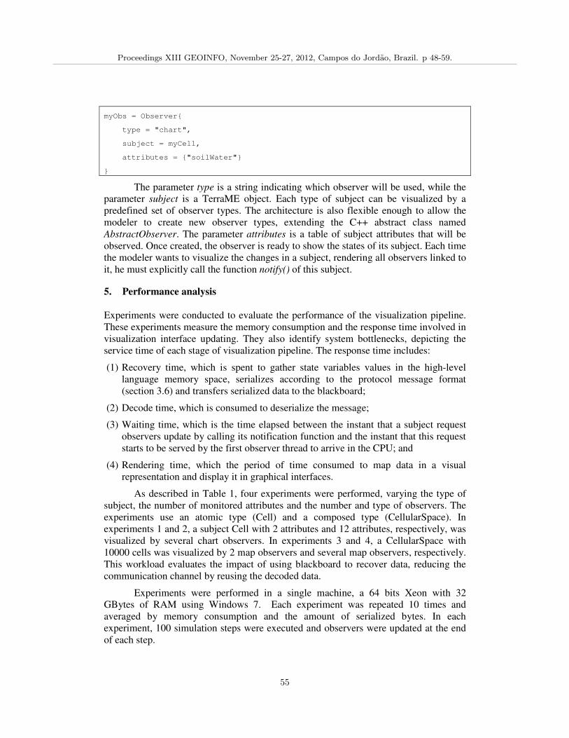
myObs = Observer{

type = "chart",

subject = myCell,

attributes = {"soilWater"}

}

The parameter type is a string indicating which observer will be used, while the

parameter subject is a TerraME object. Each type of subject can be visualized by a

predefined set of observer types. The architecture is also flexible enough to allow the

modeler to create new observer types, extending the C++ abstract class named

AbstractObserver. The parameter attributes is a table of subject attributes that will be

observed. Once created, the observer is ready to show the states of its subject. Each time

the modeler wants to visualize the changes in a subject, rendering all observers linked to

it, he must explicitly call the function notify() of this subject.

5. Performance analysis

Experiments were conducted to evaluate the performance of the visualization pipeline.

These experiments measure the memory consumption and the response time involved in

visualization interface updating. They also identify system bottlenecks, depicting the

service time of each stage of visualization pipeline. The response time includes:

(1) Recovery time, which is spent to gather state variables values in the high-level

language memory space, serializes according to the protocol message format

(section 3.6) and transfers serialized data to the blackboard;

(2) Decode time, which is consumed to deserialize the message;

(3) Waiting time, which is the time elapsed between the instant that a subject request

observers update by calling its notification function and the instant that this request

starts to be served by the first observer thread to arrive in the CPU; and

(4) Rendering time, which the period of time consumed to map data in a visual

representation and display it in graphical interfaces.

As described in Table 1, four experiments were performed, varying the type of

subject, the number of monitored attributes and the number and type of observers. The

experiments use an atomic type (Cell) and a composed type (CellularSpace). In

experiments 1 and 2, a subject Cell with 2 attributes and 12 attributes, respectively, was

visualized by several chart observers. In experiments 3 and 4, a CellularSpace with

10000 cells was visualized by 2 map observers and several map observers, respectively.

This workload evaluates the impact of using blackboard to recover data, reducing the

communication channel by reusing the decoded data.

Experiments were performed in a single machine, a 64 bits Xeon with 32

GBytes of RAM using Windows 7. Each experiment was repeated 10 times and

averaged by memory consumption and the amount of serialized bytes. In each

experiment, 100 simulation steps were executed and observers were updated at the end

of each step.


55

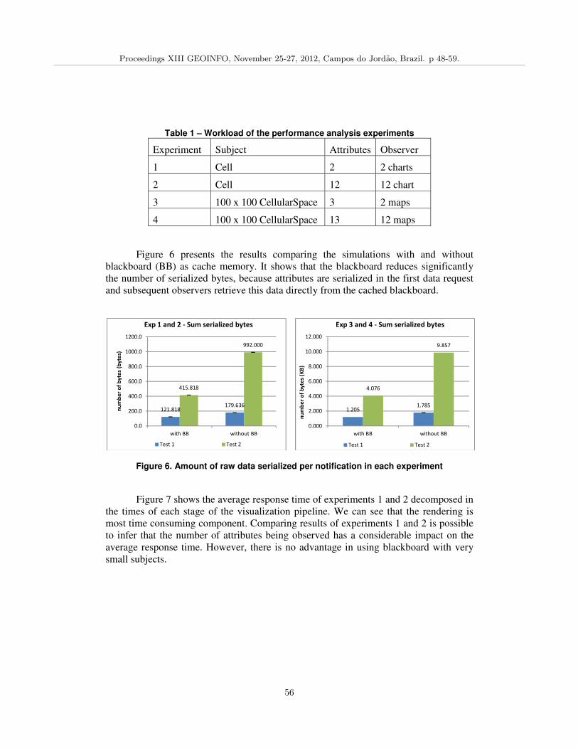
Table 1 – Workload of the performance analysis experiments

Experiment Subject Attributes Observer

1 Cell 2 2 charts

2 Cell 12 12 chart

3 100 x 100 CellularSpace 3 2 maps

4 100 x 100 CellularSpace 13 12 maps

Figure 6 presents the results comparing the simulations with and without

blackboard (BB) as cache memory. It shows that the blackboard reduces significantly

the number of serialized bytes, because attributes are serialized in the first data request

and subsequent observers retrieve this data directly from the cached blackboard.

Figure 6. Amount of raw data serialized per notification in each experiment

Figure 7 shows the average response time of experiments 1 and 2 decomposed in

the times of each stage of the visualization pipeline. We can see that the rendering is

most time consuming component. Comparing results of experiments 1 and 2 is possible

to infer that the number of attributes being observed has a considerable impact on the

average response time. However, there is no advantage in using blackboard with very

small subjects.

121.818179.636

415.818

992.000

0.0

200.0

400.0

600.0

800.0

1000.0

1200.0

with BB without BB

nu

mb

er

of

by

tes

(by

tes)

Exp 1 and 2 - Sum serialized bytes

Test 1 Test 2

1.2051.785

4.076

9.857

0.000

2.000

4.000

6.000

8.000

10.000

12.000

with BB without BB

nu

mb

er

of

by

tes

(KB

)

Exp 3 and 4 - Sum serialized bytes

Test 1 Test 2


56

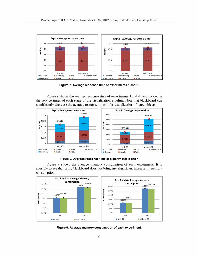
Figure 7. Average response time of experiments 1 and 2.

Figure 8 shows the average response time of experiments 3 and 4 decomposed in

the service times of each stage of the visualization pipeline. Note that blackboard can

significantly decrease the average response time in the visualization of large objects.

Figure 8. Average response time of experiments 3 and 4

Figure 9 shows the average memory consumption of each experiment. It is

possible to see that using blackboard does not bring any significant increase in memory

consumption.

Figure 9. Average memory consumption of each experiment.

3.687 3.641

0.625 0.697

4.416 4.432

0.0

1.0

2.0

3.0

4.0

5.0

with BB without BB

tim

e (

ms)

Exp 1 - Average response time

Decoder Rendering wait Handle-Draw

Recovery Handle Total

18.740 18.850

2.183 2.276

21.159 21.467

0.0

5.0

10.0

15.0

20.0

25.0

with BB without BB

tim

e (

ms)


Decoder Rendering wait Handle-Draw


48.565 74.757

153.630152.580

133.392

233.091

337.917

467.659

0.0

100.0

200.0

300.0

400.0

500.0

with BB without BB

tim

e (

ms)


Decoder Rendering Wait Handle-Draw


138.996408.358

849.503

833.238

284.063

1278.025

1283.341

2558.004

0.0

500.0

1000.0

1500.0

2000.0

2500.0

3000.0

with BB without BB

tim

e (

ms)


Decoder Rendering Wait Handle-Draw


156.328

160.701

156.275

160.604

150.0

152.0

154.0

156.0

158.0

160.0

162.0

Exp 1 Exp 2

me

mo

ry (

MB

)

Exp 1 and 2 - Average Memory

Consumption

with BB without BB

234.237

550.510

231.763

536.289

0.0

100.0

200.0

300.0

400.0

500.0

600.0

Exp 1 Exp 2

me

mo

ry (

MB

)

Exp 3 and 4 - Average memory

consumption

with BB without BB


57

6. Final Remarks

In this work, we describe an extensible visualization component for real-time

monitoring of environmental simulations. We demonstrate that combining

multithreading and blackboard is a good technique to improve visualization

performance, significantly decreasing the visualization response time with no expressive

increase in memory consumption. The developed graphical interfaces are able to render

discrete, continuous and spatial state variables of environmental models written in

TerraME, rendering instances of all TerraME types. Visualizations are also able

to graphically exhibit the co-evolution state variables, allowing the understanding of

how a variable influences other and help identify some logic faults. The monitoring

mechanism can be easily extended by inheritance. New observer types can also be

created using the same mechanism. The new visualization capabilities added to

TerraME do not affect models previously written in this modeling platform, keeping

backward compatibility. Consequently, the proposed visualization mechanism satisfies

all functional requirements stated in section 4.1.

Future works include adding a synthesis stage to the visualization pipeline. In

this new stage, it will be possible to apply filters and statistical operations to raw data to

make data analysis easier. It is also necessary to implement change control algorithms.

New experiments will be performed to measure performance by transmitting only

objects and attributes that have changed along the simulation. Other experiments will

evaluate the impact of the blackboard and of compression algorithms in a client-server

version of the proposed visualization mechanism. Initial evaluation of the client-server

version has shown that the use of blackboard on the client side reduces the exchange of

messages by half using TCP protocol. Finally, experiments will be conducted to

quantitatively compare the visualization mechanisms of the most relevant modeling

platforms with the one presented in this work.

Acknowledgements

The authors would like to thank the Pos-Graduate Program in Computer Science and the

TerraLAB modeling and simulation laboratory of the Federal University of Ouro Preto

(UFOP), in Brazil. This work was supported by the CNPq/MCT grant 560130/2010-4,

CT-INFO 09/2010.

References

Buschmann, F., Meunier, R., Rohnert, H., Sommerlad, P., and Stal, M. (1996). Pattern-

oriented software architecture: a system of patterns. John Wiley & Sons, Inc.

Câmara, G., Souza, R., Pedrosa, B., Vinhas, L., Monteiro, A.M., Paiva, J., Carvalho,

M.T., Gattass, M., (2000). TerraLib: Technology in Support of GIS Innovation, II

Brazilian Symposium on Geoinformatics, GeoInfo2000: São Paulo.

Carneiro, T. G. S. (2006). Nested-CA: a foundation for multiscale modeling of land use

and land change.. Ph.D Thesis, INPE - Instituto Nacional de Pesquisas Espaciais,

Brazil, Computação Aplicada.


58

Gamma, E., Helm, R., Johnson, R., and Vlissides, J. (1995). Design patterns: elements

of reusable object-oriented software. Addison-Wesley Professional.

Ierusalimschy, R., Figueiredo, L.H., Celes, W., (1996). Lua-an extensible extension

language. Software: Practice & Experience 26(6) 635-652.

Minar, N., Burkhart, R., Langton, C., Askenazi, M., (1996). The Swarm Simulation

System: A Toolkit for Building Multi-Agent Simulation. SFI Working Paper 96-06-

042

Moreira, E.; Costa, S.; Aguiar, A. P.; Câmara, G., Carneiro, T. G. S., (2009). Dynamical

coupling of multiscale land change models Landscape Ecology, Springer

Netherlands, 24, 1183-1194

North, M.J., Collier, N.T., Vos, J.R., (2006). Experiences Creating Three

Implementations of the Repast Agent Modeling Toolkit. ACM Transactions on

Modeling and Computer Simulation 16(1) 1-25.

Schreinemachers, P. and Berger, T. (2011). An agent-based simulation model of

human-environment interactions in agricultural systems. Environmental Modelling

& Software, 26(7):845 – 859.

Sprugel, D. G., Rascher, K. G., Gersonde, R., Dovciak, M., Lutz, J. A., and Halpern, C.

B. (2009). Spatially explicit modeling of overstory manipulations in young forests:

Effects on stand structure and light. Ecological Modelling, 220(24):3565 – 3575.

Tisue, S., Wilensky, U., (2004). NetLogo: A Simple Environment for Modeling

Complexity, International Conference on Complex Systems: Boston.

von Neumann, J., (1966). Theory of Self-Reproducing Automata. Edited and completed

by A.W. Burks., Illinois

Wood, J.; Kirschenbauer, S; Döner, J.; Lopes, Adriano and Bodum, L. (2005). Using

3D in Visualization. In: Dykes, J; Maceachren, A. M.; Kraak, J. (Eds.). Exploring

Geovisualization. Elsevier. p. 295-312.

Wooldridge, M.J., Jennings, N.R., (1995). Intelligent agents: Theory and practice.

Knowledge Engineering Review 10(2).

Wu, J. and David, J. L. (2002). A spatially explicit hierarchical approach to modeling

complex ecological systems: theory and applications. Ecological Modelling, 153(1-

2):7 – 26.

Zeigler, B.P., Kim, T.G., Praehofer, H., (2005). Theory of modeling and simulation.

Academic Press, Inc., Orlando, FL, USA.


59

Um Framework para Recuperacao Semantica deDados Espaciais

Jaudete Daltio1,2, Carlos Alberto de Carvalho3

1Embrapa Gestao Territorial, Campinas – SP – Brasil

2Instituto de Computacao - Universidade Estadual de Campinas (UNICAMP)Campinas – SP – Brasil

3Escritorio de Analise e Monitoramento de Imagens de Satelite do GSI/SAEI/PRCampinas – SP – Brasil


Abstract. Geographic data represent objects for which the geographic locationis an essential feature. Since they represent real-world objects, these datapresent a lot of intrinsic semantic, which is not always explicitly formalized.Explicit semantic allows higher accuracy in data retrieval and interpretation.The goal of this work is to propose a framework for management and retrievalof geographic data, combining semantic and spatial aspects. The maincontributions of this work are the specification and implementation of theproposed framework.

Resumo. Dados geograficos representam objetos para os quais a localizacaogeograficae uma caracterıstica essencial para sua analise. Por representaremobjetos do mundo real, esses dados possuem muita semantica intrınseca, quenem sempree explicitamente formalizada. A semantica explıcita possibilitamaior acuracia na recuperacao e interpretacao dos dados. O objetivo destetrabalho e propor um framework para recuperacao de dados geograficos quemanipule aspectos semanticos e espaciais de forma integrada. Dentre ascontribuicoes estao a especificacao e a implementacao do framework proposto.

1. Introducao e MotivacaoSistemas de Informacoes Geograficas (SIGs) sao sistemas capazes de manipulardados georreferenciados, ou seja, dados que representam fatos, objetos e fenomenosassociadosa uma localizacao sobre a superfıcie terrestre. Para estes objetos, alocalizacao geografica e uma caracterıstica inerentea informacao e indispensavelpara analisa-la [Camara et al. 1996]. Alem de dados alfanumericos, esses sistemascorrelacionam dados espaciais vetoriais e matriciais.

Por representarem objetos do mundo real, dados geograficos possuem muitasemantica intrınseca, nem sempre explicitamente formalizada. A interpretacao dosdadose, em geral, responsabilidade dos especialistas do domınio. Em grupos detrabalho dispersos, esses especialistas podem possuir metodologias, focos de pesquisae vocabularios distintos. Esse problema ganha maior dimensao para imagens desatelite, que possuem muitas informacoes agregadas e demandam elevado processamentocomputacional para sua interpretacao, como classificacao e reconhecimentos de padroes.


60

Ontologias vem se materializando como a principal tecnologia para representacaode semantica [Horrocks 2008]. Tratam-se de estruturas computacionais capazes derepresentar os termos de um domınio e seus relacionamentos. Seu uso tem sidocada vez mais difundido em geotecnologias, modelando desdeatributos e metadadosa relacionamentos espaciais. A associacao de semantica ainda representa um dos tresprincipais desafios a serem superados pela nova geracao de SIGs [Camara et al. 2009].

O objetivo deste trabalhoe especificar e implementar umframework paragerenciamento de dados geograficos, integrando aspectos semanticos e espaciais. Oframeworksera capaz de propagar a semantica entre os dados geograficos – de vetoriaispara matriciais – considerando suas correlacoes espaciais. Com isso, sera possıvelincorporar aspectos semanticos as imagens de satelite e auxiliar seu processo derecuperacao. Serao utilizadas ontologias como base para as anotacoes semanticas.

O restante desse artigo segue a seguinte organizacao: a secao 2 apresenta osaspectos de pesquisa relacionados ao trabalho. A secao 3 descreve oframeworkproposto,seus aspectos de implementacao e estudos de caso que validam a aplicabilidade da solucaoproposta. A secao 4 apresenta os resultados e as contribuicoes previstas para o trabalho.

2. Aspectos de Pesquisa EnvolvidosOs aspectos de pesquisa desse trabalho sao: anotacoes, semantica (ontologias) eferramentas de anotacao semantica. As secoes subsequentes detalham esses topicos.

2.1. Fundamentacao Teorica - Anotacoes e SemanticaAnotar e o processo de adicionar notas ou comentarios a um dado. De forma analogaaos metadados, uma anotacaoe utilizada para descrever um dado, ou parte dele, adotandoou nao um vocabulario de referencia. O termo “anotacao semantica” decorre do usode ontologias como vocabulario de referencia para a anotacao [Macario 2009], visandointeroperabilidade. Em aplicacoes geograficas, uma anotacao tambem pode consideraro componente espacial. O diferencial das anotacoes semanticas esta no processo derecuperacao. Mecanismos tradicionais de busca por palavras-chave possuem muitaslimitacoes e a analise do contexto pode melhorar a acuracia deste processo.

Ontologias sao especificacoes explıcitas de uma conceitualizacao – uma definicaoconsensual a respeito da representacao de um domınio. O domınio geografico possuivarias ontologias e, considerando os dados utilizados nestetrabalho, selecionou-seontologias adequadas para a representacao de empreendimentos de infraestruturagovernamental e dos recursos naturais a cerca deles. Sao elas:- AGROVOC 1: descreve a semantica de temas como agricultura, silvicultura, pesca eoutros domınios relacionados com alimentacao, como meio ambiente;- SWEET 2: termos sobre dados cientıficos, com conceitos ortogonais como espaco,tempo, quantidades fısicas, e de conhecimento cientıfico, como fenomenos e eventos;- VCGE 3: padrao de interoperabilidade para facilitar a indexacao de conteudo nos portaisgovernamentais, tratando de assuntos de interesse do setorpublico;- OnLocus [Borges 2006]: conceitos no domınio espaco geografico urbano, feicoesnaturais, objetos e lugares, incluindo os relacionamentosentre eles.

1http://aims.fao.org/standards/agrovoc2http://sweet.jpl.nasa.gov/ontology/3http://vocab.e.gov.br/2011/03/vcge


61

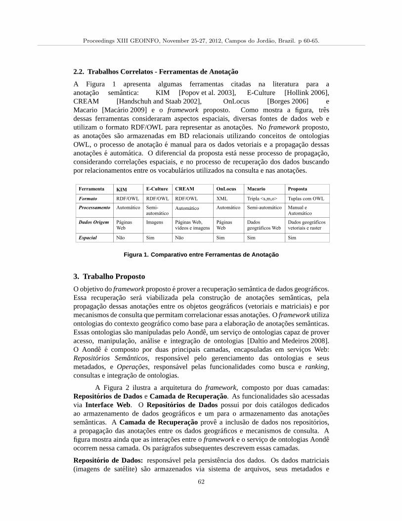
2.2. Trabalhos Correlatos - Ferramentas de Anotacao

A Figura 1 apresenta algumas ferramentas citadas na literatura para aanotacao semantica: KIM [Popov et al. 2003], E-Culture [Hollink 2006],CREAM [Handschuh and Staab 2002], OnLocus [Borges 2006] eMacario [Macario 2009] e o framework proposto. Como mostra a figura, tresdessas ferramentas consideraram aspectos espaciais, diversas fontes de dados web eutilizam o formato RDF/OWL para representar as anotacoes. Noframeworkproposto,as anotacoes sao armazenadas em BD relacionais utilizando conceitos de ontologiasOWL, o processo de anotacao e manual para os dados vetoriais e a propagacao dessasanotacoese automatica. O diferencial da proposta esta nesse processo de propagacao,considerando correlacoes espaciais, e no processo de recuperacao dos dados buscandopor relacionamentos entre os vocabularios utilizados na consulta e nas anotacoes.

Figura 1. Comparativo entre Ferramentas de Anotac ao

3. Trabalho PropostoO objetivo doframeworkpropostoe prover a recuperacao semantica de dados geograficos.Essa recuperacao sera viabilizada pela construcao de anotacoes semanticas, pelapropagacao dessas anotacoes entre os objetos geograficos (vetoriais e matriciais) e pormecanismos de consulta que permitam correlacionar essas anotacoes. Oframeworkutilizaontologias do contexto geografico como base para a elaboracao de anotacoes semanticas.Essas ontologias sao manipuladas pelo Aonde, um servico de ontologias capaz de proveracesso, manipulacao, analise e integracao de ontologias [Daltio and Medeiros 2008].O Aonde e composto por duas principais camadas, encapsuladas em servicos Web:Repositorios Semanticos, responsavel pelo gerenciamento das ontologias e seusmetadados, eOperacoes, responsavel pelas funcionalidades como busca eranking,consultas e integracao de ontologias.

A Figura 2 ilustra a arquitetura doframework, composto por duas camadas:Repositorios de Dadose Camada de Recuperacao. As funcionalidades sao acessadasvia Interface Web. O Repositorios de Dadospossui por dois catalogos dedicadosao armazenamento de dados geograficos e um para o armazenamento das anotacoessemanticas. ACamada de Recuperacao prove a inclusao de dados nos repositorios,a propagacao das anotacoes entre os dados geograficos e mecanismos de consulta. Afigura mostra ainda que as interacoes entre oframeworke o servico de ontologias Aondeocorrem nessa camada. Os paragrafos subsequentes descrevem essas camadas.

Repositorio de Dados: responsavel pela persistencia dos dados. Os dados matriciais(imagens de satelite) sao armazenados via sistema de arquivos, seus metadados e


62

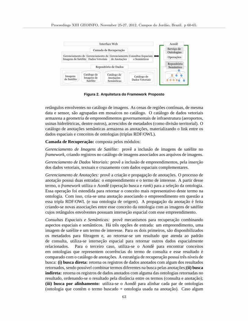
Figura 2. Arquitetura do Framework Proposto

retangulos envolventes no catalogo de imagens. As cenas de regioes contınuas, de mesmadata e sensor, sao agrupadas em mosaicos no catalogo. O catalogo de dados vetoriaisarmazena a geometria de empreendimentos governamentais deinfraestrutura (aeroportos,usinas hidreletricas, dentre outros), acrescidos de metadados (como divisao territorial). Ocatalogo de anotacoes semanticas armazena as anotacoes, materializando o link entre osdados espaciais e conceitos de ontologias (triplas RDF/OWL).

Camada de Recuperacao: composta pelos modulos:

Gerenciamento de Imagens de Satelite: prove a inclusao de imagens de satelite noframework, criando registros no catalogo de imagens associados aos arquivos de imagens.

Gerenciamento de Dados Vetoriais:prove a inclusao de empreendimentos, pela insercaodos dados vetoriais, textuais e cruzamento com dados espaciais complementares.

Gerenciamento de Anotacoes:prove a criacao e propagacao de anotacoes. O processo deanotacao possui duas entradas: o empreendimento e o termo de interesse. A partir dessetermo, oframeworkutiliza o Aonde (operacao busca erank) para a selecao da ontologia.Essa operacao foi estendida para retornar o conceito mais representativo deste termo naontologia. Com isso, cria-se uma anotacao associando o empreendimento em questao aessa tripla RDF/OWL (e sua ontologia de origem). A propagacao da anotacao e feitacriando-se novas associacoes entre esse conceito da ontologia com as imagens de satelitecujos retangulos envolventes possuam intersecao espacial com esse empreendimento.

Consultas Espaciais e Semanticas: prove mecanismos para recuperacao combinandoaspectos espaciais e semanticos. Ha tres opcoes de entrada: um empreendimento, umaimagem de satelite e um termo de interesse. Para os dois primeiros, sao disponibilizadosos metadados para filtragem e, ao retornar-se um resultado que atenda ao padraode consulta, utiliza-se intersecao espacial para retornar outros dados espacialmenterelacionados. Para o terceiro caso, utiliza-se o Aonde para encontrar conceitosem ontologias que representem ocorrencias do termo de consulta e esse resultadoecomparado com o catalogo de anotacoes. A estrategia de recuperacao possui tres nıveis debusca:(i) busca direta: retorna os registros de dados anotados com algum dos resultadosretornados, sendo possıvel combinar termos diferentes na busca pelas anotacoes;(ii) buscaindireta: retorna os registros de dados anotados com alguma das ontologias retornadas noresultado, ordenando-se o resultado pela distancia entre os termos (consulta e anotacao);(iii) busca por alinhamento: utiliza-se o Aonde para alinhar cada par de ontologias(ontologia que contem o termo buscado + ontologia usada na anotacao). Caso algum


63

alinhamento seja encontrado, o procedimento de recuperacao de dadose analogoa buscaindireta e as ontologias alinhadas sao manipuladas como se fossem uma ontologiaunica.

Interface Web: camada de visualizacao doframework. Foram desenvolvidas interfacespara a visualizacao de empreendimentos e imagens de satelite (e suas correlacoesespaciais). A interface para manipulacao das anotacoes semanticas esta em fase deelaboracao e propoe-se a adocao dearvore hiperbolica para visualizacao.

3.1. Aspectos de Implementacao

O prototipo do frameworkesta em fase de implementacao. ORepositorio de Dadosutiliza o SGBD PostgreSQL e a extensao PostGIS4 para manipulacao dos dadosgeograficos. Foram desenvolvidosscripts para a insercao automatica de imagense empreendimentos. ACamada de Recuperacao e a Interface Web estao sendoimplementadas em PHP. Para a publicacao e navegacao nos dados espaciais utiliza-se oservidor de mapas MapServer5 e o servidor Web Apache. A manipulacao das ontologiase responsabilidade do Aonde, acessado via servicos Web.

3.2. Estudo de Caso

Para esse estudo de caso, utilizou-se um conjunto de empreendimentos governamentaisde infraestrutura imageados entre 2005 e 2012. As ontologias descritas na secao2.1 foram aplicadas como vocabulario de anotacao. Para a usina hidreletrica Estreito(polıgono), localizada no Rio Tocantins, pesquisou-se os termospara anotacao:hidreletrica, barragem, rio, energia, Maranhao, Tocantins, e anotacoes foram criadasa partir dos resultados:geracao-energia-hidreletrica(VCGE), Dam (SWEET),Energiahidroelectrica, Rio, Maranhao (AgroVOC). Para a rodovia BR-153 (linha), que atravessao estado de Tocantins, pesquisou-se os termos:rodovia, estrada e transporte, e anotacoesforam criadas a partir dos resultados:Infraestrutura de transporte rodoviario (VCGE),rodovia, construcao de estradas e Transporte rodoviario (AgroVOC). Todas as anotacoespropagadas para as imagens de satelite com intersecao espacial nesses empreendimentos.

Considere a consulta aoframework: “Retorne imagens de satelite de rios a partirde 2008”. O termo de consultario, ao ser buscado no Aonde, ira retornar um dosconceitos utilizados na anotacao da hidreletrica (AgroVOC), logo todas as imagens paraas quais essa anotacao foi propagada serao retornadas por busca direta. Essas imagensserao filtradas pelo metadado “data de imageamento”, retornando apenas as que atendemao criterio de data superiora 2008. O mesmo ocorreria com qualquer termo de consultautilizando algum dos termos de anotacao. Uma consulta mais elaborada poderia envolverdois ou mais conceitos de anotacao: ‘‘Retorne imagens de satelite de rodovias e rios”.Neste caso, o mesmo processo de busca tambem seria feito com o termorodoviase seriamretornadas as imagens que possuıssem ambas anotacoes.

Considere uma consulta mais geral:“Retorne imagens de satelite deagua”. Otermo de consultaagua ira retornar o conceitoaguas, dois nıveis acima do conceitogeracao-energia-hidreletricana VGCE e, com isso, as imagens com as anotacoes dahidreletrica serao retornadas por busca indireta. Essas imagens serao penalizadas noranking por essa distancia de 2 termos. Outro possıvel caminho de indexacao ocorre

4http://postgis.refractions.net/5http://mapserver.org/


64

pelo conceitoBodyOfWater(um nıvel acima do conceitoDam). Caso imagens diferentesestivessem anotadas com esses conceitos, as anotadas comDam seriam mostradasprimeiramente. Um outro exemplo de consulta seria:“Retorne as imagens de satelite deavenidas”. O termoavenidaira retornar a ontologia OnLocus, que nao foi utilizada emnenhuma anotacao. Porem, o Aonde e capaz de alinhar essa ontologia com a AgroVOC,retornando, por busca por alinhamento, as imagens anotadascom o termorodovia.

4. Resultados Esperados e ContribuicoesEste trabalho atende uma demanda recorrente no gerenciamento de dados geograficos:a explıcita associacao de semantica aos dados e a incorporacao dessa caracterıstica emmecanismos de consulta. A assertividade na recuperacao dos dados tera influencia diretade dois principais fatores: a precisao da anotacao criada e a especificidade da ontologiautilizada nessa anotacao. Quanto mais ricas e especıficas forem as ontologias de origem,maiores serao as possibilidades de exploracao dos relacionamentos entre os termos nodomınio de interesse e de alinhamentos com outras ontologias complementares.

As principais contribuicoes esperadas deste trabalho sao: (i) levantamento deontologias utilizadas na representacao de dados geograficos; (ii) analise das estrategiasde anotacao semantica e (iii) especificacao e implementacao de umframeworkparaanotacao e recuperacao semantica de dados espaciais. A continuidade do projeto preve ainclusao da dimensao temporal na geometria dos dados vetoriais e a exploracao de outrosrelacionamentos espaciais, alem da sobreposicao. Alem disso, preve-se a adocao dospadroes de metadados reconhecidos para infraestruturas de dados espaciais6.

ReferenciasBorges, K. A. V. (2006).Uso de uma Ontologia de Lugar Urbano para Reconhecimento

e Extracao de Evidencias Geo-espaciais na Web. PhD thesis, UFMG.

Camara, G., Casanova, M. A., Hemerly, A. S., Magalhaes, G. C., and Medeiros, C. M. B.(1996).Anatomia de sistemas de informacoes geograficas. INPE, S. J. dos Campos.

Camara, G., Vinhas, L., Davis, C., Fonseca, F., and Carneiro, T.G. S. (2009).Geographical information engineering in the 21st century.In Research Trends in GIS,pages 203–218. Springer-Verlag, Berlin Heidelberg.

Daltio, J. and Medeiros, C. B. (2008). Aonde: An ontology web service forinteroperability across biodiversity applications.Inf. Syst., 33(7-8):724–753.

Handschuh, S. and Staab, S. (2002). Authoring and annotation of web pages in cream. InWWW ’02: Proc. 11th Int. Conf. WWW, pages 462–473, NY, USA. ACM.

Hollink, L. (2006). Semantic Annotation for Retrieval of Visual Resources. PhD thesis,Vrije Universiteit Amsterdam.

Horrocks, I. (2008). Ontologies and the semantic web.Commun. ACM, 51(12):58–67.

Macario, C. G. N. (2009).Semantic Annotation of Geospatial Data. PhD thesis, IC -Unicamp.

Popov, B., Kiryakov, A., Kirilov, A., Manov, D., Ognyanoff, D., and Goranov, M. (2003).Kim - semantic annotation platform. InISWC 2003, pages 834–849. Springer Berlin.6http://www.inde.gov.br/


65

Ontology-based Geographic Data Access in a Peer Data

Management System

Rafael Figueiredo1, Daniela Pitta

1, Ana Carolina Salgado

2, Damires Souza

1

1 Federal Institute of Education, Science and Technology of Paraiba, Brazil

2 Federal University of Pernambuco, Brazil

{rafa.felype,daniela.pdj}@gmail.com,[email protected],

[email protected]

Abstract. Ontology-Based Data Access (OBDA) is the problem of accessing

one or more data sources by means of a conceptual representation expressed

in terms of an ontology. We apply the principles underlying an ODBA in the

light of a Peer Data Management System, using geographic databases as data

sources. When dealing with geospatial data, specific problems regarding

query answering and data visualization occur. To help matters, in this work,

we present an approach and a tool, named easeGO, which provides access to

a geographic database using an ontology as a middle layer between the user

interface and the data. It also allows users to formulate queries using visual

elements and spatial operators. We present the principles underlying our

approach and examples illustrating how it works.

1. Introduction

In distributed data environments, particularly those involving data integration,

ontologies have been formally used to describe the semantics of the data sources. The

goal is both to facilitate the standardization using a common representation model, and

the discovery of the sources that provide the desired information [Lopes et al. 2012;

Calvanese et al. 2009]. The use of ontologies as a layer between the user and the data

source (in this work, a geographic database) adds a conceptual level over the data. It

allows the user to query the system using semantic concepts without taking care about

specific information from the database. Generally, this type of access has been called

Ontology-based Data Access (OBDA) [Calvanese et al. 2009] and its principles can be

applied to any setting where query answering is accomplished using the ontologies that

describe the sources. Typical scenarios for OBDA instantiation are Peer Data

Management Systems (PDMS) [Souza et al. 2011; King et al. 2010], Data Spaces

[Hedeler et al. 2009] and the Semantic Web [Makris et al. 2010; Calvanese et al. 2009].

We apply the OBDA principles in a PDMS named SPEED - Semantic PEEr

Data Management System [Pires 2009]. The SPEED system is composed by data

sources (called peers) and adopts an ontology-based approach to assist relevant issues in

data management such as query answering. Query answering in SPEED means to

provide capabilities of answering a query considering that such query is submitted over

one of the peers and there is a set of mappings between the peer and their neighbors.

Particularly, in this work, we are using geographic databases as data sources. In order to

uniformly deal with geospatial data without worrying about their specific heterogeneity

restrictions (syntactic or semantic), we use ontologies as uniform conceptual

representation of peer schemas. When a peer asks to enter the system, its schema is

exported to a peer ontology. During the ontology building process, a set of


66

correspondences (mappings) between the generated peer ontology components and the

original database schema is also generated. We use the produced peer ontology and the

set of correspondences to reformulate ontological queries into the database query

language and retrieve corresponding instances from the geographic database.

One important issue in our work regards the use of geospatial data. A higher

level of complexity is observed in geospatial data manipulation because of their special

characteristics (e.g., spatial location). Thus, there is also a need for special visualization

tools and exploration mechanisms to make provision for the spatial presentation and

querying of these data. Considering these presented aspects, our approach has been

specified and developed. Named as Easy Geographical Ontological access (easeGO), it

is concerned with two main issues: (i) an interface which allows working both with the

peer ontology and a cartographic representation of the data (e.g., a map) to visualize the

metadata and formulate queries and (ii) a query manager, which reformulates the query

formulated in the interface (using the ontology or the map) into queries which may be

executed by the DBMS (e.g., in SQL). After executing the query, the query manager

receives the results and represents their output according to the user preferences on data

visualization. The easeGO interface has been designed following the principles of

visual query languages (VQS) [Catarci et al. 1997]. In this light, it is based on using the

peer ontology and on direct manipulation interaction mechanisms. It may be used by

any user, including the ones who are not familiar with the syntax of query languages

such as SQL or are not interested in learning a query language. The easeGO tool has

been implemented in the light of the SPEED system, although its approach can be

applied to any OBDA environment which deals with geographic databases.

This paper is organized as follows: Section 2 introduces the SPEED system;

Section 3 presents the easeGO approach; Section 4 describes the developed easeGO

tool with some accomplished experiments. Related works are discussed in Section 5.

Finally, Section 6 draws our conclusions and points out some future work.

2. The SPEED System as an OBDA

Peer Data Management Systems (PDMS) are characterized by an architecture

constituted by various autonomous and heterogeneous data sources (e.g., files,

databases), here referred as peers. The SPEED (Semantic PEEr Data Management

System) system [Souza et al. 2011; Pires 2009] is a PDMS that adopts an ontology-

based approach to assist relevant issues in peer data management. Its architecture is

based on clustering semantically similar peers in order to facilitate the establishment of

semantic correspondences (mappings) between neighbor peers and, consequently,

improve query answering. Peers are grouped according to their knowledge domain (e.g.,

Education, Tourism), forming semantic communities. Inside a community, peers are

organized in a finer grouping level, named semantic clusters, where peers share similar

ontologies (schemas). Particularly, in SPEED, peer ontologies are employed to

represent the schema of the sources stored in peers. A peer has a module to translate an

exported schema described in its original data model to an ontology representation.

The paradigm of ontology-based data access (OBDA) has emerged as an

alternative for assisting issues in data management (e.g., data sources heterogeneity),

usually in distributed environments. The underlying idea is to facilitate access to data by

separating the user from the data sources using an ontology [Kontchakov et al. 2011].


67

This ontology provides a user-oriented view of the data and makes it accessible via

queries formulated only in the ontology language without any knowledge of the data

source schema [Calvanese 2009]. OBDA settings have some common characteristics,

such as [Lopes et al. 2012; Calvanese 2009]: (i) the data sources usually exist

independently of the ontologies which describe them, (ii) ontologies and data sources

show diverse levels of abstraction and may be represented using different models; (iii)

the ontology is the unique access point for the interaction between the users and the

system; and (iv) queries submitted on the ontology must be answered using a set of

existing mappings between the ontology elements and the data source schema.

Comparing PDMS features with OBDA’s, we can verify some common

characteristics. A PDMS is a P2P system that provides users with an interface where

queries are formulated transparently on heterogeneous and autonomous data sources

[King et al. 2010]. The main service provided by a PDMS thus concerns query

answering. Meanwhile, the main reason to build an OBDA system is to provide high-

level interfaces (through ontologies) to the users of the system. In both settings, users

should express their queries in terms of a data source view (i.e., an ontology), and the

system should reformulate these submitted queries using existing mappings that help to

translate them into suitable ones to be posed to the data sources.

Regarding these characteristics, and, since data sources schemas in SPEED are

described using ontologies (named hereafter peer ontologies), we may consider the

SPEED system as an OBDA setting. In SPEED, a query posed at a peer is routed to

other peers to find answers to the query. An important step of this task is reformulating

a query issued at a peer into a new query expressed in terms of a target peer, considering

the correspondences between them. To accomplish this task, a query reformulation

module has been developed [Souza et al. 2011]. However, such reformulation module

has taken into account only conventional data (i.e., no geospatial ones).

Recently, the SPEED system has been instantiated with geographic databases. A

tool named GeoMap was developed for automatically building a geospatial peer

ontology [Almeida et al. 2011]. This peer ontology represents a semantic view of data

stored in a geographic database. During the ontology building process, a set of

correspondences between the generated peer ontology components and the original

database schema is also automatically generated. Query reformulation in SPEED can

now be accomplished in two ways, as depicted in Figure 1: (i) vertically (highlighted in

a dashed line), between a query submitted in a peer using its local ontology and the data

source schema and (ii) horizontally (highlighted in a solid line), between a source and a

target peer ontology (i.e., between two neighbor peers). The former is the focus of this

work. Particularly, we are interested in the way we can use peer ontologies to formulate

queries and execute them, retrieving real data from geographic databases.

3. The easeGO Approach

One of the most representative realms of diversity of data representation is the

geospatial domain. Geospatial data, besides hierarchical and descriptive components

(relationships and attributes), are featured by other ones such as geometry, geospatial

location and capability of holding spatial relationships (e.g., topological) [Hess 2008].

Furthermore, geospatial data are often described according to multiple perceptions,

different terms and with different levels of detail. In our work, geospatial data are


68

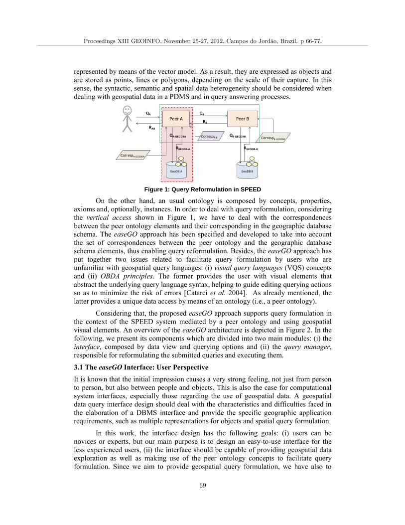
represented by means of the vector model. As a result, they are expressed as objects and

are stored as points, lines or polygons, depending on the scale of their capture. In this

sense, the syntactic, semantic and spatial data heterogeneity should be considered when

dealing with geospatial data in a PDMS and in query answering processes.

Figure 1: Query Reformulation in SPEED

On the other hand, an usual ontology is composed by concepts, properties,

axioms and, optionally, instances. In order to deal with query reformulation, considering

the vertical access shown in Figure 1, we have to deal with the correspondences

between the peer ontology elements and their corresponding in the geographic database

schema. The easeGO approach has been specified and developed to take into account

the set of correspondences between the peer ontology and the geographic database

schema elements, thus enabling query reformulation. Besides, the easeGO approach has

put together two issues related to facilitate query formulation by users who are

unfamiliar with geospatial query languages: (i) visual query languages (VQS) concepts

and (ii) OBDA principles. The former provides the user with visual elements that

abstract the underlying query language syntax, helping to guide editing querying actions

so as to minimize the risk of errors [Catarci et al. 2004]. As already mentioned, the

latter provides a unique data access by means of an ontology (i.e., a peer ontology).

Considering that, the proposed easeGO approach supports query formulation in

the context of the SPEED system mediated by a peer ontology and using geospatial

visual elements. An overview of the easeGO architecture is depicted in Figure 2. In the

following, we present its components which are divided into two main modules: (i) the

interface, composed by data view and querying options and (ii) the query manager,

responsible for reformulating the submitted queries and executing them.

3.1 The easeGO Interface: User Perspective

It is known that the initial impression causes a very strong feeling, not just from person

to person, but also between people and objects. This is also the case for computational

system interfaces, especially those regarding the use of geospatial data. A geospatial

data query interface design should deal with the characteristics and difficulties faced in

the elaboration of a DBMS interface and provide the specific geographic application

requirements, such as multiple representations for objects and spatial query formulation.

In this work, the interface design has the following goals: (i) users can be

novices or experts, but our main purpose is to design an easy-to-use interface for the

less experienced users, (ii) the interface should be capable of providing geospatial data

exploration as well as making use of the peer ontology concepts to facilitate query

formulation. Since we aim to provide geospatial query formulation, we have also to

Peer A Peer B

GeoDB A

QA QB

RB

RAB

CorrespA-B

CorrespA-GEODBA

QA-GEODBA

GeoDB B

RGEODB-A

CorrespB-GEODBB

QB-GEODBB

RGEODB-B


69

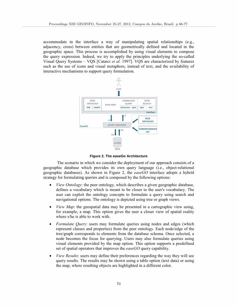
accommodate in the interface a way of manipulating spatial relationships (e.g.,

adjacency, cross) between entities that are geometrically defined and located in the

geographic space. This process is accomplished by using visual elements to compose

the query expression. Indeed, we try to apply the principles underlying the so-called

Visual Query Systems – VQS [Catarci et al. 1997]. VQS are characterized by features

such as the use of icons and visual metaphors, instead of text, and the availability of

interactive mechanisms to support query formulation.

Figure 2. The easeGo Architecture

The scenario in which we consider the deployment of our approach consists of a

geographic database which provides its own query language (i.e., object-relational

geographic databases). As shown in Figure 2, the easeGO interface adopts a hybrid

strategy for formulating queries and is composed by the following options:

View Ontology: the peer ontology, which describes a given geographic database,

defines a vocabulary which is meant to be closer to the user's vocabulary. The

user can exploit the ontology concepts to formulate a query using search and

navigational options. The ontology is depicted using tree or graph views.

View Map: the geospatial data may be presented in a cartographic view using,

for example, a map. This option gives the user a closer view of spatial reality

where s/he is able to work with.

Formulate Query: users may formulate queries using nodes and edges (which

represent classes and properties) from the peer ontology. Each node/edge of the

tree/graph corresponds to elements from the database schema. Once selected, a

node becomes the focus for querying. Users may also formulate queries using

visual elements provided by the map option. This option supports a predefined

set of spatial operators that improves the easeGO query capability.

View Results: users may define their preferences regarding the way they will see

query results. The results may be shown using a table option (text data) or using

the map, where resulting objects are highlighted in a different color.


70

When using the peer ontology to formulate a query, the user can select a node

and request instances of this node. S/he may also, from this node, set the query in a

visual way by using a form which is dynamically built. This form provides the existing

properties of the chosen node. Using this form, the user chooses the properties s/he

wants to view (as a project operation from the relational model) and determines the

conditions (as a select operation from the relational model) that the query should verify.

When formulating a query by using the map option, users may choose a

geographic object to be a query operand and drag it to a query area. Once the user has

selected the first query operand and it has been dragged to the query area, s/he selects

the spatial operator to be applied. If it is a unary operation, the query may be validated.

However, if it is a binary operation, another geographic object will be selected.

From both query formulation options, a query Q (Figure 2) is generated. This

query will be sent to the query manager, as explained in the following.

3.2 The easeGO Query Manager: Reformulating Queries

We define the query manager approach as follows: given a user query Q expressed in

terms of the concepts of the peer ontology, a target geographic database schema GeoDB

schema, and a set of correspondences between the peer ontology elements and the

database schema ones, our goal is to find a reformulated query of Q expressed in terms

of the concepts of the GeoDB schema in such a way that it may be executed by the

DBMS. The reformulated query is named Q1 which is executed in the DBMS and the

query results R1 are returned to the query manager. The query manager considers the

user preferences regarding the data visualization and sets the resulting data R which is

sent to the interface. R may be depicted using a table or highlighted on the map.

4. The easeGO Tool: Implementation and Results

The easeGO tool has been implemented in Java, using the OWLPrefuse [OWLPrefuse

2012] and GeoTools [GeoTools 2012] APIs. It provides access to geographic databases

coded in Oracle Spatial [Oracle 2012] and PostGIS [PostGIS 2012].

The query formulation and reformulation process implemented in the easeGO

tool is based on the aspects described in the previous sections. When the user starts

working, a peer ontology is depicted through a graph or tree representation. The peer

ontology is related to a particular geographic database which refers to a single

geographic region. Following this, the user can navigate at the peer ontology level,

browse geospatial data using layers over a map, or formulate queries. From the

functional point of view, the easeGO tool current release provides the following:

a) Peer Ontology Navigation: the user is able to navigate over the ontology

concepts and choose one for querying. This querying process may be

accomplished in a two-fold way: (i) by retrieving all the instances of a given

concept or, (ii) starting from a general concept, the user can choose the

properties s/he wants to see and define constraints to be applied over the data.

b) Form-based query formulation: after choosing a concept using the peer

ontology, the tool provides the user with a form which presents the concept’s

properties and enables query constraints definition. Thus, s/he is able to fill in

the form, by choosing the desired properties and establishing constraints, to

create a query expression in a high-level way.


71

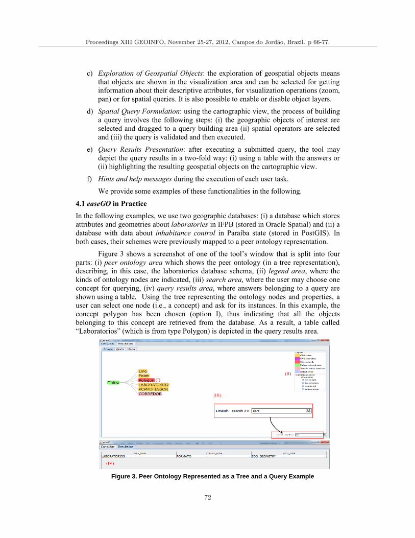
c) Exploration of Geospatial Objects: the exploration of geospatial objects means

that objects are shown in the visualization area and can be selected for getting

information about their descriptive attributes, for visualization operations (zoom,

pan) or for spatial queries. It is also possible to enable or disable object layers.

d) Spatial Query Formulation: using the cartographic view, the process of building

a query involves the following steps: (i) the geographic objects of interest are

selected and dragged to a query building area (ii) spatial operators are selected

and (iii) the query is validated and then executed.

e) Query Results Presentation: after executing a submitted query, the tool may

depict the query results in a two-fold way: (i) using a table with the answers or

(ii) highlighting the resulting geospatial objects on the cartographic view.

f) Hints and help messages during the execution of each user task.

We provide some examples of these functionalities in the following.

4.1 easeGO in Practice

In the following examples, we use two geographic databases: (i) a database which stores

attributes and geometries about laboratories in IFPB (stored in Oracle Spatial) and (ii) a

database with data about inhabitance control in Paraíba state (stored in PostGIS). In

both cases, their schemes were previously mapped to a peer ontology representation.

Figure 3 shows a screenshot of one of the tool’s window that is split into four

parts: (i) peer ontology area which shows the peer ontology (in a tree representation),

describing, in this case, the laboratories database schema, (ii) legend area, where the

kinds of ontology nodes are indicated, (iii) search area, where the user may choose one

concept for querying, (iv) query results area, where answers belonging to a query are

shown using a table. Using the tree representing the ontology nodes and properties, a

user can select one node (i.e., a concept) and ask for its instances. In this example, the

concept polygon has been chosen (option I), thus indicating that all the objects

belonging to this concept are retrieved from the database. As a result, a table called

“Laboratorios” (which is from type Polygon) is depicted in the query results area.

Figure 3. Peer Ontology Represented as a Tree and a Query Example


72

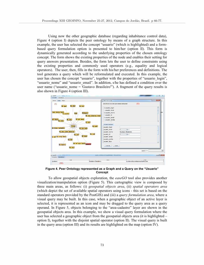
Using now the other geographic database (regarding inhabitance control data),

Figure 4 (option I) depicts the peer ontology by means of a graph structure. In this

example, the user has selected the concept “usuario” (which is highlighted) and a form-

based query formulation option is presented to him/her (option II). This form is

dynamically generated according to the underlying properties of the chosen ontology

concept. The form shows the existing properties of the node and enables their setting for

query answers presentation. Besides, the form lets the user to define constraints using

the existing properties and commonly used operators (e.g., equality and logical

operators). The user, then, fills in the form with his/her preferences and definitions. The

tool generates a query which will be reformulated and executed. In this example, the

user has chosen the concept “usuario”, together with the properties of “usuario_login”,

“usuario_nome” and “usuario_email”. In addition, s/he has defined a condition over the

user name (“usuario_nome = 'Gustavo Brasileiro'”). A fragment of the query results is

also shown in Figure 4 (option III).

Figure 4. Peer Ontology represented as a Graph and a Query on the “Usuario” Concept

To allow geospatial objects exploration, the easeGO tool also provides another

visualization/manipulation option (Figure 5). This cartographic view is composed by

three main areas, as follows: (i) geospatial objects area, (ii) spatial operators area

(which depict the set of available spatial operators using icons - this set is based on the

standard operators provided by the PostGIS) and (iii) a query formulation area, where a

visual query may be built. In this case, when a geographic object of an active layer is

selected, it is represented as an icon and may be dragged to the query area as a query

operand. In Figure 5, objects belonging to the “area-cadastro” layer are shown in the

geospatial objects area. In this example, we show a visual query formulation where the

user has selected a geographic object from the geospatial objects area (it is highlighted –

option I), together with the disjoint spatial operator (option II). The visual query is built

in the query area (option III) and its results are highlighted on the map (option IV).


73

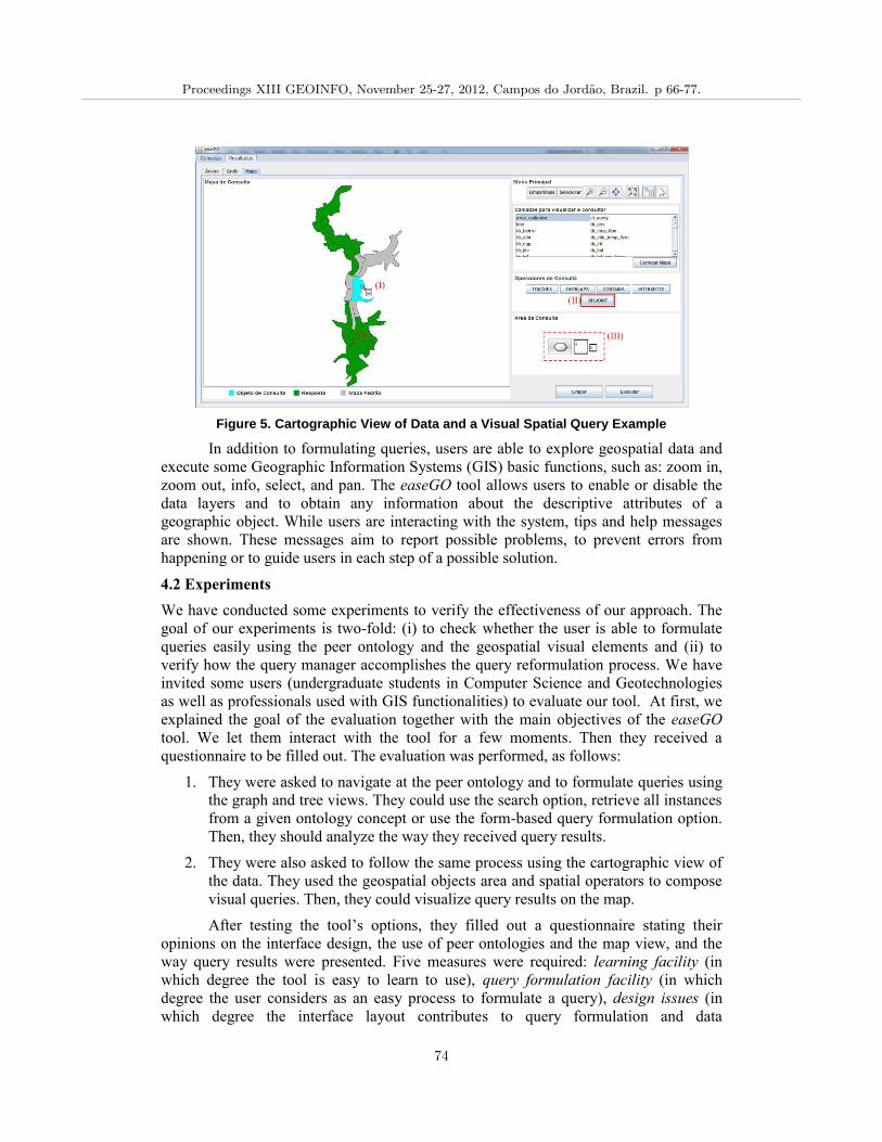
Figure 5. Cartographic View of Data and a Visual Spatial Query Example

In addition to formulating queries, users are able to explore geospatial data and

execute some Geographic Information Systems (GIS) basic functions, such as: zoom in,

zoom out, info, select, and pan. The easeGO tool allows users to enable or disable the

data layers and to obtain any information about the descriptive attributes of a

geographic object. While users are interacting with the system, tips and help messages

are shown. These messages aim to report possible problems, to prevent errors from

happening or to guide users in each step of a possible solution.

4.2 Experiments

We have conducted some experiments to verify the effectiveness of our approach. The

goal of our experiments is two-fold: (i) to check whether the user is able to formulate

queries easily using the peer ontology and the geospatial visual elements and (ii) to

verify how the query manager accomplishes the query reformulation process. We have

invited some users (undergraduate students in Computer Science and Geotechnologies

as well as professionals used with GIS functionalities) to evaluate our tool. At first, we

explained the goal of the evaluation together with the main objectives of the easeGO

tool. We let them interact with the tool for a few moments. Then they received a

questionnaire to be filled out. The evaluation was performed, as follows:

1. They were asked to navigate at the peer ontology and to formulate queries using

the graph and tree views. They could use the search option, retrieve all instances

from a given ontology concept or use the form-based query formulation option.

Then, they should analyze the way they received query results.

2. They were also asked to follow the same process using the cartographic view of

the data. They used the geospatial objects area and spatial operators to compose

visual queries. Then, they could visualize query results on the map.

After testing the tool’s options, they filled out a questionnaire stating their

opinions on the interface design, the use of peer ontologies and the map view, and the

way query results were presented. Five measures were required: learning facility (in

which degree the tool is easy to learn to use), query formulation facility (in which

degree the user considers as an easy process to formulate a query), design issues (in

which degree the interface layout contributes to query formulation and data


74

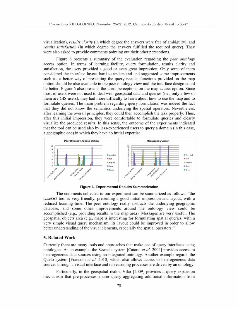
visualization), results clarity (in which degree the answers were free of ambiguity), and

results satisfaction (in which degree the answers fulfilled the required query). They

were also asked to provide comments pointing out their other perceptions.

Figure 6 presents a summary of the evaluation regarding the peer ontology

access option. In terms of learning facility, query formulation, results clarity and

satisfaction, the users provided a good or even great impression. Only some of them

considered the interface layout hard to understand and suggested some improvements

such as: a better way of presenting the query results, functions provided on the map

option should be also available in the peer ontology view and the interface design could

be better. Figure 6 also presents the users perceptions on the map access option. Since

most of users were not used to deal with geospatial data and queries (i.e., only a few of

them are GIS users), they had more difficulty to learn about how to use the map and to

formulate queries. The main problem regarding query formulation was indeed the fact

that they did not know the semantics underlying the spatial operators. Nevertheless,

after learning the overall principles, they could then accomplish the task properly. Thus,

after this initial impression, they were comfortable to formulate queries and clearly

visualize the produced results. In this sense, the outcome of the experiments indicated

that the tool can be used also by less-experienced users to query a domain (in this case,

a geographic one) in which they have no initial expertise.

Figure 6. Experimental Results Summarization

The comments collected in our experiment can be summarized as follows: “the

easeGO tool is very friendly, presenting a good initial impression and layout, with a

reduced learning time. The peer ontology really abstracts the underlying geographic

database, and some other improvements around the ontology view could be

accomplished (e.g., providing results in the map area). Messages are very useful. The

geospatial objects area (e.g., map) is interesting for formulating spatial queries, with a

very simple visual query mechanism. Its layout could be improved in order to allow

better understanding of the visual elements, especially the spatial operators.”

5. Related Work

Currently there are many tools and approaches that make use of query interfaces using

ontologies. As an example, the Sewasie system [Catarci et al. 2004] provides access to

heterogeneous data sources using an integrated ontology. Another example regards the

Quelo system [Franconi et al. 2010] which also allows access to heterogeneous data

sources through a visual interface and its reasoning processes are driven by an ontology.

Particularly, in the geospatial realm, Vilar [2009] provides a query expansion

mechanism that pre-processes a user query aggregating additional information from

0

2

4

6

8

10

12

Peer Ontology Access Option

Very bad

Bad

Regular

Good

Great

0123456789

10

Map Access Option

Very bad

Bad

Regular

Good

Great


75

ontologies. Zhao et al. [2008] provide an integrated access to distributed geospatial data

using RDF ontology and query rewriting. Zhifeng et al. [2009] use SPARQL to perform

semantic query and retrieval of geospatial information which has been converted to a

geospatial ontology. Baglioni et al. [2008] create an intermediate semantic layer

between the user and the geodatabase in order to facilitate the user’s queries. They also

enrich the generated ontology with semantics from a domain ontology by finding

correspondences between the classes and properties of the two ontologies. Also, Viegas

and Gonçalves [2006] present the GeOntoQuery approach which allows different

queries formulated over the same geographic database using an ontology.

Comparing these works with ours, we go one step further as we put together

both OBDA principles and VQL ones using a peer ontology and visual elements to

allow access over the geospatial data in the light of a PDMS setting. Another difference

is the use of the correspondences set for allowing query reformulation.

6. Conclusions and Future Work

This work is an attempt to put in an easy-to-use way the task of accessing geospatial

data using an ontology as a middle layer together with visual elements. To achieve this,

aspects related to geographic databases, query interface design and ontology navigation

have been considered. The easeGO tool provides an intuitive and transparent setting

where the user is able to work with a peer ontology or with a cartographic view of the

geospatial data. A query formulated in the interface is reformulated by the query

manager using a set of existing correspondences between the peer ontology and the

database schema. Query results can be visualized both in a table form or using the map.

Experiments accomplished with real users showed that the easeGO tool has

some advantages: (i) it does not require that users have previous knowledge about the

underlying database schema or query language; (ii) it gives the user a closer view of

spatial reality where he is able to work with; (iii) it supports a predefined set of spatial

operators that improves query capability and (iv) it allows users to pose queries by a

visual, form or ontological paradigm, helped by message tips that cover all tasks.

The easeGO tool has been implemented in the light of the SPEED system,

although its approach can be applied to any OBDA environment which deals with

geographic databases. As future work, this tool will be extended to provide query

reformulation between two neighbor peers, taking into account the semantic

correspondences between them.

References

Almeida D, Mendonça A., Salgado A. C., Souza D. (2011) “Building Geospatial Ontologies

from Geographic Database Schemas in Peer Data Management Systems”, In: Proc. of

the XII Brazilian Symposium on GeoInformatics (GeoInfo). Campos do Jordão, p. 1-12.

Baglioni, M., Giovannetti, E., Masserotti, M. G., Renso, C., Spinsanti, L. (2008) “Ontology-

supported Querying of Geographical Databases”, In: Transactions in GIS, vol. 12, issue s1,

pp. 31–44, December.

Calvanese, D., De Giacomo, G., Lembo, D., Lenzerini, M., Poggi, A., Rodriguez-Muro, M.,

and Rosati, R. (2009) “Ontologies and databases: The DL-lite approach”, In: Reasoning

Web 2009, pages 255–356.


76

Catarci, T., Dongilli, P., Di Mascio, T., Franconi, E., Santucci, G., Tessaris, S. (2004) "An

Ontology Based Visual Tool for Query Formulation Support", In: ECAI 2004: 308-312

Catarci, T., Costabile M., Leviadi S., Batini C. (1997) “Visual query systems for databases:

A survey”, In: Journal of Visual Languages and Computing. Vol. 8, pages 215-260.

Franconi E., Guagliardo P., Trevisan M., (2010) “An intelligent query interface based on

ontology navigation”. In Proceedings of the Workshop on Visual Interfaces to the Social

and Semantic Web (VISSW 2010), 2010.

Geotools (2012). Available at http://www.geotools.org/. June 2012.

Hedeler, C., Belhajjame, K., Fernandes, A.A.A., Embury, S.M., Paton, N.W. (2009)

“Dimensions of Databases”, In: Proceedings of 26th British National Conference on

Databases (BNCOD), pages 55-66, Birmingham, UK.

Hess G. (2008) “Towards effective geographic ontology semantic similarity assessment”.

PhD Thesis. UFRGS.

King, R. A., Hameurlain, A., and Morvan, F. (2010) “Query Routing and Processing in

Peer-to-Peer Data Sharing Systems”, In: International Journal of Database Management

Systems (IJDMS), vol, 2, n. 2, pages 116-139.

Kontchakov, R., Lutz, C., Toman, D., Wolter, F. and Zakharyaschev, M. (2011) “The

Combined Approach to Ontology-Based Data Access”, In: T. Walsh, editor, Proceedings

of IJCAI (Barcelona, 16-22 July), pp. 2656-2661. AAAI Press.

Lopes, F., Sacramento, R., Loscio, B. (2012) “Using Heterogeneous Mappings for

Rewriting SPARQL Queries”, In: Proc. of 11th International Workshop on Web

Semantics and Information Processing, Austria.

Makris, K., Gioldasis, N., Bikakis, N., and Christodoulakis, S. (2010) “Ontology mapping

and sparql rewriting for querying federated RDF data sources”, In: Proc. of the 9th

ODBASE, Crete, Greece.

Oracle (2012). Available at http://www.oracle.com/index.html. August 2012.

OwlPrefuse (2012). Available at http://owl2prefuse.sourceforge.net/. March 2012.

Pires C.E.S. (2009) “Ontology-Based Clustering in a Peer Data Management System”. PhD

thesis, Center for Informatics, UFPE.

PostGIS (2012). Available at http:// http://postgis.refractions.net/. August 2012.

Souza D., Pires C. E., Kedad Z., Tedesco P. C., Salgado A. C. (2011) “A Semantic-based

Approach for Data Management in a P2P System”, In LNCS Transactions on Large-

Scale Data- and Knowledge-Centered Systems.

Viegas, R. and Soares, V. (2006) “Querying a Geographic Database using an Ontology-

Based Methodology”, In: Brazilian Symposium on GeoInformatics (Geoinfo 2006), pp.

165-170, Brazil.

Vilar, B. (2009) “Semantic Query Processing Systems for biodiversity”. Master’s Thesis.

UNICAMP.

Zhao T., Zhang C., Wei M., Peng Z. (2008) “Ontology-Based Geospatial Data Query and

Integration”, In GIScience 2008, LNCS 5266, pp. 370-392,Springer.

Zhifeng, X., Lei, H., Xiaofang, Z. (2009) “Spatial Information semantic query based on

SPARQL”, In: Proceedings of the SPIE. pp. 74921P-74921P-10.


77

Expansão do conteúdo de um gazetteer: nomes hidrográficos

Tiago Henrique V. M. Moura, Clodoveu A. Davis Jr

Departamento de Ciência da Computação - Universidade Federal de Minas Gerais (UFMG) - Belo Horizonte, MG - Brasil

[thvmm,clodoveu]@dcc.ufmg.br

Abstract. The efficiency of a geographic database is directly related with the quality and completeness of its contents. In the case of gazetteers, i.e., place name dictionaries, previous work proposed ontological extensions based on the storage of geographic shape and on multiple types of relationships among places. However, in order to be more useful, gazetteers must contain large volumes of information on a large variety of themes, all of which must be geographically represented and related to places. The objective of this work is to propose techniques to expand a gazetteer’s content using relevance criteria, increasing its usefulness to solve problems such as place name disambiguation. We demonstrate these techniques using data on Brazilian rivers, which are preprocessed, and the appropriate relationships are identified and created.

Resumo. A eficiência de um banco de dados geográficos está diretamente relacionada à qualidade e completude das informações nele contidas. No caso de gazetteers, i.e., dicionários de nomes de lugares, trabalhos anteriores propuseram extensões ontológicas baseadas no armazenamento das formas geométricas e na criação de múltiplos tipos de relacionamentos entre lugares. No entanto, para que tenham maior utilidade, os gazetteers precisam conter grandes volumes de informação sobre uma variedade de temas relacionados a lugares. O objetivo deste trabalho é propor técnicas para expandir o conteúdo de um gazetteer usando critérios de relevância, aumentando sua utilidade em problemas como a desambiguação de nomes de lugares. É apresentado um estudo de caso com dados de rios brasileiros, que são pré-processados e incluídos no gazetteer, juntamente com os relacionamentos apropriados.

1. Introdução O volume de informação disponível na internet atualmente é muito grande e cresce diariamente. Buscar tal informação requer sistemas capazes de compreender o que o usuário deseja, localizar e apresentar resultados em ordem de relevância. Muitas vezes o usuário utiliza um conjunto de palavras-chave como forma de dizer o que procura para o sistema. Trabalhos anteriores (Sanderson and Kohler 2004; Wang, Xie et al. 2005; Delboni, Borges et al. 2007; Backstrom, Kleinberg et al. 2008) mostram que uma parte significativa dessas consultas envolve termos como nomes de lugares e expressões que denotam posicionamento. Por isso, é importante reconhecer a intenção do usuário que inclui termos geográficos em buscas, bem como determinar o escopo geográfico de documentos, em aplicações de recuperação de informação geográfica (RIG).

Em problemas de RIG, é frequentemente necessário reconhecer um nome como sendo uma referência a um lugar, e também distinguir entre lugares que possuem o


78

mesmo nome (Hastings 2008). Por exemplo, “São Francisco” pode ser uma cidade da região norte de Minas Gerais, um bairro de Belo Horizonte, um rio ou um santo católico. Os gazetteers (dicionários toponímicos) são recursos que auxiliam nesse processo. Visando RIG e outras aplicações, nosso grupo projetou e desenvolveu um gazetteer ontológico, denominado Ontogazetteer (Machado, Alencar et al. 2011), em que não apenas são registrados nomes de lugares, mas também relacionamentos entre eles. Nesse gazetteer1 estão também incluídos dados urbanos, utilizados cotidianamente pelos cidadãos, particularmente em mensagens disseminadas nas redes sociais online.

Este trabalho apresenta técnicas para expandir o conteúdo de um gazetteer usando critérios de relevância, voltadas especificamente para o Ontogazetteer. Trabalhos relacionados são descritos na Seção 2. Um estudo de caso envolvendo rios brasileiros é apresentado na Seção 3, sendo definidos também os relacionamentos apropriados (Seção 4). Finalmente, a Seção 5 apresenta conclusões e trabalhos futuros.

2. Trabalhos Relacionados Em geral, gazetteers contêm dados organizados segundo uma tripla <nome do lugar, tipo do lugar, footprint>, sendo que esse footprint, que representa a localização geográfica propriamente dita, se resume a um par de coordenadas (Hill 2000). Exemplos de gazetteers com essa estrutura básica incluem o GeoNames e o Getty Thesaurus of Geographical Names (TGN). Tais gazetteers são utilizados como fontes de nomes geográficos para diversas aplicações (Souza, Davis Jr. et al. 2005; Goodchild and Hill 2008). A principal função desses gazetteers é informar uma coordenada geográfica a partir de um nome de lugar dado, o que os torna apenas parcialmente adequados às necessidades de RIG.

O Ontogazetteer (Machado, Alencar et al. 2010; Machado, Alencar et al. 2011) foi proposto com uma estrutura mais complexa que a usual, em que os lugares (1) podem ser representados por pontos, linhas ou polígonos, (2) estão relacionados a outros lugares, usando relacionamentos espaciais (vizinho a, contido em, etc.) ou semânticos, (3) podem possuir nomes alternativos ou apelidos, e (4) podem estar associados a termos e expressões características (Alencar and Davis Jr 2011). Tais características adicionais são importantes para RIG, pois fornecem elementos para resolver problemas importantes, como a ambiguidade de nomes de lugares (Leidner 2007) e a detecção do contexto geográfico em textos (Silva, Martins et al. 2006). A expansão do conteúdo desse modelo semanticamente mais rico de gazetteer é um desafio importante, para ampliar a gama de situações em que técnicas de RIG poderão ser usadas para reconhecimento de lugares associados a textos. Para a expansão, podem ser utilizados dados extraídos de bancos de dados geográficos, filtrando o que é irrelevante, e detectando relacionamentos com lugares anteriormente disponíveis. A decisão quanto ao que é ou não relevante para ser incorporado ao gazetteer precisa levar em conta critérios baseados nas características dos lugares ou de seus relacionamentos com outros lugares. Diante do exposto, este trabalho busca expandir o conteúdo do OntoGazetteer, não apenas acrescentando novos nomes de lugares, mas também aumentando e diversificando os relacionamentos entre esses lugares.

1 http://geo.lbd.dcc.ufmg.br:8080/ontogazetteer/


79

3. Expansão Uma fonte para lugares e relacionamentos são bancos de dados geográficos existentes, dos quais se pode extrair nomes relacionados a objetos geográficos e determinar relacionamentos com base em sua geometria. A obtenção de relacionamentos semânticos, por outro lado, é mais complexa, pois sua natureza pode ser muito variada. Por exemplo, as cidades de Perdões (MG) e Bragança Paulista (SP) estão relacionadas por serem cortadas pela BR-381, embora não sejam vizinhas nem se localizem próximas uma a outra. Da mesma forma, lugares geograficamente desconexos podem ter ligações semânticas baseadas em características em comum (p. ex. estâncias hidrominerais de Caxambu (MG) e Poá (SP)), ou formarem grupos semanticamente coerentes (p. ex., Pico da Neblina e Pico da Bandeira), ou ainda por motivos históricos (p. ex., Mariana, Ouro Preto e Belo Horizonte, capitais de Minas Gerais ao longo da história).

Relacionamentos espaciais semânticos constituem uma vantagem para o uso do Ontogazetteer em diversas aplicações (Machado, Alencar et al. 2011). Por exemplo, uma notícia que contenha os nomes “Salvador”, “Camaçari” e “Dias D’Ávila” provavelmente se refere à Região Metropolitana de Salvador, unidade espacial de referência que contém municípios com esses nomes. Outra notícia que contenha os nomes “Sabará”, “Cordisburgo” e “Curvelo”, mesmo que esses nomes sejam devidamente associados aos municípios correspondentes, teria seu escopo geográfico definido como “Minas Gerais”, referência que contém todos os três municípios. Estando registrado um relacionamento semântico baseado em rios e bacias hidrográficas, por outro lado, seria possível concluir, com mais precisão, que o escopo na verdade é a bacia do rio das Velhas, afluente do rio São Francisco que passa pelos três municípios. O rio das Velhas, no caso, constitui uma conexão semântica entre as três cidades.

Assim, este trabalho introduz técnicas para a expansão do conteúdo do OntoGazetteer, com foco particular sobre relacionamentos semânticos. Um primeiro estudo foi realizado sobre dados de rios e bacias hidrográficas do Brasil publicados pela Agência Nacional de Águas (ANA) em seu Web site e busca obter relacionamentos semânticos entre lugares que estejam direta ou indiretamente relacionados a rios e bacias hidrográficas. Os elementos, rios e bacias, existentes nesta base foram codificados seguindo a proposta de Otto Pfafstetter (ANA 2006) e obedecem uma hierarquia onde nos níveis mais altos estão os rios que deságuam no oceano. Esses dados precisam ser transformados para carga no gazetteer, pois apresentam alguns problemas, como a falta dos nomes de alguns elementos. Por isso, uma série de filtros foram aplicados a fim de se obter os rios e bacias mais relevantes.

O primeiro filtro executado removeu elementos com nomes indeterminados, reduzindo o volume de dados em mais de 50%. Entretanto, em análises mais detalhadas constatou-se que este filtro precisava ser revisto, devido à existência de rios que passam por regiões densamente habitadas e estavam sem nome na base da ANA. Um exemplo é o Ribeirão Arrudas, que cruza a cidade de Belo Horizonte, e que tem pequena importância hidrológica por ter pequeno comprimento e baixa vazão, mas importante devido à intensa urbanização em sua bacia, que o transforma em uma referência urbana.

Outros cursos d’água se encontravam na mesma situação. Para encontrar essas situações, e buscar resolvê-las com dados de outras fontes, buscou-se estabelecer o valor de um elemento com nome indeterminado. No caso, optou-se por considerar como importantes rios que, mesmo sem nome definido e de pequeno porte, cruzassem


80

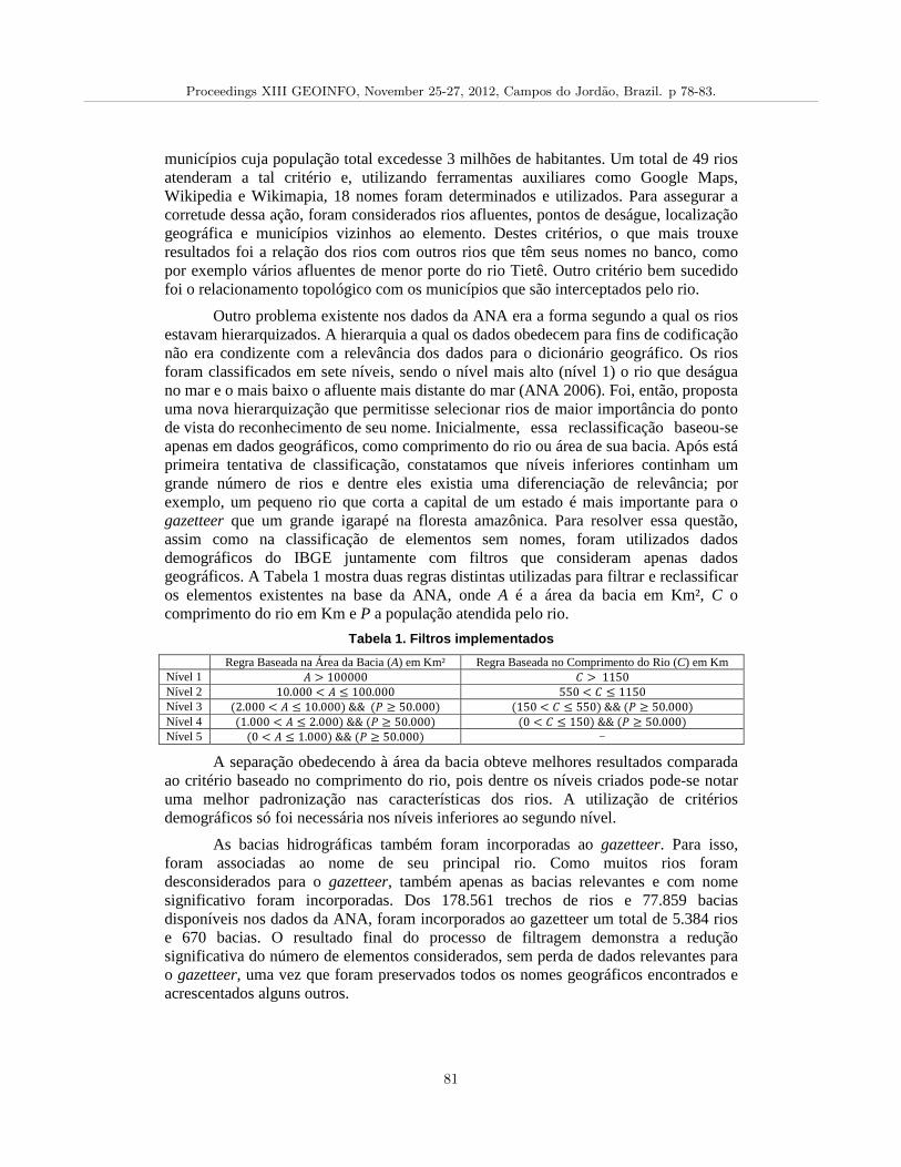
municípios cuja população total excedesse 3 milhões de habitantes. Um total de 49 rios atenderam a tal critério e, utilizando ferramentas auxiliares como Google Maps, Wikipedia e Wikimapia, 18 nomes foram determinados e utilizados. Para assegurar a corretude dessa ação, foram considerados rios afluentes, pontos de deságue, localização geográfica e municípios vizinhos ao elemento. Destes critérios, o que mais trouxe resultados foi a relação dos rios com outros rios que têm seus nomes no banco, como por exemplo vários afluentes de menor porte do rio Tietê. Outro critério bem sucedido foi o relacionamento topológico com os municípios que são interceptados pelo rio.

Outro problema existente nos dados da ANA era a forma segundo a qual os rios estavam hierarquizados. A hierarquia a qual os dados obedecem para fins de codificação não era condizente com a relevância dos dados para o dicionário geográfico. Os rios foram classificados em sete níveis, sendo o nível mais alto (nível 1) o rio que deságua no mar e o mais baixo o afluente mais distante do mar (ANA 2006). Foi, então, proposta uma nova hierarquização que permitisse selecionar rios de maior importância do ponto de vista do reconhecimento de seu nome. Inicialmente, essa reclassificação baseou-se apenas em dados geográficos, como comprimento do rio ou área de sua bacia. Após está primeira tentativa de classificação, constatamos que níveis inferiores continham um grande número de rios e dentre eles existia uma diferenciação de relevância; por exemplo, um pequeno rio que corta a capital de um estado é mais importante para o gazetteer que um grande igarapé na floresta amazônica. Para resolver essa questão, assim como na classificação de elementos sem nomes, foram utilizados dados demográficos do IBGE juntamente com filtros que consideram apenas dados geográficos. A Tabela 1 mostra duas regras distintas utilizadas para filtrar e reclassificar os elementos existentes na base da ANA, onde A é a área da bacia em Km², C o comprimento do rio em Km e P a população atendida pelo rio.

Tabela 1. Filtros implementados

Regra Baseada na Área da Bacia (A) em Km² Regra Baseada no Comprimento do Rio (C) em Km Nível 1 � > 100000 � > 1150 Nível 2 10.000 < � ≤ 100.000 550 < � ≤ 1150 Nível 3 (2.000 < � ≤ 10.000)&&(� ≥ 50.000) (150 < � ≤ 550)&&(� ≥ 50.000) Nível 4 (1.000 < � ≤ 2.000)&&(� ≥ 50.000) (0 < � ≤ 150)&&(� ≥ 50.000) Nível 5 (0 < � ≤ 1.000)&&(� ≥ 50.000) -

A separação obedecendo à área da bacia obteve melhores resultados comparada ao critério baseado no comprimento do rio, pois dentre os níveis criados pode-se notar uma melhor padronização nas características dos rios. A utilização de critérios demográficos só foi necessária nos níveis inferiores ao segundo nível.

As bacias hidrográficas também foram incorporadas ao gazetteer. Para isso, foram associadas ao nome de seu principal rio. Como muitos rios foram desconsiderados para o gazetteer, também apenas as bacias relevantes e com nome significativo foram incorporadas. Dos 178.561 trechos de rios e 77.859 bacias disponíveis nos dados da ANA, foram incorporados ao gazetteer um total de 5.384 rios e 670 bacias. O resultado final do processo de filtragem demonstra a redução significativa do número de elementos considerados, sem perda de dados relevantes para o gazetteer, uma vez que foram preservados todos os nomes geográficos encontrados e acrescentados alguns outros.


81

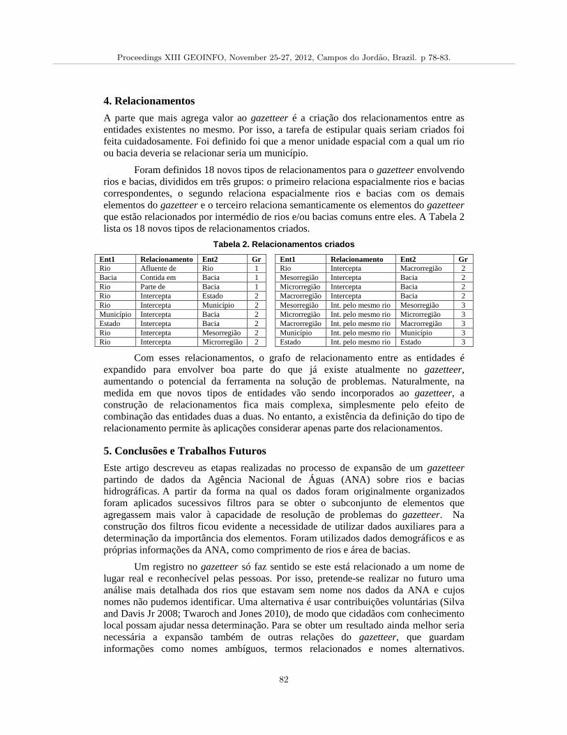
4. Relacionamentos A parte que mais agrega valor ao gazetteer é a criação dos relacionamentos entre as entidades existentes no mesmo. Por isso, a tarefa de estipular quais seriam criados foi feita cuidadosamente. Foi definido foi que a menor unidade espacial com a qual um rio ou bacia deveria se relacionar seria um município.

Foram definidos 18 novos tipos de relacionamentos para o gazetteer envolvendo rios e bacias, divididos em três grupos: o primeiro relaciona espacialmente rios e bacias correspondentes, o segundo relaciona espacialmente rios e bacias com os demais elementos do gazetteer e o terceiro relaciona semanticamente os elementos do gazetteer que estão relacionados por intermédio de rios e/ou bacias comuns entre eles. A Tabela 2 lista os 18 novos tipos de relacionamentos criados.

Tabela 2. Relacionamentos criados

Ent1 Relacionamento Ent2 Gr Ent1 Relacionamento Ent2 Gr Rio Afluente de Rio 1 Rio Intercepta Macrorregião 2 Bacia Contida em Bacia 1 Mesorregião Intercepta Bacia 2 Rio Parte de Bacia 1 Microrregião Intercepta Bacia 2 Rio Intercepta Estado 2 Macrorregião Intercepta Bacia 2 Rio Intercepta Município 2 Mesorregião Int. pelo mesmo rio Mesorregião 3 Município Intercepta Bacia 2 Microrregião Int. pelo mesmo rio Microrregião 3 Estado Intercepta Bacia 2 Macrorregião Int. pelo mesmo rio Macrorregião 3 Rio Intercepta Mesorregião 2 Município Int. pelo mesmo rio Município 3 Rio Intercepta Microrregião 2 Estado Int. pelo mesmo rio Estado 3

Com esses relacionamentos, o grafo de relacionamento entre as entidades é expandido para envolver boa parte do que já existe atualmente no gazetteer, aumentando o potencial da ferramenta na solução de problemas. Naturalmente, na medida em que novos tipos de entidades vão sendo incorporados ao gazetteer, a construção de relacionamentos fica mais complexa, simplesmente pelo efeito de combinação das entidades duas a duas. No entanto, a existência da definição do tipo de relacionamento permite às aplicações considerar apenas parte dos relacionamentos.

5. Conclusões e Trabalhos Futuros Este artigo descreveu as etapas realizadas no processo de expansão de um gazetteer partindo de dados da Agência Nacional de Águas (ANA) sobre rios e bacias hidrográficas. A partir da forma na qual os dados foram originalmente organizados foram aplicados sucessivos filtros para se obter o subconjunto de elementos que agregassem mais valor à capacidade de resolução de problemas do gazetteer. Na construção dos filtros ficou evidente a necessidade de utilizar dados auxiliares para a determinação da importância dos elementos. Foram utilizados dados demográficos e as próprias informações da ANA, como comprimento de rios e área de bacias.

Um registro no gazetteer só faz sentido se este está relacionado a um nome de lugar real e reconhecível pelas pessoas. Por isso, pretende-se realizar no futuro uma análise mais detalhada dos rios que estavam sem nome nos dados da ANA e cujos nomes não pudemos identificar. Uma alternativa é usar contribuições voluntárias (Silva and Davis Jr 2008; Twaroch and Jones 2010), de modo que cidadãos com conhecimento local possam ajudar nessa determinação. Para se obter um resultado ainda melhor seria necessária a expansão também de outras relações do gazetteer, que guardam informações como nomes ambíguos, termos relacionados e nomes alternativos.


82

Destacamos que as técnicas apresentadas aqui estão sendo utilizadas em outras expansões, envolvendo elementos tais como rodovias, ferrovias e lugares agrupados segundo categorias encontradas em bases de conhecimento tais como a Wikipedia.

Agradecimentos Este trabalho foi parcialmente financiado com recursos do CNPq (302090/2009-6 e 560027/2010-9) e FAPEMIG (CEX-PPM-00466/11), além do Instituto Nacional de Ciência e Tecnologia para a Web (InWeb, CNPq 573871/2008-6).

Referências Alencar, R.O. and Davis Jr, C.A. (2011). Geotagging aided by topic detection with Wikipedia. 14th

AGILE Conference on Geographic Information Science, Utrecht, The Netherlands:461-478. ANA (2006). Topologia hídrica: método de construção e modelagem da base hidrográfica para suporte à

gestão de recursos hídricos. Agência Nacional de Águas. Brasília (DF). Versão 1.11, 17/11/2006.

Backstrom, L., Kleinberg, J., Kumar, R. and Novak, J. (2008). Spatial Variation in Search Engine Queries. International World Wide Web Conference (WWW), Beijing, China:357-366.

Delboni, T.M., Borges, K.A.V., Laender, A.H.F. and Davis Jr., C.A. (2007). "Semantic Expansion of Geographic Web Queries Based on Natural Language Positioning Expressions." Transactions in GIS 11(3): 377-397.

Goodchild, M.F. and Hill, L.L. (2008). "Introduction to digital gazetteer research." International Journal of Geographic Information Science 22(10): 1039-1044.

Hastings, J.T. (2008). "Automated conflation of digital gazetteer data." International Journal of Geographical Information Science 22(10): 1109-1127.

Hill, L.L. (2000). Core Elements of Digital Gazetteers: Placenames, Categories, and Footprints. 4th European Conference on Research and Advanced Technology for Digital Libraries:280-290.

Leidner, J.L. (2007). Toponym Resolution in Text: annotation, evaluation and applications of spatial grounding of place names. Boca Raton, Florida, Dissertation. com.

Machado, I.M.R., Alencar, R.O., Campos Junior, R.O. and Davis Jr, C.A. (2010). An Ontological Gazetteer for Geographic Information Retrieval. XI Brazilian Symposium on Geoinformatics, Campos do Jordão (SP), Brazil:21-32.

Machado, I.M.R., Alencar, R.O., Campos Junior, R.O. and Davis Jr, C.A. (2011). "An ontological gazetteer and its application for place name disambiguation in text." Journal of the Brazilian Computer Society 17(4): 267-279.

Sanderson, M. and Kohler, J. (2004). Analyzing Geographic Queries. Proc. of the ACM SIGIR Workshop on Geographic Information Retrieval, Sheffield, UK:1-2.

Silva, J.C.T. and Davis Jr, C.A. (2008). Um framework para coleta e filtragem de dados geográficos fornecidos voluntariamente. X Brazilian Symposium on GeoInformatics (GeoInfo 2008), Rio de Janeiro (RJ), Sociedade Brasileira de Computação.

Silva, M.J., Martins, B., Chaves, M., Cardoso, N. and Afonso, A.P. (2006). "Adding Geographic Scopes to Web Resources." Computers, Environment and Urban Syst. 30: 378-399.

Souza, L.A., Davis Jr., C.A., Borges, K.A.V., Delboni, T.M. and Laender, A.H.F. (2005). The Role of Gazetteers in Geographic Knowledge Discovery on the Web. 3rd Latin American Web Congress, Buenos Aires, Argentina:157-165.

Twaroch, F.A. and Jones, C.B. (2010). A Web Platform for the Evaluation of Vernacular Place Names in Automatically Constructed Gazetteers. 6th International Workshop on Geographical Information Retrieval (GIR 2010), Zurich, Switzerland.

Wang, C., Xie, X., Wang, L., Lu, Y. and Ma, W. (2005). Detecting Geographic Locations from Web Resources. Proc. of the 2nd Int'l Workshop on Geographic Information Retrieval, Bremen, Germany:17-24.


83

M-Attract: Assessing the Attractiveness of Placesby using Moving Objects Trajectories DataAndre Salvaro Furtado12, Renato Fileto1, Chiara Renso3

1PPGCC, Federal University of Santa Catarina (UFSC)PO BOX 476, 88040-900, Florianopolis-SC, BRAZIL

2Geography Department (DG), Santa Catarina State University (UDESC)Av. Madre Benvenuta, 2007 - Itacorubi, 88035-001, Florianopolis-SC, BRAZIL

3KDD LAB, ISTI-CNR, Via Moruzzi 1, 56100, Pisa, ITALY

asalvaro,[email protected],[email protected]

Abstract. Attractiveness of places has been studied by several sciences, givingrise to distinct ways for assessing it. However, the attractiveness evaluationmethods currently available lack versatility to analyze diverse attractivenessphenomena in different kinds of places and spatial scales. This article describesa novel method, called M-Attract, to assess interesting attractiveness of places,based on moving objects trajectories. M-Attract examines trajectory episodes(e.g., stop at, pass by) that happen in places and their encompassing regions tocompute their attractiveness. It is more flexible than state-of-the-art methods,with respect to land parcels, parameters, and measures used for attractivenessassessment. M-Attract has been evaluated in experiments with real data, whichdemonstrate its contributions to analyze attractiveness of places.

1. IntroductionAttractiveness quantifies how much something is able to attract the attention and influ-ence the decisions of one or more individuals [Uchino et al. 2005]. It can help to explaina variety of spatial-temporal phenomena. Furthermore, methods to properly estimate at-tractiveness of places are important tools to build applications for several domains, suchas traffic, tourism, and retail market analysis.

The attractiveness of geographic places has been studied for decades, by disci-plines like geography and economy. Several theories have been proposed to quantify theattractive force and delimit the region of influence of a place, including the GravitationalAttractiveness Model [Reilly 1931] and the Theory of Central Places [Christaller 1933].Since these pioneering work, a myriad of proposals have been presented to assess theattractiveness of places, in fields like urban planning, transport, marketing, business, mi-gration and tourism. These works use a variety of data to derive attractiveness, includingpopulation in each region, distances between given regions and a target region, surveysbased on voting, trajectories of moving objects such as taxis, and time periods when themoves occur, among other. However, these proposals lack versatility with respect to thecategories of places they can consider, and the measures used to assess their attractiveness.

Recently, the widespread use of mobile devices (e.g., cell phones, GPS) enabledcollecting of large volumes of raw trajectories, i.e., sequences of spatial-temporal po-sitions of moving objects. It has pushed the demand for mechanisms to extract useful


84

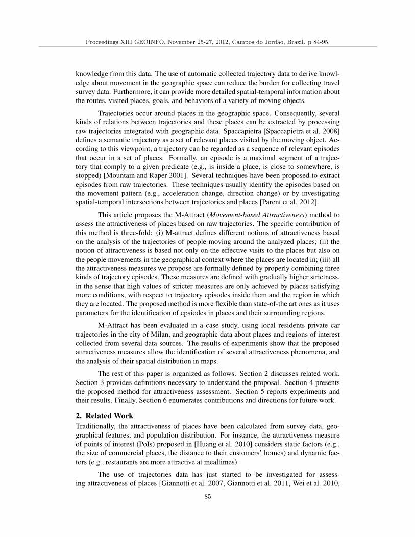
knowledge from this data. The use of automatic collected trajectory data to derive knowl-edge about movement in the geographic space can reduce the burden for collecting travelsurvey data. Furthermore, it can provide more detailed spatial-temporal information aboutthe routes, visited places, goals, and behaviors of a variety of moving objects.

Trajectories occur around places in the geographic space. Consequently, severalkinds of relations between trajectories and these places can be extracted by processingraw trajectories integrated with geographic data. Spaccapietra [Spaccapietra et al. 2008]defines a semantic trajectory as a set of relevant places visited by the moving object. Ac-cording to this viewpoint, a trajectory can be regarded as a sequence of relevant episodesthat occur in a set of places. Formally, an episode is a maximal segment of a trajec-tory that comply to a given predicate (e.g., is inside a place, is close to somewhere, isstopped) [Mountain and Raper 2001]. Several techniques have been proposed to extractepisodes from raw trajectories. These techniques usually identify the episodes based onthe movement pattern (e.g., acceleration change, direction change) or by investigatingspatial-temporal intersections between trajectories and places [Parent et al. 2012].

This article proposes the M-Attract (Movement-based Attractiveness) method toassess the attractiveness of places based on raw trajectories. The specific contribution ofthis method is three-fold: (i) M-attract defines different notions of attractiveness basedon the analysis of the trajectories of people moving around the analyzed places; (ii) thenotion of attractiveness is based not only on the effective visits to the places but also onthe people movements in the geographical context where the places are located in; (iii) allthe attractiveness measures we propose are formally defined by properly combining threekinds of trajectory episodes. These measures are defined with gradually higher strictness,in the sense that high values of stricter measures are only achieved by places satisfyingmore conditions, with respect to trajectory episodes inside them and the region in whichthey are located. The proposed method is more flexible than state-of-the art ones as it usesparameters for the identification of epsiodes in places and their surrounding regions.

M-Attract has been evaluated in a case study, using local residents private cartrajectories in the city of Milan, and geographic data about places and regions of interestcollected from several data sources. The results of experiments show that the proposedattractiveness measures allow the identification of several attractiveness phenomena, andthe analysis of their spatial distribution in maps.

The rest of this paper is organized as follows. Section 2 discusses related work.Section 3 provides definitions necessary to understand the proposal. Section 4 presentsthe proposed method for attractiveness assessment. Section 5 reports experiments andtheir results. Finally, Section 6 enumerates contributions and directions for future work.

2. Related WorkTraditionally, the attractiveness of places have been calculated from survey data, geo-graphical features, and population distribution. For instance, the attractiveness measureof points of interest (PoIs) proposed in [Huang et al. 2010] considers static factors (e.g.,the size of commercial places, the distance to their customers’ homes) and dynamic fac-tors (e.g., restaurants are more attractive at mealtimes).

The use of trajectories data has just started to be investigated for assess-ing attractiveness of places [Giannotti et al. 2007, Giannotti et al. 2011, Wei et al. 2010,


85

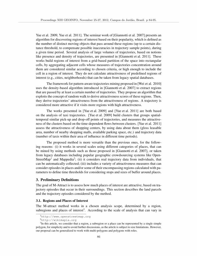
Yue et al. 2009, Yue et al. 2011]. The seminar work of [Giannotti et al. 2007] presents analgorithm for discovering regions of interest based on their popularity, which is defined asthe number of distinct moving objects that pass around these regions (up to a certain dis-tance threshold, to compensate possible inaccuracies in trajectory sample points), duringa given time period. Several analysis of large volumes of trajectories, based on notionslike presence and density of trajectories, are presented in [Giannotti et al. 2011]. Theseworks build regions of interest from a grid-based partition of the space into rectangularcells, by aggregating adjacent cells whose measures of trajectories concentration aroundthem are considered similar according to chosen criteria, or high enough to include thecell in a region of interest. They do not calculate attractiveness of predefined regions ofinterest (e.g., cities, neighborhoods) that can be taken from legacy spatial databases.

The framework for pattern-aware trajectories mining proposed in [Wei et al. 2010]uses the density-based algorithm introduced in [Giannotti et al. 2007] to extract regionsthat are passed by at least a certain number of trajectories. They propose an algorithm thatexploits the concept of random walk to derive attractiveness scores of these regions. Then,they derive trajectories’ attractiveness from the attractiveness of regions. A trajectory isconsidered more attractive if it visits more regions with high attractiveness.

The works presented in [Yue et al. 2009] and [Yue et al. 2011] are both basedon the analysis of taxi trajectories. [Yue et al. 2009] build clusters that groups spatial-temporal similar pick-up and drop-off points of trajectories, and measures the attractive-ness of the clusters based on the time-dependent flows between clusters. [Yue et al. 2011]assess the attractiveness of shopping centers, by using data about them (gloss leasablearea, number of nearby shopping malls, available parking space, etc.) and trajectory data(number of taxis within their area of influence in different time periods).

The proposed method is more versatile than the previous ones, for the follow-ing reasons: (i) it works in several scales using different categories of places, that canbe mined by using methods such as those proposed in [Giannotti et al. 2007], or takenfrom legacy databases including popular geographic crowdsourcing systems like Open-StreetMap1 and Mappedia2; (ii) it considers real trajectory data from individuals, thatcan be automatically collected; (iii) includes a variety of attractiveness measures that canconsider episodes in places and/or some of their encompassing regions calculated with pa-rameters to define time thresholds for considering stops and sizes of buffer around places.

3. Preliminary DefinitionsThe goal of M-Attract is to assess how much places of interest are attractive, based on tra-jectory episodes that occur in their surroundings. This section describes the land parcelsand the trajectory episodes considered by the method.

3.1. Regions and Places of InterestThe M-attract method works in a chosen analysis scope, determined by a region,subregions and places of interest3. According to the scale of analysis that can vary in

1http://www.openstreetmap.org2http://wikimapia.org3In this article, we consider that a region, a subregion or a place can be represented by a single simple

polygon, for simplicity and to avoid further discussions, as the article is subject to size limitations. However,our proposal can be generalized to work with multi-polygons and polygons with roles.


86

different domains of the application the same land parcel can be seen as a region or as aplace - that in our definition is the atomic unity of analysis (e.g., a shopping mall can beseen as a place or a region, depending on the interest in individual stores inside it).

Definition 3.1. A region of interest is the totality of the analyzed space. It completelycovers all the subregions, places, and trajectories taken into account.

The region of interest (r) determines the spatial scope. Depending on theapplication domain, r can be chosen in a different scale or spatial hierarchy level(if a hierarchy is available). For example, the r to analyze airspace trajectories cancover all the world or a considerable portion of it, the r to analyze long trips can in-clude some countries or provinces, and the r to analyze urban movement can be just a city.

Definition 3.2. Subregions of interest are non-overlapping portions of the region of in-terest that are relevant for the attractiveness analysis.

Many subregions of interest can be considered in an analysis. If the region r ofinterest is a city, for example, subregions s may be city zones or neighborhoods.

Definition 3.3. Places of interest are non-overlapping portions of the subregions of in-terest considered in the analysis.

Places of interest (ρ) inside a city zone or neighborhood may be, for example,commercial establishments, public services or tourist places, among others. The classesof places of interest considered in an analysis depend on the application domain.

3.2. Moving Objects’ TrajectoriesThe attractiveness of places can be estimated by the trajectories of moving objects aroundthese places. A raw trajectory can be defined as follows [Alvares et al. 2007].

Definition 3.4. A raw trajectory τ is a timely ordered sequence of observation points ofthe form (x, y, t), where x and y refer to the position of the moving object in an instant t.

The spatial-temporal points of a raw trajectory correspond to sequential observa-tions of the moving object’s position along time. These points can be collected by usingtechnologies such as GPS or GSM. Figure 1 shows in its left hand side a representation ofthe Milan city region (comune), with some subregions of interest (neighborhoods) insidethis region, and places of interest inside their respective subregions. The right hand sideof Figure 1 shows a set of local residents private car trajectories in this region.

3.3. Categories of Trajectory Episodes considered in M-AttractTrajectories of moving objects can be used to investigate relations between these objectsand other entities in the geographical space. Relevant trajectory episodes, such as stops[Parent et al. 2012], can be inferred from moving objects dynamic attributes such as speedand acceleration, or the continuous period spent inside or close to land parcels of interest.Some of these episodes are useful to determine the attractiveness of places. In this article,we estimate the attractiveness of places by using the following categories of episodes.

Definition 3.5 (stopAt(τ, ρ, ξ, δ)). A trajectory τ is said to stopAt a land parcel ρ when τcontinually stays in the buffer of size ξ ≥ 0 around ρ for at least an amount of time δ > 0.


87

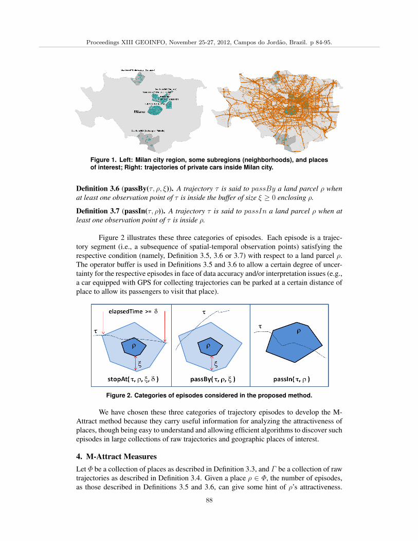
Figure 1. Left: Milan city region, some subregions (neighborhoods), and placesof interest; Right: trajectories of private cars inside Milan city.

Definition 3.6 (passBy(τ, ρ, ξ)). A trajectory τ is said to passBy a land parcel ρ whenat least one observation point of τ is inside the buffer of size ξ ≥ 0 enclosing ρ.

Definition 3.7 (passIn(τ, ρ)). A trajectory τ is said to passIn a land parcel ρ when atleast one observation point of τ is inside ρ.

Figure 2 illustrates these three categories of episodes. Each episode is a trajec-tory segment (i.e., a subsequence of spatial-temporal observation points) satisfying therespective condition (namely, Definition 3.5, 3.6 or 3.7) with respect to a land parcel ρ.The operator buffer is used in Definitions 3.5 and 3.6 to allow a certain degree of uncer-tainty for the respective episodes in face of data accuracy and/or interpretation issues (e.g.,a car equipped with GPS for collecting trajectories can be parked at a certain distance ofplace to allow its passengers to visit that place).

Figure 2. Categories of episodes considered in the proposed method.

We have chosen these three categories of trajectory episodes to develop the M-Attract method because they carry useful information for analyzing the attractiveness ofplaces, though being easy to understand and allowing efficient algorithms to discover suchepisodes in large collections of raw trajectories and geographic places of interest.

4. M-Attract MeasuresLet Φ be a collection of places as described in Definition 3.3, and Γ be a collection of rawtrajectories as described in Definition 3.4. Given a place ρ ∈ Φ, the number of episodes,as those described in Definitions 3.5 and 3.6, can give some hint of ρ’s attractiveness.


88

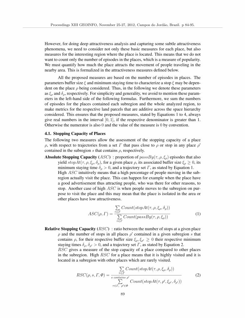
However, for doing deep attractiveness analysis and capturing some subtle attractivenessphenomena, we need to consider not only these basic measures for each place, but alsomeasures for the interesting region where the place is located. This means that we do notwant to count only the number of episodes in the places, which is a measure of popularity.We must quantify how much the place attracts the movement of people traveling in thenearby area. This is formalized in the attractiveness measures defined below.

All the proposed measures are based on the number of episodes in places. Theparameters buffer size ξ and minimum staying time to characterize a stop ξ may be depen-dent on the place ρ being considered. Thus, in the following we denote these parametersas ξρ and δρ, respectively. For simplicity and generality, we avoid to mention these param-eters in the left-hand side of the following formulas. Furthermore, we sum the numbersof episodes for the places contained each subregion and the whole analyzed region, tomake metrics for the respective land parcels that are additive across the space hierarchyconsidered. This ensures that the proposed measures, stated by Equations 1 to 4, alwaysgive real numbers in the interval [0, 1], if the respective denominator is greater than 1.Otherwise the numerator is also 0 and the value of the measure is 0 by convention.

4.1. Stopping Capacity of PlacesThe following two measures allow the assessment of the stopping capacity of a placeρ, with respect to trajectories from a set Γ that pass close to ρ or stop in any place ρ′

contained in the subregion s that contains ρ, respectively.Absolute Stopping Capacity (ASC) : proportion of passBy(τ, ρ, ξρ) episodes that also

yield stopAt(τ, ρ, ξρ, δρ), for a given place ρ, its associated buffer size ξρ ≥ 0, itsminimum staying time δρ > 0, and a trajectory set Γ , as stated by Equation 1.High ASC intuitively means that a high percentage of people moving in the sub-region actually visit the place. This can happen for example when the place havea good advertisement thus attracting people, who was there for other reasons, tostop. Another case of high ASC is when people moves to the subregion on pur-pose to visit the place and this may mean that the place is isolated in the area orother places have low attractiveness.

ASC(ρ, Γ ) =

∑τ∈Γ

Count(stopAt(τ, ρ, ξρ, δρ))

∑τ∈Γ

Count(passBy(τ, ρ, ξρ))(1)

Relative Stopping Capacity (RSC) : ratio between the number of stops at a given placeρ and the number of stops in all places ρ′ contained in a given subregion s thatcontains ρ, for their respective buffer size ξρ, ξρ′ ≥ 0 their respective minimumstaying times δρ, δρ′ > 0, and a trajectory set Γ , as stated by Equation 2.RSC gives a measure of the stop capacity of a place compared to other placesin the subregion. High RSC for a place means that it is highly visited and it islocated in a subregion with other places which are rarely visited.

RSC(ρ, s, Γ, Φ) =

∑τ∈Γ

Count(stopAt(τ, ρ, ξρ, δρ))

s contains ρ′∑τ∈Γ, ρ′∈Φ

Count(stopAt(τ, ρ′, ξρ′ , δρ′))

(2)


89

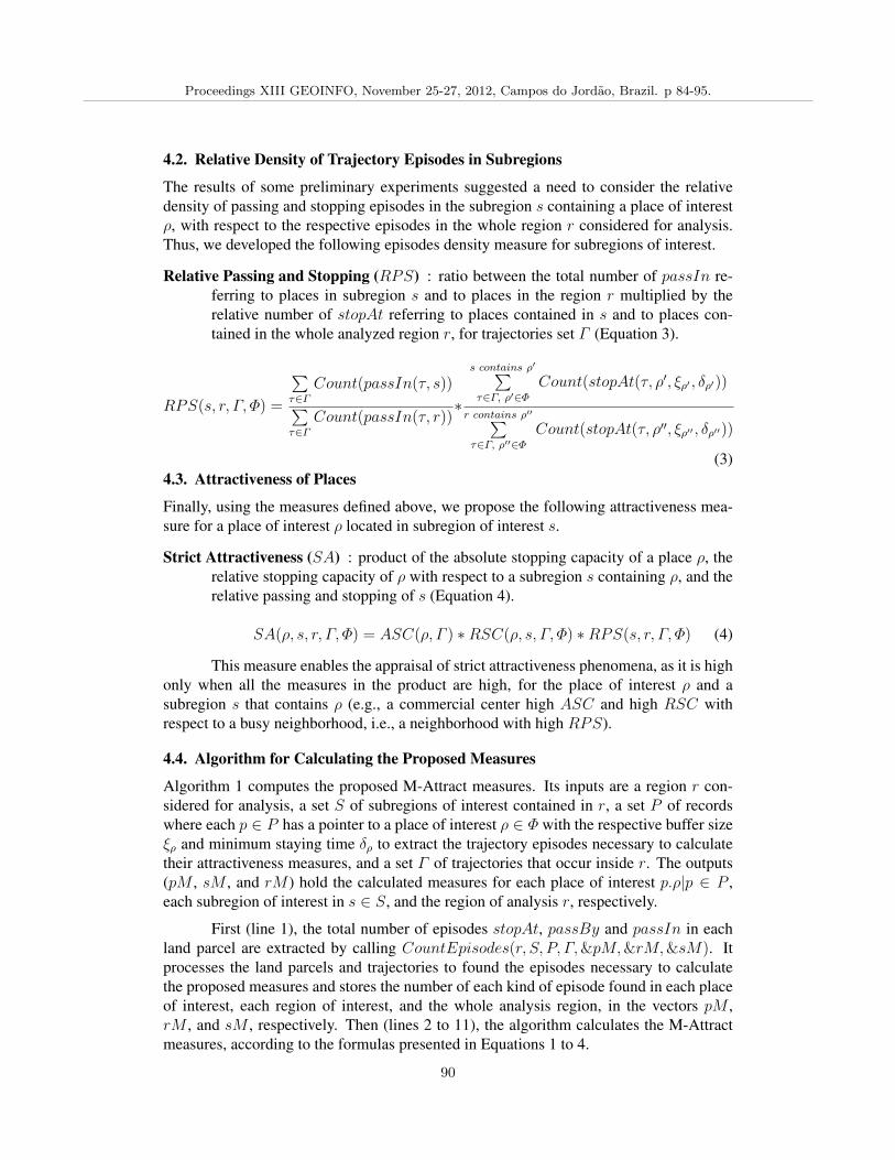
4.2. Relative Density of Trajectory Episodes in Subregions

The results of some preliminary experiments suggested a need to consider the relativedensity of passing and stopping episodes in the subregion s containing a place of interestρ, with respect to the respective episodes in the whole region r considered for analysis.Thus, we developed the following episodes density measure for subregions of interest.

Relative Passing and Stopping (RPS) : ratio between the total number of passIn re-ferring to places in subregion s and to places in the region r multiplied by therelative number of stopAt referring to places contained in s and to places con-tained in the whole analyzed region r, for trajectories set Γ (Equation 3).

RPS(s, r, Γ, Φ) =

∑τ∈Γ

Count(passIn(τ, s))

∑τ∈Γ

Count(passIn(τ, r))∗

s contains ρ′∑τ∈Γ, ρ′∈Φ

Count(stopAt(τ, ρ′, ξρ′ , δρ′))

r contains ρ′′∑τ∈Γ, ρ′′∈Φ

Count(stopAt(τ, ρ′′, ξρ′′ , δρ′′))

(3)4.3. Attractiveness of Places

Finally, using the measures defined above, we propose the following attractiveness mea-sure for a place of interest ρ located in subregion of interest s.

Strict Attractiveness (SA) : product of the absolute stopping capacity of a place ρ, therelative stopping capacity of ρ with respect to a subregion s containing ρ, and therelative passing and stopping of s (Equation 4).

SA(ρ, s, r, Γ, Φ) = ASC(ρ, Γ ) ∗RSC(ρ, s, Γ, Φ) ∗RPS(s, r, Γ, Φ) (4)

This measure enables the appraisal of strict attractiveness phenomena, as it is highonly when all the measures in the product are high, for the place of interest ρ and asubregion s that contains ρ (e.g., a commercial center high ASC and high RSC withrespect to a busy neighborhood, i.e., a neighborhood with high RPS).

4.4. Algorithm for Calculating the Proposed Measures

Algorithm 1 computes the proposed M-Attract measures. Its inputs are a region r con-sidered for analysis, a set S of subregions of interest contained in r, a set P of recordswhere each p ∈ P has a pointer to a place of interest ρ ∈ Φ with the respective buffer sizeξρ and minimum staying time δρ to extract the trajectory episodes necessary to calculatetheir attractiveness measures, and a set Γ of trajectories that occur inside r. The outputs(pM , sM , and rM ) hold the calculated measures for each place of interest p.ρ|p ∈ P ,each subregion of interest in s ∈ S, and the region of analysis r, respectively.

First (line 1), the total number of episodes stopAt, passBy and passIn in eachland parcel are extracted by calling CountEpisodes(r, S, P, Γ,&pM,&rM,&sM). Itprocesses the land parcels and trajectories to found the episodes necessary to calculatethe proposed measures and stores the number of each kind of episode found in each placeof interest, each region of interest, and the whole analysis region, in the vectors pM ,rM , and sM , respectively. Then (lines 2 to 11), the algorithm calculates the M-Attractmeasures, according to the formulas presented in Equations 1 to 4.


90

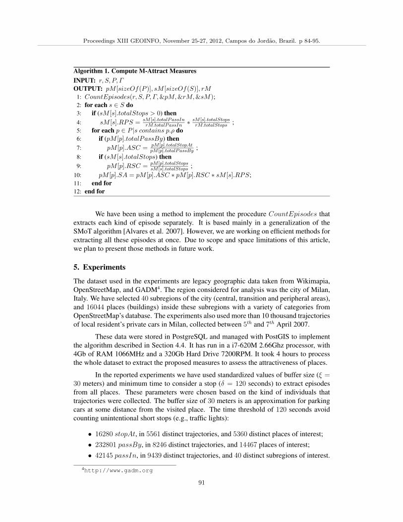
Algorithm 1. Compute M-Attract MeasuresINPUT: r, S, P, ΓOUTPUT: pM [sizeOf(P )], sM [sizeOf(S)], rM

1: CountEpisodes(r, S, P, Γ,&pM,&rM,&sM);2: for each s ∈ S do3: if (sM [s].totalStops > 0) then4: sM [s].RPS = sM [s].totalPassIn

rM.totalPassIn ∗sM [s].totalStopsrM.totalStops ;

5: for each p ∈ P |s contains p.ρ do6: if (pM [p].totalPassBy) then7: pM [p].ASC = pM [p].totalStopAt

pM [p].totalPassBy ;8: if (sM [s].totalStops) then9: pM [p].RSC = pM [p].totalStops

sM [s].totalStops ;10: pM [p].SA = pM [p].ASC ∗ pM [p].RSC ∗ sM [s].RPS;11: end for12: end for

We have been using a method to implement the procedure CountEpisodes thatextracts each kind of episode separately. It is based mainly in a generalization of theSMoT algorithm [Alvares et al. 2007]. However, we are working on efficient methods forextracting all these episodes at once. Due to scope and space limitations of this article,we plan to present those methods in future work.

5. Experiments

The dataset used in the experiments are legacy geographic data taken from Wikimapia,OpenStreetMap, and GADM4. The region considered for analysis was the city of Milan,Italy. We have selected 40 subregions of the city (central, transition and peripheral areas),and 16044 places (buildings) inside these subregions with a variety of categories fromOpenStreetMap’s database. The experiments also used more than 10 thousand trajectoriesof local resident’s private cars in Milan, collected between 5th and 7th April 2007.

These data were stored in PostgreSQL and managed with PostGIS to implementthe algorithm described in Section 4.4. It has run in a i7-620M 2.66Ghz processor, with4Gb of RAM 1066MHz and a 320Gb Hard Drive 7200RPM. It took 4 hours to processthe whole dataset to extract the proposed measures to assess the attractiveness of places.

In the reported experiments we have used standardized values of buffer size (ξ =30 meters) and minimum time to consider a stop (δ = 120 seconds) to extract episodesfrom all places. These parameters were chosen based on the kind of individuals thattrajectories were collected. The buffer size of 30 meters is an approximation for parkingcars at some distance from the visited place. The time threshold of 120 seconds avoidcounting unintentional short stops (e.g., traffic lights):

• 16280 stopAt, in 5561 distinct trajectories, and 5360 distinct places of interest;• 232801 passBy, in 8246 distinct trajectories, and 14467 places of interest;• 42145 passIn, in 9439 distinct trajectories, and 40 distinct subregions of interest.

4http://www.gadm.org


91

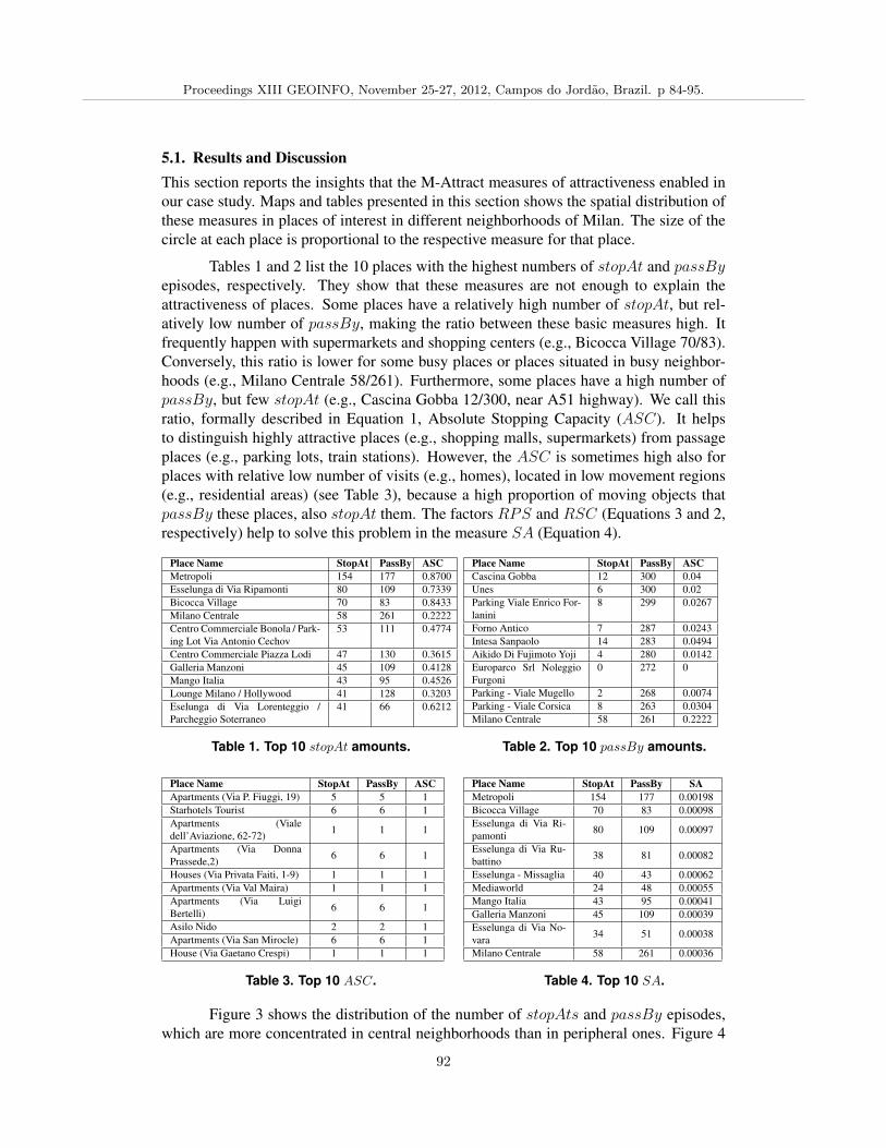
5.1. Results and DiscussionThis section reports the insights that the M-Attract measures of attractiveness enabled inour case study. Maps and tables presented in this section shows the spatial distribution ofthese measures in places of interest in different neighborhoods of Milan. The size of thecircle at each place is proportional to the respective measure for that place.

Tables 1 and 2 list the 10 places with the highest numbers of stopAt and passByepisodes, respectively. They show that these measures are not enough to explain theattractiveness of places. Some places have a relatively high number of stopAt, but rel-atively low number of passBy, making the ratio between these basic measures high. Itfrequently happen with supermarkets and shopping centers (e.g., Bicocca Village 70/83).Conversely, this ratio is lower for some busy places or places situated in busy neighbor-hoods (e.g., Milano Centrale 58/261). Furthermore, some places have a high number ofpassBy, but few stopAt (e.g., Cascina Gobba 12/300, near A51 highway). We call thisratio, formally described in Equation 1, Absolute Stopping Capacity (ASC). It helpsto distinguish highly attractive places (e.g., shopping malls, supermarkets) from passageplaces (e.g., parking lots, train stations). However, the ASC is sometimes high also forplaces with relative low number of visits (e.g., homes), located in low movement regions(e.g., residential areas) (see Table 3), because a high proportion of moving objects thatpassBy these places, also stopAt them. The factors RPS and RSC (Equations 3 and 2,respectively) help to solve this problem in the measure SA (Equation 4).

Place Name StopAt PassBy ASCMetropoli 154 177 0.8700Esselunga di Via Ripamonti 80 109 0.7339Bicocca Village 70 83 0.8433Milano Centrale 58 261 0.2222Centro Commerciale Bonola / Park-ing Lot Via Antonio Cechov

53 111 0.4774

Centro Commerciale Piazza Lodi 47 130 0.3615Galleria Manzoni 45 109 0.4128Mango Italia 43 95 0.4526Lounge Milano / Hollywood 41 128 0.3203Eselunga di Via Lorenteggio /Parcheggio Soterraneo

41 66 0.6212

Table 1. Top 10 stopAt amounts.

Place Name StopAt PassBy ASCCascina Gobba 12 300 0.04Unes 6 300 0.02Parking Viale Enrico For-lanini

8 299 0.0267

Forno Antico 7 287 0.0243Intesa Sanpaolo 14 283 0.0494Aikido Di Fujimoto Yoji 4 280 0.0142Europarco Srl NoleggioFurgoni

0 272 0

Parking - Viale Mugello 2 268 0.0074Parking - Viale Corsica 8 263 0.0304Milano Centrale 58 261 0.2222

Table 2. Top 10 passBy amounts.

Place Name StopAt PassBy ASCApartments (Via P. Fiuggi, 19) 5 5 1Starhotels Tourist 6 6 1Apartments (Vialedell’Aviazione, 62-72) 1 1 1

Apartments (Via DonnaPrassede,2) 6 6 1

Houses (Via Privata Faiti, 1-9) 1 1 1Apartments (Via Val Maira) 1 1 1Apartments (Via LuigiBertelli) 6 6 1

Asilo Nido 2 2 1Apartments (Via San Mirocle) 6 6 1House (Via Gaetano Crespi) 1 1 1

Table 3. Top 10 ASC.

Place Name StopAt PassBy SAMetropoli 154 177 0.00198Bicocca Village 70 83 0.00098Esselunga di Via Ri-pamonti 80 109 0.00097

Esselunga di Via Ru-battino 38 81 0.00082

Esselunga - Missaglia 40 43 0.00062Mediaworld 24 48 0.00055Mango Italia 43 95 0.00041Galleria Manzoni 45 109 0.00039Esselunga di Via No-vara 34 51 0.00038

Milano Centrale 58 261 0.00036

Table 4. Top 10 SA.

Figure 3 shows the distribution of the number of stopAts and passBy episodes,which are more concentrated in central neighborhoods than in peripheral ones. Figure 4


92

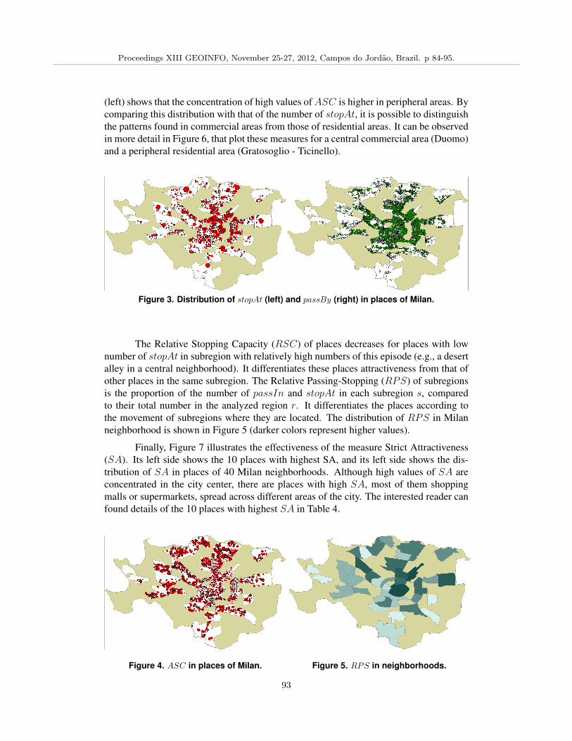
(left) shows that the concentration of high values ofASC is higher in peripheral areas. Bycomparing this distribution with that of the number of stopAt, it is possible to distinguishthe patterns found in commercial areas from those of residential areas. It can be observedin more detail in Figure 6, that plot these measures for a central commercial area (Duomo)and a peripheral residential area (Gratosoglio - Ticinello).

Figure 3. Distribution of stopAt (left) and passBy (right) in places of Milan.

The Relative Stopping Capacity (RSC) of places decreases for places with lownumber of stopAt in subregion with relatively high numbers of this episode (e.g., a desertalley in a central neighborhood). It differentiates these places attractiveness from that ofother places in the same subregion. The Relative Passing-Stopping (RPS) of subregionsis the proportion of the number of passIn and stopAt in each subregion s, comparedto their total number in the analyzed region r. It differentiates the places according tothe movement of subregions where they are located. The distribution of RPS in Milanneighborhood is shown in Figure 5 (darker colors represent higher values).

Finally, Figure 7 illustrates the effectiveness of the measure Strict Attractiveness(SA). Its left side shows the 10 places with highest SA, and its left side shows the dis-tribution of SA in places of 40 Milan neighborhoods. Although high values of SA areconcentrated in the city center, there are places with high SA, most of them shoppingmalls or supermarkets, spread across different areas of the city. The interested reader canfound details of the 10 places with highest SA in Table 4.

Figure 4. ASC in places of Milan. Figure 5. RPS in neighborhoods.


93

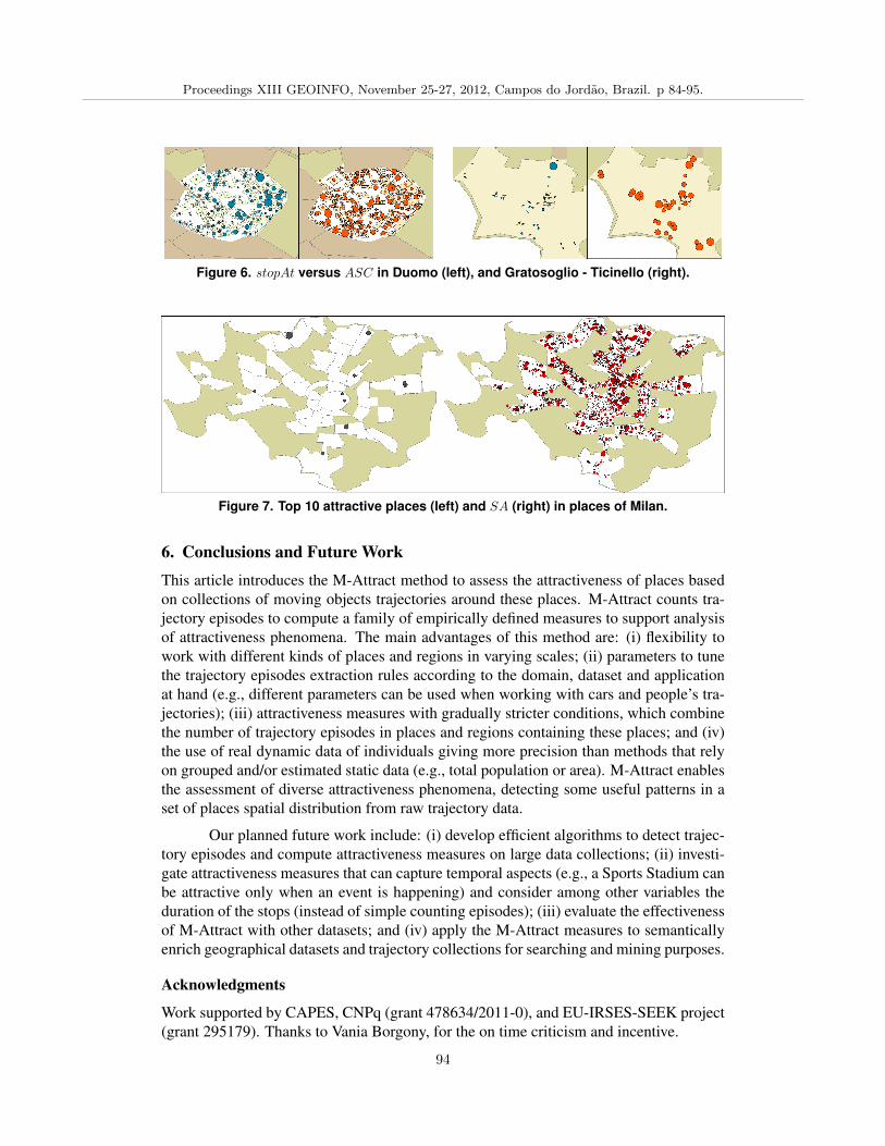
Figure 6. stopAt versus ASC in Duomo (left), and Gratosoglio - Ticinello (right).

Figure 7. Top 10 attractive places (left) and SA (right) in places of Milan.

6. Conclusions and Future WorkThis article introduces the M-Attract method to assess the attractiveness of places basedon collections of moving objects trajectories around these places. M-Attract counts tra-jectory episodes to compute a family of empirically defined measures to support analysisof attractiveness phenomena. The main advantages of this method are: (i) flexibility towork with different kinds of places and regions in varying scales; (ii) parameters to tunethe trajectory episodes extraction rules according to the domain, dataset and applicationat hand (e.g., different parameters can be used when working with cars and people’s tra-jectories); (iii) attractiveness measures with gradually stricter conditions, which combinethe number of trajectory episodes in places and regions containing these places; and (iv)the use of real dynamic data of individuals giving more precision than methods that relyon grouped and/or estimated static data (e.g., total population or area). M-Attract enablesthe assessment of diverse attractiveness phenomena, detecting some useful patterns in aset of places spatial distribution from raw trajectory data.

Our planned future work include: (i) develop efficient algorithms to detect trajec-tory episodes and compute attractiveness measures on large data collections; (ii) investi-gate attractiveness measures that can capture temporal aspects (e.g., a Sports Stadium canbe attractive only when an event is happening) and consider among other variables theduration of the stops (instead of simple counting episodes); (iii) evaluate the effectivenessof M-Attract with other datasets; and (iv) apply the M-Attract measures to semanticallyenrich geographical datasets and trajectory collections for searching and mining purposes.

Acknowledgments

Work supported by CAPES, CNPq (grant 478634/2011-0), and EU-IRSES-SEEK project(grant 295179). Thanks to Vania Borgony, for the on time criticism and incentive.


94

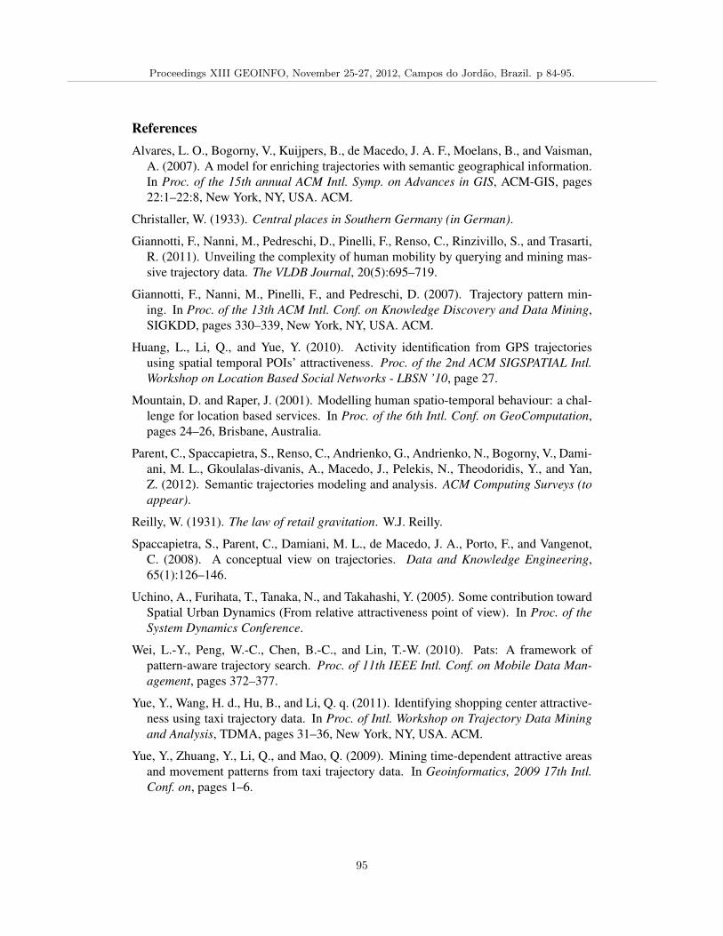
ReferencesAlvares, L. O., Bogorny, V., Kuijpers, B., de Macedo, J. A. F., Moelans, B., and Vaisman,

A. (2007). A model for enriching trajectories with semantic geographical information.In Proc. of the 15th annual ACM Intl. Symp. on Advances in GIS, ACM-GIS, pages22:1–22:8, New York, NY, USA. ACM.

Christaller, W. (1933). Central places in Southern Germany (in German).

Giannotti, F., Nanni, M., Pedreschi, D., Pinelli, F., Renso, C., Rinzivillo, S., and Trasarti,R. (2011). Unveiling the complexity of human mobility by querying and mining mas-sive trajectory data. The VLDB Journal, 20(5):695–719.

Giannotti, F., Nanni, M., Pinelli, F., and Pedreschi, D. (2007). Trajectory pattern min-ing. In Proc. of the 13th ACM Intl. Conf. on Knowledge Discovery and Data Mining,SIGKDD, pages 330–339, New York, NY, USA. ACM.

Huang, L., Li, Q., and Yue, Y. (2010). Activity identification from GPS trajectoriesusing spatial temporal POIs’ attractiveness. Proc. of the 2nd ACM SIGSPATIAL Intl.Workshop on Location Based Social Networks - LBSN ’10, page 27.

Mountain, D. and Raper, J. (2001). Modelling human spatio-temporal behaviour: a chal-lenge for location based services. In Proc. of the 6th Intl. Conf. on GeoComputation,pages 24–26, Brisbane, Australia.

Parent, C., Spaccapietra, S., Renso, C., Andrienko, G., Andrienko, N., Bogorny, V., Dami-ani, M. L., Gkoulalas-divanis, A., Macedo, J., Pelekis, N., Theodoridis, Y., and Yan,Z. (2012). Semantic trajectories modeling and analysis. ACM Computing Surveys (toappear).

Reilly, W. (1931). The law of retail gravitation. W.J. Reilly.

Spaccapietra, S., Parent, C., Damiani, M. L., de Macedo, J. A., Porto, F., and Vangenot,C. (2008). A conceptual view on trajectories. Data and Knowledge Engineering,65(1):126–146.

Uchino, A., Furihata, T., Tanaka, N., and Takahashi, Y. (2005). Some contribution towardSpatial Urban Dynamics (From relative attractiveness point of view). In Proc. of theSystem Dynamics Conference.

Wei, L.-Y., Peng, W.-C., Chen, B.-C., and Lin, T.-W. (2010). Pats: A framework ofpattern-aware trajectory search. Proc. of 11th IEEE Intl. Conf. on Mobile Data Man-agement, pages 372–377.

Yue, Y., Wang, H. d., Hu, B., and Li, Q. q. (2011). Identifying shopping center attractive-ness using taxi trajectory data. In Proc. of Intl. Workshop on Trajectory Data Miningand Analysis, TDMA, pages 31–36, New York, NY, USA. ACM.

Yue, Y., Zhuang, Y., Li, Q., and Mao, Q. (2009). Mining time-dependent attractive areasand movement patterns from taxi trajectory data. In Geoinformatics, 2009 17th Intl.Conf. on, pages 1–6.


95

A Conceptual Model for Representation of Taxi Trajectories

Ana Maria Amorim e Jorge Campos

Grupo de Aplicações e Análises Geoespaciais – GANGES

Mestrado em Sistemas e Computação – UNIFACS

Salvador, BA – Brazil [email protected], [email protected]

Abstract. The large-scale capture of data about the motion of moving objects

has enabled the development of geospatial tools to analyze and present the

characteristics of these objects’ behavior in many different fields. Intelligent

Transportation Systems, for instance, make intensive use of data collected

from embedded in-vehicle devices to analyze and monitor roads conditions

and the flow of vehicles and passengers of the public transportation system.

The taxi fleet is an important transport modality complementary to the public

transportation system. Thus, analysis of taxis’ movements can be used to

capture information about the condition of the traffic and to understand at a

finer level of granularity the movement of people in an urban environment.

This paper addresses the problem of mapping taxi raw trajectory data onto a

more abstract and structured data model. The proposed data model aims to

create an infrastructure to facilitate the implementation of algorithms for data

mining and knowledge discovery about taxi movements and people’s behavior

using this means of transport.

1. Introduction

With the evolution of technology, large-scale capture of data about the motion of

moving objects has become technically and economically feasible. As a result, there are

a growing number of new applications aiming at understanding and managing complex

phenomena involving these objects.

Intelligent Transportation Systems (ITS) encompass new kind of applications

designed to incorporate information and communication technologies to the

transportation infrastructure. The main goal of such applications is to allow users to

become more acquainted with the system functioning and to provide innovative services

to enhance the system’s coordination and maintenance. ITS make intensive use of data

collected from sensors placed along the transportation network or embedded in-vehicle

devices to analyze and monitor roads conditions and the flow of vehicles and users of

the public transportation system. Although the taxi fleet cannot be considered as a

component of the public transportation system, it is an important and complementary


96

transport modality. Thus, the analysis of taxis’ movements can be used to capture

information about the condition of the traffic and to understand at a finer level of

granularity the movement of people in an urban environment.

In the ITS arena, data about vehicles’ movements are usually stored in the form

of tuples (identifier, location, time) describing the evolution of a vehicle position over

time. This kind of data, however, does not meet the requirements of many applications

interested in capturing the characteristics of the movement, patterns or anomalies in

vehicles’ behavior. These applications often enrich trajectory data with contextualized

information about the environment, such as road conditions, landmarks or major cultural

or sport events [Spaccapietra et al. 2011] [Bogorny et al. 2011] [Yan 2009] [Alvares et

al. 2007]. Other kinds of contextualized information must be gathered during the data

acquisition process and require special sensors or the direct interference of a human

being. The latter case applies to the trajectory of taxis.

In order to illustrate a typical process of data acquisition about taxis movements,

consider, for instance, that all taxis are equipped with a mobile device with embedded

location mechanism and a mobile application capable of registering the path of all trips

throughout the day and some relevant events. Once started, the application begins to

collect and communicate data about vehicle’s location and status (i.e., full or empty).

Whenever the driver picks up a passenger, he/she should press the pick-up button and

report the number of passengers that has boarded the vehicle. At the end of the trip, the

driver must press the drop-off button indicating that the taxi has no passengers and it is

available for a new trip.

The formidable and massive dataset generated by taxis movements, however, is

barely used for analysis, data mining or knowledge discovery purpose. The major

drawbacks of using these data are twofold. First, trajectory data lack a more abstract

structure, have lots of redundant or inconsistent records, and carry little or no semantic

information. Second, there are few algorithms tailored to analyze, mine and reveal

patterns of this special kind of moving object. This paper addresses the problem of

mapping the raw data about taxis trajectories onto a generic conceptual model. This

model aims to facilitate queries and extraction of knowledge about the dynamics of this

transport modality in major urban areas. By structuring taxis’ raw trajectory data

through more abstract entities, we intend to create the data infrastructure necessary to

implement algorithms that identify patterns of people using taxi as a means of transport;

show the characteristics of the movements of passengers by taxi from the city, its origins

and predominant destinations; analyze the efficiency of the taxi system at different

periods; among others.


97

The remainder of this paper is structured as follows: section 2 discusses related

work. Section 3 presents some basic definitions used to define the conceptual model.

Section 4 discusses the main entities of a model to represent the data trajectory of taxis.

Section 5 discusses possible applications of the model and presents some conclusions.

2. Related Work

The study of the movement of taxis aiming at understanding and improving urban

mobility has become an active research field. This section discusses some works that

address different aspects of this problem.

[Peng et al. 2012] presented an analysis of the taxi passengers’ movement in

Shanghai, China. This study found out that on weekdays people use the taxi mainly for

three purposes: commuting between home and workplace, traveling between different

business places, and going for other places for leisure purpose.

[Veloso et al. 2011] analyzed the movement of taxis in Lisbon, Portugal. In this

work it is possible to visualize the spatiotemporal distribution of the vehicles, most

frequent places of origin and destination at different periods of the day, the relationship

between these locations and peaks of the system usage. This paper also analyzes the taxi

behavior in what they called downtime (i.e., the time spent by the taxi driver looking for

the next passenger) and conducts a study of predictability to locate the next passenger.

[Kamaroli et al. 2011] presented a methodology to analyze passengers’

movement at the city of Singapore at different periods of the day. The main objective of

this study was to quantify, visualize and examine the flow of taxis considering only

information about origin and destination.

The objective of [Zheng et al. 2011] was to detect flaws in the Beijing urban

planning based on information derived from the analyses taxis trajectories. As a result,

they identified regions with significant traffic problems and diagnosed failures in the

structure of links between these regions. Their findings can be used, for instance, by

urban planners to propose the construction of a new road or a new subway line.

In [Yuan et al. 2011] was presented a recommendation system with suggestions

for taxi drivers and passengers. Drivers use the system to identify locations in which the

probability to pick-up passengers is high. Passengers use the system to identify places in

a walking distance where they can easily find an empty taxi. These suggestions are

based on the patterns of the passengers (i.e., where and when they usually get in and out

of taxis) and the strategy used by most taxi drivers to pick-up passengers.


98

In [Ge et al. 2011] was presented an intelligent taxi system able to explore data

collected from taxis in the city of San Francisco and New York for commercial purpose.

The authors argue that the system increases the productivity of taxi drivers with routes

recommendations, identifies fraud in the taxi system, and provides support for new

business ideas.

In [Liu et al. 2009] was presented a methodology to analyze the behavior of taxi

drivers in Shenzhen, China. They proposed a metric to measure drivers’ skill, in what

they called “mobility intelligence”. Considering their income and behavior, taxis drivers

are ranked as top drivers or ordinary drivers. The paper concluded that while ordinary

drivers operate in fixed locations, the top drivers choose the places according to the

most opportune time.

The goals of these works illustrate only some interesting possibilities of

processing taxi trajectories data. The possibilities are endless, but they reveal a growing

interest in the area. Considering the data used to support their analyses, all related work

use raw trajectory data complemented with pick-up/drop-off information. In [Yuan et al.

2011], [Ge et al. 2011] and [Liu et al. 2009] the number of passengers is also

considered. Considering the data models used to represent this dataset, however, all

work use ad hoc data models to solve a specific problem or to carry out a particular

analysis. At the best of our knowledge, no generic data model capable of supporting a

wide range of analysis and knowledge discovery has been identified yet. The following

sections present our contribution to this area.

3. Basic Definitions

[Spaccapietra et al. 2008] proposed the first model that treats trajectories of moving

objects as a spatiotemporal concept. Spaccapietra conceptualized a trajectory as a space-

time evolution of a traveling object to reach a certain goal. The trajectory is bounded by

two instants of time (Begin and End) and an ordered sequence of pairs (point, time)

representing the movement of the object. Semantically speaking, Spaccapietra considers

a trajectory as an ordered list of Stops and Moves. A Stop is part of a trajectory that is

relevant to the application in which the travelling object did not move (i.e., the object

remains stationary for a minimal amount of time). The trajectory’s Begin and End are

not considered Stops, because their temporal extent is a single chronon (indivisible time

unit). A Move is a sub-trajectory between two Stops, between the starting point of the

trajectory (Begin) and the first Stop, or between the last Stop and the ending of the

trajectory (End). The spatial representation of a Stop is a single point, while a Move is

represented by a displacement function or a polyline built with trajectory’s points.


99

Based on Spaccapietra’s work, we present some relevant definitions to the model

aimed to represent taxis daily trajectories.

Definition 1 Working Trajectory represents the evolution of the position of a

taxi along the working hours of its driver.

Definition 2 Full-Move Sub-Trajectory corresponds to a segment of a Working

Trajectory and represents the trajectory of the taxi while occupied by a passenger.

Definition 3 Empty-Move Sub-Trajectory corresponds to a segment of a

Working Trajectory and represents the trajectory of the taxi in search of a new

passenger.

Definition 4 Pick-Up Point indicates the time and location of the beginning of a

Full-Move Sub-Trajectory, i.e., it represents the time and place of the start of a taxi’s

travel with passengers.

Definition 5 Drop-Off Point indicates the time and location of the end of a Full-

Move Sub-Trajectory, i.e., represents the time and the location where the passenger

leaves the taxi.

Definition 6 Taxi Stop Point is a known geographic location of a point where the

taxicab remains stationary for a certain period of time waiting for passengers.

Working Trajectory is equivalent to Spaccapietra’s concept of a travelling object

trajectory. A Working Trajectory is split on semantically meaningful specialization of

Stops and Moves. Full-Move and Empty-Move Sub-Trajectory correspond to Moves and

a Taxi Stop Point corresponds to a Stop. Pick-Up Point and Drop-Off Point do not

represent a Stop. They are equivalent to the endpoints of our sub-trajectories. Different

from Spaccapietra’s conceptualization, a Working Trajectory is not an alternate

sequence of Stop and Moves. A Working Trajectory can have any combination of Full-

Move Sub-Trajectory, Empty-Move Sub-Trajectory and Taxi Stop Point. These

definitions are the basis for the understanding of a conceptual model aimed to represent

the movement of taxis. This model will be presented in the next section.

4. A Conceptual Model for Taxi Trajectories

Before discussing the representation of taxi trajectory with high-level entities of a

conceptual model, it is interesting to illustrate the process of capturing raw data by

following a typical working day of John, a taxi driver. John begins his workday by

logging to an application installed on a device with an integrated GPS and connected to

a 3G network. The application sends the position of the vehicle at every minute and,

eventually, allows the registration of some relevant events. After the initial setup, John


100

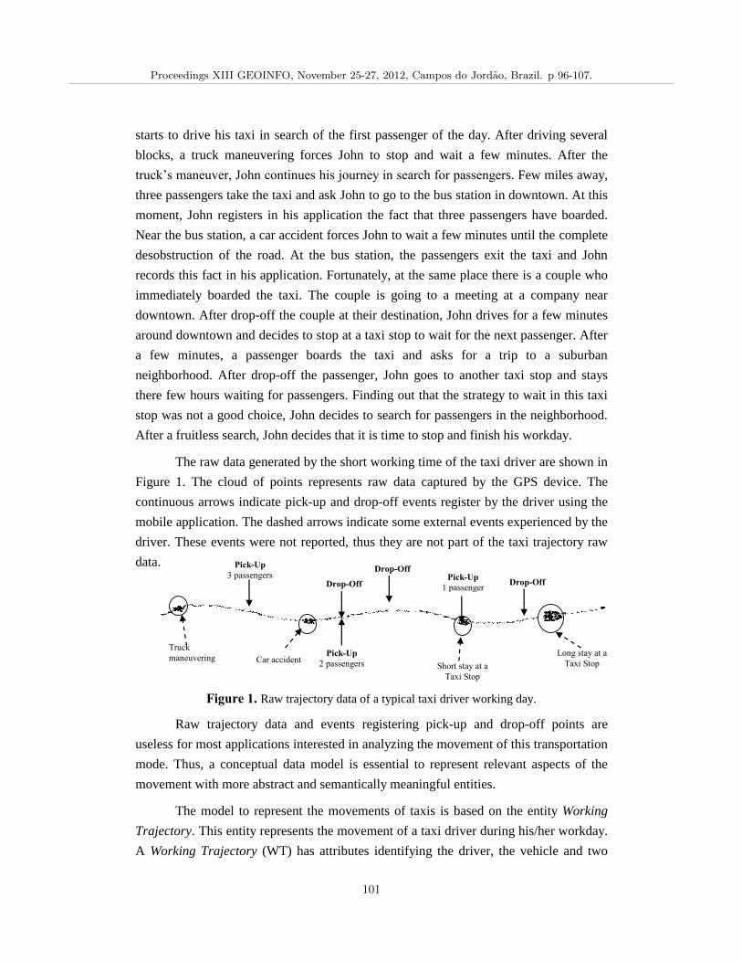
starts to drive his taxi in search of the first passenger of the day. After driving several

blocks, a truck maneuvering forces John to stop and wait a few minutes. After the

truck’s maneuver, John continues his journey in search for passengers. Few miles away,

three passengers take the taxi and ask John to go to the bus station in downtown. At this

moment, John registers in his application the fact that three passengers have boarded.

Near the bus station, a car accident forces John to wait a few minutes until the complete

desobstruction of the road. At the bus station, the passengers exit the taxi and John

records this fact in his application. Fortunately, at the same place there is a couple who

immediately boarded the taxi. The couple is going to a meeting at a company near

downtown. After drop-off the couple at their destination, John drives for a few minutes

around downtown and decides to stop at a taxi stop to wait for the next passenger. After

a few minutes, a passenger boards the taxi and asks for a trip to a suburban

neighborhood. After drop-off the passenger, John goes to another taxi stop and stays

there few hours waiting for passengers. Finding out that the strategy to wait in this taxi

stop was not a good choice, John decides to search for passengers in the neighborhood.

After a fruitless search, John decides that it is time to stop and finish his workday.

The raw data generated by the short working time of the taxi driver are shown in

Figure 1. The cloud of points represents raw data captured by the GPS device. The

continuous arrows indicate pick-up and drop-off events register by the driver using the

mobile application. The dashed arrows indicate some external events experienced by the

driver. These events were not reported, thus they are not part of the taxi trajectory raw

data.

Figure 1. Raw trajectory data of a typical taxi driver working day.

Raw trajectory data and events registering pick-up and drop-off points are

useless for most applications interested in analyzing the movement of this transportation

mode. Thus, a conceptual data model is essential to represent relevant aspects of the

movement with more abstract and semantically meaningful entities.

The model to represent the movements of taxis is based on the entity Working

Trajectory. This entity represents the movement of a taxi driver during his/her workday.

A Working Trajectory (WT) has attributes identifying the driver, the vehicle and two

Drop-Off

Drop-Off

Pick-Up

3 passengers

Pick-Up

2 passengers

Pick-Up

1 passenger Drop-Off

Truck

maneuvering

Car accident Short stay at a

Taxi Stop

Long stay at a

Taxi Stop


101

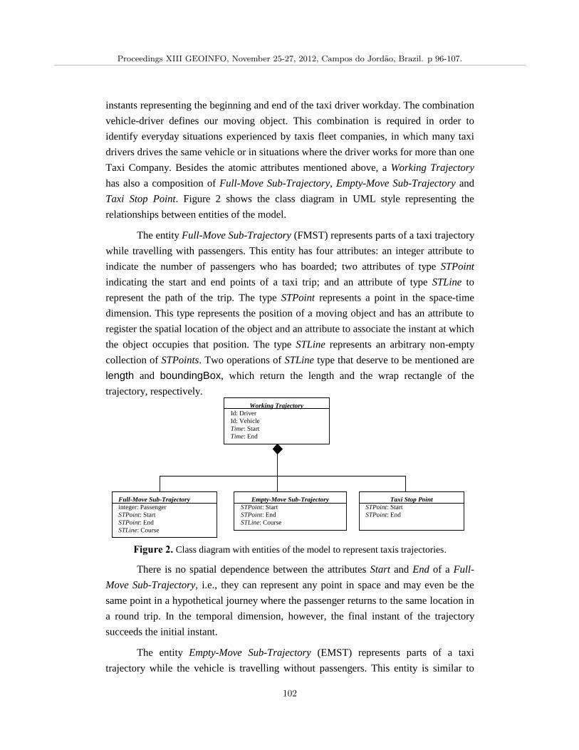
instants representing the beginning and end of the taxi driver workday. The combination

vehicle-driver defines our moving object. This combination is required in order to

identify everyday situations experienced by taxis fleet companies, in which many taxi

drivers drives the same vehicle or in situations where the driver works for more than one

Taxi Company. Besides the atomic attributes mentioned above, a Working Trajectory

has also a composition of Full-Move Sub-Trajectory, Empty-Move Sub-Trajectory and

Taxi Stop Point. Figure 2 shows the class diagram in UML style representing the

relationships between entities of the model.

The entity Full-Move Sub-Trajectory (FMST) represents parts of a taxi trajectory

while travelling with passengers. This entity has four attributes: an integer attribute to

indicate the number of passengers who has boarded; two attributes of type STPoint

indicating the start and end points of a taxi trip; and an attribute of type STLine to

represent the path of the trip. The type STPoint represents a point in the space-time

dimension. This type represents the position of a moving object and has an attribute to

register the spatial location of the object and an attribute to associate the instant at which

the object occupies that position. The type STLine represents an arbitrary non-empty

collection of STPoints. Two operations of STLine type that deserve to be mentioned are

length and boundingBox, which return the length and the wrap rectangle of the

trajectory, respectively.

Figure 2. Class diagram with entities of the model to represent taxis trajectories.

There is no spatial dependence between the attributes Start and End of a Full-

Move Sub-Trajectory, i.e., they can represent any point in space and may even be the

same point in a hypothetical journey where the passenger returns to the same location in

a round trip. In the temporal dimension, however, the final instant of the trajectory

succeeds the initial instant.

The entity Empty-Move Sub-Trajectory (EMST) represents parts of a taxi

trajectory while the vehicle is travelling without passengers. This entity is similar to

Full-Move Sub-Trajectory

integer: Passenger

STPoint: Start

STPoint: End

STLine: Course

Empty-Move Sub-Trajectory

STPoint: Start

STPoint: End

STLine: Course

Taxi Stop Point

STPoint: Start

STPoint: End

Working Trajectory

Id: Driver

Id: Vehicle

Time: Start

Time: End


102

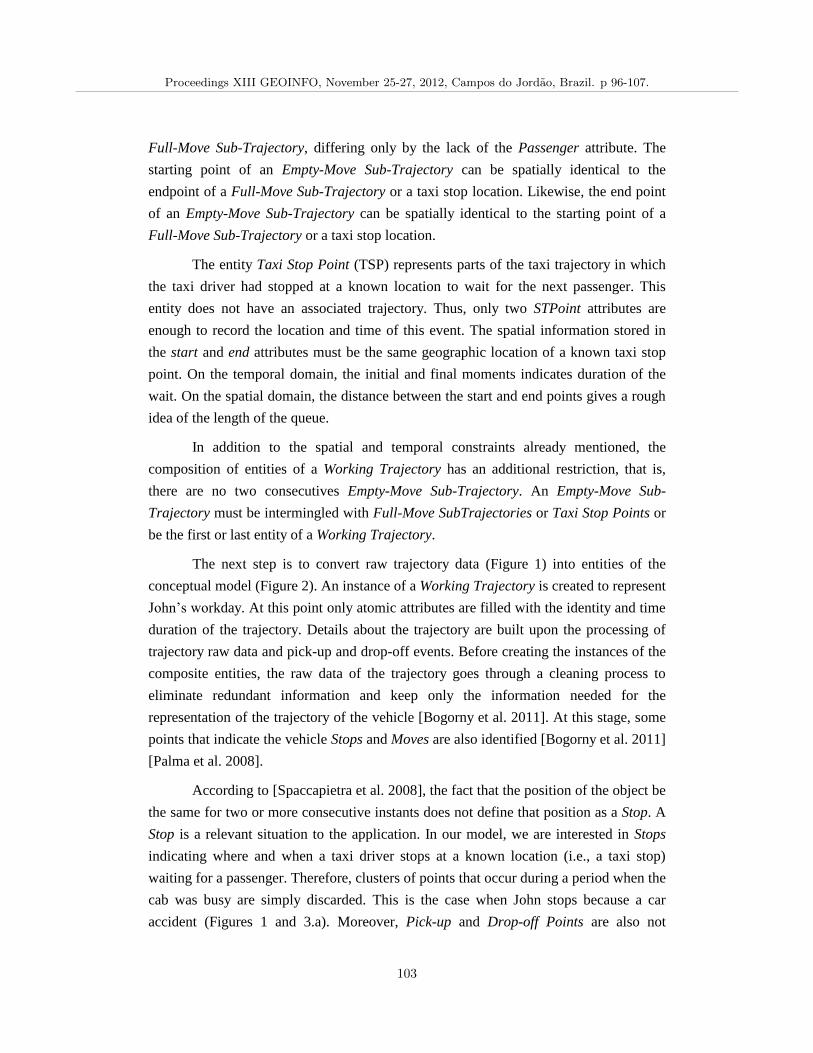
Full-Move Sub-Trajectory, differing only by the lack of the Passenger attribute. The

starting point of an Empty-Move Sub-Trajectory can be spatially identical to the

endpoint of a Full-Move Sub-Trajectory or a taxi stop location. Likewise, the end point

of an Empty-Move Sub-Trajectory can be spatially identical to the starting point of a

Full-Move Sub-Trajectory or a taxi stop location.

The entity Taxi Stop Point (TSP) represents parts of the taxi trajectory in which

the taxi driver had stopped at a known location to wait for the next passenger. This

entity does not have an associated trajectory. Thus, only two STPoint attributes are

enough to record the location and time of this event. The spatial information stored in

the start and end attributes must be the same geographic location of a known taxi stop

point. On the temporal domain, the initial and final moments indicates duration of the

wait. On the spatial domain, the distance between the start and end points gives a rough

idea of the length of the queue.

In addition to the spatial and temporal constraints already mentioned, the

composition of entities of a Working Trajectory has an additional restriction, that is,

there are no two consecutives Empty-Move Sub-Trajectory. An Empty-Move Sub-

Trajectory must be intermingled with Full-Move SubTrajectories or Taxi Stop Points or

be the first or last entity of a Working Trajectory.

The next step is to convert raw trajectory data (Figure 1) into entities of the

conceptual model (Figure 2). An instance of a Working Trajectory is created to represent

John’s workday. At this point only atomic attributes are filled with the identity and time

duration of the trajectory. Details about the trajectory are built upon the processing of

trajectory raw data and pick-up and drop-off events. Before creating the instances of the

composite entities, the raw data of the trajectory goes through a cleaning process to

eliminate redundant information and keep only the information needed for the

representation of the trajectory of the vehicle [Bogorny et al. 2011]. At this stage, some

points that indicate the vehicle Stops and Moves are also identified [Bogorny et al. 2011]

[Palma et al. 2008].

According to [Spaccapietra et al. 2008], the fact that the position of the object be

the same for two or more consecutive instants does not define that position as a Stop. A

Stop is a relevant situation to the application. In our model, we are interested in Stops

indicating where and when a taxi driver stops at a known location (i.e., a taxi stop)

waiting for a passenger. Therefore, clusters of points that occur during a period when the

cab was busy are simply discarded. This is the case when John stops because a car

accident (Figures 1 and 3.a). Moreover, Pick-up and Drop-off Points are also not


103

represented as Stops (i.e., modeled as first-class entities). These entities represent the

end points of a Full-Move Sub-trajectory and are represented by two attributes of the

type STPoint in the entity Full-Move Sub-Trajectory. Stops that occur during the period

where the taxi is empty are different. They can be either a stop in a taxi stop point or a

stop due to an external event. The former is of our interest and the latter will be also

discarded. Thus, Stops that occur while the taxi is empty are marked as candidates to

represent Taxi Stop entities (Figure 3.a). The decision whether these candidates are

actually a Taxi Stop is done in a next step.

a)

b)

c)

Figure 3. Steps in the process of creating entities of taxi trajectory conceptual model. a)

identification of taxi stop points candidates and a first attempt of sub-trajectories

entities; b) identification of real taxi stop locations; and c) object diagram with all entities of

John’s workday.

The Moves identified in this phase create either an Empty-Move Sub-trajectory

or a Full-Move Sub-trajectory. This decision is based on instants and locations of pick-

up and drop-off events reported by the driver. At this point the collection of raw

trajectory that forms the course of each sub-trajectory is also captured by the model’s

entities. Thus, based on data captured during John's journey, three Empty-Move Sub-

trajectory, three Full-Move Sub-trajectory and three candidates for Taxi Stop Point were

created (Figure 3.b).

The last step in the process of creating entities of the conceptual model is the

identification of what is really a Taxi Stop Point. The main problem in identifying this

Taxi Stop

Point

Candidates

WT start

EMST1 start

EMST1 end

FMST1 start FMST2 start

FMST1 end

FMST2 end

EMST2 start

EMST2 end

FMST3 start

FMST3 end

EMST3 start

WT end

EMST3 end

WT start

EMST1 start

EMST1 end

FMST1 start FMST2 start

FMST1 end

FMST2 end

EMST2 start

EMST2 end

FMST3 start

FMST3 end

EMST3 start

WT end

EMST4 end

TSP1 start,end

EMST3 end

EMST4 start

TSP2 start,end

EMST1 FMST1 FMST2 EMST2 TSP1 FMST3 EMST3 TSP2 EMST4

WT


104

entity is the distinction between Stops at a known taxi stop location and Stops that occur

during an Empty-Move Sub-trajectory caused by external facts. The latter type of stop

may be caused, for example, by a traffic jam or mechanical problem on the vehicle and

it is not of our interest, thus it is not explicitly represented in the model. For this

purpose, we use the approach developed by [Yuan et al. 2011]. They use the concept of

point of interest and known taxi point location to discard Stops candidates that are not a

real taxi stop.

For the data used in our example, the first Taxi Stop Point Candidate was

rejected and the last two was identified as a true Taxi Stop Point (Figure 3b). With the

creation of the last Taxi Stop Point, the third Empty-Move Sub-Trajectory was divided

into two Empty-Move Sub-Trajectory entities with a Taxi Stop Point in-between. At the

end of the raw data processing, a Working Trajectory composed by an ordered list of

entities of the type Empty-Move Sub-trajectory, Full-Move Sub-trajectory and Taxi Stop

Point is created (Figure 3.c).

We choose to not consider an event indicating when the driver stops at Taxi

Stop. We believe that different from our example, all information reported by the driver

can be completely automated. A taximeter connected to a data network, an embedded

GPS device, and a load sensor, for instance, can send pick-up and drop-off information

and an estimated number of passengers in the vehicle with no driver intervention. The

stops at taxi stops points, however, cannot be determined using this technology.

5. Conclusion and Future Work

This paper introduces a conceptual model to represent taxi raw trajectories. Unlike the

bus, train and subway systems that have pre-defined routes and stop points, taxis pick-

up and drop-off passengers wherever they want. This capillarity allows a precise

determination of people’s origin and destination.

The taxi conceptual model aims to facilitate the task of querying, analyzing, data

mining and performing knowledge discovery about this transport mode. It was shown a

technique to create entities of the conceptual model based on raw trajectory data. The

conceptual model is quite broad and can be used in many types of applications. Public

managers, for example, may be interested in identifying a pattern in the behavior of

users of the taxi system or to identify a need for a new bus itinerary. Fleet managers may

be interested in measuring the efficiency of a taxi driver through the time spent without

passengers. Users may be interested in know places with high probability of finding an

empty taxi.


105

Entities of the conceptual model carry semantic information about taxis’

movements, which facilitate the implementation of data mining and knowledge

discovery algorithms at different levels of granularity. At a low level of granularity,

historical data of taxis movement can be analyzed through the whole course of their

trajectory. Analyzing the courses of all Full-Move Sub-Trajectories, for example, it is

possible to know if the taxi took the shortest route from the origin to its destination, the

time taken to complete the trip, and the traffic conditions along the route. The courses of

all Full-Move Sub-Trajectories, Empty-Move Sub-Trajectories, and Taxi Stop Points of

a certain driver can be used to highlight the driver strategy and efficiency. The efficiency

of a taxi driver can be measured, for instance, by the ratio between the sum of the

duration of all Empty-Move Sub-Trajectories and Taxi Stop Points over the duration of

the entire journey of the driver or by the ratio between the sum of the length of the

courses of all Full-Move Sub-Trajectories and all Empty-Move Sub-Trajectories. The

former mechanism uses temporal information to measure the taxi efficiency, while the

later uses spatial information. These indices can be combined to produce a spatial-

temporal index of efficiency.

At a high level of granularity, the movement of the taxis can be used to identify,

for instance, mostly wanted origin and destination places along the day and places where

taxis are in great demand. By analyzing the start and end points of all Full-Move Sub-

Trajectories, it is possible to map all pick-up and drop-off points and to identify where

these hot spots are likely to occur along the day.

The importance of studying taxis movement is not restricted to the analysis of

the historical data. Considering that the information about taxis’ position, speed and

status is published in real time, it can be used to identify empty taxis in a given

neighborhood. This information can be used by a taxi company to dispatch the closest

taxi in response to passenger call or by passengers viewing all available taxis on a map

displayed on the screen of their Smartphone. Moreover, the average speed of thousand

of vehicles crossing the city gives an excellent overview of traffic conditions at different

locations along the road network, serving for any driver looking for the best

uncongested route and improving urban mobility.

The examples discussed above require historical data covering a significant

amount of time. Thus, the volume of data to be processed is expected to be huge. As

future work, we are planning to apply the ideas presented in this paper in a real case

scenario, that is, work with real data from a cooperative or Taxi Company and to

develop a tool to support different kind of analysis.


106

References Alvares, L.O., Bogorny, V., Kuijpers, B., Fernandes, J.A., Moelans, B., Vaisman, A.,

(2007), “A Model for Enriching Trajectories with Semantic Geographical

Information”. ACM-GIS’07.

Bogorny, V., Avancini, H., de Paula, B., C., Kuplich, C., R., Alvares, L., O., (2011),

“Weka-STPM: a Software Architecture and Prototype for Semantic Trajectory Data

Mining and Visualization”. Transactions in GIS.

Ge, Y., Liu, C., Xiong, H., Chen, J., (2011), “A Taxi Business Intelligence System“.

Proceedings of the 17th ACM SIGKDD international conference on Knowledge

discovery and data mining

Kamaroli, N.Q.B., Mulianwan, R.P., Kang, E.P.X., Ru, T.J., (2011), “Analysis of Taxi

Movement through Flow Mapping”. IS415 – Geospatial Analytics for Business

Intelligence.

Liu, L., Andris, C., Biderman, A., Ratti, C., (2009), “Uncovering Taxi Driver’s Mobility

Intelligence through His Trace”. SENSEable City Lab, Massachusetts Institute of

Technology, USA.

Palma, A.T., Bogorny, V., Kuijpers, B., Alvares, L.O., (2008), “A Clustering-based

Approach for Discovering Interesting Places in Trajectories”, ACM Symposium on

Applied Computing (SAC’08), Fortaleza, Ceará, Brazil.

Peng, C., Jin, X., Wong, K-C., Shi, M., Liò, P., (2012), “Collective Human Mobility

Pattern from Taxi Trips in Urban Area”, PLoS ONE 7(4):e34487.

doi:10.1371/journal.pone.0034487.

Spaccapietra, S., Parent, C., Damiani, M.L., Macedo, J.A., Porto, F., Vangenot, C.,

(2008), “A Conceptual View on Trajectories”, Data and Knowledge Engineering,

65(1): 126 – 146, 2008.

Spaccapietra, S., Chakraborty, D., Aberer, K., Parent, C., Yan, Z., (2011), “SeMiTri : A

Framework for Semantic Annotation of Heterogeneous Trajectories”, EDBT 2011,

March 22–24, 2011, Uppsala, Sweden.

Veloso, M., Phithakkitnukoon, S., Bento, C., (2011), “Urban Mobility Study using Taxi

Traces”, Proceedings of the 2011 international workshop on Trajectory data mining

and analysis TDMA 11 (2011).

Yan, Z., (2009), “Towards Semantic Trajectory Data Analysis : A Conceptual and

Computational Approach”. VLDB’09, Lyon, France.

Yuan, J., Zheng, Y., Zhang, L., Xie, X., Sun, G., (2011), “Where to find my next

passenger”, Proceedings of the 13th international conference on Ubiquitous

computing.

Zheng, Y., Liu, Y., Yuan, J., Xie, X., (2011), “Urban Computing with Taxicabs”,

Proceedings of the 13th International Conference on Ubiquitous Computing, pages

89-98.


107

GeoSTAT – A system for visualization, analysis and

clustering of distributed spatiotemporal data

Maxwell Guimarães de Oliveira, Cláudio de Souza Baptista

Laboratory of Information Systems – Computer Science Department

Federal University of Campina Grande (UFCG)

Av. Aprígio Veloso 882, Bloco CN, Bairro Universitário – 58.429-140

Campina Grande – PB – Brazil


Abstract. Nowadays, there is a considerable amount of spatiotemporal data

available on the web. The visualization of these data requires several visual

resources which helps users to have a correct interpretation of the data set.

Furthermore, the use of data mining algorithms has proven relevant in helping

the exploratory analysis of spatiotemporal data. This paper proposes the

GeoSTAT (GEOgraphic SpatioTemporal Analysis Tool), a system that

includes spatial and temporal visualization techniques and offers a

spatiotemporal adaptation of clustering algorithms provided by the Weka data

mining toolkit. A case study was realized to demonstrate the end-user

experience and some advantages achieved using the proposed system.

1. Introduction

Nowadays, there is a considerable volume of spatiotemporal data available in a variety

of media types, especially on the Internet. Among so much information, it is necessary

to provide decision support systems and analytics, which can help decision making

users to extract relevant knowledge, intuitively and quickly, such as the prediction of

future events, for instance.

Visualization techniques are widely known as being powerful in the decision

making domain [Johnston 2001], since they take advantage of human capabilities to

rapidly notice and interpret visual patterns [Andrienko et al. 2003][Kopanakis and

Theodoulidis 2003]. However, we know that the spatial visualization resources supplied

by most of the existing geographic information systems are not enough for decision

support systems [Bédard et al. 2001].

The visualization of spatiotemporal data is a complex task that requires the use

of appropriate visual resources that allow users to have a correct interpretation of the

information under analysis. Visualization and analysis of spatiotemporal data are tasks

that have been gaining prominence in several areas, such as biology, electrical power

transmission, urban traffic, criminology, and civil construction. This cross domain

utilization is especially due to the widespread use of devices that capture the geographic

location, generating large amounts of information concerning the time and space, such

as the trajectory of mobile objects, fire spots, dengue spots, atmospheric discharges, and

criminality maps.

According to Andrienko et al. [Andrienko et al. 2010b], it is necessary to deal

with the time in an efficient manner, when performing spatiotemporal visualization. The

understanding that space and time are inseparable and that there is nothing spatial that is


108

not temporal must permeate the research in spatiotemporal visualization. A reasonable

solution in visualization and analysis of spatiotemporal data should offer, at least:

resources for treating both the spatial and temporal dimensions (spatiality and

temporality); domain independence (generality), freedom for the user to handle the

visualized data and apply filters (flexibility); connection with several data sources in a

practical and efficient manner (interoperability); and data mining based on

spatiotemporal clustering (mining).

It is essential to provide to the users resources to handle both the spatial and the

temporal dimensions in a spatiotemporal data analysis system. The singularities in any

of these dimensions must not be discarded because they may reveal implicit

relationships which match the reality of the analyzed data.

Furthermore, the use of spatiotemporal data mining algorithms, integrated with

modern data visualization techniques, improves the usability for the decision maker

when analyzing large spatiotemporal datasets.

Nonetheless, the majority of existing spatiotemporal visualization systems do

not address appropriately the temporal dimension, as they focus only the spatial

visualization. Therefore, an important research issue is how to offer temporal

manipulation resources that, used with the spatial data manipulation resources, can

improve the experience of end users, who are interested in performing visual analysis on

spatiotemporal data.

This paper proposes a new system, called GeoSTAT - GEOgraphic

SpatioTemporal Analysis Tool, for visualization and analysis of spatiotemporal data

which takes into account, the six essential characteristics discussed by Andrienko et al.

[Andrienko et al. 2010b], as mentioned previously. A case study using the GeoSTAT

system was proposed to perform a spatiotemporal analysis using data on fire spots and

failure events in power transmission lines, aiming at finding evidences that support the

hypothesis that fires occurring close to transmission lines could be the cause of failure

events in the power system.

The rest of this paper is organized as follows. Section 2 discusses related work.

Section 3 focuses on the presentation of the proposed system. Section 4 addresses a case

study to validate the proposed ideas. Finally, section 5 concludes the paper and presents

further work to be undertaken.

2. Related Work

This section focuses on related works concerning the visualization and analysis of

spatiotemporal data.

Ferreira et al. [Ferreira et al. 2011] propose an interactive visualization system

that supports the visual analysis of spatiotemporal bird distribution models. It is a

spatiotemporal approach towards the specific domain of birds. It is important to

highlight that besides being valid for just one specific domain, the solution does not

provide mechanisms to connect to external databases, being constrained to the database

developed by the authors.

Andrienko et al. [Andrienko et al. 2010a] propose a framework based on the Self

Organizing Map technique (SOM) [Kohonen 2001], a combination of clustering and

dimensionality reduction. This technique follows the idea that objects are not just


109

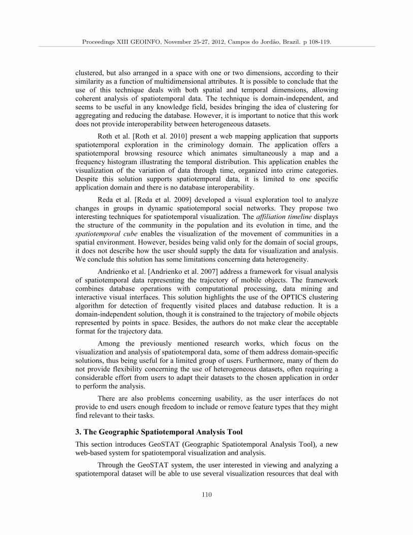
clustered, but also arranged in a space with one or two dimensions, according to their

similarity as a function of multidimensional attributes. It is possible to conclude that the

use of this technique deals with both spatial and temporal dimensions, allowing

coherent analysis of spatiotemporal data. The technique is domain-independent, and

seems to be useful in any knowledge field, besides bringing the idea of clustering for

aggregating and reducing the database. However, it is important to notice that this work

does not provide interoperability between heterogeneous datasets.

Roth et al. [Roth et al. 2010] present a web mapping application that supports

spatiotemporal exploration in the criminology domain. The application offers a

spatiotemporal browsing resource which animates simultaneously a map and a

frequency histogram illustrating the temporal distribution. This application enables the

visualization of the variation of data through time, organized into crime categories.

Despite this solution supports spatiotemporal data, it is limited to one specific

application domain and there is no database interoperability.

Reda et al. [Reda et al. 2009] developed a visual exploration tool to analyze

changes in groups in dynamic spatiotemporal social networks. They propose two

interesting techniques for spatiotemporal visualization. The affiliation timeline displays

the structure of the community in the population and its evolution in time, and the

spatiotemporal cube enables the visualization of the movement of communities in a

spatial environment. However, besides being valid only for the domain of social groups,

it does not describe how the user should supply the data for visualization and analysis.

We conclude this solution has some limitations concerning data heterogeneity.

Andrienko et al. [Andrienko et al. 2007] address a framework for visual analysis

of spatiotemporal data representing the trajectory of mobile objects. The framework

combines database operations with computational processing, data mining and

interactive visual interfaces. This solution highlights the use of the OPTICS clustering

algorithm for detection of frequently visited places and database reduction. It is a

domain-independent solution, though it is constrained to the trajectory of mobile objects

represented by points in space. Besides, the authors do not make clear the acceptable

format for the trajectory data.

Among the previously mentioned research works, which focus on the

visualization and analysis of spatiotemporal data, some of them address domain-specific

solutions, thus being useful for a limited group of users. Furthermore, many of them do

not provide flexibility concerning the use of heterogeneous datasets, often requiring a

considerable effort from users to adapt their datasets to the chosen application in order

to perform the analysis.

There are also problems concerning usability, as the user interfaces do not

provide to end users enough freedom to include or remove feature types that they might

find relevant to their tasks.

3. The Geographic Spatiotemporal Analysis Tool

This section introduces GeoSTAT (Geographic Spatiotemporal Analysis Tool), a new

web-based system for spatiotemporal visualization and analysis.

Through the GeoSTAT system, the user interested in viewing and analyzing a

spatiotemporal dataset will be able to use several visualization resources that deal with


110

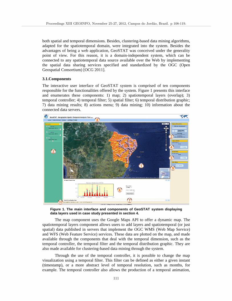
both spatial and temporal dimensions. Besides, clustering-based data mining algorithms,

adapted for the spatiotemporal domain, were integrated into the system. Besides the

advantages of being a web application, GeoSTAT was conceived under the generality

point of view. For this reason, it is a domain-independent system, which can be

connected to any spatiotemporal data source available over the Web by implementing

the spatial data sharing services specified and standardized by the OGC (Open

Geospatial Consortium) [OCG 2011].

3.1.Components

The interactive user interface of GeoSTAT system is comprised of ten components

responsible for the functionalities offered by the system. Figure 1 presents this interface

and enumerates these components: 1) map; 2) spatiotemporal layers (overlap); 3)

temporal controller; 4) temporal filter; 5) spatial filter; 6) temporal distribution graphic;

7) data mining results; 8) actions menu; 9) data mining; 10) information about the

connected data servers.

Figure 1. The main interface and components of GeoSTAT system displaying data layers used in case study presented in section 4.

The map component uses the Google Maps API to offer a dynamic map. The

spatiotemporal layers component allows users to add layers and spatiotemporal (or just

spatial) data published in servers that implement the OGC WMS (Web Map Service)

and WFS (Web Feature Service) services. These data are plotted on the map, and made

available through the components that deal with the temporal dimension, such as the

temporal controller, the temporal filter and the temporal distribution graphic. They are

also made available for clustering-based data mining through the system.

Through the use of the temporal controller, it is possible to change the map

visualization using a temporal filter. This filter can be defined as either a given instant

(timestamp), or a more abstract level of temporal resolution, such as months, for

example. The temporal controller also allows the production of a temporal animation,


111

which lets the user to visualize on the map the eventual changes in the spatial

distribution of the data as a function of the temporal variation. It also displays a specific

timestamp and enables the observation on the map of a spatial distribution of data on

this timestamp. Still, it may terminate the animation and view the spatial distribution of

the whole dataset on the map again, regardless of the temporal dimension.

Besides the temporal controller, another available temporal visualization

resource is the temporal distribution graphic. It is responsible for helping the user to

visualize changes in the spatiotemporal data as a function of time, adding to the map

resource, which helps the visualization of the distribution as a function of space.

The spatial and temporal filter components are responsible for the spatial and

temporal query and selection, respectively, of the data visualized through the

spatiotemporal layers. Through the temporal filter, the user may, by means of four filter

options and observing the temporal resolution used, reduce the spatiotemporal dataset

for visualization and analysis. The four options available for the temporal filter are:

from, until, in and between. On the other hand, through the spatial filter, it is possible to

visualize a topological relationship between two spatial or spatiotemporal layers

previously added to the system, regardless of the source data source. It is possible to

perform the following topological relations between two layers: intersects, contains,

crosses, touches, covers and overlaps. It is also possible to apply negation (not) to each

one of these relations, in cases where this is relevant for the analysis performed by the

user.

In the component of data mining, it is possible to perform the clustering-based

data mining in the previously added layers, view the result of a previous data mining

process and the detailed status of data mining processes under execution. The data

mining processes run in background, so users do not need to wait for the end of this

processing, as they may perform other tasks.

The component of data mining results is responsible for offering the statements

necessary for the spatiotemporal visualization and for browsing a layer containing data

mining results. The user may browse through the timestamps that have the occurrence

of clusters and view each cluster separately on the map. If the data mining is made with

two layers, the user will have the option of viewing just the relevant clusters, that is,

those which have at least one point of each layer, as well as options to view just the

clusters that group only points of one layer. It is also possible to see all clusters of a

given timestamp, or even all clusters.

Finally, the actions menu component offers shortcuts for the rest of the

components of the interactive graphic interface of the GeoSTAT system, and the

connected source data server component is responsible for displaying information about

the data servers that are connected to a user session of the system.

3.2.Architecture

The GeoSTAT system architecture is defined using three layers: visualization, control

and persistence.

The visualization layer is responsible for the user interface, offering components

for loading, handling and visualizing the data through the temporal and spatial

dimensions, presented in section 3.1.


112

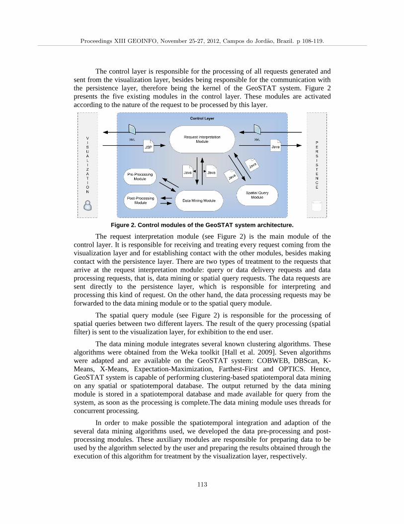
The control layer is responsible for the processing of all requests generated and

sent from the visualization layer, besides being responsible for the communication with

the persistence layer, therefore being the kernel of the GeoSTAT system. Figure 2

presents the five existing modules in the control layer. These modules are activated

according to the nature of the request to be processed by this layer.

Figure 2. Control modules of the GeoSTAT system architecture.

The request interpretation module (see Figure 2) is the main module of the

control layer. It is responsible for receiving and treating every request coming from the

visualization layer and for establishing contact with the other modules, besides making

contact with the persistence layer. There are two types of treatment to the requests that

arrive at the request interpretation module: query or data delivery requests and data

processing requests, that is, data mining or spatial query requests. The data requests are

sent directly to the persistence layer, which is responsible for interpreting and

processing this kind of request. On the other hand, the data processing requests may be

forwarded to the data mining module or to the spatial query module.

The spatial query module (see Figure 2) is responsible for the processing of

spatial queries between two different layers. The result of the query processing (spatial

filter) is sent to the visualization layer, for exhibition to the end user.

The data mining module integrates several known clustering algorithms. These

algorithms were obtained from the Weka toolkit [Hall et al. 2009]. Seven algorithms

were adapted and are available on the GeoSTAT system: COBWEB, DBScan, K-

Means, X-Means, Expectation-Maximization, Farthest-First and OPTICS. Hence,

GeoSTAT system is capable of performing clustering-based spatiotemporal data mining

on any spatial or spatiotemporal database. The output returned by the data mining

module is stored in a spatiotemporal database and made available for query from the

system, as soon as the processing is complete.The data mining module uses threads for

concurrent processing.

In order to make possible the spatiotemporal integration and adaption of the

several data mining algorithms used, we developed the data pre-processing and post-

processing modules. These auxiliary modules are responsible for preparing data to be

used by the algorithm selected by the user and preparing the results obtained through the

execution of this algorithm for treatment by the visualization layer, respectively.


113

The persistence layer is responsible for connecting the GeoSTAT system to the

databases requested by the users through the components of the visualization layer.

When a data request is received from the control layer, the persistence layer first

identifies the type of connection that will be established. It can connect either to the

OGC WMS and WFS services, or to a spatiotemporal database developed to operate

exclusively with the system. The OGC services are accessed from their web servers.

The spatiotemporal database stores information used by the GeoSTAT system to

connect to the OGC services, as well as the complete results of the data mining

processes performed by the system and available for visualization.

4. Case study: Analysis of spatiotemporal correlation between failures in

power transmission lines and fire spots

This study consists in the analysis of two sets of spatiotemporal data. Each set is

comprised of records of an spatiotemporal event.

4.1. Data

To carry out this study, we used georeferenced spatiotemporal data about fire spots

detected in the Northeastern region of Brazil, supplied by the National Institute for

Space Research1 (INPE), through the Weather Forecast and Climatic Studies Center

(CPTEC), which publishes this kind of information daily, through their Fires

Monitoring Portal2.

We obtained a total of 2,361,040 records of fire spots detected in the region, in

the period between 01-01-2002 and 12-31-2012, that is, in the last ten years. The

spatiotemporal data were obtained in the ESRI™ Shapefile format, using the WGS84

geographic reference system, and temporal data according to the GMT. According to

INPE, their system detects the presence of fire in the vegetation and the mean error in

the spatial location of the spots is of approximately 400 meters, with standard deviation

of about 3 kilometers, and with about 80% of the spots detected in a distance of one

kilometer from the coordinates indicated by the system. In the temporal validity, the

satellites offer a mean temporal resolution of 3 hours. This is the mean time between the

pass of two satellites capturing information about the same region.

Another spatiotemporal database was used in this study. It is about failure events

in power transmission lines, recorded by the San Francisco Hydroelectric Company

(Eletrobrás/Chesf), which operates throughout the Northeastern region of Brazil. Since

we could not get official data from Eletrobrás/Chesf, due to technical and

confidentiality matters, we developed an algorithm to generate spatiotemporal failure

events randomly, obeying the spatial constraint imposed by Eletrobrás/Chesf’s

transmission line network, and the temporal constraint imposed by the other database

used in this study.

We generated a total of 131,834 failure records in Eletrobrás/Chesf’s

transmission lines, in the period between 01-01-2002 and 12-31-2012, that is, also in the

last 10 years. These records were stored in a spatiotemporal database, also in the

WGS84 geographic reference system, and with temporal information according to the

1INPE –Brazilian National Institute for Space Research. More information at http://www.inpe.br/

2INPE/CPTEC –Fires Monitoring Portal. Available at http://www. inpe.br/queimadas/


114

GMT. Aiming at helping in the visual analysis of the transmission line failure events,

we also used a set of spatial data containing Eletrobrás/Chesf’s transmission line

network.

Both datasets used in this study share the same spatial geometry (POINT) and

also the same temporal resolution (timestamp). In order to use the data in GeoSTAT

system, we needed to install Geoserver web map server and create layers for each

dataset.

To conduct this study, the GeoSTAT system user will be called analyst, a

specialist user in the approached domain, looking for relevant information implicit in a

large volume of spatiotemporal data.

4.3. Experiment

Figure 1 shows the GeoSTAT system interface with the three spatiotemporal layers

loaded into the system from the data connection with Geoserver. What is seen is the

result of about two million and a half points plotted in the map, enough to fill the whole

Northeastern region.

The temporal distribution graphics, generated and shown automatically when a

spatiotemporal layer is loaded and selected in the GeoSTAT system, allows the analyst

to verify the behavior of the whole volume of data. By observing the graphic

corresponding to the fire spots layer (showed in Figure 1), we notice that there is an

annual repetition of the distribution of the number of spots detected, where the

maximums concentrate in the first and in the last months of each year. This is the period

when the Northeastern region registers the highest temperatures, which contributes to

the occurrence of new fire spots. Through this graphic, we can also observe that the

maximum number of spots detected in one day, in the 10-year period, was of 6,418

spots. This number was reached in 11-07-2005.

By observing the graphic corresponding to the transmission line failures layer,

we notice a temporal behavior that is practically continuous. Once the data was

randomly generated through an algorithm, the temporal distribution of the occurrences

was uniform, registering the maximum of three occurrences in one single day.

For a better visualization of the power line failures and of the detected fire spots,

it might use a more generic temporal resolution than timestamp, such as “Date and

Time”, for example, joining all the records occurring between “10-15-2011 15:00:00”

and “10-15-2011 15:59:59” in one single view, for example. This strategy allows

several simultaneous visualizations, time-time, of failures and fire spots within 10 years

of data. However, the cost would be too high for the analyst to view image by image,

time by time, manually, to find interesting behaviors. The use of the clustering

technique emerges as a good option to reduce the cost to the analyst, by making the

spatiotemporal clustering of the events.

With the layers “FAILURES” and “SPOTS” added to the GeoSTAT system, we

activate the spatiotemporal clustering option offered by the system to perform the data

mining with both layers. This option enables the analyst to view the spatiotemporal

clusters of each separate event and the relevant clusters, that is, the spatiotemporal

clusters containing records of both events.


115

In order to execute the data mining, besides the three input layers, the user had

to inform the following required parameters: “Date + 3-3 hours” for temporal

resolution, and DBScan as the data mining algorithm, with MinPoints = 2 and Epsilon =

0.013472.

The choice of the value 0.013472 for the Epsilon parameter of DBScan is due

fact that one second (angular measurement unit) is approximately equal to 30.9 meters.

Since about 80% of the fire spots detected by INPE occur within one kilometer from the

indicated coordinates, and the mean error in the spatial location of the records is of 400

meters, we thought reasonable that the radius of a generated cluster ranged from 1 to 1.5

kilometers. Since 48.5 seconds is approximately equal to 1,498.65 meters (1.5

kilometers) and one decimal degree has 60 minutes and 60 seconds, then we conclude

that 1,498.65 meters is approximately equal to 0.013472 meters.

4.4.Results and Conclusions

The data mining process of this case study lasted 7 hours, 37 minutes and 5 seconds. It

was executed in a web application server, running Microsoft™ Windows 7 Professional

(64-bit) operating system, with Intel™ Core i7 processor and 16 GB of RAM.

The statistical results for the classification of the records after the execution of

the algorithm showed that only 32,275 records, 1.29 of the whole dataset, were

considered relevant by the GeoSTAT system. This means that only these records are

contained in relevant spatiotemporal clusters, those which contain records of both

studied events. Approximately 86.03% of the records were associated to a

spatiotemporal cluster. The rest of the records, 13.97% of the total, were considered

outliers because they do not belong to any spatiotemporal cluster, representing only

isolated occurrences in space-time.

From the 318,901 spatiotemporal clusters generated, just 1,376 (0.43%) were

considered relevant under the viewpoint of the measurement parameters used in the

execution of the data mining algorithm. Each irrelevant cluster grouped, on average,

6,623 records, while each relevant cluster grouped, on average, just 23 records.

Figure 3 presents a screenshot captured from the GeoSTAT system showing in

the map all the relevant spatiotemporal clusters generated for the 10-year period of the

dataset. The first information that may be noticed by the analyst in this visualization is

that the region which concentrated more clusters was the region located in the Southeast

of the state of Ceará, more precisely in the border with the states of Paraíba and Rio

Grande do Norte, highlighted in the picture. The metropolitan regions of Maceió-AL

and of Recife-PE, as well as the region of the city of Sobral-CE, are also regions with

many clusters.

The generated spatiotemporal clusters can be browsed with the components for

temporal selection and, from this definition, with the individual selection of each cluster

corresponding to the previously selected timestamp. The analyst may choose the

visualization of relevant clusters only, or the visualization of all clusters. The analyst

may also visualize each individual cluster, or visualize all the clusters, regardless of the

temporal dimension.


116

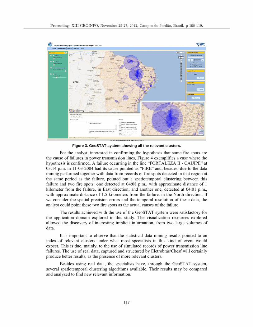
Figure 3. GeoSTAT system showing all the relevant clusters.

For the analyst, interested in confirming the hypothesis that some fire spots are

the cause of failures in power transmission lines, Figure 4 exemplifies a case where the

hypothesis is confirmed. A failure occurring in the line “FORTALEZA II - CAUIPE” at

03:14 p.m. in 11-03-2004 had its cause pointed as “FIRE” and, besides, due to the data

mining performed together with data from records of fire spots detected in that region at

the same period as the failure, pointed out a spatiotemporal clustering between this

failure and two fire spots: one detected at 04:08 p.m., with approximate distance of 1

kilometer from the failure, in East direction; and another one, detected at 04:01 p.m.,

with approximate distance of 1.5 kilometers from the failure, in the North direction. If

we consider the spatial precision errors and the temporal resolution of these data, the

analyst could point these two fire spots as the actual causes of the failure.

The results achieved with the use of the GeoSTAT system were satisfactory for

the application domain explored in this study. The visualization resources explored

allowed the discovery of interesting implicit information, from two large volumes of

data.

It is important to observe that the statistical data mining results pointed to an

index of relevant clusters under what most specialists in this kind of event would

expect. This is due, mainly, to the use of simulated records of power transmission line

failures. The use of real data, captured and structured by Eletrobrás/Chesf will certainly

produce better results, as the presence of more relevant clusters.

Besides using real data, the specialists have, through the GeoSTAT system,

several spatiotemporal clustering algorithms available. Their results may be compared

and analyzed to find new relevant information.


117

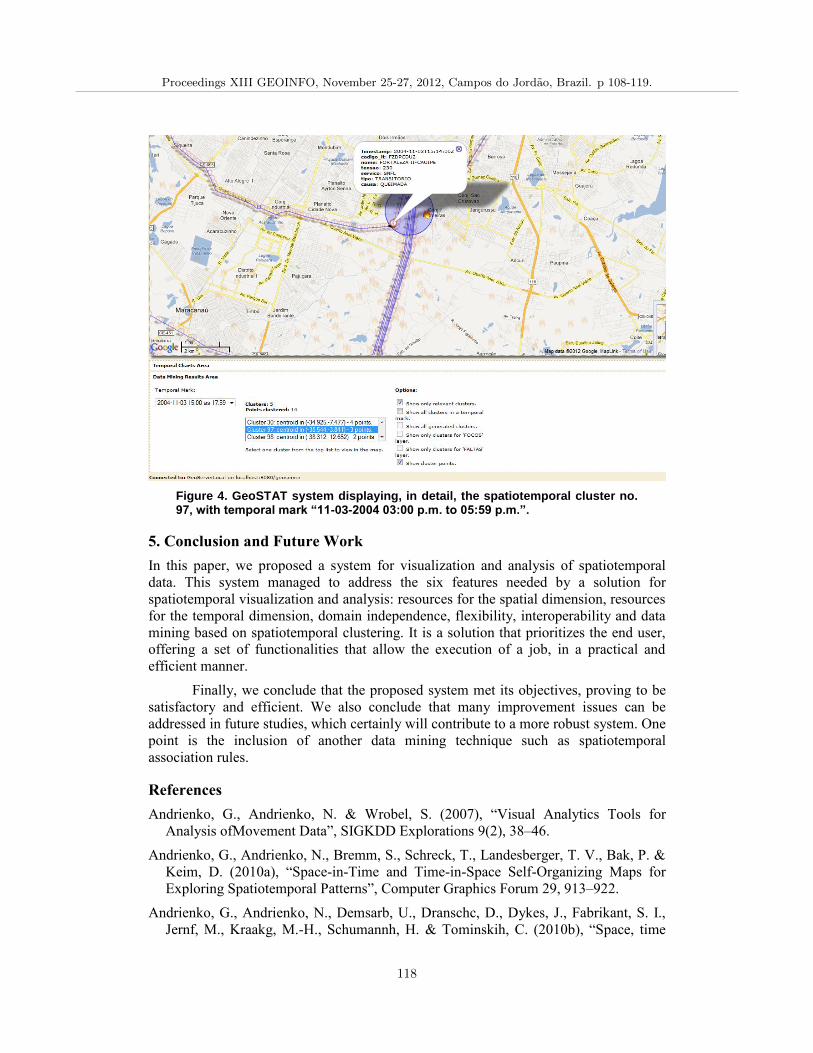
Figure 4. GeoSTAT system displaying, in detail, the spatiotemporal cluster no. 97, with temporal mark “11-03-2004 03:00 p.m. to 05:59 p.m.”.

5. Conclusion and Future Work

In this paper, we proposed a system for visualization and analysis of spatiotemporal

data. This system managed to address the six features needed by a solution for

spatiotemporal visualization and analysis: resources for the spatial dimension, resources

for the temporal dimension, domain independence, flexibility, interoperability and data

mining based on spatiotemporal clustering. It is a solution that prioritizes the end user,

offering a set of functionalities that allow the execution of a job, in a practical and

efficient manner.

Finally, we conclude that the proposed system met its objectives, proving to be

satisfactory and efficient. We also conclude that many improvement issues can be

addressed in future studies, which certainly will contribute to a more robust system. One

point is the inclusion of another data mining technique such as spatiotemporal

association rules.

References

Andrienko, G., Andrienko, N. & Wrobel, S. (2007), “Visual Analytics Tools for

Analysis ofMovement Data”, SIGKDD Explorations 9(2), 38–46.

Andrienko, G., Andrienko, N., Bremm, S., Schreck, T., Landesberger, T. V., Bak, P. &

Keim, D. (2010a), “Space-in-Time and Time-in-Space Self-Organizing Maps for

Exploring Spatiotemporal Patterns”, Computer Graphics Forum 29, 913–922.

Andrienko, G., Andrienko, N., Demsarb, U., Dranschc, D., Dykes, J., Fabrikant, S. I.,

Jernf, M., Kraakg, M.-H., Schumannh, H. & Tominskih, C. (2010b), “Space, time


118

and visual analytics”, International Journal of Geographical Information Science

24(10), 1577–1600.

Andrienko, N., Andrienko, G. & Gatalsky, P. (2003), “Exploratory spatio-temporal

visualization: an analytical review”, Journal of Visual Languages & Computing

14(6), 503–541.

Bédard, Y., Merrett, T. & Han, J. (2001), “Fundamentals of Spatial Data Warehousing

for Geographic Knowledge Discovery”, Vol. Research Monographs in GIS, Taylor

& Francis, chapter 3, pp. 53–73.

Ferreira, N., Lins, L., Fink, D., Kelling, S., Wood, C., Freire, J. & Silva, C. (2011),

“BirdVis: Visualizing and Understanding Bird Populations”, IEEE Transactions on

Visualization and Computer Graphics 17(12), 2374–2383.

Hall, M., Frank, E., Holmes, G., Pfahringer, B., Reutemann, P. & Witten, I. H. (2009),

“The WEKA data mining software: an update”, SIGKDD Explorations 11(1), 10–18.

Johnston, W. L. (2001), “Information visualization in data mining and knowledge

discovery”, Morgan Kaufmann Publishers, San Francisco, CA, USA, chapter 16.

Model Visualization, pp. 223–227.

Kohonen, T. (2001), “Self-Organizing Maps”, Vol. 30 of Information Sciences, 3rd ed.,

Springer-Verlag.

Kopanakis, I. and Theodoulidis, B. (2003), “Visual data mining modeling techniques

for the visualization of mining outcomes”, Journal of Visual Languages and

Computing 14(6), 543–589.

OGC (2011), “OGC - Making Location count”, Open Geospatial Consortium.

Disponível em: http://www.opengeospatial.org/.

Reda, K., Tantipathananandh, C., Berger-Wolf, T., Leigh, J. & Johnson, A. E. (2009),

“SocioScape - a Tool for Interactive Exploration of Spatiotemporal Group Dynamics

in Social Networks”, In: Proceedings of the IEEE Information Visualization

Conference (INFOVIS’09), Atlantic City, NJ, USA, pp. 1–2.

Roth, R. E., Ross, K. S., Finch, B. G., Luo, W. & MacEachren, A. M. (2010), “A user

centered approach for designing and developing spatiotemporal crime analysis

tools”, In: Proceedings of GIScience 2010, Zurich, Suíça, pp. 66–71.


119

Georeferencing Facts in Road Networks

Fábio da Costa Albuquerque1,3

, Ivanildo Barbosa1,2

, Marco Antonio Casanova1,3

,

Marcelo Tílio Monteiro de Carvalho3

1Departament of Informatics – PUC-Rio Rio de Janeiro – Brazil

2Department of Surveying Engineering – Military Institute of Engineering Rio de Janeiro – Brazil

3TecGraf – PUC-Rio Rio de Janeiro – Brazil

{falbuquerque, ibarbosa, casanova}@inf.puc-rio.br,

[email protected]

Abstract. Information about a location can be imprecise and context-

dependent. This is especially true for road networks, where some streets are

long or two-way, and just the name of a street may represent low-value

information for certain applications. To improve precision, geocoding

commonly includes the number of a building on a street, the highway location,

often indicated in kilometers, or the postal code in a town or city. One can

also improve the description of a location using spatial attributes, because

they are familiar concepts for humans. This article outlines a model to

precisely georeference locations, using geocoding and routing services and

considering the natural attributes used by humans regarding locations.

1. Introduction

In this article, we address the problem of inferring the location of facts that affect road conditions by analyzing real-time data retrieved from dynamic data sources on the Web. In general, the location of such facts is useful for real-time applications that monitor moving objects and that support decision making. For example, car crashes and road blocks are relevant to such applications because they affect the traffic flow by reducing the average speed and imposing changes on the planned route. However, to be useful, the location of such facts must be estimated as accurately as possible. Furthermore, they must be provided as timely as possible, which justifies exploring dynamic data sources on the Web.

The most common way to georeference locations is to use geocoding techniques, which can be defined as a process to estimate the most accurate location for a set of geographic points from locational data such as postal code, street name, building name, neighborhood, etc. As summarized by Goldberg, Wilson and Knoblock (2007), geocoded data that used to cost $4.50 per 1,000 records as recently as the mid-1980s, quickly moved to $1.00 by 2003, and can now be done for free, using online services, which however may have limitations, such as the maximum number of requests per day. For example, Yahoo! PlaceFinder allows up to 50,000 requests per day, while Google


120

allows 2,500 requests, Bing allows 15,000 requests, and CloudMade provides unlimited access to this service completely for free.

Information about a location can be imprecise and context-dependent. In a road network, where streets may be long or two-way, just the name of a street may represent low-valued information for certain applications. To improve precision, geocoding commonly includes the number of a building on the street, the highway location, often indicated in kilometers, or the postal code. Another way to reference locations, frequently used in human communication, is to use a proximity attribute, declaring that location A is near location B, rather than directly using the address of location A. Another relevant aspect of location description using natural language is the direction attribute, i.e., the direction of a street toward a location.

In this article, we outline a model to georeference the location of facts, using geocoding and routing services, from spatial descriptions commonly found in human communication. To validate the model, we describe a prototype application that uses structured traffic-related news in natural language to infer locations. The prototype application is part of a larger system to monitor moving objects in an urban environment [Albuquerque et al., 2012].

The article is organized as follows. Section 2 describes our motivation. Section 3 introduces the geocoding model. Section 4 presents the prototype application. Finally, section 5 draws some conclusions.

2. Motivation

To motivate the discussion, consider the following scenario. Every day, Twitter text messages (“tweets”) with traffic-related contents are published by institutional or individual users as a collaborative initiative. Institutional tweets, such as those published by CET-RIO1, are fairly well-structured and can be used as raw input data in the context of our target application. Each traffic-related tweet contains one or more simple facts (such as traffic intensity) or describes events (such as accidents or road blocks) and their respective location. We do not distinguish between simple facts and events here, and refer to both as facts. Retrieving these associations from raw text is not trivial because there is no commonly expected format or template for natural speech. In order to associate the facts to their accurate locations, we use a traffic-related fact structure, as explained in Section 4.1.

The naive use of location as input to the georeferencing process may produce imprecise results. As an example, consider the text illustrated in Figure 1: “Car accident on street A, located at district K, in the direction of Hospital X, near street B”. Suppose also that street A is a two-way street and is 5 kilometers long.

If the geocoding process outputs only “street A”, then the information will be quite inaccurate: we do not know the exact location of the accident along the 5 kilometers, or in which street direction it occurred. On the other hand, a geocoding service that qualifies “street A” with “near street B” provides valuable information that

1 http://twitter.com/CETRIO_ONLINE


121

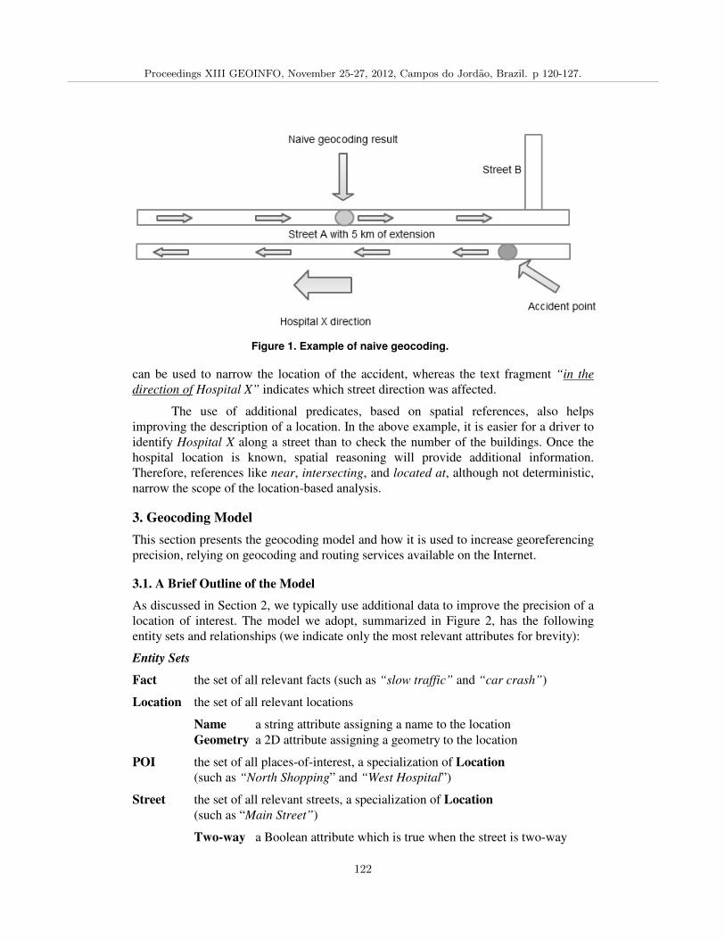
can be used to narrow the location of the accident, whereas the text fragment “in the

direction of Hospital X” indicates which street direction was affected.

The use of additional predicates, based on spatial references, also helps improving the description of a location. In the above example, it is easier for a driver to identify Hospital X along a street than to check the number of the buildings. Once the hospital location is known, spatial reasoning will provide additional information. Therefore, references like near, intersecting, and located at, although not deterministic, narrow the scope of the location-based analysis.

3. Geocoding Model

This section presents the geocoding model and how it is used to increase georeferencing precision, relying on geocoding and routing services available on the Internet.

3.1. A Brief Outline of the Model

As discussed in Section 2, we typically use additional data to improve the precision of a location of interest. The model we adopt, summarized in Figure 2, has the following entity sets and relationships (we indicate only the most relevant attributes for brevity):

Entity Sets

Fact the set of all relevant facts (such as “slow traffic” and “car crash”)

Location the set of all relevant locations

Name a string attribute assigning a name to the location

Geometry a 2D attribute assigning a geometry to the location

POI the set of all places-of-interest, a specialization of Location

(such as “North Shopping” and “West Hospital”)

Street the set of all relevant streets, a specialization of Location

(such as “Main Street”)

Two-way a Boolean attribute which is true when the street is two-way

Figure 1. Example of naive geocoding.


122

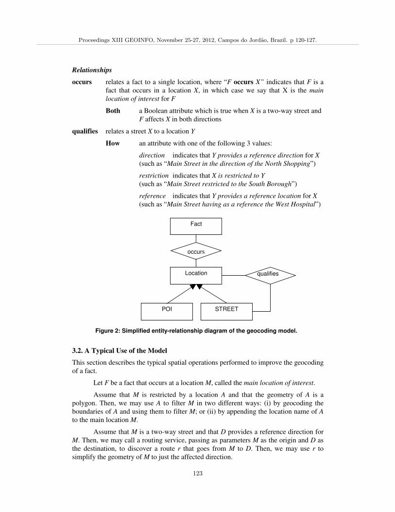
Relationships

occurs relates a fact to a single location, where “F occurs X” indicates that F is a fact that occurs in a location X, in which case we say that X is the main

location of interest for F

Both a Boolean attribute which is true when X is a two-way street and F affects X in both directions

qualifies relates a street X to a location Y

How an attribute with one of the following 3 values:

direction indicates that Y provides a reference direction for X

(such as “Main Street in the direction of the North Shopping”)

restriction indicates that X is restricted to Y (such as “Main Street restricted to the South Borough”)

reference indicates that Y provides a reference location for X

(such as “Main Street having as a reference the West Hospital”)

3.2. A Typical Use of the Model

This section describes the typical spatial operations performed to improve the geocoding of a fact.

Let F be a fact that occurs at a location M, called the main location of interest.

Assume that M is restricted by a location A and that the geometry of A is a polygon. Then, we may use A to filter M in two different ways: (i) by geocoding the boundaries of A and using them to filter M; or (ii) by appending the location name of A to the main location M.

Assume that M is a two-way street and that D provides a reference direction for M. Then, we may call a routing service, passing as parameters M as the origin and D as the destination, to discover a route r that goes from M to D. Then, we may use r to simplify the geometry of M to just the affected direction.

Fact

Location

POI STREET

Figure 2: Simplified entity-relationship diagram of the geocoding model.

occurs

qualifies


123

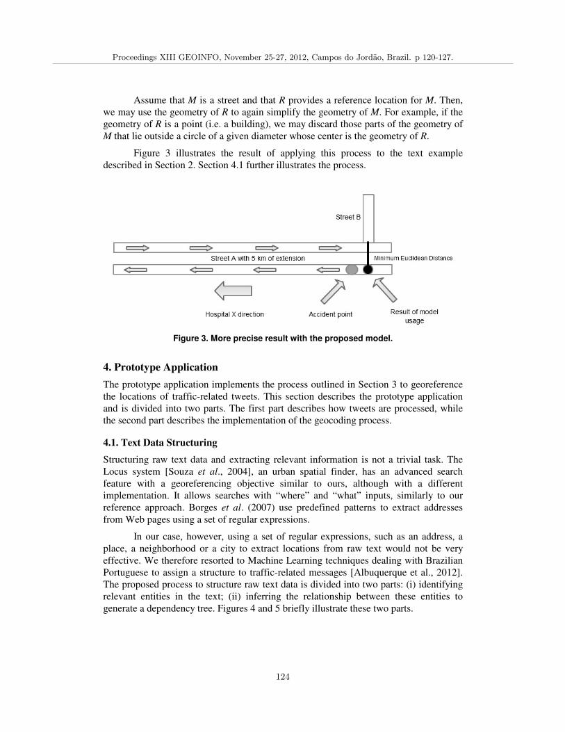
Assume that M is a street and that R provides a reference location for M. Then, we may use the geometry of R to again simplify the geometry of M. For example, if the geometry of R is a point (i.e. a building), we may discard those parts of the geometry of M that lie outside a circle of a given diameter whose center is the geometry of R.

Figure 3 illustrates the result of applying this process to the text example described in Section 2. Section 4.1 further illustrates the process.

4. Prototype Application

The prototype application implements the process outlined in Section 3 to georeference the locations of traffic-related tweets. This section describes the prototype application and is divided into two parts. The first part describes how tweets are processed, while the second part describes the implementation of the geocoding process.

4.1. Text Data Structuring

Structuring raw text data and extracting relevant information is not a trivial task. The Locus system [Souza et al., 2004], an urban spatial finder, has an advanced search feature with a georeferencing objective similar to ours, although with a different implementation. It allows searches with “where” and “what” inputs, similarly to our reference approach. Borges et al. (2007) use predefined patterns to extract addresses from Web pages using a set of regular expressions.

In our case, however, using a set of regular expressions, such as an address, a place, a neighborhood or a city to extract locations from raw text would not be very effective. We therefore resorted to Machine Learning techniques dealing with Brazilian Portuguese to assign a structure to traffic-related messages [Albuquerque et al., 2012]. The proposed process to structure raw text data is divided into two parts: (i) identifying relevant entities in the text; (ii) inferring the relationship between these entities to generate a dependency tree. Figures 4 and 5 briefly illustrate these two parts.

Figure 3. More precise result with the proposed model.


124

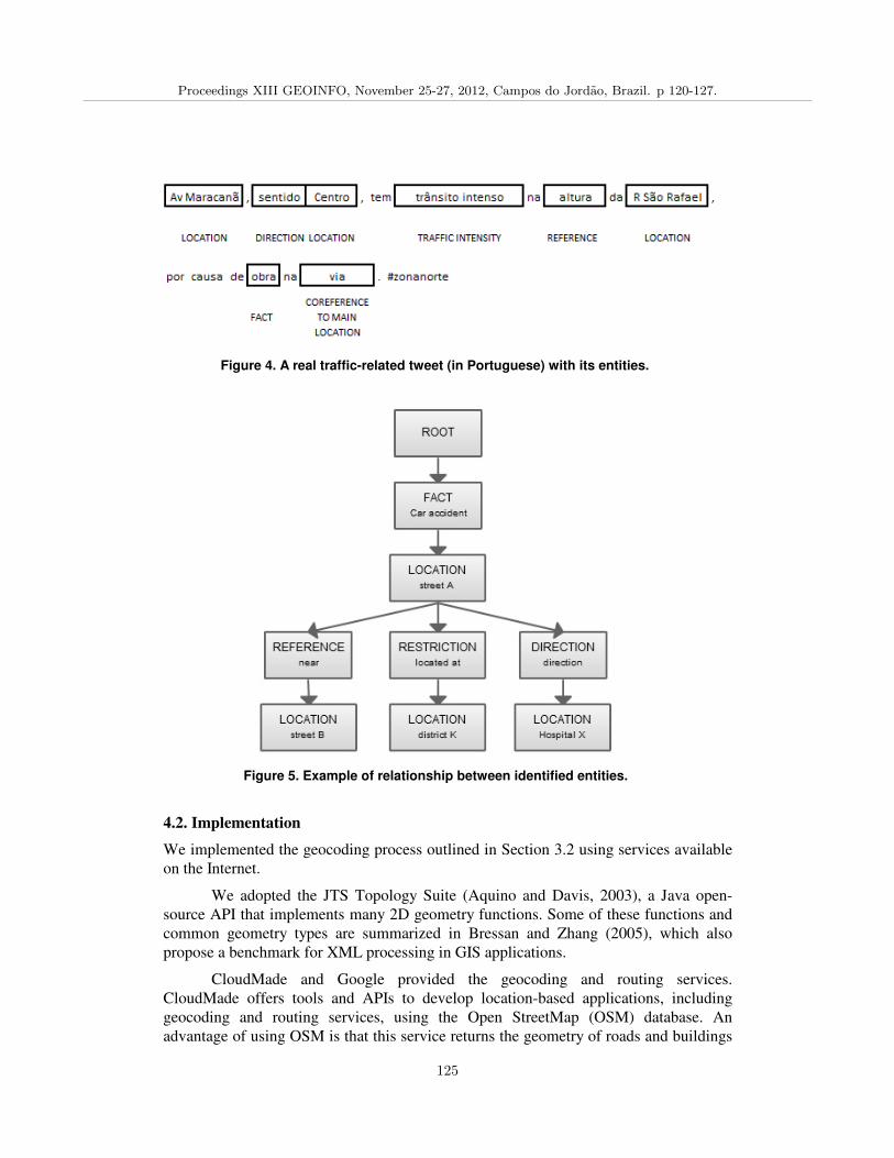
4.2. Implementation

We implemented the geocoding process outlined in Section 3.2 using services available on the Internet.

We adopted the JTS Topology Suite (Aquino and Davis, 2003), a Java open-source API that implements many 2D geometry functions. Some of these functions and common geometry types are summarized in Bressan and Zhang (2005), which also propose a benchmark for XML processing in GIS applications.

CloudMade and Google provided the geocoding and routing services. CloudMade offers tools and APIs to develop location-based applications, including geocoding and routing services, using the Open StreetMap (OSM) database. An advantage of using OSM is that this service returns the geometry of roads and buildings

Figure 5. Example of relationship between identified entities.

Figure 4. A real traffic-related tweet (in Portuguese) with its entities.


125

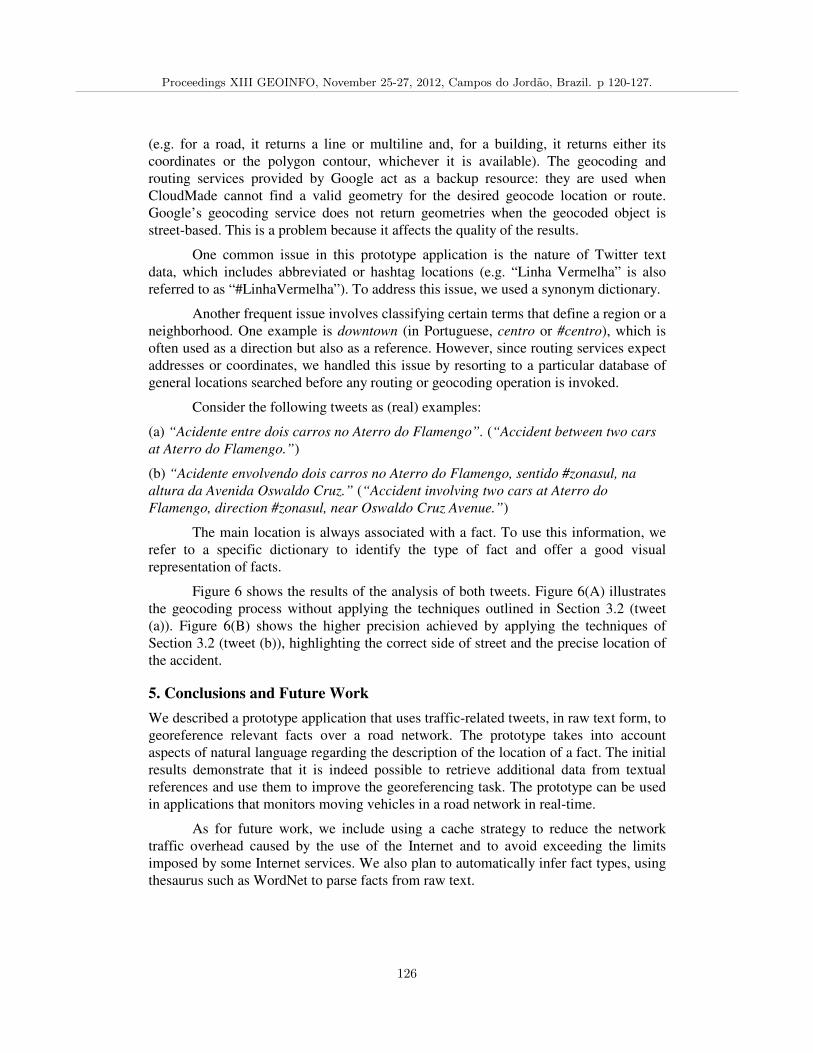
(e.g. for a road, it returns a line or multiline and, for a building, it returns either its coordinates or the polygon contour, whichever it is available). The geocoding and routing services provided by Google act as a backup resource: they are used when CloudMade cannot find a valid geometry for the desired geocode location or route. Google’s geocoding service does not return geometries when the geocoded object is street-based. This is a problem because it affects the quality of the results.

One common issue in this prototype application is the nature of Twitter text data, which includes abbreviated or hashtag locations (e.g. “Linha Vermelha” is also referred to as “#LinhaVermelha”). To address this issue, we used a synonym dictionary.

Another frequent issue involves classifying certain terms that define a region or a neighborhood. One example is downtown (in Portuguese, centro or #centro), which is often used as a direction but also as a reference. However, since routing services expect addresses or coordinates, we handled this issue by resorting to a particular database of general locations searched before any routing or geocoding operation is invoked.

Consider the following tweets as (real) examples:

(a) “Acidente entre dois carros no Aterro do Flamengo”. (“Accident between two cars

at Aterro do Flamengo.”)

(b) “Acidente envolvendo dois carros no Aterro do Flamengo, sentido #zonasul, na

altura da Avenida Oswaldo Cruz.” (“Accident involving two cars at Aterro do

Flamengo, direction #zonasul, near Oswaldo Cruz Avenue.”)

The main location is always associated with a fact. To use this information, we refer to a specific dictionary to identify the type of fact and offer a good visual representation of facts.

Figure 6 shows the results of the analysis of both tweets. Figure 6(A) illustrates the geocoding process without applying the techniques outlined in Section 3.2 (tweet (a)). Figure 6(B) shows the higher precision achieved by applying the techniques of Section 3.2 (tweet (b)), highlighting the correct side of street and the precise location of the accident.

5. Conclusions and Future Work

We described a prototype application that uses traffic-related tweets, in raw text form, to georeference relevant facts over a road network. The prototype takes into account aspects of natural language regarding the description of the location of a fact. The initial results demonstrate that it is indeed possible to retrieve additional data from textual references and use them to improve the georeferencing task. The prototype can be used in applications that monitors moving vehicles in a road network in real-time.

As for future work, we include using a cache strategy to reduce the network traffic overhead caused by the use of the Internet and to avoid exceeding the limits imposed by some Internet services. We also plan to automatically infer fact types, using thesaurus such as WordNet to parse facts from raw text.


126

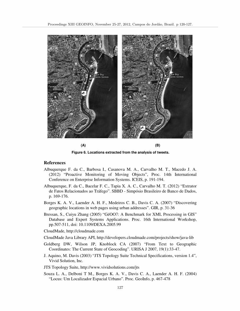
References

Albuquerque F. da C., Barbosa I., Casanova M. A., Carvalho M. T., Macedo J. A. (2012) “Proactive Monitoring of Moving Objects”, Proc. 14th International Conference on Enterprise Information Systems. ICEIS, p. 191-194.

Albuquerque, F. da C., Bacelar F. C., Tapia X. A. C., Carvalho M. T. (2012) “Extrator de Fatos Relacionados ao Tráfego”. SBBD - Simpósio Brasileiro de Banco de Dados, p. 169-176.

Borges K. A. V., Laender A. H. F., Medeiros C. B., Davis C. A. (2007) “Discovering geographic locations in web pages using urban addresses”. GIR, p. 31-36

Bressan, S., Cuiyu Zhang (2005) “GéOO7: A Benchmark for XML Processing in GIS” Database and Expert Systems Applications. Proc. 16th International Workshop, pp.507-511, doi: 10.1109/DEXA.2005.99

CloudMade, http://cloudmade.com

CloudMade Java Library API, http://developers.cloudmade.com/projects/show/java-lib

Goldberg DW, Wilson JP, Knoblock CA (2007) “From Text to Geographic Coordinates: The Current State of Geocoding”. URISA J 2007, 19(1):33-47.

J. Aquino, M. Davis (2003) “JTS Topology Suite Technical Specifications, version 1.4”, Vivid Solution, Inc.

JTS Topology Suite, http://www.vividsolutions.com/jts

Souza L. A., Delboni T M., Borges K. A. V., Davis C. A., Laender A. H. F. (2004) “Locus: Um Localizador Espacial Urbano”. Proc. GeoInfo, p. 467-478

(A) (B)

Figure 6. Locations extracted from the analysis of tweets.


127

Data Quality in Agriculture Applications∗

Joana E. Gonzales Malaverri1, Claudia Bauzer Medeiros1

1Institute of Computing – State University of Campinas (UNICAMP)13083-852 – Campinas – SP – Brasil

{jmalav09, cmbm}@ic.unicamp.br

Abstract. Data quality is a common concern in a wide range of domains. Sinceagriculture plays an important role in the Brazilian economy, it is crucial thatthe data be useful and with a proper level of quality for the decision makingprocess, planning activities, among others. Nevertheless, this requirement isnot often taken into account when different systems and databases are modeled.This work presents a review about data quality issues covering some efforts inagriculture and geospatial science to tackle these issues. The goal is to helpresearchers and practitioners to design better applications. In particular, wefocus on the different dimensions of quality and the approaches that are used tomeasure them.

1. IntroductionAgriculture is an important activity for economic growth. In 2011, agricultural activitiescontributed approximately with 22% of Brazil’s Gross National Product [CEPEA 2012].Thus there are major benefits in ensuring the quality of data used by experts and decisionmakers to support activities such as yield forecast, monitoring and planning methods. Theinvestigation of ways to measure and enhance the quality of data in GIS and remote sens-ing is not new [Chrisman 1984, Medeiros and de Alencar 1999, Lunetta and Lyon 2004,Congalton and Green 2009]. The same applies to data managed in, for instance, Informa-tion Manufacturing systems [Ballou et al. 1998]; Database systems [Widom 2005], Websystems [Hartig and Zhao 2009]; or Data Mining systems [Blake and Mangiameli 2011].All of these fields are involved in and influence agriculture applications.

Despite these efforts, data quality issues are not often taken into account whendifferent kinds of databases or information systems are modeled. Data produced and re-ported by these systems is used without considering the defects or errors that data contain[Chapman 2005, Goodchild and Li 2012]. Thus, the information obtained from these datais error prone, and decisions made by experts becomes inaccurate.

There are many challenges in ongoing data quality such as: modelingand management, quality control and assurance, analysis, storage and presentation[Chapman 2005]. The approach used to tackle each one of these issues depends onthe application scenario and the level of data quality required for the intended use[U.S. Agency for International Development 2009]. Thus, understanding what attributesof quality need to be evaluated in a specific context is a key factor.

∗Work partially financed by CNPq (grant 142337/2010-2), the Microsoft Research FAPESP Virtual In-stitute (NavScales project), CNPq (MuZOO Project and PRONEX-FAPESP), INCT in Web Science(CNPq557.128/2009-9) and CAPES, as well as individual grants from CNPq.


128

This paper presents a brief review from the literature related to issues about dataquality with special consideration to data managed in agriculture. The goal is to providea conceptual background to become the basis for development of applications in agricul-ture.

2. Data for agriculture applicationsData in agriculture applications can be thematic/textual or geospatial, from primary tosecondary sources, raw or derived. Thus, rather than just analyzing issues concerning thequality of geospatial data, this paper considers quality in all kinds of data, and providesguidelines to be applied for agriculture applications.

Research related to data quality in agriculture considers several issues. Thereare papers that concentrate on agricultural statistics data (e.g., production and consump-tion of crops) like [CountrySTAT 2012] and [Kyeyago et al. 2010]. The efforts thathave been made to study the quality of geospatial data [FGDC 1998, ISO 19115 2003,Congalton and Green 2009, Goodchild and Li 2012] are also taken advantage of in theagriculture domain. However, there are other kinds of data that need to be consideredsuch as files containing sensor-produced data, crop characteristics and soil information,human management procedures, among others [eFarms 2008].

This general scenario shows that agricultural activities encompass different kindsand sets of data from a variety of heterogeneous sources. In particular, the most com-mon kinds of data are regular data and geospatial data. Regular data can be textualor numeric and can be stored on spreadsheets or text files (e.g., crop descriptions fromofficial sources). Geospatial data correspond to georeferenced data sources and caninclude both raster and vector files, for example, satellite images using GeoTIFF for-mat or a road network on shapefiles. Geospatial data may also come in data streams[Babu and Widom 2001] - packets of continuous data records - that can be obtained fromaboard satellites, ground sensors or weather stations (e.g., temperature readings). Allthese data need different levels of access and manipulation and thus pose several chal-lenges about data quality.

3. Dimensions of data qualityData quality has various definitions and is a very subjective term [Chapman 2005]. Abroad and consensual definition for data quality is “fitness for use” [Chrisman 1984].Following this general concept, [Wang and Strong 1996] extended this definition as datathat are fit for use by data consumers, i.e. those who use the data. [Redman 2001] com-plements the data quality concept by claiming that data are fit to be used if they are freeof defects, accessible, accurate, timely, complete, consistent with other sources, relevant,comprehensive, provide a proper level of detail, and easy to read and interpret. Qualityis context-based: often data that can be considered suitable for one scenario might not beappropriate for another [Ballou et al. 1998].

Data quality is seen as a multi-dimensional concept [Wang and Strong 1996,Ballou et al. 1998, Blake and Mangiameli 2011]. Quality dimensions can be con-sidered as attributes that allow to represent a particular characteristic of quality[Wang and Strong 1996]. In particular, accuracy, completeness, timeliness and consis-tency have been extensively cited in the literature as some of the most important quality


129

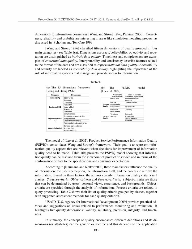
dimensions to information consumers [Wang and Strong 1996, Parssian 2006]. Correct-ness, reliability and usability are interesting in areas like simulation modeling process, asdiscussed in [Scholten and Ten Cate 1999].

[Wang and Strong 1996] classified fifteen dimensions of quality grouped in fourmain categories - see Table 1(a). Dimensions accuracy, believability, objectivity and repu-tation are distinguished as intrinsic data quality. Timeliness and completeness are exam-ples of contextual data quality. Interpretability and consistency describe features relatedto the format of the data and are classified as representational data quality. Accessibilityand security are labeled as accessibility data quality, highlighting the importance of therole of information systems that manage and provide access to information.

Table 1.

(a) The 15 dimensions framework[Wang and Strong 1996]

(b) The PSP/IQ model[Lee et al. 2002]

The model of [Lee et al. 2002], Product Service Performance Information Quality(PSP/IQ), consolidates Wang and Strong’s framework. Their goal is to represent infor-mation quality aspects that are relevant when decisions for improvement of informationquality need to be made. Table 1(b) presents the PSP/IQ model showing that informa-tion quality can be assessed from the viewpoint of product or service and in terms of theconformance of data to the specifications and consumer expectations.

According to [Naumann and Rolker 2000] three main factors influence the qualityof information: the user’s perception, the information itself, and the process to retrieve theinformation. Based on these factors, the authors classify information quality criteria in 3classes: Subject-criteria, Object-criteria and Process-criteria. Subject-criteria are thosethat can be determined by users’ personal views, experience, and backgrounds. Object-criteria are specified through the analysis of information. Process-criteria are related toquery processing. Table 2 shows their list of quality criteria grouped by classes, togetherwith suggested assessment methods for each quality criterion.

USAID [U.S. Agency for International Development 2009] provides practical ad-vices and suggestions on issues related to performance monitoring and evaluation. Ithighlights five quality dimensions: validity, reliability, precision, integrity, and timeli-ness.

In summary, the concept of quality encompasses different definitions and its di-mensions (or attributes) can be generic or specific and this depends on the application


130

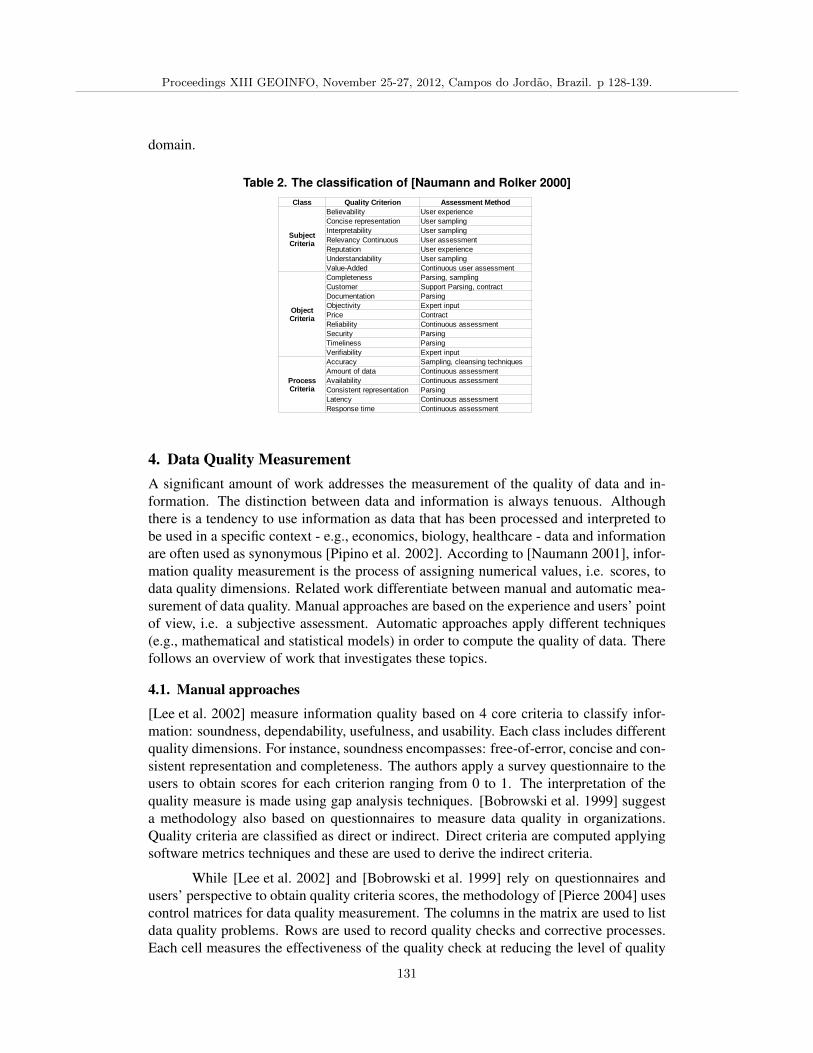
domain.

Table 2. The classification of [Naumann and Rolker 2000]

4. Data Quality MeasurementA significant amount of work addresses the measurement of the quality of data and in-formation. The distinction between data and information is always tenuous. Althoughthere is a tendency to use information as data that has been processed and interpreted tobe used in a specific context - e.g., economics, biology, healthcare - data and informationare often used as synonymous [Pipino et al. 2002]. According to [Naumann 2001], infor-mation quality measurement is the process of assigning numerical values, i.e. scores, todata quality dimensions. Related work differentiate between manual and automatic mea-surement of data quality. Manual approaches are based on the experience and users’ pointof view, i.e. a subjective assessment. Automatic approaches apply different techniques(e.g., mathematical and statistical models) in order to compute the quality of data. Therefollows an overview of work that investigates these topics.

4.1. Manual approaches

[Lee et al. 2002] measure information quality based on 4 core criteria to classify infor-mation: soundness, dependability, usefulness, and usability. Each class includes differentquality dimensions. For instance, soundness encompasses: free-of-error, concise and con-sistent representation and completeness. The authors apply a survey questionnaire to theusers to obtain scores for each criterion ranging from 0 to 1. The interpretation of thequality measure is made using gap analysis techniques. [Bobrowski et al. 1999] suggesta methodology also based on questionnaires to measure data quality in organizations.Quality criteria are classified as direct or indirect. Direct criteria are computed applyingsoftware metrics techniques and these are used to derive the indirect criteria.

While [Lee et al. 2002] and [Bobrowski et al. 1999] rely on questionnaires andusers’ perspective to obtain quality criteria scores, the methodology of [Pierce 2004] usescontrol matrices for data quality measurement. The columns in the matrix are used to listdata quality problems. Rows are used to record quality checks and corrective processes.Each cell measures the effectiveness of the quality check at reducing the level of quality


131

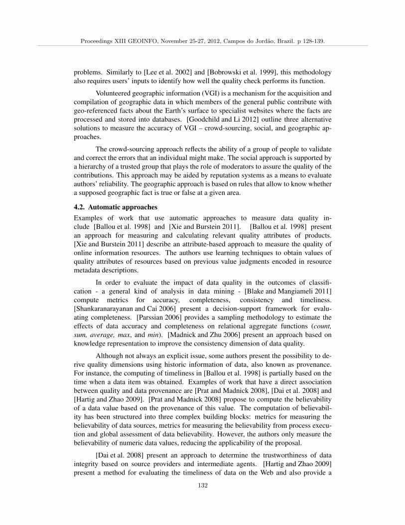
problems. Similarly to [Lee et al. 2002] and [Bobrowski et al. 1999], this methodologyalso requires users’ inputs to identify how well the quality check performs its function.

Volunteered geographic information (VGI) is a mechanism for the acquisition andcompilation of geographic data in which members of the general public contribute withgeo-referenced facts about the Earth’s surface to specialist websites where the facts areprocessed and stored into databases. [Goodchild and Li 2012] outline three alternativesolutions to measure the accuracy of VGI – crowd-sourcing, social, and geographic ap-proaches.

The crowd-sourcing approach reflects the ability of a group of people to validateand correct the errors that an individual might make. The social approach is supported bya hierarchy of a trusted group that plays the role of moderators to assure the quality of thecontributions. This approach may be aided by reputation systems as a means to evaluateauthors’ reliability. The geographic approach is based on rules that allow to know whethera supposed geographic fact is true or false at a given area.

4.2. Automatic approachesExamples of work that use automatic approaches to measure data quality in-clude [Ballou et al. 1998] and [Xie and Burstein 2011]. [Ballou et al. 1998] presentan approach for measuring and calculating relevant quality attributes of products.[Xie and Burstein 2011] describe an attribute-based approach to measure the quality ofonline information resources. The authors use learning techniques to obtain values ofquality attributes of resources based on previous value judgments encoded in resourcemetadata descriptions.

In order to evaluate the impact of data quality in the outcomes of classifi-cation - a general kind of analysis in data mining - [Blake and Mangiameli 2011]compute metrics for accuracy, completeness, consistency and timeliness.[Shankaranarayanan and Cai 2006] present a decision-support framework for evalu-ating completeness. [Parssian 2006] provides a sampling methodology to estimate theeffects of data accuracy and completeness on relational aggregate functions (count,sum, average, max, and min). [Madnick and Zhu 2006] present an approach based onknowledge representation to improve the consistency dimension of data quality.

Although not always an explicit issue, some authors present the possibility to de-rive quality dimensions using historic information of data, also known as provenance.For instance, the computing of timeliness in [Ballou et al. 1998] is partially based on thetime when a data item was obtained. Examples of work that have a direct associationbetween quality and data provenance are [Prat and Madnick 2008], [Dai et al. 2008] and[Hartig and Zhao 2009]. [Prat and Madnick 2008] propose to compute the believabilityof a data value based on the provenance of this value. The computation of believabil-ity has been structured into three complex building blocks: metrics for measuring thebelievability of data sources, metrics for measuring the believability from process execu-tion and global assessment of data believability. However, the authors only measure thebelievability of numeric data values, reducing the applicability of the proposal.

[Dai et al. 2008] present an approach to determine the trustworthiness of dataintegrity based on source providers and intermediate agents. [Hartig and Zhao 2009]present a method for evaluating the timeliness of data on the Web and also provide a


132

solution to deal with missing provenance information by associating certainty values withcalculated timeliness values. Table 3 shows a summary with the quality dimensions stud-ied in automatic approaches together with the application domain where the dimensionsare considered.

Table 3. Summary of quality dimensions covered by automatic approaches

5. Data Quality in Applications in Agriculture

Considering the impact that agriculture has on the world economy, there is a real need toensure that the data produced and used in this field have a good level of quality. Effortsto enhance the reliability of agricultural data encompass, for example, methodologiesfor collection and analysis of data, development of novel database systems and softwareapplications.

Since prevention is better than correction, data collection and compilation aresome of the first quality issues that need to be considered in the generation of data thatare fit for use [Chapman 2005]. For instance, non-reporting data, incomplete coverage ofdata, imprecise concepts and standard definitions are common problems faced during thecollection and compilation of data on land use [FAO 1997].

Statistical techniques and applications are being used to produce agriculturalstatistics such as crop yield production, seeding rate, percentage of planted and harvestedareas, among others. One example is the [CountrySTAT 2012] framework. This is a web-based system developed by the Food and Agriculture Organization of the United Nations[FAO 2012]. It integrates statistical information for food and agriculture coming from dif-ferent sources. The CountrySTAT is organized into a set of six dimensions of data qualitythat are: relevance and completeness, timeliness, accessibility and clarity, comparability,coherence, and subjectiveness.

Other example is the Data Quality Assessment Framework (DQAF)[International Monetary Fund 2003] that is being used as an international method-ology for assessing data quality related to the governance of statistical systems, statisticalprocesses, and statistical products. It is organized around a set of prerequisites and fivedimensions of data quality that are: assurance of integrity, methodological soundness,accuracy and reliability, serviceability, and accessibility.

Based on both the CountrySTAT and the DQAF frameworks,[Kyeyago et al. 2010] proposed the Agricultural Data Quality Assessment Frame-work (ADQAF) aiming at the integration of global and national perspectives to


133

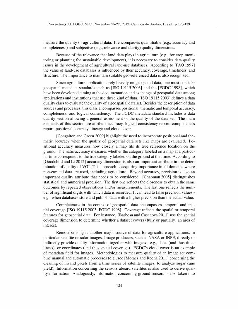
measure the quality of agricultural data. It encompasses quantifiable (e.g., accuracy andcompleteness) and subjective (e.g., relevance and clarity) quality dimensions.

Because of the relevance that land data plays in agriculture (e.g., for crop moni-toring or planning for sustainable development), it is necessary to consider data qualityissues in the development of agricultural land-use databases. According to [FAO 1997]the value of land-use databases is influenced by their accuracy, coverage, timeliness, andstructure. The importance to maintain suitable geo-referenced data is also recognized.

Since agriculture applications rely heavily on geospatial data, one must considergeospatial metadata standards such as [ISO 19115 2003] and the [FGDC 1998], whichhave been developed aiming at the documentation and exchange of geospatial data amongapplications and institutions that use these kind of data. [ISO 19115 2003] defines a dataquality class to evaluate the quality of a geospatial data set. Besides the description of datasources and processes, this class encompasses positional, thematic and temporal accuracy,completeness, and logical consistency. The FGDC metadata standard includes a dataquality section allowing a general assessment of the quality of the data set. The mainelements of this section are attribute accuracy, logical consistency report, completenessreport, positional accuracy, lineage and cloud cover.

[Congalton and Green 2009] highlight the need to incorporate positional and the-matic accuracy when the quality of geospatial data sets like maps are evaluated. Po-sitional accuracy measures how closely a map fits its true reference location on theground. Thematic accuracy measures whether the category labeled on a map at a particu-lar time corresponds to the true category labeled on the ground at that time. According to[Goodchild and Li 2012] accuracy dimension is also an important attribute in the deter-mination of quality of VGI. This approach is acquiring importance in all domains wherenon-curated data are used, including agriculture. Beyond accuracy, precision is also animportant quality attribute that needs to be considered. [Chapman 2005] distinguishesstatistical and numerical precision. The first one reflects the closeness to obtain the sameoutcomes by repeated observations and/or measurements. The last one reflects the num-ber of significant digits with which data is recorded. It can lead to false precision values -e.g., when databases store and publish data with a higher precision than the actual value.

Completeness in the context of geospatial data encompasses temporal and spa-tial coverage [ISO 19115 2003, FGDC 1998]. Coverage reflects the spatial or temporalfeatures for geospatial data. For instance, [Barbosa and Casanova 2011] use the spatialcoverage dimension to determine whether a dataset covers (fully or partially) an area ofinterest.

Remote sensing is another major source of data for agriculture applications, inparticular satellite or radar images. Image producers, such as NASA or INPE, directly orindirectly provide quality information together with images - e.g., dates (and thus time-liness), or coordinates (and thus spatial coverage). FGDC’s cloud cover is an exampleof metadata field for images. Methodologies to measure quality of an image set com-bine manual and automatic processes (e.g., see [Moraes and Rocha 2011] concerning thecleaning of invalid pixels from a time series of satellite images, to analyze sugar caneyield). Information concerning the sensors aboard satellites is also used to derive qual-ity information. Analogously, information concerning ground sensors is also taken into


134

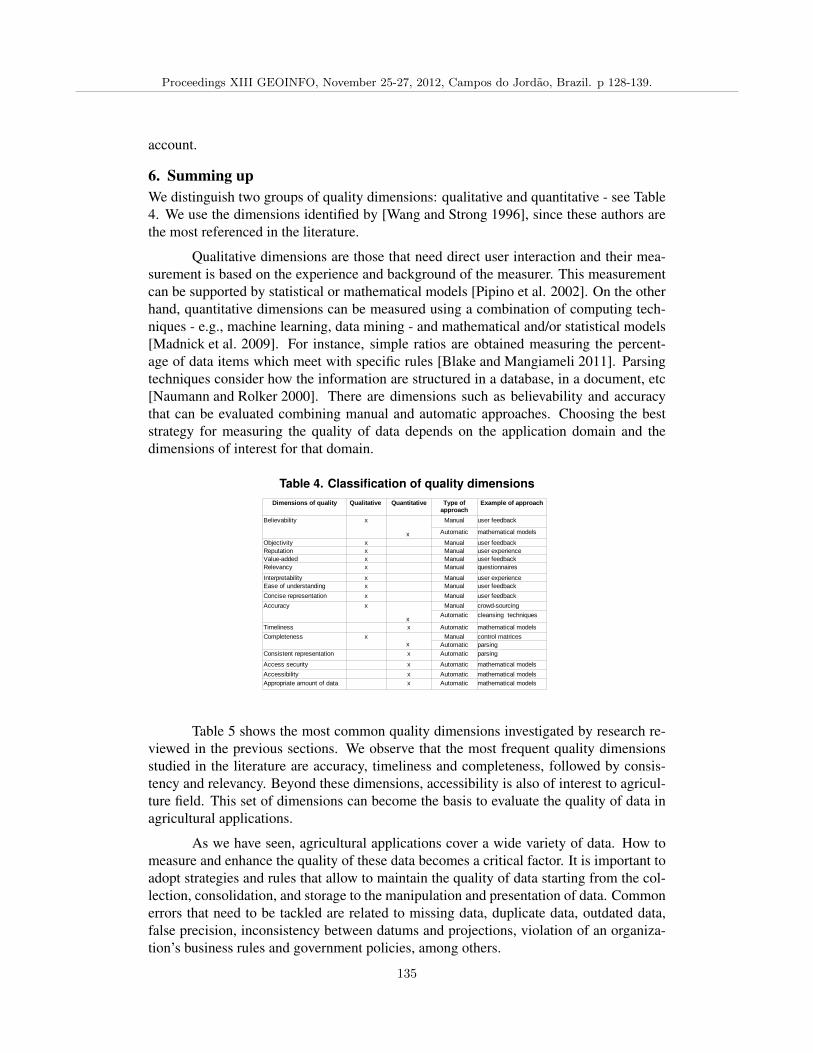
account.

6. Summing upWe distinguish two groups of quality dimensions: qualitative and quantitative - see Table4. We use the dimensions identified by [Wang and Strong 1996], since these authors arethe most referenced in the literature.

Qualitative dimensions are those that need direct user interaction and their mea-surement is based on the experience and background of the measurer. This measurementcan be supported by statistical or mathematical models [Pipino et al. 2002]. On the otherhand, quantitative dimensions can be measured using a combination of computing tech-niques - e.g., machine learning, data mining - and mathematical and/or statistical models[Madnick et al. 2009]. For instance, simple ratios are obtained measuring the percent-age of data items which meet with specific rules [Blake and Mangiameli 2011]. Parsingtechniques consider how the information are structured in a database, in a document, etc[Naumann and Rolker 2000]. There are dimensions such as believability and accuracythat can be evaluated combining manual and automatic approaches. Choosing the beststrategy for measuring the quality of data depends on the application domain and thedimensions of interest for that domain.

Table 4. Classification of quality dimensions

Table 5 shows the most common quality dimensions investigated by research re-viewed in the previous sections. We observe that the most frequent quality dimensionsstudied in the literature are accuracy, timeliness and completeness, followed by consis-tency and relevancy. Beyond these dimensions, accessibility is also of interest to agricul-ture field. This set of dimensions can become the basis to evaluate the quality of data inagricultural applications.

As we have seen, agricultural applications cover a wide variety of data. How tomeasure and enhance the quality of these data becomes a critical factor. It is important toadopt strategies and rules that allow to maintain the quality of data starting from the col-lection, consolidation, and storage to the manipulation and presentation of data. Commonerrors that need to be tackled are related to missing data, duplicate data, outdated data,false precision, inconsistency between datums and projections, violation of an organiza-tion’s business rules and government policies, among others.


135

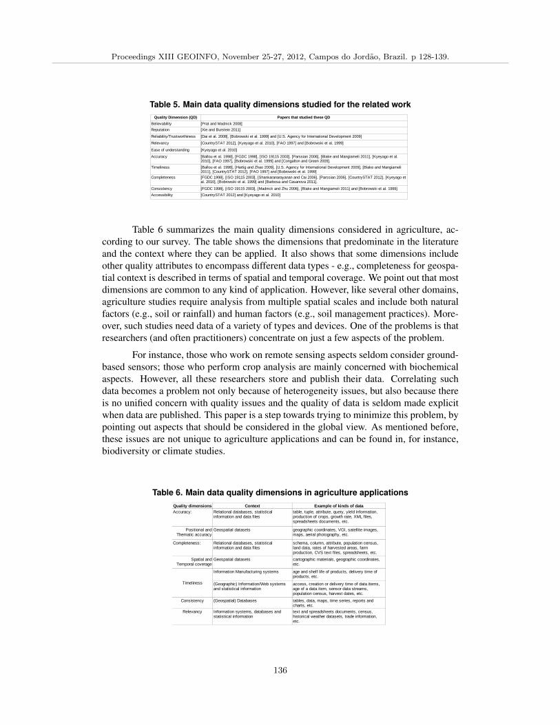
Table 5. Main data quality dimensions studied for the related work

Table 6 summarizes the main quality dimensions considered in agriculture, ac-cording to our survey. The table shows the dimensions that predominate in the literatureand the context where they can be applied. It also shows that some dimensions includeother quality attributes to encompass different data types - e.g., completeness for geospa-tial context is described in terms of spatial and temporal coverage. We point out that mostdimensions are common to any kind of application. However, like several other domains,agriculture studies require analysis from multiple spatial scales and include both naturalfactors (e.g., soil or rainfall) and human factors (e.g., soil management practices). More-over, such studies need data of a variety of types and devices. One of the problems is thatresearchers (and often practitioners) concentrate on just a few aspects of the problem.

For instance, those who work on remote sensing aspects seldom consider ground-based sensors; those who perform crop analysis are mainly concerned with biochemicalaspects. However, all these researchers store and publish their data. Correlating suchdata becomes a problem not only because of heterogeneity issues, but also because thereis no unified concern with quality issues and the quality of data is seldom made explicitwhen data are published. This paper is a step towards trying to minimize this problem, bypointing out aspects that should be considered in the global view. As mentioned before,these issues are not unique to agriculture applications and can be found in, for instance,biodiversity or climate studies.

Table 6. Main data quality dimensions in agriculture applications


136

ReferencesBabu, S. and Widom, J. (2001). Continuous queries over data streams. SIGMOD Rec.,

30(3):109–120.

Ballou, D., Wang, R., Pazer, H., and Tayi, G. K. (1998). Modeling Information Manufac-turing Systems to Determine Information Product Quality. Manage. Sci., 44:462–484.

Barbosa, I. and Casanova, M. A. (2011). Trust Indicator for Decisions Based on Geospa-tial Data. In Proc. XII Brazilian Symposium on GeoInformatics, pages 49–60.

Blake, R. and Mangiameli, P. (2011). The Effects and Interactions of Data Quality andProblem Complexity on Classification. J. Data and Information Quality, 2:8:1–8:28.

Bobrowski, M., Marre, M., and Yankelevich, D. (1999). A Homogeneous Framework toMeasure Data Quality. In Proc. IQ, pages 115–124. MIT.

CEPEA (2012). Center of Advanced Studies in Applied Economics.http://cepea.esalq.usp.br/pib/. Accessed in June 2012.

Chapman, A. D. (2005). Principles of Data Quality. Global Biodiversity InformationFacility, Copenhagen.

Chrisman, N. R. (1984). The Role of Quality Information in the Long-term Functioningof a Geographic Information System. Cartographica, 21(2/3):79–87.

Congalton, R. G. and Green, K. (2009). Assessing the accuracy of remotely sensed data:principles and practices. Number 13. CRC Press, Boca Raton, FL, 2 edition.

CountrySTAT (2012). Food and Agriculture Organization of the United Nations.www.fao.org/countrystat. Accessed on March 2012.

Dai, C., Lin, D., Bertino, E., and Kantarcioglu, M. (2008). An Approach to Evaluate DataTrustworthiness Based on Data Provenance. In Proc. of the 5th VLDB Workshop onSecure Data Management, pages 82–98, Berlin, Heidelberg. Springer-Verlag.

eFarms (2008). http://proj.lis.ic.unicamp.br/efarms/. Accessed in June 2012.

FAO (1997). Land Quality Indicators and Their Use in Sustainable Agriculture and RuralDevelopment. FAO Land and Water Bulletin. Accessed in January 2012.

FAO (2012). Food and Agriculture Organization of the United Nations.http://www.fao.org/. Accessed on March 2012.

FGDC (1998). Content Standard for Digital Geospatial Metadata FGDC-STD-001-1998.Technical report, US Geological Survey.

Goodchild, M. F. and Li, L. (2012). Assuring the quality of volunteered geographicinformation. Spatial Statistics, 1:110–120.

Hartig, O. and Zhao, J. (2009). Using web data provenance for quality assessment. InProc. of the Workshop on Semantic Web and Provenance Management at ISWC.

International Monetary Fund (2003). Data Quality Assessment Framework.http://dsbb.imf.org/. Accessed on January 2012.

ISO 19115 (2003). Geographic information – Metadata. http://www.iso.org/iso/. Ac-cessed on January 2012.


137

Kyeyago, F. O., Zake, E. M., and Mayinza, S. (2010). In the Construction of an Inter-national Agricultural Data Quality Assessment Framework (ADQAF). In The 5th Int.Conf. on Agricultural Statistics (ICAS V)m.

Lee, Y. W., Strong, D. M., Kahn, B. K., and Wang, R. Y. (2002). AIMQ: a methodologyfor information quality assessment. Information & Management, 40(2):133–146.

Lunetta, R. S. and Lyon, J. G. (2004). Remote Sensing and GIS Accuracy Assessment.CRC Press.

Madnick, S. and Zhu, H. (2006). Improving data quality through effective use of datasemantics. Data Knowl. Eng., 59:460–475.

Madnick, S. E., Wang, R. Y., Lee, Y. W., and Zhu, H. (2009). Overview and Frameworkfor Data and Information Quality Research. J. Data and Information Quality, 1:2:1–2:22.

Medeiros, C. B. and de Alencar, A. C. (1999). Data Quality and Interoperability in GIS.In Proc. of GeoInfo. In portuguese.

Moraes, R. A. and Rocha, J. V. (2011). Imagens de coeficiente de qualidade (Quality) ede confiabilidade (Reliability) para selecao de pixels em imagens de NDVI do sensorMODIS para monitoramento da cana-de-acucar no estado de Sao Paulo. In Proc. ofBrazilian Remote Sensing Symposium.

Naumann, F. (2001). From Databases to Information Systems - Information QualityMakes the Difference. In Proc. IQ.

Naumann, F. and Rolker, C. (2000). Assessment Methods for Information Quality Crite-ria. In IQ, pages 148–162. MIT.

Parssian, A. (2006). Managerial decision support with knowledge of accuracy and com-pleteness of the relational aggregate functions. Decis. Support Syst., 42:1494–1502.

Pierce, E. M. (2004). Assessing data quality with control matrices. Commun. ACM,47:82–86.

Pipino, L. L., Lee, Y. W., and Wang, R. Y. (2002). Data Quality Assessment. Commun.ACM, 45:211–218.

Prat, N. and Madnick, S. (2008). Measuring Data Believability: A Provenance Approach.In Proc. of the 41st Hawaii Int. Conf. on System Sciences, page 393.

Redman, T. C. (2001). Data quality : The Field Guide. Digital Pr. [u.a.].

Scholten, H. and Ten Cate, A. J. U. (1999). Quality assessment of the simulation modelingprocess. Comput. Electron. Agric., 22(2-3):199–208.

Shankaranarayanan, G. and Cai, Y. (2006). Supporting data quality management indecision-making. Decis. Support Syst., 42:302–317.

U.S. Agency for International Development (2009). TIPS 12: Data Quality Standards.http://www.usaid.gov/policy/evalweb/documents/TIPS-DataQualityStandards.pdf.Accessed in January 2012.

Wang, R. Y. and Strong, D. M. (1996). Beyond accuracy : What data quality means todata consumers. Journal of Management Information Systems, 12(4):5–34.


138

Widom, J. (2005). Trio: A System for Integrated Management of Data, Accuracy, andLineage. In Proc. of the 2nd Biennial Conf. on Innovative Data Systems Research(CIDR).

Xie, J. and Burstein, F. (2011). Using machine learning to support resource quality as-sessment: an adaptive attribute-based approach for health information portals. In Proc.of the 16th Int. Conf. on Database Systems for Advanced Applications.


139

Proposta de infraestrutura para a gestão de conhecimento

científico sensível ao contexto geográfico

Alaor Bianco Rodrigues1, Walter Abrahão dos Santos1, Sidnei J. Siqueira

Santanna2, Corina da Costa Freitas2

1Laboratório de Matemática e Computação Aplicada, LAC – Instituto Nacional de Pesquisas Espaciais (INPE) - São José dos Campos, SP – Brasil

2Divisão de Processamento de Imagens, DPI – Instituto Nacional de Pesquisas Espaciais (INPE) - São José dos Campos, SP – Brasil

[email protected], [email protected], {sidnei,

corina}@dpi.inpe.br

Abstract. This work discuss how the area of e-Science has been exploited to

develop an infrastructure capable of helping the management of scientific

knowledge produced in the Image Processing Division at INPE, focusing on

but not limited to, geospatial artifacts, applying a case study using as inputs

several studies conducted by researchers at INPE in the area of the Tapajos

National Forest..

Resumo. Neste trabalho é abordado como a área de e-Science foi explorada

para o desenvolvimento de uma infraestrutura capaz de auxiliar a gestão do

conhecimento científico produzido na Divisão de Processamento de Imagens

do INPE, com foco em, mas não limitado a, artefatos sensíveis ao contexto

geográfico, aplicado um estudo de caso usando como insumos diversos

trabalhos realizadas por pesquisadores do INPE na região da Floresta

Nacional do Tapajós.

1. Introdução

No início da criação de um novo conhecimento, o esforço de um pesquisador parte daquilo que foi construído anteriormente por outros pesquisadores, ou seja, recorre à literatura de sua especialidade, e, ao fim, divulga os resultados de sua pesquisa por meio dos veículos de comunicação apropriados à sua área de conhecimento.

Percebe-se assim a importância da comunicação, informar ao mundo científico seus feitos, resultados e etc. Meadows (1999) diz que a comunicação reside no coração da ciência, sendo tão vital quanto a própria pesquisa. No entanto apenas uma fração do que é produzido durante uma pesquisa é publicado, ou seja, é formalmente comunicado a comunidade. Braga (1985) ressalta que a comunicação formal é responsável por apenas 20% de todas as comunicações no processo de geração do conhecimento. Sendo que as demais são constituídas de processos informais, e uma grande parcela desse conhecimento encontra-se em um formato que poderia ser explícito, como anotações, planilha de resultados, registros de experimentos, resultados parciais, etc.

Os recursos computacionais e o ambiente Web muito contribuem para um cenário de compartilhamento e comunicação. Os recursos computacionais facilitam o trabalho em


140

rede, podendo manter os conhecimentos descentralizados junto aos locais em que são mais gerados e/ou utilizados (Davenport et al, 1998) e melhorando o grau de interatividade do usuário com os registros de conhecimentos (Davenport et al, 1998). A computação é efetivamente útil para a gestão do conhecimento, se for empregada utilizando-se uma sistemática interferência (interatividade) humana (Davenport, 2001).

2. Gestão do Conhecimento

Gestão do conhecimento é um tema relativamente novo, multidisciplinar e muito explorado em diversas pesquisas, mas quase sempre seu foco são as organizações empresariais. No entanto há iniciativas da aplicação destes conceitos da gestão de conhecimento sob o âmbito do conhecimento científico como dissertado, principalmente, em (Leite, 2006).

Nonaka e Takeuchi (1997) forneceram uma grande contribuição para o assunto, sendo suas obras as maiores referências atualmente. Estes autores realizaram uma importante distinção entre os tipos de conhecimento humano, classificando-os em conhecimento tácito e conhecimento explícito. Sendo os conhecimentos explícitos aqueles estruturados capazes de serem verbalizados, facilmente transmitido, sistematizado e comunicado. Já os conhecimentos tácitos são aqueles inerentes às pessoas, isto é, o conhecimento pessoal incorporado à experiência individual, crenças e valores. É difícil de ser articulado na linguagem formal e transmitido por se tratar da parcela não estruturada do conhecimento.

Nonaka e Takeuchi (1997), ainda, consideram que um trabalho efetivo com o conhecimento somente é possível em um ambiente em que possa ocorrer a contínua conversão entre esses dois formatos. Segundo estes autores são 4 os processos de conversão entre os dois tipos de conhecimento: socialização, externalização, combinação e internalização.

3. Gerenciamento de Conteúdo

O conceito de Enterprise Content Management (ECM) compreende "as estratégias, ferramentas, processos e habilidades que uma organização precisa para gerenciar seus ativos de informação durante o seu ciclo de vida", incluindo todos os ativos digitais, como documentos, dados, relatórios e páginas da web (Smith e McKeen 2003). O Meta Group o define como a tecnologia que fornece os meios para criar, capturar, gerenciar, armazenar, publicar, distribuir, pesquisar, personalizar, apresentar e imprimir qualquer conteúdo digital (imagens, texto, relatórios, vídeo, áudio, dados transacionais, catálogo, código). Estes sistemas se concentram na captura, armazenamento, recuperação e disseminação de arquivos digitais para uso corporativo. (Meta Group, em Weiseth et al. 2002, p. 20).

Enterprise Content Management System (ECMS), ou simplesmente Content

Management System (CMS) é a expressão utilizada para descrever ferramentas que promovem meios de gerenciamento, publicação e manutenção destes ativos de informação. Esta categoria de sistemas ainda incluem funcionalidades de fórum, listas de discussões, workflows, controle de acesso, associações, classificação e categorização, o que cria um ambiente propício para gestão do conhecimento uma vez que facilitam a existência, manutenção e crescimento dos processos de transformação citados em


141

Nonaka e Takeuchi (1997). Assumindo não apenas o papel de uma infraestrutura para tal, mas também criando condições ambientais e motivacionais que faça com que as pessoas vivam e reforcem estes ciclos de transformação, por:

1) Estimular o processo de socialização do conhecimento uma vez que a diversidade de formatos em que as informações podem existir criam condições favoráveis à assimilação do conhecimento. O resultado é uma transferência da informação e do conhecimento mais efetiva, pois muito do conhecimento científico gerado por um pesquisador não é possível de ser comunicado por meios formais e transforma parte do conhecimento que antes era puramente tácito em conhecimento explicito. Ainda sob a ótica da socialização, é estimulada a interação informal entre pesquisadores interessados em um mesmo assunto, possibilitando discussões e compartilhamento de ideias e esboços para coleta de sugestões e comentários enriquecendo as pesquisas e intensificando a troca de experiências.

2) Ser instrumento de externalização do conhecimento tácito que, segundo Nonaka e Takeuchi (1997), trata-se do processo de criação do conhecimento perfeito, ao fornecerem a possibilidade de armazenar múltiplos formatos desse conhecimento. As publicações científicas são formais e desta forma formatam o conhecimento e de certa forma limita seus horizontes. Uma infraestrutura capaz de armazenar os conhecimentos informais aproxima os demais pesquisadores aos elementos que compõe o estado do conhecimento de seu autor. Neste cenário, parte do conhecimento tácito é transformado em uma estrutura comunicável permitindo que esta seja processada, armazenada e recuperada.

3) Permitir a transformação de um determinado conjunto de conhecimento explícito, por meio de agrupamento, acréscimo, categorização e classificação, criando um novo conjunto de conhecimento ou criando e/ou acrescentando um novo conhecimento, constituindo, assim, o processo de combinação.

4) Facilitar o processo de internalização por criar condições favoráveis para que o conhecimento explícito armazenado seja convertido em conhecimento tácito do indivíduo.

5. Revisão de Literatura

Alguns autores veem desenvolvendo trabalhos sobre o tema de gestão de conhecimento científico e estudando ferramentas e alternativas para auxiliar e facilitar os processos envolvidos em tais atividades. Leite e Costa (2006) discutem a adequação e aplicabilidade de repositórios institucionais como uma ferramenta para tal, abordando as peculiaridades do conhecimento científico, bem como o ambiente no qual se dão os processos de sua criação, compartilhamento e uso.

Contexto semelhante foi explorado por Cañete et al. (2010) ao desenvolver um sistema de informações de biodiversidade baseado em banco de dados, API do Google Maps e o sistema R, que permite catalogar dados a respeitos de espécimes coletadas, analisá-los e apresentá-los num mapa.

Este trabalho se diferencia por adotar plataformas abertas e consolidadas no mercado, reduzindo customizações e sendo muito aderente a padrões existentes. Visa não apenas ser um repositório de dados, mas uma plataforma que permita que os processos de


142

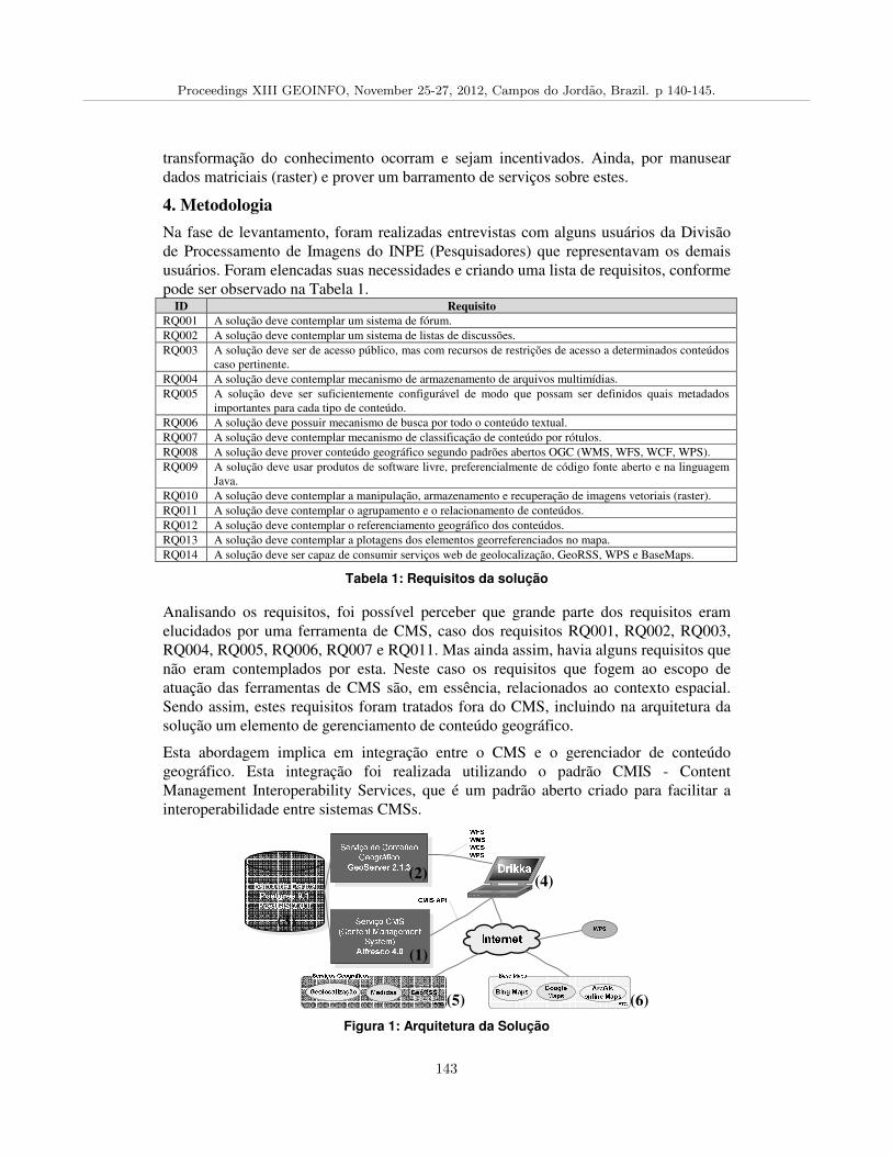
transformação do conhecimento ocorram e sejam incentivados. Ainda, por manusear dados matriciais (raster) e prover um barramento de serviços sobre estes.

4. Metodologia

Na fase de levantamento, foram realizadas entrevistas com alguns usuários da Divisão de Processamento de Imagens do INPE (Pesquisadores) que representavam os demais usuários. Foram elencadas suas necessidades e criando uma lista de requisitos, conforme pode ser observado na Tabela 1.

ID Requisito

RQ001 A solução deve contemplar um sistema de fórum. RQ002 A solução deve contemplar um sistema de listas de discussões. RQ003 A solução deve ser de acesso público, mas com recursos de restrições de acesso a determinados conteúdos

caso pertinente. RQ004 A solução deve contemplar mecanismo de armazenamento de arquivos multimídias. RQ005 A solução deve ser suficientemente configurável de modo que possam ser definidos quais metadados

importantes para cada tipo de conteúdo. RQ006 A solução deve possuir mecanismo de busca por todo o conteúdo textual. RQ007 A solução deve contemplar mecanismo de classificação de conteúdo por rótulos. RQ008 A solução deve prover conteúdo geográfico segundo padrões abertos OGC (WMS, WFS, WCF, WPS). RQ009 A solução deve usar produtos de software livre, preferencialmente de código fonte aberto e na linguagem

Java. RQ010 A solução deve contemplar a manipulação, armazenamento e recuperação de imagens vetoriais (raster). RQ011 A solução deve contemplar o agrupamento e o relacionamento de conteúdos. RQ012 A solução deve contemplar o referenciamento geográfico dos conteúdos. RQ013 A solução deve contemplar a plotagens dos elementos georreferenciados no mapa. RQ014 A solução deve ser capaz de consumir serviços web de geolocalização, GeoRSS, WPS e BaseMaps.

Tabela 1: Requisitos da solução

Analisando os requisitos, foi possível perceber que grande parte dos requisitos eram elucidados por uma ferramenta de CMS, caso dos requisitos RQ001, RQ002, RQ003, RQ004, RQ005, RQ006, RQ007 e RQ011. Mas ainda assim, havia alguns requisitos que não eram contemplados por esta. Neste caso os requisitos que fogem ao escopo de atuação das ferramentas de CMS são, em essência, relacionados ao contexto espacial. Sendo assim, estes requisitos foram tratados fora do CMS, incluindo na arquitetura da solução um elemento de gerenciamento de conteúdo geográfico.

Esta abordagem implica em integração entre o CMS e o gerenciador de conteúdo geográfico. Esta integração foi realizada utilizando o padrão CMIS - Content Management Interoperability Services, que é um padrão aberto criado para facilitar a interoperabilidade entre sistemas CMSs.

Figura 1: Arquitetura da Solução

(1)

(2)

(3)

(4)

(5) (6)


143

A Figura 1 esboça a macro-arquitetura adotada para esta solução. Foi escolhida a ferramenta Alfresco como CMS (1), que é uma ferramenta desenvolvida em Java e possui uma versão Community que é de código aberto. A ferramenta Alfresco é utilizada em várias instituições no mundo, e no Brasil, um grande exemplo de seu emprego é na Dataprev (Empresa de Tecnologia e Informações da Previdência Social) onde é utilizada para facilitar a gestão de documentos durante o processo de compras na empresa.

Como gerenciador de conteúdo geográfico (2), adotou-se o GeoServer, que é um Software livre, de código aberto, mantido pelo Open Planning Project e que é capaz de integrar diversos repositórios de dados geográficos com simplicidade e alta performance. O GeoServer é um servidor de Web Map Service (WMS), Web Coverage Service (WCS) e de Web Feature Service (WFS) completamente funcional que segue as especificações da Open Geospatial Consortium (OGC), além disso ainda provê um barramento de serviços Web Processing Service (WPS), outro padrão OGC para serviços de processamento de dados.

Tanto o Alfresco quanto o GeoServer utilizam um banco de dados relacional (3) para persistência e, uma boa solução que atende a ambos, é o Postgres com a extensão espacial PostGIS em sua versão 2.0. A aplicação cliente foi desenvolvida em Flex e consome os dados tanto do CMS via CMIS quanto do gerenciador de conteúdo geográfico via WMS, WFS e WCS. Além destes serviços, a aplicação cliente ainda consome serviços on-line (web) para geolocalização, GeoRSS e medidas de feições (5) desenvolvidos como plugins e facilmente extensíveis. O plano de fundo do mapa (Base Map) (6) é um outro exemplo de serviço web consumido pela aplicação. Hoje é possível incluir Base Map do Google, Bing e ArcGis On-Line.

Muitos dos artefatos a serem manipulados por esta solução são imagens matriciais (raster) que são armazenadas no PostGIS. Para armazená-los no banco de dados é utilizada a função raster2pgsql, carregando-as em uma tabela. Cada dado raster é carregado em uma tabela própria. Após o carregamento dos dados raster, é criado uma representação vetorial (polígono) de sua área de extensão, isso é feito utilizando a função: “SELECT ST_AsBinary(ST_Buffer(ST_Union(rast::geometry), 0.000001)) FROM raster_table”. A estratégia de criar um representação vetorial para os dados matriciais é, principalmente, por questões de performance em buscas e não causa efeito colateral, uma vez que visualmente uma imagem matricial propicia poucas informações relevantes.

O modelo de dados para os dados geográficos é muito simples, a princípio têm-se apenas classes de feição para pontos de interesse e áreas (polígonos) de interesse, com identificador, descrição simples e um atributo específico para relacionar o elemento geográfico a um conteúdo no CMS. Como supramencionado, a estratégia de separar o conteúdo geográfico do CMS implica em uma integração entre estes dados. No CMS são cadastrados os metadados de cada um dos conteúdos e cada conteúdo armazenado no CMS possui um identificador único. Caso este conteúdo tenha componente geográfica a ferramenta possibilita que seja criada ou selecionada uma geometria de ponto ou polígono que se relacionará com o conteúdo no CMS através de seu identificador único.


144

Os conteúdos multimídias, tais como arquivos de texto, planilhas, vídeos, fotos e etc, são armazenados no CMS e utilizam o modelo de metadados Dublin Core. Dublin Core pode ser definido como sendo o conjunto de elementos de metadados planejado para facilitar a descrição de recursos eletrônicos, sendo um dos padrões mais conhecidos e tradicionalmente adotados em sistemas gerenciadores de conteúdo. Os dados matriciais utilizam um versão estendida do Dublin Core, adicionando alguns atributos específicos para tal. Os usuários do sistema optaram por especificar quais atributos são importantes para os dados matriciais ao invés de usar algum metadado existente, como FGDC (Federal Geographic Data Committee) ou ISO 19115, por entender que estes modelos apresentam uma quantidade muito grande de atributos que nem sempre são utilizados e que em geral representa um desincentivo ao uso.

Trabalhos Futuros

Como continuidade deste trabalho, está sendo desenvolvido um barramento de serviços WPS que de início proverá uma série de algoritmos de classificação para os dados matriciais. Contará ainda com melhorias no mecanismo de buscas geográficas para os conteúdos vinculados ao CMS.

Referencias

BRAGA, G. M. Informação, ciência da informação: breves reflexões em três tempos. Ciência da Informação, v. 24, n. 1, p. 84-88, 1985.

CAÑETE, S. C.; TAVARES, D. L. M.; ESTRELA, P. C.; FREITAS, T. R. O.; HENKIN R.; GALANTE, R., FREITAS, C. M. D. S.. Integrando visualização e análise de dados em sistema de gerenciamento de dados de biodiversidade. IV e-Science Workshop (SBC), 2010.

DAVENPORT, T. H., PRUSAK, L.. Conhecimento empresarial. Rio de Janeiro: Campus, 1998.

DAVENPORT, T. Ecologia da informação: porque só a tecnologia não basta para o sucesso na era da informação. São Paulo: Futura, 1998. 316p.

DAVENPORT, T. H. Data to knowledge to results: building an analytic capability. California Management Review, v. 43, n. 2, p. 117-138, Winter 2001

LEITE, F. C. L. Gestão do Conhecimento Científico no Contexto Acadêmico: Proposta de um Modelo Conceitual, 2006

LEITE, F. C. L.; COSTA, S. Repositórios institucionais como ferramentas de gestão do conhecimento científico no ambiente acadêmico. 2006

MEADOWS, A. J. A comunicação científica. Brasília: Briquet de Lemos, 1999. 268p.

NONAKA, I.; TAKEUCHI, H. Criação do conhecimento nas empresas: Como as empresas japonesas geram a dinâmica da inovação. Rio de Janeiro, 1997. 358p.

Smith, H. A.; McKeen, J. D. Developments in Practice VIII: Enterprise Content Management Communications of the AIS, 2003, pp. 647-659.

Weiseth, P. E.; Olsen, H. H.; Tvedte, B.; Kleppe, A. eCollaboration Strategy 2002-2004, Statoil, Trondheim/Stavanger, 2002.


145

GeoSQL: um ambiente online para aprendizado de SQL comextensoes espaciais

Anderson L. S. Freitas1, Clodoveu A. Davis Jr.1, Thompson M. Filgueiras1

1 Departamento de Ciencia da Computacao – Universidade Federal de Minas Gerais (UFMG)Caixa Postal 702 – 30.123-970 – Belo Horizonte – MG – Brasil

{alsr, clodoveu, thom}@dcc.ufmg.br

Abstract. The standardization of the Structured Query Language (SQL) was im-portant for the popularity of relational databases. The SQL learning process issupported by several resources, such as simulators and interactive tools. Howe-ver, as far as we could ascertain, there are no tools to promote the learning ofspatial extensions to SQL in geographic databases. This work presents GeoSQL,an online learning environment for SQL with spatial extensions, which is ableto render the query results and can overlay the results of multiple queries for vi-sual comparison. GeoSQL was developed entirely using free software, and canbe operated using only a standard browser.

Resumo. A padronizacao da Structured Query Language (SQL) foi importantepara a popularizacao dos bancos de dados relacionais. O aprendizado de SQLe apoiado por diversos recursos tecnologicos, como simuladores e ferramentasinterativas. No entanto, nao encontramos tais recursos para promover o ensinode extensoes espaciais de SQL em bancos de dados geograficos. Este trabalhoapresenta o GeoSQL, ambiente online de aprendizado de SQL com extensoesespaciais, capaz de renderizar e de sobrepor os resultados de multiplas con-sultas para comparacao visual. O GeoSQL foi totalmente desenvolvido usandosoftware livre e pode ser operado usando apenas um navegador padrao.

1. IntroducaoGerenciadores de bancos de dados relacionais se tornaram amplamente populares pordiversos motivos, dentre os quais se destaca a adocao da Structured Query Language(SQL) como linguagem padrao de consulta. Como consequencia, o ensino de SQL e parteimportante do conteudo de cursos e disciplinas de bancos de dados em todo o mundo.

O mercado editorial dispoe de uma grande quantidade e variedade de materiaispara o ensino de bancos de dados, muitos deles voltados especificamente para a linguagemSQL. Isso reflete a ampla utilizacao da linguagem no mercado, mas tambem indica umapotencial dificuldade para o aprendizado. O fato de SQL ser uma linguagem declarativa, enao procedural, requer que o estudante aprenda a pensar dentro da logica de conjuntos, emvez de algoritmos (Sadiq and Orlowska, 2004). Por isso, atividades praticas individuaissao muito importantes.

O uso de SQL como linguagem para acesso a dados geograficos ja foi alvo decrıticas e restricoes (Egenhofer, 1992), porem a definicao dos padroes do Open Geos-patial Consortium (OGC) para representacao geografica em ambientes relacionais (Per-civall, 2003), e a evolucao dos sistemas de gerenciamento de bancos de dados (SGBD)


146

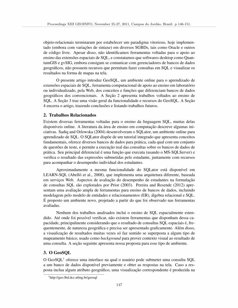
objeto-relacionais terminaram por estabelecer um paradigma vitorioso, hoje implemen-tado (embora com variacoes de sintaxe) em diversos SGBDs, tais como Oracle e outrosde codigo livre. Apesar disso, nao identificamos ferramentas voltadas para o apoio aoensino das extensoes espaciais de SQL, e constatamos que softwares desktop como Quan-tumGIS e gvSIG, embora consigam se comunicar com gerenciadores de bancos de dadosgeograficos, nao possuem recursos que permitam fazer consultas em SQL e visualizar osresultados na forma de mapas na tela.

O presente artigo introduz GeoSQL, um ambiente online para o aprendizado deextensoes espaciais de SQL, ferramenta computacional de apoio ao ensino em laboratorioou individualizado, pela Web, dos conceitos e funcoes que diferenciam bancos de dadosgeograficos dos convencionais. A Secao 2 apresenta trabalhos voltados ao ensino deSQL. A Secao 3 traz uma visao geral da funcionalidade e recursos do GeoSQL. A Secao4 encerra o artigo, trazendo conclusoes e listando trabalhos futuros.

2. Trabalhos RelacionadosExistem diversas ferramentas voltadas para o ensino da linguagem SQL, muitas delasdisponıveis online. A literatura da area de ensino em computacao descreve algumas ini-ciativas. Sadiq and Orlowska (2004) desenvolveram o SQLator, um ambiente online paraaprendizado de SQL. O SQLator dispoe de um tutorial integrado que apresenta conceitosfundamentais, oferece diversos bancos de dados para pratica, cada qual com um conjuntode questoes de teste, e permite a execucao real das consultas sobre os bancos de dados depratica. Seu principal diferencial e uma funcao que executa (usando o MS-SQLServer) everifica o resultado das expressoes submetidas pelo estudante, juntamente com recursospara acompanhar o desempenho individual dos estudantes.

Aproximadamente a mesma funcionalidade do SQLator esta disponıvel emLEARN-SQL (Abello et al., 2008), que implementa uma arquitetura diferente, baseadaem servicos Web. Aspectos de avaliacao do desempenho de estudantes na formulacaode consultas SQL sao explorados por Prior (2003). Pereira and Resende (2012) apre-sentam uma avaliacao ampla de ferramentas para ensino de bancos de dados, incluindomodelagem pelo modelo de entidades e relacionamentos (ER), algebra relacional e SQL.E proposto um ambiente novo, projetado a partir do que foi observado nas ferramentasavaliadas.

Nenhum dos trabalhos analisados inclui o ensino de SQL espacialmente esten-dido. Ate onde foi possıvel verificar, nao existem ferramentas que disponham dessa ca-pacidade, principalmente considerando que o resultado de consultas SQL espaciais e, fre-quentemente, de natureza geografica e precisa ser apresentado graficamente. Alem disso,a visualizacao de resultados muitas vezes so faz sentido se superposta a algum tipo demapeamento basico, usado como background para prover contexto visual ao resultado deuma consulta. A secao seguinte apresenta nossa proposta para esse tipo de ambiente.

3. O GeoSQLO GeoSQL1 oferece uma interface na qual o usuario pode submeter uma consulta SQLa um banco de dados disponıvel previamente e obter as respostas na tela. Caso a res-posta inclua algum atributo geografico, uma visualizacao correspondente e produzida na

1http://geo.lbd.dcc.ufmg.br/geosql


147

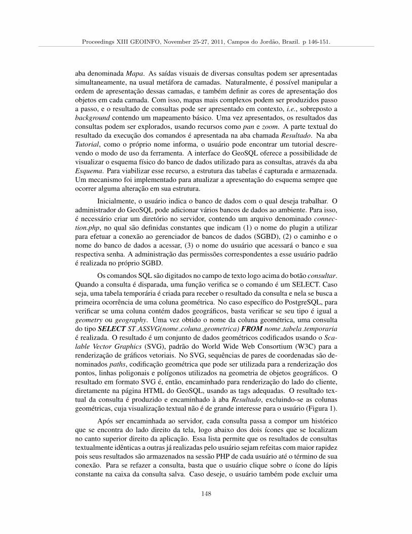
aba denominada Mapa. As saıdas visuais de diversas consultas podem ser apresentadassimultaneamente, na usual metafora de camadas. Naturalmente, e possıvel manipular aordem de apresentacao dessas camadas, e tambem definir as cores de apresentacao dosobjetos em cada camada. Com isso, mapas mais complexos podem ser produzidos passoa passo, e o resultado de consultas pode ser apresentado em contexto, i.e., sobreposto abackground contendo um mapeamento basico. Uma vez apresentados, os resultados dasconsultas podem ser explorados, usando recursos como pan e zoom. A parte textual doresultado da execucao dos comandos e apresentada na aba chamada Resultado. Na abaTutorial, como o proprio nome informa, o usuario pode encontrar um tutorial descre-vendo o modo de uso da ferramenta. A interface do GeoSQL oferece a possibilidade devisualizar o esquema fısico do banco de dados utilizado para as consultas, atraves da abaEsquema. Para viabilizar esse recurso, a estrutura das tabelas e capturada e armazenada.Um mecanismo foi implementado para atualizar a apresentacao do esquema sempre queocorrer alguma alteracao em sua estrutura.

Inicialmente, o usuario indica o banco de dados com o qual deseja trabalhar. Oadministrador do GeoSQL pode adicionar varios bancos de dados ao ambiente. Para isso,e necessario criar um diretorio no servidor, contendo um arquivo denominado connec-tion.php, no qual sao definidas constantes que indicam (1) o nome do plugin a utilizarpara efetuar a conexao ao gerenciador de bancos de dados (SGBD), (2) o caminho e onome do banco de dados a acessar, (3) o nome do usuario que acessara o banco e suarespectiva senha. A administracao das permissoes correspondentes a esse usuario padraoe realizada no proprio SGBD.

Os comandos SQL sao digitados no campo de texto logo acima do botao consultar.Quando a consulta e disparada, uma funcao verifica se o comando e um SELECT. Casoseja, uma tabela temporaria e criada para receber o resultado da consulta e nela se busca aprimeira ocorrencia de uma coluna geometrica. No caso especıfico do PostgreSQL, paraverificar se uma coluna contem dados geograficos, basta verificar se seu tipo e igual ageometry ou geography. Uma vez obtido o nome da coluna geometrica, uma consultado tipo SELECT ST ASSVG(nome coluna geometrica) FROM nome tabela temporariae realizada. O resultado e um conjunto de dados geometricos codificados usando o Sca-lable Vector Graphics (SVG), padrao do World Wide Web Consortium (W3C) para arenderizacao de graficos vetoriais. No SVG, sequencias de pares de coordenadas sao de-nominados paths, codificacao geometrica que pode ser utilizada para a renderizacao dospontos, linhas poligonais e polıgonos utilizados na geometria de objetos geograficos. Oresultado em formato SVG e, entao, encaminhado para renderizacao do lado do cliente,diretamente na pagina HTML do GeoSQL, usando as tags adequadas. O resultado tex-tual da consulta e produzido e encaminhado a aba Resultado, excluindo-se as colunasgeometricas, cuja visualizacao textual nao e de grande interesse para o usuario (Figura 1).

Apos ser encaminhada ao servidor, cada consulta passa a compor um historicoque se encontra do lado direito da tela, logo abaixo dos dois ıcones que se localizamno canto superior direito da aplicacao. Essa lista permite que os resultados de consultastextualmente identicas a outras ja realizadas pelo usuario sejam refeitas com maior rapidezpois seus resultados sao armazenados na sessao PHP de cada usuario ate o termino de suaconexao. Para se refazer a consulta, basta que o usuario clique sobre o ıcone do lapisconstante na caixa da consulta salva. Caso deseje, o usuario tambem pode excluir uma


148

pesquisa dessa lista, clicando sobre o ıcone com um ‘X’ no canto inferior esquerdo de umaconsulta armazenada. Ainda sobre cada consulta, os terceiro e quarto ıcones permitemque o usuario modifique a cor da linha e o padrao de preenchimento dos paths de umaconsulta com resultado plotado na aba Mapa.

Figura 1. Aba Mapa em destaque e historico de consultas

Dentre os dois ıcones localizados no canto superior direito, o da esquerda (1)atua como um compactador do estado de todas as informacoes presentes no ambiente dousuario em determinado momento, gerando um link que pode ser acessado em momentoposterior para recuperacao de todos os dados, incluindo cores de mapas, tabelas e listade consultas salvas, preservando-se sua ordem. Essa funcao e de grande utilidade paraquando, por exemplo, um aluno deseja enviar o resultado de um conjunto de consultas aseu professor para avaliacao em vez de ter que montar um arquivo especıfico com cadaresposta. O ıcone mais a direita (2) define uma operacao de superposicao entre as ca-madas de objetos SVG correspondentes as consultas previamente selecionadas. De cimapara baixo na lista de consultas selecionadas (destacadas em laranja), a primeira consultacorrespondera a camada inferior da visualizacao, enquanto a ultima correspondera a ca-mada superior. Com o objetivo de permitir o reordenamento das diversas camadas, cadaconsulta da lista pode ser deslocada para cima ou para baixo em operacoes drag and dropsobre cada elemento (em roxo na figura).

Ainda na Figura 1 podemos visualizar cinco consultas ja realizadas, com desta-que para a consulta no topo da lista, a qual foi refeita com nova coloracao de linha e depreenchimento. Observe-se que o mouse esta deslocando uma consulta de sua posicaooriginal para um local mais abaixo na lista e existem tres consultas selecionadas para pos-terior realizacao de merging. Na Figura 2 vemos o resultado da operacao de sobreposicaoreferente as tres consultas selecionadas na Figura 1. Nele, consta ao fundo uma camadacontendo os limites de mesorregioes brasileiras, seguido por uma segunda camada, com


149

paths delineados em preto, indicando as rodovias e, por fim, uma camada de linhas emvermelho, indicando todas as ferrovias brasileiras contidas no banco.

Figura 2. Superposicao de camadas originarias de consultas distintas

Outras caracterısticas interessantes do GeoSQL sao o suporte a aplicacao de zoomin e zoom out utilizando o botao de scroll do mouse e o deslocamento (pan) do mapaplotado na aba Mapa arrastando e soltando o objeto SVG apresentado. Como exemplo,mostramos que o objeto SVG plotado na aba Mapa apresentada na Figura 1 foi submetidoas operacoes de zoom in e pan antes de ser retirado o screenshot da tela. Alem disso, base-ado no aprendizado das colunas presentes nas tabelas do banco, o campo de realizacao deconsultas informa opcoes de code completion em uma lista que aparece dinamicamenteabaixo da area de texto a medida que o usuario digita sua consulta.

Todo o codigo do GeoSQL foi desenvolvido em PHP e jQuery utilizando os plu-gins jQueryui, jPicker e svgPan. Tambem foi implantado suporte para comunicacao comos SGBDs MySQL e PostgreSQL associado com a extensao espacial PostGIS, ambossendo intermediados por um servidor Apache 2.

4. Conclusao e Trabalhos FuturosApesar de ainda nao se encontrar em estagio final, o uso do GeoSQL na pratica demons-trou o potencial da ferramenta para o ensino (ou autoinstrucao) sobre extensoes espaciais

2Respectivamente http://www.php.net, http://jquery.com/, http://jquery.com/ui,http://code.google.com/p/jpicker/i, http://code.google.com/p/svgpan/, http://www.mysql.com/,http://www.postgresql.org/, http://postgis.refractions.net/ e http://www.apache.org


150

da linguagem SQL. Nada impede, no entanto, que o GeoSQL seja utilizado tambem noensino da linguagem SQL convencional. As decisoes tecnologicas e de implementacao daferramenta foram tomadas de modo a simplificar seu gerenciamento e administracao, per-mitindo criar ambientes para aprendizado basico (p.ex., com permissao apenas de consultae ensino de comandos SELECT). O GeoSQL tambem nao exige a instalacao de quaisquerpacotes na maquina do cliente, pois pode ser operado utilizando apenas um navegadorcomum que consiga renderizar objetos SVG.

Uma extensao do nosso trabalho se destinara a analise da melhor maneira de rea-lizar uma compressao mais eficiente dos dados que trafegam entre o servidor e o cliente.Pela estrutura modular e conteudo textual das tags SVG, acreditamos que a utilizacao decompressao em nıvel de paths ou conjuntos unicamente identificados deles possa contri-buir para a formacao de um cache compartilhado entre clientes, de modo a diminuir con-sideravelmente a quantidade de dados processados a cada consulta e encaminhados a cadacliente. Outra evolucao sera estudada no sentido de implementar recursos de segurancaque permitam a execucao de comandos de manipulacao de dados, tais como CREATETABLE, ALTER TABLE ou UPDATE, dependendo de permissoes previamente definidasno SGBD. Com isso, o GeoSQL poderia servir de interface para o aprendizado de todosos diferentes comandos de SQL.

Vislumbramos tambem a possibilidade de realizarmos modificacoes no codigo-fonte para adaptarmos os resultados das consultas para renderizacao dos dados ge-ograficos em dispositivos moveis como smartphones e tablets, no intuito de tornar nossaaplicacao ainda mais abrangente. Estao nos planos tambem outros tipos de extensoes, es-tas de natureza didatica, como a avaliacao automatica das consultas, o acompanhamentode turmas de alunos e o armazenamento de listas de exercıcios.

ReferenciasAlberto Abello, M. Elena Rodrıguez, Toni Urpı, Xavier Burgues, M. Jose Casany, Carme

Martın, and Carme Quer. LEARN-SQL: Automatic Assessment of SQL Based on IMSQTI Specification. Advanced Learning Technologies, IEEE International Conferenceon, 0:592–593, 2008.

Max J. Egenhofer. “Why not SQL!”. International journal of geographical informationsystems, 6(2):71–85, 1992.

George Percivall. OpenGIS Reference Model. OpenGIS Reference Model, Open Geos-patial Consortium, Inc, 2003.

Juliana Alves Pereira and Antonio Maria Pereira Resende. Uma analise dos ambien-tes de ensino de banco de dados. Anais do VIII Simposio Brasileiro de Sistemas deInformacao, pages 755–766, 2012.

Julia Coleman Prior. Online assessment of SQL query formulation skills. In Proceedingsof the fifth Australasian conference on Computing education - Volume 20, ACE ’03,pages 247–256, Darlinghurst, Australia, Australia, 2003. Australian Computer Society,Inc.

Shazia Sadiq and Maria Orlowska. SQLator: An Online SQL Learning Workbench. InIn Proceedings of the 9th annual SIGCSE conference on Innovation and technology incomputer science education ITiCSE ’04, page 30, 2004.


151

Determinação da rede de drenagem em grandes terrenosarmazenados em memória externa

Thiago L. Gomes1, Salles V. G. Magalhães1, Marcus V. A. Andrade1,and Guilherme C. Pena1

1 Departamento de Informática – Universidade Federal de Viçosa (UFV)Campus da UFV – 36.570-000 – Viçosa – MG - Brazil

{thiago.luange,salles,marcus,guilherme.pena}@ufv.br

Abstract. The drainage network computation is not a trivial task for huge ter-rains stored in the external memory since, in this case, the time required toaccess the external memory is much larger than the internal processing time. Inthis context, this paper presents an efficient algorithm for computing the drai-nage network in huge terrains where the main idea is to adapt the method RW-Flood [Magalhães et al. 2012b] reducing the number of disk access. The pro-posed method was compared against some classic methods as TerraFlow andr.watershed.seg and, as the tests showed, it was much faster (in some cases,more than 30 times) than both methods.

Resumo. A determinação da rede de drenagem é uma aplicação importanteem sistemas de informação geográfica e pode requerer um elevado tempo deprocessamento quando envolve grandes terrenos armazenados em memória ex-terna. Neste contexto, este artigo propõe um método eficiente para computar arede de drenagem em grandes terrenos, cuja ideia básica é adaptar o métodoRWFlood [Magalhães et al. 2012b] de modo a reduzir o numero de acessos aodisco. O método proposto foi comparado com outros métodos recentementeapresentados na literatura como TerraFlow e r.watershed.seg e os testes mos-traram que o método proposto é mais eficiente (cerca de 30 vezes) que os de-mais.

1. Introdução

O avanço da tecnologia do sensoriamento remoto tem produzido um enorme volume dedados sobre a superfície terrestre. O projeto SRTM (NASA’s Shuttle Radar TopographyMission), por exemplo, mapeou 80% da superfície da terra com resoluções de 30 metros,formando o mais completo banco de dados de alta resolução da terra, que possui mais de10 terabytes de dados [Jet Propulsion Laboratory NASA 2012].

Esse enorme volume de dados requer o desenvolvimento (ou adaptação) de al-goritmos para o processamento de dados em memória externa (geralmente discos), ondeo acesso aos dados é bem mais lento do que na memória interna. Então, os algoritmospara processamento de grande volume de dados (armazenados em memória externa) pre-cisam ser projetados e analisados utilizando um modelo computacional que considera nãoapenas o uso da CPU mas também o tempo de acesso ao disco.


152

Uma importante aplicação na área de sistemas de informação geográfica (SIGs)relacionada a modelagem de terrenos é a determinação das estruturas hidrológicas taiscomo a direção de fluxo, o fluxo acumulado, bacias de acumulação, etc. Essas estruturassão utilizadas no cálculo de atributos do terreno, tais como convergência topográfica, redede drenagem, bacias hidrográficas,etc.

Este trabalho propõe o método EMFlow para a obtenção da rede de drena-gem em grandes terrenos representados por matriz de elevação armazenadas em me-mória secundária. A idéia básica deste novo método é adaptar o algoritmo RWFlood[Magalhães et al. 2012b], alterando a forma como os dados em memória externa são aces-sados. Para isto, é utilizada uma biblioteca que gerencia as transferências de dados entreas memórias interna e externa, buscando diminuir o número de acessos ao disco.

2. Referencial teórico2.1. Determinação da rede de drenagemA rede de drenagem é composta pela direção do fluxo de escoamento e pelo fluxo acumu-lado em cada ponto (célula) do terreno e há diversos métodos para a sua obtenção. Con-forme descrito pelos autores, a maior dificuldade neste processo é a ocorrência de fossose platôs, ou seja, células onde não é possível determinar a direção de fluxo diretamenteporque ou a célula é um mínimo local (fosso) ou pertence a uma região horizontalmenteplana (platô).

De acordo com Planchon [Planchon and Darboux 2002], muitos méto-dos [O’Callaghan and Mark 1984, Jenson and Domingue 1988, Soille and Gratin 1994,Tarboton 1997] utilizam uma etapa de pré-processamento para remover os fossos e platôse, essa etapa é responsável por mais de 50% do tempo total de execução.

Quando o volume de dados é muito grande e não pode ser totalmente armazenadoem memória interna, é necessario realizar o processamento em memória externa e, nestecaso, a transferência de informações entre as memórias interna e externa frequentementedomina o tempo de processamento dos algoritmos. Portanto, o projeto e análise de algo-ritmos utilizados para manipular esses dados precisam ser feito com base em um modelocomputacional que avalia o número de operações de entrada e saída (E/S) realizadas.

Vários sistemas de informação geográfica como, por exemplo, o Arc-GIS [ESRI 2012] e o GRASS [GRASS Development Team 2010], incluem algoritmospara cálculo da direção de fluxo e do fluxo acumulado. Mas, muitos destes algorit-mos são projetados para minimizar o tempo de processamento interno e frequentementenão se ajustam muito bem para grande volume de dados [Arge et al. 2003]. Dentreos métodos desenvolvidos para o tratamento de grande volume de dados em memó-ria externa pode-se destacar os módulos TerraFlow [GRASS Development Team 2010]e r.watershed.seg [GRASS Development Team 2010] disponíveis no GRASS. O Terra-Flow é atualmente o sistema que resolve o problema de cálculo de elementos da hidro-grafia como rede de drenagem e bacia de acumulação (watershed) em grandes terrenos deforma mais eficiente [Arge et al. 2003, Toma et al. 2001]. O r.watershed, por sua vez, éum módulo do GRASS que pode ser utilizado para a obtenção da rede de drenagem emterrenos e foi adaptado para processamento em memória externa [Metz et al. 2011] com ouso da biblioteca segmented do GRASS, que permite a manipulação de grandes matrizesem memória externa.


153

3. O método EMFlow

Em [Magalhães et al. 2012b] é apresentado um novo método chamado RWFlood que ébem mais eficiente do que os outros algoritmos tradicionais, pois não utiliza uma etapade pré-processamento para remover os fossos e platôs e os trata naturalmente durante ocálculo da rede de drenagem.

A idéia básica do RWFlood para obter a rede de drenagem de um terreno é simularo processo de inundação do terreno supondo que a água entra no terreno pela sua bordavindo da parte externa. Neste caso, é importante observar que o caminho que a águapercorre à medida que vai inundando o terreno é o mesmo caminho que a água percorreriase fosse proveniente da chuva que cai sobre o terreno e escoa descendentemente.

Mais especificamente, no início, o método cria um oceano em torno do terreno ecom nível d’água definido igual à elevação da célula mais baixa entre as células da bordado terreno. Então, é realizado um processo iterativo que, a cada passo, eleva o nível dooceano e inunda as células do terreno. Se a elevação dessas células é menor do que o nívelda água então sua elevação é elevada para ficar igual ao nível do oceano.

Inicialmente, a direção de fluxo nas células da borda do terreno é definida apon-tando para fora do terreno (isto é, indicando que naquelas células a água escoa para forado terreno). Então, a direção de cada célula c que não pertence à borda é definida comoapontando para a célula vizinha a c de onde a água vem para inundar a célula c.

Depois de inundar todas as depressões e todas as células com elevação igual aonível da água e que são adjacentes à borda do oceano, o nível da água é elevado paraa elevação da célula mais baixa que é adjacente à borda desse oceano. Para obter essacélula que irá definir o nível da água, o método RWFlood utiliza um array Q de filas paraarmazenar as células que precisam ser posteriormente processadas. Ou seja, Q contémuma fila para cada elevação existente no terreno, sendo que a fila Q[m] armazena ascélulas (a serem processadas) com elevação m. Inicialmente, as células na fronteira doterreno são inseridas na fila correspondente. Assim, supondo que a célula mais baixa naborda do terreno tem elevação k, então o processo começa na fila Q[k] (isso correspondea supor que nível da água se inicia com elevação k). A partir disso, supondo que c é acélula na primeira posição da fila Q[k]; essa célula é removida da fila e é processada daseguinte forma: as células vizinhas a c que ainda não foram “visitadas" (isto é, que aindanão têm a direção de fluxo definida) têm a sua direção de fluxo definida apontando para acélula c e elas são inseridas nas respectivas filas. É importante observar que, se uma célulavizinha a c que ainda não foi visitada tem elevação menor do que c, então a elevação dessacélula é incrementada (conceitualmente, isso corresponde a inundar a célula) e depois elaé inserida na fila correspondente a essa nova elevação. Quando todas as células na filaQ[k] são processadas, o processo continua na próxima fila não vazia no vetor Q

Vale ressaltar que o método RWFlood determina a direção do fluxo de cada céluladurante a inundação. Quando uma célula c é processada, todas as células vizinhas a c queainda não foram visitadas (isto é, que não tem a sua direção de fluxo definida) têm o seusentido de fluxo definido para c e depois, são inseridas na fila correspondente.

Após o cálculo da direção de fluxo, o algoritmo RWFlood calcula o fluxo acumu-lado no terreno utilizando uma estratégia baseada em ordenação topológica. Conceitual-mente, a ideia é supor a existência de um grafo onde cada vértice representa uma célula


154

do terreno e há uma aresta ligando um vértice v a um vértice u se, e somente se, a direçãode escoamento de v aponta para u.

3.1. Adaptação do método RWFlood para processamento em memória externa

O método RWFlood original processa o terreno, representado por uma matriz, acessandoessa matriz de forma não sequencial e, portanto, o processamento de grandes terrenosarmazenados em memória externa pode não ser eficiente. No entanto, há um padrão deacessos espacial, pois, em um dado momento as células acessadas estão, na maioria dasvezes, próximas umas das outras na matriz.

Para diminuir o número de acessos ao disco, este trabalho propõe um novo mé-todo denominado EMFlow, cuja estratégia consiste em adaptar o método RWFlood deforma que os acessos realizados à matriz sejam gerenciados por uma biblioteca denomi-nada TiledMatrix [Magalhães et al. 2012a], que é capaz de armazenar e gerenciar grandesmatrizes em memória externa. Na verdade, a idéia básica desta adaptação é modificara forma de gerenciamento da memória (reorganizando a matriz) para tirar proveito dalocalidade espacial de acesso.

Assim, as matrizes em memória externa são gerenciadas pela biblioteca TiledMa-trix, que subdivide a matriz em blocos menores que são armazenados de forma sequencialem um arquivo na memória externa, sendo que a transferência destes blocos entre as me-mórias interna e externa também é gerenciada pela biblioteca que permite a adoção dediferentes políticas de gerenciamento.

Uma questão importante a se considerar na implementação da biblioteca Tiled-Matrix refere-se à política utilizada para determinar qual bloco será escolhido para cederespaço a novos blocos. Neste trabalho utilizou-se a estratégia de retirar da memória in-terna aquele bloco que está a mais tempo sem ter sido acessado pela aplicação. Essaestratégia foi adotada baseado no fato de que, durante o processamento do algoritmo RW-Flood, há uma certa localidade de acesso às células do terreno, assim blocos que estão amuito tempo sem serem acessados tendem a não serem mais acessados. No entanto, serãorealizados estudos mais detalhados para verificar se realmente essa é a melhor estratégia.

4. Resultados

O algoritmo EMFlow foi implementado em C++, compilado com o g++ 4.5.2, e váriostestes foram realizados para avaliar seu tempo de execução e seu comportamento em di-ferentes situações comparando-o contra os métodos TerraFlow e r.watershed.seg, ambosincluídos no GRASS. Os testes foram executados em uma máquina com processador IntelCore 2 Duo com 2,8GHz, HD de 5400 RPM e sistema operacional Ubuntu Linux 11.0464 bits.

Os terrenos utilizados nos testes foram gerados a partir de dados dos EUA dispo-nibilizados pelo projeto SRTM [Jet Propulsion Laboratory NASA 2012] com resoluçãohorizontal de 30 metros.

A tabela 1 exibe os tempos de processamento (em segundos) de uma determinadaregião utilizando memórias de 1GB e 4GB, sendo que no método EMFlow foram utiliza-dos blocos com 200×200 células para a memória de 1GB, e 800×800 para 4GB. No casodo TerraFlow, a versão disponível no GRASS utiliza, no máximo, 2GB de memória. No


155

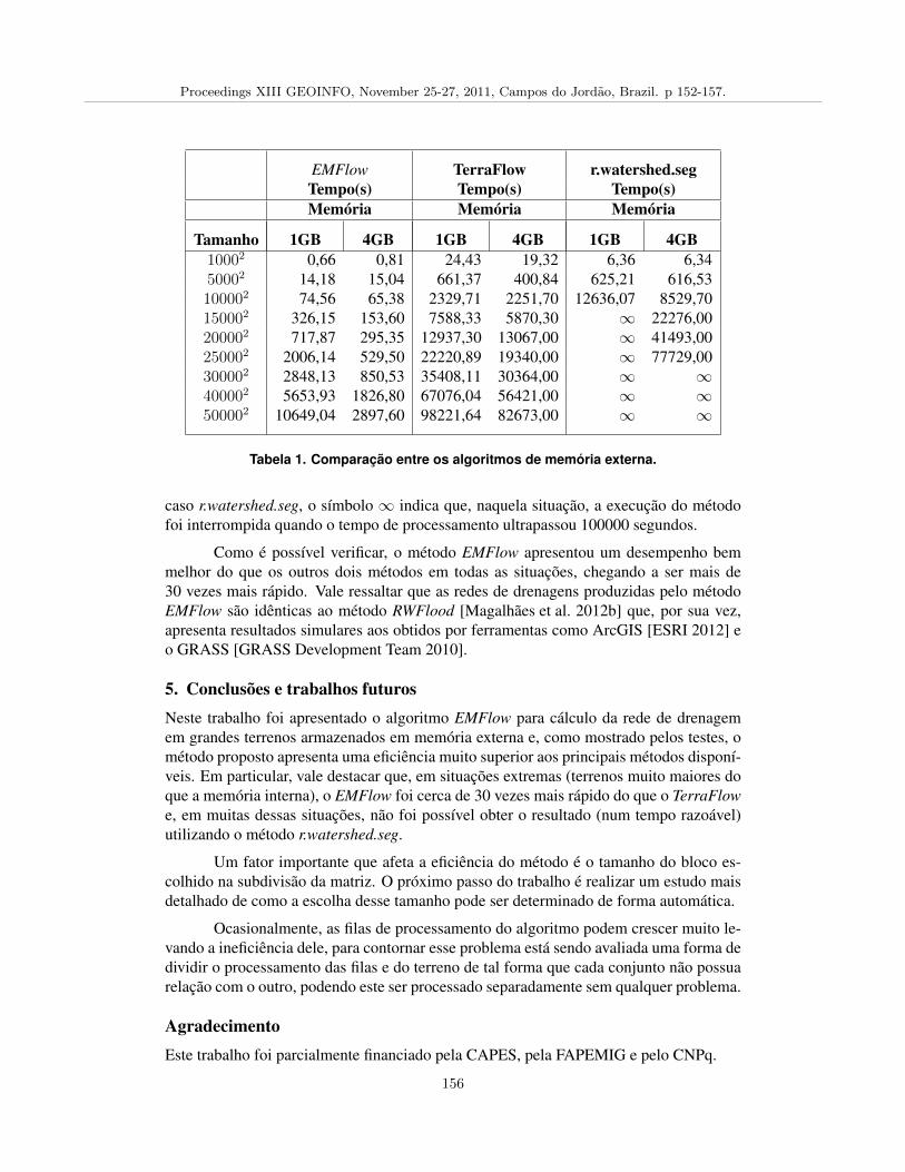
EMFlow TerraFlow r.watershed.segTempo(s) Tempo(s) Tempo(s)Memória Memória Memória

Tamanho 1GB 4GB 1GB 4GB 1GB 4GB10002 0,66 0,81 24,43 19,32 6,36 6,3450002 14,18 15,04 661,37 400,84 625,21 616,53100002 74,56 65,38 2329,71 2251,70 12636,07 8529,70150002 326,15 153,60 7588,33 5870,30 ∞ 22276,00200002 717,87 295,35 12937,30 13067,00 ∞ 41493,00250002 2006,14 529,50 22220,89 19340,00 ∞ 77729,00300002 2848,13 850,53 35408,11 30364,00 ∞ ∞400002 5653,93 1826,80 67076,04 56421,00 ∞ ∞500002 10649,04 2897,60 98221,64 82673,00 ∞ ∞

Tabela 1. Comparação entre os algoritmos de memória externa.

caso r.watershed.seg, o símbolo ∞ indica que, naquela situação, a execução do métodofoi interrompida quando o tempo de processamento ultrapassou 100000 segundos.

Como é possível verificar, o método EMFlow apresentou um desempenho bemmelhor do que os outros dois métodos em todas as situações, chegando a ser mais de30 vezes mais rápido. Vale ressaltar que as redes de drenagens produzidas pelo métodoEMFlow são idênticas ao método RWFlood [Magalhães et al. 2012b] que, por sua vez,apresenta resultados simulares aos obtidos por ferramentas como ArcGIS [ESRI 2012] eo GRASS [GRASS Development Team 2010].

5. Conclusões e trabalhos futurosNeste trabalho foi apresentado o algoritmo EMFlow para cálculo da rede de drenagemem grandes terrenos armazenados em memória externa e, como mostrado pelos testes, ométodo proposto apresenta uma eficiência muito superior aos principais métodos disponí-veis. Em particular, vale destacar que, em situações extremas (terrenos muito maiores doque a memória interna), o EMFlow foi cerca de 30 vezes mais rápido do que o TerraFlowe, em muitas dessas situações, não foi possível obter o resultado (num tempo razoável)utilizando o método r.watershed.seg.

Um fator importante que afeta a eficiência do método é o tamanho do bloco es-colhido na subdivisão da matriz. O próximo passo do trabalho é realizar um estudo maisdetalhado de como a escolha desse tamanho pode ser determinado de forma automática.

Ocasionalmente, as filas de processamento do algoritmo podem crescer muito le-vando a ineficiência dele, para contornar esse problema está sendo avaliada uma forma dedividir o processamento das filas e do terreno de tal forma que cada conjunto não possuarelação com o outro, podendo este ser processado separadamente sem qualquer problema.

AgradecimentoEste trabalho foi parcialmente financiado pela CAPES, pela FAPEMIG e pelo CNPq.


156

ReferênciasArge, L., Chase, J. S., Halpin, P., Toma, L., Vitter, J. S., Urban, D., and Wickremesinghe,

R. (2003). Efficient flow computation on massive grid terrain datasets. Geoinformatica,7.

ESRI (2012). Arcgis. Disponível em: http://www.esri.com/software/arcgis/arcgis-for-desktop/index.html. (acessado em 17/05/2012).

GRASS Development Team (2010). Geographic Resources Analysis Support System(GRASS GIS) Software. Open Source Geospatial Foundation, http://grass.osgeo.org(acessado 17/05/2012).

Jenson, S. and Domingue, J. (1988). Extracting topographic structure from digital eleva-tion data for geographic information system analysis. Photogrammetric Engineeringand Remote Sensing, 54(11):1593–1600.

Jet Propulsion Laboratory NASA (2012). NASA Shuttle Radar Topography Mission(SRTM). National Geospatial-Intelligence Agency (NGA) and National Aeronau-tics and Space Administration (NASA), http://srtm.usgs.gov/mission.php(acessado17/05/2012).

Magalhães, S. V. G., Andrade, M. V. A., Ferreira, C. R., Pena, G. C., Luange, T. G., andPompermayer, A. M. (2012a). Uma biblioteca para o gerenciamento de grandes matri-zes em memória externa. Technical report, Departamento de Informática, UniversidadeFederal de Viçosa.

Magalhães, S. V. G., Andrade, M. V. A., Franklin, W. R., and Pena, G. C. (2012b). Anew method for computing the drainage network based on raising the level of an oceansurrounding the terrain. 15th AGILE International Conference on Geographic Infor-mation Science.

Metz, M., Mitasova, H., and Harmon, R. S. (2011). Efficient extraction of drainagenetworks from massive, radar-based elevation models with least cost path search. Hy-drology and Earth System Sciences, 15(2):667–678.

O’Callaghan, J. and Mark, D. (1984). The extraction of drainage networks from digitalelevation data. Computer Vision, Graphics and Image Processing, 28:328–344.

Planchon, O. and Darboux, F. (2002). A fast, simple and versatile algorithm to fill thedepressions of digital elevation models. Catena, 46(2-3):159–176.

Soille, P. and Gratin, C. (1994). An efficient algorithm for drainage network extractionon dems. Journal of Visual Communication and Image Representation, 5(2):181–189.

Tarboton, D. (1997). A new method for the determination of flow directions and contri-buting areas in grid digital elevation models. Water Resources Research, 33:309–319.

Toma, L., Wickremesinghe, R., Arge, L., Chase, J. S., Vitter, J. S., Halpin, P. N., andUrban, D. (2001). Flow computation on massive grids. In GIS 2001 Proceedings ofthe 9th ACM international symposium on Advances in geographic information systems.


157

Index of authors

Afonso, A. P., 23Albuquerque, F. C., 120Amorim, A. M., 96Andrade, M. V. A., 152Andrade, P. R., 48

Baptista, C. S., 108Barbosa, I., 120

Campos, J. A. P., 96Carneiro, T. G. S., 48Carvalho, C. A., 60Carvalho, M. T. M., 120Casanova, M. A., 120Costa, M. A., 30

Daltio, J., 60Davis Junior, C. A., 36, 42, 78, 146De Oliveira, M. G., 108Degbelo, A., 11Dos Santos, W. A., 140

Figueiredo, R., 66Fileto, R., 84Filgueiras, T. M., 146Fonseca, F. T., 36Freitas, A. L. S., 146Freitas, C. C., 140Freitas, S., 23Furtado, A. S., 84

Gomes, T. L., 152

Jomier, G., 1

Kuhn, W., 11

Magalhaes, S. V. G., 152Malaverri, J. E. G., 128Martins Furtado, D., 36Medeiros, C. B., 1Medeiros, C. M. B., 128Moura, T. H. V., 78

Pena, G. C., 152Pitta, D., 66Prates, M. O., 30

Renso, R., 84Rodrigues, A. B., 140Rodrigues, A. J. C., 48

Salgado, A. C., 66Santanche, A., 1Santanna, S. J. S., 140Santos, M. A. C., 30Souza, D., 66

Xavier, S. I. R., 42

Zam, M., 1

158

Proceedings - GeoINFO

Documents