PROC DMNEURL: Approximation to PROC NEURAL Purpose of PROC DMNEURL In its current form, PROC DMNEURL tries to establish a nonlinear model for the prediction of a binary or interval scaled response variable (called target in data mining terminology). The approach will soon be extended to nominal and ordinal scaled response variables. The algorithm used in DMNEURL was developed to overcome some problems of PROC NEURAL for data mining purposes, especially when the data set contains many highly collinear variables: 1. The nonlinear estimation problem in common Neural Networks is seriously underdetermined yielding to highly rankdeficient Hessian matrices and result- ing in extremely slow convergence (close to linear) of nonlinear optimization algorithms. Full-rank estimation. 2. Each function call in PROC NEURAL corresponds to a single run through the entire (training) data set and normally many function calls are needed for convergent nonlinear optimization with rankdeficient Hessians. Optimization of discrete problem with all data incore. 3. Because the zero eigenvalues in a Hessian matrix correspond to long and very flat valleys in the shape of the objective function, the traditional Neural Net approach has serious problems to decide when an estimate is close to an appro- priate solution and the optimization process can be terminated. Quadratic convergence. 4. For the same reasons, the common Neural Net algorithms suffer from a high sensibility toward finding local rather than global optimal solutions and the optimization result often is very sensitive w.r.t. the starting point of the opti- mization. Good starting point. With PROC DMNEURL we deal with specified optimization problems (with full rank Hessian matrices) which have not many parameters and for which good starting points can be obtained. The convergence of the nonlinear optimizer is normally very fast, resulting mostly in less than 10 iterations per optimization. The function and derivative calls during the optimization do not need any passes through the data set, however, the search for obtaining good starting points and the final evaluations of the solutions (scoring of all observations) need passes through the data, as well as a number of preliminary tasks. In PROC DMNEURL we fit separately an entire

Welcome message from author
This document is posted to help you gain knowledge. Please leave a comment to let me know what you think about it! Share it to your friends and learn new things together.
Transcript

PROC DMNEURL: Approximation toPROC NEURAL
Purpose of PROC DMNEURLIn its current form, PROC DMNEURL tries to establish a nonlinear model for theprediction of a binary or interval scaled response variable (calledtargetin data miningterminology). The approach will soon be extended to nominal and ordinal scaledresponse variables.The algorithm used in DMNEURL was developed to overcome some problems ofPROC NEURAL for data mining purposes, especially when the data set containsmany highly collinear variables:
1. The nonlinear estimation problem in common Neural Networks is seriouslyunderdetermined yielding to highly rankdeficient Hessian matrices and result-ing in extremely slow convergence (close to linear) of nonlinear optimizationalgorithms.=) Full-rank estimation.
2. Each function call in PROC NEURAL corresponds to a single run throughthe entire (training) data set and normally many function calls are needed forconvergent nonlinear optimization with rankdeficient Hessians.=) Optimization of discrete problem with all data incore.
3. Because the zero eigenvalues in a Hessian matrix correspond to long and veryflat valleys in the shape of the objective function, the traditional Neural Netapproach has serious problems to decide when an estimate is close to an appro-priate solution and the optimization process can be terminated.=) Quadratic convergence.
4. For the same reasons, the common Neural Net algorithms suffer from a highsensibility toward finding local rather than global optimal solutions and theoptimization result often is very sensitive w.r.t. the starting point of the opti-mization.=) Good starting point.
With PROC DMNEURL we deal with specified optimization problems (with fullrank Hessian matrices) which have not many parameters and for which good startingpoints can be obtained. The convergence of the nonlinear optimizer is normally veryfast, resulting mostly in less than 10 iterations per optimization. The function andderivative calls during the optimization do not need any passes through the data set,however, the search for obtaining good starting points and the final evaluations ofthe solutions (scoring of all observations) need passes through the data, as well asa number of preliminary tasks. In PROC DMNEURL we fit separately an entire

2 � PROC DMNEURL: Approximation to PROC NEURAL
set of about 8 activation functions and select the best result. Since the optimizationprocesses for different activation functions do not depend on each other, the computertime could be reduced greatly by parallel processing.Except for applications where PROC NEURAL would hit a local solution muchworse than the global solution, it is not expected that PROC DMNEURL can beatPROC NEURAL in the precision of the prediction. However, for the applications wehave run until now we found the results of PROC DMNEURL very close to those ofPROC NEURAL. PROC DMNEURL will be faster than PROC NEURAL only forvery large data sets. For small data sets, PROC NEURAL could be much faster thanPROC DMNEURL, especially for an interval target. The most efficient applicationof PROC DMNEURL is the analysis of a binary target variable without FREQ andWEIGHT statement and without COST variables in the input data set.
Application: HMEQ Data Set:Binary Target BAD
To illustrate the use of PROC DMNEURL we choose the HMEQ data set:
libname sampsio ’/sas/a612/dmine/sampsio’;proc dmdb batch data=sampsio.hmeq out=dmdbout dmdbcat=outcat;
var LOAN MORTDUE VALUE YOJ DELINQ CLAGE NINQ CLNO DEBTINC;class BAD(DESC) REASON(ASC) JOB(ASC) DEROG(ASC);target BAD;
run;
When selecting the binary target variable BAD a typical run of PROC DMNEURLwould be the following:
proc dmneurl data=dmdbout dmdbcat=outcatoutclass=oclass outest=estout out=dsout outfit=ofitptable maxcomp=3 maxstage=5;
var LOAN MORTDUE VALUE REASON JOB YOJ DEROG DELINQCLAGE NINQ CLNO DEBTINC;
target BAD;run;
The number of parametersp estimated in each stage of the optimization isp = 2 �c + 1, wherec is the number of components that is selected at the stage. Since herec = 3 is specified with the MAXCOMP= option each optimization process estimatesonly p = 7 parameters.First some general information is printed and the four moments of the numeric dataset variables involved in the analysis:
The DMNEURL Procedure
Binary Target BADNumber Observations 5960NOBS w/o Missing Target 5960
Purpose of PROC DMNEURL � 3
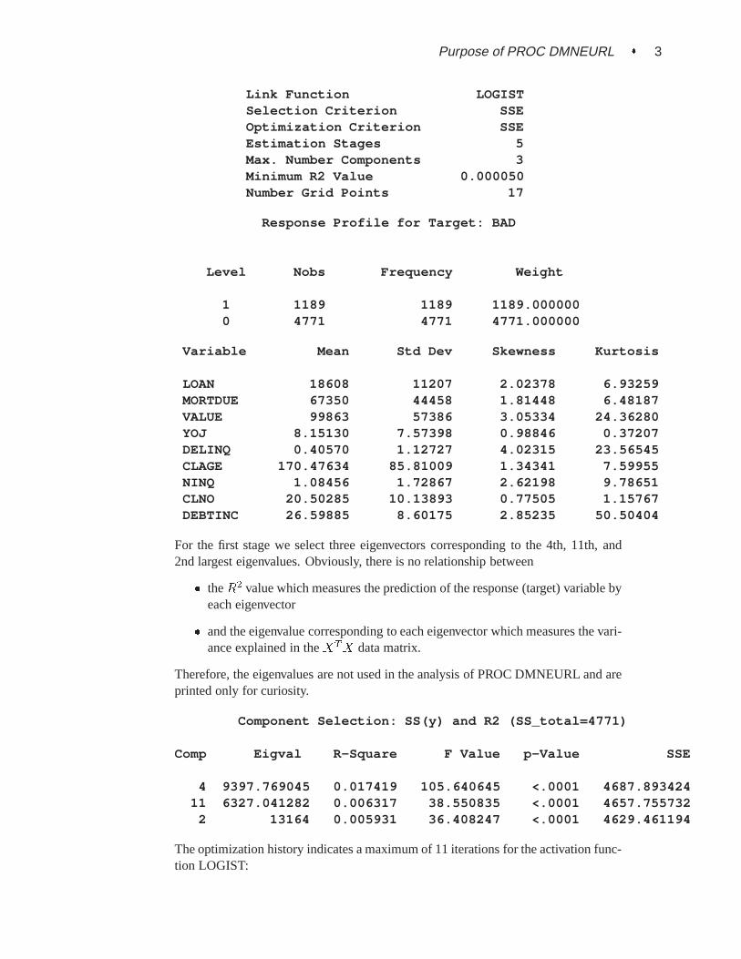
Link Function LOGISTSelection Criterion SSEOptimization Criterion SSEEstimation Stages 5Max. Number Components 3Minimum R2 Value 0.000050Number Grid Points 17
Response Profile for Target: BAD
Level Nobs Frequency Weight
1 1189 1189 1189.0000000 4771 4771 4771.000000
Variable Mean Std Dev Skewness Kurtosis
LOAN 18608 11207 2.02378 6.93259MORTDUE 67350 44458 1.81448 6.48187VALUE 99863 57386 3.05334 24.36280YOJ 8.15130 7.57398 0.98846 0.37207DELINQ 0.40570 1.12727 4.02315 23.56545CLAGE 170.47634 85.81009 1.34341 7.59955NINQ 1.08456 1.72867 2.62198 9.78651CLNO 20.50285 10.13893 0.77505 1.15767DEBTINC 26.59885 8.60175 2.85235 50.50404
For the first stage we select three eigenvectors corresponding to the 4th, 11th, and2nd largest eigenvalues. Obviously, there is no relationship between
� theR2 value which measures the prediction of the response (target) variable byeach eigenvector
� and the eigenvalue corresponding to each eigenvector which measures the vari-ance explained in theXTX data matrix.
Therefore, the eigenvalues are not used in the analysis of PROC DMNEURL and areprinted only for curiosity.
Component Selection: SS(y) and R2 (SS_total=4771)
Comp Eigval R-Square F Value p-Value SSE
4 9397.769045 0.017419 105.640645 <.0001 4687.89342411 6327.041282 0.006317 38.550835 <.0001 4657.755732
2 13164 0.005931 36.408247 <.0001 4629.461194
The optimization history indicates a maximum of 11 iterations for the activation func-tion LOGIST:

4 � PROC DMNEURL: Approximation to PROC NEURAL
------------ Optimization Cycle (Stage=0) -------------------------- Activation= SQUARE (Stage=0) --------------NOTE: ABSGCONV convergence criterion satisfied.SQUARE: Iter=5 Crit=0.06782364: SSE=808.457819 Acc= 81.6443------------ Activation= TANH (Stage=0) ----------------NOTE: ABSGCONV convergence criterion satisfied.TANH: Iter=4 Crit=0.06802595: SSE=810.869323 Acc= 81.6275------------ Activation= ARCTAN (Stage=0) --------------NOTE: ABSGCONV convergence criterion satisfied.ARCTAN: Iter=5 Crit=0.06795346: SSE=810.005204 Acc= 81.6611------------ Activation= LOGIST (Stage=0) --------------NOTE: ABSGCONV convergence criterion satisfied.LOGIST: Iter=11 Crit=0.06802943: SSE= 810.91085 Acc= 81.6107------------ Activation= GAUSS (Stage=0) ---------------NOTE: ABSGCONV convergence criterion satisfied.GAUSS: Iter=10 Crit=0.07727582: SSE=921.127726 Acc= 80.2517------------ Activation= SIN (Stage=0) -----------------NOTE: ABSGCONV convergence criterion satisfied.SIN: Iter=5 Crit=0.06811774: SSE= 811.96345 Acc= 81.6611------------ Activation= COS (Stage=0) -----------------NOTE: ABSGCONV convergence criterion satisfied.COS: Iter=9 Crit=0.07419096: SSE=884.356261 Acc= 81.1913------------ Activation= EXP (Stage=0) -----------------NOTE: ABSGCONV convergence criterion satisfied.EXP: Iter=9 Crit=0.06798656: SSE= 810.39974 Acc= 81.5436
The following approximate accuracy rates are based on the discrete values of thepredictor (x) variables:
Approximate Goodness-of-Fit Criteria (Stage 0)
Run Activation Criterion SSE Accuracy
1 SQUARE 0.067824 808.457819 81.6442953 ARCTAN 0.067953 810.005204 81.6610748 EXP 0.067987 810.399740 81.5436242 TANH 0.068026 810.869323 81.6275174 LOGIST 0.068029 810.910850 81.6107386 SIN 0.068118 811.963450 81.6610747 COS 0.074191 884.356261 81.1912755 GAUSS 0.077276 921.127726 80.251678
After running through the data set we obtain the correct accuracy tables:
Classification Table for CUTOFF = 0.5000
PredictedActivation Accuracy Observed 1 0

Purpose of PROC DMNEURL � 5
SQUARE 81.610738 1 229.0 960.00.067548 0 136.0 4635.0
TANH 82.063758 1 254.0 935.00.067682 0 134.0 4637.0
ARCTAN 81.761745 1 242.0 947.00.067722 0 140.0 4631.0
LOGIST 81.845638 1 221.0 968.00.067818 0 114.0 4657.0
SIN 81.275168 1 222.0 967.00.067867 0 149.0 4622.0
EXP 81.543624 1 197.0 992.00.068101 0 108.0 4663.0
COS 81.359060 1 101.0 1088.00.073967 0 23.0000 4748.0
GAUSS 80.167785 1 7.0000 1182.00.079573 0 0 4771.0
The activation function SQUARE seems to be most appropriate for the first stage(stage=0) of estimation. However, TANH yields an even higher accuracy rate:
Goodness-of-Fit Criteria (Ordered by SSE, Stage 0)
Run Activation SSE RMSE Accuracy
1 SQUARE 805.19026 0.367558 81.6107383 ARCTAN 805.89106 0.367718 81.7785238 EXP 806.66533 0.367895 81.5939604 LOGIST 807.30313 0.368040 81.7785232 TANH 807.72088 0.368135 81.7785236 SIN 809.31533 0.368499 81.2919467 COS 881.68579 0.384622 81.3590605 GAUSS 949.21059 0.399078 80.167785
The following is the start of the second stage of estimation (stage=1). It starts withselecting three eigenvectors which may predict the residuals best:
Component Selection: SS(y) and R2 (Stage=1)
Comp Eigval R-Square F Value p-Value
23 4763.193233 0.023292 142.109442 <.000121 5192.070258 0.018366 114.178467 <.000124 4514.317020 0.017493 110.756118 <.0001
When fitting the first order residuals the average value of the objective functiondropped from 0.068 to 0.063. For time reasons the approximate accuracy rates arenot computed after the first stage:
6 � PROC DMNEURL: Approximation to PROC NEURAL
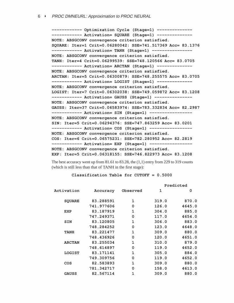
------------ Optimization Cycle (Stage=1) -------------------------- Activation= SQUARE (Stage=1) --------------NOTE: ABSGCONV convergence criterion satisfied.SQUARE: Iter=1 Crit=0.06280042: SSE=741.517369 Acc= 83.1376------------ Activation= TANH (Stage=1) ----------------NOTE: ABSGCONV convergence criterion satisfied.TANH: Iter=4 Crit=0.06299539: SSE=748.120566 Acc= 83.0705------------ Activation= ARCTAN (Stage=1) --------------NOTE: ABSGCONV convergence criterion satisfied.ARCTAN: Iter=5 Crit=0.06300879: SSE=748.255575 Acc= 83.0705------------ Activation= LOGIST (Stage=1) --------------NOTE: ABSGCONV convergence criterion satisfied.LOGIST: Iter=7 Crit=0.06302038: SSE=749.059872 Acc= 83.1208------------ Activation= GAUSS (Stage=1) ---------------NOTE: ABSGCONV convergence criterion satisfied.GAUSS: Iter=37 Crit=0.06583974: SSE=783.332834 Acc= 82.2987------------ Activation= SIN (Stage=1) -----------------NOTE: ABSGCONV convergence criterion satisfied.SIN: Iter=5 Crit=0.06294376: SSE=747.863259 Acc= 83.0201------------ Activation= COS (Stage=1) -----------------NOTE: ABSGCONV convergence criterion satisfied.COS: Iter=6 Crit=0.06575231: SSE=782.280952 Acc= 82.2819------------ Activation= EXP (Stage=1) -----------------NOTE: ABSGCONV convergence criterion satisfied.EXP: Iter=5 Crit=0.06318155: SSE=746.822973 Acc= 83.1208
The best accuracy went up from 81.61 to 83.28, the (1,1) entry from 229 to 319 counts(which is still less than that of TANH in the first stage):
Classification Table for CUTOFF = 0.5000
PredictedActivation Accuracy Observed 1 0
SQUARE 83.288591 1 319.0 870.0741.977606 0 126.0 4645.0
EXP 83.187919 1 304.0 885.0747.249371 0 117.0 4654.0
SIN 83.120805 1 306.0 883.0748.284252 0 123.0 4648.0
TANH 83.221477 1 309.0 880.0748.436926 0 120.0 4651.0
ARCTAN 83.255034 1 310.0 879.0748.614897 0 119.0 4652.0
LOGIST 83.171141 1 305.0 884.0749.309756 0 119.0 4652.0
COS 82.583893 1 309.0 880.0781.342717 0 158.0 4613.0
GAUSS 82.567114 1 309.0 880.0
Purpose of PROC DMNEURL � 7
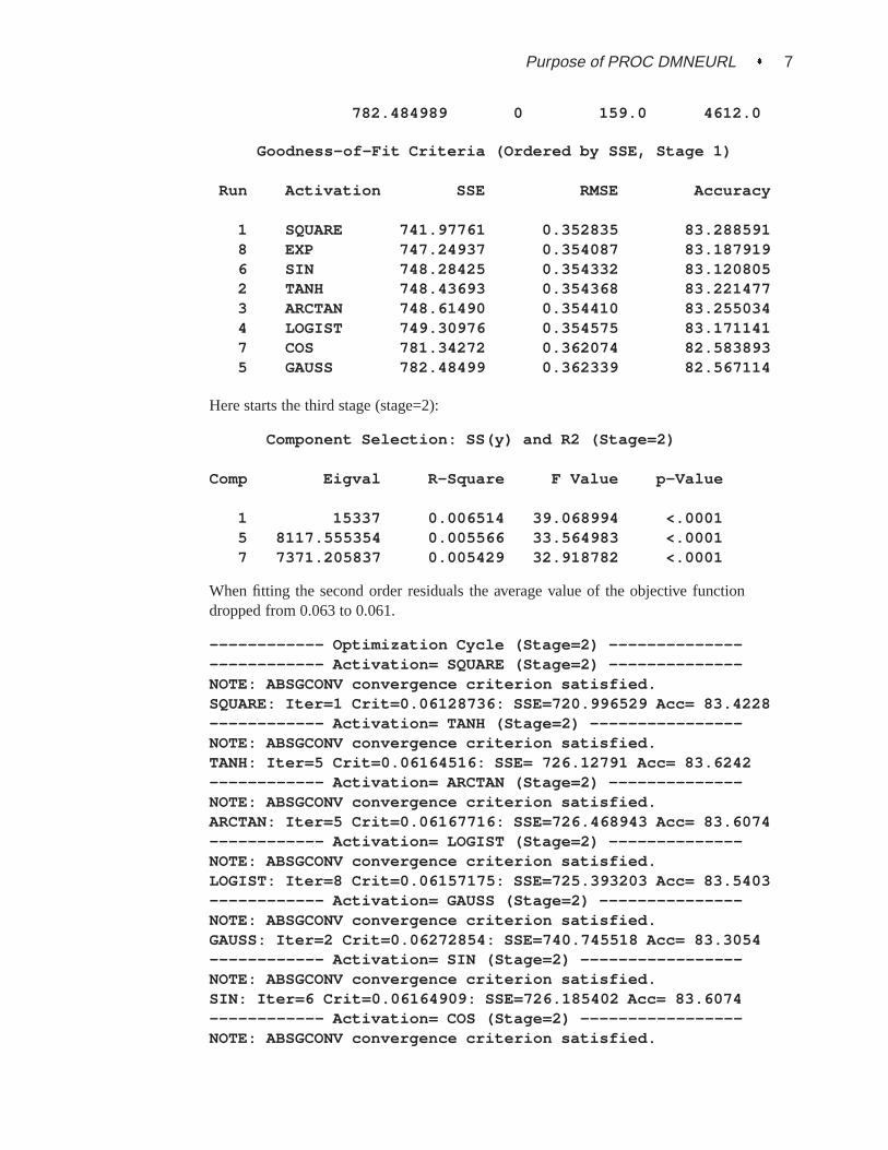
782.484989 0 159.0 4612.0
Goodness-of-Fit Criteria (Ordered by SSE, Stage 1)
Run Activation SSE RMSE Accuracy
1 SQUARE 741.97761 0.352835 83.2885918 EXP 747.24937 0.354087 83.1879196 SIN 748.28425 0.354332 83.1208052 TANH 748.43693 0.354368 83.2214773 ARCTAN 748.61490 0.354410 83.2550344 LOGIST 749.30976 0.354575 83.1711417 COS 781.34272 0.362074 82.5838935 GAUSS 782.48499 0.362339 82.567114
Here starts the third stage (stage=2):
Component Selection: SS(y) and R2 (Stage=2)
Comp Eigval R-Square F Value p-Value
1 15337 0.006514 39.068994 <.00015 8117.555354 0.005566 33.564983 <.00017 7371.205837 0.005429 32.918782 <.0001
When fitting the second order residuals the average value of the objective functiondropped from 0.063 to 0.061.
------------ Optimization Cycle (Stage=2) -------------------------- Activation= SQUARE (Stage=2) --------------NOTE: ABSGCONV convergence criterion satisfied.SQUARE: Iter=1 Crit=0.06128736: SSE=720.996529 Acc= 83.4228------------ Activation= TANH (Stage=2) ----------------NOTE: ABSGCONV convergence criterion satisfied.TANH: Iter=5 Crit=0.06164516: SSE= 726.12791 Acc= 83.6242------------ Activation= ARCTAN (Stage=2) --------------NOTE: ABSGCONV convergence criterion satisfied.ARCTAN: Iter=5 Crit=0.06167716: SSE=726.468943 Acc= 83.6074------------ Activation= LOGIST (Stage=2) --------------NOTE: ABSGCONV convergence criterion satisfied.LOGIST: Iter=8 Crit=0.06157175: SSE=725.393203 Acc= 83.5403------------ Activation= GAUSS (Stage=2) ---------------NOTE: ABSGCONV convergence criterion satisfied.GAUSS: Iter=2 Crit=0.06272854: SSE=740.745518 Acc= 83.3054------------ Activation= SIN (Stage=2) -----------------NOTE: ABSGCONV convergence criterion satisfied.SIN: Iter=6 Crit=0.06164909: SSE=726.185402 Acc= 83.6074------------ Activation= COS (Stage=2) -----------------NOTE: ABSGCONV convergence criterion satisfied.
8 � PROC DMNEURL: Approximation to PROC NEURAL
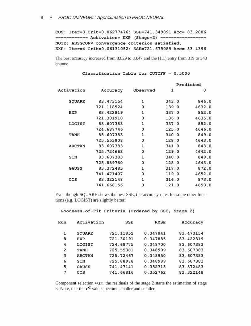
COS: Iter=3 Crit=0.06277476: SSE=741.349891 Acc= 83.2886------------ Activation= EXP (Stage=2) -----------------NOTE: ABSGCONV convergence criterion satisfied.EXP: Iter=4 Crit=0.06131052: SSE=721.679089 Acc= 83.4396
The best accuracy increased from 83.29 to 83.47 and the (1,1) entry from 319 to 343counts:
Classification Table for CUTOFF = 0.5000
PredictedActivation Accuracy Observed 1 0
SQUARE 83.473154 1 343.0 846.0721.118524 0 139.0 4632.0
EXP 83.422819 1 337.0 852.0721.301910 0 136.0 4635.0
LOGIST 83.607383 1 337.0 852.0724.687746 0 125.0 4646.0
TANH 83.607383 1 340.0 849.0725.553808 0 128.0 4643.0
ARCTAN 83.607383 1 341.0 848.0725.724668 0 129.0 4642.0
SIN 83.607383 1 340.0 849.0725.889780 0 128.0 4643.0
GAUSS 83.372483 1 317.0 872.0741.471407 0 119.0 4652.0
COS 83.322148 1 316.0 873.0741.668156 0 121.0 4650.0
Even though SQUARE shows the best SSE, the accuracy rates for some other func-tions (e.g. LOGIST) are slightly better:
Goodness-of-Fit Criteria (Ordered by SSE, Stage 2)
Run Activation SSE RMSE Accuracy
1 SQUARE 721.11852 0.347841 83.4731548 EXP 721.30191 0.347885 83.4228194 LOGIST 724.68775 0.348700 83.6073832 TANH 725.55381 0.348909 83.6073833 ARCTAN 725.72467 0.348950 83.6073836 SIN 725.88978 0.348989 83.6073835 GAUSS 741.47141 0.352715 83.3724837 COS 741.66816 0.352762 83.322148
Component selection w.r.t. the residuals of the stage 2 starts the estimation of stage3. Note, that theR2 values become smaller and smaller.

Purpose of PROC DMNEURL � 9
Component Selection: SS(y) and R2 (Stage=3)
Comp Eigval R-Square F Value p-Value
8 6938.083228 0.005571 33.383374 <.000120 5345.603436 0.004223 25.409312 <.000112 6136.575271 0.004059 24.517995 <.0001
Also the size of the objective function at the optimization results decreases:
------------ Optimization Cycle (Stage=3) -------------------------- Activation= SQUARE (Stage=3) --------------NOTE: ABSGCONV convergence criterion satisfied.SQUARE: Iter=1 Crit=0.06049339: SSE=710.516275 Acc= 83.7081------------ Activation= TANH (Stage=3) ----------------NOTE: ABSGCONV convergence criterion satisfied.TANH: Iter=4 Crit=0.06052425: SSE=710.396136 Acc= 83.7752------------ Activation= ARCTAN (Stage=3) --------------NOTE: ABSGCONV convergence criterion satisfied.ARCTAN: Iter=3 Crit=0.06052607: SSE=710.489715 Acc= 83.7081------------ Activation= LOGIST (Stage=3) --------------NOTE: ABSGCONV convergence criterion satisfied.LOGIST: Iter=6 Crit=0.06055936: SSE=711.054572 Acc= 83.6577------------ Activation= GAUSS (Stage=3) ---------------NOTE: ABSGCONV convergence criterion satisfied.GAUSS: Iter=6 Crit=0.06111674: SSE= 719.41694 Acc= 83.3725------------ Activation= SIN (Stage=3) -----------------NOTE: ABSGCONV convergence criterion satisfied.SIN: Iter=3 Crit=0.06051959: SSE=710.308709 Acc= 83.8087------------ Activation= COS (Stage=3) -----------------NOTE: ABSGCONV convergence criterion satisfied.COS: Iter=6 Crit=0.06117044: SSE=719.262211 Acc= 83.3725------------ Activation= EXP (Stage=3) -----------------NOTE: ABSGCONV convergence criterion satisfied.EXP: Iter=2 Crit=0.06051088: SSE=710.810558 Acc= 83.7081
The accuracy of the best fit impoves slightly from 83.47 to 83.79 and the size of the(1,1) entry inceases from 343 to 364.
Classification Table for CUTOFF = 0.5000
PredictedActivation Accuracy Observed 1 0
SIN 83.791946 1 364.0 825.0709.778632 0 141.0 4630.0
TANH 83.758389 1 363.0 826.0

10 � PROC DMNEURL: Approximation to PROC NEURAL
709.889256 0 142.0 4629.0ARCTAN 83.708054 1 361.0 828.0
710.036390 0 143.0 4628.0SQUARE 83.724832 1 355.0 834.0
710.075198 0 136.0 4635.0EXP 83.741611 1 356.0 833.0
710.212159 0 136.0 4635.0LOGIST 83.691275 1 357.0 832.0
710.822647 0 140.0 4631.0COS 83.355705 1 340.0 849.0
718.944913 0 143.0 4628.0GAUSS 83.288591 1 328.0 861.0
719.269965 0 135.0 4636.0
Goodness-of-Fit Criteria (Ordered by SSE, Stage 3)
Run Activation SSE RMSE Accuracy
6 SIN 709.77863 0.345095 83.7919462 TANH 709.88926 0.345122 83.7583893 ARCTAN 710.03639 0.345157 83.7080541 SQUARE 710.07520 0.345167 83.7248328 EXP 710.21216 0.345200 83.7416114 LOGIST 710.82265 0.345348 83.6912757 COS 718.94491 0.347316 83.3557055 GAUSS 719.26997 0.347394 83.288591
Now the residuals are computed and components are selected for the last estimationstage:
Component Selection: SS(y) and R2 (Stage=4)
Comp Eigval R-Square F Value p-Value
28 1195.710958 0.003997 23.916548 <.000127 3456.490592 0.001822 10.919693 0.001025 3935.018952 0.001803 10.824185 0.0010
There are no problems with the optimization processes:
------------ Optimization Cycle (Stage=4) -------------------------- Activation= SQUARE (Stage=4) --------------NOTE: ABSGCONV convergence criterion satisfied.SQUARE: Iter=1 Crit=0.05983921: SSE=703.669268 Acc= 83.6913------------ Activation= TANH (Stage=4) ----------------NOTE: ABSGCONV convergence criterion satisfied.

Purpose of PROC DMNEURL � 11
TANH: Iter=5 Crit=0.06015823: SSE=706.476969 Acc= 83.6074------------ Activation= ARCTAN (Stage=4) --------------NOTE: ABSGCONV convergence criterion satisfied.ARCTAN: Iter=3 Crit=0.06013359: SSE=706.212332 Acc= 83.7081------------ Activation= LOGIST (Stage=4) --------------NOTE: ABSGCONV convergence criterion satisfied.LOGIST: Iter=3 Crit=0.06017552: SSE=706.851414 Acc= 83.7919------------ Activation= GAUSS (Stage=4) ---------------NOTE: ABSGCONV convergence criterion satisfied.GAUSS: Iter=4 Crit=0.06032127: SSE=708.571854 Acc= 83.8255------------ Activation= SIN (Stage=4) -----------------NOTE: ABSGCONV convergence criterion satisfied.SIN: Iter=3 Crit=0.06014411: SSE=706.402904 Acc= 83.6745------------ Activation= COS (Stage=4) -----------------NOTE: ABSGCONV convergence criterion satisfied.COS: Iter=4 Crit=0.06007575: SSE=707.016805 Acc= 83.8087------------ Activation= EXP (Stage=4) -----------------NOTE: ABSGCONV convergence criterion satisfied.EXP: Iter=3 Crit=0.05983526: SSE=703.933766 Acc= 83.6074
The accuracy of the result is no longer improved and drops from 83.79 to 83.72, andalso the (1,1) entry was decreased from 365 to 363. This can happen only whenthe discretization error becomes too large in relation to the goodness of fit of thenonlinear model. Perhaps the specification of larger values for MAXCOMP= andNPOINT= could improve the solution. However, in most applications we would seethis behavior as a sign that no further improvement of the model fit is possible.
Classification Table for CUTOFF = 0.5000
PredictedActivation Accuracy Observed 1 0
SQUARE 83.724832 1 363.0 826.0702.899794 0 144.0 4627.0
EXP 83.691275 1 361.0 828.0703.295564 0 144.0 4627.0
ARCTAN 83.775168 1 364.0 825.0705.243085 0 142.0 4629.0
SIN 83.691275 1 363.0 826.0705.508160 0 146.0 4625.0
TANH 83.708054 1 362.0 827.0705.634506 0 144.0 4627.0
LOGIST 83.708054 1 360.0 829.0705.732595 0 142.0 4629.0
COS 83.842282 1 364.0 825.0707.292433 0 138.0 4633.0
GAUSS 83.791946 1 362.0 827.0708.659944 0 139.0 4632.0
12 � PROC DMNEURL: Approximation to PROC NEURAL
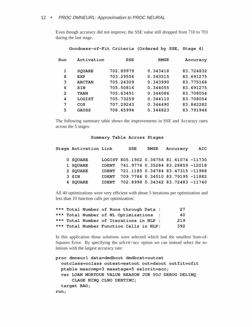
Even though accuracy did not improve, the SSE value still dropped from 710 to 703during the last stage.
Goodness-of-Fit Criteria (Ordered by SSE, Stage 4)
Run Activation SSE RMSE Accuracy
1 SQUARE 702.89979 0.343418 83.7248328 EXP 703.29556 0.343515 83.6912753 ARCTAN 705.24309 0.343990 83.7751686 SIN 705.50816 0.344055 83.6912752 TANH 705.63451 0.344086 83.7080544 LOGIST 705.73259 0.344110 83.7080547 COS 707.29243 0.344490 83.8422825 GAUSS 708.65994 0.344823 83.791946
The following summary table shows the improvements in SSE and Accuracy ratesacross the 5 stages:
Summary Table Across Stages
Stage Activation Link SSE RMSE Accuracy AIC
0 SQUARE LOGIST 805.1902 0.36756 81.61074 -117301 SQUARE IDENT 741.9776 0.35284 83.28859 -120182 SQUARE IDENT 721.1185 0.34784 83.47315 -119883 SIN IDENT 709.7786 0.34510 83.79195 -118824 SQUARE IDENT 702.8998 0.34342 83.72483 -11740
All 40 optimizations were very efficient with about 5 iterations per optimization andless than 10 function calls per optimization:
*** Total Number of Runs through Data : 27*** Total Number of NL Optimizations : 40*** Total Number of Iterations in NLP : 219*** Total Number Function Calls in NLP: 392
In this application those solutions were selected which had the smallest Sum-of-Squares Error. By specifying theselcrit=acc option we can instead select the so-lutions with the largest accuracy rate:
proc dmneurl data=dmdbout dmdbcat=outcatoutclass=oclass outest=estout out=dsout outfit=ofitptable maxcomp=3 maxstage=5 selcrit=acc;var LOAN MORTDUE VALUE REASON JOB YOJ DEROG DELINQ
CLAGE NINQ CLNO DEBTINC;target BAD;
run;
Purpose of PROC DMNEURL � 13
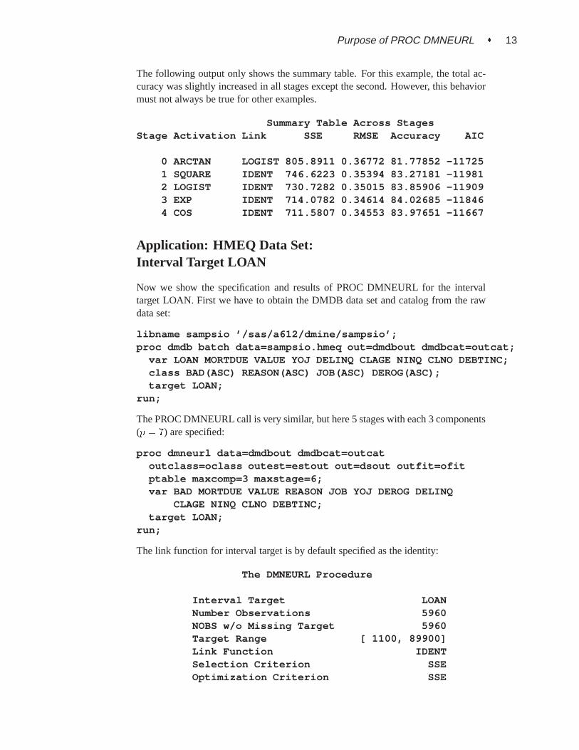
The following output only shows the summary table. For this example, the total ac-curacy was slightly increased in all stages except the second. However, this behaviormust not always be true for other examples.
Summary Table Across StagesStage Activation Link SSE RMSE Accuracy AIC
0 ARCTAN LOGIST 805.8911 0.36772 81.77852 -117251 SQUARE IDENT 746.6223 0.35394 83.27181 -119812 LOGIST IDENT 730.7282 0.35015 83.85906 -119093 EXP IDENT 714.0782 0.34614 84.02685 -118464 COS IDENT 711.5807 0.34553 83.97651 -11667
Application: HMEQ Data Set:Interval Target LOAN
Now we show the specification and results of PROC DMNEURL for the intervaltarget LOAN. First we have to obtain the DMDB data set and catalog from the rawdata set:
libname sampsio ’/sas/a612/dmine/sampsio’;proc dmdb batch data=sampsio.hmeq out=dmdbout dmdbcat=outcat;
var LOAN MORTDUE VALUE YOJ DELINQ CLAGE NINQ CLNO DEBTINC;class BAD(ASC) REASON(ASC) JOB(ASC) DEROG(ASC);target LOAN;
run;
The PROC DMNEURL call is very similar, but here 5 stages with each 3 components(p = 7) are specified:
proc dmneurl data=dmdbout dmdbcat=outcatoutclass=oclass outest=estout out=dsout outfit=ofitptable maxcomp=3 maxstage=6;var BAD MORTDUE VALUE REASON JOB YOJ DEROG DELINQ
CLAGE NINQ CLNO DEBTINC;target LOAN;
run;
The link function for interval target is by default specified as the identity:
The DMNEURL Procedure
Interval Target LOANNumber Observations 5960NOBS w/o Missing Target 5960Target Range [ 1100, 89900]Link Function IDENTSelection Criterion SSEOptimization Criterion SSE

14 � PROC DMNEURL: Approximation to PROC NEURAL
Estimation Stages 6Max. Number Components 3Minimum R2 Value 0.000050Number Grid Points 17
Variable Mean Std Dev Skewness Kurtosis
LOAN 18608 11207 2.02378 6.93259MORTDUE 67350 44458 1.81448 6.48187VALUE 99863 57386 3.05334 24.36280YOJ 8.15130 7.57398 0.98846 0.37207DELINQ 0.40570 1.12727 4.02315 23.56545CLAGE 170.47634 85.81009 1.34341 7.59955NINQ 1.08456 1.72867 2.62198 9.78651CLNO 20.50285 10.13893 0.77505 1.15767DEBTINC 26.59885 8.60175 2.85235 50.50404
For an interval target the percentiles of the response (target) variable are computedas an aside of the preliminary runs through the data. (Note, that the values of theresponsey are not all stored in RAM.)
Percentiles of Target LOAN in [1100 : 89900]
Nobs Y Value Label
1 596 7600.000000 0.0731981982 1192 10000 0.1002252253 1788 12100 0.1238738744 2384 14400 0.1497747755 2980 16300 0.1711711716 3576 18800 0.1993243247 4172 21700 0.2319819828 4768 25000 0.2691441449 5364 30500 0.331081081
10 5960 89900 1
The first estimation stage starts with the selection of the best predictor components(eigenvectors):
Component Selection: SS(y) and R2 (SS_total=326.60303927)
Comp Eigval R-Square F Value p-Value SSE
2 14414 0.015964 96.672480 <.0001 321.38916328 1232.230727 0.005739 34.949673 <.0001 319.51488611 6335.576701 0.005490 33.620923 <.0001 317.721686
A maximum of 8 iterations is needed for convergence:
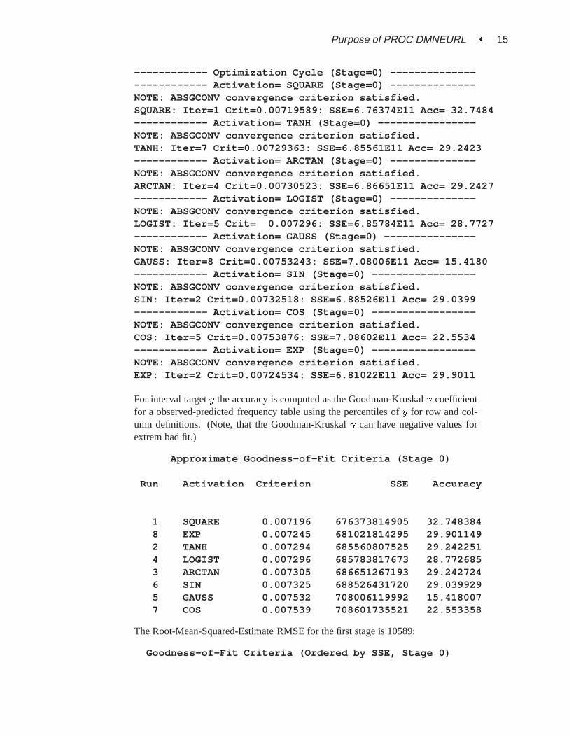
Purpose of PROC DMNEURL � 15
------------ Optimization Cycle (Stage=0) -------------------------- Activation= SQUARE (Stage=0) --------------NOTE: ABSGCONV convergence criterion satisfied.SQUARE: Iter=1 Crit=0.00719589: SSE=6.76374E11 Acc= 32.7484------------ Activation= TANH (Stage=0) ----------------NOTE: ABSGCONV convergence criterion satisfied.TANH: Iter=7 Crit=0.00729363: SSE=6.85561E11 Acc= 29.2423------------ Activation= ARCTAN (Stage=0) --------------NOTE: ABSGCONV convergence criterion satisfied.ARCTAN: Iter=4 Crit=0.00730523: SSE=6.86651E11 Acc= 29.2427------------ Activation= LOGIST (Stage=0) --------------NOTE: ABSGCONV convergence criterion satisfied.LOGIST: Iter=5 Crit= 0.007296: SSE=6.85784E11 Acc= 28.7727------------ Activation= GAUSS (Stage=0) ---------------NOTE: ABSGCONV convergence criterion satisfied.GAUSS: Iter=8 Crit=0.00753243: SSE=7.08006E11 Acc= 15.4180------------ Activation= SIN (Stage=0) -----------------NOTE: ABSGCONV convergence criterion satisfied.SIN: Iter=2 Crit=0.00732518: SSE=6.88526E11 Acc= 29.0399------------ Activation= COS (Stage=0) -----------------NOTE: ABSGCONV convergence criterion satisfied.COS: Iter=5 Crit=0.00753876: SSE=7.08602E11 Acc= 22.5534------------ Activation= EXP (Stage=0) -----------------NOTE: ABSGCONV convergence criterion satisfied.EXP: Iter=2 Crit=0.00724534: SSE=6.81022E11 Acc= 29.9011
For interval targety the accuracy is computed as the Goodman-Kruskal coefficientfor a observed-predicted frequency table using the percentiles ofy for row and col-umn definitions. (Note, that the Goodman-Kruskal can have negative values forextrem bad fit.)
Approximate Goodness-of-Fit Criteria (Stage 0)
Run Activation Criterion SSE Accuracy
1 SQUARE 0.007196 676373814905 32.7483848 EXP 0.007245 681021814295 29.9011492 TANH 0.007294 685560807525 29.2422514 LOGIST 0.007296 685783817673 28.7726853 ARCTAN 0.007305 686651267193 29.2427246 SIN 0.007325 688526431720 29.0399295 GAUSS 0.007532 708006119992 15.4180077 COS 0.007539 708601735521 22.553358
The Root-Mean-Squared-Estimate RMSE for the first stage is 10589:
Goodness-of-Fit Criteria (Ordered by SSE, Stage 0)
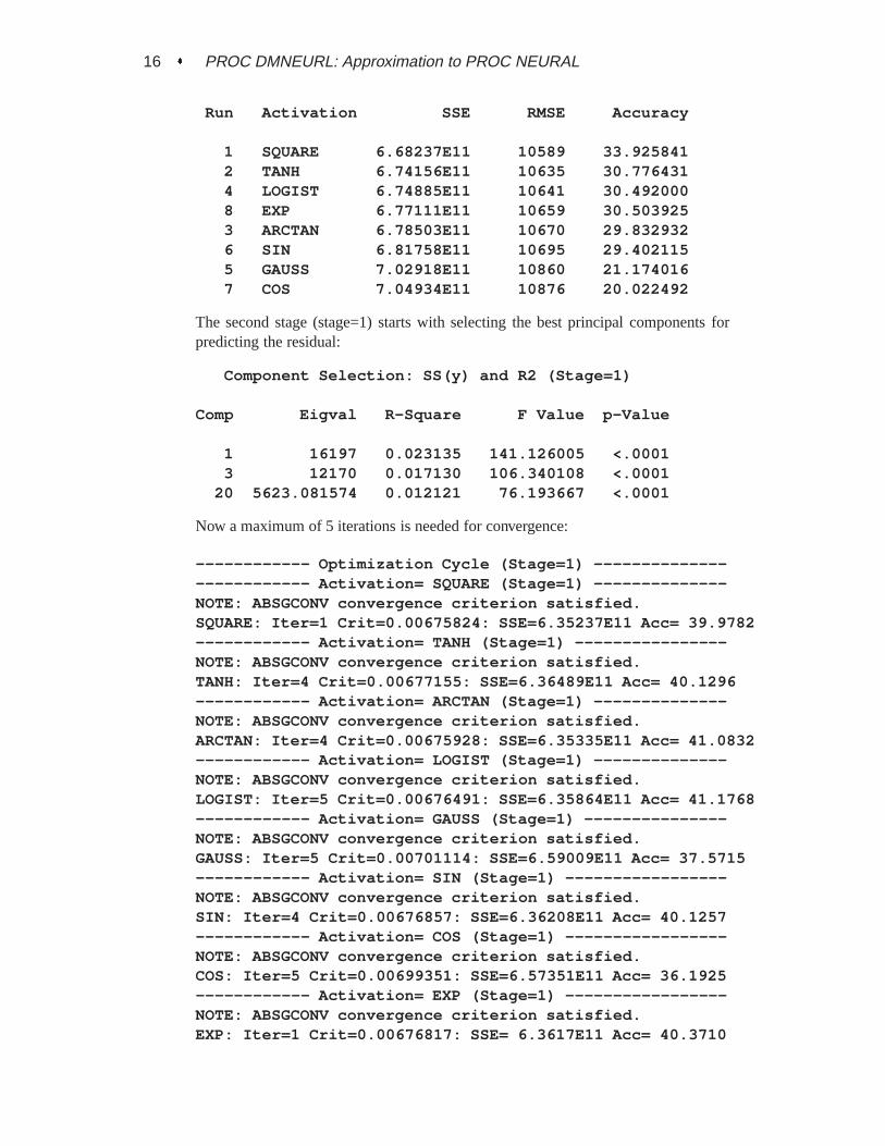
16 � PROC DMNEURL: Approximation to PROC NEURAL
Run Activation SSE RMSE Accuracy
1 SQUARE 6.68237E11 10589 33.9258412 TANH 6.74156E11 10635 30.7764314 LOGIST 6.74885E11 10641 30.4920008 EXP 6.77111E11 10659 30.5039253 ARCTAN 6.78503E11 10670 29.8329326 SIN 6.81758E11 10695 29.4021155 GAUSS 7.02918E11 10860 21.1740167 COS 7.04934E11 10876 20.022492
The second stage (stage=1) starts with selecting the best principal components forpredicting the residual:
Component Selection: SS(y) and R2 (Stage=1)
Comp Eigval R-Square F Value p-Value
1 16197 0.023135 141.126005 <.00013 12170 0.017130 106.340108 <.0001
20 5623.081574 0.012121 76.193667 <.0001
Now a maximum of 5 iterations is needed for convergence:
------------ Optimization Cycle (Stage=1) -------------------------- Activation= SQUARE (Stage=1) --------------NOTE: ABSGCONV convergence criterion satisfied.SQUARE: Iter=1 Crit=0.00675824: SSE=6.35237E11 Acc= 39.9782------------ Activation= TANH (Stage=1) ----------------NOTE: ABSGCONV convergence criterion satisfied.TANH: Iter=4 Crit=0.00677155: SSE=6.36489E11 Acc= 40.1296------------ Activation= ARCTAN (Stage=1) --------------NOTE: ABSGCONV convergence criterion satisfied.ARCTAN: Iter=4 Crit=0.00675928: SSE=6.35335E11 Acc= 41.0832------------ Activation= LOGIST (Stage=1) --------------NOTE: ABSGCONV convergence criterion satisfied.LOGIST: Iter=5 Crit=0.00676491: SSE=6.35864E11 Acc= 41.1768------------ Activation= GAUSS (Stage=1) ---------------NOTE: ABSGCONV convergence criterion satisfied.GAUSS: Iter=5 Crit=0.00701114: SSE=6.59009E11 Acc= 37.5715------------ Activation= SIN (Stage=1) -----------------NOTE: ABSGCONV convergence criterion satisfied.SIN: Iter=4 Crit=0.00676857: SSE=6.36208E11 Acc= 40.1257------------ Activation= COS (Stage=1) -----------------NOTE: ABSGCONV convergence criterion satisfied.COS: Iter=5 Crit=0.00699351: SSE=6.57351E11 Acc= 36.1925------------ Activation= EXP (Stage=1) -----------------NOTE: ABSGCONV convergence criterion satisfied.EXP: Iter=1 Crit=0.00676817: SSE= 6.3617E11 Acc= 40.3710
Purpose of PROC DMNEURL � 17
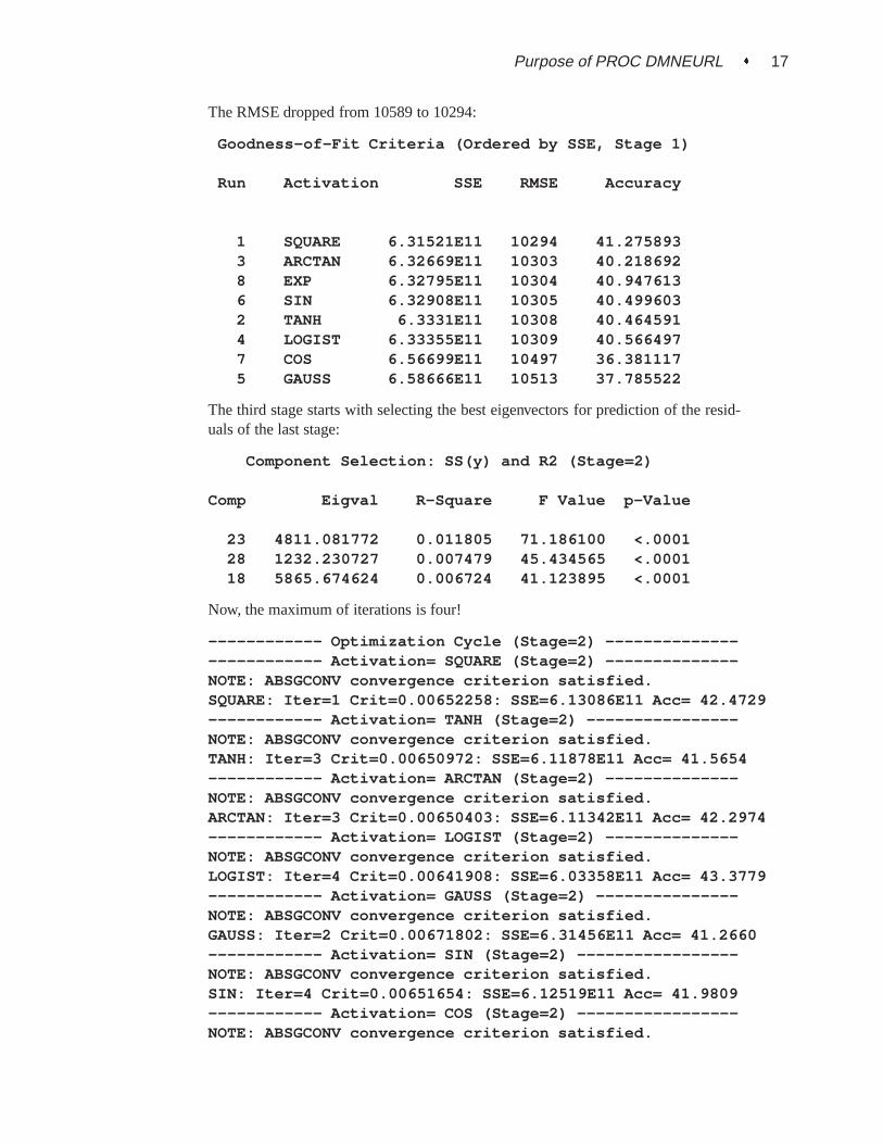
The RMSE dropped from 10589 to 10294:
Goodness-of-Fit Criteria (Ordered by SSE, Stage 1)
Run Activation SSE RMSE Accuracy
1 SQUARE 6.31521E11 10294 41.2758933 ARCTAN 6.32669E11 10303 40.2186928 EXP 6.32795E11 10304 40.9476136 SIN 6.32908E11 10305 40.4996032 TANH 6.3331E11 10308 40.4645914 LOGIST 6.33355E11 10309 40.5664977 COS 6.56699E11 10497 36.3811175 GAUSS 6.58666E11 10513 37.785522
The third stage starts with selecting the best eigenvectors for prediction of the resid-uals of the last stage:
Component Selection: SS(y) and R2 (Stage=2)
Comp Eigval R-Square F Value p-Value
23 4811.081772 0.011805 71.186100 <.000128 1232.230727 0.007479 45.434565 <.000118 5865.674624 0.006724 41.123895 <.0001
Now, the maximum of iterations is four!
------------ Optimization Cycle (Stage=2) -------------------------- Activation= SQUARE (Stage=2) --------------NOTE: ABSGCONV convergence criterion satisfied.SQUARE: Iter=1 Crit=0.00652258: SSE=6.13086E11 Acc= 42.4729------------ Activation= TANH (Stage=2) ----------------NOTE: ABSGCONV convergence criterion satisfied.TANH: Iter=3 Crit=0.00650972: SSE=6.11878E11 Acc= 41.5654------------ Activation= ARCTAN (Stage=2) --------------NOTE: ABSGCONV convergence criterion satisfied.ARCTAN: Iter=3 Crit=0.00650403: SSE=6.11342E11 Acc= 42.2974------------ Activation= LOGIST (Stage=2) --------------NOTE: ABSGCONV convergence criterion satisfied.LOGIST: Iter=4 Crit=0.00641908: SSE=6.03358E11 Acc= 43.3779------------ Activation= GAUSS (Stage=2) ---------------NOTE: ABSGCONV convergence criterion satisfied.GAUSS: Iter=2 Crit=0.00671802: SSE=6.31456E11 Acc= 41.2660------------ Activation= SIN (Stage=2) -----------------NOTE: ABSGCONV convergence criterion satisfied.SIN: Iter=4 Crit=0.00651654: SSE=6.12519E11 Acc= 41.9809------------ Activation= COS (Stage=2) -----------------NOTE: ABSGCONV convergence criterion satisfied.

18 � PROC DMNEURL: Approximation to PROC NEURAL
COS: Iter=4 Crit=0.00671738: SSE=6.31396E11 Acc= 41.2783------------ Activation= EXP (Stage=2) -----------------NOTE: ABSGCONV convergence criterion satisfied.EXP: Iter=0 Crit=0.00656615: SSE=6.17182E11 Acc= 41.6251
The RMSE dropped from 10294 to 10035:
Goodness-of-Fit Criteria (Ordered by SSE, Stage 2)
Run Activation SSE RMSE Accuracy
4 LOGIST 6.00171E11 10035 44.0763243 ARCTAN 6.11611E11 10130 42.7228532 TANH 6.12574E11 10138 42.4549256 SIN 6.12902E11 10141 42.6185361 SQUARE 6.14545E11 10154 43.4529228 EXP 6.17964E11 10183 42.5888237 COS 6.31415E11 10293 41.1533495 GAUSS 6.31533E11 10294 41.028769
In stage 3 components are selected w.r.t. the residuals from stage 2:
Component Selection: SS(y) and R2 (Stage=3)
Comp Eigval R-Square F Value p-Value
5 8108.233368 0.008115 48.751302 <.00017 7678.598513 0.004569 27.574638 <.0001
27 3496.302840 0.003929 23.802006 <.0001
------------ Optimization Cycle (Stage=3) -------------------------- Activation= SQUARE (Stage=3) --------------NOTE: ABSGCONV convergence criterion satisfied.SQUARE: Iter=1 Crit=0.00627437: SSE=5.89756E11 Acc= 46.5664------------ Activation= TANH (Stage=3) ----------------NOTE: ABSGCONV convergence criterion satisfied.TANH: Iter=2 Crit=0.00628152: SSE=5.90428E11 Acc= 46.2812------------ Activation= ARCTAN (Stage=3) --------------NOTE: ABSGCONV convergence criterion satisfied.ARCTAN: Iter=2 Crit=0.00628195: SSE=5.90469E11 Acc= 46.2125------------ Activation= LOGIST (Stage=3) --------------NOTE: ABSGCONV convergence criterion satisfied.LOGIST: Iter=5 Crit=0.00628127: SSE=5.90404E11 Acc= 45.8040------------ Activation= GAUSS (Stage=3) ---------------NOTE: ABSGCONV convergence criterion satisfied.GAUSS: Iter=2 Crit=0.00637032: SSE=5.98775E11 Acc= 45.3250------------ Activation= SIN (Stage=3) -----------------NOTE: ABSGCONV convergence criterion satisfied.SIN: Iter=6 Crit=0.00627884: SSE=5.90176E11 Acc= 46.0972
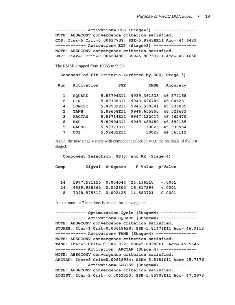
Purpose of PROC DMNEURL � 19
------------ Activation= COS (Stage=3) -----------------NOTE: ABSGCONV convergence criterion satisfied.COS: Iter=5 Crit=0.00637738: SSE=5.99438E11 Acc= 44.6439------------ Activation= EXP (Stage=3) -----------------NOTE: ABSGCONV convergence criterion satisfied.EXP: Iter=1 Crit=0.00628498: SSE=5.90753E11 Acc= 46.4650
The RMSE dropped from 10035 to 9939:
Goodness-of-Fit Criteria (Ordered by SSE, Stage 3)
Run Activation SSE RMSE Accuracy
1 SQUARE 5.88794E11 9939.361833 46.8741686 SIN 5.89308E11 9943.696786 46.0452314 LOGIST 5.89532E11 9945.590341 45.9360352 TANH 5.89658E11 9946.655850 46.5216833 ARCTAN 5.89714E11 9947.122017 46.4624708 EXP 5.89994E11 9949.489480 46.5901555 GAUSS 5.98777E11 10023 45.3389547 COS 5.99432E11 10029 44.563112
Again, the new stage 4 starts with component selection w.r.t. the residuals of the laststage3:
Component Selection: SS(y) and R2 (Stage=4)
Comp Eigval R-Square F Value p-Value
14 5977.581155 0.004044 24.196310 <.000124 4589.938565 0.002803 16.817296 <.0001
8 7098.575517 0.002425 14.583721 0.0001
A maximum of 7 iterations is needed for convergence:
------------ Optimization Cycle (Stage=4) -------------------------- Activation= SQUARE (Stage=4) --------------NOTE: ABSGCONV convergence criterion satisfied.SQUARE: Iter=1 Crit=0.00618628: SSE=5.81476E11 Acc= 46.9112------------ Activation= TANH (Stage=4) ----------------NOTE: ABSGCONV convergence criterion satisfied.TANH: Iter=5 Crit= 0.0061812: SSE=5.80998E11 Acc= 45.5545------------ Activation= ARCTAN (Stage=4) --------------NOTE: ABSGCONV convergence criterion satisfied.ARCTAN: Iter=3 Crit=0.00618984: SSE= 5.8181E11 Acc= 45.7876------------ Activation= LOGIST (Stage=4) --------------NOTE: ABSGCONV convergence criterion satisfied.LOGIST: Iter=2 Crit= 0.0062313: SSE=5.85708E11 Acc= 47.2978
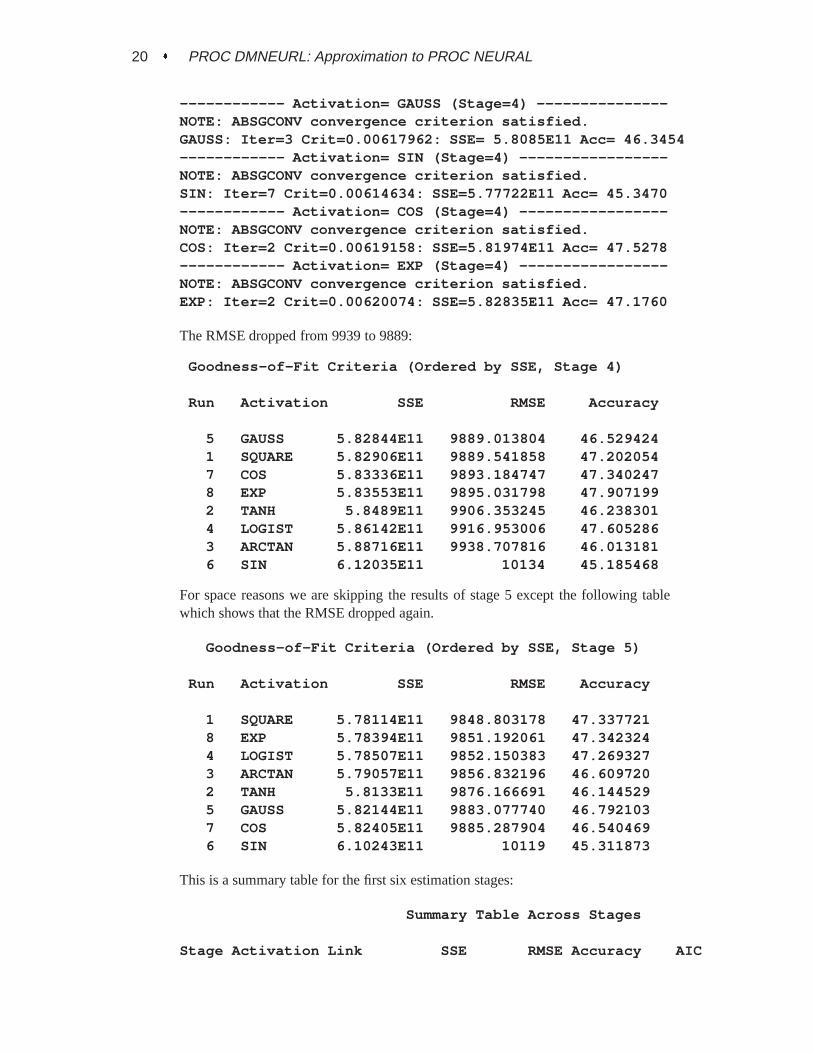
20 � PROC DMNEURL: Approximation to PROC NEURAL
------------ Activation= GAUSS (Stage=4) ---------------NOTE: ABSGCONV convergence criterion satisfied.GAUSS: Iter=3 Crit=0.00617962: SSE= 5.8085E11 Acc= 46.3454------------ Activation= SIN (Stage=4) -----------------NOTE: ABSGCONV convergence criterion satisfied.SIN: Iter=7 Crit=0.00614634: SSE=5.77722E11 Acc= 45.3470------------ Activation= COS (Stage=4) -----------------NOTE: ABSGCONV convergence criterion satisfied.COS: Iter=2 Crit=0.00619158: SSE=5.81974E11 Acc= 47.5278------------ Activation= EXP (Stage=4) -----------------NOTE: ABSGCONV convergence criterion satisfied.EXP: Iter=2 Crit=0.00620074: SSE=5.82835E11 Acc= 47.1760
The RMSE dropped from 9939 to 9889:
Goodness-of-Fit Criteria (Ordered by SSE, Stage 4)
Run Activation SSE RMSE Accuracy
5 GAUSS 5.82844E11 9889.013804 46.5294241 SQUARE 5.82906E11 9889.541858 47.2020547 COS 5.83336E11 9893.184747 47.3402478 EXP 5.83553E11 9895.031798 47.9071992 TANH 5.8489E11 9906.353245 46.2383014 LOGIST 5.86142E11 9916.953006 47.6052863 ARCTAN 5.88716E11 9938.707816 46.0131816 SIN 6.12035E11 10134 45.185468
For space reasons we are skipping the results of stage 5 except the following tablewhich shows that the RMSE dropped again.
Goodness-of-Fit Criteria (Ordered by SSE, Stage 5)
Run Activation SSE RMSE Accuracy
1 SQUARE 5.78114E11 9848.803178 47.3377218 EXP 5.78394E11 9851.192061 47.3423244 LOGIST 5.78507E11 9852.150383 47.2693273 ARCTAN 5.79057E11 9856.832196 46.6097202 TANH 5.8133E11 9876.166691 46.1445295 GAUSS 5.82144E11 9883.077740 46.7921037 COS 5.82405E11 9885.287904 46.5404696 SIN 6.10243E11 10119 45.311873
This is a summary table for the first six estimation stages:
Summary Table Across Stages
Stage Activation Link SSE RMSE Accuracy AIC

Purpose of PROC DMNEURL � 21
0 SQUARE IDENT 6.68237E11 10589 33.92584 1106751 SQUARE IDENT 6.31521E11 10294 41.27589 1105442 LOGIST IDENT 6.00171E11 10035 44.07632 1104473 SQUARE IDENT 5.88794E11 9939.36183 46.87417 1105394 GAUSS IDENT 5.82844E11 9889.01380 46.52942 1106845 SQUARE IDENT 5.78114E11 9848.80318 47.33772 110842
The six stages took 48 optimizations (each with 7 parameters) and 33 runs throughthe data. In average less than 4 iterations and about 7 function calls are needed foreach optimization:
*** Total Number of Runs through Data : 33*** Total Number of NL Optimizations : 48*** Total Number of Iterations in NLP : 159*** Total Number Function Calls in NLP: 348
Missing Values
Observations with missing values in the target variable (response or dependend vari-able) are not included in the analysis. Those observations are, however, scored, i.e.predicted values are computed.Observations with missing values in the predictor variables (independend variables)are processed depending on the scale type of the variable:
� For numeric variables, missing values are replaced by the (weighted) mean ofthe variable.
� For class variables, missing values are treated as an additional category.
Syntax of PROC DMNEURL
PROC DMNEURL options ; required statementVAR variables ;
T ARGET variables ;
FUNCTION names ;
LINK name ;
FREQ variables ;
WEIGHT variables ;
DECISION options ;
9>>>>>>>>=>>>>>>>>;
optional statements
Overview of PROC DMNEURL Options
PROC DMNEURL options;This statement invokes the DMNEURL procedure. The options available with thePROC DMNEURL statement are:

22 � PROC DMNEURL: Approximation to PROC NEURAL
DATA= SASdataset:specifies an input data set generated by PROC DMDB which is associated witha valid catalog specified by the DMDBCAT= option. This option must be spec-ified, no default is permitted. The DATA= data set must contain interval scaledvariables and CLASS variables in a specific form written by PROC DMDB.
DMDBCAT= SAScatalog:specifies an input catalog of meta information generated by PROC DMDBwhich is assiciated with a valid data set specified by the DATA= option. Thecatalog contains important information (e.g. range of variables, number ofmissing values of each variable, moments of variables) which is used by manyother procedures which require a DMDB data set. That means, that both, theDMDBCAT= catalog and the DATA= data set must beInSync to obtain properresults! This option must be specified, no default is permitted.
TESTDATA= SASdataset:specifies a second input data set which is by default NOT generated by PROCDMDB, which however must contain all variables of the DATA= input dataset which are used in the model. The variables not used in the model may bedifferent. The order of variables is not relevant. If TESTDATA= is specified,you can specify a TESTOUT= output data set (containing predicted values andresiduals) which relates to the TESTDATA= input data set the same as theOUT= data set relates to the DATA= input training data set. When specifyingthe TESTDMDB option you may use a data set generated by PROC DMDB asthe TESTDATA= input data set.
OUTCLASS=SASdataset:specifies an output data set generated by PROC DMNEURL which containsthe mapping inbetween compound variable names and the names of variablesand categories of CLASS variables used in the model. The compound variablenames are used to denote dummy variables which are created for each categoryof a CLASS variable with more than two categories. Since the compoundnames of dummy variables are used for variable names in other data sets theuser must know to which category each compound name corresponds. TheOUTCLASS= data set has only three character variables
–NAME – contains compound name used as variable names in other outputdata sets
–VAR– contains variable name used in DATA= input data set
–LEVEL – contains level name of variable as used in DATA= input data set.
Note, if the DATA= input data set does not contain any CLASS variables theOUTCLASS= data set is not written.
OUTEST=SASdataset:specifies an output data set generated by PROC DMNEURL which contains allthe model information necessary for scoring additional cases or data sets.
Variables of the output data set:
–TARGET – (character) name of the target

Purpose of PROC DMNEURL � 23
–TYPE– (character) type of observation
–NAME – (character) name of observation
–STAGE– number of stage
–MEAN – contains different numeric information
–STDEV– contains different numeric information
varnamei variables in the model variables; the first variables correspond toCLASS (categorical) the remaining variables are continuously (intervalor ratio) scaled. Note, that for nonbinary CLASS (nominal or ordinalcategorical) variables a set of binary dummy variables is created. In thosecases the prefix of variable namesvarnamei used for a group of variablesin the data set may be the same for a successive group of variables whichdiffers only by a numeric suffix.
This data set contains all the model information necessary to compute the pre-dicted model values (scores).
1. The–TYPE–=–V–MAP– and–TYPE–=–C–MAP– observations con-tain the mapping indices between the variables used in the model and thenumber of the variable in the data set.
� The–MEAN– variable contains the number of index mappings.� The –STDEV– variable contains the index of the target (response)
variable in the data set for the–TYPE–=–V–MAP– observation.For –TYPE–=–C–MAP– it contains the level (category) number ofa categorical target variable that corresponds to missing values.
2. The–TYPE–=–EIGVAL– observation contains the sorted eigenvaluesof theX 0X matrix. Here, the–MEAN– variable contains the numberof model variables (rows/columns of the modelX 0X matrix) and the
–STDEV– variable contains the numberc of model components.
3. For each stage of the estimation process two groups of observations arewritten to the OUTEST= data set:
(a) The–TYPE–=–EIGVEC– observations contain a set ofc principalcomponents which are used as predictor variables for the estimationof the original traget valuey (in stage 0) or for the prediction of thestagei residual. Here, the–MEAN– variable contains the value forthe criterion used to include the component into the model which isnormally theR2 value. The–STDEV– variable contains the eigen-value number to which the eigenvector corresponds.
1 SQUARE (a+ b � x) � x2 TANH a � tanh(b � x)3 ARCTAN a � atan(b � x)4 LOGIST exp(a � x)=(1: + exp(b � x)5 GAUSS a � exp(�(b � x)2)6 SIN a � sin(b � x)7 COS a � cos(b � x)8 EXP a � exp(b � x)
The –NAME– variable reports the corresponding name of the bestactivation function found.
24 � PROC DMNEURL: Approximation to PROC NEURAL
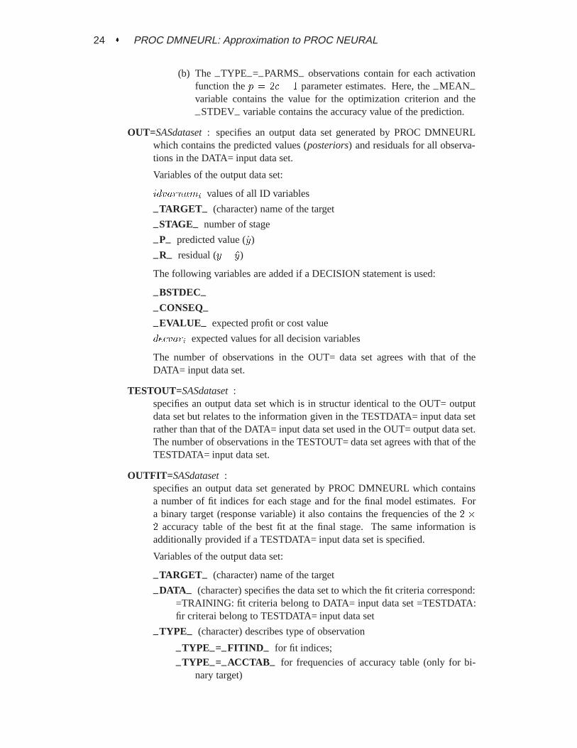
(b) The–TYPE–=–PARMS– observations contain for each activationfunction thep = 2c + 1 parameter estimates. Here, the–MEAN–variable contains the value for the optimization criterion and the
–STDEV– variable contains the accuracy value of the prediction.
OUT=SASdataset: specifies an output data set generated by PROC DMNEURLwhich contains the predicted values (posteriors) and residuals for all observa-tions in the DATA= input data set.
Variables of the output data set:
idvarnami values of all ID variables
–TARGET – (character) name of the target
–STAGE– number of stage
–P– predicted value (y)
–R– residual (y � y)
The following variables are added if a DECISION statement is used:
–BSTDEC–
–CONSEQ–
–EVALUE – expected profit or cost value
decvari expected values for all decision variables
The number of observations in the OUT= data set agrees with that of theDATA= input data set.
TESTOUT=SASdataset:specifies an output data set which is in structur identical to the OUT= outputdata set but relates to the information given in the TESTDATA= input data setrather than that of the DATA= input data set used in the OUT= output data set.The number of observations in the TESTOUT= data set agrees with that of theTESTDATA= input data set.
OUTFIT= SASdataset:specifies an output data set generated by PROC DMNEURL which containsa number of fit indices for each stage and for the final model estimates. Fora binary target (response variable) it also contains the frequencies of the2 �2 accuracy table of the best fit at the final stage. The same information isadditionally provided if a TESTDATA= input data set is specified.
Variables of the output data set:
–TARGET – (character) name of the target
–DATA – (character) specifies the data set to which the fit criteria correspond:=TRAINING: fit criteria belong to DATA= input data set =TESTDATA:fir criterai belong to TESTDATA= input data set
–TYPE– (character) describes type of observation
–TYPE–=–FITIND – for fit indices;
–TYPE–=–ACCTAB – for frequencies of accuracy table (only for bi-nary target)

Purpose of PROC DMNEURL � 25
–STAGE– number of stages in the estimation process
–SSE– sum-of-squared error of solution
–RMSE– root mean squared error of solution
–ACCU– percentage of accuracy of prediction (only for categorical target)
–AIC – Akaike information criterion
–SBC– Schwarz’ information criterion
The following variables are added if a DECISION statement is used:
–PROF–
–APROF–
–LOSS–
–ALOSS–
–IC–
–ROI–
OUTSTAT=SASdataset:specifies an output data set generated by PROC DMNEURL which contains alleigenvalues and eigenvectors of theX 0X matrix. When this option is specified,no other computations are performed and the procedure terminates after writingthis data set.
Variables of the OUTSTAT= output data set:
–TYPE– (character) type of observation
–EIGVAL – contains different numeric information
varnamei variables in the model; the first variables correspond to CLASS(categorical) the remaining variables are continuously (interval or ratio)scaled. Note, that for nonbinary CLASS (nominal or ordinal categorical)variables a set of binary dummy variables is created. In those cases theprefix of variable namesvarnamei used for a group of variables in thedata set may be the same for a successive group of variables which differsonly by a numeric suffix.
Observations of the OUTSTAT= output data set:
1. The first three observations,–TYPE–=–V–MAP– and–TYPE–=–C–MAP–,contain the mapping indices between the variables used in the model andthe number of the variables in the data set. The–EIGVAL– variablecontains the number of index mappings. This is the same informationas in the first observation of the OUTEST= data set, except that herethe –TYPE–=–EIGVAL– variables replaces the–TYPE–=–MEAN–variable in the OUTEST= data set.
2. The–TYPE–=–EIGVAL– observation contains the sorted eigenvalues oftheX 0X matrix.
3. The–TYPE–=–EIGVEC– observations contain a set ofn eigenvectorsof theX 0X matrix. Here, the–EIGVAL– variable contains the eigen-value to which the eigenvector corresponds.
26 � PROC DMNEURL: Approximation to PROC NEURAL
ABSGCONV, ABSGTOL : r � 0specifies an absolute gradient convergence criterion for the default(OPTCRIT=SSE) optimization process. See the document of PROC NLPin SAS/OR for more details. Default is ABSGCONV=5e-4 in general andABSCONV=1e-3 for FUNCTION=EXP.
CORRDF : specifies that the correct number of degrees of freedom is used for thevalues of RMSE, AIC, and SBC. Without specifying CORRDF the error de-grees of freedom are computed asW � p, whereW is the sum of weights(if the WEIGHT statement is not used, each observation has a weight of 1 as-signed, andW is the total number of observations) andp is the number ofparameters. When CORRDF is spefified the valuep is replaced by the rank ofthe joint Jacobian.
COV, CORR : specifies that a covariance or correlation matrix is used for comput-ing eigenvalues and eigenvectors compatible with the PRINCOMP procedure.The COV and CORR options are valid only if an OUTSTAT= data set is speci-fied. If neither COV nor CORR are specified, the eigenvalues and eigenvectorsof the cross product matrixXTX are computed and written to the OUTSTAT=data set.
CRITWGT=r : r > 0
specifies a positive weight for a weighted least squares fit. Currently this optionis valid only for binary target. Values ofr > 1: will enforce a better fit of the(1,1) entry in the accuracy table which may be useful for fitting rare events.Values of0 < r < 1: will enforce a better fit of the (0,0) entry in the accuracytable. Note, that values forr which are far away fromr = 1 will reduce the fitquality of the remaining entries in the frequency table. At this time values ofeither1 < r < 2 or :5 < r < 1 are preferred.
CUTOFF=r : 0 < r < 1
specifies a cutoff threshold for deciding when a predicted value of a binaryresponse is classified as 0 or 1. The default iscutoff = :5. If the value ofthe posterior,(yi), for observationi is smaller the specified cutoff value, theobservation is counted in the first column of the accuracy table (i.e. as 0),otherwise it is counted in the second column (i.e. as 1). For nonbinary targetthe cutoff= value is not used.
GCONV, GTOL : r � 0
specifies a relative gradient convergence criterion for the optimization process.See the document of PROC NLP in SAS/OR for more details. Default isGCONV=1e-8.
FCRIT specifies that the probability of theF test is being used for the selction ofprincipal components rather than the defaultR2 criterium.
MAXCOMP=i : 2 � i � 8
specifies an upper bound for the number of components selected for predictingthe target in each stage. Good values for MAXCOMP are inbetween 3 and 5.Note, that the computer time and core memory will increase superlinear for

Purpose of PROC DMNEURL � 27
larger values than 5. There is one memory allocation which takesnm longinteger values, wheren is the value specified with the NPOINT= option andm is the value specified by the MAXCOMP= option. The following table listsvalues of4nm=1000000 for specific combinations of(n;m). This is the actualmemory requirement in Megabytes assuming that a long integer takes 4 bytesstorage.
n m=3 m=4 m=5 m=6 m=7 m=85 0 0 0 0 0 27 0 0 0 0 3 23*9 0 0 0 2 19* 172
11 0 0 1 7* 78 85713 0 0 2* 19 250 326315 0 0* 3 46 683 1025217 0* 0 6 97 1641 2790319 0 1 10 188 3575 67934
The trailing asterisk indicates the default number of points for a given numberof components. Therefore, values larger than 8 fori in MAXCOMP=iare re-duced to this upper range. It seems to be better to increase the valuei of theMAXSTAGE=i option when higher precision is requested.
MAXFUNC=i : i � 0specifies an upper bound for the number of function calls in each optimization.The default is MAXFUNC=500. Normally the default number of function callswill be sufficient to reach convergence. Larger values should be used if the it-eration history indicates that the optimization process was close to a promisingsolution but would have needed more than the specified number of functioncalls. Smaller values should be specified when a faster but suboptimal solutionmay be sufficient.
MAXITER=i : i � 0
specifies an upper bound for the number of iterations in each optimization.The default is MAXITER=200. Normally the default number of iterations willbe sufficient to reach convergence. Larger values should be used if the itera-tion history indicates that the optimization process was close to a promisingsolution but would have needed more than the specified number of iterations.Smaller values should be specified when a faster but suboptimal solution maybe sufficient.
MAXROWS=i : i � 1
specifies an upper bound for the number of independent variables selected forthe model. More specific, this is an upper bound for the rows and columnsof the X’X matrix of the regression problem. The default ismaxrows =
3000. Note, that theXTX matrix used for the stepwise regression takesnrows(nrows + 1)=2 double precision values storage in RAM. For the defaultmaximum size ofnrows = 3000 you will need more than3000�1500�8 bytesRAM, which is slightly more than 36 megabytes.
MAXSTAGE=i : i � 1
specifies an upper bound for the number of stages of estimation. If

28 � PROC DMNEURL: Approximation to PROC NEURAL
MAXSTAGE is not specified, the default is MAXSTAGE=5. When a missingvalue is specified, the multistage estimation process is terminated
� if the sum-of-squares residual in the component selection process changesby less than 1%
� or when an upper range of 100 stages are processed.
That means, not specifying MAXSTAGE= or specifying a missing value aretreated differently. Large values for MAXSTAGE= may result in numericalproblems: the discretization error may be too large and the fit criterion does nolonger improve and can actually become worse. In such a case the stagewiseprocess is terminated with the last good stage.
MAXSTPT=i : i � 1
specifies the number of values of the objective function inspected for the startof the optimization process. Larger values than the default value may improvethe result of the optimization especially when more than three components areused. The default is MAXSTPT=250.
MAXVECT=i : i � 2specifies an upper bound for the number of eigenvectors made available forselection. The default is MAXVECT=400. Smaller values should be usedonly if there are memory problems for storing the eigenvectors when too manyvariables are included in the analysis. The specified value for MAXVECT=cannot be smaller than that for MINCOMP=. If the specified value ofMAXVECT= is larger than the value for MAXROWS= it is reduced to thevalue of MAXROWS=.
MEMSIZ=i : i � 1For interval targets and in a multiple stage process some memory consumingoperations are being performed. For very large data sets the computations maysignificantly depend on the size of the available RAM memory for those com-putations. By default MEMSIZ=8 specifies the availability of 8 mb of RAMfor such operations. Since other operations need additional memory not morethan 25 percent of the total amount of memory should be specified here. Ifyou are running out of memory during the DMNEURL run, you may actuallyspecify a smaller amout than the default 8 mb.
MINCOMP=i : 2 � i � 8
specifies a lower bound for the number of components selected for predictingthe target in each stage. The default is MINCOMP=2. The specified value forMINCOMP= cannot be larger than that for MAXCOMP=. The MINCOMP=specification may permit the selection of components which otherwise wouldbe rejected by the STOPR2= option. PROC DMNEURL may override thespecified value when the rank of theX 0X matrix is less than the specifiedvalue.
NOMONITOR :supresses the output of the status monitor indicating the progress made in thecomputations.

Purpose of PROC DMNEURL � 29
NOPRINT :supresses all output printed in the output window.
NPOINT=i : 5 � i � 19
number of discretization points (should be even inbetween 5 and 19). By de-fault NPOINT= is selected depending on the number of components selectedin the model using the MINCOMP= and MAXCOMP= options.
OPTCRIT=SSEjACCjWSSE :specifies the criterion for the optimization:
OPTCRIT=SSE the sum-of-squares error is minimzed.
OPTCRIT=ACC a measure of the accuracy rate is maximized. (For intervaltarget the Goodman-Kruskal is applied on a frequency table defined bydeciles of the actual target value.)
OPTCRIT=WSSE a weighted sum-of-squares criterion is minimzed.When this option is specified the weight must be specified using theCRITWGT= option. Currently this option is valid only for binary target.
PALL :
� If an OUTSTAT= data set is specified, i.e. only principal components arebeing computed, the following table illustrates the output options:
Output PSHORT default PALLSimple Stat x x xEigenvalues x x x
If PMATRIX is specified, theX 0X, the covariance, or the correlationmatrix is also printed (depending on COV and CORR option).
� If no OUTSTAT= data set is specified, i.e. a nonlinear model based onactivation and link functions is being optimized, the following table illus-trates the output options:
Output NOPRINT PSHORT default PALL
PMATRIX :This option is valid only if an OUTSTAT= data set is specified, i.e. whenDMNEURL is used only for computing eigenvalues and eigenvectors of theX 0X, covariance, or correlation matrix. If PMATRIX is specified, this matrixis being printed. Since this matrix may be very large its printout is not includedby that of the PALL option.
POPTHIS :print the detailed histories of all optimization processes. The PALL optionincludes only the summarized forms of the history output (header and result).
PSHORT :see the PALL option for the amount of output being printed.
PTABLE :specifies the output of accuracy tables. This option is invoked automatically ifthe PALL option is specified.

30 � PROC DMNEURL: Approximation to PROC NEURAL
SELCRIT=SSEjACCjWSSE :specifies the criterion for selecting the best result among all of the activationfunctions:
SELCRIT=SSE select solution with smallest sum-of-squares error.
SELCRIT=ACC select solution with largest accuracy rate. (For interval tar-get the Goodman-Kruskal is applied on a frequency table defined bydeciles of the actual target value.)
SELCRIT=WSSE select solution with smallest weighted sum-of-squares er-ror. This option is valid only for binary target. When this option is speci-fied the weight must be specified using the CRITWGT= option.
SINGULAR=r :specifies a criterion for the singularity test. The default isr = 1:e � 8 andshould not be changed if there are no significant reasons to do so.
STOPR2=r :specifies a lower value for the incremental modelR2 value at which the variableselection process is stopped. The STOPR2= criterion is used only for the R2values of the components selected in the range specified by the MINCOMP=and MAXCOMP= values. The default isr = 5e� 5.
TESTDMDB :permits the use of a data set generated by PROC DMDB to be specified as aTESTDATA= input data set. If this option is not specified, the data set specifiedwith TESTDATA= must be a normal SAS data set.
DECISION Statement
For the syntax of the DECISION statement see the document of PROC DECIDE.
FUNCTION and LINK Statement
An activation functionf and a link functiong may be specified for the mapping inbe-tween the component scoressij and the valuesyi of the response variable (stage=0)(or the residuals in stage > 0),
yi = g(f (k)(sij; �j)); i = 1; : : : ; N; j = 1; : : : ; p
for each activation functionf (k); k = 1; : : : ;K. The FUNCTION and LINK state-ment can be used to specify the functionsf (k) andg:
FUNCTION statement One or more of the following activation functionsf can bespecified

Purpose of PROC DMNEURL � 31
SQUARE (a+ b � x) � xTANH a � tanh(b � x)
ARCTAN a � atan(b � x)LOGIST exp(a � x)=(1: + exp(b � x)GAUSS a � exp(�(b � x)2)
SIN a � sin(b � x)COS a � cos(b � x)EXP a � exp(b � x)
If more than one functionf (k) is specified, each of the specified functions isevaluated during the estimation process and the best result w.r.t. to the sum-of-squares residual or accuracy (see SELCRIT= option) is selected. By default allavailable activation functions are used.
LINK statement Currently only one of the following link functions can be used forthe outer functiong:
IDENT xLOGIST exp(x)=(1: + exp(x)RECIPR 1=x
By default, the LOGIST function is used for a binary target and the IDENT(ity)function is used for interval target. In a parallelized version of PROC DM-NEURL, multiple functionsg could be feasible.
TARGET Statement
TARGET onevar;One variable name may be specified identifying the target (response) variable for thetwo regressions. Note, that one or more target variables may be specified alreadywith the PROC DMDB run. If a target is specified in the PROC DMDB run, it mustnot be specified in the PROC DMNEURL call.
VAR or VARIABLES Statement
VAR varlist ;
VARIABLES varlist ;All variables, numeric (interval) and categorical (CLASS) variables which may beused for independent variables are specified with the VAR statement.
FREQ or FREQUENCY Statement
FREQ onevar;
FREQUENCY onevar;One numeric (interval scaled) variable may be specified as a FREQ variable. Note,that a rational value is truncated to the next integer. It is recommended to specifythe FREQ variable already in the PROC DMDB run. Then the information is savedin the catalog and that variable is used automatically as a FREQ variable in PROCDMNEURL. This also ensures that the FREQ variable is being used automaticallyby all other PROCs in the EM project.

32 � PROC DMNEURL: Approximation to PROC NEURAL
WEIGHT or WEIGHTS Statement
WEIGHT onevar;
WEIGHTS onevar;One numeric (interval scaled) variable may be specified as a WEIGHT variable. It isrecommended to specify the WEIGHT variable already in the PROC DMDB invoca-tion. Then the information is saved in the catalog and that variable is used automati-cally as a FREQ variable in PROC DMNEURL.
Scoring the Model Using the OUTEST= Data set
The score valueyi is computed for each observationi = 1; : : : ; Nobs with nonmissingvalue of the target (response) variabley of the input data set. All information neededfor scoring an observation of the DMDB data set is contained in the output of theOUTEST= data set. First an observation from the input data set is mapped into avectorv of n new values in which
1. CLASS predictor variables withK categories are replaced byK + 1 or Kdummy (binary) variables, depending on the fact whether the variable has miss-ing values or not.
2. Missing values in interval predictor variables are replaced by the mean value ofthis variable in the DMDB data set. This mean value is taken from the catalogof the DMDB data set.
3. The values of a WEIGHT or FREQ variable are multiplied into the observation.
4. For an interval target variabley its value is transformed into the interval [0,1]by the relationship
ynewi =yi � ymin
ymax � ymin
5. All predictor variables are transformed into values with zero mean and unitstandard deviation by
xnewij =xij �Mean(xj)
StDev(xj)
The values forMean(xj) andStDev(xj) are listed in the OUTEST= data set.
This means, that in the presence of CLASS variables the n-vectorv has more entriesthan the observation in the data set.The scoring is additive across the stages. The following information is available forscoring each stage
� c components (eigenvectors)zl each of dimensionn
� the best activation functionf and a specified link functiong
� thep = 2c+ 1 optimal parameter estimates�j

Purpose of PROC DMNEURL � 33
For each componentzl we compute the component scoreul,
ul =nX
j=1
zljvj
similar to principal component analysis. With those valuesul the model can be ex-pressed as
y =
nstageXistage=1
g(f(u; �))
wheref is the best activation function andg is the specified link function.In other words, this means, that given theul the valuew is computed from
w = �0 +Xl
f(ul; al; bl)
whereal andbl are two of thep = 2 � c+ 1 optimal parameters� andf is defined asSQUARE w = (a+ b � u) � u
TANH w = a � tanh(b � u)ARCTAN w = a � atan(b � u)LOGIST w = exp(a � u)=(1: + exp(b � u))GAUSS w = a � exp(�(b � u)2)
SIN w = a � sin(b � u)COS w = a � cos(b � u)EXP w = a � exp(b � u)
For the first componenta1 = �1 andb1 = �2, for the second componenta2 = �3 andb2 = �4, and for the last componentac = �p�1 andbc = �p are used.The link functiong is applied onw and yields toh
IDENT h = wLOGIST h = exp(w)=(1: + exp(w)RECIPR h = 1=w
Across all stages the values ofh are added to the predicted value (posterior)y.
Related Documents


