Problems of Optical Fibre Telecommunication Systems · PDF fileIST, IMECE, PROBLEMS OF OPTICAL FIBRE TELECOMMUNICATION SYSTEMS, 2013/2014 3 Chapter 1. Introduction to Optical Fibre

Problems

of

Optical Fibre Telecommunication Systems

(with solutions)

2013/2014

Collected by Adolfo Cartaxo

February 2014

UNIVERSIDADE TÉCNICA DE LISBOA INSTITUTO SUPERIOR TÉCNICO

INTEGRATED MASTER IN

ELECTRICAL AND COMPUTER ENGINEERING

IST, IMECE, PROBLEMS OF OPTICAL FIBRE TELECOMMUNICATION SYSTEMS, 2013/2014

2

This page was left intentionally in blank.


3

Chapter 1. Introduction to Optical Fibre

Telecommunication Systems

1.1 Consider the following signal power levels: 50 µW, 1 mW and 100 mW.

(a) Calculate these power levels in dBm. (b) Calculate, in dBmV and dBµV, the voltages corresponding to those power levels measured on a resistance of 50 Ω. [A: (a) -13 dBm, 0 dBm, 20 dBm; (b) 34 dBmV, 94 dBµV, 47 dBmV, 107 dBµV, 67 dBmV, 127 dBµV ]

1.2 Consider an ideal low-pass filter, with bandwidth B and amplitude response described by:

( )1, for 10, for 1

f BH f

f B≤

= >

This filter is excited by thermal noise (white and Gaussian) with two-sided power spectral density N(f)=N0/2. Assume that N0= –110 dBm/Hz and B=4.75 MHz. (a) Determine the power spectral density of the noise at the filter output (b) Determine the average noise power at the filter output (c) Determine the noise equivalent bandwidth of the filter. [A: (a) No(f) = |H(f)|2·N(f); (b) –43.23 dBm; (c) Bn = B ]

1.3 Consider the low-pass filters family with transfer function given by:

( ) ( )1

n

H fP jf B

=

where Pn(jf/B) is a complex polynomial of order n and B is the –3 dB bandwidth. The family of Butterworth polynomials is defined by the property

( )2

1n

nfP jf BB

= +

and the corresponding filters are called low-pass Butterworth filters of order n. (a) Plot the amplitude response, in dB, of Butterworth filters of 1st, 2nd, 3rd and 4th orders. (b) Repeat Problem 1.2 for the filters considered in (a). Hint: ( ) ( ) ( )1

0 1 sin , 0mx dx m m mπ π−+∞ + = >∫

[A: (b) No(f) = 1/[1+(f/B)2n]·N(f), N0B·x/sin x with x= π/(2n), Bn = B·x/sin x with x= π/(2n) ] 1.4 A pre-amplifier of an electrical receiver, designed to amplify unipolar binary signals at

2.5 Gbit/s, presents a noise figure of 3 dB and a gain of 13 dB. The equivalent noise bandwidth of the pre-amplifier is 25% higher than the minimum bandwidth required to transmit binary signals with zero inter-symbol interference.


4

(a) Calculate the noise equivalent bandwidth of the pre-amplifier. (b) Calculate the noise power generated internally (measured at the pre-amplifier output), and

compare with the noise power amplified from the input to the pre-amplifier output, in dBm. (c) For a signal power of 1 nW at the pre-amplifier input, calculate the signal to noise ratio, in

dB, at the pre-amplifier output. [A: (a) 1.56 GHz; (b) -69.06 dBm; (c) 19.04 dB ]

1.5 Suppose that, after the pre-amplifier, an electrical amplifier with noise figure of 6 dB and gain of 20 dB is inserted. Consider that this amplifier has the same noise equivalent bandwidth as the pre-amplifier. (a) Calculate the noise power (generated internally in the amplifier) at the amplifier output. (b) Calculate the overall noise power at the amplifier output using the accumulation of noise

power along the chain. (c) Using the answer to the previous question, calculate the signal to noise ratio, in dB, at the

amplifier output for the same signal power as considered in Problem 1.4. (d) Calculate the signal to noise ratio, in dB, at the amplifier output using the Friis’ formula. (e) Explain why you do not get the same result if you use the definition of noise figure and the

result of Problem 1.4-c) to calculate the signal to noise ratio at the amplifier output. (f) Calculate the difference, in dB, between the signal to noise ratio at the pre-amplifier output

and the signal to noise ratio at the amplifier output and explain why, even with such a large amplifier noise figure, just a small degradation of signal to noise ratio is caused by the amplifier.

[A: (a) 1.87 nW; (b) 26.77 nW, -45.72 dBm; (c) 18.72 dB; (d) 18.72 dB; (e) reason is related to the definition of noise figure; (f) 0.32 dB ]

1.6 Consider that the noise at the input to the pre-amplifier of Problem 1.4 has a power spectral

density (PSD) given by Si(f)=Slf·[1+(f/fc)2] where Slf is the PSD of noise at low frequency (thermal noise at room temperature) and fc is the noise corner frequency. Consider the pre-amplifier can be modelled by an ideal low-pass filter. (a) Calculate the noise power at the pre-amplifier input in the pre-amplifier band, for fc=0.01 Rb

and fc=100 Rb, with Rb the bit rate. (b) Calculate the noise power at the pre-amplifier output, in dBm, for fc=0.01 Rb and fc=100 Rb. (c) For a signal power of 1 nW at the pre-amplifier input, calculate the signal to noise ratio, in

dB, at the pre-amplifier output for fc=0.01 Rb and fc=100 Rb using the power of noise generated internally by the pre-amplifier.

(d) Analyze if get the same result as using the definition of noise figure to calculate the signal to noise ratio at the amplifier output, for the two cases of noise corner frequency.

[A: (a) 8.15 nW, 6.26 pW; (b) -37.88 dBm, -66.04 dBm; (c) -9.12 dB, 19.04 dB] 1.7 Calculate the carrier frequency for optical communication systems operating at 0.88, 1.3, and

1.55 µm. What is the photon energy (in eV and J) in each case? [A: for λ=1.55 µm, υ =193.5 THz, Eph = 0.80 eV = 1.28×10-19 J]

1.8 Calculate the transmission distance over which the optical power will attenuate by a factor of 10

for three fibres with losses of 0.2, 20, and 2000 dB/km. Assume that the optical power decreases as exp(−αL), calculate α (in cm−1) for the three fibres. [A: for α = 0.2 dB/km, L = 50 km, α = 4.61×10-7 cm-1]


5

1.9 Assume that a digital communication system can be operated at a bit rate of up to 1% of the carrier frequency. How many digitized voice channels at 64 kb/s can be transmitted over a microwave carrier at 5 GHz and an optical carrier at 1.55 µm? [A: for 5 GHz, N = 781; for 1.55 µm, N = 3.024×107]

1.10 A 1.55 µm digital communication system operating at 1 Gb/s receives an average power of

−40 dBm at the detector. Assuming that 1 and 0 bits are equally likely to occur, calculate the number of photons received within each 1 bit. [A: Nph = 1560]

1.11 Sketch the variation of optical power with time for a digital NRZ bit stream 010111101110 by

assuming a bit rate of 2.5 Gb/s. What is the duration of the shortest and widest optical pulse? [A: 0.4 ns, 1.6 ns]

1.12 Repeat Problem 1.11 considering a RZ bit stream with duty-cycle of 50% and 25%.

[A: the shortest and longest optical pulse have the same duration; for 50% of duty-cycle, 0.2 ns; for 25% of duty-cycle, 0.1 ns]

1.13 A 1.55 µm fibre-optic communication system is transmitting digital signals over 100 km at

2 Gb/s. The transmitter launches 2 mW of average power into the fibre cable, having a net loss of 0.3 dB/km. How many photons are incident on the receiver during a single “1” bit? Assume that “0” bits carry no power, while “1” bits are in the form of a rectangular pulse occupying the entire bit slot (NRZ format). [A: Nph = 15625]

1.14 Repeat Problem 1.13, assuming that “1” bits are in the form of a rectangular pulse occupying

half bit slot duration (RZ format with 50% duty-cycle). Discuss the advantages and disadvantages of using the RZ format. [A: Nph = 15625]

1.15 A 0.8-µm optical receiver needs at least 1000 photons to detect the “1” bits accurately. What is

the maximum possible length of the fibre link for a 100-Mb/s optical communication system designed to transmit −10 dBm of average power? The fibre loss is 2 dB/km at 0.8 µm. Assume the NRZ format and a rectangular pulse shape. [A: 19.535 km]

1.16 A 1.3-µm optical transmitter is used to obtain a digital bit stream at a bit rate of 2 Gb/s.

Calculate the number of photons contained in a single “1” bit when the average power emitted by the transmitter is 4 mW. Assume that the “0” bits carry no energy. [A: Nph = 2.62×107]

1.17 We intend to compare the optical bandwidth, in nm, required to transmit 40 Gb/s using two techniques, TDM and WDM, at the third window. In case of WDM, the bit rate per channel is 10 Gbit/s, and a channel spacing of 50 GHz is used. (a) Consider the minimum bandwidth required to avoid inter-symbol interference. (b) Consider the (approximated) bandwidth required to transmit NRZ rectangular pulses.


6

(c) Comparing the results of questions (a) and (b), we might think that, for a bit rate of 1 Tbit/s, it would be preferable to use TDM as well. Explain why it is not so.

[A: (a) TDM: 0.32 nm, WDM: 1.6 nm; (b) TDM: 0.64 nm, WDM: 1.6 nm]

1.18 Consider two optical signals with the same bit rate, average optical power, and rectangular pulse shape, but with a RZ format with different duty-cycle of 66% and 33%. Assume that “0” bits carry no power. Calculate the peak power ratio of “1” bits of the two signals. [A: ppeak,33%/ppeak,66% =2]

1.19 Consider two optical signals with the same average optical power, and format (bit rate, RZ format, pulse shape, ratio between power levels for “1” and “0” bits, etc.), one operating in the second window and the other one operating at the third window of communication. (a) Which signal presents a higher number of photons per unit of time? (b) Calculate the ratio between the number of photons per unit of time of the two signals. [A: (a) third window signal; (b) 1.19]

1.20 Dry fibres have acceptable losses over a spectral region extending from 1.3 to 1.6 µm. Estimate

the capacity of a WDM system covering this entire region using 40-Gb/s channels spaced apart by 50 GHz. [A: 34.6 Tbit/s]

1.21 An average optical power of −40 dBm is incident on an optical receiver. In the optical receiver,

the conversion of the optical (power) signal to electrical (current) signal is performed by a photodetector (opto-electrical converter) characterised by a conversion factor of 0.8 A/W. The electrical pre-amplifier current gain is 20 dB. Calculate the average electrical current at the pre-amplifier output, in µA. [A: 0.8 µA]


7

Total internal reflection of light in a multimode fibre

Chapter 2. Techniques and

Technologies of Optical Fibre

Telecommunication Systems

2.1 A step-index multimode glass fibre, with a core diameter of 50 µm and cladding refractive index

of 1.45, is designed to limit the intermodal dispersion to 10 ns/km. (a) Find its acceptance angle. (b) Calculate the maximum bit rate for transmission over a distance of 20 km. [A: (a) NA = 0.093; (b) Rb = 2.5 Mb/s]

2.2 Derive an expression for the cutoff wavelength λcutoff of a step-index fibre with core radius a,

core refractive index nl, and cladding refractive index n2. Calculate the cutoff wavelength of a fibre with core radius a = 4 µm and ∆ = 0.003. [A: λcutoff = 1.214 µm]

2.3 A single-mode fiber has an index step with n1−n2 = 0.005. Calculate the core radius if the fibre

has a cutoff wavelength of 1 µm. Consider n1 = 1.45. [A: a = 3.18 µm]

2.4 Consider a step-index fibre with a core radius of 4 µm and a cladding refractive index of 1.45.

(a) For what range of values of the core refractive index will the fibre be single moded for all wavelengths in the 1.2-1.6 µm range?

(b) What is the value of the core refractive index for which the V parameter is 2.0 at λ=1.55 µm? (c) What is the propagation constant of the single mode supported by the fibre for this value of

the core refractive index? [A: (a) 1.45 < n1 < 1.4545; (b) n1 < 1.4552; (c) β = 5.887 / µm]

2.5 Assume that, in the manufacture of single-mode fibre, the tolerance in the core radius a is +5%

and the tolerance in the normalized refractive index difference ∆ is +10%, from their respective nominal values. If the nominal value of ∆ is specified to be 0.005, what is the largest nominal value that you can specify for a while ensuring that the resulting fibre will be single moded for λ > 1.2 µm even in the presence of the worst-case (but within the specified tolerances) deviations of a and ∆ from their nominal values? Assume that the refractive index of the core is 1.5. [A: a = 2.78 µm]


8

2.6 A 1.3 µm lightwave system uses a 50-km fibre link and requires at least 0.3 µW at the receiver. The fibre loss is 0.5 dB/km. Fibre is spliced every 5 km and has two connectors of 1-dB loss at both ends. Splice loss is only 0.2 dB. Determine the minimum power that must be launched into the fibre. [A: 0.227 mW]

2.7 A 1550 nm conventional optical link uses a standard single-mode fibre with dispersion parameter of 16 ps/nm/km, and a MLM laser with linewidth of 3 nm as optical transmitter. (a) Assuming the link carries a 2.5 Gbit/s binary signal, calculate an estimate of the maximum

link length imposed by chromatic dispersion. (b) Assuming the link carries a 10 Gbit/s binary signal, calculate an estimate of the maximum

link length imposed by chromatic dispersion. [A: (a) 4.17 km; (b) 1.04 km]

2.8 A 1550 nm conventional optical link uses a standard single-mode fibre with dispersion

parameter of 16 ps/nm/km, and an externally modulated SLM laser as optical transmitter. (a) Assuming the link carries a 2.5 Gbit/s binary signal, calculate an estimate of the maximum

link length imposed by chromatic dispersion. (b) Assuming the link carries a 10 Gbit/s binary signal, calculate an estimate of the maximum

link length imposed by chromatic dispersion. [A: (a) 623.9 km; (b) 39 km]

2.9 Explain how the results of Problem 2.7 change when the SSMF is replaced by a NZ-DSF with

dispersion parameter of 4 ps/nm/km. 2.10 Explain how the results of Problem 2.8 change when the SSMF is replaced by a NZ-DSF with

dispersion parameter of 4 ps/nm/km. 2.11 A link of 250 km of standard singlemode fibre with dispersion parameter of 16.8 ps/nm/km and

dispersion slope of 70 fs/nm2/km at 1550 nm is used to transmit a DWDM signal with 31 channels centred at 193.1 THz and spaced by 100 GHz. (a) Calculate the maximum and minimum dispersion of the different channels. (b) Assuming the optical transmitter is an externally modulated SLM laser and all channels

carry the same bit rate, calculate an estimate of the maximum capacity of this WDM system imposed by chromatic dispersion.

[A: (a) 4457 ps/nm, 4035 ps/nm; (b) 3.7 Gbit/s per channel, 114.7 Gbit/s]


9

2.12 DWDM link with 80 channels and channel spacing of 50 GHz uses DCF to compensate for the chromatic dispersion effects of the transmission fibre (SSMF) in each transmission section and EDFAs to compensate for the fibre losses, as depicted in Figure 2.12.

Fig. 2.12 Scheme of the optical fibre link with Nsec amplification sections. The link uses dispersion compensating

fibres (DCFs) to compensate for the effects of chromatic dispersion of the transmission fibre (standard singlemode fibre - SSMF) and erbium-doped fibre amplifiers (EDFAs) to compensate for the fibre losses.

Channels are numbered sequentially from 1 at the lowest frequency. Channel 24 is located at the ITU-T DWDM grid reference frequency of 193.1 THz. The link is composed by transmission sections of 80 km of SSMF, which has a dispersion parameter of 17 ps/(nm km) and a dispersion slope of 70 fs/(nm2·km) at 1550 nm, and a PMD parameter of 0.5 ps/√km. The used DCF has a figure of merit of 300 ps/(nm dB), a dispersion slope of 300 fs/(nm2·km) and a loss coefficient of 0.4 dB/km at 1555 nm, and a PMD parameter of 0.3 ps/√km. The link is designed so that, at channel 41 (nearly the center of transmission band), perfect dispersion compensation (i. e. zero total dispersion) is implemented. (a) Calculate the length of DCF in each transmission section. (b) Calculate the total dispersion per transmission section of the channel that suffers from the highest dispersion. (c) Assuming that each channel carries 10 Gbit/s and that each optical transmitter uses an externally modulated SLM laser, calculate an estimate of the maximum transmission distance of the link imposed by residual chromatic dispersion. (d) Calculate an estimate of the maximum transmission distance of the link imposed by PMD. Hint: for n spans of fibre with different average DGDs, <∆τ1>, …, <∆τn> respectively, the average total DGD is given by <∆τt>=(<∆τ1>2+…+<∆τn>2)1/2. [A: (a) 10.881 km; (b) 142.76 ps/nm; (c) 320 km; (d) 320 km]

2.13 A link of single-mode fibre with length of 80 km has 16 sections of fibre with the same length

and operates at 1550 nm. These sections of fibre are connected by splices with 0.05 dB of loss. The loss coefficient of the fibre is 0.2 dB/km. Connectors with 0.25 dB of loss are used only at the transmitter and receiver sides. (a) Calculate the average optical power coupled to the fibre at the transmitter to guarantee an average power at the receiver input of –35 dBm. (b) Imagine that a splice has been replaced by a connector with loss of 0.25 dB. Calculate the reduction of length of the link to guarantee the optical power levels considered in (a). [A: (a) 16.8 µW; (b) 1 km]

2.14 For the link of Problem 2.13, explain qualitatively how the answers to questions (a) and (b)

change if the link operates at the second window.

Transmitter

(Nsec times)

80 km SSMF

OLR – Optical Line Repeater

DCF EDFA EDFA

Transmission section

Receiver


10

2.15 For linear transmission along a single-mode optical fibre with length L, the Fourier transform of the complex amplitude of the electrical field at the optical fibre output, Ao(ω), is related to the Fourier transform of the complex amplitude of the electrical field at the optical fibre input, Ai(ω), by

( ) ( )2

2exp2 2o i

j LLA A β ωαω ω = ⋅ − −

where ω is the angular frequency (rad/s), α is the power loss coefficient (in m-1) and β2 is the group velocity dispersion (GVD) parameter. The GVD parameter is related to the dispersion parameter by β2 = -λ2Dλ/(2πc) where λ is the wavelength of the optical carrier, Dλ is the dispersion parameter (usually expressed in ps/nm/km) at the wavelength λ and c is the light speed in vacuum (≈ 3×108 m/s). (a) Calculate the transfer function of the electrical field of a single-mode fibre, and the corresponding amplitude and group delay responses. (b) Determine under which conditions the single-mode fibre does not cause distortion in the amplitude and does not cause distortion in the group delay. (c) Determine the slope of the group delay, and discuss the meaning of DλL and Dλ from the obtained result.

2.16 An optical time domain reflectometer (OTDR) has an error in the time basis of 0.01% and

launches pulses with width of 10 ns. Consider that the optical fibre is cut 20 km away from the place where the OTDR is connected. Calculate the maximum precision in the indication of the cut by the OTDR. [A: ±2.5 m]

2.17 The action of a fibre coupler is governed by the matrix equation Eout = TEin, where T is the 2×2

transfer matrix and E is a column vector whose two components represent the input (or output) fields at the two ports. Assuming that the total power is preserved, show that the transfer matrix T is given by

1

1

f j f

j f f

−=

− T

where f is the fraction of the power transferred to the cross port. Hint: T should be both unitary and symmetric.

2.18 Consider a fibre coupler with the transfer matrix given in Problem 2.17. Its two output ports are

connected to each other to make a loop of length L. Find an expression for the transmittivity of the fibre loop. What happens when the coupler splits the input power equally? Provide a physical explanation. [A: Tl = 1–4f(1–f)]

2.19 A star network uses directional couplers with 0.5-dB excess loss to distribute data to its

subscribers. If each receiver requires a minimum of 100 nW and each transmitter is capable of emitting 0.5 mW, calculate the maximum number of subscribers served by the network. Remark: a WDM broadcast-and-select network is based on the use of this broadcast star. [A: Ns = 1024]


11

2.20 A 128×128 broadcast star is made by using 2×2 directional couplers, each having an excess loss of 0.2 dB. Each channel transmits 1 mW of average power and requires 1 µW of average received power for operation at 1 Gb/s. What is the maximum transmission distance for each channel? Assume a cable loss of 0.25 dB/km and a loss of 3 dB from connectors and splices. [A: 18.1 km]

2.21 A Fabry–Perot filter of length L has equal reflectivities R for the two mirrors. Derive an

expression for the transmission spectrum T(υ) considering multiple round trips inside the cavity containing air. Use it to show that the finesse is given by F = π √R / (1−R).

2.22 Consider a demultiplexer, based on Fabry–Perot filters, that is used to select any of the 100

channels spaced apart by 25 GHz in a WDM system with 10 Gbit/s per channel. Speed of light in vacuum is 2.998×108 m/s. (a) Draw a scheme of the demultiplexer, and indicate the main parameters of each device that

composes the demultiplexer. (b) What should be the maximum cavity length and the mirror reflectivities of the Fabry-Perot

filters? Assume a refractive index of 1.5 and an operating wavelength of 1.55 µm. (c) What is the crosstalk suppression from each adjacent channel? (d) For a WDM system with the channels sequentially numbered from 1 at the lowest frequency

of 193.1 THz, determine the maximum cavity length of the Fabry-Perot filters that select channel 1 and channel 100.

[A: (b) Lc≤39.97 µm, R≤98.75%; (c) 14.14 dB; (d) Lc≤39.85 µm for channel 1 and Lc≤39.86 µm for channel 100]

2.23 Show that the resonant frequencies fn of a Fabry-Perot cavity satisfy fn = f0 + n ∆f, n integer, for

some fixed f0 and ∆f. Thus, the resonant frequencies are spaced equally apart. Note that the corresponding wavelengths are not spaced equally apart.

2.24 Show that the fraction of the input power that is transmitted through the Fabry-Perot filter, over

all frequencies, is (1–R)/(1+R). Note that this fraction is small for high values of R. Thus, when all frequencies are considered, only a small fraction of the input power is transmitted through a cavity with highly reflective facets.

2.25 Consider a 16-channel WDM system where the interchannel spacing is nominally 100 GHz.

Assume that one of the channels is to be selected by a filter with a 1 dB bandwidth of 2 GHz. We consider a Fabry-Perot filter for this purpose. Assume the center wavelengths of the channels do not drift. What is the required finesse and the corresponding mirror reflectivity of a Fabry-Perot filter that achieves a crosstalk suppression of 30 dB from each adjacent channel? If the center wavelengths of the channels can drift up to ±20 GHz from their nominal values, what is the required finesse and mirror reflectivity? [A: FSR ≥ 1600 GHz, 254 < F < 407, 0.988 < R < 0.992; in case of drift, the two requirements cannot be satisfied simultaneously]


12

2.26 Consider a cascade of two Fabry-Perot filters with cavity lengths l1 and l2, respectively. Assume the mirror reflectivities of both filters equal R, and the refractive index of their cavities is n. Neglect reflections from the second cavity to the first and vice versa. What is the transmission spectrum T(υ) of the cascade? If l1/l2 = k/m, where k and m are relatively prime integers, find an expression for the FSR of the cascade. Express this FSR in terms of the FSRs of the individual filters. [A: T(υ) = T1(υ) T2(υ), FSR = k FSR1 = m FSR2]

2.27 Consider the Rowland circle construction shown in Figure 2.27.

Fig. 2.27 The Rowland circle construction for the couplers used in the AWG

Show that the differences in path lengths between a fixed-input waveguide and any two successive arrayed waveguides is a constant. Assume that the length of the arc on which the arrayed waveguides are located is much smaller than the diameter of the Rowland circle. Hint: choose a Cartesian coordinate system whose origin is the point of tangency of the Rowland and grating circles. Now express the Euclidean distance between an arbitrary input (output) waveguide and an arbitrary arrayed waveguide in this coordinate system. Use the assumption stated earlier to simplify your expression. Finally, note that the vertical spacing between the arrayed waveguides is constant. Therefore, δi = d sin θi, where d is the vertical separation between successive arrayed waveguides, and θi is the angular separation of input waveguide i from the central input waveguide, as measured from the origin.

2.28 Derive an expression for the FSR of an AWG for a fixed-input waveguide i and a fixed-output

waveguide j. The FSR depends on the input and output waveguides. But show that if the arc length of the Rowland circle on which the input and output waveguides are located (see Figure 2.23) is small, then the FSR is approximately constant. Use the result from Problem 2.27 that δi = d sin θi. [A: FSR ≈ c / (n2·∆L)]

2.29 Consider an AWG that satisfies the condition given in Problem 2.28 for its FSR to be

approximately independent of the input and output waveguides. Given the FSR, determine the set of wavelengths that must be selected in order for the AWG to function as a wavelength router. Assume that the angular spacing between the input (and output) waveguides is constant. Use the result that δi = d sin θi. [A: λ00= n2·∆L / p, υi+1,j = ∆υ + υi,j with ∆υ = FSR / N]


13

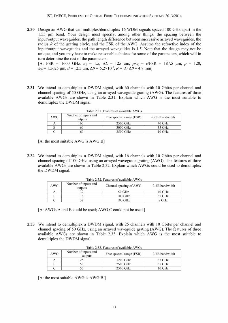
2.30 Design an AWG that can multiplex/demultiplex 16 WDM signals spaced 100 GHz apart in the 1.55 µm band. Your design must specify, among other things, the spacing between the input/output waveguides, the path length difference between successive arrayed waveguides, the radius R of the grating circle, and the FSR of the AWG. Assume the refractive index of the input/output waveguides and the arrayed waveguides is 1.5. Note that the design may not be unique, and you may have to make reasonable choices for some of the parameters, which will in turn determine the rest of the parameters. [A: FSR = 1600 GHz, n2 = 1.5, ∆L = 125 µm, pλ00 = c/FSR = 187.5 µm, p = 120, λ00 = 1.5625 µm, d = 12.5 µm, ∆θ = 5.2×10-3, R = d / ∆θ = 4.8 mm]

2.31 We intend to demultiplex a DWDM signal, with 60 channels with 10 Gbit/s per channel and

channel spacing of 50 GHz, using an arrayed waveguide grating (AWG). The features of three available AWGs are shown in Table 2.31. Explain which AWG is the most suitable to demultiplex the DWDM signal.

Table 2.31. Features of available AWGs

AWG Number of inputs and outputs Free spectral range (FSR) –3 dB bandwidth

A 60 2500 GHz 40 GHz B 60 3000 GHz 35 GHz C 60 3500 GHz 10 GHz

[A: the most suitable AWG is AWG B]


channel spacing of 100 GHz, using an arrayed waveguide grating (AWG). The features of three available AWGs are shown in Table 2.32. Explain which AWGs could be used to demultiplex the DWDM signal.


AWG Number of inputs and outputs Channel spacing of AWG –3 dB bandwidth


[A: AWGs A and B could be used; AWG C could not be used.]


channel spacing of 50 GHz, using an arrayed waveguide grating (AWG). The features of three available AWGs are shown in Table 2.33. Explain which AWG is the most suitable to demultiplex the DWDM signal.


AWG Number of inputs and outputs Free spectral range (FSR) –3 dB bandwidth


[A: the most suitable AWG is AWG B.]


14

2.34 In discussing the chromatic dispersion penalty, the Telcordia standard for SONET systems specifies the spectral width of a pulse, for single-longitudinal mode (SLM) lasers, as its 20 dB spectral width divided by 6.07. Show that, for SLM lasers whose spectra have a Gaussian profile, this is equivalent to the rms spectral width.

2.35 Consider the three optical transmitters presented in Table 2.35.

(a) Calculate the average power coupled to the optical fibre in each transmitter. Consider the optical transmitters generate rectangular NRZ optical pulses. (b) Using data presented in Table 2.35, explain which type of optical source is used in each one of the three transmitters. (c) We wish to choose one among the three transmitters for a 5 Gb/s single channel link. Explain which transmitter is the most adequate for that link.

Table 2.35. Characteristics of the optical transmitters

Transmitter Optical power level coupled to the optical fibre for 0 bits

Extinction ratio

–3 dB bandwidth

Linewidth

A 0.5 mW 10 dB 6 GHz 10 MHz B 0.5 mW 7 dB 2.5 GHz 1 MHz C 0.1 mW 13 dB 2 GHz 200 GHz

[A: (a) A => 2.75 mW, B => 1.5 mW, C => 1.05 mW; (b) A, B => SLM lasers, C => MLM laser; (c) A]

2.36 Consider a lithium niobate Mach-Zehnder modulator (MZM) with Vπ = 4 V and insertion loss of

5 dB. The MZM is biased in a push-pull configuration, and we intend an optical signal at the MZM output with an extinction ratio of 13 dB. The optical power coupled to the MZM input is 5 dBm. (a) Determine the bias and signal voltage swing so that the output average optical power is maximised. (b) Determine the bias and signal voltage swing so that the output average optical power is -2 dBm. (c) Considering that the signal voltage has the form of rectangular pulses occupying the entire bit slot (NRZ format), calculate the power levels and the average optical power at the MZM output. [A: (a)…; (b)……; (c)…… ]

2.37 In an experiment designed to measure the attenuation coefficient of optical fibre, the output

power from an optical source is coupled onto a length of the fibre and measured at the other end. If a 10 km-long spool of fibre is used, the received optical power is –20 dBm. Under identical conditions but with a 20 km-long spool of fibre (instead of the 10 km-long spool), the received optical power is –23 dBm. What is the value of α (in dB/km)? If the source-fibre coupling loss is 3 dB, the fibre-detector coupling loss is 1 dB, and there are no other losses, what is the output power of the source (expressed in W)? [A: 0.3 dB/km, 50 µW]

2.38 Calculate the responsivity of a PIN photodiode at 1.3 and 1.55 µm if the quantum efficiency is

80%. Why is the photodiode more responsive at 1.55 µm? [A: Rλ = 0.84 A/W @ 1.3 µm, Rλ = 1 A/W @ 1.55 µm]


15

2.39 Photons at a rate of 1010/s are incident on an APD with responsivity of 6 A/W. Calculate the quantum efficiency and the photocurrent at the operating wavelength of 1.5 µm for an APD gain of 10. [A: η = 0.496, Ip= 7.94 nA ]

2.40 Draw a block diagram of a digital optical receiver showing its various components. Explain the

function of each component. How is the signal used by the decision circuit related to the incident optical power?

2.41 Consider a 0.8 µm receiver with a silicon PIN photodiode. Assume 20 MHz bandwidth, 65%

quantum efficiency, 1 nA dark current, 8 pF junction capacitance, and 3 dB amplifier noise figure. The receiver is illuminated with 5 µW of optical power. Determine the root mean square (RMS) noise currents due to shot noise, thermal noise, and amplifier noise. Also calculate the signal-to-noise ratio. [A: σs = 3.66 nA, σt = 18.2 nA, σa = 18.2 nA, SNR = 38.1 dB]

2.42 The receiver of Problem 2.41 is used in a communication system that requires a signal-to-noise

ratio of at least 20 dB for satisfactory performance. What is the minimum received power when the detection is limited by (a) shot noise and (b) circuit noise? Also calculate the noise-equivalent power in the two cases. [A: 2.81 nW for shot noise limited, 616 nW for circuit noise limited]

2.43 Derive an expression for the optimum value of M for which the signal-to-noise ratio becomes

maximum by using FA(M) = Mx. 2.44 Show that the bit-error rate (BER) for an OOK direct detection receiver is given by BER =

erfc(Q/√2) / 2 with Q=(I1–I0)/(σ0+σ1). 2.45 Prove that the bit-error rate (BER) of digital optical receiver is minimum when the decision

threshold is set close to ID = (σ0I1+σ1I0) / (σ0+σ1). 2.46 Derive an expression for the optimum gain Mopt of an APD receiver that would maximize the

receiver sensitivity by taking the excess-noise factor as Mx. Plot Mopt as a function of x for σc = 0.2 µA and receiver bandwidth of 1 GHz and estimate its value for silicon APDs (x = 0.35). [A: Mopt = 113.6]

2.47 Derive an expression for the sensitivity of an APD receiver by taking into account a finite

extinction ratio for the general case in which both shot noise and circuit noise contribute to the receiver sensitivity. You can neglect the dark current.

2.48 Consider a PIN receiver (without optical amplification) assuming a circuit noise limited

operation and finite extinction ratio. (a) Derive an expression for the sensitivity of this PIN receiver. (b) Using the expression derived in (a), calculate the sensitivity of a 1.55 µm 2.5 Gb/s optical receiver that uses a PIN with quantum efficiency of 80%, square-root of one-sided power spectral density of the noise current of 4 pA/Hz1/2, and the electrical part of the receiver is


16

modelled by a third order Butterworth filter with -3 dB bandwidth of 65% of the transmission bit rate. The sensitivity is defined for a bit error probability of 10-9. Consider an infinite extinction ratio. Hint: use the result of Problem 1.3 (b). (c) Calculate the noise equivalent power (NEP), in dBm / √Hz, of the optical receiver described in (b). (d) Calculate the sensitivity of an optical receiver with the features presented in (b) for a transmission bit rate of 10 Gbit/s, using the receiver sensitivity calculated in (b). [A: (b) ≈ –30 dBm; (c) –84 dBm/√Hz; (d) ≈ –27 dBm]

2.49 A 1.3-µm digital receiver is operating at 100 Mb/s and has an effective noise bandwidth of

60 MHz. The PIN photodiode has negligible dark current and 90% quantum efficiency. The load resistance is 100 Ω and the amplifier noise figure is 3 dB. (a) Calculate the receiver sensitivity corresponding to a BER of 10−9. (b) How much does it change if the receiver is designed to operate reliably up to a BER of 10−12? [A: (a) 880 nW; (b) 1026 nW]

2.50 Calculate the receiver sensitivity (at a BER of 10−9) for the receiver in Problem 2.49 in the shot-

noise and circuit-noise limits. How many photons are incident during bit “1” in the two limits if the optical pulse can be approximated by a square pulse? [A: 0.367 nW or Nph = 48 for shot noise limited, 880 nW or Nph = 117329 for circuit noise limited]

2.51 Consider a PIN direct detection receiver where the circuit noise is the main noise component,

and its variance has the value 1.656×10-22 Rb A2, with Rb the bit rate. What is the receiver sensitivity expressed in photons per “1” bit at a bit rate of 100 Mb/s and 1 Gb/s, for a bit error rate of 10-12? Assume that the operating wavelength is 1.55 µm and the responsivity is 1.25 A/W. [A: 1.44 µW or Nph = 1.12×105 for 100 Mb/s, 4.56 µW or Nph = 35.5×103 for 1 Gb/s]

2.52 Consider the three PIN receivers with characteristics shown in Table 2.52. The sensitivity of the

three receivers was measured with the same signal at the receiver input. (a) We need to choose one receiver for a 2.5 Gbit/s link. Explain which one of the three receivers is the most indicated for that link. b) Assume the frequency response of each one of the receivers is well modelled by a third order Bessel filter with the bandwidth shown in Table 2.52. Explain which receiver has the highest noise equivalent power (NEP) and which one has the lowest NEP.

Table 2.52. Characteristics of the PIN receivers

Receiver Responsivity Sensitivity @ BER=10-9 –3 dB bandwidth A 0.6 A/W -30 dBm 2 GHz B 0.5 A/W -31 dBm 1 GHz C 0.3 A/W -29 dBm 1.5 GHz

[A: (a) A; (b) NEP(A) < NEP(B) < NEP(C) ] 2.53 An optical amplifier can amplify a 1 µW signal to the 1 mW level. What is the output power

when a 1 mW signal is incident on the same amplifier? Assume the saturation power is 10 mW. [A: 34.63 mW ]


17

2.54 Explain the concept of noise figure for an optical amplifier. Why does the SNR of the amplified signal degrade by 3 dB even for an ideal amplifier?

2.55 Consider an EDFA that is required to amplify wavelengths between 1532 nm and 1550 nm

within the C-band (separated by 100 GHz). (a) Draw a schematic of this basic EDFA, and assume the pump laser is selected to minimize ASE. Also, be sure to prevent backward reflections at the EDFA input/output. (b) Draw the relevant energy bands and associated energy transitions between these bands. (c) How many wavelengths could be amplified within this range (and spacing)? (d) Compute the required range in energy transitions to support the entire range of wavelengths. (e) Suppose we wanted to (1) add and drop a subset of these wavelengths at the EDFA and (2) add a second stage that would be best suited for maximum output powers. Please draw this new two-stage EDFA, with the add/drop multiplexing function drawn as a “black box” labeled “ADM”.

2.56 (a) Derive an expression for the sensitivity of a direct-detection receiver when an EDFA is used

as a preamplifier. (b) Calculate the receiver sensitivity at a BER of 10−9 and 10−12. Assume that the receiver operates at 1.55 µm with 3-GHz bandwidth and infinite extinction ratio. The preamplifier has a noise figure of 4 dB, and a 1-nm optical filter is installed between the preamplifier and the detector. [A: (b) –41.43 dBm for BER of 10−9, –40.42 dBm for BER of 10−12]

2.57 Using the expression derived in Problem 2.56, (a) Indicate the gain of the optical preamplifier that maximises the optically preamplified

receiver sensitivity, and obtain an expression for the sensitivity for that gain. (b) Taking into account that the available gain of a typical optical preamplifier goes up to 35

dB, what is the receiver sensitivity degradation we have when using a typical optical preamplifier relative to the situation of best sensitivity?

2.58 (a) Derive an expression for the average optical power required at the optical pre-amplifier input to guarantee a specified bit error ratio, assuming dominance of the preamplifier noise and an infinite extinction ratio. (b) Using the expression derived in (a), calculate the sensitivity of an optically preamplified 2.5 Gb/s receiver that uses the PIN and electrical part of receiver presented in Problem 2.48. Assume the bit error probability of 10-9, signal wavelength of 1550 nm, and optical amplifier with gain of 30 dB and noise figure of 5 dB. Between the optical amplifier and the PIN, an optical filter with bandwidth of 1 nm is used. (c) Calculate the sensitivity improvement, in dB, achieved by using optical preamplification. [A: (b) −42.20 dBm for BER of 10−9, (c) 12.20 dB]

2.59 Plot the receiver sensitivity as a function of bit rate for an optically preamplified receiver for three different optical bandwidths: (a) the ideal case, Bo,n = 2 Be,n, (b) Bo,n = 100 GHz, and (c) Bo,n = 30 THz, that is, an unfiltered receiver. Assume an amplifier noise figure of 6 dB, and the electrical bandwidth Be,n is half the bit rate, and use the circuit noise variance given by 1.656×10-22 Rb A2. What do you observe as the optical bandwidth is increased?

2.60 You are doing an experiment to measure the BER of an optically preamplified receiver. The

setup consists of an optical amplifier followed by a variable attenuator to adjust the power going


18

into the receiver, followed by a PIN receiver. You plot the BER versus the power going into the receiver over a wide range of received powers. Calculate and plot this function. What do you observe regarding the slope of this curve? Assume that Bo,n = 100 GHz, Be,n = 2 GHz, Rb = 2.5 Gb/s, a noise figure of 6 dB for the optical amplifier, and a noise figure of 3 dB for the front-end amplifier, and an infinite extinction ratio.

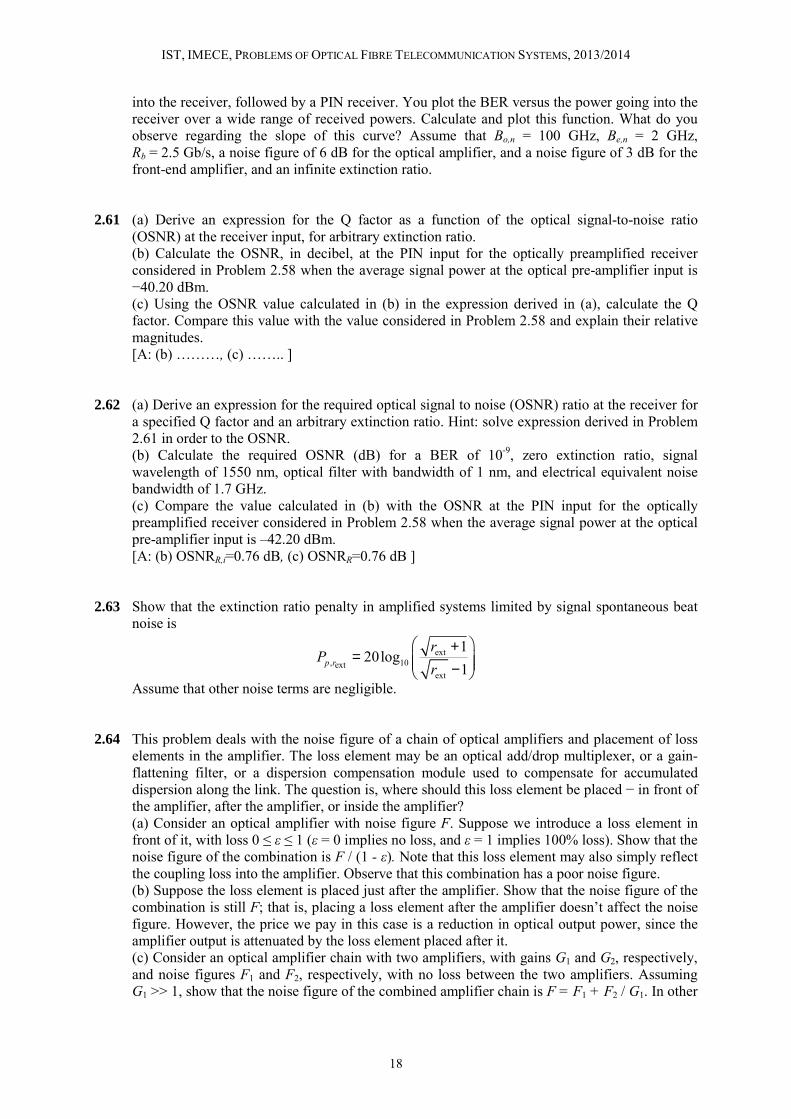
2.61 (a) Derive an expression for the Q factor as a function of the optical signal-to-noise ratio

(OSNR) at the receiver input, for arbitrary extinction ratio. (b) Calculate the OSNR, in decibel, at the PIN input for the optically preamplified receiver considered in Problem 2.58 when the average signal power at the optical pre-amplifier input is −40.20 dBm. (c) Using the OSNR value calculated in (b) in the expression derived in (a), calculate the Q factor. Compare this value with the value considered in Problem 2.58 and explain their relative magnitudes. [A: (b) ………, (c) …….. ]

2.62 (a) Derive an expression for the required optical signal to noise (OSNR) ratio at the receiver for

a specified Q factor and an arbitrary extinction ratio. Hint: solve expression derived in Problem 2.61 in order to the OSNR. (b) Calculate the required OSNR (dB) for a BER of 10-9, zero extinction ratio, signal wavelength of 1550 nm, optical filter with bandwidth of 1 nm, and electrical equivalent noise bandwidth of 1.7 GHz. (c) Compare the value calculated in (b) with the OSNR at the PIN input for the optically preamplified receiver considered in Problem 2.58 when the average signal power at the optical pre-amplifier input is –42.20 dBm. [A: (b) OSNRR,i=0.76 dB, (c) OSNRR=0.76 dB ]

2.63 Show that the extinction ratio penalty in amplified systems limited by signal spontaneous beat

noise is

ext, 10ext

ext

120log

1p rr

Pr

+= −

Assume that other noise terms are negligible. 2.64 This problem deals with the noise figure of a chain of optical amplifiers and placement of loss

elements in the amplifier. The loss element may be an optical add/drop multiplexer, or a gain-flattening filter, or a dispersion compensation module used to compensate for accumulated dispersion along the link. The question is, where should this loss element be placed − in front of the amplifier, after the amplifier, or inside the amplifier? (a) Consider an optical amplifier with noise figure F. Suppose we introduce a loss element in front of it, with loss 0 ≤ ε ≤ 1 (ε = 0 implies no loss, and ε = 1 implies 100% loss). Show that the noise figure of the combination is F / (1 - ε). Note that this loss element may also simply reflect the coupling loss into the amplifier. Observe that this combination has a poor noise figure. (b) Suppose the loss element is placed just after the amplifier. Show that the noise figure of the combination is still F; that is, placing a loss element after the amplifier doesn’t affect the noise figure. However, the price we pay in this case is a reduction in optical output power, since the amplifier output is attenuated by the loss element placed after it. (c) Consider an optical amplifier chain with two amplifiers, with gains G1 and G2, respectively, and noise figures F1 and F2, respectively, with no loss between the two amplifiers. Assuming G1 >> 1, show that the noise figure of the combined amplifier chain is F = F1 + F2 / G1. In other


19

words, the noise figure of the chain is dominated by the noise figure of the first amplifier, provided its gain is reasonably large, which is usually the case. (d) Now consider the case where a loss element with loss ε is introduced between the first and second amplifier. Assuming G1, G2 >> 1, and (1 – ε) G1 G2 >> 1, show that the resulting noise figure of the chain is given by F = F1 + F2 / [(1 – ε) G1 ]. Observe that the loss element doesn't affect the noise figure of the cascade significantly as long as (1 – ε) G1 >> 1, which is usually the case. This is an important fact that is made use of in designing systems. The amplifier is broken down into two stages, the first stage having high gain and a low noise figure, and the loss element is inserted between the two stages. This setup has the advantage that there is no reduction in the noise figure or the output power.

2.65 Consider that the optical receiver sensitivity in the absence of signal distortion due to

transmission is –30 dBm for the bit error probability of 10−12. (a) Determine the optical power required at the receiver input for the bit error probability of 10−12 when, due to optical path transmission, a power penalty of 2 dB occurs. (b) Considering that the optical receiver is a PIN receiver with circuit noise dominance, determine the optical power required at the receiver input for the bit error probability of 10−9 when, due to optical path transmission, a power penalty of 2 dB occurs. [A: (a) –28 dBm; (b) …….]


20



21

Optical fibre cable

Chapter 3. Single Channel Systems

3.1 Make the power budget and calculate the maximum transmission distance for a 1.3-µm

lightwave system operating at 100 Mb/s and using an LED for launching 0.1 mW of average power into the fibre. Assume 1-dB/km fibre loss, 0.2-dB splice loss every 2 km, 1-dB connector loss at each end of fibre link, and 100-nW receiver sensitivity. Allow 6-dB system margin. [A: 18.2 km ]

3.2 A 1.3-µm long-haul lightwave system is designed to operate at 1.5 Gb/s. It is capable of

coupling 1 mW of average power into the fibre. The 0.5-dB/km fiber-cable loss includes splice losses. The connectors at each end have 1-dB losses. The InGaAs PIN receiver has a sensitivity of 250 nW. Make the power budget and estimate the repeater spacing. [A: 52 km ]

3.3 Determine the maximum transmission distance for a 1.55-µm lightwave system operating at

4 Gb/s such that the dispersion-induced power penalty is below 1 dB. Assume a chirp parameter of 6 for the single-mode semiconductor laser and β2 = −20 ps2/km for the single-mode fibre. [A: 16.8 km ]

3.4 Repeat Problem 3.3 for the case of 8-Gb/s bit rate.

[A: 4.2 km ] 3.5 What is the dispersion-limited transmission distance for a 1.55-µm lightwave system making

use of direct modulation at 10 Gb/s? Assume a chirp parameter of 6 and use 17 ps/(km·nm) for fibre dispersion parameter.

3.6 How much improvement in the dispersion-limited transmission distance is expected if an

external modulator is used in place of direct modulation for the lightwave system of Problem 3.5?

3.7 Assume that the bit rate on the link is 1 Gb/s, the dispersion parameter at 1.55 µm is

17 ps/(km·nm), and the attenuation is 0.25 dB/km, and at 1.3 µm, the dispersion is 0 and the attenuation is 0.5 dB/km. Neglect all losses except the attenuation loss in the fibre. Assume that NRZ modulation is used.


22

(a) You have a transmitter that operates at a wavelength of 1.55 µm, has a spectral width of 1 nm, and an output power of 0.5 mW. The receiver requires −30 dBm of input power in order to achieve the desired bit error rate. What is the length of the longest link that you can build? (b) You have another transmitter that operates at a wavelength of 1.3 µm, has a spectral width of 2 nm, and an output power of 1 mW. Assume the same receiver sensitivity as in (a). What is the length of the longest link that you can build? [A: (a) 26.8 km, dispersion-limited; (b) 44 km, loss-limited ]

3.8 Compute the dispersion-limited transmission distance for links with standard single-mode fibre

at 1550 nm as a function of the bit rate (100 Mb/s, 1 Gb/s, and 10 Gb/s) for the following transmitters: (a) a Fabry-Perot laser with a spectral width of 10 nm, (b) a directly modulated DFB laser with a spectral width of 100 MHz and chirp parameter of 6, (c) an externally modulated DFB laser with a spectral width of 100 MHz. Assume that the dispersion penalty is 2 dB. Assume that NRZ modulation is used.

3.9 Repeat Problem 3.8 for NZ-DSF assuming a dispersion parameter of 5 ps/(km·nm). 3.10 Consider a length L of step-index multimode fibre having a core diameter of 50 µm and a

cladding diameter of 200 µm. The refractive indices of the core and cladding are 1.50 and 1.49, respectively. A fixed-wavelength, 1310 nm InGaAsP DFB laser (operating at 0 dBm) is used at one end of the fibre to serve as a 155.52 Mb/s transmitter source. At the far end, a photodetector is used as a receiver. Assume that NRZ modulation is used. (a) Draw and label a diagram that illustrates the above configuration. (b) What would be the corrugation period of the DFB laser at this wavelength? (c) Compute the numerical aperture for this fibre. (d) What would be the maximum acceptable fibre length when operating at this bit rate? (e) Assuming an attenuation of 0.40 dB/km, what would be the output power (in dBm) at the receive end of the fibre? (f) Assuming a perfectly efficient photodetector, what would be the resulting photocurrent? (g) If we instead used single-mode fibre for this application, what would be the new requirement on its core diameter? [A: (b) 374.3 nm; (c) 0.173; (d) 96 m; (e) 0.04 dB; (f) 1 mA; (g) 5.8 µm ]

3.11 Consider a point-to-point link connecting two nodes separated by 60 km. This link was

constructed with standard single-mode fibre, and a 2.5 Gb/s system is deployed over the link. The transmitter uses a directly modulated 1310 nm DFB laser. The receiver uses perfectly efficient PIN photodiodes, and we will assume, for this problem, that they can be modeled as ideal receivers. The bit error rate requirement for this system is 10-12. Assume α = 0.4 dB/km and that NRZ modulation is used. (a) Draw and label a diagram illustrating this configuration. (b) Is this system loss limited or dispersion limited? Briefly explain your reasoning. (c) What is the required receiver sensitivity (in mW and dBm)? (d) What would be the resulting photocurrent? (e) What would be the required launch power (in dBm)? [A: (b) loss limited; (c) −53 dBm; (d) 5.4 nA; (e) −29 dBm ]

3.12 Calculate the equivalent distance limitations of the different types of SDH systems. Assume a

loss of 0.25 dB/km at 1550 nm, and 0.5 dB/km at 1310 nm.


23

[A: at 1550 nm, SR => 0-28 km, IR => 0-48 km, LR => 40-96 km; at 1310 nm, SR => 0-14 km, IR => 0-24 km, LR => 20-48 km ]

3.13 You have to connect two SDH boxes operating at STM-16 line rate over a link that can have a

loss of anywhere from 0 to 7 dB. Unfortunately, they do not support the same interfaces. One of them supports an I-16 interface and the other has an S-16.1 interface. The detailed specifications for these interfaces, extracted from ITU Recommendation G.957, are given in Table 3.13.

Table 3.13. Specifications for STM-16 intra-office and short-haul interfaces (from ITU G.957)

Parameter I-16 S-16.1 Transmitter MLM SLM

Wavelength range 1.3 µm 1.3 µm Transmitter power (max) –3 dBm 0 dBm Transmitter power (min) –10 dBm –5 dBm

Receiver sensitivity (min) –18 dBm –27 dBm Receiver overload (min) –3 dBm 0 dBm

Can you find a way to interconnect these boxes and make the link budget work? You are allowed to use variable optical attenuators (VOA) in the link. [A: link from S-16.1 tx to I-16 rx, a VOA with a range of 3 dB is needed; link from I-16 tx to S-16.1 rx, no VOA is needed ]

3.14 Consider the linear SDH-based network shown in Figure 3.14. The network operates at 1.55 µm

and carries a STM-1 signal. The link between central offices is realized using three similar regeneration sections of optical fibre, with a total distance of 270 km. In addition to the electrical regenerator, each regenerator block comprises an opto-electrical (O/E) converter and an electro-optical (E/O) converter that are assumed similar to the O/E converter of the receiver and the E/O converter of the transmitter, respectively. Remark: the bit rate of a STM-1 signal is 155.52 Mbit/s.

Central Office

O/E E/O

Central Office

Reg Reg

RegE/O Reg O/E

Opti cal fibre

Fig. 3.14 Scheme of the SDH network considered in Problem 3.14

The optical fibre has a power loss coefficient of 0.25 dB/km. The laser used in the E/O converter is directly modulated, has a linewidth of 1 nm, a linewidth enhancement factor of 6 and the average fibre-coupled power is 0 dBm. The quantum efficiency of the optical receiver is 80% and the square root of the noise current power spectral density is 3 pA/Hz1/2. The noise equivalent bandwidth of the electrical part of the receiver is 70% of the transmission bit rate. To simplify the analysis, neglect the shot noise and assume a null extinction ratio. The target bit error probability of the link is 3×10-10. (a) Assuming that the line code is the NRZ unipolar, determine if the link is possible and calculate the system margin of each regeneration section. Consider null fibre dispersion. (b) Determine how the result of (a) is altered when G.652 optical fibre with dispersion parameter of 17 ps/(nm⋅km) is used.


24

[A: (a) Ms=12.5 dB; (b) not altered ] 3.15 In the two-fibre unidirectional path-switched ring shown in Figure 3.15, the different add-drop

multiplexers (ADM) are connected using G.652 optical fibre. At the operating wavelength of 1540 nm, the optical fibre has a dispersion parameter of 16.6 ps/nm/km and a loss coefficient (including connectors and splice losses) of 0.22 dB/km. The optical sources are DFB lasers, with a linewidth of 15 MHz and a chirp parameter of 5. The optical transmitter uses external modulation with an ideal extinction ratio and launches into the optical fibre an average power of 0 dBm. A PIN, with a quantum efficiency of 70%, is used for signal detection, the noise equivalent bandwidth of the receiver is 80% of the bit rate, and the noise equivalent power of the receiver is 10 pW/Hz1/2. The target bit error probability is 10-12, the maximum power penalty due to fibre dispersion is 1.5 dB and the required system margin is 5 dB. Note that this bit error probability should be satisfied by all connections between ADMs; therefore, the worst situation of a signal added in ADM E and extracted in ADM A should have a bit error probability not exceeding 10-12.

DSL AM

MDF

Main distribution frame

ATM

ADM

ADM

ADM

ADM

ATM ISP Internet

IP router ATM switch

Telephone network

Unidireccional two-fibre ring

Central office

ADM

E3

MuxSLI

SL I

Switch

ATM switch

A

B

C

D

E

E4

E3

Transit office

Direction of traffic with normal operation

E4

ADSL filter

Fig. 3.15 Unidirectional two-fibre ring used to transport one E3 and one E4 signal.

Consider that the ring transmission bit rate is STM-16 and that all sections have the same length. In the following analysis, the ADMs are modelled as regenerators. (a) Show that direct modulation of the DFB lasers cannot be used if the ring perimeter is 500 km. (b) Assuming that transmission is dispersion-limited, calculate the maximum length of each section. (c) Assuming that transmission is loss-limited, calculate the maximum length of each section. Compare this result with the result of (b) and draw conclusions. (d) Calculate the increase of section length allowed by using an optical preamplifier with gain of 20 dB, noise figure of 6 dB and bandwidth of 20 nm, prior to the PIN existing in each ADM. [A: (b) 954.66 km; (c) 83.67 km; (d) 46 km ]

3.16 Consider the three EDFAs presented in Table 3.16.

(a) Imagine that you are asked to choose the most suitable EDFA for preamplifier of a 10 Gbit/s link. Explain which EDFA you would choose and why. (b) Imagine that you are asked to choose the most suitable EDFA for post-amplifier of a 10 Gbit/s link. Explain which EDFA you would choose and why.


25

Table 3.16. EDFAs characteristics

EDFA Maximum gain Noise figure Maximum output power A 32 dB 4 – 5 dB 10 dBm B 25 dB 5 – 6 dB 15 dBm C 23 dB 7 – 8 dB 18 dBm

[A: (a) A; (b) C] 3.17 Compute the steady-state values of Pout and G in a long chain of amplifiers. Assume

Gmax=35 dB, l=120 km, α=0.25 dB/km, nsp=2, psat=10 mW, and Bo=50 GHz. How do these values compare against the unsaturated gain and the output saturation power of the amplifier? Plot the evolution of the signal power and optical signal-to-noise ratio as a function of distance along the link. [A: ~30 dB, 11.5 mW ]

3.18 The expression usually presented for the effective length of a link of length L with amplifiers

spaced l km apart, given by Le = (1-e-αl)/(αl)L is an approximation. (a) Why? (b) Derive a precise form of this expression.

3.19 Consider a 4000-km lightwave system designed using 50 EDFAs with 4.5-dB noise figure.

Assume a fibre-cable loss of 0.25 dB/km at 1.55 µm. A 2-nm-bandwidth optical filter is inserted after every amplifier to reduce the noise power. The average optical power at the fibre input is 1 mW. (a) Calculate the optical SNR at the output end of the lightwave system. (b) Find the electrical SNR for a receiver of 8-GHz bandwidth. [A: (a) 3.48 dB; (b) 18.43 dB]

3.20 Explain why the cascading of identical optical filters can produce signal distortion even when

the filter bandwidth is wider than the signal bandwidth. Derive an expression of the effective 3 dB bandwidth of a cascade of N filters with a Gaussian-shape transfer function with 3 dB bandwidth B3dB. Calculate the effective bandwidth of 20 cascaded filters with a Gaussian-shape transfer function with 3 dB bandwidth of 50 GHz.

3.21 An optical fibre submarine cable link between Lisboa and Lagos (Portugal), with a length of

200 km, uses an EDFA with 20 dB of gain near Sines (80 km far from Lisboa) and an EDFA preamplifier with 25 dB of gain. The link carries a STM-64 signal at 1555 nm. The EDFAs have a noise figure of 6 dB and a bandwidth of 20 nm. The optical fibre has a loss coefficient (including splices and connectors losses) of 0.24 dB/km. The fibre-coupled signal at the Lisbon site has a null extinction ratio and average optical power of 1 mW. The optical receiver uses an optical filter with 0.5 nm of bandwidth to reduce the amplified spontaneous emission noise power. A PIN with responsivity of 0.8 A/W is used to detect the optical signal, and the noise equivalent bandwidth of the electrical part of the receiver is 80% of the bit rate. The service quality corresponds to a bit error probability of 10-9. (a) Calculate the optical signal to noise ratio at the PIN input. (b) Calculate the required optical signal to noise ratio at the receiver input, under ideal transmission conditions, to guarantee the service quality. [A: (a) 16.49 dB; (b) 8.32 dB]


26

3.22 A submarine cable link carrying a STM-16 signal has a length of 3000 km and operates at the wavelength of 1540 nm. G.655 optical fibre, with dispersion parameter of 3.5 ps/(nm·km) and loss coefficient (including connectors and splices) of 0.25 dB/km, is used. The link has 50 amplification sections and uses EDFAs with bandwidth of 30 nm and noise figure of 4 dB. A PIN with quantum efficiency of 80% is used and the noise equivalent bandwidth of the electrical part of the receiver is 70% of the bit rate. Assume a null extinction ratio and consider the usual approximations in this kind of links, which should be reported. (a) Calculate the optical signal to noise ratio required at the receiver input to ensure the minimum system margin of 6 dB and a service quality corresponding to the bit error probability of 10-12. (b) Calculate the maximum allowed laser linewidth and indicate the type of laser that should be used in this link. (c) Check if it is possible to use a directly modulated DFB laser (SLM) with linewidth of 10-4 nm. If not possible, indicate the reason and propose solutions to make possible the feasibility of the link. [A: (a) 0.38 dB, (b) σλ,L≤0.0074 nm, SLM; (c) not possible, dispersion-limited ]

3.23 Check if an externally modulated optical transmitter using as optical source the laser DFB of

Problem 3.22-(c) can be used in the link of Problem 3.22. Calculate the average power coupled to the optical fibre that guarantees the system margin of 6 dB. [A: 3.12 dBm ]

3.24 Assume that we intend to improve the system margin of the link considered in Problem 3.23 by

using optical filters with bandwidth of 1 nm along the line. Calculate the improvement of the system margin. [A: 5.38 dB ]

3.25 Consider a single-channel system transmitting a STM-64 signal along 100-km optical fibre at

1552.52 nm. The system is composed by an EDFA followed by a G.652 fibre and an optical receiver (without optical pre-amplification). The EDFA presents a bandwidth of 20 nm, an output OSNR of 3 dB and an output average signal of 1 mW. The fibre has an average loss coefficient of 0.2 dB/km. The optical receiver utilizes a PIN with a quantum efficiency of 80%, has a noise equivalent bandwidth of 80% of the bit rate and a NEP of 5 pW/Hz1/2. (a) Calculate the OSNR at the receiver input. (b) Calculate the amplified spontaneous emission noise power per polarisation mode at the receiver input. (c) Calculate the bit error probability assuming an infinite extinction ratio. [A: (a) 3 dB; (b) 2.5 µW; (c) 7.24×10-40]

3.26 A 1.55 µm continuous-wave signal with 6-dBm power is launched into a fibre with 50 µm2

effective mode area. After what fibre length would the nonlinear phase shift induced by SPM become 2π? Assume n2 = 2.6×10-20 m2/W and neglect fibre losses. [A: 745 km]

3.27 Calculate the power launched into a 40-km-long single-mode fibre for which the SPM-induced

nonlinear phase shift becomes 180o. Assume λ = 1.55 µm, Aeff = 40 µm2, α = 0.2 dB/km, and n2 = 2.6×10−20 m2/W. [A: 65.22 mW]


27

3.28 Find the maximum frequency shift occurring because of the SPM-induced chirp imposed on a Gaussian pulse of 20-ps width (FWHM) and 5-mW peak power after it has propagated 100 km. Use the fibre parameters of the preceding problem but assume α = 0. [A: 14.97 GHz]

3.29 Consider a 10 Gbit/s per channel submarine cable system designed employing OLRs (with

optical dispersion compensation) with 4.5-dB noise figure, and amplification sections with length of 60 km and overall gain of 0 dB. Assume a fibre-cable loss of 0.22 dB/km at 1.55 µm (including all section losses), and a fibre nonlinearity coefficient of 1.6 W-1 km-1. A 2-nm-bandwidth optical filter is inserted after every amplifier to reduce the noise power. A typical 10 Gbit/s receiver is used. In the system design, the maximum allowed nonlinear phase shift due to self-phase modulation is π/2, the target bit error probability is 10-15, the system margin is 5 dB, and the maximum acceptable transmission penalty of 2 dB is considered. (a) Calculate the maximum length of this submarine cable system when the average power launched into the fibre at the transmitter side is 5 dBm. (b) Calculate the maximum length of this submarine cable system when the average power launched into the fibre at the transmitter side is 0 dBm. [A: (a) 960 km; (b) 2520 km]

3.30 Consider a 10 Gbit/s per channel submarine cable system designed employing OLRs (with

optical dispersion compensation) EDFAs with 4.5-dB noise figure, and amplification sections with length of 60 km and overall gain of 0 dB. At 1.55 µm, the single-mode fibre used has loss of 0.22 dB/km (including all section losses), and nonlinearity coefficient of 1.6 W-1 km-1. A 2-nm-bandwidth optical filter is inserted after every amplifier to reduce the noise power. A typical 10 Gbit/s receiver is used. In the system design, the maximum allowed nonlinear phase shift due to self-phase modulation is π/2, the target bit error probability is 10-15, the system margin is 5 dB and maximum acceptable transmission penalty is 2 dB. Calculate the maximum length of this submarine cable system and the optimum average power level launched into the fibre at the transmitter side. [A: 2820 km, 1.1 mW]


28



29

Chapter 4. Wavelength Division

Multiplexed Systems

4.1 Consider a passive WDM link of length L, consisting of single-mode fibre into which five

wavelengths are launched through an optical combiner such that the aggregate launch power at its output is 5 mW. These five wavelengths are centered on the 193.1 THz ITU grid, with uniform 100 GHz interchannel spacing. The transmitters all use directly modulated DFB lasers with a linewidth of 10 MHz and chirp parameter of 6. Each channel is transporting a SONET OC-48 (2.5 Gb/s) signal. At the end of this link, the channels are optically demultiplexed and are each received by a direct detection pin receiver. For this problem, consider 5 dB of loss in the WDM demultiplexer, and neglect crosstalk associated with the WDM multiplexer and demultiplexer. Assume that NRZ modulation is used, receiver sensitivity of -30 dBm and zero system margin. (a) Draw and label a diagram illustrating this configuration. (b) Calculate the wavelengths (in nm, to two decimal places) associated with these five channels. (c) Calculate the average launch power per channel at the output of the WDM combiner. (d) Assuming α = 0.25 dB/km, Dλ = 17 ps/nm/km, and DPMD = 0.5 ps/√km, calculate the worst-case dispersion, PMD, and loss limits for this link. (e) What is the maximum value of L meeting all of these requirements? [A: (b) 1550.918 nm, 1551.721 nm, 1552.524 nm, 1553.329 nm, 1554.134 nm (c) 1mW; (d) LPMD = 6400 km, LCD = 88.8 km, Lloss = 92 km with maximum dispersion penalty of 2 dB]

4.2 The link of Problem 3.11 is at full capacity, and we must design a solution that will enable

capacity expansion and accommodate further growth. After considering the options, we determine that the most cost-effective solution is to add a 1550 nm point-to-point system over the existing set of fibres, thereby realizing a two-wavelength (1310 nm / 1550 nm) passive WDM configuration. Assume that 3 dB couplers are used to combine the two signals just after the transmitters and separate the two signals just before the receivers. The next step is to determine what bit rate can be supported by this 1550 nm system. Assume that the 1550 nm transmitter uses a directly modulated DFB laser (with linewidth of 10 MHz and chirp parameter of 6). At 1550 nm, assume α = 0.25 dB/km, Dλ = 17 ps/nm/km, and DPMD = 1 ps/√km. (a) Draw and label a diagram illustrating this new configuration. (b) What is the launch power now required for the original 2.5 Gb/s 1310 nm system to maintain the same level of receiver performance? (c) If we assume an ideal receiver with the same 10-12 bit error rate performance for the 1550 nm system, determine the associated receiver sensitivities for both 2.5 Gb/s and 10 Gb/s signals. (d) Calculate bit rate limits based on loss, dispersion, and PMD for the new system. (e) Can 10 Gb/s be suitably transported by this new system? Briefly explain your reasoning. (f) For the 2.5 Gb/s and 10 Gb/s (if it is possible) line rates, calculate the required launch power to successfully transport the signal. [A: (b) -23 dBm (c) 2.5 Gbit/s: -53.6 dBm, 10 Gbit/s: -47.6 dBm; (d) Rb,PMD < 12.9 Gbit/s, Rb,CD < ??? Gbit/s; (e) 10 Gbit/s cannot be transported because of CD; (f) -32.6 dBm ]


30

4.3 Explain why the WDM transmission systems of core networks use only the third window of

communication. 4.4 The C and L spectral bands cover a wavelength range from 1.53 to 1.61 µm. How many

channels can be transmitted through WDM when the channel spacing is 25 GHz? What is the effective bit rate-distance product when a WDM signal covering the two bands using 10-Gb/s channels is transmitted over 2000 km. [A: Nch = 390, 7800 Tbit/s·km]

4.5 We intend to maximise the link capacity of the Problem 3.21 using dense wavelength division

multiplexing (DWDM) with channel spacing of 50 GHz, and an AWG with insertion losses of 4 dB to demultiplex the WDM signal. All channels carry signals similar to those in Problem 3.21. (a) Calculate the range of maximum power (in dBm) at the EDFA output required for a link capacity exceeding 600 Gbit/s. The overload parameter of the PIN receiver is -3 dBm. (b) Indicate the modifications to produce in the system in order to achieve that capacity of 600 Gbit/s. [A: (a) maximum average EDFA output power exceeding 18.58 dBm; (b) EDFAs with bandwidth exceeding 23.9 nm, receiving optical filter replaced by a demux with bandwidth per channel lower than 50 GHz but higher than 40 GHz, mux with the same features as demux, both with channel spacing of 50 GHz and multiplexing capacity of at least 60 channels]

4.6 In optically amplified systems, the dominant noise component is signal dependent. In this

situation, show that the power penalty due to intrachannel crosstalk when there is one interfering signal is given by

( ),intraX 1020log 1 2pP ε= − −

where ε is the average received crosstalk power expressed in terms of fraction of the average signal power.

4.7 Generalise the result of problem 4.6 to the case when there are N interfering signals rather than

just one. In this case, show that the power penalty due to intrachannel crosstalk is given by

( ),intraX 101

20log 1 2N

p ii

P ε=

= − − ∑

where εi is the average received crosstalk power of interfering signal i expressed in terms of fraction of the average signal power.

4.8 Show that the power penalty due to interchannel crosstalk when there is one interfering signal, in case of optically amplified systems, is given by

( ),interX 1020log 1pP ε= − −

where ε is the average received crosstalk power expressed in terms of fraction of the average signal power.

4.9 Generalise the result of problem 4.8 to the case when there are N interfering signals rather than just one. In this case, show that the power penalty due to interchannel crosstalk is given by


31

,interX 101

20log 1N

p ii

P ε=

= − − ∑

where εi is the average received crosstalk power of interfering signal i expressed in terms of fraction of the average signal power.

4.10 Consider a WDM system with Nch channels, each with the same average power and extinction

ratio. Derive the interchannel crosstalk power penalty for this system compared to a system with ideal extinction and no crosstalk. What should the crosstalk level be for a maximum 1 dB penalty if the extinction ratio is 10 dB?

4.11 Consider the WDM network node shown in Figure 4.11.

Fig. 4.11 Node of the WDM network

Assume the node has two inputs and two outputs. The multiplexers/demultiplexers are ideal (no crosstalk), but each switch has a crosstalk level C dB below the desired channel. Assume that, in the worst case, crosstalk in each stage adds coherently to the signal. (a) Compute the crosstalk level after N nodes. (b) What must C be so that the overall crosstalk penalty after five nodes is less than 1 dB?

4.12 Consider the WDM network node shown in Figure 4.11. Assume the node has two inputs and

two outputs. The mux/demuxes have adjacent channel crosstalk suppressions of -25 dB, and crosstalk from other channels is negligible. The switches have a crosstalk specification of -40 dB. How many nodes can be cascaded in a network without incurring more than a 1 dB penalty due to crosstalk? Consider only intrachannel crosstalk from the switches and the multiplexers/demultiplexers.

4.13 Consider a WDM system with N nodes, each node being the one shown in Figure 4.11. The

center wavelength 'cλ for each channel in a mux/demux has an accuracy of ±∆λ nm around the

nominal center wavelength λc. Assume a Gaussian passband shape for each channel in a mux; that is, the ratio of output power to input power, called the transmittance, is given by

( ) ( )2'

2exp2

cRT

λ λλ

σ

− = −

where σ is a measure of the channel bandwidth and 'cλ is the center wavelength. This passband

shape is typical for an arrayed waveguide grating.


32

(a) Plot the worst-case and best-case peak transmittance in decibels as a function of the number of nodes N for σ = 0.2 nm, ∆λ= 0.05 nm. Assume that the laser is centered exactly at λc. (b) What should ∆λ be if we must have a worst-case transmittance of 3 dB after 10 nodes? [A: (a) best case, 0 dB; worst-case, 0.1357·N dB; (b) 0.0745 nm ]

4.14 Consider a system with the same parameters as in Problem 4.13. Suppose the WDM channels

are spaced 0.8 nm apart. Consider only crosstalk from the two adjacent channels. Compute the interchannel crosstalk power relative to the signal power in decibels, as a function of N, assuming all channels are at equal power and exactly centered. Compute the crosstalk also for the case where the desired channel is exactly centered at λi, but the adjacent channels are centered at λi–1+∆λ and λi+1–∆λ.

4.15 Discuss how EDFAs can be used to provide gain in the L band. How can you use them to

provide amplification over the both C and L bands? 4.16 Imagine that you are a planner for a long-haul carrier planning to deploy an IP over WDM

network. Your job is to make the right technology and vendor choice for your network. You are given the following information. The initial requirement is to deploy 20 Gb/s of capacity between two nodes. You anticipate that this capacity will grow to 80 Gb/s in a year and over a few years grow to 320 Gb/s. You have a choice of several WDM systems from different vendors with the following prices and capabilities shown in Table 4.16.

Table 4.16. Three WDM systems from three different vendors

Vendor A B C Number of channels 80 128 32 Bit rate per channel STM-64 STM-16 STM-64 Distance between regenerators 640 km 1920 km 1920 km Amplifier spacing 80 km 80 km 80 km OLT common equipment 30 k€ 32.25 k€ 45 k€ Transponder 7.5 k€ 3.75 k€ 12 k€ Amplifier 22.5 k€ 15 k€ 18.75 k€

Assume that the common equipment prices for the optical line terminals include any amplifiers if needed. One transponder is needed for each channel at each end of the link. Once the distance between regenerators is exceeded, the signals need to be regenerated by using two terminals back to back with transponders. (a) Draw a diagram of each configuration. (b) Compute the cost of each solution for a 640 km link, a 1280 km link, and a 1920 km link. (c) What are your conclusions? (d) Other than the costs computed above, what other factors might influence your choice?

4.17 Consider the same problem as in Problem 4.16 with one difference. For the 1280 and 1920 km

cases, between the two nodes is a third node spaced 600 km from the first node, where half the capacity needs to be dropped and added. For this case, assume that vendor B and vendor C offer systems where you can use back-to-back terminals at this intermediate node without requiring transponders for the passthrough channels; transponders are still needed for the channels dropped and added. a) Repeat analysis of Problem 4.16. b) What are your conclusions?


33

4.18 If the BER of an uncoded system is p, show that the same system has a BER of 3p2 + p3 when the repetition code (each bit is repeated thrice) is used. Note that the receiver makes its decision on the value of the transmitted bit by taking a majority vote on the corresponding three received coded bits. Assume that the channel BER remains the same in both cases.

4.19 Determine the redundancy, line bit error probability, the corresponding Q-factor (dB) required

for an information bit error probability of 10-15, and the gross coding gain (a) when RS(255,239) is used; (b) when RS(255,223) is used. [A: (a) ρFEC=6.7%, Pe,b,l=8.1×10-5, QFEC=11.53 dB, Gc,G=6.47 dB;

(b) ρFEC=14.4%, Pe,b,l=6.3×10-4, QFEC=10.17 dB, Gc,G=7.83 dB ] 4.20 Using the result of Problems 2.62 and 4.19, calculate the required OSNR at the receiver input

for a bit error probability of 10-15 and zero extinction ratio, when RS(255,239) or RS(255,223) are used, and compare with the required OSNR in the absence of FEC. (a) Consider a typical 10 Gb/s receiver, with Be,n=8 GHz, Bo=40 GHz. (b) Consider a typical 40 Gb/s receiver, with Be,n=32 GHz, Bo=100 GHz. [A: (a) OSNRR,FEC=6.79 dB for RS(255,239), and OSNRR,FEC=5.93 dB for RS(255,223); (b) OSNRR,FEC=8.49 dB for RS(255,239), and OSNRR,FEC=7.60 dB for RS(255,223)]

4.21 Calculate the increase of the maximum length of the submarine cable system of Problem 3.29 when FEC using RS(255,239) is employed, for the two power levels of questions (a) and (b) of Problem 3.29, 5 and 0 dBm, respectively. Hint: if necessary, use the result of Problem 4.20. [A: no increase for 5 dBm, 600 km]

4.22 Calculate the increase of the maximum length of the submarine cable system of Problem 3.30

and the optimum average power level launched into the fibre at the transmitter side, when FEC using RS(255,239) is employed. Hint: if necessary, use the result of Problem 4.20. [A: 2400 km, 0.6 mW]


34



35

Generic access network architecture

Chapter 5. Optical Access

Networks

5.1 A distribution network uses an optical bus to distribute the signal to 10 users. Each optical tap

couples 10% of the power to the user and has 1-dB insertion loss. Assuming that the station 1 transmits 1 mW of power over the optical bus, calculate the power received by the stations 8, 9, and 10. [A: 9.5 µW, 6.8 µW, 4.9 µW ]

5.2 A cable-television operator uses an optical bus to distribute the video signal to its subscribers.

Each receiver needs a minimum of 100 nW to operate satisfactorily. Optical taps couple 5% of the power to each subscriber. Assuming 0.5 dB insertion loss for each tap and 1 mW transmitter power, estimate the number of subscribers that can be added to the optical bus? [A: 38 ]

5.3 What is meant by a passive optical network (PON)? Why is relevant using PONs as optical

access networks? 5.4 Calculate the maximum information bit rate per user for GPON and EPON, taking into account

that the mean efficiency of the line rate for GPON is 93% and for EPON is 55%, and that the OLT of GPON serves 64 users while the OLT of EPON serves 16 users. Consider the maximum normalised line rate of GPON. [A: GPON, 36.15 Mbit/s; EPON, 42.97 Mbit/s ]

5.5 Calculate the maximum number of users (power of 2) per OLT of GPON so that the information

bit rate per user exceeds 100 Mbit/s when all users are using the network simultaneously. [A: 16 ]

5.6 Consider the GPON shown in Fig. 5.6. This GPON serves 16 users per OLT (Optical Line

Termination), and operates at 2.488 Gbit/s in the downstream and upstream directions. The optical splitter is located 10 km away from the OLT. The OLT is located at the central office, emits at the wavelength of 1490 nm and receives the signals, coming from ONUs (Optical Network Unit), located at the users’ premises, at the wavelength of 1310 nm. The OLT receiver is an optical receiver operating at burst mode and a conventional optical receiver is used at the ONU. The operation penalty of a burst receiver is 0.5 dB relative to the conventional receiver. The excess losses per stage of the splitter / combiner are 0.5 dB. Similar optical transmitters are used in the OLT and ONUs. These transmitters have an average optical power coupled to the fibre of 2 dBm and an extinction ratio of 10 dB.


36

Splitter /

Combiner

1 : N

OLT ONU

ONU

Lf

Ld

ONU

λu = 1310 nm

λd =1490 nm

... ...

Connectors

Figure 5.6 Scheme of the GPON considered in Problem 5.6

The optical receivers use PIN photodetectors (similar in OLT and ONUs) with a quantum efficiency of 70%, have a NEP of 5 pW/√Hz at 1550 nm and their noise equivalent bandwidth is 70% of the line bit rate. The wavelength division duplexing is realized using a duplexer with an insertion loss of 1 dB. The optical fibre used in the GPON is G.652 with loss coefficients of 0.22 dB/km and 0.35 dB/km, at wavelengths of 1490 and 1310 nm, respectively. The connectors have an insertion loss of 0.2 dB.

For design purposes, a system margin of at least 5 dB, an overload margin of at least 1 dB, and a dispersion penalty not exceeding 1.5 dB are required. Assume that both GPON communication directions are loss-limited. (a) Calculate the maximum length of the distribution network so that a bit error probability not exceeding 10-12 can be guaranteed in both communication directions. (b) Calculate the overload parameter required to the optical receivers. [A: (a) 3.94 km; (b) -16.04 dBm ]

5.7 Assume that, for a matter of cost reduction, the MLM lasers available to be used in the GPON

of Problem 5.6 have a 3 dB linewidth exceeding 3.5 nm. Indicate which type of laser (SLM or MLM) should be used in downstream and upstream directions. The optical fibre used in the feeding and distribution networks is SSMF (G.652) with dispersion parameter of 17 ps/nm/km and dispersion slope of 70 fs/nm2/km. [A: upstream, MLM lasers; downstream, SLM lasers ]

5.8 Do a power budget calculation for the different types of PON architectures considered in this

chapter and determine the number of ONUs that can be supported in each case, assuming the parameters shown in Table 5.8.

Table 5.8. Parameters of the different PON architectures.

Laser output power -3 dBm LED output power -20 dBm Transmit bit rate 155 Mbit/s Receiver sensitivity -40 dBm Fibre loss, including connectors 10 dB 1 × 8 wavelength router loss 5 dB 1 × 32 wavelength router loss 9 dB 1 × 64 wavelength router loss 12 dB Excess splitter loss 1 dB


37

The normal wavelength router losses are indicated in Table 5.8. However, with spectral slicing, an additional loss is also incurred as only a small fraction of the spectrum is transmitted out of each port on the wavelength router. Assume that in addition to the standard loss, we get only 1/(2N) of the transmitted power in each channel, where N is the number of ONUs. [A: broadcast-and-select PON with laser, 400 ONUs; broadcast-and-select PON with led, 8 ONUs; WDM PON, 400 ONUs; WRPON with laser, feasible with 64 ONUs; WRPON with led spectral slicing, 4 ONUs ]

5.9 Describe a WDM scheme for connecting multiple users to the central office for bidirectional

data transmission without requiring any optical sources at the user’s location. Explain the relevance of not requiring any optical sources at the user’s location.

5.10 Consider the RITENET architecture shown in Figure 5.10.

Figure 5.10. RITENET architecture

Suppose the laser speed at the CO is limited to 155 Mb/s. The network needs to support 20 ONUs and provide each ONU with 10 Mb/s bandwidth from the CO to the ONU and 2 Mb/s from the ONU to the CO. How could you modify the architecture to support this requirement? [A: two lasers at the CO, one at 1.3 µm and the other at 1.55 µm + 1.3 µm / 1.55 µm coupler at the CO + filter at each ONU to select one of the wavelengths ]


38


Problems of Optical Fibre Telecommunication Systems · PDF fileIST, IMECE, PROBLEMS OF OPTICAL FIBRE TELECOMMUNICATION SYSTEMS, 2013/2014 3 Chapter 1. Introduction to Optical Fibre

Documents