Problems in Supply Chain Location and Inventory under Uncertainty by Iman Hajizadeh Saffar A thesis submitted in conformity with the requirements for the degree of Doctor of Philosophy Graduate Department of Rotman School of Management University of Toronto Copyright c 2010 by Iman Hajizadeh Saffar

Welcome message from author
This document is posted to help you gain knowledge. Please leave a comment to let me know what you think about it! Share it to your friends and learn new things together.
Transcript
Problems in Supply Chain Location and Inventory underUncertainty
by
Iman Hajizadeh Saffar
A thesis submitted in conformity with the requirementsfor the degree of Doctor of Philosophy
Graduate Department of Rotman School of ManagementUniversity of Toronto
Copyright c© 2010 by Iman Hajizadeh Saffar

Abstract
Problems in Supply Chain Location and Inventory under Uncertainty
Iman Hajizadeh Saffar
Doctor of Philosophy
Graduate Department of Rotman School of Management
University of Toronto
2010
We study three problems on supply chain location and inventory under uncertainty. In
Chapter 2, we study the inventory purchasing and allocation problem in a movie rental
chain under demand uncertainty. We formulate this problem as a newsvendor-like prob-
lem with multiple rental opportunities. We study several demand and return forecasting
models based on comparable films using iterative maximum likelihood estimation and
Bayesian estimation via Markov chain Monte Carlo simulation. Test results on data from
a large movie rental firm reveal systematic under-buying of movies purchased through
revenue sharing contracts and over-buying of movies purchased through standard ones.
For the movies considered, the model estimates an increase in the average profit per title
for new movies by 15.5% and 2.5% for revenue sharing and standard titles, respectively.
We discuss the implications of revenue sharing on the profitability of both the rental firm
and the studio.
In Chapter 3, we focus on the effect of travel time uncertainty on the location of
facilities that provide service within a given coverage radius on the transportation net-
work. Three models - expected covering, robust covering and expected p-robust covering
- are studied; each appropriate for different types of facilities. Exact and approximate
algorithms are developed. The models are used to analyze the location of fire stations
in the city of Toronto. Using real traffic data we show that the current system design is
quite far from optimality and provide recommendations for improving the performance.
ii

In Chapter 4, we continue our analysis in Chapter 3 to study the trade-off between
adding new facilities versus relocating some existing facilities. We consider a multi-
objective problem that aims at minimizing the number of facility relocations while maxi-
mizing expected and worst case network coverage. Exact and approximate algorithms are
developed to solve three variations of the problem and find expected–worst case trade-off
curves for any given number of relocations. The models are used to analyze the addition
of four new fire stations to the city of Toronto. Our results suggest that the benefit of
adding four new stations is achievable, at a lower cost, by relocating 4-5 stations.
iii

Dedication
To Golnaz,
who optimally covers my heart with absolutely no uncertainty
iv

Acknowledgements
It is my great pleasure to thank those who made this thesis possible. I am extremely
grateful to my supervisors, Professors Dmitry Krass, Oded Berman, Joseph Milner, and
Opher Baron, for their invaluable help and support throughout my PhD studies. Your
insightful comments improved this thesis significantly and your dedication to research
excellence set an example I aspire to follow. I am thankful to my external examiner,
Professor Yuri Levin, for his encouraging comments and for travelling to Toronto to
attend my defense. I would also like to extend my gratitude to Professor Philipp Afeche
for serving on my final examination committee.
I would like to thank all my friends and colleagues in the Operations Management
area at Rotman. I will always cherish our pleasant and informative discussions. My
special thanks goes to the staff at the PhD Program Services office, and in particular
Grace Raposo, for making the PhD experience an enjoyable one.
I am deeply grateful to my friends Afra Alishahi, Afsaneh Fazly, Reza Azimi, Ali
Zuashkiani, Sara Banki, Somayeh Sadat, Hossein Abouee, Solmaz Kolahi, and Vahid
Hashemian for their emotional support and for all the wonderful memories we share.
Your company was and is an invaluable asset. Nargol Azimi, I miss you the most.
I owe my deepest gratitude to my family, my parents and parents-in-law for all their
love and moral support (You too Choli). Staying apart from you was heartbreakingly
difficult. I missed you very much. Finishing the PhD program would not have been
possible without your patience and encouragement.
I am eternally indebted to my wife, Golnaz Tajeddin, for her unconditional love and
endless patience (especially during those days that I spent more time with my computer
than with you). May your light always shine on me.
v
Contents
1 Introduction 1
2 DVD Allocation for A Multiple-Location Rental Firm 6
2.1 Introduction . . . . . . . . . . . . . . . . . . . . . . . . . . . . . . . . . . 7
2.2 Literature Review . . . . . . . . . . . . . . . . . . . . . . . . . . . . . . . 10
2.3 A Model for Purchase and Allocation Decisions . . . . . . . . . . . . . . 13
2.3.1 Deterministic Problem . . . . . . . . . . . . . . . . . . . . . . . . 14
2.3.2 Stochastic Problem . . . . . . . . . . . . . . . . . . . . . . . . . . 21
2.4 Estimating Demand and Return from Rental Data . . . . . . . . . . . . . 25
2.4.1 Forecasting in Practice . . . . . . . . . . . . . . . . . . . . . . . . 25
2.4.2 Estimating Return for a New Release . . . . . . . . . . . . . . . . 27
2.4.3 Comparison of Return Models . . . . . . . . . . . . . . . . . . . . 29
2.4.4 Estimating Demand for a New Release . . . . . . . . . . . . . . . 30
2.4.5 Comparison of Demand Models . . . . . . . . . . . . . . . . . . . 36
2.5 Numerical Results . . . . . . . . . . . . . . . . . . . . . . . . . . . . . . . 40
2.6 Discussion and Future Work . . . . . . . . . . . . . . . . . . . . . . . . . 46
3 The Maximum Covering Problem with Travel Time Uncertainty 51
3.1 Introduction . . . . . . . . . . . . . . . . . . . . . . . . . . . . . . . . . . 52
3.2 Literature Review . . . . . . . . . . . . . . . . . . . . . . . . . . . . . . . 57
3.3 Model Formulation and Critical Points . . . . . . . . . . . . . . . . . . . 60
vi
3.4 The Expected Covering Problem . . . . . . . . . . . . . . . . . . . . . . . 64
3.4.1 Mathematical Programming Formulation . . . . . . . . . . . . . . 65
3.4.2 Lagrangian Relaxation . . . . . . . . . . . . . . . . . . . . . . . . 67
3.4.3 Greedy Heuristic . . . . . . . . . . . . . . . . . . . . . . . . . . . 69
3.5 The Robust Covering Problem . . . . . . . . . . . . . . . . . . . . . . . . 75
3.5.1 Special Cases . . . . . . . . . . . . . . . . . . . . . . . . . . . . . 77
3.6 The Expected p-Robust Covering Problem . . . . . . . . . . . . . . . . . 80
3.7 Numerical Results . . . . . . . . . . . . . . . . . . . . . . . . . . . . . . . 82
3.8 Case Study: Toronto Fire Stations . . . . . . . . . . . . . . . . . . . . . 86
3.8.1 Quality of the Current Locations . . . . . . . . . . . . . . . . . . 90
3.8.2 Locating Four New Fire Stations . . . . . . . . . . . . . . . . . . 94
3.9 Conclusion . . . . . . . . . . . . . . . . . . . . . . . . . . . . . . . . . . . 95
4 The Covering Relocation Problem with Travel Time Uncertainty 96
4.1 Introduction . . . . . . . . . . . . . . . . . . . . . . . . . . . . . . . . . . 97
4.2 Critical Points . . . . . . . . . . . . . . . . . . . . . . . . . . . . . . . . . 99
4.3 Expected Covering Relocation Problem . . . . . . . . . . . . . . . . . . . 101
4.3.1 Lagrangian Relaxation . . . . . . . . . . . . . . . . . . . . . . . . 102
4.3.2 Greedy Heuristic . . . . . . . . . . . . . . . . . . . . . . . . . . . 104
4.3.3 Set of Efficient Solutions . . . . . . . . . . . . . . . . . . . . . . . 105
4.4 Robust Covering Relocation Problem . . . . . . . . . . . . . . . . . . . . 108
4.5 Expected p-Robust Covering Relocation Problem . . . . . . . . . . . . . 110
4.6 Numerical Results . . . . . . . . . . . . . . . . . . . . . . . . . . . . . . . 115
4.7 Case Study: Relocating Fire Stations in Toronto . . . . . . . . . . . . . . 119
4.8 Conclusion . . . . . . . . . . . . . . . . . . . . . . . . . . . . . . . . . . . 121
Bibliography 123
vii

List of Tables
2.1 Notation . . . . . . . . . . . . . . . . . . . . . . . . . . . . . . . . . . . . 15
2.2 Comparison of the return models using the RMSE and BIAS measures. . 30
2.3 Comparison of demand models using the five proposed measures. . . . . . 39
2.4 Results: Comparison of the Firm’s actual purchase quantity and result-
ing rentals and profits to those given by the optimization fixing the total
number of copies purchased, and the optimization allowing the number of
copies purchased to be optimized. . . . . . . . . . . . . . . . . . . . . . . 41
2.5 Comparison of alternate demand and returns process estimation proce-
dures to our policy given by demand Model 1-MLE and returns Model 4.
For each we present the change in rentals and profit versus those of the
firm for the fixed copies and optimized copies cases. . . . . . . . . . . . . 43
2.6 Optimized quantity results while varying π. (The Fixed Copies case is not
sensitive to π by definition.) . . . . . . . . . . . . . . . . . . . . . . . . . 46
2.7 The mean change in supply chain benefits over the standard contract. . . 49
3.1 Optimal solutions of the three location problems . . . . . . . . . . . . . . 55
3.2 Notation . . . . . . . . . . . . . . . . . . . . . . . . . . . . . . . . . . . . 61
3.3 ECP- first facility . . . . . . . . . . . . . . . . . . . . . . . . . . . . . . . 74
3.4 ECP- second facility . . . . . . . . . . . . . . . . . . . . . . . . . . . . . 75
3.5 RCP- second facility . . . . . . . . . . . . . . . . . . . . . . . . . . . . . 78
3.6 Results- ECP . . . . . . . . . . . . . . . . . . . . . . . . . . . . . . . . . 83
viii

3.7 Results- RCP . . . . . . . . . . . . . . . . . . . . . . . . . . . . . . . . . 84
3.8 Results- EpRCP . . . . . . . . . . . . . . . . . . . . . . . . . . . . . . . . 85
3.9 Current performance of 82 fire stations in Toronto . . . . . . . . . . . . . 90
3.10 Performance of the best-found solution for the 82 fire stations in Toronto 91
4.1 Notation . . . . . . . . . . . . . . . . . . . . . . . . . . . . . . . . . . . . 100
4.2 Results- ECRP . . . . . . . . . . . . . . . . . . . . . . . . . . . . . . . . 116
4.3 Results- RCRP . . . . . . . . . . . . . . . . . . . . . . . . . . . . . . . . 117
4.4 Results- EpRCRP . . . . . . . . . . . . . . . . . . . . . . . . . . . . . . . 118
ix

List of Figures
2.1 Rental frontier . . . . . . . . . . . . . . . . . . . . . . . . . . . . . . . . . 17
2.2 Typical observed demand pattern for a movie . . . . . . . . . . . . . . . 26
3.1 Comparing three location problems . . . . . . . . . . . . . . . . . . . . . 55
3.2 Non-uniform travel speed . . . . . . . . . . . . . . . . . . . . . . . . . . . 63
3.3 Link travel times and expected link travel times for n = 5 . . . . . . . . . 64
3.4 Tightness of the greedy bound, k = 2 . . . . . . . . . . . . . . . . . . . . 72
3.5 Tightness of the greedy bound, k ≥ 2, scenario1 . . . . . . . . . . . . . . 73
3.6 Example network . . . . . . . . . . . . . . . . . . . . . . . . . . . . . . . 74
3.7 Counter example . . . . . . . . . . . . . . . . . . . . . . . . . . . . . . . 80
3.8 Network representation of Toronto . . . . . . . . . . . . . . . . . . . . . . 88
3.9 Travel time variation in Toronto . . . . . . . . . . . . . . . . . . . . . . . 88
3.10 Fire station locations to provide the current 2-min coverage . . . . . . . . 90
3.11 Fire station locations to provide the optimal 2-min coverage . . . . . . . 91
3.12 Trade-off curves for the EpRCP objective (2-min coverage) . . . . . . . . 93
3.13 Recommended fire station locations in Toronto . . . . . . . . . . . . . . . 94
4.1 A typical trade-off curve for the ECRP . . . . . . . . . . . . . . . . . . . 107
4.2 Trade-off curves for relocating k fire stations (k is shown next to each curve)120
x
Chapter 1
Introduction
In this thesis, we study three problems on facility location and inventory under uncer-
tainty. In Chapter 2, titled “DVD Allocation for A Multiple-Location Rental Firm”, we
focus on the inventory purchasing and allocation problem in a movie rental chain under
demand uncertainty. The rental process is what distinguishes and complicates the inven-
tory allocation in a rental chain compared with that of a standard sales-oriented firm.
We formulate this problem for new movies as a newsvendor-like stochastic optimization
problem with multiple rental opportunities for each copy. We prove that, when the return
process is monotone, the profit function of the rental firm is concave and non-decreasing
in the initial per store allocations. Hence, a greedy algorithm finds the optimal purchase
and allocation decisions for the new release.
We develop an objective method to estimate the demand and return for the new
release following the industry practice of using rental data from previously released com-
parable titles. The observed demand, i.e., rentals, for these comparables is often censored
(when there are no movies left on shelf). Our estimate of the demand process from the
observed data differs from previous estimates because the demand is dependent and
non-identically distributed over multiple periods and locations. We propose and empiri-
cally test several demand and return estimation models for a movie rental chain. These
1

Chapter 1. Introduction 2
demand and return models extend the aggregate models used in the OM literature to
include store–day level variations.
Movies may either be purchased outright (a standard contract) or obtained at a sig-
nificant discount in exchange for a share of rental and salvage revenue (a revenue sharing
contract). We implement the approach on a data set consisting of 20 new releases, 10
purchased under a revenue sharing contract and 10 purchased under a standard one. For
each title, one or two comparable titles were given. The data set for all titles consists
of the number of copies purchased, their allocation to the stores, and all of the transac-
tions for each film at 450 stores over the first 27 days of rental. In total there are over
9.5 million transactions in the data set. Using the data from the comparables, we esti-
mate the demand and return processes for each newly-released title and make purchase
and allocation recommendations for each. Test results reveal systematic under-buying of
movies purchased through revenue sharing contracts and over-buying of movies purchased
through standard ones. For the movies considered, our model estimates an increase in
the average profit per title for new movies by 15.5% and 2.5% for revenue sharing and
standard titles, respectively.
Finally, we study how revenue sharing contracts are used in practice in the movie
rental supply chain. We observe that in practice suppliers restrict the purchase quantity
under revenue sharing contracts. These restrictions limit the potential gain of revenue
sharing contracts for rental firms. From the supplier’s point of view, these limits might
be justified because if the rental firm were to sell its copies (obtained at a discount)
after the first month, this could cannibalize sales by the studio through other channels.
We measure the cost to the supply chain due to the distortion created by the purchase
quantity restrictions. Surprisingly, we find that had the studio offered the movies for sale
under a standard contract, they would have made a greater revenue than they did under
the quantity restricted revenue sharing contract.
In Chapter 3, titled “The Maximum Covering Problem with Travel Time Uncer-

Chapter 1. Introduction 3
tainty”, we study the effect of travel time uncertainty on the location of facilities that
provide service within a given coverage radius on the transportation network. Examples
of such facilities include fire stations, hospitals, bank branches, supermarkets, etc. For
these facilities, customers within a given travel time on the network are covered and de-
mand is lost outside the coverage area. Therefore, uncertainties that affect travel times
on the network may limit the accessibility or service level provided by such facilities. In
practice, travel times are affected by many factors ranging from predictable daily traffic
to even larger variations introduced by more rare, but still predictable, disruptive events
such as snow storms or traffic accidents, to less predictable and even more rare extreme
events such as hurricanes, earthquakes and terrorist attacks. The objective is to pro-
vide an acceptable service level under different travel time conditions. It is important,
however, to acknowledge that the concept of an acceptable service level depends on the
facility type. For example, while providing good service in most cases and low service
in extreme cases may be acceptable for a supermarket, a fire station must be able to
provide good service under the most extreme cases.
We model different travel time conditions as different “scenarios” of the transporta-
tion network (i.e., a scenario is a snapshot of the network with regard to link lengths), and
study three problems based on the definition of acceptable service and whether scenario
probabilities are available or not. (i) The expected covering problem locates facilities to
maximize the excepted weighted cover over all scenarios. This problem is appropriate
for locating facilities that are required to provide good coverage on average but not nec-
essarily in extreme cases. (ii) The robust covering problem locates facilities to maximize
the minimum weighted cover over all scenarios. This problem is appropriate for locating
facilities that are required to provide good coverage in the most extreme cases. (iii) The
expected p-robust covering problem locates facilities to maximize the excepted weighted
cover subject to a lower bound on the minimum weighted cover over all scenarios. This
problem provides a middle-ground between the previous problems and is appropriate

Chapter 1. Introduction 4
for locating facilities that are required to provide good coverage on average but also an
acceptable coverage in the most extreme cases.
We first prove that an optimal set of locations for the three problems above exists in
a finite set of points on the network. Then, for each problem, we present an integer pro-
gramming formulation. Solving the integer programming formulation directly is difficult,
especially for large problems. So, we develop Lagrangian relaxation and greedy heuristics
for the problem. We prove that the worst case relative error of the greedy heuristic is
1e≈ 37%, and construct an example to show that this bound is tight. Numerical exper-
iments reveal that both Lagrangian and greedy heuristics find good solutions, i.e., with
average optimality gaps of 1% and 2%, respectively, in a short time, but neither is dom-
inant for all problem instances. So, a useful strategy would be to solve both heuristics
and select the best solution.
Finally, we use real data for the city of Toronto to analyze the current location of fire
stations. We find that the current system design is quite far from optimality and propose
recommendations for improving the expected and worst case coverage. Based on Toronto
Fire Service’s plan of adding 4 more stations in the near future, we determine the best
locations for the new stations.
In Chapter 4, titled “The Covering Relocation Problem with Travel Time Uncer-
tainty”, we extend our analysis in Chapter 3 to study the benefit of relocating some
existing facilities instead of adding new facilities. The importance of this extension is
due to the fact that many operational networks already have some facilities installed.
So, management has two options to improve service quality: adding extra facilities or
relocating some existing facilities. In general, adding extra facilities requires large in-
vestments for obtaining the required physical and human resources to run those facilities
while relocating facilities is a less costly alternative.
We consider a location problem with three objectives: (1) minimizing the number of
facility relocations, (2) maximizing the excepted weighted cover over all scenarios, and

Chapter 1. Introduction 5
(3) maximizing the minimum weighted cover over all scenarios. We study three single-
objective relocation problems based on different combinations of the three objectives
above. In practice, it is difficult for decision makers to accurately specify preference
weights for the objectives to allow the transformation to a single objective problem.
Therefore, we aim at finding trade-off curves/efficient solutions for each problem under
study.
We first prove that an optimal set of locations for the three problems above exists in a
finite set of points on the network. Then, we present an integer programming formulation
and develop Lagrangian relaxation and greedy heuristics for each problem. The models
are used to analyze the addition of four new fire stations to the city of Toronto. Our
results suggest that the benefit of adding four new stations is achievable, at a lower cost,
by relocating 4-5 stations. Additionally, relocating about 30 out of the 82 fire stations
would allow Toronto to cover a large part of the coverage gap between the current and
optimal locations.

Chapter 2
DVD Allocation for A
Multiple-Location Rental Firm
Abstract : This chapter studies the problem of purchasing and allocating copies of films
to multiple stores of a movie rental chain. A unique characteristic of this problem is
the return process of rented movies. We formulate this problem for new movies as a
newsvendor-like problem with multiple rental opportunities for each copy. We provide
demand and return forecasts at the store–day level based on comparable films. We esti-
mate the parameters of various demand and return models using an iterative maximum
likelihood estimation and Bayesian estimation via Markov chain Monte Carlo simula-
tion. Test results on data from a large movie rental firm reveal systematic under-buying
of movies purchased through revenue sharing contracts and over-buying of movies pur-
chased through standard (non-revenue sharing) ones. For the movies considered, our
model estimates an increase in the average profit per title for new movies by 15.5% and
2.5% for revenue sharing and standard titles, respectively. We discuss the implications
of revenue sharing on the profitability of both the rental firm and the studio.
6
Chapter 2. DVD Allocation for A Multiple-Location Rental Firm 7
2.1. Introduction
The $24 billion home entertainment industry in 2007 consisted of two major parts, movie
sales ($16 billion) and movie rentals ($8 billion). Consumers spent, on average, about
three times as much money buying and renting movies than in purchasing tickets at
theater box offices (EMA 2008). Although movie sales have increased steadily at an
average annual rate of 11% since 1990, the movie rental industry has remained almost
the same size. However, its constant size does not imply that the industry is in steady
state. In fact, the movie sales and rental industry has undergone dramatic technological
changes affecting all aspects of the industry during the last 15 years.
Introduced in 1997, DVDs have, by far, surpassed traditional video cassettes in both
sales and rentals. In 2007, DVDs accounted for 99% of rentals and movies sold (EMA
2008). This technology may soon be supplanted by high definition DVDs. Also, emerging
technologies such as Internet movie downloading, video on demand, and self-destructing
discs, as well as innovative business models such as rental through the mail (e.g., Netflix)
threaten traditional business models. As a result, movie rental firms are under increasing
pressure to reduce costs and increase efficiency.
We use data from a multi-store movie rental firm to determine the number of copies
of a newly-released film to place in each of its stores. This decision is determined by
a number of factors including estimates of the uncertain demand, the process by which
copies are returned to the firm, revenues received and costs incurred to purchase copies,
and restrictions on the number of copies the firm can purchase. The latter two points
are directly related to the contract by which the firm purchases its films. Depending
on the film and studio (the supplier) films may either be purchased outright (a standard
contract) or obtained at a significant discount in exchange for a share of rental revenue (a
revenue sharing contract). Previous research indicates that revenue sharing agreements
benefit supply chains (Dana and Spier 2001).
The firm purchased films under standard and revenue sharing contracts. Further, the

Chapter 2. DVD Allocation for A Multiple-Location Rental Firm 8
studios fluctuated between both types of agreements several times over the last few years.
Because of the difference in the terms, the minimum number of times a copy has to be
rented in order to cover its purchase cost, referred to as the break-even rentals per copy,
differs between these purchase agreements. This break-even point drives all purchasing
decisions. Managers at the rental firm said that the firm’s break-even rentals per copy
are 3 and 1 for standard and revenue sharing contracts, respectively.1 Further, the firm
is restricted in the number of copies it purchases under a revenue sharing contract. Man-
agers at the rental firm confirmed that these constraints were binding for their purchases.
Through our study we comment on the effectiveness of these constraints for the supply
chain in question.
This chapter has three main contributions. First, we formulate and solve the stochas-
tic optimization problem faced by the firm to purchase inventory for its multiple stores
that rent units over multiple periods. We note that the problem can be easily solved us-
ing a Lagrangian approach and, except for a constraint on the total number purchased, is
separable by store. However, we show that under a reasonable assumption on the pattern
of rental returns the problem may be solved through a greedy approach.
Second, we propose and empirically test several demand and return estimation models
on data provided by the movie rental chain. Our data set consists of the number of copies
allocated and the rental transactions (rentals and returns) for 52 films at 450 stores for
the first 27 rental days. The 52 films in the data set are 20 new releases (10 revenue
sharing titles and 10 standard titles) and for each title, one or two comparable titles
which are used to estimate demand and returns for the new films. These movies were
chosen by the rental firm from among numerous titles. In total there are over 9.5 million
rental transactions in our database. As detailed below, for each film we estimate the
1Given a customer rental price of $5 and a typical 40% revenue sharing with the studio, this wouldimply a $15 purchase price net of any salvage value under standard contracts and a $3 purchase priceunder revenue sharing. These values are in line with publicly available contract terms (e.g., Rentrak(2008)). We test robustness of these terms. See details in Section 2.5.

Chapter 2. DVD Allocation for A Multiple-Location Rental Firm 9
demand and return process for each store and day. As such our data is aggregated by
day, so that each film consists of 24,300 data points. The data provided was relatively
clean, especially for the higher demand films. However, data cleaning was necessary to
adjust for rare cases of missing data, negative rentals, and sales of copies within the first
27 days. 2
The main challenge in estimation is that the observed demand, i.e., sales, for these
comparables is often censored (when there are no movies left on shelf). Further, the data
only records the number of copies returned, not the duration of the each rental period.
Our estimators extend similar models used in the OM literature to include store–day
level variations. In particular, demand is autocorrelated and non-identically distributed
over the days in the month, and correlated across stores. The return process is estimated
by accounting for inventory flows into and out of each store. Using these estimates and
expert forecasting opinions, we use data from all of the stores simultaneously to forecast
the inventory availability and the demand at each store on each day of the planning
horizon. We emphasize that we do not forecast individual movie demand based on the
director or associated movie stars. Rather we transform forecasts made by experts using
inventory data from comparable films to improve the purchase and allocation of films to
the various stores.
Our third contribution is an examination of how standard and revenue sharing con-
tracts are used in practice in the movie rental supply chain. For the standard contract
titles, we show that the firm generally purchases too many copies of each film. By pur-
chasing the optimal number of copies for each store, the firm can increase its profits
modestly, by approximately 2.5%. However, by reallocating the number of copies they
purchase, they can achieve a similar profit (1.1%). This indicates that the profit function
is very flat near the optimal solution, and that by combining expert opinion with previ-
ous rental data, we can improve results across the chain. In contrast, we show that for
2Some data has been disguised for reasons of confidentiality.

Chapter 2. DVD Allocation for A Multiple-Location Rental Firm 10
the revenue sharing titles, the firm would want to purchase additional copies increasing
average profit per title by 15.5%. However, the constraints on the purchase quantity
for revenue sharing contracts limit the chain’s ability to benefit. This observation is in
contrast to the common approach in the literature that considers revenue sharing as a
supply chain coordination mechanism. We discuss this point in our conclusions.
The remainder of the chapter is organized as follows. A brief review of the related
literature is presented in Section 2.2. We model the purchase and allocation decisions for
the rental firm in Section 2.3. We propose and test several demand and return models in
Section 2.4. In Section 2.5 we compare our model’s results to the current practice of the
movie rental firm and comment on the effects of revenue sharing and sales cannibalization
on the profitability of both the rental firm and the studio. Finally, in Section 2.6 we make
some observations on the implications for the movie distribution supply chain.
2.2. Literature Review
Analysis of the movie rental industry has recently become a subject of interest in the
Operations Management literature. The most related papers to our study within this
stream are Lehmann and Weinberg (2000) who study this industry from the studio’s
point of view. They focus on the optimal release times through sequential distribution
channels with sales cannibalization (e.g., theaters and rental companies). Pasternack
and Drezner (1999) focus on the purchasing problem from the rental firm’s point of view.
Based on the demand pattern, they divide the lifetime of a movie into three phases (the
first 30 days, the next t periods, and the remainder of time). Tang and Deo (2008)
investigate the impact of rental duration on the stocking level, rental price, and retailer’s
profit. Our work differs from these papers in that they assume some aggregate demand
pattern for a rental store, whereas we investigate several demand pattens empirically for
a rental chain at a store–day level. Then, given a forecast based on data, we consider

Chapter 2. DVD Allocation for A Multiple-Location Rental Firm 11
the allocation to stores alongside the purchase decision. Moreover, we test our purchase
and allocation decisions on real data for a rental chain.
Much of the research in the movie rental industry focuses on designing optimal con-
tracts, see e.g., Cachon and Lariviere (2005). For example, using evidence from this
industry, Dana and Spier (2001) prove that revenue sharing successfully integrates a sup-
ply chain with intrabrand competition among downstream firms. Gerchak et al. (2006)
provide evidence that, in addition to quantity, any contract between studios and rental
chains should focus on the shelf-retention time of movies. They propose the addition
of a license fee or subsidy to the contract to coordinate the chain when considering
shelf-retention. Mortimer (2008) provides an extensive empirical analysis of the movie
rental industry in the U.S.. Her regression analysis shows that revenue sharing contracts
have a small positive effect on retailer’s profit for popular titles, and a small negative
effect for less popular titles. In our numerical analysis we consider both standard and
revenue sharing contracts, taking the contract type as exogenous, and comment on the
effectiveness of revenue sharing contracts.
Other papers study a movie rental firm focusing mainly on asymptotic analysis of
subscription-based rentals, e.g., the Netflix model. Bassamboo and Randhawa (2007)
study the dynamic allocation of new releases to customers that are divided into two
segments based on their rental time distribution (slow, fast). Bassamboo et al. (2007)
extend the analysis to multiple customer segments focusing on the asymptotic behavior
of the usage process. Randhawa and Kumar (2008) show that, under some demand
functions, subscription based rental services provide superior profit for the rental firm
compared to pay-per-use ones, whereas no option is dominant in service quality, consumer
surplus, and social welfare. The context of these papers differs greatly from ours.
A related research stream considers the allocation of inventory from a central ware-
house to multiple locations. Graves et al. (1993) provide a comprehensive review. Some
papers, e.g., McGavin et al. (1993), provide solution procedures assuming the central
Chapter 2. DVD Allocation for A Multiple-Location Rental Firm 12
warehouse can retain some inventory and allocate it later in the fixed planning horizon.
Others, e.g., Federgruen and Zipkin (1984), study how inventory can be periodically bal-
anced among multiple locations. Based on current practice in the movie rental industry
we assume that inventory is allocated fully at the beginning of the planning horizon and
balancing is not allowed. Moreover, there are two main difference between our work and
much of this work: (1) The firm faces a single purchase opportunity and (2) inventory
units, i.e., movies, are returned and used as inventory for subsequent time periods.
Previous related work considers statistical estimation of demand from sales data in
the presence of stockouts. The importance of sales as censored demand data for the
newsvendor problem was highlighted by Conrad (1976). Wecker (1978) shows that us-
ing sales data instead of demand causes a negative forecasting bias that increases with
stockout frequency. Bell (1978, 1981) presents a newsvendor type analysis to optimize
the purchasing and distribution decisions for a magazine and newspaper wholesaler or
distributor. Hill (1992) assumes demand to depend on the number of customers as well
as customer order sizes, and estimates demand by inflating sales using historical data to
adjust for stockouts. Lau and Lau (1996) extend the work of Conrad (1976) to allow
for general demand distributions and random censoring levels. The estimation methods
in these papers assume that demand among different stores and over different periods
is independent and identically distributed (iid). In our study, demand is autocorrelated
and non-identically distributed; thus, we can not use either of the methods presented in
the above papers. We use two methods to estimate the demand based on sales data. The
first is a Bayesian analysis via Markov chain Monte Carlo simulation (see, e.g., Best et al.
1996). Specifically, we use the BUGS software discussed in detail by Lunn et al. (2000).
The second method is an iterative maximum likelihood estimation algorithm, similar in
nature to the EM algorithm in Dempster et al. (1977).
In our approach to determining the appropriate quantity to purchase for each store,
we first estimate the demand and subsequently optimize. There has been some recent

Chapter 2. DVD Allocation for A Multiple-Location Rental Firm 13
related work on joint estimation and optimization of models. Examples include Liyan-
age and Shanthikumar (2005), Besbes et al. (2009), and Cooper et al. (2006). Broadly
speaking, these papers emphasize using operational objectives when estimating or fitting
a model as opposed to more traditional measures such as least squares or maximum
likelihoods. These papers apply this concept in relatively simple cases, e.g., Liyanage
and Shanthikumar (2005) apply their approach to a newsvendor with a single unknown
demand parameter to estimate based on i.i.d. demand data. Besbes et al. (2009) consid-
ers a statistical test that incorporates decision performance into a measure of statistical
validity in the context of fitting a demand curve. Even in these cases the machinery of
deriving a best test or optimum decision is significant. While there may be benefits from
considering operational performance in our problem, the size of the estimation problem
we investigate limits the applicability of these approaches at this time.
2.3. A Model for Purchase and Allocation Decisions
In this section we present the model for determining the purchase quantity for films and
their allocation to stores. We consider first a deterministic formulation which allows us
to introduce the problem and its solution algorithm. We then generalize the model to
the stochastic case. Essential inputs for our model are estimates of demand and return
processes. In Section 2.4, we present an estimation approach for demand and return
that follows the current practice in the movie rental industry. We note, however, than
any alternative estimates for demand and return on a store-day level, e.g., using discrete
consumer choice models or neural network models, can be used in our model to find the
optimal purchase quantity and allocation to stores.
Chapter 2. DVD Allocation for A Multiple-Location Rental Firm 14
2.3.1 Deterministic Problem
We first present a mathematical programming formulation of the deterministic problem.
Let S be the set of stores and T = 27 be the number of days within the release month.
Because about 90% of a movie’s rentals occur in the first month after its release, we
consider how many copies of a film should be purchased for rent during the first month
(27 days) of its release (Pasternack and Drezner 1999). Let c be the maximum number
of copies of a film that the rental firm can purchase and let ci be the number of copies
allocated to store i, i ∈ S. These are the decision variables in our model. Let dij be the
demand at store i on day j, j = 1, . . . , T and let si =∑
j dij be the total demand at
store i. For each store i, let rij be the number of rentals on day j and lij be the number
of copies left on the shelf at the end of day j. Let rji = {ri1, ri2, . . . , ri,j−1} be the history
of rentals through day j − 1. Observe rij = dij if copies of the movie are left on the shelf
at the end of the day, i.e., lij > 0. Otherwise, rij ≤ dij, i.e., demand is censored and the
observed rentals is a lower bound on demand.
Let uij(rji ) be the number of copies returned to store i on day j expressly written to
depend on the rental history. We assume that these copies are returned at the begin-
ning of day j and placed on the shelf immediately (alternate treatments can be easily
accommodated). In the simplistic deterministic problem, dij is known and uij(rji ) is a
deterministic function of rji . Let π be the number of rentals per copy of a film required
for the firm to break-even. This is an exogenous factor determined by the rental firm.
Note that π is typically larger for copies purchased under standard contracts compared
to those purchased under revenue sharing ones. Table 2.1 provides a summary of our
notation.
We use the following integer programming formulation to define the firm’s problem

Chapter 2. DVD Allocation for A Multiple-Location Rental Firm 15
S: set of stores
T : number of days within the release month
π: break-even rentals per copy
c: maximum number of copies that the rental firm can purchase
ci: number of copies assigned to store i
si: store demand, total demand at store i within the release month
dij : demand at store i on day j
rij : number of rentals at store i on day j
lij : number of copies left on shelf at store i at the end of day j (li0 = ci)
hij : number of copies off shelf at store i during day j
ρi(ci): total number of rentals in store i in the release month if ci copies are allocated
rji : the history of rentals up to day j − 1 at store i, i.e., {ri1, ri2, . . . , ri,j−1}
uij(rji ): number of copies returned to store i on day j
pj : daily multiplier, percentage of total demand that occurs in day j
αijt: fraction of rentals made at store i on day j returned in exactly t days
Aij : a unit-mean random variable distributed as demand normalized by its mean
Table 2.1: Notation
of allocating copies of a film to the stores (ci, lij, rij are decision variables).
max∑
i∈S
T∑
j=1
(rij − πci) (2.1a)
s.t.∑
i∈S
ci ≤ c (2.1b)
rij = min{dij, lij−1} for all i ∈ S, j = 1, . . . , T (2.1c)
lij = lij−1 − rij + uij(rji ) for all i ∈ S, j = 1, . . . , T (2.1d)
li0 = ci ∈ integer for all i ∈ S (2.1e)
ci, lij, rij ≥ 0 for all i ∈ S, j = 1, . . . , T (2.1f)
Assuming, without loss of generality, that the rental price is $1 and cost per unit is

Chapter 2. DVD Allocation for A Multiple-Location Rental Firm 16
π, the objective (2.1a) maximizes the profit within the release month. Constraint (2.1b)
enforces the purchase quantity restriction. Without this restriction, e.g., for titles pur-
chased under standard contracts, the problem is separable by store and is not difficult
to solve. Constraint (2.1c) ensures that the rentals for each store-day are less than the
demand. Constraint (2.1d) presents the inventory balance equations that define the in-
teraction between the rental process and the return process. The initial allocation of
copies to stores, ci, is the only decision we make and all other variables are calculated
based on estimated demand and return and the dynamics of the problem. Therefore,
we only impose integrality on the initial allocations in (2.1e). Integrality, itself, is not
important in our context and so Problem 1 could be solved as an LP with rounding to
achieve a near optimal integral solution. However, the greedy approach we outline next
solves the integral problem and will be applied to the stochastic problem as well.
We solve Problem (2.1a)–(2.1f) directly by making several observations. First, because
the rental price is constant over the time period, there is no reason not to rent an available
copy given demand. Second, under reasonable assumptions, we can show that each copy
allocated to a store will have a non-increasing number of rentals compared to the previous
copy allocated. Therefore, one can iteratively allocate copies to the stores based on which
store will provide the greatest number of rentals until c copies are distributed or until
the marginal cost of purchasing an additional copy at any store exceeds the marginal
revenue. That is, a greedy approach can be used. We detail this approach below using
what we refer to as the rental frontier. Let ρi(ci) =∑T
j=1 rij be the total number of
rentals in store i as a function of the number of copies allocated to it, i.e., the rental
frontier (see Figure 2.1).
Example 1. Suppose the vector (2, 1, 1, 1, 1) represents the true demand at a
store during a five day period and that all copies rented return in exactly two days. The
first copy allocated to the store would rent on day 1, return and rent again on day 3,
and return and rent again on day 5, renting three times over five days. The remaining

Chapter 2. DVD Allocation for A Multiple-Location Rental Firm 17
demand during the 5 days is (1, 1, 0, 1, 0). A second copy allocated would rent on day
1, return on day 3, remain on the shelf on day 3 due to lack of demand, and rent on day
4. The remaining demand is (0, 1, 0, 0, 0). Similarly, a third copy allocated rents once
on day 2, and additional copies would not rent during the five days. Therefore, for this
example the rental frontier is,
ρi(ci) =
3 if ci = 1 ,
5 if ci = 2 ,
6 if ci ≥ 3 .
Given demand, dij, and return, uij(rji ), we can perform a similar analysis as follows
for each store in the rental chain over the release month in order to determine ρi(ci), the
number of rentals for a given allocation to store i. By definition, ρi(ci) is bounded above
by the total demand, si and for a sufficient number of copies, equals it.
Let hij be the number of copies off shelf for store i during day j (i.e., rented before
day j and not returned on or before it), i.e.,
hij =
j−1∑
t=1
rit −j∑
t=2
uit(rti)
or alternatively
hij = ci − lij − rij
The number of rentals on each day is the minimum of demand and availability, that is
rij = min {dij, ci − hij} for all i ∈ S and j = 1, . . . , T . (2.2)
Copies
Ren
tals
Figure 2.1: Rental frontier
Chapter 2. DVD Allocation for A Multiple-Location Rental Firm 18
Let ρij(ci) be the total number of rentals at store i through day j given ci copies. Then,
the rental frontier of store i, ρi(ci) =∑T
j=1 rij, is given by the recursion,
ρij(ci) = ρi,j−1(ci) + min {dij, ci − hij} for all i ∈ S, j = 1, . . . , T, (2.3)
with ρi,0(ci) = 0. Thus, ρi(ci) = ρi,T (ci).
The rental frontier depends greatly on the return process. Let uijk be the number of
copies returned to store i on day k from rentals made on day j, k > j. Then uik(rki ) =
∑k−1j=1 uijk. Let αijt be the fraction of rentals made on day j returned in exactly t days.
Then uijk = αij,k−jrij. We define the return process uik(rki ) to be monotone if the fraction
of rentals made on day j returned by day k is at least as large as the fraction returned
from any subsequent day j+1, j+2, . . . . Mathematically, the return process is monotone
if
k−j∑
t=1
αijt ≥k−j−1∑
t=1
αi,j+1,t for all j = 1, ..., T, k = 2, ..., T, i ∈ S. (2.4)
Proposition 2.1. If the return process in a store is monotone, the rental frontier of that
store, ρi(ci), is a concave non-decreasing function of the number of copies allocated ci.
Proof. ρi1 = min{di1, ci} is concave and non-decreasing in ci. Assume ρil(ci) is concave
and non-decreasing in ci for l = 1, . . . , j − 1. Observe,
ρij(ci) =ρi,j−1(ci) + min[di,j, ci − hij]
=ρi,j−1(ci) + min
[dij, ci −
j−1∑
t=1
rit +
j∑
t=2
uit(rti)
]
= min
[dij + ρi,j−1(ci), ci +
j∑
t=2
uit(rti)
]
Therefore, by induction, if∑j
t=2 uit(rti) is concave and non-decreasing in ci, we are

Chapter 2. DVD Allocation for A Multiple-Location Rental Firm 19
done. Suppressing the first subscript i ∈ S, we have
j∑
t=2
ut(rt) =
j∑
t=2
t−1∑
k=1
ukt =
j∑
t=2
t−1∑
k=1
αk,t−krk
=α11r1 + (α12r1 + α21r2) + . . .+ (α1,j−1r1 + α2,j−2r2 + . . .+ αj−1,1rj−1)
=αj−1,1rj−1 + (αj−2,1 + αj−2,2) rj−2 + . . .+
(j−1∑
t=1
α1t
)r1
=αj−1,1
j−1∑
k=1
rk + (αj−2,1 + αj−2,2 − αj−1,1)
j−2∑
k=1
rk + . . .+
(j−1∑
t=1
α1t −j−2∑
t=1
α2t
)r1
=
j−1∑
l=1
(j−l∑
t=1
αlt −j−l−1∑
t=1
αl+1,t
)ρl
The coefficients of the ρl terms are non-negative by (2.4). From the induction assumption,
∑jt=2 uit(r
ti) is the sum of concave non-decreasing functions and is, therefore, concave and
non-decreasing.
Using ρi(ci), the problem (2.1a)–(2.1f) is reformulated as
max∑i∈S ci≤c
∑
i∈S
(ρi(ci)− πci) (2.5)
with ci integer where ρi(ci) is defined by (2.3). The slope of the rental frontier, dρi(ci)/dci
defines the marginal number of rentals obtained for an additional copy allocated to store i.
Because of the linking constraint,∑
i∈S ci ≤ c, we propose the following greedy algorithm
to iteratively allocate copies to the stores stopping when c copies are allocated or the
slope of all stores is less than π.
Algorithm 2.1. Greedy approach - Deterministic Demand
1. Initialization: Let ρi(0) = 0, ci = 0, find ρi(1) using (2.3), and let Slopei = ρi(1)
for all i ∈ S.
2. Find maximum slope: Find i∗ = min [arg maxi{Slopei}].
3. Check stopping rule: If Slopei∗<π or∑
i∈S ci = c, STOP.

Chapter 2. DVD Allocation for A Multiple-Location Rental Firm 20
4. Allocate copy: Let ci∗ = ci∗ + 1.
5. Update slope: Find ρi∗(ci∗ + 1) using (2.3). Let Slopei∗ = ρi∗(ci∗ + 1)− ρi∗(ci∗). Go
to Step 2.
Algorithm 2.1 finds the store i∗ with the maximum slope of rental frontier in step 2
and allocates a copy to that store in step 4 if this slope is higher than the break-even
point and the purchase quantity restriction is not violated. The slope is then updated in
step 5 and the procedure repeats. Finding ρi(ci) using (2.3) for each store i ∈ S has a
complexity O(T ). So, the initialization step of Algorithm 2.1 has a complexity O(T |S|).
Each iteration of the algorithm involves finding ρi(ci) for one store and finding the store
with maximum slope that has a complexity O(T+ |S|) . If D represents the total demand
in all store-days, Algorithm 2.1 goes through O(D) iterations, one for each copy allocated
to a store. Since, typically, D is much larger than |S|, the overall complexity of Algorithm
2.1 is O((T + |S|)D). We show,
Proposition 2.2. If the return process is monotone, the greedy allocation in Algorithm
2.1 obtains an optimal solution to problem (2.1a)–(2.1f).
Proof. Let A∗ = {c∗i }i∈S denote the vector of optimal allocations provided by the opti-
mization problem given in (2.1a)–(2.1f) and AG = {cGi }i∈S denote the vector of greedy
allocations obtained from Algorithm 2.1. Under no purchase quantity restrictions, we
have for each i ∈ S, by Proposition 2.1
a. If c∗i > cGi , the slope of the rental frontier at c∗i −1 is no more than π. So, decreasing
c∗i by 1 will not decrease the objective function (2.1a).
b. If c∗i < cGi , the slope of the rental frontier at c∗i is no less than π. So, increasing c∗i
by 1 will not decrease the objective function (2.1a).
Chapter 2. DVD Allocation for A Multiple-Location Rental Firm 21
By repeating this analysis we can transform A∗ into AG without worsening the optimal
solution. Therefore, AG is an optimal solution of problem (2.1a)–(2.1f). The proof for
the case with purchase quantity restrictions is similar and is omitted.
2.3.2 Stochastic Problem
We now present the more general problem where demand is viewed as uncertain. For
store i and day j, let random variables Dij be the demand and Rij be the number of
rentals. We can write the stochastic problem as
max∑
i∈S
T∑
j=1
(E [Rij]− πci) (2.6a)
s.t.∑
i∈S
ci ≤ c (2.6b)
Ri1 = min{Di1, ci} for all i ∈ S (2.6c)
Rij = min
{Dij, ci −
j−1∑
t=1
(1−
j−t∑
k=1
αtk
)Rit
}for all i ∈ S, j = 2, . . . , T (2.6d)
ci ∈ integer , ci ≥ 0 for all i ∈ S (2.6e)
In this formulation we use the αtk notation to express the fraction of day t rentals
returned after k days as opposed to the equivalent uik(rki ) notation. Based on our es-
timation procedures discussed in Section 2.4, we find this to be a convenient notation.
Further, we show there that we can best estimate the demand process, Dij, as the prod-
uct of two independent random variables, Si, the total demand for store i and Pj, a
multiplier representing the fraction of demand realized on day j. Let Si have mean si
and variance σ2si
; and Pj have mean pj and variance σ2pj
. Then,
Pr (Dij ≤ dij) = Pr (SiPj ≤ dij) .
Observe that problem (2.6a)–(2.6e) is a generalization of the newsvendor problem.
There is one purchase that is used to satisfy demand over a finite horizon. If the release

Chapter 2. DVD Allocation for A Multiple-Location Rental Firm 22
month consisted of only one day, then it would be a newsvendor problem where for each
store i the problem is reduced to maximizing E [min{Di1, ci}]− πci. However, given the
return process and multiple days, the problem is more involved.
We approach the problem by first letting Aij be a unit-mean random variable dis-
tributed as Dij normalized by its mean, i.e.,
Pr (Dij ≤ dij) = Pr
(Aij ≤
dijsipj
).
The rental frontier is now given by the random variable Ri(ci) =∑T
j=1 Rij, where we
define Rij in (2.6c)–(2.6d). We can then substitute Dij = sipj ×Aij. For any realization
ai = {aij}j∈[1,T ] of {Aij}j∈[1,T ], the rental frontier, ri(ci, ai) can be calculated as:
ri1 = min{sip1ai1, ci} (2.7a)
rij = min
{sipjaij, ci −
j−1∑
t=1
(1−
j−t∑
k=1
αtk
)rit
}for all j = 2, . . . , T (2.7b)
ri(ci, ai) =T∑
j=1
rij . (2.7c)
Given a distribution of all Aij’s, the expected rental frontier for each store can be found.
We have,
Proposition 2.3. If the return process is monotone, the expected slope of the rental
frontier for store i is non-increasing in the number of copies allocated to it, ci.
Proof. For a given vector of demand realizations, the rental frontier for store i is concave
by Proposition 2.1. So, the slope of the rental frontier is non-increasing. The expected
slope of the rental frontier is a convex combination of the slope per each demand real-
ization. So, it is non-increasing in ci.
In our approach to the stochastic optimization problem, we estimate the slope of the
rental frontier in Algorithm 2.2 using a sample paths. To do so we require a distribution
for the Aij’s and estimates of the mean and variance of Si and Pj. In Section 2.4.4 we

Chapter 2. DVD Allocation for A Multiple-Location Rental Firm 23
study how to estimate these means and variances. To simplify the optimization we make
several assumptions regarding the Aij’s. First, we propose to aggregate Aij, j = 1, . . . , T
into Ai, doing so in order to reduce the number of samples required. That is, we assume
that the Aij are identically distributed across days, i.e. Aij ≡ Ai for all j for some unit
mean Ai. The variance of Aij is given by
σ2Aij
=σ2Dij
(sipj)2=σ2pjs2i + σ2
si(p2j + σ2
pj)
(sipj)2
=σ2si
s2i
[1 +
σ2pj
p2j
(1 +
s2i
σ2si
)]
We propose to let the variance of Ai be given by
σ2Ai
=σ2si
s2i
[1 + v
(1 +
s2i
σ2si
)]
where v = 1/T∑T
j=1 σ2pj/p2
j is the mean squared coefficient of variation of the Pj’s. We
performed paired t-tests per store per movie to find whether the transformation preserves
the average standard deviation of Aij, i.e. h0 : σAi = 1T
∑Tj=1 σAij . The average p-value of
all tests was 0.15. So, with a significance level of 5%, we do not reject this null hypothesis.
To avoid the inherent assumption of normality in the paired t-test, we also performed
Wilcoxon signed-rank tests and obtained the same conclusion.
Second, we assume Ai has a Gamma distribution. Overall demand at each store
may be viewed as an observation of a non-negative random variable. The relatively high
coefficient of variation observed in the data, suggest a Gamma distribution. We note that
in Section 2.5, where we test the solutions given for the stochastic optimization, the tests
are made on the observed demand and do not require the distributional assumption. We
also not that alternate demand distributions (truncated normal, log normal) give similar
results.
Based on Proposition 2.3 and the above discussion, we propose the following algorithm
to find the solution to problem (2.6a)–(2.6e). This provides the optimal number of movies
for each store i ∈ S.

Chapter 2. DVD Allocation for A Multiple-Location Rental Firm 24
Algorithm 2.2. Greedy approach - Stochastic Demand
1. Initialization: Let n be the number of intervals used to discretize Ai, prob = 1n, U =
{S}, ci = 0, ri(0, ai) = 0 for any ai, and E[slopei] = 0 for all i ∈ S.
2. Discretize Ai: For each i ∈ U , let ai = F−1Ai
(prob).
3. Find the slope: For each i ∈ U , find ri(ci + 1, ai) using recursion (2.7a)–(2.7c). Let
r′i(ci, ai) = ri(ci + 1, ai)− ri(ci, ai).
4. Find expected slope: For each i ∈ U , let E[slopei] = E[slopei] +r′i(ci,ai)n−1
.
5. prob = prob+ 1n. If prob < 1, then go to step 2.
6. Find the maximum slope: Find i∗ = min [arg maxi{E[slopei]}]. Let U = {i∗}.
7. Check stopping rule: If E[slopei∗ ] < π or∑
i∈S ci = c, then STOP; otherwise
ci∗ = ci∗ + 1, E[slopei∗ ] = 0, prob = 1n, and go to step 2.
Algorithm 2.2 discretizes Ai into n equiprobable intervals and includes two loops:
an expectation loop, steps 2 to 5, that finds the expected slope of the rental frontier
for a given store and allocation, and an allocation loop, steps 2 to 7, that, while the
purchase quantity restriction is not violated, adds a copy to the store with maximum
expected slope if the latter exceeds π and updates that store’s expected slope. In the first
iteration, Algorithm 2.2 finds the expected slope for all stores, whereas in later iterations
the expected slope is updated only for the store with maximum expected slope. So, the
complexity of steps 2 and 3 are O(T |S|) in the first iteration and O(T ) in later iterations.
Each iteration consists of n repetitions of steps 2 and 3. If D represents the total demand
in all store-days, Algorithm 2.2 goes through O(D) iterations, one for each copy allocated
to a store. Thus, the overall complexity of Algorithm 2.2 is O(nTD).
Chapter 2. DVD Allocation for A Multiple-Location Rental Firm 25
2.4. Estimating Demand and Return from Rental
Data
The main operations of a rental store consist of two processes: the rental (demand)
process and the return process. We require models of these two processes in order to
optimize the rental store’s performance. In this section we propose four models for the
returns process and four models for the demand process. Using the complete data set
for each of the comparables, we estimate the parameters of these models using a Markov
Chain Monte Carlo Simulation. For Demand Model 1, we also use a Maximum Likelihood
approach. For each new film, we then average the estimates for its comparables to provide
a method of forecasting its demand and returns. Then using the data for each of the
new films, we forecast the number of returns for each of the four returns models. We
compare the forecasted returns to the observed returns using a root mean-squared error
and bias of the forecast. We proceed similarly for the demand models, forecasting the
demand for each store and day for the four proposed models. We compare the forecasted
demand to the observed rentals, both for the uncensored days (where actual demand is
observed) and censored days (where demand is censored by lack of inventory). For the
censored days, using simulation, we measure the error in the number of censored days, the
likelihood of observing the number of censored days, and the likelihood of observing each
day as being censored. In doing so we find the best demand and return model. Prior to
doing so, we describe some common practices in demand forecasting in the movie rental
industry and explain how we build on these practices in our models.
2.4.1 Forecasting in Practice
The problem faced by the rental firm is to forecast the demand at each store and day
for a new release. The demand for a movie at each store-day depends on many factors
including demand in previous days, the day of the week, the store’s location, and the

Chapter 2. DVD Allocation for A Multiple-Location Rental Firm 26
M M M
Day (M=Monday)D
eman
d
Release Tuesday
Figure 2.2: Typical observed demand pattern for a movie
number of active users. Thus, demands at different stores or on different days are non-
identically distributed. Operational data from rental stores demonstrate that observed
demand, i.e., sales, follows a combined decay and cyclical pattern over time (see Figure
2.2). Demand is high when the movie is released and decreases over time until it reaches
a low level after one month. In addition, rental stores observe a weekly pattern of higher
demand during the weekends. In the example, the movie is released on a Tuesday (as is
typical in the U.S.) and achieves its highest demand on the following Saturday.
It is common in practice to forecast demand and return of new releases based on the
demand and return processes of comparable movies. This forecasting process includes
three steps performed by an expert movie forecaster. However, in some cases, the output
of this process is not an explicit demand and return forecast, but rather the advised
allocation of movies to stores based on an implicit forecast. In the first step, comparable
movies, i.e., ones with demand and return patterns that are believed to be similar to
that of the new release, are chosen. Typically, one to three such comparable movies are
selected for a new release. For example, when forecasting the demand and return for
Shrek 3, Shrek and Shrek 2 are reasonable comparables. Second, the expert inflates or
deflates the store allocations for each comparable subjectively to account for how the
title faired during its initial month in the stores. Third, the expert chooses weights to

Chapter 2. DVD Allocation for A Multiple-Location Rental Firm 27
apply in averaging the comparables when forecasting demand for the new release. The
weights are chosen subjectively to account for perceived differences in size between the
new release and its comparables. For example, US box office sales for Shrek, Shrek 2,
and Shrek 3 were $268M, $436M, and $320M, respectively. So, a possible set of weights
would be 320/268=1.09 for Shrek and 320/436=0.73 for Shrek 2. In practice, the weights
may be based on any number of factors, such as box office sales or marketing initiatives
undertaken by the firm or the studio.
In the next subsection we describe several statistical methods that can be used to
estimate the return processes for the comparable movies based on observed rents and
returns. We explain how these can be combined to develop an estimate of the return
process for the new release. We subsequently do the same for the demand process.
2.4.2 Estimating Return for a New Release
The return process is what distinguishes a rental store from a sales-oriented store. Al-
though customers can return products in sales-oriented stores, returns are, normally, a
small fraction of the sales and are neglected in most operational analyses. In contrast,
returns account for about half of the daily activity at a rental store and are thus a vital
part of this business. For each comparable movie we estimate the return process based
on its rij, hij, and uij. For a given film, let Uij be the forecasted returns for store i and
day j. We then combine the estimates for the comparables to forecast the return process
for the new release. We consider four possible models of the return process:
Return model 1: Uij = αij×hij (A multiplicative model with store specific parameters)
This model assumes a fixed fraction αij of copies off shelf are returned to store i
on day j. In this model, the αij’s are exactly determined given the observations of
uij and hij. Thus, while it requires the estimation of |S|(T − 1) parameters, this
estimation is straight forward.

Chapter 2. DVD Allocation for A Multiple-Location Rental Firm 28
Return model 2: Uij = αj × hij (A multiplicative model with parameters common
across stores)
This model is similar to model 1, but assumes that the return pattern is identical for
all stores. Model 2 is a parsimonious variation of model 1 that requires estimating
T − 1 parameters.
Return model 3: Uij =∑j−1
l=1 αj−l × ril (A time dependent return rate)
Here αk represents the fraction of rentals that are returned in exactly k days. This
model assumes that all rentals follow the same time dependent return process.
Model 3 requires the estimation of T − 1 parameters.
Return model 4: Uij =∑j−1
k=max{j−14,1} αk,j−k × rik (A time and day dependent return
rate)
Here αjk represents the fraction of rentals on day j that are returned in exactly k
days. This model is similar to model 3, but allows the return pattern to changes
over time. Although the rental duration is flexible, we observed that almost all
rentals are returned within 14 days. Therefore, to reduce the number of parameters
estimated, we limit the return pattern to 14 days. Model 4 requires the estimation
of fewer than 14(T − 1) parameters.
We use the observed values of uij, hij, and rij to estimate the parameters of the return
models. The parameters for Model 1 are calculated directly. Parameter estimates for
Models 2, 3, and 4 are made through a Bayesian procedure using Markov Chain Monte
Carlo simulation (MCMCS). We use an MCMCS to simulate the full joint distribution
of the parameters using Gibbs sampling. The approach starts from the specified initial
distribution for the parameters and successively samples from the conditional distribution
of each parameter given all the others in the model. We use Normal initial distributions
for unbounded parameters, Gamma for non-negative parameters, and Beta for parameters
defined between 0 and 1. The initial distribution used for α’s in BUGS was Beta(2, 2).

Chapter 2. DVD Allocation for A Multiple-Location Rental Firm 29
BUGS is a statistical software that integrates the Gibbs sampling and the updating
of parameter distributions via MCMCS. We note that BUGS does not require explicit
specification of error terms in its model (see, e.g., Best et al. 1996, models in page 329).
We use the WinBUGS software implementation of the approach for Microsoft Windows
(Lunn et al. 2000). The MCMCS results are not sensitive to the initial distributions,
converge in less than 10,000 iterations, and take, on average, 0.5, 16, and 10 minutes for
Models 2–4, respectively.
We forecast the return parameters for the new releases by averaging the estimated
parameters for each comparable movie, m. That is,
Model 1: αNewij =
1
|M |∑
m∈M
αmij , Model 2: αNewj =
1
|M |∑
m∈M
αmj ,
Model 3: αNewk =
1
|M |∑
m∈M
αmk , Model 4: αNewjk =
1
|M |∑
m∈M
αmjk.
2.4.3 Comparison of Return Models
To compare the performances of our return models, we estimate the return parameters
for all comparables using each return model and combine the estimates as discussed in
Section 2.4.2 to obtain a forecast of the return process. We use the observed rental data
for the new release to calculate two measures of fit. The measures are:
1. The root mean squared error of the forecasted returns versus the observed returns.
RMSE =
√∑i∈S∑
j∈D (uij − uij)2
N
2. The mean bias of forecasted returns.
BIAS =
∑i∈S∑
j∈D uij − uijN
Table 2.2 presents the weighted average of the RMSE and BIAS of the proposed
return models for the 20 films weighted by their size. (We note that the ranking of these

Chapter 2. DVD Allocation for A Multiple-Location Rental Firm 30
Contract Measure Model 1 Model 2 Model 3 Model 4
StandardRMSE 6.7 6.5 6.3 5.4
BIAS 0.64 0.83 0.44 -0.27
Revenue sharingRMSE 8.8 8.4 8.0 6.9
BIAS 1.65 1.77 0.67 0.47
AverageRMSE 7.8 7.4 7.2 6.2
BIAS 1.14 1.30 0.56 0.10
Table 2.2: Comparison of the return models using the RMSE and BIAS measures.
measures for the different models does not depend on the contract type used to purchase
the movies). Using a pairwise t-test across all 20 films, we find that for both measures
Model 4 performs better than the other models at a 95% confidence level. This model
predicts the fraction returned is dependent on the day the film is borrowed and the length
of time it is held.
2.4.4 Estimating Demand for a New Release
In order to estimate the demand for a new release we proceed in much the same way as
the movie rental firm, albeit more objectively. For each comparable we estimate the true
demand based on the censored demand provided by sales. Using weights based on the
firm’s estimates of the overall demand for the new release (the expert opinion), we then
forecast the demand for the new title on each day at each store. We note in our analysis
that we assumed any day with three or fewer copies left on shelf was assumed to be a
censored day (i.e., zero left on shelf). This adjustment expresses the reality that some
units returned to the store may not be available for rent on the same day. The validity
of this assumption was affirmed by the rental firm.
We propose several estimators for the demand for the comparables. These include
a multiplicative model, and three models that express the weekly and daily patterns
observed in Figure 2.2. We note that standard demand estimation models with censored
Chapter 2. DVD Allocation for A Multiple-Location Rental Firm 31
data typically assume that the demand process is independent and identically distributed
across different periods. However, in our setting demand is dependent and non-identically
distributed over time, due to weekly cycles, and over stores, due to difference in size
between stores. We propose the following four models:
Demand model 1: Dij = si × pj (A multiplicative model)
As in Section 2.3.2, si’s denote store sizes and pj’s are multipliers that represents
the daily pattern of demand. This model assumes that demand at all stores follows
the same daily pattern scaled up by the store size. To estimate the demand for
all store–days, we estimate si for all stores and pj for all days within the release
month for a total of |S|+ 26 parameter estimates - we consider the first 27 days of
demand and let p1 = 1 to normalize the values. The initial distributions we used
in BUGS are si ∼ Gamma(5, 10), pj ∼ Gamma(1, 1).
Demand model 2: Dij =∑7
k=1 βkykj +∑4
k′=1 β′k′y′kj + ρdij−1 (A cyclic, autoregressive
model)
Let ykj, k = 1, . . . , 7, be binary dummy variables representing days of the week ,
i.e., ykj = 1 if day j is the kth day of the week, and y′k′j, k′ = 1, . . . , 4, be binary
dummy variables representing weeks of the month, i.e., y′k′j = 1 if day j is in week
k′. This model assumes that demand follows a combined weekly cyclic and time
diminishing process. To estimate the demand for all store–days, we estimate six
βs, three β′s, ρ, and di0 for each store (we let β7 = β′4 = 0 to normalize the values)
for a total of |S| + 10 parameter estimates. The initial distributions we used in
BUGS are di0 ∼ Gamma(5, 10), βk and β′k′ ∼ Normal(0, 10000), ρ ∼ Beta(9, 1).
Tang and Deo (2008) used a similar autoregressive demand model but without the
cyclic term.
Demand model 3: Dij =∑7
k=1 βkykj +∑4
k′=1 β′k′y′k′j + ρj−1di0 (A cyclic, decreasing
model)
Chapter 2. DVD Allocation for A Multiple-Location Rental Firm 32
This model is similar to demand Model 2. But, here the two effects of a weekly
cyclic pattern and a time diminishing demand are separated. As above, we estimate
six βs, three β′s, ρ, and di0 for each store (|S|+10 parameters) using the same initial
parameter distributions in BUGS as in Model 2. Several studies cited in Section
2.2 use decreasing, though not necessarily exponentially, demand models without
the cyclic term (see e.g., Pasternack and Drezner 1999, Lehmann and Weinberg
2000, Gerchak et al. 2006).
Demand model 4: Dij =si(∑7
k=1 βkykj+∑4
k′=1 β′k′y′k′j
)(A multiplicative, cyclic model)
This model is a combination of the previous models in that it captures the multi-
plicative nature of model 1 but enforces the weekly cyclic pattern of models 2 and
3. Again we estimate |S| + 9 parameters. The initial distributions used in BUGS
are si ∼ Gamma(5, 10), βk and β′k′ ∼ Normal(0, 1).
We use the observed values of rij and lij (for identifying censored days) to estimate
the parameters of the demand models. Mean values of the initial distributions are based
on subjective knowledge of the data. We use initial distributions with large variances to
allow proper Bayesian updating. Note that, after convergence, the variances of posterior
distributions are small. We examined several alternative initial distributions (with large
variances) and obtained the same results, but with more iterations required for conver-
gence. In implementation, the Bayesian estimates generated by the Markov chain Monte
Carlo simulations converge in less than 10,000 iterations and take, on average, 6 minutes,
16 hours, 22 hours, and 5 minutes for demand Models 1, 2, 3, and 4, respectively.
In addition, we use a joint Maximum Likelihood Estimator (MLE)/Method of Mo-
ments procedure to estimate the values for Model 1. In this procedure we iteratively
find an MLE estimate for the pj’s and a method of moments estimate for the si’s until
convergence is achieved. Let fj(· ; x) and Fj(· ; x) be the parametric probability density
and cumulative distribution functions, respectively, for pj, the daily multiplier of day
j, where x is the parameter vector for the distribution, e.g., x includes the mean and
Chapter 2. DVD Allocation for A Multiple-Location Rental Firm 33
standard deviation if the distribution is normal. Let µj(x) be the mean of fj(· ; x). Let C
be the subset of stores with at least one day of censored demand. We estimate dij for all
i ∈ S and j = 1, . . . , T using the following algorithm. The algorithm terminates when
demand estimates converge as measured by a two-criterion test: the relative change in
total demand at each store must be less than ε1 > 0, and the average relative change in
total demand among all stores must be less than ε2 > 0. Upon completion (in step 4),
Algorithm 2.3 provides estimates for store sizes and daily multipliers.
Algorithm 2.3. Maximum Likelihood demand estimation
1. Initialization: Choose ε1 and ε2 > 0. Let n = 0 and
p(0)j =
1
|S − C|∑
i∈S−C
rij∑Tj=1 rij
for all j = 1, . . . , T .
2. Estimate store demand: For all i ∈ S, let
s(n)i =
∑j∈Di rij∑j∈Di p
(n)j
where Di = {j | lij > 0, 1 ≤ j ≤ T} .
3. Estimate daily demand: For all i ∈ S and j = 1, . . . , T , let
d(n)ij =
rij if lij > 0 ,
max{rij , s
(n)i × p(n)
j
}if lij = 0 .
4. Check convergence: for n ≥ 1, if∣∣∣∣∣∣
∑Tj=1
(d
(n)ij − d(n−1)
ij
)
∑Tj=1 d
(n−1)ij
∣∣∣∣∣∣≤ ε1 for all i ∈ S and
1
|S|
∣∣∣∣∣∣∑
i∈S
∑Tj=1
(d
(n)ij − d(n−1)
ij
)
∑Tj=1 d
(n−1)ij
∣∣∣∣∣∣≤ ε2 ,
set dij = d(n)ij , si = s
(n)i , pj = p
(n)j and STOP.
5. Maximum likelihood estimation of daily multipliers: For all j = 1, . . . , T , let
Lj(x) =∏
i∈S
gj
(rij
s(n)i
; x
)where gj(y; x) =
fj(y; x) if lij > 0 ,
1− Fj(y; x) if lij = 0
and x∗ = arg maxx{Lj(x)}.
Then, p(n+1)j = µj(x
∗).

Chapter 2. DVD Allocation for A Multiple-Location Rental Firm 34
6. Let n = n+ 1. Go to step 2.
In step 1, we estimate the daily multiplier for each day as the average daily multiplier
among stores with no censored days. In step 2 we use the latest daily multipliers to
estimate the store demand for each store based only on days in which actual demand was
observed. In step 3, we estimate the daily demand for censored days as the maximum
of the observed rentals and s(n)i × p
(n)j . The estimated demand for uncensored days is
equal to the observed rentals. Step 4 tests for convergence of the algorithm. In step
5, we use maximum likelihood estimation to re-estimate pj (see Dempster et al. 1977,
for MLE). Because the rentals among different stores are not identically distributed, we
perform the maximum likelihood estimation on the observed rentals normalized by the
store demand. Finally, we return to step 2 to estimate new store demands. The MLE
estimator for Model 1 requires on average 3 minutes.
In implementation of Algorithm 2.3, we assume that the daily multipliers are nor-
mally distributed, let ε1 = 5% and ε2 = 1%, and use Excel Premium Solver to find the
maximum of the likelihood function. In our computational experiments, demand con-
verges in 4 iterations on average. Our initial estimates of daily multipliers in Algorithm
2.3 are based on only the stores with no censored days. To assess the robustness of the
algorithm, we test different initial estimates of daily multipliers: (i) equating them for
all days; (ii) choosing them randomly from a uniform distribution; and (iii) by inversing
the original multipliers (normalized to sum to one). The algorithm converges in at most
one additional iteration to within 0.3% of the demand estimated using the original mul-
tipliers. Therefore, we conclude that Algorithm 2.3 is robust to initial estimates of daily
multipliers.
As was done for the returns model, we propose a method to combine the parameter
estimates for the comparable titles, m, into a forecast for the new release. In this case,
the process is more involved. In particular, in order to combine the estimates of si for
Models 1 and 4, or alternatively di0 for Models 2 and 3, we propose weights that are

Chapter 2. DVD Allocation for A Multiple-Location Rental Firm 35
intended to inflate or deflate the demand for each comparable such that it becomes equal
in size, i.e., demand, to the new release. As the demand of the new release is not known,
we rely on the best estimate we have, namely the true purchase quantity of the new
release made by the firm. Let cNew be this quantity.
For each of the comparables we also know the number of copies purchased. But, ex-
post demand, we can use the deterministic demand model (1a)–(1f) given in Section 2.3.1
to find the optimal purchase quantity, say cm for each comparable m. That is, for each
comparable, having observed its sales, we estimate the true demand process, dij, for the
comparables to use in (1c). We then use the best fit return model to provide uij(rji )
in (1d). We let c in (1b) be a decision variable. Finally, we let cm = c∗, the optimal
number of copies to purchase (n.b., in solving program (1a)–(1f), we use the value of
π corresponding to the new release to ensure that the quantity determined is scaled
appropriately). The weight for comparable m is then wm = cNew/cm. We note that these
weights are not perfect, especially for revenue sharing titles due to purchase restrictions
enforced by studios. The weights for each new release express the relative demand for the
new movie versus its comparables. They do not convey any information on the demand
pattern (i.e., the cyclic or declining nature of the demand), nor the relative importance
of one comparable versus another in determining the correct demand pattern. Therefore,
these weights relate only to the si’s and di0’s. For the other parameters in the models,
we take a simple average. That is, our demand process estimate for the new release is
given by:
sNewi =
1
|M |∑
m∈M
wmsmi , dNewi0 =
1
|M |∑
m∈M
wmdmi0,
(2.8)
pNewj =
1
|M |∑
m∈M
pmj , βNewk =
1
|M |∑
m∈M
βmk , β′Newk′ =
1
|M |∑
m∈M
β′mk′ .

Chapter 2. DVD Allocation for A Multiple-Location Rental Firm 36
2.4.5 Comparison of Demand Models
We consider several methods to measure the accuracy of different demand models for
the new releases. Note that our demand forecasts for the new releases, dNewij , must be
compared to observed sales for the new release that may be censored due to stock-outs.
For days without stock-out, the observed sales may be directly compared. However, for
days with stock-out, it is not valid to compare the sales to the forecast. Rather, one might
compare the predicted likelihood of a stock-out for these days. Let G(·) and g(·) be the
predicted cumulative distribution function and probability density function. Assuming
N independent observations, y1, . . . , yN , such that the first Nc ≤ N of them are censored,
i.e., di ≥ yi for i = 1, . . . , Nc, the likelihood measure
p (y|Model) =Nc∏
i=1
(1−G(yi))N∏
i=Nc+1
g(yi), (2.9)
multiplies the likelihood of observing stock-out on the days with stock-outs by the likeli-
hood of the observed demand on the days without stock-outs. Lockwood and Schervish
(2005) present a version of (2.9) that allows for dependency among observations. Recall
that for each movie we have about 12,150 demand observations (450 stores times 27 days)
that are mutually dependent. As Lockwood and Schervish (2005) discuss, evaluating the
version of (2.9) that allows correlation between these observations is impractical.
For our purposes, let D be the set of days in the release month, Dci ⊂ D be the set of
censored days for store i, N = |S|×T be the total number of store–days, Nc =∑
i∈S |Dci |
be the total number of censored store–days. Dropping the superscript, ‘New’, for store i
and day j, let Dij be the forecasted demand for the new release with PDF and CDF of fij
and Fij (assumed Gamma distributed), respectively, and rij be the observed rentals for
the new release. Our Bayesian estimation of the demand parameters provides a mean and
variance for each parameter. We follow (2.8) to calculate the mean and variance of the
demand parameters for the new release given those of the comparables. We then calculate
the mean and variance of Dij using the appropriate demand model. For example, Model

Chapter 2. DVD Allocation for A Multiple-Location Rental Firm 37
1 defines the demand as store size, Si, multiplied by daily parameter, Pj. If Si has a
mean si and variance σ2si
and Pj has a mean pj and variance σ2pj
, then, assuming Si and
Pj are independent, Dij has a mean dij = sipj and variance σ2pjs2i + σ2
si(p2j + σ2
pj). Our
MLE algorithm for demand model 1 provides a mean and variance for Pj but only a
mean for Si. In this case, we find the average coefficient of variation for store i, cvi, over
all comparable movies in our data set and estimate σ2si
= (cvi × si)2.
The first two measures we use for the accuracy of different demand models are:
1. The root mean squared error of the forecasted demand versus observed rentals over
the non-censored store-days.
RMSE-UNCENSORED =
√√√√∑
i∈S∑
j∈D−Dci
(dij − rij
)2
N −Nc
This is a standard measure in the absence of censoring. It captures fidelity to the
uncensored results and should be argued as trying to fit known data well.
2. The average loglikelihood of the observed rentals using the forecasted demand, as
in (2.9).
LL-RENTALS = −∑
i∈S
(∑j∈D−Dci
ln (fij(rij)) +∑
j∈Dciln (1− Fij(rij))
)
N
This measure captures the overall likelihood of the observed data assuming that de-
mand among different store–days is independent. As discussed following (2.9), this
measure is not perfect in our setting. Still, we believe it provides some indication
for the goodness of fit of different models.
In addition to the theoretical measures above, we performed a simulation analysis of
the demand models. Using a sample path approach, we generate a random realization
of demand for all store–days using the joint parameter distributions. This considers the
correlation among demands over different store–days. We then identify whether each

Chapter 2. DVD Allocation for A Multiple-Location Rental Firm 38
store–day is censored by comparing the simulated demand to observed availability. That
is, let dij be the simulated demand, rij be the observed number of rentals and lij be the
observed number of copies left on shelf at store i on day j. Then a day is considered
censored if dij ≥ lij + rij. Let ei be the forecasted number of censored days for store i
for a sample path and let ei be its average over all iterations. Let frq(x) be the relative
frequency of observing event x, i.e., frequency of event x in the simulation divided by the
total number of sample paths. We propose the following measures of accuracy:
3. Root mean squared error of the forecasted versus observed number of censored days
over all stores.
RMSE-CENSORED =
√∑i∈S (ei − |Dci |)2
|S|This measure captures the fidelity to the censored results, i.e., what is the difference
between the number of observed censored days and the one forecasted by the model.
4. The average loglikelihood of the observed number of censored days using the fore-
casted demand.
LL-CENSORED = −∑
i∈S ln (frq(ei = |Dci |))N
This measure also captures the fidelity to the censored results, i.e., how well the
model forecasts the number of censored days.
5. The average loglikelihood of the observed censorship pattern using the forecasted
demand.
LL-PATTERN=−∑
i∈S
(∑j∈D−Dci
ln(
frq(dij<lij+rij))+∑
j∈Dciln(
frq(dij≥ lij+rij))
N
This measures the likelihood that in the simulation a stock-out occurs on the ob-
served censored days plus the likelihood that no stock-out occurs on the observed
uncensored days. As such, this is an overall measure of the pattern of censoring in
the data.

Chapter 2. DVD Allocation for A Multiple-Location Rental Firm 39
Contract MeasureModel 1 Model 1 Model 2 Model 3 Model 4
MLE Bayesian Bayesian Bayesian Bayesian
Standard
RMSE-UNCENSORED 9.3 15.7 27.2 22.0 15.2
LL-RENTALS 2.5 2.7 5.2 4.6 3.4
RMSE-CENSORED 5.2 4.8 8.5 7.3 6.6
LL-CENSORED 2.8 5.0 6.5 8.0 6.7
LL-PATTERN 0.4 0.6 1.5 2.0 1.2
RMSE-UNCENSORED 13.8 16.8 21.0 21.0 18.4
LL-RENTALS 4.2 4.8 4.6 5.2 6.0
Revenue RMSE-CENSORED 8.3 9.2 5.7 6.2 10.3
sharing LL-CENSORED 4.1 8.0 6.6 9.2 9.0
LL-PATTERN 0.7 1.5 1.2 2.0 2.6
Average
RMSE-UNCENSORED 11.5 16.3 24.1 21.5 16.8
LL-RENTALS 3.3 3.8 4.9 4.9 4.7
RMSE-CENSORED 6.8 7.0 7.1 6.8 8.5
LL-CENSORED 3.5 6.5 6.5 8.6 7.8
LL-PATTERN 0.5 1.0 1.3 2.0 1.9
Table 2.3: Comparison of demand models using the five proposed measures.
We present the results of measures 1 to 5 for the four proposed demand models in
Table 2.3 (Again, we note that the ranking of these measures for the different models
does not depend on the contract type used to purchase the movies). We observe that
Model 1-MLE dominates the others. Using a pairwise t-test across the 20 films, we find
that measures 1, 2, 4, and 5 are statistically significant at a 95% confidence level. The
other two are inconclusive.
An intuitive explanation for the better fit of the multiplicative demand model is that
the daily variations in demand observed in the data seem to depend on the store size,
i.e., larger stores have larger daily variations and vice versa. Model 1 captures this effect

Chapter 2. DVD Allocation for A Multiple-Location Rental Firm 40
by multiplying the daily multipliers by the store size. But, models 2 and 3 assume that
daily variations are equal among all stores regardless of their sizes. While Model 4, (the
multiplicative, cyclical pattern model) is more parsimonious, in actuality we need to
estimate 459 parameters for it in contrast to 477 parameters for Model 1 (for 450 stores).
From the measures it appears the cost of parsimony is not supportable.
2.5. Numerical Results
In this section we compare results of our purchase and allocation decisions to that of the
firm and to those given by several other heuristics. We do so with respect to the expected
number of rentals and the expected profit. We proceed as follows. For each new release
we forecast the demand and return processes using the data from its comparable films and
the best models as chosen in Section 5. These models provide inputs to Algorithm 2 which
is used to determine the number of copies to purchase for each store. In solving Algorithm
2, we consider two cases. In the Fixed Copies case, the total quantity purchased is set
equal to c, i.e., we require∑
i∈S ci = c. Thus the algorithm allocates the copies to
the stores. In the Optimized Copies case, we relax the constraint on c. As noted, the
problem disaggregates by store. Also note that Proposition 2.1 indicates that a monotone
return process, as defined by (2.4), is a sufficient condition for the concavity of the rental
frontier. Based on our data set, 94% of all estimated return parameters for Model 4
satisfy monotonicity. We plotted the rental frontier for the remaining 6% and they are
concave as well. Then using the observed sales and returns for the new release, we
estimate (again using demand Model 1-MLE and return Model 4) the actual, uncensored
demand for the new release for each store and day, and the return process. Then for
each initial inventory, ci, we can estimate the number of rentals that would occur on each
day, and using the returns model, we can estimate the number of returns and available
inventory for subsequent days. Thus we compute the total expected number of rentals

Chapter 2. DVD Allocation for A Multiple-Location Rental Firm 41
and, for a given value of π, the expected profit for any initial inventory vector.
We initially compare the expected results for the Fixed Copies and Optimized Copies
cases to those for the actual purchase quantity by the firm. Table 2.4 summarizes the
Contract MovieFirm’s decision Fixed Copies Optimized Copies
Copies Rentals Profit Rentals Profit Copies Rentals Profit
Stan
dard
S1 67254 351948 150186 2.04% 4.79% -9.80% -5.14% 1.12%
S2 35349 213798 107751 -0.96% -1.91% -2.11% -2.13% -2.14%
S3 49999 204081 54084 -0.36% -1.35% -6.14% -3.62% 3.34%
S4 24730 107677 33487 1.86% 5.97% -2.57% -0.29% 4.75%
S5 28491 122458 36985 -1.81% -6.00% -14.56% -12.44% -7.56%
S6 39446 137753 19415 0.52% 3.70% -22.17% -12.59% 45.80%
S7 28545 110215 24580 0.97% 4.34% -13.74% -7.38% 14.77%
S8 5550 23167 6517 1.06% 3.76% -16.29% -11.12% 2.09%
S9 12082 57097 20851 -2.63% -7.21% -5.64% -6.74% -8.67%
S10 6495 22339 2854 2.14% 16.78% -4.59% -1.28% 21.32%
Average 29794 135053 45671 0.38% 1.14% -9.98% -5.76% 2.51%
Rev
enue
shar
ing
RS1 59923 311256 251333 0.98% 1.21% 37.50% 22.30% 18.68%
RS2 58949 262718 203769 2.94% 3.79% 23.59% 19.35% 18.12%
RS3 45782 256087 210305 -0.38% -0.47% 36.56% 19.75% 16.09%
RS4 68863 248552 179689 2.71% 3.75% 33.08% 16.15% 9.67%
RS5 29955 137532 107577 2.63% 3.36% 34.86% 27.97% 26.05%
RS6 43664 202629 158965 1.72% 2.19% 27.66% 15.18% 11.75%
RS7 40111 190298 150187 -0.01% -0.01% 28.42% 14.89% 11.28%
RS8 41922 151590 109668 2.68% 3.71% 44.59% 22.11% 13.51%
RS9 24681 101399 76718 2.35% 3.11% 24.16% 18.79% 17.06%
RS10 22905 94261 71356 2.05% 2.71% 30.17% 17.14% 12.96%
Average 43676 195632 151957 1.63% 2.10% 32.37% 19.28% 15.52%
Table 2.4: Results: Comparison of the Firm’s actual purchase quantity and resulting
rentals and profits to those given by the optimization fixing the total number of copies
purchased, and the optimization allowing the number of copies purchased to be optimized.

Chapter 2. DVD Allocation for A Multiple-Location Rental Firm 42
results of our analysis for the two sets of films, standard and revenue sharing, with 10
titles each. For each title we give the firm’s actual purchase quantity, the expected
number of rentals and the implied expected profit. The Fixed Copies column presents
the percentage change in rentals and profit. The Optimized Copies column presents the
percentage change in the number of copies purchased, rentals, and profit. We also report
the average changes for each contract type. Note negative changes in profit are possible
as the ex ante decisions are compared using ex post estimates of demand and returns.
For the standard contract we observe that under the Optimized Copies case the firm
could achieve a 2.5% higher profit by reducing the number of copies by approximately
10.0% and the number of rentals by 5.8%. However, much of this profit gain (1.1%)
is achieved by the Fixed Copies case. That is, by optimizing the allocation of copies
to stores, without changing their quantity, we are able to obtain 45% of the expected
profit. For the revenue sharing contracts, we observe that the under the Fixed Copies
we can achieve a modest 2.1% improvement through better allocation. However, without
the constraint, a 32.4% increase in copies results in 19.3% more rentals and an 15.5%
increase in profits. We observe that the firm over-buys standard titles and under buys
revenue sharing titles compared with the optimized copies decision. The 15.5% value
provides a measure for the loss resulting from the purchase restrictions imposed by the
studios. We discuss the impact of these restrictions on the benefits of revenue sharing
in the discussion section to follow. (All of the profit increases are significant at a 95%
confidence level.)
Next we compare our results to those given by more naive or simpler estimation
approaches. In this regard we test several alternatives, comparing the average results
of our estimation approach (from Table 2.4) to those for the alternative approaches in
Table 2.5.
Test 1 - Weighted Demand: A naive approach for estimating demand might be given
by a simple weighted average of observed demand of each comparable movie for each
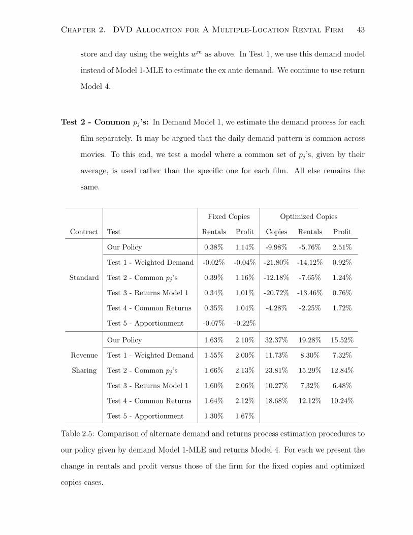
Chapter 2. DVD Allocation for A Multiple-Location Rental Firm 43
store and day using the weights wm as above. In Test 1, we use this demand model
instead of Model 1-MLE to estimate the ex ante demand. We continue to use return
Model 4.
Test 2 - Common pj’s: In Demand Model 1, we estimate the demand process for each
film separately. It may be argued that the daily demand pattern is common across
movies. To this end, we test a model where a common set of pj’s, given by their
average, is used rather than the specific one for each film. All else remains the
same.
Fixed Copies Optimized Copies
Contract Test Rentals Profit Copies Rentals Profit
Our Policy 0.38% 1.14% -9.98% -5.76% 2.51%
Test 1 - Weighted Demand -0.02% -0.04% -21.80% -14.12% 0.92%
Standard Test 2 - Common pj ’s 0.39% 1.16% -12.18% -7.65% 1.24%
Test 3 - Returns Model 1 0.34% 1.01% -20.72% -13.46% 0.76%
Test 4 - Common Returns 0.35% 1.04% -4.28% -2.25% 1.72%
Test 5 - Apportionment -0.07% -0.22%
Our Policy 1.63% 2.10% 32.37% 19.28% 15.52%
Revenue Test 1 - Weighted Demand 1.55% 2.00% 11.73% 8.30% 7.32%
Sharing Test 2 - Common pj ’s 1.66% 2.13% 23.81% 15.29% 12.84%
Test 3 - Returns Model 1 1.60% 2.06% 10.27% 7.32% 6.48%
Test 4 - Common Returns 1.64% 2.12% 18.68% 12.12% 10.24%
Test 5 - Apportionment 1.30% 1.67%
Table 2.5: Comparison of alternate demand and returns process estimation procedures to
our policy given by demand Model 1-MLE and returns Model 4. For each we present the
change in rentals and profit versus those of the firm for the fixed copies and optimized
copies cases.
Chapter 2. DVD Allocation for A Multiple-Location Rental Firm 44
Test 3 - Returns Model 1: We use the simpler returns Model 1 instead of Model 4 to
forecast the returns process of the new release. We continue to use demand Model
1-MLE. This studies the value of capturing the more detailed return process.
Test 4 - Common Returns Model: We have estimated the returns process for each
of the movies separately. It may be argued that the returns process is not movie
specific and can be estimated using a single model across all of the comparable
films at the same time. We do so in Test 4.
We observe that the results for the Fixed Copies case (with the exception of Test
1 - Weighted Demand) for both the Standard and Revenue Sharing contracts are very
similarly to those of our policy. As the Fixed Copies case amounts to reallocating supply
among the stores, it is not surprising that given a reasonable estimate of the demand
and returns, there is only so much improvement that can be made. Thus, the relative
improvement in profits of approximately 1.1% and 2.1% for the Standard and Revenue
Sharing cases, respectively, result primarily from the optimization made through Algo-
rithm 2. In contrast, for the Optimized Copies cases, we observe that the naive demand
and returns models fail to achieve the same level of profit improvement as our policy. We
observe that the Test 2-Common pj’s and Test 4-Common Returns models do achieve,
on average approximately 2/3 of the profit of our policy. This suggests, that while there
are similarities between the demand and return patterns, a 50% improvement in profit is
achieved by estimating these separately for each movie. Further, the simple demand esti-
mation procedure (averaging the observed demands for the comparables) and the simple
returns Model 1, do not perform particularly well.
It appears the optimization approach provides most of the benefit for the Fixed Copies
case. To confirm this, consider the following heuristic. Using the Optimized Copies
solution, scale the number of copies apportioned to each store so that the ci’s sum to
c, the quantity constraint. In Test 5-Apportionment in Table 2.5 we show that for the
Chapter 2. DVD Allocation for A Multiple-Location Rental Firm 45
Standard Contract case, doing so results in a loss compared with what the firm was doing.
For the Revenue Sharing case, the heuristic results in a solution that may be improved
on by 25% by our policy and those of the other heuristics. We conclude the optimization
approach significantly improves on a simpler apportionment approach.
We next test the robustness of these results with respect to π. The previous analysis
uses the values of π = 1 and 3 as given by the firm’s manager. Note π is dependent on the
salvage value obtained by the marginal unit which is not known until after demand occurs,
and on the purchase price which can vary based on supplier and quantity purchased
(see Cachon and Kok (2007) for a discussion on salvage value estimation). That is,
π = (P − S ′)/(φF ) where P is the unit purchase price, S ′ is the firm’s salvage value on
the marginal unit purchased, F is the rental fee. Let subscript ‘std.’ signify standard
contracts; ‘r.s.’, revenue sharing. The publicly available rental fee is $5. For reasons of
confidentiality the actual purchase price and marginal salvage value were not revealed
to us. However, publicly available data indicate Pstd. = $20 and Pr.s. = $3 may be valid
numbers. Then φ = 0.6, S ′std. = $5 and S ′r.s. = $0 would imply πstd. = 3 and πr.s. = 1.
Note these values may be appropriate as the greater purchase quantity resulting from
πr.s. = 1 would lead to additional units to salvage, lowering their salvage value to the
point where some units are returned to the studio (at 0 salvage value) rather than sold,
generally after about six months. Because the purchase price and marginal salvage value
may vary, we present in Table 2.6 representative summary results for the optimize copies
case in the neighborhood of the given values of π. These correspond to varying S ′std.
from $0 to $7.50 holding Pstd. = $20, and varying Pr.s. from $1.50 to $4.50 holding
S ′r.s. = $0. These represent reasonable limits on these values given publicly available data
and salvage prices observed at retail locations of the firm. As would be expected from
a newsvendor analysis, the optimal purchase quantity is very sensitive to the value of π
while the profit, as shown by its percentage change, is less so. Our conclusion that the
firm overbuys standard titles is valid unless π lies below approximately 2.7. The firm

Chapter 2. DVD Allocation for A Multiple-Location Rental Firm 46
Contract π Copies Rentals Profit
2.5 12.02% 7.87% 2.76%
3 -9.98% -5.76% 2.51%Standard
3.5 -28.15% -19.52% 9.71%
4 -43.32% -33.16% 43.10%
0.5 69.17% 32.72% 28.14%
Revenue sharing 1 32.37% 19.28% 15.52%
1.5 3.84% 3.94% 4.05%
Table 2.6: Optimized quantity results while varying π. (The Fixed Copies case is not
sensitive to π by definition.)
underbuys revenue sharing titles at all reasonable values of π, greatly if the price per
unit is low.
2.6. Discussion and Future Work
Studios generate revenue using three main channels: theatrical release, movie rentals,
and movie sales. Other revenue channels include related products and games, video-on-
demand, and cable and broadcast presentation. According to EMA (2008), the propor-
tion of consumer spending on the three main channels is 29%, 24%, and 47% for theatrical
release, movie rentals and movie sales, respectively. As this is the typical order in which
a movie is released, a large share of the revenue is received after the first month rental
period for the film. So, the studios may be using the theatrical release and rentals partly
for their revenue generation, but also for their ability to market films.
However, the movie rental firms are in trouble. Major movie rental firms have been
subject to intense competition from alternative business models, e.g., online rentals,
movie-on-demand, and download-to-rent. For example, Blockbuster, a leading global
video rental firm, reported negative net income in four out of the last five years (2004–

Chapter 2. DVD Allocation for A Multiple-Location Rental Firm 47
2008) and its share price has decreased by about 96% since its peak in 2002. Similarly,
Movie Gallery, the second largest video rental firm in the U.S. that owns Movie Gallery
and Hollywood Video stores, filed for bankruptcy in October 2007. Our study considers
how rental firms may better predict their demand and supply in order to improve their
performance.
We model the demand and return processes for DVD rental to better forecast the
supply requirements of the firm. We use the firm’s entire data set, i.e., past demand
and returns to all its stores, to forecast demand at the store and day level, rather than
relying on the data for each store individually. Our procedure is limited in several ways.
First, in order to prove concavity and optimality of our greedy algorithm, we require
monotonicity in the return rate of films. Although we find concavity holds throughout in
our data set, we do not incorporate this sufficient constraint in our estimation procedure.
Second, we assume that demand is Gamma distributed. We also reduce the numerical
computations by assuming demand is only dependent on store size (reducing Aij to Ai)
We find that by purchasing the correct quantity we are able to modestly improve
(2.5% on average) the profitability of a rental firm for movies purchased under a standard
contract. In particular, this is achieved by reducing the number of copies purchased. In
contrast, it seems appropriate to consider the Fixed Copies case for the revenue sharing
titles. There we observe that a 2.1% increase in the rental firm’s gross profit is possible,
in this case by better allocation to the stores. We find that by increasing the purchase
quantity, the firm could significantly increase its profits (15.5%). However, the firm
cannot take advantage of this potential gain due to purchase quantity restrictions imposed
by studios.
We have several comments with respect to these results. First, to place this in per-
spective, a 2.1% increase in gross profits attributable to rentals (as opposed to DVD or
other sales) at Blockbuster, Inc. , based on their 2008 annual report, results in an average
increase in net income by $37.5 million over the last three years. Blockbuster reported an

Chapter 2. DVD Allocation for A Multiple-Location Rental Firm 48
average annual operating loss of $60.2 million over this period. So a 2.1% improvement
would reduce the average operating loss by 62%. We emphasize that we present these
numbers to provide a context to understanding what 2.1% may mean in this industry
and not to declare such improvements would result. Second, our results represent only a
small sample of the films purchased and rented by the firm, and generalization to firm-
wide measures ignores various aspects of actual operations. In particular our analysis is
based on treating each film individually and ignores firm policies that might link them
such as budgetary constraints, requirements on assortments and availability of substi-
tutes, and requirements on merchandising such as shelf-space presentation. With respect
to the standard titles, it is possible that because of marketing or budgetary reasons, the
over-purchase we observe is a response to the restrictions placed on the revenue sharing
titles.
Finally, we have observed the deleterious effect on profits of the purchase restrictions
for the revenue sharing contracts. That such restrictions could have such an effect is not
surprising since the theory behind revenue sharing contracts is that without purchase
restrictions they can align supply chains to the benefit of all parties. Thus the question
is raised why do such restrictions exist? Further, one might question what determines
the contract type for different titles? Addressing these questions calls for future work.
We hypothesize that the quantity restrictions imposed may be related to studio concerns
regarding the sale of copies of DVD’s by the rental firms after the first month. That is,
the studio may be concerned with cannibalization of sales and thus acts to restrict the
number of copies.
As a demonstration of this potential reasoning we present in Table 2.7 estimates of the
average improvement over the standard contract case for the mean profit of the firm and
mean revenue of the studio, for the revenue sharing contract and the quantity-restricted
revenue sharing contract. To obtain these results, using the actual (not forecasted) sales
and returns data from the revenue sharing titles, we estimate the actual demand and
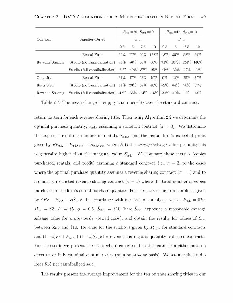
Chapter 2. DVD Allocation for A Multiple-Location Rental Firm 49
Contract Supplier/Buyer
Pstd.=20, Sstd.=10 Pstd.=15, Sstd.=10
Sr.s. Sr.s.
2.5 5 7.5 10 2.5 5 7.5 10
Revenue Sharing
Rental Firm 55% 77% 99% 122% 18% 35% 52% 69%
Studio (no cannibalization) 44% 56% 68% 80% 91% 107% 124% 140%
Studio (full cannibalization) -61% -49% -37% -25% -49% -32% -17% -1%
Quantity-
Restricted
Revenue Sharing
Rental Firm 31% 47% 63% 79% 0% 12% 25% 37%
Studio (no cannibalization) 14% 23% 32% 40% 52% 64% 75% 87%
Studio (full cannibalization) -42% -33% -24% -15% -22% -10% 1% 13%
Table 2.7: The mean change in supply chain benefits over the standard contract.
return pattern for each revenue sharing title. Then using Algorithm 2.2 we determine the
optimal purchase quantity, cstd., assuming a standard contract (π = 3). We determine
the expected resulting number of rentals, rstd., and the rental firm’s expected profit
given by Frstd. − Pstd.cstd. + Sstd.cstd. where S is the average salvage value per unit; this
is generally higher than the marginal value S ′std.. We compare these metrics (copies
purchased, rentals, and profit) assuming a standard contract, i.e., π = 3, to the cases
where the optimal purchase quantity assumes a revenue sharing contract (π = 1) and to
a quantity restricted revenue sharing contract (π = 1) where the total number of copies
purchased is the firm’s actual purchase quantity. For these cases the firm’s profit is given
by φFr − Pr.s.c + φSr.s.c. In accordance with our previous analysis, we let Pstd. = $20,
Pr.s. = $3, F = $5, φ = 0.6, Sstd. = $10 (here Sstd. expresses a reasonable average
salvage value for a previously viewed copy), and obtain the results for values of Sr.s.
between $2.5 and $10. Revenue for the studio is given by Pstd.c for standard contracts
and (1−φ)Fr+Pr.s.c+(1−φ)Sr.s.c for revenue sharing and quantity restricted contracts.
For the studio we present the cases where copies sold to the rental firm either have no
effect on or fully cannibalize studio sales (on a one-to-one basis). We assume the studio
loses $15 per cannibalized sale.
The results present the average improvement for the ten revenue sharing titles in our

Chapter 2. DVD Allocation for A Multiple-Location Rental Firm 50
data set. They are sensitive to a number of parameters, particularly the standard contract
price and average salvage value. The implication of the Table is that both the studio
and the rental firm may benefit from a revenue sharing contract or a quantity-restricted
revenue sharing when there is no cannibalization. Further, in concert with supply chain
alignment theory, the quantity restriction reduces the benefit for both parties. However,
we observe that if units purchased by the firm are sold and fully cannibalize sales (on a
one-to-one basis) with those of the studio, revenue sharing can lead to worse performance
for the studio than a standard contract, though quantity restrictions can mitigate these
losses.
These observations lead to several questions: What is the effect of cannibalization
on contract choice? If studios actually do lose money under revenue sharing contracts
compared with standard contracts, why are they used? Why were quantity restrictions
put in place as opposed to other contract types such as buy-back agreements. We em-
phasize that it is only a hypothesis that concerns on cannibalization have lead to the
quantity restrictions. Future work, which is beyond the scope of the current chapter,
should address these questions.

Chapter 3
The Maximum Covering Problem
with Travel Time Uncertainty
Abstract : Both public and private facilities often have to provide adequate service under
a variety of conditions. In particular travel times, that determine customer access, change
due to changing traffic patterns throughout the day, as well as a result of special events
ranging from traffic accidents to natural disasters. We study the maximum covering
location problem on a network with travel time uncertainty represented by different travel
time scenarios. Three model types - expected covering, robust covering and expected p-
robust covering - are studied; each one is appropriate for different types of facilities
operating under different conditions. Exact and approximate algorithms are developed.
The models are applied to the analysis of the location of fire stations in the city of
Toronto. Using real traffic data we show that the current system design is quite far from
optimality. We determine the best locations for the 4 new fire stations that the city of
Toronto is planning to add to the system and discuss alternative improvement plans.
51
Chapter 3. The Maximum Covering Problem with Travel Time Uncertainty52
3.1. Introduction
In today’s world of global competitiveness, facility location is one of the most important
long-term strategic decisions made by any organization - public or private. As such,
finding optimal locations has received considerable attention in the literature. Facility
location models (in particular covering models) try to ensure that customer’s travel times
to facilities are reasonable. This is generally achieved either by minimizing average
or worst case travel times or by defining time-dependent coverage areas for facilities.
However, travel times are not constant in practice; they are affected by many factors
ranging from predictable variations due to changes in traffic patterns during the day (that
may be quite large - an order of magnitude or more) to even larger variations introduced
by more rare disruptive events such as snow storms or traffic accidents (still for which
reliable probability estimates can be found from historical data), to less predictable and
even more rare and extreme events such as hurricanes, earthquakes and terrorist attacks.
Since facilities cannot be easily relocated, the facility network has to be able to provide
adequate service under different travel time conditions. It is also important to note
that different facility types may require different performance standards under different
conditions. For example, for a retail store it is important that the average performance
under the predictable daily variations in travel time be adequate, while the performance
under very rare disruptive events may be of less importance. On the other hand, a public
service facility such as a fire station or a hospital must be able to provide good service
under typical travel time conditions, but still maintain adequate service under the more
disruptive events. Finally, facilities that are specifically designed for response to rare
emergencies, e.g., hazardous materials response teams, must be able to provide adequate
level of service under any travel conditions, including the most extreme ones.
In this chapter we study the location of facilities that provide service to or obtain
benefit from clients within a given coverage time on a transportation network. Examples
of such facilities include fire stations, hospitals, bank branches, supermarkets, etc. Most

Chapter 3. The Maximum Covering Problem with Travel Time Uncertainty53
related studies in the literature, as we discuss in Section 3.2, either ignore possible dis-
ruptions altogether, or consider the effect on service when the facility itself is disrupted or
attacked. While this may be a concern in some cases, many coverage-providing facilities
are well built to endure catastrophic events or are not high-value targets for an attack.
For example, even during the most disruptive events, such as 9/11 attacks in New York
city or hurricane Katrina in New Orleans few of the emergency service facilities were
disrupted. However, the access to and from the facilities was seriously impacted. There-
fore, we focus on networks with travel time uncertainty, i.e., non-deterministic link travel
times.
We note that our approach to modeling the travel time uncertainty is not restricted
to catastrophic events or an attack on the network. As illustrated in our case study of
Toronto fire stations in Section 3.8, events as mundane as rush hour traffic can signifi-
cantly change travel times and limit access to coverage-providing facilities.
We model different travel time conditions as different “scenarios” of the transporta-
tion network (where a scenario is a snapshot of the network, i.e., link travel times are
deterministic conditional on scenario), and study both the cases in which the scenario
probabilities are available, or not. We further assume that the nodes of the network
have weights that represent their size/population or relative importance. This leads us
to study three types of weighted coverage location problems on a network when travel
times on links are uncertain:
1. Expected Covering Problem (ECP): Locate facilities to maximize the expected
weighted cover over all potential scenarios.
2. Robust Covering Problem (RCP): Locate facilities to maximize the minimum weighted
cover over all potential scenarios.
3. Expected p-Robust Covering Problem (EpRCP): Locate facilities to maximize the
expected weighted cover subject to a lower bound on the minimum weighted cover

Chapter 3. The Maximum Covering Problem with Travel Time Uncertainty54
over all potential scenarios.
The ECP model places rather heavy data requirements on the decision-maker, as the
scenario probabilities must be estimated for all scenarios. Moreover, since the model
optimizes average-case performance, it is not sensitive to rare or extreme events whose
probabilities are either not available, or are too small to make an appreciable impact
on the objective function. Thus, the ECP model is most suitable for locating public
service facilities such as supermarkets, restaurants or bank branches - where the main
concern is to ensure good service at different times of the day, and the probabilities of
various scenarios (representing different daily traffic flows) are easily available from the
past data.
The RCP model optimizes the worst-case performance. On the positive side, it is
not necessary to estimate event probabilities and the model is very responsive (in fact,
driven by) the extreme events. On the negative side, focusing on worst case performance
may degrade performance during typical conditions. Thus, this model is most suitable
for locating specialized emergency response centers or supply depots designed to provide
service under extreme conditions.
The EpRCP model strikes the middle ground, optimizing the average-case perfor-
mance, while requiring adequate performance in all scenarios. Note that it is not nec-
essary to estimate probabilities of rare events here - they can be set to 0 since these
events will likely not significantly impact the objective function, and the probabilities
are not necessary for the constraints. This model is most suitable for the location of
most emergency response facilities (hospitals, fire stations, etc.) that are expected to
provide good service under typical travel time fluctuations, but are still expected to
function adequately in extreme scenarios.
As an example of the difference between the three problems, consider locating a
single facility with a coverage time of T = 1 on the network presented in Figure 3.1.
Node weights and link travel times are provided next to nodes and links, respectively.

Chapter 3. The Maximum Covering Problem with Travel Time Uncertainty55
1 2 4 5 3 1 1
1
1
1
1 0.25 0.25 0.25 0.25 0
State 1
1 2 4 5 3 3 3
3
1
3
1 0.25 0.25 0.25 0.25 0
State 2
T
T
T
T
0.25 0.25
0.25 0.25
2T
2T
2T
2T
0.25 0.25
0.25 0.25
T(1+ε)
0.25 0.25
0.25 0.25
State 1: P=1-ε State 2: P=ε Expected length
T(1+ε)
T(1+ε)
T(1+ε)
1
3
4
2
1 2
4 3
5
1
2
2
1
1
1
1
1
0.25 0.25
0.25 0.25
State 1
1 2
4 3
5
2
1
1
2
2
2
2
2
0.25 0.25
0.25 0.25
State 2
1
3
4
2
Scenario 1 Scenario 2
Figure 3.1: Comparing three location problems
We consider two scenarios with probabilities P1 = 0.98 for scenario 1 and P2 = 0.02 for
scenario 2. Table 3.1 summarizes the solutions to the three location problems discussed
above. The optimal solution to the ECP is the central node 5. As expected, this location
provides the best long term average coverage at the expense of a low worst case coverage.
The opposite can be observed in nodes 1 and 3 that are the optimal robust locations. A
middle ground is reached at the optimal expected p-robust location (node 2) enforcing a
worst case coverage of 0.25.
A simplifying technique frequently used in solving stochastic location problems is to
replace the stochastic variable with its mean. In our case, this implies treating the travel
time on each link as deterministic and equal to the mean over all possible scenarios. In
fact, the classical deterministic MCLP model can be viewed as using this approximation.
Although this approach succeeds in simplifying the search for the optimal solution, the
quality of the resulting solutions can be arbitrarily poor (as proved in Proposition 3.2
ProblemOptimal Coverage
location Scenario 1 Scenario 2 Expected Worst case
ECP 5 1 0 0.98 0
EpRCP 2 0.75 0.25 0.74 0.25
RCP 1 or 3 0.5 0.5 0.5 0.5
Table 3.1: Optimal solutions of the three location problems

Chapter 3. The Maximum Covering Problem with Travel Time Uncertainty56
below). Note that for the example above, since the expected travel time on each link
is greater than 1, the optimal facility location is at any node other than 5. In partic-
ular, node 4 is an optimal location, even though it performs poorly in all three models
considered above.
As noted earlier, in this study we ignore delays or interruptions that may occur at
the facilities. In fact, queuing delays caused by congestion may certainly occur. We
note that, while on one hand the literature on location models with service congestion is
fairly rich ( (see e.g., Berman and Krass 2002) for a review) the resulting models tend to
be analytically very challenging or intractable; building an integrated model combining
queuing delays and travel time uncertainty would certainly be a worthy subject for future
research. Moreover, there is some evidence that queuing delays occur infrequently in
practice for the type of facilities we consider here (Ingolfsson et al. 2008), thus focusing
on travel time uncertainty may be valid. Moreover, avoiding queuing delays is a matter
of allocating sufficient capacity to the facilities, and while facilities cannot be easily
relocated, equipment and staff can be (see e.g., Kolesar and Walker 1974). Thus the
issues arising from travel time uncertainty are, fundamentally, more strategic.
The plan for the remainder of the chapter is as follows. After providing an overview
of the relevant literature in Section 3.2, the problem is formally defined in Section 3.3.
In this section we also prove an important localization result showing that an optimal
location can be found within the discrete set of “critical points” that can be computed
a priori. The algorithmic solution techniques for the three models are developed in
Sections 3.4, 3.5 and 3.6. Results of the computational experiments are reported in
Section 3.7. Section 3.8 contains the case study of locating fire stations in Toronto,
Canada. Concluding remarks are presented in Section 3.9.

Chapter 3. The Maximum Covering Problem with Travel Time Uncertainty57
3.2. Literature Review
Since the seminal work of Hakimi (1964) on the median and center problems, the area
of location analysis has attracted numerous researchers mostly studying deterministic
location problems. The literature on stochastic location problems is mainly focused on
node uncertainties including demand uncertainty (see Frank 1966, Mirchandani 1980,
Berman and Wang 2004, 2007) and server congestion (see Daskin 1983, ReVelle and
Hogan 1989, Berman and Krass 2002). The reader is referred to ReVelle and Eiselt
(2005) for a recent review of the literature on facility location problems and to Snyder
(2006) and Owen and Daskin (2005a) for a review of the literature on facility location
problems under uncertainty.
The maximal covering location problem (MCLP) addresses the optimal location of
facilities that provide service to customers within a coverage radius/time. Church and
ReVelle (1974) first introduced the MCLP and developed greedy heuristics to search for
the optimal facility locations on the nodes of a network. Church and Meadows (1979)
prove that an optimal set of locations for the MCLP exists in a finite set of dominant
points on the network and use linear programming and branch and bound to solve the
problem. Galvao and ReVelle (1996) present a Lagrangian based heuristic for the MCLP.
The reader is referred to Kolen and Tamir (1990) and Current et al. (2002) for a discussion
of the MCLP. Extensions of the MCLP are discussed in Berman et al. (2009b).
For networks with probabilistic links, the scenario approach to uncertainty was first
introduced by Mirchandani and Odoni (1979) and followed by Mirchandani and Oudjit
(1980) in their study of stochastic medians on a network. Weaver and Church (1983)
present solution procedures and computational results for location problems on networks
with probabilistic links. Berman and Odoni (1982) and Berman and LeBlanc (1984)
also use a scenario approach with Markovian transitions in modeling probabilistic links
to study the optimal location-relocation of a single and multiple mobile servers, respec-
tively. Serra and Marianov (1998) use a scenario approach to find optimal locations for

Chapter 3. The Maximum Covering Problem with Travel Time Uncertainty58
fire stations in Barcelona using Minmax type objectives. A related problem proposed by
Nel and Colbourn (1990) is finding the most reliable source (MRS) on a network with
unreliable links, i.e., locating facilities to maximize the expected number of nodes con-
nected to the facility when links have some independent probability of being operational.
The reader is referred to Snyder (2006) and Owen and Daskin (2005a) for a review of
the literature on facility location problems under uncertainty.
The area of robust optimization has grown rapidly in recent years. When probabil-
ities are not available or the system is expected to perform well in worst cases, robust
measures such as minimax cost and minimax regret are employed to enhance system
performance. The reader is referred to Kouvelis and Yu (1997) for a textbook treatment
of the subject. Similar to the literature on stochastic location problems, most robust
location problems study uncertainties related to the nodes of a network (e.g., demand
uncertainty, server congestion, etc.), with exceptions including the following. For a tree
with interval uncertain edge lengths and node weights, polynomial algorithms are pre-
sented by Chen and Lin (1998) and Burkard and Dollani (2001) for the minimax regret
1-median and by Averbakh and Berman (2000) and Burkard and Dollani (2002) for the
minimax regret 1-center problem. Finally, Averbakh (2003) shows that both 1-median
and weighted 1-center problems on a general network are NP-hard when edge lengths are
interval uncertain; unlike the corresponding problems with node uncertainties that are
polynomially solvable.
The concept of p-robustness was first introduced by Kouvelis et al. (1992) in a layout
planning problem for manufacturing systems. They used constraints to ensure that the
relative regret in each scenario is not greater than p. Snyder and Daskin (2006) combine
p-robustness constraints with a minimum expected cost objective to solve median and
uncapacitated fixed-charge location problems. Both problems are solved using variable
splitting.
Link disruptions are special cases of travel time uncertainty in which travel times can

Chapter 3. The Maximum Covering Problem with Travel Time Uncertainty59
be assumed to increase to infinity (or at least larger than the facility’s coverage time).
So, a related research stream is locating facilities that are resilient to disruptions. Snyder
et al. (2006) present an excellent review of the topic. Berman et al. (2007) study the
effect of service disruptions at facilities on the optimal facility locations in a p-median
context. They show that the optimal location patterns are more centralized as the disrup-
tion probability grows. Scaparra and Church (2008) present bilevel optimization models
for the r-interdiction median problem with fortification assuming service at unprotected
facilities can be disrupted. O’Hanley and Church (2008) extend the previous work to
a coverage type objective. As discussed earlier, most studies, including the ones above,
consider node disruptions whereas we study link disruptions. Related exceptions include
maximum flow interdiction problems (see e.g., Cormican et al. 1998) and shortest path
interdiction problems (see e.g., Israeli and Wood 2002) that study the impact of link
removals, but use objective functions different from ours. Berman et al. (2009a) study
the MCLP when one link of the network is disconnected by a terrorist attack or a natural
disaster. This problem is a special case of the RCP studied here in which each scenario
is the original network missing one link.
The empirical analysis of travel time uncertainty has also received considerable at-
tention in the literature. Kolesar et al. (1975) propose and empirically verify a model
for fire engine travel times in New York City that relates mean travel time to a square
root function of distance for short distances and to a linear function of distance for long
ones. This non-linear model has been revalidated using data in other cities and is still
widely used in practice (Green and Kolesar 2004). Budge et al. (2009) use data from
ambulance travel times in the city of Calgary to verify a similar non-linear model and
propose a distance dependent distribution for travel times. The distribution is shown to
have fatter tails than the Normal distribution and a coefficient of variation that decreases
with distance.
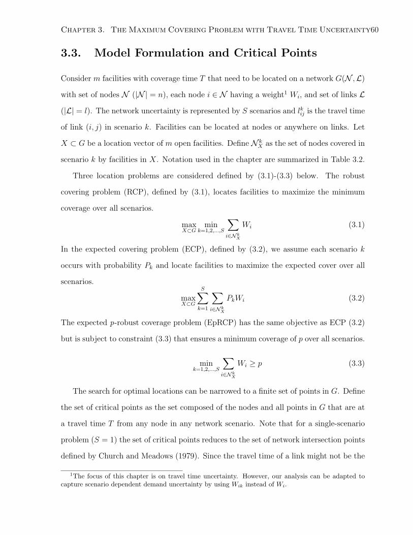
Chapter 3. The Maximum Covering Problem with Travel Time Uncertainty60
3.3. Model Formulation and Critical Points
Consider m facilities with coverage time T that need to be located on a network G(N ,L)
with set of nodes N (|N | = n), each node i ∈ N having a weight1 Wi, and set of links L
(|L| = l). The network uncertainty is represented by S scenarios and lkij is the travel time
of link (i, j) in scenario k. Facilities can be located at nodes or anywhere on links. Let
X ⊂ G be a location vector of m open facilities. Define N kX as the set of nodes covered in
scenario k by facilities in X. Notation used in the chapter are summarized in Table 3.2.
Three location problems are considered defined by (3.1)-(3.3) below. The robust
covering problem (RCP), defined by (3.1), locates facilities to maximize the minimum
coverage over all scenarios.
maxX⊂G
mink=1,2,...,S
∑
i∈N kX
Wi (3.1)
In the expected covering problem (ECP), defined by (3.2), we assume each scenario k
occurs with probability Pk and locate facilities to maximize the expected cover over all
scenarios.
maxX⊂G
S∑
k=1
∑
i∈N kX
PkWi (3.2)
The expected p-robust coverage problem (EpRCP) has the same objective as ECP (3.2)
but is subject to constraint (3.3) that ensures a minimum coverage of p over all scenarios.
mink=1,2,...,S
∑
i∈N kX
Wi ≥ p (3.3)
The search for optimal locations can be narrowed to a finite set of points in G. Define
the set of critical points as the set composed of the nodes and all points in G that are at
a travel time T from any node in any network scenario. Note that for a single-scenario
problem (S = 1) the set of critical points reduces to the set of network intersection points
defined by Church and Meadows (1979). Since the travel time of a link might not be the
1The focus of this chapter is on travel time uncertainty. However, our analysis can be adapted tocapture scenario dependent demand uncertainty by using Wik instead of Wi.

Chapter 3. The Maximum Covering Problem with Travel Time Uncertainty61
G(N ,L) the network with set of nodes N (|N | = n) and set of links L (|L| = l)
S number of network scenarios
m number of facilities to be located
T coverage time of each facility
Wi weight of node i
lkij travel time of link (i, j) in scenario k
Pk probability of scenario k occurring
N kX set of nodes covered in scenario k if the facilities are located at X ⊂ G
n′ number of critical points in the network
〈i, α, j〉 a critical point on link (i, j) at a travel time αlkij from i in scenario k
Ikij 1 if a facility located at critical point j covers node i in scenario k; 0 otherwise
xj 1 if a facility is located at critical point j; 0 otherwise
yi probability that node i is covered
yik 1 if node i is covered in scenario k; 0 otherwise
c minimum weighted cover over all scenarios
Ck coverage matrix with elements ckij = WiIkij
Z Weighted cover. Z∗: optimal -, ZG: greedy -. If locating at j, EZj : expected -,
MZj : minimum -, Zkj : - in scenario k
Table 3.2: Notation
same in different scenarios, we cannot define critical points on a link at a fixed travel
time from a node. Hence, for some 0 ≤ α ≤ 1, we define a critical point 〈i, α, j〉 on
link (i, j) at a travel time αlkij from i in scenario k. Note that although the travel time
from the critical point to any node changes in each scenario, the relative position of the
critical point on the link is fixed. For example, suppose the travel time of link (i, j) is
2 in scenario 1 and 4 in scenario 2. Then, 〈i, 0.5, j〉 is at a travel time of 1 and 2 form
node i (i.e. center of the link) in scenarios 1 and 2.
Theorem 3.1. An optimal set of locations for ECP, RCP, and EpRCP exists in the set
of critical points.
Proof. Let X ⊂ G be a location vector of m open facilities. If there exists a facility

Chapter 3. The Maximum Covering Problem with Travel Time Uncertainty62
x ∈ X that is not already on a critical point, it is always between two consecutive critical
points. Let a and b be consecutive critical points such that x ∈ [a, b]. The set of nodes
covered(N kX
)may gain or lose one or more nodes in some scenario k when we move the
facility from x across a critical point. However, we are certain, by definition, that N kX
remains unchanged on (a, b) for all k = 1, . . . , S. Based on the objective functions defined
in (3.1) and (3.2), we conclude that moving the facility from x to a or b has no effect on
the problems’ objective. In addition, by (3.3), such a move maintains the feasibility of
the solution for the EpRCP, thereby proving the theorem.
Proposition 3.1. The number of critical points, n′, is O(nlS) on a general network and
O(n2S) on a tree.
Proof. The shortest path from each point on a link to any node on a general network is
through one of the two endpoints of the link. So, each node can generate at most two
critical points on any link in each scenario. Since nodes are included in the set of critical
points, n ≤ n′ ≤ n+ 2nlS and, therefore, n′ is O(nlS). A tree has n− 1 links. So, n′ is
O(n2S) on a tree.
To show that O(n2S) is a tight representation of the number of critical points on a
tree, consider a star network with n nodes numbered 0, 1, . . . , n− 1 and S scenarios. For
an arbitrary small ε > 0, assume that each node i, except for i = 0, is connected to node
0 in scenario k via a link with travel time T − (i+ (k− 1)S)ε for all i = 1, . . . , n− 1 and
k = 1, . . . , S. Each node i generates a unique critical point on each link not adjacent to i
in each scenario. So, the number of critical points is n+(n−2)(n−1)S which is O(n2S).
We note that finding all critical points requires the availability of travel time data
in each network scenario. In the case study presented in Section 3.8 we have access to
such a data set for the city of Toronto. However, we acknowledge that access to such
data might not be always available in other settings. If, instead, only the distance data
is available, one has to decide whether to model the travel speeds as uniform or not.
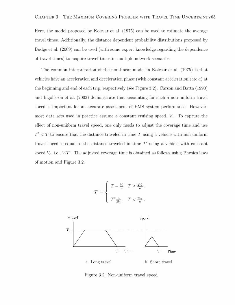
Chapter 3. The Maximum Covering Problem with Travel Time Uncertainty63
Here, the model proposed by Kolesar et al. (1975) can be used to estimate the average
travel times. Additionally, the distance dependent probability distributions proposed by
Budge et al. (2009) can be used (with some expert knowledge regarding the dependence
of travel times) to acquire travel times in multiple network scenarios.
The common interpretation of the non-linear model in Kolesar et al. (1975) is that
vehicles have an acceleration and deceleration phase (with constant acceleration rate a) at
the beginning and end of each trip, respectively (see Figure 3.2). Carson and Batta (1990)
and Ingolfsson et al. (2003) demonstrate that accounting for such a non-uniform travel
speed is important for an accurate assessment of EMS system performance. However,
most data sets used in practice assume a constant cruising speed, Vc. To capture the
effect of non-uniform travel speed, one only needs to adjust the coverage time and use
T ′ < T to ensure that the distance traveled in time T using a vehicle with non-uniform
travel speed is equal to the distance traveled in time T ′ using a vehicle with constant
speed Vc, i.e., VcT′. The adjusted coverage time is obtained as follows using Physics laws
of motion and Figure 3.2.
T ′ =
T − Vca
T ≥ 2Vca,
T 2 a2Vc
T < 2Vca.
Limits multi-dispatch to 2 vehicles, also considers objectives based on different arrival times of multi-dispatches and argues that shortest path is not optimal for multi-dispatch case (so, routing is important to reduce path covariances) Does not consider queuing and collocation of vehicles
Clarify the extent to which non-uniform travel speeds can be incorporated in the models in the paper Our data set includes travel times on links not distances. So, we don’t use any transformation from distance to time. In defining critical points, our paper states “A hidden assumption in this definition of critical points is that traveling speed on each link is uniform”. This is not necessary and should be deleted. In fact, we only assume that travel time on links is additive which is also assumed in many other studies (e.g., Daskin (1987)). Kolesar et al. (1975) present a model for travel times that considers acceleration and deceleration at a constant rate, a, for the vehicle at the beginning and end of the trip until it reaches a cruising velocity Vc. To consider such non-uniform travel times we only need to adjust our coverage radius and use T’<T to ensure that the distance traveled in time T using a vehicle with non-uniform travel speed is equal to the distance traveled in time T’ using a vehicle with constant speed Vc, i.e., VcT’. The figure below shows the non-uniform travel speed as a function of time. The distance travelled in time T using a vehicle with non-uniform travel speed can be calculated using Physics as:
So, the adjusted coverage radius is:
2
2
2
2
c c
c c
c
V VT T
a aT
a VT T
V a
2
2
2
2
2
c cc
c
V VV T T
a aD
VaTT
a
a. Long travel b. Short travel
Figure 3.2: Non-uniform travel speed

Chapter 3. The Maximum Covering Problem with Travel Time Uncertainty64
3.4. The Expected Covering Problem
In this section we study the expected covering problem (ECP), i.e., locating facilities
to maximize expected coverage over all network scenarios. We present an integer pro-
gramming formulation for the ECP in Section 3.4.1 and propose Lagrangian and greedy
heuristics for the ECP in Sections 3.4.2 and 3.4.3, respectively. But, first we show that
simplifying the location problem by averaging the travel time on links can result in arbi-
trarily suboptimal solutions.
Proposition 3.2. In the expected covering problem, the relative error of optimizing based
on average link travel times can be made arbitrarily large.
Proof. Consider a single facility location problem on a star network of n nodes with
weights of 0 and 1n−1
for the central and leaf nodes, respectively (see Figure 3.3 for
n = 5). Assume that the network has two scenarios: (1) all links have travel times equal
to the coverage time T , (2) all links have travel times equal to 2T . Further, assume that
scenarios 1 and 2 occur with probabilities 1 − ε and ε (ε > 0), respectively. For a small
ε, the optimal facility location is the central node with an expected coverage of 1 − ε.
However, since average link travel times are more than the coverage time, the optimal
location using average travel times is any leaf node and the expected coverage is 1n−1
.
The relative error can be made arbitrarily close to 100% by decreasing ε and increasing n.
1 2 4 5 3 1 1
1
1
1
1 0.25 0.25 0.25 0.25 0
State 1
1 2 4 5 3 3 3
3
1
3
1 0.25 0.25 0.25 0.25 0
State 2
T
T
T
T
0.25 0.25
0.25 0.25
2T
2T
2T
2T
0.25 0.25
0.25 0.25
T(1+ε)
0.25 0.25
0.25 0.25
State 1: P=1-ε State 2: P=ε Expected length
T(1+ε)
T(1+ε)
T(1+ε)
1
3
4
2
1 2
4 3
5
1
2
2
1
1
1
1
1
0.25 0.25
0.25 0.25
State 1
1 2
4 3
5
2
1
1
2
2
2
2
2
0.25 0.25
0.25 0.25
State 2
1
3
4
2
a. Scenario 1 b. Scenario 2 c. Average travel times
Figure 3.3: Link travel times and expected link travel times for n = 5

Chapter 3. The Maximum Covering Problem with Travel Time Uncertainty65
We note that the example provided is a mathematical oddity caused by defining coverage
as a step function. In reality, if ε is small, the demands remain covered at a travel time
of T + ε.
3.4.1 Mathematical Programming Formulation
Define coverage parameters (not decision variables) Ikij = 1 if a facility located at critical
point j covers node i in scenario k, i.e., the shortest travel time from node i to critical
point j in scenario k is not greater than T , and 0 otherwise. Let xj = 1 if a facility
is located at critical point j and 0 otherwise. Let yi be the probability that node i is
covered. The ECP, defined in (3.2), can be formulated as follows:
maxZ =n∑
i=1
Wiyi (3.4a)
s.t.S∑
k=1
Pk maxj=1,...,n′
xjIkij ≥ yi for all i = 1, . . . , n (3.4b)
n′∑
j=1
xj = m (3.4c)
xj = 0, 1 and yi ≥ 0 for all i = 1, . . . , n, j = 1, . . . , n′ (3.4d)
The problem’s objective (3.4a) is to maximize the expected coverage. Coverage prob-
abilities are calculated in (3.4b) while (3.4c) ensures that m facilities are located on the
network. The formulation is non-linear due to constraint (3.4b). To avoid non-linearity,
we introduce new decision variables yik = 1 if node i is covered in scenario k and 0
otherwise. Now, we can present an integer programming formulation for the ECP as
below:

Chapter 3. The Maximum Covering Problem with Travel Time Uncertainty66
[ECP]
maxZ =n∑
i=1
S∑
k=1
WiPkyik (3.5a)
s.t.yik ≤n′∑
j=1
xjIkij for all i = 1, . . . , n, k = 1, . . . , S (3.5b)
n′∑
j=1
xj = m (3.5c)
xj, yik = 0, 1 for all i = 1, . . . , n, j = 1, . . . , n′, k = 1, . . . , S (3.5d)
Daskin (1987) presents an alternative formulation for the maximum covering problem
with travel time uncertainty assuming travel times on non-overlapping links are indepen-
dent and calculating the coverage probabilities exogenously. Whereas our formulation
requires explicit enumeration of travel times on all links in all network scenarios, Daskin’s
formulation only requires a probability distribution for the travel time on each link. The
resulting data burden is obviously much lower with Daskin’s formulation (Erkut et al.
(2008) and Goldberg and Paz (1991) use similar independence assumptions to calculate
the coverage probabilities). However, the price one pays for the improved computa-
tional tractability is the independence assumption, which is clearly violated for a city
with time-dependent traffic pattern. For example, in the case study presented in Sec-
tion 3.8, average travel time correlation on all links during different hours of the day is
0.45 for Toronto. In this regard, our scenario-based treatment of travel times allows for
interdependent travel times, and thus is more appropriate for the Toronto data.
Note that the classical maximum covering location problem which is a special case
of ECP is proved to be NP-hard. Our numerical studies in Section 3.7 show that the
integer friendliness of the maximum covering location problem (see e.g., ReVelle 1993) is
lost when extending the problem to multiple scenarios and that the integer programming
formulation (3.5a)–(3.5d) is difficult to solve, especially for large networks. Therefore,
we present Lagrangian and greedy heuristics for the ECP in the following sections.
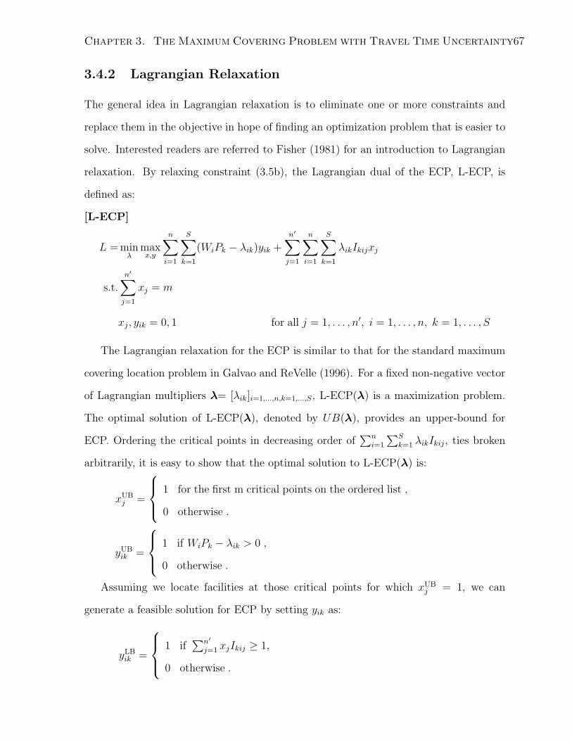
Chapter 3. The Maximum Covering Problem with Travel Time Uncertainty67
3.4.2 Lagrangian Relaxation
The general idea in Lagrangian relaxation is to eliminate one or more constraints and
replace them in the objective in hope of finding an optimization problem that is easier to
solve. Interested readers are referred to Fisher (1981) for an introduction to Lagrangian
relaxation. By relaxing constraint (3.5b), the Lagrangian dual of the ECP, L-ECP, is
defined as:
[L-ECP]
L = minλ
maxx,y
n∑
i=1
S∑
k=1
(WiPk − λik)yik +n′∑
j=1
n∑
i=1
S∑
k=1
λikIkijxj
s.t.n′∑
j=1
xj = m
xj, yik = 0, 1 for all j = 1, . . . , n′, i = 1, . . . , n, k = 1, . . . , S
The Lagrangian relaxation for the ECP is similar to that for the standard maximum
covering location problem in Galvao and ReVelle (1996). For a fixed non-negative vector
of Lagrangian multipliers λ= [λik]i=1,...,n,k=1,...,S, L-ECP(λ) is a maximization problem.
The optimal solution of L-ECP(λ), denoted by UB(λ), provides an upper-bound for
ECP. Ordering the critical points in decreasing order of∑n
i=1
∑Sk=1 λikIkij, ties broken
arbitrarily, it is easy to show that the optimal solution to L-ECP(λ) is:
xUBj =
1 for the first m critical points on the ordered list ,
0 otherwise .
yUBik =
1 if WiPk − λik > 0 ,
0 otherwise .
Assuming we locate facilities at those critical points for which xUBj = 1, we can
generate a feasible solution for ECP by setting yik as:
yLBik =
1 if∑n′
j=1 xjIkij ≥ 1,
0 otherwise .

Chapter 3. The Maximum Covering Problem with Travel Time Uncertainty68
Substituting the feasible solution in (3.5a), we obtain a lower-bound for ECP denoted by
LB(λ).
Given initial multipliers λ0 , we use the subgradient optimization method to generate
a sequence of multipliers as follows:
λt+1ik = max
{0, λtik −∆t
(n′∑
j=1
xUBj Ikij − yUB
ik
)}
where ∆t is a positive step size defined as:
∆t =αt[UB(λt)− LB(λt)
]
∑ni=1
∑Sk=1
(∑n′j=1 x
UBj Ikij − yUB
ik
)2
and αt is a scalar satisfying 0 < αt ≤ 2. Our algorithm starts with α0 = 2 and λik = 0
and cuts α by half every time UB(λ) fails to decrease after a fixed number of iterations.
The algorithm terminates when the upper and lower bounds are sufficiently close to each
other or when the iteration limit is reached. The Lagrangian relaxation algorithm for
the ECP can be formally stated as follows:
Algorithm 3.1. Lagrangian Relaxation
1. Initiation: Let λ0ik = 0, α0 = 2, t = 0. Set appropriate values for ε (convergence
error), tmax (iterations limit), and tα (iterations to decrease α).
2. Lagrangian relaxation: Find UB(λt) and LB(λt) using (3.6) and (3.6).
3. Check convergence: If UB(λt)− LB(λt) ≤ ε or t = tmax, STOP.
4. Update step size: For t > tα, if UB(λt) ≥ UB(λt−tα), αt = αt−1
2. Otherwise,
αt = αt−1.
5. Update multipliers: Find λt+1 using (3.6) and (3.6). Increase t by one. Goto step
2.

Chapter 3. The Maximum Covering Problem with Travel Time Uncertainty69
Lagrangian relaxation can be embedded in a branch and bound procedure to find
an exact solution for the ECP. However, as will be discussed later, since the optimality
gap was relatively small in all our numerical experiments, further improvement of the
solution was not necessary.
3.4.3 Greedy Heuristic
In this section we first provide an exact solution procedure for the single facility ECP.
Since the extension of this procedure to multiple facilities becomes numerically intensive,
we also present a greedy heuristic for the multiple facility ECP. For each scenario k =
1, . . . , S, define the coverage matrix Ck with elements ckij = Wi if node i is covered by a
facility located at critical point j in scenario k; and ckij = 0 otherwise, i.e., ckij = WiIkij.
Rows in the coverage matrix correspond to nodes and columns correspond to critical
points. The following algorithm finds the optimal location for the single facility ECP.
Algorithm 3.2. Single-facility ECP
1. Find weighted cover Zkj =
∑ni=1 c
kij for all k = 1, . . . , S and j = 1, . . . , n′.
2. Find expected weighted cover EZj =∑S
k=1 PkZkj for all and j = 1, . . . , n′.
3. Locate the facility at critical point j = arg maxj=1,...,n′{EZj}
The complexity of Algorithm 3.2 is mainly due to step 1. Based on Proposition 3.1,
the number of columns (critical points) in each coverage matrix is O(nlS) for a general
network and O(n2S) for a tree. So, the complexity of step 1 and the whole algorithm is
O(n2lS2) for a general network and O(n3S2) for a tree.
Algorithm 3.2 can be extended for locating m > 1 facilities by defining columns as
any combination of m critical points. The complexity of this algorithm is due to the need
for enumerating all subsets of critical points with size m. Using Sterling’s approximation
for factorials, the number of columns in each coverage matrix would be O((
nlm
)m)for

Chapter 3. The Maximum Covering Problem with Travel Time Uncertainty70
a general network and O((
n2
m
)m)for a tree. So, the complexity of Algorithm 3.2 is
O((
nlm
)mnS)
for locating m > 1 facilities on a general network and O((
n2
m
)mnS)
on
a tree. Instead, The following greedy heuristic solves the problem of locating m > 1
facilities and has a complexity of O(mn2lS2) for a general network and O(mn3S2) for a
tree.
Algorithm 3.3. Greedy heuristic for ECP
1. Locate one facility at the critical point j with maximum EZj determined by Algo-
rithm 3.2 . Let m = m− 1.
2. In each coverage matrix Ck, for all i = 1, . . . , n, if ckij > 0, change ckil to Wi for all
l = 1, . . . , n′
3. If m > 0, go to step 1; otherwise STOP.
Algorithm 3.3 locates the facilities one by one based on a greedy coverage criterion.
For each node i and scenario k, if the located facility covers node i in scenario k, step 2
changes all elements in row i of Ck to Wi. This ensures that nodes already covered are
assumed covered and not considered again when locating the next facilities. Let Z∗ be
the optimal weighted cover from (3.5a)–(3.5d) and ZG be the weighted cover obtained
by Algorithm 3.3. Then, the relative error of Algorithm 3.3 is defined as Z∗−ZGZ∗ .
Theorem 3.2. The worst case relative error of Algorithm 3.3 is 1e≈ 37%.
Proof. Nemhauser et al. (1978) discuss various properties of submodular functions and
prove that the worst case relative error of maximizing a non-decreasing submodular
function via a greedy heuristic is 1e. We prove that the weighted cover Z is a non-
decreasing submodular function. Let F be a set of facility locations (subset of the set of
critical points). By (3.5b) and (3.5d) and the objective (3.5a) that maximizes yik, yik = 1
if node i is covered by some facility j ∈ F in scenario k, i.e., if i ∈ N kF , and yik = 0

Chapter 3. The Maximum Covering Problem with Travel Time Uncertainty71
otherwise. So, (3.5a) can be rewritten as Z(F) =∑S
k=1
∑i∈N kF
WiPk. Let F1 and F2 be
sets of facility locations such that F1 ⊂ F2 and j be a critical point such that j /∈ F2.
Then,
Z (F2 ∪ {j})− Z (F2) =S∑
k=1
∑
i∈N kF2∪{j}
PkWi −S∑
k=1
∑
i∈N kF2
PkWi =S∑
k=1
∑
i∈N kj −N kF2
PkWi ≥ 0
Similarly, Z (F1 ∪ {j}) − Z (F1) =∑S
k=1
∑i∈N kj −N kF1
PkWi. But, F1 ⊂ F2 implies that
N kF1⊂ N k
F2and, hence, N k
j − N kF2⊂ N k
j − N kF1
. So, 0 ≤ Z (F2 ∪ {j}) − Z (F2) ≤
Z (F1 ∪ {j})− Z (F1) that proves Z is non-decreasing and submodular.
Proposition 3.3. The worst case bound obtained in Theorem 3.2 is tight.
Proof. To prove that the 1e
worst case bound is tight, we provide the following infinite
directed graph as an example. Consider locating two facilities on the network presented
in Figure 3.4, P1 = P2 = 0.5. Assume travel time on all links is T (coverage time). So, the
set of critical points includes nodes only. Based on the coverage matrices in Figure 3.4 for
the first facility, the expected weighted covers are 12, 1
2, 1
4, 1
4, 1
2, and 1
2for the six columns.
With a small ε adjustment, Algorithm 3.3 locates the first facility on node 1. For the
second facility, based on coverage matrices in Figure 3.4, the expected weighted covers
are 12, 1
2, 3
4, 3
4, 3
4, and 3
4for the six columns. With a small ε adjustment, Algorithm 3.3
locates the second facility on node 3. The ε adjustments required to ensure the choices
above is to change the weight of node 1 to 14
+ ε and node 3 to 18
+ ε2
for an arbitrary
small ε > 0.
The total expected weighted cover using Algorithm 3.3 is ZG = 34. However, the
optimal solution is Z∗ = 1 that is achieved by locating the facilities on nodes 5 and 6.
So, the relative error of Algorithm 3.3 for the network in Figure 3.4 is Z∗−ZGZ∗ = 1
4. By
extending our example as follows we construct a network for which the relative error of
Algorithm 3.3 approaches 1e
as the network size increases to infinity.
For any k > 1, let α = k−1k< 1 and construct a network that consists of k complete
graphs, G1, . . . , Gk, and an empty graph Gk+1. Each complete graphs Gi has k nodes

Chapter 3. The Maximum Covering Problem with Travel Time Uncertainty72
1 2
5 6
3 4
1
4
1
8
1
8 2
1
4
1
8
1
8
State 1
1 2
5 6
3 4
1
4
1
8
1
8 2
1
4
1
8
1
8
State 2
1 1 10 0 0
4 4 4
1 1 10 0 0
4 4 4
1 1 10 0 0
8 2 8 2 8 2
1 1 10 0 0
8 8 8
10 0 0 0 0
8
10 0 0 0 0
8
1 1 10 0 0
4 4 4
1 1 10 0 0
4 4 4
1 1 10 0 0
8 2 8 2 8 2
1 1 10 0 0
8 8 8
10 0 0 0 0
8
10 0 0 0 0
8
1 1 10 0 0
4 4 4
1 1 10 0 0
4 4 4
1 1 10 0 0
8 2 8 2 8 2
1 1 10 0 0
8 8 8
10 0 0 0 0
8
10 0 0 0 0
8
1 1 10 0 0
4 4 4
1 1 10 0 0
4 4 4
1 1 10 0 0
8 2 8 2 8 2
1 1 10 0 0
8 8 8
10 0 0 0 0
8
10 0 0 0 0
8
Facility 1 Facility 2
State 1
State 2
1 1 10 0 0
4 4 4
1 1 10 0 0
4 4 4
1 1 10 0 0
8 8 8
1 1 10 0 0
8 8 8
10 0 0 0 0
8
10 0 0 0 0
8
1 1 10 0 0
4 4 4
1 1 10 0 0
4 4 4
1 1 10 0 0
8 8 8
1 1 10 0 0
8 8 8
10 0 0 0 0
8
10 0 0 0 0
8
1 1 1 1 1 1
4 4 4 4 4 4
1 1 1 1 1 1
4 4 4 4 4 4
1 1 10 0 0
8 8 8
1 1 10 0 0
8 8 8
10 0 0 0 0
8
10 0 0 0 0
8
1 1 1 1 1 1
4 4 4 4 4 4
1 1 1 1 1 1
4 4 4 4 4 4
1 1 10 0 0
8 8 8
1 1 10 0 0
8 8 8
10 0 0 0 0
8
10 0 0 0 0
8
Coverage matrices for
the first facility
1 2
5 6
3 4
1
4
1
8
1
8
1
4
1
8
1
8
1 2
5 6
3 4
1
4
1
8
1
8
1
4
1
8
1
8
Coverage matrices for
the second facility
Figure 3.4: Tightness of the greedy bound, k = 2
gi1, . . . , gik with weights αi−1
k2 . The empty graph Gk+1 has k nodes gk+11 , . . . , gk+1
k with
weights αk
k. Assume the network has k scenarios, each with probability 1
k. In scenario
s, gk+1j is connected to all nodes gl(j+s−2 mod k)+1 for l = 1, . . . , k with a directed link
originating from gk+1j . That is, in scenario 1, node gk+1
1 is connected to g11, . . . , g
k1 , gk+1
2
is connected to g12, . . . , g
k2 , etc. In scenario 2, node gk+1
k is connected to g11, . . . , g
k1 , gk+1
1
is connected to g12, . . . , g
k2 , gk+1
2 is connected to g13, . . . , g
k3 , etc. Assume travel time on all
links is T (coverage time). So, the set of critical points includes nodes only.
Figure 3.4 is the realization of this network for k = 2 in which nodes 1 and 2 are
G1, nodes 3 and 4 are G2, and nodes 5 and 6 are G3. The coverage matrices for the
first facility in Figure 3.4 include 2 × 2 blocks of node weights. Following a similar
structure, the coverage matrix for scenario 1 of the extended network (k ≥ 2), presented
in Figure 3.5, includes k × k blocks of node weights. The coverage matrix for other
scenarios can be found by reordering the top part of the last k columns keeping the last

Chapter 3. The Maximum Covering Problem with Travel Time Uncertainty73
1k2 · · · 1
k21k2
.... . .
.... . .
1k2 · · · 1
k21k2
αk2 · · · α
k2αk2
.... . .
.... . .
αk2 · · · α
k2αk2
. . ....
αk−1
k2 · · · αk−1
k2αk−1
k2
.... . .
.... . .
αk−1
k2 · · · αk−1
k2αk−1
k2
αk
k. . .
αk
k
1
Figure 3.5: Tightness of the greedy bound, k ≥ 2, scenario 1
k rows unchanged.
The expected weighted cover of the first k sets of k columns (i.e., columns 1, 2 and
columns 3, 4 when k = 2) is 1k, αk, . . . , α
k−1
k, respectively. For the last k columns (i.e.,
columns 5, 6 when k = 2), the expected weighted cover is:
1
k2
(1 + . . .+ αk−1
)+αk
k=
1
k2
(1− αk1− α
)+αk
k=
1
k
(1− αk
)+αk
k=
1
k
So, with small ε adjustments, Algorithm 3.3 locates the first facility on a node in G1.
Similar analysis reveals that Algorithm 3.3 locates the ith facility on a node in Gi. Hence,
the total expected weighted cover using Algorithm 3.3 is ZG = 1k
(1 + . . .+ αk−1
)=
1 − αk. However, all nodes are covered in all scenarios if facilities are located on the
nodes of Gk+1. So, the optimal solution is Z∗ = 1k
(1 + . . .+ αk−1
)+ αk = 1 and the
relative error of Algorithm 3.3 is Z∗−ZGZ∗ = αk =
(k−1k
)k. When k increases to infinity,
the relative error of Algorithm 3.3 becomes limk→∞(k−1k
)k= 1
e.
Next we present an example to highlight the discussion here and in the next sections.
Suppose a facility with coverage time T = 4 is to be located on the two-scenario network
illustrated in Figure 3.6 where P1 = 70% and P2 = 30%. The critical points, coverage
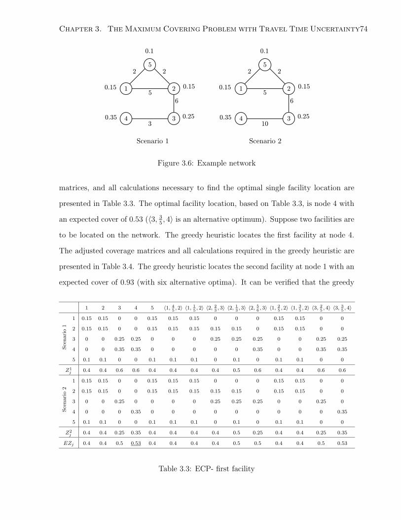
Chapter 3. The Maximum Covering Problem with Travel Time Uncertainty74
5
1 2
3 4
State 1
0.1
0.1 0.2
0.5 0.1
2 2
6
3
5
1 2
3 4
State 1
0.1
0.15 0.15
0.25 0.35
2 2
6
3
5
1 2
3 4
State 2
0.1
0.15 0.15
0.25 0.35
2 2
6
10
1 3
2 4
5 6
1
2
2
2
5 10
a b
1
0.15 0.1
0.15 0.1
0.1 0.4
State 1: P = 0.9
1 3
2 4
5 6
3
3
2
2
5 10
a b
1
0.15 0.1
0.15 0.1
0.1 0.4
State 2: P = 0.1
5 5
Scenario 1 Scenario 2
Figure 3.6: Example network
matrices, and all calculations necessary to find the optimal single facility location are
presented in Table 3.3. The optimal facility location, based on Table 3.3, is node 4 with
an expected cover of 0.53 (〈3, 35, 4〉 is an alternative optimum). Suppose two facilities are
to be located on the network. The greedy heuristic locates the first facility at node 4.
The adjusted coverage matrices and all calculations required in the greedy heuristic are
presented in Table 3.4. The greedy heuristic locates the second facility at node 1 with an
expected cover of 0.93 (with six alternative optima). It can be verified that the greedy
1 2 3 4 5 〈1, 45, 2〉 〈1, 1
5, 2〉 〈2, 2
3, 3〉 〈2, 1
3, 3〉 〈2, 5
6, 3〉 〈1, 2
5, 2〉 〈1, 3
5, 2〉 〈3, 2
5, 4〉 〈3, 3
5, 4〉
Sce
nari
o1
1 0.15 0.15 0 0 0.15 0.15 0.15 0 0 0 0.15 0.15 0 0
2 0.15 0.15 0 0 0.15 0.15 0.15 0.15 0.15 0 0.15 0.15 0 0
3 0 0 0.25 0.25 0 0 0 0.25 0.25 0.25 0 0 0.25 0.25
4 0 0 0.35 0.35 0 0 0 0 0 0.35 0 0 0.35 0.35
5 0.1 0.1 0 0 0.1 0.1 0.1 0 0.1 0 0.1 0.1 0 0
Z1j 0.4 0.4 0.6 0.6 0.4 0.4 0.4 0.4 0.5 0.6 0.4 0.4 0.6 0.6
Sce
nari
o2
1 0.15 0.15 0 0 0.15 0.15 0.15 0 0 0 0.15 0.15 0 0
2 0.15 0.15 0 0 0.15 0.15 0.15 0.15 0.15 0 0.15 0.15 0 0
3 0 0 0.25 0 0 0 0 0.25 0.25 0.25 0 0 0.25 0
4 0 0 0 0.35 0 0 0 0 0 0 0 0 0 0.35
5 0.1 0.1 0 0 0.1 0.1 0.1 0 0.1 0 0.1 0.1 0 0
Z2j 0.4 0.4 0.25 0.35 0.4 0.4 0.4 0.4 0.5 0.25 0.4 0.4 0.25 0.35
EZj 0.4 0.4 0.5 0.53 0.4 0.4 0.4 0.4 0.5 0.5 0.4 0.4 0.5 0.53
Table 3.3: ECP- first facility
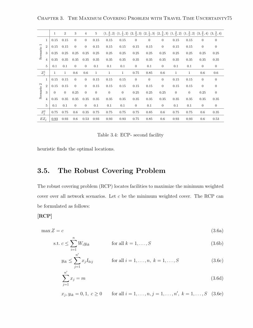
Chapter 3. The Maximum Covering Problem with Travel Time Uncertainty75
1 2 3 4 5 〈1, 45, 2〉 〈1, 1
5, 2〉 〈2, 2
3, 3〉 〈2, 1
3, 3〉 〈2, 5
6, 3〉 〈1, 2
5, 2〉 〈1, 3
5, 2〉 〈3, 2
5, 4〉 〈3, 3
5, 4〉
Sce
nari
o1
1 0.15 0.15 0 0 0.15 0.15 0.15 0 0 0 0.15 0.15 0 0
2 0.15 0.15 0 0 0.15 0.15 0.15 0.15 0.15 0 0.15 0.15 0 0
3 0.25 0.25 0.25 0.25 0.25 0.25 0.25 0.25 0.25 0.25 0.25 0.25 0.25 0.25
4 0.35 0.35 0.35 0.35 0.35 0.35 0.35 0.35 0.35 0.35 0.35 0.35 0.35 0.35
5 0.1 0.1 0 0 0.1 0.1 0.1 0 0.1 0 0.1 0.1 0 0
Z1j 1 1 0.6 0.6 1 1 1 0.75 0.85 0.6 1 1 0.6 0.6
Sce
nari
o2
1 0.15 0.15 0 0 0.15 0.15 0.15 0 0 0 0.15 0.15 0 0
2 0.15 0.15 0 0 0.15 0.15 0.15 0.15 0.15 0 0.15 0.15 0 0
3 0 0 0.25 0 0 0 0 0.25 0.25 0.25 0 0 0.25 0
4 0.35 0.35 0.35 0.35 0.35 0.35 0.35 0.35 0.35 0.35 0.35 0.35 0.35 0.35
5 0.1 0.1 0 0 0.1 0.1 0.1 0 0.1 0 0.1 0.1 0 0
Z2j 0.75 0.75 0.6 0.35 0.75 0.75 0.75 0.75 0.85 0.6 0.75 0.75 0.6 0.35
EZj 0.93 0.93 0.6 0.53 0.93 0.93 0.93 0.75 0.85 0.6 0.93 0.93 0.6 0.53
Table 3.4: ECP- second facility
heuristic finds the optimal locations.
3.5. The Robust Covering Problem
The robust covering problem (RCP) locates facilities to maximize the minimum weighted
cover over all network scenarios. Let c be the minimum weighted cover. The RCP can
be formulated as follows:
[RCP]
maxZ = c (3.6a)
s.t. c ≤n∑
i=1
Wiyik for all k = 1, . . . , S (3.6b)
yik ≤n′∑
j=1
xjIkij for all i = 1, . . . , n, k = 1, . . . , S (3.6c)
n′∑
j=1
xj = m (3.6d)
xj, yik = 0, 1, c ≥ 0 for all i = 1, . . . , n, j = 1, . . . , n′, k = 1, . . . , S (3.6e)

Chapter 3. The Maximum Covering Problem with Travel Time Uncertainty76
Constraint (3.6b) calculates the minimum weighted cover over all scenario. Constraint
(3.6c) identifies the covered nodes in each scenario and (3.6d) ensures that m facilities
are located. Solving this integer programming problem, similar to that of the ECP, is
difficult, especially for large networks. We develop Lagrangian and greedy heuristics to
solve it. The Lagrangian dual of the RCP, L-RCP, is defined by relaxing (3.6c) with
Lagrangian multipliers λik.
[L-RCP]
L = minλ
maxx,y,c
c−n∑
i=1
S∑
k=1
λikyik +n′∑
j=1
n∑
i=1
S∑
k=1
λikIkijxj
s.t. c ≤n∑
i=1
Wiyik for all k = 1, . . . , S
n′∑
j=1
xj = m
xj, yik = 0, 1, c ≥ 0 for all j = 1, . . . , n′, i = 1, . . . , n, k = 1, . . . , S
The L-RCP is separable with respect to the decision variables into an x-problem (in-
volving only xj variables) and a y-problem (involving only yik variables and c). Whereas
the x-problem is easy to solve, the y-problem is a multi-dimensional knapsack problem
that is not readily solvable. Note, however, that the Lagrangian solution provides an
upper-bound for the RCP. Therefore, we replace the set of equations (3.6b) with their
average and find an upper-bound for L-RCP, and hence an upper-bound for RCP, by
solving L′-RCP as follows:
[L′-RCP]
L′ = minλ
maxy,c
c−n∑
i=1
S∑
k=1
λikyik + maxx
n′∑
j=1
n∑
i=1
S∑
k=1
λikIkijxj
c ≤ 1
S
n∑
i=1
S∑
k=1
Wiyik
n′∑
j=1
xj = m
yik = 0, 1, c ≥ 0 xj = 0, 1

Chapter 3. The Maximum Covering Problem with Travel Time Uncertainty77
For a fixed non-negative vector of Lagrangian multipliers λ , L′-RCP(λ) is a max-
imization problem. Each non-zero yik in the optimal solution increases c by Wi
Syik and
the objective function by c − λikyik. So, a non-zero yik has a non-negative contribution
to the objective function of the y-problem if λik ≤ Wi
S. Therefore, ordering the critical
points in decreasing order of∑n
i=1
∑Sk=1 λikIkij, the optimal solution to L′-RCP(λ) is:
xUBj =
1 for the first m critical points on the ordered list ,
0 otherwise .
yUBik =
1 if λik ≤ Wi
S,
0 otherwise .
cUB =1
S
n∑
i=1
S∑
k=1
Wiyik
Lagrangian and greedy heuristics, similar to Algorithms 3.1 and 3.3 can be developed
to solve the RCP. The single facility RCP is solved optimally with a modified version of
Algorithm 3.2 noting that here we find the minimum cover MZj = mink=1,...,S{Zkj } in
step 2 and locate the facility at the critical point with maximum MZj in step 3.
Example. Continuing the example in Section 3.4.3, the maximum ofMZj = min{Z1j , Z
2j }
based on Table 3.3 is 0.5. So, the optimal solution to the one facility RCP is to locate at
〈2, 13, 3〉. For the two facility problem, the adjusted coverage matrices and all calculations
required in the greedy heuristic are presented in table 3.5. Based on table 3.5, the greedy
heuristic locates the second facility at node 4 (〈3, 34, 4〉 is an alternative optimum) with
an optimal objective value of 0.85. The greedy heuristic finds the optimal solution to the
RCP in this example.
3.5.1 Special Cases
As discussed in Section 3.1, the RCP is particularly interesting in contexts for which
the worst case effect of a disruptive event is under study such as a terrorist attack, a

Chapter 3. The Maximum Covering Problem with Travel Time Uncertainty78
1 2 3 4 5 〈1, 45, 2〉 〈1, 1
5, 2〉 〈2, 2
3, 3〉 〈2, 1
3, 3〉 〈2, 5
6, 3〉 〈1, 2
5, 2〉 〈1, 3
5, 2〉 〈3, 2
5, 4〉 〈3, 3
5, 4〉
Sta
te1
1 0.15 0.15 0 0 0.15 0.15 0.15 0 0 0 0.15 0.15 0 0
2 0.15 0.15 0.15 0.15 0.15 0.15 0.15 0.15 0.15 0.15 0.15 0.15 0.15 0.15
3 0.25 0.25 0.25 0.25 0.25 0.25 0.25 0.25 0.25 0.25 0.25 0.25 0.25 0.25
4 0 0 0.35 0.35 0 0 0 0 0 0.35 0 0 0.35 0.35
5 0.1 0.1 0.1 0.1 0.1 0.1 0.1 0.1 0.1 0.1 0.1 0.1 0.1 0.1
Z1j 0.65 0.65 0.85 0.85 0.65 0.65 0.65 0.5 0.5 0.85 0.65 0.65 0.85 0.85
Sta
te1
1 0.15 0.15 0 0 0.15 0.15 0.15 0 0 0 0.15 0.15 0 0
2 0.15 0.15 0.15 0.15 0.15 0.15 0.15 0.15 0.15 0.15 0.15 0.15 0.15 0.15
3 0.25 0.25 0.25 0.25 0.25 0.25 0.25 0.25 0.25 0.25 0.25 0.25 0.25 0.25
4 0 0 0 0.35 0 0 0 0 0 0 0 0 0 0.35
5 0.1 0.1 0.1 0.1 0.1 0.1 0.1 0.1 0.1 0.1 0.1 0.1 0.1 0.1
Z2j 0.65 0.65 0.5 0.85 0.65 0.65 0.65 0.5 0.5 0.5 0.65 0.65 0.5 0.85
MZj 0.65 0.65 0.5 0.85 0.65 0.65 0.65 0.5 0.5 0.5 0.65 0.65 0.5 0.85
Table 3.5: RCP- second facility
natural disaster, or a network failure. A realistic effect of such an event is the complete
disconnection of one or more links rather than a finite increase in their length(s). Note
that an increase in the length of a link beyond 2T is equivalent to the disconnection of
that link. We denote by “risky link” a link that might be disconnected. When all links
in the network are risky, the network has 2l states. In such a case, the complexity of the
exact and heuristic algorithms presented for the RCP increases exponentially with the
size of the network.
On a general network, if all risky links can be disconnected simultaneously, the net-
work has minimum coverage when all risky links are disconnected (proof by contra-
diction). Therefore, the RCP is reduced to solving a single state, i.e., all risky links
disconnected, maximum covering location problem. If a certain number of risky links,
but not all, can be disconnected at once, the problem becomes more complicated due to
the need for identifying links whose disconnection will cause minimum coverage.
In the single facility RCP on a tree, if all links are risky and only one link can be
disconnected, first, the coverage of a facility located at an interior point on a link is zero

Chapter 3. The Maximum Covering Problem with Travel Time Uncertainty79
if that link is disconnected. So, locating on an interior point of any link is suboptimal,
and hence, the set of critical points includes nodes only. Second, let Dil be the set of
nodes within the coverage radius of a facility located at node i if link l is disconnected
and Li be the set of links adjacent to node i. Then, the following proposition holds.
Proposition 3.4. If only one link can be disconnected on a tree, the minimum coverage
for a facility located at a node occurs when one of its adjacent links is disconnected.
Proof. Assume that a facility is located at node i. For any link (k, l) /∈ Li, assume,
without loss of generality, that (k, l) and (i, j) are on the path from i to l. Since all
links on a tree connect to i through only one of the adjacent links, Di(k,l) = Di(i,j)+{nodes
between i and l on the path from i to l}. So,∑
t∈Di(k,l)
Wt ≥∑
t∈Di(i,j)
Wt.
The coverage matrix C identifies the set of nodes that are covered by a facility located
at any node i. For each node i ∈ N and l ∈ Li label as l all nodes that connect to i
through l. Then, Dil is found by removing nodes labeled l from the set of nodes that are
covered by a facility located at node i. Based on Proposition 3.4, the following algorithm
finds the optimal robust location on a tree if all links are risky and only one link can be
disconnected. The algorithm has a complexity of O(n2).
Algorithm 3.4. Single-facility RCP on a tree
1. Find Dil for all i ∈ N and l ∈ Li.
2. Let ci = minl∈Li
{∑t∈Dil
Wt
}.
3. Locate the facility at node j = arg maxi{ci}.
Proposition 3.4, however, does not hold for a general network or for locating m > 1
facilities on a tree. As counter examples, consider the networks in Figure 3.7 with a large
facility coverage radius. Facilities are shown with black nodes. Minimum coverage in
both networks occurs when link (1, 2), not adjacent to any facility, is disconnected.

Chapter 3. The Maximum Covering Problem with Travel Time Uncertainty80
1
3
4
2 1
3
4
2
(a) General network (b) A tree with m > 1
Figure 3.7: Counter example
3.6. The Expected p-Robust Covering Problem
The expected p-robust covering problem (EpRCP) locates facilities to maximize the
expected weighted cover subject to a lower bound on the minimum weighted cover over
all scenario. The EpRCP can be formulated as follows:
[EpRCP]
maxZ =n∑
i=1
S∑
k=1
WiPkyik (3.7a)
s.t.n∑
i=1
Wiyik ≥ p for all k = 1, . . . , S (3.7b)
yik ≤n′∑
j=1
xjIkij for all i = 1, . . . , n, k = 1, . . . , S (3.7c)
n′∑
j=1
xj = m (3.7d)
xj, yik = 0, 1 for all i = 1, . . . , n, j = 1, . . . , n′, k = 1, . . . , S (3.7e)
Note that the EpRCP might become infeasible for large values of p. In fact, the
maximum value for p to maintain feasibility is the optimal coverage provided by the
RCP. The Lagrangian dual of the EpRCP, L-EpRCP, is defined by relaxing constraint
(3.7c) with Lagrangian multipliers λik.

Chapter 3. The Maximum Covering Problem with Travel Time Uncertainty81
[L-EpRCP]
L = minλ
maxx,y,c
n∑
i=1
S∑
k=1
(WiPk − λik)yik +n′∑
j=1
n∑
i=1
S∑
k=1
λikIkijxj
s.t.n∑
i=1
Wiyik ≥ p for all k = 1, . . . , S
n′∑
j=1
xj = m
xj, yik = 0, 1 for all i = 1, . . . , n, j = 1, . . . , n′, k = 1, . . . , S
For a fixed non-negative vector of Lagrangian multipliers λ , L-EpRCP(λ) is a max-
imization problem that is separable by variables x and y. In addition, the y-problem is
separable by scenario k. So, the optimal solution to L-EpRCP(λ) is as follows: (i) Or-
dering the critical points in a decreasing order of∑n
i=1
∑Sk=1 λikIkij, set xUB
j = 1 for the
first m critical points on the ordered list and xUBj = 0 for others. (ii) For each scenario
k = 1, . . . , S, arranging the nodes in a decreasing order of WiPk − λik, set yUBik = 1 in
order until both∑n
i=1 Wiyik ≥ p and WiPk − λik < 0 (yUBik = 0 for others).
A Lagrangian relaxation solution procedure, similar to Algorithm 3.1 can be developed
for the EpRCP. The greedy Algorithm 3.3, however, needs to be modified to account for
the minimum coverage bound in the EpRCP. Since the EpRCP and ECP share the same
objective, we use Algorithm 3.3 to find an initial set of greedy locations for the EpRCP. If
the initial set of locations satisfies (3.7b), the solution is feasible and we stop. Otherwise,
we use an exchange routine, starting from the last facility located, to relocate the facility
to a critical point that maximizes the minimum coverage. We continue the exchange
routine until the minimum coverage bound (3.7b) is satisfied (or the algorithm fails to
find a feasible solution). In the last iteration of the exchange routine, if more than one
location satisfies (3.7b), we choose the location that provides the maximum expected
cover. A formal statement of the greedy exchange routine is presented below.
Algorithm 3.5. Greedy exchange heuristic for EpRCP
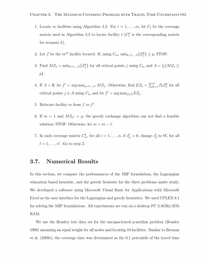
Chapter 3. The Maximum Covering Problem with Travel Time Uncertainty82
1. Locate m facilities using Algorithm 3.3. For t = 1, . . . ,m, let Ct be the coverage
matrix used in Algorithm 3.3 to locate facility t (Ckt is the corresponding matrix
for scenario k).
2. Let f be the mth facility located. If, using Cm, mink=1,...,S{Zkf } ≥ p, STOP.
3. Find MZj = mink=1,...,S{Zkj } for all critical points j using Cm and A = {j|MZj ≥
p}.
4. If A = ∅, let f ′ = arg maxj=1,...,n′MZj. Otherwise, find EZj =∑S
k=1 PkZkj for all
critical points j ∈ A using Cm and let f ′ = arg maxj∈AEZj.
5. Relocate facility m from f to f ′.
6. If m = 1 and MZf ′ < p, the greedy exchange algorithm can not find a feasible
solution; STOP. Otherwise, let m = m− 1.
7. In each coverage matrix Ckm, for all i = 1, . . . , n, if ckij > 0, change ckil to Wi for all
l = 1, . . . , n′. Go to step 2.
3.7. Numerical Results
In this section, we compare the performances of the MIP formulation, the Lagrangian
relaxation based heuristic, and the greedy heuristic for the three problems under study.
We developed a software using Microsoft Visual Basic for Applications with Microsoft
Excel as the user interface for the Lagrangian and greedy heuristics. We used CPLEX 8.1
for solving the MIP formulations. All experiments are run on a desktop PC 2.4GHz/2Gb
RAM.
We use the Beasley test data set for the uncapacitated p-median problem (Beasley
1990) assuming an equal weight for all nodes and locating 10 facilities. Similar to Berman
et al. (2009c), the coverage time was determined as the 0.1 percentile of the travel time
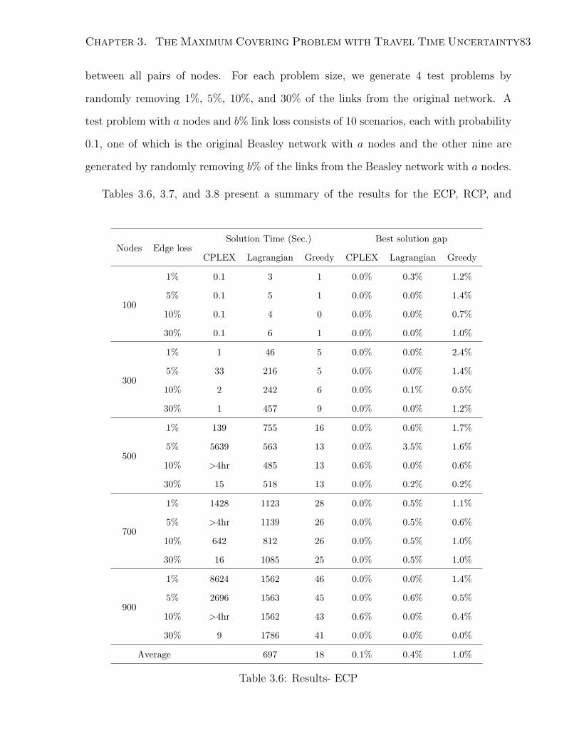
Chapter 3. The Maximum Covering Problem with Travel Time Uncertainty83
between all pairs of nodes. For each problem size, we generate 4 test problems by
randomly removing 1%, 5%, 10%, and 30% of the links from the original network. A
test problem with a nodes and b% link loss consists of 10 scenarios, each with probability
0.1, one of which is the original Beasley network with a nodes and the other nine are
generated by randomly removing b% of the links from the Beasley network with a nodes.
Tables 3.6, 3.7, and 3.8 present a summary of the results for the ECP, RCP, and
Nodes Edge lossSolution Time (Sec.) Best solution gap
CPLEX Lagrangian Greedy CPLEX Lagrangian Greedy
100
1% 0.1 3 1 0.0% 0.3% 1.2%
5% 0.1 5 1 0.0% 0.0% 1.4%
10% 0.1 4 0 0.0% 0.0% 0.7%
30% 0.1 6 1 0.0% 0.0% 1.0%
300
1% 1 46 5 0.0% 0.0% 2.4%
5% 33 216 5 0.0% 0.0% 1.4%
10% 2 242 6 0.0% 0.1% 0.5%
30% 1 457 9 0.0% 0.0% 1.2%
500
1% 139 755 16 0.0% 0.6% 1.7%
5% 5639 563 13 0.0% 3.5% 1.6%
10% >4hr 485 13 0.6% 0.0% 0.6%
30% 15 518 13 0.0% 0.2% 0.2%
700
1% 1428 1123 28 0.0% 0.5% 1.1%
5% >4hr 1139 26 0.0% 0.5% 0.6%
10% 642 812 26 0.0% 0.5% 1.0%
30% 16 1085 25 0.0% 0.5% 1.0%
900
1% 8624 1562 46 0.0% 0.0% 1.4%
5% 2696 1563 45 0.0% 0.6% 0.5%
10% >4hr 1562 43 0.6% 0.0% 0.4%
30% 9 1786 41 0.0% 0.0% 0.0%
Average 697 18 0.1% 0.4% 1.0%
Table 3.6: Results- ECP
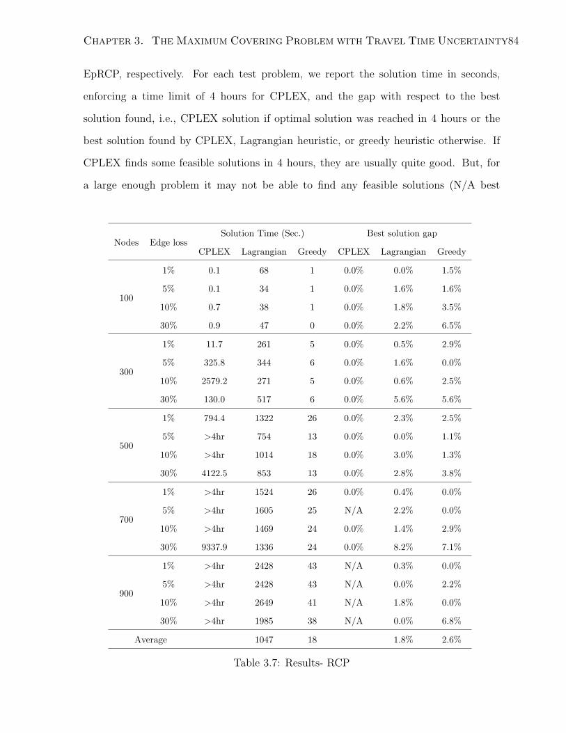
Chapter 3. The Maximum Covering Problem with Travel Time Uncertainty84
EpRCP, respectively. For each test problem, we report the solution time in seconds,
enforcing a time limit of 4 hours for CPLEX, and the gap with respect to the best
solution found, i.e., CPLEX solution if optimal solution was reached in 4 hours or the
best solution found by CPLEX, Lagrangian heuristic, or greedy heuristic otherwise. If
CPLEX finds some feasible solutions in 4 hours, they are usually quite good. But, for
a large enough problem it may not be able to find any feasible solutions (N/A best
Nodes Edge lossSolution Time (Sec.) Best solution gap
CPLEX Lagrangian Greedy CPLEX Lagrangian Greedy
100
1% 0.1 68 1 0.0% 0.0% 1.5%
5% 0.1 34 1 0.0% 1.6% 1.6%
10% 0.7 38 1 0.0% 1.8% 3.5%
30% 0.9 47 0 0.0% 2.2% 6.5%
300
1% 11.7 261 5 0.0% 0.5% 2.9%
5% 325.8 344 6 0.0% 1.6% 0.0%
10% 2579.2 271 5 0.0% 0.6% 2.5%
30% 130.0 517 6 0.0% 5.6% 5.6%
500
1% 794.4 1322 26 0.0% 2.3% 2.5%
5% >4hr 754 13 0.0% 0.0% 1.1%
10% >4hr 1014 18 0.0% 3.0% 1.3%
30% 4122.5 853 13 0.0% 2.8% 3.8%
700
1% >4hr 1524 26 0.0% 0.4% 0.0%
5% >4hr 1605 25 N/A 2.2% 0.0%
10% >4hr 1469 24 0.0% 1.4% 2.9%
30% 9337.9 1336 24 0.0% 8.2% 7.1%
900
1% >4hr 2428 43 N/A 0.3% 0.0%
5% >4hr 2428 43 N/A 0.0% 2.2%
10% >4hr 2649 41 N/A 1.8% 0.0%
30% >4hr 1985 38 N/A 0.0% 6.8%
Average 1047 18 1.8% 2.6%
Table 3.7: Results- RCP

Chapter 3. The Maximum Covering Problem with Travel Time Uncertainty85
solution gap). For the EpRCP, we set p equal to the average worst case coverage of
the solutions to ECP and RCP. In other words, we seek a solution that maximizes the
expected coverage and provides a worst case coverage that is better than that of the ECP
by 50% of the maximum possible improvement. Based on Tables 3.6, 3.7, and 3.8, we
make the following observations.
1. Solution time increases with the number of nodes for all procedures, however the
Nodes Edge lossSolution Time (Sec.) Best solution gap
CPLEX Lagrangian Greedy CPLEX Lagrangian Greedy
100
1% 0.1 2 1 0.0% 0.0% 1.2%
5% 0.1 2 1 0.0% 0.0% 1.4%
10% 0.1 4 0 0.0% 0.0% 0.7%
30% 0.1 3 1 0.0% 0.0% 1.4%
300
1% 1 30 7 0.0% 0.0% 3.0%
5% 290 225 10 0.0% 0.0% 0.9%
10% 34 199 7 0.0% 0.5% 0.1%
30% 3 249 6 0.0% 0.1% 1.9%
500
1% 207 418 21 0.0% 0.6% 1.9%
5% >4hr 486 19 0.0% 0.8% 1.5%
10% >4hr 416 17 0.0% 1.3% 0.2%
30% 15 486 20 0.0% 0.8% 2.3%
700
1% >4hr 960 42 0.0% 0.2% 1.9%
5% >4hr 849 38 0.4% 0.0% 0.4%
10% 2608 978 39 0.0% 0.5% 2.0%
30% 93 1046 38 0.0% 1.7% 4.0%
900
1% >4hr 1602 78 0.0% 0.2% 2.6%
5% 11247 1794 68 0.0% 0.3% 2.4%
10% >4hr 1573 72 0.0% 0.9% 1.2%
30% 22 1349 58 0.0% 0.0% 0.0%
Average 634 27 0.0% 0.4% 1.5%
Table 3.8: Results- EpRCP

Chapter 3. The Maximum Covering Problem with Travel Time Uncertainty86
rate of increase is quite different. To analyze these differences, we conducted re-
gression analysis using the solution time as the dependent variable and the number
of nodes as the independent variable. The regression model showed that the so-
lution time increases exponentially in the number of nodes for CPLEX. For the
Lagrangian relaxation and the greedy heuristic, quadratic model provided the best
fit. However, while the quadratic term was dominant (i.e. had the larger coeffi-
cient) for the former, it had a very low coefficient for the latter. Thus we conclude
that the solution time increased quadratically for the Lagrangian relaxation heuris-
tic, and almost linearly (quadratic with low coefficient) for the greedy heuristic.
CPLEX is unable to find any feasible solutions for large RCP instances.
2. Similar to many other network problems, the solution time is usually lower for low
density and high density networks and higher for medium density networks.
3. Both heuristics find good solutions, i.e., small optimality gaps, but none is dominant
for all problems. A useful strategy is to use both heuristics and select the best
solution.
3.8. Case Study: Toronto Fire Stations
The City of Toronto is one of North America’s largest metropolitan centers with an area
of 641 square kilometers and over 2.7 million residents. Toronto Fire Services (TFS) is the
largest fire service in Canada, and the 5th largest fire service in North America. The scope
of work is defined by the Toronto Fire Chief as “very broad, including but not limited to
fire response, hazardous materials, vehicle accidents, medical emergencies, ice and water
rescue, carbon monoxide, and false alarms.” TFS responded to more than 140,000 calls
in 2007 of which 53% were for medical services and 27% for fire related emergencies.
TFS operated with a budget of $330 million in 2007, 82% of which was directly related
to emergency response operations. 82 fire stations are currently operational in Toronto
Chapter 3. The Maximum Covering Problem with Travel Time Uncertainty87
and the TFS is planning the addition of 4 more stations (TFS 2008).
The Toronto Master Fire plan and the National Fire Protection Association (NFPA)
1710 standard recognize a target response time of 4 minutes for emergency services (TFS
2007). The response time is defined as the time since units start traveling to the emer-
gency incident until they arrive on scene not including pre-trip delays. Pre-trip delay is
the sum of the time spent on call taking and dispatching (dispatch time) and the time
from when a crew is dispatched until the vehicle starts moving (turnout time). While
NFPA 1710 sets a 1 minute standard for the pre-trip delay, Ingolfsson et al. (2008), us-
ing data from approximately 6,997 calls serviced in over 4 years in St. Albert, Alberta,
estimate an average pre-trip delay of 3 minutes for EMS calls. Based on their results it
might be more appropriate to use a 2 minute response time to ensure a 5 minute total
delay proposed in NFPA 1710.
We address two questions in the current section: (1) How effective is the current
locations of the 82 stations with respect to the ECP, RCP and EpRCP objectives? (2)
What are the “optimal” locations of the 4 new stations and, perhaps more importantly,
with is the relative impact of adding 4 stations compared to other alternatives for service
improvement.
The data on travel times in Toronto was provided by the Data Management Group of
the Civil Engineering Department at The University of Toronto who run a sophisticated
data collection system based on embedded traffic sensors at a large number of locations
in metropolitan Toronto (DMG 2004). The network consists of 3220 nodes, i.e., road
intersections, and 9630 directed links, i.e. major roads and streets in the city of Toronto
(see Figure 3.8). Link directions are important since travel times, especially during
rush hours, are not equal for both directions of a street (e.g., towards vs. away from
downtown). The city is divided into 481 zones represented by centroids (artificial nodes)
on the network that are connected to their closest intersections.
Travel times and traffic volumes in Toronto are highly dependent on the time of the

Chapter 3. The Maximum Covering Problem with Travel Time Uncertainty88
Figure 3.8: Network representation of Toronto
day. Our data set includes travel times per hour on each link of the network. Figure
3.9.a shows the average hourly variation in travel time on all links. Average travel time
increases by 18% during the morning rush hour (equivalent to a 15% decrease in average
velocity). Considering the lower population density of Toronto, this is in line with Kolesar
et al. (1975)’s estimate of a maximum 20% reduction in fire engine velocity due to hourly
traffic in New York city. While the pattern of rush hours during 7-9 AM and 4-6 PM is
common among more than 90% of the links, travel times can increase up to four times
the average on some links during the rush hour. we note, however, that the frequency of
such large deviations is small. Figure 3.9.b presents a frequency plot for Max/Average
travel time per link.
Therefore, we define 24 scenarios, one per each hour, for the network. Our data set
0%
10%
20%
30%
1 1.5 2 2.5 3 3.5 4
Max/Average travel time
Frequen
cy
-5%
0%
5%
10%
15%
20%
0 1 2 3 4 5 6 7 8 9 10 11 12 13 14 15 16 17 18 19 20 21 22 23
Hour
Deviation from av. travel tim
e
a. Hourly pattern b. Frequency plot
Figure 3.9: Travel time variation in Toronto

Chapter 3. The Maximum Covering Problem with Travel Time Uncertainty89
includes travel times on each link for each hour (scenario) and the weight (population)
of each centroid. To study system performance under adverse conditions, we include one
additional scenario - the “snow storm”, in which travel time on each link is triple the
average over the other 24 scenarios (the Federal Highway Administration at the U.S.
Department of Transportation estimates heavy snow to decrease free-flow speed by up
to 64%)2. Such events occur several times per year in Toronto and thus the fire service
certainly should take them into account. On the other hand, these events are quire rare
(on an annual basis), thus we set the probability of the associated scenario to 0.
Not all nodes of the network are realistic candidates for locating a fire station. We,
therefore, limit the fire station locations to the set of centroids defined earlier. Due to
the large size of the resulting networks, all problem instances described in the following
sections were solved using the greedy heuristic. While the resulting solutions may not be
optimal, out results in Section 3.7 indicate that the optimality gap should be small. We
also note that our data set only captures hourly variation in travel times. In reality, other
factors such as weather, route choice, or the driver taking a wrong turn could contribute
greatly to travel time variability. Further, it seems likely that the time-of-day variation
will depend on the day of the week as well, with rush hour effects less pronounced on
weekends than weekdays.
Finally, we note that travel time on a given link–hour in our data set is in fact
the average travel time within that link–hour. In reality, traffic sensor data provides
a distribution for travel time on each link–hour. while we do not have access to such
detailed data, we acknowledge that a more realistic set of scenarios can be obtained
by sampling from the joint distribution of travel times in each hour. This is especially
important in finding true worst case scenarios.
2http://ops.fhwa.dot.gov/weather/q1 roadimpact.htm

Chapter 3. The Maximum Covering Problem with Travel Time Uncertainty90
(a) Current locations (b) Minimum number of fire stations required
Figure 3.10: Fire station locations to provide the current 2-min coverage
3.8.1 Quality of the Current Locations
The locations of the current fire stations can be found on Figure 3.10(a). The percentage
of population covered with respect to ECP and RCP models for the current 82-station
system are presented on Table 3.9 for different coverage radii (time standards). As ex-
plained earlier, we are particularly interested in the 2-minute standard, which we consider
the most relevant. The performance of the best heuristic solution with respect to each
objective for each time standard is presented on Table 3.10. In addition to the value
of the objective function for the best 82-station solution found, we also present the %
improvement over the current solution (in the “% Improvement” row) and the heuris-
tic upper bound on the minimum number of stations required to achieve the current
level of performance. E.g., with respect to the 1-minute time standard the current loca-
tions achieve 22% coverage with respect to the ECP objective; the same coverage can be
achieved with at most 30 optimally located stations. We make the following observations
based on Tables 3.9 and 3.10:
CoverageResponse time
1 min 2 min 3 min 4 min 5 min
Expected (ECP) 22% 52% 83% 98% 99.9%
Worst case (RCP) 17% 18% 23% 33% 44%
Table 3.9: Current performance of 82 fire stations in Toronto

Chapter 3. The Maximum Covering Problem with Travel Time Uncertainty91
(a) Expected covering problem (b) Robust covering problem
Figure 3.11: Fire station locations to provide the optimal 2-min coverage
1. Currently, the fire stations are well located to provide a high expected coverage of
the population in 4 minutes. For example, 98% of the population is covered on
average in 4 minutes (can be improved to 100%).
2. Currently, the fire stations are not well located to accommodate shorter response
times. For example, the expected coverage of the population in 2 minutes is only
52%, while this can be improved to 74% (see Figure 3.11(a) for optimal locations).
Comparing Figures 3.10(a) and 3.11(a), the optimal locations seem to spread over
the city similar to the current locations. The improvement in service, however, is
a result of locating the fire stations closer to larger population centers.
3. Currently, the fire stations are not well located to respond to worst case scenarios.
Response time
1 min 2 min 3 min 4 min 5 min
ECP
Best coverage 43% 74% 98% 100% 100%
% Improvement 91% 42% 18% 2% 0.1%
Min stations 30 45 47 45 48
RCP
Best coverage 34% 36% 44% 52% 64%
% Improvement 97% 105% 91% 59% 45%
Min stations 30 30 30 38 44
Table 3.10: Performance of the best-found solution for the 82 fire stations in Toronto
Chapter 3. The Maximum Covering Problem with Travel Time Uncertainty92
For example, in the worst case, only 18% of the population is covered in 2 minutes,
while this can be improved to 36% (see Figure 3.11(b) for optimal locations). Com-
paring optimal and current locations in Figures 3.10(a) and 3.11(b), we observe a
higher concentration of stations in downtown (middle-bottom part) to improve the
worst case coverage.
4. The current level of coverage can be provided with drastically fewer fire stations.
For example, we can provide the current 2 minute expected coverage of 52% with
45 fire stations instead of the current 82. (see Figure 3.10(b) for optimal locations).
Since we do not consider the service capacity of fire stations in our analysis, our
results do not imply over capacity but rather propose consolidation of fire stations.
The optimal consolidation can provide the current service level, if acceptable, with
moderate savings in personnel cost and large savings in facility and equipment cost.
It was argued in the introduction that the most relevant objective for the location
of fire stations is EpRCP, since it optimizes the average (expected) performance, while
insuring an adequate level of performance under the worst-case scenario (i.e., the snow
storm scenario in our study). To compute the optimal solution for this objective, the
parameter p (required worst-case performance) must be specified. On Figure 3.12 (solid
line) we provide the trade-off curve (heuristically estimated) between expected and worst
case coverage with respect to the 2-minute time standard, as well as the performance of
the current locations. It can be seen that the current locations perform far below the
efficient frontier. For example, the lowest non-inferior p value is 23%. Thus, there exists
a solution that achieves the highest possible ECP coverage of 74% (a 42% improvement
over the current system) while still providing the worst-case (RCP) coverage of 23% (a
30% improvement over the current level of 18%). Similarly, the highest p value is 36.5%,
which has a corresponding ECP value of 55% (above the current level of 52%). Thus,
substantial improvements could be expected from the system redesign with respect to

Chapter 3. The Maximum Covering Problem with Travel Time Uncertainty93
any level of p.
If the city of Toronto were to consider re-locating some or all of their fire stations,
which p should they use? This question does not have a “correct” answer - the decision-
makers could, in principle, use any p value on Figure 3.12, depending on the expected
vs. worst-case coverage trade-off that is considered acceptable. However, a reasonable
value may be p = 31% - it lies close to the inflection point of the trade-off curve and
achieves approximately 60% of the maximal possible value with respect to both ECP
and RCP objectives (the % is expressed with respect to the range of values on the trade-
off curve). We used this value of p to derive the new locations of the 82 fire stations
that are displayed on Figure 3.13. The ECP and RCP values achieved by this solution
with respect to the 2-minute time standard are 66% and 31%, respectively - both large
improvements over the current system. With respect to the actual locations, it can be
seen that the optimized system concentrates far more facilities in the densely-populated
center of the city, while having fewer facilities in the peripheral regions (due to both,
lower population density and faster travel times in these areas).0.30684 0.6595129 ‐2.57 3
0.313621 0.6471917 ‐1.82 70.317983 0.6291223 ‐4.14 4 0.521189 0.1776790.321135 0.6252153 ‐1.24 30.322738 0.6176665 ‐4.71 20.324805 0.6114143 ‐3.02 20.327949 0.6036711 ‐2.46 30.330925 0.5944503 ‐3.10 3 0 75 ( )0.330925 0.5944503 3.10 30.336996 0.5885246 ‐0.98 60.341235 0.5854694 ‐0.72 40.34285 0.5797242 ‐3.56 2
0.346864 0.5660499 ‐3.41 4 0.65
0.7
0.75
over
age
82
(0.23,0.74)
t ti0.346864 0.5660499 3.41 40.349832 0.5612478 ‐1.62 30.35139 0.5546129 ‐4.26 2
0.355311 0.5528232 ‐0.46 40.364867 0.5467491 ‐0.64 10
0.55
0.6
0.65
0.7
0.75
Exp
ecte
dco
vera
ge
82
4
(0 365 0 55)
(0.23,0.74)
(0.19,0.56)
(0 22 0 53)
stationsnew stations
0.364867 0.5467491 ‐0.64 10
p expected coverage231 4997 740 2693
0.45
0.5
0.55
0.6
0.65
0.7
0.75
0.15 0.2 0.25 0.3 0.35
Exp
ecte
dco
vera
ge
( t )
82
4
Current 82 stations(0.18,0.52)
(0.365,0.55)
(0.23,0.74)
(0.19,0.56)
(0.22,0.53)
stationsnew stations
231.4997 740.2693245.3603 738.076251.5556 734.4561
254.16 731.4211258 8598 726 9093
0.45
0.5
0.55
0.6
0.65
0.7
0.75
0.15 0.2 0.25 0.3 0.35
Exp
ecte
dco
vera
ge
p (worst case coverage)
82
4
Current 82 stations(0.18,0.52)
(0.365,0.55)
(0.23,0.74)
(0.19,0.56)
(0.22,0.53)
stationsnew stations
258.8598 726.9093263.3391 724.0543267.7646 719.3862271.6798 714.7111
275 24 710 3301275.24 710.3301275.2945 705.5197278.593 704.0776
281.2489 703.9257283 6552 699 6932283.6552 699.6932286.4103 696.2014287.8409 690.7613288.9021 686.5656
Figure 3.12: Trade-off curves for the EpRCP objective (2-min coverage)

Chapter 3. The Maximum Covering Problem with Travel Time Uncertainty94
Figure 3.13: Recommended fire station locations in Toronto
3.8.2 Locating Four New Fire Stations
The Toronto Fire Services is planning the addition of four more stations to its current 82
(TFS 2007). We used the EpRCP framework to analyze the best locations for the four
new fire stations (in addition to the current 82 stations) with respect to the 2-minute
coverage standard. The trade-off curve is presented on Figure 3.12 (dashed line). While
the addition of the new locations obviously leads to an improvement over the current
solution (up to 8% over the current ECP value and up to 23% over the current RCP
value), these improvements are quite modest and are far below the values that can be
achieved with optimal locations for the current facilities.
Instead of investing in new facilities, it seems that Toronto Fire Services should con-
sider other improvement alternatives such as relocating some facilities or improving re-
sponse times. For example, our current analysis is based on an estimate of 3 minutes for
average pre-trip delays. If Toronto Fire Services can decrease pre-trip delays to 2 min-
utes, Table 3.9 suggest that expected and worst case coverages of the current facilities
would increase to 83% and 23%, respectively (an improvement of 60% and 28% over the
current ECP and RCP values, respectively). The improvements would increase to 88%
and 83% over the current ECP and RCP values, respectively, if Toronto Fire Services
Chapter 3. The Maximum Covering Problem with Travel Time Uncertainty95
adheres to the 1-minute standard for pre-trip delays proposed in NFPA 1710.
3.9. Conclusion
We study three variations of the maximum covering location problem on a network with
travel time uncertainty. The expected covering problem locates facilities to maximize the
expected weighted cover over all network scenarios. The robust covering problem locates
facilities to maximize the minimum weighted cover over all scenarios. The expected p-
robust covering problem locates facilities to maximize the expected weighted cover subject
to a lower bound on the minimum weighted cover over all scenarios. We present integer
programming formulations and develop Lagrangian and greedy heuristics for the three
problems. Our numerical results show that solution time increases exponentially with
size for the integer programming formulations. The Lagrangian and greedy heuristics,
instead, provide near optimal results in reasonable time.
We use real data for the city of Toronto to analyze the current location of fire stations
with respect to the 24 scenarios representing travel times during different hours of the
day and one additional scenario representing the traffic disruption due to a snow storm.
We find that the current locations of the 82 stations are not particularly well suited to
achieve the desired 5-minute total response time, either with respect to the expected
coverage or the worst-case coverage during the snow storm. We identified best locations
for the 4 new fire stations that the city of Toronto is planning to add to the system under
different expected case-worst case trade-offs and commented on alternative options for
improving system performance.

Chapter 4
The Covering Relocation Problem
with Travel Time Uncertainty
Abstract : Decision makers in many operational networks face the question of whether
to add extra facilities or relocate some existing facilities to improve service quality. The
choice becomes especially difficult when travel times on the network change due to various
causes ranging from changing traffic to natural disasters. We study a multi-objective
maximum covering problem on a network with travel time uncertainty that aims at
relocating the fewest number of facilities while maximizing expected and worst case
coverage over all scenarios of the network. We present greedy and Lagrangian relaxation
heuristics and compare their performances with MIP formulation. We use real data for
the city of Toronto to analyze the current location of fire stations. We find that most of
the optimality gap can be captured by relocating only a third of the fire stations. We
also find that, considering lower cost implications, the city should consider relocating fire
stations instead of building new ones.
96

Chapter 4. The Covering Relocation Problem with Travel Time Uncertainty97
4.1. Introduction
In the previous chapter, we studied three variations of the maximum covering location
problem on a network with travel time uncertainty: the expected covering problem,
the robust covering problem, and the expected p-robust covering problem. In all three
problems we assumed that no facilities are currently located on the network. In reality,
many operational networks already have some facilities installed. So, management has
two options to improve service quality: adding extra facilities or relocating some existing
facilities. In general, adding extra facilities requires large investments for obtaining the
required physical and human resources to run those facilities while relocating facilities is
a less costly alternative. Since relocating facilities still incurs a large cost, management is
interested in improving the service quality with minimum number of facility relocations.
We model travel time uncertainty as different “scenarios” of the transportation net-
work (where a scenario is a snapshot of the network with regard to link travel times).
Assuming a set of facilities already exists on the network, in this chapter we study the
location of coverage providing facilities using three objectives:
1. Minimizing the number of facility relocations.
2. Maximizing the excepted weighted cover over all scenarios.
3. Maximizing the minimum weighted cover over all scenarios.
The maximal covering location problem (MCLP) studies the location of facilities that
provide coverage to customers within a given radius/time. Church and ReVelle (1974)
first introduced the MCLP and developed a greedy search algorithm limited to the nodes
of a network. Church and Meadows (1979) prove that the search for optimal locations
should be extended from the nodes to a finite set of dominant points on the network and
use LP/branch and bound to solve the problem. Interested readers are referred to Kolen
and Tamir (1990) and Current et al. (2002) for a discussion of the MCLP and to Snyder

Chapter 4. The Covering Relocation Problem with Travel Time Uncertainty98
(2006) and Owen and Daskin (2005b) for a review of the literature on facility location
problems under uncertainty.
Multi-objective analysis of facility locations has received some attention in the OM
literature. Current et al. (1990) present a review of the literature on Multi-objective
facility location. A common method for solving multi-objective problems is to transform
them into single-objective problems using a utility function that captures the relative
preference of decision makers with respect to each objective. In practice, however, it is
difficult for decision makers to accurately specify these preferences a priori (see e.g., ReV-
elle et al. 1981). Alternatively, it is easier for decision makers to express their preferences
once the optimal solutions and trade-offs are revealed.
We define an efficient location vector as a feasible solution to the multi-objective
location problem defined earlier such that no other feasible solution exists that can im-
prove its performance on one objective without degrading the performance on another
objective. The set of efficient solutions, i.e. efficient set, accurately captures the trade-
offs between objectives. Therefore, we aim at finding the efficient set for the facility
location problem above. Malczewski and Ogryczak (1995) discuss three methods for
finding the efficient set for multi-objective location problems, i.e., the weighting method,
the noninferior set estimation method, and the constraint method, and their advantages
and disadvantages. Here, we use the constraint method for its ease of application and
its additional flexibility for controlling the value of each objective. For a review of the
literature on multi-objective decision making, we refer the reader to Evans (1984) and
Ehrgott and Gandibleux (2000).
We first study two variations of the relocation problem, one with objectives 1 and
2 and the other with objectives 1 and 3. For these problems, we develop exact and
heuristic methods to obtain the efficient set. Then, we study the relocation problem with
all three objectives and present a heuristic algorithm for finding the efficient set. The
three problems we study are formally defined below:

Chapter 4. The Covering Relocation Problem with Travel Time Uncertainty99
1. Expected Covering Relocation Problem (ECRP): Relocate the fewest number of
facilities such that the excepted weighted cover over all scenarios is more than a
given bound ρE.
2. Robust Covering Relocation Problem (RCRP): Relocate the fewest number of facil-
ities such that the minimum weighted cover over all scenarios is more than a given
bound ρR.
3. Expected p-Robust Covering Relocation Problem (EpRCRP): Relocate the fewest
number of facilities such that the excepted and minimum weighted covers over all
scenarios are more than given bounds ρE and ρR, respectively.
The remaining sections of the paper are organized as follows. In Section 4.2 we prove
an important localization result showing that an optimal set of locations can be found
for the problems above within the discrete set of “critical points” that can be computed
a priori. In Sections 4.3, 4.4 and 4.5 we develop algorithmic solution techniques for the
three problems and discuss how to obtain the efficient set. Results of the computational
experiments are reported in Section 4.6. Section 4.7 contains the case study of locating
fire stations in Toronto, Canada. Concluding remarks are presented in Section 4.8. We
note that although some parts of the analysis and notation are similar to those used in the
previous chapter, we repeat the exposition here when necessary to ensure a self-contained
chapter.
4.2. Critical Points
Consider m facilities with coverage time T that are located on a network G(N ,L) with
set of nodes N (|N | = n) and set of links L (|L| = l). Assume each node i ∈ N has
a weight Wi. The network uncertainty is represented by s scenarios. Let lkij be the
travel time on link (i, j) in scenario k and, if required, Pk be the occurance probability

Chapter 4. The Covering Relocation Problem with Travel Time Uncertainty100
G(N ,L) the network with set of nodes N (|N | = n) and set of links L (|L| = l)
F the set of current facility locations
E the set of efficient solutions
s number of network scenarios
m number of facilities to be located
T coverage time of each facility
Wi weight of node i
lkij travel time on link (i, j) in scenario k
Pk probability of scenario k occurring
n′ number of critical points in the network
〈i, α, j〉 a critical point on link (i, j) at a travel time αlkij from i in scenario k
Ikij 1 if a facility located at critical point j covers node i in scenario k; 0 otherwise
Fj 1 if a facility already exists at critical point j; 0 otherwise
ρE lower bound on the expected weighted cover
ρR lower bound on the minimum weighted cover
xj 1 if a facility is located at critical point j; 0 otherwise
yik 1 if node i is covered in scenario k; 0 otherwise
Ck coverage matrix with elements ckij = WiIkij
Table 4.1: Notation
of scenario k. Notations used in the paper are summarized in Table 4.1 for reader’s
convenience. Although facilities can be located anywhere on the network, the search
for optimal locations can be limited to a finite set of critical points in G that include
the nodes, the current facility locations, and all points in G that are at a travel time T
from any node in any scenario of the network. Critical points can not be defined at a
fixed travel time from a node because travel times change in each scenario. Therefore,
we define a critical point 〈i, α, j〉 on link (i, j) at a travel time αlkij from i in scenario k.
With this definition the relative position of a critical point on a link is fixed although the
travel time from the critical point to any node might change per scenarios.
Theorem 4.1. An optimal set of locations for ECRP, RCRP, and EpRCRP exists in

Chapter 4. The Covering Relocation Problem with Travel Time Uncertainty101
the set of critical points.
Proof. Let X ⊂ G be an optimal location set for m facilities. If x ∈ X is a facility that
is not already on a critical point, first, x is a relocated facility (current facility locations
are included in the set of critical points). So, moving x will not increase the number of
relocated facilities. Second, x is always between two consecutive critical points. Let a and
b be consecutive critical points on the network such that x ∈ (a, b). Moving the facility
from x across a critical point might change the coverage of some node in some scenario.
However, we are certain, by definition, that set of nodes covered remains unchanged for
all k = 1, . . . , s while moving the facility within [a, b]. So, moving the facility from x to
a or b does not violate the bounds on the average or minimum weighted cover over all
scenarios of the network, thereby proving the theorem.
The following proposition can be proved easily.
Proposition 4.1. The number of critical points, n′, is O(m+nls) on a general network
and O(m+ n2s) on a tree.
4.3. Expected Covering Relocation Problem
In this section we study the expected covering relocation problem (ECRP), i.e., relocating
the fewest number of facilities such that the excepted weighted cover is more than a given
bound ρE. By varying the parameter ρE, we find the efficient set of solutions to the
relocation problem with objectives (1) minimizing the number of facility relocations and
(2) maximizing the excepted weighted cover over all scenarios as outlined in Section 4.1.
We present an integer programming formulation and propose Lagrangian and greedy
heuristics for the ECRP.
Let Fj be location parameters such that Fj = 1 if a facility already exists at critical
point j, and 0 otherwise. Further define coverage parameters Ikij = 1 if node i is covered

Chapter 4. The Covering Relocation Problem with Travel Time Uncertainty102
by a facility located at critical point j in scenario k, i.e., the shortest distance from node
i to critical point j in scenario k is less than or equal to T , and 0 otherwise. We define
the following two decision variables: xj = 1 if a facility is located at critical point j, and
0 otherwise; and yik = 1 if node i is covered in scenario k, and 0 otherwise. The ECRP
can be formulated as follows:
[ECRP]
maxZ =n′∑
j=1
Fjxj (4.1a)
s.t. yik ≤n′∑
j=1
xjIkij for all i = 1, . . . , n, k = 1, . . . , s (4.1b)
n′∑
j=1
xj = m (4.1c)
n∑
i=1
s∑
k=1
WiPkyik ≥ ρE (4.1d)
xj, yik = 0, 1 for all i = 1, . . . , n, j = 1, . . . , n′, k = 1, . . . , s (4.1e)
The objective function (4.1a) maximizes the number of facilities that are not relocated.
Constraint (4.1d) enforces a lower bound of ρE on the expected coverage. Note that by
letting ρE = 1, s = 1, and Fj = 1 for all j = 1, . . . , n′, the ECRP reduces to the
set covering decision problem that is proved NP-Complete. Therefore, in the following
sections we develop Lagrangian relaxation and greedy heuristics for the ECRP.
4.3.1 Lagrangian Relaxation
The Lagrangian dual of the ECRP, L-ECRP, is defined by relaxing constraint (4.1b) as
follows:

Chapter 4. The Covering Relocation Problem with Travel Time Uncertainty103
[L-ECRP]
L = minλ
maxx,y
n′∑
j=1
(Fj +
n∑
i=1
s∑
k=1
λikIkij
)xj −
n∑
i=1
s∑
k=1
λikyik
s.t.n′∑
j=1
xj = m
n∑
i=1
s∑
k=1
WiPkyik ≥ ρE
xj, yik = 0, 1 for all i = 1, . . . , n, j = 1, . . . , n′, k = 1, . . . , s
The optimal solution of L-ECRP(λ), denoted by UB(λ), provides an upper-bound for
ECRP. For a fixed non-negative vector of Lagrangian multipliers λ= [λik]i=1,...,n,k=1,...,S,
L-ECRP(λ) is a maximization problem that is separable with respect to the decision
variables into an x-problem (involving only xj variables) and a y-problem (involving only
yik variables). The optimal solution to the x-problem is obtained by ordering the critical
points in a decreasing order of Fj +∑n
i=1
∑sk=1 λikIkij and setting xUB
j = 1 for the first m
critical points on the ordered list and xUBj = 0 for others. The y-problem is a knapsack
problem that is not easy to solve. But since the Lagrangian solution provides an upper-
bound for the ECRP, we can relax the integrality of yik and obtain an upper-bound for
L-ECRP (and hence an upper-bound for ECRP). Doing so, the optimal solution to the
y-problem is obtained by ordering the yik’s in a decreasing order of WiPkλik
and setting
yUBik = 1 in order until
∑ni=1
∑sk=1WiPkyik = ρE (the last yik may be fractional).
Assuming we locate facilities at those critical points for which xUBj = 1, we can
generate a solution for ECRP by setting yik as:
yLBik =
1 if∑n′
j=1 xjIkij ≥ 1,
0 otherwise .
If this solution is feasible, i.e., it satisfies the coverage bound (4.1d), we obtain a lower-
bound for ECRP denoted by LB(λ). We use the subgradient optimization method to
generate a sequence of Lagrangian multipliers. Interested readers are referred to Fisher

Chapter 4. The Covering Relocation Problem with Travel Time Uncertainty104
(1981) for an introduction to Lagrangian relaxation and a formal statement of the solution
algorithm.
4.3.2 Greedy Heuristic
In this section we provide a greedy exchange heuristic for the ECRP. Define the initial
coverage matrix C1 with elements cijk = Wi if node i is covered by a facility located at
critical point j in scenario k; and cijk = 0 otherwise, i.e., cijk = WiIkij. The coverage
matrix includes s sub-matrices in which rows correspond to nodes and columns corre-
spond to critical points. Let ECj =∑n
i=1
∑sk=1 Pkc
kij be the expected weighted cover for
locating a facility at critical point j. Further, let F be the set of current facility locations.
Recall that by definition F is a subset of critical points. The following greedy heuristic
solves the ECRP.
Algorithm 4.1. Greedy exchange heuristic- ECRP
1. Let L = 1, R = 0, A = ∅.
2. Using CL, locate one facility at the critical point j∗ ∈ F with maximum ECj.
3. Let CL+1 = CL. In CL+1, for all i = 1, . . . , n and k = 1, . . . , s, if cij∗k > 0, let
cijk = Wi for all j = 1, . . . , n′.
4. L = L+ 1. If L ≤ m, go to step 2; otherwise L = m and C ′L = CL.
5. Let j be the Lth facility located. If, using C ′L, ECj ≥ ρE, STOP.
6. Relocate facility L to critical point j∗ with maximum ECj using C ′L. Let A =
A ∪ {j∗}
7. If j∗ /∈ F , let R = R + 1.
8. If L = 1 and ECj∗ < ρE, the algorithm can not find a feasible solution; STOP.

Chapter 4. The Covering Relocation Problem with Travel Time Uncertainty105
9. Let C ′L−1 = CL−1. In C ′L−1, for all i = 1, . . . , n and k = 1, . . . , s, if cijk > 0 for
some j ∈ A, let cijk = Wi for all j = 1, . . . , n′.
10. Let L = L− 1. Go to step 5.
In steps 1 to 4, the algorithm locates the facilities in a greedy manner within the
current set of facility locations. By doing so, the algorithm orders the current facility
locations in a decreasing order of contribution to the expected cover. Whenever a facility
is located, step 3 defines the new coverage matrix such that, in each scenario, all nodes
that are covered by the new facility are assumed covered hereafter and do not affect
the location of future facilities. In steps 5 to 9, the algorithm relocates the facility
locations to increase the expected cover in a greedy manner. Step 9, similar to step 3,
ensures that nodes are not counted more than once in calculating the expected cover.
Algorithm 4.1 terminates either in step 5 with a feasible set of facility locations that
requires R relocations or in step 8 if ρE is set too high and no feasible solution is found.
4.3.3 Set of Efficient Solutions
Our main motivation for studying the ECRP, as outlined in Section 4.1, was to find
the efficient set of solutions/trade-off curve for the multi-objective relocation problem
that minimizes the number of relocations and maximizes the expected cover over all
scenarios. Assuming, without loss of generality, that the node weights add up to 1, the
efficient set can be obtained via a parametric analysis of the ECRP that varies ρE over the
interval [0, 1]. Parametric analysis of mixed integer programming problems has received
considerable attention in the literature. We refer the interested reader to Geoffrion and
Nauss (1977) and Greenberg (1998) for a review of the subject. Mitsos and Barton (2009)
discuss recent algorithmic advances for the case with binary variables.
Let EC∗ be the maximum expected weighted cover achievable with m facilities. The
ECRP becomes infeasible for any ρE ≥ EC∗. Note that EC∗ can be found using the

Chapter 4. The Covering Relocation Problem with Travel Time Uncertainty106
methods discussed for solving the expected covering problem in the previous chapter
of the thesis. Further, let ECc be the expected weighted cover of the current facility
locations. The current facility locations are optimal for any ρE ≤ ECc. Therefore, we
need only to perform the parametric analysis of ECRP for ECc < ρE ≤ EC∗. Since all
variables in the ECRP’s objective are binary, the objective value is a non-increasing step
function of ρE. Similar to Jenkins (1990), we perform a parametric analysis of the ECRP
as follows:
Algorithm 4.2. Parametric Analysis- ECRP
1. Let α = ECc, ε be a small positive number, and E = ∅
2. Solve the ECRP (4.1a)–(4.1e) for ρE = α. Let Z∗ be the optimal objective value
and EC be left hand side value of (4.1d), i.e., the expected weighted cover.
3. E = E ∪ {(EC,m− Z∗)}.
4. α = EC + ε. If α ≤ EC∗, go to step 2.
At termination of Algorithm 4.2, the efficient set E includes all the break points of
the stepwise non-decreasing trade-off curve between expected coverage and the number
of relocations (see Figure 4.1). The complexity of Algorithm 4.2 is due to the need for
solving the ECRP in each iteration. The following proposition presents an upper bound
for the number of iterations in Algorithm 4.2.
Proposition 4.2. Algorithm 4.2 terminates in at most min
EC∗−ECcε
,
n′
m
itera-
tions.
Proof. The expected weighted cover increases by at least ε per iteration from ECc to
EC∗. So, the number of iterations is no more than EC∗−ECcε
. In addition, each iteration
involves a selection of m facility locations from at most m+nls critical points. Since the
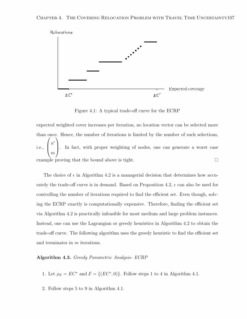
Chapter 4. The Covering Relocation Problem with Travel Time Uncertainty107
Figure 4.1: A typical trade-off curve for the ECRP
expected weighted cover increases per iteration, no location vector can be selected more
than once. Hence, the number of iterations is limited by the number of such selections,
i.e.,
n′
m
. In fact, with proper weighting of nodes, one can generate a worst case
example proving that the bound above is tight.
The choice of ε in Algorithm 4.2 is a managerial decision that determines how accu-
rately the trade-off curve is in demand. Based on Proposition 4.2, ε can also be used for
controlling the number of iterations required to find the efficient set. Even though, solv-
ing the ECRP exactly is computationally expensive. Therefore, finding the efficient set
via Algorithm 4.2 is practically infeasible for most medium and large problem instances.
Instead, one can use the Lagrangian or greedy heuristics in Algorithm 4.2 to obtain the
trade-off curve. The following algorithm uses the greedy heuristic to find the efficient set
and terminates in m iterations.
Algorithm 4.3. Greedy Parametric Analysis- ECRP
1. Let ρE = EC∗ and E = {(ECc, 0)}. Follow steps 1 to 4 in Algorithm 4.1.
2. Follow steps 5 to 9 in Algorithm 4.1.

Chapter 4. The Covering Relocation Problem with Travel Time Uncertainty108
3. E = E ∪ {(ECj∗ , R)}. L = L− 1. Go to step 2.
4.4. Robust Covering Relocation Problem
In this section we study the robust covering relocation problem (RCRP), i.e., relocating
the fewest number of facilities such that the minimum weighted cover is more than a
given bound ρR. By varying the parameter ρR, we find the efficient set of solutions to the
relocation problem with objectives (1) minimizing the number of facility relocations and
(3) maximizing the minimum weighted cover over all scenarios as outlined in Section 4.1.
We present an integer programming formulation and propose Lagrangian and greedy
heuristics for the RCRP.
Following the notations defined in Table 4.1, the RCRP can be formulated as follows:
[RCRP]
maxZ =n′∑
j=1
Fjxj (4.2a)
s.t. yik ≤n′∑
j=1
xjIkij for all i = 1, . . . , n, k = 1, . . . , s (4.2b)
n′∑
j=1
xj = m (4.2c)
n∑
i=1
Wiyik ≥ ρR for all k = 1, . . . , s (4.2d)
xj, yik = 0, 1 for all i = 1, . . . , n, j = 1, . . . , n′, k = 1, . . . , s (4.2e)
The objective function (4.2a) maximizes the number of facilities that are not relocated.
Constraint (4.2d) enforces a lower bound of ρR on the minimum coverage. Similar to the
ECRP, by letting ρR = 1, s = 1, and Fj = 1 for all j = 1, . . . , n′, the RCRP reduces
to the set covering decision problem that is proved NP-Complete. Therefore, we develop
Lagrangian relaxation and greedy heuristics for the RCRP.
The Lagrangian dual of the RCRP, L-RCRP, is defined by relaxing (4.2b) as follows:
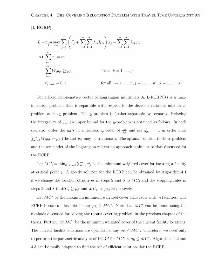
Chapter 4. The Covering Relocation Problem with Travel Time Uncertainty109
[L-RCRP]
L = minλ
maxx,y
n′∑
j=1
(Fj +
n∑
i=1
s∑
k=1
λikIkij
)xj −
n∑
i=1
s∑
k=1
λikyik
s.t.n′∑
j=1
xj = m
n∑
i=1
Wiyik ≥ ρR for all k = 1, . . . , s
xj, yik = 0, 1 for all i = 1, . . . , n, j = 1, . . . , n′, k = 1, . . . , s
For a fixed non-negative vector of Lagrangian multipliers λ, L-RCRP(λ) is a max-
imization problem that is separable with respect to the decision variables into an x-
problem and a y-problem. The y-problem is further separable by scenario. Relaxing
the integrality of yik, an upper bound for the y-problem is obtained as follows. In each
scenario, order the yik’s in a decreasing order of Wi
λikand set yUB
ik = 1 in order until
∑ni=1Wiyik = ρR (the last yik may be fractional). The optimal solution to the x-problem
and the remainder of the Lagrangian relaxation approach is similar to that discussed for
the ECRP.
Let MCj = mink=1,...,s
∑ni=1 c
kij be the minimum weighted cover for locating a facility
at critical point j. A greedy solution for the RCRP can be obtained by Algorithm 4.1
if we change the location objectives in steps 2 and 6 to MCj and the stopping rules in
steps 5 and 8 to MCj ≥ ρR and MCj∗ < ρR, respectively.
Let MC∗ be the maximum minimum weighted cover achievable with m facilities. The
RCRP becomes infeasible for any ρR ≥ MC∗. Note that MC∗ can be found using the
methods discussed for solving the robust covering problem in the previous chapter of the
thesis. Further, let MCc be the minimum weighted cover of the current facility locations.
The current facility locations are optimal for any ρR ≤ MCc. Therefore, we need only
to perform the parametric analysis of ECRP for MCc < ρR ≤MC∗. Algorithms 4.2 and
4.3 can be easily adapted to find the set of efficient solutions for the RCRP.
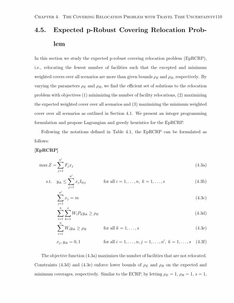
Chapter 4. The Covering Relocation Problem with Travel Time Uncertainty110
4.5. Expected p-Robust Covering Relocation Prob-
lem
In this section we study the expected p-robust covering relocation problem (EpRCRP),
i.e., relocating the fewest number of facilities such that the excepted and minimum
weighted covers over all scenarios are more than given bounds ρE and ρR, respectively. By
varying the parameters ρE and ρR, we find the efficient set of solutions to the relocation
problem with objectives (1) minimizing the number of facility relocations, (2) maximizing
the expected weighted cover over all scenarios and (3) maximizing the minimum weighted
cover over all scenarios as outlined in Section 4.1. We present an integer programming
formulation and propose Lagrangian and greedy heuristics for the EpRCRP.
Following the notations defined in Table 4.1, the EpRCRP can be formulated as
follows:
[EpRCRP]
maxZ =n′∑
j=1
Fjxj (4.3a)
s.t. yik ≤n′∑
j=1
xjIkij for all i = 1, . . . , n, k = 1, . . . , s (4.3b)
n′∑
j=1
xj = m (4.3c)
n∑
i=1
s∑
k=1
WiPkyik ≥ ρE (4.3d)
n∑
i=1
Wiyik ≥ ρR for all k = 1, . . . , s (4.3e)
xj, yik = 0, 1 for all i = 1, . . . , n, j = 1, . . . , n′, k = 1, . . . , s (4.3f)
The objective function (4.3a) maximizes the number of facilities that are not relocated.
Constraints (4.3d) and (4.3e) enforce lower bounds of ρE and ρR on the expected and
minimum coverages, respectively. Similar to the ECRP, by letting ρE = 1, ρR = 1, s = 1,

Chapter 4. The Covering Relocation Problem with Travel Time Uncertainty111
and Fj = 1 for all j = 1, . . . , n′, the EpRCRP reduces to the set covering decision problem
that is proved NP-Complete. Therefore, we develop Lagrangian relaxation and greedy
heuristics for the EpRCRP. Observe that (4.3d) is redundant if ρR ≥ ρE. In such a case,
the Lagrangian and greedy heuristics developed for the RCLP can be used to solve the
EpRCRP.
The Lagrangian dual of the EpRCRP, L-EpRCRP, is defined by relaxing (4.3b) as
follows:
[L-EpRCRP]
L = minλ
maxx,y
n′∑
j=1
(Fj +
n∑
i=1
s∑
k=1
λikIkij
)xj −
n∑
i=1
s∑
k=1
λikyik
s.t.n′∑
j=1
xj = m
n∑
i=1
s∑
k=1
WiPkyik ≥ ρE
n∑
i=1
Wiyik ≥ ρR for all k = 1, . . . , s
xj, yik = 0, 1 for all i = 1, . . . , n, j = 1, . . . , n′, k = 1, . . . , s
For a fixed non-negative vector of Lagrangian multipliers λ, L-EpRCRP(λ) is a
maximization problem that is separable with respect to the decision variables into an
x-problem and a y-problem. Relaxing the integrality of yik, an upper bound for the
y-problem is obtained using a two-stage greedy ordering algorithm as follows. First, in
each scenario, order the yik’s in a decreasing order of Wi
λik(ties broken arbitrarily) and
set yUBik = 1 in order until
∑ni=1 Wiyik = ρR (the last yik may be fractional). Then, if
ρR < ρE, order all yik’s that are not already set to 1 in a decreasing order of WiPkλik
(ties
broken arbitrarily) and set yUBik = 1 in order until
∑ni=1
∑sk=1WiPkyik = ρE (the last yik
may be fractional). Theorem 4.2 proves that the greedy ordering algorithm above finds
an optimal solution to the relaxed y-problem. The optimal solution to the x-problem
and the remainder of the Lagrangian relaxation approach is similar to that discussed for
Chapter 4. The Covering Relocation Problem with Travel Time Uncertainty112
the ECRP.
Theorem 4.2. The greedy ordering algorithm above finds an optimal solution for the
relaxed y-problem.
Proof. The greedy ordering algorithm works in two stages: stage 1 to satisfy (4.3e), and
stage 2 to satisfy (4.3d). Let yUBik = a1
ik+a2ik such that a1
ik, a2ik ≥ 0 are the contributions of
stages 1 and 2 of the greedy ordering algorithm, respectively. Further, let y∗ik’s represent
the optimal solution for the relaxed y-problem. To prove the theorem, we follow the
following three steps in order.
1. Without loss of generality, assume the nodes are ordered in each scenario k in
decreasing order of Wi
λik(ties broken arbitrarily). If y∗ik < a1
ik for some (i, k), since
y∗ik’s must satisfy (4.3e), there exists an i′ such that y∗i′k > a1i′k. Due to the greedy
nature of stage 1, a1jk = 1 for all j = 1, . . . , i − 1. So, y∗jk cannot be larger than
a1jk for any j = 1, . . . , i − 1 and, thus, i′ > i. For a small ε > 0, increasing y∗ik
by εWi
and decreasing y∗i′k by εWi′
does not violate (4.3d) and (4.3e), but increases
the objective by ε(λi′kWi′− λik
Wi
)≥ 0. Therefore, an optimal solution exists for the
relaxed y-problem such that y∗ik ≥ a1ik for all (i, k). If the greedy ordering algorithm
stops at the end of stage 1, a2ik = 0 for all (i, k). So, the argument above is identical
to y∗ik ≥ yUBik for all (i, k). In such a case we skip part 2 of the proof below.
2. Without loss of generality, assume all (i, k)’s are ordered such that (i, k) ≺ (j, l) if
WiPkλik
>WjPlλjl
(ties broken arbitrarily). If y∗ik < yUBik for some (i, k), since y∗ik’s must
satisfy (4.3d), there exists an (i′, k′) such that y∗i′k′ > yUBi′k′ . Due to the greedy nature
of stage 2, yUBjl = 1 for all (j, l) ≺ (i, k). So, y∗jl cannot be larger than yUB
jl for any
(j, l) ≺ (i, k) and, thus, (i, k) ≺ (i′, k′). Observe that y∗i′k′ > yUBi′k′ ≥ a1
i′k′ and, by
part 1 of the proof, y∗jk′ ≥ a1jk′ for all nodes j. So, for a small ε > 0, increasing y∗ik
by εWiPk
and decreasing y∗i′k′ by εWi′Pk′
does not violate (4.3e) (as long as ε is small
enough to ensure that y∗i′k′ does not fall below a1i′k′) and (4.3d), but increases the
Chapter 4. The Covering Relocation Problem with Travel Time Uncertainty113
objective by ε(
λi′k′Wi′Pk′
− λikWiPk
)≥ 0. Therefore, an optimal solution exists for the
relaxed y-problem such that y∗ik ≥ yUBik for all (i, k).
3. Since the objective of the relaxed y-problem is to minimize∑n
i=1
∑sk=1 λikyik and
λik ≥ 0 for all (i, k), if y∗ik > yUBik for some (i, k), there exists an (i′, k′) such that
y∗i′k′ < yUBi′k′ . This contradicts the argument proved in part 2 of the proof. Therefore,
an optimal solution exists for the relaxed y-problem such that y∗ik = yUBik for all (i, k).
Algorithm 4.1 can be adapted to provide a greedy solution for the EpRCRP. When
ρE ≥ ρR, constraint (4.3d) is binding in the optimal solution while (4.3e) may or may not
be so. Therefore, in the greedy heuristic, we prioritize expected coverage over minimum
coverage by ordering the current facility locations in decreasing order of their contribution
to the expected cover, i.e., we follow steps 1 to 4 as is. In step 5, we change the stopping
rule to ECj ≥ ρE and MCj ≥ ρR. In step 6, we locate the facility to improve the most
violated objective, i.e., using ECj or MCj. If the most violated objective is satisfied with
more than one potential location, we select the location that improves the other objective
the most. Finally, in step 8, we terminate the algorithm with no feasible solution if L = 1
and ECj∗ < ρE or MCj∗ < ρR.
To find the set of efficient solutions, we need to perform a parametric analysis of
the EpRCRP for all values of 0 ≤ ρE ≤ EC∗ and 0 ≤ ρR ≤ MC∗. To avoid a three
dimensional representation of the efficient set, we define the trade-off set as a set of m
trade-off curves over ρE and ρR, one per each level of the objective function. Each trade-
off curve includes a set of efficient (ρR, ρE) points that are feasible with a given number
of facility relocations.
Crema (1997) presents an algorithm for the right hand side multiparametric integer
linear programming problem that requires solving the nonparametric problem in each
step. While the algorithm is proved to obtain a complete parametric analysis in a finite

Chapter 4. The Covering Relocation Problem with Travel Time Uncertainty114
number of steps, the actual number of steps can grow as large as the number of possible
selections of m facility locations from among n′ critical points, i.e.,
n′
m
. Therefore,
considering the difficulty in solving the EpRCRP, obtaining the exact trade-off set is
computationally infeasible. Instead, we propose the following greedy algorithm to find
the trade-off set. We note that the greedy trade-off curves are lower bounds of the
corresponding exact trade-off curves.
Algorithm 4.4. Greedy Trade-Off Set- EpRCRP
1. Let z=1, Ei = ∅ for all i = 1, . . . ,m.
2. Follow steps 1 to 4 in Algorithm 4.1.
3. Follow steps 6, 7, and 9 in Algorithm 4.1.
4. If R < z, let L = L− 1 and go to step 3.
5. Let EC and MC be the expected and minimum coverage of the most recent facility
locations, respectively. Ez = Ez ∪ {(MC,EC)}.
6. Remove the location of facility L from A. Let C ′L = Cm−z+1. In C ′L, for all
i = 1, . . . , n and k = 1, . . . , s, if cijk > 0 for some j ∈ A, let cijk = Wi for all
j = 1, . . . , n′.
7. Relocate facility L to critical point j∗ with maximum MCj using C ′L. Let A =
A ∪ {j∗}
8. L = L+ 1. If L ≤ m, go to step 5.
9. Repeat steps 2 to 8 using MCj anywhere instead of ECj and vice versa.
10. Order the (x, y) items in Ez in increasing order of x (i.e., MC). Remove each item
in Ez if its y (i.e., EC) is not less than the y of the previous item (if one exists).

Chapter 4. The Covering Relocation Problem with Travel Time Uncertainty115
11. z = z + 1. If z ≤ m, go to step 2.
Algorithm 4.4 finds the efficient set Ez for each potential objective value of the
EpRCRP, i.e., z = 1, . . . ,m. Each iteration of the algorithm starts with finding, in
steps 2 to 4, the location set with z relocations and maximum expected coverage. Then,
steps 5 to 8 exchange the relocated facilities in a greedy manner in favor of increasing the
minimum coverage. Step 9 repeats the analysis above by starting at the location set with
z relocations and maximum minimum coverage and exchanging the relocated facilities in
favor of increasing the expected coverage. Finally, step 10 removes non-efficient solutions
from Ez.
4.6. Numerical Results
In this section, we compare the performances of the MIP formulation, the Lagrangian
relaxation based heuristic, and the greedy heuristic for the ECRP, RCRP, and EpRCRP.
We coded the Lagrangian and greedy heuristics using Microsoft Visual Basic and used
CPLEX 8.1 for solving the MIP formulations enforcing a time limit of 4 hours for each
problem instance. All computational experiments are run on a desktop PC 2.4GHz/2Gb
RAM.
Test networks are generated using the Beasley test data set (Beasley 1990) assuming
an equal weight for all nodes and relocating 10 facilities that are initially located randomly
on the nodes. The coverage time was determined, similar to Berman et al. (2009c), as
the 0.1 percentile of the distance between all pairs of nodes. Each test problem consists
of 10 scenarios with probability 0.1, one of which is the original Beasley network and the
other nine are generated by randomly removing 1%, 5%, 10%, or 30% of the links. The
values of ρE and ρR are set to 95% of the optimal expected and robust coverages as found
by algorithms proposed in the previous chapter (in few cases these values are adjusted
to ensure the existence of a feasible solution).

Chapter 4. The Covering Relocation Problem with Travel Time Uncertainty116
Tables 4.2, 4.3, and 4.4 present a summary of the results for the ECRP, RCRP, and
EpRCRP, respectively. For each test problem, we report the solution time in seconds
and the number of relocations recommended by CPLEX, the Lagrangian relaxation based
heuristic, and the greedy heuristic. We use N/A as the number of relocations if any of
the solution procedures fail to find a feasible solution. We note that if CPLEX can find
some feasible solutions in 4 hours, they are usually quite good. But, for a large enough
Nodes Edge lossSolution Time (Sec.) Number of relocations
CPLEX Lagrangian Greedy CPLEX Lagrangian Greedy
100
1% 0.1 84 1 6 10 7
5% 0.1 121 2 7 10 9
10% 0.1 120 2 6 10 8
30% 0.1 56 1 7 8 8
300
1% 10 716 11 8 10 9
5% 18 886 10 8 10 9
10% 1 876 10 8 10 9
30% 1 829 7 7 10 7
500
1% 530 1747 34 7 10 10
5% 2247 1570 26 7 10 8
10% 236 2036 25 7 10 8
30% 2 3048 21 7 10 7
700
1% 77 2969 49 7 10 7
5% >4hr 3519 46 8 10 7
10% >4hr 3957 53 9 10 9
30% 4 3890 39 6 10 7
900
1% 5733 5538 80 7 10 7
5% >4hr 4959 85 7 10 8
10% >4hr 4984 71 6 6 7
30% 2 12117 65 7 10 7
Average 2701 32 7.1 9.7 7.9
Table 4.2: Results- ECRP

Chapter 4. The Covering Relocation Problem with Travel Time Uncertainty117
problem it may not be able to find any feasible solutions. Based on Tables 4.2, 4.3,
and 4.4, we make the following observations.
1. Solution time increases exponentially in size for CPLEX, quadratically for the La-
grangian relaxation heuristic, and almost linearly for the greedy heuristic. CPLEX
is preferred in terms of solution time and quality for small problem instances. How-
ever, for some large instances of the RCRP and EpRCRP, CPLEX is unable to find
Nodes Edge lossSolution Time (Sec.) Number of relocations
CPLEX Lagrangian Greedy CPLEX Lagrangian Greedy
100
1% 0.1 48 1 7 10 7
5% 0.1 47 1 6 9 7
10% 1 40 1 5 9 7
30% 0.1 29 1 6 8 N/A
300
1% 3 348 10 7 10 8
5% 29 319 10 8 10 8
10% 4 253 9 8 10 8
30% 11 285 7 6 10 7
500
1% 121 700 27 7 10 8
5% 595 794 32 7 10 N/A
10% >4hr 711 23 7 9 7
30% 18 1038 18 5 10 6
700
1% 617 1549 55 7 10 8
5% 4858 1384 52 6 N/A 8
10% >4hr 1379 47 N/A 10 8
30% 37 2239 39 4 10 7
900
1% >4hr 1987 80 7 N/A 7
5% >4hr 1989 76 7 N/A 7
10% 370 2593 63 5 7 6
30% 265 4244 58 4 10 6
Average 1099 30 6.3 9.5 7.2
Table 4.3: Results- RCRP

Chapter 4. The Covering Relocation Problem with Travel Time Uncertainty118
even a feasible solutions in a reasonable time.
2. Similar to many other network problems, the solution time is usually lower for low
density and high density networks and higher for medium density networks.
3. Among the heuristics, the greedy heuristic is always better on solution time and
usually better on solution quality, but none of the heuristics is dominant for all
Nodes Edge lossSolution Time (Sec.) Number of relocations
CPLEX Lagrangian Greedy CPLEX Lagrangian Greedy
100
1% 0.1 99 1 7 10 7
5% 0.1 109 1 7 10 10
10% 0 148 1 6 10 8
30% 0.1 69 2 7 8 N/A
300
1% 8 841 11 8 10 9
5% 17 845 11 8 10 9
10% 6 936 10 8 10 9
30% 7 853 10 7 10 9
500
1% 3176 1616 31 7 10 9
5% 3692 1913 32 7 10 N/A
10% 453 2150 29 7 10 9
30% 5 2695 25 7 10 9
700
1% >4hr 3579 68 N/A 10 10
5% >4hr 3706 62 N/A 10 N/A
10% >4hr 4186 58 N/A 10 N/A
30% 32 4520 44 7 10 8
900
1% 2196 5117 102 7 10 9
5% >4hr 5245 95 N/A 10 9
10% 1284 6082 72 7 9 7
30% 27 12176 66 7 10 7
Average 2844 37 7.1 9.9 8.6
Table 4.4: Results- EpRCRP

Chapter 4. The Covering Relocation Problem with Travel Time Uncertainty119
problems. The Lagrangian relaxation based heuristic occasionally finds better so-
lutions than the greedy one or finds some solution when the greedy heuristic and
CPLEX fail to do so. A useful strategy would be to solve both heuristics and select
the best solution.
4.7. Case Study: Relocating Fire Stations in Toronto
In the previous chapter we studies the problem of improving the location of fire stations
in the city of Toronto. Toronto fire Services (TFS) operates 82 fire stations in Toronto
and is planning the addition of 4 more stations (TFS 2008). The Toronto Master Fire
plan and the National Fire Protection Association (NFPA) 1710 standard recognize a
target response time of 5 minutes for emergency services (TFS 2007). Considering pre-
trip delays, we argued in the previous chapter that we will use a 2 minute response time
for our analysis.
Our network for the city of Toronto consists of 3220 nodes, i.e., road intersections,
and 9630 links, i.e. major roads and streets. Travel times and traffic volumes in Toronto
are highly dependent on the time of the day. Therefore, we define 24 scenarios, one per
each hour, for the network. To study system performance under adverse conditions, we
include one additional scenario - the “snow storm”, which triples the travel times on
all links. Such events occur several times per year in Toronto and thus the fire service
certainly should take them into account. On the other hand, these events are quire
rare (on an annual basis), thus we set the probability of the associated scenario to 0.
Data on hourly travel times was provided by the Data Management Group of the Civil
Engineering Department at The University of Toronto.
In the previous chapter we presented optimal (greedy) locations for the 82 fire stations
based on expected coverage and worst case coverage objectives. We also presented a
recommended set of locations using the EpRCP that balances the improvement on the
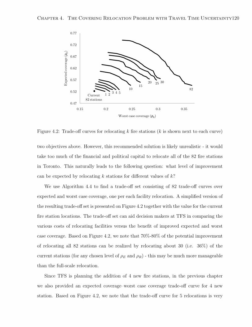
Chapter 4. The Covering Relocation Problem with Travel Time Uncertainty120
0.521189 0.177679 0.532852 0.179709 0.544194 0.179651 0.553455 0.17993 0.562571 0.185851
0.521189 0.198083 0.532852 0.198421 0.543902 0.198343 0.553081 0.199987
0.521189 0.207058 0.532563 0.207376 0.543529 0.208663
0.529174 0.212444 0.528801 0.219091
1 2 3 4
ψ
0.72
0.77
)
0.57
0.62
0.67
0.72
0.77
Exp
ecte
dco
vera
ge(ρ
E)
1015
20 25 30
82
0.47
0.52
0.57
0.62
0.67
0.72
0.77
0.15 0.2 0.25 0.3 0.35
Exp
ecte
dco
vera
ge(ρ
E)
Worst case coverage (ρR)
1 2 3 4 510
1520 25 30
Current82 stations
82
ρ ρ ρ ρ
0.47
0.52
0.57
0.62
0.67
0.72
0.77
0.15 0.2 0.25 0.3 0.35
Exp
ecte
dco
vera
ge(ρ
E)
Worst case coverage (ρR)
1 2 3 4 510
1520 25 30
Current82 stations
82
Figure 4.2: Trade-off curves for relocating k fire stations (k is shown next to each curve)
two objectives above. However, this recommended solution is likely unrealistic - it would
take too much of the financial and political capital to relocate all of the 82 fire stations
in Toronto. This naturally leads to the following question: what level of improvement
can be expected by relocating k stations for different values of k?
We use Algorithm 4.4 to find a trade-off set consisting of 82 trade-off curves over
expected and worst case coverage, one per each facility relocation. A simplified version of
the resulting trade-off set is presented on Figure 4.2 together with the value for the current
fire station locations. The trade-off set can aid decision makers at TFS in comparing the
various costs of relocating facilities versus the benefit of improved expected and worst
case coverage. Based on Figure 4.2, we note that 70%-80% of the potential improvement
of relocating all 82 stations can be realized by relocating about 30 (i.e. 36%) of the
current stations (for any chosen level of ρE and ρR) - this may be much more manageable
than the full-scale relocation.
Since TFS is planning the addition of 4 new fire stations, in the previous chapter
we also provided an expected coverage–worst case coverage trade-off curve for 4 new
station. Based on Figure 4.2, we note that the trade-off curve for 5 relocations is very

Chapter 4. The Covering Relocation Problem with Travel Time Uncertainty121
close to the trade-off curve for 4 new stations presented earlier. Thus instead of adding
new stations to the system, the planners should consider relocating a similar number of
current stations - it is likely more cost-effective and leads to better coverage levels.
4.8. Conclusion
We study a multi-objective maximum covering problem on a network with travel time
uncertainty that aims at relocating the fewest number of facilities while maximizing ex-
pected and worst case coverage over all scenarios of the network. Three single-objective
variations of the problem are presented. The expected covering relocation problem
(ECRP) relocates the fewest number of facilities such that the excepted weighted cover
over all scenarios is more than a given bound ρE. The robust covering relocation problem
(RCRP) relocates the fewest number of facilities such that the minimum weighted cover
over all scenarios is more than a given bound ρR. The expected p-robust covering reloca-
tion problem (EpRCRP) relocates the fewest number of facilities such that the excepted
and minimum weighted covers over all scenarios are more than given bounds ρE and ρR,
respectively. Varying the values of ρE and ρR, we find the set of efficient solutions for
the multi-objective problem.
We present integer programming formulations and develop Lagrangian and greedy
heuristics for the three problems. Our numerical results show that solution time increases
exponentially with size for the integer programming formulations. The Lagrangian and
greedy heuristics, instead, provide near optimal results in reasonable time. Finding the
set of efficient solutions via exact parametric optimization is computationally prohibitive.
We present a greedy exchange algorithm to find an approximate efficient set.
We use real data for the city of Toronto to analyze the current location of fire stations
with respect to the 24 scenarios representing travel times during different hours of the day
and one additional scenario representing the traffic disruption due to a snow storm. We

Chapter 4. The Covering Relocation Problem with Travel Time Uncertainty122
find that relocating about 30 stations would allow Toronto to capture a large part of the
coverage gap between the current and optimal locations. We also show that, considering
lower cost implications, the city should consider relocating fire stations instead of building
new ones.

Bibliography
Averbakh, I. 2003. Complexity of robust single facility location problems on networks with
uncertain edge lengths. Discrete Applied Mathematics 127(3) 505–522.
Averbakh, I., O. Berman. 2000. Algorithms for the robust 1-center problem on a tree. European
Journal of Operational Research 123(2) 292–302.
Bassamboo, A., S. Kumar, R.S. Randhawa. 2007. Dynamics of new product introduction in
closed rental systems. Working paper, McCombs School of Business, University of Texas
at Austin, Austin, Texas.
Bassamboo, A., R.S. Randhawa. 2007. Optimal control in a Netflix-like closed rental system.
Working paper, McCombs School of Business, University of Texas at Austin, Austin,
Texas.
Beasley, J.E. 1990. OR-library: distributing test problems by electronic mail. Journal of the
Operational Research Society 41(11) 1069–1072.
Bell, P.C. 1978. A new procedure for the distribution of periodicals. Journal of the Operational
Research Society 29(5) 427–434.
Bell, P.C. 1981. Adaptive sales forecasting with many stockouts. Journal of the Operational
Research Society 32(10) 865–873.
Berman, O., T. Drezner, Z. Drezner, G.O. Wesolowsky. 2009a. A defensive maximal covering
problem on a network. International Transactions in Operational Research 16(1) 69–86.
Berman, O., Z. Drezner, D. Krass. 2009b. Recent developments in covering location problems.
Working paper, Rotman School of Management, University of Toronto.
123

BIBLIOGRAPHY 124
Berman, O., Z. Drezner, G.O. Wesolowsky. 2009c. The maximal covering problem with some
negative weights. Geographical analysis 41(1) 30–42.
Berman, O., D. Krass. 2002. Facility location problems with stochastic demands and congestion.
Z. Drezner, H.W. Hamacher, eds., Facility Location: Applications and Theory , chap. 11.
Springer-Verlag, New York, 329–371.
Berman, O., D. Krass, M.B.C. Menezes. 2007. Facility reliability issues in network p-median
problems: Strategic centralization and co-location effects. Operations Research 55(2) 332–
350.
Berman, O., LeBlanc. 1984. Location-relocation of mobile facilities on a stochastic network.
Transportation science 18(4) 315–330.
Berman, O., A.R. Odoni. 1982. Locating mobile servers on a network with Markovian properties.
Networks 12(1) 73–86.
Berman, O., J.M. Wang. 2004. Probabilistic location problems with discrete demand weights.
Networks 44(1) 47–57.
Berman, O., J.M. Wang. 2007. The 1-minimax and 1-maximin problems with demand weights
of general probability distributions. Networks 50(2) 127–135.
Besbes, O., R. Phillips, A. Zeevi. 2009. Testing the validity of a demand model: An operations
perspective. Manufacturing and Service Operations Management (to Appear).
Best, N., D. Spiegelhalter, A. Thomas, C.E.G. Brayne. 1996. Bayesian analysis of realistically
complex models. Journal of the Royal Statistical Society. Series A (Statistics in Society)
159(2) 323–342. Stable URL: http://www.jstor.org/stable/2983178.
Budge, S., A. Ingolfsson, D. Zerom. 2009. Empirical analysis of ambulance travel times:
The case of Calgary emergency medical services. Working paper, available from
http://www.business.ualberta.ca/aingolfsson/publications.htm.
Burkard, R.E., H. Dollani. 2001. Robust location problems with pos/neg weights on a tree.
Networks 38(2) 102–113.
Burkard, R.E., H. Dollani. 2002. A note on the robust 1-center problem on trees. Annals of
Operations Research 110(1-4) 69–82.
BIBLIOGRAPHY 125
Cachon, G.P., A. G. Kok. 2007. Implementation of the newsvendor model with clearance
pricing: How to (and how not to) estimate a salvage value. Manufacturing and Service
Operations Management 9(3) 276–290.
Cachon, G.P., M.A. Lariviere. 2005. Supply chain coordination with revenue-sharing contracts:
strengths and limitations. Management Science 51(1) 30–44.
Carson, Y.M., R. Batta. 1990. Locating and ambulance on the Amherst campus of the State
University of New York at Buffalo. Interfaces 20 43–49.
Chen, B., C.-S. Lin. 1998. Minmax-regret robust 1-median location on a tree. Networks 31(2)
93–103.
Church, R., C.S. ReVelle. 1974. The maximal covering location problem. Papers of the Regional
Science Association 32 101–118.
Church, R.L., B. Meadows. 1979. Location modeling utilizing maximum service distance crite-
ria. Geographical Analysis 11(4) 358–373.
Conrad, S.A. 1976. Sales data and the estimation of demand. Operational Research Quarterly
27(1) 123–127.
Cooper, W. L., T. Homem de Mello, A. J. Kleywegt. 2006. Models of the spiral-down effect in
revenue management. Management Science 54 968–987.
Cormican, K.J., D.P. Morton, R.K. Wood. 1998. Stochastic network interdiction. Operations
Research 46(2) 184–197.
Crema, A. 1997. A contraction algorithm for the multiparametric integer linear programming
problem. European Journal of Operational Research 101(1) 130–139.
Current, J., M. Daskin, D. Schilling. 2002. Discrete network location models. Z. Drezner, H.W.
Hamacher, eds., Facility Location: Applications and Theory . Springer-Verlag, Berlin, 81–
118.
Current, J., H. Min, D. Schilling. 1990. Multiobjective analysis of facility location decisions.
European Journal of Operational Research 49 295–307.
Dana, J.D.Jr., K.E. Spier. 2001. Revenue sharing and vertical control in the video rental
industry. The Journal of Industrial Economics 49(3) 223–245.

BIBLIOGRAPHY 126
Daskin, M.S. 1983. A maximum expected covering location problem: formulation, properties
and heuristic solution. Transportation Science 17 48–70.
Daskin, M.S. 1987. Location, dispatching, and routing model for emergency services with
stochastic travel times. A. Ghosh, G. Rushton, eds., Spatial Analysis and Location Allo-
cation Models. Van Nostrand Reinhold Company, New York, 224–265.
Dempster, A.P., N.M. Laird, D.B. Rubin. 1977. Maximum likelihood from incomplete data
via the EM algorithm. Journal of the Royal Statistical Society, Series B (Methodological)
39(1) 1–38.
DMG, Data Management Group. 2004. EMME/2 GTA network coding standard 2001 A.M.
peak integrated road and transit network release 1.0/1.1. Tech. rep., Joint Program in
Transportation, University of Toronto. http://www.jpint.utoronto.ca/reports.html.
Ehrgott, M., X. Gandibleux. 2000. A survey and annotated bibliography of multiobjective
combinatorial optimization. OR Spektrum 22 425460.
EMA, (The Entertainment Merchants Association). 2008. 2007 annual report on the home
entertainment industry. http://www.entmerch.org/.
Erkut, E., A. Ingolfsson, G. Erdogan. 2008. Ambulance deployment for maximum survival.
Naval Research Logistics 55 42–58.
Evans, G.W. 1984. An overview of techniques for solving multiobjective mathematical programs.
Management Science 30(11) 1268–1282.
Federgruen, A., P. Zipkin. 1984. Approximations of dynamic, multilocation production and
inventory problems. Management Science 30(1) 69–84.
Fisher, M.L. 1981. The Lagrangian relaxation method for solving integer programming prob-
lems. Management Science 27(1) 1–18.
Frank, H. 1966. Optimum locations on a graph with probabilistic demands. Operations Research
14(3) 409–421.
Galvao, R.D., C. ReVelle. 1996. A Lagrangean heuristic for the maximal covering location
problem. European Journal of Operational Research 88(1) 114–123.

BIBLIOGRAPHY 127
Geoffrion, A.M., R. Nauss. 1977. Parametric and postoptimality analysis in integer linear
programming. Management Science 23(5) 453–466.
Gerchak, Y., R.K. Cho, S. Ray. 2006. Coordination of quantity and shelf-retention timing in
the video movie rental industry. IIE Transactions 38 525–536.
Goldberg, J., L. Paz. 1991. Locating emergency vehicle bases when service time depends on
call location. Transportation Science 25(4) 264–280.
Graves, S.C., A.H.G. RinnooyKan, P.H. Zipkin. 1993. Logistics of Production and Inventory ,
Handbooks in Operations Research and Management Science, vol. 4. North Holland, Am-
sterdam, The Netherlands.
Green, L.V., P.J. Kolesar. 2004. Improving emergency responsiveness with management science.
Management Science 50(8) 1001–1014.
Greenberg, H.J. 1998. An annotated bibliography for post-solution analysis in mixed integer
programming and combinatorial optimization. D. L. Woodruff, ed., Advances in Compu-
tational and Stochastic Optimization, Logic Programming, and Heuristic Search. Kluwer
Academic Publishers, Boston, MA, 97–148.
Hakimi, S.L. 1964. Optimum locations of switching centers and the absolute centers and medians
of a graph. Operations Research 12(3) 450–459.
Hill, R.M. 1992. Parameter estimation and performance measurement in lost sales inventory
systems. International Journal of Production Economics 28 211–215.
Ingolfsson, A., S. Budge, E. Erkut. 2008. Optimal ambulance location with random delays and
travel times. Health Care Management Science 11(3) 262–274.
Ingolfsson, A., E. Erkut, S. Budge. 2003. Simulation of single start station for Edmonton EMS.
Journal of the Operational Research Society 54(7) 736–746.
Israeli, E., R.K. Wood. 2002. Shortest-path network interdiction. Networks 40(2) 97–111.
Jenkins, L. 1990. Parametric methods in integer linear programming. Annals of Operations
Research 27(1) 77–96.
Kolen, A., A. Tamir. 1990. Covering problems. P. Mirchandani, R.L. Francis, eds., Discrete
Location Theory . Wiley-Interscience, New York, NY, 263–304.

BIBLIOGRAPHY 128
Kolesar, P., W. Walker, J. Hausner. 1975. Determining the relation between fire engine travel
times and travel distances in New York City. Operations Research 23(4) 614–627.
Kolesar, P., W.E. Walker. 1974. An algorithm for the dynamic relocation of fire companies.
Operations Research 22(2) 249–274.
Kouvelis, P., A.A. Kurawarwala, G.J. Gutierrez. 1992. Algorithms for robust single and mul-
tiple period layout planning for manufacturing systems. European Journal of Operational
Research 63(2) 287–303.
Kouvelis, P., G. Yu. 1997. Robust discrete optimization and its applications. Kluwer, Boston,
MA.
Lau, H.S., A.H. Lau. 1996. Estimating the demand distributions of single-period items having
frequent stockouts. European Journal of Operational Research 92(2) 254–265.
Lehmann, D.R., C.B. Weinberg. 2000. Sales through sequential distribution channels: an
application to movies and videos. Journal of Marketing 64(3) 18–33.
Liyanage, L. H., J. G. Shanthikumar. 2005. A practical inventory control policy using opera-
tional statistics. Operations Research Letters 33 341–348.
Lockwood, J.R., M.J. Schervish. 2005. MCMC strategies for computing Bayesian predictive
densities for censored multivariate data. Journal of Computational and Graphical Statistics
14(2) 395–414.
Lunn, D.J., A. Thomas, N. Best, D. Spiegelhalter. 2000. WinBUGS - a Bayesian modelling
framework: Concepts, structure, and extensibility. Statistics and Computing 10(4) 325–
337.
Malczewski, J., W. Ogryczak. 1995. The multiple criteria location problem: 1. a generalized
network model and the set of efficient solutions. Environment and Planning A 27(12)
1931–1960.
McGavin, E.J., L.B. Schwarz, J.E. Ward. 1993. Two-interval inventory-allocation policies in a
one-warehouse N-identical-retailer distribution system. Management Science 39(9) 1092–
1107.

BIBLIOGRAPHY 129
Mirchandani, P.B. 1980. Locational decisions on stochastic networks. Geographical Analysis
12(2) 172–183.
Mirchandani, P.B., A.R. Odoni. 1979. Locations of medians on stochastic networks. Trans-
portation Science 13(2) 85–97.
Mirchandani, P.B., A. Oudjit. 1980. Localizing 2-medians on probabilistic and deterministic
tree networks. Networks 10(4) 329–350.
Mitsos, A., P.I. Barton. 2009. Parametric mixed-integer 01 linear programming: The general
case for a single parameter. European Journal of Operational Research 194(3) 663–686.
Mortimer, J.H. 2008. Vertical contracts in the video rental industry. The Review of Economic
Studies 75(1) 165–199.
Nel, L.D., C.J. Colbourn. 1990. Locating a broadcast facility in an unreliable network. INFOR
28(4) 363–379.
Nemhauser, G.L., L.A. Wolsey, M.L. Fisher. 1978. An analysis of approximations for maximizing
submodular set functions-i. Mathematical Programming 14(3) 265–294.
O’Hanley, J., R.L. Church. 2008. Designing robust coverage networks to hedge against worstcase
facility losses. Working paper, Kent Business School.
Owen, S.H., M.S. Daskin. 2005a. Strategic facility location: A review. European Journal of
Operational Research 111(3) 423–447.
Owen, S.H., M.S. Daskin. 2005b. Strategic facility location: A review. European Journal of
Operational Research 111(3) 423–447.
Pasternack, B.A., Z. Drezner. 1999. The videotape rental model. Journal of Applied Mathe-
matics and Decision Sciences 3(2) 163–170.
Randhawa, R.S., S. Kumar. 2008. Usage restriction and subscription services: Operational
benefits with rational users. Manufacturing and Service Operations Management Forth-
coming.
Rentrak. 2008. Pricing and terms. http://www.rentrakppt.com/.
ReVelle, C. 1993. Facility siting and integer-friendly programming. European Journal of Oper-
ational Research 65(2) 147–158.

BIBLIOGRAPHY 130
ReVelle, C., J.L. Cohon, D.E. Shobrys. 1981. Multiple objective facility location: A review.
J.N. Morse, ed., Organizations: Multiple Agents with Multiple Criteria. Springer, Berlin,
320–337.
ReVelle, C.S., H.A. Eiselt. 2005. Location analysis: A synthesis and survey. European Journal
of Operational Research 165(1) 1–19.
ReVelle, C.S., K. Hogan. 1989. The maximum availability location problem. Transportation
Science 23(3) 192–200.
Scaparra, M.P., R.L. Church. 2008. A bilevel mixed-integer program for critical infrastructure
protection planning. Computers and Operations Research 35(6) 1905–23.
Serra, D., V. Marianov. 1998. The p-median problem in a changing network: the case of
Barcelona. Location Science 6 383–394.
Snyder, L.V. 2006. Facility location under uncertainty: a review. IIE Transactions 38(7)
537–554.
Snyder, L.V., M.S. Daskin. 2006. Stochastic p-robust location problems. IIE Transactions
38(11) 971–985.
Snyder, L.V., M.P. Scaparra, M.S. Daskin, R.L. Church. 2006. Planning for disruption in supply
chain networks. Tutorials in Operations Research, chap. 9. INFORMS, 234–257.
Tang, C.S., S. Deo. 2008. Rental price and rental duration under retail competition. European
Journal of Operational Research 187(3) 806–828.
TFS, Toronto Fire Services. 2007. Master fire plan 2007. http://www.toronto.ca/fire.
TFS, Toronto Fire Services. 2008. Annual report 2007. http://www.toronto.ca/fire.
Weaver, J.R., R.L. Church. 1983. Computational procedures for location problems on stochastic
networks. Transportation Science 17(2) 168–180.
Wecker, W.E. 1978. Predicting demand from sales data in the presence of stockouts. Manage-
ment Science 24(10) 1043–1054.
Related Documents