RANDOM PROCESSES AND TIME SERIES ANALYSIS. PART II: RANDOM PROCESSES Problem Sheets 1 Problem Sheet 1 Examples of Random Processes 1. Give examples of situations in which time series can be used for explanation, description, forecasting and control. 2. Give examples of a continuous and a discrete random process. 3. In the two examples of Q. 2 determine if the processes are quasideterministic or not. 4. Plot a one-dimensional probability density function (PDF) at any discrete time moment t i =iΔt (i is a positive integer and Δt is a time interval) for (a) a binary random process of throwing a fair coin, (b) a process of throwing a die at equal time intervals Δt, (c) a process of throwing at equal time intervals Δt a biased coin, in which probability of heads is 0.4 and of tails 0.6. 5. Find mean values and variances at any time moment t i of the processes (a) and (b) from Q. 4. Illustrate their positions on the plots for PDFs by analogy with examples in lecture notes. 6. Find mean value and variance of a continuous random variable α whose PDF is p α ( α ) = C cos a + π 4 ! " # $ % & with α ∈− π 4 ,0 # $ % & ' ( and C being some constant. Note, that first of all you need to find the value of constant C .

Welcome message from author
This document is posted to help you gain knowledge. Please leave a comment to let me know what you think about it! Share it to your friends and learn new things together.
Transcript

! RANDOM'PROCESSES'AND'TIME'SERIES'ANALYSIS.'PART'II:'RANDOM'PROCESSES''''''''''''''''''''''''''''''''''''''''''''''''''''''''''''''''''Problem'Sheets'
!! !
1
Problem Sheet 1
Examples of Random Processes 1. Give examples of situations in which time series can be used for explanation, description, forecasting and control. 2. Give examples of a continuous and a discrete random process. 3. In the two examples of Q. 2 determine if the processes are quasideterministic or not. 4. Plot a one-dimensional probability density function (PDF) at any discrete time moment ti=iΔt (i is a positive integer and Δt is a time interval) for
(a) a binary random process of throwing a fair coin,
(b) a process of throwing a die at equal time intervals Δt, (c) a process of throwing at equal time intervals Δt a biased coin, in which probability of heads is 0.4 and of tails 0.6.
5. Find mean values and variances at any time moment ti of the processes (a) and (b) from Q. 4. Illustrate their positions on the plots for PDFs by analogy with examples in lecture notes. 6. Find mean value and variance of a continuous random variable α whose PDF is
pα (α) =C cos a+ π4
!
"#
$
%& with α ∈ −π
4,0#
$%&'( and C being some constant. Note, that first of all you
need to find the value of constant C .

! RANDOM'PROCESSES'AND'TIME'SERIES'ANALYSIS.'PART'II:'RANDOM'PROCESSES''''''''''''''''''''''''''''''''''''''''''''''''''''''''''''''''''Problem'Sheets'
!! !
2
Problem Sheet 2 Statistical Characteristics of a Random Process, Stationarity
Consider random process X(t): 1. X(t)=Acos(ωt+ϕ)=f(ϕ,t), where A and ω are constants, ϕ is a random variable uniformly distributed in the interval [−π,π]. 2. X(t)=ξcos(ωt)=f(ξ,t), where ω is constant, ξ is a random variable uniformly distributed in the interval [-1,1]. 3. X(t)=Acos(ωt+ϕ)=f(ϕ,t), where A and ω are constants, ϕ is a random variable that with equal probability takes two values: -π/4 and π/4. 4. X(t)=Acos(ωt+ϕ)=f(ϕ,t), where A and ω are constants, ϕ is a random variable uniformly distributed in the interval [0,π/2]. 5. Let X(t)=cos(ωt+ϕ), where ω and ϕ are random variables with joint probability density function For processes 1 – 5 Find mean value and variance of random process X(t). Find autocorrelation function of random process X(t). Is the process wide sense stationary?
];[],12;8[,812 ππ−∈ϕ∈ωπ=ωϕp

! RANDOM'PROCESSES'AND'TIME'SERIES'ANALYSIS.'PART'II:'RANDOM'PROCESSES''''''''''''''''''''''''''''''''''''''''''''''''''''''''''''''''''Problem'Sheets'
!! !
3
Problem Sheet 2: Answers
€
3) X(t) =A2cosωt, σX
2 (t) =A2
2sin2ωt,
KXX (t,τ) =A2
2cos(ωτ), ΨXX (t,τ) =
A2
4cos(ωτ) − A
2
4cos(2ωt +ωτ)
€
1) X(t) ≡ 0,σX2 (t) =
A2
2, KXX (t,τ) = ΨXX (t,τ) =
A2
2cosωτ
€
2) X(t) ≡ 0, σX2 (t) =
13cos2ωt, KXX (t,τ) = ΨXX (t,τ) =
16cos(2ωt +ωτ) + cosωτ( )
€
4) X(t) =2 2Aπ
cos(ωt + π /4), σX2 (t) =
A2
2−4A2
π2&
' (
)
* + − sin(2ωt)
A2
π−4A2
π2&
' (
)
* + ,
KXX (t,τ) =A2
2cos(ωτ) − A
2
πsin(2ωt +ωτ), ΨXX (t,τ) =
A2
2−4A2
π2&
' (
)
* + cos(ωτ) −
A2
π−4A2
π2&
' (
)
* + sin(2ωt +ωτ)
€
5) X(t) ≡ 0,σX2 (t) =
12, KXX (t,τ) = ΨXX (t,τ) =
18τ
sin(12τ) − sin(8τ)( )

! RANDOM'PROCESSES'AND'TIME'SERIES'ANALYSIS.'PART'II:'RANDOM'PROCESSES''''''''''''''''''''''''''''''''''''''''''''''''''''''''''''''''''Problem'Sheets'
!! !
4
Problem Sheet 3
Properties of Autocorrelation and Covariance
Prove the following formulae:
1.
2.
3.
4.
€
σX2 (t) = X 2 t( ) − X t( )
2
€
ΨXY (t, t + τ ) = X(t) − X(t)( ) Y (t + τ ) −Y (t + τ)( )= X(t)Y (t + τ) − X(t) Y (t + τ)
€
ΨXX (t, t + τ ) = X(t) − X(t)( ) X(t + τ ) − X(t + τ)( )= X(t)X(t + τ) − X(t) X(t + τ)
€
ΨXX (t1,t2) = ΨXX (t2,t1)

! RANDOM'PROCESSES'AND'TIME'SERIES'ANALYSIS.'PART'II:'RANDOM'PROCESSES''''''''''''''''''''''''''''''''''''''''''''''''''''''''''''''''''Problem'Sheets'
!! !
5
Problem Sheet 4 Ergodicity of a Random Process
All processes are as in PS. 2. Consider random process X(t): 1. X(t)=Acos(ωt+ϕ)=f(ϕ,t), where A and ω are constants, ϕ is a random variable uniformly distributed in the interval [−π; π]. 2. X(t)=ξcos(ωt)=f(ξ,t), where ω is constant, ξ is a random variable uniformly distributed in the interval [-1; 1]. 3. X(t)=Acos(ωt+ϕ)=f(ϕ,t), where A and ω are constants, ϕ is a random variable that with equal probability takes two values: -π/4 and π/4. 4. X(t)=Acos(ωt+ϕ)=f(ϕ,t), where A and ω are constants, ϕ is a random variable uniformly distributed in the interval [0; π/2]. 5. Let X(t)=cos(ωt+ϕ), where ω and ϕ are random variables with joint probability density function For processes 1 – 5
• Find if the random process X(t) is ergodic with respect to mean value. • Find if the random process X(t) is ergodic with respect to variance and covariance.
];[],12;8[,812 ππ−∈ϕ∈ωπ=ωϕp

! RANDOM'PROCESSES'AND'TIME'SERIES'ANALYSIS.'PART'II:'RANDOM'PROCESSES''''''''''''''''''''''''''''''''''''''''''''''''''''''''''''''''''Problem'Sheets'
!! !
6
Problem Sheet 4: Answers
€
1) x(t) = X(t) ≡ 0, x(t) − x( ) x(t + τ) − x( ) = ΨXX (t,τ) =A2
2cosωτ
Yes, this process is ergodic with respect to mean, variance and covariance.
€
2) x(t) = X(t) ≡ 0, x(t) − x( ) x(t + τ) − x( ) =ξ*2
2cosωτ ≠ ΨXX (t,τ)
This process is ergodic with respect to mean, but not variance or covariance (compare with results for PS. 2 Q. 2).
€
3− 4) x(t) ≡ 0, x(t) − x( ) x(t + τ) − x( ) =A2
2cosωτ
The mean values and covariances of these processes obtained by averaging over the ensemble of realizations (see results for PS. 2, Q. 3-4) are different from those obtained by averaging along the single realization. Thus, the processes are not ergodic either with respect to mean, variance or covariance.
€
5) x(t) = X(t) ≡ 0, x(t) − x( ) x(t + τ) − x( ) =12cosω* τ ≠ ΨXX (t,τ)
This process is ergodic with respect to mean, but not covariance (compare with results for PS. 2 Q. 5).

! RANDOM'PROCESSES'AND'TIME'SERIES'ANALYSIS.'PART'II:'RANDOM'PROCESSES''''''''''''''''''''''''''''''''''''''''''''''''''''''''''''''''''Problem'Sheets'
!! !
7
Problem Sheet 5
Statistical Characteristics of a Random Process, Stationarity – More Problems
1. Consider random process X(t)=ξ(t)cos(ωt+ϕ), where ω is constant, ξ(t) is random process that is 1st order stationary and does not depend on ϕ. ϕ is random variable. Find the conditions that ϕ should satisfy to make random process X(t) wide sense stationary. Hint: consider autocorrelation function of X(t) 2. Let X(t) be a random process with autocorrelation function KXX(τ)=exp(-a|τ|), a is a positive constant. Let X(t) modulate the amplitude of a cosine process with random phase Y(t)=X(t)cos(ωt+ϕ). ϕ is a random variable uniformly distributed in the interval [-π; π] and is statistically independent of X(t). Find mean value, autocorrelation function and covariance of Y(t). 3. In problem 2 assume that the only known information about the process X(t) is that it is wide sense stationary and has autocorrelation function CXX(τ). Find mean value of Y(t). Find autocorrelation function of Y(t) in terms of CXX(τ). Is Y(t) wide sense stationary? 4. Let X(t)=Acos(ωt)+Bsin (ωt), where ω is constant, A and B are uncorrelated random variables with zero mean (they may have different distributions). Is X(t) wide sense stationary (WSS)? If the process is not WSS, what additional conditions should be imposed on A and B to make it WSS? 5. Consider a random process X(t)=αt+ξ(t)cos(ωt+ϕ), where ω =const, α is a random variable varying inside [-1; 1] whose probability density distribution (PDD) is p(α)=1/2. ξ(t) is a random process with zero mean and covariance function
€
Ψξ (t1,t2) = σξ2e−λ|τ|, where
€
τ = t1 − t2 and λ>0; ϕ is random variable varying inside [-π; π] with PDD p(ϕ)=1/(2π). Variables ϕ and α, and the process ξ(t) are all statistically independent. Find mean value, variance, autocorrelation and covariance of the process X(t) and determine if X(t) is wide-sense stationary.

! RANDOM'PROCESSES'AND'TIME'SERIES'ANALYSIS.'PART'II:'RANDOM'PROCESSES''''''''''''''''''''''''''''''''''''''''''''''''''''''''''''''''''Problem'Sheets'
!! !
8
Problem Sheet 5: Answers
1.
€
cosϕ = 0, sinϕ = 0, cos2ϕ = 0, sin2ϕ = 0.
2.
€
KYY (t,τ) =12exp(−a | τ |)cosωτ.
3.
€
Y (t) = 0 KYY (t,τ) =12CXX (τ)cosωτ . The process is WSS.
4.
€
X(t) = 0, KXX (t,τ) = cos(2ωt +ωτ) A2
2−B2
2
%
& ' '
(
) * * + cosωτ
A2
2+B2
2
%
& ' '
(
) * * . The process is not WSS. To
make the process WSS, variances of A and B should be equal.
5.
€
X(t) ≡ 0, σX2 (t) =
13t 2 +
12σξ2 ,
€
KXX (t,τ) = ΨXX (t,τ) =13t(t + τ) +
12σξ2 exp(−λ | τ |)cosωτ . The
process is not WSS.

! RANDOM'PROCESSES'AND'TIME'SERIES'ANALYSIS.'PART'II:'RANDOM'PROCESSES''''''''''''''''''''''''''''''''''''''''''''''''''''''''''''''''''Problem'Sheets'
!! !
9
Problem Sheet 6 Properties of the Fourier Transform (FT)
1. Prove the time-scaling property of the Fourier Transform (FT), i.e. prove the following. Let F(ω) be the FT of the function f(t). Let the argument t of f(t) be multiplied by some real constant a, i.e. let the time be scaled. Then the FT of the function f(at) is equal to 1/|a| F(ω/a).
2. What are the properties of the FT of an odd function f(t)?
Find Fourier amplitude and phase spectra for the realizations x(t) in problems 3-7. In all problems sketch the solution. It might be convenient to sketch x(t) first.
3. x(t)=Acos(ω0t+ψ) where ψ is not zero. 4. x(t)=Asin(ω0t) 5. Sum of two cosines with different frequencies
€
x(t) = A1 cos (ω1t) + A2 cos (ω 2t) . 6. Sum of a cosine and a sine with different frequencies
€
x(t) = A1 cos (ω1t) + A2 sin (ω 2t) . 7. Cosine with periodically modulated amplitude:
€
x(t) = (1+ m cos (ω1t))cos (ω 2t), where m< 1.
8. Find Fourier Transform of unit impulse train of period T, see Figure:
€
f (t) = δ(t − nT) =…+ δ(t + 2T) +n=−∞
∞
∑ δ(t +T) + δ(t) + δ(t −T) + δ(t − 2T) +…

! RANDOM'PROCESSES'AND'TIME'SERIES'ANALYSIS.'PART'II:'RANDOM'PROCESSES''''''''''''''''''''''''''''''''''''''''''''''''''''''''''''''''''Problem'Sheets'
!! !
10
Problem Sheet 6: Answers to selected problems
1. 2. 3.
€
F(ω) = Aπ δ ω −ω 0( ) + δ ω +ω 0( )[ ], ϕ(ω) =ψω 0
ω
4.
€
F(ω) = Aπ δ ω −ω 0( ) + δ ω +ω 0( )[ ], ϕ(ω) = −π2ωω 0
5.
€
F(ω) = A1π δ ω −ω1( ) + δ ω +ω1( )[ ] + A2π δ ω −ω 2( ) + δ ω +ω 2( )[ ], ϕ(ω) ≡ 0 6.
7. Realizations x(t) qualitatively look like in left-hand figure below.
€
F(ω) = π δ ω −ω 2( ) + δ ω +ω 2( )[ ] +m2π δ ω − (ω1 +ω 2 )( ) + δ ω + (ω1 +ω 2 )( )[ ] +
+m2π δ ω − (ω1 −ω 2 )( ) + δ ω + (ω1 −ω 2 )( )[ ], ϕ(ω) ≡ 0
In the right-hand side of the figure the amplitude of FT is shown for the parameters taken as in the left-hand side.
8.
€
ℑ δ(t − nT)n=−∞
∞
∑'
( ) *
+ , = e− jωnT
n=−∞
∞
∑

! RANDOM'PROCESSES'AND'TIME'SERIES'ANALYSIS.'PART'II:'RANDOM'PROCESSES''''''''''''''''''''''''''''''''''''''''''''''''''''''''''''''''''Problem'Sheets'
!! !
11
Problem Sheet 7 Fourier Transform and Wiener-Khintchine Theorem
1. Consider a rectangular pulse p(t)
€
p(t) =1, 0 ≤ t ≤ T,0, t < 0 or t > T.# $ %
a) Calculate the Fourier Transform (FT),
€
F(ω), of p(t). Find and sketch the amplitude Fourier spectrum,
€
F(ω ) , of p(t) for T=10. b) Consider
€
x(t) = p(t)cosω 0t . Calculate the FT,
€
F1(ω) , of x(t) directly using the definition. Compare your result with the one obtained by application of frequency-shifting property of the FT.
c) Calculate the squared amplitude Fourier spectrum,
€
F1(ω )2, of x(t). Compare your result
with the squared amplitude Fourier spectrum of
€
y(t) = p1(t)cosω 0t , where
€
p1(t) =1, −
T2≤ t ≤ T
2,
0, t >T2,
$
% &
' &
that was obtained in lecture. d) Sketch carefully the
€
F1(ω )2 for T=10, ω0=5.
2. a) Calculate the Fourier Transform (FT),
€
F2(ω) , of
€
z(t) = p(t)sinω 0t , where p(t) is the same as in Q. 1. Obtain the same result by two methods:
• from the direct definition of FT • using the frequency-shifting property of FT
b) Calculate the squared amplitude Fourier spectrum,
€
F2(ω )2 , of z(t) from a). Compare your
result with the squared amplitude Fourier spectra of x(t) and y(t) of Q. 1.
3. Which of the following functions could be a valid power spectral density, given that a, b, c, and f0 are real positive numbers? f is frequency in Hz,
€
a) afb + f 2
,
€
b) ab + f 2
,
€
c) a + cfb + f 2
,
€
d) af 2 − b
,
€
e) aa2 + f + f 2
,
€
f ) δ( f ) +a
b + f 2,
€
g) ab + jf 2
,
€
h) aδ( f − f0) − aδ( f + f0) ,
€
i) cos(3 f )1+ f 2
.
4. Consider a random process that is 1st order stationary with zero mean and the power spectral
density
€
S(ω) =W0 = const, |ω |≤ω 0
0, |ω |>ω 0
$ % &
,
Find autocorrelation function of this process and sketch it.

! RANDOM'PROCESSES'AND'TIME'SERIES'ANALYSIS.'PART'II:'RANDOM'PROCESSES''''''''''''''''''''''''''''''''''''''''''''''''''''''''''''''''''Problem'Sheets'
!! !
12
5. Consider a random process X(t)=A0cos(ω0t+ϕ)=f(ϕ,t), where A0 and ω0 are constants, ϕ is a
random variable uniformly distributed in the interval [-π; π]. Find power spectral density of X(t) by two methods: using Wiener-Khinchine theorem and from periodograms. Sketch power spectral density. [Hint: autocorrelation function of this process was found within Problem 1 of Problem Sheet 2.]
6. Consider stationary random process X(t) with zero mean and autocorrelation function
€
ΨXX (τ) =σX2e−α |τ |, α=const>0.
Find power spectral density of this process and sketch it. Find the power of the process. [Hint: you can use the following identity:
€
eax cos(bx)dx∫ =eax
a2 + b2acos(bx) + bsin(bx)( ) +C . ]
7. Find power spectral density of a wide-sense stationary process whose autocorrelation
function is
€
KXX (τ) = e−2τ
cos(4πτ) .
8. Consider a random process X(t) that is wide sense stationary with zero mean and with the power spectral density SX(ω)
€
SX (ω) =W0(1− ω ), ω ≤1,
0, ω >1.% & '
Find autocorrelation function and power of this process. Sketch autocorrelation function.
9. Consider a random process X(t) that is wide sense stationary with zero mean and with the autocorrelation function
€
KXX (τ) =A0 1−
τT
$
% &
'
( ) , −T ≤ τ ≤ T,
0, elsewhere.
+
, -
. -
Find power spectral density and power of this process. Sketch power spectral density.
0W

! RANDOM'PROCESSES'AND'TIME'SERIES'ANALYSIS.'PART'II:'RANDOM'PROCESSES''''''''''''''''''''''''''''''''''''''''''''''''''''''''''''''''''Problem'Sheets'
!! !
13
Problem Sheet 7: Answers to selected problems
1.
a)
€
F(ω ) 2 =4ω 2 sin
2 T2ω
#
$ %
&
' ( , F(ω ) =
2ωsin T
2ω
#
$ %
&
' (
b)
€
F1(ω) =12
jcos (ω −ω 0)T( ) −1
ω −ω 0
+cos (ω +ω 0)T( ) −1
ω +ω 0
$
% & &
'
( ) ) +
sin (ω −ω 0)T( )ω −ω 0
+sin (ω +ω 0)T( )
ω +ω 0
$
% & &
'
( ) )
*
+ , ,
-
. / /
c)
€
F1(ω )2
=sin2 (ω −ω 0)T
2$
% &
'
( )
ω −ω 0( )2+sin2 (ω +ω 0)T
2$
% &
'
( )
ω +ω 0( )2+cos ω 0T( )ω 2 −ω 0
2 cos ω 0T( ) − cos ωT( )[ ]
d)
The graph for
€
F1(ω )2 is symmetric with respect to zero.

! RANDOM'PROCESSES'AND'TIME'SERIES'ANALYSIS.'PART'II:'RANDOM'PROCESSES''''''''''''''''''''''''''''''''''''''''''''''''''''''''''''''''''Problem'Sheets'
!! !
14
2. a)
€
F2(ω) =12
jsin (ω +ω 0)T( )
ω +ω 0
−sin (ω −ω 0)T( )
ω −ω 0
$
% & &
'
( ) ) +
cos (ω −ω 0)T( ) −1ω −ω 0
−cos (ω +ω 0)T( ) −1
ω +ω 0
$
% & &
'
( ) )
*
+ , ,
-
. / /
b)
€
F2(ω )2
=sin2 (ω −ω 0)T
2$
% &
'
( )
ω −ω 0( )2+sin2 (ω +ω 0)T
2$
% &
'
( )
ω +ω 0( )2−cos(ω 0T)ω 2 −ω 0
2 × cos(ω 0T) − cos(ωT)[ ]
3.
(a) no, since it is not even. (b) yes since it is real, even and positive for all f. (c) no, since it is not even. (d) no, since it can be negative at f 2<b (e) no, since it is not even (f) yes, since it is real, even and positive for all f. (g) no, since it is not real (h) no, since it is negative at f=-f0 (i) no, since it is negative when cos(3f) is negative.
4.
€
KXX (τ) =W0
π τsin(ω 0τ),
P = KXX (0) = limτ→ 0
W0ω 0
πsin(ω 0τ)ω 0τ
=W0ω 0
π.
The process power can be also estimated as an integral of S(ω)
€
P =12π
S(ω )dω−∞
∞
∫ =12π2W0ω 0 =
W0ω 0
π.
5.
€
S(ω) =A02π2
δ(ω −ω 0) +δ(ω +ω 0)( )
6.
€
S(ω) =2ασX
2
α 2 +ω 2
P =σX2
)(2A
0
20 ω+ωδπ
)(2A
0
20 ω−ωδπ

! RANDOM'PROCESSES'AND'TIME'SERIES'ANALYSIS.'PART'II:'RANDOM'PROCESSES''''''''''''''''''''''''''''''''''''''''''''''''''''''''''''''''''Problem'Sheets'
!! !
15
7.
€
S(ω) = 2 14 + (4π +ω )2
+1
4 + (4π −ω)2%
& '
(
) *
8.
€
KXX (τ) =W0
2πsin τ /2( )τ /2( )
$
% &
'
( )
2
9.
€
S(ω) = A0Tsin ωT /2( )ωT /2( )
#
$ %
&
' (
2
The “width” of S(ω) is roughly proportional to the difference between the two values of ω closest to 0, at which S(ω)=0:
€
ω1,2T2
= ±π ⇒ ω1,2 = ±2πT; ω1 −ω 2 =
4πT
Thus, the wider the ACF (i.e. the larger the T), the narrower the power spectral density is.

! RANDOM'PROCESSES'AND'TIME'SERIES'ANALYSIS.'PART'II:'RANDOM'PROCESSES''''''''''''''''''''''''''''''''''''''''''''''''''''''''''''''''''Problem'Sheets'
!! !
16
Problem Sheet 8 Nyquist Theorem, Aliasing
1. A stationary random process X(t) has power spectral density SX(f):
€
SX ( f ) =27
9 + ( f − 3)2+
279 + ( f + 3)2
, f ≤10,
0, f >10.
$
% &
' &
A realization of this process is sampled with sampling frequency 12 Hz. Sketch the best power spectral density that could possibly be estimated numerically from this realization if observation time could tend to infinity. 2. Find the smallest sampling frequency necessary to discretize realizations of the random process
€
X(t) = A(t)cos(ω 0t + ϕ), where ϕ is a random variable uniformly distributed in [−π; π], and A(t) is a stationary band-width limited random process whose power spectral density SA(f) has the following form:
€
SA (ω) =W0(1− ω ), ω ≤1,
0, ω >1.% & '
A(t) and ϕ are statistically independent. Sketch power spectral density SA(f) of the process A(t) and power spectral density SX(f) of X(t), and on the latter plot show the position of the frequency sought. 3. Consider a random process X(t)=A(t)sin(6πt+ϕ), where ϕ is a random variable uniformly distributed in the interval [-π; π], A(t) is a stationary bandwidth-limited random process whose power spectral density SA(f) is given by
€
SA ( f ) =8(1− f ), f ≤1,
0, f >1.$ % &
A(t) and ϕ are statistically independent. Sketch the power spectral density of the process A(t), SA(f). Find the power spectral density of the process X(t), SX(f). Sketch SX(f) and on this plot show the smallest allowed sampling frequency. Find the power of the process X(t). 4. Consider a random process
€
X(t) = A(t) sin(8πt +ϕ) , where ϕ is a random variable uniformly distributed in [0; π], A(t) is a wide-sense stationary random process whose autocorrelation function
€
KAA (τ) is given by
€
KAA (τ) =2 1− τ
8$
% &
'
( ) , τ ≤ 8,
0, τ > 8.
+
, -
. -
Assume that realizations of this process are sampled with sampling step Δt=0.125 sec. Sketch the best power spectral density that could possibly be estimated numerically from a realization of this process if observation time could tend to infinity.
! RANDOM'PROCESSES'AND'TIME'SERIES'ANALYSIS.'PART'II:'RANDOM'PROCESSES''''''''''''''''''''''''''''''''''''''''''''''''''''''''''''''''''Problem'Sheets'
!! !
17
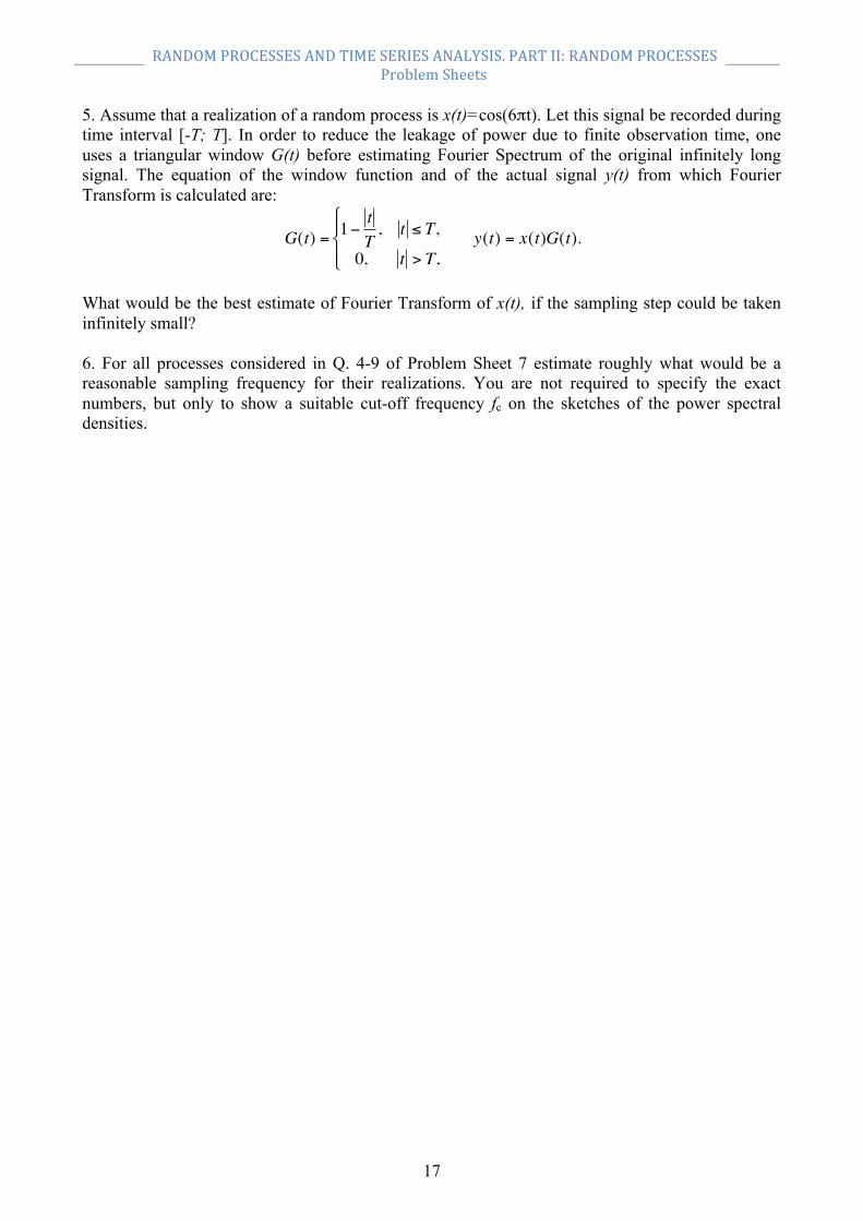
5. Assume that a realization of a random process is x(t)=cos(6πt). Let this signal be recorded during time interval [-T; T]. In order to reduce the leakage of power due to finite observation time, one uses a triangular window G(t) before estimating Fourier Spectrum of the original infinitely long signal. The equation of the window function and of the actual signal y(t) from which Fourier Transform is calculated are:
€
G(t) = 1− tT, t ≤ T,
0, t > T,
$ % &
' & y(t) = x(t)G(t).
What would be the best estimate of Fourier Transform of x(t), if the sampling step could be taken infinitely small?
6. For all processes considered in Q. 4-9 of Problem Sheet 7 estimate roughly what would be a reasonable sampling frequency for their realizations. You are not required to specify the exact numbers, but only to show a suitable cut-off frequency fc on the sketches of the power spectral densities.

! RANDOM'PROCESSES'AND'TIME'SERIES'ANALYSIS.'PART'II:'RANDOM'PROCESSES''''''''''''''''''''''''''''''''''''''''''''''''''''''''''''''''''Problem'Sheets'
!! !
18
Problem sheet 8: Answers to selected problems
1. Hint: Calculate the values of SX(f) at several points f, e.g. f=0,1,2,3,4,5,6,7,8,9,10. At negative frequencies SX(f) is the same as at the positive ones, because power spectral density is an even function. Solid thick (blue in color) line in the Figure below shows the estimate of the power spectral density sought.
2.
€
fN = 2ω 0 +12π
,
3.
€
SX ( f ) =14SA ( f + 3) +
14SA ( f − 3), P = 4, fN = 8Hz
! RANDOM'PROCESSES'AND'TIME'SERIES'ANALYSIS.'PART'II:'RANDOM'PROCESSES''''''''''''''''''''''''''''''''''''''''''''''''''''''''''''''''''Problem'Sheets'
!! !
19
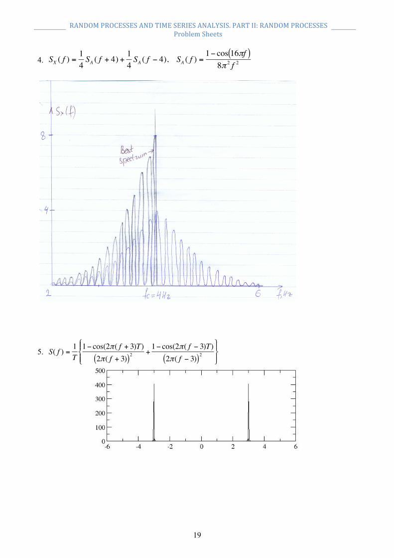
4.
€
SX ( f ) =14SA ( f + 4) +
14SA ( f − 4), SA ( f ) =
1− cos 16πf( )8π 2 f 2
5.
€
S( f ) =1T1− cos(2π( f + 3)T)
2π( f + 3)( )2+1− cos(2π( f − 3)T)
2π( f − 3)( )2$ % &
' &
( ) &
* &
Related Documents