PROBABILITY WITH APPLICATION Random outcome Example of rolling a die Repeating an experiment Simulation using StatCrunch Software Probability in Real.

PROBABILITY WITH APPLICATION

Random outcomeExample of rolling a die

Repeating an experimentSimulation using StatCrunch Software

Probability in Real Life ApplicationBlood Donor Clinic

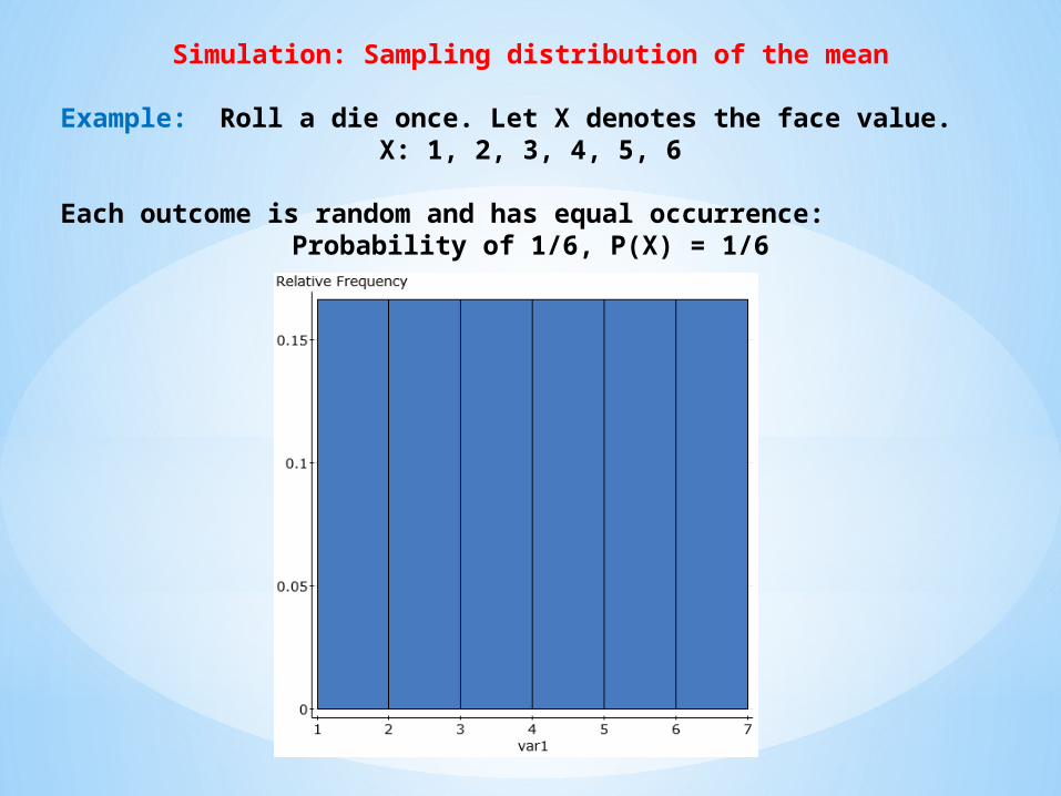
Simulation: Sampling distribution of the mean

Example: Roll a die once. Let X denotes the face value.X: 1, 2, 3, 4, 5, 6

Each outcome is random and has equal occurrence: Probability of 1/6, P(X) = 1/6

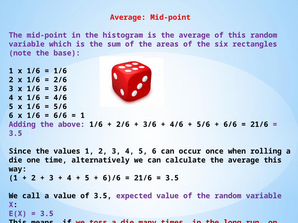
Average: Mid-point

The mid-point in the histogram is the average of this random variable which is the sum of the areas of the six rectangles (note the base):

1 x 1/6 = 1/62 x 1/6 = 2/63 x 1/6 = 3/64 x 1/6 = 4/65 x 1/6 = 5/66 x 1/6 = 6/6 = 1Adding the above: 1/6 + 2/6 + 3/6 + 4/6 + 5/6 + 6/6 = 21/6 = 3.5

Since the values 1, 2, 3, 4, 5, 6 can occur once when rolling a die one time, alternatively we can calculate the average this way:(1 + 2 + 3 + 4 + 5 + 6)/6 = 21/6 = 3.5

We call a value of 3.5, expected value of the random variable X:E(X) = 3.5This means, if we toss a die many times, in the long run, on average we get a value of 3.5. This concept is known as law of large numbers.

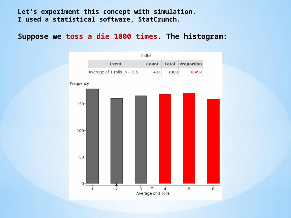
Let’s experiment this concept with simulation. I used a statistical software, StatCrunch.

Suppose we toss a die 1000 times. The histogram:

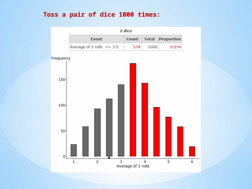
Toss a pair of dice 1000 times:

Toss 5 dice 1000 times:

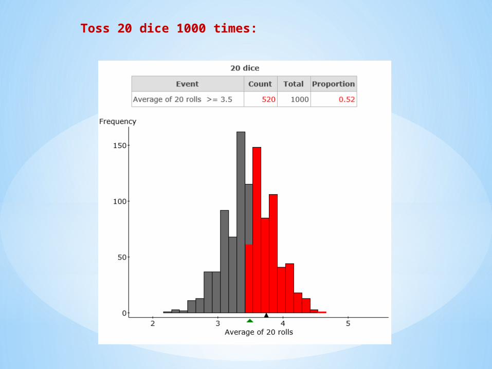
Toss 20 dice 1000 times:

Toss 50 dice 1000 times:

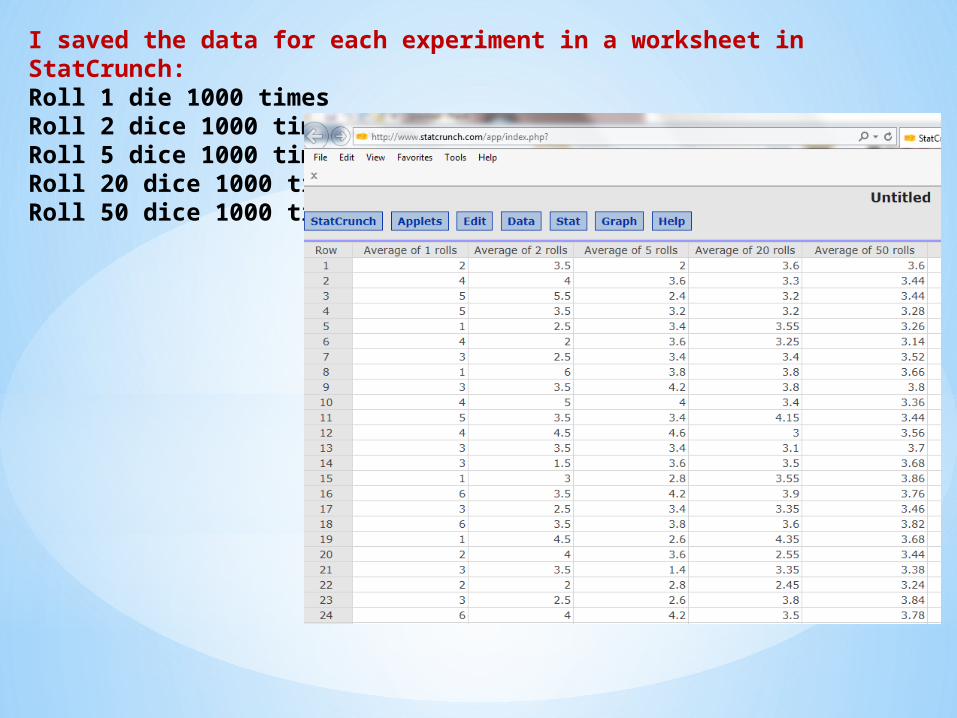
I saved the data for each experiment in a worksheet in StatCrunch:Roll 1 die 1000 timesRoll 2 dice 1000 timesRoll 5 dice 1000 timesRoll 20 dice 1000 timesRoll 50 dice 1000 times

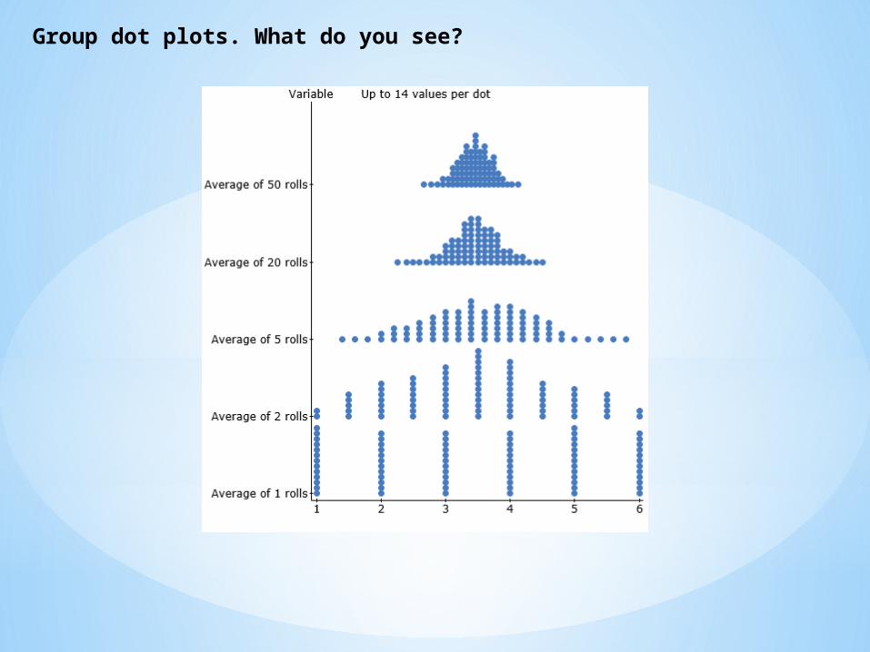
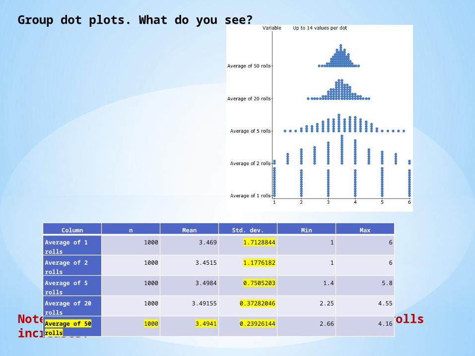
Group dot plots. What do you see?

Group dot plots. What do you see?

Note that the spread gets narrower as the number of rolls increases.

Group dot plots. What do you see?

Note that the spread gets narrower as the number of rolls increases.

Column n Mean Std. dev. Min Max

Average of 1 rolls

1000 3.469 1.7128844 1 6

Average of 2 rolls

1000 3.4515 1.1776182 1 6

Average of 5 rolls

1000 3.4984 0.7505203 1.4 5.8

Average of 20 rolls

1000 3.49155 0.37282046 2.25 4.55

Average of 50 rolls

1000 3.4941 0.23926144 2.66 4.16

Watch the following video about the idea of Central Limit Theorem

http://vimeo.com/75089338

Class Activity:

Please pair up with another person (group of 2 members: Person#1, Person#2). Each group will receive a little envelope that contains two chips: one orange and one blue chip. 

Steps:

1) Person #1: Select one chip from the envelope. Do not look inside the bag; randomly carry out your selection. Person #2: Note the outcome of person#1 selection. If the outcome is the blue chip note it as 1, otherwise give a 0 value. 2) Give the probability for all possible outcomes. Note: you either get a blue or an orange chip. Hence there are two outcomes. This is called a binary outcome (known as Bernoulli trial). 3) Construct a histogram for part 2. 4) If we repeat this task many times, in the long run, on average how many blue chips do you get?

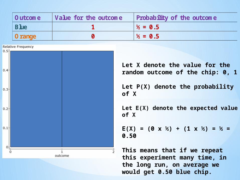
Outcome Value for the outcome Probability of the outcome

Blue 1 ½ = 0.5 Orange 0 ½ = 0.5

Let X denote the value for the random outcome of the chip: 0, 1

Let P(X) denote the probability of X

Let E(X) denote the expected value of X

E(X) = (0 x ½) + (1 x ½) = ½ = 0.50

This means that if we repeat this experiment many time, in the long run, on average we would get 0.50 blue chip.

Probability with Real Life Application

People with O-negative blood type are “universal donors”.

Only 6% of people have this blood type.

Suppose 1 donor come to a blood drive:

* What is the probability that this person has O-negative blood type?

Suppose 1 donor come to a blood drive:

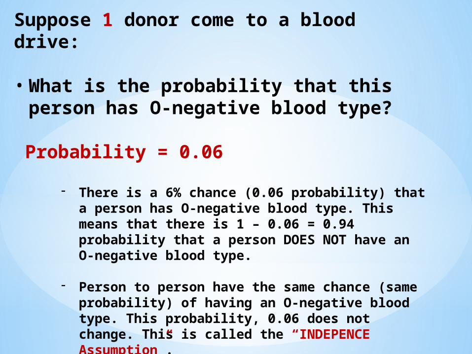
• What is the probability that this person has O-negative blood type?

Probability = 0.06

- There is a 6% chance (0.06 probability) that a person has O-negative blood type. This means that there is 1 – 0.06 = 0.94 probability that a person DOES NOT have an O-negative blood type.

- Person to person have the same chance (same probability) of having an O-negative blood type. This probability, 0.06 does not change. This is called the “INDEPENCE Assumption”.

Suppose 2 donors come to a blood drive.

* What is the probability that both of them have O-negative blood type?

Suppose 2 donors come to a blood drive.

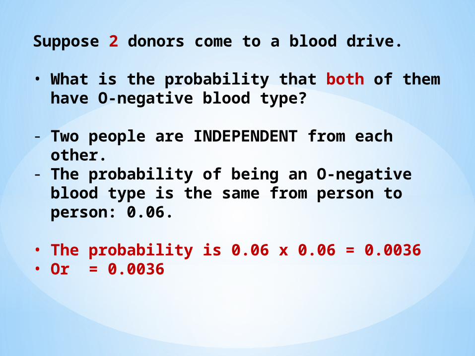
• What is the probability that both of them have O-negative blood type?

- Two people are INDEPENDENT from each other.

- The probability of being an O-negative blood type is the same from person to person: 0.06.

• The probability is 0.06 x 0.06 = 0.0036• Or = 0.0036

Suppose 20 donors come to a blood drive.

• What is the probability that all of them have O-negative blood type?

• The probability is 0

Suppose 20 donors come to a blood drive.

What is the mean of the number of O-negative blood types among the 20 people?

E(X) = 20*0.06 = 1.2

In 20 people we expect to find an average of about 1.2 o-negative blood type (universal donors).

Take away message: This means that the clinic needs a very large number of people to sample in order to obtain universal donors.

Nice meeting you!Thank you for your

participation