probability theory and stochastic processes - mrcet.ac.in

Sensitivity: Internal & Restricted

PROBABILITY THEORY AND STOCHASTIC PROCESSES

(R18A0403)

LECTURE NOTES

B.TECH (II YEAR – I SEM)

(2020-21)

Prepared by: Mrs.N.Saritha, Assistant Professor

Mr.G.S. Naveen Kumar, Assoc.Professor

Department of Electronics and Communication Engineering

MALLA REDDY COLLEGE OF ENGINEERING & TECHNOLOGY

(Autonomous Institution – UGC, Govt. of India) Recognized under 2(f) and 12 (B) of UGC ACT 1956

(Affiliated to JNTUH, Hyderabad, Approved by AICTE - Accredited by NBA & NAAC – ‘A’ Grade - ISO 9001:2015 Certified) Maisammaguda, Dhulapally (Post Via. Kompally), Secunderabad – 500100, Telangana State, India

MALLA REDDY COLLEGE OF ENGINEERING AND TECHNOLOGY (AUTONOMOUS INSTITUTION: UGC, GOVT. OF INDIA)

ELECTRONICS AND COMMUNICATION ENGINEERING

II ECE I SEM

PROBABILITY THEORY

AND STOCHASTIC

PROCESSES

SYLLABUS

UNIT-I-PROBABILITY AND RANDOM VARIABLE

UNIT-II- DISTRIBUTION AND DENSITY FUNCTIONS AND OPERATIONS ON

ONE RANDOM VARIABLE

UNIT-III-MULTIPLE RANDOM VARIABLES AND OPERATIONS

UNIT-IV-STOCHASTIC PROCESSES-TEMPORAL CHARACTERISTICS

UNIT-V- STOCHASTIC PROCESSES-SPECTRAL CHARACTERISTICS

UNITWISE IMPORTANT QUESTIONS

CONTENTS

PROBABILITY THEORY AND STOCHASTIC PROCESS

Course Objectives:

To provide mathematical background and sufficient experience so that student can read,

write and understand sentences in the language of probability theory.

To introduce students to the basic methodology of “probabilistic thinking” and apply it to

problems.

To understand basic concepts of Probability theory and Random Variables, how to deal

with multiple Random Variables.

To understand the difference between time averages statistical averages.

To teach students how to apply sums and integrals to compute probabilities, and expectations.

UNIT I:

Probability and Random Variable

Probability: Set theory, Experiments and Sample Spaces, Discrete and Continuous Sample

Spaces, Events, Probability Definitions and Axioms, Joint Probability, Conditional Probability,

Total Probability, Bayes’ Theorem, and Independent Events, Bernoulli’s trials.

The Random Variable: Definition of a Random Variable, Conditions for a Function to be a

Random Variable, Discrete and Continuous.

UNIT II:

Distribution and density functions and Operations on One Random Variable

Distribution and density functions: Distribution and Density functions, Properties, Binomial,

Uniform, Exponential, Gaussian, and Conditional Distribution and Conditional Density function

and its properties, problems.

Operation on One Random Variable: Expected value of a random variable, function of a

random variable, moments about the origin, central moments, variance and skew, characteristic

function, moment generating function.

UNIT III:

Multiple Random Variables and Operations on Multiple Random Variables

Multiple Random Variables: Joint Distribution Function and Properties, Joint density Function

and Properties, Marginal Distribution and density Functions, conditional Distribution and density

Functions, Statistical Independence, Distribution and density functions of Sum of Two Random

Variables.

Operations on Multiple Random Variables: Expected Value of a Function of Random

Variables, Joint Moments about the Origin, Joint Central Moments, Joint Characteristic

Functions, and Jointly Gaussian Random Variables: Two Random Variables case Properties.

UNIT IV:

Stochastic Processes-Temporal Characteristics: The Stochastic process Concept,

Classification of Processes, Deterministic and Nondeterministic Processes, Distribution and

Density Functions, Statistical Independence and concept of Stationarity: First-Order Stationary

Processes, Second-Order and Wide-Sense Stationarity, Nth-Order and Strict-Sense Stationarity,

Time Averages and Ergodicity, Mean-Ergodic Processes, Correlation-Ergodic Processes

Autocorrelation Function and Its Properties, Cross-Correlation Function and Its Properties,

Covariance Functions and its properties.

Linear system Response: Mean and Mean-squared value, Autocorrelation, Cross-Correlation

Functions.

UNIT V:

Stochastic Processes-Spectral Characteristics: The Power Spectrum and its Properties,

Relationship between Power Spectrum and Autocorrelation Function, the Cross-Power Density

Spectrum and Properties, Relationship between Cross-Power Spectrum and Cross-Correlation

Function.

Spectral characteristics of system response: power density spectrum of response, cross power

spectral density of input and output of a linear system

TEXT BOOKS:

1. Probability, Random Variables & Random Signal Principles -Peyton Z. Peebles, TMH,

4th Edition, 2001.

2. Probability and Random Processes-Scott Miller, Donald Childers,2Ed,Elsevier,2012

REFERENCE BOOKS:

1. Theory of probability and Stochastic Processes-Pradip Kumar Gosh, University Press

2. Probability and Random Processes with Application to Signal Processing - Henry Stark

and John W. Woods, Pearson Education, 3rd Edition.

3. Probability Methods of Signal and System Analysis- George R. Cooper, Clave D. MC

Gillem, Oxford, 3rd Edition, 1999.

4. Statistical Theory of Communication -S.P. Eugene Xavier, New Age Publications 2003

5. Probability, Random Variables and Stochastic Processes Athanasios Papoulis and

S.Unnikrishna Pillai, PHI, 4th Edition, 2002.

Probability:

Set theory

Experiments

UNIT I

Probability and Random Variable

Sample Spaces, Discrete and Continuous Sample Spaces

Events

Probability Definitions and Axioms

Joint Probability

Conditional Probability

Total Probability

Bayes’ Theorem

Independent Events

Bernoulli’s trials

Random Variable:

Definition of a Random Variable

Conditions for a Function to be a Random Variable

Discrete and Continuous Random Variables

1

UNIT – 1

PROBABILITY AND RANDOM VARIABLE

PROBABILITY

Introduction

It is remarkable that a science which began with the consideration of games of chance

should have become the most important object of human knowledge. Probability is simply how likely something is to happen. Whenever we’re unsure about the outcome of an event, we can talk about the probabilities of certain outcomes —how likely they are. The analysis of events

governed by probability is called statistics. Probability theory, a branch of mathematics concerned with the analysis of random phenomena. The outcome of a random event cannot be determined before it occurs, but it may be any one of several possible

outcomes. The actual outcome is considered to be determined by chance.

How to Interpret Probability

Mathematically, the probability that an event will occur is expressed as a number between 0 and 1.

Notationally, the probability of event A is represented by P (A).

If P (A) equals zero, event A will almost definitely not occur.

If P (A) is close to zero, there is only a small chance that event A will occur.

If P (A) equals 0.5, there is a 50-50 chance that event A will occur.

If P(A) is close to one, there is a strong chance that event A will occur.

If P(A) equals one, event A will almost definitely occur.

In a statistical experiment, the sum of probabilities for all possible outcomes is equal to one. This

means, for example, that if an experiment can have three possible outcomes (A, B, and C), then

P(A) + P(B) + P(C) = 1.

2

Applications

Probability theory is applied in everyday life in risk assessment and in trade on financial markets.

Governments apply probabilistic methods in environmental regulation, where it is called pathway

analysis

Another significant application of probability theory in everyday life is reliability. Many consumer

products, such as automobiles and consumer electronics, use reliability theory in product design to

reduce the probability of failure. Failure probability may influence a manufacturer's decisions on a

product's warranty.

The range of applications extends beyond games into business decisions, insurance, law, medical tests,

and the social sciences The telephone network, call centers, and airline companies with their randomly

fluctuating loads could not have been economically designed without probability theory.

Uses of Probability in real life

Sports – be it basketball or football or cricket a coin is tossed and both teams have 50/50 chances

of winning it.

Board Games – The odds of rolling one die and getting and even number there is a 50% chance

since three of the six numbers on a die are even.

Medical Decisions – When a patient is advised to undergo surgery, they often want to know the

success rate of the operation which is nothing but a probability rate. Based on the same the patient

takes a decision whether or not to go ahead with the same.

Life Expectancy – this is based on the number of years the same groups of people have lived in the past.

Weather – when planning an outdoor activity, people generally check the probability of rain.

Meteorologists also predict the weather based on the patterns of the previous year, temperatures and

natural disasters are also predicted on probability and nothing is ever stated as a surety but a possibility

and an approximation.

3

SET THEORY:

Set: A set is a well defined collection of objects. These objects are called elements or members of the

set. Usually uppercase letters are used to denote sets.

The set theory was developed by George Cantor in 1845-1918. Today, it is used in almost every

branch of mathematics and serves as a fundamental part of present-day mathematics.

In everyday life, we often talk of the collection of objects such as a bunch of keys, flock of birds,

pack of cards, etc. In mathematics, we come across collections like natural numbers, whole numbers,

prime and composite numbers.

We assume that,

the word set is synonymous with the word collection, aggregate, class and comprises of elements.

Objects, elements and members of a set are synonymous terms.

Sets are usually denoted by capital letters A, B, C, ...... , etc.

Elements of the set are represented by small letters a, b, c, ..... , etc.

If ‘a’ is an element of set A, then we say that ‘a’ belongs to A and it is mathematically

represented as aϵ A

If ‘b‘ is an element which does not belong to A, we represent this as b ∉ A.

Examples of sets:

1. Describe the set of vowels.

If A is the set of vowels, then A could be described as A = a, e, i, o, u.

2. Describe the set of positive integers.

Since it would be impossible to list all of the positive integers, we need to use a rule to describe this

set. We might say A consists of all integers greater than zero.

3. Set A = 1, 2, 3 and Set B = 3, 2, 1. Is Set A equal to Set B?

Yes. Two sets are equal if they have the same elements. The order in which the elements are listed

does not matter.

4. What is the set of men with four arms?

Since all men have two arms at most, the set of men with four arms contains no elements. It is the

null set (or empty set).

4

5. Set A = 1, 2, 3 and Set B = 1, 2, 4, 5, 6. Is Set A a subset of Set B?

Set A would be a subset of Set B if every element from Set A were also in Set B. However, this is

not the case. The number 3 is in Set A, but not in Set B. Therefore, Set A is not a subset of Set B

Some important sets used in mathematics are

N: the set of all natural numbers = 1, 2, 3, 4, ......

Z: the set of all integers = ....., -3, -2, -1, 0, 1, 2, 3, .....

Q: the set of all rational numbers

R: the set of all real numbers

Z+: the set of all positive integers

W: the set of all whole numbers

Types of sets:

1. Empty Set or Null Set:

A set which does not contain any element is called an empty set, or the null set or the void set and it

is denoted by ∅ and is read as phi. In roster form, ∅ is denoted by . An empty set is a finite set,

since the number of elements in an empty set is finite, i.e., 0.

For example: (a) the set of whole numbers less than 0.

(b) Clearly there is no whole number less than 0.

Therefore, it is an empty set.

(c) N = x : x ∈ N, 3 < x < 4

• Let A = x : 2 < x < 3, x is a natural number

Here A is an empty set because there is no natural number between

2 and 3

5

2. Singleton Set:

A set which contains only one element is called a singleton set.

For example:

• A = x : x is neither prime nor composite

It is a singleton set containing one element, i.e., 1.

• B = x : x is a whole number, x < 1

This set contains only one element 0 and is a singleton set.

• Let A = x : x ∈ N and x² = 4

Here A is a singleton set because there is only one element 2 whose square is 4.

• Let B = x : x is a even prime number

Here B is a singleton set because there is only one prime number which is even, i.e., 2.

3. Finite Set:

A set which contains a definite number of elements is called a finite set. Empty set is also called a

finite set.

For example:

• The set of all colors in the rainbow.

• N = x : x ∈ N, x < 7

• P = 2, 3, 5, 7, 11, 13, 17, ....... 97

4. Infinite Set:

The set whose elements cannot be listed, i.e., set containing never-ending elements is called an

infinite set.

For example:

• Set of all points in a plane

• A = x : x ∈ N, x > 1

• Set of all prime numbers

• B = x : x ∈ W, x = 2n

6

5. Cardinal Number of a Set:

The number of distinct elements in a given set A is called the cardinal number of A. It is denoted

by n(A). And read as ‘the number of elements of the set‘.

For example:

• A x : x ∈ N, x < 5

A = 1, 2, 3, 4

Therefore, n(A) = 4

• B = set of letters in the word ALGEBRA

B = A, L, G, E, B, R

Therefore, n(B) = 6

6. Equivalent Sets:

Two sets A and B are said to be equivalent if their cardinal number is same, i.e., n(A) = n(B). The

symbol for denoting an equivalent set is ‘↔‘.

For example:

A = 1, 2, 3 Here n(A) = 3

B = p, q, r Here n(B) = 3

Therefore, A ↔ B

7. Equal sets:

Two sets A and B are said to be equal if they contain the same elements. Every element of A is an

element of B and every element of B is an element of A.

For example:

A = p, q, r, s

B = p, s, r, q

Therefore, A = B

7

8. Disjoint Sets:

Two sets A and B are said to be disjoint, if they do not have any element in common.

For example;

A = x : x is a prime number

B = x : x is a composite number.

Clearly, A and B do not have any element in common and are disjoint sets.

9. Overlapping sets:

Two sets A and B are said to be overlapping if they contain at least one element in common.

For example;

• A = a, b, c, d

B = a, e, i, o, u

• X = x : x ∈ N, x < 4

Y = x : x ∈ I, -1 < x < 4

Here, the two sets contain three elements in common, i.e., (1, 2, 3)

10. Definition of Subset:

If A and B are two sets, and every element of set A is also an element of set B, then A is called a

subset of B and we write it as A ⊆ B or B ⊇ A

The symbol ⊂ stands for ‘is a subset of‘ or ‘is contained in‘

• Every set is a subset of itself, i.e., A ⊂ A, B ⊂ B.

• Empty set is a subset of every set.

• Symbol ‘⊆‘ is used to denote ‘is a subset of‘ or ‘is contained in‘.

• A ⊆ B means A is a subset of B or A is contained in B.

• B ⊆ A means B contains A.

8

Examples;

1. Let A = 2, 4, 6

B = 6, 4, 8, 2

Here A is a subset of B

Since, all the elements of set A are contained in set B.

But B is not the subset of A

Since, all the elements of set B are not contained in set A.

2. The set N of natural numbers is a subset of the set Z of integers and we write N ⊂ Z.

3. Let A = 2, 4, 6

B = x : x is an even natural number less than 8

Here A ⊂ B and B ⊂ A.

Hence, we can say A = B

4. Let A = 1, 2, 3, 4

B = 4, 5, 6, 7

Here A ⊄ B and also B ⊄ A

[⊄ denotes ‘not a subset of‘]

9

11. Proper Subset:

If A and B are two sets, then A is called the proper subset of B if A ⊆ B but A ≠ B. The symbol

‘⊂‘ is used to denote proper subset. Symbolically, we write A ⊂ B.

For example;

1. A = 1, 2, 3, 4

Here n(A) = 4

B = 1, 2, 3, 4, 5

Here n(B) = 5

We observe that, all the elements of A are present in B but the element ‗5‘ of B is not present in A.

So, we say that A is a proper subset of B.

Symbolically, we write it as A ⊂ B

Notes:

No set is a proper subset of itself.

Null set or ∅ is a proper subset of every set.

2. A = p, q, r

B = p, q, r, s, t

Here A is a proper subset of B as all the elements of set A are in set B and also A ≠ B.

Notes:

No set is a proper subset of itself.

Empty set is a proper subset of every set.

10

12. Universal Set

A set which contains all the elements of other given sets is called a universal set. The symbol for

denoting a universal set is ∪ or ξ.

For example;

1. If A = 1, 2, 3 B = 2, 3, 4 C = 3, 5, 7

then U = 1, 2, 3, 4, 5, 7

[Here A ⊆ U, B ⊆ U, C ⊆ U and U ⊇ A, U ⊇ B, U ⊇ C]

2. If P is a set of all whole numbers and Q is a set of all negative numbers then the universal set is a

set of all integers.

3. If A = a, b, c B = d, e C = f, g, h, i

then U = a, b, c, d, e, f, g, h, i can be taken as universal set.

Operations on sets:

1. Definition of Union of Sets:

Union of two given sets is the set which contains all the elements of both the sets.

To find the union of two given sets A and B is a set which consists of all the elements of A and all

the elements of B such that no element is repeated.

The symbol for denoting union of sets is ‘∪‘.

Some properties of the operation of union:

(i) A∪B = B∪A (Commutative law)

(ii) A∪(B∪C) = (A∪B)∪C (Associative law)

(iii) A ∪ Ф = A (Law of identity element, is the identity of ∪)

(iv) A∪A = A (Idempotent law)

(v) U∪A = U (Law of ∪) ∪ is the universal set.

11

Note:

A ∪ Ф = Ф∪ A = A i.e. union of any set with the empty set is always the set itself.

Examples:

1. If A = 1, 3, 7, 5 and B = 3, 7, 8, 9. Find union of two set A and B.

Solution:

A ∪ B = 1, 3, 5, 7, 8, 9

No element is repeated in the union of two sets. The common elements 3, 7 are taken only once.

2. Let X = a, e, i, o, u and Y = ф. Find union of two given sets X and Y.

Solution:

X ∪ Y = a, e, i, o, u

Therefore, union of any set with an empty set is the set itself.

2. Definition of Intersection of Sets:

Intersection of two given sets is the set which contains all the elements that are common to both

the sets.

To find the intersection of two given sets A and B is a set which consists of all the elements which

are common to both A and B.

The symbol for denoting intersection of sets is ‘∩’

Some properties of the operation of intersection

(i) A∩B = B∩A (Commutative law)

(ii) (A∩B)∩C = A∩ (B∩C) (Associative law)

(iii) Ф ∩ A = Ф (Law of Ф)

(iv) U∩A = A (Law of ∪)

(v) A∩A = A (Idempotent law)

A∩(B∪C) = (A∩B) ∪ (A∩C) (Distributive law)

A∪(B∩C) = (AUB) ∩ (AUC) (Distributive law)

12

Note:

A ∩ Ф = Ф ∩ A = Ф i.e. intersection of any set with the empty set is always the empty set.

Solved examples :

1. If A = 2, 4, 6, 8, 10 and B = 1, 3, 8, 4, 6. Find intersection of two set A and B.

Solution:

A ∩ B = 4, 6, 8

Therefore, 4, 6 and 8 are the common elements in both the sets.

2. If X = a, b, c and Y = ф. Find intersection of two given sets X and Y.

Solution:

X ∩ Y =

3. Difference of two sets

If A and B are two sets, then their difference is given by A - B or B - A.

• If A = 2, 3, 4 and B = 4, 5, 6

A - B means elements of A which are not the elements of B.

i.e., in the above example A - B = 2, 3

• If A and B are disjoint sets, then A – B = A and B – A = B

Solved examples to find the difference of two sets:

1. A = 1, 2, 3 and B = 4, 5, 6.

Find the difference between the two sets:

(i) A and B

(ii) B and A

Solution:

The two sets are disjoint as they do not have any elements in common.

(i) A - B = 1, 2, 3 = A

(ii) B - A = 4, 5, 6 = B

13

2. Let A = a, b, c, d, e, f and B = b, d, f, g.

Find the difference between the two sets:

(i) A and B

(ii) B and A

Solution:

(i) A - B = a, c, e

Therefore, the elements a, c, e belong to A but not to B

(ii) B - A = g)

Therefore, the element g belongs to B but not A.

4. Complement of a Set

In complement of a set if S be the universal set and A a subset of S then the complement of A is

the set of all elements of S which are not the elements of A.

Symbolically, we denote the complement of A with respect to S as Ac or or A'

Some properties of complement sets

(i) A ∪ A' = A' ∪ A = ∪ (Complement law)

(ii) (A ∩ B') = ϕ (Complement law) - The set and its complement are disjoint sets.

(iii) (A ∪ B) = A' ∩ B' (De Morgan‘s law)

(iv) (A ∩ B)' = A' ∪ B' (De Morgan‘s law)

(v) (A')' = A (Law of complementation)

(vi) Ф' = ∪ (Law of empty set - The complement of an empty set is a universal set.

(vii) ∪' = Ф and universal set) - The complement of a universal set is an empty set.

14

For Example; If S = 1, 2, 3, 4, 5, 6, 7

A = 1, 3, 7 find A'.

Solution:

We observe that 2, 4, 5, 6 are the only elements of S which do not belong to A.

Therefore, A' = 2, 4, 5, 6

Algebraic laws on sets:

1. Commutative Laws:

For any two finite sets A and B;

(i) A U B = B U A

(ii) A ∩ B = B ∩ A

2. Associative Laws:

For any three finite sets A, B and C;

(i) (A U B) U C = A U (B U C)

(ii) (A ∩ B) ∩ C = A ∩ (B ∩ C)

Thus, union and intersection are associative.

3. Idempotent Laws:

For any finite set A;

(i) A U A = A

(ii) A ∩ A = A

4. Distributive Laws:

For any three finite sets A, B and C;

(i) A U (B ∩ C) = (A U B) ∩ (A U C)

(ii) A ∩ (B U C) = (A ∩ B) U (A ∩ C)

Thus, union and intersection are distributive over intersection and union respectively

15

5. De Morgan’s Laws:

For any two finite sets A and B;

(i) A – (B U C) = (A – B) ∩ (A – C)

(ii) A - (B ∩ C) = (A – B) U (A – C)

De Morgan‘s Laws can also we written as:

(i) (A U B)‘ = A' ∩ B'

(ii) (A ∩ B)‘ = A' U B'

More laws of algebra of sets:

6. For any two finite sets A and B;

(i) A – B = A ∩ B'

(ii) B – A = B ∩ A'

(iii) A – B = A ⇔ A ∩ B = ∅

(iv) (A – B) U B = A U B

(v) (A – B) ∩ B = ∅

(vi) (A – B) U (B – A) = (A U B) – (A ∩ B)

Definition of De Morgan’s law:

The complement of the union of two sets is equal to the intersection of their complements and the

complement of the intersection of two sets is equal to the union of their complements. These are

called De Morgan’s laws.

For any two finite sets A and B;

(i) (A U B)' = A' ∩ B' (which is a De Morgan's law of union).

(ii) (A ∩ B)' = A' U B' (which is a De Morgan's law of intersection).

16

Venn Diagrams:

Pictorial representations of sets represented by closed figures are called set diagrams or Venn

diagrams.

Venn diagrams are used to illustrate various operations like union, intersection and difference.

We can express the relationship among sets through this in a more significant way.

In this,

• A rectangle is used to represent a universal set.

• Circles or ovals are used to represent other subsets of the universal set.

Venn diagrams in different situations

In these diagrams, the universal set is represented by a rectangular region and its subsets by circles

inside the rectangle. We represented disjoint set by disjoint circles and intersecting sets by

intersecting circles.

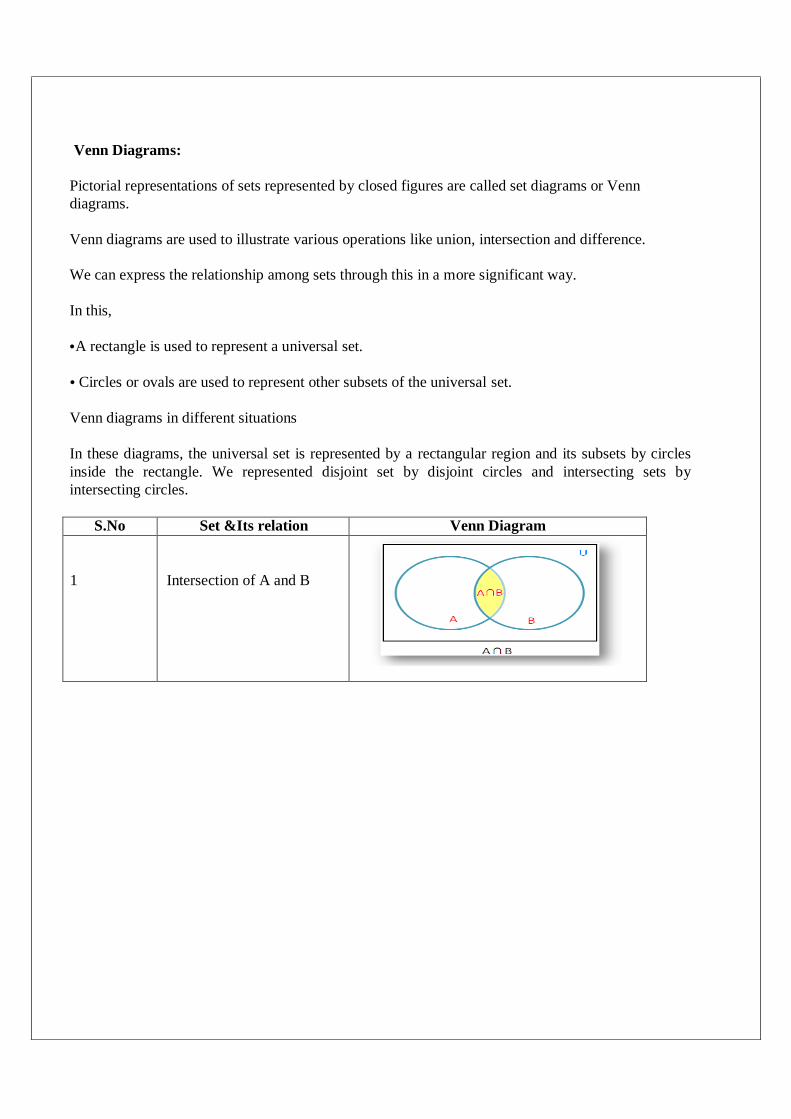
S.No Set &Its relation Venn Diagram

1

Intersection of A and B

17

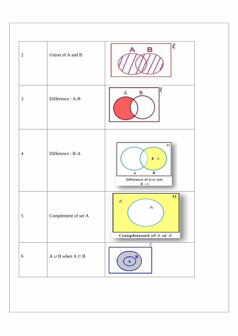
2

Union of A and B

3

Difference : A-B

4

Difference : B-A

5

Complement of set A

6

A ∪ B when A ⊂ B

18

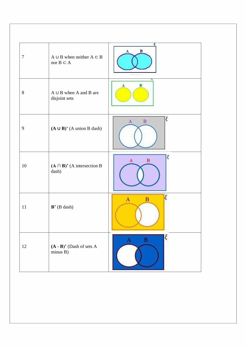
7

A ∪ B when neither A ⊂ B

nor B ⊂ A

8

A ∪ B when A and B are

disjoint sets

9

(A ∪ B)’ (A union B dash)

10

(A ∩ B)’ (A intersection B

dash)

11

B’ (B dash)

12

(A - B)’ (Dash of sets A

minus B)

19

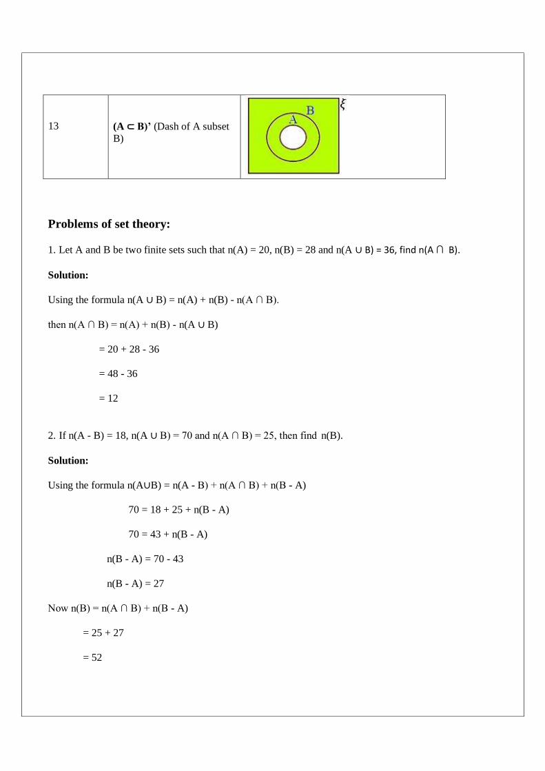
13

(A ⊂ B)’ (Dash of A subset

B)

Problems of set theory:

1. Let A and B be two finite sets such that n(A) = 20, n(B) = 28 and n(A ∪ B) = 36, find n(A ∩ B).

Solution:

Using the formula n(A ∪ B) = n(A) + n(B) - n(A ∩ B).

then n(A ∩ B) = n(A) + n(B) - n(A ∪ B)

= 20 + 28 - 36

= 48 - 36

= 12

2. If n(A - B) = 18, n(A ∪ B) = 70 and n(A ∩ B) = 25, then find n(B).

Solution:

Using the formula n(A∪B) = n(A - B) + n(A ∩ B) + n(B - A)

70 = 18 + 25 + n(B - A)

70 = 43 + n(B - A)

n(B - A) = 70 - 43

n(B - A) = 27

Now n(B) = n(A ∩ B) + n(B - A)

= 25 + 27

= 52

20

3. In a group of 60 people, 27 like cold drinks and 42 like hot drinks and each person likes at least

one of the two drinks. How many like both coffee and tea?

Solution:

Let A = Set of people who like cold drinks.

B = Set of people who like hot drinks.

Given

(A ∪ B) = 60 n(A) = 27 n(B) = 42 then;

n(A ∩ B) = n(A) + n(B) - n(A ∪ B)

= 27 + 42 - 60

= 69 - 60 = 9

= 9

Therefore, 9 people like both tea and coffee.

4. There are 35 students in art class and 57 students in dance class. Find the number of students

who are either in art class or in dance class.

• When two classes meet at different hours and 12 students are enrolled in both activities.

• When two classes meet at the same hour.

Solution:

n(A) = 35, n(B) = 57, n(A ∩ B) = 12

(Let A be the set of students in art class.

B be the set of students in dance class.)

(i) When 2 classes meet at different hours n(A ∪ B) = n(A) + n(B) - n(A ∩ B)

= 35 + 57 - 12

= 92 - 12

= 80

21

(ii) When two classes meet at the same hour, A∩B = ∅ n (A ∪ B) = n(A) + n(B) - n(A ∩ B)

= n(A) + n(B)

= 35 + 57

= 92

5. In a group of 100 persons, 72 people can speak English and 43 can speak French. How many can

speak English only? How many can speak French only and how many can speak both English and

French?

Solution:

Let A be the set of people who speak English.

B be the set of people who speak French.

A - B be the set of people who speak English and not French.

B - A be the set of people who speak French and not English.

A ∩ B be the set of people who speak both French and English.

Given,

n(A) = 72 n(B) = 43 n(A ∪ B) = 100

Now, n(A ∩ B) = n(A) + n(B) - n(A ∪ B)

= 72 + 43 - 100

= 115 - 100

= 15

Therefore, Number of persons who speak both French and English = 15

n(A) = n(A - B) + n(A ∩ B)

⇒ n(A - B) = n(A) - n(A ∩ B)

= 72 - 15

22

= 57

and n(B - A) = n(B) - n(A ∩ B)

= 43 - 15

= 28

Therefore, Number of people speaking English only = 57

Number of people speaking French only = 28

Probability Concepts

Before we give a definition of probability, let us examine the following concepts:

1. Experiment:

In probability theory, an experiment or trial (see below) is any procedure that can be

infinitely repeated and has a well-defined set of possible outcomes, known as the sample

space. An experiment is said to be random if it has more than one possible outcome,

and deterministic if it has only one. A random experiment that has exactly two (mutually

exclusive) possible outcomes is known as a Bernoulli trial.

Random Experiment:

An experiment is a random experiment if its outcome cannot be predicted precisely. One

out of a number of outcomes is possible in a random experiment. A single performance of

the random experiment is called a trial.

Random experiments are often conducted repeatedly, so that the collective results may be

subjected to statistical analysis. A fixed number of repetitions of the same experiment can

be thought of as a composed experiment, in which case the individual repetitions are

called trials. For example, if one were to toss the same coin one hundred times and record

each result, each toss would be considered a trial within the experiment composed of all

hundred tosses.

Mathematical description of an experiment:

A random experiment is described or modeled by a mathematical construct known as a probability

space. A probability space is constructed and defined with a specific kind of experiment or trial in

mind.

23

A mathematical description of an experiment consists of three parts:

1. A sample space, Ω (or S), which is the set of all possible outcomes.

2. A set of events , where each event is a set containing zero or more outcomes.

3. The assignment of probabilities to the events—that is, a function P mapping from events to

probabilities.

An outcome is the result of a single execution of the model. Since individual outcomes might be of

little practical use, more complicated events are used to characterize groups of outcomes. The

collection of all such events is a sigma-algebra . Finally, there is a need to specify each event's

likelihood of happening; this is done using the probability measure function,P.

2. Sample Space: The sample space is the collection of all possible outcomes of a

random experiment. The elements of are called sample points.

A sample space may be finite, countably infinite or uncountable.

A finite or countably infinite sample space is called a discrete sample space.

An uncountable sample space is called a continuous sample space

Ex:1. For the coin-toss experiment would be the results ―Head‖and ―Tail‖, which we may

represent by S=H T.

Ex. 2. If we toss a die, one sample space or the set of all possible outcomes is

S = 1, 2, 3, 4, 5, 6

The other sample space can be

S = odd, even

Types of Sample Space:

1. Finite/Discrete Sample Space:

Consider the experiment of tossing a coin twice.

The sample space can be

S = HH, HT, T H , TT the above sample space has a finite number of sample points. It is

called a finite sample space

24

2. Countably Infinite Sample Space:

Consider that a light bulb is manufactured. It is then tested for its life length by inserting it

into a socket and the time elapsed (in hours) until it burns out is recorded. Let the measuring

instrument is capable of recording time to two decimal places, for example 8.32 hours.

Now, the sample space becomes count ably infinite i.e.

S = 0.0, 0.01, 0.02

The above sample space is called a countable infinite sample space.

3. Un Countable/ Infinite Sample Space:

If the sample space consists of unaccountably infinite number of elements then it is called

Un Countable/ Infinite Sample Space.

3. Event: An event is simply a set of possible outcomes. To be more specific, an event is a

subset A of the sample space S.

For a discrete sample space, all subsets are events.

Ex: For instance, in the coin-toss experiment the events A=Heads and B=Tails would be

mutually exclusive.

An event consisting of a single point of the sample space 'S' is called a simple event or elementary

event.

Some examples of event sets:

Example 1: tossing a fair coin

The possible outcomes are H (head) and T (tail). The associated sample space is It is

a finite sample space. The events associated with the sample space are: and .

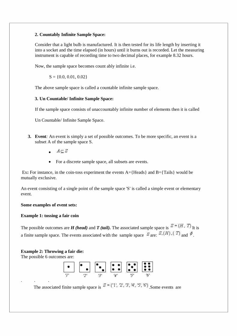
Example 2: Throwing a fair die:

The possible 6 outcomes are:

. . .

The associated finite sample space is .Some events are

25

And so on.

Example 3: Tossing a fair coin until a head is obtained

We may have to toss the coin any number of times before a head is obtained. Thus the possible outcomes are:

H, TH, TTH, TTTH,

How many outcomes are there? The outcomes are countable but infinite in number. The

countably infinite sample space is .

Example 4 : Picking a real number at random between -1 and +1

The associated Sample space is

Clearly is a continuous sample space.

Example 5: Drawing cards

Drawing 4 cards from a deck: Events include all spades, sum of the 4 cards is (assuming face cards

have a value of zero), a sequence of integers, a hand with a 2, 3, 4 and 5. There are many more

events.

Types of Events:

1. Exhaustive Events:

A set of events is said to be exhaustive, if it includes all the possible events.

Ex. In tossing a coin, the outcome can be either Head or Tail and there is no other possible

outcome. So, the set of events H , T is exhaustive.

2. Mutually Exclusive Events:

Two events, A and B are said to be mutually exclusive if they cannot occur together.

i.e. if the occurrence of one of the events precludes the occurrence of all others, then such a set of

events is said to be mutually exclusive.

If two events are mutually exclusive then the probability of either occurring is

26

f(A)=nA/n

Ex. In tossing a die, both head and tail cannot happen at the same time.

3. Equally Likely Events:

If one of the events cannot be expected to happen in preference to another, then such events

are said to be Equally Likely Events.( Or) Each outcome of the random experiment has an

equal chance of occuring.

Ex. In tossing a coin, the coming of the head or the tail is equally likely.

4. Independent Events:

Two events are said to be independent, if happening or failure of one does not affect the happening

or failure of the other. Otherwise, the events are said to be dependent.

If two events, A and B are independent then the joint probability is

5. Non-. Mutually Exclusive Events:

If the events are not mutually exclusive then

Probability Definitions and Axioms:

1. Relative frequency Definition:

Consider that an experiment E is repeated n times, and let A and B be two events associated

w i t h E. Let nA and nB be the number of times that the event A and the event B occurred

among the n repetitions respectively.

The relative frequency of the event A in the 'n' repetitions of E is defined as

f( A) = nA /n

The Relative frequency has the following properties:

1.0 ≤f(A) ≤ 1

2. f(A) =1 if and only if A occurs every time among the n repetitions.

27

If an experiment is repeated times under similar conditions and the event occurs in

times, then the probability of the event A is defined as

Limitation:

Since we can never repeat an experiment or process indefinitely, we can never know the probability

of any event from the relative frequency definition. In many cases we can't even obtain a long

series of repetitions due to time, cost, or other limitations. For example, the probability of rain

today can't really be obtained by the relative frequency definition since today can‘t be repeated

again.

2. .The classical definition:

Let the sample space (denoted by ) be the set of all possible distinct outcomes to an

experiment. The probability of some event is

provided all points in are equally likely. For example, when a die is rolled the probability of

getting a 2 is because one of the six faces is a 2.

Limitation:

What does "equally likely" mean? This appears to use the concept of probability while trying to

define it! We could remove the phrase "provided all outcomes are equally likely", but then the

definition would clearly be unusable in many settings where the outcomes in did not tend to

occur equally often.

Example1:A fair die is rolled once. What is the probability of getting a ‘6‘ ?

Here and

Example2:A fair coin is tossed twice. What is the probability of getting two ‗heads'?

Here and .

Total number of outcomes is 4 and all four outcomes are equally likely.

Only outcome favourable to is HH

28

Probability axioms:

Given an event in a sample space which is either finite with elements or countably infinite

with elements, then we can write

and a quantity , called the probability of event , is defined such that

Axiom1: The probability of any event A is positive or zero. Namely P(A)≥0. The probability

measures, in a certain way, the difficulty of event A happening: the smaller the probability, the

more difficult it is to happen. i.e

.

Axiom2: The probability of the sure event is 1. Namely P(Ω)=1. And so, the probability is always

greater than 0 and smaller than 1: probability zero means that there is no possibility for it to happen

(it is an impossible event), and probability 1 means that it will always happen (it is a sure event).i.e

.

Axiom3: The probability of the union of any set of two by two incompatible events is the sum of

the probabilities of the events. That is, if we have, for example, events A,B,C, and these are two by

two incompatible, then P(A∪B∪C)=P(A)+P(B)+P(C). i.e Additivity:

, where and are mutually exclusive.

for , 2, ..., where , , ... are mutually exclusive

(i.e., ).

Main properties of probability: If A is any event of sample space S then

1. P(A)+P( )=1

2. Since A ∪ S , P(A ∪ )=1

3. The probability of the impossible event is 0, i.e P(Ø)=0

4. If A⊂B, then P(A)≤P(B).

5. If A and B are two incompatible events, and therefore, P(A−B)=P(A)−P(A∩B).and

P(B−A)=P(B)−P(A∩B).

6. Addition Law of probability:

P(AUB)=P(A)+P(B)-P(A∩B)

29

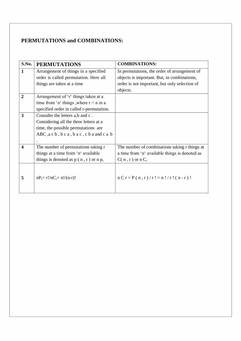
PERMUTATIONS and COMBINATIONS:

S.No. PERMUTATIONS COMBINATIONS:

1 Arrangement of things in a specified

order is called permutation. Here all

things are taken at a time

In permutations, the order of arrangement of

objects is important. But, in combinations,

order is not important, but only selection of

objects.

2 Arrangement of ‘r‘ things taken at a

time from ‘n‘ things ,where r < n in a

specified order in called r-permutation.

3 Consider the letters a,b and c .

Considering all the three letters at a

time, the possible permutations are

ABC ,a c b , b c a , b a c , c b a and c a b

.

4 The number of permutations taking r

things at a time from ‘n‘ available

things is denoted as p ( n , r ) or n pr

The number of combinations taking r things at

a time from ‘n‘ available things is denoted as

C( n , r ) or n Cr

5

nPr= r!/nCr= n!/(n-r)!

n C r = P ( n , r ) / r ! = n ! / r ! ( n - r ) !

30

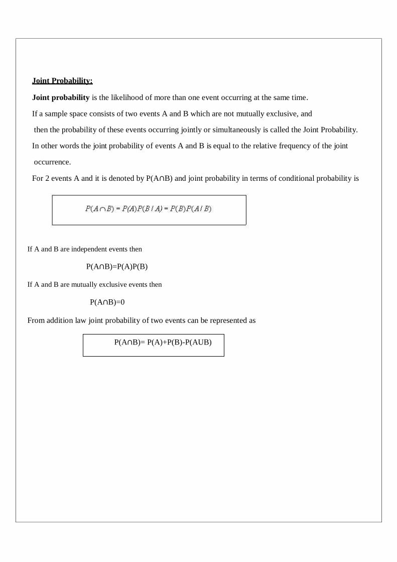
Joint Probability:

Joint probability is the likelihood of more than one event occurring at the same time.

If a sample space consists of two events A and B which are not mutually exclusive, and

then the probability of these events occurring jointly or simultaneously is called the Joint Probability.

In other words the joint probability of events A and B is equal to the relative frequency of the joint

occurrence.

For 2 events A and it is denoted by P(A∩B) and joint probability in terms of conditional probability is

If A and B are independent events then

P(A∩B)=P(A)P(B)

If A and B are mutually exclusive events then

P(A∩B)=0

From addition law joint probability of two events can be represented as

P(A∩B)= P(A)+P(B)-P(AUB)

31

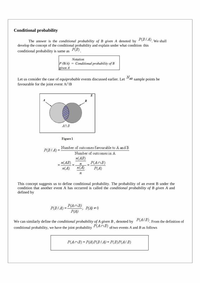
Conditional probability

The answer is the conditional probability of B given A denoted by . We shall

develop the concept of the conditional probability and explain under what condition this

conditional probability is same as .

Let us consider the case of equiprobable events discussed earlier. Let sample points be

favourable for the joint event A∩B

This concept suggests us to define conditional probability. The probability of an event B under the condition that another event A has occurred is called the conditional probability of B given A and defined by

We can similarly define the conditional probability of A given B , denoted by . From the definition of

conditional probability, we have the joint probability of two events A and B as follows

32

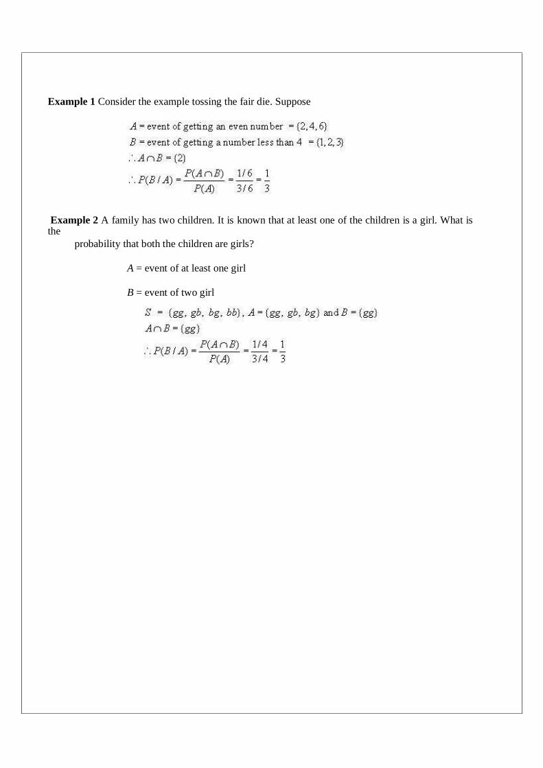
Example 1 Consider the example tossing the fair die. Suppose

Example 2 A family has two children. It is known that at least one of the children is a girl. What is the

probability that both the children are girls?

A = event of at least one girl

B = event of two girl

33

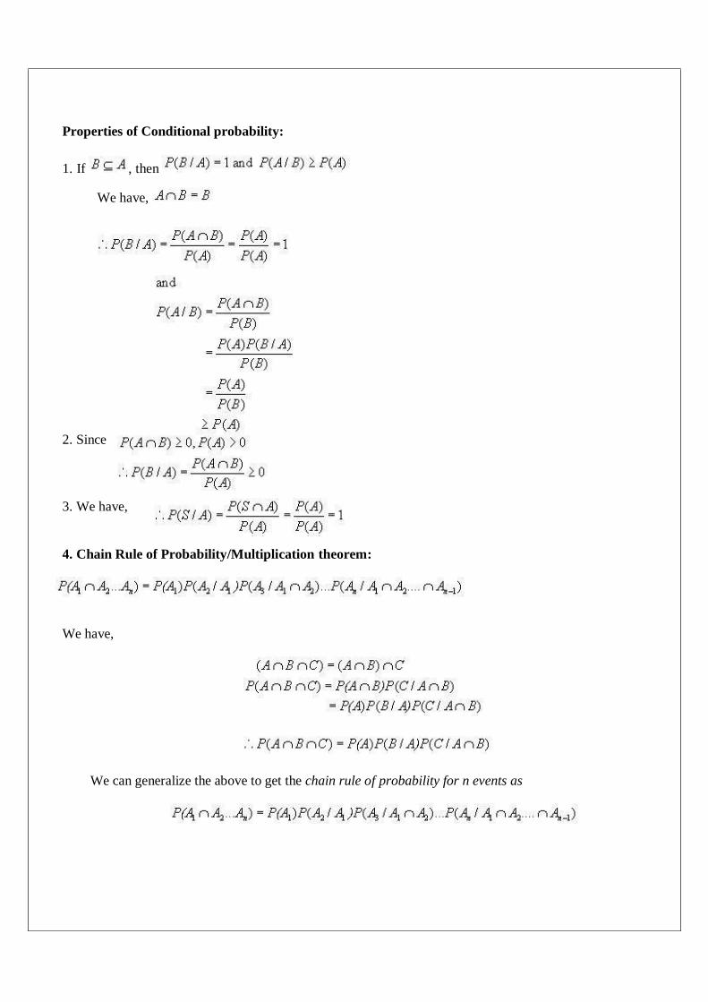
Properties of Conditional probability:

1. If , then

We have,

2. Since

3. We have,

4. Chain Rule of Probability/Multiplication theorem:

We have,

We can generalize the above to get the chain rule of probability for n events as

34

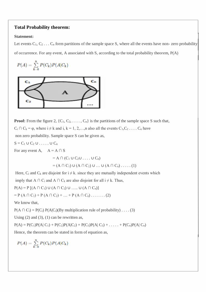
Total Probability theorem:

Statement:

Let events C1, C2 . . . Cn form partitions of the sample space S, where all the events have non- zero probability

of occurrence. For any event, A associated with S, according to the total probability theorem, P(A)

Proof: From the figure 2, C1, C2, . . . . , Cn is the partitions of the sample space S such that,

Ci ∩ Ck = φ, where i ≠ k and i, k = 1, 2,…,n also all the events C1,C2 . . . . Cn have

non zero probability. Sample space S can be given as,

S = C1 ∪ C2 ∪ . . . . . ∪ Cn

For any event A, A = A ∩ S

= A ∩ (C1 ∪ C2∪ . . . . ∪ Cn)

= (A ∩ C1) ∪ (A ∩ C2) ∪ … ∪ (A ∩ Cn) . . . . . (1)

Here, Ci and Ck are disjoint for i ≠ k. since they are mutually independent events which

imply that A ∩ Ci and A ∩ Ck are also disjoint for all i ≠ k. Thus,

P(A) = P [(A ∩ C1) ∪ (A ∩ C2) ∪ ….. ∪ (A ∩ Cn)]

= P (A ∩ C1) + P (A ∩ C2) + … + P (A ∩ Cn) . . . . . . . (2)

We know that,

P(A ∩ Ci) = P(Ci) P(A|Ci)(By multiplication rule of probability) . . . . (3)

Using (2) and (3), (1) can be rewritten as,

P(A) = P(C1)P(A| C1) + P(C2)P(A|C2) + P(C3)P(A| C3) + . . . . . + P(Cn)P(A| Cn)

Hence, the theorem can be stated in form of equation as,

35

Example:

A person has undertaken a mining job. The probabilities of completion of job on time with and without

rain are 0.42 and 0.90 respectively. If the probability that it will rain is 0.45, then determine the

probability that the mining job will be completed on time.

Solution:

Let A be the event that the mining job will be completed on time and B be the

event that it rains. We have,

P(B) = 0.45,

P(no rain) = P(B′) = 1 − P(B) = 1 − 0.45 = 0.55

From given data

P(A|B) = 0.42

P(A|B′) = 0.90

Since, events B and B′ form partitions of the sample space S, by total probability theorem,

we have

P(A) = P(B) P(A|B) + P(B′) P(A|B′)

=0.45 × 0.42 + 0.55 × 0.9

= 0.189 + 0.495 = 0.684

So, the probability that the job will be completed on time is 0.684.

36

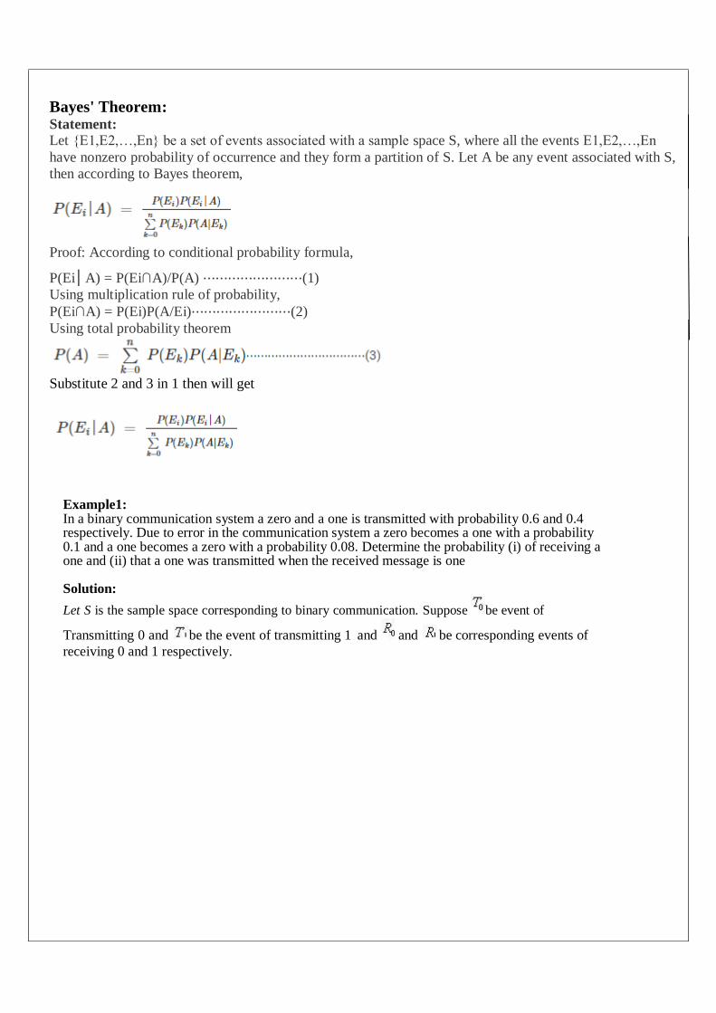
Bayes' Theorem: Statement:

Let E1,E2,…,En be a set of events associated with a sample space S, where all the events E1,E2,…,En

have nonzero probability of occurrence and they form a partition of S. Let A be any event associated with S,

then according to Bayes theorem,

Proof: According to conditional probability formula,

P(EiA) = P(Ei∩A)/P(A) ⋯⋯⋯⋯⋯⋯⋯⋯(1)

Using multiplication rule of probability,

P(Ei∩A) = P(Ei)P(A/Ei)⋯⋯⋯⋯⋯⋯⋯⋯(2)

Using total probability theorem

Substitute 2 and 3 in 1 then will get

Example1: In a binary communication system a zero and a one is transmitted with probability 0.6 and 0.4 respectively. Due to error in the communication system a zero becomes a one with a probability 0.1 and a one becomes a zero with a probability 0.08. Determine the probability (i) of receiving a one and (ii) that a one was transmitted when the received message is one

Solution:

Let S is the sample space corresponding to binary communication. Suppose be event of

Transmitting 0 and be the event of transmitting 1 and and be corresponding events of

receiving 0 and 1 respectively.

37

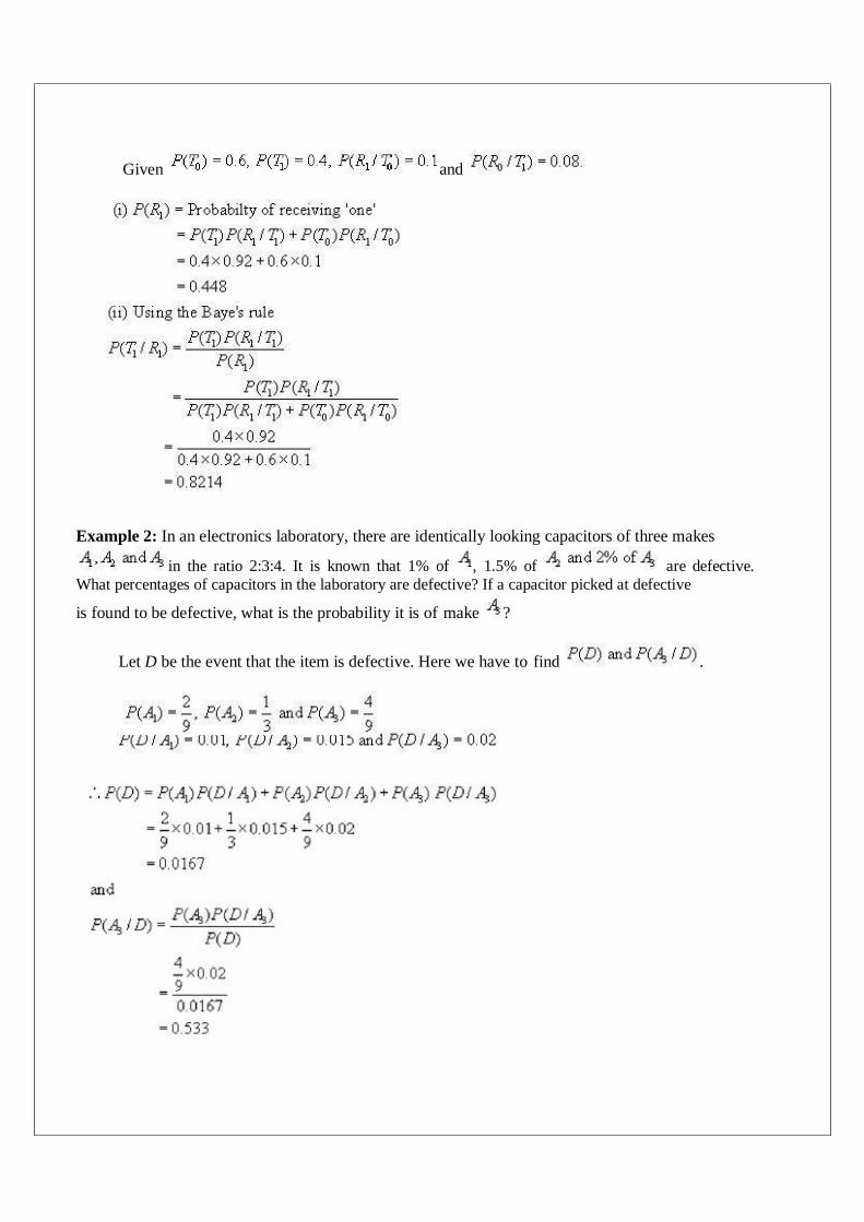
Given and

Example 2: In an electronics laboratory, there are identically looking capacitors of three makes

in the ratio 2:3:4. It is known that 1% of , 1.5% of are defective.

What percentages of capacitors in the laboratory are defective? If a capacitor picked at defective

is found to be defective, what is the probability it is of make ?

Let D be the event that the item is defective. Here we have to find .

38

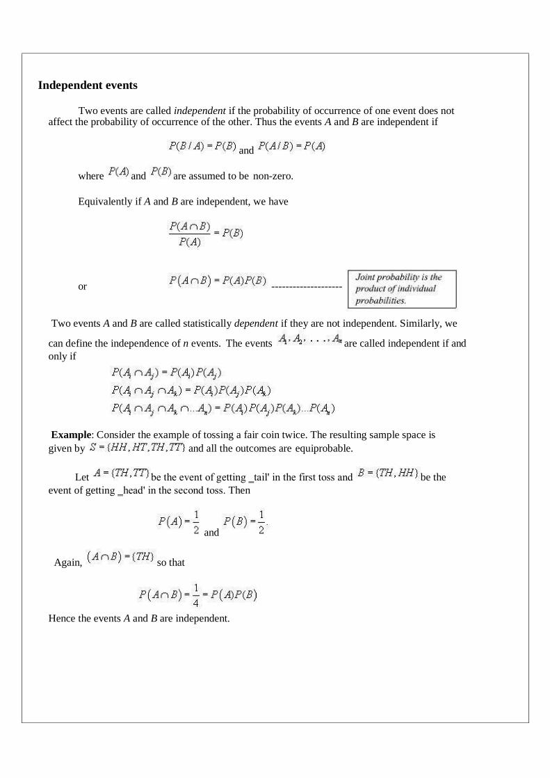
Independent events

Two events are called independent if the probability of occurrence of one event does not

affect the probability of occurrence of the other. Thus the events A and B are independent if

and

where and are assumed to be non-zero.

Equivalently if A and B are independent, we have

or --------------------

Two events A and B are called statistically dependent if they are not independent. Similarly, we

can define the independence of n events. The events are called independent if and

only if

Example: Consider the example of tossing a fair coin twice. The resulting sample space is

given by and all the outcomes are equiprobable.

Let be the event of getting ‗tail' in the first toss and be the

event of getting ‗head' in the second toss. Then

and

Again, so that

Hence the events A and B are independent.

39

Problems:

Example1.A dice of six faces is tailored so that the probability of getting every face is

proportional to the number depicted on it.

a) What is the probability of extracting a 6?

In this case, we say that the probability of each face turning up is not the same, therefore we cannot

simply apply the rule of Laplace. If we follow the statement, it says that the probability of each face

turning up is proportional to the number of the face itself, and this means that, if we say that the

probability of face 1 being turned up is k which we do not know, then:

P(1)=k, P(2)=2k, P(3)=3k, P(4)=4k,

P(5)=5k,P(6)=6k.

Now, since 1,2,3,4,5,6 form an events complete system , necessarily

P(1)+P(2)+P(3)+P(4)+P(5)+P(6)=1

Therefore

k+2k+3k+4k+5k+6k=1

which is an equation that we can already solve:

21k=1

thus

k=1/21

And so, the probability of extracting 6 is P(6)=6k=6⋅(1/21)=6/21.

b) What is the probability of extracting an odd number?

The cases favourable to event A= "to extract an odd number" are: 1,3,5. Therefore, since

they are incompatible events,

P(A)=P(1)+P(3)+P(5)=k+3k+5k=9k=9⋅(1/21)=9/21

40

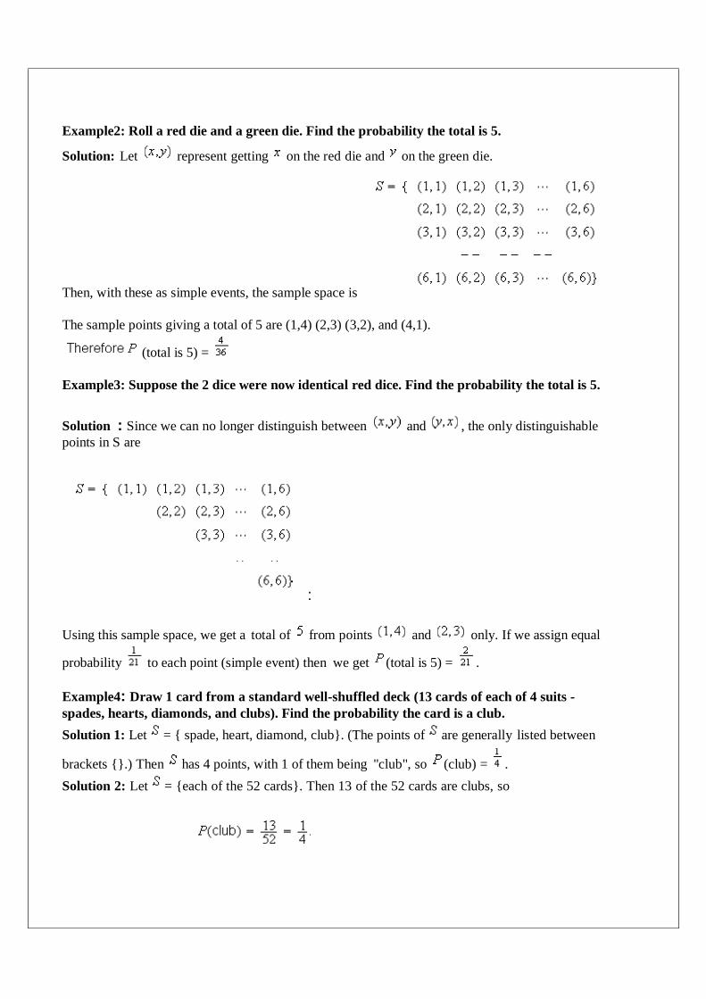
Example2: Roll a red die and a green die. Find the probability the total is 5.

Solution: Let represent getting on the red die and on the green die.

Then, with these as simple events, the sample space is

The sample points giving a total of 5 are (1,4) (2,3) (3,2), and (4,1).

(total is 5) =

Example3: Suppose the 2 dice were now identical red dice. Find the probability the total is 5.

Solution : Since we can no longer distinguish between and , the only distinguishable

points in S are

:

Using this sample space, we get a total of from points and only. If we assign equal

probability to each point (simple event) then we get (total is 5) = .

Example4: Draw 1 card from a standard well-shuffled deck (13 cards of each of 4 suits -

spades, hearts, diamonds, and clubs). Find the probability the card is a club.

Solution 1: Let = spade, heart, diamond, club. (The points of are generally listed between

brackets .) Then has 4 points, with 1 of them being "club", so (club) = .

Solution 2: Let = each of the 52 cards. Then 13 of the 52 cards are clubs, so

41

Example 5: Suppose we draw a card from a deck of playing cards. What is the probability

that we draw a spade?

Solution: The sample space of this experiment consists of 52 cards, and the probability of each

sample point is 1/52. Since there are 13 spades in the deck, the probability of drawing a spade is

P(Spade) = (13)(1/52) = 1/4

Example 6: Suppose a coin is flipped 3 times. What is the probability of getting two tails and

one head?

Solution: For this experiment, the sample space consists of 8 sample points.

S = TTT, TTH, THT, THH, HTT, HTH, HHT, HHH

Each sample point is equally likely to occur, so the probability of getting any particular sample

point is 1/8. The event "getting two tails and one head" consists of the following subset of the

sample space.

A = TTH, THT, HTT

The probability of Event A is the sum of the probabilities of the sample points in A. Therefore,

P(A) = 1/8 + 1/8 + 1/8 = 3/8

Example7: An urn contains 6 red marbles and 4 black marbles. Two marbles are

drawn without replacement from the urn. What is the probability that both of the marbles are

black?

Solution: Let A = the event that the first marble is black; and let B = the event that the second

marble is black. We know the following:

In the beginning, there are 10 marbles in the urn, 4 of which are black. Therefore, P(A) =

4/10.

After the first selection, there are 9 marbles in the urn, 3 of which are black. Therefore,

P(B|A) = 3/9.

Therefore, based on the rule of multiplication:

P(A ∩ B) = P(A) P(B|A)

P(A ∩ B) = (4/10) * (3/9) = 12/90 = 2/15

42

RANDOM VARIABLE

INTRODUCTION

In many situations, we are interested in numbers associated with the outcomes of a random

experiment. In application of probabilities, we are often concerned with numerical values which

are random in nature. For example, we may consider the number of customers arriving at a

service station at a particular interval of time or the transmission time of a message in a

communication system. These random quantities may be considered as real-valued function on

the sample space. Such a real-valued function is called real random variable and plays an

important role in describing random data. We shall introduce the concept of random variables in

the following sections.

Random Variable Definition

A random variable is a function that maps outcomes of a random experiment to real

numbers. (or)

A random variable associates the points in the sample space with real numbers

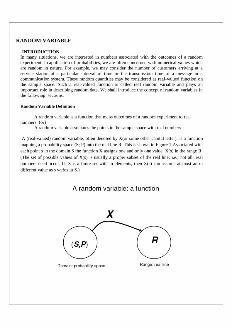
A (real-valued) random variable, often denoted by X(or some other capital letter), is a function

mapping a probability space (S; P) into the real line R. This is shown in Figure 1.Associated with

each point s in the domain S the function X assigns one and only one value X(s) in the range R.

(The set of possible values of X(s) is usually a proper subset of the real line; i.e., not all real

numbers need occur. If S is a finite set with m elements, then X(s) can assume at most an m

different value as s varies in S.)

43

Example1

A fair coin is tossed 6 times. The number of heads that come up is an example of a random

variable.

HHTTHT – 3, THHTTT -- 2.

These random variables can only take values between 0 and 6.

The Set of possible values of random variables is known as its

Range. Example2

A box of 6 eggs is rejected once it contains one or more broken eggs. If we examine 10 boxes

of eggs and define the randomvariablesX1, X2 as

1 X1- the number of broken eggs in the 10

boxes 2 X2- the number of boxes rejected

Then the range of X1 is 0, 1,2,3,4-------------- 60 and X2 is 0,1,2 --- 10 Figure 2: A (real-valued) function of a random variable is itself a random variable, i.e., a

function mapping a probability space into the real line.

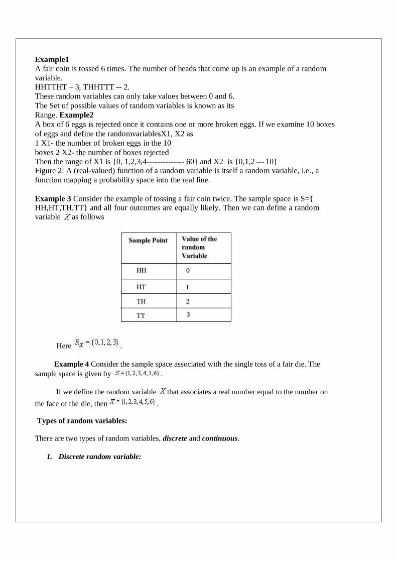
Example 3 Consider the example of tossing a fair coin twice. The sample space is S= HH,HT,TH,TT and all four outcomes are equally likely. Then we can define a random

variable as follows

Here .

Example 4 Consider the sample space associated with the single toss of a fair die. The

sample space is given by .

If we define the random variable that associates a real number equal to the number on

the face of the die, then .

Types of random variables:

There are two types of random variables, discrete and continuous.

1. Discrete random variable:

44

is an

A discrete random variable is one which may take on only a countable number of distinct

values such as 0, 1,2,3,4,. ........ Discrete random variables are usually (but not necessarily) counts. If

a random variable can take only a finite number of distinct values, then it must be discrete

(Or)

A random variable is called a discrete random variable if is piece-wise constant.

Thus is flat except at the points of jump discontinuity. If the sample space is discrete the

random variable defined on it is always discrete.

•A discrete random variable has a finite number of possible values or an infinite sequence of

countable real numbers.

–X: number of hits when trying 20 free throws.

–X: number of customers who arrive at the bank from 8:30 – 9:30AM Mon-‐Fri.

–E.g. Binomial, Poisson...

2. Continuous random variable:

A continuous random variable is one which takes an infinite number of possible values. Continuous rando

variables are usually measurements. E

A continuous random variable takes all values in an interval of real numbers.

(or)

X is called a continuous random variable if absolutely continuous function

of x . Thus is continuous everywhere on and exists everywhere except at finite or countably infinite points

3. Mixed random variable:

X is called a mixed random variable if has jump discontinuity at countable number of points and increases continuously at least in one interval of X. For a such type RV X.

Conditions for a Function to be a Random Variable:

1. Random variable must not be a multi valued function. i.e two or more values of X cannot assign for Single outcome.

2. P(X=∞)=P(X= -∞)=0

3. The probability of the event (X≤x) must be equal to the sum of probabilities of all the events Corresponding to (X≤x).

45

Bernoulli’s trials: Bernoulli Experiment with n Trials Here are the rules for a Bernoulli experiment.

1. The experiment is repeated a fixed number of times (n times).

2. Each trial has only two possible outcomes, “success” and “failure”. The possible outcomes are exactly the

same for each trial.

3. The probability of success remains the same for each trial. We use p for the probability of success

(on each trial) and q = 1 − p for the probability of failure.

4. The trials are independent (the outcome of previous trials has no influence on the outcome of the next trial).

5. We are interested in the random variable X where X = the number of successes. Note the possible values

of X are 0, 1, 2, 3, . . . , n.

An experiment in which a single action, such as flipping a coin, is repeated identically over and over.

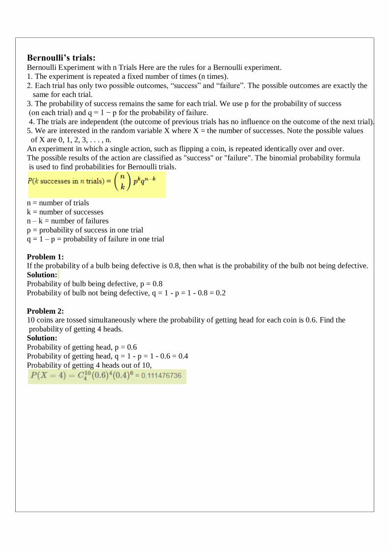
The possible results of the action are classified as "success" or "failure". The binomial probability formula

is used to find probabilities for Bernoulli trials.

n = number of trials

k = number of successes

n – k = number of failures

p = probability of success in one trial

q = 1 – p = probability of failure in one trial

Problem 1: If the probability of a bulb being defective is 0.8, then what is the probability of the bulb not being defective.

Solution:

Probability of bulb being defective, p = 0.8

Probability of bulb not being defective, q = 1 - p = 1 - 0.8 = 0.2

Problem 2: 10 coins are tossed simultaneously where the probability of getting head for each coin is 0.6. Find the

probability of getting 4 heads.

Solution:

Probability of getting head, p = 0.6

Probability of getting head, q = 1 - p = 1 - 0.6 = 0.4

Probability of getting 4 heads out of 10,

46

UNIT II

Distribution and density functions and Operations on One Random Variable

Distribution and density functions:

Distribution function and its Properties

Density function and its Properties

Important Types of Distribution and density functions

Binomial

Uniform

Exponential

Gaussian

Conditional Distribution

Conditional Density function and its properties

Problems

Operation on One Random Variable:

Expected value of a random variable, function of a random variable

Moments about the origin

Central moments - variance and skew

Characteristic function

Moment generating function.

47

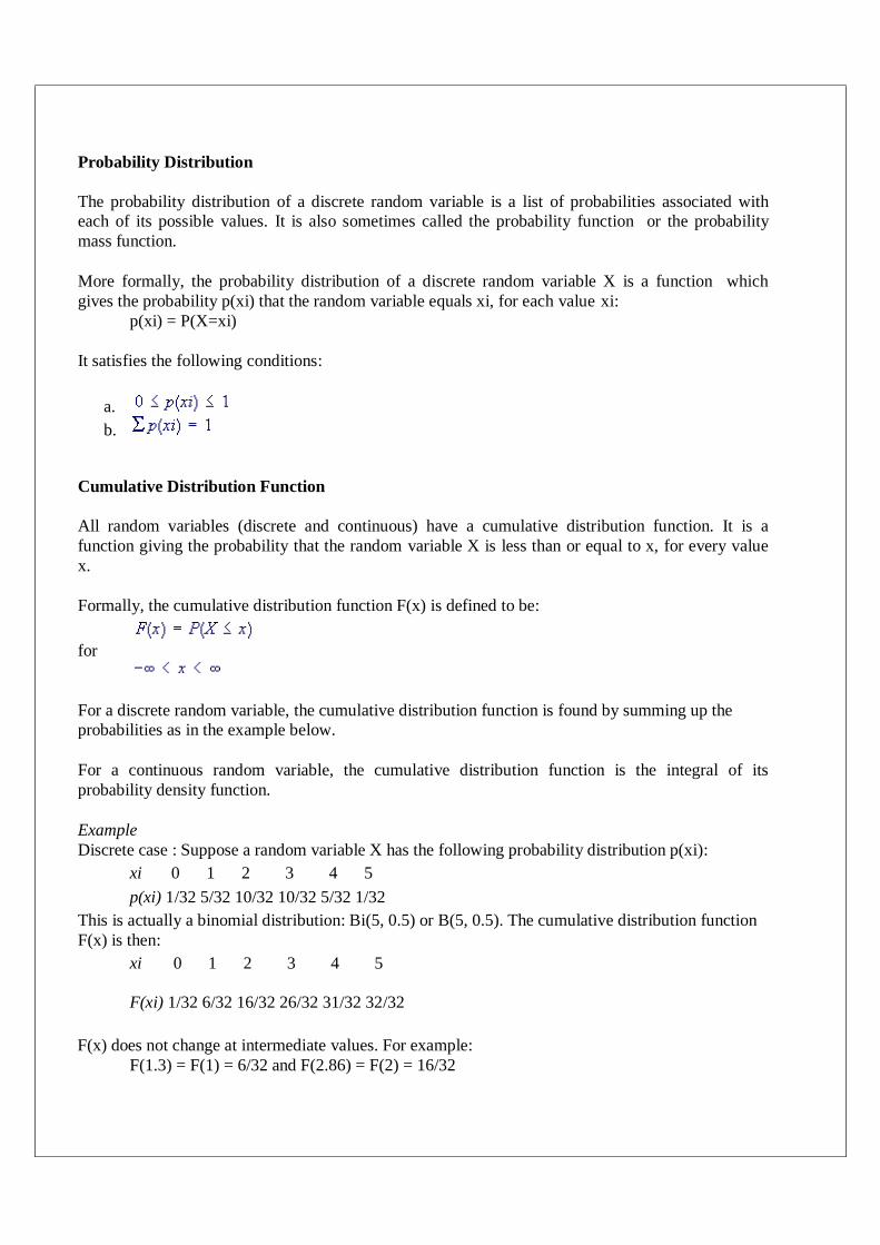
Probability Distribution

The probability distribution of a discrete random variable is a list of probabilities associated with

each of its possible values. It is also sometimes called the probability function or the probability

mass function.

More formally, the probability distribution of a discrete random variable X is a function which

gives the probability p(xi) that the random variable equals xi, for each value xi:

p(xi) = P(X=xi)

It satisfies the following conditions:

a.

b.

Cumulative Distribution Function

All random variables (discrete and continuous) have a cumulative distribution function. It is a

function giving the probability that the random variable X is less than or equal to x, for every value

x.

Formally, the cumulative distribution function F(x) is defined to be:

for

For a discrete random variable, the cumulative distribution function is found by summing up the

probabilities as in the example below.

For a continuous random variable, the cumulative distribution function is the integral of its

probability density function.

Example

Discrete case : Suppose a random variable X has the following probability distribution p(xi):

xi 0 1 2 3 4 5

p(xi) 1/32 5/32 10/32 10/32 5/32 1/32

This is actually a binomial distribution: Bi(5, 0.5) or B(5, 0.5). The cumulative distribution function

F(x) is then:

xi 0 1 2 3 4 5

F(xi) 1/32 6/32 16/32 26/32 31/32 32/32

F(x) does not change at intermediate values. For example:

F(1.3) = F(1) = 6/32 and F(2.86) = F(2) = 16/32

48

Is right continuous.

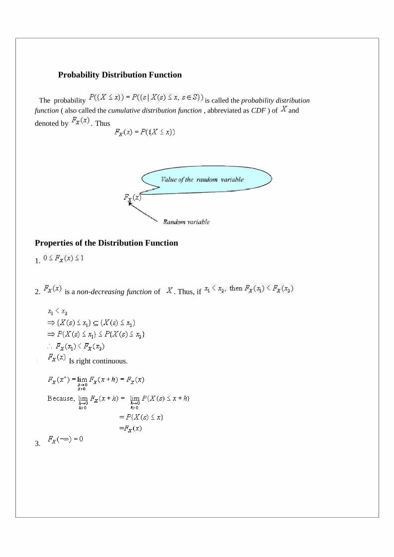
Probability Distribution Function

The probability is called the probability distribution

function ( also called the cumulative distribution function , abbreviated as CDF ) of and

denoted by . Thus

Properties of the Distribution Function

1.

2. is a non-decreasing function of . Thus, if

3.

49

.

.

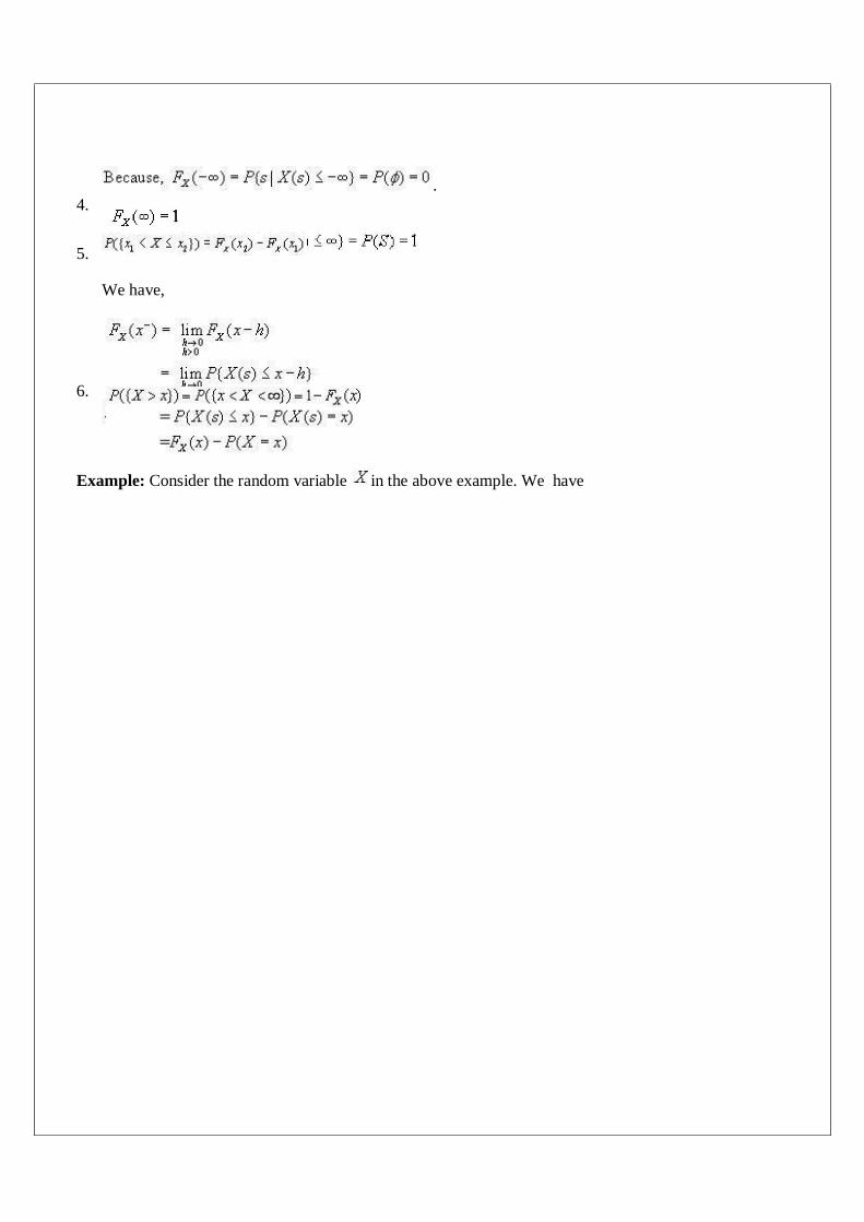
4.

5.

We have,

6.

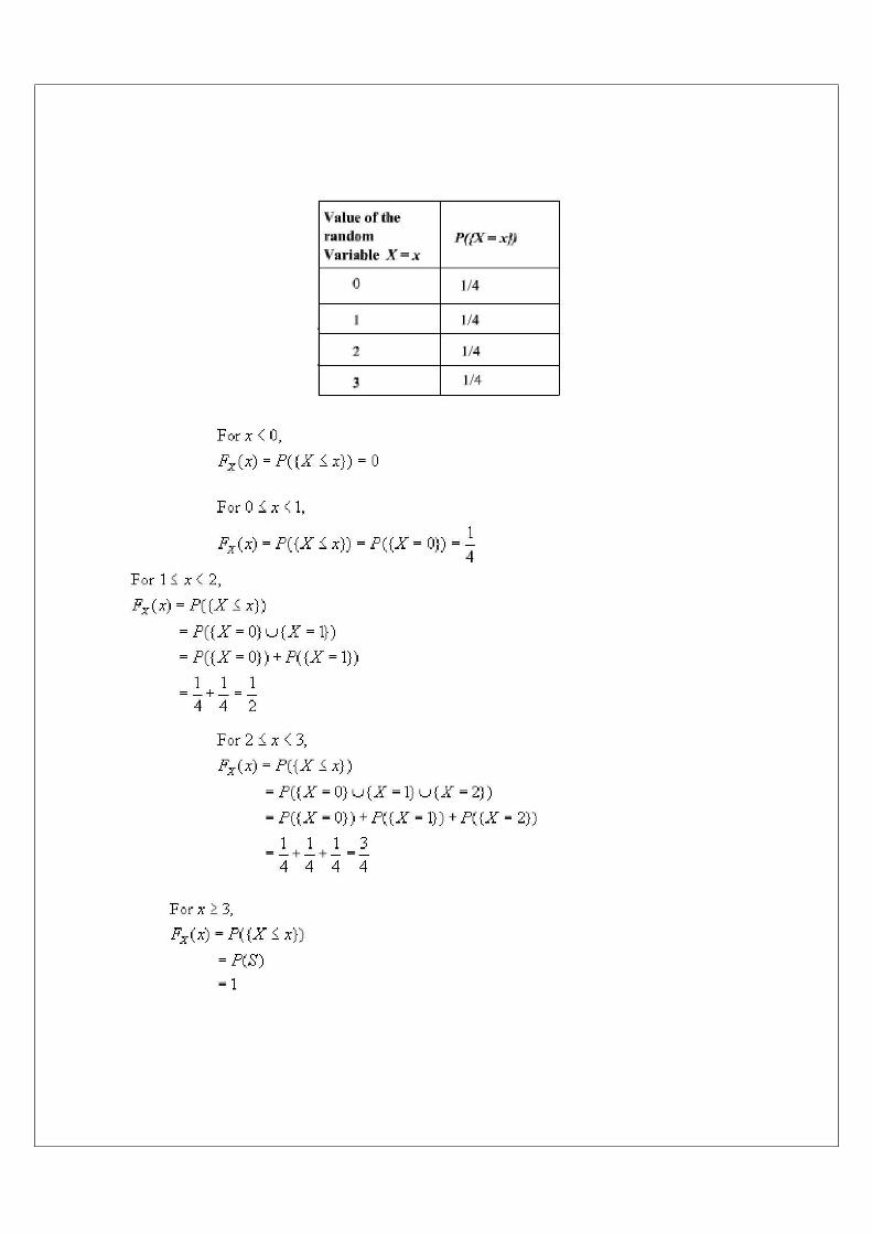
Example: Consider the random variable in the above example. We have

50

51

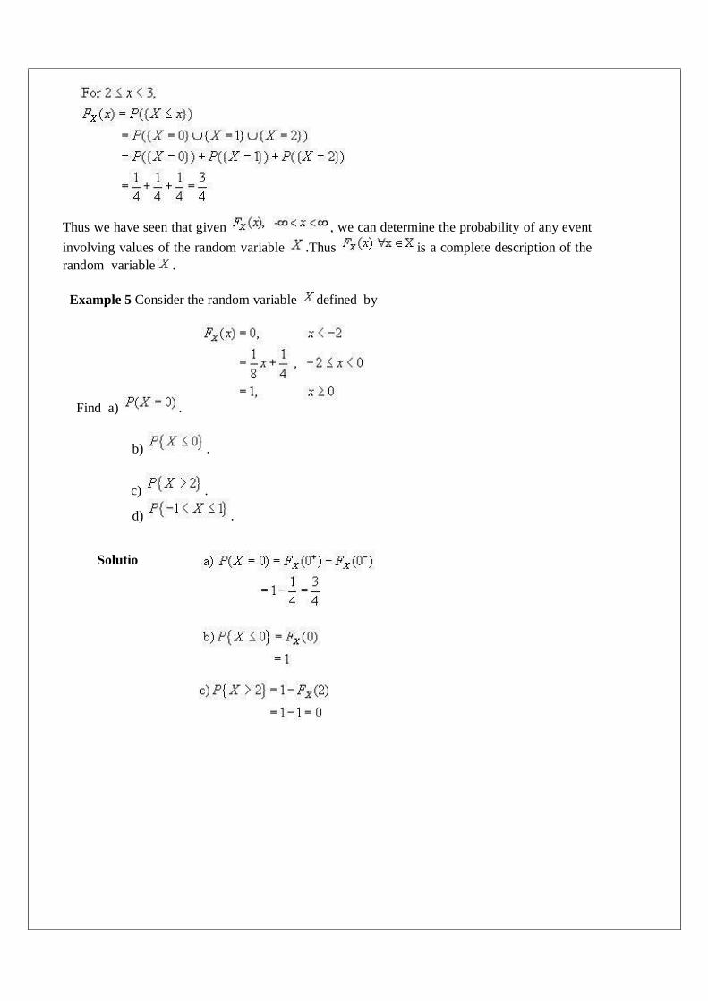
Thus we have seen that given , we can determine the probability of any event

involving values of the random variable .Thus is a complete description of the

random variable .

Example 5 Consider the random variable defined by

Find a) .

b) .

c) .

d) .

Solutio

52

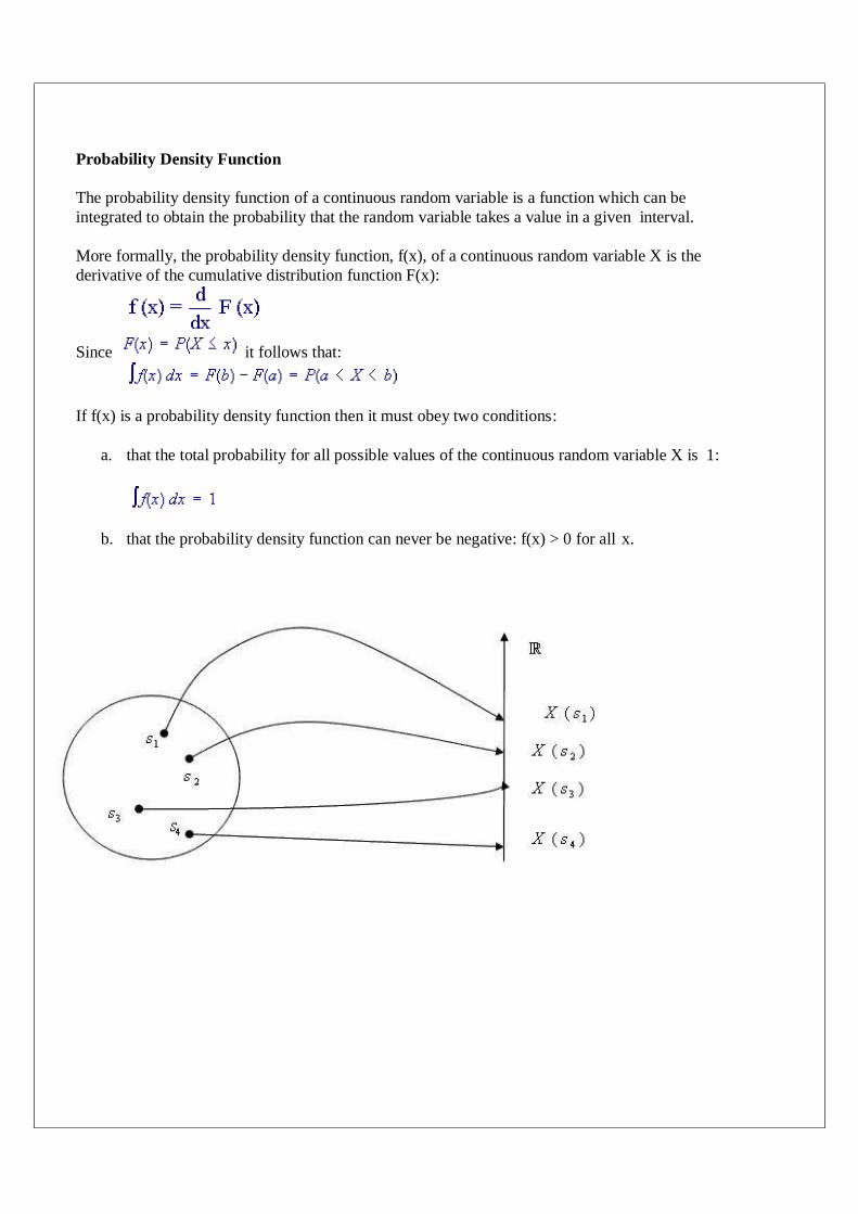
Probability Density Function

The probability density function of a continuous random variable is a function which can be

integrated to obtain the probability that the random variable takes a value in a given interval.

More formally, the probability density function, f(x), of a continuous random variable X is the

derivative of the cumulative distribution function F(x):

Since it follows that:

If f(x) is a probability density function then it must obey two conditions:

a. that the total probability for all possible values of the continuous random variable X is 1:

b. that the probability density function can never be negative: f(x) > 0 for all x.

53

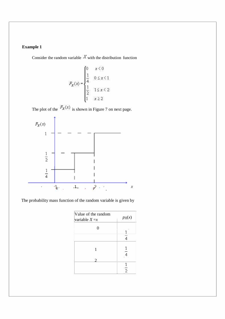
Example 1

Consider the random variable with the distribution function

The plot of the is shown in Figure 7 on next page.

The probability mass function of the random variable is given by

0

1

2

pX(x) Value of the random

variable X =x

54

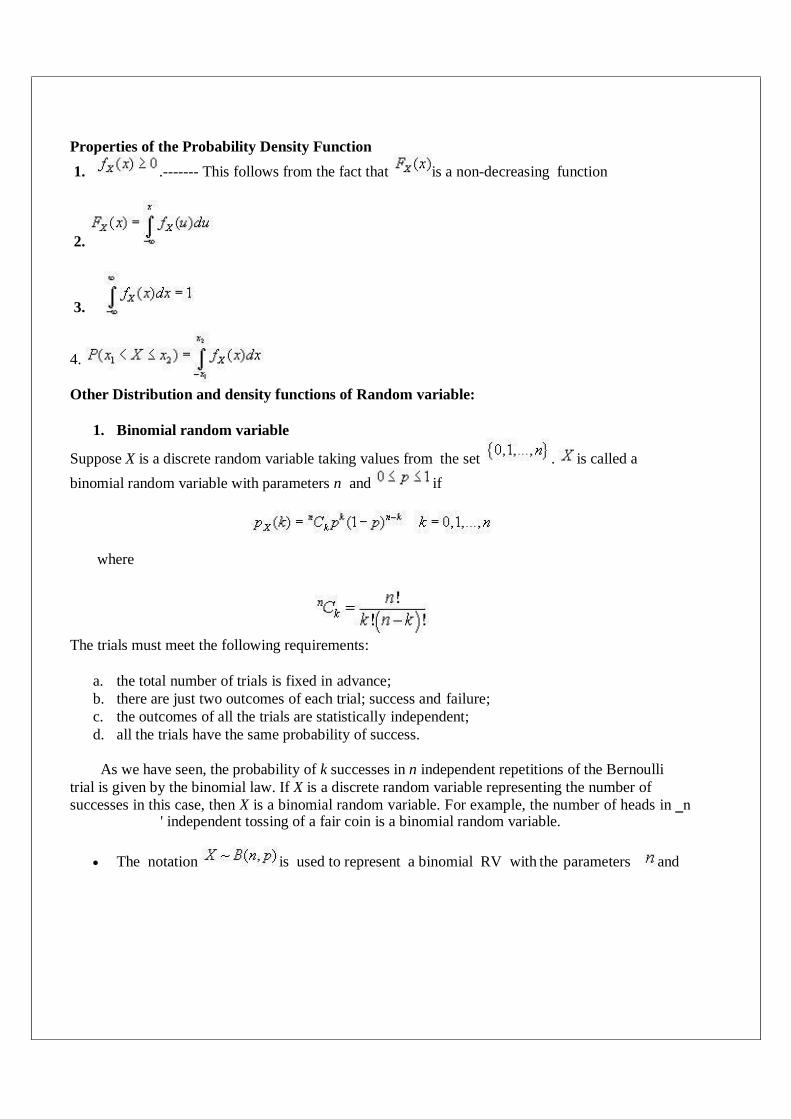
Properties of the Probability Density Function

1. .------- This follows from the fact that is a non-decreasing function

2.

3.

4.

Other Distribution and density functions of Random variable:

1. Binomial random variable

Suppose X is a discrete random variable taking values from the set . is called a

binomial random variable with parameters n and if

where

The trials must meet the following requirements:

a. the total number of trials is fixed in advance;

b. there are just two outcomes of each trial; success and failure;

c. the outcomes of all the trials are statistically independent;

d. all the trials have the same probability of success.

As we have seen, the probability of k successes in n independent repetitions of the Bernoulli

trial is given by the binomial law. If X is a discrete random variable representing the number of

successes in this case, then X is a binomial random variable. For example, the number of heads in ‗n ' independent tossing of a fair coin is a binomial random variable.

The notation is used to represent a binomial RV with the parameters and

55

.

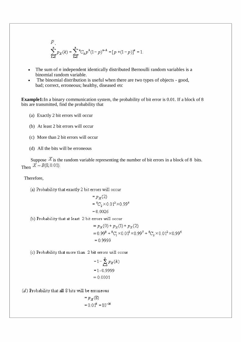
The sum of n independent identically distributed Bernoulli random variables is a binomial random variable.

The binomial distribution is useful when there are two types of objects - good, bad; correct, erroneous; healthy, diseased etc

Example1:In a binary communication system, the probability of bit error is 0.01. If a block of 8 bits are transmitted, find the probability that

(a) Exactly 2 bit errors will occur

(b) At least 2 bit errors will occur

(c) More than 2 bit errors will occur

(d) All the bits will be erroneous

Suppose is the random variable representing the number of bit errors in a block of 8 bits.

Then

Therefore,

56

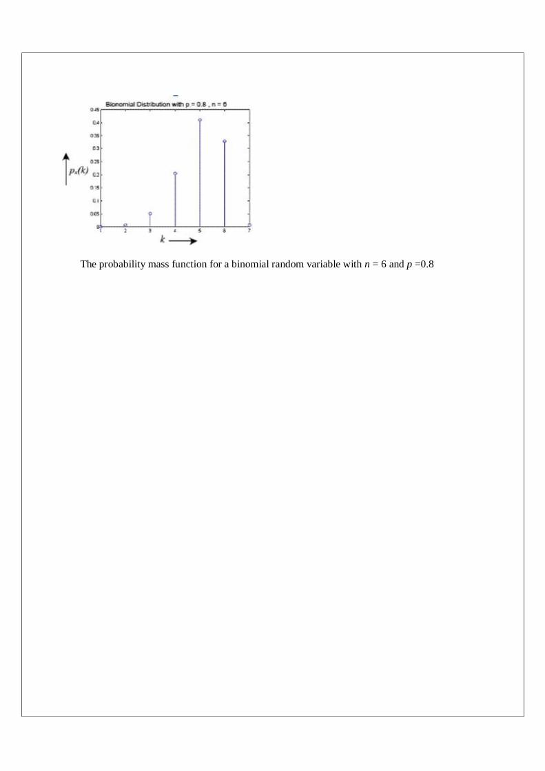
The probability mass function for a binomial random variable with n = 6 and p =0.8

57

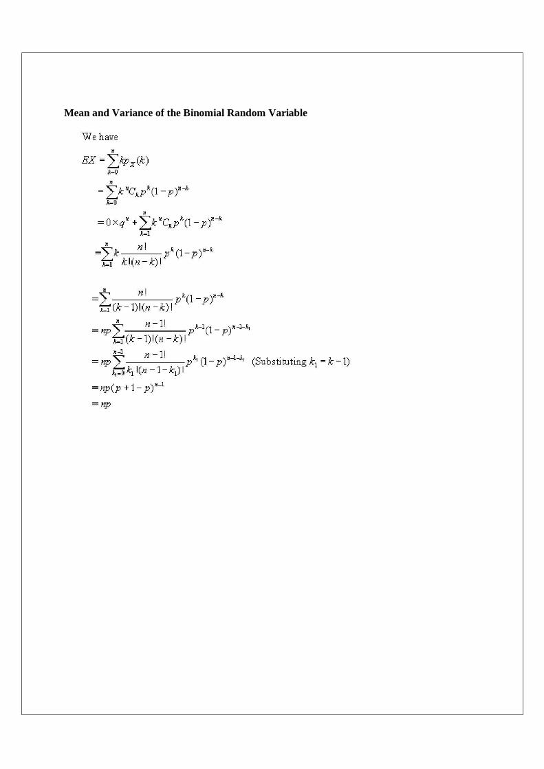
Mean and Variance of the Binomial Random Variable

58

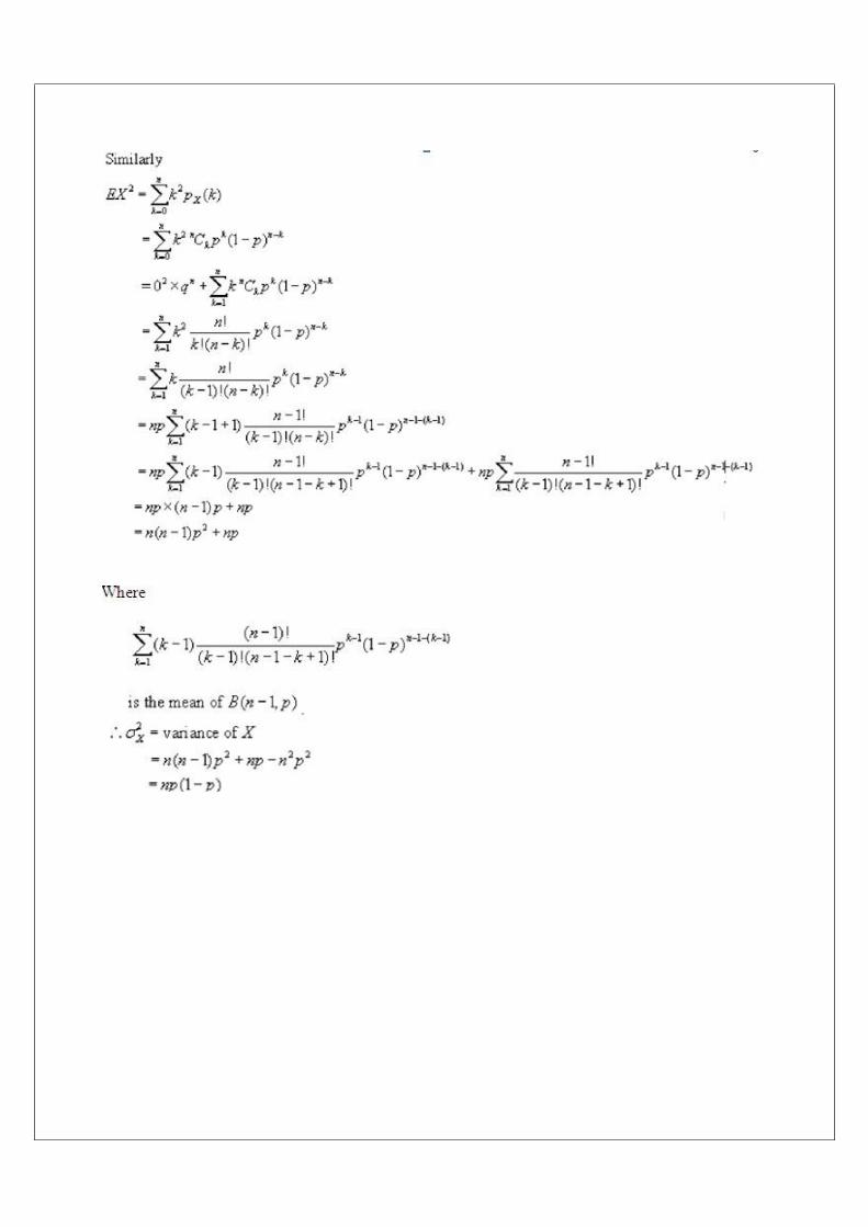
59

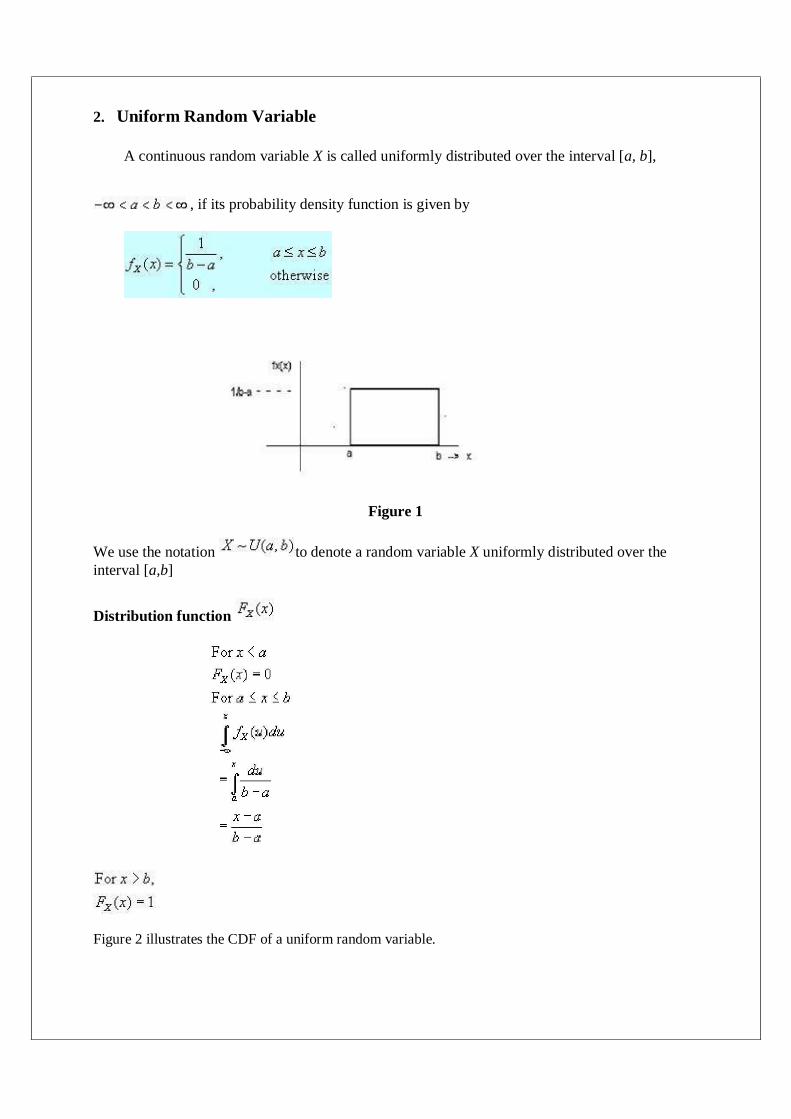
2. Uniform Random Variable

A continuous random variable X is called uniformly distributed over the interval [a, b],

, if its probability density function is given by

Figure 1

We use the notation to denote a random variable X uniformly distributed over the

interval [a,b]

Distribution function

Figure 2 illustrates the CDF of a uniform random variable.

60

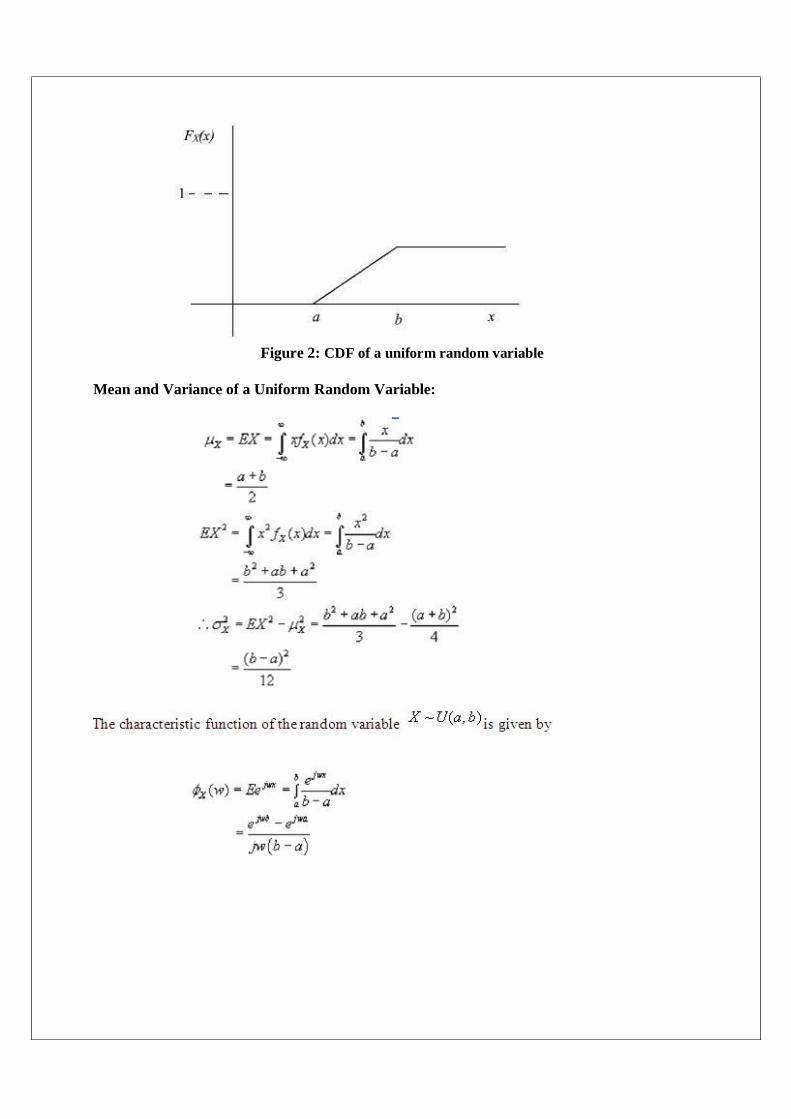
Figure 2: CDF of a uniform random variable

Mean and Variance of a Uniform Random Variable:

61

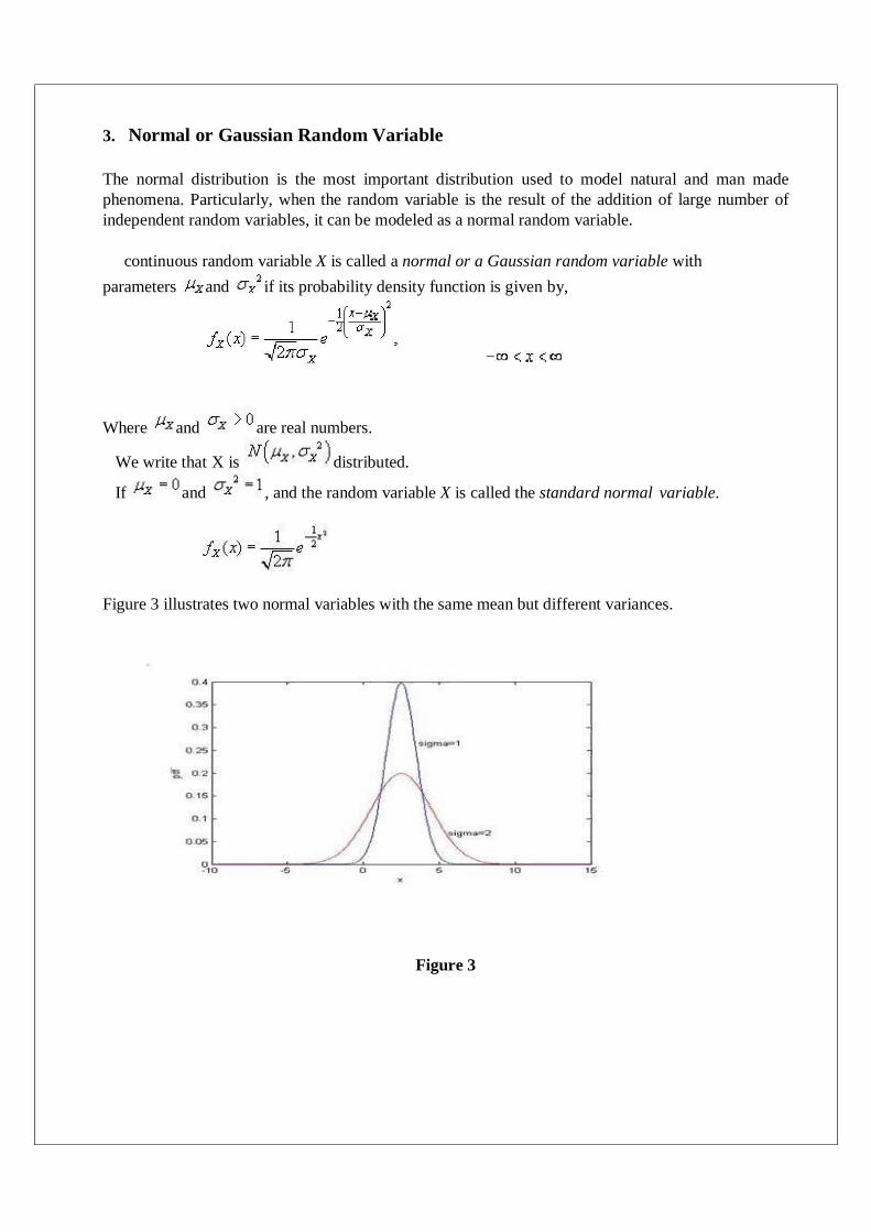
3. Normal or Gaussian Random Variable

The normal distribution is the most important distribution used to model natural and man made

phenomena. Particularly, when the random variable is the result of the addition of large number of

independent random variables, it can be modeled as a normal random variable.

continuous random variable X is called a normal or a Gaussian random variable with

parameters and if its probability density function is given by,

Where and are real numbers.

We write that X is distributed.

If and , and the random variable X is called the standard normal variable.

Figure 3 illustrates two normal variables with the same mean but different variances.

Figure 3

62

Is a bell-shaped function, symmetrical about .

Determines the spread of the random variable X . If is small X is more

concentrated around the mean .

Distribution function of a Gaussian variable is

Substituting , we get

where is the distribution function of the standard normal variable.

Thus can be computed from tabulated values of . The table was very useful in the

pre-computer days.

In communication engineering, it is customary to work with the Q function defined by,

Note that and

These results follow from the symmetry of the Gaussian pdf. The function is tabulated and the

tabulated results are used to compute probability involving the Gaussian random variable.

63

Using the Error Function to compute Probabilities for Gaussian Random Variables

The function is closely related to the error function and the complementary error

function .

Note that,

And the complementary error function is given

Mean and Variance of a Gaussian Random Variable

If X is distributed, then

Proof:

64

65

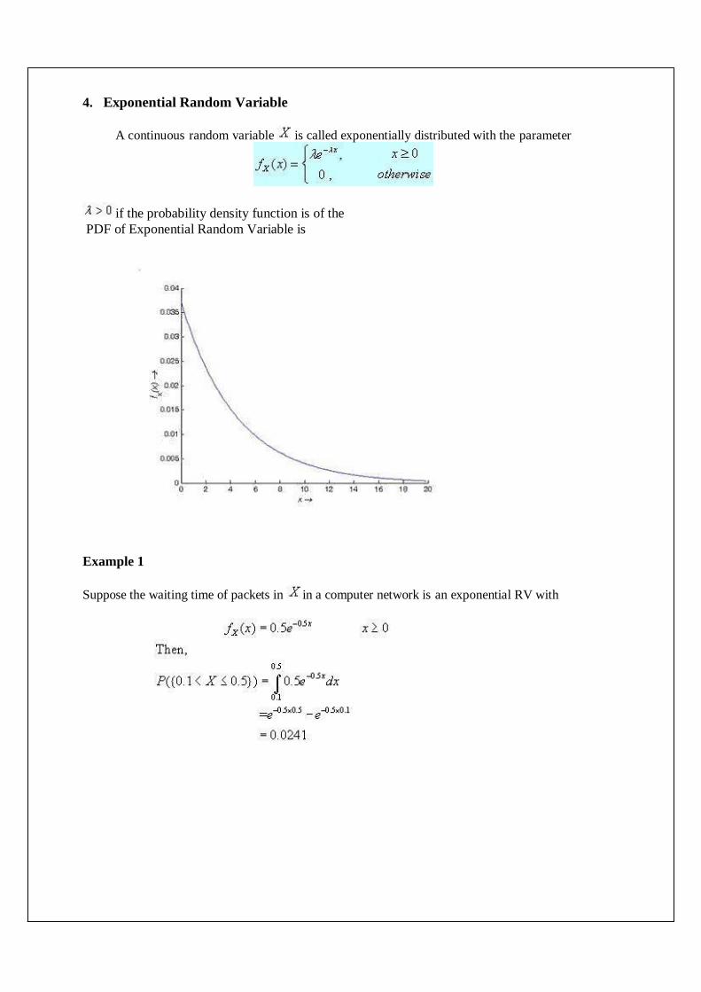
4. Exponential Random Variable

A continuous random variable is called exponentially distributed with the parameter

if the probability density function is of the

PDF of Exponential Random Variable is

Example 1

Suppose the waiting time of packets in in a computer network is an exponential RV with

66

Conditional Distribution and Density functions:

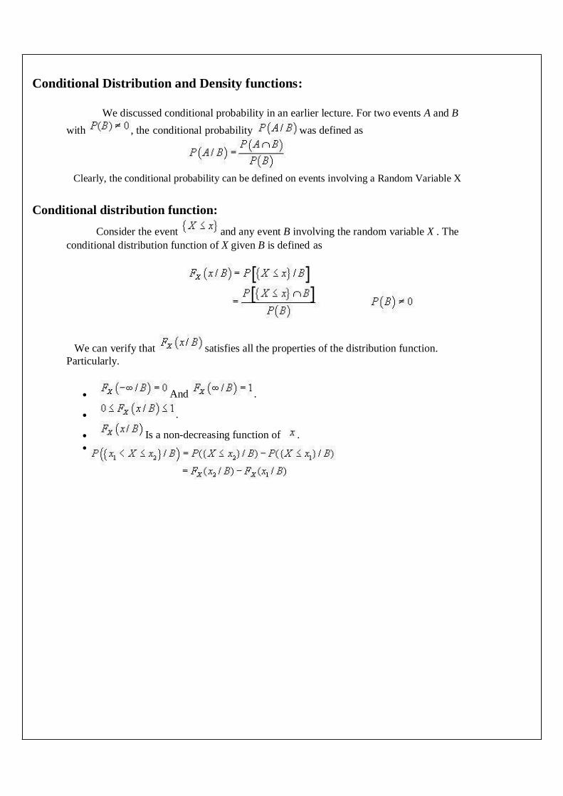
We discussed conditional probability in an earlier lecture. For two events A and B

with , the conditional probability was defined as

Clearly, the conditional probability can be defined on events involving a Random Variable X

Conditional distribution function:

Consider the event and any event B involving the random variable X . The

conditional distribution function of X given B is defined as

We can verify that satisfies all the properties of the distribution function.

Particularly.

And .

.

Is a non-decreasing function of .

67

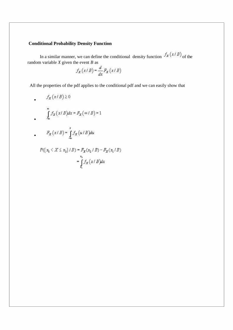
Conditional Probability Density Function

In a similar manner, we can define the conditional density function of the

random variable X given the event B as

All the properties of the pdf applies to the conditional pdf and we can easily show that

68

OPERATIONS ON RANDOM VARIABLE

Expected Value of a Random Variable:

The expectation operation extracts a few parameters of a random variable and provides

a summary description of the random variable in terms of these parameters.

It is far easier to estimate these parameters from data than to estimate the distribution or density function of the random variable.

Moments are some important parameters obtained through the expectation operation.

Expected value or mean of a random variable

The expected value of a random variable X is defined by

( )XEX xf x dx

provided ( )Xxf x dx

exists.

EX is also called the mean or statistical average of the random variable X and denoted by .X

Note that, for a discrete RV X defined by the probability mass function (pmf) ( ), 1,2,...., ,X ip x i N the

pdf ( )Xf x is given by

1

( ) ( ) ( )N

X X i i

i

f x p x x x

1

1

1

( ) ( )

= ( ) ( )

= ( )

N

X X i ii

N

X i ii

N

i X ii

EX x p x x x dx

p x x x x dx

x p x

Thus for a discrete random variable X with ( ), 1,2,...., ,X ip x i N

X1

= ( )N

i X ii

x p x

Interpretation of the mean

The mean gives an idea about the average value of the random value. The values of the random variable are

spread about this value.

Observe that

( )

( )

( ) 1

( )

X X

X

X

X

xf x dx

xf x dx

f x dx

f x dx

Therefore, the mean can be also interpreted as the centre of gravity of the pdf curve.

69

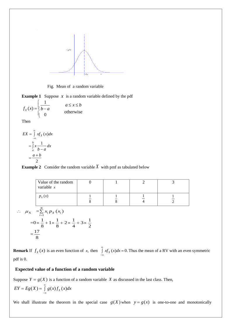
Fig. Mean of a random variable

Example 1 Suppose X is a random variable defined by the pdf

1

( ) otherwise

0X

a x bf x b a

Then

( )

1

2

X

b

a

EX xf x dx

x dxb a

a b

Example 2 Consider the random variable X with pmf as tabulated below

Value of the random

variable x

0 1 2 3

( )Xp x 1

8

1

8

1

4

1

2

X1

= ( )

1 1 1 1 =0 1 2 3

8 8 4 2

17 =

8

N

i X ii

x p x

Remark If ( )Xf x is an even function of ,x then ( ) 0.Xxf x dx

Thus the mean of a RV with an even symmetric

pdf is 0.

Expected value of a function of a random variable

Suppose ( )Y g X is a function of a random variable X as discussed in the last class. Then,

( ) ( ) ( )XEY Eg X g x f x dx

We shall illustrate the theorem in the special case ( )g X when ( )y g x is one-to-one and monotonically

70

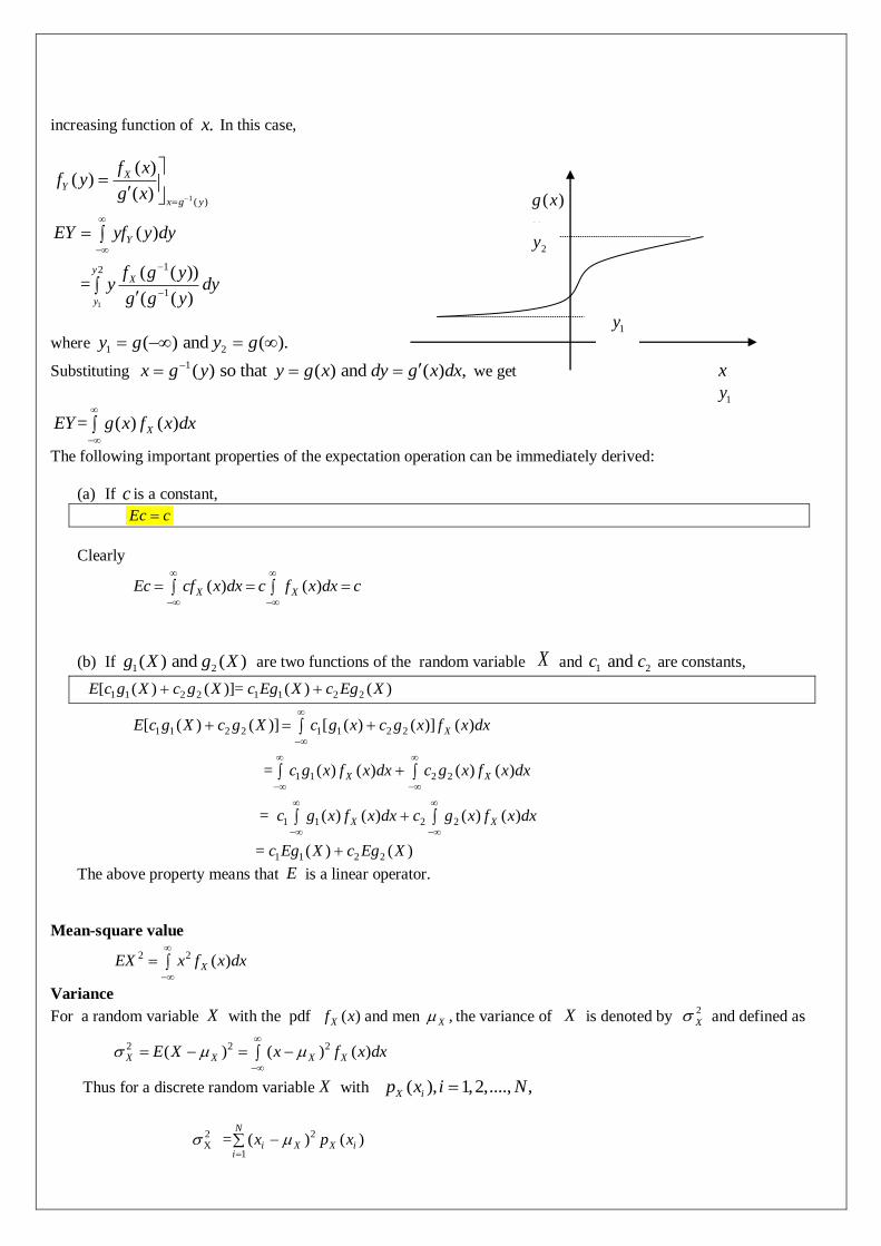
increasing function of .x In this case,

1 ( )

( )( )

( )

X

Y

x g y

f xf y

g x

1

12

1

( )

( ( )) =

( ( )

Y

yX

y

EY yf y dy

f g yy dy

g g y

where 1 2( ) and ( ).y g y g

Substituting 1( ) so that ( ) and ( ) ,x g y y g x dy g x dx we get

= ( ) ( )XEY g x f x dx

The following important properties of the expectation operation can be immediately derived:

(a) If c is a constant,

Ec c

Clearly

( ) ( )X XEc cf x dx c f x dx c

(b) If 1 2( ) and ( ) g X g X are two functions of the random variable X and 1 2 and c c are constants,

1 1 2 2 1 1 2 2[ ( ) ( )]= ( ) ( )E c g X c g X c Eg X c Eg X

1 1 2 2 1 1 2 2

1 1 2 2

1 1 2 2

[ ( ) ( )] [ ( ) ( )] ( )

= ( ) ( ) ( ) ( )

= ( ) ( ) ( ) ( )

X

X X

X X

E c g X c g X c g x c g x f x dx

c g x f x dx c g x f x dx

c g x f x dx c g x f x dx

1 1 2 2 = ( ) ( )c Eg X c Eg X

The above property means that E is a linear operator.

Mean-square value

2 2 ( )XEX x f x dx

Variance

For a random variable X with the pdf ( )Xf x and men ,X the variance of X is denoted by 2

X and defined as

2 2 2( ) ( ) ( )X X X XE X x f x dx

Thus for a discrete random variable X with ( ), 1,2,...., ,X ip x i N

2 2X

1

= ( ) ( )N

i X X ii

x p x

( )g x

1y

1y

2y

x

1y

71

The standard deviation of X is defined as

2( )X XE X

E Example3: Find the variance of the random variable discussed in Example 1.

2 2

2

2

2

2

( )

1 ( )

2

1 = [ 2

2 2

( )

12

X X

b

a

b b b

a a a

E X

a bx dx

b a

a b a bx dx xdx dx

b a

b a

Example4: Find the variance of the random variable discussed in Example 2. As already computed

17

8X

2 2

2 2 2 2

( )

17 1 17 1 17 1 17 1 (0 ) (1 ) (2 ) (3 )

8 8 8 8 8 4 8 2

117

128

X XE X

Remark Variance is a central moment and measure of dispersion of the random variable about the

mean.

2( )XE X is the average of the square deviation from the mean. It gives information about the

deviation of the values of the RV about the mean. A smaller 2

X implies that the random values are

more clustered about the mean, Similarly, a bigger 2

X means that the random values are more

scattered.

For example, consider two random variables 1 2 and XX with pmf as shown below. Note that each of

1 2 and XX has zero means. 1

2 1

2X and

2

2 5

3X implying that 2 X has more spread about the

mean

72

Properties of variance:

(1) 2 2 2X XEX

2 2

2 2

2 2

2 2 2

2 2

( )

( 2 )

2

2

X X

X X

X X

X X

X

E X

E X X

EX EX E

EX

EX

(2) If , where and are constants,Y cX b c b then 2 2 2Y Xc

2 2

2 2

2 2

( )

( )

Y X

X

X

E cX b c b

Ec X

c

(3) If c is a constant,

var( ) 0.c

73

Moments:

The nth moment of a distribution (or set of data) about a number is the expected value of the nth

power of the deviations about that number. In statistics, moments are needed about the mean, and about

the origin.

1. Moments about origin.

2. Moments about mean or central moments

The nth moment of a distribution about zero is given by E(Xn)

The nth moment of a distribution about the mean is given by E[(X−μ)n]

Then each type of measure includes a moment definition.

The expected value, E(X), is the first moment about zero.

The variance, Var(X)), is the second moment about the mean, E[(X−μ)2]

A common definition of skewness is the third moment about the mean, E[(X−μ)3]

A common definition of kurtosis is the fourth moment about the mean, E[(X−μ)4]

Since moments about zero are typically much easier to compute than moments about the mean, alternative

formulas are often provided.

Var(X)=E[(X−μ)2]=E(X2)−[E(X)]2

Skew(X)=E[(X−μ)3]=E(X3)−3E(X)E(X2)+2[E(X)]3

Kurt(X)=E[(X−μ)4]=E(X4)−4E(X)E(X3)+6[E(X)]2 E(X2)−3[E(X)]4

nth moment of a random variable

We can define the nth moment and the nth central-moment of a random variable X by the following relations

nth-orde moment ( ) 1, 2,..

nth-orde central moment ( ) ( ) ( ) 1, 2,...

n nX

n nX X X

r EX x f x dx n

r E X x f x dx n

Note that

The mean X = EX is the first moment and the mean-square value 2 EX is the second moment

The first central moment is 0 and the variance is the second central moment

The third central moment measures lack of symmetry of the pdf of a random variable. 3

3

( )X

X

E X

is

called the coefficient of skewness and If the pdf is symmetric this coefficient will be zero.

The fourth central moment measures flatness of peakednes of the pdf of a random variable.

4

4

( )X

X

E X

is called kurtosis. If the peak of the pdf is sharper, then the random variable has a higher

kurtosi

2 2( )X XE X

74

Moment generating function:

Since each moment is an expected value, and the definition of expected value involves either a sum (in

the discrete case) or an integral (in the continuous case), it would seem that the computation of moments

could be tedious. However, there is a single expected value function whose derivatives can produce each

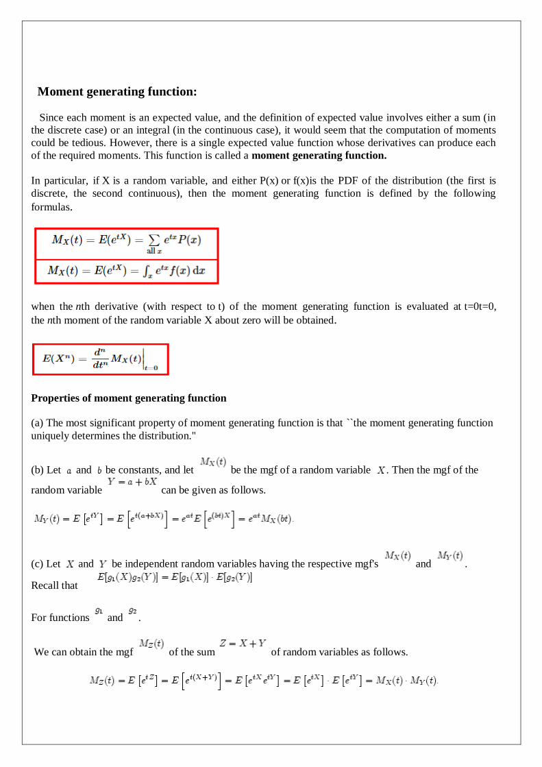
of the required moments. This function is called a moment generating function.

In particular, if X is a random variable, and either P(x) or f(x)is the PDF of the distribution (the first is

discrete, the second continuous), then the moment generating function is defined by the following

formulas.

when the nth derivative (with respect to t) of the moment generating function is evaluated at t=0t=0,

the nth moment of the random variable X about zero will be obtained.

Properties of moment generating function

(a) The most significant property of moment generating function is that ``the moment generating function

uniquely determines the distribution.''

(b) Let and be constants, and let be the mgf of a random variable . Then the mgf of the

random variable can be given as follows.

(c) Let and be independent random variables having the respective mgf's and .

Recall that

For functions and .

We can obtain the mgf of the sum of random variables as follows.

75

(d) When , it clearly follows that . Now by differentiating times, we obtain

In particular when , generates the -th moment of as follows.

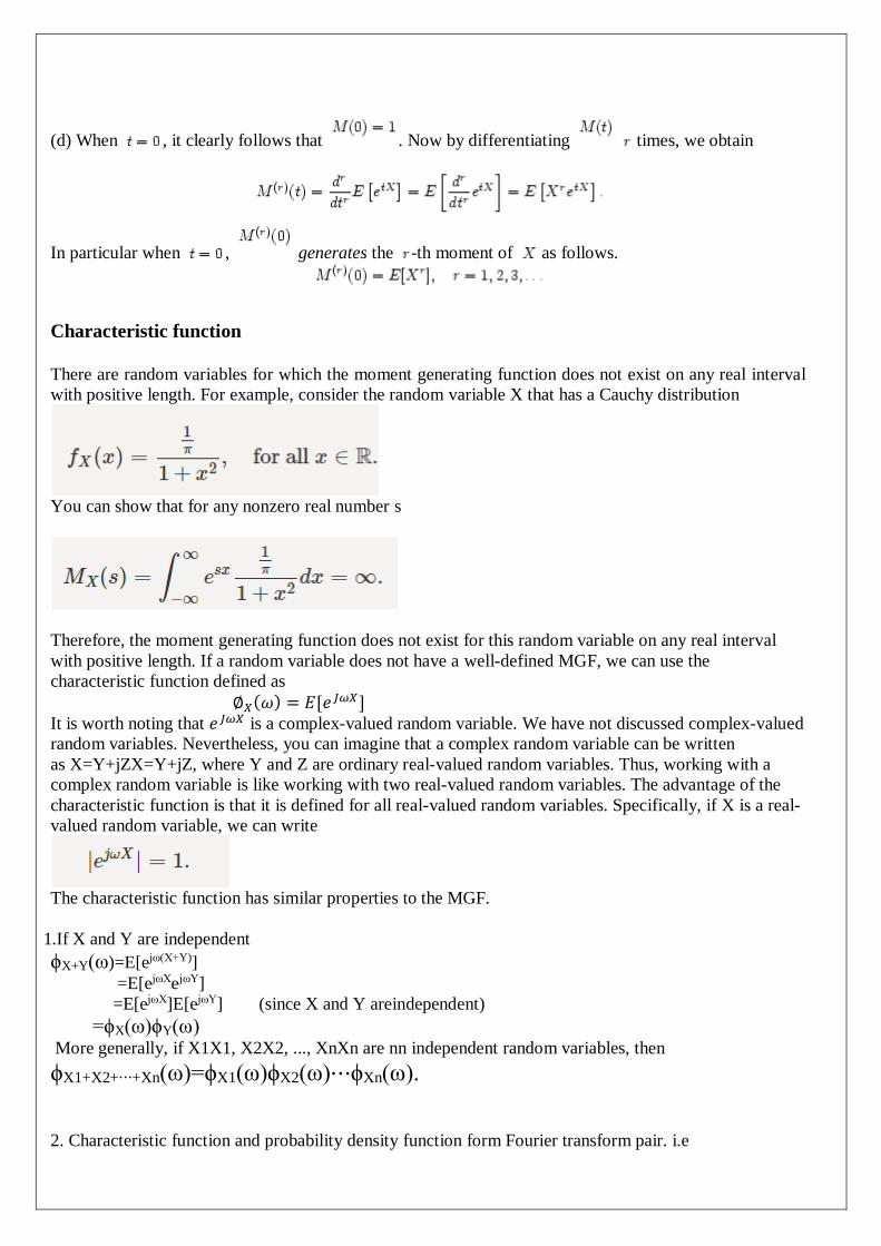
Characteristic function

There are random variables for which the moment generating function does not exist on any real interval

with positive length. For example, consider the random variable X that has a Cauchy distribution

You can show that for any nonzero real number s

Therefore, the moment generating function does not exist for this random variable on any real interval

with positive length. If a random variable does not have a well-defined MGF, we can use the

characteristic function defined as

∅𝑋(𝜔) = 𝐸[𝑒𝐽𝜔𝑋] It is worth noting that 𝑒𝐽𝜔𝑋 is a complex-valued random variable. We have not discussed complex-valued

random variables. Nevertheless, you can imagine that a complex random variable can be written

as X=Y+jZX=Y+jZ, where Y and Z are ordinary real-valued random variables. Thus, working with a

complex random variable is like working with two real-valued random variables. The advantage of the

characteristic function is that it is defined for all real-valued random variables. Specifically, if X is a real-

valued random variable, we can write

The characteristic function has similar properties to the MGF.

1.If X and Y are independent

ϕX+Y(ω)=E[ejω(X+Y)]

=E[ejωXejωY]

=E[ejωX]E[ejωY] (since X and Y areindependent)

=ϕX(ω)ϕY(ω) More generally, if X1X1, X2X2, ..., XnXn are nn independent random variables, then

ϕX1+X2+⋯+Xn(ω)=ϕX1(ω)ϕX2(ω)⋯ϕXn(ω).

2. Characteristic function and probability density function form Fourier transform pair. i.e

76

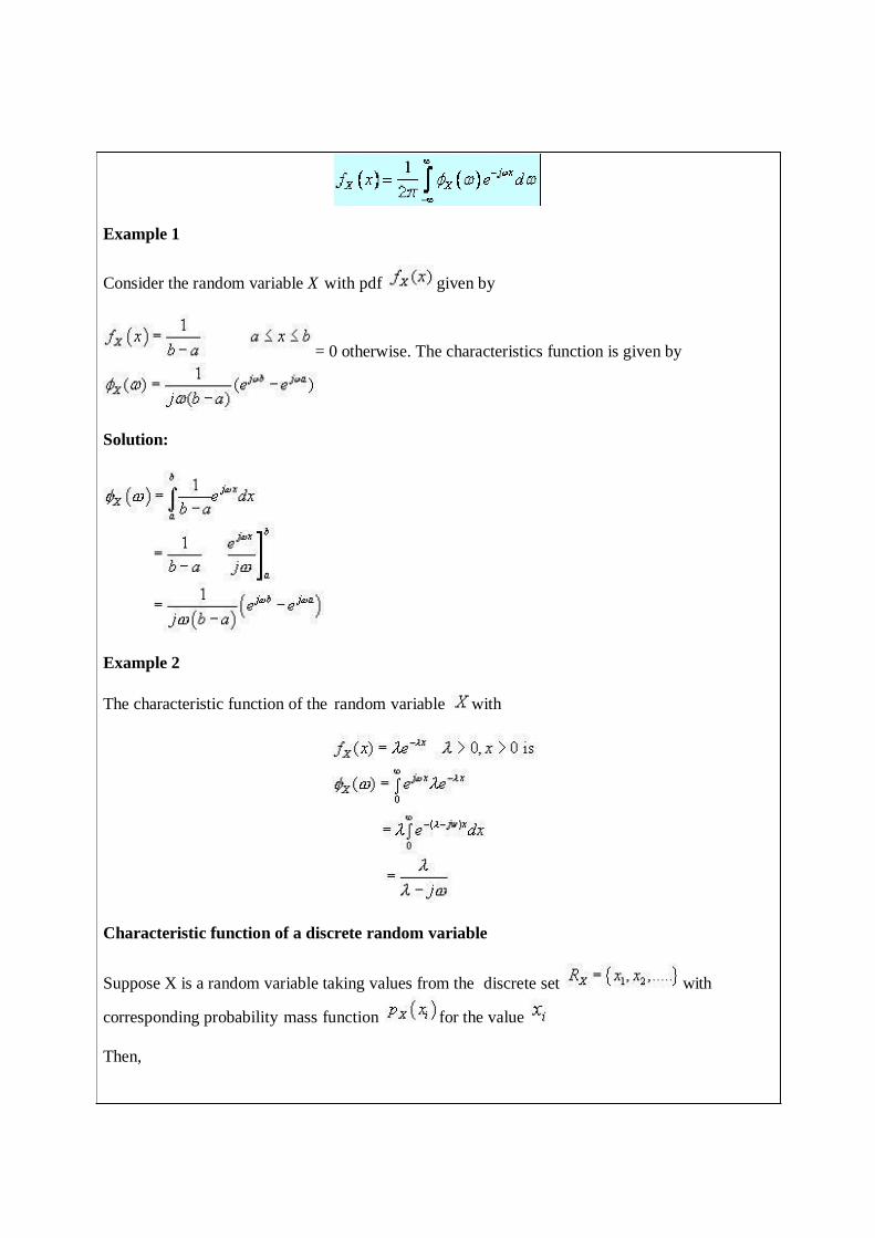
Example 1

Consider the random variable X with pdf given by

= 0 otherwise. The characteristics function is given by

Solution:

Example 2

The characteristic function of the random variable with

Characteristic function of a discrete random variable

Suppose X is a random variable taking values from the discrete set with

corresponding probability mass function for the value

Then,

77

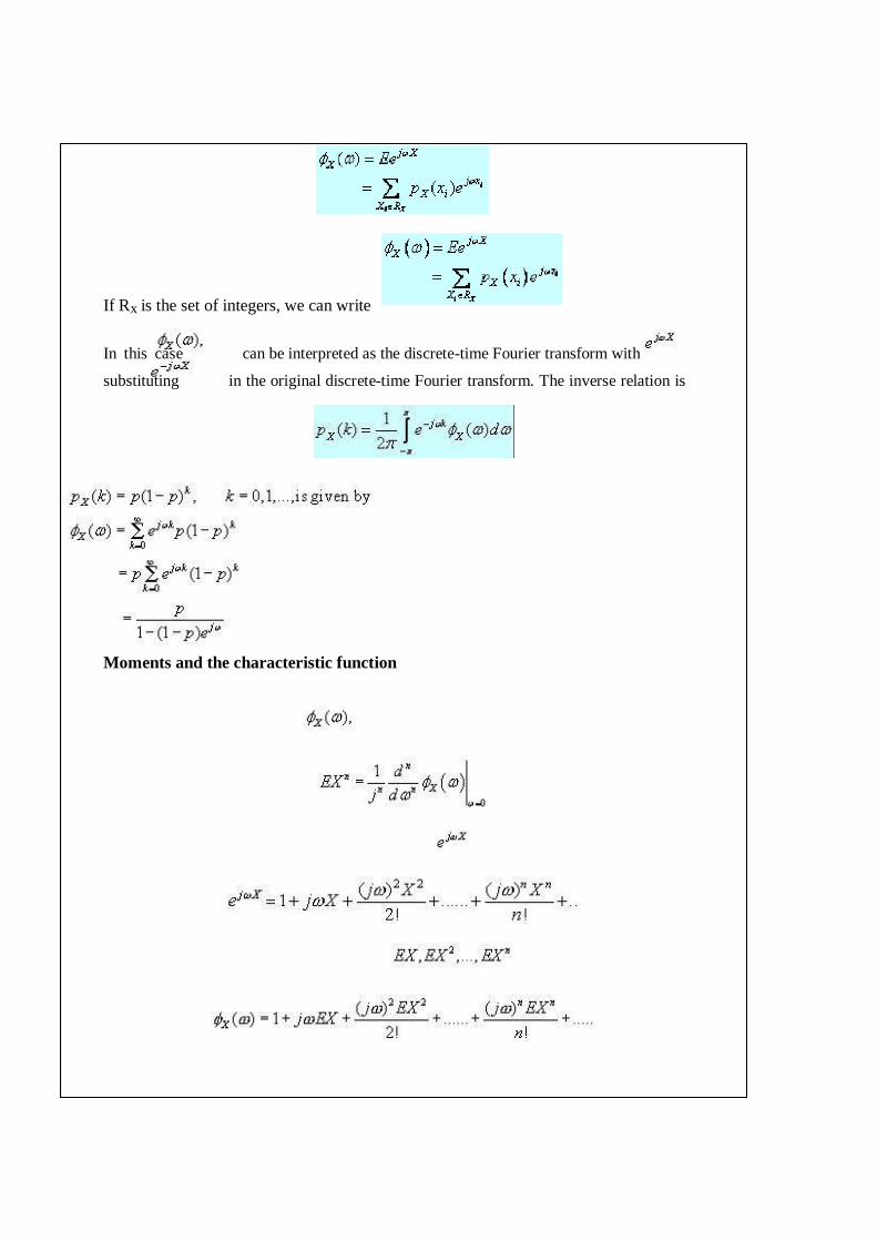
If Rx is the set of integers, we can write

In this case can be interpreted as the discrete-time Fourier transform with

substituting in the original discrete-time Fourier transform. The inverse relation is

Moments and the characteristic function

78

UNIT III

Multiple Random Variables and Operations on Multiple Random Variables

Multiple Random Variables:

Joint Distribution Function and Properties

Joint density Function and Properties

Marginal Distribution and density Functions

Conditional Distribution and density Functions

Statistical Independence

Distribution and density functions of Sum of Two Random Variables

Operations on Multiple Random Variables:

Expected Value of a Function of Random Variables

Joint Moments about the Origin

Joint Central Moments

Joint Characteristic Functions

Jointly Gaussian Random Variables: Two Random Variables case

79

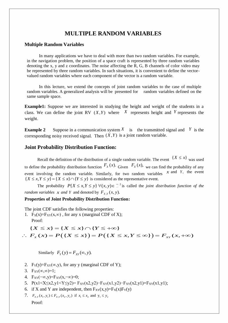
MULTIPLE RANDOM VARIABLES

Multiple Random Variables

In many applications we have to deal with more than two random variables. For example,

in the navigation problem, the position of a space craft is represented by three random variables denoting the x, y and z coordinates. The noise affecting the R, G, B channels of color video may be represented by three random variables. In such situations, it is convenient to define the vector-valued random variables where each component of the vector is a random variable.

In this lecture, we extend the concepts of joint random variables to the case of multiple

random variables. A generalized analysis will be presented for random variables defined on the same sample space.

Example1: Suppose we are interested in studying the height and weight of the students in a

class. We can define the joint RV ( , )X Y where X represents height and Y represents the

weight.

Example 2 Suppose in a communication system X is the transmitted signal and Y is the

corresponding noisy received signal. Then ( , )X Y is a joint random variable.

Joint Probability Distribution Function:

Recall the definition of the distribution of a single random variable. The event X x

was used

to define the probability distribution function ( ).XF x

Given ( ),XF x

we can find the probability of any

event involving the random variable. Similarly, for two random variables X and ,Y the event

, X x Y y X x Y y is considered as the representative event.

The probability

2 , ( , )P X x Y y x y is called the joint distribution function of the

random variables X and Y and denoted by ).,(, yxF YX

Properties of Joint Probability Distribution Function:

The joint CDF satisfies the following properties:

1. FX(x)=FXY(x,∞) , for any x (marginal CDF of X);

Proof:

Similarly ).,()( yFyF XYY

2. FY(y)=FXY(∞,y), for any y (marginal CDF of Y);

3. FXY(∞,∞)=1;

4. FXY(−∞,y)=FXY(x,−∞)=0;

5. P(x1<X≤x2,y1<Y≤y2)= FXY(x2,y2)−FXY(x1,y2)−FXY(x2,y1)+FXY(x1,y1);

6. if X and Y are independent, then FXY(x,y)=FX(x)FY(y)

7. , 1 1 , 2 2 1 2 1 2( , ) ( , ) if and yX Y X YF x y F x y x x y

Proof:

( ) , ( , )X XY

X x X x Y

F x P X x P X x Y F x

80

:

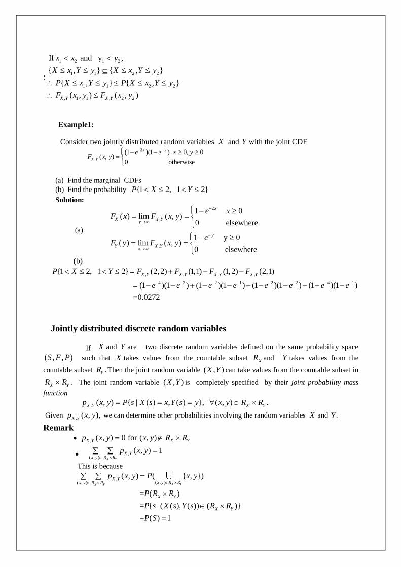
1 2 1 2

1 1 2 2

1 1 2 2

, 1 1 , 2 2

If and y ,

, ,

, ,

( , ) ( , )X Y X Y

x x y

X x Y y X x Y y

P X x Y y P X x Y y

F x y F x y

Example1:

Consider two jointly distributed random variables X and Y with the joint CDF

2

,

(1 )(1 ) 0, 0( , )

0 otherwise

x y

X Y

e e x yF x y

(a) Find the marginal CDFs

(b) Find the probability 1 2, 1 2P X Y

Solution:

(a)

2

,

,

1 0( ) lim ( , )

0 elsewhere

1 y 0( ) lim ( , )

0 elsewhere

x

X X Yy

y

Y X Yx

e xF x F x y

eF y F x y

(b)

, , , ,

4 2 2 1 2 2 4 1

1 2, 1 2 (2,2) (1,1) (1,2) (2,1)

(1 )(1 ) (1 )(1 ) (1 )(1 ) (1 )(1 )

=0.02

X Y X Y X Y X YP X Y F F F F

e e e e e e e e

72

Jointly distributed discrete random variables

If X and Y are two discrete random variables defined on the same probability space

( , , )S F P such that X takes values from the countable subset XR and Y takes values from the

countable subset .YR Then the joint random variable ( , )X Y can take values from the countable subset in

.X YR R The joint random variable ( , )X Y is completely specified by their joint probability mass

function

, ( , ) | ( ) , ( ) , ( , ) .X Y X Yp x y P s X s x Y s y x y R R

Given , ( , ),X Yp x y we can determine other probabilities involving the random variables X and .Y

Remark

, ( , ) 0 for ( , )X Y X Yp x y x y R R

,( , )

( , ) 1X Y

X Yx y R R

p x y

This is because

,( , )( , )

( , ) ( , )

= ( )

= | ( ( ), ( )) ( )

= ( ) 1

X YX Y

X Yx y R Rx y R R

X Y

X Y

p x y P x y

P R R

P s X s Y s R R

P S

81

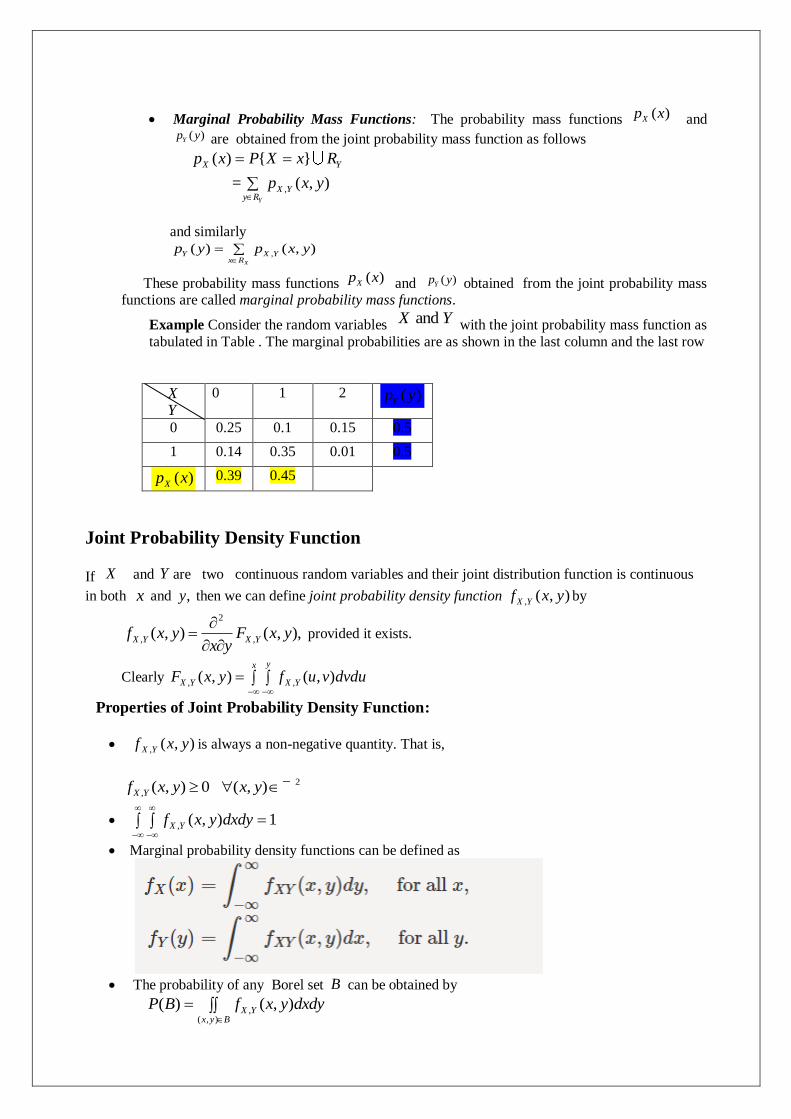
Marginal Probability Mass Functions: The probability mass functions ( )Xp x and ( )Yp y are obtained from the joint probability mass function as follows

,

( )

= ( , )Y

X Y

X Yy R

p x P X x R

p x y

and similarly

,( ) ( , )X

Y X Yx R

p y p x y

These probability mass functions ( )Xp x and ( )Yp y obtained from the joint probability mass functions are called marginal probability mass functions.

Example Consider the random variables and X Y with the joint probability mass function as

tabulated in Table . The marginal probabilities are as shown in the last column and the last row

X

Y

0 1 2 ( )Yp y

0 0.25 0.1 0.15 0.5

1 0.14 0.35 0.01 0.5

( )Xp x 0.39 0.45

Joint Probability Density Function

If X and Y are two continuous random variables and their joint distribution function is continuous

in both x and ,y then we can define joint probability density function , ( , )X Yf x y by

2

, ,( , ) ( , ),X Y X Yf x y F x yx y

provided it exists.

Clearly , ,( , ) ( , )yx

X Y X YF x y f u v dvdu

Properties of Joint Probability Density Function:

),(, yxf YX is always a non-negative quantity. That is,

2

, ( , ) 0 ( , )X Yf x y x y

, ( , ) 1X Yf x y dxdy

Marginal probability density functions can be defined as

The probability of any Borel set B can be obtained by

,( , )

( ) ( , )X Yx y B

P B f x y dxdy

82

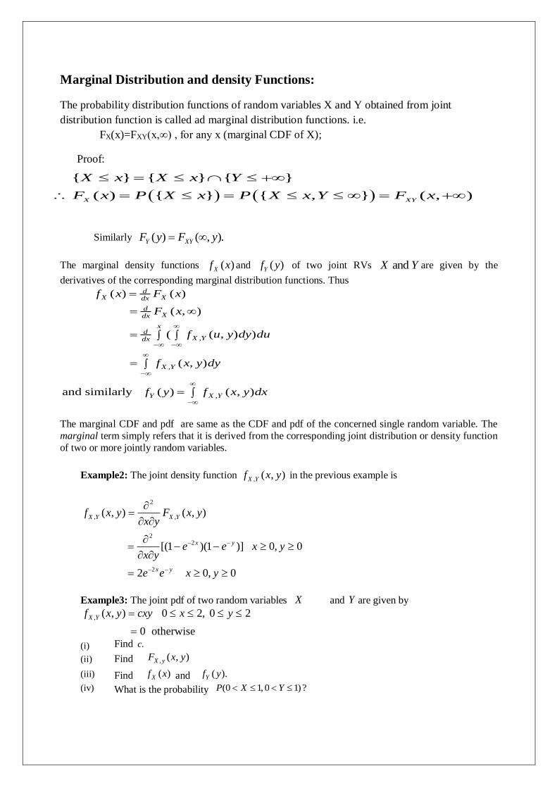
Marginal Distribution and density Functions:

The probability distribution functions of random variables X and Y obtained from joint

distribution function is called ad marginal distribution functions. i.e.

FX(x)=FXY(x,∞) , for any x (marginal CDF of X);

Proof:

Similarly ).,()( yFyF XYY

The marginal density functions ( )Xf x and ( )Yf y of two joint RVs and X Y are given by the

derivatives of the corresponding marginal distribution functions. Thus

,

,

,

( ) ( )

( , )

( ( , ) )

( , )

and similarly ( ) ( , )

dX Xdx

dXdx

xd

X Ydx

X Y

Y X Y

f x F x

F x

f u y dy du

f x y dy

f y f x y dx

The marginal CDF and pdf are same as the CDF and pdf of the concerned single random variable. The

marginal term simply refers that it is derived from the corresponding joint distribution or density function

of two or more jointly random variables.

Example2: The joint density function , ( , )X Yf x y in the previous example is

2

, ,

22

2

( , ) ( , )

[(1 )(1 )] 0, 0

2 0, 0

X Y X Y

x y

x y

f x y F x yx y

e e x yx y

e e x y

Example3: The joint pdf of two random variables X and Y are given by

, ( , ) 0 2, 0 2

0 otherwise

X Yf x y cxy x y

(i) Find .c

(ii) Find , ( , )X yF x y

(iii) Find ( )Xf x and ( ).Yf y

(iv) What is the probability (0 1, 0 1)?P X Y

( ) , ( , )X XY

X x X x Y

F x P X x P X x Y F x

83

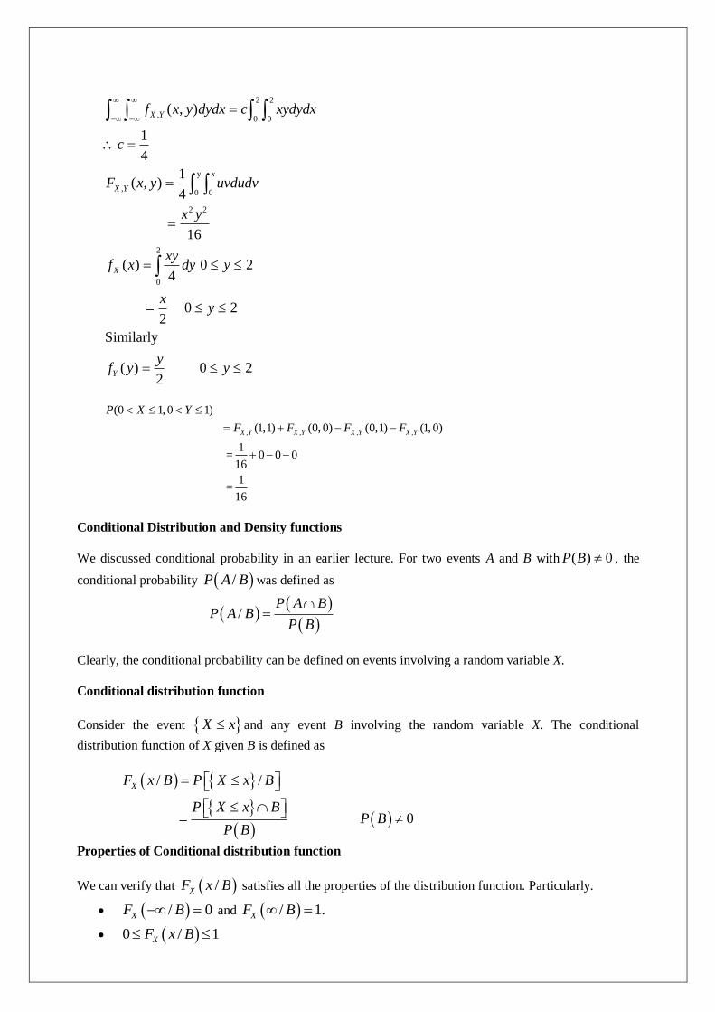
2 2

,0 0

y

,0 0

2 2

2

0

( , )

1

4

1( , )

4

16

( ) 0 2 4

0 2 2

Similarly

( ) 0 2 2

X Y

x

X Y

X

Y

f x y dydx c xydydx

c

F x y uvdudv

x y

xyf x dy y

xy

yf y y

, , , ,

(0 1, 0 1)

(1,1) (0, 0) (0,1) (1, 0)

1 = 0 0 0

16

1 =

16

X Y X Y X Y X Y

P X Y

F F F F

Conditional Distribution and Density functions

We discussed conditional probability in an earlier lecture. For two events A and B with ( ) 0P B , the

conditional probability /P A B was defined as

/

P A BP A B

P B

Clearly, the conditional probability can be defined on events involving a random variable X.

Conditional distribution function

Consider the event X x and any event B involving the random variable X. The conditional

distribution function of X given B is defined as

/ /

0

XF x B P X x B

P X x BP B

P B

Properties of Conditional distribution function

We can verify that /XF x B satisfies all the properties of the distribution function. Particularly.

/ 0XF B and / 1.XF B

0 / 1XF x B

84

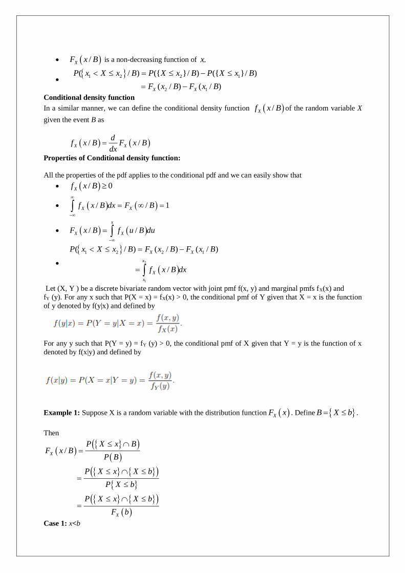
/XF x B is a non-decreasing function of .x

1 2 2 1

2 1

( / ) ( / ) ( / )

( / ) ( / )X X

P x X x B P X x B P X x B

F x B F x B

Conditional density function

In a similar manner, we can define the conditional density function /Xf x B of the random variable X

given the event B as

/ /X X

df x B F x B

dx

Properties of Conditional density function:

All the properties of the pdf applies to the conditional pdf and we can easily show that

/ 0Xf x B

/ / 1X Xf x B dx F B

/ /

x

X XF x B f u B du

2

1

1 2 2 1( / ) ( / ) ( / )

/

X X

x

X

x

P x X x B F x B F x B

f x B dx

Let (X, Y ) be a discrete bivariate random vector with joint pmf f(x, y) and marginal pmfs fX(x) and

fY (y). For any x such that P(X = x) = fX(x) > 0, the conditional pmf of Y given that X = x is the function

of y denoted by f(y|x) and defined by

For any y such that P(Y = y) = fY (y) > 0, the conditional pmf of X given that Y = y is the function of x

denoted by f(x|y) and defined by

Example 1: Suppose X is a random variable with the distribution function XF x . Define B X b .

Then

/X

X

P X x BF x B

P B

P X x X b

P X b

P X x X b

F b

Case 1: x<b

85

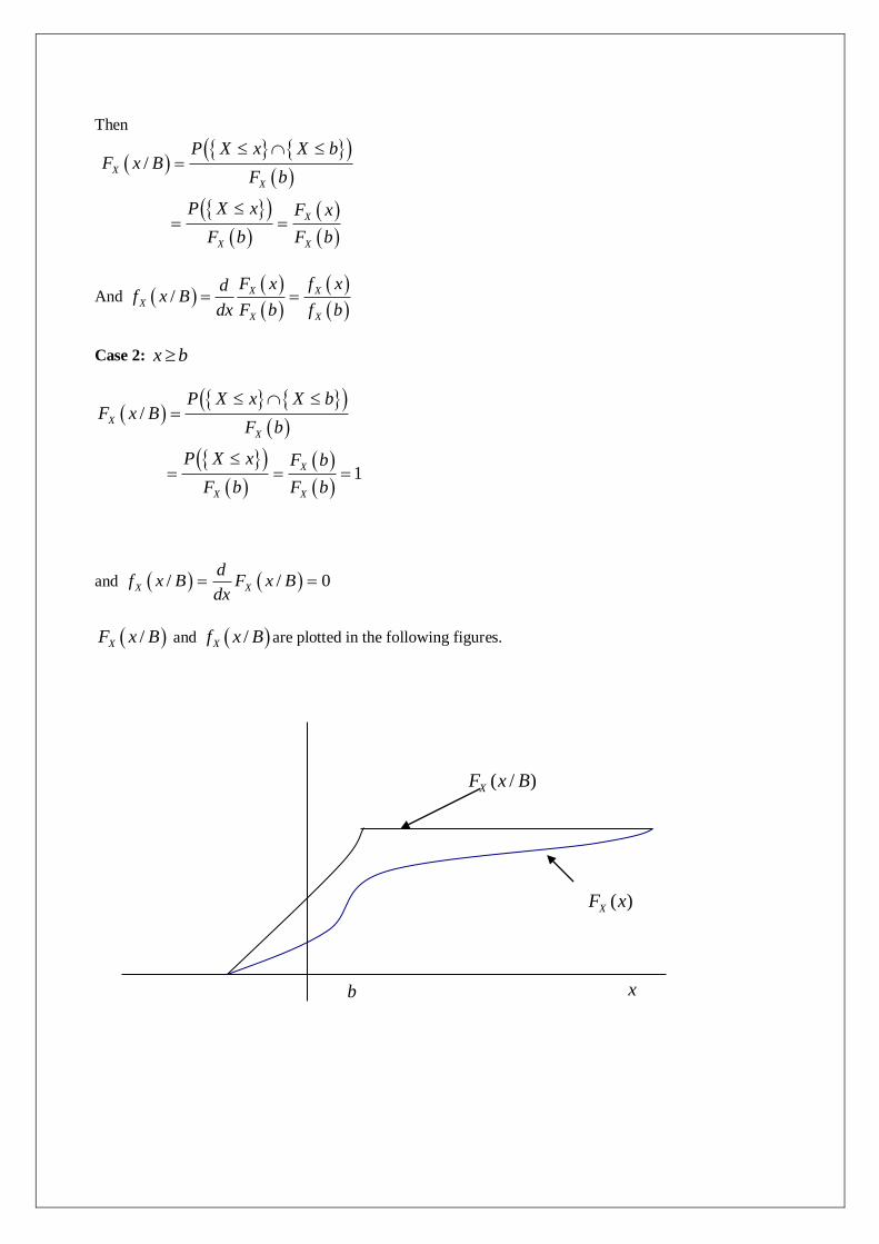
Then

/X

X

X

X X

P X x X bF x B

F b

P X x F x

F b F b

And

/

X X

X

X X

F x f xdf x B

dx F b f b

Case 2: x b

/

1

X

X

X

X X

P X x X bF x B

F b

P X x F b

F b F b

and / / 0X X

df x B F x B

dx

/XF x B and /Xf x B are plotted in the following figures.

b x

( )XF x

( / )XF x B

86

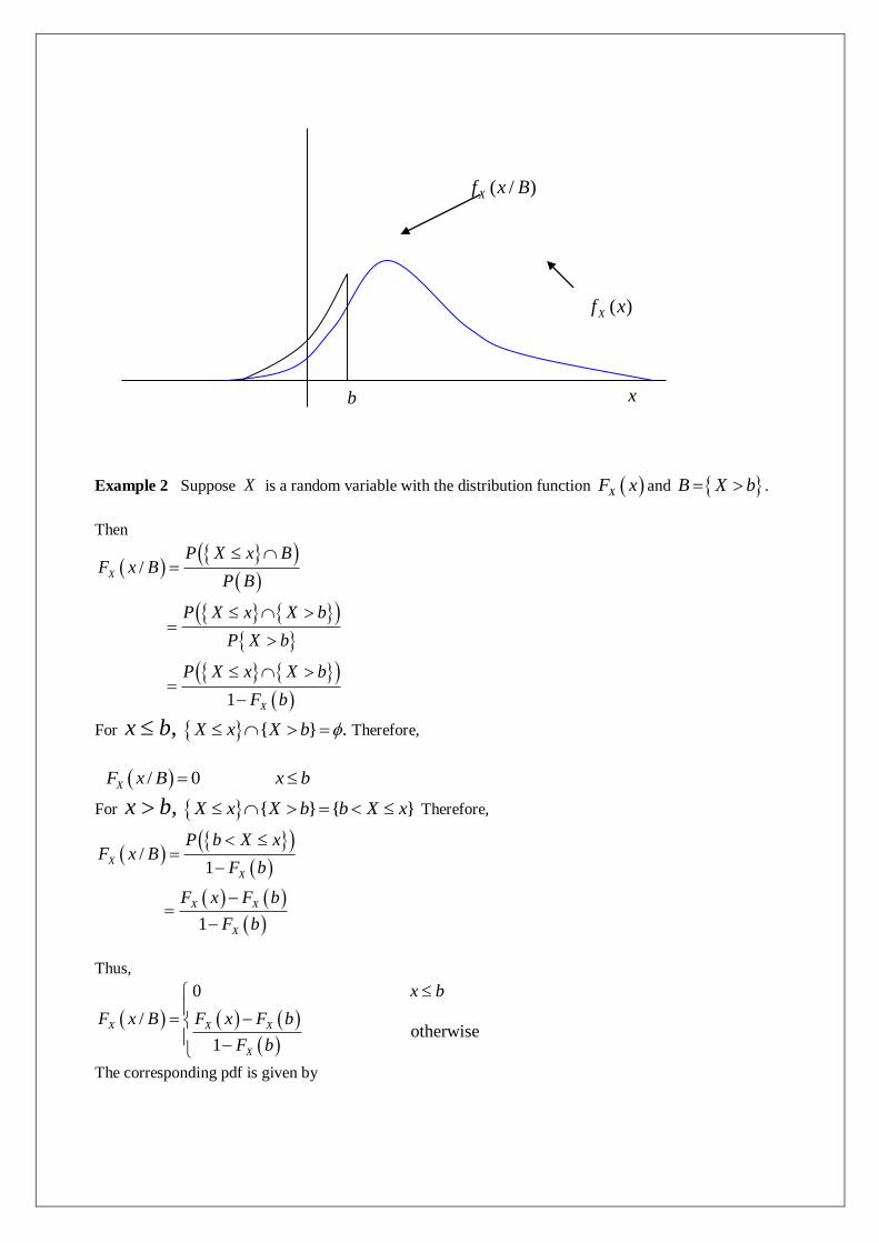
Example 2 Suppose X is a random variable with the distribution function XF x and B X b .

Then

/

1

X

X

P X x BF x B

P B

P X x X b

P X b

P X x X b

F b

For ,x b .X x X b Therefore,

/ 0 XF x B x b

For ,x b X x X b b X x Therefore,

/1

1

X

X

X X

X

P b X xF x B

F b

F x F b

F b

Thus,

0

/ otherwise

1

X X X

X

x b

F x B F x F b

F b

The corresponding pdf is given by

b x

( )Xf x

( / )Xf x B

87

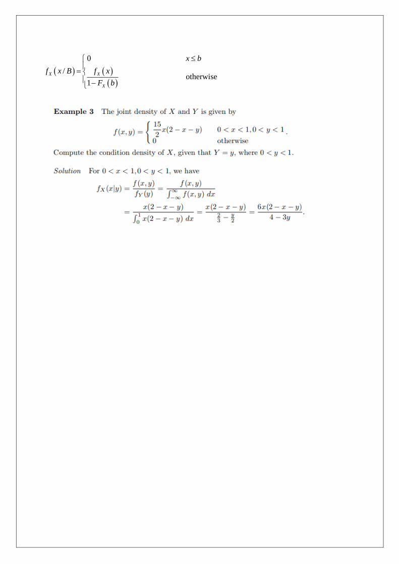
0

/ otherwise

1

X X

X

x b

f x B f x

F b

88

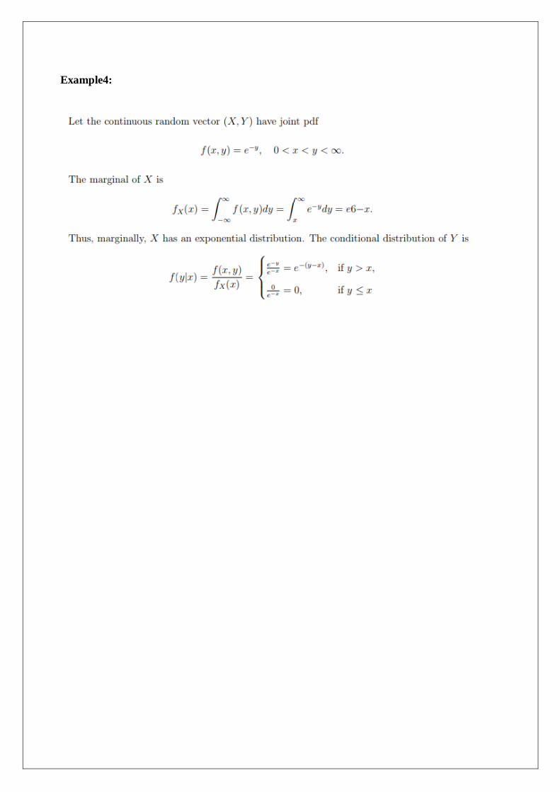
Example4:

89

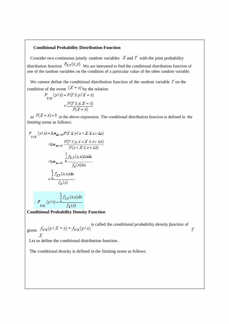
Conditional Probability Distribution Function

Consider two continuous jointly random variables and with the joint probability

distribution function We are interested to find the conditional distribution function of

one of the random variables on the condition of a particular value of the other random variable.

We cannot define the conditional distribution function of the random variable on the

condition of the event by the relation

as in the above expression. The conditional distribution function is defined in the

limiting sense as follows:

Conditional Probability Density Function

is called the conditional probability density function of

given

Let us define the conditional distribution function .

The conditional density is defined in the limiting sense as follows

90

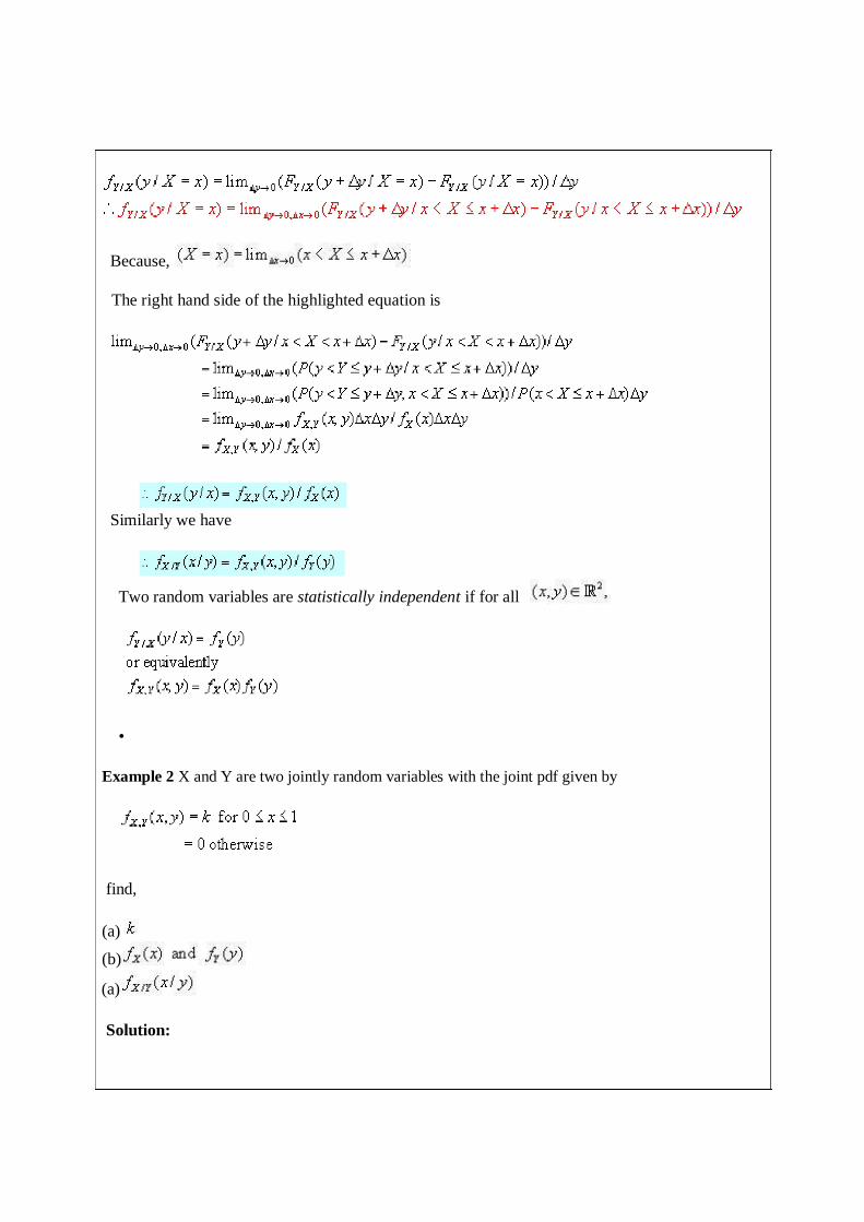
Because,

The right hand side of the highlighted equation is

Similarly we have

Two random variables are statistically independent if for all

•

Example 2 X and Y are two jointly random variables with the joint pdf given by

find,

(a)

(b)

(a)

Solution:

91

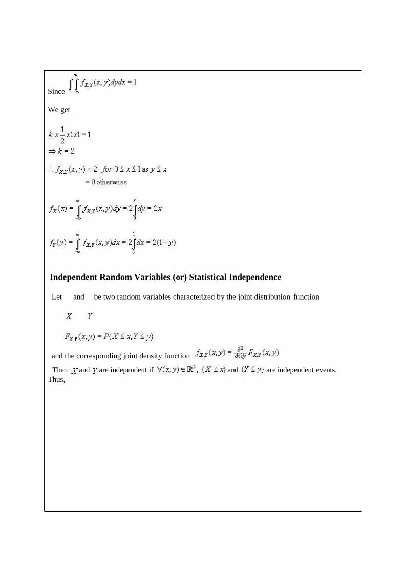
Since

We get

Independent Random Variables (or) Statistical Independence

Let and be two random variables characterized by the joint distribution function

and the corresponding joint density function

Then and are independent if and are independent events.

Thus,

92

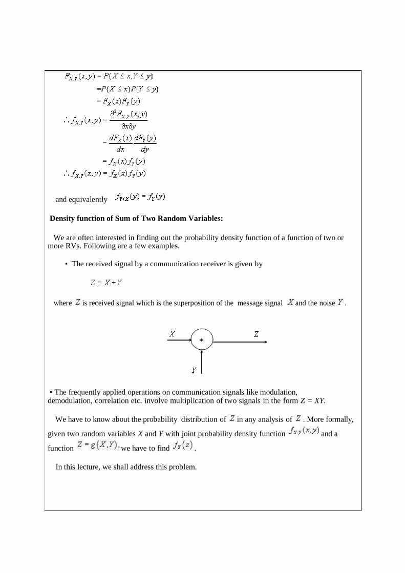
and equivalently

Density function of Sum of Two Random Variables:

We are often interested in finding out the probability density function of a function of two or

more RVs. Following are a few examples.

• The received signal by a communication receiver is given by

where is received signal which is the superposition of the message signal and the noise .

• The frequently applied operations on communication signals like modulation, demodulation, correlation etc. involve multiplication of two signals in the form Z = XY.

We have to know about the probability distribution of in any analysis of . More formally,

given two random variables X and Y with joint probability density function and a

function we have to find .

In this lecture, we shall address this problem.

93

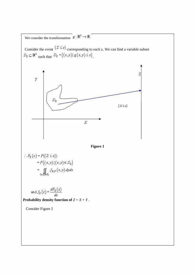
We consider the transformation

Consider the event corresponding to each z. We can find a variable subset

such that .

Figure 1

Probability density function of Z = X + Y .

Consider Figure 2

94

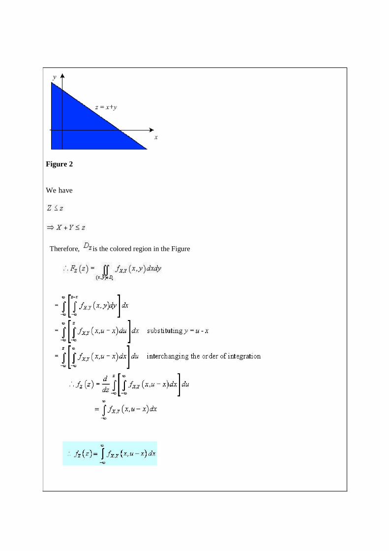
Figure 2

We have

Therefore, is the colored region in the Figure

95

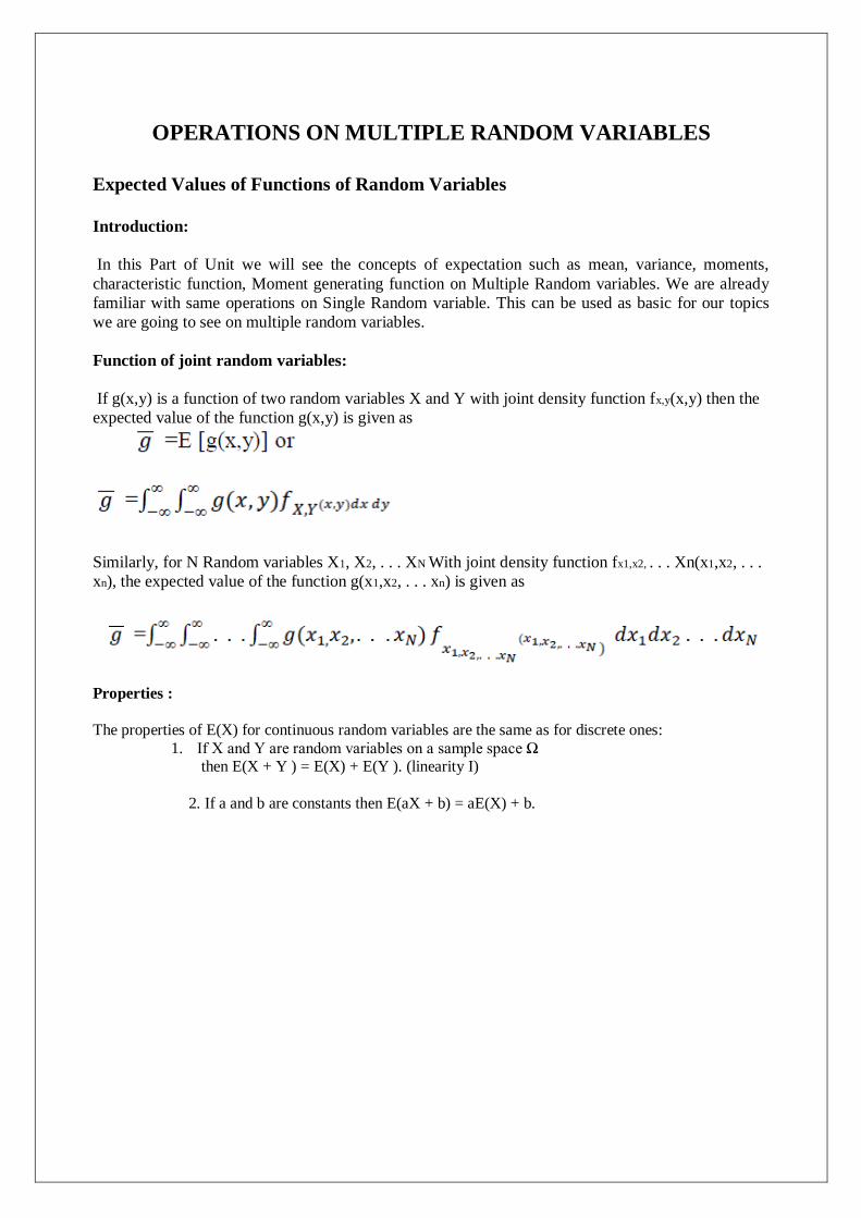
OPERATIONS ON MULTIPLE RANDOM VARIABLES

Expected Values of Functions of Random Variables

Introduction:

In this Part of Unit we will see the concepts of expectation such as mean, variance, moments,

characteristic function, Moment generating function on Multiple Random variables. We are already

familiar with same operations on Single Random variable. This can be used as basic for our topics

we are going to see on multiple random variables.

Function of joint random variables:

If g(x,y) is a function of two random variables X and Y with joint density function fx,y(x,y) then the

expected value of the function g(x,y) is given as

Similarly, for N Random variables X1, X2, . . . XN With joint density function fx1,x2, . . . Xn(x1,x2, . . .

xn), the expected value of the function g(x1,x2, . . . xn) is given as

Properties :

The properties of E(X) for continuous random variables are the same as for discrete ones:

1. If X and Y are random variables on a sample space Ω then E(X + Y ) = E(X) + E(Y ). (linearity I)

2. If a and b are constants then E(aX + b) = aE(X) + b.

96

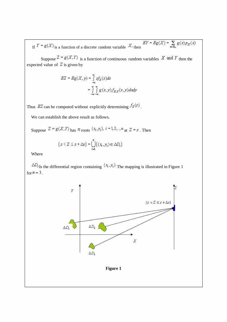
If is a function of a discrete random variable then

Suppose is a function of continuous random variables then the

expected value of is given by

Thus can be computed without explicitly determining .

We can establish the above result as follows.

Suppose has roots at . Then

Where

Is the differential region containing The mapping is illustrated in Figure 1

for .

Figure 1

97

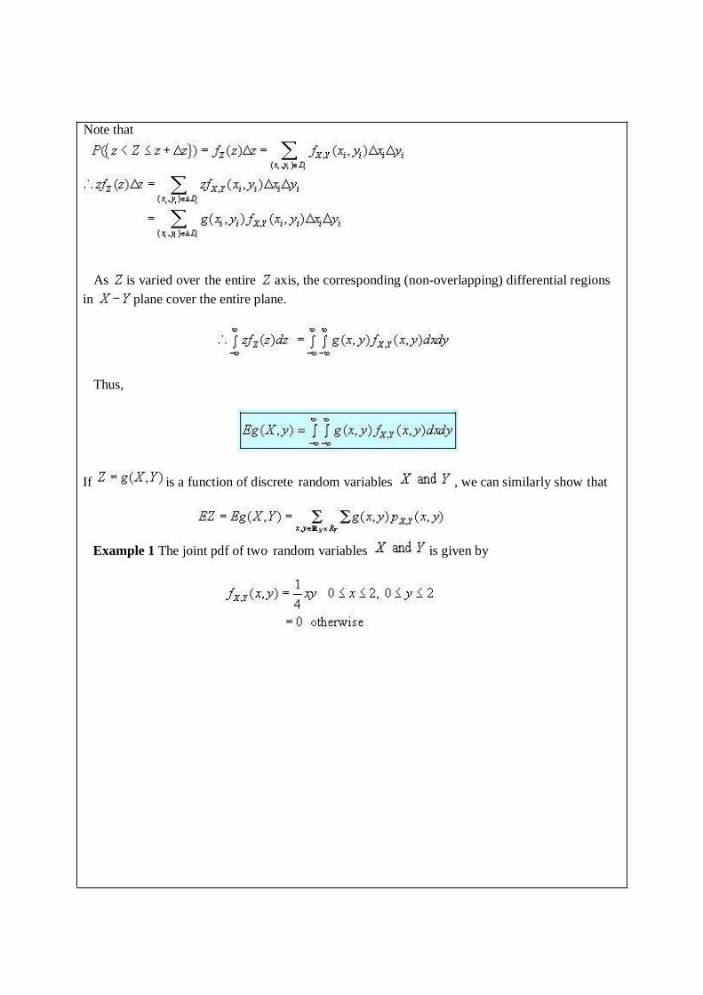
Note that

As is varied over the entire axis, the corresponding (non-overlapping) differential regions

in plane cover the entire plane.

Thus,

If is a function of discrete random variables , we can similarly show that

Example 1 The joint pdf of two random variables is given by

98

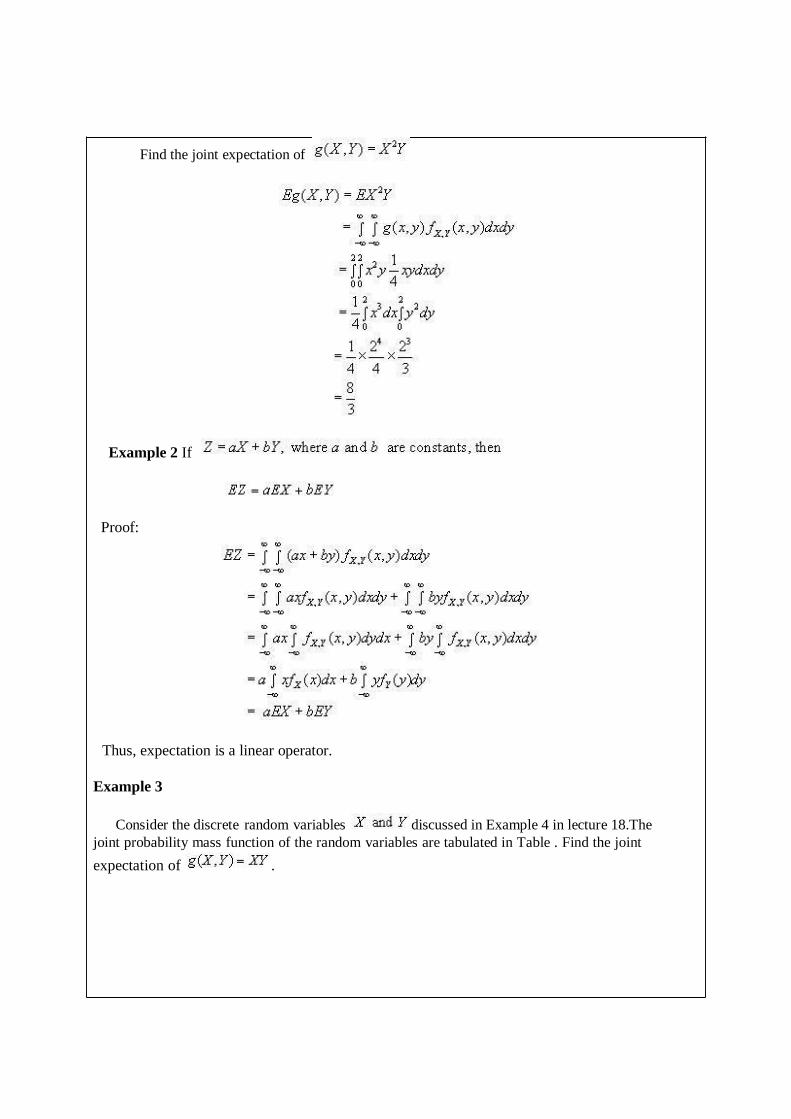
Find the joint expectation of

Example 2 If

Proof:

Thus, expectation is a linear operator.

Example 3

Consider the discrete random variables discussed in Example 4 in lecture 18.The

joint probability mass function of the random variables are tabulated in Table . Find the joint

expectation of .

99

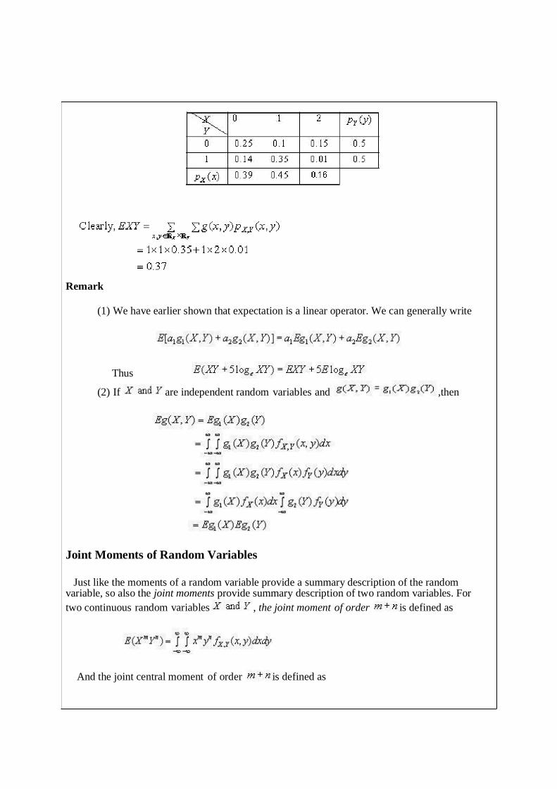
Remark

(1) We have earlier shown that expectation is a linear operator. We can generally write

Thus

(2) If are independent random variables and ,then

Joint Moments of Random Variables

Just like the moments of a random variable provide a summary description of the random

variable, so also the joint moments provide summary description of two random variables. For

two continuous random variables , the joint moment of order is defined as

And the joint central moment of order is defined as

100

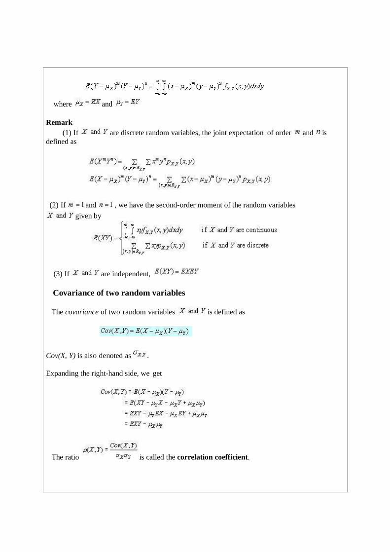
where and

Remark

(1) If are discrete random variables, the joint expectation of order and is

defined as

(2) If and , we have the second-order moment of the random variables

given by

(3) If are independent,

Covariance of two random variables

The covariance of two random variables is defined as

Cov(X, Y) is also denoted as .

Expanding the right-hand side, we get

The ratio is called the correlation coefficient.

101

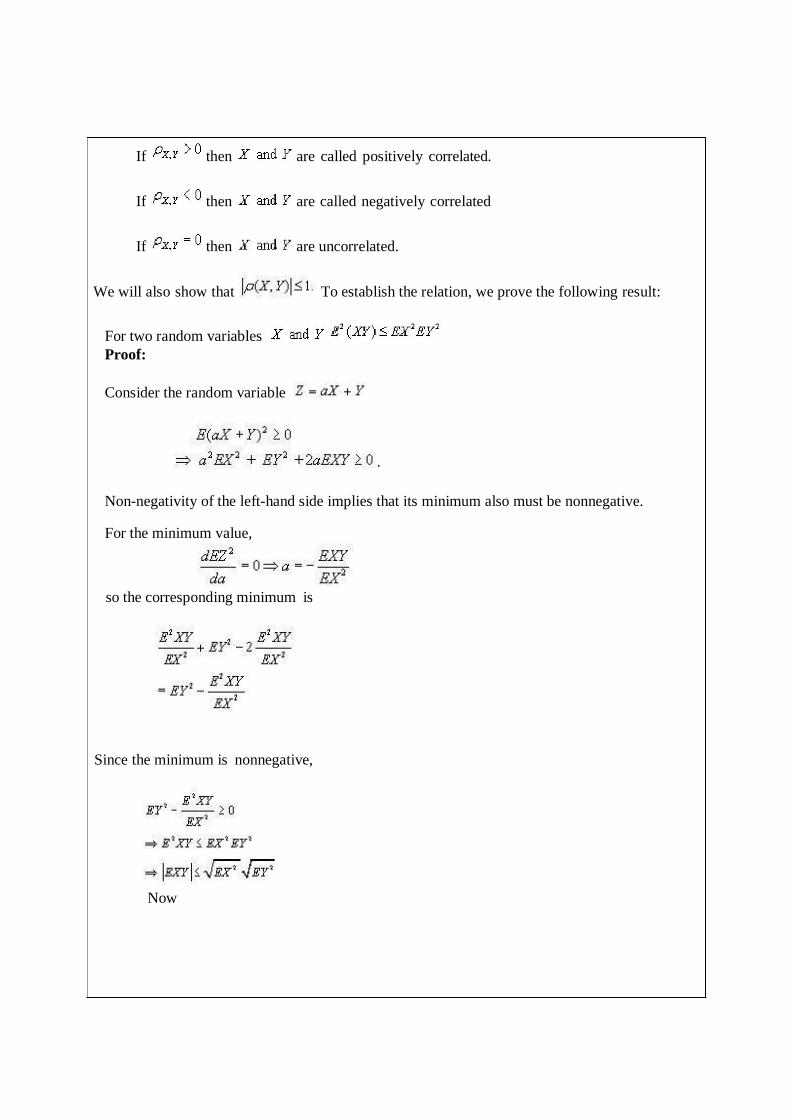
If then are called positively correlated.

If then are called negatively correlated

If then are uncorrelated.

We will also show that To establish the relation, we prove the following result:

For two random variables

Proof:

Consider the random variable

.

Non-negativity of the left-hand side implies that its minimum also must be nonnegative.

For the minimum value,

so the corresponding minimum is

Since the minimum is nonnegative,

Now

102

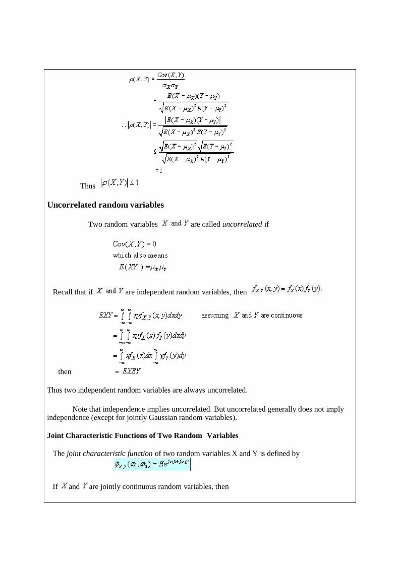
Thus

Uncorrelated random variables

Two random variables are called uncorrelated if

Recall that if are independent random variables, then

then

Thus two independent random variables are always uncorrelated.

Note that independence implies uncorrelated. But uncorrelated generally does not imply

independence (except for jointly Gaussian random variables).

Joint Characteristic Functions of Two Random Variables

The joint characteristic function of two random variables X and Y is defined by

If and are jointly continuous random variables, then

103

Note that is same as the two-dimensional Fourier transform with the basis function

instead of

is related to the joint characteristic function by the Fourier inversion formula

If and are discrete random variables, we can define the joint characteristic function in terms

of the joint probability mass function as follows:

Properties of the Joint Characteristic Function

The joint characteristic function has properties similar to the properties of the chacteristic

function of a single random variable. We can easily establish the following properties:

1.

2.

3. If and are independent random variables, then

4. We have,

104

Hence,

In general, the order joint moment is given by

Example 2 The joint characteristic function of the jointly Gaussian random variables and

with the joint pdf

Let us recall the characteristic function of a Gaussian random variable

105

If and is jointly Gaussian,

we can similarly show that

We can use the joint characteristic functions to simplify the probabilistic analysis as illustrated

on next page:

Jointly Gaussian Random Variables

Many practically occurring random variables are modeled as jointly Gaussian random variables. For example, noise samples at different instants in the communication system are modeled as jointly Gaussian random variables.

Two random variables are called jointly Gaussian if their joint probability density

106

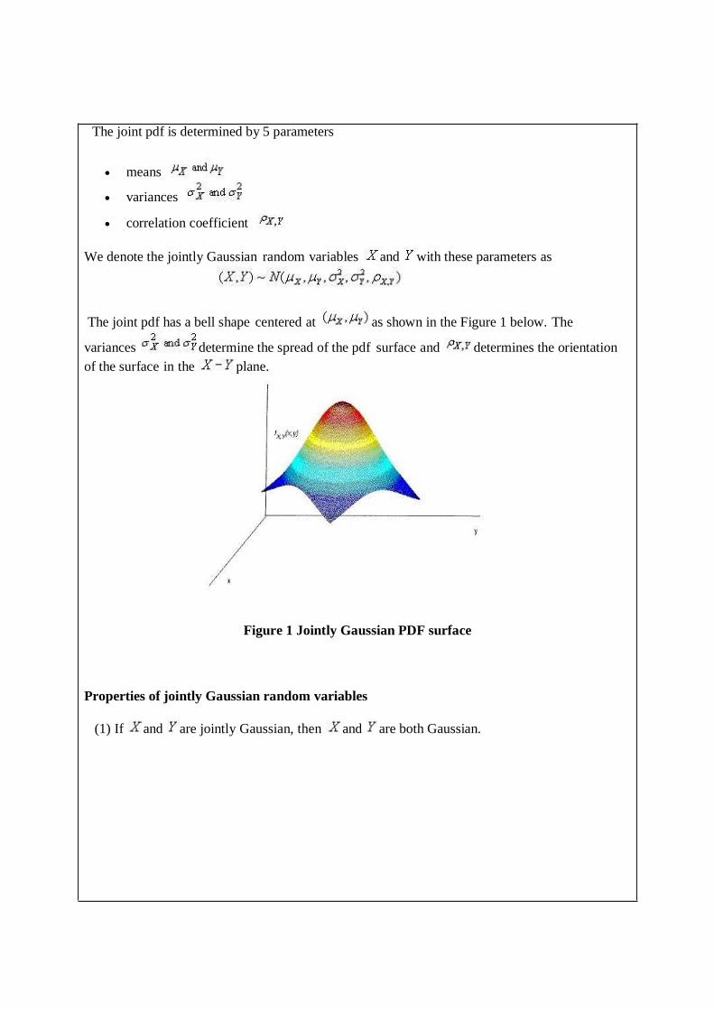
The joint pdf is determined by 5 parameters

means

variances

correlation coefficient

We denote the jointly Gaussian random variables and with these parameters as

The joint pdf has a bell shape centered at as shown in the Figure 1 below. The

variances determine the spread of the pdf surface and determines the orientation

of the surface in the plane.

Figure 1 Jointly Gaussian PDF surface

Properties of jointly Gaussian random variables

(1) If and are jointly Gaussian, then and are both Gaussian.

107

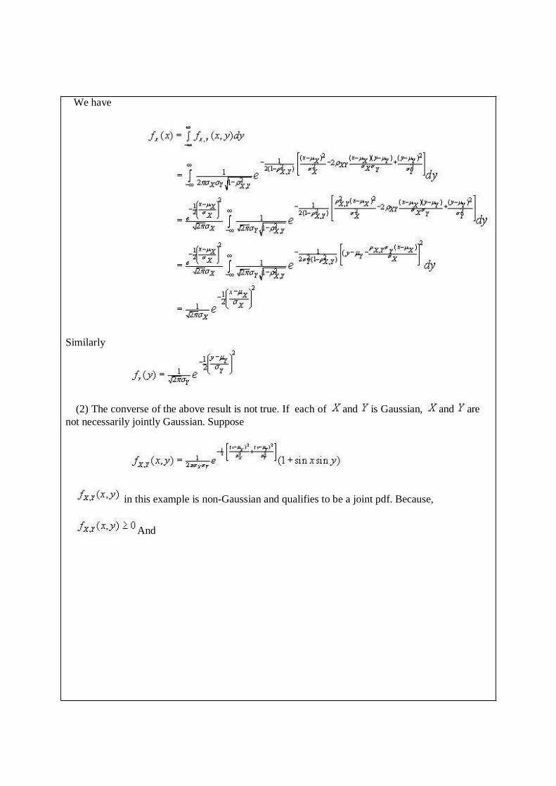
We have

Similarly

(2) The converse of the above result is not true. If each of and is Gaussian, and are

not necessarily jointly Gaussian. Suppose

in this example is non-Gaussian and qualifies to be a joint pdf. Because,

And

108

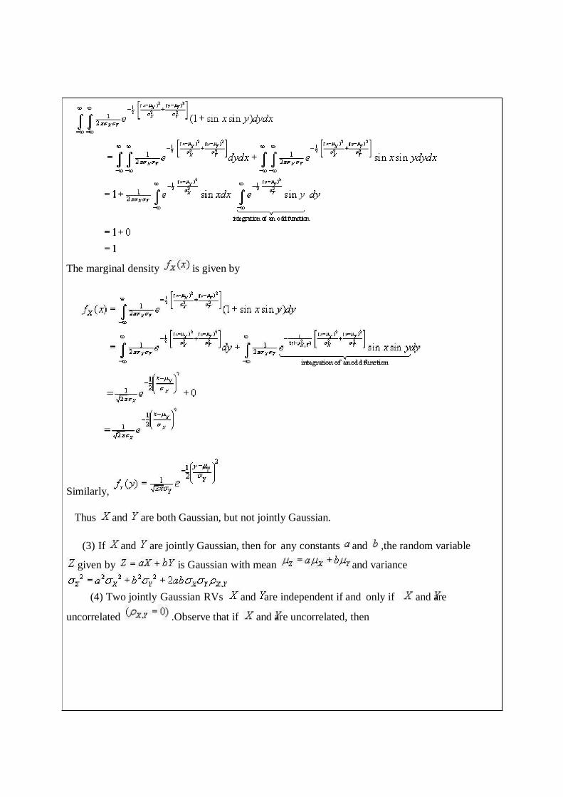
The marginal density is given by

Similarly,

Thus and are both Gaussian, but not jointly Gaussian.

(3) If and are jointly Gaussian, then for any constants and ,the random variable

given by is Gaussian with mean and variance

(4) Two jointly Gaussian RVs and are independent if and only if and are

uncorrelated .Observe that if and are uncorrelated, then

109

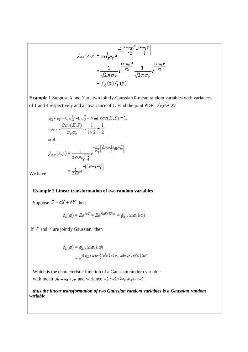
Example 1 Suppose X and Y are two jointly-Gaussian 0-mean random variables with variances

of 1 and 4 respectively and a covariance of 1. Find the joint PDF

We have

Example 2 Linear transformation of two random variables

Suppose then

If and are jointly Gaussian, then

Which is the characteristic function of a Gaussian random variable

with mean and variance

thus the linear transformation of two Gaussian random variables is a Gaussian random variable

110

UNIT IV

Stochastic Processes-Temporal Characteristics

The Stochastic process Concept

Classification of Processes, Deterministic and Nondeterministic Processes

Distribution and Density Functions

Statistical Independence

Concept of Stationarity: First-Order Stationary Processes, Second-Order and Wide-Sense Stationarity, Nth-Order and Strict-Sense Stationarity

Time Averages and Ergodicity

Mean-Ergodic Processes

Correlation-Ergodic Processes

Autocorrelation Function and Its Properties

Cross-Correlation Function and Its Properties

Covariance Functions and its properties

Linear system Response:

Mean

Mean-squared value

Autocorrelation

Cross-Correlation Functions

111

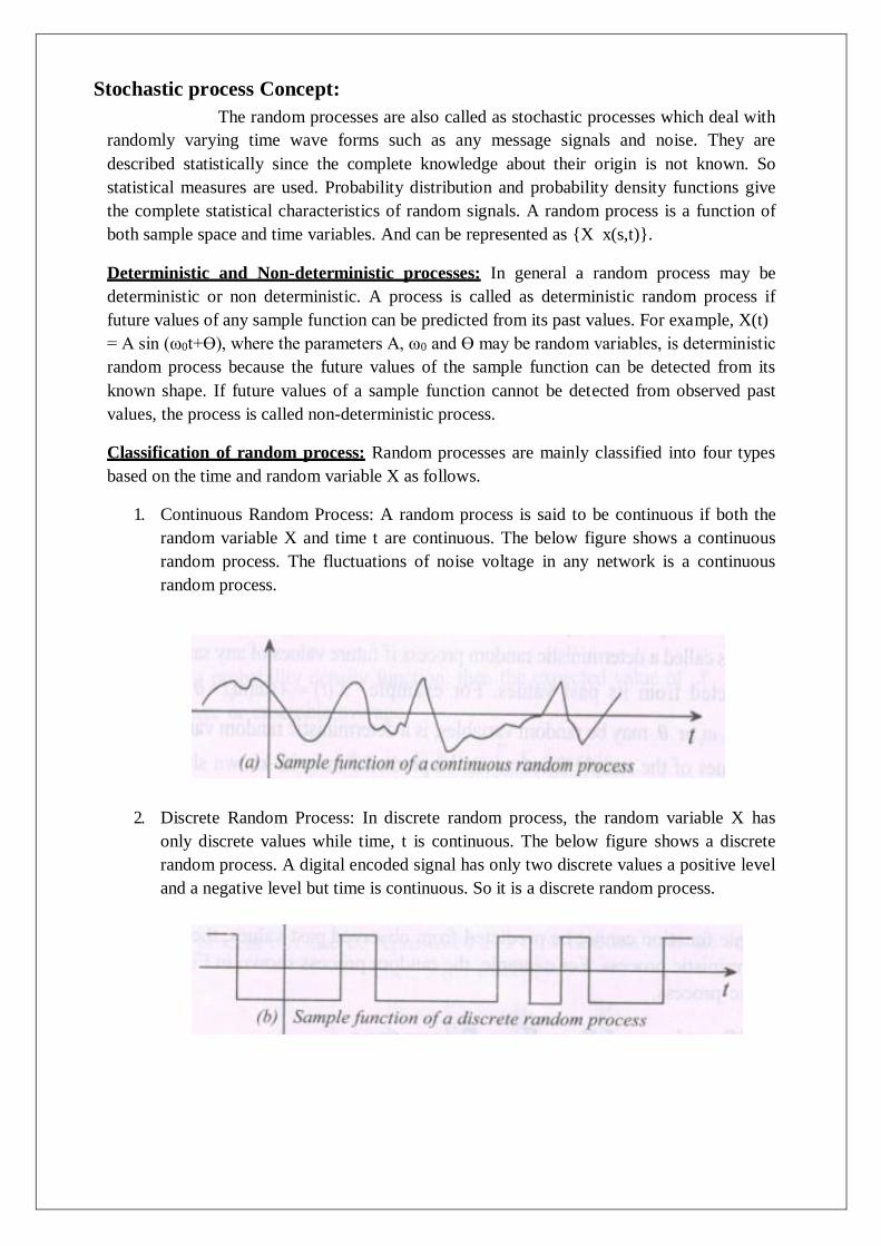
K.RAVEENDRA, Associate Professor, In-charge Examinations Branch, SVEW, TPT. Page 1

Stochastic process Concept:

The random processes are also called as stochastic processes which deal with

randomly varying time wave forms such as any message signals and noise. They are

described statistically since the complete knowledge about their origin is not known. So

statistical measures are used. Probability distribution and probability density functions give

the complete statistical characteristics of random signals. A random process is a function of

both sample space and time variables. And can be represented as X x(s,t).

Deterministic and Non-deterministic processes: In general a random process may be

deterministic or non deterministic. A process is called as deterministic random process if

future values of any sample function can be predicted from its past values. For example, X(t)

= A sin (ω0t+ϴ), where the parameters A, ω0 and ϴ may be random variables, is deterministic

random process because the future values of the sample function can be detected from its

known shape. If future values of a sample function cannot be detected from observed past

values, the process is called non-deterministic process.

Classification of random process: Random processes are mainly classified into four types

based on the time and random variable X as follows.

1. Continuous Random Process: A random process is said to be continuous if both the

random variable X and time t are continuous. The below figure shows a continuous

random process. The fluctuations of noise voltage in any network is a continuous

random process.

2. Discrete Random Process: In discrete random process, the random variable X has

only discrete values while time, t is continuous. The below figure shows a discrete

random process. A digital encoded signal has only two discrete values a positive level

and a negative level but time is continuous. So it is a discrete random process.

112

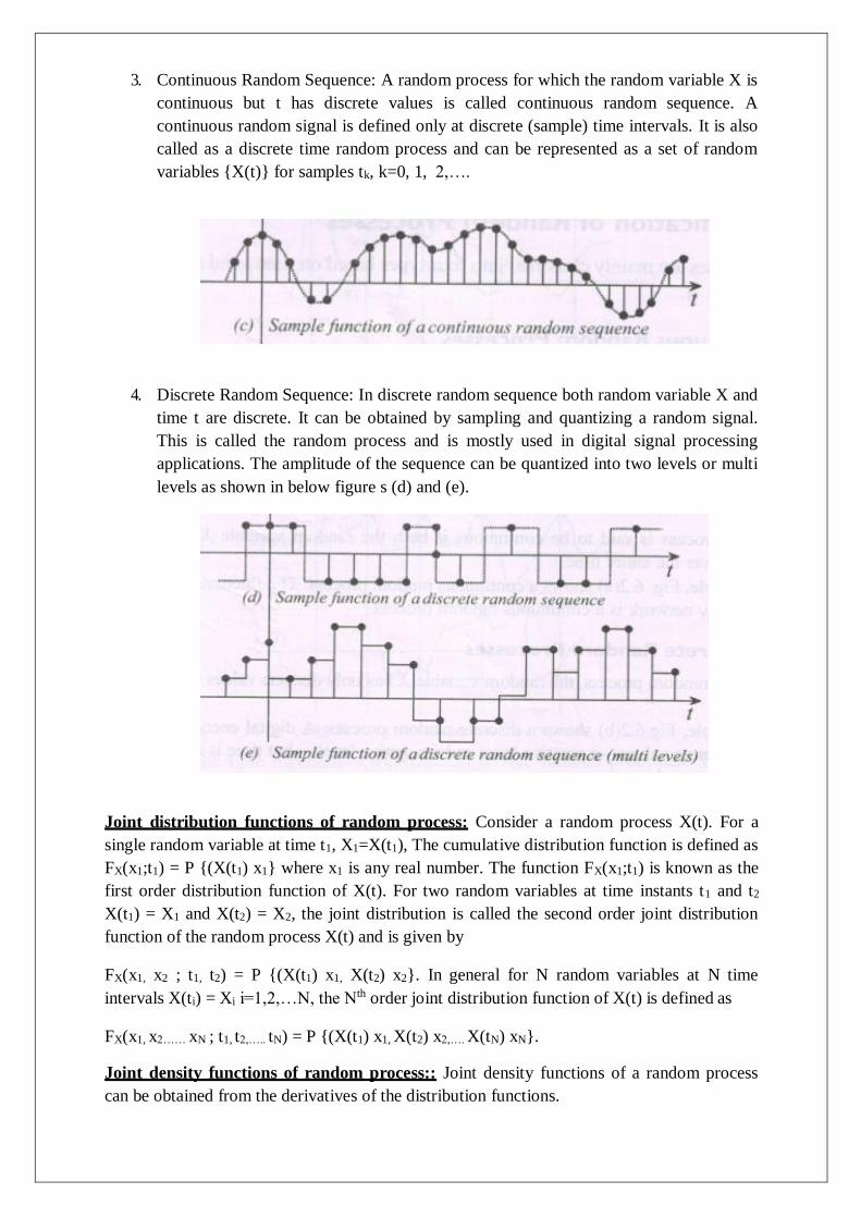
Probability Theory and Stochastic Processes (13A04304) www.raveendraforstudentsinfo.in

K.RAVEENDRA, Associate Professor, In-charge Examinations Branch, SVEW, TPT. Page 2

3. Continuous Random Sequence: A random process for which the random variable X is

continuous but t has discrete values is called continuous random sequence. A

continuous random signal is defined only at discrete (sample) time intervals. It is also

called as a discrete time random process and can be represented as a set of random

variables X(t) for samples tk, k=0, 1, 2,….

4. Discrete Random Sequence: In discrete random sequence both random variable X and

time t are discrete. It can be obtained by sampling and quantizing a random signal.

This is called the random process and is mostly used in digital signal processing

applications. The amplitude of the sequence can be quantized into two levels or multi

levels as shown in below figure s (d) and (e).

Joint distribution functions of random process: Consider a random process X(t). For a

single random variable at time t1, X1=X(t1), The cumulative distribution function is defined as

FX(x1;t1) = P (X(t1) x1 where x1 is any real number. The function FX(x1;t1) is known as the

first order distribution function of X(t). For two random variables at time instants t1 and t2

X(t1) = X1 and X(t2) = X2, the joint distribution is called the second order joint distribution

function of the random process X(t) and is given by

FX(x1, x2 ; t1, t2) = P (X(t1) x1, X(t2) x2. In general for N random variables at N time

intervals X(ti) = Xi i=1,2,…N, the Nth order joint distribution function of X(t) is defined as

FX(x1, x2…… xN ; t1, t2,….. tN) = P (X(t1) x1, X(t2) x2,…. X(tN) xN.

Joint density functions of random process:: Joint density functions of a random process

can be obtained from the derivatives of the distribution functions.

113

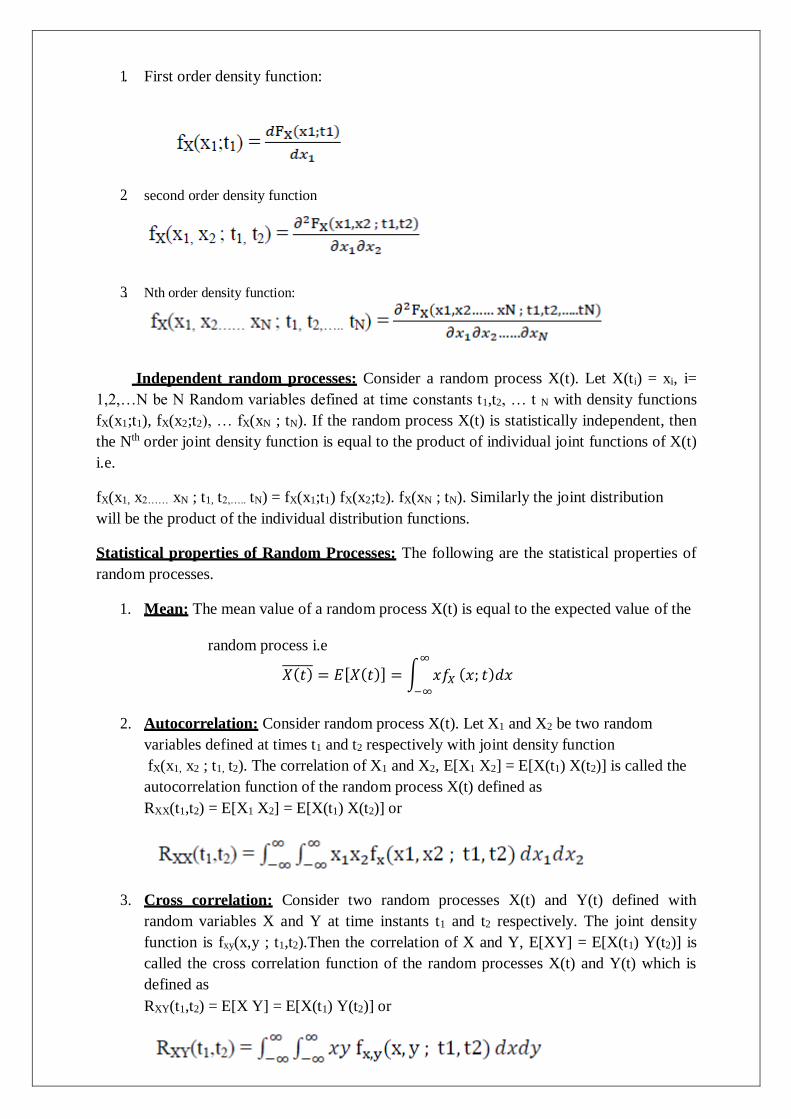
Probability Theory and Stochastic Processes (13A04304) www.raveendraforstudentsinfo.in

1. First order density function:

2. second order density function

3. Nth order density function:

Independent random processes: Consider a random process X(t). Let X(ti) = xi, i=

1,2,…N be N Random variables defined at time constants t1,t2, … t N with density functions

fX(x1;t1), fX(x2;t2), … fX(xN ; tN). If the random process X(t) is statistically independent, then

the Nth order joint density function is equal to the product of individual joint functions of X(t)

i.e.

fX(x1, x2…… xN ; t1, t2,….. tN) = fX(x1;t1) fX(x2;t2). fX(xN ; tN). Similarly the joint distribution

will be the product of the individual distribution functions.

Statistical properties of Random Processes: The following are the statistical properties of

random processes.

1. Mean: The mean value of a random process X(t) is equal to the expected value of the

random process i.e

𝑋(𝑡) = 𝐸[𝑋(𝑡)] = ∫ 𝑥𝑓𝑋

∞

−∞

(𝑥; 𝑡)𝑑𝑥

2. Autocorrelation: Consider random process X(t). Let X1 and X2 be two random

variables defined at times t1 and t2 respectively with joint density function

fX(x1, x2 ; t1, t2). The correlation of X1 and X2, E[X1 X2] = E[X(t1) X(t2)] is called the

autocorrelation function of the random process X(t) defined as

RXX(t1,t2) = E[X1 X2] = E[X(t1) X(t2)] or

3. Cross correlation: Consider two random processes X(t) and Y(t) defined with

random variables X and Y at time instants t1 and t2 respectively. The joint density

function is fxy(x,y ; t1,t2).Then the correlation of X and Y, E[XY] = E[X(t1) Y(t2)] is

called the cross correlation function of the random processes X(t) and Y(t) which is

defined as

RXY(t1,t2) = E[X Y] = E[X(t1) Y(t2)] or

114

Stationary Processes: A random process is said to be stationary if all its statistical properties

such as mean, moments, variances etc… do not change with time. The stationarity which

depends on the density functions has different levels or orders.

1. First order stationary process: A random process is said to be stationary to order one or

first order stationary if its first order density function does not change with time or shift in

time value. If X(t) is a first order stationary process then

fX(x1;t1) = fX(x1;t1+∆t) for any time t1.

Where ∆t is shift in time value. Therefore the condition for a process to be a first order

stationary random process is that its mean value must be constant at any time instant. i.e.

𝐸[𝑋(𝑡)] = = 𝑐𝑜𝑛𝑠𝑡𝑎𝑛𝑡

2. Second order stationary process: A random process is said to be stationary to order two

or second order stationary if its second order joint density function does not change with

time or shift in time value i.e. fX(x1, x2 ; t1, t2) = fX(x1, x2;t1+∆t, t2+∆t) for all t1,t2 and ∆t. It is

a function of time difference (t2, t1) and not absolute time t. Note that a second order

stationary process is also a first order stationary process. The condition for a process to be a

second order stationary is that its autocorrelation should depend only on time differences

and not on absolute time. i.e. If

RXX(t1,t2) = E[X(t1) X(t2)] is autocorrelation function and τ =t2 –t1 then

RXX(t1,t1+ τ) = E[X(t1) X(t1+ τ)] = RXX(τ) . RXX(τ) should be independent of time t.

3. Wide sense stationary (WSS) process: If a random process X(t) is a second order

stationary process, then it is called a wide sense stationary (WSS) or a weak sense

stationary process. However the converse is not true.

The conditions for a wide sense stat ionary process are

1. 𝐸[𝑋(𝑡)] = = 𝑐𝑜𝑛𝑠𝑡𝑎𝑛𝑡

2. E[X(t)X(t+τ)] = RXX(τ) is independent of absolute time t.

Joint wide sense stationary process: Consider two random processes X(t) and Y(t). If they are

jointly WSS, then the cross correlation function of X(t) and Y(t) is a function of time difference τ

=t2 –t1only and not absolute time. i.e. RXY(t1,t2) = E[X(t1) Y(t2)] . If τ =t2 –t1 then

RXY(t,t+ τ) = E[X(t) Y(t+ τ)] = RXY(τ).

Therefore the conditions for a process to be joint wide sense stationary are

1. 𝐸[𝑋(𝑡)] = = 𝑐𝑜𝑛𝑠𝑡𝑎𝑛𝑡.

2. 𝐸[𝑌(𝑡)] = = 𝑐𝑜𝑛𝑠𝑡𝑎𝑛𝑡

3. E[X(t) Y(t+ τ)] = RXY(τ) is independent of time t.

115

∫

Strict sense stationary (SSS) processes: A random process X(t) is said to be strict Sense

stationary if its Nth order joint density function does not change with time or shift in time

value. i.e.

fX(x1, x2…… xN ; t1, t2,….. tN) = fX(x1, x2…… xN ; t1+∆t, t2+∆t, . . . tN+∆t) for all t1, t2 . . . tN and ∆t.

A process that is stationary to all orders n=1,2,. . . N is called strict sense stationary process. Note

that SSS process is also a WSS process. But the reverse is not true.

Time Average Function: Consider a random process X(t). Let x(t) be a sample function

which exists for all time at a fixed value in the given sample space S. The average value of

x(t) taken over all times is called the time average of x(t). It is also called mean value of

x(t). It can be expressed as

= 𝐴[𝑋(𝑡)] = lim𝑇→∞

1

2𝑇∫ 𝑥(𝑡)𝑑𝑡

𝑇

−𝑇

Time autocorrelation function: Consider a random process X(t). The time average of the

product X(t) and X(t+ τ) is called time average autocorrelation function of x(t) and is denoted

RXX(τ) = E[X(t) X(t+ τ)] = lim𝑇→∞

1

2𝑇∫ 𝑥(𝑡)𝑥(𝑡 + 𝜏)𝑑𝑡

𝑇

−𝑇

2

Time mean square function: If τ = 0, the time average of x (t) is called time mean square

value of x(t) defined as

𝐴[𝑋2(𝑡)] = lim𝑇→∞

1

2𝑇∫ 𝑥2(𝑡)𝑑𝑡

𝑇

−𝑇 .

Time cross correlation function: Let X(t) and Y(t) be two random processes with sample

functions x(t) and y(t) respectively. The time average of the product of x(t) y(t+ τ) is called time

cross correlation function of x(t) and y(t). Denoted as

𝑅𝑋𝑌(𝜏) = lim𝑇→∞

1

2𝑇∫ 𝑥(𝑡)𝑦(𝑡 + 𝜏)𝑑𝑡

𝑇

−𝑇

116

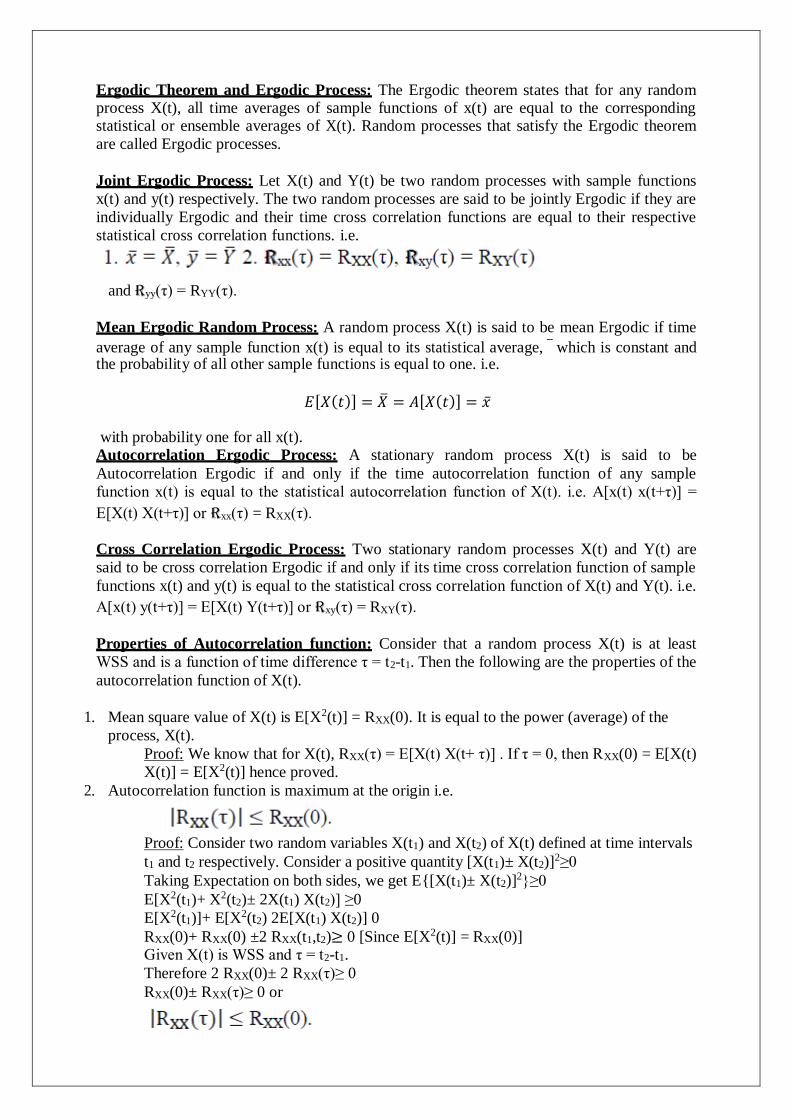
Probability Theory and Stochastic Processes (13A04304) www.raveendraforstudentsinfo.in

Ergodic Theorem and Ergodic Process: The Ergodic theorem states that for any random process X(t), all time averages of sample functions of x(t) are equal to the corresponding statistical or ensemble averages of X(t). Random processes that satisfy the Ergodic theorem

are called Ergodic processes.

Joint Ergodic Process: Let X(t) and Y(t) be two random processes with sample functions

x(t) and y(t) respectively. The two random processes are said to be jointly Ergodic if they are

individually Ergodic and their time cross correlation functions are equal to their respective

statistical cross correlation functions. i.e.

and Ryy(τ) = RYY(τ).

Mean Ergodic Random Process: A random process X(t) is said to be mean Ergodic if time

average of any sample function x(t) is equal to its statistical average, which is constant and the probability of all other sample functions is equal to one. i.e.

𝐸[𝑋(𝑡)] = = 𝐴[𝑋(𝑡)] =

with probability one for all x(t). Autocorrelation Ergodic Process: A stationary random process X(t) is said to be

Autocorrelation Ergodic if and only if the time autocorrelation function of any sample

function x(t) is equal to the statistical autocorrelation function of X(t). i.e. A[x(t) x(t+τ)] =

E[X(t) X(t+τ)] or Rxx(τ) = RXX(τ).

Cross Correlation Ergodic Process: Two stationary random processes X(t) and Y(t) are

said to be cross correlation Ergodic if and only if its time cross correlation function of sample

functions x(t) and y(t) is equal to the statistical cross correlation function of X(t) and Y(t). i.e.

A[x(t) y(t+τ)] = E[X(t) Y(t+τ)] or Rxy(τ) = RXY(τ).

Properties of Autocorrelation function: Consider that a random process X(t) is at least

WSS and is a function of time difference τ = t2-t1. Then the following are the properties of the

autocorrelation function of X(t).

1. Mean square value of X(t) is E[X2(t)] = RXX(0). It is equal to the power (average) of the

process, X(t).

Proof: We know that for X(t), RXX(τ) = E[X(t) X(t+ τ)] . If τ = 0, then RXX(0) = E[X(t)

X(t)] = E[X2(t)] hence proved.

2. Autocorrelation function is maximum at the origin i.e.

Proof: Consider two random variables X(t1) and X(t2) of X(t) defined at time intervals

t1 and t2 respectively. Consider a positive quantity [X(t1)± X(t2)]2≥0

Taking Expectation on both sides, we get E[X(t1)± X(t2)]2≥0

E[X2(t1)+ X2(t2)± 2X(t1) X(t2)] ≥0

E[X2(t1)]+ E[X2(t2) 2E[X(t1) X(t2)] 0

RXX(0)+ RXX(0) ±2 RXX(t1,t2)≥ 0 [Since E[X2(t)] = RXX(0)] Given X(t) is WSS and τ = t2-t1.

Therefore 2 RXX(0)± 2 RXX(τ)≥ 0

RXX(0)± RXX(τ)≥ 0 or

117

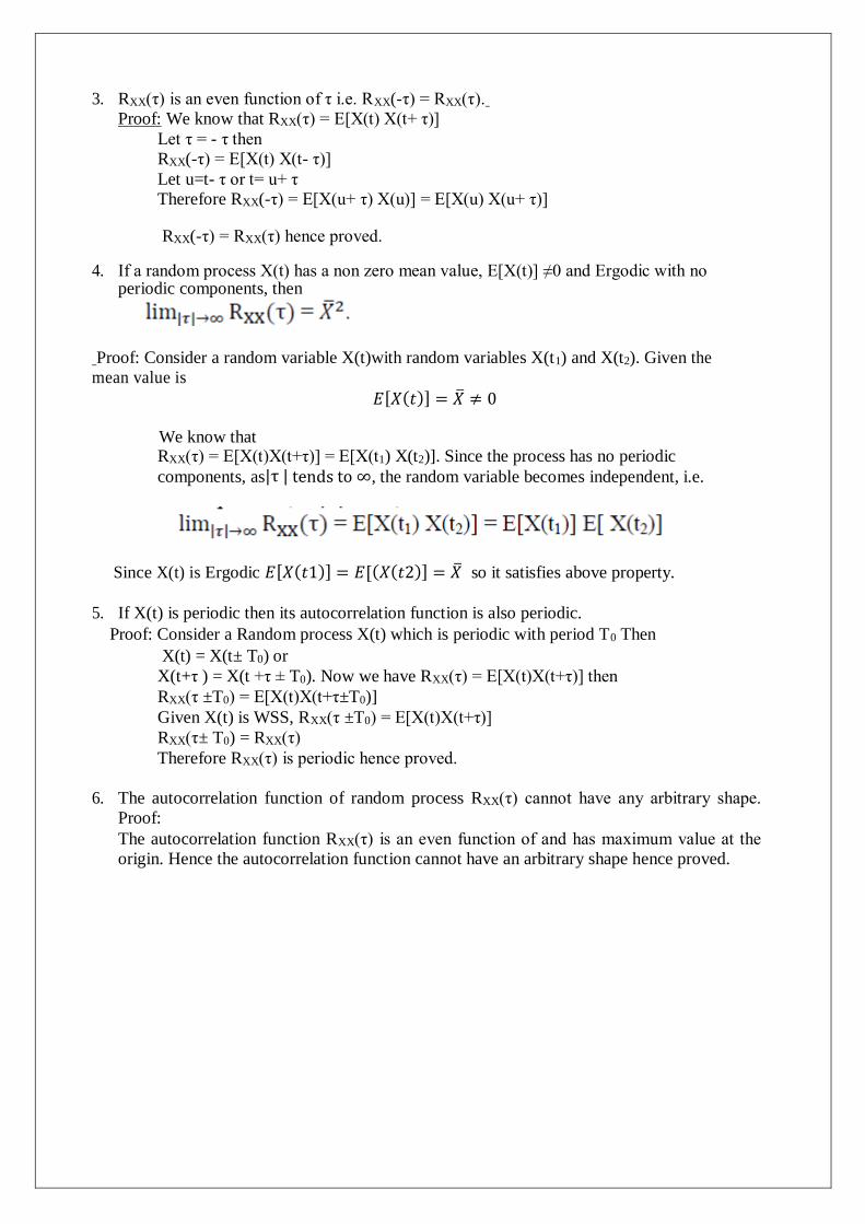
3. RXX(τ) is an even function of τ i.e. RXX(-τ) = RXX(τ).

Proof: We know that RXX(τ) = E[X(t) X(t+ τ)]

Let τ = - τ then

RXX(-τ) = E[X(t) X(t- τ)]

Let u=t- τ or t= u+ τ

Therefore RXX(-τ) = E[X(u+ τ) X(u)] = E[X(u) X(u+ τ)]

RXX(-τ) = RXX(τ) hence proved.

4. If a random process X(t) has a non zero mean value, E[X(t)] ≠0 and Ergodic with no periodic components, then

Proof: Consider a random variable X(t)with random variables X(t1) and X(t2). Given the

mean value is 𝐸[𝑋(𝑡)] = ≠ 0

We know that RXX(τ) = E[X(t)X(t+τ)] = E[X(t1) X(t2)]. Since the process has no periodic

components, as|τ | tends to ∞, the random variable becomes independent, i.e.

Since X(t) is Ergodic 𝐸[𝑋(𝑡1)] = 𝐸[(𝑋(𝑡2)] = so it satisfies above property.

5. If X(t) is periodic then its autocorrelation function is also periodic.

Proof: Consider a Random process X(t) which is periodic with period T0 Then

X(t) = X(t± T0) or

X(t+τ ) = X(t +τ ± T0). Now we have RXX(τ) = E[X(t)X(t+τ)] then

RXX(τ ±T0) = E[X(t)X(t+τ±T0)]

Given X(t) is WSS, RXX(τ ±T0) = E[X(t)X(t+τ)]

RXX(τ± T0) = RXX(τ)

Therefore RXX(τ) is periodic hence proved.

6. The autocorrelation function of random process RXX(τ) cannot have any arbitrary shape.

Proof:

The autocorrelation function RXX(τ) is an even function of and has maximum value at the

origin. Hence the autocorrelation function cannot have an arbitrary shape hence proved.

118

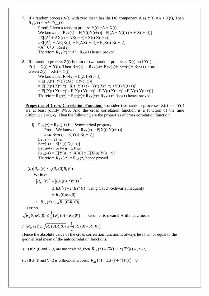
Probability Theory and Stochastic Processes (13A04304) www.raveendraforstudentsinfo.in

7. If a random process X(t) with zero mean has the DC component A as Y(t) =A + X(t), Then

RYY(τ) = A2+ RXX(τ).

Proof: Given a random process Y(t) =A + X(t).

We know that RYY(τ) = E[Y(t)Y(t+τ)] =E[(A + X(t)) (A + X(t+ τ))]

= E[(A2 + AX(t) + AX(t+ τ)+ X(t) X(t+ τ)]

= E[(A2] + AE[X(t)] + E[AX(t+ τ)]+ E[X(t) X(t+ τ)] =A2+0+0+ RXX(τ). Therefore RYY(τ) = A2+ RXX(τ) hence proved.

8. If a random process Z(t) is sum of two random processes X(t) and Y(t) i.e,

Z(t) = X(t) + Y(t). Then RZZ(τ) = RXX(τ)+ RXY(τ)+ RYX(τ)+ RYY(τ) Proof:

Given Z(t) = X(t) + Y(t).

We know that RZZ(τ) = E[Z(t)Z(t+τ)]

= E[(X(t)+Y(t)) (X(t+τ)Y(t+τ))]

= E[(X(t) X(t+τ)+ X(t) Y(t+τ) +Y(t) X(t+τ) +Y(t) Y(t+τ))]

= E[(X(t) X(t+τ)]+ E[X(t) Y(t+τ)] +E[Y(t) X(t+τ)] +E[Y(t) Y(t+τ))]

Therefore RZZ(τ) = RXX(τ)+ RXY(τ)+ RYX(τ)+ RYY(τ) hence proved.

Properties of Cross Correlation Function: Consider two random processes X(t) and Y(t)

are at least jointly WSS. And the cross correlation function is a function of the time

difference τ = t2-t1. Then the following are the properties of cross correlation function.

i) RXY(τ) = RYX(-τ) is a Symmetrical property.

Proof: We know that RXY(τ) = E[X(t) Y(t+ τ)]

also RYX(τ) = E[Y(t) X(t+ τ)]

Let τ = - τ then RYX(-τ) = E[Y(t) X(t- τ)] Let u=t- τ or t= u+ τ. then

RYX(-τ) = E[Y(u+ τ) X(u)] = E[X(u) Y(u+ τ)]

Therefore RYX(-τ) = RXY(τ) hence proved.

( ) ( ) (0) (0)XY X Yii R R R

We have

2 2

2 2

( ) ( ) ( )

( ) ( ) using Cauch-Schwarts Inequality

(0) (0)

( ) (0) (0)

XY

X Y

XY X Y

R EX t Y t

EX t EY t

R R

R R R

Further,

1

(0) (0) (0) (0) Geometric mean Arithmatic mean2

X Y X YR R R R

1

( ) (0) (0) (0) (0)2

XY X Y X YR R R R R

Hence the absolute value of the cross correlation function is always less than or equal to the

geometrical mean of the autocorrelation functions.

(iii) If X (t) and Y (t) are uncorrelated, then ( ) ( ) ( )XY X YR EX t EY t

(iv) If X (t) and Y (t) is orthogonal process, ( ) 0XYR EX t Y t

119

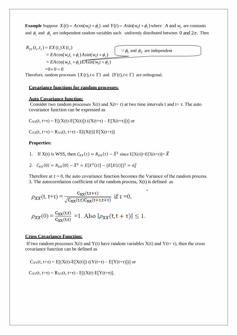
Example Suppose 0 1( ) cos( )X t A w t and

0 2( ) sin( )Y t A w t where 0 and A w are constants

and 1 and

2 are independent random variables each uniformly distributed between 0 and 2 . Then

1 2 1 2

0 1 1 0 2

0 1 1 0 2

( , ) ( ) ( )

= cos( ) sin( )

= cos( ) sin( )

=0 0 0

XYR t t EX t X t

EA w t A w t

EA w t EA w t

Therefore, random processes ( ), X t t and ( ), Y t t are orthogonal.

Covariance functions for random processes:

Auto Covariance function:

Consider two random processes X(t) and X(t+ τ) at two time intervals t and t+ τ. The auto

covariance function can be expressed as

CXX(t, t+τ) = E[(X(t)-E[X(t)]) ((X(t+τ) – E[X(t+τ)])] or

CXX(t, t+τ) = RXX(t, t+τ) - E[(X(t)] E[X(t+τ)]

Properties:

1. If X(t) is WSS, then 𝐶𝑋𝑋(𝜏) = 𝑅𝑋𝑋(𝜏) − 2 since E[X(t)]=E[X(t+τ)]=

2. 𝐶𝑋𝑋(0) = 𝑅𝑋𝑋(0) − 2 = 𝐸[𝑋2(𝑡)] − 𝐸[𝑋(𝑡)]2 = 𝜎𝑋2

Therefore at τ = 0, the auto covariance function becomes the Variance of the random process.

3. The autocorrelation coefficient of the random process, X(t) is defined as

Cross Covariance Function:

If two random processes X(t) and Y(t) have random variables X(t) and Y(t+ τ), then the cross

covariance function can be defined as

CXY(t, t+τ) = E[(X(t)-E[X(t)]) ((Y(t+τ) – E[Y(t+τ)])] or

CXY(t, t+τ) = RXY(t, t+τ) - E[(X(t) E[Y(t+τ)].

1 and 2 are independent

120

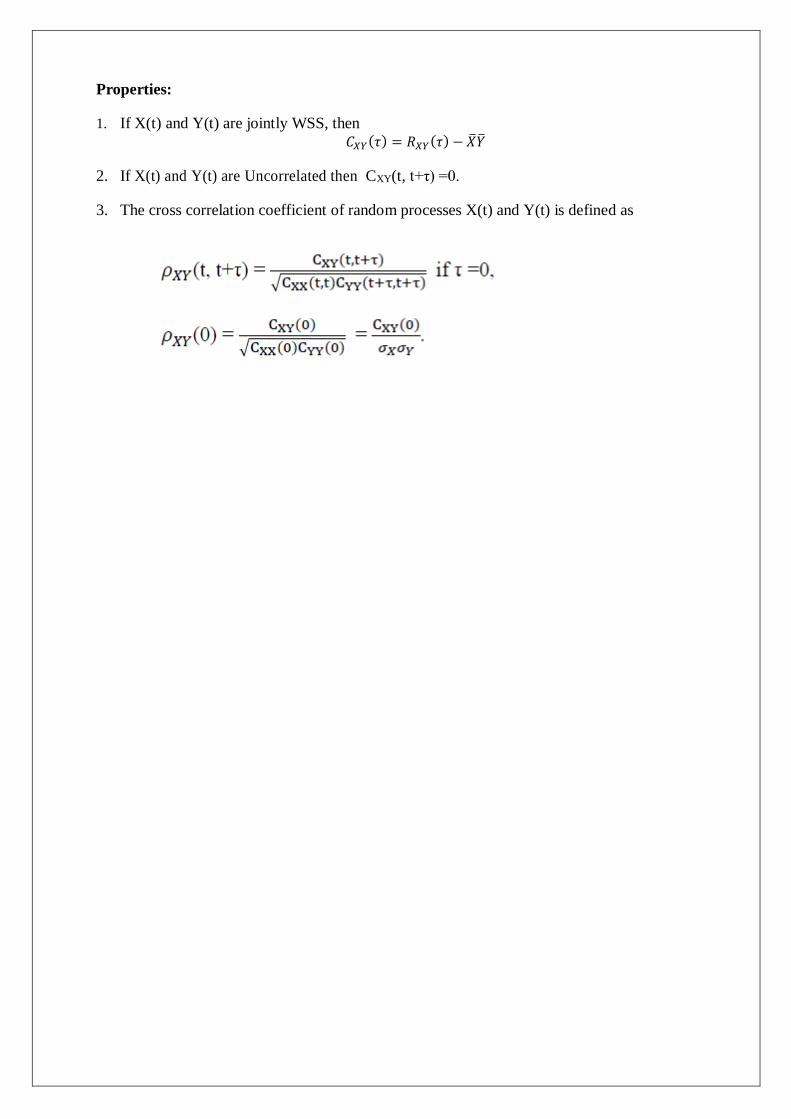
Properties:

1. If X(t) and Y(t) are jointly WSS, then 𝐶𝑋𝑌(𝜏) = 𝑅𝑋𝑌(𝜏) −

2. If X(t) and Y(t) are Uncorrelated then CXY(t, t+τ) =0.

3. The cross correlation coefficient of random processes X(t) and Y(t) is defined as

121

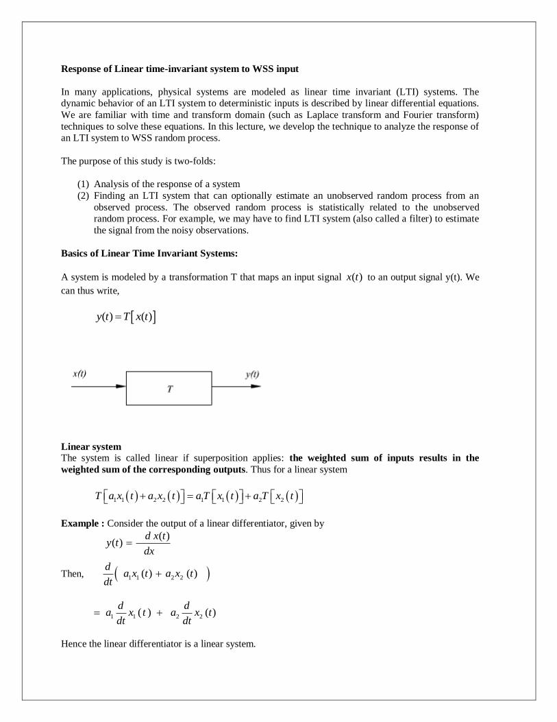
Response of Linear time-invariant system to WSS input

In many applications, physical systems are modeled as linear time invariant (LTI) systems. The dynamic behavior of an LTI system to deterministic inputs is described by linear differential equations.

We are familiar with time and transform domain (such as Laplace transform and Fourier transform)

techniques to solve these equations. In this lecture, we develop the technique to analyze the response of an LTI system to WSS random process.

The purpose of this study is two-folds:

(1) Analysis of the response of a system

(2) Finding an LTI system that can optionally estimate an unobserved random process from an

observed process. The observed random process is statistically related to the unobserved random process. For example, we may have to find LTI system (also called a filter) to estimate

the signal from the noisy observations.

Basics of Linear Time Invariant Systems:

A system is modeled by a transformation T that maps an input signal ( )x t to an output signal y(t). We

can thus write,

( ) ( )y t T x t

Linear system The system is called linear if superposition applies: the weighted sum of inputs results in the

weighted sum of the corresponding outputs. Thus for a linear system

1 1 2 2 1 1 2 2T a x t a x t a T x t a T x t

Example : Consider the output of a linear differentiator, given by

( )

( )d x t

y tdx

Then, 1 1 2 2( ) ( )d

a x t a x tdt

1 1 2 2( ) ( )d d

a x t a x tdt dt

Hence the linear differentiator is a linear system.

122

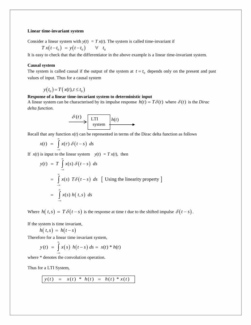
Linear time-invariant system

Consider a linear system with y(t) = T x(t). The system is called time-invariant if

0 0 0T x t t y t t t

It is easy to check that that the differentiator in the above example is a linear time-invariant system.

Causal system

The system is called causal if the output of the system at 0t t depends only on the present and past

values of input. Thus for a causal system

0 0( ),y t T x t t t

Response of a linear time-invariant system to deterministic input

A linear system can be characterised by its impulse response ( ) ( )h t T t where ( )t is the Dirac

delta function.

Recall that any function x(t) can be represented in terms of the Dirac delta function as follows

( ) ( )x t x t s ds

If x(t) is input to the linear system y(t) = T x(t), then

( ) ( )

( ) Using the linearity property

( ) ,

y t T x s t s ds

x s T t s ds

x s h t s ds

Where ,h t s T t s is the response at time t due to the shifted impulse t s .

If the system is time invariant,

,h t s h t s

Therefore for a linear time invariant system,

( ) ( ) * ( )y t x s h t s ds x t h t

where * denotes the convolution operation.

Thus for a LTI System,

( ) ( ) * ( ) ( ) * ( )y t x t h t h t x t

)(th LTI

system

)(t

x(n)

123

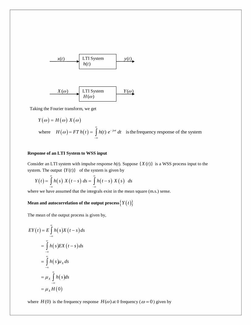
Taking the Fourier transform, we get

where ( ) is thefrequency response of the systemj t

Y H X

H FT h t h t e dt

Response of an LTI System to WSS input

Consider an LTI system with impulse response h(t). Suppose ( ) X t is a WSS process input to the

system. The output ( ) Y t of the system is given by

Y t h s X t s ds h t s X s ds

where we have assumed that the integrals exist in the mean square (m.s.) sense.

Mean and autocorrelation of the output process Y t

The mean of the output process is given by,

0

X

X

X

EY t E h s X t s ds

h s EX t s ds

h s ds

h s ds

H

where (0)H is the frequency response ( )H at 0 frequency ( 0 ) given by

( )y t

( )x t LTI System

( )h t

( )Y ( )X LTI System

( )H

124

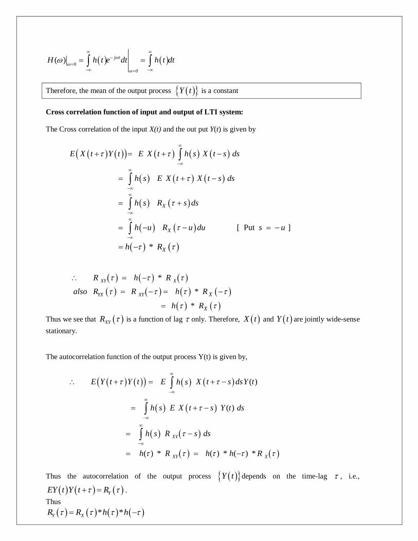
0

0

( ) j tH h t e dt h t dt

Therefore, the mean of the output process Y t is a constant

Cross correlation function of input and output of LTI system:

The Cross correlation of the input X(t) and the out put Y(t) is given by

E X t Y t E X t h s X t s ds

h s E X t X t s ds

Xh s R s ds

[ Put ]Xh u R u du s u

* Xh R

*

*

*

XY X

YX XY X

X

R h R

also R R h R

h R

Thus we see that XYR is a function of lag only. Therefore, X t and Y t are jointly wide-sense

stationary.

The autocorrelation function of the output process Y(t) is given by,

( )

( )

E Y t Y t E X t s dsY th s

h s E X t s Y t ds

( ) * ( ) * ( ) *

XY

XY X

h s R s ds

h R h h R

Thus the autocorrelation of the output process Y t depends on the time-lag , i.e.,

YEY t Y t R .

Thus

* *Y XR R h h

125

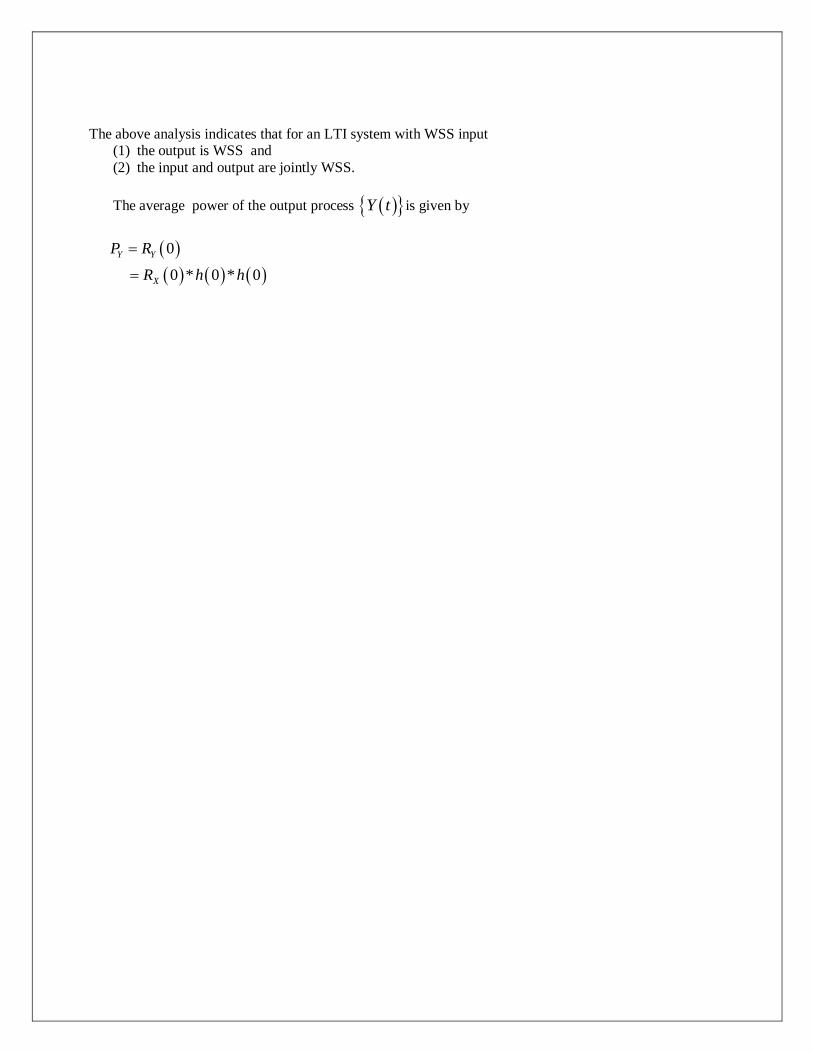
The above analysis indicates that for an LTI system with WSS input (1) the output is WSS and

(2) the input and output are jointly WSS.

The average power of the output process Y t is given by

0

0 * 0 * 0

Y Y

X

P R

R h h

126

UNIT V

Stochastic Processes-Spectral Characteristics

The Power Spectrum and its Properties

Relationship between Power Spectrum and Autocorrelation Function

The Cross-Power Density Spectrum and Properties

Relationship between Cross-Power Spectrum and Cross-Correlation Function.

Spectral characteristics of system response:

Power density spectrum of response

Cross power spectral density of input and output of a linear system

127

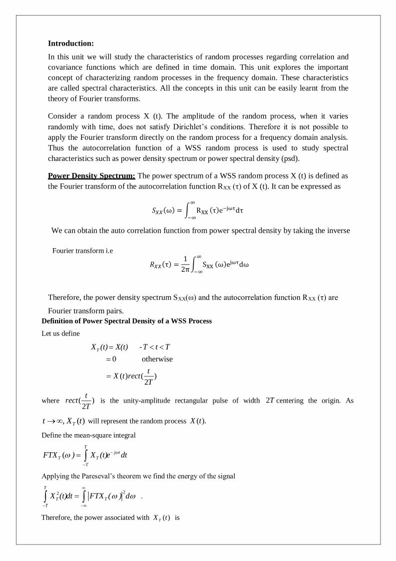
Introduction:

In this unit we will study the characteristics of random processes regarding correlation and

covariance functions which are defined in time domain. This unit explores the important

concept of characterizing random processes in the frequency domain. These characteristics

are called spectral characteristics. All the concepts in this unit can be easily learnt from the

theory of Fourier transforms.

Consider a random process X (t). The amplitude of the random process, when it varies

randomly with time, does not satisfy Dirichlet’s conditions. Therefore it is not possible to

apply the Fourier transform directly on the random process for a frequency domain analysis.

Thus the autocorrelation function of a WSS random process is used to study spectral

characteristics such as power density spectrum or power spectral density (psd).

Power Density Spectrum: The power spectrum of a WSS random process X (t) is defined as

the Fourier transform of the autocorrelation function RXX (τ) of X (t). It can be expressed as

𝑆𝑋𝑋(ω) = ∫ RXX

∞

−∞

(τ)e−jωτdτ

We can obtain the auto correlation function from power spectral density by taking the inverse

Fourier transform i.e

𝑅𝑋𝑋(τ) =1

2π∫ SXX

∞

−∞

(ω)ejωτdω

Therefore, the power density spectrum SXX(ω) and the autocorrelation function RXX (τ) are

Fourier transform pairs.

Definition of Power Spectral Density of a WSS Process

Let us define

0 otherwise

( ) ( )2

TX (t) X(t) -T t T

tX t rect

T

where ( )2

trect

T is the unity-amplitude rectangular pulse of width 2T centering the origin. As

)( , tXt T will represent the random process ).(tX

Define the mean-square integral

(

T

j t

T T

T

FTX ) X (t)e dt

Applying the Pareseval’s theorem we find the energy of the signal

22

T

T T

T

X (t)dt FTX ( ) d

.

Therefore, the power associated with ( )TX t is

128

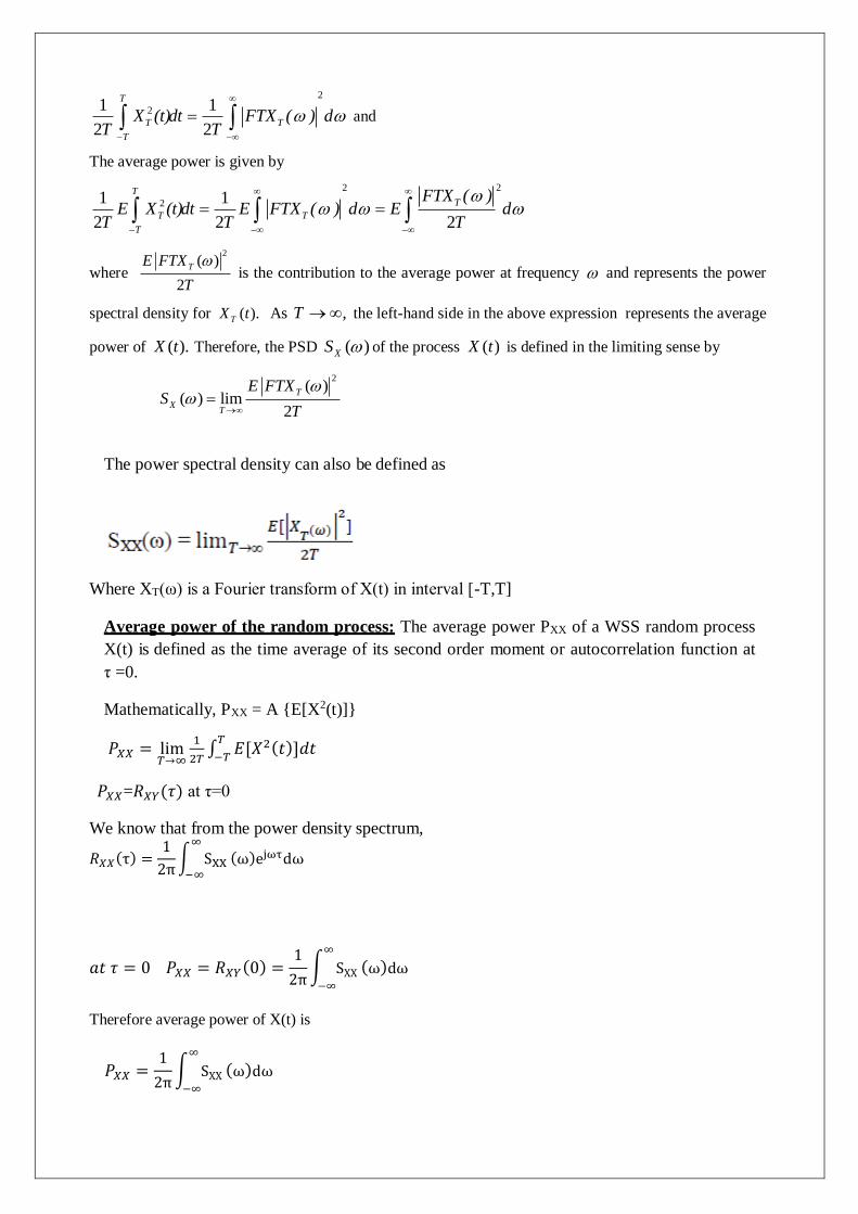
2

21 1

2 2

T

T T

T

X (t)dt FTX ( ) dT T

and

The average power is given by

22

21 1

2 2 2

TT

T T

T

FTX ( )E X (t)dt E FTX ( ) d E d

T T T

where

2( )

2

TE FTX

T

is the contribution to the average power at frequency and represents the power

spectral density for ( ).TX t As ,T the left-hand side in the above expression represents the average

power of ( ).X t Therefore, the PSD ( )XS of the process ( )X t is defined in the limiting sense by

2( )

( ) lim2

T

XT

E FTXS

T

The power spectral density can also be defined as

Where XT(ω) is a Fourier transform of X(t) in interval [-T,T]

Average power of the random process: The average power PXX of a WSS random process

X(t) is defined as the time average of its second order moment or autocorrelation function at

τ =0.

Mathematically, PXX = A E[X2(t)]

𝑃𝑋𝑋 = lim𝑇→∞

1

2𝑇∫ 𝐸[𝑋2(𝑡)]𝑑𝑡

𝑇

−𝑇

𝑃𝑋𝑋=𝑅𝑋𝑌(𝜏) at τ=0

We know that from the power density spectrum,

𝑅𝑋𝑋(τ) =1

2π∫ SXX

∞

−∞

(ω)ejωτdω

𝑎𝑡 𝜏 = 0 𝑃𝑋𝑋 = 𝑅𝑋𝑌(0) =1

2π∫ SXX

∞

−∞

(ω)dω

Therefore average power of X(t) is

𝑃𝑋𝑋 =1

2π∫ SXX

∞

−∞

(ω)dω

129

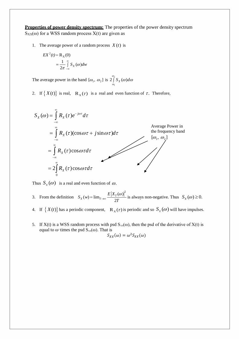
Properties of power density spectrum: The properties of the power density spectrum

SXX(ω) for a WSS random process X(t) are given as

1. The average power of a random process ( )X t is

2XR (0)

1 ( )

2X

EX (t)

S dw

The average power in the band 1 2[ , ] is 2

1

2 ( )XS d

2. If ( )X t is real, )(R X is a real and even function of . Therefore,

0

( ) ( )

( )(cos sin )

( )cos

2 ( )cos

j

X X

X

X

X

S R e d

R j d

R d

R d

Thus ( )X

S is a real and even function of .

3. From the definition

2( )

( ) lim2

TX T

E XS w

T

is always non-negative. Thus ( ) 0.XS

4. If ( )X t has a periodic component, )(R X is periodic and so ( )X

S will have impulses.

5. If X(t) is a WSS random process with psd SXX(ω), then the psd of the derivative of X(t) is

equal to ω2 times the psd SXX(ω). That is 𝑆(𝜔) = 𝜔2𝑆𝑋𝑋(𝜔)

Average Power in

the frequency band

1 2[ , ]

130

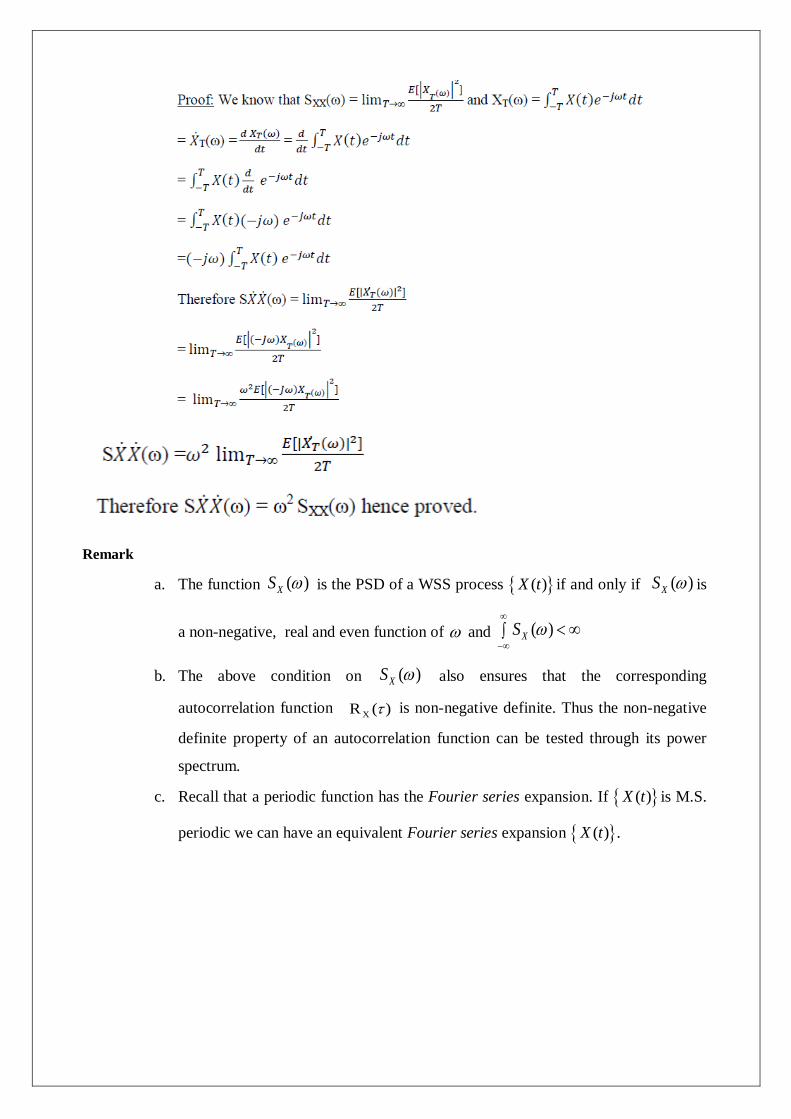
Remark

a. The function ( )XS is the PSD of a WSS process ( )X t if and only if ( )XS is

a non-negative, real and even function of and ( )XS

b. The above condition on ( )XS also ensures that the corresponding

autocorrelation function )(R X is non-negative definite. Thus the non-negative

definite property of an autocorrelation function can be tested through its power

spectrum.

c. Recall that a periodic function has the Fourier series expansion. If ( )X t is M.S.

periodic we can have an equivalent Fourier series expansion ( ) .X t

131

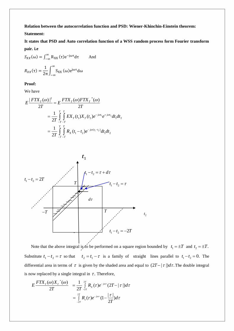
Relation between the autocorrelation function and PSD: Wiener-Khinchin-Einstein theorem:

Statement:

It states that PSD and Auto correlation function of a WSS random process form Fourier transform

pair. i.e

𝑆𝑋𝑋(ω) = ∫ RXX∞

−∞(τ)e−jωτdτ And

𝑅𝑋𝑋(τ) =1

2π∫ SXX

∞

−∞

(ω)ejωτdω

Proof:

We have

1 2

1 2

2 *

1 2 1 2

( )

1 2 1 2

| ( ) | ( ) ( )

2 2

1 ( ) ( )

2

1 ( )

2

T T T

T T

j t j t

T T

T T

T T

j t t

X

T T

FTX FTX FTXE E

T T

EX t X t e e dt dtT

R t t e dt dtT

Note that the above integral is to be performed on a square region bounded by 1t T and 2 .t T

Substitute 21 tt so that 12 tt is a family of straight lines parallel to 1 2 0.t t The

differential area in terms of is given by the shaded area and equal to (2 | |) .T d The double integral

is now replaced by a single integral in . Therefore,

* 2

2

2

2

( ) ( ) 1 ( ) (2 | |)

2 2

| | ( ) (1 )

2

TjT T

XT

Tj

xT

FTX XE R e T d

T T

R e dT

T

T

T

T

1t

2t

d

1 2t t

1 2t t d

1 2 2t t T

1 2 2t t T

132

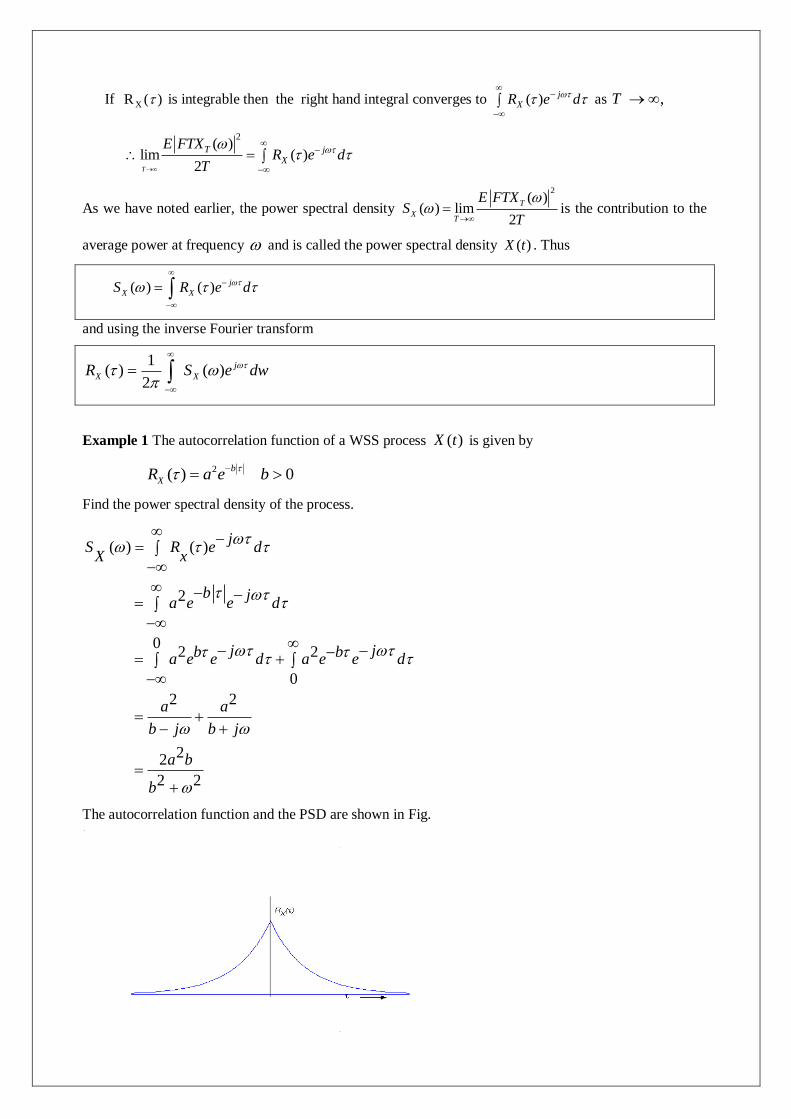
If XR ( ) is integrable then the right hand integral converges to ( ) jXR e d

as ,T

2( )

lim ( )2T

T jX

E FTXR e d

T

As we have noted earlier, the power spectral density

2( )

( ) lim2

T

XT

E FTXS

T

is the contribution to the

average power at frequency and is called the power spectral density ( )X t . Thus

( ) ( ) j

X XS R e d

and using the inverse Fourier transform

1( ) ( )

2

j

X XR S e dw

Example 1 The autocorrelation function of a WSS process ( )X t is given by

2( ) 0

b

XR a e b

Find the power spectral density of the process.

( ) ( )

2

02 2

0

2 2

22

2 2

jS R e d

X x

b ja e e d

j jb ba e e d a e e d

a a

b j b j

a b

b

The autocorrelation function and the PSD are shown in Fig.

133

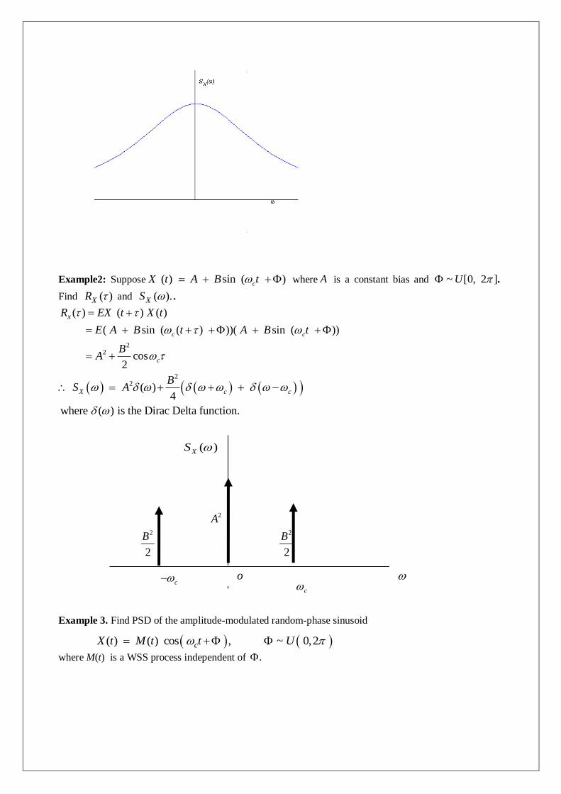
Example2: Suppose ( ) sin ( )cX t A B t where A is a constant bias and ~ [0, 2 ]U .

Find ( )XR and ( ).XS .

22

( ) ( ) ( )

( sin ( ( ) ))( sin ( ))

cos2

c c

c

xR EX t X t

E A B t A B t

BA

2

2 ( )4

where ( ) is the Dirac Delta function.

X c c

BS A

Example 3. Find PSD of the amplitude-modulated random-phase sinusoid

( ) ( ) cos , ~ 0,2cX t M t t U

where M(t) is a WSS process independent of .

2

2

B

2

2

B

2A

o c

( )XS

c

134

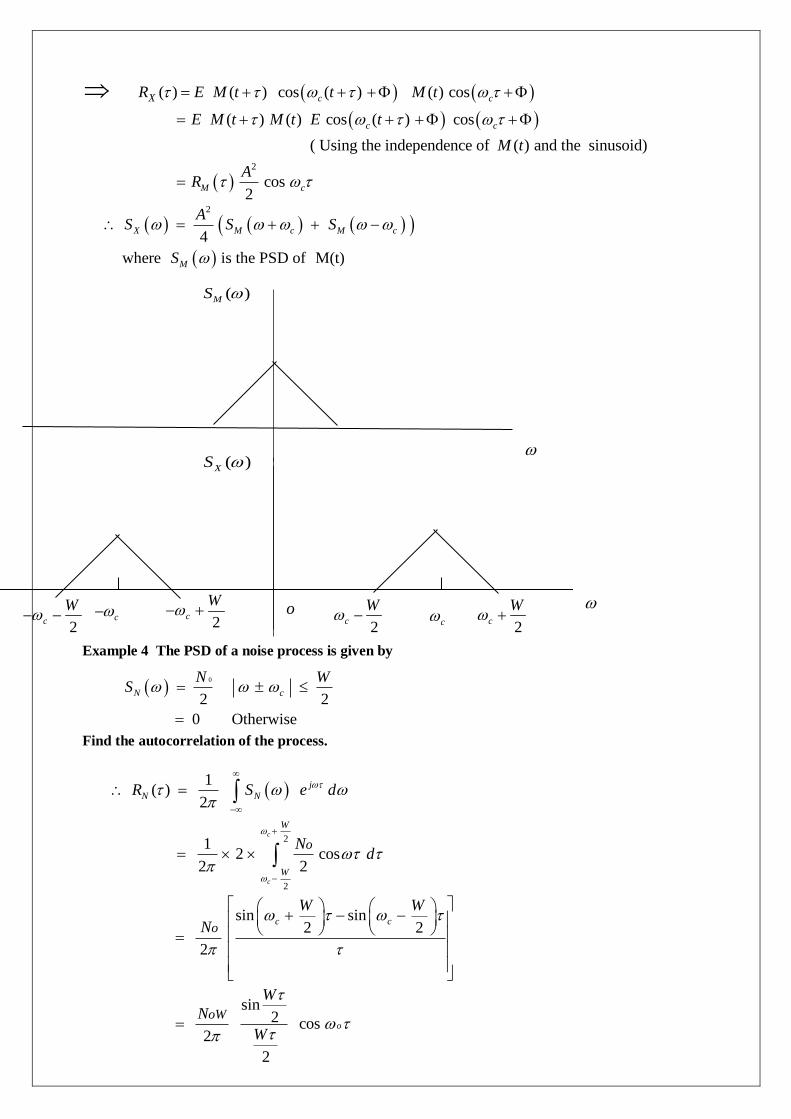
2

( ) ( ) cos ( ) ( ) cos

( ) ( ) cos ( ) cos

( Using the independence of ( ) and the sinusoid)

cos2

c c

c c

M c

XR E M t t M t

E M t M t E t

M t

AR

2

4

where is the PSD of M(t)

X M c M c

M

AS S S

S

Example 4 The PSD of a noise process is given by

0

2 2

0 Otherwise

N c

N WS

Find the autocorrelation of the process.

2

2

1( )

2

12 cos

2 2

c

c

j

N N

W

W

o

R S e d

Nd

sin sin2 2

2

c co

W W

N

sin2 cos

2

2

ooW

W

N

W

2c

W

2c

W

2c

W

2c

W o

c c

( )XS

( )MS

135

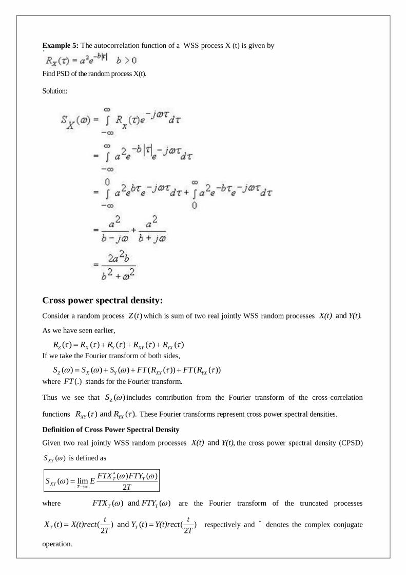
Example 5: The autocorrelation function of a WSS process X (t) is given by

Find PSD of the random process X(t).

Solution:

Cross power spectral density:

Consider a random process ( )Z t which is sum of two real jointly WSS random processes . and Y(t)X(t)

As we have seen earlier,

( ) ( ) ( ) ( ) ( )Z X Y XY YXR R R R R

If we take the Fourier transform of both sides,

( ) ( ) ( ) ( ( )) ( ( ))Z X Y XY YXS S S FT R FT R

where (.)FT stands for the Fourier transform.

Thus we see that ( )ZS includes contribution from the Fourier transform of the cross-correlation

functions ( ) and ( ).XY YXR R These Fourier transforms represent cross power spectral densities.

Definition of Cross Power Spectral Density

Given two real jointly WSS random processes and ,X(t) Y(t) the cross power spectral density (CPSD)

( )XYS is defined as

( ) ( )( ) lim

2

T TXY

T

FTX FTYS E

T

where ( ) and ( )T TFTX FTY are the Fourier transform of the truncated processes

( ) ( ) and ( ) ( )2 2

T T

t tX t X(t)rect Y t Y(t)rect

T T respectively and

denotes the complex conjugate

operation.

136

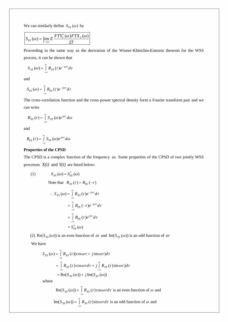
We can similarly define ( )YXS by

( ) ( )( ) lim

2

T TYX

T

FTY FTXS E

T

Proceeding in the same way as the derivation of the Wiener-Khinchin-Einstein theorem for the WSS

process, it can be shown that

( ) ( ) jXY XYS R e d

and

( ) ( ) jYX YXS R e d

The cross-correlation function and the cross-power spectral density form a Fourier transform pair and we

can write

( ) ( ) jXY XYR S e d

and

( ) ( ) jYX YXR S e d

Properties of the CPSD

The CPSD is a complex function of the frequency . Some properties of the CPSD of two jointly WSS

processes and X(t) Y(t) are listed below:

(1) *( ) ( )XY YXS S

Note that ( ) ( )XY YXR R

*

( ) ( )

( )

( )

= ( )

jXY XY

jYX

jYX

YX

S R e d

R e d

R e d

S

(2) Re( ( ))XYS is an even function of and Im( ( ))XYS is an odd function of

We have

( ) ( )(cos sin )

( )cos ( )sin )

Re( ( )) Im( ( ))

where

Re( ( )) ( )cos is an even function of and

XY XY

XY XY

XY XY

XY XY

S R j d

R d j R d

S j S

S R d

Im( ( )) ( )sin is an odd function of andXY XYS R d

137

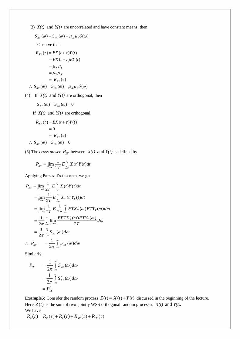
(3) and X(t) Y(t) are uncorrelated and have constant means, then

( ) ( ) ( )XY YX X YS S

Observe that

( ) ( ) ( )

( ) ( )

( )

( ) ( ) ( )

XY

X Y

Y X

XY

XY YX X Y

R EX t Y t

EX t EY t

R

S S

(4) If and X(t) Y(t) are orthogonal, then

( ) ( ) 0XY YXS S

If and X(t) Y(t) are orthogonal,

( ) ( ) ( )

0

( )

( ) ( ) 0

XY

XY

XY YX

R EX t Y t

R

S S

(5) The cross power XYP between and X(t) Y(t) is defined by

1

lim ( ) ( )2

T

XYT T

P E X t Y t dtT

Applying Parseval’s theorem, we get

*

*

1lim ( ) ( )

2

1 lim ( ) ( )

2

1 1 lim ( ) ( )

2 2

( ) ( )1 lim

2 2

1 ( )

2

1 ( )

2

T

XYT T

T TT

T TT

T T

T

XY

XY XY

P E X t Y t dtT

E X t Y t dtT

E FTX FTY dT

EFTX FTYd

T

S d

P S d

Similarly,

*

*

1 ( )

2

1 ( )

2

YX YX

XY

XY

P S d

S d

P

Example5: Consider the random process ( ) ( ) ( )Z t X t Y t discussed in the beginning of the lecture.

Here ( )Z t is the sum of two jointly WSS orthogonal random processes and .X(t) Y(t)

We have,

( ) ( ) ( ) ( ) ( )Z X Y XY YXR R R R R

138

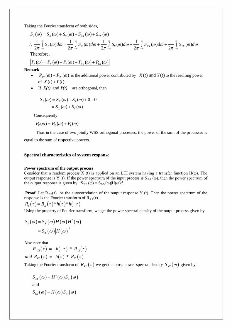
Taking the Fourier transform of both sides,

( ) ( ) ( ) ( ) ( )

1 1 1 1 1( ) ( ) ( ) ( ) ( )

2 2 2 2 2

Therefore,

( ) ( ) ( ) ( ) ( )

Z X Y XY YX

Z X Y XY YX

Z X Y XY YX

S S S S S

S d S d S d S d S d

P P P P P

Remark

( ) ( )XY YXP P is the additional power contributed by ( ) and ( )X t Y t to the resulting power

of ( ) ( )X t Y t

If and X(t) Y(t) are orthogonal, then

( ) ( ) ( ) 0 0

( ) ( )

Z X Y

X Y

S S S

S S

Consequently

( ) ( ) ( )Z X YP P P

Thus in the case of two jointly WSS orthogonal processes, the power of the sum of the processes is

equal to the sum of respective powers.

Spectral characteristics of system response:

Power spectrum of the output process

Consider that a random process X (t) is applied on an LTI system having a transfer function H(ω). The

output response is Y (t). If the power spectrum of the input process is SXX (ω), then the power spectrum of the output response is given by SYY (ω) = SXX (ω)|H(ω)|2.

Proof: Let RYY(τ) be the autocorrelation of the output response Y (t). Then the power spectrum of the response is the Fourier transform of RYY(τ) .

* *Y XR R h h

Using the property of Fourier transform, we get the power spectral density of the output process given by

*

2

Y X

X

S S H H

S H

Also note that

*

*

XY X

YX X

R h R

and R h R

Taking the Fourier transform of XYR we get the cross power spectral density XYS given by

*

and

XY X

YX X

S H S

S H S

139

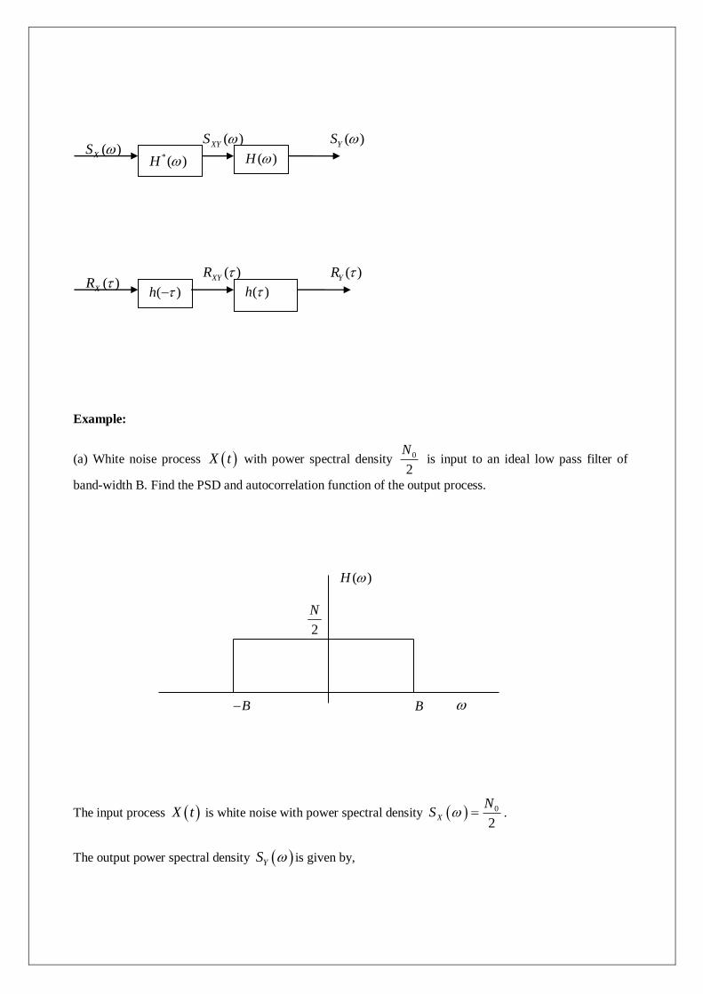
Example:

(a) White noise process X t with power spectral density 0

2

N is input to an ideal low pass filter of

band-width B. Find the PSD and autocorrelation function of the output process.

The input process X t is white noise with power spectral density 0

2X

NS .

The output power spectral density YS is given by,

2

N

( )H

B B

( )YR ( )XYR ( )XR

( )h ( )h

( )YS ( )XYS

( )XS

*( )H ( )H

140

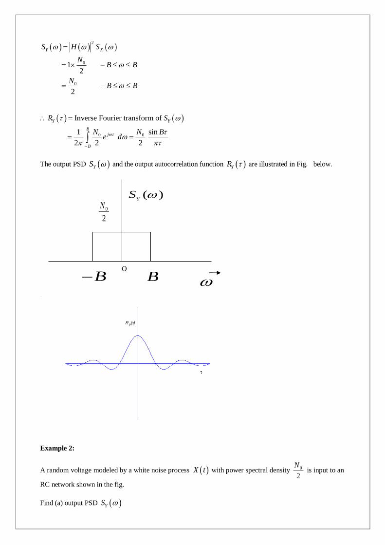
K.RAVEENDRA, Associate Professor, In-charge Examinations Branch, SVEW, TPT. Page 2

2

0

0

12

2

Y XS H S

NB B

NB B

0 0

Inverse Fourier transform of

1 sin

2 2 2

Y Y

B

j

B

R S

N N Be d

The output PSD YS and the output autocorrelation function YR are illustrated in Fig. below.

Example 2:

A random voltage modeled by a white noise process X t with power spectral density 0

2

N is input to an

RC network shown in the fig.

Find (a) output PSD YS

0

2

N

( )Y

S

O

B B

141

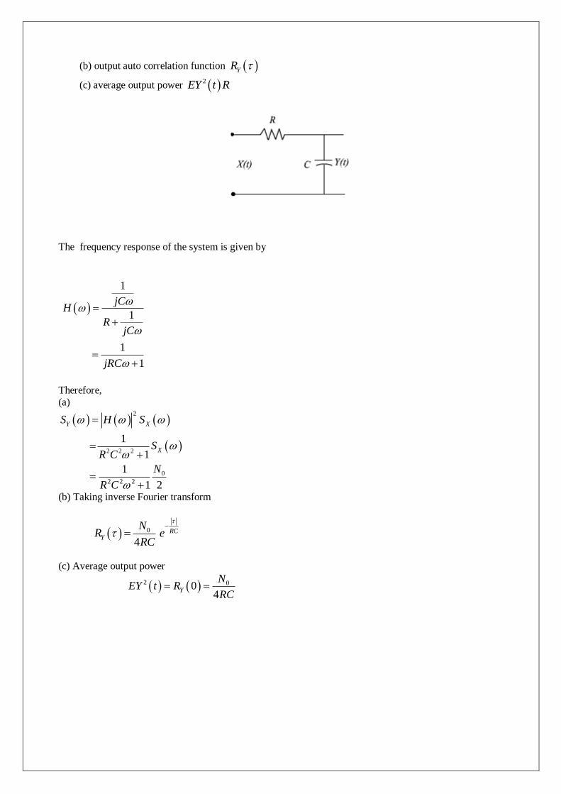
K.RAVEENDRA, Associate Professor, In-charge Examinations Branch, SVEW, TPT. Page 2

(b) output auto correlation function YR

(c) average output power 2EY t R

The frequency response of the system is given by

1

1

1

1

jCH

RjC

jRC

Therefore,

(a)

2

2 2 2

0

2 2 2

1

1

1

1 2

Y X

X

S H S

SR C

N

R C

(b) Taking inverse Fourier transform

0

4RC

Y

NR e

RC

(c) Average output power

2 004

Y

NEY t R

RC

142

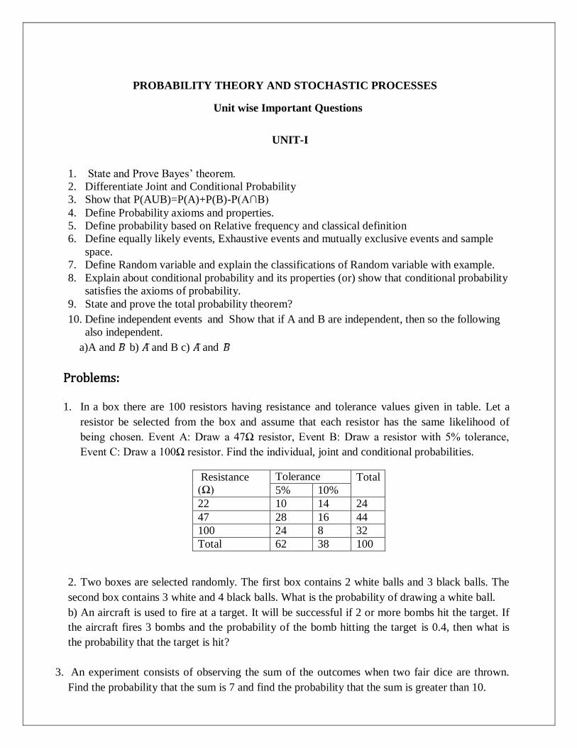
PROBABILITY THEORY AND STOCHASTIC PROCESSES

Unit wise Important Questions

UNIT-I

1. State and Prove Bayes’ theorem.

2. Differentiate Joint and Conditional Probability

3. Show that P(AUB)=P(A)+P(B)-P(A∩B)

4. Define Probability axioms and properties.

5. Define probability based on Relative frequency and classical definition

6. Define equally likely events, Exhaustive events and mutually exclusive events and sample

space.

7. Define Random variable and explain the classifications of Random variable with example.

8. Explain about conditional probability and its properties (or) show that conditional probability

satisfies the axioms of probability.

9. State and prove the total probability theorem?

10. Define independent events and Show that if A and B are independent, then so the following

also independent.

a)A and b) 𝐴 and B c) 𝐴 and

Problems: 1. In a box there are 100 resistors having resistance and tolerance values given in table. Let a

resistor be selected from the box and assume that each resistor has the same likelihood of

being chosen. Event A: Draw a 47Ω resistor, Event B: Draw a resistor with 5% tolerance,

Event C: Draw a 100Ω resistor. Find the individual, joint and conditional probabilities.

Resistance (Ω)

Tolerance Total

5% 10%

22 10 14 24

47 28 16 44

100 24 8 32

Total 62 38 100

2. Two boxes are selected randomly. The first box contains 2 white balls and 3 black balls. The

second box contains 3 white and 4 black balls. What is the probability of drawing a white ball.

b) An aircraft is used to fire at a target. It will be successful if 2 or more bombs hit the target. If

the aircraft fires 3 bombs and the probability of the bomb hitting the target is 0.4, then what is

the probability that the target is hit?

3. An experiment consists of observing the sum of the outcomes when two fair dice are thrown.

Find the probability that the sum is 7 and find the probability that the sum is greater than 10.

143

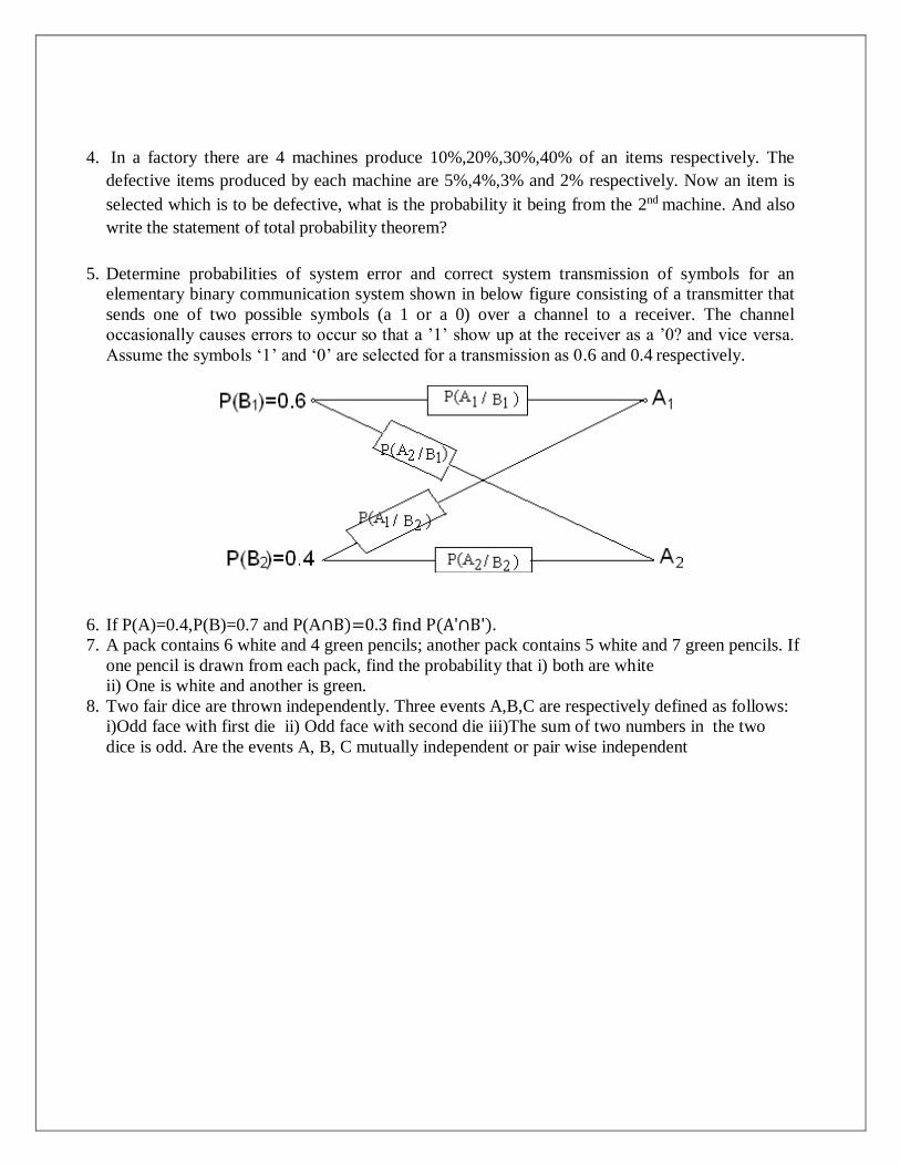
4. In a factory there are 4 machines produce 10%,20%,30%,40% of an items respectively. The

defective items produced by each machine are 5%,4%,3% and 2% respectively. Now an item is

selected which is to be defective, what is the probability it being from the 2nd machine. And also

write the statement of total probability theorem?

5. Determine probabilities of system error and correct system transmission of symbols for an

elementary binary communication system shown in below figure consisting of a transmitter that

sends one of two possible symbols (a 1 or a 0) over a channel to a receiver. The channel

occasionally causes errors to occur so that a ’1’ show up at the receiver as a ’0? and vice versa.

Assume the symbols ‘1’ and ‘0’ are selected for a transmission as 0.6 and 0.4 respectively.

6. If P(A)=0.4,P(B)=0.7 and P(A∩B)=0.3 find P(A'∩B'). 7. A pack contains 6 white and 4 green pencils; another pack contains 5 white and 7 green pencils. If

one pencil is drawn from each pack, find the probability that i) both are white

ii) One is white and another is green.

8. Two fair dice are thrown independently. Three events A,B,C are respectively defined as follows:

i)Odd face with first die ii) Odd face with second die iii)The sum of two numbers in the two

dice is odd. Are the events A, B, C mutually independent or pair wise independent

144

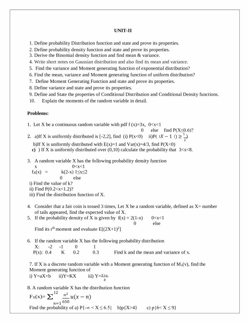
UNIT-II

1. Define probability Distribution function and state and prove its properties.

2. Define probability density function and state and prove its properties.

3. Derive the Binomial density function and find mean & variance.

4. Write short notes on Gaussian distribution and also find its mean and variance.

5. Find the variance and Moment generating function of exponential distribution?

6. Find the mean, variance and Moment generating function of uniform distribution?

7. Define Moment Generating Function and state and prove its properties.

8. Define variance and state and prove its properties.

9. Define and State the properties of Conditional Distribution and Conditional Density functions.

10. Explain the moments of the random variable in detail.

Problems:

1. Let X be a continuous random variable with pdf f (x)=3x, 0<x<1

0 else find P(X≤0.6)?

2. a)If X is uniformly distributed is [-2,2], find (i) P(x<0) ii)P(𝑋 − 1) ≥ 1

) 2

b)If X is uniformly distributed with E(x)=1 and Var(x)=4/3, find P(X<0) c) ) If X is uniformly distributed over (0,10) calculate the probability that 3<x<8.

3. A random variable X has the following probability density function

x 0<x<1 fX(x) = k(2-x) 1≤x≤2

0 else i) Find the value of k?

ii) Find P(0.2<x<1.2)?

iii) Find the distribution function of X.

4. Consider that a fair coin is tossed 3 times, Let X be a random variable, defined as X= number

of tails appeared, find the expected value of X.

5. If the probability density of X is given by f(x) = 2(1-x) 0<x<1 0 else

Find its rth moment and evaluate E[(2X+1)2]

6. If the random variable X has the following probability distribution

X: -2 -1 0 1

P(x): 0.4 K 0.2 0.3 Find k and the mean and variance of x.

7. If X is a discrete random variable with a Moment generating function of Mx(v), find the Moment generating function of

i) Y=aX+b ii)Y=KX iii) Y=𝑋+𝑎 𝑏

8. A random variable X has the distribution function 12

FX(x)= ∑ 𝑛2 𝑢(𝑥 − 𝑛)

𝑛=1 650

Find the probability of a) P-∞ < X ≤ 6.5 b)pX>4 c) p6< X ≤ 9

145

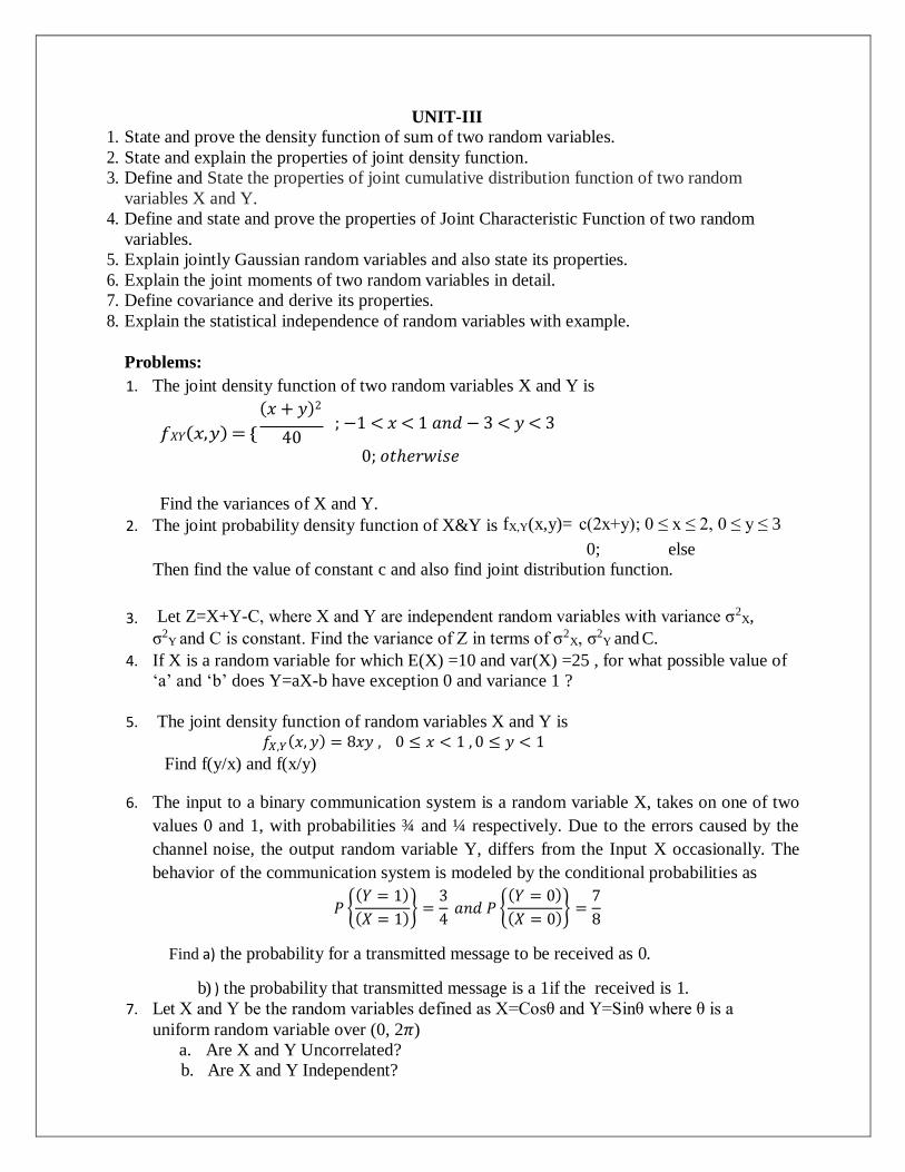
UNIT-III

1. State and prove the density function of sum of two random variables.

2. State and explain the properties of joint density function.

3. Define and State the properties of joint cumulative distribution function of two random

variables X and Y.

4. Define and state and prove the properties of Joint Characteristic Function of two random

variables.

5. Explain jointly Gaussian random variables and also state its properties.

6. Explain the joint moments of two random variables in detail.

7. Define covariance and derive its properties.

8. Explain the statistical independence of random variables with example.

Problems:

1. The joint density function of two random variables X and Y is

(𝑥 + 𝑦)2

𝑓𝑋𝑌(𝑥, 𝑦) = ; −1 < 𝑥 < 1 𝑎𝑛𝑑 − 3 < 𝑦 < 3

40 0; 𝑜𝑡ℎ𝑒𝑟𝑤𝑖𝑠𝑒

Find the variances of X and Y.

2. The joint probability density function of X&Y is fX,Y(x,y)= c(2x+y); 0 ≤ x ≤ 2, 0 ≤ y ≤ 3

0; else

Then find the value of constant c and also find joint distribution function.

3. Let Z=X+Y-C, where X and Y are independent random variables with variance σ2

X,

σ2Y and C is constant. Find the variance of Z in terms of σ2

X, σ2Y and C.

4. If X is a random variable for which E(X) =10 and var(X) =25 , for what possible value of

‘a’ and ‘b’ does Y=aX-b have exception 0 and variance 1 ?

5. The joint density function of random variables X and Y is 𝑓𝑋,𝑌(𝑥, 𝑦) = 8𝑥𝑦 , 0 ≤ 𝑥 < 1 , 0 ≤ 𝑦 < 1

Find f(y/x) and f(x/y)

6. The input to a binary communication system is a random variable X, takes on one of two

values 0 and 1, with probabilities ¾ and ¼ respectively. Due to the errors caused by the

channel noise, the output random variable Y, differs from the Input X occasionally. The

behavior of the communication system is modeled by the conditional probabilities as

𝑃 (𝑌 = 1)

(𝑋 = 1) =

3

4 𝑎𝑛𝑑 𝑃

(𝑌 = 0)

(𝑋 = 0) =

7

8

Find a) the probability for a transmitted message to be received as 0.

b) ) the probability that transmitted message is a 1if the received is 1.

7. Let X and Y be the random variables defined as X=Cosθ and Y=Sinθ where θ is a

uniform random variable over (0, 2𝜋)

a. Are X and Y Uncorrelated?

b. Are X and Y Independent?

146

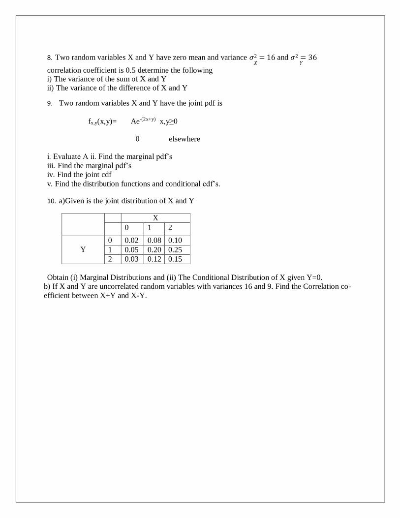
8. Two random variables X and Y have zero mean and variance 𝜎2 = 16 and 𝜎2 = 36 𝑋 𝑌

correlation coefficient is 0.5 determine the following i) The variance of the sum of X and Y

ii) The variance of the difference of X and Y

9. Two random variables X and Y have the joint pdf is

fx,y(x,y)= Ae-(2x+y) x,y≥0

0 elsewhere

i. Evaluate A ii. Find the marginal pdf’s

iii. Find the marginal pdf’s

iv. Find the joint cdf

v. Find the distribution functions and conditional cdf’s.

10. a)Given is the joint distribution of X and Y

X

0 1 2

Y

0 0.02 0.08 0.10

1 0.05 0.20 0.25

2 0.03 0.12 0.15

Obtain (i) Marginal Distributions and (ii) The Conditional Distribution of X given Y=0.

b) If X and Y are uncorrelated random variables with variances 16 and 9. Find the Correlation co-

efficient between X+Y and X-Y.

147

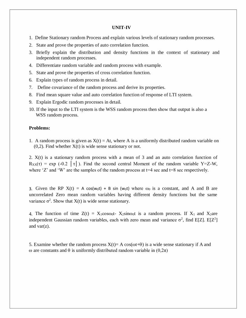
UNIT-IV

1. Define Stationary random Process and explain various levels of stationary random processes.

2. State and prove the properties of auto correlation function.

3. Briefly explain the distribution and density functions in the context of stationary and

independent random processes.

4. Differentiate random variable and random process with example.

5. State and prove the properties of cross correlation function.

6. Explain types of random process in detail.

7. Define covariance of the random process and derive its properties.

8. Find mean square value and auto correlation function of response of LTI system.

9. Explain Ergodic random processes in detail.

10. If the input to the LTI system is the WSS random process then show that output is also a

WSS random process.

Problems:

1. A random process is given as X(t) = At, where A is a uniformly distributed random variable on

(0,2). Find whether X(t) is wide sense stationary or not.

2. X(t) is a stationary random process with a mean of 3 and an auto correlation function of

RXX(τ) = exp (-0.2 τ). Find the second central Moment of the random variable Y=Z-W,

where ‘Z’ and ‘W’ are the samples of the random process at t=4 sec and t=8 sec respectively.

3. Given the RP X(t) = A cos(w0t) + B sin (w0t) where ω0 is a constant, and A and B are

uncorrelated Zero mean random variables having different density functions but the same

variance σ2. Show that X(t) is wide sense stationary.

4. The function of time Z(t) = X1cosω0t- X2sinω0t is a random process. If X1 and X2are

independent Gaussian random variables, each with zero mean and variance σ2, find E[Z]. E[Z2]

and var(z).

5. Examine whether the random process X(t)= A cos(t+) is a wide sense stationary if A and

are constants and is uniformly distributed random variable in (0,2π)

148

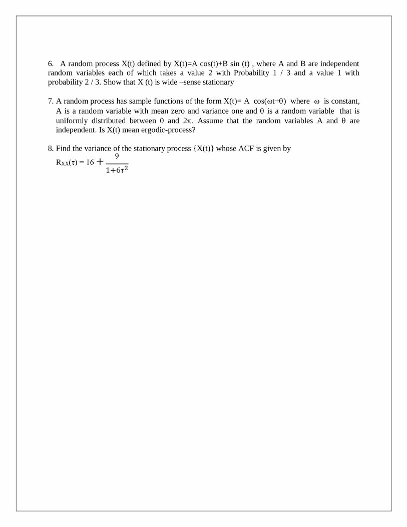
6. A random process X(t) defined by X(t)=A cos(t)+B sin (t) , where A and B are independent

random variables each of which takes a value 2 with Probability 1 / 3 and a value 1 with

probability 2 / 3. Show that X (t) is wide –sense stationary

7. A random process has sample functions of the form X(t)= A cos(t+) where is constant,

A is a random variable with mean zero and variance one and is a random variable that is

uniformly distributed between 0 and 2. Assume that the random variables A and are

independent. Is X(t) mean ergodic-process?

8. Find the variance of the stationary process X(t) whose ACF is given by 9

RXX(τ) = 16 + 1+6𝜏2

149

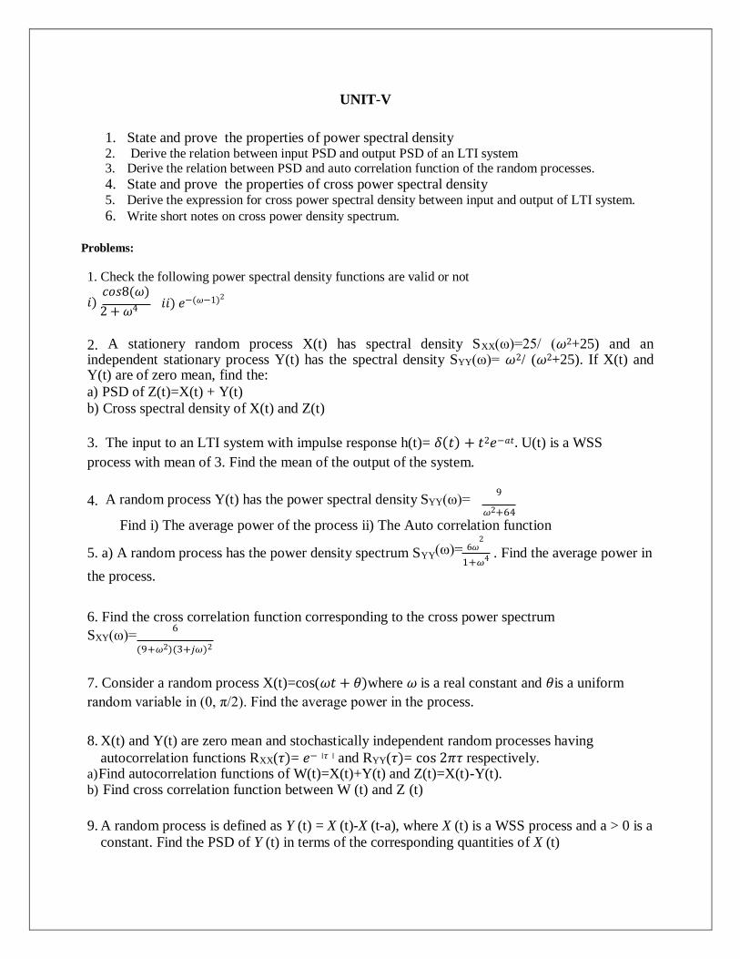
YY 4

UNIT-V

1. State and prove the properties of power spectral density 2. Derive the relation between input PSD and output PSD of an LTI system 3. Derive the relation between PSD and auto correlation function of the random processes.

4. State and prove the properties of cross power spectral density 5. Derive the expression for cross power spectral density between input and output of LTI system.

6. Write short notes on cross power density spectrum. Problems:

1. Check the following power spectral density functions are valid or not 𝑐𝑜𝑠8(𝜔)

𝑖) 2 + 𝜔4

𝑖𝑖) 𝑒−(𝜔−1)2

2. A stationery random process X(t) has spectral density SXX(ω)=25/ (𝜔2+25) and an independent stationary process Y(t) has the spectral density SYY(ω)= 𝜔2/ (𝜔2+25). If X(t) and Y(t) are of zero mean, find the:

a) PSD of Z(t)=X(t) + Y(t)

b) Cross spectral density of X(t) and Z(t)

3. The input to an LTI system with impulse response h(t)= 𝛿(𝑡) + 𝑡2𝑒−𝑎𝑡. U(t) is a WSS

process with mean of 3. Find the mean of the output of the system.

4. A random process Y(t) has the power spectral density SYY(ω)= 9

𝜔2+64

Find i) The average power of the process ii) The Auto correlation function

5. a) A random process has the power density spectrum S

the process.

(ω)= 6𝜔2

1+𝜔 . Find the average power in

6. Find the cross correlation function corresponding to the cross power spectrum

SXY(ω)= 6

(9+𝜔2)(3+𝑗𝜔)2

7. Consider a random process X(t)=cos(𝜔𝑡 + 𝜃)where 𝜔 is a real constant and 𝜃is a uniform

random variable in (0, π/2). Find the average power in the process.

8. X(t) and Y(t) are zero mean and stochastically independent random processes having

autocorrelation functions RXX(𝜏)= 𝑒−𝜏 and RYY(𝜏)= cos 2𝜋𝜏 respectively. a) Find autocorrelation functions of W(t)=X(t)+Y(t) and Z(t)=X(t)-Y(t). b) Find cross correlation function between W (t) and Z (t)

9. A random process is defined as Y (t) = X (t)-X (t-a), where X (t) is a WSS process and a > 0 is a

constant. Find the PSD of Y (t) in terms of the corresponding quantities of X (t)

150