Probability Course web page: vision.cis.udel.edu/cv March 19, 2003 Lecture 15.

Probability

Course web page:vision.cis.udel.edu/cv

March 19, 2003 Lecture 15

Announcements

• Read Forsyth & Ponce, Chapter 1.2, 1.4, 7.4 on cameras, sampling for Friday

Outline

• Random variables– Discrete– Continuous

• Joint, conditional probability• Probabilistic inference

Discrete Random Variables

• A discrete random variable X has a domain of

values fx1, …, xng that it can assume, each with a particular probability in the range [0, 1]

• For example, let X = Weather. Then the domain might be fsun, rain, clouds , snowg

• Use A, B to denote boolean random variables whose domain is ftrue, falseg

Discrete Probability

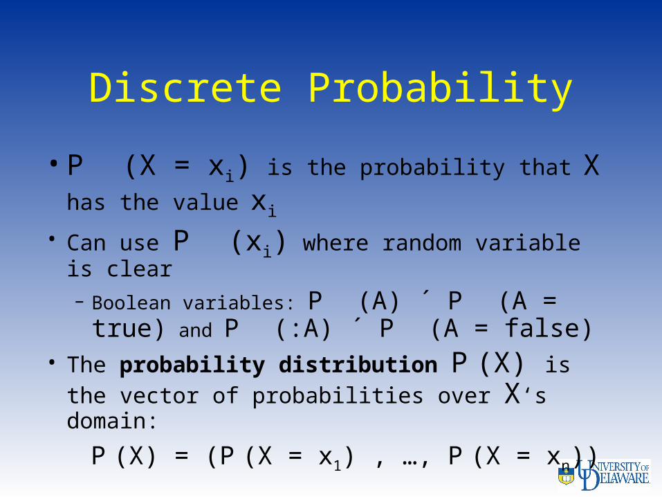
• P (X = xi) is the probability that X has

the value xi

• Can use P (xi) where random variable is clear– Boolean variables: P (A) ´ P (A = true)

and P (:A) ´ P (A = false)• The probability distribution P (X) is the

vector of probabilities over X‘s domain:

P (X) = (P (X = x1) , …, P (X = xn))

Meaning of Probability

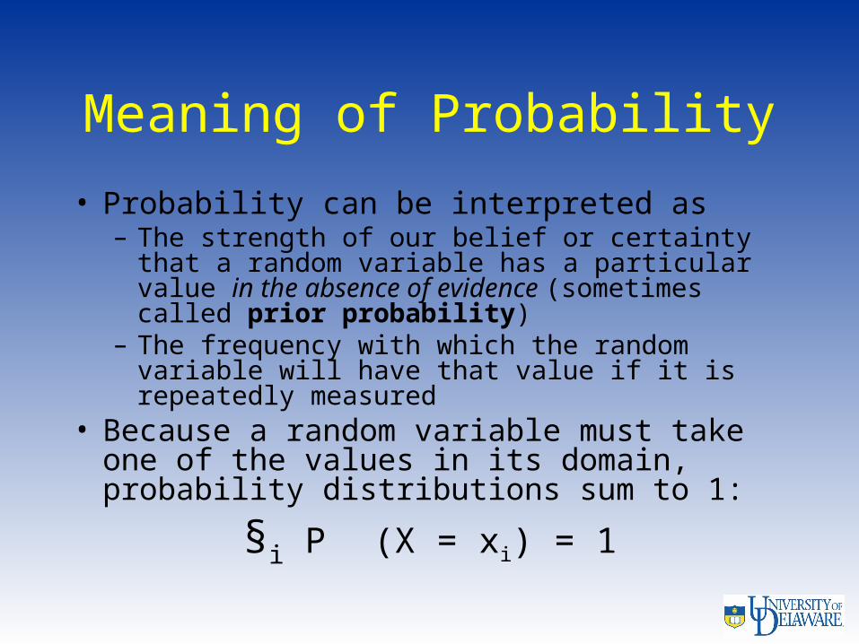
• Probability can be interpreted as– The strength of our belief or certainty that a

random variable has a particular value in the absence of evidence (sometimes called prior probability)

– The frequency with which the random variable will have that value if it is repeatedly measured

• Because a random variable must take one of the values in its domain, probability distributions sum to 1:

§i P (X = xi) = 1

Example: Distribution on Weather

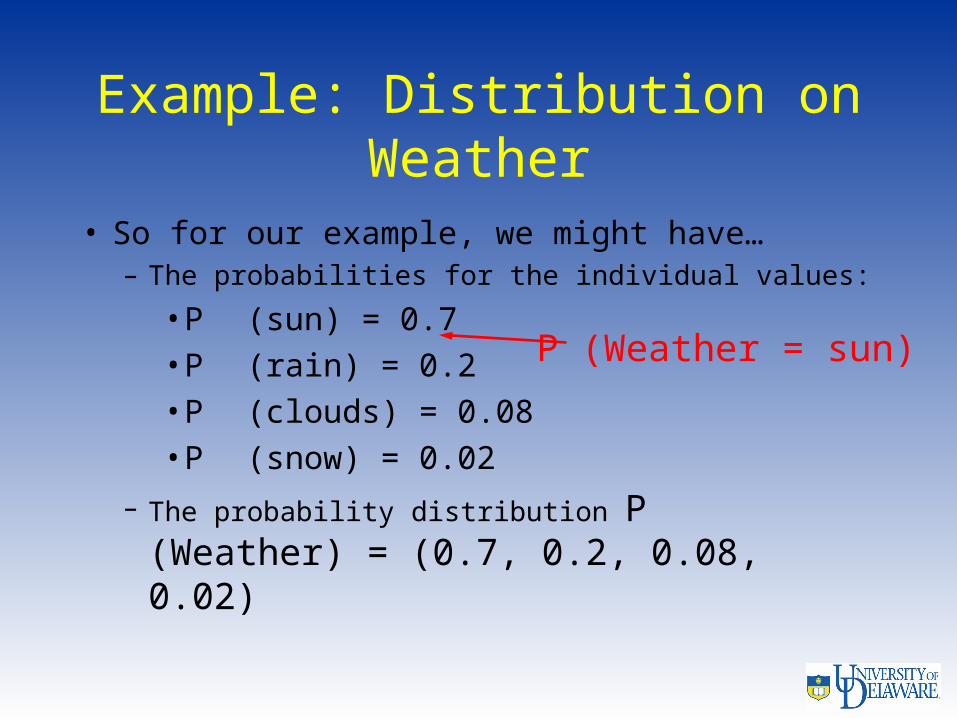
• So for our example, we might have…– The probabilities for the individual values:

•P (sun) = 0.7•P (rain) = 0.2•P (clouds) = 0.08•P (snow) = 0.02

– The probability distribution P (Weather) = (0.7, 0.2, 0.08, 0.02)

P (Weather = sun)

Joint Probability

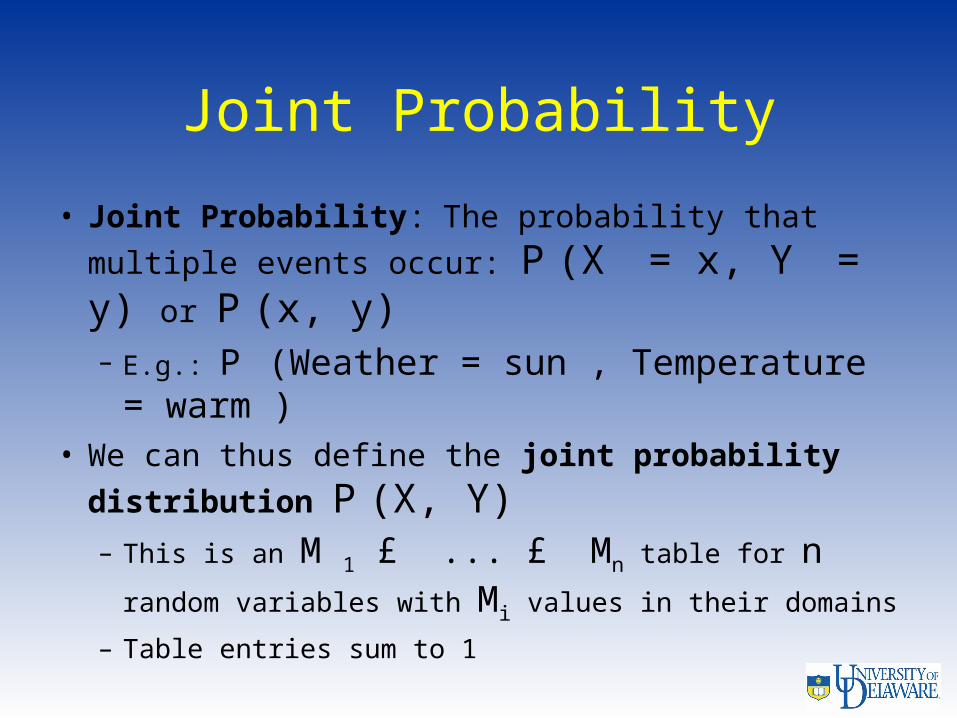
• Joint Probability: The probability that

multiple events occur: P (X = x, Y = y) or

P (x, y)– E.g.: P (Weather = sun , Temperature =

warm ) • We can thus define the joint probability

distribution P (X, Y)– This is an M 1 £ ... £ Mn table for n random

variables with Mi values in their domains

– Table entries sum to 1

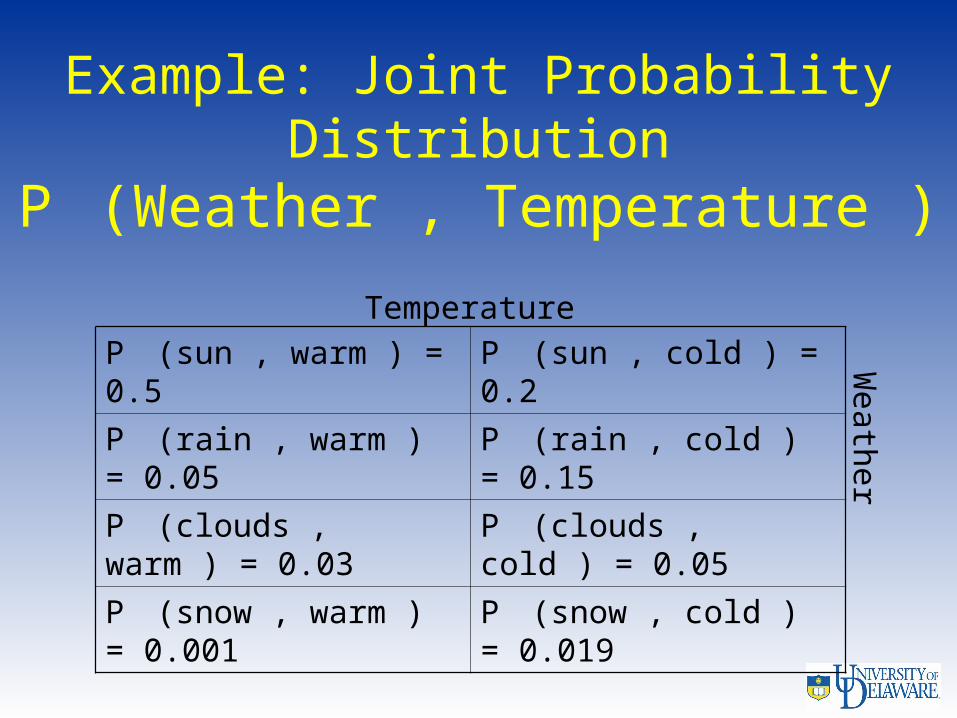
Example: Joint Probability Distribution

P (Weather , Temperature )

P (sun , warm ) = 0.5 P (sun , cold ) = 0.2

P (rain , warm ) = 0.05

P (rain , cold ) = 0.15

P (clouds , warm ) = 0.03

P (clouds , cold ) = 0.05

P (snow , warm ) = 0.001

P (snow , cold ) = 0.019

Weath

er

Temperature

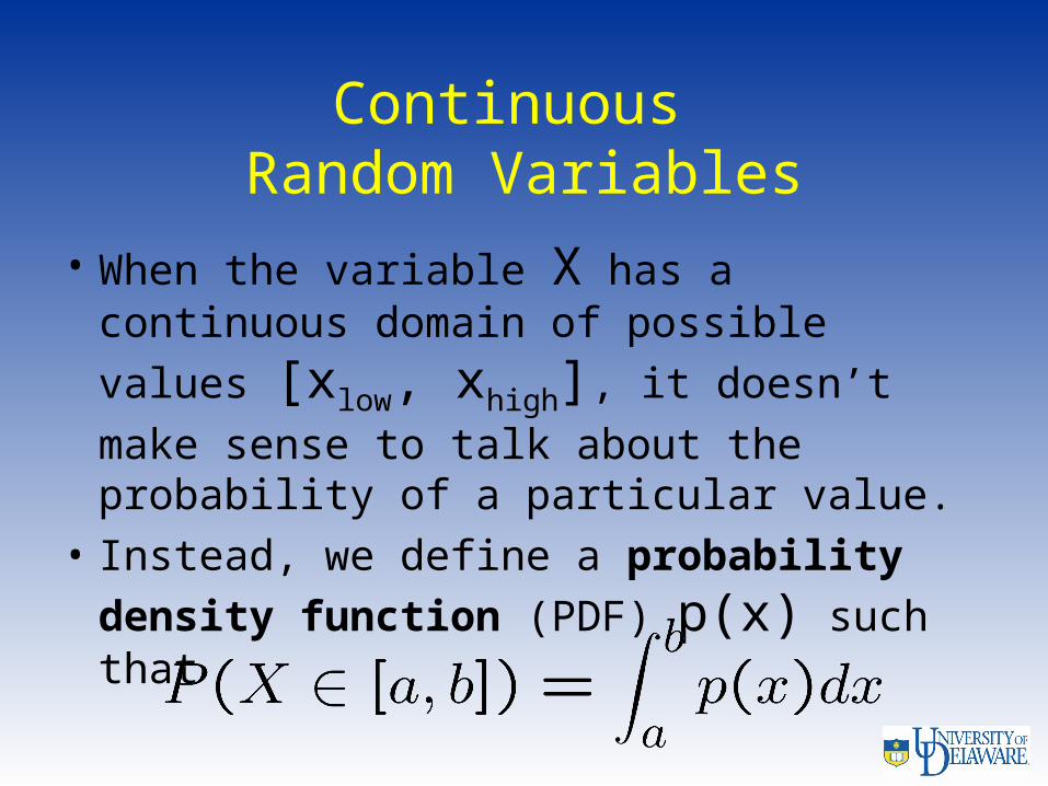
Continuous Random Variables

• When the variable X has a continuous

domain of possible values [xlow, xhigh], it doesn’t make sense to talk about the probability of a particular value.

• Instead, we define a probability density function (PDF) p(x) such that

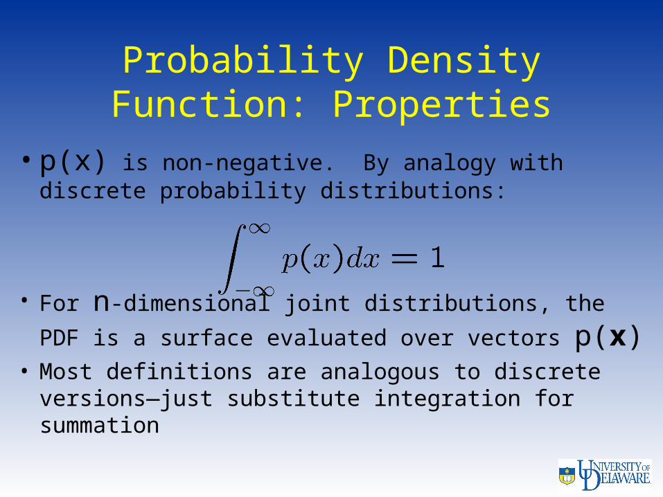
Probability Density Function: Properties

• p(x) is non-negative. By analogy with discrete probability distributions:

• For n-dimensional joint distributions, the PDF

is a surface evaluated over vectors p(x)• Most definitions are analogous to discrete

versions—just substitute integration for summation

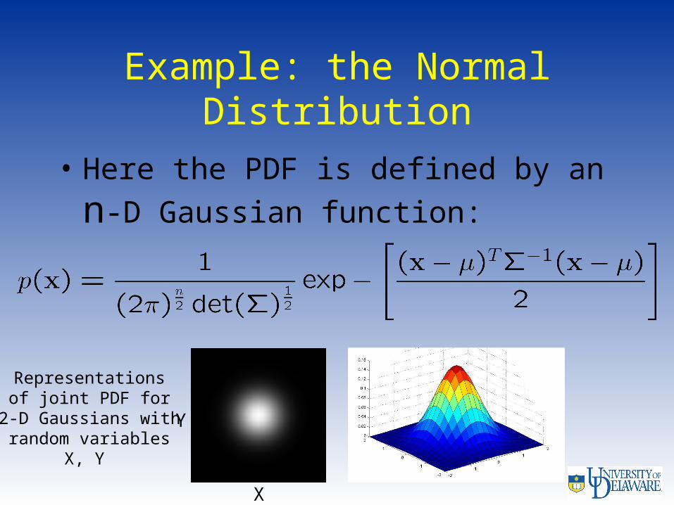
Example: the Normal Distribution

• Here the PDF is defined by an n-D Gaussian function:

Representationsof joint PDF for

2-D Gaussians withrandom variables

X, Y

Y

X

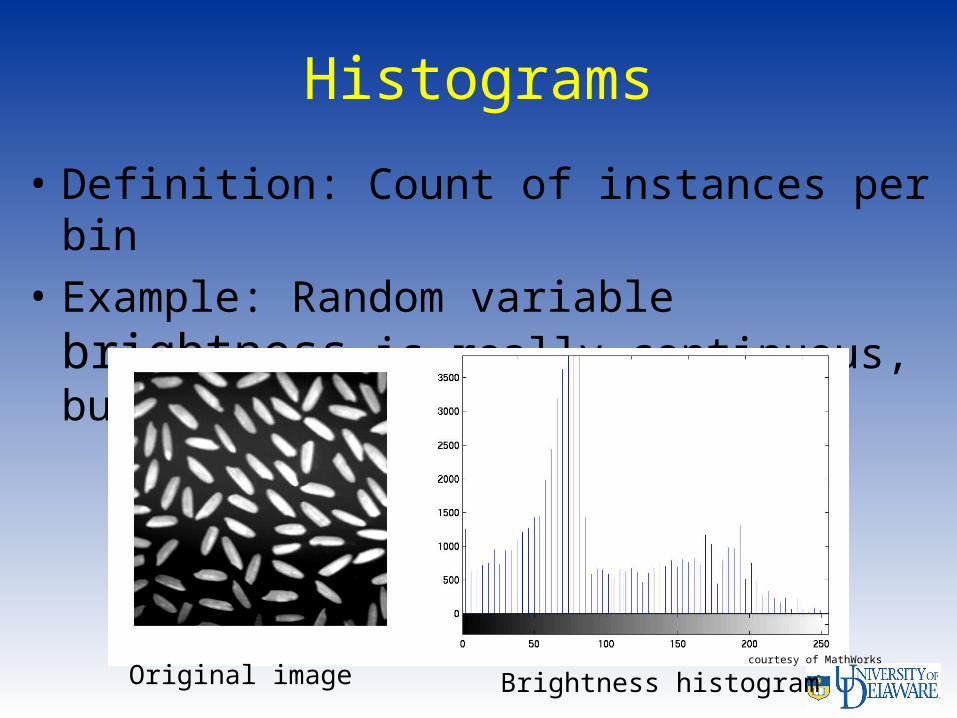
Histograms

• Definition: Count of instances per bin

• Example: Random variable brightness is really continuous, but discretized to [0, 255]

courtesy of MathWorks

Brightness histogramOriginal image

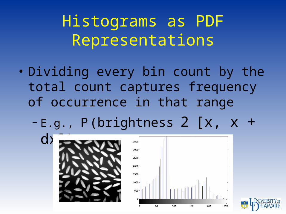
Histograms as PDF Representations

• Dividing every bin count by the total count captures frequency of occurrence in that range

– E.g., P (brightness 2 [x, x + dx])

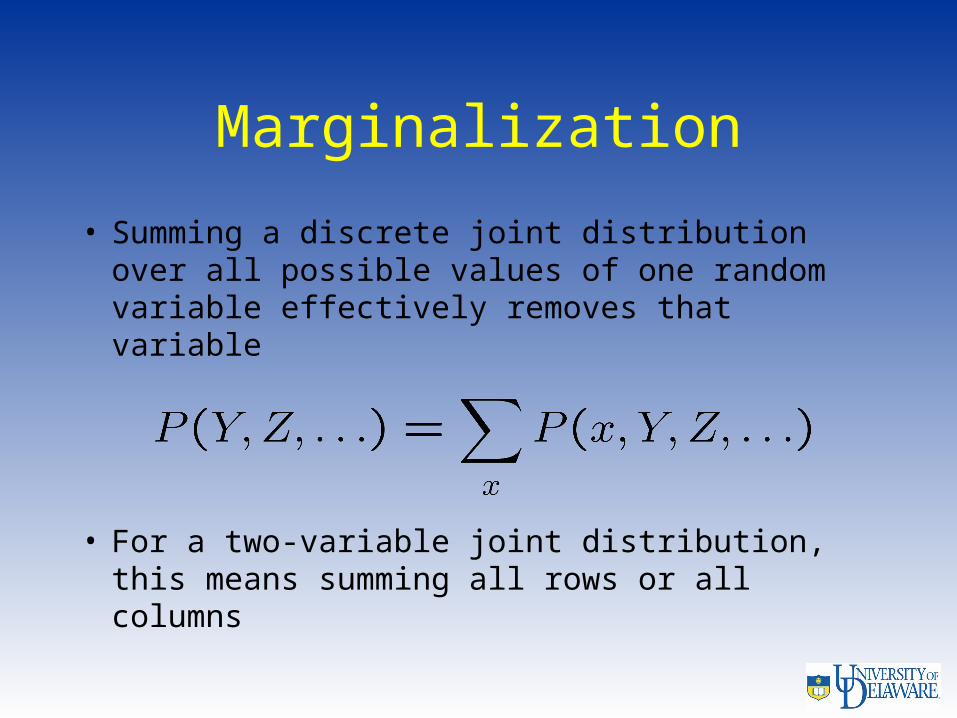
Marginalization

• Summing a discrete joint distribution over all possible values of one random variable effectively removes that variable

• For a two-variable joint distribution, this means summing all rows or all columns

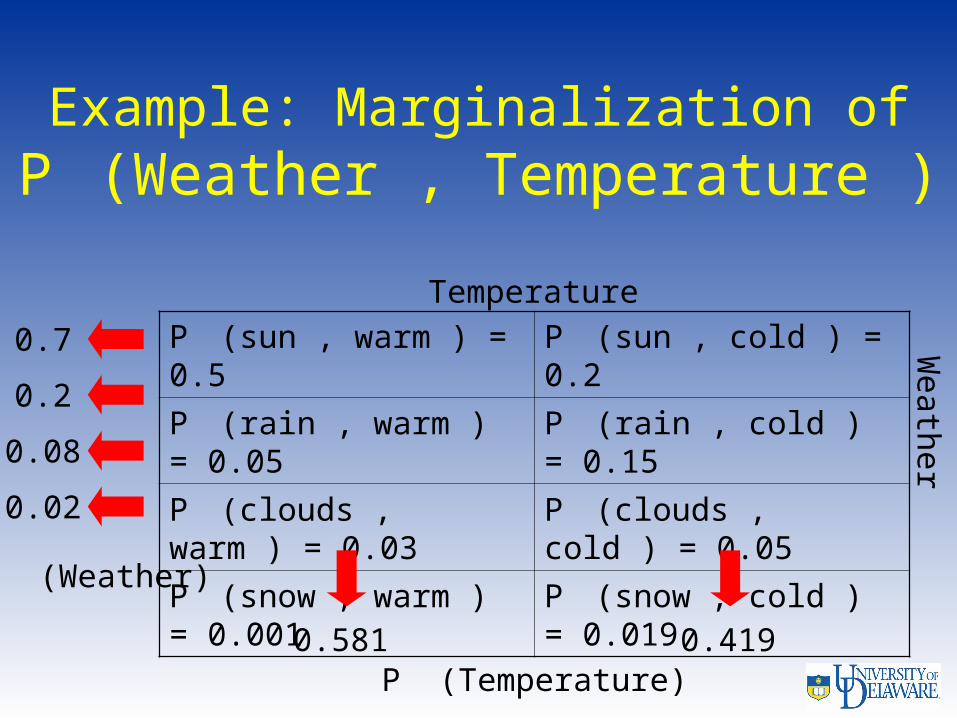
Example: Marginalization ofP (Weather , Temperature )

P (sun , warm ) = 0.5 P (sun , cold ) = 0.2

P (rain , warm ) = 0.05

P (rain , cold ) = 0.15

P (clouds , warm ) = 0.03

P (clouds , cold ) = 0.05

P (snow , warm ) = 0.001

P (snow , cold ) = 0.019

Weath

er

Temperature

0.7

0.2

0.08

0.02

0.581 0.419P (Temperature)

P (Weather)

Conditional Probability

• The conditional probability P (X = x j Y = y) quantifies the change in our beliefs given knowledge of some other event. This “after the evidence” probability is sometimes called the posterior probability on X, and it is defined with the product rule:

P (X = x, Y = y) = P (X = x j Y = y) P (Y = y)

• In terms of joint probability distributions, this is:

P (X, Y) = P (X j Y) P (Y)• Independence: P (X, Y) = P (X ) P (Y), which

implies that P (X j Y) = P (X)remember that these are different distributions

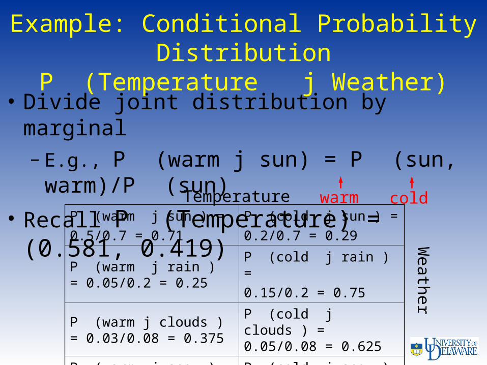
Example: Conditional Probability Distribution

P (Temperature j Weather)• Divide joint distribution by marginal

– E.g., P (warm j sun) = P (sun, warm)/P (sun)

• Recall P (Temperature) = (0.581, 0.419)P (warm j sun ) =

0.5/0.7 = 0.71P (cold j sun ) = 0.2/0.7 = 0.29

P (warm j rain ) = 0.05/0.2 = 0.25

P (cold j rain ) = 0.15/0.2 = 0.75

P (warm j clouds ) = 0.03/0.08 = 0.375

P (cold j clouds ) = 0.05/0.08 = 0.625

P (warm j snow ) = 0.001/0.02 = 0.05

P (cold j snow ) = 0.019/0.02 = 0.95

Weath

er

Temperature warm cold

Conditioning

• By the relationship of conditional probability to joint probability

P (Y , X) = P (Y j X) P (X)we can write marginalization a different way:

Bayes’ Rule

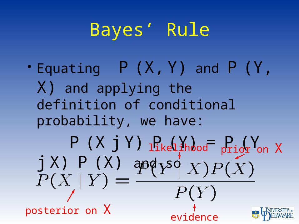
• Equating P (X, Y) and P (Y, X) and applying the definition of conditional probability, we have:

P (X j Y) P (Y) = P (Y j X) P (X) and so

likelihood prior on X

posterior on Xevidence

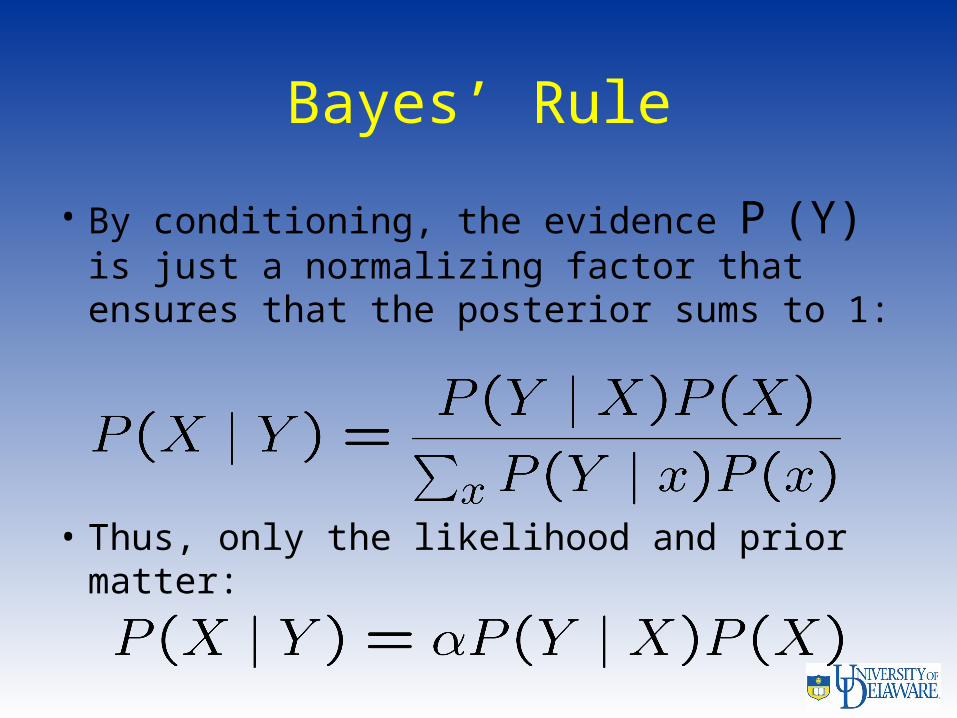
Bayes’ Rule

• By conditioning, the evidence P (Y) is just a normalizing factor that ensures that the posterior sums to 1:

• Thus, only the likelihood and prior matter:

Bayes’ Rule for Inference

• Suppose X represents possible hypotheses about some aspect of the world (e.g., the weather today), and Y represents some relevant data we have measured (e.g., thermometer temperature). Inference is the process of reasoning about how likely different values of X are conditioned on Y

• Bayes’ rule can be a useful inference tool when there is an imbalance in our knowledge or it is difficult to quantify hypothesis probabilities directly

• Inferring hypothesis values is often called parameter estimation

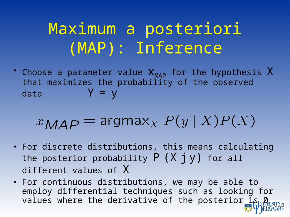
Maximum a posteriori (MAP): Inference

• Choose a parameter value xMAP for the hypothesis X that maximizes the probability of the observed data Y = y

• For discrete distributions, this means calculating the posterior probability P (X j y) for all different values of X

• For continuous distributions, we may be able to employ differential techniques such as looking for values where the derivative of the posterior is 0

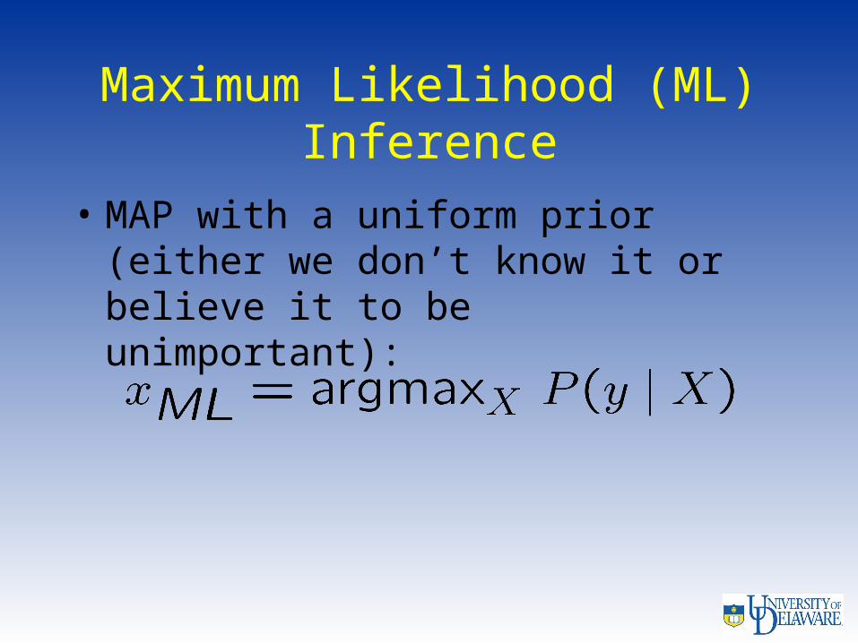
Maximum Likelihood (ML) Inference

• MAP with a uniform prior (either we don’t know it or believe it to be unimportant):

Example: Estimating the Temperature

• Suppose we want to know what the weather will be like on the basis of a thermometer reading

• Say we don’t have direct knowledge of P (Weather j Temperature), but the thermometer reading indicates a chill, and we do know something about P (Temperature j Weather)

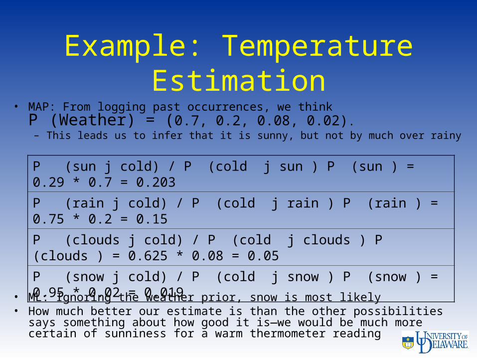
Example: Temperature Estimation

• MAP: From logging past occurrences, we think P (Weather) = (0.7, 0.2, 0.08, 0.02). – This leads us to infer that it is sunny, but not by much over rainy

• ML: Ignoring the weather prior, snow is most likely• How much better our estimate is than the other possibilities says

something about how good it is—we would be much more certain of sunniness for a warm thermometer reading

P (sun j cold) / P (cold j sun ) P (sun ) = 0.29 * 0.7 = 0.203

P (rain j cold) / P (cold j rain ) P (rain ) = 0.75 * 0.2 = 0.15

P (clouds j cold) / P (cold j clouds ) P (clouds ) = 0.625 * 0.08 = 0.05

P (snow j cold) / P (cold j snow ) P (snow ) = 0.95 * 0.02 = 0.019