Probabilistic Subgraph Matching Based on Convex Relaxation

Probabilistic Subgraph Matching Based on

Convex Relaxation

Christian Schellewald and Christoph Schnorr

Computer Vision, Graphics, and Pattern Recognition GroupDepartment of Mathematics and Computer Science;

University of Mannheim, D-68131 Mannheim, Germany

{cschelle,schnoerr}@ti.uni-mannheim.dehttp://www.cvgpr.uni-mannheim.de

Abstract. We present a novel approach to the matching of subgraphsfor object recognition in computer vision. Feature similarities betweenobject model and scene graph are complemented with a regularizationterm that measures differences of the relational structure. For the re-sulting quadratic integer program, a mathematically tight relaxation isderived by exploiting the degrees of freedom of the embedding space ofpositive semidefinite matrices. We show that the global minimum of therelaxed convex problem can be interpreted as probability distributionover the original space of matching matrices, providing a basis for effi-ciently sampling all close-to-optimal combinatorial matchings within theoriginal solution space. As a result, the approach can even handle com-pletely ambiguous situations, despite uniqueness of the relaxed convexproblem. Exhaustive numerical experiments demonstrate the promisingperformance of the approach which – up to a single inevitable regu-larization parameter that weights feature similarity against structuralsimilarity – is free of any further tuning parameters.

1 Introduction

Recognition of objects by matching relational structures of local features is akey problem of computer vision. Since such structures were suggested for imageanalysis in 1971 by Barrow and Popplestone [1], a very broad range of approacheshave been suggested to cope with the inherent combinatorial complexity of thecorresponding matching problem. A non-exhaustive list of relevant work includestree search algorithms [2], evolutionary strategies [3], spectral approaches [4, 5],the expectation maximization framework [6], matching of structures in terms ofgeneralized maximum clique search [7], interpolation-based matching [8], metricembedding [9], matching by graph seriation and sequence alignment [10], andexact probabilistic inference using sparse graphical models with computationallyfeasible junction trees [11]. Since a general discussion of related work is beyondthe scope of this contribution, we refer to [12] for a recent survey.

The specific motivation for our work comes from two different directions. Thefirst line of research originates from independent work of Gold and Rangarajan

[13] and Ishii and Sato [14] on deterministic annealing strategies for the matchingof relational structures with equal number of nodes over the convex hull of allpermutation matrices (cf. also [15, 16]). The second line of research concernsspecific instances of the general pattern of convex relaxations of combinatorialinteger programming problems [17, 18] to the specific problem addressed in [13,14], the quadratic assignment problem [19, 20]. Using established benchmarktests [21], a thorough experimental comparison of both approaches [22] revealedsimilar performance, provided the used parameters for deterministic annealing[13, 14] are optimized for each problem instance, whereas no parameter tuningis necessary for a convex relaxation approach [19, 20].

The applicability of approaches related to the quadratic assignment problemis limited to the matching of relational structures with feature sets of (almost)equal cardinality. From the viewpoint of computer vision, such approaches arenot applicable to the more frequent scenario of matching smaller model graphs

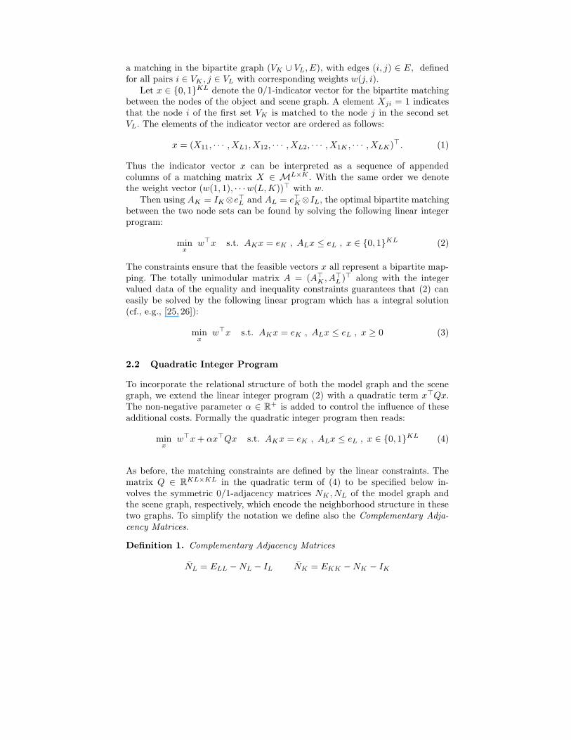
representing typical object views, to larger scene graphs representing currentobservations – see Figure 1 for an illustration.

The present paper is an attempt to overcome this limitation by a novel op-timization approach to subgraph matching. From the computational viewpoint,we consistently use semidefinite relaxation, as motivated by the discussion above,and by its performance in connection various combinatorial problems in com-puter vision [23, 24]. Besides obtaining parameter-free algorithms, we point outan additional benefit of this relaxation strategy – the interpretation of the glob-ally optimal solution to the relaxed problem as probability distribution over theoriginal combinatorial solution space. While this possibility is obvious from themathematical viewpoint, it is by no means clear that this conveys useful infor-mation about the complex original solution space. This interpretation shows,however, that uniqueness in a larger embedding space is associated with the ex-plicit representation of multiple hypotheses in the original space. In particular,our approach can cope with ambiguous situations. This accounts for a anothernovel aspect of our contribution.

Organization. We design a variational problem to subgraph matching insection 2. The domain of the resulting quadratic functional is the space of bi-nary matching matrices. The optimality of the matchings is defined in termsof feature similarities and structural similarities, weighted by a single regular-ization parameter. In section 3, a semidefinite relaxation of this combinatorialoptimization problem is derived. The additional degrees of freedom of the largerembedding space are exploited to incorporate constraints of the original prob-lem formulation, thus tightening the relaxation mathematically. A probabilisticinterpretation of the corresponding globally optimal solution and its ability tocope with ambiguous situations, is discussed in section 4. We summarize exhaus-tive numerical experiments in section 5 that characterize the performance of ourapproach.

Notation. We will use the following notation throughout this paper:x>: transpose of x; In: n × n unit matrix; en: vector of all ones: (en)i = 1, i =1, . . . , n; Enn: matrix of all ones: Enn = ee>; Tr[X ] trace of the matrix X ; A⊗B:

Kronecker product of matrices A and B; δij : Kronecker delta: δij = 1 if i = j,and 0 otherwise; Mn×m: set of n×m matching matrices; diag(X): vector of thediagonal elements of the matrix X .

2 Variational Approach

In this paper, we consider undirected graphs G = (V, E) with nodes V ={1, . . . , n} and edges E ⊂ V × V . We denote the model graph with GK andthe scene graph with GL. The corresponding sets VK and VL contain K = |VK |and L = |VL| nodes respectively. We assume L ≥ K. Furthermore, we assume adistance function w(i, j) to be given which measures the similarity of each pairof vertices i ∈ VK and j ∈ VL.

Graphs representing object views are called model graphs or object graphs

in this paper. In the same way as model graphs, scene graphs are computed byextracting local image features and spatial relationships in a preprocessing step.Our aim is to find a reasonable matching between the nodes of the model graphand the scene graph. In figure 1 a example for a subgraph matching problemis shown. The left object graph GK has to be matched against the scene graphGL. We do not discuss image preprocessing in this paper (cf. section 5.1, first

Fig. 1. The object graph GK (left) with K = 12 nodes has to be matched against thescene graph (left) with L = 41 nodes. Local feature information is ambiguous.

paragraph) but assume the model and scene graphs to be given, along with asimilarity between the nodes of the different graphs.

2.1 Bipartite Matching

If we ignore the structure in both the model and the scene graph, then anoptimal assignment of the K vertices of the model graph can be easily found as

a matching in the bipartite graph (VK ∪ VL, E), with edges (i, j) ∈ E, definedfor all pairs i ∈ VK , j ∈ VL with corresponding weights w(j, i).

Let x ∈ {0, 1}KL denote the 0/1-indicator vector for the bipartite matchingbetween the nodes of the object and scene graph. A element Xji = 1 indicatesthat the node i of the first set VK is matched to the node j in the second setVL. The elements of the indicator vector are ordered as follows:

x = (X11, · · · , XL1, X12, · · · , XL2, · · · , X1K , · · · , XLK)>. (1)

Thus the indicator vector x can be interpreted as a sequence of appendedcolumns of a matching matrix X ∈ ML×K . With the same order we denotethe weight vector (w(1, 1), · · ·w(L, K))> with w.

Then using AK = IK ⊗e>L and AL = e>K⊗IL, the optimal bipartite matchingbetween the two node sets can be found by solving the following linear integerprogram:

minx

w>x s.t. AKx = eK , ALx ≤ eL , x ∈ {0, 1}KL (2)

The constraints ensure that the feasible vectors x all represent a bipartite map-ping. The totally unimodular matrix A = (A>

K , A>L )> along with the integer

valued data of the equality and inequality constraints guarantees that (2) caneasily be solved by the following linear program which has a integral solution(cf., e.g., [25, 26]):

minx

w>x s.t. AKx = eK , ALx ≤ eL , x ≥ 0 (3)

2.2 Quadratic Integer Program

To incorporate the relational structure of both the model graph and the scenegraph, we extend the linear integer program (2) with a quadratic term x>Qx.The non-negative parameter α ∈ R

+ is added to control the influence of theseadditional costs. Formally the quadratic integer program then reads:

minx

w>x + αx>Qx s.t. AKx = eK , ALx ≤ eL , x ∈ {0, 1}KL (4)

As before, the matching constraints are defined by the linear constraints. Thematrix Q ∈ R

KL×KL in the quadratic term of (4) to be specified below in-volves the symmetric 0/1-adjacency matrices NK , NL of the model graph andthe scene graph, respectively, which encode the neighborhood structure in thesetwo graphs. To simplify the notation we define also the Complementary Adja-

cency Matrices.

Definition 1. Complementary Adjacency Matrices

NL = ELL − NL − IL NK = EKK − NK − IK

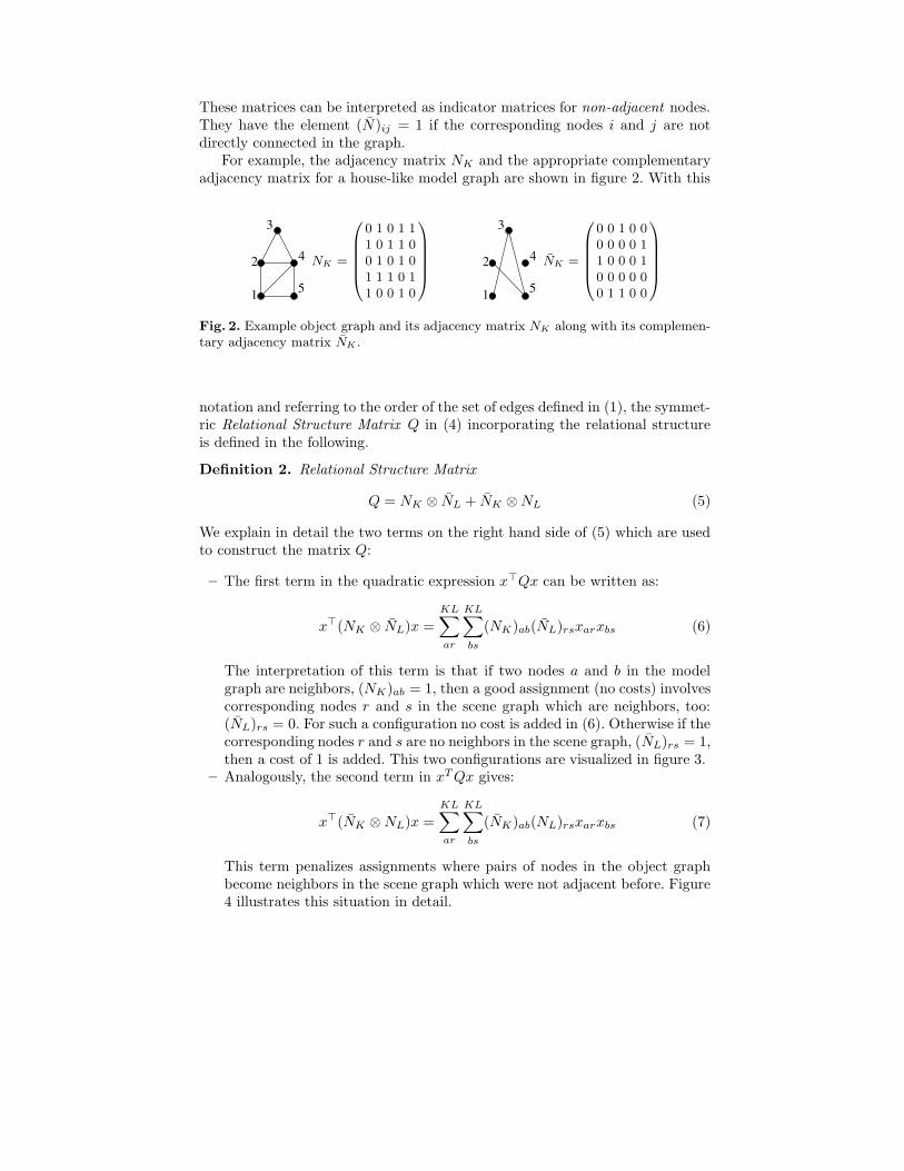
These matrices can be interpreted as indicator matrices for non-adjacent nodes.They have the element (N)ij = 1 if the corresponding nodes i and j are notdirectly connected in the graph.

For example, the adjacency matrix NK and the appropriate complementaryadjacency matrix for a house-like model graph are shown in figure 2. With this

4

1

2

3

5

NK =

0

B

B

B

B

@

0 1 0 1 11 0 1 1 00 1 0 1 01 1 1 0 11 0 0 1 0

1

C

C

C

C

A

4

1

2

3

5

NK =

0

B

B

B

B

@

0 0 1 0 00 0 0 0 11 0 0 0 10 0 0 0 00 1 1 0 0

1

C

C

C

C

A

Fig. 2. Example object graph and its adjacency matrix NK along with its complemen-tary adjacency matrix NK .

notation and referring to the order of the set of edges defined in (1), the symmet-ric Relational Structure Matrix Q in (4) incorporating the relational structureis defined in the following.

Definition 2. Relational Structure Matrix

Q = NK ⊗ NL + NK ⊗ NL (5)

We explain in detail the two terms on the right hand side of (5) which are usedto construct the matrix Q:

– The first term in the quadratic expression x>Qx can be written as:

x>(NK ⊗ NL)x =

KL∑

ar

KL∑

bs

(NK)ab(NL)rsxarxbs (6)

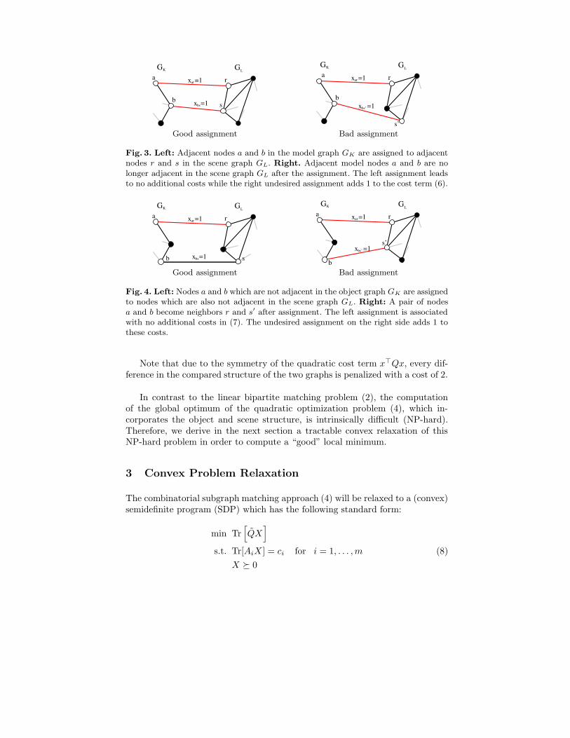
The interpretation of this term is that if two nodes a and b in the modelgraph are neighbors, (NK)ab = 1, then a good assignment (no costs) involvescorresponding nodes r and s in the scene graph which are neighbors, too:(NL)rs = 0. For such a configuration no cost is added in (6). Otherwise if thecorresponding nodes r and s are no neighbors in the scene graph, (NL)rs = 1,then a cost of 1 is added. This two configurations are visualized in figure 3.

– Analogously, the second term in xT Qx gives:

x>(NK ⊗ NL)x =

KL∑

ar

KL∑

bs

(NK)ab(NL)rsxarxbs (7)

This term penalizes assignments where pairs of nodes in the object graphbecome neighbors in the scene graph which were not adjacent before. Figure4 illustrates this situation in detail.

x =1ar

x =1bs

GLGK

b

a

s

r

x =1bs’

x =1ar

GLGK

b

r

s’

a

Good assignment Bad assignment

Fig. 3. Left: Adjacent nodes a and b in the model graph GK are assigned to adjacentnodes r and s in the scene graph GL. Right. Adjacent model nodes a and b are nolonger adjacent in the scene graph GL after the assignment. The left assignment leadsto no additional costs while the right undesired assignment adds 1 to the cost term (6).

x =1ar

x =1bs

GLGK

a r

sb

x =1ar

x =1bs’

GLGK

a r

s’

bGood assignment Bad assignment

Fig. 4. Left: Nodes a and b which are not adjacent in the object graph GK are assignedto nodes which are also not adjacent in the scene graph GL. Right: A pair of nodesa and b become neighbors r and s′ after assignment. The left assignment is associatedwith no additional costs in (7). The undesired assignment on the right side adds 1 tothese costs.

Note that due to the symmetry of the quadratic cost term x>Qx, every dif-ference in the compared structure of the two graphs is penalized with a cost of 2.

In contrast to the linear bipartite matching problem (2), the computationof the global optimum of the quadratic optimization problem (4), which in-corporates the object and scene structure, is intrinsically difficult (NP-hard).Therefore, we derive in the next section a tractable convex relaxation of thisNP-hard problem in order to compute a “good” local minimum.

3 Convex Problem Relaxation

The combinatorial subgraph matching approach (4) will be relaxed to a (convex)semidefinite program (SDP) which has the following standard form:

min Tr[

QX]

s.t. Tr[AiX ] = ci for i = 1, . . . , m (8)

X � 0

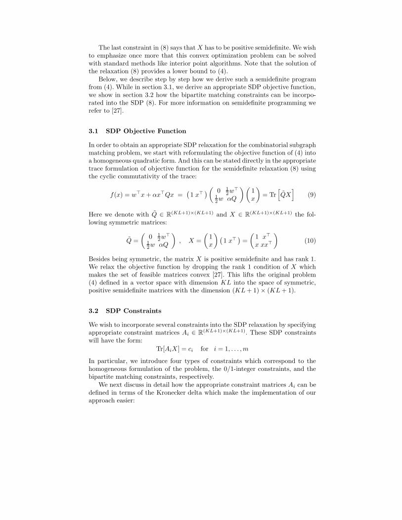
The last constraint in (8) says that X has to be positive semidefinite. We wishto emphasize once more that this convex optimization problem can be solvedwith standard methods like interior point algorithms. Note that the solution ofthe relaxation (8) provides a lower bound to (4).

Below, we describe step by step how we derive such a semidefinite programfrom (4). While in section 3.1, we derive an appropriate SDP objective function,we show in section 3.2 how the bipartite matching constraints can be incorpo-rated into the SDP (8). For more information on semidefinite programming werefer to [27].

3.1 SDP Objective Function

In order to obtain an appropriate SDP relaxation for the combinatorial subgraphmatching problem, we start with reformulating the objective function of (4) intoa homogeneous quadratic form. And this can be stated directly in the appropriatetrace formulation of objective function for the semidefinite relaxation (8) usingthe cyclic commutativity of the trace:

f(x) = w>x + αx>Qx =(

1 x>)

(

0 12w>

12w αQ

) (

1x

)

= Tr[

QX]

(9)

Here we denote with Q ∈ R(KL+1)×(KL+1) and X ∈ R

(KL+1)×(KL+1) the fol-lowing symmetric matrices:

Q =

(

0 12w>

12w αQ

)

, X =

(

1x

)

(

1 x>)

=

(

1 x>

x xx>

)

(10)

Besides being symmetric, the matrix X is positive semidefinite and has rank 1.We relax the objective function by dropping the rank 1 condition of X whichmakes the set of feasible matrices convex [27]. This lifts the original problem(4) defined in a vector space with dimension KL into the space of symmetric,positive semidefinite matrices with the dimension (KL + 1) × (KL + 1).

3.2 SDP Constraints

We wish to incorporate several constraints into the SDP relaxation by specifyingappropriate constraint matrices Ai ∈ R

(KL+1)×(KL+1). These SDP constraintswill have the form:

Tr[AiX ] = ci for i = 1, . . . , m

In particular, we introduce four types of constraints which correspond to thehomogeneous formulation of the problem, the 0/1-integer constraints, and thebipartite matching constraints, respectively.

We next discuss in detail how the appropriate constraint matrices Ai can bedefined in terms of the Kronecker delta which make the implementation of ourapproach easier:

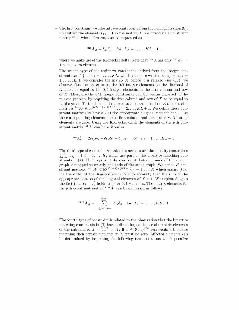
– The first constraint we take into account results from the homogenization (9).To restrict the element X11 = 1 in the matrix X , we introduce a constraintmatrix oneA whose elements can be expressed as

oneAkl = δk1δl1 for k, l = 1, . . . , KL + 1 ,

where we make use of the Kronecker delta. Note that oneA has only oneA11 =1 as non-zero element.

– The second type of constraint we consider is derived from the integer con-straints xi ∈ {0, 1}, i = 1, . . . , KL, which can be rewritten as x2

i = xi, i =1, . . . , KL. If we consider the matrix X before it is relaxed (see (10)) weobserve that due to x2

i = xi the 0/1-integer elements on the diagonal ofX must be equal to the 0/1-integer elements in the first column and rowof X . Therefore the 0/1-integer constraints can be weakly enforced in therelaxed problem by requiring the first column and row of X to be equal toits diagonal. To implement these constraints, we introduce KL constraintmatrices intAj ∈ R

(KL+1)×(KL+1), j = 2, . . . , KL + 1. We define these con-straint matrices to have a 2 at the appropriate diagonal element and −1 atthe corresponding elements in the first column and the first row. All otherelements are zero. Using the Kronecker delta the elements of the j-th con-straint matrix intAj can be written as:

intAjkl = 2δkjδlj − δkjδl1 − δljδk1 for k, l = 1, . . . , KL + 1

– The third type of constraint we take into account are the equality constraints∑L

j=1 xij = 1, i = 1, . . . , K, which are part of the bipartite matching con-straints in (4). They represent the constraint that each node of the smallergraph is mapped to exactly one node of the scene graph. We define K con-straint matrices sumAj ∈ R

(KL+1)×(KL+1), j = 1, . . . , K which ensure (tak-ing the order of the diagonal elements into account) that the sum of theappropriate portion of the diagonal elements of X is 1. We exploited againthe fact that xi = x2

i holds true for 0/1-variables. The matrix elements forthe j-th constraint matrix sumAj can be expressed as follows:

sumAjkl =

jL+1∑

i=(j−1)L+1

δikδil for k, l = 1, . . . , KL + 1

– The fourth type of constraint is related to the observation that the bipartitematching constraints in (2) have a direct impact to certain matrix elementsof the sub-matrix X = xx> of X . If x ∈ {0, 1}KL represents a bipartitematching then certain elements in X must be zero. Affected elements canbe determined by inspecting the following two cost terms which penalize

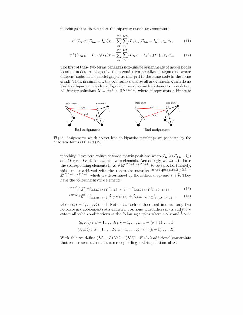
matchings that do not meet the bipartite matching constraints.

x>(IK ⊗ (ELL − IL))x =

KL∑

ar

KL∑

bs

(IK)ab(ELL − IL)rsxarxbs (11)

x>((EKK − IK) ⊗ IL)x =

KL∑

ar

KL∑

bs

(EKK − IK)ab(IL)rsxarxbs (12)

The first of these two terms penalizes non-unique assignments of model nodesto scene nodes. Analogously, the second term penalizes assignments wheredifferent nodes of the model graph are mapped to the same node in the scenegraph. Thus, in summary, the two terms penalize all assignments which do nolead to a bipartite matching. Figure 5 illustrates such configurations in detail.All integer solutions X = xx> ∈ R

KL×KL, where x represents a bipartite

x =1

x =1

ar

bs

r

s

a=bobject graph scene graph

x =1ar

x =1bs

r=s

object graph scene grapha

b

Bad assignment Bad assignment

Fig. 5. Assignments which do not lead to bipartite matchings are penalized by thequadratic terms (11) and (12).

matching, have zero-values at those matrix positions where IK ⊗ (ELL− IL)and (EKK − IK)⊗ IL have non-zero elements. Accordingly, we want to forcethe corresponding elements in X ∈ R

(KL+1)×(KL+1) to be zero. Fortunately,

this can be achieved with the constraint matrices zeros1Aars,zeros2 Asab ∈R

(KL+1)×(KL+1) which are determined by the indices a, r,s and s, a, b. Theyhave the following matrix elements

zeros1Aarskl =δk,(aL+r+1)δl,(aL+s+1) + δk,(aL+s+1)δl,(aL+r+1) , (13)

zeros2Asabkl =δk,(sK+b+1)δl,(sK+a+1) + δk,(sK+a+1))δl,(sK+b+1) , (14)

where k, l = 1, . . . , KL + 1. Note that each of these matrices has only twonon-zero matrix elements at symmetric positions. The indices a, r,s and s, a, battain all valid combinations of the following triples where s > r and b > a:

(a, r, s) : a = 1, . . . , K; r = 1, . . . , L; s = (r + 1), . . . , L

(s, a, b) : s = 1, . . . , L; a = 1, . . . , K; b = (a + 1), . . . , K

With this we define (LL − L)K/2 + (KK − K)L/2 additional constraintsthat ensure zero-values at the corresponding matrix positions of X .

Altogether we have the following 1 + KL + K + (LL−L)K/2 + (KK −K)L/2SDP constraints:

Tr[oneAX ] = 1

Tr[intAjX ] = 0 for j = 2 . . . , KL + 1

Tr[sumAjX ] = 1 for j = 1, . . . , K

Tr[zeros1AarsX ] = 0 ∀(a, r, s) , Tr[zeros2AsabX ] = 0 ∀(s, a, b)

The name gangster operator was introduced in [28] for the last two constraintoperators because they “shoot holes”,i.e. zeros, into the matrix X .We note here that we dropped the additional linear inequality constraints of thebipartite matching,

∑Ki=1 xij ≤ 1, ∀j, which, in principle, can be incorporated

by lifting schemes (see e.g. [27]). This, however, would considerably increase thenumber of constraints and slow down the computation. Our experiments (section5) show that this does not compromise the performance of our approach.

4 Combinatorial Solutions by Post-Processing

The diagonal elements of the global optimum Xbound ∈ R(KL+1)×(KL+1) to

the semidefinite relaxation (8) can be interpreted as a non-integer approxima-tion xsol = diag(Xbound) to the solution of (4). Omitting the first element inxsol ∈ R

KL+1, which was added due to the homogenization (9), we obtain theapproximation xsol ∈ R

KL for the indicator vector x ∈ {0, 1}KL.

4.1 Probabilistic Interpretation of the Non-Integer Solution

According to the constraints AKxsol = eK , we have for each node i of the modelgraph

∑Lj (xsol)ji = 1, i = 1, . . . , K. Hence, (xsol)ji may be considered as the

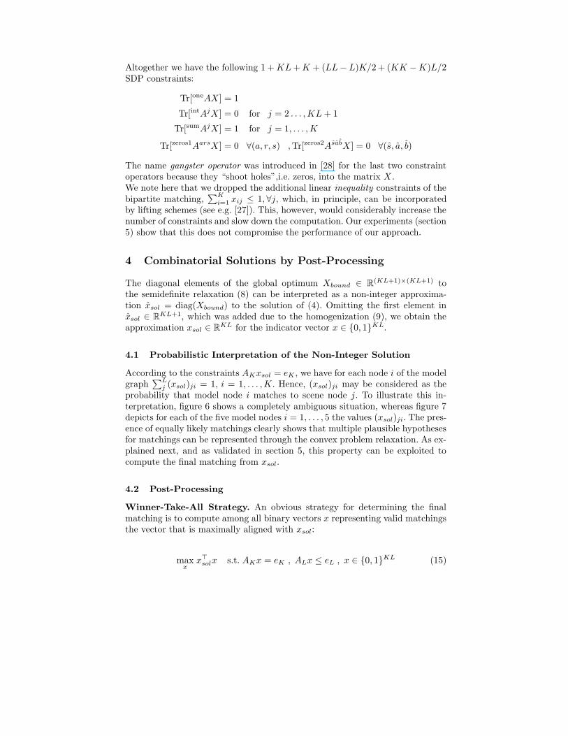
probability that model node i matches to scene node j. To illustrate this in-terpretation, figure 6 shows a completely ambiguous situation, whereas figure 7depicts for each of the five model nodes i = 1, . . . , 5 the values (xsol)ji. The pres-ence of equally likely matchings clearly shows that multiple plausible hypothesesfor matchings can be represented through the convex problem relaxation. As ex-plained next, and as validated in section 5, this property can be exploited tocompute the final matching from xsol.

4.2 Post-Processing

Winner-Take-All Strategy. An obvious strategy for determining the finalmatching is to compute among all binary vectors x representing valid matchingsthe vector that is maximally aligned with xsol:

maxx

x>

solx s.t. AKx = eK , ALx ≤ eL , x ∈ {0, 1}KL (15)

2312

1

2

3

4

5

49

107

6

81

11 3

5

13

2

2217

19 20

2114

24 16

1825

26

15

Fig. 6. Ambiguous situation with two global optima. The node colors indicate thesimilarity between the nodes of the object and the scene graph. Despite convexityand uniqueness, the semidefinite relaxation is able to represent multiple hypotheses formatching – see figure 7.

1 1 26 / 1 2 26 / 1 3 26 / 1 4 26 / 1 5 260

0.1

0.2

0.31->9 2->10

3->11 4->4 5->131->22

2->23

3->24 4->17 5->26

4->254->12

Fig. 7. The non-integer solution xsol for the ambiguous matching situation shown infigure 6. The plot is subdivided into K = 5 segments, with the i-th segment (i ∈{1, . . . , K}) representing all possible matchings from the model node i to all L = 26nodes in the scene graph. In each segment the probabilities sum up to one.

The exact solution to (15), denoted with x∗

lin, can be computed by solving a linearprogram because the constraint matrices AK and AL are total unimodular (cf.section 2.1). According to the probabilistic interpretation, x∗

lin represents themost probable matching.

Sampling. To exploit alternative hypotheses for valid matchings as well, we mayrandomly select a node i ∈ {1, . . . , K} of the model graph and assign to it a scenenode j ∈ {1, . . . , L} by sampling from the distribution (xsol)ji, j = 1, . . . , L.This assignment is only accepted if it results in a valid matching representing animproved combinatorial solution. In our experiments, we conducted 10 ·KL suchsampling steps, starting with the solution x∗

lin to (15). The resulting matchingis denoted with x∗

sampling .

5 Experiments

5.1 Real World Example

For the problem shown in figure 1, we computed feature similarities (weights w)by determining the earth mover distance [29] between local gray value histogramsfor each node. We point out that more elaborate feature selection or even learningis beyond the scope of this paper, whose main focus is the optimization.

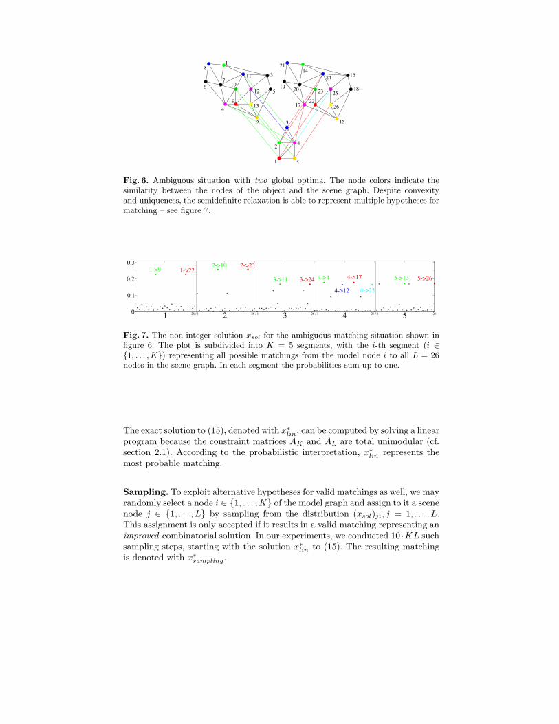
To demonstrate that the regularization in (4) is indeed necessary, we firstcomputed the bipartite matching (3). The corresponding solution, shown in fig-ure 8, just picks the locally best fitting scene graph nodes. Only the assignmentsdrawn in red are correct.

3520122536

13 291841332837

2

5

15 16 1721

2527

333511

12

9

64 3

1

5

710

8

12

3

67

28 30 32

4139

37

36

24

34

26

11

8

4

9

12 14

10

13

201918

38

3129

2223

40

23456

789

101112

1

Fig. 8. Matching computed by the linear program (3) without regularization, i.e. sen-sitivity to relational structure. Only 3 out of the 12 assignments are correct (markedwith red).

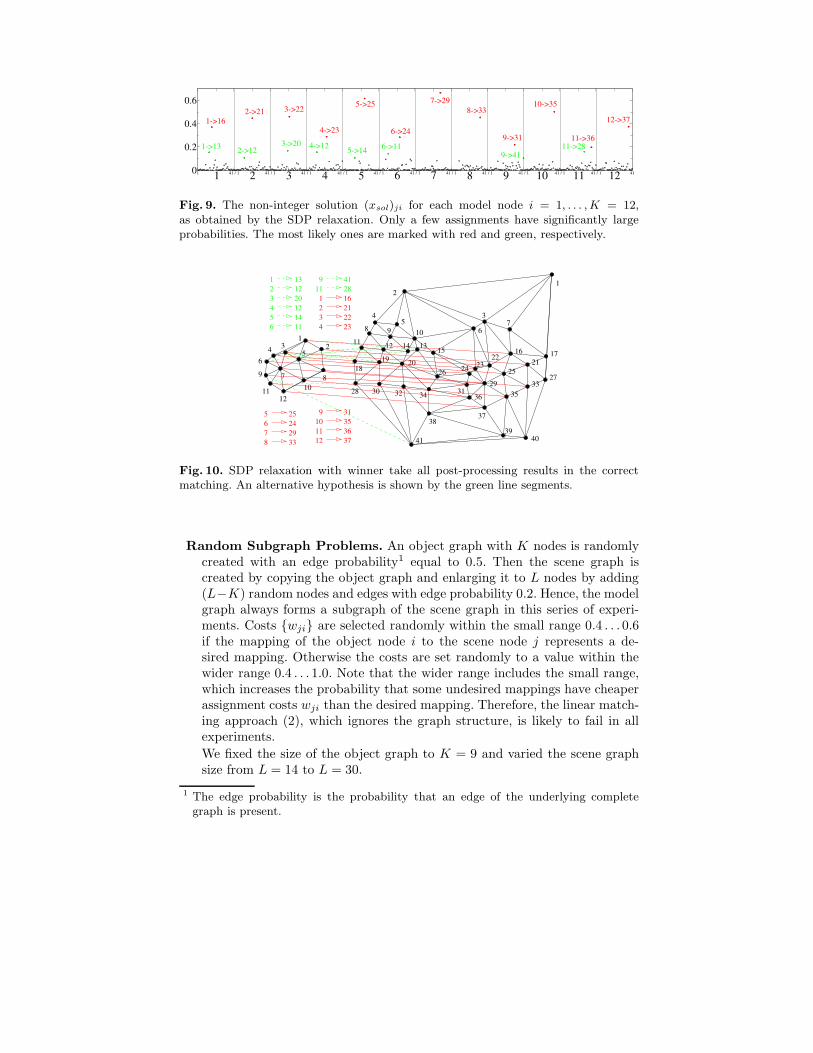
The non-integer solution xsol obtained by the SDP relaxation (8) of the ap-proach (4), is shown in figure 9, where (xsol)ji is plotted for each model nodei = 1, . . . , K. Only a few mappings i 7→ j have significantly large probabilities(xsol)ji. The most likely assignments are marked with red, and some alterna-tive candidates with (xsol)ji ≥ 0.1 are marked with green. The correspondingmatchings are shown in figure 10. The red assignments correspond to the optimalcombinatorial solution which, in turn, corresponds to the solution x∗

lin to (15).Sampling, therefore, cannot lead to further improvements, in this case.

5.2 Generating Random Problem Instances

In order to get a more complete picture of the performance of our approach,we conducted a large series of experiments with randomly generated probleminstances. Two kinds of experiments were considered:

1 1 41 / 1 2 41 / 1 3 41 / 1 4 41 / 1 5 41 / 1 6 41 / 1 7 41 / 1 8 41 / 1 9 41 / 1 10 41 / 1 11 41 / 1 12 410

0.2

0.4

0.6

1->162->21 3->22

4->23

5->25

6->24

7->298->33

9->31

10->35

11->36

12->37

1->13 2->123->20 4->12 5->14 6->11

9->4111->28

Fig. 9. The non-integer solution (xsol)ji for each model node i = 1, . . . , K = 12,as obtained by the SDP relaxation. Only a few assignments have significantly largeprobabilities. The most likely ones are marked with red and green, respectively.

5 25678

242933

23456

11220121411

13

2

5

15 16 1721

2527

333511

12

9

64 3

1

5

710

8

12

3

67

28 30 32

4139

37

36

24

34

26

11

8

4

9

12 14

10

13

201918

38

3129

2223

40

11 289 41

1 16234

212223

9 31353637

101112

Fig. 10. SDP relaxation with winner take all post-processing results in the correctmatching. An alternative hypothesis is shown by the green line segments.

Random Subgraph Problems. An object graph with K nodes is randomlycreated with an edge probability1 equal to 0.5. Then the scene graph iscreated by copying the object graph and enlarging it to L nodes by adding(L−K) random nodes and edges with edge probability 0.2. Hence, the modelgraph always forms a subgraph of the scene graph in this series of experi-ments. Costs {wji} are selected randomly within the small range 0.4 . . . 0.6if the mapping of the object node i to the scene node j represents a de-sired mapping. Otherwise the costs are set randomly to a value within thewider range 0.4 . . . 1.0. Note that the wider range includes the small range,which increases the probability that some undesired mappings have cheaperassignment costs wji than the desired mapping. Therefore, the linear match-ing approach (2), which ignores the graph structure, is likely to fail in allexperiments.

We fixed the size of the object graph to K = 9 and varied the scene graphsize from L = 14 to L = 30.

1 The edge probability is the probability that an edge of the underlying completegraph is present.

By construction, we know which subgraph of the scene corresponds to theobject in each experiment. Accordingly, the corresponding matching is de-fined to be ground truth, irrespective of the existence of other accidentalmatchings with a better objective value (4) in some rare cases.

Random Model and Scene Graphs. In this series of experiments bothobject and scene graphs with K and L nodes, respectively, are created ran-domly, and independently from each other. The similarities wji are set ran-domly within the range 0.4 . . . 1.0. The edge probability was set to 0.4 forthe smaller model graph, and to 0.3 for the larger scene graph.

To compute ground truth, we have to rely on exhaustive search, forcing usto limit2 the maximum size of the scene graph to L = 19.

For each size L, we created 1000 problem instances. The value of the regulariza-tion parameter α was 0.15 and 0.3 for the subgraph and purely random problems,respectively.

5.3 Evaluation

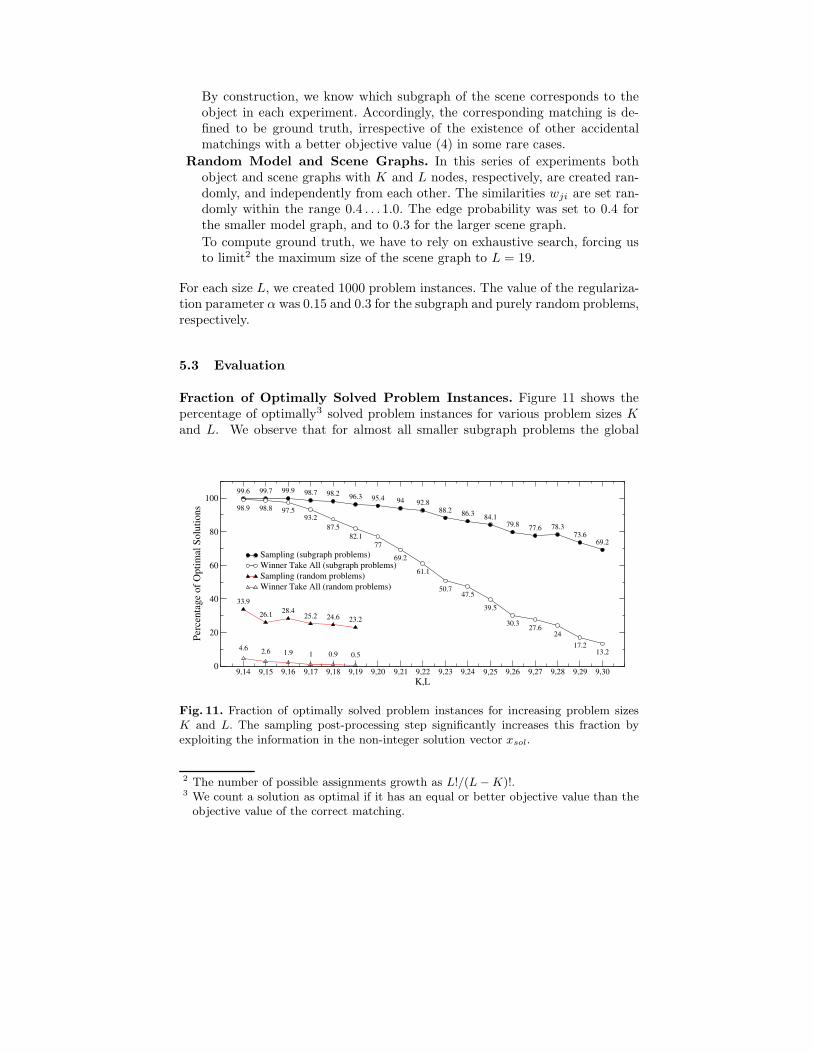
Fraction of Optimally Solved Problem Instances. Figure 11 shows thepercentage of optimally3 solved problem instances for various problem sizes Kand L. We observe that for almost all smaller subgraph problems the global

99.6 99.7 99.9 98.7 98.2 96.3 95.4 94 92.888.2 86.3 84.1

79.8 77.6 78.373.6

69.2

98.9 98.8 97.593.2

87.582.1

77

69.2

61.1

50.747.5

39.5

30.3 27.624

17.213.2

33.9

26.1 28.425.2 24.6 23.2

4.6 2.6 1.9 1 0.9 0.5

9,14 9,15 9,16 9,17 9,18 9,19 9,20 9,21 9,22 9,23 9,24 9,25 9,26 9,27 9,28 9,29 9,30K,L

0

20

40

60

80

100

Perc

enta

ge o

f Opt

imal

Sol

utio

ns

Sampling (subgraph problems)Winner Take All (subgraph problems)Sampling (random problems)Winner Take All (random problems)

Fig. 11. Fraction of optimally solved problem instances for increasing problem sizesK and L. The sampling post-processing step significantly increases this fraction byexploiting the information in the non-integer solution vector xsol.

2 The number of possible assignments growth as L!/(L − K)!.3 We count a solution as optimal if it has an equal or better objective value than the

objective value of the correct matching.

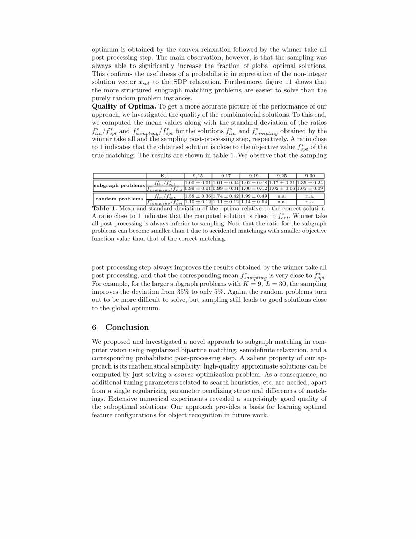
optimum is obtained by the convex relaxation followed by the winner take allpost-processing step. The main observation, however, is that the sampling wasalways able to significantly increase the fraction of global optimal solutions.This confirms the usefulness of a probabilistic interpretation of the non-integersolution vector xsol to the SDP relaxation. Furthermore, figure 11 shows thatthe more structured subgraph matching problems are easier to solve than thepurely random problem instances.Quality of Optima. To get a more accurate picture of the performance of ourapproach, we investigated the quality of the combinatorial solutions. To this end,we computed the mean values along with the standard deviation of the ratiosf∗

lin/f∗opt and f∗

sampling/f∗opt for the solutions f∗

lin and f∗

sampling obtained by thewinner take all and the sampling post-processing step, respectively. A ratio closeto 1 indicates that the obtained solution is close to the objective value f ∗

opt of thetrue matching. The results are shown in table 1. We observe that the sampling

K,L 9,15 9,17 9,19 9,25 9,30

f∗

lin/f∗

opt 1.00 ± 0.01 1.01 ± 0.04 1.02 ± 0.08 1.17 ± 0.21 1.35 ± 0.24subgraph problems

f∗

sampling/f∗

opt 0.99 ± 0.01 0.99 ± 0.01 1.00 ± 0.02 1.02 ± 0.06 1.05 ± 0.09

f∗

lin/f∗

opt 1.58 ± 0.36 1.74 ± 0.42 1.99 ± 0.49 n.a. n.a.random problems

f∗

sampling/f∗

opt 1.10 ± 0.12 1.11 ± 0.12 1.14 ± 0.14 n.a. n.a.

Table 1. Mean and standard deviation of the optima relative to the correct solution.A ratio close to 1 indicates that the computed solution is close to f∗

opt. Winner takeall post-processing is always inferior to sampling. Note that the ratio for the subgraphproblems can become smaller than 1 due to accidental matchings with smaller objectivefunction value than that of the correct matching.

post-processing step always improves the results obtained by the winner take allpost-processing, and that the corresponding mean f ∗

sampling is very close to f∗opt.

For example, for the larger subgraph problems with K = 9, L = 30, the samplingimproves the deviation from 35% to only 5%. Again, the random problems turnout to be more difficult to solve, but sampling still leads to good solutions closeto the global optimum.

6 Conclusion

We proposed and investigated a novel approach to subgraph matching in com-puter vision using regularized bipartite matching, semidefinite relaxation, and acorresponding probabilistic post-processing step. A salient property of our ap-proach is its mathematical simplicity: high-quality approximate solutions can becomputed by just solving a convex optimization problem. As a consequence, noadditional tuning parameters related to search heuristics, etc. are needed, apartfrom a single regularizing parameter penalizing structural differences of match-ings. Extensive numerical experiments revealed a surprisingly good quality ofthe suboptimal solutions. Our approach provides a basis for learning optimalfeature configurations for object recognition in future work.

References

1. H. G. Barrow and R.J. Popplestone. Relational descriptions in picture processing.Machine Intelligence, 6:377–396, 1971.

2. J.R. Ullmann. An algorithm for subgraph isomorphism. Journal of the ACM,23(1):31–42, 1976.

3. A.D.J. Cross, R.C. Wilson, and E.R. Hancock. Inexact graph matching usinggenetic search. Pattern Recog., 30(6):953–970, 1997.

4. S. Umeyama. An eigendecomposition approach to weighted graph matching prob-lems. IEEE Trans. Patt. Anal. Mach. Intell., 10(5):695–703, 1988.

5. B. Luo and E.R. Hancock. Structural graph matching using the em algorithm andsingular value decomposition. IEEE Trans. Patt. Anal. Mach. Intell., 23(10):1120–1136, 2001.

6. A.D.J. Cross and E.R. Hancock. Graph matching with a dual-step em algorithm.IEEE Trans. Patt. Anal. Mach. Intell., 20(11):1236–1253, 1998.

7. M. Pavan and M. Pelillo. Dominant sets and hierarchical clustering. In Proc. ICCV

2003 - 9th IEEE International Conference on Computer Vision, volume 1, pages362–369, 2003.

8. B.J. Van Wyk and M.A. Van Wyk. Kronecker product graph matching.Patt. Recognition, 36(9):2019–2030, 2003.

9. M.F. Demirci, A. Shoukoufandeh, Y. Keselman, S. Dickinson, and L. Bretzner.Many-to-many matching of scale-space feature hierarchies using metric embedding.In L.D. Griffin and M. Lillholm, editors, Scale-Space 2003, volume 2695 of Lecture

Notes in Computer Science, pages 17–32. Springer, 2003.

10. A. Robles-Kelley and E.R. Hancock. Graph edit distance from spectral seriation.IEEE Trans. Patt. Anal. Mach. Intell., 27(3):365–378, 2005.

11. T. Caelli and T.S. Caetano. Graphical models for graph matching: Approximatemodels and optimal algorithms. Patt. Recog. Letters, 26(3):339–346, 2005.

12. D. Conte, P. Foggia, C. Sansone, and M. Vento. Thirty years of graph matchingin pattern recognition. IJPRAI, 18(3):265–298, 2004.

13. S. Gold and A. Rangarajan. A graduated assignment algorithm for graph matching.IEEE Trans. Patt. Anal. Mach. Intell., 18(4):377–388, 1996.

14. S. Ishii and M. Sato. Doubly constrained network for combinatorial optimization.Neurocomputing, 43:239–257, 2002.

15. J.J. Kosowsky and A.L. Yuille. The invisible hand algorithm: Solving the assign-ment problem with statistical pyhysics. Neural Networks, 7(3):477–490, 1994.

16. A. Rangarajan, A. Yuille, and E. Mjolsness. Convergence properties of the sof-tassign quadratic assignment algorithm. Neural Computation, 11(6):1455–1474,1999.

17. F. Alizadeh. Interior point methods in semidefinite programming with applicationsto combinatorial optimization. SIAM Journal on Optimization, 5(1):13–51, 1995.

18. S. Poljak, F. Rendl, and H. Wolkowicz. A recipe for semidefinite relaxation for 0-1quadratic programming. Journal of Global Optimization, (7):51–73, 1995.

19. Q. Zhao, S.E. Karisch, F. Rendl, and H. Wolkowicz. Semidefinite programmingrelaxations for the quadratic assignment problem. J. Combinat. Optimization,2(1):71–109, 1998.

20. K. M. Anstreicher and N. W. Brixius. A new bound for the quadratic assignmentproblem based on convex quadratic programming. Mathematical Programming,89(3):341–357, 2001.

21. R. E. Burkard, S. Karisch, and F. Rendl. QAPLIB-A Quadratic Assignment Prob-lem Library. European Journal of Operational Research, 55:115–119, 1991.

22. C. Schellewald, S. Roth, and C. Schnorr. Evaluation of convex optimization tech-niques for the weighted graph-matching problem in computer vision. In B. Radigand S. Florczyk, editors, Mustererkennung 2001, volume 2191 of Lect. Notes

Comp. Science, pages 361–368, Munich, Germany, Sept. 12–14 2001. Springer.23. J. Keuchel, C. Schnorr, C. Schellewald, and D. Cremers. Binary partition-

ing, perceptual grouping, and restoration with semidefinite programming. IEEE

Trans. Patt. Anal. Mach. Intell., 25(11):1364–1379, 2003.24. J. Keuchel, M. Heiler, and C. Schnorr. Hierarchical image segmentation based on

semidefinite programming. In Pattern Recognition, Proc. 26th DAGM Symposium,volume 3175 of Lecture Notes in Computer Science, pages 120–128. Springer, 2004.

25. Alexander Schrijver. Theory of linear and integer programming. John Wiley &Sons, Inc. New York, NY, USA, 1986.

26. B. Korte and J. Vygen. Combinatorial Optimization: Theory and Algorithms.Algorithms and Combinatorics 21. Springer, Berlin Heidelberg New York, 2000.

27. H. Wolkowicz, R. Saigal, and L. Vandenberghe, editors. Handbook of Semidefinite

Programming, Boston, 2000. Kluwer Acad. Publ.28. Ph. L. Toint. On sparse and symmetric matrix updating subject to a linear equa-

tion. Mathematics of Computation, 31:954–961, 1977.29. Y. Rubner, C. Tomasi, and L. J. Guibas. The earth mover’s distance as a metric

for image retrieval. International Journal of Computer Vision, 40(2):99–121, 2000.