Probabilistic slope stability analysis by a copula-based sampling method

Probabilistic slope stability analysis by a copula-based sampling method

Xing Zheng Wu∗ Department of Applied Mathematics, School of Applied Science, University of Science and Technology Beijing,

30 Xueyuan Road, Haidan District, Beijing, P. R. China. Post code: 100083.

Abstract In probabilistic slope stability analysis, the influence of cross-correlation of the soil strength

parameters cohesion and internal friction angle, on the reliability index have not been investigated fully. In this paper, an expedient technique is presented for probabilistic slope stability analysis that involves sampling a series of combinations of soil strength parameters through a copula as input to an existing conventional deterministic slope stability program. The approach organises the individual marginal probability density distributions of componential shear strength as a bivariate joint distribution by the copula function to characterise the dependence between shear strengths. The technique can be used to generate an arbitrarily large sample of soil strength parameters. Examples are provided to illustrate the use of the copula-based sampling method to estimate the reliability index of given slopes, and the computed results are compared with the first-order reliability method, considering the correlated random variables. A sensitivity study was conducted to assess the influence of correlational measurements on the reliability index. The approach is simple and can be applied in practice with little effort beyond what is necessary in a conventional analysis.

Keywords: probabilistic analysis, slope stability, Monte Carlo simulation, copula, cross-correlation, cohesion, friction angle

2

1

1 Introduction 1

Slope stability analysis is a traditional problem in geotechnical engineering that is highly 2 amenable to probabilistic treatment and that has received considerable attention recently (Rackwitz, 3 2000; El-Ramly et al., 2002). Uncertainties in soil properties, environmental conditions, and 4 theoretical models are the most important sources of lack of confidence in deterministic analysis 5 (Alonso, 1976; Baecher and Christian, 2003). There have been numerous attempts to use a 6 probabilistic approach complementary to the conventional approach to analyse the safety of slopes 7 and especially to explore the effect of variabilities in soil shear strengths. A common approach to 8 determine the reliability of a slope is based on calculating the reliability index corresponding to a 9 surface with the minimum factor of safety (referred to as the critical deterministic surface, defined 10 by a limit equilibrium approach of slices), as described by Chowdhury et al. (1987) and Christian et 11 al. (1994). However, critical slip surfaces may not necessarily be those with the lowest conventional 12 factors of safety (Hassan and Wolff, 1999) but rather are determined by a combination of the mean 13 factor of safety and uncertainty (Bergado and Anderson, 1985; Chowdhury and Xu; 1993). 14

It is therefore imperative that greater use is made of probabilistic assessments of slope stability 15 and that capabilities for considering the statistical variation of input properties are enhanced (El-16 Ramly et al., 2002). These reliability model approaches do provide a better basis for making 17

engineering judgments in a more transparent way. However, correlations between the cohesion c 18

and the internal friction angle φ (referred to as the friction angle hereinafter) are commonly ignored 19

in probabilistic slope stability analysis (Tang et al., 1976; Tobutt, 1982; Nguyen and Chowdhury, 20 1984; Li and Lumb, 1987; Christian et al., 1994; Husein Malkawi et al., 2000). A number of recent 21 studies have been oriented toward careful consideration of the complicated nature of these 22 correlations (Lumb, 1970, Harr, 1987, Cherubini, 1997, Fenton and Griffiths, 2003; Forrest and Orr, 23 2010). Most of these investigators believe that the cross-correlation is negative, with a value 24 between -0.24 and -0.70. However, several researchers have reported a positive correlation (Lumb, 25 1970; Wolff, 1985). 26

2

Dependencies among the uncertainties in the estimates of these parameters can be critical to 27 obtaining correct numerical results from reliability analyses in geotechnical engineering (see, e.g., 28 Phoon and Kulhanny, 1999). Cho and Park (2010) reported their findings on stochastic behaviour in 29 a bearing capacity problem. The assumption of independence between cohesion and friction angle 30 gives conservative results if the actual correlation is negative, but slightly unconservative results are 31 obtained if the actual correlation is positive. Lü and Low (2011) investigated the probability of 32 failure with respect to the plastic zone criterion of underground rock excavations, and they 33 concluded that assuming uncorrelated friction angle and cohesion will generate a higher probability 34 of failure than assuming that these shear strength parameters are negatively correlated. 35

The influence of the correlation between strength parameters on slope stability analyses is 36 often not well understood. Some researchers have shown that the probability of failure in slope 37 stability analysis is insensitive to the correlation coefficient between the strength parameters (Hata 38 et al., 2011). However, the influence of cross-correlation between the strength parameters on the 39 reliability index of slope stability has been reported by some others (Wolff, 1985; Chowdhury and 40 Xu, 1992). Interestingly, an accurate and reliable statistical description should be required to 41 reproduce the multivariate joint characteristics of all the relevant marginal laws (the joint 42 probability distribution of c and φ ), considering the dependent relationships (their cross-correlation) 43

effectively in slope stability analysis. Recent advances in mathematics show how copulas (Joe, 44 1997; Nelsen, 2006; Salvadori et al., 2007) may be very useful in modelling dependence between 45 correlated random variables. The detailed theoretical background and descriptions of copulas can be 46 found in the literature. 47

Copulas represent an efficient tool for investigating the statistical behaviour of dependent 48 variables. Specifically, copulas are operators on the family of one-dimensional probability 49 distributions of random variables that yield multivariate laws with well-defined properties 50 (Schweizer, 1991). Their efficiency lies in the possibility of studying marginal behaviours and 51 global dependence separately. In fact, it is precisely the copula that captures many of the features of 52

3

a joint distribution: it is possible to prescribe the properties of a multivariate law simply by working 53 on the structure of the corresponding copula. The flexibility offered by copulas for constructing 54 joint distributions is evident from related studies in civil engineering (for a thorough review, see 55 Salvadori et al., 2007) and in finance (Embrechts el al., 2002). 56

In addition, the concept of a copula is relatively simple; the construction does not constrain the 57 choice of marginal distributions, and it provides a good way to impose a dependence structure on 58 predetermined marginal distributions (Clemen and Reilly, 1999; Lambert and Vandenhende, 2002). 59 Particularly when the normality assumption for data usually does not provide an adequate 60 approximation to datasets with heavy-tail, non-normal multivariate distributions are used in practice 61 (see Kotz et al., 2000). Thus, a non-normal multivariate distribution is particularly useful when a 62 geotechnical engineering problem involves the dependence properties of the random variables. 63

To obtain accurate quantitative predictions of the probability of failure of a slope system, the 64 joint probability characteristics of multivariate random soil parameters, incorporating the 65 dependence structure among parameters through a copula, should be implemented in a conventional 66 slope stability approach. Then, a parametric study of the calculated reliability index should be 67 carried out for a range of dependence properties to explore the influence of correlation extremes on 68 reliability assessment. To achieve this goal, a methodology was developed within a probabilistic 69 framework for analysing slope stability using random samplings to represent the various cross-70 correlations of soil strength properties. A joint probability distribution of the strength parameters is 71 derived through copula for the probabilistic slope stability analysis to obtain the desired reliability 72 index. The reliability indices obtained by this copula-based sampling technique are compared with 73 the results obtained by the first-order reliability method (FORM). 74

This paper presents a description of cross-correlation between cohesion and friction angle as 75 determined by shear strength tests and definitions of their correlation measurements in section 2. 76 The copula theory, including the construction of the joint description of cross-correlated shear 77 strength parameters and the forecasting of dependent random variates through copula, is presented 78

4

in section 3. Full details of the methodologies for calculating the reliability index of slope stability 79 by copula-based random sampling are discussed in section 4, and several examples are presented to 80 demonstrate the effects of correlations between shear strength parameters on reliability indices by 81 parametric sensitivity analysis. Discussion and conclusions are presented in sections 5 and 6, 82 respectively. 83

2 Marginal distributions and cross-correlation characteristics 84 of soil shear strength parameters 85

2.1 Marginal distributions of soil strength variables 86 An issue in the applicability of measured values of soil shear strength parameters is the 87

consideration of whether soil properties follow normal distributions. The applicability of the normal 88 distribution to soil properties is supported by Lumb (1970), Tobutt (1982), Baecher and Christian 89 (2003). Brejda et al. (2000) and Fenton and Griffiths (2003) found it difficult to fit a normal 90 distribution to sampled soil properties, but a log-normal distribution showed a better fit to their data. 91 Other distributions, such as the triangular, the versatile beta and the generalised gamma 92 distributions, are gaining popularity (Baecher and Christian, 2003). The best-fit criteria for marginal 93 distributions are identified by the Anderson-Darling (Anderson and Darling, 1954, AD) test initially 94 with

mp (AD statistic). However, because it does not account for the estimated number of 95

parameters, the Akaike information criterion (Akaike, 1974, AIC) values should be considered. The 96 smaller the AIC value, the better the fit is. The AIC is defined as 97

( )parameters fitted ofnumber 2+

model for the likelihood maximizedlog-2AIC×

×= (1) 98

2.2 Dependency measures 99 Soil shear strength pairs based on the Mohr-Coulomb criterion are associated with a single 100

observation, so they are not independent. The dependence between random variables is best 101 determined using Pearson’s linear correlation coefficient pρ , as reported by some investigators 102

(Lumb, 1970; Cherubini, 1997; Forrest and Orr, 2010). More extensive discussion of this important 103

5

subject requires more data that are realistic, and the development of techniques for reproducing or 104 establishing the correlations while maintaining the desired accuracy is crucial to probabilistic 105 assessment. 106

Let ‘observed’ pairs ),(),...,,( 11 njniji zzzz be drawn from a multivariate population of ( )ji ZZ , , 107

where n is the number of observations. Pearson’s product-moment correlation coefficient pρ 108

between two random variables iZ (cohesion) and jZ (friction angle) is usually written as 109

( ) ( ))()(

,CoV,22p

ji

jiji

ZZ

ZZZZ

σσρ = (2) 110

where ( )ji ZZ ,CoV is the covariance between iZ and jZ , ( ) ( ) )()(,,CoV jijiji ZZZZZZ µµµ −= . )( iZµ and 111

)( jZσ denote the mean and standard deviation of iZ , respectively. pρ is restricted to the interval 112

from -1 to 1. As stated by Embrechts et al. (2002) and Boyer et al. (1999), it is not necessarily 113 informative for non-normal distributions. 114

Kendall’s tau, which uses concordant or discordant values, is simply the probability of 115 concordance minus the probability of discordance for the bivariate random pairs ( )ji ZZ , 116

( ) ( ) ( )0)~)(~(Pr0)~)(~(Pr, <−−−>−−= jjiijjiiji ZZZZZZZZZZτ (3) 117

Obviously, Kendall’s tau is calculated by looking at the ordering of the sample for each variable of 118 interest rather than the actual numerical values. Having defined the indicator variable 119

)~)(~( sjtjsitiij ZZZZsignA −−= , as in McNeil et al. (2005), one notices that an unbiased empirical 120

estimator of Kendall’s coefficient τ can be written as 121

( ) ( ))1(2

1,

, 1

−

=

∑≤≤≤

nn

tsAZZ nst

ij

jiτ (4) 122

where sign is expressed by

<−−−≥−−=

ediscordanc,0)~)(~(,1 econcordanc,0)~)(~(,1

sjtjsiti

sjtjsiti

ZZZZZZZZsign and ( )ji ZZ

~,

~ is an 123

independent copy of the vector ( )ji ZZ , . Eq. (4) is the empirical approximation of the theoretical 124

Kendall’s tau in Eq. (3). The range of values of Kendall’s correlation coefficient is -1 to +1. 125

6

3 Understanding the relationships between shear strength 126 parameters using copula 127

As Sklar’s theorem (Sklar, 1959) states, for any joint bivariate distribution function ),(, jiZZ zzH

ji, 128

say, with marginal distribution functions )( iZ zFi

and )( jZ zFj

, there exists at least one copula C such 129

that, for all ∈ji zz , �, ( ) ( ))(),(, jjiijiZZ zFzFCzzHji

= . If )( iZ zFi

and )( jZ zFj

are continuous, then ( )ji uuC , is 130

unique; otherwise, ( )ji uuC , is uniquely determined for the range of )( iZ zFi

, which is multiplied by 131

the range of )( jZ zFj

. Thus, the joint bivariate distribution of ( )ji ZZ , is connected with their one-132

dimensional marginal probability distributions )( iZ zFi

and )( jZ zFj

through copula (Nelsen, 2006). 133

Applying probability transforms )( iZi zFui

= and )( jZj zFuj

= to iZ and jZ , there exists a bivariate joint 134

distribution function with standard uniform marginals ( )ji uuC , (Sklar, 1959; Dupuis, 2007), such 135

that 136 ( ) ( ))(),(, 11

jZiZ,ZZji uFuFHuuCjiji

−−

= (5) 137

where 10 ≤≤ iu and 10 ≤≤ ju . If F is strictly increasing, 1−F is a quasi-inverse (or quantile) of F . 138

Eq. (5) gives an expression for copulas in terms of a joint distribution function H and the ‘inverse’ 139 of the two margins. Moreover, Eq. (5) shows how copulas express dependence on a quantile scale, 140 which provides a means of generating pseudo-random samples from general classes of multivariate 141

probability distributions. That is, given a procedure to generate a sample ( )ji uu , from the copula 142

distribution, the required sample can be constructed as ( ) ( ))(),(, 11jZiZji uFuFzz

ji

−−

= (which we will return 143

to later). 144 Copulas are consulted on the assumption that marginal distributions are known or can be 145

estimated from the data. The procedure for constructing the joint distribution is flexible because no 146 restrictions are placed on the marginal distributions (Clemen and Reilly, 1999; McNeil et al. 2005). 147 In other words, marginal distributions of any form can be knitted together to obtain their joint 148 distribution, which is the main reason for the popularity of copula theory in many areas of research 149 (Embrechts et al., 2002; Lambert and Vandenhende, 2002; Zhang and Singh, 2007). Most important, 150

7

this approach can handle arbitrarily complicated dependence between the input variables. This 151 makes the approach significantly more general than methods implemented in common risk analysis 152 software packages that model correlations but not dependence in general (Ferson and Hajagos, 153 2006). 154

There are many different copulas to choose from, varying in correlation properties such as 155 symmetry, tail dependence and range of dependence (Joe, 1997; Nelsen, 2006). Considering the 156 correlation characteristics between soil strength parameters, we can choose the normal copula and 157 Student copula from the elliptical class of copulas, the Clayton, Frank, and Gumbel copula from the 158 Archimedean class, and the Plackett copula in a class of its own. These copulas are listed in Table 1, 159 along with their parameter ranges. Some of these copulas may not allow negative correlation, but 160 negating the values of one variable can achieve a positive value for the correlation. For some 161 general comments on the choice and further details of copulas, the interested reader should consult 162 Joe (1997), Nelsen (2006), and McNeil et al. (2005). The following is a brief summary of the theory 163 behind these popular copulas, limited to two-dimensional copulas for the sake of brevity. 164

3.1 Elliptical class of copulas 165 The bivariate normal copula is defined as 166

( ) ( ) ( )( )( )( ) ( ) WWΣW

Σd2

1exp21

;,;,1

22/12

p11

pρ

1 1

−==

−Φ

∞−

Φ

∞−

−−

∫ ∫− − Tu u

jijiG

i j

uΦuΦΦuuC

π

ρρ ρ

(6) 167

where ( )⋅ρΦ is a joint distribution function of a bivariate normal distribution with zero mean and 168

variance-covariance matrix 2Σ . ( ) tetΦ tz d21 2/2−

∞−∫=π

is the normal distribution and ( )tΦ 1− is the 169

quantile function of the univariate standard normal distribution. The integral variable

=

j

i

t

tW , and 170

=1

1

p

p2 ij

ij

ρρ

Σ is a symmetrical covariance matrix with the linear Pearson’s correlation coefficient 171

pρ . ijpρ represents the correlation coefficient between iZ and jZ . 172

8

The Student copula has two parameters, one corresponding to the dependence parameter and 173

the other to the number of degrees of freedom λ . The number of degrees of freedom controls the 174 heaviness of the tails, and as it increases, the copula approaches the normal copula. Both the normal 175 and Student copulas are symmetric, and the normal copula is a limiting case of the Student copula 176

when λ becomes infinity ( λ is set to 9 in this study). The advantage of the Student copula is that it 177 can capture lower- and upper-tail dependence in the data (i.e., joint non-exceedance and exceedance 178 probabilities for rare events; see McNeil et al. (2005) for details). 179

3.2 Archimedean class of copulas 180 The widely used copulas in the Archimedean class (Nelsen, 2006) are constructed in a 181

completely different way from the normal copula. An important component of constructing an 182 Archimedean copula is an explicit generator function θϕ . An Archimedean copula is usually written 183

as 184 ( ) ( ) ( )( )θϕϕϕθϕ ;,;, 1

jiji uuuuC −

= (7) 185

where θϕ is a convex decreasing function with ( ) 01 =θϕ , ( )⋅−1θϕ is the pseudo-inverse of ( )⋅θϕ , and θ 186

is a copula dependence parameter or associated parameter. The definitions of the generator function 187 for this family of copulas are given in Table 1. The Frank copula is a symmetric copula; the Clayton 188 and Gumbel copulas are asymmetric Archimedean copulas. The Clayton copula exhibits greater 189 dependence in the negative tail than in the positive, but the Gumbel copula (also known as the 190 Gumbel-Hougard copula) exhibits greater dependence in the positive tail than in the negative tail. 191

3.3 Plackett copula 192 The Plackett copula is the best known example of an algebraically constructed copula. The 193

association θ is determined by the odds ratio, based on observed frequencies in the four quadrants, 194 rather than on the correlation of random variables (Nelsen, 2006). 195

9

3.4 Relationship between Kendall’s Tau and the copula’s parameter 196 For the elliptical class of copulas, there is a relationship between the linear correlation pρ and 197

the rank correlation τ (Frees and Valdez, 1998) 198

)arcsin(2),( pij

ji ZZ ρπ

τ = (8) 199

where )arcsin(t is an inverse trigonometric function such that tt =))(sin(arcsin . This expression 200

prompts the alternative estimation of pρ . The use of Eq. (8) may be more advantageous because τ 201

is rank-dependent and invariant with respect to strictly monotonic nonlinear transformations. 202

For the Archimedean class, Genest and MacKay (1986) have shown that τ depends on the 203

generator ( )⋅θϕ and its derivative, according to the following simple form 204

( ) ( )∫

∫ ∫+=

−=

1

0 '

1

0

1

0

d)()(41

1;,d;,4),(t

tt

uuCuuCZZ jijiji

θ

θ

ϕϕ

θθτ (9) 205

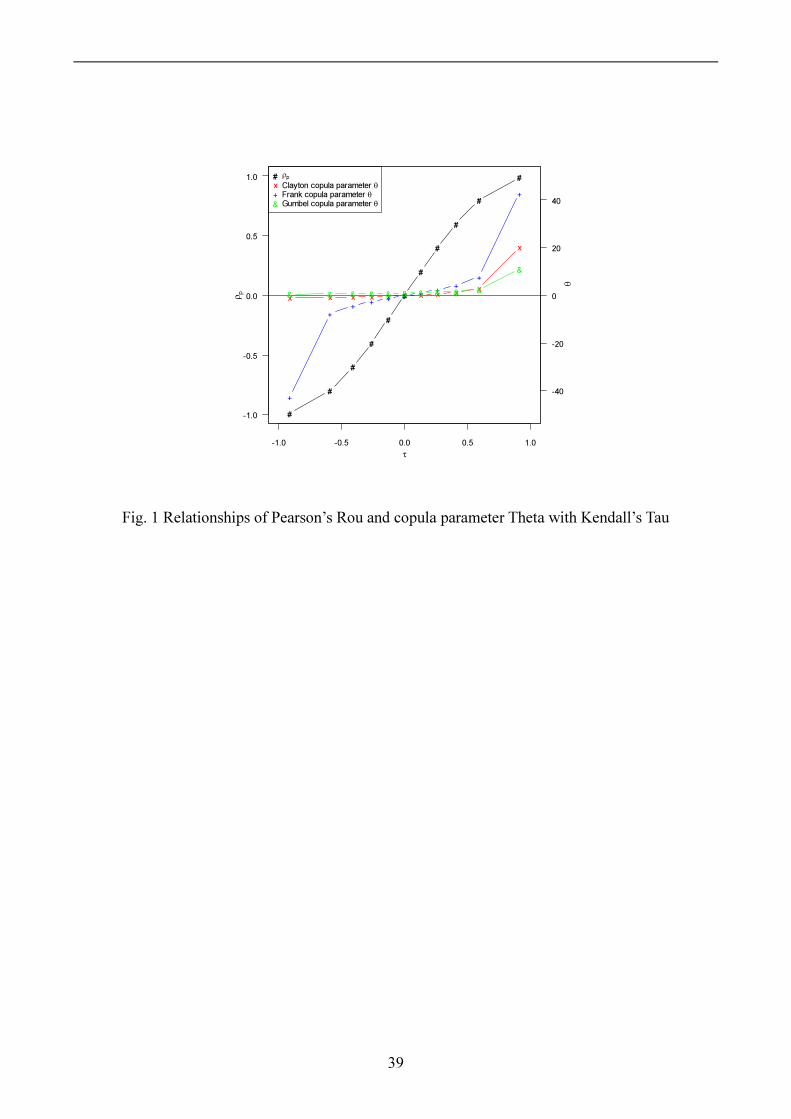
The explicit function of this expression for the copulas is given in Table 1. If Kendall’s tau is 206 known, the correlation parameter of the copula θ can be estimated using this expression. An 207 illustration of the correlation between pρ or θ and Kendall's τ is shown in Fig. 1. 208

3.5 Identification of the best-fitting copula 209 The goodness-of-fit for the alternative copulas is usually assessed using the Cramér-von Mises 210

statistic (Genest et al., 2009). The Cramér-von Mises statistic is based on the empirical process of 211 comparing the empirical copula with a parametric estimate of the copula derived under the null 212 hypothesis 0H . The Cramér-von Mises function represents a type of distance between the true and 213

the observed copula: 214

( ) ( ){ }21

,2

,1

,2

,1 ,,∑

=

−=n

i

nininininn UUCUUCS nθ (10) 215

where nC is the empirical copula used as the most objective benchmark and nCθ is an estimator of 216

C under the hypothesis that 0H : { }θCC∈ holds. Here, nθ is an estimator of θ computed from the 217

ranked pseudo-observations ( ) ( )nnnnnn UUUU ,2

,1

,12

,11 ,,...,, and could be estimated via the inversion of 218

10

Kendall's τ . Large values of nS lead to the rejection of 0H . Approximate cp -values for the test 219

function nS are obtained using a parametric bootstrapping approach (Kojadinovic and Yan, 2010). 220

The cp -value represents the level at which the copula is not rejected, meaning that models with 221

higher cp -values are better in terms of not being rejected. 222

The best-fitting copula from among the candidate copulas for the set of shear strengths is 223 assessed in terms of the AIC (Akaike, 1974). The copula associated with the smallest AIC value is 224 considered to be the best-fitting copula. 225

3.6 Copula-based sampling with correlation 226 The copula provides a convenient way to fit each variable to a distribution separately and then 227

join the marginal distributions together through their dependence (Phoon and Nadim, 2004). Thus, 228 copula-based sampling makes it possible to reconstruct the dependence structures of these observed 229 datasets by random draws from the above copula functions. In particular, if ( )ji uu , is a random draw 230

from a copula, then ( ) ( ))(),(, 11jZiZji uFuFzz

ji

−−

= is a random draw from the joint distribution 231

( ) ( ))(),(, jZiZjiZZ uFuFCzzHjiji

= . Generating random samples from the distributions that correspond to 232

those copulas are associated with a variety of algorithms called copula-based sampling methods 233 (CBSM). 234

The simulation of copulas can in principle be based on the conditional distribution approach, 235 which is appealing because only univariate simulations are required. The main steps of this 236 technique are the following (McNeil et al., 2005): 237

[1] Generate two independent uniform (0,1) variates iu and x . 238

[2] Set ( )xCuiuj1−

= , where ( )jii

ju uuCu

uCi

,)(∂∂= is a conditional copula and 1−

iuC denotes a quasi-239

inverse of iuC . 240

[3] The desired pair of cumulative distribution functions is ),( ji uu . 241

11

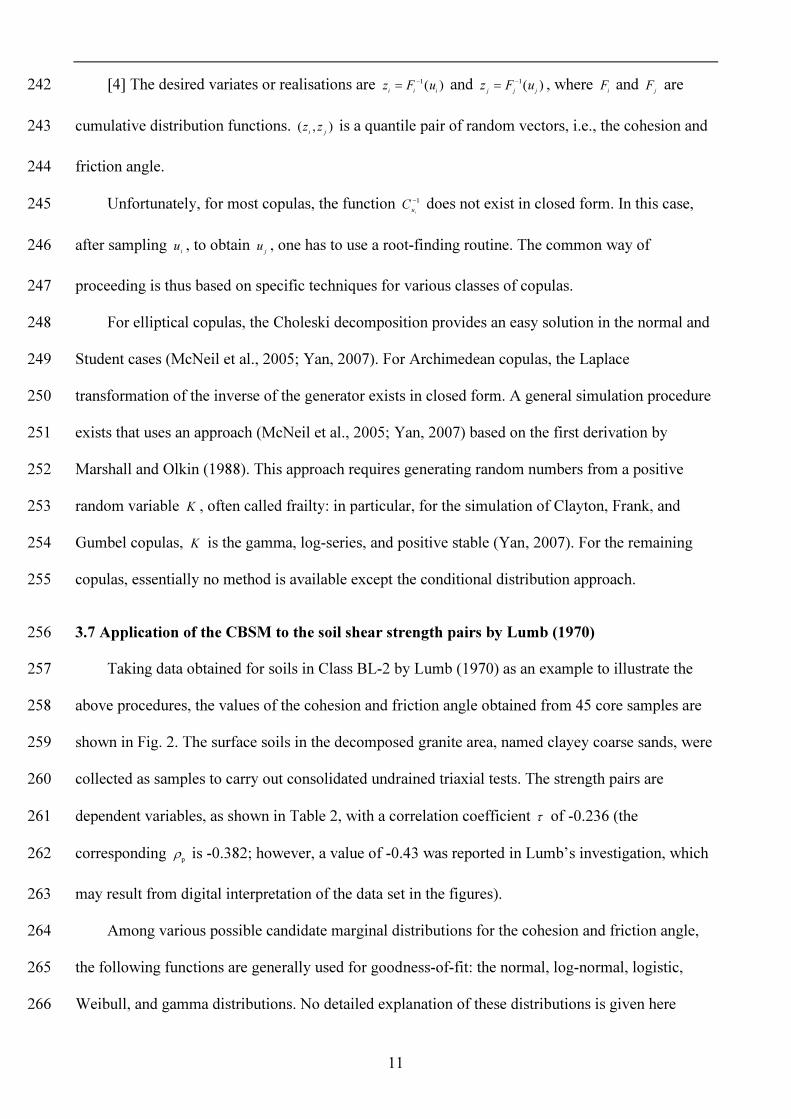
[4] The desired variates or realisations are )(1 iii uFz −

= and )(1 jjj uFz −

= , where iF and jF are 242

cumulative distribution functions. ),( ji zz is a quantile pair of random vectors, i.e., the cohesion and 243

friction angle. 244

Unfortunately, for most copulas, the function 1−iu

C does not exist in closed form. In this case, 245

after sampling iu , to obtain ju , one has to use a root-finding routine. The common way of 246

proceeding is thus based on specific techniques for various classes of copulas. 247 For elliptical copulas, the Choleski decomposition provides an easy solution in the normal and 248

Student cases (McNeil et al., 2005; Yan, 2007). For Archimedean copulas, the Laplace 249 transformation of the inverse of the generator exists in closed form. A general simulation procedure 250 exists that uses an approach (McNeil et al., 2005; Yan, 2007) based on the first derivation by 251 Marshall and Olkin (1988). This approach requires generating random numbers from a positive 252 random variable K , often called frailty: in particular, for the simulation of Clayton, Frank, and 253 Gumbel copulas, K is the gamma, log-series, and positive stable (Yan, 2007). For the remaining 254 copulas, essentially no method is available except the conditional distribution approach. 255

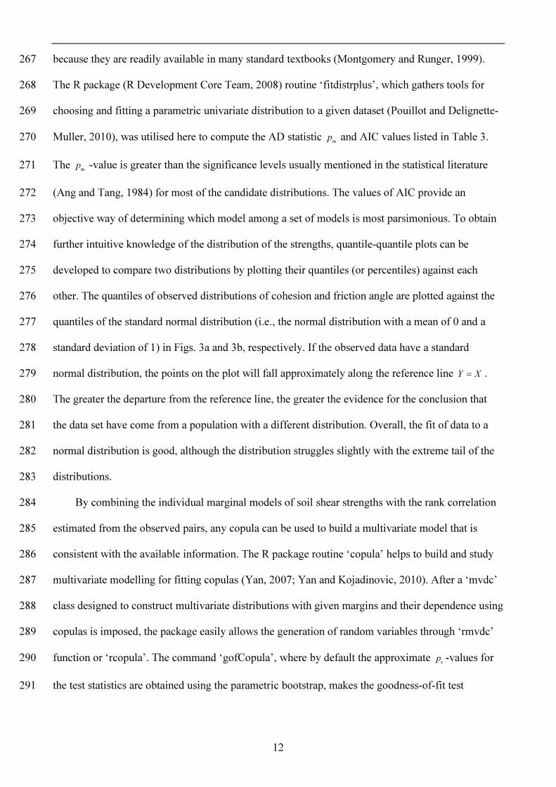
3.7 Application of the CBSM to the soil shear strength pairs by Lumb (1970) 256 Taking data obtained for soils in Class BL-2 by Lumb (1970) as an example to illustrate the 257

above procedures, the values of the cohesion and friction angle obtained from 45 core samples are 258 shown in Fig. 2. The surface soils in the decomposed granite area, named clayey coarse sands, were 259 collected as samples to carry out consolidated undrained triaxial tests. The strength pairs are 260

dependent variables, as shown in Table 2, with a correlation coefficient τ of -0.236 (the 261 corresponding pρ is -0.382; however, a value of -0.43 was reported in Lumb’s investigation, which 262

may result from digital interpretation of the data set in the figures). 263 Among various possible candidate marginal distributions for the cohesion and friction angle, 264

the following functions are generally used for goodness-of-fit: the normal, log-normal, logistic, 265 Weibull, and gamma distributions. No detailed explanation of these distributions is given here 266

12

because they are readily available in many standard textbooks (Montgomery and Runger, 1999). 267 The R package (R Development Core Team, 2008) routine ‘fitdistrplus’, which gathers tools for 268 choosing and fitting a parametric univariate distribution to a given dataset (Pouillot and Delignette-269

Muller, 2010), was utilised here to compute the AD statistic mp and AIC values listed in Table 3. 270

The mp -value is greater than the significance levels usually mentioned in the statistical literature 271

(Ang and Tang, 1984) for most of the candidate distributions. The values of AIC provide an 272 objective way of determining which model among a set of models is most parsimonious. To obtain 273 further intuitive knowledge of the distribution of the strengths, quantile-quantile plots can be 274 developed to compare two distributions by plotting their quantiles (or percentiles) against each 275 other. The quantiles of observed distributions of cohesion and friction angle are plotted against the 276 quantiles of the standard normal distribution (i.e., the normal distribution with a mean of 0 and a 277 standard deviation of 1) in Figs. 3a and 3b, respectively. If the observed data have a standard 278 normal distribution, the points on the plot will fall approximately along the reference line XY = . 279 The greater the departure from the reference line, the greater the evidence for the conclusion that 280 the data set have come from a population with a different distribution. Overall, the fit of data to a 281 normal distribution is good, although the distribution struggles slightly with the extreme tail of the 282 distributions. 283

By combining the individual marginal models of soil shear strengths with the rank correlation 284 estimated from the observed pairs, any copula can be used to build a multivariate model that is 285 consistent with the available information. The R package routine ‘copula’ helps to build and study 286 multivariate modelling for fitting copulas (Yan, 2007; Yan and Kojadinovic, 2010). After a ‘mvdc’ 287 class designed to construct multivariate distributions with given margins and their dependence using 288 copulas is imposed, the package easily allows the generation of random variables through ‘rmvdc’ 289

function or ‘rcopula’. The command ‘gofCopula’, where by default the approximate cp -values for 290

the test statistics are obtained using the parametric bootstrap, makes the goodness-of-fit test 291

13

procedure easier to compute. These R packages are freely available at the Comprehensive R 292 Archive Network (cran.r-project.org). 293

The Cramér-von Mises statistic cp -values and the AIC are listed in Table 4. Usually, two or 294

more copulas are not rejected if their cp -values are greater than 0.05. However, the Clayton copula 295

gives a slightly lower AIC value (-10.99) than the one (-6.17) given by the normal copula, which 296 indicates that the Clayton copula is better suited to this set of observations. Visual scatter plots of 297 realisations from the best-fitting copula are shown in Fig. 4. Only 200 random samples are selected 298 for legibility. The confidence region (CR) is defined in the original physical space of two random 299 variables to characterise the spread of the sampled data in different directions. At the 95% 300

confidence level, the confidence curves for both the observed (enclosed area OI ) and predicted data 301

(enclosed area PI ), determined using a 2D kernel density estimator (‘kde2d’ of MASS package in R, 302

see Venables and Ripley, 2002) using 300 grid points in each direction are illustrated in this graph. 303 To quantify the differences of these confidence regions, the percentage form of relative change aread 304

between the simulated and measured regions can be expressed by the ratio of the absolute change 305

and divided by the measured region, i.e., ( ) 100absO

OParea ×

−=

IIId . Here, the OI associated with the 306

measured region is taken as a reference value. If the relative percentage difference aread is large, the 307

predictions are less valuable than the observations. The relative percentage area difference aread of 308

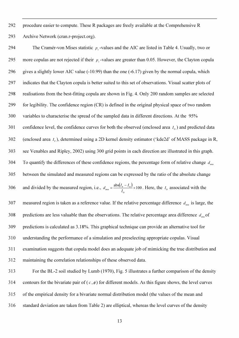
predictions is calculated as 3.18%. This graphical technique can provide an alternative tool for 309 understanding the performance of a simulation and preselecting appropriate copulas. Visual 310 examination suggests that copula model does an adequate job of mimicking the true distribution and 311 maintaining the correlation relationships of these observed data. 312

For the BL-2 soil studied by Lumb (1970), Fig. 5 illustrates a further comparison of the density 313 contours for the bivariate pair of ( c ,φ ) for different models. As this figure shows, the level curves 314

of the empirical density for a bivariate normal distribution model (the values of the mean and 315 standard deviation are taken from Table 2) are elliptical, whereas the level curves of the density 316

14

through copulas with the best-fitting marginal distributions (listed in Table 2) take a different shape. 317 The observed data are superimposed on the contour plots. The Clayton copula with the best-fitting 318 margins provides a much better fit to the bivariate shear strength pairs than the traditional bivariate 319 normal distribution model. A distinct advantage of normal copulas is their ability to capture 320 dependence behaviours often observed in geotechnical engineering. The normal copula with the 321 best-fitting margins provides a distribution that is quite similar, although not identical, to the one 322 provided by the bivariate Clayton copula, and this distribution more reasonably represents the 323 observed data than does the traditional model. 324

The information obtained from the results of a limited number of tests can only reflect a small 325 part of the entire truth. For instance, the 45 observations in this example are very meagre 326 multivariate data. Nevertheless, in engineering practice, including geotechnical design and analysis, 327 it is often necessary to assume that the engineering behaviour indicated by limited data is true of an 328 entire engineering system. The method provides a complete approximation to observed data sets. 329 The differences between the confidence regions of the observed data and the confidence regions of 330 the simulated data are not pronounced, which suggests that the copula model can provide a good 331 description of the given experimental data. Typically, these models could then be used in a Monte 332 Carlo risk analysis. Because the CBSM is obviously prone to model risk, it should be seen as a form 333 of sensitivity analysis. Varying dependencies can be chosen to represent the variability of the 334 correlated soil strength properties and to assess the performance of the existing slope stability 335 analysis program within a probabilistic framework, as illustrated below. 336

4 Probabilistic slope stability analyses 337

4.1 Deterministic analysis 338 Bishop’s deterministic simplified method (Bishop, 1955) is the most widely used limit 339

equilibrium method and is based on the effective stress approach. The soil mass is divided into a 340 number of vertical slices of equal width. The forces between the slices are neglected; each slice is 341

15

considered to be an independent column of soil of unit thickness. Considering the entire slip surface, 342

the factor of safety against sliding, sF , is expressed by the resisting moments against the driving 343

moments 344

( ){ }∑∑

−+=

α

φα mubWbc

WF 1'tan'

sin1

s (11) 345

where s

sintancos

Fm

αϕα

α

′+= , 'c and 'φ are the effective shear strength parameters, W is the weight 346

of a slice, u is the pore pressure, and b is the width of the slice. Taking one slice as an example, the 347

weight of slice W is calculated to be equal to bhaγ , where γ is the bulk unit weight of the soil, ah is 348

the average height of the slice, and b is its width. This is called Bishop’s simplified method. Eq. 349

(11) includes the factor of safety sF on both sides of the equation; therefore, the equation has to be 350

solved by an iterative process. A trial value of sF is first assumed, and the factor of safety is 351

computed by iteration until the assumed and computed values of sF coincide. 352

4.2 Reliability index determined by the correlated shear strength parameters using the CBSM 353 The reliability index is often used to express the degree of uncertainty in the calculated factor 354

of safety for an input set of basic random variables. This type of reliability-based analysis provides 355 quantification of the safety of a system by examining the variability of the relevant parameters as 356 well as their interdependence. Well-established reliability methods, such as the FORM, the first-357 order second-moment (FOSM) method, and Monte Carlo simulation, are useful in determining the 358 reliability of geotechnical designs where the random variables are correlated (Ang and Tang, 1984; 359 Baecher and Christian, 2003). The FOSM approach provides a computationally efficient way of 360 estimating the probability of failure (Ang and Tang, 1984), but the reliability index estimated using 361 this approach is not “invariant” and gives several expressions of the performance function (Duncan, 362 2000; Nadim 2007). The FORM yields an invariant definition of the reliability index (Nguyen and 363 Chowdhury 1984) by transforming basic input variables from the physical space to the standard 364 normal space. To address correlated normal distributions, two techniques may be used with the 365

16

FORM to pursue the expression for independent variables, one based on the Cholesky 366 decomposition of the correlation matrix (Baecher and Christian 2003, pp. 393-398) and the other 367 based on orthogonal transformation by solving the eigenvectors of the covariance matrix (Ang and 368 Tang, 1984, pp. 353-359). For the non-normal correlated variables, a Rosenblatt transformation 369 should be adopted. In this study, a transformation algorithm derived by Zahn (1989) is used, and 370 this algorithm does not require the user to leave the original space of the correlated variables. A 371 brief description of the FORM methodology is provided in the Appendix B. 372

The applicability of the commonly used Monte Carlo simulation method for correlated 373 variables to geotechnical problems has been described in detail in reference (Nguyen and 374 Chowdhury, 1984). A number of algorithms have been developed in the literature to generate 375 correlated random numbers (Tamimi et al. 1989). Alternatively, the technique based on the copula 376 sampling scheme imposed on the best-fitting marginal distributions and rank correlation matrices 377 provides useful reconstructions of the joint behaviour of shear strengths, and the mean and standard 378 deviation of the factor of safety can be obtained through these reconstructions by running the 379 conventional definition of

sF repeatedly. Therefore, the reliability index cbβ determined by the 380

CBSM can be calculated as (Rackwitz and Fiessler, 1977) 381

s

s

F

Fcb

1σ

µβ −= (12) 382

Finally, the failure of probability fP can be estimated by the ratio of the running sum of the 383

failed cases ( 1s <F ) m to the running sum of the total samples simn , i.e., sim

f nmP = . 384

This leads to the following computational procedure: 385 [1] Establish the number of realisations to be used, as discussed in section 3.6; 386 [2] For each point k , generate a paired value of ( )φtan,c , with consideration of the dependence; 387

[3] Calculate the factor of safety ( )φtan,scF and count the number to be added to a running sum 388

m if 1)tan,(s

≤φcF ; 389

17

[4] After all points have been evaluated, evaluate the estimate of fP from the running sum simn , 390

i.e., simf /nmP = , and calculate the reliability index cbβ . 391

When the number of simulations is sufficiently large, the standard deviation of the estimated 392

values sF can be obtained by simulating sample inverses with the square root of the simulating 393

number. Thus, the accuracy increases as the number of simulations increases. In general, when the 394

number of simulations is greater than fsim /100 Pn ≥ , the accuracy may be satisfactory (Tobutt, 1982; 395

Husein Malkawi et al., 2000), and the probability of failure fP can be calculated to represent a 396

deterministic solution. 397

4.3 Illustrative numerical example 398 To illustrate the influence of the correlation on the reliability index cbβ , a series of analyses by 399

the CBSM and the FORM are demonstrated in the following typical slope cases. 400

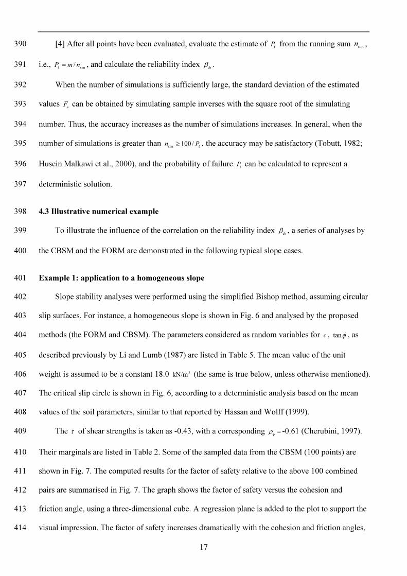
Example 1: application to a homogeneous slope 401 Slope stability analyses were performed using the simplified Bishop method, assuming circular 402

slip surfaces. For instance, a homogeneous slope is shown in Fig. 6 and analysed by the proposed 403 methods (the FORM and CBSM). The parameters considered as random variables for c , φtan , as 404

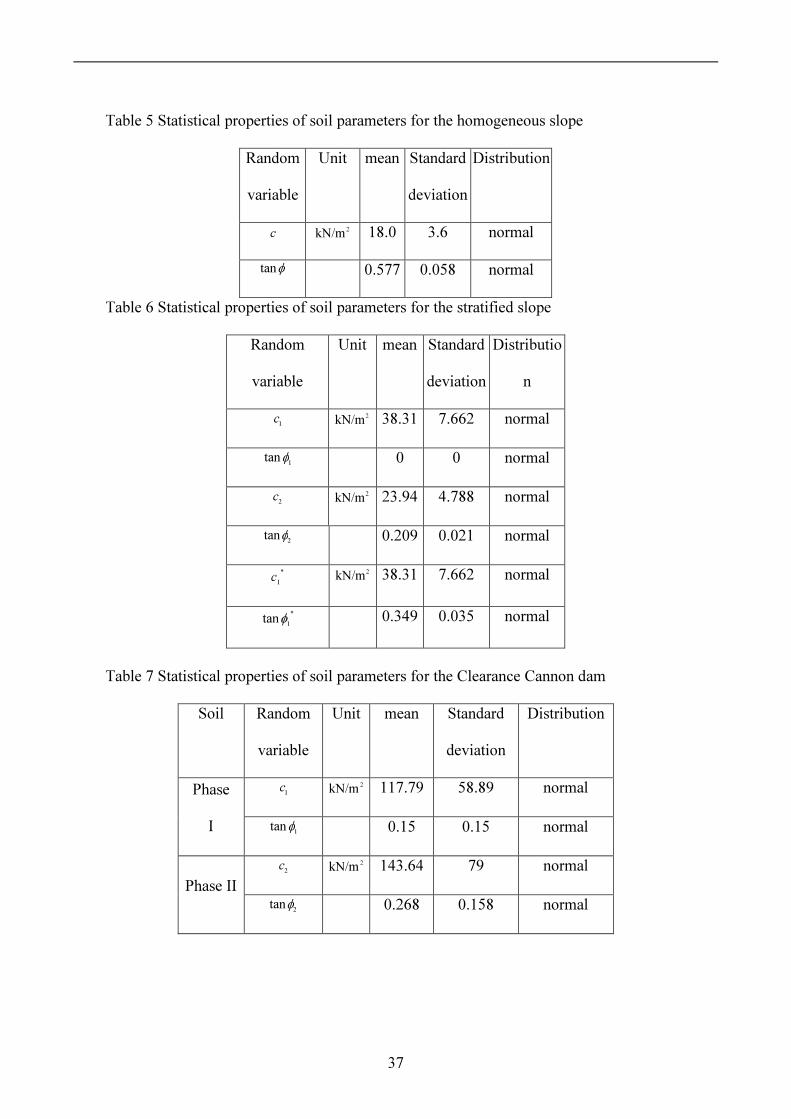
described previously by Li and Lumb (1987) are listed in Table 5. The mean value of the unit 405 weight is assumed to be a constant 18.0 3kN/m (the same is true below, unless otherwise mentioned). 406 The critical slip circle is shown in Fig. 6, according to a deterministic analysis based on the mean 407 values of the soil parameters, similar to that reported by Hassan and Wolff (1999). 408

The τ of shear strengths is taken as -0.43, with a corresponding =pρ -0.61 (Cherubini, 1997). 409

Their marginals are listed in Table 2. Some of the sampled data from the CBSM (100 points) are 410 shown in Fig. 7. The computed results for the factor of safety relative to the above 100 combined 411 pairs are summarised in Fig. 7. The graph shows the factor of safety versus the cohesion and 412 friction angle, using a three-dimensional cube. A regression plane is added to the plot to support the 413 visual impression. The factor of safety increases dramatically with the cohesion and friction angles, 414

18

although it can be less than 1 for some small values of the cohesion and friction angle. A critical 415

state line is defined as the projection line of the regression plane on the horizontal plane 1s =F , as 416

illustrated in Fig. 7. Pairs of )tan,( φc values, i.e., (15, 0.3) and (10, 0.36), follow this line. If pairs of 417

)tan,( φc values are sampled with a correlation coefficient close to perfect ( 1≈τ ), these values will 418

approximately follow a straight line on the c and φtan plane (in this case, the variance of the shear 419

strength is reduced in some degree); thus, the regression problem is reduced to a projection line 420 rather than a plane. 421

The probability of failure can be calculated for specific combinations of the cohesion and 422 friction angle. These combinations are obtained by sequentially setting one parameter with the 423 remaining parameter set at its mean value. The standard deviation of cohesion is assumed to be 20 424 per cent of the mean, and the standard deviation of friction angle is assumed to be 10 per cent of the 425 mean. The computed probability of failure is plotted against cohesion and friction angle in Fig. 8. 426 The probability of failure increases considerably as the cohesion and friction angle decrease. 427

To demonstrate the influence of correlation extremes on reliability indices, the cross-428 correlation τ is varied from -0.91 to 0.91 (such extreme values cannot be expected in reality) and 429 the same statistics (including the means and standard deviations) for the cohesion and friction angle 430 are fed into the FORM and CBSM (using the normal copula as an example, as described below). 431 The reliability indices computed for these correlation coefficients are shown in Fig. 9. The 432 reliability indices are expected to decrease as the correlation coefficients decrease. This observation 433 arises from the fact that the variance of shear strength is reduced if there is a strong negative 434 correlation between cohesion and friction angle. The results from the CBSM and the FORM show 435 good agreement, which proves to work well in determining the reliability index using the 436 computation technique presented. 437

In Fig. 9, the means of the factor of safety are also given by the deterministic limit equilibrium 438 method through those sampled strength pairs (i.e., 10,000 simulations). The correlation coefficients 439 have little influence on the means, which are always inferred from their aggregate behaviour in 440

19

terms of the mean soil strengths. Li and Lumb (1987) determined the value of the reliability index 441 using Hasofer and Lind’s approximate method. According to their results, the minimum critical 442 factor of safety in conventional design is estimated to be 1.5, and the corresponding reliability index 443 is 2.63. The results obtained in this study show some agreement with their results, although the 444 model input may be slightly different. 445

The FORM is a powerful tool in probabilistic geotechnical analysis, especially in standard 446 normal spaces. However, partial differential terms of the performance function have to be derived if 447 a gradient-based optimisation method is employed when searching for the shortest distance to the 448 failure state. The CBSM better facilitates allowing the non-normal distribution and non-linear 449 failure state function. Other types of distributions for soil strength properties, such as the triangular, 450 beta, and generalised gamma distributions (suggested by Lumb 1970; Baecher and Christian 2003; 451 Wolff 1985), can also be implemented in this approach. The CBSM is flexible in the sense that 452 different distributions can be used to describe each marginal distribution while still being able to 453 incorporate dependence, i.e., it allows the joint distribution function type to be different from the 454 marginal cumulative distribution function types (Poulin et al., 2007). 455

Example 2: application to a stratified slope 456 The cross section of a two-layer slope (Hassan and Wolff, 1999) is shown in Fig. 10. The slope 457

in clay is bounded by a hard layer below and is parallel to the ground surface. The statistics of the 458 soil strength parameters are summarised in Table 6. No water table or external water is considered. 459 The corresponding critical deterministic slip surface, based on the mean values of the soil properties, 460 is also presented in Fig. 9. A similar (circular) surface was reported by Hassan and Wolff (1999). 461

A parametric study was performed by specifying various correlation coefficients between the 462 cohesion and the friction angle. The calculated reliability indices obtained from the FORM and 463 CBSM fort various correlation coefficient values are given in Fig. 11. Varying the cross-correlation 464

τ from -0.91 to 0.91 was found to have only a minor influence on the stochastic behaviour of the 465 slope stability. This difference was not expected owing to the sliding circle slide being mostly 466

20

through layer one (its cohesion is assumed to be zero). Notably, when a single soil strength 467 parameter is used, consideration of the uncertainties will fall into a class of Monte Carlo sampling 468 method. For instance, a granular material has little or no cohesion, and a clayey material has a very 469 small or even zero friction angle. There is no difference between the CBSM and the conventional 470 Monte Carlo sampling method because no explicit dependence should be represented. 471

When the cohesion and friction strength parameters of the first layer are set with the same 472

means but with larger standard deviations, as listed in Table 6, *1c and *

1tanφ , the computed 473

reliability indices by the CBSM are shown with symbols ‘+’ in Fig. 11. The reliability indices 474 decrease as the correlation increases. 475

Example 3: Application to the Clearance Cannon dam 476 The third typical cross section of the Clearance Cannon dam previously described by Wolff et 477

al. (1995) is presented in Fig. 12. The structure consists of two zones of compacted clay, including 478 Phase I fill and Phase II fill, over layers of sand and limestone. The strength parameters of the two 479 clay layers are considered random variables. The statistics for these parameters, based on 480 unconsolidated and un-drained shear tests of samples from the embankment (Wolff, 1985), are 481 shown in Table 7. The critical deterministic circle is shown in Fig. 12. 482

A distribution with a high standard deviation, as used here for Phase I and Phase II clays, 483 implies negative values associated with the low-probability tail of the distribution, which is not 484 admissible for strength parameters. A similar truncated technique (El-Ramly et al., 2002) is 485 imposed to provide reasonable values. 486

Fig. 13 shows the relations of the factor of safety and the reliability index to the correlation 487 coefficients. The value of the factor of safety increases slightly as the correlation coefficients 488 increase. The reliability index values based on both algorithms increase when the correlation 489

coefficient between c and φ decreases from positive to negative. This is especially evident for the 490

lowest values of the coefficient of variation for the cohesion and friction angle. 491

21

5 Discussion 492

In the probabilistic stability analysis described above, the location of the critical surface is part 493 of the evaluation of the performance function and depends on the values of the strength parameters, 494 which are uncertain. As noted by Hassan and Wolff (1999), the difference between the reliability 495 index defined for the critical deterministic surface and the minimum reliability index may be 496 substantial in some cases. Locating this critical probabilistic surface may require additional 497 computational effort, and not doing so may lead to inaccurate measures of reliability. The technique 498 suggested by Hassan and Wolff for locating the surface of the minimum reliability index is used in 499 this study, which examines offset values of each of the random variables while keeping the 500 remaining parameters at their mean values. 501

Clearly, variations in the correlation parameters of the strengths can substantially affect the 502 reliability index, especially when the correlation approaches negative 1. As determined by 503 Chowdhury and Xu (1992), the reliability of a slope increases as the correlation between the 504 cohesion and friction angle decreases. Thus, when the cohesion and friction angle are negatively 505 correlated, the reliability index can be much higher than when the shear strength parameters are 506 positively correlated. Therefore, neglecting any negative correlation underestimates the reliability 507 index, while neglecting any positive correlation overestimates the reliability index. 508

These efforts in the bivariate statistical analysis of soil strength parameters are encouraging but 509 insufficient to obtain an accurate description of the soil uncertainty state, which sometimes 510 dominates multivariate problems. Some other parameters, such as the pore water pressure, unit 511 weight, consolidation coefficient, and seepage coefficient should also be considered. 512

Care should be taken, however, to ensure that the minimum and maximum values of the 513 selected distribution are consistent with the physical limits of the parameter being modelled. For 514 example, shear strength parameters should not imply negative values. If the selected distribution 515 implies negative values in the third case, then the distribution is truncated at a practical minimum 516

22

threshold. Alternatively, a best-fitting distribution, such as the log-normal, generalised gamma or 517 Weibull distribution, can fit the observed data and avoid negative samples. 518

The identified copulas can be wrong if a very small number of samples are used. Although 519 more fundamental experiments of shear tests of soils to provide enough data sets should be 520 encouraged greatly, the sample size with around 50 can be acceptable (Zhang and Singh, 2007). The 521 size of the data set has been mentioned by some researchers (Ang and Tang, 1984; Genest and 522 Favre, 2007) as affecting the confidence regions or dependence structures. 523

6 Conclusions 524

An approach to probabilistic slope stability analysis that accounts for the statistical correlation 525 of the input soil strength parameters is presented. A set of reliability indices for varying correlation 526 coefficients yield an objective description of the overall evaluation of slope stability and a better 527 description of the degree of uncertainty. The applicability of the proposed methodology (including 528 the CBSM and the FORM) described herein is examined for a variety of slope stability problems 529 from the literature, such as a homogeneous slope, a stratified slope, and the embankment of the 530 Cannon hydroelectric project. The method is proven to be a practical and efficient method for 531 facilitating a probabilistic slope stability analysis of cohesive frictional soils through copula-based 532 samplings. The method does not rely on any assumptions concerning the geometry of the failure 533 surface and can be applied to any complex clay slope geometry, layering and pore pressure 534 conditions. 535

Invoking the CBSM to take into account the interdependence of soil strength properties, the 536 new method has an advantage in implementation for inputting a combination of soil strength 537 parameters. The approach is simple and can be applied in practice with little effort beyond that 538 needed in a conventional analysis. The method permits practicing engineers to locate the surface of 539 the reliability index using existing deterministic slope stability computer programs, without special 540 software, by making a moderate number of multiple runs. 541

23

The analysis of the results and the examination of the resulting plots illustrate the importance 542 with respect to the reliability index of the correlation coefficient between soil strength properties, 543 i.e., the reliability decreasing as the correlation increases. Comparing the computed results and the 544 evaluated ones obtained using the FORM method, the CBSM tends to open the way for various 545 marginal distribution types and dependence structure. 546

7 Reference 547

Alonso, E. E. 1976. Risk analysis of slopes and its application to slopes in Canadian sensitive 548 clays. Geotechnique, 26, 453-472. 549

Akaike, H. 1974. A new look at the statistical model identification. IEEE Trans. Autom. Control, AC-550 19(6), 16-722. 551

Anderson, T.W., and D.A. Darling. 1954. A test of goodness-of-fit. J.Am. Stat. Assoc., Vol. 49, 765–552 769. 553

Ang, A. H.-S., and Tang, W. H., 1984. Probability Concepts in Engineering Planning and Design. 554 John Wiley, New York, 562pp. 555

Baecher G.B. and Christian J.T.. 2003. Reliability and statistics in geotechnical engineering. John 556 Wiley & Sons Inc. 557

Bergado, D. T., and Anderson, L. R. 1985. Stochastic analysis of pore pressure uncertainty for the 558 probabilistic assessment of the safety of earth slopes. Soils and Found., 25(2), 87-105. 559

Bishop, A.W. 1955. The Use of the Slip Circle Stability in Analysis of Slopes. Geotechnique, v.1, 560 pp.7-17. 561

Boyer, B., Gibson, M., Loretan, M., 1999. Pitfalls in tests for changes in correlation. International 562 Finance Discussion Paper 597, Board of Governors of the Federal Reserve System. 563

Brejda J., Moorman, J., Smith, T.B., Karlen, J.L., Allan,D.L., Dao, T. H., 2000. Distribution and 564 variability of surface soil properties at a regional scale. Soil Sci. Soc. Am. J. 64, 974-982. 565

Cherubini C. 1997. Data and considerations on the variability of geotechnical properties of soils. 566 Proceedings of the International Conference on safety and reliability (ESREL 97) Lisbon Vol. 2 567

24

1583-1591. 568

Cho S. E., Park H. C. 2010. Effect of spatial variability of cross-correlated soil properties on 569 bearing capacity of strip footing. Int. J. Numer. Anal. Meth. Geomech. 34:1-26. 570

Chowdhury R.N., Tang W.H., and Sidi I. 1987. Reliability model of progressive slope failure. 571 Geotechnique, 37(4), 467-481. 572

Chowdhury RN, Xu D. 1992. Reliability index for slope stability assessment-two methods 573 compared. Reliab. Eng. Syst. Safe., 37(2): 99-108. 574

Chowdhury RN, Xu DW. 1993. Rational polynomial technique in slope stability analysis. Journal of 575 Geotechnical Engineering Division, ASCE 119(12):1910-28. 576

Christian, J. T., Ladd, C. C., and Baecher, G. B. 1994. Reliability applied to slope stability analysis. 577 J. Geotech. Engrg., ASCE, 120(12), 2180-2207. 578

Clemen Robert T. and Reilly Terence. 1999. Correlations and copulas for decision and risk analysis. 579 Management Science, 45(2):208-224. 580

Duncan, J.M. 2000. Factors of safety and reliability in geotechnical engineering. Journal of 581 Geotechnical and Geoenvironmental Engineering, ASCE, 126: 307-316. 582

Dupuis DJ. 2007. Using Copulas in hydrology: benefits, cautions and issues. Journal of Hydrologic 583 Engineering, ASCE 12(4): 381-393. 584

El-Ramly, H., Morgenstern, N. R., and Cruden, D. M. 2002. Probabilistic slope stability analysis for 585 practice. Can. Geotech. J., 39, 665-683. 586

Embrechts, P., McNeil, A.J., Straumann, D., 2002. Correlation and dependence in risk 587 management: properties and pitfalls. In: Dempster, M. (Ed.), Risk Management: Value at Risk and 588 Beyond. Cambridge University Press, Cambridge, pp. 176-223. 589

Fenton, G.A. and Griffiths, D.V. 2003. Bearing capacity prediction of spatially random c -φ soils. 590 Can Geotech J. 40(1): 54-65. 591

Ferson, Scott and Hajagos, Janos G., 2006. Varying correlation coefficients can underestimate 592 uncertainty in probabilistic models, Reliability Engineering and System Safety, 91, 1461-1467. 593

Forrest William S. and Orr Trevor L.L. 2010. Reliability of shallow foundations designed to 594

25

Eurocode 7, Georisk: Assessment and Management of Risk for Engineered Systems and 595 Geohazards, 4(4): 186-207. 596

Frees, E.W., and Valdez E.A. 1998. Understanding relationships using copulas. North Amer. Actua. 597 J., 2 (1): 1-25. 598

Genest C, MacKay J. 1986. The Joy of Copulas: Bivariate Distributions with Uniform Marginals. 599 The American Statistician, 40, 280-283. 600

Genest C, Favre AC. 2007. Everything you always wanted to know about Copula modelling but 601 were afraid to ask. J. Hydrol. Eng., ASCE 12(4): 347-368. 602

Genest, C., Remillard, B., Beaudoin, D., 2009. Goodness-of-fit tests for copulas: A review and a 603 power study. Insur.: Math. Econ. 44, 199-214. 604

Harr, M.E. 1987. Reliability based design in Civil Engineering, McGraw-Hill Book Company, NY. 605

Hasofer, A. A., and Lind, A. M. 1974. Exact and invariant second moment code format. J. Engrg. 606 Mech. Div., ASCE, 100(1): 111-121. 607

Hassan, A., and Wolff, T. 1999. Search algorithm for minimum reliability index of earth slopes. 608 Journal of Geotechnical and Geoenvironmental Engineering, ASCE, 125: 301-308. 609

Hata Yoshiya, Ichii Koji and Tokida Ken-ichi. 2011. A probabilistic evaluation of the size of 610 earthquake induced slope failure for an embankment, Georisk: Assessment and Management of 611 Risk for Engineered Systems and Geohazards, DOI:10.1080/17499518.2011.604583. 612

Honjo, Y., Suzuki, M., Matsuo, M. 2000. Reliability analysis of shallow foundations in reference to 613 design codes development. Computers and Geotechnics, 26, 331-346. 614

Husein Malkawi, A.I.; Hassan, W.F and Abdulla, F. 2000. Uncertainty and reliability analysis applied 615 to slope stability. Structural Safety Journal, 22, 161-187. 616

Joe H. 1997. Multivariate Models and Dependence Concept, Chapman and Hall: New York. 617

Kojadinovic, I., Yan, J., 2010. Modeling Multivariate Distributions with Continuous Margins Using 618 the copula R Package. J. Stat. Soft. 34(9), 1-20. 619

Kotz, S., Balakrishnan, N. and Johnson, N. 2000. Continuous Multivariate Distributions. New York: 620 Wiley. 621

26

Lambert, P. and Vandenhende, F., 2002. A copula-based model for multivariate nonnormal 622 longitudinal data: analysis of a dose titration safety study on a new antidepressant, Statistics in 623 Medicine, 21, 3197-3217. 624

Li KS, Lumb P. 1987. Probabilistic design of slopes. Canadian Geotechnical Journal, 24: 520-535. 625

Lumb, P. 1970. Safety factors and the probability distribution of soil strength, Canadian 626 Geotechnical Journal, 7, 225-242. 627

Lü Qing, Low Bak Kong. 2011. Probabilistic analysis of underground rock excavations using 628 response surface method and SORM. Computers and Geotechnics, 38, 1008-1021. 629

Marshall, A.W., Olkin, I., 1988. Families of multivariate distributions. Journal of the American 630 Statistical Association 83, 834–841. 631

McNeil A J, Frey R, Embrechts P. Quantitative Risk Management: Concepts, Techniques and Tools. 632 Princeton: Princeton University Press, 2005. 633

Montgomery D. C. and Runger G. C., 1999. Applied Statistics and Probability for Engineers. Wiley-634 Interscience. 635

Nadim, F. 2007, Tools and Strategies for Dealing with Uncertainty in Geotechnics. In Probabilistic 636 Methods in Geotechnical Engineering, eds. D.V. Griffiths and G.A. Fenton, Pub. Springer, Wien, 637 New York, pp.71-96. 638

Nelsen RB. 2006. An Introduction to Copulas, Springer: New York. (2nd edition) 639

Nguyen, V.U. Chowdhury, R.N. 1984. Probabilistic study of spoil pile stability in strip coal mines-640 two techniques compared. Rock. Mech. Min. Sci. & Geomech.Abstr. pp. 303-212. 641

Phoon K.K. and Nadim F. 2004. Modelling non-Gaussian random vectors for FORM: state-of-the-642 art review. International workshop on risk assessment in site characterization and geotechnical 643 design. India Institute of Science, Bangalore, India, November 26-27. 644

Phoon, K.K., and Kulhawy, F.H. 1999. Evaluation of geotechnical property variability. Canadian 645 Geotechnical Journal, 36: 625-639. 646

Poulin A, Huard D, Favre A, Pugin S. 2007. Importance of tail dependence in bivariate frequency 647 analysis. Journal of Hydrologic Engineering, ASCE 12(4): 394-403. 648

27

Pouillot, R., Delignette-Muller, M.L., 2010. Evaluating variability and uncertainty separately in 649 microbial quantitative risk assessment using two R packages. Int. J. Food Microbiol. 142, 330-340. 650

R Development Core Team, 2008. R: A language and environment for statistical computing. R 651 Foundation for Statistical Computing, Vienna, Austria, ISBN:3-900051-07-0. http://www.R-652 project.org. 653

Rackwitz R. 2000. Reviewing probabilistic soils modeling. Computers and Geotechnics, 26(3): 199-654 223. 655

Rackwitz, R., and Fiessler, B. 1977. An algorithm for calculation of structural reliability under 656 combined loading. P Berichte zur Sicherheitstheorie der Bauwerke, Lab. f. Konstr. Ingb., Munchen, 657 Germany. 658

Salvadori G, De Michele C. Kottegoda NT & Rosso R. 2007. Extremes in Nature, Springer: 659 Dordecht, The Netherlands. 660

Schweizer, B. 1991. Thirty years of copulas. In G. Dall'Aglio, S. Kotz and G. Salinetti (eds), 661 Advances in Probability Distributions with Given Marginals. Dordrecht: Kluwer. 662

Sklar, A. 1959. Fonctions de répartition à n dimensions et leurs marges, Publications de l’Institut de 663 Statistique Université de Paris, 8, 229-231. 664

Tamimi S, Amadei B, Frangopol DM. 1989. Monte Carlo simulation of rock slope stability. Comput 665 Struct; 33(6):1495-1505. 666

Tang WH, Yucemen MS, Ang AH-S. 1976. Probability-based short term design of slopes. Canadian 667 Geotechnical Journal ,13(3):201-215. 668

Thoft-Christensen P.; Baker, MJ. 1982. Structural reliability theory and its applications. Springer-669 Verlag, New York. 670

Tobutt DC. 1982. Monte Carlo simulation methods for slope stability. Computer & Geosciences, 671 8(2): 199-208. 672

Venables, W.N., Ripley, B.D., 2002. Modern Applied Statistics with S. Fourth Edition. Springer, New 673 York. ISBN 0-387-95457-0. 674

Wolff, T. F. 1985. Analysis and design of embankment dam slopes: a probabilistic approach, Ph.D. 675

28

Thesis, Purdue University, Lafayette, Indiana. 676

Wolff T. F., Hassan A., Khan R., Ur-Rasul, I., and Miller, M. 1995. Geotechnical reliability of dam 677 and levee embankments. Technical report prepared for U.S. Army Engineer Waterways Experiment 678 Station, Geotechnical Laboratory, Vicksburg, Miss. 679

Yan, J., 2007. Enjoy the Joy of Copulas: With a Package copula. J. Stat. Soft. 21(4), 1-21. 680

Yan, J., Kojadinovic, I., 2010. copula: Multivariate Dependence with Copulas. R package version 681 0.9-5, URL http://CRAN.R-project.org/package=copula. 682

Zahn, J.J. 1989. Empirical failure criteria with correlated resistance variables. Journal of Structural 683 Engineering. 116(11): 3122-3137. 684

Zhang, L. and Singh, V. P. 2007. Trivariate flood frequency analysis using the Gumbel-Hougaard 685 copula, J. Hydrol. Eng., 12, 431-439. 686

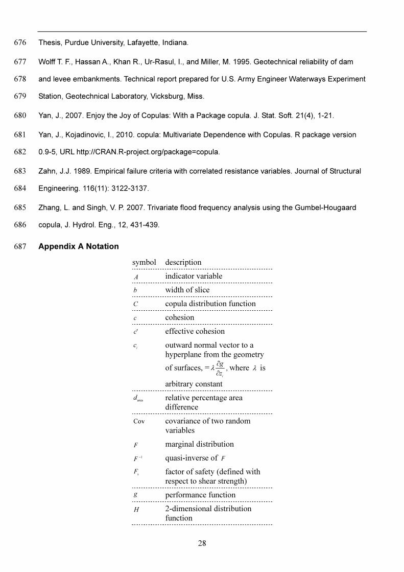
Appendix A Notation 687 symbol description A indicator variable b width of slice C copula distribution function c cohesion 'c effective cohesion ic outward normal vector to a

hyperplane from the geometry of surfaces, =

izg∂∂λ , where λ is

arbitrary constant aread relative percentage area

difference Cov covariance of two random

variables F marginal distribution 1−F quasi-inverse of F

sF factor of safety (defined with

respect to shear strength) g performance function H 2-dimensional distribution

function

29

ah average height of slice βL distance in standard deviation

units corr

βL βL for correlated variables, = ∑

=

2

1ii

Ti Rcc

m total number of failed cases αm term used in the simplified

Bishop method, =

s

sin'tancosF

αφα +

simn number of simulations cp Cramér-von Mises test statistic mp Anderson-Darling test statistic Pr probability of failure

nS Cramér-von Mises function u pore water pressure iu thi uniform random variable,

= )( iZF ju thj uniform random variable,

= )( jZF W weight of slice, = bh

aγ

iZ thi random variable *iZ dimensionless variable;

reduced variable; or standard random variable

iz thi realization of iZ jZ thj random variables jz thj realization of jZ α inclination of the slope; or the

slope of failure surface iα direction cosine, =

βLci

corr

iα iα for correlated variables, =

βLRci

HLβ the Hasofer-Lind reliability index

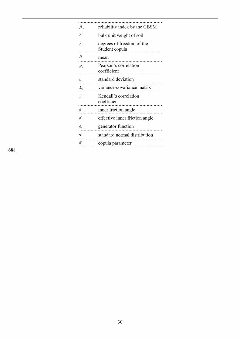
30

cbβ reliability index by the CBSM γ bulk unit weight of soil λ degrees of freedom of the

Student copula µ mean pρ Pearson’s correlation

coefficient σ standard deviation 2Σ variance-covariance matrix τ Kendall’s correlation

coefficient φ inner friction angle 'φ effective inner friction angle θφ generator function Φ standard normal distribution θ copula parameter

688

31

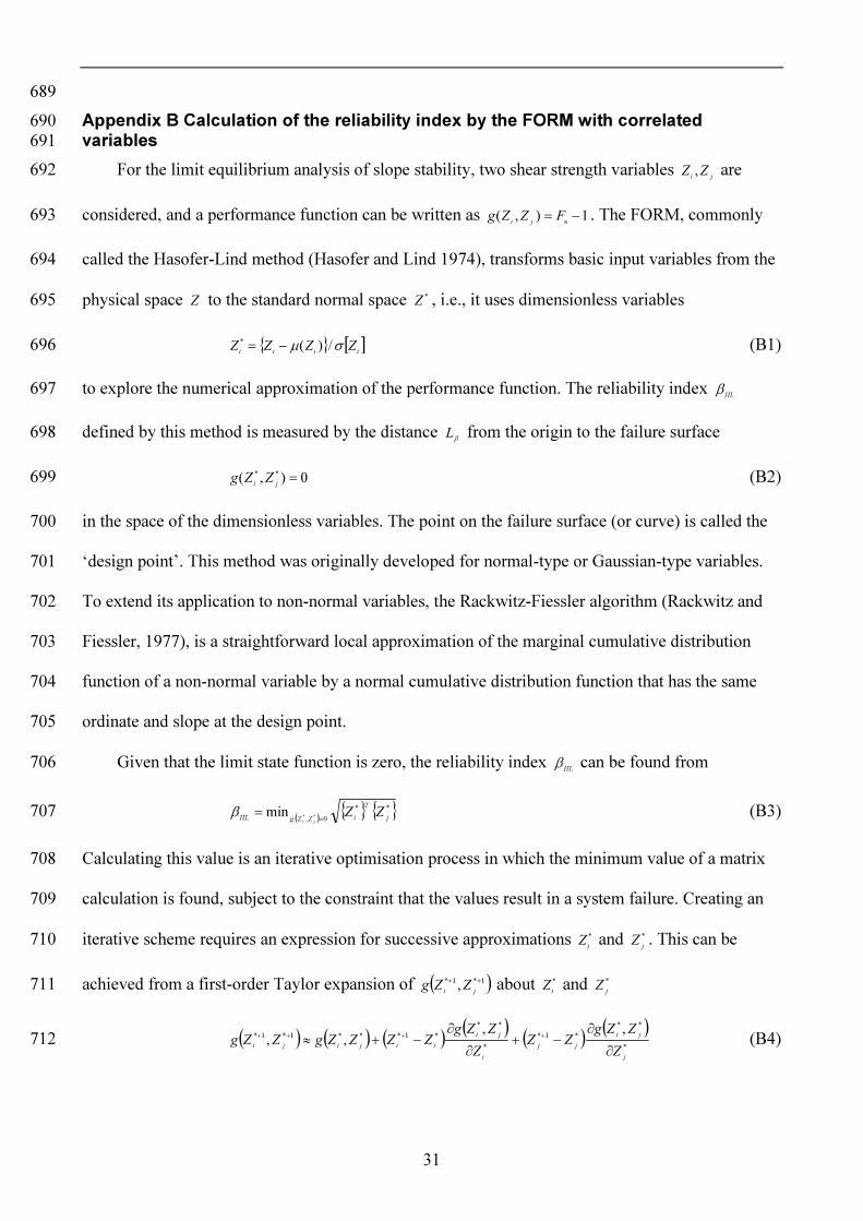
689 Appendix B Calculation of the reliability index by the FORM with correlated 690 variables 691

For the limit equilibrium analysis of slope stability, two shear strength variables ji ZZ , are 692

considered, and a performance function can be written as 1),( s −= FZZg ji . The FORM, commonly 693

called the Hasofer-Lind method (Hasofer and Lind 1974), transforms basic input variables from the 694 physical space Z to the standard normal space *Z , i.e., it uses dimensionless variables 695

{ } [ ]iiii ZZZZ σµ /)(*−= (B1) 696

to explore the numerical approximation of the performance function. The reliability index HLβ 697

defined by this method is measured by the distance βL from the origin to the failure surface 698

0),( **=ji ZZg (B2) 699

in the space of the dimensionless variables. The point on the failure surface (or curve) is called the 700 ‘design point’. This method was originally developed for normal-type or Gaussian-type variables. 701 To extend its application to non-normal variables, the Rackwitz-Fiessler algorithm (Rackwitz and 702 Fiessler, 1977), is a straightforward local approximation of the marginal cumulative distribution 703 function of a non-normal variable by a normal cumulative distribution function that has the same 704 ordinate and slope at the design point. 705

Given that the limit state function is zero, the reliability index HLβ can be found from 706

( ) { } { }**0, **min j

TiZZgHL ZZ

ji ==β (B3) 707

Calculating this value is an iterative optimisation process in which the minimum value of a matrix 708 calculation is found, subject to the constraint that the values result in a system failure. Creating an 709 iterative scheme requires an expression for successive approximations *

iZ and *jZ . This can be 710

achieved from a first-order Taylor expansion of ( )1*1* , ++

ji ZZg about *iZ and *

jZ 711

( ) ( ) ( ) ( ) ( ) ( )*

***1*

*

***1***1*1* ,,

,,

j

jijj

i

jiiijiji Z

ZZgZZZZZgZZZZgZZg

∂∂

−+∂

∂−+≈ ++++ (B4) 712

32

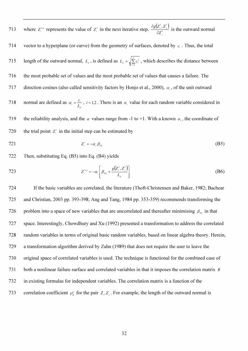
where 1*+iZ represents the value of *

iZ in the next iterative step. ( )*

**,

j

ji

ZZZg

∂∂ is the outward normal 713

vector to a hyperplane (or curve) from the geometry of surfaces, denoted by ic . Thus, the total 714

length of the outward normal, βL , is defined as ∑=

=2

1

2

iicLβ , which describes the distance between 715

the most probable set of values and the most probable set of values that causes a failure. The 716

direction cosines (also called sensitivity factors by Honjo et al., 2000), iα , of the unit outward 717

normal are defined as β

αLci

i = , 2,1=i . There is an iα value for each random variable considered in 718

the reliability analysis, and the α values range from -1 to +1. With a known iα , the coordinate of 719

the trial point *iZ in the initial step can be estimated by 720

HLiiZ βα−=* (B5) 721

Then, substituting Eq. (B5) into Eq. (B4) yields 722

( )

+−=+

ββα L

ZZgZ jiHLii

**1* , (B6) 723

If the basic variables are correlated, the literature (Thoft-Christensen and Baker, 1982; Bachear 724 and Christian, 2003 pp. 393-398; Ang and Tang, 1984 pp. 353-359) recommends transforming the 725 problem into a space of new variables that are uncorrelated and thereafter minimising HLβ in that 726

space. Interestingly, Chowdhury and Xu (1992) presented a transformation to address the correlated 727 random variables in terms of original basic random variables, based on linear algebra theory. Herein, 728 a transformation algorithm derived by Zahn (1989) that does not require the user to leave the 729 original space of correlated variables is used. The technique is functional for the combined case of 730 both a nonlinear failure surface and correlated variables in that it imposes the correlation matrix R 731 in existing formulas for independent variables. The correlation matrix is a function of the 732

correlation coefficient ijpρ for the pair ji ZZ , . For example, the length of the outward normal is 733

33

∑=

=2

1

corr

ii

Ti RccLβ and the direction cosines are

corr

corr

βα

LRci

i = . Readers can refer to Zahn (1989) for 734

more details on this numerical algorithm. 735 The scheme can now be summarised as follows: 736 [1] Standardise the basic random variables Z to the standardised normal variables *Z . 737

[2] Compute the derivative *i

i Zgc

∂∂= and the direction cosines

βα

Lci

i = (for the independent 738

case) or β

αLRci

i =corr (for the dependent case). 739

[3] Evaluate ),( **ji ZZg . 740

[4] Compute 1*+iZ using Eq. (B6) and 1+

HLβ using Eq. (B3). 741

[5] Check whether 1+HLβ and 1*+

iZ have converged; if not go to step [2]. 742

34

List of Tables Table 1 Summary of the adopted bivariate copula functions and their dependence parameters Table 2 Mean, standard deviation, and correlation coefficient for soil BL-2 Table 3 AD statistic and AIC of marginal distributions for soil BL-2

Table 4 AIC and cp -values of various copulas for soil BL-2

Table 5 Statistical properties of soil parameters for the homogeneous slope Table 6 Statistical properties of soil parameters for the stratified slope Table 7 Statistical properties of soil parameters for the Clearance Cannon dam

35

Table 1 Summary of the adopted bivariate copula functions and their dependence parameters

Family Copula function Generator function

Relationship between θ and τ Range of θ

normal ( ) ( )( )211

1, uuN −− ΦΦθ / ( )2/sin πτθ = [ ]1,1−

Student ( ) ( )( )21

11

, , uTuTT −−

λλλθ / ( )2/sin πτθ = [ ]1,1− Clayton ( ) θθθ /1

21 1 −−− −+ uu ( ) θθ /1−−t ( )ττθ −= 1/2 [ ) { }0,1 −∞−

Frank ( )( ) ( )( )( )

−−−−−−+− 1exp1exp1exp1ln1 21

θθθ

θuu ( )

( ) 1-exp1t-expln

−

−−

θθ

( )∫−

+−=θ

θθτ

02 d1exp441 t

tt ( ) { }0, −∞∞−

Gumbel ( ) ( )[ ]( )θθθ /1

21 lnlnexp uu −+−− ( )θtln− ( )τθ −= 1/1 [ )∞,1

Plackett ( )( )[ ] ( ){ }12/TermA11 1/221 −−+−+ θθ uu

( )( ){ } ( )1411TermA 212

21 −−+−+= θθθ uuuu / Obtained numerically ( ) { }1,0 −∞

Φ : cumulative distribution function of the standard normal distribution

θN : cumulative distribution function of the standard bivariate normal distribution with Pearson

correlation θ

λT : cumulative distribution function of the Student with λ degrees of freedom

λθ ,T : cumulative distribution function of the bivariate Student distribution with λ degrees of

freedom

36

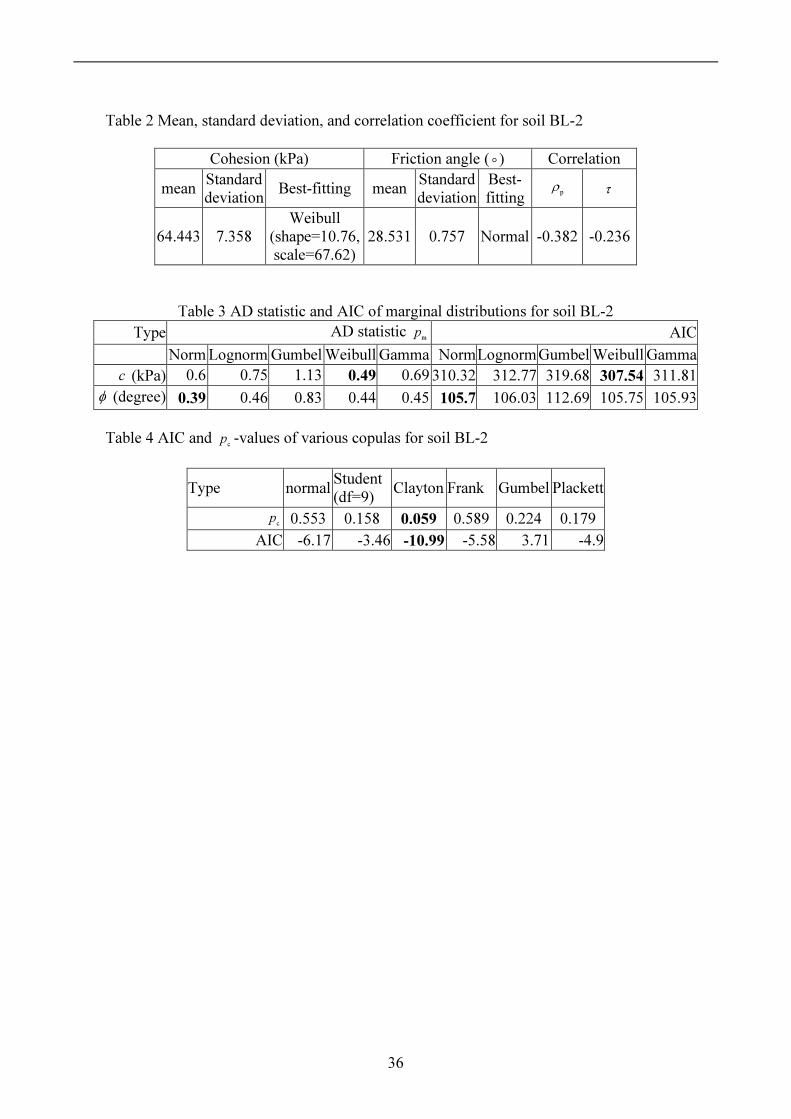
Table 2 Mean, standard deviation, and correlation coefficient for soil BL-2

Cohesion (kPa) Friction angle ( o ) Correlation mean Standard deviation Best-fitting mean Standard deviation

Best-fitting pρ τ

64.443 7.358 Weibull

(shape=10.76, scale=67.62)

28.531 0.757 Normal -0.382 -0.236

Table 3 AD statistic and AIC of marginal distributions for soil BL-2

Type AD statistic mp AIC

Norm Lognorm Gumbel Weibull Gamma Norm Lognorm Gumbel Weibull Gamma c (kPa) 0.6 0.75 1.13 0.49 0.69 310.32 312.77 319.68 307.54 311.81

φ (degree) 0.39 0.46 0.83 0.44 0.45 105.7 106.03 112.69 105.75 105.93

Table 4 AIC and cp -values of various copulas for soil BL-2

Type normal Student (df=9) Clayton Frank Gumbel Plackett cp 0.553 0.158 0.059 0.589 0.224 0.179

AIC -6.17 -3.46 -10.99 -5.58 3.71 -4.9

37

Table 5 Statistical properties of soil parameters for the homogeneous slope

Random variable

Unit mean Standard deviation

Distribution

c 2kN/m 18.0 3.6 normal φtan 0.577 0.058 normal

Table 6 Statistical properties of soil parameters for the stratified slope

Random variable

Unit mean Standard deviation

Distribution

1c 2kN/m 38.31 7.662 normal

1tanφ 0 0 normal

2c 2kN/m 23.94 4.788 normal

2tanφ 0.209 0.021 normal *

1c 2kN/m 38.31 7.662 normal *

1tanφ 0.349 0.035 normal

Table 7 Statistical properties of soil parameters for the Clearance Cannon dam

Soil Random variable

Unit mean Standard deviation

Distribution

Phase I

1c 2kN/m 117.79 58.89 normal

1tanφ 0.15 0.15 normal

Phase II 2c 2kN/m 143.64 79 normal

2tanφ 0.268 0.158 normal

38

List of Figures Fig. 1 Relationships of Pearson’s Rou and copula parameter Theta with Kendall’s Tau Fig. 2 Paired data for cohesion and internal friction angle (obtained from Lumb, 1970) Fig. 3a Observed and theoretical quantiles for quantile-quantile plots comparing observations

of the cohesion of soil BL-2 by Lumb (2000) under a normal distribution Fig. 3b Observed and theoretical quantiles for quantile-quantile plots comparing observations

of the friction angle of soil BL-2 by Lumb (1970) under a normal distribution Fig. 4 Contour of the best-fitting copula (Clayton) confidence regions of the simulated and

observed data for soil BL-2 (Lumb, 1970)

Fig. 5 Density contours of bivariate models for ( c ,φ ) for soil BL-2 by Lumb (1970) with (1) a bivariate normal density distribution, (2) a normal copula using the best-fitting margins, and (3) a Clayton copula using the best-fitting margins

Fig. 6 Homogeneous slope Fig. 7 Scatter plot of the factor of safety against cohesion and friction angle Fig. 8 Relation of probability of failure against cohesion and friction angle Fig. 9 Reliability index versus ranked correlations of soil properties for the homogeneous slope Fig. 10 Cross section of two-layer slope Fig. 11 Reliability index versus ranked correlations of soil properties for the stratified slope Fig. 12 Cross section of the Cannon Dam Fig. 13 Reliability index versus ranked correlations of soil properties for the Clearance Cannon

dam

39

#

#

#

#

#

#

#

#

#

#

#

-1.0 -0.5 0.0 0.5 1.0

-1.0

-0.5

0.0

0.5

1.0

ρ p

τ

x x x x x x x x x x

x

-40

-20

0

20

40

+

++ + + + + + +

+

+

& & & & & & & & & &

&

θ

#x+&

ρpClayton copula parameter θFrank copula parameter θGumbel copula parameter θ

Fig. 1 Relationships of Pearson’s Rou and copula parameter Theta with Kendall’s Tau

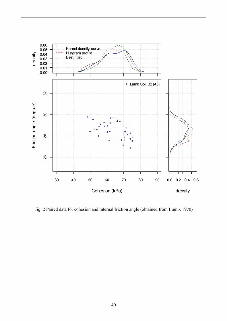
40

30 40 50 60 70 80 90

2628

3032

Cohesion (kPa)

Fricti

on an

gle (d

egree

)

Lumb Soil B2 [45]

dens

ity

0.000.010.020.030.040.050.06 Kernel density curve

Histgram profileBest fitted

density0.0 0.2 0.4 0.6

Fig. 2 Paired data for cohesion and internal friction angle (obtained from Lumb, 1970)

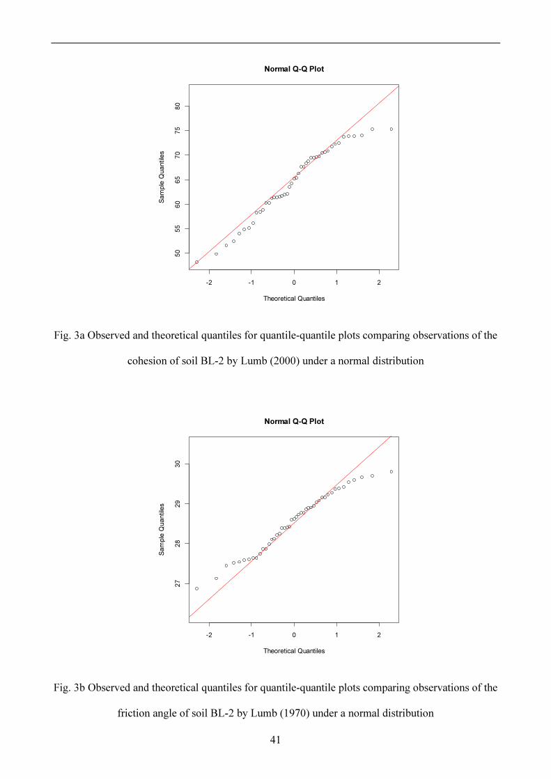
41

-2 -1 0 1 2

5055

6065

7075

80

Normal Q-Q Plot

Theoretical Quantiles

Samp

le Qu

antile

s

Fig. 3a Observed and theoretical quantiles for quantile-quantile plots comparing observations of the cohesion of soil BL-2 by Lumb (2000) under a normal distribution

-2 -1 0 1 2

2728

2930

Normal Q-Q Plot

Theoretical Quantiles

Samp

le Qu

antile

s

Fig. 3b Observed and theoretical quantiles for quantile-quantile plots comparing observations of the friction angle of soil BL-2 by Lumb (1970) under a normal distribution

42

40 50 60 70 80

2628

3032

34

Cohesion (kPa)

Fricti

on an

gle (d

egree

)

+o

ObservationPrediction

density contour95% CR of observation95% CR of prediction

0.02

0.005

Fig. 4 Contour of the best-fitting copula (Clayton) confidence regions of the simulated and observed data for soil BL-2 (Lumb, 1970)

40 50 60 70 80

2628

3032

34

Cohesion (kPa)

Fricti

on an

gle (d

egree

)

0.02 0.005 0.02 0.005

0.005

0. 01

0 . 0 1 5

0 . 0 2 0 .0 2 5

0 . 0 3

Observation

binormal densitynormal copulaClayton copula

Fig. 5 Density contours of bivariate models for ( c ,φ ) for soil BL-2 by Lumb (1970) with (1) a

bivariate normal density distribution, (2) a normal copula using the best-fitting margins, and (3) a Clayton copula using the best-fitting margins

43

11

10m

Firm Base6m

Fig. 6 Homogeneous slope

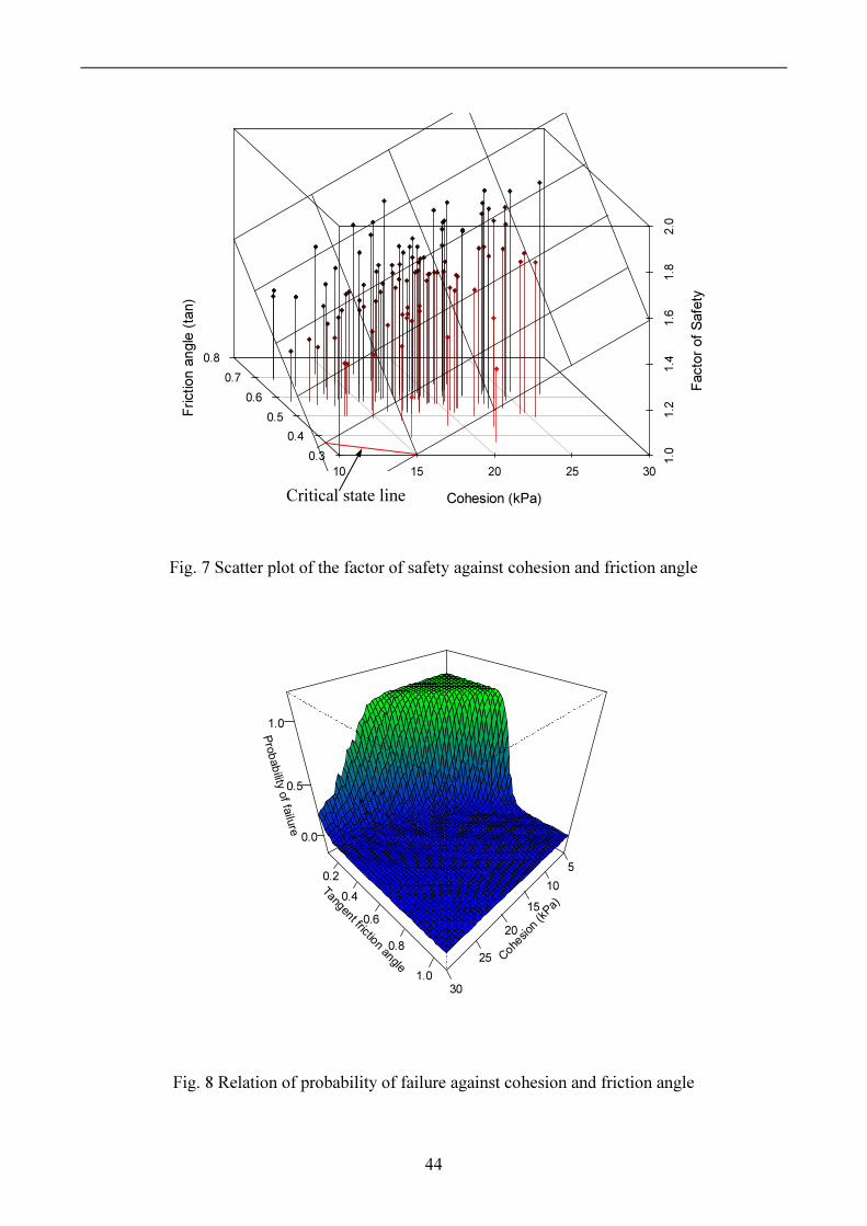
44

10 15 20 25 30

1.0

1.2

1.4

1.6

1.8

2.0

0.30.4

0.50.6

0.70.8

Cohesion (kPa)

Fricti

on an

gle (ta

n)

Facto

r of S

afety

Fig. 7 Scatter plot of the factor of safety against cohesion and friction angle

C o h esio n

( kPa )

510

15

20

25

30

Tangent f ri c t i on angl e

0.20.4

0.6

0.8

1.0

Pr obabili t y of f ailur e

0.0

0.5

1.0

Fig. 8 Relation of probability of failure against cohesion and friction angle

Critical state line

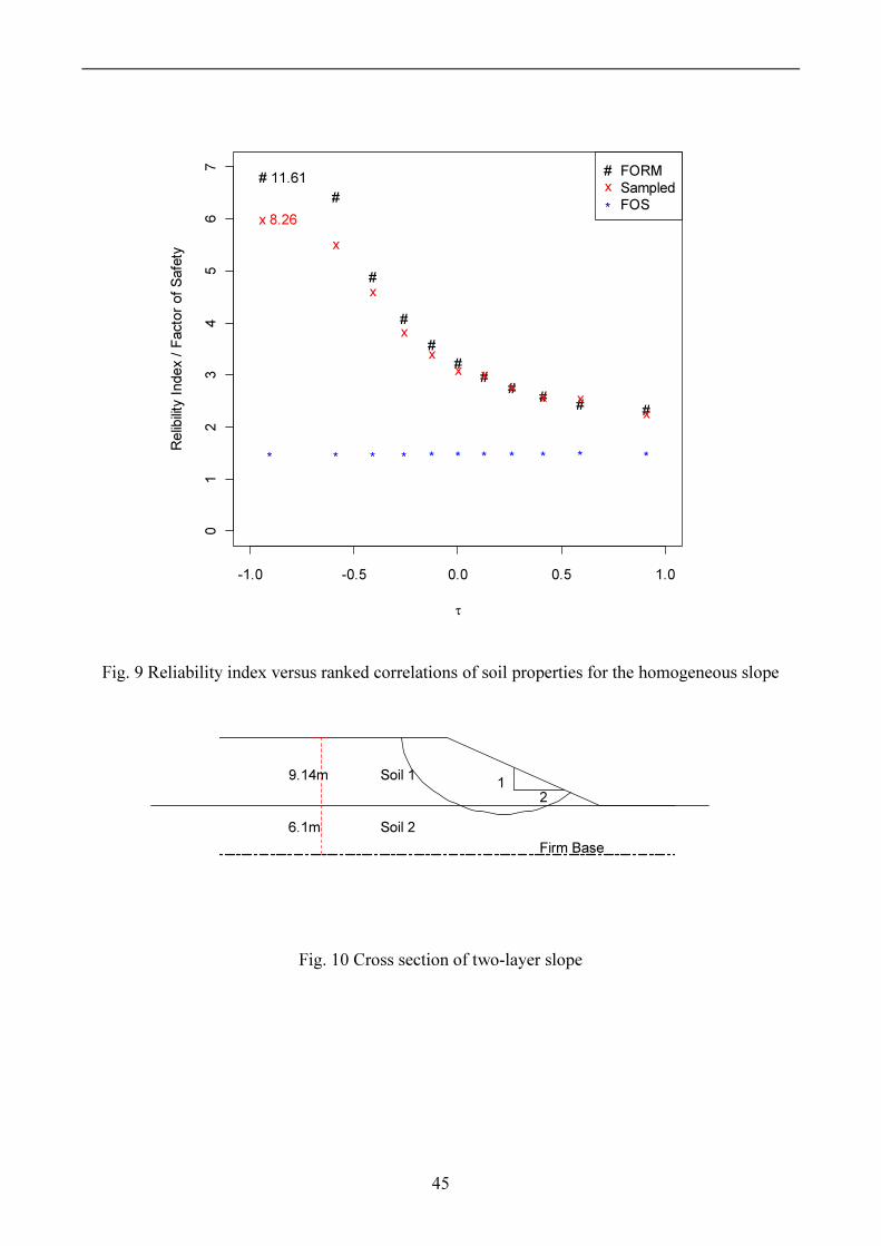
45

#

#

##

# # # # # #

-1.0 -0.5 0.0 0.5 1.0

01

23

45

67

τ

Relibi

lity In

dex /

Facto

r of S

afety x

x

xx

x x x x xx

* * * * * * * ** * *

#x*

FORMSampledFOS

# 11.61

x 8.26

Fig. 9 Reliability index versus ranked correlations of soil properties for the homogeneous slope

12

9.14m

6.1m

Soil 1

Soil 2Firm Base

Fig. 10 Cross section of two-layer slope

46

# # # # # # # ## # #

-1.0 -0.5 0.0 0.5 1.0

01

23

45

67

τ

Relibi

lity In

dex /

Facto

r of S

afety

x x x x x x x xx x x* * * * * * * ** * *

+

++ + + +

+ +

+

+ +

#x*+

FORMCBSMFOSCBSM-layer 1

Fig. 11 Reliability index versus ranked correlations of soil properties for the stratified slope

100 200 300 400 500 600

5010

015

020

025

0

Distance (m)

Eleva

tion (

m)

199.34

Sand Filter (dashed line)

Up Stream Down StreamPhase II

Phase IFoundation SandLime StoneFirm Base

Fig. 12 Cross section of the Cannon Dam

47

#

##

# # # # # # #

-1.0 -0.5 0.0 0.5 1.0

01

23

45

67

τ

Relibi

lity In

dex /

Facto

r of S

afety

x

xx

x x x x x x x

* * * * * * * **

* *

#x*

FORMSampledFOS# 11.74

x 8.44

Fig. 13 Reliability index versus ranked correlations of soil properties for the Clearance Cannon dam