Probabilistic Seismic Evaluation of Reinforced Concrete Structural Components and Systems Tae-Hyung Lee Khalid M. Mosalam Department of Civil and Environmental Engineering University of California, Berkeley PEER 2006/04 august 2006 PACIFIC EARTHQUAKE ENGINEERING RESEARCH CENTER

Welcome message from author
This document is posted to help you gain knowledge. Please leave a comment to let me know what you think about it! Share it to your friends and learn new things together.
Transcript

Probabilistic Seismic Evaluation of Reinforced Concrete Structural Components and Systems
Tae-Hyung Lee
Khalid M. Mosalam
Department of Civil and Environmental EngineeringUniversity of California, Berkeley
PEER 2006/04august 2006
PACIFIC EARTHQUAKE ENGINEERING RESEARCH CENTER

Probabilistic Seismic Evaluation ofReinforced Concrete Structural Components and Systems
Tae-Hyung LeeDepartment of Civil and Environmental Engineering
University of California, Berkeley
Khalid M. MosalamDepartment of Civil and Environmental Engineering
University of California, Berkeley
PEER Report 2006/04Pacific Earthquake Engineering Research Center
College of EngineeringUniversity of California, Berkeley
August 2006

ABSTRACT
An accurate evaluation of the structural performance of reinforced concrete structural sys-
tems under seismic loading requires a probabilistic approach due to uncertainties in struc-
tural properties and the ground motion (referred to as basic uncertainties). The objective
of this study is to identify and rank significant sources of basic uncertainties and structural
components with respect to the seismic demand (referred to as the Engineering Demand
Parameters, EDP) of reinforced concrete structural systems. The methodology for accom-
plishing this objective consists of three phases. In the first phase, the propagation of basic
uncertainties to a structural system with respect to its EDPs is studied using the first-order
second-moment (FOSM) method and the tornado diagram analysis to identify and rank sig-
nificant sources of basic uncertainties. In the second phase, the propagation of basic uncer-
tainties to structural components with respect to their capacities is studied. For this purpose,
the stochastic fiber element model is developed to build probabilistic section models such as
the moment-curvature relationships at critical sections of the structural component. In the
third phase, the propagation of uncertainty in the capacities of structural components to the
structural system with respect to its EDPs is studied. Using the FOSM method combined
with probabilistic section models, EDP uncertainties induced by structural components are
estimated to identify and rank significant components. Several case studies demonstrate the
effectiveness and robustness of the developed procedure of propagating uncertainties.
iii

ACKNOWLEDGEMENTS
This work was supported primarily by the Earthquake Engineering Research Centers Pro-
gram of the National Science Foundation under award number EEC-9701568 through the
Pacific Earthquake Engineering Research Center (PEER). Any opinions, findings, and con-
clusions or recommendations expressed in this material are those of the authors and do not
necessarily reflect those of the National Science Foundation.
iv

CONTENTS
ABSTRACT . . . . . . . . . . . . . . . . . . . . . . . . . . . . . . . . . . . . . . . . . . . . . . . . . . . . . . . . . . . . . . iiiACKNOWLEDGEMENTS . . . . . . . . . . . . . . . . . . . . . . . . . . . . . . . . . . . . . . . . . . . . . . . . ivTABLE OF CONTENTS . . . . . . . . . . . . . . . . . . . . . . . . . . . . . . . . . . . . . . . . . . . . . . . . . . vLIST OF FIGURES . . . . . . . . . . . . . . . . . . . . . . . . . . . . . . . . . . . . . . . . . . . . . . . . . . . . . . . ixLIST OF TABLES. . . . . . . . . . . . . . . . . . . . . . . . . . . . . . . . . . . . . . . . . . . . . . . . . . . . . . . . . xiii
1 Introduction. . . . . . . . . . . . . . . . . . . . . . . . . . . . . . . . . . . . . . . . . . . . . . . . . . . . . . . . . . . . 1
1.1 General . . . . . . . . . . . . . . . . . . . . . . . . . . . . . . . . . . . . . . . . . . . . . . . . . . . . . . . 1
1.2 Objectives and Scope . . . . . . . . . . . . . . . . . . . . . . . . . . . . . . . . . . . . . . . . . . . . 2
1.3 Overview . . . . . . . . . . . . . . . . . . . . . . . . . . . . . . . . . . . . . . . . . . . . . . . . . . . . . 3
2 Propagation of Uncertainty . . . . . . . . . . . . . . . . . . . . . . . . . . . . . . . . . . . . . . . . . . . . . 7
2.1 Introduction . . . . . . . . . . . . . . . . . . . . . . . . . . . . . . . . . . . . . . . . . . . . . . . . . . . 7
2.2 Performance-Based Earthquake Engineering . . . . . . . . . . . . . . . . . . . . . . . . . . 8
2.3 PBEE Methodology Developed within PEER Center . . . . . . . . . . . . . . . . . . . . 8
2.4 Uncertainty in PEER’s PBEE . . . . . . . . . . . . . . . . . . . . . . . . . . . . . . . . . . . . . 12
2.5 Uncertainty in this Report . . . . . . . . . . . . . . . . . . . . . . . . . . . . . . . . . . . . . . . . 14
2.5.1 Uncertainty in Hazard Analysis Phase . . . . . . . . . . . . . . . . . . . . . . . . . 15
2.5.2 Uncertainty in Structural Analysis Phase . . . . . . . . . . . . . . . . . . . . . . . 16
2.6 Methodology of Propagating Uncertainty in this Study . . . . . . . . . . . . . . . . . . 20
2.6.1 Overview . . . . . . . . . . . . . . . . . . . . . . . . . . . . . . . . . . . . . . . . . . . . . . . . 20
2.6.2 Component Evaluation . . . . . . . . . . . . . . . . . . . . . . . . . . . . . . . . . . . . . 21
2.6.3 System Evaluation . . . . . . . . . . . . . . . . . . . . . . . . . . . . . . . . . . . . . . . . 28
2.6.4 Suggested Iterative Evaluations of Structural Components and System 28
2.7 Concluding Remarks . . . . . . . . . . . . . . . . . . . . . . . . . . . . . . . . . . . . . . . . . . . . . 30
3 EDP Sensitivity Induced by Basic Uncertainty. . . . . . . . . . . . . . . . . . . . . . . . . . 33
3.1 Introduction . . . . . . . . . . . . . . . . . . . . . . . . . . . . . . . . . . . . . . . . . . . . . . . . . . . 33
3.2 Methods of Sensitivity Analysis . . . . . . . . . . . . . . . . . . . . . . . . . . . . . . . . . . . . 34
3.2.1 First-Order Second-Moment Method . . . . . . . . . . . . . . . . . . . . . . . . . . 34
3.2.2 Tornado Diagram Analysis . . . . . . . . . . . . . . . . . . . . . . . . . . . . . . . . . . 37
3.3 UC Science Building . . . . . . . . . . . . . . . . . . . . . . . . . . . . . . . . . . . . . . . . . . . . . 38
v

3.3.1 UCS Building Description . . . . . . . . . . . . . . . . . . . . . . . . . . . . . . . . . . . 39
3.3.2 Structural Modeling . . . . . . . . . . . . . . . . . . . . . . . . . . . . . . . . . . . . . . . 40
3.4 EDP Sensitivity of the UCS Building . . . . . . . . . . . . . . . . . . . . . . . . . . . . . . . . 48
3.4.1 Uncertainties in Structural Properties . . . . . . . . . . . . . . . . . . . . . . . . . . 48
3.4.2 Uncertainties in Ground Motion . . . . . . . . . . . . . . . . . . . . . . . . . . . . . . 49
3.4.3 Selected EDPs . . . . . . . . . . . . . . . . . . . . . . . . . . . . . . . . . . . . . . . . . . . . 54
3.4.4 Tornado Diagram Analysis . . . . . . . . . . . . . . . . . . . . . . . . . . . . . . . . . . 57
3.4.5 Analysis Using FOSM Method . . . . . . . . . . . . . . . . . . . . . . . . . . . . . . . 59
3.4.6 Comparison of Analyses Using Tornado Diagram and FOSM Method,and Suggested New Approach . . . . . . . . . . . . . . . . . . . . . . . . . . . . . . . . 62
3.4.7 Sensitivity of Local EDPs by FOSM Method . . . . . . . . . . . . . . . . . . . . 66
3.4.8 Conditional Sensitivity of EDP Given IM by FOSM Method . . . . . . . . 66
3.5 Concluding Remarks . . . . . . . . . . . . . . . . . . . . . . . . . . . . . . . . . . . . . . . . . . . . . 70
4 Uncertainty in the Capacity of Structural Components . . . . . . . . . . . . . . . . . 75
4.1 Introduction . . . . . . . . . . . . . . . . . . . . . . . . . . . . . . . . . . . . . . . . . . . . . . . . . . . 75
4.2 Fiber Element Model . . . . . . . . . . . . . . . . . . . . . . . . . . . . . . . . . . . . . . . . . . . . 76
4.2.1 Element Formulation . . . . . . . . . . . . . . . . . . . . . . . . . . . . . . . . . . . . . . . 78
4.2.2 Nonlinear Analysis Procedure . . . . . . . . . . . . . . . . . . . . . . . . . . . . . . . . 81
4.2.3 Constitutive Models . . . . . . . . . . . . . . . . . . . . . . . . . . . . . . . . . . . . . . . 84
4.2.4 Verification Examples . . . . . . . . . . . . . . . . . . . . . . . . . . . . . . . . . . . . . . 87
4.3 Stochastic Fiber Element Model . . . . . . . . . . . . . . . . . . . . . . . . . . . . . . . . . . . . 91
4.3.1 Monte Carlo Simulation . . . . . . . . . . . . . . . . . . . . . . . . . . . . . . . . . . . . 91
4.3.2 Random Field Representation . . . . . . . . . . . . . . . . . . . . . . . . . . . . . . . . 91
4.3.3 Stochastic Fiber Element Model for RC Elements . . . . . . . . . . . . . . . . 99
4.4 Strength Analysis of RC Columns . . . . . . . . . . . . . . . . . . . . . . . . . . . . . . . . . . 103
4.4.1 Probabilistic Models and Discretization of Random Fields . . . . . . . . . . 104
4.4.2 Analysis Procedure . . . . . . . . . . . . . . . . . . . . . . . . . . . . . . . . . . . . . . . . 105
4.4.3 Strength Variability . . . . . . . . . . . . . . . . . . . . . . . . . . . . . . . . . . . . . . . 108
4.4.4 The Effect of Spatial Variability . . . . . . . . . . . . . . . . . . . . . . . . . . . . . . 111
4.5 Probabilistic Evaluation of Structural Components of an RC Frame . . . . . . . . 111
vi
4.5.1 Description of the Frame VE . . . . . . . . . . . . . . . . . . . . . . . . . . . . . . . . 112
4.5.2 Typical Structural Components . . . . . . . . . . . . . . . . . . . . . . . . . . . . . . 113
4.5.3 Random Fields . . . . . . . . . . . . . . . . . . . . . . . . . . . . . . . . . . . . . . . . . . . 115
4.5.4 Probabilistic Moment-Curvature Relationship . . . . . . . . . . . . . . . . . . . 116
4.5.5 Probabilistic Shear Force-Distortion Relationship . . . . . . . . . . . . . . . . . 126
4.6 Concluding Remarks . . . . . . . . . . . . . . . . . . . . . . . . . . . . . . . . . . . . . . . . . . . . . 127
5 EDP Sensitivity Induced by Component Uncertainty . . . . . . . . . . . . . . . . . . . 131
5.1 Introduction . . . . . . . . . . . . . . . . . . . . . . . . . . . . . . . . . . . . . . . . . . . . . . . . . . . 131
5.2 Portal Frame Application . . . . . . . . . . . . . . . . . . . . . . . . . . . . . . . . . . . . . . . . . 132
5.2.1 Uncertainty in the Strength of the Portal Frame . . . . . . . . . . . . . . . . . 134
5.2.2 Relative Significance of Columns . . . . . . . . . . . . . . . . . . . . . . . . . . . . . . 136
5.3 Ductile RC Frame: VE . . . . . . . . . . . . . . . . . . . . . . . . . . . . . . . . . . . . . . . . . . . 137
5.3.1 Structural Modeling . . . . . . . . . . . . . . . . . . . . . . . . . . . . . . . . . . . . . . . 137
5.3.2 Ground Motions . . . . . . . . . . . . . . . . . . . . . . . . . . . . . . . . . . . . . . . . . . 139
5.3.3 Verification Analyses . . . . . . . . . . . . . . . . . . . . . . . . . . . . . . . . . . . . . . . 140
5.3.4 Convergence Test for FOSM Method . . . . . . . . . . . . . . . . . . . . . . . . . . 142
5.3.5 Significant Components . . . . . . . . . . . . . . . . . . . . . . . . . . . . . . . . . . . . . 144
5.3.6 Important Cross Sections . . . . . . . . . . . . . . . . . . . . . . . . . . . . . . . . . . . 146
5.3.7 Conditional Sensitivity of EDPs Given IM . . . . . . . . . . . . . . . . . . . . . . 149
5.4 Concluding Remarks . . . . . . . . . . . . . . . . . . . . . . . . . . . . . . . . . . . . . . . . . . . . . 155
6 Summary, Conclusions, and Future Extensions . . . . . . . . . . . . . . . . . . . . . . . . . . 159
6.1 Summary . . . . . . . . . . . . . . . . . . . . . . . . . . . . . . . . . . . . . . . . . . . . . . . . . . . . . 159
6.1.1 EDP Uncertainty Induced by Basic Uncertainty . . . . . . . . . . . . . . . . . . 159
6.1.2 Uncertainty in the Capacity of Structural Components . . . . . . . . . . . . 160
6.1.3 EDP Uncertainty Induced by Component Uncertainty . . . . . . . . . . . . . 161
6.2 Conclusions . . . . . . . . . . . . . . . . . . . . . . . . . . . . . . . . . . . . . . . . . . . . . . . . . . . . 161
6.3 Future Extensions . . . . . . . . . . . . . . . . . . . . . . . . . . . . . . . . . . . . . . . . . . . . . . . 163
REFERENCES. . . . . . . . . . . . . . . . . . . . . . . . . . . . . . . . . . . . . . . . . . . . . . . . . . . . . . . . . . . . 167
vii

A Derivations . . . . . . . . . . . . . . . . . . . . . . . . . . . . . . . . . . . . . . . . . . . . . . . . . . . . . . . . . . . . . 175
A.1 Element Stiffness . . . . . . . . . . . . . . . . . . . . . . . . . . . . . . . . . . . . . . . . . . . . . . . 175
A.2 Variations in the Strength of RC column . . . . . . . . . . . . . . . . . . . . . . . . . . . . . 177
A.2.1 Model Assumptions . . . . . . . . . . . . . . . . . . . . . . . . . . . . . . . . . . . . . . . . 177
A.2.2 Variance of Axial Force . . . . . . . . . . . . . . . . . . . . . . . . . . . . . . . . . . . . . 179
A.2.3 Variance of Bending Moment . . . . . . . . . . . . . . . . . . . . . . . . . . . . . . . . 180
viii

LIST OF FIGURES
1.1 Overview. . . . . . . . . . . . . . . . . . . . . . . . . . . . . . . . . . . . . . . . . . . . . . . . . . . . . . 4
2.1 Vision 2000 recommended seismic performance objectives for building, afterSEAOC (1995). . . . . . . . . . . . . . . . . . . . . . . . . . . . . . . . . . . . . . . . . . . . . . . . . . 9
2.2 PEER’s PBEE analysis methodology. . . . . . . . . . . . . . . . . . . . . . . . . . . . . . . . 11
2.3 Sensitivity of future repair cost to uncertain input parameters for Van Nuysbuilding, California, after Porter et al. (2002). . . . . . . . . . . . . . . . . . . . . . . . . . 14
2.4 Process of identifying typical structural components by elastic analysis. . . . . . 22
2.5 Idealization of a moment-curvature curve. . . . . . . . . . . . . . . . . . . . . . . . . . . . . 25
2.6 Process of developing a probabilistic moment-curvature curve. . . . . . . . . . . . . 27
2.7 System evaluation procedure using probabilistic section models and the FOSMmethod. . . . . . . . . . . . . . . . . . . . . . . . . . . . . . . . . . . . . . . . . . . . . . . . . . . . . . . 29
2.8 The suggested iterative process of propagating basic uncertainties to the struc-tural system. . . . . . . . . . . . . . . . . . . . . . . . . . . . . . . . . . . . . . . . . . . . . . . . . . . . 30
3.1 Procedure of developing a swing in tornado diagram. . . . . . . . . . . . . . . . . . . . 38
3.2 Procedure of developing a tornado diagram. . . . . . . . . . . . . . . . . . . . . . . . . . . 39
3.3 Plan view of the UCS building. . . . . . . . . . . . . . . . . . . . . . . . . . . . . . . . . . . . . 40
3.4 Elevation view and OpenSees structural model of Frame 8 of the UCS building. 41
3.5 Modeling of shear-walls. . . . . . . . . . . . . . . . . . . . . . . . . . . . . . . . . . . . . . . . . . . 43
3.6 Shear capacity (based on the modified compression field theory by Response-2000 (Bentz 2000)) and demand (due to KB-kobj) of the coupling beam atthe sixth floor (Element 55 in Figure 3.4(b)) of Frame 8 (refer to Table 3.2for its design parameters). . . . . . . . . . . . . . . . . . . . . . . . . . . . . . . . . . . . . . . . . 44
3.7 Stress-strain relationships of concrete and steel adopted from the OpenSeesmaterial library. . . . . . . . . . . . . . . . . . . . . . . . . . . . . . . . . . . . . . . . . . . . . . . . . 45
3.8 Constitutive model for the soil spring. . . . . . . . . . . . . . . . . . . . . . . . . . . . . . . . 47
3.9 UCS building site seismic hazard curve for Frame 8. . . . . . . . . . . . . . . . . . . . . 50
3.10 Response spectra of the 20 selected earthquake records for the UCS buildinganalyses. . . . . . . . . . . . . . . . . . . . . . . . . . . . . . . . . . . . . . . . . . . . . . . . . . . . . . . 54
3.11 Moment-curvature relationships at various cross sections of Frame 8 subjectedto KB-kobj (solid lines) and from monotonic section analyses (dashed lines);(a) the bottom of element 47; (b) the left of element 55; (c) the bottomof element 2; (d) the left of element 8. Element numbers are designated inFigure 3.4(b). . . . . . . . . . . . . . . . . . . . . . . . . . . . . . . . . . . . . . . . . . . . . . . . . . . 56
3.12 Tornado diagrams and FOSM results of Frame 8 of the UCS building. . . . . . . 58
3.13 Time histories of various EDPs due to TO-ttrh02. . . . . . . . . . . . . . . . . . . . . . . 61
ix

3.14 Suggested new approach of combining the tornado diagram and the FOSMmethod. . . . . . . . . . . . . . . . . . . . . . . . . . . . . . . . . . . . . . . . . . . . . . . . . . . . . . . 65
3.15 Sensitivity of the peak curvatures at critical cross sections of Frame 8 of theUCS building; (a) the bottom of element 1; (b) the left of element 8; (c)the bottom of element 2; (d) the left of element 55. Element numbers aredesignated in Figure 3.4(b). . . . . . . . . . . . . . . . . . . . . . . . . . . . . . . . . . . . . . . . 67
3.16 Scatters of global EDPs induced by the uncertainty in GM for Frame 8 of theUCS building. . . . . . . . . . . . . . . . . . . . . . . . . . . . . . . . . . . . . . . . . . . . . . . . . . . 68
3.17 Comparison of uncertainties in global EDPs for Frame 8 of the UCS buildinginduced by the uncertainty in GM only (solid line) and in structural properties(dashed line, median quantity). . . . . . . . . . . . . . . . . . . . . . . . . . . . . . . . . . . . . 69
3.18 Scatters of the peak curvature at critical cross sections of Frame 8 of the UCSbuilding induced by the uncertainty in GM ; (a) the bottom of element 1; (b)the left of element 8; (c) the bottom of element 2; (d) the left of element 55.Element numbers are designated in Figure 3.4(b). . . . . . . . . . . . . . . . . . . . . . . 71
3.19 Comparison of local EDPs uncertainty induced by the uncertainty in GMonly (solid line) and in structural properties (dashed line, median quantity)at critical cross sections of Frame 8 of the UCS building; (a) the bottom ofelement 1; (b) the left of element 8; (c) the bottom of element 2; (d) the leftof element 55. Element numbers are designated in Figure 3.4(b). . . . . . . . . . . 72
4.1 Element and section discretization. . . . . . . . . . . . . . . . . . . . . . . . . . . . . . . . . . 78
4.2 Force and deformation variables at the element and section levels. . . . . . . . . . 78
4.3 Concrete constitutive models. . . . . . . . . . . . . . . . . . . . . . . . . . . . . . . . . . . . . . . 85
4.4 Reinforcing steel constitutive model. . . . . . . . . . . . . . . . . . . . . . . . . . . . . . . . . 86
4.5 The applied loads and the design parameters of MB. . . . . . . . . . . . . . . . . . . . . 87
4.6 The applied load and the design parameters of MC. . . . . . . . . . . . . . . . . . . . . 87
4.7 The applied loads and the design parameters of KC. . . . . . . . . . . . . . . . . . . . . 88
4.8 Load-displacement relationships; (a) MB; (b) MC. . . . . . . . . . . . . . . . . . . . . . 89
4.9 Load-displacement relationships of KC . . . . . . . . . . . . . . . . . . . . . . . . . . . . . . . 90
4.10 Random fields and fiber element meshes. . . . . . . . . . . . . . . . . . . . . . . . . . . . . . 100
4.11 Analysis procedure using the stochastic fiber element model. . . . . . . . . . . . . . 101
4.12 Probabilistic constitutive models; (a) Concrete; (b) Steel. . . . . . . . . . . . . . . . . 103
4.13 Procedure of developing a probabilistic P-M interaction diagram. . . . . . . . . . . 106
4.14 Typical P-M diagram and various Pl/Pa ratios. . . . . . . . . . . . . . . . . . . . . . . . . 107
4.15 The convergence test result of the mean and standard deviation of the columnstrength for Pl/Pa = 0.02: (a) normalized mean and standard deviation; (b)COV of the mean and standard deviation. . . . . . . . . . . . . . . . . . . . . . . . . . . . . 107
4.16 Mean P-M interaction diagrams for different cases of LS. . . . . . . . . . . . . . . . . 108
x

4.17 Changes of P-M interaction diagram; (a) Deterministic P-M interaction di-agrams for various cases of LS; (b) Base bending moment-tip displacementrelationship for Pl/Pa = 0.015. . . . . . . . . . . . . . . . . . . . . . . . . . . . . . . . . . . . . . 109
4.18 COV of column strength for different cases of LS. . . . . . . . . . . . . . . . . . . . . . . 1104.19 COVs of column strength with and without spatial variability of Fc. . . . . . . . 1124.20 Design details of the VE test frame (Vecchio and Emara 1992). . . . . . . . . . . . 1134.21 Identifying the typical structural components by a linear elastic analysis of
the VE frame. . . . . . . . . . . . . . . . . . . . . . . . . . . . . . . . . . . . . . . . . . . . . . . . . . . 1144.22 Convergence test of the means and standard deviations of the six moment-
curvature parameters of CS typical component of the VE frame. . . . . . . . . . . . 1194.23 Mean trilinear moment-curvature relationships at critical cross sections of the
typical components of the VE frame. . . . . . . . . . . . . . . . . . . . . . . . . . . . . . . . . 1204.24 Histograms of moment-curvature parameters for CN typical component of the
VE frame. . . . . . . . . . . . . . . . . . . . . . . . . . . . . . . . . . . . . . . . . . . . . . . . . . . . . . 1224.25 Histograms of moment-curvature parameters for CS typical component of the
VE frame. . . . . . . . . . . . . . . . . . . . . . . . . . . . . . . . . . . . . . . . . . . . . . . . . . . . . . 1224.26 Histograms of moment-curvature parameters for BM typical component of the
VE frame. . . . . . . . . . . . . . . . . . . . . . . . . . . . . . . . . . . . . . . . . . . . . . . . . . . . . . 1234.27 The normality check of the moment-curvature parameters of CN typical com-
ponent of the VE frame. . . . . . . . . . . . . . . . . . . . . . . . . . . . . . . . . . . . . . . . . . . 1234.28 The normality check of the moment-curvature parameters of CS typical com-
ponent of the VE frame. . . . . . . . . . . . . . . . . . . . . . . . . . . . . . . . . . . . . . . . . . . 1244.29 The normality check of the moment-curvature parameters of BM typical com-
ponent of the VE frame. . . . . . . . . . . . . . . . . . . . . . . . . . . . . . . . . . . . . . . . . . . 1244.30 Mean shear force-distortion relationships of typical structural components of
the VE frame. . . . . . . . . . . . . . . . . . . . . . . . . . . . . . . . . . . . . . . . . . . . . . . . . . . 127
5.1 A portal frame subjected to fixed gravity loads and an increasing lateral load;(a) Configurations of the frame; (b) Failure mechanism. . . . . . . . . . . . . . . . . . 133
5.2 Calibration of the analytical P-M curve to the mean P-M curve of LS 3. . . . . 1355.3 Statistics of Hf/2Vn; (a) Mean and Mean±2 standard deviation; (b) COV
due to uncertainty in KC1 (dashed line), in KC2 (dotted line), or in both ofthem (solid line). . . . . . . . . . . . . . . . . . . . . . . . . . . . . . . . . . . . . . . . . . . . . . . . 136
5.4 The OpenSees model of the VE frame. . . . . . . . . . . . . . . . . . . . . . . . . . . . . . . . 1385.5 Plastic hinge model in OpenSees. . . . . . . . . . . . . . . . . . . . . . . . . . . . . . . . . . . . 1395.6 Seismic hazard curve for the VE frame. . . . . . . . . . . . . . . . . . . . . . . . . . . . . . . 1405.7 Comparison of load-displacement relationships at Level 2 of the VE frame by
the experiment (Vecchio and Emara 1992) and present analyses. . . . . . . . . . . . 1415.8 Comparison of floor displacement time histories at Level 2 of the VE frame
due to the TO-ttrh02 earthquake scaled to Sa = 0.54g. . . . . . . . . . . . . . . . . . . 1425.9 Convergence of COV of various EDPs of the VE frame. . . . . . . . . . . . . . . . . . 143
xi

5.10 Relative contributions of components of the VE frame to uncertainty in PFA2
for various earthquakes. . . . . . . . . . . . . . . . . . . . . . . . . . . . . . . . . . . . . . . . . . . 1455.11 Mean relative contributions of components of the VE frame to EDPs uncertainty.1465.12 Relative contributions of cross sections of different components in the VE
frame to uncertainty in PFA2 for various earthquakes. . . . . . . . . . . . . . . . . . . . 1475.13 Mean relative contributions of cross sections of the VE frame to EDP uncer-
tainty. . . . . . . . . . . . . . . . . . . . . . . . . . . . . . . . . . . . . . . . . . . . . . . . . . . . . . . . . 1485.14 Mean contributions of components of the VE frame to uncertainty in various
EDPs. . . . . . . . . . . . . . . . . . . . . . . . . . . . . . . . . . . . . . . . . . . . . . . . . . . . . . . . . 1505.15 Mean contributions of cross sections of the VE frame to PFA1 uncertainty. . . . 1525.16 Mean contributions of cross sections of the VE frame to PFA2 uncertainty. . . . 1525.17 Mean contributions of cross sections of the VE frame to PFD1 uncertainty. . . 1535.18 Mean contributions of cross sections of the VE frame to PFD2 uncertainty. . . 1535.19 Mean contributions of cross sections of the VE frame to IDR1 uncertainty. . . . 1545.20 Mean contributions of cross sections of the VE frame to IDR2 uncertainty. . . . 154
A.1 Discretization of the cross section. . . . . . . . . . . . . . . . . . . . . . . . . . . . . . . . . . . 178A.2 Distributions of elastic constitutive models. . . . . . . . . . . . . . . . . . . . . . . . . . . . 178
xii

LIST OF TABLES
3.1 Geometrical properties and reinforcement schedule of shear-wall cross sectionsof Frame 8 of the UCS building. . . . . . . . . . . . . . . . . . . . . . . . . . . . . . . . . . . . . 42
3.2 Geometrical properties and reinforcement schedule of coupling beam crosssections of Frame 8 of the UCS building. . . . . . . . . . . . . . . . . . . . . . . . . . . . . . 42
3.3 Statistical data of the structural properties treated as random variables forFrame 8 of the UCS building. . . . . . . . . . . . . . . . . . . . . . . . . . . . . . . . . . . . . . . 48
3.4 Percentiles of Sa used in the tornado diagrams of the UCS building. . . . . . . . 503.5 NEHRP site categories, after Dobry et al. (2000). . . . . . . . . . . . . . . . . . . . . . . 513.6 Ground motion recordings selected for the UCS building case study. . . . . . . . . 523.7 Spectral accelerations at the fundamental period of Frame 8 of the UCS building. 533.8 COV (%) of EDPs corresponding to the individual random variables of Frame 8
of the UCS building. . . . . . . . . . . . . . . . . . . . . . . . . . . . . . . . . . . . . . . . . . . . . . 603.9 Statistics of measure of EDP sensitivities to combined uncertainties in struc-
tural properties using different perturbation sizes. . . . . . . . . . . . . . . . . . . . . . . 603.10 Assumed EDP distributions and bases of assumptions. . . . . . . . . . . . . . . . . . . 633.11 Various percentiles of Sa for sensitivity of EDP given IM for Frame 8 of the
UCS building. . . . . . . . . . . . . . . . . . . . . . . . . . . . . . . . . . . . . . . . . . . . . . . . . . . 68
4.1 Material properties of MB, MC, and KC. . . . . . . . . . . . . . . . . . . . . . . . . . . . . . 884.2 Statistical properties of variables. . . . . . . . . . . . . . . . . . . . . . . . . . . . . . . . . . . . 1044.3 Sensitivity of the column strength in terms of COV (%). . . . . . . . . . . . . . . . . . 1114.4 Material properties of the VE test frame. . . . . . . . . . . . . . . . . . . . . . . . . . . . . . 1144.5 Analysis parameters for structural components of the VE frame. . . . . . . . . . . 1154.6 Probability distributions of basic random variables. . . . . . . . . . . . . . . . . . . . . . 1164.7 Estimates of means, standard deviations, and correlation coefficient matrices
of moment-curvature parameters for typical components of the VE frame. . . . 1214.8 Estimates of correlation coefficient matrices of moment-curvature parameters
at different cross sections for typical components of the VE frame. . . . . . . . . . 1254.9 Estimates of means and standard deviations of shear force-distortion param-
eters for typical components of the VE frame. . . . . . . . . . . . . . . . . . . . . . . . . . 128
5.1 Statistical properties of random variables for the P-M relationship. . . . . . . . . . 1345.2 Various percentiles of Sa for sensitivity of EDP of the VE frame given IM. . . 149
xiii

1 Introduction
1.1 GENERAL
The behavior of reinforced concrete (RC) structural members (or components), especially
the inelastic behavior, depends on various geometric and material parameters. Most of these
parameters are of a random nature, and consequently, uncertainty exists in the behavior
of the RC members in terms of the strength and ductility. Therefore, a realistic estimate
of the behavior of the RC structural system that is an assembly of a number of structural
components requires a probabilistic approach for an appropriate treatment of uncertain
structural properties, especially under seismic loading.
An accurate yet practical evaluation of the structural behavior due to seismic load-
ing is one of the critical issues of the emerging performance-based earthquake engineering
(PBEE) methodology. In particular, the estimation of the seismic loss and the correspond-
ing repair cost of the structural system depend on an accurate and realistic estimate of the
performance of the structural system. Uncertainty in the loss estimation of the structural
system, mainly due to uncertainties in the ground motion and structural properties, can be
costly because it is directly related to the repair cost. In that regard, it is important to
identify and rank both sources of uncertainty and structural components that are relatively
significant to the performance of the structural system.
The probabilistic analysis of RC structural components and systems has been the
focus of a number of research efforts. One of the earliest works is that of Shinozuka (1972),
1

who investigated the effect of uncertain material properties on the strength of plain concrete
structures. Several studies were concentrated on RC members such as beams or columns.
Frangopol et al. (1996), Mirza and MacGregor (1989), and Grant et al. (1978) conducted
strength analyses of RC beam-column members by considering uncertainties in material
properties and cross-sectional dimensions. More recent research has focused on the proba-
bilistic evaluation of RC structural systems. Chryssanthopoulos et al. (2000), Ghobarah and
Aly (1998), and Singhal and Kiremidjian (1996) recently proposed systematic ways of evalu-
ating RC framed structures by considering the uncertainties in ground motions and material
properties. However, only a few studies were performed within the context of PBEE. Porter
et al. (2002), among those few studies, investigated the sensitivity of loss estimate of an RC
building to major uncertain parameters. Despite a large number of previous studies on prob-
abilistic evaluation of RC structures, efforts on identifying relative significance of different
sources of uncertainty and/or structural components with respect to the performance (or
demand) of the structural system are scarce.
1.2 OBJECTIVES AND SCOPE
This study has three objectives that eventually aim at the main goal of the present study:
to identify significant sources of basic uncertainties and structural components with respect
to the seismic demand (referred to as the Engineering Demand Parameter, EDP) of an RC
structural system. The following are specific objectives of this study:
• To understand the propagation of basic uncertainties to a structural system with re-
spect to its seismic demands.
• To understand the propagation of basic uncertainties to structural components that
form the structural system with respect to the strength and the deformation capacity
of the component.
• To understand the propagation of uncertainty in the capacity of structural components
2

to the structural system with respect to its EDPs.
The basic uncertainty is an observable uncertainty, i.e., statistical information can be col-
lected for it. For example, material properties, member dimensions, and soil properties are
all basic uncertainties because one can physically test or measure them.
The methodology for accomplishing the objective of this study is developed for RC
framed structure within the framework of the PBEE methodology being developed by the
Pacific Earthquake Engineering Research (PEER) center. Two different modeling schemes
are used to analyze structural components and systems. The first is a fiber element mod-
eling, known for its accurate estimation of the inelastic structural response. The second
utilizes plastic-hinge modeling that is widely used in practice due to its simplicity. Different
probabilistic methods are used to understand propagation of uncertainties. Monte Carlo
simulation is used for evaluation of the strength and the deformation capacity of structural
components, while the first-order second-moment (FOSM) method and a method of deter-
ministic sensitivity analysis using a tornado diagram1 are used for evaluation of structural
systems.
1.3 OVERVIEW
This report consists of six chapters beginning with the introduction in Chapter 1 and con-
cluding with Chapter 6. Chapter 2 presents the background, literature review, and the
methodology to support the core chapters. The core chapters of this report are Chapters 3
to 5. Each core chapter presents works related to each of the three objectives discussed in
the previous section. There are three categories of uncertainty being discussed in this report,
namely basic uncertainty, uncertainty in the capacity of structural components, and EDP
uncertainty of structural systems. Each core chapter presents the relationship between two
1Tornado diagram, commonly used in decision analysis, consists of a set of horizontal bars (swings) wherethe length of each bar represents the output sensitivity to a given input variable. These bars are displayedin the descending order of the bar length from the top to the bottom. This wide-to-narrow arrangement ofthe swings eventually resembles a tornado.
3

components of these uncertainties in terms of their propagation and identifies (or ranks) the
relative significance of an individual random variable or a structural component. Fig. 1.1
shows an overview of the present study focusing on the three core chapters.
Basic uncertainties in
ground motion and
structural properties
Uncertainty in demand
of the structural system
response
Uncertainty in capacity
of structural components
Propagation of uncertainty
Chapter 3
Chapter 4 Chapter 5
Identifying (ranking) important uncertainties
Fig. 1.1 Overview.
In Chapter 2, the background of the present study is introduced including the review
of previous works. In particular, the PBEE methodology being developed by the PEER
center is summarized. General discussion of sources of uncertainty in the structural analysis
is presented. Literature on characterizing sources of uncertainties that are considered in
the present study is reviewed. Finally, a systematic procedure of probabilistic evaluation
of structural systems, which consists of component evaluation and system evaluation, is
described.
In Chapter 3, the propagation of basic uncertainties through a structural system
with respect to its EDP is discussed. Descriptions of the FOSM and the tornado diagram
methods, and the corresponding procedures of sensitivity analyses of a structural system are
presented. Propagation of uncertainty is demonstrated for a case-study building (referred to
as UCS) using both methods. Moreover, significant random variables to EDPs of UCS are
identified.
4

In Chapter 4, the propagation of basic uncertainties through structural components
with respect to their capacity is discussed. First, a newly developed stochastic fiber element
model is presented. This model combines the conventional fiber element model and one of
the random field representation methods (the mid-point method) along with Monte Carlo
simulation. Second, the model is used for a probabilistic evaluation of structural components
considering spatial variability of random variables where a study of strength variability of
an RC column due to uncertainties in structural properties is presented. Finally, structural
components of a ductile RC frame (referred to as VE) are evaluated to develop probabilistic
moment-curvature and shear force-distortion relationships at critical cross sections of the
structural components.
In Chapter 5, the propagations of uncertainties in the strength and the deformation
capacities of structural components through a structural system with respect to EDPs of the
structural system are discussed. First, the procedure is demonstrated by a ductile portal
frame to estimate the probability distribution of the lateral strength of the frame. Second,
the EDP sensitivities of VE to uncertainty in the capacity of structural components using
probabilistic component models developed in Chapter 4 are presented. Finally, significant
structural components to EDPs of VE are identified according to the FOSM method.
In Chapter 6, the summary and conclusion of the study are presented. Recommen-
dations for future extension of this study are also outlined.
5

2 Propagation of Uncertainty
2.1 INTRODUCTION
Almost all input parameters in the structural analysis such as mass, damping, material
properties, boundary conditions, and applied load are uncertain. They are uncertain either
because of the inherent physical randomness (or variability) or because of our state of knowl-
edge. The former is called aleatory uncertainty and the latter is called epistemic uncertainty.
By definition, aleatory uncertainty is irreducible and epistemic uncertainty is reducible by
improving our state of knowledge. Regardless of the type of uncertainty, these uncertainties
make the corresponding structural response also uncertain. This process is viewed as prop-
agation of uncertainty in input parameters through the structural system. In this study,
the propagation of uncertainty is studied within the framework of performance-based earth-
quake engineering (PBEE) methodology. However, the presented methodology in this study
doesn’t have to be limited to a particular PBEE framework such as the one formulated within
the PEER center, as it can be equally applied to other structural performance evaluation
process.
This chapter introduces the definitions and the background of PBEE, together with
the PBEE methodology developed within the PEER center. Also discussed is how uncer-
tainty is treated in the PBEE methodology of this study. Finally, the scope of this study in
the context of the adopted ranges of uncertainty is discussed.
7

2.2 PERFORMANCE-BASED EARTHQUAKE ENGINEERING
After the events of big earthquakes in the mid-1990s, namely the 1994 Northridge and
1995 Kobe earthquakes, the structural engineering community realized that the amount of
damage, the economic loss due to downtime (or loss of use), and repair cost of structures
were unacceptably high, even though those structures complied with applicable seismic codes
to satisfy only the life-safety performance objective. Accordingly, structural engineers and
researchers started to think about a new design philosophy. FEMA 273 (1997) and Vision
2000 by SEAOC (1995) are known as the publications that reflect the pioneering work to
formulate the PBEE methodologies.
The definition of PBEE is widespread in the literature (Bertero and Bertero 2002;
Ghobarah 2001; SEAOC 1995). PBEE is defined such that it consists of development of
conceptual, preliminary, evaluation, and final design; control of construction quality; and the
maintenance of the structure such that the stated performance objectives are achieved when
it is subjected to one of the stated levels of seismic hazard. The performance objectives may
be a level of stress not to be exceeded, a force or deformation limit state at a member level,
or a damage state at the system level. For example, Vision 2000 identifies performance levels
as fully operational, operational, life safe, and near collapse. The levels of seismic hazard
defined in Vision 2000 include frequent, occasional, rare, and very rare events. These events
reflect Poisson-arrival events with probability of exceedance stated as 50% in 30 years, 50%
in 50 years, 10% in 50 years, and 10% in 100 years, respectively. Figure 2.1 shows possible
combinations of performance objective and seismic hazard level that can be used as design
criteria.
2.3 PBEE METHODOLOGY DEVELOPED WITHIN PEER CENTER
The PEER Center, based at the University of California, Berkeley, is one of three federally
funded earthquake engineering research centers in the United States. PEER has focused on
8

Fully Near
Collapse
Frequent
(43 years)
Occasional
(72 years)
Rare
(475 years)
Very rare
(949 years)
Earthquake Performance Level
Ear
thquak
e D
esig
n L
evel
(Ret
urn
per
iod)
Unacceptable Performance
(for New Construction)
OperationalOperational Life Safe
Fig. 2.1 Vision 2000 recommended seismic performance objectives for building,
after SEAOC (1995).
developing a PBEE methodology for the past 7 years as a part of a 10-year research program.
The key features of PEER’s PBEE methodology are: (1) explicit calculation of system
performance and (2) rigorous probabilistic calculation (http://www.peertestbeds.net). The
performance of the whole system is explicitly calculated and expressed in terms of the direct
interest of various stakeholder groups such as monetary values, downtimes, and injuries
and deaths. Unlike earlier PBEE methodologies, forces and deformations of components
are indicative of, but not the same as, the system performance. Rigorous probabilistic
calculation implies that the performance is calculated and expressed in a probabilistic manner
without relying on expert opinion. Uncertainties in earthquake intensity, ground motion
detail, structural response, physical damage, and economic and human loss are explicitly
considered in the methodology. While its overview is described by Porter (2003), PEER’s
PBEE methodology is summarized in this section as it provides a background of the present
study.
PEER’s PBEE methodology consists of four phases: hazard analysis, structural anal-
9

ysis, damage analysis, and loss analysis, as illustrated in Figure 2.2 where p[X] refers to the
probability density of X and p[X|Y ] refers to the conditional probability density of X given
the event of Y = y. (2.1) is the mathematical expression of the methodology.
p[DV|O,D] =
∫∫∫
p[DV|DM]p[DM|EDP]p[EDP|IM]p[IM|O,D]dIMdEDPdDM (2.1)
where
O = Location of the structure
D = Design of the structure
IM = Intensity measure of earthquake site effects
EDP = Engineering demand parameter as a measure of structural response
DM = Measure of physical damage of various members
DV = Decision variable that is the performance parameter of interest such as
repair cost
Hazard Analysis In the hazard analysis phase, parameters related to the location and
design of the target structure are considered to develop the probabilistic seismic hazard,
p[IM|O,D]. These parameters include magnitude, mechanism, and distance of nearby faults
from the structure, and soil conditions of the site. Ground motion intensity is represented
by IM such as the damped elastic spectral acceleration at the fundamental period of the
structure. The probabilistic seismic hazard is usually expressed in the form of the annual
exceedance frequency of various levels of IM, given the location and design of the structure.
Structural Analysis In the structural analysis phase, a computational model of the struc-
ture is developed to estimate the structural responses in terms of selected EDPs, subjected
to a given IM (p[EDP|IM]). EDPs may include local parameters such as member forces or
10

damage
p[DM]
PEER PBEE ANALYSIS METHODOLOGY
facility
definition
O, D
site hazard
p[IM]
structural
response
p[EDP]
performance
p[DV]
decision
O, D OK?
fragility fns
p[DM|EDP]hazard model
p[IM|O,D]
struct'l model
p[EDP|IM]
loss model
p[DV|DM]
Hazard
analysis
Structural
analysis
Damage
analysis
Loss
analysis
IM: intensity
measure
EDP: eng'ing
demand param.
DM: damage
measure
DV: decision
variable
O: Location
D: Design
"What are my
options for the
facility location
and design?"
"How likely is an
event of
intensity IM, for
this location
and design?"
"What engineering
demands (force,
deformation, etc.)
will this facility
experience?"
"What physical
damage will
this facility
experience?"
"What loss
(economic, casualty,
etc.) will this
facility experience?"
"Are the
location and
design
acceptable?"
Fig. 2.2 PEER’s PBEE analysis methodology.
deformations, or global parameters such as floor acceleration and displacement, and inter-
story drift. Since IM is a random variable, EDP is also a random variable. In addition to
IM uncertainty, uncertainties in parameters defining the structural model can be considered
in the structural analysis phase. Uncertainties in the mass, damping, stiffness, and strength
of the structure are among those.
Damage Analysis In the damage analysis phase, a set of fragility functions of structural
and non-structural components of the target structure is developed to produce the proba-
bility of various damage levels in terms of DM, conditioned on the structural response given
in terms of EDP (p[DM|EDP]). Physical damage of a specific component is defined relative
to that of the undamaged state, considering the particular repair effort (or cost) required
to restore the component to its undamaged state. Structural and non-structural compo-
11

nents may include beams, columns, non-structural partitions, window glasses, or building
contents such as laboratory equipment or computers. Fragility functions can be developed
by laboratory experiments or by mathematical models describing physical phenomena.
Loss Analysis The loss analysis phase is the last phase of the PEER’s PBEE methodology,
where all uncertainties in previous analysis phases are integrated to develop the probabilistic
estimation of structural performance in terms of DV, conditioned on DM (p[DV|DM). As
mentioned earlier, the system performance of the structure is expressed in terms of the direct
interest of stakeholder groups such as monetary values, downtimes, and injuries and deaths.
The final product of this phase is in the form of the exceedance frequency of various levels of
DV. Finally, decision-makers decide whether the current design and location are acceptable
or not based on this final product of the PBEE methodology.
2.4 UNCERTAINTY IN PEER’S PBEE
Uncertainty is considered at each analysis phase and it propagates to the next analysis phase.
In the hazard analysis phase, the exact location, magnitude, mechanism of nearby faults,
and soil properties of the site of the target structure are uncertain. Consequently, the levels
of seismic hazard intensity or IM that the designed structure will experience are uncertain.
The details of ground motion profiles given those IMs are also uncertain.
Uncertainty in the hazard analysis phase, expressed in terms of IM, propagates to the
structural analysis phase and causes EDP uncertainty even if a mathematical model of the
structure is deterministic. In addition, sources of uncertainty in the structural model itself
exist. They include mass, damping, material properties such as steel strength and modulus
of elasticity, concrete strength and initial modulus of elasticity, and construction geometry
such as beam and column dimensions, and location of reinforcing bars. Moreover, additional
uncertainty exists in the selection of the element type and other modeling assumptions,
which is often referred to as the modeling uncertainty.
12

Similarly, in addition to the propagated uncertainty from the previous phases, the
damage analysis phase also has its own sources of uncertainty. They are experimental uncer-
tainty if a laboratory experiment is performed and modeling uncertainty if a computational
model is used to develop fragility function of a specific building content, or structural or
non-structural component. Uncertainty in the loss analysis phase can also be characterized
in a similar way.
There are several published works of PEER researchers related to uncertainty in
PEER’s PBEE methodology (Baker and Cornell 2003; Miranda and Aslani 2003; Porter
et al. 2002). Porter et al. (2002) studied the relative impact of uncertainties in so-called
major variables to the system performance of a non-ductile RC building, namely the Van
Nuys building in California, through the PEER’s PBEE analysis methodology. They con-
sidered uncertainty in the spectral acceleration as IM and details of ground motion (hazard
analysis phase), in building mass, viscous damping, and force-deformation behavior (struc-
tural analysis phase), in component fragility (damage analysis phase), and in unit repair
costs, and overhead and profit (loss analysis phase). Figure 2.3 illustrates the results of their
study showing the relative importance of random variables to system performance in terms
of the damage factor in this case. One of the deterministic sensitivity analysis methods,
using the so-called tornado diagram, is used in their study. The tornado diagram, as shown
in Figure 2.3, consists of a set of horizontal bars, one for each random variable. The length
of each bar (referred to as swing) represents the variation in the output due to the variation
in the respective random variable. Thus, a variable with larger effect on the output has a
larger swing than those with lesser effect.
Recently, Baker and Cornell (2003) developed an approach to calculate total uncer-
tainty of future repair costs of a structure using the first-order second moment (FOSM)
method. This proposed approach works within the framework of PEER’s PBEE methodol-
ogy. They estimated means and standard deviations of several conditional random variables,
namely, DV|DM and DM|EDP in (2.1), using the FOSM method to develop a single con-
13

0.00 0.25 0.50 0.75 1.00
Overhead & profit
Mass
Force-deformation behavior
Viscous damping
Unit repair costs
Ground motion
Spectral acceleration
Component fragility
Damage factor
Fig. 2.3 Sensitivity of future repair cost to uncertain input parameters for Van
Nuys building, California, after Porter et al. (2002).
ditional random variable (total repair cost in this case) given IM. Subsequently, the ground
motion hazard is treated accurately using Monte Carlo simulation based on the assumption
that ground motion uncertainty is the dominant contributor to total uncertainty of future
repair cost.
2.5 UNCERTAINTY IN THIS REPORT
The focus of this study is on the structural analysis phase of PEER’s PBEE methodology,
in particular for RC structures. Accordingly, uncertainty of interest is related to this phase.
Initially, seismic hazard (or IM) uncertainty enters into the structural analysis phase as it
represents uncertainty in the hazard analysis phase performed prior to the structural analysis
phase. Then, the structural analysis phase has its own sources of uncertainty in modeling
assumptions such as material properties, boundary conditions and structural geometry. This
section summarizes findings of other researchers on uncertainties of various parameters in
structural analysis. Only those related to applications in this study are presented in this
section.
14

2.5.1 Uncertainty in Hazard Analysis Phase
There are various ways of characterizing IM of an earthquake. The typical IMs are measured
peak ground motions and damped elastic responses in terms of acceleration, velocity, and
displacement. There have been efforts to define a proper IM of an earthquake in relation to
EDP (Taghavi and Miranda 2003; Cordova et al. 2001), where IM is strongly correlated to
EDP such that IM becomes an indicator of EDP.
Among those typical IMs, the damped elastic spectral acceleration at the fundamen-
tal period of the structure is commonly used because it is strongly correlated to various
EDPs and its probability function of occurrence is readily available. The Earthquake Haz-
ard Program in the U.S. Geological Survey (USGS) provides US national maps showing
earthquake ground motions that have a specified probability of being exceeded in 50 years
(http://eqhazmaps.usgs.gov). The peak ground acceleration and the damped elastic spectral
acceleration at the fundamental period of the structure are used as IMs in these maps.
Another type of uncertainty in seismic hazard is the ground motion profile (referred to
as details of ground motion by Porter et al. (2002)). Unlike any other uncertainty addressed
in this study, it is not straightforward to characterize the uncertainty in the ground motion
profiles using methods other than Monte Carlo simulations. In that regard, a large number
of ground motion profiles are used to obtain a set of outputs (e.g., EDP in this study)
to be subsequently post-processed for their statistics. The incremental dynamic analysis
(IDA) (Vamvatsikos and Cornell 2002) is one of the methods that can explicitly deal with
this uncertainty using a set of ground motion profiles. For such set, one may use either
recorded ground motions or simulated ones that are generated from a mathematical model.
Since the comparison between using recorded (and possibly scaled to modify IM) versus
simulated ground motion is still an on-going research in earthquake engineering, a set of
recorded ground motions is employed in the study presented in this report.
15

2.5.2 Uncertainty in Structural Analysis Phase
Sources of uncertainty associated with the structural analysis phase include structural geome-
try, material properties, modeling assumptions, and construction errors. Structural geometry
includes, for example, beam and column dimensions, and locations and sizes of reinforcing
bars. Material properties include parameters defining individual material constitutive mod-
els such as concrete compressive strength and initial modulus of elasticity, or steel yield
strength, ultimate strength, and initial modulus of elasticity. Several research efforts have
been focused on studying the effect of uncertainty in material properties or structural geom-
etry on the behavior of structural components or systems (Chryssanthopoulos et al. 2000;
Singhal and Kiremidjian 1996; Frangopol et al. 1996; Grant et al. 1978; Knappe et al.
1975). Modeling assumptions include gravity load, mass, viscous damping, force and dis-
placement boundary conditions, time step integration scheme, soil-foundation interface, and
three-dimensional effects such as floor eccentricities between center of mass and center of
rigidity. Selection of element type is also a source of uncertainty, since different elements use
different assumptions and approximations in their element formulation.
2.5.2.1 Uncertainty in Concrete Properties
Mirza et al. (1979) proposed probability distributions of various static strength parameters
of concrete by regression analyses. Of interest among those are the compressive strength and
the initial modulus of elasticity. They suggested that the compressive strength of concrete
has normal distribution with the mean computed by
f ′
c = 0.675f ′
c + 1, 100 ≤ 1.15f ′
c in psi unit (2.2)
where f ′
c is the design compressive strength of concrete and f ′
c is the mean of the compressive
strength. Dispersions of the distribution are suggested as coefficients of variations (COV)
of 10%, 15%, and 20% for excellent, average, and poor quality control, respectively, for
strength levels below 4,000 psi. For concrete with an average strength above 4,000 psi,
16

standard deviations are suggested as 400 psi, 600 psi, and 800 psi also for excellent, average,
and poor quality control. On the other hand, the initial tangent modulus of elasticity is
suggested to have normal distribution with the mean computed by a regression equation
Ec = 60, 400√
f ′
c in psi unit (2.3)
and COV = 8%. They also realized that a strong correlation between compressive strength
and the initial modulus of elasticity exists as indicated by a high correlation coefficient in
the range of 0.88 to 0.91 as the results of various regression analyses. It should be noted
that the suggestions Mirza et al. (1979) discussed above do not include long term effects on
concrete such as creep and shrinkage.
Kappos et al. (1999) studied uncertainty in the ductility of confined RC members and
suggested COV = 32–36% for ultimate strain of confined concrete where ultimate strain is
defined by the strain corresponding to 85% of the compressive strength of the corresponding
unconfined concrete along the descending branch of the stress-strain relationship.
2.5.2.2 Uncertainty in Reinforcing Steel Properties
Mirza and MacGregor (1979a) proposed probability distributions of various mechanical prop-
erties of reinforcing bars. In particular, yield strength, ultimate strength, and modulus of
elasticity of reinforcing steel are of interest. They suggested the lognormal distributions for
yield and ultimate strengths. Suggested values of means and COVs for yield strength are
respectively 48.8 ksi and 10.7% for Grade 40 bars and 71.0 ksi and 9.3% for Grade 60 bars.
They observed that an increase in mean ultimate strength of reinforcing steel over the yield
strength is on the order of 55% with COV remaining approximately unchanged. For exam-
ple, the suggested mean and standard deviation of ultimate strength is 110.1 ksi and 10.2
ksi (COV = 9.3%), respectively, for Grade 60 bars. It is also suggested that the probability
distribution of the modulus of elasticity of Grade 40 or 60 reinforcing steel is normal with
the mean 29,200 ksi and COV = 3.3%.
17
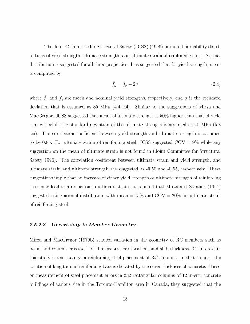
The Joint Committee for Structural Safety (JCSS) (1996) proposed probability distri-
butions of yield strength, ultimate strength, and ultimate strain of reinforcing steel. Normal
distribution is suggested for all three properties. It is suggested that for yield strength, mean
is computed by
fy = fy + 2σ (2.4)
where fy and fy are mean and nominal yield strengths, respectively, and σ is the standard
deviation that is assumed as 30 MPa (4.4 ksi). Similar to the suggestions of Mirza and
MacGregor, JCSS suggested that mean of ultimate strength is 50% higher than that of yield
strength while the standard deviation of the ultimate strength is assumed as 40 MPa (5.8
ksi). The correlation coefficient between yield strength and ultimate strength is assumed
to be 0.85. For ultimate strain of reinforcing steel, JCSS suggested COV = 9% while any
suggestion on the mean of ultimate strain is not found in (Joint Committee for Structural
Safety 1996). The correlation coefficient between ultimate strain and yield strength, and
ultimate strain and ultimate strength are suggested as -0.50 and -0.55, respectively. These
suggestions imply that an increase of either yield strength or ultimate strength of reinforcing
steel may lead to a reduction in ultimate strain. It is noted that Mirza and Skrabek (1991)
suggested using normal distribution with mean = 15% and COV = 20% for ultimate strain
of reinforcing steel.
2.5.2.3 Uncertainty in Member Geometry
Mirza and MacGregor (1979b) studied variation in the geometry of RC members such as
beam and column cross-section dimensions, bar location, and slab thickness. Of interest in
this study is uncertainty in reinforcing steel placement of RC columns. In that respect, the
location of longitudinal reinforcing bars is dictated by the cover thickness of concrete. Based
on measurement of steel placement errors in 232 rectangular columns of 12 in-situ concrete
buildings of various size in the Toronto-Hamilton area in Canada, they suggested that the
18

cover thickness can be described by a normal distribution with a mean given by
t = tsp + 0.25 + 0.004h in inch (2.5)
where t, tsp, and h are the mean and specified cover thickness, and the dimension of the long
side of the column cross section, respectively, and standard deviation of 0.166 inch.
2.5.2.4 Uncertainty in Modeling Assumptions
Quantification of building mass in a dynamic structural analysis depends on several factors,
namely materials used in construction, structural dimensions, locations of non-structural
elements, and a numerical model of the structure such as choice of its nodal coordinates.
Uncertainty in structural mass is an integration of uncertainties in those factors. Ellingwood
et al. (1980) suggested that the probability distribution of dead load is normal with a mean
value equal to the nominal dead load and COV = 10%. In this study, the probability
distribution of building mass is assumed to be normal with a mean value equal to mass
computed from the nominal self weight and the superimposed dead load.
A comprehensive discussion of uncertainty in the viscous damping ratio is presented
by Porter et al. (2002) including a summary of earlier experimental studies by Taoko (2003),
Camelo et al. (2001), and McVerry (1979). Based on these experimental studies, Porter et
al. (2002) suggested a reasonable estimate of COV of the damping ratio in the range of 30%
to 40%, while the mean of damping ratio is reported in the range of 1.1% to 11%. In this
study, the mean and COV of damping ratio are assumed to be 5% and 40%, respectively.
2.5.2.5 Excluded Uncertainty
Not all possible uncertainties are considered in this study. Among excluded ones are those due
to soil-foundation interface modeling, three-dimensional effect, non-structural components,
and gravity load including its role in P-∆ effect, all of which may significantly affect EDP
uncertainty. The propagation of these uncertainties should be studied in the future extension
19
of the presented study. Some other sources of uncertainties whose effects on EDPs are
assumed to be small such as the tensile strength of concrete are considered as deterministic
at their best estimate such as the mean or the median.
2.5.2.6 Spatial Variability
Specified uncertainties in the structural analysis phase should, in general, spatially vary. This
is commonly referred to as the spatial variability of uncertainty. Lee and Mosalam (2004)
pointed out the importance of considering the spatial variability of material and geometrical
properties in estimating the strength of RC columns. In this report, the spatial variability
of structural properties is only considered in Chapter 4 for the evaluation of structural
components, as it is not practical to consider it in the evaluation of structural systems due
to the expected high computational effort.
2.6 METHODOLOGY OF PROPAGATING UNCERTAINTY IN THIS STUDY
This section describes a systematic method for propagating uncertainty, in particular, from
the basic uncertainty to uncertainties in the capacity of structural components and from that
to EDP uncertainty of a structural system. These two types of propagation of uncertainty
are covered in Chapters 4 and 5, respectively.
2.6.1 Overview
By definition, a structural system consists of a number of structural components. In fact,
almost all structural systems consist of a few repeatedly used structural components (referred
to as typical components) such as typical columns and beams. If each of these typical
structural components is investigated separately, the result can be portable to many types
of structural systems, as if the generic structural components were tested in the laboratory
and the results are subsequently used in estimating the behavior of structural systems. Once
20

the understanding of the expected level of damage for different sets of boundary conditions
is established for typical structural components, the damage of an entire structural system
can be estimated in a systematic manner. Accordingly, the methodology of evaluating the
propagation of basic uncertainties to the structural system with respect to EDP consists of
two phases: (1) component evaluation phase where the propagation of basic uncertainties to
structural components with respect to their capacity is evaluated and (2) system evaluation
phase where the propagation of uncertainty in the capacity of structural components to the
structural system with respect to EDP is evaluated.
2.6.2 Component Evaluation
2.6.2.1 Identifying Typical Structural Components
The first step in the methodology is to identify typical structural components of a given
structural system using the conventional definitions of beam and column. For example, the
length of a typical beam is defined by the distance between two column centerlines, while
the height of a typical column is defined by the distance between the centerlines of slabs
or beams, whichever the column meets, at both ends of the column. The strength and the
deformation capacities of a typical structural component are defined and evaluated at given
force boundary conditions that can be identified by a linear elastic analysis of the entire
structural system. The gravity load and a properly distributed lateral load such as the one
that resembles the shape of the first vibrational mode of the structural system along its
height are applied in this analysis. Figure 2.4 depicts the process of identifying typical struc-
tural components. It should be noted that structural components with identical dimensions
could be subjected to different force boundary conditions depending on the location of the
structural components in the structural system.
Displacement boundary conditions of a typical structural component (modeled as a
planar beam element) are defined such that all three degrees of freedom, namely translations
21

Beam1
Column1
Column3
Column2
Axial ForceDiagram
Shear ForceDiagram
BendingMomentDiagram
Column 1
Beam1
Pl1
α1Pl1
Constant axial force
Structural model of the system
Column 2 Column 3
α2Pl2α3Pl3Pl2
Pl3
Pl4
Pa1 Pa2
Pa3
Linear elastic analysisTypical components with
force boundary conditions
H2
H1
H1
Lb
H1
H2
Lb Lb
Fig. 2.4 Process of identifying typical structural components by elastic analysis.
22
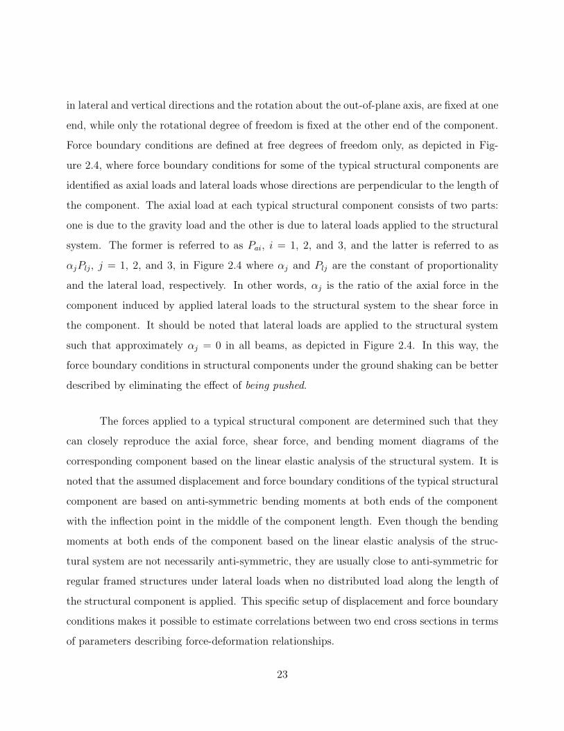
in lateral and vertical directions and the rotation about the out-of-plane axis, are fixed at one
end, while only the rotational degree of freedom is fixed at the other end of the component.
Force boundary conditions are defined at free degrees of freedom only, as depicted in Fig-
ure 2.4, where force boundary conditions for some of the typical structural components are
identified as axial loads and lateral loads whose directions are perpendicular to the length of
the component. The axial load at each typical structural component consists of two parts:
one is due to the gravity load and the other is due to lateral loads applied to the structural
system. The former is referred to as Pai, i = 1, 2, and 3, and the latter is referred to as
αjPlj, j = 1, 2, and 3, in Figure 2.4 where αj and Plj are the constant of proportionality
and the lateral load, respectively. In other words, αj is the ratio of the axial force in the
component induced by applied lateral loads to the structural system to the shear force in
the component. It should be noted that lateral loads are applied to the structural system
such that approximately αj = 0 in all beams, as depicted in Figure 2.4. In this way, the
force boundary conditions in structural components under the ground shaking can be better
described by eliminating the effect of being pushed.
The forces applied to a typical structural component are determined such that they
can closely reproduce the axial force, shear force, and bending moment diagrams of the
corresponding component based on the linear elastic analysis of the structural system. It is
noted that the assumed displacement and force boundary conditions of the typical structural
component are based on anti-symmetric bending moments at both ends of the component
with the inflection point in the middle of the component length. Even though the bending
moments at both ends of the component based on the linear elastic analysis of the struc-
tural system are not necessarily anti-symmetric, they are usually close to anti-symmetric for
regular framed structures under lateral loads when no distributed load along the length of
the structural component is applied. This specific setup of displacement and force boundary
conditions makes it possible to estimate correlations between two end cross sections in terms
of parameters describing force-deformation relationships.
23

Using an elastic analysis as a basis of identifying typical structural components of the
structural system is one of the many possible ways of defining the force boundary conditions
of structural components. It is selected in this study because it is both simple and efficient
to address variation in the axial load of the typical structural component due to applied
lateral load to the structural system. However, a possible influence of nonlinear behavior,
such as load redistribution due to damage of structural components, on changing the force
boundary conditions of typical structural components is not considered. Nevertheless, an
elastic analysis is the choice of this study because its objective is to demonstrate a system-
atic approach of understanding propagation of basic uncertainties to the structural system.
Moreover, this specific way of identifying typical structural components can be replaced by
other working approaches without affecting the developed general methodology. A possible
solution for this issue is suggested in Section 2.6.4.
2.6.2.2 Stochastic Fiber Element Model
Each identified typical structural component is evaluated to develop probabilistic section
models that describe the probability distribution of a force-deformation relationship of a
typical structural component such as the moment-curvature relationship or the shear force-
distortion relationship at critical cross sections of the component. In general, a critical cross
section is defined as the one with the largest force (e.g., bending moment) or deformation
(e.g., curvature) demand. In that regard, both end cross sections of a structural component
are defined as critical cross sections in this study because their moment or curvature demands
are the largest when no distributed load along the length of the structural component is
applied, which is assumed to be the case in this study. It is noted that one of the two critical
cross sections represents a cross section under a positive bending while the other one is under
a negative bending. For the process of developing probabilistic section models, the stochastic
fiber element model is developed in this study, such that spatial variability of the material
and geometrical properties in the structural model is accounted for in the conventional
24

(deterministic) fiber element model. This model is developed in the framework of Monte
Carlo simulation using a random field representation method as discussed in Chapter 4.
2.6.2.3 Probabilistic Moment-Curvature Relationship
Among force boundary conditions of each typical structural component, the lateral load
is monotonically increased (the part of the axial load proportional to the lateral load is
increased accordingly), while the constant part of the axial load due to the gravity load
is applied simultaneously until the ultimate deformation capacity is reached at the critical
cross section of the typical structural component. The moment-curvature relationship at this
cross section is idealized as a multilinear relationship defined by several moment-curvature
pairs. Figure 2.5 shows a trilinear moment-curvature relationship defined by three critical
points, namely the yielding point, the peak point, and the ultimate point. The yielding point
(ϕy, My) is defined by the moment and curvature corresponding to the first yielding of any
longitudinal reinforcing bar. The peak point (ϕp, Mp) is defined by the maximum moment
and its corresponding curvature. The ultimate point (ϕu, Mu) is defined by the moment and
curvature corresponding to the ultimate compressive strain of a confined concrete fiber or
the fracture strain of a steel fiber whichever occurs first (cf. Section 4.2.3).
Curvature (ϕ)
Mom
ent
(M)
Idealized M-ϕ relationship
Real M-ϕ curve
(ϕy, My)
(ϕp, Mp)
(ϕu, Mu)
Fig. 2.5 Idealization of a moment-curvature curve.
25

Monte Carlo simulation produces random samples for each of the six parameters
defining the trilinear moment-curvature relationship, and the probabilistic distributions of
these parameters can be estimated using simple statistics. In this study, the means, variances,
and covariances of the six parameters are estimated by sample means, sample variances, and
sample covariances, respectively. Let X = [X1, X2, . . . , X6]T = [My, Mp, Mu, ϕy, ϕp, ϕu]
T be
a vector containing the six random variables, i.e., the six parameters, having mean µi and
variance σ2i , i = 1, . . . , 6. The sample mean Xi and sample variance S2
i of Xi are given by
Xi =1
N
N∑
k=1
Xik (2.6)
S2i =
1
N − 1
N∑
k=1
(
Xik − Xi
)2(2.7)
where Xik is the kth sample of random variable Xi and N is the sample size. Sample
covariance Sij of Xi and Xj is given by
Sij =1
N − 1
N∑
k=1
[
(Xik − Xi)(Xjk − Xj)]
(2.8)
where Xik and Xjk are the kth samples of random variables Xi and Xj, respectively. It
should be noted that Xi, S2i , and Sij are unbiased estimates of the true means, variances,
and covariances with Xj of Xi, respectively. The final step of developing the probabilistic
moment-curvature relationship is estimating the distribution type (e.g., normal distribution)
to each of the six parameters. Rational judgment based on, e.g., a histogram or a q-q plot1
is required for this process. The process of developing a probabilistic moment-curvature
relationship is illustrated in Figure 2.6.
1The quantile-quantile (q-q) plot is a graphical technique for determining if two sets come from populationswith a common distribution.
26

Simulation results Idealizedmoment-curvature curves
Probabilistic model
Curvature
Mo
men
t
Curvature
Mo
men
t
Curvature
Mo
men
t
Fig. 2.6 Process of developing a probabilistic moment-curvature curve.
2.6.2.4 Probabilistic Shear Force-Distortion Relationship
The conventional fiber element model (including the stochastic fiber element model de-
veloped in this study) does not consider either the axial force-shear force or the bending
moment-shear force interactions at the critical cross sections of the structural components.
Therefore, probabilistic shear force-distortion relationships at the critical cross section of a
typical structural component is developed using Response 2000 (2000) software based on
the modified compression field theory (Vecchio and Collins 1986) instead of the stochastic
fiber element model. Due to the limitation of Response 2000, Monte Carlo simulation is not
appropriate for developing a probabilistic shear force-distortion relationship. Instead, the
FOSM method (cf. Section 3.2.1) is adopted.
Similar to the idealized moment-curvature relationship (cf. Figure 2.5), a computed
shear force-distortion curve is idealized as a trilinear relationship. Three points defining the
idealized shear force-distortion curve are the cracking point, the peak point, and the ultimate
point. The cracking point (γc, Vc) corresponds to the initiation of the shear crack. The peak
point (γp, Vp) is defined by the maximum shear force and its corresponding distortion. The
ultimate point (γu, Vu) corresponds to the fracture of the transverse steel. The means,
standard deviations, and correlation coefficient matrices of parameters defining the cracking,
peak, and ultimate points are estimated using the FOSM method to develop a probabilistic
27

shear force-distortion relationship.
2.6.3 System Evaluation
Although the stochastic fiber element model can be used for probabilistic evaluation of any
framed structure, it is not practical to use it for a complete structural system due to the large
computational demand of Monte Carlo simulation combined with the fiber element model.
Instead, a plastic hinge model (or a lumped plasticity model) (D’Ambrisi and Filippou
1999) is used to develop a computational model of the structural system. The behavior
of the plastic hinge model is defined by probabilistic moment-curvature and shear force-
distortion relationships obtained from the component evaluation phase. Moreover, instead
of Monte Carlo simulations, the FOSM method can be used to compute EDP uncertainty of
the structural system to avoid the need for a large computational effort. Figure 2.7 illustrates
the procedure of the system evaluation using probabilistic section models of typical structural
components in the context of the FOSM method to estimate EDP uncertainty.
In the process of propagating uncertainty from the typical structural component ca-
pacity in terms of critical section behavior to the system EDP, a practical approach can be
followed. In that regard, one should note that EDP uncertainty induced by uncertainty in
one of the structural components is a measure of sensitivity of EDP to the corresponding
component. For example, in Figure 2.7, uncertainties in the peak displacement induced by
uncertainties in Column 1 and in Beam 4 can be estimated using the FOSM method and the
corresponding measures of sensitivity such as COV can be computed. From these measures,
the relative significance of each component to the system EDP can be identified and ranked
accordingly.
2.6.4 Suggested Iterative Evaluations of Structural Components and System
As discussed in Section 2.6.2.1, the procedure of identifying typical structural components
based on the linear elastic analysis of the structural system cannot consider an influence of
28

Computational model of structural
system using plastic hinge models
Probabilistic models
of Column 1
ϕ
M
∆, Peak displacement
V
Uncertaintydue to Column 1
Column 1
FOSM method
γ
Probabilistic models
of Beam 4
ϕ γ
Uncertaintydue to Beam 4
M V
Beam 4
Fig. 2.7 System evaluation procedure using probabilistic section models and
the FOSM method.
nonlinear behavior due to damage of structural components. Possible errors caused by this
simplification will propagate to the system evaluation phase and affect the uncertainty esti-
mation of the structural system. One way of reducing the possible errors and overcoming this
drawback is to use an iterative process of the component and system evaluations such that,
for example, the methodology described in Sections 2.6.2 and 2.6.3 is considered as the first
iterative process. In this hypothetical case, information regarding forces and deformations
of the structural system at the end of the system evaluation phase will be used to modify the
boundary conditions of typical structural components in the beginning of the component
evaluation phase for the second iteration. Moreover, structural components identified as
insignificant to the selected EDPs in the previous iteration can be treated as deterministic
structural component. This iterative process is schematically described in Figure 2.8. It
should be noted that the suggested iterative approach is not pursued in this report because
it is not within the scope of the present study.
29

Structural system with
assumed basic uncertainties
Identify typical structural components
with assumed boundary conditions (BC)
Develop probabilistic section models
of typical structural component
Identify and rank
significant structural components
Check BC of
structural components
Stop
Component
evaluation
System
evaluation
O.K.
N.G.
Fig. 2.8 The suggested iterative process of propagating basic uncertainties to
the structural system.
2.7 CONCLUDING REMARKS
The propagation of basic uncertainties to the structural system with respect to its EDP is
evaluated within a general framework of the PBEE method. In this chapter, the PEER’s
PBEE methodology and the treatment of uncertainty in this methodology are introduced
as the background of the present study. The focus of this study is on the hazard analysis
and the structural analysis phases, as two important phases of several ones forming PEER’s
PBEE methodology. Accordingly, the corresponding sources of uncertainties are identified
30

and characterized based on the previous literatures.
An overview of the methodology of evaluating the propagation of basic uncertainties
to the structural system with respect to EDP is presented. This methodology consists of
two phases, namely the component evaluation and the system evaluation. In the component
evaluation phase, typical structural components that form the structural system are eval-
uated using the stochastic fiber element model to obtain probabilistic section models such
as the probabilistic moment-curvature relationship at critical cross sections of the structural
component. In the system evaluation phase, the structural system is evaluated using the
probabilistic section models developed in the component evaluation phase to estimate EDP
uncertainty of the system. EDP sensitivity to each structural component can be used to
identify and rank relatively significant structural component to a specific EDP.
31

3 EDP Sensitivity Induced by Basic
Uncertainty
3.1 INTRODUCTION
Probabilistic evaluation of structural performance subjected to seismic loading is an impor-
tant procedure for damage and loss estimation in PBEE. Recently, several researchers studied
propagation of uncertainty within the framework of PEER’s PBEE methodology (Baker and
Cornell 2003; Miranda and Aslani 2003; Porter et al. 2002). Porter et al. (2002) investigated
sensitivity of loss estimate of an RC building to major uncertain parameters in PBEE, such
as ground motion intensity, structural properties, member fragility, and unit repair cost.
Baker and Cornell (2003) proposed a procedure for estimating total uncertainty in the re-
pair cost of a structure using the FOSM method. Miranda and Aslani (2003) developed a
methodology to evaluate the expected annual loss in buildings under seismic loadings using
a component-based approach. However, research efforts focusing on the EDP sensitivity
is rare. Such investigation can identify sources of uncertainty whose further investigation
might reduce total uncertainty in EDP. On the other hand, one may ignore uncertainties of
relatively insignificant variables by treating them as deterministic ones fixing their values at
the best estimate, such as the mean or the median to reduce computational effort.
Various methods can be used for computing EDP uncertainty, e.g., Monte Carlo
simulation and the FOSM method. Monte Carlo simulation can estimate the probabilistic
distribution of EDP with good accuracy. However, this method might be computationally
33

demanding, especially for a structural model consisting of a large number of degrees of
freedom, a nonlinear time history analysis, or a large number of simulations. One of the
challenges in the probabilistic evaluation of a structural system performance is the relatively
high computational cost compared to a deterministic analysis of a structural system or a
probabilistic analysis of a structural component. On the other hand, the FOSM method can
be used as an approximate approach to estimate the mean and the standard deviation of an
EDP. Due to its simplicity and efficiency, the FOSM method is useful for sensitivity study
in situations where Monte Carlo simulation is not practical from a computational point of
view.
The objective of this chapter is to study how basic uncertainties propagate through
a structural system to affect EDP uncertainties, and to identify relatively important sources
of uncertainty to a given EDP. The procedure of such identification is illustrated using a
case study of an RC shear-wall building. In this application, relatively important random
variables to both global and local EDPs of the building are identified. Although the FOSM
method is used throughout this procedure, EDP uncertainty due to uncertainty in ground
motion profile (or record-to-record variability) is computed by Monte Carlo simulation be-
cause the FOSM method is not applicable to this type of uncertainty.
3.2 METHODS OF SENSITIVITY ANALYSIS
Two different methods are used for sensitivity analysis of EDP in this chapter. One uses the
FOSM method and the other uses a tornado diagram. These two methods are discussed in
the following two sections.
3.2.1 First-Order Second-Moment Method
Let’s consider the function Y = g(X) of a single random variable X having the mean µX and
variance σ2X . Provided that the derivatives of g(X) with respect to x exist, the first-order
34

approximation of g(X) using Taylor series expansion evaluated at x0 is given as
Y ≈ g0 +
(
dg
dx
)
0
(X − x0) (3.1)
where ( )0 denotes a function evaluated at x0. The first moment of Y , i.e., the mean µY , can
be derived from (3.1) as
µY = E[g(X)] (3.2)
≈ E
[
g0 +
(
dg
dx
)
0
(X − x0)
]
(3.3)
≈ E[g0] +
(
dg
dx
)
0
E [(X − x0)] (3.4)
≈ g0 +
(
dg
dx
)
0
(µX − x0) (3.5)
Especially when x0 = µX (this is a typical choice of FOSM method), µY can be given as
µY ≈ g(µX) (3.6)
The second moment of Y , i.e., variance σ2Y , can be derived from (3.1) as
σ2Y = E
[
g2(X)]
− µ2Y (3.7)
≈ E
[
g20 +
(
dg
dx
)
0
(X − x0)
2
+ 2g0
(
dg
dx
)
0
(X − x0)
]
− µ2Y (3.8)
≈ g20 +
(
dg
dx
)2
0
E[
(X − x0)2]
+ 2g0
(
dg
dx
)
0
(µX − x0) − µ2Y (3.9)
≈ g20 +
(
dg
dx
)2
0
σ2X + 2g0
(
dg
dx
)
0
(µX − x0) − µ2Y (3.10)
For x0 = µX , (3.10) is given as
σ2Y ≈
(
dg
dx
)2
0
σ2X (3.11)
The approximations in (3.6) and (3.11) are called the first-order second-moment (FOSM)
method (Melchers 1999). It should be noted that in (3.11), the approximate σY is propor-
tional to σX and |(dg/dx)0| represents a measure of sensitivity of the function to the variation
in X.
35

Now let’s consider a random vector X = [X1, X2, · · · , Xn]T having the mean vector
µXµXµX = [µ1, µ2, · · · , µn]T and variance-covariance matrix VC[X]. Let’s consider the func-
tions Y = g(X), Y1 = g(X1, µ2, µ3, · · · , µn), Y2 = g(µ1, X2, µ3, · · · , µn), · · · , and Yn =
g(µ1, µ2, · · · , µn−1, Xn). The first and the second moment approximations of Y , Y1, Y2, · · · ,Yn by the FOSM method are
µY = µYi≈ g(µ1, µ2, · · · , µn) = g(µXµXµX), i = 1, 2, · · · , n (3.12)
σ2Y ≈ ∇T g(X) VC[X]∇g(X) (3.13)
σ2Yi
≈(
∂g
∂xi
)2
0
σ2i , i = 1, 2, · · · , n (3.14)
where ∇g(X) = [∂g/∂x1, ∂g/∂x2, · · · , ∂g/∂xn]T , the gradient vector of g(X) with respect to
X and diag(VC[X]) = [σ21 , σ
22, · · · , σ2
n]T . σ2Yi
can be interpreted as a measure of sensitivity
of Y with respect to Xi. Using these quantities, one can compare the effect of different
random variables to the output of the function. In that regard, σ2Y is a comparable measure
of sensitivity of Y with respect to X. Note that σ2Y and σ2
Yiare all scalar quantities where
only σ2Y takes into account the correlations between the components of the random vector
X.
In this study, a finite element model (FEM) is used as the method to develop the
function g in the above derivation to evaluate the EDPs. Moreover, the gradients of g are
numerically evaluated using the finite difference approach, i.e.,
∂g
∂xi
=g(µi + ∆xi) − g(µi − ∆xi)
2∆xi
, i = 1, 2, · · · , n (3.15)
where it is assumed that ∆xi = apσi, σi is the standard deviation of the ith random variable,
and ap is a coefficient of proportionality that is determined by a convergence test. Let’s
assume that the mean of the modulus of elasticity of reinforcing steel is 29,000 ksi, while
that of its yield strain is 0.002. A fixed perturbation, e.g., ∆xi = 10, might be reasonable for
the random variable representing the modulus of elasticity, but it is not acceptable for that
of the yield strain. In this way, a fraction of σi is used as the perturbation ∆xi in (3.15) to
36

handle different scales of random variables. Further discussion on the convergence test for
determining ap is presented in Section 3.4.5.
3.2.2 Tornado Diagram Analysis
The tornado diagram, commonly used in decision analysis (Clemen 1996), has been recently
used in sensitivity analysis in earthquake engineering (Porter et al. 2002). This tornado
diagram consists of a set of horizontal bars, referred to as swings, one for each random
variable. The length of each swing represents the variation in the output due to the variation
in the respective random variable. Thus, a variable with larger effect on the output has
larger swing than those with lesser effect. In a tornado diagram, swings are displayed in
the descending order of the swing size from the top to the bottom. This wide-to-narrow
arrangement of swings eventually resembles a tornado.
In this study, the output (EDP in this case) is assumed to be a known determinis-
tic function (developed using FEM) of a set of input random variables whose probability
distributions are assumed by the analyst. For each input variable, two extreme values cor-
responding to pre-defined upper and lower bounds of its probability distribution (e.g., 10th
and 90th percentiles) are selected. For each input random variable, the deterministic func-
tion is evaluated twice, using the two extreme values of the selected input random variable,
while the other input random variables are set to their best estimates such as the medians.
Figure 3.1 schematically shows a procedure of developing a swing. This process yields two
bounding values of the output for each input random variable. The absolute difference of
these two values is the swing of the output corresponding to the selected input random vari-
able. This process is repeated for all other input random variables to compute the swings
of the output. Finally one builds the tornado diagram by arranging the obtained swings in
a descending order as mentioned above. The procedure of developing a tornado diagram is
illustrated in Figure 3.2.
37

Structural analysis
(e.g. nonlinear time history analysis)
Probability distribution
of random variable X
Probability distribution
of EDP (unknown)
XLB
(Lower bound of X)
XUB
(Upper bound of X)
EDP(XUB
)EDP(XLB
)
Swing = |EDP(XUB
)-EDP(XLB
)|
Fig. 3.1 Procedure of developing a swing in tornado diagram.
3.3 UC SCIENCE BUILDING
The presented methods for the sensitivity analysis in the previous section are applied to a
laboratory (science) building located on the campus of the University of California, Berkeley
(referred to as the UCS building in this study). This building represents one of two build-
ing test-beds, namely the UCS building and the Van Nuys building, for the PBEE design
methodology developed by the PEER Center. The Van Nuys building, a seven-story build-
ing whose structural system is a RC moment-frame with flat-plate slabs, was built in 1966
at San Fernando Valley, California, and was strongly shaken and damaged in the 1971 San
Fernando and 1994 Northridge earthquakes. PEER researchers working on the Van Nuys
building are focusing on estimating structural and architectural damage, collapse potential,
repair cost, and repair duration. On the other hand, the UCS building, a seven-story RC
38
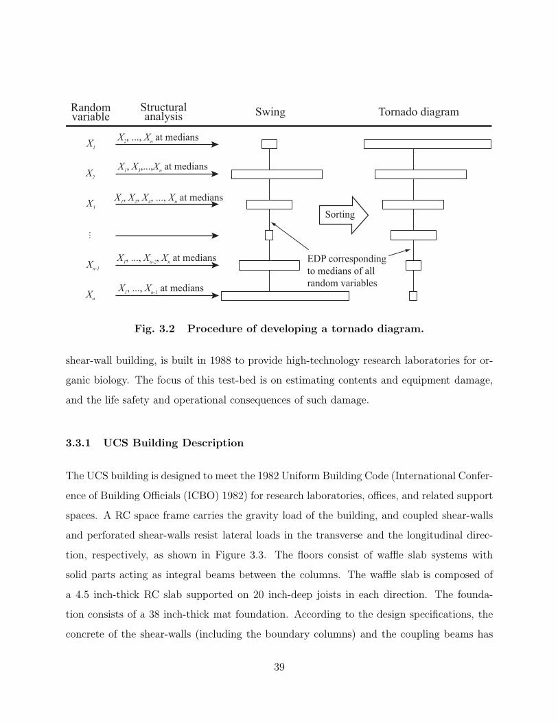
X1
X2
X3
...
Xn-1
Xn
Swing Tornado diagramRandomvariable
X2, ..., X
n at medians
Structuralanalysis
Sorting
X1, X
3,...,X
n at medians
X1, X
2, X
4, ..., X
n at medians
X1, ..., X
n-2, X
n at medians
X1, ..., X
n-1 at medians
EDP corresponding
to medians of all
random variables
Fig. 3.2 Procedure of developing a tornado diagram.
shear-wall building, is built in 1988 to provide high-technology research laboratories for or-
ganic biology. The focus of this test-bed is on estimating contents and equipment damage,
and the life safety and operational consequences of such damage.
3.3.1 UCS Building Description
The UCS building is designed to meet the 1982 Uniform Building Code (International Confer-
ence of Building Officials (ICBO) 1982) for research laboratories, offices, and related support
spaces. A RC space frame carries the gravity load of the building, and coupled shear-walls
and perforated shear-walls resist lateral loads in the transverse and the longitudinal direc-
tion, respectively, as shown in Figure 3.3. The floors consist of waffle slab systems with
solid parts acting as integral beams between the columns. The waffle slab is composed of
a 4.5 inch-thick RC slab supported on 20 inch-deep joists in each direction. The founda-
tion consists of a 38 inch-thick mat foundation. According to the design specifications, the
concrete of the shear-walls (including the boundary columns) and the coupling beams has
39

A
B
D
E
G
H
20'-9" 3@20'=60' 20'-9" 20'-9" 3@20'=60' 20'-9"
254'-1"1
9'-
9"
19
'-4
"2
2'-
10
"
10
4'-
6"
22
'-1
0"
19
'-9
"
101'-6"
N
16 o 33'20'-9" 20'
10 2 3 4 5 6 7 8 9 10 11 12 13 14 15 16
10'-4"
Perforated shear-wall
Coupled shear-wall
Fig. 3.3 Plan view of the UCS building.
nominal 28-day compressive strength f ′
c = 5 ksi, while that of all other columns and the waf-
fle slab systems has f ′
c = 3 ksi. The reinforcing steel is scheduled as ASTM A-615 Grade 40
for #4 and smaller bars and Grade 60 for #5 and larger bars. The middle frame in the
transverse direction (labeled 8 in Figure 3.3 and referred to as Frame 8) is analyzed in the
present study. Figure 3.4(a) presents the structural elevation view of Frame 8 and indicates
the story heights and the labels of the building levels. The cross sections of the shear-walls
and coupling beams, together with their reinforcement schedules of Frame 8 are shown in
Tables 3.1 and 3.2, respectively.
3.3.2 Structural Modeling
The computational model of the UCS building is developed using the modeling capabilities
of the open system for earthquake engineering simulation (OpenSees) software (McKenna
and Fenves 2001). Two-dimensional (2D) idealization is considered in the modeling. It is
noted that the longitudinal shear-walls are not considered as integrated parts of Frame 8.
The complete OpenSees model of Frame 8 is illustrated in Figures 3.4(b).
40

A B D E G H
16'-0
"13
'-6"
13'-6
"13
'-6"
13'-6
"13
'-6"
13'-6
"
97'-0
"
Level 1
Level 2
Level 3
Level 4
Level 5
Level 6
Roof
19'-9" 19'-9"19'-4"14'-10" 14'-10"8"
104'-6"
Base
8"
FC
Nonlinear beam-column element
Rigid element
Zero-length element1 2
8
55
47
for soil spring
(a) (b)
Fig. 3.4 Elevation view and OpenSees structural model of Frame 8 of the UCS
building.
41

Table 3.1 Geometrical properties and reinforcement schedule of shear-wall cross
sections of Frame 8 of the UCS building.
Column WallStory Depth (in.) Longitudinal reinf. Transverse
b1 b2 b3 WC1 WC2 WC3 reinf.t (in.) Reinf.∗
6th 24 25 24 8#8 8#8 8#8 #4@8′′ 14 #5@6′′
5th 24 25 24 8#8 8#8 8#8 #4@8′′ 14 #5@6′′
4th 24 31 24 8#8 12#8 8#8 #4@8′′ 14 #6@6′′
3rd 24 37 24 8#8 12#9 8#8 #4@8′′ 14 #6@6′′
2nd 24 44 24 8#8 16#10 8#8 #4@8′′ 16 #7@6′′
1st 33 49 30 12#9 22#10 12#9 #4@4′′ 18 #7@6′′
Basement 33 49 30 14#11 26#11 12#9 #4@4′′ 18 #7@6′′
∗ Same reinforcement in both the horizontal and vertical directions.
t t
15'-10"19'-9"
24"
b1
21'-4"
WC1
t
24"
D E F G H
ABC
b1
WC1
b4 b3 b2
WC2 WC2WC3
Table 3.2 Geometrical properties and reinforcement schedule of coupling beam
cross sections of Frame 8 of the UCS building.
Level Type “a” Type “b”
48"
20"
4.5"
24.5"
Type "a"
Type "b"
Roof 9#10 top and bottom 3#7 each face6 9#10 top and bottom 3#7 each face5 10#11 top and bottom 3#8 each face4 10#11 top and bottom 3#8 each face3 11#11 top and bottom 3#8 each face2 10#11 top and bottom 3#8 each face1 10#11 top and bottom 3#8 each face
42
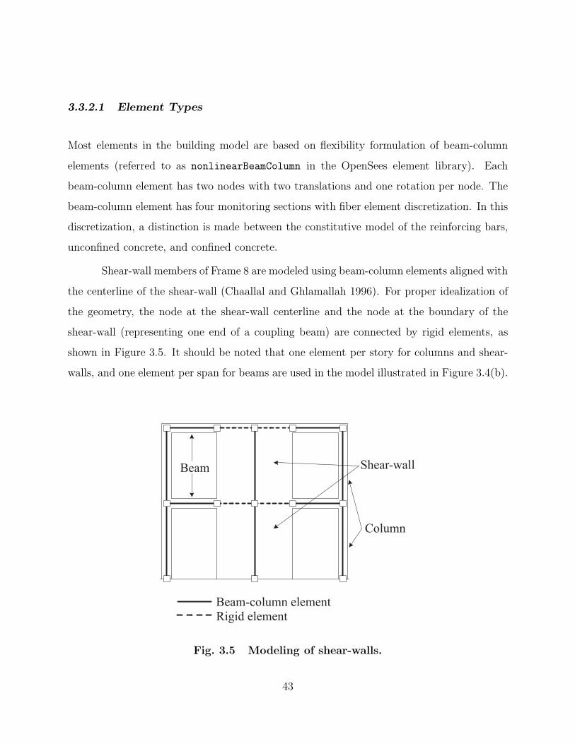
3.3.2.1 Element Types
Most elements in the building model are based on flexibility formulation of beam-column
elements (referred to as nonlinearBeamColumn in the OpenSees element library). Each
beam-column element has two nodes with two translations and one rotation per node. The
beam-column element has four monitoring sections with fiber element discretization. In this
discretization, a distinction is made between the constitutive model of the reinforcing bars,
unconfined concrete, and confined concrete.
Shear-wall members of Frame 8 are modeled using beam-column elements aligned with
the centerline of the shear-wall (Chaallal and Ghlamallah 1996). For proper idealization of
the geometry, the node at the shear-wall centerline and the node at the boundary of the
shear-wall (representing one end of a coupling beam) are connected by rigid elements, as
shown in Figure 3.5. It should be noted that one element per story for columns and shear-
walls, and one element per span for beams are used in the model illustrated in Figure 3.4(b).
Shear-wall
Column
Beam
Beam-column elementRigid element
Fig. 3.5 Modeling of shear-walls.
43

Figure 3.6 shows the shear force-distortion relationship of the coupling beam section
at the sixth floor indicating the shear force capacity as well as the shear force demand due to
KB-kobj. The shear force-distortion relationship is computed by the modified compression
field theory using the software Response-2000 (Bentz 2000). It should be noted that the shear
distortion in Figure 3.6 represents an average strain of concrete and steel reinforcement over
the cross section. Considering the intensity level of KB-kobj (Sa = 2.4g), it is concluded that
the shear force demand is well below their shear capacity of the cross section. Knowing that
the shear force demands on the other cross sections are also below the capacities, it is decided
that shear failure is not expected prior to flexural failure at the critical sections. Therefore,
conventional fiber element modeling (Spacone, Filippou, and Taucer 1996) is considered for
the UCS building.
0 0.005 0.01 0.015 0.020
100
200
300
400
500
600
700
800
Shear distortion
Sh
ear
forc
e, k
ip Shear demand = 555 kips
Shear capacity = 680 kips
Fig. 3.6 Shear capacity (based on the modified compression field theory by
Response-2000 (Bentz 2000)) and demand (due to KB-kobj) of the cou-
pling beam at the sixth floor (Element 55 in Figure 3.4(b)) of Frame 8
(refer to Table 3.2 for its design parameters).
44

3.3.2.2 Constitutive Models
In OpenSees, steel and concrete are modeled using uniaxial stress-strain relationships. In this
study, cover and core concrete materials are defined separately using the model Concrete01
that is based on the modified Kent-Park stress-strain relationship (Scott et al. 1982) with
degraded linear unloading/reloading stiffness according to the work of Karsan-Jirsa (1969)
and no tensile strength as shown in Figure 3.7(a). The behavior of the ascending branch of
the model is expressed as
fc = fo
[
2ε
ε0−(
ε
ε0
)2]
for ε ≤ ε0 (3.16)
where fc is the stress, ε is the corresponding strain, fo is the compressive strength of the
concrete expressed as fcc and fco for confined and unconfined concrete, respectively, in Fig-
ure 3.7(a), and ε0 is the strain corresponding to fo expressed as εcc and εco for confined and
unconfined concrete, respectively, in Figure 3.7(a). The expression in (3.16) is valid up to
the peak strength, beyond which the stress-strain relationships are approximated as linear
functions. A residual stress of the confined concrete, f residcc , is assumed as 0.2fcc, while it is
assumed zero for the unconfined concrete. The compressive strength and the correspond-
Stress
Strain 3
fcc
fco
εcuεcoεccεco
fcc
resid
Confined concrete
Unconfinedconcrete
(a) Concrete
Stress
Strain
fy
Es
αEs
(b) Steel
Fig. 3.7 Stress-strain relationships of concrete and steel adopted from the
OpenSees material library.
45
ing strain, and the ultimate strain of confined concrete (fcc, εcc, and εcu, respectively) are
estimated using the Mander’s model (Mander et al. 1988).
Steel reinforcing bars are modeled using a bilinear stress-strain relationship (referred
to as Steel01 in the OpenSees material library) as shown in Figure 3.7(b) with a schematic
cyclic behavior. Parameters defining this relationship are the yield strength fy, the modulus
of elasticity Es, and the hardening ratio α. In this study, all material parameters for concrete
and steel are defined in Section 3.4.1 as random variables, except for α which is specialized
as 0.01.
3.3.2.3 Gravity Load and Mass Idealization
The dead load accounts for the self-weight of the waffle slab system and the supporting
elements, i.e., shear-walls and columns. The assumed unit weight of the concrete is 145 pcf.
Accordingly, the computed dead load is 183 psf, which is a relatively high value due to the
large depth of the waffle slab system. Moreover, 25 psf representing building contents are
included as a superimposed dead load. The live load of 100 psf is assumed according to the
original design of the building. The mass of the building is modeled using lumped masses
at the nodes. Nodal masses are directly computed from the total dead load including the
self-weight and the superimposed dead load. The 2D model of Frame 8 has a tributary area
with 101′-6′′ width as shown in Figure 3.3.
3.3.2.4 Viscous Damping Idealization
The damping characteristics of the building are modeled using mass and stiffness proportional
damping with 5% of the critical damping for the first two modes of vibration. The periods
of these two modes estimated from the eigen solution using the initial elastic stiffness matrix
are 0.38 and 0.15 seconds.
46

3.3.2.5 Boundary Conditions
A flexible soil-structure interface at the foundation level is modeled using spring-type ele-
ments (referred to as zeroLength in the OpenSees element library) in the vertical direction.
These elements represent soil with a modulus of subgrade reaction of 100 lb/in.3 obtained
using the soil properties described in Section 3.4.2.2 and the procedure presented in FEMA
273 (Applied Technology Council (ATC) 1997). The same tributary areas as those of build-
ing mass are used to consider the flexible supports of the 2D model of Frame 8. To simulate
the characteristics of soil behavior, ENT material in the OpenSees material library is adopted.
An element with ENT material has elastic properties in compression and zero tensile strength
as shown in Figure 3.8.
Modulus ofsubgrade reaction
Deformation
Stress
Tension
Compression
Fig. 3.8 Constitutive model for the soil spring.
3.3.2.6 Solution Strategy
The Newmark β-method is used as the time integrator with typical coefficients γ = 0.50 and
β = 0.25. In general, a time step of 1/2 the ground motion time discretization (0.0025 to 0.01
seconds for the considered ground motions, refer to Section 3.4.2) is used for the analyses
in the present study. The modified Newton-Raphson solution algorithm that updates the
47
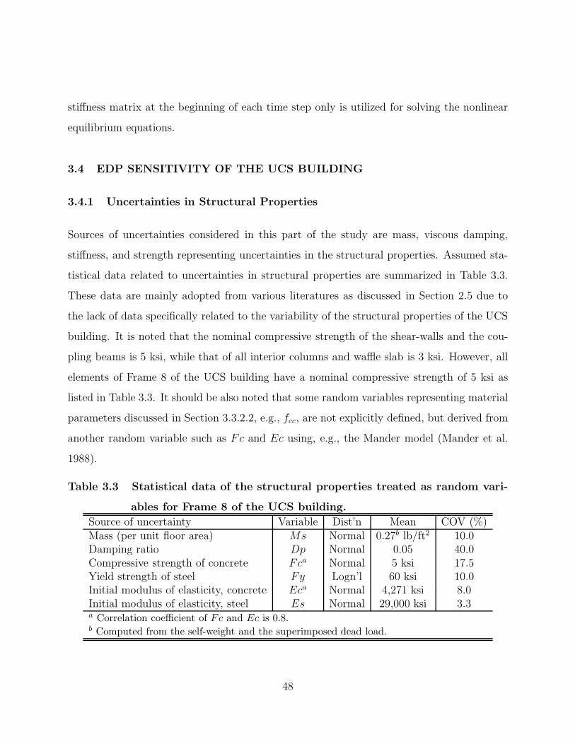
stiffness matrix at the beginning of each time step only is utilized for solving the nonlinear
equilibrium equations.
3.4 EDP SENSITIVITY OF THE UCS BUILDING
3.4.1 Uncertainties in Structural Properties
Sources of uncertainties considered in this part of the study are mass, viscous damping,
stiffness, and strength representing uncertainties in the structural properties. Assumed sta-
tistical data related to uncertainties in structural properties are summarized in Table 3.3.
These data are mainly adopted from various literatures as discussed in Section 2.5 due to
the lack of data specifically related to the variability of the structural properties of the UCS
building. It is noted that the nominal compressive strength of the shear-walls and the cou-
pling beams is 5 ksi, while that of all interior columns and waffle slab is 3 ksi. However, all
elements of Frame 8 of the UCS building have a nominal compressive strength of 5 ksi as
listed in Table 3.3. It should be also noted that some random variables representing material
parameters discussed in Section 3.3.2.2, e.g., fcc, are not explicitly defined, but derived from
another random variable such as Fc and Ec using, e.g., the Mander model (Mander et al.
1988).
Table 3.3 Statistical data of the structural properties treated as random vari-
ables for Frame 8 of the UCS building.
Source of uncertainty Variable Dist’n Mean COV (%)Mass (per unit floor area) Ms Normal 0.27b lb/ft2 10.0Damping ratio Dp Normal 0.05 40.0Compressive strength of concrete Fca Normal 5 ksi 17.5Yield strength of steel Fy Logn’l 60 ksi 10.0Initial modulus of elasticity, concrete Eca Normal 4,271 ksi 8.0Initial modulus of elasticity, steel Es Normal 29,000 ksi 3.3a Correlation coefficient of Fc and Ec is 0.8.b Computed from the self-weight and the superimposed dead load.
48

3.4.2 Uncertainties in Ground Motion
The intensity measure and the profile of ground motion are considered as two sources of
uncertainties in ground motion. This section describes information related to the chosen
seismic hazard of the UCS building site to be used for the definition of the intensity measure.
Moreover, selected different ground motions to address uncertainties in the ground motion
profile are discussed.
3.4.2.1 Seismic Hazard Curve
Frankel and Leyendecker (2001) provide a seismic hazard curve in terms of the mean annual
exceedance frequency (λ) of a specified spectral acceleration Sa for the location of the UCS
building, at the fundamental period (T1) of 0.2, 0.3, and 0.5 seconds, and B-C soil boundary
as defined by the International Building Code (International Code Council 2000). The
seismic hazard curve for Frame 8 (T1 = 0.38 second) is interpolated from those of T1 = 0.3
and 0.5 seconds without any modification for the site class. The seismic hazard curves for
Frame 8 is shown in Figure 3.9.
The temporal occurrence of an earthquake is most commonly described by a Pois-
son model (Kramer 1996). According to the Poisson assumption, the probability that no
earthquake with a spectral acceleration in excess of Sa will occur in period t is
P0 = e−λt = e−H(Sa)t (3.17)
where λ = H(Sa) denotes the mean rate of exceeding Sa (as given in Figure 3.9). From (3.17),
one can compute percentiles of Sa for a given t, e.g., the 10th, 50th (i.e., the median), and
90th percentiles of Sa for t = 50 years are indicated by circles in Figure 3.9 and by numerical
values in Table 3.4 where Sa is the random variable representing uncertainty in Sa. These
three percentiles are used in developing tornado diagrams as discussed in Sections 3.4.4.
For the FOSM method, the mean and the standard deviation of a random variable
are required rather than its percentiles. Therefore, the probability distribution of Sa is
49

10-3
10 -2
10 -1
100
10110
-5
10 -4
10 -3
10 -2
10 -1
100
An
nu
al e
xce
edan
ce f
req
uen
cy (
λ),
yr-1
Sa, g
UCS Hazard (T1=0.38 sec)
by Frankel and Leyendeker
Fitted curve by Lognormal
distribution of Sa
10th percentile
of Sa
90th percentile
of Sa
Median Sa
Fig. 3.9 UCS building site seismic hazard curve for Frame 8.
Table 3.4 Percentiles of Sa used in the tornado diagrams of the UCS building.
Percentile 10th 50th (median) 90thSa (g) 0.18 0.47 1.39
estimated by fitting the relationship between P0 and Sa in (3.17). The random variable
Sa is assumed to have a lognormal distribution. For t = 50 years, (3.17) is well-fitted by
the lognormal assumption of Sa with the mean of 0.633g and standard deviation of 0.526g
(COV=83%) as shown in Figure 3.9. These values of the mean and standard deviation of
Sa for Frame 8 are used for the FOSM method in Section 3.4.5.
3.4.2.2 Selected Ground Motions
The UCS building is located at a site consisting of stiff soil of thickness in the range of
20′ to 52′ (6 to 16 m), with an estimated average of about 39′ (12 m) above Franciscan
bedrock assumed to be not pervasively sheared and assumed to have a shear wave velocity
of about 2953 ft/sec (900 m/sec). Older alluvium overlies the Franciscan rocks at the site.
50

The alluvium typically comprises very stiff sandy clay, with average standard penetration
resistance values of 50 or greater and estimated shear wave velocity of about 1214 ft/sec (370
m/sec). The site is thus classified as NEHRP category SC according to the site classification
scheme in the NEHRP provision reproduced in Table 3.5.
Table 3.5 NEHRP site categories, after Dobry et al. (2000).
NEHRP Mean shear waveCategory
Descriptionvelocity to 30ma
A Hard rock > 1500 m/sec.B Firm to hard rock 760 – 1500 m/sec.C Dense soil, soft rock 180 – 360 m/sec.D Stiff soil < 180 m/sec.E Special study soils, e.g., liquefiable soils,
sensitive clays, organic soils, soft clays> 36 m thick
a Mean shear wave velocity from the surface to 30m depth of the ground.Note: 1 m = 3.28 ft.
The Hayward Fault, a strike-slip fault, traverses the campus of the University of
California, Berkeley, with a trace within 2900 ft (900 m) of the UCS building. The PEER
Testbeds Program (http://peertestbeds.net) provides a set of 20 recorded ground acceler-
ations to be used for the site of the UCS building. These ground motions are selected to
satisfy the distance and soil conditions of the building site for a strike-slip earthquake on
the NEHRP category SC site. Selected ground motion recordings are listed in Table 3.6.
In general, it is not easy to satisfy the intended distance and soil condition requirements.
However, these 20 ground motion records satisfy the requirements to the possible extent. For
example, all records are within about 6.2 miles (10 km) from the fault (all strike-slip fault),
and all but a few are from the SC site. Response spectra of these 20 ground accelerations
with 5% damping are plotted as well as the median response spectrum in Figure 3.10. Spec-
tral acceleration values of each of the 20 ground accelerations at the fundamental period of
Frame 8 of the UCS building are listed in Table 3.7 together with the median value.
51

Table 3.6 Ground motion recordings selected for the UCS building case study.
Earthquake Mwa Station name Dist.b Sitec NameCoyote Lake Coyote Lake Dam abutment 4.0 C CL-clydJun 8, 1979
5.7Gilroy #6 1.2 C CL-gil6Temblor 4.4 C PF-temb
Parkerfield6.0 Array #5 3.7 D PF-cs05
Jun 27, 1966Array #8 8.0 D PF-cs08
Livermore Fagundes Ranch 4.1 D LV-fgnrJan 27, 1980
5.5Morgan Territory Park 8.1 C LV-mgnpCoyote Lake Dam abutment 0.1 C MH-clyd
Morgan Hill6.2 Anderson Dam Downstream 4.5 C MH-andd
Apr 24, 1984Halls Valley 2.5 C MH-hallLos Gatos Presentation Ctr. 3.5 C LP-lgpcSaratoga Aloha Ave 8.3 C LP-srtg
Loma Prieta Corralitos 3.4 C LP-corOct 17, 1989
7.0Gavilan College 9.5 C LP-gavGilroy historic N/A C LP-gilbLexington Dam abutment 6.3 C LP-lex
Kobe, JapanJan 17, 1995
6.9 Kobe JMA 0.5 C KB-kobj
Tottori, Japan Kofu 10.0 C TO-ttr007Oct 6, 2000
6.6Hino 1.0 C TO-ttrh02
Erzincan, TurkeyMar 13, 1992
6.7 Erzincan 1.8 C EZ-erzi
a The moment magnitude (Mw) is a measure that characterizes the relative size of an
earthquake, that is based on measurement of the maximum motion records by a
seismograph.b Distance in km (1 km = 0.621 mile).c NEHRP site category (cf. Table 3.5).
52

Table 3.7 Spectral accelerations at the fundamental period of Frame 8 of the
UCS building.
Ground motion record Sa(T1 = 0.38 sec.), gCL-clyd 0.79CL-gil6 1.17EZ-erzi 0.78KB-kobj 2.45LP-cor 0.97LP-gav 1.14LP-gilb 0.62LP-lex 0.85LP-lgpc 1.49LP-srtg 0.73LV-fgnr 0.60
LV-mgnp 0.26MH-andd 0.82MH-clyd 1.63MH-hall 0.49PF-cs05 1.14PF-cs08 0.25PF-temb 1.18TO-ttr007 1.56TO-ttrh02 2.15Median 0.91
53

0 0.5 1 1.5 20
0.5
1
1.5
2
2.5
3
Period, sec.
Sa, g
Median
response
spectrum
0.38
Fig. 3.10 Response spectra of the 20 selected earthquake records for the UCS
building analyses.
3.4.3 Selected EDPs
In general, laboratory buildings contain heavy and/or sensitive equipments, and valuable
contents. Therefore, in addition to the common interest in the seismic response of structural
components, the response of non-structural components and building contents in laboratory
building, e.g., the UCS building, is of particular interest. In that regard, the peak absolute
floor acceleration and displacement, and the peak inter-story drift ratio (IDR) are selected as
the global EDPs. Here, the absolute response is the relative response to the fixed base alge-
braically added to the ground motion. The peak absolute floor acceleration and displacement
provide a basis for estimating damage to acceleration-sensitive and displacement-sensitive
building contents such as computers on bench-tops and shelves, hazardous chemicals on
shelves, and large refrigerators that are important in terms of value and life safety. More-
54

over, IDR at each story provides a way to estimate the damage to structural components
and some of the non-structural components such as windows and claddings. Among global
EDPs, only the peak absolute roof acceleration (referred to as PRA), the peak absolute roof
displacement (referred to as PRD), and the maximum IDR (referred to as MIDR) among
the seven stories of the UCS building are presented in this report.
In addition to the global EDPs, the rotational demands of each structural component
are selected as the local EDPs. However, monitoring the response history of all structural
components may not be feasible depending on the size of the computational model and
the type of the adopted finite elements to represent these components. Therefore, only
relatively important structural components, determined such that their deformations sig-
nificantly contribute to the global displacement of the building are selected for the current
sensitivity study. For this purpose, a deterministic transient analysis of the UCS building
with all random variables assigned their mean values is performed first. In this analysis, the
loading is the unscaled ground acceleration record denoted as KB-kobj in Table 3.6 with
Sa = 2.4g as the fundamental period of Frame 8 (0.38 sec.) of the UCS building.
To determine the contribution of each component to the floor displacement, moment-
curvature relationships at both ends of all components are monitored (solid lines in Fig-
ure 3.11) and compared with those obtained from section analyses under monotonically
increasing curvature (dashed lines in Figure 3.11). From Figures 3.11(a) and (c), the bot-
tom of the shear-wall in the first story shows severe nonlinear behavior including significant
deformation, while shear-walls in the other stories remain in the elastic range. On the other
hand, from Figures 3.11(b) and (d), severe nonlinear behavior is observed in all coupling
beams. Accordingly, the three shear-walls in the first story and the coupling beams in all
floors are considered as important components with respect to the floor displacement. There-
fore, in the presented sensitivity study, the curvatures of the critical cross sections where the
curvature is largest are monitored as local EDPs.
55

0 0.125 0.25
-0.5
0
0.5
1.0
x 105
Curvature, 10-3
/in.
Mom
ent,
kip
-ft
Center shear-wall at 6th story
-0.005 -0.0025 0 0.0025
Curvature, 1/in.
Mom
ent,
kip
-ft
Coupling beam at 6th floor
0 0.125 0.25
-0.5
0
0.5
1.0
x 105
Curvature, 10-3
/in.
Mom
ent,
kip
-ft
Center shear-wall at 1st story
-2000
0
2000
3000
Curvature, 1/in.
Mom
ent,
kip
-ft
Coupling beam at 1st floor
(a) (b)
(c) (d)
-0.005 -0.0025 0 0.0025
1000
-1000
-2000
0
2000
3000
1000
-1000
Fig. 3.11 Moment-curvature relationships at various cross sections of Frame 8
subjected to KB-kobj (solid lines) and from monotonic section anal-
yses (dashed lines); (a) the bottom of element 47; (b) the left of
element 55; (c) the bottom of element 2; (d) the left of element 8.
Element numbers are designated in Figure 3.4(b).
56

3.4.4 Tornado Diagram Analysis
Tornado diagrams of different EDPs are developed according to the procedure described in
Section 3.2.2. Unlike the other sources of uncertainties, uncertainty in ground motion profile
cannot be explicitly expressed as a random variable defined by a probability distribution.
In other words, one cannot define the 10th, 50th, and 90th percentiles of ground motion
profile. Therefore, the following procedure is developed to determine medians and bounds
of the ground motion profile with respect to the EDP of interest.
1. Compute the elastic spectral acceleration Sai at the fundamental period of the structure
with 5% viscous damping ratio (recall that this is the adopted definition of the IM of
a particular earthquake profile) for the ith ground motion profile.
2. Determine the scale factor (αi) by αi = target Sa/Sai where the target Sa is the median
Sa obtained from the seismic hazard curve.
3. Perform a nonlinear time history analysis of the structure using the ith scaled ground
motion (αi times the original ground motion profile) to obtain EDP corresponding to
the ith ground motion, EDPi.
4. Repeat steps 1, 2, and 3 above for another ground motion profile and sort the ground
motion profiles by their EDPs.
5. Find the 10th, 50th, and 90th percentiles of EDP from the set of EDPs obtained from
step 4 above. The corresponding ground motion profiles are respectively the 10th,
50th, and 90th percentiles of the ground motion profile.
Random variables Fc and Fy in Table 3.3 are combined to represent the strength,
and Ec and Es are also combined to represent the stiffness such that each pair of random
variables is perfectly dependent. In other words, if Ec increases by one unit, Es also increases
by one unit. This assumption is adopted to investigate the combined effect of the concrete
57

and reinforcement in terms of the stiffness and strength of the RC building, not the effect of
individual materials. In this chapter, this is the case unless otherwise noted.
Figure 3.12 shows tornado diagrams of different EDPs. The vertical lines in the
middle of these tornado diagrams indicate EDPs corresponding to the median values of all
random variables. Line-type plots are the results of using the FOSM method described in
the following section. According to this figure, Sa is the most significant random variable for
PRA, PRD, and MIDR of Frame 8 of the UCS building in a probabilistic sense. Moreover,
one can observe that uncertainty in EDPs is more sensitive to uncertainty in ground motion
(Sa and GM) than that in structural properties (Ms, Dp, Stiffness and Strength). This
implies that a better understanding of characteristics of ground motion profiles and hazard
information will greatly reduce uncertainty of the seismic demand of buildings such as the
UCS building. On the contrary, the rankings of random variables in structural properties
are different for different EDPs.
0.2 0.4 0.6 0.8 1.0 1.2
Stiffness
Ms
Strength
Dp
GM
Sa
PRA, g
(a)
0 2 4 6 8
Strength
Dp
Stiffness
Ms
GM
Sa
PRD, in.
(b)
0 0.1 0.2 0.3 0.4
Strength
Stiffness
Ms
Dp
GM
Sa
MIDR, %
(c)
Fig. 3.12 Tornado diagrams and FOSM results of Frame 8 of the UCS building.
These tornado diagrams also suggest skew of the EDP distributions. Especially, from
swings of PRA induced by GM , PRD induced by Sa and GM , and MIDR induced by Sa,
one can estimate rather strong skewness of probability distributions of the considered EDPs.
Skewness of PRD and MIDR distributions is partly caused by skew of the Sa distribution
itself, since the probability distribution of Sa can be estimated by lognormal as discussed in
Section 3.4.2.1. This suggests that the relationship between each of PRD and MIDR, and
58
Sa is close to linear. On the other hand, the swing of PRA induced by Sa does not show
a strong skewness. This suggests that the relationship between PRA and Sa is not linear.
Further investigation into the relationship between EDP and IM is not conducted in this
report because it is not within the scope of the present study. Such investigation can be
pursued by, for example, IDA (Vamvatsikos and Cornell 2002).
3.4.5 Analysis Using FOSM Method
Using the means and COVs of random variables given in Table 3.3, sensitivity of each EDP to
a random variable is estimated. To determine the perturbation size for the finite difference
approach (3.15) discussed in Section 3.2.1, sensitivity estimates of each EDP in terms of
COV are obtained using different perturbation sizes as summarized in Table 3.8. In this
table, the median ground motion profile denotes the ground motion profile that produces
the median EDP among the considered 20 ground motion profiles discussed in Section 3.4.2.
It should be noted that these ground motions are individually scaled to achieve the mean
Sa (Sa = 0.633g) according to the lognormal fit of the seismic hazard curve of the UCS
building site (Figure 3.9). The median ground motion profiles are used to estimate the
sensitivity of EDPs to any other random variable than GM that denotes the random variable
representing uncertainty in the ground motion profile itself. Table 3.8 clearly shows that the
finite difference approach adopted in this study using ap = 0.001 guarantees convergence of
the results by the FOSM method.
EDP sensitivity to combined uncertainties in structural properties in Table 3.3 are
estimated for each of the 20 ground motion profiles at the median IM level (0.91g according
to Table 3.7) using different perturbation sizes, namely ap = 1.0 and 0.001. Consequently,
20 COV values are computed for each EDP and each perturbation size. Statistics of each
of these 20 COV values, namely the mean and the COV, are compared in Table 3.9. The
difference in the levels of scatter (in terms of COV) for the different perturbation sizes is
negligible. This is another justification of the selected perturbation size, i.e., for ap = 0.001.
59

Table 3.8 COV (%) of EDPs corresponding to the individual random variables
of Frame 8 of the UCS building.
Random PRA PRD MIDRvariable ∗ ∗∗ ∗∗∗ ∗ ∗∗ ∗∗∗ ∗ ∗∗ ∗∗∗
∂g/∂xi
Sa 36.4 53.0 53.0 67.3 67.3 67.3 81.6 80.3 80.3 +veGM 14.7 64.0 9.5 N/Aa
Dp 9.0 11.7 11.7 8.0 8.0 8.0 5.8 5.4 5.4 −veMs 10.5 7.3 7.3 6.8 6.3 6.3 8.2 7.5 7.5 +ve
Strength 4.5 4.4 4.4 3.3 3.3 3.3 2.7 4.7 4.7 −veStiffness 1.8 1.8 1.8 1.9 1.9 1.9 3.1 2.8 2.8 −ve
Median GMP TO-ttrh02 TO-ttrh02 CL-clyd∗, ∗∗, and ∗∗∗ for ap = 1.0, 0.1, and 0.001, respectively. Refer to Section 3.2.1 for ap.a Monte Carlo simulation is used.
Table 3.9 Statistics of measure of EDP sensitivities to combined uncertainties
in structural properties using different perturbation sizes.
COV of PRA COV of PRD COV of MIDRStatistics
∗ ∗∗ ∗ ∗∗ ∗ ∗∗
Median (%) 16.5 16.6 12.0 12.6 19.5 19.4COV (%) 34.7 30.9 37.2 38.3 49.0 41.2
∗ and ∗∗ for ap = 1.0 and 0.001, respectively.
From Table 3.8, one observes that the effect of Sa on variability of the selected three
global EDPs is the dominant one amongst all considered random variables. However, this
result is not surprising because the variability of Sa itself (COV = 83% as discussed in
Section 3.4.2) is even larger than any of the EDP variability. It is also observed that random
variables in ground motion (Sa and GM) are more significant than those in the structural
properties.
It is noted that a random variable shows different effects on different EDPs. For
example, COVs of PRA and PRD due to the random variable Dp are 11.7% and 8.0%,
respectively. This is attributed to the fact that the selected EDPs are all peak responses and
they do not necessarily occur simultaneously. For example, Figure 3.13 shows time histories
60

of absolute and relative accelerations, and absolute and relative displacements at the roof,
as well as the respective peak responses (including PRA and PRD) that are indicated by
circles due to TO-ttrh02 scaled to the mean Sa, i.e., 0.633g. Clearly, PRA and PRD do not
occur simultaneously. Moreover, uncertainty in a peak absolute response due to a random
variable depends on contributions from the relative response and the ground motion. In
general, the contribution of the relative response (e.g., displacement) to the corresponding
peak absolute response does not necessarily agree with that of another relative response (e.g.,
acceleration). For example, in Figure 3.13, the contribution of ground acceleration to PRA
is very small, while that of ground displacement to PRD is much more significant. Both
-1
-0.5
0
0.5
1
7 8 9 10 11 12 13 14-3
-2
-1
0
1
2
3Absolute
Relative
Absolute
Relative
Acc
eler
atio
n,
gD
isp
lace
men
t, i
n.
Time, sec.
PRD
PRA
Fig. 3.13 Time histories of various EDPs due to TO-ttrh02.
61

the non-simultaneous occurrence of different EDPs and different contributions by different
relative responses to the corresponding peak absolute responses depend on the specific choice
of the ground motion profile.
COVs of EDPs due to GM are obtained using Monte Carlo simulation. In this case,
all random variables are assigned their mean values to obtain 20 samples (due to 20 ground
motions that are individually scaled to the mean Sa, i.e., 0.633g) for each EDP. It is notable
that COV of PRD is considerably larger than those of PRA and MIDR (refer to Table 3.8).
This is mostly due to uncertainty in the ground displacement itself. In fact, the COV of
the 20 peak ground displacements is 84%. On the other hand, COV of the 20 peak ground
accelerations is 40%, and its effect on PRA is less significant than that of uncertainty in the
ground displacement on PRD.
It is worth mentioning that the sign of the gradient of an EDP with respect to a
random variable (expressed as ∂g/∂xi in (3.15)) reflects if the random variable is a demand
variable or a capacity variable. Note that the output of the FOSM method is in terms of
statistics of the “demand” of the structural system in this study. In this context, a random
variable with a positive gradient of an EDP can be viewed as a “demand” variable. On
the other hand, a random variable with a negative gradient of an EDP can be viewed as a
“capacity” variable. In this study and according to Table 3.8, gradients with respect to Sa
and Ms are positive, which suggests that those are demand variables. However, gradients
with respect to the other random variables are negative, suggesting that they are capacity
variables.
3.4.6 Comparison of Analyses Using Tornado Diagram and FOSM Method, and
Suggested New Approach
It is not straightforward to compare the tornado diagram and the result of the FOSM method
directly, because a tornado diagram does not contain any statistical information on EDP
(unless EDP is a linear function of random variables), while the only outcome of the FOSM
62

method is EDP statistics. One way of comparing the tornado diagram and the result of
the FOSM method is to compare the order of importance of random variables to each EDP.
For a “better” comparison than just listing random variables in an order, the results of the
FOSM method are presented in the same format as the tornado diagram. For this purpose,
the EDPs are assumed in most cases to have the same distributions as the corresponding
random variables with estimated means and standard deviations obtained from the FOSM
method. For example, lognormal distribution is assumed for EDP distributions induced by
Sa because Sa has lognormal distribution. However, lognormal distribution is assumed for
EDP distribution induced by GM because skewness of the EDP distributions is observed
from tornado diagrams in Figure 3.12. Assumed EDP distributions corresponding to random
variables and bases of assumptions are listed in Table 3.10.
Table 3.10 Assumed EDP distributions and bases of assumptions.
Random variable Assumed EDP distribution Basis of assumptionSa Lognormal Sa distributionGM Lognormal Tornado diagramMs Normal Ms distributionDp Normal Dp distribution
Stiffness Normal Tornado diagramStrength Normal Tornado diagram
Then, the 10th and 90th percentiles of each EDP are computed for each random
variable and plotted on the same tornado diagram as shown in Figure 3.12. If an EDP is
a linear function of random variables, the envelopes obtained by the FOSM method should
exactly match the outlines of the tornado diagram because in this hypothetical case (1) the
EDPs corresponding to the 10th and 90th percentiles of a random variable are exactly the
10th and 90th percentiles of the EDP distribution; (2) the FOSM method gives the exact
solutions of the mean and standard deviation of the EDP; and (3) the distribution type of
EDP is identical to that of the random variable. However, if the function is nonlinear, none
of the above is true, and the 10th and 90th percentiles of an EDP by the FOSM method do
not have to match their counterparts of the tornado diagram. However, Figure 3.12 shows
63

a reasonable match between the tornado diagrams and envelopes obtained by the FOSM
method for the rankings of random variables. Note that these rankings are slightly different
between the tornado diagram and the outcome of the FOSM method. This is particularly
the case for the structural properties that have small effect (small swings) on the variability
of the EDPs anyway.
As simple methods (in comparison to Monte Carlo simulation) for the sensitivity
study, the tornado diagram analysis and the FOSM method are compared in a general sense.
A tornado diagram does not provide any statistics on EDP. However, one can have a rough
idea of the skew of the EDP distribution. For example, Figures 3.12(b) and (c) suggest strong
skew of PRD and MIDR distributions induced by Sa, respectively, while the distribution
of PRA induced by Sa shows weaker skew. The FOSM method estimates the two most
important statistics of EDP, namely the mean and standard deviation. Unlike the tornado
diagram analysis, the sensitivity of an EDP to a combination of correlated random variables
can be investigated by the FOSM method. This feature is explicitly utilized in Chapter
5 where EDP uncertainty induced by correlated uncertain parameters in the capacity of
a structural component is estimated, while no strong correlation is considered in the case
study of the UCS building in this chapter. However, the FOSM method does not take into
account the distribution type of the random variable and, consequently, no information on
the distribution type of the EDP can be inferred from the results of the FOSM method.
Knowing the pros and cons of both the tornado diagram and the FOSM methods, one
may think of combining these two methods so that one benefits from both merits. Obviously,
a combined method should be able to estimate the means and standard deviations of EDP
with an idea of the skewness of its probability distribution. One possible way of achieving
this is to compute the gradient of an EDP with respect to a random variable (required
for the FOSM method) using its corresponding swing from the tornado diagram analysis.
For example, if the swing of an EDP is obtained by the mean ± standard deviation of
the corresponding random variable (X), the gradient of the EDP with respect to the given
64

random variable (X) can be estimated by
dEDP
dx≈ Swing of EDP
2 × Standard deviation. (3.18)
Note that (3.18) is equivalent to (3.15) with ap = 1.0. The outcome of this approach is a
tornado diagram with estimated mean and standard deviations (obtained from FOSM with
the help of (3.18)) of EDP. Figure 3.14 illustrates the suggested new approach of combining
the tornado diagram and the FOSM method for estimating EDP uncertainty.
Structural analysis
(e.g. nonlinear time history analysis)
Probability distribution
of random variable X
Probability distribution
of EDP (unknown)
XLB
=mean-SD XUB
=mean+SD
SD: standard deviation
EDP(XUB
)EDP(XLB
)
Swing of EDP
Perturbation of X
Tornado diagram with
estimated means and SDs of EDP
Estimate of the mean EDP
= EDP corresponding to
means of all random
variables
Perturbation of X
Swing of EDP
dX
dEDP=
Fig. 3.14 Suggested new approach of combining the tornado diagram and the
FOSM method.
65

3.4.7 Sensitivity of Local EDPs by FOSM Method
Sensitivity of the local EDPs is studied by the FOSM method in terms of the peak curvature
at critical cross sections to individual random variables described in Table 3.3. Only the
FOSM method is used here assuming the sensitivities of the local EDPs estimated by both
the FOSM method and the tornado diagram analysis are close to each other as is the case
for the global EDPs. Unlike the sensitivity study of global EDPs, random variables Fc,
Fy, Ec, and Es are considered independently. Moreover, the results are presented in an
analogous format to the FOSM envelopes of the tornado diagrams in Figure 3.12. The
median ground motion profile for PRA and PRD, namely TO-ttrh02 as given in Table 3.8,
is used for sensitivity of the local EDPs to all random variables but GM . Figure 3.15 shows
the results for some critical cross sections of Frame 8 of the UCS building using the FOSM
method. Similar to the results of global EDPs, Sa is the dominant random variable for all
critical cross sections. The second significant random variable is Dp for all cross sections
where a relatively large COV (40%) assigned to Dp may have led to this high ranking of Dp.
The subsequent significant random variables differ from one cross section to the other.
3.4.8 Conditional Sensitivity of EDP Given IM by FOSM Method
In Sections 3.4.4 through 3.4.7, a measure of EDP sensitivities by the tornado diagram
analysis or analysis using the FOSM method is estimated at only one IM level, i.e., the
median or mean Sa, respectively. However, from the perspective of PBEE, it is desirable to
investigate the propagation of uncertainty at various levels of earthquake hazard. In that
regard, the conditional sensitivity of EDPs to random variables given IM is investigated
where Sa is treated as a deterministic variable at different levels. Nine levels of IM in terms
of Sa are selected for this purpose, namely the 10th, 20th, . . . , and 90th percentiles of Sa
according to (3.17) as listed in Table 3.11. The range of Sa, bounded by the 10th and the 90th
percentiles, is indicated in Figure 3.9. In this part of the study, all 20 ground motion profiles,
66

0 2.5 5.0 7.5
FyEsEcFcMsGMDpSa
Curvature, 10-6/in.
0 0.25 0.5 0.75 1.0 1.25
EsFyEcFc
GMMsDpSa
Curvature, 10-3/in.
EsFyEcMsFc
GMDpSa
EsEcFcFy
GMMsDpSa
Curvature, 10-3/in.
(a) (b)
(c) (d)
0
Curvature, 10-6/in.
2.5 5.0 7.5 0 0.25 0.5 0.75 1.0 1.25
Fig. 3.15 Sensitivity of the peak curvatures at critical cross sections of Frame 8
of the UCS building; (a) the bottom of element 1; (b) the left of
element 8; (c) the bottom of element 2; (d) the left of element 55.
Element numbers are designated in Figure 3.4(b).
not only the median ground motion profile as was conducted in Sections 3.4.4 through 3.4.7,
are used to estimate EDPs sensitivity to each random variable at each IM level. It is to be
noted that all results in this section are presented with respect to Sa on a semi-log scale due
to the wide range of the considered Sa (0.18g to 1.39g).
3.4.8.1 Global EDPs
For each IM level, a deterministic analysis where all random variables are kept at their mean
values is conducted for each ground motion that is individually scaled to achieve a given IM.
67

Table 3.11 Various percentiles of Sa for sensitivity of EDP given IM for Frame 8
of the UCS building.
Percentile 10th 20th 30th 40th 50th 60th 70th 80th 90thSa (g) 0.18 0.25 0.32 0.39 0.47 0.57 0.71 0.90 1.39
Figure 3.16 shows scatters of global EDPs reflecting the uncertainty in GM . In this figure,
the solid lines represent the median EDPs. It is observed that these medians tend to increase
as the IM level increases.
0.2 0.3 0.4 0.5 1 1.50
0.5
1
1.5
2
2.5
Sa, g
PR
A, g
(a)
0
5
10
15
20
PR
D, in
.
0.2 0.3 0.40.5 1 1.5
S , ga
25
(b)
0
0.2
0.4
0.6
0.8
1
MID
R,
%
0.2 0.3 0.40.5 1 1.5
Sa, g
(c)
Fig. 3.16 Scatters of global EDPs induced by the uncertainty in GM for Frame 8
of the UCS building.
Uncertainties of global EDPs induced by those in structural properties are estimated
by using the FOSM method and presented in Figure 3.17 in terms of COV. In this figure,
each circle represents the COV of the EDP induced by uncertainties in all structural prop-
erties namely, mass, viscous damping, strength, and stiffness for a specific ground motion
profile and IM level. The variance is obtained according to (3.13) considering correlations of
random variables to derive the COV. Figure 3.17(d) is for the peak relative roof displacement
(PRRD) that is the peak roof displacement relative to the fixed base to compare with PRD
(Figure 3.17(b)). Note that the scatter of COV values at each IM level is induced by the
inherent record-to-record variability of ground motions.
The COVs of global EDPs due to GM only (obtained from the data of Figure 3.16)
68

0.2 0.3 0.4 0.5 1 1.50
0.2
0.4
0.6
0.8
Sa , g
CO
V o
f P
RA
0.2 0.3 0.4 0.5 1 1.50
0.2
0.4
0.6
0.8
, g
CO
V o
f P
RR
D
0.2 0.3 0.4 0.5 1 1.50
0.2
0.4
0.6
0.8
, g
CO
V o
f P
RD
0.2 0.3 0.4 0.5 1 1.50
0.2
0.4
0.6
0.8
, g
CO
V o
f M
IDR
(a) (b)
(c) (d)
Sa
SaSa
Fig. 3.17 Comparison of uncertainties in global EDPs for Frame 8 of the UCS
building induced by the uncertainty in GM only (solid line) and in
structural properties (dashed line, median quantity).
are also plotted in Figure 3.17 as solid lines for comparison. Dashed lines in Figure 3.17
connect median COVs (the median of 20 COV values from the scaled 20 records for a
certain IM in terms of Sa) at each IM level induced by combined uncertainties in structural
properties. From Figures 3.17(a) and (c), at lower IM levels, uncertainty in structural
properties is more significant than that in GM on PRA and MIDR, while at higher IM
levels, the opposite is true. However, PRD uncertainty is primarily dependent on GM . This
is mostly due to the uncertainty of ground displacement itself because the COV of the 20
peak ground displacements is 84% as mentioned in Section 3.4.5. On the other hand, GM
does not dominate the PRRD uncertainty (Figure 3.17(d)) where the uncertainty of ground
displacement is canceled by the definition of PRRD. Instead, GM becomes more significant
69

than the other random variables of structural properties only at much higher IM levels.
Finally, one observes that the COV of an EDP induced by GM increases as the IM level
increases, while that induced by structural properties does not have an obvious trend.
3.4.8.2 Local EDPs
Similar to the previous section, EDP uncertainty induced by GM only is investigated first.
Figure 3.18 shows scatters of the peak curvature reflecting the uncertainty in GM only where
the solid lines represent the median EDPs. Similar to global EDPs, the medians of the peak
curvatures at all critical cross sections tend to increase as the IM level increases.
Sensitivity of the local EDPs conditioned on IM induced by uncertainties in structural
properties is studied in terms of the peak curvature demands at critical cross sections, as
shown in Figure 3.19. As in the previous section, COVs of EDPs induced by uncertainties
in all structural properties are derived from variances of EDPs obtained according to (3.13).
Similar to that of global EDPs, the scatter of COV values at each IM level is due to the
inherent record-to-record variability of ground motions. Moreover, uncertainty of the peak
curvatures depends more on uncertainty in structural properties at lower IM levels and on
uncertainty in GM at higher IM levels for all critical cross sections.
3.5 CONCLUDING REMARKS
The propagation of basic uncertainty to the structural system with respect to its seismic
demand (referred to as EDP) due to possible future earthquakes is studied in this chapter.
An approach of estimating uncertainties in EDP and identifying significant sources of basic
uncertainties is demonstrated using a case study RC shear-wall building (referred to as the
UCS building). Sensitivity of EDP to uncertainties in structural properties and ground
motion is estimated using the tornado diagram analysis and the FOSM method. From the
sensitivity measure of an EDP, the relative significance of each basic uncertainty to the given
EDP is identified and ranked.
70

0.2 0.3 0.40.5 1 1.50
5
10
15x 10
-6
Sa , g
Cu
rvat
ure
, 1
/in.
0.2 0.3 0.40.5 1 1.50
1.25
2.5
3.75
5.0
Sa , gC
urv
atu
re,
1/i
n.
0.2 0.3 0.40.5 1 1.50
5
10
15x 10
-6
Sa , g
Cu
rvat
ure
, 1
/in.
0.2 0.3 0.40.5 1 1.50
1.25
2.5
3.75
5.0
Sa , g
Cu
rvat
ure
, 1
/in.
(a) (b)
(c) (d)
x 10-3
x 10-3
Fig. 3.18 Scatters of the peak curvature at critical cross sections of Frame 8 of
the UCS building induced by the uncertainty in GM ; (a) the bottom
of element 1; (b) the left of element 8; (c) the bottom of element
2; (d) the left of element 55. Element numbers are designated in
Figure 3.4(b).
71

0.2 0.3 0.40.5 1 1.50
0.5
1
1.5
Sa , g
CO
V o
f cu
rvat
ure
0.2 0.3 0.40.5 1 1.50
0.2
0.4
0.6
0.8
, g
CO
V o
f cu
rvat
ure
0.2 0.3 0.40.5 1 1.50
0.2
0.4
0.6
0.8
, g
CO
V o
f cu
rvat
ure
0.2 0.3 0.40.5 1 1.50
0.5
1
1.5
2
2.5
, g
CO
V o
f cu
rvat
ure
(a) (b)
(c) (d)
Sa
SaSa
Fig. 3.19 Comparison of local EDPs uncertainty induced by the uncertainty in
GM only (solid line) and in structural properties (dashed line, median
quantity) at critical cross sections of Frame 8 of the UCS building; (a)
the bottom of element 1; (b) the left of element 8; (c) the bottom of
element 2; (d) the left of element 55. Element numbers are designated
in Figure 3.4(b).
72
The FOSM method estimates the mean and the standard deviation of an EDP given
means and standard deviations of various random variables. The estimated standard devia-
tion of an EDP is its measure of sensitivity to a given random variable. The FOSM method
is simple and efficient in estimating EDP sensitivity, in comparison with Monte Carlo simula-
tions in terms of computing the mean and standard deviation of EDP. The tornado diagram
analysis, one of the methods of the deterministic sensitivity study, is also simple and efficient
in identifying and ranking relatively significant random variables to EDPs. The pros and
cons of tornado diagram analysis and the FOSM method are discussed in a general sense,
and an approach of combining the two methods is suggested. The peak absolute roof ac-
celeration (PRA), peak absolute roof displacement (PRD), and maximum inter-story drift
ratio (MIDR) are selected as global EDPs, while the peak curvatures at critical cross sections
are selected as local EDPs. Moreover, several random variables representing uncertainty in
ground motion and structural properties are considered.
Sensitivity of global EDPs indicates that the intensity measure of earthquakes is the
dominant source of uncertainty to all global EDPs. Moreover, uncertainties in ground motion
are more significant than those in structural properties. A sensitivity of local EDPs indicates
that the intensity measure of earthquakes is the dominant source of uncertainty to all local
EDPs, while the second significant source of uncertainty is the viscous damping where a
relatively large COV (40%) assigned to the probability distribution of viscous damping may
have been responsible for its high ranking.
The conditional sensitivity of EDPs to random variables given IM is investigated
considering uncertainty in the ground motion profile and the combined effect of all uncer-
tainties on structural properties. For all local and global EDPs but PRD, uncertainty in the
ground motion profile is more significant than that on structural properties at higher levels
of earthquake intensity but less significant at lower levels of earthquake intensity. For PRD,
uncertainty in the ground motion profile is dominant, regardless of the level of earthquake
intensity.
73

4 Uncertainty in the Capacity of Structural
Components
4.1 INTRODUCTION
The quantification of uncertainty in the response of RC structural components in terms of the
deformation and strength capacity is necessary for the implementation of the PBEE design
methodology. The probabilistic analysis of RC structural components has been the focus of
a number of research efforts. One of the earliest works is that of Shinozuka (1972) where he
pointed out the importance of considering the spatial variability of the material properties
in estimating the strength of plain concrete structures. Several studies were concentrated on
RC frame members such as columns or beams using computational approaches such as the
Monte Carlo simulation. Knappe et al. (1975) studied the reliability of a RC beam. Grant
et al. (1978), Mirza and MacGregor (1989), and Frangopol et al. (1996) conducted strength
analyses of RC beam-column members by considering the uncertainty of material properties
and of cross-sectional dimensions. However, few research efforts considered the spatial vari-
ability of random variables of the RC frame members, which requires the discretization of
the random field and the identification of the correlation characteristics of random variables.
Because of the nature of RC construction, the spatial variability of material and geometrical
properties should be considered for reliable estimates of the nonlinear structural behavior.
In this chapter, a computational model for structural analysis considering the spatial
variability of material and geometrical properties of the RC structural members using the
75

Monte Carlo simulation method is developed. This model combines the conventional fiber
element formulation and one of the random field representation methods. The fiber element
model is selected for computing the structural response because it is a powerful tool in
estimating the inelastic behavior of RC framed structures. Among various random field
representation methods, the midpoint method (Der Kiureghian and Ke 1988) is selected in
the present study. Assumptions and formulations of the adopted fiber element model are
described in the next section. Subsequently, the stochastic fiber element model including
the random field representation method is presented. The stochastic fiber element model is
applied to several structural components to develop probabilistic section models, namely the
probabilistic axial force-bending moment diagram and the probabilistic moment-curvature
relationship.
As a part of demonstrating the systematic procedure of evaluating a structural system,
namely component evaluation phase (cf. Section 2.6.1), typical structural components of a
ductile RC frame are identified and evaluated to develop their probabilistic section models.
The procedure of the system evaluation phase using these probabilistic section models of
typical structural components is demonstrated in Chapter 5.
The main objective of the developed computational model is the probabilistic evalu-
ation of RC structural members such as columns and beams. Although the developed com-
putational procedure can be applied for probabilistic evaluation of any framed structure, it
is not practical to use it for a complete structural system due to the large computational
demand of the Monte Carlo simulation method combined with the fiber element model.
A demonstration of a systematic approach for the probabilistic evaluation of a structural
system using various probabilistic section models is presented in Chapter 5.
4.2 FIBER ELEMENT MODEL
Material nonlinearity in a frame element is commonly described by either a lumped (D’Ambrisi
and Filippou 1999) or distributed (Spacone et al. 1996) plasticity model. In the lumped
76

plasticity model, a frame element consists of two zero-length nonlinear rotational spring
elements and an elastic element connecting them. The nonlinear behavior of a structure
is captured by the nonlinear moment-rotation relationships of these spring elements. Due
to the simplicity of the formulation, the lumped plasticity model is widely used when the
computational cost of the analysis is high, e.g., in the case of nonlinear time-history analysis
of a large structure. An example of a structural model using the concentrated plasticity
formulation is discussed in Section 5.3.1. On the other hand, material nonlinearity of a
structure can develop anywhere in the element using the distributed plasticity model. Due
to its capacity for describing nonlinear structural behavior, the distributed plasticity model
is widely used for more accurate estimation of the structural response. In this chapter,
only the distributed plasticity model is employed for the nonlinear frame element with the
fiber section discretization. It is one of the best models to accommodate random fields of
structural properties of RC frame members.
The formulation of a nonlinear frame element is categorized by the flexibility (force-
based) method or the stiffness (displacement-based) method. The flexibility method uses
assumed force interpolation functions along the element, and a smaller number of elements
than that of the stiffness method may be required. The stiffness method uses assumed
displacement interpolation functions along the element, and this feature requires the use
of a sufficient number of elements for a member to model an accurate structural response.
The element formulation in the flexibility method is more complex than that of the stiffness
method, because material constitutive models are usually given in the form σ = σ(ε), where
σ and ε are stress and strain measures, respectively, which is suitable for the stiffness method.
On the other hand, the element formulation in the stiffness method is more straightforward
and widely used in conventional finite element methods.
In this chapter, the stiffness method is used to formulate the distributed plasticity
under the assumptions of the Bernoulli beam theory. An element is represented by several
cross sections located at the numerical integration points. Each section is subdivided into
77

a number of fibers where each fiber is under a uniaxial state of stress. This discretization
process is shown in Figure 4.1 for the special case of an RC structural member.
Element Section
Monitoring sections
z
y
x
z
y
Concrete fiberSteel fiber
Fig. 4.1 Element and section discretization.
4.2.1 Element Formulation
Force and deformation variables at the element and section levels are shown in Figure 4.2.
From this figure, the element force and deformation vectors are given by
Force ≡ p = [p1, p2, . . . , p6]T (4.1)
Deformation ≡ u = [u1, u2, . . . , u6]T (4.2)
On the other hand, the section force and deformation vectors are given by
Element Section
u2, p2
u4, p4u1, p1
u5, p5
u3, p3
u6, p6M(x), ϕ(x)
N(x), ε0(x)
x
Fig. 4.2 Force and deformation variables at the element and section levels.
78

Force ≡ q(x) = [N(x), M(x)]T (4.3)
Deformation ≡ vs(x) = [ε0(x), ϕ(x)]T (4.4)
The normal force N , bending moment M , axial strain at the reference axis ε0, and curvature
ϕ are functions of the section position x.
The strain increment in the ith fiber is defined by
dεi = dε0(x) − yidϕ(x)
= as(y)dvs(x)(4.5)
where as(y) = [1, −yi], dvs(x) = [dε0(x), dϕ(x)]T , and yi is the distance between the ith
fiber and the reference axis. Section deformations vs(x) are determined from the strain-
deformation relationship such that
vs(x) =
[
B(x) +1
2G(x)
]
un+1 (4.6)
where un+1 = un +∆u is the element deformation vector at the load step n+1, B(x) is the
first-order strain-deformation transformation matrix which consists of the well-known first
and second derivatives of the displacement interpolation matrix assuming small deformations,
and G(x) is another strain-deformation transformation matrix such that 12G(x) represents
the second-order term of the strain-deformation relationship. G(x) can be expressed as
G(x) =
1
0
C(x)un+1T C(x) (4.7)
where C(x) is a strain-deformation transformation matrix which consists of the first deriva-
tives of displacement interpolation matrix. Explicit forms of B(x) and C(x) are provided in
Section A.1 of Appendix A.
Tangent modulus Eti and stress σi are determined from the strain εi using a particular
constitutive relationship for the material of the ith fiber. In this way, the section stiffness
79

ks(x) and resisting force rs(x) are determined using the principle of virtual work such that
ks(x) =
∫
A(x)
asT (y)Et(x, y)as(y)dA (4.8)
rs(x) =
∫
A(x)
asT (y)Et(x, y)dA (4.9)
These integrals are evaluated by the midpoint rule with n fibers. Thus, ks(x) and rs(x) are
numerically obtained as follows
ks(x) =
n∑
i=1
asTi Etiasiai (4.10)
rs(x) =n∑
i=1
asTi Etiai (4.11)
where the cross-sectional area A(x) =n∑
i=1
ai.
For nonlinear analysis, the force-displacement relationship at the element level is
commonly expressed in an incremental form such that ∆p = ke∆u where ke is the element
tangent stiffness matrix. Once vs(x) is determined, the section stiffness ks(x) and resisting
forces rs(x) are evaluated. Subsequently, the element stiffness ke and resisting forces re are
derived from the principle of virtual work and can be expressed as follows
ke =
∫
L
TT (x)ks(x)T(x)dx +
∫
L
CT (x)C(x)Ns(x)dx (4.12)
re =
∫
L
TT (x)rs(x)dx (4.13)
where T(x) = B(x) + G(x), Ns(x) is a component of rs(x) representing the axial force
resultant and L is the element length. Derivation of this element stiffness matrix is provided
in Section A.1 of Appendix A. In the present study, the Gauss-Lobatto integration scheme
is adopted to evaluate these integrations. Four integration points per element are used in
this study. Thus, x’s are selected at the Gauss integration points. The element stiffness
and resisting forces are then assembled by the conventional finite element method procedure
to determine the global stiffness and resisting forces. For nonlinear conditions, equilibrium
80

between the applied forces and the resisting forces is usually not satisfied in one iteration.
Therefore, an incremental-iterative numerical technique should be utilized to enforce the
equilibrium conditions. The adopted nonlinear iterative solution scheme is described in the
following section.
4.2.2 Nonlinear Analysis Procedure
An incremental-iterative solution procedure is utilized to solve the nonlinear equilibrium
equations obtained from the fiber element model. By the conventional Newton-type analysis
method, it is not possible to capture the post-critical response of the structure, which is
essential for the performance-based design of an RC structure. This drawback is due to the
numerical feature that holds the load parameter constant throughout the iterations within
each load step. Passing limit points is therefore impossible due to the singular nature of
the tangent stiffness matrix in the vicinity of a limit point. Various techniques to overcome
this drawback have been developed. A detailed description and summary of these schemes
are found in reference (Clarke and Hancock 1990). Among these methods, the minimum
unbalanced displacement norm method is selected in the present study and described in the
subsequent paragraphs.
In the incremental-iterative solution method, each load step starts with the applica-
tion of a load increment and subsequent iterations for equilibrium. In the following, subscript
k is used to denote the load step number, while superscript i is used to denote the iteration
number within each load step.
4.2.2.1 First Iteration
At the first iteration of each load step, the “tangent” displacement Utk is computed by
KkUtk = Pref (4.14)
81

where Kk is the tangent stiffness matrix of the structure at the end of the previous load
step and Pref is the reference external force vector. Next, the incremental displacement is
evaluated by
∆U1k = ∆λ1
kUtk (4.15)
where ∆λ1k is a load step parameter for the first iteration of the kth load step, which can be
determined by the following procedure.
lk = lk−1
(
Jd
Jk−1
)γ
(4.16)
∆λ1k =
±lk√
UtTk Ut
(4.17)
where Jd is the desired iteration number for convergence, typically 3 to 5, Jk−1 is the actual
iteration number for convergence in the previous load step, and l1 = ∆λ11
√
UtT1 Ut1. The
exponent γ typically lies between 0.5 to 1.0 (Clarke and Hancock 1990). In (4.17), the sign
follows that of the determinant of the stiffness matrix. Then, the total displacement and
load parameter are updated from the previous load step by
U1k = Uk−1 + ∆U1
k (4.18)
λ1k = λk−1 + ∆λ1
k (4.19)
4.2.2.2 Equilibrium Iterative Cycles
The incremental change in the displacements can be written as the solution of
Kk∆Uik = ∆λi
kPref −Pui−1k (4.20)
where Pu denotes the vector of the unbalanced forces. Since the modified-Newton-Raphson
method is adopted in this study, Kk doesn’t have superscript i, i.e., it is not updated at each
iteration. In the above equation,
Pui−1k = Pi−1
k − Pri−1k (4.21)
82

where Pi−1k = λi−1
k Pref and Pri−1k is the resisting force vector obtained by the assembly
of relem vectors given in the previous section. From the above equations, the incremental
displacement vector ∆Uik can be obtained by
∆Uik = ∆λi
kUti−1k + ∆Ur
ik (4.22)
where ∆Urik is the residual displacement vector obtained by solving
Kk∆Urik = Pr
i−1k (4.23)
Determination of the incremental load parameter ∆λik is discussed in the next section. The
total displacement vector and load parameter are updated from the previous iteration by
Uik = Ui−1
k + ∆Uik (4.24)
λik = λi−1
k + ∆λik (4.25)
Iterations are continued until a convergence criterion is satisfied. In this study, L2 norm of
the unbalanced force vector (Pui−1k ) normalized by that of the total force vector (Pi−1
k ) is
used for the convergence criterion and the tolerance is set to 10−4. If divergence is detected
or convergence is not achieved within a specified number of iterations (typically selected as
10 iterations), the iterative procedure for the current load step restarts with a reduced initial
load increment.
4.2.2.3 Iterative Scheme
The incremental load parameter ∆λik can be obtained by various constraint equtions. In
this study, the minimun unbalanced displacement norm method is selected. Among various
iterative schemes such as arc-length method, this method is simple to implement and is
verified to work well (Clarke and Hancock 1990).
The constraint equation involving ∆λik is
∂ ‖ ∆Uik ‖
∂∆λik
= 0 (4.26)
83

which guarantees a minimum value for the unbalanced displacement norm in each iteration.
Accordingly,
∆λik = −Ut
Tk Ur
ik
UtTk Utk
(4.27)
4.2.3 Constitutive Models
In the fiber element analysis, the behavior of each fiber is governed by a specific uniaxial
stress-strain relationship. For RC members, three constitutive models are necessary: (1) an
unconfined concrete model for cover concrete, (2) a confined concrete model for core concrete,
i.e., concrete inside the transverse reinforcement, and (3) a steel model for longitudinal
reinforcing bars.
Figure 4.3 depicts typical stress-strain relationships for confined and unconfined con-
crete. Relevant parameters in the compression regime are the compressive strength fcc, the
corresponding strain εcc, and the ultimate strain εcu of confined concrete, and the compressive
strength fco and the corresponding strain εco of unconfined concrete. The tension regime is
defined by the tensile strength f ′
t and the ultimate tensile strain εtu. Initial tangent stiffness
Ec is usually assumed to be the same for both the compression and the tension regimes.
In this study, the model proposed by Hoshikuma et al. (1997) is employed for the
confined concrete. This model is expressed as
Ascending branch: fc = Ecεc
[
1 − 1
n
(
εc
εcc
)n−1]
(4.28)
Descending branch: fc = fcc − Edes (εc − εcc) ≥ f residcc (4.29)
where fc and εc are stress and corresponding strain in the confined concrete and Edes is the
slope of the descending branch. The model parameters n and Edes are given by
n =Ecεcc
Ecεcc − fcc
(4.30)
Edes =fcc − f resid
cc
εcu − εcc
(4.31)
84

Stress
Strain 3
fcc
fco
f'tεcuεcoεccεco
εtu
fcc
resid
Ec
Confined concrete
Unconfinedconcrete
Fig. 4.3 Concrete constitutive models.
where εcu can be given by
εcu = 0.004 +1.4ρshfyhεsuh
fcc
(4.32)
according to Mander’s model (Mander et al. 1988) where ρsh, εsuh, and fyh are respectively
the volumetric ratio, the ultimate strain, and the yield strength of the transverse reinforce-
ment. Other material parameters are expressed as
fcc = fco + 3.8αρshfyh (4.33)
εcc = 0.002 + 0.033βρshfyh
fco
(4.34)
where α and β are cross-sectional shape factors. For a circular cross section, α = β = 1.0
and for a square cross section, α = 0.2 and β = 0.4. To avoid numerical difficulties in the
present study, 0.2fcc is assumed as a residual value of the confined concrete strength f residcc .
The constitutive model of the unconfined concrete in compression consists of a non-
linear ascending branch and a linearly descending branch (Figure 4.3). The expressions for
these two branches are the same as those of the confined concrete model (Equations 4.28
to 4.30), except for the following: fcc and εcc are substituted by fco and εco, respectively, and
Edes is expressed as Edes = fco/2εco. In the present study fco is taken as 0.85f ′
c where f ′
c is
the compressive strength of concrete from the standard compressive test, and εco is taken
85

as 0.002. It is assumed that the strength is zero when εc ≥ 3εco to represent spalling of the
cover concrete.
A bilinear constitutive model is adopted for the confined and unconfined concrete
in tension as shown in Figure 4.3. The tensile strength f ′
t is computed by f ′
t = 6√
f ′
c in
psi units. The ultimate tensile strain εtu is assumed to equal 10εt, where εt is obtained by
εt = f ′
t/Ec. It is assumed that a fiber with its tensile strain ≥ 10εt is fully cracked and has
completely lost its tensile strength.
The constitutive model of the reinforcing steel consists of a bilinear elastic-plastic
portion followed by a strain hardening region calculated by the following expression:
fs = fu − (fu − fy)
(
εsu − εs
εsu − εsh
)2
, εsh < εs < εsu (4.35)
where fs is the steel stress corresponding to the steel strain εs, fy is the yield stress, fu is the
ultimate stress, εsh is the strain at the onset of hardening, and εsu is the ultimate strain as
shown in Figure 4.4. Stress is assumed to be zero beyond the ultimate strain. For simplicity,
this constitutive model is adopted in both the tension and the compression regimes. Note
that only envelopes of the three constitutive models are adopted because only monotonic
loading is considered in this chapter.
Stress
Strainεsuεsh
εy
fu
fy
Es
Fig. 4.4 Reinforcing steel constitutive model.
86

4.2.4 Verification Examples
A nonlinear static analysis Matlab program (Hanselman and Littlefield 1998) for RC struc-
tures is developed based on the nonlinear fiber element formulation described in the previous
section. This program is numerically verified using three sets of experiments. The first set of
experiments conducted by Mosalam (2002) at the University of California, Berkeley, includes
eight identical, simply supported ductile RC beams (referred to as MB) under four-point
bending. The second set, also conducted by Mosalam (2002) at the University of California,
Berkeley, includes seven identical RC columns (referred to as MC) having square cross sec-
tion under the effect of axial load. Figures 4.5 and 4.6 show the design parameters of MB
P/2 P/2
24" 24" 24"
72"
3/4" clear cover
(Typical)
3/16" wire @ 3"
10.5"
5"
2-#4 bars
2-#4 bars
2 - 3/16" wires as stirrup hangers
Fig. 4.5 The applied loads and the design parameters of MB.
#2 wire @ 1.5"
4-#4 bars
6.5"
6.5"24"
P
3/4" clear cover(Typical)
Fig. 4.6 The applied load and the design parameters of MC.
87

and MC, respectively. The third set includes the column designated A1 that was tested by
Kunnath et al. (1997) under constant axial load and monotonically increasing lateral load at
the tip of the column. In the present study, this column is referred to as KC where Figure 4.7
shows its design parameters. The KC specimen was designed such that failure due to flexure
preceded that due to shear with ample margin (Kunnath et al. 1997). Nominal values of
material properties of MB, MC, and KC are given in Table 4.1.
0.57"12.0"
21-#3
0.16" spirals@ 0.75"
Pl
54.02"
Pa
Fig. 4.7 The applied loads and the design parameters of KC.
Table 4.1 Material properties of MB, MC, and KC.
Material property MB MC KCCompressive strength of concrete, psi 4,216 5,192 5,149Yield stress of longitudinal steel, ksi 71 71 65Ultimate stress of longitudinal steel, ksi 100 100 100Strain at on-set of hardening of longitudinal steel 0.01 0.01 0.01Yield stress of transverse steel, ksi 71 71 65Modulus of elasticity of steel, ksi 29,000 29,000 29,000
Figure 4.8(a) compares load-displacement relationships from the analysis with the
experimental results for MB. Load is the sum of the applied two point loads and displacement
is measured at mid-span. The analytical results show good agreement with the experimental
results. It is interesting to note that the experimental results for the tested eight beams are
88

scattered even though these beams were identical. This can be explained by the variability
of material and geometric properties of the beams, which motivated the present study.
The results from the column tests of MC are compared in Figure 4.8(b). These
results are presented in terms of load-displacement relationships in the axial direction of the
column. From the comparison, excellent agreement with the experimental results up to the
displacement of 0.2 inch is clear. Beyond that the analysis reasonably match the experimental
trend. It should be noted that the experiments were conducted under load control where it
was rather difficult to control the descending branch of the load-displacement relationship.
Similar to the tests of MB, experimental results of MC are scattered in spite of their identical
designs and construction.
0 0.5 1 1.5 20
5
10
15
20
25
30
Displacement, in.
Load
, k
ip
Analysis
Experiment
(a)
0 0.2 0.4 0.6 0.80
100
200
300
Displacement, in.
Load
, k
ip
Analysis
Experiment
(b)
Fig. 4.8 Load-displacement relationships; (a) MB; (b) MC.
Figure 4.9 shows load-displacement relationships obtained by analysis and experiment
of KC. These relationships are for the response in the lateral direction at the column tip.
The comparison is shown for two types of analyses. In the first, the effect of P -∆ is ignored
(dotted line). This analysis did not capture the experimentally recorded descending branch.
The second analysis invoked the P -∆ capability of the program where an excellent agreement
89

0 1 2 3 4 5 6 70
5
10
15
20
Displacement, in.
Lat
eral
load
, kip
Experiment
Analysis,P- ∆
Analysis,no P- ∆
Fig. 4.9 Load-displacement relationships of KC
with the experiment is observed (dashed line). It should be noted that in the experiment of
KC, small initial loading cycles were applied which are not included in the analysis. Due to
this simplification, minor adjusting of the material properties was necessary for good match
with the experiments at the initial stage of loading. This was conducted by 10% reduction of
the concrete compressive strength and the steel yield strength from their specified nominal
values.
Figures 4.8 and 4.9 show the capability of the program developed in this study in
estimating the softening behavior of RC structural members. The comparisons in Figures 4.8
and 4.9 imply good match between the analytical predictions and the experimental data.
Accordingly, the developed computational tool is an accurate one for deterministic nonlinear
analysis of RC structures. This tool is subsequently extended to account for the variabilities
of material and geometrical properties as discussed in the following section.
It should be noted that shear deformation is ignored in the present fiber element
formulation. Accordingly, shear failure is assumed not to occur prior to flexure failure,
which is the case in most of the examples presented in this chapter.
90

4.3 STOCHASTIC FIBER ELEMENT MODEL
In general, stochastic finite element method (SFEM) refers to the finite element method
that accounts for spatial variability in the material properties, geometry of the structure, or
applied loads. In this context, the stochastic fiber element model is developed in this study,
such that spatial variability of the material and geometrical properties in the structural
model is accounted for in the conventional (deterministic) fiber element model.
4.3.1 Monte Carlo Simulation
Monte Carlo simulation (Rubinstein 1981) is one of the methods widely used to analyze
random problems. In a random problem, random outputs are obtained in probabilistic or
statistical forms using random inputs. In Monte Carlo simulation, random inputs are rep-
resented by sets of deterministic values, often called samples. Then, a random problem is
transformed into a set of deterministic problems that can be solved using conventional tools
such as the finite element method. From each set of deterministic inputs, one can generate
a set of deterministic outputs. Finally, one can construct probabilistic or statistical forms
of outputs from the sets of deterministic outputs. Because of its simplicity and robust-
ness, Monte Carlo simulation is frequently used to analyze random problems in engineering
applications and to validate other probabilistic analysis methods.
4.3.2 Random Field Representation
In most of SFEM, it is necessary to represent a random field in terms of random variables.
This process is usually called representation of the random field. Several methods for rep-
resentation of random fields have been proposed. These include the midpoint method (Der
Kiureghian and Ke 1988), the spatial averaging method (Vanmarcke and Grigoriu 1983),
the shape function method (Liu et al. 1986), and the series expansion method (Ghanem
and Spanos 1991; Lawrence 1987; Li and Der Kiureghian 1993; Spanos and Ghanem 1989;
91

Zhang and Ellingwood 1994). In this section, existing methods for random field generation
are reviewed and issues on random field mesh size are discussed.
Let v(x),x ∈ Ω, denote a multidimensional Gaussian random field defined in the
domain Ω. This field is completely described by its mean function µ(x), variance function
σ2(x), and autocorrelation coefficient function ρ(x,x′) between the two random variables x
and x′.
4.3.2.1 Midpoint Method
The simplest method of discretization is the midpoint method applied to the stochastic
problem by Der Kiureghian and Ke (1988). In this method, the random field is represented
by a constant value over each element. A representing value for each element is the one
evaluated at the centroid xc of the element, i.e.,
v(x) = v(xc); x ∈ Ωe (4.36)
where v(x) is an approximation of v(x), and Ωe is an element domain. Mean µ and covariance
matrix Σvv of v = v(x1c), . . . , v(xne
c ) are obtained from µ(x), σ2(x), and ρ(x,x′) of v(·)evaluated at centroids of all elements having the number ne. It has been shown that this
method tends to over-represent the variability of the random field within each element (Der
Kiureghian and Ke 1988).
4.3.2.2 Spatial Averaging Method
In this method proposed by Vanmarcke and Grigoriu (1983), the random field is also repre-
sented by a constant value over each element. A representing value is the spatial average of
the field over the element. Mathematically, this can be written as
v(x) =
∫
Ωe
v(x)dΩ∫
Ωe
dΩ= ve; x ∈ Ωe (4.37)
92

The mean and covariance matrix of v are obtained from µ(x), σ2(x), and ρ(x,x′) of v(·) as
integrals over the domain Ωe. This averaging process allows us to expect a better estimate
on the random field than the midpoint method. Matthies et al. (1997) pointed out the
difficulties involved in this method as follows:
• the approximations of the non-rectangular elements may lead to a non-positive definite
covariance matrix.
• this method is practically limited to cases where the random field is Gaussian because
the distribution function of each random variable vi is almost impossible to obtain
except for Gaussian random fields.
Moreover, this method is known to under-represent the local variance of the random field (Der
Kiureghian and Ke 1988).
4.3.2.3 Shape Function Method
The shape function method, proposed by Liu et al. (1986), uses sets of nodal values and
corresponding shape functions to describe the random field, i.e.,
v(x) =nn∑
i=1
Ni(x)v(xi); x ∈ Ωe (4.38)
where nn is the number of nodes in the element, Ni is the ith shape function, and xi is the
ith nodal coordinates. The mean and covariance are approximated by the following:
E[v(x)] =nn∑
i=1
Ni(x)µ(xi) (4.39)
Cov[v(x), v(x′)] =
nn∑
i,j=1
Ni(x)Nj(x′)Cov[v(xi), v(xj)] (4.40)
Here, the random field is described by a continuous function, while the aforementioned two
methods use discontinuous functions.
93

4.3.2.4 Optimal Linear Estimation
In the optimal linear estimation (OLE) method, presented by Li and Der Kiureghian (1993),
the random field is estimated by a linear estimator v expressed as
v(x) = a(x) +nn∑
i=1
bi(x)v(xi)
= a(x) + bT (x)v; x ∈ Ω
(4.41)
where, nn is the number of nodes in the domain, v = [v(xi)] is the nodal vector. Using the
linear estimation theory, we determine a(x) and b(x) such that the variance of the error
v(x) − v(x) is minimized, where v(x) is an unbiased estimator of v(x), i.e.,
minimize Var[v(x) − v(x)] (4.42)
subject to E[v(x) − v(x)] = 0; x ∈ Ω (4.43)
According to Li and Der Kiureghian (1993) after finding the solution of this problem, v(x)
can be rewritten as
v(x) = µ(x) + ΣTv(x)vΣ
−1vv
(v − µ); x ∈ Ω (4.44)
where Σv(x)v is the vector containing the covariance of v(x) with the elements of v, and µ
and Σvv are the mean vector and variance-covariance matrix of v. It is notable that this
method always under-represents the variance of the actual random field v(x) (Li and Der
Kiureghian 1993).
4.3.2.5 Karhunen-Loeve Expansion
In the Karhunen-Loeve expansion (KL) method (Spanos and Ghanem 1989), the random
field is expressed in terms of its spectral decomposition. The random field can be written as
v(x) = µ(x) +
∞∑
i=1
ξi
√
λi φi(x); x ∈ Ω (4.45)
94

where ξi is statically independent standard normal variables, and λi and φi are eigenvalues
and eigenfunctions of ρ(x,x′) such that∫
Ω
ρ(x,x′)φi(x′)dx′ = λiφi(x) (4.46)
and
∫
Ω
φi(x)φj(x)dx = δij (Kronecker delta) (4.47)
However, usually only a few of the terms with the largest eigenvalues are important in
the spectral decomposition. Thus, by truncating insignificant terms with relatively small
eigenvalues, (4.45) can be approximated by
v(x) = µ(x) +
r∑
i=1
ξi
√
λi φi(x); x ∈ Ω (4.48)
where r is the number of terms included in the series. Some of the interesting properties of
this method can be found in (Li and Der Kiureghian 1993; Matthies et al. 1997; Sudret and
Der Kiureghian 2000) and briefly summarized here.
• The set of random variables ξi, i = 1, 2, . . . is orthonormal in the sense that
E[ξiξj] = δij (4.49)
• ξi, i = 1, 2, . . . form a set of independent standard normal random variables.
• This method always under-represents the true variance of the random field.
Provided that the exact solution of the eigenvalue problem given by (4.47), this
method is very efficient for simulating a random field, since it requires small number of
random variables to describe the random field with a given level of accuracy. However, the
eigenvalue problem seldom has an exact solution except for some special cases as discussed
by Spanos and Ghanem (1989), and an approximation method should be used. Ghanem
and Spanos (1991) suggested a Galerkin-type procedure where the eigenfunctions φi are
approximated by a set of basis functions and a corresponding set of coefficients. Subsequently,
the integral eigenvalue problem in (4.46) and (4.47) is converted into a discrete (matrix)
eigenvalue problem.
95

4.3.2.6 Orthogonal Series Expansion
The orthogonal series expansion method is proposed by Zhang and Ellingwood (1994). This
method avoids solving the eigenvalue problem in (4.46 and 4.47) by selecting a proper set
of orthogonal functions instead of the eigenfunctions. A random field v(x) with its mean
function µ(x) and correlation function ρ(x,x′) can be expressed as
v(x) = µ(x) +∞∑
i=1
χihi(x) (4.50)
where hi(x) are orthogonal functions and χi are correlated random variables. It should be
noted that Lawrence (1987) proposed a similar method to the orthogonal series expansion
called the basis random variable expansion. Using the orthogonality of hi’s and some basic
algebra, it can be shown that
χi =
∫
Ω
[v(x) − µ(x)]hi(x)dΩ (4.51)
(Σvv)ij ≡ E[χiχj] =
∫
Ω
∫
Ω
ρ(x,x′)hi(x)hj(x′)dΩdΩ (4.52)
For Gaussian v(x), (4.51) proves that χi’s are zero-mean random variables. A random field
in (4.50) can be approximated by selecting a set of proper orthogonal functions and a finite
number of terms used in the expression, i.e.,
v(x) = µ(x) +r∑
i=1
χihi(x) (4.53)
where r is the number of terms included.
4.3.2.7 Expansion Optimal Linear Estimation
The expansion optimal linear estimation (EOLE) method, proposed by Li and Der Ki-
ureghian (1993), uses a spectral decomposition of the random field vector v of size N in
OLE method. If v(x) is assumed to be Gaussian random variable, the spectral decomposi-
96

tion of its covariance matrix Σvv is expressed as
v(x) = µ(x) +N∑
i=1
√
λi ξiφi (4.54)
where ξi’s are independent standard normal variables, and λi and φi are the eigenvalues and
eigenvectors of Σvv, such that
Σvvφi = λiφi (4.55)
Substituting (4.54) into (4.44) gives
v(x) = µ(x) +N∑
i=1
ξi√λi
φTi Σv(x)v (4.56)
The second term on the right-hand side of (4.56) can be approximated by using only r terms
which have significant eigenvalues, i.e.,
v(x) = µ(x) +
r∑
i=1
ξi√λi
φTi Σv(x)v, r < N (4.57)
This expression is optimal in the sense that it minimizes the error in the variance. It is to be
noted that EOLE always under-represents the true variance (Li and Der Kiureghian 1993).
Comparison between the above methods mentioned in this chapter for random field
representation is presented by Sudret and Der Kiureghian (2000). Even though the midpoint
method may exhibit relatively poor performance for representing a given random field, this
method is adopted in this study for its simplicity. However, replacing this simple method by
a more sophisticated method should neither pose a major difficulty nor alter the conclusions
of the present study.
4.3.2.8 Nataf Model
In general, v(x) is a non-Gaussian random field. In this case, v(x) = [v1, . . . , vne] is
a vector of dependent non-Gaussian random variables whose joint distribution function is
not known and only the marginal distribution and correlation coefficient matrix (R = ρij,
97

i, j = 1, . . . , ne) are available in many applications. In this general case, the Nataf model (Liu
et al. 1986) can be used to simulate v(x). Using the marginal transformation of vi, a standard
normal random vector Z = [Z1, . . . , Zne] is defined by
Zi = Φ−1[Fvi(vi)], i = 1, 2, . . . , ne (4.58)
where Φ(·) is the standard normal cumulative distribution function and Fvi(vi) is the marginal
cumulative distribution function of vi. Nataf’s distribution of v(x) is obtained by assuming
Z is jointly normal with the correlation coefficient matrix R0 = ρ0,ij, i, j = 1, . . . , ne.
Approximate relations of ρ0,ij(ρij) for a large number of distribution types are given by Liu
and Der Kiureghian (1986). In Monte Carlo simulation, the procedure of simulating v(x) is
summarized as follows:
1. Generate a vector U of size ne, whose components are independent standard normal
random samples.
2. Compute Z = L0U where L0 is a lower triangle matrix of R0 such that R0 = L0LT0 .
3. Compute vi = F−1vi
[Φ(Zi)] to simulate v(x).
4.3.2.9 Issues on Random Field Mesh Size
One of the important issues in SFEM is selecting the mesh sizes. While the finite element
mesh size is governed by the geometry and the expected gradient of the stress field, the
random field mesh size is controlled by the rate of fluctuation of the random field. This fact
implies that two independent mesh discretizations are acceptable: one for the finite element
and the other for the random field.
The rate of fluctuation of the random field is usually measured by the so-called cor-
relation length θ which is defined as a measure of the distance over which significant loss of
correlation occurs. Mathematically, this correlation length can be written as
θ =
∫
∞
0
ρ(∆x)d∆x (4.59)
98
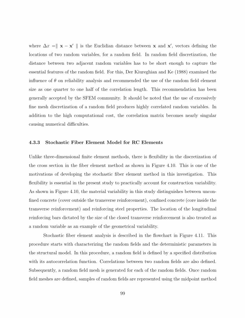
where ∆x =‖ x − x′ ‖ is the Euclidian distance between x and x′, vectors defining the
locations of two random variables, for a random field. In random field discretization, the
distance between two adjacent random variables has to be short enough to capture the
essential features of the random field. For this, Der Kiureghian and Ke (1988) examined the
influence of θ on reliability analysis and recommended the use of the random field element
size as one quarter to one half of the correlation length. This recommendation has been
generally accepted by the SFEM community. It should be noted that the use of excessively
fine mesh discretization of a random field produces highly correlated random variables. In
addition to the high computational cost, the correlation matrix becomes nearly singular
causing numerical difficulties.
4.3.3 Stochastic Fiber Element Model for RC Elements
Unlike three-dimensional finite element methods, there is flexibility in the discretization of
the cross section in the fiber element method as shown in Figure 4.10. This is one of the
motivations of developing the stochastic fiber element method in this investigation. This
flexibility is essential in the present study to practically account for construction variability.
As shown in Figure 4.10, the material variability in this study distinguishes between uncon-
fined concrete (cover outside the transverse reinforcement), confined concrete (core inside the
transverse reinforcement) and reinforcing steel properties. The location of the longitudinal
reinforcing bars dictated by the size of the closed transverse reinforcement is also treated as
a random variable as an example of the geometrical variability.
Stochastic fiber element analysis is described in the flowchart in Figure 4.11. This
procedure starts with characterizing the random fields and the deterministic parameters in
the structural model. In this procedure, a random field is defined by a specified distribution
with its autocorrelation function. Correlations between two random fields are also defined.
Subsequently, a random field mesh is generated for each of the random fields. Once random
field meshes are defined, samples of random fields are represented using the midpoint method
99

A finite element mesh withfiber discretization
Reinforcingsteel fiber
Unconfinedconcrete fiber
Confinedconcrete fiber
A random field mesh forconcrete properties
A random field mesh forreinforcing steel properties
x
z
y
Mid-pointsξ
z
ξp
Fig. 4.10 Random fields and fiber element meshes.
where samples of material properties are assigned to the proper fiber element. Defining
boundary conditions completes the model. Using a nonlinear analysis algorithm, structural
responses of interest are obtained and added to the database of the simulation output.
This procedure is repeated for the required number (sample size) of simulations such that
the variation of the output of interest is less than a specified tolerance for convergence.
The sample size and the selected convergence criteria are discussed in Section 4.4.2 using
numerical examples.
100

Define the
fiber element model
Random field generation
etc.
steel Young's modulus
steel yield strength
conc. Young's modulus
Mesh for the concretecompressive strength
Assign random samples of materialproperties into fiber element mesh
Apply boundary conditions andrun nonlinear analysis
Characterizationof material
uncertainties
Characterizationof geometricuncertainties
Definedeterministicparameters
Obtain structuralresponses of interest
Fig. 4.11 Analysis procedure using the stochastic fiber element model.
4.3.3.1 Variability of Material Properties
Let C(x) denote the random field representing one of the concrete properties, e.g., com-
pressive strength. Let µC(x), σ2C(x), and ρCC(ξij) denote the mean, variance, and auto-
correlation coefficient function of C(x), respectively. The separation vector ξij is given by
ξij =[
ξijx ξij
y ξijz
]T= xi − xj where xi and xj are the position vectors of random variables i
and j, respectively. Amongst the commonly used autocorrelation coefficient functions found
in Li and Der Kiureghian (1993), the author adopts the following,
ρCC(ξij) = exp
−
√
√
√
√
(
ξijp
θp
)2
+
(
ξijz
θz
)2
(4.60)
101

where ξijp =
√
(ξijx )2 + (ξij
y )2 and ξijz are, respectively, in-plane distance and distance along
the length of the element between the two random variables. Using the midpoint method,
the random variables are associated with the centroids of the fiber elements as shown in Fig-
ure 4.10. The scale parameters θp and θz are related to the scale of fluctuation of the random
field within the cross section and along the longitudinal axis of the structural component,
respectively. Distinction is necessary between θp and θz because it is expected that there is
a significant difference between the size of the random field mesh within the cross section
and along the length of the structural component.
Let S(x) denote the random field representing one of the reinforcing steel properties,
e.g., yield strength. Let µS(x), σ2S(x), and ρSS(xi,xj) denote the mean, variance, and
autocorrelation coefficient function of S(x), respectively. We assume the autocorrelation
coefficient function as
ρSS(xi,xj) = 1, i = j and ρSS(xi,xj) = ρS, i 6= j (4.61)
where ρS is a constant correlation coefficient. It should be noted that unlike ρCC(ξij),
ρSS(xi,xj) is not a function of the separation vector ξij. This implies that the correlation
between any two reinforcing bars is constant regardless of their locations.
Figures 4.12(a) and (b) show schematic views of probabilistic constitutive models of
unconfined and confined concrete, and reinforcing steel, respectively. In Figure 4.12(a), the
random variables are fco and fcc, while the random variable in Figure 4.12(b) is fy. In these
figures, upper and lower bounds of the constitutive model are schematically shown as well
as the mean model.
4.3.3.2 Variability of Construction Geometry
The variability of the location of the longitudinal reinforcement is accounted for as a variabil-
ity of construction geometry. For a circular structural component, for example, the location
of the longitudinal reinforcement is dictated by the size of the circle representing the trans-
102

Stress
Strain 3
Mean
fcc
fco
f'tεcuεcoεccεco
εtu
fcc
resid
(a)
Stress
Strainεsuεshεy
fu
fy Mean
(b)
Fig. 4.12 Probabilistic constitutive models; (a) Concrete; (b) Steel.
verse reinforcement, or by the thickness of the concrete cover. In the present study, the
cover thickness is treated as a random variable that is assumed to remain constant along the
length of the structural component. In other words, spatial variability of the cover thickness
is not considered. Before each simulation, a sample of the cover thickness is generated from
a particular distribution function. This sample is used as an input parameter to define the
fiber element mesh and the corresponding random field meshes as illustrated in Figure 4.11.
4.4 STRENGTH ANALYSIS OF RC COLUMNS
As an example of the probabilistic analysis procedure developed in the present study, a
probabilistic strength analysis of an RC column is conducted. The strength of the RC column
is affected by the strength properties of the concrete and the steel and the construction
geometry such as cross-sectional dimensions and locations of the reinforcing bars. Therefore,
variation in the overall strength of the RC column depends on variations in those variables
of the material properties and the construction geometry. The specimen selected for the
probabilistic strength analysis is one of the specimens used for the verification examples,
referred to as KC in Section 4.2.4. The variability of the strength of KC is investigated in
terms of the axial load-bending moment (P-M) interaction at the column base.
103

4.4.1 Probabilistic Models and Discretization of Random Fields
In this study, only variables that are considered to have significant effect on the strength of
the RC column are selected as random fields. Selected variables are compressive strength
and initial modulus of elasticity for material variability of concrete, yield strength and initial
modulus of elasticity for material variability of reinforcing steel, and concrete cover thickness
to account for variability of construction geometry. Statistical properties of random fields
are given in Table 4.2. These parameters are adopted from the works of Mirza et al. (1979,
1979a, 1979b) as discussed in Section 2.5.2. The correlation between Fc and Ec is assumed
to be 0.8 (Mirza and MacGregor 1979b), while any other random fields are assumed to be
uncorrelated.
Table 4.2 Statistical properties of variables.
Source of uncertainty Variable Dist’n Mean COV (%)Compressive strength of concrete Fc Normal 3.5 ksi 17.5Initial modulus of elasticity of concrete Ec Normal 3,375 ksi 12.0Yield strength of steel Fy Logn’l 71 ksi 9.3Initial modulus of elasticity of steel Es Normal 29,000 ksi 3.3Cover thickness Tc Normal 0.8 in. 14.5Note: Correlation coefficient of Fc and Ec is 0.8
Random field mesh for Fc and Ec is identical to the fiber element mesh along the
length of the column. However, within the cross section, the random field element size for
concrete properties is taken as four times the fiber element size. The scale parameters θp and
θz in (4.60) are taken as the length of one random field element and the distance between
two adjacent random field fibers within the cross section, respectively. For each of the two
random fields of Fy and Es, one random variable is used along the length of the column,
while within the cross section, different random variables are used for different reinforcing
bars. It is assumed that ρS = 0.8 in (4.61) for both Fy and Es.
It should be noted that a non-positive sample of Fc, Ec, or Es is rejected to avoid
an unrealistic realization. Sample rejection is not recommended when using Monte Carlo
104

simulation because the sample distribution can statistically differ from the assumed one.
Nevertheless, the normal distribution assumption with a sample rejection is adopted in this
analysis for simplicity. However, the sample rejection rarely occurs in the actual analysis of
this study due to the specific values of means and standard deviations. Thus, the distortion
of the sample distributions can be ignored. The distribution of Tc is also truncated at the
mean ± two standard deviations for the same reason.
4.4.2 Analysis Procedure
The process of developing the probabilistic P-M interaction diagram is described in Fig-
ure 4.13. At first, random fields are defined and the corresponding random variables are
generated using the midpoint method. Incremental axial load (Pa) and lateral load (Pl)
are applied at the tip of the column simultaneously (Figure 4.7) until the extreme con-
crete fiber strain exceeds a specified value. In each analysis, the Pl/Pa ratio is kept con-
stant such that the base moment is proportional to the axial load. Nine different ratios of
Pl/Pa = 0, 0.01, 0.02, 0.04, 0.07, 0.1, 0.2, 0.3, and ∞ are considered, where the ratio of
0 represents zero lateral load and the ratio of ∞ corresponds to zero axial load. Then, nine
pairs of the maximum axial load and the corresponding bending moment at the base of the
column corresponding to a specified limit state in terms of the strain at the extreme fibers
are obtained to form a P-M interaction diagram as shown in Figure 4.14. This process is
repeated up to the required sample size to guarantee the convergence of the estimated quan-
tities, namely, the mean and the standard deviation of axial loads and bending moments.
In this study, 2000 sets of random variables are generated for each of the random
fields, e.g., compressive strength of concrete and yield strength of steel. The nine cases
with different Pl/Pa ratios are considered for each of the random field sets. Consequently,
18,000 pairs of maximum axial load and bending moment are obtained at the end of the
simulations. Subsequently, nine different means and standard deviations of axial loads and
105

Characterization of random anddeterministic parameters
Define random field andfiber element meshes
Apply loads and run analysis fora specified value of Pl/Pa ratio
Are all values ofPl/Pa considered?
No
Is simulation number= the sample size?
Yes
No
End of Monte Carlosimulation
Yes
Fig. 4.13 Procedure of developing a probabilistic P-M interaction diagram.
bending moments corresponding to Pl/Pa ratios are computed. The minimum required
sample size is determined according to a selected tolerance. Figure 4.15 shows the result
of a convergence test of the mean and the standard deviation of the column strength for
Pl/Pa = 0.02. Figure 4.15(a) shows the convergence with respect to the sample size of the
mean and the standard deviation of axial loads corresponding to extreme (outmost) concrete
fiber strain of 0.005. In this plot, mean and standard deviations are respectively normalized
by the mean and standard deviation of the simulated 2000 axial loads. Figure 4.15(b) shows
the COVs corresponding to the results in Figure 4.15(a). It is evident that the sample size
of 2000 is large enough to satisfy the selected tolerance of convergence, namely a COV of
5%. The convergence test is conducted for the other Pl/Pa ratios and the selected sample
size of 2000 is determined to be satisfactory.
106
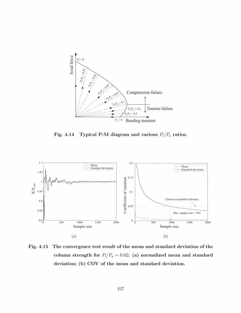
Bending moment
Ax
ial
forc
e
Pl = 0
Pl/
Pa =
0.0
1
Compression-failure
Tension-failure
P l/P a
= 0
.02
P l/P a
= 0
.05
P l/Pa = 0.07
P l/Pa = 0.1
Pl/Pa = 0.2
Pl/Pa = 0.3
Pa = 0
Fig. 4.14 Typical P-M diagram and various Pl/Pa ratios.
0 500 1000 1500 20000.8
0.85
0.9
0.95
1
1.05
1.1
X/X
2000
Sample size
MeanStandard deviation
(a)
0 500 1000 1500 20000
0.05
0.1
0.15
0.2
Sample size
Co
effi
cien
t o
f v
aria
tio
n
MeanStandard deviation
Chosen acceptable tolerance
Min. sample size = 954
(b)
Fig. 4.15 The convergence test result of the mean and standard deviation of the
column strength for Pl/Pa = 0.02: (a) normalized mean and standard
deviation; (b) COV of the mean and standard deviation.
107

4.4.3 Strength Variability
For generating P-M interaction diagrams, three different limit states (LS) in terms of the
strain of the concrete extreme fiber (εc,ext) are considered: (1) LS 1: εc,ext = 0.003, (2) LS 2:
εc,ext = 0.004, and (3) LS 3: εc,ext = 0.005. Figure 4.16 shows mean P-M interaction diagrams
for these three cases of LS. Axial forces and bending moments are normalized by the mean
pure axial capacity and the mean pure bending moment capacity, respectively, for LS 1. It
is noted that the P-M interaction diagram expands as LS increases. This is because while
the strength of unconfined concrete, where the extreme concrete fiber is located, decreases
as the strain increases from 0.003 to 0.005, the strength of confined concrete and reinforcing
bars increase as can be shown in Figures 4.3 and 4.4 when introducing the numerical values
of Table 4.1 for the KC specimen. To demonstrate the expansion and contraction of the P-M
interaction diagram, higher cases of LS are investigated. For example, Figure 4.17(a) clearly
0 0.2 0.4 0.6 0.8 1 1.20
0.2
0.4
0.6
0.8
1
Normalized bending moment
Norm
aliz
ed a
xia
l fo
rce
Limit state 1
Limit state 2
Limit state 3
Pl/
Pa
= 0
.01
P l/Pa =
0.05
Pl/Pa = 0.3
1.2
Fig. 4.16 Mean P-M interaction diagrams for different cases of LS.
108

shows changes of the deterministic P-M interaction diagrams depending on the adopted LS.
The base bending moment-tip displacement relationship shown in Figure 4.17(b) corresponds
to the deterministic P-M interaction diagrams shown in Figure 4.17(a) for Pl/Pa = 0.015
where the corresponding limiting points are marked.
0 400 800 12000
200
400
600
Bending moment, kip-in
Ax
ial
forc
e, k
ip
εc,ext = 0.003
Pl/P
a =
0.0
15
εc,ext = 0.009εc,ext = 0.015εc,ext = 0.020
(a)
0 1 2 30
50
100
150
200
250
300
350
400
Tip displacement, in.
Bas
e b
end
ing
mo
men
t, k
ip-i
n
εc,ext= 0.003εc,ext= 0.009
εc,ext= 0.020εc,ext= 0.015
(b)
Fig. 4.17 Changes of P-M interaction diagram; (a) Deterministic P-M interac-
tion diagrams for various cases of LS; (b) Base bending moment-tip
displacement relationship for Pl/Pa = 0.015.
COVs of column strength for different cases of LS are plotted in Figure 4.18. It is
observed that variability of the column strength is higher when Pl/Pa ≤ 0.01 and Pl/Pa ≥0.2. This result agrees with that of Mirza and MacGregor (1989) where they investigated the
strength variability of slender RC columns without considering spatial variability of random
variables. One can also observe that the COV increases as the LS increases. When only the
axial load is applied to the column, the strength variability of the column depends only on
the combination of variability of random fields. As the Pl/Pa ratio increases, the strength
variability begins to be dependent on the geometry of the cross section as well because the
curvature is introduced to the cross section due to the applied bending moment. Once the
curvature is introduced, the strains in fibers within the cross section become different from
109

0 0.05 0.1 0.15 0.2 0.25 0.30.03
0.04
0.05
0.06
0.07
CO
V
Limit state 1
Limit state 2
Limit state 3
Pl/Pa ratio
Fig. 4.18 COV of column strength for different cases of LS.
one fiber to the other. As Figure 4.12 shows, variability of stress changes as the strain
level does. This fact causes the changes of strength variability from one Pl/Pa ratio to the
other, and also from one LS to the other. These arguments are theoretically discussed in
Section A.2 of Appendix A.
The sensitivity of the column strength to an individual random field is investigated
for Fc, Fy, and Tc. The effect of each of these random fields is studied keeping all other
variables at their mean values. In this analysis, only three Pl/Pa ratios are considered,
namely 0.01, 0.05, and 0.3 spanning different failure modes from compression to tension as
shown in Figures 4.14 and 4.16. COVs of column strength for each sensitivity analysis are
summarized in Table 4.3. For the sensitivity of Fc, the variation of the column strength in
the compression-failure region (Pl/Pa = 0.01 and 0.05) is larger than that in the tension-
failure region. Conversely, for the sensitivity of Fy, it is obvious that the variation in the
tension-failure region is larger than that in the compression-failure region. The strength
variability due to variability of the cover thickness is not significant relative to the other
110

sources of variability.
Table 4.3 Sensitivity of the column strength in terms of COV (%).
Random field Fc Fy TcPl/Pa 0.01 0.05 0.3 0.01 0.05 0.3 0.01 0.05 0.3LS 1 3.7 3.4 2.4 2.1 1.1 3.9 0.8 0.2 0.1LS 2 3.3 3.4 2.4 2.7 2.4 5.1 1.4 0.8 0.5LS 3 3.0 3.3 2.3 2.7 2.3 5.5 1.8 1.5 0.7
4.4.4 The Effect of Spatial Variability
The effect of the spatial variability of Fc on the column strength is studied in this section.
For this purpose, the sensitivity analysis of Fc is conducted with and without considering
the spatial variability of Fc while keeping all other random variables at their mean values.
COVs of the column strength without spatial variability of Fc are significantly larger than
those considering spatial variability of Fc, as shown in Figure 4.19. This result justifies the
importance (to avoid overestimating COVs when spatial variability is ignored) of considering
spatial variability of random variables in the probabilistic evaluation of RC structures.
4.5 PROBABILISTIC EVALUATION OF STRUCTURAL COMPONENTS
OF AN RC FRAME
This section presents the probabilistic evaluation of typical structural components of a duc-
tile RC frame (referred to as VE), representing the structural system in the present study,
according to the methodology discussed in Section 2.6. A description of the VE frame is pre-
sented, followed by the presentation of a process of identifying typical structural components.
Probabilistic moment-curvature relationships of typical components of the VE frame are de-
veloped using the stochastic fiber element model and OpenSees. Finally, probabilistic shear
force-distortion relationships of these components are developed using Response 2000 (Bentz
2000), based on the modified compression field theory, and the FOSM method.
111

0 0.05 0.1 0.15 0.2 0.25 0.3
0.02
0.04
0.06
0.08
0.1
0.12
CO
V
Without spatial variability, dashed lines
With spatial variability, solid lines
o
+
x
εc,ext= 0.003εc,ext= 0.004εc,ext= 0.005
Pl/Pa ratio
Fig. 4.19 COVs of column strength with and without spatial variability of Fc.
4.5.1 Description of the Frame VE
The VE frame was experimentally tested by Vecchio and Emara (1992). It is a two-story,
one-bay RC frame which consists of beams and columns with rectangular cross sections, as
shown in Figure 4.20. It was designed with a center-to-center span of 137.8 inches (3,500
mm), a story height of 78.7 inches (2,000 mm) and an overall height of 181.1 inches (4,600
mm) including an integrally constructed large heavily reinforced concrete base beam. All
frame members were 11.8-inches (300 mm) wide by 15.7-inches (400 mm) deep and reinforced
with four No. 20M deformed bars on both sides of the cross section. The transverse steel
reinforcement consists of No. 10M deformed bars in the form of closed stirrups or ties spaced
at 4.9 inches (125 mm). Note that the nominal cross-sectional areas of No. 10M and No. 20M
bars are 0.166 in.2 (75 mm2) and 0.465 in.2 (300 mm2), respectively. The testing sequence
involved initial application of a total axial load of 157.5 kips (700 kN) to each column, which
was maintained through the test. The lateral load was then monotonically applied until
the ultimate capacity of the frame was achieved. The failure mechanism involved ductile
112

Fig. 4.20 Design details of the VE test frame (Vecchio and Emara 1992).
hinging at the ends of the beams and at the bases of the columns. The material properties of
concrete, and longitudinal and transverse reinforcing steel bars are listed in Table 4.4. The
same material properties are used for all beams and columns.
4.5.2 Typical Structural Components
According to the methodology proposed in the present study (cf. Section 2.6), a linear
elastic analysis of the VE frame is performed to obtain the bending moment, shear force,
and axial force diagrams. Following the procedure discussed in Section 2.6, force boundary
conditions of all six structural components (referred to as C1, C2, C3, C4, B1, and B2 as
shown in Figure 4.21(a)) are identified where the force boundary condition is defined by a
constant axial load (Pa), monotonic lateral load (Pl), and monotonic axial load (αPl) that
is proportional to Pl with the constant of proportionality α as shown in Figure 4.21(b).
Parameters defining force boundary conditions of all six components are listed in part (a) of
Table 4.5.
113

Table 4.4 Material properties of the VE test frame.
Property Nominal value(a) Concrete
Compressive strength 4,350 psi (30 MPa)(b) Longitudinal steel (No. 20M)
Yield strength 61 ksi (418 MPa)Ultimate strength 86 ksi (596 MPa)Modulus of elasticity 27,900 ksi (192 GPa)Strain at the onset of hardening 9.5 × 10⁻³
Modulus of strain hardening 450 ksi (3,100 MPa)Ultimate strain 0.07
(c) Transverse steel (No. 10M)Yield strength 66 ksi (454 MPa)Ultimate strength 93 ksi (640 MPa)
700 kN 700 kN
B2
B1
C1 C2
C3 C4Pl
Plat
αPl
Pa
Co
mp
on
ent
len
gth
Monitoring
sections
(a) Structural system model of VE (b) Structural component model
Fixed FixedFixed
Plat
Fig. 4.21 Identifying the typical structural components by a linear elastic anal-
ysis of the VE frame.
114

Table 4.5 Analysis parameters for structural components of the VE frame.
Component Pa (kips) αa Length (in.)(a) All six components
C1 157.5 -1.46 78.7C2 157.5 1.46 78.7C3 157.5 -0.63 78.7C4 157.5 0.63 78.7B1 0.0 0.0b 137.8B2 0.0 0.0b 137.8
(b) Typical componentsCN 157.5 1.0 78.7CS 157.5 -1.0 78.7BM 0.0 0.0 137.8
a Negative indicates tension.b Refer to Section 2.6.2.1 for approximation.
For simplicity, three typical components are identified by grouping components in
part (a) of Table 4.5 with similar boundary conditions and modifying analysis parameters.
Part (b) of Table 4.5 shows analysis parameters of the identified typical structural compo-
nents. CN represents north columns (C2 and C4) subjected to an incremental axial load in
compression with α = −1.0, an average of C2 and C4. On the other hand, CS represents
south columns (C1 and C3) subjected to an incremental axial load in tension with α = 1.0,
an average of C1 and C3. BM represents beam components (B1 and B2) without any applied
axial load.
4.5.3 Random Fields
Random fields of the VE frame are defined based on design parameters as given in Table 4.4
and summarized in Table 4.6. Assumed statistical data related to these random fields are
mainly adopted from various literatures as discussed in Section 2.5 due to the lack of data
specifically related to the variability of the structural properties of the VE frame. It should
be noted that properties of some random fields, e.g., initial modulus of elasticity of concrete,
are derived from those of another random fields, e.g., compressive strength of concrete.
115

Table 4.6 Probability distributions of basic random variables.
Uncertain source Distribution Mean COV (%)(a) Concrete
Compressive strengtha Normal 4,036 psi 15Initial modulus of elasticityb Normal 3,984 ksic 8
(b) Longitudinal reinforcing steelYield strengthd Lognormal 60.61 ksi 9Ultimate strengthe Lognormal 86.42 ksi 9Young’s modulus Normal 27,900 ksi 3.3Fracture strainf Normal 0.07 20
(c) Transverse reinforcing steelYield strengthd Lognormal 65.83 ksi 9Ultimate strengthe Lognormal 93.86 ksi 9Young’s modulus Normal 27,900 ksi 3.3Fracture strainf Normal 0.07 20Correlation coefficient of a and b, d and f , and e and f are
0.8, -0.5, and -0.55, respectively (cf. Sections 2.5.2.1 and 2.5.2.2).c Computed by (2.3) given in Section 2.5.2.1.
Uncertainty in concrete cover thickness is ignored, assuming that its effect on moment-
curvature relationships at critical cross sections of the VE frame’s components is negligible
according to one of the observations in Section 4.4.3. As discussed in Section 4.4.1, non-
positive samples of a normal random variable are rejected to avoid an unrealistic realization
in Monte Carlo simulation. However, the sample rejection rarely occurs in the actual analysis
of this study due to the specific values of means and standard deviations. Thus, the distortion
of the sample distributions can be ignored.
4.5.4 Probabilistic Moment-Curvature Relationship
A series of pushover analysis is performed to develop probabilistic moment-curvature re-
lationships at critical cross sections of each typical structural component using OpenSees
(McKenna and Fenves 2001) and the stochastic fiber element model described in Section 4.3.
OpenSees has its own reliability toolbox that is mainly aimed at estimating the failure
probability of a structure for a given limit-state function, rather than EDP statistics. Con-
116

sequently, the stochastic fiber element model developed in this study is used to generate
OpenSees inputs for Monte Carlo simulation considering various random fields to estimate
EDP statistics.
4.5.4.1 Modeling Assumptions
Random fields of concrete properties along the length of a component are modeled by four
random field elements. Within the cross section, random fields are described by sixteen
identical rectangular patches (each side of the cross section is divided into four). The scale
parameters θz and θp, refer to (4.60), are taken as the length of one random field element
and the length of the long side of the cross section (15.7 in.), respectively. For each of the
random fields of steel properties, one random variable is used along the length of the column,
while within the cross section, different random variables are used for different reinforcing
bars. It is assumed that ρS = 0.8, refer to (4.61), for random fields of steel properties.
To model a typical component, four nonlinearBeamColumn elements are used along
the length of the component. Since nonlinearBeamColumn is formulated by a flexibility
method (refer to Section 4.2), only one element is sufficient to capture the nonlinear response
of the typical component given force boundary conditions. However, the finite element mesh
is dictated by the random field mesh for concrete properties in this case.
Among many constitutive models in OpenSees material library, Steel01 is used for
the reinforcement. As for the concrete, Concrete01 material model based on the modified
Kent-Park stress-strain relationship (Scott et al. 1982) is used for both confined and uncon-
fined concrete fibers (with zero tensile strength). Refer to Section 3.3.2.2 for descriptions of
these material models of OpenSees.
4.5.4.2 Probabilistic Moment-Curvature Relationship
Moment-curvature relationships at two critical cross sections (both ends of the component as
shown in Figure 4.21(b)) are monitored during the pushover analysis. For each component,
117

Monte Carlo simulation is performed with the sample size of 1500 to obtain a set of 1500
moment-curvature curves at each critical cross section. Each of the 1500 moment-curvature
curves at the cross section close to the fixed base in Figure 4.21(b) (referred to as Cross
section 1, while the cross section at the other end of the typical component is referred to as
Cross section 2) are idealized as a trilinear moment-curvature relationship according to the
procedure described in Section 2.6.2.3.
A convergence test with respect to the sample size of Monte Carlo simulation is
necessary to guarantee the accuracy of the estimated quantity as discussed in Section 4.4.2.
Figure 4.22 shows the result of a convergence test of the means and the standard deviations
of the six moment-curvature parameters of the CS typical component; refer to part (b) of
Table 4.5. It is evident that the sample size of 1500 is large enough to satisfy the selected
tolerance of convergence, namely a COV of 5%. The convergence test is conducted for
all parameters of CN and BM, and the selected sample size of 1500 is determined to be
satisfactory.
Figure 4.23 shows the means of the idealized moment-curvature relationships of the
three typical components of the VE frame. CN shows softening behaviors in the moment-
curvature relationship, while BM and CS show hardening behavior in an average sense.
Generated moment-curvature relationships of BM by Monte Carlo simulation are idealized
by bilinear relationships because no distinctive peak points are observed. Therefore, the
means and standard deviations of only four, instead of six for CN and CS, parameters,
namely My, Mu, ϕy, and ϕu (cf. Section 2.6.2.3) are estimated for BM. It is noted that
definitions of the four parameters remain unchanged.
Estimated means, standard deviations, and correlation coefficients of the moment-
curvature parameters for the three typical components of the VE frame are listed in Table 4.7.
It is observed that uncertainties related to the yielding point are smaller than those related
to the peak or the ultimate points. This can be explained by the fact that uncertainties
in the yielding point are only strongly related to the uncertainty in the yield strength of
118

0 500 1000 1500 0 500 1000 1500
0.4
0.6
0.8
1
1.2
1.4
0
0.1
0.2
0.3
0.4
0.5
Sample sizeSample size
CO
VX
/X1500
SDs of parametersMeans of parameters
Chosen convergence tolerance
Fig. 4.22 Convergence test of the means and standard deviations of the six
moment-curvature parameters of CS typical component of the VE
frame.
reinforcing steel. On the contrary, uncertainties of the peak and the ultimate points are
related to all sources of uncertainties. It is also observed that COVs of curvature parameters
(ϕy, ϕp, and ϕu) are larger than those of moment parameters (My, Mp, and Mu). This is an
expected observation because deformation uncertainty is often larger than force uncertainty
according to the stress-strain behavior. For example, uncertainty in the strain corresponding
to the compressive strength of concrete is related to both uncertainties of the compressive
strength and the initial modulus of elasticity of concrete (cf. Table 4.6), and it also affects
uncertainty in the ultimate strain of concrete as shown in Figure 4.3.
From correlation matrices in Table 4.7, one can notice that only negative correlation
coefficients are those related to ϕu. This is mostly due to the assigned correlation coefficient
to random variables representing yield strength, ultimate strength, and fracture strain of
longitudinal reinforcing steel as given in Table 4.6.
119
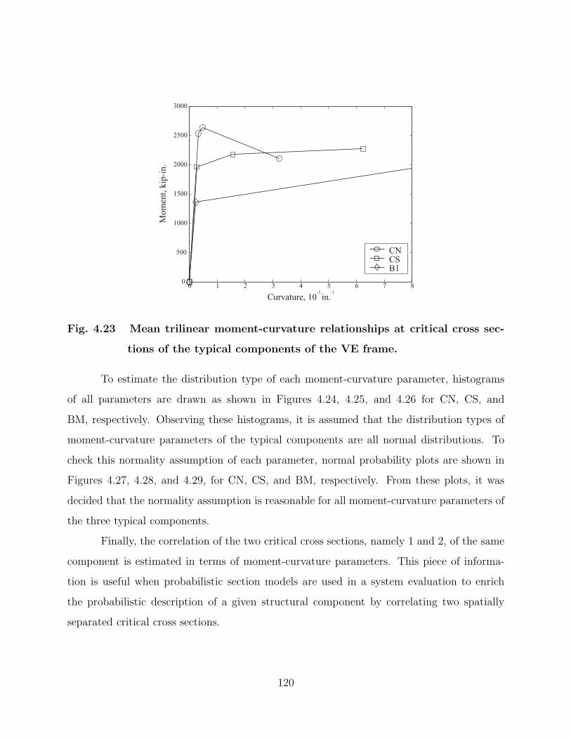
0 1 2 3 4 5 6 7 80
500
1000
1500
2000
2500
3000
Curvature, 10-3
in.-1
Mom
ent,
kip
-in.
CNCSB1
Fig. 4.23 Mean trilinear moment-curvature relationships at critical cross sec-
tions of the typical components of the VE frame.
To estimate the distribution type of each moment-curvature parameter, histograms
of all parameters are drawn as shown in Figures 4.24, 4.25, and 4.26 for CN, CS, and
BM, respectively. Observing these histograms, it is assumed that the distribution types of
moment-curvature parameters of the typical components are all normal distributions. To
check this normality assumption of each parameter, normal probability plots are shown in
Figures 4.27, 4.28, and 4.29, for CN, CS, and BM, respectively. From these plots, it was
decided that the normality assumption is reasonable for all moment-curvature parameters of
the three typical components.
Finally, the correlation of the two critical cross sections, namely 1 and 2, of the same
component is estimated in terms of moment-curvature parameters. This piece of informa-
tion is useful when probabilistic section models are used in a system evaluation to enrich
the probabilistic description of a given structural component by correlating two spatially
separated critical cross sections.
120

Table 4.7 Estimates of means, standard deviations, and correlation coefficient
matrices of moment-curvature parameters for typical components of
the VE frame.Correlation coefficients
Parameter Mean SD COVMy Mp Mu ϕy ϕp ϕu
(a) CNMy 2536 132 5.2% 1Mp 2638 143 5.4% 0.92 1Mu 2107 173 8.2% 0.77 0.85 1ϕy 0.317 0.031 9.9% 0.62 0.36 0.27 1ϕp 0.474 0.071 14.9% 0.44 0.60 0.54 0.13 1ϕu 3.233 0.436 13.5% -0.30 -0.24 -0.18 -0.31 -0.04 1
(b) CSMy 1964 102 5.2% 1Mp 2176 125 5.7% 0.92 1Mu 2274 183 8.1% 0.78 0.88 1ϕy 0.263 0.022 8.5% 0.87 0.69 0.60 1ϕp 1.562 0.310 19.8% 0.30 0.51 0.40 0.00 1ϕu 6.237 0.748 12.0% -0.18 -0.25 -0.22 -0.19 -0.17 1
(c) BMMy 1360 112 8.2% 1 - -Mu 2320 190 8.2% 0.73 - 1 -ϕy 0.234 0.023 9.7% 0.91 - 0.63 1 -ϕu 12.964 2.379 18.3% -0.43 - -0.45 -0.37 - 1
Note: moment in kip-in. and curvature in 10−3/in. for means and SDs.
121

2000 2500 30000
0.05
0.1
0.15
0.2
2000 3000 40000
0.05
0.1
0.15
0.2
1000 2000 30000
0.1
0.2
0.3
0.4
0.0002 0.00050
0.05
0.1
0.15
0.2
0.25
0 0.0005 0.001
0
0.05
0.1
0.15
0.2
0.002 0.0050
0.1
0.2
ϕy, in.-1
Fre
quen
cyF
requen
cy
My, kip-in. Mp, kip-in. Mu, kip-in.
ϕp, in.-1
ϕu, in.-1
Fig. 4.24 Histograms of moment-curvature parameters for CN typical compo-
nent of the VE frame.
1500 2000 25000
0.05
0.1
0.15
0.2
1000 2000 30000
0.05
0.1
0.15
0.2
0 2000 40000
0.1
0.2
0.3
0.4
0.0002 0.00040
0.05
0.1
0.15
0.2
0 0.002 0.004
0
0.05
0.1
0.15
0.2
0.004 0.006 0.008
0
0.05
0.1
0.15
0.2
0.25
ϕy, in.-1
Fre
quen
cyF
requen
cy
My, kip-in. Mp, kip-in. Mu, kip-in.
ϕp, in.-1
ϕu, in.-1
Fig. 4.25 Histograms of moment-curvature parameters for CS typical compo-
nent of the VE frame.
122

500 1000 1500 20000
0.05
0.1
0.15
0.2
1500 2000 2500 3000 35000
0.05
0.1
0.15
0.2
0.25
1.5 2 2.5 3 3.50
0.05
0.1
0.15
0.2
0.005 0.01 0.015 0.02 0.0250
0.05
0.1
0.15
0.2
ϕy, 10-4
in.-1
Fre
quen
cyF
requen
cy
ϕu, in.-1
My, kip-in. Mu, kip-in.
Fig. 4.26 Histograms of moment-curvature parameters for BM typical compo-
nent of the VE frame.
2200 2400 2600 2800 3000 2400 2600 2800 3000
0.001
0.01
0.05
0.25
0.50
0.75
0.95
0.99
0.999
1500 2000 2500
0.001
0.01
0.05
0.25
0.50
0.75
0.95
0.99
0.999
2.5 3 3.5 4 4.5 4 6 8
0.001
0.01
0.05
0.25
0.50
0.75
0.95
0.99
0.999
2.5 3 3.5 4
0.001
0.01
0.05
0.25
0.50
0.75
0.95
0.99
0.999
ϕy, 10-4
in.-1
Pro
bab
ilit
y
0.001
0.01
0.05
0.25
0.50
0.75
0.95
0.99
0.999
0.001
0.01
0.05
0.25
0.50
0.75
0.95
0.99
0.999
Pro
bab
ilit
y
My, kip-in. Mp, kip-in. Mu, kip-in.
ϕp, 10-4
in.-1
ϕu, 10-3
in.-1
Fig. 4.27 The normality check of the moment-curvature parameters of CN
typical component of the VE frame.
123

1800 2000 2200 2000 2200 2400 2600 1500 2000 2500 3000
2 2.5 3 1 1.5 2 2.5 5 6 7
0.001
0.01
0.05
0.25
0.50
0.75
0.95
0.99
0.999
0.001
0.01
0.05
0.25
0.50
0.75
0.95
0.99
0.999
0.001
0.01
0.05
0.25
0.50
0.75
0.95
0.99
0.999
0.001
0.01
0.05
0.25
0.50
0.75
0.95
0.99
0.999
ϕy, 10-4
in.-1
Pro
bab
ilit
y
0.001
0.01
0.05
0.25
0.50
0.75
0.95
0.99
0.999
0.001
0.01
0.05
0.25
0.50
0.75
0.95
0.99
0.999
Pro
bab
ilit
y
My, kip-in. Mp, kip-in. Mu, kip-in.
ϕp, 10-3
in.-1
ϕu, 10-3
in.-1
Fig. 4.28 The normality check of the moment-curvature parameters of CS
typical component of the VE frame.
1000 1200 1400 1600 1500 2000 2500 3000
0.0002 0.00025 0.0003 0.01 0.015 0.02
0.001
0.01
0.05
0.25
0.50
0.75
0.95
0.99
0.999
0.001
0.01
0.05
0.25
0.50
0.75
0.95
0.99
0.999
0.001
0.01
0.05
0.25
0.50
0.75
0.95
0.99
0.999
0.001
0.01
0.05
0.25
0.50
0.75
0.95
0.99
0.999
ϕy, in.-1
Pro
bab
ilit
yP
robab
ilit
y
ϕu, in.-1
My, kip-in. Mu, kip-in.
Fig. 4.29 The normality check of the moment-curvature parameters of BM
typical component of the VE frame.
124

Table 4.8 shows the correlation coefficient matrices of the two end cross sections for
CN, CS, and BM typical components of the VE frame. Overall trends of CN, CS, and BM
are almost the same. For example, three moment parameters, namely My, Mp, and Mu
are strongly correlated to each other with the mean correlation coefficient = 0.75, involving
all 22 (9 for CN, 9 for CS, and 4 for BM) correlation coefficients related to these three
moment parameters for CN, CS, and BM. Correlation coefficients related to ϕu are almost
all negative. As discussed earlier in this section, this negative correlation is attributed to the
assigned correlation coefficients to random variables representing yield strength, ultimate
strength, and fracture strain of the longitudinal steel.
Table 4.8 Estimates of correlation coefficient matrices of moment-curvature
parameters at different cross sections for typical components of the
VE frame.Cross section 2
Cross section 1My Mp Mu ϕy ϕp ϕu
(a) CNMy 0.79 0.80 0.65 0.69 0.41 -0.16Mp 0.71 0.75 0.56 0.59 0.43 -0.19Mu 0.62 0.63 0.47 0.55 0.34 -0.28ϕy 0.62 0.57 0.58 0.63 0.26 0.01ϕp 0.42 0.49 0.32 0.34 0.45 -0.15ϕu -0.38 -0.41 -0.55 -0.32 -0.22 -0.11
(b) CSMy 0.87 0.86 0.75 0.77 0.34 0.19Mp 0.82 0.84 0.79 0.72 0.31 0.09Mu 0.77 0.82 0.79 0.67 0.26 -0.05ϕy 0.75 0.74 0.65 0.75 0.30 0.13ϕp 0.23 0.19 0.16 0.21 0.07 -0.02ϕu -0.21 -0.37 -0.48 -0.19 -0.15 0.17
(c) BMMy 0.85 - 0.75 0.78 - -0.35Mu 0.75 - 0.77 0.65 - -0.58ϕy 0.78 - 0.65 0.72 - -0.32ϕu -0.39 - -0.69 -0.34 - 0.67
125

4.5.5 Probabilistic Shear Force-Distortion Relationship
Similar to the moment-curvature relationship, probabilistic shear force-distortion relation-
ships at critical cross sections of the typical components of the VE frame are developed
considering uncertainties in structural properties as given in Table 4.6. To compute the
shear force-distortion relationship at a given critical cross section, Response 2000 (Bentz
2000), software based on the modified compression field theory (Vecchio and Collins 1986),
is used. Since Response 2000 is only for a deterministic computation, Monte Carlo simu-
lation is not appropriate for developing a probabilistic shear force-distortion relationship.
Instead, it is decided to use the FOSM method (cf. Section 3.2.1) to estimate uncertainties
in the shear force-distortion relationship.
The mean shear force-distortion relationships of all typical structural components of
the VE frame are shown in Figure 4.30. It is to be noted that the incremental axial load
(αPl as given in Table 4.5) is not considered due to the capability of Response 2000, while
the constant axial load is considered. Consequently, CN and CS are identical in terms of the
shear force-distortion relationship.
Estimated means and standard deviations of shear force-distortion parameters for the
three typical components of the VE frames are given in Table 4.9. Similar to the observation
of moment-curvature COVs, force parameters are less sensitive to basic uncertainties than
deformation parameters. As previously mentioned, this can be attributed to the fact that
the deformation uncertainty is often larger than the force uncertainty at the stress-strain
level.
Compared to statistical data for the moment-curvature relationship provided in Sec-
tion 4.5.4.2, those for the shear force-distortion relationship presented in this section lack
sufficient information. For example, estimations of distribution types and correlations of
shear force-distortion parameters are not provided. This is attributed to the fact that the
FOSM method estimates only the mean and the standard deviation of the output as dis-
cussed in Section 3.2.1, while Monte Carlo simulation, used to estimate moment-curvature
126

0 2 4 6 8 10 12 14 16 18 200
20
40
60
80
100
120
Shear distortion, 10-3
Sh
ear
forc
e, k
ipCN or CS of VE
BM of VE
Fig. 4.30 Mean shear force-distortion relationships of typical structural com-
ponents of the VE frame.
parameters in Section 4.5.4.2, provides the basis of estimating all parameters of the prob-
ability distribution of the output. In Chapter 5, probabilistic section models developed in
this section will be used in estimating EDP sensitivity of the VE frame using the FOSM
method. It should be noted that all shear force-distortion parameters will be arbitrarily
assumed to be uncorrelated due to lack of information. However, the focus of Chapter 5 is
on the demonstration of the methodology of propagating basic uncertainties to structural
systems.
4.6 CONCLUDING REMARKS
The propagation of basic uncertainties to the capacity of structural components is investi-
gated in this chapter. An effort is made to consider the effect of basic uncertainties including
127

Table 4.9 Estimates of means and standard deviations of shear force-distortion
parameters for typical components of the VE frame.
(a) CN and CS (b) BMParameter
Mean SD COV Mean SD COVVc 55.9 2.29 4.1% 29.2 0.93 3.2%Vp 105.5 5.47 5.2% 98.1 5.70 5.8%Vu 99.9 3.06 3.1% 65.3 7.84 12.0%γc 0.318 0.037 11.6% 0.187 0.038 20.6%γp 4.514 0.292 6.5% 8.417 0.547 6.5%γu 9.177 0.616 6.7% 15.161 1.802 11.9%
Note: shear force in kip and distortion in 10−3.
their spatial variability and the nonlinear behavior of RC members in the most accurate and
realistic way to the possible extent. For this, a computational tool for probabilistic evalu-
ation of RC structural components is developed using stochastic fiber element formulation.
This formulation accounts for the spatial variability of material and geometrical properties of
RC components using Monte Carlo simulation. In this stochastic fiber element formulation,
conventional fiber element model and the midpoint method for representing random fields
are combined. Assumptions and formulations of the fiber element model adopted in this
study are described. The verification examples show that the deterministic capability of the
developed program for estimating structural behaviors of different experimental studies.
A probabilistic strength analysis of a RC column subjected to combined axial load
(Pa) and lateral load (Pl) is conducted in terms of the axial load-bending moment (P-M)
interaction. For generating P-M interaction diagrams, different limit states in terms of the
strain of the concrete at the extreme fiber (εc,ext) are considered. The coefficient of variation
of column strength ranges from 3.7% to 7.2% depending on the limit state and the Pl/Pa
ratio. Variability of the column strength is higher when Pl/Pa ≤ 0.01 and Pl/Pa ≥ 0.2.
Variability increases as εc,ext increases except for the compression-failure region where change
of variability with the Pl/Pa ratio is insignificant.
According to sensitivity analyses, the variation of the compressive strength of concrete
128

controls the variation of the column strength in the compression-failure region, while the
variation of the steel strength controls that in the tension-failure region. The importance of
considering spatial variability of a random variable is also investigated. It is observed that
neglecting the spatial variability of concrete strength can lead to overestimating the strength
variation of a RC component.
Due to the computational demand, the use of the stochastic fiber element method
using Monte Carlo simulation is practically limited to RC structural components. An exam-
ple of a probabilistic evaluation of a RC structural system using the developed probabilistic
P-M interaction diagram will be presented in Chapter 5.
The typical structural components of a ductile case study RC frame (referred to
as VE) are identified and evaluated to develop their probabilistic section models. This is
conducted as a demonstration of the first phase, namely the component evaluation phase, of
the systematic procedure of evaluating a structural system as discussed in Section 2.6.1.
The typical structural components of the VE frame are evaluated using the stochas-
tic fiber element model and OpenSees software to develop probabilistic moment-curvature
relationships at critical cross sections of the typical components. On the other hands, prob-
abilistic shear force-distortion relationships at critical cross sections of the typical compo-
nents are developed using the FOSM method and software Response 2000. Each of the
moment-curvature and shear force-distortion relationships are idealized by either a trilinear
relationship defined by six parameters (three force and three deformation parameters) or
a bilinear curve defined by four parameters (two force and two deformation parameters).
Therefore, each of the probabilistic component models is defined by means, standard devi-
ations, and correlation coefficient matrices of these parameters. These probabilistic section
models will be used in estimating EDP sensitivity of the VE frame using the FOSM method
in Chapter 5.
Normal distributions can be assumed for all parameters defining a multilinear moment-
curvature relationship. Variability of curvature parameters at the critical cross section of
129

RC structural components is larger than those of moment parameters because deformation
uncertainty is often larger than force uncertainty according to the stress-strain behavior.
130

5 EDP Sensitivity Induced by Component
Uncertainty
5.1 INTRODUCTION
Identifying critical structural components to a specific EDP of the structural system is an
important component of a PBEE methodology. This identification provides an insight of
how the structural system behaves under the seismic loading in terms of a specific EDP.
The quantification of the importance of structural components should consider the location
of each individual component in the system, the stiffness contribution of each component,
and the probabilistic distribution of the strength and deformation capacities of each struc-
tural component. This identification can be also useful for the decision-making process, in
particular, for the rehabilitation of an existing structure within the framework of the PBEE.
In spite of a large number of publications on the probabilistic evaluation of struc-
tural systems (Baker and Cornell 2003; Chryssanthopoulos et al. 2000; Ghobarah and Aly
1998; Singhal and Kiremidjian 1996), the effort of assessing the importance of structural
components on the system performance is very rare. Gharaibeh et al. (2002) studied the
relative importance of structural members using reliability methods. They used the conven-
tional system reliability formulation for the mixed series-parallel system where the system
reliability is an explicit function of a set of known component reliability corresponding to
a specified limit-state function that distinguishes the failure and safety of the component.
Due to this failure-or-not nature of the description of components, the conventional system
131

reliability method can only be applicable to few types of structures, e.g., truss structures. In
addition, the conventional system reliability method requires the identification of all possible
cutsets1. However, this process tends to be very difficult when the static indeterminacy of
the structure is high or the number of structural components is large, because the number
of cutsets is large in any of these cases.
In this chapter, the propagation of uncertainty in the strength and deformation capac-
ities of structural components to their structural system with respect to its EDP is investi-
gated. First, a probabilistic strength analysis of a portal frame is performed to demonstrate
an application of probabilistic component models to the system evaluation. Then, EDP
sensitivity to individual components of the VE frame discussed in Chapter 4 is estimated
using the FOSM method. EDP uncertainty induced by uncertainty in each structural com-
ponent is used to identify significant structural components of these case study frames for
a specific EDP. The significance of a structural component is defined in terms of the EDP
sensitivity where a more significant component corresponds to a higher EDP sensitivity for
this particular component.
5.2 PORTAL FRAME APPLICATION
The example presented in this section shows an application of using the stochastic fiber
element method (cf. Section 4.3) to evaluate a RC structural system. Rather than selecting
a real structural system, a relatively simple one is chosen to demonstrate the methodology.
The same approach can be easily extended to more complex structures.
Consider a portal frame consisting of an elastic beam and two inelastic circular
columns subjected to two gravity loads (N) and a lateral load (H) as shown in Figure 5.1(a).
In this application, the statistics of the failure lateral load (Hf in Figure 5.1(b)) for fixed
gravity loads is determined. It is assumed that the design of the two columns is identical to
1Cutset is a mixed series-parallel sub-system that is defined such that the system fails when any of thecutsets occurs.
132

h = 60"
L = 90"
NH
N NH
f
N
(a) (b)
Elastic beam
KC1 KC
2Plastic hinge
Fig. 5.1 A portal frame subjected to fixed gravity loads and an increasing lateral
load; (a) Configurations of the frame; (b) Failure mechanism.
that of the KC specimen in Section 4.4.
The columns are modeled using lumped plasticity with the expected failure mecha-
nism consisting of plastic hinges located at the tops of the columns as shown in Figure 5.1(b).
The behavior of each plastic hinge is controlled by the predefined probabilistic P-M curve,
i.e., the plastic hinge forms when the axial force and bending moment pair at the section is
on the P-M curve.
Various levels of gravity load are considered ranging from N = 0 to N = 400 kips.
For each level of gravity load, the lateral load H is incrementally increased until the first
plastic hinge forms at one of the two critical sections (Figure 5.1(b)) and axial forces in the
two columns are computed. The bending moment at this first plastic hinge is obtained such
that the bending moment and axial force pair is located on the P-M curve. Subsequently,
the bending moment at the other critical section is computed to satisfy equilibrium. This
process is continued with increasing H until the second plastic hinge forms and a failure
mechanism (corresponding to failure load Hf) is obtained.
133

5.2.1 Uncertainty in the Strength of the Portal Frame
Using Monte Carlo simulation, 4000 samples of P-M curves are generated for each column
and the procedure described in the previous section is repeated for each P-M curve. It should
be noted that P-M random curves for these two columns are assumed to be uncorrelated.
El-Tawil and Deierlein (2001) suggested an expression of P-M curve for RC columns where
the bending moment capacity M corresponding to the axial force P at a section is obtained
by
M = Mb
1 −(
δP
∆P
)a
(5.1)
where Mb is the balanced bending moment, δP = |P − Pb|, and ∆P = Pc − Pb if P ≥ Pb
and ∆P = Pb − Pt if P < Pb. Strength parameters Pb, Pc, and Pt are the balanced axial
force, crushing strength, and tensile strength, respectively. Parameter a controls the shape
of the curve and is determined by calibration. In this study, it is determined that a = 1.8
for P ≥ Pb and, a = 1.9 for P < Pb for the mean P-M curve of LS 3 (corresponding to
εc,ext = 0.005) in Section 4.4. Pc, Pb, Pt, and Mb are selected as random variables, and their
statistical properties (mean, COV, and correlation coefficient) are obtained from the results
of Section 4.4 as listed in Table 5.1. Figure 5.2 shows the mean P-M curve of LS 3 and
the calibrated one where the top bar of a symbol indicates the mean of the random variable
represented by this symbol.
Table 5.1 Statistical properties of random variables for the P-M relationship.
Correlation coefficientParameter Dist’n Mean COV
Pc Pb Pt Mb
Pc Normal 507 kips 5.0% 1.0 0.7 -0.04 0.7Pb Normal 115 kips 5.0% 1.0 -0.03 0.9Pt Normal -220 kips 5.0% 1.0 -0.03Mb Normal 955 kip-in 5.0% Symmetric 1.0
Figure 5.3(a) shows the mean values of Hf (solid line) at different gravity load levels
(N). In this figure, Hf is normalized by the shear capacity of the two columns, i.e., 2Vn
where Vn is the nominal shear capacity of the circular column section (estimated according
134

Bending moment
Ax
ial
forc
e
Simulation
FittedP
c
Pt
Pb
Mb
0
Fig. 5.2 Calibration of the analytical P-M curve to the mean P-M curve of
LS 3.
to ACI 318-02 (2002) as 42.3 kips), and N is normalized by Pc. It is obvious that the mean
values of Hf are far below the shear capacity of the frame, which verifies the assumed failure
mechanism. Accordingly, Hf is determined by the bending moment capacity of sections,
and the shape of the N -Hf interaction curve is similar to that of P-M interaction curve
as shown in Figure 5.3(a). Moreover, figure 5.3(a) shows the mean±2 standard deviation
curves (dashed lines) to show the dispersion of Hf/2Vn. Figure 5.3(b) shows COV of Hf
(solid line labeled as “Total”). Note that the other two curves labeled KC1 and KC2 are
explained in the next section. From this figure, one observes that the variability of Hf
increases as N increases for N/Pc > 0.1. In other words, Hf is more sensitive to uncertainty
of structural properties when the gravity load level is high. This is because Hf depends only
on the bending moment capacity of the sections, and the variability of the bending moment
capacity is high when the axial load level is high. This can be shown from (5.1) by taking
the variance of M numerically.
135

0.1 0.15 0.2 0.25 0.3 0.35 0.4 0.450
0.1
0.2
0.3
0.4
0.5
0.6
0.7
0.8
Hf /2Vn
N/P
c
Mean
Mean+2SD_
(a)
0 1 2 3 4 50
0.1
0.2
0.3
0.4
0.5
0.6
0.7
0.8
Total
KC1
KC2
COV (%) of Hf
N/P
c(b)
Fig. 5.3 Statistics of Hf/2Vn; (a) Mean and Mean±2 standard deviation; (b)
COV due to uncertainty in KC1 (dashed line), in KC2 (dotted line), or
in both of them (solid line).
5.2.2 Relative Significance of Columns
The sensitivity of Hf to the strength uncertainty of an individual column is estimated. When
KC1 is considered as the column with uncertain strength, KC2 is considered as deterministic
whose P-M curve is described as the mean P-M curve, and vice versa. The dashed line
and the dotted line in Figure 5.3(b) show variability of Hf (in terms of COV) induced by
uncertainty in the strength of KC1 and KC2, respectively. The contributions of each column
to Hf variability are different from one to another and they vary depending on the applied
level of axial load. The contribution of KC2 to Hf variability is larger than that of KC1
when N/Pc > 0.1. In other words, KC2 is more significant to Hf variability than KC1
when N/Pc > 0.1. However, the difference in the relative significance of these two columns
decreases as N/Pc increases and one can ignore the difference in the relative significance of
the two columns for N/Pc > 0.7.
136

5.3 DUCTILE RC FRAME: VE
The method of evaluating the propagation of uncertainty in the strength and deformation
capacities of structural components to the structural system and identifying significant struc-
tural components with respect to EDP is demonstrated using a ductile RC frame, VE, as
introduced in Section 4.5. The FOSM method is used to estimate the mean and standard
deviation of an EDP due to the given uncertainty in the capacity of each typical structural
component. Uncertainty in the capacity of the structural component is described by the
probabilistic moment-curvature relationship or the probabilistic shear force-distortion rela-
tionship as discussed in Sections 4.5.4 and 4.5.5, respectively. COV is used as a measure
of sensitivity of EDP to individual structural components. A structural component with
larger corresponding COV of EDP is considered as more significant than that with smaller
corresponding COV of EDP. The peak absolute floor acceleration (PFA), the peak absolute
floor displacement (PFD), and the peak inter-story drift ratio (IDR) are selected as EDPs in
this study because they are commonly used EDPs of structures in earthquake engineering.
5.3.1 Structural Modeling
The description of the VE frame is presented in Section 4.5.1 including material properties,
dimensions, and reinforcement of beams and columns. The 2D computational model of the
VE frame is developed using OpenSees as illustrated in Figure 5.4.
5.3.1.1 Element Type
All structural components in the VE frame are modeled by a plastic hinge model (referred
to as beamWithHinges element in the OpenSees element library). Figure 5.5 illustrates
the configuration of the beamWithHinges element. Each element has two nodes with two
translations and one rotation per node. The beamWithHinges element consists of one elastic
beam and two plastic hinge regions at both ends of the elastic beam as shown in Figure 5.5.
137

6
3
1 2
4 5
Fixed Fixed
1 2
3 4
5 6
Element
Node
S11
S12
S21
S22
S41
S51
S42
S52
S61
S62
S31
S32
Sij
Section j of element i
Level 2
Level 1
Fig. 5.4 The OpenSees model of the VE frame.
Each plastic hinge region has one monitoring section whose behavior is dictated by the
assigned moment-curvature relationship and/or shear force-distortion relationship to capture
a possible nonlinear behavior of the section and eventually a nonlinear behavior of the
element. The monitoring section is located at the center of the plastic hinge region for
performing the required numerical integration along the length of the plastic hinge region.
The lengths of the two plastic hinge regions (hi and hj in Figure 5.5) are not necessarily
identical. According to the evaluation of the components of the VE frame using the fiber
element model (cf. Section 4.5.4.2), it is decided that 1/8 of the total element length is used
as the plastic hinge length on each side of the element. They are 62% and 110% of the
depth of the cross section (15.7 inches), respectively, for the column and the beam. It should
be noted that the plastic hinge length is not considered as a random variable in this study
because modeling uncertainty is not within the scope of this study. Certainly, this plastic
hinge length is an important candidate to address modeling uncertainty in a future study.
138

Elastic beam
Element length
hi
hj
Node i Node j
M M
ϕ ϕ
V
γ
V
γ
Fig. 5.5 Plastic hinge model in OpenSees.
5.3.1.2 Mass and Viscous Damping
Mass is derived from the applied gravity loads for the pushover test and lumped at each node.
Accordingly, 203 lb of mass is assigned to each node in each translational direction. The
damping characteristics of the VE frame are modeled using mass and stiffness proportional
damping with 5% of the critical damping for the first two models of vibration. The periods
of these two modes estimated from the eigen solution using the initial elastic stiffness matrix
are 0.55 and 0.15 seconds.
5.3.1.3 Solution Strategy
The Newmark β-method with typical coefficients γ = 0.50 and β = 0.25 is used as the time
integrator. A half the ground motion time discretization is used for the analysis time step.
Nonlinear equilibrium equations are solved using the modified Newton-Raphson solution
algorithm.
5.3.2 Ground Motions
It is assumed that the VE frame is located at the same site as the UCS building, the case
study building in Chapter 3. This assumption is made for convenience because the seismic
139

hazard curve and a set of ground motion profiles are readily available. The seismic hazard
curves for the fundamental period (T1) of 0.3 and 0.5 seconds, provided by Frankel and
Leyendecker (2001), are used to obtain the seismic hazard curve for T1 = 0.55 second for
the VE frame. Figure 5.6 shows the seismic hazard curve for the VE frame in terms of the
mean annual exceedance frequency of a specified spectral acceleration Sa. Assuming the
Poisson occurrence of an earthquake and lognormal distribution of the random variable Sa
denoting uncertainty in Sa, the mean and the standard deviation of Sa are estimated as 0.54g
and 0.50g (COV=93%). The seismic hazard curve derived from the assumed distribution of
Sa fits well with the seismic hazard curve given by Frankel and Leyendecker, as shown in
Figure 5.6.
10-3
10 -2
10 -1
100
10110
-5
10 -4
10 -3
10 -2
10 -1
100
Annual
exce
edan
ce f
requen
cy (
λ),
yr-1
Sa, g
VE Hazard (T1= 0.55 sec)
by Frankel and Leyendeker
Fitted curve by Lognormal
distribution of Sa
10th percentile
of Sa
90th percentile
of Sa
Fig. 5.6 Seismic hazard curve for the VE frame.
5.3.3 Verification Analyses
In this section, the developed plastic hinge computational model of the VE frame is verified.
For the first verification, another computational model of the VE frame is developed using
140

the fiber element model and nominal material properties as given in Table 4.4. Pushover
analyses with applied gravity loads of 157 kips (700 kN) at each column are performed by
both the fiber model and the plastic hinge model. The relationships between the lateral
load and the lateral displacement at Level 2 (Figure 5.4) obtained by the experiment, the
fiber model, and the plastic hinge model are compared in Figure 5.7. The load-displacement
relationship of the fiber model shows an excellent agreement with the experiment, while that
of the plastic hinge model shows some disagreement with the experiment particularly in the
displacement range of 1 to 2 inches. However, the estimations of the initial stiffness and
the shear strength are considered accurate enough considering the simplicity of the element
formulation of the plastic hinge model. Moreover, both the fiber model and the plastic hinge
model successfully identify the experimentally identified failure mechanism that involves
plastic hinges at both ends of the two beams and the two column bases.
The second verification is performed by the fiber model and the plastic hinge model
0 1 2 3 4 5 60
10
20
30
40
50
60
70
80
Displacement, in
Bas
e sh
ear,
kip
s
Experiment [66]Fiber modelPlastic hinge model
Fig. 5.7 Comparison of load-displacement relationships at Level 2 of the VE
frame by the experiment (Vecchio and Emara 1992) and present anal-
yses.
141

under a seismic loading. Figure 5.8 shows the time histories of the relative floor displacement
at Level 2 with respect to the base due to the TO-ttrh02 earthquake scaled such that Sa =
0.54g for the VE frame by the fiber model (solid line) and by the plastic hinge model (dashed
line). It is clear that the two time histories show a good overall agreement except for the
prediction of the residual displacement. However, predictions of the peak displacement,
which is of major interest, by the two models are very close as indicated by the circle in
Figure 5.8 (2.42 inches and 2.52 inches by the plastic hinge model and the fiber model,
respectively).
5 10 15 20 25-3
-2
-1
0
1
2
Time, sec.
Dis
pla
cem
en, in
.
Fiber modelPlastic hinge model
Fig. 5.8 Comparison of floor displacement time histories at Level 2 of the VE
frame due to the TO-ttrh02 earthquake scaled to Sa = 0.54g.
5.3.4 Convergence Test for FOSM Method
Since the finite difference approach is used in computing the gradient of EDP for the FOSM
method, the convergence test with respect to the perturbation size is necessary to obtain
a stable and reliable solution. According to Section 3.2.1, the perturbation size ∆xi is
142

expressed as ∆xi = apσi where σi is the standard deviation of the random variable and ap
is the coefficient of proportionality that is to be determined by the convergence test. In
this study, ap = 1.0, 0.1, 0.01, and 0.001 are considered in the convergence test where the
convergence of COV of EDPs induced by individual random variables is tested. Among 20
ground motion profiles (cf. Table 3.6), TO-ttrh02 scaled to correspond to the mean IM level
(Sa = 0.54g) is chosen for this convergence test.
Figure 5.9 shows COVs of PFA and PFD at Level 2 (referred to as PFA2 and PFD2,
respectively), and IDR at the second story (referred to as IDR2). It is noted that the data
labeled as ET represent the uncertainty in EDPs induced by uncertainty in the capacity of
all structural components. From Figure 5.9, it is observed that COVs of all EDPs due to Sa,
Dp, and Ms converge when ap ≤ 0.1. On the other hand, COVs of all EDPs for the ET case
start to diverge from ap = 0.01 and smaller. This divergence is attributed to a numerical
error, e.g., round-off error, caused by using an unnecessarily small perturbation size with
respect to the solution (the EDP gradient with respect to a random variable in this case) in
the finite difference approach. Based on these observations, it is decided to use ap = 0.1 to
compute the perturbation size for the subsequent analyses.
10-30
5
10
15
20
25
30
ap
CO
V (
%) Sa
Dp
Ms
ET
10-2
10-1
100
(a) PFA2
0
20
40
60
80
100
10-3
ap
CO
V (
%)
Sa
Dp
Ms
ET
10-2
10-1
100
(b) PFD2
0
20
40
60
80
100
10-3
ap
CO
V (
%)
Sa
Dp
Ms
ET
10-2
10-1
100
(c) IDR2
Fig. 5.9 Convergence of COV of various EDPs of the VE frame.
143

5.3.5 Significant Components
In this section, only sensitivity of EDPs to the strength and deformation capacity of different
structural components is studied. Each structural component is considered as a random
variable and COVs of an EDP induced by each random variable are compared to identify
the relative importance of each random variable or each structural component. The relative
importance of a structural component is expressed as the ratio of its contribution due to EDP
uncertainty to the contribution of all components due to EDP uncertainty. This investigation
is conducted excluding the effects of the random variables Ms, Dp, and Sa. Mathematically,
the contribution of ith structural component is σ2i /σ
2T where σ2
T =n∑
j=1
σ2j and n is the number
of structural components that is specialized to six in this study. However, the effect of
uncertainty in the ground motion profile is accounted for in identifying rankings of structural
components using Monte Carlo simulation. Figure 5.10 shows the relative contributions of
different structural components to uncertainty in PFA2 for 20 different earthquakes. In this
figure, structural components are plotted in a descending order of relative significance to
PFA2, similar to the tornado diagram. It is notable that rankings of structural components
and their corresponding contributions are different for different earthquakes. For example,
the beam on Level 2 (referred to as Element 6 in Figure 5.4) is the most significant component
to PFA2 among all six components of the VE frame for 13 out of 20 earthquakes, while the
beam on Level 1 (referred to as Element 3 in Figure 5.4) is the most significant component
to PFA2 for 6 out of 20 earthquakes.
To take into account the effect of uncertainty in the ground motion profile, the contri-
butions of each structural component to EDP uncertainty are compared in an average sense.
Figure 5.11 shows mean relative contributions from the 20 earthquakes of different structural
components to uncertainties in various EDPs. It is observed that the two columns in the
second story (referred to as Elements 4 and 5 in Figure 5.4) have the least contribution to
all EDPs. It is clear that Element 6 is the most significant structural component for PFA
at Level 1 (referred to as PFA1) and PFA2. Element 3 is also significant to PFA2, while its
144

0 0.5 1
354216
0 0.5 1
541236
0 0.5 1
453216
0 0.5 1
542136
0 0.5 1
456123
0 0.5 1
542136
0 0.5 1
452136
0 0.5 1
451263
0 0.5 1
541236
0 0.5 1
453216
0 0.5 1
543126
0 0.5 1
154236
0 0.5 1
654213
0 0.5 1
415236
0 0.5 1
654213
0 0.5 1
542136
0 0.5 1
415632
0 0.5 1
451263
0 0.5 1
542136
0 0.5 1
456213
Com
ponen
t
Relative contribution to PRA2 uncertainty
CL-clyd CL-gil6 EZerzi KB-jobj LP-cor
LP-gav LP-gilb LP-lex1 LP-lgpc LP-srtg
LV-fgnr LV-mgnp MH-andd MH-clyd MH-hall
PF-cs05 PF-cs08 PF-temb TO-ttr007 TO-ttrh02
Fig. 5.10 Relative contributions of components of the VE frame to uncertainty
in PFA2 for various earthquakes.
contribution to PFA1 is not that significant. Contributions of structural components with
respect to PFD at Level 1 (referred to as PFD1) and PFD2 are similar even though their
rankings are slightly different. Elements 3 and 6, and the two columns in the first story
(referred to as Elements 1 and 2 in Figure 5.4) are almost equally significant to PFD1 and
PFD2. Elements 1, 6, 2, and 3 are almost equally significant to IDR at the first story (re-
ferred to as IDR1), while Elements 3, 2, and 1 are almost equally significant to IDR2 where
their contributions to IDR2 is next to that of Element 6. Figure 5.11 suggests that structural
145

0 0.5 1
4
5
2
1
3
6
0 0.5 1
5
4
6
2
1
3
0 0.5 1
5
4
1
2
3
6
0 0.5 1
5
4
2
3
1
6
0 0.5 1
5
4
6
3
1
2
0 0.5 1
5
4
3
2
6
1
PFA2
PFA1
PFD1
PFD2 IDR
2
IDR1
Com
ponen
tC
om
ponen
t
Relative contribution to EDP uncertainty
Fig. 5.11 Mean relative contributions of components of the VE frame to EDPs
uncertainty.
components that are involved in the failure mechanism (identified through the experiment)
are more significant than the other components.
5.3.6 Important Cross Sections
The contribution of a structural component is a combination of the contributions of the
two cross sections of the component accounting for their correlation. Accordingly, it is
important to investigate the relative significance of each cross section to different EDPs.
Figure 5.12 shows the relative contributions of different cross sections to PFA2 uncertainty
for the considered 20 earthquakes. In this figure, the section label Sij denotes the Section
146

0 0.5
S31S32S41S22S12S51S52S42S21S11S62S61
CL-clyd
0 0.5
S52S42S12S51S22S41S11S21S31S32S61S62
CL-gil6
0 0.5
S52S42S31S32S41S22S51S12S21S61S62S11
EZerzi
0 0.5
S51S22S41S52S12S42S21S11S32S31S61S62
KB-jobj
0 0.5
S22S12S51S41S52S42S62S61S11S21S31S32
LP-cor
0 0.5
S22S12S52S51S41S42S21S11S32S31S62S61
LP-gav
0 0.5 1
S42S51S22S12S41S52S21S31S11S61S32S62
LP-gilb
0 0.5
S42S52S41S22S51S12S11S21S61S62S32S31
LP-lex1
0 0.5
S51S12S22S41S52S42S11S21S31S32S61S62
LP-lgpc
0 0.5
S52S12S42S22S32S31S41S62S51S21S11S61
LP-srtg
0 0.5
S31S12S52S42S22S51S32S41S62S61S11S21
LV-fgnr
0 0.5
S12S22S42S52S51S11S41S32S21S31S62S61
LV-mgnp
0 0.5 1
S62S61S52S12S42S22S51S41S21S31S32S11
MH-andd
0 0.5 1
S42S12S22S51S41S11S52S31S21S61S32S62
MH-clyd
0 0.5
S62S61S51S12S41S22S52S42S21S31S11S32
MH-hall
0 0.5
S42S52S12S22S41S51S31S32S62S21S11S61
PF-cs05
0 0.5
S52S42S62S31S61S32S11S21S12S41S22S51
PF-cs08
0 0.5
S12S42S22S51S41S52S61S11S32S31S62S21
PF-temb
0 0.5
S22S12S52S51S42S41S21S62S11S31S32S61
TO-ttr007
0 0.5
S51S41S12S42S22S61S62S52S21S11S31S32
TO-ttrh02
Sec
tio
n
Relative contribution to PRA2 uncertainty
Fig. 5.12 Relative contributions of cross sections of different components in the
VE frame to uncertainty in PFA2 for various earthquakes.
j of component i (cf. Figure 5.4). It is notable that rankings of cross sections and their
corresponding contributions to PFA2 are different for different earthquakes.
To take into account the effect of uncertainty in the ground motion profile, the con-
tributions of each cross section to EDP uncertainty are compared in an average sense. Fig-
ure 5.13 shows mean relative contributions from the 20 earthquakes of different cross sections
to uncertainties in various EDPs. It is observed that the six least significant ones among the
12 cross sections to all EDPs are the four cross sections of Elements 4 and 5 (referred to as
147

0 0.1 0.2 0.3 0.4
S42
S52
S12
S22
S41
S51
S21
S31
S11
S32
S61
S62
0 0.1 0.2 0.3 0.4
S51
S22
S12
S42
S52
S41
S62
S61
S31
S32
S21
S11
0 0.1 0.2 0.3 0.4
S52
S51
S42
S22
S12
S41
S32
S31
S61
S62
S21
S11
0 0.1 0.2 0.3 0.4
S12
S52
S22
S42
S41
S51
S31
S32
S21
S62
S11
S61
0 0.1 0.2 0.3 0.4
S22
S42
S12
S52
S51
S41
S62
S61
S31
S32
S11
S21
0 0.1 0.2 0.3 0.4
S51
S22
S52
S12
S42
S41
S31
S32
S62
S61
S21
S11
PFA2
PFA1
PFD1
PFD2 IDR
2
IDR1
Relative contribution to EDP uncertainty
Sec
tio
nS
ecti
on
0.5 0.5 0.5
0.5 0.5 0.5
Fig. 5.13 Mean relative contributions of cross sections of the VE frame to EDP
uncertainty.
S41, S42, S51, and S52), and the upper cross sections of Elements 1 and 2 (referred to as
S12 and S22). Moreover, the contributions of these 6 cross sections are distinctively smaller
than those of the other 6 cross sections (S11, S21, S31, S32, S61, and S62) for all EDPs.
This observation confirms the failure mechanism of the VE frame reported by Vecchio and
Emara (1992).
It is noted that rankings of cross sections with respect to PFA1 are different from those
with respect to PFA2. On the other hand, rankings of cross sections with respect to PFD1
are identical to those with respect to PFD2, and those with respect to IDR1 are identical to
148

those with respect to IDR2. In particular, S11 and S21 are the two most significant cross
sections with respect to PFD1, PFD2, IDR1, and IDR2 with distinctive contributions to
these EDPs. It is interesting to note that PFD2 and IDR2 are most sensitive to S11 and S21
even though the locations of these cross sections are far from Level 2 or the second story.
This is partly attributed to the fact that the relative floor displacement at Level 2 implicitly
includes that at Level 1 and the relative floor displacement at Level 1 is obviously sensitive
to sections S11 and S21.
5.3.7 Conditional Sensitivity of EDPs Given IM
Similar to the conditional sensitivity study discussed in Section 3.4.8, the conditional sensi-
tivity of EDPs of the VE frame to random variables given IM is investigated in this section.
Selected IM levels in this section, bounded by the 10th and the 90th percentiles as shown in
Figure 5.6, are listed in Table 5.2. All 20 ground motion profiles are used to estimate EDP
sensitivity to each random variable at each IM level. As before, all results in this section are
presented as semi-log plots due to the wide range of the considered Sa (0.14g to 1.10g).
Table 5.2 Various percentiles of Sa for sensitivity of EDP of the VE frame given
IM.Percentile 10th 20th 30th 40th 50th 60th 70th 80th 90th
Sa (g) 0.14 0.20 0.25 0.32 0.39 0.48 0.59 0.77 1.10
5.3.7.1 Significant Components
The procedure of identifying significant components described in Section 5.3.5 is repeated,
but at various IM levels. Figure 5.14 shows mean relative contributions from the 20 earth-
quakes of different structural components to uncertainties in various EDPs at various IM
levels.
It is observed that the relative contribution of each structural component to an EDP
varies depending on the IM level. The significance of Elements 4 and 5 is the least among all
149

0.1 0.2 0.3 0.5 1 1.50
0.2
0.4
0.6
0.1 0.2 0.3 0.5 1 1.50
0.2
0.4
0.6
0.1 0.2 0.3 0.5 1 1.50
0.2
0.4
0.6
0.1 0.2 0.3 0.5 1 1.50
0.2
0.4
0.6
0.1 0.2 0.3 0.5 1 1.50
0.2
0.4
0.6
0.1 0.2 0.3 0.5 1 1.50
0.2
0.4
0.6
Sa, g
Rel
ativ
e co
ntr
ibuti
on t
o E
DP
unce
rtai
nty
Sa, g S
a, g
Sa, gS
a, g S
a, g
PFA2
PFA1
PFD2
PFD1
IDR2
IDR1
E1 E2 E3 E4 E5 E6
Fig. 5.14 Mean contributions of components of the VE frame to uncertainty in
various EDPs.
components to all EDPs at almost all IM levels. It is interesting to note that the significance
of Element 6 to PFA1 and PFA2 increases from the least to the most as IM level increases.
On the other hand, the significance of Element 6 to PFD1, PFD2, IDR1, and IDR2 increases
as IM level increases up to Sa = 0.5g, and then decreases as IM level increases thereafter.
In general, contributions of components to PFA1 and PFA2 vary with IM level more than
those to the other EDPs.
150

5.3.7.2 Significant Cross Sections
The significance of each cross section to various EDPs at various IM levels is investigated in
this section. Figures 5.15 to 5.20 show mean relative contributions from the 20 earthquakes
of different cross sections to uncertainties in PFA, PFD, and IDR.
From Figure 5.15, it is observed that S11 and S21 are the most significant cross
sections to PFA1 when Sa ≤ 0.39g. The significance of S61 and S62 increases as the IM level
increases, while that of S31 and S32 stays at relatively low level as the IM level increases.
From Figure 5.16, it is observed that S11 and S21 are the most significant cross sections to
PFA2 when Sa ≤ 0.25g. Similar to PFA1, the significance of S61 and S62 increases as the
IM level increases. Unlike PFA1, the significance of S31 and S32 to PFA2 is not negligible
and varies with the IM level.
Overall observations of Figures 5.17 and 5.18 are almost identical. For all IM levels,
S11 and S21 are the most significant cross sections to PFD uncertainty, while S31 and S32
are the next significant ones, except for the case when Sa = 0.48g where S61 and S62 are
equally significant as S31 and S32.
From Figures 5.19 and 5.20, it is observed that S11 and S21 are the most significant
cross sections to IDR uncertainty for all IM levels. The significance of S31 and S32 to IDR
uncertainty does not change appreciably as the IM level increases. Moreover, S31 and S32
are the second significant cross sections to IDR1 for all IM levels. The significance of S61
and S62 to IDR uncertainty increases as the IM level increases up to Sa = 0.48g and then
decreases thereafter.
5.3.7.3 Discussions
Several conclusions can be drawn from observations related to the conditional sensitivity of
EDPs to individual components or cross sections of the VE frame. These conclusions can be
summarized as follows:
151

0.1 0.2 0.3 0.5 1 20
0.1
0.2
0.3
0.4
0.5S11S12S21S22S31S32S41S42S51S52S61S62
Rel
ativ
e co
ntr
ibu
tio
n t
o P
FA
1 u
nce
rtai
nty
Sa, g
Fig. 5.15 Mean contributions of cross sections of the VE frame to PFA1 uncer-
tainty.
0.1 0.2 0.3 0.5 1 20
0.1
0.2
0.3
0.4
0.5S11S12S21S22S31S32S41S42S51S52S61S62
Rel
ativ
e co
ntr
ibu
tio
n t
o P
FA
2 u
nce
rtai
nty
Sa, g
Fig. 5.16 Mean contributions of cross sections of the VE frame to PFA2 uncer-
tainty.
152

0.1 0.2 0.3 0.5 1 20
0.1
0.2
0.3
0.4
0.5S11S12S21S22S31S32S41S42S51S52S61S62
Rel
ativ
e co
ntr
ibu
tio
n t
o P
FD
1 u
nce
rtai
nty
Sa, g
Fig. 5.17 Mean contributions of cross sections of the VE frame to PFD1 uncer-
tainty.
0.1 0.2 0.3 0.5 1 20
0.1
0.2
0.3
0.4
0.5S11S12S21S22S31S32S41S42S51S52S61S62
Rel
ativ
e co
ntr
ibu
tio
n t
o P
FD
2 u
nce
rtai
nty
Sa, g
Fig. 5.18 Mean contributions of cross sections of the VE frame to PFD2 uncer-
tainty.
153

0.1 0.2 0.3 0.5 1 20
0.1
0.2
0.3
0.4
0.5S11S12S21S22S31S32S41S42S51S52S61S62
Rel
ativ
e co
ntr
ibu
tio
n t
o I
DR
1 u
nce
rtai
nty
Sa, g
Fig. 5.19 Mean contributions of cross sections of the VE frame to IDR1 uncer-
tainty.
0.1 0.2 0.3 0.5 1 20
0.1
0.2
0.3
0.4
0.5S11S12S21S22S31S32S41S42S51S52S61S62
Rel
ativ
e co
ntr
ibu
tio
n t
o I
DR
2 u
nce
rtai
nty
Sa, g
Fig. 5.20 Mean contributions of cross sections of the VE frame to IDR2 uncer-
tainty.
154

• The sensitivity of EDP to cross sections provides clearer trends than the sensitivity of
EDP to structural components.
• For a wide range of IM levels, upper story columns are negligible in terms of their
contributions to uncertainties of all EDPs.
• The significance of structural components to all EDPs varies depending on the IM
level. In particular, contributions of the top level beam to all EDPs vary within the
widest range of all structural components.
• At lower IM levels (i.e., Sa ≤ 0.2g), only first story columns and first floor beam are
significant to all EDPs implying that the first yielding may occur in one or some of
these structural components.
• The significance of the top level beam to all EDPs at low IM levels is negligible. This
implies that such component only yields at high level of earthquake intensity.
• Both end-sections of the two beams and the bases of the first story columns are signif-
icant cross sections to all EDPs at all IM levels. This confirms the failure mechanism
of the VE frame reported by Vecchio and Emara (1992).
• The bases of the first story columns are the most significant cross sections to all EDPs
at all IM levels except for PFA at higher IM levels where the contributions of the two
cross sections of the top level beam are also significant.
5.4 CONCLUDING REMARKS
The quantification of the propagation of basic uncertainty in structural components to the
structural system with respect to its EDP is an important component of PBEE methodology.
In this chapter, the propagation of uncertainty in the capacities of structural components
to the structural system with respect to its EDP is investigated. First, an example of
155

a probabilistic evaluation of an RC portal frame using the probabilistic P-M interaction
diagram is presented. It demonstrates an application of probabilistic component models to
the evaluation of the structural system.
A systematic approach of identifying significant structural component or cross sections
using the FOSM method is demonstrated by a ductile RC frame (referred to as VE). Sen-
sitivity of EDPs (i.e., the peak absolute floor acceleration and displacement, and the peak
inter-story drift ratio) to individual structural components is estimated using the FOSM
method. Uncertainty in the strength and deformation capacities of the component is ex-
pressed as probabilistic moment-curvature and shear force-distortion relationships at critical
cross sections of the component located at its ends. EDP uncertainty induced by each
structural component is used to determine which components are most significant to the
corresponding EDP. To consider the effect of uncertainty in the ground motion profile, a set
of 20 ground motion records are selected and scaled according to specified IM levels.
The significance of an individual structural component or a cross section to EDP un-
certainty is different for different earthquakes. Therefore, contributions of different structural
components to EDP uncertainty are compared in an average sense to identify significant com-
ponents. A conditional sensitivity of EDPs to uncertainty in the capacity of the structural
component is estimated where the sensitivity study is performed at specified IM levels.
For the VE frame, the two beams and the two first-story columns are significant to
EDPs at almost all IM levels. In particular, the beam at Level 1 and the two first-story
columns are more significant than any other structural components to all EDPs at lower IM
levels implying that the first yielding may occur in one or more of these three components.
Both end-sections of the two beams and the first-story column bases are significant cross
sections to all EDPs at all IM levels.
As an extension of the present study, it is recommended to consider uncertainties in
the mass and the viscous damping at each element, not at the system level where only a single
random variable for each of the two variables is considered for a whole structural system. In
156

this way, more realistic evaluation of the significance of each structural component to EDP
uncertainties can be achieved. Investigations on generic structural systems with another
modes of failure such as non-ductile frame are also recommended for completeness.
157

6 Summary, Conclusions, and Future
Extensions
6.1 SUMMARY
A systematic way of understanding propagation of uncertainties in ground motion and struc-
tural properties (referred to as basic uncertainties) to the structural system, and identifying
significant sources of basic uncertainties and structural components with respect to seismic
demand (referred to as engineering demand parameter, EDP) of a RC structural system is
developed. A structural system is defined as an assembly of a number of typical structural
components such as beams and columns. The developed procedure consists of three phases.
The details of each of these phases are described in a separate chapter of this report where
the method is demonstrated using case study structures. Procedures and observations of
these case studies of each phase are summarized in this section.
6.1.1 EDP Uncertainty Induced by Basic Uncertainty
The propagation of basic uncertainty to the structural system with respect to its EDPs
due to possible future earthquakes is investigated using a case study RC shear-wall building
(referred to as the UCS building). The peak absolute roof acceleration, peak absolute roof
displacement, and maximum inter-story drift ratio are selected as global EDPs, while the
peak curvatures at critical cross sections are selected as local EDPs. On the other hand,
159

several random variables representing uncertainty in ground motion and structural properties
are considered.
At first, sensitivity of global and local EDPs to the basic uncertainties is estimated
by a FOSM method and a tornado diagram analysis at the mean and the median IM levels,
respectively. The pros and cons of the FOSM method and the tornado diagram analysis are
discussed and an approach of combining the two methods is suggested. Then, conditional
sensitivity of EDPs to the basic uncertainties except for the random variable representing
IM is estimated using the FOSM method at a wide range of IM levels. From the sensitivity
measure of an EDP, relative significance of each basic uncertainty to the given EDP is
identified.
6.1.2 Uncertainty in the Capacity of Structural Components
The propagation of basic uncertainties to structural components with respect to their strength
and deformation capacities is investigated. For this purpose, a computational tool for prob-
abilistic evaluation of RC structural components is developed using stochastic fiber element
formulation. This formulation accounts for the spatial variability of material and geometri-
cal properties of RC members using the midpoint method within the framework of Monte
Carlo simulation. Assumptions and formulations of the adopted fiber element model are de-
scribed. The verification examples show the capability of the developed computer program
to estimate the structural behaviors of several tested specimens.
A probabilistic strength analysis of a RC column, referred to as the KC column,
subjected to combined axial load (Pa) and lateral load (Pl) is conducted in terms of the
axial load-bending moment (P-M) interaction. For generating P-M interaction diagrams,
different limit states in terms of the strain of the concrete at the extreme fiber (εc,ext) are
considered. The sensitivity of the column strength to an individual random field is investi-
gated for concrete compressive strength, steel yield strength, and concrete cover thickness.
The importance of considering the spatial variability of a random variable is also investigated.
160

The typical structural components of a ductile RC frame (referred to as VE) are
identified and evaluated using the stochastic fiber element model and OpenSees software. In
this way, probabilistic moment-curvature relationships at critical cross sections of the typ-
ical components are developed. Probabilistic shear force-distortion relationships at critical
cross sections of the typical components are also developed using the FOSM method and
Response 2000 software. These probabilistic section models of typical structural components
of the VE frames are used in estimating EDP sensitivity of these frames in the third phase
of the developed methodology using the FOSM method.
6.1.3 EDP Uncertainty Induced by Component Uncertainty
The propagation of uncertainty in the strength and the deformation capacities of structural
components to the structural system with respect to its EDP is investigated. In this case,
the peak absolute horizontal acceleration and displacement at each floor, and the maximum
inter-story drift ratio of each story are selected as EDPs. First, a probabilistic evaluation
of a RC portal frame using the probabilistic P-M interaction diagram is presented. This
example demonstrates an application of probabilistic component models to the evaluation
of a simple structural system.
Sensitivity of EDPs to individual structural components and cross sections of the VE
frames is estimated using the FOSM method where EDP uncertainty is used to determine
which component is most significant to the corresponding EDP. Conditional sensitivity of
EDPs at various IM levels is also estimated.
6.2 CONCLUSIONS
Several conclusions can be drawn from the three chapters where the developed procedure of
propagating basic uncertainties to the structural system is demonstrated. These conclusions
can be summarized as follows:
161
• The FOSM method and the tornado diagram analysis are simple and efficient in iden-
tifying and ranking significant sources of basic uncertainties with respect to EDP of
the structural system.
• A new approach where the tornado diagram analysis is used in conjunction with the
FOSM method is suggested to better characterize EDP uncertainties induced by basic
uncertainties. In this approach, the tornado diagram facilitates assuming the EDP
distribution based on the swings and their skew, while the FOSM method is used to
assess the EDP statistics.
• The intensity measure (IM) of the earthquakes is the dominant source of uncertainty
to all global and local EDPs of the UCS building. Moreover, uncertainties in ground
motion are more significant than those in structural properties to global EDPs.
• For most EDPs of the UCS building, uncertainty in the ground motion profile is more
significant than those in structural properties at higher IM levels but less significant
at lower IM levels.
• The developed stochastic fiber element model combining Monte Carlo simulation and
fiber element model is robust and accurate in estimating the probabilistic distributions
of the strength and deformation capacities of structural components.
• The strength uncertainty of the KC column varies depending on the limit state and
the Pl/Pa ratio. Moreover, uncertainty of the compressive strength of concrete controls
uncertainty of the column strength in the compression-failure region, while uncertainty
of the steel strength controls that in the tension-failure region.
• Neglecting the spatial variability of concrete strength can lead to overestimating the
strength uncertainty of a RC member.
• Uncertainties of curvature parameters at the critical cross section of structural com-
ponents of the VE frame are larger than those of moment parameters because defor-
162

mation uncertainty is often larger than force uncertainty according to the stress-strain
behavior. Moreover, normal distributions can be assumed for all parameters defining
a multilinear moment-curvature relationship.
• The developed procedure of identifying and ranking significant structural components
with respect to the EDP of the structural system using the FOSM method is simple,
yet efficient and robust.
• For the VE frame, the level of significance of each of the structural components and
cross sections to an EDP changes as the IM level does. Moreover, significant structural
components and cross sections identified by the developed procedure at a given IM
level indicate the failure mechanism of the structural system at the IM level.
6.3 FUTURE EXTENSIONS
During the course of the present study, several issues are determined to be worthy of future
investigations. These issues are summarized in the following sections.
Uncertainty Several sources of basic uncertainties considered as significant to selected
EDPs are selected and taken into account in the course of the present study. Among excluded
sources of uncertainties are soil-foundation interface modeling, three-dimensional effect, and
non-structural components. These excluded ones may affect uncertainties in the selected
EDPs significantly. Moreover, the spatial distribution of structural properties may affect
uncertainties in the EDPs of the structural system. Therefore, it is recommended to examine
the effect of these aforementioned uncertainties and the spatial distribution of structural
properties to EDPs.
In the procedure of identifying significant structural components to a given EDP, the
dynamic properties of structural components, namely mass and viscous damping are not
taken into account in this study. As an extension of the present study, it is recommended
163

to consider uncertainties in the mass and the viscous damping at each element, not at the
system level where only a single random variable for each of the two variables is considered
for a whole structural system. In this way, more realistic evaluation of the significance of
each structural component to EDP uncertainties can be achieved.
Class of Structures This study adopts several case study structural components and
systems to demonstrate the procedure of propagating uncertainties and identifying significant
sources of uncertainties to a given EDP in the structural analysis. Specially, a seven-story
ductile shear-wall building and a two-story ductile frame are used as the main case study
structural systems in this study. Consequently, conclusions drawn from the investigation
of these structures should be evaluated for other classes of structures. It is recommended
to examine other generic types of structures to confirm the generality of the conclusions
discussed in Section 6.1.
Structural Modeling Most of the fiber element formulations including the stochastic fiber
element model developed in this study and the formulations of nonlinear beam-column ele-
ments in OpenSees do not have the capability of describing the axial force-bending moment-
shear force interaction at the monitoring cross section of the beam-column element. It is
recommended to develop and implement a beam-column element with such a capability in
software such as OpenSees for a more accurate and realistic evaluation of structural compo-
nents to eventually develop probabilistic component models. Moreover, modeling reinforcing
bar buckling in the framework of the fiber element model is recommended for a possible in-
clusion in a stochastic setting, eventually.
Most of the lumped plasticity elements including beam with hinges element in OpenSees
do not have the capability of describing the interaction between the axial force and the bend-
ing moment at the plastic hinge of the beam-column element. The formulation of a nonlinear
beam-column element using a bounding surface plasticity model as in reference (El-Tawil and
Deierlein 2001) can be adopted. A stress-resultant bounding surface plasticity model, anal-
164

ogous to yield surface plasticity model, describes the interaction between the axial force
and the bending moment. This type of strength model defined at the section level of the
element can be useful for more accurate evaluation of structures using the lumped plasticity
elements.
165

Bibliography
ACI Committe 318 (2002). Building code requirements for structural concrete (ACI 318-
02) and commentary (ACI 318R-02). Farmington Hills, Michigan: American Concrete
Institute.
Applied Technology Council (ATC) (1997). NEHRP Guidelines for the seismic reha-
bilitation of buildings. Washington, D.C.: Federal Emergency Management Agency
(FEMA).
Baker, J. W. and C. A. Cornell (2003). Uncertainty specification and propagation for loss
estimation using FOSM methods. In Der Kiureghian, Madanat, and Pestana (Eds.),
Proc. of ninth Int. Conf. on Applications of Statistics and Probability in Civil Eng.,
ICASP9, San Francisco, California, USA, July 6-9, 2003, pp. 669–676.
Bentz, E. (2000). Response-2000 Manual. http://www.ecf.utoronto.ca/ bentz/r2k.htm:
University of Toronto, Canada.
Bertero, R. D. and V. V. Bertero (2002). Performance-based seismic engineering: the
need for a reliable conceptual comprehensive approach. Earthquake Engineering and
Structural Dynamics 31 (3), 627–652.
Camelo, V. S., J. L. Beck, and J. F. Hall (2001). Dynamic characteristics of woodframe
structures. Richmond, CA, Consortium of Universities for Research in Earthquake
Engineering.
Chaallal, O. and N. Ghlamallah (1996). Seismic response of flexibly supported coupled
shear walls. Journal of Structural Engineering, ASCE 122 (10), 1197–1197.
Chryssanthopoulos, M. K., C. Dymiotis, and A. J. Kappos (2000). Probabilistic evaluation
of behaviour factors in EC8-designed R/C frames. Engineering Structures 22, 1028–41.
Clarke, M. J. and G. J. Hancock (1990). A study of incremental iterative strategies for non-
linear analysis. International Journal of Numerical Method in Engineering 29, 1365–91.
167
Clemen, R. T. (1996). Making a hard decisions: An introductory to decision analysis (2nd
ed.). Belmont, CA: Duxbury.
Cordova, P. P., J. L. Beck, and J. F. Hall (2001). Development of a two-parameter seismic
intensity measure and probabilistic assessment procedure. In 2nd U.S.-Japan Work-
shop on Performance-Based Earthquake Engineering for Reinforced Concrete Building
Structures, 11-13, September 2000 in Sapporo, Japan. Pacific Earthquake Engineering
Research Center, Richmond, CA.
D’Ambrisi, A. and F. C. Filippou (1999). Modeling of cyclic shear behavior in RC mem-
bers. Journal of Structural Engineering, ASCE 125 (10), 1143–50.
Der Kiureghian, A. and J.-B. Ke (1988). The stochastic finite element method in structural
reliability. Probabilistic Engineering Mechanics 3 (2), 83–91.
Dobry, R., R. D. Borcherdt, C. B. Crouse, I. M. Idriss, W. B. Joyner, G. R. Martin,
M. S. Power, E. E. Rinne, and R. B. Seed (2000). New site coefficients and site clas-
sification system used in recent building seismic code provisions. Earthquake Spectra,
EERI 16 (1), 41–67.
El-Tawil, S. and G. G. Deierlein (2001). Nonlinear analysis of mixed steel-concrete frames.
II: Implementation and verification. Journal of Structural Engineering, ASCE 127 (6),
656–65.
Ellingwood, B., T. V. Galambos, and J. G. MacGregor (1980). Development of a
probability-based load criterion for American National Standard A58. Washington, D.C.
Frangopol, D. M., E. Spacone, and I. Iwaki (1996). A new look at reliability of reinforced
concrete columns. Structural Safety 18 (2), 123–150.
Frankel, A. and E. V. Leyendecker (2001). Uniform hazard response spectra and seismic
hazard curves for the United States. Menlo Park, CA: US Geological Survey.
Ghanem, R. and P. D. Spanos (1991). Stochastic finite elements: A spectral approach.
Berlin: Springer.
168

Gharaibeh, E. S., D. M. Frangopol, and T. Onoufriou (2002). Reliability-based importance
assessment of structural members with applications to complex structures. Computers
and Structures 80 (12), 1113–1131.
Ghobarah, A. (2001). Performance-based design in earthquake engineering: state of de-
velopment. Engineering Structures 23 (8), 878–884.
Ghobarah, A. and N. M. Aly (1998). Seismic reliability assessment of existing reinforced
concrete buildings. Journal of Earthquake Engineering 2 (4), 569–592.
Grant, L. H., S. A. Mirza, and J. G. MacGregor (1978). Monte carlo study of strength of
concrete columns. ACI Journal 75 (8), 348–58.
Hanselman, D. and B. Littlefield (1998). Mastering MATLAB 5. Upper Saddle River:
Prentice Hall.
Hoshikuma, J., K. Kawashima, K. Nagaya, and A. W. Taylor (1997). Stress-strain model
for confined reinforced concrete in bridge piers. Journal of Structural Engineering,
ASCE 123 (5), 624–33.
International Code Council (2000). International Building Code. Whittier, CA: Interna-
tional Code Council.
International Conference of Building Officials (ICBO) (1982). Uniform building code.
Whittier, CA: International Conference of Building Officials (ICBO).
Joint Committee for Structural Safety (1996). Probabilistic model code. Part 3: Resistance
models. Working Document JCSS-VROV-08-02-96.
Kappos, A. J., M. K. Chryssanthopoulos, and D. C. (1999). Uncertainty analysis of
strength and ductility of confined reinforced concrete members. Engineering Struc-
tures 21 (3), 195–208.
Karsan, I. D. and J. O. Jirsa (1969). Behavior of concrete under compressive loadings.
Journal of Structural Division, ASCE 95 (ST12), 2543–2563.
169

Knappe, O. W., G. I. Schueller, and F. H. Wittmann (1975). On the probability of failure
of a reinforced concrete beam. In Proc. of the Second International Conference on
Application Statistic Probabilistic in Soil Structure Eng., ICASP, Aachen, Germany,
September,1975, pp. 153–170.
Kramer, S. L. (1996). Geotechnical earthquake engineering. Upper Saddle River, N.J.:
Prentice Hall.
Kunnath, S. K., A. El-Bahy, A. Taylor, and W. Stone (1997). Cumulative seismic damage
of reinforced concrete bridge piers. Technical Report NCEER-97-0006, NCEER.
Lawrence, M. (1987). Basis random variables in finite element analysis. International Jour-
nal of Numerical Method in Engineering 24, 1849–63.
Lee, T.-H. and K. M. Mosalam (2004). Probabilistic fiber element modeling of reinforced
concrete structures. Computers and Structures 82 (27), 2285–2299.
Li, C. C. and A. Der Kiureghian (1993). Optimal discretization of random field. Journal
of Engineering Mechanics, ASCE 119 (6), 1136–54.
Liu, P.-L. and A. Der Kiureghian (1986). Multivariate distribution models with prescribed
marginals and covariances. Probabilistic Engineering Mechanics 1 (2), 105–112.
Liu, W. K., T. Belytschko, and A. Mani (1986). Random field finite elements. International
Journal Numerical Method in Engineering 23 (10), 1831–45.
Mander, J. B., M. J. N. Priestley, and R. Park (1988). Theoretical stress-strain model for
confined concrete. Journal of Structural Engineering, ASCE 114 (8), 1804–26.
Matthies, H. G., C. E. Brenner, C. G. Bucher, and C. G. Soares (1997). Uncertainties
in probabilistic numerical analysis of structures and solids-Stochastic finite elements.
Structural Safety 19 (3), 283–336.
McKenna, F. and G. L. Fenves (2001). OpenSees Manual. http://opensees.berkeley.edu:
Pacific Earthquake Engineering Research (PEER) Center.
170

McVerry, G. H. (1979). Frequency domain identification of structural models for earth-
quake records. Technical Report No. EERL 79-02, California Institute of Technology,
Pasadena, CA.
Melchers, R. E. (1999). Structural reliability analysis and prediction. Chichester: John
Wiley and Sons.
Miranda, E. and H. Aslani (2003, September). Probabilistic response assessment for
building-specific loss estimation. Technical Report No. PEER 2003/03, Pacific Earth-
quake Engineering Research (PEER) Center, University of California, Berkeley.
Mirza, S. A., M. Hatzinikolas, and J. G. MacGregor (1979). Statistical descriptions of
strength of concrete. Journal of Structural Division, ASCE 105 (ST6), 1021–37.
Mirza, S. A. and J. G. MacGregor (1979a). Variability of mechanical properties of rein-
forcing bars. Journal of Structural Division, ASCE 105 (ST5), 921–37.
Mirza, S. A. and J. G. MacGregor (1979b). Variations in dimensions of reinforced concrete
members. Journal of Structural Division, ASCE 105 (ST4), 751–66.
Mirza, S. A. and J. G. MacGregor (1989). Slenderness and strength reliability of reinforced
concrete columns. ACI Structural Journal 86 (4), 428–38.
Mirza, S. A. and B. W. Skrabek (1991). Reliability of short composite beam-column
strength interaction. Journal of Structural Engineering, ASCE 117 (8), 2320–2339.
Mosalam, K. M. (2002). private communication.
Porter, K. A. (2003). An overview of PEER’s performance-based earthquake engineer-
ing methodology. In Der Kiureghian, Madanat, and Pestana (Eds.), Proc. of ninth
Int. Conf. on Applications of Statistics and Probability in Civil Eng., ICASP9, San
Francisco, California, USA, July 6-9, 2003, Rotterdam, pp. 973–980. Millpress.
Porter, K. A., J. L. Beck, and R. V. Shaikhutdinov (2002). Sensitivity of building loss
estimates to major uncertain variables. Earthquake Spectra 18 (4), 719–743.
171

Rubinstein, R. Y. (1981). Simulation and the Monte Carlo method. New York, N.Y.: Wiley
and Sons, Inc.
Scott, B. D., R. Park, and M. J. N. Priestley (1982). Stress-strain behavior of concrete
confined by overlapping hoops at low and high strain rates. ACI Journal 79 (1), 13–27.
Shinozuka, M. (1972). Probabilistic modeling of concrete structures. Journal of Engineer-
ing Mechanics Division, ASCE 98 (6), 1433–51.
Singhal, A. and A. Kiremidjian (1996). Method for probabilistic evaluation of seismic
structural damage. Journal of Structural Engineering, ASCE 122 (12), 1459–67.
Spacone, E., F. C. Filippou, and F. F. Taucer (1996). Fiber beam-column model for non-
linear analysis of R/C frames II: Applications. Earthquake Engineering and Structural
Dynamics 25 (7), 727–42.
Spanos, P. D. and R. Ghanem (1989). Stochastic finite element expansion for random
media. Journal of Engineering Mechanics, ASCE 115 (5), 1035–53.
Structural Engineers Association of California (SEAOC) (1995). Vision 2000,
Performance-based seismic engineering. Sacramento, CA: SEAOC.
Sudret, B. and A. Der Kiureghian (2000). Stochastic finite element methods and reliability:
A state-of-the-art report. Technical Report UCB/SEMM-2000/08, Dept. Civil & Env.
Eng., Univ. of California, Berkeley.
Taghavi, S. and E. Miranda (2003). Probabilistic study of peak floor acceleration demands
in linear structures. In Der Kiureghian, Madanat, and Pestana (Eds.), Proc. of ninth
Int. Conf. on Applications of Statistics and Probability in Civil Eng., ICASP9, San
Francisco, California, USA, July 6-9, 2003, pp. 1565–1572.
Taoko, G. T. (2003). Damping measurements of tall structures. In Proc. Second Spe-
cialty Conference on Dynamic Response of Structures: Experimentation, Observation,
Prediction, and Control, Atlanta, GA, January 15–16, 1981, pp. 308–322. American
Society of Civil Engineers, New York, NY.
172

Vamvatsikos, D. and C. A. Cornell (2002). Incremental dynamic analysis. Earthquake
Engineering and Structural Dynamics 31 (3), 491–514.
Vanmarcke, E. H. and M. Grigoriu (1983). Stochastic finite element analysis of simple
beams. Journal of Engineering Mechanics, ASCE 89 (1), 46–56.
Vecchio, F. J. and M. P. Collins (1986). The modified compression field theory for rein-
forced concrete elements subjected to shear. ACI Journal 83 (2), 219–231.
Vecchio, F. J. and M. B. Emara (1992). Shear deformations in reinforced concrete frames.
Structural Journal, ACI 89 (1), 46–56.
Zhang, J. and B. Ellingwood (1994). Orthogonal series expansion of random fields in
reliability analysis. Journal of Engineering Mechanics, ASCE 120 (12), 2660–77.
173

A Derivations
A.1 ELEMENT STIFFNESS
Consider the element displacement vector u, element force vector p, section deformations
ε(x) and ϕ(x), and section force resultants N(x) and M(x) as specified in Section 4.2.1.
Here ε(x) is the axial strain considering the second order effect, such that ε(x) = ε0(x) +
12v(x)′2 = u(x)′ + 1
2v(x)′2 where u(x) and v(x) are the axial and transverse displacements at
x, respectively, and ′ denotes a partial derivative with respect to the coordinate x. In the
subsequent derivations, the argument x will be dropped for convenience. The principle of
virtual work implies
δuT p =
∫
L
[
δε δϕ]
N
M
dx (A.1)
where L is the element length. Since δε = δu′ + v′δv′, (A.1) can be rewritten as
δuTp =
∫
L
[
δu′ + v′δv′ δϕ]
N
M
dx
=
∫
L
[
δu′ δϕ]
N
M
dx +
∫
L
v′δv′Ndx
(A.2)
Now consider two interpolation functions
B(x) =
− 1L
0 0 1L
0 0
0 −6 1L2 + 12 x
L3
(
−4 1L2 + 6 x
L3
)
L 0 6 1L2 − 12 x
L3
(
−2 1L2 + 6 x
L3
)
L
(A.3)
175

and
C(x) =
0 0 0 0 0 0
0 −6 xL2 + 6 x2
L3
(
1L− 4 x
L2 + 3 x2
L3
)
L 0 6 xL2 − 6 x2
L3
(
−2 xL2 + 3 x2
L3
)
L
(A.4)
such that
u′
ϕ
= Bu and
0
v′
= Cu. Substituting variational forms of these equations
into (A.2) gives
δuTp =
∫
L
(Bδu)T
N
M
dx +
∫
L
(Cδu)T CuNdx (A.5)
Then we get the weak form of equilibrium as
p =
∫
L
BTqdx +
∫
L
CTCuNdx (A.6)
where q = q(x) =[
N M]T
. To obtain the element stiffness matrix ke, take the derivative
of p with respect to u as
ke =∂p
∂u=
∫
L
BT ∂q
∂udx +
∫
L
CTCu∂N
∂udx +
∫
L
CTCNdx (A.7)
From the section equilibrium,
q = ks
ε
ϕ
= ks
u′ + 12v′2
ϕ
= ks
B +1
2
1
0
(Cu)TC
u
(A.8)
where ks = ks(x) is the section stiffness matrix. Therefore,
∂q
∂u= ks
B +
1
0
(Cu)TC
= ks (B + G)
(A.9)
176

where G =
1
0
(Cu)TC. Moreover,
∂N
∂u= [1 0]ks (B + G) (A.10)
Consequently,
ke =
∫
L
BTks(B + G)dx +
∫
L
CTCu[1 0]ks(B + G)dx +
∫
L
CTCNdx
=
∫
L
BTks(B + G)dx +
∫
L
GT ks(B + G)dx +
∫
L
CTCNdx
=
∫
L
(B + G)Tks(B + G)dx +
∫
L
CTCNdx
=
∫
L
TTksTdx +
∫
L
CTCNdx
(A.11)
where T = B + G.
A.2 VARIATIONS IN THE STRENGTH OF RC COLUMN
A.2.1 Model Assumptions
Consider a RC component with a rectangular cross section. As shown in Figure A.1, this
cross section is discretized into nb×nh concrete fibers and ns steel fibers. The area of a steel
fiber is as and that of a concrete fiber is ac. Let nc = nb×nh be the total number of concrete
fibers. It is assumed that all concrete fibers have the identical probabilistic constitutive
model dictated by the distribution of the compressive strength f ′
c. The correlation coefficient
between the ith and the jth concrete fibers is ρij , which is a function of the distance between
the two fibers such that ρij decreases as the distance increases. It is assumed that all steel
fibers have the identical probabilistic constitutive model dictated by the distribution of the
yield strength fy. The correlation coefficient between the ith and the jth steel fibers is
constant, ρs. It is assumed that f ′
c and fy are uncorrelated.
Let σc be the standard deviation of f ′
c and σci be that of fci, where fci is the stress
in the ith concrete fiber at any strain level. Similarly, let σs be the standard deviation of fy
177

nb
nh
ysi
ysj
i-th steel fiber
j-th steel fiber
j-th conc. fiber
i-th conc. fiber
c.g.
yci
ycj
Fig. A.1 Discretization of the cross section.
Strain
Stress
f'c
fc2
fc1
Concrete
Strain
Stress
fy
fs2
fs1
Steel
Fig. A.2 Distributions of elastic constitutive models.
and σsi be that of fsi, where fsi is the stress in the ith steel fiber at any strain level. In the
elastic case of concrete and steel, σc1 < σc2 < σc and σs1 < σs2 < σs hold for fc1 < fc2 < f ′
c
and fs1 < fs2 < fy, respectively, as shown in Figure A.2.
178
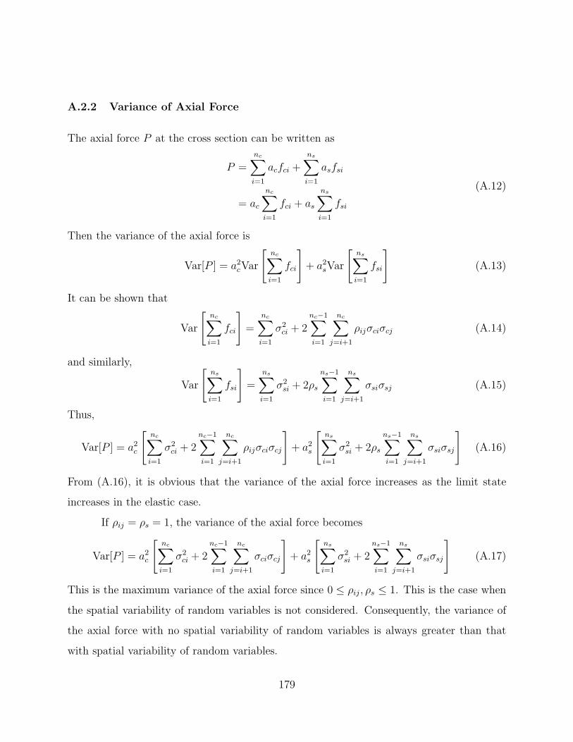
A.2.2 Variance of Axial Force
The axial force P at the cross section can be written as
P =nc∑
i=1
acfci +ns∑
i=1
asfsi
= ac
nc∑
i=1
fci + as
ns∑
i=1
fsi
(A.12)
Then the variance of the axial force is
Var[P ] = a2cVar
[
nc∑
i=1
fci
]
+ a2sVar
[
ns∑
i=1
fsi
]
(A.13)
It can be shown that
Var
[
nc∑
i=1
fci
]
=
nc∑
i=1
σ2ci + 2
nc−1∑
i=1
nc∑
j=i+1
ρijσciσcj (A.14)
and similarly,
Var
[
ns∑
i=1
fsi
]
=
ns∑
i=1
σ2si + 2ρs
ns−1∑
i=1
ns∑
j=i+1
σsiσsj (A.15)
Thus,
Var[P ] = a2c
[
nc∑
i=1
σ2ci + 2
nc−1∑
i=1
nc∑
j=i+1
ρijσciσcj
]
+ a2s
[
ns∑
i=1
σ2si + 2ρs
ns−1∑
i=1
ns∑
j=i+1
σsiσsj
]
(A.16)
From (A.16), it is obvious that the variance of the axial force increases as the limit state
increases in the elastic case.
If ρij = ρs = 1, the variance of the axial force becomes
Var[P ] = a2c
[
nc∑
i=1
σ2ci + 2
nc−1∑
i=1
nc∑
j=i+1
σciσcj
]
+ a2s
[
ns∑
i=1
σ2si + 2
ns−1∑
i=1
ns∑
j=i+1
σsiσsj
]
(A.17)
This is the maximum variance of the axial force since 0 ≤ ρij , ρs ≤ 1. This is the case when
the spatial variability of random variables is not considered. Consequently, the variance of
the axial force with no spatial variability of random variables is always greater than that
with spatial variability of random variables.
179

If only the axial load is applied, all fibers have the same stress levels, in the cross
section,
σc1 = σc2 = . . . = σcncand σs1 = σs2 = . . . = σsns
(A.18)
Accordingly, the variance of the axial force becomes
Var[P ] = a2cσ
2c1
[
nc + 2
nc−1∑
i=1
nc∑
j=i+1
ρij
]
+ a2sσ
2s1
[
ns + 2ρs
ns−1∑
i=1
ns∑
j=i+1
1
]
= a2cσ
2c1
[
nc + 2
nc−1∑
i=1
nc∑
j=i+1
ρij
]
+ a2sσ
2s1 [ns + ρsns(ns − 1)]
= a2cσ
2c1
[
nc + 2nc−1∑
i=1
nc∑
j=i+1
ρij
]
+ a2sσ
2s1
[
ρsn2s + (1 − ρs)ns
]
(A.19)
If ρij = ρs = 1 under the pure axial load condition, the variance of the axial force becomes
Var[P ] = a2cn
2cσ
2c1 + a2
sn2sσ
2s1 (A.20)
A.2.3 Variance of Bending Moment
The bending moment M at the cross section can be written as
M =nc∑
i=1
acfciyci +ns∑
i=1
asfsiysi
= ac
nc∑
i=1
fciyci + as
ns∑
i=1
fsiysi
(A.21)
It can be shown that
Var
[
nc∑
i=1
fciyci
]
=
nc∑
i=1
y2ciσ
2ci + 2
nc−1∑
i=1
nc∑
j=i+1
yciycjρijσciσcj (A.22)
and similarly,
Var
[
ns∑
i=1
fsiysi
]
=
ns∑
i=1
y2siσ
2si + 2ρs
ns−1∑
i=1
ns∑
j=i+1
ysiysjσsiσsj (A.23)
180

Thus,
Var[M ] = a2c
[
nc∑
i=1
y2ciσ
2ci + 2
nc−1∑
i=1
nc∑
j=i+1
yciycjρijσciσcj
]
+ a2s
[
ns∑
i=1
y2siσ
2si + 2ρs
ns−1∑
i=1
ns∑
j=i+1
ysiysjσsiσsj
] (A.24)
From (A.24), it is obvious that variance of the bending moment increases as the limit state
increases in the elastic case.
If ρij = ρs = 1, the variance of the axial force becomes
Var[M ] = a2c
[
nc∑
i=1
y2ciσ
2ci + 2
nc−1∑
i=1
nc∑
j=i+1
yciycjσciσcj
]
+ a2s
[
ns∑
i=1
y2siσ
2si + 2
ns−1∑
i=1
ns∑
j=i+1
ysiysjσsiσsj
] (A.25)
This value is also the maximum variance of the bending moment. Consequently, the variance
of the bending moment with no spatial variability of random variables is always greater than
that with spatial variability of random variables.
181

PEER REPORTS
PEER reports are available from the National Information Service for Earthquake Engineering (NISEE). To order PEER reports, please contact the Pacific Earthquake Engineering Research Center, 1301 South 46th Street, Richmond, California 94804-4698. Tel.: (510) 665-3405; Fax: (510) 665-3420. PEER 2006/04 Probabilistic Seismic Evaluation of Reinforced Concrete Structural Components and Systems. Tae Hyung Lee
and Khalid M. Mosalam. August 2006. PEER 2006/01 Bracing Berkeley. A Guide to Seismic Safety on the UC Berkeley Campus. Mary C. Comerio, Stephen Tobriner,
and Ariane Fehrenkamp. January 2006. PEER 2005/15 CPT-Based Probabilistic Assessment of Seismic Soil Liquefaction Initiation. R. E. S. Moss, R. B. Seed, R. E.
Kayen, J. P. Stewart, and A. Der Kiureghian. April 2006. PEER 2005/13 Stochastic Characterization and Decision Bases under Time-Dependent Aftershock Risk in Performance-Based
Earthquake Engineering. Gee Liek Yeo and C. Allin Cornell. July 2005. PEER 2005/12 PEER Testbed Study on a Laboratory Building: Exercising Seismic Performance Assessment. Mary C. Comerio,
editor. November 2005. PEER 2005/11 Van Nuys Hotel Building Testbed Report: Exercising Seismic Performance Assessment. Helmut Krawinkler,
editor. October 2005. PEER 2005/10 First NEES/E-Defense Workshop on Collapse Simulation of Reinforced Concrete Building Structures. September
2005. PEER 2005/08 Damage Accumulation in Lightly Confined Reinforced Concrete Bridge Columns. R. Tyler Ranf, Jared M. Nelson,
Zach Price, Marc O. Eberhard, and John F. Stanton. April 2006. PEER 2005/07 Experimental and Analytical Studies on the Seismic Response of Freestanding and Anchored Laboratory
Equipment. Dimitrios Konstantinidis and Nicos Makris. January 2005. PEER 2005/06 Global Collapse of Frame Structures under Seismic Excitations. Luis F. Ibarra and Helmut Krawinkler.
September 2005. PEER 2005/05 Performance Characterization of Bench- and Shelf-Mounted Equipment. Samit Ray Chaudhuri and Tara C.
Hutchinson. May 2006. PEER 2005/04 Numerical Modeling of the Nonlinear Cyclic Response of Shallow Foundations. Chad Harden, Tara Hutchinson,
Geoffrey R. Martin, and Bruce L. Kutter. August 2005. PEER 2005/03 A Taxonomy of Building Components for Performance-Based Earthquake Engineering. Keith A. Porter.
September 2005. PEER 2005/02 Fragility Basis for California Highway Overpass Bridge Seismic Decision Making. Kevin R. Mackie and Bozidar
Stojadinovic. June 2005. PEER 2005/01 Empirical Characterization of Site Conditions on Strong Ground Motion. Jonathan P. Stewart, Yoojoong Choi,
and Robert W. Graves. June 2005. PEER 2004/09 Electrical Substation Equipment Interaction: Experimental Rigid Conductor Studies. Christopher Stearns and
André Filiatrault. February 2005. PEER 2004/08 Seismic Qualification and Fragility Testing of Line Break 550-kV Disconnect Switches. Shakhzod M. Takhirov,
Gregory L. Fenves, and Eric Fujisaki. January 2005. PEER 2004/07 Ground Motions for Earthquake Simulator Qualification of Electrical Substation Equipment. Shakhzod M.
Takhirov, Gregory L. Fenves, Eric Fujisaki, and Don Clyde. January 2005. PEER 2004/06 Performance-Based Regulation and Regulatory Regimes. Peter J. May and Chris Koski. September 2004.
PEER 2004/05 Performance-Based Seismic Design Concepts and Implementation: Proceedings of an International Workshop.
Peter Fajfar and Helmut Krawinkler, editors. September 2004. PEER 2004/04 Seismic Performance of an Instrumented Tilt-up Wall Building. James C. Anderson and Vitelmo V. Bertero. July
2004.

PEER 2004/03 Evaluation and Application of Concrete Tilt-up Assessment Methodologies. Timothy Graf and James O. Malley. October 2004.
PEER 2004/02 Analytical Investigations of New Methods for Reducing Residual Displacements of Reinforced Concrete Bridge
Columns. Junichi Sakai and Stephen A. Mahin. August 2004. PEER 2004/01 Seismic Performance of Masonry Buildings and Design Implications. Kerri Anne Taeko Tokoro, James C.
Anderson, and Vitelmo V. Bertero. February 2004. PEER 2003/18 Performance Models for Flexural Damage in Reinforced Concrete Columns. Michael Berry and Marc Eberhard.
August 2003. PEER 2003/17 Predicting Earthquake Damage in Older Reinforced Concrete Beam-Column Joints. Catherine Pagni and Laura
Lowes. October 2004. PEER 2003/16 Seismic Demands for Performance-Based Design of Bridges. Kevin Mackie and Božidar Stojadinovic. August
2003. PEER 2003/15 Seismic Demands for Nondeteriorating Frame Structures and Their Dependence on Ground Motions. Ricardo
Antonio Medina and Helmut Krawinkler. May 2004. PEER 2003/14 Finite Element Reliability and Sensitivity Methods for Performance-Based Earthquake Engineering. Terje
Haukaas and Armen Der Kiureghian. April 2004. PEER 2003/13 Effects of Connection Hysteretic Degradation on the Seismic Behavior of Steel Moment-Resisting Frames. Janise
E. Rodgers and Stephen A. Mahin. March 2004. PEER 2003/12 Implementation Manual for the Seismic Protection of Laboratory Contents: Format and Case Studies. William T.
Holmes and Mary C. Comerio. October 2003. PEER 2003/11 Fifth U.S.-Japan Workshop on Performance-Based Earthquake Engineering Methodology for Reinforced
Concrete Building Structures. February 2004. PEER 2003/10 A Beam-Column Joint Model for Simulating the Earthquake Response of Reinforced Concrete Frames. Laura N.
Lowes, Nilanjan Mitra, and Arash Altoontash. February 2004. PEER 2003/09 Sequencing Repairs after an Earthquake: An Economic Approach. Marco Casari and Simon J. Wilkie. April 2004. PEER 2003/08 A Technical Framework for Probability-Based Demand and Capacity Factor Design (DCFD) Seismic Formats.
Fatemeh Jalayer and C. Allin Cornell. November 2003. PEER 2003/07 Uncertainty Specification and Propagation for Loss Estimation Using FOSM Methods. Jack W. Baker and C. Allin
Cornell. September 2003. PEER 2003/06 Performance of Circular Reinforced Concrete Bridge Columns under Bidirectional Earthquake Loading. Mahmoud
M. Hachem, Stephen A. Mahin, and Jack P. Moehle. February 2003. PEER 2003/05 Response Assessment for Building-Specific Loss Estimation. Eduardo Miranda and Shahram Taghavi.
September 2003. PEER 2003/04 Experimental Assessment of Columns with Short Lap Splices Subjected to Cyclic Loads. Murat Melek, John W.
Wallace, and Joel Conte. April 2003. PEER 2003/03 Probabilistic Response Assessment for Building-Specific Loss Estimation. Eduardo Miranda and Hesameddin
Aslani. September 2003. PEER 2003/02 Software Framework for Collaborative Development of Nonlinear Dynamic Analysis Program. Jun Peng and
Kincho H. Law. September 2003. PEER 2003/01 Shake Table Tests and Analytical Studies on the Gravity Load Collapse of Reinforced Concrete Frames. Kenneth
John Elwood and Jack P. Moehle. November 2003. PEER 2002/24 Performance of Beam to Column Bridge Joints Subjected to a Large Velocity Pulse. Natalie Gibson, André
Filiatrault, and Scott A. Ashford. April 2002. PEER 2002/23 Effects of Large Velocity Pulses on Reinforced Concrete Bridge Columns. Greg L. Orozco and Scott A. Ashford.
April 2002. PEER 2002/22 Characterization of Large Velocity Pulses for Laboratory Testing. Kenneth E. Cox and Scott A. Ashford. April
2002.

PEER 2002/21 Fourth U.S.-Japan Workshop on Performance-Based Earthquake Engineering Methodology for Reinforced Concrete Building Structures. December 2002.
PEER 2002/20 Barriers to Adoption and Implementation of PBEE Innovations. Peter J. May. August 2002. PEER 2002/19 Economic-Engineered Integrated Models for Earthquakes: Socioeconomic Impacts. Peter Gordon, James E.
Moore II, and Harry W. Richardson. July 2002. PEER 2002/18 Assessment of Reinforced Concrete Building Exterior Joints with Substandard Details. Chris P. Pantelides, Jon
Hansen, Justin Nadauld, and Lawrence D. Reaveley. May 2002. PEER 2002/17 Structural Characterization and Seismic Response Analysis of a Highway Overcrossing Equipped with
Elastomeric Bearings and Fluid Dampers: A Case Study. Nicos Makris and Jian Zhang. November 2002. PEER 2002/16 Estimation of Uncertainty in Geotechnical Properties for Performance-Based Earthquake Engineering. Allen L.
Jones, Steven L. Kramer, and Pedro Arduino. December 2002. PEER 2002/15 Seismic Behavior of Bridge Columns Subjected to Various Loading Patterns. Asadollah Esmaeily-Gh. and Yan
Xiao. December 2002. PEER 2002/14 Inelastic Seismic Response of Extended Pile Shaft Supported Bridge Structures. T.C. Hutchinson, R.W.
Boulanger, Y.H. Chai, and I.M. Idriss. December 2002. PEER 2002/13 Probabilistic Models and Fragility Estimates for Bridge Components and Systems. Paolo Gardoni, Armen Der
Kiureghian, and Khalid M. Mosalam. June 2002. PEER 2002/12 Effects of Fault Dip and Slip Rake on Near-Source Ground Motions: Why Chi-Chi Was a Relatively Mild M7.6
Earthquake. Brad T. Aagaard, John F. Hall, and Thomas H. Heaton. December 2002. PEER 2002/11 Analytical and Experimental Study of Fiber-Reinforced Strip Isolators. James M. Kelly and Shakhzod M. Takhirov.
September 2002. PEER 2002/10 Centrifuge Modeling of Settlement and Lateral Spreading with Comparisons to Numerical Analyses. Sivapalan
Gajan and Bruce L. Kutter. January 2003. PEER 2002/09 Documentation and Analysis of Field Case Histories of Seismic Compression during the 1994 Northridge,
California, Earthquake. Jonathan P. Stewart, Patrick M. Smith, Daniel H. Whang, and Jonathan D. Bray. October 2002.
PEER 2002/08 Component Testing, Stability Analysis and Characterization of Buckling-Restrained Unbonded BracesTM. Cameron
Black, Nicos Makris, and Ian Aiken. September 2002. PEER 2002/07 Seismic Performance of Pile-Wharf Connections. Charles W. Roeder, Robert Graff, Jennifer Soderstrom, and Jun
Han Yoo. December 2001. PEER 2002/06 The Use of Benefit-Cost Analysis for Evaluation of Performance-Based Earthquake Engineering Decisions.
Richard O. Zerbe and Anthony Falit-Baiamonte. September 2001. PEER 2002/05 Guidelines, Specifications, and Seismic Performance Characterization of Nonstructural Building Components and
Equipment. André Filiatrault, Constantin Christopoulos, and Christopher Stearns. September 2001. PEER 2002/04 Consortium of Organizations for Strong-Motion Observation Systems and the Pacific Earthquake Engineering
Research Center Lifelines Program: Invited Workshop on Archiving and Web Dissemination of Geotechnical Data, 4–5 October 2001. September 2002.
PEER 2002/03 Investigation of Sensitivity of Building Loss Estimates to Major Uncertain Variables for the Van Nuys Testbed.
Keith A. Porter, James L. Beck, and Rustem V. Shaikhutdinov. August 2002. PEER 2002/02 The Third U.S.-Japan Workshop on Performance-Based Earthquake Engineering Methodology for Reinforced
Concrete Building Structures. July 2002. PEER 2002/01 Nonstructural Loss Estimation: The UC Berkeley Case Study. Mary C. Comerio and John C. Stallmeyer.
December 2001. PEER 2001/16 Statistics of SDF-System Estimate of Roof Displacement for Pushover Analysis of Buildings. Anil K. Chopra,
Rakesh K. Goel, and Chatpan Chintanapakdee. December 2001. PEER 2001/15 Damage to Bridges during the 2001 Nisqually Earthquake. R. Tyler Ranf, Marc O. Eberhard, and Michael P.
Berry. November 2001.

PEER 2001/14 Rocking Response of Equipment Anchored to a Base Foundation. Nicos Makris and Cameron J. Black. September 2001.
PEER 2001/13 Modeling Soil Liquefaction Hazards for Performance-Based Earthquake Engineering. Steven L. Kramer and
Ahmed-W. Elgamal. February 2001. PEER 2001/12 Development of Geotechnical Capabilities in OpenSees. Boris Jeremi . September 2001. PEER 2001/11 Analytical and Experimental Study of Fiber-Reinforced Elastomeric Isolators. James M. Kelly and Shakhzod M.
Takhirov. September 2001. PEER 2001/10 Amplification Factors for Spectral Acceleration in Active Regions. Jonathan P. Stewart, Andrew H. Liu, Yoojoong
Choi, and Mehmet B. Baturay. December 2001. PEER 2001/09 Ground Motion Evaluation Procedures for Performance-Based Design. Jonathan P. Stewart, Shyh-Jeng Chiou,
Jonathan D. Bray, Robert W. Graves, Paul G. Somerville, and Norman A. Abrahamson. September 2001. PEER 2001/08 Experimental and Computational Evaluation of Reinforced Concrete Bridge Beam-Column Connections for
Seismic Performance. Clay J. Naito, Jack P. Moehle, and Khalid M. Mosalam. November 2001. PEER 2001/07 The Rocking Spectrum and the Shortcomings of Design Guidelines. Nicos Makris and Dimitrios Konstantinidis.
August 2001. PEER 2001/06 Development of an Electrical Substation Equipment Performance Database for Evaluation of Equipment
Fragilities. Thalia Agnanos. April 1999. PEER 2001/05 Stiffness Analysis of Fiber-Reinforced Elastomeric Isolators. Hsiang-Chuan Tsai and James M. Kelly. May 2001. PEER 2001/04 Organizational and Societal Considerations for Performance-Based Earthquake Engineering. Peter J. May. April
2001. PEER 2001/03 A Modal Pushover Analysis Procedure to Estimate Seismic Demands for Buildings: Theory and Preliminary
Evaluation. Anil K. Chopra and Rakesh K. Goel. January 2001. PEER 2001/02 Seismic Response Analysis of Highway Overcrossings Including Soil-Structure Interaction. Jian Zhang and Nicos
Makris. March 2001. PEER 2001/01 Experimental Study of Large Seismic Steel Beam-to-Column Connections. Egor P. Popov and Shakhzod M.
Takhirov. November 2000. PEER 2000/10 The Second U.S.-Japan Workshop on Performance-Based Earthquake Engineering Methodology for Reinforced
Concrete Building Structures. March 2000. PEER 2000/09 Structural Engineering Reconnaissance of the August 17, 1999 Earthquake: Kocaeli (Izmit), Turkey. Halil Sezen,
Kenneth J. Elwood, Andrew S. Whittaker, Khalid Mosalam, John J. Wallace, and John F. Stanton. December 2000.
PEER 2000/08 Behavior of Reinforced Concrete Bridge Columns Having Varying Aspect Ratios and Varying Lengths of
Confinement. Anthony J. Calderone, Dawn E. Lehman, and Jack P. Moehle. January 2001. PEER 2000/07 Cover-Plate and Flange-Plate Reinforced Steel Moment-Resisting Connections. Taejin Kim, Andrew S. Whittaker,
Amir S. Gilani, Vitelmo V. Bertero, and Shakhzod M. Takhirov. September 2000. PEER 2000/06 Seismic Evaluation and Analysis of 230-kV Disconnect Switches. Amir S. J. Gilani, Andrew S. Whittaker, Gregory
L. Fenves, Chun-Hao Chen, Henry Ho, and Eric Fujisaki. July 2000. PEER 2000/05 Performance-Based Evaluation of Exterior Reinforced Concrete Building Joints for Seismic Excitation. Chandra
Clyde, Chris P. Pantelides, and Lawrence D. Reaveley. July 2000. PEER 2000/04 An Evaluation of Seismic Energy Demand: An Attenuation Approach. Chung-Che Chou and Chia-Ming Uang. July
1999. PEER 2000/03 Framing Earthquake Retrofitting Decisions: The Case of Hillside Homes in Los Angeles. Detlof von Winterfeldt,
Nels Roselund, and Alicia Kitsuse. March 2000. PEER 2000/02 U.S.-Japan Workshop on the Effects of Near-Field Earthquake Shaking. Andrew Whittaker, ed. July 2000. PEER 2000/01 Further Studies on Seismic Interaction in Interconnected Electrical Substation Equipment. Armen Der Kiureghian,
Kee-Jeung Hong, and Jerome L. Sackman. November 1999.

PEER 1999/14 Seismic Evaluation and Retrofit of 230-kV Porcelain Transformer Bushings. Amir S. Gilani, Andrew S. Whittaker, Gregory L. Fenves, and Eric Fujisaki. December 1999.
PEER 1999/13 Building Vulnerability Studies: Modeling and Evaluation of Tilt-up and Steel Reinforced Concrete Buildings. John
W. Wallace, Jonathan P. Stewart, and Andrew S. Whittaker, editors. December 1999. PEER 1999/12 Rehabilitation of Nonductile RC Frame Building Using Encasement Plates and Energy-Dissipating Devices.
Mehrdad Sasani, Vitelmo V. Bertero, James C. Anderson. December 1999. PEER 1999/11 Performance Evaluation Database for Concrete Bridge Components and Systems under Simulated Seismic
Loads. Yael D. Hose and Frieder Seible. November 1999. PEER 1999/10 U.S.-Japan Workshop on Performance-Based Earthquake Engineering Methodology for Reinforced Concrete
Building Structures. December 1999. PEER 1999/09 Performance Improvement of Long Period Building Structures Subjected to Severe Pulse-Type Ground Motions.
James C. Anderson, Vitelmo V. Bertero, and Raul Bertero. October 1999. PEER 1999/08 Envelopes for Seismic Response Vectors. Charles Menun and Armen Der Kiureghian. July 1999. PEER 1999/07 Documentation of Strengths and Weaknesses of Current Computer Analysis Methods for Seismic Performance of
Reinforced Concrete Members. William F. Cofer. November 1999. PEER 1999/06 Rocking Response and Overturning of Anchored Equipment under Seismic Excitations. Nicos Makris and Jian
Zhang. November 1999. PEER 1999/05 Seismic Evaluation of 550 kV Porcelain Transformer Bushings. Amir S. Gilani, Andrew S. Whittaker, Gregory L.
Fenves, and Eric Fujisaki. October 1999. PEER 1999/04 Adoption and Enforcement of Earthquake Risk-Reduction Measures. Peter J. May, Raymond J. Burby, T. Jens
Feeley, and Robert Wood. PEER 1999/03 Task 3 Characterization of Site Response General Site Categories. Adrian Rodriguez-Marek, Jonathan D. Bray,
and Norman Abrahamson. February 1999. PEER 1999/02 Capacity-Demand-Diagram Methods for Estimating Seismic Deformation of Inelastic Structures: SDF Systems.
Anil K. Chopra and Rakesh Goel. April 1999. PEER 1999/01 Interaction in Interconnected Electrical Substation Equipment Subjected to Earthquake Ground Motions. Armen
Der Kiureghian, Jerome L. Sackman, and Kee-Jeung Hong. February 1999. PEER 1998/08 Behavior and Failure Analysis of a Multiple-Frame Highway Bridge in the 1994 Northridge Earthquake. Gregory L.
Fenves and Michael Ellery. December 1998. PEER 1998/07 Empirical Evaluation of Inertial Soil-Structure Interaction Effects. Jonathan P. Stewart, Raymond B. Seed, and
Gregory L. Fenves. November 1998. PEER 1998/06 Effect of Damping Mechanisms on the Response of Seismic Isolated Structures. Nicos Makris and Shih-Po
Chang. November 1998. PEER 1998/05 Rocking Response and Overturning of Equipment under Horizontal Pulse-Type Motions. Nicos Makris and
Yiannis Roussos. October 1998. PEER 1998/04 Pacific Earthquake Engineering Research Invitational Workshop Proceedings, May 14–15, 1998: Defining the
Links between Planning, Policy Analysis, Economics and Earthquake Engineering. Mary Comerio and Peter Gordon. September 1998.
PEER 1998/03 Repair/Upgrade Procedures for Welded Beam to Column Connections. James C. Anderson and Xiaojing Duan.
May 1998. PEER 1998/02 Seismic Evaluation of 196 kV Porcelain Transformer Bushings. Amir S. Gilani, Juan W. Chavez, Gregory L.
Fenves, and Andrew S. Whittaker. May 1998. PEER 1998/01 Seismic Performance of Well-Confined Concrete Bridge Columns. Dawn E. Lehman and Jack P. Moehle.
December 2000.
Related Documents