Probabilistic Number Theory

Probabilistic Number Theory

Dr. Jorn Steuding

Dedicated to Prof. Jonas Kubilius

and the members of his working group at Vilnius University,for their outstanding work in probabilistic number theory

and their kind hospitality!

This is a first introduction to Probabilistic Number Theory, based on a course givenat the Johann Wolfgang Goethe-Universitat Frankfurt in 2001. We focusourselves to some classical results on the prime divisor counting function ω(n) whichwere discovered in the first half of the 20th century. Nowadays, these facts arethe basics for heuristical arguments on the expected running time of algorithms incryptography. Furthermore, this gives a first view inside the methods and problemsin this modern field of research. Especially the growing interest in probabilisticalgorithms, which give with a certain probability the right answer (e.g. probabilisticprime number tests), underlines the power and influence of doing number theoryfrom a probability theoretical point of view.

For our studies we require only a small background in elementary number theoryas well as in probability theory, and, for the second half additionally, the fundamen-tals of complex analysis; good recommendations to refresh the knowledge on thesetopics are [16], [14] and [21]. We will use the same standard notations as in [30],which is also the main source of this course.

I am very grateful to Rasa Slezeviciene for her interest and her several helpfulcomments, remarks and corrections.

Jorn Steuding, Frankfurt 01/30/2002.

1

Contents

1 Introduction 3

2 Densities on the set of positive integers 8

3 Limiting distributions of arithmetic functions 15

4 Expectation and variance 21

5 Average order and normal order 25

6 The Turan-Kubilius inequality 31

7 The theorem of Hardy-Ramanujan 37

8 A duality principle 41

9 Dirichlet series and Euler products 44

10 Characteristic functions 50

11 Mean value theorems 56

12 Uniform distribution modulo 1 59

13 The theorem of Erdos-Kac 62

14 A zero-free region for ζ(s) 66

15 The Selberg-Delange method 71

16 The prime number theorem 77

2

Chapter 1

Introduction

Instead of probabilistic number theory one should speak about studying arithmeticfunctions with probabilistic methods. First approaches in this direction date back to

• Gauss, who used in 1791 probabilistic arguments for his speculations on thenumber of products consisting of exactly k distinct prime factors below a givenbound; the case k = 1 led to the prime number theorem (see [10], vol.10, p.11)- we shall return to this question in Chapter 16;

• Cesaro, who observed in 1881 that the probability that two randomly chosenintegers are coprime is 6

π2 (see [1]) - we will prove this result in Chapter 4.

In number theory one is interested in the value distribution of arithmetic functionsf : N→ C (i.e. complex-valued sequences). An arithmetic function f is said to beadditive if

f(m · n) = f(m) + f(n) for gcd(m,n) = 1,

and f is called multiplicative if

f(m · n) = f(m) · f(n) for gcd(m,n) = 1;

f is completely additive- and completely multiplicative, resp., when the con-dition of coprimality can be removed (the symbol gcd(m,n) stands, as usual, forthe greatest common divisor of the integers m and n). Obviously, the values ofadditive or multiplicative functions are determined by the values on the prime pow-ers, or even on the primes when the function in question is completely additive orcompletely multiplicative. But prime number distribution is a difficult task.

We shall give two important examples. Let the prime divisor counting func-tions ω(n) and Ω(n) of a positive integer n (with and without multiplicities, resp.)

3

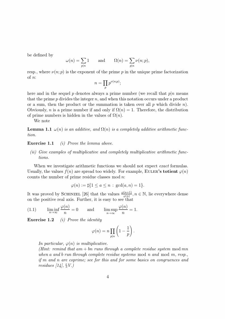
be defined byω(n) =

∑p|n

1 and Ω(n) =∑p|n

ν(n; p),

resp., where ν(n; p) is the exponent of the prime p in the unique prime factorizationof n:

n =∏p

pν(n;p);

here and in the sequel p denotes always a prime number (we recall that p|n meansthat the prime p divides the integer n, and when this notation occurs under a productor a sum, then the product or the summation is taken over all p which divide n).Obviously, n is a prime number if and only if Ω(n) = 1. Therefore, the distributionof prime numbers is hidden in the values of Ω(n).

We note

Lemma 1.1 ω(n) is an additive, and Ω(n) is a completely additive arithmetic func-tion.

Exercise 1.1 (i) Prove the lemma above.

(ii) Give examples of multiplicative and completely multiplicative arithmetic func-tions.

When we investigate arithmetic functions we should not expect exact formulas.Usually, the values f(n) are spread too widely. For example, Euler’s totient ϕ(n)counts the number of prime residue classes mod n:

ϕ(n) := ]1 ≤ a ≤ n : gcd(a, n) = 1.

It was proved by Schinzel [26] that the values ϕ(n+1)ϕ(n)

, n ∈ N, lie everywhere denseon the positive real axis. Further, it is easy to see that

lim infn→∞

ϕ(n)

n= 0 and lim sup

n→∞

ϕ(n)

n= 1.(1.1)

Exercise 1.2 (i) Prove the identity

ϕ(n) = n∏p|n

(1−

1

p

).

In particular, ϕ(n) is multiplicative.(Hint: remind that am+ bn runs through a complete residue system modmnwhen a and b run through complete residue systems mod n and mod m, resp.,if m and n are coprime; see for this and for some basics on congruences andresidues [14], §V.)

4

(ii) Prove formulae (1.1).(Hint: make use of formula (2.3) below.)

(iii) Try to find lower and upper bounds for ω(n) and Ω(n).

In our studies on the value distribution of arithmetic functions we are restrictedto asymptotic formulas. Hence, we need a notion to deal with error terms. We write

f(x) = O(g(x)) and f(x) g(x),

resp., when there exists a positive function g(x) such that

lim supx→∞

|f(x)|

g(x)

exists. Then the function f(x) grows not faster than g(x) (up to a multiplicativeconstant), and, hopefully, the growth of the function g(x) is easier to understandthan the one of f(x), as x → ∞. This is not only a convenient notation due toLandau and Vinogradov, but, in the sense of developping the right language, animportant contribution to mathematics as well.

We illustrate this with an easy example. What is the order of growth of thetruncated (divergent) harmonic series ∑

n≤x

1

n,

as x→∞? Obviously, for n ≥ 2,

1

n<∫ n

n−1

dt

t<

1

n − 1.

Denote by [x] the maximum over all integers ≤ x, then, by summation over 2 ≤ n ≤[x],

[x]∑n=2

1

n<∫ [x]

1

dt

t<

[x]−1∑n=1

1

n.

Therefore integration yields∑n≤x

1

n=∫ x

1

dt

t+O(1) = log x+O(1);(1.2)

here and in the sequel log denotes always the natural logarithm, i.e. the logarithmto the base e = exp(1). We learned above an important trick which we will usein the following several times: the sum over a sufficiently smooth function can beconsidered - up to a certain error - as a Riemann sum and its integral, resp., whichis hopefully calculable.

5

Exercise 1.3 Prove for x→∞ that

(i) the number of squares n2 ≤ x is√x+O(1);

(ii) log x xε for any ε > 0;

(iii) xm exp(x) for any m > 0;

(iv)∑n≤x n = 1

2x2 +O(x).

We return to number theory. In 1917 Hardy and Ramanujan [13] discoveredthe first deep result on the prime divisor counting function, namely that for fixedδ ∈ (0, 1

2) and N ≥ 3

1

N]n ≤ N : |ω(n)− log log n| > (log logn)

12

+δ 1

(log logN)2δ.(1.3)

Since the right hand side above tends to zero, as N → ∞, the values of ω(n) withn ≤ N are concentrated around log log n (the set of integers n, for which ω(n)deviates from log log n, has zero density, in the language of densities; see Chapter2). For example, a 50-digit number has on average only about 5 distinct primedivisors!

Moreover, Hardy and Ramanujan proved with similar arguments the corre-sponding result for Ω(n). Unfortunately, their approach is complicated and notextendable to other functions. In 1934 Turan [31] found a new proof based on theestimate ∑

n≤N

(ω(n)− log log n)2 N log logN,(1.4)

and an argument similar to Cebysev’s proof of the law of large numbers in prob-ability theory (which was unknown to the young Turan). His approach allowsgeneralizations (and we will deduce the Hardy-Ramanujan result (1.3) as an im-mediate consequence of a much more general result which holds for a large class ofadditive functions, namely the Turan-Kubilius inequality; see Chapter 6). Theeffect of Turan’s paper was epoch-making. His ideas were the starting point forthe development of probabilistic number theory in the following years.

To give finally a first glance on the influence of probabilistic methods on numbertheory we mention one of its highlights, discovered by Erdos and Kac [7] in 1939,namely that ω(n) satisfies (after a certain normalization) the Gaussian error law:

limN→∞

1

N]

n ≤ N :

ω(n) − log logN√

log logN≤ x

=

1√

2π

∫ x

−∞exp

(−τ 2

2

)dτ.(1.5)

6

Therefore, the values ω(n) are asymptotically normally distributed with expectationlog log n and standard deviation

√log log n (this goes much beyond (1.3); we will

prove a stronger version of (1.5) in Chapter 13).This classical result has some important implications to cryptography. For an

analysis of the expected running time of many modern primality tests and factor-ization tests one needs heuristical arguments on the distribution of prime numbersand so-called smooth numbers, i.e. numbers which have only small prime divisors(see [27], §11).

For a deeper and more detailed history of probabilistic number theory read thehighly recommendable introductions of [6] and [18].

7

Chapter 2

Densities on the set of positiveintegers

It is no wonder that probabilistic number theory has its roots in the 1930s. Onlyin 1933 Kolmogorov gave the first widely accepted axiomization of probabilitytheory.

We recall these basics. A probability space is a triple (Ω,B,P) consisting ofthe sure event Ω (a non-empty set), a σ-algebra B (i.e. a system of subsets of Ω,for example, the power set of Ω), and a probability measure P, i.e. a functionP : B → [0, 1] satisfying

• P(Ω) = 1,

• P(A) ≥ 0 for all A ∈ B,

• P (⋃∞n=1 An) =

∑∞n=1 P(An) for all pairwise disjoint An ∈ B.

Then, P(A) is the probability of A ∈ B. We say that two events A,B ∈ B areindependent if

P(A ∩B) = P(A) ·P(B).

Based on Kolmogorov’s axioms one can start to define random variables, theirexpectations and much more to build up the powerful theory of probability (see [16]for more details).

But our aim is different. We are interested to obtain knowledge on the valuedistribution of arithmetic functions. The first idea is to define a probability lawon the set of positive integers. However, we are restricted to be very careful asthe following statement shows: by intuition we expect that the probability, that arandomly chosen integer is even, equals 1

2, but:

8

Theorem 2.1 There exists no probability law on N such that

P(aN) =1

a(a ∈ N),(2.1)

where aN := n ∈ N : n ≡ 0 mod a.

Proof via contradiction. By the Chinese remainder theorem (see [14], §VIII.1), onehas for coprime integers a, b

aN ∩ bN = abN.Now assume additionally that P is a probability measure on N satisfying (2.1), then

P(aN ∩ bN) = P(abN) =1

ab= P(aN) ·P(bN).

Thus, the events aN and bN, and their complements

Na := N \ aN and Nb := N \ bN,

resp., are independent. Furthermore

P(Na ∩Nb) = (1−P(aN))(1−P(bN)) =(

1−1

a

)(1−

1

b

).

By induction, we obtain for arbitrary integers m < x

P(m) ≤ P

⋂m<p≤x

Np

=∏

m<p≤x

(1−

1

p

);(2.2)

here the inequality is caused by m ∈ Np for all p > m). In view to the unique primefactorization of the integers and (1.2) we get

∏p≤x

(1 +

1

p+

1

p2+ . . .

)≥∑n≤x

1

n= log x+O(1).

Hence, by the geometric series expansion,

∏p≤x

(1−

1

p

)≤

1

log x+O(1).(2.3)

This leads with x→∞ in formula (2.2) to P(m) = 0, giving the contradiction. •

In spite of that we may define a probability law on N as follows. Assume that

∞∑n=1

λn = 1 with 0 ≤ λn ≤ 1,

9

then we set for any sequence A ⊂ N

P(A) =∑n∈A

λn.

Obviously, this defines a probability measure. Unfortunately, the probability of asequence depends drastically on its initial values (since for any ε > 0 there existsN ∈ N such that P(1, 2, . . . , N) ≥ 1− ε).

To construct a model which fits more to our intuition we need the notion ofdensity. Introducing a divergent series

∞∑n=1

λn =∞ with λn ≥ 0,

we define the density d(A) of a sequence A of positive integers to be the limit(when it exists)

d(A) = limx→∞

∑n≤x;n∈A λn∑n≤x λn

.(2.4)

This yields not a measure on N (since sequences do not form a σ-algebra, anddensities are not subadditive). Nevertheless, the concept of density allows us tobuild up a model which matches to our intuition. Putting λn = 1 in (2.4), we obtainthe natural density (when it exists)

dA = limx→∞

1

x]n ≤ x : n ∈ A;

moreover, the lower and upper natural density are given by

dA = lim infx→∞

1

x]n ≤ x : n ∈ A and dA = lim sup

x→∞

1

x]n ≤ x : n ∈ A,

respectively. We give some examples. Any arithmetic progression n ≡ b mod a hasthe natural density

limx→∞

1

x

([x

a

]+O(1)

)=

1

a,

corresponding to our intuition.

Exercise 2.1 Show that

(i) the sequence a1 < a2 < . . . has natural density α ∈ [0, 1] if, and only if,

limn→∞

n

an= α;

(Hint: for the implication of necessity note that n = ]j : aj ≤ an.)

10

(ii) the sequence A of positive integers n with leading digit 1 in the decimal expan-sion has no natural density, since

dA =1

9<

5

9= dA.

We note the following important(!) connection between natural density andprobability theory: if νN denotes the probability law of the uniform distributionwith weight 1

Non 1, 2, . . . , N, i.e.

νNA =∑n∈A

λn with λn =

1N

if n ≤ N,0 if n > N,

then (when the limit exists)

limN→∞

νNA = limN→∞

1

N]n ≤ N : n ∈ A = dA.

Therefore, the natural density of a sequence is the limit of its frequency in the firstN positive integers, as N →∞.

Setting λn = 1n

in (2.4), we obtain the logarithmic density

δA := limx→∞

1

log x

∑n≤xn∈A

1

n;

the lower and upper logarithmic density are given by

δA = lim infx→∞

1

log x

∑n≤xn∈A

1

nand δA = lim sup

x→∞

1

log x

∑n≤xn∈A

1

n,

respectively; note that the occuring log x comes from (1.2).

Exercise 2.2 Construct a sequence which has no logarithmic density.

The following theorem gives a hint for the solution of the exercise above.

Theorem 2.2 For any sequence A ⊂ N,

dA ≤ δA ≤ δA ≤ dA.

In particular, a sequence with a natural density has a logarithmic density as well,and both densities are equal.

11

Before we give the proof we recall a convenient technique in number theory.

Lemma 2.3 (Abel’s partial summation) Let λ1 < λ2 < . . . be a divergent se-quence of real numbers, define for αn ∈ C the function A(x) =

∑λn≤x αn, and let

f(x) be a complex-valued, continuous differentiable function for x ≥ λ1. Then∑λn≤x

αnf(λn) = A(x)f(x)−∫ x

λ1

A(u)f ′(u) du.

For those who are familiar with the Riemann-Stieltjes integral there is nearlynothing to show. Nevertheless,

Proof. We have

A(x)f(x)−∑λn≤x

αnf(λn) =∑λn≤x

αn(f(x)− f(λn)) =∑λn≤x

∫ x

λnαnf

′(u) du.

Since λ1 ≤ λn ≤ u ≤ x, changing integration and summation yields the assertion. •

Proof of Theorem 2.2. Defining A(x) =∑n≤x,n∈A 1, partial summation yields,

for x ≥ 1,

L(x) :=∑n≤xn∈A

1

n=A(x)

x+∫ x

1

A(t)

t2dt(2.5)

For any ε > 0 exists a t0 such that, for all t > t0,

dA− ε ≤A(t)

t≤ dA+ ε.

Thus, for x > t0,

(dA− ε)(log x− log t0) = (dA− ε)∫ x

t0

dt

t≤∫ x

1

A(t)

t2dt,

and ∫ x

1

A(t)

t2dt ≤

∫ t0

1

dt

t+ (dA+ ε)

∫ x

t0

dt

t= (dA+ ε)(log x− log t0) + log t0.

In view to (2.5) we obtain

(dA− ε)

(1−

log t0log x

)≤L(x)

log x−

A(x)

x log x≤ (dA+ ε)

(1−

log t0log x

)+

log t0log x

.

Taking lim inf and lim sup, as x→∞, and sending then ε→ 0, the assertion of thetheorem follows. •

12

Exercise 2.3 Show that the existence of the logarithmic density does not imply theexistence of natural density.(Hint: have a look on the sequence A in Exercise 2.1.)

Taking λn = λn(σ) = n−σ in (2.4), we define the analytic density of a sequenceA ⊂ N by the limit (when it exists)

limσ→1+

1

ζ(σ)

∑n∈A

1

nσ,(2.6)

where

ζ(s) :=∞∑n=1

1

ns=∏p

(1−

1

ps

)−1

(2.7)

is the famous Riemann zeta-function; obviously the series converges for s > 1(resp., from the complex point of view, in the half plane Re s > 1). Note thatthe equality between the infinite series and the infinite product is a consequenceof the unique prime factorization in Z (for more details see [30], §II.1). By partialsummation it turns out that one may replace the reciprocal of ζ(σ) in (2.6) by thefactor σ−1. We leave this training on the use of Lemma 2.3 to the interested reader.

Exercise 2.4 Write s = σ + it with i :=√−1 and σ, t ∈ R. Prove for σ > 0

ζ(s) =s

s− 1− s

∫ ∞1

x− [x]

xs+1dx.

In particular, ζ(s) has an analytic continuation to the half plane σ > 0 except for asimple pole at s = 1 with residue 1.(Hint: partial summation with

∑N<n≤M n−s; the statement about the analytic con-

tinuation requires some fundamentals from the theory of functions.)

The analytic and arithmetic properties of ζ(s) make the analytic density veryuseful for a plenty of applications. We note

Theorem 2.4 A sequence A of positive integers has analytic density if and only ifA has logarithmic density; in this case the two densities are equal.

A proof can be found in [30], §III.1.We conclude with a further density, which differs from the above given exam-

ples, but is very useful in questions concerning the addition of sequences of positiveintegers, defined by

A+ B := a+ b : a ∈ A, b ∈ B.

13

The Schnirelmann density is defined by

σ(A) = infn≥1

1

n]m ≤ n : m ∈ A.

σ(A) stresses the initial values in the sequence A. For the addition of sequences onehas Mann’s inequality

σ(A+ B) ≥ min1, σ(A)σ(B);

the interested reader can find a proof of this result and its implication to problemsin additive number theory (for example, Waring’s problem of the representationof posiitve integers as sums of k-th powers, or the famous Goldbach conjecturewhich asks whether each even positive integer is the sum of two primes or not) in[12], §I.2.

As we will see in the sequel, the concept of density makes it possible in ourinvestigations on the value distribution of an arithmetic function to exclude extremalvalues, and to have a look on its normal behaviour.

14

Chapter 3

Limiting distributions ofarithmetic functions

We recall from probability theory some basic notions. A random variable ona probability space (Ω,B,P) is a measurable function X defined on Ω. When,for example, Ω = R, then the function F (x) := P(X(ω) ∈ (−∞, x]) contains alot of information about the random variable X and its values X(ω), ω ∈ Ω. Adistribution function is a non-decreasing, right-continuous function F : R →[0, 1], satisfying

F(−∞) = 0 and F(+∞) = 1.

Denote by D(F) and C(F) the set of discontinuity points and continuity points ofF, respectively. Obviously, D(F) ∪ C(F) = R. Each discontinuity point z has theproperty F(z + ε) > F(z − ε) for any ε > 0 (the converse is not true). WriteD(F) = zk, then the function

F(z) =∑zk≤z

(F(zk)− F(zk−))

increases exclusively for z = zk, and is constant in any closed interval free of dis-continuity points zk (it is a step-function). If D(F) is not empty, then F is up to amultiplicative constant a distribution function; such a distribution function is calledatomic. Obviously, the function F−F is continuous. A distribution function F issaid to be absolutely continuous if there exists a positive, Lebesgue-integrablefunction h with

F(z) =∫ z

−∞h(t) dt.

15

Finally, a distribution function F is purely singular if F is continuous with supporton a subset N ⊂ R with Lebesgue measure zero, i.e.∫

NdF(z) = 1.

We note:

Theorem 3.1 (Lebesgue) Each distribution function F has a unique representa-tion

F = α1F1 + α2F2 + α3F3,

where α1, α2, α3 are non-negative constants with α1 + α2 + α3 = 1, and where F1 isabsolutely continuous, F2 is purely singular and F3 is atomic.

The proof follows from the observations above and the Theorem of Radon-

Nikodym; see [30], §III.2 and [16], §28.The next important notion is weak convergence. We say that a sequence Fn

of distribution functions converges weakly to a function F if

limn→∞

Fn(z) = F(z) for all z ∈ C(F),

i.e. pointwise convergence on the set of continuity points of the limit.We give an interesting example from probability theory (without details). Let

(Xj) be a sequence of independent and identically distributed random variables withexpectation µ and variance σ2 ∈ (0,∞). By the central limit theorem (see [16], §21),the distribution functions of the sequence of random variables

Yn :=1√nσ2

n∑j=1

Xj − nµ

converge weakly to the standard Normal distribution

Φ(x) :=1√

2π

∫ x

−∞exp

(−τ 2

2

)dτ(3.1)

(with expectation 0 and variance 1). In particular, we obtain for a sequence ofindependent random variables Xj with

P(Xj = −1) = P(Xj = +1) =1

2

for the random walk Zn, given by

Z0 := 0 and Zn+1 := Zn +Xn (n ∈ N),

16

that

limn→∞

P

(Zn√n< x

)= Φ(x).(3.2)

The distribution functions of the Zn are atomic whereas their limit is absolutelycontinuous. Note that one can construct Brownian motion as a certain limit ofrandom walks; see [9], §VI.6.

We return to probabilistic number theory. An arithmetic function f : N → Cmay be viewed as a sequence of random variables

fN = (f, νN)

which takes the values f(n), 1 ≤ n ≤ N , with probability 1N

, i.e. the uniformdistribution νN on the set n : n ≤ N. The fundamental question is: does thereexist a distribution law, as N →∞?

Therefore, we associate to an arithmetic function f for each N ∈ N the atomicdistribution function

FN(z) := νNn : f(n) ≤ z =1

N]n ≤ N : f(n) ≤ z.(3.3)

We say that f possesses a limiting distribution function F if the sequence FN,defined by (3.3), converges weakly to a limit F, and if F is a distribution function.Then f is said to have a limit law.

An arithmetic function f is completely determined by the sequence of the asso-ciated FN, defined by (3.3). However, we may hope to obtain sufficiently preciseknowledge on the global value distribution of f when its limiting distribution func-tion (when it exists) can be described adequately precise.

Important for practical use is the following

Theorem 3.2 Let f be a real-valued arithmetic function. Suppose that for anypositive ε there exists a sequence aε(n) of positive integers such that

(i) limε→0 lim supT→∞ dn : aε(n) > T = 0,

(ii) limε→0 dn : |f(n) − f(aε(n))| > ε = 0, and

(iii) for each a ≥ 1 the density dn : aε(n) = a exists.

Then f has a limit law.

17

Before we give the proof we recall some useful notation. Related to the O-notation, we write

f(x) = o(g(x)),

when there exists a positive function g(x) such that

limx→∞

|f(x)|

g(x)= 0.

In view to Exercises 1.2 and 1.3 do

Exercise 3.1 Show for any ε > 0

(i) log x = o(xε) and xε = o(exp(x)), as x→∞;

(ii) ϕ(n)n1+ε = o(1), as n→∞.

We return to our observations on limit laws for arithmetic functions to give the

Proof of Theorem 3.2. Let ε = ε(η) and T = T (ε) be two positive functionsdefined for η > 0 with

limη→0+

ε(η) = 0 and limη→0+

T (ε(η)) =∞

such that dn : aε(n) > T ≤ η. Further, define

F (z, η) =∑

a≤T (ε)f(a)≤z

dn : aε(n) = a and F(z) = lim supη→0

F (z, η).

With FN, given by (3.3), it follows in view to the conditions of the theorem that,for any z ∈ C(F),

FN(z) ≤1

N]n ≤ N : aε(n) ≤ T (ε), f(aε(n)) ≤ z + ε

+1

N]n ≤ N : aε(n) > T (ε)

+1

N]n ≤ N : |f(n) − f(aε(n))| > ε

= F(z + ε, η) + o(1),

as N →∞; recall that the notation o(1) stands for some quantity which tends withN →∞ to zero. Therefore,

lim supN→∞

FN(z) ≤ lim supη→0

F (z + ε(η), η) = F(z),

18

and, analogously,

lim infN→∞

FN(z) ≥ lim supη→0

F (z + ε(η), η) = F(z);

here we used that F (z, η) is non-decreasing in z, and that z ∈ C(F). Thus, FN con-verges weakly to F, and by normalization we may assume that F is right-continuous.Since

F(z) = limN→∞

FN(z) for z ∈ C(F),

we have 0 ≤ F(z) ≤ 1. For ε > 0 choose z ∈ C(F) with z > maxf(a) : a ≤T (ε)+ ε. Then f(n) > z implies either

aε(n) > T or |f(n) − f(aε(n))| > ε.

In view to the conditions of the theorem the corresponding density 1− F(z) tendswith η → 0+ to zero. This gives F(+∞) = 0, and F(−∞) = 0 can be shownanalogously. Thus F is a limiting distribution function. •

We give an application:

Theorem 3.3 The function ϕ(n)n

possesses a limiting distribution function.

Sketch of proof. For ε > 0 let

aε(n) :=∏

p|n;p≤ε−2

pν(n;p) = n ·∏

p|n;p>ε−2

p−ν(n;p).

Therefore, one finds with a simple sieve-theoretical argument, for any a ∈ N,

]

n ≤ N : a =∏

p|n; p≤ε−2

pν(n;p)

= ]

n ≤ N :n

a=

∏p|n; p>ε−2

pν(n;p)

=

N

a

∏p≤ε−2

(1−

1

p

)+ o(1)

(for details have a look on the sieve of Eratosthenes in [30], §I.4). Thus, condition(iii) of Theorem 3.2 holds. Further,∣∣∣∣∣ϕ(n)

n−ϕ(aε(n))

aε(n)

∣∣∣∣∣ ≤ ∑p|n

p>ε−2

1

p,

19

which yields condition (ii). Finally,

∑n≤N

log aε(n) log1

ε·∑n≤x

∑p|n;p≤ε−2

ν(n; p) x

(log

1

ε

)2

,

which implies (i). Hence, applying Theorem 3.2, yields the existence of a limiting

distribution function for ϕ(n)n

. •

For more details on Euler’s totient and its limit law see [17], §4.2. In Chapter10 we will get to know a more convenient way to obtain information on the existenceof a limit law and the limiting distribution itself.

20

Chapter 4

Expectation and variance

Now we introduce, similarly to probability theory, the expectation and the vari-ance of an arithmetic function f with respect to the uniform distribtuion νN by

EN(f) :=∫ ∞−∞

z dFN(z) =1

N

∑n≤N

f(n)

and

VN(f) :=∫ ∞−∞

(z − EN(f))2 dFN(z) =1

N

∑n≤N

(f(n) − EN(f))2,

resp., where FN is defined by (3.3).

We give an example. In (1.1) we have seen that limn→∞ϕ(n)n

does not exist.

Actually, if we replace ϕ(n)n

by its expectation value EN, then the correspondinglimit exists.

Theorem 4.1 (Mertens, 1874) As N →∞,

∑n≤N

ϕ(n)

n=

6

π2N +O(logN).

In particular,

limN→∞

EN

(ϕ(n)

n

)=

6

π2= 0.607 9 . . . .

Moreover, we are able to give Cesaro’s statement on coprime integers, mentionedin the introduction. His interpretation of the theorem above is that the probability

21

that two randomly chosen integers are coprime equals

d(a, b) ∈ N2 : gcd(a, b) = 1 = limN→∞

EN

(]a ≤ n : gcd(a, n) = 1

]a ≤ n

)

= limN→∞

EN

(ϕ(n)

n

)=

6

π2.

Before we give the proof of Theorem 4.1 we recall some well-known facts fromnumber theory. The Mobius µ-function is defined by

µ(n) =

(−1)ω(n) if ω(n) = Ω(n),0 otherwise.

Integers n with the property ω(n) = Ω(n) are called squarefree. µ(n) vanishesexactly on the complement of the squarefree numbers.

Exercise 4.1 (i) Prove that µ is multiplicative.

(ii) Show

∑d|n

µ(d) =

1 if n = 1,0 else.

(4.1)

(Hint: use the multiplicativity of µ.)

Proof of Theorem 4.1. Using (4.1), we find

ϕ(n) =∑a≤n

∑d|gcd(a,n)

µ(d) =∑d|n

µ(d)∑a≤nd|a

1 =∑d|n

µ(d)n

d.

This yields

∑n≤N

ϕ(n)

n=

∑n≤N

∑d|n

µ(d)

d=∑d≤N

µ(d)

d

(N

d+O(1)

)

= N∞∑d=1

µ(d)

d2+O

N ∑d>N

1

d2+∑d≤N

1

d

.(4.2)

Again with (4.1) we get

∞∑b=1

1

b2·∞∑d=1

µ(d)

d2=∞∑n=1

1

n2

∑d|n

µ(d) = 1,

22

and therefore, in view to (2.7),

∞∑d=1

µ(d)

d2=

1

ζ(2).

It is well-known that ζ(2) = π2

6; however, we sketch in Exercise 4.2 below a simple

proof of this classical result. Further, we have

∑d>N

1

d2=∫ ∞N

dt

t2+O

(1

N

)

1

N,

as N →∞. Hence, in view to (1.2), we deduce from (4.2) the assertion. •

Exercise 4.2 (Calabi, 1993) Show that

∞∑m=0

1

(2m+ 1)2=

∞∑m=0

∫ 1

0

∫ 1

0x2my2m dx dy =

∫ 1

0

∫ 1

0

∞∑m=0

(xy)2m dx dy

=∫ 1

0

∫ 1

0

dx dy

1− x2y2=π2

8

(Hint: for the last equality use the transformation x = sin ucos v

, y = sin vcosu

),

and deduce ζ(2) =∑∞n=1

1n2 = π2

6.

For a fixed complex number α we define the arithmetic function

σα(n) =∑d|n

dα.

It is easily shown that σα(n) is multiplicative. We write traditionally

• divisor function: τ (n) = σ0(n);

• sum of divisors-function: σ(n) = σ1(n).

Exercise 4.3 (i) Prove the identity σα(n) = nασ−α(n);

(ii) Show

σα(n) =

∏p|n(1 + ν(n; p)) if α = 0,∏p|n

pα(ν(n;p)+1)−1pα−1

otherwise;

in particular, σα(n) is multiplicative.

23

(iii) Prove, as N →∞,

∑n≤N

σ(n)

n= ζ(2)N +O(logN),

and deduce limN→∞EN

(σ(n)n

)= π2

6.

(iv) What is limN→∞EN(σ−1(n))?

As we have seen above, the mean value 1N

∑n≤N f(n) of an arithmetic function

f contains interesting information on the value distribution of f . In the followingchapter we will give further examples, but also draw down the limits.

24

Chapter 5

Average order and normal order

We say that an arithmetic function f has average order g if g is an arithmeticfunction such that

limN→∞

∑n≤N f(n)∑n≤N g(n)

= 1.

Obviously, the above limit can be replaced by the condition EN(f) = EN (g)(1 +o(1)), as N →∞.

To give a first example we consider the divisor function.

Theorem 5.1 As N →∞,∑n≤N

τ (n) = N logN +O(N).

In particular, τ (n) has average order logn.

Proof. We have

∑n≤N

τ (n) =∑bd≤N

1 =∑b≤N

∑d≤N

b

1 =∑b≤N

(N

b+O(1)

).

In view to (1.2) we obtain the asymptotic formula of the theorem. Further,

∑n≤N

logn =∫ N

1log udu+O(logN) = N logN +O(N),

which proves the statement on the average order. •

With a simple geometric idea one can improve the above result drastically.

25

Exercise 5.1 (Dirichlet’s hyperbola method) Prove the asymptotic formula∑n≤N

τ (n) = N logN + (2γ − 1)N +O(N12 ),

where γ is the Euler-Mascheroni constant, given by

γ := limN→∞

(N∑n=1

1

n− logN

)= 1−

∫ ∞1

u− [u]

u2du = 0.577 . . . .

(Hint: interpret the sum in question as the number of integral lattice points underthe hyperbola bd = N in the (b, d)-plane; the integral representation of γ followsfrom manipulating the defining series by partial summation.)

The situation for the prime divisor counting functions is more delicate.

Theorem 5.2 As N →∞,∑n≤N

ω(n) = N log logN +O(N).

In particular, ω(n) has average order log logn.

For the proof we need some information on the distribution of prime numbers; thereader having a thorough knowledge of that subject can jump directly to the proofof Theorem 5.2.

Theorem 5.3 (Mertens, 1874) As x→∞,

∑p≤x

log p

p= log x+O(1).

Sketch of proof. Let n ∈ N. By the formula

ν(n!; p) =∑k≥1

[n

pk

],(5.1)

we find

logn! =∑p≤n

ν(n!; p) log p =∑p≤n

∑k≥1

[n

pk

]log p =

∑p≤n

[n

p

]log p+O(n).

By the so-called weak Stirling formula,

log n! = n log n− n+O(log n),(5.2)

26

we obtain

∑p≤n

[n

p

]log p = n logn +O(n).(5.3)

Since [2n

p

]− 2

[n

p

]=

1 if n < p ≤ 2n,0 if p ≤ n,

we find, using formula (5.3) with n and with 2n instead of n,

∑n<p≤2n

log p =∑p≤2n

([2n

p

]− 2

[n

p

])log p = 2n log(2n)− 2 · n logn+O(n) n.

Obviously, the same estimate holds with an arbitrary real x instead of n ∈ N.Furthermore,

ϑ(x) :=∑p≤x

log p =∑k≥1

∑x

2k<p≤ x

2k−1

log p x.(5.4)

Now, removing the Gauss brackets in (5.3), gives in view to the latter estimate theassertion of the theorem. •

For the sake of completeness

Exercise 5.2 Prove

(i) formula (5.1);(Hint: the p-exponent in n! is =

∑k≥1 k

∑m≤n

ν(m;p)=k1.)

(ii) the weak Stirling formula (5.2).(Hint: express the left hand side by a sum and, up to an error term, an integral,respectively.)

As an immediate consequence of Mertens’ theorem we deduce

Corollary 5.4 As x→∞,

∑p≤x

1

p= log log x+O(1).

In particular, the set of prime numbers has logarithmic density zero: δP = 0.

27

Proof. According to Mertens’ theorem 5.3 let A(x) :=∑p≤x

logpp

= log x+O(1).Then partial summation yields

∑p≤x

1

p=

∑p≤x

log p

p·

1

log p=A(x)

log x+∫ x

2

A(u)

u(log u)2du.

= 1 +O

(1

log x

)+∫ x

2

du

u log u+O

(∫ x

2

du

u(log u)2

),

which gives the asymptotic formula. Consequently,

δP = lim supx→∞

1

log x

∑p≤x

1

p= lim

x→∞

log log x

log x= 0.

This proves the corollary. •

Now we are able to give the

Proof of Theorem 5.2. We have

∑n≤N

ω(n) =∑n≤N

∑p|n

1 =∑p≤N

[N

p

]= N

∑p≤N

1

p+O(N).

Application of Corollary 5.4 yields the asymptotic formula of the theorem. Thestatement on the normal order is an easy exercise in integration. •

Exercise 5.3 Prove

(i) As N →∞, ∑n≤N

Ω(n) = N log logN +O(N);

(ii) Ω(n) has average order log log n.

Arithmetic functions do not necessarily take values in the neighbourhood of theiraverage orders. For example, a simple combinatorial argument shows that for anyn ∈ N

2ω(n) ≤ τ (n) ≤ 2Ω(n).(5.5)

Since ω(n) and Ω(n) both have average order log logn, one might expect that τ (n)has many values of order (logn)log 2 while its average order is logn. It seems thatthe average order depends too much on extreme values to give deeper insights in thevalue distribution of an arithmetic function.

28

A fruitful concept in probability theory is the one of almost sure events. Accord-ing to that we introduce now a notion which allows us to exclude extremal valuesfrom our investigations on the value distribution of arithmetic functions. We saythat an arithmetic function f has normal order g if g is an arithmetic functionsuch that for any positive ε the inequality

|f(n)− g(n)| ≤ ε|g(n)|

holds on a set of integers n ∈ N with natural density 1; we may write equivalently

f(n) = (1 + o(1))g(n) almost everywhere.

This important notion was introduced by Hardy and Ramanujan in [13], and canbe seen as the first step towards using probabilistic concepts in number theory.

In terms of distribution functions the existence of a normal order can be seenafter a suitable renormalization as the convergence to a certain limit law: assumingthat f, g are positive arithmetic functions, then, f has a normal order g if, and onlyif, the distribution functions

νNn : f(n) ≤ z · g(n) =1

N]n ≤ N : f(n) ≤ z · g(n)

converge weakly to the one-point step-function

1[1,∞](z) =

1 if 1 ≤ z,0 else.

Therefore, normal order seems to be the right concept for studying the value distri-bution of arithmetic functions with probabilistic methods.

We conclude with an easy example which is related to the above observations onprime number distribution. Define the prime counting function by

π(x) = ]p ≤ x.

Then the characteristic function on the prime numbers 1P(n) = π(n)−π(n−1) hasnormal order 0. This follows from

Theorem 5.5 (Cebysev, 1852) As x→∞,

π(x)x

log x.

In particular, the set of prime numbers has natural density zero: dP = 0.

29

Proof. In view to (5.4),

ϑ(x) ≥∑

√x<p≤x

log p ≥ log√x(π(x)− π(

√x)),

and therefore

π(x) ≤2ϑ(x)

log x+ π(√x)

x

log x,

which proves the estimate in the theorem. Consequently,

dP = lim supx→∞

π(x)

x≤ lim

x→∞

1

log x= 0,

and the assertion about the natural density follows immediately. •

Actually, Cebysev proved much more, namely that the estimate

0.956 . . . ≤ π(x)logx

x≤ 1.045 . . . .

holds for all sufficiently large x.

Exercise 5.4 (i) Prove that, as x→∞,

π(x)x

log x.

(Hint: consider∑αx<p≤x

log pp

for a sufficiently small α > 0 with regard to

Mertens’ theorem.)Can you give explicit values for the implicit constants in the formula above aswell as in the one of Theorem 5.5?

(ii) Show that, as N →∞,

1

N

∑n≤N

(Ω(n)− ω(N)) =∑p

1

p(p− 1)+ o(1).

After having been conjectured by Gauss in 1792 the celebrated prime numbertheorem,

π(x) = (1 + o(1))x

log x,(5.6)

was proved independently in 1896 by Hadamard and de La Vallee-Poussin; aproof of this deep result can be found in [30], §II.4; in Chapter 16 we will give anunconvenient proof of an interesting generalization of the prime number theorem.Note that we have not used deeper knowledge on prime number distribution - i.e.Cebysev’s theorem 5.5 or even the prime number theorem - to prove the meanvalue results of this chapter.

30

Chapter 6

The Turan-Kubilius inequality

Let Xj be a sequence of random variables with expectation value EXj = µ andvariance ≤M <∞, and let ε > 0. Then the weak law of large numbers states that

P

∣∣∣∣∣∣1nn∑j=1

Xj − µ

∣∣∣∣∣∣ ≥ ε

≤ M

ε2n,

which tends with n→∞ to zero. This is a fundamental result in probability theory,justifying the frequency concept of probability. The weak law of lage numbers is animmediate consequence of the Cebysev inequality

P(|X − EX| ≥ ε) ≤σ2

ε2,

which holds for any random variable X with finite variance σ2. That means, in asense, that the best prediction for the value of a random variable is its expectationvalue. This idea can be extended to additive arithmetic functions.

An additive arithmetic function f(n) is called strongly additive if f(pk) = f(p)holds for all primes p and all positive integers k. For example, ω(n) is stronglyadditive whereas Ω(n) is not strongly additive. If f is strongly additive, then

EN(f) =1

N

∑n≤N

f(n) =1

N

∑n≤N

∑p|n

f(p) =1

N

∑p≤N

f(p)

[N

p

]

=∑p≤N

f(p)

p+O

1

N

∑p≤N

f(p)

,(6.1)

and we may expect that f(n) has many values of order∑p≤N

f(p)p

.

31

However, for an analogue of the Cebysev inequality we have to define for anarithmetic function f

E(x) := E(x; f) :=∑pk≤x

f(pk)

pk

(1−

1

p

),

D(x) := D(x; f) :=

∑pk≤x

|f(pk)|2

pk

12

,

where D(x) is the non-negative root. These quantities can be interpreted as theexpectation and the deviation of f (but may differ from the expectation EN(f) andthe root of the variance VN(f) of our probabilistic model defined in Chapter 4).

Exercise 6.1 (i) Let f be a strongly additive function. Show that

E(N ; f) =∑p≤N

f(p)

p+O

∑p≤N

f(p)

p[ logNlog p

]

.(This should be compared with (6.1).)

(ii) Show that log ϕ(n)n

is strongly additive. Do the limits limN→∞EN(log ϕ(n)n

) and

limN→∞ E(N ; log ϕ(n)n

) exist?

The following theorem gives an estimate for the difference of the values off(n), 1 ≤ n ≤ x, from its expectational value E(x; f) in terms of its deviation D(x; f).

Theorem 6.1 (Turan-Kubilius inequality, 1955) There exists a function ε(x)with limx→∞ ε(x) = 0 such that the estimate

1

x

∑n≤x

|f(n)− E(x)|2 ≤ (2 + ε(x))D(x)2(6.2)

holds uniformly for all additive arithmetic functions f and real x ≥ 2.

Proof. In the sequel we denote by q always a prime number. We define

ε(x) =4

x

∑pkql≤xp6=q

pkql

12

+4

x

∑pk≤x

ql≤x

p−kql

12

.(6.3)

32

By Corollary 5.4,

∑pk≤x

p−k =∑p≤x

1

p+∑pk≤xk≥2

1

pk= log log x+O(1),(6.4)

and, by Cebysev’s theorem 5.5,

∑ql≤x

ql =∑q≤x

∑l≤ log x

log q

ql ∑q≤x

qlogxlog q = xπ(x)

x2

log x.

This yields ∑pk≤x

ql≤x

p−kql x2 log log x

log x.

Further,∑pkql≤xp6=q

pkql = 2∑

pkql≤xp>q

pkql ∑pk≤x

pk∑

p<q≤ x

pk

∑l≤ log(x/pk)

log q

ql ∑pk≤x

pk∑

p<q≤ x

pk

x

pk

x∑pk≤x

π

(x

pk

),

which is, by Cebysev’s theorem and (6.4),

x2

log x

∑pk≤x

p−k x2 log log x

log x.

This gives in (6.3) the upper bound

ε(x)

(log log x

log x

) 12

,

which tends to zero as x→∞.Without loss of generality we may assume that x ∈ N.First, assume that f is real and non-negative. Then

1

x

∑n≤x

(f(n) − E(x))2 =1

x

∑n≤x

f(n)2 − 2E(x)

x

∑n≤x

f(n) + E(x)2.(6.5)

33

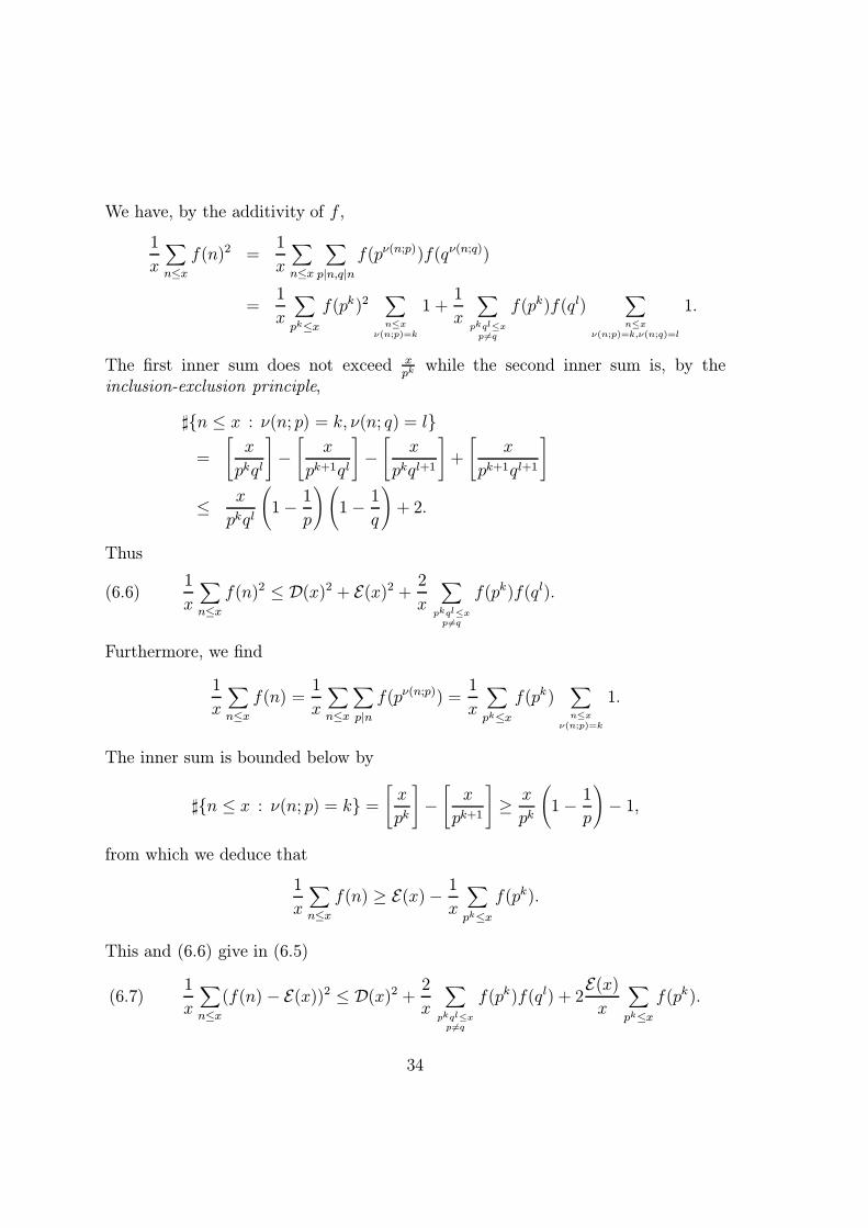
We have, by the additivity of f ,

1

x

∑n≤x

f(n)2 =1

x

∑n≤x

∑p|n,q|n

f(pν(n;p))f(qν(n;q))

=1

x

∑pk≤x

f(pk)2∑n≤x

ν(n;p)=k

1 +1

x

∑pkql≤xp6=q

f(pk)f(ql)∑n≤x

ν(n;p)=k,ν(n;q)=l

1.

The first inner sum does not exceed xpk

while the second inner sum is, by theinclusion-exclusion principle,

]n ≤ x : ν(n; p) = k, ν(n; q) = l

=

[x

pkql

]−

[x

pk+1ql

]−

[x

pkql+1

]+

[x

pk+1ql+1

]

≤x

pkql

(1−

1

p

)(1−

1

q

)+ 2.

Thus

1

x

∑n≤x

f(n)2 ≤ D(x)2 + E(x)2 +2

x

∑pkql≤xp6=q

f(pk)f(ql).(6.6)

Furthermore, we find

1

x

∑n≤x

f(n) =1

x

∑n≤x

∑p|n

f(pν(n;p)) =1

x

∑pk≤x

f(pk)∑n≤x

ν(n;p)=k

1.

The inner sum is bounded below by

]n ≤ x : ν(n; p) = k =

[x

pk

]−

[x

pk+1

]≥

x

pk

(1−

1

p

)− 1,

from which we deduce that

1

x

∑n≤x

f(n) ≥ E(x)−1

x

∑pk≤x

f(pk).

This and (6.6) give in (6.5)

1

x

∑n≤x

(f(n) − E(x))2 ≤ D(x)2 +2

x

∑pkql≤xp6=q

f(pk)f(ql) + 2E(x)

x

∑pk≤x

f(pk).(6.7)

34

Note that the quadratic term E(x)2 is cancelled. By the Cauchy-Schwarz in-equality, we obtain

E(x) ≤∑pk≤x

f(pk)

pk2

· pk2 ≤ D(x)

∑pk≤x

p−k

12

,

∑pk≤x

f(pk) =∑pk≤x

f(pk)

pk2

· p−k2 ≤ D(x)

∑pk≤x

pk

12

,

∑pkql≤xp6=q

f(pk)f(ql) =∑

pkql≤xp6=q

f(pk)

pk2

f(ql)

ql2

· pk2 q

l2 ≤ D(x)2

∑pkql≤xp6=q

pkql

12

.

This gives in (6.7)

1

x

∑n≤x

(f(n) − E(x))2 ≤(

1 +1

2ε(x)

)D(x)2,(6.8)

which is even stronger than the estimate (6.2) in the theorem (by a factor of 2).Now assume that f is real-valued but takes values of both signs. Then we

introduce the functions f± defined by

f±(pk) = max±f(pk), 0.

Obviously, f = f+−f−. Since f+f− vanishes identically, we have f2 = (f+)2+(f−)2,and we obtain for 1 ≤ n ≤ x

D(x; f)2 = D(x; f+)2 +D(x; f−)2,

(f(n)− E(x; f))2 = (f+(n)− E(x; f+)− (f−(n)− E(x; f−)))

≤ 2(f+(n) − E(x; f+))2 + 2(f−(n)− E(x; f−))2.

Thus, an application of the previous estimate (6.8) gives (6.2).Finally, when f is complex-valued, then an application of the above estimate to

the real part and the imaginary parts of f seperately yield (6.2). The theorem isproved. •

In 1983 Kubilius [19] showed that the constant 2 in the Turan-Kubilius in-equality can be replaced by 3

2+o(1), and also that this is optimal. On the other side,

the corresponding probabilistic model gives an upper estimate with the constant 1,which shows not only the similarity but also the discrepancy between probabilisticnumber theory and probability theory; for details see [30], §III.4.

35

Exercise 6.2 Deduce from the Turan-Kubilius inequality, for sufficiently largex, the estimate

1

x

∑n≤x

|f(n)−A(x)|2 ≤ 6D(x)2 , where A(x) :=∑pk≤x

f(pk)

pk.

(Hint: use the Cauchy-Schwarz inequality.)

In the following chapter we shall derive from the Turan-Kubilius inequalitythe celebrated Hardy-Ramanujan result (1.3) mentioned in the introduction.

36

Chapter 7

The theorem of Hardy-Ramanujan

The expectation of an arithmetic function f is a good candidate for a normal orderof f . The Turan-Kubilius inequality gives a sufficient condition for f(n) to havenormal order E(n; f) ≈ En(f).

Theorem 7.1 Let f be an additive arithmetic function. If

D(N) = o(E(N)),

as N →∞, then E(n) is a normal order for f(n).

Proof. Using the Cauchy-Schwarz inequality, we obtain for√N < n ≤ N

|E(N) − E(n)| =

∣∣∣∣∣∣∑

n<pk≤N

f(pk)

pk

(1−

1

p

)∣∣∣∣∣∣ ∑√N<p≤N

p−k∑pk≤N

|f(pk)|2

pk

12

.

Using Lemma 5.4, we find

∑√N<p≤N

1

pk=

∑√N<p≤N

1

p+O(1) = log logN − log log

√N +O(1) 1,

which gives above |E(N) − E(n)| D(N). Since the right hand side is under theassumption of the theorem = o(E(N)), it follows that E(n) = E(N)(1 + o(1)) for alln ≤ N except at most o(N). To prove the assertion of the theorem we may use theTuran-Kubilius inequality to estimate, for any ε > 0,

νNn : |f(n) − E(N)| > ε|E(N)| <1

N

∑n≤N

∣∣∣∣∣f(n)− E(N)

εE(N)

∣∣∣∣∣2

∣∣∣∣∣ D(N)

εE(N)

∣∣∣∣∣2

,

37

which is = o(1) by assumption. The theorem is proved. •

Now we apply our results to the prime divisor counting function ω(n). In viewto Theorem 5.2 and Corollary 5.4 (resp. Exercise 6.1):

E(N ;ω) = log logN +O(1) and D(N ;ω)2 = log logN +O(1).

The Turan-Kubilius inequality yields Turan’s estimate (1.4): since ω(n) is non-negative, we may use (6.8) to obtain

1

N

∑n≤N

(ω(n)− log logN)2 ≤ log logN +O(1).

Further, Theorem 7.1 gives the normal order of ω(n), and we obtain immediatelythe following improvement of (1.3):

Theorem 7.2 (Hardy+Ramanujan, 1917; Turan, 1934) For any ξ(N) →∞,

νNn : |ω(n)− log logN | > ξ(N)√

log logN ξ(N)−2,

anddn : |ω(n) − log logn| > ξ(N)

√log logN = 0.

In particular, log logn is a normal order of ω(n).

It is easy to do the same for Ω(n).

Exercise 7.1 (i) Show that, for any ξ(N)→∞,

νNn : |Ω(n) − log logN | > ξ(N)√

log logN ξ(N)−2,

and deduce that Ω(n) has normal order log logn;

(ii) calculate EN(Ω) and VN(Ω), and compare these values with E(N ; Ω) andD(N ; Ω)2.

We continue our discussion on the value distribution of the divisor functionstarted in Chapter 5. In view to (5.5) we get as an immediate consequence of theHardy-Ramanujan results on ω(n) and Ω(n)

Corollary 7.3 We have

τ (n) = (logn)log 2+o(1) almost everywhere.

In particular, log τ (n) has normal order log 2 · log logn.

38

That means that the divisor function τ (n) has a normal order different to its averageorder log n. This is caused by some extraordinary large values of τ (n).

We say that an arithmetic function f has maximal order g if g is a positivenon-decreasing arithmetic function such that

lim supn→∞

f(n)

g(n)= 1,

and we say that f has minimal order g if g is a positive non-decreasing arithmeticfunction such that

lim infn→∞

f(n)

g(n)= 0.

In (1.1) we have seen that the identity n 7→ n is both a minimal and a maximalorder for Euler’s ϕ-function.

Theorem 7.4 A maximal order for log τ (n) is log 2·lognlog logn

.

Proof. By the multiplicativity of τ (n) (see Exercise 4.3),

τ (n) =∏p|n

(1 + ν(n; p)) ≤∏p≤xp|n

(1 + ν(n; p))∏p>xp|n

2ν(n;p)

≤

(1 +

log n

log 2

)x∏p|n

pν(n;p)

log 2log x

≤ exp

(x(2 + log logn) +

log 2 · log n

log x

).

The choice x = logn(log logn)3 yields

τ (n) ≤ exp

(log 2 · logn

log logn

(1 +O

(log log log n

log logn

))).

This shows that

lim supn→∞

log τ (n) ·log logn

log 2 · logn≤ 1.

In order to prove that the above lim sup is also ≥ 1 we have a look on integers withmany prime divisors. Denote by pj the jth prime number (ordered with respect totheir absolute value), and define nk =

∏kj=1 pj for k ∈ N. Then τ (nk) = 2k, and

log nk =k∑j=1

log p ≤ k log pk.

39

Since by Exercise 5.4

pk ϑ(pk) =k∑j=1

log pj = log nk,

where the implicit constant does not depend on k, we obtain

log τ (nk) = k · log 2 ≥log 2 · log nk

log pk≥

log 2 · log nklog lognk

(1 +O

(1

log lognk

)).

This shows the theorem. •

Via (5.5) Theorem 7.4 has also an effect on the prime divisor counting functions(answering one question posed in Exercise 1.2):

Exercise 7.2 Show that

(i) ω(n) has maximal order lognlog logn

;

(ii) Ω(n) has maximal order lognlog 2

.

The value distribution of the divisor function is ruled by the arcsine law.

Theorem 7.5 (Deshouillers+Dress+Tenenbaum, 1979) Uniformly for x ≥2, 0 ≤ z ≤ 1,

1

x

∑n≤x

1

τ (n)

∑d|nd≤nz

1 =2

πarcsin

√z +O

((log x)−

12

).

Rewriting the asymptotic formula of the theorem, we have

1

x

∑n≤x

νnd|n : d ≤ nz =2

πarcsin

√z +O

((log x)−

12

).

This shows that, on average, an integer has many small (resp., many large) divisors!This can be proved by the Selberg-Delange method, which we shall derive inChapter 15. Nevertheless, the proof is beyond the scope of this course; the interestedreader can find a detailed proof of this result in [30], §II.5, II.6.

40

Chapter 8

A duality principle

The Turan-Kubilius inequality has an interesting dual variant.

Theorem 8.1 (Elliott, 1979) The inequality

∑pk≤N

pk

∣∣∣∣∣∣∣∑n≤N

k=ν(n;p)

xn −1

pk

(1−

1

p

) ∑n≤N

xn

∣∣∣∣∣∣∣2

≤ (2 + o(1))N∑n≤N

|xn|2

holds uniformly for all N , and complex numbers xn, 1 ≤ n ≤ N .

This theorem has several nice consequences as, for example, in the theory ofquadratic residues. Let p be an odd prime, and assume that a ∈ Z is not divis-ible by p. Then we say that a is a quadratic residue mod p, if the congruenceX2 ≡ a mod p is soluble; otherwise, a is called quadratic non-residue. Elliott

proved for the least pair of consecutive quadratic non-residues modp, the upperbound

p14(1−1

2exp(−10))+ε,

where p ≥ 5, and the implicit constant does not depend on p. For details andmuch more on dual versions of the Turan-Kubilius inequality, as for exampletheir appearance in the theory of the large sieve, see [6], §4.

For the proof of Theorem 8.1 we will make use of

Lemma 8.2 (Duality principle) Let (cnr) be an N ×R matrix with complex en-tries, and let C be an arbitrary positive constant. Then the following three inequal-ities are equivalent:

41

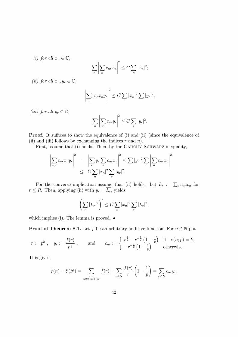
(i) for all xn ∈ C, ∑r

∣∣∣∣∣∑n

cnrxn

∣∣∣∣∣2

≤ C∑n

|xn|2;

(ii) for all xn, yr ∈ C, ∣∣∣∣∣∑n,r

cnrxnyr

∣∣∣∣∣2

≤ C∑n

|xn|2∑r

|yr|2;

(iii) for all yr ∈ C, ∑n

∣∣∣∣∣∑r

cnryr

∣∣∣∣∣2

≤ C∑r

|yr|2.

Proof. It suffices to show the equivalence of (i) and (ii) (since the equivalence of(ii) and (iii) follows by exchanging the indices r and n).

First, assume that (i) holds. Then, by the Cauchy-Schwarz inequality,∣∣∣∣∣∑n,r

cnrxnyr

∣∣∣∣∣2

=

∣∣∣∣∣∑r

yr∑n

cnrxn

∣∣∣∣∣2

≤∑r

|yr|2∑r

∣∣∣∣∣∑n

cnrxn

∣∣∣∣∣2

≤ C∑n

|xn|2∑r

|yr|2.

For the converse implication assume that (ii) holds. Let Lr :=∑n cnrxn for

r ≤ R. Then, applying (ii) with yr = Lr, yields(∑r

|Lr|2

)2

≤ C∑n

|xn|2∑r

|Lr|2,

which implies (i). The lemma is proved. •

Proof of Theorem 8.1. Let f be an arbitrary additive function. For n ∈ N put

r := pk , yr :=f(r)

r12

, and cnr :=

r12 − r−

12

(1− 1

p

)if ν(n; p) = k,

−r−12

(1− 1

p

)otherwise.

This gives

f(n)− E(N) =∑r|n

n6≡0 mod pr

f(r) −∑r≤N

f(r)

r

(1−

1

p

)=∑r≤N

cnryr.

42

Thus, we can rewrite the Turan-Kubilius inequality (6.2) as

∑n≤N

∣∣∣∣∣∣∑r≤N

cnryr

∣∣∣∣∣∣2

≤ (2 + o(1))N∑r≤N

|yr|2.

Since the yr are arbitrary complex numbers, application of Lemma 8.2 shows thatthe inequality ∑

r≤N

∣∣∣∣∣∣∑n≤N

cnrxn

∣∣∣∣∣∣2

≤ (2 + o(1))N∑n≤N

|xn|2

holds for arbitrary complex numbers xn. In view to the definition of the cnr theassertion of the theorem follows. •

We conclude with an interesting interpretation of the dual form of the Turan-

Kubilius inequality: since

∑pk≤N

pk ≈N2

logNand

1

pk

(1−

1

p

)≈ νNn : ν(n; p) = k,

we may deduce that every sufficiently dense sequence of integers xn is well distributedamong the residue classes n ≡ 0 mod pk.

For deeper knowledge on the value distribution of arithmetic functions we haveto recall some facts from the beginnings of analytic number theory. The reader whois familiar with these fundamentals may jump to Chapter 10.

43

Chapter 9

Dirichlet series and Euler

products

In probability theory many information on random variables can be derived bystudying their generating functions. The same concept applies to number theory aswell (and has even its origins there).

We write s = σ+it with σ, t ∈ R and i :=√−1, and associate to every arithmetic

function f : N→ C its Dirichlet series

∞∑n=1

f(n)

ns;

here ns is defined by ns = exp(s·logn). The prototype of such series is the Riemann

zeta-function (2.7). First, we consider these series only as formal objects. Withthe usual addition and multiplication of series the set of Dirichlet series forma commutative ring isomorphic to the ring of arithmetic functions R, where themultiplication is the convolution

(f ∗ g)(n) :=∑d|n

f(d)g(n

d

),

and where the addition is given by superposition.

Exercise 9.1 (i) Prove the identities

∞∑n=1

µ(n)

ns=

1

ζ(s),

∞∑n=1

ϕ(n)

ns=ζ(s− 1)

ζ(s)and

∞∑n=1

σα(n)

ns= ζ(s)ζ(s− α);

44

(ii) verify that the set of arithmetic functions R is a commutative ring with (mul-tiplicative) identity

η(n) :=

1 if n = 1,0 if n 6= 1;

(iii) show that an arithmetic function f is a unit in the ring R if and only iff(1) 6= 0;

(iv) let ε(n) := 1, n ∈ N, and prove for f and F := f ∗ ε ∈ R the Mobius

inversion formula: f = F ∗ µ.

In the case of Dirichlet series with multiplicative coefficients we obtain a prod-uct representation, the so-called Euler product.

Lemma 9.1 Assume that∑∞n=1 |f(n)| < ∞. If f(n) is a multiplicative arithmetic

function, then∞∑n=1

f(n) =∏p

(1 + f(p) + f(p2) + . . .),

and if f is completely multiplicative, then∞∑n=1

f(n) =∏p

1

1− f(p).

The well-known formula (2.7) is here the standard example. We may extend thisfor z ∈ C, z 6= 0, and σ > 1, which leads to

ζ(s)z =∏p

(1−

1

ps

)−z=∞∑n=1

τz(n)

ns,(9.1)

where τz(n) is the multiplicative function given by τz(1) = 1 and

τz(pk)

=

(z + k − 1

k

):=

1

k!

k∏j=1

(z + k − j);

this is an immediate consequence of the binomial series expansion in the factors ofthe Euler product.

In view to later applications we introduce two more Euler products. Let z ∈ Cwith 0 < |z| ≤ 1. Since ω(n) is additive, the arithmetic function zω(n)

nsis multiplica-

tive, and therefore a simple calculation shows

L(s, z, ω) :=∞∑n=1

zω(n)

ns=∏p

(1 +

∞∑k=1

z

ps

)=∏p

(1 +

z

ps − 1

),(9.2)

where all series and product representations are valid in the half plane σ > 1 (weshall return to the question of convergence later on).

45

Exercise 9.2 Let z ∈ C with 0 < |z| ≤ 1. Prove, for σ > 1,

L(s, z,Ω) :=∞∑n=1

zΩ(n)

ns=∏p

(1−

z

ps

)−1

.(9.3)

Proof of Lemma 9.1. By the multiplicativity of f(n) and the unique primefactorization of the integers,∏

p≤x

(1 + f(p) + f(p2) + . . .) =∑n

p|n⇒p≤x

f(n).

Since ∣∣∣∣∣∣∣∞∑n=1

f(n) −∑n

p|n=⇒p≤x

f(n)

∣∣∣∣∣∣∣ ≤∑n>x

|f(n)|,

the convergence of∑∞n=1 |f(n)| implies the first assertion; the second follows in view

to f(pk) = f(p)k and application of the formula for the geometric series. •

We can obtain new insights on the value distribution of an arithmetic functionby studying the associated Dirichlet series as an analytic function. Since

|ns| = |nσ exp(it logn)| = nσ,

Dirichlet series converge in half planes; it is possible that this half plane is empty,or that it is the whole complex plane.

Theorem 9.2 Suppose that the series∑∞n=1

f(n)nc

converges for some c ∈ R. Thenthe Dirichlet series

F (s) :=∞∑n=1

f(n)

ns

converges for any δ > 0 uniformly in

Hδ :=s ∈ C : | arg(s− c)| ≤

π

2− δ

.

In particular, the function F (s) is analytic in the half plane σ > c.

Proof. Let s ∈ Hδ. Partial summation shows, for 0 ≤M < N ,∑M<n≤N

f(n)

ns=

∑M<n≤N

f(n)

nc · ns−c

= N c−s∑

M<n≤N

f(n)

nc+ (s− c)

∫ N

M

∑M<n≤x

f(n)

ncdx

xs+1−c.

46

By the convergence of∑∞n=1

f(n)nc

, there exists for any ε > 0 an index M0 such that∣∣∣∣∣∣∑

M<n≤N

f(n)

nc

∣∣∣∣∣∣ < ε for all M ≥M0.

Hence, for those M ,

∑M<n≤N

f(n)

ns ε

(N c−σ + |s− c|

∫ N

Mxc−σ−1 dx

)

ε

(N c−σ +

|s− c|

σ − cM c−σ

) ε

(1 +

1

sin δ

),

since |s − c| < (σ − c) sin δ. This proves the uniform convergence (by fixed δ).Weierstrass’ theorem states that the limit F (s) of the uniform convergent se-

quence of analytic functions∑n≤M

f(n)ns

, as M → ∞, is analytic itself (see [21],§V.1). This proves the theorem. •

Exercise 9.3 Assume that the series∑∞n=1

f(n)ns

converges exactly in the (non-empty) half plane σ > c. Show that the series converges absolutely for σ > c+ 1.

The proof of Theorem 9.2 yields, in the region of absolute convergence,

∞∑n=1

f(n)

ns= s

∫ ∞1

∑n≤x

f(n)dx

xs+1(9.4)

(this should be compared with Exercise 2.4); here and in the sequel we write∫∞

for limT→∞∫ T when the limit exists. We are interested in an inversion, i.e. a for-

mula where the transform∑n≤x f(n) is expressed by an integral over the associated

Dirichlet series∑∞n=1

f(n)ns

.

Lemma 9.3 Let c and y be positive and real. Then

1

2πi

∫ c+i∞

c−i∞

ys

sds =

0 if 0 < y < 1,12

if y = 1,1 if y > 1.

Proof. First, if y = 1, then the integral in question equals

1

2π

∫ ∞−∞

dt

c+ it=

1

πlimT→∞

∫ T

0

c

c2 + t2dt =

1

πlimT→∞

arctanT

c=

1

2,

by well-known properties of the arctan-function.

47

Secondly, assume that 0 < y < 1 and r > c. Since the integrand is analytic inσ > 0, Cauchy’s theorem implies, for T > 0,∫ c+iT

c−iT

ys

sds =

∫ r−iT

c−iT+∫ r+iT

r−iT+∫ c+iT

r+iT

ys

sds.

It is easily be shown that∫ c±iT

r±iT

ys

sds

1

T

∫ c

ryσ dσ

yc

T | log y|,∫ r+iT

r−iT

ys

sds

yr

r+ yr

∫ T

1

dt

t yr

(1

r+ logT

).

Sending now r and then T to infinity, the first case follows.Finally, if y > 1, then we bound the corresponding integrals over the rectangular

contour with corners c± iT,−r± iT , analogously. Now the pole of the integrand ats = 0 with residue

Res s=0ys

s= lim

s→0s ·

ys

s= 1

gives via the calculus of residues 2πi as the value for the integral in this case. •

Exercise 9.4 Prove

(i) for α ∈ R, ∫ ∞−∞

exp(iαu)− exp(−iαu)

iudu = sgn (α)2π,

where sgn (α) = 0 if α = 0, and = α|α| otherwise;

(Hint: shift the path of integration into the right half plane by use of Cauchy’stheorem, and apply Lemma 9.3.)

(ii) for α > 0, ∫ ∞−∞

(sinαu

αu

)2

du =π

α.

(Hint: partial summation and part (i).)

We deduce from Lemma 9.3

Theorem 9.4 (Perron’s formula) Suppose that the Dirichlet series∑∞n=1

f(n)ns

converges for σ = c absolutely. Then, for x 6∈ Z,

∑n≤x

f(n) =1

2πi

∫ c+i∞

c−i∞

∞∑n=1

f(n)

nsxs

sds,(9.5)

48

and, for arbitrary x,∫ x

0

∑n≤u

f(n) du =1

2πi

∫ c+i∞

c−i∞

∞∑n=1

f(n)

nsxs+1

s(s+ 1)ds.(9.6)

Perron’s formula gives a first glance on the intimate relation between arithmeticfunctions (number theory) and their associated Dirichlet series (analysis).

Proof. Obviously, the integral in formula (9.5) equals

∫ c+i∞

c−i∞

∞∑n=1

f(n)

nsxs

sds =

∞∑n=1

f(n)∫ c+i∞

c−i∞

(x

n

)s ds

s;

here interchanging integration and summation is allowed by the absolute convergenceof the series. In view to Lemma 9.4 formula (9.5) follows.

In order to prove formula (9.6) we apply (9.5) with f(n)nw, w ≥ 0, instead off(n), and obtain

∑n≤x

f(n)nw =1

2πi

∫ c+i∞

c−i∞

∞∑n=1

f(n)

nsxs+w

s+ wds.

Thus we get by subtraction

∑n≤x

f(n)(xw − nw) =1

2πi

∫ c+i∞

c−i∞

∞∑n=1

f(n)

nswxs+w

s(s+ w)ds.

Obviously, this formula holds for x ∈ N too. We set w = 1, and note∫ x

0

∑n≤u

f(n) du =∑n≤x

f(n)∫ x

ndu =

∑n≤x

f(n)(x− n).

Thus we obtain (9.6), and the theorem is shown. •

As an immediate application we note, for 0 < |z| ≤ 1 and c > 1,∫ x

0

∑n≤u

zω(n) du =1

2πi

∫ c+i∞

c−i∞L(s, z, ω)

xs+1

s(s+ 1)ds;(9.7)

a similar formula holds when we replace ω(n) by Ω(n). Later we shall prove anasymptotic formula for the arithmetic expression on the left hand side by evaluatingthe analytic right hand side.

49

Chapter 10

Characteristic functions

Many information on a probability law can be derived by studying the related charac-teristic function. Let F be a distribution function, then its characteristic functionis given by the Fourier transform of the Stieltjes measure dF(z), namely

ϕF(τ ) :=∫ ∞−∞

exp(iτz) dF(z).

This defines a uniformly continuous function on the real line which satisfies, forτ ∈ R,

|ϕF(τ )| ≤∫ ∞−∞

dF(z) = 1 = ϕF(0).

The intimate relationship between the distribution function F and its characteristicfunction ϕF is ruled by the following

Lemma 10.1 (Inversion formula) Let F be a distribution function with charac-tersitic function ϕF. Then, for α, β ∈ C(F),

F(β)−F(α) =1

2π

∫ ∞−∞

exp(−iτα)− exp(−iτβ)

iτϕF(τ ) dτ.

In particular, the distribution function is uniquely determined by its charcteristicfunction.

Note that the singularity of the integrand in the formula of the above lemma isremovable.

Proof. Without loss of generality α ≤ β. Using Fubini’s theorem, we can rewritethe integral on the right hand side of the formula in the lemma as∫ ∞

−∞

exp(−iτα)− exp(−iτβ)

iτ

∫ ∞−∞

exp(iτw) dF(w) dτ

50

=∫ ∞−∞

∫ ∞−∞

exp(iτ (w − α))− exp(iτ (w − β))

iτdτ dF(w).

By Exercise 9.4 the inner integral equals

1

2

∫ ∞−∞

exp(iu(w − α))− exp(−iu(w − α))

iudu

−1

2

∫ ∞−∞

exp(iu(w − β))− exp(−iu(w− β))

iudu

= π(sgn (w − α) − sgn (w − β)),

which is = 2π if α < w < β, and = 0 if w < α or w > β. This leads to the formulain the lemma. If the distribution function G has the same characteristic function,then the formula proved above yields F(α) = G(α) for almost all α. Since F and Gboth are right-continuous and non-decreasing, we finally obtain F = G. The lemmais shown. •

This lemma has some powerful consequences which we will use in what follows.

Exercise 10.1 Let h > 0 and let F be a distribution function with characteristicfunction ϕF.

(i) Prove, for z ∈ R,

1

h

∫ z+h

z−∫ z

z−h

F(t) dt =

1

2π

∫ ∞−∞

(sin τ

2τ2

)2

exp(−iτz

h

)ϕF

(τ

h

)dτ ;

(Hint: apply Lemma 10.1 to the integrals on the left hand side, and calculatetheir characteristic functions by partial integration.)

(ii) show that1

h

∫ z+h

zF(t) dt and

1

h

∫ z

z−hF(t) dt

both define distribution functions.(Hint: for all ε > 0 there exists an t0 such that F (t) ≥ F (+∞) − ε for allt ≥ t0.)

It is time to give an example. We note for the standard normal distribution(3.1):

Lemma 10.2 The characteristic function of the standard normal distribution Φ isgiven by

ϕΦ(τ ) = exp

(−τ 2

2

).

51

Proof. By definition,

ϕΦ(τ ) =∫ ∞∞

exp(iτz) dΦ(z) =1√

2π

∫ ∞−∞

exp(iτz) exp

(−z2

2

)dz

=1√

2π

∫ ∞−∞

(cos(τz) + i sin(τz)) exp

(−z2

2

)dz

=1√

2π

∫ ∞−∞

cos(τz) exp

(−z2

2

)dz,

since sin(τz) exp(− z2

2) is an odd function. Differentiation on both sides with re-

spect to τ (which is obviously allowed), and integration by parts (with sin(τz) andz exp(− z2

2)), yields

ϕΦ′(τ ) = −

1√

2π

∫ ∞−∞

z sin(τz) exp

(−z2

2

)dz

= −1√

2π

∫ ∞−∞

τ cos(τz) exp

(−z2

2

)dz

= −τϕΦ(τ ).

Therefore, the characteristic function ϕΦ(τ ) solves the differential equation

y′

y= −τ,

and hence, integration yields

log |ϕΦ(τ )| =∫ ϕ′ΦϕΦ

(τ ) dτ + c′ = −∫τ dτ + c′ = −

τ 2

2+ c,

where c′, c are constants. Taking the exponential gives

ϕΦ(τ ) = exp

(c−

τ 2

2

).

In view to ϕΦ(0) = 1 we obtain c = 0, which finishes the proof. •

The proof above is not straightforward but elementary. It is much easier to find thecharacteristic function of the uniform distribution.

Exercise 10.2 Prove that the characteristic function of the uniform distribution νon the interval [0, 1] is given by

ϕν(τ ) =exp(iτ )− 1

iτ.

52

The following theorem links the weak convergence of a sequence of distribu-tion functions to the pointwise convergence of the corresponding sequence of theircharacteristic functions.

Theorem 10.3 (Levy’s continuity theorem, 1925) Let Fn be a sequence ofdistribution functions and ϕFn the corresponding sequence of their charactersiticfunctions. Then Fn converges weakly to a distribution function F if and only if ϕFn

converges pointwise on R to a function ϕ which is continuous at 0. Additionally,in this case, ϕ is the characteristic function of F, and the convergence of ϕFn toϕ = ϕF is uniform on any compact subset.

The following proof is due to Cramer.

Proof. We start with the necessity. If Fn converges weakly to F, then there existsfor any ε > 0 a real number T = T (ε) such that

supn∈N

supτ∈R

∣∣∣∣∣∫|z|>T

exp(iτz) dFn(z)

∣∣∣∣∣ ≤ supn∈N

∫|z|>T

dFn(z) ≤ ε.

Without loss of generality we may assume that ±T ∈ C(F), then∫ T

−Texp(iτz) dFn(z)→

∫ T

−Texp(iτz) dF(z),

in any finite τ -interval, as n→∞ (Stieltjes integrals behave sufficiently smooth).The last integral equals ϕF(τ ) + O(ε), which implies that ϕFn → ϕF uniformly onany compact subset, as n→∞.

To prove the converse, it is sufficient to show that, if ϕFn converges pointwise toa limit ϕ, and if ϕ is continuous at 0, then Fn converges weakly to a distributionfunction F. By the above given part of the proof it will then follow that ϕ is thecharacteristic function of F, and that the convergence ϕFn → ϕF, as n → ∞, isuniform on compact subsets.

Let Z := z1, z2, . . . be a dense subset of R consisting of continuity points ofF and all Fn. Since the values of Fn(zk) lie in [0, 1], the theorem of Bolzano-

Weierstrass yields the existence of a convergent subsequence Fn1(z1), and, bya standard diagonal argument, there exists a sub-subsequence Fnn of Fn whichconverges on Z. Using the properties of the distribution functions Fn, one caneven find a subsequence Fnj

which converges weakly to a non-decreasing right-continuous function F. Obviously, 0 ≤ F(z) ≤ 1 for all z ∈ R. It remains to showthat F(+∞)−F(−∞) = 1. We have, by Exercise 10.1,

1

h

∫ h

0−∫ 0

−h

Fnj

(t) dt =1

2π

∫ ∞−∞

(sin τ

2τ2

)2

ϕFnj

(τ

h

)dτ.

53

Sending j →∞ and applying Lebesgue’s theorem, we arrive at

1

h

∫ h

0−∫ 0

−h

F(t) dt =

1

2π

∫ ∞−∞

(sin τ

2τ2

)2

ϕ(τ

h

)dτ ;

here F is the weak limit of Fnj, and ϕ is the pointwise limit of ϕFnj

. By Exercise10.1, we may interpret the left hand side as the difference of distribution functions.Hence, as h→∞,

F(+∞)− F(−∞) = limh→∞

1

2π

∫ ∞−∞

(sin τ

2τ2

)2

ϕ(τ

h

)dτ.

Since ϕ is bounded and continuous at 0, we may interchange by Lebesgue’s theoremthe limit with the integration and use Exercise 9.4 to obtain

F(+∞)− F(−∞) =1

2π

∫ ∞−∞

(sin τ

2τ2

)2

limh→∞

ϕ

(τ

h

)dτ

= ϕ(0) ·1

2π

∫ ∞−∞

(sin τ

2τ2

)2

dτ

= ϕ(0).

Further, ϕ(0) = limn→∞ ϕFnj(0), and ϕFnj

(0) = 1 for all n ∈ N. Therefore, F(+∞)−

F(−∞) = 1, and the weak limit F of the sequence Fnjis a distribution function.

Obviously, this holds also for any other weak limit G. But since G has also thecharacteristic function ϕ, and distribution functions are uniquely determined bytheir characteristic functions, we obtain F = G. Hence any weakly convergentsubsequence of Fn converges to the same limit F, and hence, Fn itself convergesweakly to F. The theorem is shown. •

For a special class of distribution functions F one can find a quantative estimatefor approximations of F in terms of the corresponding characteristic functions bythe following result. Define for a real-valued function f , given on the compact setR ∪ ±∞,

‖f‖∞ = max−∞≤x≤∞

|f(x)|.

Then

Theorem 10.4 (Berry-Esseen inequality, 1941/1945) Let F,G be two distri-bution functions with characteristic functions ϕF, ϕG. Suppose that G is differen-tiable and that G′ is bounded on R. Then, for all T > 0,

‖F−G‖∞ ‖G′‖∞T

+∫ T

−T

∣∣∣∣∣ϕF(τ )− ϕG(τ )

τ

∣∣∣∣∣ dτ,

54

where the implicit constant is absolute.

We omit the lengthy proof, which, for example, can be found in [30] or in [6], §1, butgive an interesting application to a result mentioned in Chapter 3. The convergenceof the scaled random walk to the normal distribution (3.2) satisfies the quantitativeestimate

P

(Zn√n< x

)= Φ(x) +O

(n−

12

),

as n→∞. For this and other applications we refer to [6], §1 and §3.

55

Chapter 11

Mean value theorems

Levy’s continuity theorem has an important consequence, namely a criterionwhether an arithmetic function possesses a limit law or not.

Corollary 11.1 Let f be a real-valued arithmetic function. Then f possesses alimit law F if and only if the sequence of functions

1

N

∑n≤N

exp(iτf(n))

converges with N →∞ pointwise on R to a function ϕ(τ ) which is continuous at 0.In this case ϕ = ϕF is the characteristic function of F.

Proof. By (3.3) the characteristic function of the distribution function FN of f is

ϕFN(τ ) =

∫ ∞−∞

exp(iτz) dFN(z) =1

N

∑n≤N

exp(iτf(n)).

Consequently, Levy’s continuity theorem translates the weak convergence of the dis-tribution functions to the pointwise convergence of the corresponding characteristicfunctions. •

If f is an additive function, then the function n 7→ exp(iτf(n)) is for each fixedτ a multiplicative arithmetic function. Thus, the problem of the existence of a limitlaw for f is equivalent to the problem of the existence of the mean value of a certainmultiplicative function. A complete solution was found by Erdos and Wintner

[8]:

56

Theorem 11.2 (Erdos+Wintner, 1939) A real-valued additive function f(n)possesses a limit law if and only if the following three series converge simultaneouslyfor at least one value R > 0:

∑|f(p)|>R

1

p,

∑|f(p)|≤R

f(p)2

p,

∑|f(p)|≤R

f(p)

p.

If this is the case, then the characteristic function of the limiting distribution functionF is given by the convergent product

ϕF(n) =∏p

(1−

1

p

)∞∑k=0

exp(iτf(pk))

pk.

The idea of proof is based on Kolmogorov’s three series theorem on sums ofindependent random variables; see [9], §IX.9.

In the following years the question arose when a multiplicative function of mod-ulus ≤ 1 has a non-zero mean value. The ultimative answer was given by Halasz

[11], namely

Theorem 11.3 (Halasz, 1968) Let g be a multiplicative function with values inthe unit disc. If there exists some τ ∈ R such that

∑p

1− Re g(p)p−iτ

p

converges, then

1

x

∑n≤x

g(n) =xiτ

1 + iτ

∏p≤x

(1−

1

p

)∞∑k=0

g(pk)

pk(1+iτ )+ o(1),

as x→∞. If there exists no τ with the above property, then

1

x

∑n≤x

g(n) = o(1).

Note that Wirsing [33] obtained a similar result for real-valued multiplicative func-tions in 1967. To indicate the power of these results note that an application toMobius’ µ-function yields ∑

n≤x

µ(n) = o(x),

which is equivalent to the prime number theorem (5.6) (for the equivalence see [30],§I.3).

57

Unfortunately, the proofs of these mean value theorems are beyond the scopeof this course, we refer the interested reader to the original papers and [30], §III.4;further mean value results can be found in [28].

A further application of characteristic functions is to find in the theory of uniformdistribution modulo 1.

58

Chapter 12

Uniform distribution modulo 1

We say that a sequence of non-negative real numbers αn is uniformly distributedmodulo 1 if for any interval I ⊂ [0, 1)

dn : αn − [αn] ∈ I = λ(I),

where λ(I) is the Lebesgue-measure of I (i.e. the length of I). This means thatthe proportion of αn, which fractional parts αn − [αn] lie in I, corresponds to theproportion of the interval I in [0, 1).

H. Weyl’s celebrated criterion on uniform distribution [32] states

Theorem 12.1 (H. Weyl; 1916) A sequence of real numbers αn is uniformly dis-tributed mod 1 if, and only if, for each non-zero integer m

limN→∞

1

N

∑n≤N

exp(2πimαn) = 0.

Proof. Assume that the sequence αn is uniformly distributed mod 1, then thecorresponding distribution functions

FN(z) =1

N

∑n≤N

αn−[αn]≤z

1

converge weakly to the uniform distribution on [0, 1], as N → ∞, and, by Levy’scontinuity theorem, the corresponding characteristic functions converge pointwiseto the characteristic function of the uniform distribution, i.e.

ϕFN(τ ) =

∫ 1

0exp(iτz) dFN(z) → ϕν(τ ) =

∫ 1

0exp(iτz) dFν(z),

59

as N →∞. Setting τ = 2πm,m 6= 0, we obtain in view to Exercise 10.2 that

1

N

∑n≤N

exp(2πimαn) =∫ 1

0exp(2πimz) dFN(z)

tends with N →∞ to∫ 1

0exp(2πimz) dz =

exp(2πim)− 1

2πim= 0.

We give only a sketch of the argument for the converse implication. For sim-plicity, we may assume that F is absolutely continuous. With a little help fromFourier analysis one can show that F has a representation

F(z) =∫ 1

0F(u) du+

∞∑m=−∞m6=0

cm − 1

2πimexp(2πimz),

where

cm :=∫ 1

0exp(−2πimz) dF(z).

Since ∫ 1

0exp(2πimz) dFN(z) =

1

N

∑n≤N

exp(2πimαn)

tends with N →∞ to zero, it follows that cm = 0 for non-zero m. This gives above

F (z) =1

2−

∞∑m=−∞m6=0

exp(2πimz)

2πim= z,

which implies the uniform distribution for αm. •

Exercise 12.1 (for experts in Fourier analysis) Fill the gaps in the sketch of proofof the converse implication above.

We note a nice application to indicate the power of this criterion.

Corollary 12.2 (Kronecker’s approximation theorem; 1884) The sequencenξ is uniformly distributed mod 1 if and only if ξ is irrational.

Proof. Let ξ be irrational. By the formula for the geometric series, we have, forany non-zero integer m,

limN→∞

1

N

∑n≤N

exp(2πimnξ) = limN→∞

1

N

exp(2πimξ)− exp(2πim(N + 1)ξ)

1− exp(2πimξ)= 0.

60

Otherwise, if ξ = ab, then the limit is non-zero for multiples m of b. Thus, Weyl’s

criterion yields the assertion of the corollary. •

Moreover, we say that the sequence αn lies dense mod 1 if for any ε > 0, andany α ∈ [0, 1), exists an αn such that

|α − (αn − [αn])| < ε.

Obviously, a sequence which is uniformly distributed mod 1 lies also dense mod 1.However, the converse implication is not true in general.

Exercise 12.2 Show that the sequence logn

(i) lies dense mod 1;(Hint: consider the subsequence log(2k).)

(ii) is not uniformly distributed mod 1.(Hint: replace the sum in Theorem 12.1 by the corresponding integral.)

An interesting open problem is whether the sequence exp(n) is uniformly dis-tributed or not. A further application of uniform distribution modulo 1 is numericalintegration. The interested reader can find more details on this and allied topics in[15].

61

Chapter 13

The theorem of Erdos-Kac

Now we are going to prove the explicit form (1.5) of the limit distribution of theprime divisor counting functions ω(n) and Ω(n). The easiest and first proof dueto Erdos and Kac [7] is elementary but tricky and quite delicate. We will give aproof more or less following the one of Renyi and Turan [24], including a certainmodification due to Selberg [29], which enables one to obtain further knowledgeconcerning the speed of convergence to the normal distribution. Moreover, thismethod applies to other problems as well. For some interesting historical commentssee [6], §12, pp.18.

Let z be a non-zero complex constant of modulus ≤ 1. We shall prove in Chapter15 by analytic methods the asymptotic formula∑

n≤x

zω(n) = λ(z)x(log x)z−1 +O(x(log x)Rez−2

),(13.1)

where λ(z) is an entire function with λ(1) = 1. This implies

Theorem 13.1 (Erdos+Kac, 1939; Renyi+Turan, 1957) As N →∞,

νN

n :

ω(n)− log logN√

log logN≤ x

= Φ(x) +O

((log logN)−

12

).

Proof. We consider

FN(x) = νN

n :

ω(n)− log logN√

log logN≤ x

,

and denote by ϕFN(τ ) its characteristic function, i.e.

ϕFN(τ ) =

∫ ∞∞

exp(iτz) dFN(z) =1

N

∑n≤N

exp

(iτ (ω(n)− log logN√

log logN

).

62

By (13.1), we have, uniformly for N ≥ 2, t ∈ R,

1

N

∑n≤N

exp(itω(n)) = λ(exp(it))(logN)exp(it)−1 +O((logN)cos t−2).

Putting T :=√

log logN , and t := τT

, then the latter formual implies for |τ | ≤ T

ϕFN(τ ) =

1

N

∑n≤N

exp

(iτ (ω(n)− T 2)

T

)

= λ(exp(it)) exp((exp(it)− 1)T 2 − iτT ) +O(exp(T 2(cos t− 2))

).(13.2)

Since cos t− 1 ≤ −2( tπ)2 for |t| ≤ 1, we deduce

ϕFN(τ ) exp

(−

2τ 2

π2

);(13.3)

we shall use this estimate later for large values of τ . Since, for |t| ≤ 1,

exp(it)− 1 = it−t2

2+O(|t|3),

and since λ(z) is an entire function with λ(1) = 1, we have

λ(exp(it)) =∞∑k=0

λ(k)(1)

k!(exp(it)− 1)k = 1 +O(|t|)

for |t| ≤ 1. Therefore, we obtain in view to (13.2), for |τ | < T13 ,

ϕFN(τ ) = exp

(−τ 2

2

)(1 +O

(|τ |+ |τ |3

T

))+O

(1

logN

);(13.4)

we shall use this formula later for 1logN

≤ |τ | < T13 . Sending N →∞, we deduce in

view to Lemma 10.2 that

ϕFN(τ )→ exp

(−τ 2

2

)= ϕΦ(τ ),

i.e. the characteristic functions ϕFNconverge pointwise to the characteristic function

of the normal distribution Φ(x). Applying Levy’s continuity theorem, we get

limN→∞

νN

n :

ω(n) − log logN√

log logN≤ x

= Φ(x);

63

this is exactly Erdos’ and Kac’s formula (1.5).In order to obtain the quantitive result of the theorem we need a further estimate

of ϕFN(τ ) for small values of τ . When |τ | ≤ 1

logN, then the trivial estimate exp(iy) =

1 +O(y), y ∈ R, yields in combination with the Cauchy-Schwarz inequality

ϕFN(τ ) = 1 +O

|τ |TN

∑n≤N

|ω(n)− log logN |

= 1 +O

|τ |TN

N ∑n≤N

|ω(n)− log logN |2 1

2

,which leads in view to the Hardy-Ramanujan Theorem 7.2 to

ϕFN(τ ) = 1 +O(|τ |).(13.5)

Now we apply the Berry-Esseen inequality Theorem 10.4. In view to Lemma 10.2we get

‖FN −Φ‖∞ ‖Φ′‖∞T

+∫ T

−T

∣∣∣∣∣ϕFN(τ )− ϕΦ(τ )

τ

∣∣∣∣∣ dτ

1

T+∫ T

−T

∣∣∣∣∣ϕFN(τ )− exp

(−τ 2

2

)∣∣∣∣∣ dτ

|τ |.

We split the appearing integral into three parts, and estimate in view to (13.5),(13.4) and (13.3)∫ 1

logN

− 1logN

∫ 1

logN

− 1logN

dτ 1

logN,

∫ ±T 13

± 1logN

∫ ∞−∞

(1 + τ 2

T

)exp

(−τ 2

2

)dτ +

1

logN

∫ T13

1logN

dτ

τ

1

T,

∫ ±∞±T

13

∫ ∞T

13

exp

(−

2τ 2

π2

)dτ

τ

1

T.

This proves the theorem. •

It can be shown that the error term in Theorem 13.1 is best possible. Thisfollows by studying the frequencies of positive integers n with ν(n) = k, k ∈ N; fordetails we refer to [30], §III.4.

64

Exercise 13.1 Deduce from the asymptotic formula∑n≤x

zΩ(n) = µ(z)x(log x)z−1 +O(x(log x)Rez−2

),(13.6)

where µ(z) is an entire function with µ(1) = 1, the limit law

νN

n :

Ω(n) − log logN√

log logN≤ x

= Φ(x) +O

((log logN)−

12

),

as N →∞.

It remains to show formula (13.1). The first step towards a proof was done by(9.7) in Chapter 9. In Chapter 15 we will calculate the appearing integral by movingthe path of integration to the left of the line σ = 1. Therefore, we need an analyticcontinuation of L(s, z, ω).

However, it suffices to find a zero-free region for the Riemann zeta-function.The Euler product representation (2.7) implies immediately the non-vanishing ofζ(s) in the half plane of absolute convergence σ > 1. As we shall see in the followingchapter one can extend this zero-free region to the left.

We observe that the Euler product representation (9.2) of L(s, z, ω) is similarto (9.1). Define G(s, z) = L(s, z, ω)ζ(s)−z, then, for σ > 1,

G(s, z) =∏p

(1 +

z

ps − 1

)(1−

1

ps

)z=∞∑n=1

bz(n)

ns,(13.7)

where bz = zω ∗ τ−z is multiplicative with

bz(1) = 1 , bz(pk) = (−1)k

(z

k

)+ z

k−1∑j=0

(−1)j(z

j

).

Since bz(p) = 0, we have, for σ > 12,

logG(s, z) =∑p

log

(1 +

∞∑k=2

bz(pk)

pks

)∑p

1

p2σ 1.(13.8)

This shows thatL(s, z, ω) = G(s, z)ζ(s)z

is analytically continuable to any zero-free region of ζ(s) covering the half plane ofabsolute convergence σ > 1.

65

Chapter 14

A zero-free region for ζ(s)

To establish a zero-free region for the Riemann zeta-function to the left of the halfplane of absolute convergence of its series expansion is a rather delicate problem. Inview to (9.4) (Exercise 2.4, resp.) we have, for σ > 0,

ζ(s) =∑n≤N

1

ns+N1−s

s− 1+ s

∫ ∞N

[x]− x

xs+1dx(14.1)

=∑n≤N

1

ns+N1−s

s− 1+O

(N−σ

(1 +|s|

σ

)).(14.2)

This gives an analytic continuation of ζ(s) to the half plane σ > 0 except for asimple pole at s = 1.

Lemma 14.1 For |t| ≥ 1, 1− 12(log(|t|+ 1))−1 ≤ σ ≤ 2,

ζ(s) log(|t|+ 1) , and ζ ′(s) (log(|t|+ 1))2.

Proof. Since ns = ns, it follows that

ζ(s) =∞∑n=1

1

ns=∞∑n=1

1

ns= ζ(s)

for σ > 1, and by analytic contiunation elsewhere. Therefore, it suffices to consideronly t > 1. Let 1− (log(t+ 1))−1 ≤ σ ≤ 3, then formula (14.2) implies

ζ(s)∑

n≤t+1

1

n+

(t+ 1)1−σ

σ log(t+ 1).

66

The estimate for ζ ′(s) follows immediately from Cauchy’s formula

ζ ′(s) =1

2πi

∮ζ(z)

(z − s)2dz,

and standard estimates of integrals. •

For σ > 1,

|ζ(σ + it)| = exp

(∑p

∞∑k=1

1

kpkσcos(kt log p)

).

Since

17 + 24 cos α+ 8 cos(2α) = (3 + 4 cosα)2 ≥ 0,(14.3)

it follows that

ζ(σ)17|ζ(σ + it)|24|ζ(σ + 2it)|8 ≥ 1.(14.4)

Therefore

Lemma 14.2 ζ(1 + it) 6= 0 for t ∈ R.

Proof. For small σ > 1, ζ(σ) 1σ−1

by (14.1). Assuming that ζ(1 + it) has a zerofor t = t0 6= 0, then it would follow that

|ζ(σ + it0)| ≤ ζ(σ) σ − 1.

This leads tolimσ→1+

ζ(σ)17|ζ(σ + it0)|24 = 0,

contradicting (14.4). •

It can be shown that this non-vanishing of ζ(1 + it) is equivalent to the primenumber theorem (5.6) (see [22], §2.3.

A simple refinement of the argument in the proof of Lemma 14.2 allows a lowerestimate of ζ(1 + it): for |t| ≥ 1 and 1 < σ < 2, we deduce from (14.4) and Lemma14.1

1

|ζ(σ + it)|≤ ζ(σ)

1724 |ζ(σ + 2it)|

13 (σ − 1)−

1724 (log(|t|+ 1))

13 .

Furthermore, with Lemma 14.1,

ζ(1 + it)− ζ(σ + it) = −∫ σ

1ζ ′(u+ it) du |σ − 1|(log(|t|+ 1))2.(14.5)

67

Hence

|ζ(1 + it)| ≥ |ζ(σ + it)| − c1(σ − 1)(log(|t|+ 1))2

≥ c2(σ − 1)1724 (log(|t|+ 1))−

13 − c1(σ − 1)(log(|t|+ 1))2,

where c1, c2 are certain positive constants. Chosing a constant B > 0 such thatA := c2B

1724 − c1B > 0 and putting σ = 1 +B(log(|t|+ 1)−8, we obtain now

|ζ(1 + it)| ≥A

(log(|t|+ 1))6.(14.6)

This gives even an estimate on the left of the line σ = 1.

Lemma 14.3 There exists a positive constant δ such that

ζ(s) 6= 0 for σ ≥ 1− δmin1, (log(|t|+ 1))−8;

further, under the assumption |s− 1| ≥ 1, the estimates

ζ ′

ζ(s) (log(|t|+ 1))8 , log ζ(s) log(2 log(|t|+ 1))

hold.

Here we choose that branch of logarithm log ζ(s) which is real on the real axis; theother values are defined by analytic continuation in a standard way.

Proof. In view to Lemma 14.1 the estimate (14.5) holds for 1− δ(log(|t|+ 1))−8 ≤σ ≤ 1. Using (14.6), it follows that

|ζ(σ + it)| ≥A− c1δ

(log(|t|+ 1))6,

where the right hand side is positve for sufficiently small δ. This yields the zero-freeregion of Lemma 14.3; the estimate of the logarithmic derivative follows from theestimate above by use of Lemma 14.1. Finally, to obtain the bound for log ζ(s) lets0 = 1 + η + it with some positive parameter η. Then

log

(ζ(s)

ζ(s0)

)=∫ s

s0

ζ ′

ζ(u) du |s− s0|(log(|t|+ 1))8.

Using (14.1),

| log ζ(s0)| ≤ log ζ(1 + η) = log

(1

η

)+O(1).

68

Setting η = c(log(|t|+ 1))−8, we obtain

log ζ(s) log

(1

η

)+ |σ − 1− η|(log(|t|+ 1))8 log(2 log(|t|+ 1)).

The lemma is shown. •

Exercise 14.1 Show that (14.3) gives the best possible estimates (by the methodabove).

The famous and yet unproved Riemann hypothesis states that all complexzeros of ζ(s) lie on the so-called critical line σ = 1

2, or equivalently, the non-

vanishing of ζ(s) in the half plane σ > 12. It seems that this hypothetical distribution

of zeros is connected with the functional equation

π−s2 Γ(s

2

)ζ(s) = π−

1−s2 Γ

(1− s

2

)ζ(1− s),(14.7)

which implies a symmetry of the zeros of ζ(s) with repsect to the critical line; for aproof of (14.7) see [30], §II.3.

In fact, the first zero on the critical line (i.e. the one with minimal imaginarypart in the upper half plane) is

1

2+ i 14.13472 . . . .

Nevertheless, we show

Lemma 14.4 ζ(s) 6= 0 for |s− 1| < 1.

Proof. Integration by parts in (14.1) (resp. Euler’s summation formula) yields

ζ(s) =1

s− 1+

1

2+

s

12−s(s+ 1)

2

∫ ∞1

B2(u− [u])

us+2du,

where

B2(u) = u2 − u+1

6

is the second Bernoulli polynomial; note that |B2(u − [u])| ≤ 16. Suppose that

% = β + iγ is a zero of ζ(s) with |s− 1| ≤ 1. By symmetry, we may assume in viewto the functional equation (14.7) that β ≥ 1

2. Setting s = % in the formula above, an

application of the mean-value theorem yields the existence of some θ with |θ| ≤ 1such that

0 =1

%− 1+

1

2+

%

12−θ%(% + 1)

12

∫ ∞1

du

uβ+2du.

69

Multiplying this with 1− %, we may rewrite this as

1 =1− %

2

(1 +

%

6−θ%(% + 1)

6

∫ ∞1

du

u52

du

).(14.8)

The modulus of the right hand side is

1

2

(1 +|%|

6+|%(%+ 1)|

9

)<

1

2

(1 +

1

3+

2

3

)= 1,

which gives a contradiction to (14.8). This proves the lemma. •

In order to prove formula (13.1) we state some consequences we will use lateron. By Lemma 14.4, the function

1

s((s− 1)ζ(s))z

is analytic in |s− 1| < 1, and hence, has there a power series expansion

1

s((s− 1)ζ(s))z =

∞∑j=0

γj(z)

j!(s− 1)j ,(14.9)

where, by Cauchy’s formula,

γj(z) =j!

2πi

∮|s−1|=r

1

s((s− 1)ζ(s))z

ds

(s− 1)j+1.(14.10)

Note that the γj(z) are entire functions in z, satisfying the estimate

γj(z)

j! (1 + ε)j,

where the implicit constant depends only on z and ε ∈ (0, 1).

Exercise 14.2 Show that γ0(z) = 1,

γj(1) = (−1)j∫ ∞

1

(u− [u])(log u)j−1

u2du,

and, in particular, γ1(1) = γ − 1, where γ is the Euler-Masceroni constant.(Hint: see Exercise 5.1.)

For more details on the fascinating topic of the location of zeros of the Riemannzeta-function and its implications to number theory see [22], §2.4+2.5, as well asthe monography [23].

70

Chapter 15

The Selberg-Delange method

Our aim is to prove the asymptotic formula (13.1); the proof of (13.6) is left tothe reader. The proof bases on the Selberg-Delange method which works formore general Dirichlet series than (9.2) and (9.3) which we have to consider.This powerful method was developped by Selberg [29]; later it was generalized byDelange [3].

Theorem 15.1 There exist constants c1, c2 > 0 such that, uniformly for sufficientlylarge x,N ≥ 0, 0 < |z| ≤ 1,

∑n≤x

zω(n) = x(log x)z−1

N∑k=0

λk(z)

(log x)k+O

exp(−c1

√log x) +

(c2N + 1

log x

)N+1

with

λk(z) :=1

Γ(z − k)

∑h+j=k

γj(z)

h!j!

[dh

dshL(s, z, ω)ζ(s)−z

]s=1

,

where γj(z) is defined in (14.10).

Before we are able to start with the proof of Theorem 15.1 we quote a classicalintegral representation for the Gamma-function, which is for Re z > 0 defined by

Γ(z) =∫ ∞

0uz−1 exp(−u) du,

and by analytic continuation elsewhere except for simple poles at z = 0,−1,−2, . . .;for this and other properties of the Gamma-function, which we need later on, see[21].

71

Lemma 15.2 (Hankel’s formula) Denote by H the path formed by the circle|s| = r > 0, excluding the point s = −r, together with two copies of the half line(−∞,−r] with respective arguments ±π. Then, for any complex z,

1

Γ(z)=

1

2πi

∫Hs−z exp(s) ds.(15.1)

If H(x) denotes the part of H which is located in the half plane σ > −x, thenuniformly for x > 1

1

2πi

∫H(§)

s−z exp(s) ds =1

Γ(z)+O

((2e)π|z|Γ(1 + |z|) exp

(−x

2

)).

Proof. Obviously, the integral appearing in (15.1) is absolutely and uniformlyconvergent for all z. Hence, it defines an entire function of z, which, by the calculusof residues, does not dependent on r. When Re z < −1, the integral over the circlepart |s| = r of H tends with r to zero, and the the integral over the remaining pathtends to

1

2πi

∫ ∞0

(exp(iπz)− exp(−iπz))σ−z exp(−σ) dσ

=sinπz

π

∫ ∞0

σ−z exp(−σ) dσ =sinπz

πΓ(1− z) =

1

Γ(z);

here we used the well-known identity Γ(z)Γ(1 − z) = πsinπz

. This proves the firstformula for Re z < 1, and for arbitrary z by analytic continuation.

Now we consider the integral over the truncated contour H(x). Writing s =% exp(±iπ), we have

|s−z exp(s)| ≤ (exp(π)σ)|z| exp(−σ).

Thus,∫H−∫H(§)

s−z exp(s) ds exp(π|z|)

∫ ∞x

%|z| exp(−%) d%

≤ exp(π|z| −

x

2

) ∫ x

0%|z| exp

(−%

2

)d%.

Changing the variable % = 2t yields the estimate of the lemma. •

Now we are able to give the

Proof of Theorem 15.1. In view to our observations on the function G(s, z),defined by (13.7), in Chapter 13, it came out that L(s, z, ω) = G(s, z)ζ(s)z can be

72

analytically continued to any zero-free region of ζ(s) covering the half plane σ > 1.Hence Lemma 14.3 implies that L(s, z, ω) is analytic in the region

σ ≥ 1− δmin1, (log(|t|+ 1))−8,(15.2)

where δ is some small positive constant. Furthermore, using (13.8), L(s, z, ω) satis-fies there the estimate

L(s, z, ω) = G(s, z) exp(z log ζ(s)) (|t|+ 1)ε.

Hence, setting c := 1 + 1log x

, we find∫ c±i∞

c±iTL(s, z, ω)

xs+1

s(s+ 1)ds x1+c

∫ ∞T

tε−2 dt x2T ε−1.

Therefore, we can deduce from (9.7)∫ x

0

∑n≤u

zω(n) du =1

2πi

∫ c+iT

c−iTL(s, z, ω)

xs+1

s(s+ 1)ds+O

(x2T ε−1

).(15.3)

Now denote by C the path (symmetrical with respect to the real axis) consistingof the truncated Hankel contour H(r) surrounding the point s = 1 with radiusr = 1

2(log x)−1, linear parts joining 1− r to 1− 1

2δ, the arcs A±

σ = σ(t) := 1−δ

2min1, (log(|t|+ 1))−8,

and the linear segments [σ(T ) ± iT, c ± iT ]. Here, let x be sufficiently large suchthat C is contained in the region (15.2). Applying Cauchy’s theorem, we obtain∫ c+iT

c−iTL(s, z, ω)

xs+1

s(s+ 1)ds =

∫CL(s, z, ω)

xs+1

s(s+ 1)ds,

since the integrand is analytic in (15.2). Obviously,∫ κ±iT

σ(T )±iTL(s, z, ω)

xs+1

s(s+ 1)ds x2T ε−2,

∫A±

L(s, z, ω)xs+1

s(s+ 1)ds x1+σ(T )

∫ T

0(1 + t)ε−2 dt x1+σ(T ).

Putting T = exp(√

δ2−2ε

log x)

for sufficiently large x, it follows from (15.3) that∫ x

0

∑n≤u

zω(n) du =1

2πi

∫H(r)

L(s, z, ω)xs+1

s(s+ 1)ds(15.4)

+O(x2 exp

(−c√

log x))

,

73

where c =√

(1− ε)δ. Obviously, the integral

`(x) :=1

2πi

∫H(r)

L(s, z, ω)xs+1

s(s+ 1)ds,

appearing in (15.4), is an infinitely differentiable function of x > 0, and, in particular,we have

`′(x) :=1

2πi

∫H(r)

L(s, z, ω)xs

sds , `′′(x) :=

1

2πi

∫H(r)

L(s, z, ω)xs−1 ds.(15.5)

By the expansion (14.9) it follows, for s ∈ H(r), that

L(s, z)1

|s− 1|=

1

r.

Consequently, a trivial estimate gives

`′′(x) log x.(15.6)

In view to (13.8) formula (14.9) implies, for s ∈ H(r),

G(s, z)((s− 1)ζ(s))z

s=∞∑k=0

gk(z)(s− 1)k

with

gk(z) :=1

k!

∑h+j=k

(k

j

)γj(z)

[dh

dshL(s, z, ω)ζ(s)−z

]s=1

= Γ(z − k)λk(z),

where

gk(z) =k!

2πi

∮G(s, u)

((s− 1)ζ(s))u

s(u− z)k+1 δ−k,(15.7)

since the integrand is analytic in |s− 1| ≤ δ. Therefore, we have on the truncatedHankel contour H(r)

G(s, z)((s− 1)ζ(s))z

s=

N∑k=0

gk(z)(s− 1)k +O

( |s− 1|

δ

)N+1 .

Substituting this in (15.5) gives

`′(x) =N∑k=0

gk(z)1

2πi

∫H(r)

xs(s− 1)k−z ds+O(δ−NR(x)),(15.8)

74

where

R(x) :=∫H|xs(s− 1)N+1−z||ds|

∫ 1−r

1−12δ(1− σ)N+1−Rezxσ dσ + x1+rrN+2−Rez.

Since the Gamma-function interpolates the factorials we have in view to (5.2)

Γ(n+ 1) = n! = exp(n log n− n+O(log n)

for n ∈ N. Therefore, putting u = (1− σ) log x, it follows that

R(x) x(log x)Rez−N−2

(∫ ∞12

uN+1−Rez exp(−u) du+ 2−N)

x(log x)Rez−N−2Γ(N + 3) x(log x)Rez−1

(BN + 1

log x

)N+1

;

here, and in the sequel, B denotes some positive absolute constant, not necessarilyalways the same. In order to simplify formula (15.8), changing the variable byw = (s− 1) log x, and applying Lemma 15.2, yields

1

2πi

∫H(r)

xs(s− 1)k−z ds =x(log x)z−1−k

2πi

∫H( δ

2log x)

wk−z exp(w) dw

= x(log x)z−1−k

(1

Γ(z − k)+O

((Bk + 1)kx−

δ4

)).

Therefore, we get for the main term in (15.8)

x(log x)z−1

(N∑k=0

λk(z)

(log x)k+ EN

),

where

EN x−δ4

N∑k=0

|gk(z)|

(Bk + 1

log x

)k x−

δ4BN

N∑k=0

k!

(5

δ log x

)k

x−δ4

(B

log x

)N N∑k=0

N !

(N − k)!

(log x

B

)N−k

x−δ4N !

(B

log x

)N

(BN + 1

log x

)N+1

;

75

here we used the weak Stirling formula (5.2) and (15.7). This lengthy calculationleads in (15.8) to

`′(x) = x(log x)z−1

N∑k=0

λk(z)

(log x)k+O

(BN + 1

log x

)N+1 .(15.9)

Now we are able to finish the proof. Applying formula (15.9) with x+ h and x,where 0 < h < x

2, leads to∫ x+h

x

∑n≤u

zω(n) du = `(x+ h)− `(x) +O

(x2 exp(−B

√log x)

).

By (15.6)

`(x+ h)− `(x) = h`′(x) + h2∫ 1

0(1− u)`′′(x+ uh) du = h`′(x) +O(h2 log x),

which leads to∑n≤x

zω(n) =1

h

∫ x+h

x

∑n≤u

zω(n) du+O

(L

h

)

= `′(x) +O

(x2

hexp(−B

√log x) + h log x+

L

h

),

where

L :=∫ x+h

x

∣∣∣∣∣∣∑n≤x

zω(n) −∑n≤u

zω(n)

∣∣∣∣∣∣ du.

In view to |zω(n)| ≤ 1, we get

L ≤∫ x+h

x

∑x<n≤u

1 du =∫ x+h

x(u− x) du+O(h) h2.

Thus, choosing h := x exp(−B√

log x), we obtain

∑n≤x

zω(n) du = `′(x) +O

(x2

hexp(−B

√log x) + h log x

).

Now the assertion of the theorem follows from (15.9). •

Exercise 15.1 Prove a similar result as in Theorem 15.1 for∑n≤x z

Ω(n).

In the last chapter we give an application of the Selberg-Delange method onthe frequency of integers n with ω(n) = k. This returns us to Gauss’ conjecturewith which we started in the introduction.

76

Chapter 16

The prime number theorem

As a generalization of the prime counting function π(x) we define, for k ∈ N,

πk(x) = ]n ≤ x : ω(n) = k.

Note that the influence of prime powers pj ≤ x for fixed k is small. For example, ifk = 1, then

π1(x) = π(x) + ]pj ≤ x : j ≥ 2 = π(x) +O(x12 ).

Therefore, πk(x) counts asymptotically the number of integers n which are the prod-uct of exactly k distinct prime numbers. Now we shall prove

Theorem 16.1 (Sathe, 1953/1954; Selberg, 1954) We have, uniformly forsufficiently large x and 1 ≤ k ≤ log log x,

πk(x) =x

log x

(log log x)k−1

(k − 1)!

(λ

(k − 1

log log x

)+O

(k

(log log x)2

)),

where

λ(z) :=1

Γ(z + 1)

∏p

(1 +

z

p− 1

)(1−

1

p

)z.

In particular, the asymptotic formula of the theorem yields

πk(x) = (1 + o(1))x

log x

(log log x)k−1

(k − 1)!= (1 + o(1))π(x)

(log log x)k−1

(k − 1)!.

As we mentioned in the introduction, this result was first conjectured by Gauss.The first proof was given by Landau [20]; see also [14] where it is proved as a

77

consequence of the prime number theorem by induction on k. Our proof is basedon Theorem 15.1.

Proof of Theorem 16.1. Obviously,∑k≥0

πk(x)zk =∑n≤x

zω(n).

Consequently, πk(x) equals, up to a small error, the coefficient of zk in the mainterm of the asymptotic formula of Theorem 15.1. Therefore, we obtain

πk(x) =x

log x

1

k!

dk

dzk

[(log x)zλk(z) + (log x)zE(x)

]z=0

,

where E(x) (log x)−1. By Cauchy’s formula, it turns out that

dk

dzk

[(log x)zE(x)

]z=0

=1

2πi

∮|z|=r

(log x)zE(x)

zk+1dz

log log x

k!E(x)

by putting r = klog logx

. Furthermore,

dk

dzk

[(log x)zλk(z)

]z=0

=1

2πi

∮|z|=r

(log x)zλk(z)

zk+1dz.

Recall that λk(0) = 0. Thus, using the functional equation for the Gamma-functionΓ(z + 1) = zΓ(z), we may write λk(z) = zλ(z). Then we can replace the integrandabove by

λ(z)∞∑j=0

1

j!(log log x)jzj−k,

which gives, by the calculus of residues, the asymptotic formula of the theorem. •

The case k = 1 yields the celebrated prime number theorem (5.6).

Corollary 16.2 (Prime number theorem) As x→∞,

π(x) =x

log x+O

(x

log x(log log x)2

).

The prime number theorem allows a plenty of interesting speculations in numbertheory. In view to

π(x) = (1 + o(1))x

log x=∫ x

2

du

log u+ error,

78

we can build up a probabilistic model for primality, in which an integer n is primewith probability 1

logn. This idea dates back to Cramer [2], who discussed with his

model the still open conjecture that there is always a prime number in between twoconsecutive squares

n2 < p < (n+ 1)2.

We give an easier example. When a, b > 1 are integers, then

2a·b − 1 = (2a − 1) · (2a(b−1) + . . .+ 2a + 1).

But if the composite integer ab is replaced by a prime number, then the situation isdifferent; for example

23 − 1 = 7, 25 − 1 = 31, 27 − 1 = 127, 213 − 1 = 8191 ∈ P.

For a prime p the Mersenne number Mp is defined by

Mp = 2p − 1.

The Lucas-Lehmer algorithm,

s := 4, for i from 3 to p do s := s2 − 2 mod (2p − 1),

returns the value s = 0 if and only if Mp is prime; for a proof of this deep theoremsee [13], §XV.5. Iteration yields

s = 4 7→ 14 = 2 · 7 7→ 194 7→ 37 634 = 2 · 31 · 607,

which gives the first Mersenne primes. Not all prime p lead to prime Mp; forexample M11 = 23 · 89. Meanwhile, 39 Mersenne primes are known; recentlyCameron discovered by intensive computer calculations that

M13 466 917 = 213 466 917 − 1

is prime. This largest known prime number exceeds the number of atoms in theuniverse, and has more than four million digits! It is an open question whetherthere exist infinitely many Mersenne primes or not. In view to our probabilisticmodel the probability that Mp is prime equals

P(Mp ∈ P) ≈1

logMp

≈1

p log 2.

Therefore, the expectation value for the number of Mersenne primes is

E(]Mp ∈ P) =∑p

P(Mp ∈ P) ≈1

log 2

∑p

1

p,

which diverges by Corollary 5.4. Thus we expect that there are infinitely manyMersenne primes.

79

Exercise 16.1 For a non-negative integer k the kth Fermat number is definedby Fk = 22k + 1.

(i) Calculate the first seven Fermat numbers.

(ii) Do you think that there are infinitely many or only finitely many Fermat

primes?

(The Fermat numbers are of special interest for the problem of the construction ofthe regular polygon of n sides; see [13], §V.8.)

However, the probabilistic model has also limits; see [22], §3. For many problemsin number theory a deeper knowledge on the prime number distribution is neededthan that what is known yet. One can show that

π(x) =∫ x

2

du

log u+O(xθ+ε) ⇐⇒ ζ(s) 6= 0 in σ > θ

(for a proof see [30], §2.4). Since there are zeros of ζ(s) on the critical line σ = 12,

Riemann’s hypothesis states that the prime numbers are distributed as uniformlyas possible!

It is known that ζ(s) has infinitely many zeros in the strip 0 < σ < 1. Manycomputations were done to find a counter example to the Riemann hypothesis, thatis to find a zero in the half plane σ > 1

2. However the first 1 500 000 001 zeros lie

without exception on σ = 12. Further, it is known that at least 40 percent have the

predicted distribution; for more details we refer the interested reader to [23].We conclude with a probabilistic interpretation of Riemann’s hypothesis due to

Denjoy [4]. If and only if the Riemann hypothesis is true, i.e. that ζ(s) is free ofzeros in σ > 1

2, the reciprocal

1

ζ(s)=∏p

(1−

1

ps

)

has an analytic continuation to the half plane σ > 12. This turns out to be equivalent

to the estimate∑n≤x

µ(n) x12

+ε.(16.1)

Now assume that the values µ(n) behave like independent random variables Xn with

P(Xn = +1) = P(Xn = −1) =1

2.

80

Then

Z0 := 0 und Zn :=n∑j=1

Xj

defines a random walk, and formula (3.2) yields

P

∣∣∣∣∣∣∑n≤x

Xn

∣∣∣∣∣∣ ≤ cn12

−→ Φ(c).

From that point of view the validity of formula (16.1), and therefore the truth ofRiemann’s hypothesis seems highly probable.

”It is evident that the primes are randomly distributedbut, unfortunately, we don’t know what ’random’ means.”

R.C. Vaughan

81

Bibliography

[1] Cesaro, Demonstration elementaire et generalisation de quelques theoremesde M. Berger, Mathesis 1 (1881), 99-102

[2] H. Cramer, On the order of magnitude of the difference between consecutiveprimes, Acta Arith. 2 (1936), 23-46

[3] H. Delange, Sur de formules de Atle Selberg, Acta Arith. 19 (1971), 105-146

[4] A. Denjoy, L’Hypothese de Riemann sur la distribution des zeros de ζ(s),reliee a la theorie des probabilites, C.R.Acad. Sci. Paris 192 (1931), 656-658

[5] J.-M. Deshouillers, F. Dress, G. Tenenbaum, Lois de repartition desdiviseurs 1, Acta Arith. 23 (1979), 273-285

[6] P.D.T.A. Elliott, Probabilistic Number Theory I, II, Springer 1979

[7] P. Erdos, M. Kac, On the Gaussian law of errors in the theory of additivefunctions, Proc. Nat. Acad. Sci. USA 25 (1939), 206-207

[8] P. Erdos, A. Wintner, Additive arithmetical functions and statistical inde-pendence, Amer. J. Math. 61 (1939), 713-721

[9] W.J. Feller, An introduction to probability theory and its applications, JohnWiley 1950

[10] C.F. Gauss, Collected Works, Teubner 1917

[11] G. Halasz, Uber die Mittelwerte multiplikativer zahlentheoretischer Funktio-nen, Acta Math. Acad. Sci. Hung. 19 (1968), 365-403

[12] H. Halberstam, K.F. Roth, Sequences, Oxford 1966

[13] G.H. Hardy, S. Ramanujan, The normal number of prime factors of anumber n, Quart. J. Math. (Oxford) 48 (1917), 76-92

82

[14] G.H. Hardy, E.M. Wright, An introduction to the theory of numbers, Ox-ford 1938

[15] E. Hlawka, Theorie der Gleichverteilung, BIB Mannheim 1979

[16] J. Jacod, P. Protter, Probability Essentials, Springer 2000

[17] M. Kac, Statistical Independence in Probability, Analysis and Number Theory,Carus Mathematical Monographs, John Wiley 1959

[18] J. Kubilius, Probabilistic Methods in the Theory of Numbers, AMS Mono-graphs 1964

[19] J. Kubilius, Estimation of the central moment for strongly additive arithmeticfunctions, Lietovsk. Mat. Sb. 23 (1983), 110-117 (in Russian)

[20] E. Landau, Handbuch der Lehre von der Verteilung der Primzahlen, Teubner1909

[21] S. Lang, Complex Analysis, Springer 1977

[22] M. Mendes France, G. Tenenbaum, The Prime Numbers and their distri-bution, AMS 2000

[23] W. Narkiewicz, The development of prime number theory, Springer 2000

[24] A. Renyi, P. Turan, On a theorem of Erdos-Kac, Acta Arith. 4 (1958), 71-84

[25] L.G. Sathe, On a problem of Hardy and Ramanujan on the distribution ofintegers having a given number of prime factors I, II, J. Indian Math. Soc. 17(1953), 63-141; 18 (1954), 27-81

[26] A. Schinzel, Generalisation of a theorem of B.S.K.R. Somayajulu on theEuler’s function ϕ(n), Ganita 5 (1954), 123-128

[27] M.R. Schroeder, Number theory in science and communication, Springer1997, 3rd ed.

[28] W. Schwarz, J. Spilker, Arithmetical Functions, London Math. Soc. Lec-ture Notes 184, Cambridge 1994

[29] A. Selberg, Note on a paper by L.G. Sathe, J. Indian Math. Soc. B. 18 (1954),83-87

83

[30] G. Tenenbaum, Introduction to analytic and probabilistic number theory,Cambridge University Press 1995

[31] P. Turan, On a theorem of Hardy and Ramanujan, J. London Math. Soc. 9(1934), 274-276

[32] H. Weyl, Uber die Gleichverteilung von Zahlen mod Eins, Math. Annalen 77(1916), 313-352

[33] E. Wirsing, Das asymptotische Verhalten von Summen uber multiplikativeFunktionen II, Acta Math. Acad. Sci. Hung. 18, 411-467

84