Probabilistic Models for Qualitative Choice Behavior

Documents 2000/1 • Statistics Norway, January 2000

John K. Dagsvik

Probabilistic Models forQualitative Choice BehaviorAn Introduction

Preface:The econometric discipline has been criticized for being too similar to mathematical statistics and only toa limited degree linked to formalized theoretical models. This is particularly the case as regardsformulation and specification of the stochastic elements in econometric models. Ragnar Frisch, who isknown to be the originator of econometrics, expressed both in theory and practice an opposite ideal;namely econometrics as an almost symbiotic blend of statistical methodology and mathematicallyformulated theory, cf. Frisch (1926). See also Bjerkholt (1995).

Theory and econometric methodology for qualitative choice behavior is developed in a traditionwhich I believe is somewhat closer to the ideal of Frisch than much of the traditional textbook approachto econometrics. This stems from the fact that the theory of qualitative choice is rooted in a traditionwhere probabilistic concepts and formulations play a key role in contrast to the point of departure intraditional micro theory, which is deterministic. Since probabilistic concepts are integral parts of thetheory of qualitative choice this means that the gap between theory and empirical model specification inapplications often becomes less wide than is the case in the traditional micro-economic approach.

The present compendium is a fifth revised version of an introductory course in the theory ofqualitative choice behavior (often called the theory of discrete choice).

Acknowledgement: I acknowledge the helpful comments by Steinar Strøm, Yun Li and a number ofstudents that followed the course. I also thank Anne Skoglund for word processing assistance.

Address: John K. Dagsvik, Statistics Norway, Research Department, P.O.Box 8131 Dep., N-0033 Oslo,Norway. E-mail: [email protected].

Contents

1. Introduction 4

2. Statistical analysis when the dependent variable is discrete 62.1. Models with discrete response 6

2.1.1. The multinomial Logit model 72.1.2. The binary Probit and Logit model 82.1.3. Binary models derived from latent variable specifications 9

3. Theoretical developments of probabilistic choice models 103.1. Random utility models 10

3.1.1. The Thurstone model 103.1.2. The neoclassisist's approach 113.1.3. General systems of choice probabilities 12

3.2. Independence from Irrelevant Alternatives and the Luce model 143.3 The relationship between Ø and the random utility formulation 183.4. The independent random utility model 223.5. Specification of the structural terms, examples 243.6. Aggregation of latent alternatives 263.7. Stochastic models for ranking 273.8. Stochastic dependent utilities across alternatives 303.9. The multinomial Probit model 323.10. The Generalized Extreme Value model 32

3.10.1. The Nested multinomial logit model (nested logit model) 35

4. Applications of discrete choice analysis 414.1. Labor supply (I) 414.2. Labor supply (II) 434.3. Labor supply (III) 474.4. Transportation 494.5. Firms' location of plants (I) 504.6. Firms' location of plants (II) 514.7. Firms' location of plants (III) 524.8. Potential demand for alternative fuel vehicles 524.9. Oligopolistic competition with product differentiation 554.10. Social network 56

5. Discrete/continuous choice 615.1. The nonstructural Tobit model 615.2. The general structural setting 615.3. The Gorman Polar functional form 635.4. Perfect substitute models 66

6. Applications of discrete/continuous choice analysis 716.1. Behavior of the firm when technology is a discrete choice variable 716.2. Labor supply with taxes (I) 736.3. Labor supply with taxes (II) 79

2

7. Estimation 817.1. Maximum likelihood 81

7.2. Berkson's method (minimum logit chi-square method) 827.3. Maximum likelihood estimation of the Tobit model 837.4. Estimation of the Tobit model by Heckman's two stage method 85

7.4.1. Heckman's method with normally distributed random terms 857.4.2. Heckman's method with logistically distributed random term 87

7.5. The likelihood ratio test 887.6. McFadden's goodness-of-fit measure 88

Appendix A 90Appendix B 96

References 97

3

1. IntroductionThe traditional theory for individual choice behavior, such as it usually is presented in textbooks of

consumer theory, presupposes that the goods offered in the market are infinitely divisible. However,

many important economic decisions involve choice among qualitative—or discrete alternatives.

Examples are choice among transportation alternatives, labor force participation, family size,

residential location, type and level of education, brand of automobile, etc. In transportation analyses,

for example, one is typically interested in estimating price and income elasticities to evalutate the

effect from changes in alternative-specific attributes such as fuel prices and user-cost for automobiles.

In addition, it is of interest to be able to predict the changes in the aggregate distribution of

commuters that follow from introducing a new transportation alternative, or closing down an old one.

The set of alternatives may be "structurally" discrete or only "observationally" discrete. The

set of feasible transportation alternatives is an example of a structurally categorical setting while

different levels of labor supply such as "part time", and "full time" employment may be interpreted as

only observationally discrete since the underlying set of feasible alternatives, "hours of work", is a

continuum.

In several applications the interest is to model choice behavior for so-called

discrete/continuous settings. Typical examples of phenomena where the response is

discrete/continuous are variants of consumer demand models with corner solutions. Here the discrete

choice consists in whether or not to purchase a positive quantity of a specific commodity, and the

continuous choice is how much to purchase, given that the discrete decision is to purchase a positive

amount. Another type of application is the demand for durables combined with the intensity of use.

For example, a consumer that purchases an automobile has preferences over the intensity of use, and a

household that purchases an electric appliance is also concerned with the intensity of use of the

equipment.

The recent theory of probabilistic, or discrete/continuous choice is designed to model these

kind of choice settings, and to provide the corresponding econometric methodology for empirical

analyses. Due to variables that are unobservable to the econometrician (and possibly also to the

individual agents themselves), the observations from a sample of agents' discrete choices can be

viewed as outcomes generated by a stochastic model. Statistically, these observations can be

considered as outcomes of multinomial experiments, since the alternatives typically are mutually

exclusive. In the context of choice behavior, the probabilities in the multinomial model are to be

interpreted as the probability of choosing the respective alternatives (choice probabilities), and the

purpose of the theory of discrete choice is to provide a structure of the probabilities that can be

justified from behavioral arguments. Specifically, one is, analogously to the standard textbook theory

of consumer behavior, interested in expressing the choice probabilities as functions of the agents'

preferences and the choice constraints. The choice constraints are represented by the usual economic

4

budget constraint and in addition, the choice set (possibly individual specific), which is the set of

alternatives that are feasible to the agent. For example, in transportation modelling some commuters

may have access to railway transportation while others may not.

In the last 25 years there has been an almost explosive development in the theoretical and

methodological literature within the field of discrete choice. Originally, much of the theory was

develop by psychologists, and it was not until the mid-sixties that economists startet to adopt and

adjust the theory with the purpose of analyzing discrete choice problems. In the present compendium

we shall discuss central parts of the theory of discrete/continuous choice as well as some of the

econometric methods that apply.

In contrast to standard textbooks and surveys in econometric modelling of discrete choice

such as Maddala (1983), Train (1986), Amemiya (1981), McFadden (1984) and Ben-Akiva and

Lerman (1985), the focus of the present treatment is more on the theoretical developments than on

statistical methodology. The reason for this is two-fold. First, it is believed that it is of substantial

interest to bring forward some of the recent theoretical results that otherwise would not be easily

accessible for the non-expert student. Second, the statistical methodology for estimation, testing and

diagnostic analysis is rather well covered by the textbooks and surveys mentioned above.'

This survey is organized as follows: In Section 2 I give a brief overview of reduced form type

specifications of models with discrete response. In Section 3 I discuss some important elements of

probabilistic choice theory, and in Section 4 I discuss the modeling of a few selected applications of

discrete choice analysis. In Section 5 the extension to discrete/continuous choice model is treated. In

Section 6 I discuss applications on discrete/continuous modeling. In the final section an outline of

standard methods for estimation and testing is provided.

I An elementary survey in Norwegian is Dagsvik (1985).

5

2. Statistical analysis when the dependent variable is discreteAs mentioned in the introduction there are many interesting phenomena which naturally can be

modelled with a dependent variable being qualitative (discrete) or where the dependent variable may

be both discrete and continuous.

While most of the subsequent chapters will discuss theoretical aspects of discrete/continuous

choice, we shall in this chapter give a brief summary of the most common statistical models which are

useful for analyzing phenomena when the dependent variable is discrete, without assuming that the

underlying response variables necessarily are generated by agents that make decisions. A more

detailed exposition is found in Maddala (1983), chapter one and two. However, the statistical

methodology we discuss is of relevance for estimating the choice models for agents (consumers,

firms, workers, etc.), and will be further discussed in subsequent chapters.

2.1. Models with discrete response

When analyzing "demand for housing", "tourist destinations", "type of accident", etc. the

response—or dependent variable—is typically discrete and it often has the structure of a binomial, or

more generally, a multinomial variable. Recall that in multinomial experiments with m possible

categories only one out of m outcomes can occur in each experiment. In other words, the outcomes are

mutually exclusive. For example, out of m possible housing alternatives the household will only select

one. Similarly, a student who has the choice between m different schools will only select one.

Statistically, a multinomial model is represented by probabilities, Pi , j =1,2,..., m, where Pi is the

probability that outcome j shall occur.

Let YY denote the corresponding response variable, where Yi =1 if outcome j occurs and zero

otherwise. (For simplicity, we suppress the indexation of the agent.) Then

EYE =P Yi =1 •1+P Yi =0 •0=P Yi =1) =Pi . We can therefore write

(2.1) Y. =P.+ +e.

where le i I are random terms with zero mean. Thus, once the systematic term P i has been specified as

a function of explanatory variables, one could estimate the unknown parameters by regression

analysis. However, it is problematic to specify the probabilities {Pi } as linear functions of the

explanatory variables due to the fact that a linear specification does not necessarily satisfy the

constraints that 0 <_ Pi 5_1, and 1 i Pi =1 (cf. Maddala, 1983, pp. 15-16, or Greene, 1990, pp. 636-

441).

6

Example 2.1

Consider the modelling of labor force participation. In this case m = 2 , where alternative two

represents participation, while alternative one represents nonparticipation. It is believed that a number

of factors, such as age, marital status, number of small children, education, etc., explain the outcome.

Let X be the vector of relevant (observable) variables that explain the outcome. Thus

(2.2)

P2 = 111 (X 13)

where yr(•) is a suitable chosen functional form while (3 is a vector of unknown parameters. If one

could estimate (3 it would for example be possible to assess the marginal effect of education on labor

force participation. We realize that yr(•) must be positive and 05_ yl(•) <_ 1.

2.1.1. The multinomial Logit model

One convenient and commonly used specification that fulfills the restrictions that 05_ P i <_ 1, and

Pi =1, is the multinomial logit model. One version of the multinomial logit model has the

structure

(2.3)exp(X(3 i )

Pi =H i (X;f3)=

44.41c=1 eXP^X Rk^

where X is, typically, a vector of agent-specific variables P i , j = 1,2,..., m, are vectors of unknown

parameters, and 3 = 03 1 ,13 2 ,...,13 m ) . This specification is also convenient for estimation purposes as

we shall discuss in Section 6.

From (2.3) it follows that

log( H(X;f)

=x((3 ; —(3,).H 1 (X;(3)

Eq. (2.4) demonstrates that at most P i — 0 1 can be identified. To realize this, suppose 13; , are

parameter vectors such that f 3; # f3, , j = 1,2, ... , m . If

P ; =13 ; -Pi +Pi

for j = 2, ... , m, then 113;1will satisfy (2.4), and consequently

therefore, without loss of generality, put [31 = 0 , and write

Pi are not identified. We can

(2.4)

7

(2.5a)

Hi(X'(3) m 1

1+1 exp(X(3 k )k=2

and

(2.5b)exp(X(3 i )

H,(x;f3) = m1+1 exp(X(3 k )

k=2

for j = 2,3, ... , m . Evidently, with sufficient variation in the X-vector, p i , i = 2,3,..., m, will be

identified.

Example 2.2

Consider the choice of tourist destination. Suppose there are m actual destinations. We

assume that actual variables that influence this choice are age, income, education, marital status,

family size, etc. Let X be the vector of these variables. The probability of choosing destination j can

be modelled as in (2.5) .

2.1.2. The binary Probit and Logit model

Let Ø(•) denote the cumulative normal distribution, N(0,1). Then by letting yr(•) =Ø(•) we obtain the

binary Probit model as

(2.6)"t z

P(Y2 =1) =Ø(X1

(3) = exp -- dt .

Let L(•) denote the standard cumulative logistic distribution given by

L = 1 (y) 1+ exp(—y)

By letting yr(•) =L(•) we obtain the binary Logit model, which also of course follows from (2.3) when

m=2.

The normal and the logistic distributions are rather close, and in most applications one has

found that the binary logit and probit models are (almost) indistinguishable.

In case there are extreme values of the explanatory variables the predictions from the logit and

probit model conditional on these extreme values may, however, differ since the logistic distribution

has slightly heavier tails than the normal distribution.

(2.7)

8

2.1.3. Binary models derived from latent variable specifications

For the sake of motivation let us reconsider Example 2.1. Let now U; be the individual's utility of

alternative j, j = 1,2, and let

(2.8)

U. =X(3^ +u^

where u; is a random variable that is supposed to capture unobserved variables that affect the utility of

alternative j . Let

(2.9) Y' - U 2 - U i =X(3 — u

where (3 =P 2 - p i and u = u l — u 2 . Let yr(y) __ P(u 5 y) , be the cumulative distribution function of

u, which we assume is independent of X. Consistent with the notation in Example 2.1, let the

observable variable, Y2, be given by

^ l if Y'>0

YZ 0 otherwise

and Y1 = 1 —Y2 . From (2.9) it follows that the probability of participation equals

P2 =P(Y2 =1)=P(Y * >0)

= P(X(3 - u> 0^ = P (X(3> u^ = yr (X(3).

If v(y)= Ø(y) , where Ø(•) is given by (2.6), the Probit model follows, whereas if iv() = L(•) , where

L(.) is given by (2.7), the binary Logit model follows.

For example, in the labor force participation example, Y * may be interpreted as the difference

between the agent's (expected) market wage and the reservation wage. This, and further examples will

be discussed in Sections 4 and 7.

9

3. Theoretical developments of probabilistic choice models

3.1. Random utility models

As indicated above, the basic problem confronted by discrete choice theory is the modelling of choice

from a set of mutually exclusive and collectively exhaustive alternatives. In principle, one could apply

the conventional microeconomic approach for divisible commodities to model these phenomena but a

moment's reflection reveals that this would be rather ackward. This is due to the fact that when the

alternatives are discrete, it is not possible to base the modelling of the agent's chosen quantities by

evaluating marginal rates of substitution (marginal calculus), simply because the utility function will

not be differentiable. In other words, the standard marginal calculus approach does not work in this

case. Consequently, discrete choice analysis calls for a different approach.

3.1.1. The Thurstone model

Historically, discrete choice analysis was initiated by psychologists. Thurstone (1927) proposed the

Thurstone model to explain the results from psychological and psychophysical experiments. These

experiments involved asking students to compare intensities of physical stimuli. For example, a

student could be asked to rank objects in terms of weights, or tones in terms of loudness. The data

from these experiments revealed that there seemed to be the case that some students would make

different rankings when the choice experiments were replicated. To account for the variability in

responses, Thurstone proposed a model based on the idea that a stimulus induces a "psychological

state" that is a realization of a random variable. Specifically, he represented the preferences over the

alternatives by random variables, so that the individual decision-maker would choose the alternative

with the highest value of the random variable. The interpretation is two-fold: First, the utilities may

vary across individuals due to variables that are not observable to the analyst. Second, the utility of a

given alternative may also vary from one moment to the next, for the same individual, due to

fluctuations in the individual's psychological state. As a result, the observed decisions may vary

across identical experiments even for the same individual.

In many experiments Thurstone asked each individual to make several binary comparisons,

and he represented the utility of each alternative by a normally distributed random variable. Let U;

and U 2 denote the utilities a specific individual associates with the alternatives in replication no. i,

i = 1,2,..., n . Thurstone assumed that

U^ =v^ +E^

where E ii , j =1,2, i = 1,2,..., n, are independent and normally distributed where E ii has zero mean and

standard deviation equal to ts; . Thus according to the decision rule the individual would choose

1 0

alternative one in replication i if U I is greater than 02 . Due to the "error term", E ii , the individual

may make different judgments in replications of the same experiment. Let Yi =1 if alternative j is

chosen in replication i and zero otherwise. The relative number of times the individual chooses

alternative j, Pi , equals

n

PJ - YJ

n ,i=1

j = 1,2. When the number of replications increases, then it follows from the law of large numbers that

P1 tends towards the theoretical probability;

(3.1) P1 =P(U l V1' 2

11a ; +6 Z /

where Ø(•) is the standard cumulative normal distribution. The last equality in (3.1) follows from the

assumption that the error terms are normally distributed random variables. The probability in (3.1)

represents the propensity of choosing alternative j and it is a function of the standard deviations and

the means, v 1 and v2 . While vi repesents the "average" utility of alternative j the respective standard

deviations account for the degree of instability in the individuals preferences across replicated

experiments. We recognize (3.1) as a version of the binary probit model.

Although Thurstone suggested that the above approach could be extended to the multinomial

choice setting, and with other distribution functions than the normal one, the statistical theory at that

time was not sufficiently developed to make such extensions practical.

3.1.2. The neoclassisist's approach

The tradition in economics is somewhat different from the psychologist's approach. Specifically, the

econometrician usually is concerned with analyzing discrete data obtained from a sample of

individuals. With a neoclassical point of departure, the tradition is that preferences are typically

assumed to be deterministic from the agent' point of view, in the sense that if the experiment were

replicated, the agent would make identical decisions. In practice, however, one may observe that

observationally identical agents make different choices. This is explained as resulting from variables

that affect the choice process and are unobservable to the econometrician. The unobservables are,

however, assumed to be perfectly known to the individual agents. Consequently, the utility function is

modeled as random from the observing econometricians point of view, while it is interpreted as

deterministic to the agent himself. Thus the randomness is due to the lack of information available to

11

the observer. Thus, in contrast to the psychologist, the neoclassical economist seems usually reluctant

to interpret the random variables in the utility function as random to the agent himself. Since the

economist often does not have access to data from replicated experiments, he is not readily forced to

modify his point of view either. There are, however, exceptions, see for example Quandt (1956) and

Georgescu-Roegen (1958).

3.1.3. General systems of choice probabilities

Formally, we shall define a system of choice probabilities as follows:

Definition 1; System of choice probabilities

(i) A univers of choice alternatives, S. Each alternative in S may be characterized byaset of

variables which we shall call attributes.

(ii) Possibly a set of agent-specific characteristics.

(iii) A family of choice probabilities {P(B), j E B c S), where Pi(B) is the probability of choosing

alternative j when B is the set (choice set) of feasible alternatives presented to the agent. The

choice probabilities are possible dependent on individual characteristics of the agent and of

attributes of the alternatives within the choice set.

Evidently, for each given B c S,P(B)=1, since for given B, P P(B) are "multinomial"JE B

probabilities.

Definition 2

A system of choice probabilities constitutes a random utility model ifthere exists a set of

(latent) random variables {U , j E s} such that

(3.2) Pj ^ (B) = P I U i keB k= max U J

The random variable U, is called the utility of alternative j. If the joint distribution function of

the utilities has been specified it is possible to derive the structure of the choice probabilities by

means of (3.2) as a function of the joint distribution of the utilities. However, in most cases the

resulting expression will be rather complicated. As explained above, the empirical counterpart of

P,(B) is the fraction of individuals with observationally identical characteristics that have chosen

alternative j from B.

Often , the random utilities are assumed to have an additively separable structure,

12

(3.3) U. =V•+£^

where vi is a deterministic term and Ei is a random variable. The joint distribution of the terms

(E 1 ,E 2 ,...) is assumed to be independent of Iv . In empirical applications the deterministic terms

are specified as functions of observable attributes and individual characteristics.

Similarly to Manski (1977) we may identify the following sources of uncertainty that

contribute to the randomness in the preferences:

(i:) Unobservable attributes: The vector of attributes that characterize the alternatives may only

partly be observable to the econometrician.

(ii) Unobservable individual-specific characteristics: Some of the variables that influence the

variation in the agents tastes may partly be unobservable to the econometrician.

(iii) Measurement errors: There may be measurement errors in the attributes, choice sets and

individual characteristics.

(iv) Functional misspecification: The functional form of the utility function and the distribution of

the random terms are not fully known by the observer. In practice, he must specify a parametric

form of the utility function as well as the distribution function which at best are crude

approximations to the true underlying functional forms.

(v) Bounded rationality: One might go along with the psychologists point of view in allowing the

utilities to be random to the agent himself. In addition to the assessment made by Thurstone,

there is an increasing body of empirical evidence, as well as common daily life experience,

suggesting that agents in the decision-process seem to have difficulty with assessing the precise

value of each alternative. Consequently, their preferences may change from one moment to the

next in a manner that is unpredictable (to the agents themselves).

To summarize, it is possible to interpret the randomness of the agents utility functions as

partly an effect of unobservable taste variation and partly an effect that stem from the agents difficulty

of dealing with the complexity of assessing the proper value to the alternatives. In other words, it

seems plausible to interpret the utilities as random variables both to the observer as well as to the

agent himself. In practice, it will seldom be possible to identify the contribution from the different

sources to the uncertainty in preferences. For example, if the data at hand consists of observations

from a cross-section of consumers, we will not be able to distinguish between seemingly inconsistent

choice behavior that results from unobservables versus preferences that are uncertain to the agents

themselves.

Before we discuss the random utility approach further we shall next turn to a very important

contribution in the theory of discrete choice.

13

3.2. Independence from Irrelevant Alternatives and the Luce model

Luce (1959) introduced a class of probabilistic discrete choice model that has become very important

in many fields of choice analyses. Instead of Thurstone's random utility approach, Luce postulated a

structure on the choice probabilities directly without assuming the existence of any underlying

(random) utility function. Recall that P P(B) means the probability that the agent shall choose

alternative j from B when B is the choice set. Statistically, for each given B, recall that these are the

probabilities in a multinomial model, (due to the fact that the choices are mutually exclusive), which

sum up to one. However, the question remains how these probabilities should be specified as a

function of the attributes and how the choice probabilities should depend on the choice set, i.e., in

other words, how should {Pi (B) and Pi (A)} be related when j E B n A ? To deal with this

challenge, Luce proposed his famous Choice Axiom, which has later been known as the IIA property;

"Independence from Irrelevant Alternatives". To describe Ø we think of the agent as if he is

organizing his decision-process in two (or several) stages: In the first stage he selects a subset A from

B, where A contains alternatives that are preferable to the alternatives in B\A. In the second stage the

agent subsequently chooses his preferred alternative from A. So far this entails no essential loss of

generality, since it is usually always possible to think of the decision process in this manner. The

crucial assumption Luce made is that, on average, the choice from A in the last stage does not depend

on alternatives outside A; the alternatives discarded in the first stage has been completely "forgotten"

by the agent. In other words, the alternatives outside A are irrelevant. A probabilistic statement of this

property is as follows: Let PA(B) denote the probability of selecting a subset A from B, defined by

PA (B)= Pi (B)jeA

Specifically, PA(B) means the probability of selecting a set of alternatives A which are at least as

attractive as the alternatives BSA.

Definition 3; Independence from irrelevant alternatives (IIA)

A system of choice probabilities, {Pi (B)}, satisfies IIA ifand only if all j, A, B such that

jE AcBcS, the following is true:

(i) If, for given j E A, P (j, k) E (0,1) for all k E A , then

(3.4) Pj (B) = PA (B)Pj (A).

(ii) If P(k, j) = 0 for some j, k E B , then, for all A c B

14

Pa(B)= Pai{k}(BI {k}).

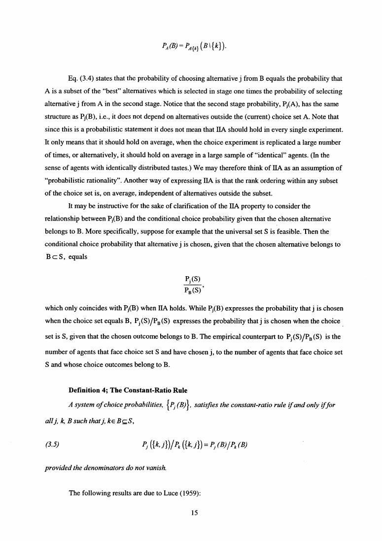
Eq. (3.4) states that the probability of choosing alternative j from B equals the probability that

A is a subset of the "best" alternatives which is selected in stage one times the probability of selecting

alternative j from A in the second stage. Notice that the second stage probability, P ;(A), has the same

structure as P;(B), i.e., it does not depend on alternatives outside the (current) choice set A. Note that

since this is a probabilistic statement it does not mean that Ø should hold in every single experiment.

It only means that it should hold on average, when the choice experiment is replicated a large number

of times, or alternatively, it should hold on average in a large sample of "identical" agents. (In the

sense of agents with identically distributed tastes.) We may therefore think of Ø as an assumption of

"probabilistic rationality". Another way of expressing HA is that the rank ordering within any subset

of the choice set is, on average, independent of alternatives outside the subset.

It may be instructive for the sake of clarification of the Ø property to consider the

relationship between Pi(B) and the conditional choice probability given that the chosen alternative

belongs to B. More specifically, suppose for example that the universal set S is feasible. Then the

conditional choice probability that alternative j is chosen, given that the chosen alternative belongs to

BcS, equals

P; (S)

PB (S)

which only coincides with Pi(B) when HA holds. While P;(B) expresses the probability that j is chosen

when the choice set equals B, P ; (S)/PB (S) expresses the probability that j is chosen when the choice

set is S, given that the chosen outcome belongs to B. The empirical counterpart to P ; (S) PB (S) is the

number of agents that face choice set S and have chosen j, to the number of agents that face choice set

S and whose choice outcomes belong to B.

Definition 4; The Constant-Ratio Rule

A system of choice probabilities, {Pi (B)}, satisfies the constant-ratio rule ifand only jffor

all j, k, B such that j, kE BcS,

(3.5) Pi ak> Pk ak, .1}J = P; (B)IPk (B)

provided the denominators do not vanish.

The following results are due to Luce (1959):

15

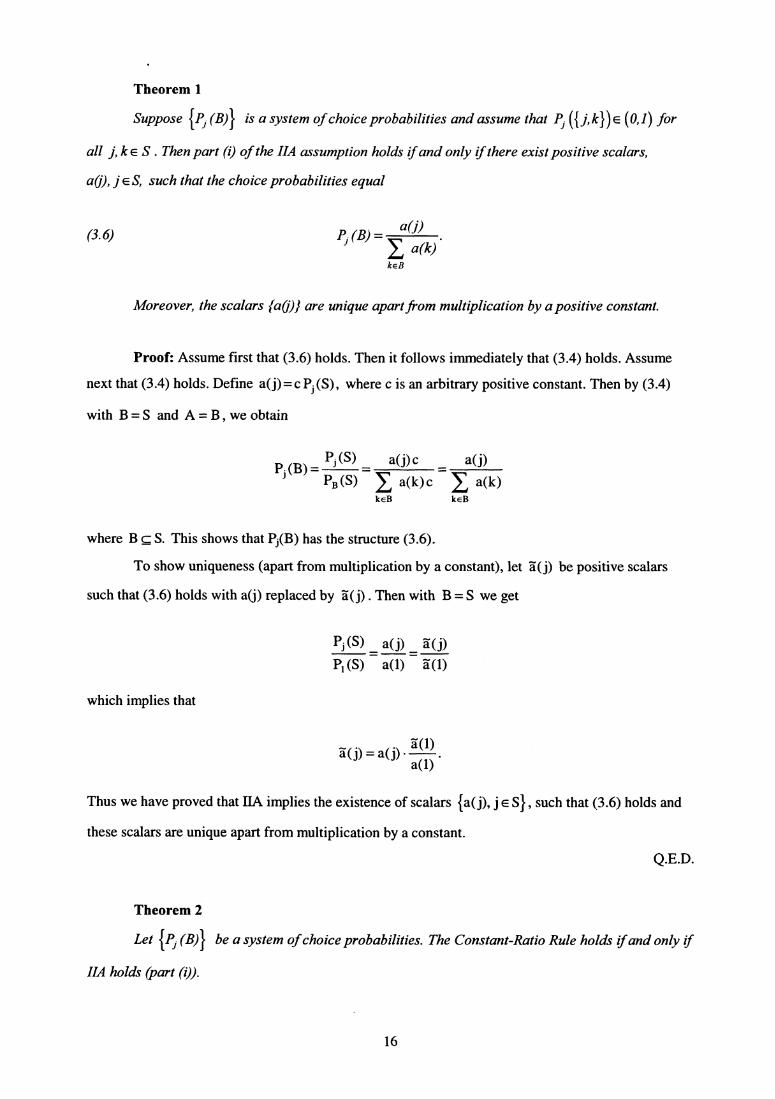
Theorem 1

Suppose {Pj (B)} is a system of choice probabilities and assume that Pi ({j,k})E (0,1) for

all j, k E S . Then part (i) of the HA assumption holds ifand only ifthere exist positive scalars,

a(j), j E S, such that the choice probabilities equal

(3.6) pi (B) _ _ a(I)

a(k)kEB

Moreover, the scalars {a(j)} are unique apart from multiplication by a positive constant.

Proof: Assume first that (3.6) holds. Then it follows immediately that (3.4) holds. Assume

next that (3.4) holds. Define a(j) = c Pi (S), where c is an arbitrary positive constant. Then by (3.4)

with B = S and A = B , we obtain

Pi (S) a( j) ca( j)

PB(S) a(k)c a(k)kEB kEB

where B c S. This shows that Pj(B) has the structure (3.6).

To show uniqueness (apart from multiplication by a constant), let a"( j) be positive scalars

such that (3.6) holds with a(j) replaced by å(j) . Then with B = S we get

P;(S) a(j) å(j)

P, (S) a(1) a- 0)

which implies that

^ . å(1)a(^)=a(i) • .

a(1)

Thus we have proved that Ø implies the existence of scalars {a(j), j E S},such that (3.6) holds and

these scalars are unique apart from multiplication by a constant.

Q.E.D.

Theorem 2

Let {Pi (B)} be a system of choice probabilities. The Constant-Ratio Rule holds ifand only if

HA holds (part (i)).

16

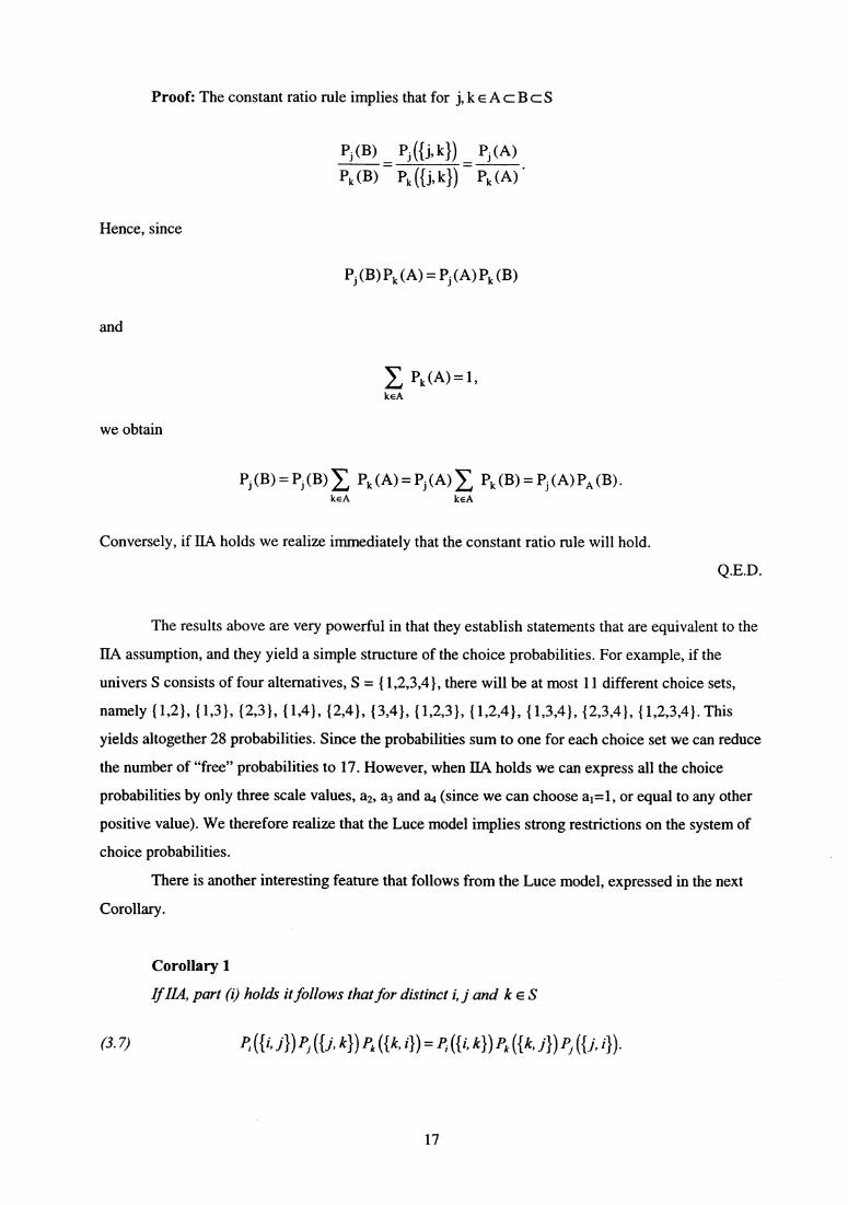
Proof: The constant ratio rule implies that for j, k E A c B c S

Pi (B) Pi (0, kl) Pi (A)

Pk (B) Pk (0,14) Pk (A)

Hence, since

Pi (B) Pk (A) = Pj (A) Pk (B)

and

Pk (A)=1,kEA

we obtain

P;(B)—P;(B) / Pk (A)=Pi(A)/ Pk (B)=P(A)Pn(B)•kEA kEA

Conversely, if HA holds we realize immediately that the constant ratio rule will hold.

Q.E.D.

The results above are very powerful in that they establish statements that are equivalent to the

IIA assumption, and they yield a simple structure of the choice probabilities. For example, if the

univers S consists of four alternatives, S = {1,2,3,4), there will be at most 11 different choice sets,

namely {1,2}, { {2,3}, { {2,4}, { {1,2,3}, { {1,3,4), { {1,2,3,4}. This

yields altogether 28 probabilities. Since the probabilities sum to one for each choice set we can reduce

the number of "free" probabilities to 17. However, when Ø holds we can express all the choice

probabilities by only three scale values, a2, a3 and a4 (since we can choose a 1 =1, or equal to any other

positive value). We therefore realize that the Luce model implies strong restrictions on the system of

choice probabilities.

There is another interesting feature that follows from the Luce model, expressed in the next

Corollary.

Corollary 1

If IIA, part (i) holds it follows that for distinct i, j and k E S

(3.7)

P, ({r, j}) Pi k}) Pk i}) = P ({1' k}) Pk ({k, j})

17

(3.10) P; (B)= P(UJ =max Uk)=

ev;

evk •

kE B

keBkE B

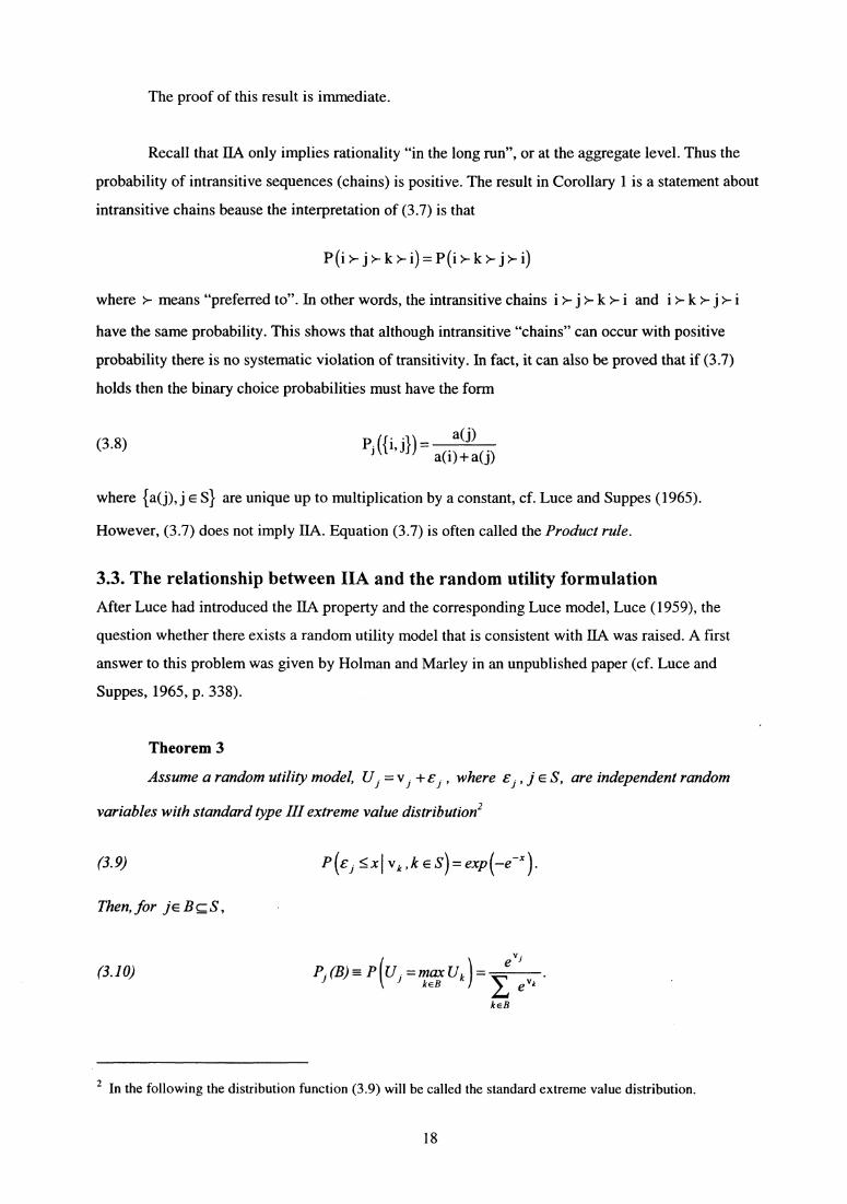
The proof of this result is immediate.

Recall that Ø only implies rationality "in the long run", or at the aggregate level. Thus the

probability of intransitive sequences (chains) is positive. The result in Corollary 1 is a statement about

intransitive chains beause the interpretation of (3.7) is that

P(ir j>k >- i)=P(i>-k jri)

where >- means "preferred to". In other words, the intransitive chains i >- j >- k >- i and i >-1c>-- j >- i

have the same probability. This shows that although intransitive "chains" can occur with positive

probability there is no systematic violation of transitivity. In fact, it can also be proved that if (3.7)

holds then the binary choice probabilities must have the form

(3.8) P.; i, j = a(j) a(i) + a(i)

where {a(j),j E s} are unique up to multiplication by a constant, cf. Luce and Suppes (1965).

However, (3.7) does not imply IIA. Equation (3.7) is often called the Product rule.

3.3. The relationship between IIA and the random utility formulation

After Luce had introduced the IIA property and the corresponding Luce model, Luce (1959), the

question whether there exists a random utility model that is consistent with IIA was raised. A first

answer to this problem was given by Holman and Marley in an unpublished paper (cf. Luce and

Suppes, 1965, p. 338).

Theorem 3

Assume a random utility model, U = v i +E ./ , where Ei , j E S. are independent random

variables with standard type III extreme value distribution

(3.9) P(Ei<_xl v k ,kES)=exp(—e-").

Then, for j E B c S,

2 In the following the distribution function (3.9) will be called the standard extreme value distribution.

18

We realize that (3.10) is a Luce model with v i = log a(j) . Thus, by Theorem 3 there exists a

random utility model that rationalizes the Luce model.

Proof: Let us first derive the cumulative distribution for Vi = max kEB \ { j} Uk . We have

(3.11) P(Vi<_y)= ^ P(Ek5.Y — Vk) — ^ eXP(—e iki -eXp(—e-yD i)

keB\{ j) keB\l1)

where

(3.12) Di = e "k .kEB\{ j}

Hence

00

(3.13)

(U i =111(NU k )=-"P(Ui>Vi)=P(Ei+vi>VJ )= P(y>Vj)P E j +v j E(y,y +dy)).

Note next that since by (3.9)

it follows that

P U^ <_ y)=P(e-+v.<y)=exp(—e vrY )

P ^E+v i E (y,y+dy))=exp(—e ° ' -Y ) e " '-y dy.

Hence

00

if P(y> Vi )P(E i +v i E(y,y+dy))= f exp(—D i e- '' e"j-y "j -y dy

(3.14) =e "' J exp(—(D i +e"')e-'')e-'"dy

"j Texp (_ (Dj+evJ ) e_Y ) =v

"ie

D+e' '

^

Since

eDj+"'= e"k

kEB

the result of the Theorem follows from (3.13) and (3.14).

Q.E.D.

19

An interesting question is whether or not there exists other distribution functions than (3.9)

which imply the Luce model. McFadden (1973) proved that under particular assumptions the answer

is no. Later Yellott (1977) and Strauss (1979) gave proofs of this result under weaker conditions.

Yellott (1977) proved the following result.

Theorem 4

Assume that S contains more than two alternatives, and U =v + ej , where ei , j E S, are

i.i.d. with cumulative distribution function that is independent of Iv , j E Si} and is strictly increasing

on the real line. Then (3.10) holds ifand only ife has the standard extreme value distribution

function.

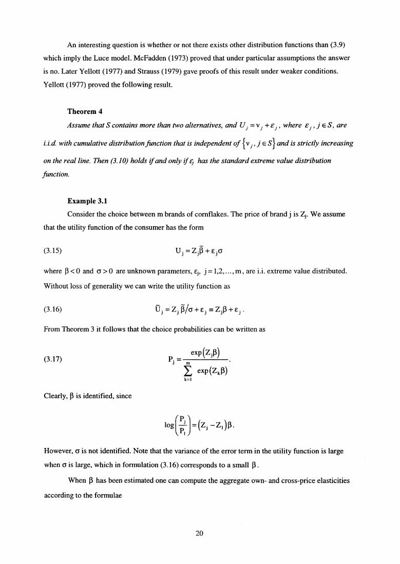
Example 3.1

Consider the choice between m brands of cornflakes. The price of brand j is We assume

that the utility function of the consumer has the form

(3.15) Ui = Z j i3 + e i a

where (3 < 0 and a > 0 are unknown parameters, q, j = 1,2,..., m , are i.i. extreme value distributed.

Without loss of generality we can write the utility function as

(3.16) ffi =Z i 'pa E i z i p + E i .

From Theorem 3 it follows that the choice probabilities can be written as

(3.17)

PJ = m exp (Z i (3)

exp(Z k (3)k=1

Clearly, R is identified, since

log(-1-13og P—

P ' =(Z. —Z 1 )(3.

PI

However, a is not identified. Note that the variance of the error term in the utility function is large

when 6 is large, which in formulation (3.16) corresponds to a small 0.

When (3 has been estimated one can compute the aggregate own- and cross-price elasticities

according to the formulae

20

(3.18)a log P; —Z^1— P. ^a log Z i

and

(3.19)

for k # j .

a log P .= -RZk Pka log Zk

Example 3.2

Consider a transportation choice problem. There are two feasible alternatives, namely driving

own car (Alternative 1), or riding a bus (Alternative 2).

Let i index the commuter and let

1 if j =1Zij1 = 0 otherwise ,

Zu2 = In-vehicle time, alternative j,

Z ij3 = Out-of-vehicle time, alternative j,

Zu4 = Transportation cost, alternative j .

The variable Ziji is supposed to represent the intrinsic preference for driving own car. The utility

function is assumed to have the structure

U ;j =Z ;, f3 + Eij

where Z ;i = Z ; , , Z ;i2 , Z;3 , Z ;34 , EH and c12 are i.i. extreme value distributed, and [3 is a vector of

unknown coefficients. From these assumptions it follows that the probability that commuter i shall

choose alternative j is given by

exp(3.20)

P;i = 2 •exp(Z ;k (»

k=1

From a sample of observations of individual choices and attribute variables one can estimate (3 by the

maximum likelihood procedure.

Let us consider how the model above can be applied in policy simulations once (3 has been

estimated. Consider a group of individuals facing some attribute vector 4, j =1,2. The corresponding

choice probability equals

21

(3.21)

PJ = 2

exp (z3)

exp(Z k (3)k=1

for j =1,2. From (3.21) it follows that

a log Pi(3.22) a log Zir — R Z

^r ^1— P^

and

a log P;(3.23) _—^ Zkr Pka log Z ig.

for k # j . Eq. (3.22) expresses the "own elasticities" while (3.23) expresses the "cross elasticities".

Specifically, (3.22) yields the relative increase in the fraction of individuals that choose alternative j

that follows from a relative increase in Zjr by one unit.

3.4. The independent random utility model

We now consider the problem of deriving the choice probabilities in a random utility model,

U i = v i + E i , where e i , j E S , are independent with P E <_ y)= F i (y) . In this case the choice

probabilities can be expressed as

(3.24)

for BcS.

Pj (B)= j n Fk (y—vk^Fi^Y—vdYkeB\{j}

To realize that (3.24) holds note that since e i , j E S , are independent we get

P1 max U k 5 y I= P`keB\{j} J

t

kEn{J}(£ k Sy—V k )I= kE J} P IEkS k /Y-V Fk(y—Vk).

^ keB\{1}

Furthermore,

P ^U E (y,y+dy)) = F;(Y)dY •

Hence,

P;(B)=P(U'> k max

Uk ) = P (y> k sa{^}U'`)F:(Y)dy= f ^ Fk (y —v k F;(Y)dY •ØØ keB\{j}

22

1 2 dy p' (B)— fl Øf (Y_vk)exP[_(_vJ )

42n

00

(3.28)

Example 3.3. (Multinomial logit)

Assume that

(3.25) F(y) = exp (—e -y ).

Then (3.24) yields

(3.26) Pj(B) =e v;

e Vk •

kEB

Example 3.4. (Independent multinomial probit)

If

(3.27)^ ^ 1 _ly2

F^(y) — Ø (y) = e 22^t

then we obtain the socalled Independent multinomial Probit model;

It has been found through simulations and empirical applications that the independent probit model

yields choice probabilities that are close to the multinomial logit choice probabilities.

Example 3.5. (Binary probit)

Assume that B={1,2} and Fi (y)=Ø(y,5). Then

(3.29) p (u u 2 ) = (v - v 2 ) .

Example 3.6. (Binary Arcus- tangens)

Assume that B=11,21 and

(3.30) F;(y) =2

n(1+4y 2 )

The density (3.30) is the density of a Cauchy distribution. Then

(3.31) P(U I >U 2 )= 1 + 1 Arctgv, —v 2 ).2 n

23

The Arcus-tangens model differs essentially from the binary logit and probit models in that the tails of

the Arcus-tangens model are much heavier than for the other two models.

3.5. Specification of the structural terms, examples

Let Z = (Z j , , Z i2 , ... , Z iK denote a vector of attributes that characterize alternative j. In the absence

of individual characteristics, a convenient functional form is

(3.32)

A more general specification is

(3.33)

K

Vj = Zi — ^ Z jk Pkk=1

K

V j —hk(Zj ^X)F'kk=1

where h k (z j , X , k =1,..., K, are known functions of the attribute vector and a vector variable X

that characterizes the agent.

Example 3.7

Let X = (X 1 , X Z ) and Z j =(z 1 , Z i . A type of specification that is often used is

(3.34)

w ; =z ;1 Rt +Z ;aR2 +Z ;i X 1R3 +Z ;i X aRa +Z ;2 X ^ Ps +Z ;z XzR6•

In some applications the assumption of linear-in-parameter functional form may, however, be too

restrictive.

Example 3.8. (Box-Cox transformation):

Let Z j = Zj1, Zi2 , Z jk >0, k =1,2,

and

(3.35) v.1 = - 1 + Z^2 - 1

] 12a, a2

where a l , a 2 , , 02 are unknown parameters. The transformation

(3.36)y a —1

a

24

y > 0, is called a Box-Cox transformation of y and it contains the linear function as a special case

(cz=1).When a --> 0 then

y " -1 ---> logy.

a

When a <1, (ya —1)/a is concave while it is convex when a >1. For any a, (y" —1)/a is

increasing in y.

Example 3.9

A problem which is usually overlooked in discrete choice analyses is the fact that

simultaneous equation problems can arise as a result of unobservable attributes. Consider the

following example where the utility function has the structure

U i = Z i R + Z i X 1 0 2 + Z i X2 0 3 + e i

where is an attribute variable (scalar) and X1, X2 are individual characteristics. The random error

term Ei is assumed to be uncorrelated with Z3 , X 1 and X2. Also Z; is assumed uncorrelated with X 1 and

X2. However, X2 is unobservable to the researcher. The researcher therefore specifies the utility

function as

(3.37) U* = Z f3 1 + ;X i ^i + E*.

Thus, the interpretation of E; is as

(3.38) Ei _£ i +Z i X 2 0 3 .

Then

E(E; X 1 ,Zi)=Zj(3 3 E(X 21 X 1) .

In this case we therefore get that the error terms are correlated with the structural terms when X 1 and

X2 are correlated. A completely similar argument applies in the case with unobservable attributes.

This simple example shows that simultaneous equation bias may be a serious problem in

many cases where data contains limited information about population heterogeneity or/and relevant

attributes. Note that even if we were able to observe the relevant explanatory variables, we may still

face the risk of getting simultaneous equation bias as a result of misspesified functional form of the

deterministic term of the utility function. This is easily demonstrated by a similar argument as the one

above.

25

3.6. Aggregation of latent alternatives

In this section we shall obtain a characterization of the choice model that may be justified in

applications that conform to the following general description. For the sake of expository convenience

we proceed by means of a concrete example.

Consider migration choice: The agent faces a set B of feasible regions. Within region j there

is a set B; of feasible schooling and/or employment opportunities. The agent's problem is to choose his

favorite opportunity. The researcher only observes the choice of region but not the choice within the

chosen region. The agent is assumed to have the utility function with structure

(3.39) •U^r =V- +Ejr

where j =1,2,...,m, indexes the regions and r E B i indexes the opportunities within B i . The term vj is

deterministic and represents the systematic mean utility across all opportunities within B j , while E;r,

r E B, j =1,2,..., m, are i.i.d. with cumulative distribution function F. Let n n be the number of

opportunities in B i . Evidently the (indirect) utility of choosing region j equals

U^=maxU•jrrE=v . +E•B j

where

^E - = max C- = max E- .

^ rEB,

Suppose next that F satisfies Condition (A.6) in Appendix A. Then Theorem A3 implies, provided n^

is large, that for some positive constant c one has

P(

1t jr — log c n i <_ x = expr_n j

which means that

(3.40) vi + E - v i + log n i + log c + E i

where Ej , j =1,2, ..., m, are standard type III extreme value distributed. Thus we obtain fromTheorem

3 that the probability of moving to region j equals

26

( ^

l exp(vi+logc +logneP^ = PIU=maxU J —

^ ` ^ kEB k exp(vk+logc+lognk)kE B

c n ev

' ni ev

'_ .c n k evk

nke"k

kEB kEB

If variables that characterize the regions are available these can be utilized to model In i } and Iv } .

The crucial point in the development above is that even if we are only interested in the

analysis of the choice of region, we can exploit the (theoretical) structure of the problem to obtain a

characterization of the choice model. Specifically, we have demonstrated that aggregation of a large

number of latent alternatives in fact implies IIA. Moreover, the set of latent alternatives {B i } are

represented in the model by the respective sizes {n i }

3.7. Stochastic models for ranking

So far we have only discussed models in which the interest is the agent's (most) preferred alternative.

However, in several cases it is of interest to specify the joint probability of the rank ordering of

alternatives that belong to S or to some subset of S. For example, in stated preference surveys, where

the agents are presented with hypothetical choice experiments, one has the possibility of designing the

questionaires so as to elicit information about the agents' rank ordering. This yields more information

about preferences than data on solely the highest ranked alternatives, and it is therefore very useful for

empirical analysis. This type of modeling approach has for example been applied to analyze the

potential demand for products that may be introduced in the market, see Section 4.8.

The systematic development of stochastic models for ranking started with Luce (1959) and

Block and Marschak (1960). Specifically, they provided a powerful theoretical rationale for the

structure of the so-called ordered Luce model. The theoretical assumptions that underly the ordered

Luce model can briefly be described as follows.

Let R(B) = (R 1 (B), R 2 (B), ..., R m (B)) be the agent's rank ordering of the alternatives in B,

where m is the number of alternatives in B, and B c S. This means that R ;(B) denotes the element in

B that has the i'th rank. As above let Pi (B), j E B , be the probability that the agent shall rank

alternative j on top when B is the set of feasible alternatives. Recall that the empirical counterpart of

these probabilities is the respective number of times the agent chooses a particular rank ordering to

the total number of times the experiment is replicated, or alternatively, the fraction of (observationally

identical) agents that choose a particular rank ordering. Let p(B) = (p 1 , p 2 ,..., p m ) , where the

components of the vector p(B) are distinct and p k E B for all k <_ m .

27

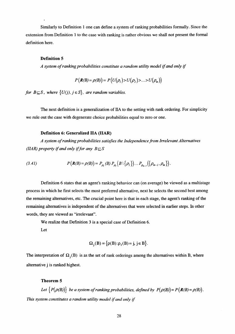
Similarly to Definition 1 one can define a system of ranking probabilities formally. Since the

extension from Definition 1 to the case with ranking is rather obvious we shall not present the formal

definition here.

Definition 5

A system of ranking probabilities constitute a random utility model ifand only if

P(R(B)= p(B)) = P(U(Pr )> UWPzJ>...>U(Pm))

for B c S , where {U(j), j E S}, are random variables.

The next definition is a generalization of Ø to the setting with rank ordering. For simplicity

we rule out the case with degenerate choice probabilities equal to zero or one.

Definition 6: Generalized IIA (IIAR)

A system of ranking probabilities satisfies the Independence from Irrelevant Alternatives

(HAR) property ifand only iffor any B c S

(3.41) P(R(B)=p(B))=PPS (B)Pm(BI{pr})...Pa_1({Pm-r,Pm})•

Definition 6 states that an agent's ranking behavior can (on average) be viewed as a multistage

process in which he first selects the most preferred alternative, next he selects the second best among

the remaining alternatives, etc. The crucial point here is that in each stage, the agent's ranking of the

remaining alternatives is independent of the alternatives that were selected in earlier steps. In other

words, they are viewed as "irrelevant".

We realize that Definition 3 is a special case of Definition 6.

Let

(B) = fp(B): p (B) = j, j E13}.

The interpretation of S2 j (B) is as the set of rank orderings among the alternatives within B, where

alternative j is ranked highest.

Theorem 5

Let {P(p("B))} be a system of ranking probabilities, defined by P( p(B)) = P (R(B) = p(B)) .

This system constitutes a random utility model ifand only if

28

P (B) _ P( p(B))

A proof of Theorem 5 is given by Block and Marschak (1960, p. 107).

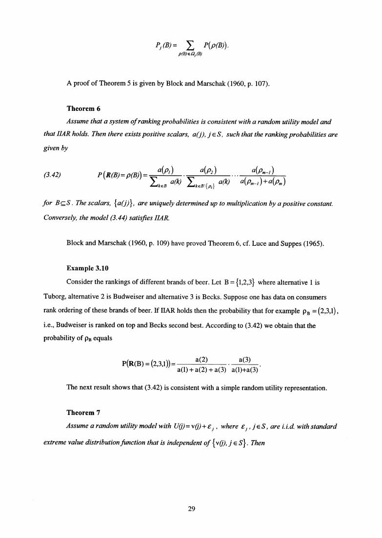
Theorem 6

Assume that a system of ranking probabilities is consistent with a random utility model and

that HAR holds. Then there exists positive scalars, a(j), j E S, such that the ranking probabilities are

given by

(3.42) P (R(B) = p(B)) _ a(Pi) a(P2) ...

a(Pm-1)

IkeB a(k) jkeBl { p, } Q(R) a(pm_1)±R(pm )

for BcS. The scalars, {a(j)}, are uniquely determined up to multiplication by a positive constant.

Conversely, the model (3.44) satisfies HAR.

Block and Marschak (1960, p. 109) have proved Theorem 6, cf. Luce and Suppes (1965).

Example 3.10

Consider the rankings of different brands of beer. Let B = {1,2,3} where alternative 1 is

Tuborg, alternative 2 is Budweiser and alternative 3 is Becks. Suppose one has data on consumers

rank ordering of these brands of beer. If ØR holds then the probability that for example p B = (2,3,1

i.e., Budweiser is ranked on top and Becks second best. According to (3.42) we obtain that the

probability of pB equals

KR(B) = (2,3,1))= a(2) a(3)

a(1) + a(2) + a(3) a(1)+a(3)

The next result shows that (3.42) is consistent with a simple random utility representation.

Theorem 7

Assume a random utility model with U(j)=v0+ e , where Ei , j ES, are i.i.d. with standard

extreme value distribution function that is independent of {vO), j E S}. Then

29

(3.43)

P(R(B)=p(B)) = P(U(Pr)>U(Pz)>...>U(P„,))

exp(v(p^)) exp(v(p2))

eXP(v(p„,-i))

^ ...

kEa eXp^^(k)^ ^ke81{p^} exP(v(k)) exP(v(p,,,-1))+exP(v(Pm))

Also here we realize that Theorem 1 is a special case of Theorem 6 and Theorem 3 is a special

case of Theorem 7 because the choice probability P j(B) is equal to the sum of all ranking probabilities

with p i = i . A proof of Theorem 7 is given in Strauss (1979).

3.8. Stochastic dependent utilities across alternatives

In the random utility models discussed above we only focused on models with random terms that are

independent across alternatives. In particular we noted that the independent extreme value random

utility model is equivalent to the Luce model. It has been found that the independent multinomial

probit model is "close" to the Luce model in the sense that the choice probabilities are close provided

the structural terms of the two models have the same structure (see for example, Hausman and Wise,

1978). However, the assumption of independent random terms is rather restrictive in some cases,

which the following example will demonstrate.

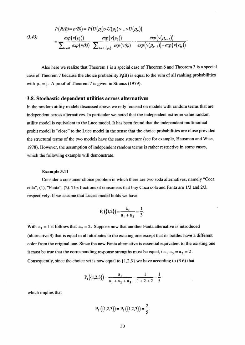
Example 3.11

Consider a consumer choice problem in which there are two soda alternatives, namely "Coca

cola", (1), "Fanta", (2). The fractions of consumers that buy Coca cola and Fanta are 1/3 and 2/3,

respectively. If we assume that Luce's model holds we have

P1 (11,21) = a _ 1a l +a 2 3^

With a l =1 it follows that a 2 = 2 . Suppose now that another Fanta alternative is introduced

(alternative 3) that is equal in all attributes to the existing one except that its bottles have a different

color from the original one. Since the new Fanta alternative is essential equivalent to the existing one

it must be true that the corresponding response strengths must be equal, i.e., a 3 = a 2 = 2 .

Consequently, since the choice set is now equal to {1,2,3} we have according to (3.6) that

P^ ^{1,2,3}^ =a^ _ 1 _ 1

a, +a 2 +a 3 1+2+2 5

which implies that

P2 ({1,2,3}) = P3 ({1,2,3}) =-1.

30

But intuitively, this seems unrealistic because it is plausible to assume that the consumers will tend to

treat the two alternatives as a single alternative so that

P1 ({1,2,3}) = 3and

P2 ({1,2,3}) = P3 (11,2,31) = 3 .

This example demonstrates that if alternatives are "similar" in some sense, then the Luce model is not

appropriate. A version of this example is due to Debreu (1960).

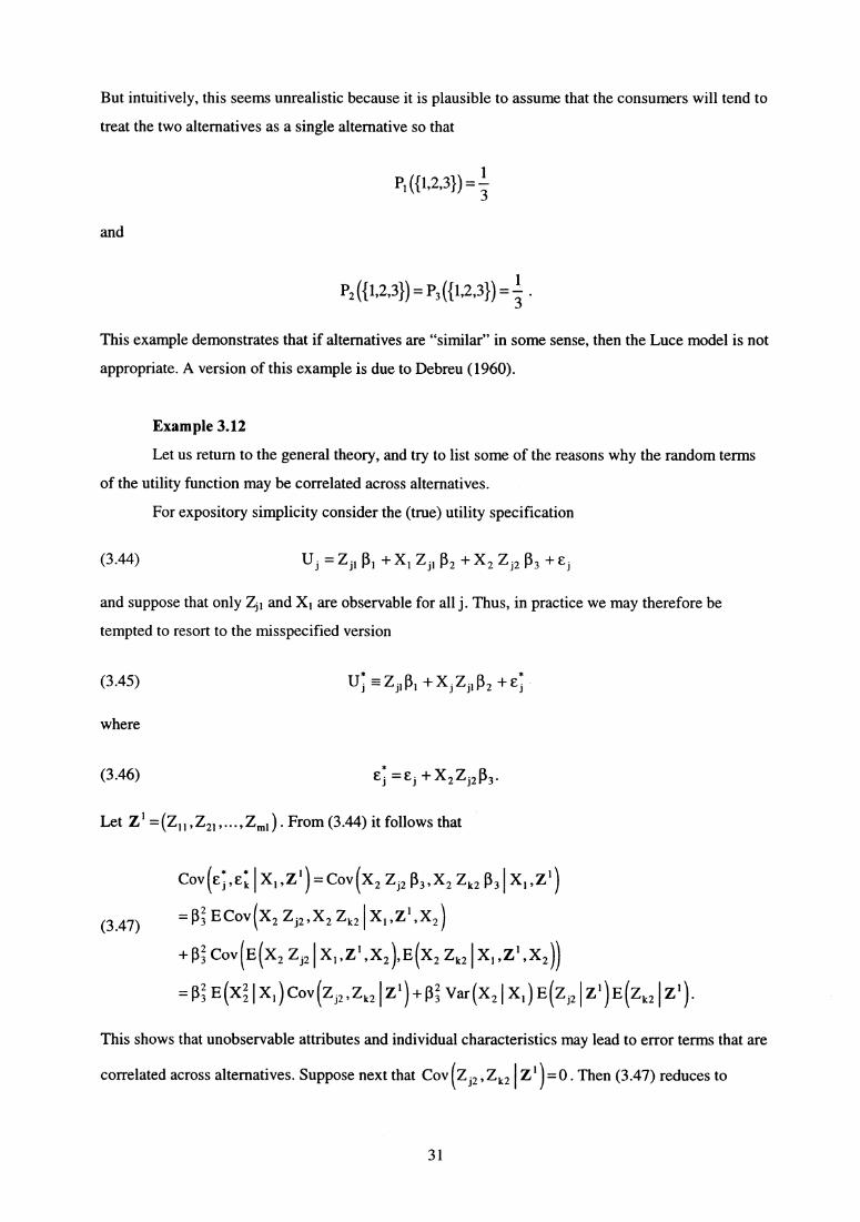
Example 3.12

Let us return to the general theory, and try to list some of the reasons why the random terms

of the utility function may be correlated across alternatives.

For expository simplicity consider the (true) utility specification

(3.44)

Uj '7= Zjl (3 1 + X1 Z jl 0 2 + X2 Z j2 (3 3 + E j

and suppose that only Zj1 and X 1 are observable for all j. Thus, in practice we may therefore be

tempted to resort to the misspecified version

(3.45) Uj E- +Xz j1 E3 2 + E j

where

(3.46) Ej =Ej + X2Zj213 3.

Let Z = (Z1 1 , Z 2 1 , ... , Zml) . From (3.44) it follows that

Cov(C,Ek ( X1,Z1)=Cov(X2 Zj2 ^s ,X2 Zk2 f3 3 1X 1 ,Z 1 )

(3.47) =(33 ECovI

1X2 Z WZ ,X Z Zk2 IIx 1 ,z',c2)

+(33 Cov(E1X 2 Z jZ I X1,Z1,X2/'E1X2 Zk2 I X'XZ//_ (33 E(X2I Xi)Cov(Z ;zPZkz I Z l )+M Var(X2 I Xi) E(Ziz

Z')E 1zk2 l z, /'

This shows that unobservable attributes and individual characteristics may lead to error terms that are

correlated across alternatives. Suppose next that Coy (z J2 , Zk2 1Z 1 ) = 0 . Then (3.47) reduces to

31

(3.48) COV E k X 1 ,Z 1 )=M E(Z j2 Z' ) E (Zk2 Z') var (x 2 I x i ).

Eq. (3.48) shows that even if the unobservable attributes are uncorrelated the error terms will still be

correlated if Var (x 2 (X i )*() . (If Var (x 2 I X ^ ^ = 0 , x2 is perfectly predicted by X1.)

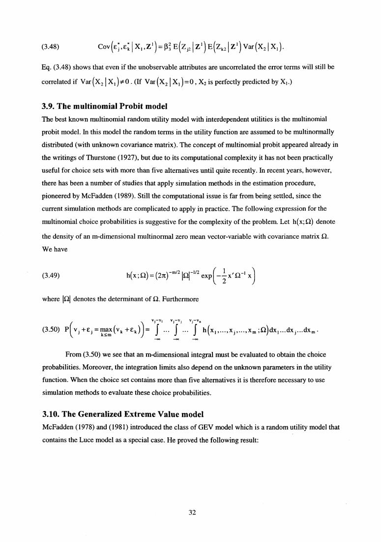
3.9. The multinomial Probit model

The best known multinomial random utility model with interdependent utilities is the multinomial

probit model. In this model the random terms in the utility function are assumed tO be multinormally

distributed (with unknown covariance matrix). The concept of multinomial probit appeared already in

the writings of Thurstone (1927), but due to its computational complexity it has not been practically

useful for choice sets with more than five alternatives until quite recently. In recent years, however,

there has been a number of studies that apply simulation methods in the estimation procedure,

pioneered by McFadden (1989). Still the computational issue is far from being settled, since the

current simulation methods are complicated to apply in practice. The following expression for the

multinomial choice probabilities is suggestive for the complexity of the problem. Let h(x; a) denote

the density of an m-dimensional multinorma1 zero mean vector-variable with covariance matrix SZ.

We have

(3.49)

h(x; _ (21t}-mi2 ICI-viz eXP( ^ X' sri x)

where ILI denotes the determinant of S2. Furthermore

v^-v l vi -v i vrv A

(3.50) J +£- =max(v k +£ k ) _ ••• •••

k<_mØ

h x l ,...,x j ,...,x m ;S2 dx l ...dx J ...dx m •

From (3.50) we see that an m-dimensional integral must be evaluated to obtain the choice

probabilities. Moreover, the integration limits also depend on the unknown parameters in the utility

function. When the choice set contains more than five alternatives it is therefore necessary to use

simulation methods to evaluate these choice probabilities.

3.10. The Generalized Extreme Value model

McFadden (1978) and (1981) introduced the class of GEV model which is a random utility model that

contains the Luce model as a special case. He proved the following result:

32

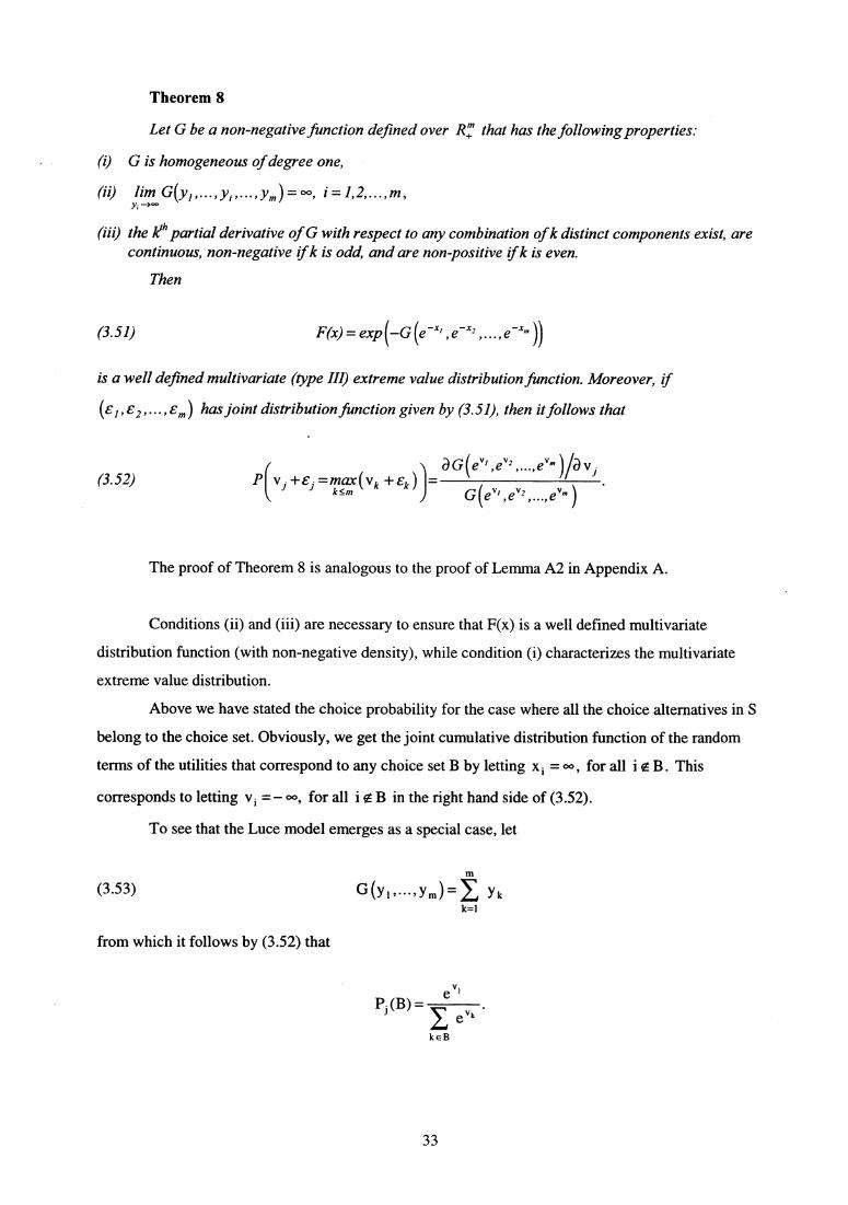
Theorem 8

Let G be a non-negative function defined over R+ that has the following properties:

(i) G is homogeneous of degree one,

(ii) lim G(y-.• , y... , ym ) = i =1,2,...,m,

(iii) the km partial derivative of G with respect to any combination of k distinct components exist, arecontinuous, non-negative ifk is odd, and are non positive ifk is even.

Then

(3.51) F(x) = exp —G e -'r',e -x2 ,...,e -xm

is a well defined multivariate (type III) extreme value distribution function. Moreover, If

(E I ,e2 ,...,Em ) has joint distribution function given by (3.51), then it follows that

(3.52)a G (ev',e"2 ,...,e"m avi

P vi +E,=max(vk +Ek ) = %< m "1 "2 "m •G e

The proof of Theorem 8 is analogous to the proof of Lemma A2 in Appendix A.

Conditions (ii) and (iii) are necessary to ensure that F(x) is a well defined multivariate

distribution function (with non-negative density), while condition (i) characterizes the multivariate

extreme value distribution.

Above we have stated the choice probability for the case where all the choice alternatives in S

belong to the choice set. Obviously, we get the joint cumulative distribution function of the random

terms of the utilities that correspond to any choice set B by letting x i = oo , for all i B. This

corresponds to letting v i =— oo , for all i o B in the right hand side of (3.52).

To see that the Luce model emerges as a special case, let

m

(3.53) G(Y... > Y^- ^ Ykk=1

from which it follows by (3.52) that

P . (B)= "kekEB

e ";

33

Example 3.13

Let S = {1,2,3} and assume that

(3.54)

G (Y>>Y2 , Y3) = Y^ + (Yzve

+Y3ve e

where 0 <0 5.1. It can be demonstrated that 0 has the interpretation

(3.55)

and

COIT(£2,E3)=1 0 2

corn E 1 ,0= 0, j=2,3.

From Theorem 8 we obtain that

e"'(3.56) P1 (S) _

^ ie ve

ev' + e 2 +eie3

and

e"2/0 +e"3ie e-1 e " ; ie

(3.57)P^(S) = ee ", + e " 2 m +e "3 ie

for j = 2,3 . If B = {1,2} , then

e"'(3.58) P1 ({1,2}) =

e", +e

When alternative 2 and alternative 3 are close substitutes 0 should be close to zero. By applying

l'Hopital's rule we obtain

lim log e " eie + e"3 'e = max (v 2 , v 3 ).

e--0

Consequently, when 0 is close to zero the choice probabilities above are close to

(3.59)

and

Pl (S)=e"'

e"' +exp(max(v 2 ,v 3 ))

34

(3.60) P2 (S) =e V2

e"' +e v2

if v 2 > v 3 , and zero otherwise, and similarly for P 3(S). For v 2 = v 3 we obtain

(3.61) Pl (S) =V2e +e

and

(3.62) Pi (S) _

for j=2,3.

Consider again Example 3.11. With v 2 = V 3 , V 1 = 0 and e v2 = 2 . Eq. (3.61) and (3.62) yield

P1 (11,21) =1 / 3

and

P2 ({1,2,3}) = P3 ({1,2,3}) =1 / 3.

Thus the model generated from (3.54) with A close to zero is able to capture the underlying structure

of Example 3.11.

3.10.1. The Nested multinomial logit model (nested logit model)

The nested logit model is an extension of the multinomial logit model which belongs to the GEV

class. The nested logit framework is appropriate in a modelling situation where the decision problem

has a "tree-structure". This means that the choice set can be partitioned into a hierarchical system of

subsets that each group together alternatives having several observable characteristics in common. It

is assumed that the agent chooses one of the subsets A r (say) in the first stage from which he selects

the preferred alternative. The choice problem in Example 3.11 has such a tree structure: Here the first

stage concerns the choice between Coca cola and Fanta while the second stage alternatives are the two

Fanta variants in case the first stage choice was Fanta.

Example 3.14

To illustrate further the typical choice situation, consider the choice of residential location.

Specifically, suppose the agent is considering a move to one out of two cities, which includes a

e v,

ev2

2 e v' +e v2

35

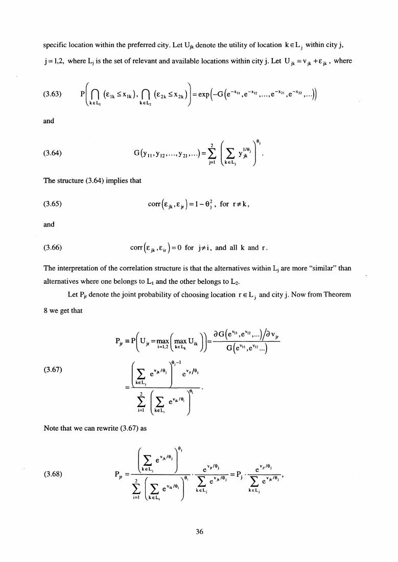
specific location within the preferred city. Let Ujk denote the utility of location k E L i within city j,

j =1,2, where Li is the set of relevant and available locations within city j. Let U ik = V jk -I- E jk , where

(3.63)

and

(3.64)

P n (Elk^xlk), n (E2k^x2k )

keL, keLz)

2 l e'1/Ø;

G(y 11 ,y 12 ,...,y 21 ,...)= Yjkj=1 k EL;

= exp —G(e-X11 , e-" 1 2 , . .. , e -x21 , e -x22 , ...))

The structure (3.64) implies that

(3.65)corr E jk , E jr =1— 8 i , for r # k ,

and

(3.66) Corr (Eik , E ir = 0 for j^i, and all k and r .

The interpretation of the correlation structure is that the alternatives within L i are more "similar" than

alternatives where one belongs to L 1 and the other belongs to L2.

Let Pjr denote the joint probability of choosing location r E L i and city j. Now from Theorem

8 we get that

Pi, = P U jr =max max Uik ))=

i =1,2 kE Lk

a G e"11 ,ev12 , ... a vjr

G ev11 , ev12 ...)

(3.67); --1

e v ;k / Ø ; e v ;r /e ;

kE L;

2 1ni

evik /Øi

i=1 kE L i

Note that we can rewrite (3.67) as

(3.68)

e v;k /Ø ;

k E L;e v;

re v /Ø ;

Pjr Ø i

v;k /Ø; = Pj v;k ! Ø ;

kEL ; kEL;

e ev ik /Ø i

e

i =1 k E L i

36

where

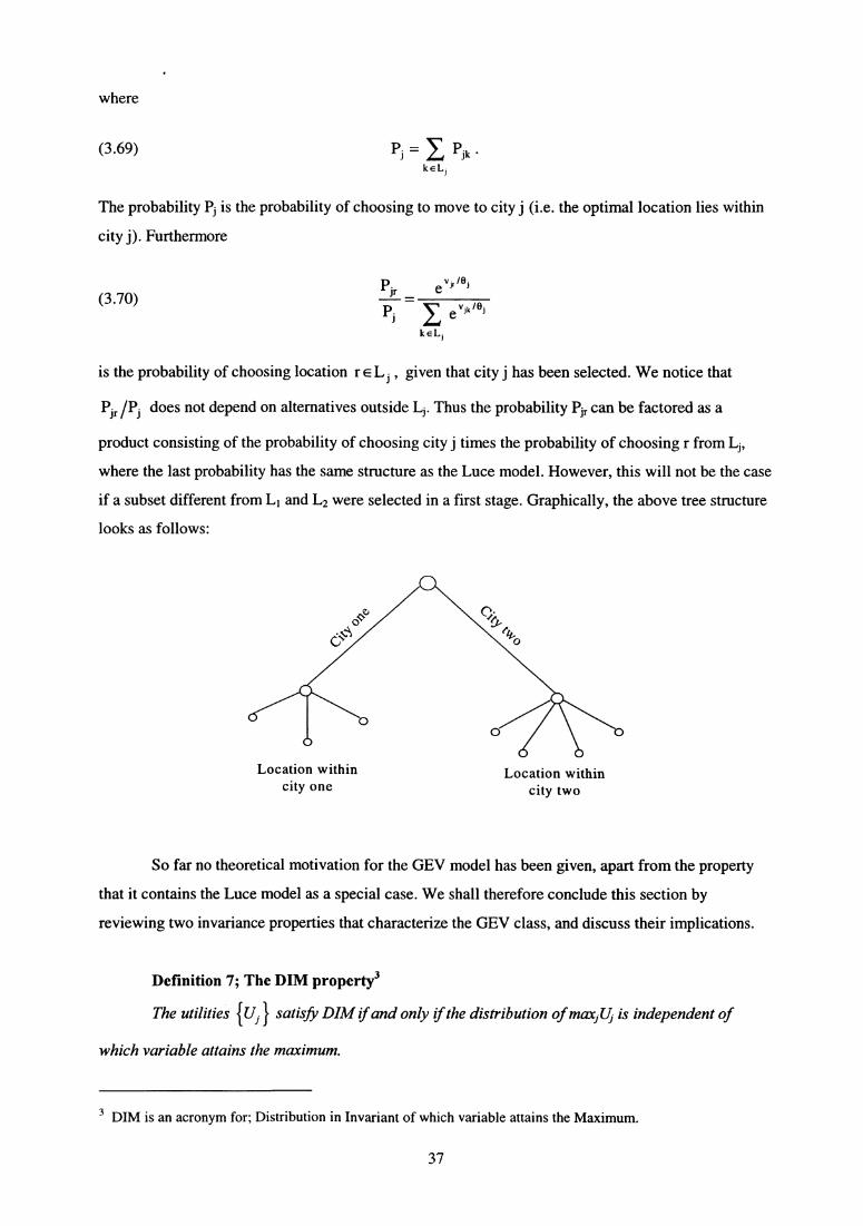
(3.69) P . = P. •kEL ;

The probability Pi is the probability of choosing to move to city j (i.e. the optimal location lies within

city j). Furthermore

(3.70) Pjr en,. /8 j

e V ;k ie;P^

kELi

is the probability of choosing location r E L i , given that city j has been selected. We notice that

Pjr /Pi does not depend on alternatives outside L i . Thus the probability P ir can be factored as a

product consisting of the probability of choosing city j times the probability of choosing r from Li ,

where the last probability has the same structure as the Luce model. However, this will not be the case

if a subset different from L 1 and L2 were selected in a first stage. Graphically, the above tree structure

looks as follows:

Location within Location withincity one city two

So far no theoretical motivation for the GEV model has been given, apart from the property

that it contains the Luce model as a special case. We shall therefore conclude this section by

reviewing two invariance properties that characterize the GEV class, and discuss their implications.

Definition 7; The DIM property3

The utilities It j } satisfy DIM ifand only ifthe distribution of rnaxU is independent of

which variable attains the maximum.

3 DIM is an acronym for; Distribution in Invariant of which variable attains the Maximum.

37

Definition 8; The MSD property 4

The utilities {U } satisfy MSD ifand only ifthe distribution of maxiU is the same (apart

from a location shift) as the distribution of U,.

If the utilities satisfy DIM it means that the indirect utility is not correlated with the utility of

the chosen alternative.

This property corresponds to the notion that the indirect utility in the deterministic micro

theory has prices and income as arguments, but the chosen quantities do not enter as arguments, nor

do their corresponding direct utility.

The MSD property is natural, since it implies that the stochastic properties of the utilities are

invariant under aggregation of alternatives. To realize this suppose that the univers of alternatives is

divided into subsets of alternatives called "aggregate alternatives". Thus each aggregate alternative

consists of one or several "basic" alternatives. It is understood that the consumer's choice of an

aggregate alternative means that he chooses a basic alternative that belongs to the aggregate one.

Consequently, the utility of the aggregate alternative must be the maximum of the utilities of the basic

alternatives within the aggregate one. Under MSD, the utility of the aggregate alternative will

therefore have the same distribution (apart from a location shift) as the basic utilities.

Theorem 9

Assume that Ui =v i +Ei ,where the cumulative distribution function F of

E=(E j ,E2 ,...,Em ) does not depend on {v }.

(i;) Then F satisfies DIM ifand only if

(3. 71) F(x l ,x2 , ... ,xm ) = y^ G e-x, ,e-x,

where G is a homogeneous function and gris a positive function (subject to F being a proper

distribution function).

(ii) If E^ , Ez, ... , ^„„ have a common cumulative distribution function then F satisfies MSD ifand only if

(3.71) holds.

A proof of Theorem 9 is given by Robertson and Strauss (1981), and Lindberg et al. (1995).

From (3.71) and Theorem 8 we realize that when w(x) = exp(—x) we obtain the GEV class.

4 MSD is an acronym for; The Maximum utility has the Same Distribution as the distribution of U 1 + b.

38

Strauss (1979) has proved the following result which follows readily from Theorem 9, and

extends the result of Theorem 8. This result shows that the choice probabilities do not depend on ti.

Corollary 2

If (3.71) holds then the choice probabilities are given by

a G e"' ,e"2 ,...,e"m a v^P vi+Ei=max(vk+ek) _

k <_m G e"' e e"m^"z ,...,

Thus, from Theorem 9 we realize that the class of models determined by (3.71) is equivalent

to the GEV class.

Until resently it has not been clear which restrictions on the choice probabilities are implied

by the GEV class. Dagsvik (1995) proved that the GEV class is very large; in fact the GEV class

yields no other restrictions on the choice probabilities beyond those following from the random utility

assumption.

Theorem 10

Assume that Uj =v i + Ej , where the cumulative distribution function F of (E 1 , E , ... , .)

does not depend on {v } . If (3.71) holds then IIA holds ifand only if

mF (x 1 ,x2 ,...,xm ) _ , e -Øk

k=1(3.72)

where a>0 is an arbitrary constant and yi is defined in Theorem 9.

A proof of Theorem 10 is given by Strauss (1979).

From (3.72) we realize that when yr(x)=exp(—x) we obtain the independent extreme value

model.

Example 3.15

Another example is obtained when

(3.73)

in which case (3.72) yields

1w(x)= ,

l+x

39

/ m )1/a )

.

\.

(3.76) F(yl , y2 ,..., ym )=exp — e -aYk

k=1

(3.74) F(y l ,y 2,. ..,y m)= m

1 + e -ayk

k=1

Example 3.16

Assume that

(3.75) W(x) = exp (—X l

ia

)

with a >1. Then (3.72) implies that

In this model it can be demonstrated that

(3.77) COrr (E i , E i ) = i - 12

a

which shows that the Luce model is consistent with a random utility model with any correlation

(different from zero and one) between the utilities as long as the correlation structure is symmetric.

40

v(c,L)= (Cal -1)\ p i +a,

L aZ —1M

R2M ,(4.4)

^

a 2

4. Applications of discrete choice analysis

4.1. Labor supply (I)

Consider the binary decision problem of choosing between the alternatives "working" and "not

working". Take the standard neo-classical model as a point of departure. Let V(C,L) be the agent's

utility in consumption, C, and annual leisure, L. The budget constraint equals

(4.1) C =hW +I

where W is the wage rate the agent faces in the market, h is annual hours of work and I is non-labor

income (for example the income provided by the spouse). The time constraint equals

(4.2) h + L 5 M (= 8760) .

According to this model utility maximization implies that the agent supplies labor if

(4.3) W > a 2v(I,M) -w '

,v 0, M)

where a; denotes the partial derivative with respect to component j . If the inequality is reversed, then

the agent will not wish to work. W * is called the reservation wage. Suppose for example that the

utility function has the form

where a l <1, a 2 <1, [31 > 0, P 2 > 0. Then V(C,L) is increasing and strictly concave in (C,L) . The

reservation wage equals

(4.5)* a 2v(i,m) 0 2 T i-a,

a , M) 13 1

After taking the logarithm on both sides of (4.3) and inserting (4.5) we get that the agent will supply

labor if

log W > (1— a 1 ) log I + log 20,

Suppose next that we wish to estimate the unknown parameters of this model from a sample of

individuals of which some work and some do not work. Unfortunately, it is a problem with using (4.6)

as a point of departure for estimation because the wage rate is not observed for those individuals that

(4.6)

41

do not work. For all individuals in the sample we observe, say, age, non-labor income, length of

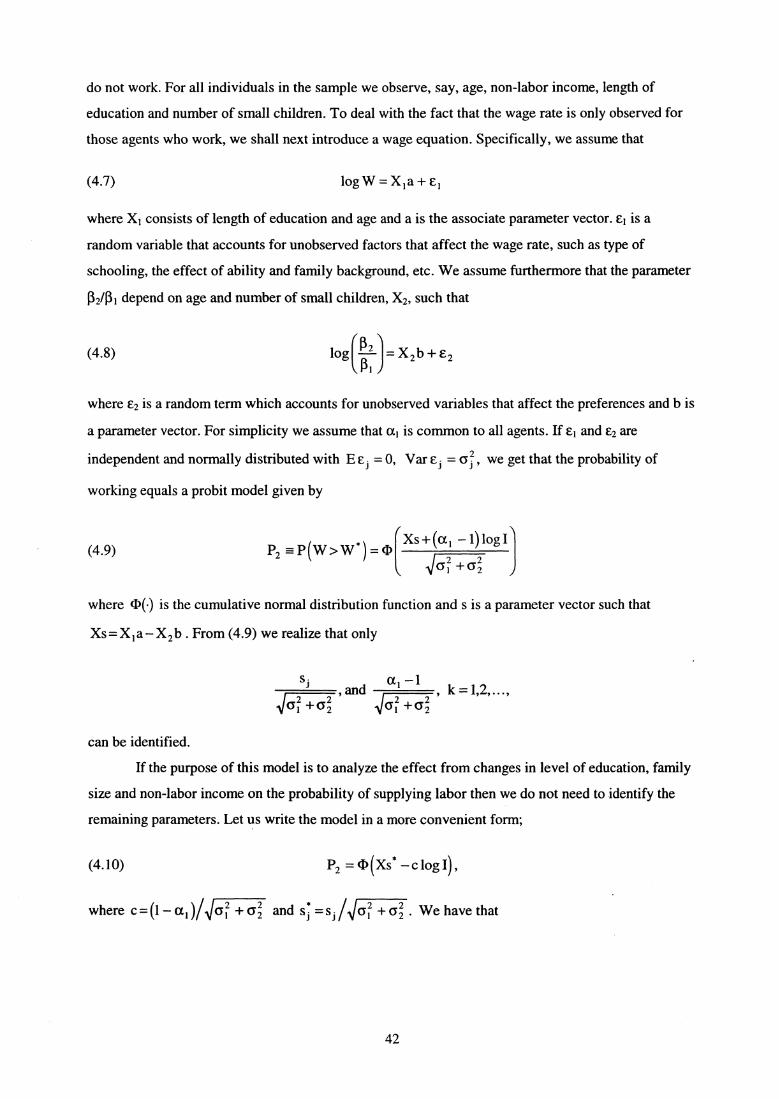
education and number of small children. To deal with the fact that the wage rate is only observed for

those agents who work, we shall next introduce a wage equation. Specifically, we assume that

(4.7) logW =X I a+E i

where X 1 consists of length of education and age and a is the associate parameter vector. E l is a

random variable that accounts for unobserved factors that affect the wage rate, such as type of

schooling, the effect of ability and family background, etc. We assume furthermore that the parameter

[32/p, depend on age and number of small children, X2, such that

(4.8)

log Rz =X Z b+E 2

where E2 is a random term which accounts for unobserved variables that affect the preferences and b is

a parameter vector. For simplicity we assume that a 1 is common to all agents. If E i and E2 are

independent and normally distributed with E E i = 0, Var E i = 6 , we get that the probability of

working equals a probit model given by

(4.9) PZ =P (W> W;) =Ø(Xs+(a, —1)IogI^

V0.21 + 0 22

where Ø(•) is the cumulative normal distribution function and s is a parameter vector such that

Xs = X 1 a — X 2 b . From (4.9) we realize that only

s i al ai+1 k=122 2^an 2^^^...^

61+62 Val +a'2

can be identified.

If the purpose of this model is to analyze the effect from changes in level of education, family

size and non-labor income on the probability of supplying labor then we do not need to identify the

remaining parameters. Let us write the model in a more convenient form;

(4.10) P2 =Ø(Xs * —c log I),

where c = (l — a l )/11a 12 + 62 and s; =s i A/6 12 + a2 . We have that

42

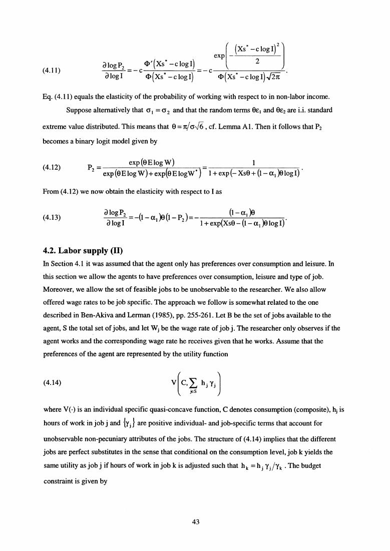
(4.11)

( ^Xs * —c1ogI) 2

exp _a log P2 __^ Ø'(Xs"—c1ogF _ —c ■ ^ ^ .

alogi Ø^Xs' —c log I^ (xs*_c1ogI).sJ27c

Eq. (4.11) equals the elasticity of the probability of working with respect to in non-labor income.

Suppose alternatively that a, = 6 2 and that the random terms أ, and 0E2 are i.i. standard

extreme value distributed. This means that 0 = , cf. Lemma Al. Then it follows that P2

becomes a binary logit model given by

(4.12) P2 =exp (Ø E log W) 1

exp (Ø E log W) + exp(Ø E logW * ) 1 + exp (— XsØ + (1 — a l )O logl) •

From (4.12) we now obtain the elasticity with respect to I as

(4.13)a logP2 _ —(1—a0Ø(l—PZ)= (i—a1)ea log I 1 + exp(XsØ — (1— a l » log I) •

4.2. Labor supply (II)

In Section 4.1 it was assumed that the agent only has preferences over consumption and leisure. In

this section we allow the agents to have preferences over consumption, leisure and type of job.

Moreover, we allow the set of feasible jobs to be unobservable to the researcher. We also allow

offered wage rates to be job specific. The approach we follow is somewhat related to the one

described in Ben-Akiva and Lerman (1985), pp. 255-261. Let B be the set of jobs available to the

agent, S the total set of jobs, and let WW be the wage rate of job j. The researcher only observes if the

agent works and the corresponding wage rate he receives given that he works. Assume that the

preferences of the agent are represented by the utility function

(4.14) V C, E h i y^,Es

where V() is an individual specific quasi-concave function, C denotes consumption (composite), h i is

hours of work in job j and iyi } are positive individual- and job-specific terms that account for

unobservable non-pecuniary attributes of the jobs. The structure of (4.14) implies that the different

jobs are perfect substitutes in the sense that conditional on the consumption level, job k yields the

same utility as job j if hours of work in job k is adjusted such that h k = h j yi tyk . The budget

constraint is given by

43

VZ (I,0)

V^ (I,0)

(4.18)

and

(4.19)

U i = log W j — logy ]

U 0 = log

(4.15) C = h jWj + I,jeB

where I is nonlabor income. Note that the maximization of (4.14) subject to (4.15) is formally

equivalent to maximizing of

(4.16)

with respect to C and jx i I subject to

W.(4.17) C=1, x j ' +I, jeB

iE B Yj

where h i = x j /y j . Since (4.16) is symmetric in x l , x 2 ... , the agent will choose x i > 0 solely for the

j with the highest value of the modified wage rates, {W iy i , j E B1. Let

v c, / X ;jeB

where Vk(•) denotes the partial derivative with respect to the k-th component. The interpretation of U o

is as the logarithm of the reservation wage. Thus, the individual will choose job j if

U ^ =maxlUo , max U k ^ke B

and choose not to work if

Uo > max U k .

keB

Assume furthermore that

(4.20) Uo = vo + 6o

where vo is a structural term and Eo is a random variable. In (4.18), W i is possibly correlated with yj

and we therefore introduce an instrument variable equation

(4.21) log Wj = X13 + r^^

44

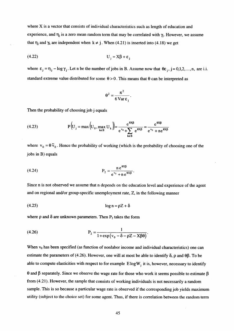
1PZ l+ exp (v o —S—pZ—X(3Ø) •

(4.26)

where X is a vector that consists of individual characteristics such as length of education and

experience, and inj is a zero mean random term that may be correlated with yj . However, we assume

that Tb and yk are independent when k # j . When (4.21) is inserted into (4.18) we get

(4.22)

where E i _ l ^ — log yi . Let n be the number of jobs in B. Assume now that OE , j = 0,1,2, ..., n, are i.i.

standard extreme value distributed for some 0 > 0 . This means that Ø can be interpreted as

TC 202 =

•6VarE i

Then the probability of choosing job j equals

(4.23) e exa e exRP U ^= max (u 0 , max U k ))= v° exR v° exøkEB e +1, e e ne

kE B

where v o = 0 vo . Hence the probability of working (which is the probability of choosing one of the

jobs in B) equals

(4.24) P2 =n e exR

•e v° +ne ex

Since n is not observed we assume that n depends on the education level and experience of the agent

and on regional and/or group-specific unemployment rate, Z, in the following manner

(4.25) log n = pZ + b

where p and S are unknown parameters. Then P2 takes the form

When vo has been specified (as function of nonlabor income and individual characteristics) one can

estimate the parameters of (4.26). However, one will at most be able to identify 8, p and O. To be

able to compute elasticities with respect to for example E logW i it is, however, necessary to identify

Ø and f3 separately. Since we observe the wage rate for those who work it seems possible to estimate ffrom (4.21). However, the sample that consists of working individuals is not necessarily a random

sample. This is so because a particular wage rate is observed if the corresponding job yields maximum

utility (subject to the choice set) for some agent. Thus, if there is correlation between the random term

45

in (4.21) and the selection rule (the random terms in the indirect utility function), then the

application of OLS to (4.21) may yield biased estimate of p. Let us now discuss this problem more in

detail. A formal way of expressing the problem discussed above is as follows: Let J denote the most

preferred alternative in B u {0} (the job alternatives and the non-working alternative) and let J *

denote the most preferred alternative in B. If it is the case that

E (in J. I U j. > Uo ) 0

then OLS will give biased estimate of (3.

Assume next that

(4.27) E ^^Ui)=a(BUj—EBUi)

where a is a constant. If i j and ØU i where jointly normally distributed (4.27) would follow due to

the fact that the conditional mean in a bivariate normal distribution is linear. This is not the case here,

so we cannot be sure (4.27) holds exactly. We still assume that (4.27) holds approximately. Note that

it is necessary to substract EOU J from W i to ensure that Ei = 0 . By Lemma A2 in Appendix A it

follows that

(4.28)

Furthermore, we have that

E(Ou j. Uj. > U0 ) = E(OU, = U .1 ) = E 0 U j

(4.29)

P(eu, <_y)—P max OUk <_y = rj P(eUk <_y)keBJ{0}ICE$V{O}

= exp(—e y(e"0 +neeXø))=exp(—exp (log (e"0 +neexø ^ _y1111

But this implies that

(4.30)

Similarly it follows that

(4.31)

•

EØUJ =1oge"° +neBXa)+0.5772.

E Ø =logn + 8X(3 + 0.5772.

Now from (4.27), (4.28), (4.30) and (4.31) it follows that

46

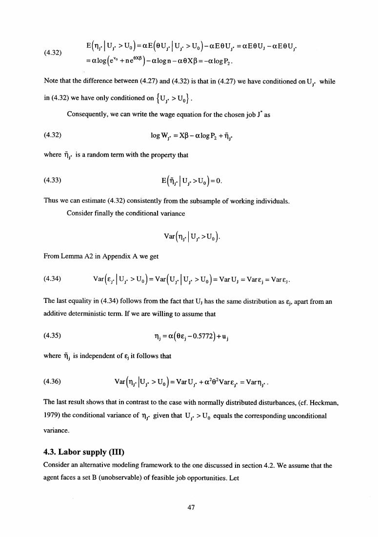
(4.32)E(Tij. I U1. >Uo )=aE(ØUj.IUj.>Uo )—aEBU j. =aEØU N —aEØU B .

=alog(e"° +ne eXR )—alogn—oeØX(3=—alog P2 .

Note that the difference between (4.27) and (4.32) is that in (4.27) we have conditioned on UJ» while

in (4.32) we have only conditioned on { u. > Uo .

Consequently, we can write the wage equation for the chosen job J * as

(4.32) log WJ. = X13 — a log P2 + flJ*

where fiJ' is a random term with the property that

(4.33) E (fl J. I u >U0 )= O.

Thus we can estimate (4.32) consistently from the subsample of working individuals.

Consider finally the conditional variance

Var (T J. I u,. >Uo ).

From Lemma A2 in Appendix A we get

(4.34) Var(Ef I U j. > Uo ) = Vaz(U j. I Uj. > Uo ) = Var U J =Vare = VazEJ .

The last equality in (4.34) follows from the fact that U j has the same distribution as cj , apart from an

additive deterministic term. If we are willing to assume that

(4.35) r^ ^ =a(Ø£ i —0.5772+u i

where ^j is independent of E i it follows that

(4.36) Var (Ty I U j. > Uo = VarU J. +a282Var£J* =

The last result shows that in contrast to the case with normally distributed disturbances, (cf. Heckman,

1979) the conditional variance of ^` given that U J . > U0 equals the corresponding unconditional

variance.

4.3. Labor supply (III)

Consider an alternative modeling framework to the one discussed in section 4.2. We assume that the

agent faces a set B (unobservable) of feasible job opportunities. Let

47

(4.37)

U .1 =v(W-J E ^

j =1,3, ..., n, be the utility of job j with wage rate W^ , where v Wi is the structural part of the utility

function that is common to all agents, while Ej is an agent-specific random term that accounts for non-

pecuniary aspect associated with job j. Similarly, let

(4.38) U0 = v 0 + C o

be the utility of not working. Suppose furthermore that e , j = 0,1, ..., are i.i. standard extreme value

distributed.

Let B(w) be the subset of B that consists of all feasible jobs with wage rate w, and let n(w) be

the number of jobs in B(w), and let D be the set of all possible wages. The probability of choosing job

j in B equals

PJ = PI U J = max (U o , max U k)JkeB

ev(w

i)

(4.39)

e "° +I e v(wk )kEB

e

"° "(Wk)_

e "°+ n(y)ev ( Y ) 'e + e}/ED kEB(y) yED

Hence the probability of choosing a job with wage rate w equals

(4.40)

where

13(w).-_-=. p . = jEB(w)

jEB(w) ^ e "° + n(y)ev(Y)yED

n(w)e v(w) ev (w)_

e "° + n(y)ev(Y) e "° +I eV(Y)

yED yED

(4.41) V(y) = log n(y) + v(y).

From (4.41) we realize that we cannot without further assumptions separate n(w) from v(w).

To this end suppose that the agent also receives nonlabor income. For example, a married woman or

man may receive income from the spouse. In this case

(4.42) v(w) = v` (w + I)

where I denoted nonlabor income, and v *(•) is a concave parametric function.

48

The type of framework considered above with latent opportunity sets is discussed in Ben-

Akiva and Lerman (1985), p.p. 254-260.

4.4. Transportation

Suppose that commuters have the choice between driving own car or taking a bus. One is interested in

estimating a behavioral model to study, for example, how the introduction of a new subway line will

affect the commuters' transportation choices. Consider a particular commuter (agent) and let U U(x) be

the agent's joint utility of commodity vector x and transportation alternative j, j =1,2. Assume that the

utility function has the structure

(4.43)

The budget constraint is given by

(4.44)

TJ(x).U j (x) =U, i +

px = y — gj,x? 0,

where p is a vector of commodity prices and q j is the per-unit-cost of transportation. By maximizing

Uj(x) with respect to x subject to (4.44) we obtain the conditional indirect utility, given j, as

(4.45) V;(p,Y-9;)=Ul;+V P,Y — qi)

where the function V *(p,y) is defined by

(4.46) V * (p, y) = max U (x ).p x=y

Assume that

(4.47) U1i= (3TT+Ej

where Ti is the travelling time with alternative j, 13 is an unknown parameter and {£ j } are random

terms that account for the effect of unobserved variables, such as walking distances and comfort. We

assume that E 1 and £2 are i.i. standard extreme value distributed. Assume furthermore that

(4.48) V*(p,Y-9=V(P)+Ølogy—qi)

where 0 > 0 is an unknown parameter. The assumptions above yield

(4.49) Vj (p,y — q J= f3Tj + Ølog& — q^+ V(p) + E j

which implies that

49

Prl = P U r = max max U ik )) =i kEC;

e"r

e"rm m

er ni e "i

i=1 kEC ; i=1

(4.52)

(4.50) ^exp 43Tj + Ø log (Y — q ^^^

P^ ({1,2}) =

^ 2k=1 exp (J3Tk + Ø log (y — q k ^^

for j =1,2. After the unknown parameters Q and 8 have been estimated one can predict the fraction of

commuters that will choose the subway alternative (alternative 3) given that T3 and q3 have been

specified. Here, it is essential that one believes that Ti and qi are the main attributes of importance.

We thus get that the probability of choosing alternative j from {1,2,3} equals

(4.51) Pi ({1,2,3}) = 3 exp

(13Tj + Ø log — qi ^^

1k=1 exp (J3Tk + Ø log (y — q k ^^

4.5. Firms' location of plants (I)

In this example we outline a framework for analyzing firms' location of plants. Specifically, we

assume that the firms face the choice of establishing a plant in one of m differents sites (counties).

Suppose furthermore that firms profit functions (or expected profit functions) depend on observable

characteristics that are common for all sites within particular regions. Let C r denote the set of counties

within region r, r =1,2,..., m, and let n r be the number of counties in C r. The regional attributes of

interest may be the population density and macro indicators that describe the industry structure.

Finally, certain tax rates may differ across regions (tax shelters). Consider an arbitrarily selected firm.

Let U ri = v r + E d denote the firms utility of establishing a plant in county j E C r , where {E rj

are i.i.

standard extreme value distributed terms that account for unobserved region and county-specific

attributes and {v r } are structural terms that depend on the attributes specific to region r. Let P, i be the

probability of a location in county j in region r. We get

Hence, we get that the probability of a location within region r equals

n r e " re "r

(4.53) Pr = P,j = m = m ,

JECr ni ev;1i=1 i =1

where

(4.54) y r = y r + log n r .

50

I

0

m nr

^r=1 j=1

G(Y) = I, y ^ e

If we assume that v r = Z r J , where Zr is the vector of observable attributes associated with region r,

we get

(4.55) Vr = ZrF' + log n r

4.6. Firms' location of plants (II)

We now consider an extension of the setting in Section 4.5. Suppose now that the error terms for

counties within a common region are correlated. This may be a plausible assumption since it is often

the case that counties within regions are more homogeneous than counties across regions. We shall

now apply the nested logit framework to model this case. Let

(4.56)

and let

F(x) = exp —G e -X11 ,a -X12,...

be the joint distribution function of (E li ,..., E 1 n, , . • . , E mi , • • • , E mn m . Then it follows that

(4.57)

for i s j, i, j E C r , and

(4.58)

corr E ri ,E rj = 1-0 2

corr E ri , E sj = 0

for i EC r , JE C s ,r s, where 0<0<_1. From Theorem 8 we get

(4.59)

9-1e v ; ie e y r ie

jECr e ^r n e 1Prj = e = m • •

^;^e e^; ne n re

i =1 jEC; i=1

Specifically, the probability of choosing region r equals

(4.60) Pr = _ evr n e _ e "rP _ r _

r)m m

jECr e" i n? e ^;,

i =1 i=1

51

where

(4.61)*

v r =V r +Ølog n r .

From (4.60) we get

(4.62)

and

(4.63)

a log Pr= 9 0- - Pr) 1og n r

a log Pk=Ø Pra log n r

for k # r. The interpretation of (4.62) and (4.63) is as the effect from increasing the size of Cr. For

example, one may wish to assess the effect of changing the number of counties that belong to a region

with "tax shelters".

4.7. Firms' location of plants (III)

The setting here is the same as the one in Section 4.6. Suppose now that In r } are unobservable, but

that we observe the number of locations in at least one county in each region, say in county number

one. Let Mnl be the observed number of locations in county one in C r, and let Mr be the total number

of observed locations within region r. Finally, let M=1 M r . Then M il /M r is an estimate of Prlr=1

and M r /M is an estimate of Pr. Since by (4.59)

P .- p 1rl r n r

it follows that consistent estimates for n r is given by

(4.64)M 2

n r = r , r =1,2,..., m.M rt M

4.8. Potential demand for alternative fuel vehicles

This example is taken from Dagsvik et al. (1996). To assess the potential demand for alternative fuel

vehicles such as; "electric" (1), "liquid propane gas" (lpg) (2), and "hybrid" (3), vehicles, an ordered

logit model was estimated on the basis of a "stated preference" survey. In this survey each responent

in a randomly selected sample was exposed to 15 experiments. In each experiment the respondent was

asked to rank three hypothetical vehicles characterized by specified attributes, according to the

52

respondent's preferences. These attributes are: "Purchase price", "Top speed", "Driving range

between refueling/recharging", and "Fuel consumption". The total sample size (after the non-

respondent individuals are removed) consisted of 662 individuals. About one half of the sample

(group A) received choice sets with the alternatives "electric", "lpg", and "gasoline" vehicles, while

the other half (group B) received "hybrid", "lpg" and "gasoline" vehicles. In this study "hybrid"

means a combination of electric and gasoline technology. The gasoline alternative is labeled

alternative 4.

The individuals' utility function was specified as

(4.65) Uj(t)=Zi(t)(3 +µgi +E j (t)

where Z,(t) is a vector consisting of the four attributes of vehicle j in experiment t, t =1,2,...,15 , and

pi and f are unknown parameters. Without loss of generality, we set g 4 = 0. As mentioned above

group A has choice set, C A = {1,2,4} , while group B has choice set, C B =12,3,44. Let Piit(C) be the

probability that an individual shall rank alternative i on top and j second best in experiment t, and let

Yip (t) =1 if individual h ranks i on top and j second best in experiment t, and zero otherwise. From

Theorem 3 it follows that if te j (t) are assumed to be i.i. standard extreme value distributed then

(4.66)exp(Z i (t)p +µ ^ ) exp(Zi(t)(3+11j)

eXP(Z r (t)(3+µ r) y, eXP(Z r (t)P+µ r )rEC rEC\ {i}

where C is equal to CA or CB,. We also assume that the random terms {E j (t)} are independent across

experiments. Consequently, it follows that the loglikelihood function has the form

15

(4.67) t=1, E Yli log Put (C a ) ^ ^ / Y; (t) log Put (C Bt=1 hEA i j hEB i j

The sample is further split into six age and gender groups, and Table 4.1 displays the estimation

results for these groups.

53

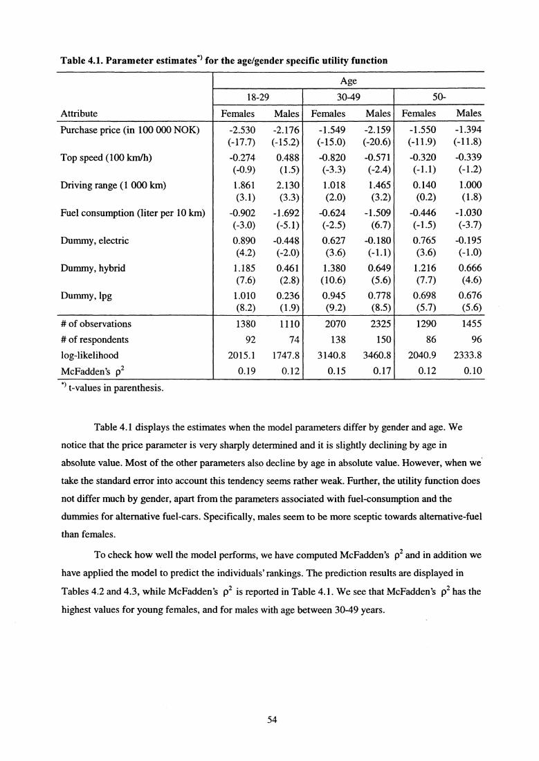
18-29 50-30-49

Age

Attribute

Purchase price (in 100 000 NOK)

Top speed (100 km/h)

Driving range (1 000 km)

Fuel consumption (liter per 10 km)

Dummy, electric

Dummy, hybrid

Dummy, 1pg

# of observations

# of respondents

log-likelihood

McFadden's p2

Females Males

-2.530 -2.176

(-17.7)

(-15.2)

-0.274

0.488

(-0.9)

(1.5)

1.861

2.130

(3.1)

(3.3)

-0.902 -1.692

(-3.0)

(-5.1)

0.890 -0.448

(4.2)

(-2.0)

1.185

0.461

(7.6)

(2.8)

1.010

0.236

(8.2)

(1.9)

1380 1110

92 74

2015.1 1747.8

0.19 0.12

Females Males

-1.549 -2.159

(-15.0)

(-20.6)

-0.820 -0.571

(-3.3)

(-2.4)

1.018

1.465

(2.0)

(3.2)

-0.624 -1.509

(-2.5)

(6.7)

0.627 -0.180

(3.6)

(-1.1)

1.380

0.649

(10.6)

(5.6)

0.945

0.778

(9.2)

(8.5)

2070 2325

138 150

3140.8 3460.8

0.15 0.17

Females Males

-1.550 -1.394

(-11.9) (-11.8)

-0.320 -0.339

(-1.1) (-1.2)

0.140 1.000

(0.2) (1.8)

-0.446 -1.030

(-1.5) (-3.7)

0.765 -0.195

(3.6) (-1.0)

1.216 0.666

(7.7) (4.6)

0.698 0.676

(5.7) (5.6)

1290 1455

86 96

2040.9 2333.8

0.12 0.10

Table 4.1. Parameter estimates *) for the age/gender specific utility function

*) t-values in parenthesis.

Table 4.1 displays the estimates when the model parameters differ by gender and age. We

notice that the price parameter is very sharply determined and it is slightly declining by age in

absolute value. Most of the other parameters also decline by age in absolute value. However, when we'

take the standard error into account this tendency seems rather weak. Further, the utility function does

not differ much by gender, apart from the parameters associated with fuel-consumption and the

dummies for alternative fuel-cars. Specifically, males seem to be more sceptic towards alternative-fuel

than females.

To check how well the model performs, we have computed McFadden's p 2 and in addition we

have applied the model to predict the individuals' rankings. The prediction results are displayed in

Tables 4.2 and 4.3, while McFadden's p 2 is reported in Table 4.1. We see that McFadden's p 2 has the

highest values for young females, and for males with age between 30-49 years.

54

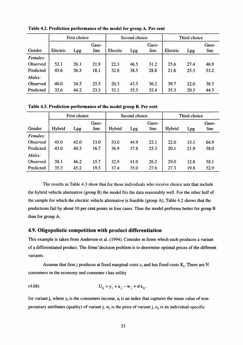
Table 4.2. Prediction performance of the model for group A. Per cent

First choice Second choice Third choice

Gaso- Gaso- Gaso-Gender Electric Lpg line Electric Lpg line Electric Lpg line

Females:Observed 52.1 26.1 21.9 22.3 46.5 31.2 25.6 27.4 46.9Predicted 45.6 36.3 18.1 32.8 38.5 28.8 21.6 25.3 53.2

Males:Observed 40.0 34.5 25.5 20.3 43.5 36.2 39.7 22.0 38.3Predicted 32.6 44.2 23.3 32.1 35.5 32.4 35.3 20.3 44.3

Table 4.3. Prediction performance of the model group B. Per cent

First choice Second choice Third choice

Gaso- Gaso- Gaso-Gender Hybrid Lpg line Hybrid Lpg line Hybrid Lpg line

Females:Observed 45.0 42.0 13.0 33.0 44.9 22.1 22.0 13.1 64.9Predicted 43.0 40.3 16.7 36.9 37.8 25.3 20.1 21.9 58.0

Males:Observed 38.1 46.2 15.7 32.9 41.0 26.2 29.0 12.8 58.1Predicted 35.3 45.2 19.5 37.4 35.0 27.6 27.3 19.8 52.9

The results in Table 4.3 show that for those individuals who receive choice sets that include

the hybrid vehicle alternative (group B) the model fits the data reasonably well. For the other half of

the sample for which the electric vehicle alternative is feasible (group A), Table 4.2 shows that the

predictions fail by about 10 per cent points in four cases. Thus the model performs better for group B

than for group A.

4.9. Oligopolistic competition with product differentiation

This example is taken from Anderson et al. (1994). Consider m firms which each produces a variant

of a differentiated product. The firms' decision problem is to determine optimal prices of the different

variants.

Assume that firm j produces at fixed marginal costs c ; and has fixed costs There are N

consumers in the economy and consumer i has utility

(4.68) U;^= y ;+a^-w^ +6E.

for variant j, where y ; is the consumers income, a; is an index that captures the mean value of non-

pecuniary attributes (quality) of variant j, w; is the price of variant j, is an individual-specific

55

PJ =Q (w)= m

k=1exp (a,

— Wk

(4.69)

aa

random taste-shifter that captures unobservable product attributes as well as unobservable individual-

specific characteristics and cs > 0 is a parameter (unknown). If we assume that E i; , j =1,2,..., m,

i =1,2,...,N, are i.i. standard extreme value distributed we get that the aggregate demand for variant j

equals NP; where

expaj—wi

66

Assume next that the firm knows the mean fractional demands {Q i (w) as a function of prices, w.

Consequently, a firm that produces variant j can calculate expected profit, it, conditional on the

prices;

(4.70) it = (Vs/ C )N Q (w) — K • .

Now firm j takes the prices set by other firms as given and chooses the price of variant j that

maximizes (4.70). Anderson et al. (1992) demonstrate that there exists a unique Nash equilibrium set

of prices, w * = (w; , w; , ... , w m which are determined by

(4.71) W ; = c ; +a

1—Q • (w

4.10. Social network

This example is borrowed from Dagsvik (1985). In the time-use survey conducted by Statistics

Norway, 1980-1981, the survey respondents were asked who they would turn to if they needed help.

The respondents were divided into two age groups, where group (i) and (ii) consist of individuals less

than 45 years of age and more than 45 years of age, respectively. Here, we shall only analyze the

subsample of individuals less than 45 years of age. The univers of alternatives S consisted of five

alternatives, namely

S = {Mother (1), father (2), brother (3), sister (4), neighbor (5)1.

However, the set of feasible alternatives (choice set) were less for many of the respondents.

Specifically, there turn out to be 11 different choice sets in the sample; B 1 , B 2 , ... , Bi . The data for

each of the 11 groups are given in Table 4.5. Group (i) consists of 526 individuals.

56

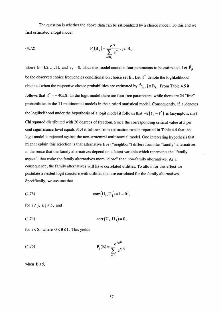
The question is whether the above data can be rationalized by a choice model. To this end we

first estimated a logit model

(4.72) P^ (Bk ^ =e v;

jE Bk,^ '

e r

iE B k

where k =1,2,...,11, and v 5 = 0. Thus this model contains four parameters to be estimated. Let Pik

be the observed choice frequencies conditional on choice set Bk. Let .e * denote the loglikelihood

obtained when the respective choice probabilities are estimated by Pik , jEB k . From Table 4.5 it

follows that £ * =— 405.8. In the logit model there are four free parameters, while there are 24 "free"

probabilities in the 11 multinomial models in the a priori statistical model. Consequently, if £ , denotes

the loglikelihood under the hypothesis of a logit model it follows that —2 (.e i — t * ) is (asymptotically)

Chi squared distributed with 20 degrees of freedom. Since the corresponding critical value at 5 per

cent significance level equals 31.4 it follows from estimation results reported in Table 4.4 that the

logit model is rejected against the non-structural multinomial model. One interesting hypothesis that

might explain this rejection is that alternative five ("neighbor") differs from the "family" alternatives

in the sense that the family alternatives depend on a latent variable which represents the "family

aspect", that make the family alternatives more "close" than non-family alternatives. As a

consequence, the family alternatives will have correlated utilities. To allow for this effect we

postulate a nested logit structure with utilities that are correlated for the family alternatives.

Specifically, we assume that

(4.73)

for i# j, i,j#5, and

(4.74)

for i < 5, where 0 < 0 < 1. This yields

(4.75)

when B 3 5,

con (u„, U, =1- 8 2 ,

corr(U ; ,U S ) = 0,

y i p)P (B) — e e V r /e

TE B

57

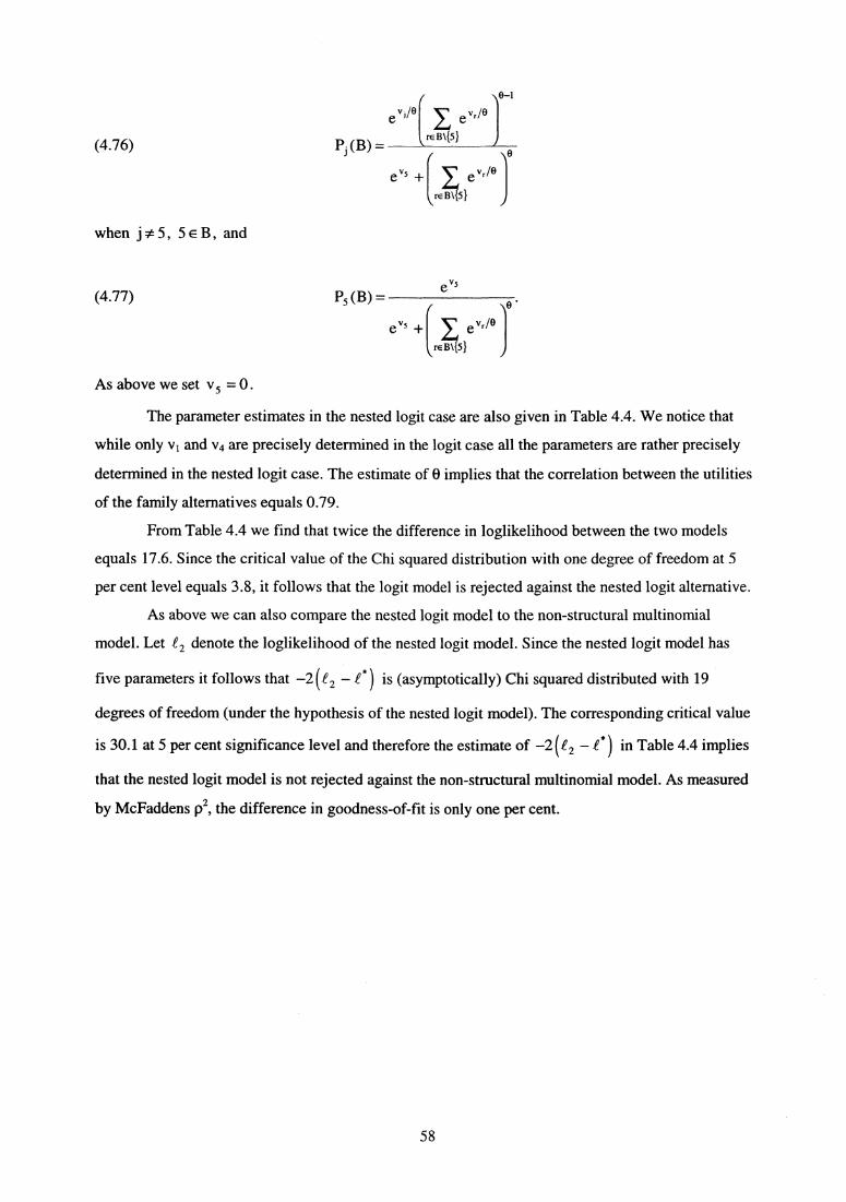
( e-1

ev e vr/Ø

\. rEB\{5}P^ (B) -- e

e v5 .+ e V r /8

yEB\{5}

(

(4.76)

when j#5, 5 E B, and

(4.77) PS (B) _e"' + e°

rE B \{5}

As above we set v 5 = 0.

The parameter estimates in the nested logit case are also given in Table 4.4. We notice that

while only v 1 and v4 are precisely determined in the logit case all the parameters are rather precisely

determined in the nested logit case. The estimate of 0 implies that the correlation between the utilities

of the family alternatives equals 0.79.

From Table 4.4 we find that twice the difference in loglikelihood between the two models

equals 17.6. Since the critical value of the Chi squared distribution with one degree of freedom at 5

per cent level equals 3.8, it follows that the logit model is rejected against the nested logit alternative.

As above we can also compare the nested logit model to the non-structural multinomial

model. Let £2 denote the loglikelihood of the nested logit model. Since the nested logit model has

five parameters it follows that —2 (f 2 — 2l is (asymptotically) Chi squared distributed with 19

degrees of freedom (under the hypothesis of the nested logit model). The corresponding critical value

is 30.1 at 5 per cent significance level and therefore the estimate of —2 (t 2 — P * ) in Table 4.4 implies

that the nested logit model is not rejected against the non-structural multinomial model. As measured

by McFaddens p2, the difference in goodness-of-fit is only one per cent.

e vs

58

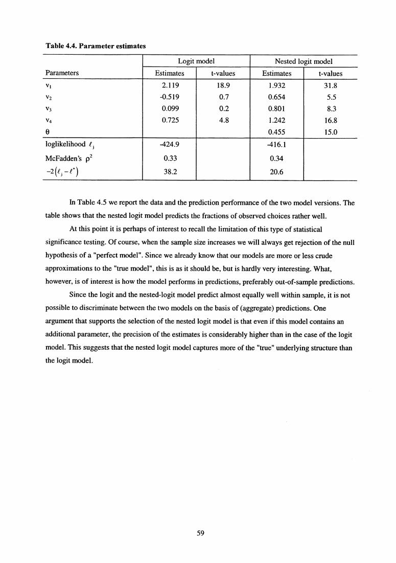
Parameters

v i

V2

V3

V4

0

loglikelihood t i

McFadden's p2

—2 (i i _,^ * )

Estimates

2.119

-0.519

0.099

0.725

-424.9

0.33

38.2

t-values

18.9

0.7

0.2

4.8

Nested lo

Estimates

1.932

0.654

0.801

1.242

0.455

-416.1

0.34

20.6

git model

t-values

31.8

5.5

8.3

16.8

15.0

Logit model

Table 4.4. Parameter estimates

In Table 4.5 we report the data and the prediction performance of the two model versions. The

table shows that the nested logit model predicts the fractions of observed choices rather well.

At this point it is perhaps of interest to recall the limitation of this type of statistical

significance testing. Of course, when the sample size increases we will always get rejection of the null

hypothesis of a "perfect model". Since we already know that our models are more or less crude

approximations to the "true model", this is as it should be, but is hardly very interesting. What,

however, is of interest is how the model performs in predictions, preferably out-of-sample predictions.

Since the logit and the nested-logit model predict almost equally well within sample, it is not

possible to discriminate between the two models on the basis of (aggregate) predictions. One

argument that supports the selection of the nested logit model is that even if this model contains an

additional parameter, the precision of the estimates is considerably higher than in the case of the logit

model. This suggests that the nested logit model captures more of the "true" underlying structure than

the logit model.

59

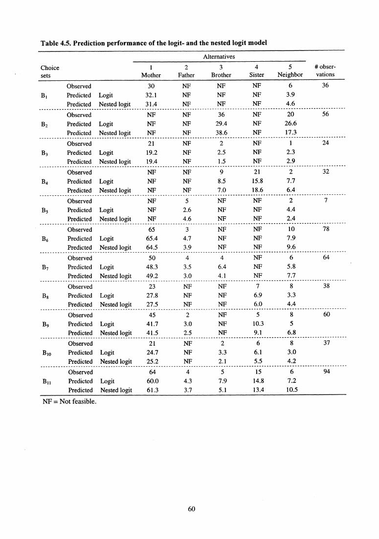
Table 4.5. Prediction performance of the logit- and the nested logit model

Alternatives

Choice 1 2 3 4 5 # obser-sets Mother Father Brother Sister Neighbor vations

Observed 30 NF NF NF 6 36

B 1 Predicted Logit 32.1 NF NF NF 3.9

Predicted Nested logit 31.4 NF NF NF 4.6

Observed NF NF 36 NF 20 56

B2 Predicted Logit NF NF 29.4 NF 26.6

Predicted Nested logit NF NF 38.6 NF 17.3

Observed 21 NF 2 NF 1 24

B 3 Predicted Logit 19.2 NF 2.5 NF 2.3

Predicted Nested logit 19.4 NF 1.5 NF 2.9

Observed NF NF 9 21 2 32

B4 Predicted Logit NF NF 8.5 15.8 7.7

Predicted Nested logit NF NF 7.0 18.6 6.4

Observed NF 5 NF NF 2 7

B 5 Predicted Logit NF 2.6 NF NF 4.4

Predicted Nested logit NF 4.6 NF NF 2.4

Observed 65 3 NF NF 10 78

B 6 Predicted Logit 65.4 4.7 NF NF 7.9

Predicted Nested logit 64.5 3.9 NF NF 9.6

Observed 50 4 4 NF 6 64

B 7Predicted Logit 48.3 3.5 6.4 NF 5.8

Predicted Nested logit 49.2 3.0 4.1 NF 7.7

Observed 23 NF NF 7 8 38

B 8 Predicted Logit 27.8 NF NF 6.9 3.3

Predicted Nested logit 27.5 NF NF 6.0 4.4

Observed 45 2 NF 5 8 60

B9 Predicted Logit 41.7 3.0 NF 10.3 5

Predicted Nested logit 41.5 2.5 NF 9.1 6.8

Observed 21 NF 2 6 8 37

B 10 Predicted Logit 24.7 NF 3.3 6.1 3.0

Predicted Nested logit 25.2 NF 2.1 5.5 4.2

Observed 64 4 5 15 6 94

B 11 Predicted Logit 60.0 4.3 7.9 14.8 7.2

Predicted Nested logit 61.3 3.7 5.1 13.4 10.5

NF = Not feasible.

60

5. Discrete/continuous choice

5.1. The nonstructural Tobit model

In this section we shall describe a type of statistical model, usually called the Tobit model. The Tobit

model (Tobin, 1958) is motivated from the latent variable specification similarly to Section 2.1.3, but

in contrast to the case described there we now also observe the left hand side variable when it is

positive. Thus we observe Y defined by

(5.1)JXf+ucT if X13+ua>0

Y=0 otherwise,

where 6 > 0 is a scale parameter, and u is a zero mean random variable with cumulative distribution

function F(•). Another way of expressing (5.1) is as

(5.2) Y = max (0,X(3 + u6) .

Tobin (1958) assumed that u is normally distributed N(0,1), but it is also convenient to work with the

logistic distribution.

An example of a Tobit formulation is the standard labor supply model. Here we may interpret

X(3c + uyc as an index that measures the desire to work of an agent with characteristics X. When this

index is positive, the desired hours of work is typically assumed proportional to X f 3c + usac where 1/c

is the proportionality factor. The variable vector X may contain education, work experience, and the

unobservable term u may capture the effect of unobservable variables such as specific skills and

training. When the index X f 3c + uac is negative and large, say, it means that the agent has strong

tendence to choose leisure. Since the actual hours og work always will be non-negative we therefore

get the structure (5.1).

5.2. The general structural setting

Models such as the Tobit one account for some of the statistical nature of the data, but is not

structural in a "deep" sense. We shall now discuss structural specifications derived from choice

theory. In many situations a decision-maker makes interrelated choices where one choice is discrete

and the other is continuous. For example, a worker may face the decision problem of which job to

choose and how many hours to work, (conditional on the choice of job). Another example is a

consumer that considers purchasing electric versus gas appliances, as well as how much electricity or

gas to consume. A third example is a household that chooses which type of car to own and the

intensity of car use.

Such choice situations are called discrete/continuous, reflecting the fact that the choice set

along one dimension is discrete while it is continuous along another. Theories and methods for

61

specifying and estimating structural models for discrete/continuous choice have been developed

among others by Heckman (1974, 1979), Dubin and McFadden (1984), Lee and Trost (1978), King

(1980) and Dagsvik (1994).

We now consider an agent that faces two choices; first which alternative to choose from a

finite and exhaustive set of mutually exclusive alternatives, and second; how much of a particular

good to consume. Since it is often the case that these choices depend on the same underlying factors

this should be taken into account in the formulation of the model and in the corresponding

econometric specification. Suppose for expository simplicity that there are only two continuous

goods. Let U ; (x i , x 2 ) be the utility of alternative (j, x 1 , x 2 ), where j =1,2,..., indexes the discrete

alternatives and (x 1 , x 2 ) the continuous ones. Thus the agent's optimization problem is to maximize

U ; (x 1 , x 2 ) with respect to (j, x I , x 2 ) subject to the budget constraints j E B and

xl p 1 + x2 p2 + Sk Ck =y, x 1 ^^^ x2k

where B is the choice set of feasible (discrete) alternatives, Pi , p 2 are prices, y is the agent's income

(exogenous), c; is the cost (or annual user cost) of the discrete alternative j and 8 k =1 if alternative

k E B is chosen and zero otherwise. Consider now the continuous choice given the discrete alternative

j. Let

(5.4)

V; p, y —c;) = maxX 1P , +X2P2 =Y-c ;

X2)xi Z0, z2 >0

which means that Vj (p, y — c j ) is the conditional indirect utility, given that the discrete alternative j is

chosen. Since Vi (p, y — c j ) expresses the highest possible utility conditional on alternative j, it must

be the case that alternative j is chosen if

(p y — c .) = max V (p y — c

Second, it follows from Roy's identity that under standard regularity conditions we obtain the

corresponding continuous demands by

(5.6)aVjp,y—c,013,

v;(p,y— c;Vay

(5.3)

(5.5)

62

for r =1,2, given that j is the preferred discrete alternative, i.e., given that (5.5) holds. Thus the

discrete as well as the continuous choices are here derived from a common representation of the

preferences.

It is known from duality theory that under standard regularity conditions the specification of

the indirect utility is equivalent to the specification of the corresponding direct utility. Therefore, in

econometric model building, it is convenient to start with a parametric functional form of the indirect

utility function, including alternative-specific random terms.

5.3. The Gorman Polar functional form

When the conditional indirect utility function belongs to the class of functional forms called "Gorman

Polar forms", (Gorman, 1953), then the structure of the demand equations and choice probabilities

become particularly convenient. The Gorman Polar functional form is given by

y—ci +a(p)(E i +m j )v- V.(13 —

b(p)

where a(•) and b() are functions that are homogeneous of degree one, concave and non-decreasing in

p and {m 3 } are alternative-specific terms which are independent of prices and income. It then follows

that Vi is non-increasing and convex in prices. Here {E i } are random terms that are supposed to

account for unobservables that affect preferences and m; is (possibly) a function of observable

attributes associated with alternative j.

From (5.7) it follows that the choice probabilities are defined by

P^(B) =P C.+m.J - a(P) -

max l E k mk— (P)^ .kEB l a

In case ic i } are i.i. extreme value distributed we obtain

(5.9)exp (m j _c/a(p))

Pi (B)_ LkEB eXP(mk —ckia(P)).

By Roy's identity we obtain the demands as

(5.10)(a(p) br(P) 1 br(P) (a(p)b,(p)1

X°= b(p) — ar(P))mi + ^Y—ci) b(p) + b(p) —ar(P))Ei

where ar(p) and b•(p) denote the respective partial derivatives with respect to component r.

(5.7)

(5.8)

63

P. = exp(Zkoc+plZk[31+p2Zkr32 —Øc k )

k

(5.15)exp Z ia+p 1 Z i1i 1 +p 2 Z i fi 2 — ec i

Recall, however, that due to the selectivity problem we cannot automatically apply standard

methods to estimate (5.10), as we shall discuss in further detail below.

Example 5.1

Assume that the conditional indirect utility function has the form

(5.11) Vi(p,y—cj)=(Zia+p,Zi(3l+p2;02+0(y—cj)+Ei)exp(-01.tip,-01.1.2p2

where H are i.i. standard extreme value distributed random terms and a, BB Ø, µ^, µ2, are

parameters.5 However, the specification does not have the Gorman Polar functional form. From (5.11)

we obtain

v i (p, y —c j )

(5.12) — (ZiPr — eµ (Zia+PiZ;R, +P2Zif3 2 +e(Y —c+E ^)) exp^—ص^ P ^ — Ø11zPz)a Pr

and

(5.13)

Consequently, by (5.6)

Vi (p,y—c i )a —eeXP(—eµ1pi

— eµ2P2).y

(5.14) ^' F'r xrj — Zj a µr — + Pl Zjllr + P2 Z jR21i r +gre(Y - ci)+11 r Ei .e

Second, note that maximization of V-J ^p , y — c ^) is equivalent to maximizing

Z ia+p il i (3 1 +p 2 N3 2 —Oc i + E i .

Therefore, the probability of choosing alternative j equals

5 Note that (5.11) is not homogeneous of degree zero in prices and income. We may, however, interpret (5.11) asan indirect utility function in normalized prices and income. This is possible because a function v(p,y) ofnormalized prices and income is the indirect utility function of some locally nonsatiated utility function if andonly if it is lower semicontinuous, quasi-convex, increasing in y, nonincreasing in p, and has v(Xp,Ay)nondecreasing in X.

64

Recall while the unconditional mean of £j by Lemma Al in Appendix A is equal to 0.5772, which is

different from the conditional mean given that alternative j has been selected.

For notational simplicity let

x J = ;cc +p,Z j (3, +p 2 Z J (3 2 —Øc i .

Recall that by Lemma Al in Appendix A we have

E(E j I E i +x j =max k (E k +K k ))

(5.16) = E(E i +K i I £ i +K J =max k (£ k +K k ))—K i

=Emax k (£ k -I-K k )—K j =OS%%2— K j + log M k e K'`)

Hence, by (5.15) and (5.16) we get

(5.17)

E x rj

=— Z

£ i -I-K J =max k (E k +K g )1

ec +µrex j +µry +µr E(E J

h'r xk._z + r O y + 0.5772 ^.t, r + ^,t, r log k e .

The interpretation of (5.17) is as the mean demand of good r given that j is the preferred discrete

alternative. Assume now that observations at different points in time are available. The result in (5.17)

implies that we can write

(5.18)x rjt -' ;Krt'r + g r O y + 05772g,

+µ r log Mk exp(Zkta+ PltZktP1 +P2tZktt'2 — Oc kt ) +ej t

where t indexes time, 13 r = fr /13 and ejt is a random error term with the property that the mean of e jt

given that j is the chosen alternative equals zero. The estimation can be carried out in two steps: First

estimate a, ph R2 and 0 by the maximum likelihood procedure. Second apply these estimates to

compute

log / exp(Z kt a+ Pit Z01 + P2t Zkt13 2 —Øc kt)k

which, analogous to Heckman's two stage procedure, is used as a known regressor in (5.18), and the

remaining parameters can be estimated by OLS in a second stage.

65

Example 5.2

Assume that the conditional indirect utility has the Gorman Polar form with

(5.19) a(p) = a o n p ak kk

(5.20) b(p) = b o 133,1(k

where ao, bo, ak, R k are positive and

ak =^k Pk =1.k

As above, suppose data at different points in time are available. From (5.10), (5.19) and (5.20) it

follows that

(5.21)

Xri► P rt =a(Pt )(Pr —a r ^ m it + ^ Y— ci )Rr +a(P,)0Rr —a r )£ it

If {E i, } are standard extreme value distributed the discrete choice probabilities are as in (5.9) with

(5.19) inserted. If for example m it = Z it y + b , where 4 is an observable attribute vector and y and S

are parameters, then if {Z it }, {c jt } and {p i, } vary sufficiently over time it is possible to estimate y,

{a k } and ao from observations on the agents' discrete choices. The remaining panamaters to be

estimated are {P r } and S. These paramters can be estimated in a second stage by applying (5.21) and

controlling for the selectivity bias as discussed in Example 5.1.

5.4. Perfect substitute models

We now consider choice problems in which there are m +1 goods of which m brands are perfect

substitutes, cf. Hanemann (1984). The utility function has the structure

(5.22) U(xivz)=U[^ W k X k ,Zk=1

and the budget constraint is

m

(5.23) ^ p k X k +Z= y.k=1

and

66

exp kR—µ log Pk) •

exp (Z i (3—µ log p i )Pi =(5.29)

Here, {'vk } are unknown parameters and U is a conventional utility function. Letting yr k x k = z k ,the

corresponding utility maximization problem can be written as

(5.24)

subject to

(5.25)

max U(km Z k ,Z=1

m h- z +z=y, X k >o.

k=l V k

Clearly, this maximization problem implies a "corner" solution where the consumer selects the brand

with the lowest "price". Thus, brand j is chosen if

(5.26) pi=min ( Pkk

W ; W k

while x k = 0, for k j.

Now assume that

(5.27) log yr t = Z i f3/i + Edµ

where Zj is a vector of non-pecuniary attributes associated with brand j while P. and µ > 0 are

unknown parameters and are i.i. standard extreme value distributed. From (5.22) and (5.26) we

obtain that brand j is chosen if U = max k U k , where

(5.28)

and therefore the choice probabilities are given by

The expression (5.29) can be used to estimate (3 and by applying data from a single cross-section.

Note that in this case there are no fixed costs associated with the discrete choice. As above, the

continuous demands follow by applying Roy's identity.

The corresponding indirect utility equals

67

(5.30) V- = max U z z — V p> >^(—i ,yZ +Z ; P; ^y^ ; = y ^ .

where V(q,y) is the indirect utility that corresponds to the direct utility U

(5.31) V(q,y)= max U z)z+qz ; =y

where q represents "price".

Example 5.3 (Hanemann, 1984, p. 550)

Let

e q 1-p e -rlyV(q,y)= — , 0>0, 1#0.

p —i

It follows from (5.27) that the continuous demand for brand j is given by

(5.32) • =

tVj a2V P^ ,y

where a l and a2 denote the respective partial derivatives. From (5.32) and (5.29) we get

log (x i p i )= log Ø+ (p —l) log yr i +(1—p) log p i +Tly

= log Ø + (p — i)

Z^(3 + (1— O log p ^ + ^y + (p— i)

^ ^ .

Hence, it follows that

E(log(z i p i )

U i =max k Uk ) =1ogØ+ y+^p-1) E(UI U i =max k Uk).

From Lemma A2 in Appendix A we have that

E(U i I U i =max k U k ) =EmaxU

(5.34)=05772+log I, exp(Z k (3 — µ log p k )

k

zi, z , i•e•,

aiVfPi

,yVi \ _ ep ^P WP-^ enr

(5.33)

k

which implies that

(5.35)

E(log(zi p i )I U i =max k U k )

= log 0 + 05772 (P l) + ll Y + (P —1

) log ^ exp (Z k (3 — µ log p k )J.k

Similarly, Lemma A2 implies that

(5.36)

Var(UJ

IUJ=max k U k ) = Var(max k U k ,.

Note that in the conditional expectations and variances above it is implicitly understood that y and

{Zk } are given. Apart from an additive deterministic term, maxkUk has the same distribution as E; .

Consequently, (5.33) and Lemma Al imply that

(5.37)z 2

Var (log (x pi)lUi=maxkUk) =Var P —l E' _ (p -1) n•

6µ 2

Suppose now that our sample only consists of a simple cross-section. Then, since {Z k } do not vary

across individuals we may write

5.38lo g(5 ) = a + + lo (1, ex Z f3-- lo ^ + SC ) S ^^ P ; ^lY ^P - g PC kµ log ik

where

(5.39) a = log 0 + 05772 (1)

—1)µ

and bj is a random term which due to (5.39) has the property that

E(S i I U i =max k U k ) =0

and

-1)Vaz(S i (U j =max k U k ) = ^P6µ

2 ^z

Assume now that observations at different points in time are available. Then we can use

(5.38) to estimate the remaining parameters in a second stage.

Stage 1: Estimate p and µ from data on the discrete choices by means of (5.31).

Stage 2: Estimate a, 11 and (p —1)/g on the basis on (5.38). By inserting the estimates of a, µ, p — 1

and (3 in (5.39) an estimate of 0 can be obtained.

69

Similarly to (5.35) it is easy to prove that

(5.40)

logE(z j p i l U j =max k U k )

=1og8+logI'I 1+ 1 µ P 1 +ray+ ^Pµ 1 ) log(x"' exp(Z k (3—µ log p k )^ J kk

where f(.) is the Gamma function.

6. Applications of discrete/continuous choice analysis

6.1. Behavior of the firm when technology is a discrete choice variable

Suppose the firm faces the choice of choosing one out of m possible technologies. Let

(6.1) ^ ^ = f(pi,qj)eXp(Ei/a),

j = 1,2, ..., m , be the firm's profit conditional on technology j, where pi is the output price, ci is a

vector of input prices, Ej is a random term that accounts for unobservable variables that affect

production with technology j. We assume that {E i are i.i. standard extreme value distributed and

a > 0 is a constant. We realize that when a decreases then the effect of unobservable heterogeneity

will increase.

By Hotelling's Lemma we obtain that output, Y j , conditional on technology j, is given by

af(p^ >q;) Y i = exp /09

a pJ

and similarly input of type r, conditional on technology j is equal to

o f p^,q^x^ exp_— ^ ^ ^E /a).

aqr^

Let

(6.4) V^ =alogf(p i ,q i )+E i

It follows from (6.1) and (6.4) that the probability that the firm shall choose technology j equals

(6.5)exp(alogf(pj,qi))

=max k Ti k ) =P(Vi =max k Vk )= Lk exp(a log f(Pk,9k.

Recall that by Lemma A2 in Appendix A

(6.6) P (max k Vk <_yl Vj = max k Vk ) = P (max k Vk y) .

Therefore we obtain that

(6.7) E exp (-1

V^I V^= max k Vk I = E exp (å max k Vk I . J J

Moreover,

(6.2)

(6.3)

71

(6.8) P (max k Vk <_ y) _ P (Vk= exp (—e - '"A)k

where

(6.9) A= exp(a log f(pk , gk)) •

Hence

(6.10) Eexp(åmaxk Vk ^ = e''/" •exp(—e - '" A ^ Ae -ydyØ

which by change of variable, A e_ y

= x , reduces to

(6.11) Eexpl 1 max k Vk)=q^ia ( X -v« e -" dx =pv« I'll 1aJJla o

provided a >1. When a 5_1 this mean is infinite. From (6.2), (6.7) and (6.11) we get

(6.12)

E(y; lni=maxkick)= aflpi,9i)

Eexp 1 Vi )1 VY =max k Vk lf ^, i ap i ( ^a J

a logf(p p q ; ) 1= a Eexp(a max Vk)

P;

a lo f( v«=

log P ' '

q' [2dk exp^alogf^Pk ^ 9k ^ ^^

t 1-I).P ;

Similarly, it follows that

(6.13) E(zrj 1it i =max k 7C k )=atogf(p;,9;)(v

9 k^

1/aexp(a log f (pk , gk)^, I' 1— 1

(6.14) E(^^ In- =mak k ^ k )=E^max k ^ k ^=[^k exp(alogf(p k ,q ))]1/a r(l al

^

and

(6.15) E (log it j I n i =max k te k ) = E (max k log E k )= å log [1k exp(a log f(Pk , gk)),+ 0.5å72

From the results above we can deduce an interesting aggregation property. We get from (6.14) that

72

(6.16)

E(max kk Irk)

ap p= r a

l) k

= r - ) [1k

-1 alogf(p,q)exp(alogf(P k , 9 k

))] 1/a

exp(a log f (p i ,q i ^) a P'

li« a logqp i , q i )iexp(a log f(p k> q k))1 Pi

a ps

But by comparing (6.12) and (6.16) we realize that

(6.17)E(max k nk) _—P; E(y i lic i =max k n k )=Ey e .

a ps

Similarly, it follows readily that

(6.18)E(max k n k )

a q ij= PJ E(z,i = max k =Exri .

Finally, it can easily be demonstrated that

(6.19)alog E(max k 'Irk)

•P. =a log n i

The results above demonstrate that assumptions (6.1) and (6.2) imply that it is possible to

define a representative agent with profit function E (max k ic k ,from which one can derive fractional

technology choice rates, Pfi , and aggregate demands and output. These are equivalent to the choice

probabilities and aggregate demands and production derived from profitmaximizing micro agents. An

extensive discussion on analogous representative agent approaches is found in Anderson et al. (1992).

6.2. Labor supply with taxes (I)

This example is an extension of the example in section 4.1. Consider the choice of "working" versus

"not working", and annual hours of work when working. We assume that there is no rationing in the

market so that of the agent wishes to work he will be able to get work. Let the agent's utility function

in consumption and (normalized) leisure, L =1— h / M, be given by

(6.20)(Cal —101

((1- 11 )a2 —1 (3 z M

a, a2

where M = 8760, is total number of hours a year, h is hours of work and a l <1, a 2 <1,

F' 1 > 0, 0 2 > 0. The budget constraint is given by

(6.21) C = hW + I — S(hW, I)

73

where W is the wage rate, I is nonlabor income and S(•) is the tax function. There is no fixed cost of

working.

The marginal rate of substitution equals

(6.22)

Let

(6.23) g(x, y) = x + y — S(x, y) .

Then it follows that the agent wishes to work if

(6.24) Wa1g(o, I) >_

and hours of work, h , is determined from

2V(g(0, I) ,1) h'2 g(0, I)1-a,

a, v(g(o, I),1) R,

2 V(g^hW,I),1— h/M) —(6.25) Wa^g^ hW,I ) = 2

a, V(g(hW, I),1— hN)

.., va2 -11--

h (hWI)IaI

N1

provided (6.24) holds. The left hand side of (6.24) is called the marginal wage rate at zero hours of

work, and the right hand side of (6.24) is called the reservation wage. Assume that (3 2 /(3 1 and W are

specified as in (4.8) and (4.7).

Estimation by Heckman's two stage method

From (6.25) it follows that hours of work is determined by

(6.26) (a2 _ 1) log 1—M = log W+ log a, g(hW,I)+ (a l —l) log g(hW,I)—log RZ

Pi

provided (6.24) holds. Therefore, we face the usual "Tobit problem" that the random term, £1 — E 2 ,

does not have zero expectation and consequently we cannot apply standard regression analysis. Both

h and W are endogenous variables. h is endogenous because it is the hours of work function.

Although W is exogenous theoretically it may be endogenous statistically due to unobservables that

affect preferences through the hours of work function. If log 03 2 /p, ) are replaced by (4.8) and we

divide both sides of (6.26) by 1— a 2 we obtain

h a2-1

(i _ )Ra2V(C, L) M 2

a 1 V(C, L) —^

Ca , -1 •

74

(6.27) —log 1—M = max (o, — X 2 b r1 + r1 E log W+r ^ log a, g(hW,I)+ r2 log OW, I) + r 1 (E — £2))

where r1 =1/(1— a 2 ) and r2 = (a 1 —1)/(l — a 2 ), and where E log W is given by (4.7). Now the

labor supply eq. (6.27) is well defined for both working and non-working individuals. However, it is

nonlinear in parameters, and there still remains the endogenous variable hW on the right hand side.

On the subsample of those who work it is, however, linear, but we cannot apply standard regression

analysis because, in addition to the endogeneity problem, the conditional expectation of the error

terms given the subsample of workers is not equal to zero. To account for these problems we shall

apply Heckman's two stage method. Let

(6.28) — E 2 1r1 >0)

= 1 E(£ i —E 2 —X Z br, +r, logW+r, loga,g(hW,I)+r 2 logg(O,I)+r,(E, —E 2 )>0)

where

T2 = rl Var (E2 E1 ) .

By applying the result obtained in section 6.4.1, it follows that

ØXsr1 + r1 log a l g(0, I) + r2 log g(0, I)

(6.29) _ ti

P2

where P2 is the probability of working, which can be written as

(6.30) 2 =Xsrl + rl log a l g(0, I) + r2 log g(0, I)

ti

and where Xs = X 1 a — X 2 b. Hence, it follows that

(6.31) E —log 1— M `h>0 = Xsr, + r, log a lg (Wh,I)+r2 log g ^Wh,I ^ +iX

which means that we can write

(6.32) —log 1— M =Xsr1 + r, log a ^ g ^Wh , I) +r2 log g ^Wh , I) +tid, + ^ 2

where 112 is a random term with the property that

75

E(i 2 > = O.

Similarly, it can be demonstrated that

(6.33) E(logW1h>0)=X,a+pa1X

where

p=corr(ei,e, — 6 2 )

and

62 = Var E^

The relation (6.33) is useful because it enables us to estimate the wage equation from a sample of

working individuals, as we shall see in a moment. The term p6,X in (6.33) may be called the

"selectivity bias". It is different from zero when p # 0 due to the fact that in this case there is

correlation between the random term in the wage equation and the sample selection criteria (namely,

h > 0) . Due to (6.33) we can write

(6.34) IogW=Xla+p6iX+11

where

E(Th I > = O.

If k were known it would be possible to estimate (6.32) and (6.34) as a simultaneous equation system.

Unfortunately, X is unknown and this is therefore not possible. We can, however, apply the estimates

from the probability of working to obtain an estimate of X.

Step 1

Estimate the parameters of the probit model (6.30) on the basis of discrete observations on

whether the agents are working or not working.

Step 2

Estimate the wage equation (6.34) by using X as a regressor, where X is an estimate of X

obtained from step one.

76

Step 3

Replace log a 1 g Wh, I and log g Wh, I by instrument relations;

(6.35)

log a i g(Wh, I) =ZØ, +u,

and

(6.36)

logg(Wh,I)= ZØ 2 +u 2

where Z is a set of instrument variables; Z = (X, I), and u, and u 2 are zero mean random terms.

Estimate (6.35) and (6.36).

Step 4

Insert i and the estimated wage equation (without the selectivity term) and the estimated

instrument relations (6.35) and (6.65) into (6.32) from which the structural parameters can be

estimated.

Estimation by maximum likelihood

Since E i and E2 are normally distributed we can write

d(6.37) E2 — £1 =0E 1 + E3

where E3 is a zero mean normal variable that is independent of E i and 0 is some constant. Let 52 be the

subsample of individuals that work and S i the subsample of individuals that do not work. Let i index

individual i. From (6.26), (4.7), (4.8) and (6.37) we have that when h > 0

E 3i =—ØE 1; +01-41X 2 )1041---1-4)±

X 11 a+loga 1 g(6.38)

+ (ai —1)logg h1Wi , I; — X2ib.

Note that we can express Eli as

(6.39) E i i = log W1 — X 1 i a.

Let 12 be the (conditional) loglikelihood for the subsample of individuals that work. From (6.38) we

have

77

loga i g h ; W; ,I ; +^a, —1) logg h ; W; ,I —ØlogW; +X 1; a(0+1)—X 2i b+(1—a 2 )logh;

M

a

3

— icI '11

iES2 3

(6.40)a 2 — 1 w, aig wh ^ I (a1 —i)wi a lg

^

M—h ; a i g W;h;,I; g W; h ; ,i ;

The loglikelihood for the subsample of those who work becomes

(6.41)

log t 2

. 1 Ø , log W; — X l; a 1

where Ø'(•) is the standard normal density, 61 = Var E 1 i and 0 23 = Var £ 3i .

The likelihood for non-working individuals equals

(6.42) exp t i = Øles,

where 6 2 = Var(£ 2 —C 1 ). The total loglikelihood, , is therefore equal to

t= .Q 1 +t 2

Results from empirical analysis of a sample of married women in Norway, 1979/1980

Dagsvik et al. (1986) analyze female labor supply in Norway based on a sample of married women

from the level of living survey/tax return files, 1979/1980, by applying the model discussed above.

The variables that affect the women's preferences are specified to be "Age", "Age squared", "Number

of children below six years of age", "Number of children above six years", a disability dummy and an

index of job opportunities for women.

The variables that affect the wage quation are assumed to be "Age", "Age squared" and

"Years of education".

The estimates obtained by the four step procedure are displayed in Tables 6.1 and 6.2 below.

loga l g(O,I ; )+(a i —1)logg(0,I ; )+X ; d

78

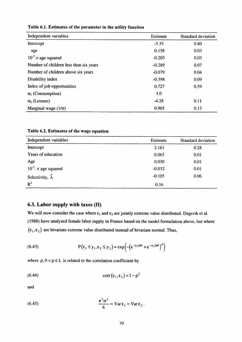
6(6.45)

X 2 6 2

= Var e l = Var E 2 .

Table 6.1. Estimates of the parameter in the utility function

Independent variables Estimate Standard deviation

Intercept -5.35 0.80

age 0.158 0.03

10-2 x age squared -0.205 0.03

Number of children less than six years -0.289 0.07

Number of children above six years -0.079 0.04

Disability index -0.398 0.09

Index of job-opportunities 0.727 0.59

a, (Consumption) 1.0

a2 (Leisure) -4.28 0.11

Marginal wage (1/a) 0.965 0.13

Table 6.2. Estimates of the wage equation

Independent variables Estimate Standard deviation

Intercept 2.161 0.28

Years of education 0.065 0.01

Age 0.030 0.01

10-2 . x age squared -0.032 0.01

Selectivity, i-0.105 0.06

R2 0.16

6.3. Labor supply with taxes (In

We will now consider the case where c i and EZ are jointly extreme value distributed. Dagsvik et al.

(1988) have analyzed female labor supply in France based on the model formulation above, but where

(£ 1 ,E2 ) are bivariate extreme value distributed instead of bivariate normal. Thus,

(6.43)

P (c1 ^ Yi , £2 ^ Y 2 )= exp(—(e -r i /Ø +e -r2 /a6) °

/

where p, 0 < p <_ 1, is related to the correlation coefficient by

(6.44) corr (E, , Ez) =1— pz

and

79

Moreover, it follows that

(6.46)2

T 2 = Var^^ ^ —£ Z ^= 6 6 2 p 2 .

Since E l and E2 are jointly extreme value distributed we get by Theorem 8 that

(6.47)P(e2 < ci + y ) = P(-1E <- 1E + -Y-)

6 6

exp (y/P6) 1l+exp(y/pa) 1+exp(—y/6p)

which means that EZ - E l has a logistic distribution. From (6.47) and (6.27) we get

(6.48) ( >o) = 1 l+exp(—(Xsr l +r, log a l g(O,I)+rZ log g(O,I)) / rw6)

From Lemma A3 in Appendix A we get

(6.49)

log(1-11>0))—E Z )I h>0)=— (X sr, +r, log a g(Wh,I

ti (Ï>o) ti

From (6.32), (6.48) and (6.49) we thus obtain

+ r2 log g(Wh, I)) .

(6.50) — l0 1— = Xsr + r log ~ I+ r2 log h I+ ti^ + ~g i ^ og a^g h,2 gg ^ ^1 2M

where 1 2 is a random term such that E i 2 h > 0)=0. Similarly, it can be proved that

(6.51) log W = X,a — p61og P (h > 0)+1),

where F1, is a random term such that E (fi l I h > 0)=0.

It is now clear that the model specified above can be estimated in the same way as the model

specification in Section 6.2.

80

7. EstimationWe shall briefly review maximum likelihood estimation, Berkson's method and finally Heckman's two

stage method.

7.1. Maximum likelihood

Suppose the multinomial or binary probability model has been specified, for example as (2.2), (2.5a,b)

and (2.6). Let Y ;i =1, if agent i in a sample of randomly selected agents, falls into category j and zero

otherwise, and let {H i (X ; ; (3)} be the corresponding multinomial logit probabilities given by (2.3),

where X i is the vector of explanatory variables for agent i. The total likelihood of the observed

outcome equals

fl in H X i ; R Y^^

i=1 j=1

where N is the sample size. The loglikelihood function can therefore be written as

N m(7.1)

2 = ^ ^ Y;i IogH i (X ; ;(3).i=1 j=1

By the maximum likelihood principle the unknown parameters are estimated by maximizing £ with

respect to the unknown parameters.

The logit structure implies that the first order conditions of the loglikelihood function equals

at N(Y-k —H r (X i ;f3)X ik ) = 0

a ^ rk ^_^

for r = 2,3,..., m, k = 1,2,..., K, where Xik is the k-th component component of X i, with associated

coefficient frk•

Let Z = (Z 1 , Z2 , ..., Z m ) and suppose next that the logit model has the structure

(7.3)exp(h(Zi,X;)R)

Hi(Z , X;;(3)= meXp(h(Z k ,X j )13)

k=1

where

K(7.4) h ^ZX(3= ^ h r (Z i , X ; )(3 i

r=1

(7.2)

81

Examples of this structure were given in Section 3.5. Note that in this case the parameters are not

alternative-specific.

When the logit model has the structure given by (7.3) and (7.4), then the first order conditions

yield

(7.5)

at -^N m

(YI —H(Z,X I ;f))h k (Z,X I )=O

for k =1,2,...,K.

McFadden (1973) has proved that when the probabilities are given by (7.3) and (7.4), the

loglikelihood function is globally strictly concave, and therefore a unique solution to (7.5) is

guarantied.

7.2. Berkson's method (Minimum logit chi-square method)

If we have a case with several observations for each value of the explanatory variable it is possible to

carry out estimation by Berkson's method (Berkson, 1953). Model (3.17) in Example 3.1 is an

example of a case where this method is applicable, since this model does not depend on individual

characteristics. Let

fl. =itJ Yi^N

and replace H; by fi i in (3.17). We then obtain

H^(7.6)

H^

where Tb is a random error term. By the strong law of large numbers H i ---÷ H i with probability one as

the sample size increases, the error term Ili will be small when N is "large". Also by first order Taylor

approximation we get

(h:s1AI H (h_H ) (A l _H

log „' = log H . — log log ' + ' —H1 ' L}I) Hi H1

which shows that

i = 1

82

H.E^ i =Elog ' —(Z i —Z 1 ^i

H, j

(7.7) -= log

1 + EHj —Hi (En1— 111)

(Z i — Z, )RH, Hi Hi

=log( --H' —(Z i —Z I )(3=0.

Thus, even in samples of limited size the mean of the error terms {i i } is approximately equal

to zero. Define the dependent variable Yj by

^H ^

Y^ = logH..H1

We now realize that due to (7.6) we can estimate (3 by regression analysis with {Y^ } as dependent

variables and {Z i — Z 1 1 as independent variables. See Maddala (1983, p. 30) for a more detailed

treatment of Berkson's method.

7.3. Maximum likelihood estimation of the Tobit model

Notice first that due to the form of (5.2) ordinary regression analysis will not do because of the

nonlinear operation on the right hand side of (5.2).

From (5.2) it follows that

(7.8) P(Y = 0) = P(u <_ —X(3 I = F(—X(• / a)

where F(y) denotes the cumulative distribution of u, and

(7.9)

P(YE (Y,Y+dY))-P(u6 E (y — X13,Y +dy — XEi))-6F'( y 6 R )dY ,

for y > 0. Consider now the estimation of the unknown parameters based on observations from a

random sample of individuals, and as above, let i =1,2,... be an indexation of the individuals in the

sample. Let S i be the set of N i individuals for which Yi > 0 and So the remaining set of individuals

for whom Yi = 0 . We shall distinguish between two cases, namely the cases where we observe X i

and Yi for all the individuals (Case I), and the case where we do not observe X i when i E S o (Case II).

83

IE .

Yi—xiR log 6 + log F

iEs l 6 iEs0(7.10) Q = (log F'

Case I: X, is observed for all i E So u S1 (Censored case)

From (7.9) it follows that the density of Y ; when Y; > 0 equals

F,(y— X;(3) 16 j6

while, by (7.8), the probability that i E S o equals

F ^

Therefore the total loglikelihood equals

Example 7.1

Suppose F(y) is a standard normal distribution function, Ø(y). Then, since

Ø ,

( ) u = e -u 2 /2

2 -TE

it follows that the loglikelihood in this case reduces to

(7.11)-.^_— (Y1xf3)222 N, loga + E log Ø ^ å' R ^ —

N1 log (2n) .

IES^ IESQ

We realize that applying OLS to the equation Y = XV, + u6 corresponds to neglecting the last term in

(7.11) and will therefore produce biased estimates.

Example 7.2

Suppose that F(y) is a standard logistic distribution, L(y), given by (2.7). Since

1—L(—y)=L(y) and

(7.12) L'(Y) = L(Y)(1— L(Y))

it follows from (7.10) that the loglikelihood function in this case is

(7.13) Q= , [loL( Y' — X ' R J +logi 1—L ^ Y' XI)) N i— loga +I logL6 l6 Eso

84

Case II: X is not observed for i E So (Truncated case)

In this case we must evaluate the conditional likelihood function given that the individuals

belong to S i . The conditional probability of Y; E (y, y + dy), y > 0, given that Y; > 0 equals

P(Yi E (y , y+ dy) Y; > 0) =

F, Y Xi^ 1 dYP (Y; E (y, y + dy), Y; > 0^ P (Y; E (y, y + dy)) ( a 6

P(Yi > 0) P (Yi >)

Therefore, the conditional loglikelihood given that Y; > 0 for all i, equals

(7.14) logF'r' '—log(l—FLX;(311

—N i loga..Es, a ^

7.4. Estimation of the Tobit model by Heckman's two stage method

Heckman (1979) suggested a two stage method for estimating the tobit model. We shall briefly review

his method for the case where F(y) is either the normal distribution or the logistic distribution.

7.4.1. Heckman's method with normally distributed random terms

As above Ø(•) denotes the cumulative normal distribution function. From (5.2) we get

(7.15) E(YIY>O)=X13+6E(uIY>0).

Since E (u I Y > 0) in general is different from zero we cannot, as mentioned above, do linear

regression analysis based on the subsample of individuals in S i . Now note that

(7.16)

NuE(y,y+dy)IY>O)=quE(y,y +dy)

quE(y,y+dy),u>— XRJa

P(u >— 6R )

U> — X^^

P E (y,y+dy)) ØV(Y)dy

P —u < XR Ø XRa ) a

since -u has the same distribution as u due to symmetry. We therefore get

(7.17)

But

E (u l Y > 0) = 1 J u Ø'(u) du .

Ø(a) å

85

u 2 u2^00 ,u e 2 °° e 2 1(7.18) uØ (u)du= f du=— I = • exp

xR yp fi- a 2^ 2^t- a

X13 I Z /2]= 0,(x13)

J l J

a a

which together with (7.16) yields

(7.19)

44)01 X

E (u I Y > 0) =_

XR ^,^ R

a

Ø\ 6 1

where the last notation (X) is introduced for convenience.

Heckman suggested the following approach: First estimate X3/6 by probit analysis, i.e., by

maximizing the likelihood with the dependent variable equal to one if i E S i and zero otherwise. The

corresponding loglikelihood equals

(7.20) Q =1, log Ø( +^ log \1-6l' o a

From the estimates (3* of (3/6, compute

Ø' X i p*

Øpc,f3*

and estimate (3 and a by regression analysis on the basis of

^(7.21) Yi = X i (3+6^, ; + ^ i

by applying the observations from S,. This gives unbiased estimates because it follows from (7.15)

and (7.19) that

^E ^ ; IY; >0 = E Yi —X ; ^—a'^, i I Y; 0)

=E au ; -6^, ; I Yi >0 =6E u ; IY; >0 - 6^, ;

X ; (3= 6 ^ - 6 ^. -0..

Heckman (1979) has also obtained the asymptotic covariance matrix of the parameter estimates that

take into account that one of the regressors, Xi, is represented by the estimate, X 1 .

86

Note that this procedure leads to two separate estimates of 6, namely the one obtained as a

regression coefficient in (7.21) and the one that follows by dividing the mean component value of the

estimated (3 by the corresponding mean based on f3'.

7.4.2. Heckman's method with logistically distributed random term

Assume now that u is distributed according to the logistic distribution L(y). Then by Lemma A3 in

Appendix A it is proved that

(7.22) E (u I Y > 0) _ (1+ exp(—X(3 / 6)) log(1+exp(X13 / 6)) — X(3 / a.

In this case the regression model that corresponds to (7.21) equals

(7.23) Y = X ; (3 + 6 Ø ; + ^;

where

(7.24) ei = (i + exp(_X1 )) log(1 + exp(X1 )) _ X1(3*

and (3' is the first stage maximum likelihood estimate of X3/6 based on the binary logit model with

loglikelihood equal to (7.20) with Ø(y) replaced by L(y).

A modified version of Heckman's method

Since

P(Y > 0) =

it follows from (7.22) that

11+ exp (—X1i I 6)

EY = P(Y > 0) (E(u I Y > 0) a+ XEi)

(7.25) = 6 log (1+exp(X(3 / a^^

= 6 log (1+ exp(—X(3 / 6)) + X(3 = X(3 - 61og P(Y > 0) .

Eq. (7.25) implies that we may alternatively apply regression analysis on the whole sample based on

the regression equation

(7.26) Y = X ; f3 + a µ; + b ;

where

(7.27) µ; =1og(l+exp(—X;r))

87

and b; is an error term with zero mean. This is so because (7.25) implies that

ES ; = E Y ; —X ; t3+alogP(Y ; > 0)). O.

With the present state of computer software, where maximum likelihood procedures are readily

available and easy to apply, Heckman's two stage approach may thus be of less interest.

7.5. The likelihood ratio test

The likelihood ratio test is a very general method which can be applied in wide variety of cases. A

typical null hypothesis (H) is that there are specific constraints on the parameter values. For example,

several parameters may be equal to zero, or two or more parameters may be equal to each other. Let

H denote the constrained maximum likelihood estimate obtained when the likelihood is maximized

subject to the restrictions on the parameters under H. Similarly, let 11 denote the parameter estimate

obtained from unconstrained maximization of the likelihood. Let t((3 11 ) and 0) denote the

loglikelihood values evaluated at (3 H and 3 , respectively. Let r be the number of independent

restrictions implied by the null hypothesis. By "independent restrictions" it is meant that no restriction

should be a function of the other restrictions. It can be demonstrated that under the null hypothesis

—Z (OH^ — P1 pl)

is asymptotically chi squared distributed with r degrees of freedom. Thus, if —2 H —t(i:i))is

"large" (i.e. exceeds the critical value of the chi squared with r degrees of freedom), then the null

hypothesis is rejected.

In the literature, other types of tests, particularly designed for testing the "Independence from

Irrelevant Alternatives" hypothesis have been developed. I refer to Ben-Akiva and Lerman (1985, p.

183), for a review of these tests.

7.6. McFadden's goodness-of-fit measure

As a goodness-of-fit measure McFadden has proposed a measure given by

(7.28) z t(r 3 )

where, as before, t((3) is the unrestricted loglikelihood evaluated at and A0) is the loglikelihood

evaluated by setting all parameters equal to zero. A motivation for (7.28) is as follows: If the

88

estimated parameters do no better than the model with zero parameters then £(13)= t(0), and thus

p 2 = 0. This is the lowest value that p 2 can take (since if k(p) is less than A0) , then 11 would not be

the maximum likelihood estimate). Suppose instead that the model was so good that each outcome in

the sample could be predicted perfectly. Then the corresponding likelihood would be one which

means that the loglikelihood 0) is equal to zero. Thus in this case p 2 =1, which is the highest value

p2 can take. This goodness-of-fit measure is similar to the familiar R 2 measure used in regression

analysis in that it ranges between zero and one. However, there are no general guidelines for when a

p2 value is sufficiently high, cf. Sections 4.8 and 4.10.

89

Appendix A

Some properties of the extreme value and the logistic distributionsIn this appendix we collect some classical results about the logistic and the extreme value

distributions.

Let X 1 , X Z ,..., be independent random variables with a common distribution function F(x).

Let

(A.1) Mn = max(X I ,X 2 ,...,X n ).

Theorem Al

Suppose that, for some a>0,

(A.2) lim xa (1— F(x)) = c,x--,ø

where c > 0 . Then

(A.3) lim P Mn <x = exp(—x -a) for x>0,nom °° (Cfly'/a for C<0 .

Theorem A2

Suppose that for some zg , F(xo ) =1, and that for some a>0,

(A.4)a

lim (x0 — x) (1— F(x)) = c ,x0

where c > 0 . Then

fin? M" —x° < x = exp(—Ixl a ) for x<0

"-30° (Cn)ila 1 for x

Theorem A3

Suppose that

(A.6) lim ex (1—F(x))=c,x -> W

where c > 0 . Then

(A.5)

90

(A.7)

lim P(M„—log (c n)<_x)=expk—e -X\

for all x.

Proofs of Theorems Al to A3 are found in Lamperti (1996), for example. Moreover, it can be

proved that the distributions (A.3), (A.5) and (A.7) are the only ones possible.

The three classes of limiting distributions for maxima were discovered during the 1920s by

M. Frechet, R.A. Fisher and L.H.C. Tippett. In 1943 B. Gnedenko gave a systematic exposition of

limiting distributions of the maximum of a random sample.

Note that there is some similarity between the Central Limit Theorem and the results above in

that the limiting distributions are, apart from rather general conditions, independent of the original

distribution. While the Central Limit Theorem yields only one limiting distribution, the limiting

distributions of maxima are of three types, depending on the tail behavior of the distribution. The

three types of distributions (A.3), (A.5) and (A.7) are called standard type I, II and III extreme value

distributions, cf. Resnick (1987).

The extreme value distributions have the following property: if X 1 and X2 are type III

independent extreme value distributed with different location parameters, i.e.,

P(X <x .)= b -x

where b l and b2 are constants, then X.= max (X I , X 2 ) is also type III extreme value distributed. This

is seen as follows: We have

P(Xx)=PPC 1 X)n(X 2 X))

= P (X 1P 2 = exp ^—e b ' -" 1 • eXp (—e b 2 -"l

= exp (—e-" (e bI i- e b2 = exp (—eb_Xl

where

b=log e b' +eb2 .

Similar results hold for the other two types of extreme value distributions.

In the multivariate case where the random variables are vectors, there exists similar

asymptotic results for maxima as in the univariate case, where maximum of a vector is defined as

maximum taken componentwise. The resulting limiting distributions are called multivariate extreme

value distributions, and they are of three types as in the univariate case. A characterization of type III

91

is given in Theorem 8 in Section 3.10. More details about the multivariate extreme value distributions

can be found in Resnick (1987).

A general type Ø extreme value distribution has the form

exp (—e -(X-b)/a

and it has the mean b + 05772 .... , and variance equal to a 2 it 2 /6 , cf. Lemma Al below.

Lemma Al

Let e be standard type III extreme value distributed and let s < 1. Then

E es' = 111 — s)

where T(•) denotes the Gamma function. In particular

EE=-T(1)=0.5772...

and

2Var & = T"(1) - T'(1) 2

= 6 .

Proof:

We have

00

E e S E= e" exp(—e -" e-" dx.

By change of variable t = e -" this expression reduces to

00

E e SE = t -S e - ` dt s).Ø

Moreover, the formulaes E £=- I''(1) and E E 2 =F"(1) follows immediately. The values of T'(1)

and F"(1) can be found in any standard tables on the Gamma function.

Q.E.D.

92

e "' a 1 ,G e "' e " 2e "m, ... , " " "

• exp —e -YGe',e 2 ,...,e m )).

Lemma A2

Suppose U i = v + E , where (E E 2 , ••• , E m ) is multivariate extreme value distributed. Then

P (maxk Uk <_ y I U^ = maxk Uk) = P (U <_ ylU = maxk Uk) = P (mcxk Uk 5 y) .

Proof: According to the definition of the multivariate extreme value distribution

(A.8) P(U 1 <_ y 1 , U 2 5_ y 2 ,...,U m <_ ym) = F(y1,y2,...) = exp —G e v'',e"2-Y 2 ,...,e"m -Ym

where G(•) is homogeneous of degree one. For notational simplicity let j =1, since the general case is

completely analogous. Let aj denote the partial derivative with respect to component j . We have

(A.9)P(max k U k E(z,z+dz),U 1 =max k U k )=P(U 1 E(z,z+dz),U 2

Since by assumption

(A.10)we get

(A.11)Hence

(A.12)

G e "'-y1 7 e"2 -Y2 ..., e "in

-Ym = e -Y G e"' -Y 1+Y , e"2-Y2+Y ,..., evm-Ym +Y

a 1 F(z,z,...)= exp —e -Z G e"',e" 2 ,...,e"m 01G(e"l, e "2,...,e"m e"i -Z .

Y

P(max k U k <_y,U 1 = max k U k = f Y

=e "' a 1 G e "',e" 2 ,...,e"m f exp _e -Z G e"' , e"Z , ... , e"m ))e -z dz

With y = in (A.12) we realize that the first factor on the right hand side equals the choice

probability, P (U i = max k U k ). Hence we have proved Theorem 8 as well. This implies also that the

second factor on the right hand side equals P(max k U k <_ y) . Moreover, it follows that the events

1U 1 =max k U k and {max k U k <_ y} are stochastically independent.

Q.E.D.

93

I+expl -'u(>yl Y>0^= ` 6lPu (A.13)

1+ exp (y)

Ç > y,u>- µ1P(u>ylY>0)= a

(A.15)

Lemma A3

Assume that Y = ,u + on, where

1 P(u^Y) - l+exp(-Y)

Then

for y > - 'u , and equal to one for y <-1 -. Furthermore,6 d'

(A.14) l ( 1l lo P Y<0E(ul Y>0)=

^JJI+exp^-^ Vogl I+exp^-' = - g ^ ^ -'U

6 ^ ` o^ 6 P(Y>0) 6

Proof:

For y>- 11-1 we have

P(-u<-y) P(u<-y) 1+expl - µJ

P(-u<µ I P u<µ1 1+exp(y)^ 6J ^ a)

which proves (A.13).

Consider next (A.14). Let "1""=Y/a. Then for y >_ 0

l+exP(Y>yY>0 PY>y P(-1-1)

('>o) ('>o)

Hence

l+exp(y-å)l

94

E(YIY >0)= J P(Y>yY>0)dy=^l+expaJJ" d/Y µl

0 1+ exp I y 60

(A.17) =(1+expl —exp C a — YJ dyEl µ l lµ l 6 0=^l+ exp^—J^ I ^- log(l+ exp(—yJ^J

l+exp(--y Ia ^

= ^l+ exp (—µ IJlog(l+ expl µJ I.6 / \6 J

This implies that

E(uIY>O)=E(YI Y >0)-6=I6JJ

l+exp^— Ilog^

and (A.14) has thus been proved.

+ exp^a)) 6

Q.E.D.

95

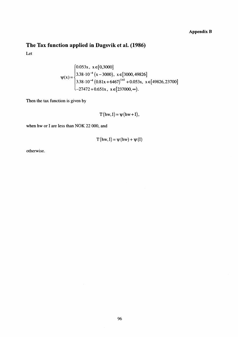
Appendix B

The Tax function applied in Dagsvik et al. (1986)Let

0.053x , x E [0,3000]

3.38.10`` (x — 3000), x E [3000, 49826]

338.10 (0.81x +Ø67) 1.6' +0.053x, x E [49826, 23700]

—27472+0.651x, x E [237000, 00 ) .

Then the tax function is given by

T (hw, I) = yr (hw+I),

when hw or I are less than NOK 22 000, and

T (hw, I) = yt (hw) + yl (I)

otherwise.

96

ReferencesAmemiya, T. (1981): Qualitative Response Models: A Survey. Journal of Economic Literature, 19,1483-1536.

Anderson, S.P., A. de Palma and J.-F. Thisse (1992): Discrete Choice Theory of ProductDifferentiation. MIT Press, Cambridge, Massachusetts.

Ben-Akiva, M., and S. Lerman (1985): Discrete Choice Analysis: Theory and Application to PredictTravel Demand. MIT Press, Cambridge, Massachusetts.

Berkson, J. (1953): A Statistically Precise and Relatively Simple Method of Estimating the Bio-Assaywith Quantal Response, Based on the Logistic Function. Journal of the American StatisticalAssociation, 48, 529-549.

Bjerkholt, 0. (1995): Introduction: Ragnar Frisch, the Originator of Econometrics. In 0. Bjerkholt(ed.): Foundations of Modern Econometrics. The Selected Essays of Ragnar Frisch, Vol. I. E. Elgar,Aldershot, UK.

Block, H.D., and J. Marschak (1960): Random Orderings and Stochastic Theories of Response. In I.Olkin (ed.): Contributions to Probability and Statistics. Stanford University Press, Stanford.

Dagsvik, J.K. (1985): Kvalitativ valghandlingsteori, en oversikt over feltet. Sosialokonomen, no. 2,1985, 32-38.

Dagsvik, J.K. (1994): Discrete and Continuous Choice, Max-Stable Processes and Independence fromIrrelevant Attributes. Econometrica, 62, 1179-1205.

Dagsvik, J.K. (1995): How Large is the Class of Generalized Extreme Value Random Utility Models?Journal of Mathematical Psychology, 39, 90-98.

Dagsvik, J.K., F. Laisney, S. Strøm and J. Østervold (1988): Female Labour Supply and the TaxBenefit System in France. Anna1es d'Economie et de Statistique, 11, 5-40.

Dagsvik, J.K., 0. Ljones, S. Strøm and Rolf Aaberge (1986): Gifte kvinners arbeidstilbud, skatter ogfordelingsvirkninger. Rapporter 86/14, Statistics Norway.

Dagsvik, J.K., D.G. Wetterwald and R. Aaberge (1996): Potential Demand for Alternative FuelVehicles. Discussion Papers, no. 165, Statistics Norway.

Debreu, G. (1960): Review of R.D. Luce, Individual Choice Behavior: A Theoretical Analysis.American Economic Review, 50, 186-188.

Dubin, J., and D. McFadden (1984): An Econometric Analysis of Residential Electric ApplianceHoldings and Consumption. Econometrica, 52, 345-362.

Frisch, R. (1926): Sur un probleme d'econoetie pure. English translation in 0. Bjerkholt (ed.):Foundation of Modern Econometrics. The Selected Essays of Ragnar Frisch, 1995, Vol. I. E. Elgar,Aldershot, UK.

Georgescu-Roegen, N. (1958): Threshold in Choice and the Theory Demand. Econometrica, 26, 157-168.

97

Gorman, W.M. (1953): Community Preference Fields. Econometrica, 21, 63-80.

Greene, W.H. (1993): Econometric Analysis. Prentice Hall, Englewood Cliffs, New Jersey.

Hanemann, W.M. (1984): Discrete/Continuous Choice of Consumer Demand. Econometrica, 52,541-561.

Hausman, J., and D.A. Wise (1978): A Conditional Probit Model for Qualitative Choice: DiscreteDecisions Recognizing Interdependence and Heterogeneous Preferences. Econometrica, 46, 403-426.

Heckman, J.J. (1974): Shadow Prices, Market Wages, and Labor Supply. Econometrica, 42, 679-694.

Heckman, J.J. (1979): Sample Selection Bias as a Specification Error. Econometrica, 47, 153-161.

King, M. (1980): An Econometric Model of Tenure Choice and Demand for Housing as a JointDecision. Journal of Public Economics, 14, 137-159.

Lamperti, J.W. (1996): Probability. J. Wiley & Sons, Inc., New York.

Lee, L.F., and R.P. Trost (1978): Estimation of Some Limited Dependent Variable Models withApplication to Housing Demand. Journal of Econometrics, 8, 357-382.

Lindberg, P.O., E.A. Eriksson and L.-G. Mattsson (1995): Invariance of Achieved Utility in RandomUtility Models. Environment and Planning A, 27, 121-142.

Luce, R.D. (1959): Individual Choice Behavior: A Theoretical Analysis. Wiley, New York.

Luce, R.D., and P. Suppes (1965): Preference, Utility and Subjective Probability. In R.D. Luce, R.R.Bush, and E. Galanter (eds.): Handbook of Mathematical Psychology, III. Wiley, New York.

Maddala, G.S. (1983): Limited-dependent and Qualitative Variables in Econometrics. CambridgeUniversity Press, New York.

Manski, C.F. (1977): The Structure of Random Utility Models. Theory and Decision, 8, 229-254.

McFadden, D. (1973): Conditional Logit Analysis of Qualitative Choice Behavior. In P. Zarembka(ed.), Frontiers in Econometrics, Academic Press, New York.

McFadden, D. (1978): Modelling the Choice of Residential Location. In A. Karlqvist, L. Lundqvist,F. Snickars, and J. Weibull (eds.): Spatial Interaction Theory and Planning Models. North Holland,Amsterdam.

McFadden, D. (1981): Econometric Models of Probabilistic Choice. In C.F. Manski and D. McFadden(eds.), Structural Analysis of Discrete Data with Econometric Applications. MIT Press, Cambridge,Massachusetts.

McFadden, D. (1984): Econometric Analysis of Qualitative Response Models. In Z. Griliches andM.D. Intriligator (eds.): Handbook of Econometrics, Vol. II, Elsevier Science Publishers BV, NewYork.

McFadden, D. (1989): A Method of Simulated Moments of Discrete Response Models withoutNumerical Integration. Econometrica, 57, 995-1026.

98

Quandt, R.E. (1956): A Probabilistic Theory of Consumer Behavior. Quarterly Journal of Economics,70, 507-536.

Resnick, S.I. (1987): Extreme Values, Regular Variation and Point Processes. Springer-Verlag, NewYork.

Robertson, C.A. and D. Strauss (1981): A Characterization Theorem for Random Utility Variables.Journal of Mathematical Psychology, 23, 184-189.

Strauss, D. (1979): Some Results on Random Utility Models. Journal of Mathematical Psychology,20, 35-52.

Thurstone, L.L. (1927): A Law of Comparative Judgment. Psychological Review, 34, 273-286.Tobin, J. (1958): Estimation of Relationships for Limited Dependent Variables. Econometrica, 26,24-36.

Train, K. (1986): Qualitative Choice Analysis: Theory, Econometrics, and an Application toAutomobile Demand. MIT Press, Cambridge, Massachusetts.

Yellott, J.I. (1977): The Relationship between Luce's Choice Axiom, Thurstone's Theory ofComparative Judgment, and the Double Exponential Distribution. Journal of MathematicalPsychology, 15, 109-144.

99

Recent publications in the series Documents

98/9 R. Kjeldstad: Single Parents in the NorwegianLabour Market. A changing Scene?

98/10 H. Brungger and S. Longva: InternationalPrinciples Governing Official Statistics at theNational Level: are they Relevant for theStatistical Work of International Organisationsas well?

98/11 H.V. Sæbø and S. Longva: Guidelines forStatistical Metadata on the Internet

98/12 M. Rønsen: Fertility and Public Policies -Evidence from Norway and Finland

98/13 A. Bråten and T. L. Andersen: The ConsumerPrice Index of Mozambique. An analysis ofcurrent methodology — proposals for a new one.A short-term mission 16 April - 7 May 1998

98/14 S. Holtskog: Energy Use and Emmissions toAir in China: A Comparative Literature Study

98/15 J.K. Dagsvik: Probabilistic Models forQualitative Choice Behavior: An introduction

98/16 H.M. Edvardsen: Norwegian RegionalAccounts 1993: Results and methods

98/17 S. Glomsrød: Integrated Environmental-Economic Model of China: A paper for initialdiscussion

98/18 H.V. Sæbø and L. Rogstad: Dissemination ofStatistics on Maps

98/19 N. Keilman and P.D. Quang: PredictiveIntervals for Age-Specific Fertility

98/20 K.A. Brekke (Coauthor on appendix: JonGjerde): Hicksian Income from StochasticResource Rents

98/21 K.A.Brekke and Jon Gjerde: OptimalEnvironmental Preservation with StochasticEnvironmental Benefits and IrreversibleExtraction

99/1 E. Holmøy, B. Strøm and T. Åvitsland:Empirical characteristics of a static version ofthe MSG-6 model

99/2 K. Rypdal and B. Tomsjø: Testing the NOSEManual for Industrial Discharges to Water inNorway

99/3 K. Rypdal: Nomenclature for Solvent Produc-tion and Use

99/4 K. Rypdal and B. Tornsjø: Construction ofEnvironmental Pressure Information System(EPIS) for the Norwegian Offshore Oil and GasProduction

99/5 M. Søberg: Experimental Economics and theUS Tradable SO2 Permit Scheme: A Discussionof Parallelism

99/6 J. Epland: Longitudinal non-response:Evidence from the Norwegian Income Panel

99/7 W. Yixuan and W. Taoyuan: The EnergyAccount in China: A Technical Documentation

99/8 T.L. Andersen and R. Johannessen: TheConsumer Price Index of Mozambique: A shortterm mission 29 November — 19 December1998

99/9 L-C. Zhang: SMAREST: A Survey of SMallARea ESTimation

99/10 L-C. Zhang: Some Norwegian Experience withSmall Area Estimation

99/11 H. Snorrason, O. Ljones and B.K. Wold: Mid-Term Review: Twinning Arrangement 1997-2000, Palestinian Central Bureau of Statisticsand Statistics Norway, April 1999

99/12 K.-G. Lindquist: The Importance of Disaggre-gation in Economic Modelling

99/13 Y. Li: An Analysis of the Demand for SelectedDurables in China

99/14 T.I. Tysse and K. Vaage: Unemployment ofOlder Norwegian Workers: A Competing RiskAnalysis

1999/15 L. Solheim and D. Roll-Hansen: Photocopyingin Higher Education

1999/16 F. Brunvoll, E.H. Davila, V. Palm, S. Ribacke,K. Rypdal and L. Tangden: Inventory ofClimate Change Indicators for the NordicCountries.

1999/17 P. Schøning, M.V. Dysterud and E. Engelien:Computerised delimitation of urbansettlements: A method based on the use ofadministrative registers and digital maps.

1999/18 L.-C. Zhang and J. Sexton: ABC of Markovchain Monte Carlo

1999/20 K. Skrede: Gender Equality in the LabourMarket - still a Distant Goal?

1999/21 E. Engelien and P. Schøning: Land Use Statis-tics for Urban Settlements: Methods based onthe use of administrative registers and digitalmaps

1999/22 R. Kjeldstad: Lone Parents and the "WorkLine": Changing Welfare Schemes and Chang-ing Labour Market

100

Documents B Returadresse:Statistisk sentralbyråN-2225 Kongsvinger

Statistics NorwayP.O.B. 8131 Dep.N-0033 Oslo

Tel: +47-22 86 45 00Fax: +47-22 86 49 73

ISSN 0805-9411

OW40 Statistisk sentralbyråStatistics Norway