PROBABILISTIC MODELLING TECHNIQUES AND A ROBUST DESIGN METHODOLOGY FOR OFFSHORE WIND FARMS A thesis submitted to the University of Manchester for the degree of PhD in the Faculty of Engineering and Physical Sciences 2012 Muhammad Ali Electrical Energy and Power Systems Group School of Electrical and Electronic Engineering

Welcome message from author
This document is posted to help you gain knowledge. Please leave a comment to let me know what you think about it! Share it to your friends and learn new things together.
Transcript

PROBABILISTIC MODELLING TECHNIQUES AND
A ROBUST DESIGN METHODOLOGY FOR
OFFSHORE WIND FARMS
A thesis submitted to the University of Manchester for the degree of
PhD
in the Faculty of Engineering and Physical Sciences
2012
Muhammad Ali
Electrical Energy and Power Systems Group
School of Electrical and Electronic Engineering

2

3
Table of Contents
List of Tables ............................................................................................................................ 8
List of Figures .......................................................................................................................... 9
List of Symbols and Abbreviations ................................................................................. 14
Abstract ............................................................................................................................. 24
Declaration ............................................................................................................................. 25
Copyright Statement ........................................................................................................... 26
Acknowledgement ................................................................................................................ 28
Chapter 1 Introduction ..................................................................................................... 29
1.1 The Need for Improved Modelling and Design ................................................. 32
1.2 Overview of Wind Power Generation ................................................................ 36
1.2.1 Wind farm capacities and turbine sizes in European offshore wind farms .. 36
1.2.2 Components of an offshore wind farm ............................................................. 38
1.2.2.1 Wind turbines ........................................................................................... 38
1.2.2.2 Types of foundation .................................................................................. 40
1.2.2.3 Wind turbine array .................................................................................. 41
1.2.2.4 Array configurations ................................................................................ 41
1.2.2.5 Offshore substation .................................................................................. 44
1.2.2.6 Platform interconnection ......................................................................... 45
1.2.2.7 Transmission of electricity to shore ........................................................ 46
1.2.2.8 Onshore substations ................................................................................. 47
1.3 Wind Farm Costs ................................................................................................ 47
1.4 Review of Relevant Previous Works .................................................................. 48
1.4.1 Aggregate models for transient stability studies............................................ 48
1.4.2 Energy yield estimation and cost-benefit analysis for offshore wind farms . 50
1.4.3 Wind energy curtailments ................................................................................ 52
1.5 Summary of the Past Work ................................................................................ 54
1.6 Research Objectives ............................................................................................ 55
1.7 Major Contributions of the Research ................................................................ 56
1.7.1 Vector based wake calculation program (VebWake) ...................................... 56
1.7.2 Probabilistic wake effect model ....................................................................... 56
1.7.3 Probabilistic aggregate model of a wind farm ................................................ 56
1.7.4 Advanced method for wind farm energy yield calculation ............................. 57
1.7.5 Assessment of wind energy curtailment ......................................................... 57
1.7.6 Probabilistic identification of critical wind turbines inside the wind farm .. 57
1.7.7 Methodology for cost-benefit analysis of offshore electrical network design 57
1.7.8 Industrial software for offshore wind farm design and loss evaluation........ 58
1.8 Overview of Thesis ............................................................................................. 58
Chapter 2 Wind Turbine and Power System Components Modelling ................... 61
2.1 Introduction ........................................................................................................ 61
2.2 Wind Turbine Modelling .................................................................................... 62
2.2.1 Power extraction from a wind turbine ............................................................ 62
2.2.2 Power coefficient models and look-up table .................................................... 64

4
2.2.3 Thrust coefficient .............................................................................................. 66
2.2.4 Operating range of wind turbines .................................................................... 66
2.3 Modelling of Doubly Fed Induction Generator .................................................. 67
2.3.1 Drive train ......................................................................................................... 69
2.3.2 Generator model ................................................................................................ 71
2.3.3 Rotor-side and Grid-side converter .................................................................. 73
2.3.4 Protection system .............................................................................................. 76
2.3.4.1 DC link chopper ........................................................................................ 77
2.3.5 Rotor speed controller ....................................................................................... 77
2.3.6 Pitch control ....................................................................................................... 79
2.3.7 Yaw control ........................................................................................................ 80
2.4 Power Transmission Line Modelling ................................................................. 80
2.5 Transformer Modelling ....................................................................................... 81
2.6 Summary ............................................................................................................. 84
Chapter 3 Modelling of Wake Effects ............................................................................. 85
3.1 Introduction ......................................................................................................... 85
3.2 Wake Effects ........................................................................................................ 86
3.3 Detailed Wake Effect Modelling......................................................................... 89
3.3.1 Single wakes ...................................................................................................... 90
3.3.2 Partial wakes ..................................................................................................... 90
3.3.3 Multiple wakes .................................................................................................. 91
3.4 Development of Vector Based Wake Calculation Program .............................. 92
3.5 Impact of Wind Speed and Direction on Wind Turbine Power Output ........... 94
3.6 Effect of Height on Wind Speed ......................................................................... 97
3.7 Weibull Distribution ........................................................................................... 97
3.8 Wind Measurements ........................................................................................... 98
3.9 Wind Farm Layouts ............................................................................................ 99
3.10 Capacity Factor ................................................................................................. 101
3.11 Wind and Wake Turbulence ............................................................................. 101
3.12 Probabilistic Wake Model ................................................................................. 103
3.12.1 Jensen‘s wake model (deterministic) ............................................................. 104
3.12.2 Turbulence model ............................................................................................ 104
3.13 Case Study ......................................................................................................... 105
3.14 Power Output Analysis ..................................................................................... 107
3.15 Energy Yield Analysis ....................................................................................... 109
3.16 Summary ........................................................................................................... 110
Chapter 4 Probabilistic Aggregate Dynamic Model of a Wind Farm ................... 112
4.1 Introduction ....................................................................................................... 112
4.2 Aggregation by Wind Speed ............................................................................. 114
4.3 Support Vector Clustering ................................................................................ 116
4.4 Wind Turbine Clustering .................................................................................. 117
4.4.1 Wind farm layout ............................................................................................ 117
4.4.2 Clustering ........................................................................................................ 117
4.5 Probabilistic Clustering of Wind Turbines ...................................................... 120
4.5.1 Formation of groups ........................................................................................ 120
4.5.2 Probability of groups ....................................................................................... 121
4.5.3 Information of wind at a site .......................................................................... 122
4.5.4 Probabilistic group identification ................................................................... 122
4.6 Dynamic Simulations ........................................................................................ 125
5
4.6.1 Wind plant description ................................................................................... 125
4.6.2 Impact of wind turbines in different strings on WF aggregation ................ 125
4.6.3 Setting up equivalent wind turbines ............................................................. 126
4.6.4 Aggregation of cables ...................................................................................... 129
4.6.5 Adjustment of turbine powers for any wind speed and direction ................ 131
4.6.6 Dynamic response comparison between probabilistic aggregate model and
the detailed model .......................................................................................... 132
4.6.7 Simulation time .............................................................................................. 134
4.6.8 Smaller wind farm test ................................................................................... 135
4.7 Comparison with Existing Aggregate Models ................................................ 135
4.7.1 Single-unit equivalent .................................................................................... 136
4.7.1.1 Case study ............................................................................................... 136
4.7.2 Cluster representation ................................................................................... 136
4.7.2.1 Case study ............................................................................................... 137
4.7.3 Results of comparison of different aggregate models ................................... 138
4.7.3.1 Dynamic response analysis .................................................................... 139
4.8 Summary ........................................................................................................... 142
Chapter 5 Probabilistic Assessment of Wind Farm Energy Yield ........................ 144
5.1 Introduction ...................................................................................................... 144
5.2 Power Transmission Limitations .................................................................... 145
5.2.1 Bus Voltage limit ............................................................................................ 145
5.2.2 Thermal limit .................................................................................................. 146
5.2.3 Methods to overcome power transmission bottlenecks ................................ 146
5.3 Estimation of Wind Energy Yield .................................................................... 148
5.3.1 Wind potential availability ............................................................................ 149
5.3.2 Wind farm layout ............................................................................................ 150
5.3.3 Wake effects .................................................................................................... 150
5.3.4 Electrical power losses ................................................................................... 151
5.3.5 Wind farm losses due to reliability considerations ...................................... 153
5.3.5.1 Wind farm availability distribution function ....................................... 153
5.3.5.2 Wind power production distribution ..................................................... 156
5.3.5.3 Correlation between wind speed and wind turbine availability ......... 157
5.3.5.4 Losses due to unavailability of WF components .................................. 158
5.3.6 Losses due to wind energy curtailment ......................................................... 159
5.3.6.1 Correlation between wind power production and transmission line
loading ..................................................................................................... 160
5.3.6.2 No correlation between wind power production and transmission line
loading ..................................................................................................... 161
5.4 Case Study ........................................................................................................ 161
5.4.1 Wake losses ..................................................................................................... 162
5.4.2 Electrical power losses ................................................................................... 163
5.4.3 Wind resource availability ............................................................................. 166
5.4.4 Wind farm component availability ................................................................ 166
5.4.5 Wind energy curtailments .............................................................................. 167
5.4.6 Overall Losses and Capacity Factor .............................................................. 170
5.5 Summary ........................................................................................................... 172
Chapter 6 Probabilistic Identification of Critical Wind Turbines inside a Wind
Farm ................................................................................................................. 174
6.1 Introduction ...................................................................................................... 174

6
6.2 Wind Flow Modelling and Data Clustering ..................................................... 176
6.2.1 Site information ............................................................................................... 176
6.2.2 Wind speed variation due to wake effects ..................................................... 176
6.2.3 Clustering data ................................................................................................ 177
6.3 Probabilistic Power Output of Wind Farm ...................................................... 177
6.4 Case Study ......................................................................................................... 178
6.4.1 Wind farm power production and energy yield analysis .............................. 182
6.4.2 Energy yield analysis ...................................................................................... 183
6.5 Summary ........................................................................................................... 184
Chapter 7 Robust Design Methodology for Offshore Wind Farms ....................... 186
7.1 Introduction ....................................................................................................... 186
7.2 Offshore wind farm network ............................................................................ 189
7.2.1 Wind turbines .................................................................................................. 190
7.2.2 Wind turbine foundations ............................................................................... 190
7.2.3 Wind turbine array ......................................................................................... 190
7.2.4 Offshore substation transformers .................................................................. 190
7.2.5 Switchgear ....................................................................................................... 191
7.2.6 Transmission link to shore ............................................................................. 191
7.2.6.1 HVAC and HVDC link features ............................................................. 192
7.3 Cost Models ....................................................................................................... 195
7.3.1 Wind turbines .................................................................................................. 195
7.3.1.1 Foundations ............................................................................................. 196
7.3.2 Submarine cables ............................................................................................ 197
7.3.3 Offshore platform ............................................................................................ 198
7.3.4 VSC converters ................................................................................................ 199
7.3.5 HVDC cables .................................................................................................... 199
7.3.6 Offshore and onshore compensation device ................................................... 199
7.3.7 Transformers ................................................................................................... 200
7.3.8 Switchgear ....................................................................................................... 201
7.4 Robust Offshore Wind Farm Electrical Layout ............................................... 202
7.4.1 Possible Design Options.................................................................................. 203
7.4.2 Quantity and rating of components ............................................................... 204
7.4.3 Level of redundancy ........................................................................................ 207
7.5 Short-Listing Layouts based on Investment Cost and Redundancy Level ... 208
7.6 Electrical Loss and Reliability Calculations ................................................... 213
7.6.1 Wind power frequency curve .......................................................................... 213
7.6.2 Voltage/reactive power compliance and coordination ................................... 214
7.6.3 Electrical loss methodology ............................................................................ 214
7.6.4 Reliability assessment methodology .............................................................. 215
7.7 Results of the Analysis ..................................................................................... 217
7.7.1 Electrical losses ............................................................................................... 217
7.7.2 Reliability based losses ................................................................................... 217
7.7.3 Total energy losses and investment cost ....................................................... 219
7.7.4 Net present value analysis ............................................................................. 219
7.8 Discussion .......................................................................................................... 220
7.9 Software Tool for Automated Design and Loss Analysis of an Offshore Grid
221
7.9.1 Implementation of the software tool .............................................................. 222
7.9.2 Input parameters ............................................................................................ 222

7
7.9.3 Creation of an electrical network .................................................................. 225
7.9.4 Load flow and loss evaluation studies ........................................................... 227
7.10 Case Study ........................................................................................................ 227
7.10.1 Parameters and loss studies .......................................................................... 228
7.10.2 Network development time ............................................................................ 228
7.11 Summary ........................................................................................................... 230
Chapter 8 Conclusions and Future Work ................................................................... 232
8.1 Future Work...................................................................................................... 236
8.1.1 Future work on modelling .............................................................................. 237
8.1.2 Challenges to overcome for Round 3 offshore wind farms ........................... 239
References ........................................................................................................................... 241
Appendix A Parameters of Wind Turbines .................................................................. 254
Appendix B Results of Aggregation using a Small Wind Farm .............................. 256
Appendix C Cost of Transmission Lines ...................................................................... 260
Appendix D Failure Rates and Repair Times for Components .............................. 261
Appendix E Screenshots of the Developed Software Tool ....................................... 262
Appendix F Author’s Thesis Based Publications ....................................................... 266
Appendix G VeBWake Software CD .............................................................................. 268
Word Count: 60,283

8
List of Tables
Table 1.1: Round 3 Offshore Wind Zones [9] ............................................................................ 31
Table 2.1: Coefficients c1 to c6 .................................................................................................... 64
Table 2.2: Coefficients αi,j for corresponding variables i and j ................................................ 65
Table 2.3: Wind turbines with DFIG technology ..................................................................... 68
Table 3.1: Surface roughness of different terrains ................................................................... 97
Table 3.2: Energy yield comparison using deterministic and probabilistic wake model ..... 109
Table 4.1: Cluster components at 15 m/s for various wind directions .................................. 118
Table 4.2: Formation of Groups at different wind conditions ............................................... 121
Table 4.3: Most probable groups to represent the WF ........................................................... 123
Table 4.4. Parameters to be adjusted in order to represent turbines by an equivalent wind
turbine ..................................................................................................................... 128
Table 4.5: Simulation time comparison with different models ............................................. 135
Table 4.6: WF modelling with incoming wind speed = 12 m/s, wind direction = 349o. Using
constant step size of 0.75 ms ................................................................................. 138
Table 4.7: WF modelling with incoming wind speed = 24 m/s, wind direction = 0o. Using
constant step size of 0.75 ms ................................................................................. 138
Table 5.1: Effects of various factors on wake losses within a WF ......................................... 162
Table 5.2: Wind resource availability on site and for each wind turbine (WT) during one
year .......................................................................................................................... 166
Table 5.3: Impact of WF component availability on annual energy losses .......................... 167
Table 5.4: Impact of correlation between component availability and wind power production
on annual energy losses ......................................................................................... 167
Table 5.5: Combinations for correlation between wind speed and TLL as well as between
wind speed and wind turbine availability ............................................................ 170
Table 5.6: Capacity factor for each wind farm case considered ............................................ 171
Table 5.7: Impact of losses on capacity factor of a wind farm ............................................... 172
Table 6.1: Wind turbines arranged in clusters from high to low wind speeds at 10m/s (wind
direction = 0 to 360o) .............................................................................................. 179
Table 6.2: Energy yield comparison in three scenarios ......................................................... 184
Table 7.1: Approximate reactive power generation by XLPE AC cables [29, 32] ................ 192
Table 7.2: Cost coefficient constants for various voltages ..................................................... 197
Table 7.3: Cost of offshore and onshore reactive power compensation ................................. 200
Table 7.4: Voltage level and cost of single busbar GIS switchgear ....................................... 201
Table 7.5: Rating of components in four cases considered .................................................... 212
Table 7.6: Losses as % of annual energy production, incurring cost of losses, investment cost
and NPV per case ................................................................................................... 220

9
List of Figures
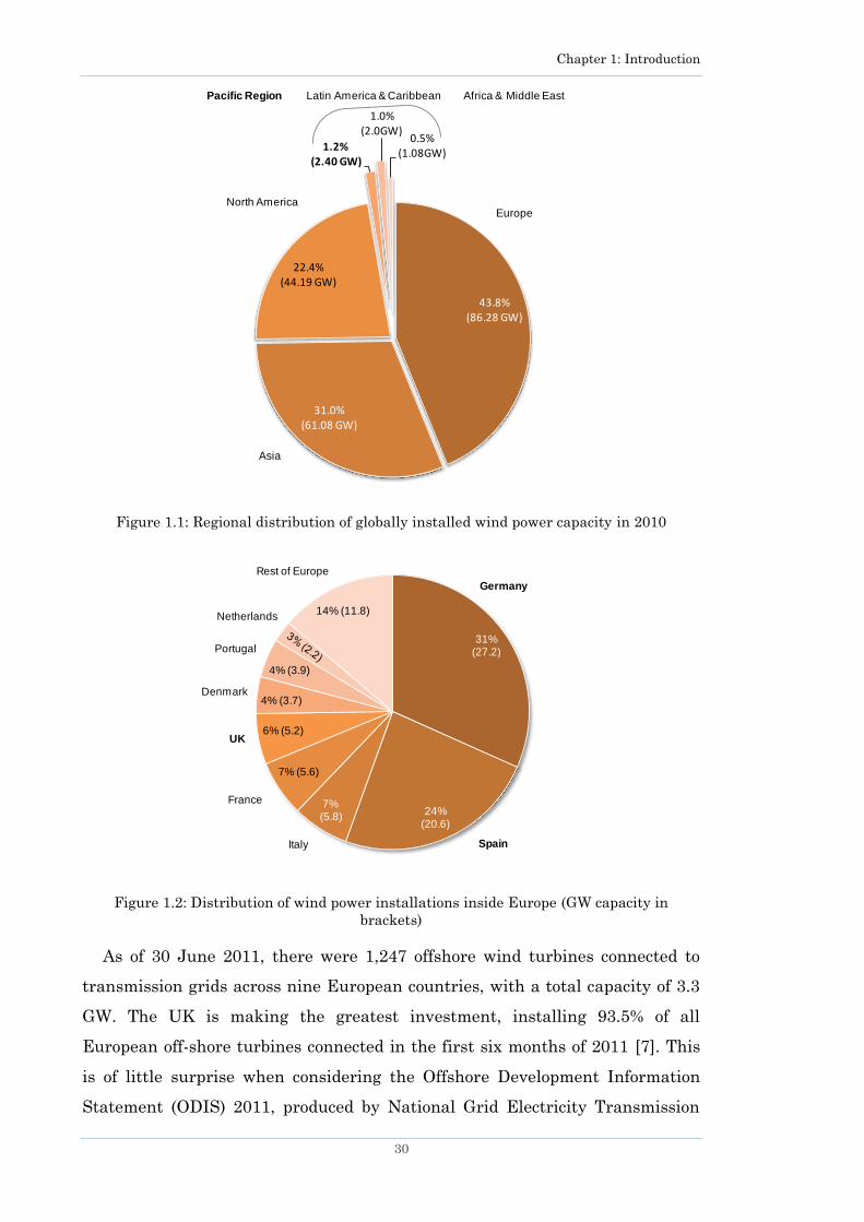
Figure 1.1: Regional distribution of globally installed wind power capacity in 2010 ........... 30
Figure 1.2: Distribution of wind power installations inside Europe (GW capacity in
brackets) ................................................................................................................ 30
Figure 1.3: Capacities of wind farms in Europe ...................................................................... 36
Figure 1.4: Wind farm capacity and their distance to shore for present and future wind
farm installations .................................................................................................. 37
Figure 1.5: Different type of wind turbine generators (adopted from [13]) ........................... 39
Figure 1.6: Wind turbine capacity in offshore wind farms currently installed and planned
for future ................................................................................................................ 40
Figure 1.7: Radial connection ................................................................................................... 42
Figure 1.8: Radial connection with an End loop to provide redundancy (a) no fault (b) fault
cleared by line disconnection ................................................................................ 42
Figure 1.9: Starburst connection with MV bus ........................................................................ 43
Figure 1.10: Central network connected with the MV bus ..................................................... 43
Figure 1.11: Single-sided ring system (a) no fault condition (b) after line disconnection to
clear the fault ........................................................................................................ 44
Figure 2.1: General principle of a wind turbine aerodynamic model ..................................... 64
Figure 2.2: Power coefficient of Vestas V80 wind turbine ...................................................... 65
Figure 2.3: A typical Cp(λ,β) characteristic for pitch angle between 0o and 25o .................... 65
Figure 2.4: Thrust coefficient of Vestas V80 wind turbine ..................................................... 66
Figure 2.5: Power curve of Vestas V80 a pitch controlled wind turbine (adopted from [15]) 67
Figure 2.6: Generic wind turbine model with a DFIG ............................................................ 68
Figure 2.7: Interaction between components inside a DFIG (adopted from [44]) ................. 69
Figure 2.8: Two – mass drive train model (adopted from [124, 125]) .................................... 69
Figure 2.9: Built-in DFIG model in DIgSILENT PowerFactory............................................. 74
Figure 2.10: DFIG with an extended RSC and crowbar protection (dotted lines) (based on
[125]) ...................................................................................................................... 75
Figure 2.11: Grid-side converter (GSC) .................................................................................... 75
Figure 2.12: Maximum Power Tracking characteristic for the turbine ................................. 78
Figure 2.13: Model for pitch angle controller ........................................................................... 80
Figure 2.14: Equivalent π circuit of a transmission line ........................................................ 81
Figure 2.15: Positive sequence model of a 2-winding transformer (in Ohms) ....................... 81
Figure 2.16: Positive sequence model of a 3-winding transformer with a short-circuit at
medium voltage (MV) side, open-circuit on LV side (for HV-MV measurement)
................................................................................................................................ 82
Figure 3.1: Generation of wakes behind a turbine (adopted from [13]) ................................. 87
Figure 3.2: Wake structure by using Jensen model (symbols defined in the text)................ 90

10
Figure 3.3: Partial shading of a wind turbine‘s rotor disc ....................................................... 91
Figure 3.4: Multiple wakes faced by turbines in the same row .............................................. 91
Figure 3.5: Wakes (in blue lines) of wind turbines (red lines) 400 m apart facing wind from
θ degrees ................................................................................................................. 93
Figure 3.6: Nacelle moves to be directed into the wind (yaw control) .................................... 93
Figure 3.7: Simulated mean wind speed at turbines in the same row placed 400 m apart .. 94
Figure 3.8: Wind speed at each turbine in an exemplary wind farm, incoming wind speed =
10 m/s, wind direction = 0o to 360o (1o direction interval) ................................... 95
Figure 3.9: Total power generation (MW) from a wind farm at 10 m/s for wind directions
from 0o to 360o ........................................................................................................ 95
Figure 3.10: Wind power (MW) production from the wind farm at various wind speeds and
directions ................................................................................................................ 96
Figure 3.11: Probability density curve (Weibull) for wind speed data in year 2000.............. 98
Figure 3.12: Probability density curve for wind direction in year 2000 ................................. 99
Figure 3.13: Layout of the large 49 turbine wind farm ......................................................... 100
Figure 3.14: Layout of a small 9 turbine wind farm .............................................................. 100
Figure 3.15: Bird‘s eye view of a 49 turbine wind farm receiving wind from 315o .............. 100
Figure 3.16: Wind turbines in the same row .......................................................................... 102
Figure 3.17: Wake turbulence as faced by a downwind turbine (adopted from [178]) ........ 105
Figure 3.18: Distribution of wind speeds at each wind turbine (dots) and result from
deterministic wake model (line) at incoming wind speed of 10m/s from wind
direction = 270o ± 3o ............................................................................................. 106
Figure 3.19: Gaussian wind speed distribution at wind turbine (WT) 21 for wind entering
the wind farm at 10 m/s from wind direction = 270o ± 3o .................................. 106
Figure 3.20: Wind plot of wind turbine 13 for incoming wind speed of 10 m/s showing
results of deterministic wake model (black line) and probabilistic model (red
crosses). Circles indicate wind speed magnitude (m/s) from each wind direction
.............................................................................................................................. 107
Figure 3.21: Total wind power output in MW from the wind farm at each wind direction for
fixed wind speed of 10 m/s, with deterministic (black line) and probabilistic
wake model (red cross) ........................................................................................ 108
Figure 3.22: Difference in power output for wind entering from all directions in the WF at
wind speed of 10 m/s ............................................................................................ 108
Figure 4.1: Response of a DFIG machine under two wind speeds (a) Generator rotor speed
(b) Active power (c) Reactive power .................................................................... 115
Figure 4.2: Wind speed variation inside a wind farm at 15 m/s, 322o .................................. 119
Figure 4.3: Probability of every unique group found ............................................................. 122
Figure 4.4: Probability of equivalent turbines ....................................................................... 123
Figure 4.5: Number of equivalent turbines that can represent a WF and number of possible
ways to model them ............................................................................................. 124

11
Figure 4.6: Electrical layout of the detailed wind farm ........................................................ 125
Figure 4.7: Dynamic response of three DFIG machines arranged in a radial configuration
(a) Active power (b) Reactive power ................................................................... 126
Figure 4.8: Group A representation with load flow power of equivalent wind turbines
(shown at the left side) at wind speed = 10 m/s, wind direction = 100°........... 129
Figure 4.9: Active power response for Detailed and Probabilistic model at wind speed = 10
m/s, wind direction = 100° .................................................................................. 132
Figure 4.10: Reactive power response for Detailed and Probabilistic model at wind speed =
10 m/s, wind direction = 100° ............................................................................. 133
Figure 4.11: Active power response for Detailed and Probabilistic model at wind speed = 24
m/s, wind direction = 0° ...................................................................................... 134
Figure 4.12: Reactive power response for Detailed and Probabilistic model at wind speed =
24 m/s, wind direction = 0° ................................................................................. 134
Figure 4.13: Active power response for all three aggregation methods and detailed model at
wind speed = 12 m/s, wind direction = 349o....................................................... 140
Figure 4.14: Reactive power response for all three aggregation methods and detailed model
at wind speed = 12 m/s, wind direction = 349o .................................................. 140
Figure 4.15: Active power response for all three aggregation methods and detailed model at
wind speed = 24 m/s, wind direction = 0o ........................................................... 141
Figure 4.16: Reactive power response for all three aggregation methods and detailed model
at wind speed = 24 m/s, wind direction = 0o ...................................................... 141
Figure 5.1: Radial configuration ............................................................................................. 152
Figure 5.2: Central configuration ........................................................................................... 152
Figure 5.3: Single-sided ring configuration ........................................................................... 152
Figure 5.4: Starburst configuration ........................................................................................ 152
Figure 5.5: One row of wind turbines and cables within a WF ............................................ 154
Figure 5.6: Dashed line (C) denotes the transmission limit over the line. The area
(highlighted) between (WPDC‘+TDC) and C corresponds to energy curtailed.
Correlation between wind speed and wind turbine availability is 1 ............... 160
Figure 5.7: Effect of changing wind direction while keeping wind speed constant at 10 m/s
(Offshore scenarios) ............................................................................................. 163
Figure 5.8: Effect of changing wind direction while keeping wind speed constant at 10 m/s
(Onshore scenarios) ............................................................................................. 163
Figure 5.9: Electrical losses inside Radial network for various cable sizes inside the array
(connecting turbines) and for cable connecting to shore................................... 164
Figure 5.10: Electrical losses inside Central network for various cable sizes inside the array
(connecting turbines) and for cable connecting to shore................................... 164
Figure 5.11: Electrical losses inside Single-sided network for various cable sizes inside the
array (connecting turbines) and for cables connecting to shore ....................... 165

12
Figure 5.12: Electrical losses inside Starburst network for various cable sizes inside the
array (connecting turbines) and for cable connecting to shore ......................... 165
Figure 5.13: A congested system with a transmission bottleneck ........................................ 168
Figure 5.14: WF Production Probability Distribution Function (WDF) 1-FX(x), actual
Transmission Probability Distribution Function (TDF) 1-FY(y), New
Transmission Probability Distribution Functions (NTDF) 1-FZ(z) and
Transmission Limit (TL) of the case study line ................................................. 169
Figure 5.15: Effect of WF cabling configuration and correlation coefficient combinations on
energy yield for one year. .................................................................................... 169
Figure 5.16: Wind farm losses due to various factors in percentage .................................... 171
Figure 6.1: Frequency of wind turbines in each cluster ........................................................ 180
Figure 6.2: Frequency of wind turbines in high wind speed Cluster 1 and 2 ...................... 180
Figure 6.3: Frequency of wind turbines in low wind speed Cluster 4 and 5 ........................ 180
Figure 6.4: Wind farm layout showing important wind turbines in the red, less important
wind turbines in blue and frequency of wind from various direction sectors in
the background .................................................................................................... 181
Figure 6.5: Plot of a wind rose showing frequency of wind from each direction .................. 182
Figure 6.6: Probability of total power production from a WF (in year 2000) when all
turbines are on (black), when important wind turbines are off (blue) and when
less important wind turbines are off (red) ......................................................... 183
Figure 7.1 Main components of an offshore wind farm electrical system ............................ 189
Figure 7.2: Two types of links to shore and the components required ................................. 190
Figure 7.3: Typical VSC-HVDC system (adopted from [222]) ............................................... 194
Figure 7.4: Monopolar HVDC with (a) ground return (b) metallic return ........................... 195
Figure 7.5: Bipolar HVDC system ........................................................................................... 195
Figure 7.6: Relationship between cost, voltage level and capacity of cables ........................ 198
Figure 7.7: Flow chart of the method for selection of robust offshore wind farm design
option .................................................................................................................... 203
Figure 7.8: Combination of components and options for an offshore wind farm electrical
layout .................................................................................................................... 207
Figure 7.9: Result after first level short listing, highlighted (red rectangle) area indicates
investment budget range, diamond dots are electrical layouts ........................ 209
Figure 7.10: Investment cost and redundancy level of layouts after third level short-listing
.............................................................................................................................. 210
Figure 7.11: Electrical layouts of four short listed cases ....................................................... 211
Figure 7.12: Wind power frequency curve .............................................................................. 214
Figure 7.13: (a) Fault on line between Bus 1 and 2 under normal operation (b) Fault cleared
by opening nearest circuit breakers ................................................................... 216
Figure 7.14: Software tool screen shots (Offshore platform data entry) .............................. 224
Figure 7.15: Software tool screen shots (Turbine array data entry)..................................... 225

13
Figure 7.16: Design and calculation process .......................................................................... 226
Figure 7.17: Diagram of network created in PSS®E by the software tool ........................... 229

14
List of Symbols and Abbreviations
Symbol Description
R Aerodynamic rotor radius
Pr Gas pressure
RG Gas constant
Tp Gas temperature
ρ Air density
A Area swept by the rotor
β Pitch angle
βm,l Ratio of turbine area covered under wake to total rotor area
Ct Thrust coefficient
Cp Power coefficient
λ Tip speed ratio
λi Variable to calculate c2
α Coefficient to calculate Cp
D Rotor diameter
ma Moving mass of air
v Incoming wind speed to the turbine
Pw Power inside moving mass of air
Prot Mechanical power extracted by the aerodynamic rotor
Trot Mechanical torque on aerodynamic rotor shaft
ωrot Angular speed of the aerodynamic rotor
c1-c6 Coefficients for calculating Cp
VDC DC voltage
IDC Direct current
PDC DC power
PAC AC power
IAC Alternating current
VAC AC voltage
Vr,dq d, q- axis components of voltage at rotor windings
Pm,dq Modulation factor in d and q axis
Vr,nom Nominal voltage of the rotor
Ir Current in the rotor windings
Pc Converter real power

15
Qc Converter reactive power
Pr Power in the rotor winding
Vdc Direct axis component of the converter voltage
Vqc Quadrature axis component of the converter voltage
Idc Direct axis component of the converter current
Iqc Quadrature axis component of the converter current
Jrot Aerodynamic rotor inertia
Jm Generator inertia
Trot Aerodynamic torque of the rotor
Tshaft Torque of the low speed shaft
1:ngear Gearbox ratio
θk Angular difference between two ends of the shaft
cd Damping coefficient of low speed shaft
ξ Damping ratio
δs Logarithmic decrement
a(t) Amplitude of the signal at the beginning of the period
a(t+tp) Amplitude of the signal at the end of the next period
Ks Stiffness of the low speed shaft
Mf Modulation factor
sl Slip
ωm Mechanical frequency of the generator
ωs Stator electrical frequency
Pm Mechanical power at the generator shaft
Hm Inertia constant of the generator rotor
Tm Mechanical torque on the high-speed shaft
Te Electromagnetic torque of the generator
Lm Mutual inductance
Lsσ Stator leakage inductance
Lrσ Rotor leakage inductance
p Number of poles
Rs Resistance of the stator windings
Rr Resistance of the rotor windings
Ids d-axis component of stator current
Idr d-axis component of rotor current
Iqs q-axis component of stator current
Iqr q- axis component of rotor current

16
Rc Resistance of the crowbar
Xc Reactance of the crowbar
Vdr d-axis component of rotor voltage
Vqr q-axis component of rotor voltage
Vds d-axis component of stator voltage
Vqs q-axis component of stator voltage
Ψds d-axis of stator flux linkage
Ψqs q-axis of stator flux linkage
Ψdr d-axis of rotor flux linkage
Ψqr q-axis of rotor flux linkage
Ps Stator active power
Qs Stator reactive power
Pr Rotor active power
Qr Rotor reactive power
Ptotal Total active power fed into the grid by a DFIG
Qtotal Total reactive power fed into the grid by a DFIG
Vr,dq d,q-axis components of rotor voltage affected by the rotor-side
converter
|Vst| Stator terminal voltage magnitude
ZL Impedance of the line (cable)
RL Resistance of the line (cable)
XL Reactance of the line (cable)
YL Admittance of the line (cable)
BL Susceptance of the line (cable)
C Capacitance of the line (cable)
G Conductance of the line (cable)
XM Magnetizing reactance of the core
ZM Magnetizing impedance of the core
RFE Iron loss resistance of the transformer winding
io No load current in a transformer winding
Io Measured no load current at the transformer winding
PFE Measured no load losses in a transformer winding
PCu Copper losses in a transformer winding
RCu,HV Winding resistance of the HV-side of transformer
RCu,LV Winding resistance of the LV-side of transformer
Xσ,HV Winding reactance of the HV-side of transformer
Xσ,LV Winding reactance of the LV-side of transformer

17
VHV Voltage at the HV-terminal of the transformer
Srat Rated power of the transformer
Vrat Rated voltage at the transformer winding
Irat Rated current at the transformer winding
VSC Positive sequence short-circuit voltage at the transformer
windings
Sref Reference power similar to HV-side rated power of the
transformer
ro Wind turbine rotor radius
k Entrainment constant
xo Distance between two turbines
rw Wake radius
v1 Wind speed behind a turbine separated by xo
v2 Wind speed at third turbine in a row
vm Wind speed entering into turbine under partial wake shade
Vps,l Wind speed inside wake of turbine l
Βm,l Ratio of rotor area under wake of turbine l
vn Wind speed entering the nth turbine under multiple wake
z Height of the turbine
zref Height at which wind speed is measured
zo Surface roughness
U(zref) Wind speed at height zref
U(z) Wind speed at the height of the turbine
u Free-stream wind speed
sc Scale parameters of Weibull distribution
ks Shape parameter of Weibull distribution
Ploss Active power losses in a radial network string
Qloss Reactive power losses in a radial network string
Ri Resistance of the ith portion of the string
Xi Reactance of the ith portion of the string
Ploss,WF Active power losses inside the wind farm
Qloss,WF Reactive power losses inside the wind farm
IWF Total current flowing out of the wind farm
SWF Apparent power of a wind farm
IeqWTj Current from an aggregate wind turbine
SeqWTj Rated capacity of the aggregate wind turbine
Ploss,eqWFj Active power losses in a cable connected to the aggregate
turbine

18
Qloss,eqWFj Reactive power losses in a cable connected to the aggregate
turbine
Ploss,eqWTj Active power loss in the string connected to an aggregate
turbine
Qloss,eqWTj Reactive power loss in the string connected to an aggregate
turbine
Req Equivalent resistance of the cable connecting the aggregate
turbine
Req Equivalent reactance of the cable connecting the aggregate
turbine
Mp Number of turbines clustered into an equivalent turbine p
Seq_WT Rated apparent power of the equivalent turbine
Sindividual_WTs Rated apparent power of each wind turbine
Scoh_mat The size of the coherency matrix
nWD Number of wind directions considered
nWTs Number of wind turbines
nWS Number of wind speeds considered
σ standard deviation of wind speed over a period of 10 min or 1
hour
U mean wind speed
s Distance between turbines in seperate rows
s1 Separation between wind turbines in a row normalised by rotor
diameter
Iaddwf Added wind farm turbulence intensity
I Turbulence intensity
βw Characteristic width of the wake
βi Angle between line connecting the turbines and the wind
direction
Io Ambient turbulence
Iw Wake added turbulence
αw Constant expressed by Io and Iw
PJ Heat gain due to joule heating
PM Heat gain due to ferromagnetic heating
PS Heat gain due to solar heating
Pi Heat gain due to ionization heating
Pcon Heat loss due to convection
PR Heat loss due to radiation
PW Heat loss due to evaporation
ki Takes into account thermal diffusion
fY Discrete probability density function
FY Probability distribution function
hY Frequency of y
19
_ _cable to shore
lossP Active power loss in cable connected from the turbine array to
the shore total
lossP Total active power loss in array and cable/s to the shore
string
lossP Active power loss in a wind turbine array string
_total star
lossP Active power loss in starburst array
Failure rate
r Repair time
p Availability of each wind farm component
q Unavailability of each wind farm component
l Length of the cable
pc
Availability of the cable
qc
Unavailability of the cable
pwt
Availability of a wind turbine
pmc
Availability of the main cable
ptr
Availability of wind turbine transformer
,
WTp Overall availability of a wind turbine
,
WTq Overall unavailability of a wind turbine
cs Component statuses
Ncs
Number of component statuses
Ci
Status of a cable i
Ti Status of a wind turbine and its transformer i
Kr
Number of wind turbines in a row
pcs
Probability of certain combination of component statuses
Prow(k)
Probability that in one row k turbines are available
K Number of wind turbines
k Number of wind turbines available in a row
SWT_eq
Equivalent power curve of a wind turbine
t Discretisation step
Tc Number of hours with transmission congestion
X Amount of power transmitted through bottleneck before wind
power installation in MW
Y Wind power production in MW
Z Transmission after wind power is installed
N Number of wind speed measurements
T Time period
fx (x) Discrete probability density function of power transmission
before wind power is installed
Fx(x) Discrete probability distribution function of power
transmission before wind power is installed
20
fz(z) Discrete probability density function of transmission with wind
power installed
Fz(z) Discrete probability distribution function of transmission with
wind power installed
pWF(k)
Availability density of a starburst configured wind farm
Lav Range of losses due to unavailability of wind farm components
Lcurtail Curtailment losses
lc Number of components in a row
kn Number of available wind turbines in a wind farm
pm Availability of the main cable to shore
y Step at which wind production probability distribution
function FY(y) is discretised
C Transmission line capacity
A1 to A3 Cost coefficients for submarine cables
Sn Rated power of the cable
Vr Rated voltage of the cable
Ir Rated current of the cable
Ap and Bp Offset constants to calculate cost of wind turbines
PWT Rated power of a wind turbine
NWT Number of wind turbines in a wind farm
h Height of the turbine
Sd Sea depth for wind turbine foundations
CostWT Cost of a wind turbine
CostWT_TI Cost of wind turbine including transport and installation
CostF Cost of wind turbine foundation
CostF_TI Cost of wind turbine foundation including transport and
installation
CostAC_CABLE Cost of manufacturing for AC submarine cable
CostAC_T&I Cost of transport and installation of AC submarine cable
CostAC_CABLE_TOTAL Total cost of manufacturing, transport and installation of AC
submarine cable
CostDC_CABLE_150kV Cost for 150 kV submarine DC cable
CostDC_CABLE_320kV Cost for 320 kV submarine DC cable
CostTRANS Cost of a transformer
T1, T2 and T3 Offset constants to calculate cost of transformers
g Slope constant to calculate cost of transformers
PTRANS Capacity of the transformer
S1, S2 Offset constant, slope constant for switchgear
NWT_cap Number of wind turbine capacities considered

21
Narr Number of different types of array configurations considered
Narr_Vol Number of different MV levels considered
Ncoll_trans_win Number of different types of collector transformer windings
considered
Ncoll_trans_cap Number of different collector transformer capacities considered
Ntransm_Vol Number of different HV levels considered at collector
transformer secondary windings
Ncoll_trans_red Number of extra options considered having redundant collector
transformers
NTot_HVAC Total number of electrical layouts when an HVAC link is used
to connect the offshore platform with the shore
NTot_1 Total number of combinations if the electrical network from
the wind turbines to the collector transformer is considered
Ntransm_cab_quant Number of different quantities of HVAC cables considered
NTot_HVDC Total number of electrical layouts with an HVDC link from
platform to shore
Nconv_tr_vol Number of different EHV voltage levels considered at the
converter transformer secondary windings
Nconv_tr_cap Number of different capacities of converter transformers
considered
Nconv_cap Number of different VSC converter capacities considered
NTot Total number of electrical layouts when both HVAC link and
HVDC link options are considered
LLOAD Load VSC converter losses
LNO-LOAD No-load VSC converter losses
Pb Power in a bin in a power frequency curve
Hb Ratio of hours in that bin to the total number of hours (8760)
22
Abbreviations
DFIG Doubly Fed Induction Generator
IGBT Insulated Gate Bipolar Transistor
RSC Rotor-Side Converter
GSC Grid-Side Converter
BERR Department for Business Enterprise & Regulatory Reform
PWM Pulse Width Modulation
VSC Voltage Source Converter
LCC Line Commutated Converter
HVAC High Voltage Alternative Current
HVDC High Voltage Direct Current
SVC Support Vector Clustering
PCC Point of Common Coupling
WT Wind Turbine
WF Wind Farm
NPV Net Present Value
CSA Cross Sectional Area (of a cable)
OFTO Offshore Transmission Owner
AEI Annual Energy Interruption
VeBWake Vector Based Wake Calculation Program
FR Failure rate
MTTR Mean Time to Repair
WPPDF Wind Power Production Distribution Function
ADF Availability Density Function
WPDC Wind Production Duration Curve
ADC Availability Duration Curve
WPDC’ New Wind Production Duration Curve
UDC Unavailability Distribution Curve
TDC Transmission Duration Curve
TDF Transmission probability Distribution Function
WDF Wind farm production probability Distribution Function
NTDF New Transmission probability Distribution Function
TL Transmission Limit
XLPE Cross-linked Poly Ethylene
AIS Air Insulated Switchgear
GIS Gas Insulated Switchgear

23
PI Power Interrupted
MV Medium Voltage
HV High Voltage
EHV Extra High Voltage
API Application Programming Interface
24
Abstract
The University of Manchester
Candidate: Muhammad Ali
Degree: Doctor of Philosophy (PhD)
Title: Probabilistic Modelling Techniques and a Robust Design
Methodology for Offshore Wind Farms
Date: 15 July 2012
Wind power installations have seen a significant rise all over the world in
the past decade. Further significant growth is expected in the future. The
UK‘s ambitions for offshore wind installations are reflected through Round
1, 2 and 3 projects. It is expected that Round 3 alone will add at least 25 GW
of offshore wind generation into the system. Current research knowledge is
mostly limited to smaller wind farms, the aim of this research is to improve
offline and online modelling techniques for large offshore wind farms.
A critical part of offline modelling is the design of the wind farm. Design
of large wind farms particularly requires careful consideration as high
capital costs are involved. This thesis develops a novel methodology which
leads to a cost-effective and reliable design of an offshore wind farm. A new
industrial-grade software tool is also developed during this research. The
tool enables multiple offshore wind farm design options to be built and
tested quickly with minimal effort using a Graphical User Interface (GUI).
The GUI is designed to facilitate data input and presentation of the results.
This thesis also develops an improved method to estimate a wind farm‘s
energy yield. Countries with large-scale penetration of wind farms often
carry out wind energy curtailments. Prior knowledge of estimated energy
curtailments from a wind farm can be advantageous to the wind farm
owner. An original method to calculate potential wind energy curtailment is
proposed. In order to perform wind energy curtailments a network operator
needs to decide which turbines to shut down. This thesis develops a novel
method to identify turbines inside a wind farm that should be prioritised for
shut down and given priority when scheduling preventive maintenance of
the wind farm.
Once the wind farm has been built and connected to the network, it
operates as part of a power system. Real-time online simulation techniques
are gaining popularity among system operators. These techniques allow
operators to carry out simulations using short-term forecasted wind
conditions. A novel method is proposed to probabilistically estimate the
power production of a wind farm in real-time, taking into account variation
in wind speed and effects of turbulence inside the wind farm. Furthermore,
a new probabilistic aggregation technique is proposed to establish a dynamic
equivalent model of a wind farm. It determines the equivalent number and
parameters of wind turbines that can be used to simulate the dynamic
response of the wind farm throughout the year.

25
Declaration
No portion of the work referred to in the thesis has been submitted in support
of an application for another degree or qualification of this or any other
university or other institute of learning.

26
Copyright Statement
i. The author of this thesis (including any appendices and/or schedules to
this thesis) owns certain copyright or related rights in it (the
―Copyright‖) and s/he has given The University of Manchester certain
rights to use such Copyright, including for administrative purposes.
ii. Copies of this thesis, either in full or in extracts and whether in hard or
electronic copy, may be made only in accordance with the Copyright,
Designs and Patents Act 1988 (as amended) and regulations issued
under it or, where appropriate, in accordance with licensing
agreements which the University has from time to time. This page
must form part of any such copies made.
iii. The ownership of certain Copyright, patents, designs, trade marks and
other intellectual property (the ―Intellectual Property‖) and any
reproductions of copyright works in the thesis, for example graphs and
tables (―Reproductions‖), which may be described in this thesis, may not
be owned by the author and may be owned by third parties. Such
Intellectual Property and Reproductions cannot and must not be made
available for use without the prior written permission of the owner(s) of
the relevant Intellectual Property and/or Reproductions.
iv. Further information on the conditions under which disclosure,
publication and commercialisation of this thesis, the Copyright and
any Intellectual Property and/or Reproductions described in it may take
place is available in the University IP Policy (see
http://documents.manchester.ac.uk/DocuInfo.aspx?DocID=487), in any
relevant Thesis restriction declarations deposited in the University
Library, The University Library‘s regulations (see
http://www.manchester.ac.uk/library/aboutus/regulations) and in The
University‘s policy on Presentation of Theses.

27
To my loving parents

28
Acknowledgement
I am highly grateful to the Engineering and Physical Sciences Research
Council (EPSRC) and BP Plc for providing financial support for this research.
I would like to express my deepest and sincerest gratitude to my supervisor
Prof. Jovica V. Milanović for his help and support throughout my PhD. His
commitment to achieve the highest standards has been inspirational and has
kept me motivated to work hard. I would also like to thank him for his effort in
reviewing this thesis and other publications written during the course of this
research.
Special thanks go to Dr. Julija Matevosyan and Dr. Irinel-Sorin Ilie for the
constructive technical discussions we had and their advice on technical issues
that lead to several joint publications.
I would like to thank Siemens PTI in Manchester for giving me an
opportunity to do a four month industrial placement which gave me a practical
insight into various aspects of my research. Many thanks to Dr. Dusko P.
Nedic, Dr. Soon Kiat Yee, Dr. Srdjan Curcic and Mr. Steve Stapleton for being
extremely helpful and cooperative throughout my placement.
My appreciation goes to everyone in Power Quality and Power System
Dynamics group for maintaining a friendly work environment that had a
positive impact on my research. I would like to thank Mr. Nick Woolley, Mr.
Manuel Avendaño and Mr. Robin Preece for the wonderful time we had, and for
helping me out with my English. A word of thanks to my friends and
colleagues: Dr. Abdulaziz Almutairi, Dr. Sarat Chandra Vegunta, Dr. Jhan-
Yhee Chan, Dr. Chua Liang Su and Dr. Mustafa Kayikci for being supportive
throughout.
My ultimate gratitude goes to my father Mr. Waheed-ud-din Qaiser and my
mother Mrs. Nuzhat Qaiser. This work would not have been possible without
their endless prayer, love, kindness, patience, continual encouragement and
belief. I would also like to thank my uncles Mr. Shahid Amjad, Mr. Hamid
Amjad, Mr. Abid Amjad, Mr. Arif Amjad and my aunt Ms. Riffat Amjad. They
have helped me all the way since the beginning of my studies.

Chapter 1: Introduction
29
Chapter 1 Introduction
Introduction
Wind power has experienced a dramatic rise since the last decade. Volatility
in fuel prices and climate change has pushed the energy sector to look for more
renewable and emission free electricity sources. Wind energy has answered the
call. Due to its free fuel and emission free output it has become an attractive
option in the current scenario.
In 2010, total wind energy deployment around the globe reached 197 GW [1]
which is 180 GW more than the deployments in 2000 [2]. Through regional
distribution illustrated in Figure 1.1, it can be seen that Europe is leading the
world with the largest number of wind installations. Amongst European
countries, Germany and Spain have the highest portion of total installed
capacity [1] as seen from Figure 1.2.
The wind energy sector is expected to achieve an even faster growth rate in
the future. One reason for this drive is the European Union‘s Renewable
Directive of 2008 that committed its member countries to satisfy 20% of their
energy needs through renewable sources by 2020. The UK has a national target
to satisfy 15% of its energy needs through renewable sources, where as much as
40% of this is expected to be in the form of renewable electricity generation [3,
4]. Although modern technology allows electricity production from various
renewable sources such as solar, wind, geothermal etc. the offshore wind is
likely to play a vital role in achieving this target. A substantial amount of
Europe‘s offshore wind resource is located in Britain‘s waters which is another
reason for investing in electricity production from offshore wind [5]. According
to [6], theoretically it is possible to generate more than 1000 TWh per annum
from wind in the UK, far exceeding the electricity consumption of the entire
nation.
Chapter 1: Introduction
30
Figure 1.1: Regional distribution of globally installed wind power capacity in 2010
Figure 1.2: Distribution of wind power installations inside Europe (GW capacity in
brackets)
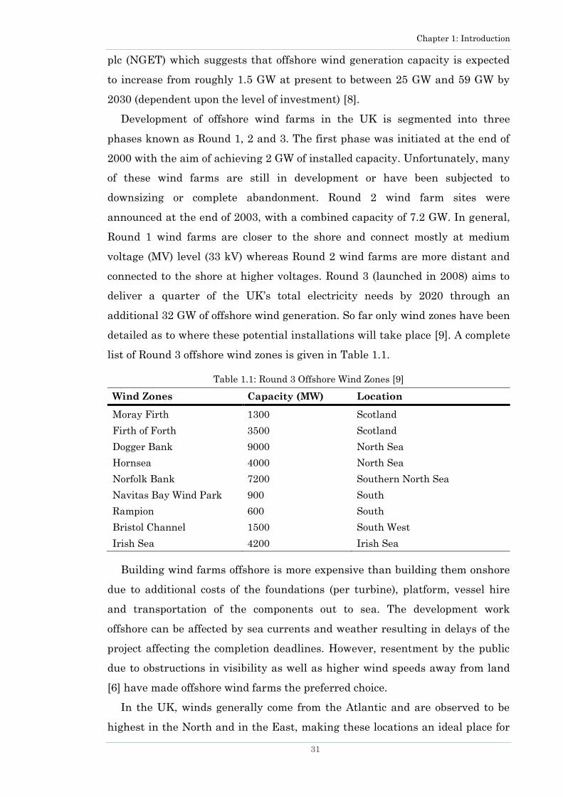
As of 30 June 2011, there were 1,247 offshore wind turbines connected to
transmission grids across nine European countries, with a total capacity of 3.3
GW. The UK is making the greatest investment, installing 93.5% of all
European off-shore turbines connected in the first six months of 2011 [7]. This
is of little surprise when considering the Offshore Development Information
Statement (ODIS) 2011, produced by National Grid Electricity Transmission
43.8%(86.28 GW)
31.0%(61.08 GW)
22.4%(44.19 GW)
1.2%(2.40 GW)
1.0%(2.0GW)
0.5%(1.08GW)
Europe
Asia
North America
Pacific Region Latin America & Caribbean Africa & Middle East
31%(27.2)
24%(20.6)
7%(5.8)
7% (5.6)
6% (5.2)
4% (3.7)
4% (3.9)
14% (11.8)
Germany
SpainItaly
France
UK
Denmark
Portugal
Netherlands
Rest of Europe
Chapter 1: Introduction
31
plc (NGET) which suggests that offshore wind generation capacity is expected
to increase from roughly 1.5 GW at present to between 25 GW and 59 GW by
2030 (dependent upon the level of investment) [8].
Development of offshore wind farms in the UK is segmented into three
phases known as Round 1, 2 and 3. The first phase was initiated at the end of
2000 with the aim of achieving 2 GW of installed capacity. Unfortunately, many
of these wind farms are still in development or have been subjected to
downsizing or complete abandonment. Round 2 wind farm sites were
announced at the end of 2003, with a combined capacity of 7.2 GW. In general,
Round 1 wind farms are closer to the shore and connect mostly at medium
voltage (MV) level (33 kV) whereas Round 2 wind farms are more distant and
connected to the shore at higher voltages. Round 3 (launched in 2008) aims to
deliver a quarter of the UK‘s total electricity needs by 2020 through an
additional 32 GW of offshore wind generation. So far only wind zones have been
detailed as to where these potential installations will take place [9]. A complete
list of Round 3 offshore wind zones is given in Table 1.1.
Table 1.1: Round 3 Offshore Wind Zones [9]
Wind Zones Capacity (MW) Location
Moray Firth 1300 Scotland
Firth of Forth 3500 Scotland
Dogger Bank 9000 North Sea
Hornsea 4000 North Sea
Norfolk Bank 7200 Southern North Sea
Navitas Bay Wind Park 900 South
Rampion 600 South
Bristol Channel 1500 South West
Irish Sea 4200 Irish Sea
Building wind farms offshore is more expensive than building them onshore
due to additional costs of the foundations (per turbine), platform, vessel hire
and transportation of the components out to sea. The development work
offshore can be affected by sea currents and weather resulting in delays of the
project affecting the completion deadlines. However, resentment by the public
due to obstructions in visibility as well as higher wind speeds away from land
[6] have made offshore wind farms the preferred choice.
In the UK, winds generally come from the Atlantic and are observed to be
highest in the North and in the East, making these locations an ideal place for

Chapter 1: Introduction
32
wind farms. Integration of large-scale offshore generation into the grid requires
an upgrade of existing transmission lines and development of new networks.
Widespread installations at wind hot spots around the country can take
generation far from demand. At times, power generated in the North (Scotland)
may have to be exported in order to satisfy load demand in the South (London).
In such scenarios, the transmission network might require a redesign to carry
the wind power all the way to the South with least amount of loss. Although
there are transmission links between England and Scotland their capacity is
limited, so as the amount of wind power generation increases in the North it
will become essential to build new lines to transmit this power to the load
centres, predominantly located in the south of the country.
1.1 The Need for Improved Modelling and Design
Offshore wind farms installed in Round 1 and Round 2 projects are relatively
small in capacity and nearer to the shore compared to the Round 3 projects. In
Round 3, offshore wind farms will be large in capacity and further away from
the shore which as a consequence, will dramatically increase their project costs.
These large offshore wind farms will have to be designed so that they lead to
maximum benefits at lower costs. The knowledge gained by designing smaller
wind farms may not be directly applicable when designing large offshore wind
farms that are much deeper in the sea. Furthermore, large-scale integration of
wind power into the network requires a change in the way wind farms are
currently modelled in the power system. Considering this scenario, it can be
deduced that an improvement is needed in modelling techniques for integration
and design of large offshore wind farms.
There are two types of modelling techniques investigated in this research i.e.
offline and online analysis. Offline analysis is often carried out by system
operators when stability of a system has to be tested prior to integration of a
new line, a customer (load) or a generator etc. Such studies have been and still
are a popular type of analysis. But with large-scale integration of rapidly
varying power generators and loads (electric vehicles), a new type of modelling
is gaining importance in industry, which is the online analysis. Through this,
system operators will be able to regularly test the stability of a network in real-
time, a few minutes or hours ahead, using forecasted wind speed and load
demand. Such analysis will gain importance in future when several large wind

Chapter 1: Introduction
33
farms will be installed at various geographical locations. Since wind is
stochastic in nature, power generation from wind farms will vary according to
the wind conditions therefore real time modelling of power flows is needed.
System operators would thus need rapid analysis to estimate power generation
for a given forecast and to test the stability of the network. In such scenario
online analysis will be crucial for efficient operation of the network. This was
not the case prior large-scale integration of renewable generation as power
output from conventional generators was largely controllable.
The use of offline analysis is not just restricted to system operators.
Designing the layout (including electrical network) and carrying out a pre-
feasibility study for a new wind farm is also part of the offline analysis. The
pre-feasibility study of new a wind farm determines whether it is economically
and technically feasible to connect a wind power plant to the grid. The method
of evaluation should consider all realistic factors so that a reliable energy
estimate can be obtained. Such studies normally include determination of
energy yield, power loss evaluation due to electrical and reliability based losses
as well as fault current analysis. In cases where a wind farm is located in a
remote area connected with a weak electrical infrastructure, it may lead to
additional losses known as energy curtailments. This type of energy loss is
usually not considered during the pre-feasibility studies.
Curtailing wind energy is a common practice in countries with a large
presence of wind farms, where some countries pay the wind farm owner for
curtailing the wind power but others don‘t. In either case, the curtailments take
place with bilateral agreement between the wind farm owner and the utility.
Energy curtailments are often regional and they normally take place if there is
a sufficient level of wind power available at any one time but there is less
demand. Internationally carried out energy curtailment practices compiled in
[10] show that a certain level of compensation is made to the wind farm owners
in Germany and Ireland, whereas in Spain and New Zealand no compensation
is made. Therefore, it would be useful if a wind farm owner can determine,
prior to investing in a wind project, whether it will be economically feasible to
curtail some energy or to build a new transmission line, so that a more
informed decision can be made.
The main control centre (transmission system operator) is responsible for
deciding power from which wind farms should be reduced. Depending on the

Chapter 1: Introduction
34
Grid Code requirement, a utility may not be allowed to trip a wind farm
completely but it may have the authority to reduce its power generation, as is
the case in Spain. Curtailments often take place by either pitching the blades
of wind turbines out of wind or by switching off some of the operating wind
turbines. Former is valid for modern pitch control wind turbines whereas latter
for stall control wind turbines. If wind turbines are stall controlled it can be
difficult to decide which turbines to shut down. This shutting down process can
be made more efficient if only those wind turbines are switched off that have a
higher chance of suffering from mechanical fatigue damage. This would help
improve its lifetime and reduce the preventive maintenance cost of wind
turbines.
Another factor that leads to energy loss is the wake effect. These are
aerodynamic losses that lead to reduced power output and subsequently, a
reduced energy yield. The effect is so significant that it can exceed electrical
losses, therefore it should not be ignored during pre-feasibility studies and in
general modelling of the wind farms. Wake effects explain the difference in
power production often observed between wind turbines at the same wind farm.
Several complex models have been developed in the past but not all of them are
suitable for electrical engineering studies where a fast, yet relatively accurate
estimate would be sufficient.
Large wind farm capacities and increasing distances from the shore pose a
new challenge in designing offshore wind farms. Development costs of such
projects can be significantly high. For instance, if the current cost of production
is considered (€3.45m/MW)[3] a 400 MW wind farm will cost around €1.38 bn.
Although the final cost depends on a variety of factors, the cost of equipment
represents a major portion. Therefore it is absolutely essential that the design
and choice of equipment are optimal and justifiable. A better approach would be
to analyse several possible network layouts prior deciding on one. With growing
dependence on wind energy, reliability and security of power supply can no
longer be treated as a secondary concern. A cost-effective layout should balance
the costs and provide a certain level of reliability. So far, research in designing
large offshore networks is very limited. A methodology to solve this problem
will be advantageous for the wind industry.
Apart from offline analysis, real-time online simulations are becoming a need
for networks with a larger presence of wind farms. In order to perform

Chapter 1: Introduction
35
simulations in real-time (using forecasted wind and load demand) the models
should provide quick output of results. The calculation process to estimate the
instantaneous power output from wind farms should be fast and accurate so
that it can be used to quickly simulate change in wind conditions. For this
purpose, faster probabilistic methods would suffice rather than deterministic
models, due to non-steady flow and stochastic nature of wind.
Real time transient stability simulations are another leap forward in online
studies. Data such as protection and control settings can be gathered in real-
time from devices installed in the network. Generally, transient stability
simulations are time consuming, especially when dealing with networks with a
large number of generators. For this reason, these analyses are often carried
out offline. In future, bigger wind farms are expected to consist of numerous
wind turbines that will lead to very large simulation times if each turbine is to
be modelled separately. This problem can be solved by the use of aggregation
techniques that can reduce the complexity of a wind farm model. However, this
leads to an interesting problem as it requires aggregation of wind turbines
facing different levels of wind speed (due to wake effects), thus producing
different amounts of power. An array of cabling further complicates this issue
since wind turbines producing different amounts of power can be in different
strings (as in a radial configuration).
The motivation for this research has been to gain a deeper understanding
about wind farms and techniques used for their modelling. Potential growth in
the capacity of offshore wind farms require a re-look at existing methods
normally applied to smaller wind plants. It is hoped that through this thesis an
insight into the current issues will be gained and the models proposed will be
useful not only for wind farm designers but also for utilities and consultancy
companies in general.
A critical review of existing techniques is carried out in the following sections
to identify whether current knowledge is sufficient to tackle the projected
issues.

Chapter 1: Introduction
36
1.2 Overview of Wind Power Generation
1.2.1 Wind farm capacities and turbine sizes in European
offshore wind farms
By observing existing offshore operational wind farms and those planned in
the future it can be said that their capacity will increase in the near future. To
make this analysis clearer, wind farms are classified into four categories:
1) operational
2) under construction
3) approved
4) submitted
All four categories are analysed for 120 offshore wind farms in Europe [9, 11,
12], which includes 46 operational, 9 under construction, 61 approved and 4
submitted in the UK (data for all submitted European wind farms was not
available)1. Wind farms in the planning phase (such as Round 3 in the UK)
have been excluded from analysis as their exact capacity is not finalised yet.
Wind farms in category 1 and 2 are characterised as present installations,
whereas those in category 3 and 4 consists of wind farms likely to be installed
in the future. This analysis is aimed to investigate dominant capacities of wind
farms in present and future offshore installations.
Figure 1.3: Capacities of wind farms in Europe
1 Data gathered in August 2011
0
5
10
15
20
25
30
35
40
45
Nu
mb
er
of
off
sh
ore
win
d f
arm
s
Wind Farm Capacity (MW)
All installations Present installations Future installations
0 100 200 300 400 500 600 700 800
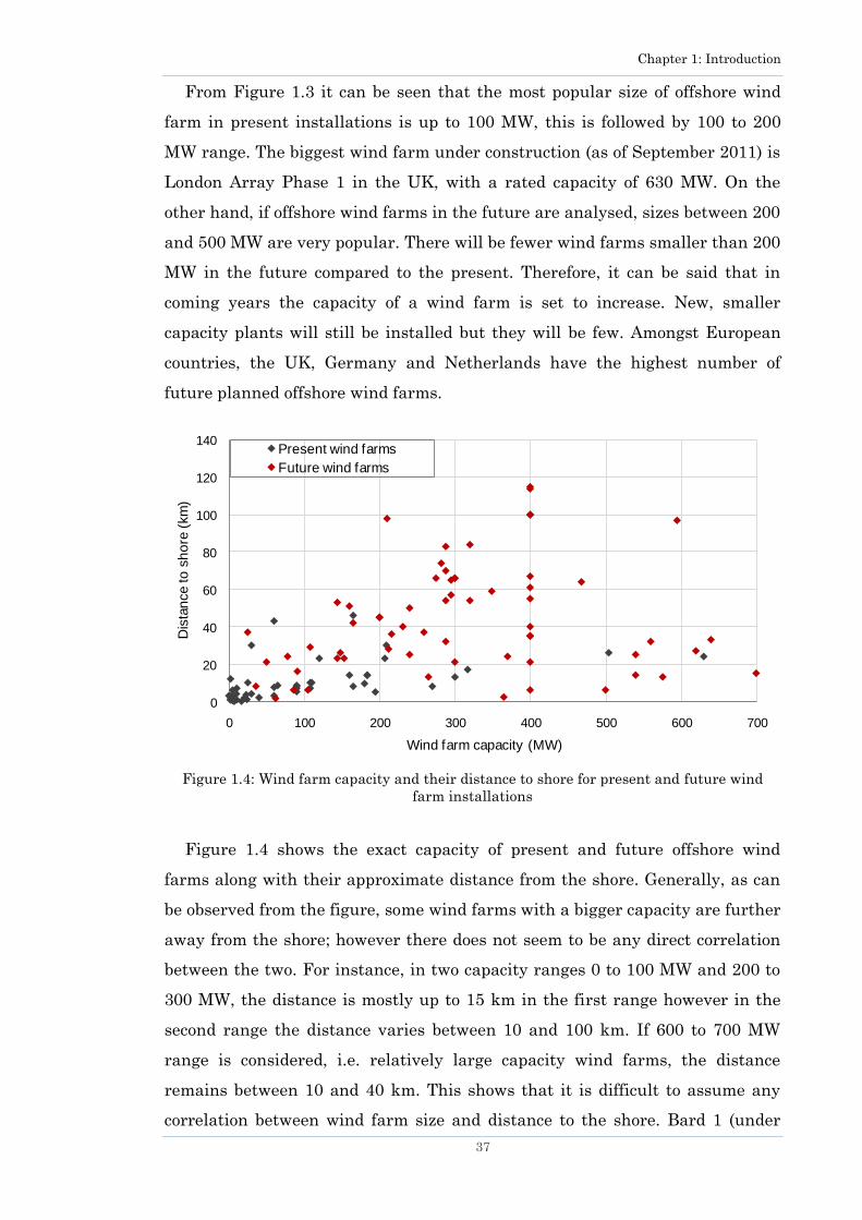
Chapter 1: Introduction
37
From Figure 1.3 it can be seen that the most popular size of offshore wind
farm in present installations is up to 100 MW, this is followed by 100 to 200
MW range. The biggest wind farm under construction (as of September 2011) is
London Array Phase 1 in the UK, with a rated capacity of 630 MW. On the
other hand, if offshore wind farms in the future are analysed, sizes between 200
and 500 MW are very popular. There will be fewer wind farms smaller than 200
MW in the future compared to the present. Therefore, it can be said that in
coming years the capacity of a wind farm is set to increase. New, smaller
capacity plants will still be installed but they will be few. Amongst European
countries, the UK, Germany and Netherlands have the highest number of
future planned offshore wind farms.
Figure 1.4: Wind farm capacity and their distance to shore for present and future wind
farm installations
Figure 1.4 shows the exact capacity of present and future offshore wind
farms along with their approximate distance from the shore. Generally, as can
be observed from the figure, some wind farms with a bigger capacity are further
away from the shore; however there does not seem to be any direct correlation
between the two. For instance, in two capacity ranges 0 to 100 MW and 200 to
300 MW, the distance is mostly up to 15 km in the first range however in the
second range the distance varies between 10 and 100 km. If 600 to 700 MW
range is considered, i.e. relatively large capacity wind farms, the distance
remains between 10 and 40 km. This shows that it is difficult to assume any
correlation between wind farm size and distance to the shore. Bard 1 (under
0
20
40
60
80
100
120
140
0 100 200 300 400 500 600 700
Dis
tan
ce
to
sh
ore
(km
)
Wind farm capacity (MW)
Present wind farms
Future wind farms
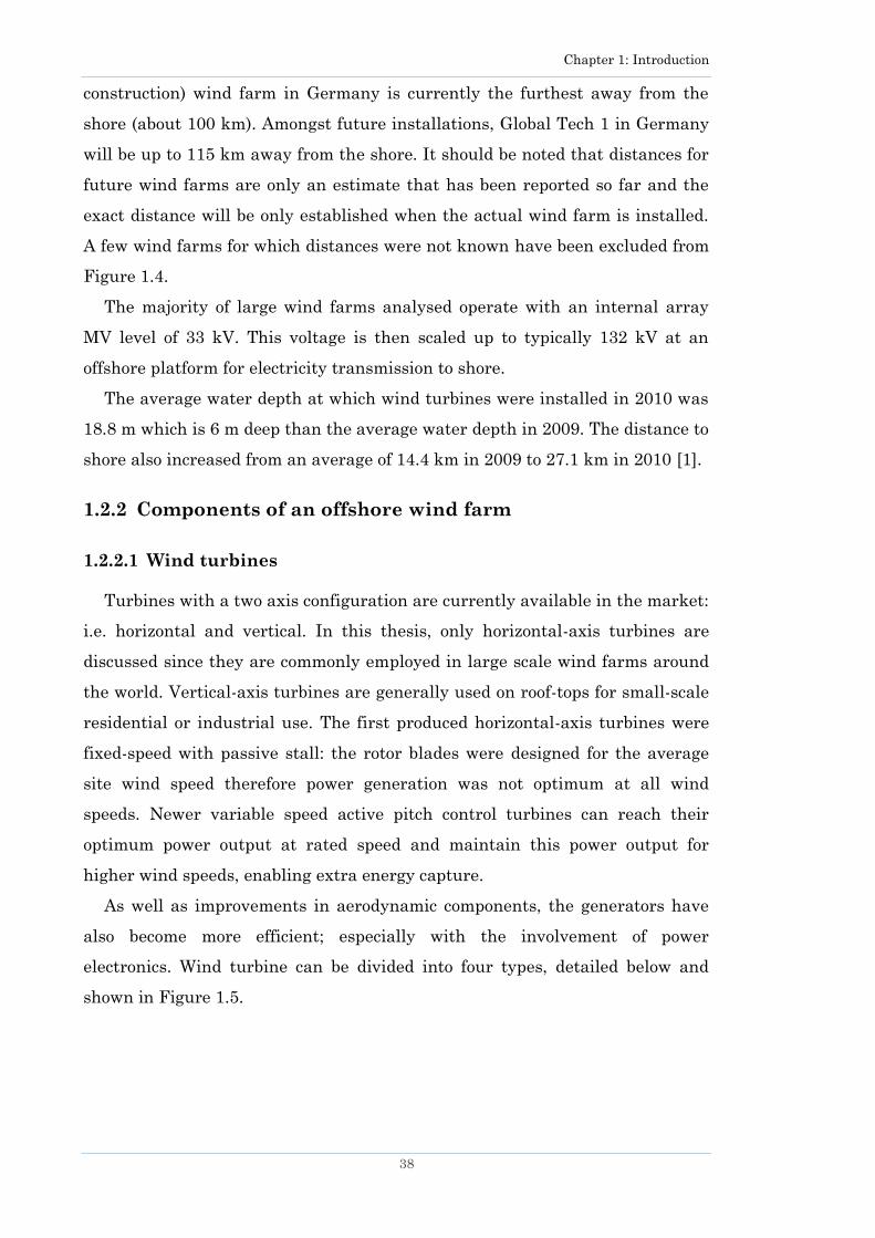
Chapter 1: Introduction
38
construction) wind farm in Germany is currently the furthest away from the
shore (about 100 km). Amongst future installations, Global Tech 1 in Germany
will be up to 115 km away from the shore. It should be noted that distances for
future wind farms are only an estimate that has been reported so far and the
exact distance will be only established when the actual wind farm is installed.
A few wind farms for which distances were not known have been excluded from
Figure 1.4.
The majority of large wind farms analysed operate with an internal array
MV level of 33 kV. This voltage is then scaled up to typically 132 kV at an
offshore platform for electricity transmission to shore.
The average water depth at which wind turbines were installed in 2010 was
18.8 m which is 6 m deep than the average water depth in 2009. The distance to
shore also increased from an average of 14.4 km in 2009 to 27.1 km in 2010 [1].
1.2.2 Components of an offshore wind farm
1.2.2.1 Wind turbines
Turbines with a two axis configuration are currently available in the market:
i.e. horizontal and vertical. In this thesis, only horizontal-axis turbines are
discussed since they are commonly employed in large scale wind farms around
the world. Vertical-axis turbines are generally used on roof-tops for small-scale
residential or industrial use. The first produced horizontal-axis turbines were
fixed-speed with passive stall: the rotor blades were designed for the average
site wind speed therefore power generation was not optimum at all wind
speeds. Newer variable speed active pitch control turbines can reach their
optimum power output at rated speed and maintain this power output for
higher wind speeds, enabling extra energy capture.
As well as improvements in aerodynamic components, the generators have
also become more efficient; especially with the involvement of power
electronics. Wind turbine can be divided into four types, detailed below and
shown in Figure 1.5.
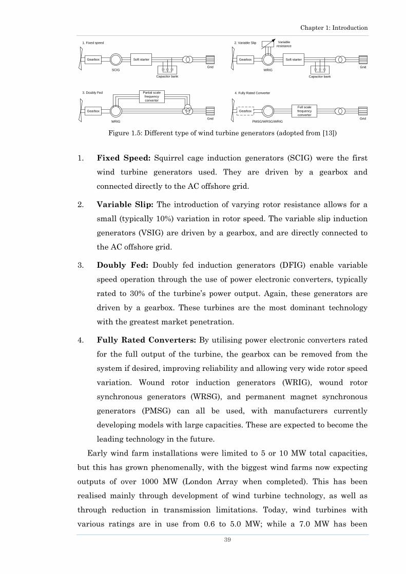
Chapter 1: Introduction
39
Figure 1.5: Different type of wind turbine generators (adopted from [13])
1. Fixed Speed: Squirrel cage induction generators (SCIG) were the first
wind turbine generators used. They are driven by a gearbox and
connected directly to the AC offshore grid.
2. Variable Slip: The introduction of varying rotor resistance allows for a
small (typically 10%) variation in rotor speed. The variable slip induction
generators (VSIG) are driven by a gearbox, and are directly connected to
the AC offshore grid.
3. Doubly Fed: Doubly fed induction generators (DFIG) enable variable
speed operation through the use of power electronic converters, typically
rated to 30% of the turbine‘s power output. Again, these generators are
driven by a gearbox. These turbines are the most dominant technology
with the greatest market penetration.
4. Fully Rated Converters: By utilising power electronic converters rated
for the full output of the turbine, the gearbox can be removed from the
system if desired, improving reliability and allowing very wide rotor speed
variation. Wound rotor induction generators (WRIG), wound rotor
synchronous generators (WRSG), and permanent magnet synchronous
generators (PMSG) can all be used, with manufacturers currently
developing models with large capacities. These are expected to become the
leading technology in the future.
Early wind farm installations were limited to 5 or 10 MW total capacities,
but this has grown phenomenally, with the biggest wind farms now expecting
outputs of over 1000 MW (London Array when completed). This has been
realised mainly through development of wind turbine technology, as well as
through reduction in transmission limitations. Today, wind turbines with
various ratings are in use from 0.6 to 5.0 MW; while a 7.0 MW has been
Gearbox Soft starter
Grid
Capacitor bank
SCIG
Gearbox Soft starter
Grid
Capacitor bank
WRIG
Variable
resistance
Gearbox
GridWRIG
Partial scale
frequency
converter
Gearbox
GridPMSG/WRSG/WRIG
Full scale
frequency
converter
1. Fixed speed 2. Variable Slip
3. Doubly Fed 4. Fully Rated Converter
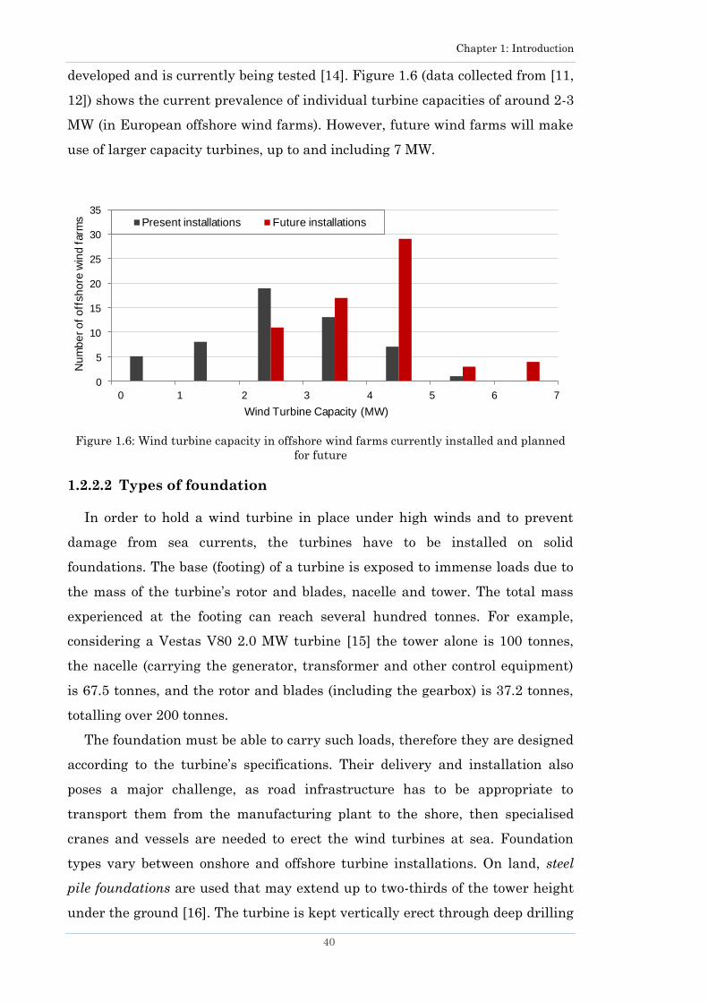
Chapter 1: Introduction
40
developed and is currently being tested [14]. Figure 1.6 (data collected from [11,
12]) shows the current prevalence of individual turbine capacities of around 2-3
MW (in European offshore wind farms). However, future wind farms will make
use of larger capacity turbines, up to and including 7 MW.
Figure 1.6: Wind turbine capacity in offshore wind farms currently installed and planned
for future
1.2.2.2 Types of foundation
In order to hold a wind turbine in place under high winds and to prevent
damage from sea currents, the turbines have to be installed on solid
foundations. The base (footing) of a turbine is exposed to immense loads due to
the mass of the turbine‘s rotor and blades, nacelle and tower. The total mass
experienced at the footing can reach several hundred tonnes. For example,
considering a Vestas V80 2.0 MW turbine [15] the tower alone is 100 tonnes,
the nacelle (carrying the generator, transformer and other control equipment)
is 67.5 tonnes, and the rotor and blades (including the gearbox) is 37.2 tonnes,
totalling over 200 tonnes.
The foundation must be able to carry such loads, therefore they are designed
according to the turbine‘s specifications. Their delivery and installation also
poses a major challenge, as road infrastructure has to be appropriate to
transport them from the manufacturing plant to the shore, then specialised
cranes and vessels are needed to erect the wind turbines at sea. Foundation
types vary between onshore and offshore turbine installations. On land, steel
pile foundations are used that may extend up to two-thirds of the tower height
under the ground [16]. The turbine is kept vertically erect through deep drilling
0
5
10
15
20
25
30
35
Nu
mb
er
of
off
sh
ore
win
d f
arm
s
Wind Turbine Capacity (MW)
Present installations Future installations
0 1 2 3 4 5 6 7

Chapter 1: Introduction
41
and insertion of steel piles in the ground. In an offshore environment, this
method is not useful due to soil stiffness and other parameters, therefore
different types of foundations are commonly employed such as: gravity,
monopile, jacket, tripile, and (currently experimental) floating foundations [11,
17].
These offshore foundations have been used in existing European wind farms
[11] and may be used in future projects. The selection of foundation type also
depends on sea depth, soil formation and the site‘s atmospheric conditions.
Among the types mentioned above the monopile has so far been used in most
offshore wind farms, followed by gravity foundations. In Bard 1, tripile
foundations are used [12] in water depths of around 40 m [18]. The floating
foundation is still in the experimental phase and is expected to be useful in
deep waters.
1.2.2.3 Wind turbine array
Spacing of turbines is an important factor. A large spacing might be ideal to
reduce any wake induced power losses, however longer distances imply larger
cable lengths which results in higher costs. Normally, wind turbines are
connected through AC Cross-Linked Poly Ethylene (XLPE) 3-core submarine
cables with a Copper or Aluminium conductor. Cables are specially designed to
prevent moisture ingress and therefore have a thicker outer protective layer.
The correct choice of voltage level inside an array is important. At a low voltage
the current level will be high, leading to greater I2R losses. On the other hand,
if the voltage level is too high then the cost of cables and equipment will
increase due to extra insulation.
Newer wind turbines have a built-in transformer located inside the nacelle.
This scales up the generator voltage level (usually 690 V) to a MV level at
which the turbines are interconnected. Offshore wind farms in Europe typically
use a MV level of 22 kV or 30-36 kV (more commonly employed) [12].
1.2.2.4 Array configurations
An array collector system gathers power from all turbines and delivers it to
the collector transformer installed at the offshore substation. There are several
ways to connect wind turbines inside an offshore wind farm but factors such as
the distances between them (influenced by wake effects), voltage level inside
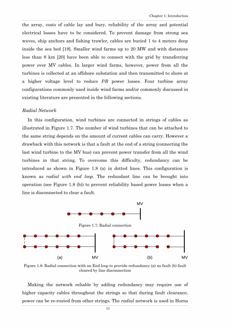
Chapter 1: Introduction
42
the array, costs of cable lay and bury, reliability of the array and potential
electrical losses have to be considered. To prevent damage from strong sea
waves, ship anchors and fishing trawler, cables are buried 1 to 4 meters deep
inside the sea bed [19]. Smaller wind farms up to 20 MW and with distances
less than 8 km [20] have been able to connect with the grid by transferring
power over MV cables. In larger wind farms, however, power from all the
turbines is collected at an offshore substation and then transmitted to shore at
a higher voltage level to reduce I2R power losses. Four turbine array
configurations commonly used inside wind farms and/or commonly discussed in
existing literature are presented in the following sections.
Radial Network
In this configuration, wind turbines are connected in strings of cables as
illustrated in Figure 1.7. The number of wind turbines that can be attached to
the same string depends on the amount of current cables can carry. However a
drawback with this network is that a fault at the end of a string (connecting the
last wind turbine to the MV bus) can prevent power transfer from all the wind
turbines in that string. To overcome this difficulty, redundancy can be
introduced as shown in Figure 1.8 (a) in dotted lines. This configuration is
known as radial with end loop. The redundant line can be brought into
operation (see Figure 1.8 (b)) to prevent reliability based power losses when a
line is disconnected to clear a fault.
Figure 1.7: Radial connection
Figure 1.8: Radial connection with an End loop to provide redundancy (a) no fault (b) fault
cleared by line disconnection
Making the network reliable by adding redundancy may require use of
higher capacity cables throughout the strings so that during fault clearance,
power can be re-routed from other strings. The radial network is used in Horns
MV
MV MV(a) (b)

Chapter 1: Introduction
43
Rev 1 and 2 offshore wind farms [21, 22] and is also discussed in existing
literature [23], [24]. A radial with end loop connection is used in Greater
Gabbard offshore wind farm in the UK [25].
Starburst Network
In this network the turbines are connected to a central node by individual
cables as illustrated in Figure 1.9. The network is very reliable in case of a
single cable fault but implementation can be more expensive due to extra
lengths of diagonally laid cables and complex switchgear of the node where all
cables meet. Redundancy is not needed, as failure of any cable does not
interrupt power from other turbines, however if a fault occurs at the main
power carrying cable to the MV bus, then power transfer from all turbines is
halted.
Figure 1.9: Starburst connection with MV bus
Lower capacity cables can be employed throughout, except at the link
between the nodal point and platform. The starburst connection is discussed in
[24], and it was one of the considered options for Middelgrunden offshore wind
farm [26].
Central (Tree) Network
The central network links all turbines in a tree-branch configuration as
shown in Figure 1.10.
Figure 1.10: Central network connected with the MV bus
MV
MV
MV
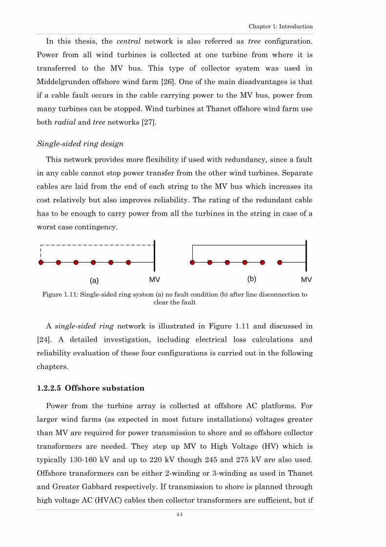
Chapter 1: Introduction
44
In this thesis, the central network is also referred as tree configuration.
Power from all wind turbines is collected at one turbine from where it is
transferred to the MV bus. This type of collector system was used in
Middelgrunden offshore wind farm [26]. One of the main disadvantages is that
if a cable fault occurs in the cable carrying power to the MV bus, power from
many turbines can be stopped. Wind turbines at Thanet offshore wind farm use
both radial and tree networks [27].
Single-sided ring design
This network provides more flexibility if used with redundancy, since a fault
in any cable cannot stop power transfer from the other wind turbines. Separate
cables are laid from the end of each string to the MV bus which increases its
cost relatively but also improves reliability. The rating of the redundant cable
has to be enough to carry power from all the turbines in the string in case of a
worst case contingency.
Figure 1.11: Single-sided ring system (a) no fault condition (b) after line disconnection to
clear the fault
A single-sided ring network is illustrated in Figure 1.11 and discussed in
[24]. A detailed investigation, including electrical loss calculations and
reliability evaluation of these four configurations is carried out in the following
chapters.
1.2.2.5 Offshore substation
Power from the turbine array is collected at offshore AC platforms. For
larger wind farms (as expected in most future installations) voltages greater
than MV are required for power transmission to shore and so offshore collector
transformers are needed. They step up MV to High Voltage (HV) which is
typically 130-160 kV and up to 220 kV though 245 and 275 kV are also used.
Offshore transformers can be either 2-winding or 3-winding as used in Thanet
and Greater Gabbard respectively. If transmission to shore is planned through
high voltage AC (HVAC) cables then collector transformers are sufficient, but if
MV(a) (b) MV
Chapter 1: Introduction
45
high voltage DC (HVDC) is to be used then the platform should be able to carry
converter transformers and converters.
The cables used in wind farm arrays produce reactive power due to shunt
capacitance; this can affect the MV level at the offshore busbars. Conversely,
collector transformers absorb reactive power. If the link to shore is made
through HVAC cables, then they also act as a reactive power source raising the
voltage levels. Therefore, a source of reactive power compensation is required
on the offshore platform. A compensation device not only improves the voltage
quality but also provides the power factor correction to follow the requirements
of the Grid Code. If the link to shore is made through HVDC technology, an
offshore device for reactive power compensation may not be needed as
converters have the ability to regulate reactive power.
Offshore substations are often completely prefabricated on land and installed
offshore in one piece. Alternatively, they can be of modular design for easy
assemblage at sea. Transformers for offshore use have to be specifically
designed for the weight and volume restrictions imposed by the platform.
Furthermore, the total weight to be lifted cannot exceed that of the crane to be
used; (the current largest sea crane Thialf can haul 14,200 tonnes [28]).
A typical large wind farm offshore AC collection substation will include:
One or more collector transformers (2- or 3-winding) to step up voltage to
transmission levels.
Devices for reactive power compensation.
AC switchgear: usually gas insulated (GIS) [25] due its improved
reliability, minimal maintenance requirements, resilience to the corrosive
environment and a smaller footprint [29].
Instrumentation and protection systems.
Neutral earthing resistors.
Auxiliary backup diesel generator.
1.2.2.6 Platform interconnection
When the capacity of a wind farm is very large, a single platform may not be
sufficient to house all the required equipment. Limitations exist not only in
terms of the civil works of the platform (the weight it can withstand) but also
on the number of cables that can be safely brought in a limited space. For these
reasons, as well as for the reliability improvements that interconnection brings

Chapter 1: Introduction
46
(increasing redundancy), having more than one platform is beneficial. These
inter-platform connections are made using HVAC cables. One major
disadvantage of this approach is the cost of additional offshore substations;
however a full cost-benefit analysis will reveal the optimal configuration.
Many of the European wind farms with authorised consent for development
at higher power capacities will have two offshore substations. Amongst wind
farms near completion, London Array (currently in development in the UK) will
utilise two offshore substations in Phase One (1,250 tonnes each) delivering 630
MW of power to shore [30]. Sheringham Shoal and Greater Gabbard wind
farms in the UK will make use of two offshore substations [25, 31].
1.2.2.7 Transmission of electricity to shore
Power transmission to shore in large offshore wind farms can take place by
either High-voltage AC (HVAC) or High-voltage DC (HVDC) cables. HVAC line
losses are less compared to HVDC for shorter distances whereas, HVDC is more
economical for large wind farms when the distance to shore is greater than 90
km [32]. For distances greater than 90 km, power transfer by HVAC is limited
due to the capacitive nature of the cables [33] (as they generate reactive
current) unless reactive compensation is installed at each end. Generation of
reactive current reduces the capacity to carry the active current. In this
situation HVDC becomes the preferred option as it offers no technical
limitations on the length of submarine cables.
Systems interconnected by HVDC do not need to operate synchronously with
each other, thus preventing propagation of cascading system failures which are
observable in AC systems. Apart from this, it allows controllability of the
magnitude and direction of power flow that can improve the stability of the
system.
HVDC can be implemented through two different technologies: Line
Commutated Converter (LCC) and Voltage Source Converter (VSC). AC to DC
rectifier and DC to AC inverters are needed at offshore and onshore substations
respectively.
LCC is a thyristor based HVDC technology; it is a conventional way to
transfer power over a HVDC line. ABB sells this technology under the name of
HVDC Classic.
Chapter 1: Introduction
47
The VSC technology is relatively new and is gaining world-wide recognition
as it is lightweight, compact and has better control than conventional LCC. So
far VSC technology has only been used in projects in Sweden, Denmark,
Australia and USA. It offers numerous benefits over LCC but is very expensive.
Pulse Width Modulation (PWM) and Insulated Gate Bipolar Transistors (IGBT)
are used in this technology. VSC allows flexible control of reactive power. In
industry it has been developed by ABB and Siemens with the product names
HVDC Light® and HVDC PLUS respectively.
A more detailed comparison between LCC and VSC, as well as between
monopole and bipolar configurations is presented in Section 7.2.6.
1.2.2.8 Onshore substations
To accommodate power injection from the wind farms onshore, substations
would have to be modified or new ones constructed. The voltage level may have
to be adjusted through onshore transformers if power has to be added directly
to Distribution or Transmission Lines. Creation or extension of new substations
will involve land acquisition and planning permissions will also be required
[29]. Onshore reactive power compensation may have to be installed, depending
on the VAr creation in the HVAC lines. If an HVDC link is used, then an
Inverter will also have to be installed to convert the voltage and current back
into AC. Protection and control equipment, Air Insulated Switchgear (AIS) and
AIS Disconnectors may also be needed on an onshore substation.
1.3 Wind Farm Costs
Many factors contribute towards the total project cost to build a large wind
farm. These include price of the equipment, transport, installation, shipping,
labour, planning and construction. With so many potentially volatile costs
(including currency and commodity price movements) to incorporate and the
fact that specific details of each project play an important role in determining
the required level of investment, it is difficult to predict the price of future wind
farms.
Despite a general reduction in prices during the 1990s, from the mid-2000s
prices have been escalating. Initial projects carried price tags of approximately
€2.08 million/MW (Vindeby, 1991), later reducing to €1.20 million/MW (Horns
Rev, 2002). However, current costs are now much higher at approximately

Chapter 1: Introduction
48
€3.45 million/MW [3] (e.g. 300 MW Thanet wind farm completed in 2010 came
in at a cost of €3.0 million/MW) [34].
Due to the cost of an offshore platform, cable connection to shore and in
general, higher costs of foundations, installation and construction, offshore
power per MW costs more than onshore [35]. Not only this, but also operational
expenditure (OpEx) for offshore wind farms is higher than onshore since access
to the wind farm is dependent on weather conditions and availability of a
vessel.
1.4 Review of Relevant Previous Works
1.4.1 Aggregate models for transient stability studies
Increasing use of wind generation requires suitable models of WFs that can
be easily deployed in power system studies. Detailed dynamic models of large
WFs consisting of tens and even hundreds of wind turbines are not suitable as
they can significantly increase the size of the mathematical model of the power
system and thus increase the overall simulation time. In spite of significant
computer power available and efficient numeric algorithms to handle large
mathematical models, it is still desirable to reduce the order of the model of
individual system components as much as possible. Although model reduction
is entirely preventable by use of a super computer [36] this may prove to be an
expensive solution. The studies involving very large power systems (e.g., pan-
European system) involving thousands of generators are becoming more and
more sought after and every reasonable reduction in mathematical model of
individual components is welcomed as long as equivalent/aggregate models
retain the required level of accuracy. Several aggregate WF models [37-42]
have been proposed over the last decade with the aim of reducing
computational effort and simulation time during transient stability analyses to
enable very fast, first approximation, assessment of WF performance and
consequently WF effect on power system performance.
Wind speed variation (due to wake effects) inside a wind farm, turbine type
and wind turbine interconnection in different strings makes the aggregation
non-trivial. A single-unit aggregate wind turbine model, proposed in [43]
represents the entire wind farm by one equivalent machine. All wind turbines
are modelled through simplified wind turbines and variation in wind speed is

Chapter 1: Introduction
49
taken into account in [44]. The importance of wake effect consideration during
wind farm aggregation is highlighted in [45]. A multi-machine model is
reported in [37] by clustering wind turbines with similar wind speeds.
Aggregation by wind speed (for DFIG) is performed in [46] by summation of
mechanical torques from individual turbines which then feed into an equivalent
generator. Wind farm behaviour emulative models can represent wind farms as
a DC current source [47] however they have been built for full converter
machines. An aggregate model for wind farms consisting of fixed-speed turbines
is presented in [48]. Variable speed wind turbines can be represented by a
transfer function in [49] whereas a complete wind farm model reduction
through singular perturbation theory is proposed in [40].
Wind farms are usually built in areas with higher wind speeds and this can
eventually lead to a wider geographical gap between generation and demand.
In future, when power networks will have a significant amount of large-scale
wind farms installed, the centre of power generation will no longer be fixed. In
this case, offline analysis may no longer be effective and real time transient
stability simulations will have to be performed using short-term forecasted
wind speed as input. Wind pattern models for short term forecasts from a few
minutes to several hours ahead [50], [51], [52, 53] already exist. Aggregate
models of wind farms can be plugged in to real-time simulators to reduce
simulation time as proposed in [54].
Problem statement 1:
All aforementioned aggregation methods were designed for offline
simulations, however they have not been tested on a real-time simulator. Some
of these studies involve simplified wind turbine models leading to lower
accuracy of dynamic results while others use simplified wind models, e.g.,
neglecting wake effects and assuming that every turbine inside the WF receives
the same wind speed. Doing so does not accurately estimate the power output
from a WF. Some of the above mentioned models are accurate and cause
reduction in simulation time, but as a consequence, increased application
difficulty. A model that considers wake effects that is fast and practical to be
used in an online real-time simulator is needed.

Chapter 1: Introduction
50
1.4.2 Energy yield estimation and cost-benefit analysis for
offshore wind farms
Evaluation of the energy yield analysis of a wind farm is necessary to
determine the feasibility of a project. It is a prerequisite for obtaining planning
permission and to justify project financing. Therefore it is essential to
determine this value as close to reality as possible. However, this can only be
achieved once all influential factors have been considered during the analysis.
These factors are generally losses that reduce power output and thus energy
yield of a wind farm. One such factor is wake effect and several models have
been presented in the past [55-59] to take it into consideration, however some
models are more complex than others. Although complex models can model
wakes very closely and in greater detail, they are computationally very
demanding. Simple analytical models exist but they are mostly deterministic.
Wake models are covered in greater detail in Chapter 3.
Recording wind speed measurements for a wind farm project for at least one
year [60-62] is a common practice as it helps in assessing the energy yield.
However, if mast and anemometer installation costs have to be avoided or if a
general estimate of wind potential is needed, then a Weibull distribution [63,
64] can be also used.
The energy yield for wind farms is calculated in [65, 66]. Currently existing
energy yield evaluation techniques [64, 67] often ignore some or all of the loss
factors. Reliability is another important factor because if a component becomes
unavailable it can cause power interruption and thus reduction in energy yield.
Models for reliability evaluation of power systems with a large proportion of
wind generation already exist [68-70]. Very few models have been established
however, that carry out reliability based loss evaluation of wind farm energy
[71], yet impact of a wind farm‘s internal grid is often neglected [62, 72]. A brief
discussion on existing reliability models for wind farms can be found in [73].
Markov models and Monte Carlo simulations have been ubiquitously used in
the past.
Several software tools such as IPSA [74, 75], PSS®E [76, 77], DIgSILENT
PowerFactory [78], PowerWorld [79] can be used to build up a wind farm
network and carry out detailed analysis. Due to growing interest in wind farm
studies, dedicated software have been developed for wind farm design and
Chapter 1: Introduction
51
energy yield evaluation including WindFarmer [80] from GL Garrad Hassan
and WAsP (Wind Atlas Analysis and Application Program) [81].
Several techniques exist that can increase the energy yield of a wind farm
through optimal placement of wind turbines [82-84] and selection of
appropriate turbines [85]. Wind farm designs have been discussed in various
studies [86-89] including profit optimisation through Net Present Value (NPV)
analysis (with various turbine tower heights and locations) [90, 91]. Investment
cost analysis for building an offshore wind farm is provided in [92] (excluding
VSC converters and DC line costs). Electrical losses and investment costs of
electrical collector systems is investigated in [24]. However, a complete cost-
benefit study analysing various possible offshore electrical configurations (from
turbine to shore) along with losses and reliability is not available.
Increasing wind farm capacity and distance from shore has raised questions
as to whether HVAC or HVDC should be used for electricity transmission to
shore. Although an AC link is generally an economical choice, higher charging
currents and bigger losses makes it unfeasible for longer distances and this is
when the HVDC link appears to be a more suitable solution [19]. Transmission
link options from an offshore platform to shore are investigated in [32, 93].
Amongst the new electrical designs, a DC grid has been given serious thought.
When considering a complete DC grid based wind farm [88, 89] it was observed
that this configuration is suitable for large offshore wind farms, whereas series
connected DC wind turbines have the potential to yield lower cost of energy
production for distances than 20 km [86].
Problem statement 2
An optimisation algorithm is needed that deals with all aspects of wind farm
design collectively whether they are the physical placement of turbines, choice
of electrical layouts, choice of components or even transmission options to
shore. Maximisation of energy yield and minimisation of cost and losses have to
be looked at simultaneously. Existing studies lack such holistic optimisation
since only parts of the design are dealt with in previous studies.
Problem statement 3
Although current studies are very useful for layout design (turbine
placement) of an offshore wind farm, there is no comprehensive methodology
that provides a complete solution for an optimal electrical layout selection that

Chapter 1: Introduction
52
is reliable yet cost-efficient. With growing wind farm sizes it gets difficult to
choose the right electrical components, voltage levels, type of transmission,
turbine capacity, array configuration etc. that satisfy both criteria. Electrical
and reliability based losses should also be considered as part of the layout and
component selection process.
Problem statement 4
Energy yield calculation is essential during pre-feasibility studies as well as
during the design process. The methods used in the commercial software that
evaluate wind farm energy yield are hardly visible. In fact, several factors
contribute towards this final value and therefore this value should be
probabilistic and project specific. All loss factors including electrical losses,
wake losses and reliability based losses should be modelled. Current studies
ignore some, or all of these factors, while others generalise the total losses or
represent them by a deterministic value. In reality these losses are project and
site dependant, therefore a complete methodology is needed that can be easily
followed.
Problem statement 5
Analytical wake modelling techniques should be able to predict wind speed
probabilistically since wind interaction with a turbine changes the flow of wind.
Although complex models can simulate such phenomena, they are mostly used
during blade design and are not computationally efficient for electrical
engineering studies.
Problem statement 6
Reliability studies considering components internal to a wind farm are few
and in those studies only single component failures are considered. A multi-
component failure is a possibility and hence a methodology to calculate its
effect is needed.
1.4.3 Wind energy curtailments
In general, rural, open and low population areas are good locations for wind
farms. Electrical infrastructure, e.g. the transmission network, in these places
may not be sufficiently strong to accommodate integration of large-scale in feed
from wind farms. Transmission line reinforcement or network component

Chapter 1: Introduction
53
upgrade is an expensive option. The transmission corridor may already be
reserved for existing conventional generators installed in the area.
Furthermore, power imbalances between generation and demand can happen
under a high wind low demand situation. In such circumstances, curtailment of
wind energy might seem to be a feasible, yet cheaper alternative. Curtailments
are carried out in several parts of the world including the US [94], Spain, New
Zealand, Ireland, Germany and Canada‘s Alberta province [10]. Curtailments
were initially suggested in [95] and then widely discussed in the existing
literature [96-98]. Although methods for wind farm energy curtailment
evaluation have been proposed in the past [99-101] some of them require
detailed network parameters to be known, while others require a unit
commitment schedule. Such methods are generally applicable when
information about the network or generator scheduling is available.
In future, electricity storage devices (e.g. battery) will have the potential to
limit curtailment losses by effectively storing excess energy and later using it
as a backup reserve [102]. However, such devices are still very expensive or of
limited capacity, therefore, in the short to medium term, wind curtailments
may prove to be a more economic option. Although curtailments are performed
by reducing power output from a wind farm, very few if any studies have been
carried out to determine which turbines to shut down first.
Problem statement 7
A method is needed to estimate annual energy curtailments for wind farms
which consider the influence of realistic factors such as internal wind farm
losses, turbine availabilities and correlation between wind power generation
and loading of transmission lines (ignored in the previous studies) so that a
realistic estimate is obtained.
Problem statement 8
During curtailments it is not known which turbines should be given priority
to shut down. A procedure should be devised that allows determination of such
turbines. This has not been studied so far in the literature.
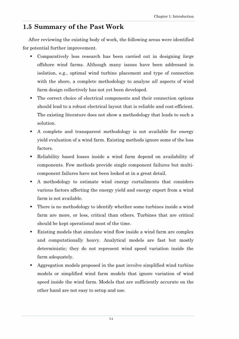
Chapter 1: Introduction
54
1.5 Summary of the Past Work
After reviewing the existing body of work, the following areas were identified
for potential further improvement.
Comparatively less research has been carried out in designing large
offshore wind farms. Although many issues have been addressed in
isolation, e.g., optimal wind turbine placement and type of connection
with the shore, a complete methodology to analyse all aspects of wind
farm design collectively has not yet been developed.
The correct choice of electrical components and their connection options
should lead to a robust electrical layout that is reliable and cost-efficient.
The existing literature does not show a methodology that leads to such a
solution.
A complete and transparent methodology is not available for energy
yield evaluation of a wind farm. Existing methods ignore some of the loss
factors.
Reliability based losses inside a wind farm depend on availability of
components. Few methods provide single component failures but multi-
component failures have not been looked at in a great detail.
A methodology to estimate wind energy curtailments that considers
various factors affecting the energy yield and energy export from a wind
farm is not available.
There is no methodology to identify whether some turbines inside a wind
farm are more, or less, critical than others. Turbines that are critical
should be kept operational most of the time.
Existing models that simulate wind flow inside a wind farm are complex
and computationally heavy. Analytical models are fast but mostly
deterministic; they do not represent wind speed variation inside the
farm adequately.
Aggregation models proposed in the past involve simplified wind turbine
models or simplified wind farm models that ignore variation of wind
speed inside the wind farm. Models that are sufficiently accurate on the
other hand are not easy to setup and use.

Chapter 1: Introduction
55
1.6 Research Objectives
Several areas that can be further improved have been identified and
summarised in the previous section. The main aims of this research are derived
from identified areas for further improvement and summarised below:
1. Identify and summarise gaps and areas in need of further
improvement based on the existing body of literature.
2. Critically evaluate existing methods for wind farm aggregation and
develop a more easy to use yet accurate methodology for wind farm
aggregation.
3. Evaluate the developed aggregation approach against full wind farm
model and existing aggregate models.
4. Collect and compare existing methods and if required, develop new
methodologies for energy loss calculation inside a wind farm to
establish complete set of methods that can be followed in different
types of studies.
5. Develop curtailment evaluation method which considers various
realistic factors and can estimate curtailments for a wind farm in a
remote location without detailed network parameter information.
6. Determine and quantify the effects of wake on wind farm power
output and energy curtailments.
7. Investigate existing wake effect models and if required, develop a new
fast, probabilistic wake model which can be used during online
studies.
8. Develop methodology to identify wind turbines that face high wind
speeds/remain under wake most of the time, so that more power
producing turbines and those under greater mechanical stress can be
identified.
9. Develop methodology to identify a robust electrical layout for an
offshore wind farm and to choose component ratings effectively using
cost-benefit analysis.
10. Develop user friendly software tool with an appropriate Graphical
User Interface (GUI) for quick and effortless design of large offshore
wind farm electrical systems.

Chapter 1: Introduction
56
1.7 Major Contributions of the Research
The contributions made during the course of this research are summarised
as follows. (Research papers published or submitted for publication to
International Journals, and International Conferences based on particular
contribution are given in the parenthesis. List of author‘s thesis based
publications can be found in Appendix F).
1.7.1 Vector based wake calculation program (VebWake)
A software is developed in MATLAB that allows calculation of wind speed at
any turbine inside the wind farm. The software uses detailed wake effect
models (considering single, partial and multiple wakes) to estimate the wind
speeds. A wind farm consisting of any number of turbines arranged in any
layout at any location can be simulated for any incoming wind speed and wind
direction. Integrated power curve of the turbines allow rapid evaluation of
power output of the wind farm. The software estimates the wind speed using
the vector intersection method detailed in Chapter 3.
1.7.2 Probabilistic wake effect model
Existing wake effect models used in wind farm studies are mostly
deterministic. Detailed and reasonably complex models of wake effect exist,
however they are mostly suitable for turbine blade design and add significant
and possibly unnecessary computation burden. A new analytical wake model is
proposed in this thesis by combining two existing widely adopted models. The
model allows probabilistic evaluation of power output from a wind farm, it is
efficient and can be used during online analysis. Details about this model can
be found in Chapter 3. [F.6]
1.7.3 Probabilistic aggregate model of a wind farm
A novel method is developed through which a large wind farm can be
represented by fewer turbines. The concept of aggregation is extended to
include wake effects, electrical losses, site wind characteristics and wind farm
layout. A dynamic response comparison is also provided with the detailed
model. The approach is practical and leads to significant reduction in
simulation time.

Chapter 1: Introduction
57
The probabilistic aggregation method is compared with existing approaches.
Factors such as simulation time, ease of setup and use and dynamic stability
performance are evaluated. The technique and the comparison are presented in
Chapter 4. [F.2] [F.5] [F.8]
1.7.4 Advanced method for wind farm energy yield calculation
A method is proposed for probabilistic calculation of wind farm energy yield.
It comprises a new method for reliability evaluation that takes into account
availability of wind turbines, turbine cables, transformers and cables to shore.
It is developed for four commonly used array collector systems i.e. radial,
starburst, tree and single-sided ring configurations. The sensitivity of energy
yield calculation to various factors that contribute towards energy losses is also
established. The calculation procedure is described in Chapter 5. [F.1] [F.4]
1.7.5 Assessment of wind energy curtailment
A new method is proposed to evaluate energy curtailment losses for wind
farms installed in remote areas with transmission bottlenecks. It takes into
account correlation between transmission line loading, wind turbine
availability and wind speed. It also considers factors such as wake effects and
electrical losses inside the wind farm during calculation. The method developed
is discussed in Chapter 5. [F.1] [F.9]
1.7.6 Probabilistic identification of critical wind turbines
inside the wind farm
A new method is developed to identify turbines that face high and low wind
speeds inside a wind farm during a year. Wind farm layout, height and rotor
radius of turbines, site‘s wind characteristics (wind speed and direction), wake
effects and positioning of turbines are all taken into account. The method is
applicable to both onshore and offshore wind farm installations. The model is
presented in Chapter 6. [F.7]
1.7.7 Methodology for cost-benefit analysis of offshore
electrical network design
A novel methodology is proposed to select a robust design option for an
offshore wind farm. Several design options are possible for a large offshore wind

Chapter 1: Introduction
58
farm considering voltage levels, choice of turbines, rating and quantity of
components that can be employed. The proposed method short-lists a robust
design option from a list of feasible design options. The method considers
capital cost, level of redundancy, electrical losses and reliability based losses.
The cost of losses is computed and a cost-benefit analysis carried out using the
Net Present Value (NPV) calculation for all short-listed options. The method
developed and assessment procedure is described in Chapter 7.
1.7.8 Industrial software for offshore wind farm design and
loss evaluation
An industrial-grade software tool is developed that allows a user to quickly
develop and test large wind farm electrical systems. The tool is based on
commercially available power system software PSS®E. Data is entered through
a Graphical User Interface (GUI) which is then used for the automated design
of the network. Once network development is complete, rapid analysis of
electrical losses (compliant with Grid Code) is also possible. Reliability based
energy losses can also be evaluated through an automated procedure. The
developed software tool significantly reduces the time and effort needed in
carrying out such calculations. Details about the software and design
methodology are described in Chapter 7. [F.3] [F.10]
1.8 Overview of Thesis
There are nine chapters in this dissertation. An outline of each of them apart
from the introduction is presented below:
Chapter 2: Wind Turbine and Power System Components Modelling
Basic models for power system and wind turbine components are given in
this chapter. These include line, transformer, doubly-fed induction generator,
rotor-side and grid-side converter, power and thrust coefficient, drive train,
protection system, pitch and rotor speed controller models.
Chapter 3: Modelling of Wake Effects
Existing wake effect models are critically reviewed and the most suitable
model for use is identified in this chapter. The wake calculation program which
has been developed is also introduced here and illustrative simulation

Chapter 1: Introduction
59
screenshots are presented. Models of large and small wind farms used in the
analysis throughout the thesis are also shown in this chapter.
A new probabilistic wake model is proposed by combining two analytical
wake models to take into account wake induced turbulence in wind speed and
its impact on power output. The method is tested on a large wind farm and
illustrative results are presented.
Chapter 4: Probabilistic Aggregate Dynamic Model of a Wind Farm
This chapter introduces a novel methodology to establish a probabilistic
aggregate model of a wind farm that can be used during the year. The
aggregate model can be used for transient stability studies to simulate dynamic
response of a large wind farm. Development of the aggregate model considers
layout of the wind farm, wake effects and wind characteristics at the site.
Support Vector Clustering is performed to cluster wind turbines facing the
same wind speed. Groups are then formed out of these clusters; the most
probable group is then chosen to represent the wind farm. Aggregation of the
collector system is also proposed so that electrical losses can also be taken into
account. The method is tested on a large wind farm against a detailed wind
farm model to compare transient stability results and simulation time. A
comparison with existing aggregate models is also provided to compare
accuracy, simulation time, ease of setup and use.
Chapter 5: Probabilistic Assessment of Wind Farm Energy Yield
In the early sections of this chapter likely causes of transmission bottlenecks
are discussed, including voltage stability limits and thermal limits of the
equipment. This is followed by factors that affect energy yield production from
a wind farm such as wake effects, electrical losses and reliability based losses.
A methodology is then provided to calculate energy loss due to each factor,
looking especially at the reliability calculation where a new method is proposed,
based on combinatorial algorithms. A new method to determine curtailments in
a region with transmission bottlenecks is also presented. Case studies and
sensitivity analysis are performed on a small wind farm. The method is
applicable for offline pre-feasibility studies (i.e. prior to wind farm
development) to facilitate informed decisions by a wind farm owner.

Chapter 1: Introduction
60
Chapter 6: Probabilistic Identification of Critical Wind Turbines inside a Wind
Farm
The chapter presents a new methodology to identify wind turbines inside a
wind farm that are exposed to different winds during the year. The technique is
demonstrated on a case study involving a large wind farm.
Chapter 7: Robust Design Methodology for Offshore Wind Farms
A new methodology is proposed in this chapter that allows wind farm
designers to select a cost-efficient and reliable electrical network layout for the
offshore wind farm. A method for short-listing of options filters out layouts
based on investment cost and a reliability level index. The short-listed layouts
are then further tested for detailed electrical and reliability based losses. The
cost of losses is calculated based on energy price. Feasibility of each layout is
tested by NPV analysis. As a case study, a 400 MW offshore wind farm was
used to demonstrate the methodology.
A software tool to assist wind farm designers and consultants was developed
during an industrial placement. This chapter also describes key features and
advantages of this software, along with its design and calculation process.
Illustrative screenshots of developed GUI are also provided in this chapter. The
software automates electrical losses as well as reliability based losses.
Chapter 8: Conclusions and Future Work
The chapter presents major conclusions of this research as well as proposals
for future research and development that could advance the research presented
in this thesis.

Chapter 2: Wind Turbine and Power System Components Modelling
61
Chapter 2 Wind Turbine and Power System
Components Modelling
Wind Turbine and Power System
Components Modelling
2.1 Introduction
This chapter provides models for power system and wind turbine
components. Among four types of wind turbine technologies covered in the
previous chapter, the variable speed Doubly Fed Induction Generator (DFIG)
(Type 3) is most widely used commercially. This is because it provides a low
cost solution over Fully Rated Converter type of turbines [103] yet improved
power quality over Fixed Speed turbines. It should be pointed however that
although DFIG is a popular concept at present, but Fully Rated Converter type
is rapidly gaining popularity and might be used more commonly in the future.
This however will not change the relevance of the research presented in this
thesis. However model reduction for dynamic studies (presented in Chapter 4)
may have to be done differently.
Initial sections of the chapter discuss the basic energy extraction procedure
of a wind turbine, this is followed by aerodynamic, electrical and mechanical
component models. Operation and role of each wind turbine component in a
DFIG is discussed. Models for power coefficient, thrust coefficient, drive-train,
generator, rotor-side converter (RSC), grid-side converter (GSC) and pitch angle
controller are provided along with power system component models for cable
and transformers (2-winding and 3-winding). Protection system, DC link
chopper, rotor speed controller and yaw control of a wind turbine are also
briefly discussed.

Chapter 2: Wind Turbine and Power System Components Modelling
62
2.2 Wind Turbine Modelling
A wind turbine extracts kinetic energy from the wind and converts it into
mechanical and then electrical energy. Two main components inside the
turbine enable this conversion process to take place: the turbine rotor and the
electrical generator. A rotor extracts the energy from the wind and converts it
into mechanical torque while the generator converts this mechanical energy in
the torque into electricity which is then fed into the grid. This is a general
working principle of a wind turbine, which sounds rather simple. In reality
however, a wind turbine is a complex system that can consist of several
components, including:
Aerodynamic rotor (with typically three blades),
Yaw mechanism,
Gear box,
Pitch control for the blades,
Electrical generator,
Anemometers,
Power electronics (Converters) and
Controllers
2.2.1 Power extraction from a wind turbine
Kinetic energy (KE) in a moving mass ma of air travelling at a speed v is
given as [104]:
21
2aKE m v
(2.1)
Power inside this moving mass of air can be expressed as:
Pw = 1
2(Mass flow rate per second) v2 (2.2)
If mass flow rate of air (ρAv) in kilograms per second is added to (2.2), this
equation can be re-written as:
21
2w
P Av v
(2.3)
where Pw is the mechanical power in the moving mass of air, A is swept area by
the rotor and ρ is air density.

Chapter 2: Wind Turbine and Power System Components Modelling
63
Power coefficient (Cp) also known as performance coefficient calculates the
fraction of power a wind turbine can extract from the wind. The amount of
kinetic energy that can be converted into mechanical energy depends on
turbine parameters as well as the wind speed. Turbine parameters such as
blade pitch angle, radius of the rotor and angular rotor speed determine the
fraction of power captured. A higher Cp implies that a turbine is more efficient
in extracting power from the wind. Mechanical power that a rotor extracts from
the wind is given by:
rot p wP C P
(2.4)
Substituting (2.3) into (2.4) gives:
31
2rot pP Av C
(2.5)
Power coefficient is a non-linear function of tip-speed ratio λ and pitch angle
β. It can vary with the type of turbine but has a maximum theoretical limit of
16/27 (59.3%) according to the Betz law [105]. Mechanical torque on
aerodynamic rotor shaft can be determined using turbine rotational speed ωrot:
rot
rot
rot
PT
(2.6)
A tip speed ratio is defined as the ratio of rotor tip speed to free wind speed
[105], it can be calculated through the following expression:
rot
R
v (2.7)
where R is the rotor radius and v is the incoming wind speed. Together ωrotR
make up the blade‘s linear speed at the outer tip.
Wind power varies linearly with air density. If air pressure Pr and
temperature Tp are known air density at a location can be determined using:
r
G p
P
R T
(2.8)
where RG is the gas constant. Under one atmospheric pressure (14.7 psi) and
60o Fahrenheit the air density is 1.225 kg/m3.
Figure 2.1 depicts operation (i.e. mechanical torque extraction from the
wind) of an aerodynamic model of a wind turbine.

Chapter 2: Wind Turbine and Power System Components Modelling
64
Figure 2.1: General principle of a wind turbine aerodynamic model
2.2.2 Power coefficient models and look-up table
Power coefficient characteristic of a wind turbine can be calculated through
analytical models using non-linear functions if actual measurements from a
wind turbine manufacturer are not available. One such model is given [106] as
follows:
61.5
1 2 3 4 5( , ) ( )
c
pC c c c c c e
(2.9)
Coefficients c1 to c6 can vary with the type of wind turbine, some exemplary
values are given below [106], [107]:
Table 2.1: Coefficients c1 to c6
c1 = 0.5 c2 = 116/λi c3 = 0.4
c4 = 0 c5 = 5 c6 = 21/λi
where λi can be obtained from the following expression:
1
3
1 0.035
0.08 1
i
(2.10)
Another mathematical model that can be used to calculate power coefficient
is obtained by curve fitting [108]:
4 4
,
0 0
( , )
i j
p i j
i j
C
(2.11)
The model is found to be accurate for the range 2 < λ < 13 whereas αi,j
coefficients are tabulated as below:
rot R
v( , )pC
2 31
2m pP R v C
mP
mT
,v R
rotpC
m
m
rot
PT
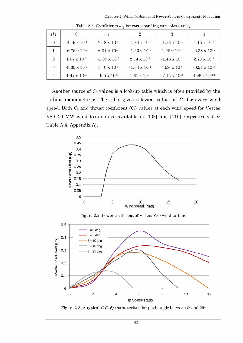
Chapter 2: Wind Turbine and Power System Components Modelling
65
Table 2.2: Coefficients αi,j for corresponding variables i and j
i\j 0 1 2 3 4
0 -4.19 x 10⁻¹ 2.18 x 10⁻¹ -1.24 x 10⁻² -1.33 x 10⁻⁴ 1.15 x 10⁻⁵
1 -6.76 x 10⁻² 6.04 x 10⁻² -1.39 x 10⁻² 1.06 x 10⁻³ -2.38 x 10⁻⁵
2 1.57 x 10⁻² -1.09 x 10⁻² 2.14 x 10⁻³ -1.48 x 10⁻⁴ 2.79 x 10⁻⁶
3 -8.60 x 10⁻⁴ 5.70 x 10⁻⁴ -1.04 x 10⁻⁴ 5.99 x 10⁻⁶ -8.91 x 10⁻⁸
4 1.47 x 10⁻⁵ -9.5 x 10⁻⁶ 1.61 x 10⁻⁶ -7.15 x 10⁻⁸ 4.96 x 10⁻¹⁰
Another source of Cp values is a look-up table which is often provided by the
turbine manufacturer. The table gives relevant values of Cp for every wind
speed. Both Cp and thrust coefficient (Ct) values at each wind speed for Vestas
V80-2.0 MW wind turbine are available in [109] and [110] respectively (see
Table A.4, Appendix A).
Figure 2.2: Power coefficient of Vestas V80 wind turbine
Figure 2.3: A typical Cp(λ,β) characteristic for pitch angle between 0o and 25o
0
0.05
0.1
0.15
0.2
0.25
0.3
0.35
0.4
0.45
0.5
0 5 10 15 20
Pow
er C
oeff
icie
nt (C
p)
Wind speed (m/s)
0
0.1
0.2
0.3
0.4
0.5
0 2 4 6 8 10 12
Po
wer C
oeff
icie
nt (C
p)
Tip Speed Ratio
B = 0 deg
B = 5 deg
B = 10 deg
B = 15 deg
B = 25 deg
Chapter 2: Wind Turbine and Power System Components Modelling
66
Typical power coefficient (Cp) characteristics for different tip-speed ratios
and pitch angles are illustrated in Figure 2.3.
2.2.3 Thrust coefficient
The amount of thrust (force) generated on the rotor blades by a pressure
drop can be characterised by a thrust coefficient [105]. Its value changes with
the incoming wind speed. Exemplary behaviour of Ct at different wind speeds in
a pitch controlled wind turbine (Vestas V80) is illustrated in Figure 2.4. The
data used to produce the plot was obtained from [110].
Figure 2.4: Thrust coefficient of Vestas V80 wind turbine
Similar to Cp, the data for Ct should also be obtained from the wind turbine
manufacturer, however in case that this data is not available a general
estimate given in (2.12) [111] can be used. The formula (2.12) was validated in
[112] after comparing Ct curves for several wind turbines.
2
3.5(2 3.5) 7/t
vC m s
v v
(2.12)
2.2.4 Operating range of wind turbines
Generally wind turbines operate with in a certain range of wind speed that is
defined by two thresholds known as the cut-in and cut-out levels. Cut-in is the
lowest wind speed at which the turbine starts generating power while cut-out is
the highest wind speed when the turbine stops producing power. The cut-out
speed is defined to ensure safety of the turbine components, that easily get
0
0.1
0.2
0.3
0.4
0.5
0.6
0.7
0.8
0.9
1
0 5 10 15 20 25 30
Thru
st C
oeff
icie
nt (C
t)
Wind speed (m/s)
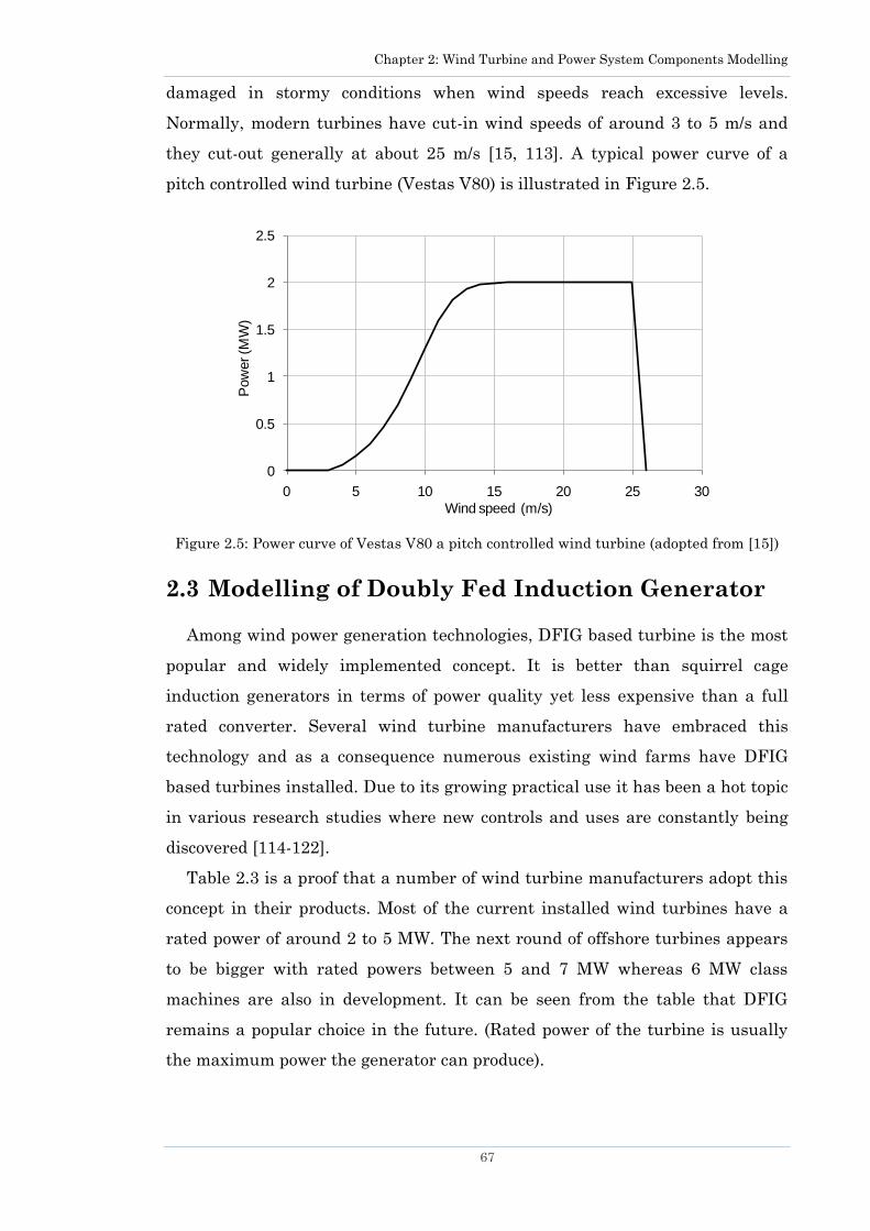
Chapter 2: Wind Turbine and Power System Components Modelling
67
damaged in stormy conditions when wind speeds reach excessive levels.
Normally, modern turbines have cut-in wind speeds of around 3 to 5 m/s and
they cut-out generally at about 25 m/s [15, 113]. A typical power curve of a
pitch controlled wind turbine (Vestas V80) is illustrated in Figure 2.5.
Figure 2.5: Power curve of Vestas V80 a pitch controlled wind turbine (adopted from [15])
2.3 Modelling of Doubly Fed Induction Generator
Among wind power generation technologies, DFIG based turbine is the most
popular and widely implemented concept. It is better than squirrel cage
induction generators in terms of power quality yet less expensive than a full
rated converter. Several wind turbine manufacturers have embraced this
technology and as a consequence numerous existing wind farms have DFIG
based turbines installed. Due to its growing practical use it has been a hot topic
in various research studies where new controls and uses are constantly being
discovered [114-122].
Table 2.3 is a proof that a number of wind turbine manufacturers adopt this
concept in their products. Most of the current installed wind turbines have a
rated power of around 2 to 5 MW. The next round of offshore turbines appears
to be bigger with rated powers between 5 and 7 MW whereas 6 MW class
machines are also in development. It can be seen from the table that DFIG
remains a popular choice in the future. (Rated power of the turbine is usually
the maximum power the generator can produce).
0
0.5
1
1.5
2
2.5
0 5 10 15 20 25 30
Pow
er (M
W)
Wind speed (m/s)

Chapter 2: Wind Turbine and Power System Components Modelling
68
Table 2.3: Wind turbines with DFIG technology
Manufacturer/Type Rated power
(MW)
Rotor
diameters (m)
Operational
range (m/s)
GE Wind Energy 1.5s 1.5 70.5 4 - 25
Vestas V80 2.0 80 4 - 25
Suzlon S95 2.1 95 3.5 - 25
Nordex N100 2.5 100 3 - 25
Vestas V90 3.0 90 3.5 - 25
Sinovel SL3000 3.0 91.3 3 - 25
BARD 5.0 5.0 122 3 - 25
Repower 5M 5.0 126 3 - 25
Repower 6M 6.15 126 3.5 - 25
In a DFIG configuration, stator of generator is connected directly to the grid,
which makes it synchronous with the grid frequency, while the rotor is
connected to the grid through a power electronic converter, as visible from
Figure 2.6. Active power can be controlled by current in the RSC through
variation in electric torque and generator excitation. Reactive power can be
independently controlled by adjusting rotor currents in the RSC which
determines the stator reactive power and through control settings of a GSC.
Interaction between different components of a DFIG with corresponding signal
exchange is illustrated in Figure 2.7. A DFIG can be operated in super-
synchronous or sub-synchronous modes because of its bi-directional converter.
Figure 2.6: Generic wind turbine model with a DFIG
DC
AC DC
AC
Rotor side
converter
Gear
box DFIG
Grid
Grid side
converter
Crow
bar
Filter Filter
Controller
Turbine
DC-Link Capacitor
DC-Chopper
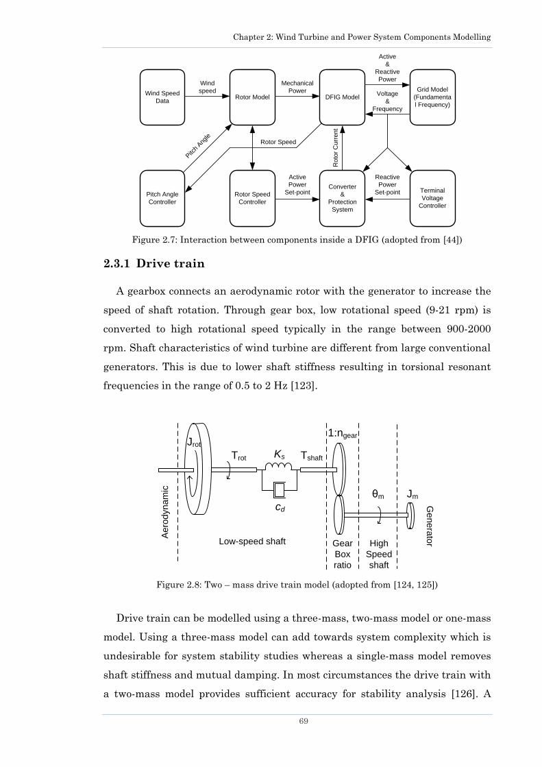
Chapter 2: Wind Turbine and Power System Components Modelling
69
Figure 2.7: Interaction between components inside a DFIG (adopted from [44])
2.3.1 Drive train
A gearbox connects an aerodynamic rotor with the generator to increase the
speed of shaft rotation. Through gear box, low rotational speed (9-21 rpm) is
converted to high rotational speed typically in the range between 900-2000
rpm. Shaft characteristics of wind turbine are different from large conventional
generators. This is due to lower shaft stiffness resulting in torsional resonant
frequencies in the range of 0.5 to 2 Hz [123].
Figure 2.8: Two – mass drive train model (adopted from [124, 125])
Drive train can be modelled using a three-mass, two-mass model or one-mass
model. Using a three-mass model can add towards system complexity which is
undesirable for system stability studies whereas a single-mass model removes
shaft stiffness and mutual damping. In most circumstances the drive train with
a two-mass model provides sufficient accuracy for stability analysis [126]. A
Wind Speed
DataRotor Model DFIG Model
Grid Model
(Fundamenta
l Frequency)
Terminal
Voltage
Controller
Converter
&
Protection
System
Rotor Speed
Controller
Pitch Angle
Controller
Wind
speed
Mechanical
Power
Active
&
Reactive
Power
Ro
tor
Cu
rre
nt
Voltage
&
Frequency
Reactive
Power
Set-point
Active
Power
Set-point
Pitc
h Ang
leRotor Speed
Jrot
Ks
cd
Jm
1:ngear
TshaftTrot
Ae
rod
yn
am
ic
Low-speed shaft Gear
Box
ratio
High
Speed
shaft
Ge
ne
rato
r
θm

Chapter 2: Wind Turbine and Power System Components Modelling
70
two-mass model has been validated against an actual wind turbine in [127], it
has been used in various stability studies [122, 128]. Figure 2.8 shows a two-
mass model representing turbine and generator rotor inertias connected by a
shaft with damping components. Inertia of the gear-box is not modelled
separately and it is included in generator inertia.
The equations (2.13) to (2.15) describe the two-mass model. Typically, an
aerodynamic rotor has a large while an electrical generator has a smaller mass
[125]:
rotrot
d
dt
(2.13)
k m
rot
gear
d
dt n (2.14)
rot shaftrot
rot
T Td
dt J
(2.15)
where Jrot corresponds to the rotor inertia, m is the rotational speed of the
generator rotor, Tshaft is the torque acting on the low speed shaft, Jm is the
mechanical inertia of the generator rotor, is the angular difference between
the rotor and the generator end of shafts, the ratio of an ideal gear box is
assumed to be 1:ngear and aerodynamic torque is represented by Trot. The
mechanical torque of the low-speed shaft is:
mshaft d rot s k
gear
T c Kn
(2.16)
where low speed shaft has a stiffness Ks and it has a damping coefficient of cd.
The mechanical power at the generator shaft is given by:
shaft
m m
gear
TP
n
(2.17)
2d s rotc K J (2.18)
2 24
s
s
(2.19)
k
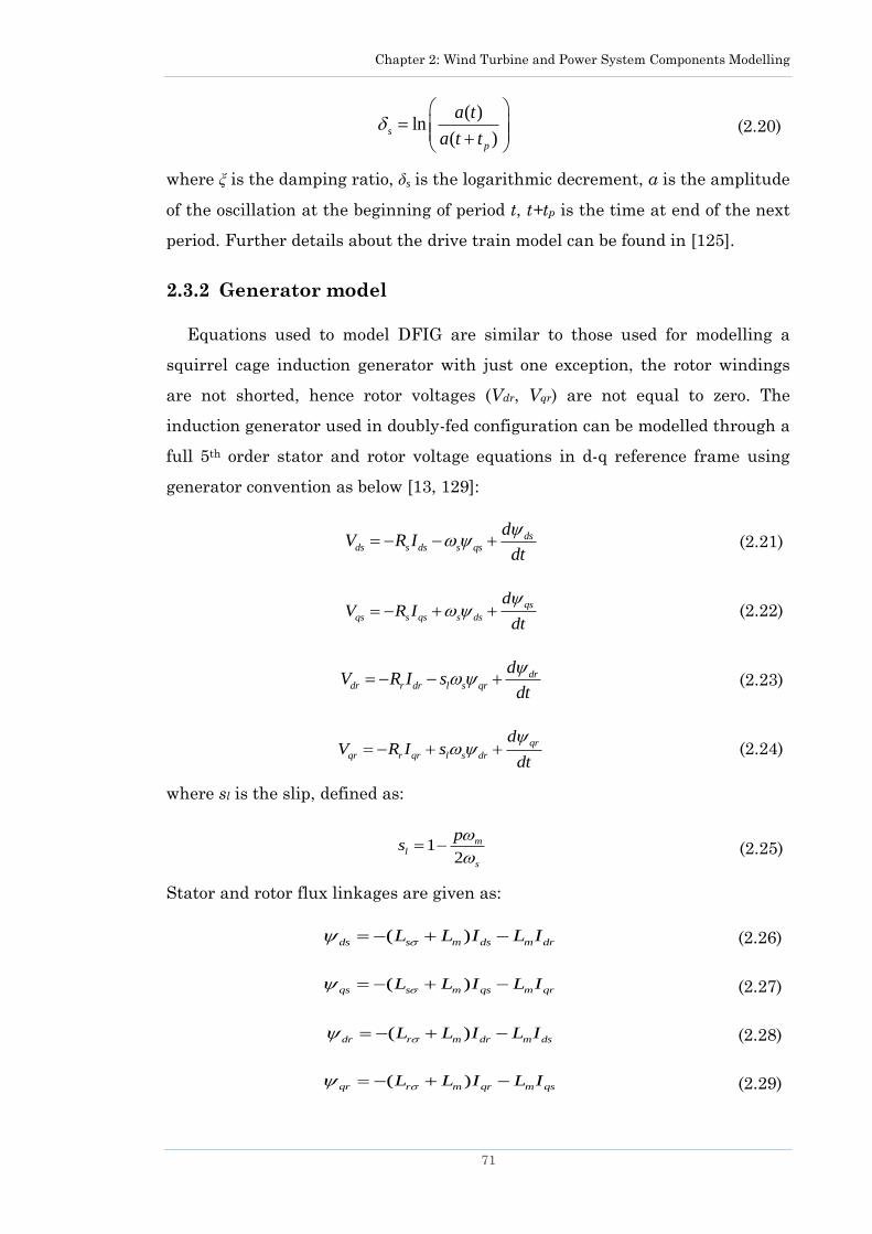
Chapter 2: Wind Turbine and Power System Components Modelling
71
( )ln
( )s
p
a t
a t t
(2.20)
where ξ is the damping ratio, δs is the logarithmic decrement, a is the amplitude
of the oscillation at the beginning of period t, t+tp is the time at end of the next
period. Further details about the drive train model can be found in [125].
2.3.2 Generator model
Equations used to model DFIG are similar to those used for modelling a
squirrel cage induction generator with just one exception, the rotor windings
are not shorted, hence rotor voltages (Vdr, Vqr) are not equal to zero. The
induction generator used in doubly-fed configuration can be modelled through a
full 5th order stator and rotor voltage equations in d-q reference frame using
generator convention as below [13, 129]:
dsds s ds s qs
dV R I
dt
(2.21)
qs
qs s qs s ds
dV R I
dt
(2.22)
dr
dr r dr l s qr
dV R I s
dt (2.23)
qr
qr r qr l s dr
dV R I s
dt (2.24)
where sl is the slip, defined as:
12
m
l
s
ps
(2.25)
Stator and rotor flux linkages are given as:
( )ds s m ds m drL L I L I (2.26)
( )qs s m qs m qrL L I L I (2.27)
( )dr r m dr m dsL L I L I (2.28)
( )qr r m qr m qsL L I L I (2.29)

Chapter 2: Wind Turbine and Power System Components Modelling
72
The difference between mechanical and electrical torque results in change of
generator speed that can be calculated from the following expression:
1
2
m
m e
m
dT T
dt H
(2.30)
e ds qs qs dsT I I qr dr dr qrI I (2.31)
where Te is the electric torque of the generator. The equations for active and
reactive power exchange with the grid are similar to that of a squirrel cage
induction generator, except the rotor windings can also be accessed in a DFIG
hence the rotor component in equations (2.36) and (2.37). Converters can
consume or produce reactive power but they cannot produce or consume active
power, thus total active power fed into the grid by a DFIG can be expressed by
Ptotal. However, reactive power fed into the grid is not the same as Qtotal in (2.37)
because it is affected by the converter. (Total reactive power fed into the grid by
a DFIG is explained and calculated in the following section.)
s ds ds qs qsP V I V I (2.32)
s qs ds ds qsQ V I V I
(2.33)
r dr dr qr qrP V I V I
(2.34)
r qr dr dr qrQ V I V I (2.35)
rtotal s ds ds qs qs dr dr qr qrP P P V I V I V I V I
(2.36)
rtotal s qs ds ds qs qr dr dr qrQ Q Q V I V I V I V I
(2.37)
where p is the number of poles, I is the current, R is the resistance of the
corresponding rotor or stator, Ψ is the flux linkage, Lm is the mutual
inductance, Lσ is the leakage inductance, Hm is inertia constant of the generator
rotor, Tm is the mechanical torque and ωm is the angular frequency of the
generator rotor. Subscripts s and r indicate stator or rotor side, d and q stand
for direct and quadrature components, respectively. Ptotal is the active power fed
into the grid by a DFIG. If, however, converter efficiency has to be taken into
account the terms with rotor subscript in this expression must be multiplied
with converter efficiency to access total power injected into the grid, Qtotal is the
reactive power but is not necessarily the amount fed into the grid because the
Chapter 2: Wind Turbine and Power System Components Modelling
73
converters can generate or consume reactive power which thus affects the total
amount of reactive power fed into the grid.
In generator convention, for modelling electrical machines the current
leaving the machine is positive while that entering the machine is negative.
The induction generator model presented above is a full 5th order dynamic
model that includes both stator and rotor transients. In stability studies,
transient phenomena associated with stator transients, e.g., electromagnetic
transients are usually ignored. Neglecting stator transients ( dsd
dt
, qsd
dt
)
converts a 5th order model into a 3rd order model. (This exclusion is equivalent
to ignoring the DC component in the stator transient current.) In both models
the electrical torque equation remains the same.
More details about modelling of induction machines can be found in [44,
125], [130].
2.3.3 Rotor-side and Grid-side converter
Converters are the key feature of a DFIG machine as they play an important
role. They allow variation in generator angular speed which enables a DFIG to
operate at variable speeds [37]. This is essential because fluctuating wind speed
causes mechanical power to fluctuate and if the converters are missing (as in
fixed speed turbines) all the fluctuation will be reflected in the power supplied
to the grid. In comparison with the full-scale power converter (used e.g. in
Permanent magnet synchronous machines) the DFIG converters are smaller in
size, cost less and lead to lower losses. In both types of variable speed turbines
(DFIG and full-scale converter connected) behaviour of the generator is
controlled by converters and controllers.
The power electronic converter in a DFIG machine is rated to about 30% of
turbine‘s rated power [131], for this reason it is also known as a partial-scale
converter. Both RSC and GSC are self-commutated and made up of six-pulse
bridges. These converters allow control over reactive power and power factor.
DFIG model built into DIgSILENT PowerFactory has an induction machine
joined together with a RSC as illustrated in Figure 2.9 and Figure 2.10. RSC
enables variation in generator‘s AC voltage magnitude and phase angle (by
modifying the pulse-width modulation factor, Mf ) that allows fast and flexible
control of the generator.
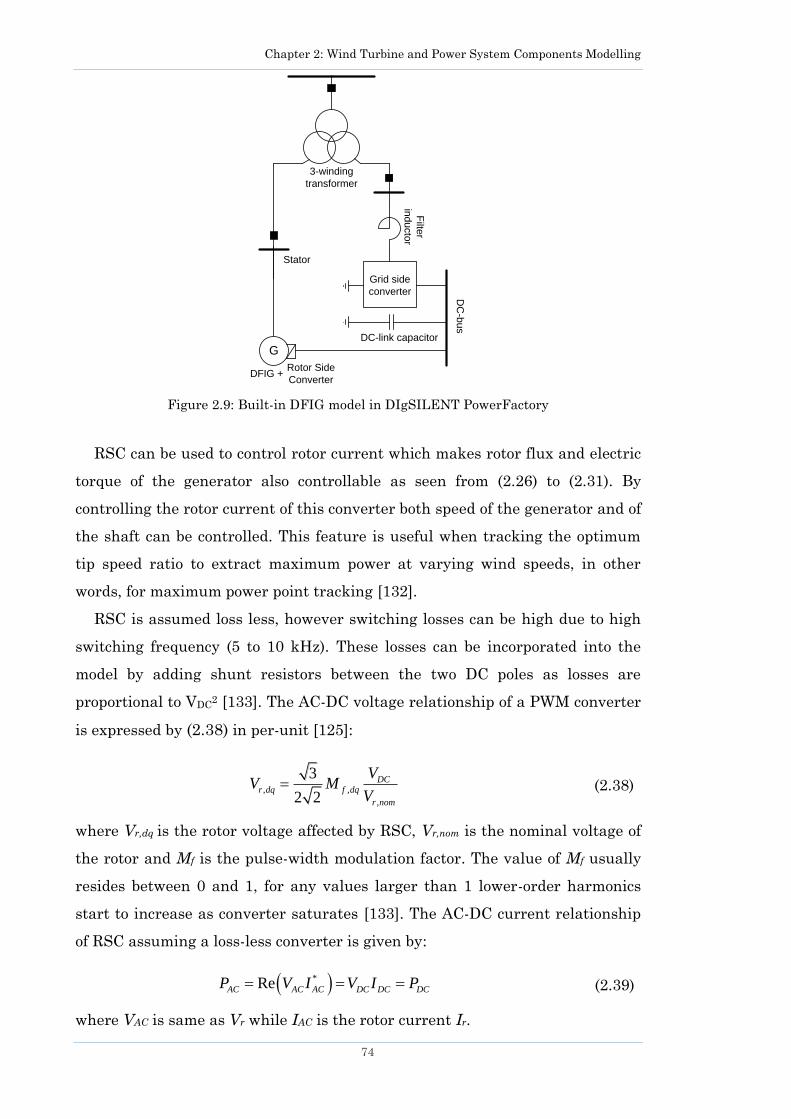
Chapter 2: Wind Turbine and Power System Components Modelling
74
Figure 2.9: Built-in DFIG model in DIgSILENT PowerFactory
RSC can be used to control rotor current which makes rotor flux and electric
torque of the generator also controllable as seen from (2.26) to (2.31). By
controlling the rotor current of this converter both speed of the generator and of
the shaft can be controlled. This feature is useful when tracking the optimum
tip speed ratio to extract maximum power at varying wind speeds, in other
words, for maximum power point tracking [132].
RSC is assumed loss less, however switching losses can be high due to high
switching frequency (5 to 10 kHz). These losses can be incorporated into the
model by adding shunt resistors between the two DC poles as losses are
proportional to VDC2 [133]. The AC-DC voltage relationship of a PWM converter
is expressed by (2.38) in per-unit [125]:
, ,
,
3
2 2 DC
r dq f dq
r nom
VV M
V
(2.38)
where Vr,dq is the rotor voltage affected by RSC, Vr,nom is the nominal voltage of
the rotor and Mf is the pulse-width modulation factor. The value of Mf usually
resides between 0 and 1, for any values larger than 1 lower-order harmonics
start to increase as converter saturates [133]. The AC-DC current relationship
of RSC assuming a loss-less converter is given by:
*ReAC AC AC DC DC DCP V I V I P
(2.39)
where VAC is same as Vr while IAC is the rotor current Ir.
Grid side
converter
G
Rotor Side
Converter
DC-link capacitorD
C-b
us
Filte
r
ind
ucto
rDFIG +
Stator
3-winding
transformer
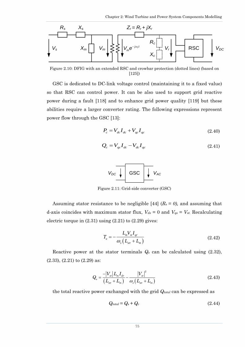
Chapter 2: Wind Turbine and Power System Components Modelling
75
Figure 2.10: DFIG with an extended RSC and crowbar protection (dotted lines) (based on
[125])
GSC is dedicated to DC-link voltage control (maintaining it to a fixed value)
so that RSC can control power. It can be also used to support grid reactive
power during a fault [118] and to enhance grid power quality [119] but these
abilities require a larger converter rating. The following expressions represent
power flow through the GSC [13]:
c dc dc qc qcP V I V I
(2.40)
c qc dc dc qcQ V I V I
(2.41)
Figure 2.11: Grid-side converter (GSC)
Assuming stator resistance to be negligible [44] (Rs = 0), and assuming that
d-axis coincides with maximum stator flux, Vds = 0 and Vqs = Vst. Recalculating
electric torque in (2.31) using (2.21) to (2.29) gives:
m st qr
e
s s m
L V IT
L L
(2.42)
Reactive power at the stator terminals Qs can be calculated using (2.32),
(2.33), (2.21) to (2.29) as:
2
st m dr st
s
s m s s m
V L I VQ
L L L L (2.43)
the total reactive power exchanged with the grid Qtotal can be expressed as
Qtotal = Qs + Qc
(2.44)
Zr = Rr + jXr
Xm Vm
XsRs
RSCVs Vr rj t
mV e VDC
Xc
Rc
GSC VACVDC
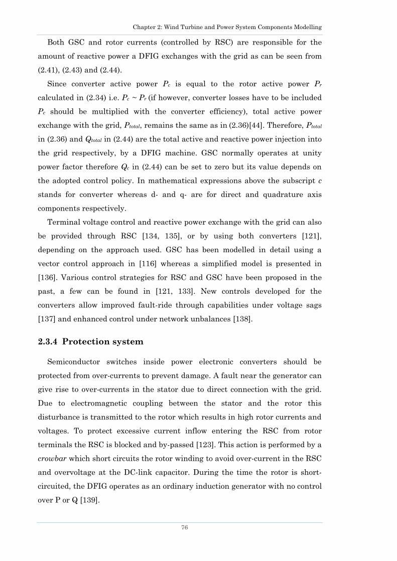
Chapter 2: Wind Turbine and Power System Components Modelling
76
Both GSC and rotor currents (controlled by RSC) are responsible for the
amount of reactive power a DFIG exchanges with the grid as can be seen from
(2.41), (2.43) and (2.44).
Since converter active power Pc is equal to the rotor active power Pr
calculated in (2.34) i.e. Pc ~ Pr (if however, converter losses have to be included
Pc should be multiplied with the converter efficiency), total active power
exchange with the grid, Ptotal, remains the same as in (2.36)[44]. Therefore, Ptotal
in (2.36) and Qtotal in (2.44) are the total active and reactive power injection into
the grid respectively, by a DFIG machine. GSC normally operates at unity
power factor therefore Qc in (2.44) can be set to zero but its value depends on
the adopted control policy. In mathematical expressions above the subscript c
stands for converter whereas d- and q- are for direct and quadrature axis
components respectively.
Terminal voltage control and reactive power exchange with the grid can also
be provided through RSC [134, 135], or by using both converters [121],
depending on the approach used. GSC has been modelled in detail using a
vector control approach in [116] whereas a simplified model is presented in
[136]. Various control strategies for RSC and GSC have been proposed in the
past, a few can be found in [121, 133]. New controls developed for the
converters allow improved fault-ride through capabilities under voltage sags
[137] and enhanced control under network unbalances [138].
2.3.4 Protection system
Semiconductor switches inside power electronic converters should be
protected from over-currents to prevent damage. A fault near the generator can
give rise to over-currents in the stator due to direct connection with the grid.
Due to electromagnetic coupling between the stator and the rotor this
disturbance is transmitted to the rotor which results in high rotor currents and
voltages. To protect excessive current inflow entering the RSC from rotor
terminals the RSC is blocked and by-passed [123]. This action is performed by a
crowbar which short circuits the rotor winding to avoid over-current in the RSC
and overvoltage at the DC-link capacitor. During the time the rotor is short-
circuited, the DFIG operates as an ordinary induction generator with no control
over P or Q [139].

Chapter 2: Wind Turbine and Power System Components Modelling
77
Converters must be protected from over currents whereas generators and
DC-link capacitor against over voltages. Therefore protection system constantly
monitors both rotor current and DC-link voltage signals to activate the
protection system if either of them exceeds a set limit.
A crowbar is effectively a set of resistors that get connected in parallel with
the rotor windings in case of an interruption or fault to limit rotor current. The
value of resistance is dependant on the generator but it varies with different
generators. Generally the protection scheme has a strategy and a criteria to
detect whether a wind turbine should be disconnected as well as a strategy and
criteria for its reconnection. The reconnection is decided based on the voltage
and frequency at the wind turbine terminals [13]. The effect of crowbar
impedance and the effect of RSC restart are discussed in [139]. In line with
fault ride through requirements (FRT), schemes have been proposed in the past
[140] that can allow wind turbines to stay connected with the grid during the
fault. Generally a higher crowbar resistance can efficiently damp higher rotor
currents and electromagnetic torques [120]. Converter protection schemes
using a series dynamic resistor (SDR) [132] can also avoid DFIG control being
disabled.
2.3.4.1 DC link chopper
DC-link braking resistor, also known as the DC-link chopper, is also used to
dissipate excess energy inside the DC-link capacitor during a grid fault to
protect the Insulated Gate Bipolar Transistors (IGBT) from overvoltage.
Several units can be installed in parallel to increase the amount of energy that
can be dissipated.
2.3.5 Rotor speed controller
The speed of generator rotor is also controlled to make energy capture from
the wind optimal. The process begins by measuring the value of rotor speed
through sampling techniques. Then, depending on the rotor speed
corresponding active power set point is chosen from rotor speed generator
power characteristic (shown in Figure 2.12). Next, a torque set point is derived
using measured rotor speed and active power set point. Since there is a direct
correlation between electric torque and rotor current, the required torque is
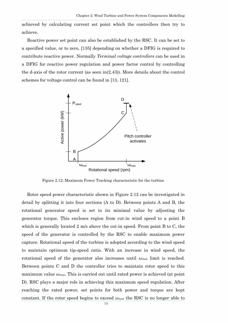
Chapter 2: Wind Turbine and Power System Components Modelling
78
achieved by calculating current set point which the controllers then try to
achieve.
Reactive power set point can also be established by the RSC. It can be set to
a specified value, or to zero, [135] depending on whether a DFIG is required to
contribute reactive power. Normally Terminal voltage controllers can be used in
a DFIG for reactive power regulation and power factor control by controlling
the d-axis of the rotor current (as seen in(2.43)). More details about the control
schemes for voltage control can be found in [13, 121].
Figure 2.12: Maximum Power Tracking characteristic for the turbine
Rotor speed power characteristic shown in Figure 2.12 can be investigated in
detail by splitting it into four sections (A to D). Between points A and B, the
rotational generator speed is set to its minimal value by adjusting the
generator torque. This encloses region from cut-in wind speed to a point B
which is generally located 2 m/s above the cut-in speed. From point B to C, the
speed of the generator is controlled by the RSC to enable maximum power
capture. Rotational speed of the turbine is adopted according to the wind speed
to maintain optimum tip-speed ratio. With an increase in wind speed, the
rotational speed of the generator also increases until ωmax limit is reached.
Between points C and D the controller tries to maintain rotor speed to this
maximum value ωmax. This is carried out until rated power is achieved (at point
D). RSC plays a major role in achieving this maximum speed regulation. After
reaching the rated power, set points for both power and torque are kept
constant. If the rotor speed begins to exceed ωmax the RSC is no longer able to
Rotational speed (rpm)
Active
po
we
r (k
W)
A
B
C
D
ωmin ωmax
Prated
Pitch controller
activates

Chapter 2: Wind Turbine and Power System Components Modelling
79
keep it below maximum. In this case aerodynamic torque is reduced by pitching
away the blades from wind using a pitch controller. Reduction in aerodynamic
torque (Trot) reduces mechanical torque acting on the generator (Tm) and
generator rotor speed ( ) can be maintained to a constant level [125, 141].
2.3.6 Pitch control
In the past, wind turbines did not have the ability to fully utilise wind‘s
potential at higher wind speeds as blades were fixed at an angle. Modern
turbines, however, feature pitch control that allow them to rotate aerodynamic
rotor blades according to the incoming wind speed (measured by an
anemometer). This mechanism makes full extraction of power possible by
adjusting the blades to an optimal pitch angle. At above nominal (rated) wind
speeds, the pitch controller tries to maintain power output to its maximum
until wind speed rises to cut-out level. The controller is activated above rated
wind speed when generator rotor speed is no longer controllable by simply
adjusting the torque. By correcting the pitch angle the value of Cp can be varied
and hence thrust produced and power generation can be controlled. For wind
speeds below nominal the pitch angle is set to minimum (close to zero degrees)
whereas Cp is maximised (to extract maximum power from the wind) by setting
tip-speed ratio to its optimal value through variation in rotor speed ωm.
A generic pitch control model is presented in Figure 2.13. It can be easily
modified for use in other wind turbines. The difference between the maximum
rotor speed ωmax and the current angular speed of the generator ωm is fed into
the PID controller which generates a reference pitch angle βref. This signal is
then sent to the actuator (servo) which sets the final pitch angle β of the blades.
The rate of change of pitch angle is limited by the speed of the servo motor (± 10
deg/s) [142, 143]. Therefore the process of setting the new pitch angle on the
blades can take some time depending how fast the servo motor can operate.
Limitations on the angle exists hence blade angle can be set between a
minimum and a maximum value (0 to 30 deg) [143]. The model presented also
accounts for time constant of the servo motor Tservo.
m
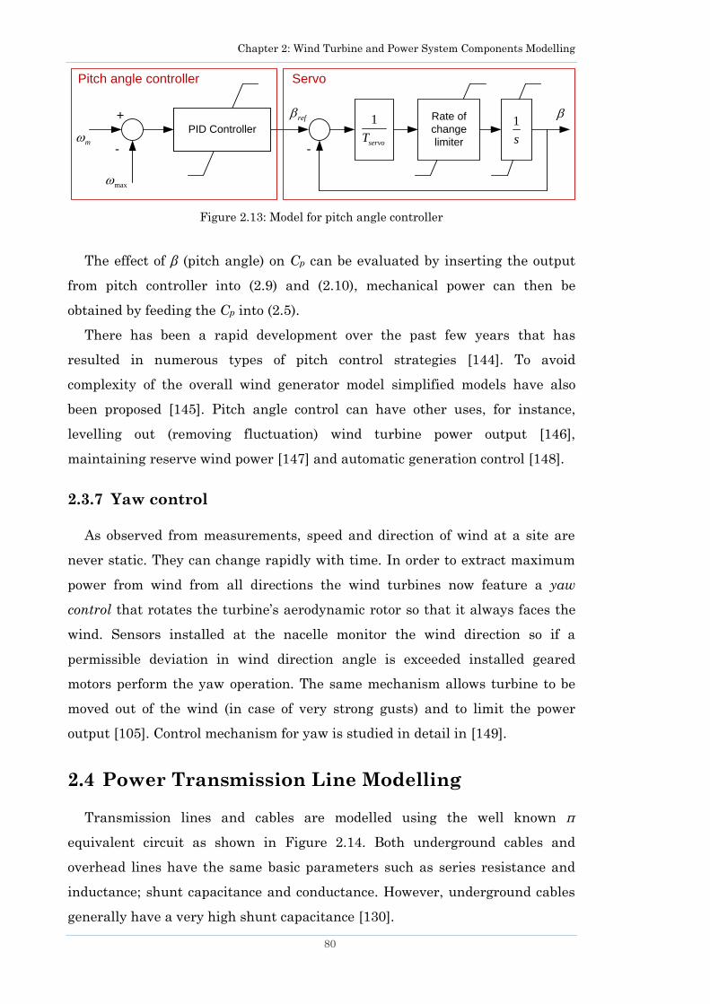
Chapter 2: Wind Turbine and Power System Components Modelling
80
Figure 2.13: Model for pitch angle controller
The effect of β (pitch angle) on Cp can be evaluated by inserting the output
from pitch controller into (2.9) and (2.10), mechanical power can then be
obtained by feeding the Cp into (2.5).
There has been a rapid development over the past few years that has
resulted in numerous types of pitch control strategies [144]. To avoid
complexity of the overall wind generator model simplified models have also
been proposed [145]. Pitch angle control can have other uses, for instance,
levelling out (removing fluctuation) wind turbine power output [146],
maintaining reserve wind power [147] and automatic generation control [148].
2.3.7 Yaw control
As observed from measurements, speed and direction of wind at a site are
never static. They can change rapidly with time. In order to extract maximum
power from wind from all directions the wind turbines now feature a yaw
control that rotates the turbine‘s aerodynamic rotor so that it always faces the
wind. Sensors installed at the nacelle monitor the wind direction so if a
permissible deviation in wind direction angle is exceeded installed geared
motors perform the yaw operation. The same mechanism allows turbine to be
moved out of the wind (in case of very strong gusts) and to limit the power
output [105]. Control mechanism for yaw is studied in detail in [149].
2.4 Power Transmission Line Modelling
Transmission lines and cables are modelled using the well known π
equivalent circuit as shown in Figure 2.14. Both underground cables and
overhead lines have the same basic parameters such as series resistance and
inductance; shunt capacitance and conductance. However, underground cables
generally have a very high shunt capacitance [130].
+
-
1
s
ref
-
max
m
Pitch angle controller Servo
1
servoT
Rate of
change
limiter
PID Controller
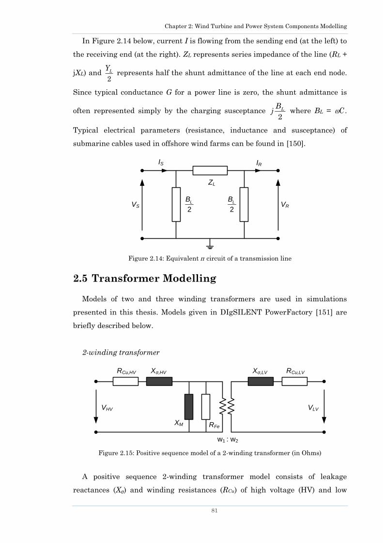
Chapter 2: Wind Turbine and Power System Components Modelling
81
In Figure 2.14 below, current I is flowing from the sending end (at the left) to
the receiving end (at the right). ZL represents series impedance of the line (RL +
jXL) and 2L
Y represents half the shunt admittance of the line at each end node.
Since typical conductance G for a power line is zero, the shunt admittance is
often represented simply by the charging susceptance 2
LB
j where BL = C .
Typical electrical parameters (resistance, inductance and susceptance) of
submarine cables used in offshore wind farms can be found in [150].
Figure 2.14: Equivalent π circuit of a transmission line
2.5 Transformer Modelling
Models of two and three winding transformers are used in simulations
presented in this thesis. Models given in DIgSILENT PowerFactory [151] are
briefly described below.
2-winding transformer
Figure 2.15: Positive sequence model of a 2-winding transformer (in Ohms)
A positive sequence 2-winding transformer model consists of leakage
reactances (Xσ) and winding resistances (RCu) of high voltage (HV) and low
VS VR
ZL
2LB
2LB
IS IR
w1 : w2
RCu,HV Xσ,HV
XM RFe
VHV VLV
RCu,LVXσ,LV
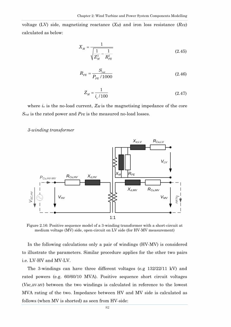
Chapter 2: Wind Turbine and Power System Components Modelling
82
voltage (LV) side, magnetizing reactance (XM) and iron loss resistance (RFE)
calculated as below:
2 2
1
1 1M
M FE
X
Z R
(2.45)
/1000rat
FE
FE
SR
P (2.46)
1
/100M
o
Zi
(2.47)
where io is the no-load current, ZM is the magnetising impedance of the core
Srat is the rated power and PFE is the measured no-load losses.
3-winding transformer
Figure 2.16: Positive sequence model of a 3-winding transformer with a short-circuit at
medium voltage (MV) side, open-circuit on LV side (for HV-MV measurement)
In the following calculations only a pair of windings (HV-MV) is considered
to illustrate the parameters. Similar procedure applies for the other two pairs
i.e. LV-HV and MV-LV.
The 3-windings can have three different voltages (e.g 132/22/11 kV) and
rated powers (e.g. 60/60/10 MVA). Positive sequence short circuit voltages
(Vsc,HV-MV) between the two windings is calculated in reference to the lowest
MVA rating of the two. Impedance between HV and MV side is calculated as
follows (when MV is shorted) as seen from HV-side:
RCu,HV Xσ,HV
VHV VMV
RCu,MVXσ,MV
VLV
RCu,LVXσ,LV
IN,M
V
1:1
PCu,HV-MV
VS
C,H
V
XM RFE
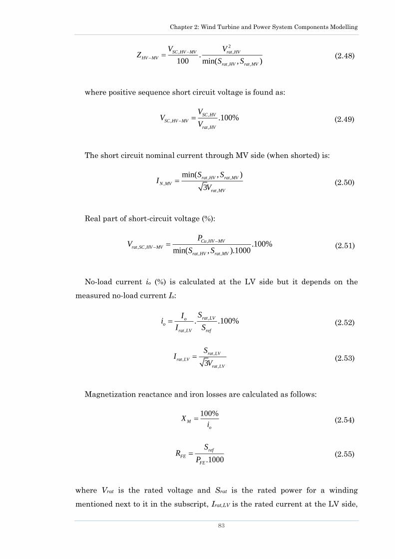
Chapter 2: Wind Turbine and Power System Components Modelling
83
2
, ,
, ,
.100 min( , )
SC HV MV rat HV
HV MV
rat HV rat MV
V VZ
S S
(2.48)
where positive sequence short circuit voltage is found as:
,
,
,
.100%SC HV
SC HV MV
rat HV
VV
V
(2.49)
The short circuit nominal current through MV side (when shorted) is:
, ,
,
,
min( , )
3
rat HV rat MV
N MV
rat MV
S SI
V
(2.50)
Real part of short-circuit voltage (%):
,
, ,
, ,
.100%min( , ).1000
Cu HV MV
rat SC HV MV
rat HV rat MV
PV
S S
(2.51)
No-load current io (%) is calculated at the LV side but it depends on the
measured no-load current Io:
,
,
. .100%rat LVo
o
rat LV ref
SIi
I S
(2.52)
,
,
,3
rat LV
rat LV
rat LV
SI
V (2.53)
Magnetization reactance and iron losses are calculated as follows:
100%M
o
Xi
(2.54)
.1000
ref
FE
FE
SR
P
(2.55)
where Vrat is the rated voltage and Srat is the rated power for a winding
mentioned next to it in the subscript, Irat,LV is the rated current at the LV side,

Chapter 2: Wind Turbine and Power System Components Modelling
84
Sref is the reference power equal to HV side rated power, PCu,HV-MV is copper
losses of path HV-MV, PFE is measured iron losses.
Further details about transformer models and related parameters can be
found in [151].
2.6 Summary
A variable speed turbine consists of several components including generator,
converter and controllers. This chapter briefly discussed models for various
components that are required to model a wind turbine with a DFIG. Apart from
this, models for power system transmission lines and transformers are also
presented.
In this research, built-in models of wind turbine in a commercially available
software tool DIgSILENT PowerFactory are used for stability studies. Other
commercial software including PSS®E and IPSA+ are used for steady-state
analysis such as load flow and loss evaluation.

Chapter 3: Modelling of Wake Effects
85
Chapter 3 Modelling of Wake Effects
Modelling of Wake Effects
3.1 Introduction
Wind is a highly variable energy resource. Generally, it varies according to
the season, time of the year and time of the day. Changes that occur over period
of days are called Synoptic variations while variations according to the time of
the day are called Diurnal variations. A third type of variation which is more
random and has a much shorter timescale (minutes to seconds) is called the
Turbulence [105]. Others factors such as wind shear, type of terrain and
thermal effects will also influence its characteristics [152, 153]. Several wind
speed simulation and forecasting models [44, 50, 154-157] have been proposed
in the past.
Wind interaction with objects makes its behaviour hard to predict as the
objects distort wind flow. The change in wind flow is the reason why modelling
techniques are required. Although complex models can estimate and simulate
wind interaction with high accuracy, for electrical engineering applications a
simpler model is needed. Existing models used for the prediction of wind speed
inside a wind farm (wake models) are briefly discussed along with a wake
calculation program developed during the research.
Wind speed characteristics at a site can often be defined by a probability
distribution called a Weibull distribution. This distribution can be created for
any site if measured data is not available. However if internal flow of wind
within wind farm is to be modelled correctly, the wind direction is also needed.
Recordings of wind speed and direction at a site in North Sweden were
available and are presented in this chapter. The effects of wind shear and
surface roughness on wind speed are also explored.
In order to consider the effect of wake on the power output the system
operators may have to use existing wake models. However, the majority of

Chapter 3: Modelling of Wake Effects
86
existing analytical wake models are deterministic, therefore at a given wind
condition they give a deterministic output. In reality, the flow of wind changes
as it enters the wind farm due to interaction with the wind turbines. This is
evident from the behaviour of wind in the wake of a turbine. The wind inside
the wake is both reduced in speed and highly turbulent. A few of the existing
analytical wake models predict the reduction in wind speed but neglect the
turbulence. It was observed in [158] and [159] that turbulence can affect the
power output of a wind turbine.
Simulation techniques such as Finite Element Modelling [160], Navier
Stokes equations [55] and Computational Fluid Dynamics (CFD) [161] can be
used for simulating the wind inside a wind farm. These models can lead to
reliable results, but they are often complex and cumbersome to implement.
Most of these models can significantly increase the simulation time depending
on the computing power available.
This chapter also presents a new probabilistic wake effect model that
considers the effect of turbulence inside a wind farm. The model enables
network operators to estimate wind power output probabilistically for a
forecasted wind condition (few minutes or hours ahead). The probabilistic
output from the wind farm can indicate to the operator that the power output
may vary within certain limits as opposed to a deterministic output. This
information is useful for the network operator while carrying out generation
dispatch or reserve allocation. Furthermore, this chapter also compares the
wind power output and energy output results from the proposed probabilistic
wake model with a deterministic wake model. The model developed is efficient
and easy to use which makes it suitable for use in online simulations. It is also
computationally less demanding than the simulation techniques mentioned
above.
3.2 Wake Effects
The law of the conservation of energy dictates that energy can neither be
created nor destroyed, but it can be transformed. Based on this statement a
wind turbine can be said to be a converter as it converts kinetic energy present
in the wind into mechanical and then electrical energy. However, this process of
extraction is not 100% efficient. Extracting kinetic energy from the wind causes
the wind speed behind the rotor to slow down in a turbulent manner, known as
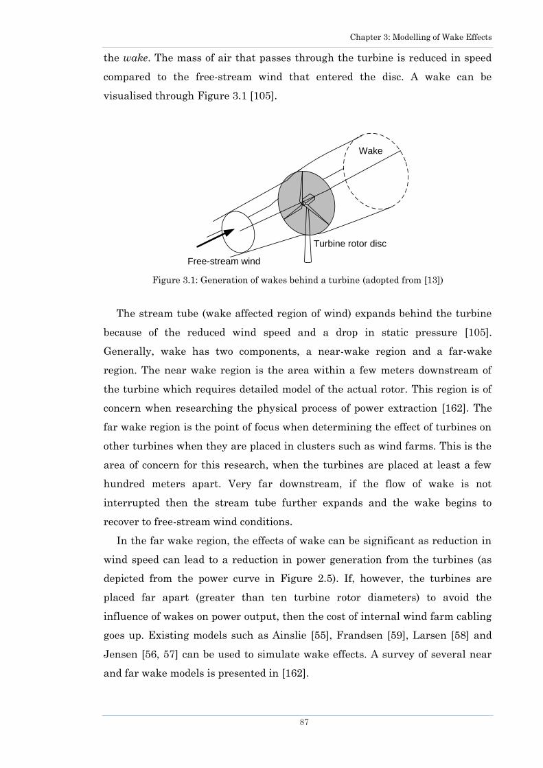
Chapter 3: Modelling of Wake Effects
87
the wake. The mass of air that passes through the turbine is reduced in speed
compared to the free-stream wind that entered the disc. A wake can be
visualised through Figure 3.1 [105].
Figure 3.1: Generation of wakes behind a turbine (adopted from [13])
The stream tube (wake affected region of wind) expands behind the turbine
because of the reduced wind speed and a drop in static pressure [105].
Generally, wake has two components, a near-wake region and a far-wake
region. The near wake region is the area within a few meters downstream of
the turbine which requires detailed model of the actual rotor. This region is of
concern when researching the physical process of power extraction [162]. The
far wake region is the point of focus when determining the effect of turbines on
other turbines when they are placed in clusters such as wind farms. This is the
area of concern for this research, when the turbines are placed at least a few
hundred meters apart. Very far downstream, if the flow of wake is not
interrupted then the stream tube further expands and the wake begins to
recover to free-stream wind conditions.
In the far wake region, the effects of wake can be significant as reduction in
wind speed can lead to a reduction in power generation from the turbines (as
depicted from the power curve in Figure 2.5). If, however, the turbines are
placed far apart (greater than ten turbine rotor diameters) to avoid the
influence of wakes on power output, then the cost of internal wind farm cabling
goes up. Existing models such as Ainslie [55], Frandsen [59], Larsen [58] and
Jensen [56, 57] can be used to simulate wake effects. A survey of several near
and far wake models is presented in [162].
Free-stream wind
Turbine rotor disc
Wake

Chapter 3: Modelling of Wake Effects
88
Ainslie‘s wake model determines the total momentum deficit inside a wake
by using the thrust coefficient of the turbine. It takes into account all relevant
meteorological effects and the description of flow structure is also very
accurate. Navier Stokes equations and the concept of turbulent viscosity is
applied. This model is best used if a detailed study on wakes is required [55].
Frandsen‘s model is an analytical model applicable to both small and large
wind farms. It takes into account the complex interaction of wakes when
merging downstream from neighbouring rows. It assumes an asymptotic flow
deficit inside the wake.
Larsen‘s model is a semi analytical model that uses Prandtl‘s turbulent
boundary layer equations. The model calculates the width of wake at a given
distance as well as the mean wind profile in the wake. The wake flow is
assumed to be incompressible and stationary.
Some of these models are more complicated than others with extra
computational burden leading to higher simulation times. Blade element
momentum is another way of modelling turbine blades and wind flow. In this
method a turbine blade is divided into several smaller cross-sections and the
total force on the blade is calculated by summing the forces on each section
[163]. This method is normally used for design of wind turbines [164]. Some of
the other models apply Computational Fluid Dynamic (CFD) [161] schemes,
however these schemes are not computationally feasible when faster
simulations are needed.
The models described above are dedicated for near-field and far-field wake
effects. They are useful for detailed modelling of wakes often required during
the design and manufacturing of wind turbines. Some of them are made to
model wind flow over complex terrains in case of a flow separation, though
these are more intricate. For electrical engineering purposes a moderately
simple model that can estimate the wind speed in a wake at a certain distance
should be sufficient.
The wake model postulated by Jensen [56], [57] is a mathematical model
designed to minimise input parameters and reduce computation burden. In this
model, a wake expands linearly with distance xo while the spread of the wake
has a Gaussian distribution often referred as a top-hat distribution. The
entrainment constant k controls the development of the wake and a value of
this constant has been found to be 0.075 for onshore sites and 0.04 for offshore
Chapter 3: Modelling of Wake Effects
89
sites [57]. In general, the model seems to fit well when compared with actual
wake measurements [56]. Moreover, it is simple to implement and fast during
simulation, however it should not be used to model flow in complex terrains
such as hills and mountains where the other models described above would be
more useful. In this research, only onshore plains and sea are considered,
therefore, Jensen‘s wake model is perfectly applicable as it leads to shorter
simulation times.
The model is commercially used in softwares such as WAsP [165] and
WindPro [166] to simulate wake effects and calculate wind farm production.
The choice of a simple model is further validated through a comparison between
wake models carried out in [167] revealing that sophisticated models do not
predict momentum deficit significantly better than simplified wake models.
Wake models using CFD techniques, Blade Element Momentum and Navier
Stokes equations are useful for simulating wind flow in a near wake region and
are more suitable during design of wind turbine blades. For far wake region (to
calculate wake effect on other turbines) Jensen‘s model is commonly used in
electrical engineering studies to estimate effect of wake on power output of
turbines. This model is efficient and leads to reduced simulation times yet
provides sufficient level of accuracy. Furthermore, Jensen‘s model has also been
implemented by various commercial software to calculate power output and
energy yield of a wind farm. Due to these reasons, Jensen‘s wake model has
been used in this thesis and is often referred as deterministic wake model in
this chapter.
3.3 Detailed Wake Effect Modelling
Wake effect is dependant not only on the incoming wind speed and direction
but also on the wind farm layout, therefore the distance between the turbines
also plays an important role. A detailed wake effect model is implemented
considering single, partial and multiple wakes inside a farm which takes into
account rotor radius, thrust coefficient and expansion of stream tube. The
effects of the turbine hub height and surface roughness can be also simulated
by considering wind shear.

Chapter 3: Modelling of Wake Effects
90
3.3.1 Single wakes
A single wake occurs when rotor disc of a turbine downwind is under full
shadow of only one turbine. The single wakes are computed using Jensen‘s
kinematic wake model. Expansion of the wake radius behind a single turbine is
described by:
w o or r kx (3.1)
In Jensen‘s model the wind speed immediately behind the turbine, vo, is
assumed to be u/3. This assumption is replaced to make the analysis more
realistic by including the turbine‘s thrust coefficient.
The wind behind the turbine can then be computed as . Mean wind
speed in the wake of a single turbine under free-stream wind u at a distance xo
is dependant on the Ct of the turbine:
2
1 1 1 1ot
o o
rv u C
r kx
(3.2)
where k is the entrainment constant or opening angle which represents the
effects of atmospheric stability, ro is the radius of wind turbine rotor, rw is the
radius of the wake and u is the wind speed entering the upstream turbine. The
expansion of wake behind a wind turbine is represented in Figure 3.2.
Figure 3.2: Wake structure by using Jensen model (symbols defined in the text)
3.3.2 Partial wakes
A partial wake is a phenomenon which occurs when one or more upwind
turbines cast a single shadow on a downwind turbine partially covering its
rotor disk (as illustrated in Figure 3.3).
1 tu C
ro
k
uv1
rw = kxo + ro
xo
Wind
turbine

Chapter 3: Modelling of Wake Effects
91
Figure 3.3: Partial shading of a wind turbine‘s rotor disc
The wind speed entering into the turbine is then given by [147]:
2
,
,1 1ps l
m m l
l
vv u
u
(3.3)
where βm,l is the ratio (the weighting factor) of the rotor area in wake to the
total rotor area, m is the turbine under wake, l is the upwind turbine, u is the
initial wind speed entering into the wind turbine l, and vps,l is the wind speed in
the wake of l falling on m. The expression also works if more than one upwind
turbine places a single shadow on a turbine downwind.
3.3.3 Multiple wakes
Multiple wakes occur when two or more upwind turbines slow down the wind
approaching the turbine in the same row. Figure 3.4 illustrates the effect of
multiple wakes on the third turbine, since it is under wake of the second
turbine which in turn is under wake of the first one. It is seen through
measurements in [168] that effect of wake behind the first turbine is the
strongest and causes the most significant reduction in wind speed.
Figure 3.4: Multiple wakes faced by turbines in the same row
Free-stream wind
Turbine rotor disc
WakePartially
shaded rotor
disc of a
turbine
downwind
l
m
rouv1
xo
WT 1
xo
v2
WT 2 WT 3
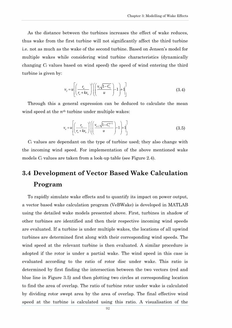
Chapter 3: Modelling of Wake Effects
92
As the distance between the turbines increases the effect of wake reduces,
thus wake from the first turbine will not significantly affect the third turbine
i.e. not as much as the wake of the second turbine. Based on Jensen‘s model for
multiple wakes while considering wind turbine characteristics (dynamically
changing Ct values based on wind speed) the speed of wind entering the third
turbine is given by:
2
1
2
11 1
to
o o
v Crv u
r kx u
(3.4)
Through this a general expression can be deduced to calculate the mean
wind speed at the nth turbine under multiple wakes:
2 1
1 11 1
n
n ton
o o
v Crv u
r kx u
(3.5)
Ct values are dependant on the type of turbine used; they also change with
the incoming wind speed. For implementation of the above mentioned wake
models Ct values are taken from a look-up table (see Figure 2.4).
3.4 Development of Vector Based Wake Calculation
Program
To rapidly simulate wake effects and to quantify its impact on power output,
a vector based wake calculation program (VeBWake) is developed in MATLAB
using the detailed wake models presented above. First, turbines in shadow of
other turbines are identified and then their respective incoming wind speeds
are evaluated. If a turbine is under multiple wakes, the locations of all upwind
turbines are determined first along with their corresponding wind speeds. The
wind speed at the relevant turbine is then evaluated. A similar procedure is
adopted if the rotor is under a partial wake. The wind speed in this case is
evaluated according to the ratio of rotor disc under wake. This ratio is
determined by first finding the intersection between the two vectors (red and
blue line in Figure 3.5) and then plotting two circles at corresponding location
to find the area of overlap. The ratio of turbine rotor under wake is calculated
by dividing rotor swept area by the area of overlap. The final effective wind
speed at the turbine is calculated using this ratio. A visualisation of the
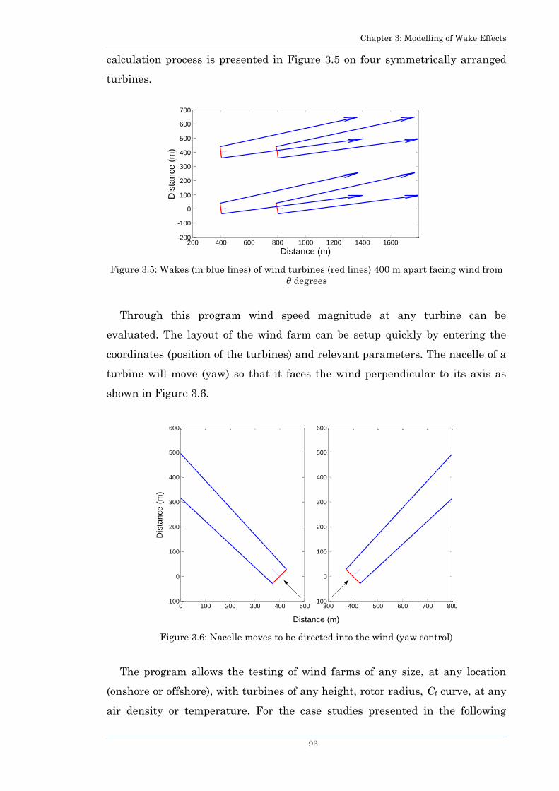
Chapter 3: Modelling of Wake Effects
93
calculation process is presented in Figure 3.5 on four symmetrically arranged
turbines.
Figure 3.5: Wakes (in blue lines) of wind turbines (red lines) 400 m apart facing wind from
θ degrees
Through this program wind speed magnitude at any turbine can be
evaluated. The layout of the wind farm can be setup quickly by entering the
coordinates (position of the turbines) and relevant parameters. The nacelle of a
turbine will move (yaw) so that it faces the wind perpendicular to its axis as
shown in Figure 3.6.
Figure 3.6: Nacelle moves to be directed into the wind (yaw control)
The program allows the testing of wind farms of any size, at any location
(onshore or offshore), with turbines of any height, rotor radius, Ct curve, at any
air density or temperature. For the case studies presented in the following
200 400 600 800 1000 1200 1400 1600-200
-100
0
100
200
300
400
500
600
700
Distance (m)
Dis
tance (
m)
Distance (m)
Dis
tan
ce
(m
)
0 100 200 300 400 500-100
0
100
200
300
400
500
600
300 400 500 600 700 800-100
0
100
200
300
400
500
600
Distance (m)
Dis
tan
ce
(m
)
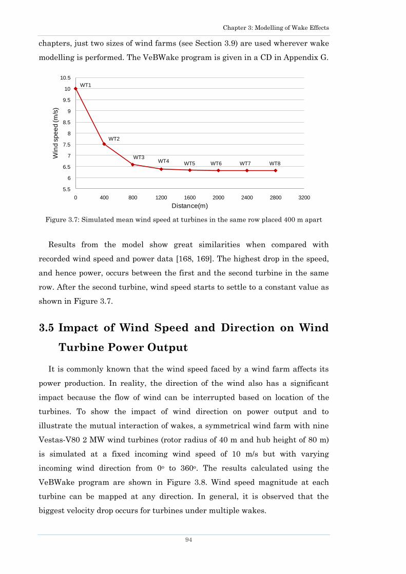
Chapter 3: Modelling of Wake Effects
94
chapters, just two sizes of wind farms (see Section 3.9) are used wherever wake
modelling is performed. The VeBWake program is given in a CD in Appendix G.
Figure 3.7: Simulated mean wind speed at turbines in the same row placed 400 m apart
Results from the model show great similarities when compared with
recorded wind speed and power data [168, 169]. The highest drop in the speed,
and hence power, occurs between the first and the second turbine in the same
row. After the second turbine, wind speed starts to settle to a constant value as
shown in Figure 3.7.
3.5 Impact of Wind Speed and Direction on Wind
Turbine Power Output
It is commonly known that the wind speed faced by a wind farm affects its
power production. In reality, the direction of the wind also has a significant
impact because the flow of wind can be interrupted based on location of the
turbines. To show the impact of wind direction on power output and to
illustrate the mutual interaction of wakes, a symmetrical wind farm with nine
Vestas-V80 2 MW wind turbines (rotor radius of 40 m and hub height of 80 m)
is simulated at a fixed incoming wind speed of 10 m/s but with varying
incoming wind direction from 0o to 360o. The results calculated using the
VeBWake program are shown in Figure 3.8. Wind speed magnitude at each
turbine can be mapped at any direction. In general, it is observed that the
biggest velocity drop occurs for turbines under multiple wakes.
5.5
6
6.5
7
7.5
8
8.5
9
9.5
10
10.5
0 400 800 1200 1600 2000 2400 2800 3200
Win
d s
pe
ed
(m
/s)
Distance(m)
WT2
WT1
WT3WT4
WT5 WT6 WT7 WT8

Chapter 3: Modelling of Wake Effects
95
Figure 3.8: Wind speed at each turbine in an exemplary wind farm, incoming wind speed =
10 m/s, wind direction = 0o to 360o (1o direction interval)
Figure 3.9: Total power generation (MW) from a wind farm at 10 m/s for wind directions
from 0o to 360o
0
2
4
6
8
100
0
2
4
6
8
100
0
2
4
6
8
100
0
2
4
6
8
100
0
2
4
6
8
100
0
2
4
6
8
100
0
2
4
6
8
100
0
2
4
6
8
100
0
2
4
6
8
100
0o
0.0
2.0
4.0
6.0
8.0
10.0
12.0
0
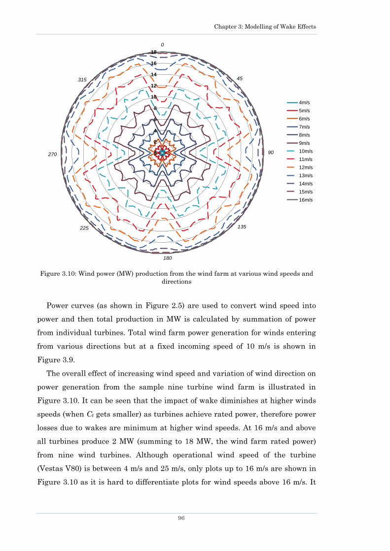
Chapter 3: Modelling of Wake Effects
96
Figure 3.10: Wind power (MW) production from the wind farm at various wind speeds and
directions
Power curves (as shown in Figure 2.5) are used to convert wind speed into
power and then total production in MW is calculated by summation of power
from individual turbines. Total wind farm power generation for winds entering
from various directions but at a fixed incoming speed of 10 m/s is shown in
Figure 3.9.
The overall effect of increasing wind speed and variation of wind direction on
power generation from the sample nine turbine wind farm is illustrated in
Figure 3.10. It can be seen that the impact of wake diminishes at higher winds
speeds (when Ct gets smaller) as turbines achieve rated power, therefore power
losses due to wakes are minimum at higher wind speeds. At 16 m/s and above
all turbines produce 2 MW (summing to 18 MW, the wind farm rated power)
from nine wind turbines. Although operational wind speed of the turbine
(Vestas V80) is between 4 m/s and 25 m/s, only plots up to 16 m/s are shown in
Figure 3.10 as it is hard to differentiate plots for wind speeds above 16 m/s. It
0
2
4
6
8
10
12
14
16
18
0
45
90
135
180
225
270
315
4m/s
5m/s
6m/s
7m/s
8m/s
9m/s
10m/s
11m/s
12m/s
13m/s
14m/s
15m/s
16m/s
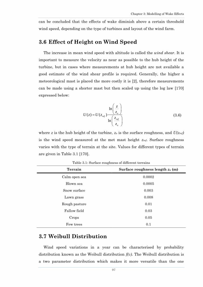
Chapter 3: Modelling of Wake Effects
97
can be concluded that the effects of wake diminish above a certain threshold
wind speed, depending on the type of turbines and layout of the wind farm.
3.6 Effect of Height on Wind Speed
The increase in mean wind speed with altitude is called the wind shear. It is
important to measure the velocity as near as possible to the hub height of the
turbine, but in cases where measurements at hub height are not available a
good estimate of the wind shear profile is required. Generally, the higher a
meteorological mast is placed the more costly it is [2], therefore measurements
can be made using a shorter mast but then scaled up using the log law [170]
expressed below:
ln
( ) ( )
ln
o
ref
ref
o
z
zU z U z
z
z
(3.6)
where z is the hub height of the turbine, zo is the surface roughness, and U(zref)
is the wind speed measured at the met mast height zref. Surface roughness
varies with the type of terrain at the site. Values for different types of terrain
are given in Table 3.1 [170].
Table 3.1: Surface roughness of different terrains
Terrain Surface roughness length zo (m)
Calm open sea 0.0002
Blown sea 0.0005
Snow surface 0.003
Lawn grass 0.008
Rough pasture 0.01
Fallow field 0.03
Crops 0.05
Few trees 0.1
3.7 Weibull Distribution
Wind speed variations in a year can be characterised by probability
distribution known as the Weibull distribution f(v). The Weibull distribution is
a two parameter distribution which makes it more versatile than the one
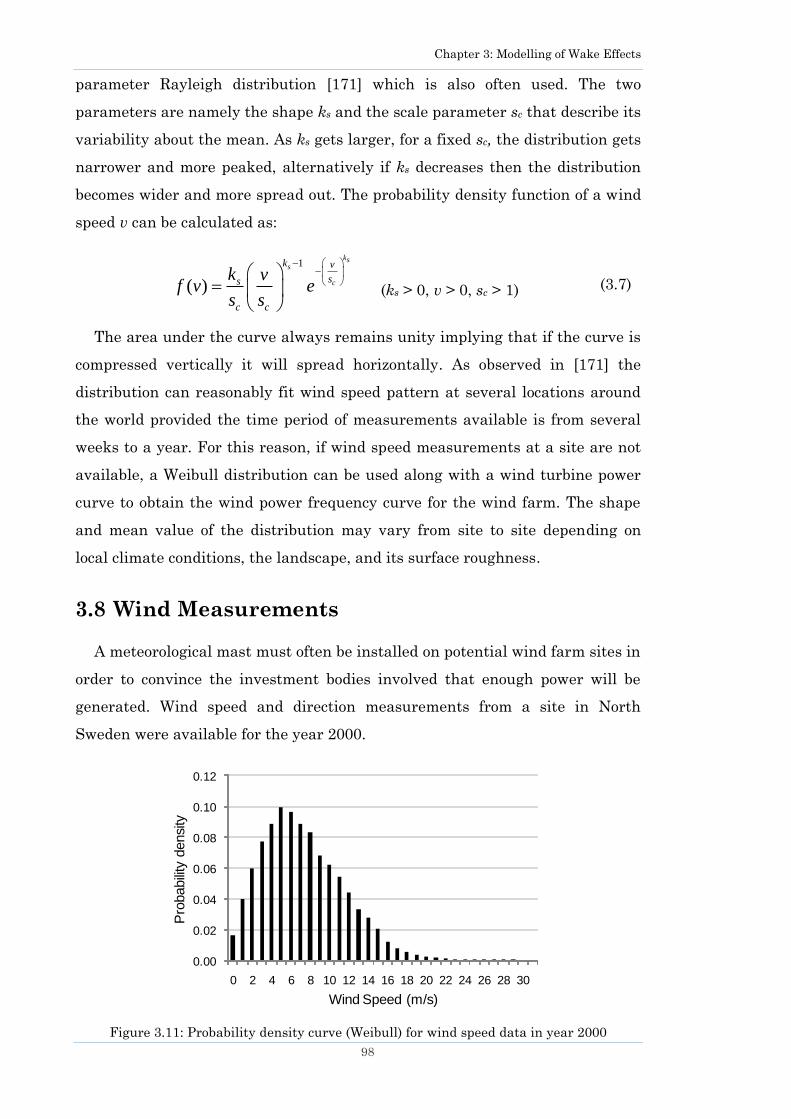
Chapter 3: Modelling of Wake Effects
98
parameter Rayleigh distribution [171] which is also often used. The two
parameters are namely the shape ks and the scale parameter sc that describe its
variability about the mean. As ks gets larger, for a fixed sc, the distribution gets
narrower and more peaked, alternatively if ks decreases then the distribution
becomes wider and more spread out. The probability density function of a wind
speed v can be calculated as:
1
( )
kss
c
k v
ss
c c
k vf v e
s s
(ks > 0, v > 0, sc > 1) (3.7)
The area under the curve always remains unity implying that if the curve is
compressed vertically it will spread horizontally. As observed in [171] the
distribution can reasonably fit wind speed pattern at several locations around
the world provided the time period of measurements available is from several
weeks to a year. For this reason, if wind speed measurements at a site are not
available, a Weibull distribution can be used along with a wind turbine power
curve to obtain the wind power frequency curve for the wind farm. The shape
and mean value of the distribution may vary from site to site depending on
local climate conditions, the landscape, and its surface roughness.
3.8 Wind Measurements
A meteorological mast must often be installed on potential wind farm sites in
order to convince the investment bodies involved that enough power will be
generated. Wind speed and direction measurements from a site in North
Sweden were available for the year 2000.
Figure 3.11: Probability density curve (Weibull) for wind speed data in year 2000
0.00
0.02
0.04
0.06
0.08
0.10
0.12
0 2 4 6 8 10 12 14 16 18 20 22 24 26 28 30
Pro
babili
ty d
ensi
ty
Wind Speed (m/s)

Chapter 3: Modelling of Wake Effects
99
Figure 3.12: Probability density curve for wind direction in year 2000
The recordings were made at 10 minute intervals using an anemometer and
a wind vane stationed at a meteorological mast 35 meters high. A probability
density plot of this data is evaluated as shown in Figure 3.11 and Figure 3.12.
In the UK, a general estimate about the wind speed at a site can be obtained
from [172, 173].
It is visible from Figure 3.11 that the measurements form the shape of a
Weibull distribution; therefore if ks and sc parameters are accurately estimated,
equation (3.7) can be made to fit this curve. Wind speeds between 5 and 8 m/s
are most probable whereas higher wind speeds above 20 m/s are the least
probable as seen from Figure 3.11. It can be seen from Figure 3.12 that wind is
more probable from two directions i.e. between 100o and 180o and between 280o
and 360o.
In cases where recorded data is not available, wind speed models [44] can be
used to simulate average value, ramp, gust and turbulence. If past wind speed
time series and averages are available then the Markov chain method can be
used to obtain hourly mean wind speed predictions [174].
3.9 Wind Farm Layouts
Two sizes of wind farms are used in the following chapters as case studies;
they are illustrated in Figure 3.13 and Figure 3.14. Both wind farms have a
symmetrical layout; the larger one has 49 turbines while the smaller one has 9
0.000
0.002
0.004
0.006
0.008
0.010
0.012
0.014
0.016
0
20
40
60
80
10
0
12
0
14
0
16
0
18
0
20
0
22
0
24
0
26
0
28
0
30
0
32
0
34
0
36
0
Pro
babili
ty d
ensi
ty
Wind Direction (degrees)
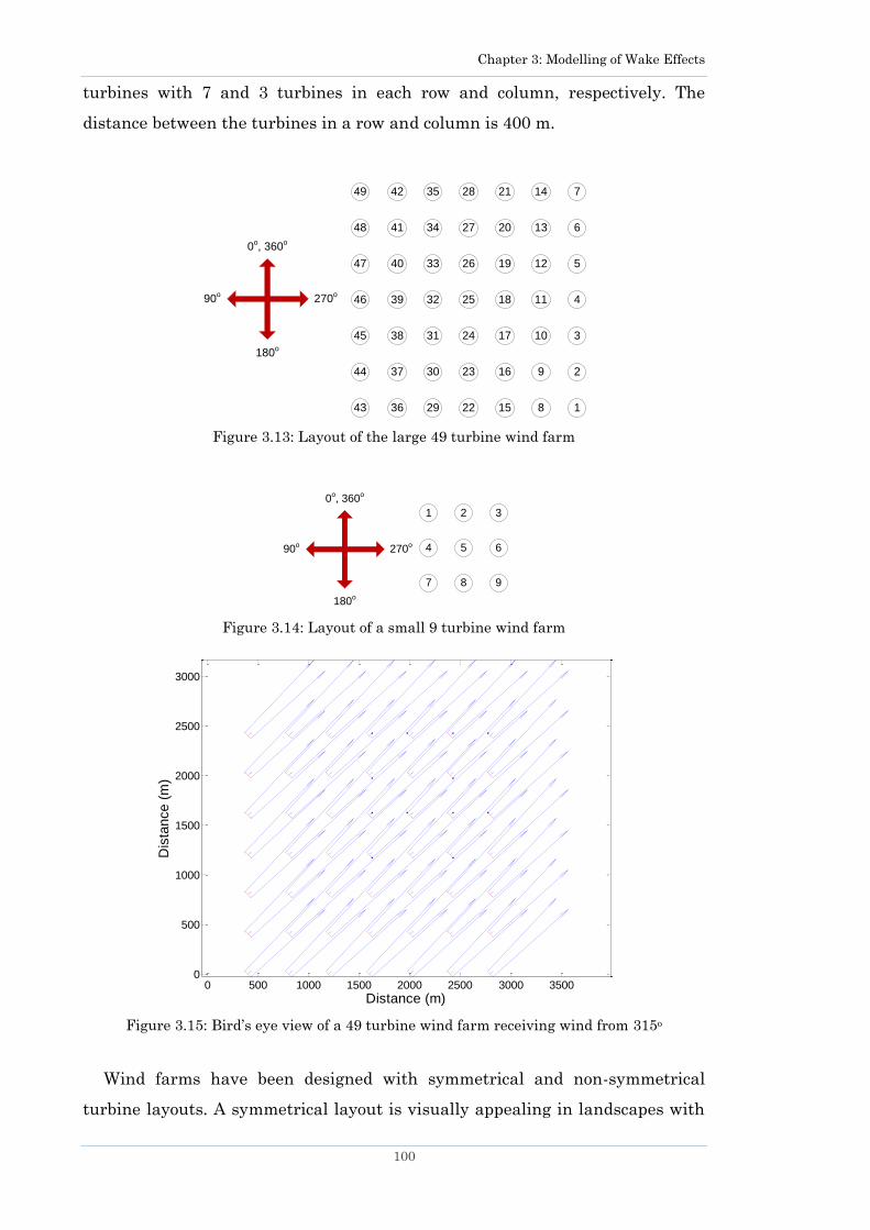
Chapter 3: Modelling of Wake Effects
100
turbines with 7 and 3 turbines in each row and column, respectively. The
distance between the turbines in a row and column is 400 m.
Figure 3.13: Layout of the large 49 turbine wind farm
Figure 3.14: Layout of a small 9 turbine wind farm
0 500 1000 1500 2000 2500 3000 35000
500
1000
1500
2000
2500
3000
Distance (m)
Dis
tan
ce
(m
)
Figure 3.15: Bird‘s eye view of a 49 turbine wind farm receiving wind from 315o
Wind farms have been designed with symmetrical and non-symmetrical
turbine layouts. A symmetrical layout is visually appealing in landscapes with
7
6
5
4
3
2
1
14
13
12
11
10
9
8
21
20
19
18
17
16
15
28
27
26
25
24
23
22
35
34
33
32
31
30
29
42
41
40
39
38
37
36
49
48
47
46
45
44
43
0o, 360
o
90o
180o
270o
3
6
9
2
5
8
1
4
7
0o, 360
o
90o
180o
270o
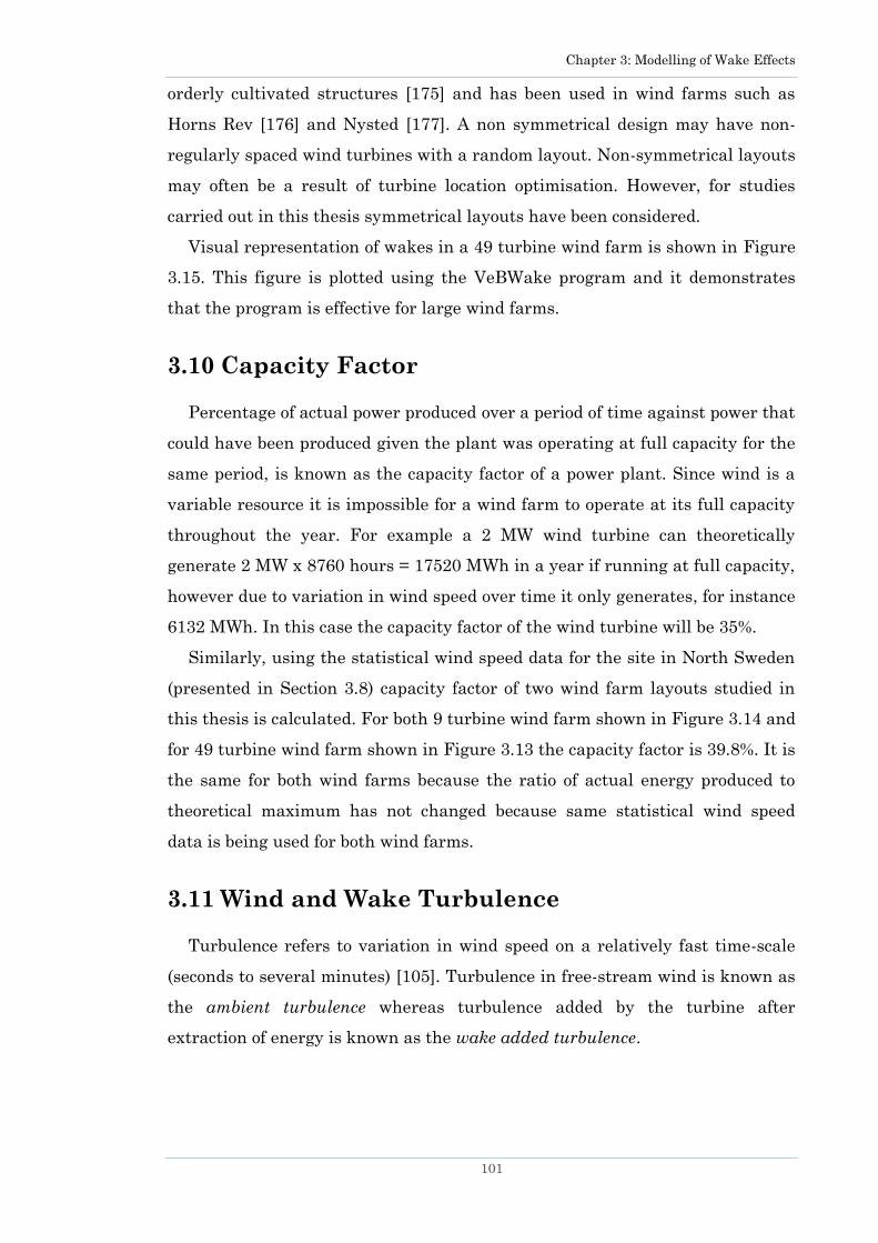
Chapter 3: Modelling of Wake Effects
101
orderly cultivated structures [175] and has been used in wind farms such as
Horns Rev [176] and Nysted [177]. A non symmetrical design may have non-
regularly spaced wind turbines with a random layout. Non-symmetrical layouts
may often be a result of turbine location optimisation. However, for studies
carried out in this thesis symmetrical layouts have been considered.
Visual representation of wakes in a 49 turbine wind farm is shown in Figure
3.15. This figure is plotted using the VeBWake program and it demonstrates
that the program is effective for large wind farms.
3.10 Capacity Factor
Percentage of actual power produced over a period of time against power that
could have been produced given the plant was operating at full capacity for the
same period, is known as the capacity factor of a power plant. Since wind is a
variable resource it is impossible for a wind farm to operate at its full capacity
throughout the year. For example a 2 MW wind turbine can theoretically
generate 2 MW x 8760 hours = 17520 MWh in a year if running at full capacity,
however due to variation in wind speed over time it only generates, for instance
6132 MWh. In this case the capacity factor of the wind turbine will be 35%.
Similarly, using the statistical wind speed data for the site in North Sweden
(presented in Section 3.8) capacity factor of two wind farm layouts studied in
this thesis is calculated. For both 9 turbine wind farm shown in Figure 3.14 and
for 49 turbine wind farm shown in Figure 3.13 the capacity factor is 39.8%. It is
the same for both wind farms because the ratio of actual energy produced to
theoretical maximum has not changed because same statistical wind speed
data is being used for both wind farms.
3.11 Wind and Wake Turbulence
Turbulence refers to variation in wind speed on a relatively fast time-scale
(seconds to several minutes) [105]. Turbulence in free-stream wind is known as
the ambient turbulence whereas turbulence added by the turbine after
extraction of energy is known as the wake added turbulence.
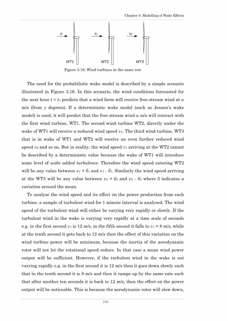
Chapter 3: Modelling of Wake Effects
102
Figure 3.16: Wind turbines in the same row
The need for the probabilistic wake model is described by a simple scenario
illustrated in Figure 3.16. In this scenario, the wind conditions forecasted for
the next hour t = t1 predicts that a wind farm will receive free-stream wind at u
m/s (from y degrees). If a deterministic wake model (such as Jensen‘s wake
model) is used, it will predict that the free-stream wind u m/s will interact with
the first wind turbine, WT1. The second wind turbine WT2, directly under the
wake of WT1 will receive a reduced wind speed v1. The third wind turbine, WT3
that is in wake of WT1 and WT2 will receive an even further reduced wind
speed v2 and so on. But in reality, the wind speed v1 arriving at the WT2 cannot
be described by a deterministic value because the wake of WT1 will introduce
some level of wake added turbulence. Therefore the wind speed entering WT2
will be any value between v1 + δ1 and v1 - δ1. Similarly the wind speed arriving
at the WT3 will be any value between v2 + δ2 and v2 - δ2 where δ indicates a
variation around the mean.
To analyse the wind speed and its effect on the power production from each
turbine, a sample of turbulent wind for 1 minute interval is analysed. The wind
speed of the turbulent wind will either be varying very rapidly or slowly. If the
turbulent wind in the wake is varying very rapidly at a time scale of seconds
e.g. in the first second v1 is 12 m/s, in the fifth second it falls to v1 = 8 m/s, while
at the tenth second it gets back to 12 m/s then the effect of this variation on the
wind turbine power will be minimum, because the inertia of the aerodynamic
rotor will not let the rotational speed reduce. In that case a mean wind power
output will be sufficient. However, if the turbulent wind in the wake is not
varying rapidly e.g. in the first second it is 12 m/s then it goes down slowly such
that in the tenth second it is 8 m/s and then it ramps up by the same rate such
that after another ten seconds it is back to 12 m/s, then the effect on the power
output will be noticeable. This is because the aerodynamic rotor will slow down,
u v1 v2
WT1 WT2 WT3
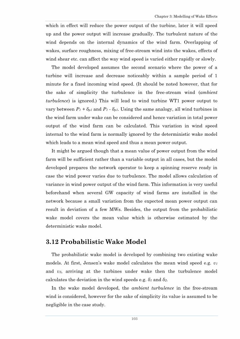
Chapter 3: Modelling of Wake Effects
103
which in effect will reduce the power output of the turbine, later it will speed
up and the power output will increase gradually. The turbulent nature of the
wind depends on the internal dynamics of the wind farm. Overlapping of
wakes, surface roughness, mixing of free-stream wind into the wakes, effects of
wind shear etc. can affect the way wind speed is varied either rapidly or slowly.
The model developed assumes the second scenario where the power of a
turbine will increase and decrease noticeably within a sample period of 1
minute for a fixed incoming wind speed. (It should be noted however, that for
the sake of simplicity the turbulence in the free-stream wind (ambient
turbulence) is ignored.) This will lead to wind turbine WT1 power output to
vary between P1 + δp1 and P1 - δp1. Using the same analogy, all wind turbines in
the wind farm under wake can be considered and hence variation in total power
output of the wind farm can be calculated. This variation in wind speed
internal to the wind farm is normally ignored by the deterministic wake model
which leads to a mean wind speed and thus a mean power output.
It might be argued though that a mean value of power output from the wind
farm will be sufficient rather than a variable output in all cases, but the model
developed prepares the network operator to keep a spinning reserve ready in
case the wind power varies due to turbulence. The model allows calculation of
variance in wind power output of the wind farm. This information is very useful
beforehand when several GW capacity of wind farms are installed in the
network because a small variation from the expected mean power output can
result in deviation of a few MWs. Besides, the output from the probabilistic
wake model covers the mean value which is otherwise estimated by the
deterministic wake model.
3.12 Probabilistic Wake Model
The probabilistic wake model is developed by combining two existing wake
models. At first, Jensen‘s wake model calculates the mean wind speed e.g. v1
and v2, arriving at the turbines under wake then the turbulence model
calculates the deviation in the wind speeds e.g. δ1 and δ2.
In the wake model developed, the ambient turbulence in the free-stream
wind is considered, however for the sake of simplicity its value is assumed to be
negligible in the case study.

Chapter 3: Modelling of Wake Effects
104
3.12.1 Jensen’s wake model (deterministic)
The detail wake effect model discussed in Section 3.3 is used to calculate the
mean wind speed at each turbine (the top-hat distribution is ignored). Single,
partial and multiple wakes are modelled to consider wind entering the wind
farm from any direction.
3.12.2 Turbulence model
Generally, turbulence intensity is defined as a measure of the overall level of
turbulence and is expressed as follows [105]:
(3.8)
where is the standard deviation of wind speed over a short period of time
and is the mean wind speed.
The model employed for wake added turbulence calculation in this chapter
can be used with single, partial and multiple wakes. The turbulence model is
given in [111], [178] and expressed as follows:
2
(1 )exp io w
w
I I
(3.9)
(3.10)
where βi is the angle between line connecting two turbines and the wind
direction as shown in Figure 3.17, βw is the characteristic width of the wake, s is
the distance between the turbines in separate rows, αw is a constant expressed
by the ambient turbulence Io, and the wake added turbulence (at hub height in
the centre of the wake) Iw.:
(3.11)
The wake added turbulence Iw is the turbulence introduced by the wake of a
turbine. It is expressed as [178]:
(3.12)
IU
U
1 01 180 1 25.tan 10 [deg]
2w
s s
2
1 1ww
o
I
I
1
1.5 0.3wI
s u

Chapter 3: Modelling of Wake Effects
105
If thrust coefficient, Ct of a turbine is known for every wind speed then the
following expression can be used instead:
(3.13)
where s is the distance between two turbines which wake one or the other, u is
the mean wind speed.
Figure 3.17: Wake turbulence as faced by a downwind turbine (adopted from [178])
In probabilistic wake model proposed the mean wind speed at a turbine is
calculated using (3.2) to (3.5) while the range of speed variation is calculated
using (3.8), (3.9) to (3.13) where defines the width of this range.
3.13 Case Study
The distribution of wind speed faced by turbine/s downwind is computed
using the above mentioned approach. A 49 turbine wind farm shown in Figure
3.13 is used for simulation purposes. Each turbine has a rated power of 2 MW
with hub height of 80 m and rotor radius of 40 m. Rated power of the wind farm
is 98 MW. The wind farm is located at sea with surface roughness of 0.0002.
Distance between two turbines in the same row is 400 m while the diagonal
distance is 565 m. Ambient turbulence Io is assumed to be negligible.
Once the mean wind speed and the variance at each turbine are obtained,
Monte Carlo simulations are performed to obtain wind speed distribution. For
turbines arranged in the same row, the wind speed distribution is plotted in
Figure 3.18. The distribution is assumed to be Gaussian as shown for wind
turbine 21 in Figure 3.19.
1
1.5 0.1 tw
Is C
wind wind
i
Iw
Io
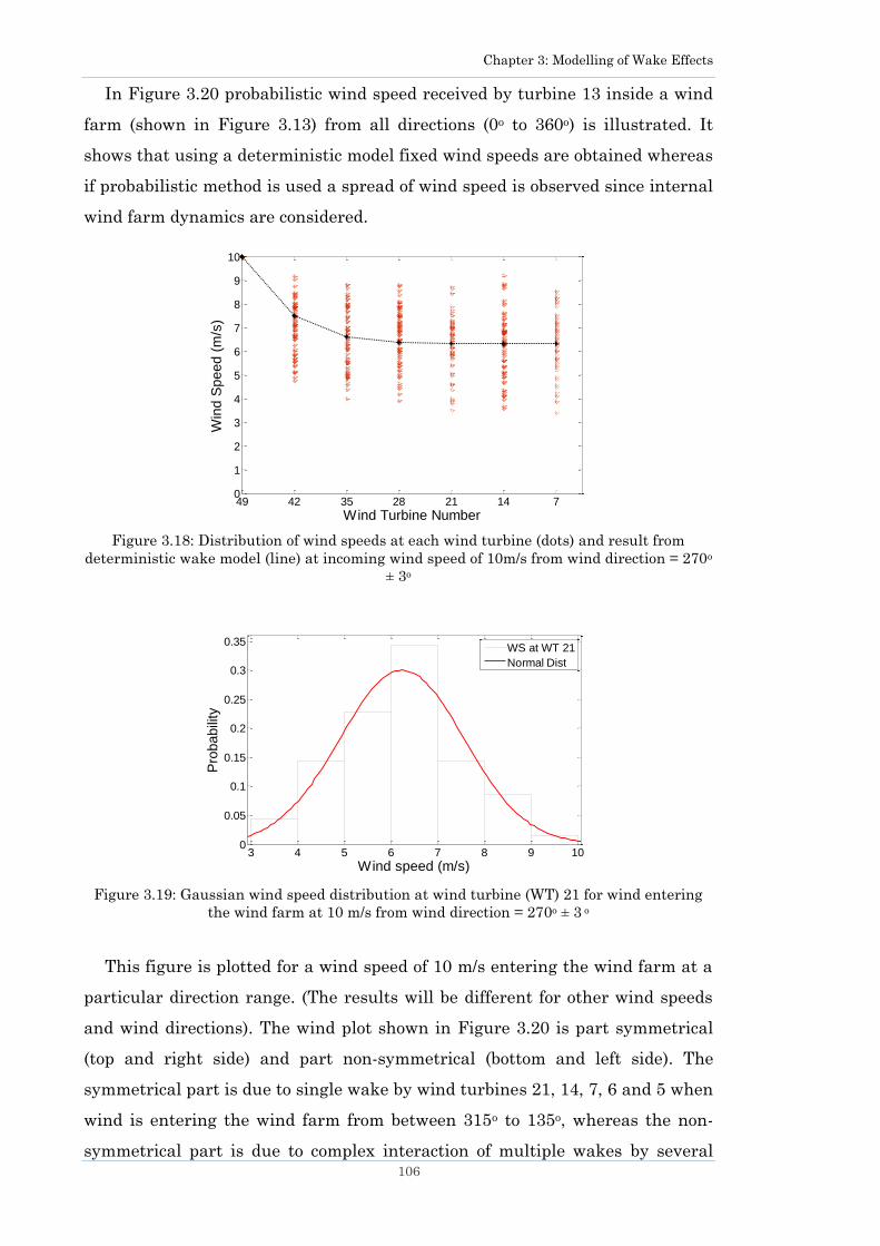
Chapter 3: Modelling of Wake Effects
106
In Figure 3.20 probabilistic wind speed received by turbine 13 inside a wind
farm (shown in Figure 3.13) from all directions (0o to 360o) is illustrated. It
shows that using a deterministic model fixed wind speeds are obtained whereas
if probabilistic method is used a spread of wind speed is observed since internal
wind farm dynamics are considered.
Figure 3.18: Distribution of wind speeds at each wind turbine (dots) and result from
deterministic wake model (line) at incoming wind speed of 10m/s from wind direction = 270o
± 3o
Figure 3.19: Gaussian wind speed distribution at wind turbine (WT) 21 for wind entering
the wind farm at 10 m/s from wind direction = 270o ± 3 o
This figure is plotted for a wind speed of 10 m/s entering the wind farm at a
particular direction range. (The results will be different for other wind speeds
and wind directions). The wind plot shown in Figure 3.20 is part symmetrical
(top and right side) and part non-symmetrical (bottom and left side). The
symmetrical part is due to single wake by wind turbines 21, 14, 7, 6 and 5 when
wind is entering the wind farm from between 315o to 135o, whereas the non-
symmetrical part is due to complex interaction of multiple wakes by several
49 42 35 28 21 14 70
1
2
3
4
5
6
7
8
9
10
Wind Turbine Number
Win
d S
peed (
m/s
)
3 4 5 6 7 8 9 100
0.05
0.1
0.15
0.2
0.25
0.3
0.35
Wind speed (m/s)
Pro
ba
bili
ty
WS at WT 21
Normal Dist

Chapter 3: Modelling of Wake Effects
107
wind turbines at the bottom left side of turbine 13 when wind is entering the
wind farm from between 135o to about 315o.
Figure 3.20: Wind plot of wind turbine 13 for incoming wind speed of 10 m/s showing
results of deterministic wake model (black line) and probabilistic model (red crosses).
Circles indicate wind speed magnitude (m/s) from each wind direction
3.14 Power Output Analysis
Power curves are used to trace the power at the corresponding wind speed.
The total power output of the wind farm is obtained by summing up the power
from individual wind turbines. Applying the probabilistic wake model gives a
range of power output for each turbine. The test was performed for wind
entering the wind farm at 10 m/s but from various directions. The results are
compared with those obtained using the deterministic wake model, as shown in
Figure 3.21.
The difference between wind power output obtained using the probabilistic
and the deterministic wake model is illustrated in Figure 3.22. It can be seen
that the difference varies from several kilowatts to Megawatts. For example, at
wind speed 10 m/s and wind direction of 91o the difference in power output can
be seen as large as 7 MW, implying that total power production can be as much
as 7 MW different to that predicted by the deterministic model. However on
average this difference is plus or minus 2 MW. Although only one wind speed is
simulated in this case study, the probabilistic wake model can be used for any
speed and direction of wind entering the wind farm. The variation in power
24
68
1012
14
180o
0o
270o
90o
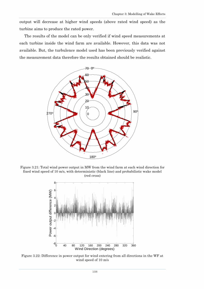
Chapter 3: Modelling of Wake Effects
108
output will decrease at higher wind speeds (above rated wind speed) as the
turbine aims to produce the rated power.
The results of the model can be only verified if wind speed measurements at
each turbine inside the wind farm are available. However, this data was not
available. But, the turbulence model used has been previously verified against
the measurement data therefore the results obtained should be realistic.
Figure 3.21: Total wind power output in MW from the wind farm at each wind direction for
fixed wind speed of 10 m/s, with deterministic (black line) and probabilistic wake model
(red cross)
Figure 3.22: Difference in power output for wind entering from all directions in the WF at
wind speed of 10 m/s
0
10
20
30
40
50
60
70
90o
0o
180o
270o
0 40 80 120 160 200 240 280 320 360-8
-6
-4
-2
0
2
4
6
8
Wind Direction (degrees)
Po
we
r o
utp
ut
diffe
ren
ce
(M
W)

Chapter 3: Modelling of Wake Effects
109
3.15 Energy Yield Analysis
Traditionally energy yield is calculated using wind speed data from a
Weibull distribution and the power curves of wind turbines; or if wind
measurements at the site are available, the power of a turbine is calculated for
every wind speed and then multiplied by the total number of turbines. Both
techniques overestimate energy yield because wake losses are ignored. In this
chapter, energy yield is calculated using deterministic and probabilistic wake
models, the results are given in Table 3.2.
Wind speed and direction measurements (see Section 3.8) recorded at a site
in North Sweden are used for the analysis. When using probabilistic wake
model, some power outputs in the year were higher while some were lower than
the mean power, equalling out the rise and fall in energy yield. However, the
difference observed after several simulations is shown below.
Table 3.2: Energy yield comparison using deterministic and probabilistic wake model
Energy yield ignoring
wake effects
Energy yield with
deterministic wake model
Energy yield with
probabilistic wake model
Reference -15.41% -15.41% ± 0.2%
It can be seen that deterministic model results in energy yield losses of about
15.41% (compared to the case when wake is completely ignored) while inclusion
of probabilistic nature of wind converts these losses into a range of (15.41 ±
0.2%). The capacity factor is also calculated using the deterministic wake
model. It was found that the capacity factor reduced from 39.8% to 33.7% due to
15.41% reduction in energy yield. It should be noted however that results
presented in Table 3.2 are valid for this case study, i.e. for wind farm with
layout shown in Figure 3.13, with turbines 80 m high installed at a site with
wind characteristics shown in Figure 3.11 and Figure 3.12. If either wind farm
layout, wind turbine type or wind site characteristics changes these results will
vary accordingly.
From Table 3.2 it can be seen that the difference in energy yield by using the
probabilistic wake model is not significant which makes it more applicable for
online usage rather than for offline use.
Chapter 3: Modelling of Wake Effects
110
3.16 Summary
The power production from a turbine is sensitive to the wind speed it
receives. It was shown in this chapter that wake effects can significantly reduce
the power output below rated wind speeds. Wake effect models presented in the
past were briefly discussed while Jensen‘s model is chosen for detailed wake
modelling. A program (VeBWake) is developed in which a wind farm of any
layout consisting of turbines of any rotor radius and height can be simulated to
calculate the wind speed experienced at each individual turbine. Jensen‘s wake
model is commonly adopted for electrical engineering related research studies
as well as in commercially available software. The MATLAB software
environment was chosen for development of this program to allow modelling
flexibility and parameter accessibility.
It was also noticed that terrain roughness, wind shear and the direction of
the incoming wind can affect the power generation from a turbine inside a wind
farm. Therefore it is essential to take these factors into account when modelling
wake effects. Wind speed measurements at a site and the Weibull distribution
are also presented. Two wind farm layouts consistently used in the case studies
throughout this thesis were also presented within this chapter.
A new probabilistic wake model to account for wind farm power output
variation due to the stochastic nature of wind (inside the wind farm) is also
presented in this chapter. This model is different from Jensen‘s wake model
that always provides a deterministic output at a given incoming wind speed.
Using this method, the range of power output and energy yield can be
estimated. It is an attempt to include turbulence of wind in an analytical wake
model. Deterministic wake models do not take into account dynamic
characteristics of wind inside a wind farm. The presented approach is
computationally efficient in comparison to the complex modelling techniques
available. The main advantage includes estimating a range of possible wind
farm power output for an available forecast of wind speed and wind direction a
few minutes ahead. This method is beneficial for online simulations as many
large wind farms are expected to be installed in the network, a range of power
output from each WF can enable the network operator to allocate spinning
reserve and generator dispatch. The results of the model are dependent on the
location, layout and the type of wind turbines installed in a wind farm. Other

Chapter 3: Modelling of Wake Effects
111
factors that can influence the results are the distance between the wind
turbines, the thrust coefficient, the speed and direction of the wind entering the
wind farm.
It is also shown by the analysis that the probabilistic wake model does not
significantly affect the energy yield of the wind farm because of the zero mean
effect. These results support the fact that the turbulence can be ignored for
offline studies such as for energy yield analysis. For this reason, deterministic
wake models are used in the following chapters.

Chapter 4: Probabilistic Aggregate Dynamic Model of a Wind Farm
112
Chapter 4 Probabilistic Aggregate Dynamic
Model of a Wind Farm
Probabilistic Aggregate Dynamic Model
of a Wind Farm
4.1 Introduction
Increased wind penetration in the network has led to major challenges but
simultaneously, advancement in communication technologies has provided
some solutions. Utilities are now implementing real-time monitoring
techniques to enable them to obtain wind power outputs from wind farms
connected with the system. With large scale wind penetration, instantaneous
regional shift in power generation will be common as wind flow changes. This
requires modelling tools that are fast and accurate so that stability of the
system within the following few hours can be simulated by testing faults in
critical areas. Using wind speed and direction measurements along with a
forecasting tool, wind conditions from a few minutes to hours ahead can be
predicted. Although dramatic increases in computational power over the recent
years has led to faster simulation times, handling large numbers of nodes and
solving hundreds (if not thousands) of differential equations still leads to long
simulation times.
Since wind is a variable energy resource, deterministic models often do not
lead to a reliable solution so for this purpose probabilistic techniques are often
more suitable. This can mean testing multiple scenarios with variable
parameters. If each wind farm in the system is modelled with all its turbines,
this will not only increase the computation burden during transient stability
simulations but it will also be cumbersome for the system operator to reset the
parameters to model the wind farm when wind conditions change.

Chapter 4: Probabilistic Aggregate Dynamic Model of a Wind Farm
113
Although detailed modelling of wind farms is reasonable during the design
stage, where faults internal to the wind farm have to be tested, when analysing
several wind farms as part of a network, this type of study is not suitable [43].
To solve this issue, wind farm aggregation models have been introduced in the
past (as discussed in Section 1.4.1). They enable a large wind farm to be
simulated by fewer turbines. Some of the existing models have already been
explored in the literature review.
An innovative probabilistic clustering approach is proposed in this chapter
which determines the equivalent number of wind turbines (and their
corresponding parameters) that can be used most frequently throughout the
year to model a WF accurately. The quantity and rated power of each
equivalent turbine is dependent on a variety of factors such as the statistical
analysis of the site and the wind farm layout. The number of equivalent
turbines is determined only once using the probabilistic clustering approach,
then the same set of turbines are used to represent the wind farm in any wind
condition.
The approach is applicable to wind farms with symmetrical or arbitrary
layouts as it takes into account wind speed variation inside the WF due to
wakes. The only information needed for model development apart from the
electrical and mechanical parameters of individual wind turbines, cable
parameters and WF topology is the wind data at the site, i.e., wind speed and
wind direction. The availability of wind data at each wind turbine inside the
WF (which is still not something that most of the WF operators would have)
will simplify and speed up the computational process. If this data is
unavailable, wind speed at each wind turbine can be calculated through the
wake effect model (VeBWake).
Accuracy of dynamic simulation is compared against results from the
detailed model. It is assumed that all turbines inside the wind farm are of the
same type. The model is useful in real-time simulators where modelling
individual wind turbines requires multiple computer processors [179]. The
model proposed is equally useful for offline studies. A comparison with popular
existing aggregation models is also performed to test simulation time, dynamic
response, ease of setup and use.

Chapter 4: Probabilistic Aggregate Dynamic Model of a Wind Farm
114
4.2 Aggregation by Wind Speed
It is argued in [37] that irregularity of wind distribution inside the wind
farm (due to wakes) will lead to wind turbines running at different operating
points from one another. Dynamic behaviour of a wind turbine during a fault in
the system is influenced by the controller‘s actions, which depends on the wind
speed faced by the turbine. At low wind speed, the controller would try to track
the optimal point of operation, whereas at higher wind speed the controller
would attempt to keep the angular speed inside an acceptable range to
maintain power production.
Furthermore, the stiffness of the shaft also affects the dynamic behaviour of
the turbines [77]. A wind turbine has a soft shaft system which accumulates
potential energy when twisted during normal operation and some of this energy
is released when a short circuit fault occurs in the network. Potential energy
stored in all the turbine shafts at a point of fault can in some instances, be
larger than that predicted by a single-unit model [77] because it assumes the
same operating point for all turbines. For this reason, a single-unit model will
also predict less acceleration of the turbines at faults, such influencing their
overall dynamic behaviour. Dynamic results in [180] show that a single-unit
equivalent is only suitable when the wind profile at each turbine is similar.
This model is no longer suitable when profiles differ between turbines. Multi-
machine models however can predict this accumulation of potential energy
more accurately as described in [37, 77].
To test the claims which say that turbines facing different wind speed will be
operating at different operating point, the dynamic behaviour of a DFIG
machine is simulated at two different wind speeds i.e. at below rated wind
speed and at rated wind speed. A 3-phase fault is applied at the cable
connecting the wind turbine with the grid (infinite bus) at 1 second and cleared
after 200 ms. Results in Figure 4.1 shows the difference in dynamic response of
a wind turbine operating at two different operating points when it receives two
different wind speeds. In steady state condition, the per unit generator rotor
speed is slightly higher for the turbine facing the rated wind speed because it is
operating at ωmax (see Figure 2.12) whereas at lower wind speed the rotor speed
is below ωmax . It can be seen from Figure 4.1 that the rotor speed, active power
and reactive power dynamic response take longer to stabilise when the turbine
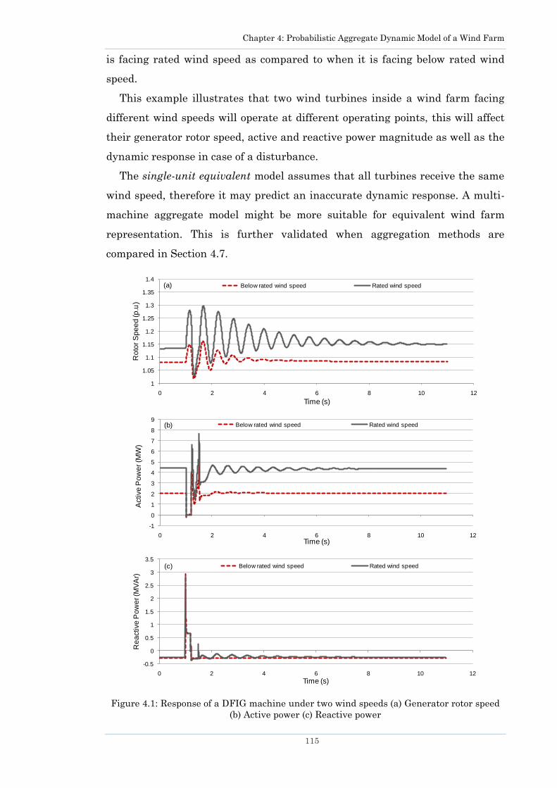
Chapter 4: Probabilistic Aggregate Dynamic Model of a Wind Farm
115
is facing rated wind speed as compared to when it is facing below rated wind
speed.
This example illustrates that two wind turbines inside a wind farm facing
different wind speeds will operate at different operating points, this will affect
their generator rotor speed, active and reactive power magnitude as well as the
dynamic response in case of a disturbance.
The single-unit equivalent model assumes that all turbines receive the same
wind speed, therefore it may predict an inaccurate dynamic response. A multi-
machine aggregate model might be more suitable for equivalent wind farm
representation. This is further validated when aggregation methods are
compared in Section 4.7.
Figure 4.1: Response of a DFIG machine under two wind speeds (a) Generator rotor speed
(b) Active power (c) Reactive power
1
1.05
1.1
1.15
1.2
1.25
1.3
1.35
1.4
0 2 4 6 8 10 12
Ro
tor
Sp
ee
d (p
.u)
Time (s)
Below rated wind speed Rated wind speed(a)
-1
0
1
2
3
4
5
6
7
8
9
0 2 4 6 8 10 12
Active
Po
we
r (M
W)
Time (s)
Below rated wind speed Rated wind speed(b)
-0.5
0
0.5
1
1.5
2
2.5
3
3.5
0 2 4 6 8 10 12
Re
active
Po
we
r (M
VA
r)
Time (s)
Below rated wind speed Rated wind speed(c)

Chapter 4: Probabilistic Aggregate Dynamic Model of a Wind Farm
116
4.3 Support Vector Clustering
In order to consider irregularity of wind speed inside a wind farm due to
wakes, the wake effect program VeBWake is used. Wind speed at each turbine
is calculated for wind entering the farm at various speeds from various
directions. Since wind turbines that face similar wind speeds operate at the
same operating point they can be clustered together [37]. The clustering is
performed using a Support Vector Clustering (SVC) method.
The SVC has been introduced as a further step to the support vector machine
concept introduced in [181]. It consists of determining the support vectors and
cluster labelling characterised by the identification of the final clusters. The
clustering procedure is carried out following two major steps:
1) Determination of the support vectors: a data set with N multi-dimensional
features is transformed from the original data space D to a high-dimensional
feature space T through a nonlinear transformation. Then, an optimization
procedure is applied to minimize the radius of the sphere enclosing the
image of the features mapped into the T-space [182]. Three types of features
are defined according to the location of their image in the transformed space
inside the enclosing sphere (internal vectors, IVs), on the boundary of the
enclosing sphere (support vectors), and outside the sphere (bounded support
vectors).
2) Cluster labelling: the support vector computation only refers to the distances
in the T-space between the features and the centre of the enclosing sphere,
and no information is provided on the directional coordinates of the features.
Thus, a second step is needed to form the final clusters [182]. The full
procedure for the SVC is described in [183], in which the data points
corresponding to bounded support vectors are considered as outliers and are
assigned to individual clusters, while the data points corresponding to the
non-bounded support vectors are grouped into clusters through a
deterministic algorithm.
In the SVC-based algorithm [183], the number of final clusters depends only
on a single, user–defined, threshold parameter, thus avoiding settings of
additional parameter learning heuristics as in [184]. The main goal of the SVC
algorithm is to assign multidimensional data features to groups and obtain
accurate and non-overlapped clusters.
Chapter 4: Probabilistic Aggregate Dynamic Model of a Wind Farm
117
Various clustering methods including follow-the-leader, k-means, fuzzy k-
means, hierarchical clustering (average linkage criterion, Ward linkage
criterion) and Kohonen’s self organizing map are tested against the SVC in
[183]. The SVC is found to have better clustering validity than other listed
methods and it performs well when number of clusters is relatively small. For
these reasons, this algorithm was chosen for clustering of turbines based on
their wind speeds.
4.4 Wind Turbine Clustering
As mentioned above, wind turbine clustering is addressed by applying the
SVC algorithm. All wind speeds within the turbine‘s operating range are tested
from 0o to 360o and then VeBWake program (mentioned in Section 3.4) is used
to obtain the proper wind speed received by each wind turbine within the plant.
Wind turbine clusters are then created based on their wind speed and direction
profiles using the SVC algorithm.
4.4.1 Wind farm layout
A test WF consisting of 49 identical offshore wind turbines with the rated
power of SWF = 98 MW is used in the case study. Variable speed, pitch
controlled and yaw enabled turbines with a 2 MW DFIG are used. They have an
operating range between 4 m/s and 25 m/s with a rated wind speed of 15 m/s
[15]. Distance between adjacent wind turbines is 400 m. A symmetrical WF
layout is chosen for the case study, the layout is shown in Figure 3.13; however,
the methodology developed is applicable to a wind farm of any size and layout.
All steady state and dynamic simulations are performed using DIgSILENT
PowerFactory [151].
4.4.2 Clustering
The test WF is used to illustrate the way wind turbine clustering is
performed. At a given time in the future, the speed and direction of the wind
impacting on the WF is assumed to be known from wind forecasting. The wind
speed patterns at each wind turbine (obtained through wake effect program,
VebWake) are the inputs of the SVC algorithm used to establish distinct and
non-overlapped clusters. This corresponds in particular to a target wind speed
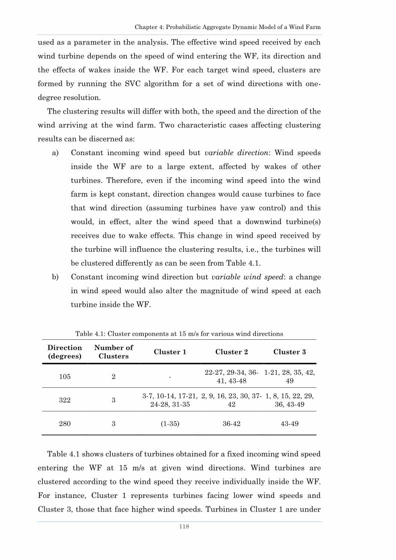
Chapter 4: Probabilistic Aggregate Dynamic Model of a Wind Farm
118
used as a parameter in the analysis. The effective wind speed received by each
wind turbine depends on the speed of wind entering the WF, its direction and
the effects of wakes inside the WF. For each target wind speed, clusters are
formed by running the SVC algorithm for a set of wind directions with one-
degree resolution.
The clustering results will differ with both, the speed and the direction of the
wind arriving at the wind farm. Two characteristic cases affecting clustering
results can be discerned as:
a) Constant incoming wind speed but variable direction: Wind speeds
inside the WF are to a large extent, affected by wakes of other
turbines. Therefore, even if the incoming wind speed into the wind
farm is kept constant, direction changes would cause turbines to face
that wind direction (assuming turbines have yaw control) and this
would, in effect, alter the wind speed that a downwind turbine(s)
receives due to wake effects. This change in wind speed received by
the turbine will influence the clustering results, i.e., the turbines will
be clustered differently as can be seen from Table 4.1.
b) Constant incoming wind direction but variable wind speed: a change
in wind speed would also alter the magnitude of wind speed at each
turbine inside the WF.
Table 4.1: Cluster components at 15 m/s for various wind directions
Direction
(degrees)
Number of
Clusters Cluster 1 Cluster 2 Cluster 3
105 2 - 22-27, 29-34, 36-
41, 43-48
1-21, 28, 35, 42,
49
322 3 3-7, 10-14, 17-21,
24-28, 31-35
2, 9, 16, 23, 30, 37-
42
1, 8, 15, 22, 29,
36, 43-49
280 3 (1-35) 36-42 43-49
Table 4.1 shows clusters of turbines obtained for a fixed incoming wind speed
entering the WF at 15 m/s at given wind directions. Wind turbines are
clustered according to the wind speed they receive individually inside the WF.
For instance, Cluster 1 represents turbines facing lower wind speeds and
Cluster 3, those that face higher wind speeds. Turbines in Cluster 1 are under
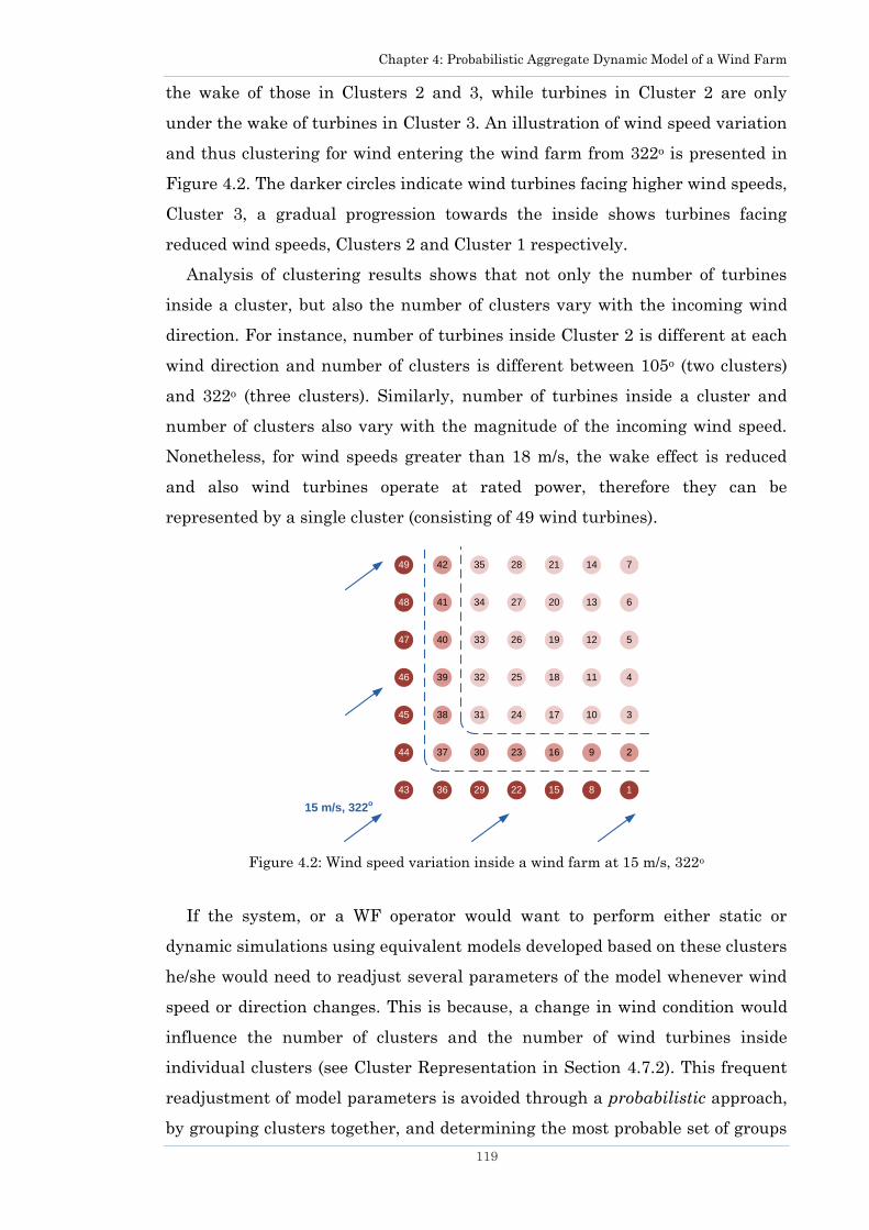
Chapter 4: Probabilistic Aggregate Dynamic Model of a Wind Farm
119
the wake of those in Clusters 2 and 3, while turbines in Cluster 2 are only
under the wake of turbines in Cluster 3. An illustration of wind speed variation
and thus clustering for wind entering the wind farm from 322o is presented in
Figure 4.2. The darker circles indicate wind turbines facing higher wind speeds,
Cluster 3, a gradual progression towards the inside shows turbines facing
reduced wind speeds, Clusters 2 and Cluster 1 respectively.
Analysis of clustering results shows that not only the number of turbines
inside a cluster, but also the number of clusters vary with the incoming wind
direction. For instance, number of turbines inside Cluster 2 is different at each
wind direction and number of clusters is different between 105o (two clusters)
and 322o (three clusters). Similarly, number of turbines inside a cluster and
number of clusters also vary with the magnitude of the incoming wind speed.
Nonetheless, for wind speeds greater than 18 m/s, the wake effect is reduced
and also wind turbines operate at rated power, therefore they can be
represented by a single cluster (consisting of 49 wind turbines).
Figure 4.2: Wind speed variation inside a wind farm at 15 m/s, 322o
If the system, or a WF operator would want to perform either static or
dynamic simulations using equivalent models developed based on these clusters
he/she would need to readjust several parameters of the model whenever wind
speed or direction changes. This is because, a change in wind condition would
influence the number of clusters and the number of wind turbines inside
individual clusters (see Cluster Representation in Section 4.7.2). This frequent
readjustment of model parameters is avoided through a probabilistic approach,
by grouping clusters together, and determining the most probable set of groups
7
6
5
4
3
2
1
14
13
12
11
10
9
8
21
20
19
18
17
16
15
28
27
26
25
24
23
22
35
34
33
32
31
30
29
42
41
40
39
38
37
36
49
48
47
46
45
44
43
15 m/s, 322o

Chapter 4: Probabilistic Aggregate Dynamic Model of a Wind Farm
120
that would work for most wind conditions throughout the year (or any time
period).
4.5 Probabilistic Clustering of Wind Turbines
The probabilistic model provides a unique representation of the wind plant
that could be used throughout the year. The clusters established for each wind
condition are further arranged into groups. Through probabilistic analysis of
wind conditions at the site, the most probable group is established. This most
probable group defines the number of equivalent turbines that will represent
the wind farm throughout the year. The following sections provide detail
description of each step of the process.
4.5.1 Formation of groups
Once clustering of wind turbines is achieved according to the wind speed
they receive, these clusters are further arranged into groups. An example is
shown in Table 4.2. Sometimes the same group can occur for more than one
wind condition. Groups are classified as different (i.e., unique groups), if either
or both the criterion is met:
1) Number of clusters in any two groups is different.
2) Number of clusters in any two groups is the same, but the number of
turbines in the clusters are different.
The number of clusters represents the number of equivalent turbine(s)
needed for WF representation, while the number of turbines inside each cluster
allows calculation of rated power of the equivalent turbine(s). The total number
of unique groups that exist for all wind speeds and directions are identified
first. Probabilities for each of these unique groups are then calculated using the
wind information at the site (this will be shown in the next section).
A change in wind speed or direction can affect the way wind turbines are
clustered (as seen in previous section), which in turn can alter the number of
groups and the probability of group occurrences.
An illustration of group formation for various wind conditions is shown in
Table 4.2. For instance when wind speed is 15 m/s and wind direction is 105°,
two clusters of wind turbines are identified by the SVC algorithm (as shown in
Table 4.1), and these clusters are assembled into a group G1. Group G1 can
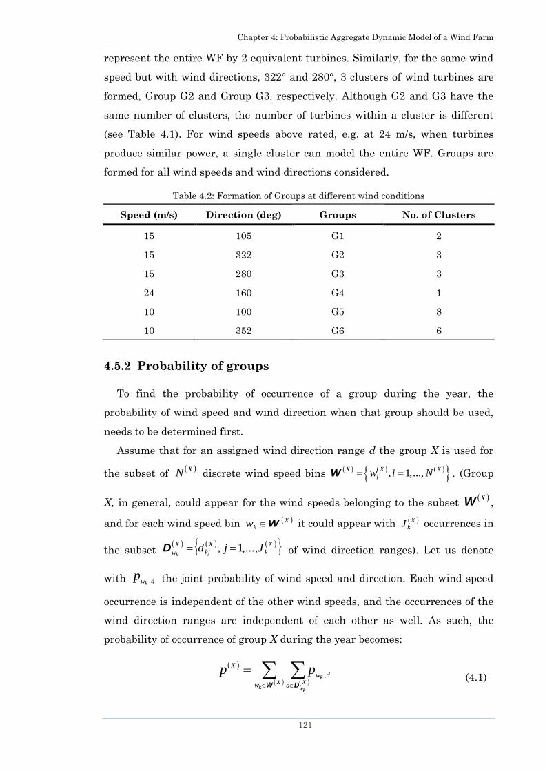
Chapter 4: Probabilistic Aggregate Dynamic Model of a Wind Farm
121
represent the entire WF by 2 equivalent turbines. Similarly, for the same wind
speed but with wind directions, 322° and 280°, 3 clusters of wind turbines are
formed, Group G2 and Group G3, respectively. Although G2 and G3 have the
same number of clusters, the number of turbines within a cluster is different
(see Table 4.1). For wind speeds above rated, e.g. at 24 m/s, when turbines
produce similar power, a single cluster can model the entire WF. Groups are
formed for all wind speeds and wind directions considered.
Table 4.2: Formation of Groups at different wind conditions
Speed (m/s) Direction (deg) Groups No. of Clusters
15 105 G1 2
15 322 G2 3
15 280 G3 3
24 160 G4 1
10 100 G5 8
10 352 G6 6
4.5.2 Probability of groups
To find the probability of occurrence of a group during the year, the
probability of wind speed and wind direction when that group should be used,
needs to be determined first.
Assume that for an assigned wind direction range d the group X is used for
the subset of discrete wind speed bins . (Group
X, in general, could appear for the wind speeds belonging to the subset ,
and for each wind speed bin it could appear with occurrences in
the subset of wind direction ranges). Let us denote
with the joint probability of wind speed and direction. Each wind speed
occurrence is independent of the other wind speeds, and the occurrences of the
wind direction ranges are independent of each other as well. As such, the
probability of occurrence of group X during the year becomes:
X
kX
kw
k
w d
dw
X ppW D
,
(4.1)
XN , 1,...,X X X
iw i N W
XW
X
kw W X
kJ
X
k
X
kj
X
wJjd
k,...,1, D
dwkp
,

Chapter 4: Probabilistic Aggregate Dynamic Model of a Wind Farm
122
For example, if group X occurs with a different combination of wind speed
and direction, i.e., once for w = 4 m/s and directions 100° to 120°, then for w = 6
m/s and directions 120° to 140°, (4.1) is used with = {4, 6}, = {100°,
101°,…, 120°}, and = {120°, 121°,…, 140°}.
By using (4.1), the probability of any group during the year can be
determined for any site. The number of groups can vary based on size and
layout of the WF, wind characteristics at a site during the year, wind speed and
direction step used.
4.5.3 Information of wind at a site
It is assumed that the 49 turbine wind farm is placed at a site in North
Sweden for which wind speed measurements are given in Section 3.8. It can be
seen from Figure 3.12 that there are two dominant ranges of wind directions
during the year, i.e., 100o to 180o and 280o to 360o so for this reason only these
direction ranges were analysed with a step of 1o. Although the most probable
wind speeds (in Figure 3.11) are in the range from 4 m/s to 15 m/s, all wind
speeds within the entire wind turbine operating range are considered (with a
step of 1 m/s) for wind turbine clustering.
4.5.4 Probabilistic group identification
A total of about 3500 groups were identified after testing all wind conditions,
out of these there were 321 unique groups.
Figure 4.3: Probability of every unique group found
XW X
4D
X
6D
0 50 100 150 200 250 3000
0.02
0.04
0.06
0.08
0.1
0.12
Pro
ba
bili
ty
Unique Groups
Group C
Group A
Group B
Group D
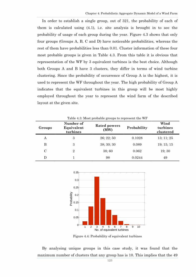
Chapter 4: Probabilistic Aggregate Dynamic Model of a Wind Farm
123
In order to establish a single group, out of 321, the probability of each of
them is calculated using (4.1), i.e. site analysis is brought in to see the
probability of usage of each group during the year. Figure 4.3 shows that only
four groups (Groups A, B, C and D) have noticeable probabilities, whereas the
rest of them have probabilities less than 0.01. Cluster information of these four
most probable groups is given in Table 4.3. From this table it is obvious that
representation of the WF by 3 equivalent turbines is the best choice. Although
both Groups A and B have 3 clusters, they differ in terms of wind turbine
clustering. Since the probability of occurrence of Group A is the highest, it is
used to represent the WF throughout the year. The high probability of Group A
indicates that the equivalent turbines in this group will be most highly
employed throughout the year to represent the wind farm of the described
layout at the given site.
Table 4.3: Most probable groups to represent the WF
Groups
Number of
Equivalent
turbines
Rated powers
(MW) Probability
Wind
turbines
clustered
A 3 26; 22; 50 0.1028 13; 11; 25
B 3 38; 30; 30 0.089 19; 15; 15
C 2 38; 60 0.062 19; 30
D 1 98 0.0244 49
1 2 3 4 5 6 7 8 9 100
0.05
0.1
0.15
0.2
0.25
0.3
0.35
No. of equivalent turbines
Pro
ba
bili
ty
Figure 4.4: Probability of equivalent turbines
By analysing unique groups in this case study, it was found that the
maximum number of clusters that any group has is 10. This implies that the 49

Chapter 4: Probabilistic Aggregate Dynamic Model of a Wind Farm
124
WT wind farm, considered here, can be represented by a maximum of 10
equivalent turbines.
The probability to represent the wind farm by 1 equivalent turbine is found
to be very low as seen from Figure 4.4. This shows that if a single-unit
equivalent model (which represents a wind farm by a single turbine) is used it
will not accurately represent the wind farm throughout the year. This is
because the probability when a single turbine could be used to accurately
represent the wind farm is extremely low. The selection of Group A with 3
equivalent turbines is justified as the probability of representing the wind farm
with 3 equivalent turbines is the highest (as seen from this figure).
Figure 4.5: Number of equivalent turbines that can represent a WF and number of possible
ways to model them
It was seen in Table 4.3 that Groups A and B have the highest probability of
usage throughout the year, both represent the wind farm by 3 equivalent
turbines but they differ in their rated capacity. This showed that there is more
than one way to setup the equivalent turbines. Possible ways to setup
equivalent turbines in all unique groups are further explored. Figure 4.5 shows
that there are about 48 different ways to setup 3 equivalent turbines, whereas
there are 82 different ways to setup 5 equivalent turbines. The difference
occurs due to the number of turbines in each cluster (in a group) which affects
the rating of an equivalent turbine.
1 2 3 4 5 6 7 8 9 100
10
20
30
40
50
60
70
80
90
No. of equivalent turbines
No.
of
uniq
ue w
ays t
o m
odel
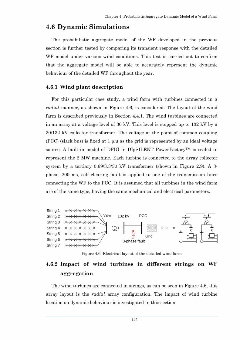
Chapter 4: Probabilistic Aggregate Dynamic Model of a Wind Farm
125
4.6 Dynamic Simulations
The probabilistic aggregate model of the WF developed in the previous
section is further tested by comparing its transient response with the detailed
WF model under various wind conditions. This test is carried out to confirm
that the aggregate model will be able to accurately represent the dynamic
behaviour of the detailed WF throughout the year.
4.6.1 Wind plant description
For this particular case study, a wind farm with turbines connected in a
radial manner, as shown in Figure 4.6, is considered. The layout of the wind
farm is described previously in Section 4.4.1. The wind turbines are connected
in an array at a voltage level of 30 kV. This level is stepped up to 132 kV by a
30/132 kV collector transformer. The voltage at the point of common coupling
(PCC) (slack bus) is fixed at 1 p.u as the grid is represented by an ideal voltage
source. A built-in model of DFIG in DIgSILENT PowerFactoryTM is scaled to
represent the 2 MW machine. Each turbine is connected to the array collector
system by a tertiary 0.69/3.3/30 kV transformer (shown in Figure 2.9). A 3-
phase, 200 ms, self clearing fault is applied to one of the transmission lines
connecting the WF to the PCC. It is assumed that all turbines in the wind farm
are of the same type, having the same mechanical and electrical parameters.
Figure 4.6: Electrical layout of the detailed wind farm
4.6.2 Impact of wind turbines in different strings on WF
aggregation
The wind turbines are connected in strings, as can be seen in Figure 4.6, this
array layout is the radial array configuration. The impact of wind turbine
location on dynamic behaviour is investigated in this section.
PCC
String 1
String 2
String 3
String 4
String 5
String 6
String 7
30kV 132 kV
3-phase fault
Grid
=
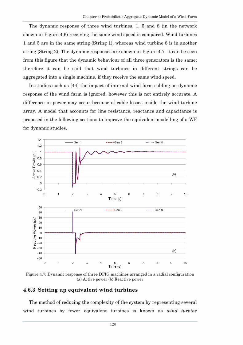
Chapter 4: Probabilistic Aggregate Dynamic Model of a Wind Farm
126
The dynamic response of three wind turbines, 1, 5 and 8 (in the network
shown in Figure 4.6) receiving the same wind speed is compared. Wind turbines
1 and 5 are in the same string (String 1), whereas wind turbine 8 is in another
string (String 2). The dynamic responses are shown in Figure 4.7. It can be seen
from this figure that the dynamic behaviour of all three generators is the same;
therefore it can be said that wind turbines in different strings can be
aggregated into a single machine, if they receive the same wind speed.
In studies such as [44] the impact of internal wind farm cabling on dynamic
response of the wind farm is ignored, however this is not entirely accurate. A
difference in power may occur because of cable losses inside the wind turbine
array. A model that accounts for line resistance, reactance and capacitance is
proposed in the following sections to improve the equivalent modelling of a WF
for dynamic studies.
Figure 4.7: Dynamic response of three DFIG machines arranged in a radial configuration
(a) Active power (b) Reactive power
4.6.3 Setting up equivalent wind turbines
The method of reducing the complexity of the system by representing several
wind turbines by fewer equivalent turbines is known as wind turbine

Chapter 4: Probabilistic Aggregate Dynamic Model of a Wind Farm
127
aggregation. This type of aggregation has been performed in [37, 46, 77, 180].
An aggregate model of the wind farm is required to fulfil two conditions:
1) The pre-fault active and reactive power output from the aggregate model
should be the same as that from a detailed wind farm model
2) The dynamic response of the aggregate model should be the same as that
of a detail wind farm model response
In this case study, the number of the equivalent turbines and the number of
wind turbines the equivalent turbine represents is given by Group A. From
Table 4.3 it can be seen that there will be 3 equivalent turbines of capacity 26
MW, 22 MW, 50 MW, i.e., each equivalent turbine represents 13, 11 and 25
wind turbines respectively. Although wind turbine aggregation had been
performed in several previous studies, no research study described in detail
which internal parameters of the machine should be adjusted.
Setting up an equivalent turbine requires adjusting of mechanical as well as
electrical parameters. As a starting point, pre-fault mechanical power should be
the same as electrical power which implies that if a large induction machine is
used it will require an equally sized mechanical rotor. Thus, when bigger
turbine rotor is used, the inertia constant and damping coefficients should be
adjusted (increased) accordingly. Also, wind turbines usually have softer shafts
than conventional generators, therefore, stiffness of the shaft needs to be
adjusted appropriately.
On the electrical side, transformer, converter, capacitor and inductor which
will be handling larger current than before will need to be rescaled. The
amount of current inside the induction machine will increase with an upscale of
the MVA power rating in a linear fashion since voltages are assumed to remain
static. When generator will have larger MVA ratings they will be physically
larger, therefore the inertia of its rotor will also be larger. All these parameters
are scaled up in the DIgSILENT PowerFactory to simulate an equivalent
turbine model. Table 4.4 shows in a summarised form the parameters that need
to be scaled in order to setup aggregate wind turbines. The scaling factor
mentioned in this table is the number of turbines an equivalent turbine will
represent. For instance, if the 2 MW machine is being scaled up to represent 13
(26 MW) such machines then the scaling factor is 13.
The rated apparent power of an equivalent turbine is calculated as the sum
of rated apparent powers of individual turbines in a cluster:

Chapter 4: Probabilistic Aggregate Dynamic Model of a Wind Farm
128
(4.2)
where n is the number of aggregated turbines in a cluster, Sindividual_WTs is the
rated apparent power of each wind turbine in the cluster and Seq_WT is the rated
apparent power of the equivalent wind turbine.
It is assumed that the rated voltage at the terminal of an equivalent wind
turbine is the same as that of a single turbine (in a detail wind farm).
Table 4.4. Parameters to be adjusted in order to represent turbines by an equivalent wind
turbine
Parameters Scale factor
Rated Mechanical Power Multiply by scaling factor
Active Power (initial conditions) Multiply by scaling factor
Reactive Power (initial conditions) Multiply by scaling factor
Converter Rating Multiply by scaling factor
Reactive Power set-point Multiply by scaling factor
DC-Link Capacitor size Multiply by scaling factor
Rotor side converter rating (PQ measurement) Multiply by scaling factor
Rated Power of Generator Multiply by scaling factor
Rotor Inertia (without generator) Multiply by scaling factor
Shaft Stiffness Multiply by scaling factor
Torsional Damping Multiply by scaling factor
Series Inductor Rated Power Multiply by scaling factor
Rated power of transformer at HV, MV and LV
side Multiply by scaling factor
Positive-seq short-circuit voltage at HV-MV Adjust manually
Positive-seq short-circuit voltage at MV-LV Adjust manually
Positive-seq short-circuit voltage at LV-HV Adjust manually
Inertia of Generator Multiply by scaling factor
Acceleration time constant Automatically adjusted according
to inertia
Mechanical Power of Turbine Multiply by scaling factor
Those parameters of the generator, rotor-side converter, crow-bar protection,
current control, grid-side converter, 3-winding transformer and reactor
(inductor) that are in per-units are not modified as they will be adjusted
according to the rated apparent power and rated voltage base. No parameter of
_ _
1
n
eq WT individual WTs
i
S S
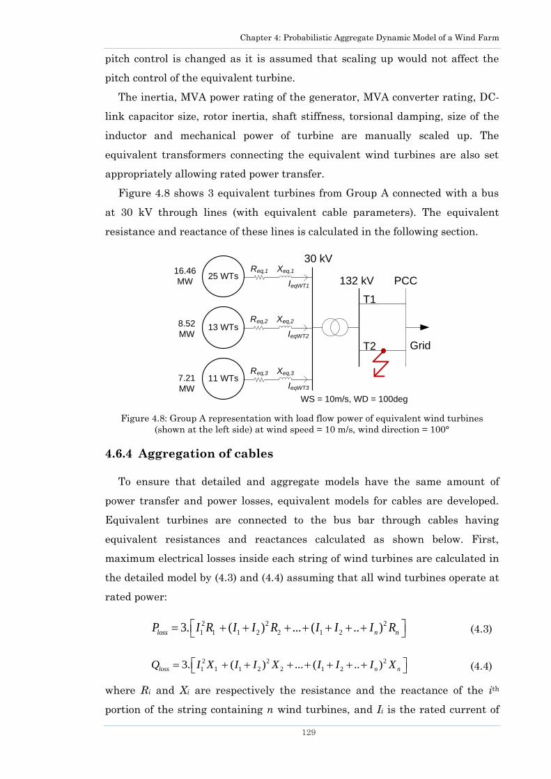
Chapter 4: Probabilistic Aggregate Dynamic Model of a Wind Farm
129
pitch control is changed as it is assumed that scaling up would not affect the
pitch control of the equivalent turbine.
The inertia, MVA power rating of the generator, MVA converter rating, DC-
link capacitor size, rotor inertia, shaft stiffness, torsional damping, size of the
inductor and mechanical power of turbine are manually scaled up. The
equivalent transformers connecting the equivalent wind turbines are also set
appropriately allowing rated power transfer.
Figure 4.8 shows 3 equivalent turbines from Group A connected with a bus
at 30 kV through lines (with equivalent cable parameters). The equivalent
resistance and reactance of these lines is calculated in the following section.
Figure 4.8: Group A representation with load flow power of equivalent wind turbines
(shown at the left side) at wind speed = 10 m/s, wind direction = 100°
4.6.4 Aggregation of cables
To ensure that detailed and aggregate models have the same amount of
power transfer and power losses, equivalent models for cables are developed.
Equivalent turbines are connected to the bus bar through cables having
equivalent resistances and reactances calculated as shown below. First,
maximum electrical losses inside each string of wind turbines are calculated in
the detailed model by (4.3) and (4.4) assuming that all wind turbines operate at
rated power:
2 2 2
1 1 1 2 2 1 23. ( ) ... ( .. )loss n nP I R I I R I I I R (4.3)
2 2 2
1 1 1 2 2 1 23. ( ) ... ( .. )loss n nQ I X I I X I I I X (4.4)
where Ri and Xi are respectively the resistance and the reactance of the ith
portion of the string containing n wind turbines, and Ii is the rated current of
25 WTsPCC
Grid
T1
T2
30 kV
132 kV
13 WTs
11 WTs
WS = 10m/s, WD = 100deg
16.46
MW
8.52
MW
7.21
MW
IeqWT1
Req,1 Xeq,1
IeqWT2
Req,2 Xeq,2
IeqWT3
Req,3 Xeq,3

Chapter 4: Probabilistic Aggregate Dynamic Model of a Wind Farm
130
the ith wind turbine in the string, for i = 1,…, n. Total electrical losses
( , ) inside the WF are calculated as a sum of losses inside each
string (in the detailed wind farm model). Considering the WF rated voltage V,
the total current flowing out of the WF is evaluated as:
3WF WFI S V
(4.5)
In the aggregate model, as shown in Figure 4.8, for a total of p equivalent
turbines, the current from each can be evaluated as:
3eqWTj eqWTjI S V
(4.6)
where j = 1, 2, 3, …, p and SeqWTj is the rated capacity of the jth equivalent
turbine. Sum of total losses from all equivalent wind turbines should be equal
to total power losses in the detailed WF:
, ,
1
p
loss eqWTj loss WF
j
P P
, , ,
1
p
loss eqWTj loss WF
j
Q Q
(4.7)
In the case studied and for any set of clustered wind turbines the following
expression is valid:
, 1 , 2 , 3
1 2 3
loss eqWT loss eqWT loss eqWTP P P
M M M ,…=
,loss eqWTp
p
P
M (4.8)
2 2 2
1 ,1 2 ,2 3 ,3
1 2 3
3 3 3eqWT eq eqWT eq eqWT eqI R I R I R
M M M ,… =
2
,3 eqWTp eq p
p
I R
M (4.9)
By solving these equations simultaneously, equivalent resistance of each line
connecting the equivalent wind turbines (Req,j) with the 30 kV bus can be
determined. The value for the first equivalent line, for instance, is evaluated as
below:
, 1
,1 2
1 1 2 33
loss WF
eq
eqWT
P MR
I M M M
(4.10)
Equivalent reactance (Xeq,j) can be evaluated in the same way by replacing R
with X:
, 1
,1 2
1 1 2 33
loss WF
eq
eqWT
Q MX
I M M M
(4.11)
,loss WFP ,loss WFQ
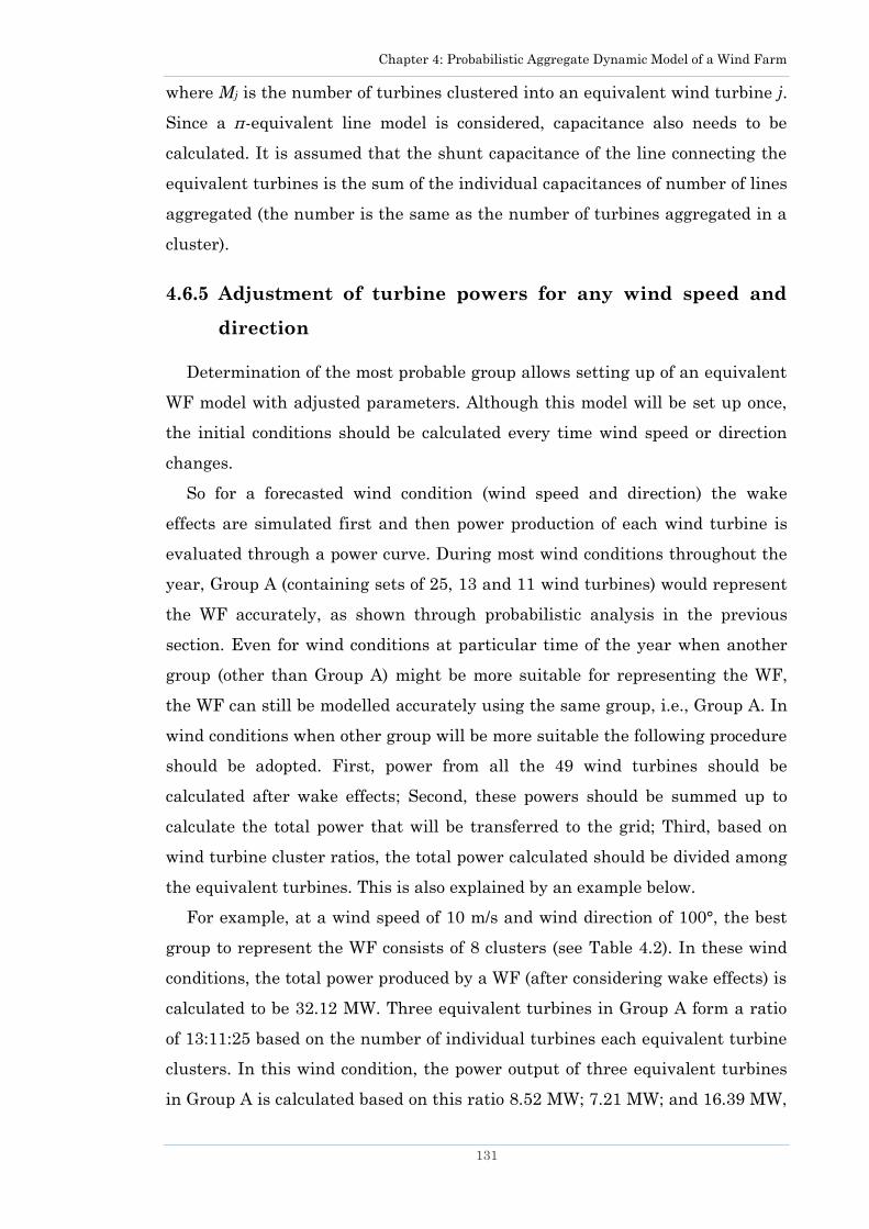
Chapter 4: Probabilistic Aggregate Dynamic Model of a Wind Farm
131
where Mj is the number of turbines clustered into an equivalent wind turbine j.
Since a π-equivalent line model is considered, capacitance also needs to be
calculated. It is assumed that the shunt capacitance of the line connecting the
equivalent turbines is the sum of the individual capacitances of number of lines
aggregated (the number is the same as the number of turbines aggregated in a
cluster).
4.6.5 Adjustment of turbine powers for any wind speed and
direction
Determination of the most probable group allows setting up of an equivalent
WF model with adjusted parameters. Although this model will be set up once,
the initial conditions should be calculated every time wind speed or direction
changes.
So for a forecasted wind condition (wind speed and direction) the wake
effects are simulated first and then power production of each wind turbine is
evaluated through a power curve. During most wind conditions throughout the
year, Group A (containing sets of 25, 13 and 11 wind turbines) would represent
the WF accurately, as shown through probabilistic analysis in the previous
section. Even for wind conditions at particular time of the year when another
group (other than Group A) might be more suitable for representing the WF,
the WF can still be modelled accurately using the same group, i.e., Group A. In
wind conditions when other group will be more suitable the following procedure
should be adopted. First, power from all the 49 wind turbines should be
calculated after wake effects; Second, these powers should be summed up to
calculate the total power that will be transferred to the grid; Third, based on
wind turbine cluster ratios, the total power calculated should be divided among
the equivalent turbines. This is also explained by an example below.
For example, at a wind speed of 10 m/s and wind direction of 100°, the best
group to represent the WF consists of 8 clusters (see Table 4.2). In these wind
conditions, the total power produced by a WF (after considering wake effects) is
calculated to be 32.12 MW. Three equivalent turbines in Group A form a ratio
of 13:11:25 based on the number of individual turbines each equivalent turbine
clusters. In this wind condition, the power output of three equivalent turbines
in Group A is calculated based on this ratio 8.52 MW; 7.21 MW; and 16.39 MW,
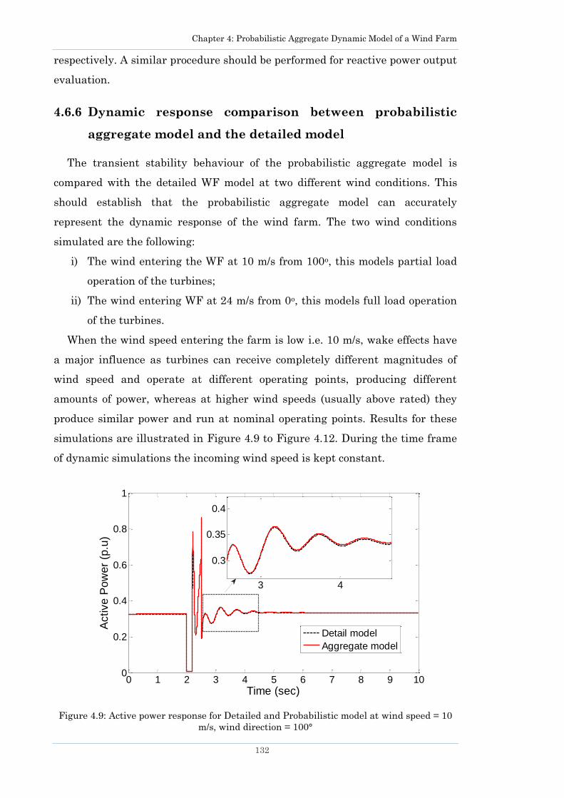
Chapter 4: Probabilistic Aggregate Dynamic Model of a Wind Farm
132
respectively. A similar procedure should be performed for reactive power output
evaluation.
4.6.6 Dynamic response comparison between probabilistic
aggregate model and the detailed model
The transient stability behaviour of the probabilistic aggregate model is
compared with the detailed WF model at two different wind conditions. This
should establish that the probabilistic aggregate model can accurately
represent the dynamic response of the wind farm. The two wind conditions
simulated are the following:
i) The wind entering the WF at 10 m/s from 100o, this models partial load
operation of the turbines;
ii) The wind entering WF at 24 m/s from 0o, this models full load operation
of the turbines.
When the wind speed entering the farm is low i.e. 10 m/s, wake effects have
a major influence as turbines can receive completely different magnitudes of
wind speed and operate at different operating points, producing different
amounts of power, whereas at higher wind speeds (usually above rated) they
produce similar power and run at nominal operating points. Results for these
simulations are illustrated in Figure 4.9 to Figure 4.12. During the time frame
of dynamic simulations the incoming wind speed is kept constant.
Figure 4.9: Active power response for Detailed and Probabilistic model at wind speed = 10
m/s, wind direction = 100°
0 1 2 3 4 5 6 7 8 9 100
0.2
0.4
0.6
0.8
1
Time (sec)
Active
Po
we
r (p
.u)
3 4
0.3
0.35
0.4
Detail model
Aggregate model
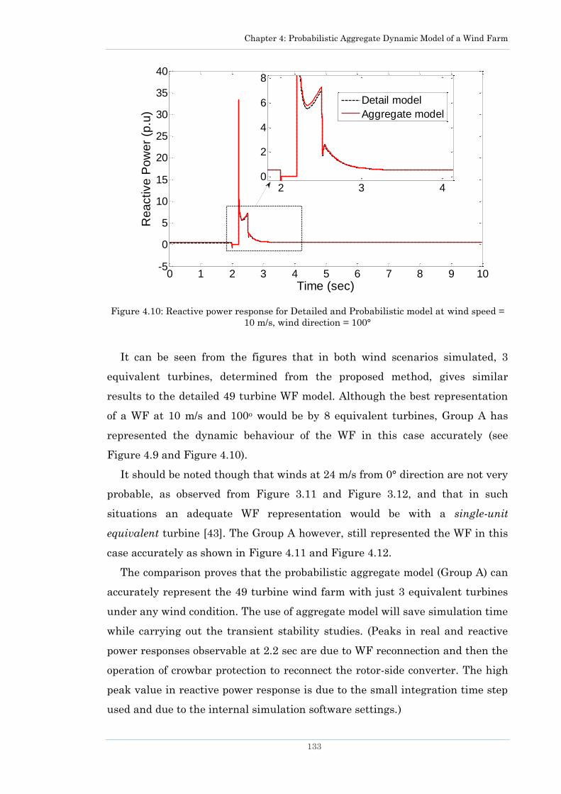
Chapter 4: Probabilistic Aggregate Dynamic Model of a Wind Farm
133
Figure 4.10: Reactive power response for Detailed and Probabilistic model at wind speed =
10 m/s, wind direction = 100°
It can be seen from the figures that in both wind scenarios simulated, 3
equivalent turbines, determined from the proposed method, gives similar
results to the detailed 49 turbine WF model. Although the best representation
of a WF at 10 m/s and 100o would be by 8 equivalent turbines, Group A has
represented the dynamic behaviour of the WF in this case accurately (see
Figure 4.9 and Figure 4.10).
It should be noted though that winds at 24 m/s from 0° direction are not very
probable, as observed from Figure 3.11 and Figure 3.12, and that in such
situations an adequate WF representation would be with a single-unit
equivalent turbine [43]. The Group A however, still represented the WF in this
case accurately as shown in Figure 4.11 and Figure 4.12.
The comparison proves that the probabilistic aggregate model (Group A) can
accurately represent the 49 turbine wind farm with just 3 equivalent turbines
under any wind condition. The use of aggregate model will save simulation time
while carrying out the transient stability studies. (Peaks in real and reactive
power responses observable at 2.2 sec are due to WF reconnection and then the
operation of crowbar protection to reconnect the rotor-side converter. The high
peak value in reactive power response is due to the small integration time step
used and due to the internal simulation software settings.)
0 1 2 3 4 5 6 7 8 9 10-5
0
5
10
15
20
25
30
35
40
Time (sec)
Reactive P
ow
er
(p.u
)
2 3 40
2
4
6
8
Detail model
Aggregate model
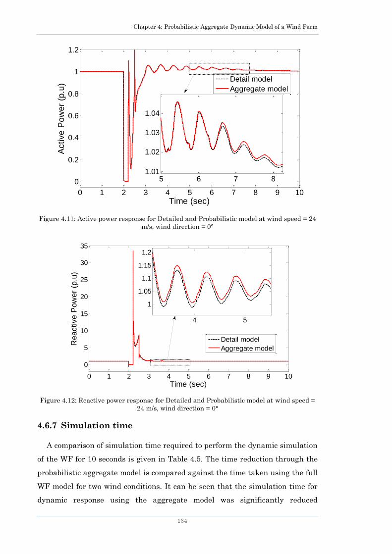
Chapter 4: Probabilistic Aggregate Dynamic Model of a Wind Farm
134
Figure 4.11: Active power response for Detailed and Probabilistic model at wind speed = 24
m/s, wind direction = 0°
Figure 4.12: Reactive power response for Detailed and Probabilistic model at wind speed =
24 m/s, wind direction = 0°
4.6.7 Simulation time
A comparison of simulation time required to perform the dynamic simulation
of the WF for 10 seconds is given in Table 4.5. The time reduction through the
probabilistic aggregate model is compared against the time taken using the full
WF model for two wind conditions. It can be seen that the simulation time for
dynamic response using the aggregate model was significantly reduced
0 1 2 3 4 5 6 7 8 9 10
0
0.2
0.4
0.6
0.8
1
1.2
Time (sec)
Active
Pow
er
(p.u
)
5 6 7 81.01
1.02
1.03
1.04
Detail model
Aggregate model
0 1 2 3 4 5 6 7 8 9 10
0
5
10
15
20
25
30
35
Time (sec)
Re
active
Po
we
r (p
.u)
4 5
1
1.05
1.1
1.15
1.2
Detail model
Aggregate model

Chapter 4: Probabilistic Aggregate Dynamic Model of a Wind Farm
135
compared to the full WF model. For the cases studied, modelling 3 instead of 49
turbines led to a significant reduction in simulation time.
Table 4.5: Simulation time comparison with different models
Model
Wind
Speed
(m/s)
Wind
Direction
(deg)
Simulation Time
(s)
Number of
wind turbines
Detail 10 100 925 49
24 0 925 49
Probabilistic
(Aggregate)
10 100 44.9 3
24 0 34.8 3
In all simulations a constant step size of 0.75 milliseconds was used to make
the time comparisons adequate.
Table 4.5 shows that the detail model takes 925 seconds to complete the
simulation in Figure 4.9 and Figure 4.10, whereas the probabilistic model takes
only 45 seconds. This shows a simulation time reduction of about 95.14%, but
the largest reduction in simulation time occurs for the 24 m/s, 0o case i.e. a
reduction of 96.23%.
4.6.8 Smaller wind farm test
The probabilistic aggregate model was also tested on a smaller wind farm
consisting of only 9 wind turbines arranged in a symmetrical manner shown in
Figure 3.14. The same wind speed measurements were used and clustering was
performed using the SVC method. It was found that the proposed method is
equally applicable to smaller wind farms. The full results of this study can be
found in Appendix B.
4.7 Comparison with Existing Aggregate Models
The choice of an aggregation technique depends on the type of study it will
be used for. Various existing aggregate models have been critically examined in
the literature review in Chapter 1. Generally, the main requirement for a WF
aggregate model is that the active and reactive power output at the PCC should
be the same as that from the detailed model. Another requirement is that the
aggregate model should be able to adequately represent the dynamic behaviour
Chapter 4: Probabilistic Aggregate Dynamic Model of a Wind Farm
136
of a WF in case of a disturbance. Accuracy of aggregation methods is verified by
comparing the resulting active and reactive power exchanges and responses
with those obtained with a full WF model. Apart from this, an aggregate model
should lead to a reduction in simulation time without sacrificing the accuracy of
the results. To implement an aggregate model in an online real-time simulator
the model should also be easy to setup and use.
An overview of two common aggregation methods, single-unit equivalent and
cluster representation, is provided below, followed by a comparison with the
detailed model and probabilistic model proposed in this chapter. The same 49
turbine wind farm used earlier (shown in Section 4.6.1) is used here as a case
study.
4.7.1 Single-unit equivalent
This method assumes that all wind turbines inside the wind farm receive the
same magnitude of wind speed (normally wind speed coming to the WF or an
average value), hence they can be replaced by a single equivalent wind turbine
[43, 185]. Rated apparent power of this equivalent machine is the same as rated
apparent power of the wind farm i.e. the sum of rated apparent powers of all
individual turbines. At a particular wind speed, the load flow power is the sum
of power outputs of individual turbines.
The transformer connecting the equivalent turbine to the grid is also scaled
appropriately to allow power transfer of the aggregate generator. The
equivalent WF model has all mechanical and electrical components and
controllers scaled appropriately (according to parameter scaling in Table 4.4).
4.7.1.1 Case study
In this case, all 49 wind turbines are represented by a single equivalent
turbine. Cables with equivalent parameters are used to ensure that losses are
similar and that power flowing out of the aggregated WF is the same as in the
detailed WF model.
4.7.2 Cluster representation
This method considers the wake effect, therefore wind turbines receiving
similar wind speeds are clustered into an equivalent turbine. This is based on

Chapter 4: Probabilistic Aggregate Dynamic Model of a Wind Farm
137
the assumption that turbines receiving similar wind speeds operate at the same
operating point (see Section 4.2).
Rated terminal voltage of the equivalent turbines should be the same as that
of individual turbines. Rated apparent power of an equivalent unit is the sum of
rated apparent powers of the turbines that it replaced. The number of
equivalent turbines used to represent a WF at a particular time depends on the
incoming wind speed, wind direction, WF layout and the level of accuracy
required during clustering. The use of a multi-machine equivalent model
provides the ability to account for different acceleration of individual turbines
in the farm based on their actual operating points.
A drawback of this approach is that it requires modelling a new set of
equivalent turbines every time either wind speed or direction changes.
Therefore a constant update of the equivalent model is needed which can be
cumbersome for the operator, as parameters of the equivalent turbines and
equivalent cable circuits will have to be calculated every time the wind
direction or speed changes. Also in some cases this aggregation method can
result in several equivalent turbines that can lead to longer simulation times
and extra effort in setting up the model. When several wind farms are
collectively modelled in a power network, the operator will have to re-evaluate
and re-setup equivalent turbines for all wind farms whenever wind conditions
change.
A coherency matrix stores the number of equivalent turbines needed in each
wind speed or wind direction. The size of this matrix is calculated using the
following expression [37]:
_ . .coh mat WDi WTs WSiS n n n
(4.12)
where is the number of wind directions, is the number of turbines
inside a wind farm, is the number of wind speeds. The number of wind
directions and speeds are dictated by a step size.
4.7.2.1 Case study
This approach will require the creation of a 360 x 49 x 22 = 388,080 entry
matrix from which relevant clustered information will have to be used every
time wind speed and wind direction changes. This will require a new set of
equivalent turbines to be selected from 7920 (22 x 360) possible combinations.
WDin WTsn
WSin

Chapter 4: Probabilistic Aggregate Dynamic Model of a Wind Farm
138
In this case study the clustering algorithm is used with an accuracy of 0.1
m/s at 1o direction intervals to identify turbines receiving similar wind speeds.
4.7.3 Results of comparison of different aggregate models
Time domain simulations are performed comparing active and reactive
power behaviour of different aggregate models. The test is performed under two
wind conditions and performance of each aggregation method is summarised in
Table 4.6 and Table 4.7. In the first scenario, partial load operation is
considered for wind entering the wind farm from 349o at 12 m/s. In the second
scenario, full load operation is considered simulating wind from 0o at 24 m/s.
Table 4.6: WF modelling with incoming wind speed = 12 m/s, wind direction = 349o. Using
constant step size of 0.75 ms
Model Simulation Time (s) Time Reduction No. of wind
turbines
Detailed 925 - 49
Single-Unit
Equivalent 15.2 98.4% 1
Cluster
Representation 58.5 93.7% 5
Probabilistic
Clustering 34.2 96.3% 3
Table 4.7: WF modelling with incoming wind speed = 24 m/s, wind direction = 0 o. Using
constant step size of 0.75 ms
Model Simulation Time (s) Time Reduction No. of wind
turbines
Detailed 925 - 49
Single-Unit
Equivalent 18.9 97.9% 1
Cluster
Representation 18.9 97.9% 1
Probabilistic
Clustering 34.8 96.2% 3
At 12 m/s, the effect of the wake is strong therefore turbines receive different
wind speeds, thus the cluster representation approach leads to wind farm
representation by 5 equivalent units. At higher wind speeds (usually above
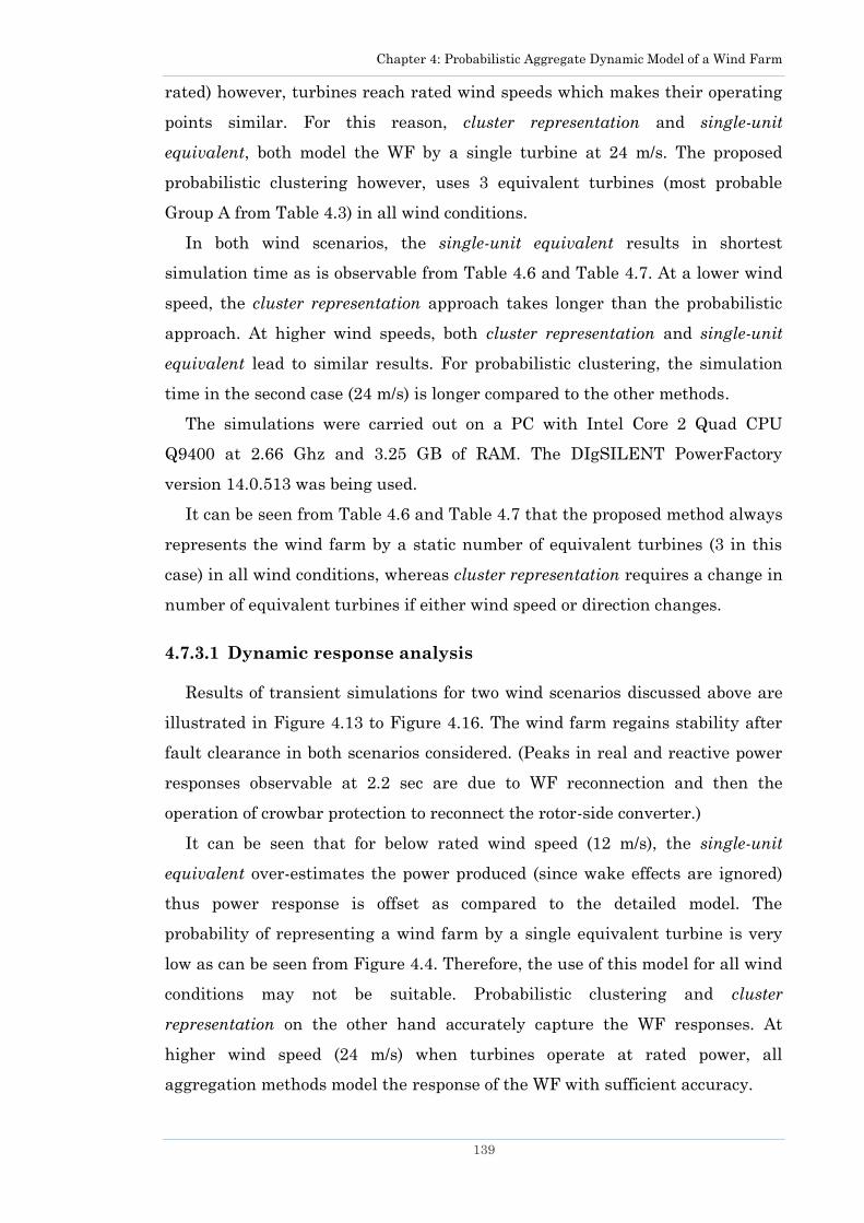
Chapter 4: Probabilistic Aggregate Dynamic Model of a Wind Farm
139
rated) however, turbines reach rated wind speeds which makes their operating
points similar. For this reason, cluster representation and single-unit
equivalent, both model the WF by a single turbine at 24 m/s. The proposed
probabilistic clustering however, uses 3 equivalent turbines (most probable
Group A from Table 4.3) in all wind conditions.
In both wind scenarios, the single-unit equivalent results in shortest
simulation time as is observable from Table 4.6 and Table 4.7. At a lower wind
speed, the cluster representation approach takes longer than the probabilistic
approach. At higher wind speeds, both cluster representation and single-unit
equivalent lead to similar results. For probabilistic clustering, the simulation
time in the second case (24 m/s) is longer compared to the other methods.
The simulations were carried out on a PC with Intel Core 2 Quad CPU
Q9400 at 2.66 Ghz and 3.25 GB of RAM. The DIgSILENT PowerFactory
version 14.0.513 was being used.
It can be seen from Table 4.6 and Table 4.7 that the proposed method always
represents the wind farm by a static number of equivalent turbines (3 in this
case) in all wind conditions, whereas cluster representation requires a change in
number of equivalent turbines if either wind speed or direction changes.
4.7.3.1 Dynamic response analysis
Results of transient simulations for two wind scenarios discussed above are
illustrated in Figure 4.13 to Figure 4.16. The wind farm regains stability after
fault clearance in both scenarios considered. (Peaks in real and reactive power
responses observable at 2.2 sec are due to WF reconnection and then the
operation of crowbar protection to reconnect the rotor-side converter.)
It can be seen that for below rated wind speed (12 m/s), the single-unit
equivalent over-estimates the power produced (since wake effects are ignored)
thus power response is offset as compared to the detailed model. The
probability of representing a wind farm by a single equivalent turbine is very
low as can be seen from Figure 4.4. Therefore, the use of this model for all wind
conditions may not be suitable. Probabilistic clustering and cluster
representation on the other hand accurately capture the WF responses. At
higher wind speed (24 m/s) when turbines operate at rated power, all
aggregation methods model the response of the WF with sufficient accuracy.
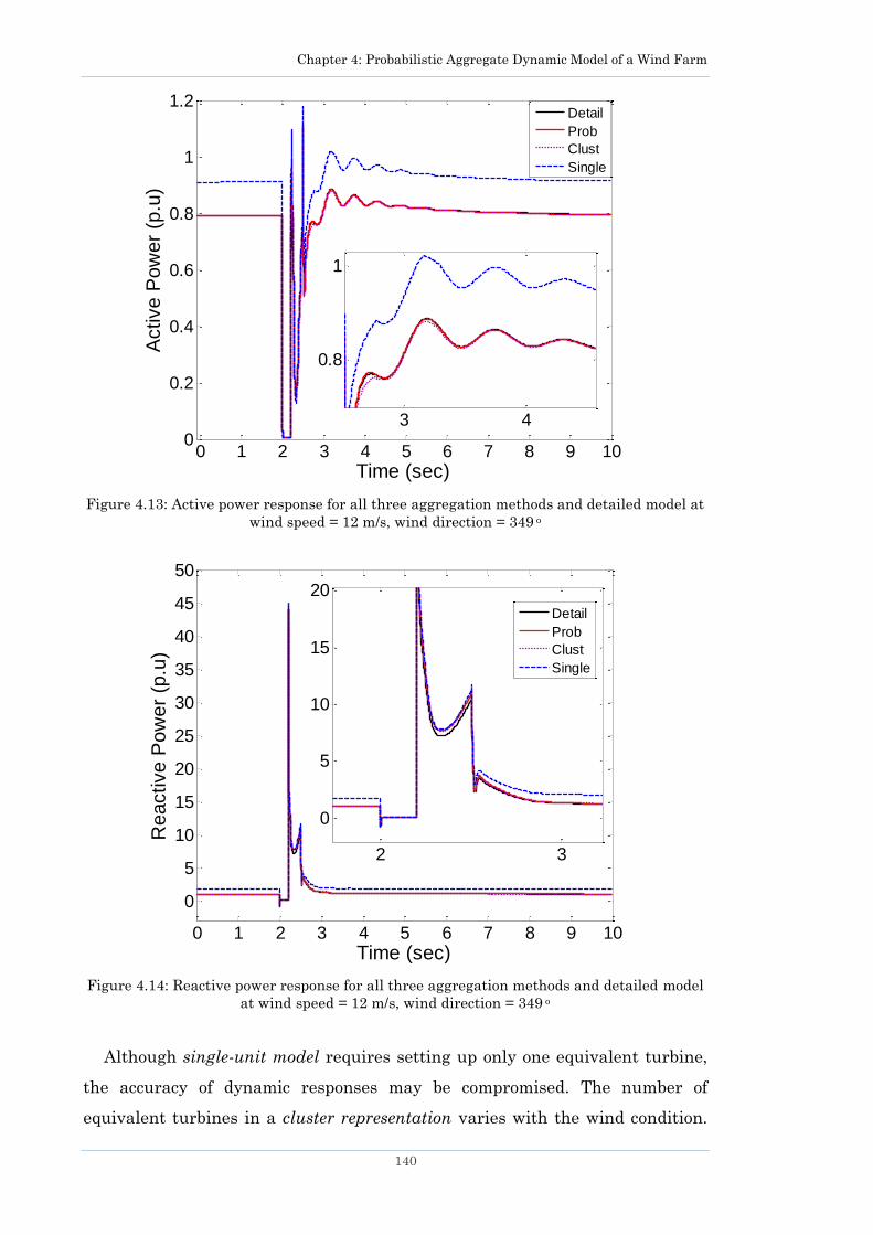
Chapter 4: Probabilistic Aggregate Dynamic Model of a Wind Farm
140
Figure 4.13: Active power response for all three aggregation methods and detailed model at
wind speed = 12 m/s, wind direction = 349 o
Figure 4.14: Reactive power response for all three aggregation methods and detailed model
at wind speed = 12 m/s, wind direction = 349 o
Although single-unit model requires setting up only one equivalent turbine,
the accuracy of dynamic responses may be compromised. The number of
equivalent turbines in a cluster representation varies with the wind condition.
0 1 2 3 4 5 6 7 8 9 100
0.2
0.4
0.6
0.8
1
1.2
Time (sec)
Active
Po
we
r (p
.u)
Detail
Prob
Clust
Single
3 4
0.8
1
0 1 2 3 4 5 6 7 8 9 10
0
5
10
15
20
25
30
35
40
45
50
Time (sec)
Reactive P
ow
er
(p.u
)
2 3
0
5
10
15
20
Detail
Prob
Clust
Single
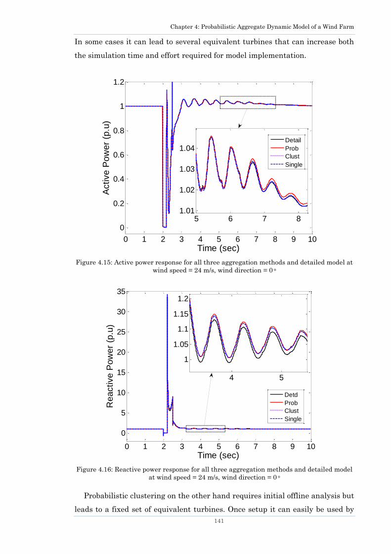
Chapter 4: Probabilistic Aggregate Dynamic Model of a Wind Farm
141
In some cases it can lead to several equivalent turbines that can increase both
the simulation time and effort required for model implementation.
Figure 4.15: Active power response for all three aggregation methods and detailed model at
wind speed = 24 m/s, wind direction = 0 o
Figure 4.16: Reactive power response for all three aggregation methods and detailed model
at wind speed = 24 m/s, wind direction = 0 o
Probabilistic clustering on the other hand requires initial offline analysis but
leads to a fixed set of equivalent turbines. Once setup it can easily be used by
0 1 2 3 4 5 6 7 8 9 10
0
0.2
0.4
0.6
0.8
1
1.2
Time (sec)
Active P
ow
er
(p.u
)
5 6 7 81.01
1.02
1.03
1.04
Detail
Prob
Clust
Single
0 1 2 3 4 5 6 7 8 9 10
0
5
10
15
20
25
30
35
Time (sec)
Re
active
Po
we
r (p
.u)
4 5
1
1.05
1.1
1.15
1.2
Detd
Prob
Clust
Single

Chapter 4: Probabilistic Aggregate Dynamic Model of a Wind Farm
142
simply adjusting the load flow parameters when wind conditions change. The
proposed method provides results with a good level of accuracy and leads to
significant reduction in simulation time. The proposed method is easier to use
under any wind condition. These features make it suitable for on-line (real
time) studies.
4.8 Summary
Aggregate WF models are required to reduce both complexity of the WF
network and the simulation time. This chapter presented a probabilistic
clustering method which can be applied to a WF of any size and layout
consisting of variable speed DFIG machines. It allows determination of a static
number of equivalent wind turbines and their corresponding rated powers that
will most accurately represent the WF during the year. It led to development of
probabilistic aggregate model of the WF.
Accuracy and reduction in simulation time of different aggregation methods
has been compared through dynamic response analysis. Performance of
detailed model of the WF was compared against two popular aggregation
methods, single-unit equivalent and cluster representation, as well as against
proposed probabilistic aggregate model. Comparison was made using a large 49
turbine wind farm connected to the grid through a collector transformer and
two transmission lines. A 3-phase fault was applied to one of the lines and
cleared after 200 ms.
The proposed probabilistic aggregation technique requires initial off-line
analysis of wind data to determine the most probable equivalent model of the
WF but subsequently leads to a simple aggregate model and shorter simulation
times. In the case studied, simulation time was reduced by 96%. It has been
demonstrated through dynamic simulations that the most probable group
(Group A) determined using the proposed technique can represent the WF for
any wind condition during the year, although it works best if the most probable
wind speeds and directions are used. To prove this point, two distinct cases
were tested that cover probable and least probable wind scenarios, but the
technique can be further validated by testing it at all wind speeds (within wind
turbine operating range) and wind directions (0o to 360o).
The method takes into account wind farm layout, wake effects and location
yet does not require, as in previously proposed methods, changes in an

Chapter 4: Probabilistic Aggregate Dynamic Model of a Wind Farm
143
equivalent model every time the wind speed or direction changes. This makes
the method very practical and easy to use. In previous method that considered
wake effect a different set of equivalent turbines had to be used if wind
conditions changed. The proposed technique leads to a static number of
equivalent turbines for any wind condition saving operator time and effort
readjusting the equivalent model. The probabilistic aggregate model also
provides much more accurate results than the single-unit equivalent model
(commonly applied to model WFs) at low wind speeds.
It has been demonstrated that the model is very useful for on-line and offline
studies as it can significantly reduce simulation time in modelling power
networks with large-scale penetration of wind power generation.
Chapter 5: Probabilistic Assessment of Wind Farm Energy Yield
144
Chapter 5 Probabilistic Assessment of Wind
Farm Energy Yield
Probabilistic Assessment of Wind Farm
Energy Yield
5.1 Introduction
Energy output is the main factor that contributes towards the feasibility of a
wind project. Its evaluation is essential for profit estimation and such analyses
are usually part of the pre-feasibility study for any wind farm (WF). Energy
output can vary due to several factors including site location and the WF
layout. Other factors such as availability of the wind resource at the site,
terrain characteristics of the site, wake losses in the WF, wind turbine and
cable availability in a WF collector system and electrical power losses occurring
inside the WF are also some of the influential factors that affect the energy
yield. Therefore, a reasonably realistic estimate of the energy output can be
only obtained once all important factors have been taken into account. This
chapter provides detailed methodologies to calculate the influence of these
factors on the energy output. A novel method to account for losses due to
unavailability of wind turbines and cables within a WF for four collector
systems is also proposed in this chapter.
The aim is to provide a complete methodology to perform energy yield study
for a new wind farm. A complete methodology should not only take into account
all influential factors that affect the energy output from a wind farm but also
the energy delivered to the grid. Transmission of energy to the grid is an
important consideration because the profits from a wind farm depend on the
energy sold. Therefore, prior to building the wind farm the owner of the wind
farm should have a complete picture of how much energy will be produced and
how much of this energy can be sold to the grid. In case a wind farm is planned

Chapter 5: Probabilistic Assessment of Wind Farm Energy Yield
145
to be built in an area with transmission bottlenecks it is likely that some of its
energy will be curtailed. For this reason, a new method to estimate the wind
energy curtailments is proposed. This method allows energy curtailment
evaluation in various possible scenarios, through use of correlation coefficients
between the wind power produced and the transmission line loading.
The impact of wind resource variation on the energy output and the energy
curtailed is also investigated. Furthermore, a sensitivity analysis is performed
to quantify the effect of different parameters on the energy yield.
5.2 Power Transmission Limitations
Wind farms are usually installed in open areas where wind speeds are high
and less disturbed. Such areas are often not very close to the load centres or
transmission lines [186]. An ideal location (a relatively windy site) for a WF in
terms of wind speeds may be a remote area, but the network in that area might
not be too strong. The wind power that can be transmitted to the grid may be
limited due to the capacity of the transmission lines.
Therefore, along with a good estimation of energy yield (considering all
influencing factors) it is also beneficial to determine the amount of energy that
can be transferred into the network. A complete study can enable a WF owner
to know the amount of energy that will be produced and the amount that will
be transferred into the grid.
Several factors can limit the power transmission in a network. The following
sections explore these factors briefly and provide potential measures to
overcome this bottleneck.
5.2.1 Bus Voltage limit
Voltage stability indicates the ability of a power system to maintain steady
voltages at all buses in the system under normal conditions and after being
subjected to a disturbance. Voltage instability commonly occurs due to voltage
drop but it has an equal chance of occurring due to over-voltages. Voltage drop
instability happens when reactive power demand increases beyond reactive
power support the system can provide, leading to loss of regional load. Over-
voltage instability is related to the capacitive behaviour of the network as well
as inability of synchronous compensators and generators to absorb the excess

Chapter 5: Probabilistic Assessment of Wind Farm Energy Yield
146
reactive power [187]. Typically, power system networks all over the world
define a range of acceptable voltages at the buses.
5.2.2 Thermal limit
Current flowing through a conductor can increase its temperature due to I2R
load losses caused by resistance of the conductor. To prevent a transmission
line from sagging and losing tensile strength, thermal power flow limits are
imposed. Generally, transmission components age with time and temperature.
To prevent putting at risk the integrity of the physical components and to
ensure a reliable operation, it is essential to identify safe thermal operating
limits for the network components. This is often performed based on regional
climate.
Meteorological factors such as solar radiation, speed of the wind and ambient
temperature affects the temperature of an overhead line [188]. The
temperature of the line conductor can be calculated using (5.1) and (5.2), more
details can be found in [189].
Heat Gain = Heat Loss (5.1)
( ) J M S i i con R WP P P k P P P P (5.2)
where PJ is heat gain due to Joule heating, PM is heat gain due to ferromagnetic
heating, PS is heat gain due to the solar heating, Pi heat gain due to ionization
heating, (PJ, PM, PS and Pi are given in per unit length per unit time,) factor ki
takes into account thermal diffusion, Pcon is heat loss by convection, PR is heat
loss by radiation and PW is heat loss by evaporation respectively.
5.2.3 Methods to overcome power transmission bottlenecks
Thermal limit constraints can be relaxed by optimising the distribution of
power flow to minimise the current at critical branches, or by increasing the
current handling capacity of the lines, breakers and transformers. A few
possible solutions to remove thermal limit concerns are discussed below [190]:
Replace substation equipment to handle more current.
Introduce dynamic line rating; it works by determining the dynamic
current carrying capacity of the lines through real-time monitoring of
line tension, sag, temperature and current flow. The network operator
can decide on the line loading based on the online temperature readings.

Chapter 5: Probabilistic Assessment of Wind Farm Energy Yield
147
Re-tension and re-conductor the existing lines [191] e.g. replace a
conductor rated at 500 A at 75 degrees with a thicker conductor to allow
higher current flow or with a high temperature low sag conductor to
double the original line rating (1000 A at 200 degrees).
Control the power flow through Flexible Alternating Current
Transmission System (FACTS) devices, Phase Angle Regulars (PARs),
capacitors and Static Var Compensators.
Use phase shifting transformers.
Re-calculate thermal line ratings using more realistic weather conditions
(measurements made on the site).
Voltage stability limit problems can be solved with the use of shunt reactors
and tap-changing transformers. If power generated by a WF has to be
transmitted far away then series capacitors can be installed to maintain the
voltages at the line terminals.
Building an overhead transmission line can solve power flow problems,
however, it is getting increasingly difficult to obtain planning permissions to
build new lines as they affect the landscape and lead to public and political
resistance [192]. Apart from this, new lines are very expensive to build
especially when new towers have to be put in place. Generally, installation of a
new line is accompanied with modifications to the substation components such
as switchgears and reactors. All of these factors can offset the cost of the project
[191]. In the UK, a WF developer has to the bear cost for building a new
infrastructure needed for WF installation [20]. Estimated cost (per mile) to
build a new overhead line [193] is illustrated in Table C.1 in Appendix C. It can
be seen from Table C.1 that the cost per mile of a new transmission line can be
as high as €1.15 Million (£1 Million).
One possible way to relax power transfer limitation is to convert high voltage
AC (HVAC) lines to high voltage DC (HVDC) lines as this allows increase in
power transmission rating and reduces transmission losses. The costs of HVDC
converter stations are however very high and they significantly increase the
cost of the overall HVDC transmission link.
Another possible option is to curtail (prevent injection into the line) excess
power from the WF at times when loading of the line is high and wind power
generation is also high. Depending on the capacity and flexibility of the
generators present the utilities may prefer to keep supply from more reliable
Chapter 5: Probabilistic Assessment of Wind Farm Energy Yield
148
generators which might lead to temporary wind power curtailments. When
curtailments are needed system operators request wind generators to reduce
their power output (by pitching the blades out of wind or by completely shutting
down the turbines). This practise is common in countries such as the UK, parts
of USA [194] and Spain. It prevents making changes to the transmission
network, but on the other hand, WF owner might lose money for not selling the
available energy to the grid. If potential energy loss due to possible future
curtailments can be estimated by the WF owner in advance then a correct
economic decision could be made.
All measures discussed above will increase costs either to the utility or to the
WF owner (depending on the country policy), therefore, wind power curtailment
might be a cheaper option. The following sections present a methodology to
estimate as accurately as possible the energy yield from a WF considering all
important factors and energy curtailments.
5.3 Estimation of Wind Energy Yield
This section provides complete methodology for estimation of wind farm
energy yield. The impact of various factors including wake effects, electrical
losses, availability of wind farm components and variation in wind resource is
tested on the overall energy yield output.
A wind farm installed at two different locations (onshore and offshore), with
wind turbines of different heights and at different distances from each other is
simulated to determine the wake induced power losses in different scenarios. A
new methodology to study the impact of wind farm component availability on
annual energy production is developed. The impact of annual variation in wind
speed (at a site) on annual energy output is also tested considering internal
wind farm losses.
As a case study a hypothetical wind farm is assumed to be installed at an
area with a transmission bottleneck. A new methodology developed to estimate
the curtailment losses from a wind farm. The method is based on an existing
technique proposed in [96]. The factors that affect the energy yield of a wind
farm were, however, largely ignored there. In the method proposed here, the
effect of wake losses, electrical losses, impact of component availability, impact
of variation in wind resource at a site and correlation coefficients between wind
speed, turbine availability and transmission line loading are all included.
Chapter 5: Probabilistic Assessment of Wind Farm Energy Yield
149
Therefore, the new methodology provides a more realistic solution as all
influential factors are now considered.
5.3.1 Wind potential availability
In order to evaluate wind potential at a site, the wind speed is measured for
at least one year. Wind turbine generates power only if the incoming wind
speed is between its operating range, i.e. between the cut-in and the cut-out
wind speed. For a general estimate of the energy yield a Weibull distribution is
sufficient, but for pre-feasibility studies of the wind farms the wind
measurement data is usually essential. In this study, the power output from a
wind turbine is calculated by tracing the wind speed on the power curve.
Using the recorded wind data a wind speed distribution can be obtained.
Once wind speed distribution is known, the wind power production distribution
function (WPPDF) can be calculated.
For simplicity, let Y be the expected wind power production in MW. Using
wind speed distribution function, the power production state Y of the planned
WF can be obtained multiplying (2.5) with number of wind turbines K in a WF.
Then discrete probability mass function and distribution functions of Y can
be calculated as follows [96]:
N
yhyYPyf Y
Y
)()()(
yyi
iYY
i
yfyYPyF:
)()()(
(5.3)
where P(Y = y) is the probability that wind power production Y is equal to y
(MW), hY(y) is frequency of y, N is number of wind speed measurements.
Finally, energy yield of a WF can be calculated as:
max
0
( )y
Y
y
E F y y
(5.4)
where y is a step at which WPPDF ( )YF y is discretised. This method to obtain
an initial estimate of energy yield was used in [63] and [64]. Wake losses and
electrical losses inside a WF are then subtracted using very general loss
estimates. Those losses however are case specific and in reality can vary
significantly with size and layout of the WF.
Chapter 5: Probabilistic Assessment of Wind Farm Energy Yield
150
5.3.2 Wind farm layout
A small 9 turbine WF consisting of 2 MW Vestas V80 wind turbines is used
for the analysis (see Figure 3.14). Each wind turbine has a built-in 0.69/33 kV
transformer in the nacelle that steps up the voltage level from the generator
voltage to 33 kV. This voltage level is used inside the collector system
connecting the turbines. Based on the available data from existing WFs of
similar size [21, 26] as the one studied here it is assumed that the studied WF
does not have an offshore transformer. The WF is assumed to be 8 km away
from the shore and is connected with the grid through AC XLPE cables. Four
different electrical layouts presented in Section 1.2.2.4 are studied for losses.
One year of wind measurement data measured at the height of 35 meters
(given in Section 3.8) are scaled up to the turbine height using (3.6).
5.3.3 Wake effects
Detailed models are used for wake effect calculation considering single,
partial and multiple shadowing of wind turbines as discussed in Section 3.3.
Applying wake models to the up scaled wind measurements, wind speed at each
turbine within a WF is estimated for the given WF layout. Since wake effect
depends on both, the speed and direction of the incoming wind, the power
production from each wind turbine is calculated after modelling wakes for every
incoming wind speed and wind direction. Total energy yield of the WF is then
estimated by summing the individual wind turbine power production for the
whole year.
There are many site specific factors which influence the wake effects and
hence the energy yield. These include wind characteristics at a site, size and
layout of the WF, height of the wind turbines, distance between the turbines,
terrain of the site, radius of the wind turbine rotor, thrust coefficient curve and
power curve of the wind turbine. Impact of some of these factors on the energy
yield are briefly discussed below. Wake effects are simulated for a wind farm in
two terrain conditions i.e. onshore and offshore, with standard terrain
roughness lengths of 0.0002 m and 0.1 m respectively (see Table 3.1).
Highest wake losses are observed to occur for wind speeds between 6 and 10
m/s when the thrust coefficient Ct is relatively high.

Chapter 5: Probabilistic Assessment of Wind Farm Energy Yield
151
5.3.4 Electrical power losses
Energy yield from a WF is further reduced due to electrical losses in the
collector system. These losses vary with the type of the collector system, cable
and transformers parameters. Four typical collector systems namely radial,
starburst, single-sided ring and central are analysed for electrical losses. These
collector systems are discussed in Section 1.2.2.4 in detail. In a radial collector
system shown in Figure 5.1, the electrical power loss in a string can be found
as:
2 22
1 1 1 1 13 ... ...
string
loss n n n n n n nP R I R I I R I I I
(5.5)
where R is line resistance, I is the current flowing in the lines. Once power loss
from each string is evaluated, the total power loss in the WF can be calculated
as the sum of power loss in m strings along with power loss in the main cable
carrying current from all m strings to the shore.
2
_ _
1
3
mcable to shore
loss T iP R I
(5.6)
_ _
1
mtotal string cable to shore
loss loss lossP P P
(5.7)
In central collector system configuration, Figure 5.2, power losses can be
calculated as in radial configuration with only two strings using (5.5), (5.6) and
(5.7). Current from two strings is collected at one central wind turbine from
where it is passed on to the shore through a main cable.
In single-sided ring system shown in Figure 5.3, the power loss is computed
for each string in a similar way to that of the radial configuration (5.5),
however in this case each string is carrying power directly to the shore. Total
losses are equal to the sum of losses in the individual strings. Each string is
equipped with a redundant cable (shown in grey colour) capable of transferring
power in case of a fault in the main cable or in any cable within the string.
Increased security comes however at extra cost for redundant lines.
The power loss calculation for the starburst collector system shown in Figure
5.4 is slightly different. There are different ways to set-up a starburst network
as discussed in [24] and [26]. The configuration analysed here is based on [24],
where the total power loss is calculated using (5.8) to (5.11) for m clusters.
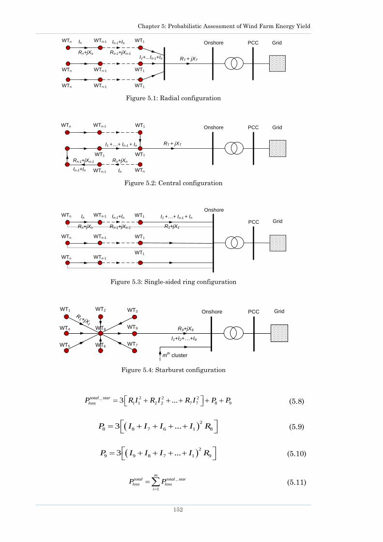
Chapter 5: Probabilistic Assessment of Wind Farm Energy Yield
152
Figure 5.1: Radial configuration
Figure 5.2: Central configuration
Figure 5.3: Single-sided ring configuration
Figure 5.4: Starburst configuration
_ 2 2 2
1 1 2 2 7 7 8 93 ...total star
lossP R I R I R I P P (5.8)
2
8 8 7 6 1 83 ...P I I I I R
(5.9)
2
9 9 8 7 1 93 ...P I I I I R
(5.10)
_
1
mtotal total star
loss loss
i
P P
(5.11)
InWTn
Rn+jXn
WTn-1 WT1In-1+In
I1+...In-1+In
Onshore PCC
RT + jXT
Rn-1+jXn-1
WTn WTn-1 WT1
WTn WTn-1 WT1
Grid
In
WTn
Rn+jXn
WTn-1
In-1+In
Onshore PCC
RT + jXT
Rn-1+jXn-1
WTT
WTnWTn-1
WT1
I1 +…+ In-1 + In
WT1 Grid
InWTn WTn-1 WT1In-1+In
Onshore
PCC
WTn WTn-1 WT1
WTn WTn-1
WT1
I1 +…+ In-1 + In
Rn+jXn Rn-1+jXn-1 R1+jX1
Grid
WT1 WT2 WT3 Onshore PCC
R9+jX9WT4 WT8WT9
WT5 WT6WT7
R1+jX
1
I1+I2+…+I9
mth cluster
Grid
Chapter 5: Probabilistic Assessment of Wind Farm Energy Yield
153
In general, losses inside the transformers are divided into two types, no-load
losses and load losses. No-losses arise due to energisation of the core of the
transformer and remain unaffected by the loading of the transformer. Load
losses vary depending on the amount of power transferred through the
windings (copper losses). Load losses are simply I2R losses and can increase as
the amount of current increases through the winding coils. Therefore if current
and resistance of the winding coils are known they can be easily computed. No-
load losses on the other hand remain constant; and are generally a small
percentage of the MVA of a transformer.
5.3.5 Wind farm losses due to reliability considerations
With development of wind turbine technology and increase of WF size,
reliability is becoming more important as it influences the energy delivered.
Analysis of reliability indices of different wind turbine components based on
cumulative statistics is given in [195]. Reference [196] provides a more detailed
analysis from a group of 3 adjacent WFs. It is shown that there is significant
variability in occurrence and duration of tripping of WTs depending on their
location within a WF. In [197] reliability indices of a WF are calculated based
on component failure rates, repair times and duration of switching operation.
However wind speed duration curve is approximated by several characteristic
regions weighted by corresponding probability of occurrence. Single component
failures and some multi-component failures (only those with highest
probabilities) are simulated.
In this chapter, single and all multi-component failures are considered. Wind
speed duration curve is discretised to integer values and all wind speeds within
wind turbine operating range are taken into account.
5.3.5.1 Wind farm availability distribution function
5.3.5.1.1 Wind farm configurations (without redundancy)
A step-by-step procedure is developed for calculation of WF availability using
combinatorial algorithms. These steps are described below:
Step 1: Obtain failure rates and repair rates of involved components (wind
turbines, transformers, cables);
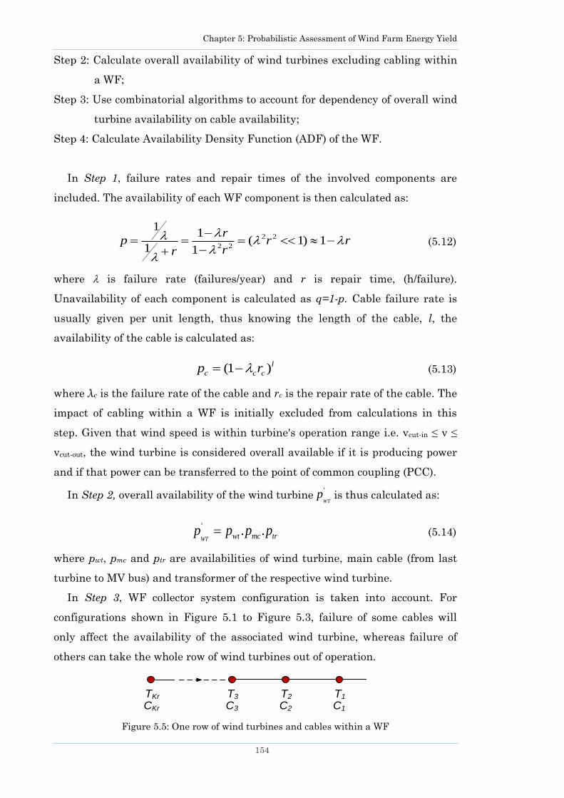
Chapter 5: Probabilistic Assessment of Wind Farm Energy Yield
154
Step 2: Calculate overall availability of wind turbines excluding cabling within
a WF;
Step 3: Use combinatorial algorithms to account for dependency of overall wind
turbine availability on cable availability;
Step 4: Calculate Availability Density Function (ADF) of the WF.
In Step 1, failure rates and repair times of the involved components are
included. The availability of each WF component is then calculated as:
2 2
2 2
11
( 1) 11 1
rp r r
rr
(5.12)
where is failure rate (failures/year) and r is repair time, (h/failure).
Unavailability of each component is calculated as q=1-p. Cable failure rate is
usually given per unit length, thus knowing the length of the cable, l, the
availability of the cable is calculated as:
(1 )l
c c cp r
(5.13)
where λc is the failure rate of the cable and rc is the repair rate of the cable. The
impact of cabling within a WF is initially excluded from calculations in this
step. Given that wind speed is within turbine's operation range i.e. vcut-in ≤ v ≤
vcut-out, the wind turbine is considered overall available if it is producing power
and if that power can be transferred to the point of common coupling (PCC).
In Step 2, overall availability of the wind turbine'
WTp is thus calculated as:
' . .WT wt mc trp p p p
(5.14)
where pwt, pmc and ptr are availabilities of wind turbine, main cable (from last
turbine to MV bus) and transformer of the respective wind turbine.
In Step 3, WF collector system configuration is taken into account. For
configurations shown in Figure 5.1 to Figure 5.3, failure of some cables will
only affect the availability of the associated wind turbine, whereas failure of
others can take the whole row of wind turbines out of operation.
Figure 5.5: One row of wind turbines and cables within a WF
TKr
CKr
T3
C3
T2
C2
T1
C1
Chapter 5: Probabilistic Assessment of Wind Farm Energy Yield
155
Calculation of WF availability for radial, single-sided ring and central
configurations are discussed below. Consider just one row of the wind turbines
first, as shown in Figure 5.5. For lc components in a row, all possible
combinations of component statuses, cs, are generated using a combinatorial
algorithm [198]. The component status is assumed to be 1 if in operation and 0
otherwise. Thus 2lc x lc matrix is obtained. Each row of the matrix contains a
unique combination of component statuses. For each combination the number
of overall available wind turbines is calculated:
1 1 2 2 ... ...cs Kr KrN C T C T C T
(5.15)
where Ci is a status of cable i, Ti is status of wind turbine and its transformer,
Kr is the number of wind turbines in a row. If instead of component statuses Ti
and Ci, respective component availabilities p'WT and pc (if status=1) or
unavailabilities q'WT and qc (if status=0) are substituted in the matrix and then
(5.15) is applied, the result is probability of certain combination of component
statuses, pcs. Summing probabilities of combinations cs that yield the same
number of available wind turbines (i.e. equal values of Ncs) overall availability
of WTs in a row is obtained, Availability Density Function of a row is then:
r
:
( ) , [0, ]cs
ow cs r
cs N k
P k p k K
(5.16)
where Prow (k) is probability that in one row k wind turbines are available and
able to deliver power to the PCC.
In Step 4, availability density of the entire WF is calculated. Assuming WF
consists of m rows of wind turbines. In each row 0 to Kr wind turbines can be
available. Let k(0, Kr) denote the row status. Using combinatorial algorithm
(Kr+1)m x m matrix is generated. Each row of the matrix contains a unique
combination of WF row statuses. If each element of the matrix is substituted
with respective probability, Prow(k), then product of the elements in each row of
the matrix will yield probability of the combination. Summing probabilities of
combinations yielding same number of available wind turbines in the WF,
similarly to (5.16), ADF of the entire WF can be obtained.
For starburst WF configuration, the availability of the interconnecting cable,
c, within a WF will only affect the overall availability of the associated wind
turbine:
Chapter 5: Probabilistic Assessment of Wind Farm Energy Yield
156
' . . .WT wt mc tr cp p p p p
(5.17)
For K identical wind turbines within a WF each of which may fail, there are
K + 1 wind turbine availability statuses. The probability of each status depends
on total number of wind turbines and overall availability of a single turbine.
Availability density of the starburst configured WF system [199]:
' '!
( ) (1 )!( )!
k K k
WF WT WT
Kp k p p
k K k
(5.18)
where p'WT is the overall wind turbine availability, calculated by (5.17).
5.3.5.2 Wind power production distribution
All the above factors, i.e., wake effect, electrical losses and WF availability
should be accounted for in the WPPDF, in order to calculate realistic WF
energy yield. Because of wake effects, power production of each wind turbine
depends on its location within a WF, wind speed and wind direction. Thus to
calculate WF power production state, wake effect model presented above should
be used, rather than just (2.5) multiplied by number of wind turbines in a WF
over a year. Respective electrical losses based on collector system should be
subtracted and then discrete probability density and distribution functions of
WF power production calculated from (5.3). Each power production state then
accounts for wake and electrical losses, and probability of each state depends on
probability of the corresponding wind speed and wind direction.
Next factor to account for is the availability of wind turbines, associated
transformers and cables. However, location of unavailable wind turbines will
affect the wake that neighbouring turbines are experiencing. This leads to a
very high number of availability states that need to be taken into account. In
order to resolve the trade-off between dimensionality and accuracy a
simplification is introduced. Power production of each wind turbine within a
WF is calculated for each wind speed and direction considering the wake effects
and electrical losses. Sum of individual wind turbine productions is then
divided by a number of wind turbines in a WF, yielding equivalent power curve
of wind turbine, SWT_eq(v). The individual impact of wake and electrical losses at
turbine level is thus effectively averaged amongst all wind turbines in a WF.
Chapter 5: Probabilistic Assessment of Wind Farm Energy Yield
157
Change in wake effect and electrical losses due to wind turbines being out of
service are neglected. Location of unavailable wind turbines in this way
becomes irrelevant.
All possible WF power production states can now be obtained multiplying
SWT_eq(v) by number of available wind turbines kn, kn{0, K}, where K is a total
number of wind turbines in a WF. Note that WF power production states do not
uniquely correspond to certain wind speed as the same power production states
can occur at several (kn, v) combinations, where v is the wind speed.
5.3.5.3 Correlation between wind speed and wind turbine
availability
To account for overall wind turbine availability in WPPDF an assumption
should be made about correlation between wind speed and wind turbine failure.
If there is a strong negative correlation between wind speed and overall wind
turbine availability then more energy is lost. So far, there have been no publicly
available reports addressing this problem. Data from [200] from 3 adjacent
onshore WFs were used to analyze correlation between failures of wind
turbines and wind speed within operating range of wind turbine. For each wind
turbine in the WFs the time series of wind speed measurements and
simultaneous time series of wind turbine statuses (1 if in operation, 0
otherwise) were used to obtain correlation coefficients between wind turbine
status and wind speed. For the studied WFs the correlation between wind
turbine failures and wind speed conditions proved to be very weak (close to 0).
It is difficult to draw general conclusions based on just one study, in
particular as WFs in [200] were onshore. It is possible though that offshore
weather conditions have more impact on the availability of wind turbines.
Thus, the method for evaluation of all extreme correlation combinations
between wind speed and overall wind turbine availability, i.e., 1, 0, -1, is
presented in this chapter.
If correlation between wind speed and wind turbine availability is 1,
meaning wind turbines are in operation when wind speed is high, Wind
Production Duration Curve (WPDC) is constructed from wind power production
distribution function calculated in Section 5.3.5.2. The WPDC already includes
the effect of wake and electrical losses. Availability density calculated as in
Section 5.3.5.1 is then multiplied by number of hours in studied period T and
Chapter 5: Probabilistic Assessment of Wind Farm Energy Yield
158
sorted in the descending order by the number of available wind turbines
yielding availability duration curve (ADC). New Wind Production Duration
Curve (WPDC’) including the impact of wind turbine availability is then
obtained as follows:
)()(
)(' tADCK
tWPDCtWPDC
(5.19)
where t is a discretisation step of the duration curves, (e.g. 1 hour) and K is
total number of wind turbines in a WF.
Similar calculations are performed if correlation is -1 between wind speed
conditions and overall wind turbine availability, i.e., fewer wind turbines are
available when the wind speed is high. Discrete Availability Distribution is
then sorted in the ascending order by the number of available wind turbines to
obtain discrete Unavailability Distribution Curve (UDC). The UDC is then
substituted in (5.19), instead of ADC.
For both cases, i.e., correlation 1 and -1, the WF production discrete
probability distribution function (WPPDF) FY (y), with wind turbine availability
included, is obtained as inverted WPDC' divided by period T.
If correlation between wind turbine failures and wind speed is 0, WF
production discrete probability distribution function FY(y) can be obtained by
combining WF discrete Availability Distribution Function and discrete
Distribution Function of WF power production states from Section 5.3.5.1 (see
[201] for details).
5.3.5.4 Losses due to unavailability of WF components
According to statistics in [202], [203] availability of the wind turbine varies
approximately between 95% and 100% on yearly basis depending on the
weather conditions, age of wind turbine, etc. Results from [200] however show
that wind turbine availability can diverge significantly from these values
depending on wind turbine location within a WF. Comparing FY(y) calculated
with different correlation assumptions, (Section 5.3.5.3), with FY(y) where
reliability is disregarded (Section 5.3.1) the range of losses due to unavailability
of WF components is obtained:

Chapter 5: Probabilistic Assessment of Wind Farm Energy Yield
159
max
0
max'
0
( ).
( ). | 100%
y
Y
y
av y
Y WT
y
F y y
L
F y y p
(5.20)
where y is a step at which Wind Production Probability Distribution
Function FY(y) is discretised
5.3.6 Losses due to wind energy curtailment
If total power produced by a WF cannot be injected into the system, i.e., if
there is congestion; additional losses might be introduced in form of wind
energy curtailments. Alternatively, transmission system may need
reinforcement.
Under deregulated market conditions it is not always clear how the
investment costs should be divided between the network operators and the
production utilities. Different countries use different approaches (Deep,
Shallowish, Shallow) [13] when determining network connection costs. An
optimal balance therefore, should be found between extra benefits arising from
increased transmission capacity and costs of respective network
reinforcements. Findings in [96] confirmed that in some cases it is more
economical to curtail some wind energy during transmission congestion
situations than to build a new transmission line. This alternative is currently
used, e.g. in Spain where significant number of WFs located between Galicia
and Madrid produce power below their full capacity since the necessary
reinforcements of the transmission grid have not been realized yet [204].
Wind energy curtailment at each hour depends on wind speed, wake losses,
electrical losses, availability of wind turbines and already committed
transmission over the line, i.e., Transmission Line Loading (TLL). In order to
estimate potential wind energy curtailments accurately, realistic assumption
needs to be made regarding correlation between wind speed and wind turbine
availability and between TLL and WF power production. In this study, it is
assumed that there is a single transmission corridor between the load centre
and the WF connection point and that curtailment is a cheaper option as WF
capacity is not significantly large. This method is particularly useful when less
information about the network is available i.e. only Transmission Duration
Curve (TDC) and Line Capacity (C) are known.
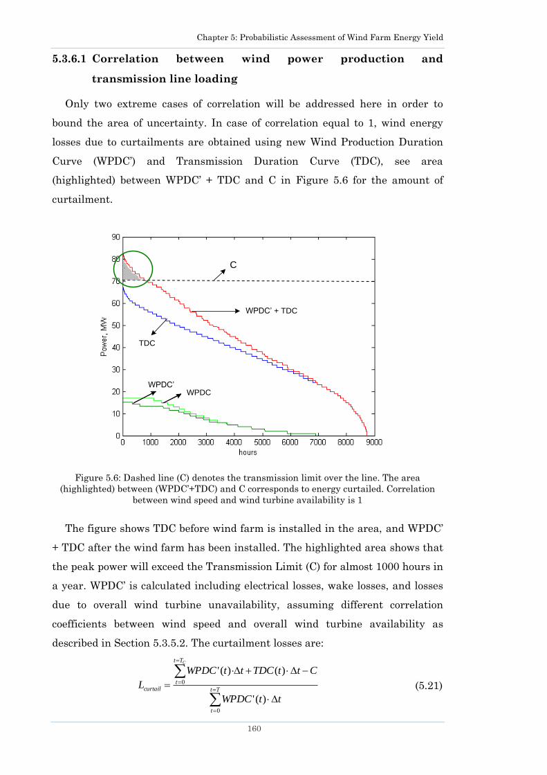
Chapter 5: Probabilistic Assessment of Wind Farm Energy Yield
160
5.3.6.1 Correlation between wind power production and
transmission line loading
Only two extreme cases of correlation will be addressed here in order to
bound the area of uncertainty. In case of correlation equal to 1, wind energy
losses due to curtailments are obtained using new Wind Production Duration
Curve (WPDC‘) and Transmission Duration Curve (TDC), see area
(highlighted) between WPDC‘ + TDC and C in Figure 5.6 for the amount of
curtailment.
Figure 5.6: Dashed line (C) denotes the transmission limit over the line. The area
(highlighted) between (WPDC‘+TDC) and C corresponds to energy curtailed. Correlation
between wind speed and wind turbine availability is 1
The figure shows TDC before wind farm is installed in the area, and WPDC‘
+ TDC after the wind farm has been installed. The highlighted area shows that
the peak power will exceed the Transmission Limit (C) for almost 1000 hours in
a year. WPDC‘ is calculated including electrical losses, wake losses, and losses
due to overall wind turbine unavailability, assuming different correlation
coefficients between wind speed and overall wind turbine availability as
described in Section 5.3.5.2. The curtailment losses are:
Tt
t
Tt
tcurtail
ttWPDC
CttTDCttWPDC
L
C
0
0
)('
)()('
(5.21)
TDC
WPDC’ + TDC
WPDC’WPDC
C
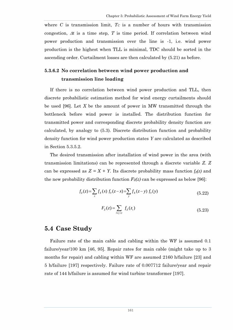
Chapter 5: Probabilistic Assessment of Wind Farm Energy Yield
161
where C is transmission limit, TC is a number of hours with transmission
congestion, t is a time step, T is time period. If correlation between wind
power production and transmission over the line is -1, i.e. wind power
production is the highest when TLL is minimal, TDC should be sorted in the
ascending order. Curtailment losses are then calculated by (5.21) as before.
5.3.6.2 No correlation between wind power production and
transmission line loading
If there is no correlation between wind power production and TLL, then
discrete probabilistic estimation method for wind energy curtailments should
be used [96]. Let X be the amount of power in MW transmitted through the
bottleneck before wind power is installed. The distribution function for
transmitted power and corresponding discrete probability density function are
calculated, by analogy to (5.3). Discrete distribution function and probability
density function for wind power production states Y are calculated as described
in Section 5.3.5.2.
The desired transmission after installation of wind power in the area (with
transmission limitations) can be represented through a discrete variable Z. Z
can be expressed as Z = X + Y. Its discrete probability mass function fZ(z) and
the new probability distribution function FZ(z) can be expressed as below [96]:
( ) ( ) ( ) ( ) ( )Z X Y X Y
x y
f z f x f z x f z y f y
(5.22)
:
( ) ( )i
Z Z i
i z z
F z f z
(5.23)
5.4 Case Study
Failure rate of the main cable and cabling within the WF is assumed 0.1
failure/year/100 km [46, 95]. Repair rates for main cable (might take up to 3
months for repair) and cabling within WF are assumed 2160 h/failure [23] and
5 h/failure [197] respectively. Failure rate of 0.007712 failure/year and repair
rate of 144 h/failure is assumed for wind turbine transformer [197].
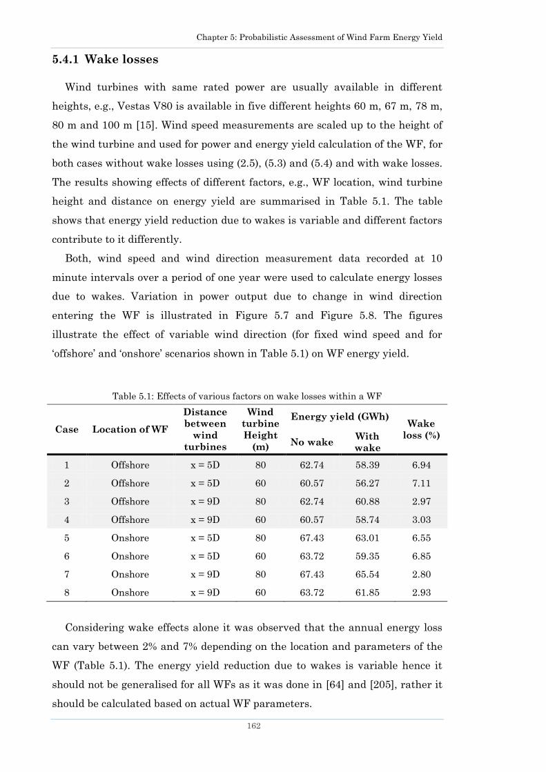
Chapter 5: Probabilistic Assessment of Wind Farm Energy Yield
162
5.4.1 Wake losses
Wind turbines with same rated power are usually available in different
heights, e.g., Vestas V80 is available in five different heights 60 m, 67 m, 78 m,
80 m and 100 m [15]. Wind speed measurements are scaled up to the height of
the wind turbine and used for power and energy yield calculation of the WF, for
both cases without wake losses using (2.5), (5.3) and (5.4) and with wake losses.
The results showing effects of different factors, e.g., WF location, wind turbine
height and distance on energy yield are summarised in Table 5.1. The table
shows that energy yield reduction due to wakes is variable and different factors
contribute to it differently.
Both, wind speed and wind direction measurement data recorded at 10
minute intervals over a period of one year were used to calculate energy losses
due to wakes. Variation in power output due to change in wind direction
entering the WF is illustrated in Figure 5.7 and Figure 5.8. The figures
illustrate the effect of variable wind direction (for fixed wind speed and for
‗offshore‘ and ‗onshore‘ scenarios shown in Table 5.1) on WF energy yield.
Table 5.1: Effects of various factors on wake losses within a WF
Case Location of WF
Distance
between
wind
turbines
Wind
turbine
Height
(m)
Energy yield (GWh) Wake
loss (%) No wake
With
wake
1 Offshore x = 5D 80 62.74 58.39 6.94
2 Offshore x = 5D 60 60.57 56.27 7.11
3 Offshore x = 9D 80 62.74 60.88 2.97
4 Offshore x = 9D 60 60.57 58.74 3.03
5 Onshore x = 5D 80 67.43 63.01 6.55
6 Onshore x = 5D 60 63.72 59.35 6.85
7 Onshore x = 9D 80 67.43 65.54 2.80
8 Onshore x = 9D 60 63.72 61.85 2.93
Considering wake effects alone it was observed that the annual energy loss
can vary between 2% and 7% depending on the location and parameters of the
WF (Table 5.1). The energy yield reduction due to wakes is variable hence it
should not be generalised for all WFs as it was done in [64] and [205], rather it
should be calculated based on actual WF parameters.
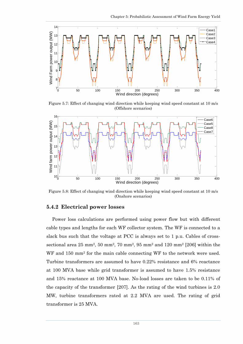
Chapter 5: Probabilistic Assessment of Wind Farm Energy Yield
163
0 50 100 150 200 250 300 350 4007
8
9
10
11
12
13
14
Wind direction (degrees)
Win
d F
arm
pow
er
outp
ut
(MW
)
Case1
Case2
Case3
Case4
Figure 5.7: Effect of changing wind direction while keeping wind speed constant at 10 m/s
(Offshore scenarios)
0 50 100 150 200 250 300 350 40010
11
12
13
14
15
16
Wind direction (degrees)
Win
d f
arm
pow
er
outp
ut
(MW
)
Case6
Case5
Case8
Case7
Figure 5.8: Effect of changing wind direction while keeping wind speed constant at 10 m/s
(Onshore scenarios)
5.4.2 Electrical power losses
Power loss calculations are performed using power flow but with different
cable types and lengths for each WF collector system. The WF is connected to a
slack bus such that the voltage at PCC is always set to 1 p.u. Cables of cross-
sectional area 25 mm2, 50 mm2, 70 mm2, 95 mm2 and 120 mm2 [206] within the
WF and 150 mm2 for the main cable connecting WF to the network were used.
Turbine transformers are assumed to have 0.22% resistance and 6% reactance
at 100 MVA base while grid transformer is assumed to have 1.5% resistance
and 15% reactance at 100 MVA base. No-load losses are taken to be 0.11% of
the capacity of the transformer [207]. As the rating of the wind turbines is 2.0
MW, turbine transformers rated at 2.2 MVA are used. The rating of grid
transformer is 25 MVA.
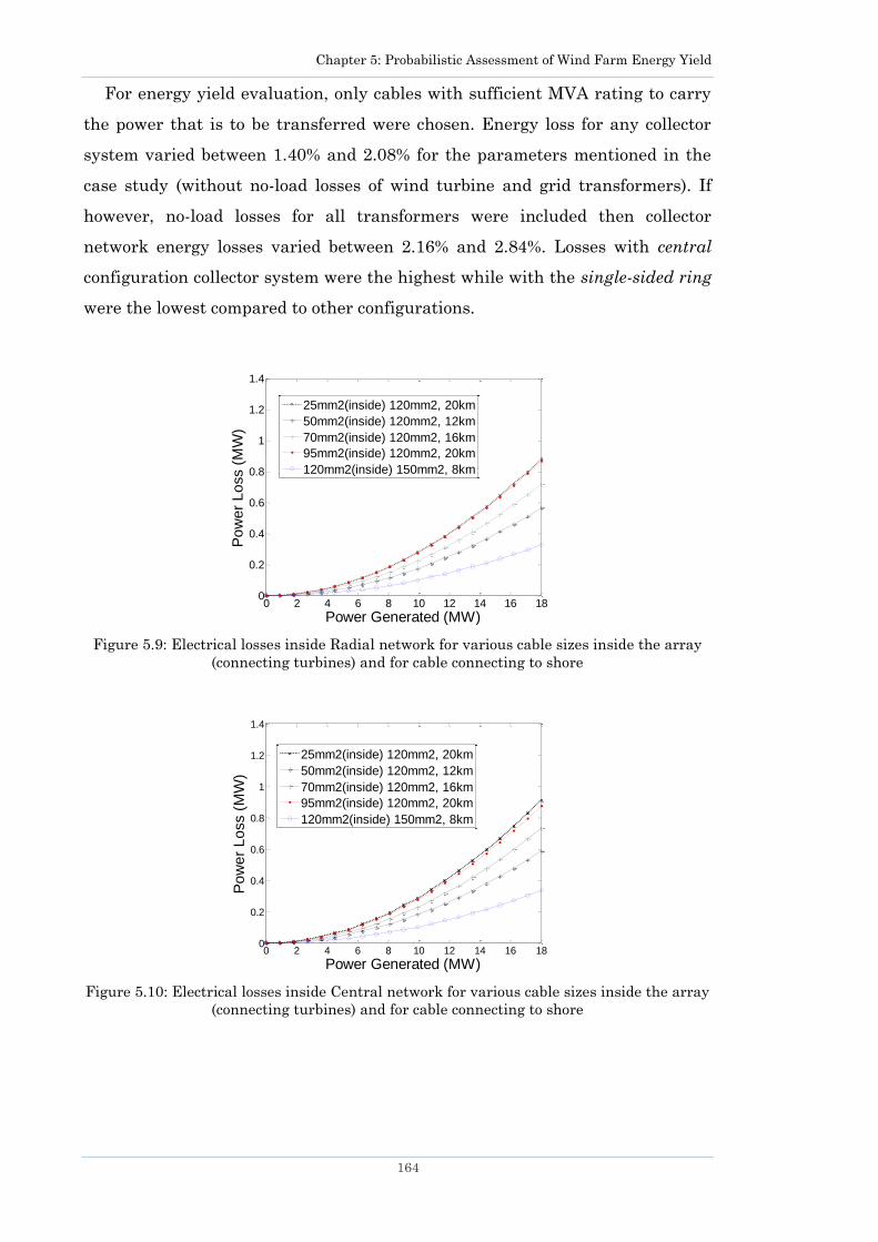
Chapter 5: Probabilistic Assessment of Wind Farm Energy Yield
164
For energy yield evaluation, only cables with sufficient MVA rating to carry
the power that is to be transferred were chosen. Energy loss for any collector
system varied between 1.40% and 2.08% for the parameters mentioned in the
case study (without no-load losses of wind turbine and grid transformers). If
however, no-load losses for all transformers were included then collector
network energy losses varied between 2.16% and 2.84%. Losses with central
configuration collector system were the highest while with the single-sided ring
were the lowest compared to other configurations.
0 2 4 6 8 10 12 14 16 180
0.2
0.4
0.6
0.8
1
1.2
1.4
Power Generated (MW)
Po
we
r L
oss (
MW
)
25mm2(inside) 120mm2, 20km
50mm2(inside) 120mm2, 12km
70mm2(inside) 120mm2, 16km
95mm2(inside) 120mm2, 20km
120mm2(inside) 150mm2, 8km
Figure 5.9: Electrical losses inside Radial network for various cable sizes inside the array
(connecting turbines) and for cable connecting to shore
0 2 4 6 8 10 12 14 16 180
0.2
0.4
0.6
0.8
1
1.2
1.4
Power Generated (MW)
Po
we
r L
oss (
MW
)
25mm2(inside) 120mm2, 20km
50mm2(inside) 120mm2, 12km
70mm2(inside) 120mm2, 16km
95mm2(inside) 120mm2, 20km
120mm2(inside) 150mm2, 8km
Figure 5.10: Electrical losses inside Central network for various cable sizes inside the array
(connecting turbines) and for cable connecting to shore
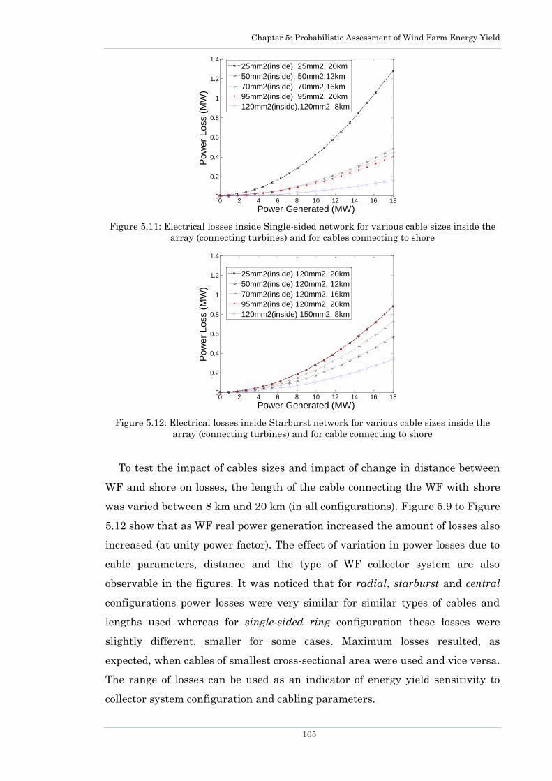
Chapter 5: Probabilistic Assessment of Wind Farm Energy Yield
165
0 2 4 6 8 10 12 14 16 180
0.2
0.4
0.6
0.8
1
1.2
1.4
Power Generated (MW)P
ow
er
Lo
ss (
MW
)
25mm2(inside), 25mm2, 20km
50mm2(inside), 50mm2,12km
70mm2(inside), 70mm2,16km
95mm2(inside), 95mm2, 20km
120mm2(inside),120mm2, 8km
Figure 5.11: Electrical losses inside Single-sided network for various cable sizes inside the
array (connecting turbines) and for cables connecting to shore
0 2 4 6 8 10 12 14 16 180
0.2
0.4
0.6
0.8
1
1.2
1.4
Power Generated (MW)
Po
we
r L
oss (
MW
)
25mm2(inside) 120mm2, 20km
50mm2(inside) 120mm2, 12km
70mm2(inside) 120mm2, 16km
95mm2(inside) 120mm2, 20km
120mm2(inside) 150mm2, 8km
Figure 5.12: Electrical losses inside Starburst network for various cable sizes inside the
array (connecting turbines) and for cable connecting to shore
To test the impact of cables sizes and impact of change in distance between
WF and shore on losses, the length of the cable connecting the WF with shore
was varied between 8 km and 20 km (in all configurations). Figure 5.9 to Figure
5.12 show that as WF real power generation increased the amount of losses also
increased (at unity power factor). The effect of variation in power losses due to
cable parameters, distance and the type of WF collector system are also
observable in the figures. It was noticed that for radial, starburst and central
configurations power losses were very similar for similar types of cables and
lengths used whereas for single-sided ring configuration these losses were
slightly different, smaller for some cases. Maximum losses resulted, as
expected, when cables of smallest cross-sectional area were used and vice versa.
The range of losses can be used as an indicator of energy yield sensitivity to
collector system configuration and cabling parameters.
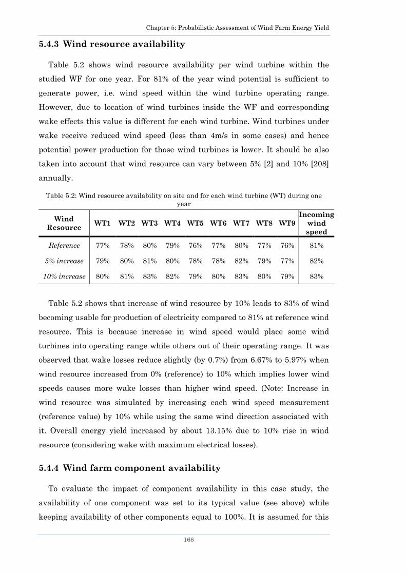
Chapter 5: Probabilistic Assessment of Wind Farm Energy Yield
166
5.4.3 Wind resource availability
Table 5.2 shows wind resource availability per wind turbine within the
studied WF for one year. For 81% of the year wind potential is sufficient to
generate power, i.e. wind speed within the wind turbine operating range.
However, due to location of wind turbines inside the WF and corresponding
wake effects this value is different for each wind turbine. Wind turbines under
wake receive reduced wind speed (less than 4m/s in some cases) and hence
potential power production for those wind turbines is lower. It should be also
taken into account that wind resource can vary between 5% [2] and 10% [208]
annually.
Table 5.2: Wind resource availability on site and for each wind turbine (WT) during one
year
Wind
Resource WT1 WT2 WT3 WT4 WT5 WT6 WT7 WT8 WT9
Incoming
wind
speed
Reference 77% 78% 80% 79% 76% 77% 80% 77% 76% 81%
5% increase 79% 80% 81% 80% 78% 78% 82% 79% 77% 82%
10% increase 80% 81% 83% 82% 79% 80% 83% 80% 79% 83%
Table 5.2 shows that increase of wind resource by 10% leads to 83% of wind
becoming usable for production of electricity compared to 81% at reference wind
resource. This is because increase in wind speed would place some wind
turbines into operating range while others out of their operating range. It was
observed that wake losses reduce slightly (by 0.7%) from 6.67% to 5.97% when
wind resource increased from 0% (reference) to 10% which implies lower wind
speeds causes more wake losses than higher wind speed. (Note: Increase in
wind resource was simulated by increasing each wind speed measurement
(reference value) by 10% while using the same wind direction associated with
it. Overall energy yield increased by about 13.15% due to 10% rise in wind
resource (considering wake with maximum electrical losses).
5.4.4 Wind farm component availability
To evaluate the impact of component availability in this case study, the
availability of one component was set to its typical value (see above) while
keeping availability of other components equal to 100%. It is assumed for this
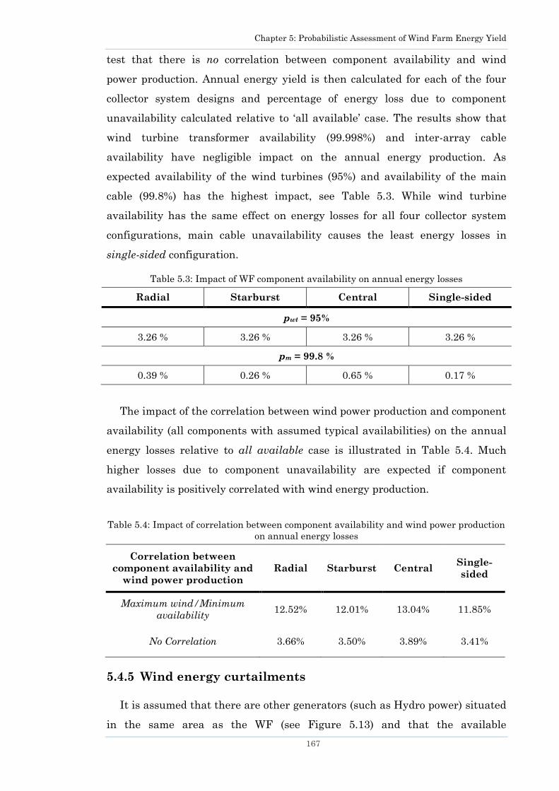
Chapter 5: Probabilistic Assessment of Wind Farm Energy Yield
167
test that there is no correlation between component availability and wind
power production. Annual energy yield is then calculated for each of the four
collector system designs and percentage of energy loss due to component
unavailability calculated relative to ‗all available‘ case. The results show that
wind turbine transformer availability (99.998%) and inter-array cable
availability have negligible impact on the annual energy production. As
expected availability of the wind turbines (95%) and availability of the main
cable (99.8%) has the highest impact, see Table 5.3. While wind turbine
availability has the same effect on energy losses for all four collector system
configurations, main cable unavailability causes the least energy losses in
single-sided configuration.
Table 5.3: Impact of WF component availability on annual energy losses
Radial Starburst Central Single-sided
pwt = 95%
3.26 % 3.26 % 3.26 % 3.26 %
pm = 99.8 %
0.39 % 0.26 % 0.65 % 0.17 %
The impact of the correlation between wind power production and component
availability (all components with assumed typical availabilities) on the annual
energy losses relative to all available case is illustrated in Table 5.4. Much
higher losses due to component unavailability are expected if component
availability is positively correlated with wind energy production.
Table 5.4: Impact of correlation between component availability and wind power production
on annual energy losses
Correlation between
component availability and
wind power production
Radial Starburst Central Single-
sided
Maximum wind/Minimum
availability 12.52% 12.01% 13.04% 11.85%
No Correlation 3.66% 3.50% 3.89% 3.41%
5.4.5 Wind energy curtailments
It is assumed that there are other generators (such as Hydro power) situated
in the same area as the WF (see Figure 5.13) and that the available
Chapter 5: Probabilistic Assessment of Wind Farm Energy Yield
168
transmission capacity from the area is limited to 70 MW. Existing generators
were supplying load in that area and across the transmission line therefore a
transmission line of that rating had been installed based on the existing level of
power transfer. But with installation of new wind power priority will still be
given to the existing generators (such as hydro power) to transfer their power
and any excess wind power will be curtailed. Power transmission
measurements were available for a transmission line and they are assumed to
be representative for the case studied.
Figure 5.13: A congested system with a transmission bottleneck
Power transmission from the WF through the transmission corridor may not
be possible at all times. Wind energy curtailment during the periods of
transmission congestion is considered as an alternative to transmission line
reinforcement. The method for estimation of wind energy curtailment presented
in Section 5.3.6 is applied in this case study. When correlation between wind
power production and TLL is 1 then Section 5.3.6.1 (5.21) is used as illustrated
in Figure 5.6 to determine curtailed energy. Similarly for correlation of -1,
curtailment losses are calculated as described in Section 5.3.6.1. When there is
no correlation between wind power production and TLL then method defined in
Section 5.3.6.2 is used and results are shown in Figure 5.14. The figure
illustrates results of the discrete probabilistic estimation. Figure 5.14 shows the
probability of production from the wind farm 1-Fx(x), transmission of power
from the line without wind power 1-Fy(y), transmission of power from the line
with wind power 1-Fz(z) and transmission line limit TL. As FZ (z) = P(Z z), the
value 1-FZ (C), in Figure 5.14 corresponds to the probability that the
transmission limit C is exceeded. The area under 1-FZ (C z < ) in Figure 5.14
is equal to wind energy that would be curtailed. Availability of wind turbines is
considered to be between 95% and 100% [209]. More possible correlation
scenarios are depicted in Table 5.5.
Other power sources
(such as Hydro power)
Wind power
Load
Other power source
Load
Limited transmission
capacity
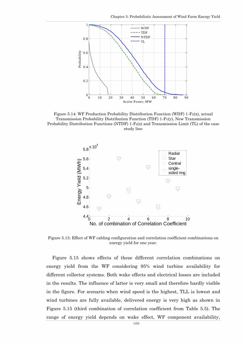
Chapter 5: Probabilistic Assessment of Wind Farm Energy Yield
169
Figure 5.14: WF Production Probability Distribution Function (WDF) 1-FX(x), actual
Transmission Probability Distribution Function (TDF) 1-FY(y), New Transmission
Probability Distribution Functions (NTDF) 1-FZ(z) and Transmission Limit (TL) of the case
study line
Figure 5.15: Effect of WF cabling configuration and correlation coefficient combinations on
energy yield for one year.
Figure 5.15 shows effects of these different correlation combinations on
energy yield from the WF considering 95% wind turbine availability for
different collector systems. Both wake effects and electrical losses are included
in the results. The influence of latter is very small and therefore hardly visible
in the figure. For scenario when wind speed is the highest, TLL is lowest and
wind turbines are fully available, delivered energy is very high as shown in
Figure 5.15 (third combination of correlation coefficient from Table 5.5). The
range of energy yield depends on wake effect, WF component availability,
0 10 20 30 40 50 60 70 80 900
0.2
0.4
0.6
0.8
1
Active Power, MW
Pro
ba
bil
ity
WDF
TDF
NTDF
TL
0 2 4 6 8 104.4
4.6
4.8
5
5.2
5.4
5.6
5.8x 10
4
No. of combination of Correlation Coefficient
En
erg
y Y
ield
(M
Wh
)
Radial
Star
Central
single-sided ring
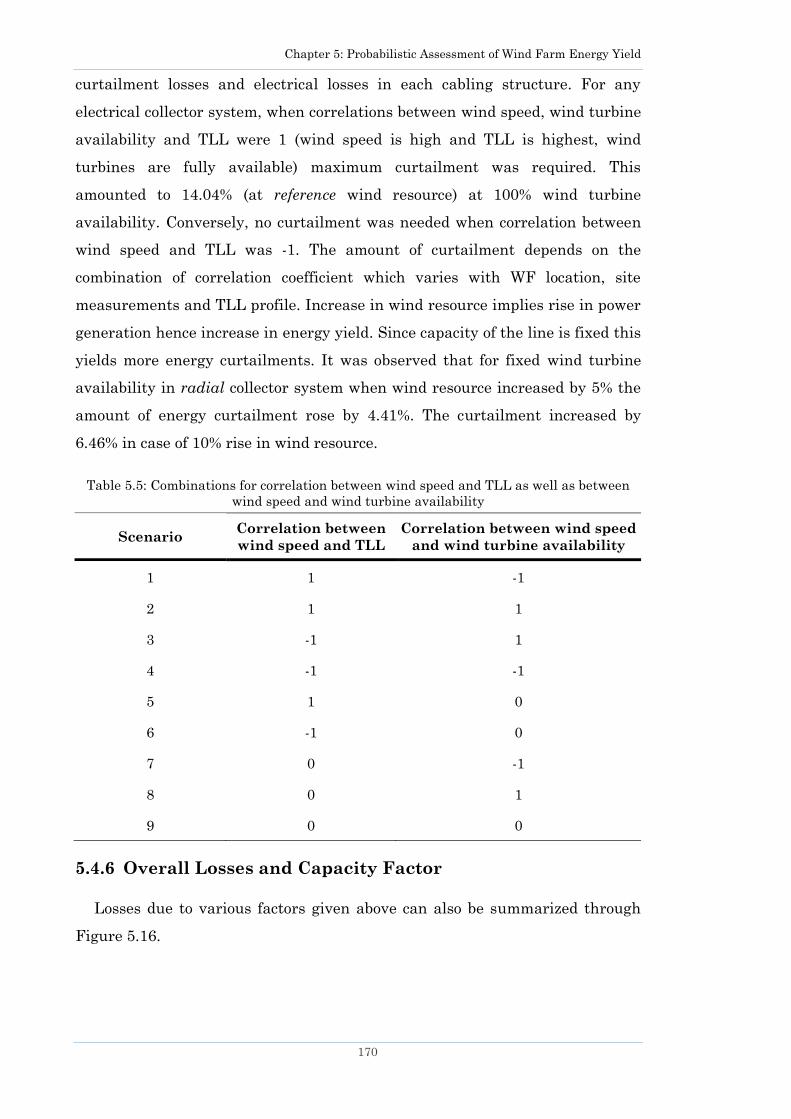
Chapter 5: Probabilistic Assessment of Wind Farm Energy Yield
170
curtailment losses and electrical losses in each cabling structure. For any
electrical collector system, when correlations between wind speed, wind turbine
availability and TLL were 1 (wind speed is high and TLL is highest, wind
turbines are fully available) maximum curtailment was required. This
amounted to 14.04% (at reference wind resource) at 100% wind turbine
availability. Conversely, no curtailment was needed when correlation between
wind speed and TLL was -1. The amount of curtailment depends on the
combination of correlation coefficient which varies with WF location, site
measurements and TLL profile. Increase in wind resource implies rise in power
generation hence increase in energy yield. Since capacity of the line is fixed this
yields more energy curtailments. It was observed that for fixed wind turbine
availability in radial collector system when wind resource increased by 5% the
amount of energy curtailment rose by 4.41%. The curtailment increased by
6.46% in case of 10% rise in wind resource.
Table 5.5: Combinations for correlation between wind speed and TLL as well as between
wind speed and wind turbine availability
Scenario Correlation between
wind speed and TLL
Correlation between wind speed
and wind turbine availability
1 1 -1
2 1 1
3 -1 1
4 -1 -1
5 1 0
6 -1 0
7 0 -1
8 0 1
9 0 0
5.4.6 Overall Losses and Capacity Factor
Losses due to various factors given above can also be summarized through
Figure 5.16.
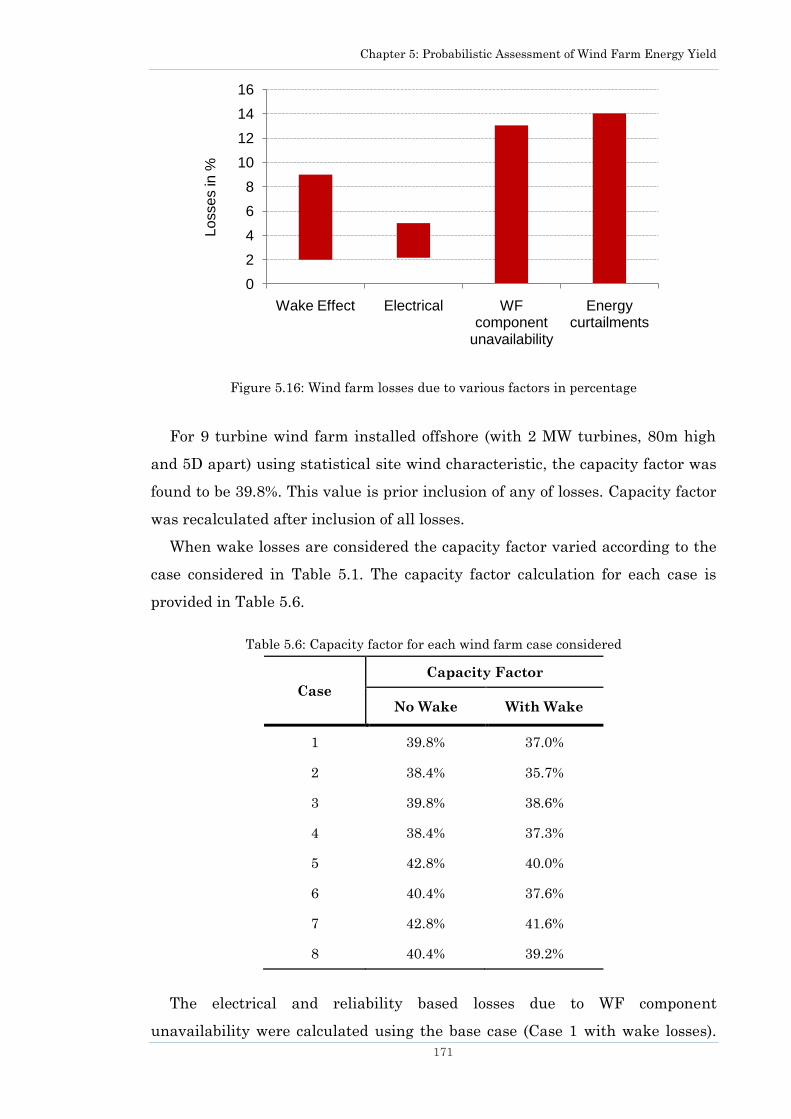
Chapter 5: Probabilistic Assessment of Wind Farm Energy Yield
171
Figure 5.16: Wind farm losses due to various factors in percentage
For 9 turbine wind farm installed offshore (with 2 MW turbines, 80m high
and 5D apart) using statistical site wind characteristic, the capacity factor was
found to be 39.8%. This value is prior inclusion of any of losses. Capacity factor
was recalculated after inclusion of all losses.
When wake losses are considered the capacity factor varied according to the
case considered in Table 5.1. The capacity factor calculation for each case is
provided in Table 5.6.
Table 5.6: Capacity factor for each wind farm case considered
Case
Capacity Factor
No Wake With Wake
1 39.8% 37.0%
2 38.4% 35.7%
3 39.8% 38.6%
4 38.4% 37.3%
5 42.8% 40.0%
6 40.4% 37.6%
7 42.8% 41.6%
8 40.4% 39.2%
The electrical and reliability based losses due to WF component
unavailability were calculated using the base case (Case 1 with wake losses).
0
2
4
6
8
10
12
14
16
Wake Effect Electrical WF component
unavailability
Energy curtailments
Losse
s in
%
Chapter 5: Probabilistic Assessment of Wind Farm Energy Yield
172
The impact of various internal wind farm losses and network related
curtailment losses on capacity factor are summarised in Table 5.7.
Table 5.7: Impact of losses on capacity factor of a wind farm
Factors that affect the Energy Yield Capacity Factor
Electrical losses (2.16% to 2.84%) 36.23% to 35.98%
WF component unavailability (0% to 13.04%) 36.23% to 31.3%
Curtailment losses (0% to 14.04%) 36.23% to 26.9%
Impact of wind resource (10% rise) 35.4%
Impact of wind resource(10% rise) and curtailment 28.1%
It can be seen from Table 5.7 that capacity factor reduced to a maximum of
35.98% when electrical losses of 2.84% are considered. It reduced further to
31.3% when WF component unavailability of 13.04% is considered. The effect of
energy curtailment due to network constraints is also included in capacity
factor calculation. It can be seen from the table that 14.4% curtailments will
further reduce the capacity factor to 26.9%.
When a 10% increase in wind resource is considered the overall energy yield
(including wake, electrical and WF component unavailability losses) increased
by 13.15% which increased the capacity factor to 35.4%. But this also increased
the curtailment losses as wind energy export increased. Overall, the minimum
capacity factor after all losses was found to be 26.9% whereas without any
losses it was 39.8%. Thus inclusion of losses reduced the capacity factor by
12.9%.
The capacity factors calculated are valid for the wind turbines, wind farm
layout and wind conditions used in this case study. The results will differ if
either of the parameters is different.
5.5 Summary
This chapter presented a comprehensive methodology for probabilistic
assessment of WF energy yield. A new method to calculate losses due to
reliability of WF components was presented for four collector systems. Also, a
technique to determine amount of energy curtailments considering all internal
WF losses was given. Correlation combinations covering all extreme scenarios

Chapter 5: Probabilistic Assessment of Wind Farm Energy Yield
173
were computed to assess the impact of wind power production, TLL and wind
turbine availability on the amount of curtailments.
In the case studied, energy losses due to wake varied between 2% and 7%,
electrical losses inside the WF between 2.16% and 2.84%. Losses due to
unavailability of wind turbine and other components within the WF were
between 0% and 13.05% during a year depending on component availability,
WF collector system configuration and correlation between wind turbine
availability and wind power production. Impact of variation in wind resource on
energy yield, losses and curtailments were also analysed by increasing wind
resource by 5% and 10%. A 10% increase in wind resource led to 13.15% rise in
energy yield (including losses, wind turbine availability 100%, excluding
network constraints). Losses due to wind energy curtailments were found to be
between 0% and 14.04% (at reference wind resource), however, energy
curtailments rose by further 6.46% when wind resource increased by 10%. The
highest curtailment losses occurred for correlation coefficient equal to 1
between wind power, TLL and wind turbine availability, whereas lowest wind
energy curtailment occurred for correlation coefficient of -1 between wind power
production and TLL. Impact of losses on capacity factor of a wind farm was also
analysed. It was found that consideration of all losses (internal to wind farm
and due to curtailments) reduced the capacity factor by 12.9%. It should be
noted that the values for energy losses computed are valid for this particular
case study. If parameters of a wind farm are different the results will vary
accordingly. Therefore, these losses should be computed using actual wind farm
data during a prefeasibility study. Based on sensitivity analysis, it can be
concluded that energy yield should not be computed as a single deterministic
value but rather as a range, or as a probability density function. Methodologies
presented can help WF developers make more reliable decisions regarding
collector system design, cross-section of cables, height of wind turbines, location
of the WF and connection with the grid. It can also contribute to assess more
accurately the option of wind energy curtailment against the option of
transmission line reinforcement in areas with transmission corridor congestion.
Chapter 6: Probabilistic Identification of Critical Wind Turbines inside a Wind Farm
174
Chapter 6 Probabilistic Identification of
Critical Wind Turbines inside a Wind Farm
Probabilistic Identification of Critical
Wind Turbines inside a Wind Farm
6.1 Introduction
Preventive maintenance is carried out to avoid component failures by
replacing worn components before they fail. A sub category of preventive
maintenance is the scheduled preventive maintenance which is generally
cheaper than the corrective maintenance [210], therefore it is popular amongst
wind farms today [211]. Scheduled preventive maintenance is performed on an
established time schedule [211, 212], its frequency however depends on the age
of the wind turbines in the wind farm. The process of scheduling can be made
more efficient if wind turbines that produce large amount of power are
scheduled for maintenance on less windy days.
Apart from this, the process of wind energy curtailment can be also made
more efficient by prioritising shut down of wind turbines. This chapter proposes
methodology for probabilistic identification of critical wind turbines that could
yield better scheduling of preventive maintenance of wind turbines and also
result in developing better wind energy curtailment strategy.
Wind turbines inside a wind farm do not produce the same amount of power
at any given time because the wind speed incident on each turbine is different.
The wind speed incident on a turbine is influenced by the physical location of
the turbine along with wake effects caused by the local topology and other wind
turbines. Another factor influencing wind speed is turbulence within the wakes,
which negatively impacts on the WFs operation by causing turbine fatigue
damage [111]. Turbines under wake suffer greater fatigue load compared to
turbines in free-stream wind [213]. It is assumed that this consequently affects

Chapter 6: Probabilistic Identification of Critical Wind Turbines inside a Wind Farm
175
the wind turbine component reliability and therefore adds towards operation
and maintenance costs.
In this chapter, a novel probabilistic methodology is presented to identify
wind turbines in the WF that face higher and lower wind speeds during the
year. The methodology takes into account WF layout, WF location and wind
turbine positions. Probabilistic site analysis is performed along with turbine
clustering, after determining the wind speed approaching each turbine by using
a detailed wake effect model. The developed approach can help to identify those
turbines which are mostly under wake and consequently facing reduced wind
speeds. The approach presented in this chapter can be applied to a generic wind
farm of any size, layout or location.
The wind turbines in a WF can be broadly split into two groups, Important
wind turbines and Less Important wind turbines. Wind turbines that face
higher wind speeds can be defined as Important wind turbines while those that
face reduced wind speed due to wakes can be defined as Less Important wind
turbines. Outages on Important wind turbines cause greater losses in WF total
power production compared with outages in Less Important wind turbines.
Identifying Important wind turbines and Less Important wind turbines requires
information on the wind characteristics at the site of interest, including wind
speed and wind direction measurements data for at least one year, so that most
probable wind directions and speeds can be determined.
Once the Important wind turbines and Less Important wind turbines have
been identified, the turbines under the greatest stress can be pro-actively shut
down first during wind energy curtailments. Shutting down these turbines is
advantageous because it prevents fatigue damage to a wind turbine‘s
mechanical components. During preventive maintenance it can be profitable to
schedule turbines producing higher energy on days with less wind speed to
avoid loss of extra energy capture.
The methodology presented in this chapter is tested on a large WF but it is
equally applicable to a WF of any size and layout. All quantitative results are
dependent on the layout and location of a WF as well as on wind characteristic
at the site. The method is applicable for carrying out offline studies on existing
wind farms. At present, there are no reports in open literature presenting
methodology for identifying wind turbines facing high and low wind speeds
within a WF. The methodology presented here uses data from only one
Chapter 6: Probabilistic Identification of Critical Wind Turbines inside a Wind Farm
176
anemometer for the whole wind farm. It thus saves significant wind
measurement effort.
6.2 Wind Flow Modelling and Data Clustering
6.2.1 Site information
In order to determine the most probable wind speeds and directions at a site,
it is necessary to have a site‘s wind measurements available for at least one
year. Based on this information the frequency of wind direction for the whole
year can be determined. By analysing wind speed measurement data (given in
Section 3.8) of a site in the north of Sweden for year 2000, it is evident that the
wind during the year is prevailing from two directions: one ranging between
100o and 180o, and one ranging between 280o and 360o. This can be seen from
Figure 3.12.
The probability distribution of different wind speeds at a site can be found
from wind measurements and represented through Weibull distribution. Figure
3.11 shows that prevalent wind speeds occur between 4 m/s and 15 m/s. Wind
speeds greater than 15 m/s were not analysed because their probability of
occurrence is low. The most probable wind speed and directions are then used
in further calculations whereas low probability wind speeds and wind
directions were ignored. A large 49 turbine wind farm shown in Figure 3.13 is
used for the analysis.
6.2.2 Wind speed variation due to wake effects
To be able to identify wind turbines receiving high and low wind speeds it is
essential to consider the WF layout, incoming wind speed and direction as well
as wake effects. Once wind speed approaching each turbine for every incoming
wind speed and wind direction is obtained, a power curve for the turbine can be
used to determine its power production. The amount of wind speed each turbine
receives inside a WF is dependent on the layout of the WF, the number of
turbines, their position in WF and the wind speed and direction entering the
farm. It was observed that both incoming wind speed and wind direction (even
when treated independently) affect the wind speed incident on a turbine.
Therefore, both of these factors should be considered whenever the assessment
of total WF power production is needed. Wake effect models and VeBWake
Chapter 6: Probabilistic Identification of Critical Wind Turbines inside a Wind Farm
177
program described in Section 3.3 and 3.4 respectively, are used to estimate
wind speed at each turbine.
6.2.3 Clustering data
Once essential wind speed data at each turbine is obtained through wake
effect modelling, the Support Vector Clustering (SVC) method [183] (given in
Section 4.3) is applied to cluster wind turbines according to their wind speed
with a direction interval (DI) of 20o. A Direction Interval is used to collectively
consider and cluster wind turbines inside 20 directions (e.g. from 100o to 120o
and from 120o to 140o and so on). A cluster DI of 20o was selected due to
similarities in wind patterns within this range and to reduce computational
effort, without any loss of generality. If increased accuracy is needed, or if there
is dissimilarity in the wind patterns within the considered range, a smaller DI
(e.g., 10o, 5o or even 1o), should be used. It should be pointed out that clustering
of wind turbines based on wind speeds is not new. References [38] and [214], for
example, presented methods which clustered wind turbines based on their wind
speeds.
Turbines are then arranged in clusters based on magnitude of wind speeds
they face, i.e., those facing higher wind speeds are arranged in one cluster,
whereas those facing slightly lower wind speed in another, and so on. Those
turbines that appear most frequently in the cluster of high wind speeds are the
ones that face the highest wind speeds during the year. On the other hand,
those turbines that appear most frequently in the lower wind speed cluster are
the ones that are under wake most of the time during the year. A more detailed
description of the process is given in the following sections.
6.3 Probabilistic Power Output of Wind Farm
The probability mass function for wind power output can be expressed as:
( ) ( ) ( ) /Y Yf y P Y y freq y N (6.1)
where Y corresponds to wind power production in MW. P(Y = y) is the
probability that wind power Y is the same as a level y, freqY(y) is the frequency
of level y and N is the total number of measurements in a year.
The distribution function for wind power production is then:
Chapter 6: Probabilistic Identification of Critical Wind Turbines inside a Wind Farm
178
:
( ) ( ) ( )i
Y Y i
i y y
F y P Y y f y
(6.2)
where P(Y ≤ y) is the probability that wind power output Y is less than or equal
to level y. Finally, the probability to produce Y amount of wind power during
the year by the WF can be obtained as 1-FY(y) [215].
6.4 Case Study
For all selected wind speeds (4 m/s to 15 m/s) and directions (100o, 101o, 102o,
… 180o and 280o, 281o, 282o, … 360o) wind flow and wake effects inside the farm
are simulated. The range of wind speeds in this simulation is reduced from the
full range of wind speeds (0 to 25 m/s) and directions (0 to 360o) to only the
prominent wind speeds and directions. In the case where wind conditions are
not easily segmented into prominent regions using the wind speed and
direction probability distributions (obtained from wind measurements), the full
range of wind speed and directions should be used. Doing so provides wind
speed at each turbine after which classification of turbines is performed by the
SVC algorithm. Turbines that face high wind speed are placed in Cluster 1
while those that face low wind speeds (as they stay in wake in most wind
conditions) are placed in the subsequent clusters. The number of clusters differs
with incoming wind speed and direction. An example is shown in Table 6.1 for
incoming wind speed of 10 m/s. Tables similar to this are formed for every
incoming wind speed between 4 m/s and 15 m/s.
Using the tables for each wind speed, the frequency of each wind turbine in
each cluster can be calculated. If a wind turbine exists more frequently in
Cluster 1 it implies that it faces higher wind speed than others, whereas if a
turbine frequently appears in Cluster 5 it faces reduced wind speed during the
year. Frequency of turbines in each cluster is illustrated in Figure 6.1.
At different directions and wind speeds, turbines in a WF face different
levels of wind. Figure 6.1 shows that it is difficult to choose Important wind
turbines and Less Important wind turbines as the resulting frequencies are
relatively close to one another. To simplify the analysis, Cluster 1 and 2 are
merged together since wind speeds in both are relatively high. Similarly,
Clusters 4 and 5 are also merged together. This leads to reduction in clusters
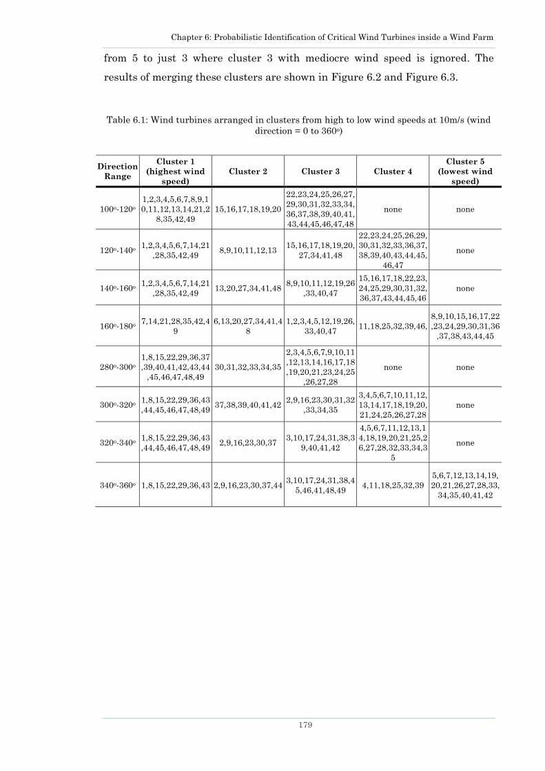
Chapter 6: Probabilistic Identification of Critical Wind Turbines inside a Wind Farm
179
from 5 to just 3 where cluster 3 with mediocre wind speed is ignored. The
results of merging these clusters are shown in Figure 6.2 and Figure 6.3.
Table 6.1: Wind turbines arranged in clusters from high to low wind speeds at 10m/s (wind
direction = 0 to 360o)
Direction
Range
Cluster 1
(highest wind
speed)
Cluster 2 Cluster 3 Cluster 4
Cluster 5
(lowest wind
speed)
100o-120o
1,2,3,4,5,6,7,8,9,1
0,11,12,13,14,21,2
8,35,42,49
15,16,17,18,19,20
22,23,24,25,26,27,
29,30,31,32,33,34,
36,37,38,39,40,41,
43,44,45,46,47,48
none none
120o-140o 1,2,3,4,5,6,7,14,21
,28,35,42,49 8,9,10,11,12,13
15,16,17,18,19,20,
27,34,41,48
22,23,24,25,26,29,
30,31,32,33,36,37,
38,39,40,43,44,45,
46,47
none
140o-160o 1,2,3,4,5,6,7,14,21
,28,35,42,49 13,20,27,34,41,48
8,9,10,11,12,19,26
,33,40,47
15,16,17,18,22,23,
24,25,29,30,31,32,
36,37,43,44,45,46
none
160o-180o 7,14,21,28,35,42,4
9
6,13,20,27,34,41,4
8
1,2,3,4,5,12,19,26,
33,40,47 11,18,25,32,39,46,
8,9,10,15,16,17,22
,23,24,29,30,31,36
,37,38,43,44,45
280o-300o
1,8,15,22,29,36,37
,39,40,41,42,43,44
,45,46,47,48,49
30,31,32,33,34,35
2,3,4,5,6,7,9,10,11
,12,13,14,16,17,18
,19,20,21,23,24,25
,26,27,28
none none
300o-320o 1,8,15,22,29,36,43
,44,45,46,47,48,49 37,38,39,40,41,42
2,9,16,23,30,31,32
,33,34,35
3,4,5,6,7,10,11,12,
13,14,17,18,19,20,
21,24,25,26,27,28
none
320o-340o 1,8,15,22,29,36,43
,44,45,46,47,48,49 2,9,16,23,30,37
3,10,17,24,31,38,3
9,40,41,42
4,5,6,7,11,12,13,1
4,18,19,20,21,25,2
6,27,28,32,33,34,3
5
none
340o-360o 1,8,15,22,29,36,43 2,9,16,23,30,37,44 3,10,17,24,31,38,4
5,46,41,48,49 4,11,18,25,32,39
5,6,7,12,13,14,19,
20,21,26,27,28,33,
34,35,40,41,42
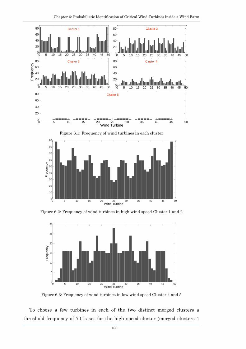
Chapter 6: Probabilistic Identification of Critical Wind Turbines inside a Wind Farm
180
0 5 10 15 20 25 30 35 40 45 500
20
40
60
80 Cluster 1
0 5 10 15 20 25 30 35 40 45 500
20
40
60
80 Cluster 2
0 5 10 15 20 25 30 35 40 45 500
20
40
60
80
Fre
qu
en
cy
Cluster 3
0 5 10 15 20 25 30 35 40 45 500
20
40
60
80 Cluster 4
0 5 10 15 20 25 30 35 40 45 500
20
40
60
80
Wind Turbine
Cluster 5
Figure 6.1: Frequency of wind turbines in each cluster
0 5 10 15 20 25 30 35 40 45 500
10
20
30
40
50
60
70
80
90
Wind Turbine
Fre
qu
en
cy
Figure 6.2: Frequency of wind turbines in high wind speed Cluster 1 and 2
0 5 10 15 20 25 30 35 40 45 500
5
10
15
20
25
30
Wind Turbine
Fre
qu
en
cy
Figure 6.3: Frequency of wind turbines in low wind speed Cluster 4 and 5
To choose a few turbines in each of the two distinct merged clusters a
threshold frequency of 70 is set for the high speed cluster (merged clusters 1

Chapter 6: Probabilistic Identification of Critical Wind Turbines inside a Wind Farm
181
and 2), while for low speed clusters (clusters 4 and 5) this value is set to 17.
This means turbines in Figure 6.2 with frequency above 70 are Important while
turbines in Figure 6.3 with frequency above 17 are defined as Less Important
wind turbines.
Figure 6.4: Wind farm layout showing important wind turbines in the red, less important
wind turbines in blue and frequency of wind from various direction sectors in the
background
It can be seen that wind turbines 1, 2, 8, 42, 48 and 49 receive higher wind
speeds, whereas wind turbines 11, 18, 24, 25, 26, 32 and 39 are more likely to
receive reduced wind speeds. From the layout of the WF in Figure 6.4 it is
visible that, as expected, turbines receiving reduced wind speed more
frequently are the ones deep inside the WF (highlighted in blue). Studies in
literature [111, 213] report that the turbines in the middle of WF (under wake)
will be under greater fatigue loads compared with wind turbines in the free-
stream wind. It is assumed that turbines under fatigue loads will be under
greater mechanical stress. Figure 6.4 shows that the turbines highlighted in
red face higher wind speeds as they remain under free-stream wind most of the
time. This is because wind is highly frequent from two directions at this site as
visible from Figure 6.5. These turbines will hardly be under wake as direction
of the wind is diagonal during most of the year. Wind turbines identified as
Important and Less important in this case study are valid for this particular
wind farm layout and for the site wind characteristic considered. The results
will vary according to the geometry of the wind farm, wind turbine height and
7
6
5
4
3
2
1
14
13
12
11
10
9
8
21
20
19
18
17
16
15
28
27
26
25
24
23
22
35
34
33
32
31
30
29
42
41
40
39
38
37
36
49
48
47
46
45
44
43
0o
180o
90o270
o
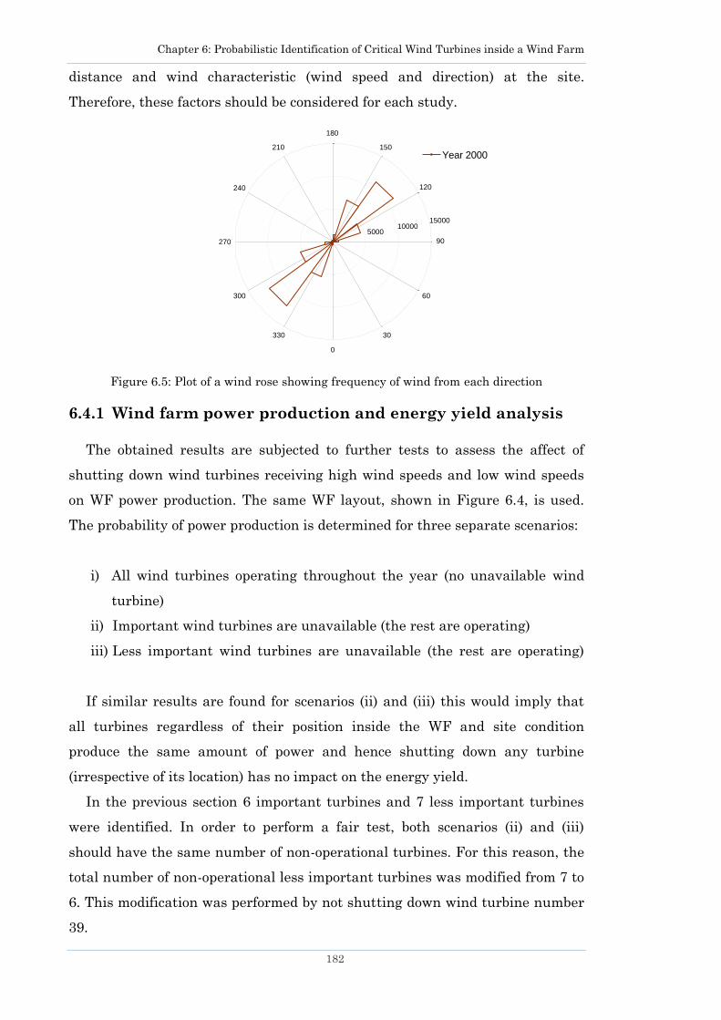
Chapter 6: Probabilistic Identification of Critical Wind Turbines inside a Wind Farm
182
distance and wind characteristic (wind speed and direction) at the site.
Therefore, these factors should be considered for each study.
Figure 6.5: Plot of a wind rose showing frequency of wind from each direction
6.4.1 Wind farm power production and energy yield analysis
The obtained results are subjected to further tests to assess the affect of
shutting down wind turbines receiving high wind speeds and low wind speeds
on WF power production. The same WF layout, shown in Figure 6.4, is used.
The probability of power production is determined for three separate scenarios:
i) All wind turbines operating throughout the year (no unavailable wind
turbine)
ii) Important wind turbines are unavailable (the rest are operating)
iii) Less important wind turbines are unavailable (the rest are operating)
If similar results are found for scenarios (ii) and (iii) this would imply that
all turbines regardless of their position inside the WF and site condition
produce the same amount of power and hence shutting down any turbine
(irrespective of its location) has no impact on the energy yield.
In the previous section 6 important turbines and 7 less important turbines
were identified. In order to perform a fair test, both scenarios (ii) and (iii)
should have the same number of non-operational turbines. For this reason, the
total number of non-operational less important turbines was modified from 7 to
6. This modification was performed by not shutting down wind turbine number
39.
5000 10000
15000
30
210
60
240
90270
120
300
150
330
180
0
Year 2000
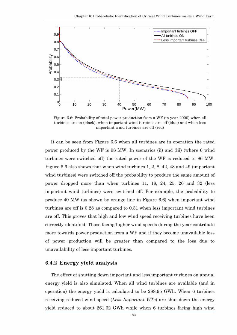
Chapter 6: Probabilistic Identification of Critical Wind Turbines inside a Wind Farm
183
Figure 6.6: Probability of total power production from a WF (in year 2000) when all
turbines are on (black), when important wind turbines are off (blue) and when less
important wind turbines are off (red)
It can be seen from Figure 6.6 when all turbines are in operation the rated
power produced by the WF is 98 MW. In scenarios (ii) and (iii) (where 6 wind
turbines were switched off) the rated power of the WF is reduced to 86 MW.
Figure 6.6 also shows that when wind turbines 1, 2, 8, 42, 48 and 49 (important
wind turbines) were switched off the probability to produce the same amount of
power dropped more than when turbines 11, 18, 24, 25, 26 and 32 (less
important wind turbines) were switched off. For example, the probability to
produce 40 MW (as shown by orange line in Figure 6.6) when important wind
turbines are off is 0.28 as compared to 0.31 when less important wind turbines
are off. This proves that high and low wind speed receiving turbines have been
correctly identified. Those facing higher wind speeds during the year contribute
more towards power production from a WF and if they become unavailable loss
of power production will be greater than compared to the loss due to
unavailability of less important turbines.
6.4.2 Energy yield analysis
The effect of shutting down important and less important turbines on annual
energy yield is also simulated. When all wind turbines are available (and in
operation) the energy yield is calculated to be 288.95 GWh. When 6 turbines
receiving reduced wind speed (Less Important WTs) are shut down the energy
yield reduced to about 261.62 GWh while when 6 turbines facing high wind
0 10 20 30 40 50 60 70 80 90 1000
0.1
0.2
0.3
0.4
0.5
0.6
0.7
0.8
0.9
1
Power(MW)
Pro
ba
bili
ty
Important turbines OFF
All turbines ON
Less important turbines OFF
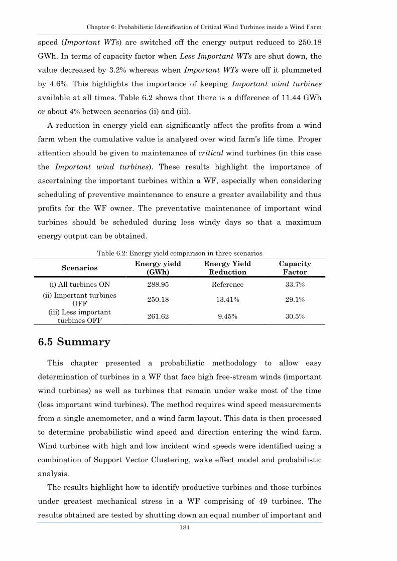
Chapter 6: Probabilistic Identification of Critical Wind Turbines inside a Wind Farm
184
speed (Important WTs) are switched off the energy output reduced to 250.18
GWh. In terms of capacity factor when Less Important WTs are shut down, the
value decreased by 3.2% whereas when Important WTs were off it plummeted
by 4.6%. This highlights the importance of keeping Important wind turbines
available at all times. Table 6.2 shows that there is a difference of 11.44 GWh
or about 4% between scenarios (ii) and (iii).
A reduction in energy yield can significantly affect the profits from a wind
farm when the cumulative value is analysed over wind farm‘s life time. Proper
attention should be given to maintenance of critical wind turbines (in this case
the Important wind turbines). These results highlight the importance of
ascertaining the important turbines within a WF, especially when considering
scheduling of preventive maintenance to ensure a greater availability and thus
profits for the WF owner. The preventative maintenance of important wind
turbines should be scheduled during less windy days so that a maximum
energy output can be obtained.
Table 6.2: Energy yield comparison in three scenarios
Scenarios Energy yield
(GWh)
Energy Yield
Reduction
Capacity
Factor
(i) All turbines ON 288.95 Reference 33.7%
(ii) Important turbines
OFF 250.18 13.41% 29.1%
(iii) Less important
turbines OFF 261.62 9.45% 30.5%
6.5 Summary
This chapter presented a probabilistic methodology to allow easy
determination of turbines in a WF that face high free-stream winds (important
wind turbines) as well as turbines that remain under wake most of the time
(less important wind turbines). The method requires wind speed measurements
from a single anemometer, and a wind farm layout. This data is then processed
to determine probabilistic wind speed and direction entering the wind farm.
Wind turbines with high and low incident wind speeds were identified using a
combination of Support Vector Clustering, wake effect model and probabilistic
analysis.
The results highlight how to identify productive turbines and those turbines
under greatest mechanical stress in a WF comprising of 49 turbines. The
results obtained are tested by shutting down an equal number of important and

Chapter 6: Probabilistic Identification of Critical Wind Turbines inside a Wind Farm
185
less important turbines, then calculating the wind farm power output
probability curve and performing energy yield analysis. It was found that
shutting down important wind turbines lead to a greater loss in power and
hence energy yield.
The proposed methodology is very flexible and can be used for a wind farm of
any size and layout, installed at any location. It can be used with a wind farm
having wind turbines of any height at any distance apart. The methodology can
be used during pre-feasibility studies and on commissioned WFs. The method
can be applied to a pre-feasibility study to test the shape and topology of the
WF layout (wind farm layout optimisation) by ensuring the number of turbines
receiving higher wind speeds is maximised. The method can also prove to be
helpful during asset management of wind turbines. For instance, during
normal operation and maintenance of a WF, the method can identify turbines
facing higher wind speeds so that their maintenance can be prioritised to help
reduce loss of profits.
Furthermore, the method can be useful during wind energy curtailments. It
was discussed in Section 1.1 that in wind farms with stall control wind turbines
the curtailment is performed by shutting down the turbines. The proposed
method can also help identify wind turbines receiving reduced wind speeds and
increased mechanical stresses. These wind turbines can be prioritised to be
shut down when wind energy curtailments are required to prevent mechanical
degradation of their components. Therefore, the method proposed can be useful
for system operators as well as wind farm owners.

Chapter 7: Robust Design Methodology for Offshore Wind Farms
186
Chapter 7 Robust Design Methodology for
Offshore Wind Farms
Robust Design Methodology for Offshore
Wind Farms
7.1 Introduction
In view of difficulty in gaining planning permission for onshore
developments, in recent years attention has been given in particular to offshore
wind farms. The world‘s biggest offshore wind farm (Greater Gabbard) is
currently under construction off the east coast of England, providing 500 MW of
capacity and due for completion before the end of 2012 [216] and another bigger
wind farm (London Array, Phase One, 630 MW) is planned for connection into
the south east corner of England around the same time [30]. Recent reports
published by the UK Carbon Trust [4] indicate that Britain could need at least
29 GW of offshore wind power to meet the EU‘s renewable energy and low-
carbon emission targets by 2020. Related reports published by BERR [217] and
the Crown Estate [4] envisage that a number of large offshore wind farms will
be built. The capacity of offshore wind farms in the future is expected to
increase not only in the UK, but in many countries in Europe, as discussed in
Chapter 1 and as shown in Figure 1.3. Apart from offshore wind farm capacity,
the distance from shore is also expected to increase, with distances reaching up
to 120 km away from the shore as seen in Figure 1.4.
As the capacity of a wind farm increases, the number of potential design
options (i.e. choice of wind turbine capacity and quantity, type of transmission
link with the shore, number of transmission cables, type of array configuration,
choice of voltage levels and choice of substation equipment) also increases. This
intensifies the complexity of the design task. In small capacity wind farms,
many of the potential options are just not applicable, for instance, there is no

Chapter 7: Robust Design Methodology for Offshore Wind Farms
187
need for a substation or consideration of a high voltage DC (HVDC) option to
link with the shore or very high voltage levels. Thus possible numbers of
layouts in a small offshore wind farm are less as compared to a large offshore
wind farm. In this chapter, design option for an offshore wind farm is also
referred to as layout or electrical layout.
Designing an electrical network for a large offshore wind farm is a multi-
dimensional problem where investment costs, reliability of the system and
losses have to be balanced. In an offshore farm, achieving a certain level of
redundancy is difficult as the cost of the project can rise significantly. Ideally
an optimal layout should feature adequate level of reliability and be cost-
effective, but as it will be seen in this chapter, a trade-off exists between these
two factors.
Previous studies [24, 32, 73] have looked into ways of interconnecting
turbines, choice of cables, possible connection options with the shore and so on.
No methodology presented in open literature, however, looks at the wind farm
design as a whole, i.e., from reliability, loss and cost perspectives. At present,
prior to designing a wind farm, wind farm developers analyse a few electrical
layouts based on the knowledge and experience they have gained from the
previous projects. The capacity of the wind farms however will be much larger
in the future in comparison to the past; hence a better approach is needed to
identify cost-efficient electrical layouts for a large offshore wind farm.
This chapter provides a novel methodology that leads to the selection of an
optimal electrical layout for a large offshore wind farm through cost-benefit
analysis. A multi-level short-listing process is devised to narrow down the
options. To start with, a list of all possible electrical layouts is created with
different types and quantities of components. Through first level short-listing, a
number of layouts are selected based on their technical feasibility and benefits.
The investment cost of the remaining electrical layouts is evaluated using the
cost models. At the second level of short-listing, the investment cost range set
by the wind farm owner is considered, and therefore any layouts that fall
beyond that range are discarded. The level of redundancy is then calculated in
the layouts that remain to identify layouts with high and low reliability. At the
third level of short-listing, layouts are selected based on the required
redundancy criteria. The layouts selected are further tested for electrical and
reliability based losses. Net Present Value (NPV) analysis is then carried out to

Chapter 7: Robust Design Methodology for Offshore Wind Farms
188
identify which layout performs better overall during the lifetime of the wind
farm. The case study is performed on a 400 MW wind farm. The cases are
developed and tested for losses in a commercially available power system
software PSS®E.
At present, building a large electrical network (for an offshore wind farm) in
commercial power system software takes a significant amount of time and
effort because all the components have to be added manually. This means
several nodes have to be added and named, voltage levels have to be defined,
switchgear and cables have to be added, electrical data for transformers, cables,
high voltage DC (HVDC) converters, wind turbine generators and onshore
substation components have to be specified. It can be even more difficult when
an offshore wind farm has more than one platform because then components for
those platforms also have to be modelled. Performing load flow and reliability
studies on such a large network manually can also be a very time consuming
task.
To solve this problem a novel industrial-grade software tool has been
developed as part of this research that can minimise the time and effort in
building and testing such large networks. This chapter discusses the software
tool that can be used for automated design and loss analysis of an offshore grid.
The tool features a Graphical User Interface (GUI) through which parameters
such as wind farm capacity, the distance between the turbines and the length of
cables can be entered. Electrical parameters such as resistance, inductance and
susceptance values for cables are loaded directly from component catalogues,
available from manufacturers, to allow realistic estimation of electrical losses.
The software allows a user to build and test a complete electrical grid for an
offshore wind farm. A set of calculations including load flow, reactive power
compensation, electrical and reliability based loss evaluations are automated.
The costs of losses are determined based on the cost of energy entered. Since a
large wind farm can have multiple platforms, the software also caters for this
need and allows for creation of more than just a single platform. The platforms
can be linked through cables by simply selecting the bus terminals and cable
types in the GUI. The software features a save and read function through
which entered parameters can be saved into an external file and later read back
into the software tool. Using this feature, multiple electrical layouts can be
rapidly generated without re-entering all the parameters into the GUI. The

Chapter 7: Robust Design Methodology for Offshore Wind Farms
189
software tool has been developed using Python programming language, QT,
PyQT and PSS®E Application Programming Interface (APIs).
The software tool is a user-friendly application. It is useful for building and
testing large offshore wind farm electrical networks in a short space of time
with minimal effort. This chapter describes features of the software tool
including inputs, outputs, structure and briefly the methodology behind the
calculations.
7.2 Offshore wind farm network
Electrical layout of a large offshore wind farm is made up of a number of
components as can be seen from Figure 7.1, this includes:
a) Wind turbines
b) Cables interconnecting the wind turbines
c) Offshore substation carrying:
i) Collector transformers (2-winding or 3-winding) stepping up
medium voltage (MV) to high voltage (HV).
ii) Reactive power devices.
iii) Converters for an HVDC link.
iv) Converter transformers (for a HVDC link) stepping up High
Voltage (HV) to converter voltage i.e. Extra High Voltage
(EHV).
v) Switchgears.
d) Transmission link (HVAC or HVDC) to shore, see Figure 7.2.
Figure 7.1 Main components of an offshore wind farm electrical system
HV
MV
Transmission
(HVAC or HVDC)
Tie Lines to other
platforms
Offshore Substation
Collector
Transformer
Turbine and
Transformer
Array
Onshore
substation
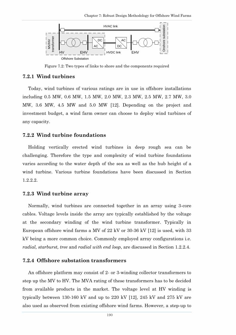
Chapter 7: Robust Design Methodology for Offshore Wind Farms
190
Figure 7.2: Two types of links to shore and the components required
7.2.1 Wind turbines
Today, wind turbines of various ratings are in use in offshore installations
including 0.5 MW, 0.6 MW, 1.5 MW, 2.0 MW, 2.3 MW, 2.5 MW, 2.7 MW, 3.0
MW, 3.6 MW, 4.5 MW and 5.0 MW [12]. Depending on the project and
investment budget, a wind farm owner can choose to deploy wind turbines of
any capacity.
7.2.2 Wind turbine foundations
Holding vertically erected wind turbines in deep rough sea can be
challenging. Therefore the type and complexity of wind turbine foundations
varies according to the water depth of the sea as well as the hub height of a
wind turbine. Various turbine foundations have been discussed in Section
1.2.2.2.
7.2.3 Wind turbine array
Normally, wind turbines are connected together in an array using 3-core
cables. Voltage levels inside the array are typically established by the voltage
at the secondary winding of the wind turbine transformer. Typically in
European offshore wind farms a MV of 22 kV or 30-36 kV [12] is used, with 33
kV being a more common choice. Commonly employed array configurations i.e.
radial, starburst, tree and radial with end loop, are discussed in Section 1.2.2.4.
7.2.4 Offshore substation transformers
An offshore platform may consist of 2- or 3-winding collector transformers to
step up the MV to HV. The MVA rating of these transformers has to be decided
from available products in the market. The voltage level at HV winding is
typically between 130-160 kV and up to 220 kV [12], 245 kV and 275 kV are
also used as observed from existing offshore wind farms. However, a step-up to
On
sh
ore
su
bsta
tio
n
MV
/HV
tra
nsfo
rme
r
HVAC link
AC
DC
DC
AC
HVDC linkEHV EHVHV
Offshore Substation

Chapter 7: Robust Design Methodology for Offshore Wind Farms
191
400 kV is also likely [218, 219]. The correct choice of rating and quantity is
essential to have a cost-effective and reliable offshore network. For instance,
installing two smaller units might be better in terms of reliability than having
a single unit. On the other hand, two smaller capacity units might cost more
than one large capacity unit. Therefore, various options should be tested.
Normally, collector transformers are sufficient if the transmission link to
shore is established through HVAC cables, but if an HVDC link has to be setup
then converter transformers are also needed. They convert HV (determined by
the secondary winding of collector transformers) to EHV which is dependent on
the converter voltage.
7.2.5 Switchgear
Switchgears are circuit breakers used to isolate and protect an electrical
component; they also serve to clear a fault. Switchgears are used for connecting
all components inside an offshore network. In case of cables, there is one circuit
breaker at each end, while in the case of transformers, one circuit breaker at
each winding is used. Gas Insulated Switchgear (GIS) is used in offshore
platforms, whereas Air Insulated Switchgear (AIS) is used on onshore
platforms. GIS is used in offshore platforms because it is resilient to an adverse
climate and has a smaller footprint [29].
7.2.6 Transmission link to shore
A number of options can be considered when deciding on the type of
transmission link to shore. The decision is influenced by the capacity of the
wind farm as well as the distance to shore. A larger distance (several
kilometres) means more reactive current generation due to line capacitance in
an AC cable which can hinder the active current carrying capacity. At above 10
km (6 miles) some form of reactive power compensation is needed [19] but this
adds towards the project costs. The size of a compensation device can be
established by approximating the reactive power generation from cables.
Reactive power generation of HVAC Cross Linked Poly Ethylene (XLPE) cables
per km at various voltage levels can be estimated from Table 7.1. In Round 1
and 2 offshore wind farm projects in the UK (discussed in Chapter 1),
connection with the shore is made mainly through submarine cables rather
than overhead lines [20] Therefore wherever links from offshore platform to

Chapter 7: Robust Design Methodology for Offshore Wind Farms
192
shore are discussed in this chapter they are assumed to be through submarine
cables.
An HVAC link can be made using either 3-core or 3 single-core XLPE
submarine cables. In comparison, the installation (cable lay and bury) cost of a
3-core cable is less than 3 single core cables. Another way to establish a
connection with the shore is through an HVDC link but considering the cost of
setup and converter losses, this option is only feasible for wind farms very far
away. According to [32] for wind farms of up to 500 MW, 60 km away from the
shore, a Voltage Source Converter High Voltage DC (VSC-HVDC) link is more
expensive than an HVAC link (at 150 kV or 400 kV). If the distance to the shore
equals to or exceeds 90 km then HVDC seems to be a cheaper option, even if the
wind farm is only 100 MW. Hence both HVAC and HVDC link options should
be considered during the electrical layout design of a large offshore wind farm
as the choice will depend on the cost as well as the electrical losses.
Table 7.1: Approximate reactive power generation by XLPE AC cables [29, 32]
Voltage level Reactive power generation with length
33 kV 100 – 150 kVAr/km
132 kV 1 – 1.16 MVAr/km
245 kV 2.9 MVAr/km
400 kV 6 – 8 MVAr/km
7.2.6.1 HVAC and HVDC link features
Characteristics of both an AC and a DC link are discussed below [19, 32,
220]:
HVAC link
Submarine AC cables can generate a significant amount of reactive
power at longer distances due to cable capacitance. Therefore a reactive
power compensation is needed otherwise this can reduce the active
power carrying capability of the cable.
High capacitance of an AC cable may lead to resonance issues between
the offshore and onshore grid which can distort the shape of the voltage
profile.
A fault in either the turbine array grid or in the main grid can propagate
between each other since they are synchronously coupled.
The link is cost effective unless distances (cable lengths) are very long.

Chapter 7: Robust Design Methodology for Offshore Wind Farms
193
HVDC link
There is no capacitance issue, therefore no resonance between cables and
other AC equipment. There is virtually no limit on the connection
distance.
There is no charging current for DC cables.
Faults in the array grid do not propagate because the collection system
and the main grid are not synchronously coupled.
A DC link with VSC provides control over reactive power, therefore no
extra reactive power compensation is needed.
No contribution towards short-circuit current.
An AC link in comparison to a DC link is generally cheaper for shorter
distances due to no extra costs of converters and converter transformers. But, if
cables alone are considered then DC cables are less expensive than AC cables
[220].
HVDC exists in two technologies:
1) Conventional thyristor based Line Commutated Converters (LCC).
2) Insulated Gate Bipolar Transistors (IGBT) based Voltage Sourced
Converters (VSC). A typical VSC-HVDC system is shown in Figure 7.3.
LCC
Features of a conventional HVDC are briefly discussed below [19, 21]:
A well established technology for land based transmission links.
Suitable for very high capacity links at very long distances.
Commutation voltage is needed for an offshore converter to work
properly which is generally supplied by a synchronous compensator or a
STATCOM.
Deployment of filters and switchgear can take up an immense amount of
space.
Overall an LCC converter station takes about twice the area than that of
a VSC converter station.
VSC
Characteristics of VSC-HVDC are briefly explored below [93, 221]:

Chapter 7: Robust Design Methodology for Offshore Wind Farms
194
Self commutating (with high voltage and currents now possible with
IGBTs) i.e. the current can be switched off hence no need for an active
commutation voltage.
Reactive power flow can be controlled at two terminals independent of
each other.
Overall size of VSC is smaller since harmonic distortion (at AC side
voltage) is lower hence filters are not needed compared to LCC.
VSC transmission losses are almost double that of LCC.
Figure 7.3: Typical VSC-HVDC system (adopted from [222])
For offshore wind farms, LCC is not well suited. Firstly, for commutation
purposes it requires some source of AC current along with a reactive current
source at the wind farm side and secondly, the size of conventional converters
are quite large which adds towards structural costs of the platform [19]. It is
also highly susceptible to AC network disturbances that can lead to a complete
shut down of the HVDC system in worst case scenarios [32]. As an alternative,
the VSC is a much better option both due to its ability to independently control
active and reactive power exchange with the grid and its smaller installation
size. For this reason, only the VSC is considered when HVDC links are
discussed in this chapter.
Each of the two options can be connected either in a monopolar or bipolar
configuration [223]. In case of a monopolar configuration, there is only one DC
cable between the converters while the other end is connected to earth
(ground), while in another configuration a monopolar connection can also be
made with a return path as shown in Figure 7.4 (a) and Figure 7.4 (b)
respectively. In a bipolar configuration, there are two DC cables between the
two converters, both of them have opposite polarity to each other and are at a
higher potential from the ground level. In cases when a single converter has a
lower rated capacity than the wind farm, two or more monopolar connections
AC
filterDC cable
AC
filter
Phase
reactor
Phase
reactor
AC
syste
m
AC
syste
m
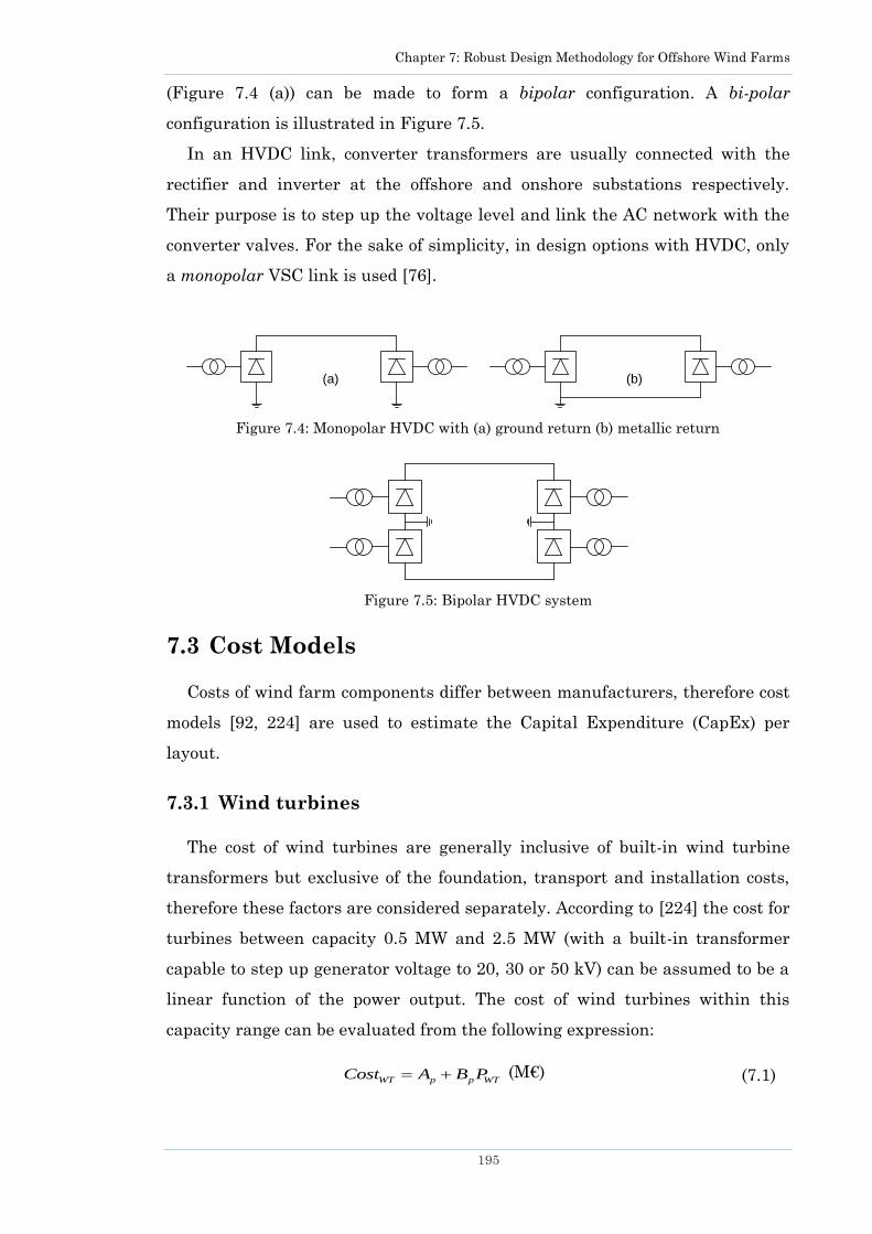
Chapter 7: Robust Design Methodology for Offshore Wind Farms
195
(Figure 7.4 (a)) can be made to form a bipolar configuration. A bi-polar
configuration is illustrated in Figure 7.5.
In an HVDC link, converter transformers are usually connected with the
rectifier and inverter at the offshore and onshore substations respectively.
Their purpose is to step up the voltage level and link the AC network with the
converter valves. For the sake of simplicity, in design options with HVDC, only
a monopolar VSC link is used [76].
Figure 7.4: Monopolar HVDC with (a) ground return (b) metallic return
Figure 7.5: Bipolar HVDC system
7.3 Cost Models
Costs of wind farm components differ between manufacturers, therefore cost
models [92, 224] are used to estimate the Capital Expenditure (CapEx) per
layout.
7.3.1 Wind turbines
The cost of wind turbines are generally inclusive of built-in wind turbine
transformers but exclusive of the foundation, transport and installation costs,
therefore these factors are considered separately. According to [224] the cost for
turbines between capacity 0.5 MW and 2.5 MW (with a built-in transformer
capable to step up generator voltage to 20, 30 or 50 kV) can be assumed to be a
linear function of the power output. The cost of wind turbines within this
capacity range can be evaluated from the following expression:
WT p p WTCost A B P (M€) (7.1)
(a) (b)
Chapter 7: Robust Design Methodology for Offshore Wind Farms
196
where PWT is the rated power of a wind turbine, Ap and Bp are offset and slope
constants with values -0.1848 and 1.0609 respectively.
In [225], the cost of wind turbines of capacity 2 MW to 5 MW is derived from
data available from wind turbine manufacturers and is described by the
following expression:
32.95 10 ln( ) 375.2 WT WTCost x P (k€) (7.2)
Transport and installation costs for all wind turbine units can be considered
collectively, and although this depends on how far away they have to be
transported, a general expression is assumed to include these costs [92]:
_ 1.1WT TI WT WTCost N Cost (7.3)
where NWT is the number of wind turbines in the wind farm.
7.3.1.1 Foundations
Wind turbine foundations used for offshore installations are generally very
expensive. The turbine foundations have to be transported from the
manufacturing facility to the sea and then installed for each turbine. Therefore
manufacturing, transport and installation costs should be calculated for each
turbine foundation. Offshore wind turbines are generally installed in water
depths of 2 to 30 meters. If foundation costs for onshore wind turbines and
offshore wind turbines are compared it will be seen that there is almost a five
fold difference. Normally, foundations for onshore turbines cost between 40 and
50 €/kW, but for offshore turbine foundations this value is around 250 to 300
€/kW in a water depth of 8 meters. The cost for offshore wind turbine
foundations increases by 2% per meter for a sea depth greater than 8 meters. A
general cost model is proposed in [17] that can be used to obtain approximate
offshore wind turbine foundation costs. The influence of the turbine dimension
is considered through a Load Factor (LF):
2
2
DLF h (7.4)
where h is the turbine hub height in meters, D is the turbine rotor diameter in
meters. The foundation cost can then be calculated by the following expression
[92]:
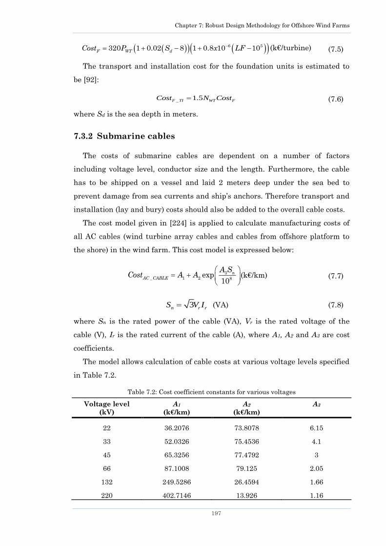
Chapter 7: Robust Design Methodology for Offshore Wind Farms
197
6 5320 1 0.02 8 1 0.8 10 10F WT d
Cost P S x LF (k€/turbine) (7.5)
The transport and installation cost for the foundation units is estimated to
be [92]:
_ 1.5F TI WT FCost N Cost (7.6)
where Sd is the sea depth in meters.
7.3.2 Submarine cables
The costs of submarine cables are dependent on a number of factors
including voltage level, conductor size and the length. Furthermore, the cable
has to be shipped on a vessel and laid 2 meters deep under the sea bed to
prevent damage from sea currents and ship‘s anchors. Therefore transport and
installation (lay and bury) costs should also be added to the overall cable costs.
The cost model given in [224] is applied to calculate manufacturing costs of
all AC cables (wind turbine array cables and cables from offshore platform to
the shore) in the wind farm. This cost model is expressed below:
3_ 1 2 8
exp10
nAC CABLE
A SCost A A (k€/km) (7.7)
(VA) (7.8)
where Sn is the rated power of the cable (VA), Vr is the rated voltage of the
cable (V), Ir is the rated current of the cable (A), where A1, A2 and A3 are cost
coefficients.
The model allows calculation of cable costs at various voltage levels specified
in Table 7.2.
Table 7.2: Cost coefficient constants for various voltages
Voltage level
(kV)
A1
(k€/km)
A2
(k€/km)
A3
22 36.2076 73.8078 6.15
33 52.0326 75.4536 4.1
45 65.3256 77.4792 3
66 87.1008 79.125 2.05
132 249.5286 26.4594 1.66
220 402.7146 13.926 1.16
3n r rS V I
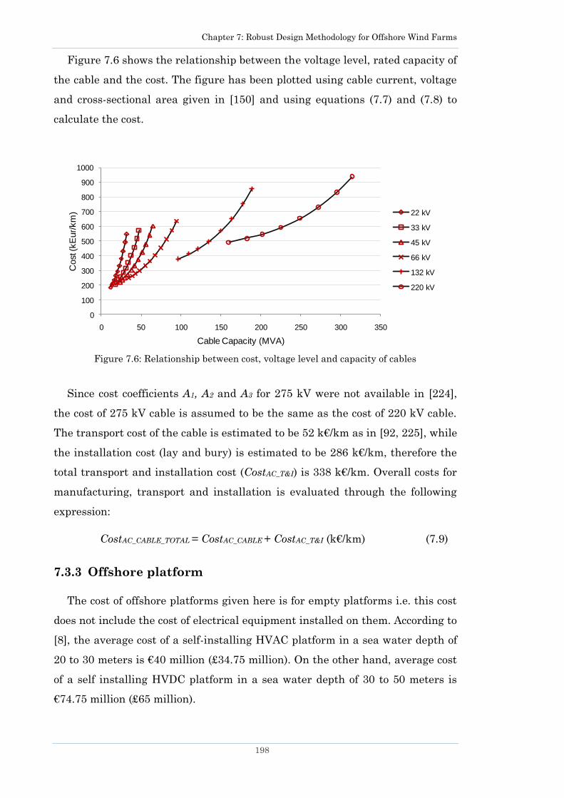
Chapter 7: Robust Design Methodology for Offshore Wind Farms
198
Figure 7.6 shows the relationship between the voltage level, rated capacity of
the cable and the cost. The figure has been plotted using cable current, voltage
and cross-sectional area given in [150] and using equations (7.7) and (7.8) to
calculate the cost.
Figure 7.6: Relationship between cost, voltage level and capacity of cables
Since cost coefficients A1, A2 and A3 for 275 kV were not available in [224],
the cost of 275 kV cable is assumed to be the same as the cost of 220 kV cable.
The transport cost of the cable is estimated to be 52 k€/km as in [92, 225], while
the installation cost (lay and bury) is estimated to be 286 k€/km, therefore the
total transport and installation cost (CostAC_T&I) is 338 k€/km. Overall costs for
manufacturing, transport and installation is evaluated through the following
expression:
CostAC_CABLE_TOTAL = CostAC_CABLE + CostAC_T&I (k€/km) (7.9)
7.3.3 Offshore platform
The cost of offshore platforms given here is for empty platforms i.e. this cost
does not include the cost of electrical equipment installed on them. According to
[8], the average cost of a self-installing HVAC platform in a sea water depth of
20 to 30 meters is €40 million (£34.75 million). On the other hand, average cost
of a self installing HVDC platform in a sea water depth of 30 to 50 meters is
€74.75 million (£65 million).
0
100
200
300
400
500
600
700
800
900
1000
0 50 100 150 200 250 300 350
Cost
(kE
ur/
km
)
Cable Capacity (MVA)
22 kV
33 kV
45 kV
66 kV
132 kV
220 kV

Chapter 7: Robust Design Methodology for Offshore Wind Farms
199
An AC platform is used for an HVAC link, while a DC platform is used for an
HVDC link. An HVAC offshore platform consists of collector transformers, MV
& HV switchgears and reactive power compensation. A DC platform consists of
collector transformers, converter transformers, converters and MV, HV and
EHV switchgears. The cost of equipment installed on the platforms is
calculated separately using the cost models given in the sections below.
7.3.4 VSC converters
The cost of a VSC converter is estimated to be €166.75/kW (£145/kW) from
data available in [8].
7.3.5 HVDC cables
A cost model for DC cables is developed using cable data given in [226] and
cable cost data given in [8] for two voltage levels (150 kV and 320 kV). These
two voltage levels are assumed because a VSC converter in [226] operates at
these voltages. Two types of DC cables, Extruded subsea and Mass Impregnated
Insulated are commonly used in an offshore environment. The cost model is
developed for Extruded subsea cable using average material and installation
costs.
150 kV:
_ _150 0.1486 736 DC CABLE kVCost CSA (€/m) (7.10)
320 kV:
_ _320 0.1017 869.71 DC CABLE kVCost CSA (€/m) (7.11)
where CSA is the cable cross-sectional area in mm2.
The number of DC cables that connect an offshore platform with the shore is
dependent on the number of VSC converters. Since monopole configuration is
used, each converter has one cable attached to it. The model provides costs for a
single DC cable buried under the sea bed in a single trench.
7.3.6 Offshore and onshore compensation device
Components inside an electrical system for an offshore wind farm can
generate or consume reactive power. For instance, wind turbine array AC
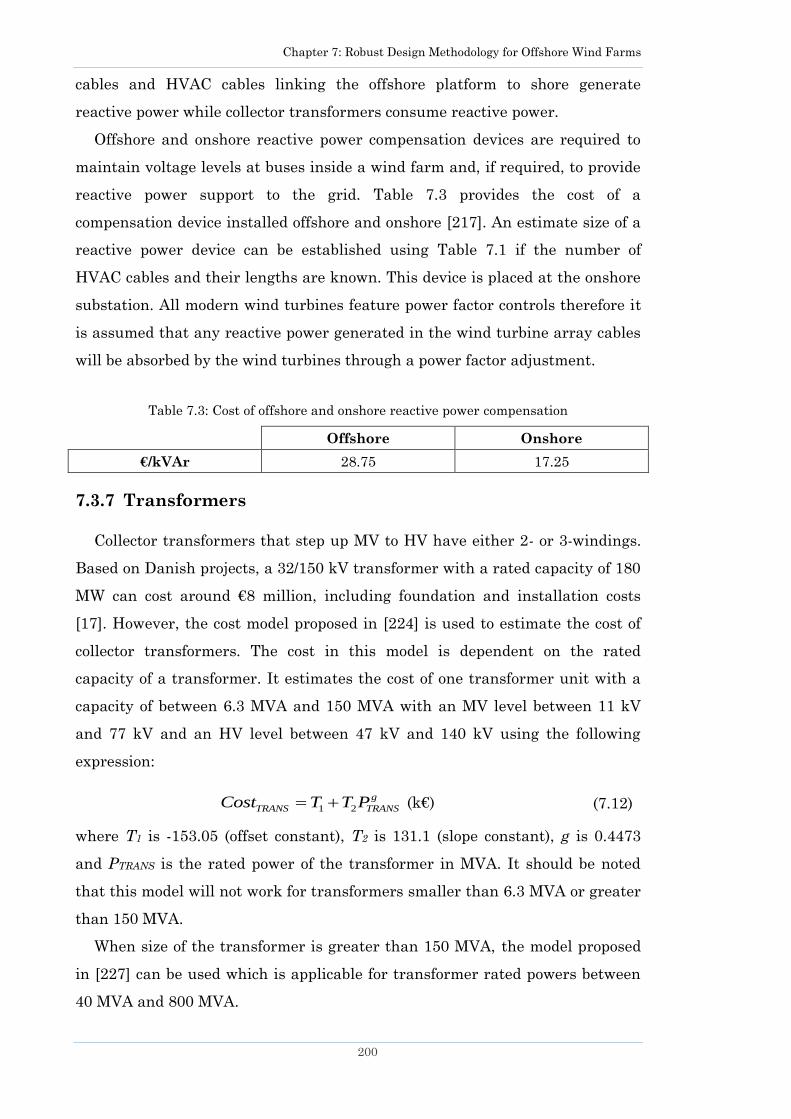
Chapter 7: Robust Design Methodology for Offshore Wind Farms
200
cables and HVAC cables linking the offshore platform to shore generate
reactive power while collector transformers consume reactive power.
Offshore and onshore reactive power compensation devices are required to
maintain voltage levels at buses inside a wind farm and, if required, to provide
reactive power support to the grid. Table 7.3 provides the cost of a
compensation device installed offshore and onshore [217]. An estimate size of a
reactive power device can be established using Table 7.1 if the number of
HVAC cables and their lengths are known. This device is placed at the onshore
substation. All modern wind turbines feature power factor controls therefore it
is assumed that any reactive power generated in the wind turbine array cables
will be absorbed by the wind turbines through a power factor adjustment.
Table 7.3: Cost of offshore and onshore reactive power compensation
Offshore Onshore
€/kVAr 28.75 17.25
7.3.7 Transformers
Collector transformers that step up MV to HV have either 2- or 3-windings.
Based on Danish projects, a 32/150 kV transformer with a rated capacity of 180
MW can cost around €8 million, including foundation and installation costs
[17]. However, the cost model proposed in [224] is used to estimate the cost of
collector transformers. The cost in this model is dependent on the rated
capacity of a transformer. It estimates the cost of one transformer unit with a
capacity of between 6.3 MVA and 150 MVA with an MV level between 11 kV
and 77 kV and an HV level between 47 kV and 140 kV using the following
expression:
1 2 g
TRANS TRANSCost T T P (k€) (7.12)
where T1 is -153.05 (offset constant), T2 is 131.1 (slope constant), g is 0.4473
and PTRANS is the rated power of the transformer in MVA. It should be noted
that this model will not work for transformers smaller than 6.3 MVA or greater
than 150 MVA.
When size of the transformer is greater than 150 MVA, the model proposed
in [227] can be used which is applicable for transformer rated powers between
40 MVA and 800 MVA.
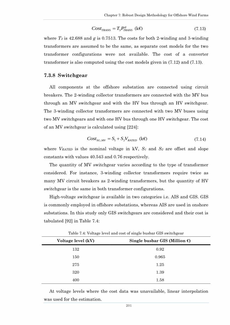
Chapter 7: Robust Design Methodology for Offshore Wind Farms
201
3 g
TRANS TRANSCost T P (k€) (7.13)
where T3 is 42.688 and g is 0.7513. The costs for both 2-winding and 3-winding
transformers are assumed to be the same, as separate cost models for the two
transformer configurations were not available. The cost of a converter
transformer is also computed using the cost models given in (7.12) and (7.13).
7.3.8 Switchgear
All components at the offshore substation are connected using circuit
breakers. The 2-winding collector transformers are connected with the MV bus
through an MV switchgear and with the HV bus through an HV switchgear.
The 3-winding collector transformers are connected with two MV buses using
two MV switchgears and with one HV bus through one HV switchgear. The cost
of an MV switchgear is calculated using [224]:
, 1 2 SG MV RATEDCost S S V (k€) (7.14)
where VRATED is the nominal voltage in kV, S1 and S2 are offset and slope
constants with values 40.543 and 0.76 respectively.
The quantity of MV switchgear varies according to the type of transformer
considered. For instance, 3-winding collector transformers require twice as
many MV circuit breakers as 2-winding transformers, but the quantity of HV
switchgear is the same in both transformer configurations.
High-voltage switchgear is available in two categories i.e. AIS and GIS. GIS
is commonly employed in offshore substations, whereas AIS are used in onshore
substations. In this study only GIS switchgears are considered and their cost is
tabulated [92] in Table 7.4:
Table 7.4: Voltage level and cost of single busbar GIS switchgear
Voltage level (kV) Single busbar GIS (Million €)
132 0.92
150 0.965
275 1.25
320 1.39
400 1.58
At voltage levels where the cost data was unavailable, linear interpolation
was used for the estimation.

Chapter 7: Robust Design Methodology for Offshore Wind Farms
202
7.4 Robust Offshore Wind Farm Electrical Layout
There are several components to choose from when creating an offshore
electrical layout. These components are:
Capacity of the wind turbines
Type of array configuration
Array voltage level
Type of collector transformers (2-winding or 3-winding)
Quantity and capacity of the collector transformers (with and without a
redundant transformer)
Type of transmission link to shore
Transmission voltage level
If an HVAC link is used, then the number of cables from platform to the
shore (with and without a redundant cable) and the size of reactive
power compensation
If an HVDC link is used, then the capacity and voltage level of the
converters and capacity of converter transformers.
Each of these components has further options, represented by a variable N, a
combination of which leads to several possible electrical layouts. For instance,
starting with the wind turbines; say there are two wind turbine capacities
available to choose from e.g. a 2 MW or a 3 MW machine; to connect the
turbines in an array configuration, a radial, starburst, tree or radial with end
loop might be used. Therefore, either 2 MW or 3 MW turbines can be used in
either of four array configurations. In this example, only 2 possible wind
turbine capacities and 4 possible array configurations were discussed and this
lead to 8 possible combinations. Similarly, when all components are considered
collectively, where each component has its own options, this leads to several
combinations and thus several possible electrical layouts. In order to narrow
down the choice of layouts a novel methodology is proposed as shown in the
flow chart in Figure 7.7.
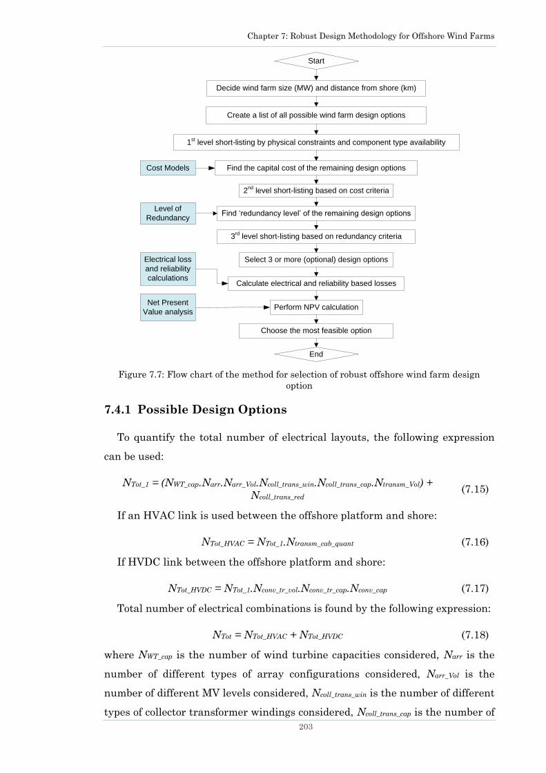
Chapter 7: Robust Design Methodology for Offshore Wind Farms
203
Figure 7.7: Flow chart of the method for selection of robust offshore wind farm design
option
7.4.1 Possible Design Options
To quantify the total number of electrical layouts, the following expression
can be used:
NTot_1 = (NWT_cap.Narr.Narr_Vol.Ncoll_trans_win.Ncoll_trans_cap.Ntransm_Vol) +
Ncoll_trans_red (7.15)
If an HVAC link is used between the offshore platform and shore:
NTot_HVAC = NTot_1.Ntransm_cab_quant (7.16)
If HVDC link between the offshore platform and shore:
NTot_HVDC = NTot_1.Nconv_tr_vol.Nconv_tr_cap.Nconv_cap (7.17)
Total number of electrical combinations is found by the following expression:
NTot = NTot_HVAC + NTot_HVDC (7.18)
where NWT_cap is the number of wind turbine capacities considered, Narr is the
number of different types of array configurations considered, Narr_Vol is the
number of different MV levels considered, Ncoll_trans_win is the number of different
types of collector transformer windings considered, Ncoll_trans_cap is the number of
Start
Decide wind farm size (MW) and distance from shore (km)
Create a list of all possible wind farm design options
1st level short-listing by physical constraints and component type availability
2nd
level short-listing based on cost criteria
3rd
level short-listing based on redundancy criteria
Calculate electrical and reliability based losses
End
Find the capital cost of the remaining design options
Find ‘redundancy level’ of the remaining design options
Select 3 or more (optional) design options
Perform NPV calculation
Choose the most feasible option
Cost Models
Level of
Redundancy
Net Present
Value analysis
Electrical loss
and reliability
calculations

Chapter 7: Robust Design Methodology for Offshore Wind Farms
204
different collector transformer capacities considered, Ntransm_Vol is the number of
different HV levels considered at collector transformer secondary windings,
Ncoll_trans_red is the number of extra options considered having redundant
collector transformers, NTot_HVAC is the total number of electrical layouts when
an HVAC link is used to connect the offshore platform with the shore, NTot_1 is
the total number of combinations if the electrical layout from the wind turbines
to the collector transformer is considered, Ntransm_cab_quant is the number of
different quantities of HVAC cables considered, NTot_HVDC is the total number of
electrical layouts with an HVDC link from platform to shore, Nconv_tr_vol is the
number of different EHV voltage levels considered at the converter transformer
secondary windings, Nconv_tr_cap is the number of different capacities of converter
transformers considered, Nconv_cap is the number of different VSC converter
capacities considered and NTot is the total number of electrical layouts when
both HVAC link and HVDC link options are considered.
As a case study, a 400 MW wind farm is used that is 50 km away from the
shore. This capacity and distance from the shore was selected by analysing
present and future installations of offshore wind farms in Europe. The analysis
is presented in Chapter 1. It can be seen from Figure 1.3 and Figure 1.4 that 11
offshore wind farms with an exact capacity of 400 MW are proposed, implying
they are either under construction, submitted or approved. Although it is
difficult to build a consensus on the distance to shore, as seen from Figure 1.4
wind farms will on average be 50 km away from shore. The wind turbines
inside the wind farm are assumed to be 400 m apart. Nevertheless, the method
proposed can be applied to a wind farm of any capacity at any distance from the
shore.
7.4.2 Quantity and rating of components
The methodology is demonstrated by applying it to a 400 MW wind farm.
Therefore, all possible combinations for an electrical layout for this wind farm
are created.
First of all, wind turbine capacities that are most popular are determined.
This is done by analysing data from 120 offshore wind farms in Europe
including those existing, under construction, submitted and approved offshore
wind farms. From this analysis it was determined that 2 MW, 2.3 MW, 3.6 MW
and 5 MW capacity wind turbines are very popular. (All wind turbines are
Chapter 7: Robust Design Methodology for Offshore Wind Farms
205
assumed to have power factor varying capability, such that they can vary their
power factor between 0.95 leading and 0.95 lagging).
In order to connect these wind turbines together, four popular array
configurations are investigated i.e. radial, starburst, tree and radial with end
loop, as they are the typical array configurations within existing wind farms or
are most commonly discussed in the literature. Details on these array
configurations can be found in Section 1.2.2.4. The voltage level inside the
array is assumed to be 33 kV, because this is a very commonly used voltage
level inside offshore wind farms. All turbines have a built-in 0.69/33 kV
transformer. Power generated by these wind turbines is collected at an offshore
substation from where its voltage level is stepped up to HV level and then this
power is transmitted to the shore.
Next, the voltage level for transmission has to be selected. The MV level can
be stepped up from 33 kV to 132 kV, 275 kV or 400 kV. Each voltage level has
its own characteristics which affects both the cost of the components as well as
the electrical losses. Therefore, all three HV level options will be considered.
To scale up the voltage level from MV to HV, collector transformers are
needed. These transformers can have either 2- or 3-windings. Both 2-winding
and 3-winding transformers will have a certain MVA rating. Three different
MVA ratings of 100 MVA, 120 MVA and 240 MVA [8, 228] are tested for 2-
winding and 3-winding transformers in the case study. The quantity of the
collector transformers is dependent on the capacity of the wind farm.
Next, power transmission options from the offshore platform to the shore are
analysed. Both HVAC and VSC-HVDC link (monopolar) options are considered.
In the case of an HVAC link, the power from the collector transformers is
delivered to the shore through HVAC cables. Based on the collector transformer
voltage level, an HVAC link can be established using 132 kV, 275 kV or 400 kV
cables. The quantity of the cables depends on the current carrying capacity of a
cable and the voltage level used. For example, a 132 kV cable can carry a
maximum of 188 MVA, hence three of these will be employed to carry 400 MW
to the shore but if 275 kV is considered, then one 392 MVA cable will be
sufficient. Cable data from [150] is used.
In the case of an HVDC link, the VSC converter voltage levels can be 150 kV
or 320 kV, according to ABB‘s Light technology [226]. In order to step up the
voltage level from HV (132 kV, 275 kV or 400 kV) to EHV (150 kV or 320 kV),
Chapter 7: Robust Design Methodology for Offshore Wind Farms
206
converter transformers are used. Only 2-winding converter transformers are
considered and these converter transformers can be available in different MVA
ratings. In this case study, two different capacity converter transformers are
used i.e. 200 MVA and 400 MVA. The quantity of converter transformers
depends on the capacity of the wind farm.
The capacity of the VSC converters varies with the voltage rating of the
converters. At 150 kV, the VSC converters can send rated powers of 190 MW,
373 MW and 570 MW, while at 320 kV the converters can send powers of 408
MW, 802 MW and 1224 MW [226]. Therefore, converters with all voltage levels
and capacities are considered in the analysis. The quantity of converters
depends on the capacity of the wind farm. DC cables with enough capacity to
carry the power to the shore are chosen from [226].
An estimated size of the reactive power compensation device is established
where the link to the shore is made through HVAC. The ability of wind
turbines to consume or produce reactive power is exploited to maintain unity
power factor at the primary side of collector transformers (MV bus). For an
HVAC link, a reactive compensation device is installed onshore. For an HVAC
link, the size of reactive compensation depends on the voltage, length and
quantity of cables installed and is approximated through values given in Table
7.1. In the case of a VSC-HVDC link, having a reactive power compensation
device is not mandatory, as converters have the ability to regulate reactive
power.
All the above mentioned components and their options lead to several
electrical layout combinations. Further, additional layouts are also produced
with a certain level of redundancy to test the impact on the investment cost and
reliability of the offshore electrical network. In this case study additional
electrical networks with redundant collector transformers and redundant
HVAC cables were created. The process of combination development can be
visualised from Figure 7.8.
An NTot x Ncomp matrix stores all electrical layout combinations in NTot rows,
whereas Ncomp defines the number of columns of this matrix and each column
stores the type, capacity and quantity of each component.
Using the approach illustrated in this example, possible electrical layouts for
an offshore wind farm of any capacity can be created. However, only those
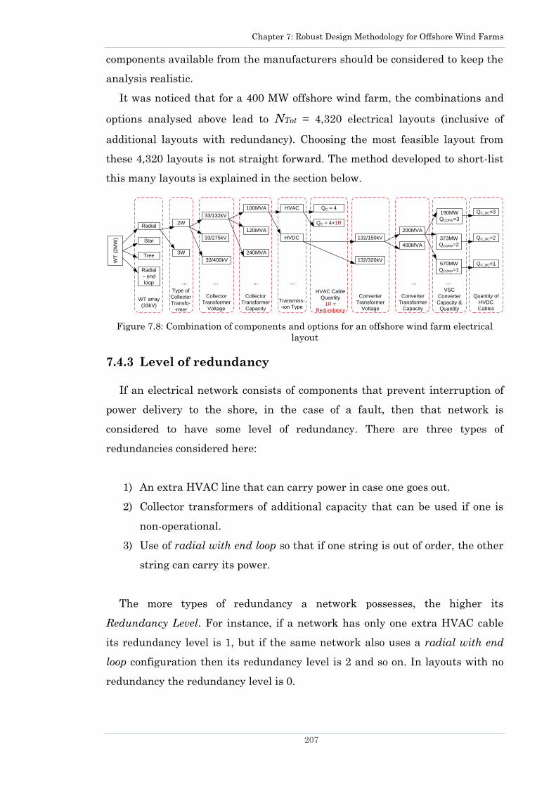
Chapter 7: Robust Design Methodology for Offshore Wind Farms
207
components available from the manufacturers should be considered to keep the
analysis realistic.
It was noticed that for a 400 MW offshore wind farm, the combinations and
options analysed above lead to NTot = 4,320 electrical layouts (inclusive of
additional layouts with redundancy). Choosing the most feasible layout from
these 4,320 layouts is not straight forward. The method developed to short-list
this many layouts is explained in the section below.
Figure 7.8: Combination of components and options for an offshore wind farm electrical
layout
7.4.3 Level of redundancy
If an electrical network consists of components that prevent interruption of
power delivery to the shore, in the case of a fault, then that network is
considered to have some level of redundancy. There are three types of
redundancies considered here:
1) An extra HVAC line that can carry power in case one goes out.
2) Collector transformers of additional capacity that can be used if one is
non-operational.
3) Use of radial with end loop so that if one string is out of order, the other
string can carry its power.
The more types of redundancy a network possesses, the higher its
Redundancy Level. For instance, if a network has only one extra HVAC cable
its redundancy level is 1, but if the same network also uses a radial with end
loop configuration then its redundancy level is 2 and so on. In layouts with no
redundancy the redundancy level is 0.
WT
(2M
W)
Radial
Star
Tree
Radial
– end
loop
33/132kV
33/275kV
33/400kV
2W
3W
WT array
(33kV)
Collector
Transformer
Voltage
100MVA
120MVA
240MVA
Type of
Collector
Transfo-
-rmer
HVAC
HVDC 132/150kV
132/320kV
200MVA
400MVA
570MW
QCONV=1
190MW
QCONV=3
373MW
QCONV=2
............ ... ...
Collector
Transformer
Capacity
Transmiss-
-ion Type
Converter
Transformer
Voltage
QC = 4
QC = 4+1R
HVAC Cable
Quantity
1R =
Redundancy
Converter
Transformer
Capacity
VSC
Converter
Capacity &
Quantity
QC_DC=1
QC_DC=3
QC_DC=2
Quantity of
HVDC
Cables

Chapter 7: Robust Design Methodology for Offshore Wind Farms
208
7.5 Short-Listing Layouts based on Investment
Cost and Redundancy Level
The total number of possible electrical layouts for any large WF is enormous.
Analysing so many electrical layouts for electrical losses, reliability based
losses and investment costs is not practical. Therefore, short listing is
performed to eliminate economically unfeasible options.
The first level of short-listing is performed to rule out layouts with
components that are least likely as either they are too expensive or they would
not add significant benefit. The following criteria can be used as a general rule
for any WF:
1) The use of three VSC-HVDC links with capacity 190 MW each will lead
to a total of 570 MW, out of which 170 MW will not be used, therefore
two links with a maximum capacity of 380 MW can be used instead. This
will save the investment cost of converters and cables. The probability of
WF operation at full power is low therefore this is a fair assumption.
2) Any VSC-HVDC links (to shore) made with a converter capacity larger
than 405 MW can be ignored. VSC-HVDC links up to 1224 MW were
considered during the combination development.
3) A radial array configuration is normally built with an end-loop,
therefore a simple radial array configuration can be removed from
consideration. A tree configuration is more commonly used in existing
wind farms than a starburst, hence a starburst can also be taken out of
consideration.
4) Having a redundant collector transformer is too expensive so any extra
capacity in transformers can be used to provide redundancy. For
instance, if four 120 MW transformers are used and if one goes out,
about 360 MW can still be transferred. This option is cheaper than
having a fifth (redundant) transformer of 120 MW which may rarely be
used.
Layouts with components mentioned in the four points above will be
removed from consideration. Although these suggestions are to reduce the
number of total layouts so that they can be easily analysed, if any of these
suggestions are not relevant for a particular wind farm design they can be
ignored. After first-level of short listing, 4320 options (electrical layouts) were
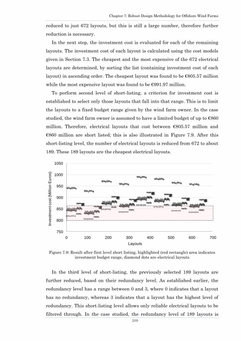
Chapter 7: Robust Design Methodology for Offshore Wind Farms
209
reduced to just 672 layouts, but this is still a large number, therefore further
reduction is necessary.
In the next step, the investment cost is evaluated for each of the remaining
layouts. The investment cost of each layout is calculated using the cost models
given in Section 7.3. The cheapest and the most expensive of the 672 electrical
layouts are determined, by sorting the list (containing investment cost of each
layout) in ascending order. The cheapest layout was found to be €805.57 million
while the most expensive layout was found to be €991.97 million.
To perform second level of short-listing, a criterion for investment cost is
established to select only those layouts that fall into that range. This is to limit
the layouts to a fixed budget range given by the wind farm owner. In the case
studied, the wind farm owner is assumed to have a limited budget of up to €860
million. Therefore, electrical layouts that cost between €805.57 million and
€860 million are short listed; this is also illustrated in Figure 7.9. After this
short-listing level, the number of electrical layouts is reduced from 672 to about
189. These 189 layouts are the cheapest electrical layouts.
Figure 7.9: Result after first level short listing, highlighted (red rectangle) area indicates
investment budget range, diamond dots are electrical layouts
In the third level of short-listing, the previously selected 189 layouts are
further reduced, based on their redundancy level. As established earlier, the
redundancy level has a range between 0 and 3, where 0 indicates that a layout
has no redundancy, whereas 3 indicates that a layout has the highest level of
redundancy. This short-listing level allows only reliable electrical layouts to be
filtered through. In the case studied, the redundancy level of 189 layouts is
750
800
850
900
950
1000
1050
0 100 200 300 400 500 600 700
Inve
stm
en
t co
st (M
illio
n E
uro
s)
Layouts
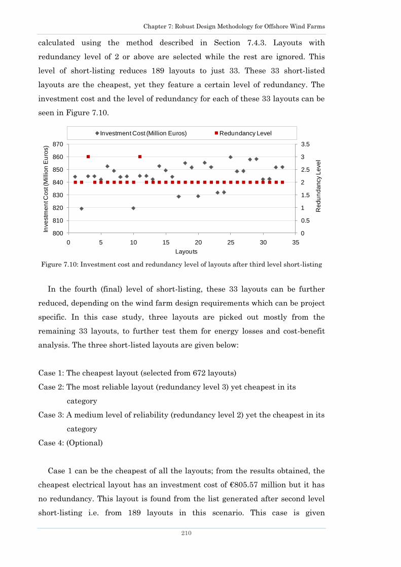
Chapter 7: Robust Design Methodology for Offshore Wind Farms
210
calculated using the method described in Section 7.4.3. Layouts with
redundancy level of 2 or above are selected while the rest are ignored. This
level of short-listing reduces 189 layouts to just 33. These 33 short-listed
layouts are the cheapest, yet they feature a certain level of redundancy. The
investment cost and the level of redundancy for each of these 33 layouts can be
seen in Figure 7.10.
Figure 7.10: Investment cost and redundancy level of layouts after third level short-listing
In the fourth (final) level of short-listing, these 33 layouts can be further
reduced, depending on the wind farm design requirements which can be project
specific. In this case study, three layouts are picked out mostly from the
remaining 33 layouts, to further test them for energy losses and cost-benefit
analysis. The three short-listed layouts are given below:
Case 1: The cheapest layout (selected from 672 layouts)
Case 2: The most reliable layout (redundancy level 3) yet cheapest in its
category
Case 3: A medium level of reliability (redundancy level 2) yet the cheapest in its
category
Case 4: (Optional)
Case 1 can be the cheapest of all the layouts; from the results obtained, the
cheapest electrical layout has an investment cost of €805.57 million but it has
no redundancy. This layout is found from the list generated after second level
short-listing i.e. from 189 layouts in this scenario. This case is given
0
0.5
1
1.5
2
2.5
3
3.5
800
810
820
830
840
850
860
870
0 5 10 15 20 25 30 35
Re
du
nd
an
cy L
eve
l
Inve
stm
en
t Co
st (
Millio
n E
uro
s)
Layouts
Investment Cost (Million Euros) Redundancy Level
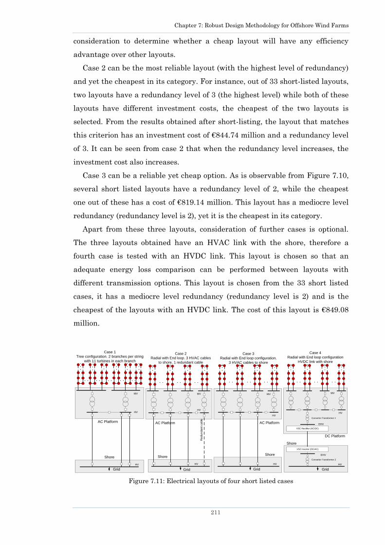
Chapter 7: Robust Design Methodology for Offshore Wind Farms
211
consideration to determine whether a cheap layout will have any efficiency
advantage over other layouts.
Case 2 can be the most reliable layout (with the highest level of redundancy)
and yet the cheapest in its category. For instance, out of 33 short-listed layouts,
two layouts have a redundancy level of 3 (the highest level) while both of these
layouts have different investment costs, the cheapest of the two layouts is
selected. From the results obtained after short-listing, the layout that matches
this criterion has an investment cost of €844.74 million and a redundancy level
of 3. It can be seen from case 2 that when the redundancy level increases, the
investment cost also increases.
Case 3 can be a reliable yet cheap option. As is observable from Figure 7.10,
several short listed layouts have a redundancy level of 2, while the cheapest
one out of these has a cost of €819.14 million. This layout has a mediocre level
redundancy (redundancy level is 2), yet it is the cheapest in its category.
Apart from these three layouts, consideration of further cases is optional.
The three layouts obtained have an HVAC link with the shore, therefore a
fourth case is tested with an HVDC link. This layout is chosen so that an
adequate energy loss comparison can be performed between layouts with
different transmission options. This layout is chosen from the 33 short listed
cases, it has a mediocre level redundancy (redundancy level is 2) and is the
cheapest of the layouts with an HVDC link. The cost of this layout is €849.08
million.
Figure 7.11: Electrical layouts of four short listed cases
HV
MV
Shore
Case 1
Tree configuration. 2 branches per string
with 11 turbines in each branch
HV
AC Platform
Grid
HV
MV
Shore
Case 2
Radial with End loop. 3 HVAC cables
to shore, 1 redundant cable
HV
Re
du
nd
an
t ca
ble
AC Platform
Grid
HV
MV
Shore
Case 3
Radial with End loop configuration.
3 HVAC cables to shore
HV
AC Platform
Grid
HV
MV
Shore
Case 4
Radial with End loop configuration
HVDC link with shore
HV
DC Platform
Converter Transformer 1
VSC Rectifier (AC/DC)
VSC Inverter (DC/AC)
EHV
EHV
Converter Transformer 2
Grid
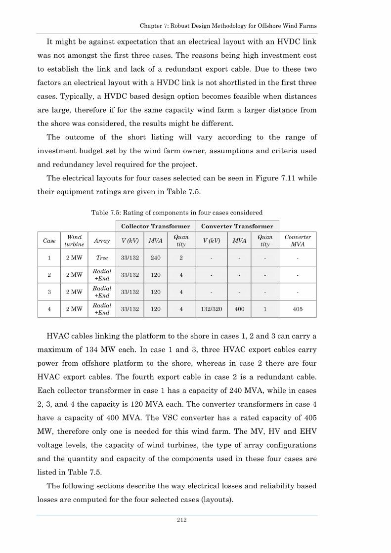
Chapter 7: Robust Design Methodology for Offshore Wind Farms
212
It might be against expectation that an electrical layout with an HVDC link
was not amongst the first three cases. The reasons being high investment cost
to establish the link and lack of a redundant export cable. Due to these two
factors an electrical layout with a HVDC link is not shortlisted in the first three
cases. Typically, a HVDC based design option becomes feasible when distances
are large, therefore if for the same capacity wind farm a larger distance from
the shore was considered, the results might be different.
The outcome of the short listing will vary according to the range of
investment budget set by the wind farm owner, assumptions and criteria used
and redundancy level required for the project.
The electrical layouts for four cases selected can be seen in Figure 7.11 while
their equipment ratings are given in Table 7.5.
Table 7.5: Rating of components in four cases considered
Collector Transformer Converter Transformer
Case Wind
turbine Array V (kV) MVA
Quan
tity V (kV) MVA
Quan
tity
Converter
MVA
1 2 MW Tree 33/132 240 2 - - - -
2 2 MW Radial
+End 33/132 120 4 - - - -
3 2 MW Radial
+End 33/132 120 4 - - - -
4 2 MW Radial
+End 33/132 120 4 132/320 400 1 405
HVAC cables linking the platform to the shore in cases 1, 2 and 3 can carry a
maximum of 134 MW each. In case 1 and 3, three HVAC export cables carry
power from offshore platform to the shore, whereas in case 2 there are four
HVAC export cables. The fourth export cable in case 2 is a redundant cable.
Each collector transformer in case 1 has a capacity of 240 MVA, while in cases
2, 3, and 4 the capacity is 120 MVA each. The converter transformers in case 4
have a capacity of 400 MVA. The VSC converter has a rated capacity of 405
MW, therefore only one is needed for this wind farm. The MV, HV and EHV
voltage levels, the capacity of wind turbines, the type of array configurations
and the quantity and capacity of the components used in these four cases are
listed in Table 7.5.
The following sections describe the way electrical losses and reliability based
losses are computed for the four selected cases (layouts).
Chapter 7: Robust Design Methodology for Offshore Wind Farms
213
7.6 Electrical Loss and Reliability Calculations
This section focuses on the methodology behind the following tasks:
Calculation of electrical losses
Voltage/reactive power compliance and coordination
Reliability assessment
The final outcome of all calculations is the cost of:
Annual energy lost due to electrical losses.
Annual energy loss due to reliability based losses
To calculate the energy losses, a wind power frequency curve is used to
estimate wind speed and power production from the wind turbines.
7.6.1 Wind power frequency curve
The use of chronological wind speed measurements would take a substantial
amount of time to perform load flow and to calculate electrical losses, therefore
the power bin frequency method is applied. A generic wind power frequency
curve is developed using the Weibull distribution and wind turbine power
curves. The Weibull function given in (7.19) is used to estimate the wind speeds
and their probability at a site during the year. The probabilities are converted
into frequencies (in hours) by multiplying them with the total number of hours
in a year (8760). Turbine power curves are used to convert wind speed into
power output; this yields a wind power frequency curve as shown in Figure
7.12. Using this curve, the frequency of each power bin can be obtained. Shape
and scale parameters ks = 1.8 and sc = 11.2 were used. These parameters were
derived from wind speed data available at a site in the east coast of the UK.
(Similar parameters have been reported in [229] for the North Sea).
1
( )
sks
c
k
v ss
c c
k vf v e
s s
(7.19)
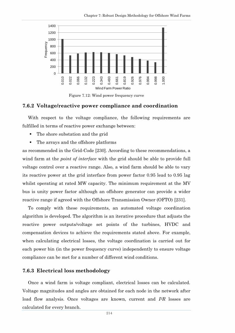
Chapter 7: Robust Design Methodology for Offshore Wind Farms
214
Figure 7.12: Wind power frequency curve
7.6.2 Voltage/reactive power compliance and coordination
With respect to the voltage compliance, the following requirements are
fulfilled in terms of reactive power exchange between:
The shore substation and the grid
The arrays and the offshore platforms
as recommended in the Grid-Code [230]. According to these recommendations, a
wind farm at the point of interface with the grid should be able to provide full
voltage control over a reactive range. Also, a wind farm should be able to vary
its reactive power at the grid interface from power factor 0.95 lead to 0.95 lag
whilst operating at rated MW capacity. The minimum requirement at the MV
bus is unity power factor although an offshore generator can provide a wider
reactive range if agreed with the Offshore Transmission Owner (OFTO) [231].
To comply with these requirements, an automated voltage coordination
algorithm is developed. The algorithm is an iterative procedure that adjusts the
reactive power outputs/voltage set points of the turbines, HVDC and
compensation devices to achieve the requirements stated above. For example,
when calculating electrical losses, the voltage coordination is carried out for
each power bin (in the power frequency curve) independently to ensure voltage
compliance can be met for a number of different wind conditions.
7.6.3 Electrical loss methodology
Once a wind farm is voltage compliant, electrical losses can be calculated.
Voltage magnitudes and angles are obtained for each node in the network after
load flow analysis. Once voltages are known, current and I2R losses are
calculated for every branch.
0
200
400
600
800
1000
1200
1400
0.0
10
0.0
22
0.0
66
0.1
32
0.2
23
0.3
43
0.4
93
0.6
61
0.8
19
0.9
26
0.9
76
0.9
94
0.9
98
1.0
00
Fre
qu
en
cy
Wind Farm Power Ratio
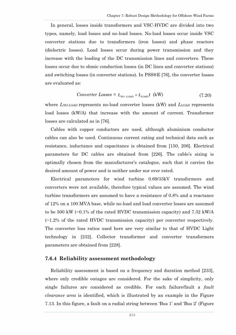
Chapter 7: Robust Design Methodology for Offshore Wind Farms
215
In general, losses inside transformers and VSC-HVDC are divided into two
types, namely, load losses and no-load losses. No-load losses occur inside VSC
converter stations due to transformers (iron losses) and phase reactors
(dielectric losses). Load losses occur during power transmission and they
increase with the loading of the DC transmission lines and converters. These
losses occur due to ohmic conduction losses (in DC lines and converter stations)
and switching losses (in converter stations). In PSS®E [76], the converter losses
are evaluated as:
Converter Losses = NO LOAD LOADL L I (kW) (7.20)
where LNO-LOAD represents no-load converter losses (kW) and LLOAD represents
load losses (kW/A) that increase with the amount of current. Transformer
losses are calculated as in [76].
Cables with copper conductors are used, although aluminium conductor
cables can also be used. Continuous current rating and technical data such as
resistance, inductance and capacitance is obtained from [150, 206]. Electrical
parameters for DC cables are obtained from [226]. The cable‘s sizing is
optimally chosen from the manufacturer‘s catalogue, such that it carries the
desired amount of power and is neither under nor over rated.
Electrical parameters for wind turbine 0.69/33kV transformers and
converters were not available, therefore typical values are assumed. The wind
turbine transformers are assumed to have a resistance of 0.8% and a reactance
of 12% on a 100 MVA base, while no-load and load converter losses are assumed
to be 500 kW (~0.1% of the rated HVDC transmission capacity) and 7.32 kW/A
(~1.2% of the rated HVDC transmission capacity) per converter respectively.
The converter loss ratios used here are very similar to that of HVDC Light
technology in [232]. Collector transformer and converter transformers
parameters are obtained from [228].
7.6.4 Reliability assessment methodology
Reliability assessment is based on a frequency and duration method [233],
where only credible outages are considered. For the sake of simplicity, only
single failures are considered as credible. For each failure/fault a fault
clearance area is identified, which is illustrated by an example in the Figure
7.13. In this figure, a fault on a radial string between ‗Bus 1‘ and ‗Bus 2‘ (Figure
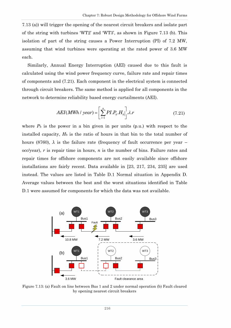
Chapter 7: Robust Design Methodology for Offshore Wind Farms
216
7.13 (a)) will trigger the opening of the nearest circuit breakers and isolate part
of the string with turbines ‗WT2‘ and ‗WT3‘, as shown in Figure 7.13 (b). This
isolation of part of the string causes a Power Interruption (PI) of 7.2 MW,
assuming that wind turbines were operating at the rated power of 3.6 MW
each.
Similarly, Annual Energy Interruption (AEI) caused due to this fault is
calculated using the wind power frequency curve, failure rate and repair times
of components and (7.21). Each component in the electrical system is connected
through circuit breakers. The same method is applied for all components in the
network to determine reliability based energy curtailments (AEI).
1
( / ) . . . .n
b bi
AEI MWh year PI P H r (7.21)
where Pb is the power in a bin given in per units (p.u.) with respect to the
installed capacity, Hb is the ratio of hours in that bin to the total number of
hours (8760), λ is the failure rate (frequency of fault occurrence per year –
occ/year), r is repair time in hours, n is the number of bins. Failure rates and
repair times for offshore components are not easily available since offshore
installations are fairly recent. Data available in [23, 217, 234, 235] are used
instead. The values are listed in Table D.1 Normal situation in Appendix D.
Average values between the best and the worst situations identified in Table
D.1 were assumed for components for which the data was not available.
Figure 7.13: (a) Fault on line between Bus 1 and 2 under normal operation (b) Fault cleared
by opening nearest circuit breakers
WT1 WT2 WT3
Fault
10.8 MW 3.6 MW7.2 MW
WT1 WT2 WT3
3.6 MW
(a)
(b)
Bus1 Bus2 Bus3
Bus1 Bus2 Bus3
Fault clearance area

Chapter 7: Robust Design Methodology for Offshore Wind Farms
217
7.7 Results of the Analysis
The electrical and reliability based energy losses (MWh) are computed for
four cases using the procedure and the parameters described in the previous
section. Both types of losses are calculated assuming that the wind farm
connected to the grid operates at unity power factor. The energy losses in MWh
are then converted into €, using the cost of offshore energy, to estimate the cost
of losses in each case. Finally, Net Present Value (NPV) analysis is performed
to decide the economic feasibility of the four cases. The cost of offshore wind
energy is estimated to be 6 €cent/kWh [3, 236] in all calculations.
7.7.1 Electrical losses
Electrical losses for all four short listed layouts are evaluated using the
methodology described in the previous section. It can be seen from Table 7.6
that the lowest losses occur in case 2, while the highest losses occur in case 4.
Losses in case 2 should be the same as case 3 as same components are used
in both, however in case 2 the redundant HVAC cable is also brought into use
under normal operation which allows power flow through four cables instead of
three. This allowed distribution of power equally among four cables and thus
reduction in overall transmission losses.
Overall, case 2 leads to the lowest amount of electrical losses, whereas case 4
leads to the highest electrical losses. A greater portion of electrical losses in
case 4 occurs inside the VSC converter stations, which amounts to about 3.11%,
whereas losses inside the DC cables are just 0.26%. In cases 1, 2 and 3 the
HVAC cables are the leading source of electrical losses compared to electrical
losses in other components. By comparing losses inside wind turbine arrays, it
was found that the tree configuration leads to higher electrical losses than the
radial with end loop configuration.
7.7.2 Reliability based losses
Reliability based losses for all four cases (short-listed layouts) are given in
Table 7.6. It can be seen from Figure 7.11 that both cases 1 and 3 have three
HVAC cables carrying power to the shore. Tripping of a single HVAC cable in
both cases will lead to a power interruption of 134 MW. Case 1, however has
higher reliability based losses than case 3 because the tree array configuration

Chapter 7: Robust Design Methodology for Offshore Wind Farms
218
does not provide any redundancy, whereas the radial with end loop
configuration can handle a single cable outage by connecting the redundant
link between the two strings in case of an inter-turbine cable outage. Therefore,
the radial with end loop configuration prevents power loss from several
turbines in a string, whereas in a tree configuration, a single fault in the cable
linking the last wind turbine to the MV bus can cause a major power
interruption. Another difference between case 1 and case 3 is that case 1 has
two 240 MVA collector transformers, whereas case 3 has four 120 MVA
collector transformers. Hence outage of one collector transformer in case 1 leads
to a power interruption of 160 MVA, whereas in case 3 the power interruption
will be of just 40 MVA (when wind farm is operating at its rated capacity).
Case 2 has a redundant HVAC cable therefore outage of a single cable will
not cause any power interruption because if power delivery from one cable is
stopped, the redundant line will be brought into operation and it will carry that
power. In case 2, power interruption due to loss of a single HVAC cable is zero.
Furthermore, case 2 has four 120 MVA collector transformers implying that
loss of one collector transformer will only reduce power by 40 MVA. The wind
turbines are connected in a radial with end loop configuration, hence the loss of
one cable will not lead to loss of power from all turbines in a string. For these
reasons, case 2 leads to the lowest reliability based losses compared to the other
layouts.
In case 4 the reliability based losses are 6.67%, although this layout has
radial with end loop configuration (to connect wind turbines) and four 120 MVA
collector transformers, but only one DC cable carrying 400 MW to the shore.
Therefore, a fault in either converter transformer, VSC converter station or the
DC line will lead to a complete power interruption.
Overall, case 1 leads to the highest amount of reliability based losses (as it
has no level of redundancy) in comparison to the other three cases, but it is the
cheapest option in terms of investment cost. Case 2 on the other hand has the
highest level of redundancy and thus leads to lowest reliability based losses.
However, case 2 is significantly more expensive. Cases 3 and 4 have
significantly high total energy losses than case 2, but they are lower than that
of case 1.

Chapter 7: Robust Design Methodology for Offshore Wind Farms
219
7.7.3 Total energy losses and investment cost
Total energy losses are computed as the sum of electrical and reliability
based losses. The cost of losses is computed by multiplying the MWh energy
losses with the cost of energy in €/MWh. It can be seen from Table 7.6 that case
1 leads to the highest overall energy losses. But on the other hand, it is the
cheapest layout in terms of investment cost. Case 2 leads to the lowest energy
losses but it is €39.17 million more expensive than case 1. Case 3 is a trade-off
between reliability and investment cost; it has a mediocre level of redundancy
and leads to 11.51% energy losses per annum. The investment cost of case 3 is
also not significantly higher than case 1. Case 4 has lower energy losses than
case 3 but has a higher investment cost.
An electrical layout can be chosen from these four short-listed cases
depending on whether the requirement is to spend less (case 1), have a more
reliable layout (case 2) or to have a reliable yet cheap layout (case 3). But when
the rate of investment return and operation and maintenance costs over the
lifetime of the wind farm also has to be considered, a Net Present Value (NPV)
analysis should be performed.
7.7.4 Net present value analysis
The four cases are further tested using an NPV analysis to investigate their
profitability. NPV is a technique used to analyse the profitability of an
investment. A positive value indicates the project will be profitable, while a
negative and null value indicates non-profitability and breaking even
respectively [90]. The following expression can be used for NPV formulation:
1( , ) ...1 (1 )
t
t
NNNPV i t IC
i i (7.22)
where Nk is the net cash flow at kth year representing income produced by
selling wind power to the grid (after all losses), i is the discount rate, t is the
number of years spanned by the investment, IC is the investment (capital) cost.
The lifetime of the wind farm is typically 20 years [237]. The operation and
maintenance cost (O&M) is related to sea water depth and the distance from
the shore for offshore projects. According to [238], O&M will increase linearly
per annum, this cost is assumed to be €60,000/MW/annum. This amounts to
about €24million/annum for a 400 MW wind farm. A linear increase in O&M
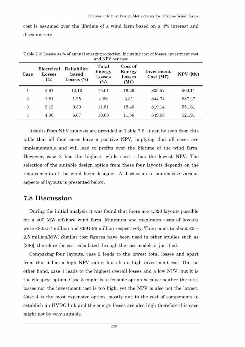
Chapter 7: Robust Design Methodology for Offshore Wind Farms
220
cost is assumed over the lifetime of a wind farm based on a 4% interest and
discount rate.
Table 7.6: Losses as % of annual energy production, incurring cost of losses, investment cost
and NPV per case
Case
Electrical
Losses
(%)
Reliability
based
Losses (%)
Total
Energy
Losses
(%)
Cost of
Energy
Losses
(M€)
Investment
Cost (M€) NPV (M€)
1 2.91 12.10 15.01 16.26 805.57 500.11
2 1.81 1.25 3.06 3.31 844.74 687.27
3 2.12 9.39 11.51 12.46 819.14 551.61
4 4.00 6.67 10.68 11.56 849.08 521.91
Results from NPV analysis are provided in Table 7.6. It can be seen from this
table that all four cases have a positive NPV, implying that all cases are
implementable and will lead to profits over the lifetime of the wind farm.
However, case 2 has the highest, while case 1 has the lowest NPV. The
selection of the suitable design option from these four layouts depends on the
requirements of the wind farm designer. A discussion to summarise various
aspects of layouts is presented below.
7.8 Discussion
During the initial analysis it was found that there are 4,320 layouts possible
for a 400 MW offshore wind farm. Minimum and maximum costs of layouts
were €805.57 million and €991.96 million respectively. This comes to about €2 –
2.5 million/MW. Similar cost figures have been used in other studies such as
[236], therefore the cost calculated through the cost models is justified.
Comparing four layouts, case 2 leads to the lowest total losses and apart
from this it has a high NPV value, but also a high investment cost. On the
other hand, case 1 leads to the highest overall losses and a low NPV, but it is
the cheapest option. Case 3 might be a feasible option because neither the total
losses nor the investment cost is too high, yet the NPV is also not the lowest.
Case 4 is the most expensive option, mostly due to the cost of components to
establish an HVDC link and the energy losses are also high therefore this case
might not be very suitable.

Chapter 7: Robust Design Methodology for Offshore Wind Farms
221
The decision about the final layout for implementation has to be made by the
wind farm developer or the wind farm owner. Features, losses, reliability and
costs of each layout are different; some offer a higher level of redundancy, some
have lower losses while some have a lower investment cost. Given these four
cases, case 3 is a good trade-off between redundancy and investment cost,
therefore, it can be declared as a robust offshore wind farm design option. This
layout features a certain level of redundancy and the losses and the investment
cost are not the highest among the four cases.
The methodology proposed allows selection of three robust layouts out of the
possible 4,320. Short listing is dependent on the criteria imposed by the wind
farm designer, with the procedure being sensitive to the components being
considered, the budget and the level of reliability required.
The methodology presented is scalable according to the wind farm capacity.
However, for very large wind farms (> 1GW) the number of electrical layouts
will increase tremendously since multiple platforms will have to be considered.
In that scenario, more assumptions and criteria will have to be introduced in
the first level of short-listing to limit the electrical layouts, however the second
and third levels of short-listing will still be applicable.
The case study performed in this chapter on a 400 MW considered real
components available from manufacturer‘s catalogues (e.g. AC cable ratings,
capacity of VSC converters, voltage levels, capacity of wind turbines) during the
electrical layout combination testing. However, when using the proposed
methodology for a real wind farm design, the data about existing components
available in the market should be collected and used. Although cost models
have been used in this case study, if the cost of real components is available
then they should be used instead.
7.9 Software Tool for Automated Design and Loss
Analysis of an Offshore Grid
A novel software tool has been developed in this thesis that allows rapid
creation and testing of large offshore wind farm electrical layouts. The software
tool which has been developed is novel because currently no existing
commercial power system software offers the facility to build and test electrical
networks for an offshore wind farm with such minimal effort. Existing
commercial software packages allow the user to create an electrical network by

Chapter 7: Robust Design Methodology for Offshore Wind Farms
222
selecting components and then manually building up the network. To evaluate
electrical losses in existing software packages, parameters have to be
continuously adjusted manually. For example, power generation of wind
turbines have to be continually adjusted for each bin of wind power frequency
curve. Furthermore, voltage levels should be made Grid Code compliant and for
this, the power factor of wind turbines and HVDC converter settings may also
need adjusting for each power bin. Often, existing software features either
automated load flow or automated electrical loss studies or automated
reliability studies. It is difficult to find a commercial software that can do all of
these studies with minimal user input.
The main features of the software tool developed are described as follows:
The software utilises a GUI that can be used to drive the design of an
offshore wind farm with or without platform interconnections.
It creates a steady-state network model for an offshore wind farm that
can be used as a starting point for load flow and short-circuit calculation
studies.
It carries out automated calculations for: load flow, size of reactive power
compensation required, calculation of electrical losses and assessment of
annual reliability based energy losses.
It uses manufacturer‘s data from the catalogues of components (where
available) for calculation of losses.
7.9.1 Implementation of the software tool
The tool has been developed using Python programming language, QT, PyQT
library (for the development of the user interface) and PSS®E (a power system
analysis software) [76] API.
7.9.2 Input parameters
The structure of the software tool and the input parameter options are
designed to build an offshore wind farm electrical layout, therefore it is
essential that a user has knowledge of typical offshore wind farm components.
For instance, the user should know that a large offshore wind farm normally
consists of wind turbine arrays (MV cables, turbines and turbine transformers),
an offshore collecting point (platform/s carrying two or three winding MV/HV
collector transformers, MV/HV switchgear, HVDC converter stations) and

Chapter 7: Robust Design Methodology for Offshore Wind Farms
223
transmission circuits (to link offshore platform/s with an onshore substation),
as illustrated in Figure 7.1. There can also be a number of offshore platforms
interconnected via high voltage AC (HVAC) cables for the same offshore wind
farm.
Electrical parameters of components such as resistance, inductance and
susceptance of AC cables available from manufacturer component catalogues
are stored in a common database as illustrated in the flow chart in Figure 7.16.
Depending on the component category, relevant electrical parameters are
loaded into the GUI dropdown menu from the database as shown in Figure
7.15. For instance, if a user wants to select a 33 kV array cable, the following
cables appear in the drop-down menu: 70 mm2, 95 mm2, 120 mm2, 150 mm2,
185 mm2, 240 mm2, 300 mm2, 400 mm2, 500 mm2 and 630 mm2. By selecting
any of these cables the electrical parameters are automatically adjusted in the
electrical network.
The following points describe the complete set of information that should be
entered through the GUI of this tool:
1. The choice of nominal voltages for turbines, MV and HV (see Figure
7.14).
2. The size of the wind farm and size of each wind turbine (see Figure
7.15).
3. The selection of the transmission system to be used (AC or DC).
4. The number and type (AC or DC) of collector platforms, the number
and arrangements of MV and HV busbars and the number and type (2-
winding or 3-winding) of collector transformers.
5. The layout of the arrays (for example, radial turbine strings, radial
turbine strings with end loops, array tree configuration or starburst
configuration), a screenshot is shown in Figure 7.15.
6. If DC transmission is selected then the number of HVDC converters per
platform, and the voltage and rating of these converters need to be
provided. The number and rating of converter transformers and the
number of cables connecting each converter to the shore are required.
7. The type of HVDC link (e.g. monopolar, bipolar-metallic return,
bipolar-ground return) also needs to be selected.
8. If HVAC transmission is selected, then the number of AC cables
connecting the platform(s) with the shore needs to be provided.
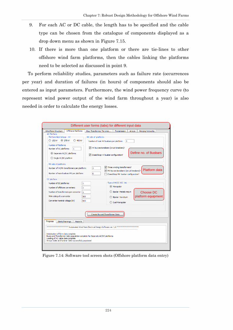
Chapter 7: Robust Design Methodology for Offshore Wind Farms
224
9. For each AC or DC cable, the length has to be specified and the cable
type can be chosen from the catalogue of components displayed as a
drop down menu as shown in Figure 7.15.
10. If there is more than one platform or there are tie-lines to other
offshore wind farm platforms, then the cables linking the platforms
need to be selected as discussed in point 9.
To perform reliability studies, parameters such as failure rate (occurrences
per year) and duration of failures (in hours) of components should also be
entered as input parameters. Furthermore, the wind power frequency curve (to
represent wind power output of the wind farm throughout a year) is also
needed in order to calculate the energy losses.
Figure 7.14: Software tool screen shots (Offshore platform data entry)
Platform data
Define no. of Busbars
Choose DC
platform equipment
Different user forms (tabs) for different input data

Chapter 7: Robust Design Methodology for Offshore Wind Farms
225
Figure 7.15: Software tool screen shots (Turbine array data entry)
7.9.3 Creation of an electrical network
There are two options in terms of entering data:
1. A new design can be created entirely driven by the user interface
(following all ten steps mentioned in Section 7.9.2).
2. Modification of an existing design where the previously created offshore
design is loaded into the user interface and then modified.
For new designs, the user enters data into the forms that can be used for
instant creation of the network, otherwise it can be saved in a configuration
file. When modifying existing designs, any previously saved configuration files
can be loaded into the software that populates data back into the forms. Using
this save and read functionality, a set of sub-options or scenarios can be created
quickly with minimal effort. More screenshots of the software tool can be seen
in Appendix E.
The information from the configuration files and the manufacturer
catalogues are then fed into PSS®E through the Python API (Application
Programming Interface), where the creation of the actual network model takes
place. In the network model formed, all components are connected with busbars
Linking arrays to the platform
Turbine array parameters
Turbine array cabling configuration
Cable catalogue
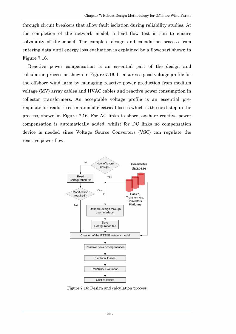
Chapter 7: Robust Design Methodology for Offshore Wind Farms
226
through circuit breakers that allow fault isolation during reliability studies. At
the completion of the network model, a load flow test is run to ensure
solvability of the model. The complete design and calculation process from
entering data until energy loss evaluation is explained by a flowchart shown in
Figure 7.16.
Reactive power compensation is an essential part of the design and
calculation process as shown in Figure 7.16. It ensures a good voltage profile for
the offshore wind farm by managing reactive power production from medium
voltage (MV) array cables and HVAC cables and reactive power consumption in
collector transformers. An acceptable voltage profile is an essential pre-
requisite for realistic estimation of electrical losses which is the next step in the
process, shown in Figure 7.16. For AC links to shore, onshore reactive power
compensation is automatically added, whilst for DC links no compensation
device is needed since Voltage Source Converters (VSC) can regulate the
reactive power flow.
Figure 7.16: Design and calculation process
Offshore design through
user-interface.
Creation of the PSS®E network model
New offshore
design?
Read
Configuration file
Save
Configuration file
Cables,
Transformers,
Converters,
Platforms
Electrical losses
Reliability Evaluation
Cost of losses
Modification
required?
Parameter
database
Yes
Yes
No
No
Reactive power compensation
Chapter 7: Robust Design Methodology for Offshore Wind Farms
227
7.9.4 Load flow and loss evaluation studies
The software tool makes the electrical network Grid Code compliant to
perform load flow and loss evaluation studies. Both electrical and reliability
based losses can be calculated through an automated procedure.
The calculation of electrical losses is based on a number of different loading
conditions where each is created using a wind power frequency curve (as shown
in Figure 7.12). A voltage coordination and reactive power compensation
strategy is developed (described in Section 7.6) to ensure Grid Code
requirements are followed. This check is performed for all loading conditions
prior to electrical loss evaluation. The final outcome of this calculation is the
annual MWh estimation of electrical losses that is converted into cost (€) using
a €/MWh cost value.
The reliability based loss evaluation is based on a state-enumeration
technique which is a frequency and duration method [233]. The state-
enumeration technique processes only the credible failures and, based on their
frequency of failure and duration, calculates the wind energy that will be not
delivered per year. For each failure, a fault clearance area is located (as shown
in Figure 7.13) and possibilities in terms of network reconfiguration are
considered. If there are no possibilities in terms of reconfiguration, or they are
limited, the wind power cut takes place and the energy not delivered is
calculated using the wind power frequency curves. The main output of the
reliability evaluation is an estimated MWh energy loss that can be converted
into costs (€) similar to the conversion discussed above for electrical losses. The
procedure for reliability based loss calculation is described in Section 7.6.4.
The software tool can be further improved by integration of cost models
described in Section 7.3. This will allow the user to evaluate the investment
cost for each electrical layout which can lead to a more complete cost-benefit
analysis.
7.10 Case Study
As a test study, a sample network of a 400 MW wind farm is created using
the software tool in PSS®E. The inputs to the software tool‘s GUI are the
parameters for the wind farm electrical layout. The input parameters that can
be entered are discussed in Section 7.9.2 and illustrated through Figure 7.14

Chapter 7: Robust Design Methodology for Offshore Wind Farms
228
and Figure 7.15. The outcome of the calculation and developed software is the
electrical network built into PSS®E as shown in Figure 8.4.
In the network created in this case study the wind turbines are connected in
a radial configuration at MV level of 33 kV. Four 2-winding collector
transformers scale up the voltage from 33 kV to 275 kV and from this point the
power is transmitted to shore by a VSC HVDC link in a monopole
configuration.
7.10.1 Parameters and loss studies
Failure rate and repair times are collected from various sources (as
mentioned in Section 7.6.4 and these are given in Appendix D.
7.10.2 Network development time
This software significantly reduces the time required for creation of a large
network. In this example of a 400 MW wind farm, the offshore network has
1,042 buses, 843 circuit breakers, 211 branches, 202 machines, 206
transformers (wind turbine, collector and converter), 2 VSC converters
(rectifier/inverter) and 1 HVDC line. Setting up all these components in PSS®E
one-by-one manually (with names) will take a long time (perhaps a day or
longer). However, by using this software tool, it only takes couple of minutes to
fill-in the GUI and seconds for the network creation in PSS®E. The naming of
the components is also done automatically so that the user can identify each
component in the network. Automation of the design and calculation process
illustrated in Figure 7.16 saves a considerable amount of time.
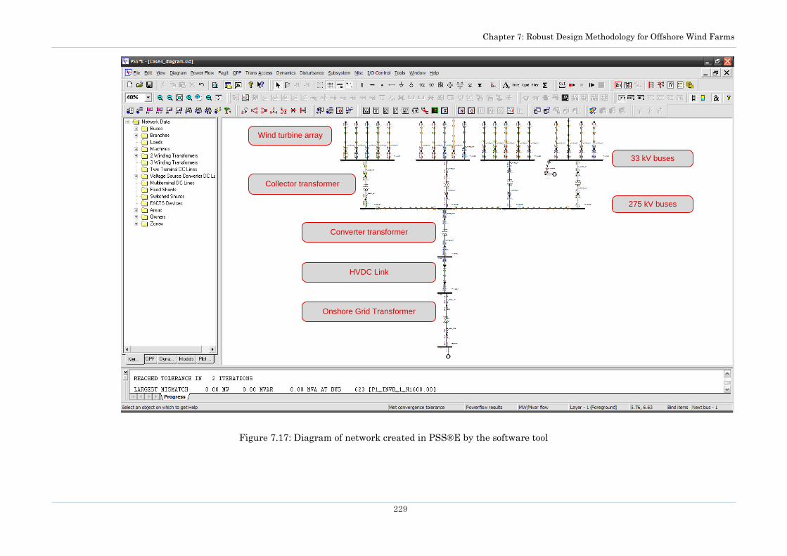
Chapter 7: Robust Design Methodology for Offshore Wind Farms
229
Figure 7.17: Diagram of network created in PSS®E by the software tool
Converter transformer
HVDC Link
Onshore Grid Transformer
275 kV buses
33 kV buses
Collector transformer
Wind turbine array

Chapter 7: Robust Design Methodology for Offshore Wind Farms
230
7.11 Summary
This chapter presented a novel methodology for selection of a robust design
option (electrical layout) for an offshore wind farm through cost-benefit
analysis. A case study has shown that a large capacity wind farm can have
several possible electrical layouts from which a wind farm designer has to
choose the most feasible layout. At present, no methodology allows such
comprehensive and detailed investigation and short-listing of electrical layouts
for an offshore wind farm.
At first, a comprehensive list of possible layouts is generated, considering
components that are available and that can be used for the electrical layout
design. Technically possible combinations of various components and their
options such as capacity of wind turbines, MV/HV/EHV levels, types of array
configurations, capacity of collector transformers, types of transmission links
etc. lead to several electrical layouts. Then, through a process of multi-level
short-listing these electrical layouts are filtered down. The investment cost of
the layouts is calculated using the cost models.
Multi-level short listing is then performed to narrow down the selection. In
the first level, technically non-feasible options are eliminated. In the second
level, layouts are filtered according to the investment budget available. In the
third level, layouts with a higher redundancy level are selected from previously
short listed layouts. In the final level, the three cheapest yet most reliable
options are picked out and considered for further analysis. More than three
options can be considered but this is optional.
Further tests on the three selected layouts are performed to calculate annual
electrical and reliability based losses. The NPV is analysed to determine the
most and the least profitable layouts for a 20 year lifetime of the wind farm.
Since each layout has a different capital cost, redundancy level, losses and
NPV the final choice depends on the criteria or preferences set by the wind
farm designer. Choice of an electrical layout after analysing several possible
configurations can lead to a justifiable solution. The methodology can be used
by wind farm designers or wind farm owners in general. This technique is
applicable to an offshore wind farm of any size and layout and at any distance
from the shore.

Chapter 7: Robust Design Methodology for Offshore Wind Farms
231
Furthermore, this chapter also presented a novel software tool which has
been created for the automated design and loss analysis of an offshore wind
farm. The software tool developed has a user-friendly interface and it allows a
quick creation of an offshore wind farm electrical network. It also features an
automated electrical and reliability loss evaluation procedure that enables fast
analysis of energy losses and requires minimal effort. Using this software,
several offshore wind farm electrical layouts can be tested. The layouts may
differ in array configurations, medium or high voltage levels, type of
transmission link to the shore, type and quantity of collector transformers,
number of platforms and electrical parameters. The chapter also describes the
design and calculation process of the software, the input parameters required
and the parameter save and read functionality. The software tool significantly
reduces both the time and effort required to build and test a large offshore wind
farm electrical system in a commercial power system software PSS®E.

Chapter 8: Conclusions and Future Work
232
Chapter 8 Conclusions and Future Work
Conclusions and Future Work
This thesis proposed improvements to offline and online modelling
techniques for offshore wind farms. The potential areas of improvement were
identified through a comprehensive literature review. The thesis also presents
an overview of the present and future offshore wind farm installations in the
UK and the rest of Europe. It was observed that in future the presence of wind
power in the network will increase mainly through offshore wind farms. These
offshore projects will have very large capacities and will be further away from
the shore.
Two types of modelling are considered in this analysis i.e. offline studies and
online studies. In normal practice, offline studies are performed during the
design phase of a wind farm and when a pre-feasibility study has to be
performed. Generally, offline modelling is performed prior to integration of a
wind farm into the network. But due to the growing presence of high capacity
wind farms in the network, online modelling is gaining popularity amongst
transmission and distribution utilities. Online analysis will allow system
operators to carry out transient stability simulations using data collected in
real-time from network components. The earlier chapters of this thesis
presented models for online studies and this is followed by models for offline
use in the later chapters.
The presence of several rapidly varying power producing units (wind farms)
in the system requires fast modelling tools for steady-state as well as dynamic
analysis. A new aggregation model has been developed in this thesis that
allows a large wind farm to be represented by few wind turbines determined by
probabilistic analysis. The developed methodology takes into account layout of
the wind farm (position of wind turbines), wake effects, array collector system
and site‘s wind characteristics. The methodology works by first calculating the
wind speed at each turbine for every wind measurement. This calculation is
performed through VebWake, a software program developed (in this thesis) to

Chapter 8: Conclusions and Future Work
233
calculate wind speed at each turbine in a wind farm. Then, clustering wind
turbines receiving similar wind speeds using the Support Vector Clustering
technique and then arranging these clusters further into groups. The most
probable group is chosen (through probabilistic analysis) as the best
representation of the wind farm for the entire year. As a case study, an
aggregate model of a large wind farm consisting of Doubly Fed Induction
Generators (DFIG) is established. Results from probabilistic aggregation model
showed that a 49 turbine wind farm can be modelled with just 3 equivalent
wind turbines for the whole year. The dynamic response from the aggregate
model is compared (at two wind conditions) against the detailed wind farm
response as well as against two existing aggregation models. A simulation time
reduction of up to 96% was achieved in the case studied. The model is intended
to be used by utilities and wind farm operators during real-time, online,
simulation studies which are gaining popularity among transmission system
operators. The proposed probabilistic aggregation model is compared against
existing aggregate models to test simulation time reduction, accuracy of
dynamic response, ease of setup and use. It was found that the developed
probabilistic aggregate model is practical, accurate and easy to use for online
analysis. The development of the VebWake software program and development
of a new probabilistic aggregation technique are the first and second original
contributions of this thesis.
To facilitate the increasing need for accurate yet fast simulation models, a
new method to probabilistically estimate the power production from a wind
farm is developed. This method is useful during real-time online studies. The
methodology evaluates the fluctuation in wind speed at a turbine under wake
in a wind farm. This fluctuation occurs due to turbulence added by the wake of
the turbines. Due to this fluctuation, at a given incoming wind speed and
direction, a wind turbine under wake can produce different amounts of power.
Therefore, a probabilistic power output is more likely than a deterministic
power output. To simulate this fluctuation inside a wind farm, Frandsen‘s
turbulence model is combined with Jensen‘s wake model. The model is useful to
obtain probabilistic power outputs from wind farms for a forecasted wind
condition. The wind power output obtained from this method can allow system
operators to decide on the unit commitment and spinning reserve allocation.
Due to a lower computation burden and reduced simulation time, the model is

Chapter 8: Conclusions and Future Work
234
useful for online studies (instantaneous power estimation). The probabilistic
wake effect model was applied to calculate power output (in real time) and
energy yield from a wind farm. In the case studied (98 MW wind farm) it was
found that deviations in power output for a given wind scenario reached as
large as 7 MW whereas on average this difference was about 2 MW. When used
for energy yield calculation the results did not show a significant difference
than with a deterministic wake model. Therefore probabilistic wake model
should be used for real time power output estimation from a wind farm whereas
deterministic wake model should be used for energy yield estimation. The
development of probabilistic wake model is the third original contribution of the
thesis.
Realistic estimation of energy yield can only be obtained once all factors that
influence the outcome have been taken into account. Several factors can affect
the overall energy yield from a wind farm. These factors include wake effect,
electrical losses, reliability based losses and wind resource variation. Profit
from a wind farm depends on the energy sold to the grid, therefore it is also
important to have a good estimate of potential energy curtailments if a wind
farm is being built in an area with a transmission bottleneck. A new analytical
method is proposed to evaluate the reliability based losses and energy losses
due to curtailments. The reliability method takes into account both single and
all multi-component failures for four array collector systems. A brief
investigation involving three wind farms in a hilly area revealed that there is
no correlation between wind speed and turbine availability. This might not be
the case for other wind farms located on plains and offshore, therefore all
possible correlations were investigated in conjunction with transmission line
loading. Through correlation coefficient analysis, it was found that maximum
curtailment losses occurred when wind speed was high, turbines were available
and the transmission line was occupied. Pre-feasibility studies often under
estimate the loss due to wake effects and it was shown through a sensitivity
analysis that wake losses can be high. From case study it was found that
energy yield was reduced due to: wake losses by 2% to 7%, electrical losses by
2.16% to 2.84%, wind farm component unavailability by 0% to 13.05% and
energy curtailment by 0% and 14.04%. A 10% variation (increase) in wind
resource increased the energy yield by 13.05% but energy curtailments also
rose up by 6.46%. The impact of energy losses due to various factors on capacity

Chapter 8: Conclusions and Future Work
235
factor of a wind farm was also analysed. It was found that when all losses are
included, the capacity factor decreased from 39.8% (without any losses) to
26.9% (in worst case with all losses). The methods proposed are useful for
offline pre-feasibility studies regularly carried out prior to wind farm
installation. These methods can enable a wind farm owner to reach a more
informed decision about feasibility of the project and whether curtailments are
a better option than transmission line reinforcement. The reliability based loss
evaluation method and the wind energy curtailment loss evaluation method are
the fourth and the fifth original contribution of the thesis.
Curtailment of wind energy is commonly carried out by shutting down a few
wind turbines inside the wind farm. A new methodology is presented in this
thesis that allows wind farm operators to identify turbines in an existing wind
farm that receive higher and lower wind speeds. Turbines that stay under
single or multiple wakes can more often accumulate fatigue loading, therefore
it is suggested that these turbines should be given priority during the
curtailment shut down procedure. The results obtained are also useful to
schedule preventive maintenance. Wind turbines facing high wind speed (free-
stream wind) during the year produce the most amount of power. Therefore
they should be scheduled for preventive maintenance on less windy days so that
they are operational most time during the year and produce power when wind
is high. As a case study, high and low wind speed receiving turbines were
identified in a 49 turbine wind farm. From the geometry of the wind farm and
site wind conditions studied, it was found that turbines deeper inside face lower
wind speeds and are more prone to fatigue damage as compared to those
outside. This method is the sixth original contribution of the thesis.
With an increase in offshore wind farm capacity, the design complexity has
also increased. Due to the millions of € of investment cost involved in these
large-scale wind farm projects, careful consideration is needed for their design.
A new methodology is developed that investigates various possible electrical
layouts for cost-benefit analysis and filters out the few best layouts based on
the criteria used. At first, a list of possible electrical layouts is generated using
available components from the manufacturers. Then, through a multi-level
short listing process, the total number of layouts is reduced to just a few. These
short-listed layouts are further tested for electrical and reliability based losses.
The electrical parameters are collected from the manufacturer‘s catalogues
Chapter 8: Conclusions and Future Work
236
(where possible), whereas failure rates and repair times are gathered from
various studies. An NPV analysis on the short-listed layouts further helps in
deciding which layout is economically more feasible. The case study showed
that for a 400 MW wind farm there were more than 4300 possible layouts,
based on the components considered. Through the short-listing procedure, the
total number of layouts was reduced to just three. From these layouts, only one
was chosen as it was a good trade off between redundancy and investment cost.
This layout had electrical losses of about 2.12%, reliability based losses of
9.39% and an investment cost of €819.14M. The outcome of the method depends
on the criteria imposed and the assumptions made during the short-listing
process. This method is the seventh original contribution of the thesis.
A bigger capacity of wind farms implies use of more equipment involving
large sets of buses and cables. Developing a network model for a large wind
farm with all buses, cables and switchgears etc. in a commercially available
power system can be a tedious and time consuming task. It was noticed that a
network for a wind farm of 400 MW can easily exceed more than 1000 buses,
200 cables and transformers. Moreover, entering electrical parameters for each
component can take the user even longer. A novel industrial-grade software has
been developed using Python, QT and Python QT programming languages. The
software tool allows the user to enter wind farm data by a Graphical User
Interface (GUI). The user can select electrical parameters for components from
manufacturer‘s catalogues that are stored in the software database. Once all
the data has been entered, the software tool automatically creates the electrical
layout for an offshore wind farm in PSS®E. The tool also enables a user to
quickly evaluate the electrical and reliability based losses of the electrical
layout developed. The design and calculation process, along with screenshots of
the software tool developed are presented in this thesis. Overall, the tool allows
fast development of an electrical layout with minimal effort. Using this
software tool, several electrical layouts can be tested easily in a very short
space of time. The developed software is the eighth original contribution of the
thesis.
8.1 Future Work
Although various areas for improvement were identified in the first chapter
and summarised in the form of problem statements but some of these areas

Chapter 8: Conclusions and Future Work
237
could not be addressed due to limitation of time. The following section provides
areas identified but not addressed as well as potential further improvements of
the methodologies developed in this thesis. A general overview of the possible
challenges that the wind industry may face in the near future is also discussed
in this section.
8.1.1 Future work on modelling
This section describes possible advancements that can be made to the work
presented in this thesis.
The cost-benefit methodology developed in Chapter 7 is very new and it
analyses all components for an offshore wind farm design collectively. Variation
in wind speed inside the wind farm due to wakes was ignored during the cost-
benefit analysis. This is because the aim was to test and obtain the best
offshore wind farm design with complete set of electrical components that
should be used. In the design phase however, consideration of wake effects is
essential when deciding on the placement of the wind turbines. To advance the
methodology developed further, the physical layout of the wind turbines can be
considered in conjunction with the electrical system of the wind turbine array
because both of these factors are linked. If wind turbines are placed too close to
each other, it increases the wake losses, if they are quite far apart, however, it
increases the distance and hence the costs of the array cables. In terms of wind
turbine array cabling configurations, only radial, starburst, tree and radial with
end loop configurations were considered in that chapter. An optimisation
algorithm can be developed in the future to optimise both the placement of
wind turbines as well as the array cabling route. This will allow analysing the
problem holistically, i.e., placing wind turbines in such a way to reduce wake
losses yet optimising the electrical cable costs. Furthermore, different medium
voltage levels can also be considered as part of overall optimisation. This way
an optimal wind turbine array electrical system can be obtained, that is cost-
effective yet leads to lower losses. The optimised array system can be studied in
conjunction with the methodology developed in Chapter 7 to obtain a more cost-
efficient overall wind farm design. The need for such holistic optimisation
approach was also identified in problem statement 2 mentioned in Section 1.4.2
but could not be completed due to limitation of time.

Chapter 8: Conclusions and Future Work
238
The cost-benefit methodology proposed for wind farm electrical layout design
(in Chapter 7) can be advanced to incorporate very large offshore wind farms
that are bigger than 1 GW. More criteria and assumptions will have to be
introduced for the optimal design of such large wind farms because multiple
platforms will become a possibility. In that case, the methodology should be
able to provide for an optimal choice of components at each platform. Overall, it
should lead to a cost-effective and reliable electrical layout for a wind farm with
multiple platforms. To reduce the explosion of possible design options in a
multiple platform wind farm a true optimisation algorithm can be developed for
multi-objective optimisation. The objective function should be to maximise the
reliability of design while minimising the capital costs.
The probabilistic aggregate model developed in Chapter 4 has been tested on
wind turbines with Doubly Fed Induction Generators (DFIGs). It will be
interesting to analyse how the model performs on a Full Scale Converter Rating
wind turbines. The probabilistic aggregate model can be further validated by
testing and comparing the transient stability plots with detailed wind farm
model under all wind conditions i.e. for all wind speeds (within turbine
operating range) and wind directions (0o to 360o). Furthermore, an aggregate
model for a radial array configuration has been proposed in that chapter,
because this configuration is very commonly used in wind farms. An aggregate
model for other array connection layouts such as starburst and tree layout can
also be developed. Apart from this, probabilistic wake effect model developed in
this thesis can be used instead of Jensen‘s wake model.
The correlation between wind speed and wind turbine availability in Chapter
5 could only be tested for three existing wind farms. More wind farms should be
analysed to see if there is any correlation between the wind speed and the wind
turbine availability. The curtailment method presented in Chapter 5 allows
determination of energy that will be curtailed in a year. A study can be
performed in which energy from a wind farm installed in an area with a
transmission bottleneck can be stored in the storage device instead of spilling
the energy through curtailments. A cost-benefit analysis can determine the
advantage of either curtailments or installing a storage device as compared to
building a new transmission line. Different types of storage devices can also be
explored and their investment costs compared. Additionally, the model
proposed in that chapter assumes that the transmission line has a fixed

Chapter 8: Conclusions and Future Work
239
transfer capacity, instead, seasonal line ratings or dynamic line ratings could
be introduced. The method could be tested with a more complex power network
rather than with a single line connected wind farm.
The probabilistic wake model proposed in Chapter 3 should be validated
against wind speed measurements obtained at wind turbines in several wind
farms. Measured wind speed data at the wind turbines was not available. This
is the first time such a model has been devised, therefore there is certainly a
room for further testing and improvement.
8.1.2 Challenges to overcome for Round 3 offshore wind farms
This section provides an overview of technical challenges that the wind farm
industry is likely to face within the next 7 or 8 years. Round 3 in the UK was
announced in January 2010, however installations of the wind farms may only
begin to take place around 2017 as so far, only zones have been identified. This
round includes wind farms with a big capacity and distances which are very far
away from the shore as compared to both Round 1 and 2 wind farms. Offshore
wind farms may be built as far as 300 km away from shore [239]. Such
extensive distances bring new challenges, including greater sea depths. It is
forecasted that offshore wind turbines may have to be installed in sea depths of
60 m which is much deeper than the current depths of 20 m. For this purpose,
better foundations are needed for offshore turbines and offshore platforms since
capacity and thus weight of turbines will increase. Commuting is another issue,
as vessels currently used for turbine and substation installation have to turn
back to shore if the sea is predicted to get rough. Newer vessels will be needed
that can withstand such weather conditions and can stay at the site for days.
According to an estimate, an investment of €2.25 billion (£2 billion) might be
needed just for one installation vessel. Platforms will have to include medical
facilities in case the crew gets injured so they can be treated offshore, as
travelling time by air (helicopter) to get to shore may take around 3 hours. Self
installing platforms should be built that can sail and install themselves which
can save extra installation costs.
Installation of cables to connect wind farms this far away also presents
another major issue. A single long cable is a preferred option, rather than
adding joints which makes the offshore network more prone to faults. Making a
cable joint in a submarine cable takes around a week and is extremely

Chapter 8: Conclusions and Future Work
240
expensive. On the other hand, longer cables have a greater mass, and generally
the weight of a cable is 90 kg/m therefore a 100 km cable weighs around 9000
tonnes. Transportation of such heavy cables from the manufacturing plant to
the shore and then their transfer onto the vessel will pose additional
challenges. The development of such long cables is another issue as the
manufacturers may face an excessive demand which can add delay in supplying
them. The chances of these transmission cables under the sea getting dragged
by shipping anchors will increase as their length and quantity increases.
Therefore, a Global Positioning System (GPS) mapping of cable routes may be
needed to avoid such damage.
Much higher DC voltage cables will have to be tested to reduce load losses
during transmission. At present, all turbine arrays use AC cables but DC
voltage should also be considered as an option to connect array turbines and
this might even lead to elimination of converters from the turbines.
Furthermore, keeping in mind the aforementioned issues, the cost of the overall
project has to be minimised. Connections between wind farms is a possibility
which can be looked into further as this will not only reduce the offshore
cabling cost but also add a certain level of reliability in security of supply. On
land, the equipment and land leasing cost (for an onshore substation) will also
be reduced. However coordination between the wind farm manufacturers will
be needed to enable wind farm interconnection. A set of rules for this
coordination might have to be established that must be followed by all parties
involved. This is to have complete awareness of expectations and so nothing is
left out.
References
241
References
References
[1] Global Wind Energy Council (GWEC), "Global wind report: Annual market
update 2010," 2010.
[2] European Wind Energy Association (EWEA), Wind Energy - The Facts, A
guide to the technology, economics and future of wind power, London:
Earthscan, 2009.
[3] United Kingdom Energy Research Centre (UKERC), "Great Expectations:
The cost of offshore wind in UK waters - understanding the past and
projecting the future," 2010.
[4] Carbon Trust, "Offshore wind power: big challenge, big opportunity,"
Report: CTC743, 2008.
[5] The British Wind Energy Association (BWEA), "BWEA briefing sheet -
Offshore wind (embrace the revolution)" [Online]. Available:
http://www.bwea.com/pdf/briefings/offshore05_small.pdf.
[6] Department of Trade and Industry (DTI), "The UK wind resource - Wind
energy fact sheet 8," 2001.
[7] EWEA, "The European offshore wind industry - key trends and statistics:
1st half 2011," 2011.
[8] National Grid, "Offshore Development Information Statement (ODIS) -
Appendix: Future scenarios supporting data," 2011.
[9] Renewable UK, "Offshore wind farms" [Online]. Available:
http://www.bwea.com/ukwed/offshore.asp.
[10] J. Rogers, S. Fink, and K. Porter, "Examples of Wind Energy Curtailment
Practices," NREL Report: SR-550-48737, 2010.
[11] European Wind Energy Association, "List of Operational Offshore Wind
Farms in Europe, end 2010" [Online]. Available: www.ewea.org.
[12] 4C Offshore - OrbisEnergy Centre, "Global offshore wind farms database"
[Online]. Available: http://www.4coffshore.com/windfarms/.
[13] T. Ackermann, Wind Power in Power Systems, John Wiley and Sons, 2005.
[14] Vestas, "Vestas and DONG Energy enter into agreement on testing of new 7
MW offshore wind turbine" [Online]. Available: www.vestas.com.
[15] Vestas, "V80-2.0 MW. Pitch regulated wind turbine with OptiTip® and
OptiSpeed®," 2009.
[16] T. Bay, "AVEC foundation design for wind turbines," presented at the 2005
Wind energy training seminar, Alaska, USA.
[17] P. Nielsen (EMD), "Offshore wind energy projects feasibility study
guidelines SEAWIND," Altener project 4.1030/Z/01-103/2001,, 2003.
[18] BARD Engineering, "BARD Offshore 1" [Online]. Available: www.bard-
offshore.de/en/projects/offshore/bard-offshore-1.html.
[19] S. D. Wright, A. L. Rogers, J. F. Manwell, and A. Ellis, "Transmission
options for offshore wind farms in the United States" [Online]. Available:
www.ceere.org/rerl/publications/published/2002/.
[20] Department of Business Enterprise and Regulatory Reform, "GB SQSS sub-
group final recommendations" [Online]. Available:
http://www.dti.gov.uk/energy/sources/renewables/policy/offshore-
transmission/offshore-transmission-experts-group/page34541.html.
[21] T. Ackermann, "Transmission systems for offshore wind farms," IEEE
Power Engineering, vol. 22, no. 12, pp. 23 - 27, 2002.
[22] Dong Energy, "Cables" [Online]. Available: www.dongenergy.com/hornsrev2.
References
242
[23] P. Gardner, L. M. Craig, and G. J. Smith, "Electrical systems for offshore
wind farms," in Proc. 20th British Wind Energy Association (BWEA)
Conference, Cardiff, UK, 1998.
[24] G. Q-Varela, G. W. Ault, O. A-Lara, and J. R. McDonald, "Electrical collector
system options for large offshore wind farms," IET Renewable Power
Generation, vol. 1, no. 2, pp. 107-114, 2007.
[25] H. J. Koch, "Offshore Wind Farms Europe 2010" [Online]. Available:
http://ewh.ieee.org/cmte/substations/scm0/Montreal%20Meeting/Conference
%20PDFs/Main%20meeting%20slides/Offshore%20Wind%20Farms%20Euro
pe%202010%20Final.pdf.
[26] Middelgrundens Vindmøllelaug I/S, (2003). "Middelgrunden Offshore Wind
farm - A popular Initiative" [Online]. Available:
http://www.middelgrunden.dk/middelgrunden/sites/default/files/public/file/
mg-pjece_72dpi_rgb.pdf.
[27] Vattenfall, "Thanet offshore wind farm (Diagram of the cable route)"
[Online]. Available: www.vattenfall.co.uk.
[28] Alpha Ventus, "The largest crane vessel in the world is busy at alpha
ventus: 'Thialf' is placing the foundations for the REpower turbines"
[Online]. Available: www.alpha-ventus.de.
[29] J. Overton, "Econnect - Study on the development of the offshore grid for
connection of the Round Two wind farms," Renewables Advisory Board,
2005.
[30] London Array, "Harnessing the power of offshore wind" [Online]. Available:
www.londonarray.com.
[31] Sheringham Shoal - Scira Offshore Energy, "Components" [Online].
Available: http://www.scira.co.uk/offshore/components.html.
[32] P. Bresesti, W. L. Kling, R. L. Hendriks, and R. Vailati, "HVDC connection
of offshore wind farms to the transmission system," IEEE Transactions on
Energy Conversion, vol. 22, no. 1, 2007.
[33] J. Green, A. Bowen, L. J. Fingersh, and Y-H. Wan, "Electrical collection and
transmission systems for offshore wind power " in Proc. Offshore Technology
Conference, Houston, Texas, US, 2007.
[34] Vattenfall, "Thanet offshore wind farm" [Online]. Available:
www.vattenfall.co.uk/en/thanet-offshore-wind-farm.htm.
[35] European Environment Agency (EEA), "Europe's onshore and offshore wind
energy potential: An assessment of environmental and economic
constraints," 2009.
[36] R. Gagnon, G. Turmel, C. Larose, J. Brochu, G. Sybille, and M. Fecteau,
"Large-scale real-time simulation of wind power plants into hydro-Quebec
power system," in Proc. 9th International workshop on large-scale
integration of wind power into power systems as well as on transmission
networks for offshore wind power plants, Quebec, Canada, 2010.
[37] K. Rudion, "Aggregated Modelling of Wind Farms," Ph.D. dissertation, Otto-
von-Guericke-Universitat Magdeburg, Magdeburg, 2008.
[38] L. M. Fernandez, J. R. Saenz, and F. Jurado, "Dynamic Models of Wind
Farms with Fixed Speed Wind Turbines," Renewable Energy, vol. 31, pp.
1203-1230, 2006.
[39] W. L. Kling and J. G. Slootweg, "Modeling of Large Wind Farms in Power
System Simulations," in Proc. IEEE Power Engineering Society Summer
Meeting, vol. 1, pp. 503-508 2002.
[40] M. G. Castro and J. M. Ferreira de Jesus, "A wind park reduced–order
model using singular perturbation theory," IEEE Transactions on Energy
Conversion, vol. 11, no. 4, pp. 735-741, 1996.
[41] J.G. Slootweg, S.W.H. de Haan, H. Polinder, and W.L. Kling, "Aggregated
modelling of wind parks with variable speed wind turbines in power system
References
243
dynamics simulations," in Proc. 14th Power System Computation Conference
(PSCC), Sevilla, 2002.
[42] J. Usaola, P. Ledesma, J. M. Rodrigues, J. L. Fernandez, D. Beato, R.
Iturbe, and J. R. Wilhelmi, "Transient stability studies in grids with great
wind power penetration. Modelling issues and operation requirements," in
Proc. IEEE Power and Energy Society General Meeting, pp. 1534-1541, 2003.
[43] NREL, "Final Project Report - WECC Wind Generator Development," 2008.
[44] J. G. Slootweg, "Wind Power - Modelling and Impact on Power System
Dynamics," Ph.D. dissertation, Technische Universiteit Delft, Delft, 2003.
[45] A. Marinopoulos, J. Pan, M. Zarghami, M. Reza, K. Yunus, C. Yue, and K.
Srivastava, "Investigating the impact of wake effect on wind farm
aggregation," in Proc. IEEE Trondheim PowerTech, 2011.
[46] L. M. Fernandez, F. Jurado, and J. R. Saenz, "Aggregated dynamic model
for wind farms with doubly fed induction generator wind turbines,"
Renewable Energy, vol. 33, pp. 129-140, 2008.
[47] J. Conroy and R. Watson, "Aggregate modelling of wind farms containing
full-converter wind turbine generators with permanent magnet synchronous
machines: transient stability studies," IET Renewable Power Generation,
vol. 3, no. 1, pp. 39-52, 2008.
[48] A. Perdana, S. U. - Joutsenvuo, O. Carlson, and B. Lemström, "Comparison
of an aggregated model of a wind farm consisting of fixed-speed wind
turbines with field measurement," Wind Energy, vol. 11, pp. 13-17, 2008.
[49] J. Soens, J. Driesen, and R. Belmans, "Equivalent transfer function for a
variable speed wind turbine in power system dynamic simulations,"
International Journal of Distributed Energy Resources, vol. 1, no. 2, pp. 111-
133, 2005.
[50] C. Wang, Z. Lu, and Y. Qiao, "Modeling of wind pattern and its application
in wind speed forecasting," in Proc. International conference on
SUPERGEN, 2009.
[51] M. C. Alexiadis, P. S. Dokopoulos, and H. S. Sahsamanoglou, "Wind speed
and power forecasting based on spatial correlation models," IEEE
Transactions on Energy Conversion, vol. 14, no. 3, pp. 836-842, 1999.
[52] C. Lei and L. Ran, "Short-term wind speed forecasting model for wind farm
based on wavelet decomposition," in Proc. 3rd international Conference on
Electric Utility Deregulation and Restructuring and Power Technologies,
Nanjing, China, 2008.
[53] A. Sfetsos, "A novel approach for the forecasting of mean hourly wind speed
time series," Renewable Energy, vol. 27, pp. 163-174, 2002.
[54] V. J.-Marandi, L.-Fu Pak, and V. Dinavahi, "Real-time simulation of grid-
connected wind farms using physical aggregation," IEEE Transactions on
industrial electronics, vol. 57, no. 9, pp. 3010-3021, 2010.
[55] J. F. Ainslie, "Calculating the flowfield in the wake of wind turbines,"
Journal of Wind Engineering and Industrial Aerodynamics, vol. 27, pp. 213-
224, 1988.
[56] N.O. Jensen, "A note on Wind Generator Interaction," Technical Report
RISO-M-2411, 1983.
[57] I. Katic, J. Højstrup, and N. O. Jensen, "A simple model for cluster
efficiency," in Proc. European Wind Energy Conference (EWEC), Rome, Italy,
1986.
[58] G. C. Larsen, "A simple wake calculation procedure," RISO National
Laboratory, Roskilde, Denmark, 1988.
[59] S. Frandsen, R. Barthelmie, S. Pryor, O. Rathmann, S. Larsen, J. Højstrup,
and M. Thøgersen, "Analytical modelling of wind speed deficit in large
offshore wind farms," Wind Energy, vol. 9, pp. 39-53, 2006.
References
244
[60] E. S. Hrayshat, "Wind resource assessment of the Jordanian southern
region (Technical Note)," Renewable Energy, vol. 32, pp. 1948-1960, 2007.
[61] A. M-S. Jeong, B. C-J. Moon, C. M. S. Choi, D. G-S. Jeong, and E. Y-H.
Chang, "The prediction of energy production and planning of the southwest
coast offshore wind farm," in Proc. 8th IEEE International Conference on
Power Electronics and ECCE Asia (ICPE & ECCE), The Shilla Jeju, Korea,
2011.
[62] A. S. Dobakhshari and M. F.-Firuzabad, "A reliability model of large wind
farms for power system adequacy studies," IEEE Transactions on Energy
Conversion, vol. 24, no. 3, pp. 792-801, 2009.
[63] J. K. Kaldellis, "The wind potential impact on the maximum wind energy
penetration in autonomous electrical grids," Renewable Energy, vol. 33, pp.
1665–1677, 2008.
[64] S. A. Papathanassioua and N. G. Boulaxis, "Power limitations and energy
yield evaluation for wind farms operating in island systems," Renewable
Energy, vol. 31, pp. 457–479, 2006.
[65] F. B. Amar, M. Elamouri, and R. Dhifaoui, "Energy assessment of the first
wind farm section of Sidi Daoud Tunisia," Renewable Energy, vol. 33, pp.
2311-2321, 2008.
[66] L. de Araujo Lima and C. R. B. Filho, "Wind energy assessment and wind
farm simulation in Triunfo - Pernambuco Brazil," Renewable Energy, vol.
35, pp. 2705-2713, 2010.
[67] M. C. Mabel and E. Fernandez, "Estimation of energy yield from wind farms
using artificial neural networks," IEEE Transactions on Energy Conversion,
vol. 24, no. 2, pp. 459-464, 2009.
[68] R. Karki, P. Hu, and R. Billinton, "A simplified wind power generation
model for reliability evaluation," IEEE Transactions on Energy Conversion,
vol. 21, no. 2, pp. 533-540, 2006.
[69] A. S.-Dobakhshari and M. F.-Firuzabad, "Integration of large-scale wind
farm projects including system reliability analysis," IET Renewable Power
Generation, vol. 5, no. 1, pp. 89-98, 2011.
[70] R. Billinton and W. Wangdee, "Reliability based transmission reinforcement
planning associated with large scale wind farms," IEEE Transactions on
Power Systems, vol. 22, no. 1, pp. 34-41, 2007.
[71] A. G. Bakirtzis, "A probabilistic method for the evaluation of the reliability
of stand alone wind energy systems," IEEE Transactions on Energy
Conversion, vol. 7, no. 1, pp. 99-107, 1992.
[72] F. C. Sayas and R. N. Allan, "Generation availability assessment of wind
farms," IEE Proceedings on Generation, Transmission and Distribution, vol.
143, no. 5, 1996.
[73] N. B. Negra, O. Holmstrøm, B. B - Jensen, and P. Sorensen, "Aspects of
Relevance in Offshore Wind Farm Reliability Assessment," IEEE
Transactions on Energy Conversion, vol. 22, no. 1, 2007.
[74] IPSA Power Ltd, "Integration of offshore wind farms into the local
distribution network," DTI report, K/EL/00272/REP (URN 03/1641), 2003.
[75] IPSA Power Ltd, "Modelling protection and switching schemes in networks
with embedded generation," DTI report, K/EL/000342/00/00 (URN: 06/1798),
2006.
[76] Siemens, "PTI - PSS® E User Manual," 2011.
[77] V. Akhmatov and H. Knudsen, "An aggregate model of a grid-connected,
large scale, offshore wind farm for power stability investigations -
importance of windmill mechanical system," Electrical Power and Energy
Systems, vol. 24, pp. 709-717, 2002.
References
245
[78] A. D. Hansen, P. Sorensen, L. Janosi, and J. Bech, "Wind farm modelling for
power quality," in Proc. 27th annual conference of the IEEE Industrial
Electronics Society, 2001.
[79] I. S.Naser, O. A.-Lara, and K. L. Lo, "Study of the impact of wind generation
on voltage stability in transmission networks," in Proc. 4th International
Conference on Electric Utility Deregulation and Restructuring and Power
Technologies, 2011.
[80] GL Garrad Hassan, "Impact of large neighbouring wind farms on energy
yield of offshore wind farms," in Proc. EWEA offshore conference,
Amsterdam, 2011.
[81] E. Migoyaa, A. Crespoa, J. Garcıaa, F. Morenob, F. Manuela, A. Jimenez,
and A. Costac, "Comparative study of the behaviour of wind turbines in a
wind farm," Energy, vol. 32, pp. 1871-1885, 2007.
[82] A. Kusiak and Z. Song, "Design of wind farm layout for maximum wind
energy capture," Renewable Energy, vol. 35, no. 3, pp. 685-694, 2010.
[83] G. Mosetti, C. Poloni, and B. Diviacco, "Optimization of wind turbine
positioning in large windfarms by means of a genetic algorithm," Journal of
Wind Engineering and Industrial Aerodynamics, vol. 51, pp. 105-116, 1994.
[84] J. S. Gonzalez, A. G. G. Rodriguez, J. C. Mora, J. R. Santos, and M. B.
Payan, "Optimization of wind farm turbines layout using an evolutive
algorithm," Renewable Energy, vol. 35, pp. 1671-1681, 2010.
[85] S. Chowdhury, J. Zhang, A. Messac, and L. Castillo, "Unrestricted wind
farm layout optimization (UWFLO): Investigating key factors influencing
the maximum power generation," Renewable Energy, vol. 38, pp. 16-30,
2012.
[86] S. Lundberg, "Evaluation of wind farm layouts," EPE Journal, vol. 16, no. 1,
pp. 14-21, 2006.
[87] P. Bauer, S. W. H. de Haan, C. R. Meyl, and J. T. G. Pierik, "Evaluation of
Electrical systems for offshore wind farms," in Proc. IEEE Conference
Record of the 2000 Industry Applications Conference, Rome, Italy, 2000.
[88] J. Robinson, D. Jovcic, and G. Joós, "Analysis and design of an offshore wind
farm using a MV DC grid," IEEE Transactions on Power Delivery, vol. 25,
no. 4, pp. 2164-2173, 2010.
[89] A. B. Mogstad and M. Molinas, "Power collection and integration on the
electric grid from offshore wind parks," in Proc. Nordic Workshop on Power
and Industrial Electronics, 2008.
[90] J. C. Mora, J. M. C. Baron, J. M. R. Santos, and M. B. Payan, "An evolutive
algorithm for wind farm optimal design," Neurocomputing, vol. 70, pp. 2651-
2658, 2007.
[91] J. S. González, Á. G. G. Rodríguez, J. C. Mora, M. B. Payán, and J. R.
Santos, "Overall design optimization of wind farms," Renewable Energy, vol.
36, pp. 1973-1982, 2011.
[92] M. Dicorato, G. Forte, M. Pisani, and M. Trovato, "Guidelines for
assessment of investment cost for offshore wind generation," Renewable
energy, vol. 36, no. 8, pp. 2043-2051, 2011.
[93] N. M. Kirby, L. Xu, M. Luckett, and W. Siepmann, "HVDC transmission for
large offshore wind farms," Power Engineering Journal, vol. 16, no. 3, pp.
135-141, 2002.
[94] S. Fink, C. Mudd, K. Porter, and B. Morgenstern, "Wind energy curtailment
case studies," NREL report SR-550-46716 2009.
[95] Garrad Hassan and Partners, "The impacts of increased levels of wind
penetration on the electricity systems of the republic of ireland and
northern ireland: Final report," Report document no: 3096/GR/04, Issue: E,
2003.
References
246
[96] J. Matevosyan, "Wind power integration in power systems with
transmission bottlenecks," Ph.D. dissertation, School of Electrical
Engineering, Royal Institute of Tech., Stockholm, Sweden, 2006.
[97] J. Evans and Z. Shawwash, "Assessing the benefits of wind power
curtailment in a hydro-dominated power system," in Proc. CIGRE/IEEE
PES Joint Symposium on Integration of Wide-Scale Renewable Resources
Into the Power Delivery System, 2009.
[98] D. J. Burke and M. J. O' Malley, "Transmission connected wind curtailment
with increasing wind capacity connection," in Proc. IEEE Power and Energy
Society General Meeting, 2009.
[99] D. J. Burke and M. J. O‘ Malley, "Factors influencing wind energy
curtailment," IEEE Transactions on Sustainable Energy, vol. 2, no. 2, pp.
185-193, 2011.
[100] S. Faias, J. de Sousa, and R. Castro, "Strategies for the integration of wind
energy into the grid: An application to the Portuguese power system," in
Proc. 7th International Conference on the European Energy Market (EEM),
2010.
[101] M. H. Albadi and E. F. El-Saadany, "Comparative study on impacts of wind
profiles on thermal units scheduling costs," IET Renewable Power
Generation, vol. 5, no. 1, pp. 26-35, 2011.
[102] R. Loisel, A. Mercier, C. Gatzen, N. Elms, and H. Petric, "Valuation
framework for large scale electricity storage in a case with wind
curtailment," Energy Policy, vol. 38, pp. 7323-7337, 2010.
[103] H. Polinder, F. F. A. van der Pijl, G.-Jan de Vilder, and P. J. Tavner,
"Comparison of direct-drive and geared generator concepts for wind
turbines," IEEE Transactions on Energy Conversion, vol. 21, no. 3, pp. 725-
733, 2006.
[104] M. R. Patel, Wind and solar power systems, Florida: CRC Press LLC, 1999.
[105] T. Burton, Wind Energy Handbook, Chichester: John Wiley & Sons, Ltd,
2001.
[106] S. Heier, Grid Integration of Wind Energy Conversion Systems, England:
John Wiley and Sons 1998.
[107] A. Perdana, "Dynamic Models of Wind Turbines - A contribution towards
the establishment of standardized models of wind turbines for power system
stability studies," Ph.D. dissertation, Deptartment of Energy and
Environment, Chalmers University of Technology, Sweden, 2008.
[108] K. Clara, N. W. Miller, and J. J. Sanchez-Gasca, "Modeling of GE wind
turbine-generators for grid studies," GE Energy Technical Report version
4.5, 2010.
[109] D. Wood, Small wind turbines: Analysis, Design and Application, Springer-
Verlag London Ltd., 2011.
[110] L. E. Jensen, "Wake measurements from the Horns Rev wind farm," in Proc.
European Wind Energy Conference, 2004.
[111] S. Frandsen and M. L. Thogersen, "Integrated fatigue loading for wind
turbines in wind farms by combining ambient turbulence and wakes," Wind
Engineering, vol. 23, no. 6, pp. 327-339, 1999.
[112] P. Frohboese and C. Schmuck, "Thrust coefficients used for estimation of
wake effects for fatigue load calculation," in Proc. European Wind Energy
Conference, Warsaw, Poland, 2010.
[113] Siemens, "Wind turbine SWT-2.3-82 VS brochure ", 2011.
[114] K. E Okedu, "A study of wind farm stabilization using DFIG or STATCOM
considering grid requirements," Journal of Engineering Science and
Technology Review, vol. 3, no. 1, pp. 200-209, 2010.
References
247
[115] J. B. Ekanayake, L. Holdsworth, X. Wu, and N. Jenkins, "Dynamic
modeling of doubly fed induction generator wind turbines," IEEE
Transactions on Power Systems, vol. 18, no. 2, pp. 803-809, 2003.
[116] R. Pena, J. Clare, and G. Asher, "Doubly fed induction generator using back-
to-back PWN converters and its application to variable speed wind energy
generation," IEE Proc. Electric Power Application, vol. 143, no. 3, pp. 231-
241, 1996.
[117] D. Saidani, O. Hasnaoui, and R. Dhifaoui, "Control of double fed induction
generator for wind energy conversion system," International Journal of
Sciences and Techniques of Automatic Control and Computer Engineering,
vol. 2, no. 2, pp. 710-721, 2008.
[118] A. D. Hansen and G. Michalke, "Voltage grid support of DFIG wind turbines
during grid faults," in Proc. European Wind Energy Conference and
Exhibition (EWEC), Milan, Italy, 2007.
[119] E. Tremblay, A. Chandra, and P.J. Lagacé, "Grid-side converter control of
DFIG wind turbines to enhance power quality of distribution network," in
Proc. IEEE Power Engineering Society General Meeting, 2006.
[120] A. D. Hansen and G. Michalke, "Fault ride-through capability of DFIG wind
turbines," Renewable Energy, vol. 32, pp. 1594-1610, 2007.
[121] M. Kayikçi and J. V. Milanovic´, "Reactive power control strategies for
DFIG-based plants " IEEE Transactions on Energy Conversion, vol. 22, no.
2, pp. 389-396, 2007.
[122] M. Kayikçi and J. V. Milanovic´, "Dynamic contribution of DFIG-based wind
plants to system frequency disturbances," IEEE Transactions on Power
Systems, vol. 24, no. 2, pp. 859-867, 2009.
[123] DigSilent, "Dynamic modelling of doubly-fed induction machine wind-
generators," Germany, 2003.
[124] A. D. Hansen, P. Sørensen, F. Blaabjerg, and J. Becho, "Dynamic modelling
of wind farm grid interaction," Wind Engineering, vol. 26, no. 4, 2002.
[125] A. D. Hansen, C. Jauch, P. Sørensen, F. Iov, and F. Blaabjerg, "Dynamic
wind turbine models in power system simulation tool DIgSILENT," Risø
National Laboratory, Roskilde, 2003.
[126] V. Akhmatov, "Analysis of dynamic behaviour of electric power systems
with large amount of wind power," PhD Thesis, Technical University of
Denmark, 2003.
[127] J. K. Pedersen, K. O. Helgelsen-Pedersen, N. K. Poulsen, V. Akhmatov, and
A. H. Nielsen, "Contribution to a dynamic wind turbine model validation
from a wind farm islanding experiment," Electric Power Systems Research,
vol. 64, pp. 41-51, 2003.
[128] L. Yang, G. Y. Yang, Z. Xu, Z. Y. Dong, K. P. Wong, and X. Ma, "Optimal
controller design of a doubly-fed induction generator wind turbine system
for small signal stability enhancement," IET Generation, Transmission and
Distribution, doi: 10.1049/iet-gtd.2009.0553, 2009.
[129] M. V. A. Nunes, J. A. P. Lopes, H. H. Zürn, U. H. Bezerra, and R. G.
Almeida, "Influence of the variable-speed wind generators in transient
stability margin of the conventional generators integrated in electrical
grids," IEEE Transaction on Energy Conversion, vol. 19, no. 4, 2004.
[130] P. Kundur, Power System Stability and Control, New York: McGraw-Hill,
1994.
[131] H. Polinder, D.-Je Bang, H. Li, and Z. Chen, "Project UpWind - Concept
report on generator topologies, mechanical and electromagnetic
optimization," 2007.
[132] J. Yang, J. E. Fletcher, and J. O‘ Reilly, "A series-dynamic-resistor-based
converter protection scheme for doubly-fed induction generator during
References
248
various fault conditions," IEEE Transactions on Energy Conversion, vol. 25,
no. 2, pp. 422-432, 2010.
[133] M. A. Poller, "Doubly Fed Induction Machine Models for Stability
Assessment of Wind Farms," in Proc. IEEE Power Tech, Bologna, Italy,
2003.
[134] J. Ekanayake, L. Holdsworth, and N. Jenkins, "Control of DFIG wind
turbines," Power Engineer, vol. 17, no. 1, pp. 28-32, 2003.
[135] M. K. Das, S. Chowdhury, and S. P. Chowdhury, "Protection and voltage
control of DFIG wind turbines during grid faults," in Proc. 10th IET
international conference on developments in power system protection, 2010.
[136] S. Seman, "Transient performance analysis of wind power induction
generators," Doctoral dissertation, Dept. of Electrical and Communications
Engineering, Helsinki University of Technology, 2006.
[137] K. Lima, Á. Luna, E. H. Watanabe, and P. Rodríguez, "Control strategy for
the rotor side converter of a DFIG WT under balanced voltage sag," in Proc.
Power Electronics Conference (COBEP), 2009.
[138] L. Xu, "Coordinated control of DFIG‘s rotor and grid side converters during
network unbalance," IEEE Transactions on Power Electronics, vol. 23, no. 3,
pp. 1041-1049, 2008.
[139] M. Kayikçi and J. V. Milanovic´, "Assessing transient response of DFIG-
based wind plants - The Influence of model simplifications and parameters,"
IEEE Transactions on Power Systems, vol. 23, no. 2, pp. 545-554, 2008.
[140] J. Morren and S. W. H. de Haan, "Ridethrough of wind turbines with
doubly-fed induction generator during a voltage dip," IEEE Transactions on
Energy Conversion, vol. 20, no. 2, pp. 435-441, 2005.
[141] H. Camblong, I. M. de Alegria, M. Rodriguez, and G. Abad, "Experimental
evaluation of wind turbines maximum power point tracking controllers,"
Energy Conversion and Management, vol. 47, pp. 2846-2858, 2006.
[142] N. A. Schinas, N. A. Vovos, and G. B. Giannakopoulos, "An autonomous
system supplied only by a pitch-controlled variable-speed wind turbine,"
IEEE Transactions on Energy Conversion, vol. 22, no. 7, pp. 325-331, 2007.
[143] M. H. Hansen, A. Hansen, T. J. Larsen, S. Øye, P. Sørensen, and P.
Fuglsang, "Control design for a pitch-regulated, variable speed wind
turbine," Report No.: Risø-R-1500(EN), Risø National Laboratory, Roskilde,
Denmark, 2005.
[144] J. Zhang, M. Cheng, Z. Chen, and X. Fu, "Pitch angle control for variable
speed wind turbines," in Proc. 3rd international Conference on Electric
Utility Deregulation and Restructuring and Power Technologies, Nanjing,
China, 2008.
[145] L. Lin, J. Zhang, and Y. Yang, "Comparison of pitch angle control models of
wind farm for power system analysis," in Proc. IEEE Power & Energy
Society General Meeting, 2009.
[146] R. Sakamoto, T. Senjyu, T. Kinjo, and N. Urasaki, "Output power leveling of
wind turbine generator by pitch angle control using adaptive control
method," in Proc. International Conference on Power System Technology
(POWERCON), Singapore, 2004.
[147] A. Lebioda, K. Rudion, A. Orths, and Z. Styczynski, "Investigation of
Disposable Reserve Power in a Large-Scale Wind Farm," in Proc. IEEE
Power Tech, St. Petersburg, Russia, 2005.
[148] J. L. R.-Amenedo, S. Arnalte, and J. C. Burgos, "Automatic generation
control of a wind farm with variable speed wind turbines," IEEE
Transactions on Energy Conversion, vol. 17, no. 2, pp. 279-284, 2002.
[149] K. C. Wu, R. K. Joseph, and N. K. Thupili, "Evaluation of classical and fuzzy
logic controllers for wind turbine yaw control," in Proc. The First IEEE
Regional Conference on Aerospace Control Systems, 1993.

References
249
[150] ABB, "XLPE Submarine Cable Systems: Attachment to XLPE Land Cable
Systems - User's Guide," 2011.
[151] DigSilent GmbH, "DIgSILENT PowerFactory v14 - User Manual," 2010.
[152] G. Sinden, "Characteristics of the UK wind resource: Long term patterns
and relationship to energy demand," Energy Policy, vol. 35, pp. 112-127,
2007.
[153] S. Rehman and N. M. Al-Abbadi, "Wind shear coefficients and their effect on
energy production," Energy Conversion and Management, vol. 46, pp. 2578-
2591, 2005.
[154] A. E. Feijoo, J. Cidras, and J. L. G. Dornelas, "Wind speed simulation in
wind farms for steady-state security assessment of electrical power
systems," IEEE Transactions on Energy Conversion, vol. 14, no. 4, pp. 1582-
1588, 1999.
[155] C. Nichita, D. Luca, B. Dakyo, and E. Ceanga, "Large band simulation of the
wind speed for real time wind turbine simulators," IEEE Transactions on
Energy Conversion, vol. 17, no. 4, pp. 523-529, 2002.
[156] R. A. Schlueter, G. L. Park, R. Bouwmeester, and L. Shu, "Simulation and
assessment of wind array power variations based on simultaneous wind
speed measurements," IEEE Transactions on Power Apparatus and
Systems, vol. PAS-103, no. 5, pp. 1008-1016, 1984.
[157] Z. Hui, L. Bin, and Z. Zhuo-qun, "Short-term wind speed forecasting
simulation research based on ARIMA-LSSVM combination method," in
Proc. International Conference on Materials for Renewable Energy &
Environment (ICMREE), 2011.
[158] E. Muljadi, C. P. Butterfield, and Jr. M. L. Buhl, "Effects of turbulence on
power generation for variable speed wind turbines," in Proc. ASME Wind
Energy Symposium, Reno, Nevada, 1997.
[159] W. D. Lubitz, "Impact of ambient turbulence on performance of a small wind
turbine," in Proc. World Renewable Energy Congress, Linkoping, Sweden,
2011.
[160] M. E. Bechly and P. D. Clausen, "Structural design of a composite wind
turbine blade using finite element analysis," Computers and Structures, vol.
63, no. 3, pp. 639-646, 1997.
[161] J. F. Wendt, Computational Fluid Dynamics: An introduction (3rd edition),
Springer-Verlag Berlin Heidelberg, 2009.
[162] L. J. Vermeer, J. N. Sorensen, and A. Crespo, "Wind turbine wake
aerodynamics," Aerospace Sciences, vol. 39, pp. 467-510, 2003.
[163] G. Ingram, "Wind turbine blade analysis using the Blade Element
Momentum method," Durham University, 2011.
[164] E. Benini and A. Toffolo, "Optimal design of horizontal-axis wind turbines
using blade-element theory and evolutionary computation," Journal of Solar
Energy Engineering, vol. 124, no. 4, pp. 357-363, 2002.
[165] WAsP - the Wind Atlas Analysis and Application Program, (2010, Oct. 10).
"Wake effect model" [Online]. Available:
http://www.wasp.dk/Products/WAsP/WakeEffectModel.html.
[166] EMD International A/S, (2009, Jun.). "WindPRO" [Online]. Available:
http://www.emd.dk/WindPRO/Modules/.
[167] R.J. Barthelmie, L. Folkerts, G.C. Larsen, K. Rados, S.C. Pryor, S.T.
Frandsen, B. Lange, and G. Schepers, "Comparison of wake model
simulations with offshore wind turbine wake profiles measured by Sodar,"
Journal of Atmospheric and Oceanic Technology, vol. 23, pp. 888-901, 2006.
[168] M. Méchali, R. Barthelmie, S. Frandsen, L. Jensen, and P-E. Réthoré,
"Wake effects at Horns Rev and their influence on energy production " in
Proc. European Wind Energy Conference and Exhibition, Athens, Greece,
2006.

References
250
[169] S. Frandsen, R. Barthelmie, O. Rathmann, H. E. Jørgensen, J. Badger, K.
Hansen, S. Ott, P-E. Rethore, S. E. Larsen, and L. E. Jensen, "Summary
report: The shadow effect of large wind farms: measurements, data analysis
and modelling " Risø National Laboratory, Roskilde, Denmark, 2007.
[170] M. L. Ray, A. L. Rogers, and J.G. McGowan, "Analysis of wind shear models
and trends in different terrains," Renewable Energy Research Laboratory,
Amherst, 2006.
[171] G. L. Johnson, Wind Energy Systems, Manhattan, KS: Electronic Version,
2001.
[172] Renewable UK, "UK Wind speed database" [Online]. Available:
http://www.bwea.com/noabl/index.html.
[173] RenSMART, "NOABL Wind Map" [Online]. Available:
http://www.rensmart.com/Weather/BERR.
[174] A. D. Sahin and Z. Sen, "First-order Markov chain approach to wind speed
modelling," Journal of Wind Engineering and Industrial Aerodynamics, vol.
89, pp. 263-269, 2001.
[175] GL Garrad Hassan, "Maximum yield from symmetrical wind farm layouts,"
in Proc. 10th German Wind Energy Conference, Bremen, Germany, 2010.
[176] J. R. Kristoffersen, "The Horns Rev wind farm and the operational
experience with the wind farm main controller," in Proc. Offshore wind,
Copenhagen, Denmark, 2005.
[177] R. J. Barthelmie, O. Rathmann, S. T. Frandsen, K. Hansen, E. Politis, J.
Prospathopoulos, K. Rados, D. Cabezón, W. Schlez, J. Phillips, A. Neubert,
J. G. Schepers, and S. P. van der Pijl, "Modelling and measurements of
wakes in large wind farms," Journal of Physics: Conference Series 75 (2007)
012049, 2007.
[178] S. T. Frandsen, "Turbulence and turbulence-generated structural loading in
wind turbine clusters," Ph.D. dissertation, Technical University of
Denmark, Roskilde, Denmark, 2007.
[179] OPAL-RT Technologies, "A hardware-In-the-loop simulation platform for
prototyping and testing of wind generator controllers," in Proc. CIGRE
Conference on Power Systems, Winnipeg, Canada, 2008.
[180] R. M. G. Castro and J. M. Ferreira de Jesus, "An aggregated wind park
model," in Proc. 13th PSCC Power Systems Computation Conference,
Trondheim, Norway, 1999.
[181] V. Vapnik, The Nature of Statistical Learning Theory, New York: Springer,
1995.
[182] A. Ben Hur, D. Horn, H.T. Siegelmann, and V. Vapnik, "Support Vector
Clustering," Journal of Machine Learning Research, vol. 2, pp. 125-137,
2001.
[183] G. Chicco and I.-S. Ilie, "Support Vector Clustering of Electrical Load
Pattern Data," IEEE Transaction on Power Systems, vol. 24, no. 3, pp. 1619-
1628, 2009.
[184] J.H. Chiang and P.Y. Hao, "A New Kernel-Based Fuzzy Clustering
Approach: Support Vector Clustering with Cell Growing," IEEE Transaction
on Fuzzy Systems, vol. 11, no. 4, pp. 518-527, 2003.
[185] M. A. B. Amora and U. H. Bezerra, "Assessment of the Effects of Wind
Farms Connected in a Power System," in Proc. IEEE Power Tech, Porto,
Portugal, 2001.
[186] E. Ela, "Using economics to determine the efficient curtailment of wind
energy," NREL Report: TP-550-45071, 2009.
[187] P. Kundur, J. Paserba, V. Ajjarapu, G. Andersson, A. Bose, C. Canizares, N.
Hatziargyriou, D. Hill, A. Stankovic, C. Taylor, T. Van Cutsem, and V.
Vittal, "Definition and classification of power system stability," IEEE
Transactions on Power Systems, vol. 19, no. 2, pp. 1387-1401, 2004.

References
251
[188] F. S. Moreira, T. Ohishi, and J. I. da Silva Filho, "Influence of the thermal
limits of transmission lines in the economic dispatch," in Proc. IEEE Power
and Energy Society General Meeting, 2006.
[189] V. T. Morgan, "The thermal rating of overhead-line conductors. Part 1: The
steady-state thermal model," 1982.
[190] D. Douglas, "Can utilities squeeze more capacity out of the grid?" [Online].
Available: www.tdworld.com.
[191] National Grid, "Bramford to Twinstead 400kV overhead line project -
Strategic optioneering report," 2009.
[192] L. Weimers, "HVDC Light - a new technology for a better environment,"
IEEE Power Engineering Review, 1998.
[193] P. Ng (Pacific Gas and Electric Company), "Draft unit cost guide for
transmission lines," Stakeholders meeting, Folsom, CA, USA, 2009.
[194] J. Runyon, "BPA Decision To Curtail Wind Power Sends 'Chilling Signal' To
Industry" [Online]. Available: http://www.renewableenergyworld.com.
[195] J. Ribrant and L.M. Bertling, "Survey of Failures in Wind Power Systems
With Focus on Swedish Wind Power Plants During 1997–2005," IEEE
Transaction on Energy Conversion, vol. 22, pp. 167-173, 2007.
[196] I.-S. Ilie, G. Chicco, P. Di Leo, and F. Spertino, "Protection impact on the
availability of a wind power plant operating in real conditions," in Proc.
IEEE Power Tech, Bucharest, Romania, 2009.
[197] E. Spahić, A. Underbrink, V. Buchert, J. Hanson, I. Jeromin, and G. Balzer,
"Reliability Model of Large Offshore Wind Farms," in Proc. IEEE Power
Tech, 2009.
[198] P. J. Cameron, Combinatorics: Topics, Techniques, Algorithms, Cambridge
University Press, 1994.
[199] C. Shuyong, D. Huizhu, B. Xaiomin, and Z. Xiaoxin, "Evaluation of Grid
Connected Wind Power Plants," in Proc. International Conference on Power
System Technology, POWERCON '98, Beijing, China, pp. 1208-1212, 1998.
[200] G. Chicco, P. Di Leo, I.-S. Ilie, and F. Spertino, "Operational Characteristics
of a 27-MW Wind Farm from Experimental Data," IEE Melecon, 2008.
[201] P. Giorisetto and K. F. Utsurogi, "Development of a new procedure for
reliability modelling of wind turbine generators," IEEE Transactions on
Power Apparatus and Systems, vol. PAS-102, no. 1, pp. 134-143, 1983.
[202] J. M. F. Carter, "North Hoyle offshore wind farm: design and build,"
Proceedings of the Institution of Civil Engineers, 2007.
[203] Elforsk, "Operation follow up of wind turbines, wind statistics" [Online].
Available: www.elforsk.se/varme/varm-vind.html (in Swedish).
[204] E. Centeno Lopez and T. Ackermann, "Grid Issues of Electricity Production
based on Renewable Energy Sources in Spain, Portugal, Germany and
United Kingdom," Statens Offentliga Utredningar, Stockholm 2008.
[205] J. R. Mclean, "Equivalent wind power curves," Garrad Hassan and Partners
Ltd.,, Tradewind Report - WP2.6,, 2008.
[206] ABB, "ABB XLPE Cable Systems User's Guide," 2011.
[207] L. W. Pierce, "Transformer Design and Application considerations for Nonsinusoidal
load currents," IEEE Transactions on Industry Applications, vol. 32, no. 3, 1996.
[208] A. Albers, "Wind index 1998," in DEWI Magazine No. 14, pp. 36-38, 1999.
[209] Elforsk, "Operation follow up of wind turbines, wind statistics" [Online].
Available: www.elforsk.se/varme/varm-vind.html (in Swedish).
[210] L. W. M. M. Rademakers, H. Braam, and T. W. Verbruggen, "R&D needs for
O&M of wind turbines," ECN Wind Energy Report. Available [Online]:
ftp://www.kernenergie.nl/pub/www/library/report/2003/rx03045.pdf,
2003.
[211] J. Nilsson and L. Bertling, "Maintenance management of wind power
systems using condition monitoring systems—life cycle cost analysis for two
References
252
case studies," IEEE Transactions on Energy Conversion, vol. 22, no. 1, pp.
223-229, 2007.
[212] J. A. Andrawus, J. Watson, M. Kishk, and A. Adam, "The selection of a
suitable maintenance strategy for wind turbines," Wind Engineering, vol.
30, no. 6, pp. 471-486, 2006.
[213] K. Thomsen and P. Sorensen, "Fatigue loads for wind turbines operating in
wakes," Journal of Wind Engineering and Industrial Aerodynamics, vol. 80,
pp. 121-136, 1999.
[214] A. Perdana and O. Carlson, "Aggregated Models of a Large Wind Farm
Consisting of Variable Speed Wind Turbines for Power System Stability
Studies," in Proc. 8th International Workshop on Large-Scale Integration of
Wind Power into Power Systems as well as on Transmission Networks for
Offshore Wind Farms, Bremen, Germany, 2009.
[215] J. Matevosyan and L. Söder, "Estimation of Potential Wind Energy
Curtailment for Wind Power Plants in Power Systems with Bottleneck
Problems," in Proc. 11th International Power Electronics and Motion Control
Conference, Riga, Latvia, 2004.
[216] SSE, "Greater Gabbard" [Online]. Available:
www.sse.com/GreaterGabbard/ProjectInformation/.
[217] P. Djapic and G. Strbac, "Cost Benefit Methodology for Optimal Design of
Offshore Transmission Systems, BERR Centre for Sustainable Electricity &
Distributed Generation," 2008.
[218] ABB, "Grid connection of offshore wind farms - BorWin1," 2012.
[219] A. Woyte, P. Gardner, and H. Snodin, "Concerted action for offshore wind
energy deployment (COD)," Report on Work package 8: Grid Issues, 2005.
[220] ABB (Power T & D solutions), "Power System Technology Navigator
(PSTN)," 2011.
[221] B. R. Andersen, L. Xu, P. J. Horton, and P. Cartwright, "Topologies for VSC
transmission," Power Engineering Journal, vol. 16, no. 3, pp. 142-150, 2002.
[222] C. Du, M. H. J. Bollen, E. Agneholm, and A. Sannino, "A new control
strategy of a VSC–HVDC system for high-quality supply of industrial
plants," IEEE Transactions on Power Delivery, vol. 22, no. 4, 2007.
[223] N. Flourentzou, V. G. Agelidis, and G. D. Demetriades, "VSC-based HVDC
power transmission systems: An overview," IEEE Transactions on Power
Electronics, vol. 24, no. 3, 2009.
[224] S. Lundberg, "Performance comparison of wind park configurations,"
Deparment of Electric Power Engineering, Chalmers University of
Technology, Technical Report, 2003.
[225] Department of Trade and Industry (DTI), "Study of the costs of offshore
wind generation: A report to the renewables advisory board & DTI," URN
Number: 07/779, 2007.
[226] ABB, "It's time to connect - Technical description of HVDC Light
Technology (revised edition)," 2010.
[227] L. P. Lazaridis, "Economic comparison of HVAC and HVDC solutions for
large offshore wind farms under special consideration of reliability,"
Masters Thesis, Department of electrical engineering, Royal Institure of
Technology, Stockholm, 2005.
[228] National Grid, "2011 National Electricity Transmission System (NETS)
Seven Year Statement" [Online]. Available:
http://www.nationalgrid.com/uk/Electricity/SYS/current/.
[229] Statistics for Energy and the Environment Brighton Webs Ltd., "Weibull
Distribution (two parameter) - Seasonality" [Online]. Available:
http://www.brighton-webs.co.uk/distributions/weibull2.htm.

References
253
[230] National Grid, "The Grid Code - Issue 4 - Dated - 31st December 2010"
[Online]. Available:
http://www.nationalgrid.com/uk/Electricity/Codes/gridcode/.
[231] A. Johnson, N. Tleis, and J. Greasley, "The Development of Connection
Requirements for Offshore Generation and Transmission in Great Britain,"
in Proc. 8th International Workshop on Large-Scale Integration of Wind
Power into Power Systems as well as on Transmission Networks for Offshore
Wind Farms, Bremen, Germany, 2009.
[232] ABB, "HVDC Light transmission losses" [Online]. Available:
http://www.abb.com/industries/db0003db004333/ac3bfe5336bf33c0c1257489
002f1ce9.aspx.
[233] R. Billinton and R. N. Allan, Reliability Evaluation of Power Systems,
Plenum Press, 233 Spring Street, New York, 1984.
[234] National Grid, "Offshore development information statement (Appendices),"
2009.
[235] K. Linden, B. Jacobson, M. H. J. Bollen, and J. Lundquist, "CIGRE report
on reliability study methodology for HVDC grids," 2010.
[236] Airtricity, "European offshore Supergrid proposal: Vision and executive
summary" [Online]. Available: http://www.trec-
uk.org.uk/resources/airtricity_supergrid_V1.4.pdf.
[237] M. I. Blanco, "The economics of wind energy," Renewable and Sustainable
Energy Reviews, vol. 13, pp. 1372-1382, 2009.
[238] Ernst & Young, "Cost of and financial support for offshore wind: A report for
the department of energy and climate change," Department of Energy and
Climate Change, 2009.
[239] National Grid, "SQSS Fundamental Review: Offshore Transmission
Systems," Working Group 5 Progress Report, 2010.
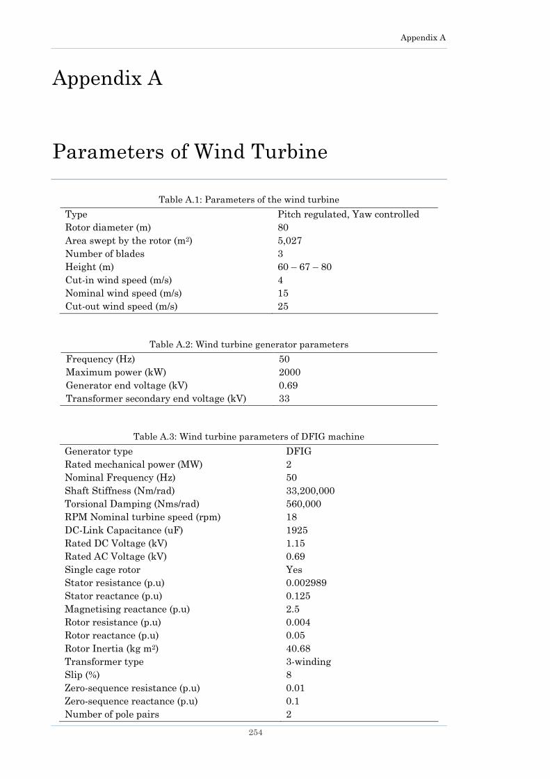
Appendix A
254
Appendix A Parameters of Wind
Turbines
Parameters of Wind Turbine
Table A.1: Parameters of the wind turbine
Type Pitch regulated, Yaw controlled
Rotor diameter (m) 80
Area swept by the rotor (m2) 5,027
Number of blades 3
Height (m) 60 – 67 – 80
Cut-in wind speed (m/s) 4
Nominal wind speed (m/s) 15
Cut-out wind speed (m/s) 25
Table A.2: Wind turbine generator parameters
Frequency (Hz) 50
Maximum power (kW) 2000
Generator end voltage (kV) 0.69
Transformer secondary end voltage (kV) 33
Table A.3: Wind turbine parameters of DFIG machine
Generator type DFIG
Rated mechanical power (MW) 2
Nominal Frequency (Hz) 50
Shaft Stiffness (Nm/rad) 33,200,000
Torsional Damping (Nms/rad) 560,000
RPM Nominal turbine speed (rpm) 18
DC-Link Capacitance (uF) 1925
Rated DC Voltage (kV) 1.15
Rated AC Voltage (kV) 0.69
Single cage rotor Yes
Stator resistance (p.u) 0.002989
Stator reactance (p.u) 0.125
Magnetising reactance (p.u) 2.5
Rotor resistance (p.u) 0.004
Rotor reactance (p.u) 0.05
Rotor Inertia (kg m2) 40.68
Transformer type 3-winding
Slip (%) 8
Zero-sequence resistance (p.u) 0.01
Zero-sequence reactance (p.u) 0.1
Number of pole pairs 2
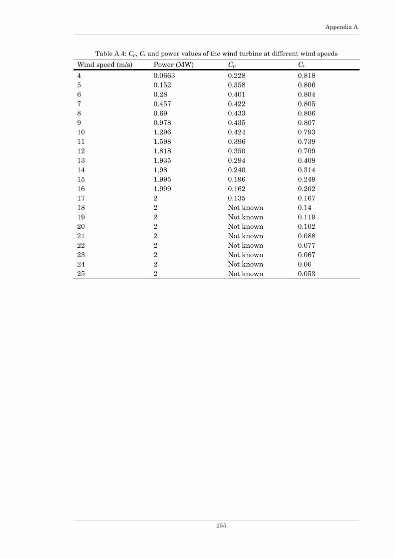
Appendix A
255
Table A.4: Cp, Ct and power values of the wind turbine at different wind speeds
Wind speed (m/s) Power (MW) Cp Ct
4 0.0663 0.228 0.818
5 0.152 0.358 0.806
6 0.28 0.401 0.804
7 0.457 0.422 0.805
8 0.69 0.433 0.806
9 0.978 0.435 0.807
10 1.296 0.424 0.793
11 1.598 0.396 0.739
12 1.818 0.350 0.709
13 1.935 0.294 0.409
14 1.98 0.240 0.314
15 1.995 0.196 0.249
16 1.999 0.162 0.202
17 2 0.135 0.167
18 2 Not known 0.14
19 2 Not known 0.119
20 2 Not known 0.102
21 2 Not known 0.088
22 2 Not known 0.077
23 2 Not known 0.067
24 2 Not known 0.06
25 2 Not known 0.053
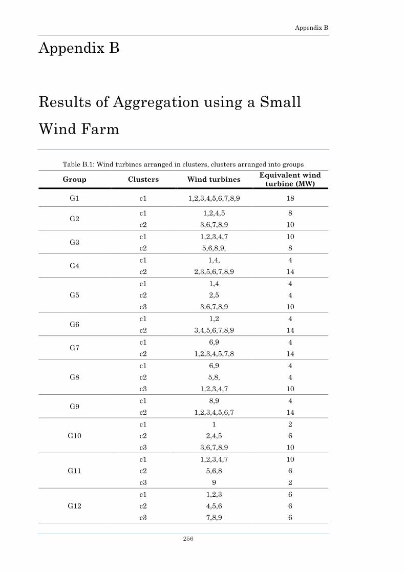
Appendix B
256
Appendix B Results of Aggregation using a Small Wind Farm
Results of Aggregation using a Small
Wind Farm
Table B.1: Wind turbines arranged in clusters, clusters arranged into groups
Group Clusters Wind turbines Equivalent wind
turbine (MW)
G1 c1 1,2,3,4,5,6,7,8,9 18
G2 c1 1,2,4,5 8
c2 3,6,7,8,9 10
G3 c1 1,2,3,4,7 10
c2 5,6,8,9, 8
G4 c1 1,4, 4
c2 2,3,5,6,7,8,9 14
G5
c1 1,4 4
c2 2,5 4
c3 3,6,7,8,9 10
G6 c1 1,2 4
c2 3,4,5,6,7,8,9 14
G7 c1 6,9 4
c2 1,2,3,4,5,7,8 14
G8
c1 6,9 4
c2 5,8, 4
c3 1,2,3,4,7 10
G9 c1 8,9 4
c2 1,2,3,4,5,6,7 14
G10
c1 1 2
c2 2,4,5 6
c3 3,6,7,8,9 10
G11
c1 1,2,3,4,7 10
c2 5,6,8 6
c3 9 2
G12
c1 1,2,3 6
c2 4,5,6 6
c3 7,8,9 6
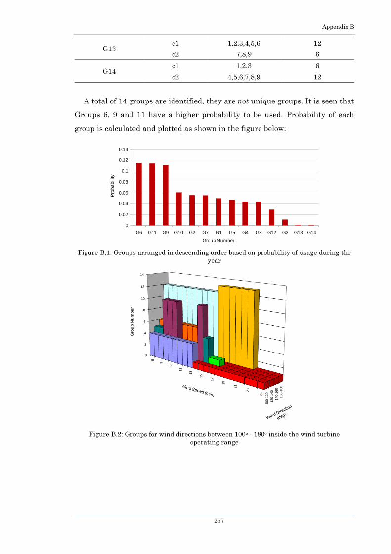
Appendix B
257
G13 c1 1,2,3,4,5,6 12
c2 7,8,9 6
G14 c1 1,2,3 6
c2 4,5,6,7,8,9 12
A total of 14 groups are identified, they are not unique groups. It is seen that
Groups 6, 9 and 11 have a higher probability to be used. Probability of each
group is calculated and plotted as shown in the figure below:
Figure B.1: Groups arranged in descending order based on probability of usage during the
year
Figure B.2: Groups for wind directions between 100o - 180o inside the wind turbine
operating range
0
0.02
0.04
0.06
0.08
0.1
0.12
0.14
G6 G11 G9 G10 G2 G7 G1 G5 G4 G8 G12 G3 G13 G14
Pro
ba
bility
Group Number
100-1
20
120-1
40
140-1
60
160-1
80
0
2
4
6
8
10
12
14
5
7
9
11
13
15
17
19
21
23
25
Gro
up
Nu
mb
er
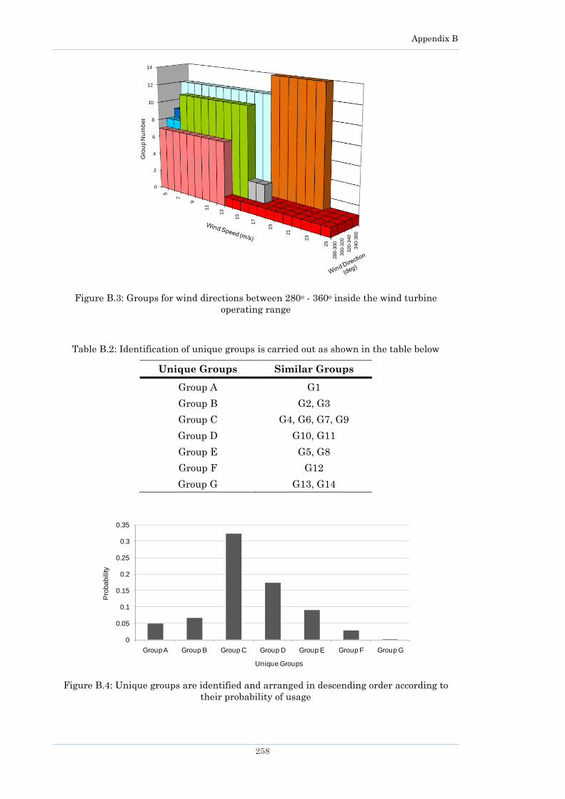
Appendix B
258
Figure B.3: Groups for wind directions between 280o - 360o inside the wind turbine
operating range
Table B.2: Identification of unique groups is carried out as shown in the table below
Unique Groups Similar Groups
Group A G1
Group B G2, G3
Group C G4, G6, G7, G9
Group D G10, G11
Group E G5, G8
Group F G12
Group G G13, G14
Figure B.4: Unique groups are identified and arranged in descending order according to
their probability of usage
280-3
00
300-3
20
320-3
40
340-3
60
0
2
4
6
8
10
12
14
5
7
9
11
13
15
17
19
21
23
25
Gro
up
Nu
mb
er
0
0.05
0.1
0.15
0.2
0.25
0.3
0.35
Group A Group B Group C Group D Group E Group F Group G
Pro
ba
bility
Unique Groups

Appendix B
259
Group C has the highest probability therefore this will be used for the wind
farm representation during the year. Its components can be seen from the
tables above. A 9 turbine wind farm can be represented by just 2 equivalent
turbines with the rated powers of 4 MW and 14 MW.
Figure B.5: Circuit diagrams for (a) detailed nine WIND TURBINE model and (b)
aggregated two turbine equivalent model
(a)
(b)

Appendix C
260
Appendix C Cost of Transmission Lines
Cost of Transmission Lines
Table C.1: Types of transmission lines and their costs for different voltage levels
New Transmission Line Unit 60/70kV 115kV 230kV
Double Circuit, Strung on both
sides, Lattice Tower per mile £874,800 £874,800 £1,036,800
Double Circuit, Strung on one
side, sides, Lattice Tower per mile £680,400 £680,400 £810,000
Double Circuit, Strung on both
sides, Tubular Steel Pole per mile £946,080 £946,080 £1,166,400
Double Circuit, Strung on one
side, sides, Tubular Steel Pole per mile £810,000 £810,000 £939,600
Single Circuit, Tubular Steel Pole per mile £609,120 £609,120 £712,800

Appendix D
261
Appendix D Failure Rates and Repair Times for Components
Failure Rates and Repair Times for
Components
Table D.1: Failure rates and repair times for offshore wind farm components
Worst Situation Normal Situation Best Situation
Equipment
Failure
rate
(1/year)
MTTR
Failure
rate
(1/year)
MTTR
Failure
rate
(1/year)
MTTR
Turbine
Transformer 0.0131 30 days 0.0131 20 days 0.0131 10 days
Collector
Transformer 0.03 6 months 0.03 4 months 0.03 3 months
Converter
Transformer 0.02 5 months 0.02 4 months 0.02 2 months
Array Cable
(1/km) 0.001 3 months 0.0094 2 months 0.0008 2 month
Export Cable
(1/km) 0.001 3 months 0.0094 2 months 0.0008 2 month
Converter 0.12 4 weeks 0.12 2 weeks 0.12 1 week
DC Cable 0.00148 3 months 0.00094 2 months 0.0004 1 month

Appendix E
262
Appendix E Screenshots of the Developed Software Tool
Screenshots of the Developed Software
Tool
Figure E.1: GUI Form (Main window – Enter basic information)
Read and Save data
Progress Report
Basic Wind farm
parameters
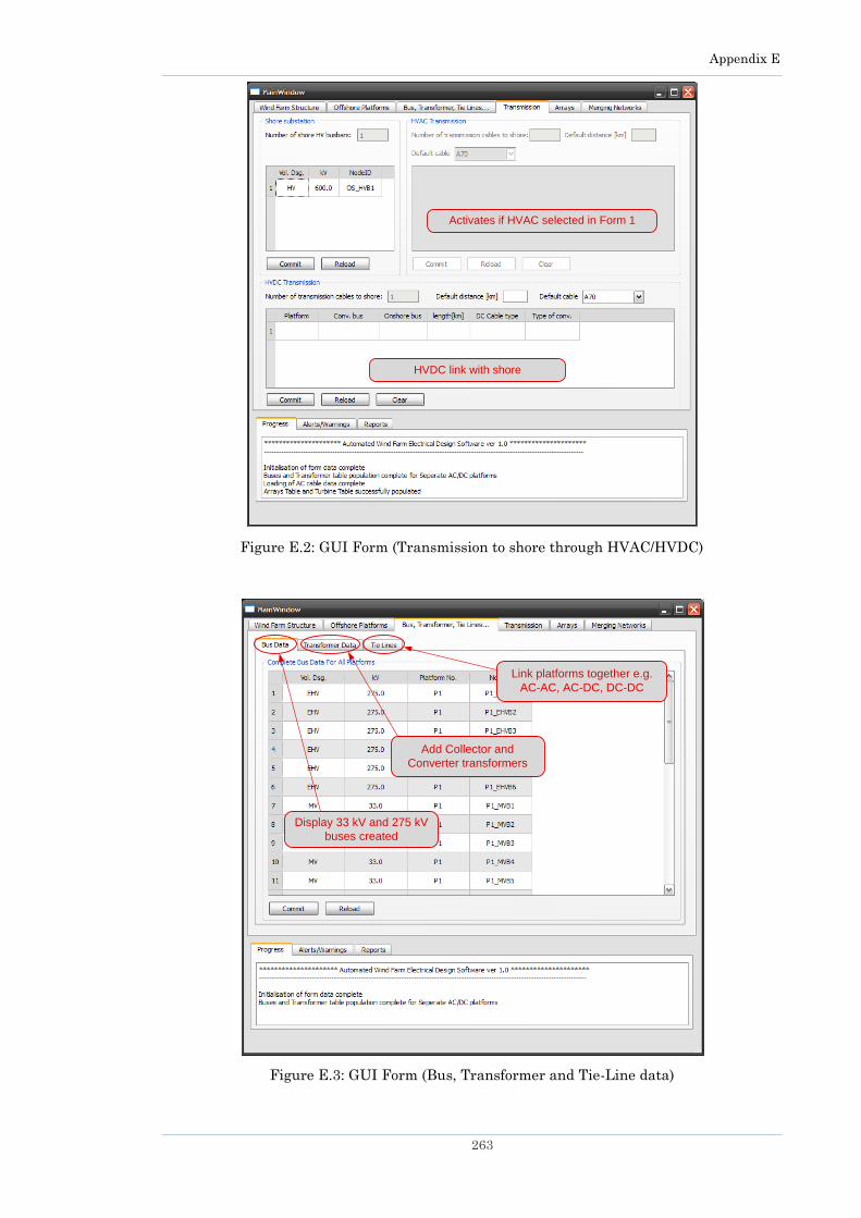
Appendix E
263
Figure E.2: GUI Form (Transmission to shore through HVAC/HVDC)
Figure E.3: GUI Form (Bus, Transformer and Tie-Line data)
Activates if HVAC selected in Form 1
HVDC link with shore
Display 33 kV and 275 kV
buses created
Add Collector and
Converter transformers
Link platforms together e.g.
AC-AC, AC-DC, DC-DC
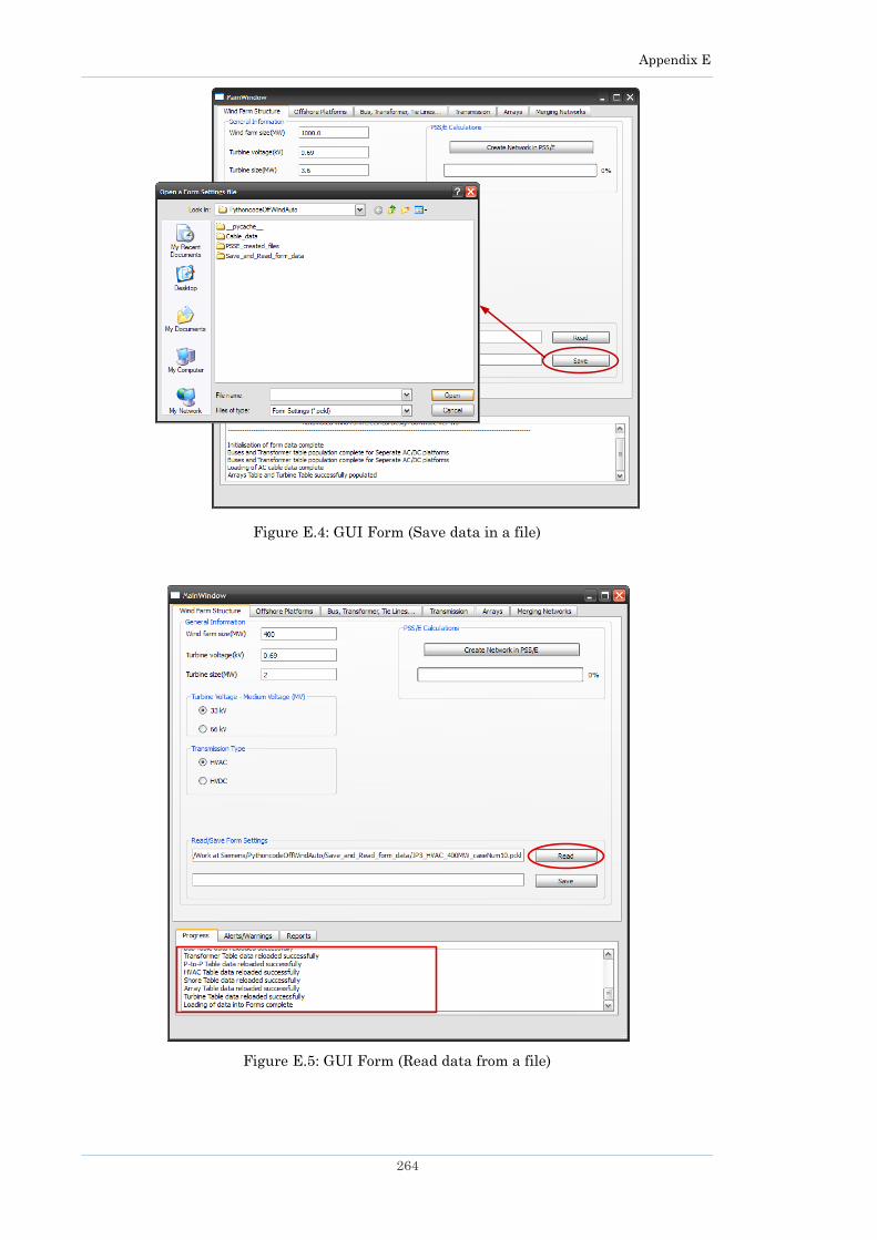
Appendix E
264
Figure E.4: GUI Form (Save data in a file)
Figure E.5: GUI Form (Read data from a file)
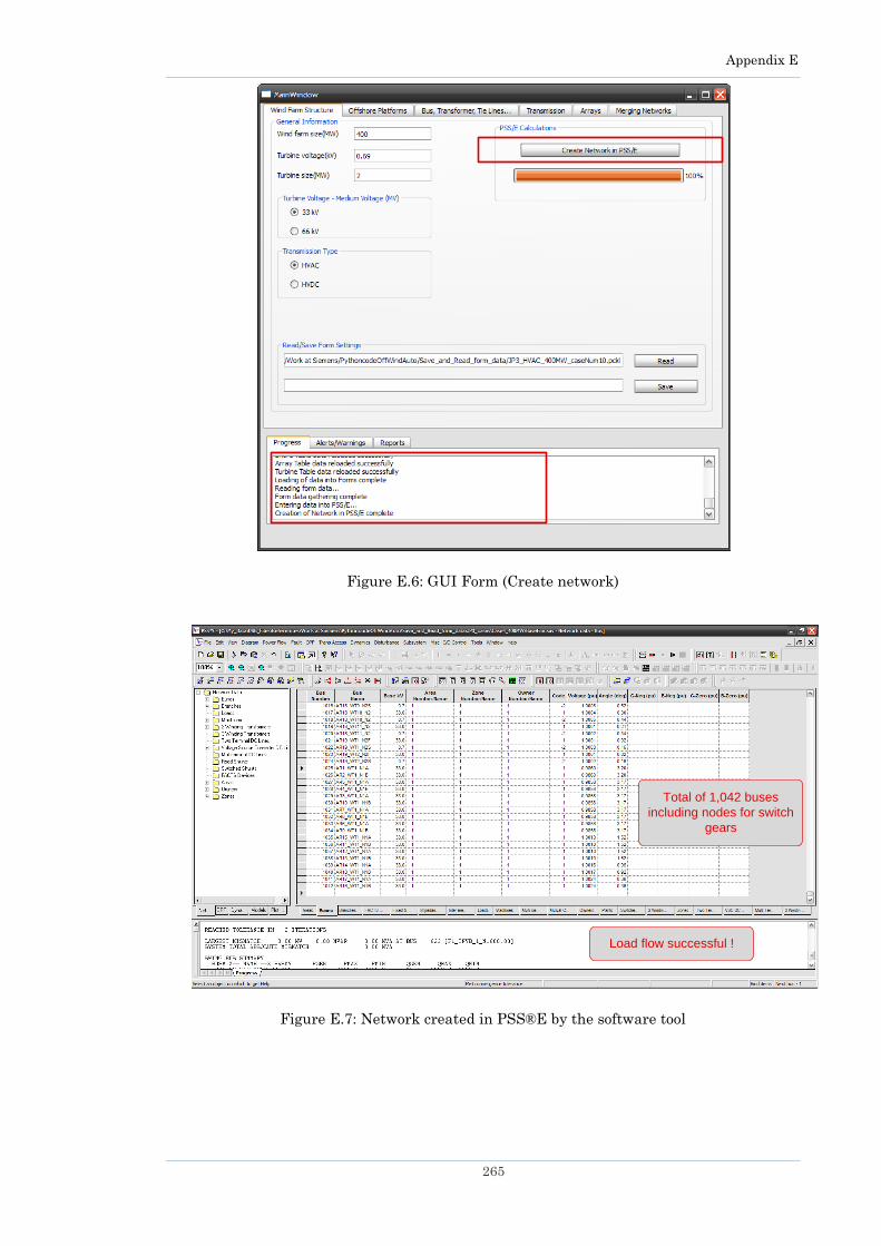
Appendix E
265
Figure E.6: GUI Form (Create network)
Figure E.7: Network created in PSS®E by the software tool
Load flow successful !
Total of 1,042 buses
including nodes for switch
gears
Appendix F
266
Appendix F Author‘s Thesis Based Publications
Author‘s Thesis Based Publications
International Journal Papers
F.1 M. Ali, J. Matevosyan and J. V. Milanović, ―Probabilistic Assessment of
Wind Farm Annual Energy Production‖, Electric Power Systems
Research, vol. 89, pp. 70-79, August 2012. DOI information:
10.1016/j.epsr.2012.01.019 (published online: 29 March 2012).
F.2 M. Ali, I-S. Ilie, J. V. Milanović and G. Chicco, ―Wind Farm Model
Aggregation using Probabilistic Clustering‖, IEEE Transactions on
Power Systems, TPWRS-00929-2011 (accepted for publication on
29/05/2012).
International Conference Papers
F.3 D. P. Nedic, M. Ali and J. V. Milanović, ―Software Tool for Automated
Design and Cost Benefit Analysis of Offshore Grid‖, in Proc. 2nd IEEE
PES International Conference and Exhibition on Innovative Smart Grid
Technologies (ISGT Europe) – 2011, Manchester, UK, December 5-7,
2011.
F.4 M. Ali, J. Matevosyan and J. V. Milanović, ―Probabilistic Assessment of
Wind Farm Energy Yield‖, in Proc. 17th Power System Computation
Conference (PSCC), Stockholm, Sweden, August 22-26, 2011.
F.5 M. Ali, J. V. Milanović, I-S Ilie and G. Chicco, ―Comparison of Wind
Farm Aggregate Models for Transient Stability Studies‖, in Proc. 17th
Power System Computation Conference (PSCC), Stockholm, Sweden,
August 22-26, 2011.
F.6 M. Ali and J. V. Milanović, ―Probabilistic Assessment of Wind Farm
Energy Yield Considering Wake Turbulence and Variable Turbine
Availabilities‖, in Proc. of the 21st International Conference and
Exhibition on Electricity Distribution (CIRED), Frankfurt, Germany,
June 6-9, 2011.

Appendix F
267
F.7 M. Ali, I-S. Ilie, J. V. Milanović and G. Chicco, ―Probabilistic
Identification of Turbines Facing High and Low Wind Speeds in a Wind
Farm‖, in Proc. IEEE 11th International Conference on Probabilistic
Methods Applied to Power Systems (PMAPS 2010), Singapore, June 14-
17, 2010.
F.8 M. Ali, I-S. Ilie, J. V. Milanović and G. Chicco, ―Probabilistic Clustering
of Wind Generators‖, in Proc. IEEE Power and Energy Society General
Meeting, Minneapolis, MN, USA, July 25-29, 2010.
F.9 M. Ali, J. Matevosyan, J. V. Milanović and Lennart Söder, ―Effect of
Wake Consideration on Estimated Cost of Wind Energy Curtailments‖,
in Proc. 8th International Workshop on Large-Scale Integration of Wind
Power into Power Systems as well as on Transmission Networks for
Offshore Wind Power Plants, Bremen, Germany, October 14-15, 2009.
Industrial Software
F.10 Software tool for cost-benefit analysis of offshore wind farm electrical
system, version 1.0, updated 16/06/2011.

Appendix G
268
Appendix G VeBWake Software CD
VeBWake Software CD
The CD is attached to the back cover of this thesis.
Related Documents