PROBABILISTIC ANALYSIS AND RESULTS OF COMBINATORIAL PROBLEMS WITH MILITARY APPLICATIONS By DON A. GRUNDEL A DISSERTATION PRESENTED TO THE GRADUATE SCHOOL OF THE UNIVERSITY OF FLORIDA IN PARTIAL FULFILLMENT OF THE REQUIREMENTS FOR THE DEGREE OF DOCTOR OF PHILOSOPHY UNIVERSITY OF FLORIDA 2004

Welcome message from author
This document is posted to help you gain knowledge. Please leave a comment to let me know what you think about it! Share it to your friends and learn new things together.
Transcript

PROBABILISTIC ANALYSIS AND RESULTSOF COMBINATORIAL PROBLEMSWITH MILITARY APPLICATIONS
By
DON A. GRUNDEL
A DISSERTATION PRESENTED TO THE GRADUATE SCHOOLOF THE UNIVERSITY OF FLORIDA IN PARTIAL FULFILLMENT
OF THE REQUIREMENTS FOR THE DEGREE OFDOCTOR OF PHILOSOPHY
UNIVERSITY OF FLORIDA
2004

Copyright 2004
by
Don A. Grundel

I dedicate this work to Bonnie, Andrew and Erin.

ACKNOWLEDGMENTS
I wish to express my heartfelt thanks to Professor Panos Pardalos for his guidance
and support. His extraordinary energetic personality inspires all those around him.
What I appreciate most about Professor Pardalos is he sets high goals for himself and
his students and then tirelessly strives to reach those goals.
I am grateful to the United States Air Force for its financial support and for
allowing me to pursue my lifelong goal. Within the Air Force, I owe a debt of
gratitude to Dr. David Jeffcoat for his counsel and assistance throughout my PhD
efforts.
My appreciation also goes to my committee members Stan Uryasev, Joseph Ge-
unes, and William Hager for their time and thoughtful guidance. I would like to thank
my collaborators Anthony Okafor, Carlos Oliveira, Pavlo Krakhmal, and Lewis Pasil-
iao.
Finally, to my family, Bonnie, Andrew and Erin, who have been extremely sup-
portive – I could not have completed this work without their love and understanding.
iv
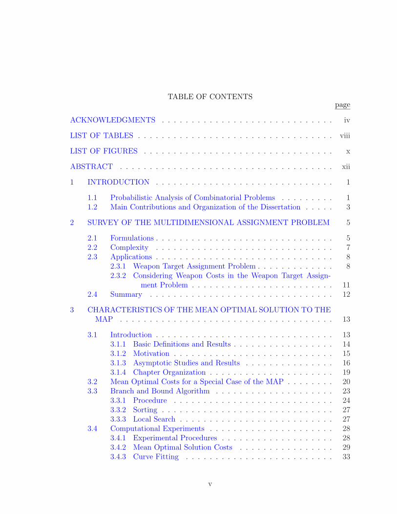
TABLE OF CONTENTSpage
ACKNOWLEDGMENTS . . . . . . . . . . . . . . . . . . . . . . . . . . . . . iv
LIST OF TABLES . . . . . . . . . . . . . . . . . . . . . . . . . . . . . . . . . viii
LIST OF FIGURES . . . . . . . . . . . . . . . . . . . . . . . . . . . . . . . . x
ABSTRACT . . . . . . . . . . . . . . . . . . . . . . . . . . . . . . . . . . . . xii
1 INTRODUCTION . . . . . . . . . . . . . . . . . . . . . . . . . . . . . . 1
1.1 Probabilistic Analysis of Combinatorial Problems . . . . . . . . . 11.2 Main Contributions and Organization of the Dissertation . . . . . 3
2 SURVEY OF THE MULTIDIMENSIONAL ASSIGNMENT PROBLEM 5
2.1 Formulations . . . . . . . . . . . . . . . . . . . . . . . . . . . . . . 52.2 Complexity . . . . . . . . . . . . . . . . . . . . . . . . . . . . . . 72.3 Applications . . . . . . . . . . . . . . . . . . . . . . . . . . . . . . 8
2.3.1 Weapon Target Assignment Problem . . . . . . . . . . . . . 82.3.2 Considering Weapon Costs in the Weapon Target Assign-
ment Problem . . . . . . . . . . . . . . . . . . . . . . . . 112.4 Summary . . . . . . . . . . . . . . . . . . . . . . . . . . . . . . . 12
3 CHARACTERISTICS OF THE MEAN OPTIMAL SOLUTION TO THEMAP . . . . . . . . . . . . . . . . . . . . . . . . . . . . . . . . . . . . 13
3.1 Introduction . . . . . . . . . . . . . . . . . . . . . . . . . . . . . . 133.1.1 Basic Definitions and Results . . . . . . . . . . . . . . . . . 143.1.2 Motivation . . . . . . . . . . . . . . . . . . . . . . . . . . . 153.1.3 Asymptotic Studies and Results . . . . . . . . . . . . . . . 163.1.4 Chapter Organization . . . . . . . . . . . . . . . . . . . . . 19
3.2 Mean Optimal Costs for a Special Case of the MAP . . . . . . . . 203.3 Branch and Bound Algorithm . . . . . . . . . . . . . . . . . . . . 23
3.3.1 Procedure . . . . . . . . . . . . . . . . . . . . . . . . . . . 243.3.2 Sorting . . . . . . . . . . . . . . . . . . . . . . . . . . . . . 273.3.3 Local Search . . . . . . . . . . . . . . . . . . . . . . . . . . 27
3.4 Computational Experiments . . . . . . . . . . . . . . . . . . . . . 283.4.1 Experimental Procedures . . . . . . . . . . . . . . . . . . . 283.4.2 Mean Optimal Solution Costs . . . . . . . . . . . . . . . . 293.4.3 Curve Fitting . . . . . . . . . . . . . . . . . . . . . . . . . 33
v
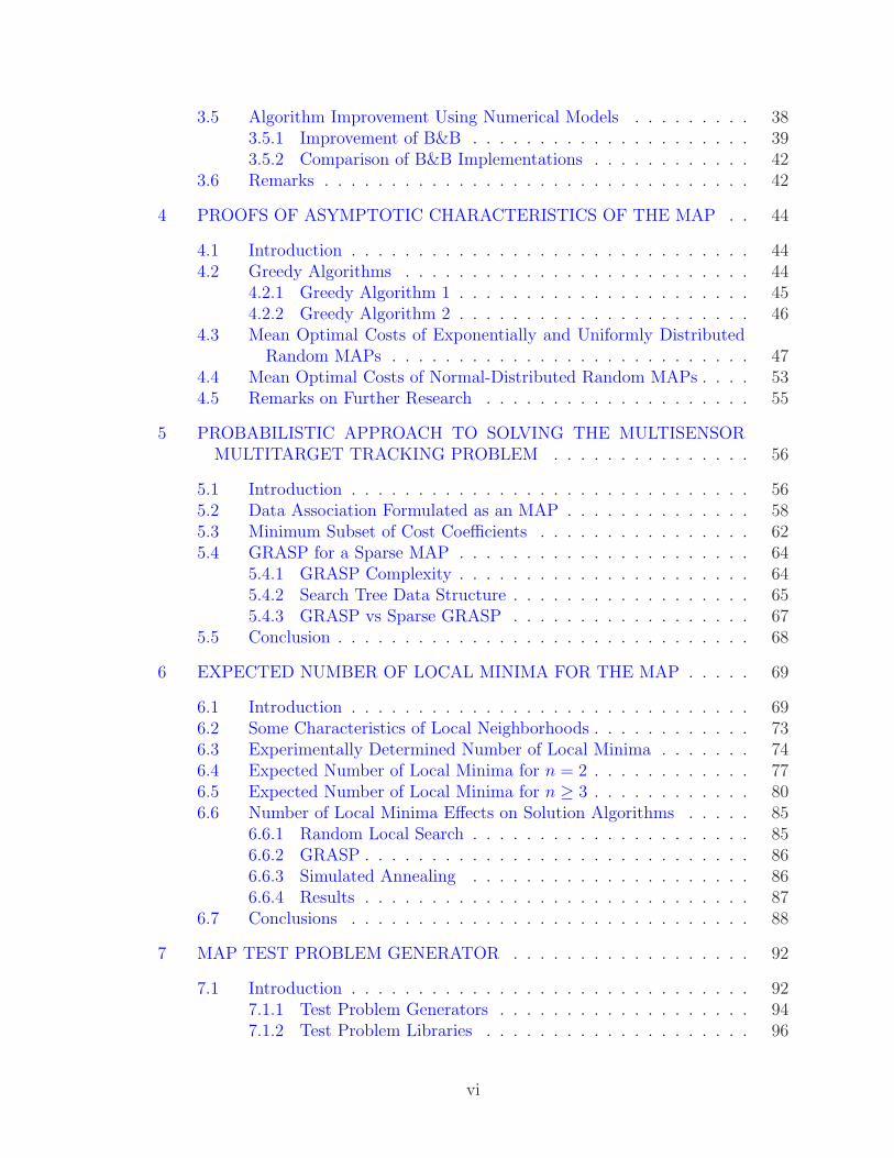
3.5 Algorithm Improvement Using Numerical Models . . . . . . . . . 383.5.1 Improvement of B&B . . . . . . . . . . . . . . . . . . . . . 393.5.2 Comparison of B&B Implementations . . . . . . . . . . . . 42
3.6 Remarks . . . . . . . . . . . . . . . . . . . . . . . . . . . . . . . . 42
4 PROOFS OF ASYMPTOTIC CHARACTERISTICS OF THE MAP . . 44
4.1 Introduction . . . . . . . . . . . . . . . . . . . . . . . . . . . . . . 444.2 Greedy Algorithms . . . . . . . . . . . . . . . . . . . . . . . . . . 44
4.2.1 Greedy Algorithm 1 . . . . . . . . . . . . . . . . . . . . . . 454.2.2 Greedy Algorithm 2 . . . . . . . . . . . . . . . . . . . . . . 46
4.3 Mean Optimal Costs of Exponentially and Uniformly DistributedRandom MAPs . . . . . . . . . . . . . . . . . . . . . . . . . . . 47
4.4 Mean Optimal Costs of Normal-Distributed Random MAPs . . . . 534.5 Remarks on Further Research . . . . . . . . . . . . . . . . . . . . 55
5 PROBABILISTIC APPROACH TO SOLVING THE MULTISENSORMULTITARGET TRACKING PROBLEM . . . . . . . . . . . . . . . 56
5.1 Introduction . . . . . . . . . . . . . . . . . . . . . . . . . . . . . . 565.2 Data Association Formulated as an MAP . . . . . . . . . . . . . . 585.3 Minimum Subset of Cost Coefficients . . . . . . . . . . . . . . . . 625.4 GRASP for a Sparse MAP . . . . . . . . . . . . . . . . . . . . . . 64
5.4.1 GRASP Complexity . . . . . . . . . . . . . . . . . . . . . . 645.4.2 Search Tree Data Structure . . . . . . . . . . . . . . . . . . 655.4.3 GRASP vs Sparse GRASP . . . . . . . . . . . . . . . . . . 67
5.5 Conclusion . . . . . . . . . . . . . . . . . . . . . . . . . . . . . . . 68
6 EXPECTED NUMBER OF LOCAL MINIMA FOR THE MAP . . . . . 69
6.1 Introduction . . . . . . . . . . . . . . . . . . . . . . . . . . . . . . 696.2 Some Characteristics of Local Neighborhoods . . . . . . . . . . . . 736.3 Experimentally Determined Number of Local Minima . . . . . . . 746.4 Expected Number of Local Minima for n = 2 . . . . . . . . . . . . 776.5 Expected Number of Local Minima for n ≥ 3 . . . . . . . . . . . . 806.6 Number of Local Minima Effects on Solution Algorithms . . . . . 85
6.6.1 Random Local Search . . . . . . . . . . . . . . . . . . . . . 856.6.2 GRASP . . . . . . . . . . . . . . . . . . . . . . . . . . . . . 866.6.3 Simulated Annealing . . . . . . . . . . . . . . . . . . . . . 866.6.4 Results . . . . . . . . . . . . . . . . . . . . . . . . . . . . . 87
6.7 Conclusions . . . . . . . . . . . . . . . . . . . . . . . . . . . . . . 88
7 MAP TEST PROBLEM GENERATOR . . . . . . . . . . . . . . . . . . 92
7.1 Introduction . . . . . . . . . . . . . . . . . . . . . . . . . . . . . . 927.1.1 Test Problem Generators . . . . . . . . . . . . . . . . . . . 947.1.2 Test Problem Libraries . . . . . . . . . . . . . . . . . . . . 96
vi
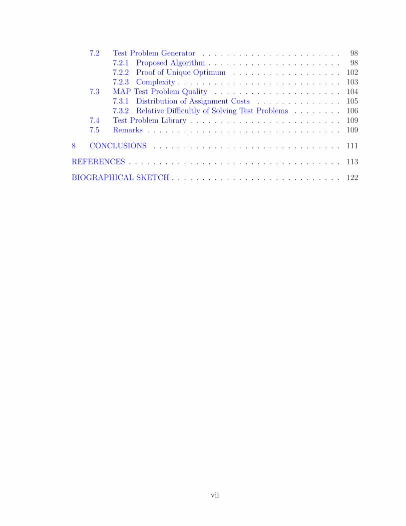
7.2 Test Problem Generator . . . . . . . . . . . . . . . . . . . . . . . 987.2.1 Proposed Algorithm . . . . . . . . . . . . . . . . . . . . . . 987.2.2 Proof of Unique Optimum . . . . . . . . . . . . . . . . . . 1027.2.3 Complexity . . . . . . . . . . . . . . . . . . . . . . . . . . . 103
7.3 MAP Test Problem Quality . . . . . . . . . . . . . . . . . . . . . 1047.3.1 Distribution of Assignment Costs . . . . . . . . . . . . . . 1057.3.2 Relative Difficultly of Solving Test Problems . . . . . . . . 106
7.4 Test Problem Library . . . . . . . . . . . . . . . . . . . . . . . . . 1097.5 Remarks . . . . . . . . . . . . . . . . . . . . . . . . . . . . . . . . 109
8 CONCLUSIONS . . . . . . . . . . . . . . . . . . . . . . . . . . . . . . . 111
REFERENCES . . . . . . . . . . . . . . . . . . . . . . . . . . . . . . . . . . . 113
BIOGRAPHICAL SKETCH . . . . . . . . . . . . . . . . . . . . . . . . . . . . 122
vii
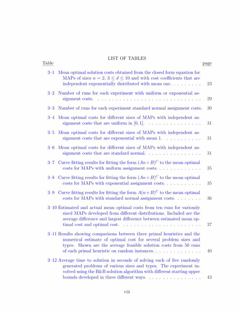
LIST OF TABLESTable page
3–1 Mean optimal solution costs obtained from the closed form equation forMAPs of sizes n = 2, 3 ≤ d ≤ 10 and with cost coefficients that areindependent exponentially distributed with mean one. . . . . . . . . 23
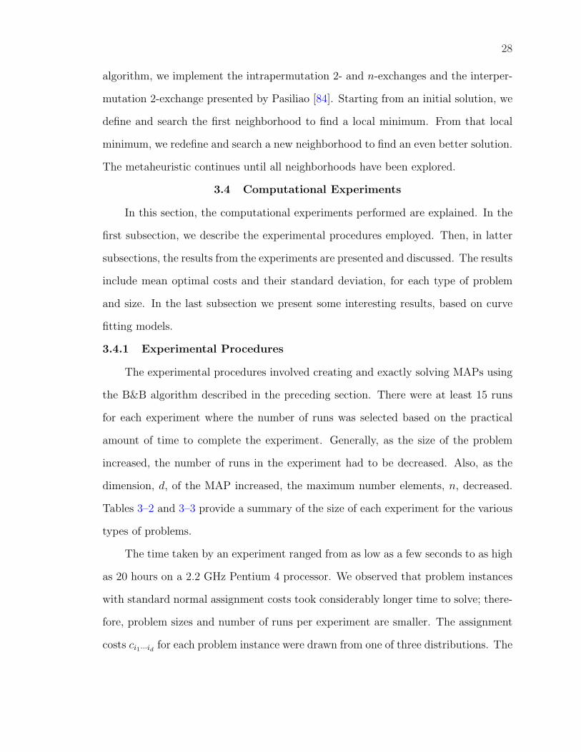
3–2 Number of runs for each experiment with uniform or exponential as-signment costs. . . . . . . . . . . . . . . . . . . . . . . . . . . . . . 29
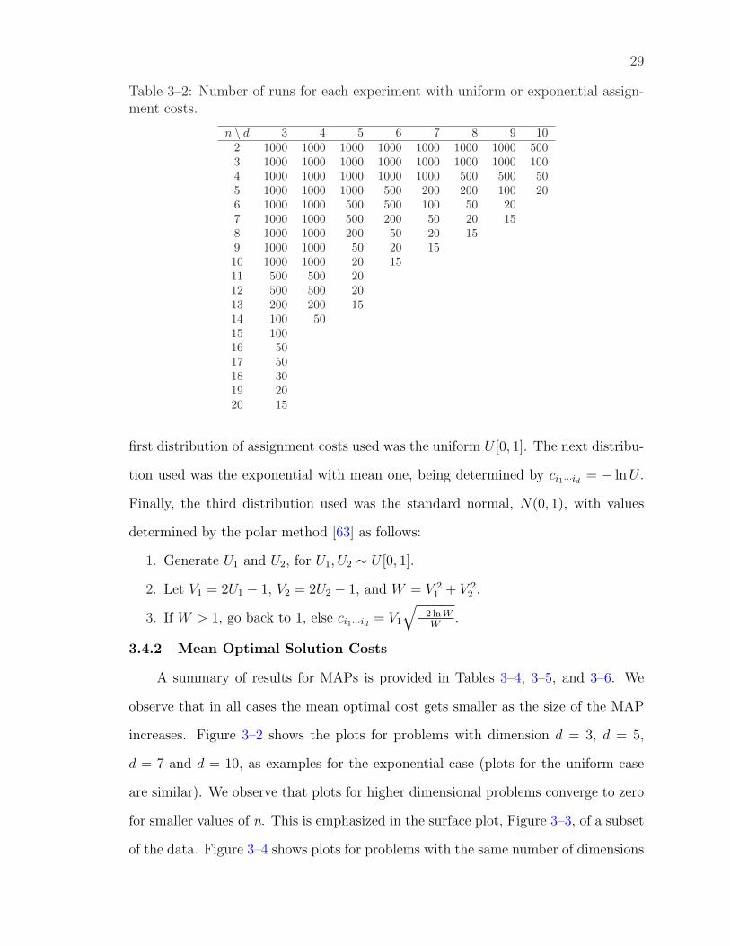
3–3 Number of runs for each experiment standard normal assignment costs. 30
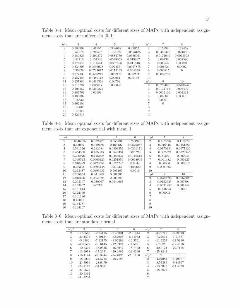
3–4 Mean optimal costs for different sizes of MAPs with independent as-signment costs that are uniform in [0, 1]. . . . . . . . . . . . . . . . 31
3–5 Mean optimal costs for different sizes of MAPs with independent as-signment costs that are exponential with mean 1. . . . . . . . . . . 31
3–6 Mean optimal costs for different sizes of MAPs with independent as-signment costs that are standard normal. . . . . . . . . . . . . . . . 31
3–7 Curve fitting results for fitting the form (An+B)C to the mean optimalcosts for MAPs with uniform assignment costs. . . . . . . . . . . . . 35
3–8 Curve fitting results for fitting the form (An+B)C to the mean optimalcosts for MAPs with exponential assignment costs. . . . . . . . . . . 35
3–9 Curve fitting results for fitting the form A(n+B)C to the mean optimalcosts for MAPs with standard normal assignment costs. . . . . . . . 36
3–10 Estimated and actual mean optimal costs from ten runs for variouslysized MAPs developed from different distributions. Included are theaverage difference and largest difference between estimated mean op-timal cost and optimal cost. . . . . . . . . . . . . . . . . . . . . . . 37
3–11 Results showing comparisons between three primal heuristics and thenumerical estimate of optimal cost for several problem sizes andtypes. Shown are the average feasible solution costs from 50 runsof each primal heuristic on random instances. . . . . . . . . . . . . . 40
3–12 Average time to solution in seconds of solving each of five randomlygenerated problems of various sizes and types. The experiment in-volved using the B&B solution algorithm with different starting upperbounds developed in three different ways. . . . . . . . . . . . . . . . 43
viii
5–1 Comparisons of the number of cost coefficients of original MAP to thatin A. . . . . . . . . . . . . . . . . . . . . . . . . . . . . . . . . . . . 63
5–2 Table of experimental results of comparing solution quality and time-to-solution for GRASP in solving fully dense and reduced simulatedMSMTT problems. Five runs of each algorithm were conductedagainst each problem. . . . . . . . . . . . . . . . . . . . . . . . . . . 68
6–1 Average number of local minima (2-exchange neighborhood) for differ-ent sizes of MAPs with independent assignment costs. . . . . . . . . 75
6–2 Average number of local minima (3-exchange neighborhood) for differ-ent sizes of MAPs with i.i.d. standard normal assignment costs. . . 76
6–3 Proportion of local minima to total number of feasible solutions fordifferent sizes of MAPs with i.i.d. standard normal costs. . . . . . . 76
7–1 Timed results of producing test problems of various sizes. . . . . . . . 105
7–2 Chi-square goodness-of-fit test for normal distribution of assignmentcosts for six randomly selected 5x5x5 test problems. . . . . . . . . . 106
7–3 Number of discrete local minima per 106 feasible solutions. The rangeis a 95-percent confidence interval based on proportionate sampling. 108
7–4 Comparison of solution times in seconds using an exact solution algo-rithm of the branch-and-bound variety. . . . . . . . . . . . . . . . . 109
7–5 Comparison of solution results using a GRASP algorithm. . . . . . . . 109
ix
LIST OF FIGURESFigure page
3–1 Branch and Bound on the Index Tree. . . . . . . . . . . . . . . . . . . 24
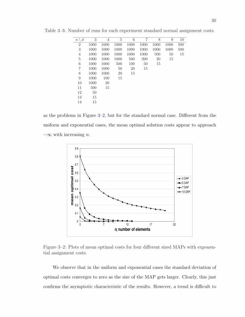
3–2 Plots of mean optimal costs for four different sized MAPs with expo-nential assignment costs. . . . . . . . . . . . . . . . . . . . . . . . . 30
3–3 Surface plots of mean optimal costs for 3 ≤ d ≤ 10 and 2 ≤ n ≤ 10sized MAPs with exponential assignment costs. . . . . . . . . . . . 32
3–4 Plots of mean optimal costs for four different sized MAPs with standardnormal assignment costs. . . . . . . . . . . . . . . . . . . . . . . . . 32
3–5 Plots of standard deviation of mean optimal costs for four differentsized MAPs with exponential assignment costs. . . . . . . . . . . . 33
3–6 Plots of standard deviation of mean optimal costs for four differentsized MAPs with standard normal assignment costs. . . . . . . . . 34
3–7 Three dimensional MAP with exponential assignment costs. Plot in-cludes both observed mean optimal cost values and fitted values.The two lines are nearly indistinguishable. . . . . . . . . . . . . . . 36
3–8 Plots of fitted and mean optimal costs from ten runs of variously sizedMAPs developed from the uniform distribution on [10, 20]. Notethat the observed data and fitted data are nearly indistinguishable. 38
3–9 Plots of fitted and mean optimal costs from ten runs of variously sizedMAPs developed from the exponential distribution with mean three. 38
3–10 Plots of fitted and mean optimal costs from ten0 runs of variously sizedMAPs developed from a normal distribution, N(µ = 5, σ = 2). . . . 39
3–11 Branch and bound on the index tree. . . . . . . . . . . . . . . . . . . 41
5–1 Example of noisy sensor measurements of target locations. . . . . . . 57
5–2 Example of noisy sensor measurements of close targets. In this casethere is false detection and missed targets. . . . . . . . . . . . . . . 57
5–3 Search tree data structure used to find a cost coefficient or determinea cost coefficient does not exist. . . . . . . . . . . . . . . . . . . . . 66
5–4 Search tree example of a sparse MAP. . . . . . . . . . . . . . . . . . . 67
x
6–1 Proportion of feasible solutions that are local minima when consideringthe 2-exchange neighborhood and where costs are i.i.d. standardnormal. . . . . . . . . . . . . . . . . . . . . . . . . . . . . . . . . . 76
6–2 Plots of solution quality versus number of local minima when using the2-exchange neighborhood. The MAP has a size of d = 4, n = 5 withcost coefficients that are i.i.d. standard normal. . . . . . . . . . . . 89
6–3 Plots of solution quality versus number of local minima when using a3-exchange neighborhood. The MAP has a size of d = 4, n = 5 withcost coefficients that are i.i.d. standard normal. . . . . . . . . . . . 90
7–1 Tree graph for 3x4x4 MAP. . . . . . . . . . . . . . . . . . . . . . . . 98
7–2 Initial tree graph with assignment costs and lower bound path costs. . 101
7–3 Tree graph with optimal path and costs. . . . . . . . . . . . . . . . . 102
7–4 Tree graph used to consider all feasible nodes at level 3 from the firstnode in level 2. . . . . . . . . . . . . . . . . . . . . . . . . . . . . . 103
7–5 Final tree graph for a 3x4x4 MAP. . . . . . . . . . . . . . . . . . . . 104
7–6 Typical normal probability plot for a 5x5x5 test problem. . . . . . . . 106
7–7 Typical histogram of 20x30x40 test problem. . . . . . . . . . . . . . . 107
xi
Abstract of Dissertation Presented to the Graduate Schoolof the University of Florida in Partial Fulfillment of theRequirements for the Degree of Doctor of Philosophy
PROBABILISTIC ANALYSIS AND RESULTSOF COMBINATORIAL PROBLEMSWITH MILITARY APPLICATIONS
By
Don A. Grundel
August 2004
Chair: Panagote M. PardalosMajor Department: Industrial and Systems Engineering
The work in this dissertation examines combinatorial problems from a probabilis-
tic approach in an effort to improve existing solution methods or find new algorithms
that perform better. Applications addressed here are focused on military uses such
as weapon-target assignment, path planning and multisensor multitarget tracking;
however, these may be easily extended to the civilian environment.
A probabilistic analysis of combinatorial problems is a very broad subject; how-
ever, the context here is the study of input data and solution values.
We investigate characteristics of the mean optimal solution values for random
multidimensional assignment problems (MAPs) with axial constraints. Cost coeffi-
cients are taken from three different random distributions: uniform, exponential and
standard normal. In the cases where cost coefficients are independent uniform or
exponential random variables, experimental data indicate that the average optimal
value of the MAP converges to zero as the MAP size increases. We give a short
proof of this result for the case of exponentially distributed costs when the number
of elements in each dimension is restricted to two. In the case of standard normal
xii
costs, experimental data indicate the average optimal value of the MAP goes to neg-
ative infinity as the MAP size increases. Using curve fitting techniques, we develop
numerical estimates of the mean optimal value for various sized problems. The exper-
iments indicate that numerical estimates are quite accurate in predicting the optimal
solution value of a random instance of the MAP.
Using a novel probabilistic approach, we provide generalized proofs of the asymp-
totic characteristics of the mean optimal costs of MAPs. The probabilistic approach
is then used to improve the efficiency of the popular greedy randomized adaptive
search procedure.
As many solution approaches to combinatorial problems rely, at least partly,
on local neighborhood searches, it is widely assumed the number of local minima
has implications on solution difficulty. We investigate the expected number of local
minima for random instances of the MAP. We report on empirical findings that the
expected number of local minima does impact the effectiveness of three different
solution algorithms that rely on local neighborhood searches.
A probabilistic approach is used to develop an MAP test problem generator that
creates difficult problems with known unique solutions.
xiii
CHAPTER 1INTRODUCTION
Combinatorial optimization problems are found in everyday life. They are par-
ticularly important in military applications as they most often concern management
and efficient use of scarce resources. Applications of combinatorial problems are in
a period of rapid development which follows from the widespread use of computers
and the data available from information systems. Although computers have allowed
expanded combinatorial applications, most of these problems remain very hard to
solve. The purpose of the work in this dissertation is to examine combinatorial prob-
lems from a probabilistic approach in an effort to improve existing solution methods
or find new algorithms that perform better. Most applications addressed here are fo-
cused on military applications; however, most may be easily extended to the civilian
environment.
1.1 Probabilistic Analysis of Combinatorial Problems
In general, probabilistic analysis of combinatorial problems is a very broad sub-
ject; however, the context being used here is the study of problem input values and
solution values of combinatorial problems. An obvious goal is to determine if param-
eters (e.g., mean, standard deviation, etc.) of these values can be used to improve
the efficiency of a solution algorithm. Alternatively, parameters of these values may
be useful in selecting an appropriate solution algorithm. Although problem instance
size is directly correlated with the difficulty of determining a solution, we often face
problems of similar size that have far different computing times. One can conclude
from this that characteristics of the problem data are significant factors.
An example of the study of solution values is by Barvinok and Stephen [13], where
the authors obtain a number of results regarding the distribution of solution values
1
2
of the quadratic assignment problem. In the paper, the authors consider questions
such as, how well does the optimum of a sample of random permutations approximate
the true optimum? They explore an interesting approach in which they consider the
“k-th sphere” around the true optimum. The k-th sphere, in simple terms, quantifies
the nearness of permutations to the optimum permutation. By allowing the true
optimum to represent a bullseye, the authors observe as the k-th sphere contracts
to the optimal permutation, the average solution value of a sample of permutations
steadily improves.
A study of the quadratic assignment problem (QAP) is found work by Abreu
et al. [1] where the authors consider using average and variance of solution costs to
establish the difficulty of a particular instance.
Sanchis and Schnabl [103] study the “landscape” of the traveling salesman prob-
lem. Considered are number of local minima and autocorrelation functions. The
concept of landscape was introduced by Wright [111] and can be thought of as a map
of solution values such that there are peaks and valleys. Landscape roughness can
give an indication of problem difficulty.
In a study of cost inputs, Reilly [94] suggests that the degree of correlation among
input data may influence the difficulty of finding a solution. It is suggested that an
extreme level of correlation can produce very challenging problems.
In this dissertation, we use a probabilistic approach to consider how input costs
affect solution values in an important class of problems called the multidimensional
assignment problem. We also consider the mean optimal costs of various problem
instances to include some asymptotic characteristics. We include another interesting
probabilistic analysis which is our study of local minima and how the number of local
minima affects solution methods. Finally, we use a probabilistic approach to design
and analyze a test problem generator.
3
1.2 Main Contributions and Organization of the Dissertation
The main contributions and organization of this dissertation are briefly discussed
in the following paragraphs.
Survey of the multidimensional assignment problem. A brief survey of
the multidimensional assignment problem (MAP) is provided in Chapter 2. In this
chapter, we provide alternative formulations and applications for this important and
difficult problem.
Mean optimal solution values of the MAP. In Chapter 3 we report exper-
imentally determined values of the mean optimal solution costs of MAPs with cost
coefficients that are independent random variables that are uniformly, exponentially
or normally distributed. Using the experimental data, we then find curve fitting
models that can be used to accurately determine their mean optimal solution costs.
Finally, we show how the numerical estimates can be used to improve at least two
solution methods of the MAP.
Proof of asymptotic characteristics of the MAP. In Chapter 4 we prove
some asymptotic characteristics of the mean optimal costs using a novel probabilistic
approach.
Probabilistic approach to solving the data association problem. Us-
ing the probabilistic approach introduced in Chapter 4, we extend the approach in
Chapter 5 to more efficiently solve the data association problem that results from the
multisensor multitarget tracking problem. In the multisensor multitarget problem
noisy measurements are made with an arbitrary number of spatially diverse sensors
regarding an arbitrary number of targets with the goal of estimating the trajectories
of all the targets present. Furthermore, the number of targets may change by moving
into and out of detection range. The problem involves a data association of sensor
measurements to targets and estimates the current state of each target. The combi-
natorial nature of the problem results from the data association problem; that is how
4
do we optimally partition the entire set of measurements so that each measurement
is attributed to no more than one target and each sensor detects a target no more
than once?
Expected number of local minima for the MAP. The number of local
minima in a problem may provide insight to more appropriate solution methods.
Chapter 6 explores the number of local minima in the MAP and then considers the
impact of the number of local minima on three solution methods.
MAP test problem generator. As examined in the first five chapters, a
probabilistic analysis can be used to develop a priori knowledge of problem instance
hardness. In Chapter 7 we develop an MAP test problem generator and use some
probabilistic analyses to determine the generator’s effectiveness in creating quality
test problems with known unique optimal solutions. Also included is a brief survey
of sources of combinatorial test problems.
CHAPTER 2SURVEY OF THE MULTIDIMENSIONAL ASSIGNMENT PROBLEM
The MAP is a higher dimensional version of the standard (two-dimensional,
or linear) assignment problem. The MAP is stated as follows: given d, n−sets
A1, A2, . . . , Ad, there is a cost for each d-tuple1 in A1 ×A2 × · · · ×Ad. The problem
is to minimize the cost of n tuples such that each element in A1 ∪ A2 ∪ · · · ∪ Ad is
in exactly one tuple. The problem was first introduced by Pierskalla [86]. Solution
methods have included branch and bound [87, 10, 84], Greedy Randomized Adap-
tive Search Procedure (GRASP) [4, 74], Lagrangian relaxation [90, 85], a genetic
algorithm based heuristic [25], and simulated annealing [27].
2.1 Formulations
A well-known instance of the MAP is the three-dimensional assignment problem
(3DAP). An example of the 3DAP consists of minimizing the total cost of assigning
ni items to nj locations at nk points in time. The three-dimensional MAP can be
1 Tuple an abstraction of the sequence: single, double, triple,..., d-tuple. Tuple isused in denote a point in a multidimensional coordinate system.
5
6
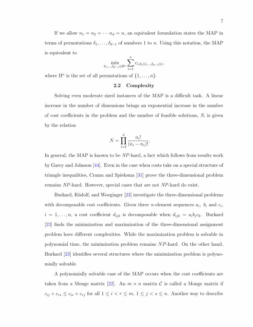
formulated as
min
ni∑i=1
nj∑j=1
nk∑
k=1
cijkxijk
s.t.
nj∑j=1
nk∑
k=1
xijk = 1 for all i = 1, 2, . . . , ni,
ni∑i=1
nk∑
k=1
xijk ≤ 1 for all j = 1, 2, . . . , nj,
ni∑i=1
nj∑j=1
xijk ≤ 1 for all k = 1, 2, . . . , nk,
xijk ∈ {0, 1} for all i, j, k ∈ {1, . . . , n},
ni ≤ nj ≤ nk,
where cijk is the cost of assigning item i to location j at time k. In this formulation,
the variable xijk is equal to 1 if and only if the i-th item is assigned to the j-th
location at time k and zero otherwise. If we consider additional dimensions for this
problem, the formulation can be similarly extended in the following way:
min
n1∑i1=1
· · ·nd∑
id=1
ci1···idxi1···id
s.t.
n2∑i2=1
· · ·nd∑
id=1
xi1···id = 1 for all i1 = 1, 2, . . . , n1,
n1∑i1=1
· · ·nk−1∑
ik−1=1
nk+1∑ik+1=1
· · ·nd∑
id=1
xi1···id ≤ 1
for all k = 2, . . . , d− 1, and ik = 1, 2, . . . , nk,n2∑
i2=1
· · ·nd−1∑
id−1=1
xi1···id ≤ 1 for all id = 1, 2, . . . , nd,
xi1···id ∈ {0, 1} for all i1, i2, . . . , id ∈ {1, . . . , n},
n1 ≤ n2 ≤ · · ·nd,
where d is the dimension of the MAP.
7
If we allow n1 = n2 = · · ·nd = n, an equivalent formulation states the MAP in
terms of permutations δ1, . . . , δd−1 of numbers 1 to n. Using this notation, the MAP
is equivalent to
minδ1,...,δd−1∈Πn
n∑i=1
ci,δ1(i),...,δd−1(i),
where Πn is the set of all permutations of {1, . . . , n}.2.2 Complexity
Solving even moderate sized instances of the MAP is a difficult task. A linear
increase in the number of dimensions brings an exponential increase in the number
of cost coefficients in the problem and the number of feasible solutions, N, is given
by the relation
N =d∏
i=2
ni!
(ni − n1)!.
In general, the MAP is known to be NP -hard, a fact which follows from results work
by Garey and Johnson [44]. Even in the case when costs take on a special structure of
triangle inequalities, Crama and Spieksma [31] prove the three-dimensional problem
remains NP -hard. However, special cases that are not NP -hard do exist.
Burkard, Rudolf, and Woeginger [23] investigate the three-dimensional problems
with decomposable cost coefficients. Given three n-element sequences ai, bi and ci,
i = 1, . . . , n, a cost coefficient dijk is decomposable when dijk = aibjck. Burkard
[23] finds the minimization and maximization of the three-dimensional assignment
problem have different complexities. While the maximization problem is solvable in
polynomial time, the minimization problem remains NP -hard. On the other hand,
Burkard [23] identifies several structures where the minimization problem is polyno-
mially solvable.
A polynomially solvable case of the MAP occurs when the cost coefficients are
taken from a Monge matrix [22]. An m × n matrix C is called a Monge matrix if
cij + crs ≤ cis + crj for all 1 ≤ i < r ≤ m, 1 ≤ j < s ≤ n. Another way to describe
8
the Monge array is to again consider the matrix C. Any two rows and two columns
must intersect at exactly four elements. The rows and columns satisfy the Monge
property if the sum of the upper-left and lower-right elements is at most the sum of the
upper-right and lower-left elements. This can easily be extended to higher dimensions.
Because of the special structure of the Monge matrix, the MAP becomes polynomially
solvable with a lexicographical greedy algorithm and the identity permutation is an
optimal solution.
2.3 Applications
The MAP has applications in numerous areas such as, data association [8],
scheduling teaching practices [42], production of printed circuit boards [30], placement
of distribution warehouses [87], multisensor multitarget problems [74, 91], tracking
elementary particles [92] and multiagent path planning [84]. More examples and an
extensive discussions of the subject can be found in two extensive surveys [81, 19]. A
particular military application of the MAP is the Weapon Target Assignment problem
which is discussed in the following subsection.
2.3.1 Weapon Target Assignment Problem
The target-based Weapon Target Assignment (WTA) problem [81] considers op-
timally assigning W weapons to T targets so that the total expected damage to the
targets is maximized. The term target-based is used to distinguish these problems
from the asset-based or defense-based problems where the goal of these problems
is to assign weapons to incoming missiles to maximize the surviving assets. The
target-based problems primarily apply to offensive strategies.
Assume at a particular instant in time the number and location of weapons and
targets are known with certainty. Then a single assignment may be made at that
instant. Consider W weapons and T targets and define xij, i = 1, 2, . . . , W, j =
9
1, 2, . . . , T as:
xij =
1 if weapon i assigned to target j,
0 otherwise.
Given that weapon i engages target j, the outcome is random.
P (target j is destroyed by weapon i) = Pij
P (target j is not destroyed by weapon i) = 1− Pij
If one assumes that each weapon engagement is independent of every other en-
gagement, then the outcomes of the engagements are independent and Bernoulli dis-
tributed. Note that we let qij = (1 − Pij) which is the probability that target j
survives an encounter with weapon i.
Now assign Vj to indicate a value for each target j. The objective is to maximize
the damage to targets or minimize the value of the targets which may be formulated
minimizeT∑
j=1
Vj
W∏i=1
qxij
ij (2.1)
subject toT∑
j=1
xij = 1, i = 1, 2, . . . , W
xij = {0, 1}.
This is a nonlinear assignment problem and is known to be NP -complete. Notice a
few characteristics of the above problem.
• Since there is no cost for employing a weapon, all weapons will be used.
• The solution may result in some targets not being targeted because they are
relatively worthless and/or because they are very difficult to defeat.
A transformation of this formulation to an MAP may be accomplished. Using a
two weapon, two target example, the transformation follows. First observe that the
objective function of (2.1) may be written as
minimize V1[qx1111 qx21
21 ] + V2[qx1212 qx22
22 ]. (2.2)
10
Obviously, the individual probabilities of survival, qij, go to one if weapon i does not
engage target j. Therefore, using the first term of the objective function in equation
(2.2) as an example, the first term becomes
V1[q11q21] if x11 = 1 and x21 = 1, or
V1[q11] if x11 = 1 and x21 = 0, or
V1[q21] if x11 = 0 and x21 = 1, or
V1 if x11 = 0 and x21 = 0.
Notice these terms are now constant cost values. A different decision variable, ραβj,
may be introduced that represents the status of engaging the different weapons on
target j. α = {1, 2} represents weapon 1’s status of engagement on target j, where
α = 1 means weapon 1 engages target j and α = 2 otherwise. Similarly, β = {1, 2}represents weapon 2’s status of engagement of target j. For example,
ρ11j =
1 both the first and second weapon engage target j,
0 else,
and,
ρ12j =
1 the first but not the second weapon engages target j,
0 else.
The cost values may now be represented by cαβj. For example, c111 = V1[q11q21]
and c121 = V1[q11]. Using these representations, the first term of objective function
(2.2) becomes
c111ρ111 + c121ρ121 + c211ρ211 + c221ρ221.
11
For the two weapon, two target scenario, (2.1) may reformulated to a three
dimensional MAP as follows.
min2∑
α=1
2∑
β=1
2∑j=1
cαβjραβj
s.t.2∑
j=1
2∑
β=1
ραβj = 1 ∀ α = 1, 2
2∑α=1
2∑
β=1
ραβj = 1 ∀ j = 1, 2
2∑α=1
2∑j=1
ραβj = 1 ∀ β = 1, 2
ραβj ∈ {0, 1} ∀ α, β, j.
In general, reformulation of (2.1) will result in a W + 1 dimensional MAP. The
number of indices will be T. As mentioned above, weapon costs are not considered
in this formulation which results in all weapons being assigned. A more realistic
formulation that considers weapon costs is developed in the next subsection.
2.3.2 Considering Weapon Costs in the Weapon Target Assignment Prob-lem
The formulation in the previous subsection excludes weapon costs which can
result in overkill or poor use of expensive weapons on low valued targets. A more
realistic formulation includes weapon costs. Let Ci be the cost of the i-th weapon
and let j = T + 1 be a dummy target. We may now reformulate (2.1) as
minimizeW∑i=1
T∑j=1
Cixij −W∑
i=1,j=T+1
Cixij +T∑
j=1
Vj
W∏i=1
qxij
ij (2.3)
subject toT+1∑j=1
xij = 1, i = 1, 2, . . . ,W
xij = {0, 1}.
12
The first summation term considers the costs of weapons assigned to actual targets.
The second summation term considers the savings by applying weapons to the dummy
target.
Following a similar development as in the previous subsection, we obtain a gen-
eralized MAP formulation that incorporates weapon costs.
minT+1∑w1=1
T+1∑w2=1
· · ·T+1∑j=1
cw1w2···jρw1w2···j
s.t.T+1∑w2=1
· · ·T+1∑j=1
ρw1w2···j = 1 ∀ w1 = 1, 2, . . . , T + 1
T+1∑w1=1
· · ·T+1∑
wk−1=1
T+1∑wk+1=1
· · ·T+1∑j=1
ρw1w2···j = 1
∀ k = 1, . . . , W − 1, and wk = 1, 2, . . . , T + 1T+1∑w1=1
· · ·T+1∑
wW =1
ρw1w2···j = 1 ∀ j = 1, 2, . . . , T + 1
ρw1w2···j ∈ {0, 1} ∀ w1, w2, . . . , j.
This formulation results in a W + 1 dimensional MAP with T + 1 elements in each
dimension.
2.4 Summary
The MAP has been studied extensively in the last couple of decades and its appli-
cations in both military and civilian arenas has been rapidly expanding. The difficult
nature of the problem requires researchers to continuously consider novel solution
methods and a probabilistic approach provides some needed insight in developing
these solution methods.
CHAPTER 3CHARACTERISTICS OF THE MEAN OPTIMAL SOLUTION TO THE MAP
In this chapter, we investigate characteristics of the mean optimal solution values
for random MAPs with axial constraints. Throughout the study, we consider cost
coefficients taken from three different random distributions: uniform, exponential
and standard normal. In the cases of uniform and exponential costs, experimental
data indicate that the mean optimal value converges to zero when the problem size
increases. We give a short proof of this result for the case of exponentially distributed
costs when the number of elements in each dimension is restricted to two. In the case
of standard normal costs, experimental data indicate the mean optimal value goes
to negative infinity with increasing problem size. Using curve fitting techniques, we
develop numerical estimates of the mean optimal value for various sized problems.
The experiments indicate that numerical estimates are quite accurate in predicting
the optimal solution value of a random instance of the MAP.
3.1 Introduction
NP -hard problems present important challenges to the experimental researcher
in the field of algorithms. That is because, being difficult to solve in general, careful
restrictions must be applied to a combinatorial optimization problem in order to
solve some of its instances. However, it is also difficult to create instances that are
representative of the problem, suitable for the technique or algorithm being used, and
at the same time interesting from the practical point of view.
One of the simplest and, in some cases, most useful ways of creating problem
instances consists of drawing values from a random distribution. Using this procedure,
one wishes to create a problem that is difficult “on average,” but that can also appear
as the outcome of some natural process.
13
14
Thus, one of the questions that arises is how a random problem will behave in
terms of solution value, given some distribution function and parameters from which
values are taken. This question turns out to be very difficult to solve in general. As
an example, for the Linear Assignment Problem (LAP), results have not been easy
to prove, despite intense research in this field [5, 28, 29, 55, 82].
In this chapter we perform a computational study of the asymptotic behavior
for instances of the MAP.
3.1.1 Basic Definitions and Results
The MAP is an NP -hard combinatorial optimization problem, which extends the
Linear Assignment Problem (LAP) by adding more sets to be matched. The number
d of sets corresponds to the dimension of the MAP. In the special case of the LAP,
we have d = 2. Chapter 2 provides an overview of the MAP to include formulations
and applications.
Let z(I) be the value of the optimum solution for an instance I of the MAP.
We denote by z∗ the expected value of z(I), over all instances I constructed from
a random distribution (the context will make clear what specific distribution we
are talking about). In the problem instances considered in this chapter, we have
n1 = n2 = · · ·nd = n.
Our main contribution in this chapter is the development of numerical estimates
of the mean optimal costs for randomly generated instances of the MAP. The experi-
ments performed show that for uniform [0, 1] and exponentially distributed costs, the
optimum value converges to zero as the problem size increases. These results are not
surprising for an increase in d since the number of cost coefficients increases exponen-
tially with d. However, convergence to zero for increasing n is not as obvious since
the objective function is the sum of n cost coefficients. Experiments with standard
normally distributed costs show that the optimum value goes to −∞ as the problem
15
size increases. More interestingly, the experiments show convergence even for small
values of n and d.
The three distributions (exponential, uniform and normal) were chosen for anal-
ysis as they are very familiar to most practitioners. Although we would not expect
real-world problems to have cost coefficients that follow exactly these distributions,
we believe that our results may be extended to other cost coefficient distributions.
3.1.2 Motivation
The study of asymptotic values for MAPs has important motivations arising from
theory and from practical applications. First, there are few theoretical results on this
subject, and therefore, practical experiments are a good method for determining how
MAPs behave for instances with random values. Determining asymptotic values for
such problems is a major open question in combinatorics, which can be made clear
by careful experimentation.
Another motivation for this work has been the possible use of asymptotic results
in the practical setting of heuristic algorithms. When working with MAPs, one of
the greatest difficulties is the need to cope with a large number of entries in the
multidimensional vector of costs. For example, in an instance with d dimensions and
minimum dimension size n, there are nd cost elements that must be considered for
the optimum assignment. Solving an MAP can become very hard when all elements
of the cost vector must be read and considered during the algorithm execution. This
happens because the time needed to read nd values makes the algorithm exponential
on d. A possible use of the results shown in this chapter allows one, having good
estimates of the expected value of an optimal solution and the distribution of costs,
to discard a large number of entries in the cost vector, which have low probability of
being part of the solution. By doing this, we can improve the running time of most
algorithms for the MAP.
16
Finally, while some computational studies have been performed for the random
LAP, such as by Pardalos and Ramakrishnan [82], there are limited practical and
theoretical results for the random MAP. In this chapter we try to improve in this
respect by presenting extensive results of computational experiments for the MAP.
3.1.3 Asymptotic Studies and Results
Asymptotical studies of random combinatorial problems can be traced back to
the work of Beardwood, Halton and Hammersley [14] on the traveling salesman prob-
lem (TSP). Other work includes studies of the minimum spanning tree [41, 105],
Quadratic Assignment Problem (QAP) [21] and, most notably, studies of the Linear
Assignment Problem (LAP) [5, 28, 55, 64, 83, 76, 82, 109]. A more general analysis
was made on random graphs by Lueker[69].
In the case of the TSP, the problem is to let Xi, Xi = 1, . . . , n, be independent
random variables uniformly distributed on the unit square [0, 1]2, and let Ln denote
the length of the shortest closed path (usual Euclidian distance) which connects each
element of {X1, X2, . . . , Xn}. The classic result proved by Beardwood et al. [14] is
limn→∞
Ln√n
= β
with probability one for a finite constant β. This becomes significant, as addressed by
Steele [104], because it is key to Karp’s algorithm [54] for solving the TSP. Karp uses
a cellular dissection algorithm for the approximate solution. The above result may be
summarized as implying that the optimal tour through n points is sharply predictable
when n is large and the dissection method tends to give near-optimal solutions when
n is large. This points to an idea of using asymptotic results to develop effective
solution algorithms.
In the minimum spanning tree problem, consider an undirected graph G = (N,A)
defined by the set N of n nodes and a set A of m arcs, with a length cij associated with
each arc (i, j) ∈ A. The problem is to find a spanning tree of G, called a minimum
17
spanning tree (MST), that has the smallest total length, LMST , of its constituent arcs
[3]. If we let each arc length cij be an independent random variable drawn from the
uniform distribution on [0, 1], Frieze [41] showed that
E[LMST ] → ζ(3) = Σ∞j=1
1
j3= 1.202 · · · as n →∞.
This was followed by Steele [105], where the Tutte polynomial for a connected graph is
used to develop an exact formula for the expected value of LMST for a finite graph with
uniformly distributed arc costs. Additional work concerning the directed minimum
spanning tree is also available [17].
For the Steiner tree problem which is an NP -hard variant of the MST, Bollobas,
et al. [18] proved that with high probability the weight of the Steiner tree is (1 +
O(1))(k− 1)(log n− log k)/n when k = O(n) and n →∞ and where n is the number
of vertices in a complete graph with edge weights chosen as i.i.d. random variables
distributed as exponential with mean one. In the problem, k is the number of vertices
contained in the Steiner tree.
A famous result that some call the Burkard-Fincke condition relates to the QAP.
The QAP was introduced by Koopmans and Beckmann [60] in 1957 as a model for
the location of a set of indivisible economical activities. QAP applications, extensions
and solution methods are well covered in work by Horst et al. [51]. The Burkard-
Fincke condition [21] is that the ratio between the best and worst solution values
approaches one as the size of the problem increases.
Another way to think of this is for a large problem any permutation is close to
optimal. According to Burkard and Fincke [21] this condition applies to all problems
in the class of combinatorial optimization problems with sum- and bottleneck objec-
tive functions. The Linear Ordering Problem (LOP) [26] falls into this category as
well. Burkard and Fincke suggest that this result means that very simple heuristic
algorithms can yield good solutions for very large problems.
18
Recent work by Aldous and Steele [6] provides part survey, part tutorial on
the objective method in understanding asymptotic characteristics of combinatorial
problems. They provide some concrete examples of the approach and point out some
unavoidable limitations.
In terms of the asymptotic nature of combinatorial problems, the most explored
problem has been the LAP. In the LAP we are given a matrix Cn×n with coefficients
cij. The objective is to find a minimum cost assignment; i.e., n elements c1j1 , . . . , cnjn ,
such that jp 6= jq for all p 6= q, with ji ∈ {1, . . . , n}, and∑n
i=1 cijiis minimum.
A well known conjecture by Mezard and Parisi [71, 72] states that the opti-
mal solution for instances where costs cij are drawn from an exponential or uniform
distribution, approaches π2/6 when n (the size of the instance) approaches infinity.
Pardalos and Ramakrishnan [82] provide additional empirical evidence that the con-
jecture is indeed valid. The conjecture was expanded by Parisi [83], where in the case
of costs drawn from an exponential distribution the expected value of the optimal
solution of an instance of size n is given by
n∑i=1
1
i2. (3.1)
Moreover,
n∑i=1
1
i2→ π2
6as n →∞.
This conjecture has been further strengthened by Coppersmith and Sorkin [28]. The
authors conjecture that the expected value of the optimum k-assignment, for a fixed
matrix of size n×m, is given by
∑
i,j≥0, i+j<k
1
(m− i)(n− j).
19
They also presented proofs of this conjecture for small values of n, m and k. The
conjecture is consistent with previous work [71, 83], since it can be proved that for
m = n = k this is simply the expression in (3.1)
Although until recently the proofs of these conjectures have eluded many re-
searchers, there has been progress in the determination of upper and lower bounds.
Walkup [109] proved an upper bound of 3 on the asymptotic value of the objective
function, when the problem size increases. This was improved by Karp [55], who
showed that the limit is at most 2. On the other hand, Lazarus [64] proved a lower
bound of 1 + 1/e ≈ 1.3679. More recently this result was improved by Olin [76] to
the tighter lower bound value of 1.51.
Finally, recent papers by Linusson and Wastlund [67] and Nair et al. [75] have
solved the conjectures of Mezard and Parisi, and Coppersmith and Sorkin.
Concerning the MAP, not many results are known about the asymptotic behav-
ior of the optimum solution for random instances. However, one example of resent
work is that by Huang et. al. [52]. In this work the authors consider the complete
d -partite graph with n vertices in each of d sets. If all edges in this graph are assigned
independent weights that are uniformly distributed on [0,1], then the expected mini-
mum weight perfect d -dimensional matching is at least 316
n1−2/d. They also describe
a randomized algorithm to solve this problem where the expected solution has weight
at most 5d3n1−2/d + d15 for all d ≥ 3. However, note that for even a moderate size
for d, this upper bound is not tight.
3.1.4 Chapter Organization
This chapter is organized as follows. In the next section, we give a closed form
result on the mean optimal costs for a special case of the MAP when the number
of elements in each dimension is equal to 2. The method used to solve the MAP
employs a branch-and-bound algorithm, described in Section 3.3, to find exact solu-
tions to the problem. Then, in Section 3.4 we present the computational results and
20
curve fitting models to estimate the mean optimal costs. Following this, we provide
some methods to use the numerical models to improve the efficiency of two solution
algorithms. Finally, concluding remarks and future research directions are presented
in Section 3.6.
3.2 Mean Optimal Costs for a Special Case of the MAP
In this section we present a result regarding the asymptotical behavior of z∗ in
the special case of the MAP where n = 2, d ≥ 3, and cost elements are independent
exponentially distributed with mean one. This is done to give a flavor of how these
results can be obtained. For proofs of a generalization of this theorem, including
normal distributed costs, refer to Chapter 4. Initially, we employ the property stated
in the following proposition.
Proposition 3.1 In an instance of the MAP with n = 2 and i.i.d. exponential cost
coefficients with mean 1, the cost of each feasible solution is an independent gamma
distributed random variable with parameters α = 2, and λ = 1.
Proof: Let I be an instance of MAP with n = 2. Each feasible solution for I
is an assignment a1 = c1,δ1(1),...,δd−1(1), a2 = c2,δ1(2),...,δd−1(2), with cost z = a1 + a2.
The important feature of such assignments is that for each fixed entry c1,δ1(1),...,δd−1(1),
there is just one remaining possibility, namely c2,δ1(2),...,δd−1(2), since each dimension has
only two elements. This implies that different assignments cannot share elements in
the cost vector, and therefore different assignments have independent costs z. Now,
a1 and a2 are independent exponential random variables with parameter 1. Thus
z = a1 + a2 is a Gamma(α, λ) random variable, with parameters α = 2 and λ = 1.
According to the proof above, it is clear why instances with n ≥ 3 do not have
the same property. Different feasible solutions share elements of the cost vector,
and therefore the feasible solutions are not independent of each other. For example,
consider a problem of size d = 3, n = 3. A feasible solution to this problem is
21
c111, c232, and c323. Another feasible solution is c111, c223, and c332. Note that both
solutions share the cost coefficient c111 and are not independent.
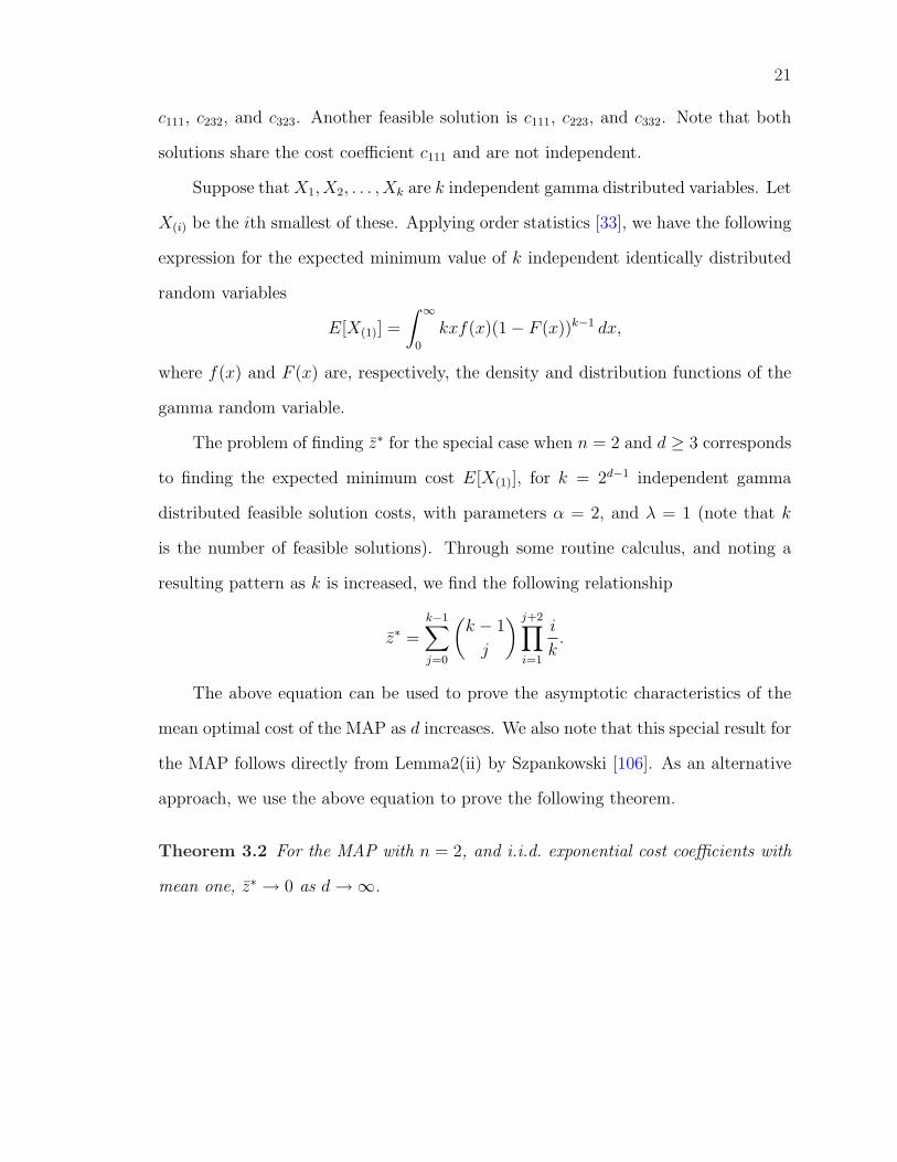
Suppose that X1, X2, . . . , Xk are k independent gamma distributed variables. Let
X(i) be the ith smallest of these. Applying order statistics [33], we have the following
expression for the expected minimum value of k independent identically distributed
random variables
E[X(1)] =
∫ ∞
0
kxf(x)(1− F (x))k−1 dx,
where f(x) and F (x) are, respectively, the density and distribution functions of the
gamma random variable.
The problem of finding z∗ for the special case when n = 2 and d ≥ 3 corresponds
to finding the expected minimum cost E[X(1)], for k = 2d−1 independent gamma
distributed feasible solution costs, with parameters α = 2, and λ = 1 (note that k
is the number of feasible solutions). Through some routine calculus, and noting a
resulting pattern as k is increased, we find the following relationship
z∗ =k−1∑j=0
(k − 1
j
) j+2∏i=1
i
k.
The above equation can be used to prove the asymptotic characteristics of the
mean optimal cost of the MAP as d increases. We also note that this special result for
the MAP follows directly from Lemma2(ii) by Szpankowski [106]. As an alternative
approach, we use the above equation to prove the following theorem.
Theorem 3.2 For the MAP with n = 2, and i.i.d. exponential cost coefficients with
mean one, z∗ → 0 as d →∞.
22
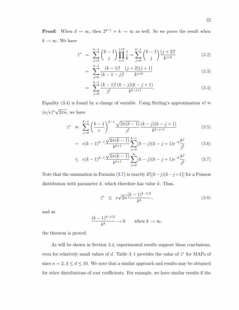
Proof: When d → ∞, then 2d−1 = k → ∞ as well. So we prove the result when
k →∞. We have
z∗ =k−1∑j=0
(k − 1
j
) j+2∏i=1
i
k=
k−1∑j=0
(k − 1
j
)(j + 2)!
kj+2(3.2)
=k−1∑j=0
(k − 1)!
(k − 1− j)!
(j + 2)(j + 1)
kj+2(3.3)
=k−1∑j=0
(k − 1)!
j!
(k − j)(k − j + 1)
kk−j+1. (3.4)
Equality (3.4) is found by a change of variable. Using Stirling’s approximation n! ≈(n/e)n
√2πn, we have
z∗ ≈k−1∑j=0
(k − 1
e
)k−1√
2π(k − 1)
j!
(k − j)(k − j + 1)
kk−j+1(3.5)
= e(k − 1)k−1
√2π(k − 1)
kk+1
k−1∑j=0
(k − j)(k − j + 1)e−k kj
j!(3.6)
≤ e(k − 1)k−1
√2π(k − 1)
kk+1
∞∑j=0
(k − j)(k − j + 1)e−k kj
j!. (3.7)
Note that the summation in Formula (3.7) is exactly E[(k−j)(k−j+1)] for a Poisson
distribution with parameter k, which therefore has value k. Thus,
z∗ ≤ e√
2π(k − 1)k−1/2
kk, (3.8)
and as
(k − 1)k−1/2
kk→ 0 when k →∞,
the theorem is proved.
As will be shown in Section 3.4, experimental results support these conclusions,
even for relatively small values of d. Table 3–1 provides the value of z∗ for MAPs of
sizes n = 2, 3 ≤ d ≤ 10. We note that a similar approach and results may be obtained
for other distributions of cost coefficients. For example, we have similar results if the
23
cost coefficients are independent gamma distributed random variables, since the sum
of gamma random variables is again a gamma random variable.
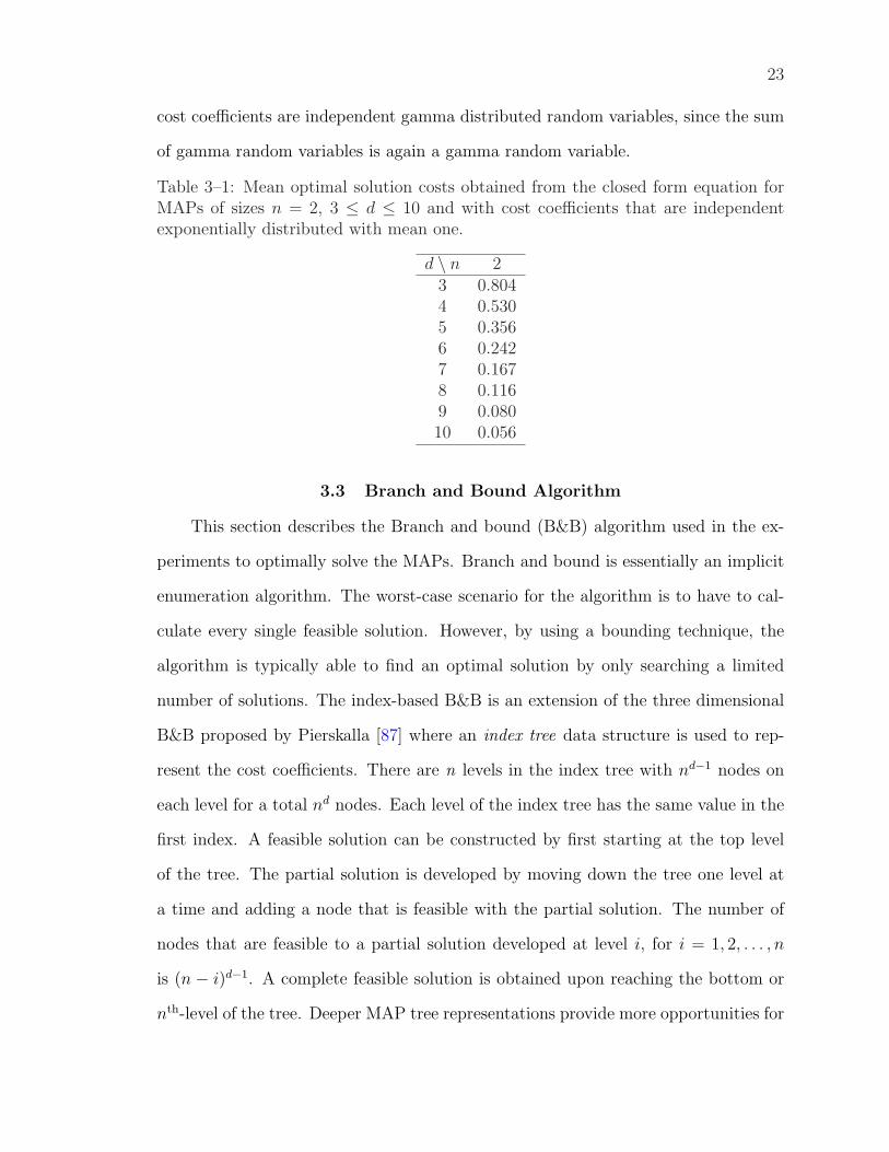
Table 3–1: Mean optimal solution costs obtained from the closed form equation forMAPs of sizes n = 2, 3 ≤ d ≤ 10 and with cost coefficients that are independentexponentially distributed with mean one.
d \ n 23 0.8044 0.5305 0.3566 0.2427 0.1678 0.1169 0.08010 0.056
3.3 Branch and Bound Algorithm
This section describes the Branch and bound (B&B) algorithm used in the ex-
periments to optimally solve the MAPs. Branch and bound is essentially an implicit
enumeration algorithm. The worst-case scenario for the algorithm is to have to cal-
culate every single feasible solution. However, by using a bounding technique, the
algorithm is typically able to find an optimal solution by only searching a limited
number of solutions. The index-based B&B is an extension of the three dimensional
B&B proposed by Pierskalla [87] where an index tree data structure is used to rep-
resent the cost coefficients. There are n levels in the index tree with nd−1 nodes on
each level for a total nd nodes. Each level of the index tree has the same value in the
first index. A feasible solution can be constructed by first starting at the top level
of the tree. The partial solution is developed by moving down the tree one level at
a time and adding a node that is feasible with the partial solution. The number of
nodes that are feasible to a partial solution developed at level i, for i = 1, 2, . . . , n
is (n − i)d−1. A complete feasible solution is obtained upon reaching the bottom or
nth-level of the tree. Deeper MAP tree representations provide more opportunities for
24
B&B algorithms to eliminate branches. Therefore, we would expect the index-based
B&B to be more effective for a larger number of elements in each dimension.
3.3.1 Procedure
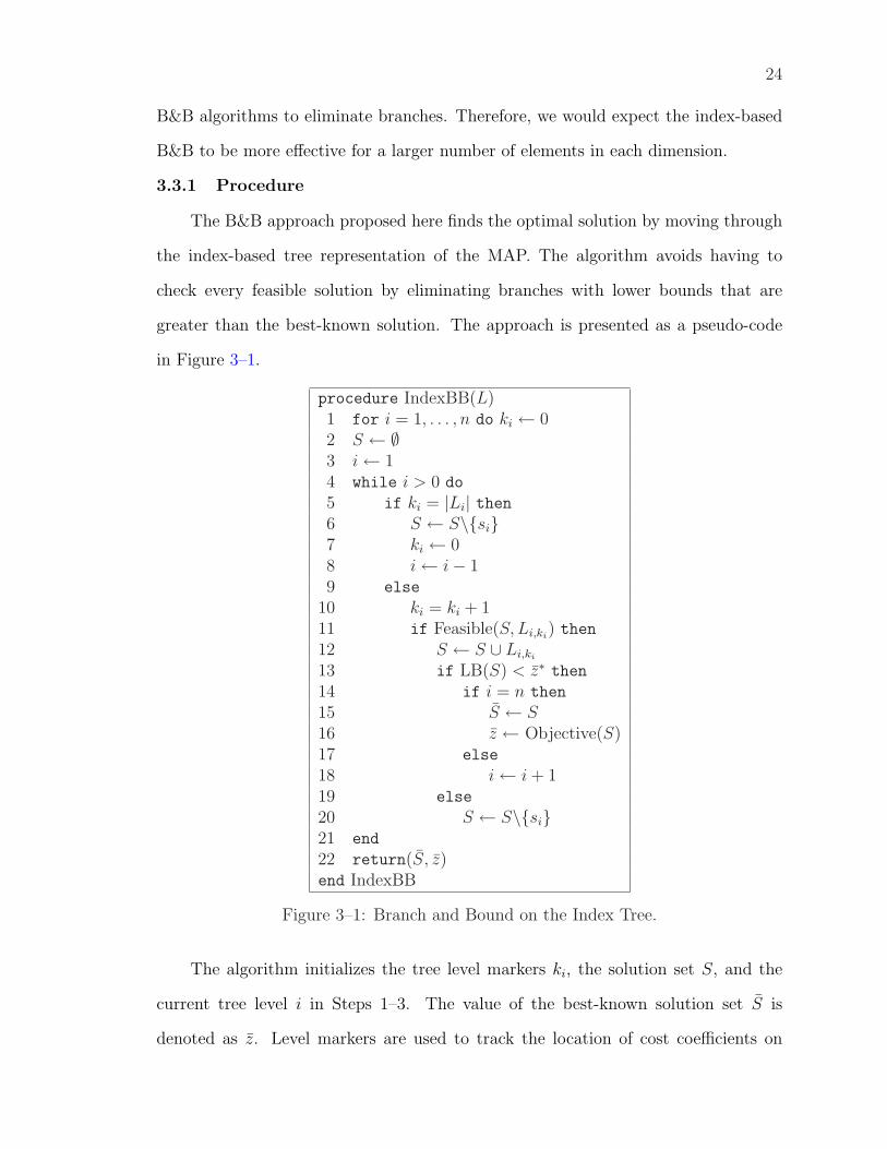
The B&B approach proposed here finds the optimal solution by moving through
the index-based tree representation of the MAP. The algorithm avoids having to
check every feasible solution by eliminating branches with lower bounds that are
greater than the best-known solution. The approach is presented as a pseudo-code
in Figure 3–1.
procedure IndexBB(L)1 for i = 1, . . . , n do ki ← 02 S ← ∅3 i ← 14 while i > 0 do
5 if ki = |Li| then6 S ← S\{si}7 ki ← 08 i ← i− 19 else
10 ki = ki + 111 if Feasible(S, Li,ki
) then12 S ← S ∪ Li,ki
13 if LB(S) < z∗ then14 if i = n then
15 S ← S16 z ← Objective(S)17 else
18 i ← i + 119 else
20 S ← S\{si}21 end
22 return(S, z)end IndexBB
Figure 3–1: Branch and Bound on the Index Tree.
The algorithm initializes the tree level markers ki, the solution set S, and the
current tree level i in Steps 1–3. The value of the best-known solution set S is
denoted as z. Level markers are used to track the location of cost coefficients on
25
the tree levels and Li is the set of coefficients at each level i. The solution set S
contains the cost coefficients taken from the different tree levels. Steps 4–21 perform
an implicit enumeration of every feasible path in the index-based tree. The procedure
investigates every possible path below a given node before moving on to the next node
in the same tree level. Once all the nodes in a given level are searched or eliminated
from consideration through the use of upper and lower bounds, the algorithm moves
up to the previous level and moves to the next node in the new level. Step 11 checks
if a given cost coefficient Li,ki, which is the ki-th node on level i, is feasible to the
partial solution set. If the cost coefficient is feasible and if its inclusion does not cause
the lower bound of the objective function to surpass the best-known solution, then
the coefficient is kept in the solution set. Otherwise, it is removed from S in Step 20.
A lower bound that may be implemented to try to remove some of the tree
branches is given by:
LB(S) =r∑
i=1
Si +n∑
i=r+1
min∀jm
ci,j2,...,jd,
where r = |S| is the size of the partial solution and Si is the cost coefficient selected
from level i of the index-based MAP representation. This expression finds a lower
bound by summing the values of all the cost coefficients that are already in the partial
solution and the minimum cost coefficient at each of the tree levels underneath the
last level searched. The lower bound consists of n elements, one from each level. If
a cost coefficient from a given level is in the partial solution, then that coefficient is
used in the calculation of the lower bound. If none of the coefficients from a given
level is found in the partial solution, then the smallest coefficient from that level is
used.
Before starting the algorithm, an initial feasible solution is needed for an upper
bound. A natural selection would be
S = { ci,j2,j3,...,jd| i = jm for m = 2, 3, . . . , d; i = 1, 2, . . . , n} .
26
The algorithm initially partitions the cost array into n groups or tree levels with
respect to the value of their first index. The first coefficient to be analyzed is the
node furthest to the left at level i = 1. If the lower bound of the partial solution
that includes that node is lower than the initial solution, the partial solution is kept.
It then moves to the next level with i = 2 and again analyzes the node furthest
to the left. The algorithm keeps moving down the tree until it either reaches the
bottom or finds a node that results in a partial solution having a lower bound value
higher than the initial solution. If it does reach the bottom, a feasible solution has
been found. If the new solution has a lower objective value than the initial solution,
the latest solution is kept as the current best-known solution. On the other hand
if the algorithm does encounter a node which has a lower bound greater than the
best-known solution, then that node and all the nodes underneath it are eliminated
from the search. The algorithm then analyzes the next node to the right of the node
that did not meet the lower bound criteria. Once all nodes at a given level have been
analyzed, the algorithm moves up to the previous level and begins searching on the
next node to the right of the last node analyzed on that level.
We discuss different modifications that may be implemented on the original B&B
algorithm to help increase the rate of convergence. The B&B algorithm’s performance
is directly related to the tightness of the upper and lower bounds. The rest of this
section addresses the problem of obtaining a tighter upper bound. The objective is to
obtain a good solution as early as possible. By having a low upper bound early in the
procedure, we are able to eliminate more branches and guarantee an optimal solution
in a shorter amount of time. The modifications that we introduce are sorting the
nodes in all the tree levels and performing a local search algorithm that guarantees
local optimality.
27
3.3.2 Sorting
There are two ways to sort the index-based tree. The first is to sort every
level of the tree once before the branch and bound algorithm begins. By using this
implementation, the sorting complexity is minimized. However, the drawback is that
infeasible cost coefficients are mixed in with the feasible ones. The algorithm would
have to perform a large number of feasibility checks whenever a new coefficient is
needed from each level.
The second way to sort the tree is to perform a sort procedure every time a cost
coefficient is chosen. At a given tree level, a set of coefficients that are still feasible
to the partial solution is created and sorted. Finding coefficients that are feasible is
computationally much less demanding than checking if a particular coefficient is still
feasible. The drawback with the second method is the high number of sorting proce-
dures that need to be performed. For our test problems, we have chosen to implement
the first approach, which is to perform a single initial sorting of the coefficients for
each tree level. This choice was made because the first method performed best in
practice for the instances we tested.
3.3.3 Local Search
The local search procedure improves upon the best-known solution by searching
within a predefined neighborhood of the current solution to see if a better solution
can be found. If an improvement is found, this solution is then stored as the current
solution and a new neighborhood is searched. When no better solution can be found,
the search is terminated and a local minimum is returned.
Because an optimal solution in one neighborhood definition is not usually op-
timal in other neighborhoods, we implement a variable neighborhood approach. A
description of this metaheuristic and its applications to different combinatorial opti-
mization problems is given by Hansen and Mladenovic [47]. Variable neighborhood
works by exploring multiple neighborhoods one at a time. For our branch and bound
28
algorithm, we implement the intrapermutation 2- and n-exchanges and the interper-
mutation 2-exchange presented by Pasiliao [84]. Starting from an initial solution, we
define and search the first neighborhood to find a local minimum. From that local
minimum, we redefine and search a new neighborhood to find an even better solution.
The metaheuristic continues until all neighborhoods have been explored.
3.4 Computational Experiments
In this section, the computational experiments performed are explained. In the
first subsection, we describe the experimental procedures employed. Then, in latter
subsections, the results from the experiments are presented and discussed. The results
include mean optimal costs and their standard deviation, for each type of problem
and size. In the last subsection we present some interesting results, based on curve
fitting models.
3.4.1 Experimental Procedures
The experimental procedures involved creating and exactly solving MAPs using
the B&B algorithm described in the preceding section. There were at least 15 runs
for each experiment where the number of runs was selected based on the practical
amount of time to complete the experiment. Generally, as the size of the problem
increased, the number of runs in the experiment had to be decreased. Also, as the
dimension, d, of the MAP increased, the maximum number elements, n, decreased.
Tables 3–2 and 3–3 provide a summary of the size of each experiment for the various
types of problems.
The time taken by an experiment ranged from as low as a few seconds to as high
as 20 hours on a 2.2 GHz Pentium 4 processor. We observed that problem instances
with standard normal assignment costs took considerably longer time to solve; there-
fore, problem sizes and number of runs per experiment are smaller. The assignment
costs ci1···id for each problem instance were drawn from one of three distributions. The
29
Table 3–2: Number of runs for each experiment with uniform or exponential assign-ment costs.
n \ d 3 4 5 6 7 8 9 102 1000 1000 1000 1000 1000 1000 1000 5003 1000 1000 1000 1000 1000 1000 1000 1004 1000 1000 1000 1000 1000 500 500 505 1000 1000 1000 500 200 200 100 206 1000 1000 500 500 100 50 207 1000 1000 500 200 50 20 158 1000 1000 200 50 20 159 1000 1000 50 20 1510 1000 1000 20 1511 500 500 2012 500 500 2013 200 200 1514 100 5015 10016 5017 5018 3019 2020 15
first distribution of assignment costs used was the uniform U [0, 1]. The next distribu-
tion used was the exponential with mean one, being determined by ci1···id = − ln U .
Finally, the third distribution used was the standard normal, N(0, 1), with values
determined by the polar method [63] as follows:
1. Generate U1 and U2, for U1, U2 ∼ U [0, 1].
2. Let V1 = 2U1 − 1, V2 = 2U2 − 1, and W = V 21 + V 2
2 .
3. If W > 1, go back to 1, else ci1···id = V1
√−2 ln W
W.
3.4.2 Mean Optimal Solution Costs
A summary of results for MAPs is provided in Tables 3–4, 3–5, and 3–6. We
observe that in all cases the mean optimal cost gets smaller as the size of the MAP
increases. Figure 3–2 shows the plots for problems with dimension d = 3, d = 5,
d = 7 and d = 10, as examples for the exponential case (plots for the uniform case
are similar). We observe that plots for higher dimensional problems converge to zero
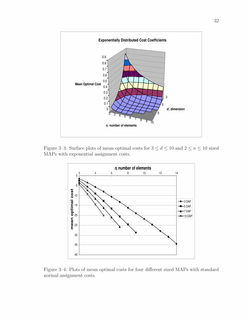
for smaller values of n. This is emphasized in the surface plot, Figure 3–3, of a subset
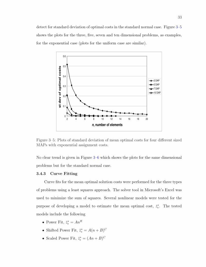
of the data. Figure 3–4 shows plots for problems with the same number of dimensions
30
Table 3–3: Number of runs for each experiment standard normal assignment costs.
n \ d 3 4 5 6 7 8 9 102 1000 1000 1000 1000 1000 1000 1000 5003 1000 1000 1000 1000 1000 1000 1000 5004 1000 1000 1000 1000 1000 500 50 155 1000 1000 1000 500 200 20 156 1000 1000 500 100 50 157 1000 1000 50 20 158 1000 1000 20 159 1000 100 1510 1000 2011 500 1512 5013 1514 15
as the problems in Figure 3–2, but for the standard normal case. Different from the
uniform and exponential cases, the mean optimal solution costs appear to approach
−∞ with increasing n.
0
0.1
0.2
0.3
0.4
0.5
0.6
0.7
0.8
0.9
2 7 12 17 22
3 DAP
5 DAP
7 DAP
10 DAP
n, number of elements
me
an
op
tim
al
co
st
Figure 3–2: Plots of mean optimal costs for four different sized MAPs with exponen-tial assignment costs.
We observe that in the uniform and exponential cases the standard deviation of
optimal costs converges to zero as the size of the MAP gets larger. Clearly, this just
confirms the asymptotic characteristic of the results. However, a trend is difficult to
31
Table 3–4: Mean optimal costs for different sizes of MAPs with independent assign-ment costs that are uniform in [0, 1].
n\d 3 4 5 6 n\d 7 82 0.584509 0.41955 0.308078 0.21852 2 0.15998 0.1124583 0.54078 0.295578 0.155189 0.0853185 3 0.0455428 0.0248624 0.480825 0.209272 0.0884739 0.0386061 4 0.0171049 0.00755085 0.41716 0.151543 0.0549055 0.019867 5 0.00736 0.0025966 0.374046 0.114551 0.0357428 0.011516 6 0.003542 0.000947 0.334805 0.0897928 0.02465 0.0067875 7 0.001724 0.00028 0.30329 0.0724017 0.0175195 0.004348 8 0.000815 09 0.277139 0.0587219 0.012982 0.00253 9 0.000273310 0.252156 0.0486118 0.00961 0.00168 1011 0.237884 0.0419366 0.00762 n\d 9 1012 0.216287 0.035617 0.006025 2 0.0792026 0.054352613 0.205552 0.0310225 3 0.0134717 0.00749214 0.185769 0.02696 4 0.0032106 0.00123215 0.180002 5 0.00082 0.0001316 0.16832 6 0.000117 0.162104 7 018 0.14787 819 0.14583 920 0.129913 10
Table 3–5: Mean optimal costs for different sizes of MAPs with independent assign-ment costs that are exponential with mean 1.
n\d 3 4 5 6 n\d 7 82 0.8046875 0.532907 0.353981 0.241978 2 0.167296 0.1102793 0.63959 0.319188 0.165122 0.0829287 3 0.046346 0.02518844 0.531126 0.212984 0.0903552 0.0391171 4 0.0170434 0.00771265 0.454308 0.155833 0.0548337 0.020256 5 0.007272 0.00269456 0.396976 0.116469 0.0355034 0.0116512 6 0.003491 0.0009447 0.349543 0.0909123 0.0251856 0.0068995 7 0.001482 0.0003258 0.310489 0.0723551 0.0175745 0.0044 8 0.00066 0.0000139 0.28393 0.0595148 0.01233 0.002665 9 0.000166710 0.263487 0.0493535 0.009165 0.0019 1011 0.238954 0.041809 0.007305 n\d 9 1012 0.218666 0.0354624 0.005385 2 0.0789626 0.056292613 0.203397 0.030967 0.0044667 3 0.0132625 0.00739414 0.193867 0.0279 4 0.0031852 0.00124815 0.181644 5 0.000723 0.000116 0.172359 6 0.0000317 0.161126 7 018 0.15081 819 0.144787 920 0.134107 10
Table 3–6: Mean optimal costs for different sizes of MAPs with independent assign-ment costs that are standard normal.
n\d 3 4 5 6 n\d 7 82 -1.52566 -2.04115 -2.46001 -2.91444 2 -3.29715 -3.680933 -3.41537 -4.59134 -5.57906 -6.44952 3 -7.22834 -7.915874 -5.6486 -7.52175 -9.05299 -10.3701 4 -11.5257 -12.59165 -8.00522 -10.6145 -12.6924 -14.5221 5 -16.128 -17.46766 -10.6307 -13.9336 -16.5947 -18.7402 6 -20.9121 -22.71787 -13.2918 -17.2931 -20.6462 -23.4246 7 -25.82418 -16.1144 -20.8944 -24.7095 -28.1166 n\d 9 109 -18.9297 -24.5215 -28.7188 2 -4.04084 -4.2947710 -21.7916 -28.6479 3 -8.57385 -9.1470711 -24.7175 -31.9681 4 -13.5045 -14.432812 -27.9675 5 -18.887313 -30.9362 614 -34.4204 7
32
3
6
92 3 4 5 6 78 9
10
0
0.1
0.2
0.3
0.4
0.5
0.6
0.7
0.8
0.9
Mean Optimal Cost
d , dimension
n, number of elements
Exponentially Distributed Cost Coefficients
Figure 3–3: Surface plots of mean optimal costs for 3 ≤ d ≤ 10 and 2 ≤ n ≤ 10 sizedMAPs with exponential assignment costs.
-40
-35
-30
-25
-20
-15
-10
-5
02 4 6 8 10 12 14
n, number of elements
mean
op
tim
al co
st
3 DAP
5 DAP
7 DAP
10 DAP
Figure 3–4: Plots of mean optimal costs for four different sized MAPs with standardnormal assignment costs.
33
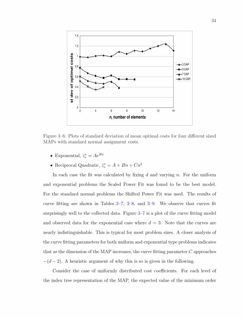
detect for standard deviation of optimal costs in the standard normal case. Figure 3–5
shows the plots for the three, five, seven and ten dimensional problems, as examples,
for the exponential case (plots for the uniform case are similar).
0
0.1
0.2
0.3
0.4
0.5
0.6
2 4 6 8 10 12 14 16 18 20
n, number of elements
st
dev o
f o
pti
mal co
sts
3 DAP
5 DAP
7 DAP
10 DAP
Figure 3–5: Plots of standard deviation of mean optimal costs for four different sizedMAPs with exponential assignment costs.
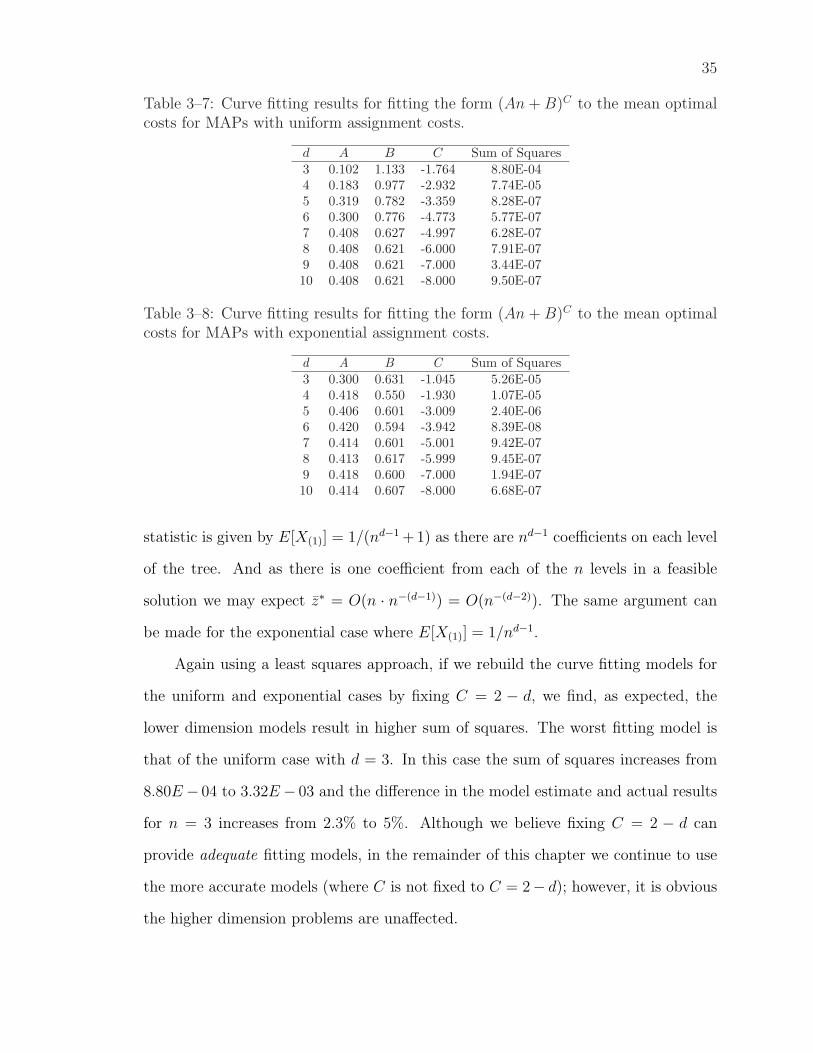
No clear trend is given in Figure 3–6 which shows the plots for the same dimensional
problems but for the standard normal case.
3.4.3 Curve Fitting
Curve fits for the mean optimal solution costs were performed for the three types
of problems using a least squares approach. The solver tool in Microsoft’s Excel was
used to minimize the sum of squares. Several nonlinear models were tested for the
purpose of developing a model to estimate the mean optimal cost, z∗e . The tested
models include the following
• Power Fit, z∗e = AnB
• Shifted Power Fit, z∗e = A(n + B)C
• Scaled Power Fit, z∗e = (An + B)C
34
0
0.2
0.4
0.6
0.8
1
1.2
1.4
2 4 6 8 10 12 14
n, number of elements
st
dev o
f o
pti
mal co
sts
3 DAP
5 DAP
7 DAP
10 DAP
Figure 3–6: Plots of standard deviation of mean optimal costs for four different sizedMAPs with standard normal assignment costs.
• Exponential, z∗e = AeBn
• Reciprocal Quadratic, z∗e = A + Bn + Cn2
In each case the fit was calculated by fixing d and varying n. For the uniform
and exponential problems the Scaled Power Fit was found to be the best model.
For the standard normal problems the Shifted Power Fit was used. The results of
curve fitting are shown in Tables 3–7, 3–8, and 3–9. We observe that curves fit
surprisingly well to the collected data. Figure 3–7 is a plot of the curve fitting model
and observed data for the exponential case where d = 3. Note that the curves are
nearly indistinguishable. This is typical for most problem sizes. A closer analysis of
the curve fitting parameters for both uniform and exponential type problems indicates
that as the dimension of the MAP increases, the curve fitting parameter C approaches
−(d− 2). A heuristic argument of why this is so is given in the following.
Consider the case of uniformly distributed cost coefficients. For each level of
the index tree representation of the MAP, the expected value of the minimum order
35
Table 3–7: Curve fitting results for fitting the form (An + B)C to the mean optimalcosts for MAPs with uniform assignment costs.
d A B C Sum of Squares3 0.102 1.133 -1.764 8.80E-044 0.183 0.977 -2.932 7.74E-055 0.319 0.782 -3.359 8.28E-076 0.300 0.776 -4.773 5.77E-077 0.408 0.627 -4.997 6.28E-078 0.408 0.621 -6.000 7.91E-079 0.408 0.621 -7.000 3.44E-0710 0.408 0.621 -8.000 9.50E-07
Table 3–8: Curve fitting results for fitting the form (An + B)C to the mean optimalcosts for MAPs with exponential assignment costs.
d A B C Sum of Squares3 0.300 0.631 -1.045 5.26E-054 0.418 0.550 -1.930 1.07E-055 0.406 0.601 -3.009 2.40E-066 0.420 0.594 -3.942 8.39E-087 0.414 0.601 -5.001 9.42E-078 0.413 0.617 -5.999 9.45E-079 0.418 0.600 -7.000 1.94E-0710 0.414 0.607 -8.000 6.68E-07
statistic is given by E[X(1)] = 1/(nd−1 +1) as there are nd−1 coefficients on each level
of the tree. And as there is one coefficient from each of the n levels in a feasible
solution we may expect z∗ = O(n · n−(d−1)) = O(n−(d−2)). The same argument can
be made for the exponential case where E[X(1)] = 1/nd−1.
Again using a least squares approach, if we rebuild the curve fitting models for
the uniform and exponential cases by fixing C = 2 − d, we find, as expected, the
lower dimension models result in higher sum of squares. The worst fitting model is
that of the uniform case with d = 3. In this case the sum of squares increases from
8.80E − 04 to 3.32E − 03 and the difference in the model estimate and actual results
for n = 3 increases from 2.3% to 5%. Although we believe fixing C = 2 − d can
provide adequate fitting models, in the remainder of this chapter we continue to use
the more accurate models (where C is not fixed to C = 2− d); however, it is obvious
the higher dimension problems are unaffected.
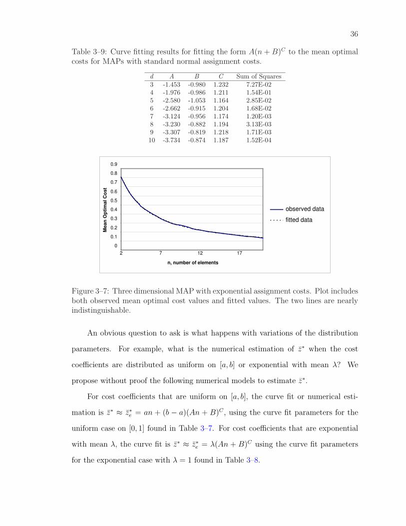
36
Table 3–9: Curve fitting results for fitting the form A(n + B)C to the mean optimalcosts for MAPs with standard normal assignment costs.
d A B C Sum of Squares3 -1.453 -0.980 1.232 7.27E-024 -1.976 -0.986 1.211 1.54E-015 -2.580 -1.053 1.164 2.85E-026 -2.662 -0.915 1.204 1.68E-027 -3.124 -0.956 1.174 1.20E-038 -3.230 -0.882 1.194 3.13E-039 -3.307 -0.819 1.218 1.71E-0310 -3.734 -0.874 1.187 1.52E-04
0
0.1
0.2
0.3
0.4
0.5
0.6
0.7
0.8
0.9
2 7 12 17
n, number of elements
Me
an
Op
tim
al
Co
st
observed data
fitted data
Figure 3–7: Three dimensional MAP with exponential assignment costs. Plot includesboth observed mean optimal cost values and fitted values. The two lines are nearlyindistinguishable.
An obvious question to ask is what happens with variations of the distribution
parameters. For example, what is the numerical estimation of z∗ when the cost
coefficients are distributed as uniform on [a, b] or exponential with mean λ? We
propose without proof the following numerical models to estimate z∗.
For cost coefficients that are uniform on [a, b], the curve fit or numerical esti-
mation is z∗ ≈ z∗e = an + (b − a)(An + B)C , using the curve fit parameters for the
uniform case on [0, 1] found in Table 3–7. For cost coefficients that are exponential
with mean λ, the curve fit is z∗ ≈ z∗e = λ(An + B)C using the curve fit parameters
for the exponential case with λ = 1 found in Table 3–8.
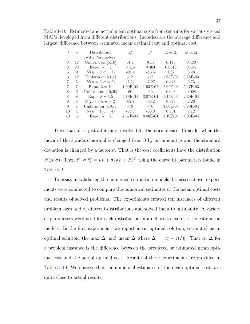
37
Table 3–10: Estimated and actual mean optimal costs from ten runs for variously sizedMAPs developed from different distributions. Included are the average difference andlargest difference between estimated mean optimal cost and optimal cost.
d n Distribution z∗e z∗ Ave ∆ Max ∆with Parameters
3 12 Uniform on [5,10] 61.1 61.1 0.143 0.4283 20 Expo, λ = 3 0.415 0.404 0.0618 0.1545 9 N(µ = 0, σ = 3) -86.4 -86.5 1.62 3.485 12 Uniform on [-1,1] -12 -12 1.65E-03 3.16E-037 5 N(µ = 5, σ = 2) -7.24 -7.27 0.448 0.737 7 Expo, λ = 10 1.90E-02 1.95E-02 2.62E-03 5.47E-038 6 Uniform on [10,20] 60 60 0.003 0.0088 8 Expo, λ = 1.5 4.13E-04 3.07E-04 1.15E-04 2.30E-049 5 N(µ = −5, σ = 2) -62.8 -63.2 0.944 2.269 7 Uniform on [-10,-5] -70 -70 3.60E-04 6.70E-0410 4 N(µ = 1, σ = 4) -53.8 -53.3 0.831 2.1210 5 Expo, λ = 2 7.57E-04 8.00E-04 1.10E-04 4.03E-04
The situation is just a bit more involved for the normal case. Consider when the
mean of the standard normal is changed from 0 by an amount µ and the standard
deviation is changed by a factor σ. That is the cost coefficients have the distribution
N(µ, σ). Then z∗ ≈ z∗e = nµ + σA(n + B)C using the curve fit parameters found in
Table 3–9.
To assist in validating the numerical estimation models discussed above, experi-
ments were conducted to compare the numerical estimates of the mean optimal costs
and results of solved problems. The experiments created ten instances of different
problem sizes and of different distributions and solved them to optimality. A variety
of parameters were used for each distribution in an effort to exercise the estimation
models. In the first experiment, we report mean optimal solution, estimated mean
optimal solution, the max ∆, and mean ∆ where ∆ = |z∗e − z(I)|. That is, ∆ for
a problem instance is the difference between the predicted or estimated mean opti-
mal cost and the actual optimal cost. Results of these experiments are provided in
Table 3–10. We observe that the numerical estimates of the mean optimal costs are
quite close to actual results.
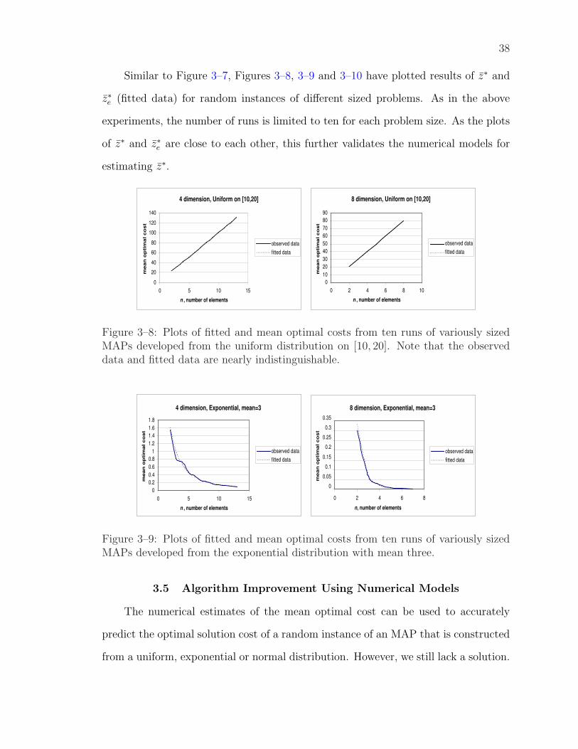
38
Similar to Figure 3–7, Figures 3–8, 3–9 and 3–10 have plotted results of z∗ and
z∗e (fitted data) for random instances of different sized problems. As in the above
experiments, the number of runs is limited to ten for each problem size. As the plots
of z∗ and z∗e are close to each other, this further validates the numerical models for
estimating z∗.
4 dimension, Uniform on [10,20]
0
20
40
60
80
100
120
140
0 5 10 15
n , number of elements
mean
op
tim
al co
st
observed data
fitted data
8 dimension, Uniform on [10,20]
0
10
20
30
40
50
60
70
80
90
0 2 4 6 8 10
n , number of elements
mean
op
tim
al co
st
observed data
fitted data
Figure 3–8: Plots of fitted and mean optimal costs from ten runs of variously sizedMAPs developed from the uniform distribution on [10, 20]. Note that the observeddata and fitted data are nearly indistinguishable.
4 dimension, Exponential, mean=3
0
0.2
0.4
0.6
0.8
1
1.2
1.4
1.6
1.8
0 5 10 15
n , number of elements
mean
op
tim
al co
st
observed data
fitted data
8 dimension, Exponential, mean=3
0
0.05
0.1
0.15
0.2
0.25
0.3
0.35
0 2 4 6 8
n, number of elements
me
an
op
tim
al
co
st
observed data
fitted data
Figure 3–9: Plots of fitted and mean optimal costs from ten runs of variously sizedMAPs developed from the exponential distribution with mean three.
3.5 Algorithm Improvement Using Numerical Models
The numerical estimates of the mean optimal cost can be used to accurately
predict the optimal solution cost of a random instance of an MAP that is constructed
from a uniform, exponential or normal distribution. However, we still lack a solution.
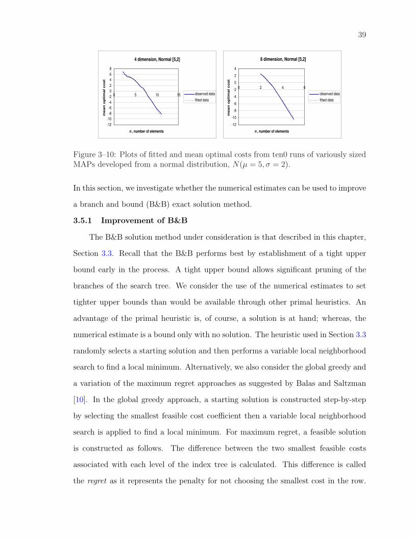
39
4 dimension, Normal [5,2]
-12
-10
-8
-6
-4
-2
0
2
4
6
8
0 5 10 15
n , number of elements
mean
op
tim
al co
st
observed data
fitted data
8 dimension, Normal [5,2]
-12
-10
-8
-6
-4
-2
0
2
4
0 2 4 6
n , number of elements
mean
op
tim
al co
st
observed data
fitted data
Figure 3–10: Plots of fitted and mean optimal costs from ten0 runs of variously sizedMAPs developed from a normal distribution, N(µ = 5, σ = 2).
In this section, we investigate whether the numerical estimates can be used to improve
a branch and bound (B&B) exact solution method.
3.5.1 Improvement of B&B
The B&B solution method under consideration is that described in this chapter,
Section 3.3. Recall that the B&B performs best by establishment of a tight upper
bound early in the process. A tight upper bound allows significant pruning of the
branches of the search tree. We consider the use of the numerical estimates to set
tighter upper bounds than would be available through other primal heuristics. An
advantage of the primal heuristic is, of course, a solution is at hand; whereas, the
numerical estimate is a bound only with no solution. The heuristic used in Section 3.3
randomly selects a starting solution and then performs a variable local neighborhood
search to find a local minimum. Alternatively, we also consider the global greedy and
a variation of the maximum regret approaches as suggested by Balas and Saltzman
[10]. In the global greedy approach, a starting solution is constructed step-by-step
by selecting the smallest feasible cost coefficient then a variable local neighborhood
search is applied to find a local minimum. For maximum regret, a feasible solution
is constructed as follows. The difference between the two smallest feasible costs
associated with each level of the index tree is calculated. This difference is called
the regret as it represents the penalty for not choosing the smallest cost in the row.
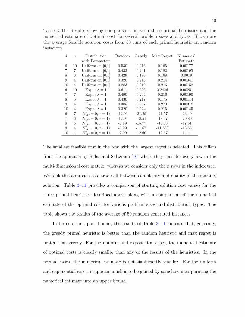
40
Table 3–11: Results showing comparisons between three primal heuristics and thenumerical estimate of optimal cost for several problem sizes and types. Shown arethe average feasible solution costs from 50 runs of each primal heuristic on randominstances.
d n Distribution Random Greedy Max Regret Numericalwith Parameters Estimate
6 10 Uniform on [0,1] 0.530 0.216 0.165 0.001777 7 Uniform on [0,1] 0.433 0.201 0.182 0.001958 6 Uniform on [0,1] 0.429 0.186 0.168 0.00199 4 Uniform on [0,1] 0.320 0.218 0.214 0.0034110 4 Uniform on [0,1] 0.283 0.219 0.216 0.001526 10 Expo, λ = 1 0.611 0.226 0.2426 0.002517 7 Expo, λ = 1 0.490 0.244 0.216 0.001908 6 Expo, λ = 1 0.430 0.217 0.175 0.001149 4 Expo, λ = 1 0.385 0.267 0.270 0.0031810 4 Expo, λ = 1 0.320 0.224 0.215 0.001456 7 N(µ = 0, σ = 1) -12.91 -21.29 -21.57 -23.407 6 N(µ = 0, σ = 1) -12.91 -18.51 -18.97 -20.898 5 N(µ = 0, σ = 1) -8.99 -15.77 -16.08 -17.519 4 N(µ = 0, σ = 1) -6.99 -11.67 -11.883 -13.5310 4 N(µ = 0, σ = 1) -7.00 -12.60 -12.67 -14.44
The smallest feasible cost in the row with the largest regret is selected. This differs
from the approach by Balas and Saltzman [10] where they consider every row in the
multi-dimensional cost matrix, whereas we consider only the n rows in the index tree.
We took this approach as a trade-off between complexity and quality of the starting
solution. Table 3–11 provides a comparison of starting solution cost values for the
three primal heuristics described above along with a comparison of the numerical
estimate of the optimal cost for various problem sizes and distribution types. The
table shows the results of the average of 50 random generated instances.
In terms of an upper bound, the results of Table 3–11 indicate that, generally,
the greedy primal heuristic is better than the random heuristic and max regret is
better than greedy. For the uniform and exponential cases, the numerical estimate
of optimal costs is clearly smaller than any of the results of the heuristics. In the
normal cases, the numerical estimate is not significantly smaller. For the uniform
and exponential cases, it appears much is to be gained by somehow incorporating the
numerical estimate into an upper bound.
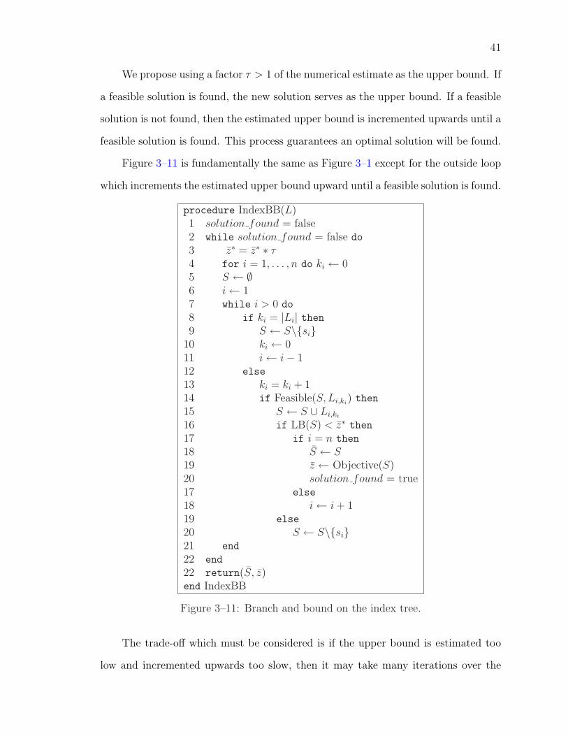
41
We propose using a factor τ > 1 of the numerical estimate as the upper bound. If
a feasible solution is found, the new solution serves as the upper bound. If a feasible
solution is not found, then the estimated upper bound is incremented upwards until a
feasible solution is found. This process guarantees an optimal solution will be found.
Figure 3–11 is fundamentally the same as Figure 3–1 except for the outside loop
which increments the estimated upper bound upward until a feasible solution is found.
procedure IndexBB(L)1 solution found = false2 while solution found = false do
3 z∗ = z∗ ∗ τ4 for i = 1, . . . , n do ki ← 05 S ← ∅6 i ← 17 while i > 0 do
8 if ki = |Li| then9 S ← S\{si}
10 ki ← 011 i ← i− 112 else
13 ki = ki + 114 if Feasible(S, Li,ki
) then15 S ← S ∪ Li,ki
16 if LB(S) < z∗ then17 if i = n then
18 S ← S19 z ← Objective(S)20 solution found = true17 else
18 i ← i + 119 else
20 S ← S\{si}21 end
22 end
22 return(S, z)end IndexBB
Figure 3–11: Branch and bound on the index tree.
The trade-off which must be considered is if the upper bound is estimated too
low and incremented upwards too slow, then it may take many iterations over the
42
index tree before a feasible solution is found. However, no benefit is gained by setting
the upper bound too high. We found through less-than-rigorous analysis that τ set to
a value such that the upper bound is incremented upward by one standard deviation
of the optimal cost (see Figures 3–5 and 3–6) is a nice compromise.
3.5.2 Comparison of B&B Implementations
Table 3–12 compares the performance of the B&B algorithm using the random
primal heuristic for a starting upper bound versus using the maximum regret heuris-
tic versus using a numerical estimate for the upper bound. The table shows the
average times to solution of five runs on random instances of various problem sizes
and distribution types. In the uniform and exponential cases, we observe that B&B
using maximum regret generally does slightly better than using a random starting
solution. We also observe the approach of using a numerically estimated upper bound
significantly outperforms the other approaches in solving problems with uniformly or
exponentially distributed costs. However, there is no clear difference between the
approaches when solving problems with normally distributed costs. This is explained
by the small differences in the starting upper bounds for each approach.
3.6 Remarks
In this chapter we presented experimental results for the asymptotic value of the
optimal solution for random instances of the MAP. The results lead to the following
conjectures which will be addressed in detail in Chapter 4.
Conjecture 3.3 Given a d-dimensional MAP with n elements in each dimension,
if the nd cost coefficients are independent exponentially distributed random variables
with mean 1 or independent uniformly distributed random variables in [0,1], z∗ → 0
as n →∞ or d →∞.
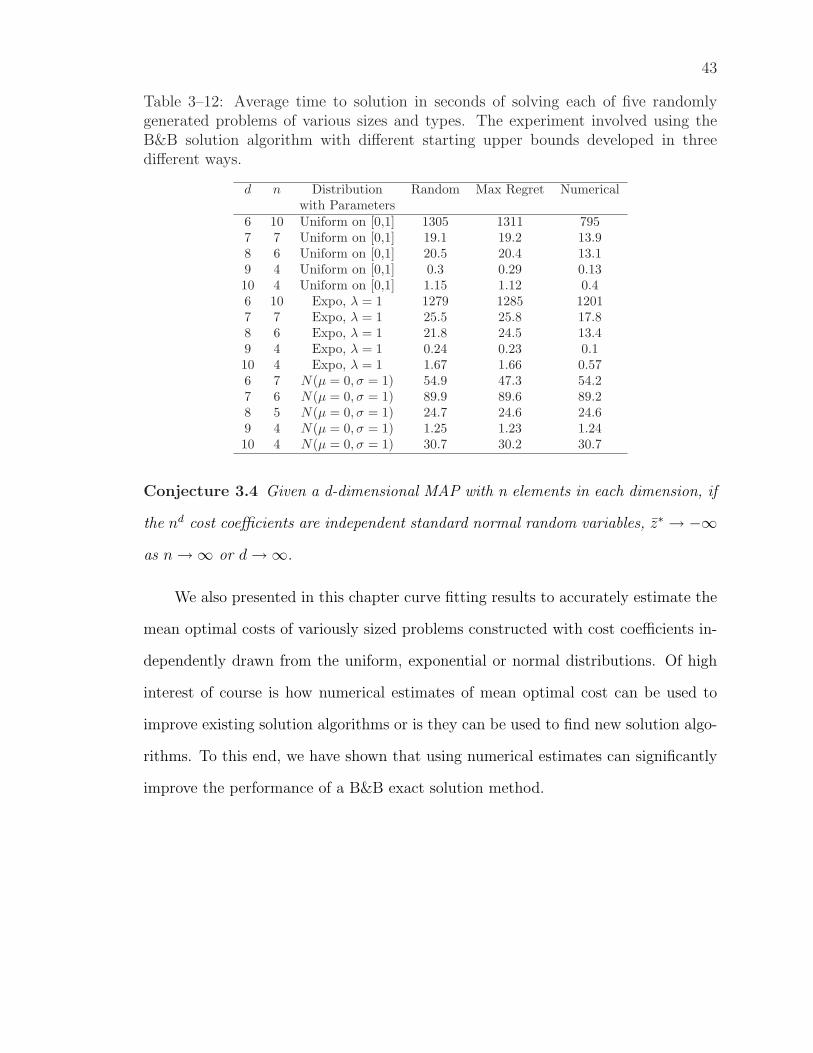
43
Table 3–12: Average time to solution in seconds of solving each of five randomlygenerated problems of various sizes and types. The experiment involved using theB&B solution algorithm with different starting upper bounds developed in threedifferent ways.
d n Distribution Random Max Regret Numericalwith Parameters
6 10 Uniform on [0,1] 1305 1311 7957 7 Uniform on [0,1] 19.1 19.2 13.98 6 Uniform on [0,1] 20.5 20.4 13.19 4 Uniform on [0,1] 0.3 0.29 0.1310 4 Uniform on [0,1] 1.15 1.12 0.46 10 Expo, λ = 1 1279 1285 12017 7 Expo, λ = 1 25.5 25.8 17.88 6 Expo, λ = 1 21.8 24.5 13.49 4 Expo, λ = 1 0.24 0.23 0.110 4 Expo, λ = 1 1.67 1.66 0.576 7 N(µ = 0, σ = 1) 54.9 47.3 54.27 6 N(µ = 0, σ = 1) 89.9 89.6 89.28 5 N(µ = 0, σ = 1) 24.7 24.6 24.69 4 N(µ = 0, σ = 1) 1.25 1.23 1.2410 4 N(µ = 0, σ = 1) 30.7 30.2 30.7
Conjecture 3.4 Given a d-dimensional MAP with n elements in each dimension, if
the nd cost coefficients are independent standard normal random variables, z∗ → −∞as n →∞ or d →∞.
We also presented in this chapter curve fitting results to accurately estimate the
mean optimal costs of variously sized problems constructed with cost coefficients in-
dependently drawn from the uniform, exponential or normal distributions. Of high
interest of course is how numerical estimates of mean optimal cost can be used to
improve existing solution algorithms or is they can be used to find new solution algo-
rithms. To this end, we have shown that using numerical estimates can significantly
improve the performance of a B&B exact solution method.
CHAPTER 4PROOFS OF ASYMPTOTIC CHARACTERISTICS OF THE MAP
4.1 Introduction
The experimental work detailed in Chapter 3 leads to conjectures concerning the
asymptotic characteristics of the mean optimal costs of randomly generated instances
of the MAP where costs are assigned independently to assignments. In this chapter,
we provide proofs of more generalized instances of Conjecture 3.3 and prove Conjec-
ture 3.4. The proofs are based on building an index tree [87] to represent the cost
coefficients of the MAP and then selecting a minimum subset of cost coefficients such
that at least one feasible solution can be expected from this subset. Then an upper
bound on the cost of this feasible solution is established and used to complete the
proofs. Throughout this chapter we consider MAPs with n elements in each of the d
dimensions.
Before presenting the theorems and their proofs concerning the asymptotic na-
ture of these problems, we first consider a naive approach [28] to establishing the
asymptotic characteristics based on some greedy algorithms.
4.2 Greedy Algorithms
Consider the case of the MAP where cost coefficients are independent exponen-
tially distributed random variables with mean 1. By Conjecture 3.3 the mean optimal
costs are thought to go to zero with increasing problem size. Suppose we consider
the solution from a greedy algorithm. As the solution serves as an upper bound to
the optimal solution, we can try to prove the conjecture if we can show the mean of
the sub-optimal solutions goes to zero with increasing problem size. However, as will
be shown this is difficult with two common greedy algorithms.
44
45
4.2.1 Greedy Algorithm 1
The first algorithm that we consider uses the index tree data structure proposed
by Pierskalla [87] to represent the cost coefficients of the MAP. There are n levels
in the index tree with nd−1 nodes on each level for a total nd nodes. Each level
of the index tree has the same value in the first index. A feasible solution can be
constructed by first starting at the top level of the tree. The partial solution is
developed by moving down the tree one level at a time and adding a node that is
feasible with the partial solution. The number of nodes at level i that are feasible to
a partial solution developed from levels 1, 2, . . . , i − 1 is (n − i + 1)d−1. A complete
feasible solution is obtained upon reaching the bottom or nth-level of the tree.
The proposed greedy algorithm is as follows:
Input MAP of dimension d and n elements in each dimension in the form of an index
tree.
Build a partial solution, Si, i = 1, by choosing the smallest cost coefficient from row
1 of the tree.
For i = 2, . . . , n, continue to construct a solution by choosing the smallest cost
coefficient in row i of the tree that is feasible with Si−1 constructed from rows 1, . . . , i−1.
We wish to calculate the expected solution cost from this algorithm for the
MAP constructed from i.i.d. exponential random variables with mean 1. Let the
mean solution cost resulting from the algorithm be represented by z∗u. Suppose that
X1, X2, . . . , Xk are k i.i.d. exponential random variables with mean 1. Let X(i) be the
ith smallest of these. Applying order statistics [33], we have the following expression
for the expected minimum value of k independent identically distributed random
variables: E[X(1)] = 1/k.
We may now construct a feasible solution using the above greedy algorithm. We
do so by recalling that the number of nodes that are feasible at level i+1 to a partial
46
solution developed down to level i, for i = 1, 2, . . . , n is (n − i)d−1. Considering this
and the fact that cost coefficients are independent, the expected solution cost of S1
is 1nd−1 , the expected solution cost of S2 is 1
nd−1 + 1(n−1)d−1 and so forth. Therefore, we
find
z∗ =n−1∑i=0
1
(n− i)d−1(4.1)
> 1, (4.2)
where equation (4.2) holds because the n-th term of equation (4.1) is one.
Since z∗ > 0, we conclude this greedy approach cannot be used to prove Conjec-
ture 3.3. However, maybe a more global approach will work.
4.2.2 Greedy Algorithm 2
The following algorithm is described by Balas and Saltzman [10] as the GREEDY
heuristic. The algorithm is as follows:
Input MAP of dimension d and n elements in each dimension as matrix A.
For i = 1, . . . , n, construct the partial solution Si by choosing the smallest element
in matrix A and then exclude the d rows covered by this element.
Using this covering approach, we see the number of nodes that are feasible to a
partial solution developed up to iteration i, for i = 1, 2, . . . , n is (n−i)d. For example,
all nd cost coefficients are considered in the first iteration. The next iteration has
(n − 1)d nodes for consideration. The expected solution cost of S1 is 1/nd. The
expected solution cost of S2 is 1/nd + 1/nd + 1/(n − 1)d. The extra 1/nd appears
in the expression because, in general, the expected minimum value of the uncovered
nodes is at least as much as the expected minimum value found in the previous
iteration. We could now develop the expression for z∗; however, we note that the
algorithm’s last iteration will consider only one cost coefficient. Therefore, again, we
have the result that z∗ > 1 when using this algorithm.
47
We conclude that these simple greedy approaches cannot be used to prove the
conjectures concerning the asymptotic characteristics of the MAP. In the next sec-
tions, we resort to a novel probabilistic approach.
4.3 Mean Optimal Costs of Exponentially and Uniformly DistributedRandom MAPs
To find the asymptotic cost when the costs are uniformly or exponentially dis-
tributed, we use an argument based on the probabilistic method [7]. Basically, we
show that, for a subset of the index tree, the expected value of the number of feasible
paths in this subset is at least one. Thus, such a set must contain a feasible path and
this fact can be used to give an upper bound on the cost of the optimum solution.
This is explained in the next proposition.
Proposition 4.1 Using an index tree to represent the cost coefficients of the MAP,
randomly select α different nodes from each level of the tree and combine these nodes
from each level into set A. A is expected to produce at least one feasible solution to
the MAP when
α =
⌈nd−1
(n!)d−1
n
⌉and |A| = nα. (4.3)
Proof: Consider there are nd−1 cost coefficients on each of the n levels of the index
tree representation of an MAP of dimension d and with n elements in each dimension.
Now consider there are (nd−1)n paths (not necessarily feasible to the MAP) in the
index tree from the top level to the bottom level. The number of feasible paths (or
feasible solutions to the MAP) in the index tree is (n!)d−1. Therefore, the proportion
% of feasible paths to all paths in the entire index tree is
% =(n!)d−1
(nd−1)n. (4.4)
Create a set A of nodes to represent a reduced index tree by selecting α nodes
randomly from each level of the overall index tree and placing them on a corresponding
48
level in the reduced index tree. The number of nodes in A is obviously nα. For this
reduced index tree of A, there are αn paths (not necessarily feasible to the MAP)
from the top level to the bottom level. Since the set of nodes in A were selected
randomly, we may now use % to determine the expected number of feasible paths in
A by simply multiplying % by the number of all paths in the reduced tree of A. That
is
E[number feasible paths in A] = %αn.
We wish to ensure that the expected number of feasible paths A is at least one. Thus,
over all possible choices of the n subsets of α elements, there must be one choice such
that there is one feasible path (in fact there may be many since the expected value
gives only the average over all possible solutions). Therefore,
%αn ≥ 1,
which results
α ≥(
1
%
) 1n
.
Incorporating the value of % from (4.4) we get
α ≥ nd−1
(n!)d−1
n
.
Therefore, since α must be an integer, we get (4.3).
We now take a moment to discuss the concept of order statistics. For more
complete information, refer to statistics books such as by David [33]. Suppose
that X1, X2, . . . , Xk are k independent identically distributed variables. Let X(i)
be the i-th smallest of these. Then X(i) is called the i-th order statistic for the set
{X1, X2, . . . , Xk}.
49
In the rest of the section, we will consider bounds for the value of the α-th order
statistic of i.i.d. variables drawn from a random distribution. This value will be used
to derive an upper bound on the cost of the optimal solution for random instances,
when n or d increases. Note that, in some places (e.g., Equation (4.6)), we assume
that α = nd−1/n!d−1
n . This is a good approximation in the following formulas because
(a) if n is fixed and d → ∞, then α → ∞, and therefore there is no difference
between α and nd−1/n!d−1
n ;
(b) if d is fixed and n →∞, then α → ed−1. This is not difficult to derive, since
n
n!1n
≈ n[(n
e)n(2πn)
12
] 1n
=e
(2πn)12n
.
But
(2πn)12n = (2πelog n)
12n = (2π)
12n · e log n
2n ,
and both factors in the right have limit equal to 1. However, ed−1 is a constant
value, and will not change the limit of the whole formula, as n →∞.
Proposition 4.2 Let z∗u = nE[X(α)], where E[X(α)] is the expected value of the αth
order statistic for each level of the index tree representation of the MAP. Then, z∗u
is an upper bound to the mean optimal solution cost of an instance of an MAP with
independent identically distributed cost coefficients.
Proof: Consider any level j of the index tree and select the α elements with lowest
cost on that level. Let Aj be the set composed by the selected elements. Since the cost
coefficients are independent and identically distributed, the nodes in Aj are randomly
distributed across the level j. Now, pick the maximum node v ∈ Aj, i.e.,
v = max{w | w ∈ Aj}.
The expected value of v is the same as the expected value of the αth order statistic
among nd−1 cost values for this level of the tree. Since each level of the index tree
50
has the same number of independent and identically distributed cost values, we may
conclude that E[X(α)] is the same for each level in the index tree. By randomly
selecting α cost values from each of the n levels of the index tree, we expect to have
at least one feasible solution to the MAP by Proposition 4.1. Thus, it is clear that
an upper bound cost for the expected feasible solution is z∗u = nE[X(α)].
Theorem 4.3 Given a d-dimensional MAP with n elements in each dimension, if
the nd cost coefficients are independent exponentially distributed random variables
with mean λ > 0, then z∗ → 0 as n →∞ or d →∞.
Proof: We first note that for independent exponentially distributed variables the
expected value of the αth order statistic for k i.i.d. variables is given by
E[X(α)] =α−1∑j=0
λ
k − j. (4.5)
Note that (4.5) has α terms and the term of largest magnitude is the last term. Using
the last term, an upper bound on (4.5) is developed as
E[X(α)]u ≤α−1∑j=0
λ
k − (α− 1)
=αλ
k − α + 1.
Now, using Propositions 4.1 and 4.2, the upper bound for the mean optimal solution
to the MAP with exponential costs may be developed as
z∗u = nαλ
k − α + 1≤ n
αλ
k − α=
nλkα− 1
,
where k = nd−1 is the number of cost elements on each level of the index tree. To
prove z∗u → 0, we must first substitute the values of k and α into (4.6), which gives
z∗u ≤nλ
(n!)d−1
n − 1. (4.6)
51
Let n = γ and n! = δ, where γ and δ are some fixed numbers. Then (4.6) becomes
z∗u ≤ γλ
δd−1
γ − 1≈ γλ
δd−1
γ
,
as d gets large. Therefore,
limd→∞
z∗u ≤ limd→∞
γλ
δd−1
γ
= 0.
Now, let d− 1 = γ, where γ is some fixed number. Then (4.6) becomes
z∗u =nλ
(n!)γn − 1
≈ nλ
(n!)γn
,
as n gets large. Using Stirling’s approximation n! ≈ (n/e)n√
2πn,
nλ
(n!)γn
≈ nλ
((n/e)n√
2πn)γn
=nλ
((n/e)γ(2πn)γ2n
=nλ
n(γ+ γ2n
)(1e)γ(2π)
γ2n
≤ nλ
n( 2nγ+γ2n
)(1e)γ
(4.7)
=λ
n(2n(γ−1)+γ
2n)(1
e)γ
, (4.8)
where (4.7) holds because (2π)γ2n approaches one from the right as n → ∞. Con-
sidering that (1e)γ is a constant and that the exponent to n is greater than one for
any γ ≥ 2, which holds because d ≥ 3, then (4.8) will approach zero as n → ∞.
Therefore, for the exponential case
limn→∞
z∗u = 0 and limd→∞
z∗u = 0 from above.
Note that z∗ is bounded from below by zero because the lower bound of any cost
coefficient is zero (a characteristic of the exponential random variable with λ > 0).
Since 0 ≤ z∗ ≤ z∗u, the proof is complete.
52
Theorem 4.4 Given a d-dimensional MAP with n elements in each dimension, if the
nd cost coefficients are independent uniformly distributed random variables in [0, 1],
then z∗ → 0 as n →∞ or d →∞.
Proof: For the case of the uniform variable in [0, 1], the expected value of the αth
order statistic for k i.i.d. variables is given by
E[X(α)] =α
k + 1.
Therefore, using Propositions 4.1 and 4.2, the upper bound on the mean optimal
solution for an MAP with uniform costs in [0, 1] is
z∗u =nα
k + 1≤ nα
k, (4.9)
where k = nd−1 is the number of cost elements on each level of the index tree. We
must now substitute the values of k and α into (4.9), which becomes
z∗u ≤ n
(n!)d−1
n
. (4.10)
Applying to (4.10) Stirling’s approximation, in the same way as used in Theorem 4.3,
we see that z∗u → 0 as n →∞ or d →∞. Note again that z∗ is bounded from below
by zero because the lower bound of any cost coefficient is zero (a characteristic of the
uniform random variable in [0, 1]). Since 0 ≤ z∗ ≤ z∗u, this completes the proof.
Theorem 4.5 Given a d-dimensional MAP with n elements in each dimension, for
some fixed n, if the nd cost coefficients are independent, uniformly distributed random
variables in [a, b], then z∗ → na as d →∞.
Proof: For the case of the uniform variable in [a, b], the expected value of the αth
order statistic for k i.i.d. variables is given by David [33]
E[X(α)] = a +(b− a)α
k + 1.
53
Therefore, using Propositions 4.1 and 4.2, the upper bound on the mean optimal
solution for an MAP with uniform costs in [a, b] is
z∗u = n
(a +
(b− a)α
k + 1
)≤ n
(a +
(b− a)α
k
)
= na +(b− a)nα
k, (4.11)
where k = nd−1 is the number of cost elements on each level of the index tree. We
must now substitute values of k and α into (4.11), which results
z∗u ≤ na +(b− a)n
(n!)d−1
n
. (4.12)
It becomes immediately obvious from (4.12) that for a fixed n and as d →∞, z∗u →nα. As z∗ ≤ z∗u and na is an obvious lower bound for this instance of the MAP we
conclude that, for fixed n, z∗ → na as d →∞.
4.4 Mean Optimal Costs of Normal-Distributed Random MAPs
We want to now prove results similar to the theorems above, for the case where
cost values are taken from a normal distribution. This will allow us to prove Conjec-
ture 3.4. A bound on the cost of the optimal solution for normal distributed random
MAPs can be found, using a technique similar to the one used in the previous section.
However, in this case a reasonable bound is given by the median order statistics, as
described in the proof of the following theorem.
Theorem 4.6 Given a d-dimensional MAP, for a fixed d, with n elements in each
dimension, if the nd cost coefficients are independent standard normal random vari-
ables, then z∗ → −∞ as n →∞.
Proof: First note that for odd k = 2r + 1, X(r+1) is the median order statistic and
for even k = 2r, we define the median as 12(X(r) + X(r+1)). Obviously, the expected
value of the median in both cases is zero. Let k = nd−1 and note that, as n or d get
large, α ¿ r for either odd or even case. Therefore we may immediately conclude
54
E[X(α)] < 0. Using Propositions 4.1 and 4.2, we see that z∗ ≤ z∗u = nE[X(α)] and
z∗ → −∞ as n →∞.
Theorem 4.7 Given a d-dimensional MAP with n elements in each dimension, for a
fixed n, if the nd cost coefficients are independent standard normal random variables,
then z∗ → −∞ as d →∞.
Proof: We use the results from Cramer [32] to establish the expected value of the
ith order statistic of k independent standard normal variables. With i ≤ k/2 we have
E[X(i)] = −√
2 log k +log(log k) + log(4π) + 2(S1 − C)
2√
2 log k−O(
1
log k), (4.13)
where S1 = 11
+ 12
+ · · · + 1i−1
and C denotes Euler’s constant, C ≈ 0.57722. As
d → ∞, k → ∞ and the last term of (4.13) may be dropped. In addition, a slight
rearrangement of (4.13) is useful:
E[X(i)] ≈ −√
2 log k +log(log k)
2√
2 log k+
log(4π)
2√
2 log k+
(S1 − C)√2 log k
. (4.14)
It is not difficult to see that as k →∞, the sum of the first three terms of (4.14) goes
to −∞. Therefore, we consider the last term of (4.14) as k →∞.
(S1 − C)√2 log k
=−C +
∑i−1j=1
1j√
2 log k≈−C +
∫ i−1
11j√
2 log k=
log(i− 1)− C√2 log k
=log(i− 1)√
2 log k− C√
2 log k. (4.15)
55
Noting that the second term of (4.15) goes to zero as k → ∞, and also making the
substitutions i = α = nd−1/n!d−1
n and k = nd−1, we have
(S1 − C)√2 log k
≤log
(nd−1
(n!)d−1
n− 1
)
√2 log nd−1
≤log
(nd−1
(n!)d−1
n
)
√2 log nd−1
=log(nd−1)− log
((n!)
d−1n
)√
2 log nd−1
=(d− 1) log(n)− (d− 1) log(n!
1n
)√
2 log nd−1. (4.16)
It is clear that for a fixed n, and as d →∞, the right hand side of (4.16) approaches
zero. Therefore, using Propositions 4.1 and 4.2 we have z∗ ≤ z∗u = nE[X(α)] and
E[X(α)] → −∞ for a fixed n and d →∞. The proof is complete.
4.5 Remarks on Further Research
In this chapter, we proved some asymptotic characteristics of random instances
of the MAP. This was accomplished using a probabilistic approach. An interest-
ing direction of research is how the probabilistic approach can be used to improve
the performance of existing solution algorithms. Chapter 5 applies the probabilistic
approach to reduce the cardinality of the MAP which, in turn, is then solved by
GRASP. We show this process can result in better solutions in less time for the data
association problem in the multisensor multitarget tracking problem.
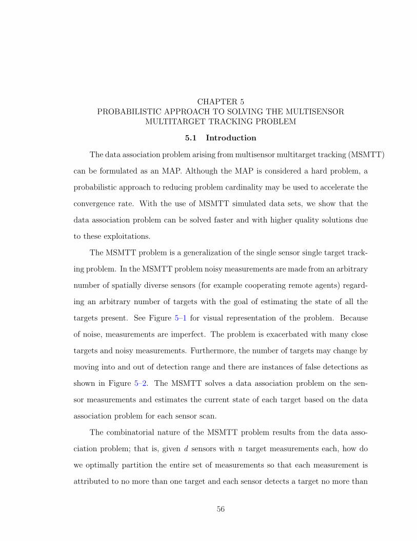
CHAPTER 5PROBABILISTIC APPROACH TO SOLVING THE MULTISENSOR
MULTITARGET TRACKING PROBLEM
5.1 Introduction
The data association problem arising from multisensor multitarget tracking (MSMTT)
can be formulated as an MAP. Although the MAP is considered a hard problem, a
probabilistic approach to reducing problem cardinality may be used to accelerate the
convergence rate. With the use of MSMTT simulated data sets, we show that the
data association problem can be solved faster and with higher quality solutions due
to these exploitations.
The MSMTT problem is a generalization of the single sensor single target track-
ing problem. In the MSMTT problem noisy measurements are made from an arbitrary
number of spatially diverse sensors (for example cooperating remote agents) regard-
ing an arbitrary number of targets with the goal of estimating the state of all the
targets present. See Figure 5–1 for visual representation of the problem. Because
of noise, measurements are imperfect. The problem is exacerbated with many close
targets and noisy measurements. Furthermore, the number of targets may change by
moving into and out of detection range and there are instances of false detections as
shown in Figure 5–2. The MSMTT solves a data association problem on the sen-
sor measurements and estimates the current state of each target based on the data
association problem for each sensor scan.
The combinatorial nature of the MSMTT problem results from the data asso-
ciation problem; that is, given d sensors with n target measurements each, how do
we optimally partition the entire set of measurements so that each measurement is
attributed to no more than one target and each sensor detects a target no more than
56
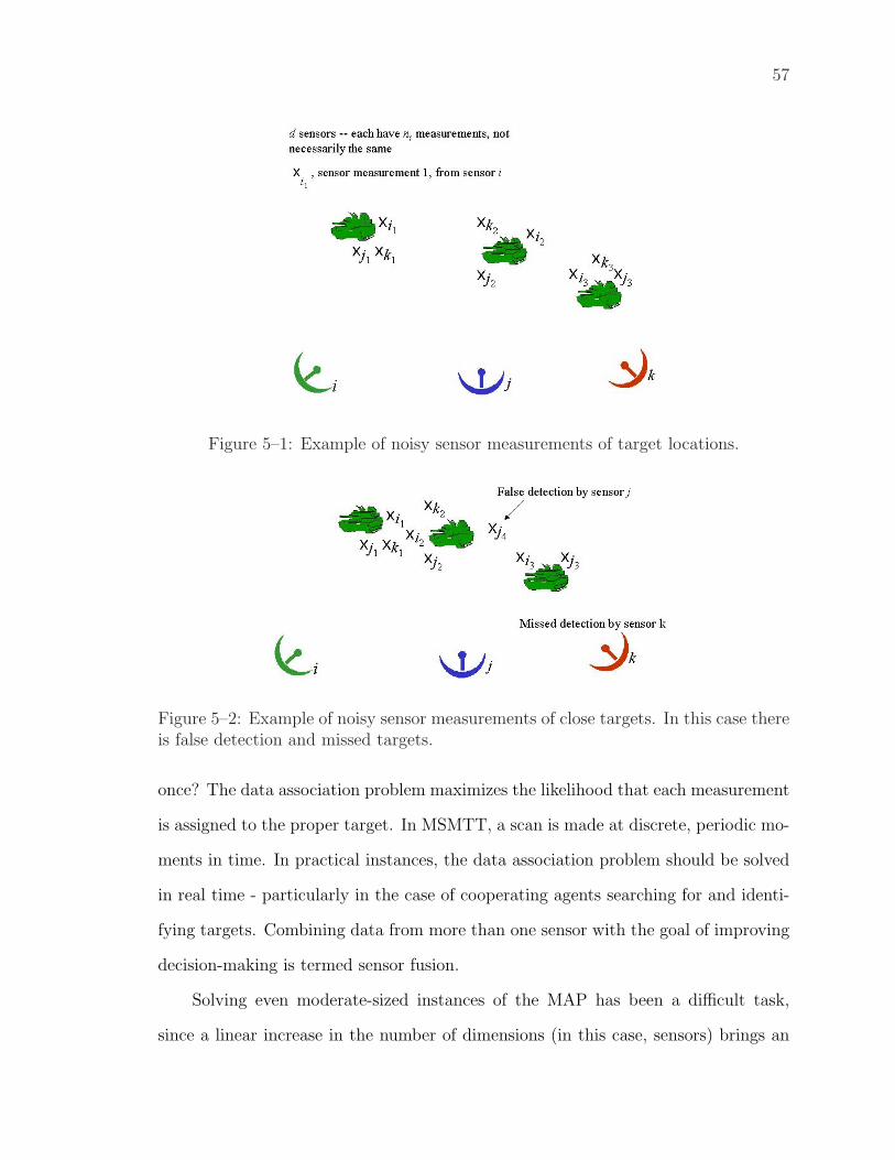
57
Figure 5–1: Example of noisy sensor measurements of target locations.
Figure 5–2: Example of noisy sensor measurements of close targets. In this case thereis false detection and missed targets.
once? The data association problem maximizes the likelihood that each measurement
is assigned to the proper target. In MSMTT, a scan is made at discrete, periodic mo-
ments in time. In practical instances, the data association problem should be solved
in real time - particularly in the case of cooperating agents searching for and identi-
fying targets. Combining data from more than one sensor with the goal of improving
decision-making is termed sensor fusion.
Solving even moderate-sized instances of the MAP has been a difficult task,
since a linear increase in the number of dimensions (in this case, sensors) brings an
58
exponential increase in the size of the problem. As such, several heuristic algorithms
[74, 90] have been applied to this problem. However, due to the size and complexity
of the problem, even the heuristics struggle to achieve solutions in realtime. In this
chapter we propose a systematic approach to reduce the size and complexity of the
data association problem, yet achieve higher quality solutions in faster times.
This chapter is organized as follows. We first give some background on data
association for the MSMTT problem. We then introduce a technique that may be used
to reduce the size of the problem. Following that, we discuss the heuristic, Greedy
Randomized Adaptive Search Procedure (GRASP), and how GRASP can be modified
to work effectively on a sparse problem. Finally, we provide some comparative results
of these solution methods.
5.2 Data Association Formulated as an MAP
Data association is formulated as an MAP where the cost coefficients are derived
from a computationally expensive negative log-likelihood function. The data asso-
ciation problem for the MSMTT problem is to match sensor measurements in such
a way that no measurement is matched more than once and overall matching is the
most likely association of measurements to targets. In the MAP, elements from d dis-
joint sets are matched in such a way that the total cost associated with all matchings
is minimized. It is an extension of the two-dimensional assignment problem where
there are only two disjoint sets. For sets of size n, the two-dimensional assignment
problem has been demonstrated to be solvable in O(n3) arithmetic operations using
the Hungarian method [62], for example. However, the three-dimensional assignment
problem is a generalization of the three dimensional matching problem which is shown
by Garey and Johnson [44] to be NP -hard.
A review of the multitarget multisensor problem formulation and algorithms is
provided by Poore [89]. Bar-Shalom, Pattipati, and Yeddanapudi [11] also present a
combined likelihood function in multisensor air traffic surveillance.
59
Suppose that we have S sensors observing an unknown number of targets T . The
Cartesian coordinates of sensor s is known to be ωs = [xs, ys, zs]′, while the unknown
position of target t is given by ωt = [xt, yt, zt]′. Sensor s takes ns measurements, zs,is .
Since the measurements of target locations are noisy, we have the following expression
for measurement is from sensor s:
zs,is =
hs(ωt, ωs) + ωs,is if measurement is is produced by target t
υs,is if measurement is is a false alarm
The measurement noise, ωs,is , is assumed to be normally distributed with zero mean
and covariance matrix Rs. The nonlinear transformation of measurements from the
spherical to Cartesian frame is given by hs(ωt, ωs).
Consider the S-tuple of measurements Zi1,i2,...,iS , each element is produced by a
different sensor. Using dummy measurements zs,0 to make a complete assignment,
the likelihood that each measurement originates from the same target t located at ωt
is given.
Λ(Zi1,i2,...,iS |ωt) =S∏
s=1
[PDs · p(zs,is|ωt)]δs,is [1− PDs ]
1−δs,is , (5.1)
where
δs,is =
0 if is = 0 (dummy measurement)
1 if is > 0 (actual measurement)
and PDs ≤ 1 is the the detection probability for sensor m. The likelihood that the
set of measurements Zi1,i2,...,iS corresponds to a false alarm is as follows.
Λ(Zi1,i2,...,iS |t = 0) =S∏
s=1
[PFs ]δs,is , (5.2)
where PFs ≥ 0 is the probability of false alarm for sensor s.
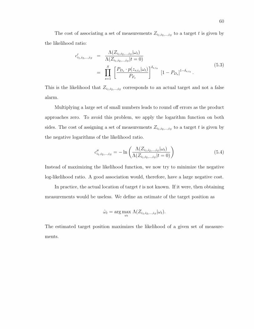
60
The cost of associating a set of measurements Zi1,i2,...,iS to a target t is given by
the likelihood ratio:
c′i1,i2,...,iS=
Λ(Zi1,i2,...,iS |ωt)
Λ(Zi1,i2,...,iS |t = 0)
=S∏
s=1
[PDs · p(zs,is|ωt)
PFs
]δs,is
[1− PDs ]1−δs,is .
(5.3)
This is the likelihood that Zi1,i2,...,iS corresponds to an actual target and not a false
alarm.
Multiplying a large set of small numbers leads to round off errors as the product
approaches zero. To avoid this problem, we apply the logarithm function on both
sides. The cost of assigning a set of measurements Zi1,i2,...,iS to a target t is given by
the negative logarithms of the likelihood ratio.
c′′i1,i2,...,iS= − ln
(Λ(Zi1,i2,...,iS |ωt)
Λ(Zi1,i2,...,iS |t = 0)
)(5.4)
Instead of maximizing the likelihood function, we now try to minimize the negative
log-likelihood ratio. A good association would, therefore, have a large negative cost.
In practice, the actual location of target t is not known. If it were, then obtaining
measurements would be useless. We define an estimate of the target position as
ωt = arg maxωt
Λ(Zi1,i2,...,iS |ωt).
The estimated target position maximizes the likelihood of a given set of measure-
ments.
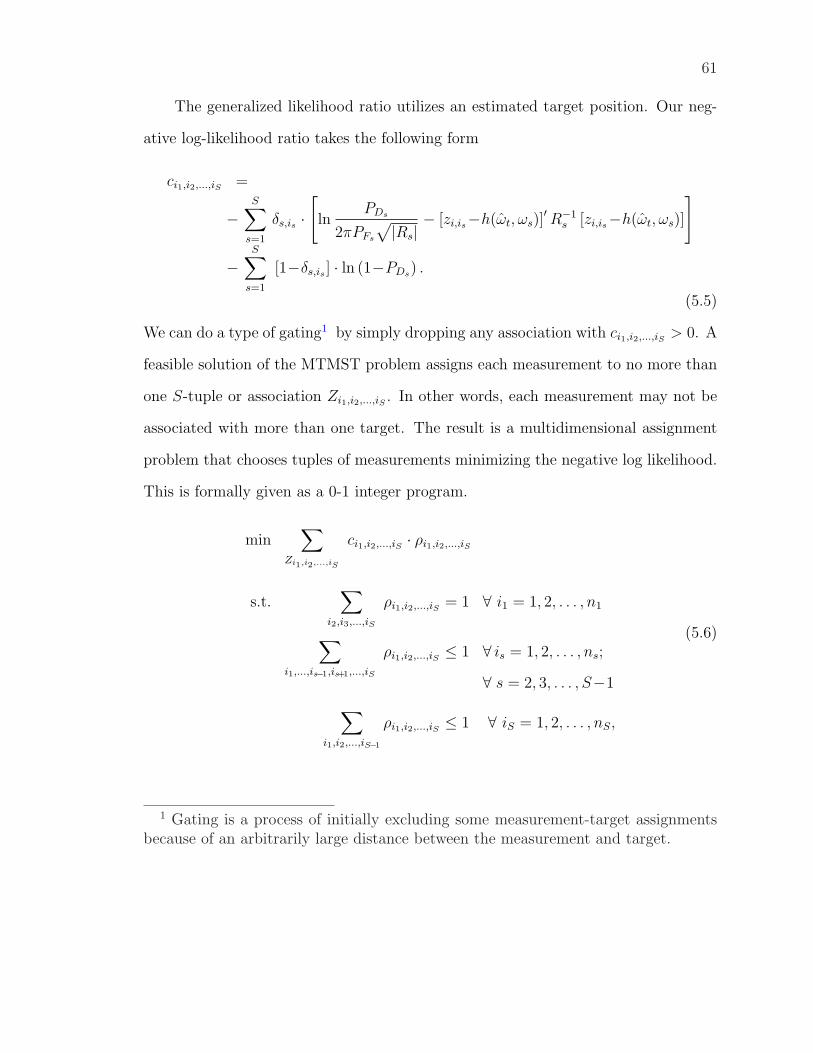
61
The generalized likelihood ratio utilizes an estimated target position. Our neg-
ative log-likelihood ratio takes the following form
ci1,i2,...,iS =
−S∑
s=1
δs,is ·[ln
PDs
2πPFs
√|Rs|
− [zi,is−h(ωt, ωs)]′ R−1
s [zi,is−h(ωt, ωs)]
]
−S∑
s=1
[1−δs,is ] · ln (1−PDs) .
(5.5)
We can do a type of gating1 by simply dropping any association with ci1,i2,...,iS > 0. A
feasible solution of the MTMST problem assigns each measurement to no more than
one S-tuple or association Zi1,i2,...,iS . In other words, each measurement may not be
associated with more than one target. The result is a multidimensional assignment
problem that chooses tuples of measurements minimizing the negative log likelihood.
This is formally given as a 0-1 integer program.
min∑
Zi1,i2,...,iS
ci1,i2,...,iS · ρi1,i2,...,iS
s.t.∑
i2,i3,...,iS
ρi1,i2,...,iS = 1 ∀ i1 = 1, 2, . . . , n1
∑i1,...,is−1,is+1,...,iS
ρi1,i2,...,iS ≤ 1 ∀ is = 1, 2, . . . , ns;
∀ s = 2, 3, . . . , S−1
∑i1,i2,...,iS−1
ρi1,i2,...,iS ≤ 1 ∀ iS = 1, 2, . . . , nS,
(5.6)
1 Gating is a process of initially excluding some measurement-target assignmentsbecause of an arbitrarily large distance between the measurement and target.
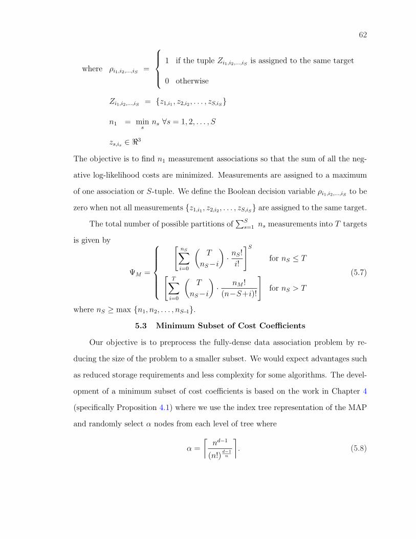
62
where ρi1,i2,...,iS =
1 if the tuple Zi1,i2,...,iS is assigned to the same target
0 otherwise
Zi1,i2,...,iS = {z1,i1 , z2,i2 , . . . , zS,iS}
n1 = mins
ns ∀s = 1, 2, . . . , S
zs,is ∈ <3
The objective is to find n1 measurement associations so that the sum of all the neg-
ative log-likelihood costs are minimized. Measurements are assigned to a maximum
of one association or S-tuple. We define the Boolean decision variable ρi1,i2,...,iS to be
zero when not all measurements {z1,i1 , z2,i2 , . . . , zS,iS} are assigned to the same target.
The total number of possible partitions of∑S
s=1 ns measurements into T targets
is given by
ΨM =
[nS∑i=0
(T
nS−i
)· nS!
i!
]S
for nS ≤ T
[T∑
i=0
(T
nS−i
)· nM !
(n−S+i)!
]for nS > T
(5.7)
where nS ≥ max {n1, n2, . . . , nS−1}.5.3 Minimum Subset of Cost Coefficients
Our objective is to preprocess the fully-dense data association problem by re-
ducing the size of the problem to a smaller subset. We would expect advantages such
as reduced storage requirements and less complexity for some algorithms. The devel-
opment of a minimum subset of cost coefficients is based on the work in Chapter 4
(specifically Proposition 4.1) where we use the index tree representation of the MAP
and randomly select α nodes from each level of tree where
α =
⌈nd−1
(n!)d−1
n
⌉. (5.8)
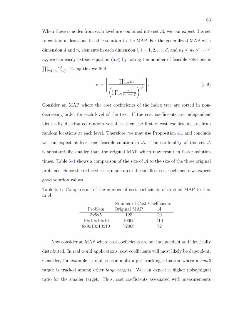
63
When these α nodes from each level are combined into set A, we can expect this set
to contain at least one feasible solution to the MAP. For the generalized MAP with
dimension d and ni elements in each dimension i, i = 1, 2, . . . , d, and n1 ≤ n2 ≤ · · · ≤nd, we can easily extend equation (5.8) by noting the number of feasible solutions is∏d
i=2ni!
(ni−n1)!. Using this we find
α =
⌈ ∏di=2 ni(∏d
i=2ni!
(ni−n1)!
) 1n1
⌉. (5.9)
Consider an MAP where the cost coefficients of the index tree are sorted in non-
decreasing order for each level of the tree. If the cost coefficients are independent
identically distributed random variables then the first α cost coefficients are from
random locations at each level. Therefore, we may use Proposition 4.1 and conclude
we can expect at least one feasible solution in A. The cardinality of this set Ais substantially smaller than the original MAP which may result in faster solution
times. Table 5–1 shows a comparison of the size of A to the size of the three original
problems. Since the reduced set is made up of the smallest cost coefficients we expect
good solution values.
Table 5–1: Comparisons of the number of cost coefficients of original MAP to thatin A.
Number of Cost CoefficientsProblem Original MAP A5x5x5 125 20
10x10x10x10 10000 1108x9x10x10x10 72000 72
Now consider an MAP where cost coefficients are not independent and identically
distributed. In real world applications, cost coefficients will most likely be dependent.
Consider, for example, a multisensor multitarget tracking situation where a small
target is tracked among other large targets. We can expect a higher noise/signal
ratio for the smaller target. Thus, cost coefficients associated with measurements
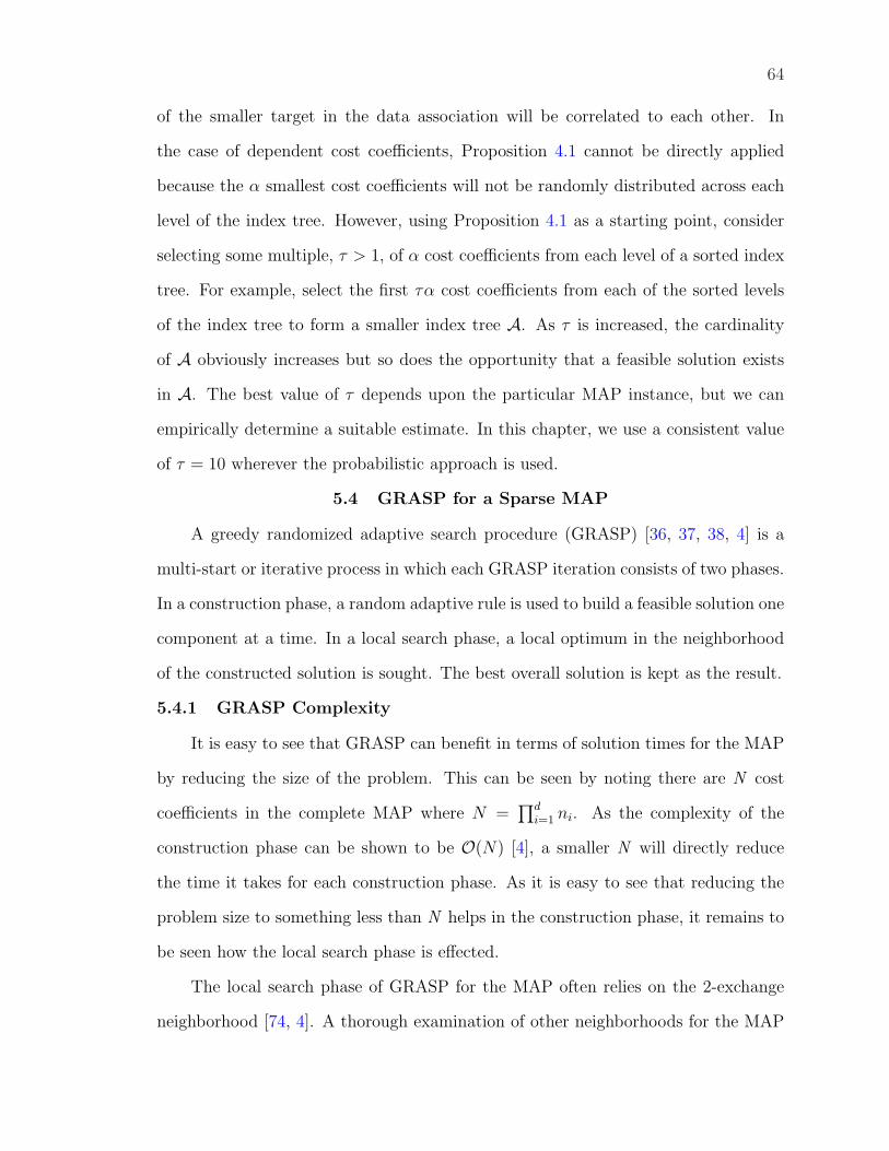
64
of the smaller target in the data association will be correlated to each other. In
the case of dependent cost coefficients, Proposition 4.1 cannot be directly applied
because the α smallest cost coefficients will not be randomly distributed across each
level of the index tree. However, using Proposition 4.1 as a starting point, consider
selecting some multiple, τ > 1, of α cost coefficients from each level of a sorted index
tree. For example, select the first τα cost coefficients from each of the sorted levels
of the index tree to form a smaller index tree A. As τ is increased, the cardinality
of A obviously increases but so does the opportunity that a feasible solution exists
in A. The best value of τ depends upon the particular MAP instance, but we can
empirically determine a suitable estimate. In this chapter, we use a consistent value
of τ = 10 wherever the probabilistic approach is used.
5.4 GRASP for a Sparse MAP
A greedy randomized adaptive search procedure (GRASP) [36, 37, 38, 4] is a
multi-start or iterative process in which each GRASP iteration consists of two phases.
In a construction phase, a random adaptive rule is used to build a feasible solution one
component at a time. In a local search phase, a local optimum in the neighborhood
of the constructed solution is sought. The best overall solution is kept as the result.
5.4.1 GRASP Complexity
It is easy to see that GRASP can benefit in terms of solution times for the MAP
by reducing the size of the problem. This can be seen by noting there are N cost
coefficients in the complete MAP where N =∏d
i=1 ni. As the complexity of the
construction phase can be shown to be O(N) [4], a smaller N will directly reduce
the time it takes for each construction phase. As it is easy to see that reducing the
problem size to something less than N helps in the construction phase, it remains to
be seen how the local search phase is effected.
The local search phase of GRASP for the MAP often relies on the 2-exchange
neighborhood [74, 4]. A thorough examination of other neighborhoods for the MAP
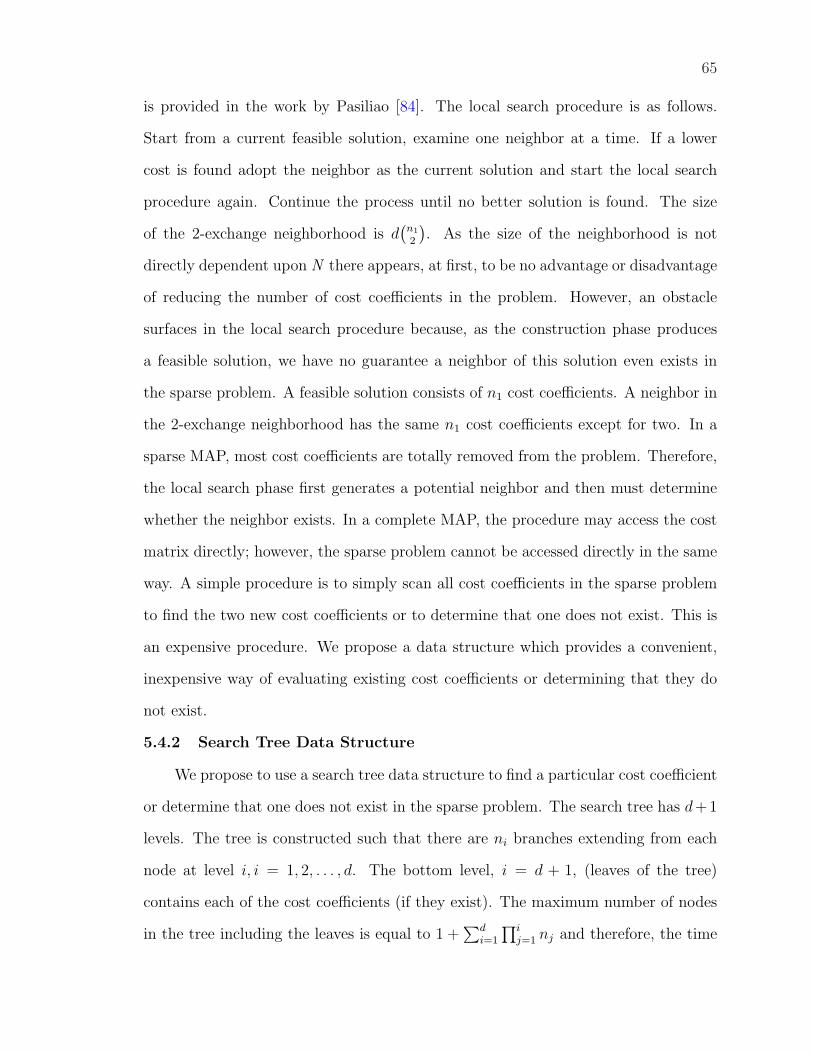
65
is provided in the work by Pasiliao [84]. The local search procedure is as follows.
Start from a current feasible solution, examine one neighbor at a time. If a lower
cost is found adopt the neighbor as the current solution and start the local search
procedure again. Continue the process until no better solution is found. The size
of the 2-exchange neighborhood is d(
n1
2
). As the size of the neighborhood is not
directly dependent upon N there appears, at first, to be no advantage or disadvantage
of reducing the number of cost coefficients in the problem. However, an obstacle
surfaces in the local search procedure because, as the construction phase produces
a feasible solution, we have no guarantee a neighbor of this solution even exists in
the sparse problem. A feasible solution consists of n1 cost coefficients. A neighbor in
the 2-exchange neighborhood has the same n1 cost coefficients except for two. In a
sparse MAP, most cost coefficients are totally removed from the problem. Therefore,
the local search phase first generates a potential neighbor and then must determine
whether the neighbor exists. In a complete MAP, the procedure may access the cost
matrix directly; however, the sparse problem cannot be accessed directly in the same
way. A simple procedure is to simply scan all cost coefficients in the sparse problem
to find the two new cost coefficients or to determine that one does not exist. This is
an expensive procedure. We propose a data structure which provides a convenient,
inexpensive way of evaluating existing cost coefficients or determining that they do
not exist.
5.4.2 Search Tree Data Structure
We propose to use a search tree data structure to find a particular cost coefficient
or determine that one does not exist in the sparse problem. The search tree has d+1
levels. The tree is constructed such that there are ni branches extending from each
node at level i, i = 1, 2, . . . , d. The bottom level, i = d + 1, (leaves of the tree)
contains each of the cost coefficients (if they exist). The maximum number of nodes
in the tree including the leaves is equal to 1 +∑d
i=1
∏ij=1 nj and therefore, the time
66
to construct the tree is O(N). An example of this search tree is given in Figure 5–3
for a complete 3x3x3 MAP. When searching for a particular cost coefficient, start at
level i = 1 and traverse down branch y, y = 0, . . . , ni where y is the element of the ith
dimension for the cost coefficient. Continue this process until either level i = d + 1 is
reached, in which case the cost coefficient exists, or a null pointer is reached, in which
case we may conclude the cost coefficient does not exist. It is obvious the search time
is O(d).
000 001 002 010 011 012 020 021 022 100 101 102 110 111 112 120 121 122 200 201 202 210 211 212 220 221 222
0 1 2
Level 1
Dimension 1
Level 3
Dimension 3
Level 2
Dimension 2
0 1 2 0 1 2 0 1 2
0 1 2 0 1 2 0 1 2 0 1 2 0 1 2 0 1 2 0 1 2 0 1 2 0 1 2
Figure 5–3: Search tree data structure used to find a cost coefficient or determine acost coefficient does not exist.
A search tree built from sparse data is shown in Figure 5–4. As an example of
searching for cost coefficient (001), start at level 1 and traverse down branch labelled
“0” to the node at level 2. From level 2, traverse again down branch labelled “0”
to the node at level 3. From level 3, traverse down branch labelled “1” to the cost
coefficient. Another example is searching for cost coefficient (222). Start at level 1
and traverse down branch labelled “2” to the node at level 2. From level 2, traverse
again down branch labelled “2” to find it is a null pointer. The null pointer indicates
the cost coefficient does not exist in the sparse MAP.
67
Level 1
Dimension 1
Level 3
Dimension 3
Level 2
Dimension 2
000 001 010 021 102 112 120 200 201 211 212
0 1 2
0 1 2 0 1 2 0 1 2
0 1 2 0 1 2 0 1 2 0 1 2 0 1 2 0 1 2 0 1 2 0 1 2
Figure 5–4: Search tree example of a sparse MAP.
The GRASP algorithm can benefit from this search tree data structure if the
problem is sparse. In a dense problem, it would be best to put cost coefficients in
a matrix which can be directly accessed – this would benefit the local search phase.
However, in the sparse problem, completely eliminating cost coefficients reduces stor-
age and benefits the construction phase. It remains a matter of experimentation and
closer examination to find the level of sparseness where the search tree data structure
becomes more beneficial.
5.4.3 GRASP vs Sparse GRASP
To compare the performance of GRASP to solve a fully dense problem against
the performance of GRASP to solve a sparse problem, we used simulated data from
a multisensor multitarget tracking problem [74]. The problems ranged in size from
five to seven sensors. Those with five sensors had five to nine targets. Problems
with six and seven sensors had just five targets. Two problems of each size were
tested. The problem size is indicated by the problem title. For example, “s5t6rm1”
means problem one with five sensors and six targets. The experiment conducted
five runs of each solution algorithm and reports the average time-to-solution, the
average solution value and the best solution value from the five runs. The solution
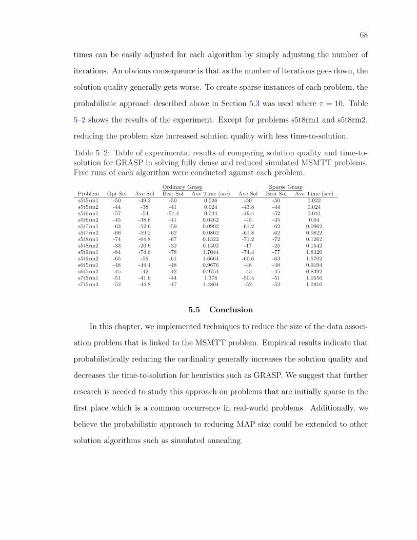
68
times can be easily adjusted for each algorithm by simply adjusting the number of
iterations. An obvious consequence is that as the number of iterations goes down, the
solution quality generally gets worse. To create sparse instances of each problem, the
probabilistic approach described above in Section 5.3 was used where τ = 10. Table
5–2 shows the results of the experiment. Except for problems s5t8rm1 and s5t8rm2,
reducing the problem size increased solution quality with less time-to-solution.
Table 5–2: Table of experimental results of comparing solution quality and time-to-solution for GRASP in solving fully dense and reduced simulated MSMTT problems.Five runs of each algorithm were conducted against each problem.
Ordinary Grasp Sparse Grasp
Problem Opt Sol Ave Sol Best Sol Ave Time (sec) Ave Sol Best Sol Ave Time (sec)s5t5rm1 -50 -49.2 -50 0.026 -50 -50 0.022s5t5rm2 -44 -38 -41 0.024 -43.8 -44 0.024s5t6rm1 -57 -54 -51.4 0.044 -49.4 -52 0.044s5t6rm2 -45 -38.6 -41 0.0462 -45 -45 0.04s5t7rm1 -63 -52.6 -59 0.0902 -61.2 -62 0.0962s5t7rm2 -66 -59.2 -62 0.0862 -61.8 -62 0.0822s5t8rm1 -74 -64.8 -67 0.1322 -71.2 -72 0.1262s5t8rm2 -33 -20.6 -32 0.1402 -17 -25 0.1542s5t9rm1 -84 -74.6 -78 1.7044 -74.4 -77 1.8326s5t9rm2 -65 -59 -61 1.6664 -60.6 -63 1.5702s6t5rm1 -48 -44.4 -48 0.9676 -48 -48 0.9194s6t5rm2 -45 -42 -42 0.9754 -45 -45 0.8392s7t5rm1 -51 -41.6 -44 1.378 -50.4 -51 1.0556s7t5rm2 -52 -44.8 -47 1.4804 -52 -52 1.0916
5.5 Conclusion
In this chapter, we implemented techniques to reduce the size of the data associ-
ation problem that is linked to the MSMTT problem. Empirical results indicate that
probabilistically reducing the cardinality generally increases the solution quality and
decreases the time-to-solution for heuristics such as GRASP. We suggest that further
research is needed to study this approach on problems that are initially sparse in the
first place which is a common occurrence in real-world problems. Additionally, we
believe the probabilistic approach to reducing MAP size could be extended to other
solution algorithms such as simulated annealing.
CHAPTER 6EXPECTED NUMBER OF LOCAL MINIMA FOR THE MAP
As discussed in previous chapters, the MAP is an NP -hard combinatorial op-
timization problem occurring in many applications, such as data association. As
many solution approaches to this problem rely, at least partly, on local neighborhood
searches, it is widely assumed the number of local minima has implications on solution
difficulty. In this chapter, we investigate the expected number of local minima for
random instances of this problem. Both 2-exchange and 3-exchange neighborhoods
are considered. We report on experimental findings that expected number of local
minima does impact effectiveness of three different solution algorithms that rely on
local neighborhood searches.
6.1 Introduction
In this chapter we develop relationships for the expected number of local minima.
The 2-exchange local neighborhood appears as the most commonly used neighborhood
in meta-heuristics such as GRASP that are applied to the MAP as evidenced in
several different works [4, 74, 27]. Although the 2-exchange is most common in the
literature, we include in this chapter some analysis of the 3-exchange neighborhood
for comparison purposes.
The motivation of this chapter is that the number of distinct local minima of an
MAP may have implications for heuristics that rely, at least partly, on repeated local
searches in neighborhoods of feasible solutions [112]. In general, if the number of local
minima is small then we may expect better performance from meta-heuristic algo-
rithms that rely on local neighborhood searches. A solution landscape is considered
to be rugged if the number of local minima is exponential with respect to the size of
the problem [78]. Evidence by Angel and Zissimopoulos [9] showed that ruggedness
69
70
of the solution landscape has a direct impact on the effectiveness of the simulated an-
nealing heuristic in solving at least one other hard problem, the quadratic assignment
problem.
The concept of solution landscapes was first introduced by Wright [111] as a non-
mathematical way to describe the action during evolution of selection and variation
[102]. The idea is to imagine the space in which evolution occurs as a landscape.
In one dimension there is the genotype and in another dimension there is a height
or fitness. Evolution can be viewed as the movement of the population, represented
as a set of points (genotypes), towards higher (fitter) areas of the landscape. In
an analogous way, a solution process for a combinatorial problem can be viewed as
the movement from some feasible solution with its associated cost (fitness) towards
better cost (fitter) areas within the solution landscape. As pointed out by Smith et al.
[102], the difficulty of searching in a given problem is related to the structure of the
landscape, however, the exact relationship between different landscape features and
the time taken to find good solutions is not clear. To name a couple of the landscape
features of interest are number local optima and basins of attraction.
Reidys and Stadler [93] describe some characteristics of landscapes and express
that local optima play an important role since they might be obstacles on the way
to the optimal solution. From a minimization perspective, if x is a feasible solution
of some optimization problem and f(x) is the solution cost, then x is a local min-
ima iff f(x) ≤ f(y) for all y in the neighborhood of x. Obviously the size of the
neighborhood depends upon the definition of the neighborhood. According to Reidys
and Stadler [93] there is no simple way of computing the number of local minima
without exhaustively generating the solution landscape. However, the number can
be estimated as done in some recent works [43, 45].
Rummukainen [98] describes some aspects of landscape theory which have been
used to prove convergence of simulated annealing. Of particular interest are some
71
results on the behavior of local optimization on a few different random landscape
classes. For example, the expected number of local minima is given for the N − k
landscape.
Associated with local minima is a basin B(x) defined by means of a steepest
descent algorithm [93]. Let f(xi) be the cost of some feasible solution xi. Starting
from xi, i = 0, record for all y−neighbors the solution cost f(y). Let xi + 1 = y for
neighbor y where f(y) is the smallest for all neighbors and f(y) < f(xi). Stop when
xi is a local minima. It becomes apparent; however, that a basin may have more than
one local minima because of the definition of local minima is not strict. The basin
sizes becomes important for simple meta-heuristics. For example, consider selecting
a set of feasible solutions that are uniformly distributed in the solution landscape and
performing a steepest descent. A question is what is the probability of starting in the
basin with the global minima? This question is partially addressed by Garnier and
Kaller [45].
Long and Williams [68] mention that problems are generally easier to solve when
the number of local optima is small, but the difficulty can increase significantly when
the number of local optima is large. The authors consider the quadratic 0-1 problem
where instances are randomly generated over integers symmetric about 0. For such
problems, the authors show the expected number of local maxima increases expo-
nentially with respect to n, the size of the problem. They also reconcile this result
with Pardalos and Jha [80] who showed when test data are generated from a normal
distribution, the expected number of local maxima approaches 1 as n gets large.
Angel and Zissimopoulos [9] introduce a ruggedness coefficient which measures
the ruggedness of the QAP solution landscape. They conclude that because the QAP
landscape is rather flat, this gives theoretical justification for the effectiveness of local
search algorithms. The ruggedness coefficient is an extension of the autocorrelation
coefficient introduced by Weinberger [110]. The larger the autocorrelation coefficient
72
the more flat is the landscape – and so, as postulated by the authors, the more
suited is the problem for any local-search-based heuristic. Angel and Zissimopoulos
[9] calculate the autocorrelation coefficient for the QAP as being no smaller than
n/4 and no larger than n/2 which is considered relatively large. They develop the
parameter, ruggedness coefficient, ζ, which is independent of problem size and lies
between 0 to 100. Close to 100 means the the landscape is very steep. They go on
to show experimentally that increasing ζ for the same problem size results in higher
relative solution error and higher number of steps when using a simulated annealing
algorithm by Johnson et al. [53]. The conclusions Angel and Zissimopoulos [9] are a
relatively low ruggedness coefficient for the QAP gives theoretical justification of the
effectiveness of local-search-based heuristics for the QAP.
This chapter will further investigate the assumption that number of local minima
impacts the effectiveness of algorithms such as simulated annealing in solving the
MAP.
The next section provides some additional background on the 2-exchange and
3-exchange local search neighborhoods. Then in Section 6.3, we provide experimen-
tal results on the average number of local minima for variously sized problems with
assignment costs independently drawn from different distributions. Section 6.4 de-
scribes the expected number of local minima for MAPs of size of n = 2 and d ≥ 3
where the cost elements are independent identically distributed random variables
from any probability distribution. Section 6.5 describes lower and upper bounds for
the expected number of local minima for all sizes of MAPs where assignment costs are
independent standard normal random variables. Then in Section 6.6, we investigate
whether the expected number of local minima impacts the performance of various
algorithms that rely on local searches. Some concluding remarks are given in the last
section.
73
6.2 Some Characteristics of Local Neighborhoods
A first step is to establish the definition of a neighborhood of a feasible solution.
Let Np(k) be the p-exchange neighborhood of the k-th feasible solution, k = 1, . . . , N ,
where N is the number of feasible solutions to the MAP. The p-exchange neighborhood
is all p- or less element exchange permutations in each dimension of the feasible
solution. The neighborhood is developed from the work by Lin and Kernighan [66].
If zk is the solution cost of the k-th solution, then zk is a discrete local minimum
iff zk ≤ zj for all j ∈ Np(k). As an example of a 2-exchange neighbor, consider the
following feasible solution to an MAP with d = 3, n = 3: {111, 222, 333}. A neighbor
is {111, 322, 233}. The solution {111, 222, 333} is a local minimum if its solution cost
is less than or equal to all of its neighbor’s solution costs.
The formula for the number of neighbors, J , of a feasible solution in the 2-
exchange neighborhood of an MAP with dimension d and n elements in each dimen-
sion is as follows
J = |N2(k)| = d
(n
2
). (6.1)
It is obvious that for a fixed n, J is linear in d. On the other hand for a fixed d, J
is quadratic in n. If we define a flat MAP as one with relatively small n and define
a deep MAP as one with relatively large n, then we expect larger neighborhoods in
deep problems.
Similarly, for n > 2 the size of the 3-exchange neighborhood is as follows
J = |N3(k)| = d[(n
2
)+ 2
(n
3
)]. (6.2)
Similar to above for the 2-exchange, it becomes clear J is linear with respect to d
and cubic with respect to n.
The minimum number of local minima for any instance is one - the global mini-
mum. At the other extreme, the maximum number of local minima is (n!)d−1 which
74
is the number of feasible solutions of an MAP. This occurs if all cost coefficients are
equal.
6.3 Experimentally Determined Number of Local Minima
Studies were made of randomly produced instances of MAPs to empirically de-
termine E[M ]. The assignment costs ci1···id for each problem instance were drawn
from one of three distributions. The first distribution of assignment costs used is the
uniform, U [0, 1]. The next distribution used is the exponential with mean one, being
determined by ci1···id = − ln U . Finally, the third distribution used was the standard
normal, N(0, 1), with values determined by the polar method [63].
Table 6–1 shows the average number of local minima for randomly generated
instances of the MAP when considering a 2-exchange neighborhood. For small sized
problems, the study was conducted by generating an instance of an MAP and count-
ing number of local minima through complete enumeration of the feasible solutions.
The values in the tables are the average number of local minima from 100 problem
instances. For larger problems (indicated by * in the table), the average number
of local minima was found by examining a large number1 of generated problem in-
stances. For each instance of a problem we randomly selected a feasible solution and
determined whether it was a local minimum. This technique gives an estimate of the
probability that any feasible solution is a local minima. This relationship was then
used to estimate the average number of local minima by multiplying the probability
by the number of feasible solutions. This technique showed to have results consistent
with the complete enumeration method mentioned above for small problems. Re-
gardless of the distribution that cost coefficients were drawn, a standard deviation
of 40-percent and 5-percent were observed for problems of sizes d = 3, n = 3 and
1 The number examined depends on problem size. The number ranged from 106
to 107.
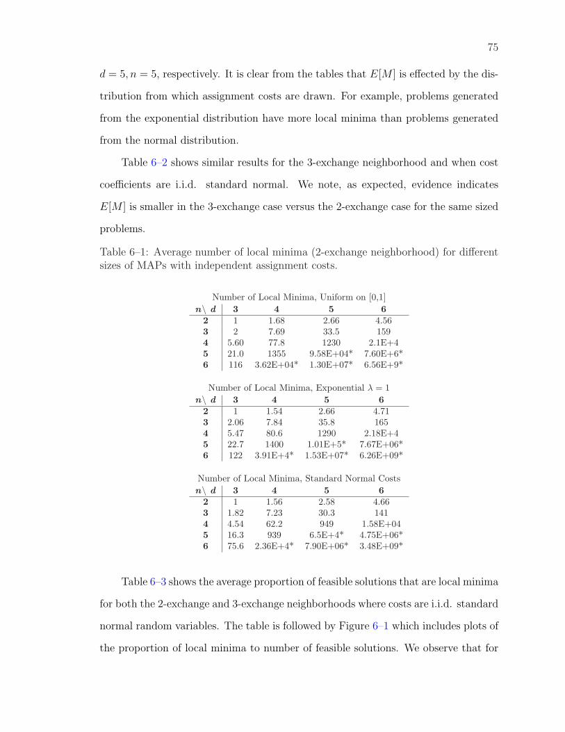
75
d = 5, n = 5, respectively. It is clear from the tables that E[M ] is effected by the dis-
tribution from which assignment costs are drawn. For example, problems generated
from the exponential distribution have more local minima than problems generated
from the normal distribution.
Table 6–2 shows similar results for the 3-exchange neighborhood and when cost
coefficients are i.i.d. standard normal. We note, as expected, evidence indicates
E[M ] is smaller in the 3-exchange case versus the 2-exchange case for the same sized
problems.
Table 6–1: Average number of local minima (2-exchange neighborhood) for differentsizes of MAPs with independent assignment costs.
Number of Local Minima, Uniform on [0,1]n\ d 3 4 5 6
2 1 1.68 2.66 4.563 2 7.69 33.5 1594 5.60 77.8 1230 2.1E+45 21.0 1355 9.58E+04* 7.60E+6*6 116 3.62E+04* 1.30E+07* 6.56E+9*
Number of Local Minima, Exponential λ = 1n\ d 3 4 5 6
2 1 1.54 2.66 4.713 2.06 7.84 35.8 1654 5.47 80.6 1290 2.18E+45 22.7 1400 1.01E+5* 7.67E+06*6 122 3.91E+4* 1.53E+07* 6.26E+09*
Number of Local Minima, Standard Normal Costsn\ d 3 4 5 6
2 1 1.56 2.58 4.663 1.82 7.23 30.3 1414 4.54 62.2 949 1.58E+045 16.3 939 6.5E+4* 4.75E+06*6 75.6 2.36E+4* 7.90E+06* 3.48E+09*
Table 6–3 shows the average proportion of feasible solutions that are local minima
for both the 2-exchange and 3-exchange neighborhoods where costs are i.i.d. standard
normal random variables. The table is followed by Figure 6–1 which includes plots of
the proportion of local minima to number of feasible solutions. We observe that for
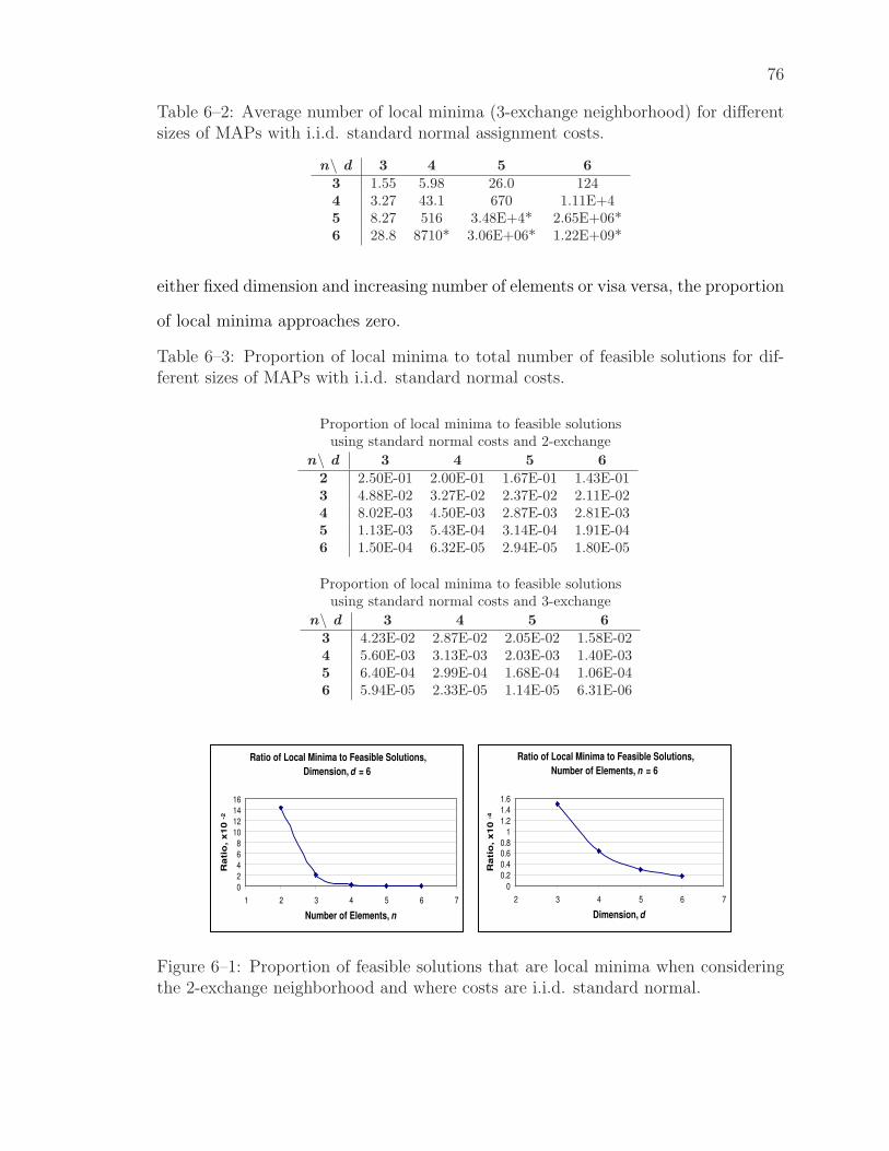
76
Table 6–2: Average number of local minima (3-exchange neighborhood) for differentsizes of MAPs with i.i.d. standard normal assignment costs.
n\ d 3 4 5 63 1.55 5.98 26.0 1244 3.27 43.1 670 1.11E+45 8.27 516 3.48E+4* 2.65E+06*6 28.8 8710* 3.06E+06* 1.22E+09*
either fixed dimension and increasing number of elements or visa versa, the proportion
of local minima approaches zero.
Table 6–3: Proportion of local minima to total number of feasible solutions for dif-ferent sizes of MAPs with i.i.d. standard normal costs.
Proportion of local minima to feasible solutionsusing standard normal costs and 2-exchange
n\ d 3 4 5 62 2.50E-01 2.00E-01 1.67E-01 1.43E-013 4.88E-02 3.27E-02 2.37E-02 2.11E-024 8.02E-03 4.50E-03 2.87E-03 2.81E-035 1.13E-03 5.43E-04 3.14E-04 1.91E-046 1.50E-04 6.32E-05 2.94E-05 1.80E-05
Proportion of local minima to feasible solutionsusing standard normal costs and 3-exchange
n\ d 3 4 5 63 4.23E-02 2.87E-02 2.05E-02 1.58E-024 5.60E-03 3.13E-03 2.03E-03 1.40E-035 6.40E-04 2.99E-04 1.68E-04 1.06E-046 5.94E-05 2.33E-05 1.14E-05 6.31E-06
Ratio of Local Minima to Feasible Solutions,
Dimension, d = 6
0
2
4
6
8
10
12
14
16
1 2 3 4 5 6 7
Number of Elements, n
Ra
tio
, x
10
-2
Ratio of Local Minima to Feasible Solutions,
Number of Elements, n = 6
0
0.2
0.4
0.6
0.8
1
1.2
1.4
1.6
2 3 4 5 6 7
Dimension, d
Ra
tio
, x
10
-4
Figure 6–1: Proportion of feasible solutions that are local minima when consideringthe 2-exchange neighborhood and where costs are i.i.d. standard normal.
77
6.4 Expected Number of Local Minima for n = 2
In the special case of an MAP where n = 2, d ≥ 3, and cost elements are inde-
pendent identically distributed random variables from some continuous distribution
with c.d.f F (·), one can establish a closed form expression for the expected num-
ber of local minima. To show this, we recall that distribution FX+Y of the sum of
two independent random variables X and Y is determined by the convolution of the
respective distribution functions, FX+Y = FX ∗ FY .
We now borrow from Proposition 3.1 to construct the following proposition.
Proposition 6.1 In an instance of the MAP with n=2 and with cost coefficients that
are i.i.d. random variables with continuous distribution F , the costs of all feasible
solutions are independent distributed random variables with distribution F ∗ F .
Proof: Let I be an instance of MAP with n = 2. Each feasible solution for I
is an assignment a1 = c1,δ1(1),...,δd−1(1), a2 = c2,δ1(2),...,δd−1(2), with cost z = a1 + a2.
The important feature of such assignments is that for each fixed entry c1,δ1(1),...,δd−1(1),
there is just one remaining possibility, namely c2,δ1(2),...,δd−1(2), since each dimension
has only two elements. This implies that different assignments cannot share elements
in the cost vector, and therefore different assignments have independent costs z. Now,
a1 and a2 are independent variables from F . Thus z = a1 + a2 is a random variable
with distribution F ∗ F .
One other proposition is important to this development.
Proposition 6.2 Given j i.i.d. random variables with continuous distributions, the
probability that the rth, r = 1, . . . , j, variable is the minimum value is 1/j.
Proof: Consider j i.i.d. random variables, Xi, i = 1, . . . , j, with c.d.f. F (·) and
p.d.f. f(·). Let X(j−1) be the minimum of j − 1 of these variables,
X(j−1) = min{Xi | i = 1, . . . , j, i 6= r},
78
whose c.d.f. and p.d.f. are computed trivially as
F(j−1)(x) = P [X(j−1) ≤ x] = 1− (1− F (x))j−1,
f(j−1)(x) =d
dxF(j−1)(x) = (j − 1)(1− F (x))j−2f(x).
Then, the probability that the rth random variable is minimal among j i.i.d. contin-
uous variables, is
P [rth r.v. is minimal] = P [Xr ≤ X(j−1)] = P[Y ≤ 0] = FY (0). (6.3)
Here FY (·) is the c.d.f. of random variable Y = Xr − X(j−1), and, by convolution
rule, it equals to
FY (x) =
∫ +∞
−∞F (x− y)(j − 1)(1− F (−y))j−2f(−y)dy.
Hence, the probability (6.3) can immediately be calculated as
P[Xr ≤ X(j−1)] =
∫ +∞
−∞F (−y)(j − 1)(1− F (−y))j−2f(−y)dy
=1
j
∫ +∞
−∞j(1− F (−y))j−1f(−y)dy =
1
j,
since j(1 − F (−y))j−1f(−y) is the p.d.f. of −X(j) = −min{X1, . . . , Xj}. The last
equality yields the statement of the proposition.
The obvious consequence of Proposition 6.2 is that given a sequence of indepen-
dent random variables from a continuous distribution, position of the minimum value
is uniformly located within the sequence regardless of the parent distribution.
We are now ready to prove the main result of this section.
Theorem 6.3 In an MAP with cost coefficients that are i.i.d. continuous random
variables where n = 2 and d ≥ 3, the expected number of local minima is given by
E[M ] =2d−1
d + 1. (6.4)
79
Proof: Let N be the number of feasible solutions to an n = 2 MAP, N = 2d−1.
Introducing indicator variables
Yk =
1, kth solution, k = 1, . . . , N , is a local minimum;
0, otherwise,(6.5)
one can write M as the sum of indicator variables:
M =N∑
k=1
Yk.
From the elementary properties of expectation it follows that
E[M ] =N∑
k=1
E[Yk] =N∑
k=1
P [Yk = 1], (6.6)
where P [Yk = 1] is the probability that the cost of k-th feasible solution does not
exceed the cost of any of its neighbors. Any feasible solution has J = d(
n2
)= d
neighbors whose costs, by virtue of Proposition 6.1, are i.i.d. continuous random
variables. Then, Proposition 6.2 implies that the probability of the cost of k-th
feasible solution being minimal among its neighbors is equal to
P [Yk = 1] =1
d + 1,
which, upon substitution into (6.6), yields the statement of the theorem (6.4).
Remark 6.3.1 Equality (6.4) implies that the number of local minima in an n =
2, d ≥ 3 MAP is exponential in d when the cost coefficients are independently drawn
from any continuous distribution.
Corollary 6.4 The proved relation (6.4) can be used to derive the expected ratio
of the number of local minima M to the total number of feasible solutions N in an
n = 2, d ≥ 3 MAP:
E[M/N ] =E[M ]
N=
1
d + 1.
80
This shows that the number of local minima in an n = 2 MAP becomes infinitely
small comparing to the number of feasible solutions, when dimension d of the problem
increases. This asymptotic characteristic is reflected in the numerical data above and
may be useful for the development of novel solution methods.
6.5 Expected Number of Local Minima for n ≥ 3
Our ability to derive a closed-form expression (6.4) for the expected number of
local minima E[M ] in the previous section has relied on the independence of costs of
feasible solutions in an n = 2 MAP. As it is easy to verify directly, in case of n ≥ 3
the costs coefficients are generally not independent. This complicates significantly the
analysis if an arbitrary continuous distribution for assignment costs ci1···id is assumed.
However, as we show below, one can derive upper and lower bounds for E[M ] in the
case when the costs coefficients of (2.1) are normally distributed random variables.
First, we introduce a proposition, which follows a similar development by Beck
[16].
Proposition 6.5 Consider an n ≥ 3, d ≥ 3 MAP whose costs are i.i.d. continuous
random variables. Then the expected number of local minima can be represented as
E[M ] =N∑
k=1
P[ ⋂
j ∈N2(k)
zk − zj ≤ 0]
(6.7)
where N2(k) is the 2-exchange neighborhood of the k-th feasible solution, and zi is the
cost of the i-th feasible solution.
Proof: As before, M can be written as the sum of indicator variables Yk (6.5), which
consequently leads to
E[M ] =N∑
k=1
E[Yk] =N∑
k=1
P [Yk = 1]. (6.8)
As Yk = 1 means zk ≤ zj for all j ∈ N2(k), it is obvious that P [Yk = 1] = P [zk− zj ≤0, ∀ j ∈ N2(k)], which proves the proposition.
81
If we allow the nd cost coefficients ci1···id ∼ N(0, 1) of the MAP to be independent
standard normal N(0, 1) random variables, then for any two feasible solutions the
difference of their costs Zij = zi − zj is a normal variable with mean zero.
Without loss of generality, consider the k = 1 feasible solution to (2.1) whose
cost is
z1 = c1···1 + c2···2 + . . . + cn···n. (6.9)
In the 2-exchange neighborhood N2(1), the cost of a feasible solution differs from
(6.9) by two cost coefficients, e.g.,
z2 = c21···1 + c12···2 + c3···3 + . . . + cn···n.
Generally, the difference z1 − zl of costs of (6.9) and that of any neighbor l ∈ N2(1)
has the form
Zrsq = cr···r + cs···s − cr···rsr···r − cs···srs···s, (6.10)
where the last two coefficients have “switched” indices in the q-th position, q =
1, . . . , d. Observing that
Zrsq = Zsrq for r, s = 1, . . . , n; q = 1, . . . , d,
consider the J-dimensional random vector
Z = (Z111, . . . , Z11d, Z121, . . . , Z12d, · · ·
· · · , Zrs1, . . . , Zrsd, · · · , Znn1, . . . , Znnd) , r ≤ s. (6.11)
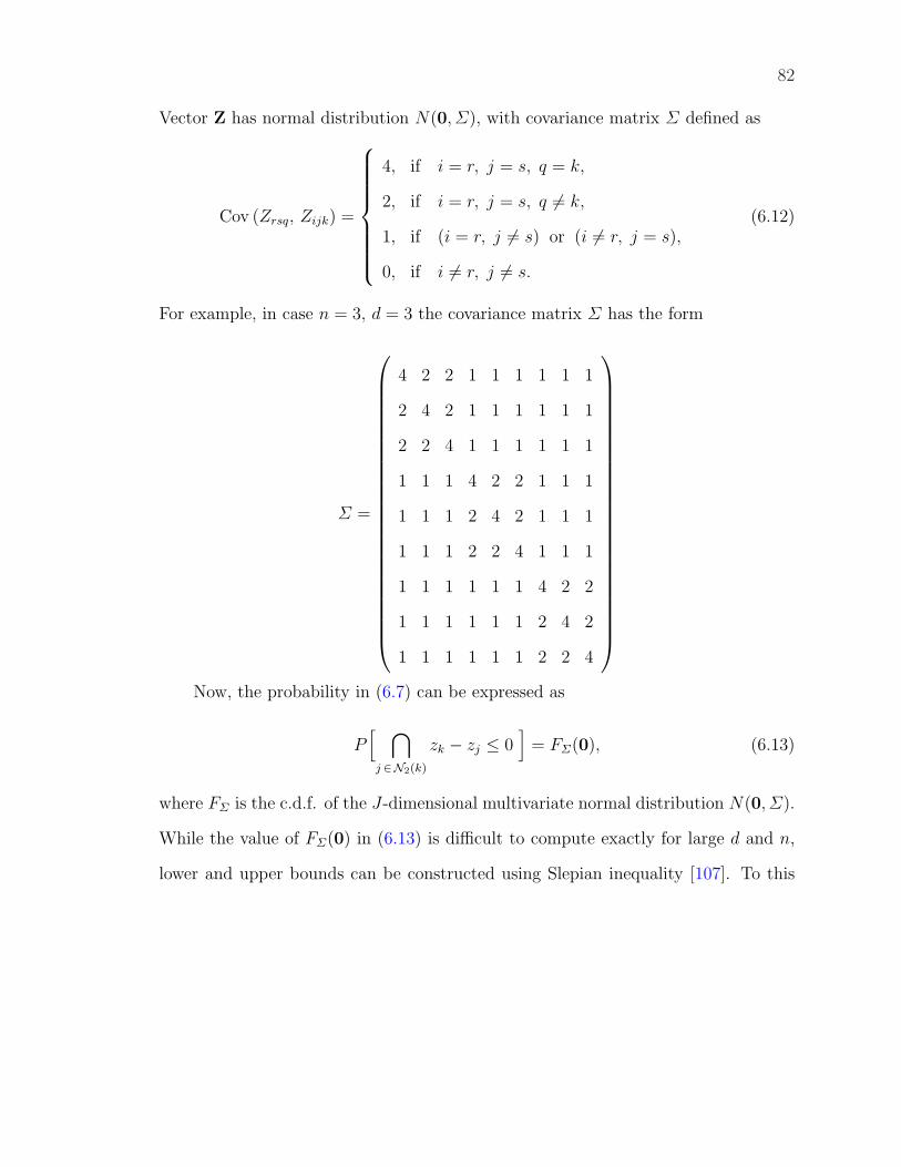
82
Vector Z has normal distribution N(0, Σ), with covariance matrix Σ defined as
Cov (Zrsq, Zijk) =
4, if i = r, j = s, q = k,
2, if i = r, j = s, q 6= k,
1, if (i = r, j 6= s) or (i 6= r, j = s),
0, if i 6= r, j 6= s.
(6.12)
For example, in case n = 3, d = 3 the covariance matrix Σ has the form
Σ =
4 2 2 1 1 1 1 1 1
2 4 2 1 1 1 1 1 1
2 2 4 1 1 1 1 1 1
1 1 1 4 2 2 1 1 1
1 1 1 2 4 2 1 1 1
1 1 1 2 2 4 1 1 1
1 1 1 1 1 1 4 2 2
1 1 1 1 1 1 2 4 2
1 1 1 1 1 1 2 2 4
Now, the probability in (6.7) can be expressed as
P[ ⋂
j ∈N2(k)
zk − zj ≤ 0]
= FΣ(0), (6.13)
where FΣ is the c.d.f. of the J-dimensional multivariate normal distribution N(0, Σ).
While the value of FΣ(0) in (6.13) is difficult to compute exactly for large d and n,
lower and upper bounds can be constructed using Slepian inequality [107]. To this
83
end, let us introduce covariance matrices Σ = (σij) and Σ = (σij)
σij =
4, if i = j,
2, if i 6= j and (i− 1) div d = (j − 1) div d,
0, otherwise,
(6.14a)
σij =
4, if i = j,
2, otherwise,(6.14b)
so that σij ≤ σij ≤ σij holds for all 1 ≤ i, j ≤ J , with σij being the components of
the covariance matrix Σ (6.12). Then, the Slepian inequality claims that
FΣ(0) ≤ FΣ(0) ≤ FΣ(0), (6.15)
where FΣ(0) and FΣ(0) are c.d.f.’s of random variables XΣ ∼ N(0, Σ) and XΣ ∼N(0, Σ), respectively.
As the variable XΣ is equicorrelated, the upper bound in (6.15) can be expressed
by the one-dimensional integral (see, e.g., [107])
∫ +∞
−∞
[Φ(az)
]JdΦ(z), a =
√ρ
1− ρ, (6.16)
where Φ(·) is the c.d.f. of standard normal distribution:
Φ(z) =
∫ z
−∞
1√2π
e−t2
2 dt,
and ρ = σij/√
σii σjj is the correlation coefficient of distinct components of the cor-
responding random vector. The correlation coefficient of the components of vector
XΣ is ρ = 12, which allows for a simple closed-form expression for the upper bound
in (6.15)
FΣ(0) =
∫ +∞
−∞
[Φ(z)
]JdΦ(z) =
1
J + 1. (6.17)
84
This immediately yields the value of the upper bound E[M ] for the expected number
of local minima E[M ]:
E[M ] =N∑
k=1
FΣ(0) =2 (n!)d−1
n(n− 1)d + 2.
Let us now calculate the lower bound for E[M ] using (6.15). According to the
covariance matrix Σ (6.14a), the vector XΣ is comprised of n(n−1)2
groups of variables,
each consisting from d elements,
XΣ =(X1, . . . , Xd, · · · , X(i−1)d+1, . . . , Xid, · · ·
· · · , X(n(n−1)/2−1)d, . . . , X(n(n−1)/2)d
),
such that the variables from different groups are independent, whereas variables
within a group have d × d covariance matrix defined as in (6.14b). Thus, one can
express the lower bound FΣ(0) in (6.15) as a product
FΣ(0) =
n(n−1)2∏
i=1
P[
X(i−1)d+1 ≤ 0, . . . , Xid ≤ 0].
Since variables X(i−1)d+1, . . . , Xid, are equicorrelated with correlation coefficient ρ =
12, each probability term in the last equality can be computed similarly to evaluation
of the lower-bound probability (6.17), i.e.,
FΣ(0) =
n(n−1)2∏
i=1
∫ +∞
−∞
[Φ(z)
]ddΦ(z) =
(1
d + 1
)n(n−1)2
.
This finally leads to a lower bound for the number of expected minima:
E[M ] =N∑
k=1
FΣ(0) =(n!)d−1
(d + 1)n(n−1)/2.
In such a way, we have proved the following
85
Theorem 6.6 In an n ≥ 3, d ≥ 3 MAP with i.i.d. standard normal cost coefficients,
the expected number of local minima is bounded as
(n!)d−1
(d + 1)n(n−1)/2≤ E[M ] ≤ 2 (n!)d−1
n(n− 1)d + 2. (6.18)
Remark 6.6.1 From (6.18) it follows that for fixed n ≥ 3, the expected number of
local minima is exponential in d.
Corollary 6.7 Similarly to the case n = 2, the developed lower and upper bounds
can (6.18) can be used to estimate the expected ratio of the number of local minima
M to the total number of feasible solutions N in an n ≥ 3, d ≥ 3 MAP:
1
(d + 1)n(n−1)/2≤ E[M/N ] ≤ 2
n(n− 1)d + 2.
6.6 Number of Local Minima Effects on Solution Algorithms
In this section, we examine the question of whether number of local minima in
the MAP has an impact on heuristics that rely, at least in part, on local neighborhood
searches. We consider three heuristics
• Random Local Search
• Greedy Randomized Adaptive Search (GRASP)
• Simulated Annealing
The heuristics described in the following three subsections were exercised against
various sized problems that were randomly generated from the standard normal dis-
tribution.
6.6.1 Random Local Search
The random local search procedure simply steps through a given number of iter-
ations. Each iteration begins by selecting a random starting solution. The algorithm
then conducts a local search until no better solution can be found. The algorithm
86
captures the overall best solution and reports it after executing the maximum number
of iterations. The following is a more detailed description of the steps involved.
1. Set iteration number to zero, Iter = 0.
2. Randomly select a current solution, xcurrent.
3. While not all neighbors of xcurrent examined, select a neighbor, xnew, of the
current solution.
If zxnew < zxcurrent , then xcurrent ← xnew.
4. If zxcurrent < zxbest, then xbest ← xcurrent.
5. If Iter < Itermax, increment Iter by one and go to Step 2. Otherwise, end.
6.6.2 GRASP
A greedy randomized adaptive search procedure (GRASP) [36, 37, 38] is a multi-
start or iterative process, in which each GRASP iteration consists of two phases. In
a construction phase, a random adaptive rule is used to build a feasible solution one
component at a time. In a local search phase, a local optimum in the neighborhood
of the constructed solution is sought. The best overall solution is kept as the result.
The neighborhood search is conducted similar to that in the random local search
algorithm above. That is neighbors of a current solution are examined one at a time
and if an improving solution is found, it is adopted as the current solution and local
search starts again. Local search ends when no improving solution is found.
GRASP has been used in many applications and specifically in solving the MAP
[4, 74].
6.6.3 Simulated Annealing
Simulated Annealing is a popular heuristic used in solving a variety of problems
[57, 70]. Simulated annealing uses a local search procedure, but the process allows
uphill moves. The probability of moving uphill is higher at high temperatures, but
as the process cools, there is less probability of moving uphill. The specific steps
87
for simulated annealing used in this chapter are taken from work by Gosavi [46].
Simulated annealing was recently applied to the MAP by Clemmons et al. [27].
6.6.4 Results
The heuristic solution quality, Q, which is the relative difference from the optimal
value, is reported and compared for the same sized problems with assignment costs
independently drawn from the standard normal distribution. The purpose of our
analysis is not to compare the efficiency of the heuristic algorithms, but to determine
the extent to which the number of local minima affects the performance of these
algorithms. Each run of an experiment involved the following general steps:
1. Generate random MAP instance with cost coefficients that are i.i.d. standard
normal random variables.
2. Obtain M by checking each feasible solution for being a local minimum.
3. Solve the generated MAP instance using each of the above heuristics 100 times
and return the average solution quality, Q, for each heuristic method.
Problem sizes were chosen based on the desire to test a variety of sizes and the
practical amount of time to determine M (as counting M is the obvious bottleneck
in the experiment). Four problem sizes chosen were d = 3, n = 6; d = 4, n = 5; d =
4, n = 6; and d = 6, n = 4. For problem size d = 4, n = 6 which has the largest N ,
a single run took approximately four hours on a 2.2 GHz Pentium 4 machine. The
number of runs of each experiment varied for each problem size with fewer runs for
larger problems. The number of runs were 100, 100, 30, and 50, respectively, for the
problem sizes listed above.
Figure 6–2 displays plots of the average solution quality for each of the three
heuristics versus the number of local minima. The plots are the results from problem
size d = 4, n = 5 and are typical for the other problem sizes. Included in each plot
is a best-fit linear least-squares line that provides some insight on the effect of M
on solution quality. A close examination of the figures indicates that the solution
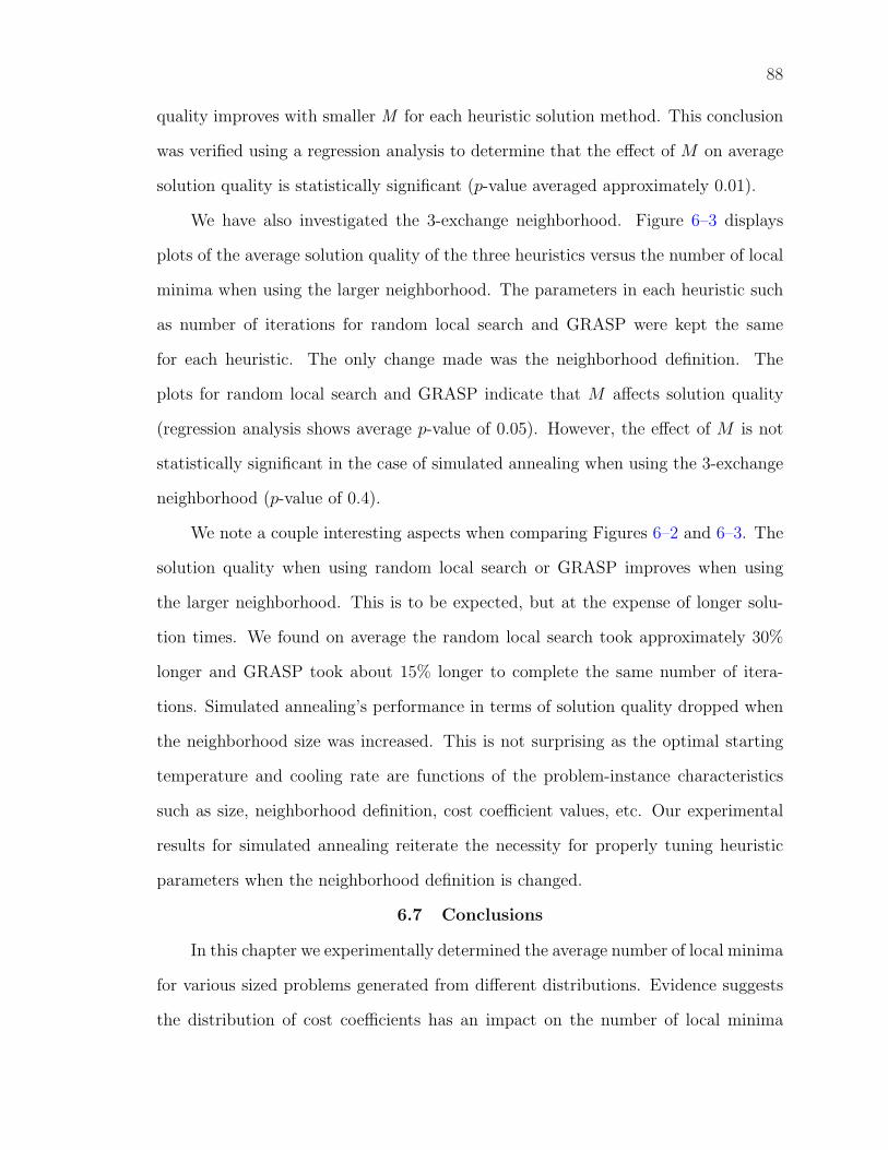
88
quality improves with smaller M for each heuristic solution method. This conclusion
was verified using a regression analysis to determine that the effect of M on average
solution quality is statistically significant (p-value averaged approximately 0.01).
We have also investigated the 3-exchange neighborhood. Figure 6–3 displays
plots of the average solution quality of the three heuristics versus the number of local
minima when using the larger neighborhood. The parameters in each heuristic such
as number of iterations for random local search and GRASP were kept the same
for each heuristic. The only change made was the neighborhood definition. The
plots for random local search and GRASP indicate that M affects solution quality
(regression analysis shows average p-value of 0.05). However, the effect of M is not
statistically significant in the case of simulated annealing when using the 3-exchange
neighborhood (p-value of 0.4).
We note a couple interesting aspects when comparing Figures 6–2 and 6–3. The
solution quality when using random local search or GRASP improves when using
the larger neighborhood. This is to be expected, but at the expense of longer solu-
tion times. We found on average the random local search took approximately 30%
longer and GRASP took about 15% longer to complete the same number of itera-
tions. Simulated annealing’s performance in terms of solution quality dropped when
the neighborhood size was increased. This is not surprising as the optimal starting
temperature and cooling rate are functions of the problem-instance characteristics
such as size, neighborhood definition, cost coefficient values, etc. Our experimental
results for simulated annealing reiterate the necessity for properly tuning heuristic
parameters when the neighborhood definition is changed.
6.7 Conclusions
In this chapter we experimentally determined the average number of local minima
for various sized problems generated from different distributions. Evidence suggests
the distribution of cost coefficients has an impact on the number of local minima
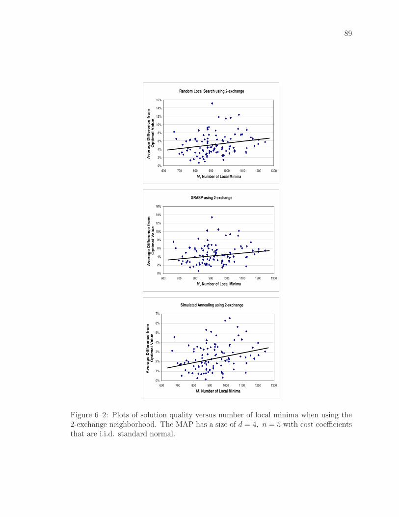
89
Random Local Search using 2-exchange
0%
2%
4%
6%
8%
10%
12%
14%
16%
600 700 800 900 1000 1100 1200 1300
M , Number of Local Minima
Av
era
ge
Dif
fere
nc
e f
ro
m
Op
tim
al
Va
lue
GRASP using 2-exchange
0%
2%
4%
6%
8%
10%
12%
14%
16%
600 700 800 900 1000 1100 1200 1300
M , Number of Local Minima
Av
era
ge
Dif
fere
nc
e f
ro
m
Op
tim
al
Va
lue
Simulated Annealing using 2-exchange
0%
1%
2%
3%
4%
5%
6%
7%
600 700 800 900 1000 1100 1200 1300
M , Number of Local Minima
Av
era
ge
Dif
fere
nc
e f
ro
m
Op
tim
al
Va
lue
Figure 6–2: Plots of solution quality versus number of local minima when using the2-exchange neighborhood. The MAP has a size of d = 4, n = 5 with cost coefficientsthat are i.i.d. standard normal.
90
Random Local Search using 3-exchange
0%
2%
4%
6%
8%
10%
12%
14%
16%
300 350 400 450 500 550 600 650 700 750
M , Number of Local Minima
Av
era
ge
Dif
fere
nc
e f
ro
m
Op
tim
al
Va
lue
GRASP using 3-exchange
0%
2%
4%
6%
8%
10%
12%
14%
16%
300 350 400 450 500 550 600 650 700 750
M , Number of Local Minima
Av
era
ge
Dif
fere
nc
e f
ro
m
Op
tim
al
Va
lue
Simulated Annealing using 3-exchange
0%
1%
2%
3%
4%
5%
6%
7%
300 350 400 450 500 550 600 650 700 750
M, Number of Local Minima
Averag
e D
iffe
ren
ce f
ro
m
Op
tim
al V
alu
e
Figure 6–3: Plots of solution quality versus number of local minima when using a3-exchange neighborhood. The MAP has a size of d = 4, n = 5 with cost coefficientsthat are i.i.d. standard normal.
91
when n > 2. We proved a closed form expression for E[M ] when n = 2, d ≥ 3. The
expression holds for any case when the cost coefficients are i.i.d. from a continuous
distribution. Upper and lower bounds to E[M ] are given in the case of n > 2, d ≥ 3
and cost coefficients are i.i.d. standard normal variables. The bounds show that
E[M ] is exponential with respect to d. Finally, experimental results are provided that
show at least three heuristics that rely, at least partly, on local search are adversely
impacted by increasing number of local minima.
CHAPTER 7MAP TEST PROBLEM GENERATOR
Test problems are often used in computational studies to establish the efficiency
of solution methods, or, as pointed out by Yong and Pardalos [112], test problems are
important for comparing new solution methods against existing algorithms. Along
with a collection of combinatorial test problems, the book by Floudas et al. [39]
emphasizes the importance of well designed problems. As Barr et al. [12] point out,
there is a definite need for a variety of test problems to check the robustness and
accuracy of proposed algorithms. A probabilistic approach in the development and
study of test problems may result in higher quality test instances.
In this chapter we develop a test problem generator for the MAP and use a
probabilistic analysis to determine its effectiveness in generating hard problems.
7.1 Introduction
There are at least four basic sources of test problems:
1. Real world problems (e.g. [95]).
2. Libraries of standard test problems [20, 59, 95].
3. Randomly generated problems such as those with cost coefficients drawn inde-
pendently from some distribution such as uniform on [0,1].
4. Problems generated from an algorithm such as the quadratic test problem gen-
erator [112].
As noted by Reilly [94], real world problems have the advantage of providing
results consistent with at least some problems encountered in practice. However,
in most cases there is not a sizeable set of real world problems to constitute a sat-
isfactory experiment. Libraries of standard test problems serve as a good source
of problems; however, again there may not be enough of the right-sized problems.
92
93
Randomly generated problems provide virtually an infinite supply of test problems;
however, the optimal solution to large problems may remain unknown. An additional
hazard with randomly generated problems is they are often “easy” to solve [21, 101].
These may be significant issues when evaluating the performance of a new algorithm.
Generated test problems with known solutions can also be in virtually infinite supply
and, importantly, a unique known solution can be very useful in fully evaluating a
solution algorithm’s performance. Careful study of generated problems is necessary
to determine the relative usefulness of the problems in terms of difficulty, realism,
etc. Sanchis [99] mentions generated problems should have the following properties
• polynomial-time generability with known solution
• hardness
• diversity
Sanchis goes on to say that meeting all three requirements can be difficult. For ex-
ample, meeting the first requirement can be quite simple by creating a trivial instance;
however, a trivial instance would most likely violate the second property. Also, it is
recognized by many researchers that there is a need for standardized representations
of problem instances [40]. A popular technique in designing nonlinear programming
test problems is the use of Karush-Kuhn-Tucker optimality conditions as proposed by
Rosen and Suzuki [97]. Test problem generators for integer-programming problems
are difficult to construct and require a deep insight into the problem structure [56].
An interesting approach to test problem generation is that of the Discrete Math-
ematics and Theoretical Computer Science (DIMACS) challenges [34]. Over the past
decade, the challenges have had the goal of encouraging the experimental evaluation
of algorithms. It is recognized that comparisons must be made on standard test prob-
lems that are included as part of the challenges. Challenges have been held for TSP,
cliques, coloring, and satisfiability.
94
To summarize sources of test problems, the following two sections describe avail-
able test problem generators and libraries that include ready-made test problems.
7.1.1 Test Problem Generators
Steiner problem in graphs. Khoury et al. [56] present a binary-programming
formulation for the Steiner problem in graphs which is well known to be NP -hard.
They use this formulation to generate test problems with known optimal solutions.
The technique uses the KKT optimality conditions on the corresponding quadrati-
cally constrained optimization problem.
Maximum clique problem. In the comprehensive work by Hasselberg et
al. [48], the authors consider several interesting problems. They introduce different
test problem generators that arise from a variety of practical applications as well
as the problem of maximum clique. Applications include coding theory problems,
problems from Keller’s Conjecture, and problems in fault diagnosis. Work by Sanchis
and Jagota [100] discusses a test problem generator that builds the complementary
minimum vertex cover problem. The hardness of their generated problems relies on
construction parameters. Sanchis [99] provides an algorithm to generate minimum
vertex cover problem that is diverse, hard and of known solution.
Quadratic assignment problem (QAP). As early as 1991, Pardalos [79]
provided a method for constructing test problems for constrained bivalent quadratic
programming. Also provided is a standardized random test problem generator for
the unconstrained quadratic zero-one programming problem. Yong and Pardalos [112]
provide easy methods to generate test problems with known optimal solutions for gen-
eral types of QAPs. A code is available at http://www.ici.ro/camo/forum/92006.
FOR. Calamai et al. [24] describe a technique for generating convex, strictly concave
and indefinite (bilinear or not) quadratic programming problems. Their approach
95
involves combining m two-variable problems to construct a separable quadratic prob-
lem. Palubeckis [77] provides a method for generating hard rectilinear QAPs with
known optimal solutions.
Graph colorability. The graph colorability problem is the difficult problem of
finding the least number of colors that colors a graph where no two adjacent nodes are
of the same color. An algorithm for generating a test problem with known solution
can be found in work by Sanchis [99].
Minimum dominating set. A minimum dominating set problem generator
is provided in work by Sanchis [99].
Satisfiability. Achlioptas et al. [2] propose a generator that only outputs
satisfiable problem instances. They show how to finely control the hardness of the
instances by establishing a connection between problem hardness and a kind of phase
transition phenomenon in the space of problem instances. Uchida et al. [108] provide
a web page dedicated to two methods of generating instances of the 3-satisfiability
problem.
Traveling salesman problem (TSP). A web site dedicated to generating
the Euclidean TSP is maintained by Moscato [73]. The site provides information
concerning research in generation of instances of TSPs with known optimal solution.
An approach to generating discrete problems with known optima based on a partial
description of the solution polytope is provided by Pilcher and Rardin [88]. The
approach is used to generate instances of the symmetric traveling salesman problem.
Minimum cut-set. The minimum cut-set is the problem of partitioning a
graph in two parts such that the edges between the two partitions are the minimal
separating set of edges. For applications involving circuit designs, Krishnamurthy
[61] provides an appropriate test problem generator.
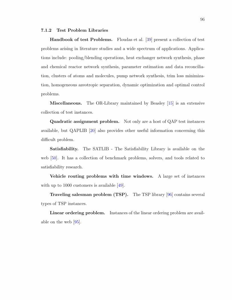
96
7.1.2 Test Problem Libraries
Handbook of test Problems. Floudas et al. [39] present a collection of test
problems arising in literature studies and a wide spectrum of applications. Applica-
tions include: pooling/blending operations, heat exchanger network synthesis, phase
and chemical reactor network synthesis, parameter estimation and data reconcilia-
tion, clusters of atoms and molecules, pump network synthesis, trim loss minimiza-
tion, homogeneous azeotropic separation, dynamic optimization and optimal control
problems.
Miscellaneous. The OR-Library maintained by Beasley [15] is an extensive
collection of test instances.
Quadratic assignment problem. Not only are a host of QAP test instances
available, but QAPLIB [20] also provides other useful information concerning this
difficult problem.
Satisfiability. The SATLIB - The Satisfiability Library is available on the
web [50]. It has a collection of benchmark problems, solvers, and tools related to
satisfiability research.
Vehicle routing problems with time windows. A large set of instances
with up to 1000 customers is available [49].
Traveling salesman problem (TSP). The TSP library [96] contains several
types of TSP instances.
Linear ordering problem. Instances of the linear ordering problem are avail-
able on the web [95].
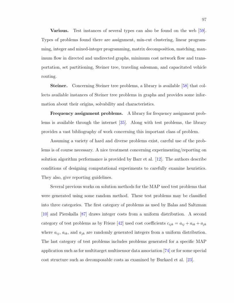
97
Various. Test instances of several types can also be found on the web [59].
Types of problems found there are assignment, min-cut clustering, linear program-
ming, integer and mixed-integer programming, matrix decomposition, matching, max-
imum flow in directed and undirected graphs, minimum cost network flow and trans-
portation, set partitioning, Steiner tree, traveling salesman, and capacitated vehicle
routing.
Steiner. Concerning Steiner tree problems, a library is available [58] that col-
lects available instances of Steiner tree problems in graphs and provides some infor-
mation about their origins, solvability and characteristics.
Frequency assignment problems. A library for frequency assignment prob-
lems is available through the internet [35]. Along with test problems, the library
provides a vast bibliography of work concerning this important class of problem.
Assuming a variety of hard and diverse problems exist, careful use of the prob-
lems is of course necessary. A nice treatment concerning experimenting/reporting on
solution algorithm performance is provided by Barr et al. [12]. The authors describe
conditions of designing computational experiments to carefully examine heuristics.
They also, give reporting guidelines.
Several previous works on solution methods for the MAP used test problems that
were generated using some random method. These test problems may be classified
into three categories. The first category of problems as used by Balas and Saltzman
[10] and Pierskalla [87] draws integer costs from a uniform distribution. A second
category of test problems as by Frieze [42] used cost coefficients cijk = aij + aik + ajk
where aij, aik, and ajk are randomly generated integers from a uniform distribution.
The last category of test problems includes problems generated for a specific MAP
application such as for multitarget multisensor data association [74] or for some special
cost structure such as decomposable costs as examined by Burkard et al. [23].
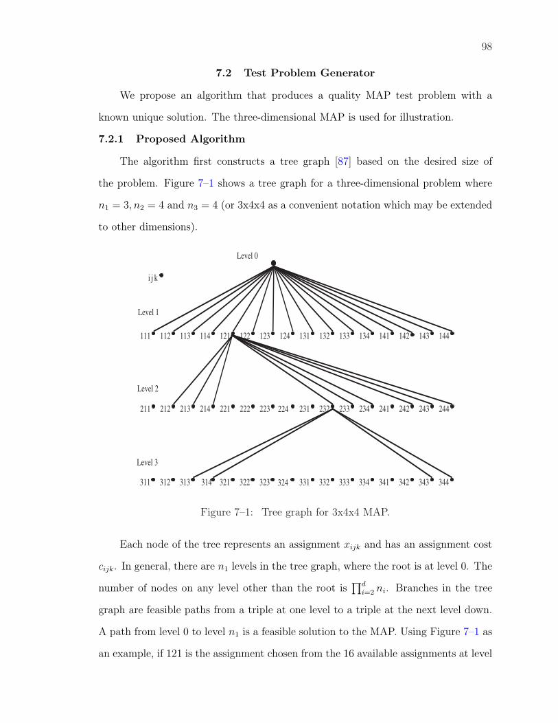
98
7.2 Test Problem Generator
We propose an algorithm that produces a quality MAP test problem with a
known unique solution. The three-dimensional MAP is used for illustration.
7.2.1 Proposed Algorithm
The algorithm first constructs a tree graph [87] based on the desired size of
the problem. Figure 7–1 shows a tree graph for a three-dimensional problem where
n1 = 3, n2 = 4 and n3 = 4 (or 3x4x4 as a convenient notation which may be extended
to other dimensions).
144143142141134133132131124123122121114113112111
244243242241234233232231224223222221214213212211
344343342341334333332331324323322321314313312311
Level 1
Level 2
Level 3
Level 0
i j k
Figure 7–1: Tree graph for 3x4x4 MAP.
Each node of the tree represents an assignment xijk and has an assignment cost
cijk. In general, there are n1 levels in the tree graph, where the root is at level 0. The
number of nodes on any level other than the root is∏d
i=2 ni. Branches in the tree
graph are feasible paths from a triple at one level to a triple at the next level down.
A path from level 0 to level n1 is a feasible solution to the MAP. Using Figure 7–1 as
an example, if 121 is the assignment chosen from the 16 available assignments at level
99
1, then the feasible assignments at the next level are 212, 213, 214, 232, 233, 234,
242, 243, 244. If 232 is then chosen at level 2, then 313, 314, 343, 344 are available
at level 3. Using this procedure, a feasible path is 121, 232, 313.
In addition to the assignment cost, cijk, associated with each node, there is
another cost called Lower Bound Path Cost, lbijk. This is the cost of the assignment
plus the minimum lower bound path cost of any feasible node (assignment) at the
next level down. A lower bound path cost for any node provides a lower bound for
the additional cost of going through that particular node on a path to the lowest
level. The algorithm identifies a feasible solution that will remain the unique optimal
solution. Once this optimal set of assignments is identified, random costs are applied
to each of the assignments in the optimal set. Then working from level n1 to the
highest level of the tree, apply assignment costs, cijk, and lower bound path costs,
lbijk, to each node (except for those on the optimal path that already have these costs
assigned).
The following are procedural steps for generating an MAP of controllable size
with a known unique optimal solution.
Step 1: Based on the dimension and number of elements for each alternative,
build a tree graph of all possible assignments such that
ci1···id = ∞,
lbi1···id = ∞,
∀ i1, i2, . . . , id.
Step 2: Select an optimal path from the root node to a leaf node.
Step 3: Apply random assignment costs that are uniform between some lower
and upper values to each node on the optimal path and update their lower bound
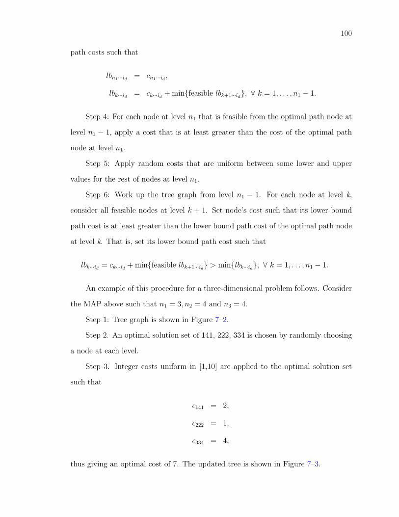
100
path costs such that
lbn1···id = cn1···id ,
lbk···id = ck···id + min{feasible lbk+1···id}, ∀ k = 1, . . . , n1 − 1.
Step 4: For each node at level n1 that is feasible from the optimal path node at
level n1 − 1, apply a cost that is at least greater than the cost of the optimal path
node at level n1.
Step 5: Apply random costs that are uniform between some lower and upper
values for the rest of nodes at level n1.
Step 6: Work up the tree graph from level n1 − 1. For each node at level k,
consider all feasible nodes at level k + 1. Set node’s cost such that its lower bound
path cost is at least greater than the lower bound path cost of the optimal path node
at level k. That is, set its lower bound path cost such that
lbk···id = ck···id + min{feasible lbk+1···id} > min{lbk···id}, ∀ k = 1, . . . , n1 − 1.
An example of this procedure for a three-dimensional problem follows. Consider
the MAP above such that n1 = 3, n2 = 4 and n3 = 4.
Step 1: Tree graph is shown in Figure 7–2.
Step 2. An optimal solution set of 141, 222, 334 is chosen by randomly choosing
a node at each level.
Step 3. Integer costs uniform in [1,10] are applied to the optimal solution set
such that
c141 = 2,
c222 = 1,
c334 = 4,
thus giving an optimal cost of 7. The updated tree is shown in Figure 7–3.
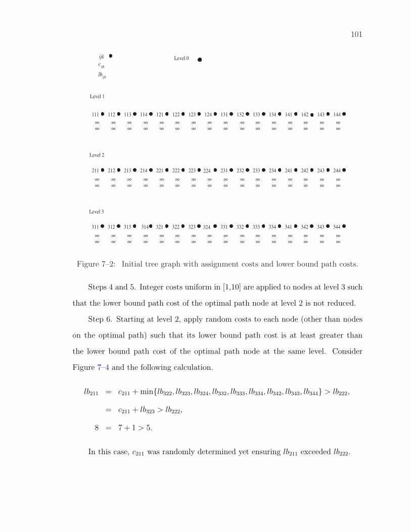
101
144143142141134133132131124123122121114113112111
244243242241234233232231224223222221214213212211
344343342341334333332331324323322321314313312311
Level 1
Level 2
Level 3
Level 0ijk
ijk
ijk
c
lb
∞ ∞ ∞ ∞ ∞ ∞ ∞ ∞ ∞ ∞ ∞ ∞ ∞ ∞ ∞ ∞
∞ ∞ ∞ ∞ ∞ ∞ ∞ ∞ ∞ ∞ ∞ ∞ ∞ ∞ ∞ ∞
∞ ∞ ∞ ∞ ∞ ∞ ∞ ∞ ∞ ∞ ∞ ∞ ∞ ∞ ∞ ∞
∞ ∞ ∞ ∞ ∞ ∞ ∞ ∞ ∞ ∞ ∞ ∞ ∞ ∞ ∞ ∞
∞ ∞ ∞ ∞ ∞ ∞ ∞ ∞ ∞ ∞ ∞ ∞ ∞ ∞ ∞ ∞
∞ ∞ ∞ ∞ ∞ ∞ ∞ ∞ ∞ ∞ ∞ ∞ ∞ ∞ ∞ ∞
Figure 7–2: Initial tree graph with assignment costs and lower bound path costs.
Steps 4 and 5. Integer costs uniform in [1,10] are applied to nodes at level 3 such
that the lower bound path cost of the optimal path node at level 2 is not reduced.
Step 6. Starting at level 2, apply random costs to each node (other than nodes
on the optimal path) such that its lower bound path cost is at least greater than
the lower bound path cost of the optimal path node at the same level. Consider
Figure 7–4 and the following calculation.
lb211 = c211 + min{lb322, lb323, lb324, lb332, lb333, lb334, lb342, lb343, lb344} > lb222,
= c211 + lb323 > lb222,
8 = 7 + 1 > 5.
In this case, c211 was randomly determined yet ensuring lb211 exceeded lb222.
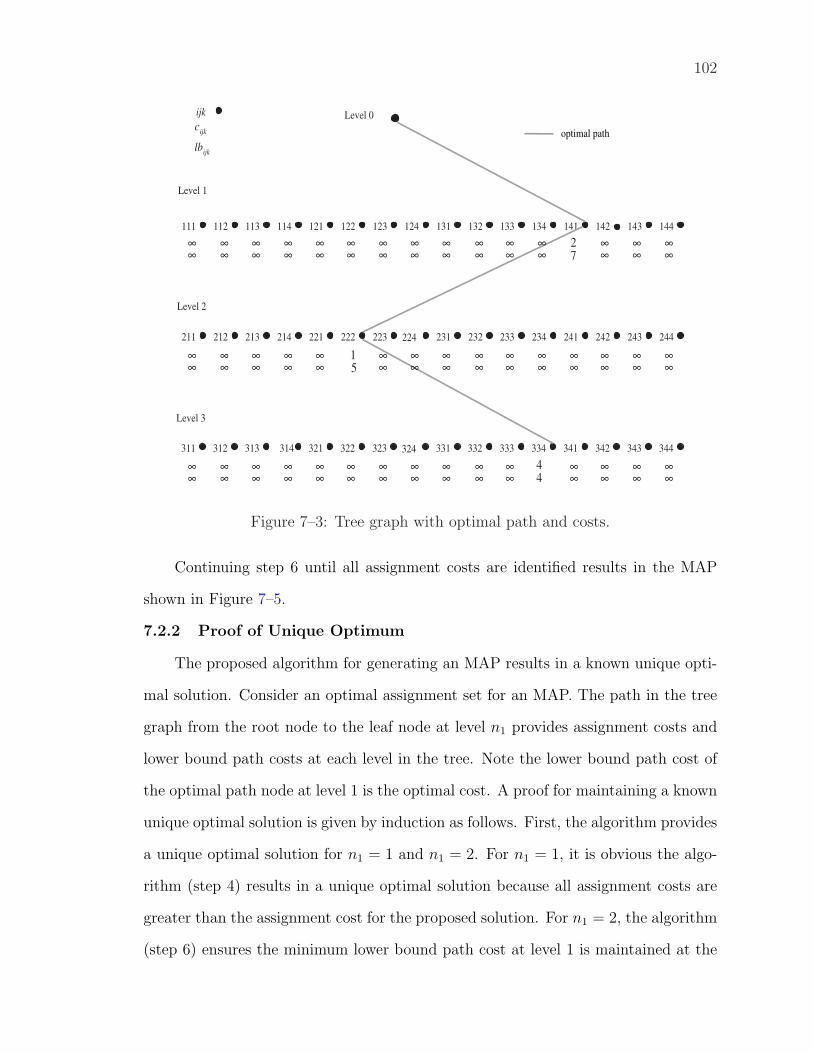
102
144143142141134133132131124123122121114113112111
244243242241234233232231224223222221214213212211
344343342341334333332331324323322321314313312311
Level 1
Level 2
Level 3
Level 0ijk
ijk
ijk
c
lb
27
15
44
optimal path
∞ ∞ ∞ ∞ ∞ ∞ ∞ ∞ ∞ ∞ ∞ ∞ ∞ ∞ ∞
∞ ∞ ∞ ∞ ∞ ∞ ∞ ∞ ∞ ∞ ∞ ∞ ∞ ∞ ∞
∞ ∞ ∞ ∞ ∞ ∞ ∞ ∞ ∞ ∞ ∞ ∞ ∞ ∞ ∞
∞ ∞ ∞ ∞ ∞ ∞ ∞ ∞ ∞ ∞ ∞ ∞ ∞ ∞ ∞
∞ ∞ ∞ ∞ ∞ ∞ ∞ ∞ ∞ ∞ ∞ ∞ ∞ ∞ ∞
∞ ∞ ∞ ∞ ∞ ∞ ∞ ∞ ∞ ∞ ∞ ∞ ∞ ∞ ∞
Figure 7–3: Tree graph with optimal path and costs.
Continuing step 6 until all assignment costs are identified results in the MAP
shown in Figure 7–5.
7.2.2 Proof of Unique Optimum
The proposed algorithm for generating an MAP results in a known unique opti-
mal solution. Consider an optimal assignment set for an MAP. The path in the tree
graph from the root node to the leaf node at level n1 provides assignment costs and
lower bound path costs at each level in the tree. Note the lower bound path cost of
the optimal path node at level 1 is the optimal cost. A proof for maintaining a known
unique optimal solution is given by induction as follows. First, the algorithm provides
a unique optimal solution for n1 = 1 and n1 = 2. For n1 = 1, it is obvious the algo-
rithm (step 4) results in a unique optimal solution because all assignment costs are
greater than the assignment cost for the proposed solution. For n1 = 2, the algorithm
(step 6) ensures the minimum lower bound path cost at level 1 is maintained at the
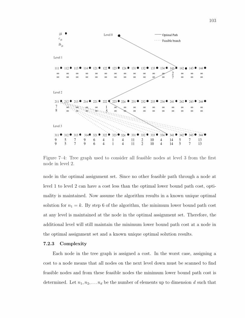
103
144143142141134133132131124123122121114113112111
244243242241234233232231224223222221214213212211
344343342341334333332331324323322321314313312311
Level 1
Level 2
Level 3
Level 0ijk
ijk
ijk
c
lb
78
99
55
77
99
66
44
11
44
1111
22
1010
44
1414
55
77
1313
Optimal Path
Feasible branch
27
15
∞ ∞ ∞ ∞ ∞ ∞ ∞ ∞ ∞ ∞ ∞ ∞ ∞ ∞ ∞
∞ ∞ ∞ ∞ ∞ ∞ ∞ ∞ ∞ ∞ ∞ ∞ ∞ ∞ ∞
∞ ∞ ∞ ∞ ∞ ∞ ∞ ∞ ∞ ∞ ∞ ∞ ∞ ∞
∞ ∞ ∞ ∞ ∞ ∞ ∞ ∞ ∞ ∞ ∞ ∞ ∞ ∞
Figure 7–4: Tree graph used to consider all feasible nodes at level 3 from the firstnode in level 2.
node in the optimal assignment set. Since no other feasible path through a node at
level 1 to level 2 can have a cost less than the optimal lower bound path cost, opti-
mality is maintained. Now assume the algorithm results in a known unique optimal
solution for n1 = k. By step 6 of the algorithm, the minimum lower bound path cost
at any level is maintained at the node in the optimal assignment set. Therefore, the
additional level will still maintain the minimum lower bound path cost at a node in
the optimal assignment set and a known unique optimal solution results.
7.2.3 Complexity
Each node in the tree graph is assigned a cost. In the worst case, assigning a
cost to a node means that all nodes on the next level down must be scanned to find
feasible nodes and from these feasible nodes the minimum lower bound path cost is
determined. Let n1, n2, . . . nd be the number of elements up to dimension d such that
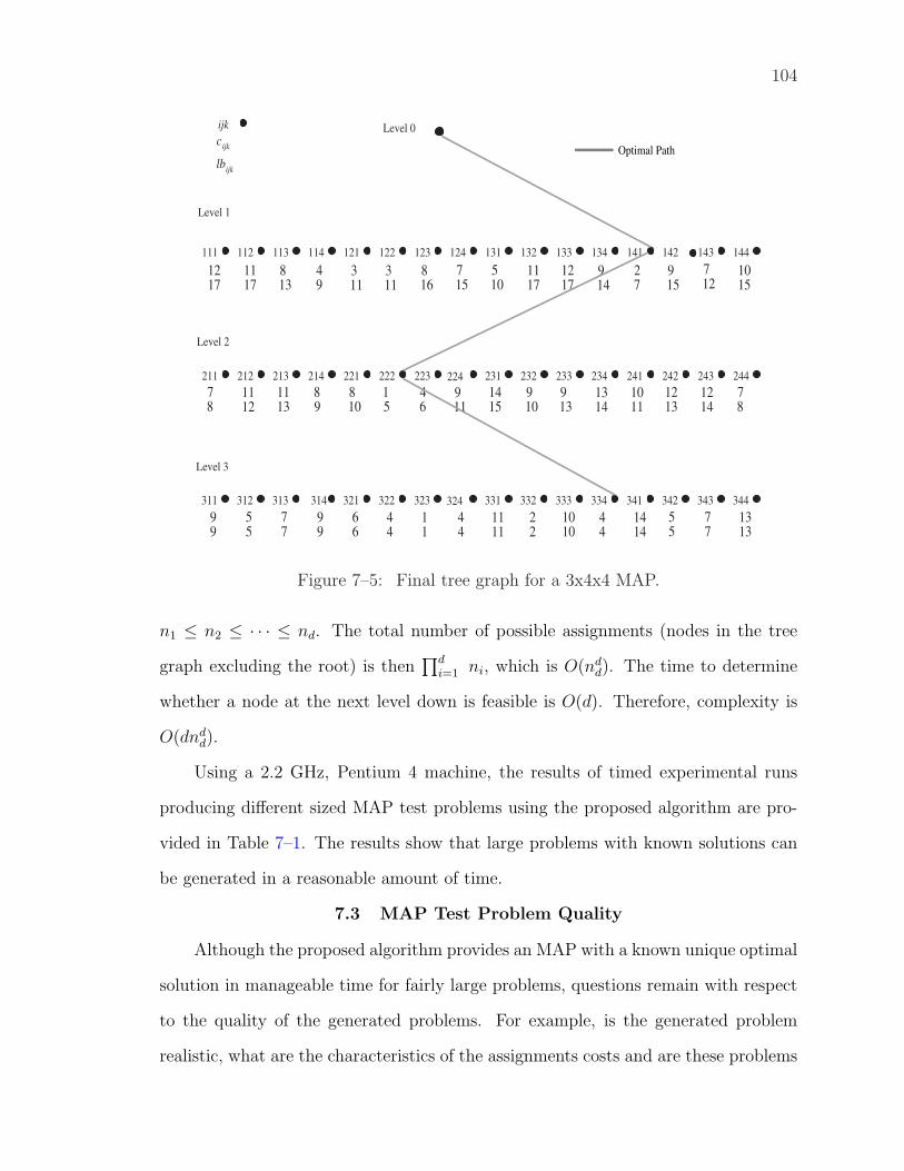
104
144143142141134133132131124123122121114113112111
244243242241234233232231224223222221214213212211
344343342341334333332331324323322321314313312311
Level 1
Level 2
Level 3
Level 0ijk
ijk
ijk
c
lb
1217
1117
813
49
311
311
816
715
510
1117
1217
914
27
915
712
1015
78
1112
1113
89
810
15
46
911
1415
910
913
1314
1011
1213
1214
78
99
55
77
99
66
44
11
44
1111
22
1010
44
1414
55
77
1313
Optimal Path
Figure 7–5: Final tree graph for a 3x4x4 MAP.
n1 ≤ n2 ≤ · · · ≤ nd. The total number of possible assignments (nodes in the tree
graph excluding the root) is then∏d
i=1 ni, which is O(ndd). The time to determine
whether a node at the next level down is feasible is O(d). Therefore, complexity is
O(dndd).
Using a 2.2 GHz, Pentium 4 machine, the results of timed experimental runs
producing different sized MAP test problems using the proposed algorithm are pro-
vided in Table 7–1. The results show that large problems with known solutions can
be generated in a reasonable amount of time.
7.3 MAP Test Problem Quality
Although the proposed algorithm provides an MAP with a known unique optimal
solution in manageable time for fairly large problems, questions remain with respect
to the quality of the generated problems. For example, is the generated problem
realistic, what are the characteristics of the assignments costs and are these problems
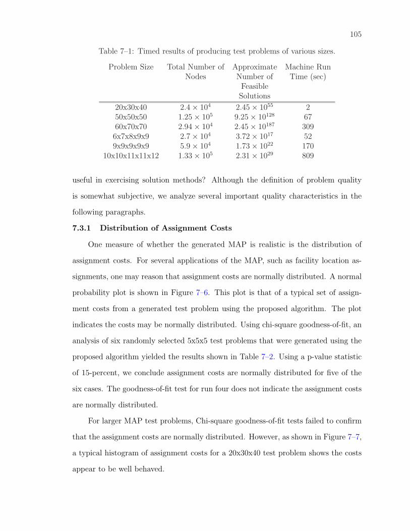
105
Table 7–1: Timed results of producing test problems of various sizes.
Problem Size Total Number of Approximate Machine RunNodes Number of Time (sec)
FeasibleSolutions
20x30x40 2.4× 10⁴ 2.45× 1055 250x50x50 1.25× 10⁵ 9.25× 10128 6760x70x70 2.94× 10⁴ 2.45× 10187 3096x7x8x9x9 2.7× 10⁴ 3.72× 10¹⁷ 529x9x9x9x9 5.9× 10⁴ 1.73× 10²² 170
10x10x11x11x12 1.33× 10⁵ 2.31× 1029 809
useful in exercising solution methods? Although the definition of problem quality
is somewhat subjective, we analyze several important quality characteristics in the
following paragraphs.
7.3.1 Distribution of Assignment Costs
One measure of whether the generated MAP is realistic is the distribution of
assignment costs. For several applications of the MAP, such as facility location as-
signments, one may reason that assignment costs are normally distributed. A normal
probability plot is shown in Figure 7–6. This plot is that of a typical set of assign-
ment costs from a generated test problem using the proposed algorithm. The plot
indicates the costs may be normally distributed. Using chi-square goodness-of-fit, an
analysis of six randomly selected 5x5x5 test problems that were generated using the
proposed algorithm yielded the results shown in Table 7–2. Using a p-value statistic
of 15-percent, we conclude assignment costs are normally distributed for five of the
six cases. The goodness-of-fit test for run four does not indicate the assignment costs
are normally distributed.
For larger MAP test problems, Chi-square goodness-of-fit tests failed to confirm
that the assignment costs are normally distributed. However, as shown in Figure 7–7,
a typical histogram of assignment costs for a 20x30x40 test problem shows the costs
appear to be well behaved.
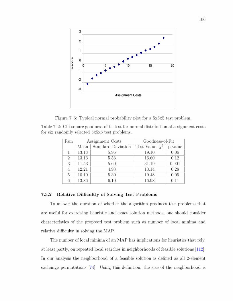
106
-3
-2
-1
0
1
2
3
0 5 10 15 20
Assignment Costs
z-s
co
re
Figure 7–6: Typical normal probability plot for a 5x5x5 test problem.
Table 7–2: Chi-square goodness-of-fit test for normal distribution of assignment costsfor six randomly selected 5x5x5 test problems.
Run Assignment Costs Goodness-of-FitMean Standard Deviation Test Value, χ2 p-value
1 13.18 5.95 19.10 0.062 13.13 5.53 16.60 0.123 11.53 5.60 31.19 0.0014 12.21 4.93 13.14 0.285 10.10 5.30 19.48 0.056 13.86 6.10 16.98 0.11
7.3.2 Relative Difficultly of Solving Test Problems
To answer the question of whether the algorithm produces test problems that
are useful for exercising heuristic and exact solution methods, one should consider
characteristics of the proposed test problem such as number of local minima and
relative difficulty in solving the MAP.
The number of local minima of an MAP has implications for heuristics that rely,
at least partly, on repeated local searches in neighborhoods of feasible solutions [112].
In our analysis the neighborhood of a feasible solution is defined as all 2-element
exchange permutations [74]. Using this definition, the size of the neighborhood is
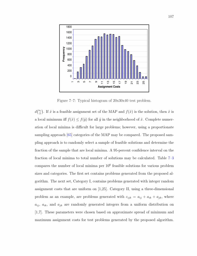
107
0
200
400
600
800
1000
1200
1400
1600
1800
1 3 5 7 9
11
13
15
17
19
21
23
25
Assignment Costs
Fre
qu
en
cy
Figure 7–7: Typical histogram of 20x30x40 test problem.
d(
n1
2
). If x is a feasible assignment set of the MAP and f(x) is the solution, then x is
a local minimum iff f(x) ≤ f(y) for all y in the neighborhood of x. Complete numer-
ation of local minima is difficult for large problems; however, using a proportionate
sampling approach [65] categories of the MAP may be compared. The proposed sam-
pling approach is to randomly select a sample of feasible solutions and determine the
fraction of the sample that are local minima. A 95-percent confidence interval on the
fraction of local minima to total number of solutions may be calculated. Table 7–3
compares the number of local minima per 106 feasible solutions for various problem
sizes and categories. The first set contains problems generated from the proposed al-
gorithm. The next set, Category I, contains problems generated with integer random
assignment costs that are uniform on [1,25]. Category II, using a three-dimensional
problem as an example, are problems generated with cijk = aij + aik + ajk, where
aij, aik, and ajk are randomly generated integers from a uniform distribution on
[1,7]. These parameters were chosen based on approximate spread of minimum and
maximum assignment costs for test problems generated by the proposed algorithm.
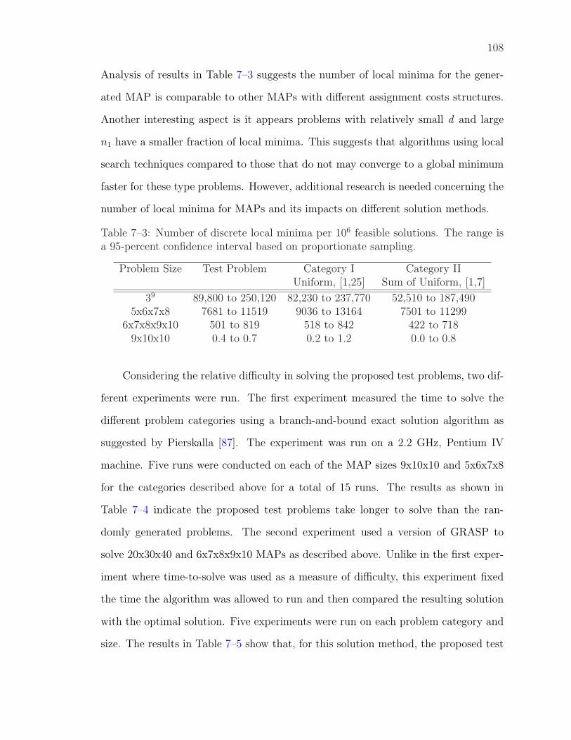
108
Analysis of results in Table 7–3 suggests the number of local minima for the gener-
ated MAP is comparable to other MAPs with different assignment costs structures.
Another interesting aspect is it appears problems with relatively small d and large
n1 have a smaller fraction of local minima. This suggests that algorithms using local
search techniques compared to those that do not may converge to a global minimum
faster for these type problems. However, additional research is needed concerning the
number of local minima for MAPs and its impacts on different solution methods.
Table 7–3: Number of discrete local minima per 106 feasible solutions. The range isa 95-percent confidence interval based on proportionate sampling.
Problem Size Test Problem Category I Category IIUniform, [1,25] Sum of Uniform, [1,7]
39 89,800 to 250,120 82,230 to 237,770 52,510 to 187,4905x6x7x8 7681 to 11519 9036 to 13164 7501 to 11299
6x7x8x9x10 501 to 819 518 to 842 422 to 7189x10x10 0.4 to 0.7 0.2 to 1.2 0.0 to 0.8
Considering the relative difficulty in solving the proposed test problems, two dif-
ferent experiments were run. The first experiment measured the time to solve the
different problem categories using a branch-and-bound exact solution algorithm as
suggested by Pierskalla [87]. The experiment was run on a 2.2 GHz, Pentium IV
machine. Five runs were conducted on each of the MAP sizes 9x10x10 and 5x6x7x8
for the categories described above for a total of 15 runs. The results as shown in
Table 7–4 indicate the proposed test problems take longer to solve than the ran-
domly generated problems. The second experiment used a version of GRASP to
solve 20x30x40 and 6x7x8x9x10 MAPs as described above. Unlike in the first exper-
iment where time-to-solve was used as a measure of difficulty, this experiment fixed
the time the algorithm was allowed to run and then compared the resulting solution
with the optimal solution. Five experiments were run on each problem category and
size. The results in Table 7–5 show that, for this solution method, the proposed test
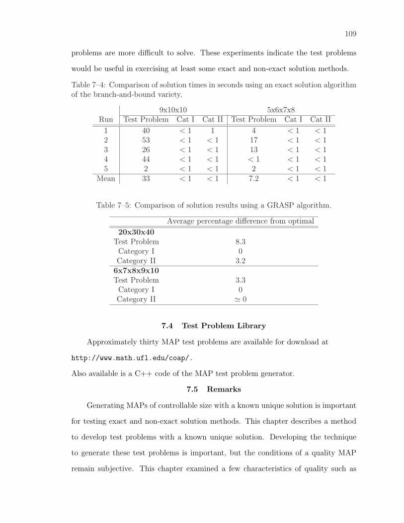
109
problems are more difficult to solve. These experiments indicate the test problems
would be useful in exercising at least some exact and non-exact solution methods.
Table 7–4: Comparison of solution times in seconds using an exact solution algorithmof the branch-and-bound variety.
9x10x10 5x6x7x8Run Test Problem Cat I Cat II Test Problem Cat I Cat II
1 40 < 1 1 4 < 1 < 12 53 < 1 < 1 17 < 1 < 13 26 < 1 < 1 13 < 1 < 14 44 < 1 < 1 < 1 < 1 < 15 2 < 1 < 1 2 < 1 < 1
Mean 33 < 1 < 1 7.2 < 1 < 1
Table 7–5: Comparison of solution results using a GRASP algorithm.
Average percentage difference from optimal
20x30x40Test Problem 8.3Category I 0Category II 3.2
6x7x8x9x10Test Problem 3.3Category I 0Category II ' 0
7.4 Test Problem Library
Approximately thirty MAP test problems are available for download at
http://www.math.ufl.edu/coap/.
Also available is a C++ code of the MAP test problem generator.
7.5 Remarks
Generating MAPs of controllable size with a known unique solution is important
for testing exact and non-exact solution methods. This chapter describes a method
to develop test problems with a known unique solution. Developing the technique
to generate these test problems is important, but the conditions of a quality MAP
remain subjective. This chapter examined a few characteristics of quality such as
110
distribution of assignment costs, number of local minima and difficulty to solve. Based
on these few characteristics, the generated MAP test problems appear to be realistic
and challenging for exercising exact and heuristic solution methods.
CHAPTER 8CONCLUSIONS
The work in this dissertation examined combinatorial problems from a proba-
bilistic approach in an effort to improve existing solution methods or find new algo-
rithms that perform better. A probabilistic analysis of combinatorial problems is a
very broad subject; however, the context here is the study of input data and solution
values.
We investigated characteristics of the mean optimal solution values for random
multidimensional assignment problems (MAPs) with axial constraints. In the cases
of uniform and exponential costs, experimental data indicates that the mean optimal
value converges to zero when the problem size increases. In the case of standard
normal costs, experimental data indicates the mean optimal value goes to negative
infinity with increasing problem size. Using curve fitting techniques, we developed
numerical estimates of the mean optimal value for various sized problems. The exper-
iments indicate that numerical estimates are quite accurate in predicting the optimal
solution value of a random instance of the MAP.
Our experimental approach to the MAP can be easily extended to other hard
problems. For example, solution approaches to the QAP may benefit from numerical
estimates of the optimal values. Additionally, future work is needed using real-world
data. Other interesting work includes closer study of the numerical models. It is
clear the parameters asymptotically approach particular values. Questions remain on
what these values are and why they exist.
Further research and thought are needed to see how the numerical estimates
of the mean optimal values can be used to improve existing solution algorithms or
developing new algorithms.
111
112
Using a novel probabilistic approach, we proved the asymptotic characteristics
of the mean optimal costs of MAPs. Further work is needed to develop and prove
more global theorems on the asymptotic characteristics of combinatorial problems.
In the example of the MAP, it appears the lower support of the parent distribution
has some bearing on the mean optimal costs.
We investigated the expected number of local minima for random instances of
the MAP and reported on their impact on three different solution algorithms that
rely on local neighborhood searches. We also provided a closed form relationship
for the average number of local minima in a special case of the MAP. We provided
bounds on the average in more general cases of the MAP. More work in needed in
this area. For example, an interesting study is to consider the distribution of local
minima across the solution landscape and the distance between these local minima.
An answer to this question may lead to novel solution approaches.
A probabilistic approach was used to develop an MAP test problem generator
that creates difficult problems with known unique solutions. Test problem generators
are often very useful to researchers. Additional work is necessary to create other
generators and to use a probabilistic approach to ensure the generators produce hard
problems that are useful in exercising solution algorithms.
Finally, continued exploitation of dual-use applications (military and civilian)
is of great interest. Cross-fertilization of ideas benefits practitioners in all areas of
research.
REFERENCES
[1] N.M.M. Abreu, P.O.B. Netto, T. M. Querido, and E.F. Gouvea, “Classes ofquadratic assignment problem instances: Isomorphism and difficulty measureusing a statistical approach,” Discrete Applied Mathematics 124:103–116, 2002.
[2] D. Achlioptas, C. Gomes, H. Kautz, and B. Selman, “Generating satisfiableproblem instances,” American Association for Artificial Intelligence, pp. 256–261, 2000.
[3] R.K. Ahuja, T.L. Magnanti, and J.B. Orlin, Network Flows: Theory, Algo-rithms, and Applications, Prentice-Hall, Englewood Cliffs, NJ, 1993.
[4] R.M. Aiex, M.G.C. Resende, P.M. Pardalos, and G. Toraldo, “GRASP withpath relinking for the three-index assignment problem,” Technical report,AT&T Labs Research, Florham Park, NJ 07733, 2001.
[5] D. Aldous, “Asymptotics in the random assignment problem,” Probab. Th.Related Fields, 93:507–534, 1992.
[6] D. Aldous and J.M. Steele, “The objective method: probabilistic combinatorialoptimization and local weak convergence,” Discrete and Combinatorial Proba-bility, H. Kesten (ed.), Springer-Verlag, 2003.
[7] N. Alon and J. Spencer, The Probabilistic Method, 2nd Edition, InterscienceSeries in Discrete Mathematics and Optimization, John Wiley, New York, 2000.
[8] S. M. Andrijich and L. Caccetta, “Solving the multisensor data associationproblem,” Nonlinear Analysis, 47:5525–5536, 2001.
[9] E. Angel and V. Zissimopoulos, “On the landscape ruggedness of the quadraticassignment problem,” Theoretic Computer Science, 263:159–172, 2001.
[10] E. Balas and M.J. Saltzman, “An algorithm for the three-index assignmentproblem,” Operations Research, 39:150–161, 1991.
[11] Y. Bar-Shalom, K. Pattipati, and M. Yeddanapudi, “IMM estimation formultitarget-multisensor air traffic surveillance,” Proceedings of the IEEE,85(1):80–94, January 1997.
[12] R.S. Barr, B.L. Golden, J.P. Kelly, M.G.C. Resende and W.R. Stewart, “De-signing and reporting on computational experiments with heuristic methods,”J. Heuristics, 1:9–32, 1995.
113
114
[13] A. Barvinok and T. Stephen, “On the distribution of values in the quadraticassignment problem,” in Novel Approaches to Hard Discrete Optimization, P.Pardalos and Henry Wolkowicz (eds.) Fields Institute Communications, vol. 37,2003.
[14] J. Beardwood, J.H. Halton, and J.M. Hammersley, “The shortest path throughmany points.” Proc. Cambridge Philosophical Society 55:299–327, 1959.
[15] J.E. Beasley, OR-Library: Distributing test problems by electronic mail, Jour-nal of the Operational Research Society, 41(11):1069–1072, 1990, web basedlibrary accessed at http://www.ms.ic.ac.uk/info.html on 1 May 2004.
[16] A. Beck, “On the number of local maxima for the max-cut and bisection prob-lems,” School of Mathematical Sciences, Tel-Aviv University, June 2003.
[17] A.G. Bhatt and R. Roy, “On a random directed spanning tree,” Indian Statis-tical Institute, Delhi Centre, New Delhi India, 2 May 2003.
[18] B. Bollobas, D. Gamarnik, O. Riordan, and B. Sudakov, “On the value of arandom minimum weight Steiner tree,” Combinatorica, 24(2):187–207, 2004.
[19] R.E. Burkard, “Selected topics on assignment problems,” Discrete AppliedMathematics, 123:257–302, 2002.
[20] R. Burkard, E. Cela, S. Karisch and F. Rendlqaplib, A Quadratic AssignmentProblem Library, accessed at http://www.opt.math.tu-graz.ac.at/qaplib/on 1 May 2004.
[21] R. Burkard and U. Fincke, “Probabilistic asymptotic properties of some com-binatorial optimization problems,” Discrete Appl. Math., 12:21–29, 1985.
[22] R. Burkard, B. Klinz, and R. Rudolf, “Perspectives of Monge properties inoptimization,” Discrete Applied Mathematics, 70:95–161, 1996.
[23] R. Burkard, R. Rudolf, and G.J. Woeginger, “Three-dimensional axial assign-ment problems with decomposible cost coefficients,” Discrete Applied Mathe-matics, 65:123–139, 1996.
[24] P.H. Calamai, L.N. Vicente and J.J. Judice, “A new technique for generatingquadratic programming test problems,” Mathematical Programming, 61:215–231, 1993.
[25] G. Chen and L. Hong, “A genetic algorithm based multi-dimensional data asso-ciation algorithm for multi-sensor multi-target tracking,” Mathl. Comput. Mod-elling, 26(4):57–69, 1997.
115
[26] B.H. Chiarini, W. Chaovalitwongse, and P. Pardalos, “A new algorithm forthe triangulation of input-output tables in eEconomics,” in Supply Chain andFinance, P. Pardalos, A. Migdalas, and G. Baourakis (eds.), World Scientific,New Jersey, 2004.
[27] W. Clemons, D. Grundel, and D. Jeffcoat, “Applying simulated annealing onthe multidimensional assignment problem,” in Theory and Algorithms for Co-operative Systems, D. Grundel, R. Murphey, and P. Pardalos (eds.), WorldScientific, New Jersey, (to appear) 2004.
[28] D. Coppersmith and G. Sorkin, “Constructive bounds and exact expecta-tions for the random assignment problem,” Random Structures and Algorithms,15:133–144, 1999.
[29] D. Coppersmith and G. Sorkin, “On the expected incremental cost of a mini-mum assignment,” Technical report, IBM T.J. Watson Research Center, 1999.
[30] Y. Crama, A. Kolen, A. Oerlemans, and F. Spieksma, “Throughput rate op-timization in the automated assembly on printed circuit boards,” Annals ofOperation Research, 26:455–480.
[31] Y. Crama and F. Spieksma, “Approximate algorithms for three-dimensional as-signment problems with triangle inequalities,” European Journal of OperationalResearch, 60:273–279, 1992.
[32] H. Cramer, Mathematical Methods of Statistics, Princeton University Press,Princeton, New Jersey, 1957.
[33] H. David, Order Statistics, John Wiley and Sons, Inc., New York, 1970.
[34] DIMACS Center, Rutgers University, NJ, accessed at http://dimacs.
rutgers.edu/ on 1 May 2004.
[35] A. Eisenblatter and A. Koster, FAP web, A website about frequency assignmentproblems, accessed at http://fap.zib.de/index.php on 1 May 2004.
[36] T.A. Feo and M.G.C. Resende, “A probabilistic heuristic for a computationallydifficult set covering problem,” Operations Research Letters, 8:67–71, 1989.
[37] T.A. Feo and M.G.C. Resende, “Greedy randomized adaptive search proce-dures,” Journal of Global Optimization, 6:109–133, 1995.
[38] P. Festa and M.G.C. Resende, “GRASP: an annotated bibliography,” Technicalreport, AT&T Labs Research, Florham Park, NJ 07733, 2000.
[39] C.A. Floudas, P.M. Pardalos, C.S. Adjiman, W.R. Esposito, Z.H. Gms, S.T.Harding, J.L. Klepeis, C.A. Meyer, and C.A. Schweiger, Handbook of Test Prob-lems in Local and Global Optimization, Kluwer, Dordrecht, Netherlands, 1999.
116
[40] R. Fourer, L. Lopes, and K. Martin, “LPFML: a W3C XML schema for lin-ear programming,” working paper accessed at http://gsbkip.uchicago.edu/fml/paper.html on 1 May 2004.
[41] A.M. Frieze, “On the value of a random minimum spanning tree problem,”Discrete Appl. Math., 10:47–56, 1985.
[42] A.M. Frieze and J. Yadegar, “An algorithm for solving 3-dimensional assign-ment problems with application to scheduling a teaching practice,” Journal ofOperational Research Society, 32:989–995, 1981.
[43] R. Garcıa and P. Stadler, “Correlation length, isotropy and meta-stable states,”Physica D, 107:240–254, 1997.
[44] M.R. Garey and D.S. Johnson, Computers and Intractability: A Guide to theTheory of NP-Completeness, W.H. Freeman, New York, 1979.
[45] J. Garnier and L. Kallel, “Efficiency of local search with multiple local optima,”SIAM J. Discrete Math, 15(1):122-141, 2002.
[46] A. Gosavi, Simulation-Based Optimization: Parametric Optimization Tech-niques and Reinforcement Learning, Kluwer Academic Publishing, Norwell,MA, pp. 110–117, 2003.
[47] P. Hansen and N. Mladenovic, “Variable neighborhood search,” in Handbookof Applied Optimization, P.M. Pardalos and M.G.C. Resende (eds.), OxfordUniversity Press, New York NY, Ch. 3.6.9, pp. 221–234, 2002.
[48] J. Hasselberg, P.M. Pardalos and G. Vairaktarakis, “Test case generators andcomputational results for the maximum clique problem,” Journal of GlobalOptimization, 3:463–482, 1993.
[49] J. Homberger, Extended SOLOMON’s vehicle routing problems with time win-dows, accessed at http://www.fernuni-hagen.de/WINF/touren/menuefrm/
probinst.htm on 1 May 2004.
[50] H. Hoos and T. Sttzle, SATLIB - The satisfiability library, Darmstadt Univer-sity of Technology, accessed at http://www.satlib.org/ on 1 May 2004.
[51] R. Horst, P.M. Pardalos, and N.V. Thoai. Introduction to Global Optimization,2nd ed. Kluwer Academic Publishers, Dordrecht, Boston, London, 2000.
[52] B. Huang, L. Perkovicc, and E. Schmutz, “Inexpensive d-dimensional match-ings,” Random Structures and Algorithms, 20(1):50–58, 2002.
[53] D. Johnson, C. Aragon, L. McGeoch, and C. Schevon, “Optimization by simu-lated annealing: an experimental evalution; part I, graph partitioning,” Oper-ations Research, 37(6):865–892, 1989.
117
[54] R.M. Karp, “The probabilistic analysis of some combinatorial search algo-rithms,” in Algorithms and Complexity: New Directions and Recent Results,J.F. Taub (ed.), Academic Press, New York, pp. 1–19, 1976.
[55] R.M. Karp, “An upper bound on the expected cost of an optimal assignment,”in Discrete Algorithms and Complexity, D. Johnson et al. (eds.), AcademicPress, pp. 1–4, 1987.
[56] B.N. Khoury, P.M. Paradalos and D.-Z Du, “A test problem generator forthe steiner problem in graphs,” ACM Transactions on Mathematical Software,19:4:509-522, 1993.
[57] S. Kirkpatrick, C. Gelatt, and M. Vecchi. “Optimization by simulated anneal-ing,” Science, 220:671–680, 1983.
[58] T. Koch, A. Martin and S. Voß, SteinLib: an updated library on steiner treeproblems in graphs, accessed at http://elib.zib.de/steinlib/steinlib.
php on 1 May 2004.
[59] Konrad-Zuse-Zentrum fr Informationstechnik Berlin (ZIB), 1994-2002, accessedat http://elib.zib.de/pub/Packages/mp-testdata/index.html on 1 May2004.
[60] T.C. Koopmans and M.J. Beckmann, “Assignment problems and the locationof economic activities,” Econometrica, 25:53–76, 1957.
[61] B. Krishnamurthy, “Constructing test cases for partitioning heuristics,” IEEETransactions on Computers, 36(9):1112–1114, September 1987.
[62] H.W. Kuhn, “The Hungarian method for solving the assignment problem,”Naval Research Logistics Quarterly, 2:83–97, 1955.
[63] A.M. Law and W.D. Kelton, Simulation Modeling and Analysis, 2nd ed.,McGraw-Hill, Inc., New York, 1991.
[64] A.J. Lazarus, “The assignment problem with uniform (0,1) cost matrix,” Mas-ter’s Thesis, Dept. of Mathematics, Princeton University, 1979.
[65] E.E. Lewis, Introduction to Reliability Engineering, 2nd ed., John Wiley andSons, New York, pp. 25–30, 1996.
[66] S. Lin and B.W. Kernighan, “An effective heuristic algorithm for the travelingsalesman problem,” Operations Research, 21:498–516, 1973.
[67] S. Linusson and J. Waastlund, “A proof of Parisi’s conjecture on the randomassignment problem,” accessed at http://www.mai.liu.se/~svlin/ on 1 May2004.
118
[68] J. Long and A.C. Williams, “On the number of local maxima in quadratic 0-1programs,” Operations Research Letters, 13:75–78, 1993.
[69] G.S. Lueker, “Optimization problems on graphs with independent random edgeweights,” SIAM Journal of Computing, 10(2):338–351, May 1981.
[70] N. Metropolis, A. Rosenbluth, M. Rosenbluth, A. Teller, and E. Teller, “Equa-tion of state calculations by fast computing machines,” J. Chem. Phys.,21(6):1087–1092, 1953.
[71] M. Mezard and G. Parisi, “Replicas and optimization,” J Phys Letters, 46:771–778, 1985.
[72] M. Mezard and G. Parisi, “On the solution of the random link matching prob-lems,” J Phys Letters, 48:1451–1459, 1987.
[73] P. Moscato, “Fractal instances of the traveling salesman problem,” Densis,FEEC, UNICAMP Universidade Estadual de Campinas, accessed at http://
www.ing.unlp.edu.ar/cetad/mos/FRACTAL_TSP_home.html on 1 May 2004.
[74] R. Murphey, P. Pardalos, and L. Pitsoulis, “A greedy randomized adaptivesearch procedure for the multitarget multisensor tracking problem,” in Networkdesign: Connectivity and Facilities Location, volume 40 of DIMACS Series onDiscrete Mathematics and Theoretical Computer Science, P.M. Pardalos andD.-Z. Du (eds.), pp. 277–302, 1998.
[75] C. Nair, B. Prabhakar, and M. Sharma, “A proof of the conjecture due to Parisifor the finite random assignment problem,” accessed at http://www.stanford.edu/~balaji/papers/parisi.pdf on 1 May 2004.
[76] B. Olin, “Asymptotic properties of random assignment problems,” PhD thesis,Kungl Tekniska Hogskolan, Stockholm, Sweden, 1992.
[77] G. Palubeckis, “Generating hard test instances with known optimal solution forthe rectilinear quadratic assignment problem,” Journal of Global Optimization,15:127–156, 1999.
[78] R. Palmer, “Optimization on rugged landscapes,” Molecular Evolution onRugged Ladscapes: Proteins, RNA, and the Immune System, A. Perelson andS. Kauffman (eds.), Addison Wesley, Redwood City CA, pp. 3–25, 1991.
[79] P. Pardalos, “Construction of test problems in quadratic bivalent program-ming,” ACM Transactions on Mathematical Software, 17(1):74–87, March 1991.
[80] P. Pardalos and S. Jha, “Parallel search algorithms for quadratic zero-oneprogramming,” Computer Science Department, Pennsylvania State University,University Park, PA, 1988.
119
[81] P. Pardalos and L. Pitsoulis (eds.), Nonlinear Assignment Problems, Algorithmsand Applications, Kluwer, Dordrecht, pp. 1–12, 2000.
[82] P.M. Pardalos and K.G. Ramakrishnan, “On the expected optimal value ofrandom assignment problems: experimental results and open questions,” Com-putational Optimization and Applications, 2:261–271, 1993.
[83] G. Parisi, “A conjecture on random bipartite matching,” Physics e-Printarchive, Jan 1998, accessed at http://xxx.lanl.gov/ps/cond-mat/9801176
on 1 May 2004.
[84] E.L. Pasiliao, “Algorithms for Multidimensional Assignment Problems,” Ph.D.Dissertation, University of Florida, 2003.
[85] K. Pattipati, S. Deb, Y. Bar-Shalom, and R. Washburn, “A new relaxation al-gorithm and passive sensor data association,” IEEE Transactions on AutomaticControl, 37(2):198–213 February 1992.
[86] W. Pierskalla, “The tri-substitution method for the three-dimensional assign-ment problem,” CORS Journal, 5:71–81, 1967.
[87] W. Pierskalla, “The multidimensional assignment problem,” Operations Re-search, 16:422–431, 1968.
[88] M. Pilcher and R. Rardin, “Partial polyhedral description and generation ofdiscrete optimization problems with known optima,” Naval Research Logistics,39:839–858, 1992.
[89] A. Poore, “MD assignment of data association,” in Nonlinear Assignment Prob-lems, Algorithms and Applications, P. Pardalos and L. Pitsoulis (eds.), Kluwer,Dordrecht, pp. 13–38, 2000.
[90] A. Poore and N. Rijavec, “A Lagrangian relaxation algorithm for multidimen-sional assignment problems arising from multitarget tracking,” SIAM Journalon Optimization, 3:544–563, 1993.
[91] A. Poore, N. Rijavec, M. Liggins, and V. Vannicola, “Data association prob-lems posed as multidimensional assignment problems: problem formulation,”In Signal and Data Processing of Small Targets, O. E. Drummond (ed.), pp.552–561. SPIE, Bellingham, WA, 1993.
[92] J. Pusztaszeri, P. Rensing, and T. Liebling, “Tracking elementary particles neartheir primary vertex: a combinatorial approach,” Journal of Global Optimiza-tion, 16:422–431, 1995.
[93] C. Reidys and P. Stadler, “Combinatorial landscapes,” The Santa Fe Institute,Working Papers with Number 01-03-014, 2001.
120
[94] C.H. Reilly, “Input models for synthetic optimization problems,” Proceedingsof the 1999 Winter Simulation Conference, P.A. Farrington, H.B. Nembhard,D.T. Sturrock, and G.W. Evans (eds.) 1999.
[95] G. Reinelt, Linear Ordering Library (LOLIB), accessed at http://www.iwr.
uni-heidelberg.de/groups/comopt/software/LOLIB/ on 1 May 2004.
[96] G. Reinelt and B. Bixby, TSP Library, accessed at http://elib.zib.de/pub/Packages/mp-testdata/tsp/tsplib/tsplib.html on 1 May 2004.
[97] J. Rosen and S. Suzuki, “Construction of nonlinear programming test prob-lems,” Communications of the ACM, 8(2):113, Feb 1965.
[98] H. Rummukainen, “Dynamics on landscapes,” Notes from PostgraduateCourse in Theoretical Computer Science, Landscape Theory, Spring 2002,accessed at http://www.tcs.hut.fi/Studies/T-79.300/2002S/esitelmat/
rummukainen_paper_020318.pdf on 1 May 2004.
[99] L. Sanchis, “Generating hard and diverse test sets for NP -hard graph prob-lems,” Discrete Applied Mathematics 58:35–66, 1995.
[100] L. Sanchis and A. Jagota, “Some experimental and theoretical results on testcase generators for the maximum clique problem,” INFORMS Journal on Com-puting, 8:2:87–102, Spring 1996.
[101] B. Selman, D. Mitchell, and H. Levesque, “Generating hard satisfiability prob-lems,” Artificial Intelligence, 81:17–29, 1996.
[102] T. Smith, P. Husbands, P. Layzell, and M. O’Shea, “Fitness landscapes andevolvability,” Evolutionary Computation, 10(1):1–34, 2001.
[103] P. Stadler and W. Schnabl, “The landscape of the traveling salesman problem,”Physics Letters A, 161:337–344, 1992.
[104] J.M. Steele, “Complete convergence of short paths and Karp’s algorithm forthe TSP,” Mathematics of Operations Research, 6(3):374–378, 1981.
[105] J.M. Steele, “Minimal spanning trees for graphs with random edge lengths,” inMathematics and Computer Science II: Algorithms, Trees, Combinatorics andProbabilities, B. Chauvin, Ph. Flajolet, D. Gardy, and A. Mokkadem (eds.),Birkhuser, Boston, 2002.
[106] W. Szpankowski, “Average case analysis of algorithms,” in Handbook of Algo-rithms and Theory of Computation, M. Atallah (ed.), CRC press, Boca Raton,FL, pp. 14.1–14.38, 1998.
[107] Y.L. Tong, The Multivariate Normal Distribution, Springer Verlag, Berlin,1990.
121
[108] T. Uchida, M. Motoki, and O. Watanabe, “SAT instance generation page,”Watanabe Research Group of Dept. of Math. and Computing Sciences, TokyoInst. of Technology, accessed at http://www.is.titech.ac.jp/~watanabe/
gensat/index.html on 1 May 2004.
[109] D.W. Walkup, “On the expected value of a random assignment problem,” SIAMJournal of Computing, 8:440–442, 1979.
[110] E.D. Weinberger, “Correlated and uncorrelated fitness landscapes and how totell the difference,” Biology Cybernet, 63:325–336, 1990.
[111] S. Wright, “The roles of mutation, inbreeding, and selection in evolution,”Proceedings of the Sixth Congress on Genetics, 1:365–366, 1932.
[112] L. Yong and P.M. Pardalos, “Generating quadratic assignment test problemswith known optimal permutations,” Computational Optimization and Applica-tions, 1(2):163–184, 1992.
BIOGRAPHICAL SKETCH
The author, Don A. Grundel, was born in Fresno, California, in 1963. He grew
up in Ocala, Florida, where he met his lovely wife Bonnie. He and his wife have two
wonderful children, Andrew and Erin. He graduated from the University of Florida
in 1986 with a Bachelor of Mechanical Engineering and went to work at Eglin AFB,
Florida, as a design and construction engineer for the base’s civil works department.
In 1994, he obtained an MBA from the University of West Florida. He went back
to school at the University of Florida, Graduate Engineering and Research Center
and obtained a master’s in industrial and systems engineering in 2001. He earned his
PhD in August 2004.
122
Related Documents


![PROBABILISTIC COMBINATORIAL OPTIMIZATION: MOMENTS,web.mit.edu/dbertsim/www/papers/MomentProblems/... · model studied in probabilistic combinatorial optimization [28]. Examples of](https://static.cupdf.com/doc/110x72/5ed2213cd4113d0f84097bbc/probabilistic-combinatorial-optimization-momentswebmitedudbertsimwwwpapersmomentproblems.jpg)