Print ED364598.TIF (24 pages) - ERIC · DOCUMENT RESUME. ED 364 598. TM 020 846. AUTHOR Wang, Lin TITLE Planned versus Unplanned Contrasts: Exactly Why. Planned …

DOCUMENT RESUME

ED 364 598 TM 020 846

AUTHOR Wang, LinTITLE Planned versus Unplanned Contrasts: Exactly Why

Planned Contrast Tend To Have More Power againstType II Error.

PUB DATE Nov 93NOTE 24p.; Paper presented at the Annual Meeting of the

Mid-South Educational Research Association (22nd, NewOrleans, LA, November 9-12, 1993).

PUB TYPE Reports - Evaluative/Feasibility (142) --Speeches /Conference Papers (150)

EDRS PRICE MF01/PC01 Plus Postage.DESCRIPTORS Analysis of Variance; *Comparative Analysis;

*Hypothesis Testing; Literature Reviews; ResearchDesign; *Research Methodology; Robustness(Statistics)

IDENTIFIERS *Planned Comparisons; Power (Statistics); *Type IIErrors; Unplanned Contrasts

ABSTRACTThe literature is reviewed regarding the difference

between planned contrasts, OVA and unplanned contrasts. Therelationship between statistical power of a test method and Type I,Type II error rates is first explored to provide a framework for thediscussion. The concepts and formulation of contrast, orthogonal andnon-orthogonal contrasts are introduced. It is argued that plannedcontrasts are confused on thoughtful research questions of interestand reflect researchers' rational anticipation. An OVA test orunplanned contrasts, on the other hand, do not provide desiredinformation in many situations. It is also explained that, to controlfor the possible inflated error rate for unplanned contrasts whichusually test a large nuaber of hypotheses, wanted or unwanted, someBonferroni type of corrections are invoked. It is these corrections,usually built into statistical tables, that reduce the power ofunplanned contrasts. This is demonstrated through a comparison of thecritical values for planned contrasts and for some popular unplannedcontrasts. (Contains 27 references.) (Author)

*************************%(********************************************

Reproductions supplied by EDRS are the bust that can be madefrom the original document.

********************************************************k**************

U.S. DEPARTMENT Of EOUCATMONOeme d Educatronel Reemircn and ImmOmment

ED ,ATIONAL RESOURCES INFORMATIONCENTER (ERIC)

Zech,' document has 0On reproduced asreciovs0 born the person of organaabon0,4Pnlahng.,

C Nhnor changes have been made td .MtNoverogNOCIoCt.0, Cluilrty

PPot1101 *o+ Or 00.0.0oS stated .n INS ClOotrmen! do not necessaroy represent othc.sI

OE R) sosmon or policy

"PERMISSION. TO REPRODUCE THISMATERIAL HAS BEEN GRANTED BY

4/A1 WAA4

TO THE EDUCATIONAL RESOURCESINFORMATION CENTER (ERIC)."

r41

PLANNED VERSUS UNPLANNED CONTRASTS: EXACTLY WHY

PLANNED CONTRASTS TEND TO HAVE MORE POWER

AGAINST TYPE II ERROR

Lin Wang

University of Texas A&M University 77843-4225

Paper presented at the annual meeting of the Mid-South Educational Research

Association, New Orleans, Louisiana, November 11, 1993

2 BEST COPY AVAILABLE

4:"1111410411101iiii°414..;-°

_ -ABSTRACT

The literature is reviewed regarding the difference between planned contrasts,

OVA and unplanned contrasts. The relationship between statistical power of a test

method and Type I, Type II error rates is first explored to provide a framework for the

discussion. The concepts and formulation of contrast, orthogonal and nonorthogonal

contrasts are introduced. It is argued that planned contrasts are focused on thoughtful

research questions of interest and reflect researchers' rational anticipation. An OVA test

or unplanned contrasts, on the other hand, do not provide desired information in many

situations. It is also explained that, to control for the possible inflated error rate for

unplanned contrasts which usually test a large number of hypotheses, wanted or unwanted,

some Bonferroni type of corrections are invoked. It is these corrections, usually built into

statistical tables, that reduce the power of unplanned contrasts. This is demonstrated

through a comparison of the critical values for planned contrasts and for some popular

unplanned contrasts.

3

The classical analysis of variance (ANOVA) method developed by Fisher used to

be a predominant analytical method favored by educational researchers (Willson, 1980).

Historically, before the development of more powerful analytical methods like regression,

general linear model or canonical analysis and the birth of modern high-speed computers,

ANOVA was perhaps the only method that could be conveniently and effectively used to

compare more than two (treatment or group) means. Somehow this method has become a

sort of tradition and has ever since remained a popular analytical method in educational

research (Daniel, 1989; Elmore & Woehlke, 1988; Goodwin & Goodwin, 1985a, 1985b).

A related category of methods is generally known as multiple comparisons, although a

variety of labels are readily available such as unplanned contrasts (used in this paper

hereafter), a posteriori (or post hoc) comparisons, post-anova tests. This category

includes methods such as LSD, Bonferroni, Tukey, SNK, Duncan, Scheffee, etc.. Once

the omnibus ANOVA E test, or OVA test (Thompson, 1985) detects some statistically

significant difference, involving problems with more than two groups, at least one of those

unplanned contrasts is needed, as is suggested in many statistics textbooks (Keppel, 1982;

Kirk, 1968; Ott, 1989, to name a few), if researchers wish to find out which pair of means

are different. These unplanned contrasts also seem to have been popular because they are

known to have protection against Type I error and are easy to perform, especially with a

computer package.

Despite the popularity of OVA and unplanned contrasts, many researchers have

expressed their concerns with the technical problems and inappropriate applications of

OVA and unplanned contrasts (Games, 1971; Hale, 1977; Jones, 1984; Rosnow &

Rosenthal, 1989 ). One important issue raised involves the redundancy and irrelevance of

OVA and unplanned contrasts in hypothesis testing in many situations: these methods test

all possible hypotheses that are embedded in the combinations of mean comparisons,

while researchers may be only interested in testing a few specific well defined research

4

hypotheses. An alternative method, planned contrasts, is then highly recommended in this

situation (Hale, 1977; Keppel, 1982; Thompson, 1990).

Planned contrasts are analyses that are planned before the experiment even starts

and are constructed from research hypotheses based on theory and the goal of the study

(Keppel, 1982). Many researchers have argued in favor of planned contrasts (Hale, 1977;

Rosnow & Rosenthal, 1989; Thompson, 1990; Tucker, 1991). One of the key arguments

for this preference is that planned contrasts tend to have greater statistical power (power,

for short hereafter) than OVA and unplanned contrasts (Hale, 1977; Hays, 1963; Keppel,

1982; Thompson, 1990). The treatment of this power issue, however, is anything but

sufficient or informative, and usually is mentioned only with a passing comment in a

chapter on planned contrasts in statistics textbooks. Thompson (1990) and Tucker (1991)

render similar concrete discussions with small data sets to show that, for a given set of

data, one of a set of planned contrasts can detect a significant difference between a pair of

(complex) means while an OVA test fails to find anything statistically significant. Hale

(1971) presents another case where planned contrasts are used for trend analysis. The

planned tests give significant findings but the OVA test doesn't. Little explanation is

however available about why this is so. Few educational researchers understand why

planned contrasts have more power than OVA and unplanned contrasts, even

though a good understanding of the advantage of using planned contrasts can be

rewarding in many research situations. This may account for the fact that planned

contrasts have not been frequently used in educational research.

It is the aim of this paper to present an in-depth explanation to non-statistician

educational researchers about why planned contrasts can have more power than do OVA

and unplanned contrasts. The power issue in analysis is always related to the issue of

significance testing of statistical hypothesis. While it is important to realize' that

significance testing is influenced by several factors, particularly sample size, and does not

evaluate practical significance (Carver, 1978; Cohen, 1988; Rosnow & Rosenthal, 1989;

2

Thompson, 1988), it remains important to see that lack of power due to

inappropriate analytic methods causes even worse problems than only failing to get

statistically significant results. With a significant finding, being it an artifact of sample

size or something else, a report can get published. Lack of power, however, makes a test

fail to detect a real difference in the data and consequently & E ,akes the researcher suffer the

possible loss of many wonderful things (job, tenure and fame) that a significant finding at

.05 level may offer (Rosnow & Rosenthal, 1989). In fact, in many educational research

situations, such as research in special education, educational counseling or educational

psychology, in innovative curriculum or instruction methods, factors like small and/or

unequal sample sizes, and small effect sizes in the population are likely to reduce the

power of statistical tests. It therefore becomes especially important for educational

researchers to know how to select appropriate powerful analytical methods or tests.

Experimental design plays a critical role, but this is not the issue in this paper.

This paper is intended to demonstrate that, where appropriate, use of planned

contrasts can detect significant differences among means that OVA or unplanned contrasts

can't. The relationship between power and two types of error is first examined and

explained. This leads to the elaboration on the nature of contrasts, planned and unplanned

contrasts, with regard to such important aspects as the rationale from using planned

contrasts, the problem of error rate inflation in unplanned contrasts, and the required

Bonferroni type correction. Two sets hypothetical data with one-way design will be

employed to demonstrate that planned contrasts tend to have more power than OVA or

unplanned contrasts and make the discussion concrete. This can be extended for more

complicated designs and analyses (see Thompson, 1990; Hinkle et al, 1988). A relatively

generalizable account is also presented to point out that error rate correction reduces the

power of unplanned contrasts. The controversial issue of whether, and how, error rate

correction should be applied to planned contrasts is introduced and discussed in the

conclusion of the main body of this paper.

3

Type I error. Type II error and statistical power

There is an intricate relationship among Type I error, Type II error and statistical

power of a test in hypothesis testing. A clear understanding of these concepts and their

mutual influence helps an educational researcher in planning for a good research with an

adequate design and analysis that promises maximum statistical power.

Type I error is defined as the error committed by falsely rejecting a true null

hypothesis like Ho: )11 .112 .113 = = }Lk. This means that the test finds a statistically

significant difference between at least one pair of means of all the k means while, in fact,

there is none. Type II error is just to the opposite in that this error is committed when a

null hypothesis is falsely retained. In other words, the test fails to detect a statistically

significant difference among the k means when at least one pair of means in the population

are really different. The probability of committing an error is called an error rate and

implies the amount of risk a researcher is willing to take. Since statistics is about

probability and approximation, errors are unavoidable. The only thing researchers can do

is to hope that this probability, i.e., error rate, does not get out of hand to become

intolerably big. For some reasons, Type I error seems to be more of a concern to

educational researchers and most other behavioral science researchers, and a .05 or 0.01

Type I error rate (denoted by a) is conventionally regarded as an acceptable risk.

Type II error rate (denoted by 13) is seldom explicitly expressed by researchers and

has not been given due attention. Type II error rate is quantified as the complement to

power: 13 = I - Power, where power is the probability of correctly rejecting a false null

hypothesis, i.e.,, the probability of finding a significant difference when there is one. This

indicates that power is a measure against Type II error and that only with sufficient power

will a test be more likely to reject a false null hypothesis. Hence, the greater power, the

lower is Type II error risk. However, since Type II error rate is inversely related to Type

I error rate, smaller Type II error rate means higher Type I error risk. And higher power

also implies a higher Type I error rate. It is therefore a challenge to the researcher to

47

44Ai -114v-

strike a balance among these three factors when they select analytic methods. For the

discussion in this paper, it is enough to remember that Type I error rate can determine

both the Type II error rate and the power of a test. Readers interested in the power issue

are referred to the handbook on power by Cohen (1988) and to the article of McNamara

(1991) on the importance of power in educational research.

Contrasts. planned contrasts versus unplanned contrasts

"A contrast between two means is the difference between the means, disregarding

the algebraic sign, " as (Kirk, 1968) explains. In this sense, all comparisons between

means are contrasts. A contrast is also understood as the linear function of the sum of all

weighted means such that the weights may sum to zero. The weights here are called

contrast coefficients and denoted as c,. Therefore a contrast can be expressed by the

formula: = Ec, X, where c, is the assigned coefficient or weight for a mean X- and

Eca = 0. A mean can be a simple mean like that of each group or a treatment, or can be a

complex mean which is the average of several group or treatment means, for example,XI + X2 + X3

X123 = With three means X1, X3, a comparison between simple3

means XI and X2 is the contrast: C = (+1)(X1) + (-1)(X2) + (0)(X3), where the three

coefficients add up to zero: (+1) + (-1) + (0) + 0. A comparison between XI and the

complex mean for X2 and X3 is the contrast: C = (+2)(X1) + (-1)(X2) + (-1)(X3), the

three coefficients sum to zero.

In a set of contrasts where not all contrast coefficients are zero, if the cross

products of the contrast coefficients in any pair sum to zero, i.e., E cc, = 0, where i and

denote different contrasts within the set, this set of contrasts are called mutually

orthogonal contrasts. For k > 2 means, there can be several sets of orthogonal contrasts,

but within each set, there can be only (k - 1) mutually orthogonal (i.e.,, uncorrelated)

contrasts. Mutually orthogonal contrasts are equivalent to independent tests with each

contrast contributing a piece of non-overlapping information about the whole set of tests.

5

8

The sum of squaress of individual contrasts add up to the total sum of squaress for the

contrast set. This total sum of squaress is of the same value as the .sum of squares of

treatment in the corresponding OVA test. Some researchers have disagreed on whether to

always use orthogonal or nonorthogonal contrasts ( Huberty & Morris, 1988; Keppel,

1982; Lentner & Bishop, 1986; Thompson, 1990). The debate over this is beyond this

paper. Both orthogonal and nonorthogonal contrasts will be used in this paper.

Planned contrasts, as was defined earlier, refer to comparisons of means (simple or

complex) that are of the only interest to researchers and the researchers anticipate that

these means might be different. This is usually the case in educational research because

most studies are of theory-confirmatory in nature. Researchers usually derive research

hypotheses from theories in the field, from their own work in the past and from the

problems to be solved at hand. In Keppel's term (1982), planned contrasts are "the

motivating force behind an experiment". Researchers know what there are looking for and

they translate their research hypotheses into statistical hypotheses for testing. Huberty and

Morris (1988) state that there are very few research situations where researchers are

unable to specify all contrasts of interest before examining any outcome measures. They

in fact even refute the effort to distinguish planned and unplanned contrasts and advocate

that a single contrast test suffices in most contrast situations. The number of planned

contrasts is usually small because experiments tend to be focused.

Although the term "unplanned" is said to sound "pejorative" (Thompson, 1990),

"unplanned contrasts" is used in this paper merely to reflect the point that researchers

don't need to formulate these comparisons before the experiment starts. In most statistics

textbooks, it is said that when an OVA test is significant, that means something is going

on or happening in the data, and further analyses are desired to find out what is going on.

Hence one may use unplanned contrasts to comb through the data searching for significant

differences. This is not to say that combing through data is a bad practice; in certain

situations where researchers don't have much clue as to what is there in the data, this

6

'"'r " -re*: -%.#0*-.0.-ijeka

might be the only sensible way to go. One serious concern with unplanned contrasts is the

inflated Type I error rate and how to control this error rate. In almost all statistics

textbooks and articles on unplanned contrasts, a discussion of this topic is inevitable. It is

well known that , if the Type I error rate for one contrast is fixed at a level, the total error

rate for m has an upper bound of [1 - (1 - a)m]. If the m contrasts are mutually

orthogonal, i.e., independent, the total error rate reaches the upper bound or the maximum

error rate This total error rate is generally called experimentwise error rate and the error

rate for each contrast is the comparisonwise or testwise error rate.

Unplanned contrasts make virtually all possible pairwise comparisons among

means one way or another. For k simple means, there are [k(k - 1)]/2 possible pairwise

contrasts; there are also contrasts of complex means. For example, if the means for three

groups are A, B and C, there are three contrasts of simple means: A vs J. A vs C, B vs C;

there are also three contrasts of complex means: A vs (K), B vs (AC), c vs (AB).

Permutation and combination laws say that the number of contrasts grows quickly with

every one more group mean added to the set. As a result, the experimentwise error rate

can be extremely high. If a = .05 for one test, the error rate for 5 independent tests is .23,

and .40 for 10 tests! Various methods have been developed to exercise control over the

inflation of error rate in unplanned comparisons and all the methods incorporate a

Bonferroni type correction (Games, 1971; Thompson, 1990). These corrections are built

into various tables available in statistics books and are also taken care of in computer

packages like SAS for statistical analysis.

Planned contrasts have more power than OVA tests and unplanned contrasts

In planned, unplanned contrasts and OVA procedure, an E test is used. The

calculated E statistic has to exceed a critical value that is determined by the specified a,

and the degrees of freedom for both numerator and denominator. Given the same data set

and the same a level, but different test methods, logically, a method that yields a

statistical significance is more powerful than a method that doesn't. In computer output,

7

10

.24+.-

. 4&W"arraALLA AIL t

the calculated P value is another indicator. A small P value can be taken as evidence that

the null hypothesis can be rejected at a very low a level if this a level is chosen. The P

value, therefore, also suggests how powerful a test is.

The hypothetical data set in Table I contains scores for four treatment groups A,

B, C and D) with four subjects each. The treatments are not structured and trend analysis

is not considered here. Suppose the researchers want to investigate two research

questions:

1) Is the effect of treatment A different from the effects of treatments B, C and D?

2) Does treatment B has a different effect than treatments C and D?

The researchers can use either planned contrasts or OVA and unplanned contrasts for

analysis.

Insert Table 1 about here

The OVA procedure tests the statistical hypothesis Ho: }LA = AB = }Lc = AD. This

would be answering the question, "Is there any different treatment effect between any pair

of treatment groups?" This is, however, not what the researchers want to do because the

test is not going to give any concrete information except that something In,-ipens or

nothing happens in the data. The results from OVA for this hypothetical data are given in

Table 2.

Insert Table 2 about here

The test fails to reject the null hypothesis and one may think that the data wouldn't

warrant the conclusion th)t, there is any statistically significant difference between any

treatment group effects. This is, however, somewhat counter-intuitive, for the gap

between some group (A and D) means seems rather big (8 vs 4). The eta square is .37,

8

11

4.

7.Sz "'"=" ""-a". TIii" -'- Ak. Zr

and this suggests a moderate effect size. The explanation is that an OVA in effect tests

the average difference of all possible comparisons, and in so doing, the degrees of freedom

for the numerator (treatment) is the number of treatment (k) minus 1, df = k - 1. Given a

fixed effect size in the data, the mean square of treatment decreases as more treatments

used in the OVA. On the other hand, the degrees of freedom for residuals, or error, also

decreases and this leads to the inflation of the mean square residual. The E test statistic is

then reduced, and so is the power of the test. This is exactly what Rosnow and Rosenthal

(1989) has described

All the while that a particular predicted pattern among the means is evident

to the naked eye, the standard F-test is often insufficiently illuminating to

reject the null hypothesis that several means are statistically identical. (p.

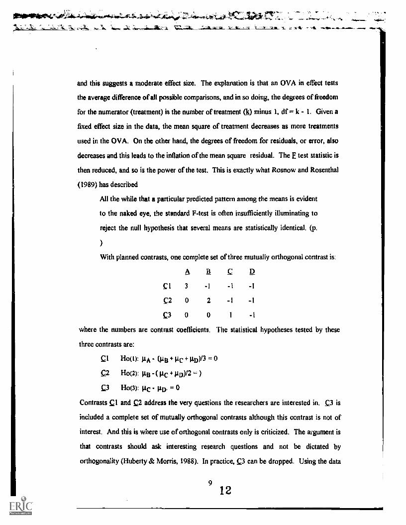
With planned contrasts, one complete set of three mutually orthogonal contrast is:

AB C D

Cl 3 -1 -1 -1

C2 0 2 -1 -1

C3 0 0 1 -1

where the numbers are contrast coefficients. The statistical hypotheses tested by these

three contrasts are:

c1 H0(t): gA (Pa +Pc + 403 '0

Ho(2): µg -( +pD)/2 = )

Ho(3): pc - 413 = 0

Contrasts Cl and C2 address the very questions the researchers are interested in. c3 is

included a complete set of mutually orthogonal contrasts although this contrast is not of

interest. And this is where use of orthogonal contrasts only is criticized. The argument is

that contrasts should ask interesting research questions and not be dictated by

orthogonality (Huberty & Morris, 1988). In practice, can be dropped. Using the data

912

in Table 1, two sets of orthogonal contrasts are made with k - I, or 4 - 1 = 3 contrasts in

each set. Table 3 shows that, in either Set 1 or Set 2, each contrast has one degree of

freedom, the E statistic for each contrast is the mean square of contrast divided by the

mean square of the pooled variance which is the value of the mean square of residual in an

OVA test. The three sum of squaresss of contrast (30.83, 5.042, 1.125) add up to 36.25,

the total sum of squaress of the contrast set. This value is the same as the sum of squaress

of treatment in OVA test in Table 2. Each contrast is tested at a specified a level, or error

rate, no adjustment of the a level is recommended by many researchers for reasons to be

discussed later. In Set 1, the contrast between A and BCD is found significant and so is

the contrast between AB and CD in Set 2.

Insert Table 3 about here

Unplanned contrasts present a complicated case for the sheer number of methods

developed for these tests. Only a few popular unplanned contrast procedures in

educational research are considerei in this discussion. Included are Tukey's HSD,

Bonferroni /Dunn, and Scheffee. Fisher's LSD, Duncan and SNK will also be mentioned.

Although no unplanned contrasts should even be done here since the OVA test fails to

reject the null hypothesis, Table 4 is presented to show that none of these unplanned

contrasts are able to detect significant difference between treatment group means.

Insert Table 4 about here

If, in another similar experiment, another set of data were obtained as in Table 5.

The researchers are interested in learning: 1) whether, among treatments A, B, C and D,

the effect of A is different from B, C and D, and 2) whether the effects of A and B are

different from C and D. The contrasts both have significant results, as noted in Table 6.

Insert Tables 5 and 6 about here

Note, however, the two contrasts are not orthogonal in this example:

CA.BCD (3)A + (-1)B + (-1)C + (-1)D

CCD = (1)A + (1)B + (-1)C + (-1)D

The sum of the cross products of the contrast coefficients in the pair is:

ECiCj = (3)(1) + (-1)(1) + (-1)(-1) + (-1)(-1) = 4, or ECiCj * 0.

The sum of squaresss of the two contrasts (28.521, 22.563) is 51.084, which is greater

than 34.688, the sum of squaress of treatment in OVA test in Table 7 below. This

difference suggests that the two nonorthogonal contrast provide some overlapping

information. The OVA test in Table 7 also rejects the null hypothesis for this data set.

Now that the OVA test indicates that at least one pair of treatment means are significantly

different, unplanned contrasts may now be performed to see which means are different.

The results of the different unplanned contrasts are summarized in Table 8.

Insert Tables 7 and 8 about here

Note that Bonferroni and Scheffe tests fail to detect any significant difference

between the treatment effects. Of all the unplanned contrasts, Scheffe is the only method

recommended for comparisons of complex means. The two research questions should be

tested against the following two null hypotheses:

Ho(1): gA -,;;Ig+gc+1.))/3 -... 0

H0(2): (11A + p.B)/2 - (..tc + IUD) /2 = 0

The OVA test, though significant, gives no information about these two questions, and

Scheffe indicates no significant difference from such comparisons. The planned contrasts,

n14

however, unambiguously reject the two null hypotheses. Had the researchers used the

OVA test or Scheffe test, they would have ended up in failure in this hypothetical research

situation.

Error rate protection accounts for the low power of unplanned contrasts

The test results from the two hypothetical data sets have shown that planned

contrasts are more powerful than either OVA or unplanned contrasts. It was explained

earlier that the difference between OVA test and planned contrasts can be accounted for

by the different degrees of freedom they use respectively. In the case of planned versus

unplanned contrasts, the difference in power is in essence due to the fact that all

unplanned contrasts invoke some protection measures to control for the possible inflation

of Type I error rate because the likelihood of a large number of tests involved in

unplanned contrasts.

For a specified Type I error rate, a level, the actual a level for each test is adjusted

in various ways, depending on the type of unplanned contrasts, and is no longer the

original a level. In general, the a level is reduced for each test and the critical value for a

test is therefore bigger, making it more difficult to reject the null hypothesis.. Most of the

tests for unplanned contrasts between simple means, for instance, Bonferroni/Dunn,

Tukey, SNK, etc., have been incorporated into statistical tables for easy reference. The

critical values for these tests and planned contrasts for simple means are tabulated in Table

9 to illustrate the point that planned contrasts have lower critical values than unplanned

ones. Note that a critical value fort test is used for planned contrasts, because, for n

observations and k treatment groups, a planned contrast has an E statistic with the degrees

of freedom of 1 and n - k for the numerator and denominator respectively. The square

root of this E statistic is a one-tailed I statistic with n k degrees of freedom at the same

specified a level. The critical values for both one-tailed and two-tailed a two-tailed t test

are provided in Table 9.

12 15

Insert Table 9 about here

The critical values for all unplanned contrasts, because of the error rate protection

adjustment, are greater than the / critical values for the planned contrasts between simple

mean comparisons. This holds true for complex mean comparisons where Scheffe test is

used, as was shown earlier in the example with the second hypothetical data set. It can

also be shown that the formula for Scheffe test is the same as for planned contrast (Hinkle

et al., 1988, p. 378). However, while the critical value for planned contrasts is Ec with 1

and n - k degrees of freedom, the critical value for Scheffe test is Ec* and Ec* = (k - 1)F,

where E has (k - I) and (ri k) degrees of freedom. Therefore, the critical value for

Scheffe test is inflated by (k - 1), or the degree of freedom for the numerator. Hence the

Scheffe testis very conservative.

It is clear from the discussion up to this point that the planned contrasts tend to

have more power than unplanned contrasts, especially in complex mean comparisons, and

that the power for planned contrasts is gained because no adjustment is made for the error

rate in the tests of hypotheses. This may appear unfair at the first glance to some people.

In fact, some researchers believe that the same Bonferroni type of correction of error rate

should be applied to planned contrasts (Huberty & Morris, 1988) or at least applied to

nonorthogonal planned contrasts (Pedhzur, 1991),

Most of the researchers writing on this issue, however, feel that no adjustment or

error rate is necessary, although some conditions are necessary, such as only a small

number of hypotheses (no more than the number of treatment minus one) are being tested

(Keppel, 1982; Winer, 1971), or as Thompson (1990, 1991) recommends, "the multiple

correlation between the planned contrast coding vectors and the vector designating

assignment for a given effect does not exceed one".

13

16

The argument for no adjustment emphasizes that planned contrasts require that

researchers have to think carefully about what they are looking for (Keppel, 1982; Tucker,

1991). If researchers believe that the hypotheses to be tested are well supported by theory

or other research and they don't want to miss what they think exists in the data, they have

legitimate reasons to have a more powerful test to guard against Type H error. Besides,

from the practical point of view, well-oriented researchers wouldn't try to test hypotheses

formulated from all possible combinations of treatments. In the hypothetical example and

data in this paper, for instance, only two c- three hypotheses of interest, out of 12 all

possible combinations (6 for simple means and 6 for complex means), have been tested.

Another interesting suggestion for handling error rate in planned contrasts is the

idea of assigning different error rate to individual hypothesis test such that the tests of

most interest have a higher a level , say, .05 each, to ensure significant findings while the

other tests of less interest or importance are given more stringent a level, say .01 or even

.001. The total error rate will then add up to less or equal to the specified a level for the

entire experiment. In Miller's words (1980), there is no law that insists on one a level

being equal to another one. Similar statements are also found in Kurtz et al. (1965), and

Games (1971). There is also controversy over this idea (O'Neil & Wetherill, 1971).

This writer feels that the idea of differentially assigning error rate is acceptable.

However, this seems to be appropriate only where a complete set of orthogonal contrasts

are formed, but some of the contrasts are included solely for the purpose of obtaining the

set of mutually contrasts, as in Table 3. After all, the question of what is an acceptable

Type I error rate is largely a subjective consideration influenced by many non-statistical

factors such as the convention in one's field, and the relevant graveness of committing a

Type I error and a Type II error. Therefore, as Jones (1984) points out, this question "can

only be answered in the context of a given experimental situation."

The controversy over plausible error rate for planned contrasts as well as the

debate on the use of orthogonal versus nonorthogonal contrasts invites more research in

14

17

this area. Some empirical investigation and simulation experiments may be able to shed

more light on the question whether or when researchers should become concerned with

the outcome of analysis if different approaches are employed.

Summary

The literature was reviewed regarding the difference between planned contrasts,

OVA and unplanned contrasts. The relationship between statistical power of a test

method and Type I, and Type II error rates was first explored to provide a framework for

the discussion. It was explained that a higher Type II error rate means lower power for a

test; a lower desired Type I error rate (a small a. value) also makes a test less powerful.

The concepts and formulation of contrast, orthogonal and nonorthogonal contrasts

were introduced. It was argued that planned contrasts are focused on thoughtful research

questions of interest and reflect the researchers' rational anticipation. An OVA test or

unplanned contrasts, on the other hand, do not provide desired information in many

situations. Planned contrasts, OVA and unplanned contrasts were compared and the

results show that planned contrasts yielded statistically significant findings where neither

OVA nor unplanned contrast did. For complex mean comparisons, in particular, planned

contrasts always have greater power than unplanned contrasts. Two small sets of

hypothetical data were employed to make the discussion concrete.

It was also explained that, to control for the possible inflated error rate for

unplanned contrasts that usually test a large number of hypotheses, wanted or unwanted,

some Bonferroni type of corrections are invoked, It is these corrections, usually built into

statistical tables, that reduce the power of unplanned contrasts. This was demonstrated

through a comparison of the critical values for planned contrasts and for some popular

unplanned contrasts: Tukey, SNK, Bonferroni, Duncan and Scheffe. The issue whether

planned contrasts should also be subject to Bonferroni type corrections and whether it is

acceptable to assign a different error rate to each individual planned contrast in a set of

contrasts was also briefly examined.

15 is

References

Carver, R. P. (1978). The case against statistical significance testing.

Harvard Educational Review, 48(3), 378-399.

Cohen, J. (1988). Statistical power analysis for the behavioral sciences (2nd ed.).

Hillsdale, NJ: Lawrence Erlbaum Associates.

Danial, L. G. (1989, January). Use of the jackknife statistic tr, establish the external

validity of discriminant analysis results. Paper presented at the annual meeting of the

Southwest Educational Research Association, Houston, TX. (ERIC Document

Reproduction Service No. ED 305 382)

Elmore, P. B., & Woehlke, P. L. (1988). Statistical methods employed in American

Educational Research Journal, Educational Researcher, and Review of Educational

Research from 1978 to 1987. Educational Researcher, 17 (9), 19-20.

Games, P. A. (1971). Multiple comparisons of means. American Educational Research

Journal, 1, 531-565.

Goodwin, L. D., & Goodwin, W. L. (1985). Statistical techniques in AERJ articles,

1979-1983: The preparation of graduate students to read the educational research

literature. Educational Researcher, 14(2), 5-11.

Hale, G. A. (1977). On use of ANOVA in developmental research. Child Development,

48, 1101-1106.

Hays, W. L. (1963). Statistics for psychologists. New York: Holt, Rinehart and Winston.

Hinkle, D. E., Wiersma, W., & Jurs, S. G. (1988). Applied statistics for the behavioral

sciences (2nd ed.). Boston: Houghton Mofflin Company.

Huberty, C. J. & Morris, L. D. (1978). A single contrast test procedure. Educational and

Psychological Measurement, gt, 567-578.

Jones, D. (1984). Use, misuse, and role of multiple-comparison procedures in ecological

and agricultural entomology. Environmental Entomology, la, 635-649

16

19

Keppel, G. (1989). Data analysis for research designs: Analysis of variance and multiple

regression/correlation approaches. New York: W. H. Freeman,

Kirk, R. E. (1968). experimental design: Procedures for the behavioral sciences,

Belmont, CA: Brooks/Cole.

Kurtz, T. E., Link, R. F., Tukey, J. W., & Wallace, D. L. (1965). Shortcut multiple

comparisons for balanced single and double classification. Part 1. Results.

Technometrics, 7, 95-161.

Lentner, M. & Bishop, T. (1986). Experimental design and analysis. Blacksburg,

VA: Valley Book Company.

McNamara, J. F. (1991), Statistical power in educational research. National Forum of

Applied Educational Research Journal, 3(2), 23-36.

Miller, R. G. Jr. (1980). Simultaneous statistical inference (2nd ed.). New York:

Springer-Verlag.

O'Neill, R., Wtherill, G. B. (1989), The present state of multiple comparison methods.

Journal of Royal Statistics Society, (B) 36: 218-250.

Ott, L. (1989). An introduction to statistical methods and data analysis (3rd ed.).

Boston: PWS-Kent Publishing Company.

Pedhzur, E. J., & Schmelkin, L. P. (1991). Measurement. design, and analysis: An

integrated approach (Student edition). Hillsdale, NJ: Lawrence Erlbaum Associates.

Rosnow, R. L., & Rosenthal, R. (1989). Statistical procedures and the justification of

knowledge in psychological science. American Ps lyoologist, 44(10), 1276-1284.

Thompson, B. (1985). Alternative methods for analyzing data from education

experiments. Journal of Experimental Education, 54, 50-55.

Thompson, B. (1990, April). Planned versus unplanned and orthogonal versus

nonorthogonal contrasts: The neo-classical perspective. Paper presented at the

annual meeting of the American Educational Research Association, Boston.

(ERIC Document Reproduction Service No. ED 318 753)

1720

Thompson, B. (1991). [Review of Data analysis for research designs]. Educational and

Psychological Measurement, 51, 500-510.

Tucker, M. L. (1991). A compendium of textbook views on planned versus post hoc

tests. In B. Thompson (Ed.), Advances in educational research: Substantive findings,

methodological developments (Vol. 1, pp. 107-118). Greenwich, CT: JAI Press..

Willson, V. L. (1980). Research techniques in AERJ articles: 1969 to 1978.

Educational Researcher, 9, 5-10.

Winer, B. J. (1971). Statistical principles in experimental design (2nd ed.). New York:

McGraw-Hill.

18 21

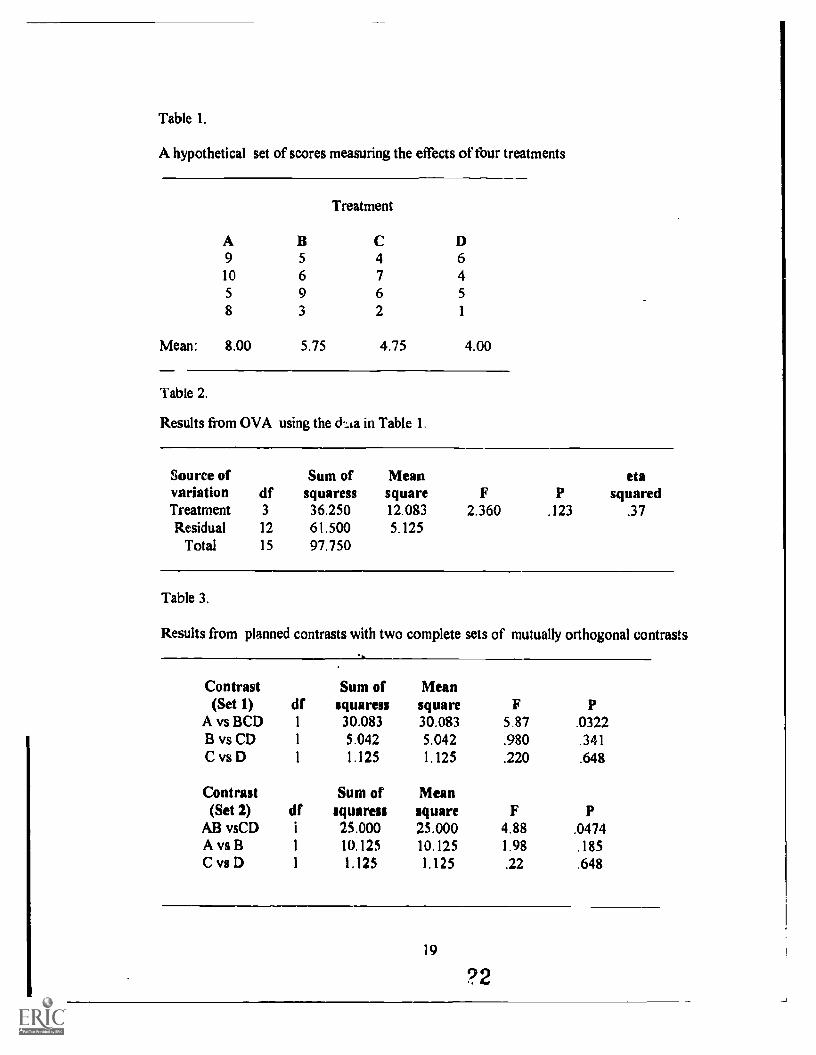
Table 1.

A hypothetical set of scores measuring the effects of four treatments

Treatment

A B C D9 5 4 610 6 7 45 9 6 5

8 3 2 1

Mean: 8.00 5.75 4.75 4.00

Table 2.

Results from OVA using the d .:.ta in Table 1.

Source of Sum of Mean etavariation df squaress square F P squaredTreatment 3 36.250 12.083 2.360 .123 .37Residual 12 61.500 5.125

Total 15 97.750

Table 3.

Results from planned contrasts with two complete sets of mutually orthogonal contrasts11.

Contrast Sum of Mean(Set 1) df squaress square F P

A vs BCD 1 30.083 30.083 5.87 .0322B vs CD 1 5.042 5,042 .980 .341C vs D 1 1.125 1,125 .220 .648

Contrast Sum of Mean(Set 2) df squaress square F P

AB vsCD 1 25.000 25.000 4.88 .0474A vs B 1 10.125 10.125 1.98 185C vs D 1 1,125 1,125 .22 648

19

?2

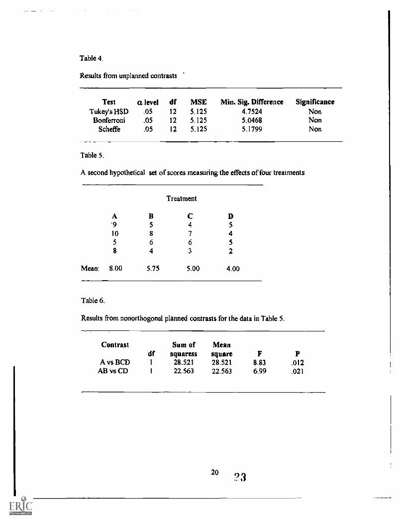
Table 4.

Results from unplanned contrasts

Test a level df MSE Min. Sig. Difference SignificanceTukey's 1-1SD .05 12 5.125 4.7524 NonBonferroni .05 12 5.125 5.0468 Non

Scheffe .05 12 5.125 5.1799 Non

Table 5.

A second hypothetical set of scores measuring the effects of four treatments

Treatment

A B C D'9 5 4 510 8 7 45 6 6 58 4 3 2

Mean: 8.00 5.75 5.00 4.00

Table 6.

Results from nonorthogonal planned contrasts for the data in Table 5.

Contrast

A vs BCDAB vs CD

df1

1

Sum of Meansquaress square

28.521 28.52122.563 22.563

F8.836.99

p.012.021

20

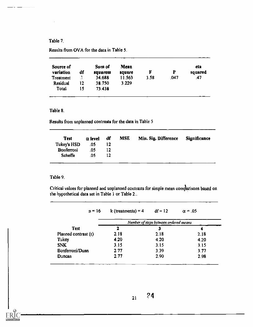
Table 7.

Results from OVA for the data in Table 5.

Source of Sum of Mean etavariation df squaress square F P squaredTreatment 7, 34.688 11.563 3.58 .047 .47Residual 12 38.750 3.229

Total 15 73,438

Table 8.

Results from unplanned contrasts for the data in Table 5

Test a level df MSE Min. Sig. Difference SignificanceTukey's HSD .05 12

Bonferroni .05 12Scheffe .05 12

Table 9.

Critical values for planned and unplanned contrasts for simple mean comparisons based onthe hypothetical data set in Table 1 or Table 2..

n = 16 k (treatments) = 4 df = 12 04 = .05

Number of steps between ordered means

Test 2 3 4Planned contrast (t) 2.18 2.18 2.18Tukey 4.20 4.20 4.20SNK 3.15 3.15 3.15Bonferroni/Dunn 2.77 3.39 3.77Duncan 2.77 2.90 2.98

21 24