Principles of Subtractive Synthesis

Gabriel Beckford MCT3 Indepenent Study

Principles of Subtractive Synthesis

Any discussion of synthesis must at least touch upon timbre because an understanding of its principles is dependent upon a grasp of the qualitative nature of sound itself.

Perhaps the biggest advance in our understanding of the nature of timbre was provided by Fourier who devised the FFT system (Sethares 2005 pg.13). Fourier's system decomposes a sound wave into a sequence of sine waves differentiated by amplitude phase and frequency. In his system they are the irreducible components of the sound source as a unit . The lowest of these partials is the fundamental and unless a sound has a strong noise component the ear tends to identify this as the fundamental pitch. The organisation of higher level partials determines the overtone sequence and also influences how the timbre is perceived.

PartialsF + 2f + 3f + 4f +5f

Overtones

Fig 1. (Loy 2011 pg.2)

Fig.1 illustrates the harmonic spectrum of an instrument with the fundamental given as f. Each subsequent overtone creates a positive integer additive series. Each of these overtones creates a harmonic series but if each is shifted so that it is no longer a multiple of the fundamental the characteristics of the sound are altered. Though the fundamental tone still defines overall pitch the auditory processing centres aggregate all the tones and identify a proximal pitch. We are able to extract tonal information from an inharmonic sequence as well as inferring or deducing a fundamental frequency where one is not present. The auditory system attempts to extrapolate a pattern from the relation of the overtones to the fundamental frequency (Bregman 1994 pg.236)

The way in which the amplitude phase and frequency vary over time is also crucial. The “ballistics” (Loy 2011 pg.2) of these components act as additional markers for the auditory processing system to extract timbral information. “Spectral energy distribution” and temporal variation serve as the main “acoustical determinants” of sound quality.

Due to the lack of compositionally specific timbre controls on acoustic instruments the field of timbre has been neglected. Compare this to pitch and harmony where microtonal variations can be precisely calculated and defined. Both acoustic and electronic instruments produce time variant spectra which defies qualitative analysis.

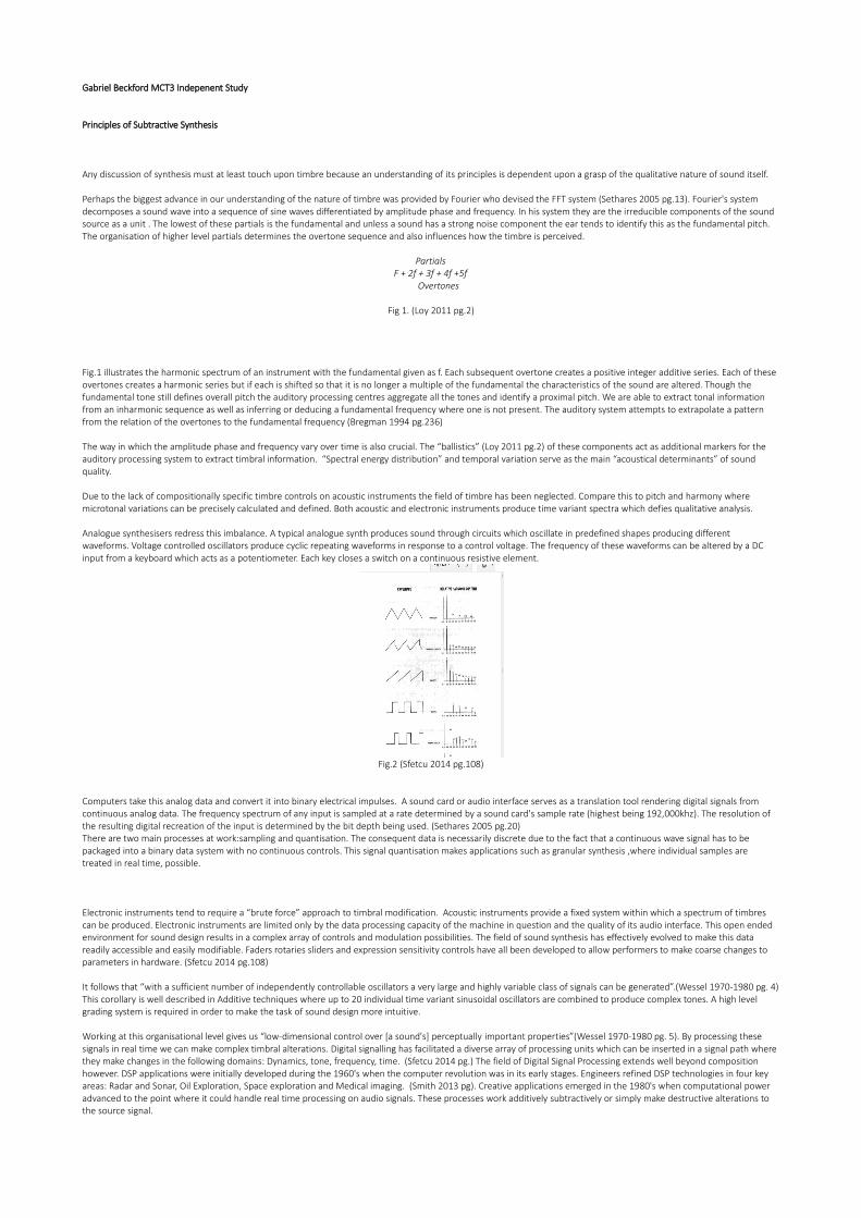
Analogue synthesisers redress this imbalance. A typical analogue synth produces sound through circuits which oscillate in predefined shapes producing different waveforms. Voltage controlled oscillators produce cyclic repeating waveforms in response to a control voltage. The frequency of these waveforms can be altered by a DC input from a keyboard which acts as a potentiometer. Each key closes a switch on a continuous resistive element.

Fig.2 (Sfetcu 2014 pg.108)

Computers take this analog data and convert it into binary electrical impulses. A sound card or audio interface serves as a translation tool rendering digital signals from continuous analog data. The frequency spectrum of any input is sampled at a rate determined by a sound card's sample rate (highest being 192,000khz). The resolution of the resulting digital recreation of the input is determined by the bit depth being used. (Sethares 2005 pg.20)There are two main processes at work:sampling and quantisation. The consequent data is necessarily discrete due to the fact that a continuous wave signal has to be packaged into a binary data system with no continuous controls. This signal quantisation makes applications such as granular synthesis ,where individual samples are treated in real time, possible.

Electronic instruments tend to require a “brute force” approach to timbral modification. Acoustic instruments provide a fixed system within which a spectrum of timbres can be produced. Electronic instruments are limited only by the data processing capacity of the machine in question and the quality of its audio interface. This open ended environment for sound design results in a complex array of controls and modulation possibilities. The field of sound synthesis has effectively evolved to make this data readily accessible and easily modifiable. Faders rotaries sliders and expression sensitivity controls have all been developed to allow performers to make coarse changes to parameters in hardware. (Sfetcu 2014 pg.108)

It follows that “with a sufficient number of independently controllable oscillators a very large and highly variable class of signals can be generated”.(Wessel 1970-1980 pg. 4)This corollary is well described in Additive techniques where up to 20 individual time variant sinusoidal oscillators are combined to produce complex tones. A high level grading system is required in order to make the task of sound design more intuitive.

Working at this organisational level gives us “low-dimensional control over [a sound's] perceptually important properties”(Wessel 1970-1980 pg. 5). By processing these signals in real time we can make complex timbral alterations. Digital signalling has facilitated a diverse array of processing units which can be inserted in a signal path where they make changes in the following domains: Dynamics, tone, frequency, time. (Sfetcu 2014 pg.) The field of Digital Signal Processing extends well beyond composition however. DSP applications were initially developed during the 1960's when the computer revolution was in its early stages. Engineers refined DSP technologies in four key areas: Radar and Sonar, Oil Exploration, Space exploration and Medical imaging. (Smith 2013 pg). Creative applications emerged in the 1980's when computational power advanced to the point where it could handle real time processing on audio signals. These processes work additively subtractively or simply make destructive alterations to the source signal.

Subtractive synthesis

Introduction

Subtractive synthesis is not in fact a closed synthesis system. It is in fact a ubiquitous form of DSP. It coevolved with the analog synthesiser as a response to the need for musicians to shape sound signals in real time. Subtractive synthesis makes it possible to harness raw voltage and treat it to manipulations which produce controlled time variant audio signals.

The basis of subtractive synthesis is the idea that the principle element of a sound involves excitation and resonance. A raw signal is generated which is shaped by a resonator. The resonator shapes the signal by varying its spectrum through the filtering or subtraction of unwanted partials. The subtraction of partials alters the harmonic balance of a signal which can have profound effects on the overall timbre. The excitation sources and resonators thus work in tandem.

The key is to select an excitation source with a rich harmonic spectrum which can then be shaped and contoured. Noise and pulse signals are the most common. Noise based signals generate a range of partials across a wide bandwidth while pulses oscillate periodically/cyclically

It is the presence of resonators which defines subtractive synthesis and as a result it is in fact possible to work with alternative excitation sources. Any waveform can be shaped subtractively to alter the harmonic spectrum and produce timbral alterations. Cyclic waveforms have a stable harmonic distribution pattern across the spectrum which does however make it far easier to obtain predictable and linear subtractive edits.

This linearity makes Subtractive synthesis inappropriate for modelling the physics of vocal or instrumental timbres because the relationship between source and resonator is non linear. The timbre of a saxophone is for example influenced by resonating feedback from the brass tube. This feedback coupling is crucial to the dynamism and resonance of any instrument.

That notwithstanding human vocalisations use subtractive processes. The spectrally rich impulse (air) is channelled and shaped by the vocal components to produce precisewaveforms. Subtractive synthesis is capable of reproducing authentic speech but lacks the depth and “suppleness” required to simulate spectral and harmonic transitions. Itis thus not feasible to concatenate phonemes into full sentences which can be shaped at will. (Miranda 2012 pg.30-40)

Excitation Sources

Audio capture transfers air pressure oscillations onto a storage medium. A microphone diaphragm oscillates sympathetically within an Electromagnetic field. These vibrations are then converted into a voltage which corresponds to the original sound source. Synthesisers generate raw voltages which a transducer then outputs as an audio signal. The resultant waves are ideal forms which do not occur in nature. In order to generate complexity each oscillator is finally routed through synthesiser modules which apply precisely determined transformations.

A sawtooth waveform consists of odd and even harmonics. The oscillator generates this waveform and routes it through two filters running in parallel. These parallel filters produce a dual signal which is recombined at the output stage. The resulting waveform has a different periodicity but we can in fact generate further complexity by employing multi wave oscillators. The combination of several sine waves generates beat frequencies which result from constructive and destructive interference. Destructive interference occurs when the peak and trough of the respective waves coincide. In recording and production situations this is known as phase cancellation. Thebeat frequency can be calculated by working out the absolute difference between the frequencies of the constituent waves. In real world terms the audio processing centres perceive the overall pitch as opposed to separate pitches.One well known application of this concept is the “supersaw” synth. It consists of multiple sawtooth waves which are symmetrically detuned. Assymetric tunings can produce more unpredictable results. This is very much an additive process and the same approach is used in additive synthesis.

Most synthesisers employ four basic waveform types. Sine waves oscillate at a single fundamental frequency. A sine wave sweep across the audible frequency range can in fact be used to generate an impulse response which can then be convolved with an audio signal. Sine waves can also be used to measure distortion by comparing the spectral transformation pre and post amplifier. In terms of subtractive synthesis sine waves are ill suited to filtering because they do not have the spectral richness of the other waves. (Sfetcu 2014 pg.11-20)

Triangle waves are comprised of odd numbered harmonics. A fundamental triangle wave at 100hz will thus have harmonics of diminishing magnitude at 300 500 700 and soon. The same also applies to square waveforms. The harmonic distribution occurs due to the symmetry of the waveforms. In contrast sawtooth waves possess both odd andeven harmonics with diminishing magnitude into the upper reaches of the spectrum as a result of their asymmetrical shape.

Pulse waves are in fact a variation on the square waveform but are differentiated by their pulse width/duty cycle. A pulse wave with a duty cycle of 5% has a positive value 5% of the time. It follows that a square wave is a pulse wave with 50% pulse width which can be described as on/off. A waveform's duty cycle is also directly linked to the difference between peak and average levels (crest factor). Reducing the duty cycle of a pulse wave from 50% only alters the average amplitude of the wave with peak volume remaining unaffected.

Each of these waveforms can of course be generated from sine waves as Fourier postulated. An infinite number of sine waves placed at the odd harmonics will thus create an ideal square wave. (Loy 2011 pg.30-34)

Resonance sources

Once an impulse has been produced it then excites a resonance source i.e. filter. The four primary types are: Low Pass, High Pass, Bandpass and Band Reject. Bandpass filters reject high and low frequencies and have a passband in the middle of these two extremes. The position of the passband is defined by the passband frequency and its bandwidth (difference between upper and lower frequencies) is defined by resonance. (Sethares 2005 pg.30)

Band Reject filters attenuate a single frequency band. This attenuation is again described by resonance bandwidth and passband frequency. The depth of attenuation at the stopband is an additional defining characteristic of the Band Reject or Notch filter. Low Pass filters on the other hand reject spectral components which exceed the cutoff point The high pass filter functions in reverse with a passband situated at the higher end of the spectrum and a stopband positioned at the lower end

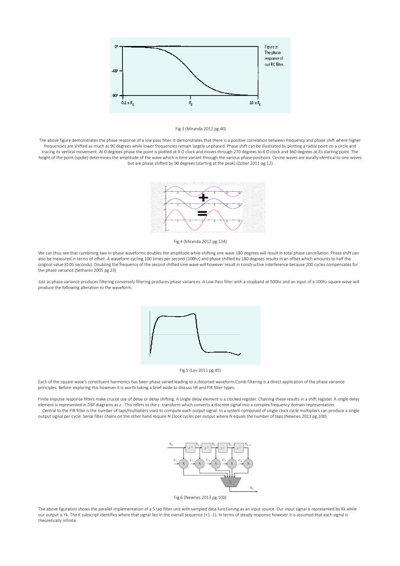
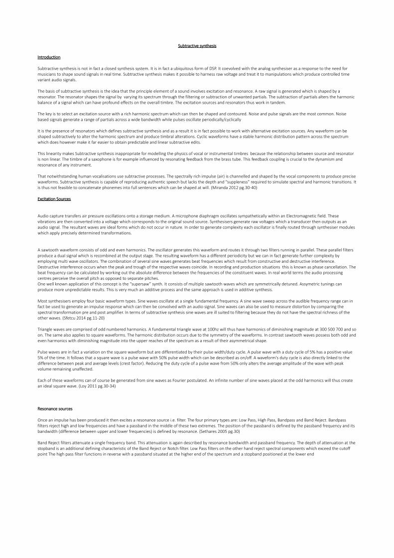
Fig 3 (Miranda 2012 pg.40)

The above figure demonstrates the phase response of a low pass filter. It demonstrates that there is a positive correlation between frequency and phase shift where higherfrequencies are shifted as much as 90 degrees while lower frequencies remain largely unphased. Phase shift can be illustrated by plotting a radial point on a circle and

tracing its vertical movement. At 0 degrees phase the point is plotted at 9 O clock and moves through 270 degrees to 6 O clock and 360 degrees at its starting point. Theheight of the point (spoke) determines the amplitude of the wave which is time variant through the various phase positions. Cosine waves are aurally identical to sine waves

but are phase shifted by 90 degrees (starting at the peak) (Zolzer 2011 pg.12)

Fig 4 (Miranda 2012 pg.134)

We can thus see that combining two in-phase waveforms doubles the amplitude while shifting one wave 180 degrees will result in total phase cancellation. Phase shift can also be measured in terms of offset. A waveform cycling 100 times per second (100hz) and phase shifted by 180 degrees results in an offset which amounts to half the original value (0.05 seconds). Doubling the frequency of the second shifted sine wave will however result in constructive interference because 200 cycles compensates for the phase variance.(Sethares 2005 pg.23)

Just as phase variance produces filtering conversely filtering produces phase variances. A Low Pass filter with a stopband at 500hz and an input of a 100hz square wave will produce the following alteration to the waveform:

Fig.5 (Lov 2011 pg.45)

Each of the square wave's constituent harmonics has been phase varied leading to a distorted waveform.Comb filtering is a direct application of the phase variance principles. Before exploring this however it is worth taking a brief aside to discuss IIR and FIR filter types.

Finite impulse response filters make crucial use of delay or delay shifting. A single delay element is a clocked register. Chaining these results in a shift register. A single delay element is represented in DSP diagrams as z-. This refers to the z- transform which converts a discrete signal into a complex frequency domain representation. Central to the FIR filter is the number of taps/multipliers used to compute each output signal. In a system composed of single clock cycle multipliers can produce a single output signal per cycle. Serial filter chains on the other hand require N Clock cycles per output where N equals the number of taps.(Newnes 2013 pg.100)

Fig.6 (Newnes 2013 pg.100)

The above figuration shows the parallel implementation of a 5 tap filter unit with sampled data functioning as an input source. Our input signal is represented by Xk while our output is Yk. The K subscript identifies where that signal lies in the overall sequence (+1 -1). In terms of steady response however it is assumed that each signal is theoretically infinite.

This diagram can be reconstructed using the following equation:

C0 . Xk + C1.Xk-1 + C2. Xk-2 + C3.Xk-3 + C4 Xk-4.

The datastream is being fed through a series of steady state coefficients. At each clock cycle the data is cross multiplied with the coefficients and the output of each multiplier is summed. During the following clock cycle our signal is then shifted relative to the value of the coefficients.(Zolzer 2011 pg.12)

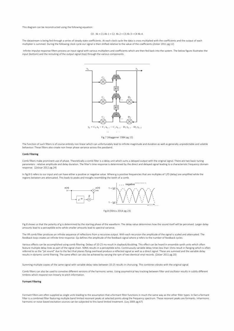
Infinite impulse response filters process an input signal with various multipliers and coefficients which are then fed back into the system. The below figure illustrates the input (bottom) and the rerouting of the output signal (top) through the various components.

Fig.7 (Waggener 1984 pg.12)

The function of such filters is of course entirely non linear which can unfortunately lead to infinite magnitude and duration as well as generally unpredictable and volatile behaviour. These filters also create non linear phase variance across the passband.

Comb Filtering

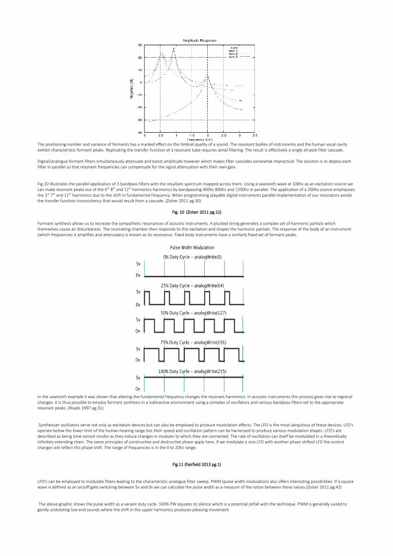
Comb filters make prominent use of phase. Theoretically a comb filter is a delay unit which sums a delayed output with the original signal. There are two basic tuning parameters : relative amplitude and delay duration. The filter's time response is determined by the direct and delayed signal leading to a characteristic frequency domain response. (Zolzsar 2011 pg.24)

In fig.8 G refers to our input and can have either a positive or negative value. Where g is positive frequencies that are multiples of 1/D (delay) are amplified while the regions between are attenuated. This leads to peaks and troughs resembling the teeth of a comb

Fig.8 (Sfetcu 2014 pg.23)

Fig.8 shows us that the polarity of g is determined by the starting phase of the waveform. The delay value determines how the sound itself will be perceived. Larger delay amounts lead to a perceptible echo while smaller amounts lead to spectral variance.

The IIR comb filter produces an infinite sequence of reflections from a recursive output. With each recursion the amplitude of the signal is scaled and attenuated. The feedback loop creates an infinite time response. Gp defines the amplitude of the feedback signal where p refers to the number of feedback cycles.

Various effects can be accomplished using comb filtering. Delays of 10-25 ms result in slapback/doubling. This effect can be heard in ensemble synth units which often feature multiple delay lines as part of the signal chain. 50Ms results in a perceptible echo. Continuously variable delay times less than 15ms result in flanging which is often referred to as the “jet sound” due to the fact that planes flying overhead produce a reflected signal as well as a direct signal. These are summed and the variable delay results in dynamic comb filtering. The same effect can also be achieved by varying the rpm of two dientical vinyl records. (Zolzer 2011 pg.20)

Summing multiple copies of the same signal with variable delay rates between 10-25 results in chorusing. This combines vibrato with the original signal.

Comb filters can also be used to convolve different versions of the harmonic series. Using assymetrical key tracking between filter and oscillator results in subtly different timbres which respond non linearly to pitch information.

Formant Filtering

Formant filters are often supplied as single units leading to the assumption that a formant filter functions in much the same way as the other filter types. In fact a formant filter is a combined filter featuring multiple band limited resonant peaks at selected points along the frequency spectrum. These resonant peaks are formants. Inharmonic harmonic or noise based excitation sources can be subjected to this band limited treatment. (Loy 2005 pg.67)

The positioning number and variance of formants has a marked effect on the timbral quality of a sound. The resonant bodies of instruments and the human vocal cavity exhibit characteristic formant peaks. Replicating the transfer function of a resonant tube requires serial filtering. The result is effectively a single all-pole filter cascade.

Digital/analogue formant filters simultaneously attenuate and boost amplitude however which makes filter cascades somewhat impractical. The solution is to deploy each filter in parallel so that resonant frequencies can compensate for the signal attenuation with their own gain.

Fig.10 Illustrates the parallel application of 3 bandpass filters with the resultant spectrum mapped across them. Using a sawtooth wave at 100hz as an excitation source we can make resonant peaks out of the 4th 8th and 12th harmonics harmonics by bandpassing 400hz 800hz and 1200hz in parallel. The application of a 200hz source emphasisesthe 3rd 7th and 11th harmonics due to the shift in fundamental frequency. When programming playable digital instruments parallel implementation of our resonators avoids the transfer function inconsistency that would result from a cascade. (Zolzer 2011 pg.30)

Fig. 10 (Zolzer 2011 pg.12)

Formant synthesis allows us to recreate the sympathetic resonances of acoustic instruments. A plucked string generates a complex set of harmonic partials which themselves cause air disturbances. The resonating chamber then responds to this excitation and shapes the harmonic partials. The response of the body of an instrument (which frequencies it amplifies and attenuates) is known as its resonance. Fixed body instruments have a similarly fixed set of formant peaks.

In the sawtooth example it was shown that altering the fundamental frequency changes the resonant harmonics. In acoustic instruments this process gives rise to registral changes. It is thus possible to employ formant synthesis in a subtractive environment using a complex of oscillators and various bandpass filters set to the appropriate resonant peaks. (Roads 1997 pg.31)

Synthesiser oscillators serve not only as excitation devices but can also be employed to produce modulation effects. The LFO is the most ubiquitous of these devices. LFO's operate below the lower limit of the human hearing range but their speed and oscillation pattern can be harnessed to produce various modulation shapes. LFO's are described as being time variant insofar as they induce changes in modules to which they are connected. The rate of oscillation can itself be modulated in a theoretically infinitely extending chain. The same principles of constructive and destructive phase apply here. If we modulate a sine LFO with another phase shifted LFO the control changes will reflect this phase shift. The range of frequencies is in the 0 to 20hz range.

Fig.11 (Fairfield 2013 pg.1)

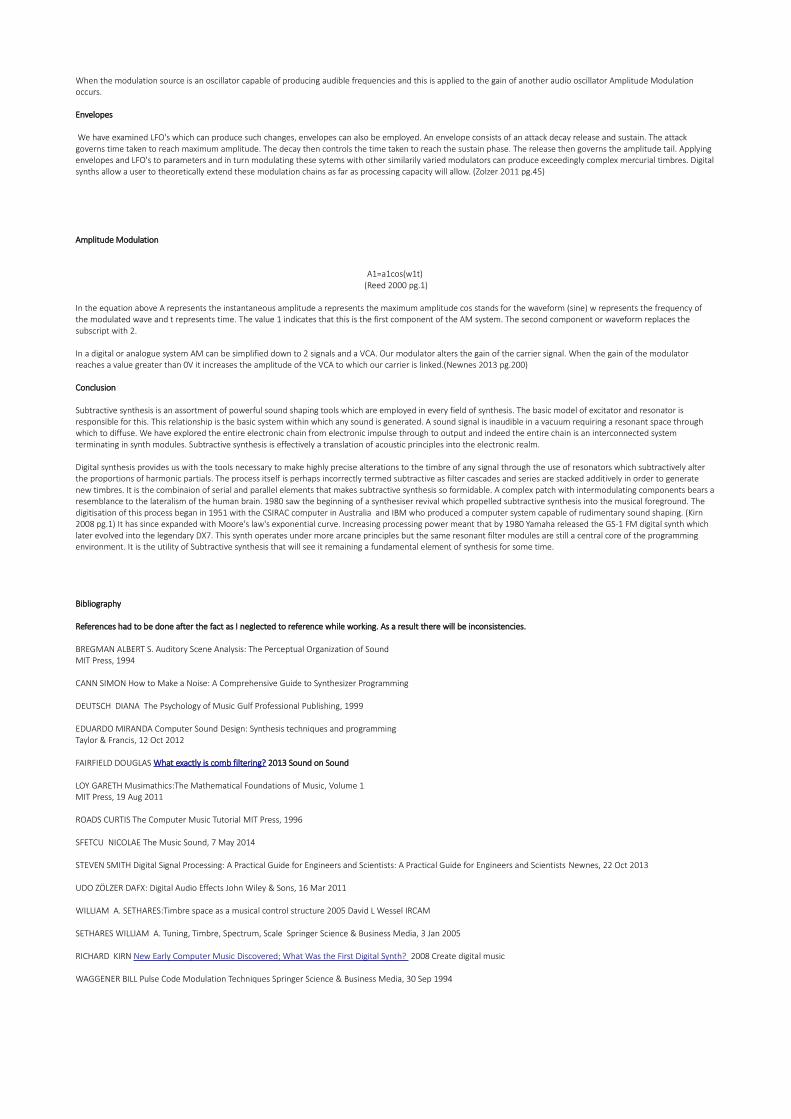
LFO's can be employed to modulate filters leading to the characteristic analogue filter sweep. PWM (pulse width modulation) also offers interesting possibilities. If a square wave is defined as an on/off gate switching between 5v and 0v we can calculate the pulse width as a measure of the ration between these values (Zolzer 2011 pg.42)

The above graphic shows the pulse width as a variant duty cycle. 100% PW equates to silence which is a potential pitfall with the technique. PWM is generally suited to gently undulating low end sounds where the shift in the upper harmonics produces pleasing movement.

When the modulation source is an oscillator capable of producing audible frequencies and this is applied to the gain of another audio oscillator Amplitude Modulation occurs.

Envelopes

We have examined LFO's which can produce such changes, envelopes can also be employed. An envelope consists of an attack decay release and sustain. The attack governs time taken to reach maximum amplitude. The decay then controls the time taken to reach the sustain phase. The release then governs the amplitude tail. Applying envelopes and LFO's to parameters and in turn modulating these sytems with other similarily varied modulators can produce exceedingly complex mercurial timbres. Digitalsynths allow a user to theoretically extend these modulation chains as far as processing capacity will allow. (Zolzer 2011 pg.45)

Amplitude Modulation

A1=a1cos(w1t) (Reed 2000 pg.1)

In the equation above A represents the instantaneous amplitude a represents the maximum amplitude cos stands for the waveform (sine) w represents the frequency of the modulated wave and t represents time. The value 1 indicates that this is the first component of the AM system. The second component or waveform replaces the subscript with 2.

In a digital or analogue system AM can be simplified down to 2 signals and a VCA. Our modulator alters the gain of the carrier signal. When the gain of the modulator reaches a value greater than 0V it increases the amplitude of the VCA to which our carrier is linked.(Newnes 2013 pg.200)

Conclusion

Subtractive synthesis is an assortment of powerful sound shaping tools which are employed in every field of synthesis. The basic model of excitator and resonator is responsible for this. This relationship is the basic system within which any sound is generated. A sound signal is inaudible in a vacuum requiring a resonant space through which to diffuse. We have explored the entire electronic chain from electronic impulse through to output and indeed the entire chain is an interconnected system terminating in synth modules. Subtractive synthesis is effectively a translation of acoustic principles into the electronic realm.

Digital synthesis provides us with the tools necessary to make highly precise alterations to the timbre of any signal through the use of resonators which subtractively alter the proportions of harmonic partials. The process itself is perhaps incorrectly termed subtractive as filter cascades and series are stacked additively in order to generate new timbres. It is the combinaion of serial and parallel elements that makes subtractive synthesis so formidable. A complex patch with intermodulating components bears aresemblance to the lateralism of the human brain. 1980 saw the beginning of a synthesiser revival which propelled subtractive synthesis into the musical foreground. The digitisation of this process began in 1951 with the CSIRAC computer in Australia and IBM who produced a computer system capable of rudimentary sound shaping. (Kirn 2008 pg.1) It has since expanded with Moore's law's exponential curve. Increasing processing power meant that by 1980 Yamaha released the GS-1 FM digital synth which later evolved into the legendary DX7. This synth operates under more arcane principles but the same resonant filter modules are still a central core of the programming environment. It is the utility of Subtractive synthesis that will see it remaining a fundamental element of synthesis for some time.

Bibliography

References had to be done after the fact as I neglected to reference while working. As a result there will be inconsistencies.

BREGMAN ALBERT S. Auditory Scene Analysis: The Perceptual Organization of SoundMIT Press, 1994

CANN SIMON How to Make a Noise: A Comprehensive Guide to Synthesizer Programming

DEUTSCH DIANA The Psychology of Music Gulf Professional Publishing, 1999

EDUARDO MIRANDA Computer Sound Design: Synthesis techniques and programmingTaylor & Francis, 12 Oct 2012

FAIRFIELD DOUGLAS What exactly is comb filtering? 2013 Sound on Sound

LOY GARETH Musimathics:The Mathematical Foundations of Music, Volume 1MIT Press, 19 Aug 2011

ROADS CURTIS The Computer Music Tutorial MIT Press, 1996

SFETCU NICOLAE The Music Sound, 7 May 2014

STEVEN SMITH Digital Signal Processing: A Practical Guide for Engineers and Scientists: A Practical Guide for Engineers and Scientists Newnes, 22 Oct 2013

UDO ZÖLZER DAFX: Digital Audio Effects John Wiley & Sons, 16 Mar 2011

WILLIAM A. SETHARES:Timbre space as a musical control structure 2005 David L Wessel IRCAM

SETHARES WILLIAM A. Tuning, Timbre, Spectrum, Scale Springer Science & Business Media, 3 Jan 2005

RICHARD KIRN New Early Computer Music Discovered; What Was the First Digital Synth? 2008 Create digital music

WAGGENER BILL Pulse Code Modulation Techniques Springer Science & Business Media, 30 Sep 1994