Principles of Quantum Statistics · Principles of Quantum Statistics In this chapter we will study one of the most important assumptions of the quantum the-ory, the symmetrization

Chapter 2

Principles of Quantum Statistics

In this chapter we will study one of the most important assumptions of the quantum the-ory, the symmetrization postulate, and its consequence for the statistical properties of anensemble of particles at thermal equilibrium. The three representative distribution func-tions, Maxwell-Boltzmann, Bose-Einstein and Fermi-Dirac distributions, are introducedhere. Then, we will describe the other important assumption of the quantum theory,the non-commutability of conjugate observables, and its consequence for the uncertaintyproduct in determining a certain pair of observables. The discussions in this chapter pro-vide the foundation of thermal noise and quantum noise. Most of the discussions in thischapter follow the excellent texts on stastical mechanics by F. Rief [1] and on quantummechanics by C. Cohen-Tannoudji et al. [2].

2.1 Symmetrization Postulate of Quantum Mechanics

2.1.1 Quantum indistinguishability

Let us consider a following thought experiment. Two identical quantum particles areincident upon a 50%–50% particle beam splitter and we measure the output by two particlecounters.

1 or 2 ?

50-50%beam splitter

Figure 2.1: Collision of two identical particles.

To analyze this problem, we label the two particles as particle 1 and particle 2 based on

1

the click event in the detectors. One possible input state is

|1, R; 2, L〉 · · · particle 1 is in the right input port andparticle 2 is in the left input port.

Since identical quantum particles are “indistinguishable”, the following input state isequally possible :

|1, L; 2, R〉 · · · particle 1 is in the left input port andparticle 2 is in the right input port.

Most general input state is thus constructed as the linear superposition of the two :

c0|1, R; 2, L〉+ c1|1, L; 2, R〉(|c0|2 + |c1|2 = 1 if the two states are orthogonal.)

(2.1)

As shown below, an experimental result is dependent on the choice of the two c-numbers c0

and c1. Therefore, the above mathematical state has an inherent ambiguity in predictingan experimental result and we need a fundamental assumption of the theory, “symmetriza-tion postulate”[2].

2.1.2 Statement of the postulate

A physical state which represents a real system consisting of identical quantum particles iseither symmetric or anti-symmetric with respect to the permutation of any two particles.A particle which obeys the former is called a boson and a particle which obeys the latteris called a fermion. For instance, the quantum states of two identical bosons and fermionsare

Boson :1√2[|1, R; 2, L〉+ |1, L; 2, R〉],

Fermion :1√2[|1, R; 2, L〉 − |1, L; 2, R〉],

(2.2)

if the two states are orthogonal. To demonstrate the important conseque of this newpostulate, next let us calculate the probability of finding the two particles in the sameoutput port (L). This probability consists of two possibilities.

2

1

direct term

2 2

exchange term

1

+

Figure 2.2: Two possibilities for an output state |1, L; 2, L〉.

3

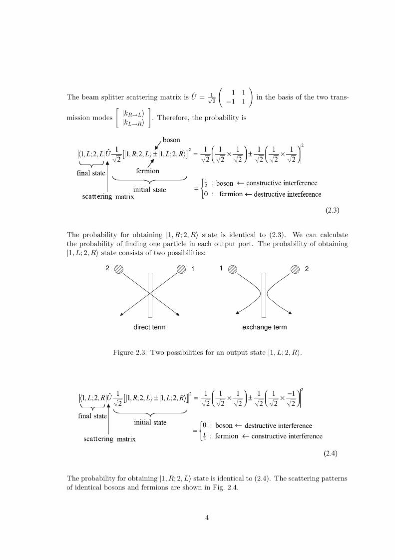
The beam splitter scattering matrix is U = 1√2

(1 1

−1 1

)in the basis of the two trans-

mission modes

[|kR→L〉|kL→R〉

]. Therefore, the probability is

The probability for obtaining |1, R; 2, R〉 state is identical to (2.3). We can calculatethe probability of finding one particle in each output port. The probability of obtaining|1, L; 2, R〉 state consists of two possibilities:

direct term exchange term

12 21

Figure 2.3: Two possibilities for an output state |1, L; 2, R〉.

The probability for obtaining |1, R; 2, L〉 state is identical to (2.4). The scattering patternsof identical bosons and fermions are shown in Fig. 2.4.

4

boson

ψout

= −[ ]12

1 2 1 2, ; , , ; ,R R L L

fermion

ψout

= −[ ]12

1 2 1 2, ; , , ; ,R L L R

Figure 2.4: The scattering behaviours of two identical bosons and fermions at50-50% beam splitter.

Comments :

1. The (2, 0) and (0, 2) output characteristics of bosons are called a “bunching” effect.The constructive interference enhances the probability of finding two particles inthe same state. This is the ultimate origin of final state stimulation in lasers, BoseEinstein condensation and superconductivity.

2. The deterministic (1, 1) output characteristics of fermions are called “anti-bunching”effect. The destructive interference between the direct and exchange terms sup-presses the probability of finding more than two particles in the same state. This isthe manifestation of Pauli’s exclusion principle.

2.1.3 Symmetrization postulate for spin −12

particles

Next let us consider a following thought experiment. Two spin −12 particles are incident

upon a 50%–50% beam splitter. The scattering matrix of a beam splitter is assumed tobe spin-independent. If the two particles are in spin triplet states (symmetric spin states),the orbital states are symmetric for bosons and anti-symmetric for fermions to satisfy thesymmetrization postulate for overall states :

Boson :1√2

[|R〉1|L〉2 + |L〉1|R〉2]⊗

| ↑〉1| ↑〉2| ↓〉1| ↓〉21√2[| ↑〉1| ↓〉2 + | ↓〉1| ↑〉2]

Fermion :1√2

[|R〉1|L〉2 − |L〉1|R〉2]⊗

| ↑〉1| ↑〉2| ↓〉1| ↓〉21√2[| ↑〉1| ↓〉2 + | ↓〉1| ↑〉2]

(2.5)

5

Their collision characteristics are the same as those for spin-less particles mentioned above.However, if the two particles are in a spin singlet state (anti-symmetric spin state), theorbital states are anti-symmetric for bosons and symmetric for fermions to satisfy thesymmetrization postulate for overall states :

Boson :1√2[|R〉1|L〉2 − |L〉1|R〉2]⊗ 1√

2[| ↑〉1| ↓〉2 − | ↓〉1| ↑〉2]

Fermion :1√2[|R〉1|L〉2 + |L〉1|R〉2]⊗ 1√

2[| ↑〉1| ↓〉2 − | ↓〉1| ↑〉2]

(2.6)

Now, the bosons feature a fermionic collision, i.e. (1, 1) output, and the fermions featurea bosonic collision, i.e. (2, 0) or (0, 2) output. This example illustrates a very importantnature of two spin −1

2 fermions which can occupy the same state. Conversely if twoidentical fermions occupy the same orbital state, their spin state is always a spin singletstate.

Γ|x〉1|x〉2 ⊗ 1√2[| ↑〉1| ↓〉2 − | ↓〉1| ↑〉2] (2.7)

same orbital state

¢¢AAK

2.2 Thermodynamic Partition Functions

2.2.1 A small system in contact with a large heat reservoir

Let us consider an ideal gas of non-interacting identical particles in a volume V and at atemperature T . We assume the total number of particles,

∑r nr = N , is constant, where

r designates a microscopic state and nr is the number of particles in that state. The totalenergy of such an ideal gas system is

ER =∑r

εrnr , (2.8)

where εr is the kinetic energy of a microscopic state r and R designates a macroscopicstate represented by the occupation number of each microscopic state, n1, n2, · · · , nr, · · ·.The thermodynamic partition function Z is defined by

Z =∑

R

e−βER , (2.9)

where∑

R stands for summation over all possible macroscopic states, β = 1/kBT is atemperature parameter and kB is a Boltzmann constant.

Next let us obtain the probability of finding a particular macroscopic state R. Forthis purpose we assume that our system is a small system A in thermal contact to a largeheat reservoir A′. We also assume the interaction between A and A′ is extremely small, sothat their energies are additive. The energy of A is not fixed and depends on the specific

6

macroscopic state R. It is the total energy of the combined system A and A′ which has aconstant value ET . This constant total energy is split into those of A and A′:

ET = ER + E′ , (2.10)

where E′ is the energy of A′.According to the fundamental postulate of statistical mechanics, the probability of

finding A in a specific macroscopic state R is proportioned to the number of statesΩ′ (ET −ER) accessible to A′ when its energy lies in a range δE near E′ = ET − ER.Hence

PR = C ′Ω′ (ET − ER) , (2.11)

where C ′ is a constant independent of R and determined by the normalization condition∑R pR = 1.Since A is a much smaller system than A′, ER ¿ ET and (2.11) can be approximated

by expanding the logarithm of Ω′ (ET − ER) about E′ = ET :

lnΩ′ (ET − ER) ' lnΩ′ (ET )−[

∂

∂E′ lnΩ′(E′)]

ET

· ER . (2.12)

The derivative in (2.12) is the definition of the temperature parameter of the heat reservoiraccording to the statistical mechanics [1],

[∂

∂E′ lnΩ′(E′)]

ET

≡ β = 1/kBT . (2.13)

The above result means that the heat reservoir A′ is much larger than A so that itstemperature T remains unchanged by such a small amount of energy it gives to A. Thus,we obtain

Ω′ (ET − ER) = Ω′ (ET ) e−βER . (2.14)

since Ω′ (ET ) is a constant independent of R, (2.11) becomes

PR = Ce−βER , (2.15)

where C = C ′Ω′ (ET ) can be determined by the above mentioned normalization condition∑R pR = 1.The probability of finding the gas in a specific macroscopic state R = n1, n2, · · · , nr, · · ·

is finally given by

PR =e−βER

∑

R′e−βER′

=e−βER

Z. (2.16)

If the above is true, such a system is called a canonical ensemble[1, 3].

Mean and variance of particle number and total energy

Once we know the thermodynamic function Z, various physical quantities can be evaluatedfrom Z. As a simple example, let us calculate the statistical values for a particle numberns of a specific state and a total energy E.

7

A. Mean of particle umber

〈ns〉 =∑

R

nsPR

=

∑

R

nse−β(ε1n1+ε2n2+···)

Z

= − 1βZ

∂

∂εsZ

= − 1β

∂

∂εslog Z (2.17)

B. Mean-square of particle umber

〈n2s〉 =

∑

R

n2sPR

=

∑

R

n2se−β(ε1n1+ε2n2+···)

Z

=1

β2Z

∂2

∂ε2s

Z (2.18)

C. Variance of particle umber

σ2ns

= 〈n2s〉 − 〈ns〉2

=1

β2Z

∂2

∂ε2s

Z −(

1βZ

)2 (∂

∂εsZ

)2

=1β2

[∂

∂εs

(1Z

∂Z

∂εs

)+

1Z2

(∂Z

∂εs

)2]− 1

β2Z2

(∂Z

∂εs

)2

=1β2

∂2

∂ε2s

log Z . (2.19)

D. Mean energy

〈E〉 =∑

R

ERPR

=1Z

∑

R

ERe−βER

= − 1Z

∂

∂βZ

= − ∂

∂βlog Z . (2.20)

E. Mean square of energy

〈E2〉 =∑

R

E2RPR

=1Z

∂2

∂β2Z . (2.21)

8

F. Variance of energy

σ2E = 〈E2〉 − 〈E〉2

=1Z

∂2

∂β2Z −

(1Z

∂

∂βZ

)2

=∂

∂β

(1Z

∂

∂βZ

)

=∂2

∂β2log Z . (2.22)

2.3 Various Distribution Functions

If an ensemble of identical particles is at thermal equilibrium, there are certain probabilitydistributions of finding n particles in a specific state s with an energy εs. We will derivethe four representative probability distribution functions in this section.

2.3.1 Maxwell-Boltzmann statistics

Let us consider an ensemble of “hypothetical” identical particles which can be individuallyidentified. Since it does not obey the principle of quantum indistinguishability, it is oftenreferred to as classical particles.

The thermodynamic partition function for distinguishable particles should be modifiedfrom Eq. (2.9) since all particles are “different” or have “unique labels” in an ensemble ofdistinguishable particles,

Z =∑

n1,n2,···

(N !

n1!n2! · · ·)

e−β(ε1n1+ε2n2+···)

=(e−βε1 + e−βε2 + · · ·

)N, (2.23)

log Z = N log

(∑r

e−βεr

). (2.24)

Using Eq. (2.23) in Eq. (2.17), we obtain the mean particle number in a specific state,

〈ns〉 = − 1β

∂

∂εslog Z

= N × e−βεs

∑r

e−βεr. (2.25)

This is a Maxwell-Boltzmann distribution. The variance of the particle number is calcu-lated using Eq. (2.19),

〈∆n2s〉 = − 1

β

∂

∂εs〈ns〉

= 〈ns〉(

1− 〈ns〉N

)

' 〈ns〉 . (2.26)

9

The above result suggests that the probability of finding ns particles in a specific state inthe Maxwell-Boltzmann distribution obeys a Poisson distribution.

2.3.2 Bose-Einstein statistics

If an ensemble of identical bosonic particles is at thermal equilibrium, it is enough tospecify how many particles are in each state n1, n2, · · ·. Therefore, the mean particlenumber in a microscopic state s is

〈ns〉 =

∑

n1,n2,···nse

−β(ε1n1+ε2n2+···)

∑

n1,n2,···e−β(ε1n1+ε2n2+···)

=

∑ns

nse−βεsns ·

(s)∑e−β(ε1n1+ε2n2+···)

∑ns

e−βεsns ·(s)∑

e−β(ε1n1+ε2n2+···). (2.27)

Here∑(s) stands for the summation over n1, n2, · · · except for the particular microscopic

state s.If the particular microscopic state s does not have a particle, i.e. ns = 0, N particles

must be distributed over the states other than s,

Zs(N) =(s)∑

e−β(ε1n1+ε2n2+···)

(s)∑r

nr = N . (2.28)

If the particular state s has one particle, i.e. ns = 1, the remaining N − 1 particles mustbe distributed over the states other than s,

Zs(N − 1) =(s)∑

e−β(ε1n1+ε2n2+···)

(s)∑r

nr = N − 1 . (2.29)

Using these notations, Eq. (2.27) can be rewritten as

〈ns〉 =0× Zs(N) + e−βεsZs(N − 1) + 2e−2βεsZs(N − 2) + · · ·

Zs(N) + e−βεsZs(N − 1) + e−2βεsZs(N − 2) + · · · . (2.30)

In order to proceed the evaluation of Eq. (2.30), we introduce a new parameter α by

log Zs(N −∆N) ' log Zs(N) +[

∂

∂Nlog Zs(N)

](−∆N)

= log Zs(N)− αs∆N , (2.31)

10

whereαs =

∂

∂Nlog Zs(N) ' ∂

∂Nlog Z(N) = α . (2.32)

Eq.(2.32) holds by the following reason. Since Zs(N) is a summation over very manystates, variation of its logarithm with respect to the total number of particles should beinsensitive as to which particular state s is omitted. Using Eq. (2.32) in Eq. (2.31), weobtain

Zs(N −∆N) = Zs(N)e−α∆N , (2.33)

〈ns〉 =Zs(N)

[0 + e−βεs−α + 2e−2βεs−2α + · · ·

]

Zs(N) [1 + e−βεs−α + e−2βεs−2α + · · ·]

=

∑ns

nse−ns(βεs+α)

∑ns

e−ns(βεs+α)

= − 1β

∂

∂εslog

(∑ns

e−ns(βεs+α)

)

= − 1β

∂

∂εslog

[1

1− e−(βεs+α)

]

=1

eβεs+α − 1. (2.34)

The parameter α is determined by the total number of particles,

N =∑r

〈nr〉 =∑r

1eβεr+α − 1

. (2.35)

Rewriting α in terms of µ = −αβ = −kBTα, Eq. (2.34) is reduced to

〈ns〉 =1

eβ(εs−µ) − 1. (2.36)

This is a Bose-Einstein distribution and µ is called a chemical potential. Note that thechemical potential µ must be always smaller than the minimum energy εs,min of thesystem to conserve the particle number.

The variance in the particle number is

〈∆n2s〉 = − 1

β

∂

∂εs〈ns〉

=1β· eβ(εs−µ)

[eβ(εs−µ) − 1

]2 · β(

1− ∂µ

∂εs

)

= 〈ns〉(1 + 〈ns〉)(

1− ∂µ

∂εs

). (2.37)

Unless a temperature is so low that only a very few states are occupied, a small change ofεs leaves µ unchanged and we have ∂µ

∂εs= 0. In this case, we have the two limiting cases:

〈∆n2s〉 =

〈ns〉2 : εs − µ ¿ kBT (quantumdegenerategas)

〈ns〉 : εs − µ À kBT (non− degenerategas). (2.38)

11

If a temperature is very low, most of the particles are at the lowest energy ground stateor nearly degenerate low-energy state, which satisfy εs − µ ¿ kBT . Such a situation iscalled Bose-Einstein condensation.

2.3.3 Photon statistics

There is another type of bosonic particles, which are photons and phonons. Those particlesare quantized electromagnetic fields and lattice vibrations. Such elementary excitationsdo not have any constraint on the total number of particles when a temperature is varied.Thus we cannot determine a chemical potential µ through the relation Eq. (2.35). Weset the chemical potential µ to be zero for this case.

The mean particle number is

〈ns〉 =

∑ns

nse−βεsns

∑ns

e−βεsns

= − 1β

∂

∂εslog

(∑ns

e−βεsns

)

= − 1β

∂

∂εslog

[1

1− e−βεs

]

=1

eβεs − 1. (2.39)

Here εs = hωs is an energy of photon or phonon, which is uniquely determined by theoscillation frequency ωs. This is called a Planck distribution. The variance in the particlenumber is

〈∆n2s〉 = − 1

β

∂

∂εs〈ns〉

= 〈ns〉(1 + 〈ns〉

)

=

〈ns〉2 : εs ¿ kBT

〈ns〉 : εs À kBT. (2.40)

2.3.4 Fermi-Dirac statistics

Due to the Pauli exclusion principle, each state has the occupation number, either 0 or 1,for an ensemble of identical Fermionic particles. Thus, the mean particle number is

〈ns〉 =

∑ns

nse−βεsns ·

(s)∑e−β(ε1n1+ε2n2+···)

∑ns

e−βεsns ·(s)∑

e−β(ε1n1+ε2n2+···)

=0× Zs(N) + e−βεsZs(N − 1)

Zs(N) + e−βεsZs(N − 1)

12

=1

eβεs+α + 1

=1

eβ(εs−µ) + 1, (2.41)

where Zs(N −1) = Zs(N)e−α and µ = −αβ are used. Note that there is no constraint for a

chemical potential µ with respect to εs in this case. The chemical potential can be muchsmaller or much larger than the minimum energy εs,min. The variance in the particlenumber is

〈∆n2s〉 = − 1

β

∂

∂εs〈ns〉

= 〈ns〉(1− 〈ns〉

) (1− ∂µ

∂εs

)

' 〈ns〉(1− 〈ns〉

). (2.42)

The maximum variance is 〈∆n2s〉 = 1

4 at εs = µ (at Fermi energy) and the variancedisappears at εs ¿ µ due to constant and full occupation of ns = 1. If a temperatureis very low, most of the particles are under this full occupation and there are very fewparticles near the chemical potential and subject to a finite variance 〈∆n2

s〉. Such a gas iscalled Fermi degeneracy.

It is interesting to note that the quantum statistics play an important role in theparticle distribution when a temperature is very low and only a few states are occupied.When a temperature is very high and the particles are distributed over very many statesthe Bose-Einstein distribution and the Fermi-Dirac distribution become indistinguishablefrom the (classical) Maxwell-Boltzmann distribution because the mean particle numberper state is much smaller than one at such a high temperature limit. However, for photonstatistics, the mean particle number can be much greater than one whenever εs ¿ kBTand so the photon statistics can never be reduced to the (classical) Maxwell-Boltzmannstatistics no matter how high a temperature is.

2.4 Equipartition Theorem of Statistical Mechanics

Let us derive here the equipartition theorem mentioned in the previous chapter. Statementof the theorem: If a total system energy is given by the independent sum of quadraticterms of each degree of freedom (DOF), the thermal equilibrium energy per DOF is equalto 1

2kBθ.This is the equipartition theorem. The proof runs as follows[1]. The total energy

of a system consisting of f subsystems depends on f generalized coordinates qk and fgeneralized momenta pk(k = 1, 2, · · · f). Then, this total energy is split into

E(q1 · · · qf , p1 · · · pf ) = εi(pi) + E′(q1 · · · qf , p1 · · · pf ) , (2.43)

does not depend on pi

whereεi(pi) = bp2

i (2.44)

13

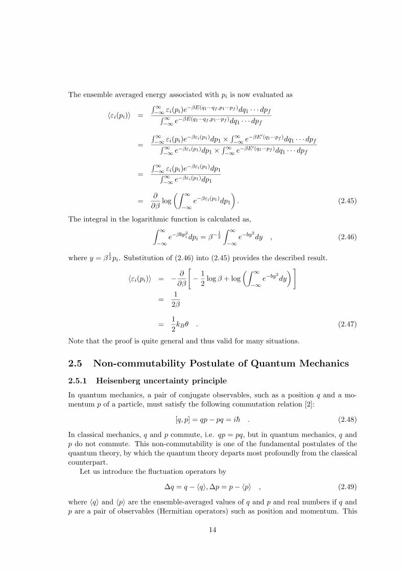
The ensemble averaged energy associated with pi is now evaluated as

〈εi(pi)〉 =∫∞−∞ εi(pi)e−βE(q1···qf ,p1···pf )dq1 · · · dpf∫∞

−∞ e−βE(q1···qf ,p1···pf )dq1 · · · dpf

=∫∞−∞ εi(pi)e−βεi(p1)dp1 ×

∫∞−∞ e−βE′(q1···pf )dq1 · · · dpf∫∞

−∞ e−βεi(p1)dp1 ×∫∞−∞ e−βE′(q1···pf )dq1 · · · dpf

=∫∞−∞ εi(pi)e−βεi(p1)dp1∫∞

−∞ e−βεi(p1)dp1

=∂

∂βlog

(∫ ∞

−∞e−βεi(p1)dp1

). (2.45)

The integral in the logarithmic function is calculated as,∫ ∞

−∞e−βbp2

i dpi = β−12

∫ ∞

−∞e−by2

dy , (2.46)

where y = β12 pi. Substitution of (2.46) into (2.45) provides the described result.

〈εi(pi)〉 = − ∂

∂β

[− 1

2log β + log

(∫ ∞

−∞e−by2

dy

) ]

=12β

=12kBθ . (2.47)

Note that the proof is quite general and thus valid for many situations.

2.5 Non-commutability Postulate of Quantum Mechanics

2.5.1 Heisenberg uncertainty principle

In quantum mechanics, a pair of conjugate observables, such as a position q and a mo-mentum p of a particle, must satisfy the following commutation relation [2]:

[q, p] = qp− pq = ih . (2.48)

In classical mechanics, q and p commute, i.e. qp = pq, but in quantum mechanics, q andp do not commute. This non-commutability is one of the fundamental postulates of thequantum theory, by which the quantum theory departs most profoundly from the classicalcounterpart.

Let us introduce the fluctuation operators by

∆q = q − 〈q〉,∆p = p− 〈p〉 , (2.49)

where 〈q〉 and 〈p〉 are the ensemble-averaged values of q and p and real numbers if q andp are a pair of observables (Hermitian operators) such as position and momentum. This

14

assumption is supported by the fact that whenever we measure a physical quantity, themeasurement result is always a real number. Using (2.49) we can rewrite (2.48) as

[∆q,∆p] = ih . (2.50)

In order to calculate the uncertainty product for ∆q and ∆p, we let |ϕ〉 = ∆q|ψ〉 and|χ〉 = ∆p|ψ〉 and use the Schwartz inequality

〈ϕ|ϕ〉〈χ|χ〉 ≥ |〈ϕ|χ〉|2 , (2.51)

where |ψ〉 is a ket vector representing a quantum state of a given particle system [2]. In(2.51), the equality holds if and only if |ϕ〉 and |χ〉 represent an identical state:

|ϕ〉 = c1|χ〉 , (2.52)

where c1 is a c-number. The state is uniquely determined by the “direction” of the statevector (its norm is irrelevant) so that (2.52) means |ϕ〉 and |χ〉 represent an identical state.Since q and p are Hermitian operators, it follows that ∆q = ∆q+ and ∆p = ∆p+. Theinequality (2.51) is rewritten as

〈∆q2〉〈∆p2〉 ≥ |〈∆q∆p〉|2 , (2.53)

where

∆q∆p =12

(∆q∆p + ∆p∆q) +12

(∆q∆p−∆p∆q) (2.54)

=12

(∆q∆p + ∆p∆q) +i

2h .

From (2.53) and (2.55), we obtain

〈∆q2〉〈∆p2〉 ≥ 14|〈∆q∆p + ∆p∆q〉+ ih|2 . (2.55)

Here 〈∆q∆p+∆p∆q〉 is a real number since it is an ensemble-averaged value of a Hermitianoperator. Accordingly, (2.55) may be further rewritten as

〈∆q2〉〈∆p2〉 ≥ h2

4. (2.56)

This is the Heisenberg uncertainty principle. It places an irreducible lower bound on theproduct of the uncertainties in the measurements of q and p.

2.5.2 Minimum uncertainty wavepacket

For the equality to hold in (2.56), the state vector |ψ〉 must satisfy the following twoconditions simultaneously:

∆q|ψ〉 = c1∆p|ψ〉 , (2.57)

〈ψ|∆q∆p + ∆p∆q|ψ〉 . (2.58)

15

Next let us obtain such a state that satisfies (2.57) and (2.58). If we use (2.57) and itsadjoint in (2.58), we have

(c1 + c∗1) 〈ψ|∆p2|ψ〉 = 0 . (2.59)

If |ψ〉 is not an eigenstate of p, 〈∆p2〉 6= 0 so that ca must be a pure imaginary number.If we let c1 = −ic2, where c2 is a real number, (2.57) is rewritten as

(q − 〈q〉) |ψ〉 = −ic2(p− 〈p〉)|ψ〉 . (2.60)

If we project an eigen-bra 〈q′| from the left of (2.60), we obtain

(q′ − 〈q〉) ψ(q′) = −ic2

(h

i

∂

∂q′− 〈p〉

)ψ(q′) . (2.61)

Here ψ(q′) ≡ 〈q′|ψ〉 is the Schrodinger wavefunction of the state |ψ〉 in q′-representationand we use the identity [2]

〈q′|p|ψ〉 =h

i

∂

∂q′ψ(q′) . (2.62)

The solution of (2.61) is given by

ψ(q′) = c3 exp[

i

h〈p〉q′ − 1

2hc2(q′ − 〈q〉)2

], (2.63)

where c3 is a constant of integration. c2 and c3 in (2.63) can be determined by the relations:∫ ∞

−∞|ψ(q′)|2dq′ = 1 , (2.64)

∫ ∞

−∞(q′ − 〈q〉)2|ψ(q′)|2dq′ = 〈∆q2〉 , (2.65)

Using (2.63) in (2.64) and (2.65), we find that c2 = 2〈∆q2〉h and |c3|2 = 1√

2π〈∆q2〉 . Without

loss of generality, we can choose c3 is a real positive number, and then (2.63) becomes

ψ(q′) = (2π〈∆q2〉)− 14 exp

[i

h〈p〉q′ − (q′ − 〈q〉)2

4〈∆q2〉

], (2.66)

This is the Gaussian wavepacket centered at q′ = 〈q〉 with a variance 〈∆q2〉.The Schrodinger wavefunction in p′-representation can be obtained by the Fourier

transform of (2.66) [4]:

ϕ(p′) ≡ 〈p′|ψ〉 =1√2πh

∫ ∞

−∞exp

(− i

hp′q′

)ψ(q′)dq′ (2.67)

= (2π〈∆p2〉)− 14 exp

[− i

h〈q〉(p′ − 〈p〉 − (p′〈p〉)2

4〈∆p2〉

],

where 〈∆p2〉 = h2/4〈∆q2〉 as expected.Equation (2.60) can be rewritten as

(erq + ie−rp

) |ψ〉 =(er〈q〉ie−r〈p〉) |ψ〉 , (2.68)

where a new parameter is defined by c2 = e−2r. The above equation suggests the very im-portant insight: The minimum uncertainty state |ψ〉 is an eigenstate of a “non-Hermitian”operator erq + ie−rp with a c-number eigenvalue er〈q〉+ ie−r〈p〉.

16

2.5.3 coherent state and squeezed state

If we interpret the previous result for a mechanical harmonic oscillator, in which theHamiltonian corresponding to the total energy of the system is given by

H =p2

2m+

12kq2 . (2.69)

The oscillation frequency is given by ω =√

km . The minimum uncertainty state of such

a mechanical harmonic oscillator is given by the eigenstate of the nor-Hermitian operator(2.68). The uncertainties of q and p are respectively given by

〈∆q2〉 =h

2e−2r , (2.70)

〈∆p2〉 =h

2e2r . (2.71)

The parameter r determines the noise distribution between q and p under the constraintof (2.56) with equality. Thus, it is called a squeezing parameter.

The position and momentum operators can be replaced by the annihilation and creationoperators for an elementary excitation of a harmonic oscillator by the transformation

q =

√h

2mω

(a + a+)

, (2.72)

p =1i

√hωm

2(a− a+)

. (2.73)

If the Hamiltonian amplitude operators a1 and a2 are introduced by the relation,

a1 =12

(a + a+)

=√

mω

2hq , (2.74)

a2 =12i

(a− a+)

=√

12hωm

p , (2.75)

the new commutator bracket and resulting uncertainty relation are

[a1, a2] =i

2, (2.76)

〈∆a21〉〈∆a2

2〉 ≥116

. (2.77)

The minimum uncertainty state is an eigenstate of the non-Hermitian operator, era1 +ie−ra2, and possesses the following uncertainties

〈∆a21〉 =

14e−2r , (2.78)

〈∆a22〉 =

14e2r . (2.79)

17

When the squeezing parameter is r = 0, the non-Hermitian operator is reduced to theannihilation operator a and the minimum uncertainty state in this special case is a coherentstate [5]. Time evolution of the coherent state with a positive excitation amplitude, isschematically shown in Fig. 2.5(a). When the squeezing parameter r is positive or negativeand there is the same excitation amplitude 〈a1〉 > 0, oscillation behavior of the state isshown in Fig. 2.5(b) and (c). They are respectively called amplitude squeezed state andphase squeezed state, since the quantum uncertainty is minimum when an amplitude ismeasured for r > 0 and when a phase is measured when r < 0. The pulsating uncertaintiesof the normalized position 〈∆a2

1〉 = mω2h 〈∆q2〉 are shown in Fig. 2.6 [6].

Figure 2.5: The minimum uncertain wavepackets in a harmonic potential V (q) = 12kq2.

(a) coherent state and (b)(c) quadrature amplitude squeezed states.

18

Figure 2.6: (a) A coherent state of light, (b) (amplitude) squeezed state of light, (c)(phase)squeezed state of light, and (d) number-phase squeezed state of light.

2.6 Quantum and thermal noise of a simple harmonic oscil-lator

When a harmonic oscillator is at thermal equilibrium, the energy associated with the po-sition q and momentum p are independently given by 1

2kBT according to the equipartitiontheorem of statistical mechanics. If we take into account the quantization effect, that is,the energy of a simple harmonic oscillator is quantized in unit of hω, the thermal energyis given by

Et = hωn =hω

ehω/kBT − 1, (2.80)

where n is the equilibrium photon statistics at a temperature T . When hω ¿ kBT , thequantization effect is not important and (2.80) is reduced to Et = kBT . This is an expectedresult since a simple harmonic oscillator energy consists of two degrees of freedom, q andp, and each degree of freedom carries and energy of 1

2kBT .When hω À kBT (zero temperature limit), (2.80) is reduced to zero. This is not

correct. Even at zero temperature T = 0, the uncertainty principle requires the zero-pointfluctuation in both position and momentum. The ground state |0〉 of the simple harmonicoscillator is defined by

a|0〉 = 0 , (2.81)

19

which indicates that the ground state |0〉 is a coherent state with an eigenvalue of zero.The zero-point energy associated with the ground state is

Eq =1

2m〈∆p2〉+

12k〈∆x2〉 (2.82)

= hω(〈∆a2

1〉+ 〈∆a22〉

)

=12hω ,

The total energy of a simple harmonic oscillator is thus given by

ET = Et + Eq = hω

(1

ehω/hBT − 1+

12

). (2.83)

Et is referred to as thermal noise while Eq is called quantum noise. The measurement ofthe position or momentum of a simple harmonic oscillator at equilibrium condition is thusconstrained by the quantum mechanical zero-point fluctuation when hω À kBT and bythe thermal equilibrium noise when hω ¿ kBT .

20

Bibliography

[1] F. Reif, “Fundamentals of Statistical and Thermal Physics” (McGraw-Hill, New York,1965).

[2] C. Cohen-Tannondji, B. Diu and F. Laloe, “Quantum Mechanics” (John Wiley &Sons, New York, 1977).

[3] R. Kubo, “Statistical Mechanics” (North Holland, Amsterdam, 1965).

[4] W. H. Louisell,“Quantum statistical properties of radiation” (Wiley, New York, 1973).

[5] R. Glauber, Phys. Rev. 130, 2529 (1963); ibid 131, 2766 (1963).

[6] Y. Yamamoto and A. Imamoglu,“Mesoscopic Quantum Optics” (John Wiley & Sons,New York, 1999).

21