PRINCIPLES OF PHYLOGENETICS: ECOLOGY AND EVOLUTION Integrative Biology …ib.berkeley.edu/courses/ib200/lect/lect18.pdf ·  · 2018-01-13"PRINCIPLES OF PHYLOGENETICS: ECOLOGY AND

"PRINCIPLES OF PHYLOGENETICS: ECOLOGY AND EVOLUTION" Integrative Biology 200 Spring 2018 University of California, Berkeley D.D. Ackerly Feb 28, 2018 Reading: Felsenstein J. 1985. Phylogenies and the comparative method. Amer. Nat. 125:1-15 Oakley TH, Cunningham CW. 2000. Independent contrasts succeed where ancestral

reconstruction fails in a known bacteriophage phylogeny. Evolution 54:397-405 I. Continuous characters – ancestral states Many traits of interest are measured on continuous or metric scales – size and shape, physiological rates, etc. Continuous traits are often useful for species identification and taxonomic descriptions; historically, they were also used in phylogenetic analysis through the use of clustering algorithms that can group taxa based on multivariate phenetic similarity. With the advent of cladistics and the proliferation of molecular data, reconstruction has shifted (almost) entirely to discrete trait analysis. In principal, ordinal traits take on discrete states while continuous traits are real numbers. In reality, there is a continuum from ordered discrete traits with only a few states (1,2,3,4,5 petals) to those with enough states that we may treat them as continuous (dozens to hundreds). It is also possible to 'discretize' a continuous trait at real or arbitrary breaks in the distributions across species. Distributions of continuous traits may take on any arbitrary shape, but certain distributions occur repeatedly, possibly reflecting underlying 'natural' processes. Normal distribution: sum of many small additive effects Exponential distribution: product of many small multiplicative effects Poisson distribution: frequencies of rare events in discrete intervals etc. This becomes important when we consider whether ancestral reconstruction of continuous traits should reflect an underlying evolutionary model of the process that describes or drives trait evolution. Traits may be transformed to better meet an appropriate distribution (e.g. log-transform). I.B. Parsimony methods for ancestral states 1. Linear or Wagner Parsimony: minimize the sum of absolute or linear changes along each branch (analogous to normal parsimony for discrete traits). The ancestral value at each node will be the median of the three values around it (two child nodes, one parent node). The root is a special case, where it will be the median of the two child nodes, as there is no parent node. This often results in a range of trait values for ancestors, where any value within the range is equivalent; shifting one way or the other just shifts the branches on which changes are reconstructed, but not total tree length. 2. Squared Change Parsimony: minimize the sum of squared changes along each branch. The ancestral value at each node will be the mean of the three values around it (two child nodes, one parent node). Weighted SCP can also be calculated, where the change along each branch is divided by its branch length before summing – a given change on a long branch is penalized less, and values at any given node will be most similar to adjacent nodes connected by short branches. The rationale for these branch length functions makes more sense after considering the Brownian motion model

I.C. Brownian motion and maximum likelihood ancestral states Brownian motion (BM) is the term for a random walk in a continuous valued variable. If a trait was determined by multiple, independent additive factors of small effect, and if each factor was mutating or changing at random (e.g., by drift), then the character change would constitute BM. Brownian motion is the starting point for discussions of continuous character evolution, for its simplicity and its close ties to parametric statistics based on normal distributions. In Brownian motion the size of each step can be drawn from any distribution, and by the Central Limit Theorem the outcome over large number of steps will be a normal distribution. For analytic purposes, it is useful to also use a normal distribution for the individual steps, with mean = 0 (no trend) and variance s2 (= standard deviation s), where each step is a unit of time. When we consider Brownian motion as a process, this variance is viewed as a rate parameter, β. One of the fundamental principles of probability theory is that the variance of the sum of two random processes is the sum of their variances. In other words, if the variance of a Brownian motion process is β after one time step, it will be β + β = 2β after two time steps and tβ after t times steps. So the variance increases linearly with time. If you apply BM to a large number of independent random walks, with time = t along each walk, then you can probably see that the variance of the resulting values at the tips of the walks will be tβ. What is less intuitive for most of us (if you are not used to statistical thinking) is that a single value resulting from a random walk also has a variance that refers to the underlying (and unobserved) distribution from which that value has been drawn, assuming you know or have independently estimated the branch length and rate parameter underlying evolution along that branch. Ancestral states: Now we apply the same principles to solve for ancestral states under ML and Brownian motion, treating each ancestral state as the ML solution for a local BM process derived from that node, and finding the set of ancestral states that maximizes the likelihood over the entire tree. The branch lengths are key now, as the overall s2 value at each node is proportional to the BM rate parameter times the branch lengths. Local likelihood solution: The ML reconstruction of ancestral states can be calculated as a local ML solution, based only on the trait data of tips descended from a node. This amounts to a recursive averaging process down the tree, except that at each node you calculate the weighted average of the two daughter nodes, weighted by the inverse of the square root of the branch length (more on that later). (The everyday mean that we calculate for data sets is also a maximum likelihood solution for that value that minimizes the squared changes between the mean and the data points, i.e. minimizes the variance around the mean). Global likelihood solution: The global ML solution uses information from the entire tree, including descendent taxa and all sister clades at and above (towards the root) a given node. Since ML is minimizing the sum of squared changes, the ancestral states found under the global likelihood solution are equivalent to the results under squared change parsimony. When a solution is found, a BM rate parameter is also calculated, based on the variance of the normal distribution per unit branch length (see Schluter al. 1997, top right of p. 1701). The big difference

between squared change parsimony and ML is that ML techniques use branch lengths and can provide confidence intervals on the ancestors! Given the BM rate parameter, we can calculate a distribution of ancestral states (i.e. support limits) that are consistent with the observed data. The rather troubling result of much work in this area is that sometimes the error bars exceed the range of values observed in the terminal taxa (in other words the ancestor could be anywhere in the range of present-day trait values, or even outside it!). See Schluter et al. 1997 Fig. 7 and Fig. 8 (error bars in Fig. 8 don't seem to show up in the pdf - check the printed journal). I.D. Do ancestral state reconstructions work? Three papers set out to empirically test ancestral state reconstructions for continuous traits: Oakley and Cunningham 2000, Polly 2001, Webster and Purvis 2002. The first used experimental bacteriophage lineages, directly examining properties of ancestral populations. The other two used comparisons with fossils. Polly found that fossil values were quite close to ancestral estimates, and closer than might be expected based on the confidence limits. The Oakley and Webster papers both conclude that ancestral state methods perform very poorly—in both cases, there were significant evolutionary trends across the entire clade that caused the problems. I.E. Citations on ancestral states for continuous characters Cunningham CW, Omland K, Oakley TH. 1998. Reconstructing ancestral character states: a critical reappraisal.

TREE 13:361-366 Losos J. 1999. Commentaries : Uncertainty in the reconstruction of ancestral character states and limitations on the

use of phylogenetic comparative methods. Animal Behaviour 58:1319-1324 Maddison W. 1991. Squared-change parsimony reconstructions of ancestral states for continuous-valued characters

on a phylogenetic tree. Syst. Zool. 40:304-314 Martins EP. 1999. Estimation of ancestral states of continuous characters: a computer simulation study. Syst. Biol.

48:642-650 Oakley TH, Cunningham CW. 2000. Independent contrasts succeed where ancestral reconstruction fails in a known

bacteriophage phylogeny. Evolution 54:397-405 Polly PD. 2001. Paleontology and the comparative method: ancestral node reconstructions versus observed node

values. Amer. Nat. 157:596-609 Schluter D, Price T, Mooers A, Ludwig D. 1997. Likelihood of ancestor states in adaptive radiation. Evolution

51:1699-1711 Schultz T, Cocroft R, Churchill G. 1996. The reconstruction of ancestral character states. Evolution 50:504-511 Swofford DL, Maddison WP. 1987. Reconstructing ancestral states under Wagner parsimony. Math. Biosci. 87:199-

229 Webster AJ, Purvis A. 2002. Testing the accuracy of methods for reconstructing ancestral states of continuous

characters. Proc. Roy. Soc. London Ser. B 269:143-149

Linear Parsimony

!

0 0 0 1 2 4 0

! Squared change parsimony (no BL, or equivalently all BL = 1)

!

0 0 0 1 2 4 0

! ML under Brownian motion (with BL as drawn)

!

0 0 0 1 2 4 0

!

## 7 taxon example, ace solution require(ape) tree = "(t1:5,((t2:1,t3:1):3,((t4:2,(t5:1,t6:1):1):1,t7:3):1):1);" phy = read.tree(text=tree) plot(phy) x = c(0,0,0,1,2,4,0) ace(x,phy)

TEST YOURSELF: Under ML ancestral state reconstructions, do you think the root value will be lower on tree 2 (all BL = 1) or on tree 3 (BL as drawn).

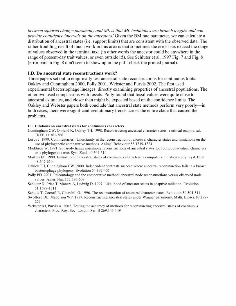
II. Continuous characters – Independent contrasts II.A. One of the most common questions in comparative biology is whether two traits are correlated or allometrically proportional to one another. Is tree height correlated with seed size? Does brain size increase allometrically (disproportionately) with body size? Questions of trait correlations usually address an underlying adaptive hypothesis. E.g., If larger animals require more food, and the rate of energy supply to ecosystems is relatively constant (e.g. solar energy inputs), then larger animals should require larger home range and have lower population densities. As an evolutionary question, these hypotheses can be addressed at many levels. For a population geneticist, it would be ideal to find individual genotypes that exhibit variation in the different traits, and test for genetic correlations and selection on different trait combinations. This is usually extremely difficult and requires very large sample sizes. It could also be addressed by comparing different populations within a species, which is a little easier if multiple populations occupying different conditions can be identified. However, most comparative tests are conducted using species as the units of analysis, representing the outcomes of the evolutionary process. The underlying logic is that if selection has acted on two traits together, such that evolutionary changes in one trait are correlated with changes in another trait, and if the selective history is different for different species, leading to different outcomes, then we can use correlations of species trait values to test the hypothesis of correlated evolution between the two traits. In some cases these hypotheses are explicitly evolutionary, which is to say the underlying hypothesis addresses patterns of trait change arising from natural selection: as body size increases (evolutionarily) does range size also increase. In this case, one can restate the hypothesis as a test of correlations in evolutionary changes (if we knew the history of trait change). In other cases, the hypothesis is more ecological and functional: among present day species, is seed dispersal greater for taller trees? In this case, it is less obvious that an evolutionary or phylogenetic framework is needed. However, even here if these traits have evolved through descent with modification, such that close relatives do exhibit some degree of trait similarity, then tests using species data may encounter statistical issues arising from the non-independence of species values. In either case, comparative methods, especially independent contrasts, are an important tool to incorporate phylogenetic knowledge and use it to improve hypothesis tests, from both historical and statistical perspectives. Numerous studies have conducted such tests over the past decades, many of them based on simple correlation statistics using species values as data points. This is sometimes called the cross-species, ahistorical, or TIP correlation (based on the species values at the tips of the phylogeny). Since Darwin (see Ridley 1992), many researchers recognized that comparisons of closely related species were particular valuable. For example, Salisbury (1942) compared the seed size of congeneric species found in open vs. closed habitats, to test the hypothesis that shaded habitats favored larger seeds. Why should it be important to use congeneric species pairs? Presumably there are some other factors shaping seed size evolution, such as breeding system, dispersal mode, or overall plant stature. If these factors are shared by species within a genus, then the use of congeneric pairs provides a way of holding these factors constant within each comparison, while testing the adaptive hypothesis based on the divergence within each pair. Note the underlying assumption: there are some, possibly unmeasured, factors which exhibit strong phylogenetic signal such that they are shared among relatives, and these can be held constant while testing the role of another factor that exhibits less signal, and has diverged between close relatives. Statistically, this is essentially a paired t-test.

One of the basic principles of standard statistical tests is that the residuals in the data, after fitting to a statistical model, are independently and identically distributed (IID). The relatedness among species creates problems for the independence part, and the differences in branch lengths connecting the species affect the identically distributed part. The degree of non-independence in species values is a function of how much shared history species exhibit, in the context of the clade being studied. Shared history is simply measured by the ratio of shared branch lengths to the total length from root to tips. This can be visualized on the tree and represented in matrices of phylogenetic distances (D, distance down to MRCA and back up to another species) and phylogenetic covariance (shared history = C = 1 - D/max(D)). So, if you calculate a correlation of (X,Y) where X and Y are trait values for a set of species, the shared history means that there is an elevated chance (of some magnitude) that related species will share similar trait values for both traits, even if they evolved independently on the tree, with no underlying correlation. Since they share trait values for both traits, we may incorrectly reject the null hypothesis leading to elevated type I error. • Example: 1) Simulate the independent evolution of 2 traits on this tree: 2) Calculate the pearson correlation coefficient between the two traits. Here is one example:

3) Repeat 1000 times

and look at the distribution of correlation coefficients. In contrast, the expected distribution, for random data sets with N = 10 is shown on the right. For N = 10, the critical significance value at p <= 0.05 is 0.63; the type I error rate is a whopping 60%!

II.B.

Independent contrasts: In 1985, with the rise of

3.5 4.0 4.5 5.0

45

67

89

R = 0.83

t3

t4

t8

t6

t7

t2

t1

t10

t9

t5

pearR

-1.0 -0.5 0.0 0.5 1.0

050100

200

traits evolved on tree

pearR

-1.0 -0.5 0.0 0.5 1.0

050

100

200

traits evolved independently

phylogenetics and comparative biology, Felsenstein introduced a generalization of this paired comparisons method, based on the divergences that have occurred at each bifurcation in a phylogenetic tree. These divergences represent contrasts (differences) between the trait values. If we assume that traits evolve independently in each lineage, following speciation, then the trait divergences that occur at one node are independent of the divergences at other nodes. Hence the name, phylogenetic independent contrasts (often abbreviated PICs). The independent contrasts method is derived from the Brownian Motion model. Let's start with a single divergence:

Assume a trait of interest starts with value X0 at the ancestor. After speciation, the trait evolves independently along each branch, with a Brownian Motion parameter s2 (the variance of expected character change per unit branch length). If the length of the subtending branches are v1 and v2, then the changes that occur on each branch will be drawn from normal distributions with mean = 0 and variance = s2•v1 and s2•v2, respectively. The resulting trait values will be:

X1 = X0 + N{0, s2•v1} X2 = X0 + N{0, s2•v2}

The shared X0 value in the distribution for both traits reflects the covariance issue between trait values for related species. So, if we could somehow address the changes that occur along each branch, rather than the observed trait values of the species themselves, then we would have independent estimates of evolutionary change, and we could ask if there are correlated changes between two traits. In other words, we would like to know: X1 - X0 X2 - X0 But, we don't know X0. And if we use only comparative data, we can only estimate it from the values of X1 and X2, so any estimate we got would not be independent of those data. Also, a tree with N species has 2N-2 internal branches. So it seems there's something wrong with increasing the number of data values than we start with. Felsenstein's solution is to calculate the difference between X1 and X2, reflecting the cumulative divergence in trait values from their common ancestor, without necessarily knowing how much of the change occurred along each branch. So we want to know the expected distribution of the difference or contrast in the resulting trait values. We can take advantage of the fact that the variance of the sum or difference of two random variates is the sum of the variances. Therefore, CU = (X1 – X2) = N{0, s2 (v1+v2)} In other words, the mean value of the contrast will be zero, on average. And the variance around this mean will be the rate parameter s2, times the sum of the branch lengths connecting the two taxa. This value is termed the unstandardized contrast, because it is not standardized for the branch lengths. If two taxa are connected by long branches, we expect larger contrasts, and if they share a more recent common ancestor, we expect smaller contrasts. Statistical theory is developed on the assumption that the variates are independent, and are drawn from normal distributions with equal variance or standard deviation. To achieve this, we now standardize the contrast, by

dividing by the standard deviation of the expected distribution (since the rate parameter β is constant over the tree, and only relative values of the contrasts are important, β or s2 is usually dropped at this step and the contrast is just standardized by the summed branch lengths):

€

CS =CU

v1 + v2

In theory, if the trait has evolved following Brownian Motion, the values of CS now represent a set of independent, normal variates drawn from distributions of equal variance, and these meet the assumptions for use in standard statistical tests such as correlations, regressions, and analysis of variance. The calculation of contrasts, as illustrated above, require trait values at each pair of nodes sharing a common ancestor. Starting at the tips, these are the species values provided by the data set. Moving down the tree, however, we need to calculate a set of estimated internal values to obtain the appropriate contrasts. These are based on the local (top-down) maximum likelihood algorithm—essentially a weighted average of the nodes above, using the inverse of the branch lengths as weighting factors:

€

X0 =

1v1

" # $ %

& ' X1 + 1

v2" # $ %

& ' X2

1v1

+ 1v2

As a final step, the branch length below node 0 is lengthened, reflecting the increased uncertainty associated with deeper nodes (since a longer branch results in higher variance):

€

v'0 = v0 + v1v2(v1 + v2) With the new internal node values calculated, the calculation of contrasts proceeds down the tree. These internal values are essentially the local (not global) maximum likelihood ancestral states based only on information from descendents, not the totality of information obtained when considering both descendents and other taxa in the tree, as in the full ancestral state algorithms discussed above. II.C. Correlations of independent contrasts: Before we conduct a statistical test with independent contrasts, note that they have one unusual property. Each contrast is based on subtraction of one value from another. Clearly, the direction of subtraction is arbitrary, as long as it is kept the same for all traits at each node. As a result, each contrast has a mirror image of the opposite sign. So clearly the average value of all contrasts must be zero, since each one could be flipped around. As a result, all correlations and regression analyses must be calculated through the origin, and anovas would have to be conducted without a grand mean term. The formula for the correlation coefficient through the origin is a bit different than the familiar one in a stats textbook:

€

rxy =CxCy∑

Cx2∑ Cy

2∑{ }12

where Cx and Cy are the standardized contrasts for traits x and y. See Garland et al. 1992 for additional discussion.

picR

-1.0 -0.5 0.0 0.5 1.0

050

150

250

Returning to our example above with the 10 taxon tree, here is the distribution of independent contrasts under the null hypothesis. Type I error for 1000 reps is 0.051% - perfect! Citations below provide examples of independent contrast correlations and the interpretations that can be drawn from comparisons of TIPs and PICs analyses. III. General linear models There is an alternative approach to this problem, which we will not address in detail, but it is important for you to be aware of it. Conventional linear models that we use in statistics are a special case of a more general class of general linear models, or generalized least squares. In these general models, one can relax the assumption that residuals are identically and independently distributed, and instead include in the model a correlation matrix that specifies the expected pattern of non-independence among residuals. The model is then 'corrected' for this expected non-independence, and provides appropriate results for hypothesis tests. For the phylogenetic case, the phylogenetic covariance matrix (p. 2 above) can be used for the error covariance structure. This then allows one to use the full array of linear models, including anova, regression, ancova, etc., opening up possibilities beyond what can be done with independent contrasts. For the case of two continuous variables, it can be shown (though not by me!) that the results converge and the independent contrasts and generalized least squares approaches are the same. In ape, the gls approach looks like this, where x and y are the dependent and independent variables, contained in data.frame dat: m1 <- gls(y~x,data=dat, correlation=corBrownian(1,phy)) For the null model on the ten taxon tree in the example above, the type I error rate was exactly the same as the independent contrasts.

-50

510

-6-4-202468

cont

rast

s fo

r x

contrasts for y5

1015

681012141618

x

y

5 11

13

17

9 14

4 12

6 10

10

10

16

15

2 8

6 16

1 6

11

14

8.5 9

11.5

11

19

18

13

12

4 8

10 8

3 2

-6

-6

6 5

2 -2

8 6

a bc

R =

0.7

4R

= 0

.92

Ackerly and Reich, 1999, Amer J Bot

closed circles: angiosperms closed squares: conifers cross: basal contrast between angios and conifers

II.D. Citations for independent contrasts Abouheif E. 1998. Random trees and the comparative method: a cautionary tale. Evolution

52:1197-1204 Abouheif E. 1999. A method for testing the assumption of phylogenetic independence in

comparative data. Evol. Ecol. Res. 1:895-909 Ackerly DD, Reich PB. 1999. Convergence and correlations among leaf size and function in

seed plants: a comparative test using independent contrasts. Amer. J. Bot. 86:1272-1281 Ackerly DD. 2000. Taxon sampling, correlated evolution and independent contrasts. Evolution

54:1480-1492 Armstrong D, Westoby M. 1993. Seedlings from large seeds tolerate defoliation better: a test

using phylogenetically independent contrasts. Ecology 74:1092-1100 Bauwens D, Garland T, Jr., Castilla A, Van Damme R. 1995. Evolution of sprint speed in

Lacertid lizards: morphological, physiological and behavioral covariation. Evolution 49:848-863

Burt A. 1989. Comparative methods using phylogenetically independent contrasts. OxfSurvEvolBiol. 6:33-53

Diaz-Uriarte R, Garland T, Jr. 1996. Testing hypotheses of correlated evolution using phylogenetically independent contrasts: sensitivity to deviations from Brownian motion. Syst. Biol. 45:27-47

Felsenstein J. 1985. Phylogenies and the comparative method. Amer. Nat. 125:1-15 Felsenstein J. 2008. Comparative methods with sampling error and within-species variation:

Contrasts revisited and revised. Amer. Nat. 171:713-725 Freckleton RP. 2000. Phylogenetic tests of ecological and evolutionary hypotheses: checking for

phylogenetic independence. Func. Ecol. 14:129-134 Garland T, Jr. 1992. Rate tests for phenotypic evolution using phylogenetically independent

contrasts. Amer. Nat. 140:509-519 Garland Jr, T., P. H. Harvey, and A. R. Ives. 1992. Procedures for the analysis of comparative

data using phylogenetically independent contrasts. Systematic Biology 41:18-32. McPeek, M.A. (1995) Testing hypotheses about evolutionary change on single branches of a

phylogeny using evolutionary contrasts. Amer Nat, 145, 686-703. Oakley TH, Cunningham CW. 2000. Independent contrasts succeed where ancestral

reconstruction fails in a known bacteriophage phylogeny. Evolution 54:397-405 Pagel M. 1993. Seeking the evolutionary regression coefficient: an analysis of what comparative

methods measure. JTheorBiol. 164:191-205 Price T. 1997. Correlated evolution and independent contrasts. Phil. Trans. Roy. Soc. Lond. Ser.

B 352:519-529 Purvis A, Rambaut A. 1995. Comparative analysis by independent contrasts (CAIC): an Apple

Macintosh application for analysing comparative data. Comp. Appl. Bios. 11:247-251 Ricklefs RE, Starck JM. 1996. Applications of phylogenetically independent contrasts: a mixed

progress report. Oikos 77:167-172 Ridley M. 1992. Darwin sound on comparative method. TREE 7:37 Salisbury E. 1942. The reproductive capacity of plants. Bell, London Starck J. 1998. Non-independence of data in biological comparisons a critical appraisal of

current concepts assumptions and solutions. Theory Biosci. 117:109-138