Principles of Compiler Design

Welcome message from author
This document is posted to help you gain knowledge. Please leave a comment to let me know what you think about it! Share it to your friends and learn new things together.
Transcript
Principles of Compiler Design
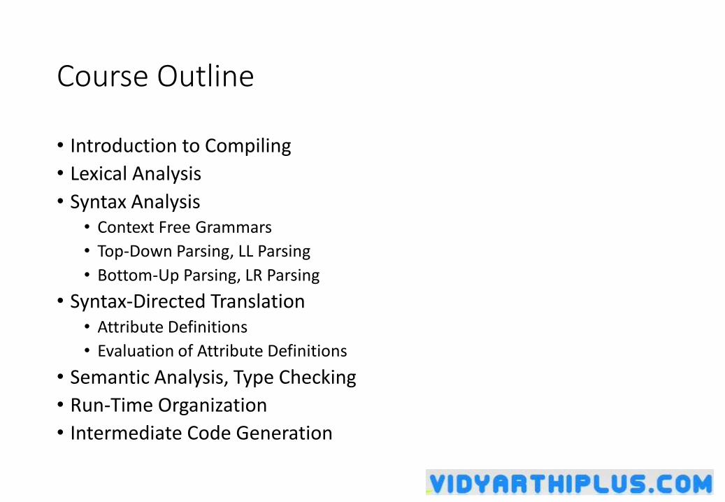
Course Outline
• Introduction to Compiling
• Lexical Analysis
• Syntax Analysis• Context Free Grammars
• Top-Down Parsing, LL Parsing
• Bottom-Up Parsing, LR Parsing
• Syntax-Directed Translation• Attribute Definitions
• Evaluation of Attribute Definitions
• Semantic Analysis, Type Checking
• Run-Time Organization
• Intermediate Code Generation
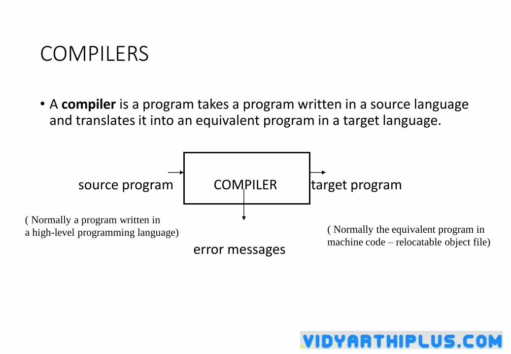
COMPILERS
• A compiler is a program takes a program written in a source language and translates it into an equivalent program in a target language.
source program COMPILER target program
error messages
( Normally a program written in
a high-level programming language) ( Normally the equivalent program in
machine code – relocatable object file)
Other Applications
• In addition to the development of a compiler, the techniques used in compiler design can be applicable to many problems in computer science.
• Techniques used in a lexical analyzer can be used in text editors, information retrieval system, and pattern recognition programs.
• Techniques used in a parser can be used in a query processing system such as SQL.
• Many software having a complex front-end may need techniques used in compiler design.• A symbolic equation solver which takes an equation as input. That program should parse
the given input equation.
• Most of the techniques used in compiler design can be used in Natural Language Processing (NLP) systems.
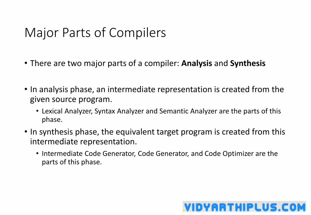
Major Parts of Compilers
• There are two major parts of a compiler: Analysis and Synthesis
• In analysis phase, an intermediate representation is created from the given source program.
• Lexical Analyzer, Syntax Analyzer and Semantic Analyzer are the parts of this phase.
• In synthesis phase, the equivalent target program is created from this intermediate representation.
• Intermediate Code Generator, Code Generator, and Code Optimizer are the parts of this phase.
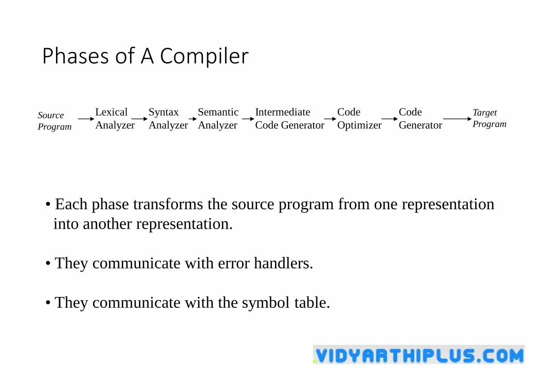
Phases of A Compiler
Lexical
Analyzer
Semantic
Analyzer
Syntax
Analyzer
Intermediate
Code Generator
Code
Optimizer
Code
Generator
Target
ProgramSource
Program
• Each phase transforms the source program from one representation
into another representation.
• They communicate with error handlers.
• They communicate with the symbol table.
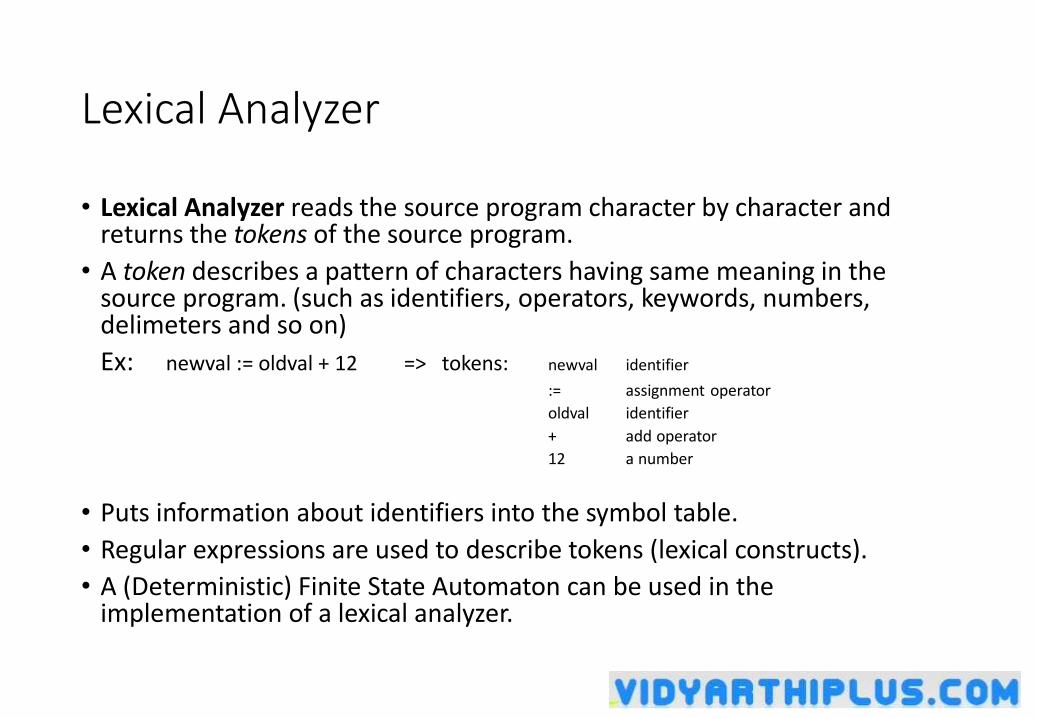
Lexical Analyzer
• Lexical Analyzer reads the source program character by character and returns the tokens of the source program.
• A token describes a pattern of characters having same meaning in the source program. (such as identifiers, operators, keywords, numbers, delimeters and so on)
Ex: newval := oldval + 12 => tokens: newval identifier
:= assignment operator
oldval identifier
+ add operator
12 a number
• Puts information about identifiers into the symbol table.
• Regular expressions are used to describe tokens (lexical constructs).
• A (Deterministic) Finite State Automaton can be used in the implementation of a lexical analyzer.
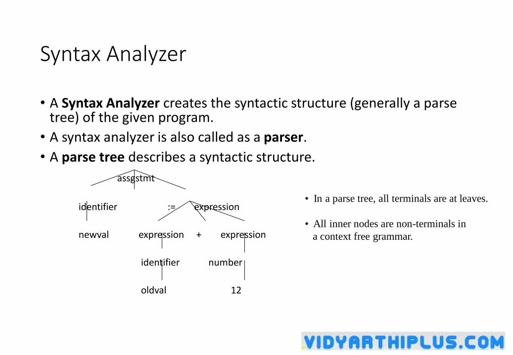
Syntax Analyzer
• A Syntax Analyzer creates the syntactic structure (generally a parse tree) of the given program.
• A syntax analyzer is also called as a parser.
• A parse tree describes a syntactic structure.
assgstmt
identifier := expression
newval expression + expression
identifier number
oldval 12
• In a parse tree, all terminals are at leaves.
• All inner nodes are non-terminals in
a context free grammar.
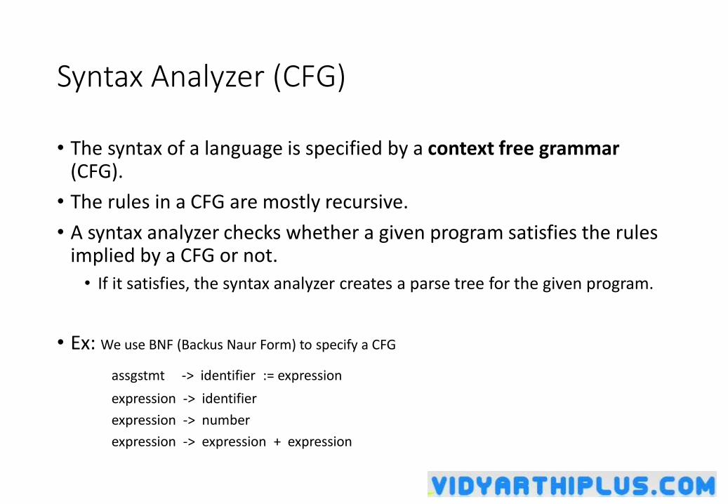
Syntax Analyzer (CFG)
• The syntax of a language is specified by a context free grammar(CFG).
• The rules in a CFG are mostly recursive.
• A syntax analyzer checks whether a given program satisfies the rules implied by a CFG or not.
• If it satisfies, the syntax analyzer creates a parse tree for the given program.
• Ex: We use BNF (Backus Naur Form) to specify a CFG
assgstmt -> identifier := expression
expression -> identifier
expression -> number
expression -> expression + expression
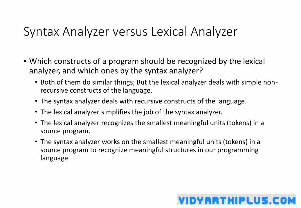
Syntax Analyzer versus Lexical Analyzer
• Which constructs of a program should be recognized by the lexical analyzer, and which ones by the syntax analyzer?
• Both of them do similar things; But the lexical analyzer deals with simple non-recursive constructs of the language.
• The syntax analyzer deals with recursive constructs of the language.
• The lexical analyzer simplifies the job of the syntax analyzer.
• The lexical analyzer recognizes the smallest meaningful units (tokens) in a source program.
• The syntax analyzer works on the smallest meaningful units (tokens) in a source program to recognize meaningful structures in our programming language.
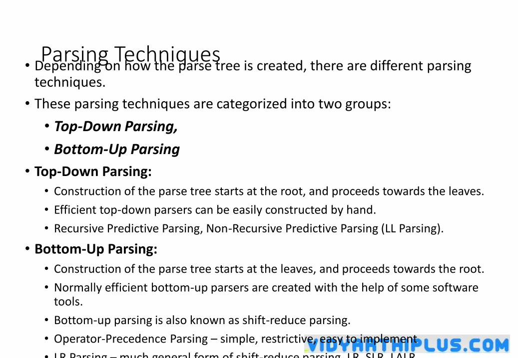
Parsing Techniques• Depending on how the parse tree is created, there are different parsing
techniques.
• These parsing techniques are categorized into two groups:
• Top-Down Parsing,
• Bottom-Up Parsing
• Top-Down Parsing:
• Construction of the parse tree starts at the root, and proceeds towards the leaves.
• Efficient top-down parsers can be easily constructed by hand.
• Recursive Predictive Parsing, Non-Recursive Predictive Parsing (LL Parsing).
• Bottom-Up Parsing:
• Construction of the parse tree starts at the leaves, and proceeds towards the root.
• Normally efficient bottom-up parsers are created with the help of some software tools.
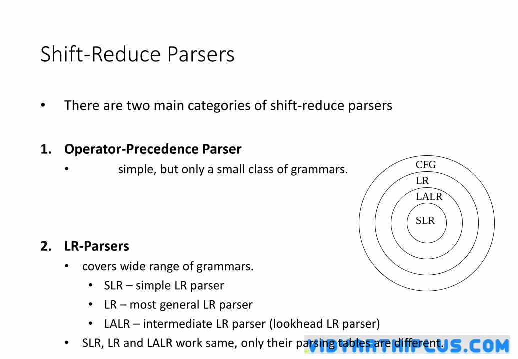
• Bottom-up parsing is also known as shift-reduce parsing.
• Operator-Precedence Parsing – simple, restrictive, easy to implement
• LR Parsing – much general form of shift-reduce parsing, LR, SLR, LALR
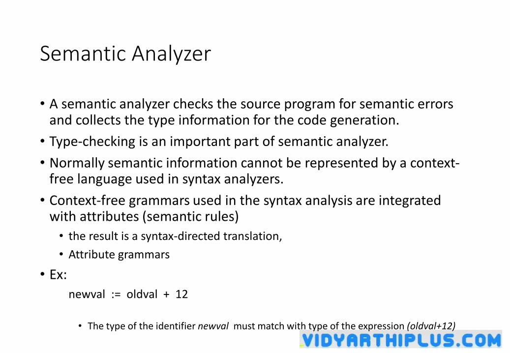
Semantic Analyzer
• A semantic analyzer checks the source program for semantic errors and collects the type information for the code generation.
• Type-checking is an important part of semantic analyzer.
• Normally semantic information cannot be represented by a context-free language used in syntax analyzers.
• Context-free grammars used in the syntax analysis are integrated with attributes (semantic rules)
• the result is a syntax-directed translation,
• Attribute grammars
• Ex:
newval := oldval + 12
• The type of the identifier newval must match with type of the expression (oldval+12)
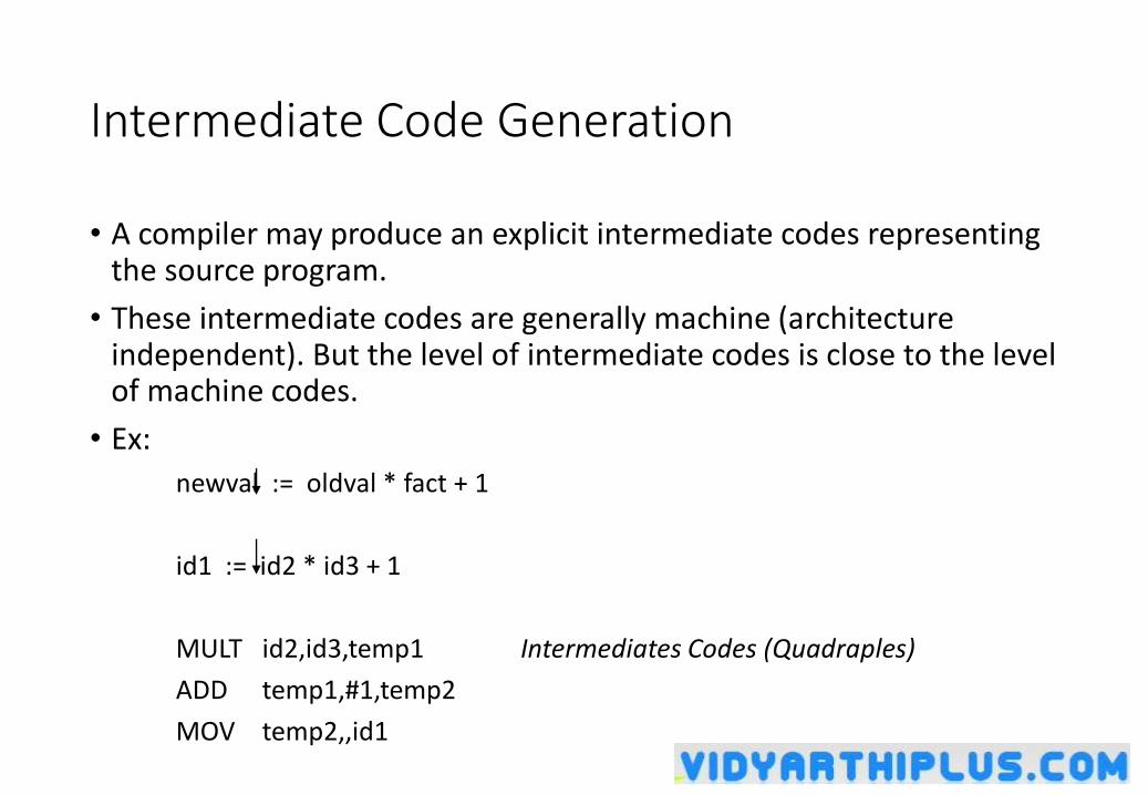
Intermediate Code Generation
• A compiler may produce an explicit intermediate codes representing the source program.
• These intermediate codes are generally machine (architecture independent). But the level of intermediate codes is close to the level of machine codes.
• Ex:
newval := oldval * fact + 1
id1 := id2 * id3 + 1
MULT id2,id3,temp1 Intermediates Codes (Quadraples)
ADD temp1,#1,temp2
MOV temp2,,id1
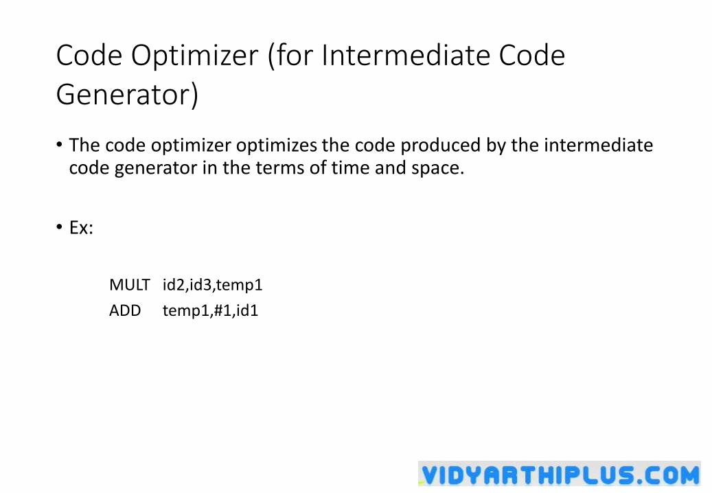
Code Optimizer (for Intermediate Code Generator)
• The code optimizer optimizes the code produced by the intermediate code generator in the terms of time and space.
• Ex:
MULT id2,id3,temp1
ADD temp1,#1,id1
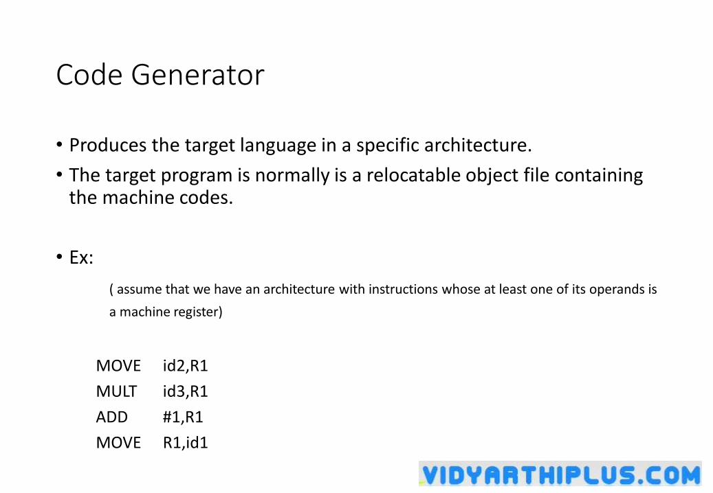
Code Generator
• Produces the target language in a specific architecture.
• The target program is normally is a relocatable object file containing the machine codes.
• Ex:
( assume that we have an architecture with instructions whose at least one of its operands is
a machine register)
MOVE id2,R1
MULT id3,R1
ADD #1,R1
MOVE R1,id1
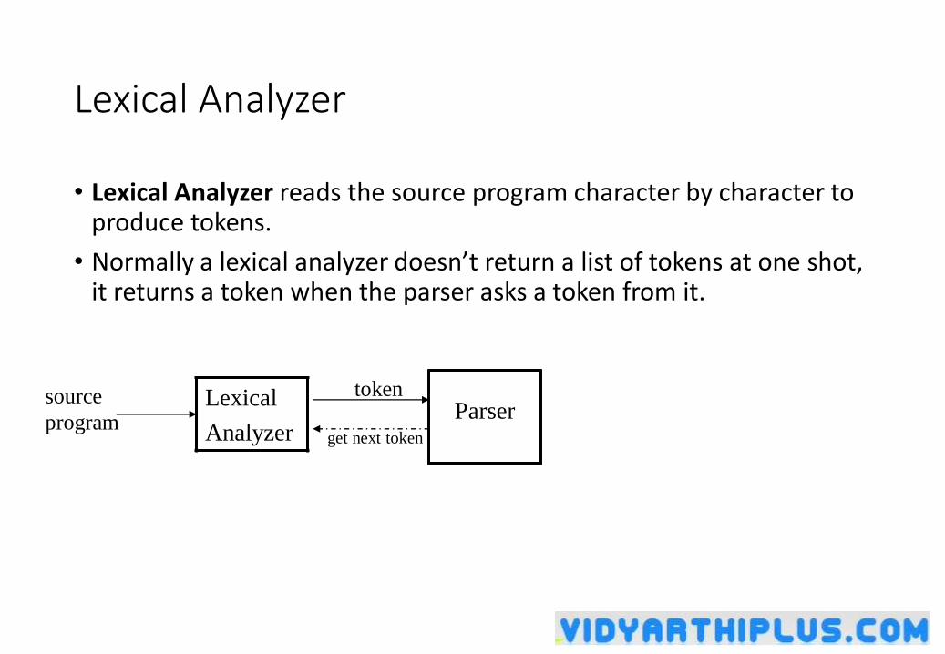
Lexical Analyzer
• Lexical Analyzer reads the source program character by character to produce tokens.
• Normally a lexical analyzer doesn’t return a list of tokens at one shot, it returns a token when the parser asks a token from it.
Lexical
AnalyzerParser
source
program
token
get next token
Token
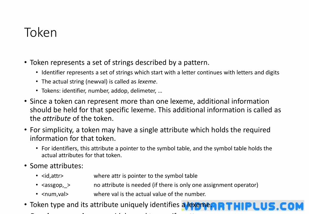
• Token represents a set of strings described by a pattern.• Identifier represents a set of strings which start with a letter continues with letters and digits
• The actual string (newval) is called as lexeme.
• Tokens: identifier, number, addop, delimeter, …
• Since a token can represent more than one lexeme, additional information should be held for that specific lexeme. This additional information is called as the attribute of the token.
• For simplicity, a token may have a single attribute which holds the required information for that token. • For identifiers, this attribute a pointer to the symbol table, and the symbol table holds the
actual attributes for that token.
• Some attributes:• <id,attr> where attr is pointer to the symbol table
• <assgop,_> no attribute is needed (if there is only one assignment operator)
• <num,val> where val is the actual value of the number.
• Token type and its attribute uniquely identifies a lexeme.
• Regular expressions are widely used to specify patterns.
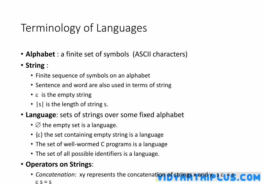
Terminology of Languages
• Alphabet : a finite set of symbols (ASCII characters)
• String :
• Finite sequence of symbols on an alphabet
• Sentence and word are also used in terms of string
• is the empty string
• |s| is the length of string s.
• Language: sets of strings over some fixed alphabet
• the empty set is a language.
• {} the set containing empty string is a language
• The set of well-wormed C programs is a language
• The set of all possible identifiers is a language.
• Operators on Strings:
• Concatenation: xy represents the concatenation of strings x and y. s = s s = s
Operations on Languages
• Concatenation:• L1L2 = { s1s2 | s1 L1 and s2 L2 }
• Union• L1 L2 = { s | s L1 or s L2 }
• Exponentiation:• L0 = {} L1 = L L2 = LL
• Kleene Closure
• L* =
• Positive Closure
• L+ =
0i
iL
1i
iL
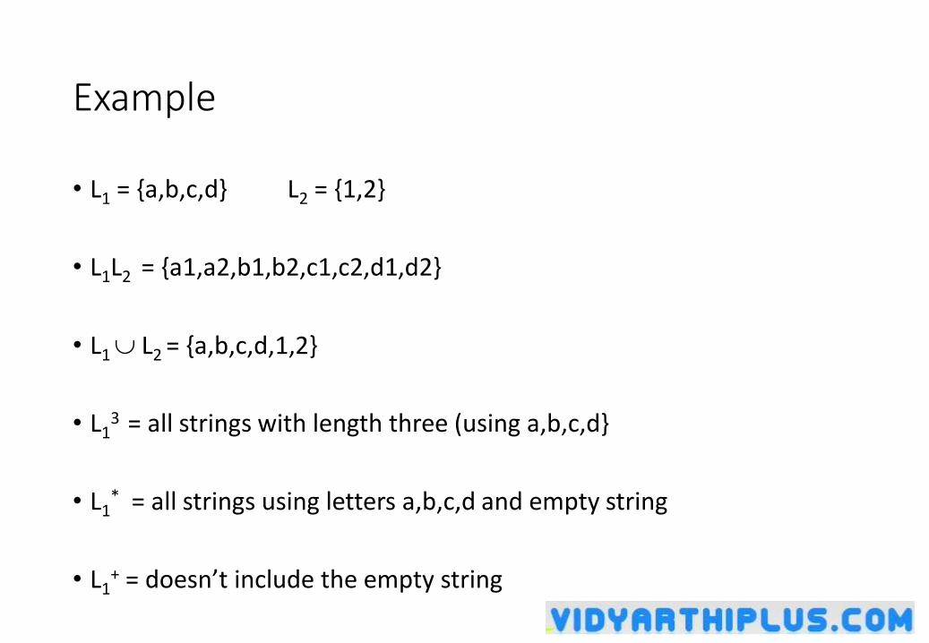
Example
• L1 = {a,b,c,d} L2 = {1,2}
• L1L2 = {a1,a2,b1,b2,c1,c2,d1,d2}
• L1 L2 = {a,b,c,d,1,2}
• L13 = all strings with length three (using a,b,c,d}
• L1* = all strings using letters a,b,c,d and empty string
• L1+ = doesn’t include the empty string
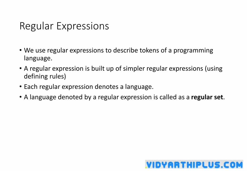
Regular Expressions
• We use regular expressions to describe tokens of a programming language.
• A regular expression is built up of simpler regular expressions (using defining rules)
• Each regular expression denotes a language.
• A language denoted by a regular expression is called as a regular set.
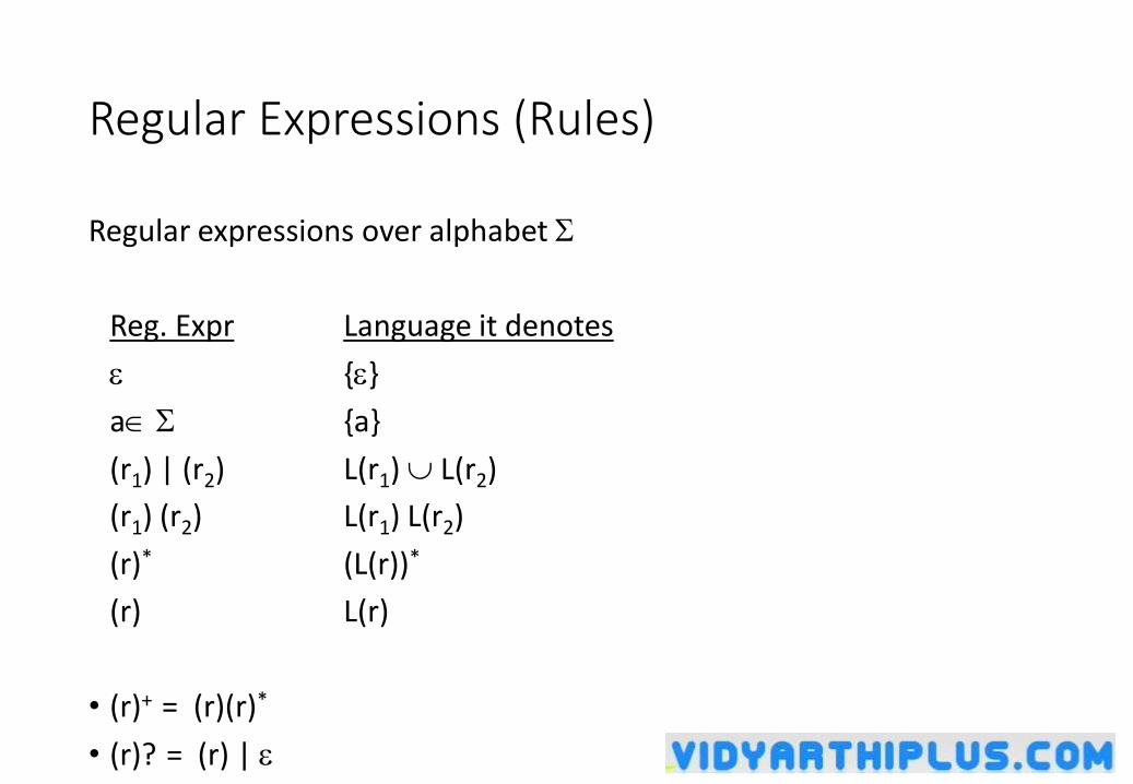
Regular Expressions (Rules)
Regular expressions over alphabet
Reg. Expr Language it denotes
{}
a {a}
(r1) | (r2) L(r1) L(r2)
(r1) (r2) L(r1) L(r2)
(r)* (L(r))*
(r) L(r)
• (r)+ = (r)(r)*
• (r)? = (r) |
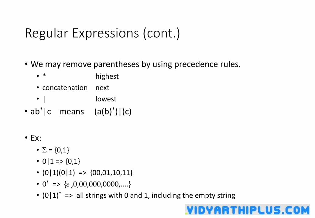
Regular Expressions (cont.)
• We may remove parentheses by using precedence rules.
• * highest
• concatenation next
• | lowest
• ab*|c means (a(b)*)|(c)
• Ex:
• = {0,1}
• 0|1 => {0,1}
• (0|1)(0|1) => {00,01,10,11}
• 0* => { ,0,00,000,0000,....}
• (0|1)* => all strings with 0 and 1, including the empty string
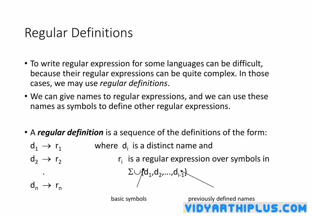
Regular Definitions
• To write regular expression for some languages can be difficult, because their regular expressions can be quite complex. In those cases, we may use regular definitions.
• We can give names to regular expressions, and we can use these names as symbols to define other regular expressions.
• A regular definition is a sequence of the definitions of the form:
d1 r1 where di is a distinct name and
d2 r2 ri is a regular expression over symbols in
. {d1,d2,...,di-1}
dn rn
basic symbols previously defined names
Regular Definitions (cont.)
• Ex: Identifiers in Pascalletter A | B | ... | Z | a | b | ... | z
digit 0 | 1 | ... | 9
id letter (letter | digit ) *
• If we try to write the regular expression representing identifiers without using regular definitions, that regular expression will be complex.
(A|...|Z|a|...|z) ( (A|...|Z|a|...|z) | (0|...|9) ) *
• Ex: Unsigned numbers in Pascaldigit 0 | 1 | ... | 9
digits digit +
opt-fraction ( . digits ) ?
opt-exponent ( E (+|-)? digits ) ?
unsigned-num digits opt-fraction opt-exponent
Finite Automata
• A recognizer for a language is a program that takes a string x, and answers “yes” if x is a sentence of that language, and “no” otherwise.
• We call the recognizer of the tokens as a finite automaton.
• A finite automaton can be: deterministic(DFA) or non-deterministic (NFA)
• This means that we may use a deterministic or non-deterministic automaton as a lexical analyzer.
• Both deterministic and non-deterministic finite automaton recognize regular sets.
• Which one?• deterministic – faster recognizer, but it may take more space
• non-deterministic – slower, but it may take less space
• Deterministic automatons are widely used lexical analyzers.
• First, we define regular expressions for tokens; Then we convert them into a DFA to get a lexical analyzer for our tokens.• Algorithm1: Regular Expression NFA DFA (two steps: first to NFA, then to DFA)
• Algorithm2: Regular Expression DFA (directly convert a regular expression into a DFA)
Non-Deterministic Finite Automaton (NFA)
• A non-deterministic finite automaton (NFA) is a mathematical model that consists of:
• S - a set of states
• - a set of input symbols (alphabet)
• move – a transition function move to map state-symbol pairs to sets of states.
• s0 - a start (initial) state
• F – a set of accepting states (final states)
• - transitions are allowed in NFAs. In other words, we can move from one state to another one without consuming any symbol.
• A NFA accepts a string x, if and only if there is a path from the starting state to one of accepting states such that edge labels along this path spell out x.
NFA (Example)
10 2a b
start
a
b
0 is the start state s0
{2} is the set of final states F
= {a,b}
S = {0,1,2}
Transition Function: a b
0 {0,1} {0}
1 _ {2}
2 _ _
Transition graph of the NFA
The language recognized by this NFA is (a|b) * a b
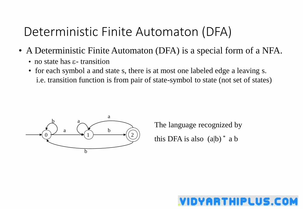
Deterministic Finite Automaton (DFA)
• A Deterministic Finite Automaton (DFA) is a special form of a NFA.• no state has - transition
• for each symbol a and state s, there is at most one labeled edge a leaving s.
i.e. transition function is from pair of state-symbol to state (not set of states)
10 2ba
a
b
The language recognized by
this DFA is also (a|b) * a b
b a
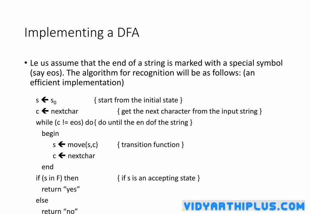
Implementing a DFA
• Le us assume that the end of a string is marked with a special symbol (say eos). The algorithm for recognition will be as follows: (an efficient implementation)
s s0 { start from the initial state }
c nextchar { get the next character from the input string }
while (c != eos) do{ do until the en dof the string }
begin
s move(s,c) { transition function }
c nextchar
end
if (s in F) then { if s is an accepting state }
return “yes”
else
return “no”
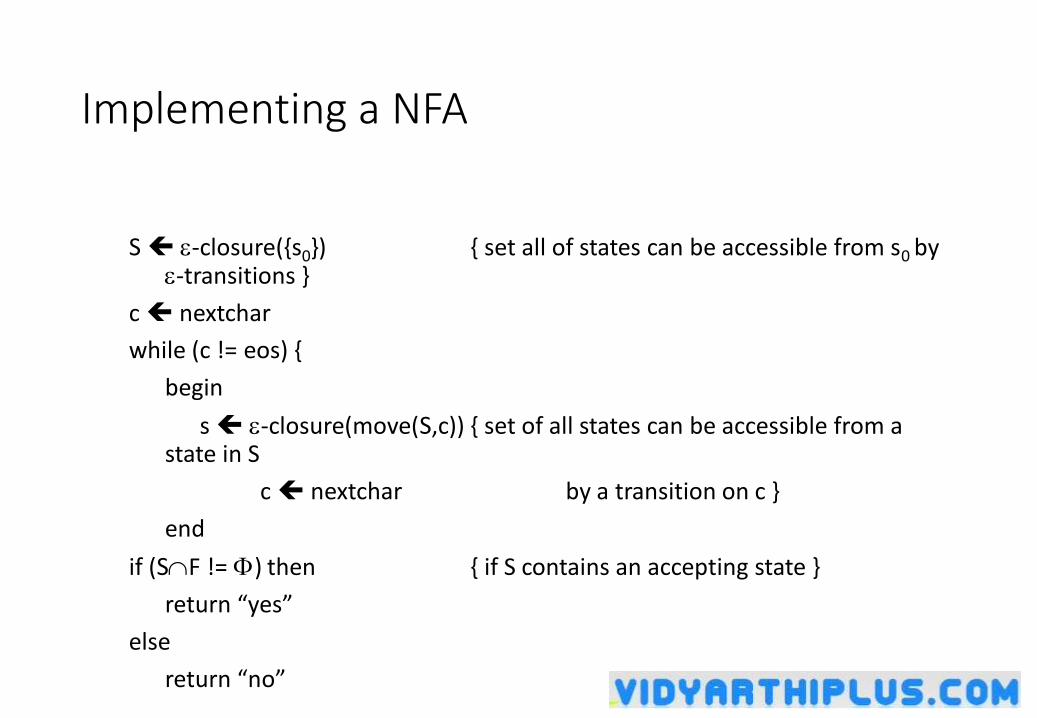
Implementing a NFA
S -closure({s0}) { set all of states can be accessible from s0 by -transitions }
c nextchar
while (c != eos) {
begin
s -closure(move(S,c)) { set of all states can be accessible from a state in S
c nextchar by a transition on c }
end
if (SF != ) then { if S contains an accepting state }
return “yes”
else
return “no”
Converting A Regular Expression into A NFA (Thomson’s Construction)
• This is one way to convert a regular expression into a NFA.
• There can be other ways (much efficient) for the conversion.
• Thomson’s Construction is simple and systematic method. It guarantees that the resulting NFA will have exactly one final state, and one start state.
• Construction starts from simplest parts (alphabet symbols). To create a NFA for a complex regular expression, NFAs of its sub-expressions are combined to create its NFA,
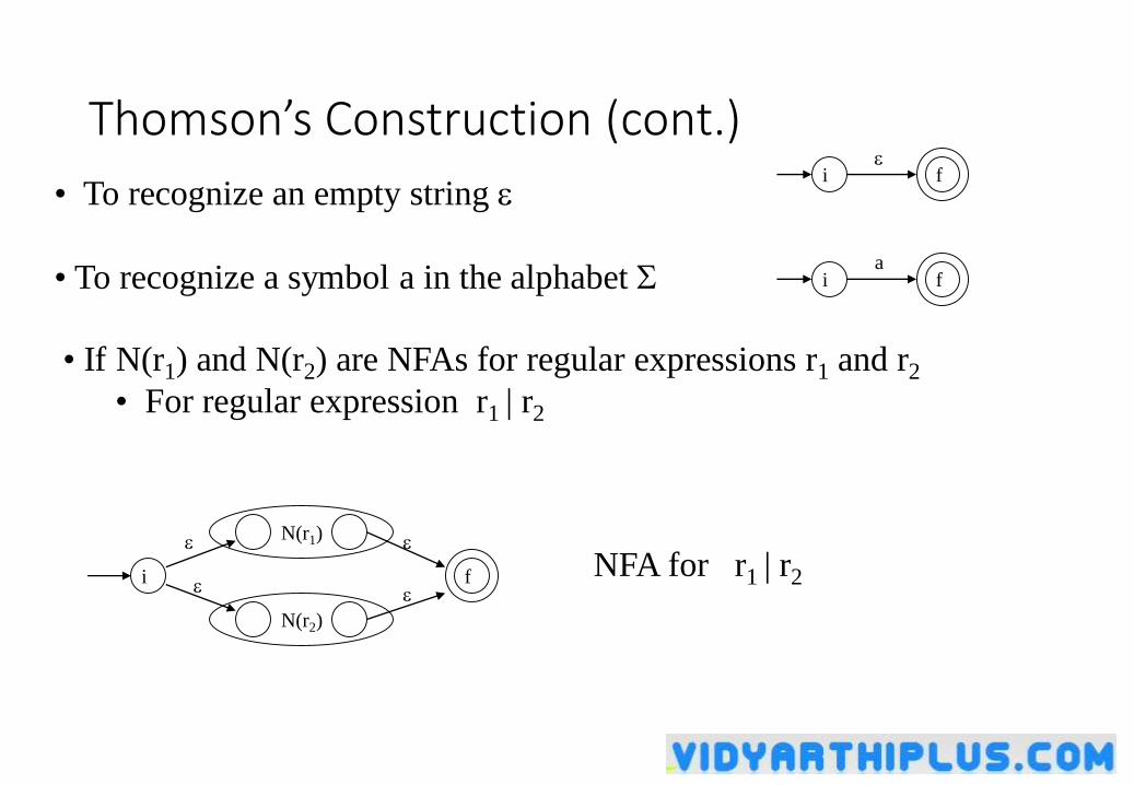
• To recognize an empty string
• To recognize a symbol a in the alphabet
• If N(r1) and N(r2) are NFAs for regular expressions r1 and r2
• For regular expression r1 | r2
a
fi
fi
N(r2)
N(r1)
fi NFA for r1 | r2
Thomson’s Construction (cont.)
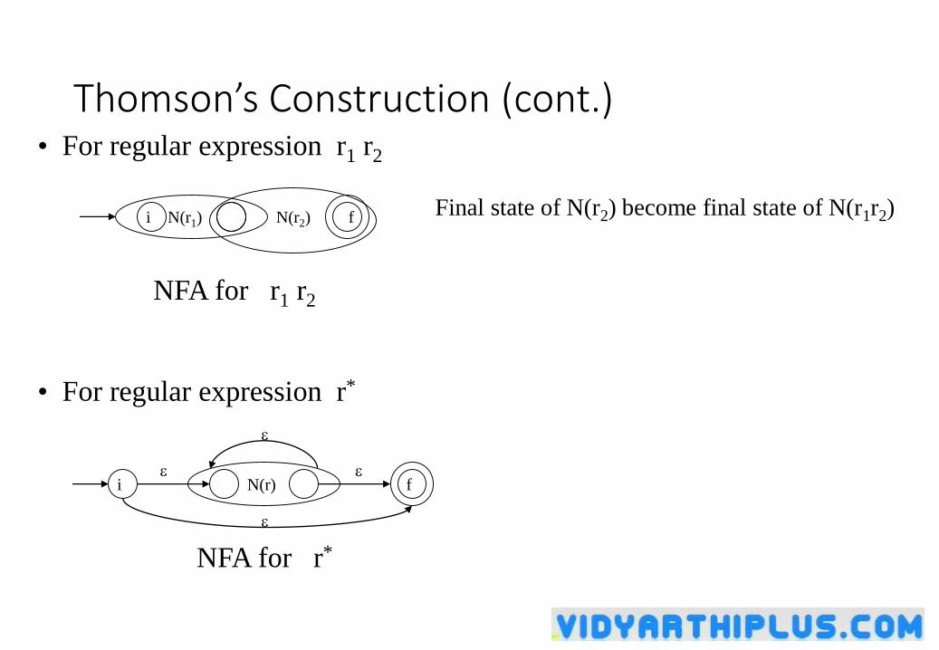
Thomson’s Construction (cont.)• For regular expression r1 r2
i fN(r2)N(r1)
NFA for r1 r2
Final state of N(r2) become final state of N(r1r2)
• For regular expression r*
N(r)i f
NFA for r*
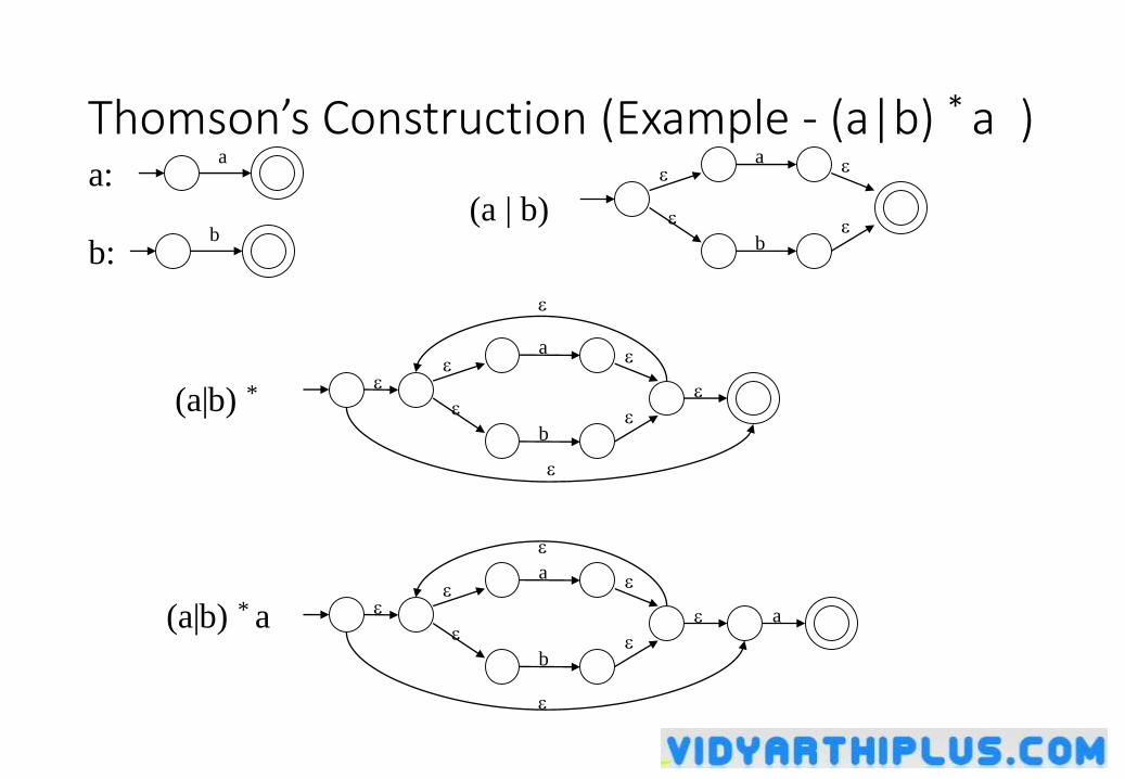
Thomson’s Construction (Example - (a|b) * a )a:
a
b
b:
(a | b)
a
b
b
a
(a|b) *
b
a
a(a|b) * a
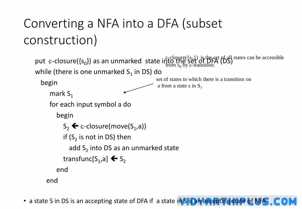
Converting a NFA into a DFA (subset construction)
put -closure({s0}) as an unmarked state into the set of DFA (DS)
while (there is one unmarked S1 in DS) do
begin
mark S1
for each input symbol a do
begin
S2 -closure(move(S1,a))
if (S2 is not in DS) then
add S2 into DS as an unmarked state
transfunc[S1,a] S2
end
end
• a state S in DS is an accepting state of DFA if a state in S is an accepting state of NFA
• the start state of DFA is -closure({s })
set of states to which there is a transition on
a from a state s in S1
-closure({s0}) is the set of all states can be accessible
from s0 by -transition.
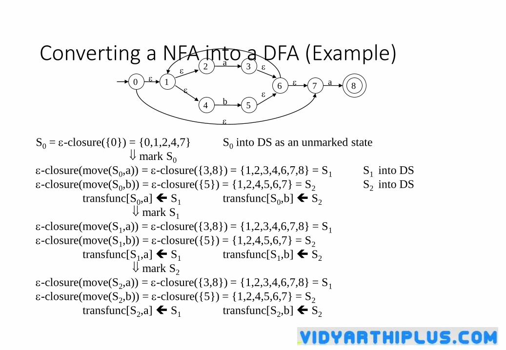
Converting a NFA into a DFA (Example)
b
a
a0 1
3
4 5
2
7 86
S0 = -closure({0}) = {0,1,2,4,7} S0 into DS as an unmarked state
mark S0
-closure(move(S0,a)) = -closure({3,8}) = {1,2,3,4,6,7,8} = S1 S1 into DS
-closure(move(S0,b)) = -closure({5}) = {1,2,4,5,6,7} = S2 S2 into DS
transfunc[S0,a] S1 transfunc[S0,b] S2
mark S1
-closure(move(S1,a)) = -closure({3,8}) = {1,2,3,4,6,7,8} = S1
-closure(move(S1,b)) = -closure({5}) = {1,2,4,5,6,7} = S2
transfunc[S1,a] S1 transfunc[S1,b] S2
mark S2
-closure(move(S2,a)) = -closure({3,8}) = {1,2,3,4,6,7,8} = S1
-closure(move(S2,b)) = -closure({5}) = {1,2,4,5,6,7} = S2
transfunc[S2,a] S1 transfunc[S2,b] S2
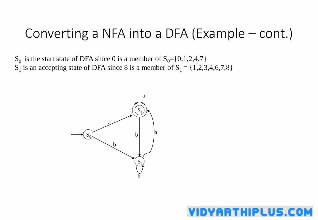
Converting a NFA into a DFA (Example – cont.)
S0 is the start state of DFA since 0 is a member of S0={0,1,2,4,7}
S1 is an accepting state of DFA since 8 is a member of S1 = {1,2,3,4,6,7,8}
b
a
a
b
b
a
S1
S2
S0
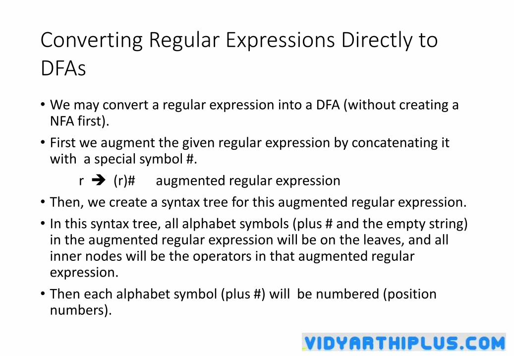
Converting Regular Expressions Directly to DFAs
• We may convert a regular expression into a DFA (without creating a NFA first).
• First we augment the given regular expression by concatenating it with a special symbol #.
r (r)# augmented regular expression
• Then, we create a syntax tree for this augmented regular expression.
• In this syntax tree, all alphabet symbols (plus # and the empty string) in the augmented regular expression will be on the leaves, and all inner nodes will be the operators in that augmented regular expression.
• Then each alphabet symbol (plus #) will be numbered (position numbers).
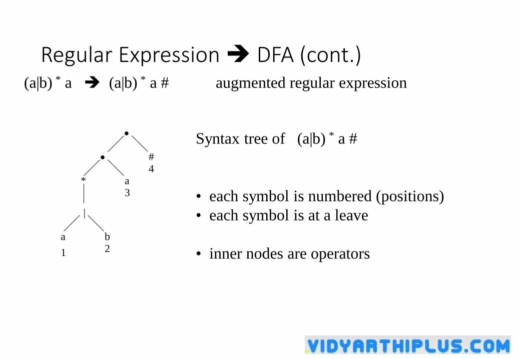
Regular Expression DFA (cont.)(a|b) * a (a|b) * a # augmented regular expression
*
|
b
a
#
a
1
4
3
2
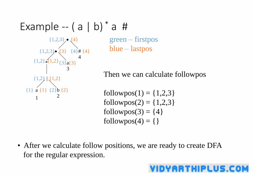
Syntax tree of (a|b) * a #
• each symbol is numbered (positions)
• each symbol is at a leave
• inner nodes are operators
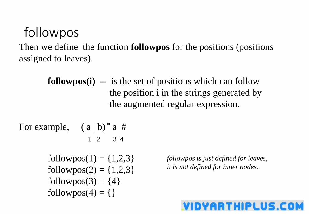
followposThen we define the function followpos for the positions (positions
assigned to leaves).
followpos(i) -- is the set of positions which can follow
the position i in the strings generated by
the augmented regular expression.
For example, ( a | b) * a #
1 2 3 4
followpos(1) = {1,2,3}
followpos(2) = {1,2,3}
followpos(3) = {4}
followpos(4) = {}
followpos is just defined for leaves,
it is not defined for inner nodes.
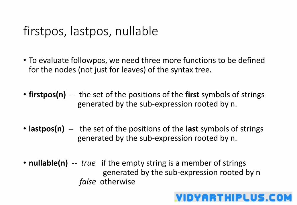
firstpos, lastpos, nullable
• To evaluate followpos, we need three more functions to be defined for the nodes (not just for leaves) of the syntax tree.
• firstpos(n) -- the set of the positions of the first symbols of strings generated by the sub-expression rooted by n.
• lastpos(n) -- the set of the positions of the last symbols of strings generated by the sub-expression rooted by n.
• nullable(n) -- true if the empty string is a member of strings generated by the sub-expression rooted by n
false otherwise
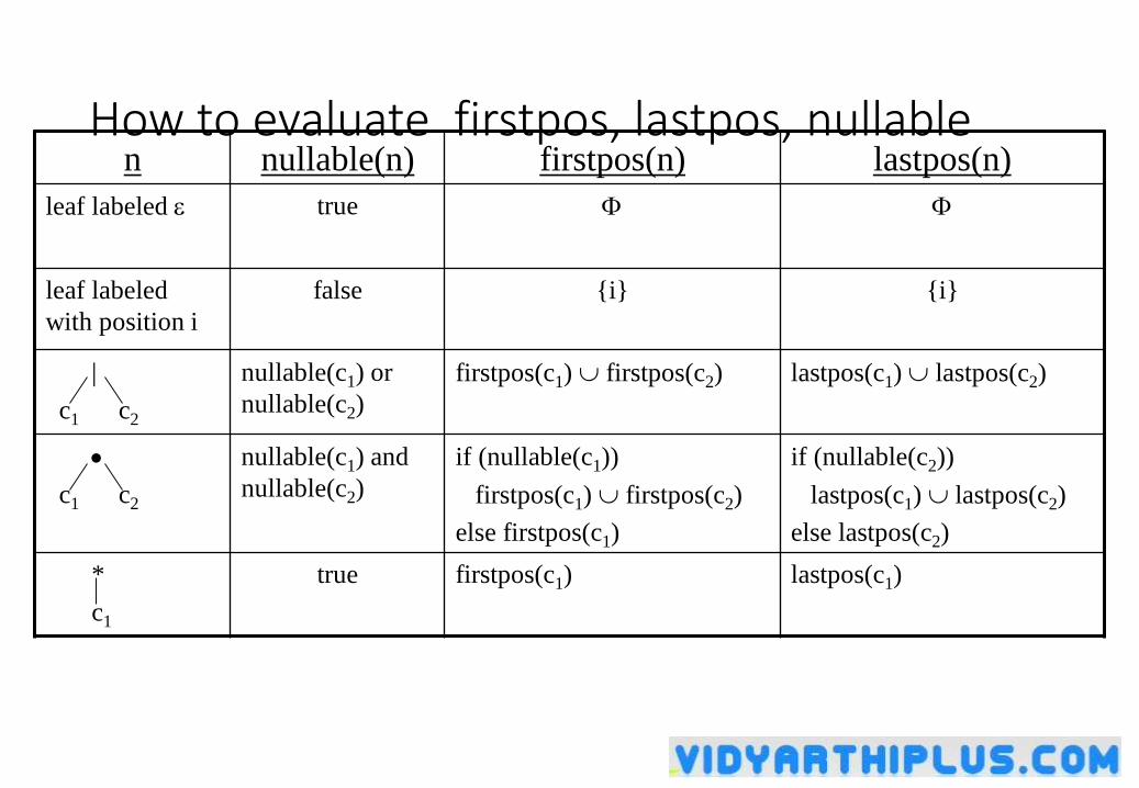
How to evaluate firstpos, lastpos, nullablen nullable(n) firstpos(n) lastpos(n)
leaf labeled true
leaf labeled
with position i
false {i} {i}
|
c1 c2
nullable(c1) or
nullable(c2)
firstpos(c1) firstpos(c2) lastpos(c1) lastpos(c2)
c1 c2
nullable(c1) and
nullable(c2)
if (nullable(c1))
firstpos(c1) firstpos(c2)
else firstpos(c1)
if (nullable(c2))
lastpos(c1) lastpos(c2)
else lastpos(c2)
*
c1
true firstpos(c1) lastpos(c1)
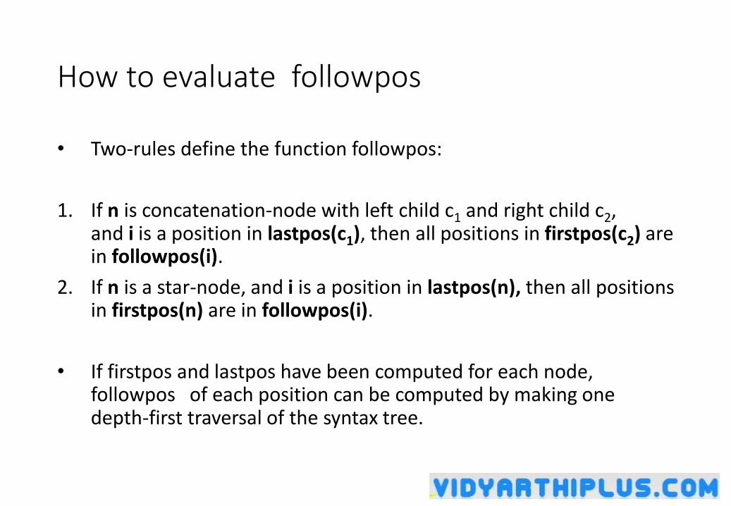
How to evaluate followpos
• Two-rules define the function followpos:
1. If n is concatenation-node with left child c1 and right child c2, and i is a position in lastpos(c1), then all positions in firstpos(c2) are in followpos(i).
2. If n is a star-node, and i is a position in lastpos(n), then all positions in firstpos(n) are in followpos(i).
• If firstpos and lastpos have been computed for each node, followpos of each position can be computed by making one depth-first traversal of the syntax tree.
Example -- ( a | b) * a #
*
|
b
a
#
a
1
4
3
2{1}{1}
{1,2,3}
{3}
{1,2,3}
{1,2}
{1,2}
{2}
{4}
{4}
{4}{3}
{3}{1,2}
{1,2}
{2}
green – firstpos
blue – lastpos
Then we can calculate followpos
followpos(1) = {1,2,3}
followpos(2) = {1,2,3}
followpos(3) = {4}
followpos(4) = {}
• After we calculate follow positions, we are ready to create DFA
for the regular expression.
Algorithm (RE DFA)
• Create the syntax tree of (r) #
• Calculate the functions: followpos, firstpos, lastpos, nullable
• Put firstpos(root) into the states of DFA as an unmarked state.
• while (there is an unmarked state S in the states of DFA) do
• mark S
• for each input symbol a do
• let s1,...,sn are positions in S and symbols in those positions are a
• S’ followpos(s1) ... followpos(sn)
• move(S,a) S’
• if (S’ is not empty and not in the states of DFA)
• put S’ into the states of DFA as an unmarked state.
• the start state of DFA is firstpos(root)
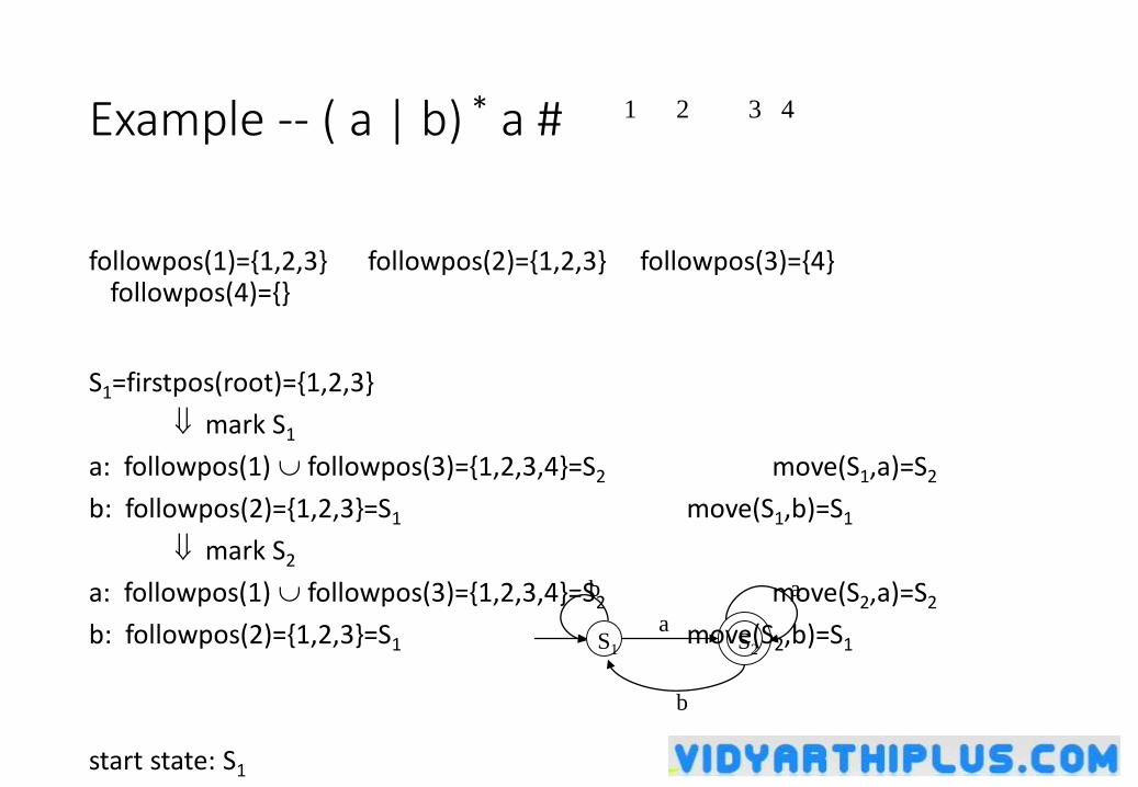
Example -- ( a | b) * a #
followpos(1)={1,2,3} followpos(2)={1,2,3} followpos(3)={4} followpos(4)={}
S1=firstpos(root)={1,2,3}
mark S1
a: followpos(1) followpos(3)={1,2,3,4}=S2 move(S1,a)=S2
b: followpos(2)={1,2,3}=S1 move(S1,b)=S1
mark S2
a: followpos(1) followpos(3)={1,2,3,4}=S2 move(S2,a)=S2
b: followpos(2)={1,2,3}=S1 move(S2,b)=S1
start state: S1
accepting states: {S }
1 2 3 4
S1 S2
a
b
b
a
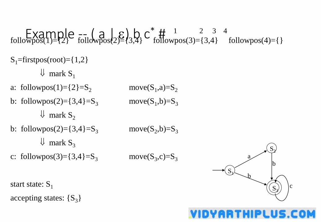
Example -- ( a | ) b c* # 1 2 3 4
followpos(1)={2} followpos(2)={3,4} followpos(3)={3,4} followpos(4)={}
S1=firstpos(root)={1,2}
mark S1
a: followpos(1)={2}=S2 move(S1,a)=S2
b: followpos(2)={3,4}=S3 move(S1,b)=S3
mark S2
b: followpos(2)={3,4}=S3 move(S2,b)=S3
mark S3
c: followpos(3)={3,4}=S3 move(S3,c)=S3
start state: S1
accepting states: {S3}
S3
S2
S1
c
ab
b
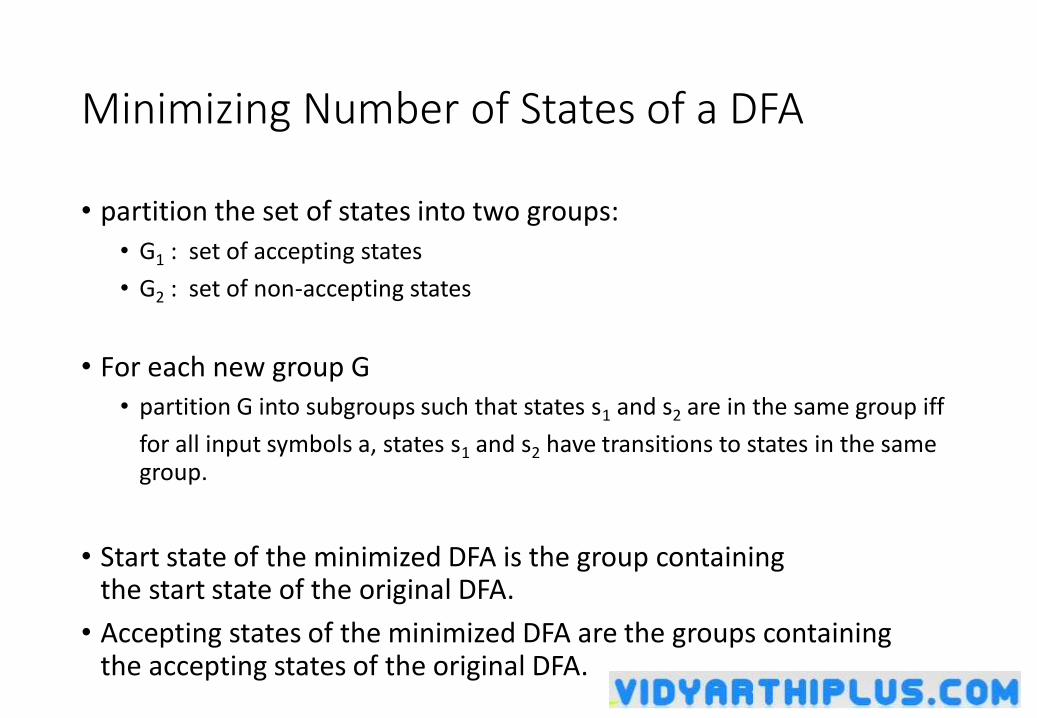
Minimizing Number of States of a DFA
• partition the set of states into two groups:
• G1 : set of accepting states
• G2 : set of non-accepting states
• For each new group G
• partition G into subgroups such that states s1 and s2 are in the same group iff
for all input symbols a, states s1 and s2 have transitions to states in the same group.
• Start state of the minimized DFA is the group containing the start state of the original DFA.
• Accepting states of the minimized DFA are the groups containing the accepting states of the original DFA.
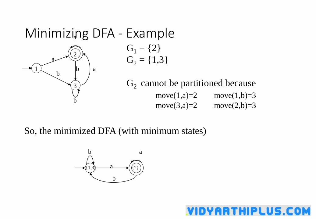
Minimizing DFA - Example
b a
a
a
b
b
3
2
1
G1 = {2}
G2 = {1,3}
G2 cannot be partitioned because
move(1,a)=2 move(1,b)=3
move(3,a)=2 move(2,b)=3
So, the minimized DFA (with minimum states)
{1,3}
a
a
b
b
{2}
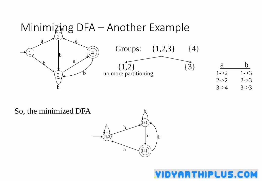
Minimizing DFA – Another Example
b
b
b
a
a
a
a
b 4
3
2
1Groups: {1,2,3} {4}
a b 1->2 1->3
2->2 2->3
3->4 3->3
{1,2} {3}no more partitioning
So, the minimized DFA
{1,2}
{4}
{3}
b
a
a
a
b
b
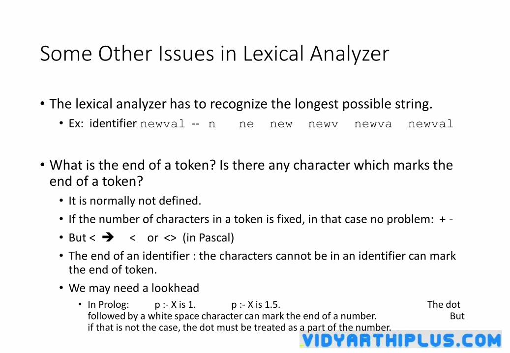
Some Other Issues in Lexical Analyzer
• The lexical analyzer has to recognize the longest possible string.
• Ex: identifier newval -- n ne new newv newva newval
• What is the end of a token? Is there any character which marks the end of a token?
• It is normally not defined.
• If the number of characters in a token is fixed, in that case no problem: + -
• But < < or <> (in Pascal)
• The end of an identifier : the characters cannot be in an identifier can mark the end of token.
• We may need a lookhead• In Prolog: p :- X is 1. p :- X is 1.5. The dot
followed by a white space character can mark the end of a number. But if that is not the case, the dot must be treated as a part of the number.
Some Other Issues in Lexical Analyzer (cont.)
• Skipping comments
• Normally we don’t return a comment as a token.
• We skip a comment, and return the next token (which is not a comment) to the parser.
• So, the comments are only processed by the lexical analyzer, and the don’t complicate the syntax of the language.
• Symbol table interface
• symbol table holds information about tokens (at least lexeme of identifiers)
• how to implement the symbol table, and what kind of operations.
• hash table – open addressing, chaining
• putting into the hash table, finding the position of a token from its lexeme.
• Positions of the tokens in the file (for the error handling).
Syntax Analyzer
• Syntax Analyzer creates the syntactic structure of the given source program.
• This syntactic structure is mostly a parse tree.
• Syntax Analyzer is also known as parser.
• The syntax of a programming is described by a context-free grammar (CFG). We will use BNF (Backus-Naur Form) notation in the description of CFGs.
• The syntax analyzer (parser) checks whether a given source program satisfies the rules implied by a context-free grammar or not.• If it satisfies, the parser creates the parse tree of that program.
• Otherwise the parser gives the error messages.
• A context-free grammar• gives a precise syntactic specification of a programming language.
• the design of the grammar is an initial phase of the design of a compiler.
• a grammar can be directly converted into a parser by some tools.
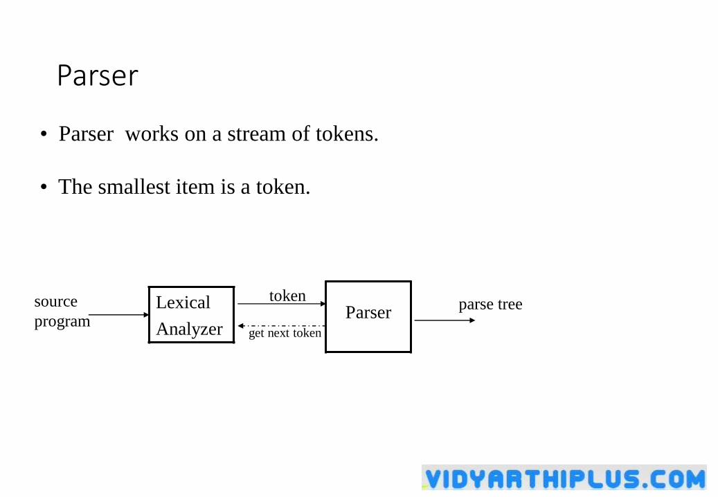
Parser
Lexical
AnalyzerParser
source
program
token
get next token
parse tree
• Parser works on a stream of tokens.
• The smallest item is a token.
Parsers (cont.)
• We categorize the parsers into two groups:
1. Top-Down Parser
• the parse tree is created top to bottom, starting from the root.
2. Bottom-Up Parser
• the parse is created bottom to top; starting from the leaves
• Both top-down and bottom-up parsers scan the input from left to right (one symbol at a time).
• Efficient top-down and bottom-up parsers can be implemented only for sub-classes of context-free grammars.
• LL for top-down parsing
• LR for bottom-up parsing
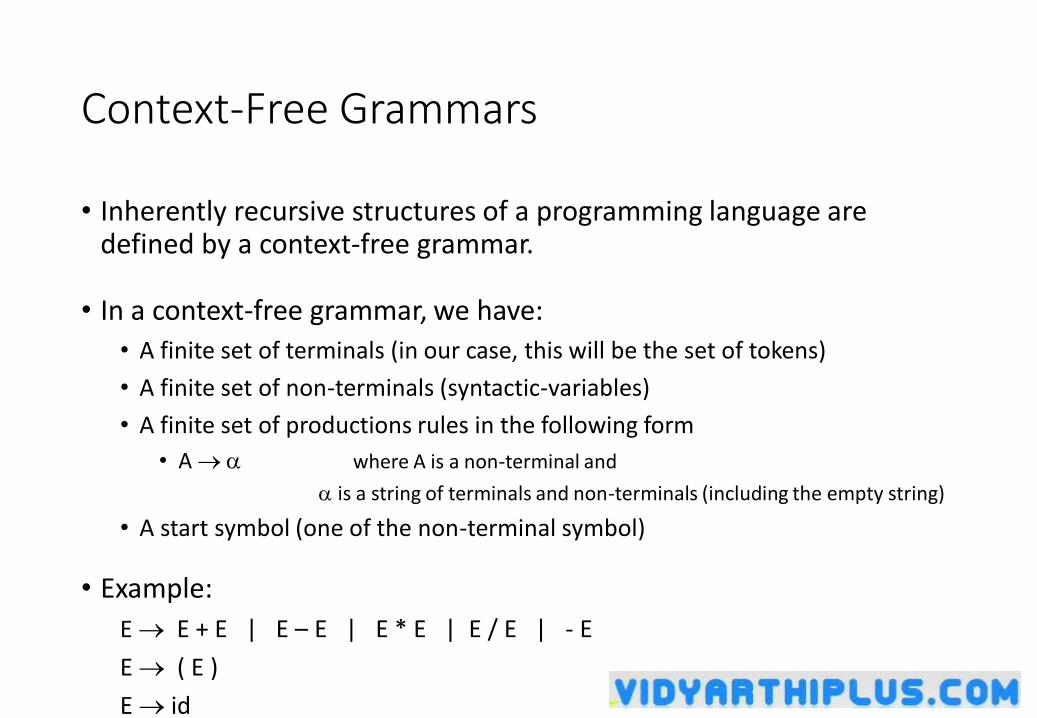
Context-Free Grammars
• Inherently recursive structures of a programming language are defined by a context-free grammar.
• In a context-free grammar, we have:
• A finite set of terminals (in our case, this will be the set of tokens)
• A finite set of non-terminals (syntactic-variables)
• A finite set of productions rules in the following form
• A where A is a non-terminal and
is a string of terminals and non-terminals (including the empty string)
• A start symbol (one of the non-terminal symbol)
• Example:
E E + E | E – E | E * E | E / E | - E
E ( E )
E id
Derivations
E E+E
• E+E derives from E
• we can replace E by E+E
• to able to do this, we have to have a production rule EE+E in our grammar.
E E+E id+E id+id
• A sequence of replacements of non-terminal symbols is called a derivation of id+id from E.
• In general a derivation step is
A if there is a production rule A in our grammar
where and are arbitrary strings of terminal and non-terminal symbols
1 2 ... n (n derives from 1 or 1 derives n )
: derives in one step
: derives in zero or more steps
: derives in one or more steps
*
+
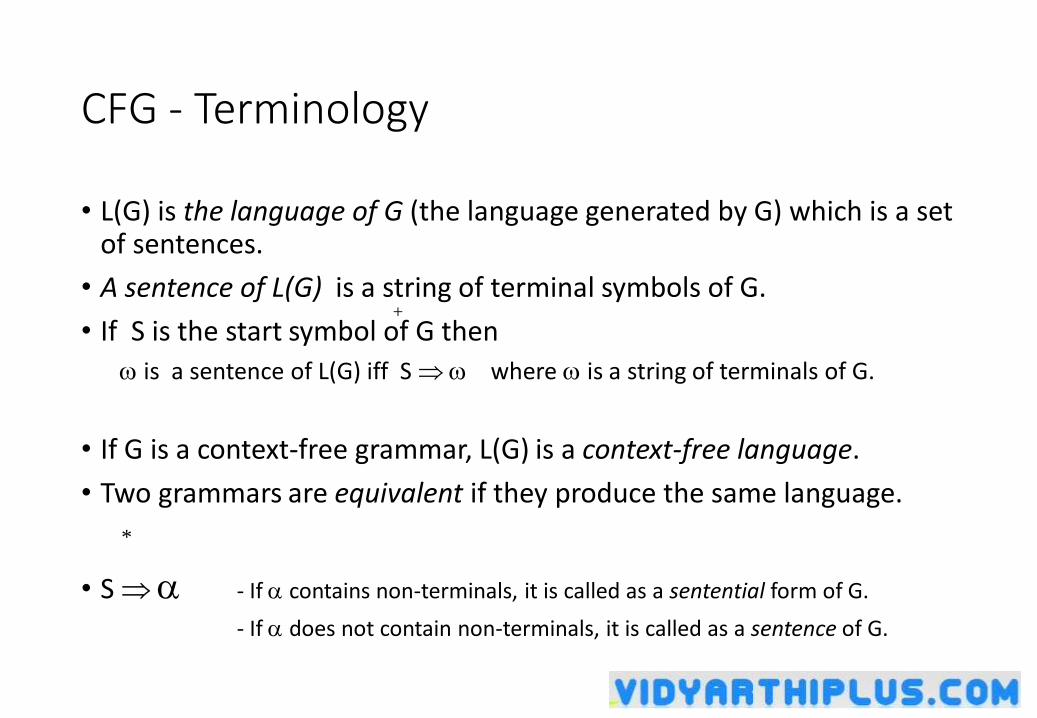
CFG - Terminology
• L(G) is the language of G (the language generated by G) which is a set of sentences.
• A sentence of L(G) is a string of terminal symbols of G.
• If S is the start symbol of G then
is a sentence of L(G) iff S where is a string of terminals of G.
• If G is a context-free grammar, L(G) is a context-free language.
• Two grammars are equivalent if they produce the same language.
• S - If contains non-terminals, it is called as a sentential form of G.
- If does not contain non-terminals, it is called as a sentence of G.
+
*
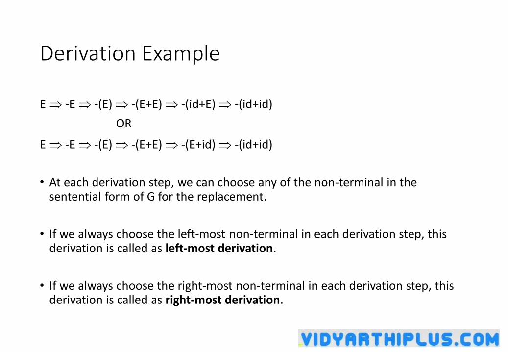
Derivation Example
E -E -(E) -(E+E) -(id+E) -(id+id)
OR
E -E -(E) -(E+E) -(E+id) -(id+id)
• At each derivation step, we can choose any of the non-terminal in the sentential form of G for the replacement.
• If we always choose the left-most non-terminal in each derivation step, this derivation is called as left-most derivation.
• If we always choose the right-most non-terminal in each derivation step, this derivation is called as right-most derivation.
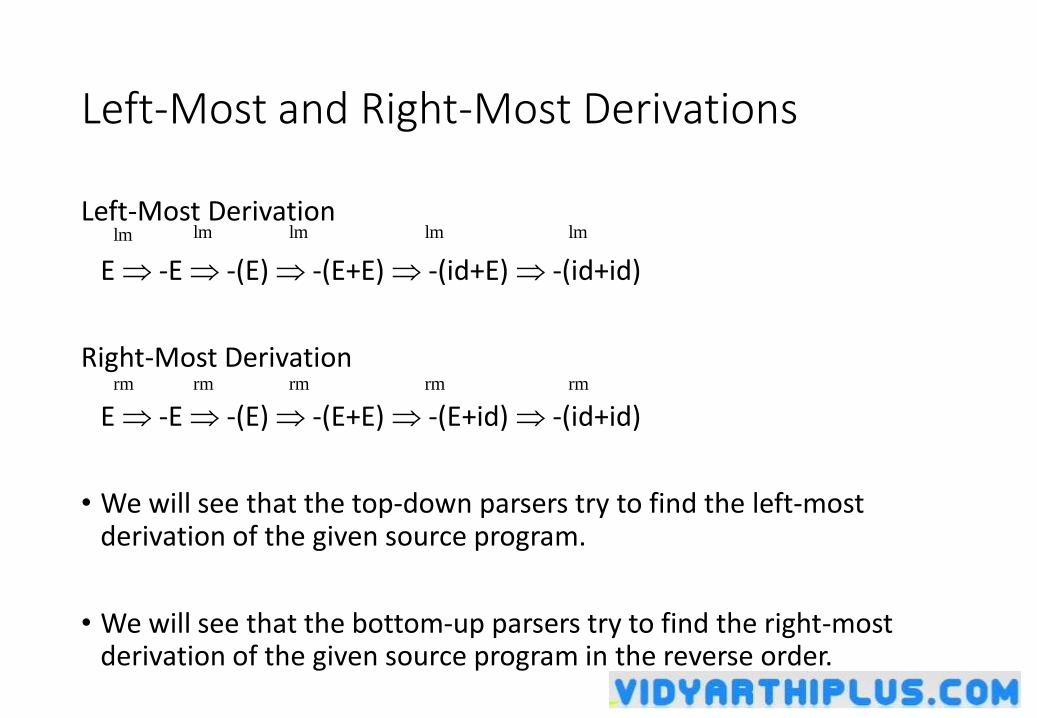
Left-Most and Right-Most Derivations
Left-Most Derivation
E -E -(E) -(E+E) -(id+E) -(id+id)
Right-Most Derivation
E -E -(E) -(E+E) -(E+id) -(id+id)
• We will see that the top-down parsers try to find the left-most derivation of the given source program.
• We will see that the bottom-up parsers try to find the right-most derivation of the given source program in the reverse order.
lmlmlmlmlm
rmrmrmrmrm
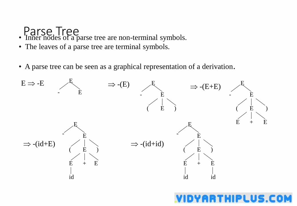
Parse Tree• Inner nodes of a parse tree are non-terminal symbols.
• The leaves of a parse tree are terminal symbols.
• A parse tree can be seen as a graphical representation of a derivation.
E -E E
E-
E
E
EE
E
+
-
( )
E
E
E-
( )
E
E
id
E
E
E +
-
( )
id
E
E
E
EE +
-
( )
id
-(E) -(E+E)
-(id+E) -(id+id)
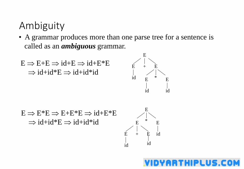
Ambiguity• A grammar produces more than one parse tree for a sentence is
called as an ambiguous grammar.
E E+E id+E id+E*E
id+id*E id+id*id
E E*E E+E*E id+E*E
id+id*E id+id*id
E
id
E +
id
id
E
E
* E
E
E +
id E
E
* E
id id
Ambiguity (cont.)
• For the most parsers, the grammar must be unambiguous.
• unambiguous grammar
unique selection of the parse tree for a sentence
• We should eliminate the ambiguity in the grammar during the design phase of the compiler.
• An unambiguous grammar should be written to eliminate the ambiguity.
• We have to prefer one of the parse trees of a sentence (generated by an ambiguous grammar) to disambiguate that grammar to restrict to this choice.
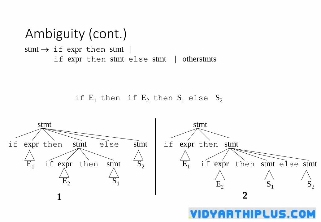
Ambiguity (cont.)stmt if expr then stmt |
if expr then stmt else stmt | otherstmts
if E1 then if E2 then S1 else S2
stmt
if expr then stmt else stmt
E1 if expr then stmt S2
E2 S1
stmt
if expr then stmt
E1 if expr then stmt else stmt
E2 S1 S2
1 2
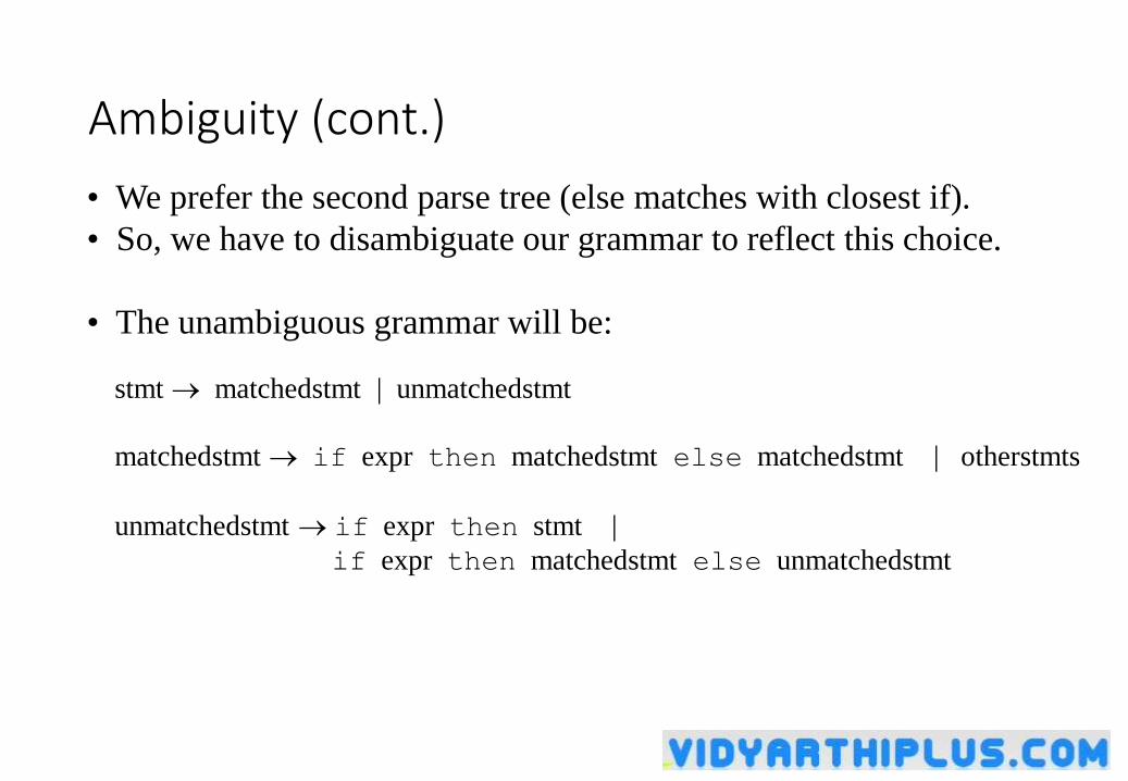
Ambiguity (cont.)
• We prefer the second parse tree (else matches with closest if).
• So, we have to disambiguate our grammar to reflect this choice.
• The unambiguous grammar will be:
stmt matchedstmt | unmatchedstmt
matchedstmt if expr then matchedstmt else matchedstmt | otherstmts
unmatchedstmt if expr then stmt |
if expr then matchedstmt else unmatchedstmt
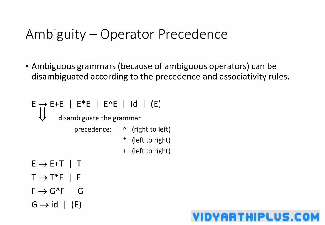
Ambiguity – Operator Precedence
• Ambiguous grammars (because of ambiguous operators) can be disambiguated according to the precedence and associativity rules.
E E+E | E*E | E^E | id | (E)
disambiguate the grammar
precedence: ^ (right to left)
* (left to right)
+ (left to right)
E E+T | T
T T*F | F
F G^F | G
G id | (E)
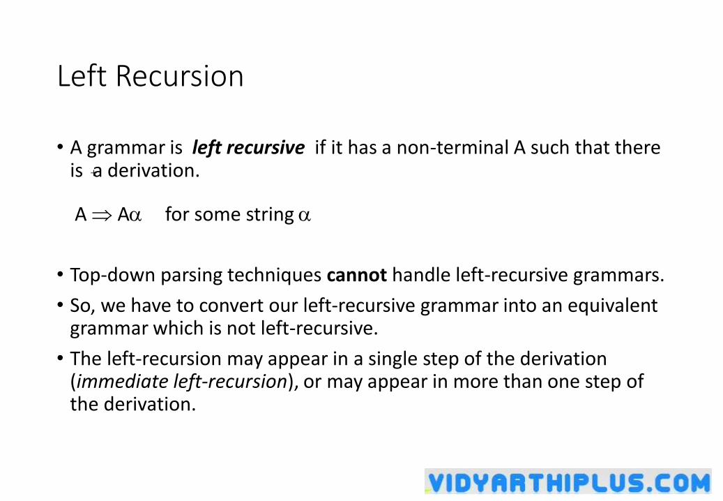
Left Recursion
• A grammar is left recursive if it has a non-terminal A such that there is a derivation.
A A for some string
• Top-down parsing techniques cannot handle left-recursive grammars.
• So, we have to convert our left-recursive grammar into an equivalent grammar which is not left-recursive.
• The left-recursion may appear in a single step of the derivation (immediate left-recursion), or may appear in more than one step of the derivation.
+
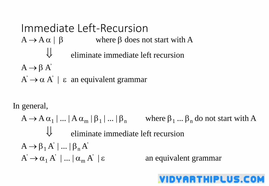
Immediate Left-RecursionA A | where does not start with A
eliminate immediate left recursion
A A’
A’ A’ | an equivalent grammar
A A 1 | ... | A m | 1 | ... | n where 1 ... n do not start with A
eliminate immediate left recursion
A 1 A’ | ... | n A’
A’ 1 A’ | ... | m A’ | an equivalent grammar
In general,
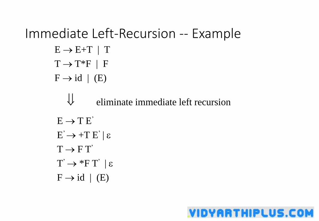
Immediate Left-Recursion -- ExampleE E+T | T
T T*F | F
F id | (E)
E T E’
E’ +T E’ |
T F T’
T’ *F T’ |
F id | (E)
eliminate immediate left recursion
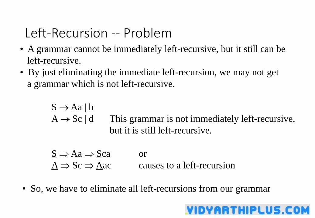
Left-Recursion -- Problem• A grammar cannot be immediately left-recursive, but it still can be
left-recursive.
• By just eliminating the immediate left-recursion, we may not get
a grammar which is not left-recursive.
S Aa | b
A Sc | d This grammar is not immediately left-recursive,
but it is still left-recursive.
S Aa Sca or
A Sc Aac causes to a left-recursion
• So, we have to eliminate all left-recursions from our grammar
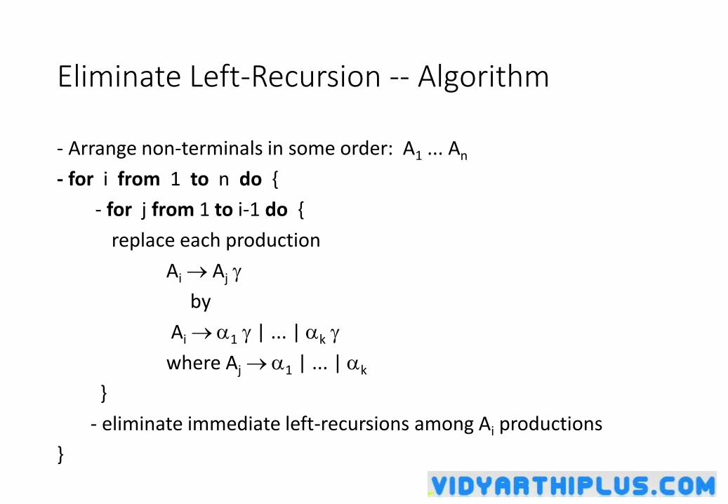
Eliminate Left-Recursion -- Algorithm
- Arrange non-terminals in some order: A1 ... An
- for i from 1 to n do {
- for j from 1 to i-1 do {
replace each production
Ai Aj
by
Ai 1 | ... | k
where Aj 1 | ... | k
}
- eliminate immediate left-recursions among Ai productions
}
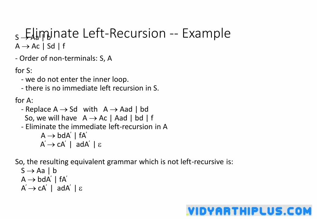
Eliminate Left-Recursion -- ExampleS Aa | bA Ac | Sd | f
- Order of non-terminals: S, A
for S:- we do not enter the inner loop.- there is no immediate left recursion in S.
for A:- Replace A Sd with A Aad | bd
So, we will have A Ac | Aad | bd | f- Eliminate the immediate left-recursion in A
A bdA’ | fA’
A’ cA’ | adA’ |
So, the resulting equivalent grammar which is not left-recursive is:S Aa | bA bdA’ | fA’
A’ cA’ | adA’ |
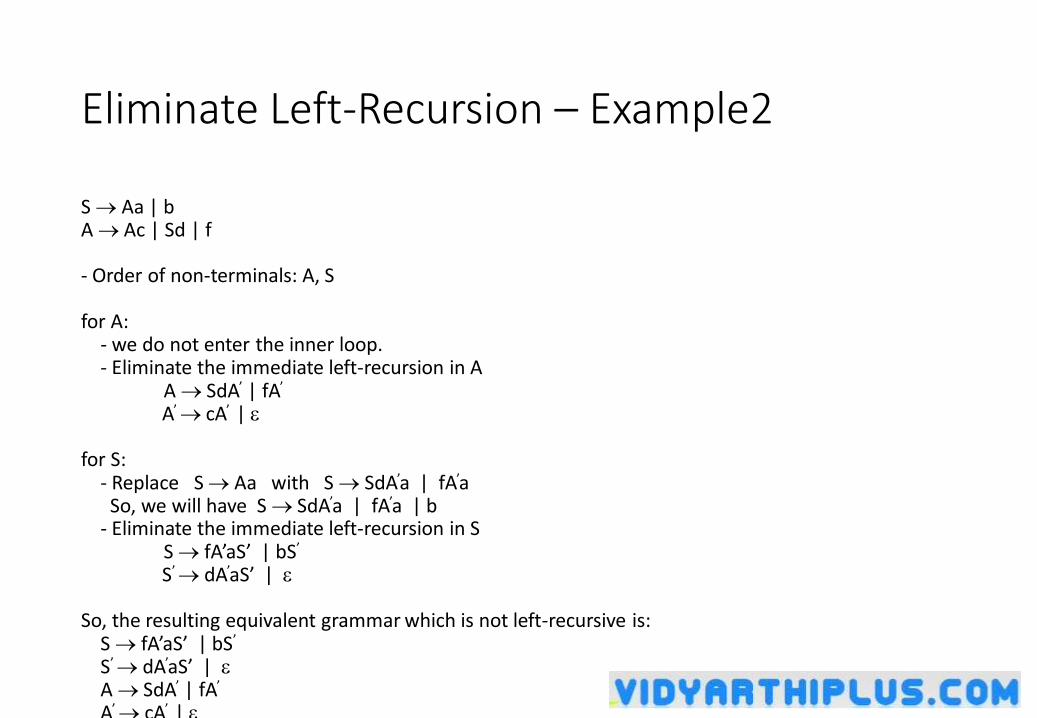
Eliminate Left-Recursion – Example2
S Aa | bA Ac | Sd | f
- Order of non-terminals: A, S
for A:- we do not enter the inner loop.- Eliminate the immediate left-recursion in A
A SdA’ | fA’
A’ cA’ |
for S:- Replace S Aa with S SdA’a | fA’a So, we will have S SdA’a | fA’a | b
- Eliminate the immediate left-recursion in S S fA’aS’ | bS’
S’ dA’aS’ |
So, the resulting equivalent grammar which is not left-recursive is:S fA’aS’ | bS’
S’ dA’aS’ | A SdA’ | fA’
A’ cA’ |
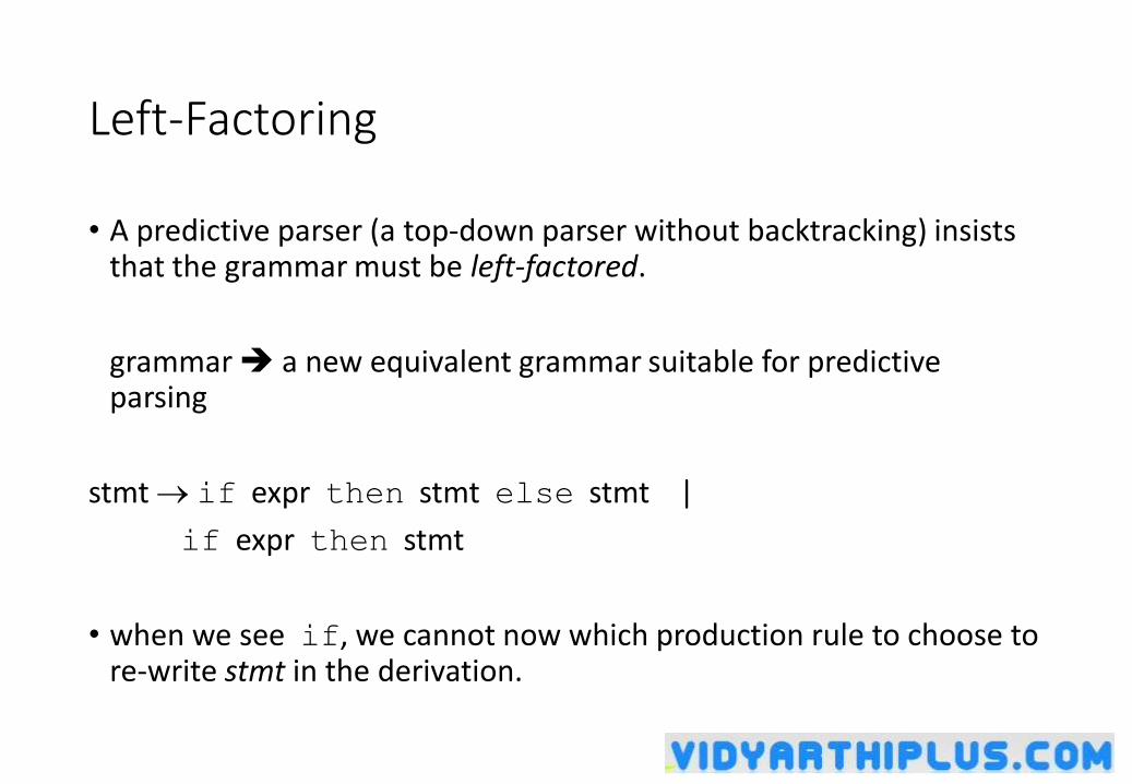
Left-Factoring
• A predictive parser (a top-down parser without backtracking) insists that the grammar must be left-factored.
grammar a new equivalent grammar suitable for predictive parsing
stmt if expr then stmt else stmt |
if expr then stmt
• when we see if, we cannot now which production rule to choose to re-write stmt in the derivation.
Left-Factoring (cont.)
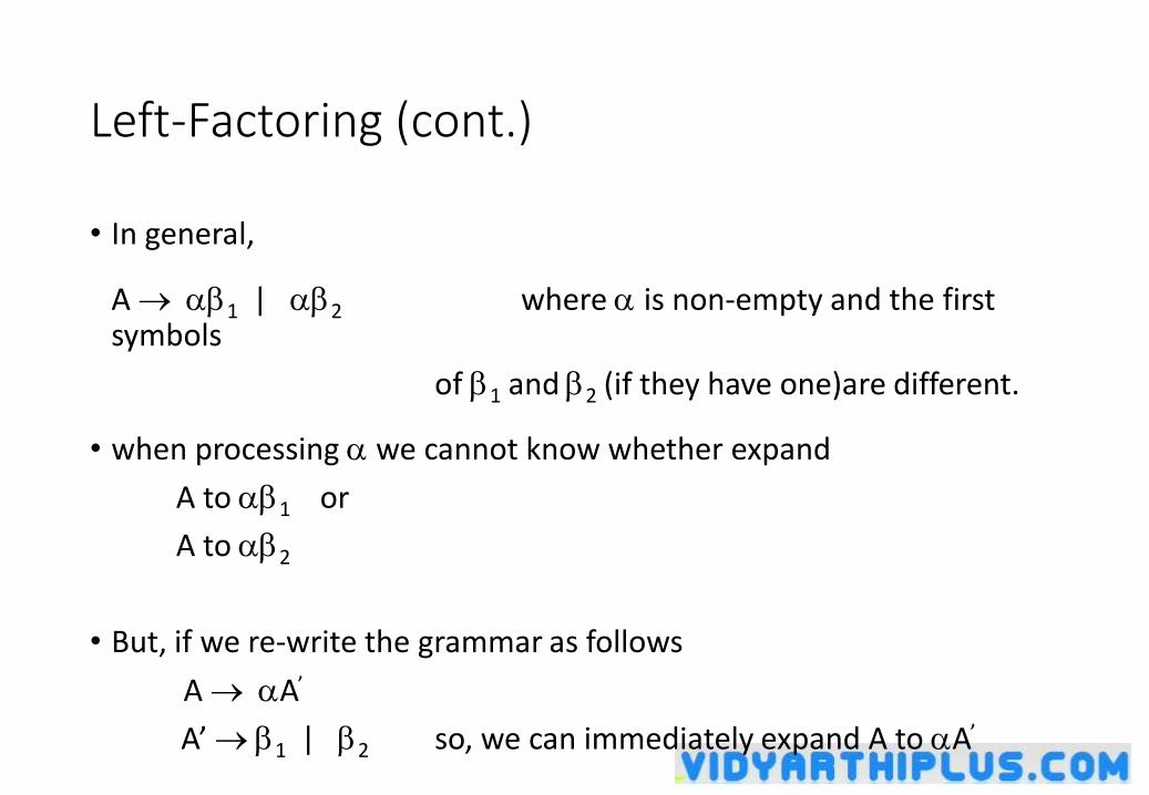
• In general,
A 1 | 2 where is non-empty and the first symbols
of 1 and 2 (if they have one)are different.
• when processing we cannot know whether expand
A to 1 or
A to 2
• But, if we re-write the grammar as follows
A A’
A’ 1 | 2 so, we can immediately expand A to A’
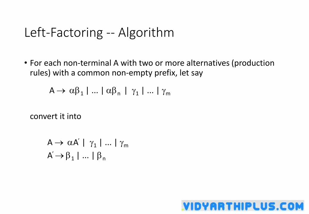
Left-Factoring -- Algorithm
• For each non-terminal A with two or more alternatives (production rules) with a common non-empty prefix, let say
A 1 | ... | n | 1 | ... | m
convert it into
A A’ | 1 | ... | m
A’ 1 | ... | n
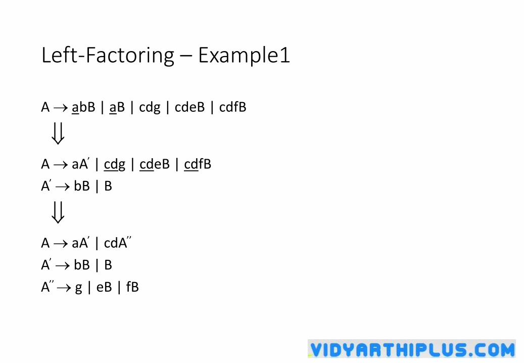
Left-Factoring – Example1
A abB | aB | cdg | cdeB | cdfB
A aA’ | cdg | cdeB | cdfB
A’ bB | B
A aA’ | cdA’’
A’ bB | B
A’’ g | eB | fB
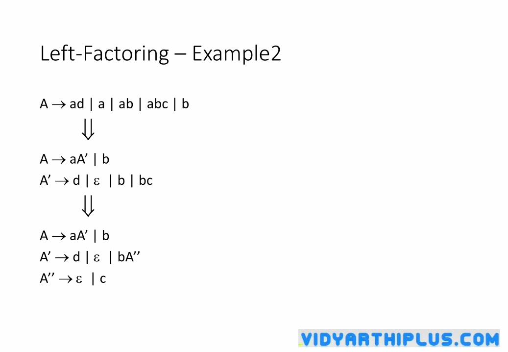
Left-Factoring – Example2
A ad | a | ab | abc | b
A aA’ | b
A’ d | | b | bc
A aA’ | b
A’ d | | bA’’
A’’ | c
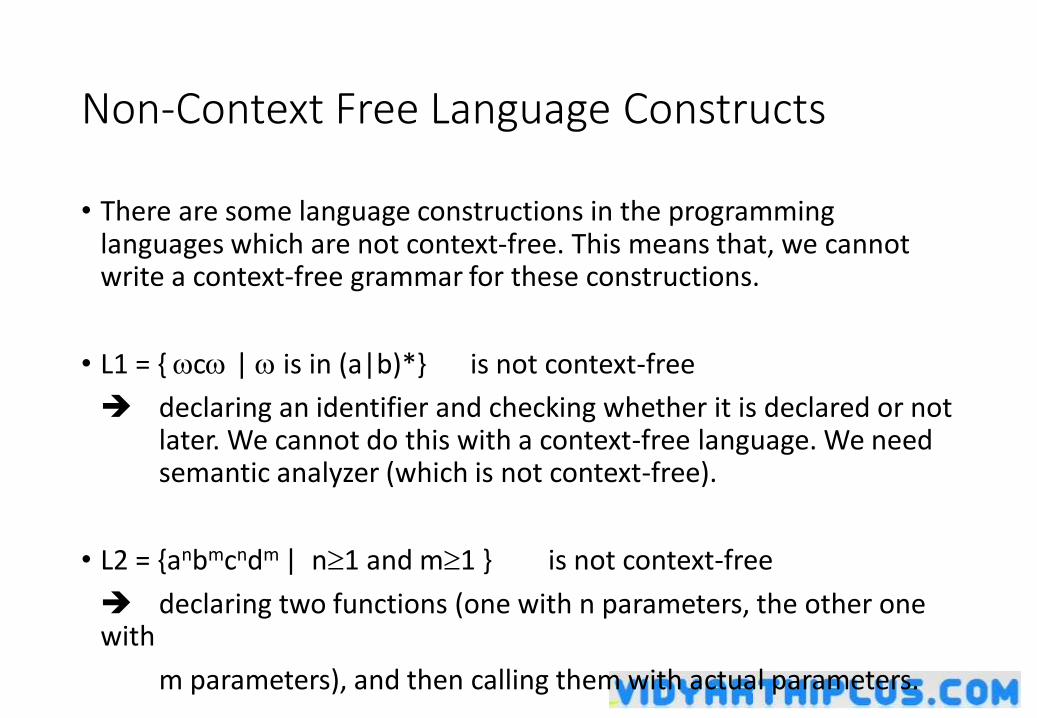
Non-Context Free Language Constructs
• There are some language constructions in the programming languages which are not context-free. This means that, we cannot write a context-free grammar for these constructions.
• L1 = { c | is in (a|b)*} is not context-free
declaring an identifier and checking whether it is declared or not later. We cannot do this with a context-free language. We need semantic analyzer (which is not context-free).
• L2 = {anbmcndm | n1 and m1 } is not context-free
declaring two functions (one with n parameters, the other one with
m parameters), and then calling them with actual parameters.
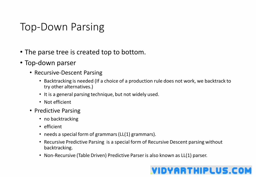
Top-Down Parsing
• The parse tree is created top to bottom.
• Top-down parser
• Recursive-Descent Parsing
• Backtracking is needed (If a choice of a production rule does not work, we backtrack to try other alternatives.)
• It is a general parsing technique, but not widely used.
• Not efficient
• Predictive Parsing• no backtracking
• efficient
• needs a special form of grammars (LL(1) grammars).
• Recursive Predictive Parsing is a special form of Recursive Descent parsing without backtracking.
• Non-Recursive (Table Driven) Predictive Parser is also known as LL(1) parser.
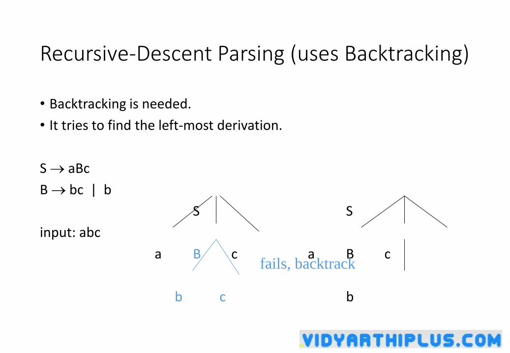
Recursive-Descent Parsing (uses Backtracking)
• Backtracking is needed.
• It tries to find the left-most derivation.
S aBc
B bc | b
S S
input: abc
a B c a B c
b c b
fails, backtrack
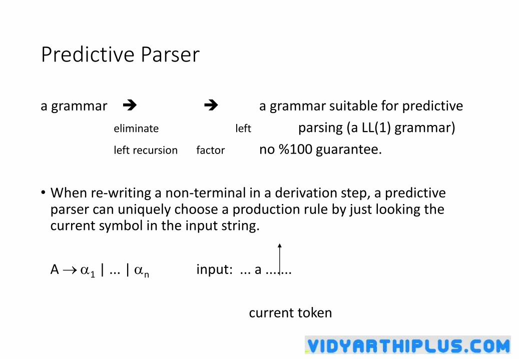
Predictive Parser
a grammar a grammar suitable for predictive
eliminate left parsing (a LL(1) grammar)
left recursion factor no %100 guarantee.
• When re-writing a non-terminal in a derivation step, a predictive parser can uniquely choose a production rule by just looking the current symbol in the input string.
A 1 | ... | n input: ... a .......
current token
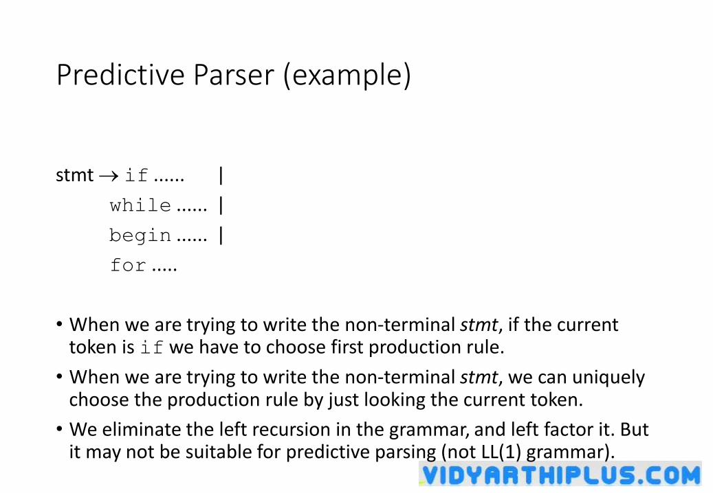
Predictive Parser (example)
stmt if ...... |
while ...... |
begin ...... |
for .....
• When we are trying to write the non-terminal stmt, if the current token is if we have to choose first production rule.
• When we are trying to write the non-terminal stmt, we can uniquely choose the production rule by just looking the current token.
• We eliminate the left recursion in the grammar, and left factor it. But it may not be suitable for predictive parsing (not LL(1) grammar).
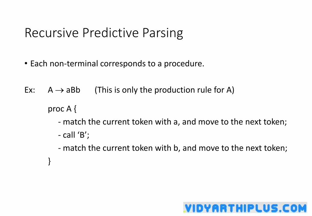
Recursive Predictive Parsing
• Each non-terminal corresponds to a procedure.
Ex: A aBb (This is only the production rule for A)
proc A {
- match the current token with a, and move to the next token;
- call ‘B’;
- match the current token with b, and move to the next token;
}
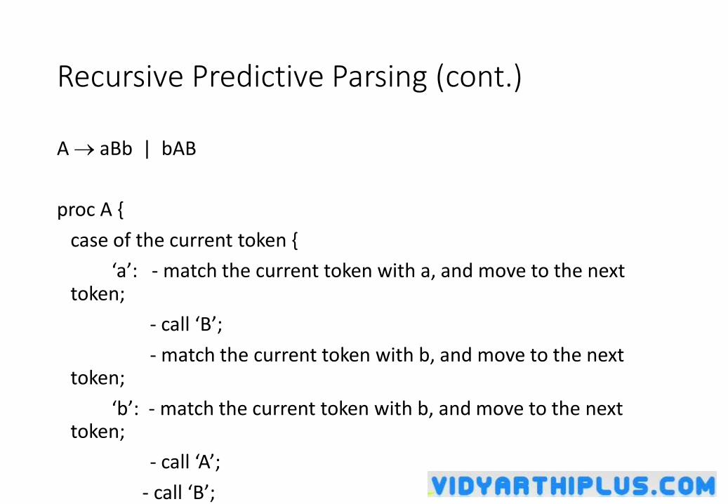
Recursive Predictive Parsing (cont.)
A aBb | bAB
proc A {
case of the current token {
‘a’: - match the current token with a, and move to the next token;
- call ‘B’;
- match the current token with b, and move to the next token;
‘b’: - match the current token with b, and move to the next token;
- call ‘A’;
- call ‘B’;
}
Recursive Predictive Parsing (cont.)
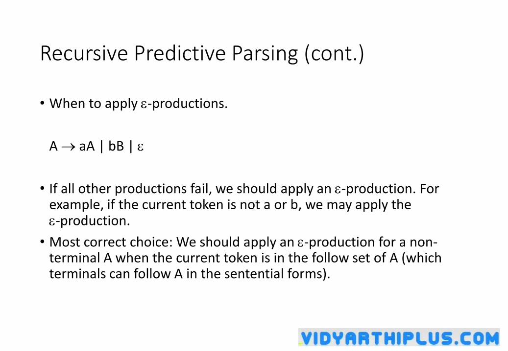
• When to apply -productions.
A aA | bB |
• If all other productions fail, we should apply an -production. For example, if the current token is not a or b, we may apply the -production.
• Most correct choice: We should apply an -production for a non-terminal A when the current token is in the follow set of A (which terminals can follow A in the sentential forms).
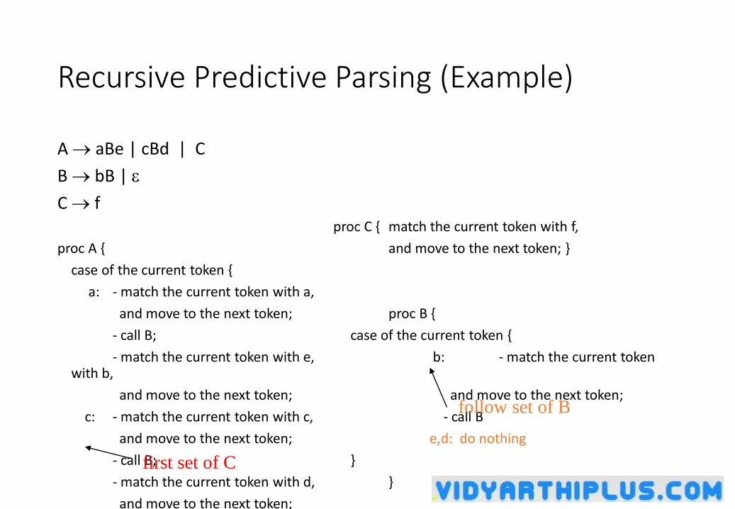
Recursive Predictive Parsing (Example)
A aBe | cBd | C
B bB |
C fproc C { match the current token with f,
proc A { and move to the next token; }
case of the current token {
a: - match the current token with a,
and move to the next token; proc B {
- call B; case of the current token {
- match the current token with e, b: - match the current token with b,
and move to the next token; and move to the next token;
c: - match the current token with c, - call B
and move to the next token; e,d: do nothing
- call B; }
- match the current token with d, }
and move to the next token;
follow set of B
first set of C
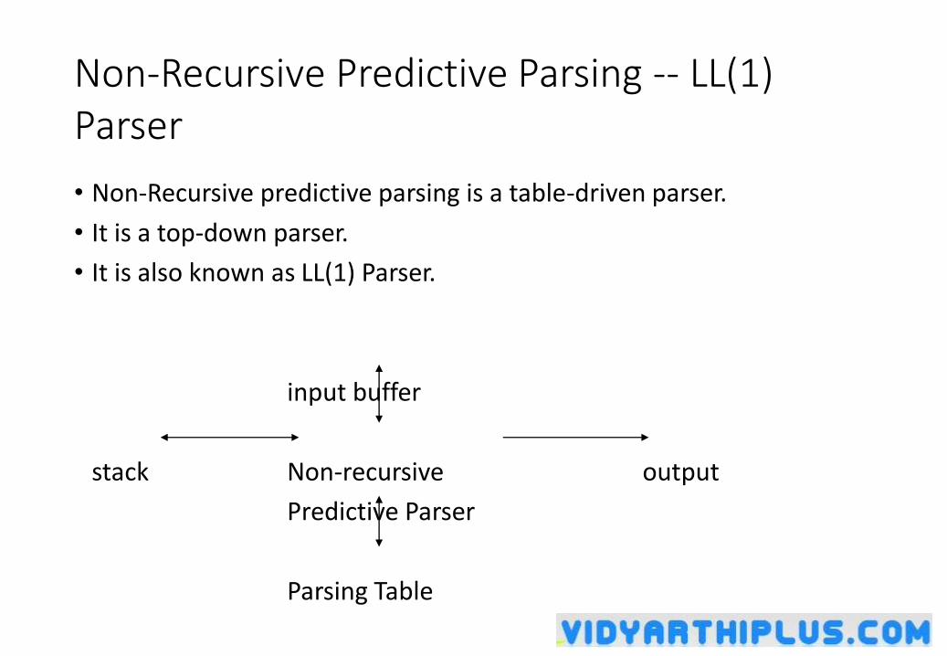
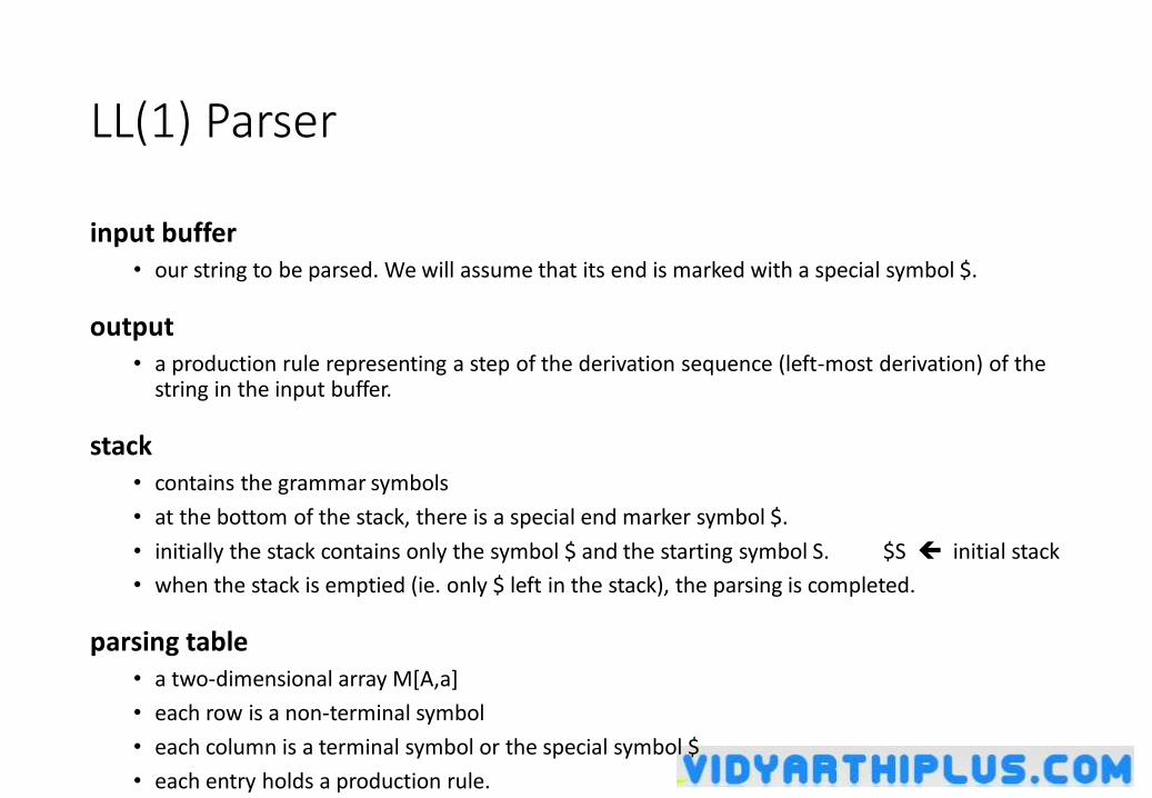
Non-Recursive Predictive Parsing -- LL(1) Parser
• Non-Recursive predictive parsing is a table-driven parser.
• It is a top-down parser.
• It is also known as LL(1) Parser.
input buffer
stack Non-recursive output
Predictive Parser
Parsing Table
LL(1) Parser
input buffer• our string to be parsed. We will assume that its end is marked with a special symbol $.
output• a production rule representing a step of the derivation sequence (left-most derivation) of the
string in the input buffer.
stack• contains the grammar symbols
• at the bottom of the stack, there is a special end marker symbol $.
• initially the stack contains only the symbol $ and the starting symbol S. $S initial stack
• when the stack is emptied (ie. only $ left in the stack), the parsing is completed.
parsing table• a two-dimensional array M[A,a]
• each row is a non-terminal symbol
• each column is a terminal symbol or the special symbol $
• each entry holds a production rule.
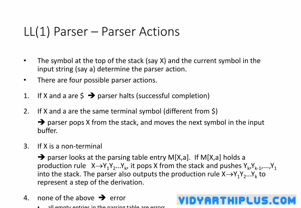
LL(1) Parser – Parser Actions
• The symbol at the top of the stack (say X) and the current symbol in the input string (say a) determine the parser action.
• There are four possible parser actions.
1. If X and a are $ parser halts (successful completion)
2. If X and a are the same terminal symbol (different from $)
parser pops X from the stack, and moves the next symbol in the input buffer.
3. If X is a non-terminal
parser looks at the parsing table entry M[X,a]. If M[X,a] holds a production rule XY1Y2...Yk, it pops X from the stack and pushes Yk,Yk-1,...,Y1
into the stack. The parser also outputs the production rule XY1Y2...Yk to represent a step of the derivation.
4. none of the above error • all empty entries in the parsing table are errors.
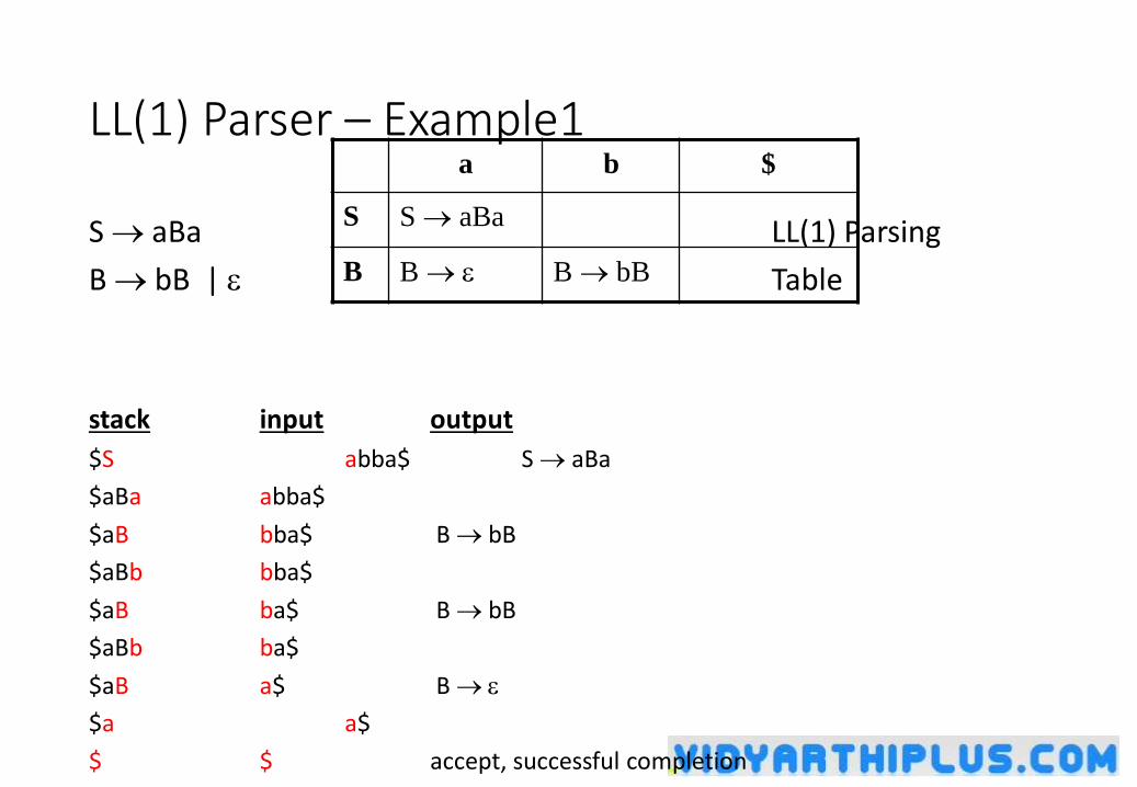
LL(1) Parser – Example1
S aBa LL(1) Parsing
B bB | Table
stack input output
$S abba$ S aBa
$aBa abba$
$aB bba$ B bB
$aBb bba$
$aB ba$ B bB
$aBb ba$
$aB a$ B
$a a$
$ $ accept, successful completion
a b $
S S aBa
B B B bB
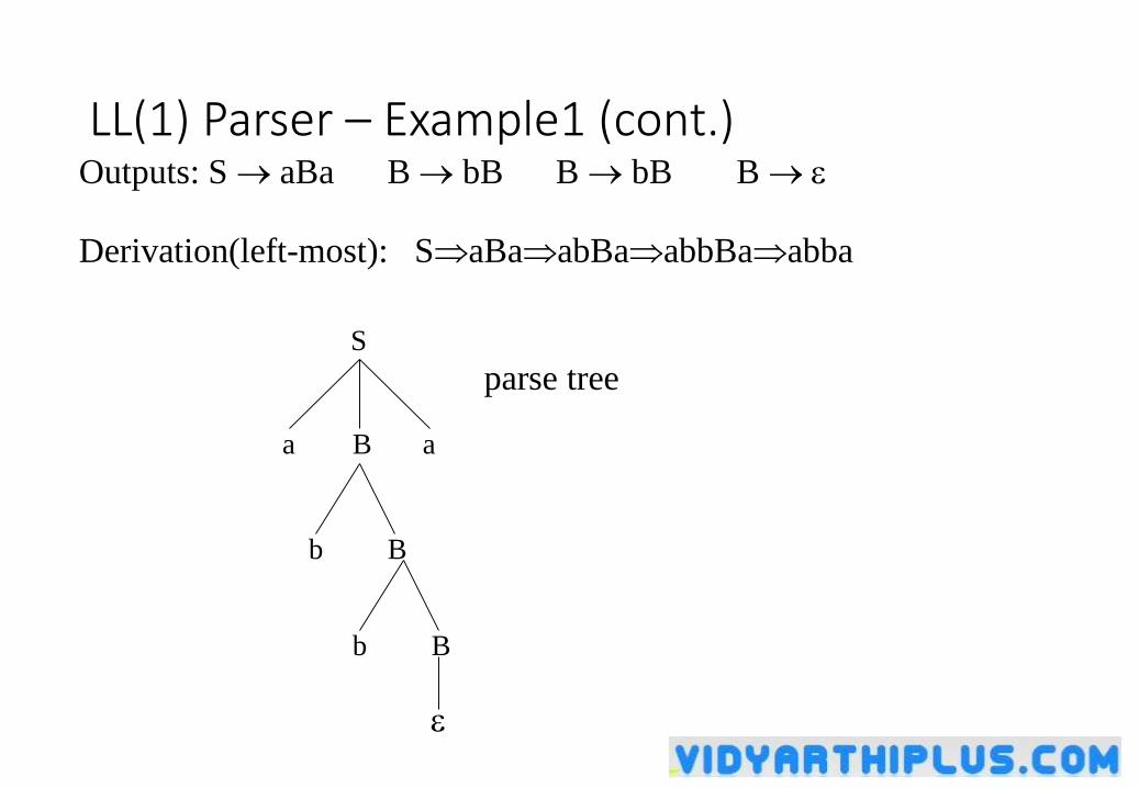
LL(1) Parser – Example1 (cont.)Outputs: S aBa B bB B bB B
Derivation(left-most): SaBaabBaabbBaabba
S
Ba a
B
Bb
b
parse tree
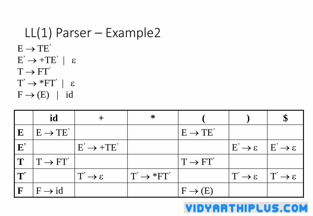
LL(1) Parser – Example2E TE’
E’ +TE’ |
T FT’
T’ *FT’ |
F (E) | id
id + * ( ) $
E E TE’ E TE’
E’ E’ +TE’ E’ E’
T T FT’ T FT’
T’ T’ T’ *FT’ T’ T’
F F id F (E)
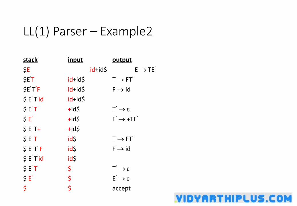
LL(1) Parser – Example2
stack input output
$E id+id$ E TE’
$E’T id+id$ T FT’
$E’ T’F id+id$ F id
$ E’ T’id id+id$
$ E’ T’ +id$ T’
$ E’ +id$ E’ +TE’
$ E’ T+ +id$
$ E’ T id$ T FT’
$ E’ T’ F id$ F id
$ E’ T’id id$
$ E’ T’ $ T’
$ E’ $ E’
$ $ accept
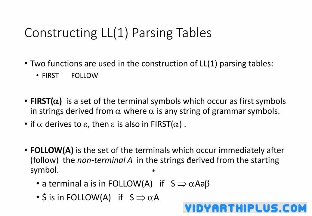
Constructing LL(1) Parsing Tables
• Two functions are used in the construction of LL(1) parsing tables:
• FIRST FOLLOW
• FIRST() is a set of the terminal symbols which occur as first symbols in strings derived from where is any string of grammar symbols.
• if derives to , then is also in FIRST() .
• FOLLOW(A) is the set of the terminals which occur immediately after (follow) the non-terminal A in the strings derived from the starting symbol.
• a terminal a is in FOLLOW(A) if S Aa
• $ is in FOLLOW(A) if S A
*
*
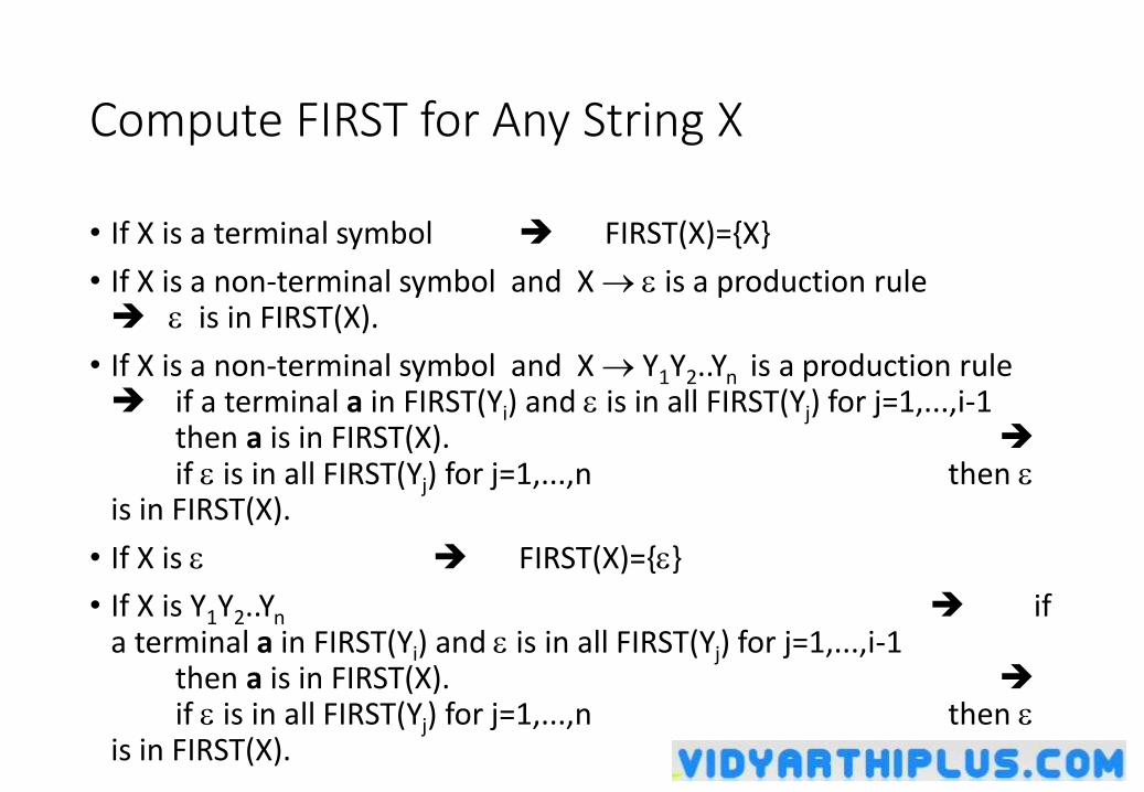
Compute FIRST for Any String X
• If X is a terminal symbol FIRST(X)={X}
• If X is a non-terminal symbol and X is a production rule is in FIRST(X).
• If X is a non-terminal symbol and X Y1Y2..Yn is a production rule if a terminal a in FIRST(Yi) and is in all FIRST(Yj) for j=1,...,i-1
then a is in FIRST(X). if is in all FIRST(Yj) for j=1,...,n then
is in FIRST(X).
• If X is FIRST(X)={}
• If X is Y1Y2..Yn if a terminal a in FIRST(Yi) and is in all FIRST(Yj) for j=1,...,i-1
then a is in FIRST(X). if is in all FIRST(Yj) for j=1,...,n then
is in FIRST(X).
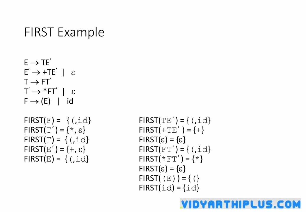
FIRST Example
E TE’
E’ +TE’ | T FT’
T’ *FT’ | F (E) | id
FIRST(F) = {(,id} FIRST(TE’) = {(,id}FIRST(T’) = {*, } FIRST(+TE’ ) = {+}FIRST(T) = {(,id} FIRST() = {}FIRST(E’) = {+, } FIRST(FT’) = {(,id}FIRST(E) = {(,id} FIRST(*FT’) = {*}
FIRST() = {}FIRST((E)) = {(}FIRST(id) = {id}
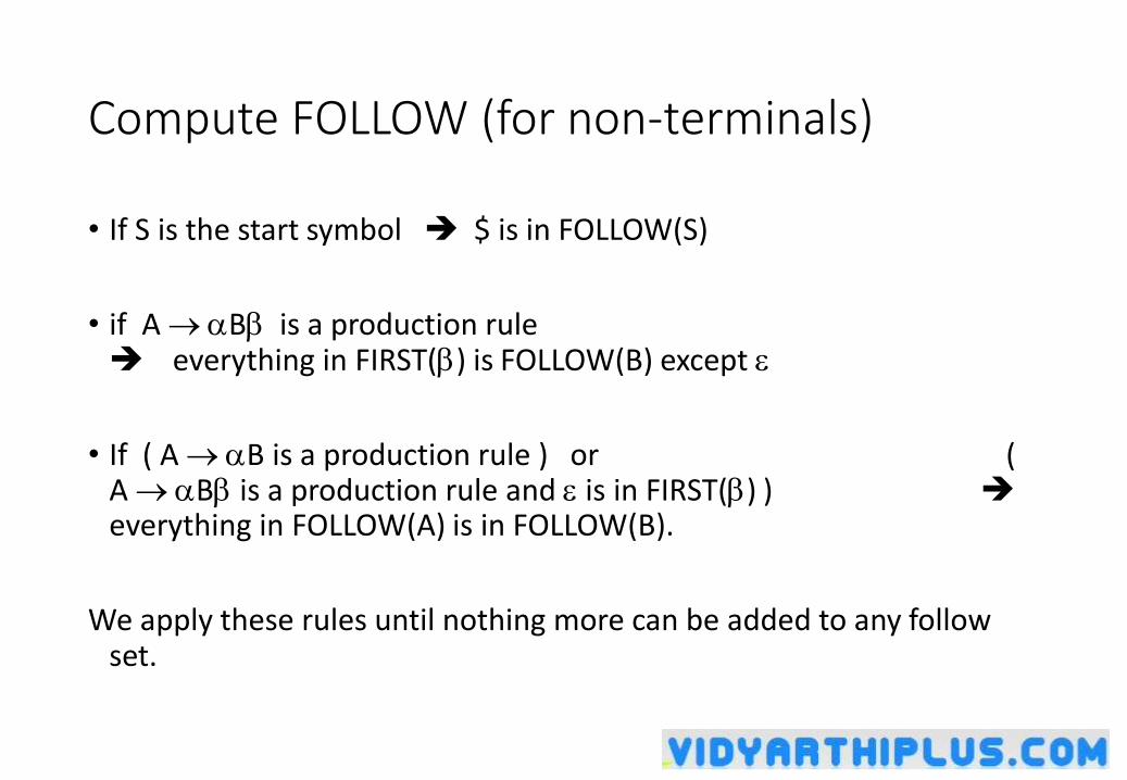
Compute FOLLOW (for non-terminals)
• If S is the start symbol $ is in FOLLOW(S)
• if A B is a production rule everything in FIRST() is FOLLOW(B) except
• If ( A B is a production rule ) or ( A B is a production rule and is in FIRST() ) everything in FOLLOW(A) is in FOLLOW(B).
We apply these rules until nothing more can be added to any follow set.
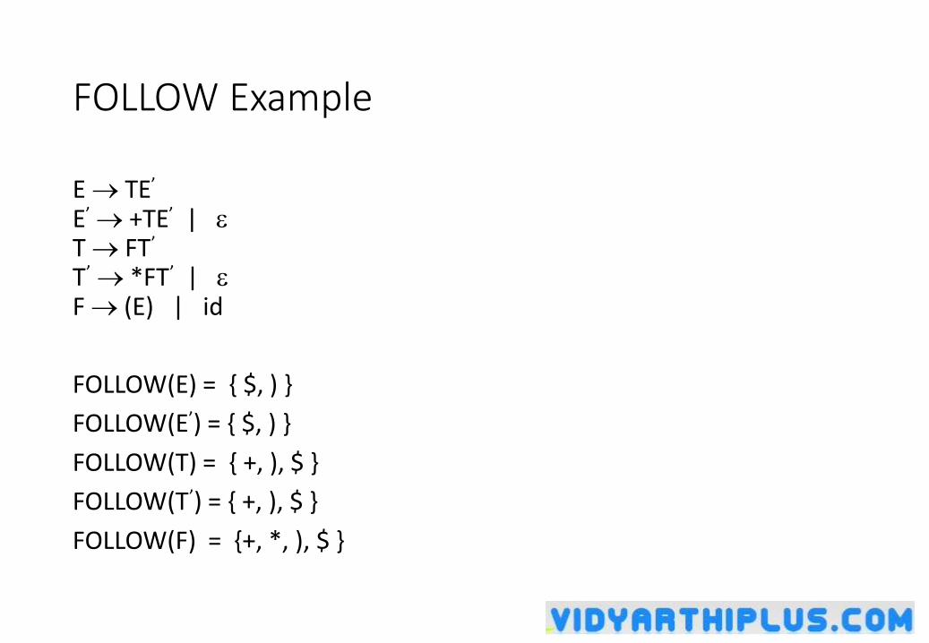
FOLLOW Example
E TE’
E’ +TE’ | T FT’
T’ *FT’ | F (E) | id
FOLLOW(E) = { $, ) }
FOLLOW(E’) = { $, ) }
FOLLOW(T) = { +, ), $ }
FOLLOW(T’) = { +, ), $ }
FOLLOW(F) = {+, *, ), $ }
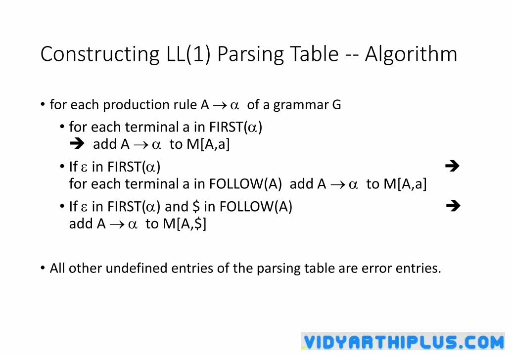
Constructing LL(1) Parsing Table -- Algorithm
• for each production rule A of a grammar G
• for each terminal a in FIRST() add A to M[A,a]
• If in FIRST() for each terminal a in FOLLOW(A) add A to M[A,a]
• If in FIRST() and $ in FOLLOW(A) add A to M[A,$]
• All other undefined entries of the parsing table are error entries.
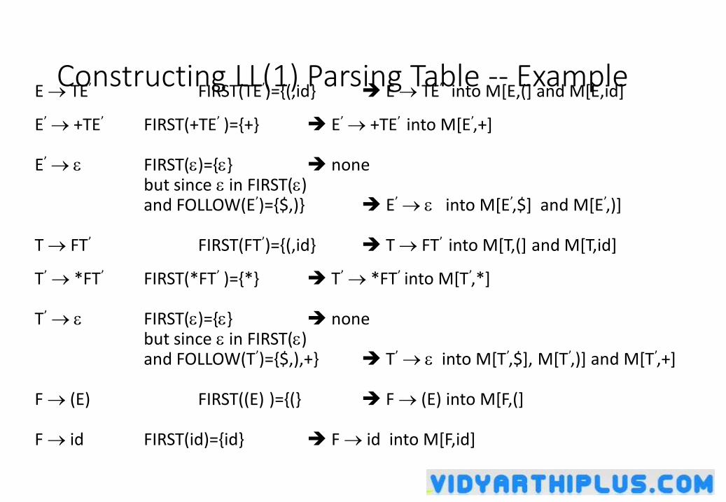
Constructing LL(1) Parsing Table -- ExampleE TE’ FIRST(TE’)={(,id} E TE’ into M[E,(] and M[E,id]
E’ +TE’ FIRST(+TE’ )={+} E’ +TE’ into M[E’,+]
E’ FIRST()={} nonebut since in FIRST() and FOLLOW(E’)={$,)} E’ into M[E’,$] and M[E’,)]
T FT’ FIRST(FT’)={(,id} T FT’ into M[T,(] and M[T,id]
T’ *FT’ FIRST(*FT’ )={*} T’ *FT’ into M[T’,*]
T’ FIRST()={} nonebut since in FIRST() and FOLLOW(T’)={$,),+} T’ into M[T’,$], M[T’,)] and M[T’,+]
F (E) FIRST((E) )={(} F (E) into M[F,(]
F id FIRST(id)={id} F id into M[F,id]
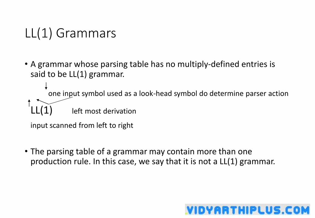
LL(1) Grammars
• A grammar whose parsing table has no multiply-defined entries is said to be LL(1) grammar.
one input symbol used as a look-head symbol do determine parser action
LL(1) left most derivation
input scanned from left to right
• The parsing table of a grammar may contain more than one production rule. In this case, we say that it is not a LL(1) grammar.
A Grammar which is not LL(1)
S i C t S E | a FOLLOW(S) = { $,e }
E e S | FOLLOW(E) = { $,e }
C b FOLLOW(C) = { t }
FIRST(iCtSE) = {i}
FIRST(a) = {a}
FIRST(eS) = {e}
FIRST() = {}
FIRST(b) = {b}
two production rules for M[E,e]
Problem ambiguity
a b e i t $
S S a S iCtSE
E E e S
E
E
C C b
A Grammar which is not LL(1) (cont.)
• What do we have to do it if the resulting parsing table contains multiply defined entries?
• If we didn’t eliminate left recursion, eliminate the left recursion in the grammar.
• If the grammar is not left factored, we have to left factor the grammar.
• If its (new grammar’s) parsing table still contains multiply defined entries, that grammar is ambiguous or it is inherently not a LL(1) grammar.
• A left recursive grammar cannot be a LL(1) grammar.
• A A | any terminal that appears in FIRST() also appears FIRST(A) because A .
If is , any terminal that appears in FIRST() also appears in FIRST(A) and FOLLOW(A).
• A grammar is not left factored, it cannot be a LL(1) grammar
• A 1 | 2
any terminal that appears in FIRST(1) also appears in FIRST(2).
• An ambiguous grammar cannot be a LL(1) grammar.
Properties of LL(1) Grammars
• A grammar G is LL(1) if and only if the following conditions hold for two distinctive production rules A and A
1. Both and cannot derive strings starting with same terminals.
2. At most one of and can derive to .
3. If can derive to , then cannot derive to any string starting with a terminal in FOLLOW(A).
Error Recovery in Predictive Parsing
• An error may occur in the predictive parsing (LL(1) parsing)
• if the terminal symbol on the top of stack does not match with the current input symbol.
• if the top of stack is a non-terminal A, the current input symbol is a, and the parsing table entry M[A,a] is empty.
• What should the parser do in an error case?
• The parser should be able to give an error message (as much as possible meaningful error message).
• It should be recover from that error case, and it should be able to continue the parsing with the rest of the input.
Error Recovery Techniques• Panic-Mode Error Recovery
• Skipping the input symbols until a synchronizing token is found.
• Phrase-Level Error Recovery
• Each empty entry in the parsing table is filled with a pointer to a specific error routine to take care that error case.
• Error-Productions
• If we have a good idea of the common errors that might be encountered, we can augment the grammar with productions that generate erroneous constructs.
• When an error production is used by the parser, we can generate appropriate error diagnostics.
• Since it is almost impossible to know all the errors that can be made by the programmers, this method is not practical.
• Global-Correction
• Ideally, we we would like a compiler to make as few change as possible in processing incorrect inputs.
• We have to globally analyze the input to find the error.
• This is an expensive method, and it is not in practice.
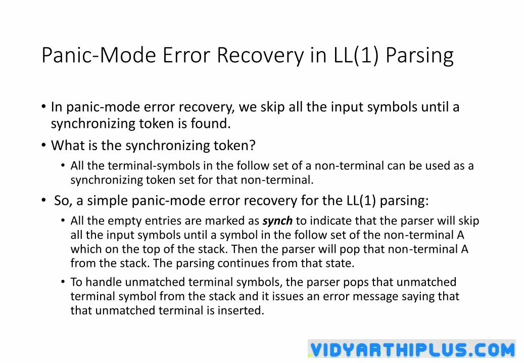
Panic-Mode Error Recovery in LL(1) Parsing
• In panic-mode error recovery, we skip all the input symbols until a synchronizing token is found.
• What is the synchronizing token?
• All the terminal-symbols in the follow set of a non-terminal can be used as a synchronizing token set for that non-terminal.
• So, a simple panic-mode error recovery for the LL(1) parsing:
• All the empty entries are marked as synch to indicate that the parser will skip all the input symbols until a symbol in the follow set of the non-terminal A which on the top of the stack. Then the parser will pop that non-terminal A from the stack. The parsing continues from that state.
• To handle unmatched terminal symbols, the parser pops that unmatched terminal symbol from the stack and it issues an error message saying that that unmatched terminal is inserted.
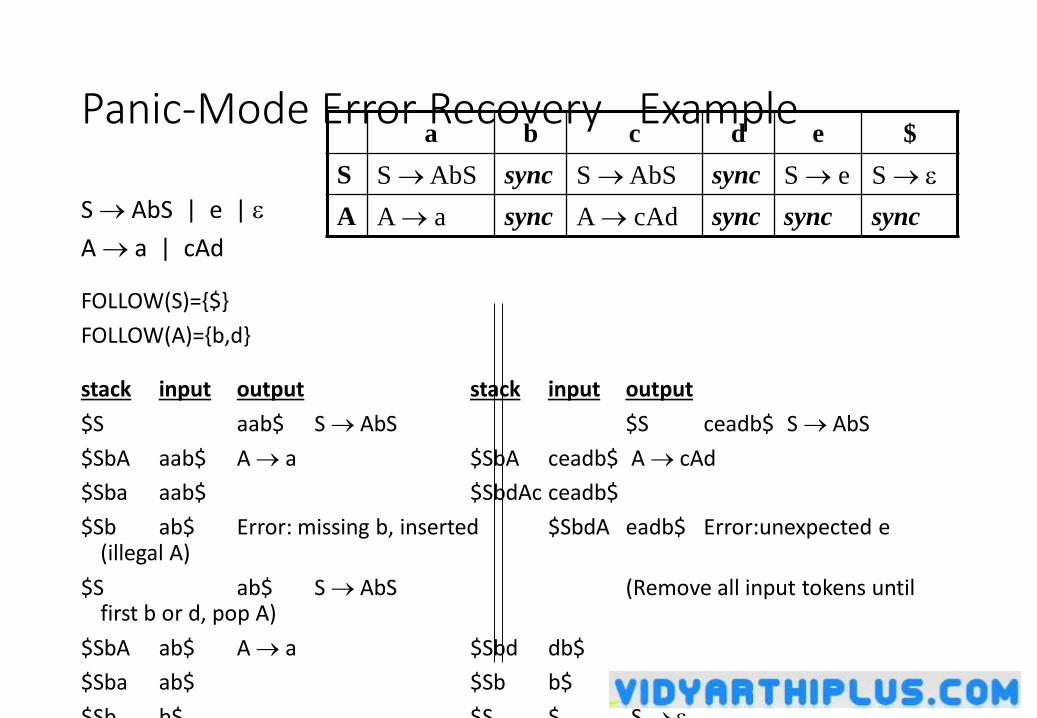
Panic-Mode Error Recovery - Example
S AbS | e |
A a | cAd
FOLLOW(S)={$}
FOLLOW(A)={b,d}
stack input output stack input output
$S aab$ S AbS $S ceadb$ S AbS
$SbA aab$ A a $SbA ceadb$ A cAd
$Sba aab$ $SbdAc ceadb$
$Sb ab$ Error: missing b, inserted $SbdA eadb$ Error:unexpected e (illegal A)
$S ab$ S AbS (Remove all input tokens until first b or d, pop A)
$SbA ab$ A a $Sbd db$
$Sba ab$ $Sb b$
$Sb b$ $S $ S
a b c d e $
S S AbS sync S AbS sync S e S
A A a sync A cAd sync sync sync
Phrase-Level Error Recovery
• Each empty entry in the parsing table is filled with a pointer to a special error routine which will take care that error case.
• These error routines may:
• change, insert, or delete input symbols.
• issue appropriate error messages
• pop items from the stack.
• We should be careful when we design these error routines, because we may put the parser into an infinite loop.
Bottom-Up Parsing
• A bottom-up parser creates the parse tree of the given input starting from leaves towards the root.
• A bottom-up parser tries to find the right-most derivation of the given input in the reverse order.
S ... (the right-most derivation of )
(the bottom-up parser finds the right-most derivation in the reverse order)
• Bottom-up parsing is also known as shift-reduce parsing because its two main actions are shift and reduce.
• At each shift action, the current symbol in the input string is pushed to a stack.
• At each reduction step, the symbols at the top of the stack (this symbol sequence is the right side of a production) will replaced by the non-terminal at the left side of that production.
• There are also two more actions: accept and error.
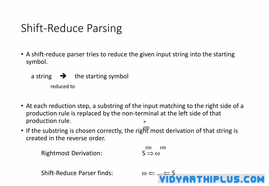
Shift-Reduce Parsing
• A shift-reduce parser tries to reduce the given input string into the starting symbol.
a string the starting symbol
reduced to
• At each reduction step, a substring of the input matching to the right side of a production rule is replaced by the non-terminal at the left side of that production rule.
• If the substring is chosen correctly, the right most derivation of that string is created in the reverse order.
Rightmost Derivation: S
Shift-Reduce Parser finds: ... S
*rm
rm rm
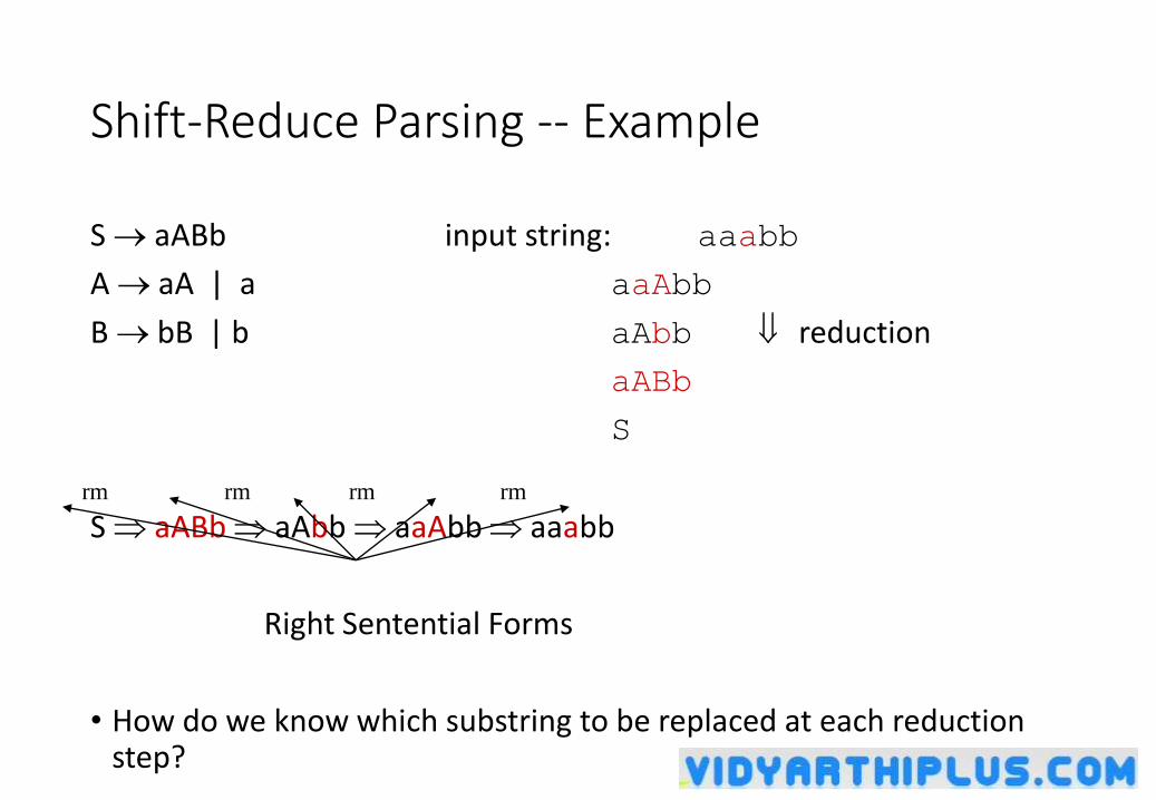
Shift-Reduce Parsing -- Example
S aABb input string: aaabb
A aA | a aaAbb
B bB | b aAbb reduction
aABb
S
S aABb aAbb aaAbb aaabb
Right Sentential Forms
• How do we know which substring to be replaced at each reduction step?
rmrmrmrm
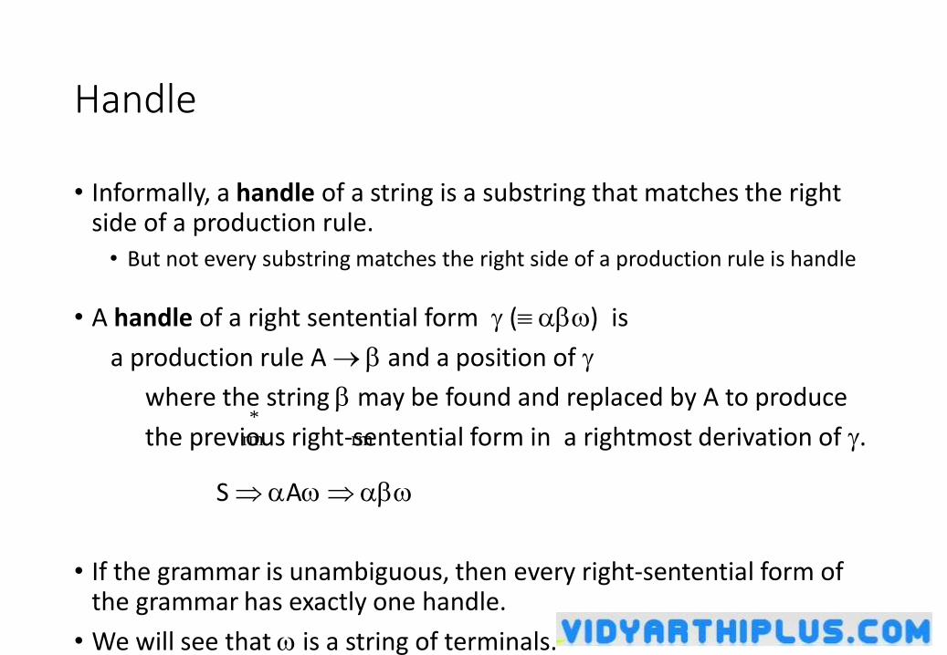
Handle
• Informally, a handle of a string is a substring that matches the right side of a production rule.
• But not every substring matches the right side of a production rule is handle
• A handle of a right sentential form ( ) is
a production rule A and a position of
where the string may be found and replaced by A to produce
the previous right-sentential form in a rightmost derivation of .
S A
• If the grammar is unambiguous, then every right-sentential form of the grammar has exactly one handle.
• We will see that is a string of terminals.
rm rm*
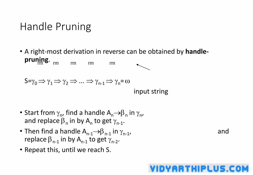
Handle Pruning
• A right-most derivation in reverse can be obtained by handle-pruning.
S=0 1 2 ... n-1 n=
input string
• Start from n, find a handle Ann in n, and replace n in by An to get n-1.
• Then find a handle An-1n-1 in n-1, and replace n-1 in by An-1 to get n-2.
• Repeat this, until we reach S.
rmrmrm rmrm
A Shift-Reduce Parser
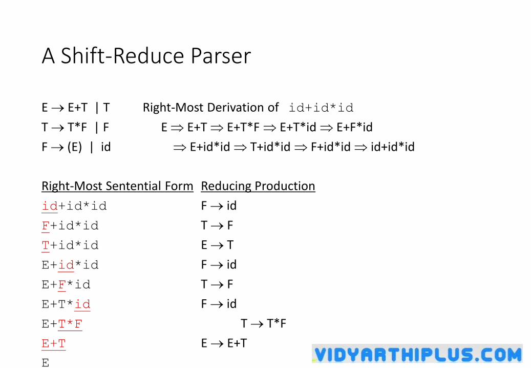
E E+T | T Right-Most Derivation of id+id*id
T T*F | F E E+T E+T*F E+T*id E+F*id
F (E) | id E+id*id T+id*id F+id*id id+id*id
Right-Most Sentential Form Reducing Production
id+id*id F id
F+id*id T F
T+id*id E T
E+id*id F id
E+F*id T F
E+T*id F id
E+T*F T T*F
E+T E E+T
E
A Stack Implementation of A Shift-Reduce Parser
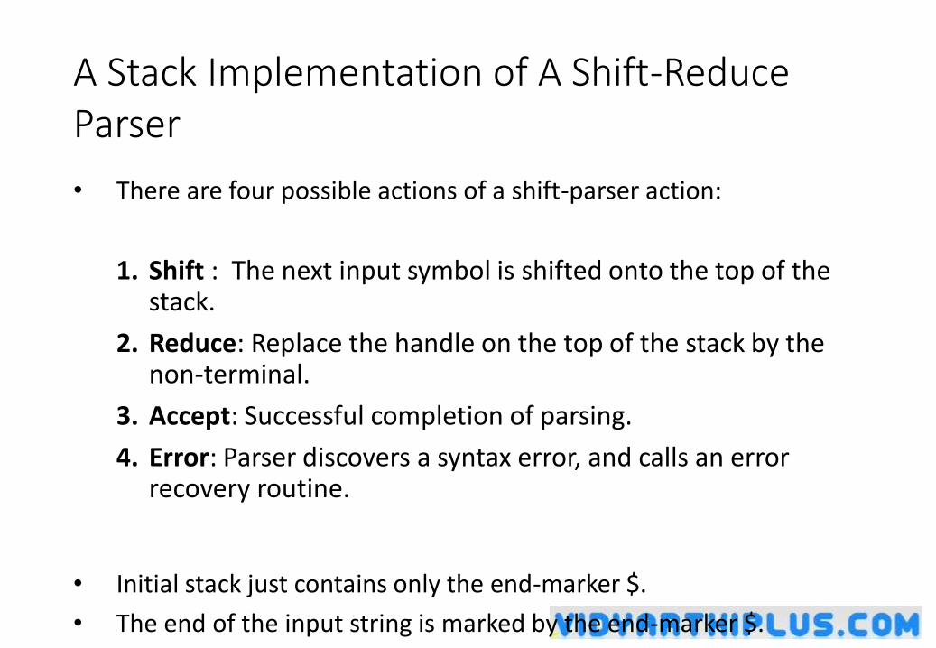
• There are four possible actions of a shift-parser action:
1. Shift : The next input symbol is shifted onto the top of the stack.
2. Reduce: Replace the handle on the top of the stack by the non-terminal.
3. Accept: Successful completion of parsing.
4. Error: Parser discovers a syntax error, and calls an error recovery routine.
• Initial stack just contains only the end-marker $.
• The end of the input string is marked by the end-marker $.
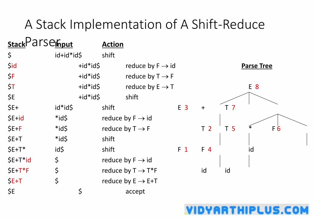
A Stack Implementation of A Shift-Reduce Parser Stack Input Action
$ id+id*id$ shift
$id +id*id$ reduce by F id Parse Tree
$F +id*id$ reduce by T F
$T +id*id$ reduce by E T E 8
$E +id*id$ shift
$E+ id*id$ shift E 3 + T 7
$E+id *id$ reduce by F id
$E+F *id$ reduce by T F T 2 T 5 * F 6
$E+T *id$ shift
$E+T* id$ shift F 1 F 4 id
$E+T*id $ reduce by F id
$E+T*F $ reduce by T T*F id id
$E+T $ reduce by E E+T
$E $ accept
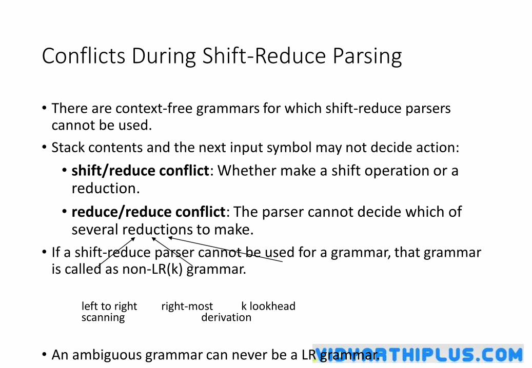
Conflicts During Shift-Reduce Parsing
• There are context-free grammars for which shift-reduce parsers cannot be used.
• Stack contents and the next input symbol may not decide action:
• shift/reduce conflict: Whether make a shift operation or a reduction.
• reduce/reduce conflict: The parser cannot decide which of several reductions to make.
• If a shift-reduce parser cannot be used for a grammar, that grammar is called as non-LR(k) grammar.
left to right right-most k lookheadscanning derivation
• An ambiguous grammar can never be a LR grammar.
Shift-Reduce Parsers
• There are two main categories of shift-reduce parsers
1. Operator-Precedence Parser
• simple, but only a small class of grammars.
2. LR-Parsers
• covers wide range of grammars.
• SLR – simple LR parser
• LR – most general LR parser
• LALR – intermediate LR parser (lookhead LR parser)
• SLR, LR and LALR work same, only their parsing tables are different.
SLR
CFG
LR
LALR
Operator-Precedence Parser
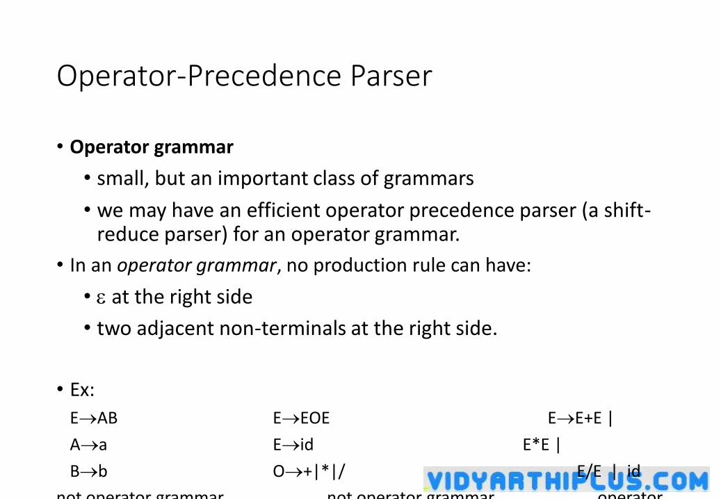
• Operator grammar
• small, but an important class of grammars
• we may have an efficient operator precedence parser (a shift-reduce parser) for an operator grammar.
• In an operator grammar, no production rule can have:
• at the right side
• two adjacent non-terminals at the right side.
• Ex:
EAB EEOE EE+E |
Aa Eid E*E |
Bb O+|*|/ E/E | id
not operator grammar not operator grammar operator
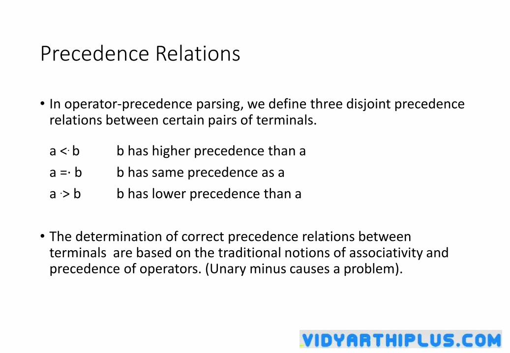
Precedence Relations
• In operator-precedence parsing, we define three disjoint precedence relations between certain pairs of terminals.
a <. b b has higher precedence than a
a =· b b has same precedence as a
a .> b b has lower precedence than a
• The determination of correct precedence relations between terminals are based on the traditional notions of associativity and precedence of operators. (Unary minus causes a problem).
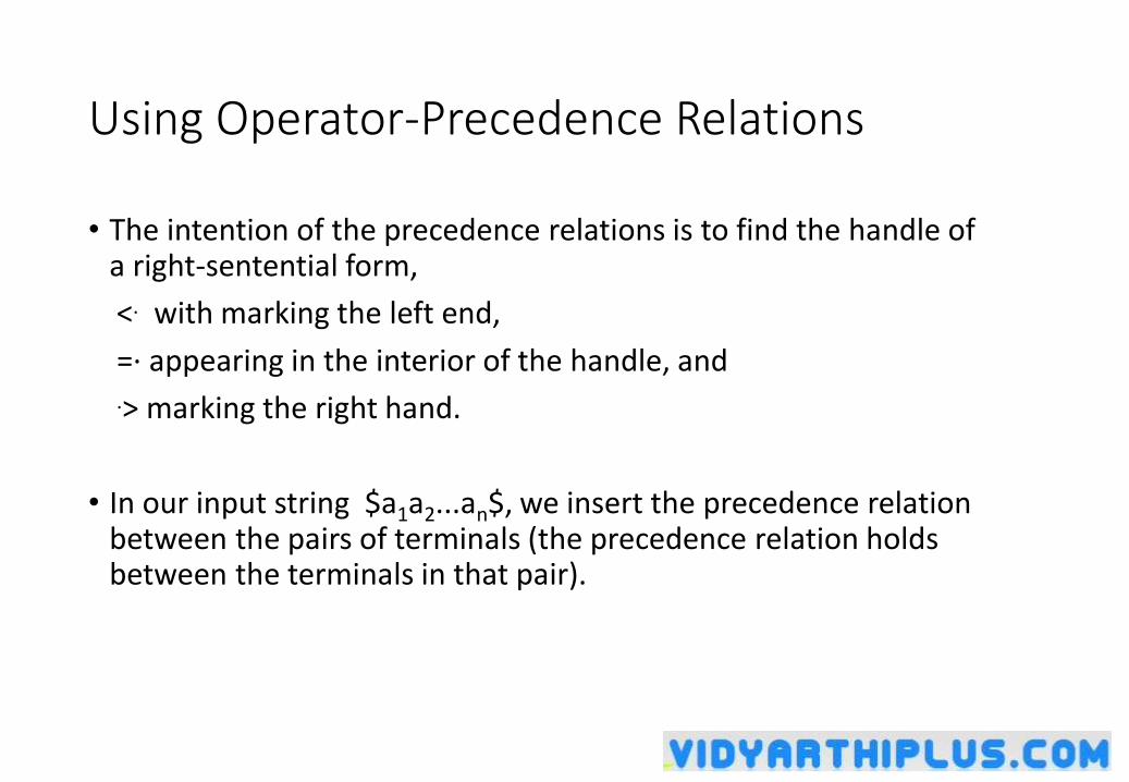
Using Operator-Precedence Relations
• The intention of the precedence relations is to find the handle of a right-sentential form,
<. with marking the left end,
=· appearing in the interior of the handle, and.> marking the right hand.
• In our input string $a1a2...an$, we insert the precedence relation between the pairs of terminals (the precedence relation holds between the terminals in that pair).
Using Operator -Precedence Relations
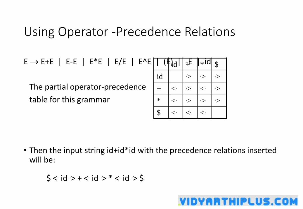
E E+E | E-E | E*E | E/E | E^E | (E) | -E | id
The partial operator-precedence
table for this grammar
• Then the input string id+id*id with the precedence relations inserted will be:
$ <. id .> + <. id .> * <. id .> $
id + * $
id .> .> .>
+ <. .> <. .>
* <. .> .> .>
$ <. <. <.
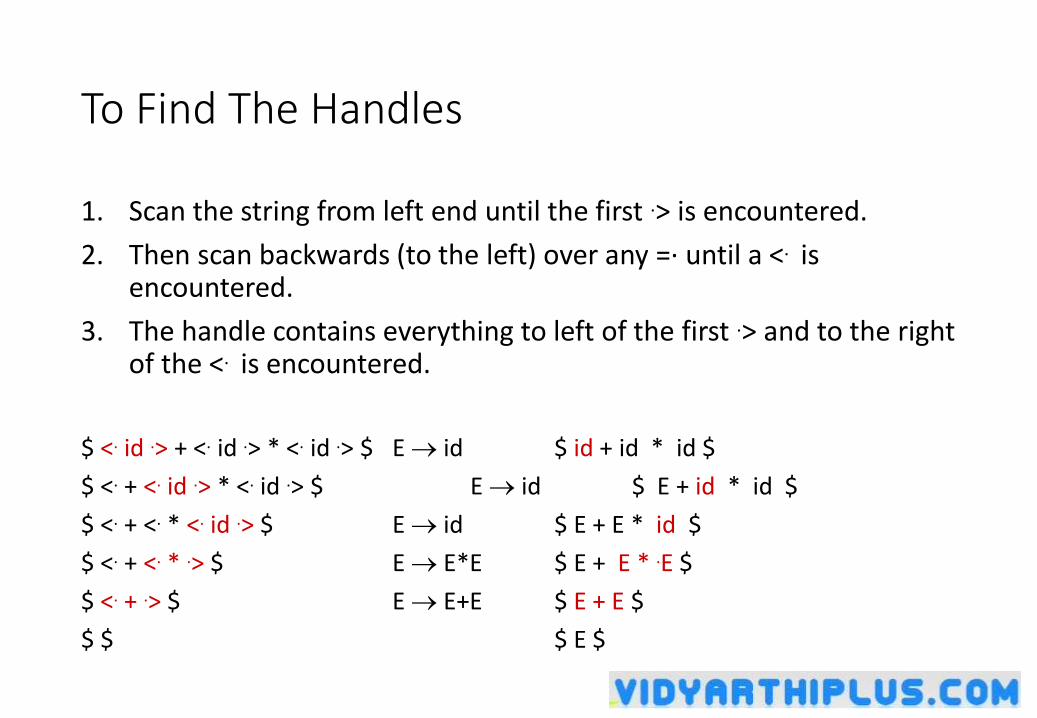
To Find The Handles
1. Scan the string from left end until the first .> is encountered.
2. Then scan backwards (to the left) over any =· until a <. is encountered.
3. The handle contains everything to left of the first .> and to the right of the <. is encountered.
$ <. id .> + <. id .> * <. id .> $ E id $ id + id * id $
$ <. + <. id .> * <. id .> $ E id $ E + id * id $
$ <. + <. * <. id .> $ E id $ E + E * id $
$ <. + <. * .> $ E E*E $ E + E * .E $
$ <. + .> $ E E+E $ E + E $
$ $ $ E $
Operator-Precedence Parsing Algorithm
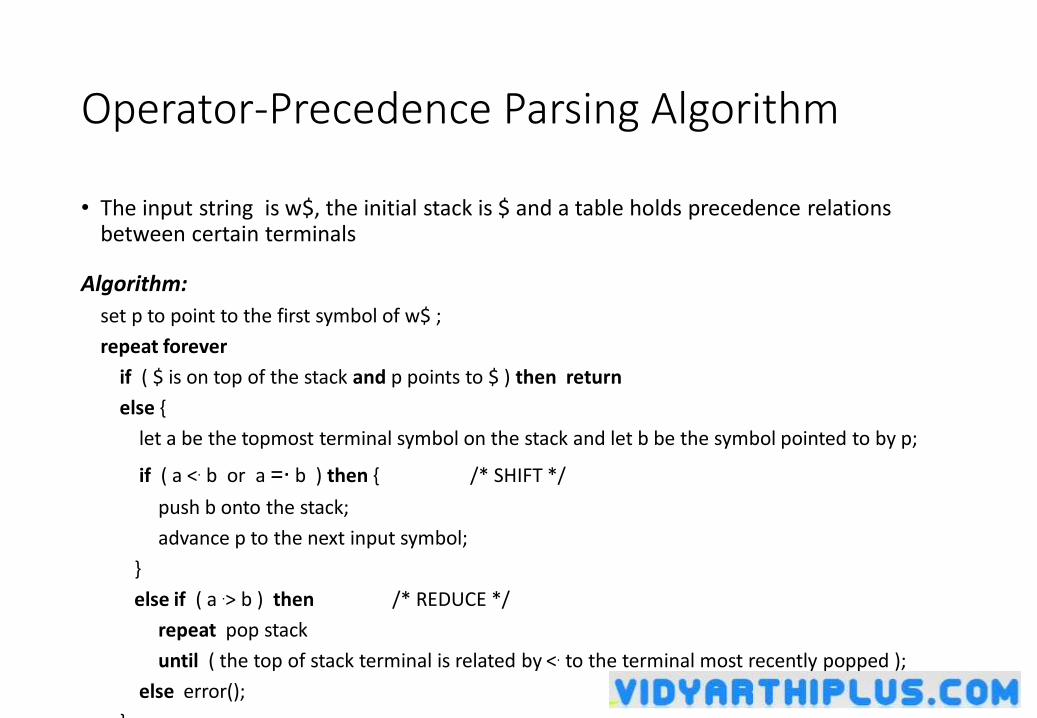
• The input string is w$, the initial stack is $ and a table holds precedence relations between certain terminals
Algorithm:
set p to point to the first symbol of w$ ;
repeat forever
if ( $ is on top of the stack and p points to $ ) then return
else {
let a be the topmost terminal symbol on the stack and let b be the symbol pointed to by p;
if ( a <. b or a =· b ) then { /* SHIFT */
push b onto the stack;
advance p to the next input symbol;
}
else if ( a .> b ) then /* REDUCE */
repeat pop stack
until ( the top of stack terminal is related by <. to the terminal most recently popped );
else error();
}
Operator-Precedence Parsing Algorithm --Example
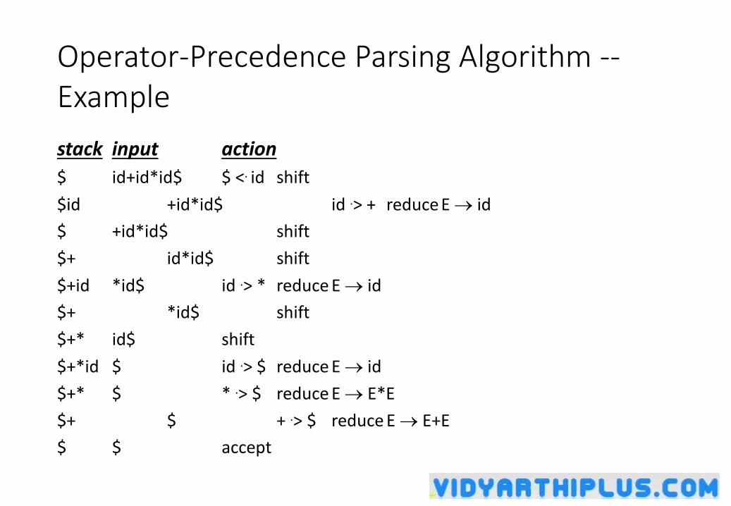
stack input action
$ id+id*id$ $ <. id shift
$id +id*id$ id .> + reduce E id
$ +id*id$ shift
$+ id*id$ shift
$+id *id$ id .> * reduce E id
$+ *id$ shift
$+* id$ shift
$+*id $ id .> $ reduce E id
$+* $ * .> $ reduce E E*E
$+ $ + .> $ reduce E E+E
$ $ accept
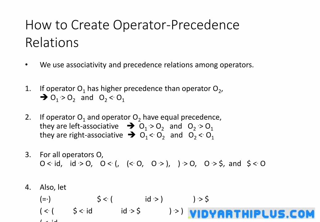
How to Create Operator-Precedence Relations
• We use associativity and precedence relations among operators.
1. If operator O1 has higher precedence than operator O2, O1
.> O2 and O2 <. O1
2. If operator O1 and operator O2 have equal precedence, they are left-associative O1
.> O2 and O2.> O1
they are right-associative O1 <. O2 and O2 <. O1
3. For all operators O, O <. id, id .> O, O <. (, (<. O, O .> ), ) .> O, O .> $, and $ <. O
4. Also, let
(=·) $ <. ( id .> ) ) .> $
( <. ( $ <. id id .> $ ) .> )
( <. id
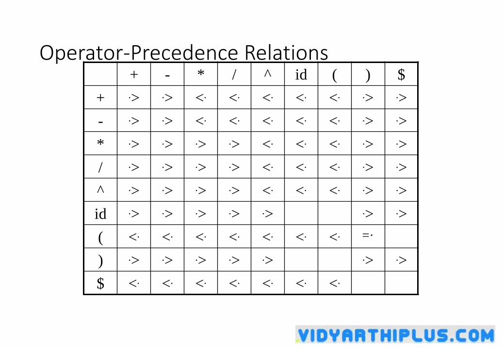
Operator-Precedence Relations+ - * / ^ id ( ) $
+ .> .> <. <. <. <. <. .> .>
- .> .> <. <. <. <. <. .> .>
* .> .> .> .> <. <. <. .> .>
/ .> .> .> .> <. <. <. .> .>
^ .> .> .> .> <. <. <. .> .>
id .> .> .> .> .> .> .>
( <. <. <. <. <. <. <. =·
) .> .> .> .> .> .> .>
$ <. <. <. <. <. <. <.
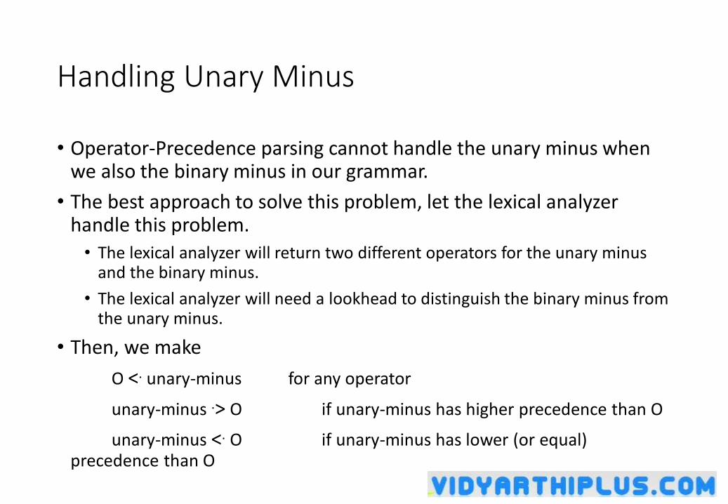
Handling Unary Minus
• Operator-Precedence parsing cannot handle the unary minus when we also the binary minus in our grammar.
• The best approach to solve this problem, let the lexical analyzer handle this problem.
• The lexical analyzer will return two different operators for the unary minus and the binary minus.
• The lexical analyzer will need a lookhead to distinguish the binary minus from the unary minus.
• Then, we make
O <. unary-minus for any operator
unary-minus .> O if unary-minus has higher precedence than O
unary-minus <. O if unary-minus has lower (or equal) precedence than O
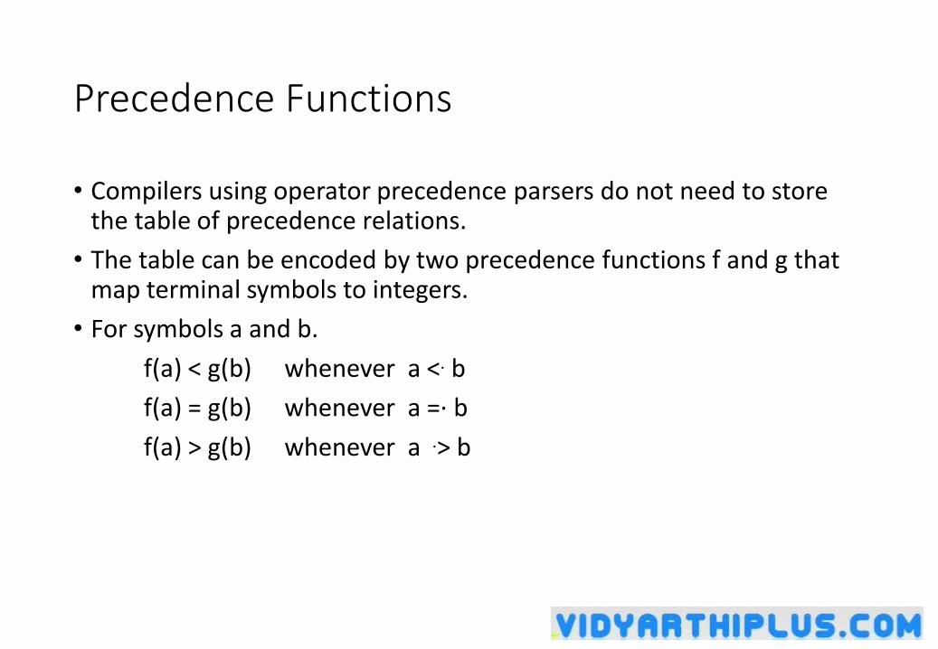
Precedence Functions
• Compilers using operator precedence parsers do not need to store the table of precedence relations.
• The table can be encoded by two precedence functions f and g that map terminal symbols to integers.
• For symbols a and b.
f(a) < g(b) whenever a <. b
f(a) = g(b) whenever a =· b
f(a) > g(b) whenever a .> b
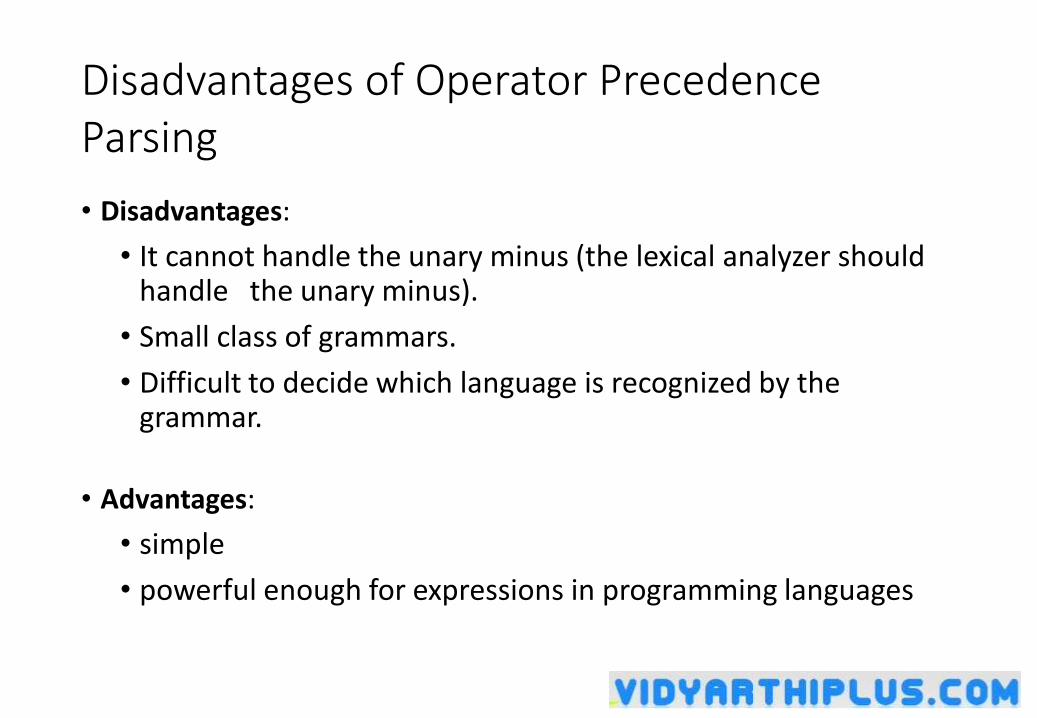
Disadvantages of Operator Precedence Parsing
• Disadvantages:
• It cannot handle the unary minus (the lexical analyzer should handle the unary minus).
• Small class of grammars.
• Difficult to decide which language is recognized by the grammar.
• Advantages:
• simple
• powerful enough for expressions in programming languages
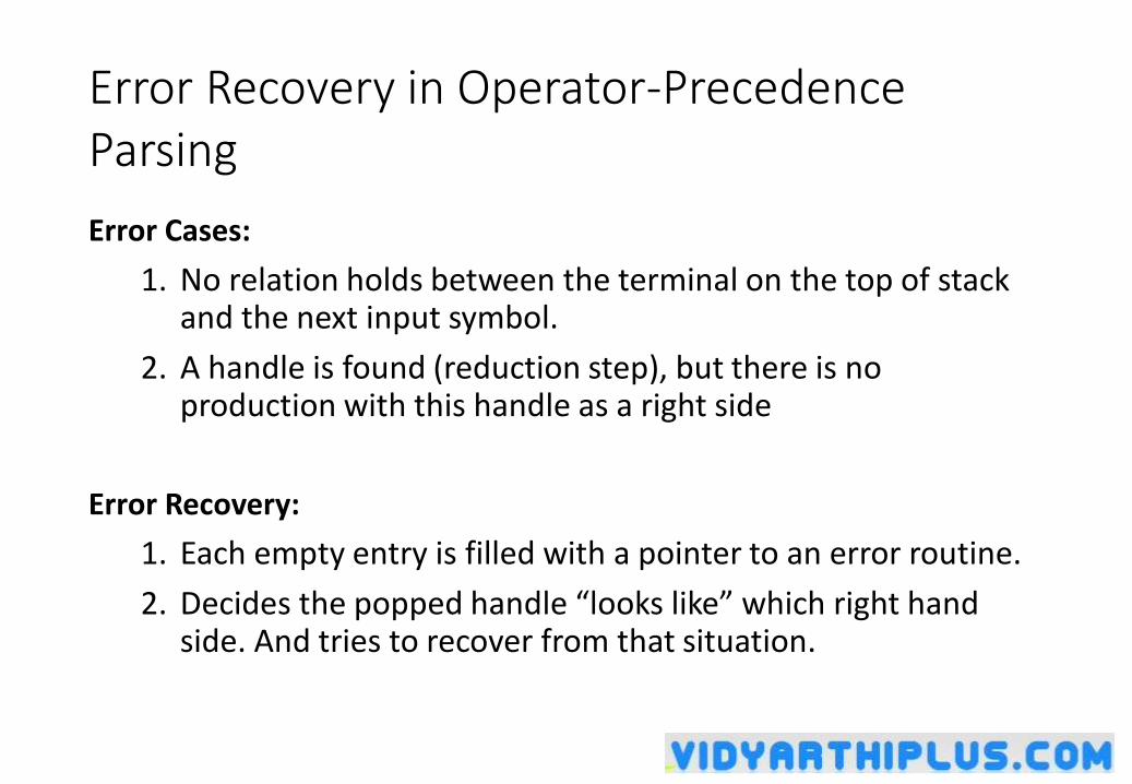
Error Recovery in Operator-Precedence Parsing
Error Cases:
1. No relation holds between the terminal on the top of stack and the next input symbol.
2. A handle is found (reduction step), but there is no production with this handle as a right side
Error Recovery:
1. Each empty entry is filled with a pointer to an error routine.
2. Decides the popped handle “looks like” which right hand side. And tries to recover from that situation.
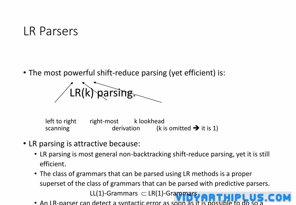
LR Parsers
• The most powerful shift-reduce parsing (yet efficient) is:
LR(k) parsing.
left to right right-most k lookheadscanning derivation (k is omitted it is 1)
• LR parsing is attractive because:• LR parsing is most general non-backtracking shift-reduce parsing, yet it is still
efficient.
• The class of grammars that can be parsed using LR methods is a proper
superset of the class of grammars that can be parsed with predictive parsers.
LL(1)-Grammars LR(1)-Grammars
• An LR-parser can detect a syntactic error as soon as it is possible to do so a
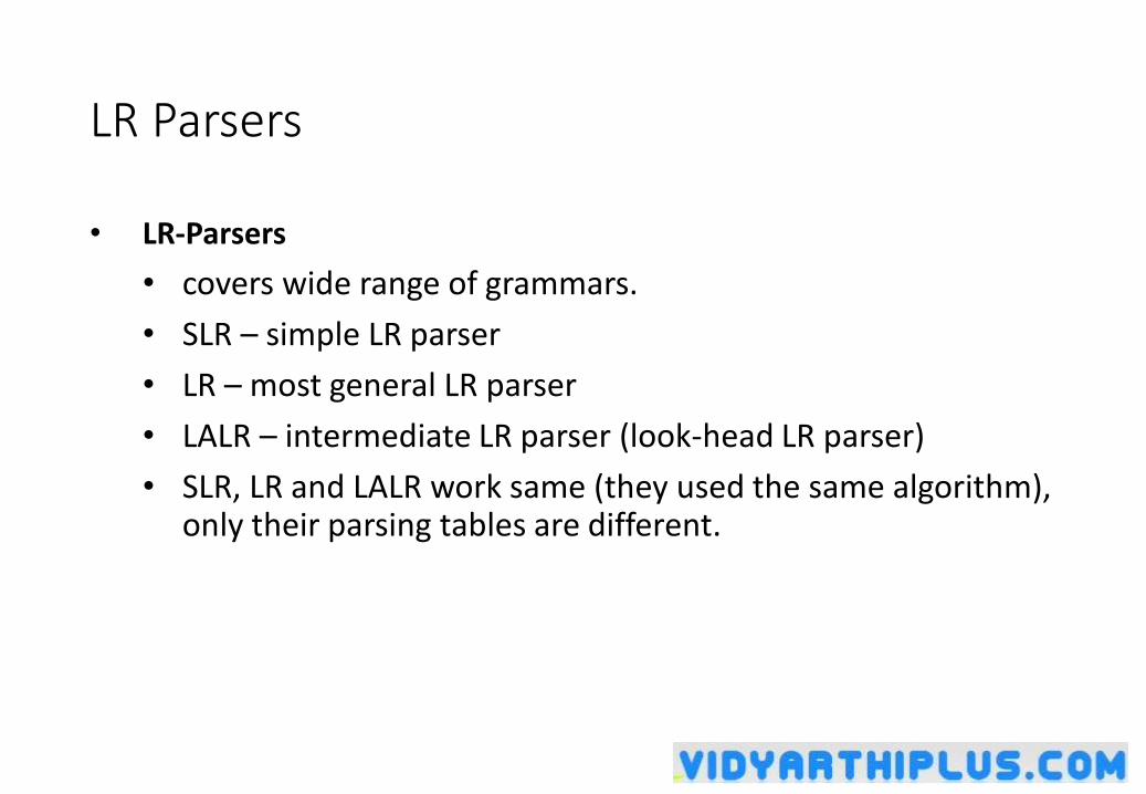
LR Parsers
• LR-Parsers
• covers wide range of grammars.
• SLR – simple LR parser
• LR – most general LR parser
• LALR – intermediate LR parser (look-head LR parser)
• SLR, LR and LALR work same (they used the same algorithm), only their parsing tables are different.
LR Parsing Algorithm
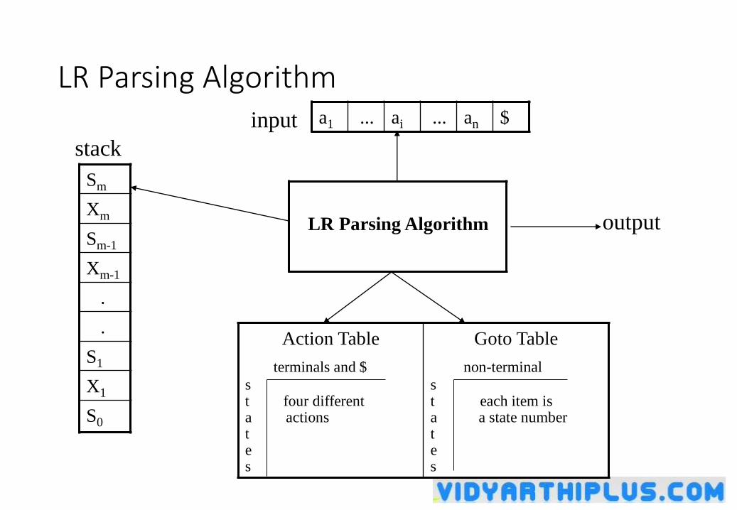
Sm
Xm
Sm-1
Xm-1
.
.
S1
X1
S0
a1 ... ai ... an $
Action Table
terminals and $
st four different a actionstes
Goto Table
non-terminal
st each item isa a state numbertes
LR Parsing Algorithm
stack
input
output
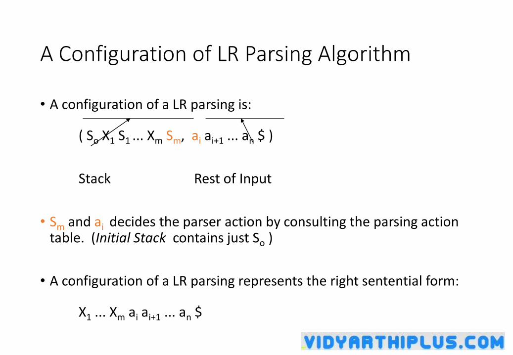
A Configuration of LR Parsing Algorithm
• A configuration of a LR parsing is:
( So X1 S1 ... Xm Sm, ai ai+1 ... an $ )
Stack Rest of Input
• Sm and ai decides the parser action by consulting the parsing action table. (Initial Stack contains just So )
• A configuration of a LR parsing represents the right sentential form:
X1 ... Xm ai ai+1 ... an $
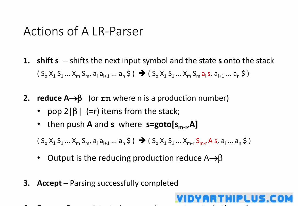
Actions of A LR-Parser
1. shift s -- shifts the next input symbol and the state s onto the stack
( So X1 S1 ... Xm Sm, ai ai+1 ... an $ ) ( So X1 S1 ... Xm Sm ai s, ai+1 ... an $ )
2. reduce A (or rn where n is a production number)
• pop 2|| (=r) items from the stack;
• then push A and s where s=goto[sm-r,A]
( So X1 S1 ... Xm Sm, ai ai+1 ... an $ ) ( So X1 S1 ... Xm-r Sm-r A s, ai ... an $ )
• Output is the reducing production reduce A
3. Accept – Parsing successfully completed
4. Error -- Parser detected an error (an empty entry in the action
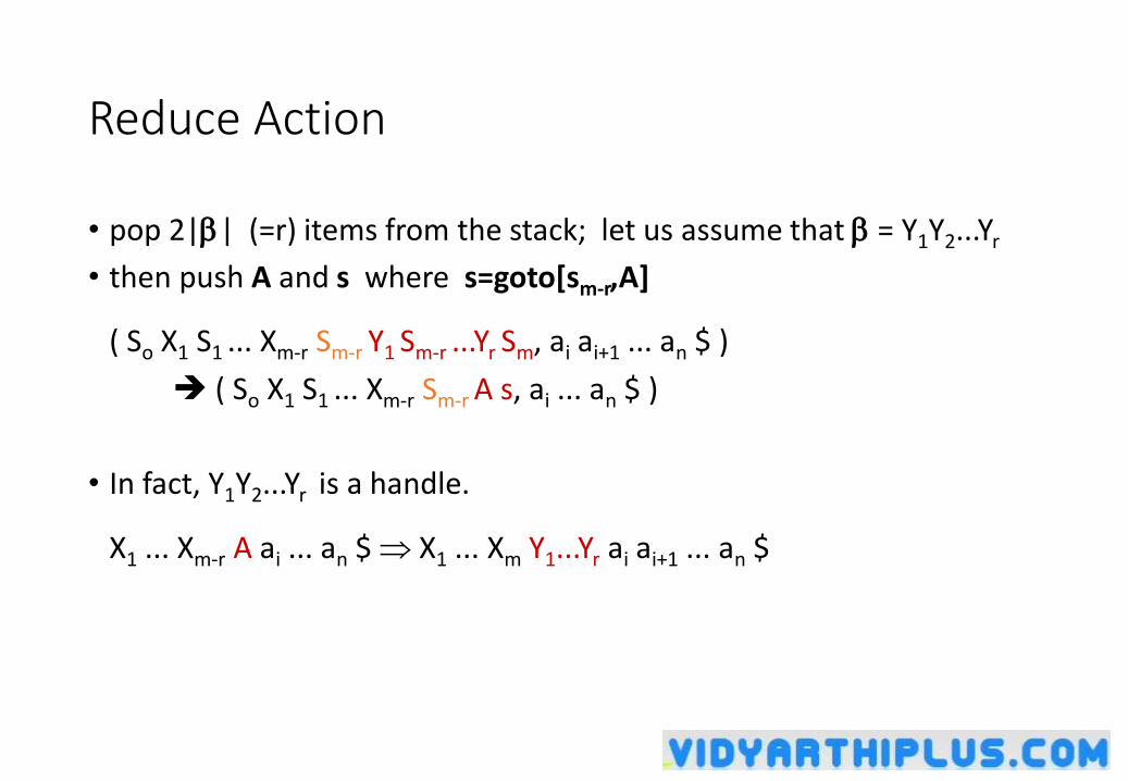
Reduce Action
• pop 2|| (=r) items from the stack; let us assume that = Y1Y2...Yr
• then push A and s where s=goto[sm-r,A]
( So X1 S1 ... Xm-r Sm-r Y1 Sm-r ...Yr Sm, ai ai+1 ... an $ )
( So X1 S1 ... Xm-r Sm-r A s, ai ... an $ )
• In fact, Y1Y2...Yr is a handle.
X1 ... Xm-r A ai ... an $ X1 ... Xm Y1...Yr ai ai+1 ... an $
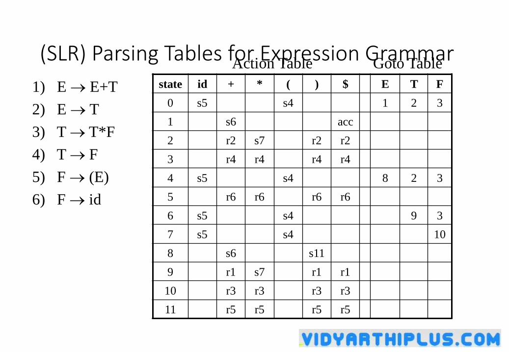
(SLR) Parsing Tables for Expression Grammarstate id + * ( ) $ E T F
0 s5 s4 1 2 3
1 s6 acc
2 r2 s7 r2 r2
3 r4 r4 r4 r4
4 s5 s4 8 2 3
5 r6 r6 r6 r6
6 s5 s4 9 3
7 s5 s4 10
8 s6 s11
9 r1 s7 r1 r1
10 r3 r3 r3 r3
11 r5 r5 r5 r5
Action Table Goto Table
1) E E+T
2) E T
3) T T*F
4) T F
5) F (E)
6) F id
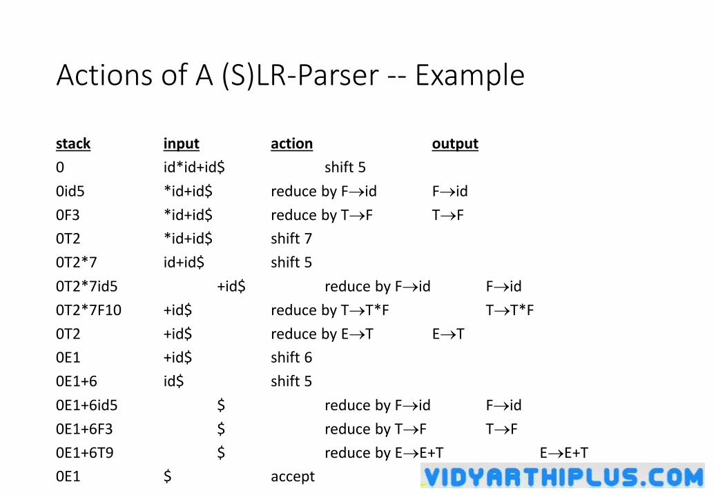
Actions of A (S)LR-Parser -- Example
stack input action output
0 id*id+id$ shift 5
0id5 *id+id$ reduce by Fid Fid
0F3 *id+id$ reduce by TF TF
0T2 *id+id$ shift 7
0T2*7 id+id$ shift 5
0T2*7id5 +id$ reduce by Fid Fid
0T2*7F10 +id$ reduce by TT*F TT*F
0T2 +id$ reduce by ET ET
0E1 +id$ shift 6
0E1+6 id$ shift 5
0E1+6id5 $ reduce by Fid Fid
0E1+6F3 $ reduce by TF TF
0E1+6T9 $ reduce by EE+T EE+T
0E1 $ accept
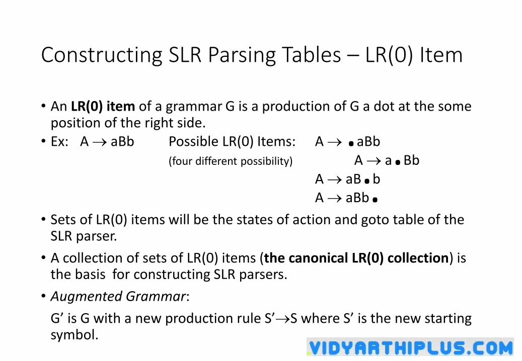
Constructing SLR Parsing Tables – LR(0) Item
• An LR(0) item of a grammar G is a production of G a dot at the some position of the right side.
• Ex: A aBb Possible LR(0) Items: A .aBb(four different possibility) A a.Bb
A aB.bA aBb.
• Sets of LR(0) items will be the states of action and goto table of the SLR parser.
• A collection of sets of LR(0) items (the canonical LR(0) collection) is the basis for constructing SLR parsers.
• Augmented Grammar:
G’ is G with a new production rule S’S where S’ is the new starting symbol.
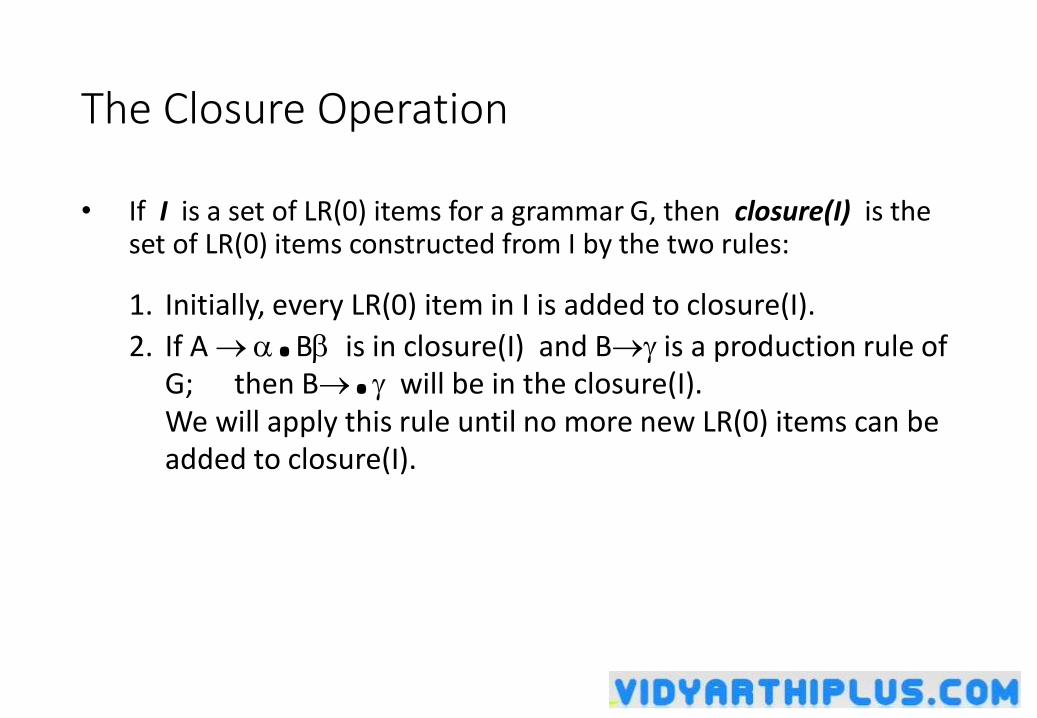
The Closure Operation
• If I is a set of LR(0) items for a grammar G, then closure(I) is the set of LR(0) items constructed from I by the two rules:
1. Initially, every LR(0) item in I is added to closure(I).
2. If A .B is in closure(I) and B is a production rule of G; then B. will be in the closure(I). We will apply this rule until no more new LR(0) items can be added to closure(I).
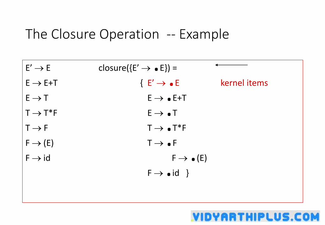
The Closure Operation -- Example
E’ E closure({E’ .E}) =
E E+T { E’ .E kernel items
E T E .E+T
T T*F E .T
T F T .T*F
F (E) T .F
F id F .(E)
F .id }
Goto Operation
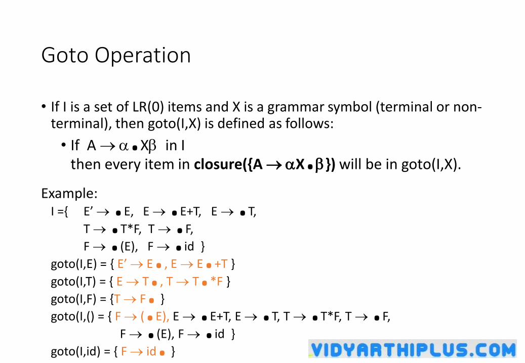
• If I is a set of LR(0) items and X is a grammar symbol (terminal or non-terminal), then goto(I,X) is defined as follows:
• If A .X in I then every item in closure({A X.}) will be in goto(I,X).
Example:I ={ E’ .E, E .E+T, E .T,
T .T*F, T .F,
F .(E), F .id }
goto(I,E) = { E’ E., E E.+T }
goto(I,T) = { E T., T T.*F }
goto(I,F) = {T F. }
goto(I,() = { F (.E), E .E+T, E .T, T .T*F, T .F,
F .(E), F .id }
goto(I,id) = { F id. }
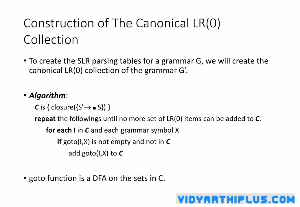
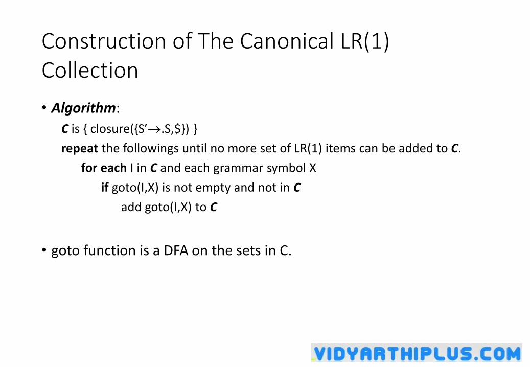
Construction of The Canonical LR(0) Collection
• To create the SLR parsing tables for a grammar G, we will create the canonical LR(0) collection of the grammar G’.
• Algorithm:
C is { closure({S’.S}) }
repeat the followings until no more set of LR(0) items can be added to C.
for each I in C and each grammar symbol X
if goto(I,X) is not empty and not in C
add goto(I,X) to C
• goto function is a DFA on the sets in C.
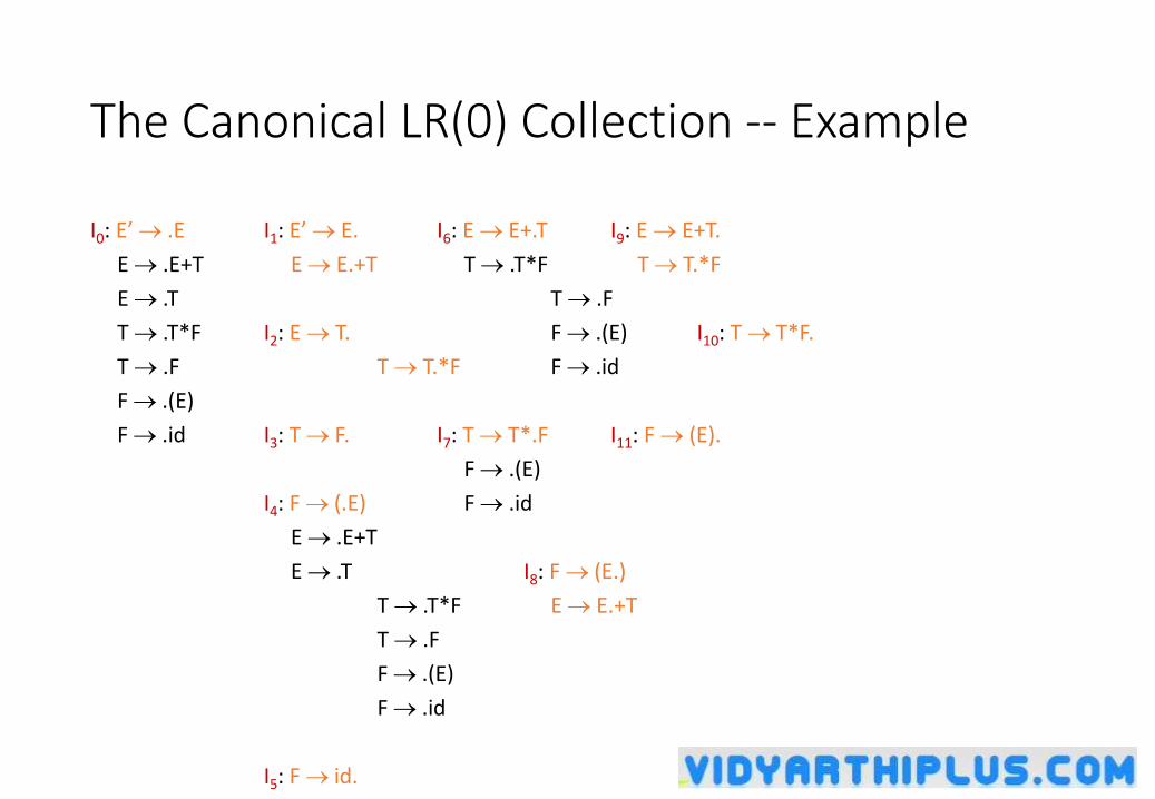
The Canonical LR(0) Collection -- Example
I0: E’ .E I1: E’ E. I6: E E+.T I9: E E+T.
E .E+T E E.+T T .T*F T T.*F
E .T T .F
T .T*F I2: E T. F .(E) I10: T T*F.
T .F T T.*F F .id
F .(E)
F .id I3: T F. I7: T T*.F I11: F (E).
F .(E)
I4: F (.E) F .id
E .E+T
E .T I8: F (E.)
T .T*F E E.+T
T .F
F .(E)
F .id
I5: F id.
Transition Diagram (DFA) of Goto Function
I0 I1
I2
I3
I4
I5
I6
I7
I8
to I2
to I3
to I4
I9
to I3
to I4
to I5
I10
to I4
to I5
I11
to I6
to I7
id
(
F
*
E
E
+T
T
T
)
F
FF
(
idid
(
*
(
id
+
Constructing SLR Parsing Table (of an augumented grammar G’)
1. Construct the canonical collection of sets of LR(0) items for G’. C{I0,...,In}
2. Create the parsing action table as follows
• If a is a terminal, A.a in Ii and goto(Ii,a)=Ij then action[i,a] is shift j.
• If A. is in Ii , then action[i,a] is reduce A for all a in FOLLOW(A) where AS’.
• If S’S. is in Ii , then action[i,$] is accept.
• If any conflicting actions generated by these rules, the grammar is not SLR(1).
3. Create the parsing goto table
• for all non-terminals A, if goto(Ii,A)=Ij then goto[i,A]=j
4. All entries not defined by (2) and (3) are errors.
5. Initial state of the parser contains S’.S
Parsing Tables of Expression Grammarstate id + * ( ) $ E T F
0 s5 s4 1 2 3
1 s6 acc
2 r2 s7 r2 r2
3 r4 r4 r4 r4
4 s5 s4 8 2 3
5 r6 r6 r6 r6
6 s5 s4 9 3
7 s5 s4 10
8 s6 s11
9 r1 s7 r1 r1
10 r3 r3 r3 r3
11 r5 r5 r5 r5
Action Table Goto Table
SLR(1) Grammar
• An LR parser using SLR(1) parsing tables for a grammar G is called as the SLR(1) parser for G.
• If a grammar G has an SLR(1) parsing table, it is called SLR(1) grammar (or SLR grammar in short).
• Every SLR grammar is unambiguous, but every unambiguous grammar is not a SLR grammar.
shift/reduce and reduce/reduce conflicts
• If a state does not know whether it will make a shift operation or reduction for a terminal, we say that there is a shift/reduce conflict.
• If a state does not know whether it will make a reduction operation using the production rule i or j for a terminal, we say that there is a reduce/reduce conflict.
• If the SLR parsing table of a grammar G has a conflict, we say that that grammar is not SLR grammar.
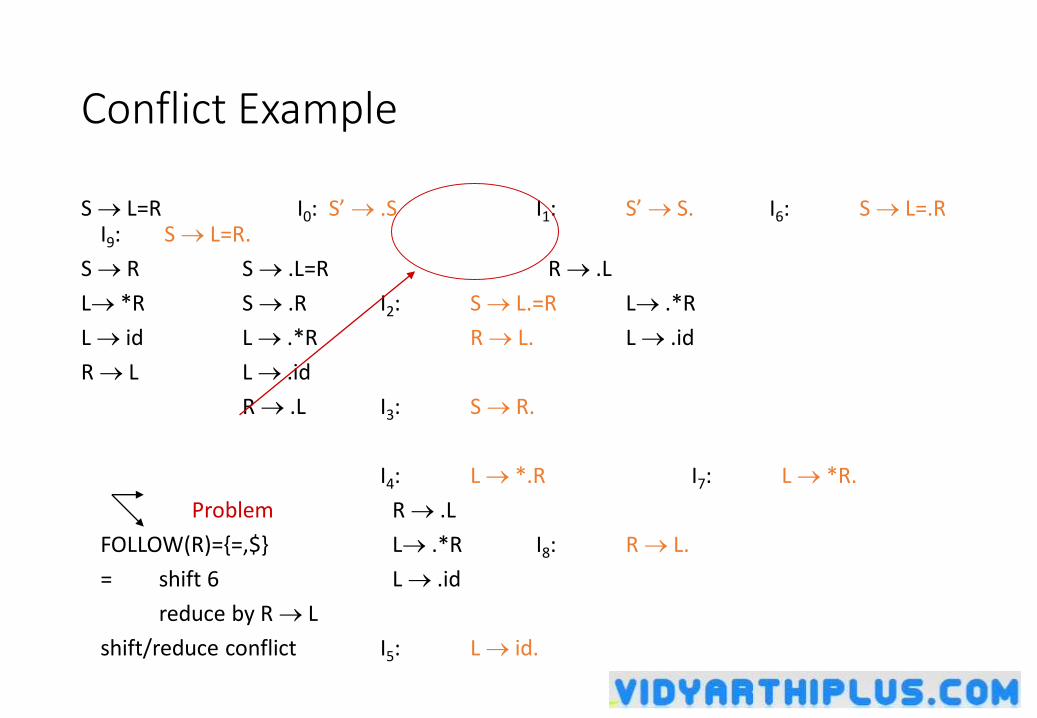
Conflict Example
S L=R I0: S’ .S I1: S’ S. I6: S L=.RI9: S L=R.
S R S .L=R R .L
L *R S .R I2: S L.=R L .*R
L id L .*R R L. L .id
R L L .id
R .L I3: S R.
I4: L *.R I7: L *R.
Problem R .L
FOLLOW(R)={=,$} L .*R I8: R L.
= shift 6 L .id
reduce by R L
shift/reduce conflict I5: L id.
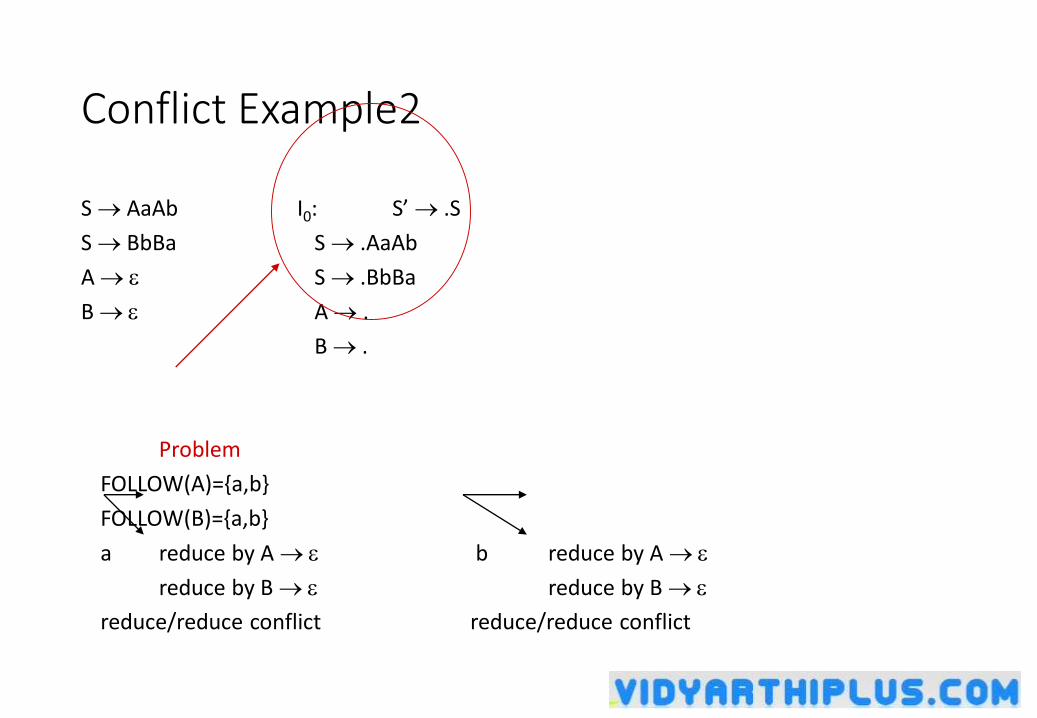
Conflict Example2
S AaAb I0: S’ .S
S BbBa S .AaAb
A S .BbBa
B A .
B .
Problem
FOLLOW(A)={a,b}
FOLLOW(B)={a,b}
a reduce by A b reduce by A
reduce by B reduce by B
reduce/reduce conflict reduce/reduce conflict
Constructing Canonical LR(1) Parsing Tables
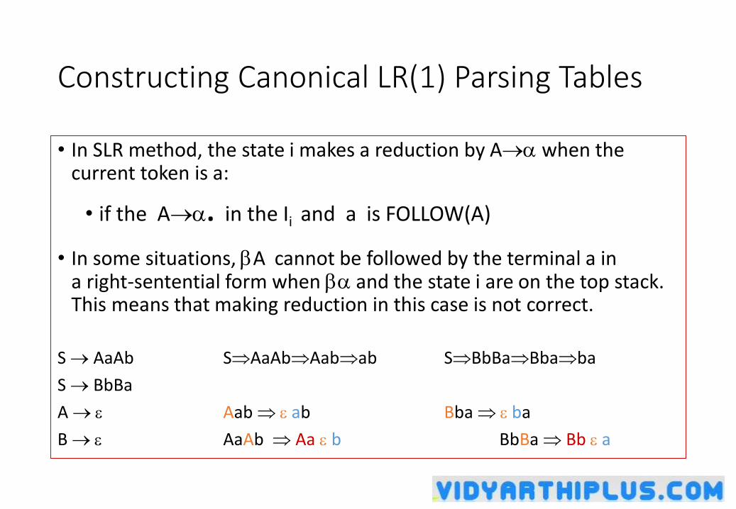
• In SLR method, the state i makes a reduction by A when the current token is a:
• if the A. in the Ii and a is FOLLOW(A)
• In some situations, A cannot be followed by the terminal a in a right-sentential form when and the state i are on the top stack. This means that making reduction in this case is not correct.
S AaAb SAaAbAabab SBbBaBbaba
S BbBa
A Aab ab Bba ba
B AaAb Aa b BbBa Bb a
LR(1) Item
• To avoid some of invalid reductions, the states need to carry more information.
• Extra information is put into a state by including a terminal symbol as a second component in an item.
• A LR(1) item is:
A .,a where a is the look-head of the LR(1) item
(a is a terminal or end-marker.)
LR(1) Item (cont.)
• When ( in the LR(1) item A .,a ) is not empty, the look-head does not have any affect.
• When is empty (A .,a ), we do the reduction by A only if the next input symbol is a (not for any terminal in FOLLOW(A)).
• A state will contain A .,a1 where {a1,...,an} FOLLOW(A)
...
A .,an
Canonical Collection of Sets of LR(1) Items
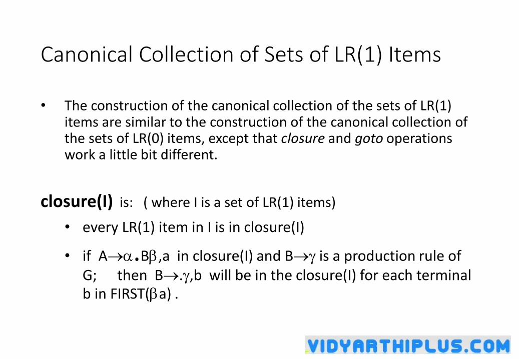
• The construction of the canonical collection of the sets of LR(1) items are similar to the construction of the canonical collection of the sets of LR(0) items, except that closure and goto operations work a little bit different.
closure(I) is: ( where I is a set of LR(1) items)
• every LR(1) item in I is in closure(I)
• if A.B,a in closure(I) and B is a production rule of G; then B.,b will be in the closure(I) for each terminal b in FIRST(a) .
goto operation
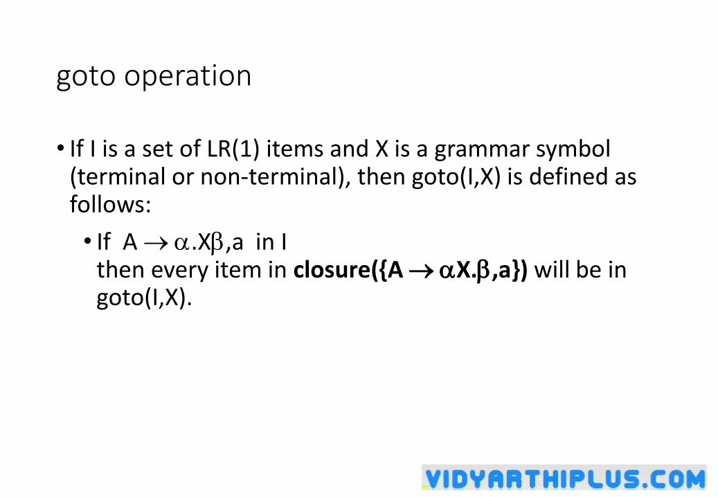
• If I is a set of LR(1) items and X is a grammar symbol (terminal or non-terminal), then goto(I,X) is defined as follows:
• If A .X,a in I then every item in closure({A X.,a}) will be in goto(I,X).
Construction of The Canonical LR(1) Collection
• Algorithm:
C is { closure({S’.S,$}) }
repeat the followings until no more set of LR(1) items can be added to C.
for each I in C and each grammar symbol X
if goto(I,X) is not empty and not in C
add goto(I,X) to C
• goto function is a DFA on the sets in C.
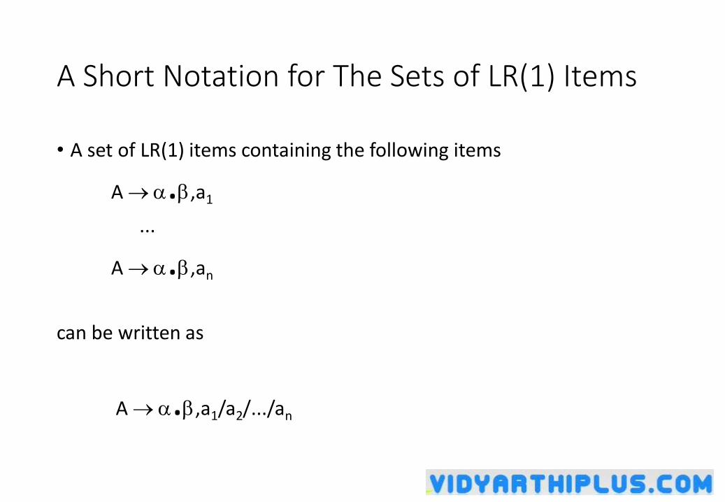
A Short Notation for The Sets of LR(1) Items
• A set of LR(1) items containing the following items
A .,a1
...
A .,an
can be written as
A .,a1/a2/.../an
Canonical LR(1) Collection -- Example
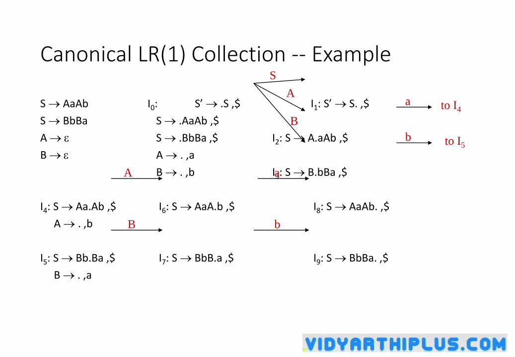
S AaAb I0: S’ .S ,$ I1: S’ S. ,$
S BbBa S .AaAb ,$
A S .BbBa ,$ I2: S A.aAb ,$
B A . ,a
B . ,b I3: S B.bBa ,$
I4: S Aa.Ab ,$ I6: S AaA.b ,$ I8: S AaAb. ,$
A . ,b
I5: S Bb.Ba ,$ I7: S BbB.a ,$ I9: S BbBa. ,$
B . ,a
S
A
B
a
b
A
B
a
b
to I4
to I5
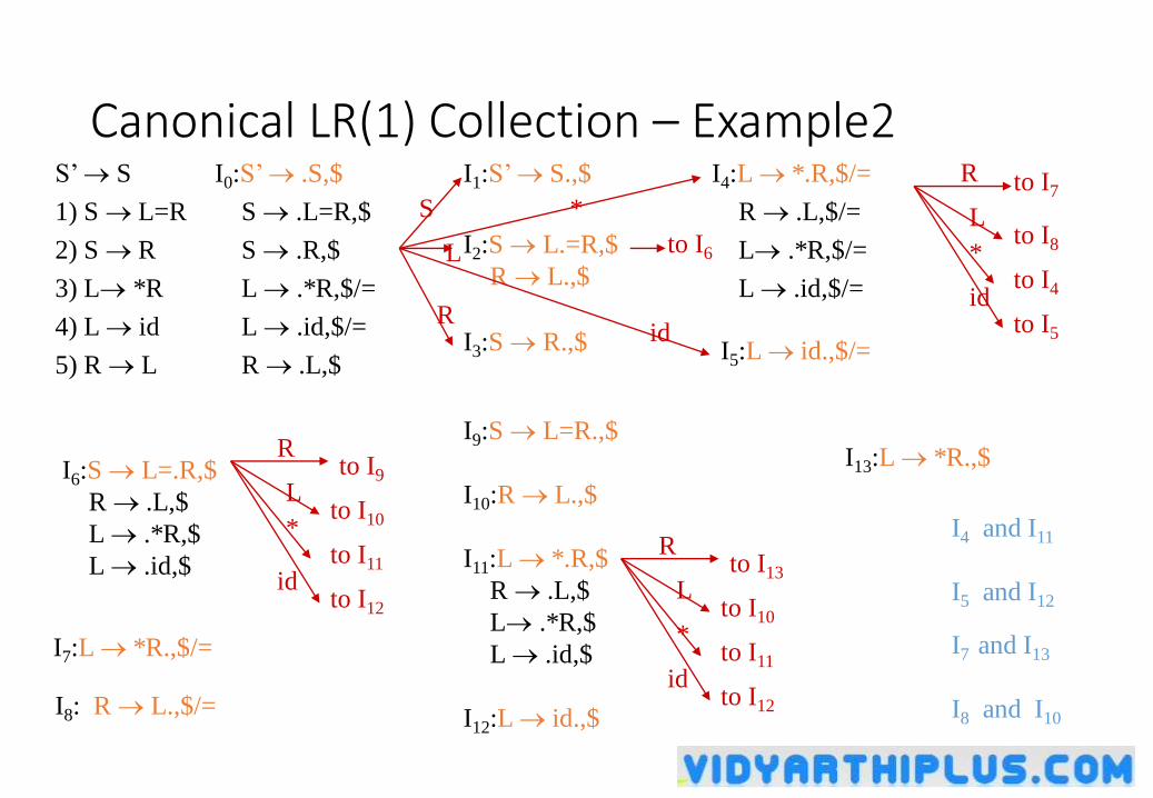
Canonical LR(1) Collection – Example2S’ S
1) S L=R
2) S R
3) L *R
4) L id
5) R L
I0:S’ .S,$
S .L=R,$
S .R,$
L .*R,$/=
L .id,$/=
R .L,$
I1:S’ S.,$
I2:S L.=R,$
R L.,$
I3:S R.,$
I4:L *.R,$/=
R .L,$/=
L .*R,$/=
L .id,$/=
I5:L id.,$/=
I6:S L=.R,$
R .L,$
L .*R,$
L .id,$
I7:L *R.,$/=
I8: R L.,$/=
I9:S L=R.,$
I10:R L.,$
I11:L *.R,$
R .L,$
L .*R,$
L .id,$
I12:L id.,$
I13:L *R.,$
to I6
to I7
to I8
to I4
to I5
to I10
to I11
to I12
to I9
to I10
to I11
to I12
to I13
id
S
L
L
L
R
R
R
id
id
id
R
L
*
*
*
*
I4 and I11
I5 and I12
I7 and I13
I8 and I10
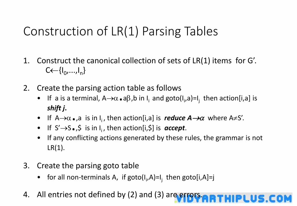
Construction of LR(1) Parsing Tables
1. Construct the canonical collection of sets of LR(1) items for G’. C{I0,...,In}
2. Create the parsing action table as follows• If a is a terminal, A.a,b in Ii and goto(Ii,a)=Ij then action[i,a] is
shift j.
• If A.,a is in Ii , then action[i,a] is reduce A where AS’.
• If S’S.,$ is in Ii , then action[i,$] is accept.
• If any conflicting actions generated by these rules, the grammar is not
LR(1).
3. Create the parsing goto table
• for all non-terminals A, if goto(Ii,A)=Ij then goto[i,A]=j
4. All entries not defined by (2) and (3) are errors.
5. Initial state of the parser contains S’.S,$
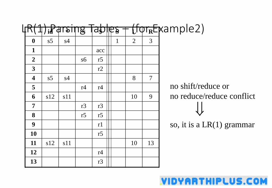
LR(1) Parsing Tables – (for Example2)id * = $ S L R
0 s5 s4 1 2 3
1 acc
2 s6 r5
3 r2
4 s5 s4 8 7
5 r4 r4
6 s12 s11 10 9
7 r3 r3
8 r5 r5
9 r1
10 r5
11 s12 s11 10 13
12 r4
13 r3
no shift/reduce or
no reduce/reduce conflict
so, it is a LR(1) grammar
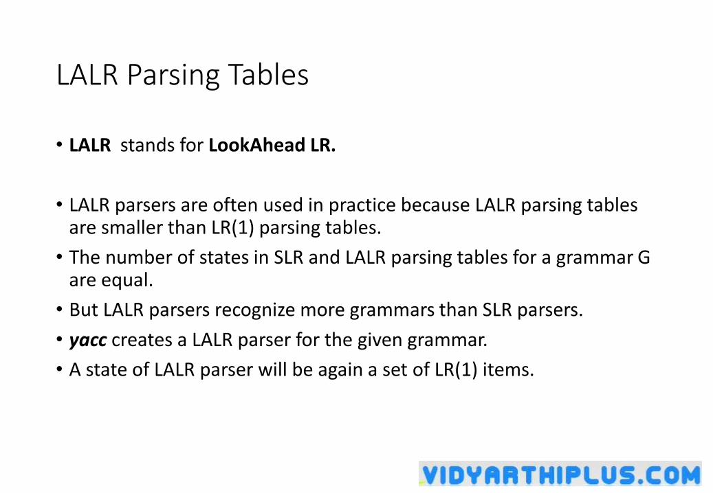
LALR Parsing Tables
• LALR stands for LookAhead LR.
• LALR parsers are often used in practice because LALR parsing tables are smaller than LR(1) parsing tables.
• The number of states in SLR and LALR parsing tables for a grammar G are equal.
• But LALR parsers recognize more grammars than SLR parsers.
• yacc creates a LALR parser for the given grammar.
• A state of LALR parser will be again a set of LR(1) items.
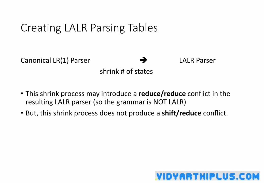
Creating LALR Parsing Tables
Canonical LR(1) Parser LALR Parser
shrink # of states
• This shrink process may introduce a reduce/reduce conflict in the resulting LALR parser (so the grammar is NOT LALR)
• But, this shrink process does not produce a shift/reduce conflict.
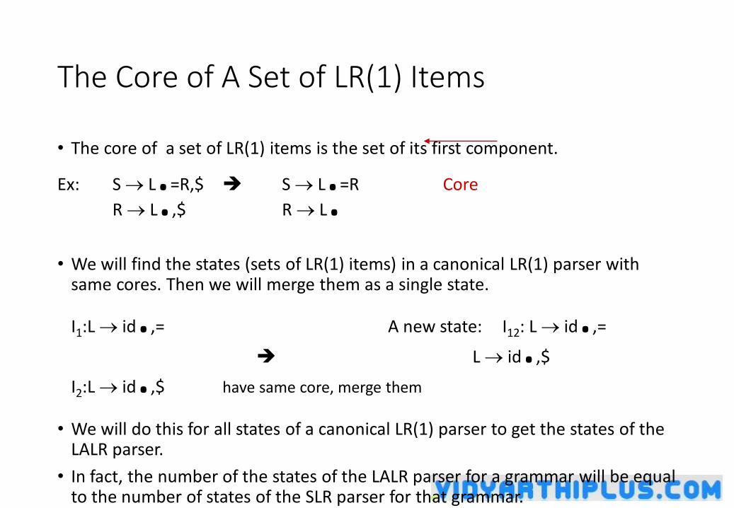
The Core of A Set of LR(1) Items
• The core of a set of LR(1) items is the set of its first component.
Ex: S L.=R,$ S L.=R Core
R L.,$ R L.• We will find the states (sets of LR(1) items) in a canonical LR(1) parser with
same cores. Then we will merge them as a single state.
I1:L id.,= A new state: I12: L id.,=
L id.,$
I2:L id.,$ have same core, merge them
• We will do this for all states of a canonical LR(1) parser to get the states of the LALR parser.
• In fact, the number of the states of the LALR parser for a grammar will be equal to the number of states of the SLR parser for that grammar.
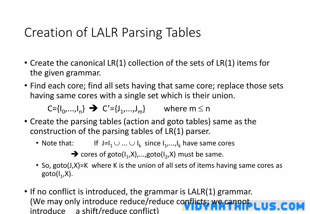
Creation of LALR Parsing Tables
• Create the canonical LR(1) collection of the sets of LR(1) items for the given grammar.
• Find each core; find all sets having that same core; replace those sets having same cores with a single set which is their union.
C={I0,...,In} C’={J1,...,Jm} where m n
• Create the parsing tables (action and goto tables) same as the construction of the parsing tables of LR(1) parser.
• Note that: If J=I1 ... Ik since I1,...,Ik have same cores
cores of goto(I1,X),...,goto(I2,X) must be same.
• So, goto(J,X)=K where K is the union of all sets of items having same cores as goto(I1,X).
• If no conflict is introduced, the grammar is LALR(1) grammar. (We may only introduce reduce/reduce conflicts; we cannot introduce a shift/reduce conflict)
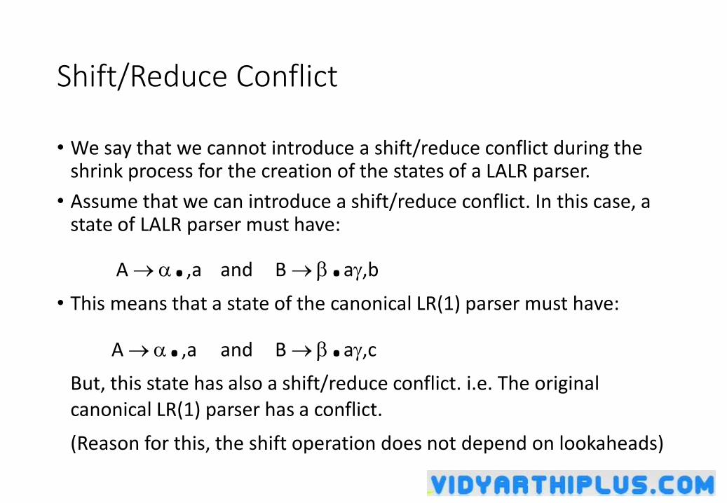
Shift/Reduce Conflict
• We say that we cannot introduce a shift/reduce conflict during the shrink process for the creation of the states of a LALR parser.
• Assume that we can introduce a shift/reduce conflict. In this case, a state of LALR parser must have:
A .,a and B .a,b
• This means that a state of the canonical LR(1) parser must have:
A .,a and B .a,c
But, this state has also a shift/reduce conflict. i.e. The original canonical LR(1) parser has a conflict.
(Reason for this, the shift operation does not depend on lookaheads)
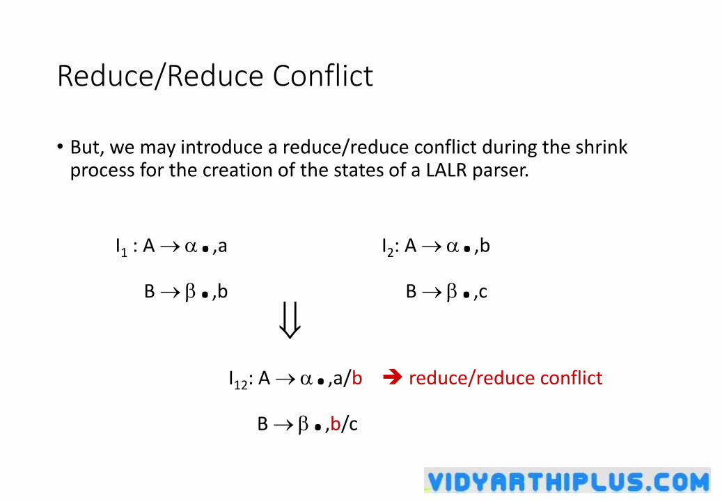
Reduce/Reduce Conflict
• But, we may introduce a reduce/reduce conflict during the shrink process for the creation of the states of a LALR parser.
I1 : A .,a I2: A .,b
B .,b B .,c
I12: A .,a/b reduce/reduce conflict
B .,b/c
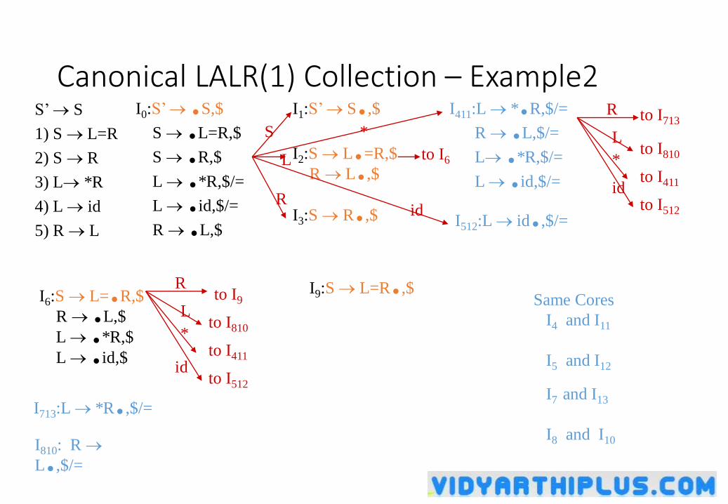
Canonical LALR(1) Collection – Example2S’ S
1) S L=R
2) S R
3) L *R
4) L id
5) R L
I0:S’ .S,$
S .L=R,$
S .R,$
L .*R,$/=
L .id,$/=
R .L,$
I1:S’ S.,$
I2:S L.=R,$
R L.,$
I3:S R.,$
I411:L *.R,$/=
R .L,$/=
L .*R,$/=
L .id,$/=
I512:L id.,$/=
I6:S L=.R,$
R .L,$
L .*R,$
L .id,$
I713:L *R.,$/=
I810: R
L.,$/=
I9:S L=R.,$
to I6
to I713
to I810
to I411
to I512
to I810
to I411
to I512
to I9
S
L
L
L
R
R
id
id
id
R
*
*
*
Same Cores
I4 and I11
I5 and I12
I7 and I13
I8 and I10
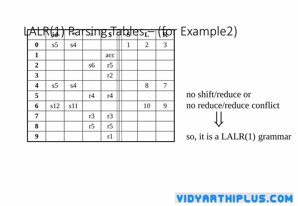
LALR(1) Parsing Tables – (for Example2)id * = $ S L R
0 s5 s4 1 2 3
1 acc
2 s6 r5
3 r2
4 s5 s4 8 7
5 r4 r4
6 s12 s11 10 9
7 r3 r3
8 r5 r5
9 r1
no shift/reduce or
no reduce/reduce conflict
so, it is a LALR(1) grammar
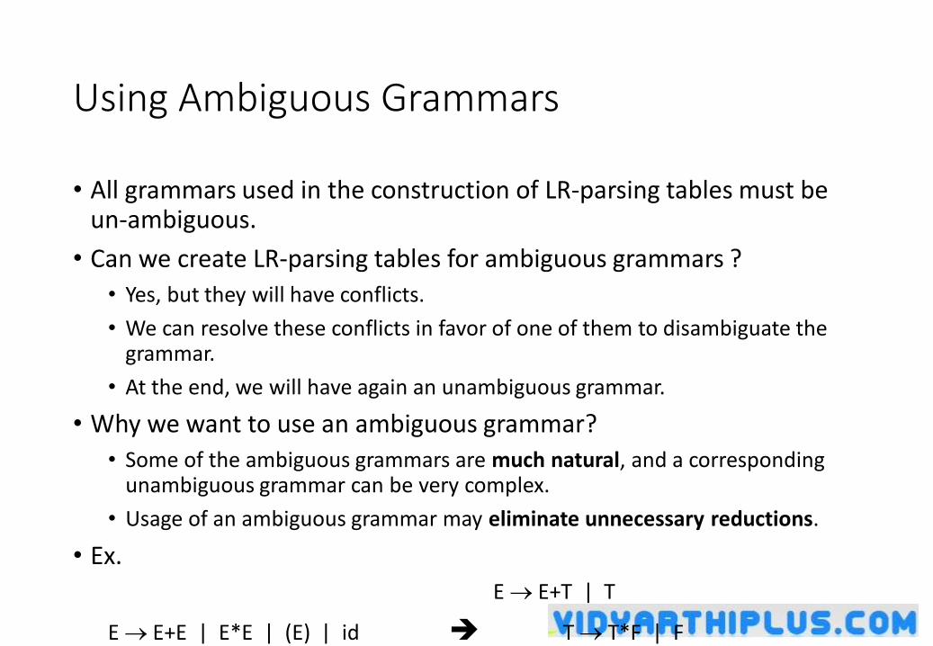
Using Ambiguous Grammars
• All grammars used in the construction of LR-parsing tables must be un-ambiguous.
• Can we create LR-parsing tables for ambiguous grammars ?
• Yes, but they will have conflicts.
• We can resolve these conflicts in favor of one of them to disambiguate the grammar.
• At the end, we will have again an unambiguous grammar.
• Why we want to use an ambiguous grammar?
• Some of the ambiguous grammars are much natural, and a corresponding unambiguous grammar can be very complex.
• Usage of an ambiguous grammar may eliminate unnecessary reductions.
• Ex.
E E+T | T
E E+E | E*E | (E) | id T T*F | F
F (E) | id
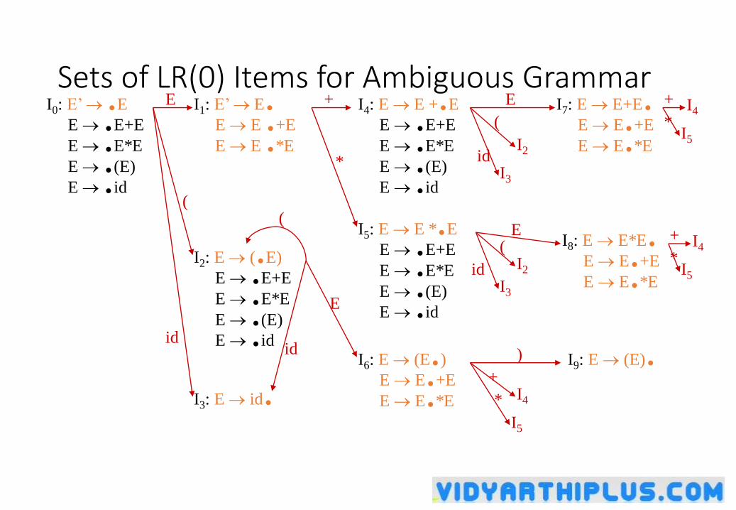
Sets of LR(0) Items for Ambiguous GrammarI0: E’ .E
E .E+E
E .E*E
E .(E)
E .id
I1: E’ E.E E .+E
E E .*E
I2: E (.E)
E .E+E
E .E*E
E .(E)
E .id
I3: E id.
I4: E E +.E
E .E+E
E .E*E
E .(E)
E .id
I5: E E *.E
E .E+E
E .E*E
E .(E)
E .id
I6: E (E.)
E E.+E
E E.*E
I7: E E+E.E E.+E
E E.*E
I8: E E*E.E E.+E
E E.*E
I9: E (E).
I5
)
E
E
E
E
*
+
+
+
+
*
*
*
(
(
((
id
id
idid
I4
I2
I2
I3
I3
I4
I4
I5
I5
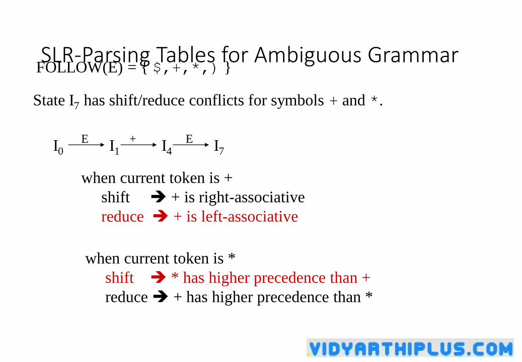
SLR-Parsing Tables for Ambiguous GrammarFOLLOW(E) = { $,+,*,) }
State I7 has shift/reduce conflicts for symbols + and *.
I0 I1 I7I4E+E
when current token is +
shift + is right-associative
reduce + is left-associative
when current token is *
shift * has higher precedence than +
reduce + has higher precedence than *

SLR-Parsing Tables for Ambiguous GrammarFOLLOW(E) = { $,+,*,) }
State I8 has shift/reduce conflicts for symbols + and *.
I0 I1 I7I5E*E
when current token is *
shift * is right-associative
reduce * is left-associative
when current token is +
shift + has higher precedence than *
reduce * has higher precedence than +
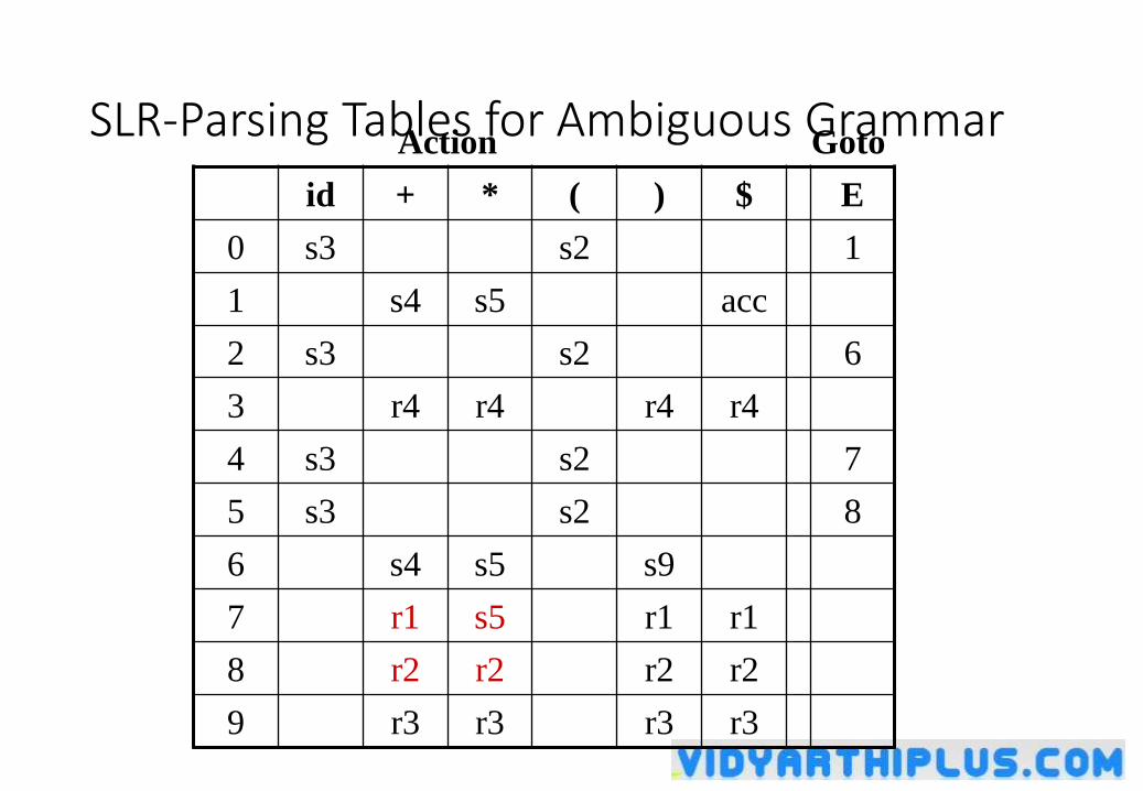
SLR-Parsing Tables for Ambiguous Grammar
id + * ( ) $ E
0 s3 s2 1
1 s4 s5 acc
2 s3 s2 6
3 r4 r4 r4 r4
4 s3 s2 7
5 s3 s2 8
6 s4 s5 s9
7 r1 s5 r1 r1
8 r2 r2 r2 r2
9 r3 r3 r3 r3
Action Goto
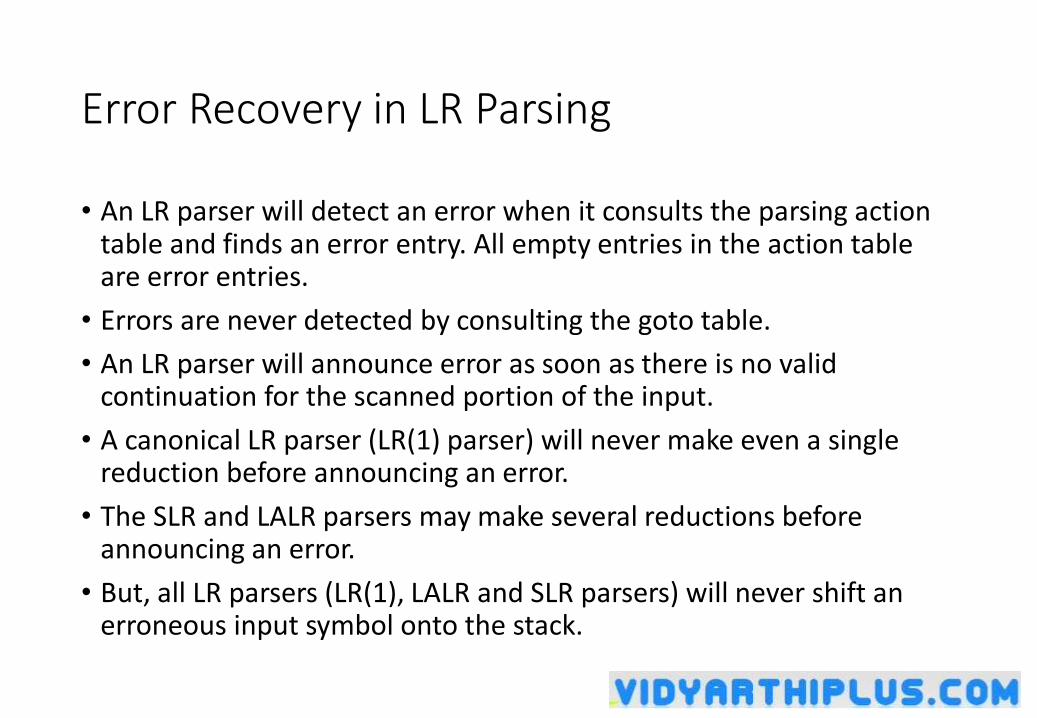
Error Recovery in LR Parsing
• An LR parser will detect an error when it consults the parsing action table and finds an error entry. All empty entries in the action table are error entries.
• Errors are never detected by consulting the goto table.
• An LR parser will announce error as soon as there is no valid continuation for the scanned portion of the input.
• A canonical LR parser (LR(1) parser) will never make even a single reduction before announcing an error.
• The SLR and LALR parsers may make several reductions before announcing an error.
• But, all LR parsers (LR(1), LALR and SLR parsers) will never shift an erroneous input symbol onto the stack.
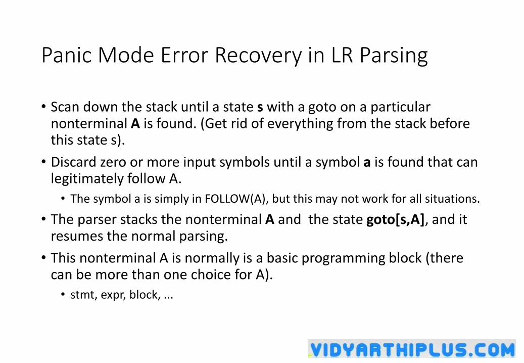
Panic Mode Error Recovery in LR Parsing
• Scan down the stack until a state s with a goto on a particular nonterminal A is found. (Get rid of everything from the stack before this state s).
• Discard zero or more input symbols until a symbol a is found that can legitimately follow A.
• The symbol a is simply in FOLLOW(A), but this may not work for all situations.
• The parser stacks the nonterminal A and the state goto[s,A], and it resumes the normal parsing.
• This nonterminal A is normally is a basic programming block (there can be more than one choice for A).
• stmt, expr, block, ...
Phrase-Level Error Recovery in LR Parsing
• Each empty entry in the action table is marked with a specific error routine.
• An error routine reflects the error that the user most likely will make in that case.
• An error routine inserts the symbols into the stack or the input (or it deletes the symbols from the stack and the input, or it can do both insertion and deletion).
• missing operand
• unbalanced right parenthesis
Semantic Analysis
Need for Semantic Analysis
•Not all program properties can be represented using context-free grammars.
E.g.: “variables must be declared before use” is not a context-free property.
• Parsing context-sensitive grammars is expensive.
•As a pragmatic measure, compilers combine context-free and context-sensitive checking:• Context-free parsing used to check “code shape;”
• Additional rules used to check context-sensitive aspects.
Syntax-Directed Translation
• Basic Idea: • Associate information with grammar symbols using attributes.
An attribute can represent any reasonable aspect of a program, e.g., character string, numerical value, type, memory location, etc.
• Use semantic rules associated with grammar productions to compute attribute values.
•A parse tree showing attribute values at each node is called an annotated parse tree.
• Implementation: Add code to parser to compute and propagate attribute values.
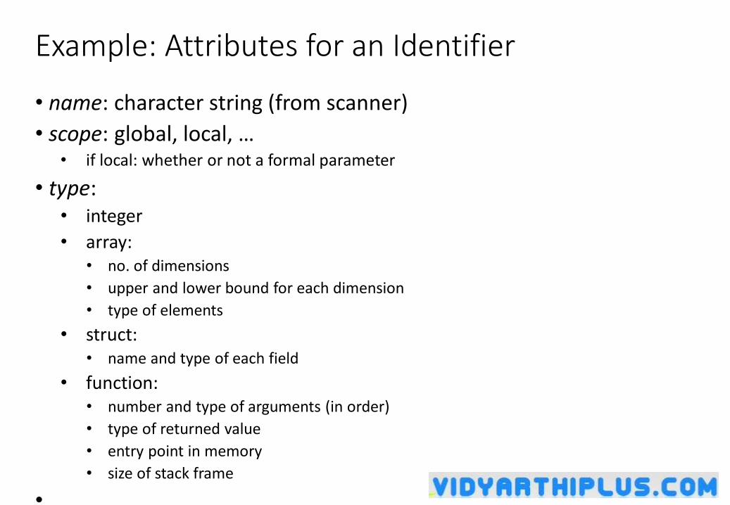
Example: Attributes for an Identifier
• name: character string (from scanner)
• scope: global, local, …• if local: whether or not a formal parameter
• type:• integer
• array:• no. of dimensions
• upper and lower bound for each dimension
• type of elements
• struct:• name and type of each field
• function:• number and type of arguments (in order)
• type of returned value
• entry point in memory
• size of stack frame
• …
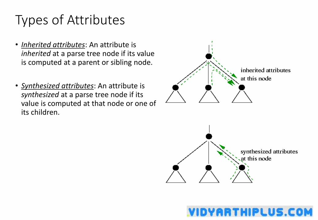
Types of Attributes
• Inherited attributes: An attribute is inherited at a parse tree node if its value is computed at a parent or sibling node.
• Synthesized attributes: An attribute is synthesized at a parse tree node if its value is computed at that node or one of its children.
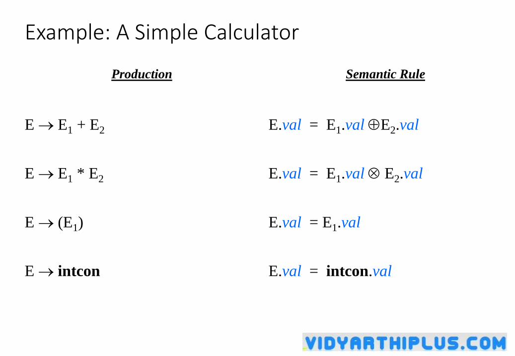
Example: A Simple Calculator
Production Semantic Rule
E E1 + E2 E.val = E1.val E2.val
E E1 * E2 E.val = E1.val E2.val
E (E1) E.val = E1.val
E intcon E.val = intcon.val
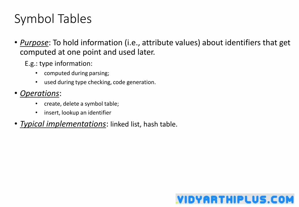
Symbol Tables
• Purpose: To hold information (i.e., attribute values) about identifiers that get computed at one point and used later.
E.g.: type information:• computed during parsing;
• used during type checking, code generation.
• Operations: • create, delete a symbol table;
• insert, lookup an identifier
• Typical implementations: linked list, hash table.
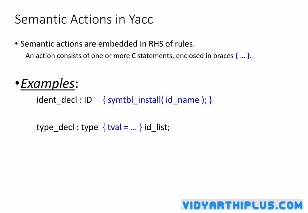
Semantic Actions in Yacc
• Semantic actions are embedded in RHS of rules.
An action consists of one or more C statements, enclosed in braces { … }.
•Examples:ident_decl : ID { symtbl_install( id_name ); }
type_decl : type { tval = … } id_list;
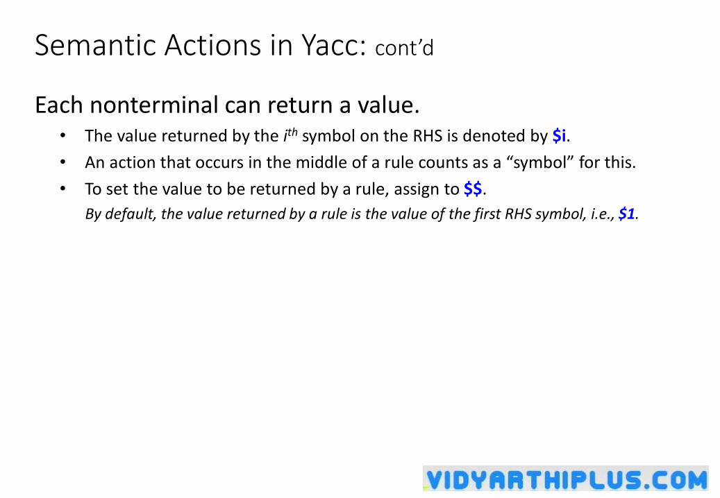
Semantic Actions in Yacc: cont’d
Each nonterminal can return a value.• The value returned by the ith symbol on the RHS is denoted by $i.
• An action that occurs in the middle of a rule counts as a “symbol” for this.
• To set the value to be returned by a rule, assign to $$.
By default, the value returned by a rule is the value of the first RHS symbol, i.e., $1.
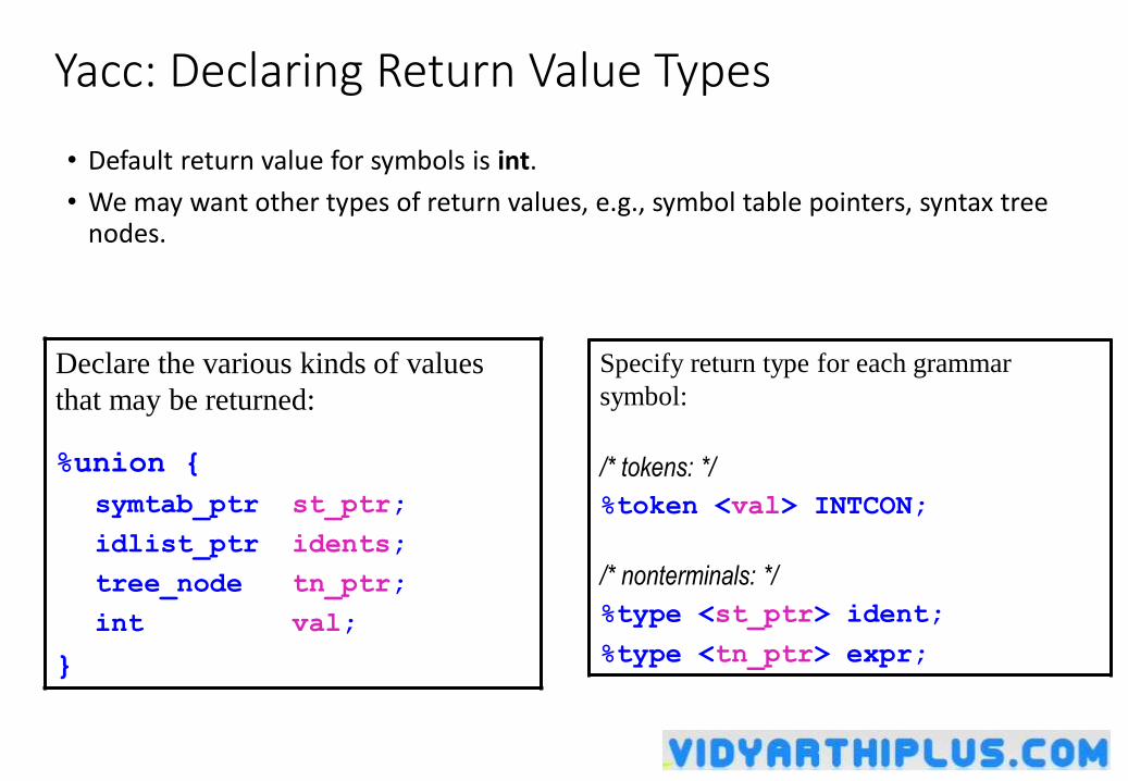
Yacc: Declaring Return Value Types
Declare the various kinds of values
that may be returned:
%union {
symtab_ptr st_ptr;
idlist_ptr idents;
tree_node tn_ptr;
int val;
}
Specify return type for each grammar
symbol:
/* tokens: */
%token <val> INTCON;
/* nonterminals: */
%type <st_ptr> ident;
%type <tn_ptr> expr;
• Default return value for symbols is int.
• We may want other types of return values, e.g., symbol table pointers, syntax tree nodes.
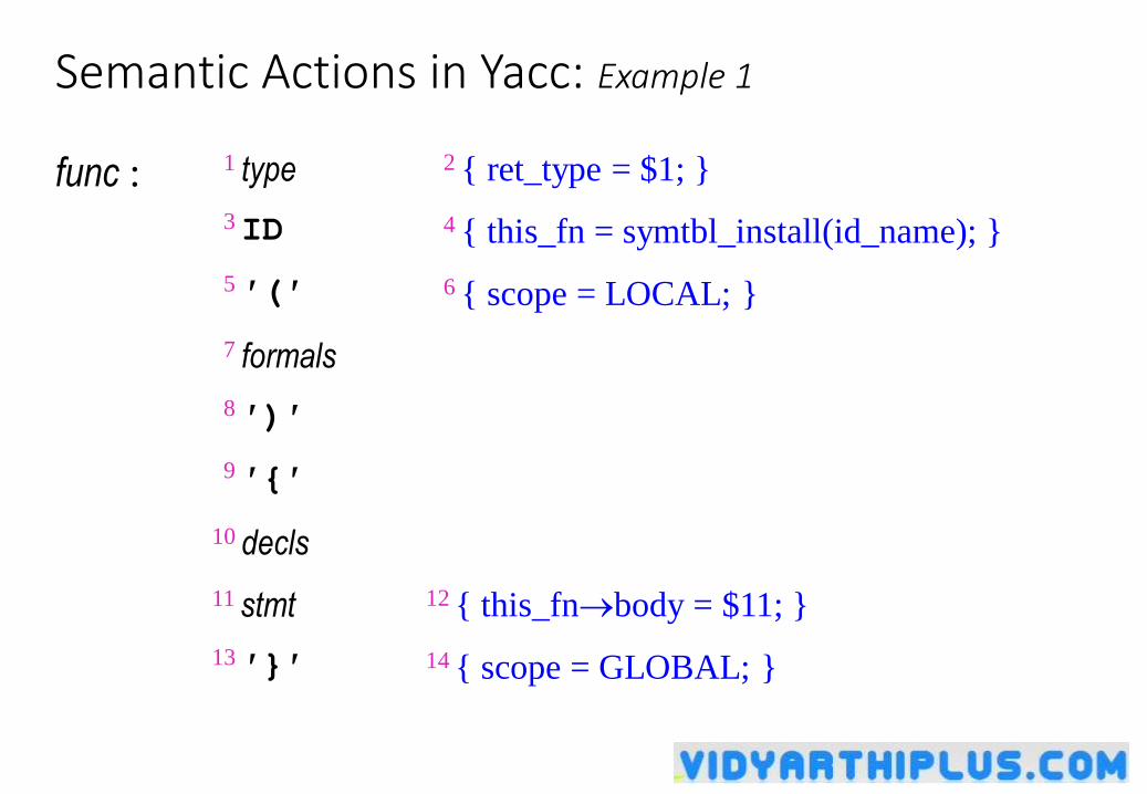
Semantic Actions in Yacc: Example 1
func : 1 type 2 { ret_type = $1; }
3 ID 4 { this_fn = symtbl_install(id_name); }
5 ′(′ 6 { scope = LOCAL; }
7 formals
8 ′)′
9 ′{′
10 decls
11 stmt 12 { this_fnbody = $11; }
13 ′}′ 14 { scope = GLOBAL; }
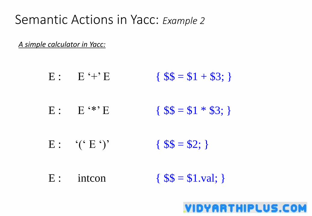
Semantic Actions in Yacc: Example 2
E : E ‘+’ E { $$ = $1 + $3; }
E : E ‘*’ E { $$ = $1 * $3; }
E : ‘(‘ E ‘)’ { $$ = $2; }
E : intcon { $$ = $1.val; }
A simple calculator in Yacc:
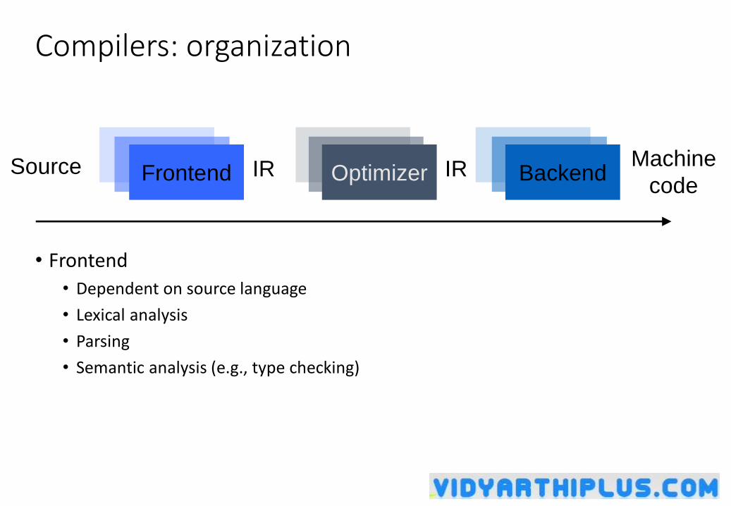
Compilers: organization
• Frontend
• Dependent on source language
• Lexical analysis
• Parsing
• Semantic analysis (e.g., type checking)
Frontend Optimizer BackendSource Machine
codeIR IR
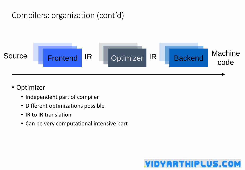
Compilers: organization (cont’d)
• Optimizer
• Independent part of compiler
• Different optimizations possible
• IR to IR translation
• Can be very computational intensive part
Frontend Optimizer BackendSource Machine
codeIR IR
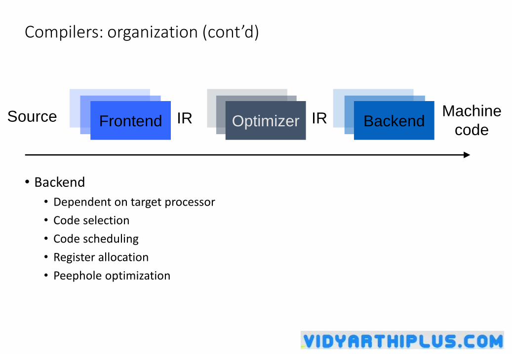
Compilers: organization (cont’d)
• Backend
• Dependent on target processor
• Code selection
• Code scheduling
• Register allocation
• Peephole optimization
Frontend Optimizer BackendSource Machine
codeIR IR
Frontend
Introduction to parsing using LEX and YACC
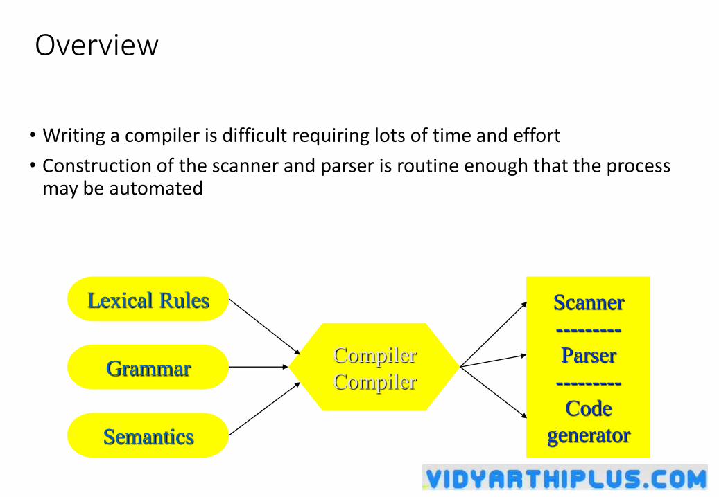
Overview
• Writing a compiler is difficult requiring lots of time and effort
• Construction of the scanner and parser is routine enough that the process may be automated
Lexical Rules
Grammar
Semantics
Compiler
Compiler
Scanner
---------
Parser
---------
Code
generator
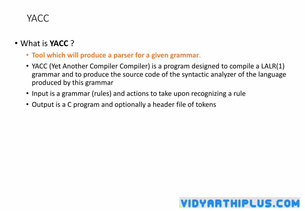
YACC
• What is YACC ?
• Tool which will produce a parser for a given grammar.
• YACC (Yet Another Compiler Compiler) is a program designed to compile a LALR(1) grammar and to produce the source code of the syntactic analyzer of the language produced by this grammar
• Input is a grammar (rules) and actions to take upon recognizing a rule
• Output is a C program and optionally a header file of tokens
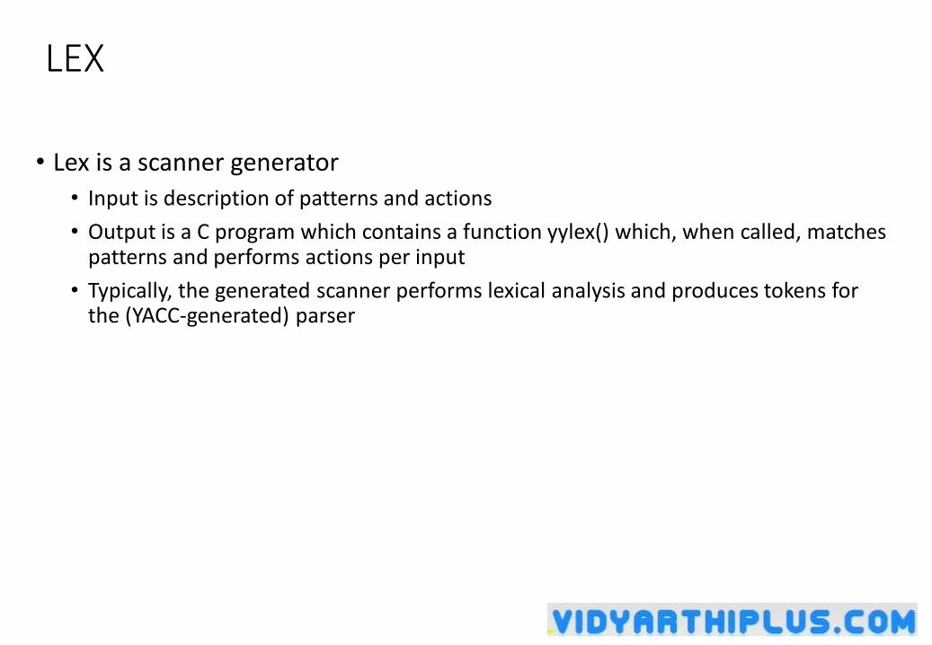
LEX
• Lex is a scanner generator
• Input is description of patterns and actions
• Output is a C program which contains a function yylex() which, when called, matches patterns and performs actions per input
• Typically, the generated scanner performs lexical analysis and produces tokens for the (YACC-generated) parser
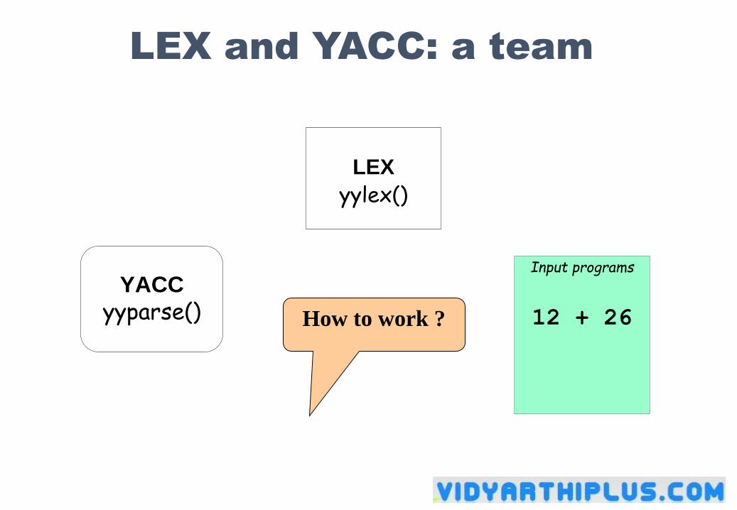
LEX and YACC: a team
YACC
yyparse()
Input programs
12 + 26
LEX
yylex()
How to work ?
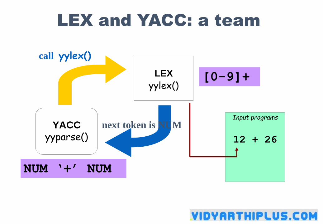
LEX and YACC: a team
YACC
yyparse()
Input programs
12 + 26
LEX
yylex()
call yylex()
[0-9]+
next token is NUM
NUM ‘+’ NUM
Availability
• lex, yacc on most UNIX systems
• bison: a yacc replacement from GNU
• flex: fast lexical analyzer
• BSD yacc
• Windows/MS-DOS versions exist
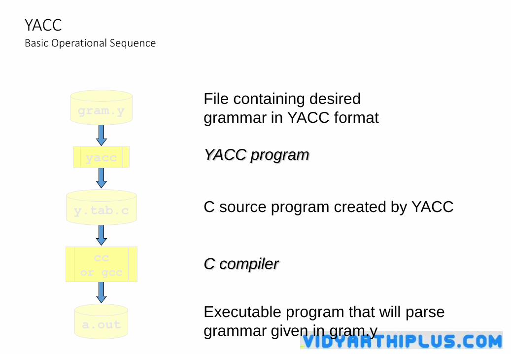
YACCBasic Operational Sequence
a.out
File containing desired
grammar in YACC format
YACC program
C source program created by YACC
C compiler
Executable program that will parse
grammar given in gram.y
gram.y
yacc
y.tab.c
cc
or gcc
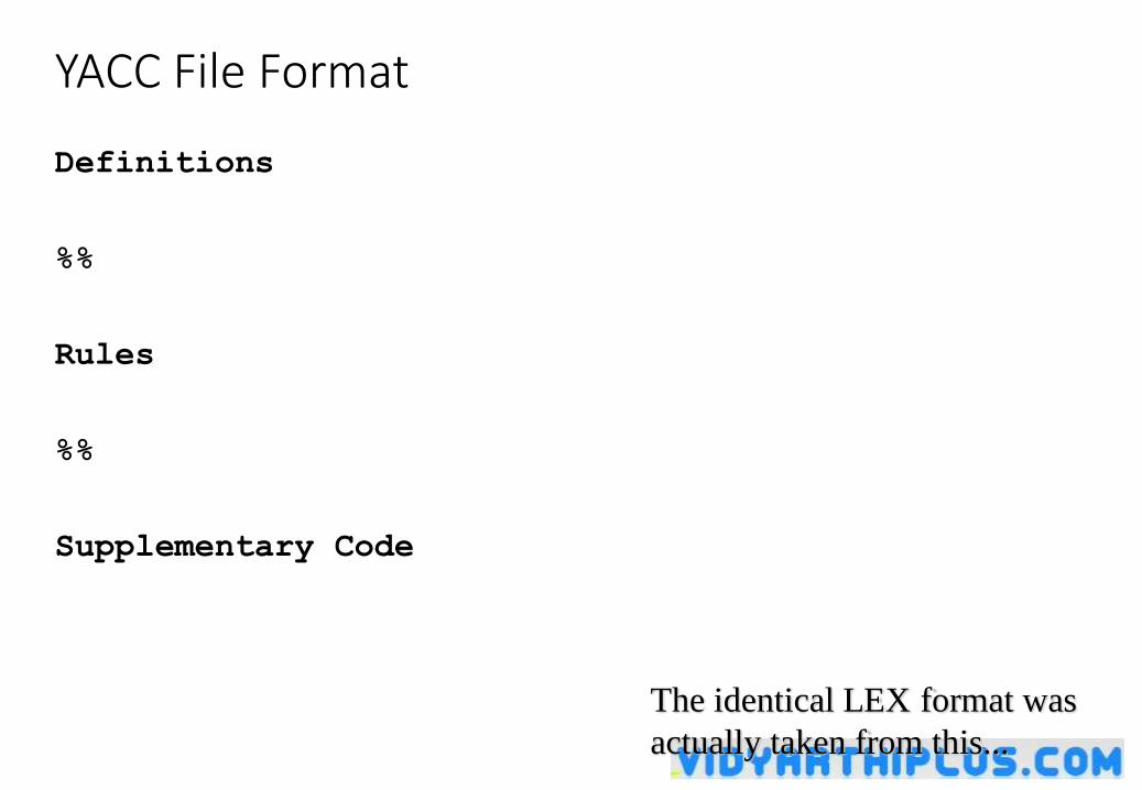
YACC File Format
Definitions
%%
Rules
%%
Supplementary Code
The identical LEX format was
actually taken from this...
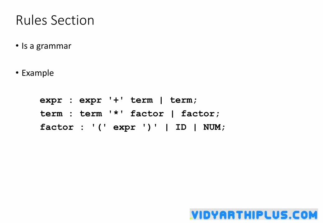
Rules Section
• Is a grammar
• Example
expr : expr '+' term | term;
term : term '*' factor | factor;
factor : '(' expr ')' | ID | NUM;
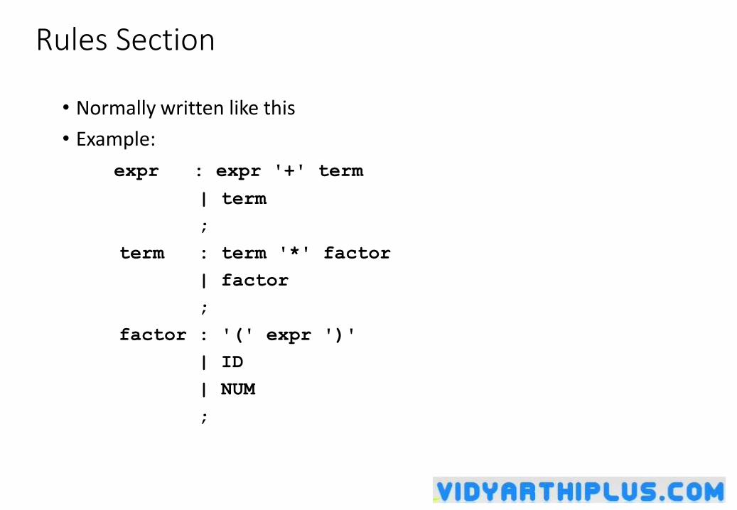
Rules Section
• Normally written like this
• Example:
expr : expr '+' term
| term
;
term : term '*' factor
| factor
;
factor : '(' expr ')'
| ID
| NUM
;
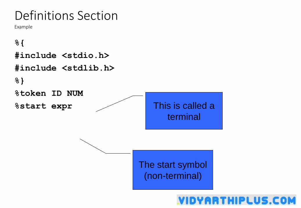
Definitions SectionExample
%{
#include <stdio.h>
#include <stdlib.h>
%}
%token ID NUM
%start expr This is called a
terminal
The start symbol
(non-terminal)
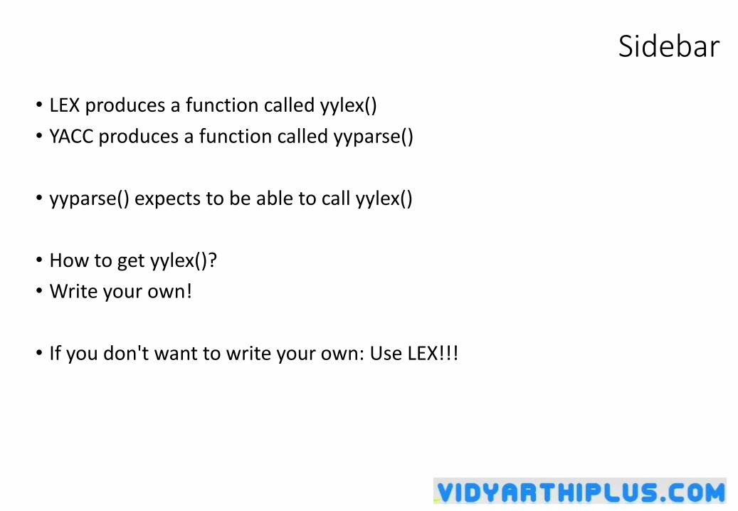
Sidebar
• LEX produces a function called yylex()
• YACC produces a function called yyparse()
• yyparse() expects to be able to call yylex()
• How to get yylex()?
• Write your own!
• If you don't want to write your own: Use LEX!!!
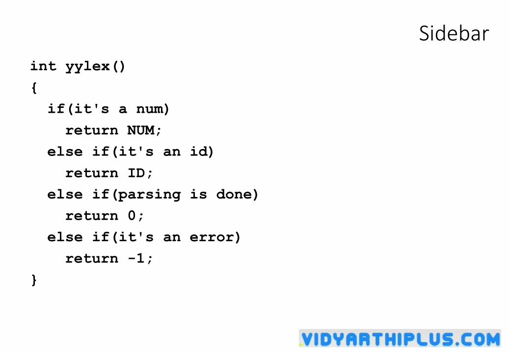
Sidebar
int yylex()
{
if(it's a num)
return NUM;
else if(it's an id)
return ID;
else if(parsing is done)
return 0;
else if(it's an error)
return -1;
}
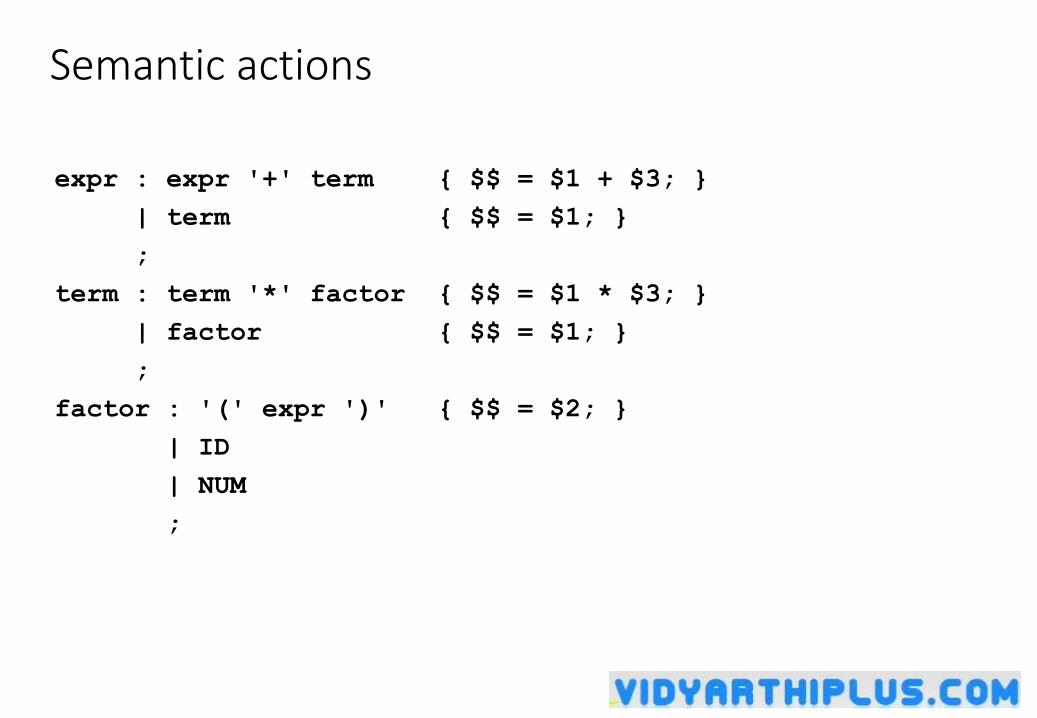
Semantic actions
expr : expr '+' term { $$ = $1 + $3; }
| term { $$ = $1; }
;
term : term '*' factor { $$ = $1 * $3; }
| factor { $$ = $1; }
;
factor : '(' expr ')' { $$ = $2; }
| ID
| NUM
;
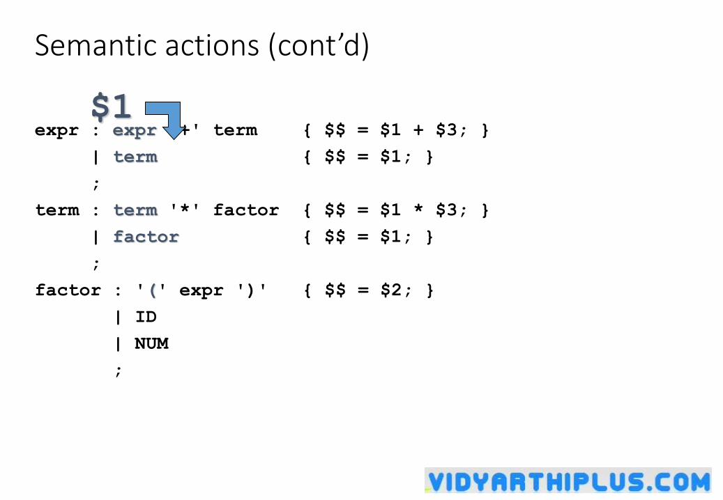
Semantic actions (cont’d)
expr : expr '+' term { $$ = $1 + $3; }
| term { $$ = $1; }
;
term : term '*' factor { $$ = $1 * $3; }
| factor { $$ = $1; }
;
factor : '(' expr ')' { $$ = $2; }
| ID
| NUM
;
$1
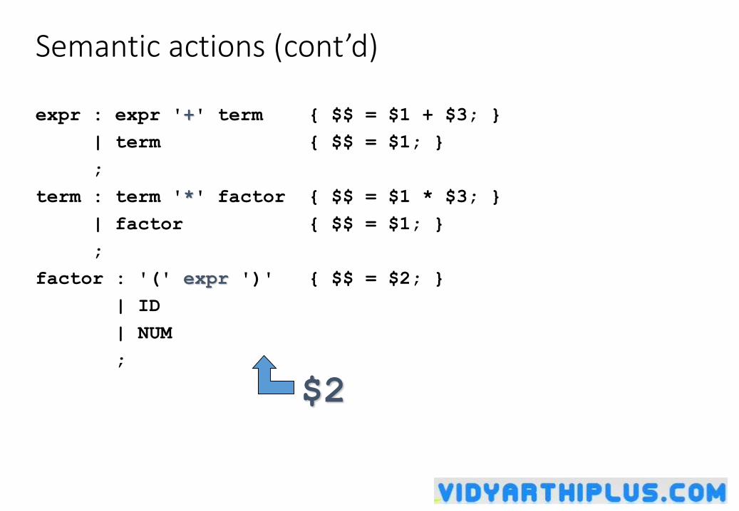
Semantic actions (cont’d)
expr : expr '+' term { $$ = $1 + $3; }
| term { $$ = $1; }
;
term : term '*' factor { $$ = $1 * $3; }
| factor { $$ = $1; }
;
factor : '(' expr ')' { $$ = $2; }
| ID
| NUM
;
$2
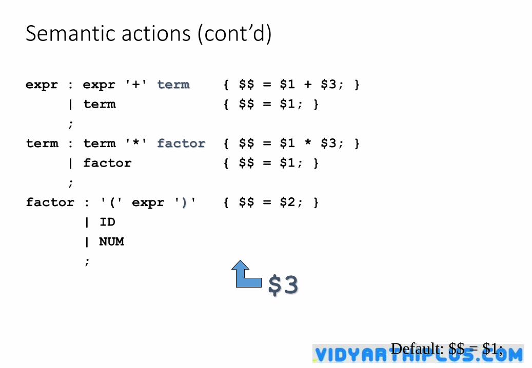
Semantic actions (cont’d)
expr : expr '+' term { $$ = $1 + $3; }
| term { $$ = $1; }
;
term : term '*' factor { $$ = $1 * $3; }
| factor { $$ = $1; }
;
factor : '(' expr ')' { $$ = $2; }
| ID
| NUM
;
$3
Default: $$ = $1;
yacc -v gram.y
• Will produce:
y.output
Bored, lonely? Try this!
yacc -d gram.y
• Will produce:
y.tab.h
Look at this and you'll never be unhappy again!
Shows "State Machine"®
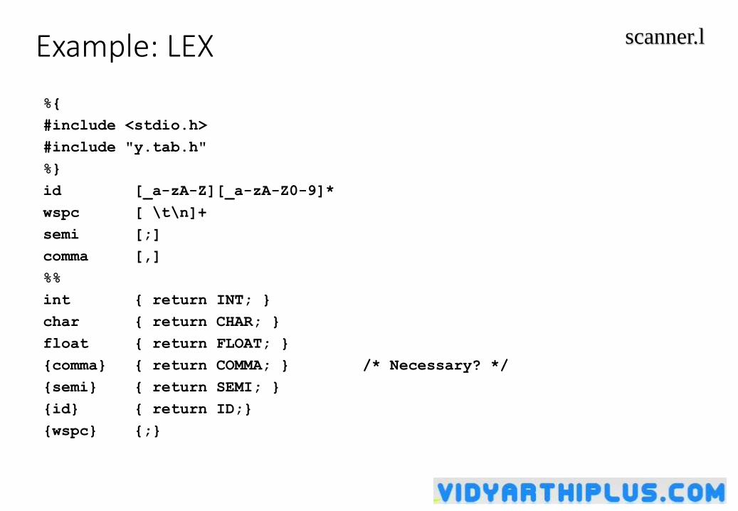
Example: LEX
%{
#include <stdio.h>
#include "y.tab.h"
%}
id [_a-zA-Z][_a-zA-Z0-9]*
wspc [ \t\n]+
semi [;]
comma [,]
%%
int { return INT; }
char { return CHAR; }
float { return FLOAT; }
{comma} { return COMMA; } /* Necessary? */
{semi} { return SEMI; }
{id} { return ID;}
{wspc} {;}
scanner.l
Example: Definitions
%{
#include <stdio.h>
#include <stdlib.h>
%}
%start line
%token CHAR, COMMA, FLOAT, ID, INT, SEMI
%%
decl.y
Example: Rules
/* This production is not part of the "official"
* grammar. It's primary purpose is to recover from
* parser errors, so it's probably best if you leave
* it here. */
line : /* lambda */
| line decl
| line error {
printf("Failure :-(\n");
yyerrok;
yyclearin;
}
;
decl.y
Example: Rules
decl : type ID list { printf("Success!\n"); } ;
list : COMMA ID list
| SEMI
;
type : INT | CHAR | FLOAT
;
%%
decl.y
Example: Supplementary Code
extern FILE *yyin;
main()
{
do {
yyparse();
} while(!feof(yyin));
}
yyerror(char *s)
{
/* Don't have to do anything! */
}
decl.y
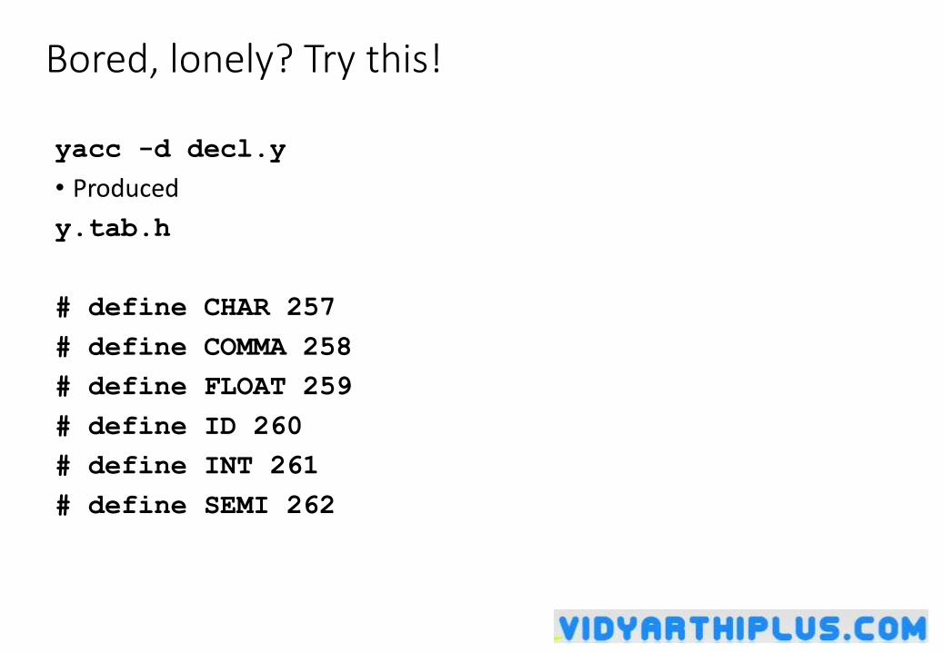
Bored, lonely? Try this!
yacc -d decl.y
• Produced
y.tab.h
# define CHAR 257
# define COMMA 258
# define FLOAT 259
# define ID 260
# define INT 261
# define SEMI 262
Symbol attributes
• Back to attribute grammars...
• Every symbol can have a value
• Might be a numeric quantity in case of a number (42)
• Might be a pointer to a string ("Hello, World!")
• Might be a pointer to a symbol table entry in case of a variable
• When using LEX we put the value into yylval
• In complex situations yylval is a union
• Typical LEX code:[0-9]+ {yylval = atoi(yytext); return NUM}
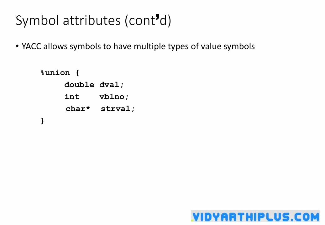
Symbol attributes (cont’d)
• YACC allows symbols to have multiple types of value symbols
%union {
double dval;
int vblno;
char* strval;
}
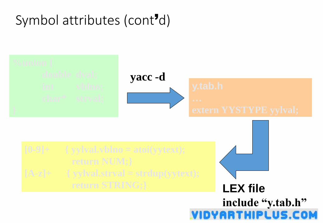
Symbol attributes (cont’d)
%union {
double dval;
int vblno;
char* strval;
}
yacc -dy.tab.h
…
extern YYSTYPE yylval;
[0-9]+ { yylval.vblno = atoi(yytext);
return NUM;}
[A-z]+ { yylval.strval = strdup(yytext);
return STRING;} LEX file
include “y.tab.h”
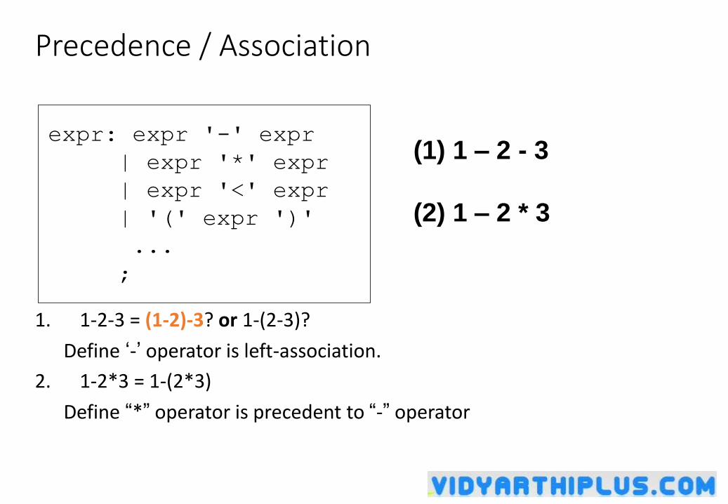
Precedence / Association
1. 1-2-3 = (1-2)-3? or 1-(2-3)?
Define ‘-’ operator is left-association.
2. 1-2*3 = 1-(2*3)
Define “*” operator is precedent to “-” operator
expr: expr '-' expr
| expr '*' expr
| expr '<' expr
| '(' expr ')'
...
;
(1) 1 – 2 - 3
(2) 1 – 2 * 3
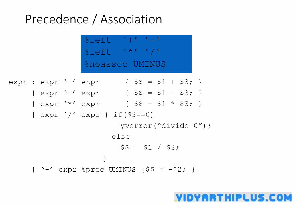
Precedence / Association
expr : expr ‘+’ expr { $$ = $1 + $3; }
| expr ‘-’ expr { $$ = $1 - $3; }
| expr ‘*’ expr { $$ = $1 * $3; }
| expr ‘/’ expr { if($3==0)
yyerror(“divide 0”);
else
$$ = $1 / $3;
}
| ‘-’ expr %prec UMINUS {$$ = -$2; }
%left '+' '-'
%left '*' '/'
%noassoc UMINUS
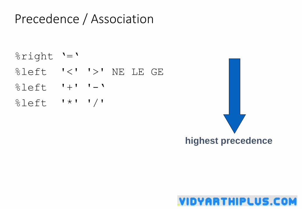
Precedence / Association
%right ‘=‘
%left '<' '>' NE LE GE
%left '+' '-‘
%left '*' '/'
highest precedence
Big trick
Getting YACC & LEX to work together!
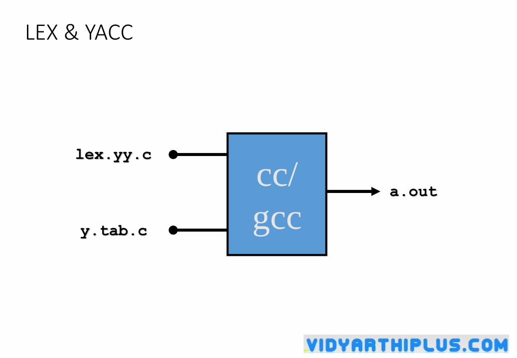
LEX & YACC
cc/
gcc
lex.yy.c
y.tab.c
a.out
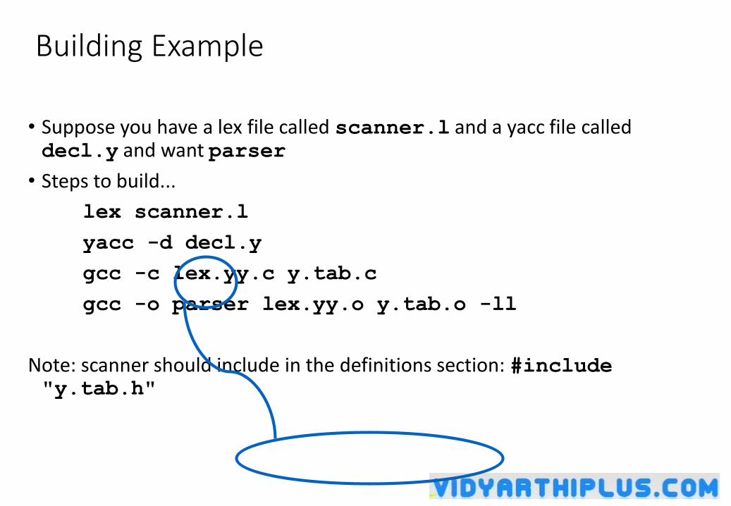
Building Example
• Suppose you have a lex file called scanner.l and a yacc file called decl.y and want parser
• Steps to build...
lex scanner.l
yacc -d decl.y
gcc -c lex.yy.c y.tab.c
gcc -o parser lex.yy.o y.tab.o -ll
Note: scanner should include in the definitions section: #include "y.tab.h"
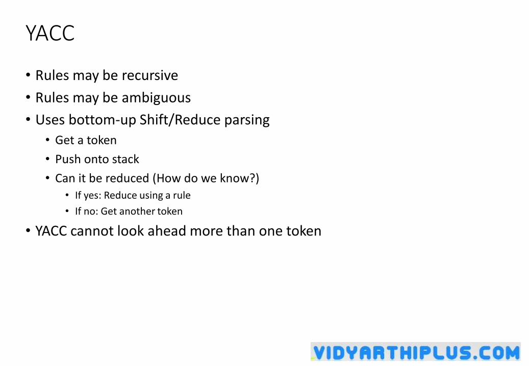
YACC
• Rules may be recursive
• Rules may be ambiguous
• Uses bottom-up Shift/Reduce parsing
• Get a token
• Push onto stack
• Can it be reduced (How do we know?)• If yes: Reduce using a rule
• If no: Get another token
• YACC cannot look ahead more than one token
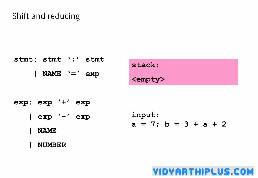
Shift and reducing
stmt: stmt ‘;’ stmt
| NAME ‘=‘ exp
exp: exp ‘+’ exp
| exp ‘-’ exp
| NAME
| NUMBER
input:
a = 7; b = 3 + a + 2
stack:
<empty>
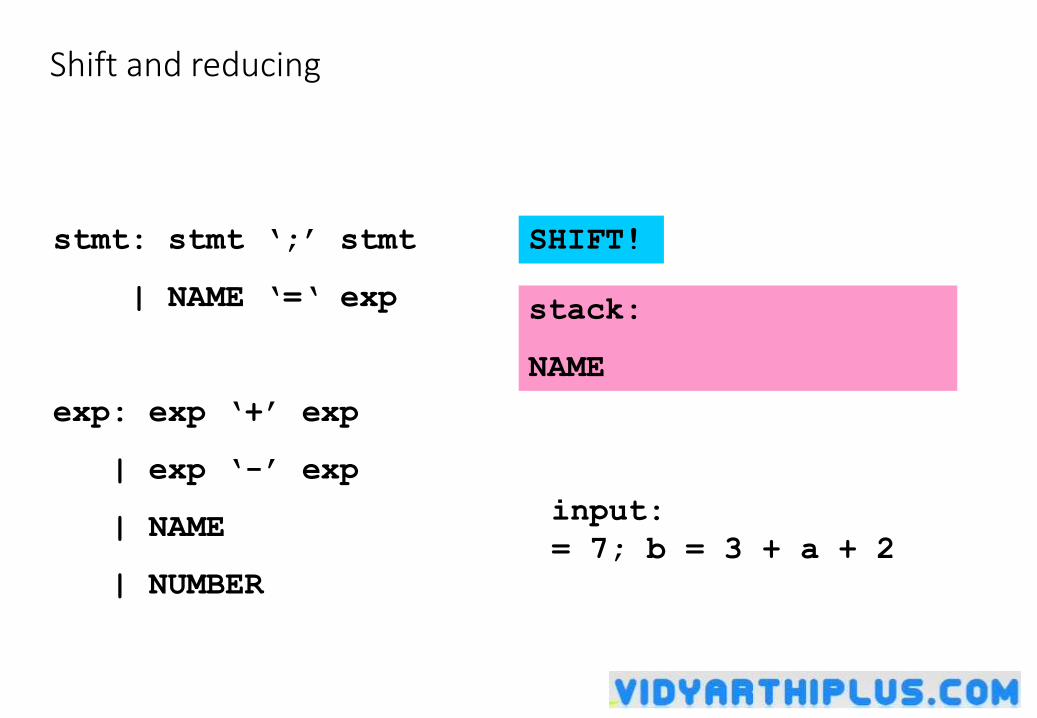
Shift and reducing
stmt: stmt ‘;’ stmt
| NAME ‘=‘ exp
exp: exp ‘+’ exp
| exp ‘-’ exp
| NAME
| NUMBER
input:
= 7; b = 3 + a + 2
stack:
NAME
SHIFT!
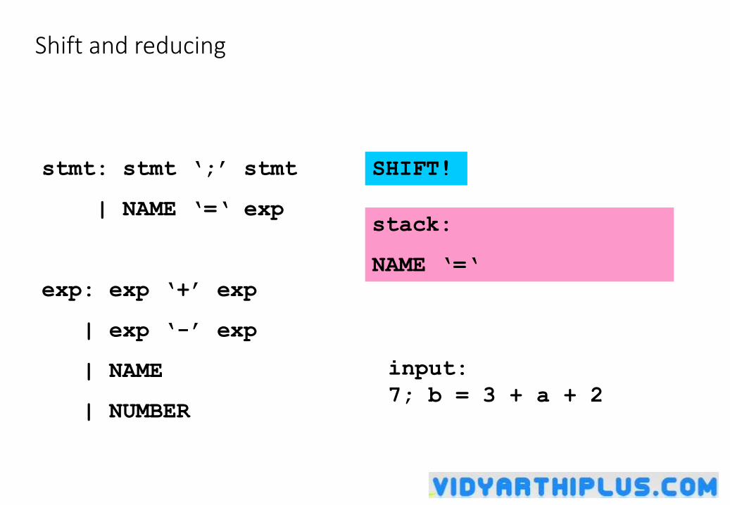
Shift and reducing
stmt: stmt ‘;’ stmt
| NAME ‘=‘ exp
exp: exp ‘+’ exp
| exp ‘-’ exp
| NAME
| NUMBER
input:
7; b = 3 + a + 2
stack:
NAME ‘=‘
SHIFT!
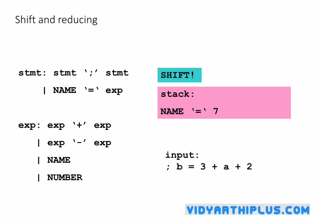
Shift and reducing
stmt: stmt ‘;’ stmt
| NAME ‘=‘ exp
exp: exp ‘+’ exp
| exp ‘-’ exp
| NAME
| NUMBER
input:
; b = 3 + a + 2
stack:
NAME ‘=‘ 7
SHIFT!
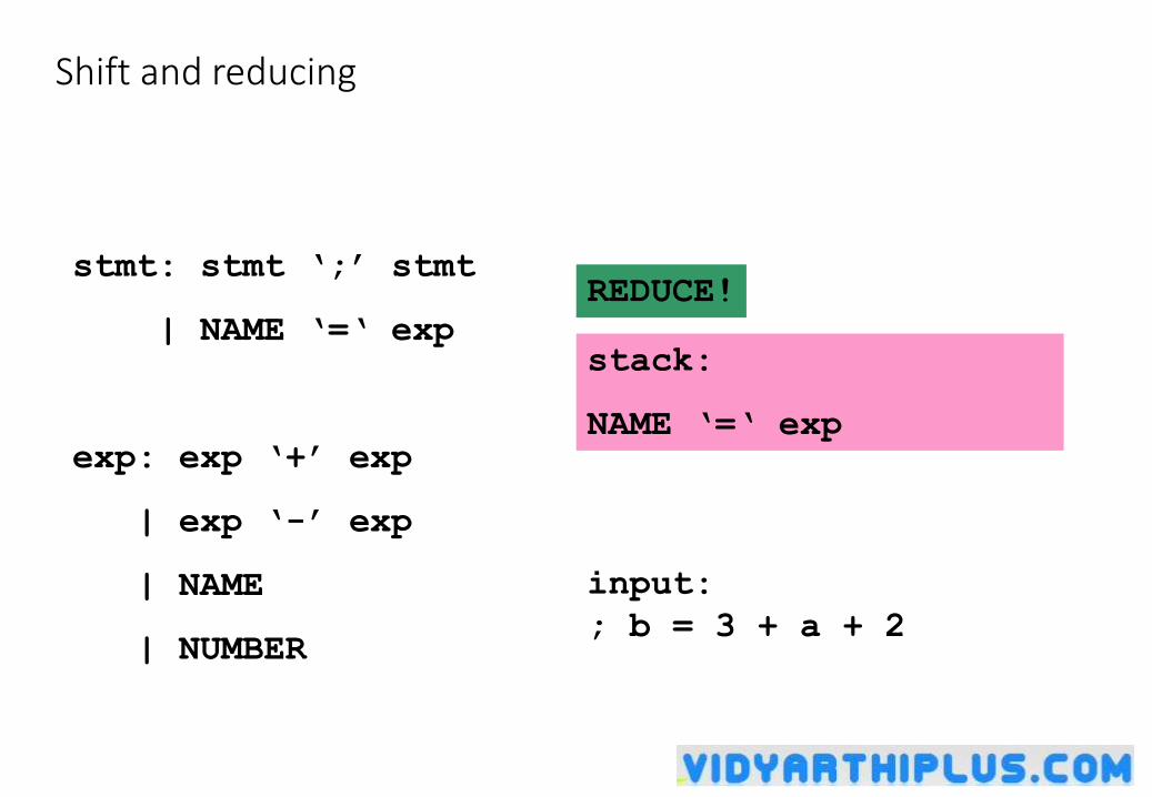
Shift and reducing
stmt: stmt ‘;’ stmt
| NAME ‘=‘ exp
exp: exp ‘+’ exp
| exp ‘-’ exp
| NAME
| NUMBER
input:
; b = 3 + a + 2
stack:
NAME ‘=‘ exp
REDUCE!
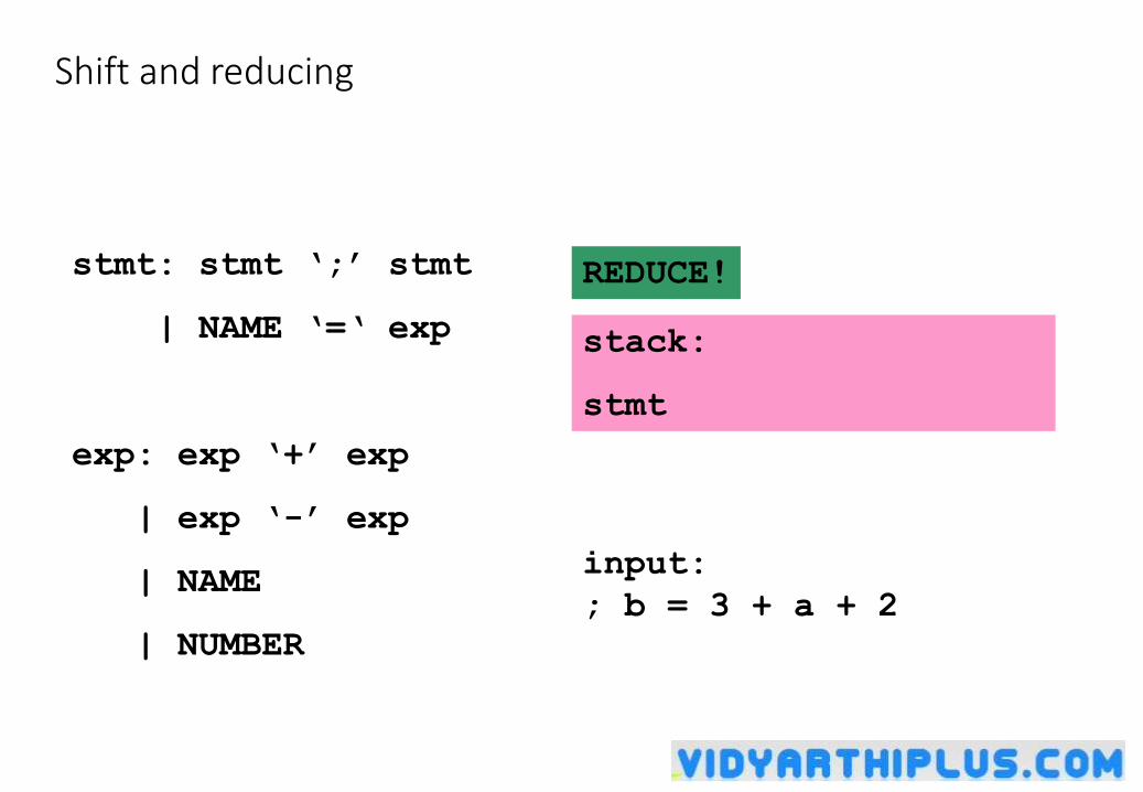
Shift and reducing
stmt: stmt ‘;’ stmt
| NAME ‘=‘ exp
exp: exp ‘+’ exp
| exp ‘-’ exp
| NAME
| NUMBER
input:
; b = 3 + a + 2
stack:
stmt
REDUCE!
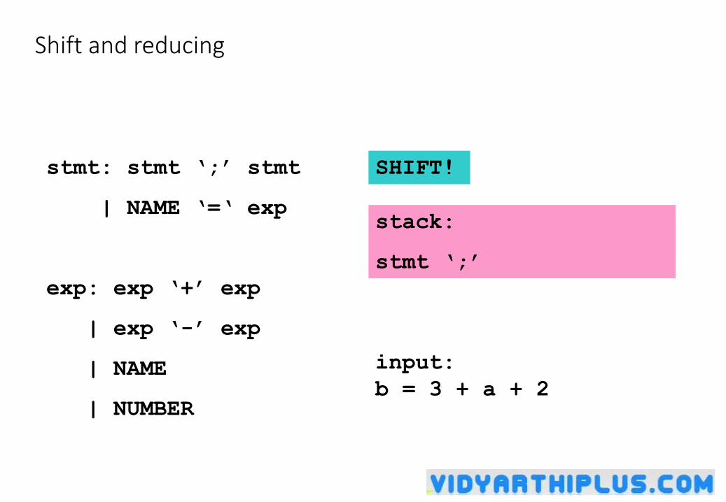
Shift and reducing
stmt: stmt ‘;’ stmt
| NAME ‘=‘ exp
exp: exp ‘+’ exp
| exp ‘-’ exp
| NAME
| NUMBER
input:
b = 3 + a + 2
stack:
stmt ‘;’
SHIFT!
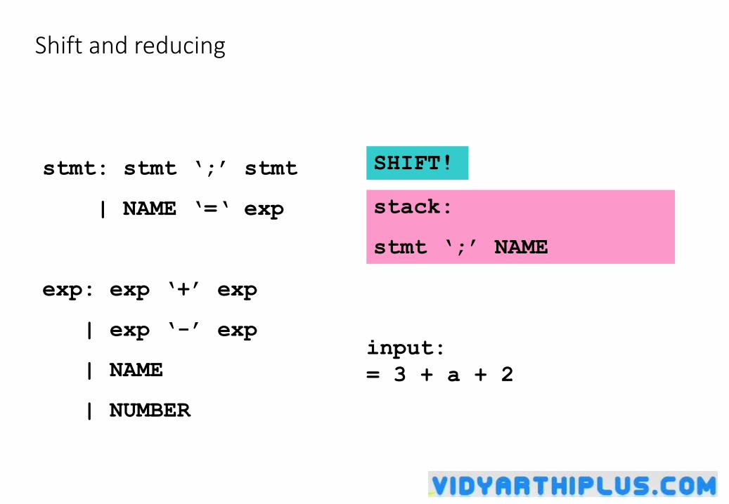
Shift and reducing
stmt: stmt ‘;’ stmt
| NAME ‘=‘ exp
exp: exp ‘+’ exp
| exp ‘-’ exp
| NAME
| NUMBER
input:
= 3 + a + 2
stack:
stmt ‘;’ NAME
SHIFT!
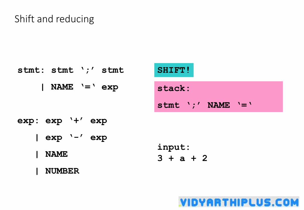
Shift and reducing
stmt: stmt ‘;’ stmt
| NAME ‘=‘ exp
exp: exp ‘+’ exp
| exp ‘-’ exp
| NAME
| NUMBER
input:
3 + a + 2
stack:
stmt ‘;’ NAME ‘=‘
SHIFT!
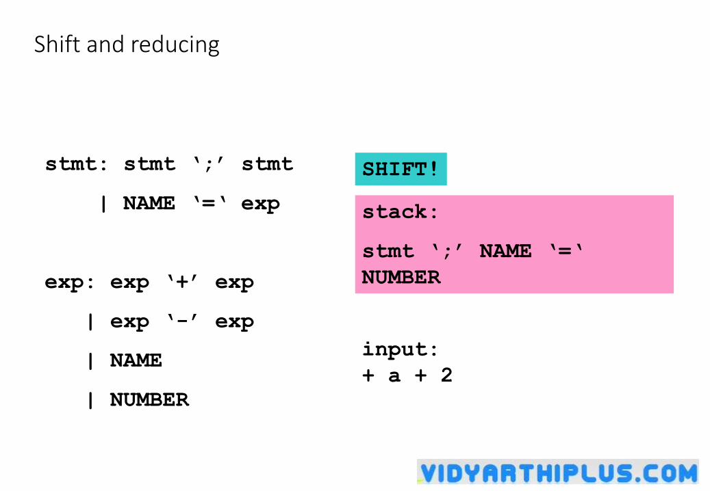
Shift and reducing
stmt: stmt ‘;’ stmt
| NAME ‘=‘ exp
exp: exp ‘+’ exp
| exp ‘-’ exp
| NAME
| NUMBER
input:
+ a + 2
stack:
stmt ‘;’ NAME ‘=‘
NUMBER
SHIFT!
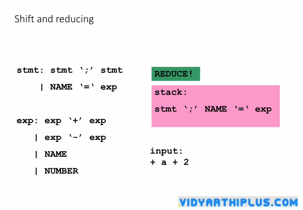
Shift and reducing
stmt: stmt ‘;’ stmt
| NAME ‘=‘ exp
exp: exp ‘+’ exp
| exp ‘-’ exp
| NAME
| NUMBER
input:
+ a + 2
stack:
stmt ‘;’ NAME ‘=‘ exp
REDUCE!
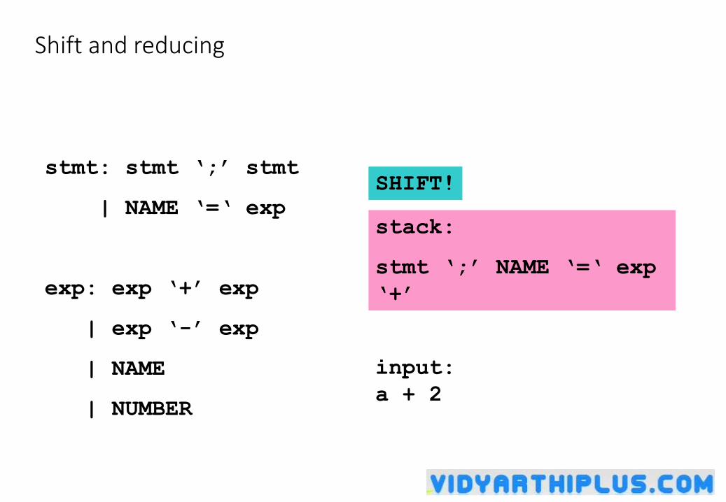
Shift and reducing
stmt: stmt ‘;’ stmt
| NAME ‘=‘ exp
exp: exp ‘+’ exp
| exp ‘-’ exp
| NAME
| NUMBER
input:
a + 2
stack:
stmt ‘;’ NAME ‘=‘ exp
‘+’
SHIFT!
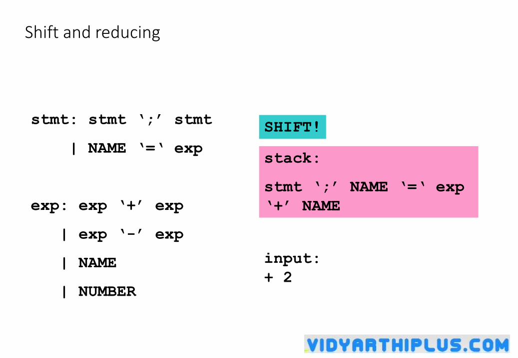
Shift and reducing
stmt: stmt ‘;’ stmt
| NAME ‘=‘ exp
exp: exp ‘+’ exp
| exp ‘-’ exp
| NAME
| NUMBER
input:
+ 2
stack:
stmt ‘;’ NAME ‘=‘ exp
‘+’ NAME
SHIFT!
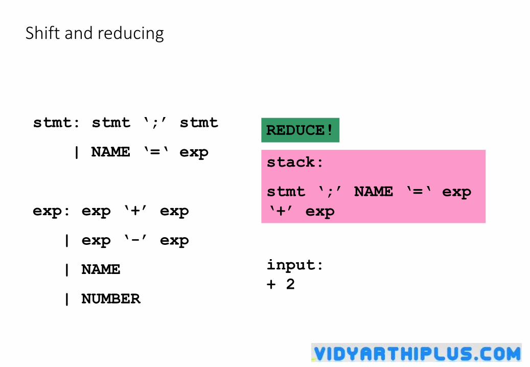
Shift and reducing
stmt: stmt ‘;’ stmt
| NAME ‘=‘ exp
exp: exp ‘+’ exp
| exp ‘-’ exp
| NAME
| NUMBER
input:
+ 2
stack:
stmt ‘;’ NAME ‘=‘ exp
‘+’ exp
REDUCE!
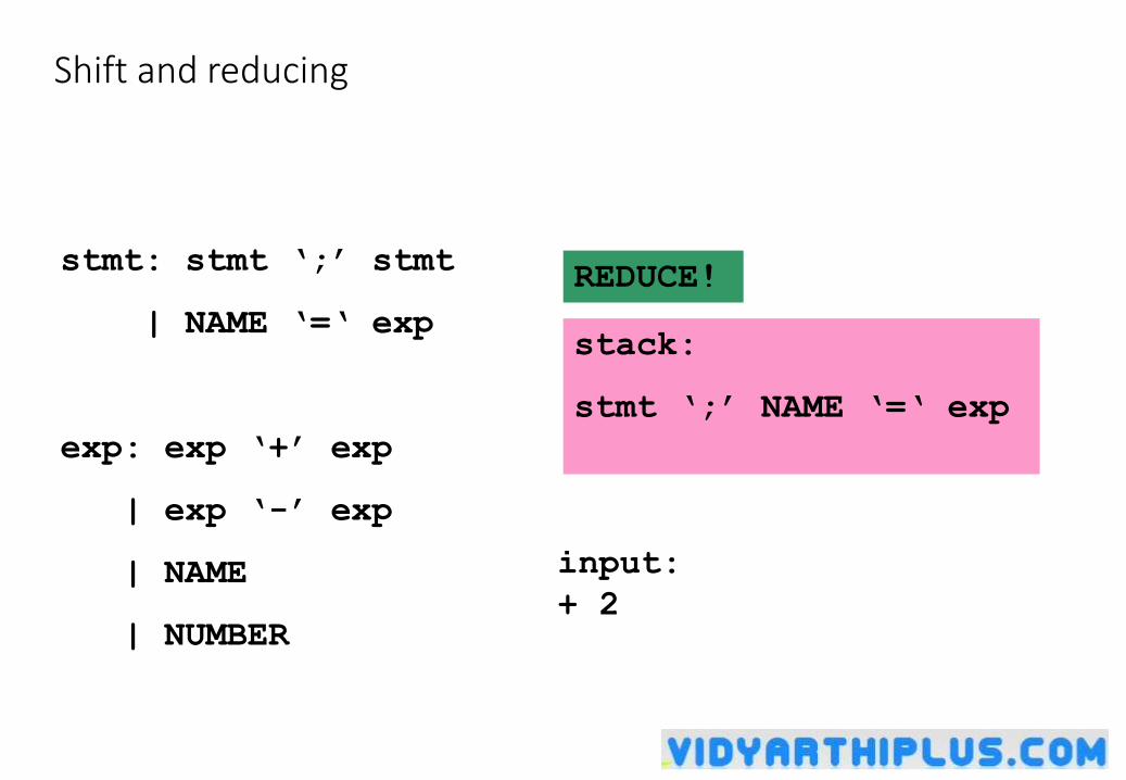
Shift and reducing
stmt: stmt ‘;’ stmt
| NAME ‘=‘ exp
exp: exp ‘+’ exp
| exp ‘-’ exp
| NAME
| NUMBER
input:
+ 2
stack:
stmt ‘;’ NAME ‘=‘ exp
REDUCE!
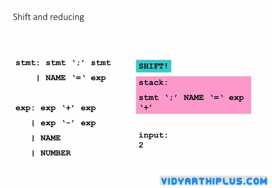
Shift and reducing
stmt: stmt ‘;’ stmt
| NAME ‘=‘ exp
exp: exp ‘+’ exp
| exp ‘-’ exp
| NAME
| NUMBER
input:
2
stack:
stmt ‘;’ NAME ‘=‘ exp
‘+’
SHIFT!
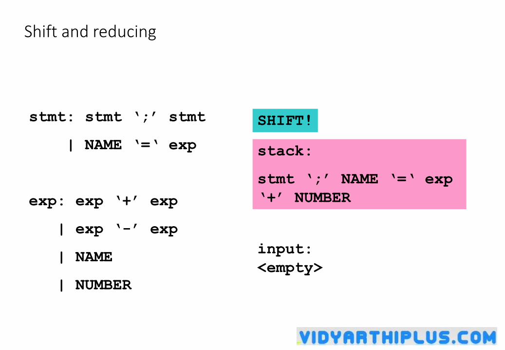
Shift and reducing
stmt: stmt ‘;’ stmt
| NAME ‘=‘ exp
exp: exp ‘+’ exp
| exp ‘-’ exp
| NAME
| NUMBER
input:
<empty>
stack:
stmt ‘;’ NAME ‘=‘ exp
‘+’ NUMBER
SHIFT!
Shift and reducing
stmt: stmt ‘;’ stmt
| NAME ‘=‘ exp
exp: exp ‘+’ exp
| exp ‘-’ exp
| NAME
| NUMBER
input:
<empty>
stack:
stmt ‘;’ NAME ‘=‘ exp
‘+’ exp
REDUCE!
Shift and reducing
stmt: stmt ‘;’ stmt
| NAME ‘=‘ exp
exp: exp ‘+’ exp
| exp ‘-’ exp
| NAME
| NUMBER
input:
<empty>
stack:
stmt ‘;’ NAME ‘=‘ exp
REDUCE!
Shift and reducing
stmt: stmt ‘;’ stmt
| NAME ‘=‘ exp
exp: exp ‘+’ exp
| exp ‘-’ exp
| NAME
| NUMBER
input:
<empty>
stack:
stmt ‘;’ stmt
REDUCE!
Shift and reducing
stmt: stmt ‘;’ stmt
| NAME ‘=‘ exp
exp: exp ‘+’ exp
| exp ‘-’ exp
| NAME
| NUMBER
input:
<empty>
stack:
stmt
REDUCE!
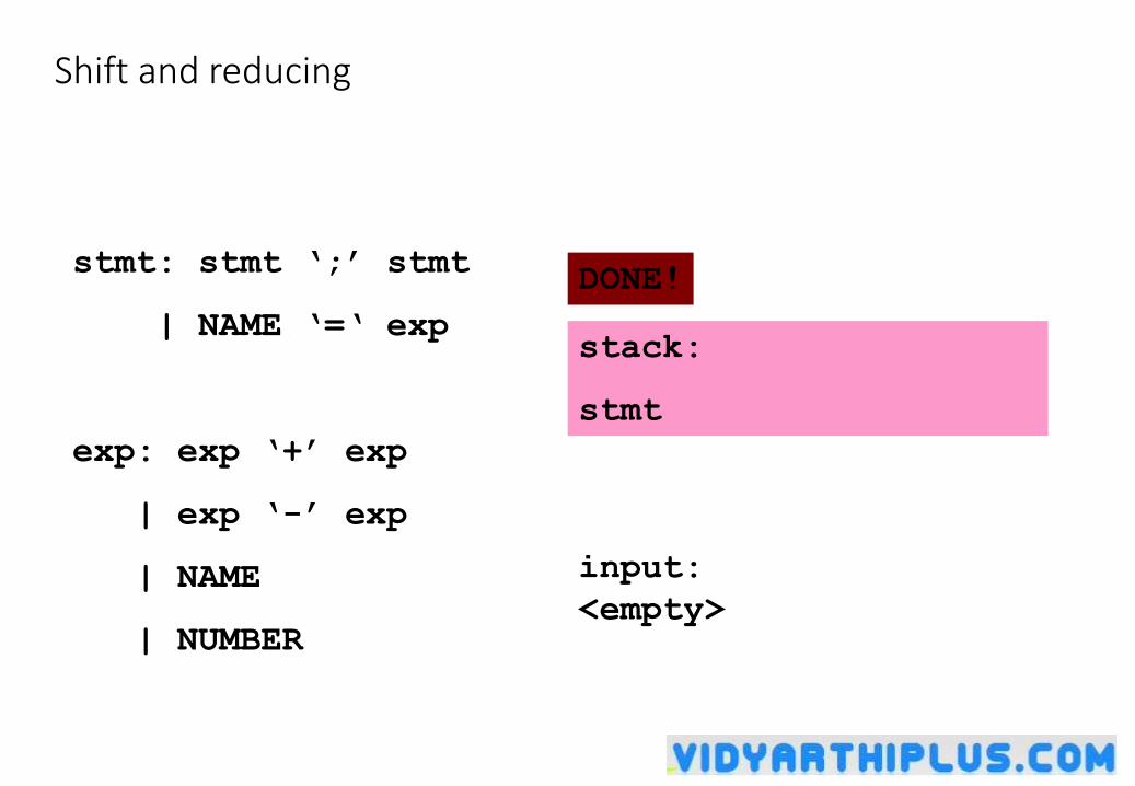
Shift and reducing
stmt: stmt ‘;’ stmt
| NAME ‘=‘ exp
exp: exp ‘+’ exp
| exp ‘-’ exp
| NAME
| NUMBER
input:
<empty>
stack:
stmt
DONE!
IF-ELSE Ambiguity
• Consider following rule:
Following state : IF expr IF expr stmt . ELSE stmt
• Two possible derivations:
IF expr IF expr stmt . ELSE stmt
IF expr IF expr stmt ELSE . stmt
IF expr IF expr stmt ELSE stmt .
IF expr stmt
IF expr IF expr stmt . ELSE stmt
IF expr stmt . ELSE stmt
IF expr stmt ELSE . stmt
IF expr stmt ELSE stmt .
IF-ELSE Ambiguity
• It is a shift/reduce conflict
• YACC will always do shift first
• Solution 1 : re-write grammar
stmt : matched
| unmatched
;
matched: other_stmt
| IF expr THEN matched ELSE matched
;
unmatched: IF expr THEN stmt
| IF expr THEN matched ELSE unmatched
;
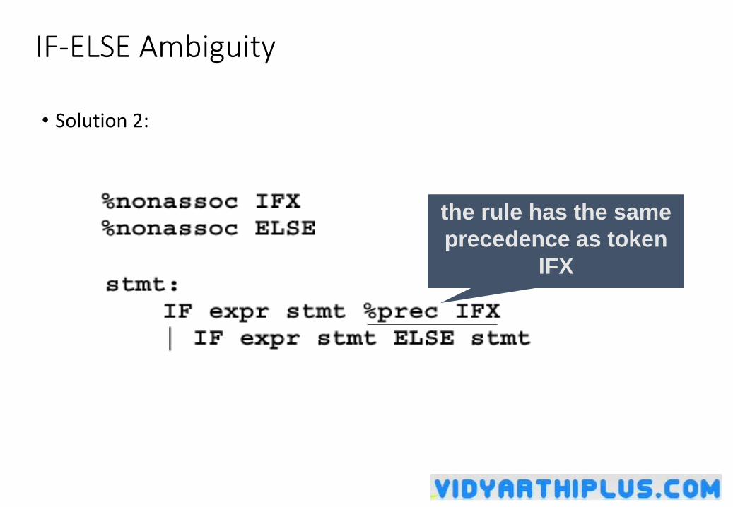
IF-ELSE Ambiguity
• Solution 2:
the rule has the same
precedence as token
IFX
Shift/Reduce Conflicts
• shift/reduce conflict
• occurs when a grammar is written in such a way that a decision between shifting and reducing can not be made.
• e.g.: IF-ELSE ambiguity
• To resolve this conflict, YACC will choose to shift
Reduce/Reduce Conflicts
• Reduce/Reduce Conflicts:
start : expr | stmt
;
expr : CONSTANT;
stmt : CONSTANT;
• YACC (Bison) resolves the conflict by reducing using the rule that occurs earlier in the grammar. NOT GOOD!!
• So, modify grammar to eliminate them
Error Messages
• Bad error message:
• Syntax error
• Compiler needs to give programmer a good advice
• It is better to track the line number in LEX:
void yyerror(char *s)
{
fprintf(stderr, "line %d: %s\n:", yylineno, s);
}
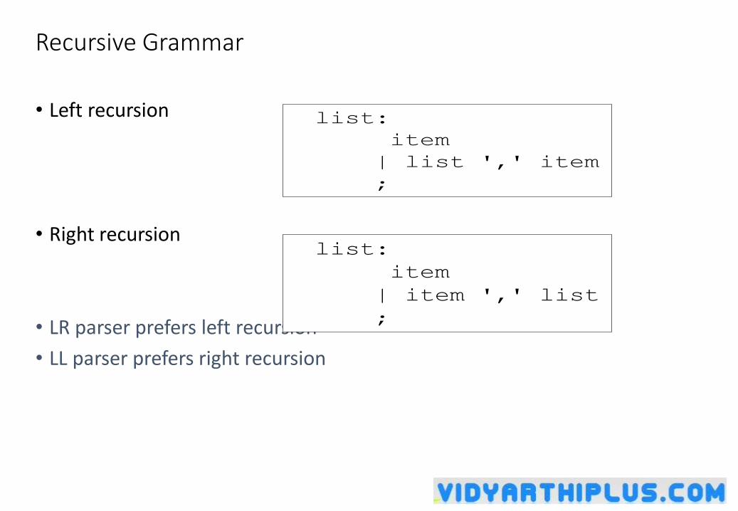
Recursive Grammar
• Left recursion
• Right recursion
• LR parser prefers left recursion
• LL parser prefers right recursion
list:
item
| list ',' item
;
list:
item
| item ',' list
;
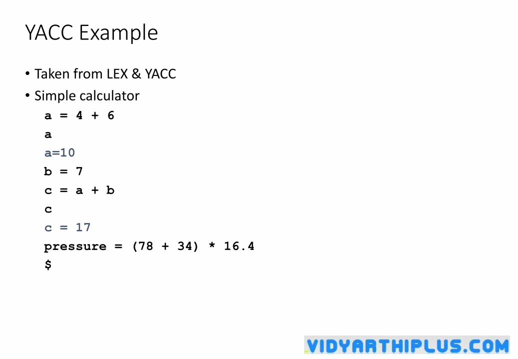
YACC Example
• Taken from LEX & YACC
• Simple calculatora = 4 + 6
a
a=10
b = 7
c = a + b
c
c = 17
pressure = (78 + 34) * 16.4
$
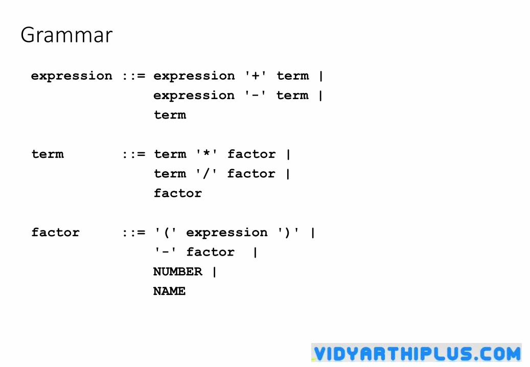
Grammar
expression ::= expression '+' term |
expression '-' term |
term
term ::= term '*' factor |
term '/' factor |
factor
factor ::= '(' expression ')' |
'-' factor |
NUMBER |
NAME
parser.h
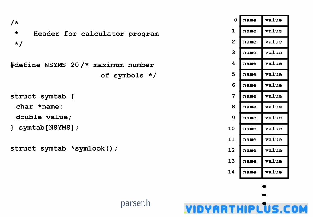
/*
* Header for calculator program
*/
#define NSYMS 20/* maximum number
of symbols */
struct symtab {
char *name;
double value;
} symtab[NSYMS];
struct symtab *symlook();
parser.h
name value0
name value1
name value2
name value3
name value4
name value5
name value6
name value7
name value8
name value9
name value10
name value11
name value12
name value13
name value14
parser.y
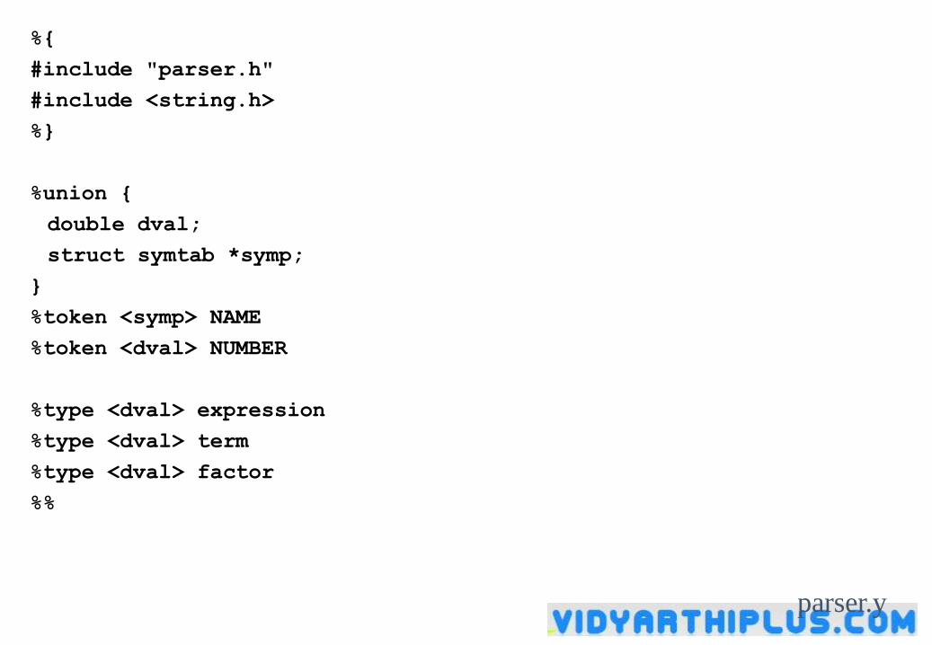
%{
#include "parser.h"
#include <string.h>
%}
%union {
double dval;
struct symtab *symp;
}
%token <symp> NAME
%token <dval> NUMBER
%type <dval> expression
%type <dval> term
%type <dval> factor
%%
parser.y
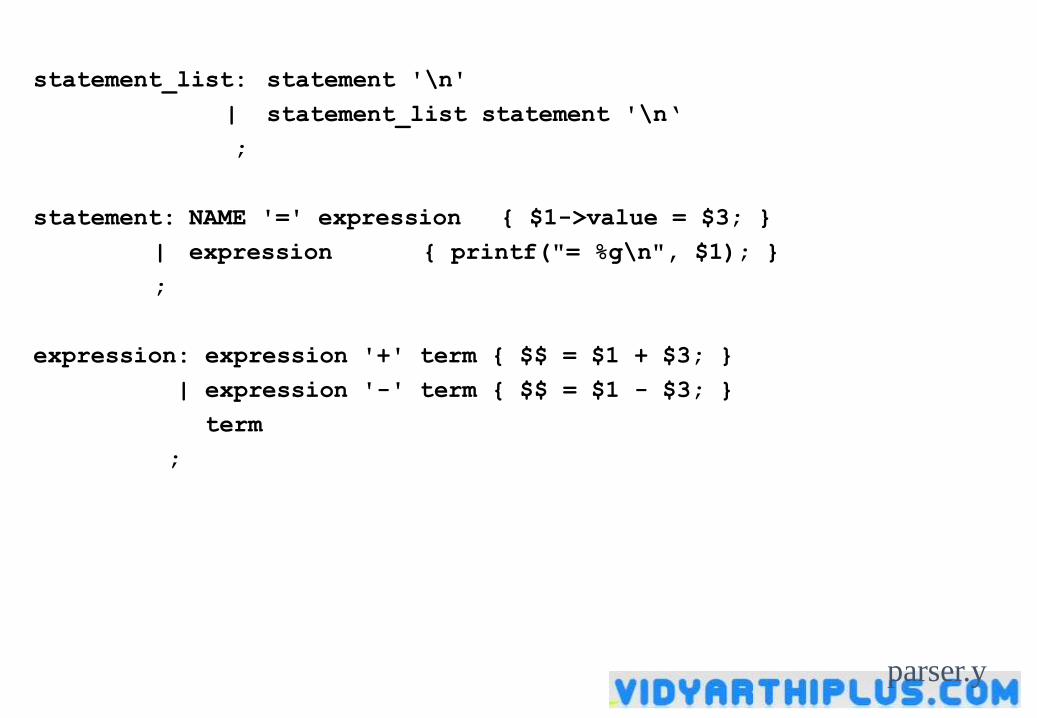
statement_list: statement '\n'
| statement_list statement '\n‘
;
statement: NAME '=' expression { $1->value = $3; }
| expression { printf("= %g\n", $1); }
;
expression: expression '+' term { $$ = $1 + $3; }
| expression '-' term { $$ = $1 - $3; }
term
;
parser.y
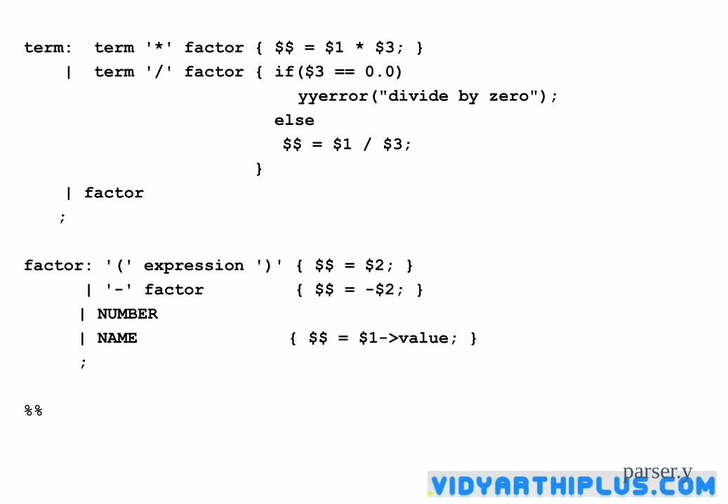
term: term '*' factor { $$ = $1 * $3; }
| term '/' factor { if($3 == 0.0)
yyerror("divide by zero");
else
$$ = $1 / $3;
}
| factor
;
factor: '(' expression ')' { $$ = $2; }
| '-' factor { $$ = -$2; }
| NUMBER
| NAME { $$ = $1->value; }
;
%%
parser.y
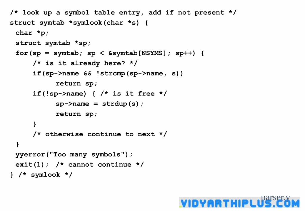
/* look up a symbol table entry, add if not present */
struct symtab *symlook(char *s) {
char *p;
struct symtab *sp;
for(sp = symtab; sp < &symtab[NSYMS]; sp++) {
/* is it already here? */
if(sp->name && !strcmp(sp->name, s))
return sp;
if(!sp->name) { /* is it free */
sp->name = strdup(s);
return sp;
}
/* otherwise continue to next */
}
yyerror("Too many symbols");
exit(1); /* cannot continue */
} /* symlook */
parser.y
yyerror(char *s)
{
printf( "yyerror: %s\n", s);
}
parser.y
typedef union
{
double dval;
struct symtab *symp;
} YYSTYPE;
extern YYSTYPE yylval;
# define NAME 257
# define NUMBER 258
y.tab.h

calclexer.l
%{
#include "y.tab.h"
#include "parser.h"
#include <math.h>
%}
%%
calclexer.l
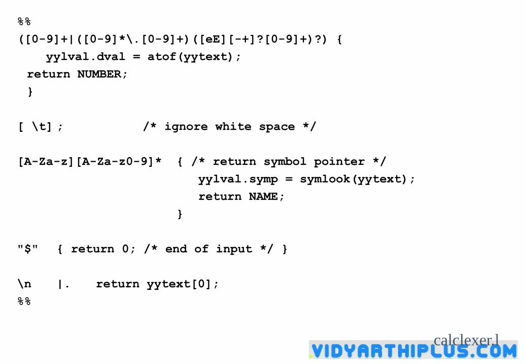
%%
([0-9]+|([0-9]*\.[0-9]+)([eE][-+]?[0-9]+)?) {
yylval.dval = atof(yytext);
return NUMBER;
}
[ \t] ; /* ignore white space */
[A-Za-z][A-Za-z0-9]* { /* return symbol pointer */
yylval.symp = symlook(yytext);
return NAME;
}
"$" { return 0; /* end of input */ }
\n |. return yytext[0];
%%
calclexer.l
Makefile
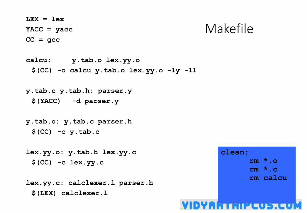
MakefileLEX = lex
YACC = yacc
CC = gcc
calcu: y.tab.o lex.yy.o
$(CC) -o calcu y.tab.o lex.yy.o -ly -ll
y.tab.c y.tab.h: parser.y
$(YACC) -d parser.y
y.tab.o: y.tab.c parser.h
$(CC) -c y.tab.c
lex.yy.o: y.tab.h lex.yy.c
$(CC) -c lex.yy.c
lex.yy.c: calclexer.l parser.h
$(LEX) calclexer.l
clean:
rm *.o
rm *.c
rm calcu
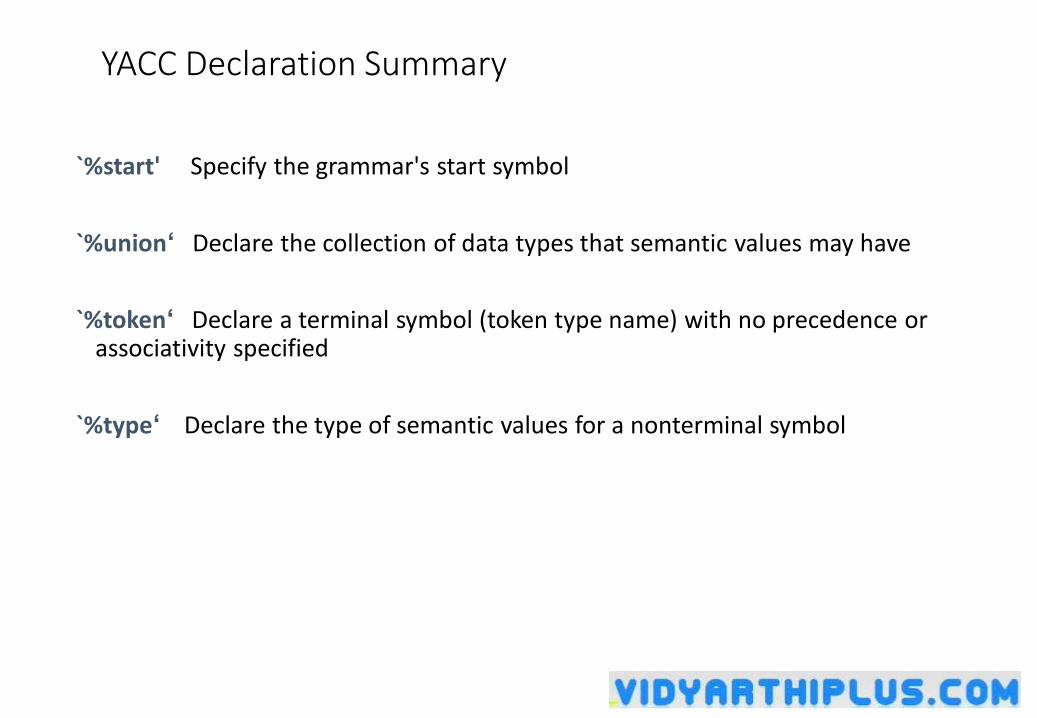
YACC Declaration Summary
`%start' Specify the grammar's start symbol
`%union‘ Declare the collection of data types that semantic values may have
`%token‘ Declare a terminal symbol (token type name) with no precedence or associativity specified
`%type‘ Declare the type of semantic values for a nonterminal symbol
YACC Declaration Summary
`%right‘ Declare a terminal symbol (token type name) that is right-associative
`%left‘ Declare a terminal symbol (token type name) that is left-associative
`%nonassoc‘ Declare a terminal symbol (token type name) that is nonassociative (using it in a way that would be associative is a syntax error, e.g.: x op. y op. z is syntax error)
Intermediate Code
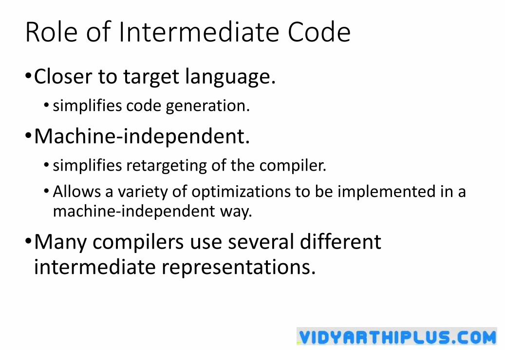
Role of Intermediate Code
•Closer to target language. • simplifies code generation.
•Machine-independent.• simplifies retargeting of the compiler.
•Allows a variety of optimizations to be implemented in a machine-independent way.
•Many compilers use several different intermediate representations.
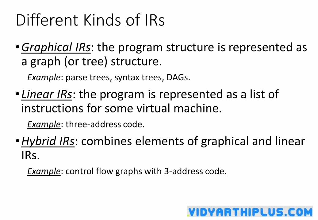
Different Kinds of IRs
•Graphical IRs: the program structure is represented as a graph (or tree) structure.
Example: parse trees, syntax trees, DAGs.
•Linear IRs: the program is represented as a list of instructions for some virtual machine.
Example: three-address code.
•Hybrid IRs: combines elements of graphical and linear IRs.
Example: control flow graphs with 3-address code.
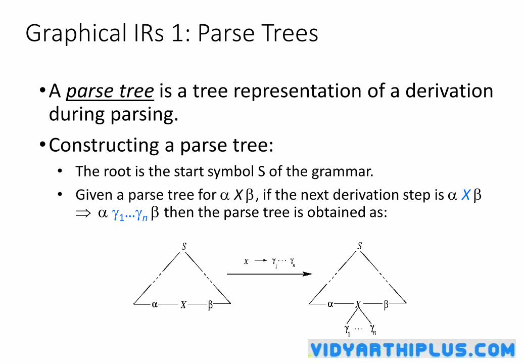
Graphical IRs 1: Parse Trees
•A parse tree is a tree representation of a derivation during parsing.
•Constructing a parse tree:• The root is the start symbol S of the grammar.
• Given a parse tree for X , if the next derivation step is X 1…n then the parse tree is obtained as:
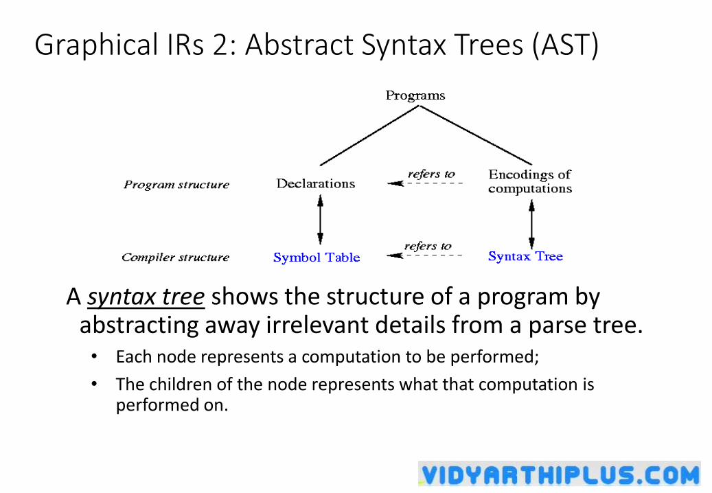
Graphical IRs 2: Abstract Syntax Trees (AST)
A syntax tree shows the structure of a program by abstracting away irrelevant details from a parse tree.• Each node represents a computation to be performed;
• The children of the node represents what that computation is performed on.
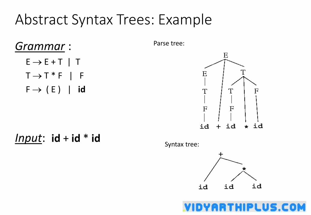
Abstract Syntax Trees: Example
Grammar :E E + T | T
T T * F | F
F ( E ) | id
Input: id + id * id
Parse tree:
Syntax tree:
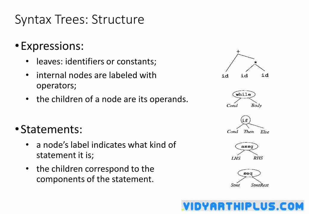
Syntax Trees: Structure
•Expressions:• leaves: identifiers or constants;
• internal nodes are labeled with operators;
• the children of a node are its operands.
•Statements:• a node’s label indicates what kind of
statement it is;
• the children correspond to the components of the statement.
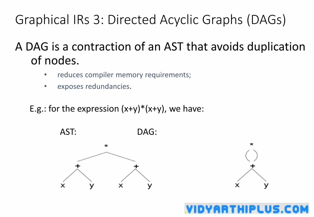
Graphical IRs 3: Directed Acyclic Graphs (DAGs)
A DAG is a contraction of an AST that avoids duplication of nodes.
• reduces compiler memory requirements;
• exposes redundancies.
E.g.: for the expression (x+y)*(x+y), we have:
AST: DAG:
Linear IRs
•A linear IR consists of a sequence of instructions that execute in order.• “machine-independent assembly code”
• Instructions may contain multiple operations, which (if present) execute in parallel.
• They often form a starting point for hybrid representations (e.g., control flow graphs).
Linear IR 1: Three Address Code
• Instructions are of the form ‘x = y op z,’ where x, y, z are variables, constants, or “temporaries”.
•At most one operator allowed on RHS, so no ‘built-up”expressions.
Instead, expressions are computed using temporaries (compiler-generated variables).
• The specific set of operators represented, and their level of abstraction, can vary widely.
Three Address Code: Example
• Source: if ( x + y*z > x*y + z)
a = 0;
• Three Address Code:t1 = y*z
t2 = x+t1 // x + y*z
t3 = x*y
t4 = t3+z // x*y + z
if (t2 t4) goto L
a = 0
L:
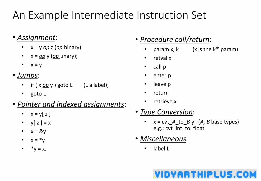
An Example Intermediate Instruction Set
• Assignment:• x = y op z (op binary)
• x = op y (op unary);
• x = y
• Jumps:• if ( x op y ) goto L (L a label);
• goto L
• Pointer and indexed assignments:• x = y[ z ]
• y[ z ] = x
• x = &y
• x = *y
• *y = x.
• Procedure call/return:• param x, k (x is the kth param)
• retval x
• call p
• enter p
• leave p
• return
• retrieve x
• Type Conversion:• x = cvt_A_to_B y (A, B base types)
e.g.: cvt_int_to_float
• Miscellaneous• label L
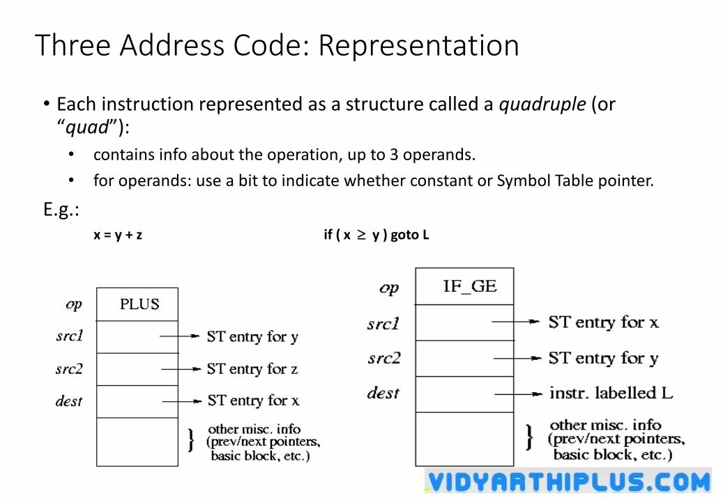
Three Address Code: Representation
• Each instruction represented as a structure called a quadruple (or “quad”):
• contains info about the operation, up to 3 operands.
• for operands: use a bit to indicate whether constant or Symbol Table pointer.
E.g.: x = y + z if ( x y ) goto L
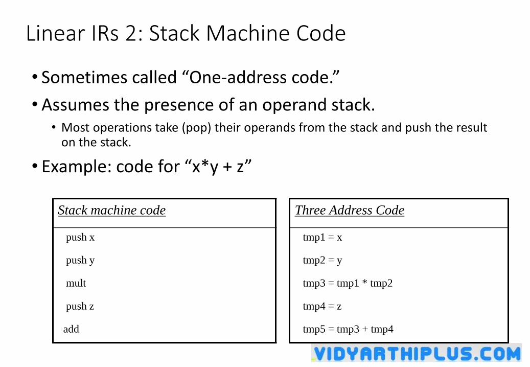
Linear IRs 2: Stack Machine Code
Three Address Code
tmp1 = x
tmp2 = y
tmp3 = tmp1 * tmp2
tmp4 = z
tmp5 = tmp3 + tmp4
Stack machine code
push x
push y
mult
push z
add
• Sometimes called “One-address code.”
•Assumes the presence of an operand stack. • Most operations take (pop) their operands from the stack and push the result
on the stack.
• Example: code for “x*y + z”
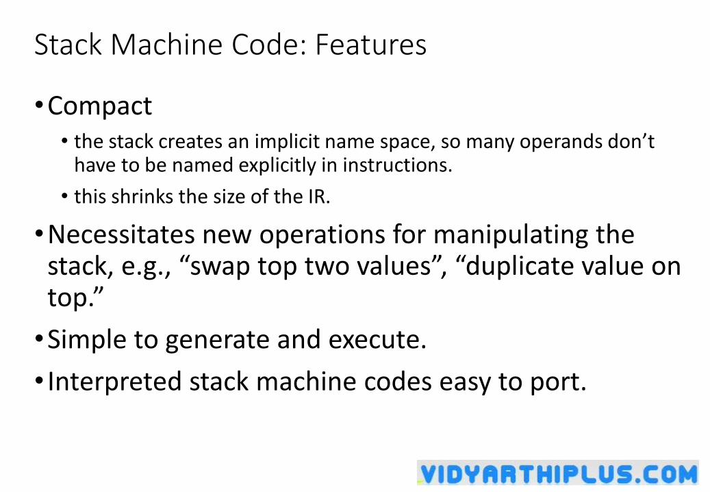
Stack Machine Code: Features
•Compact• the stack creates an implicit name space, so many operands don’t
have to be named explicitly in instructions.
• this shrinks the size of the IR.
•Necessitates new operations for manipulating the stack, e.g., “swap top two values”, “duplicate value on top.”
•Simple to generate and execute.
• Interpreted stack machine codes easy to port.
Linear IRs 3: Register Transfer Language (GNU RTL)
• Inspired by (and has syntax resembling) Lisp lists.
•Expressions are not “flattened” as in three-address code, but may be nested.• gives them a tree structure.
• Incorporates a variety of machine-level information.
RTLs (cont’d)
Low-level information associated with an RTL expression include:
• “machine modes” – gives the size of a data object;
• information about access to registers and memory;
• information relating to instruction scheduling and delay slots;
•whether a memory reference is “volatile.”
RTLs: Examples
Example operations:• (plus:m x y), (minus:m x y), (compare:m x y), etc., where m is a
machine mode.
• (cond [test1 value1 test2 value2 …] default)
• (set lval x) (assigns x to the place denoted by lval).
• (call func argsz), (return)
• (parallel [x0 x1 …]) (simultaneous side effects).
• (sequence [ins1 ins2 … ])
RTL Examples (cont’d)
•A call to a function at address a passing n bytes of arguments, where the return value is in a (“hard”) register r:
(set (reg:m r) (call (mem:fm a) n))
• here m and fm are machine modes.
•A division operation where the result is truncated to a smaller size:
(truncate:m1 (div:m2 x (sign_extend:m2 y)))
Hybrid IRs
•Combine features of graphical and linear IRs:• linear IR aspects capture a lower-level program
representation;
• graphical IR aspects make control flow behavior explicit.
•Examples:• control flow graphs
• static single assignment form (SSA).
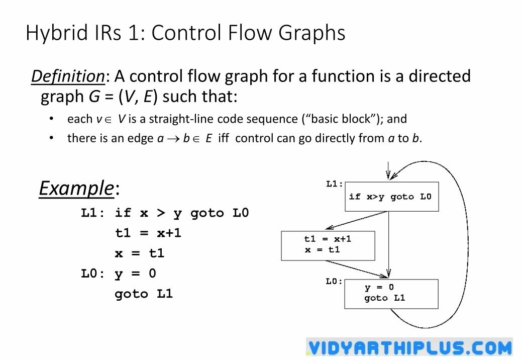
Hybrid IRs 1: Control Flow Graphs
Example:L1: if x > y goto L0
t1 = x+1
x = t1
L0: y = 0
goto L1
Definition: A control flow graph for a function is a directed graph G = (V, E) such that:• each v V is a straight-line code sequence (“basic block”); and
• there is an edge a b E iff control can go directly from a to b.
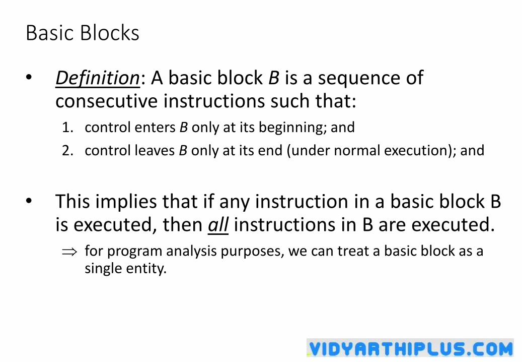
Basic Blocks
• Definition: A basic block B is a sequence of consecutive instructions such that:1. control enters B only at its beginning; and
2. control leaves B only at its end (under normal execution); and
• This implies that if any instruction in a basic block B is executed, then all instructions in B are executed. for program analysis purposes, we can treat a basic block as a
single entity.
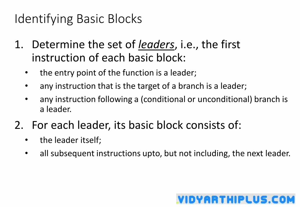
Identifying Basic Blocks
1. Determine the set of leaders, i.e., the first instruction of each basic block:
• the entry point of the function is a leader;
• any instruction that is the target of a branch is a leader;
• any instruction following a (conditional or unconditional) branch is a leader.
2. For each leader, its basic block consists of:• the leader itself;
• all subsequent instructions upto, but not including, the next leader.
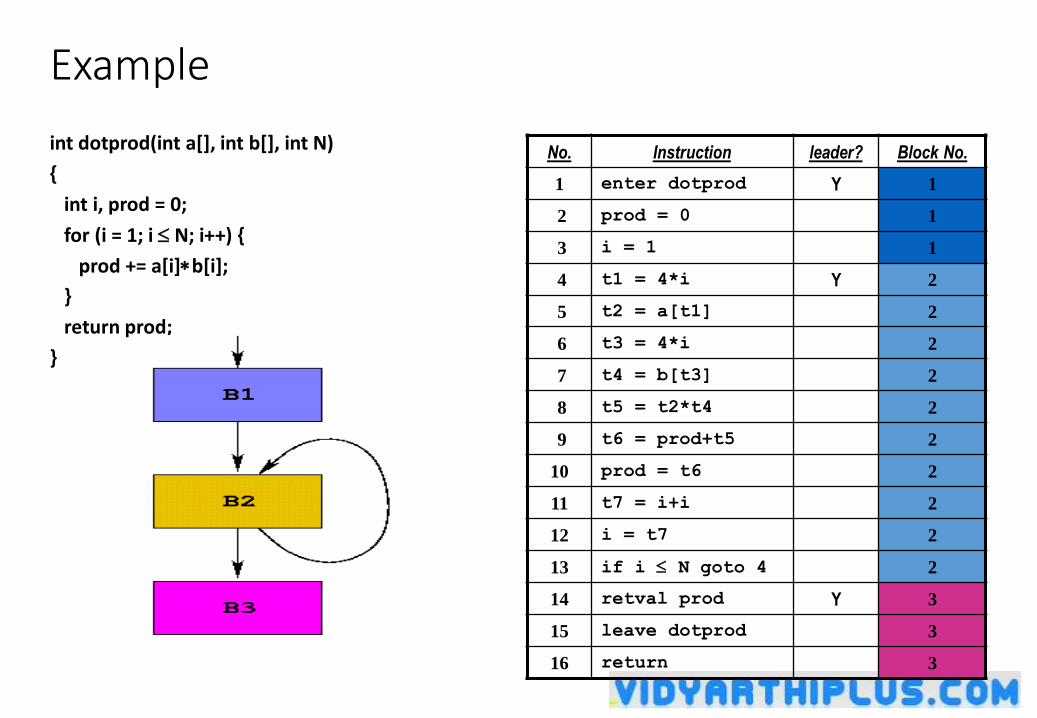
Example
int dotprod(int a[], int b[], int N)
{
int i, prod = 0;
for (i = 1; i N; i++) {
prod += a[i]b[i];
}
return prod;
}
No. Instruction leader? Block No.
1 enter dotprod Y 1
2 prod = 0 1
3 i = 1 1
4 t1 = 4*i Y 2
5 t2 = a[t1] 2
6 t3 = 4*i 2
7 t4 = b[t3] 2
8 t5 = t2*t4 2
9 t6 = prod+t5 2
10 prod = t6 2
11 t7 = i+i 2
12 i = t7 2
13 if i N goto 4 2
14 retval prod Y 3
15 leave dotprod 3
16 return 3
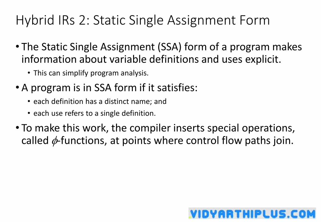
Hybrid IRs 2: Static Single Assignment Form
• The Static Single Assignment (SSA) form of a program makes information about variable definitions and uses explicit.• This can simplify program analysis.
•A program is in SSA form if it satisfies:• each definition has a distinct name; and
• each use refers to a single definition.
• To make this work, the compiler inserts special operations, called -functions, at points where control flow paths join.
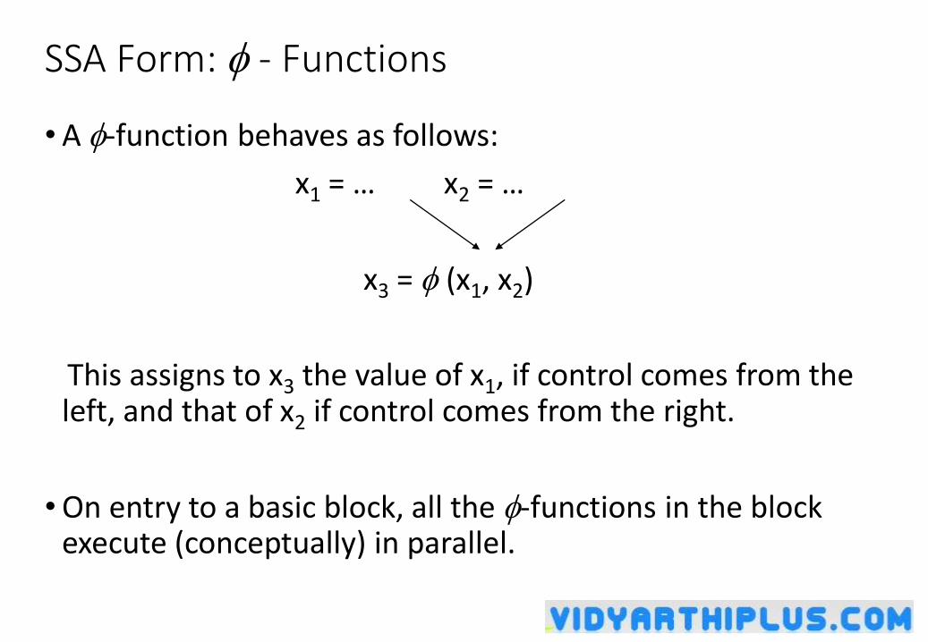
SSA Form: - Functions
•A -function behaves as follows:
x1 = … x2 = …
x3 = (x1, x2)
This assigns to x3 the value of x1, if control comes from the left, and that of x2 if control comes from the right.
•On entry to a basic block, all the -functions in the block execute (conceptually) in parallel.
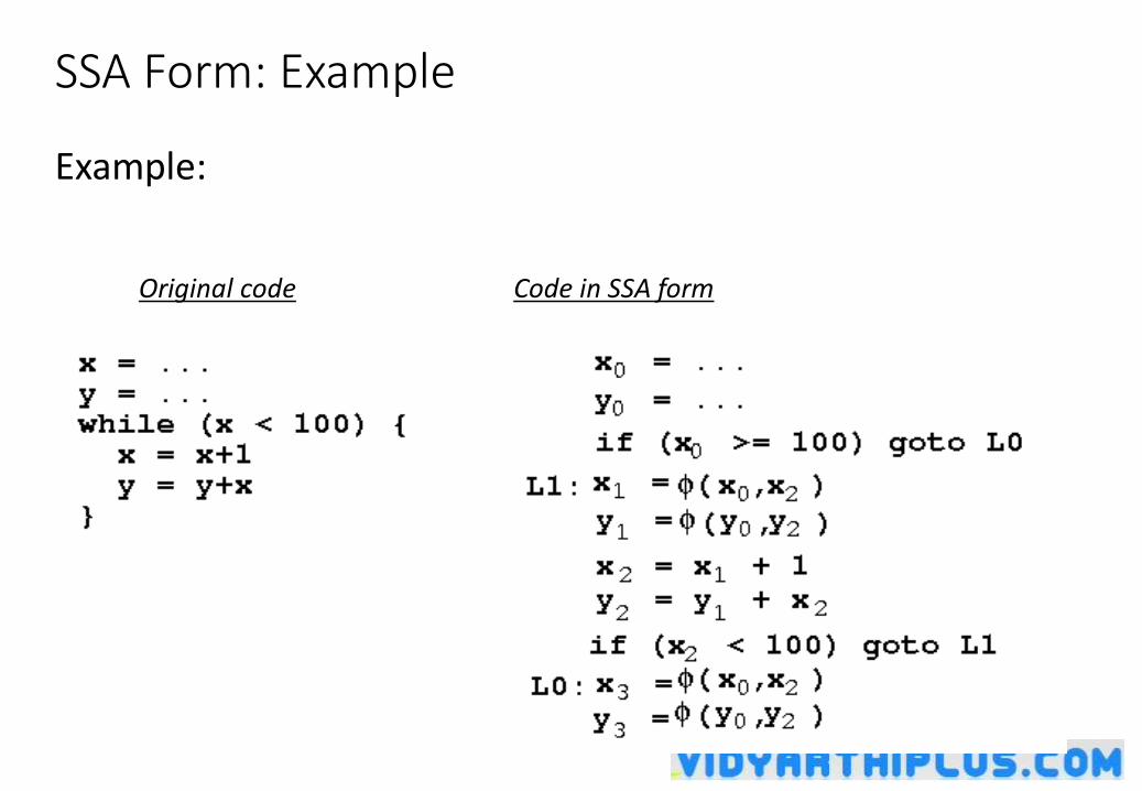
SSA Form: Example
Example:
Original code Code in SSA form
•INTERMEDIATE CODE GENERATION
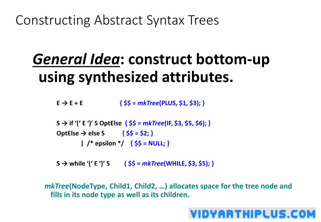
Constructing Abstract Syntax Trees
General Idea: construct bottom-up using synthesized attributes.
E → E + E { $$ = mkTree(PLUS, $1, $3); }
S → if ‘(‘ E ‘)’ S OptElse { $$ = mkTree(IF, $3, $5, $6); }
OptElse → else S { $$ = $2; }
| /* epsilon */ { $$ = NULL; }
S → while ‘(‘ E ‘)’ S { $$ = mkTree(WHILE, $3, $5); }
mkTree(NodeType, Child1, Child2, …) allocates space for the tree node and fills in its node type as well as its children.
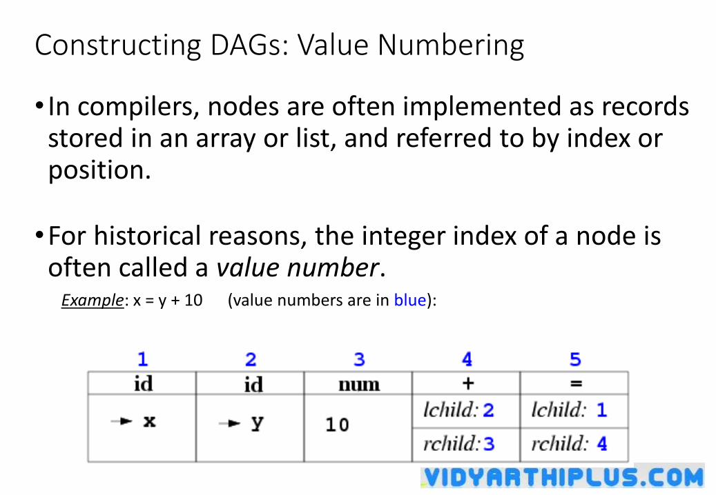
Constructing DAGs: Value Numbering
• In compilers, nodes are often implemented as records stored in an array or list, and referred to by index or position.
•For historical reasons, the integer index of a node is often called a value number.
Example: x = y + 10 (value numbers are in blue):
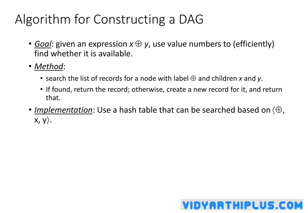
Algorithm for Constructing a DAG
• Goal: given an expression x y, use value numbers to (efficiently) find whether it is available.
• Method:
• search the list of records for a node with label and children x and y.
• If found, return the record; otherwise, create a new record for it, and return that.
• Implementation: Use a hash table that can be searched based on , x, y.
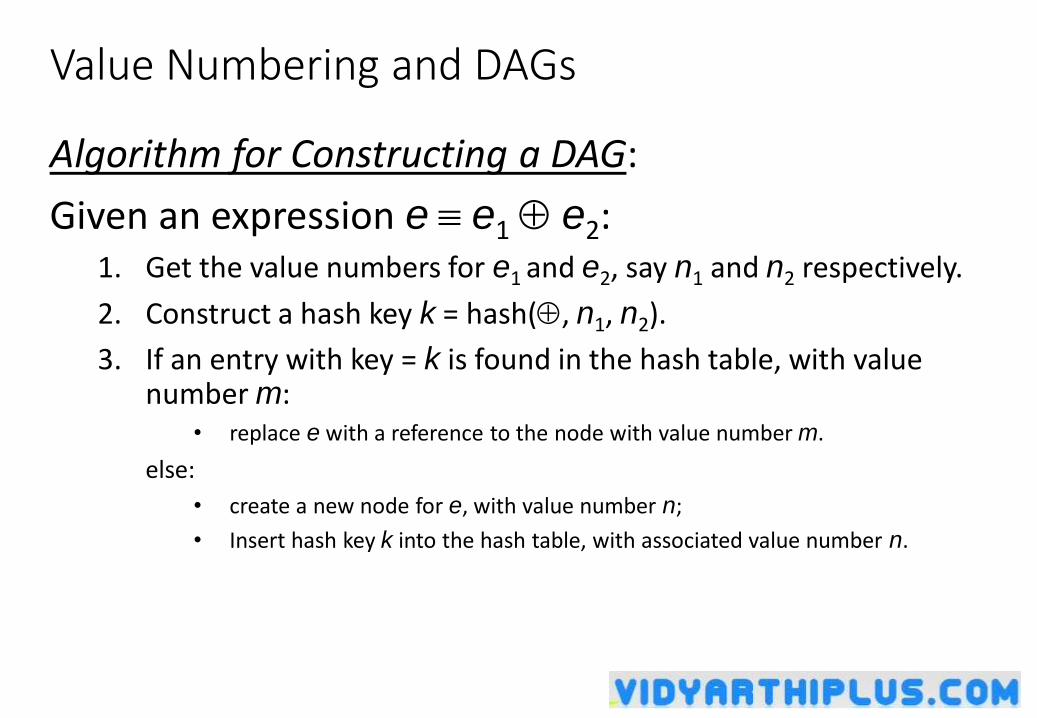
Value Numbering and DAGs
Algorithm for Constructing a DAG:
Given an expression e e1 e2:1. Get the value numbers for e1 and e2, say n1 and n2 respectively.
2. Construct a hash key k = hash(, n1, n2).
3. If an entry with key = k is found in the hash table, with value number m:
• replace e with a reference to the node with value number m.
else:
• create a new node for e, with value number n;
• Insert hash key k into the hash table, with associated value number n.

Three Address Code: Representation
• Each instruction represented as a structure called a quadruple (or “quad”):• contains info about the operation, up to 3 operands.
• for operands: use a bit to indicate whether constant or Symbol Table pointer.
E.g.: x = y + z if ( x y ) goto L
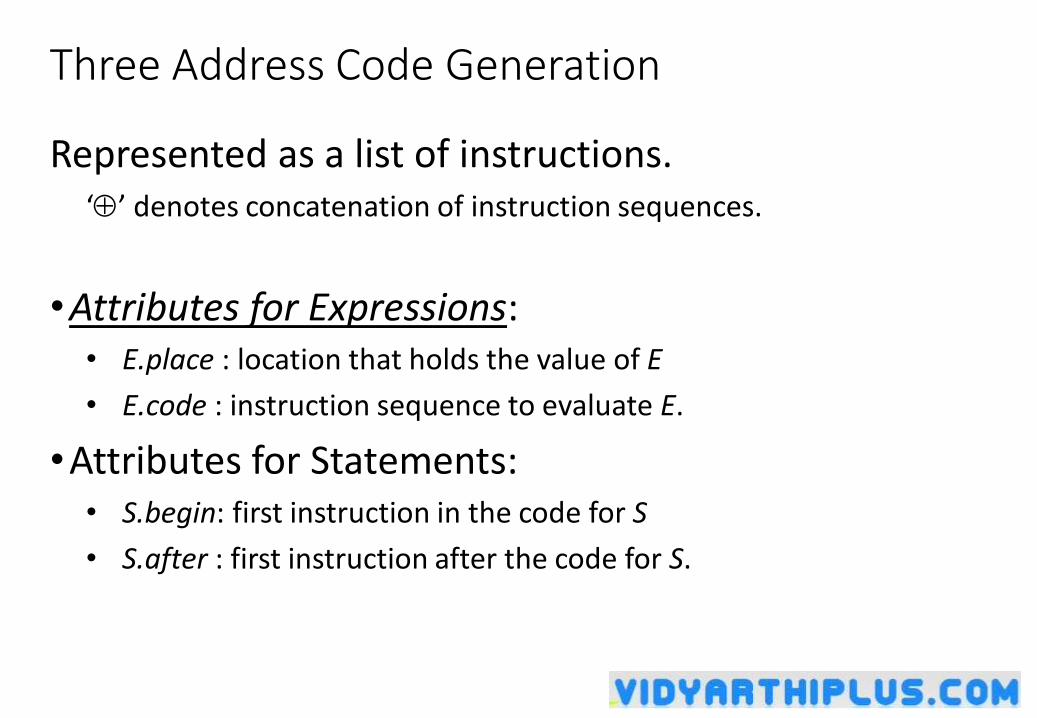
Three Address Code Generation
Represented as a list of instructions.‘’ denotes concatenation of instruction sequences.
•Attributes for Expressions:• E.place : location that holds the value of E
• E.code : instruction sequence to evaluate E.
•Attributes for Statements:• S.begin: first instruction in the code for S
• S.after : first instruction after the code for S.
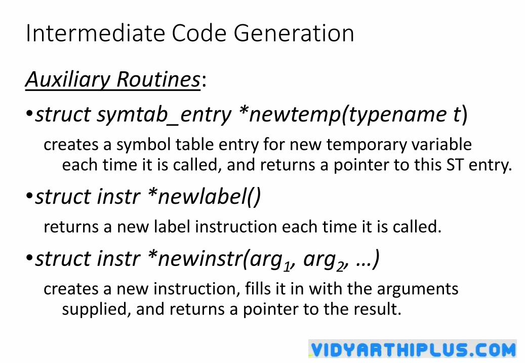
Intermediate Code Generation
Auxiliary Routines:
•struct symtab_entry *newtemp(typename t) creates a symbol table entry for new temporary variable
each time it is called, and returns a pointer to this ST entry.
•struct instr *newlabel()returns a new label instruction each time it is called.
•struct instr *newinstr(arg1, arg2, …)creates a new instruction, fills it in with the arguments
supplied, and returns a pointer to the result.
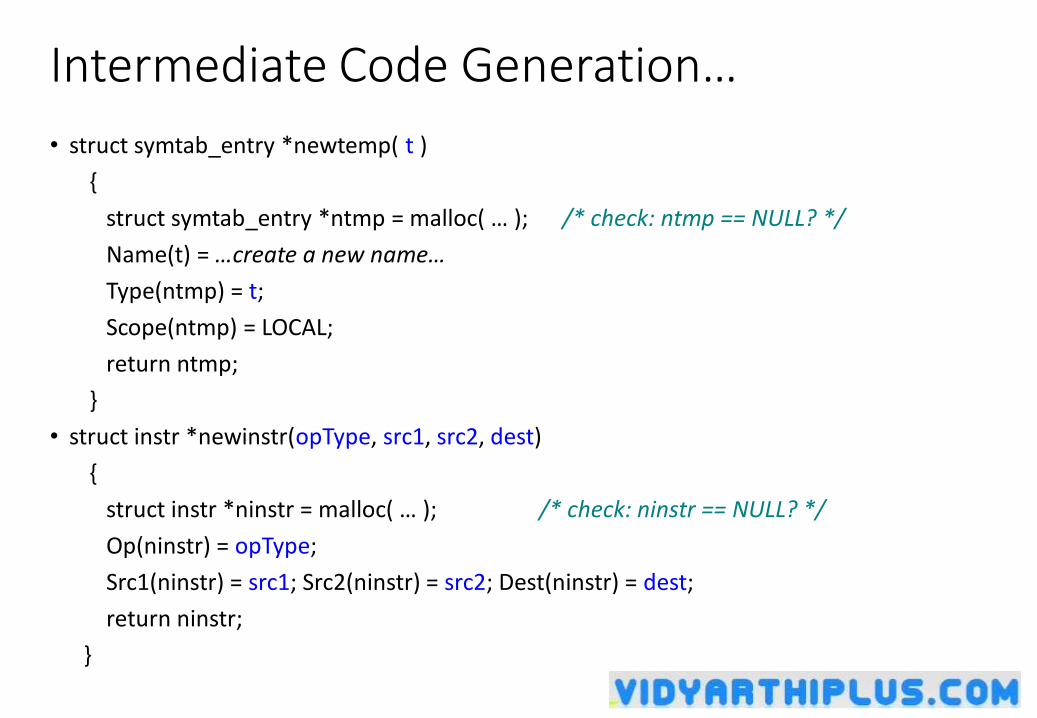
Intermediate Code Generation…
• struct symtab_entry *newtemp( t )
{
struct symtab_entry *ntmp = malloc( … ); /* check: ntmp == NULL? */
Name(t) = …create a new name…
Type(ntmp) = t;
Scope(ntmp) = LOCAL;
return ntmp;
}
• struct instr *newinstr(opType, src1, src2, dest)
{
struct instr *ninstr = malloc( … ); /* check: ninstr == NULL? */
Op(ninstr) = opType;
Src1(ninstr) = src1; Src2(ninstr) = src2; Dest(ninstr) = dest;
return ninstr;
}
CODE OPTIMIZATION
Code Optimization
•Aim: to improve program performance.• “optimization” a misnomer: attaining “optimal”
performance is impossible or impractical in general.
•Criteria:•must be “safe,” i.e., preserve program semantics;
• on average, should improve performance measurably;
• occasionally, a few programs may suffer performance degradation.
• the transformation should be worth the effort.
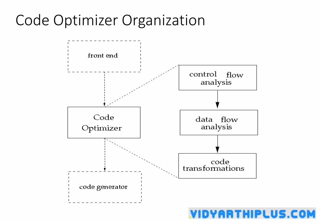
Code Optimizer Organization
Control Flow Analysis
•Overall goals:• Identify control flow relationships in a program.
• Identify the “structure” of control flow, e.g., loops.
•Main issues: indirect control flow.• indirect calls through function pointers in C;
• higher order constructs (e.g., function-valued arguments and return values) in functional languages;
• virtual functions in object-oriented languages.
Dominators
•Definition: A node d in a flow graph Gdominates a node n (written “d dom n”) iff every path from the entry node of G to ncontains the node d.
•Facts:• every node dominates itself;
• the “dom” relation is a partial order;
• every node has a unique immediate dominator.
the dominator relationships in a flow graph form a tree (the “dominator tree.”)
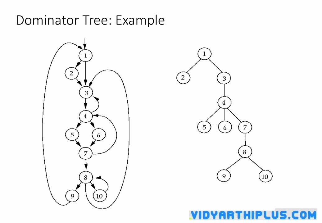
Dominator Tree: Example
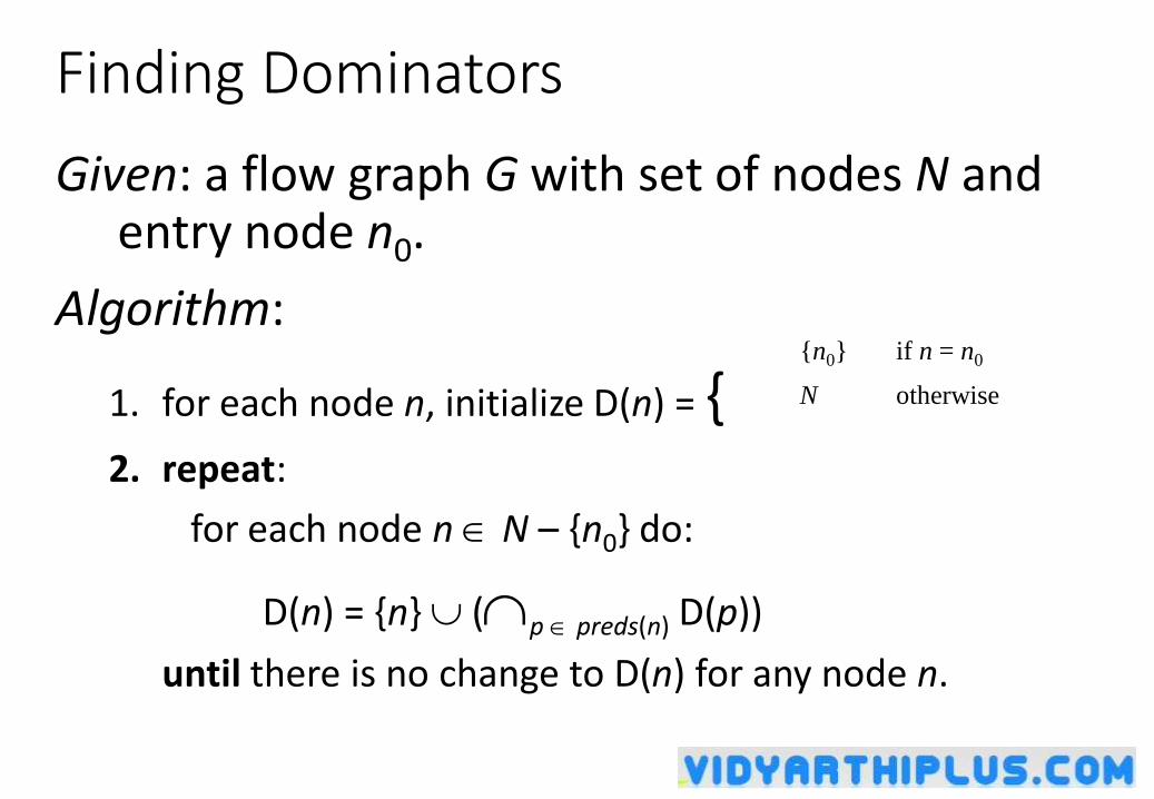
Finding Dominators
Given: a flow graph G with set of nodes N and entry node n0.
Algorithm:
1. for each node n, initialize D(n) = {2. repeat:
for each node n N – {n0} do:
D(n) = {n} (p preds(n) D(p))
until there is no change to D(n) for any node n.
{n0} if n = n0
N otherwise
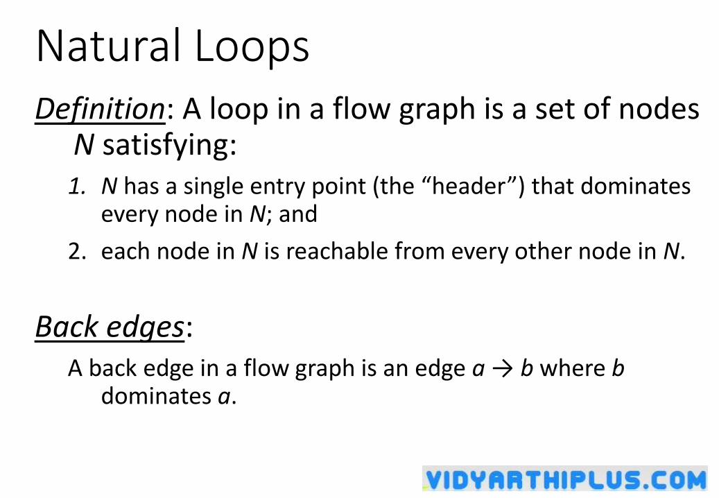
Natural LoopsDefinition: A loop in a flow graph is a set of nodes
N satisfying:1. N has a single entry point (the “header”) that dominates
every node in N; and
2. each node in N is reachable from every other node in N.
Back edges: A back edge in a flow graph is an edge a → b where b
dominates a.
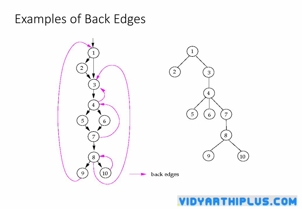
Examples of Back Edges
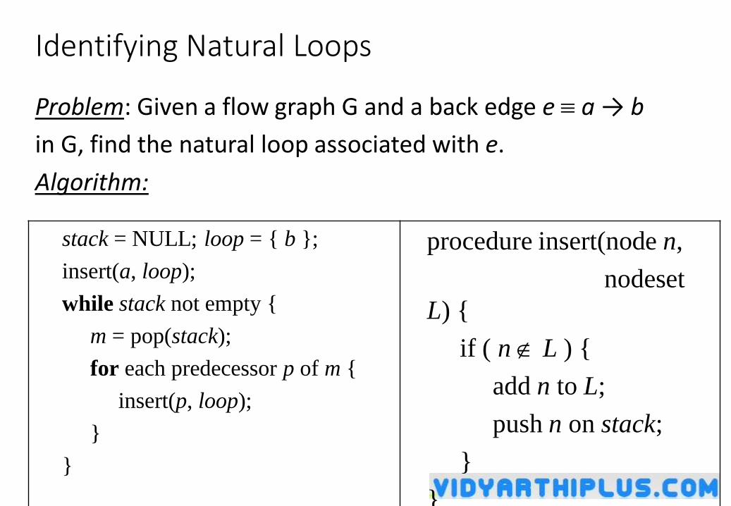
Identifying Natural Loops
Problem: Given a flow graph G and a back edge e a → b
in G, find the natural loop associated with e.
Algorithm:
stack = NULL; loop = { b };
insert(a, loop);
while stack not empty {
m = pop(stack);
for each predecessor p of m {
insert(p, loop);
}
}
procedure insert(node n,
nodeset
L) {
if ( n L ) {
add n to L;
push n on stack;
}
}
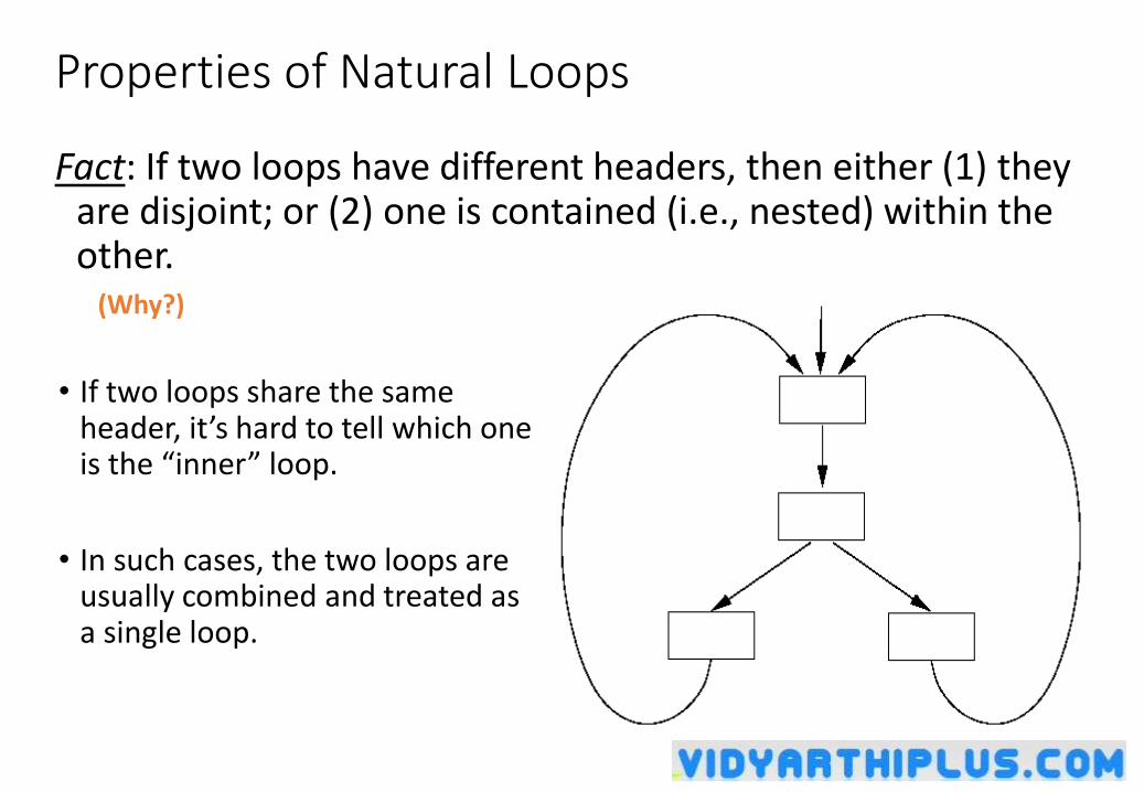
Properties of Natural Loops
• If two loops share the same header, it’s hard to tell which one is the “inner” loop.
• In such cases, the two loops are usually combined and treated as a single loop.
Fact: If two loops have different headers, then either (1) they are disjoint; or (2) one is contained (i.e., nested) within the other.
(Why?)
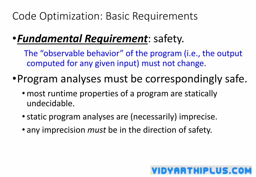
Code Optimization: Basic Requirements
•Fundamental Requirement: safety.The “observable behavior” of the program (i.e., the output computed for any given input) must not change.
•Program analyses must be correspondingly safe.•most runtime properties of a program are statically
undecidable.
• static program analyses are (necessarily) imprecise.
• any imprecision must be in the direction of safety.
Global Dataflow Analysis
•Set up equations relating properties at different program points in terms of properties at other “nearby” points.
Usually, for each block B:
• one equation expresses how the property is affected by the instructions in B;
• one equation captures the effect of the flow of values across basic block boundaries.
•We then solve these equations iteratively.
Analysis 1. Reaching Definitions
•A definition of a variable x is an instruction that (may) assign a value to it.• unambiguous definitions: instructions that definitely assign to x;
• ambiguous definitions: instructions that may (or may not) assign to x, e.g., indirect stores, function calls.
•A definition of x is killed along a path if x is (definitely) redefined somewhere along .
•A definition d reaches a point p if there is some path from d to p such that d is not killed along .
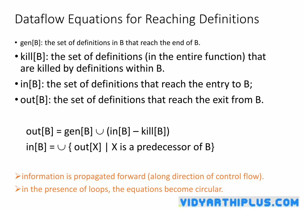
Dataflow Equations for Reaching Definitions
• gen[B]: the set of definitions in B that reach the end of B.
• kill[B]: the set of definitions (in the entire function) that are killed by definitions within B.
• in[B]: the set of definitions that reach the entry to B;
• out[B]: the set of definitions that reach the exit from B.
out[B] = gen[B] (in[B] – kill[B])
in[B] = { out[X] | X is a predecessor of B}
information is propagated forward (along direction of control flow).
in the presence of loops, the equations become circular.
Final Code Generation
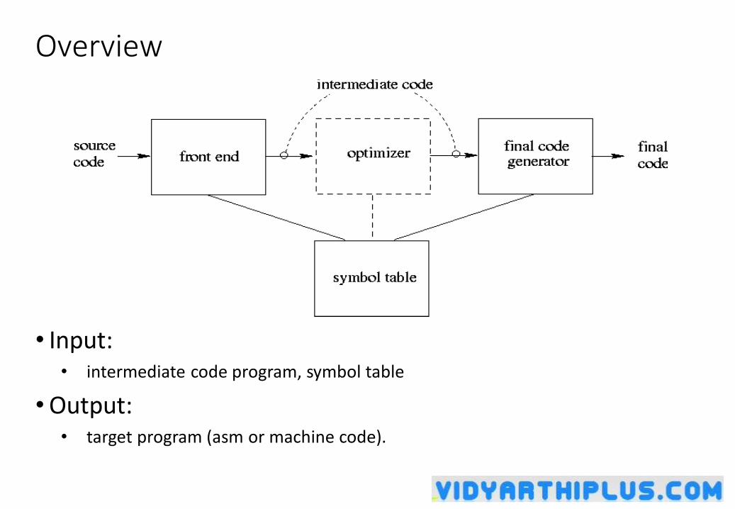
Overview
• Input:• intermediate code program, symbol table
•Output:• target program (asm or machine code).
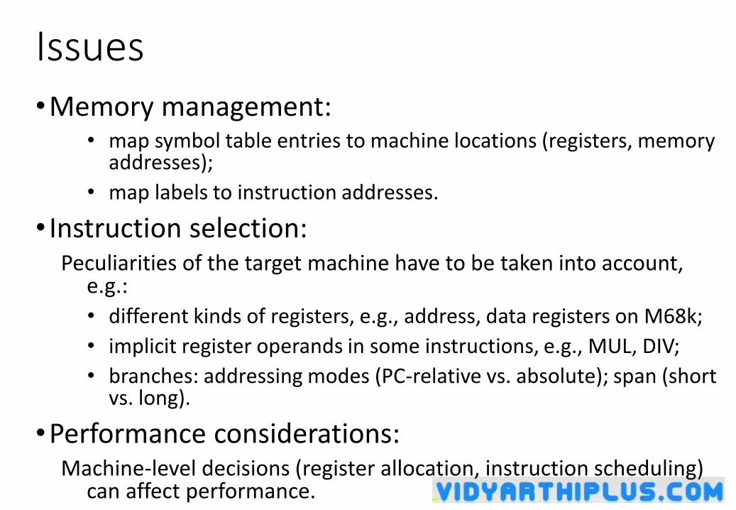
Issues•Memory management:
• map symbol table entries to machine locations (registers, memory addresses);
• map labels to instruction addresses.
• Instruction selection: Peculiarities of the target machine have to be taken into account,
e.g.:
• different kinds of registers, e.g., address, data registers on M68k;
• implicit register operands in some instructions, e.g., MUL, DIV;
• branches: addressing modes (PC-relative vs. absolute); span (short vs. long).
•Performance considerations:Machine-level decisions (register allocation, instruction scheduling)
can affect performance.
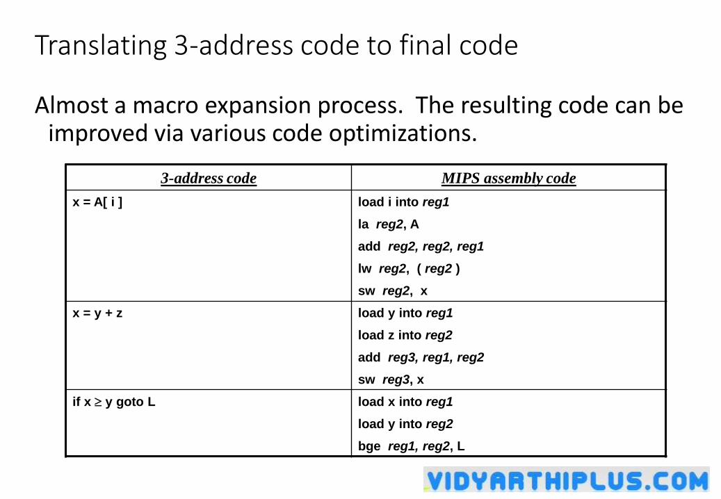
Translating 3-address code to final code
Almost a macro expansion process. The resulting code can be improved via various code optimizations.
3-address code MIPS assembly code
x = A[ i ] load i into reg1
la reg2, A
add reg2, reg2, reg1
lw reg2, ( reg2 )
sw reg2, x
x = y + z load y into reg1
load z into reg2
add reg3, reg1, reg2
sw reg3, x
if x y goto L load x into reg1
load y into reg2
bge reg1, reg2, L
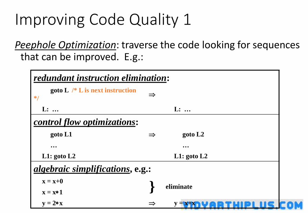
Improving Code Quality 1
Peephole Optimization: traverse the code looking for sequences that can be improved. E.g.:
redundant instruction elimination:
goto L /* L is next instruction
*/
L: … L: …
control flow optimizations:
goto L1 goto L2
… …
L1: goto L2 L1: goto L2
algebraic simplifications, e.g.:
x = x+0
} eliminatex = x1
y = 2x y = x+x
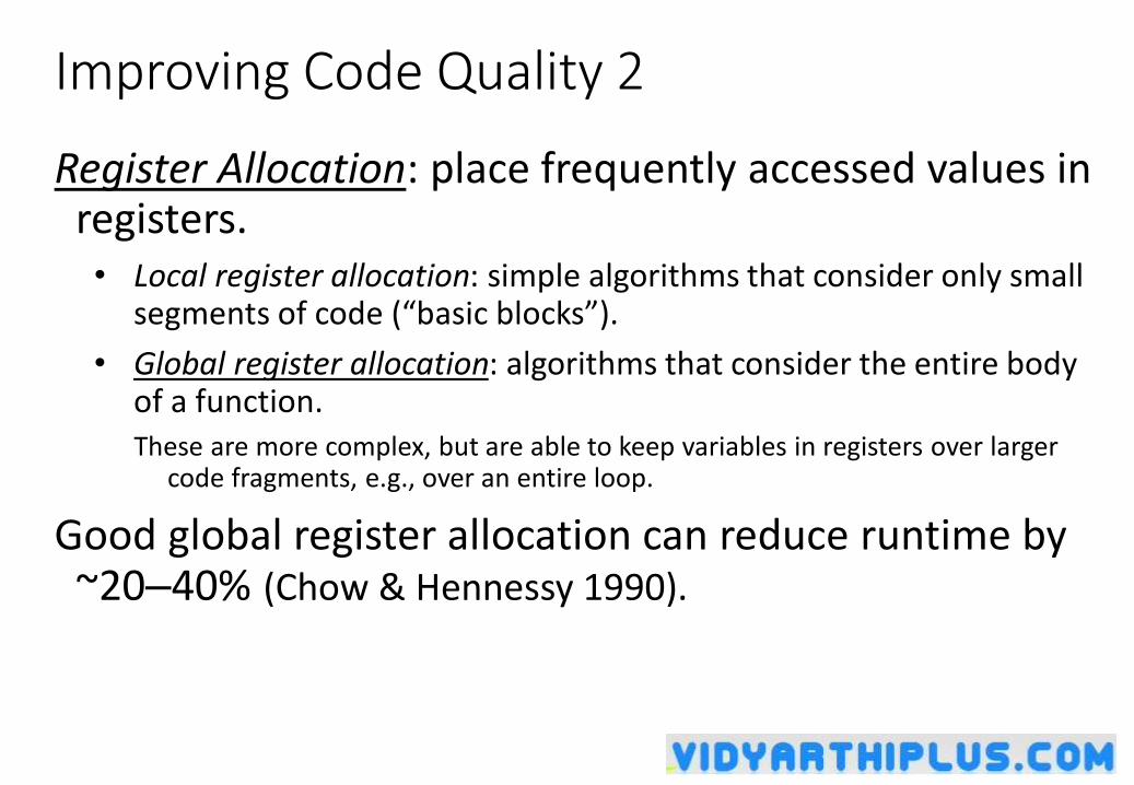
Improving Code Quality 2
Register Allocation: place frequently accessed values in registers.• Local register allocation: simple algorithms that consider only small
segments of code (“basic blocks”).
• Global register allocation: algorithms that consider the entire body of a function.These are more complex, but are able to keep variables in registers over larger
code fragments, e.g., over an entire loop.
Good global register allocation can reduce runtime by ~20–40% (Chow & Hennessy 1990).
Improving Code Quality 3
Code Optimization:
•Examine the program to identify specific program properties (“dataflow analysis”).
•Use this information to change the code so as to improve its performance. E.g.:• invariant code motion out of loops
• common subexpression elimination
• dead code elimination
Improving Code Quality 4
Instruction Scheduling: Some instructions take many cycles to execute.
On modern architectures, this can cause the instruction pipeline to be blocked (“stalled”) for several cycles.
Instruction scheduling refers to choosing an execution order on the instructions that allows useful work to be done by the CPU while it is waiting for an expensive operation to complete.
Improving Code Quality 5
Memory Hierarchy Optimizations:
•Modern processors typically use a multi-level memory hierarchy (cache, main memory).
Accessing main memory can be very expensive.
•Careful code layout can improve instruction cache utilization:• uses execution frequency information;
• reduces cache conflicts between frequently executed code.
Basic Blocks and Flow Graphs
•For program analysis and optimization, we usually need to know control flow relationships between different pieces of code.
•Usually done via control flow graphs:• vertices: basic blocks (single-entry, single-exit, straight-line instruction
sequences).
• edges: represent possible control flow between blocks.
(Details discussed in Intermediate Representations.)
Representing Basic Blocks
Many different representations possible, with different tradeoffs. One possibility is:
struct bbl {
int bblnum;
instruction * first_instr;
instruction * last_instr;
struct bbl *pred, *succ; // control flow graph info
struct bbl *prev, *next; // bbls all linked into a list
… other information from analyses …
}
Register Allocation
•Goals: reduce (minimize?) memory accesses.
•Interaction with code generation:• Code generation assumes an infinite no. of “virtual
registers”.
• Register allocation: determine which virtual registers get mapped to physical registers.
• Register assignment: determine the actual mapping from physical registers to virtual registers.
Levels of Register Allocation
• Expression level: use Sethi-Ullman numbering to determine evaluation order for expressions. [Ershov 59]
• Local allocation: register allocation limited in scope to individual basic blocks. [Freiburghouse 74]
•Global allocation: register allocation over an entire function; generally based on graph coloring. [Chaitin 82, Chow & Hennessey 90, …]
Expression-level Register Allocation
• Idea: Choose an evaluation order for the subexpressions of an expression so as to minimize the no. of registers used.
• Algorithm: Given a syntax tree for an expression:1. [Pass 1]: Use a postorder traversal to assign a label to each
syntax tree node.The label of a node gives the max. no. of registers needed to evaluate the
subexpression rooted at that node.
2. [Pass 2]: Traverse the expression tree and generate code, using node labels to guide which subexpression gets evaluated first.
Evaluation Order: Sethi-Ullman Numbering
Labeling algorithm:
if n is a leaf node then
label(n) = 1;
else
let the labels for the children of n be l1, l2;
label(n) = (l1 l2 ? max(l1, l2) : l1+1);
endif
Evaluation Order: Code Generation
Tree Traversal and Code Generation Algorithm:
if n is a leaf node then
locate a free register r, and generate a load into r;
else
let the children of n be n1 and n2, with labels l1 and l2 resp;
if l1 l2 then /* needs max(l1, l2) registers */
• generate code to evaluate the subexpression with the larger label;
• free all but one register used by that subexpression;
• generate code to evaluate the other subexpression;
else /* needs l1+1 registers */
• generate code to evaluate n1 using l1 registers;
• free up l11 registers;
• use l1 registers to evaluate n2;
endif
endif
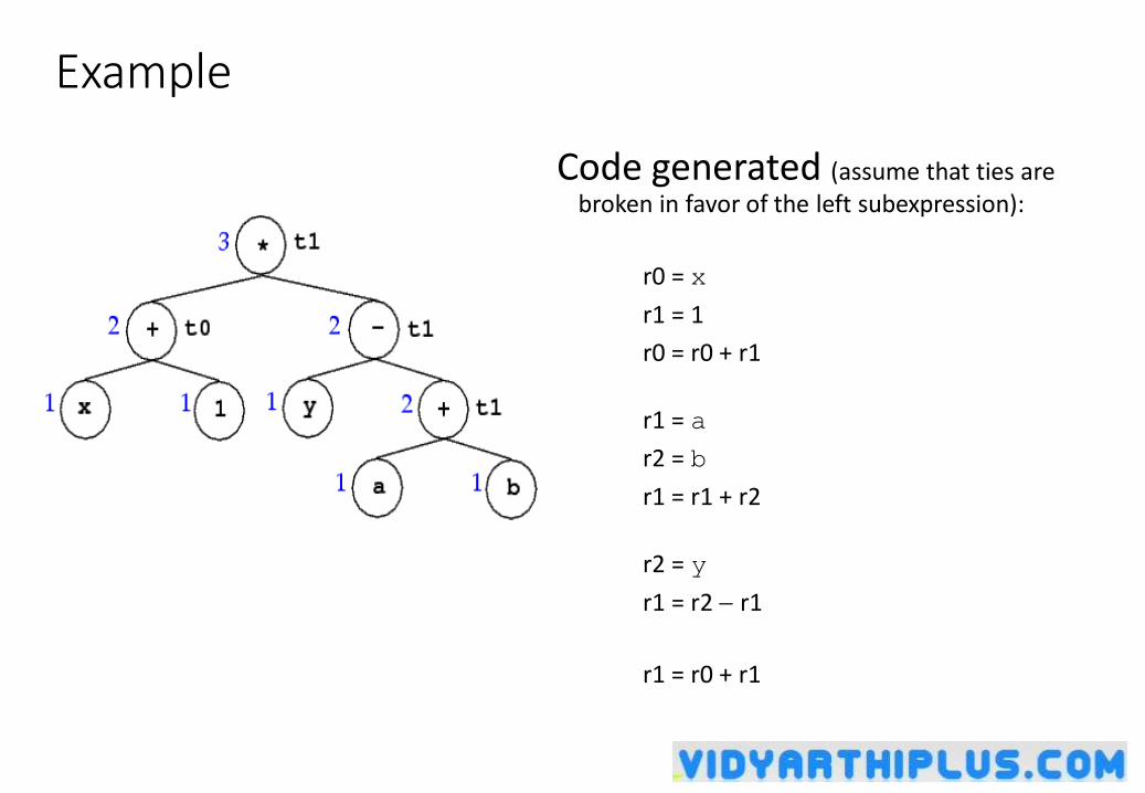
Example
Code generated (assume that ties are broken in favor of the left subexpression):
r0 = x
r1 = 1
r0 = r0 + r1
r1 = a
r2 = b
r1 = r1 + r2
r2 = y
r1 = r2 r1
r1 = r0 + r1
Comments on the Evaluation Order Algorithm:
•O(n) in the size of the expression tree.
•Easily adapted to the case where leaf node variables don’t have to be loaded into registers.
• If there are no common subexpressions, the algorithm is provably optimal in terms of no. of registers used.• Optimal code generation for expression DAGs is NP-complete.
• The algorithm can be adapted to handle DAGs. This produces usually good code that is not necessarily optimal.
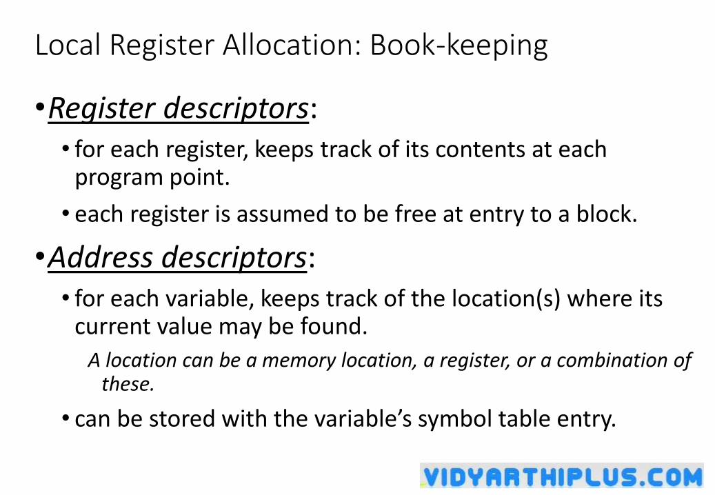
Local Register Allocation: Book-keeping
•Register descriptors: • for each register, keeps track of its contents at each
program point.
• each register is assumed to be free at entry to a block.
•Address descriptors:• for each variable, keeps track of the location(s) where its
current value may be found.
A location can be a memory location, a register, or a combination of these.
• can be stored with the variable’s symbol table entry.
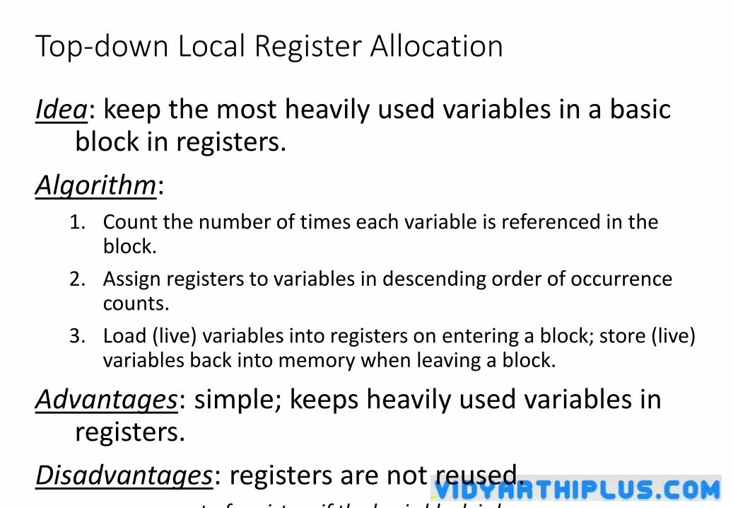
Top-down Local Register Allocation
Idea: keep the most heavily used variables in a basic block in registers.
Algorithm:1. Count the number of times each variable is referenced in the
block.
2. Assign registers to variables in descending order of occurrence counts.
3. Load (live) variables into registers on entering a block; store (live) variables back into memory when leaving a block.
Advantages: simple; keeps heavily used variables in registers.
Disadvantages: registers are not reused.• can run out of registers if the basic block is large.
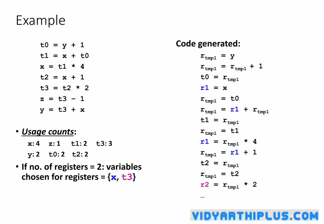
Example
t0 = y + 1
t1 = x + t0
x = t1 * 4
t2 = x + 1
t3 = t2 * 2
z = t3 – 1
y = t3 + x
• Usage counts:x: 4 z: 1 t1: 2 t3: 3
y: 2 t0: 2 t2: 2
• If no. of registers = 2: variables chosen for registers = {x, t3}
Code generated:rtmp1 = y
rtmp1 = rtmp1 + 1
t0 = rtmp1
r1 = x
rtmp1 = t0
rtmp1 = r1 + rtmp1
t1 = rtmp1
rtmp1 = t1
r1 = rtmp1 * 4
rtmp1 = r1 + 1
t2 = rtmp1
rtmp1 = t2
r2 = rtmp1 * 2
…
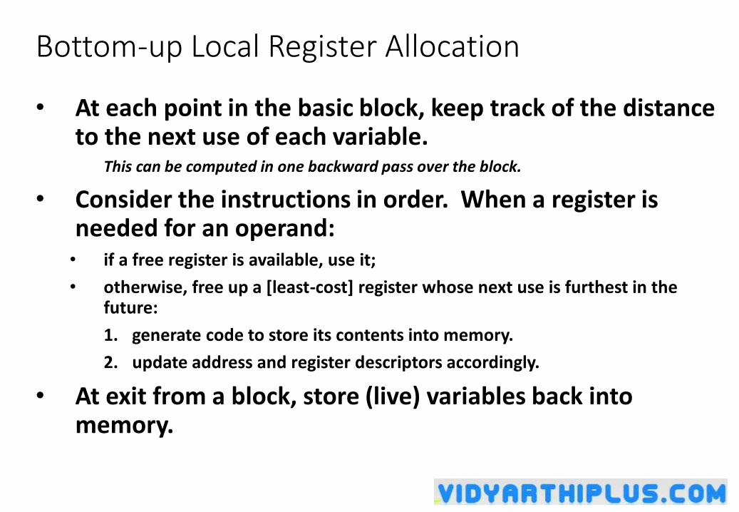
Bottom-up Local Register Allocation
• At each point in the basic block, keep track of the distance to the next use of each variable.
This can be computed in one backward pass over the block.
• Consider the instructions in order. When a register is needed for an operand:• if a free register is available, use it;
• otherwise, free up a [least-cost] register whose next use is furthest in the future:
1. generate code to store its contents into memory.
2. update address and register descriptors accordingly.
• At exit from a block, store (live) variables back into memory.
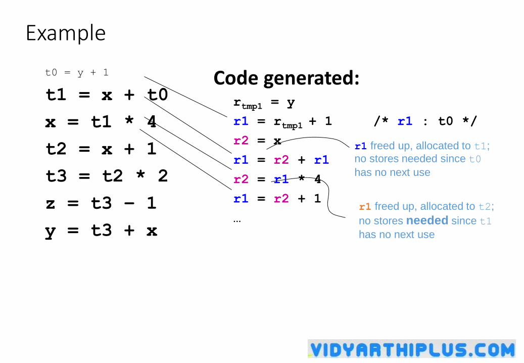
Example
t0 = y + 1
t1 = x + t0
x = t1 * 4
t2 = x + 1
t3 = t2 * 2
z = t3 – 1
y = t3 + x
Code generated:rtmp1 = y
r1 = rtmp1 + 1 /* r1 : t0 */
r2 = x
r1 = r2 + r1
r2 = r1 * 4
r1 = r2 + 1
…
r1 freed up, allocated to t1;
no stores needed since t0
has no next use
r1 freed up, allocated to t2;
no stores needed since t1
has no next use
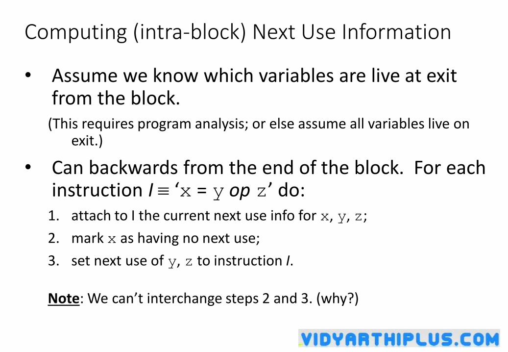
Computing (intra-block) Next Use Information
• Assume we know which variables are live at exit from the block.
(This requires program analysis; or else assume all variables live on exit.)
• Can backwards from the end of the block. For each instruction I ‘x = y op z’ do:
1. attach to I the current next use info for x, y, z;
2. mark x as having no next use;
3. set next use of y, z to instruction I.
Note: We can’t interchange steps 2 and 3. (why?)
Local Register Allocation: extensions
•Handling copy instructions:For an instruction ‘x = y,’ if y is in a register ry:
• update ry’s register descriptor to indicate that it also contains x;
• no need to generate an explicit store (yet).
This means that in general, a register may contain multiple variables.
•Not all of the values in a register r need to be stored back into memory when freeing up r:• a variable x whose memory value is current need not be stored back;
• a known constant value need not be stored (it can be recomputed).
Classify register values as clean or dirty: only dirty values need to be stored.
• This can be incorporated into the spill cost estimation.
Register Allocation: beyond basic blocks
•Need to coordinate the flow of values across basic block boundaries.
•Live ranges:• A live range consists of a set of definitions D and uses U of a variable
x, such that:• for each use u U, every definition that can reach u is in D.
• for each definition d D, every use that d can reach is in U.
•Live ranges form the unit of global register allocation.
Live Ranges: Example
Live Ranges
x y
x = y + 1
z = x + a
y = u + w
v = x + 4
x = y * z
v = x - y
u = v / x
Global Register Allocation by Graph Coloring
• Graph coloring is a systematic way of allocating registers and managing spills.
• Consists of two passes:1. Target machine instructions are selected as though there is an
unbounded no. of symbolic registers.
2. Physical registers are assigned to symbolic registers in a way that minimizes spill costs.
This is done by constructing a register interference graph for the function being compiled, and then k-coloring this graph (k = no. of available registers).
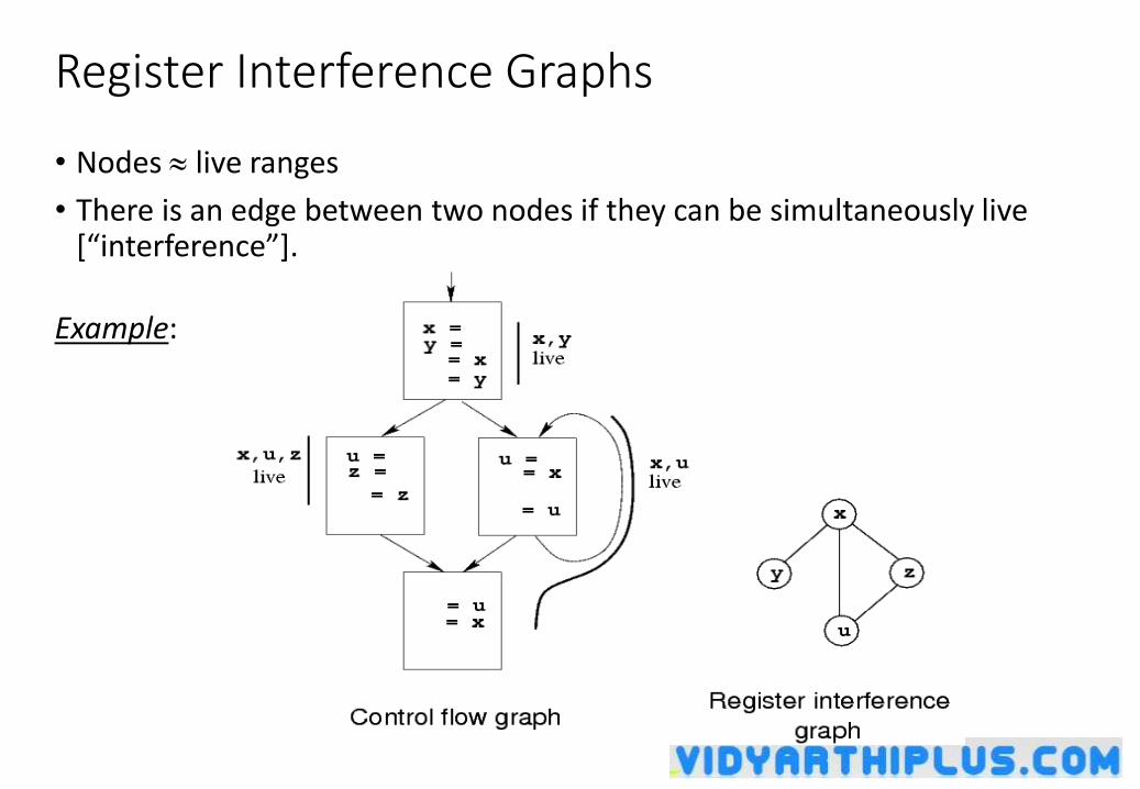
Register Interference Graphs
• Nodes live ranges
• There is an edge between two nodes if they can be simultaneously live [“interference”].
Example:
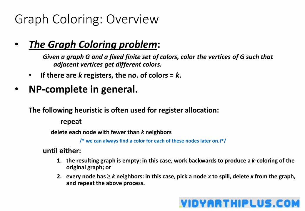
Graph Coloring: Overview
• The Graph Coloring problem:Given a graph G and a fixed finite set of colors, color the vertices of G such that
adjacent vertices get different colors.
• If there are k registers, the no. of colors = k.
• NP-complete in general.
The following heuristic is often used for register allocation:
repeat
delete each node with fewer than k neighbors
/* we can always find a color for each of these nodes later on.)*/
until either:1. the resulting graph is empty: in this case, work backwards to produce a k-coloring of the
original graph; or
2. every node has k neighbors: in this case, pick a node x to spill, delete x from the graph, and repeat the above process.
Graph Coloring Register Allocation: Issues
• Identifying live ranges:• use SSA form; or
• use dataflow analysis (liveness/reaching definitions).
•Constructing the interference graph.
•Choosing spill nodes.• need to estimate spill costs.
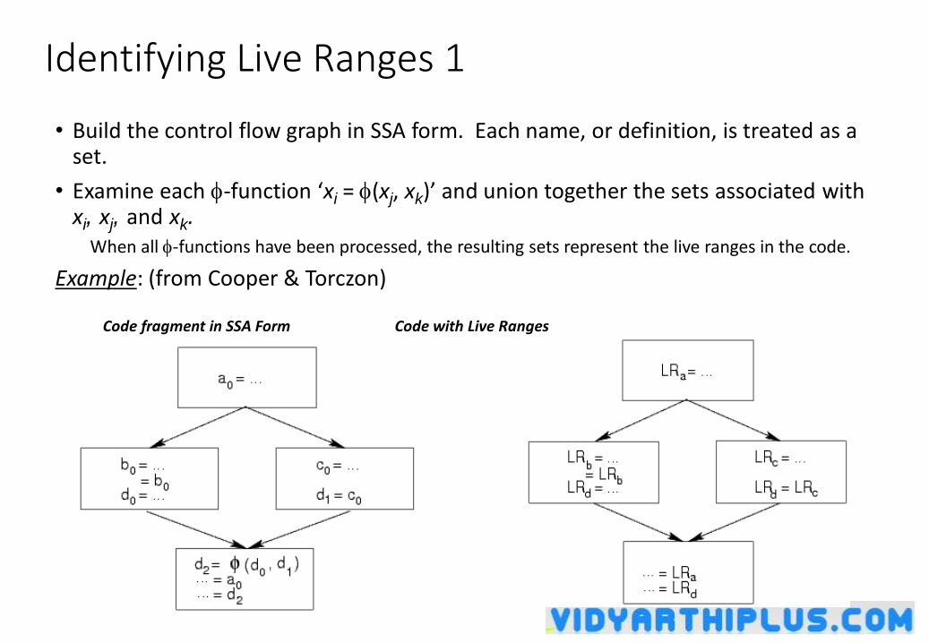
Identifying Live Ranges 1
• Build the control flow graph in SSA form. Each name, or definition, is treated as a set.
• Examine each -function ‘xi = (xj, xk)’ and union together the sets associated with xi, xj, and xk.
When all -functions have been processed, the resulting sets represent the live ranges in the code.
Example: (from Cooper & Torczon)
Code fragment in SSA Form Code with Live Ranges
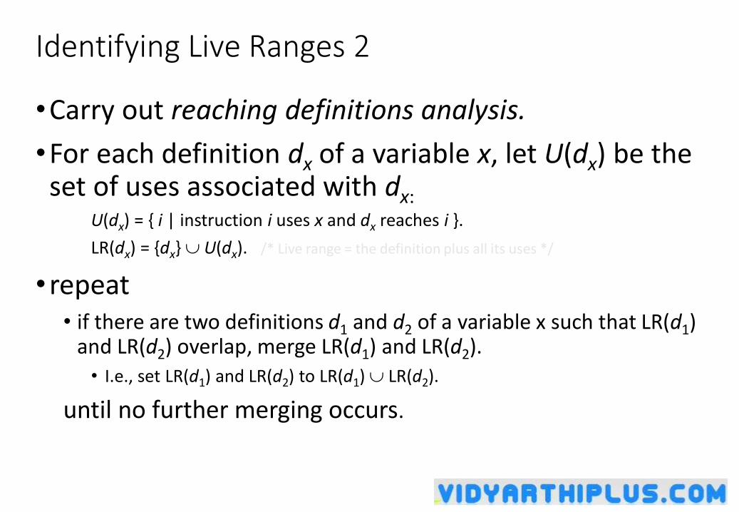
Identifying Live Ranges 2
•Carry out reaching definitions analysis.
•For each definition dx of a variable x, let U(dx) be the set of uses associated with dx:
U(dx) = { i | instruction i uses x and dx reaches i }.
LR(dx) = {dx} U(dx). /* Live range = the definition plus all its uses */
• repeat • if there are two definitions d1 and d2 of a variable x such that LR(d1)
and LR(d2) overlap, merge LR(d1) and LR(d2). • I.e., set LR(d1) and LR(d2) to LR(d1) LR(d2).
until no further merging occurs.
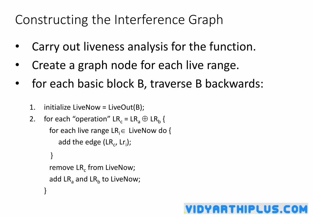
Constructing the Interference Graph
• Carry out liveness analysis for the function.
• Create a graph node for each live range.
• for each basic block B, traverse B backwards:
1. initialize LiveNow = LiveOut(B);
2. for each “operation” LRc = LRa LRb {
for each live range LRi LiveNow do {
add the edge (LRc, Lri);
}
remove LRc from LiveNow;
add LRa and LRb to LiveNow;
}
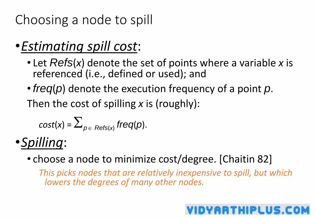
Choosing a node to spill
•Estimating spill cost: • Let Refs(x) denote the set of points where a variable x is
referenced (i.e., defined or used); and
• freq(p) denote the execution frequency of a point p.
Then the cost of spilling x is (roughly):
cost(x) = p Refs(x) freq(p).
•Spilling: • choose a node to minimize cost/degree. [Chaitin 82]
This picks nodes that are relatively inexpensive to spill, but which lowers the degrees of many other nodes.
Estimating Execution Frequencies
•Simple approach: heuristics relating to loop nesting depth:• preorder traversal of the syntax tree;
• execution frequency of root node = 1;
• each loop assumed to execute a “reasonable” no. of times (typically, 8–12);
• each branch of a conditional assumed to be equally likely.
This effectively pushes spill code away from inner loops.
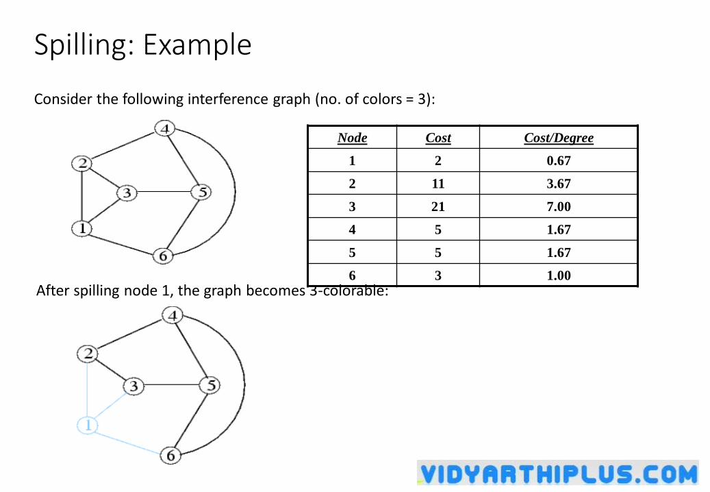
Spilling: Example
Consider the following interference graph (no. of colors = 3):
After spilling node 1, the graph becomes 3-colorable:
Node Cost Cost/Degree
1 2 0.67
2 11 3.67
3 21 7.00
4 5 1.67
5 5 1.67
6 3 1.00
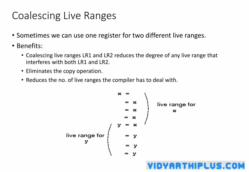
Coalescing Live Ranges
• Sometimes we can use one register for two different live ranges.
• Benefits:
• Coalescing live ranges LR1 and LR2 reduces the degree of any live range that interferes with both LR1 and LR2.
• Eliminates the copy operation.
• Reduces the no. of live ranges the compiler has to deal with.
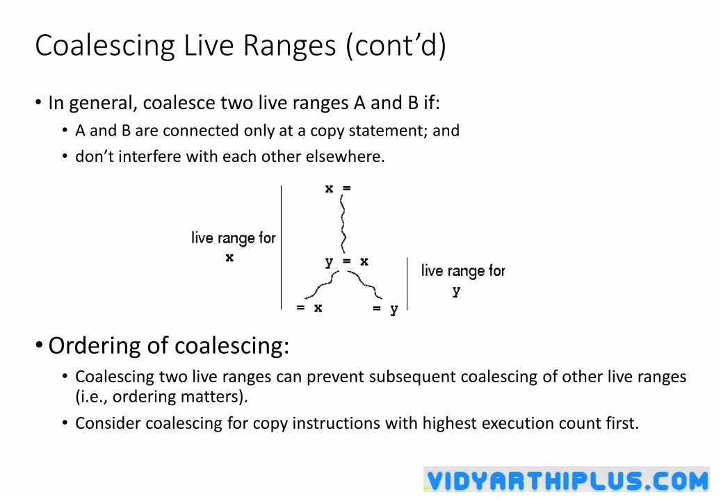
Coalescing Live Ranges (cont’d)
• In general, coalesce two live ranges A and B if:
• A and B are connected only at a copy statement; and
• don’t interfere with each other elsewhere.
•Ordering of coalescing:• Coalescing two live ranges can prevent subsequent coalescing of other live ranges
(i.e., ordering matters).
• Consider coalescing for copy instructions with highest execution count first.
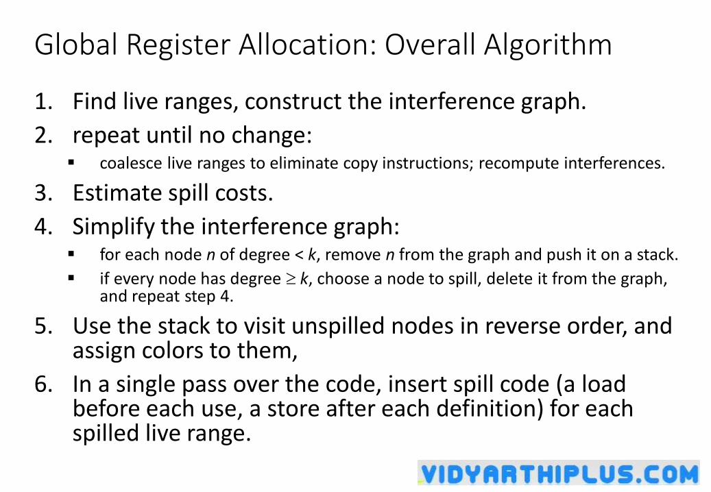
Global Register Allocation: Overall Algorithm
1. Find live ranges, construct the interference graph.
2. repeat until no change: coalesce live ranges to eliminate copy instructions; recompute interferences.
3. Estimate spill costs.
4. Simplify the interference graph: for each node n of degree < k, remove n from the graph and push it on a stack.
if every node has degree k, choose a node to spill, delete it from the graph, and repeat step 4.
5. Use the stack to visit unspilled nodes in reverse order, and assign colors to them,
6. In a single pass over the code, insert spill code (a load before each use, a store after each definition) for each spilled live range.
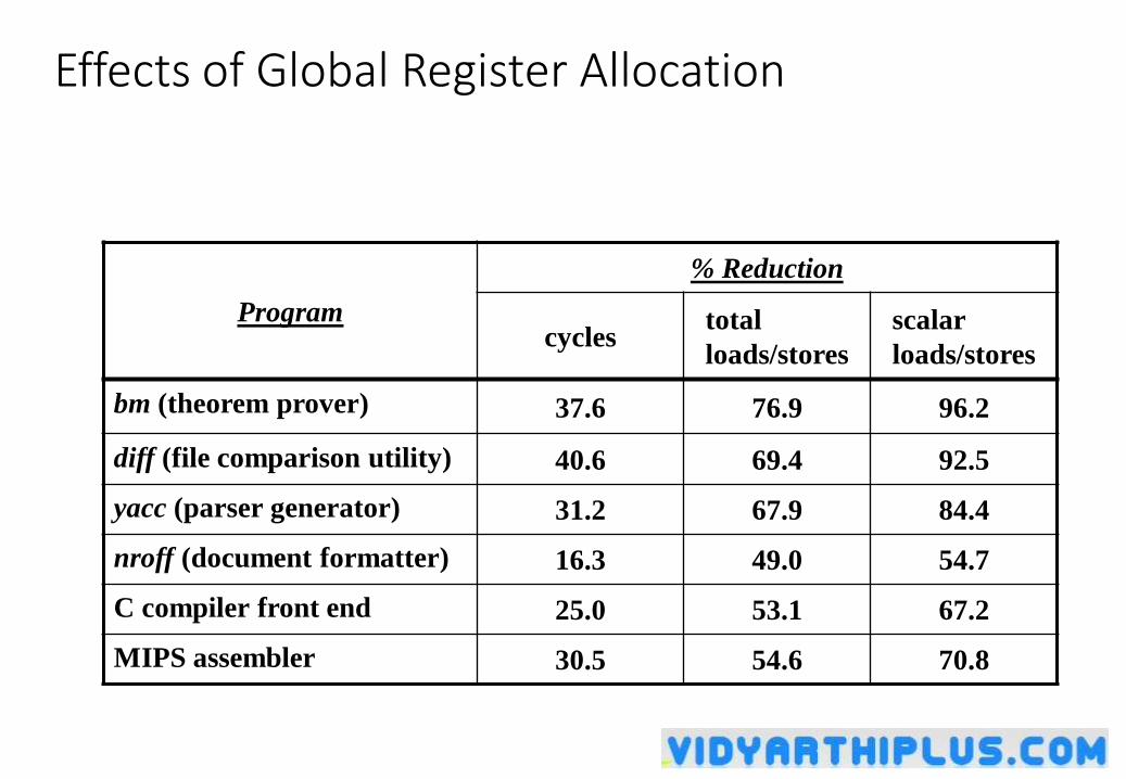
Effects of Global Register Allocation
Program
% Reduction
cyclestotal
loads/stores
scalar
loads/stores
bm (theorem prover) 37.6 76.9 96.2
diff (file comparison utility) 40.6 69.4 92.5
yacc (parser generator) 31.2 67.9 84.4
nroff (document formatter) 16.3 49.0 54.7
C compiler front end 25.0 53.1 67.2
MIPS assembler 30.5 54.6 70.8
Related Documents