1 Lecture 15. Principles of active remote sensing: Lidar sensing of aerosols, gases and clouds. 1. Optical interactions of relevance to lasers. 2. General principles of lidars. 3. Lidar equation. 4. Examples of lidar sensing of aerosols, gases, and clouds. 5. Lidars in space: LITE and CALIPSO Required reading : S: 8.4.1, 8.4.2, 8.4.3, 8.4.4 Additional/advanced reading : CALIPSO: http://www-calipso.larc.nasa.gov/ CALIPSO ALGORITHM THEORETICAL BASIS DOCUMENTS (ATBDs): (4 large documents) http://www-calipso.larc.nasa.gov/resources/project_documentation.php 1. Optical interactions of relevance to lasers. Laser is a key component of the lidar. Lidar (LIght Detection And Ranging) Laser (Light Amplification by Stimulated Emission of Radiation) Basic principles of laser: stimulated emission in which atoms in an upper energy level can be triggered (or stimulated) in phase by an incoming photon of a specific energy. The emitted photons all possess the same wavelength and vibrate in phase with the incident photons (the light is said to be COHERENT). The emitted light is said to be INCOHERENT in time and space if the light is composed of many different wavelengths the light is emitted in random directions

Welcome message from author
This document is posted to help you gain knowledge. Please leave a comment to let me know what you think about it! Share it to your friends and learn new things together.
Transcript

1
Lecture 15.
Principles of active remote sensing: Lidar sensing of aerosols, gases and
clouds. 1. Optical interactions of relevance to lasers.
2. General principles of lidars.
3. Lidar equation.
4. Examples of lidar sensing of aerosols, gases, and clouds.
5. Lidars in space: LITE and CALIPSO
Required reading:
S: 8.4.1, 8.4.2, 8.4.3, 8.4.4
Additional/advanced reading:
CALIPSO: http://www-calipso.larc.nasa.gov/
CALIPSO ALGORITHM THEORETICAL BASIS DOCUMENTS (ATBDs):
(4 large documents)
http://www-calipso.larc.nasa.gov/resources/project_documentation.php
1. Optical interactions of relevance to lasers.
Laser is a key component of the lidar.
Lidar (LIght Detection And Ranging)
Laser (Light Amplification by Stimulated Emission of Radiation)
Basic principles of laser: stimulated emission in which atoms in an upper energy level
can be triggered (or stimulated) in phase by an incoming photon of a specific energy. The
emitted photons all possess the same wavelength and vibrate in phase with the incident
photons (the light is said to be COHERENT).
The emitted light is said to be INCOHERENT in time and space if the light is composed of many different wavelengths
the light is emitted in random directions

2
the light is emitted with different amplitudes
there is no phase correspondence between any of the emitted photons
Properties of laser light:
Monochromaticity
Coherence
Beam divergence:
All photons travel in the same direction; the light is contained in a very narrow
pencil (almost COLLIMATED), laser light is low in divergence (usually).
High irradiance:
Let’s estimate the irradiance of a 1 mW laser beam with a diameter of 1 mm. The
irradiance (power per unit area incident on a surface) is
F = P/S = 1x10⁻³ W/( (1x10⁻³ m)2/4) = 1273 W/m2
Elastic scattering is when the scattering frequency is the same as the frequency
of the incident light (e.g., Rayleigh scattering and Mie scattering). Inelastic
scattering is when there is a change in the frequency.
3
Optical interactions of relevance to laser environmental sensing
• Rayleigh scattering: laser radiation elastically scattered from atoms or molecules
with no change of frequency
• Mie scattering: laser radiation elastically scattered from particulates (aerosols or
clouds) of sizes comparable to the wavelengths of radiation with no change of
frequency
• Raman Scattering: laser radiation inelastically scattered from molecules with a
frequency shift characteristic of the molecule
• Resonance scattering: laser radiation matched in frequency to that of a specific
atomic transition is scattered by a large cross section and observed with no change
in frequency
• Fluorescence: laser radiation matched in frequency to a specific electronic
transition of an atom or molecule is absorbed with subsequent emission at the
lower frequency
• Absorption: attenuation of laser radiation when the frequency matched to the
absorption band of given molecule
Types of laser relevant to atmospheric remote sensing :
• solid state lasers (e.g., ruby laser, 694.3 nm)
• gas lasers (e.g., CO2, 9-11 µm)
• semiconductor lasers (GaAs, 820 nm)
2. General principles of lidars. There are several main types of lidars:
Backscatter lidars measure backscattered radiation and polarization (often called the
Mie lidar)
DIfferential Absorption Lidar (DIAL) is used to measure concentrations of chemical
species (such as ozone, water vapor, pollutants) in the atmosphere.

4
Principles: A DIAL lidar uses two different laser wavelengths which are selected so that
one of the wavelengths is absorbed by the molecule of interest while the other
wavelength is not. The difference in intensity of the two return signals can be used to
deduce the concentration of the molecule being investigated.
Raman (inelastic backscattering) Lidars: detect selected species by monitoring the
wavelength-shifted molecular return produced by vibrational Raman scattering from the
chosen molecules.
High Spectral Resolution Lidar (HSRL) measures optical properties of the atmosphere
by separating the Doppler-broadened molecular backscatter return from the unbroadened
aerosol return. The molecular signal is then used as a calibration target which is available
at each point in the lidar profile. This calibration allows unambiguous measurements of
aerosol scattering cross section, optical depth, and backscatter phase function (see S
8.4.3).
Doppler lidar is used to measure the velocity of a target. When the light transmitted
from the lidar hits a target moving towards or away from the lidar, the wavelength of the
light reflected/scattered off the target will be changed slightly. This is known as a
Doppler shift - hence Doppler Lidar. If the target is moving away from the lidar, the
return light will have a longer wavelength (sometimes referred to as a red shift), if
moving towards the lidar the return light will be at a shorter wavelength (blue shifted).
The target can be either a hard target or an atmospheric target - the atmosphere contains
many microscopic dust and aerosol particles which are carried by the wind.
Lidars compared to radars:
• Lidar uses laser radiation and a telescope/scanner similar to the way radar uses
radio frequency emissions and a dish antenna.
• Optically thick cloud and precipitation can attenuate the lidar beam, but radar
signals can penetrate heavy clouds (and precipitation).
5
• In optically clear air, radar return signals may be obtained from insects and birds,
and from air refractive index variations due to humidity, temperature, or pressure
fluctuations.
• Lidar beam divergence is two to three orders of magnitude smaller compared to
conventional 5 and 10 cm wavelength radars.
• The combination of the short pulse (of the order of 10-8 s) and the small beam
divergence (about 10-3 to 10-4 radiant) gives a small volume illuminated by a lidar
(about a few m3 at ranges of tens of km).
3. Lidar equation.
In general, the form of a lidar equation depends upon the kind of interaction invoked by
the laser radiation.
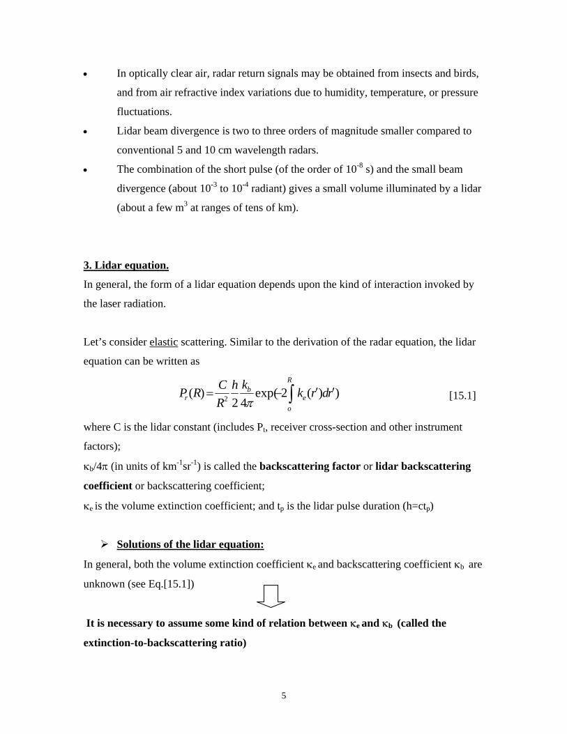
Let’s consider elastic scattering. Similar to the derivation of the radar equation, the lidar
equation can be written as
))(2exp(42
)( 2 rdrkkhRCRP e
R
o
br ′′−= ∫π [15.1]
where C is the lidar constant (includes Pt, receiver cross-section and other instrument
factors);
κb/4π (in units of km-1sr-1) is called the backscattering factor or lidar backscattering
coefficient or backscattering coefficient;
κe is the volume extinction coefficient; and tp is the lidar pulse duration (h=ctp)
Solutions of the lidar equation:
In general, both the volume extinction coefficient κe and backscattering coefficient κb are
unknown (see Eq.[15.1])
It is necessary to assume some kind of relation between κe and κb (called the
extinction-to-backscattering ratio)

6
EXAMPLE: Consider Rayleigh scattering. Assuming no absorption at the lidar
wavelength, the volume extinction coefficient is equal to the volume scattering
coefficient
se kk =
On the other hand, Eq.[14.22] gives
)180( 0=Θ= Pkk sb
Using the Rayleigh scattering phase function, we have
5.1))180(cos1(43)180( 020 =+==ΘP
Thus, for Rayleigh scattering
essb kkPkk 5.15.1)180( ===Θ= [15.2]
To eliminate system constants, the range-normalized signal variable, S, can be defined
as
))(ln()( 2 RPRRS r= [15.3]
If So is the signal at the reference range R0, from Eq.[15.1] we have
drrkkkRSRS e
R
Rob
b )(2ln)()(0,
0 ∫−⎟⎟⎠
⎞⎜⎜⎝
⎛=−
or in the differential form
)(2)()(
1 RkdR
RdkRkdR
dSe
b
b
−= [15.4]
Solution of the lidar equation based on the slope method: assumes that the scatterers are
homogeneously distributed along the lidar path so
0)(≈
dRRdk b [15.5]
Thus

7
ekdRdS 2−= [15.6]
and ke is estimated from the slope of the plot S vs. R
Limitations: applicable for a homogeneous path only.
Techniques based on the extinction-to-backscattering ratio:
use a priori relationship between ke and kb typically in the form
neb bkk = [15.7]
where b and n are specified constants.
Substituting Eq.[15.7] in Eq.[15.4], we have
)(2)()(
RkdR
RdkRk
ndRdS
ee
e
−= [15.8]
with a general solution at the range R
dr
nSS
nk
nSS
k R
Re
e
o
⎟⎠⎞
⎜⎝⎛ −
−
⎟⎠⎞
⎜⎝⎛ −
=
∫ 0
0,
0
exp21
exp [15.9]
NOTE:
• Eq.[15.9] is derived ignoring the multiple scattering
• Eq.[15.9] requires the assumption on the extinction-to-backscattering ratio
• Eq.[15.9] is instable with respect to ke (some modifications were introduced to
avoid this problem. For instance, use the reference point at the predetermined end
range, Rm, so the solution is generated for R< Rm instead of R>Ro)

8
4. Examples of lidar sensing of aerosols , gases, and clouds.
Retrieval of the gas density from DIAL measurements:
DIfferential Absorption Lidar (DIAL) uses two wavelengths: one is in the maximum of
the absorption line of the gas of interest, and a second wavelength is in the region of low
absorption.
For each wavelength, the total extinction coefficient is due to the aerosol
extinction and the absorption by the gas (assumed that Rayleigh scattering is easy to
correct for)
gagaeree kkk ,, )()( ρλλ += [15.10]
where
aerek , is the aerosol volume extinction coefficient; gρ is the density of the absorbing gas;
and gak , is the mass absorption coefficient of the absorbing gas.
The two wavelengths are selected so that the aerosol optical properties are the same at
these wavelengths
)()( 2,1, λλ aereaere kk = and )()( 2,1, λλ aerbaerb kk = [15.11]
Taking the logarithm of both sites of Eq.[15.1], we have (for each wavelength)
rdrkkhRCPRP e
R
o
btr ′′−= ∫ )(2)
42ln()/)(ln( 2 π [15.12]
Subtracting the measurements at two wavelengths, we have
rdrkrkrRPRP gagag
R
o
′−′′−= ∫ )]'()()[(2))(/)(ln( 2,,1,,21 λλρ [15.13]
where P1(R) and P2(R) are the normalized power received from the range R at two
wavelengths.
Eq.[15.13] gives the density of the absorbing gas as a function of range.
• DIAL systems can measure the following gases: H2O, NO2, SO2 and O3.

9
Elastic Mie Backscattering Lidars => gives aerosol extinction-to-backscatter ratio as a
function of altitude (or the profile of ke for an assumed relationship between ke and kb)
Example: MPL-Net is a worldwide network of ground-based micro-pulse lidars (MPLs)
operated by NASA (http://mplnet.gsfc.nasa.gov/). MPL operates at the wavelength 0.523
µm.
Raman (inelastic backscattering) Lidars => enable measurements of aerosol extinction
and backscattering independently.
Principles: Raman lidar systems detect selected species by monitoring the wavelength-
shifted molecular return produced by vibrational Raman scattering from the chosen
molecule (or molecules)
By taking the ratio of the signal at the water-vapor wavelength to the signal at the
nitrogen wavelength, most of the range-dependent terms drop out, and one is left
with a quantity that is almost directly proportional to the water-vapor mixing
ratio.
The Raman lidar equation can be written as
))],(),([exp(4
),,(2
),,( 2 rdrkrkRkhRCRP ReLe
R
o
RLbRLr ′′+′−= ∫ λλ
πλλλλ [15.14]
where λL and λR are the lidar and Raman wavelengths, respectively; backscattering
coefficient κb(R, λL,λR) is linked to the differential Raman backscatter cross section of a

10
gas and molecule number density, κe(R, λL) and κe(R ,λR) are due to molecular
(Rayleigh) scattering and aerosol extinction
In Raman lidars, the inelastic Raman backscatter signal is affected by the aerosol
attenuation but not by aerosol backscatter => aerosol extinction profile can be retrieved
Example: Raman lidar at DOE/ARM SGP site: Nd:YAG lidar (355 nm)
Receiving Wavelengths: Rayleigh/Aerosol (355 nm); Depolarization (355 nm) ,
Raman water vapor (408 nm), Raman nitrogen (387 nm)
Aerosol characteristics retrieved from SGP Raman lidar:
• Aerosol Scattering Ratio (also called lidar scattering ratio)
is defined as the ratio of the total (aerosol+molecular) scattering to molecular scattering
[kb,m(λ,z)+ kb,a(λ,z))]/ kb,m(λ,z)
• Aerosol Backscattering Coefficient
Profiles of the aerosol volume backscattering coefficient kb(λ=355 nm, z) are computed
using the aerosol scattering ratio profiles derived from the SGP Raman Lidar data and
profiles of the molecular backscattering coefficient. The molecular backscattering
coefficient is obtained from the molecular density profile which is computed using
radiosonde profiles of pressure and temperature from the balloon-borne sounding system
(BBSS) and/or the Atmospheric Emitted Radiance Interferometer (AERI). No additional
data and/or assumptions are required.
• Aerosol Extinction/Backscatter Ratio
Profiles of the aerosol extinction/backscatter ratio are derived by dividing the aerosol
extinction profiles by the aerosol backscattering profiles.
• Aerosol Optical Thickness
Aerosol optical thickness is derived by integrating the aerosol extinction profiles with
altitude.
11
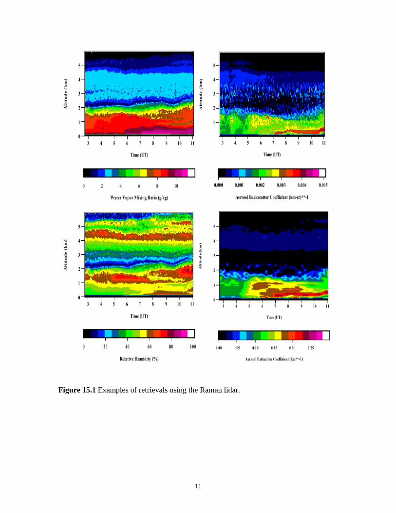
Figure 15.1 Examples of retrievals using the Raman lidar.
12
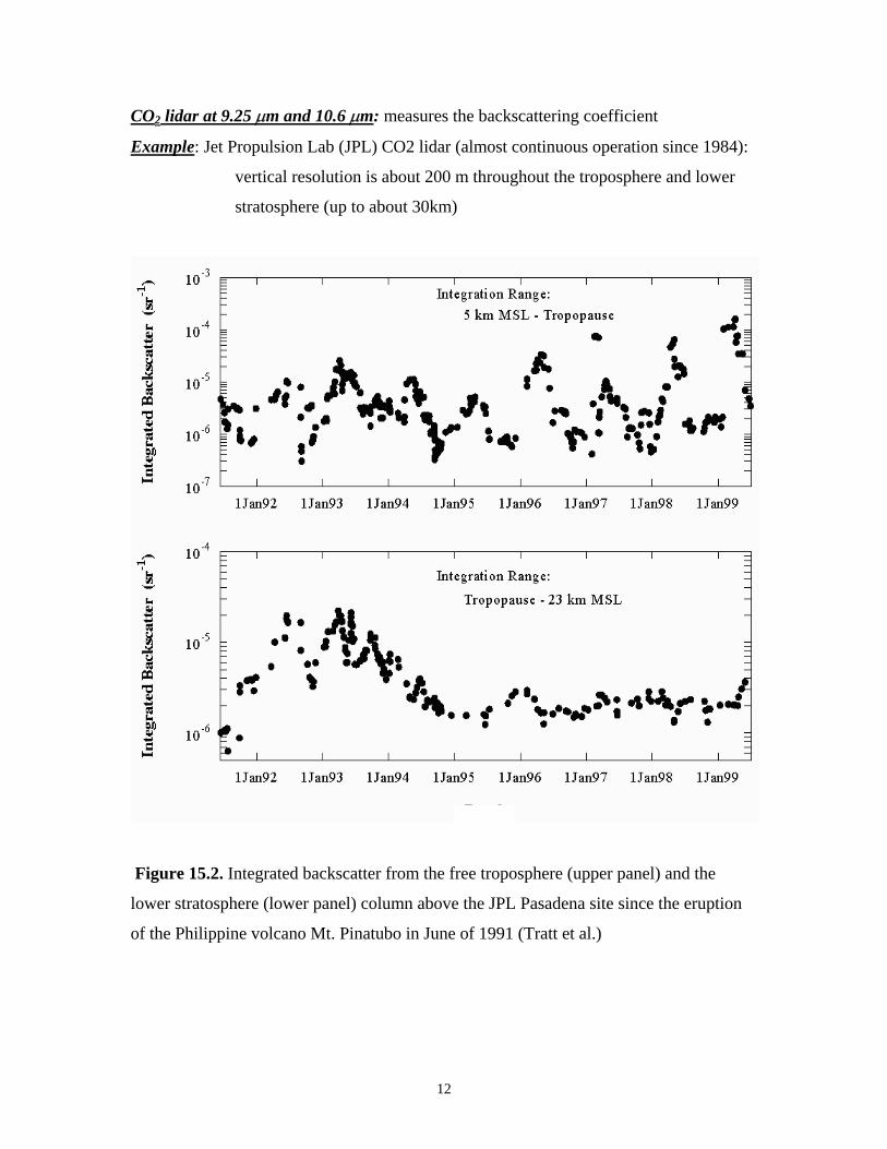
CO2 lidar at 9.25 µm and 10.6 µm: measures the backscattering coefficient
Example: Jet Propulsion Lab (JPL) CO2 lidar (almost continuous operation since 1984):
vertical resolution is about 200 m throughout the troposphere and lower
stratosphere (up to about 30km)
Figure 15.2. Integrated backscatter from the free troposphere (upper panel) and the
lower stratosphere (lower panel) column above the JPL Pasadena site since the eruption
of the Philippine volcano Mt. Pinatubo in June of 1991 (Tratt et al.)

13
Lidar sensing of clouds.
Figure 15.3. Four typical examples of range corrected lidar backscatter versus altitude
(ARM Raman lidar, 10 min average, Sassen et al.). Fig. 15.3a illustrates a clear sky
backscatter, which decrease with altitude due to the decrease in molecular density. Fig.
15.3b shows a backscatter from cirrus, which has a strong increase in backscatter above
cloud base, and air return above cloud top. Backscatter, which is totally attenuated in
clouds, is shown in Fig. 15.3c. Compare with clear sky case (Fig. 15.3a), we can find a
very strong increase in lidar backscatter form clouds (Fig. 15.3b-c), but it is not always
observable (Fig. 15.3d). The other common feature for cloud signal is there is a fast
decrease region in cloud backscatter due to strong attenuation of clouds or transition form
cloud to clear region. So strong negative and strong positive slopes in lidar backscatter
signal are observable in the presence of clouds.
Cloud boundary detection: there is no universal algorithm
Common approach: analysis of dP/dR (i.e., retuned power vs. the range)
14
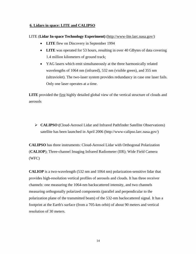
6. Lidars in space: LITE and CALIPSO
LITE (LLiiddaarr IInn--ssppaaccee TTeecchhnnoollooggyy EExxppeerriimmeenntt)) ((http://www-lite.larc.nasa.gov/)
• LITE flew on Discovery in September 1994
• LITE was operated for 53 hours, resulting in over 40 GBytes of data covering
1.4 million kilometers of ground track;
• YAG lasers which emit simultaneously at the three harmonically related
wavelengths of 1064 nm (infrared), 532 nm (visible green), and 355 nm
(ultraviolet). The two-laser system provides redundancy in case one laser fails.
Only one laser operates at a time.
LITE provided the first highly detailed global view of the vertical structure of clouds and
aerosols
CALIPSO (Cloud-Aerosol Lidar and Infrared Pathfinder Satellite Observations)
satellite has been launched in April 2006 (http://www-calipso.larc.nasa.gov/)
CALIPSO has three instruments: Cloud-Aerosol Lidar with Orthogonal Polarization
(CALIOP); Three-channel Imaging Infrared Radiometer (IIR); Wide Field Camera
(WFC)
CALIOP is a two-wavelength (532 nm and 1064 nm) polarization-sensitive lidar that
provides high-resolution vertical profiles of aerosols and clouds. It has three receiver
channels: one measuring the 1064-nm backscattered intensity, and two channels
measuring orthogonally polarized components (parallel and perpendicular to the
polarization plane of the transmitted beam) of the 532-nm backscattered signal. It has a
footprint at the Earth's surface (from a 705-km orbit) of about 90 meters and vertical
resolution of 30 meters.

15
Figure 15.4 Functional block diagram of CALIOP (from CALIPSO ATBD).
Figure 15.5 Block diagram of calibration and Level 1 data products.
Etalon
532 ||
PolarizationBeam Splitter
Φ|| + Φ⊥
1064
532 ⊥
Interference Filter
LaserBackscatter
fromClouds/Aerosols
Detectors andElectronics
Depolarizer
(Calibrate)
Transmitter

16
Example of CALIOP data: dust, cirrus and smoke
Fire locations (MODIS) 06/10/2006 CALIPSO track

17
CALIPSO Level 2 Aerosol and Cloud Products:
layer heights and descriptive properties (e.g., integrated attenuated backscatter,
layer integrated depolarization ratio, etc.);
layer identification and typing (i.e., cloud vs. aerosol, ice cloud vs. water cloud,
etc.); and
profiles of cloud and aerosol backscatter and extinction coefficients.
Before the retrieval of extinction coefficients can be performed, clouds must be located and discriminated from aerosol, and water clouds must be discriminated from ice clouds. In the Level 2 algorithms, the Selective Iterated BoundarY Locator (SIBYL) detects layers, the Scene Classification Algorithm (SCA) classifies these layers, and the Hybrid Extinction Retrieval Algorithms (HERA) perform extinction retrievals. Although the location of cloud and aerosol layers and the determination of cloud ice/water phase are necessary precursors to extinction retrieval.

18
Schematic of the Scene Classification Algorithm (SCA):
A schematic of the scene classification tasks is shown below. The SCA first identifies layers as either cloud or aerosol, based primarily on scattering strength and the spectral dependence of backscattering. The SCA computes the depolarization profile within layers using the (Level 1) 532 nm parallel and perpendicular profiles. Cloud layers are then classified as ice or water, primarily using the depolarization signal and the temperature profile supplied as part of the ancillary data. Aerosol layers are similarly distinguished according to type using indicators such as depolarization, geophysical location, and backscatter intensity. Based on this classification according to type, the SCA then estimates values of the lidar ratio, S, for clouds and aerosols, and selects the appropriate range-dependent multiple scattering correction function for the layer.
NOTE: That CALIPSO extinction (optical depth) retrievals are strongly depend on the
assumed aerosol (or cloud) lidar ratio (pre-defied based on the type of aerosol and
clouds).
19
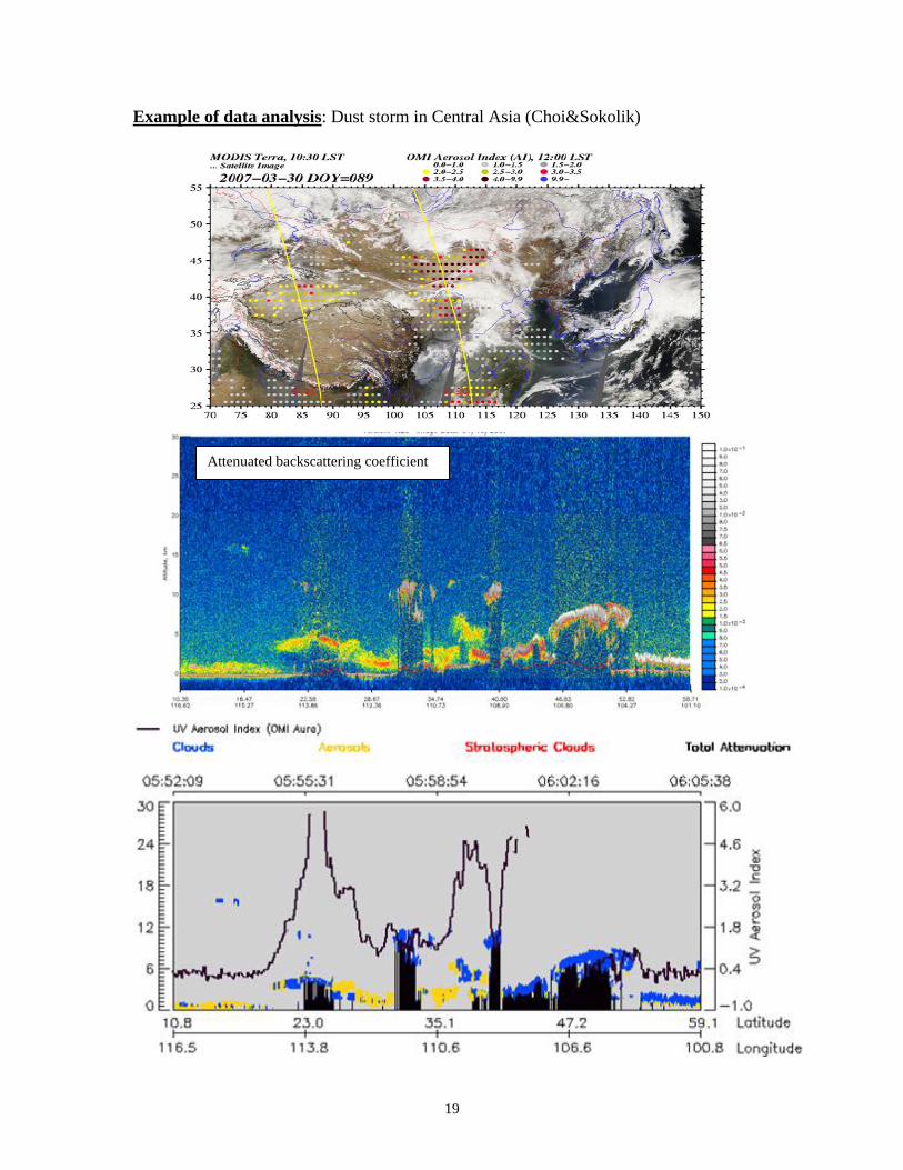
Example of data analysis: Dust storm in Central Asia (Choi&Sokolik)
Attenuated backscattering coefficient
Related Documents