MONOPOLY MICROECONOMICS MICROECONOMICS MICROECONOMICS MICROECONOMICS Principles and Analysis

Welcome message from author
This document is posted to help you gain knowledge. Please leave a comment to let me know what you think about it! Share it to your friends and learn new things together.
Transcript
MONOPOLY
MICROECONOMICSMICROECONOMICSMICROECONOMICSMICROECONOMICSPrinciples and Analysis
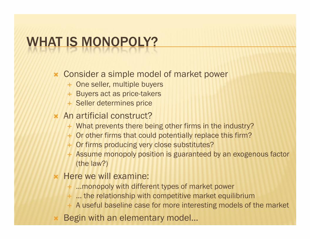
WHAT IS MONOPOLY?
� Consider a simple model of market power� One seller, multiple buyers� Buyers act as price-takers� Seller determines price
� An artificial construct?� An artificial construct?� What prevents there being other firms in the industry?� Or other firms that could potentially replace this firm?� Or firms producing very close substitutes?� Assume monopoly position is guaranteed by an exogenous factor
(the law?)
� Here we will examine: � …monopoly with different types of market power� … the relationship with competitive market equilibrium� A useful baseline case for more interesting models of the market
� Begin with an elementary model…

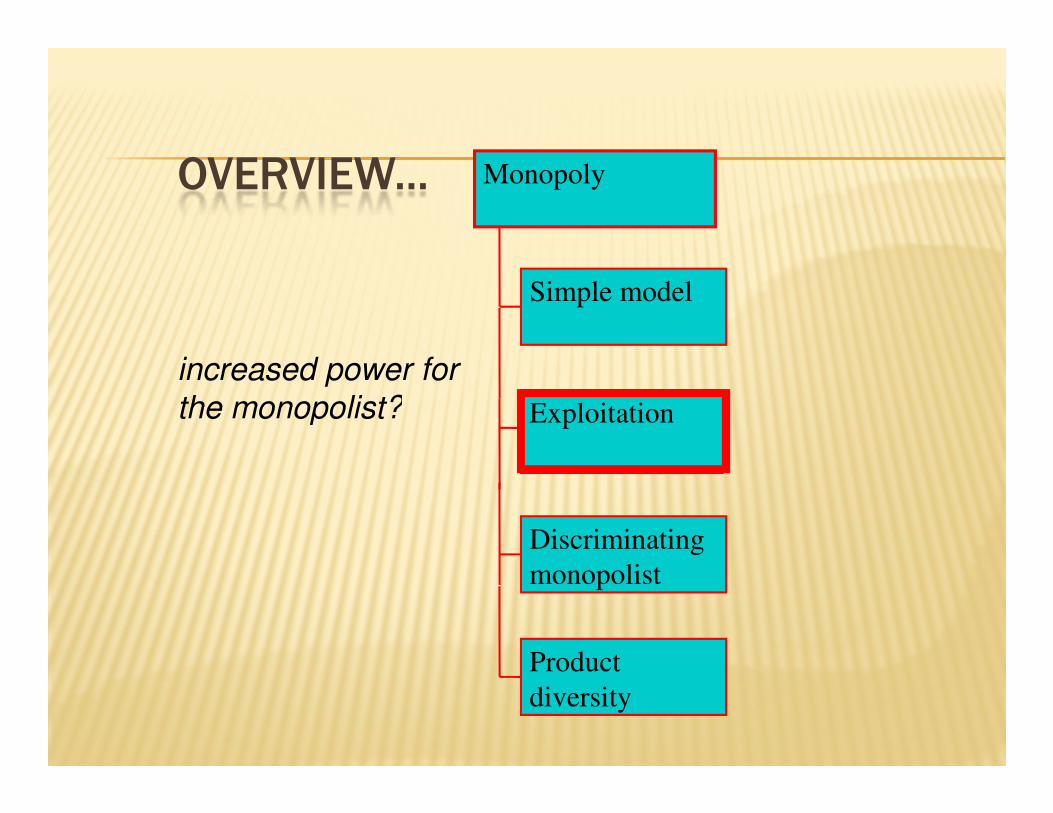
OVERVIEW...
Exploitation
Monopoly
An elementary
extension of profit
Simple model
Discriminating
monopolist
Exploitation
Product
diversity
extension of profit
maximisation
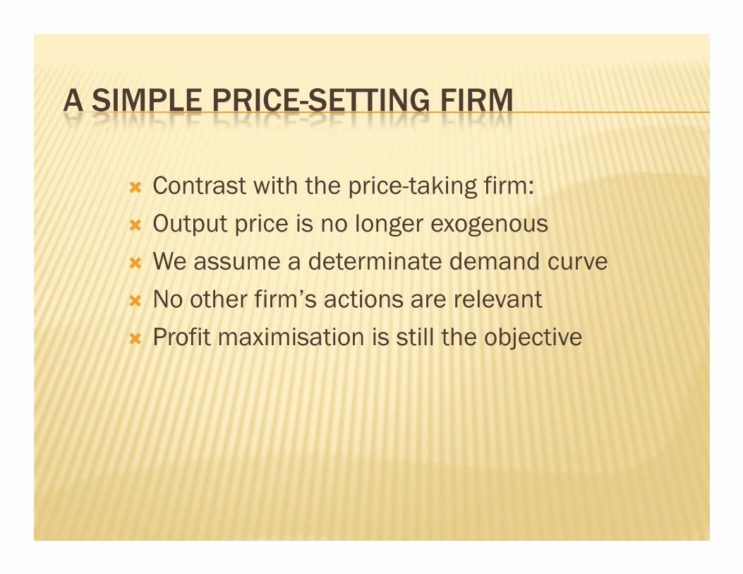
A SIMPLE PRICE-SETTING FIRM
� Contrast with the price-taking firm:
� Output price is no longer exogenous
� We assume a determinate demand curve
No other firm’s actions are relevant� No other firm’s actions are relevant
� Profit maximisation is still the objective
MONOPOLY – MODEL STRUCTURE
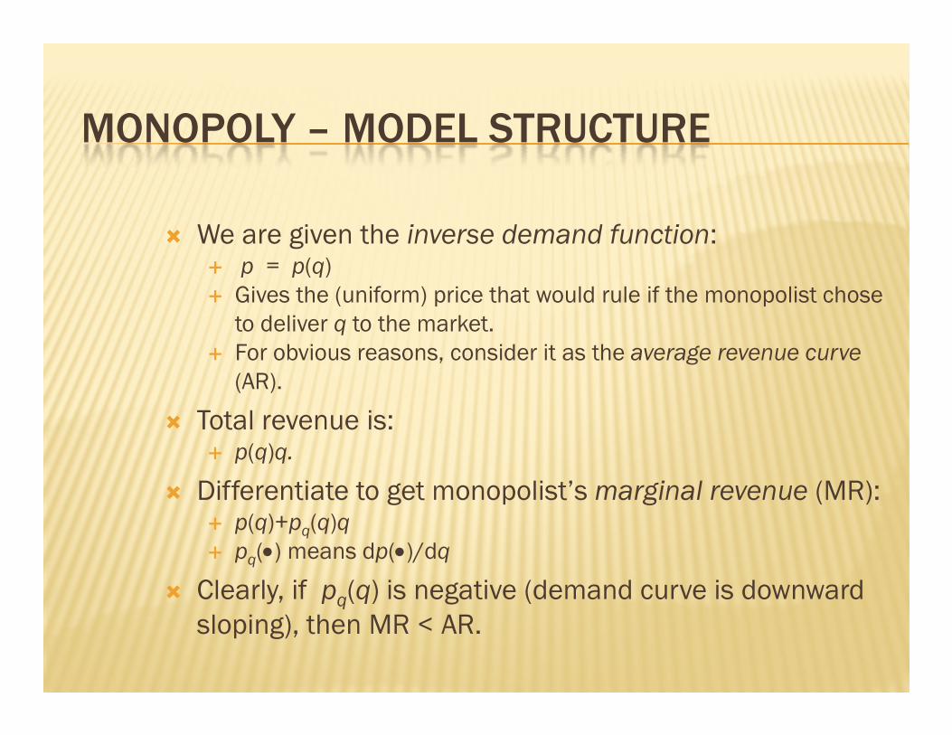
� We are given the inverse demand function:� p = p(q)� Gives the (uniform) price that would rule if the monopolist chose
to deliver q to the market.� For obvious reasons, consider it as the average revenue curve
(AR).(AR).
� Total revenue is: � p(q)q.
� Differentiate to get monopolist’s marginal revenue (MR):� p(q)+pq(q)q � pq(•) means dp(•)/dq
� Clearly, if pq(q) is negative (demand curve is downward sloping), then MR < AR.

AVERAGE AND MARGINAL REVENUE
p �AR curve is just the market demand curve...
�Total revenue: area in the rectangle underneath
�Differentiate total revenue to get marginal revenue
q
p(q)
AR
p(q)q
MR
dp(q)q
dq

MONOPOLY – OPTIMISATION PROBLEM
� Introduce the firm’s cost function C(q).� Same basic properties as for the competitive firm.
� From C we derive marginal and average cost:� MC: Cq(q).� AC: C(q) / q.� AC: C(q) / q.
� Given C(q) and total revenue p(q)q profits are: � Π(q) = = = = p(q)q − C(q)
� The shape of Π is important:� We assume it to be differentiable� Whether it is concave depends on both C(•) and p(•).� Of course Π(0) = = = = 0....
� Firm maximises Π(q) subject to q ≥ 0.
MONOPOLY – SOLVING THE PROBLEM
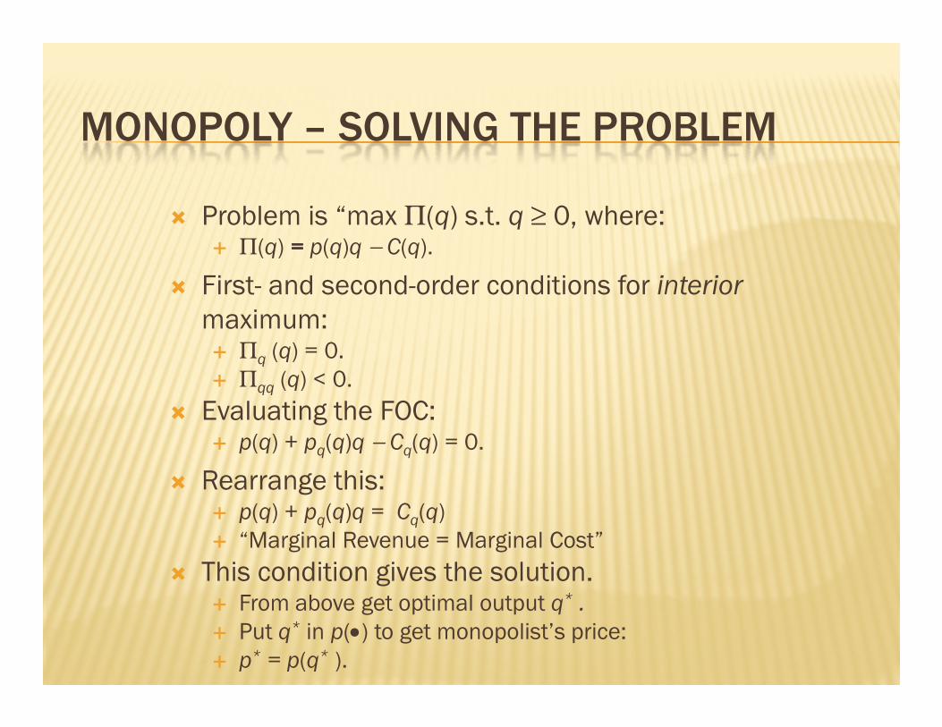
� Problem is “max Π(q) s.t. q ≥ 0, where: � Π(q) = = = = p(q)q − C(q).
� First- and second-order conditions for interiormaximum:� Πq (q) = 0.
Πq (q) = 0.
� Πqq (q) < 0.
� Evaluating the FOC:� p(q) + pq(q)q − Cq(q) = 0.
� Rearrange this: � p(q) + pq(q)q = Cq(q)� “Marginal Revenue = Marginal Cost”
� This condition gives the solution.� From above get optimal output q* .
� Put q* in p(•) to get monopolist’s price:� p* = p(q* ).
Check this diagrammatically…

MONOPOLIST’S OPTIMUM
p �AR and MR
�Marginal and average cost
�Optimum where MC=MR
MC
� Monopolist’s optimum price.
� Monopolist’s profit
q
AR
MR
AC
MC
q*
p*
� Monopolist’s profit
Π
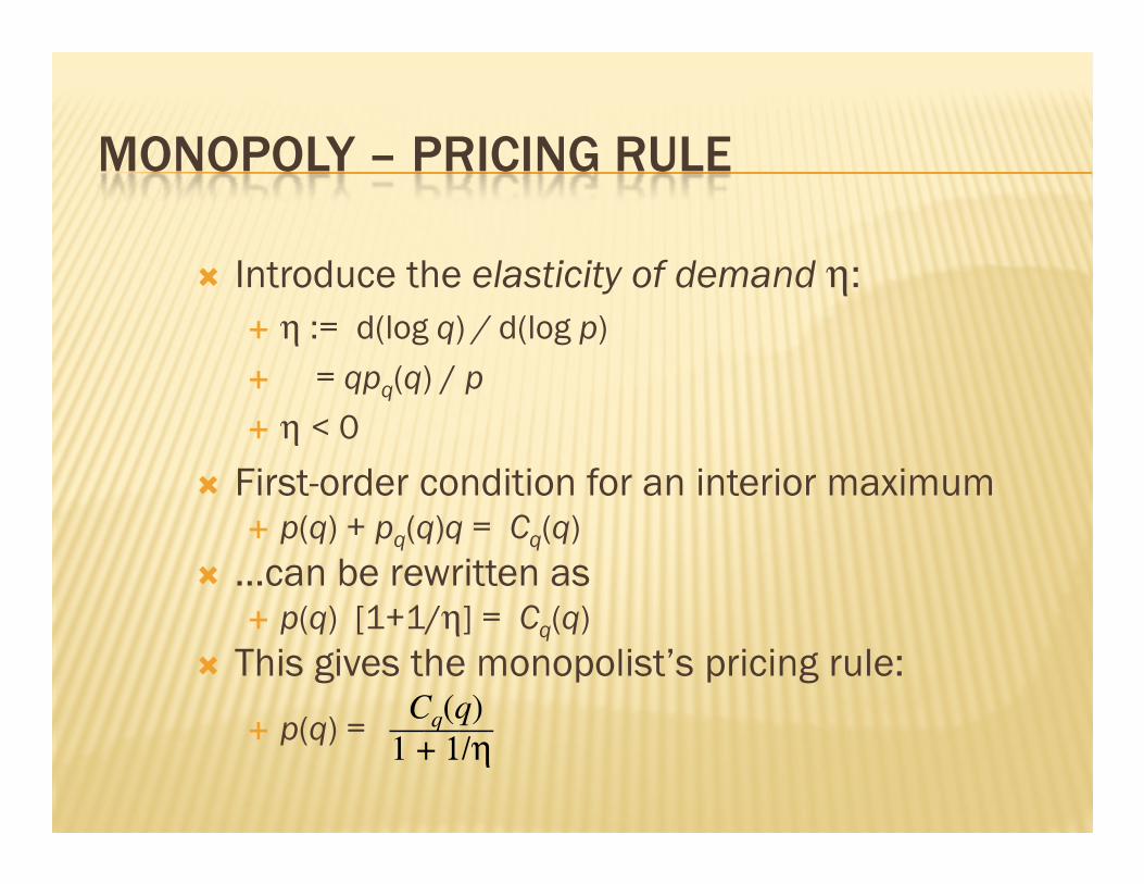
MONOPOLY – PRICING RULE
� Introduce the elasticity of demand η:� η := d(log q) / d(log p)
� = qpq(q) / p
� η < 0� η < 0
� First-order condition for an interior maximum� p(q) + pq(q)q = Cq(q)
� …can be rewritten as� p(q) [1+1/η] = Cq(q)
� This gives the monopolist’s pricing rule:
� p(q) =Cq(q)
———1 + 1/η
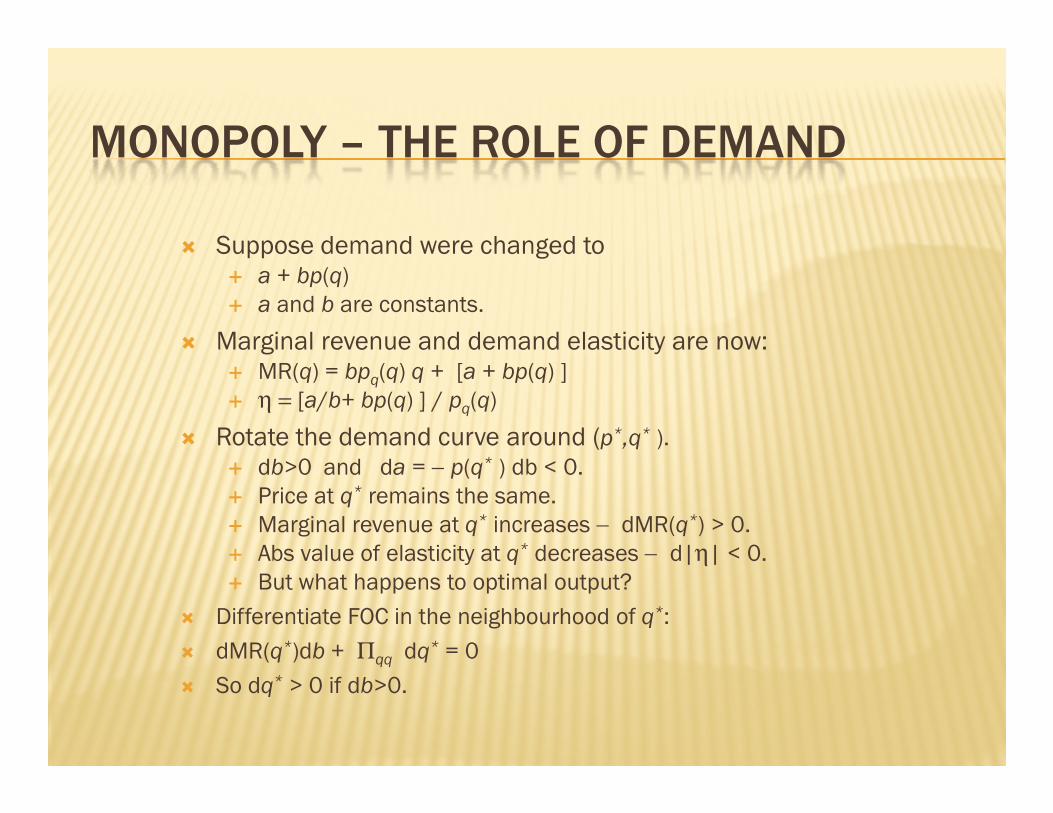
MONOPOLY – THE ROLE OF DEMAND
� Suppose demand were changed to� a + bp(q)� a and b are constants.
� Marginal revenue and demand elasticity are now: � MR(q) = bpq(q) q + [a + bp(q) ]� η = [a/b+ bp(q) ] / pq(q)� η = [a/b+ bp(q) ] / pq(q)
� Rotate the demand curve around (p*,q* ).� db>0 and da = − p(q* ) db < 0. � Price at q* remains the same.� Marginal revenue at q* increases − dMR(q*) > 0.� Abs value of elasticity at q* decreases − d|η| < 0.� But what happens to optimal output?
� Differentiate FOC in the neighbourhood of q*:
� dMR(q*)db + Πqq dq* = 0
� So dq* > 0 if db>0.
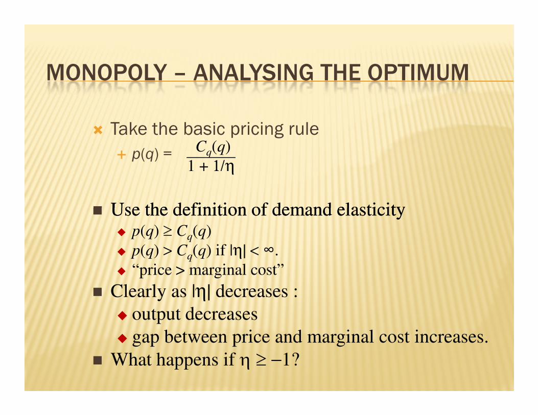
MONOPOLY – ANALYSING THE OPTIMUM
� Take the basic pricing rule� p(q) = Cq(q)
———1 + 1/η
�� Use the definition of demand elasticityUse the definition of demand elasticity�� Use the definition of demand elasticityUse the definition of demand elasticity� p(q) ≥ Cq(q)
� p(q) > Cq(q) if |η| < ∞.
� “price > marginal cost”
� Clearly as |η| decreases :
� output decreases
� gap between price and marginal cost increases.
� What happens if η ≥ −1?
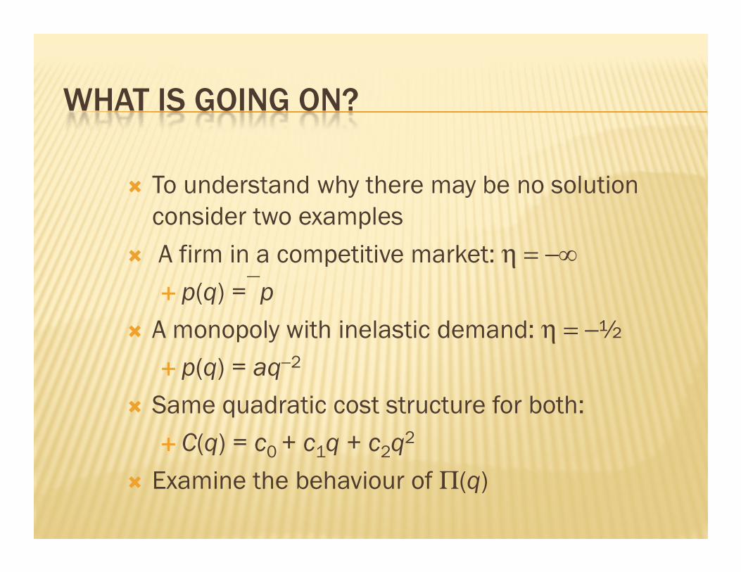
WHAT IS GOING ON?
� To understand why there may be no solution consider two examples
� A firm in a competitive market: η = −∞
� p(q) =p� p(q) =p
� A monopoly with inelastic demand: η = −½
� p(q) = aq−2
� Same quadratic cost structure for both:
� C(q) = c0 + c1q + c2q2
� Examine the behaviour of Π(q)
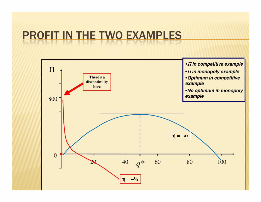
PROFIT IN THE TWO EXAMPLES
800
1000
Π�ΠΠΠΠ in competitive example
�ΠΠΠΠ in monopoly example
�Optimum in competitive example
�No optimum in monopoly example
There’s a
discontinuity
here
-200
0
200
400
600
800
20 40 60 80 100
q
q*
η = η = η = η = −−−−∞∞∞∞
nn
η = η = η = η = −−−−½
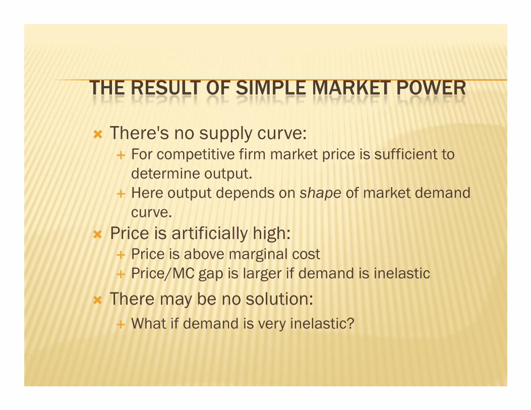
THE RESULT OF SIMPLE MARKET POWER
� There's no supply curve:� For competitive firm market price is sufficient to determine output.
� Here output depends on shape of market demand curve.curve.
� Price is artificially high:� Price is above marginal cost� Price/MC gap is larger if demand is inelastic
� There may be no solution:� What if demand is very inelastic?
OVERVIEW...
Exploitation
Monopoly
increased power for
the monopolist?
Simple model
Discriminating
monopolist
Exploitation
Product
diversity
the monopolist?
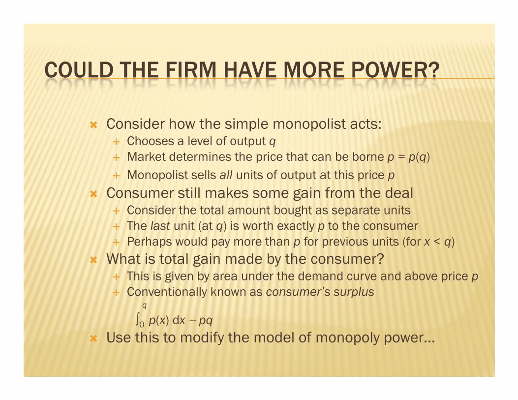
COULD THE FIRM HAVE MORE POWER?
� Consider how the simple monopolist acts:� Chooses a level of output q� Market determines the price that can be borne p = p(q)
� Monopolist sells all units of output at this price p
� Consumer still makes some gain from the dealConsumer still makes some gain from the deal� Consider the total amount bought as separate units� The last unit (at q) is worth exactly p to the consumer � Perhaps would pay more than p for previous units (for x < q)
� What is total gain made by the consumer?� This is given by area under the demand curve and above price p� Conventionally known as consumer’s surplus
q
∫0 p(x) dx − pq
� Use this to modify the model of monopoly power…

THE FIRM WITH MORE POWER
� Suppose monopolist can charge for the right to purchase� Charges a fixed “entry fee” F for customers� Only works if it is impossible to resell the good
� This changes the maximisation problem� This changes the maximisation problem� Profits are now
F + pq − C (q)q
where F = ∫0 p(x) dx − pq
� which can be simplified toq
∫0 p(x) dx − C (q)� Maximising this with respect to q we get the FOC
p(q) = C (q)
� This yields the optimum output…
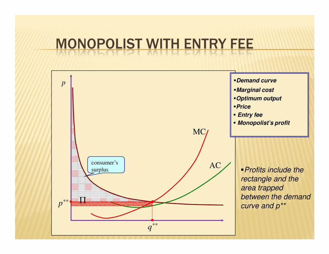
MONOPOLIST WITH ENTRY FEE
p
MC
�Demand curve
�Marginal cost
�Optimum output
�Price
� Entry fee
� Monopolist’s profit
q
AC
MC
q**
p** Π
consumer’s
surplus �Profits include the
rectangle and the
area trapped
between the demand
curve and p**
MONOPOLIST WITH ENTRY FEE
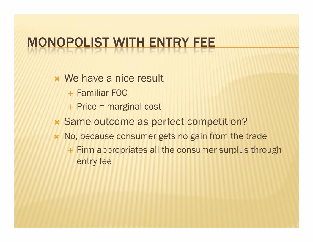
� We have a nice result� Familiar FOC
� Price = marginal cost
� Same outcome as perfect competition?� Same outcome as perfect competition?� No, because consumer gets no gain from the trade
� Firm appropriates all the consumer surplus through entry fee
OVERVIEW...
Exploitation
Monopoly
Monopolist working
in many markets
Simple model
Discriminating
monopolist
Exploitation
Product
diversity
in many markets
MULTIPLE MARKETS
� Monopolist sells same product in more than one market� An alternative model of increased power� Perhaps can discriminate between the markets
� Can the monopolist separate the markets? � Charge different prices to customers in different marketsCharge different prices to customers in different markets� In the limit can see this as similar to previous case…� …if each “market” consists of just one customer
� Essentials emerge in two-market case� For convenience use a simplified linear model:
� Begin by reviewing equilibrium in each market in isolation� Then combine model….� …how is output determined…?� …and allocated between the markets
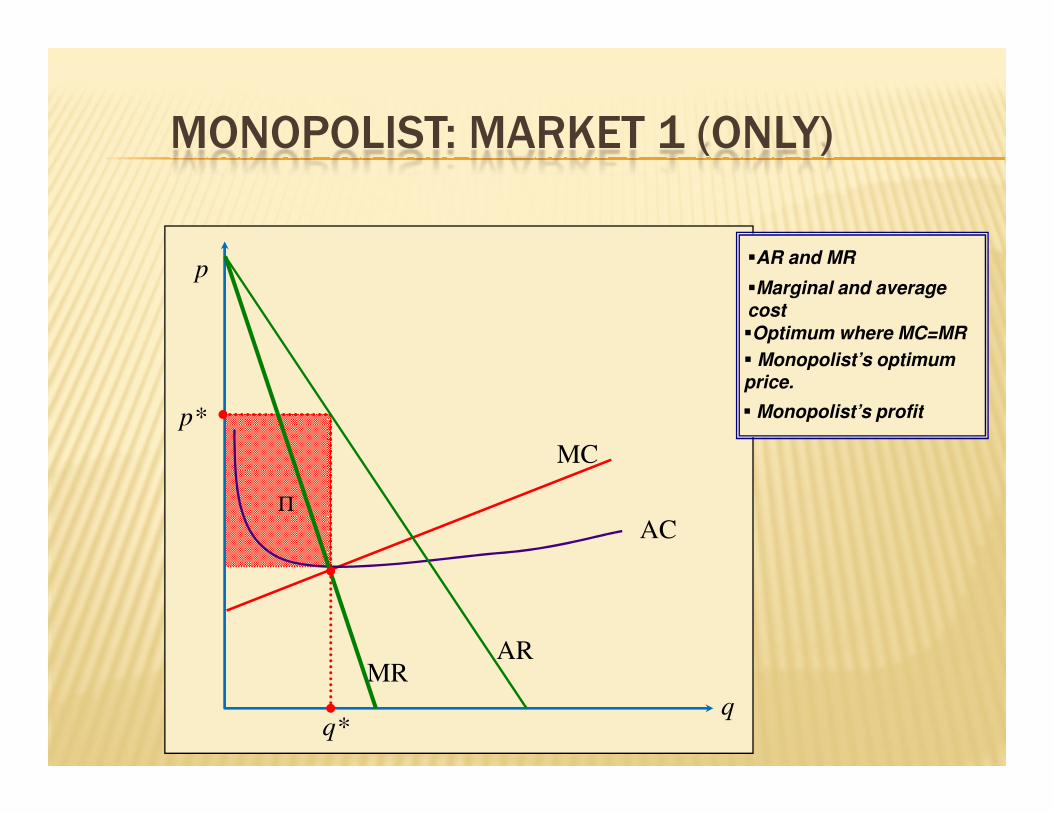
MONOPOLIST: MARKET 1 (ONLY)
p�AR and MR
�Marginal and average cost
�Optimum where MC=MR
� Monopolist’s optimum price.
p* � Monopolist’s profit
q
ARMR
AC
MC
q*
p* � Monopolist’s profit
Π

MONOPOLIST: MARKET 2 (ONLY)
p�AR and MR
�Marginal and average cost
�Optimum where MC=MR
� Monopolist’s optimum price.
� Monopolist’s profit
q
ARMR
AC
MC
q*
p*
� Monopolist’s profit
Π
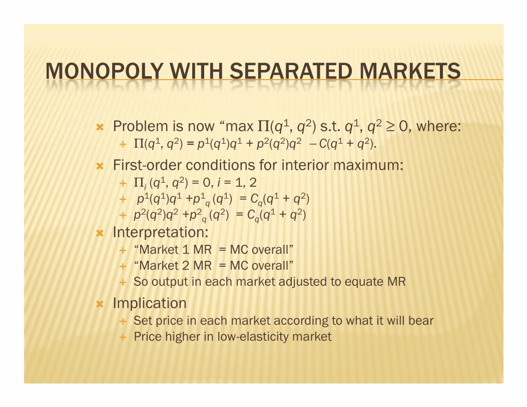
MONOPOLY WITH SEPARATED MARKETS
� Problem is now “max Π(q1, q2) s.t. q1, q2 ≥ 0, where: � Π(q1, q2) = = = = p1(q1)q1 + p2(q2)q2 − C(q1 + q2).
� First-order conditions for interior maximum:� Πi (q1, q2) = 0, i = 1, 2� p1(q1)q1 +p1q (q1) = Cq(q1 + q2)� p (q )q +p q (q ) = Cq(q + q )� p2(q2)q2 +p2q (q2) = Cq(q1 + q2)
� Interpretation:� “Market 1 MR = MC overall”� “Market 2 MR = MC overall”� So output in each market adjusted to equate MR
� Implication� Set price in each market according to what it will bear� Price higher in low-elasticity market

OPTIMUM WITH SEPARATED MARKETS
p�MR1 and MR2
�“Horizontal sum”
�Optimum total output
� Allocation of output to markets
� Marginal cost
q
MR1
MC
MR2
q1*+
q2*
q1* q2*

� Marginal cost
OPTIMUM WITH SEPARATED MARKETS
p�MR1 and MR2
�“Horizontal sum”
�Optimum total output
� Allocation of output to marketsp*
q
MR1
MC
q1*
Π
� Price & profit in market 1
AR1
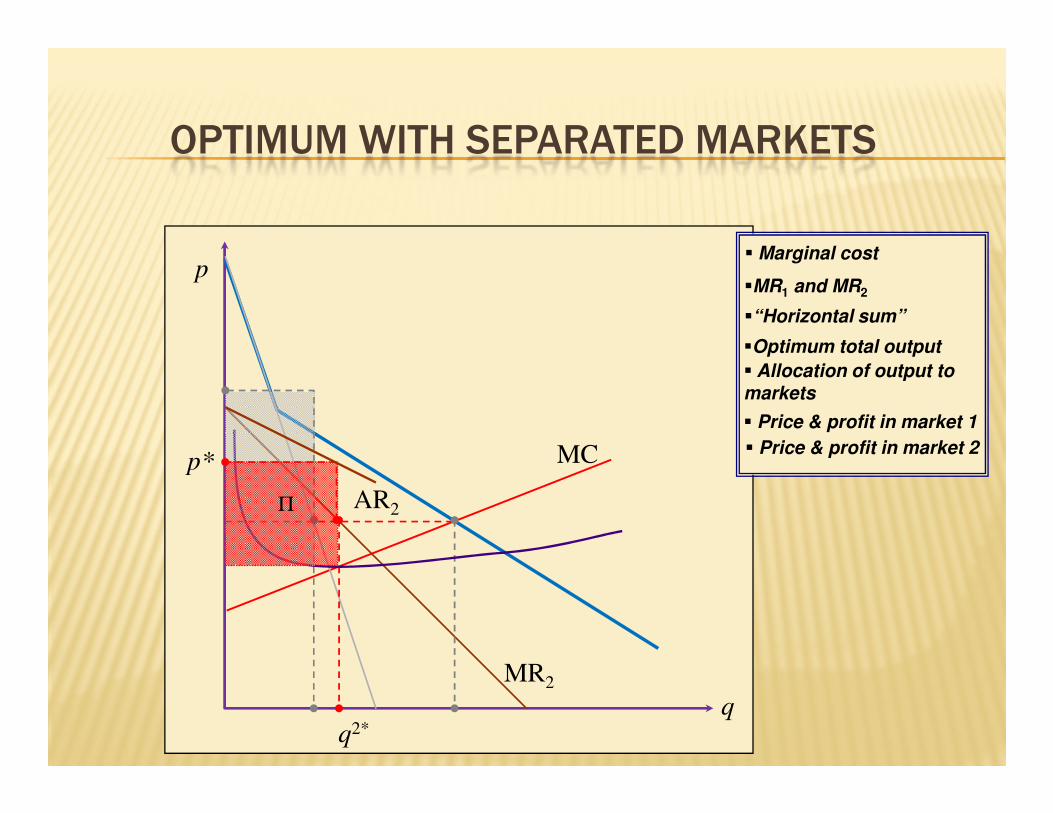
OPTIMUM WITH SEPARATED MARKETS
p�MR1 and MR2
�“Horizontal sum”
�Optimum total output
� Allocation of output to markets
� Marginal cost
q
MC
� Price & profit in market 1
q2*
p*
Π
MR2
� Price & profit in market 2
AR2

MULTIPLE MARKETS AGAIN
� We’ve assumed that the monopolist can separate the markets
� What happens if this power is removed?� Retain assumptions about the two markets
� But now require same price
� Use the standard monopoly model� Trick is to construct combined AR…
� …and from that the combined MR
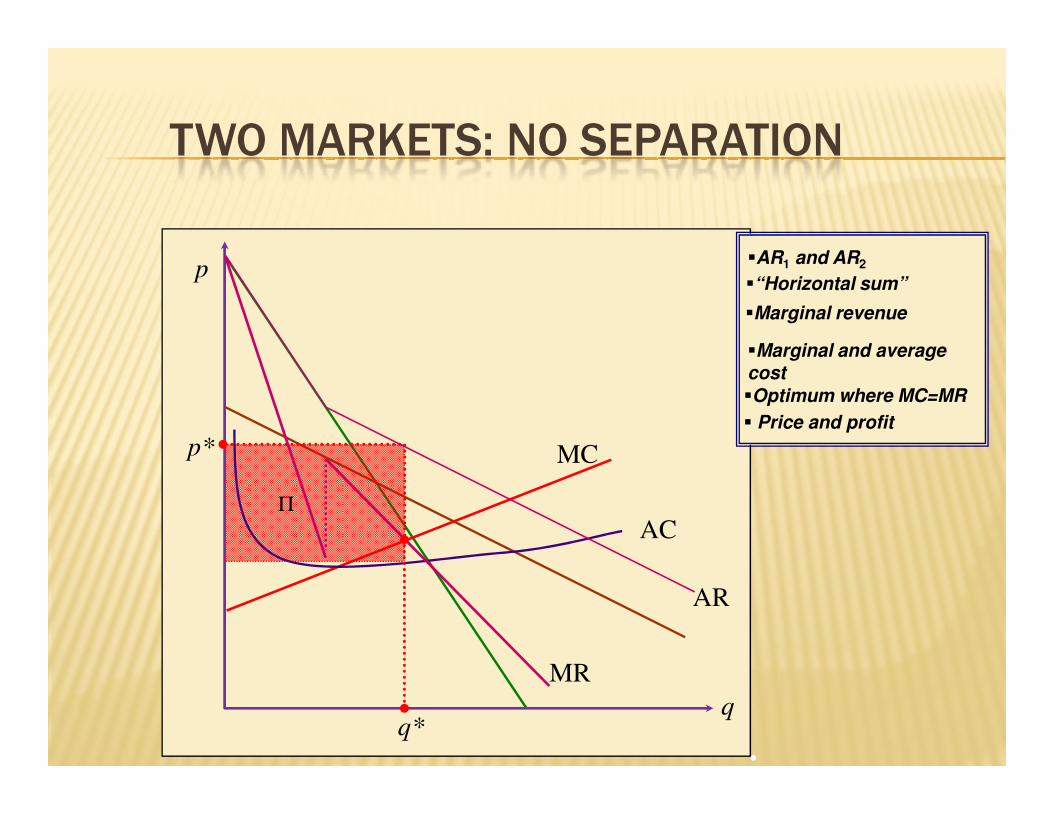
TWO MARKETS: NO SEPARATION
p�AR1 and AR2
�Marginal and average cost
�Optimum where MC=MR
�“Horizontal sum”
�Marginal revenue
q
AR
AC
MC
� Price and profit
q*
p*
Π
MR
..

COMPARE PRICES
AND PROFITS
� Separated markets 1, 2� Combined markets 1+2� Higher profits if you can separate…
Markets 1+2
Market 2Market 1
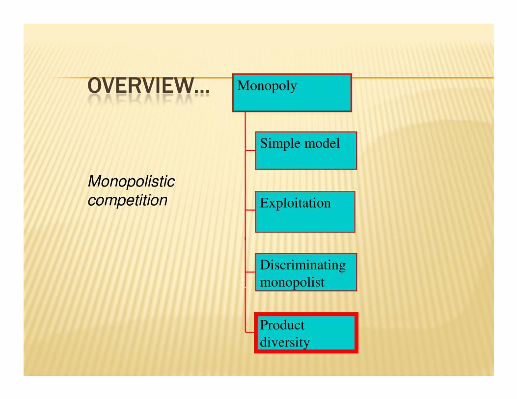
OVERVIEW...
Exploitation
Monopoly
Monopolistic
competition
Simple model
Discriminating
monopolist
Exploitation
Product
diversity
competition

MARKET POWER AND PRODUCT
DIVERSITY
� Nature of product is a major issue in classic monopoly� No close substitutes?� Otherwise erode monopoly position
� Now suppose potentially many firms making substitutes� Firms' products differ one from anotherFirms' products differ one from another� Each firm is a local monopoly – downward-sloping demand
curve� New firms can enter with new products� Diversity may depend on size of market� Like corner shops dotted around the neighbourhood
� Use standard analysis� Start with a single firm – use monopoly paradigm� Then consider entry of others, attracted by profit…� …process similar to competitive industry

ACMC
MONOPOLISTIC COMPETITION: 1 FIRM
�For simplicity take linear demand curve (AR)
�Marginal and average costs
�Optimal output for single firm
�The derived MR curve
Π1
p
q1 output of
firm 1
ARMR
firm
�Price and profits
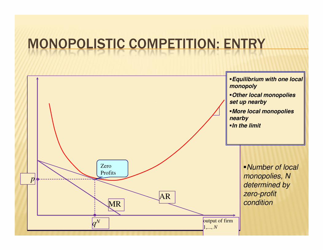
MONOPOLISTIC COMPETITION: ENTRY
ACMC ACMC ACMC ACMC
�Equilibrium with one local monopoly
�Other local monopolies set up nearby
�More local monopolies nearby
�In the limit
Π1
p
q1 output of
firm 1
ARMR
qf output of firm
1,..., f
pΠf
MRAR
qf output of firm
1,..., f
MR
pΠf
AR
p
qN output of firm
1,..., N
MRAR
Zero
Profits
�In the limit
�Number of local
monopolies, N
determined by
zero-profit
condition

WHAT NEXT?
� All variants reviewed here have a common element…
� Firm does not have to condition its behaviour on what other firms do…what other firms do…
� Does not attempt to influence behaviour of other firms� Not even of potential entrants
� Need to introduce strategic interdependence
Related Documents